Scala Guide Data Science Professionals
User Manual: Pdf
Open the PDF directly: View PDF ![]() .
.
Page Count: 1101 [warning: Documents this large are best viewed by clicking the View PDF Link!]
- Cover
- Copyright
- Credits
- Preface
- Table of Contents
- Module 1: Scala for Data Science
- Chapter 1: Scala and Data Science
- Chapter 2: Manipulating Data with Breeze
- Chapter 3: Plotting with breeze-viz
- Chapter 4: Parallel Collections and Futures
- Chapter 5: Scala and SQL through JDBC
- Chapter 6: Slick – A Functional Interface for SQL
- Chapter 7: Web APIs
- Chapter 8: Scala and MongoDB
- Chapter 9: Concurrency with Akka
- GitHub follower graph
- Actors as people
- Hello world with Akka
- Case classes as messages
- Actor construction
- Anatomy of an actor
- Follower network crawler
- Fetcher actors
- Routing
- Message passing between actors
- Queue control and the pull pattern
- Accessing the sender of a message
- Stateful actors
- Follower network crawler
- Fault tolerance
- Custom supervisor strategies
- Life-cycle hooks
- What we have not talked about
- Summary
- References
- Chapter 10: Distributed Batch Processing with Spark
- Chapter 11: Spark SQL and DataFrames
- Chapter 12: Distributed Machine Learning with MLlib
- Chapter 13: Web APIs with Play
- Client-server applications
- Introduction to web frameworks
- Model-View-Controller architecture
- Single page applications
- Building an application
- The Play framework
- Dynamic routing
- Actions
- Interacting with JSON
- Querying external APIs and consuming JSON
- Creating APIs with Play: a summary
- Rest APIs: best practice
- Summary
- References
- Chapter 14: Visualization with D3 and the Play Framework
- Appendix: Pattern Matching and Extractors
- Module 2: Scala Data Analysis Cookbook
- Chapter 1: Getting Started with Breeze
- Chapter 2: Getting Started with Apache Spark DataFrames
- Chapter 3: Loading and Preparing Data – DataFrame
- Chapter 4: Data Visualization
- Chapter 5: Learning from Data
- Introduction
- Supervised and unsupervised learning
- Gradient descent
- Predicting continuous values using linear regression
- Binary classification using LogisticRegression and SVM
- Binary classification using LogisticRegression with Pipeline API
- Clustering using K-means
- Feature reduction using principal component analysis
- Chapter 6: Scaling Up
- Chapter 7 : Going Further
- Module 3: Scala for Machine Learning
- Chapter 1: Getting Started
- Chapter 3: Hello World!
- Chapter 3: Data Preprocessing
- Chapter 4: Unsupervised Learning
- Chapter 5: Naïve Bayes Classifiers
- Chapter 6: Regression and Regularization
- Chapter 7: Sequential Data Models
- Chapter 8: Kernel Models and Support Vector Machines
- Chapter 9: Artificial Neural Networks
- Chapter 10 : Genetic Algorithms
- Chapter 11: Reinforcement Learning
- Chapter 12: Scalable Frameworks
- Appendix A : Basic Concepts
- Bibliography


Scala: Guide for Data Science
Professionals
Scala will be a valuable tool to have on hand during your data science journey for
everything from data cleaning to cutting-edge machine learning
A course in three modules
BIRMINGHAM - MUMBAI
Scala: Guide for Data Science Professionals
Copyright © 2017 Packt Publishing
All rights reserved. No part of this course may be reproduced, stored in a retrieval
system, or transmitted in any form or by any means, without the prior written
permission of the publisher, except in the case of brief quotations embedded in
critical articles or reviews.
Every effort has been made in the preparation of this course to ensure the accuracy
of the information presented. However, the information contained in this course
is sold without warranty, either express or implied. Neither the authors, nor Packt
Publishing, and its dealers and distributors will be held liable for any damages
caused or alleged to be caused directly or indirectly by this course.
Packt Publishing has endeavored to provide trademark information about all of the
companies and products mentioned in this course by the appropriate use of capitals.
However, Packt Publishing cannot guarantee the accuracy of this information.
Published on: January 2017
Published by Packt Publishing Ltd.
Livery Place
35 Livery Street
Birmingham B3 2PB, UK.
ISBN 978-1-78728-285-8
www.packtpub.com

Credits
Authors
Pascal Bugnion
Arun Manivannan
Patrick R. Nicolas
Reviewers
Umanga Bista
Radek Ostrowski
Yuanhang Wang
Amir Hajian
Shams Mahmood Imam
Gerald Loefer
Subhajit Datta
Rui Gonçalves
Patricia Hoffman, PhD
Md Zahidul Islam
Content Development Editor
Trusha Shriyan
Graphics
Kirk D'Penha
Production Coordinator
Shantanu N. Zagade

[ i ]
Preface
Scala is a popular language for data science. By emphasizing immutability and
functional constructs, Scala lends itself well to the construction of robust libraries
for concurrency and big data analysis. A rich ecosystem of tools for data science has
therefore developed around Scala, including libraries for accessing SQL and NoSQL
databases, frameworks for building distributed applications like Apache Spark and
libraries for linear algebra and numerical algorithms. We will explore this rich and
growing ecosystem in this learning path.
What this learning path covers
Module 1, Scala for Data Science, will introduce you to the libraries for ingesting,
storing, manipulating, processing, and visualizing data in Scala. Packed with real-
world examples and interesting data sets, this module will teach you to ingest data
from at les and web APIs and store it in a SQL or NoSQL database. It will show
you how to design scalable architectures to process and modeling your data, starting
from simple concurrency constructs such as parallel collections and futures, through
to actor systems and Apache Spark. As well as Scala's emphasis on functional
structures and immutability, you will learn how to use the right parallel construct
for the job at hand, minimizing development time without compromising scalability.
Finally, you will learn how to build beautiful interactive visualizations using web
frameworks. This module gives tutorials on some of the most common Scala libraries
for data science, allowing you to quickly get up to speed with building data science
and data engineering solutions.

Preface
[ ii ]
Module 2, Scala Data Analysis Cookbook, will introduce you to the most popular
Scala tools, libraries, and frameworks through practical recipes around loading,
manipulating, and preparing your data. It will also help you explore and make sense
of your data using stunning and insightful visualizations, and machine learning
toolkits.Starting with introductory recipes on utilizing the Breeze and Spark libraries,
get to grips with how to import data from a host of possible sources and how to
pre-process numerical, string, and date data. Next, you'll get an understanding of
concepts that will help you visualize data using the Apache Zeppelin and Bokeh
bindings in Scala, enabling exploratory data analysis. Discover how to program
quintessential machine learning algorithms using Spark ML library. Work through
steps to scale your machine learning models and deploy them into a standalone
cluster, EC2, YARN, and Mesos. Finally dip into the powerful options presented by
Spark Streaming, and machine learning for streaming data, as well as utilizing
Spark GraphX.
Module 3, Scala for Machine Learning, will introduce you to the functional
capabilities of the Scala programming language that are critical to the creation
of machine learning algorithms such as dependency injection and implicits.Your
learning journey starts with data pre-processing and ltering techniques, then
move on to clustering and dimension reduction, Naïve Bayes, regression models,
sequential data, regularization and kernelization, support vector machines, Neural
networks, generic algorithms and re-enforcement learning. The review of the Akka
framework and Apache Spark clusters concludes the tutorial. Techniques throughout
the module is applied to the analysis, recommendation, classication, and prediction
of nancial markets.
This module will guide you through the process of building AI applications with
diagrams, formal mathematical notation, source code snippets and useful tips.
What you need for this learning path
The examples provided in this learning path require that you have a working Scala
installation and SBT, the Simple Build Tool, a command line utility for compiling
and running Scala code. We will walk you through how to install these in the next
sections. We do not require a specic IDE. The code examples can be written in your
favorite text editor or IDE.
Who this learning path is for
This learning path is perfect for those who are comfortable with Scala programming
and now want to enter the eld of data science. Some knowledge of statistics is
expected.

Preface
[ iii ]
Reader feedback
Feedback from our readers is always welcome. Let us know what you think about
this course—what you liked or disliked. Reader feedback is important for us as it
helps us develop titles that you will really get the most out of.
To send us general feedback, simply e-mail feedback@packtpub.com, and mention
the course's title in the subject of your message.
If there is a topic that you have expertise in and you are interested in either writing
or contributing to a book, see our author guide at www.packtpub.com/authors.
Customer support
Now that you are the proud owner of a Packt course, we have a number of things to
help you to get the most from your purchase.
Downloading the example code
You can download the example code les for this course from your account at
http://www.packtpub.com. If you purchased this course elsewhere, you can visit
http://www.packtpub.com/support and register to have the les e-mailed directly
to you.
You can download the code les by following these steps:
1. Log in or register to our website using your e-mail address and password.
2. Hover the mouse pointer on the SUPPORT tab at the top.
3. Click on Code Downloads & Errata.
4. Enter the name of the course in the Search box.
5. Select the course for which you're looking to download the code les.
6. Choose from the drop-down menu where you purchased this course from.
7. Click on Code Download.
You can also download the code les by clicking on the Code Files button on the
course's webpage at the Packt Publishing website. This page can be accessed by
entering the course's name in the Search box. Please note that you need to be logged
in to your Packt account.

Preface
[ iv ]
Once the le is downloaded, please make sure that you unzip or extract the folder
using the latest version of:
• WinRAR / 7-Zip for Windows
• Zipeg / iZip / UnRarX for Mac
• 7-Zip / PeaZip for Linux
The code bundle for the course is also hosted on GitHub at https://github.
com/PacktPublishing/Scala-Guide-for-Data-Science-Professionals.We
also have other code bundles from our rich catalog of books, videos, and courses
available at https://github.com/PacktPublishing/. Check them out!
Errata
Although we have taken every care to ensure the accuracy of our content, mistakes
do happen. If you nd a mistake in one of our courses—maybe a mistake in the text
or the code—we would be grateful if you could report this to us. By doing so, you
can save other readers from frustration and help us improve subsequent versions
of this course. If you nd any errata, please report them by visiting http://www.
packtpub.com/submit-errata, selecting your course, clicking on the Errata
Submission Form link, and entering the details of your errata. Once your errata are
veried, your submission will be accepted and the errata will be uploaded to our
website or added to any list of existing errata under the Errata section of that title.
To view the previously submitted errata, go to https://www.packtpub.com/books/
content/support and enter the name of the course in the search eld. The required
information will appear under the Errata section.
Piracy
Piracy of copyrighted material on the Internet is an ongoing problem across all
media. At Packt, we take the protection of our copyright and licenses very seriously.
If you come across any illegal copies of our works in any form on the Internet, please
provide us with the location address or website name immediately so that we can
pursue a remedy.
Please contact us at copyright@packtpub.com with a link to the suspected pirated
material.
We appreciate your help in protecting our authors and our ability to bring you
valuable content.

Preface
[ v ]
Questions
If you have a problem with any aspect of this course, you can contact us at
questions@packtpub.com, and we will do our best to address the problem.

[ i ]
Module 1: Scala for Data Science
Chapter 1: Scala and Data Science 3
Data science 3
Programming in data science 6
Why Scala? 7
When not to use Scala 14
Summary 14
References 15
Chapter 2: Manipulating Data with Breeze 17
Code examples 17
Installing Breeze 18
Getting help on Breeze 18
Basic Breeze data types 19
An example – logistic regression 37
Towards re-usable code 45
Alternatives to Breeze 47
Summary 47
References 47
Chapter 3: Plotting with breeze-viz 49
Diving into Breeze 50
Customizing plots 52
Customizing the line type 55
More advanced scatter plots 60
Multi-plot example – scatterplot matrix plots 62
Managing without documentation 67
Breeze-viz reference 68
Data visualization beyond breeze-viz 69
Summary 69

Table of Contents
[ ii ]
Chapter 4: Parallel Collections and Futures 71
Parallel collections 71
Futures 85
Summary 95
References 95
Chapter 5: Scala and SQL through JDBC 97
Interacting with JDBC 98
First steps with JDBC 98
JDBC summary 106
Functional wrappers for JDBC 107
Safer JDBC connections with the loan pattern 108
Enriching JDBC statements with the "pimp my library" pattern 110
Wrapping result sets in a stream 113
Looser coupling with type classes 115
Creating a data access layer 121
Summary 122
References 122
Chapter 6: Slick – A Functional Interface for SQL 125
FEC data 125
Invokers 137
Operations on columns 138
Aggregations with "Group by" 140
Accessing database metadata 142
Slick versus JDBC 143
Summary 143
References 143
Chapter 7: Web APIs 145
A whirlwind tour of JSON 146
Querying web APIs 147
JSON in Scala – an exercise in pattern matching 148
Extraction using case classes 154
Concurrency and exception handling with futures 158
Authentication – adding HTTP headers 160
Summary 164
References 165

Table of Contents
[ iii ]
Chapter 8: Scala and MongoDB 167
MongoDB 168
Connecting to MongoDB with Casbah 169
Inserting documents 172
Extracting objects from the database 178
Complex queries 182
Casbah query DSL 184
Custom type serialization 185
Beyond Casbah 187
Summary 187
References 188
Chapter 9: Concurrency with Akka 189
GitHub follower graph 189
Actors as people 191
Hello world with Akka 193
Case classes as messages 195
Actor construction 196
Anatomy of an actor 197
Follower network crawler 198
Fetcher actors 200
Routing 204
Message passing between actors 205
Queue control and the pull pattern 211
Accessing the sender of a message 213
Stateful actors 214
Follower network crawler 215
Fault tolerance 218
Custom supervisor strategies 220
Life-cycle hooks 222
What we have not talked about 226
Summary 227
References 227
Chapter 10: Distributed Batch Processing with Spark 229
Installing Spark 229
Acquiring the example data 230
Resilient distributed datasets 231
Building and running standalone programs 246

Table of Contents
[ iv ]
Spam ltering 250
Lifting the hood 258
Data shufing and partitions 261
Summary 263
Reference 263
Chapter 11: Spark SQL and DataFrames 265
DataFrames – a whirlwind introduction 265
Aggregation operations 270
Joining DataFrames together 272
Custom functions on DataFrames 274
DataFrame immutability and persistence 276
SQL statements on DataFrames 277
Complex data types – arrays, maps, and structs 279
Interacting with data sources 282
Standalone programs 284
Summary 285
References 285
Chapter 12: Distributed Machine Learning with MLlib 287
Introducing MLlib – Spam classication 288
Pipeline components 291
Evaluation 302
Regularization in logistic regression 308
Cross-validation and model selection 310
Beyond logistic regression 315
Summary 315
References 315
Chapter 13: Web APIs with Play 317
Client-server applications 318
Introduction to web frameworks 318
Model-View-Controller architecture 319
Single page applications 321
Building an application 323
The Play framework 324
Dynamic routing 329
Actions 330
Interacting with JSON 335
Querying external APIs and consuming JSON 337
Creating APIs with Play: a summary 344

Table of Contents
[ v ]
Rest APIs: best practice 344
Summary 345
References 345
Chapter 14: Visualization with D3 and the Play Framework 347
GitHub user data 348
Do I need a backend? 348
JavaScript dependencies through web-jars 349
Towards a web application: HTML templates 350
Modular JavaScript through RequireJS 353
Bootstrapping the applications 355
Client-side program architecture 357
Drawing plots with NVD3 366
Summary 369
References 370
Appendix: Pattern Matching and Extractors 371
Pattern matching in for comprehensions 374
Pattern matching internals 374
Extracting sequences 376
Summary 377
Reference 378
Module 2: Scala Data Analysis Cookbook
Chapter 1: Getting Started with Breeze 381
Introduction 381
Getting Breeze – the linear algebra library 382
Working with vectors 385
Working with matrices 393
Vectors and matrices with randomly distributed values 405
Reading and writing CSV les 408
Chapter 2: Getting Started with Apache Spark DataFrames 413
Introduction 413
Getting Apache Spark 414
Creating a DataFrame from CSV 415
Manipulating DataFrames 418
Creating a DataFrame from Scala case classes 429

Table of Contents
[ vi ]
Chapter 3: Loading and Preparing Data – DataFrame 433
Introduction 433
Loading more than 22 features into classes 434
Loading JSON into DataFrames 443
Storing data as Parquet les 450
Using the Avro data model in Parquet 458
Loading from RDBMS 466
Preparing data in Dataframes 470
Chapter 4: Data Visualization 479
Introduction 479
Visualizing using Zeppelin 480
Creating scatter plots with Bokeh-Scala 492
Creating a time series MultiPlot with Bokeh-Scala 502
Chapter 5: Learning from Data 507
Introduction 507
Supervised and unsupervised learning 507
Gradient descent 508
Predicting continuous values using linear regression 509
Binary classication using LogisticRegression and SVM 516
Binary classication using LogisticRegression with Pipeline API 526
Clustering using K-means 532
Feature reduction using principal component analysis 539
Chapter 6: Scaling Up 549
Introduction 549
Building the Uber JAR 550
Submitting jobs to the Spark cluster (local) 557
Running the Spark Standalone cluster on EC2 563
Running the Spark Job on Mesos (local) 573
Running the Spark Job on YARN (local) 578
Chapter 7: Going Further 587
Introduction 587
Using Spark Streaming to subscribe to a Twitter stream 588
Using Spark as an ETL tool 593
Using StreamingLogisticRegression to classify a Twitter
stream using Kafka as a training stream 598
Using GraphX to analyze Twitter data 602

Table of Contents
[ vii ]
Module 3: Scala for Machine Learning
Chapter 1: Getting Started 611
Mathematical notation for the curious 612
Why machine learning? 612
Why Scala? 613
Model categorization 616
Taxonomy of machine learning algorithms 617
Tools and frameworks 621
Source code 624
Let's kick the tires 628
Summary 639
Chapter 2: Hello World! 641
Modeling 641
Designing a workow 644
Assessing a model 656
Summary 664
Chapter 3: Data Preprocessing 665
Time series 665
Moving averages 668
Fourier analysis 675
The Kalman lter 687
Alternative preprocessing techniques 699
Summary 699
Chapter 4: Unsupervised Learning 701
Clustering 702
Dimension reduction 728
Performance considerations 735
Summary 737
Chapter 5: Naïve Bayes Classiers 739
Probabilistic graphical models 739
Naïve Bayes classiers 741
Multivariate Bernoulli classication 757
Naïve Bayes and text mining 758
Pros and cons 770
Summary 770

Table of Contents
[ viii ]
Chapter 6: Regression and Regularization 771
Linear regression 771
Regularization 786
Numerical optimization 793
The logistic regression 794
Summary 807
Chapter 7: Sequential Data Models 809
Markov decision processes 809
The hidden Markov model (HMM) 811
Conditional random elds 834
CRF and text analytics 839
Comparing CRF and HMM 851
Performance consideration 852
Summary 852
Chapter 8: Kernel Models and Support Vector Machines 853
Kernel functions 854
The support vector machine (SVM) 858
Support vector classier (SVC) 864
Anomaly detection with one-class SVC 884
Support vector regression (SVR) 886
Performance considerations 890
Summary 890
Chapter 9: Articial Neural Networks 891
Feed-forward neural networks (FFNN) 891
The multilayer perceptron (MLP) 895
Evaluation 917
Benets and limitations 926
Summary 928
Chapter 10: Genetic Algorithms 929
Evolution 929
Genetic algorithms and machine learning 932
Genetic algorithm components 932
Implementation 942
GA for trading strategies 953
Advantages and risks of genetic algorithms 965
Summary 966

Table of Contents
[ ix ]
Chapter 11: Reinforcement Learning 967
Introduction 967
Learning classier systems 993
Summary 1005
Chapter 12: Scalable Frameworks 1007
Overview 1008
Scala 1009
Scalability with Actors 1015
Akka 1017
Apache Spark 1033
Summary 1048
Appendix A: Basic Concepts 1049
Scala programming 1049
Mathematics 1059
Finances 101 1069
Suggested online courses 1075
References 1075
Bibliography 1077
Module 1
Scala for Data Science
Leverage the power of Scala to build scalable, robust data science applications
[ 3 ]
Scala and Data Science
The second half of the 20th century was the age of silicon. In fty years, computing
power went from extremely scarce to entirely mundane. The rst half of the 21st
century is the age of the Internet. The last 20 years have seen the rise of giants such as
Google, Twitter, and Facebook—giants that have forever changed the way we view
knowledge.
The Internet is a vast nexus of information. Ninety percent of the data generated by
humanity has been generated in the last 18 months. The programmers, statisticians,
and scientists who can harness this glut of data to derive real understanding will
have an ever greater inuence on how businesses, governments, and charities
make decisions.
This book strives to introduce some of the tools that you will need to synthesize the
avalanche of data to produce true insight.
Data science
Data science is the process of extracting useful information from data. As a discipline,
it remains somewhat ill-dened, with nearly as many denitions as there are experts.
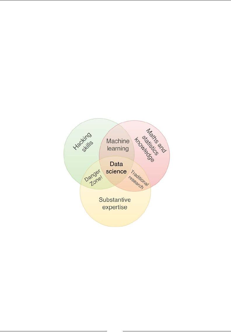
Rather than add yet another denition, I will follow Drew Conway's description
(http://drewconway.com/zia/2013/3/26/the-data-science-venn-diagram).
He describes data science as the culmination of three orthogonal sets of skills:
• Data scientists must have hacking skills. Data is stored and transmitted
through computers. Computers, programming languages, and libraries
are the hammers and chisels of data scientists; they must wield them with
confidence and accuracy to sculpt the data as they please. This is where Scala
comes in: it's a powerful tool to have in your programming toolkit.
Scala and Data Science
[ 4 ]
• Data scientists must have a sound understanding of statistics and numerical
algorithms. Good data scientists will understand how machine learning
algorithms function and how to interpret results. They will not be fooled by
misleading metrics, deceptive statistics, or misinterpreted causal links.
• A good data scientist must have a sound understanding of the problem
domain. The data science process involves building and discovering
knowledge about the problem domain in a scientifically rigorous manner.
The data scientist must, therefore, ask the right questions, be aware of
previous results, and understand how the data science effort fits in the wider
business or research context.
Drew Conway summarizes this elegantly with a Venn diagram showing data
science at the intersection of hacking skills, maths and statistics knowledge,
and substantive expertise:
It is, of course, rare for people to be experts in more than one of these areas. Data
scientists often work in cross-functional teams, with different members providing the
expertise for different areas. To function effectively, every member of the team must
nevertheless have a general working knowledge of all three areas.

Chapter 1
[ 5 ]
To give a more concrete overview of the workow in a data science project, let's
imagine that we are trying to write an application that analyzes the public perception
of a political campaign. This is what the data science pipeline might look like:
• Obtaining data: This might involve extracting information from text files,
polling a sensor network or querying a web API. We could, for instance,
query the Twitter API to obtain lists of tweets with the relevant hashtags.
• Data ingestion: Data often comes from many different sources and might be
unstructured or semi-structured. Data ingestion involves moving data from
the data source, processing it to extract structured information, and storing
this information in a database. For tweets, for instance, we might extract the
username, the names of other users mentioned in the tweet, the hashtags, text
of the tweet, and whether the tweet contains certain keywords.
• Exploring data: We often have a clear idea of what information we want to
extract from the data but very little idea how. For instance, let's imagine that
we have ingested thousands of tweets containing hashtags relevant to our
political campaign. There is no clear path to go from our database of tweets
to the end goal: insight into the overall public perception of our campaign.
Data exploration involves mapping out how we are going to get there. This
step will often uncover new questions or sources of data, which requires
going back to the first step of the pipeline. For our tweet database, we might,
for instance, decide that we need to have a human manually label a thousand
or more tweets as expressing "positive" or "negative" sentiments toward
the political campaign. We could then use these tweets as a training set to
construct a model.
• Feature building: A machine learning algorithm is only as good as the
features that enter it. A significant fraction of a data scientist's time involves
transforming and combining existing features to create new features more
closely related to the problem that we are trying to solve. For instance, we
might construct a new feature corresponding to the number of "positive"
sounding words or pairs of words in a tweet.
• Model construction and training: Having built the features that enter the
model, the data scientist can now train machine learning algorithms on their
datasets. This will often involve trying different algorithms and optimizing
model hyperparameters. We might, for instance, settle on using a random
forest algorithm to decide whether a tweet is "positive" or "negative" about
the campaign. Constructing the model involves choosing the right number
of trees and how to calculate impurity measures. A sound understanding of
statistics and the problem domain will help inform these decisions.

Scala and Data Science
[ 6 ]
• Model extrapolation and prediction: The data scientists can now use their
new model to try and infer information about previously unseen data points.
They might pass a new tweet through their model to ascertain whether it
speaks positively or negatively of the political campaign.
• Distillation of intelligence and insight from the model: The data scientists
combine the outcome of the data analysis process with knowledge of the
business domain to inform business decisions. They might discover that
specific messages resonate better with the target audience, or with specific
segments of the target audience, leading to more accurate targeting. A key
part of informing stakeholders involves data visualization and presentation:
data scientists create graphs, visualizations, and reports to help make the
insights derived clear and compelling.
This is far from a linear pipeline. Often, insights gained at one stage will require the
data scientists to backtrack to a previous stage of the pipeline. Indeed, the generation
of business insights from raw data is normally an iterative process: the data scientists
might do a rapid rst pass to verify the premise of the problem and then gradually
rene the approach by adding new data sources or new features or trying new
machine learning algorithms.
In this book, you will learn how to deal with each step of the pipeline in Scala,
leveraging existing libraries to build robust applications.
Programming in data science
This book is not a book about data science. It is a book about how to use Scala, a
programming language, for data science. So, where does programming come in
when processing data?
Computers are involved at every step of the data science pipeline, but not necessarily
in the same manner. The style of programs that we build will be drastically different
if we are just writing throwaway scripts to explore data or trying to build a scalable
application that pushes data through a well-understood pipeline to continuously
deliver business intelligence.
Let's imagine that we work for a company making games for mobile phones in
which you can purchase in-game benets. The majority of users never buy anything,
but a small fraction is likely to spend a lot of money. We want to build a model that
recognizes big spenders based on their play patterns.

Chapter 1
[ 7 ]
The rst step is to explore data, nd the right features, and build a model based on
a subset of the data. In this exploration phase, we have a clear goal in mind but little
idea of how to get there. We want a light, exible language with strong libraries to
get us a working model as soon as possible.
Once we have a working model, we need to deploy it on our gaming platform to
analyze the usage patterns of all the current users. This is a very different problem:
we have a relatively clear understanding of the goals of the program and of how to
get there. The challenge comes in designing software that will scale out to handle all
the users and be robust to future changes in usage patterns.
In practice, the type of software that we write typically lies on a spectrum ranging
from a single throwaway script to production-level code that must be proof against
future expansion and load increases. Before writing any code, the data scientist
must understand where their software lies on this spectrum. Let's call this the
permanence spectrum.
Why Scala?
You want to write a program that handles data. Which language should you choose?
There are a few different options. You might choose a dynamic language such as
Python or R or a more traditional object-oriented language such as Java. In this
section, we will explore how Scala differs from these languages and when it might
make sense to use it.
When choosing a language, the architect's trade-off lies in a balance of provable
correctness versus development speed. Which of these aspects you need to
emphasize will depend on the application requirements and where on the
permanence spectrum your program lies. Is this a short script that will be used by a
few people who can easily x any problems that arise? If so, you can probably permit
a certain number of bugs in rarely used code paths: when a developer hits a snag,
they can just x the problem as it arises. By contrast, if you are developing a database
engine that you plan on releasing to the wider world, you will, in all likelihood, favor
correctness over rapid development. The SQLite database engine, for instance, is
famous for its extensive test suite, with 800 times as much testing code as application
code (https://www.sqlite.org/testing.html).
What matters, when estimating the correctness of a program, is not the perceived
absence of bugs, it is the degree to which you can prove that certain bugs are absent.

Scala and Data Science
[ 8 ]
There are several ways of proving the absence of bugs before the code has even run:
• Static type checking occurs at compile time in statically typed languages,
but this can also be used in strongly typed dynamic languages that support
type annotations or type hints. Type checking helps verify that we are using
functions and classes as intended.
• Static analyzers and linters that check for undefined variables or suspicious
behavior (such as parts of the code that can never be reached).
• Declaring some attributes as immutable or constant in compiled languages.
• Unit testing to demonstrate the absence of bugs along particular code paths.
There are several more ways of checking for the absence of some bugs at runtime:
• Dynamic type checking in both statically typed and dynamic languages
• Assertions verifying supposed program invariants or expected contracts
In the next sections, we will examine how Scala compares to other languages in
data science.
Static typing and type inference
Scala's static typing system is very versatile. A lot of information as to the program's
behavior can be encoded in types, allowing the compiler to guarantee a certain
level of correctness. This is particularly useful for code paths that are rarely used. A
dynamic language cannot catch errors until a particular branch of execution runs, so
a bug can persist for a long time until the program runs into it. In a statically typed
language, any bug that can be caught by the compiler will be caught at compile time,
before the program has even started running.
Statically typed object-oriented languages have often been criticized for being
needlessly verbose. Consider the initialization of an instance of the Example
class in Java:
Example myInstance = new Example() ;
We have to repeat the class name twice—once to dene the compile-time type of
the myInstance variable and once to construct the instance itself. This feels like
unnecessary work: the compiler knows that the type of myInstance is Example (or a
superclass of Example) as we are binding a value of the Example type.

Chapter 1
[ 9 ]
Scala, like most functional languages, uses type inference to allow the compiler to
infer the type of variables from the instances bound to them. We would write the
equivalent line in Scala as follows:
val myInstance = new Example()
The Scala compiler infers that myInstance has the Example type at compile time. A
lot of the time, it is enough to specify the types of the arguments and of the return
value of a function. The compiler can then infer types for all the variables dened in
the body of the function. Scala code is usually much more concise and readable than
the equivalent Java code, without compromising any of the type safety.
Scala encourages immutability
Scala encourages the use of immutable objects. In Scala, it is very easy to dene an
attribute as immutable:
val amountSpent = 200
The default collections are immutable:
val clientIds = List("123", "456") // List is immutable
clientIds(1) = "589" // Compile-time error
Having immutable objects removes a common source of bugs. Knowing that some
objects cannot be changed once instantiated reduces the number of places bugs
can creep in. Instead of considering the lifetime of the object, we can narrow in
on the constructor.
Scala and functional programs
Scala encourages functional code. A lot of Scala code consists of using higher-order
functions to transform collections. You, as a programmer, do not have to deal with
the details of iterating over the collection. Let's write an occurrencesOf function
that returns the indices at which an element occurs in a list:
def occurrencesOf[A](elem:A, collection:List[A]):List[Int] = {
for {
(currentElem, index) <- collection.zipWithIndex
if (currentElem == elem)
} yield index
}
How does this work? We rst declare a new list, collection.zipWithIndex, whose
elements are (collection(0), 0), (collection(1), 1), and so on: pairs of the
collection's elements and their indexes.

Scala and Data Science
[ 10 ]
We then tell Scala that we want to iterate over this collection, binding the
currentElem variable to the current element and index to the index. We apply
a lter on the iteration, selecting only those elements for which currentElem ==
elem. We then tell Scala to just return the index variable.
We did not need to deal with the details of the iteration process in Scala. The syntax is
very declarative: we tell the compiler that we want the index of every element equal to
elem in collection and let the compiler worry about how to iterate over collection.
Consider the equivalent in Java:
static <T> List<Integer> occurrencesOf(T elem, List<T> collection) {
List<Integer> occurrences = new ArrayList<Integer>() ;
for (int i=0; i<collection.size(); i++) {
if (collection.get(i).equals(elem)) {
occurrences.add(i) ;
}
}
return occurrences ;
}
In Java, you start by dening a (mutable) list in which to put occurrences as you nd
them. You then iterate over the collection by dening a counter, considering each
element in turn and adding its index to the list of occurrences, if need be. There are
many more moving parts that we need to get right for this method to work. These
moving parts exist because we must tell Java how to iterate over the collection, and
they represent a common source of bugs.
Furthermore, as a lot of code is taken up by the iteration mechanism, the line that
denes the logic of the function is harder to nd:
static <T> List<Integer> occurrencesOf(T elem, List<T> collection) {
List<Integer> occurences = new ArrayList<Integer>() ;
for (int i=0; i<collection.size(); i++) {
if (collection.get(i).equals(elem)) {
occurrences.add(i) ;
}
}
return occurrences ;
}
Note that this is not meant as an attack on Java. In fact, Java 8 adds a slew of
functional constructs, such as lambda expressions, the Optional type that mirrors
Scala's Option, or stream processing. Rather, it is meant to demonstrate the benet of
functional approaches in minimizing the potential for errors and maximizing clarity.

Chapter 1
[ 11 ]
Null pointer uncertainty
We often need to represent the possible absence of a value. For instance, imagine that
we are reading a list of usernames from a CSV le. The CSV le contains name and
e-mail information. However, some users have declined to enter their e-mail into
the system, so this information is absent. In Java, one would typically represent the
e-mail as a string or an Email class and represent the absence of e-mail information
for a particular user by setting that reference to null. Similarly, in Python, we might
use None to demonstrate the absence of a value.
This approach is dangerous because we are not encoding the possible absence
of e-mail information. In any nontrivial program, deciding whether an instance
attribute can be null requires considering every occasion in which this instance is
dened. This quickly becomes impractical, so programmers either assume that a
variable is not null or code too defensively.
Scala (following the lead of other functional languages) introduces the Option[T] type
to represent an attribute that might be absent. We might then write the following:
class User {
...
val email:Option[Email]
...
}
We have now encoded the possible absence of e-mail in the type information. It is
obvious to any programmer using the User class that e-mail information is possibly
absent. Even better, the compiler knows that the email eld can be absent, forcing
us to deal with the problem rather than recklessly ignoring it to have the application
burn at runtime in a conagration of null pointer exceptions.
All this goes back to achieving a certain level of provable correctness. Never using
null, we know that we will never run into null pointer exceptions. Achieving the
same level of correctness in languages without Option[T] requires writing unit tests
on the client code to verify that it behaves correctly when the e-mail attribute is null.
Note that it is possible to achieve this in Java using, for instance, Google's
Guava library (https://code.google.com/p/guava-libraries/wiki/
UsingAndAvoidingNullExplained) or the Optional class in Java 8. It is more a
matter of convention: using null in Java to denote the absence of a value has long
been the norm.

Scala and Data Science
[ 12 ]
Easier parallelism
Writing programs that take advantage of parallel architectures is challenging. It is
nevertheless necessary to tackle all but the simplest data science problems.
Parallel programming is difcult because we, as programmers, tend to think
sequentially. Reasoning about the order in which different events can happen in a
concurrent program is very challenging.
Scala provides several abstractions that greatly facilitate the writing of parallel code.
These abstractions work by imposing constraints on the way parallelism is achieved.
For instance, parallel collections force the user to phrase the computation as a
sequence of operations (such as map, reduce, and lter) on collections. Actor systems
require the developer to think in terms of actors that encapsulate the application
state and communicate by passing messages.
It might seem paradoxical that restricting the programmer's freedom to write parallel
code as they please avoids many of the problems associated with concurrency.
However, limiting the number of ways in which a program behaves facilitates
thinking about its behavior. For instance, if an actor is misbehaving, we know that
the problem lies either in the code for this actor or in one of the messages that the
actor receives.
As an example of the power afforded by having coherent, restrictive abstractions,
let's use parallel collections to solve a simple probability problem. We will calculate
the probability of getting at least 60 heads out of 100 coin tosses. We can estimate
this using Monte Carlo: we simulate 100 coin tosses by drawing 100 random Boolean
values and check whether the number of true values is at least 60. We repeat this
until results have converged to the required accuracy, or we get bored of waiting.
Let's run through this in a Scala console:
scala> val nTosses = 100
nTosses: Int = 100
scala> def trial = (0 until nTosses).count { i =>
util.Random.nextBoolean() // count the number of heads
}
trial: Int

Chapter 1
[ 13 ]
The trial function runs a single set of 100 throws, returning the number of heads:
scala> trial
Int = 51
To get our answer, we just need to repeat trial as many times as we can and
aggregate the results. Repeating the same set of operations is ideally suited to
parallel collections:
scala> val nTrials = 100000
nTrials: Int = 100000
scala> (0 until nTrials).par.count { i => trial >= 60 }
Int = 2745
The probability is thus approximately 2.5% to 3%. All we had to do to distribute the
calculation over every CPU in our computer is use the par method to parallelize
the range (0 until nTrials). This demonstrates the benets of having a coherent
abstraction: parallel collections let us trivially parallelize any computation that can be
phrased in terms of higher-order functions on collections.
Clearly, not every problem is as easy to parallelize as a simple Monte Carlo problem.
However, by offering a rich set of intuitive abstractions, Scala makes writing parallel
applications manageable.
Interoperability with Java
Scala runs on the Java virtual machine. The Scala compiler compiles programs to
Java byte code. Thus, Scala developers have access to Java libraries natively. Given
the phenomenal number of applications written in Java, both open source and as
part of the legacy code in organizations, the interoperability of Scala and Java helps
explain the rapid uptake of Scala.
Interoperability has not just been unidirectional: some Scala libraries, such as the
Play framework, are becoming increasingly popular among Java developers.

Scala and Data Science
[ 14 ]
When not to use Scala
In the previous sections, we described how Scala's strong type system, preference
for immutability, functional capabilities, and parallelism abstractions make it easy to
write reliable programs and minimize the risk of unexpected behavior.
What reasons might you have to avoid Scala in your next project? One important
reason is familiarity. Scala introduces many concepts such as implicits, type classes,
and composition using traits that might not be familiar to programmers coming
from the object-oriented world. Scala's type system is very expressive, but getting to
know it well enough to use its full power takes time and requires adjusting to a new
programming paradigm. Finally, dealing with immutable data structures can feel
alien to programmers coming from Java or Python.
Nevertheless, these are all drawbacks that can be overcome with time. Scala does
fall short of the other data science languages in library availability. The IPython
Notebook, coupled with matplotlib, is an unparalleled resource for data exploration.
There are ongoing efforts to provide similar functionality in Scala (Spark Notebooks
or Apache Zeppelin, for instance), but there are no projects with the same level of
maturity. The type system can also be a minor hindrance when one is exploring data
or trying out different models.
Thus, in this author's biased opinion, Scala excels for more permanent programs. If
you are writing a throwaway script or exploring data, you might be better served
with Python. If you are writing something that will need to be reused and requires a
certain level of provable correctness, you will nd Scala extremely powerful.
Summary
Now that the obligatory introduction is over, it is time to write some Scala code. In
the next chapter, you will learn about leveraging Breeze for numerical computations
with Scala. For our rst foray into data science, we will use logistic regression to
predict the gender of a person given their height and weight.

Chapter 1
[ 15 ]
References
By far, the best book on Scala is Programming in Scala by Martin Odersky, Lex Spoon,
and Bill Venners. Besides being authoritative (Martin Odersky is the driving force
behind Scala), this book is also approachable and readable.
Scala Puzzlers by Andrew Phillips and Nermin Šerifović provides a fun way to learn
more advanced Scala.
Scala for Machine Learning by Patrick R. Nicholas provides examples of how to write
machine learning algorithms with Scala.
[ 17 ]
Manipulating Data
with Breeze
Data science is, by and large, concerned with the manipulation of structured data.
A large fraction of structured datasets can be viewed as tabular data: each row
represents a particular instance, and columns represent different attributes of that
instance. The ubiquity of tabular representations explains the success of spreadsheet
programs like Microsoft Excel, or of tools like SQL databases.
To be useful to data scientists, a language must support the manipulation of columns
or tables of data. Python does this through NumPy and pandas, for instance.
Unfortunately, there is no single, coherent ecosystem for numerical computing in
Scala that quite measures up to the SciPy ecosystem in Python.
In this chapter, we will introduce Breeze, a library for fast linear algebra and
manipulation of data arrays as well as many other features necessary for scientic
computing and data science.
Code examples
The easiest way to access the code examples in this book is to clone the GitHub
repository:
$ git clone 'https://github.com/pbugnion/s4ds'
The code samples for each chapter are in a single, standalone folder. You may also
browse the code online on GitHub.

Manipulating Data with Breeze
[ 18 ]
Installing Breeze
If you have downloaded the code examples for this book, the easiest way of using
Breeze is to go into the chap02 directory and type sbt console at the command
line. This will open a Scala console in which you can import Breeze.
If you want to build a standalone project, the most common way of installing Breeze
(and, indeed, any Scala module) is through SBT. To fetch the dependencies required
for this chapter, copy the following lines to a le called build.sbt, taking care to
leave an empty line after scalaVersion:
scalaVersion := "2.11.7"
libraryDependencies ++= Seq(
"org.scalanlp" %% "breeze" % "0.11.2",
"org.scalanlp" %% "breeze-natives" % "0.11.2"
)
Open a Scala console in the same directory as your build.sbt le by typing sbt
console in a terminal. You can check that Breeze is working correctly by importing
Breeze from the Scala prompt:
scala> import breeze.linalg._
import breeze.linalg._
Getting help on Breeze
This chapter gives a reasonably detailed introduction to Breeze, but it does not aim
to give a complete API reference.
To get a full list of Breeze's functionality, consult the Breeze Wiki page on GitHub
at https://github.com/scalanlp/breeze/wiki. This is very complete for some
modules and less complete for others. The source code (https://github.com/
scalanlp/breeze/) is detailed and gives a lot of information. To understand how a
particular function is meant to be used, look at the unit tests for that function.

Chapter 2
[ 19 ]
Basic Breeze data types
Breeze is an extensive library providing fast and easy manipulation of arrays of
data, routines for optimization, interpolation, linear algebra, signal processing,
and numerical integration.
The basic linear algebra operations underlying Breeze rely on the netlib-java
library, which can use system-optimized BLAS and LAPACK libraries, if present.
Thus, linear algebra operations in Breeze are often extremely fast. Breeze is still
undergoing rapid development and can, therefore, be somewhat unstable.
Vectors
Breeze makes manipulating one- and two-dimensional data structures easy. To start,
open a Scala console through SBT and import Breeze:
$ sbt console
scala> import breeze.linalg._
import breeze.linalg._
Let's dive straight in and dene a vector:
scala> val v = DenseVector(1.0, 2.0, 3.0)
breeze.linalg.DenseVector[Double] = DenseVector(1.0, 2.0, 3.0)
We have just dened a three-element vector, v. Vectors are just one-dimensional
arrays of data exposing methods tailored to numerical uses. They can be indexed
like other Scala collections:
scala> v(1)
Double = 2.0
They support element-wise operations with a scalar:
scala> v :* 2.0 // :* is 'element-wise multiplication'
breeze.linalg.DenseVector[Double] = DenseVector(2.0, 4.0, 6.0)
They also support element-wise operations with another vector:
scala> v :+ DenseVector(4.0, 5.0, 6.0) // :+ is 'element-wise addition'
breeze.linalg.DenseVector[Double] = DenseVector(5.0, 7.0, 9.0)

Manipulating Data with Breeze
[ 20 ]
Breeze makes writing vector operations intuitive and considerably more readable
than the native Scala equivalent.
Note that Breeze will refuse (at compile time) to coerce operands to the correct type:
scala> v :* 2 // element-wise multiplication by integer
<console>:15: error: could not find implicit value for parameter op:
...
It will also refuse (at runtime) to add vectors together if they have different lengths:
scala> v :+ DenseVector(8.0, 9.0)
java.lang.IllegalArgumentException: requirement failed: Vectors must have
same length: 3 != 2
...
Basic manipulation of vectors in Breeze will feel natural to anyone used to working
with NumPy, MATLAB, or R.
So far, we have only looked at element-wise operators. These are all prexed with
a colon. All the usual suspects are present: :+, :*, :-, :/, :% (remainder), and :^
(power) as well as Boolean operators. To see the full list of operators, have a look at
the API documentation for DenseVector or DenseMatrix (https://github.com/
scalanlp/breeze/wiki/Linear-Algebra-Cheat-Sheet).
Besides element-wise operations, Breeze vectors support the operations you might
expect of mathematical vectors, such as the dot product:
scala> val v2 = DenseVector(4.0, 5.0, 6.0)
breeze.linalg.DenseVector[Double] = DenseVector(4.0, 5.0, 6.0)
scala> v dot v2
Double = 32.0

Chapter 2
[ 21 ]
Pitfalls of element-wise operators
Besides the :+ and :- operators for element-wise addition and
subtraction that we have seen so far, we can also use the more
traditional + and - operators:
scala> v + v2
breeze.linalg.DenseVector[Double] = DenseVector(5.0,
7.0, 9.0)
One must, however, be very careful with operator precedence rules
when mixing :+ or :* with :+ operators. The :+ and :* operators have
very low operator precedence, so they will be evaluated last. This can
lead to some counter-intuitive behavior:
scala> 2.0 :* v + v2 // !! equivalent to 2.0 :* (v + v2)
breeze.linalg.DenseVector[Double] = DenseVector(10.0,
14.0, 18.0)
By contrast, if we use :+ instead of +, the mathematical precedence of
operators is respected:
scala> 2.0 :* v :+ v2 // equivalent to (2.0 :* v) :+ v2
breeze.linalg.DenseVector[Double] = DenseVector(6.0,
9.0, 12.0)
In summary, one should avoid mixing the :+ style operators with the +
style operators as much as possible.
Dense and sparse vectors and the vector trait
All the vectors we have looked at thus far have been dense vectors. Breeze also
supports sparse vectors. When dealing with arrays of numbers that are mostly zero,
it may be more computationally efcient to use sparse vectors. The point at which
a vector has enough zeros to warrant switching to a sparse representation depends
strongly on the type of operations, so you should run your own benchmarks to
determine which type to use. Nevertheless, a good heuristic is that, if your vector is
about 90% zero, you may benet from using a sparse representation.
Sparse vectors are available in Breeze as the SparseVector and HashVector classes.
Both these types support many of the same operations as DenseVector but use a
different internal implementation. The SparseVector instances are very memory-
efcient, but adding non-zero elements is slow. HashVector is more versatile, at
the cost of an increase in memory footprint and computational time for iterating
over non-zero elements. Unless you need to squeeze the last bits of memory out of
your application, I recommend using HashVector. We will not discuss these further
in this book, but the reader should nd them straightforward to use if needed.
DenseVector, SparseVector, and HashVector all implement the Vector trait,
giving them a common interface.

Manipulating Data with Breeze
[ 22 ]
Breeze remains very experimental and, as of this writing, somewhat
unstable. I have found dealing with specic implementations of the
Vector trait, such as DenseVector or SparseVector, to be more
reliable than dealing with the Vector trait directly. In this chapter,
we will explicitly type every vector as DenseVector.
Matrices
Breeze allows the construction and manipulation of two-dimensional arrays in a
similar manner:
scala> val m = DenseMatrix((1.0, 2.0, 3.0), (4.0, 5.0, 6.0))
breeze.linalg.DenseMatrix[Double] =
1.0 2.0 3.0
4.0 5.0 6.0
scala> 2.0 :* m
breeze.linalg.DenseMatrix[Double] =
2.0 4.0 6.0
8.0 10.0 12.0
Building vectors and matrices
We have seen how to explicitly build vectors and matrices by passing their
values to the constructor (or rather, to the companion object's apply method):
DenseVector(1.0, 2.0, 3.0). Breeze offers several other powerful ways of
building vectors and matrices:
scala> DenseVector.ones[Double](5)
breeze.linalg.DenseVector[Double] = DenseVector(1.0, 1.0, 1.0, 1.0, 1.0)
scala> DenseVector.zeros[Int](3)
breeze.linalg.DenseVector[Int] = DenseVector(0, 0, 0)
The linspace method (available in the breeze.linalg package object) creates a
Double vector of equally spaced values. For instance, to create a vector of 10 values
distributed uniformly between 0 and 1, perform the following:
scala> linspace(0.0, 1.0, 10)
breeze.linalg.DenseVector[Double] = DenseVector(0.0, 0.1111111111111111,
..., 1.0)

Chapter 2
[ 23 ]
The tabulate method lets us construct vectors and matrices from functions:
scala> DenseVector.tabulate(4) { i => 5.0 * i }
breeze.linalg.DenseVector[Double] = DenseVector(0.0, 5.0, 10.0, 15.0)
scala> DenseMatrix.tabulate[Int](2, 3) {
(irow, icol) => irow*2 + icol
}
breeze.linalg.DenseMatrix[Int] =
0 1 2
2 3 4
The rst argument to DenseVector.tabulate is the size of the vector, and the
second is a function returning the value of the vector at a particular position.
This is useful for creating ranges of data, among other things.
The rand function lets us create random vectors and matrices:
scala> DenseVector.rand(2)
breeze.linalg.DenseVector[Double] = DenseVector(0.8072865137359484,
0.5566507203838562)
scala> DenseMatrix.rand(2, 3)
breeze.linalg.DenseMatrix[Double] =
0.5755491874682879 0.8142161471517582 0.9043780212739738
0.31530195124023974 0.2095094278911871 0.22069103504148346
Finally, we can construct vectors from Scala arrays:
scala> DenseVector(Array(2, 3, 4))
breeze.linalg.DenseVector[Int] = DenseVector(2, 3, 4)
To construct vectors from other Scala collections, you must use the splat operator,
:_ *:
scala> val l = Seq(2, 3, 4)
l: Seq[Int] = List(2, 3, 4)
scala> DenseVector(l :_ *)
breeze.linalg.DenseVector[Int] = DenseVector(2, 3, 4)

Manipulating Data with Breeze
[ 24 ]
Advanced indexing and slicing
We have already seen how to select a particular element in a vector v by its index
with, for instance, v(2). Breeze also offers several powerful methods for selecting
parts of a vector.
Let's start by creating a vector to play around with:
scala> val v = DenseVector.tabulate(5) { _.toDouble }
breeze.linalg.DenseVector[Double] = DenseVector(0.0, 1.0, 2.0, 3.0, 4.0)
Unlike native Scala collections, Breeze vectors support negative indexing:
scala> v(-1) // last element
Double = 4.0
Breeze lets us slice the vector using a range:
scala> v(1 to 3)
breeze.linalg.DenseVector[Double] = DenseVector(1.0, 2.0, 3.0)
scala v(1 until 3) // equivalent to Python v[1:3]
breeze.linalg.DenseVector[Double] = DenseVector(1.0, 2.0)
scala> v(v.length-1 to 0 by -1) // reverse view of v
breeze.linalg.DenseVector[Double] = DenseVector(4.0, 3.0, 2.0, 1.0, 0.0)
Indexing by a range returns a view of the original vector: when running
val v2 = v(1 to 3), no data is copied. This means that slicing is
extremely efcient. Taking a slice of a huge vector does not increase the
memory footprint at all. It also means that one should be careful updating
a slice, since it will also update the original vector. We will discuss
mutating vectors and matrices in a subsequent section in this chapter.
Breeze also lets us select an arbitrary set of elements from a vector:
scala> val vSlice = v(2, 4) // Select elements at index 2 and 4
breeze.linalg.SliceVector[Int,Double] = breeze.linalg.SliceVector@9c04d22

Chapter 2
[ 25 ]
This creates a SliceVector, which behaves like a DenseVector (both implement
the Vector interface), but does not actually have memory allocated for values: it
just knows how to map from its indices to values in its parent vector. One should
think of vSlice as a specic view of v. We can materialize the view (give it its own
data rather than acting as a lens through which v is viewed) by converting it to
DenseVector:
scala> vSlice.toDenseVector
breeze.linalg.DenseVector[Double] = DenseVector(2.0, 4.0)
Note that if an element of a slice is out of bounds, an exception will only be thrown
when that element is accessed:
scala> val vSlice = v(2, 7) // there is no v(7)
breeze.linalg.SliceVector[Int,Double] = breeze.linalg.
SliceVector@2a83f9d1
scala> vSlice(0) // valid since v(2) is still valid
Double = 2.0
scala> vSlice(1) // invalid since v(7) is out of bounds
java.lang.IndexOutOfBoundsException: 7 not in [-5,5)
...
Finally, one can index vectors using Boolean arrays. Let's start by dening an array:
scala> val mask = DenseVector(true, false, false, true, true)
breeze.linalg.DenseVector[Boolean] = DenseVector(true, false, false,
true, true)
Then, v(mask) results in a view containing the elements of v for which mask is true:
scala> v(mask).toDenseVector
breeze.linalg.DenseVector[Double] = DenseVector(0.0, 3.0, 4.0)
This can be used as a way of ltering certain elements in a vector. For instance, to
select the elements of v which are less than 3.0:
scala> val filtered = v(v :< 3.0) // :< is element-wise "less than"
breeze.linalg.SliceVector[Int,Double] = breeze.linalg.
SliceVector@2b1edef3
scala> filtered.toDenseVector
breeze.linalg.DenseVector[Double] = DenseVector(0.0, 1.0, 2.0)

Manipulating Data with Breeze
[ 26 ]
Matrices can be indexed in much the same way as vectors. Matrix indexing functions
take two arguments—the rst argument selects the row(s) and the second one slices
the column(s):
scala> val m = DenseMatrix((1.0, 2.0, 3.0), (5.0, 6.0, 7.0))
m: breeze.linalg.DenseMatrix[Double] =
1.0 2.0 3.0
5.0 6.0 7.0
scala> m(1, 2)
Double = 7.0
scala> m(1, -1)
Double = 7.0
scala> m(0 until 2, 0 until 2)
breeze.linalg.DenseMatrix[Double] =
1.0 2.0
5.0 6.0
You can also mix different slicing types for rows and columns:
scala> m(0 until 2, 0)
breeze.linalg.DenseVector[Double] = DenseVector(1.0, 5.0)
Note how, in this case, Breeze returns a vector. In general, slicing returns the
following objects:
• A scalar when single indices are passed as the row and column arguments
• A vector when the row argument is a range and the column argument is a
single index
• A vector transpose when the column argument is a range and the row
argument is a single index
• A matrix otherwise
The symbol :: can be used to indicate every element along a particular direction. For
instance, we can select the second column of m:
scala> m(::, 1)
breeze.linalg.DenseVector[Double] = DenseVector(2.0, 6.0)

Chapter 2
[ 27 ]
Mutating vectors and matrices
Breeze vectors and matrices are mutable. Most of the slicing operations described
above can also be used to set elements of a vector or matrix:
scala> val v = DenseVector(1.0, 2.0, 3.0)
v: breeze.linalg.DenseVector[Double] = DenseVector(1.0, 2.0, 3.0)
scala> v(1) = 22.0 // v is now DenseVector(1.0, 22.0, 3.0)
We are not limited to mutating single elements. In fact, all the indexing operations
outlined above can be used to set the elements of vectors or matrices. When mutating
slices of vectors or matrices, use the element-wise assignment operator, :=:
scala> v(0 until 2) := DenseVector(50.0, 51.0) // set elements at
position 0 and 1
breeze.linalg.DenseVector[Double] = DenseVector(50.0, 51.0)
scala> v
breeze.linalg.DenseVector[Double] = DenseVector(50.0, 51.0, 3.0)
The assignment operator, :=, works like other element-wise operators in Breeze. If
the right-hand side is a scalar, it will automatically be broadcast to a vector of the
given shape:
scala> v(0 until 2) := 0.0 // equivalent to v(0 until 2) :=
DenseVector(0.0, 0.0)
breeze.linalg.DenseVector[Double] = DenseVector(0.0, 0.0)
scala> v
breeze.linalg.DenseVector[Double] = DenseVector(0.0, 0.0, 3.0)
All element-wise operators have an update counterpart. For instance, the :+=
operator acts like the element-wise addition operator :+, but also updates its
left-hand operand:
scala> val v = DenseVector(1.0, 2.0, 3.0)
v: breeze.linalg.DenseVector[Double] = DenseVector(1.0, 2.0, 3.0)
scala> v :+= 4.0
breeze.linalg.DenseVector[Double] = DenseVector(5.0, 6.0, 7.0)
scala> v
breeze.linalg.DenseVector[Double] = DenseVector(5.0, 6.0, 7.0)
Manipulating Data with Breeze
[ 28 ]
Notice how the update operator updates the vector in place and returns it.
We have learnt how to slice vectors and matrices in Breeze to create new views of
the original data. These views are not independent of the vector they were created
from—updating the view will update the underlying vector and vice-versa. This is
best illustrated with an example:
scala> val v = DenseVector.tabulate(6) { _.toDouble }
breeze.linalg.DenseVector[Double] = DenseVector(0.0, 1.0, 2.0, 3.0, 4.0,
5.0)
scala> val viewEvens = v(0 until v.length by 2)
breeze.linalg.DenseVector[Double] = DenseVector(0.0, 2.0, 4.0)
scala> viewEvens := 10.0 // mutate viewEvens
breeze.linalg.DenseVector[Double] = DenseVector(10.0, 10.0, 10.0)
scala> viewEvens
breeze.linalg.DenseVector[Double] = DenseVector(10.0, 10.0, 10.0)
scala> v // v has also been mutated!
breeze.linalg.DenseVector[Double] = DenseVector(10.0, 1.0, 10.0, 3.0,
10.0, 5.0)
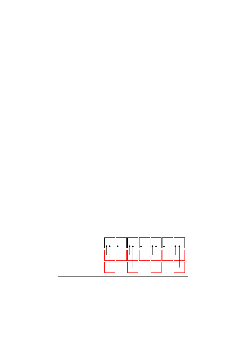
This quickly becomes intuitive if we remember that, when we create a vector or
matrix, we are creating a view of an underlying data array rather than creating the
data itself:
underlying
array 0123456
v
v(0 to 6 by 2)
A vector slice v(0 to 6 by 2) of the v vector is just a different view of the array underlying v.
The view itself contains no data. It just contains pointers to the data in the original array. Internally,
the view is just stored as a pointer to the underlying data and a recipe for iterating over that data: in the
case of this slice, the recipe is just "start at the first element of the underlying data and go to the seventh element
of the underlying data in steps of two".

Chapter 2
[ 29 ]
Breeze offers a copy function for when we want to create independent copies of data.
In the previous example, we can construct a copy of viewEvens as:
scala> val copyEvens = v(0 until v.length by 2).copy
breeze.linalg.DenseVector[Double] = DenseVector(10.0, 10.0, 10.0)
We can now update copyEvens independently of v.
Matrix multiplication, transposition, and the
orientation of vectors
So far, we have mostly looked at element-wise operations on vectors and matrices.
Let's now look at matrix multiplication and related operations.
The matrix multiplication operator is *:
scala> val m1 = DenseMatrix((2.0, 3.0), (5.0, 6.0), (8.0, 9.0))
breeze.linalg.DenseMatrix[Double] =
2.0 3.0
5.0 6.0
8.0 9.0
scala> val m2 = DenseMatrix((10.0, 11.0), (12.0, 13.0))
breeze.linalg.DenseMatrix[Double]
10.0 11.0
12.0 13.0
scala> m1 * m2
56.0 61.0
122.0 133.0
188.0 205.0

Manipulating Data with Breeze
[ 30 ]
Besides matrix-matrix multiplication, we can use the matrix multiplication operator
between matrices and vectors. All vectors in Breeze are column vectors. This means
that, when multiplying matrices and vectors together, a vector should be viewed as
an (n * 1) matrix. Let's walk through an example of matrix-vector multiplication. We
want the following operation:
23 1
56 2
89
⎛⎞
⎛⎞
⎜⎟
⎜⎟
⎜⎟
⎝⎠
⎜⎟
⎝⎠
scala> val v = DenseVector(1.0, 2.0)
breeze.linalg.DenseVector[Double] = DenseVector(1.0, 2.0)
scala> m1 * v
breeze.linalg.DenseVector[Double] = DenseVector(8.0, 17.0, 26.0)
By contrast, if we wanted:
()
10 11
1212 13
⎛⎞
⎜⎟
⎝⎠
We must convert v to a row vector. We can do this using the transpose operation:
scala> val vt = v.t
breeze.linalg.Transpose[breeze.linalg.DenseVector[Double]] =
Transpose(DenseVector(1.0, 2.0))
scala> vt * m2
breeze.linalg.Transpose[breeze.linalg.DenseVector[Double]] =
Transpose(DenseVector(34.0, 37.0))
Note that the type of v.t is Transpose[DenseVector[_]]. A
Transpose[DenseVector[_]] behaves in much the same way as a DenseVector as far
as element-wise operations are concerned, but it does not support mutation or slicing.
Data preprocessing and feature engineering
We have now discovered the basic components of Breeze. In the next few sections,
we will apply them to real examples to understand how they t together to form a
robust base for data science.

Chapter 2
[ 31 ]
An important part of data science involves preprocessing datasets to construct useful
features. Let's walk through an example of this. To follow this example and access
the data, you will need to download the code examples for the book (www.github.
com/pbugnion/s4ds).
You will nd, in directory chap02/data/ of the code attached to this book, a CSV le
with true heights and weights as well as self-reported heights and weights for 181
men and women. The original dataset was collected as part of a study on body image.
Refer to the following link for more information: http://vincentarelbundock.
github.io/Rdatasets/doc/car/Davis.html.
There is a helper function in the package provided with the book to load the data
into Breeze arrays:
scala> val data = HWData.load
HWData [ 181 rows ]
scala> data.genders
breeze.linalg.Vector[Char] = DenseVector(M, F, F, M, ... )
The data object contains ve vectors, each 181 element long:
• data.genders: A Char vector describing the gender of the participants
• data.heights: A Double vector of the true height of the participants
• data.weights: A Double vector of the true weight of the participants
• data.reportedHeights: A Double vector of the self-reported height of
the participants
• data.reportedWeights: A Double vector of the self-reported weight of
the participants
Let's start by counting the number of men and women in the study. We will
dene an array that contains just 'M' and do an element-wise comparison with
data.genders:
scala> val maleVector = DenseVector.fill(data.genders.length)('M')
breeze.linalg.DenseVector[Char] = DenseVector(M, M, M, M, M, M,... )
scala> val isMale = (data.genders :== maleVector)
breeze.linalg.DenseVector[Boolean] = DenseVector(true, false, false, true
...)

Manipulating Data with Breeze
[ 32 ]
The isMale vector is the same length as data.genders. It is true where the
participant is male, and false otherwise. We can use this Boolean array as a mask
for the other arrays in the dataset (remember that vector(mask) selects the elements
of vector where mask is true). Let's get the height of the men in our dataset:
scala> val maleHeights = data.heights(isMale)
breeze.linalg.SliceVector[Int,Double] = breeze.linalg.
SliceVector@61717d42
scala> maleHeights.toDenseVector
breeze.linalg.DenseVector[Double] = DenseVector(182.0, 177.0, 170.0, ...
To count the number of men in our dataset, we can use the indicator function. This
transforms a Boolean array into an array of doubles, mapping false to 0.0 and
true to 1.0:
scala> import breeze.numerics._
import breeze.numerics._
scala> sum(I(isMale))
Double: 82.0
Let's calculate the mean height of men and women in the experiment. We can
calculate the mean of a vector using mean(v), which we can access by importing
breeze.stats._:
scala> import breeze.stats._
import breeze.stats._
scala> mean(data.heights)
Double = 170.75690607734808
To calculate the mean height of the men, we can use our isMale array to slice data.
heights; data.heights(isMale) is a view of the data.heights array with all the
height values for the men:
scala> mean(data.heights(isMale)) // mean male height
Double = 178.0121951219512
scala> mean(data.heights(!isMale)) // mean female height
Double = 164.74747474747474

Chapter 2
[ 33 ]
As a somewhat more involved example, let's look at the discrepancy between real
and reported weight for both men and women in this experiment. We can get an
array of the percentage difference between the reported weight and the true weight:
scala> val discrepancy =
(data.weights - data.reportedWeights) / data.weights
breeze.linalg.Vector[Double] = DenseVector(0.0, 0.1206896551724138,
-0.018867924528301886, -0.029411764705882353, ... )
Notice how Breeze's overloading of mathematical operators allows us to manipulate
data arrays easily and elegantly.
We can now calculate the mean and standard deviation of this array for men:
scala> mean(discrepancy(isMale))
res6: Double = -0.008451852933123775
scala> stddev(discrepancy(isMale))
res8: Double = 0.031901519634244195
We can also calculate the fraction of men who overestimated their height:
scala> val overReportMask =
(data.reportedHeights :> data.heights).toDenseVector
breeze.linalg.DenseVector[Boolean] = DenseVector(false, false, false,
false...
scala> sum(I(overReportMask :& isMale))
Double: 10.0
There are thus ten men who believe they are taller than they actually are. The
element-wise AND operator :& returns a vector that is true for all indices for which
both its arguments are true. The vector overReportMask :& isMale is thus true for
all participants that are male and over-reported their height.
Breeze – function optimization
Having studied feature engineering, let's now look at the other end of the data
science pipeline. Typically, a machine learning algorithm denes a loss function that
is a function of a set of parameters. The value of the loss function represents how
well the model ts the data. The parameters are then optimized to minimize (or
maximize) the loss function.

Manipulating Data with Breeze
[ 34 ]
In Chapter 12, Distributed Machine Learning with MLlib, we will look at MLlib, a
machine learning library that contains many well-known algorithms. Often, we
don't need to worry about optimizing loss functions directly since we can rely on the
machine learning algorithms provided by MLlib. It is nevertheless useful to have a
basic knowledge of optimization.
Breeze has an optimize module that contains functions for nding a local minimum:
scala> import breeze.optimize._
import breeze.optimize._
Let's create a toy function that we want to optimize:
()
2
i
i
fx x=
∑
We can represent this function in Scala as follows:
scala> def f(xs:DenseVector[Double]) = sum(xs :^ 2.0)
f: (xs: breeze.linalg.DenseVector[Double])Double
Most local optimizers also require the gradient of the function being optimized. The
gradient is a vector of the same dimension as the arguments to the function. In our
case, the gradient is:
2fx∇=!
We can represent the gradient in Breeze with a function that takes a vector argument
and returns a vector of the same length:
scala> def gradf(xs:DenseVector[Double]) = 2.0 :* xs
gradf: (xs:breeze.linalg.DenseVector[Double])breeze.linalg.
DenseVector[Double]
For instance, at the point (1, 1, 1), we have:
scala> val xs = DenseVector.ones[Double](3)
breeze.linalg.DenseVector[Double] = DenseVector(1.0, 1.0, 1.0)
scala> f(xs)
Double = 3.0
scala> gradf(xs)
breeze.linalg.DenseVector[Double] = DenseVector(2.0, 2.0, 2.0)

Chapter 2
[ 35 ]
Let's set up the optimization problem. Breeze's optimization methods require that
we pass in an implementation of the DiffFunction trait with a single method,
calculate. This method must return a tuple of the function and its gradient:
scala> val optTrait = new DiffFunction[DenseVector[Double]] {
def calculate(xs:DenseVector[Double]) = (f(xs), gradf(xs))
}
breeze.optimize.DiffFunction[breeze.linalg.DenseVector[Double]] =
<function1>
We are now ready to run the optimization. The optimize module provides a
minimize function that does just what we want. We pass it optTrait and a starting
point for the optimization:
scala> val minimum = minimize(optTrait, DenseVector(1.0, 1.0, 1.0))
breeze.linalg.DenseVector[Double] = DenseVector(0.0, 0.0, 0.0)
The true minimum is at (0.0, 0.0, 0.0). The optimizer therefore correctly nds
the minimum.
The minimize function uses the L-BFGS method to run the optimization by default.
It takes several additional arguments to control the optimization. We will explore
these in the next sections.
Numerical derivatives
In the previous example, we specied the gradient of f explicitly. While this is
generally good practice, calculating the gradient of a function can often be tedious.
Breeze provides a gradient approximation function using nite differences. Reusing
the same objective function def f(xs:DenseVector[Double]) = sum(xs :^ 2.0)
as in the previous section:
scala> val approxOptTrait = new ApproximateGradientFunction(f)
breeze.optimize.ApproximateGradientFunction[Int,breeze.linalg.
DenseVector[Double]] = <function1>
The trait approxOptTrait has a gradientAt method that returns an approximation
to the gradient at a point:
scala> approxOptTrait.gradientAt(DenseVector.ones(3))
breeze.linalg.DenseVector[Double] = DenseVector(2.00001000001393,
2.00001000001393, 2.00001000001393)

Manipulating Data with Breeze
[ 36 ]
Note that this can be quite inaccurate. The ApproximateGradientFunction
constructor takes an epsilon optional argument that controls the size of the step
taken when calculating the nite differences. Changing the value of epsilon can
improve the accuracy of the nite difference algorithm.
The ApproximateGradientFunction instance implements the DiffFunction trait. It
can therefore be passed to minimize directly:
scala> minimize(approxOptTrait, DenseVector.ones[Double](3))
breeze.linalg.DenseVector[Double] = DenseVector(-5.000001063126813E-6,
-5.000001063126813E-6, -5.000001063126813E-6)
This, again, gives a result close to zero, but somewhat further away than when we
specied the gradient explicitly. In general, it will be signicantly more efcient
and more accurate to calculate the gradient of a function analytically than to rely on
Breeze's numerical gradient. It is probably best to only use the numerical gradient
during data exploration or to check analytical gradients.
Regularization
The minimize function takes many optional arguments relevant to machine learning
algorithms. In particular, we can instruct the optimizer to use a regularization
parameter when performing the optimization. Regularization introduces a penalty
in the loss function to prevent the parameters from growing arbitrarily. This is useful
to avoid overtting. We will discuss regularization in greater detail in Chapter 12,
Distributed Machine Learning with MLlib.
For instance, to use L2Regularization with a hyperparameter of 0.5:
scala> minimize(optTrait,
DenseVector(1.0, 1.0, 1.0), L2Regularization(0.5))
breeze.linalg.DenseVector[Double] = DenseVector(0.0, 0.0, 0.0)
The regularization makes no difference in this case, since the parameters are zero at
the minimum.
To see a list of optional arguments that can be passed to minimize, consult the
Breeze documentation online.
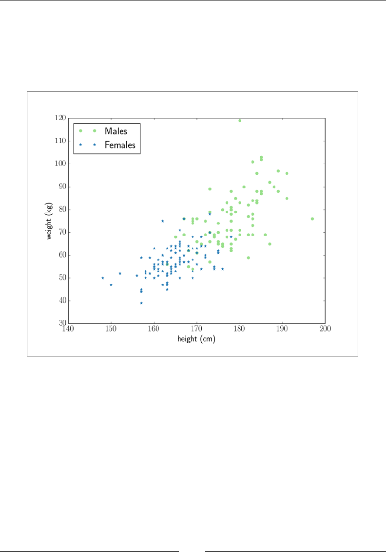
Chapter 2
[ 37 ]
An example – logistic regression
Let's now imagine we want to build a classier that takes a person's height and
weight and assigns a probability to their being Male or Female. We will reuse the
height and weight data introduced earlier in this chapter. Let's start by plotting
the dataset:
Height versus weight data for 181 men and women
There are many different algorithms for classication. A rst glance at the data
shows that we can, approximately, separate men from women by drawing a straight
line across the plot. A linear method is therefore a reasonable initial attempt at
classication. In this section, we will use logistic regression to build a classier.
A detailed explanation of logistic regression is beyond the scope of this book. The
reader unfamiliar with logistic regression is referred to The Elements of Statistical
Learning by Hastie, Tibshirani, and Friedman. We will just give a brief summary here.

Manipulating Data with Breeze
[ 38 ]
Logistic regression estimates the probability of a given height and weight belonging to
a male with the following sigmoid function:
( ) ( )
( )
1
|, 1 exp , ;
P male height weight fheight weight params
=+−
Here, f is a linear function:
()() () ()
,; 0 1 2fheight weight params params height params weight params=+⋅+⋅
Here,
params
is an array of parameters that we need to determine using the training
set. If we consider the height and weight as a features = (height, weight) matrix, we can
re-write the sigmoid kernel f as a matrix multiplication of the features matrix with the
params vector:
()() ()
; 0 1:ffeatures params params features params=+⋅
To simplify this expression further, it is common to add a dummy feature whose
value is always 1 to the features matrix. We can then multiply params(0) by this
feature, allowing us to write the entire sigmoid kernel f as a single matrix-vector
multiplication:
( )
;ffeatures params params features=⋅
The feature matrix, features, is now a (181 * 3) matrix, where each row is (1, height,
weight) for a particular participant.
To nd the optimal values of the parameters, we can maximize the likelihood
function, L(params|features). The likelihood takes a given set of parameter values
as input and returns the probability that these particular parameters gave rise
to the training set. For a set of parameters and associated probability function
P(male|featuresi), the likelihood is:

Chapter 2
[ 39 ]
( ) ( )
( )
| |
1|
i
i
i
i
target is male
i
i
target not male
L paramsfeatures P male features
P male features
=×
−
∏
∏
If we magically know, ahead of time, the gender of everyone in the population,
we can assign P(male)=1 for the men and P(male)=0 for the women. The likelihood
function would then be 1. Conversely, any uncertainty leads to a reduction in
the likelihood function. If we choose a set of parameters that consistently lead to
classication errors (low P(male) for men or high P(male) for women), the likelihood
function drops to 0.
The maximum likelihood corresponds to those values of the parameters most likely
to describe the observed data. Thus, to nd the parameters that best describe our
training set, we just need to nd parameters that maximize L(params|features).
However, maximizing the likelihood function itself is very rarely done, since it
involves multiplying many small values together, which quickly leads to oating
point underow. It is best to maximize the log of the likelihood, which has the
same maximum as the likelihood. Finally, since most optimization algorithms
are geared to minimize a function rather than maximize it, we will minimize
( )
( )
log|
L params features
−.
For logistic regression, this is equivalent to minimizing:
() ()( )
( )
log exp 1
i i i
i
Cost params target params features params features=×⋅ − ⋅+
∑
Here, the sum runs over all participants in the training data, i
features
is a vector
( )
1, ,
i i
height weight of the i-th observation in the training set, and
i
target
is 1 if the
person is male, and 0 if the participant is female.
To minimize the Cost function, we must also know its gradient with respect to the
parameters. This is:
( )
|
params i i i
i
Cost features P male features target∇=⋅ −
⎡ ⎤
⎣ ⎦
∑

Manipulating Data with Breeze
[ 40 ]
We will start by rescaling the height and weight by their mean and standard deviation.
While this is not strictly necessary for logistic regression, it is generally good practice.
It facilitates the optimization and would become necessary if we wanted to use
regularization methods or build superlinear features (features that allow the boundary
separating men from women to be curved rather than a straight line).
For this example, we will move away from the Scala shell and write a standalone
Scala script. Here's the full code listing. Don't worry if this looks daunting. We will
break it up into manageable chunks in a minute:
import breeze.linalg._
import breeze.numerics._
import breeze.optimize._
import breeze.stats._
object LogisticRegressionHWData extends App {
val data = HWData.load
// Rescale the features to have mean of 0.0 and s.d. of 1.0
def rescaled(v:DenseVector[Double]) =
(v - mean(v)) / stddev(v)
val rescaledHeights = rescaled(data.heights)
val rescaledWeights = rescaled(data.weights)
// Build the feature matrix as a matrix with
//181 rows and 3 columns.
val rescaledHeightsAsMatrix = rescaledHeights.toDenseMatrix.t
val rescaledWeightsAsMatrix = rescaledWeights.toDenseMatrix.t
val featureMatrix = DenseMatrix.horzcat(
DenseMatrix.ones[Double](rescaledHeightsAsMatrix.rows, 1),
rescaledHeightsAsMatrix,
rescaledWeightsAsMatrix
)
println(s"Feature matrix size: ${featureMatrix.rows} x " +
s"${featureMatrix.cols}")
// Build the target variable to be 1.0 where a participant
// is male, and 0.0 where the participant is female.
val target = data.genders.values.map {

Chapter 2
[ 41 ]
gender => if(gender == 'M') 1.0 else 0.0
}
// Build the loss function ready for optimization.
// We will worry about refactoring this to be more
// efficient later.
def costFunction(parameters:DenseVector[Double]):Double = {
val xBeta = featureMatrix * parameters
val expXBeta = exp(xBeta)
- sum((target :* xBeta) - log1p(expXBeta))
}
def costFunctionGradient(parameters:DenseVector[Double])
:DenseVector[Double] = {
val xBeta = featureMatrix * parameters
val probs = sigmoid(xBeta)
featureMatrix.t * (probs - target)
}
val f = new DiffFunction[DenseVector[Double]] {
def calculate(parameters:DenseVector[Double]) =
(costFunction(parameters), costFunctionGradient(parameters))
}
val optimalParameters = minimize(f, DenseVector(0.0, 0.0, 0.0))
println(optimalParameters)
// => DenseVector(-0.0751454743, 2.476293647, 2.23054540)
}
That was a mouthful! Let's take this one step at a time. After the obvious imports, we
start with:
object LogisticRegressionHWData extends App {
By extending the built-in App trait, we tell Scala to treat the entire object as a main
function. This just cuts out def main(args:Array[String]) boilerplate. We
then load the data and rescale the height and weight to have a mean of zero and a
standard deviation of one:
def rescaled(v:DenseVector[Double]) =
(v - mean(v)) / stddev(v)
val rescaledHeights = rescaled(data.heights)
val rescaledWeights = rescaled(data.weights)

Manipulating Data with Breeze
[ 42 ]
The rescaledHeights and rescaledWeights vectors will be the features of our
model. We can now build the training set matrix for this model. This is a (181 * 3)
matrix, for which the i-th row is (1, height(i), weight(i)), corresponding to the
values of the height and weight for the ith participant. We start by transforming both
rescaledHeights and rescaledWeights from vectors to (181 * 1) matrices
val rescaledHeightsAsMatrix = rescaledHeights.toDenseMatrix.t
val rescaledWeightsAsMatrix = rescaledWeights.toDenseMatrix.t
We must also create a (181 * 1) matrix containing just 1 to act as the dummy feature.
We can do this using:
DenseMatrix.ones[Double](rescaledHeightsAsMatrix.rows, 1)
We now need to combine our three (181 * 1) matrices together into a single feature
matrix of shape (181 * 3). We can use the horzcat method to concatenate the three
matrices together:
val featureMatrix = DenseMatrix.horzcat(
DenseMatrix.ones[Double](rescaledHeightsAsMatrix.rows, 1),
rescaledHeightsAsMatrix,
rescaledWeightsAsMatrix
)
The nal step in the data preprocessing stage is to create the target variable. We need
to convert the data.genders vector to a vector of ones and zeros. We assign a value
of one for men and zero for women. Thus, our classier will predict the probability
that any given person is male. We will use the .values.map method, a method
equivalent to the .map method on Scala collections:
val target = data.genders.values.map {
gender => if(gender == 'M') 1.0 else 0.0
}
Note that we could also have used the indicator function which we discovered earlier:
val maleVector = DenseVector.fill(data.genders.size)('M')
val target = I(data.genders :== maleVector)
This results in the allocation of a temporary array, maleVector, and might
therefore increase the program's memory footprint if there were many
participants in the experiment.

Chapter 2
[ 43 ]
We now have a matrix representing the training set and a vector denoting the target
variable. We can write the loss function that we want to minimize. As mentioned
previously, we will minimize
( )
( )
log |Lparameterstraining−. The loss function
takes as input a set of values for the linear coefcients and returns a number
indicating how well those values of the linear coefcients t the training data:
def costFunction(parameters:DenseVector[Double]):Double = {
val xBeta = featureMatrix * parameters
val expXBeta = exp(xBeta)
- sum((target :* xBeta) - log1p(expXBeta))
}
Note that we use log1p(x) to calculate log(1+x). This is robust to underow for small
values of x.
Let's explore the cost function:
costFunction(DenseVector(0.0, 0.0, 0.0)) // 125.45963968135031
costFunction(DenseVector(0.0, 0.1, 0.1)) // 113.33336518036882
costFunction(DenseVector(0.0, -0.1, -0.1)) // 139.17134594294433
We can see that the cost function is somewhat lower for slightly positive values of
the height and weight parameters. This indicates that the likelihood function is larger
for slightly positive values of the height and weight. This, in turn, implies (as we
expect from the plot) that people who are taller and heavier than average are more
likely to be male.
We also need a function that calculates the gradient of the loss function, since that
will help with the optimization:
def costFunctionGradient(parameters:DenseVector[Double])
:DenseVector[Double] = {
val xBeta = featureMatrix * parameters
val probs = sigmoid(xBeta)
featureMatrix.t * (probs - target)
}
Having dened the loss function and gradient, we are now in a position to set up
the optimization:
val f = new DiffFunction[DenseVector[Double]] {
def calculate(parameters:DenseVector[Double]) =
(costFunction(parameters), costFunctionGradient(parameters))
}
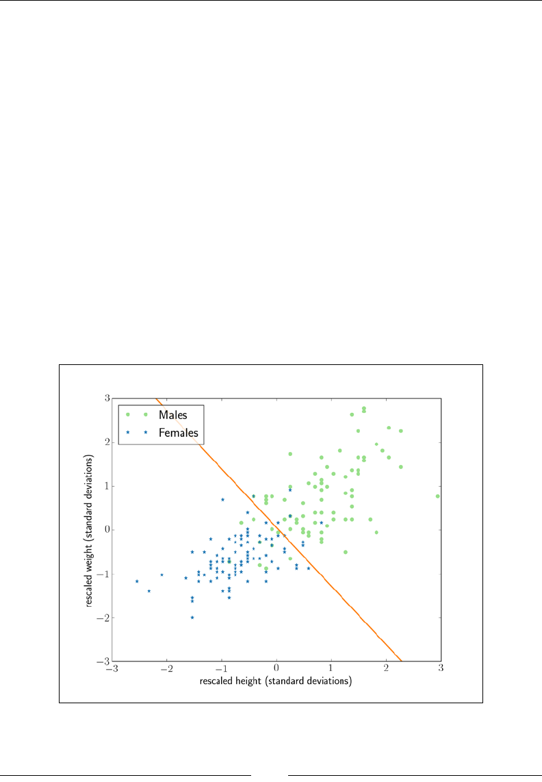
Manipulating Data with Breeze
[ 44 ]
All that is left now is to run the optimization. The cost function for logistic
regression is convex (it has a single minimum), so the starting point for optimization
is irrelevant in principle. In practice, it is common to start with a coefcient vector
that is zero everywhere (equating to assigning a 0.5 probability of being male to
every participant):
val optimalParameters = minimize(f, DenseVector(0.0, 0.0, 0.0))
This returns the vector of optimal parameters:
DenseVector(-0.0751454743, 2.476293647, 2.23054540)
How can we interpret the values of the optimal parameters? The coefcients for
the height and weight are both positive, indicating that people who are taller and
heavier are more likely to be male.
We can also get the decision boundary (the line separating (height, weight) pairs
more likely to belong to a woman from (height, weight) pairs more likely to belong
to a man) directly from the coefcients. The decision boundary is:
0.075 2.48 2.23 0rescaledHeight rescaledWeight−+ + =
Height and weight data (shifted by the mean and rescaled by the standard deviation).
The orange line is the logistic regression decision boundary. Logistic regression predicts that
individuals above the boundary are male.

Chapter 2
[ 45 ]
Towards re-usable code
In the previous section, we performed all of the computation in a single script. While
this is ne for data exploration, it means that we cannot reuse the logistic regression
code that we have built. In this section, we will start the construction of a machine
learning library that you can reuse across different projects.
We will factor the logistic regression algorithm out into its own class. We construct a
LogisticRegression class:
import breeze.linalg._
import breeze.numerics._
import breeze.optimize._
class LogisticRegression(
val training:DenseMatrix[Double],
val target:DenseVector[Double])
{
The class takes, as input, a matrix representing the training set and a vector denoting
the target variable. Notice how we assign these to vals, meaning that they are set
on class creation and will remain the same until the class is destroyed. Of course, the
DenseMatrix and DenseVector objects are mutable, so the values that training
and target point to might change. Since programming best practice dictates that
mutable state makes reasoning about program behavior difcult, we will avoid
taking advantage of this mutability.
Let's add a method that calculates the cost function and its gradient:
def costFunctionAndGradient(coefficients:DenseVector[Double])
:(Double, DenseVector[Double]) = {
val xBeta = training * coefficients
val expXBeta = exp(xBeta)
val cost = - sum((target :* xBeta) - log1p(expXBeta))
val probs = sigmoid(xBeta)
val grad = training.t * (probs - target)
(cost, grad)
}

Manipulating Data with Breeze
[ 46 ]
We are now all set up to run the optimization to calculate the coefcients that best
reproduce the training set. In traditional object-oriented languages, we might dene
a getOptimalCoefficients method that returns a DenseVector of the coefcients.
Scala, however, is more elegant. Since we have dened the training and target
attributes as vals, there is only one possible set of values of the optimal coefcients.
We could, therefore, dene a val optimalCoefficients = ??? class attribute
that holds the optimal coefcients. The problem with this is that it forces all the
computation to happen when the instance is constructed. This will be unexpected
for the user and might be wasteful: if the user is only interested in accessing the cost
function, for instance, the time spent minimizing it will be wasted. The solution is to
use a lazy val. This value will only be evaluated when the client code requests it:
lazy val optimalCoefficients = ???
To help with the calculation of the coefcients, we will dene a private helper method:
private def calculateOptimalCoefficients
:DenseVector[Double] = {
val f = new DiffFunction[DenseVector[Double]] {
def calculate(parameters:DenseVector[Double]) =
costFunctionAndGradient(parameters)
}
minimize(f, DenseVector.zeros[Double](training.cols))
}
lazy val optimalCoefficients = calculateOptimalCoefficients
We have refactored the logistic regression into its own class, that we can reuse across
different projects.
If we were planning on reusing the height-weight data, we could, similarly, refactor
it into a class of its own that facilitates data loading, feature scaling, and any other
functionality that we nd ourselves reusing often.

Chapter 2
[ 47 ]
Alternatives to Breeze
Breeze is the most feature-rich and approachable Scala framework for linear algebra
and numeric computation. However, do not take my word for it: experiment with
other libraries for tabular data. In particular, I recommend trying Saddle, which
provides a Frame object similar to data frames in pandas or R. In the Java world, the
Apache Commons Maths library provides a very rich toolkit for numerical computation.
In Chapter 10, Distributed Batch Processing with Spark, Chapter 11, Spark SQL and
DataFrames, and Chapter 12, Distributed Machine Learning with MLlib, we will explore
Spark and MLlib, which allow the user to run distributed machine learning algorithms.
Summary
This concludes our brief overview of Breeze. We have learned how to manipulate
basic Breeze data types, how to use them for linear algebra, and how to perform
convex optimization. We then used our knowledge to clean a real dataset and
performed logistic regression on it.
In the next chapter, we will discuss breeze-viz, a plotting library for Scala.
References
The Elements of Statistical Learning, by Hastie, Tibshirani, and Friedman, gives a lucid,
practical description of the mathematical underpinnings of machine learning.
Anyone aspiring to do more than mindlessly apply machine learning algorithms as
black boxes ought to have a well-thumbed copy of this book.
Scala for Machine Learning, by Patrick R. Nicholas, describes practical implementations
of many useful machine learning algorithms in Scala.
The Breeze documentation (https://github.com/scalanlp/breeze/wiki/
Quickstart), API docs (http://www.scalanlp.org/api/breeze/#package), and
source code (https://github.com/scalanlp/breeze) provide the most up-to-date
sources of documentation on Breeze.

[ 49 ]
Plotting with breeze-viz
Data visualization is an integral part of data science. Visualization needs fall into
two broad categories: during the development and validation of new models and,
at the end of the pipeline, to distill meaning from the data and the models to provide
insight to external stakeholders.
The two types of visualizations are quite different. At the data exploration and
model development stage, the most important feature of a visualization library
is its ease of use. It should take as few steps as possible to go from having data as
arrays of numbers (or CSVs or in a database) to having data displayed on a screen.
The lifetime of graphs is also quite short: once the data scientist has learned all he
can from the graph or visualization, it is normally discarded. By contrast, when
developing visualization widgets for external stakeholders, one is willing to tolerate
increased development time for greater exibility. The visualizations can have
signicant lifetime, especially if the underlying data changes over time.
The tool of choice in Scala for the rst type of visualization is breeze-viz. When
developing visualizations for external stakeholders, web-based visualizations
(such as D3) and Tableau tend to be favored.
In this chapter, we will explore breeze-viz. In Chapter 14, Visualization with D3
and the Play Framework, we will learn how to build Scala backends for JavaScript
visualizations.
Breeze-viz is (no points for guessing) Breeze's visualization library. It wraps
JFreeChart, a very popular Java charting library. Breeze-viz is still very experimental.
In particular, it is much less feature-rich than matplotlib in Python, or R or MATLAB.
Nevertheless, breeze-viz allows access to the underlying JFreeChart objects so one
can always fall back to editing these objects directly. The syntax for breeze-viz is
inspired by MATLAB and matplotlib.

Plotting with breeze-viz
[ 50 ]
Diving into Breeze
Let's get started. We will work in the Scala console, but a program similar to this
example is available in BreezeDemo.scala in the examples corresponding to this
chapter. Create a build.sbt le with the following lines:
scalaVersion := "2.11.7"
libraryDependencies ++= Seq(
"org.scalanlp" %% "breeze" % "0.11.2",
"org.scalanlp" %% "breeze-viz" % "0.11.2",
"org.scalanlp" %% "breeze-natives" % "0.11.2"
)
Start an sbt console:
$ sbt console
scala> import breeze.linalg._
import breeze.linalg._
scala> import breeze.plot._
import breeze.plot._
scala> import breeze.numerics._
import breeze.numerics._
Let's start by plotting a sigmoid curve,
()
()
1/ 1x
fx e
−
=+. We will rst generate the
data using Breeze. Recall that the linspace method creates a vector of doubles,
uniformly distributed between two values:
scala> val x = linspace(-4.0, 4.0, 200)
x: DenseVector[Double] = DenseVector(-4.0, -3.959798...
scala> val fx = sigmoid(x)
fx: DenseVector[Double] = DenseVector(0.0179862099620915,...
We now have the data ready for plotting. The rst step is to create a gure:
scala> val fig = Figure()
fig: breeze.plot.Figure = breeze.plot.Figure@37e36de9
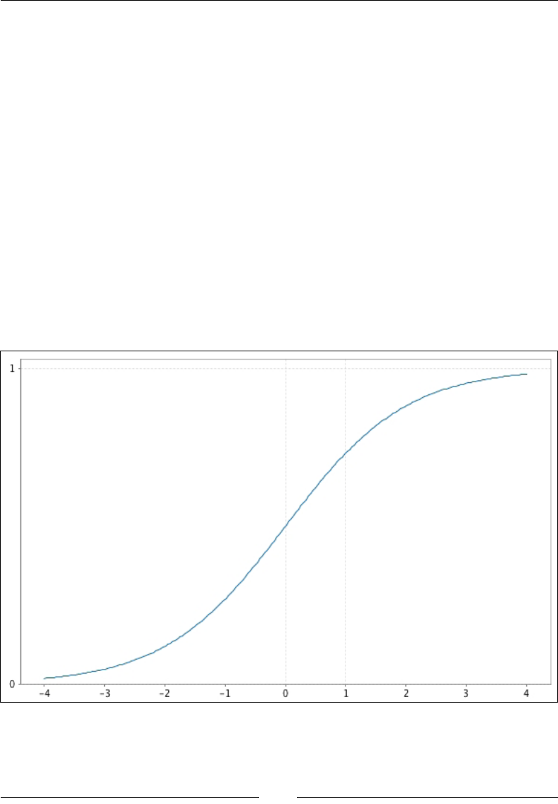
Chapter 3
[ 51 ]
This creates an empty Java Swing window (which may appear on your taskbar or
equivalent). A gure can contain one or more plots. Let's add a plot to our gure:
scala> val plt = fig.subplot(0)
plt: breeze.plot.Plot = breeze.plot.Plot@171c2840
For now, let's ignore the 0 passed as argument to .subplot. We can add data points
to our plot:
scala> plt += plot(x, fx)
breeze.plot.Plot = breeze.plot.Plot@63d6a0f8
The plot function takes two arguments, corresponding to the x and y values of the
data series to be plotted. To view the changes, you need to refresh the gure:
scala> fig.refresh()
Look at the Swing window now. You should see a beautiful sigmoid, similar to the
one below. Right-clicking on the window lets you interact with the plot and save the
image as a PNG:

Plotting with breeze-viz
[ 52 ]
You can also save the image programmatically as follows:
scala> fig.saveas("sigmoid.png")
Breeze-viz currently only supports exporting to PNG.
Customizing plots
We now have a curve on our chart. Let's add a few more:
scala> val f2x = sigmoid(2.0*x)
f2x: breeze.linalg.DenseVector[Double] = DenseVector(3.353501304664E-4...
scala> val f10x = sigmoid(10.0*x)
f10x: breeze.linalg.DenseVector[Double] = DenseVector(4.2483542552
9E-18...
scala> plt += plot(x, f2x, name="S(2x)")
breeze.plot.Plot = breeze.plot.Plot@63d6a0f8
scala> plt += plot(x, f10x, name="S(10x)")
breeze.plot.Plot = breeze.plot.Plot@63d6a0f8
scala> fig.refresh()
Looking at the gure now, you should see all three curves in different colors. Notice
that we named the data series as we added them to the plot, using the name=""
keyword argument. To view the names, we must set the legend attribute:
scala> plt.legend = true
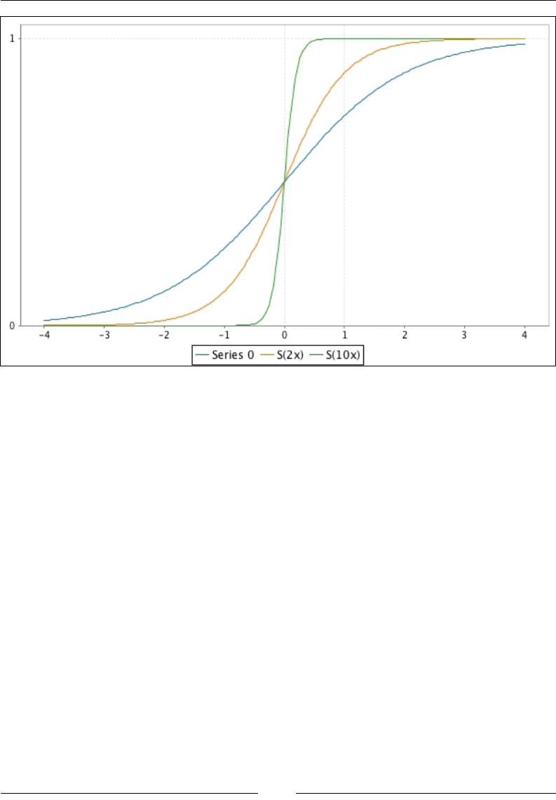
Chapter 3
[ 53 ]
Our plot still leaves a lot to be desired. Let's start by restricting the range of the x axis
to remove the bands of white space on either side of the plot:
scala> plt.xlim = (-4.0, 4.0)
plt.xlim: (Double, Double) = (-4.0,4.0)
Now, notice how, while the x ticks are sensibly spaced, there are only two y ticks: at
0 and 1. It would be useful to have ticks every 0.1 increment. Breeze does not provide
a way to set this directly. Instead, it exposes the underlying JFreeChart Axis object
belonging to the current plot:
scala> plt.yaxis
org.jfree.chart.axis.NumberAxis = org.jfree.chart.axis.NumberAxis@0
The Axis object supports a .setTickUnit method that lets us set the tick spacing:
scala> import org.jfree.chart.axis.NumberTickUnit
import org.jfree.chart.axis.NumberTickUnit
scala> plt.yaxis.setTickUnit(new NumberTickUnit(0.1))

Plotting with breeze-viz
[ 54 ]
JFreeChart allows extensive customization of the Axis object. For a full list of
methods available, consult the JFreeChart documentation (http://www.jfree.org/
jfreechart/api/javadoc/org/jfree/chart/axis/Axis.html).
Let's also add a vertical line at x=0 and a horizontal line at f(x)=1. We will need to
access the underlying JFreeChart plot to add these lines. This is available (somewhat
confusingly) as the .plot attribute in our Breeze Plot object:
scala> plt.plot
org.jfree.chart.plot.XYPlot = org.jfree.chart.plot.XYPlot@17e4db6c
We can use the .addDomainMarker and .addRangeMarker methods to add vertical
and horizontal lines to JFreeChart XYPlot objects:
scala> import org.jfree.chart.plot.ValueMarker
import org.jfree.chart.plot.ValueMarker
scala> plt.plot.addDomainMarker(new ValueMarker(0.0))
scala> plt.plot.addRangeMarker(new ValueMarker(1.0))
Let's also add labels to the axes:
scala> plt.xlabel = "x"
plt.xlabel: String = x
scala> plt.ylabel = "f(x)"
plt.ylabel: String = f(x)
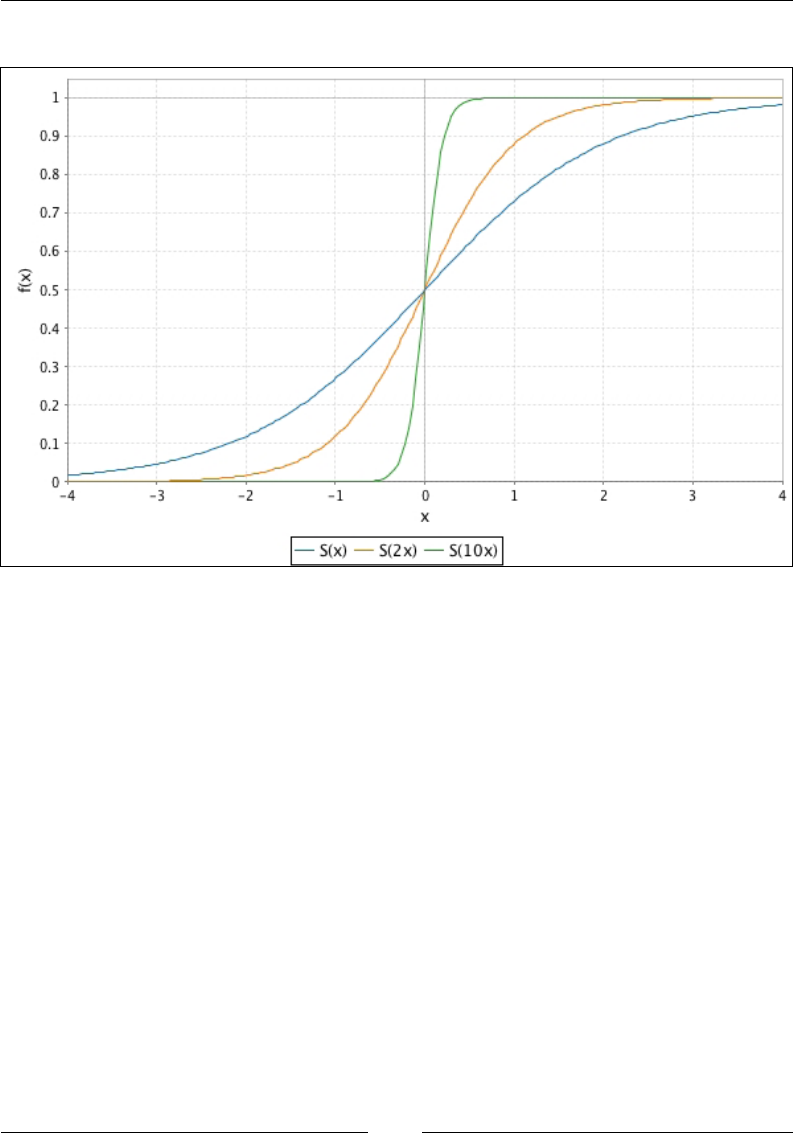
Chapter 3
[ 55 ]
If you have run all these commands, you should have a graph that looks like this:
We now know how to customize the basic building blocks of a graph. The next step
is to learn how to change how curves are drawn.
Customizing the line type
So far, we have just plotted lines using the default settings. Breeze lets us customize
how lines are drawn, at least to some extent.
For this example, we will use the height-weight data discussed in Chapter 2,
Manipulating Data with Breeze. We will use the Scala shell here for demonstrative
purposes, but you will nd a program in BreezeDemo.scala that follows the
example shell session.
The code examples for this chapter come with a module for loading the data,
HWData.scala, that loads the data from the CSVs:
scala> val data = HWData.load
data: HWData = HWData [ 181 rows ]
scala> data.heights
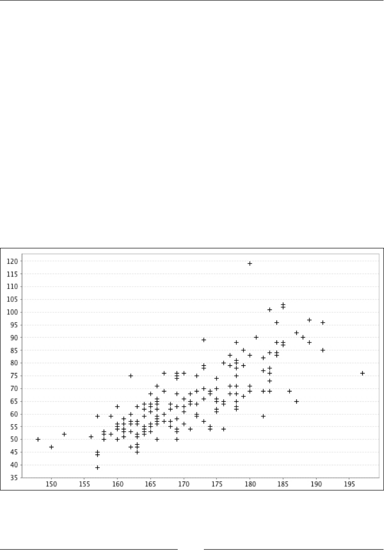
Plotting with breeze-viz
[ 56 ]
breeze.linalg.DenseVector[Double] = DenseVector(182.0, ...
scala> data.weights
breeze.linalg.DenseVector[Double] = DenseVector(77.0, 58.0...
Let's create a scatter plot of the heights against the weights:
scala> val fig = Figure("height vs. weight")
fig: breeze.plot.Figure = breeze.plot.Figure@743f2558
scala> val plt = fig.subplot(0)
plt: breeze.plot.Plot = breeze.plot.Plot@501ea274
scala> plt += plot(data.heights, data.weights, '+',
colorcode="black")
breeze.plot.Plot = breeze.plot.Plot@501ea274
This produces a scatter-plot of the height-weight data:
Chapter 3
[ 57 ]
Note that we passed a third argument to the plot method, '+'. This controls the
plotting style. As of this writing, there are three available styles: '-' (the default),
'+', and '.'. Experiment with these to see what they do. Finally, we pass a
colorcode="black" argument to control the color of the line. This is either a color
name or an RGB triple, written as a string. Thus, to plot red points, we could have
passed colorcode="[255,0,0]".
Looking at the height-weight plot, there is clearly a trend between height and
weight. Let's try and t a straight line through the data points. We will t the
following function:
() ()
weight Kg a b height cm=+×
Scientic literature suggests that it would be better to t
something more like 2
mass height∝. You should nd it
straightforward to t a quadratic line to the data, should you
wish to.
We will use Breeze's least squares function to nd the values of a and b. The
leastSquares method expects an input matrix of features and a target vector, just
like the LogisticRegression class that we dened in the previous chapter. Recall
that in Chapter 2, Manipulating Data with Breeze, when we prepared the training set
for logistic regression classication, we introduced a dummy feature that was one for
every participant to provide the degree of freedom for the y intercept. We will use
the same approach here. Our feature matrix, therefore, contains two columns—one
that is 1 everywhere and one for the height:
scala> val features = DenseMatrix.horzcat(
DenseMatrix.ones[Double](data.npoints, 1),
data.heights.toDenseMatrix.t
)
features: breeze.linalg.DenseMatrix[Double] =
1.0 182.0
1.0 161.0
1.0 161.0
1.0 177.0
1.0 157.0
...
scala> import breeze.stats.regression._

Plotting with breeze-viz
[ 58 ]
import breeze.stats.regression._
scala> val leastSquaresResult = leastSquares(features, data.weights)
leastSquaresResult: breeze.stats.regression.LeastSquaresRegressionResult
= <function1>
The leastSquares method returns an instance of LeastSquareRegressionResult,
which contains a coefficients attribute containing the coefcients that best t the
data:
scala> leastSquaresResult.coefficients
breeze.linalg.DenseVector[Double] = DenseVector(-131.042322, 1.1521875)
The best-t line is therefore:
() ()
131.04 1.1522weight Kg height cm=−+×
Let's extract the coefcients. An elegant way of doing this is to use Scala's pattern
matching capabilities:
scala> val Array(a, b) = leastSquaresResult.coefficients.toArray
a: Double = -131.04232269750622
b: Double = 1.1521875435418725
By writing val Array(a, b) = ..., we are telling Scala that the right-hand side of
the expression is a two-element array and to bind the rst element of that array to the
value a and the second to the value b. See Appendix, Pattern Matching and Extractors,
for a discussion of pattern matching.
We can now add the best-t line to our graph. We start by generating evenly-spaced
dummy height values:
scala> val dummyHeights = linspace(min(data.heights),
max(data.heights), 200)
dummyHeights: breeze.linalg.DenseVector[Double] = DenseVector(148.0, ...
scala> val fittedWeights = a :+ (b :* dummyHeights)
fittedWeights: breeze.linalg.DenseVector[Double] = DenseVector(39.4814...
scala> plt += plot(dummyHeights, fittedWeights, colorcode="red")
breeze.plot.Plot = breeze.plot.Plot@501ea274
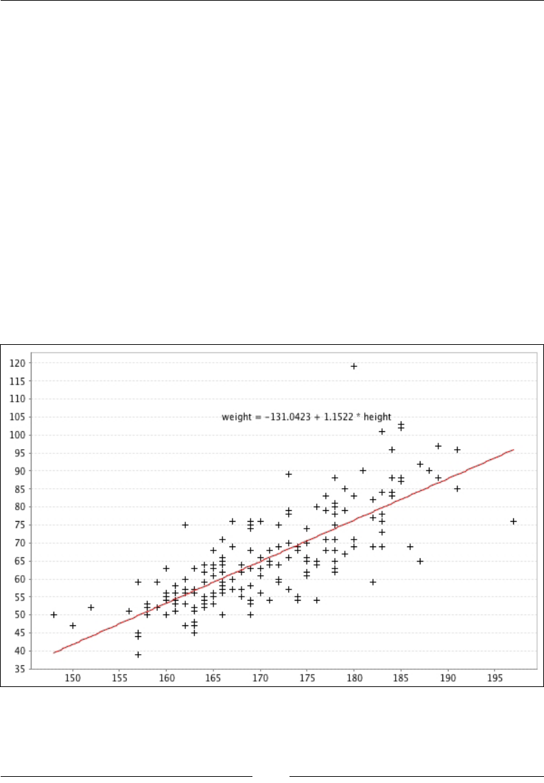
Chapter 3
[ 59 ]
Let's also add the equation for the best-t line to the graph as an annotation. We will
rst generate the label:
scala> val label = f"weight = $a%.4f + $b%.4f * height"
label: String = weight = -131.0423 + 1.1522 * height
To add an annotation, we must access the underlying JFreeChart plot:
scala> import org.jfree.chart.annotations.XYTextAnnotation
import org.jfree.chart.annotations.XYTextAnnotation
scala> plt.plot.addAnnotation(new XYTextAnnotation(label, 175.0, 105.0))
The XYTextAnnotation constructor takes three parameters: the annotation string
and a pair of (x, y) coordinates dening the centre of the annotation on the graph.
The coordinates of the annotation are expressed in the coordinate system of the
data. Thus, calling new XYTextAnnotation(label, 175.0, 105.0) generates an
annotation whose centroid is at the point corresponding to a height of 175 cm and
weight of 105 kg:

Plotting with breeze-viz
[ 60 ]
More advanced scatter plots
Breeze-viz offers a scatter function that adds a signicant degree of customization
to scatter plots. In particular, we can use the size and color of the marker points to
add additional dimensions of information to the plot.
The scatter function takes, as its rst two arguments, collections of x and y points.
The third argument is a function mapping an integer i to a Double indicating the
size of the ith point. The size of the point is measured in units of the x axis. If you
have the sizes as a Scala collection or a Breeze vector, you can use that collection's
apply method as the function. Let's see how this works in practice.
As with the previous examples, we will use the REPL, but you can nd a sample
program in BreezeDemo.scala:
scala> val fig = new Figure("Advanced scatter example")
fig: breeze.plot.Figure = breeze.plot.Figure@220821bc
scala> val plt = fig.subplot(0)
plt: breeze.plot.Plot = breeze.plot.Plot@668f8ae0
scala> val xs = linspace(0.0, 1.0, 100)
xs: breeze.linalg.DenseVector[Double] = DenseVector(0.0,
0.010101010101010102, 0.0202 ...
scala> val sizes = 0.025 * DenseVector.rand(100) // random sizes
sizes: breeze.linalg.DenseVector[Double] =
DenseVector(0.014879265631723166, 0.00219551...
scala> plt += scatter(xs, xs :^ 2.0, sizes.apply)
breeze.plot.Plot = breeze.plot.Plot@668f8ae0

Chapter 3
[ 61 ]
Selecting custom colors works in a similar manner: we pass in a colors argument
that maps an integer index to a java.awt.Paint object. Using these directly
can be cumbersome, so Breeze provides some default palettes. For instance, the
GradientPaintScale maps doubles in a given domain to a uniform color gradient.
Let's map doubles in the range 0.0 to 1.0 to the colors between red and green:
scala> val palette = new GradientPaintScale(
0.0, 1.0, PaintScale.RedToGreen)
palette: breeze.plot.GradientPaintScale[Double] = <function1>
scala> palette(0.5) // half-way between red and green
java.awt.Paint = java.awt.Color[r=127,g=127,b=0]
scala> palette(1.0) // green
java.awt.Paint = java.awt.Color[r=0,g=254,b=0]
Besides the GradientPaintScale, breeze-viz provides a CategoricalPaintScale
class for categorical palettes. For an overview of the different palettes, consult the
source le PaintScale.scala at scala: https://github.com/scalanlp/breeze/
blob/master/viz/src/main/scala/breeze/plot/PaintScale.scala.
Let's use our newfound knowledge to draw a multicolor scatter plot. We will assume
the same initialization as the previous example. We will assign a random color to
each point:
scala> val palette = new GradientPaintScale(0.0, 1.0,
PaintScale.MaroonToGold)
palette: breeze.plot.GradientPaintScale[Double] = <function1>
scala> val colors = DenseVector.rand(100).mapValues(palette)
colors: breeze.linalg.DenseVector[java.awt.Paint] = DenseVector(java.awt.
Color[r=162,g=5,b=0], ...
scala> plt += scatter(xs, xs :^ 2.0, sizes.apply, colors.apply)
breeze.plot.Plot = breeze.plot.Plot@8ff7e27
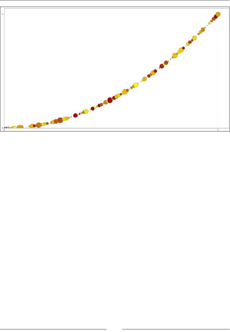
Plotting with breeze-viz
[ 62 ]
Multi-plot example – scatterplot matrix
plots
In this section, we will learn how to have several plots in the same gure.
The key new method that allows multiple plots in the same gure is fig.
subplot(nrows, ncols, plotIndex). This method, an overloaded version of the
fig.subplot method we have been using up to now, both sets the number of rows
and columns in the gure and returns a specic subplot. It takes three arguments:
• nrows: The number of rows of subplots in the figure
• ncols: The number of columns of subplots in the figure
• plotIndex: The index of the plot to return
Users familiar with MATLAB or matplotlib will note that the .subplot method is
identical to the eponymous methods in these frameworks. This might seem a little
complex, so let's look at an example (you will nd the code for this in BreezeDemo.
scala):
import breeze.plot._
def subplotExample {
val data = HWData.load
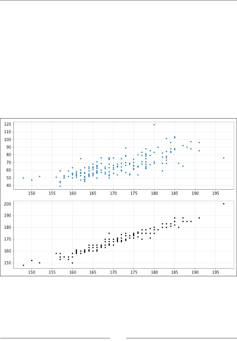
Chapter 3
[ 63 ]
val fig = new Figure("Subplot example")
// upper subplot: plot index '0' refers to the first plot
var plt = fig.subplot(2, 1, 0)
plt += plot(data.heights, data.weights, '.')
// lower subplot: plot index '1' refers to the second plot
plt = fig.subplot(2, 1, 1)
plt += plot(data.heights, data.reportedHeights, '.',
colorcode="black")
fig.refresh
}
Running this example produces the following plot:
Now that we have a basic grasp of how to add several subplots to the same gure,
let's do something a little more interesting. We will write a class to draw scatterplot
matrices. These are useful for exploring correlations between different features.

Plotting with breeze-viz
[ 64 ]
If you are not familiar with scatterplot matrices, have a look at the gure at the end
of this section for an idea of what we are constructing. The idea is to build a square
matrix of scatter plots for each pair of features. Element (i, j) in the matrix is a scatter
plot of feature i against feature j. Since a scatter plot of a variable against itself is
of limited use, one normally draws histograms of each feature along the diagonal.
Finally, since a scatter plot of feature i against feature j contains the same information
as a scatter plot of feature j against feature i, one normally only plots the upper
triangle or the lower triangle of the matrix.
Let's start by writing functions for the individual plots. These will take a Plot object
referencing the correct subplot and vectors of the data to plot:
import breeze.plot._
import breeze.linalg._
class ScatterplotMatrix(val fig:Figure) {
/** Draw the histograms on the diagonal */
private def plotHistogram(plt:Plot)(
data:DenseVector[Double], label:String) {
plt += hist(data)
plt.xlabel = label
}
/** Draw the off-diagonal scatter plots */
private def plotScatter(plt:Plot)(
xdata:DenseVector[Double],
ydata:DenseVector[Double],
xlabel:String,
ylabel:String) {
plt += plot(xdata, ydata, '.')
plt.xlabel = xlabel
plt.ylabel = ylabel
}
...
Notice the use of hist(data) to draw a histogram. The argument to hist must
be a vector of data points. The hist method will bin these and represent them
as a histogram.

Chapter 3
[ 65 ]
Now that we have the machinery for drawing individual plots, we just need to wire
everything together. The tricky part is to know how to select the correct subplot
for a given row and column position in the matrix. We can select a single plot by
calling fig.subplot(nrows, ncolumns, plotIndex), but translating from a (row,
column) index pair to a single plotIndex is not obvious. The plots are numbered in
increasing order, rst from left to right, then from top to bottom:
0 1 2 3
4 5 6 7
...
Let's write a short function to select a plot at a (row, column) index pair:
private def selectPlot(ncols:Int)(irow:Int, icol:Int):Plot = {
fig.subplot(ncols, ncols, (irow)*ncols + icol)
}
We are now in a position to draw the matrix plot itself:
/** Draw a scatterplot matrix.
*
* This function draws a scatterplot matrix of the correlation
* between each pair of columns in `featureMatrix`.
*
* @param featureMatrix A matrix of features, with each column
* representing a feature.
* @param labels Names of the features.
*/
def plotFeatures(
featureMatrix:DenseMatrix[Double],
labels:List[String]
) {
val ncols = featureMatrix.cols
require(ncols == labels.size,
"Number of columns in feature matrix "+
"must match length of labels"
)
fig.clear
fig.subplot(ncols, ncols, 0)
(0 until ncols) foreach { irow =>
val p = selectPlot(ncols)(irow, irow)
plotHistogram(p)(featureMatrix(::, irow), labels(irow))
(0 until irow) foreach { icol =>

Plotting with breeze-viz
[ 66 ]
val p = selectPlot(ncols)(irow, icol)
plotScatter(p)(
featureMatrix(::, irow),
featureMatrix(::, icol),
labels(irow),
labels(icol)
)
}
}
}
}
Let's write an example for our class. We will use the height-weight data again:
import breeze.linalg._
import breeze.numerics._
import breeze.plot._
object ScatterplotMatrixDemo extends App {
val data = HWData.load
val m = new ScatterplotMatrix(Figure("Scatterplot matrix demo"))
// Make a matrix with three columns: the height, weight and
// reported weight data.
val featureMatrix = DenseMatrix.horzcat(
data.heights.toDenseMatrix.t,
data.weights.toDenseMatrix.t,
data.reportedWeights.toDenseMatrix.t
)
m.plotFeatures(featureMatrix,
List("height", "weight", "reportedWeights"))
}
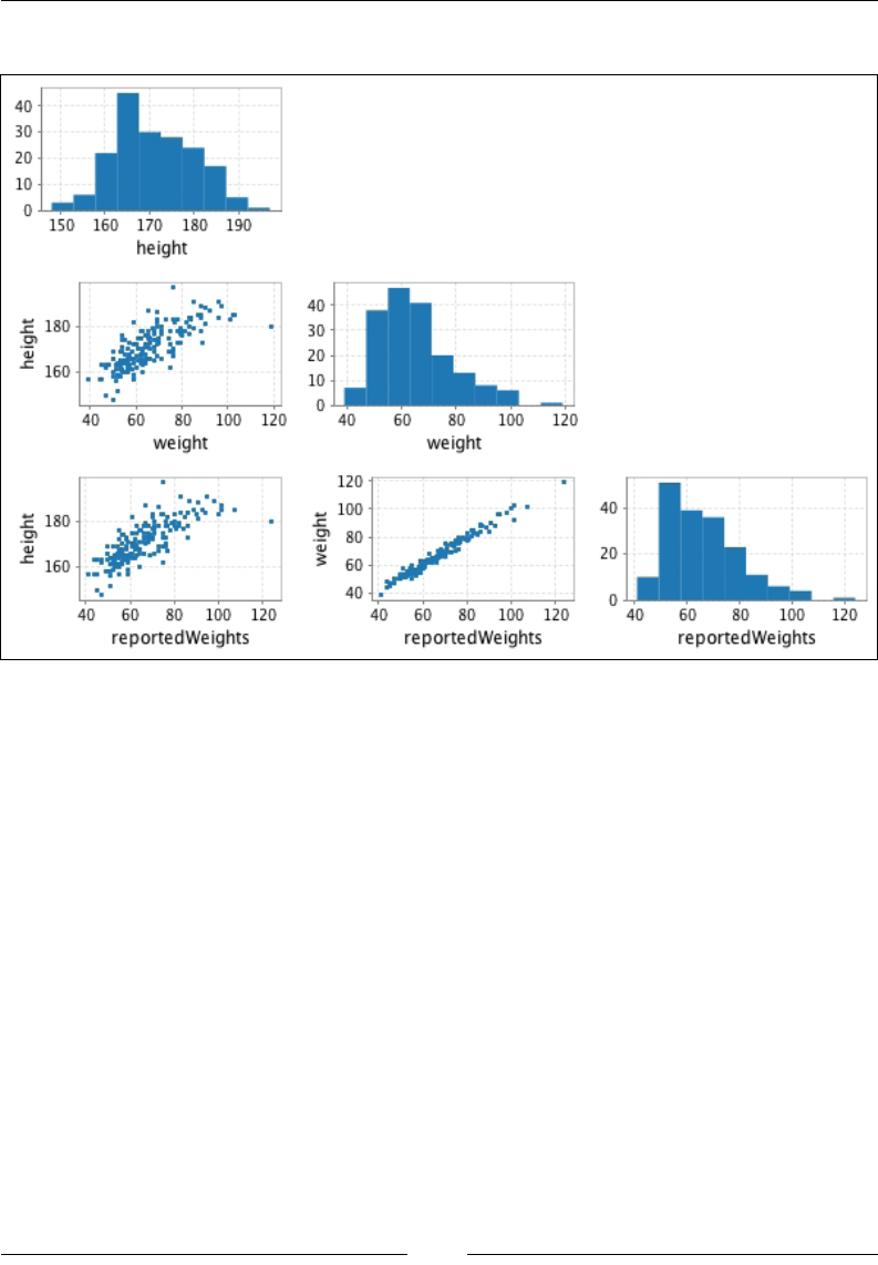
Chapter 3
[ 67 ]
Running this through SBT produces the following plot:
Managing without documentation
Breeze-viz is unfortunately rather poorly documented. This can make the learning
curve somewhat steep. Fortunately, it is still quite a small project: at the time of
writing, there are just ten source les (https://github.com/scalanlp/breeze/
tree/master/viz/src/main/scala/breeze/plot). A good way to understand
exactly what breeze-viz does is to read the source code. For instance, to see what
methods are available on a Plot object, read the source le Plot.scala. If you
need functionality beyond that provided by Breeze, consult the documentation
for JFreeChart to discover if you can implement what you need by accessing the
underlying JFreeChart objects.

Plotting with breeze-viz
[ 68 ]
Breeze-viz reference
Writing a reference in a programming book is a dangerous exercise: you quickly
become out of date. Nevertheless, given the paucity of documentation for breeze-viz,
this section becomes more relevant – it is easier to compete against something that
does not exist. Take this section with a pinch of salt, and if a command in this section
does not work, head over to the source code:
Command Description
plt += plot(xs, ys) This plots a series of (xs, ys) values. The xs and ys
values must be collection-like objects (Breeze vectors,
Scala arrays, or lists, for instance).
plt += scatter(xs, ys,
size)
plt += scatter(xs, ys,
size, color)
This plots a series of (xs, ys) values as a scatter plot.
The size argument is an (Int) => Double function
mapping the index of a point to its size (in the same
units as the x axis). The color argument is an (Int)
=> java.awt.Paint function mapping from integers
to colors. Read the more advanced scatter plots section for
further details.
plt += hist(xs)
plt += hist(xs, bins=10)
This bins xs and plots a histogram. The bins argument
controls the number of bins.
plt += image(mat) This plots an image or matrix. The mat argument
should be Matrix[Double]. Read the package.
scala source file in breeze.plot for details
(https://github.com/scalanlp/breeze/blob/
master/viz/src/main/scala/breeze/plot/
package.scala).
It is also useful to summarize the options available on a plot object:
Attribute Description
plt.xlabel = "x-label"
plt.ylabel = "y-label"
This sets the axis label
plt.xlim = (0.0, 1.0)
plt.ylim = (0.0, 1.0)
This sets the axis maximum and minimum value
plt.logScaleX = true
plt.logScaleY = true
This switches the axis to a log scale
plt.title = "title" This sets the plot title

Chapter 3
[ 69 ]
Data visualization beyond breeze-viz
Other tools for data visualization in Scala are emerging: Spark notebooks (https://
github.com/andypetrella/spark-notebook#description) based on the IPython
notebook and Apache Zeppelin (https://zeppelin.incubator.apache.org). Both
of these rely on Apache Spark, which we will explore later in this book.
Summary
In this chapter, we learned how to draw simple charts with breeze-viz. In the last
chapter of this book, we will learn how to build interactive visualizations using
JavaScript libraries.
Next, we will learn about basic Scala concurrency constructs—specically,
parallel collections.

[ 71 ]
Parallel Collections
and Futures
Data science often involves processing medium or large amounts of data. Since the
previously exponential growth in the speed of individual CPUs has slowed down
and the amount of data continues to increase, leveraging computers effectively must
entail parallel computation.
In this chapter, we will look at ways of parallelizing computation and data
processing over a single computer. Virtually all new computers have more than one
processing unit, and distributing a calculation over these cores can be an effective
way of hastening medium-sized calculations.
Parallelizing calculations over a single chip is suitable for calculations involving
gigabytes or a few terabytes of data. For larger data ows, we must resort to
distributing the computation over several computers in parallel. We will discuss
Apache Spark, a framework for parallel data processing in Chapter 10, Distributed
Batch Processing with Spark.
In this book, we will look at three common ways of leveraging parallel architectures
in a single machine: parallel collections, futures, and actors. We will consider the rst
two in this chapter, and leave the study of actors to Chapter 9, Concurrency with Akka.
Parallel collections
Parallel collections offer an extremely easy way to parallelize independent tasks.
The reader, being familiar with Scala, will know that many tasks can be phrased as
operations on collections, such as map, reduce, lter, or groupBy. Parallel collections
are an implementation of Scala collections that parallelize these operations to run
over several threads.

Parallel Collections and Futures
[ 72 ]
Let's start with an example. We want to calculate the frequency of occurrence of each
letter in a sentence:
scala> val sentence = "The quick brown fox jumped over the lazy dog"
sentence: String = The quick brown fox jumped ...
Let's start by converting our sentence from a string to a vector of characters:
scala> val characters = sentence.toVector
Vector[Char] = Vector(T, h, e, , q, u, i, c, k, ...)
We can now convert characters to a parallel vector, a ParVector. To do this, we use
the par method:
scala> val charactersPar = characters.par
ParVector[Char] = ParVector(T, h, e, , q, u, i, c, k, , ...)
ParVector collections support the same operations as regular vectors, but their
methods are executed in parallel over several threads.
Let's start by ltering out the spaces in charactersPar:
scala> val lettersPar = charactersPar.filter { _ != ' ' }
ParVector[Char] = ParVector(T, h, e, q, u, i, c, k, ...)
Notice how Scala hides the execution details. The filter operation was performed
using multiple threads, and you barely even noticed! The interface and behavior of a
parallel vector is identical to its serial counterpart, save for a few details that we will
explore in the next section.
Let's now use the toLower function to make the letters lowercase:
scala> val lowerLettersPar = lettersPar.map { _.toLower }
ParVector[Char] = ParVector(t, h, e, q, u, i, c, k, ...)
As before, the map method was applied in parallel. To nd the frequency of
occurrence of each letter, we use the groupBy method to group characters into
vectors containing all the occurrences of that character:
scala> val intermediateMap = lowerLettersPar.groupBy(identity)
ParMap[Char,ParVector[Char]] = ParMap(e -> ParVector(e, e, e, e), ...)

Chapter 4
[ 73 ]
Note how the groupBy method has created a ParMap instance, the parallel equivalent
of an immutable map. To get the number of occurrences of each letter, we do a
mapValues call on intermediateMap, replacing each vector by its length:
scala> val occurenceNumber = intermediateMap.mapValues { _.length }
ParMap[Char,Int] = ParMap(e -> 4, x -> 1, n -> 1, j -> 1, ...)
Congratulations! We've written a multi-threaded algorithm for nding the frequency
of occurrence of each letter in a few lines of code. You should nd it straightforward
to adapt this to nd the frequency of occurrence of each word in a document, a
common preprocessing problem for analyzing text data.
Parallel collections make it very easy to parallelize some operation pipelines: all we
had to do was call .par on the characters vector. All subsequent operations were
parallelized. This makes switching from a serial to a parallel implementation very easy.
Limitations of parallel collections
Part of the power and the appeal of parallel collections is that they present the same
interface as their serial counterparts: they have a map method, a foreach method, a
filter method, and so on. By and large, these methods work in the same way on
parallel collections as they do in serial. There are, however, some notable caveats.
The most important one has to do with side effects. If an operation on a parallel
collection has a side effect, this may result in a race condition: a situation in which
the nal result depends on the order in which the threads perform their operations.
Side effects in collections arise most commonly when we update a variable dened
outside of the collection. To give a trivial example of unexpected behavior, let's
dene a count variable and increment it a thousand times using a parallel range:
scala> var count = 0
count: Int = 0
scala> (0 until 1000).par.foreach { i => count += 1 }
scala> count
count: Int = 874 // not 1000!
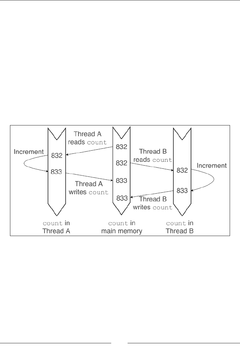
Parallel Collections and Futures
[ 74 ]
What happened here? The function passed to foreach has a side effect: it increments
count, a variable outside of the scope of the function. This is a problem because the
+= operator is a sequence of two operations:
• Retrieve the value of count and add one to it
• Assign the result back to count
To understand why this causes unexpected behavior, let's imagine that the foreach
loop has been parallelized over two threads. Thread A might read the count variable
when it is 832 and add one to it to give 833. Before it has time to reassign 833 to
count, Thread B reads count, still at 832, and adds one to give 833. Thread A then
assigns 833 to count. Thread B then assigns 833 to count. We've run through two
updates but only incremented the count by one. The problem arises because += can
be separated into two instructions: it is not atomic. This leaves room for threads to
interleave their operations:
The anatomy of a race condition: both thread A and thread B are trying to update count concurrently,
resulting in one of the updates being overwritten. The final value of count is 833 instead of 834.
To give a somewhat more realistic example of problems caused by non-atomicity,
let's look at a different method for counting the frequency of occurrence of each letter
in our sentence. We dene a mutable Char -> Int hash map outside of the loop.
Each time we encounter a letter, we increment the corresponding integer in the map:
scala> import scala.collection.mutable
import scala.collection.mutable
scala> val occurenceNumber = mutable.Map.empty[Char, Int]

Chapter 4
[ 75 ]
occurenceNumber: mutable.Map[Char,Int] = Map()
scala> lowerLettersPar.foreach { c =>
occurenceNumber(c) = occurenceNumber.getOrElse(c, 0) + 1
}
scala> occurenceNumber('e') // Should be 4
Int = 2
The discrepancy occurs because of the non-atomicity of the operations in the
foreach loop.
In general, it is good practice to avoid side effects in higher-order functions on
collections. They make the code harder to understand and preclude switching from
serial to parallel collections. It is also good practice to avoid exposing mutable state:
immutable objects can be shared freely between threads and cannot be affected by
side effects.
Another limitation of parallel collections occurs in reduction (or folding) operations.
The function used to combine items together must be associative. For instance:
scala> (0 until 1000).par.reduce {_ - _ } // should be -499500
Int = 63620
The minus operator, –, is not associative. The order in which consecutive operations
are applied matters: (a – b) – c is not the same as a – (b – c). The function
used to reduce a parallel collection must be associative because the order in which
the reduction occurs is not tied to the order of the collection.
Error handling
In single-threaded programs, exception handling is relatively straightforward: if an
exception occurs, the function can either handle it or escalate it. This is not nearly
as obvious when parallelism is introduced: a single thread might fail, but the others
might return successfully.
Parallel collection methods will throw an exception if they fail on any element, just
like their serial counterparts:
scala> Vector(2, 0, 5).par.map { 10 / _ }
java.lang.ArithmeticException: / by zero
...

Parallel Collections and Futures
[ 76 ]
There are cases when this isn't the behavior that we want. For instance, we might
be using a parallel collection to retrieve a large number of web pages in parallel.
We might not mind if a few of the pages cannot be fetched.
Scala's Try type was designed for sandboxing code that might throw exceptions. It is
similar to Option in that it is a one-element container:
scala> import scala.util._
import scala.util._
scala> Try { 2 + 2 }
Try[Int] = Success(4)
Unlike the Option type, which indicates whether an expression has a useful value,
the Try type indicates whether an expression can be executed without throwing an
exception. It takes on the following two values:
• Try { 2 + 2 } == Success(4) if the expression in the Try statement is
evaluated successfully
• Try { 2 / 0 } == Failure(java.lang.ArithmeticException: / by
zero) if the expression in the Try block results in an exception
This will make more sense with an example. To see the Try type in action, we will
try to fetch web pages in a fault tolerant manner. We will use the built-in Source.
fromURL method which fetches a web page and opens an iterator of the page's
content. If it fails to fetch the web page, it throws an error:
scala> import scala.io.Source
import scala.io.Source
scala> val html = Source.fromURL("http://www.google.com")
scala.io.BufferedSource = non-empty iterator
scala> val html = Source.fromURL("garbage")
java.net.MalformedURLException: no protocol: garbage
...
Instead of letting the expression propagate out and crash the rest of our code, we can
wrap the call to Source.fromURL in Try:
scala> Try { Source.fromURL("http://www.google.com") }

Chapter 4
[ 77 ]
Try[BufferedSource] = Success(non-empty iterator)
scala> Try { Source.fromURL("garbage") }
Try[BufferedSource] = Failure(java.net.MalformedURLException: no
protocol: garbage)
To see the power of our Try statement, let's now retrieve a list of URLs in parallel in
a fault tolerant manner:
scala> val URLs = Vector("http://www.google.com",
"http://www.bbc.co.uk",
"not-a-url"
)
URLs: Vector[String] = Vector(http://www.google.com, http://www.bbc.
co.uk, not-a-url)
scala> val pages = URLs.par.map { url =>
url -> Try { Source.fromURL(url) }
}
pages: ParVector[(String, Try[BufferedSource])] = ParVector((http://
www.google.com,Success(non-empty iterator)), (http://www.bbc.
co.uk,Success(non-empty iterator)), (not-a-url,Failure(java.net.
MalformedURLException: no protocol: not-a-url)))
We can then use a collect statement to act on the pages we could fetch successfully.
For instance, to get the number of characters on each page:
scala> pages.collect { case(url, Success(it)) => url -> it.size }
ParVector[(String, Int)] = ParVector((http://www.google.com,18976),
(http://www.bbc.co.uk,132893))
By making good use of Scala's built-in Try classes and parallel collections, we have
built a fault tolerant, multithreaded URL retriever in a few lines of code. (Compare
this to the myriad of Java/C++ books that prex code examples with 'error handling
is left out for clarity'.)

Parallel Collections and Futures
[ 78 ]
The Try type versus try/catch statements
Programmers with imperative or object-oriented backgrounds will be
more familiar with try/catch blocks for handling exceptions. We could
have accomplished similar functionality here by wrapping the code for
fetching URLs in a try block, returning null if the call raises an exception.
However, besides being more verbose, returning null is less satisfactory:
we lose all information about the exception and null is less expressive
than Failure(exception). Furthermore, returning a Try[T] type
forces the caller to consider the possibility that the function might fail, by
encoding this possibility in the type of the return value. In contrast, just
returning T and coding failure with a null value allows the caller to ignore
failure, raising the possibility of a confusing NullPointerException
being thrown at a completely different point in the program.
In short, Try[T] is just another higher-order type, like Option[T] or
List[T]. Treating the possibility of failure in the same way as the rest of
the code adds coherence to the program and encourages programmers to
tackle the possibility of exceptions explicitly.
Setting the parallelism level
So far, we have considered parallel collections as black boxes: add par to a normal
collection and all the operations are performed in parallel. Often, we will want more
control over how the tasks are executed.
Internally, parallel collections work by distributing an operation over multiple
threads. Since the threads share memory, parallel collections do not need to copy any
data. Changing the number of threads available to the parallel collection will change
the number of CPUs that are used to perform the tasks.
Parallel collections have a tasksupport attribute that controls task execution:
scala> val parRange = (0 to 100).par
parRange: ParRange = ParRange(0, 1, 2, 3, 4, 5,...
scala> parRange.tasksupport
TaskSupport = scala.collection.parallel.ExecutionContextTaskSupport@311a0
b3e
scala> parRange.tasksupport.parallelismLevel
Int = 8 // Number of threads to be used

Chapter 4
[ 79 ]
The task support object of a collection is an execution context, an abstraction capable
of executing Scala expressions in a separate thread. By default, the execution context
in Scala 2.11 is a work-stealing thread pool. When a parallel collection submits tasks,
the context allocates these tasks to its threads. If a thread nds that it has nished
its queued tasks, it will try and steal outstanding tasks from the other threads. The
default execution context maintains a thread pool with number of threads equal to
the number of CPUs.
The number of threads over which the parallel collection distributes the work can
be changed by changing the task support. For instance, to parallelize the operations
performed by a range over four threads:
scala> import scala.collection.parallel._
import scala.collection.parallel._
scala> parRange.tasksupport = new ForkJoinTaskSupport(
new scala.concurrent.forkjoin.ForkJoinPool(4)
)
parRange.tasksupport: scala.collection.parallel.TaskSupport = scala.
collection.parallel.ForkJoinTaskSupport@6e1134e1
scala> parRange.tasksupport.parallelismLevel
Int: 4
An example – cross-validation with parallel
collections
Let's apply what you have learned so far to solve data science problems. There are
many parts of a machine learning pipeline that can be parallelized trivially. One such
part is cross-validation.
We will give a brief description of cross-validation here, but you can refer to
The Elements of Statistical Learning, by Hastie, Tibshirani, and Friedman for a more
in-depth discussion.
Typically, a supervised machine learning problem involves training an algorithm
over a training set. For instance, when we built a model to calculate the probability
of a person being male based on their height and weight, the training set was the
(height, weight) data for each participant, together with the male/female label for
each row. Once the algorithm is trained on the training set, we can use it to classify
new data. This process only really makes sense if the training set is representative of
the new data that we are likely to encounter.

Parallel Collections and Futures
[ 80 ]
The training set has a nite number of entries. It will thus, inevitably, have
idiosyncrasies that are not representative of the population at large, merely due to
its nite nature. These idiosyncrasies will result in prediction errors when predicting
whether a new person is male or female, over and above the prediction error of the
algorithm on the training set itself. Cross-validation is a tool for estimating the error
caused by the idiosyncrasies of the training set that do not reect the population
at large.
Cross-validation works by dividing the training set in two parts: a smaller, new
training set and a cross-validation set. The algorithm is trained on the reduced
training set. We then see how well the algorithm models the cross-validation set.
Since we know the right answer for the cross-validation set, we can measure how
well our algorithm is performing when shown new information. We repeat this
procedure many times with different cross-validation sets.
There are several different types of cross-validation, which differ in how we
choose the cross-validation set. In this chapter, we will look at repeated random
subsampling: we select k rows at random from the training data to form the cross-
validation set. We do this many times, calculating the cross-validation error for
each subsample. Since each iteration is independent of the previous ones, we
can parallelize this process trivially. It is therefore a good candidate for parallel
collections. We will look at an alternative form of cross-validation, k-fold cross-
validation, in Chapter 12, Distributed Machine Learning with MLlib.
We will build a class that performs cross-validation in parallel. I encourage you
to write the code as you go, but you will nd the source code corresponding to
these examples on GitHub (https://github.com/pbugnion/s4ds).We will use
parallel collections to handle the parallelism and Breeze data types in the inner loop.
The build.sbt le is identical to the one we used in Chapter 2, Manipulating Data
with Breeze:
scalaVersion := "2.11.7"
libraryDependencies ++= Seq(
"org.scalanlp" %% "breeze" % "0.11.2",
"org.scalanlp" %% "breeze-natives" % "0.11.2"
)
We will build a RandomSubsample class. The class exposes a type alias, CVFunction,
for a function that takes two lists of indices—the rst corresponding to the
reduced training set and the second to the validation set—and returns a Double
corresponding to the cross-validation error:
type CVFunction = (Seq[Int], Seq[Int]) => Double

Chapter 4
[ 81 ]
The RandomSubsample class will expose a single method, mapSamples, which takes a
CVFunction, repeatedly passes it different partitions of indices, and returns a vector
of the errors. This is what the class looks like:
// RandomSubsample.scala
import breeze.linalg._
import breeze.numerics._
/** Random subsample cross-validation
*
* @param nElems Total number of elements in the training set.
* @param nCrossValidation Number of elements to leave out of
training set.
*/
class RandomSubsample(val nElems:Int, val nCrossValidation:Int) {
type CVFunction = (Seq[Int], Seq[Int]) => Double
require(nElems > nCrossValidation,
"nCrossValidation, the number of elements " +
"withheld, must be < nElems")
private val indexList = DenseVector.range(0, nElems)
/** Perform multiple random sub-sample CV runs on f
*
* @param nShuffles Number of random sub-sample runs.
* @param f user-defined function mapping from a list of
* indices in the training set and a list of indices in the
* test-set to a double indicating the out-of sample score
* for this split.
* @returns DenseVector of the CV error for each random split.
*/
def mapSamples(nShuffles:Int)(f:CVFunction)
:DenseVector[Double] = {
val cvResults = (0 to nShuffles).par.map { i =>
// Randomly split indices between test and training
val shuffledIndices = breeze.linalg.shuffle(indexList)
val Seq(testIndices, trainingIndices) =
split(shuffledIndices, Seq(nCrossValidation))
// Apply f for this split

Parallel Collections and Futures
[ 82 ]
f(trainingIndices.toScalaVector,
testIndices.toScalaVector)
}
DenseVector(cvResults.toArray)
}
}
Let's look at what happens in more detail, starting with the arguments passed to
the constructor:
class RandomSubsample(val nElems:Int, val nCrossValidation:Int)
We pass the total number of elements in the training set and the number of elements
to leave out for cross-validation in the class constructor. Thus, passing 100 to nElems
and 20 to nCrossValidation implies that our training set will have 80 random
elements of the total data and that the test set will have 20 elements.
We then construct a list of all integers between 0 and nElems:
private val indexList = DenseVector.range(0, nElems)
For each iteration of the cross-validation, we will shufe this list and take the
rst nCrossValidation elements to be the indices of rows in our test set and the
remaining to be the indices of rows in our training set.
Our class exposes a single method, mapSamples, that takes two curried arguments:
nShuffles, the number of times to perform random subsampling, and f, a
CVFunction:
def mapSamples(nShuffles:Int)(f:CVFunction):DenseVector[Double]
With all this set up, the code for doing cross-validation is deceptively simple. We
generate a parallel range from 0 to nShuffles and, for each item in the range,
generate a new train-test split and calculate the cross-validation error:
val cvResults = (0 to nShuffles).par.map { i =>
val shuffledIndices = breeze.linalg.shuffle(indexList)
val Seq(testIndices, trainingIndices) =
split(shuffledIndices, Seq(nCrossValidation))
f(trainingIndices.toScalaVector, testIndices.toScalaVector)
}
The only tricky part of this function is splitting the shufed index list into a list
of indices for the training set and a list of indices for the test set. We use Breeze's
split method. This takes a vector as its rst argument and a list of split-points as
its second, and returns a list of fragments of the original vector. We then use pattern
matching to extract the individual parts.

Chapter 4
[ 83 ]
Finally, mapSamples converts cvResults to a Breeze vector:
DenseVector(cvResults.toArray)
Let's see this in action. We can test our class by running cross-validation on the
logistic regression example developed in Chapter 2, Manipulating Data with Breeze.
In that chapter, we developed a LogisticRegression class that takes a training
set (in the form of a DenseMatrix) and target (in the form of a DenseVector) at
construction time. The class then calculates the parameters that best represent the
training set. We will rst add two methods to the LogisticRegression class to use
the trained model to classify previously unseen examples:
• The predictProbabilitiesMany method uses the trained model to calculate
the probability of having the target variable set to one. In the context of our
example, this is the probability of being male, given a height and weight.
• The classifyMany method assigns classification labels (one or zero) to
members of a test set. We will assign a one if predictProbabilitiesMany
returns a value greater than 0.5.
With these two functions, our LogisticRegression class becomes:
// Logistic Regression.scala
class LogisticRegression(
val training:DenseMatrix[Double],
val target:DenseVector[Double]
) {
...
/** Probability of classification for each row
* in test set.
*/
def predictProbabilitiesMany(test:DenseMatrix[Double])
:DenseVector[Double] = {
val xBeta = test * optimalCoefficients
sigmoid(xBeta)
}
/** Predict the value of the target variable
* for each row in test set.
*/
def classifyMany(test:DenseMatrix[Double])
:DenseVector[Double] = {
val probabilities = predictProbabilitiesMany(test)
I((probabilities :> 0.5).toDenseVector)
}
...
}

Parallel Collections and Futures
[ 84 ]
We can now put together an example program for our RandomSubsample class. We
will use the same height-weight data as in Chapter 2, Manipulating Data with Breeze.
The data preprocessing will be similar. The code examples for this chapter provide a
helper module, HWData, to load the height-weight data into Breeze vectors. The data
itself is in the data/ directory of the code examples for this chapter (available on
GitHub at https://github.com/pbugnion/s4ds/tree/master/chap04).
For each new subsample, we create a new LogisticRegression instance, train it
on the subset of the training set to get the best coefcients for this train-test split, and
use classifyMany to generate predictions on the cross-validation set in this split. We
then calculate the classication error and report the average classication error over
every train-test split:
// RandomSubsampleDemo.scala
import breeze.linalg._
import breeze.linalg.functions.manhattanDistance
import breeze.numerics._
import breeze.stats._
object RandomSubsampleDemo extends App {
/* Load and pre-process data */
val data = HWData.load
val rescaledHeights:DenseVector[Double] =
(data.heights - mean(data.heights)) / stddev(data.heights)
val rescaledWeights:DenseVector[Double] =
(data.weights - mean(data.weights)) / stddev(data.weights)
val featureMatrix:DenseMatrix[Double] =
DenseMatrix.horzcat(
DenseMatrix.ones[Double](data.npoints, 1),
rescaledHeights.toDenseMatrix.t,
rescaledWeights.toDenseMatrix.t
)
val target:DenseVector[Double] = data.genders.values.map {
gender => if(gender == 'M') 1.0 else 0.0
}
/* Cross-validation */
val testSize = 20

Chapter 4
[ 85 ]
val cvCalculator = new RandomSubsample(data.npoints, testSize)
// Start parallel CV loop
val cvErrors = cvCalculator.mapSamples(1000) {
(trainingIndices, testIndices) =>
val regressor = new LogisticRegression(
data.featureMatrix(trainingIndices, ::).toDenseMatrix,
data.target(trainingIndices).toDenseVector
)
// Predictions on test-set
val genderPredictions = regressor.classifyMany(
data.featureMatrix(testIndices, ::).toDenseMatrix
)
// Calculate number of mis-classified examples
val dist = manhattanDistance(
genderPredictions, data.target(testIndices)
)
// Calculate mis-classification rate
dist / testSize.toDouble
}
println(s"Mean classification error: ${mean(cvErrors)}")
}
Running this program on the height-weight data gives a classication error of 10%.
We now have a fully working, parallelized cross-validation class. Scala's parallel
range made it simple to repeatedly compute the same function in different threads.
Futures
Parallel collections offer a simple, yet powerful, framework for parallel operations.
However, they are limited in one respect: the total amount of work must be
known in advance, and each thread must perform the same function (possibly
on different inputs).
Imagine that we want to write a program that fetches a web page (or queries a web
API) every few seconds and extracts data for further processing from this web page.
A typical example might involve querying a web API to maintain an up-to-date
value of a particular stock price. Fetching data from an external web page takes a few
hundred milliseconds, typically. If we perform this operation on the main thread, it
will needlessly waste CPU cycles waiting for the web server to reply.

Parallel Collections and Futures
[ 86 ]
The solution is to wrap the code for fetching the web page in a future. A future is
a one-element container containing the future result of a computation. When you
create a future, the computation in it gets off-loaded to a different thread in order to
avoid blocking the main thread. When the computation nishes, the result is written
to the future and thus made accessible to the main thread.
As an example, we will write a program that queries the "Markit on demand"
API to fetch the price of a given stock. For instance, the URL for the current price
of a Google share is http://dev.markitondemand.com/MODApis/Api/v2/
Quote?symbol=GOOG. Go ahead and paste this in the address box of your web
browser. You will see an XML string appear with, among other things, the current
stock price. Let's fetch this programmatically without resorting to a future rst:
scala> import scala.io._
import scala.io_
scala> val url = "http://dev.markitondemand.com/MODApis/Api/v2/
Quote?symbol=GOOG"
url: String = http://dev.markitondemand.com/MODApis/Api/v2/
Quote?symbol=GOOG
scala> val response = Source.fromURL(url).mkString
response: String = <StockQuote><Status>SUCCESS</Status>
...
Notice how it takes a little bit of time to query the API. Let's now do the same, but
using a future (don't worry about the imports for now, we will discuss what they
mean in more detail further on):
scala> import scala.concurrent._
import scala.concurrent._
scala> import scala.util._
import scala.util._
scala> import scala.concurrent.ExecutionContext.Implicits.global
import scala.concurrent.ExecutionContext.Implicits.global
scala> val response = Future { Source.fromURL(url).mkString }
response: Future[String] = Promise$DefaultPromise@3301801b

Chapter 4
[ 87 ]
If you run this, you will notice that control returns to the shell instantly before
the API has had a chance to respond. To make this evident, let's simulate a slow
connection by adding a call to Thread.sleep:
scala> val response = Future {
Thread.sleep(10000) // sleep for 10s
Source.fromURL(url).mkString
}
response: Future[String] = Promise$DefaultPromise@231f98ef
When you run this, you do not have to wait for ten seconds for the next prompt to
appear: you regain control of the shell straightaway. The bit of code in the future is
executed asynchronously: its execution is independent of the main program ow.
How do we retrieve the result of the computation? We note that response has type
Future[String]. We can check whether the computation wrapped in the future has
nished by querying the future's isCompleted attribute:
scala> response.isCompleted
Boolean = true
The future exposes a value attribute that contains the computation result:
scala> response.value
Option[Try[String]] = Some(Success(<StockQuote><Status>SUCCESS</Status>
...
The value attribute of a future has type Option[Try[T]]. We have already seen
how to use the Try type to handle exceptions gracefully in the context of parallel
collections. It is used in the same way here. A future's value attribute is None until
the future is complete, then it is set to Some(Success(value)) if the future ran
successfully, or Some(Failure(error)) if an exception was thrown.
Repeatedly calling f.value until the future completes works well in the shell,
but it does not generalize to more complex programs. Instead, we want to tell the
computer to do something once the future is complete: we want to bind a callback
function to the future. We can do this by setting the future's onComplete attribute.
Let's tell the future to print the API response when it completes:
scala> response.onComplete {
case Success(s) => println(s)

Parallel Collections and Futures
[ 88 ]
case Failure(e) => println(s"Error fetching page: $e")
}
scala>
// Wait for response to complete, then prints:
<StockQuote><Status>SUCCESS</Status><Name>Alphabet Inc</
Name><Symbol>GOOGL</Symbol><LastPrice>695.22</LastPrice><Chan...
The function passed to onComplete runs when the future is nished. It takes a single
argument of type Try[T] containing the result of the future.
Failure is normal: how to build resilient applications
By wrapping the output of the code that it runs in a Try type, futures
force the client code to consider the possibility that the code might
fail. The client can isolate the effect of failure to avoid crashing the
whole application. They might, for instance, log the exception. In the
case of a web API query, they might add the offending URL to be
queried again at a later date. In the case of a database failure, they
might roll back the transaction.
By treating failure as a rst-class citizen rather than through
exceptional control ow bolted on at the end, we can build
applications that are much more resilient.
Future composition – using a future's result
In the previous section, you learned about the onComplete method to bind a
callback to a future. This is useful to cause a side effect to happen when the future is
complete. It does not, however, let us transform the future's return value easily.
To carry on with our stocks example, let's imagine that we want to convert the query
response from a string to an XML object. Let's start by including the scala-xml
library as a dependency in build.sbt:
libraryDependencies += "org.scala-lang" % "scala-xml" % "2.11.0-M4"
Let's restart the console and reimport the dependencies on scala.concurrent._,
scala.concurrent.ExecutionContext.Implicits.global, and scala.io._. We
also want to import the XML library:
scala> import scala.xml.XML
import scala.xml.XML

Chapter 4
[ 89 ]
We will use the same URL as in the previous section:
http://dev.markitondemand.com/MODApis/Api/v2/Quote?symbol=GOOG
It is sometimes useful to think of a future as a collection that either contains one
element if a calculation has been successful, or zero elements if it has failed. For
instance, if the web API has been queried successfully, our future contains a string
representation of the response. Like other container types in Scala, futures support a
map method that applies a function to the element contained in the future, returning
a new future, and does nothing if the calculation in the future failed. But what does
this mean in the context of a computation that might not be nished yet? The map
method gets applied as soon as the future is complete, like the onComplete method.
We can use the future's map method to apply a transformation to the result of the
future asynchronously. Let's poll the "Markit on demand" API again. This time,
instead of printing the result, we will parse it as XML.
scala> val strResponse = Future {
Thread.sleep(20000) // Sleep for 20s
val res = Source.fromURL(url).mkString
println("finished fetching url")
res
}
strResponse: Future[String] = Promise$DefaultPromise@1dda9bc8
scala> val xmlResponse = strResponse.map { s =>
println("applying string to xml transformation")
XML.loadString(s)
}
xmlResponse: Future[xml.Elem] = Promise$DefaultPromise@25d1262a
// wait while the remainder of the 20s elapses
finished fetching url
applying string to xml transformation
scala> xmlResponse.value
Option[Try[xml.Elem]] = Some(Success(<StockQuote><Status>SUCCESS</
Status>...
By registering subsequent maps on futures, we are providing a road map to the
executor running the future for what to do.

Parallel Collections and Futures
[ 90 ]
If any of the steps fail, the failed Try instance containing the exception gets
propagated instead:
scala> val strResponse = Future {
Source.fromURL("empty").mkString
}
scala> val xmlResponse = strResponse.map {
s => XML.loadString(s)
}
scala> xmlResponse.value
Option[Try[xml.Elem]] = Some(Failure(MalformedURLException: no protocol:
empty))
This behavior makes sense if you think of a failed future as an empty container.
When applying a map to an empty list, it returns the same empty list. Similarly,
when applying a map to an empty (failed) future, the empty future is returned.
Blocking until completion
The code for fetching stock prices works ne in the shell. However, if you paste it
in a standalone program, you will notice that nothing gets printed and the program
nishes straightaway. Let's look at a trivial example of this:
// BlockDemo.scala
import scala.concurrent._
import scala.concurrent.ExecutionContext.Implicits.global
import scala.concurrent.duration._
object BlockDemo extends App {
val f = Future { Thread.sleep(10000) }
f.onComplete { _ => println("future completed") }
// "future completed" is not printed
}

Chapter 4
[ 91 ]
The program stops running as soon as the main thread has completed its tasks,
which, in this example, just involves creating the futures. In particular, the line
"future completed" is never printed. If we want the main thread to wait for a
future to execute, we must explicitly tell it to block execution until the future has
nished running. This is done using the Await.ready or Await.result methods.
Both these methods block the execution of the main thread until the future
completes. We could make the above program work as intended by adding this line:
Await.ready(f, 1 minute)
The Await methods take the future as their rst argument and a Duration object
as the second. If the future takes longer to complete than the specied duration, a
TimeoutException is thrown. Pass Duration.Inf to set an innite timeout.
The difference between Await.ready and Await.result is that the latter returns
the value inside the future. In particular, if the future resulted in an exception, that
exception will get thrown. In contrast, Await.ready returns the future itself.
In general, one should try to avoid blocking as much as possible: the whole point
of futures is to run code in background threads in order to keep the main thread of
execution responsive. However, a common, legitimate use case for blocking is at
the end of a program. If we are running a large-scale integration process, we might
dispatch several futures to query web APIs, read from text les, or insert data into
a database. Embedding the code in futures is more scalable than performing these
operations sequentially. However, as the majority of the intensive work is running in
background threads, we are left with many outstanding futures when the main thread
completes. It makes sense, at this stage, to block until all the futures have completed.
Controlling parallel execution with execution
contexts
Now that we know how to dene futures, let's look at controlling how they run. In
particular, you might want to control the number of threads to use when running a
large number of futures.
When a future is dened, it is passed an execution context, either directly or implicitly.
An execution context is an object that exposes an execute method that takes a block
of code and runs it, possibly asynchronously. By changing the execution context, we
can change the "backend" that runs the futures. We have already seen how to use
execution contexts to control the execution of parallel collections.
So far, we have just been using the default execution context by importing scala.
concurrent.ExecutionContext.Implicits.global. This is a fork / join thread
pool with as many threads as there are underlying CPUs.

Parallel Collections and Futures
[ 92 ]
Let's now dene a new execution context that uses sixteen threads:
scala> import java.util.concurrent.Executors
import java.util.concurrent.Executors
scala> val ec = ExecutionContext.fromExecutorService(
Executors.newFixedThreadPool(16)
)
ec: ExecutionContextExecutorService = ExecutionContextImpl$$anon$1@1351
ce60
Having dened the execution context, we can pass it explicitly to futures as they
are dened:
scala> val f = Future { Thread.sleep(1000) } (ec)
f: Future[Unit] = Promise$DefaultPromise@458b456
Alternatively, we can dene the execution context implicitly:
scala> implicit val context = ec
context: ExecutionContextExecutorService = ExecutionContextImpl$$anon$1@1
351ce60
It is then passed as an implicit parameter to all new futures as they are constructed:
scala> val f = Future { Thread.sleep(1000) }
f: Future[Unit] = Promise$DefaultPromise@3c4b7755
You can shut the execution context down to destroy the thread pool:
scala> ec.shutdown()
When an execution context receives a shutdown command, it will nish executing its
current tasks but will refuse any new tasks.
Futures example – stock price fetcher
Let's bring some of the concepts that we covered in this section together to build a
command-line application that prompts the user for the name of a stock and fetches
the value of that stock. The catch is that, to keep the UI responsive, we will fetch the
stock using a future:
// StockPriceDemo.scala
import scala.concurrent._

Chapter 4
[ 93 ]
import scala.concurrent.ExecutionContext.Implicits.global
import scala.io._
import scala.xml.XML
import scala.util._
object StockPriceDemo extends App {
/* Construct URL for a stock symbol */
def urlFor(stockSymbol:String) =
("http://dev.markitondemand.com/MODApis/Api/v2/Quote?" +
s"symbol=${stockSymbol}")
/* Build a future that fetches the stock price */
def fetchStockPrice(stockSymbol:String):Future[BigDecimal] = {
val url = urlFor(stockSymbol)
val strResponse = Future { Source.fromURL(url).mkString }
val xmlResponse = strResponse.map { s => XML.loadString(s) }
val price = xmlResponse.map {
r => BigDecimal((r \ "LastPrice").text)
}
price
}
/* Command line interface */
println("Enter symbol at prompt.")
while (true) {
val symbol = readLine("> ") // Wait for user input
// When user puts in symbol, fetch data in background
// thread and print to screen when complete
fetchStockPrice(symbol).onComplete { res =>
println()
res match {
case Success(price) => println(s"$symbol: USD $price")
case Failure(e) => println(s"Error fetching $symbol: $e")
}
print("> ") // Simulate the appearance of a new prompt
}
}
}

Parallel Collections and Futures
[ 94 ]
Try running the program and entering the code for some stocks:
[info] Running StockPriceDemo
Enter symbol at prompt:
> GOOG
> MSFT
>
GOOG: USD 695.22
>
MSFT: USD 47.48
> AAPL
>
AAPL: USD 111.01
Let's summarize how the code works. when you enter a stock, the main thread
constructs a future that fetches the stock information from the API, converts it to
XML, and extracts the price. We use (r \ "LastPrice").text to extract the text
inside the LastPrice tag from the XML node r. We then convert the value to a big
decimal. When the transformations are complete, the result is printed to screen by
binding a callback through onComplete. Exception handling is handled naturally
through our use of .map methods to handle transformations.
By wrapping the code for fetching a stock price in a future, we free up the main
thread to just respond to the user. This means that the user interface does not get
blocked if we have, for instance, a slow internet connection.
This example is somewhat articial, but you could easily wrap much more
complicated logic: stock prices could be written to a database and we could add
additional commands to plot the stock price over time, for instance.
We have only scratched the surface of what futures can offer in this section. We will
revisit futures in more detail when we look at polling web APIs in Chapter 7, Web
APIs and Chapter 9, Concurrency with Akka.
Futures are a key part of the data scientist's toolkit for building scalable systems.
Moving expensive computation (either in terms of CPU time or wall time) to
background threads improves scalability greatly. For this reason, futures are an
important part of many Scala libraries such as Akka and the Play framework.

Chapter 4
[ 95 ]
Summary
By providing high-level concurrency abstractions, Scala makes writing parallel code
intuitive and straightforward. Parallel collections and futures form an invaluable
part of a data scientist's toolbox, allowing them to parallelize their code with minimal
effort. However, while these high-level abstractions obviate the need to deal directly
with threads, an understanding of the internals of Scala's concurrency model is
necessary to avoid race conditions.
In the next chapter, we will put concurrency on hold and study how to interact with
SQL databases. However, this is only temporary: futures will play an important role
in many of the remaining chapters in this book.
References
Aleksandar Prokopec, Learning Concurrent Programming in Scala. This is a detailed
introduction to the basics of concurrent programming in Scala. In particular, it
explores parallel collections and futures in much greater detail than this chapter.
Daniel Westheide's blog gives an excellent introduction to many Scala concepts,
in particular:
• Futures: http://danielwestheide.com/blog/2013/01/09/the-
neophytes-guide-to-scala-part-8-welcome-to-the-future.html
• The Try type: http://danielwestheide.com/blog/2012/12/26/the-
neophytes-guide-to-scala-part-6-error-handling-with-try.html
For a discussion of cross-validation, see The Elements of Statistical Learning by Hastie,
Tibshirani, and Friedman.

[ 97 ]
Scala and SQL
through JDBC
One of data science's raison d'être is the difculty of manipulating large datasets.
Much of the data of interest to a company or research group cannot t conveniently
in a single computer's RAM. Storing the data in a way that is easy to query is
therefore a complex problem.
Relational databases have been successful at solving the data storage problem.
Originally proposed in 1970 (http://www.seas.upenn.edu/~zives/03f/cis550/
codd.pdf), the overwhelming majority of databases in active use today are still
relational. In that time, the price of RAM per megabyte has decreased by a factor of a
hundred million. Similarly, hard drive capacity has increased from tens or hundreds
of megabytes to terabytes. It is remarkable that, despite this exponential growth in
data storage capacity, the relational model has remained dominant.
Virtually all relational databases are described and queried with variants of SQL
(Structured Query Language). With the advent of distributed computing, the
position of SQL databases as the de facto data storage standard is being challenged
by other types of databases, commonly grouped under the umbrella term NoSQL.
Many NoSQL databases are more partition-tolerant than SQL databases: they can
be split into several parts residing on different computers. While this author expects
that NoSQL databases will become increasingly popular, SQL databases are likely to
remain prevalent as a data persistence mechanism; hence, a signicant portion of this
book is devoted to interacting with SQL from Scala.

Scala and SQL through JDBC
[ 98 ]
While SQL is standardized, most implementations do not follow the full standard.
Additionally, most implementations provide extensions to the standard. This
means that, while many of the concepts in this book will apply to all SQL backends,
the exact syntax will need to be adjusted. We will consider only the MySQL
implementation here.
In this chapter, you will learn how to interact with SQL databases from Scala using
JDBC, a bare bones Java API. In the next chapter, we will consider Slick, an Object
Relational Mapper (ORM) that gives a more Scala-esque feel to interacting with SQL.
This chapter is roughly composed of two sections: we will rst discuss the basic
functionality for connecting and interacting with SQL databases, and then discuss
useful functional patterns that can be used to create an elegant, loosely coupled, and
coherent data access layer.
This chapter assumes that you have a basic working knowledge of SQL. If you do
not, you would be better off rst reading one of the reference books mentioned at the
end of the chapter.
Interacting with JDBC
JDBC is an API for connecting to SQL databases in Java. It remains the simplest way
of connecting to SQL databases from Scala. Furthermore, the majority of higher-level
abstractions for interacting with databases still use JDBC as a backend.
JDBC is not a library in itself. Rather, it exposes a set of interfaces to interact with
databases. Relational database vendors then provide specic implementations of
these interfaces.
Let's start by creating a build.sbt le. We will declare a dependency on the MySQL
JDBC connector:
scalaVersion := "2.11.7"
libraryDependencies += "mysql" % "mysql-connector-java" % "5.1.36"
First steps with JDBC
Let's start by connecting to JDBC from the command line. To follow with the
examples, you will need access to a running MySQL server. If you added the
MySQL connector to the list of dependencies, open a Scala console by typing
the following command:
$ sbt console

Chapter 5
[ 99 ]
Let's import JDBC:
scala> import java.sql._
import java.sql._
We then need to tell JDBC to use a specic connector. This is normally done using
reection, loading the driver at runtime:
scala> Class.forName("com.mysql.jdbc.Driver")
Class[_] = class com.mysql.jdbc.Driver
This loads the appropriate driver into the namespace at runtime. If this seems
somewhat magical to you, it's probably not worth worrying about exactly how this
works. This is the only example of reection that we will consider in this book, and it
is not particularly idiomatic Scala.
Connecting to a database server
Having specied the SQL connector, we can now connect to a database. Let's assume
that we have a database called test on host 127.0.0.1, listening on port 3306. We
create a connection as follows:
scala> val connection = DriverManager.getConnection(
"jdbc:mysql://127.0.0.1:3306/test",
"root", // username when connecting
"" // password
)
java.sql.Connection = com.mysql.jdbc.JDBC4Connection@12e78a69
The rst argument to getConnection is a URL-like string with jdbc:mysql://
host[:port]/database. The second and third arguments are the username and
password. Pass in an empty string if you can connect without a password.
Creating tables
Now that we have a database connection, let's interact with the server. For these
examples, you will nd it useful to have a MySQL shell open (or a MySQL GUI such
as MySQLWorkbench) as well as the Scala console. You can open a MySQL shell by
typing the following command in a terminal:
$ mysql

Scala and SQL through JDBC
[ 100 ]
As an example, we will create a small table to keep track of famous physicists. In a
mysql shell, we would run the following command:
mysql> USE test;
mysql> CREATE TABLE physicists (
id INT(11) AUTO_INCREMENT PRIMARY KEY,
name VARCHAR(32) NOT NULL
);
To achieve the same with Scala, we send a JDBC statement to the connection:
scala> val statementString = """
CREATE TABLE physicists (
id INT(11) AUTO_INCREMENT PRIMARY KEY,
name VARCHAR(32) NOT NULL
)
"""
scala> val statement = connection.prepareStatement(statementString)
PreparedStatement = JDBC4PreparedStatement@c983201: CREATE TABLE ...
scala> statement.executeUpdate()
results: Int = 0
Let's ignore the return value of executeUpdate for now.
Inserting data
Now that we have created a table, let's insert some data into it. We can do this with a
SQL INSERT statement:
scala> val statement = connection.prepareStatement("""
INSERT INTO physicists (name) VALUES ('Isaac Newton')
""")
scala> statement.executeUpdate()
Int = 1

Chapter 5
[ 101 ]
In this case, executeUpdate returns 1. When inserting rows, it returns the number
of rows that were inserted. Similarly, if we had used a SQL UPDATE statement, this
would return the number of rows that were updated. For statements that do not
manipulate rows directly (such as the CREATE TABLE statement in the previous
section), executeUpdate just returns 0.
Let's just jump into a mysql shell to verify the insertion performed correctly:
mysql> select * from physicists ;
+----+--------------+
| id | name |
+----+--------------+
| 1 | Isaac Newton |
+----+--------------+
1 row in set (0.00 sec)
Let's quickly summarize what we have seen so far: to execute SQL statements that do
not return results, use the following:
val statement = connection.prepareStatement("SQL statement string")
statement.executeUpdate()
In the context of data science, we frequently need to insert or update many rows at a
time. For instance, we might have a list of physicists:
scala> val physicistNames = List("Marie Curie", "Albert Einstein", "Paul
Dirac")
We want to insert all of these into the database. While we could create a statement
for each physicist and send it to the database, this is quite inefcient. A better
solution is to create a batch of statements and send them to the database together.
We start by creating a statement template:
scala> val statement = connection.prepareStatement("""
INSERT INTO physicists (name) VALUES (?)
""")
PreparedStatement = JDBC4PreparedStatement@621a8225: INSERT INTO
physicists (name) VALUES (** NOT SPECIFIED **)
This is identical to the previous prepareStatement calls, except that we replaced
the physicist's name with a ? placeholder. We can set the placeholder value with
the statement.setString method:
scala> statement.setString(1, "Richard Feynman")

Scala and SQL through JDBC
[ 102 ]
This replaces the rst placeholder in the statement with the string Richard Feynman:
scala> statement
com.mysql.jdbc.JDBC4PreparedStatement@5fdd16c3:
INSERT INTO physicists (name) VALUES ('Richard Feynman')
Note that JDBC, somewhat counter-intuitively, counts the placeholder positions from
1 rather than 0.
We have now created the rst statement in the batch of updates. Run the following
command:
scala> statement.addBatch()
By running the preceding command, we initiate a batch insert: the statement is
added to a temporary buffer that will be executed when we run the executeBatch
method. Let's add all the physicists in our list:
scala> physicistNames.foreach { name =>
statement.setString(1, name)
statement.addBatch()
}
We can now execute all the statements in the batch:
scala> statement.executeBatch
Array[Int] = Array(1, 1, 1, 1)
The return value of executeBatch is an array of the number of rows altered or
inserted by each item in the batch.
Note that we used statement.setString to ll in the template with a particular
name. The PreparedStatement object has setXXX methods for all basic types. To get
a complete list, read the PreparedStatement API documentation (http://docs.
oracle.com/javase/7/docs/api/java/sql/PreparedStatement.html).
Reading data
Now that we know how to insert data into a database, let's look at the converse:
reading data. We use SQL SELECT statements to query the database. Let's do this in
the MySQL shell rst:
mysql> SELECT * FROM physicists;
+----+-----------------+
| id | name |

Chapter 5
[ 103 ]
+----+-----------------+
| 1 | Isaac Newton |
| 2 | Richard Feynman |
| 3 | Marie Curie |
| 4 | Albert Einstein |
| 5 | Paul Dirac |
+----+-----------------+
5 rows in set (0.01 sec)
To extract this information in Scala, we dene a PreparedStatement:
scala> val statement = connection.prepareStatement("""
SELECT name FROM physicists
""")
PreparedStatement = JDBC4PreparedStatement@3c577c9d:
SELECT name FROM physicists
We execute this statement by running the following command:
scala> val results = statement.executeQuery()
results: java.sql.ResultSet = com.mysql.jdbc.JDBC4ResultSet@74a2e158
This returns a JDBC ResultSet instance. The ResultSet is an abstraction
representing a set of rows from the database. Note that we used statement.
executeQuery rather than statement.executeUpdate. In general, one should
execute statements that return data (in the form of ResultSet) with executeQuery.
Statements that modify the database without returning data (insert, create, alter, or
update statements, among others) are executed with executeUpdate.
The ResultSet object behaves somewhat like an iterator. It exposes a next method
that advances itself to the next record, returning true if there are records left in
ResultSet:
scala> results.next // Advance to the first record
Boolean = true
When the ResultSet instance points to a record, we can extract elds in this record
by passing in the eld name:
scala> results.getString("name")
String = Isaac Newton

Scala and SQL through JDBC
[ 104 ]
We can also extract elds using positional arguments. The elds are indexed
from one:
scala> results.getString(1) // first positional argument
String = Isaac Newton
When we are done with a particular record, we call the next method to advance the
ResultSet to the next record:
scala> results.next // advances the ResultSet by one record
Boolean = true
scala> results.getString("name")
String = Richard Feynman
getString("name")="Richard Feynman"
ResultSet ResultSet ResultSet
getString("name")="Isaac Newton" getString("name")="Marie Curie"
next()=true next()=falsenext()=true next()=true
A ResultSet object supports the getXXX(fieldName) methods to access the fields of a record and a next
method to advance to the next record in the result set.
One can iterate over a result set using a while loop:
scala> while(results.next) { println(results.getString("name")) }
Marie Curie
Albert Einstein
Paul Dirac

Chapter 5
[ 105 ]
A word of warning applies to reading elds that are nullable. While
one might expect JDBC to return null when faced with a null SQL
eld, the return type depends on the getXXX command used. For
instance, getInt and getLong will return 0 for any eld that is
null. Similarly, getDouble and getFloat return 0.0. This can
lead to some subtle bugs in code. In general, one should be careful
with getters that return Java value types (int, long) rather than
objects. To nd out if a value is null in the database, query it rst
with getInt (or getLong or getDouble, as appropriate), then use
the wasNull method that returns a Boolean if the last read value
was null:
scala> rs.getInt("field")
0
scala> rs.wasNull // was the last item read null?
true
This (surprising) behavior makes reading from ResultSet
instances error-prone. One of the goals of the second part of this
chapter is to give you the tools to build an abstraction layer on top
of the ResultSet interface to avoid having to call methods such as
getInt directly.
Reading values directly from ResultSet objects feels quite unnatural in Scala. We
will look, further on in this chapter, at constructing a layer through which you can
access the result set using type classes.
We now know how to read and write to a database. Having nished with the
database for now, we close the result sets, prepared statements, and connections:
scala> results.close
scala> statement.close
scala> connection.close
While closing statements and connections is not important in the Scala shell (they
will get closed when you exit), it is important when you run programs; otherwise,
the objects will persist, leading to "out of memory exceptions". In the next sections,
we will look at establishing connections and statements with the loan pattern, a
design pattern that closes a resource automatically when we nish using it.

Scala and SQL through JDBC
[ 106 ]
JDBC summary
We now have an overview of JDBC. The rest of this chapter will concentrate on
writing abstractions that sit above JDBC, making database accesses feel more natural.
Before we do this, let's summarize what we have seen so far.
We have used three JDBC classes:
• The Connection class represents a connection to a specific SQL database.
Instantiate a connection as follows:
import java.sql._
Class.forName("com.mysql.jdbc.Driver")
val connection = DriverManager.getConnection(
"jdbc:mysql://127.0.0.1:3306/test",
"root", // username when connecting
"" // password
)
Our main use of Connection instances has been to generate
PreparedStatement objects:
connection.prepareStatement("SELECT * FROM physicists")
• A PreparedStatement instance represents a SQL statement about to be sent
to the database. It also represents the template for a SQL statement with
placeholders for values yet to be filled in. The class exposes the following
methods:
statement.executeUpdate This sends the statement to the database. Use this for
SQL statements that modify the database and do not
return any data, such as INSERT, UPDATE, DELETE, and
CREATE statements.
val results =
statement.executeQuery
This sends the statement to the database. Use this for SQL
statements that return data (predominantly, the SELECT
statements). This returns a ResultSet instance.
statement.addBatch
statement.executeBatch
The addBatch method adds the current statement to a
batch of statements, and executeBatch sends the batch
of statements to the database.

Chapter 5
[ 107 ]
statement.setString(1,
"Scala")
statement.setInt(1, 42)
statement.setBoolean(1,
true)
Fill in the placeholder values in the
PreparedStatement. The first argument is the position
in the statement (counting from 1). The second argument
is the value.
One common use case for these is in a batch update or
insert: we might have a Scala list of objects that we want
to insert into the database. We fill in the placeholders
for each object in the list using the .setXXX methods,
then add this statement to the batch using .addBatch.
We can then send the entire batch to the database using
.executeBatch.
statement.setNull(1,
java.sql.Types.BOOLEAN)
This sets a particular item in the statement to NULL.
The second argument specifies the NULL type. If we
are setting a cell in a Boolean column, for instance, this
should be Types.BOOLEAN. A full list of types is given
in the API documentation for the java.sql.Types
package (http://docs.oracle.com/javase/7/
docs/api/java/sql/Types.html).
• A ResultSet instance represents a set of rows returned by a SELECT or SHOW
statement. ResultSet exposes methods to access fields in the current row:
rs.getString(i)
rs.getInt(i)
These methods get the value of the ith field in the
current row; i is measured from 1.
rs.getString("name")
rs.getInt("age")
These methods get the value of a specific field, which
is indexed by the column name.
rs.wasNull This returns whether the last column read was NULL.
This is particularly important when reading Java value
types, such as getInt, getBoolean, or getDouble, as
these return a default value when reading a NULL value.
The ResultSet instance exposes the .next method to move to the next row; .next
returns true until the ResultSet has advanced to just beyond the last row.
Functional wrappers for JDBC
We now have a basic overview of the tools afforded by JDBC. All the objects that we
have interacted with so far feel somewhat clunky and out of place in Scala. They do
not encourage a functional style of programming.

Scala and SQL through JDBC
[ 108 ]
Of course, elegance is not necessarily a goal in itself (or, at least, you will probably
struggle to convince your CEO that he should delay the launch of a product because
the code lacks elegance). However, it is usually a symptom: either the code is
not extensible or too tightly coupled, or it is easy to introduce bugs. The latter is
particularly the case for JDBC. Forgot to check wasNull? That will come back to
bite you. Forgot to close your connections? You'll get an "out of memory exception"
(hopefully not in production).
In the next sections, we will look at patterns that we can use to wrap JDBC types in
order to mitigate many of these risks. The patterns that we introduce here are used
very commonly in Scala libraries and applications. Thus, besides writing robust
classes to interact with JDBC, learning about these patterns will, I hope, give you
greater understanding of Scala programming.
Safer JDBC connections with the loan
pattern
We have already seen how to connect to a JDBC database and send statements to the
database for execution. This technique, however, is somewhat error prone: you have
to remember to close statements; otherwise, you will quickly run out of memory. In
more traditional imperative style, we write the following try-nally block around
every connection:
// WARNING: poor Scala code
val connection = DriverManager.getConnection(url, user, password)
try {
// do something with connection
}
finally {
connection.close()
}
Scala, with rst-class functions, provides us with an alternative: the loan pattern. We
write a function that is responsible for opening the connection, loaning it to the client
code to do something interesting with it, and then closing it when the client code is
done. Thus, the client code is not responsible for closing the connection any more.

Chapter 5
[ 109 ]
Let's create a new SqlUtils object with a usingConnection method that leverages
the loan pattern:
// SqlUtils.scala
import java.sql._
object SqlUtils {
/** Create an auto-closing connection using
* the loan pattern */
def usingConnection[T](
db:String,
host:String="127.0.0.1",
user:String="root",
password:String="",
port:Int=3306
)(f:Connection => T):T = {
// Create the connection
val Url = s"jdbc:mysql://$host:$port/$db"
Class.forName("com.mysql.jdbc.Driver")
val connection = DriverManager.getConnection(
Url, user, password)
// give the connection to the client, through the callable
// `f` passed in as argument
try {
f(connection)
}
finally {
// When client is done, close the connection
connection.close()
}
}
}
Let's see this function in action:
scala> SqlUtils.usingConnection("test") {
connection => println(connection)
}
com.mysql.jdbc.JDBC4Connection@46fd3d66

Scala and SQL through JDBC
[ 110 ]
Thus, the client doesn't have to remember to close the connection, and the resultant
code (for the client) feels much more like Scala.
How does our usingConnection function work? The function denition is
def usingConnection( ... )(f : Connection => T ):T. It takes, as its
second set of arguments, a function that acts on a Connection object. The body of
usingConnection creates the connection, then passes it to f, and nally closes the
connection. This syntax is somewhat similar to code blocks in Ruby or the with
statement in Python.
Be careful when mixing the loan pattern with lazy operations. This
applies particularly to returning iterators, streams, and futures from
f. As soon as the thread of execution leaves f, the connection will be
closed. Any data structure that is not materialized at this point will
not be able to carry on accessing the connection.
The loan pattern is, of course, not exclusive to database connections. It is useful
whenever you have the following pattern, in pseudocode:
open resource (eg. database connection, file ...)
use resource somehow // loan resource to client for this part.
close resource
Enriching JDBC statements with the
"pimp my library" pattern
In the previous section, we saw how to create self-closing connections with the
loan pattern. This allows us to open connections to the database without having
to remember to close them. However, we still have to remember to close any
ResultSet and PreparedStatement that we open:
// WARNING: Poor Scala code
SqlUtils.usingConnection("test") { connection =>
val statement = connection.prepareStatement(
"SELECT * FROM physicists")
val results = statement.executeQuery
// do something useful with the results
results.close
statement.close
}

Chapter 5
[ 111 ]
Having to open and close the statement is somewhat ugly and error prone. This is
another natural use case for the loan pattern. Ideally, we would like to write the
following:
usingConnection("test") { connection =>
connection.withQuery("SELECT * FROM physicists") {
resultSet => // process results
}
}
How can we dene a .withQuery method on the Connection class? We do not
control the Connection class denition as it is part of the JDBC API. We would
like to be able to somehow reopen the Connection class denition to add the
withQuery method.
Scala does not let us reopen classes to add new methods (a practice known as
monkey-patching). We can still, however, enrich existing libraries with implicit
conversions using the pimp my library pattern (http://www.artima.com/weblogs/
viewpost.jsp?thread=179766). We rst dene a RichConnection class that
contains the withQuery method. This RichConnection class is created from an
existing Connection instance.
// RichConnection.scala
import java.sql.{Connection, ResultSet}
class RichConnection(val underlying:Connection) {
/** Execute a SQL query and process the ResultSet */
def withQuery[T](query:String)(f:ResultSet => T):T = {
val statement = underlying.prepareStatement(query)
val results = statement.executeQuery
try {
f(results) // loan the ResultSet to the client
}
finally {
// Ensure all the resources get freed.
results.close
statement.close
}
}
}

Scala and SQL through JDBC
[ 112 ]
We could use this class by just wrapping every Connection instance in a
RichConnection instance:
// Warning: poor Scala code
SqlUtils.usingConnection("test") { connection =>
val richConnection = new RichConnection(connection)
richConnection.withQuery("SELECT * FROM physicists") {
resultSet => // process resultSet
}
}
This adds unnecessary boilerplate: we have to remember to convert every connection
instance to RichConnection to use withQuery. Fortunately, Scala provides an easier
way with implicit conversions: we tell Scala how to convert from Connection to
RichConnection and vice versa, and tell it to perform this conversion automatically
(implicitly), if necessary:
// Implicits.scala
import java.sql.Connection
// Implicit conversion methods are often put in
// an object called Implicits.
object Implicits {
implicit def pimpConnection(conn:Connection) =
new RichConnection(conn)
implicit def depimpConnection(conn:RichConnection) =
conn.underlying
}
Now, whenever pimpConnection and depimpConnection are in the current
scope, Scala will automatically use them to convert from Connection instances to
RichConnection and back as needed.
We can now write the following (I have added type information for emphasis):
// Bring the conversion functions into the current scope
import Implicits._
SqlUtils.usingConnection("test") { (connection:Connection) =>
connection.withQuery("SELECT * FROM physicists") {
// Wow! It's like we have just added
// .withQuery to the JDBC Connection class!
resultSet => // process results
}
}

Chapter 5
[ 113 ]
This might look like magic, so let's step back and look at what happens when we
call withQuery on a Connection instance. The Scala compiler will rst look to see if
the class denition of Connection denes a withQuery method. When it nds that
it does not, it will look for implicit methods that convert a Connection instance to
a class that denes withQuery. It will nd that the pimpConnection method allows
conversion from Connection to RichConnection, which denes withQuery. The
Scala compiler automatically uses pimpConnection to transform the Connection
instance to RichConnection.
Note that we used the names pimpConnection and depimpConnection for the
conversion functions, but they could have been anything. We never call these
methods explicitly.
Let's summarize how to use the pimp my library pattern to add methods to an
existing class:
1. Write a class that wraps the class you want to enrich: class
RichConnection(val underlying:Connection). Add all the methods that
you wish the original class had.
2. Write a method to convert from your original class to your enriched class
as part of an object called (conventionally) Implicits. Make sure that you
tell Scala to use this conversion automatically with the implicit keyword:
implicit def pimpConnection(conn:Connection):RichConnection.
You can also tell Scala to automatically convert back from the enriched class
to the original class by adding the reverse conversion method.
3. Allow implicit conversions by importing the implicit conversion methods:
import Implicits._.
Wrapping result sets in a stream
The JDBC ResultSet object plays very badly with Scala collections. The only real
way of doing anything useful with it is to loop through it directly with a while loop.
For instance, to get a list of the names of physicists in our database, we could write
the following code:
// WARNING: poor Scala code
import Implicits._ // import implicit conversions
SqlUtils.usingConnection("test") { connection =>
connection.withQuery("SELECT * FROM physicists") { resultSet =>
var names = List.empty[String]
while(resultSet.next) {

Scala and SQL through JDBC
[ 114 ]
val name = resultSet.getString("name")
names = name :: names
}
names
}
}
//=> List[String] = List(Paul Dirac, Albert Einstein, Marie Curie,
Richard Feynman, Isaac Newton)
The ResultSet interface feels unnatural because it behaves very differently from
Scala collections. In particular, it does not support the higher-order functions that we
take for granted in Scala: no map, filter, fold, or for comprehensions. Thankfully,
writing a stream that wraps ResultSet is quite straightforward. A Scala stream is a
lazily evaluated list: it evaluates the next element in the collection when it is needed
and forgets previous elements when they are no longer used.
We can dene a stream method that wraps ResultSet as follows:
// SqlUtils.scala
object SqlUtils {
...
def stream(results:ResultSet):Stream[ResultSet] =
if (results.next) { results #:: stream(results) }
else { Stream.empty[ResultSet] }
}
This might look quite confusing, so let's take it slowly. We dene a stream method
that wraps ResultSet, returning a Stream[ResultSet]. When the client calls
stream on an empty result set, this just returns an empty stream. When the client
calls stream on a non-empty ResultSet, the ResultSet instance is advanced by one
row, and the client gets back results #:: stream(results). The #:: operator on a
stream is similar to the cons operator, ::, on a list: it prepends results to an existing
Stream. The critical difference is that, unlike a list, stream(results) does not get
evaluated until necessary. This, therefore, avoids duplicating the entire ResultSet
in memory.
Let's use our brand new stream function to get the name of all the physicists in our
database:
import Implicits._
SqlUtils.usingConnection("test") { connection =>
connection.withQuery("SELECT * FROM physicists") { results =>
val resultsStream = SqlUtils.stream(results)

Chapter 5
[ 115 ]
resultsStream.map { _.getString("name") }.toVector
}
}
//=> Vector(Richard Feynman, Albert Einstein, Marie Curie, Paul Dirac)
Streaming the results, rather than using the result set directly, lets us interact with
the data much more naturally as we are now dealing with just a Scala collection.
When you use stream in a withQuery block (or, generally, in a block that
automatically closes the result set), you must always materialize the stream within
the function, hence the call to toVector. Otherwise, the stream will wait until its
elements are needed to materialize them, and by then, the ResultSet instance will
be closed.
Looser coupling with type classes
So far, we have been reading and writing simple types to the database. Let's imagine
that we want to add a gender column to our database. We will store the gender as an
enumeration in our physicists database. Our table is now as follows:
mysql> CREATE TABLE physicists (
id INT(11) AUTO_INCREMENT PRIMARY KEY,
name VARCHAR(32) NOT NULL,
gender ENUM("Female", "Male") NOT NULL
);
How can we represent genders in Scala? A good way of doing this is with an
enumeration:
// Gender.scala
object Gender extends Enumeration {
val Male = Value
val Female = Value
}
However, we now have a problem when deserializing objects from the database:
JDBC has no built-in mechanism to convert from a SQL ENUM type to a Scala Gender
type. We could achieve this by just converting manually every time we need to read
gender information:
resultsStream.map {
rs => Gender.withName(rs.getString("gender"))
}.toVector

Scala and SQL through JDBC
[ 116 ]
However, we would need to write this everywhere that we want to read the gender
eld. This goes against the DRY (don't repeat yourself) principle, leading to code
that is difcult to maintain. If we decide to change the way gender is stored in the
database, we would need to nd every instance in the code where we read the
gender eld and change it.
A somewhat better solution would be to add a getGender method to the ResultSet
class using the pimp my library idiom that we used extensively in this chapter. This
solution is still not optimal. We are adding unnecessary specicity to ResultSet: it is
now coupled to the structure of our databases.
We could create a subclass of ResultSet using inheritance, such as
PhysicistResultSet, that can read the elds in a specic table. However, this
approach is not composable: if we had another table that kept track of pets, with
name, species, and gender elds, we would have to either reimplement the code
for reading gender in a new PetResultSet or factor out a GenderedResultSet
superclass. As the number of tables grows, the inheritance hierarchy would become
unmanageable. A better approach would let us compose the functionality that we
need. In particular, we want to decouple the process of extracting Scala objects from
a result set from the code for iterating over a result set.
Type classes
Scala provides an elegant solution using type classes. Type classes are a very powerful
arrow in the Scala architect's quiver. However, they can present a bit of a learning
curve, especially as there is no direct equivalent in object-oriented programming.
Instead of presenting an abstract explanation, I will dive into an example: I will
describe how we can leverage type classes to convert elds in a ResultSet to Scala
types. The aim is to dene a read[T](field) method on ResultSet that knows
exactly how to deserialize to objects of type T. This method will replace and extend
the getXXX methods in ResultSet:
// results is a ResultSet instance
val name = results.read[String]("name")
val gender = results.read[Gender.Value]("gender")

Chapter 5
[ 117 ]
We start by dening an abstract SqlReader[T] trait that exposes a read method to
read a specic eld from a ResultSet and return an instance of type T:
// SqlReader.scala
import java.sql._
trait SqlReader[T] {
def read(results:ResultSet, field:String):T
}
We now need to provide a concrete implementation of SqlReader[T] for every T
type that we want to read. Let's provide concrete implementations for the Gender and
String elds. We will place the implementation in a SqlReader companion object:
// SqlReader.scala
object SqlReader {
implicit object StringReader extends SqlReader[String] {
def read(results:ResultSet, field:String):String =
results.getString(field)
}
implicit object GenderReader extends SqlReader[Gender.Value] {
def read(results:ResultSet, field:String):Gender.Value =
Gender.withName(StringReader.read(results, field))
}
}
We could now use our ReadableXXX objects to read from a result set:
import SqlReader._
val name = StringReader.read(results, "name")
val gender = GenderReader.read(results, "gender")
This is already somewhat better than using the following:
Gender.withName(results.getString("gender"))
This is because the code to map from a ResultSet eld to Gender.Value is
centralized in a single place: ReadableGender. However, it would be great if we
could tell Scala to use ReadableGender whenever it needs to read Gender.Value,
and use ReadableString whenever it needs to read a String value. This is exactly
what type classes do.

Scala and SQL through JDBC
[ 118 ]
Coding against type classes
We dened a Readable[T] interface that abstracts how to read an object of type T
from a eld in a ResultSet. How do we tell Scala that it needs to use this Readable
object to convert from the ResultSet elds to the appropriate Scala type?
The key is the implicit keyword that we used to prex the GenderReader and
StringReader object denitions. It lets us write:
implicitly[SqlReader[Gender.Value]].read(results, "gender")
implicitly[SqlReader[String]].read(results, "name")
By writing implicitly[SqlReader[T]], we are telling the Scala compiler to nd a
class (or an object) that extends SqlReader[T] that is marked for implicit use. Try
this out by pasting the following in the command line, for instance:
scala> :paste
import Implicits._ // Connection to RichConnection conversion
SqlUtils.usingConnection("test") {
_.withQuery("select * from physicists") {
rs => {
rs.next() // advance to first record
implicitly[SqlReader[Gender.Value]].read(rs, "gender")
}
}
}
Of course, using implicitly[SqlReader[T]] everywhere is not particularly elegant.
Let's use the pimp my library idiom to add a read[T] method to ResultSet. We rst
dene a RichResultSet class that we can use to "pimp" the ResultSet class:
// RichResultSet.scala
import java.sql.ResultSet
class RichResultSet(val underlying:ResultSet) {
def read[T : SqlReader](field:String):T = {
implicitly[SqlReader[T]].read(underlying, field)
}
}

Chapter 5
[ 119 ]
The only unfamiliar part of this should be the read[T : SqlReader] generic
denition. We are stating here that read will accept any T type, provided an instance
of SqlReader[T] exists. This is called a context bound.
We must also add implicit methods to the Implicits object to convert from
ResultSet to RichResultSet. You should be familiar with this now, so I will not
bore you with the details. You can now call results.read[T](fieldName) for
any T for which you have a SqlReader[T] implicit object dened:
import Implicits._
SqlUtils.usingConnection("test") { connection =>
connection.withQuery("SELECT * FROM physicists") {
results =>
val resultStream = SqlUtils.stream(results)
resultStream.map { row =>
val name = row.read[String]("name")
val gender = row.read[Gender.Value]("gender")
(name, gender)
}.toVector
}
}
//=> Vector[(String, Gender.Value)] = Vector((Albert Einstein,Male),
(Marie Curie,Female))
Let's summarize the steps needed for type classes to work. We will do this in the
context of deserializing from SQL, but you will be able to adapt these steps to solve
other problems:
• Define an abstract generic trait that provides the interface for the type class,
for example, SqlReader[T]. Any functionality that is independent of T can
be added to this base trait.
• Create the companion object for the base trait and add implicit objects
extending the trait for each T, for example,
implicit object StringReader extends SqlReader[T].
• Type classes are always used in generic methods. A method that relies
on the existence of a type class for an argument must contain a context
bound in the generic definition, for example, def read[T : SqlReader]
(field:String):T. To access the type class in this method, use the
implicitly keyword: implicitly[SqlReader[T]].

Scala and SQL through JDBC
[ 120 ]
When to use type classes
Type classes are useful when you need a particular behavior for many different
types, but exactly how this behavior is implemented varies between these types.
For instance, we need to be able to read several different types from ResultSet, but
exactly how each type is read differs between types: for strings, we must read from
ResultSet using getString, whereas for integers, we must use getInt followed by
wasNull.
A good rule of thumb is when you start thinking "Oh, I could just write a generic
method to do this. Ah, but wait, I will have to write the Int implementation as a
specic edge case as it behaves differently. Oh, and the Gender implementation. I
wonder if there's a better way?", then type classes might be useful.
Benets of type classes
Data scientists frequently have to deal with new input streams, changing
requirements, and new data types. Having an object-relational mapping layer that
is easy to extend or alter is therefore critical to responding to changes efciently.
Minimizing coupling between code entities and separation of concerns are the only
ways to ensure that the code can be changed in response to new data.
With type classes, we maintain orthogonality between accessing records in the
database (through the ResultSet class) and how individual elds are transformed
to Scala objects: both can vary independently. The only coupling between these two
concerns is through the SqlReader[T] interface.
This means that both concerns can evolve independently: to read a new data
type, we just need to implement a SqlReader[T] object. Conversely, we can
add functionality to ResultSet without needing to reimplement how elds are
converted. For instance, we could add a getColumn method that returns a Vector[T]
of all the values of a eld in a ResultSet instance:
def getColumn[T : SqlReader](field:String):Vector[T] = {
val resultStream = SqlUtils.stream(results)
resultStream.map { _.read[T](field) }.toVector
}
Note how we could do this without increasing the coupling to the way in which
individual elds are read.

Chapter 5
[ 121 ]
Creating a data access layer
Let's bring together everything that we have seen and build a data-mapper class
for fetching Physicist objects from the database. These classes (also called data
access objects) are useful to decouple the internal representation of an object from its
representation in the database.
We start by dening the Physicist class:
// Physicist.scala
case class Physicist(
val name:String,
val gender:Gender.Value
)
The data access object will expose a single method, readAll, that returns a
Vector[Physicist] of all the physicists in our database:
// PhysicistDao.scala
import java.sql.{ ResultSet, Connection }
import Implicits._ // implicit conversions
object PhysicistDao {
/* Helper method for reading a single row */
private def readFromResultSet(results:ResultSet):Physicist = {
Physicist(
results.read[String]("name"),
results.read[Gender.Value]("gender")
)
}
/* Read the entire 'physicists' table. */
def readAll(connection:Connection):Vector[Physicist] = {
connection.withQuery("SELECT * FROM physicists") {
results =>
val resultStream = SqlUtils.stream(results)
resultStream.map(readFromResultSet).toVector
}
}
}

Scala and SQL through JDBC
[ 122 ]
The data access layer can be used by client code as in the following example:
object PhysicistDaoDemo extends App {
val physicists = SqlUtils.usingConnection("test") {
connection => PhysicistDao.readAll(connection)
}
// physicists is a Vector[Physicist] instance.
physicists.foreach { println }
//=> Physicist(Albert Einstein,Male)
//=> Physicist(Marie Curie,Female)
}
Summary
In this chapter, we learned how to interact with SQL databases using JDBC.
We wrote a library to wrap native JDBC objects, aiming to give them a more
functional interface.
In the next chapter, you will learn about Slick, a Scala library that provides functional
wrappers to interact with relational databases.
References
The API documentation for JDBC is very complete: http://docs.oracle.com/
javase/7/docs/api/java/sql/package-summary.html
The API documentation for the ResultSet interface (http://docs.oracle.com/
javase/7/docs/api/java/sql/ResultSet.html), for the PreparedStatement
class (http://docs.oracle.com/javase/7/docs/api/java/sql/
PreparedStatement.html) and the Connection class (http://docs.oracle.com/
javase/7/docs/api/java/sql/Connection.html) is particularly relevant.
The data mapper pattern is described extensively in Martin Fowler's Patterns of
Enterprise Application Architecture. A brief description is also available on his website
(http://martinfowler.com/eaaCatalog/dataMapper.html).

Chapter 5
[ 123 ]
For an introduction to SQL, I suggest Learning SQL by Alan Beaulieu (O'Reilly).
For another discussion of type classes, read http://danielwestheide.com/
blog/2013/02/06/the-neophytes-guide-to-scala-part-12-type-classes.
html.
This post describes how some common object-oriented design patterns can be
reimplemented more elegantly in Scala using type classes:
https://staticallytyped.wordpress.com/2013/03/24/gang-of-four-
patterns-with-type-classes-and-implicits-in-scala-part-2/
This post by Martin Odersky details the Pimp my Library pattern:
http://www.artima.com/weblogs/viewpost.jsp?thread=179766

[ 125 ]
Slick – A Functional
Interface for SQL
In Chapter 5, Scala and SQL through JDBC, we investigated how to access SQL
databases with JDBC. As interacting with JDBC feels somewhat unnatural, we
extended JDBC using custom wrappers. The wrappers were developed to provide
a functional interface to hide the imperative nature of JDBC.
With the difculty of interacting directly with JDBC from Scala and the ubiquity of
SQL databases, you would expect there to be existing Scala libraries that wrap JDBC.
Slick is such a library.
Slick styles itself as a functional-relational mapping library, a play on the more
traditional object-relational mapping name used to denote libraries that build objects
from relational databases. It presents a functional interface to SQL databases,
allowing the client to interact with them in a manner similar to native Scala
collections.
FEC data
In this chapter, we will use a somewhat more involved example dataset. The
Federal Electoral Commission of the United States (FEC) records all donations to
presidential candidates greater than $200. These records are publicly available. We
will look at the donations for the campaign leading up to the 2012 general elections
that resulted in Barack Obama's re-election. The data includes donations to the two
presidential candidates, Obama and Romney, and also to the other contenders in the
Republican primaries (there were no Democrat primaries).
In this chapter, we will take the transaction data provided by the FEC, store it in a
table, and learn how to query and analyze it.

Slick – A Functional Interface for SQL
[ 126 ]
The rst step is to acquire the data. If you have downloaded the code samples
from the Packt website, you should already have two CSVs in the data directory
of the code samples for this chapter. If not, you can download the les using the
following links:
• data.scala4datascience.com/fec/ohio.csv.gz (or ohio.csv.zip)
• data.scala4datascience.com/fec/us.csv.gz (or us.csv.zip)
Decompress the two les and place them in a directory called data/ in the same
location as the source code examples for this chapter. The data les correspond
to the following:
• The ohio.csv file is a CSV of all the donations made by donors in Ohio.
• The us.csv file is a CSV of all the donations made by donors across the
country. This is quite a large file, with six million rows.
The two CSV les contain identical columns. Use the Ohio dataset for more
responsive behavior, or the nationwide data le if you want to wrestle with a
larger dataset. The dataset is adapted from a list of contributions downloaded
from http://www.fec.gov/disclosurep/PDownload.do.
Let's start by creating a Scala case class to represent a transaction. In the context of
this chapter, a transaction is a single donation from an individual to a candidate:
// Transaction.scala
import java.sql.Date
case class Transaction(
id:Option[Int], // unique identifier
candidate:String, // candidate receiving the donation
contributor:String, // name of the contributor
contributorState:String, // contributor state
contributorOccupation:Option[String], // contributor job
amount:Long, // amount in cents
date:Date // date of the donation
)
The code repository for this chapter includes helper functions in an FECData
singleton object to load the data from CSVs:
scala> val ohioData = FECData.loadOhio
s4ds.FECData = s4ds.FECData@718454de

Chapter 6
[ 127 ]
Calling FECData.loadOhio or FECData.loadAll will create an FECData object with
a single attribute, transactions, which is an iterator over all the donations coming
from Ohio or the entire United States:
scala> val ohioTransactions = ohioData.transactions
Iterator[Transaction] = non-empty iterator
scala> ohioTransactions.take(5).foreach(println)
Transaction(None,Paul, Ron,BROWN, TODD W MR.,OH,Some(ENGINE
ER),5000,2011-01-03)
Transaction(None,Paul, Ron,DIEHL, MARGO SONJA,OH,Some(RETIR
ED),2500,2011-01-03)
Transaction(None,Paul, Ron,KIRCHMEYER, BENJAMIN,OH,Some(COMPUTER
PROGRAMMER),20120,2011-01-03)
Transaction(None,Obama, Barack,KEYES, STEPHEN,OH,Some(HR EXECUTIVE /
ATTORNEY),10000,2011-01-03)
Transaction(None,Obama, Barack,MURPHY, MIKE W,OH,Some(MANAG
ER),5000,2011-01-03)
Now that we have some data to play with, let's try and put it in the database so that
we can run some useful queries on it.
Importing Slick
To add Slick to the list of dependencies, you will need to add "com.typesafe.slick"
%% "slick" % "2.1.0" to the list of dependencies in your build.sbt le. You will
also need to make sure that Slick has access to a JDBC driver. In this chapter, we
will connect to a MySQL database, and must, therefore, add the MySQL connector
"mysql" % "mysql-connector-java" % "5.1.37" to the list of dependencies.
Slick is imported by importing a specic database driver. As we are using MySQL,
we must import the following:
scala> import slick.driver.MySQLDriver.simple._
import slick.driver.MySQLDriver.simple._
To connect to a different avor of SQL database, import the relevant driver. The
easiest way of seeing what drivers are available is to consult the API documentation
for the slick.driver package, which is available at http://slick.typesafe.com/
doc/2.1.0/api/#scala.slick.driver.package. All the common SQL avors are
supported (including H2, PostgreSQL, MS SQL Server, and SQLite).

Slick – A Functional Interface for SQL
[ 128 ]
Dening the schema
Let's create a table to represent our transactions. We will use the following schema:
CREATE TABLE transactions(
id INT(11) AUTO_INCREMENT PRIMARY KEY,
candidate VARCHAR(254) NOT NULL,
contributor VARCHAR(254) NOT NULL,
contributor_state VARCHAR(2) NOT NULL,
contributor_occupation VARCHAR(254),
amount BIGINT(20) NOT NULL,
date DATE
);
Note that the donation amount is in cents. This allows us to use an integer eld
(rather than a xed point decimal, or worse, a oat).
You should never use a oating point format to represent money
or, in fact, any discrete quantity because oats cannot represent
most fractions exactly:
scala> 0.1 + 0.2
Double = 0.30000000000000004
This seemingly nonsensical result occurs because there is no way to
store 0.3 exactly in doubles.
This post gives an extensive discussion of the limitations of the
oating point format:
http://docs.oracle.com/cd/E19957-01/806-3568/ncg_
goldberg.html
To use Slick with tables in our database, we rst need to tell Slick about the database
schema. We do this by creating a class that extends the Table abstract class. The way
in which a schema is dened is quite straightforward, so let's dive straight into the
code. We will store our schema in a Tables singleton. We dene a Transactions
class that provides the mapping to go from collections of Transaction instances to
SQL tables structured like the transactions table:
// Tables.scala
import java.sql.Date
import slick.driver.MySQLDriver.simple._
/** Singleton object for table definitions */

Chapter 6
[ 129 ]
object Tables {
// Transactions table definition
class Transactions(tag:Tag)
extends Table[Transaction](tag, "transactions") {
def id = column[Int]("id", O.PrimaryKey, O.AutoInc)
def candidate = column[String]("candidate")
def contributor = column[String]("contributor")
def contributorState = column[String](
"contributor_state", O.DBType("VARCHAR(2)"))
def contributorOccupation = column[Option[String]](
"contributor_occupation")
def amount = column[Long]("amount")
def date = column[Date]("date")
def * = (id.?, candidate, contributor,
contributorState, contributorOccupation, amount, date) <> (
Transaction.tupled, Transaction.unapply)
}
val transactions = TableQuery[Transactions]
}
Let's go through this line by line. We rst dene a Transactions class, which must
take a Slick Tag object as its rst argument. The Tag object is used by Slick internally
to construct SQL statements. The Transactions class extends a Table object,
passing it the tag and name of the table in the database. We could, optionally, have
added a database name by extending Table[Transaction](tag, Some("fec"),
"transactions") rather than just Table[Transaction](tag, "transactions").
The Table type is parametrized by Transaction. This means that running SELECT
statements on the database returns Transaction objects. Similarly, we will insert
data into the database by passing a transaction or list of transactions to the relevant
Slick methods.
Let's look at the Transactions class denition in more detail. The body of the class
starts by listing the database columns. For instance, the id column is dened as follows:
def id = column[Int]("id", O.PrimaryKey, O.AutoInc)
We tell Slick that it should read the column called id and transform it to a Scala
integer. Additionally, we tell Slick that this column is the primary key and that
it is auto-incrementing. The Slick documentation contains a list of available
options for column.

Slick – A Functional Interface for SQL
[ 130 ]
The candidate and contributor columns are straightforward: we tell Slick to read
these as String from the database. The contributor_state column is a little more
interesting. Besides specifying that it should be read from the database as a String,
we also tell Slick that it should be stored in the database with type VARCHAR(2).
The contributor_occupation column in our table can contain NULL values. When
dening the schema, we pass the Option[String] type to the column method:
def contributorOccupation =
column[Option[String]]("contributor_occupation")
When reading from the database, a NULL eld will get converted to None for columns
specied as Option[T]. Conversely, if the eld has a value, it will be returned as
Some(value).
The last line of the class body is the most interesting part: it species how to
transform the raw data read from the database into a Transaction object and how to
convert a Transaction object to raw elds ready for insertion:
def * = (id.?, candidate, contributor,
contributorState, contributorOccupation, amount, date) <> (
Transaction.tupled, Transaction.unapply)
The rst part is just a tuple of elds to be read from the database: (id.?,
candidate, contributor, contributorState, contributorOccupation,
amount, date), with a small amount of metadata. The second part is a pair of
functions that describe how to transform this tuple into a Transaction object and
back. In this case, as Transaction is a case class, we can take advantage of the
Transaction.tupled and Transaction.unapply methods automatically provided
for case classes.
Notice how we followed the id entry with .?. In our Transaction class, the
donation id has the Option[Int] type, but the column in the database has the
INT type with the additional O.AutoInc option. The .? sufx tells Slick to use the
default value provided by the database (in this case, the database's auto-increment)
if id is None.
Finally, we dene the value:
val transactions = TableQuery[Transactions]
This is the handle that we use to actually interact with the database. For instance, as
we will see later, to get a list of donations to Barack Obama, we run the following
query (don't worry about the details of the query for now):
Tables.transactions.filter {_.candidate === "Obama, Barack"}.list

Chapter 6
[ 131 ]
Let's summarize the parts of our Transactions mapper class:
• The Transactions class must extend the Table abstract class parametrized
by the type that we want to return: Table[Transaction].
• We define the columns to read from the database explicitly using column,
for example, def contributorState = column[String]("contributor_
state", O.DBType("VARCHAR(2)")). The [String] type parameter defines
the Scala type that this column gets read as. The first argument is the SQL
column name. Consult the Slick documentation for a full list of additional
arguments (http://slick.typesafe.com/doc/2.1.0/schemas.html).
• We describe how to convert from a tuple of the column values to a Scala
object and vice versa using def * = (id.?, candidate, ...) <>
(Transaction.tupled, Transaction.unapply).
Connecting to the database
So far, you have learned how to dene Table classes that encode the transformation
from rows in a SQL table to Scala case classes. To move beyond table denitions and
start interacting with a database server, we must connect to a database. As in the
previous chapter, we will assume that there is a MySQL server running on localhost
on port 3306.
We will use the console to demonstrate the functionality in this chapter, but you can
nd an equivalent sample program in SlickDemo.scala. Let's open a Scala console
and connect to the database running on port 3306:
scala> import slick.driver.MySQLDriver.simple._
import slick.driver.MySQLDriver.simple._
scala> val db = Database.forURL(
"jdbc:mysql://127.0.0.1:3306/test",
driver="com.mysql.jdbc.Driver"
)
db: slick.driver.MySQLDriver.backend.DatabaseDef = slick.jdbc.JdbcBackend
$DatabaseDef@3632d1dd
If you have read the previous chapter, you will recognize the rst argument as a
JDBC-style URL. The URL starts by dening a protocol, in this case, jdbc:mysql,
followed by the IP address and port of the database server, followed by the database
name (test, here).

Slick – A Functional Interface for SQL
[ 132 ]
The second argument to forURL is the class name of the JDBC driver. This driver is
imported at runtime using reection. Note that the driver specied here must match
the Slick driver imported statically.
Having dened the database, we can now use it to create a connection:
scala> db.withSession { implicit session =>
// do something useful with the database
println(session)
}
scala.slick.jdbc.JdbcBackend$BaseSession@af5a276
Slick functions that require access to the database take a Session argument
implicitly: if a Session instance marked as implicit is available in scope, they will
use it. Thus, preceding session with the implicit keyword saves us having to pass
session explicitly every time we run an operation on the database.
If you have read the previous chapter, you will recognize that Slick deals with the
need to close connections with the loan pattern: a database connection is created in the
form of a session object and passed temporarily to the client. When the client code
returns, the session is closed, ensuring that all opened connections are closed. The
client code is therefore spared the responsibility of closing the connection.
The loan pattern is very useful in production code, but it can be somewhat
cumbersome in the shell. Slick lets us create a session explicitly as follows:
scala> implicit val session = db.createSession
session: slick.driver.MySQLDriver.backend.Session = scala.slick.jdbc.Jdbc
Backend$BaseSession@2b775b49
scala> session.close
Creating tables
Let's use our new connection to create the transaction table in the database. We
can access methods to create and drop tables using the ddl attribute on our
TableQuery[Transactions] instance:
scala> db.withSession { implicit session =>
Tables.transactions.ddl.create
}

Chapter 6
[ 133 ]
If you jump into a mysql shell, you will see that a transactions table has been created:
mysql> describe transactions ;
+------------------------+--------------+------+-----+
| Field | Type | Null | Key |
+------------------------+--------------+------+-----+
| id | int(11) | NO | PRI |
| candidate | varchar(254) | NO | |
| contributor | varchar(254) | NO | |
| contributor_state | varchar(2) | NO | |
| contributor_occupation | varchar(254) | YES | |
| amount | bigint(20) | NO | |
| date | date | NO | |
+------------------------+--------------+------+-----+
7 rows in set (0.01 sec)
The ddl attribute also includes a drop method to drop the table. Incidentally, ddl
stands for "data-denition language" and is commonly used to refer to the parts of
SQL relevant to schema and constraint denitions.
Inserting data
Slick TableQuery instances let us interact with SQL tables with an interface similar
to Scala collections.
Let's create a transaction rst. We will pretend that a donation occurred on the 22nd
of June, 2010. Unfortunately, the code to create dates in Scala and pass these to JDBC
is particularly clunky. We rst create a java.util.Date instance, which we must
then convert to a java.sql.Date to use in our newly created transaction:
scala> import java.text.SimpleDateFormat
import java.text.SimpleDateFormat
scala> val date = new SimpleDateFormat("dd-MM-yyyy").parse("22-06-2010")
date: java.util.Date = Tue Jun 22 00:00:00 BST 2010
scala> val sqlDate = new java.sql.Date(date.getTime())
sqlDate: java.sql.Date = 2010-06-22
scala> val transaction = Transaction(

Slick – A Functional Interface for SQL
[ 134 ]
None, "Obama, Barack", "Doe, John", "TX", None, 200, sqlDate
)
transaction: Transaction = Transaction(None,Obama, Barack,Doe,
John,TX,None,200,2010-06-22)
Much of the interface provided by the TableQuery instance mirrors that of a mutable
list. To insert a single row in the transaction table, we can use the += operator:
scala> db.withSession {
implicit session => Tables.transactions += transaction
}
Int = 1
Under the hood, this will create a JDBC prepared statement and run this statement's
executeUpdate method.
If you are committing many rows at a time, you should use Slick's bulk insert
operator: ++=. This takes a List[Transaction] as input and inserts all the
transactions in a single batch by taking advantage of JDBC's addBatch and
executeBatch functionality.
Let's insert all the FEC transactions so that we have some data to play with when
running queries in the next section. We can load an iterator of transactions for Ohio
by calling the following:
scala> val transactions = FECData.loadOhio.transactions
transactions: Iterator[Transaction] = non-empty iterator
We can also load the transactions for the whole of United States:
scala> val transactions = FECData.loadAll.transactions
transactions: Iterator[Transaction] = non-empty iterator
To avoid materializing all the transactions in a single fell swoop—thus potentially
exceeding our computer's available memory—we will take batches of transactions
from the iterator and insert them:
scala> val batchSize = 100000
batchSize: Int = 100000
scala> val transactionBatches = transactions.grouped(batchSize)
transactionBatches: transactions.GroupedIterator[Transaction] = non-empty
iterator

Chapter 6
[ 135 ]
An iterator's grouped method splits the iterator into batches. It is useful to split a
long collection or iterator into manageable batches that can be processed one after
the other. This is important when integrating or processing large datasets.
All that we have to do now is iterate over our batches, inserting them into the
database as we go:
scala> db.withSession { implicit session =>
transactionBatches.foreach {
batch => Tables.transactions ++= batch.toList
}
}
While this works, it is sometimes useful to see progress reports when doing
long-running integration processes. As we have split the integration into batches,
we know (to the nearest batch) how far into the integration we are. Let's print the
progress information at the beginning of every batch:
scala> db.withSession { implicit session =>
transactionBatches.zipWithIndex.foreach {
case (batch, batchNumber) =>
println(s"Processing row ${batchNumber*batchSize}")
Tables.transactions ++= batch.toList
}
}
Processing row 0
Processing row 100000
...
We use the .zipWithIndex method to transform our iterator over batches into
an iterator of (batch, current index) pairs. In a full-scale application, the progress
information would probably be written to a log le rather than to the screen.
Slick's well-designed interface makes inserting data very intuitive, integrating well
with native Scala types.

Slick – A Functional Interface for SQL
[ 136 ]
Querying data
In the previous section, we used Slick to insert donation data into our database. Let's
explore this data now.
When dening the Transactions class, we dened a TableQuery object,
transactions, that acts as the handle for accessing the transaction table. It exposes
an interface similar to Scala iterators. For instance, to see the rst ve elements in our
database, we can call take(5):
scala> db.withSession { implicit session =>
Tables.transactions.take(5).list
}
List[Tables.Transactions#TableElementType] =
List(Transaction(Some(1),Obama, Barack,Doe, ...
Internally, Slick implements the .take method using a SQL LIMIT. We can, in fact,
get the SQL statement using the .selectStatement method on the query:
scala> db.withSession { implicit session =>
println(Tables.transactions.take(5).selectStatement)
}
select x2.`id`, x2.`candidate`, x2.`contributor`, x2.`contributor_
state`, x2.`contributor_occupation`, x2.`amount`, x2.`date` from
(select x3.`date` as `date`, x3.`contributor` as `contributor`,
x3.`amount` as `amount`, x3.`id` as `id`, x3.`candidate` as `candidate`,
x3.`contributor_state` as `contributor_state`, x3.`contributor_
occupation` as `contributor_occupation` from `transactions` x3 limit 5)
x2
Our Slick query is made up of the following two parts:
• .take(n): This part is called the invoker. Invokers build up the SQL
statement but do not actually fire it to the database. You can chain many
invokers together to build complex SQL statements.
• .list: This part sends the statement prepared by the invoker to the database
and converts the result to Scala object. This takes a session argument,
possibly implicitly.

Chapter 6
[ 137 ]
Invokers
Invokers are the components of a Slick query that build up the SQL select statement.
Slick exposes a variety of invokers that allow the construction of complex queries.
Let's look at some of these invokers here:
• The map invoker is useful to select individual columns or apply operations
to columns:
scala> db.withSession { implicit session =>
Tables.transactions.map {
_.candidate
}.take(5).list
}
List[String] = List(Obama, Barack, Paul, Ron, Paul, Ron, Paul,
Ron, Obama, Barack)
• The filter invoker is the equivalent of the WHERE statements in SQL. Note
that Slick fields must be compared using ===:
scala> db.withSession { implicit session =>
Tables.transactions.filter {
_.candidate === "Obama, Barack"
}.take(5).list
}
List[Tables.Transactions#TableElementType] =
List(Transaction(Some(1),Obama, Barack,Doe,
John,TX,None,200,2010-06-22), ...
Similarly, to filter out donations to Barack Obama, use the =!= operator:
scala> db.withSession { implicit session =>
Tables.transactions.filter {
_.candidate =!= "Obama, Barack"
}.take(5).list
}
List[Tables.Transactions#TableElementType] =
List(Transaction(Some(2),Paul, Ron,BROWN, TODD W MR.,OH,...
• The sortBy invoker is the equivalent of the ORDER BY statement in SQL:
scala> db.withSession { implicit session =>
Tables.transactions.sortBy {
_.date.desc

Slick – A Functional Interface for SQL
[ 138 ]
}.take(5).list
}
List[Tables.Transactions#TableElementType] = List(Transactio
n(Some(65536),Obama, Barack,COPELAND, THOMAS,OH,Some(COLLEGE
TEACHING),10000,2012-01-02)
• The leftJoin, rightJoin, innerJoin, and outerJoin invokers are used
for joining tables. As we do not cover interactions between multiple tables
in this tutorial, we cannot demonstrate joins. See the Slick documentation
(http://slick.typesafe.com/doc/2.1.0/queries.html#joining-and-
zipping) for examples of these.
• Aggregation invokers such as length, min, max, sum, and avg can be used for
computing summary statistics. These must be executed using .run, rather
than .list, as they return single numbers. For instance, to get the total
donations to Barack Obama:
scala> db.withSession { implicit session =>
Tables.transactions.filter {
_.candidate === "Obama, Barack"
}.map { _.amount }.sum.run
}
Option[Int] = Some(849636799) // (in cents)
Operations on columns
In the previous section, you learned about the different invokers and how they
mapped to SQL statements. We brushed over the methods supported by columns
themselves, however: we can compare for equality using ===, but what other
operations are supported by Slick columns?
Most of the SQL functions are supported. For instance, to get the total donations to
candidates whose name starts with "O", we could run the following:
scala> db.withSession { implicit session =>
Tables.transactions.filter {
_.candidate.startsWith("O")
}.take(5).list
}
List[Tables.Transactions#TableElementType] = List(Transaction(So
me(1594098)...

Chapter 6
[ 139 ]
Similarly, to count donations that happened between January 1, 2011 and
February 1, 2011, we can use the .between method on the date column:
scala> val dateParser = new SimpleDateFormat("dd-MM-yyyy")
dateParser: java.text.SimpleDateFormat = SimpleDateFormat
scala> val startDate = new java.sql.Date(dateParser.parse("01-01-2011").
getTime())
startDate: java.sql.Date = 2011-01-01
scala> val endDate = new java.sql.Date(dateParser.parse("01-02-2011").
getTime())
endDate: java.sql.Date = 2011-02-01
scala> db.withSession { implicit session =>
Tables.transactions.filter {
_.date.between(startDate, endDate)
}.length.run
}
Int = 9772
The equivalent of the SQL IN (...) operator that selects values in a specic set is
inSet. For instance, to select all transactions to Barack Obama and Mitt Romney, we
can use the following:
scala> val candidateList = List("Obama, Barack", "Romney, Mitt")
candidateList: List[String] = List(Obama, Barack, Romney, Mitt)
scala> val donationCents = db.withSession { implicit session =>
Tables.transactions.filter {
_.candidate.inSet(candidateList)
}.map { _.amount }.sum.run
}
donationCents: Option[Long] = Some(2874484657)
scala> val donationDollars = donationCents.map { _ / 100 }
donationDollars: Option[Long] = Some(28744846)
So, between them, Mitt Romney and Barack Obama received over 28 million dollars
in registered donations.

Slick – A Functional Interface for SQL
[ 140 ]
We can also negate a Boolean column with the ! operator. For instance, to calculate
the total amount of donations received by all candidates apart from Barack Obama
and Mitt Romney:
scala> db.withSession { implicit session =>
Tables.transactions.filter {
! _.candidate.inSet(candidateList)
}.map { _.amount }.sum.run
}.map { _ / 100 }
Option[Long] = Some(1930747)
Column operations are added by implicit conversion on the base Column instances.
For a full list of methods available on String columns, consult the API documentation
for the StringColumnExtensionMethods class (http://slick.typesafe.com/
doc/2.1.0/api/#scala.slick.lifted.StringColumnExtensionMethods). For
the methods available on Boolean columns, consult the API documentation for
the BooleanColumnExtensionMethods class (http://slick.typesafe.com/
doc/2.1.0/api/#scala.slick.lifted.BooleanColumnExtensionMethods). For
the methods available on numeric columns, consult the API documentation for
NumericColumnExtensionMethods (http://slick.typesafe.com/doc/2.1.0/
api/#scala.slick.lifted.NumericColumnExtensionMethods).
Aggregations with "Group by"
Slick also provides a groupBy method that behaves like the groupBy method of
native Scala collections. Let's get a list of candidates with all the donations for
each candidate:
scala> val grouped = Tables.transactions.groupBy { _.candidate }
grouped: scala.slick.lifted.Query[(scala.slick.lifted.Column[...
scala> val aggregated = grouped.map {
case (candidate, group) =>
(candidate -> group.map { _.amount }.sum)
}
aggregated: scala.slick.lifted.Query[(scala.slick.lifted.Column[...
scala> val groupedDonations = db.withSession {
implicit session => aggregated.list
}

Chapter 6
[ 141 ]
groupedDonations: List[(String, Option[Long])] = List((Bachmann,
Michele,Some(7439272)),...
Let's break this down. The rst statement, transactions.groupBy { _.candidate
}, species the key by which to group. You can think of this as building an
intermediate list of (String, List[Transaction]) tuples mapping the group key
to a list of all the table rows that satisfy this key. This behavior is identical to calling
groupBy on a Scala collection.
The call to groupBy must be followed by a map that aggregates the groups. The
function passed to map must take the tuple (String, List[Transaction]) pair
created by the groupBy call as its sole argument. The map call is responsible for
aggregating the List[Transaction] object. We choose to rst pick out the amount
eld of each transaction, and then to run a sum over these. Finally, we call .list
on the whole pipeline to actually run the query. This just returns a Scala list. Let's
convert the total donations from cents to dollars:
scala> val groupedDonationDollars = groupedDonations.map {
case (candidate, donationCentsOption) =>
candidate -> (donationCentsOption.getOrElse(0L) / 100)
}
groupedDonationDollars: List[(String, Long)] = List((Bachmann,
Michele,74392),...
scala> groupedDonationDollars.sortBy {
_._2
}.reverse.foreach { println }
(Romney, Mitt,20248496)
(Obama, Barack,8496347)
(Paul, Ron,565060)
(Santorum, Rick,334926)
(Perry, Rick,301780)
(Gingrich, Newt,277079)
(Cain, Herman,210768)
(Johnson, Gary Earl,83610)
(Bachmann, Michele,74392)
(Pawlenty, Timothy,42500)
(Huntsman, Jon,23571)
(Roemer, Charles E. 'Buddy' III,8579)
(Stein, Jill,5270)
(McCotter, Thaddeus G,3210)

Slick – A Functional Interface for SQL
[ 142 ]
Accessing database metadata
Commonly, especially during development, you might start the script by dropping
the table if it exists, then recreating it. We can nd if a table is dened by accessing
the database metadata through the MTable object. To get a list of tables with name
matching a certain pattern, we can run MTable.getTables(pattern):
scala> import slick.jdbc.meta.MTable
import slick.jdbc.meta.MTable
scala> db.withSession { implicit session =>
MTable.getTables("transactions").list
}
List[scala.slick.jdbc.meta.MTable] = List(MTable(MQName(fec.transactions)
,TABLE,,None,None,None) ...)
Thus, to drop the transactions table if it exists, we can run the following:
scala> db.withSession { implicit session =>
if(MTable.getTables("transactions").list.nonEmpty) {
Tables.transactions.ddl.drop
}
}
The MTable instance contains a lot of metadata about the table. Go ahead and
recreate the transactions table if you dropped it in the previous example. Then, to
nd information about the table's primary keys:
scala> db.withSession { implicit session =>
val tableMeta = MTable.getTables("transactions").first
tableMeta.getPrimaryKeys.list
}
List[MPrimaryKey] = List(MPrimaryKey(MQName(test.transactions),id,1,Some(
PRIMARY)))
For a full list of methods available on MTable instances, consult the Slick
documentation (http://slick.typesafe.com/doc/2.1.0/api/index.
html#scala.slick.jdbc.meta.MTable).

Chapter 6
[ 143 ]
Slick versus JDBC
This chapter and the previous one introduced two different ways of interacting with
SQL. In the previous chapter, we described how to use JDBC and build extensions
on top of JDBC to make it more usable. In this chapter, we introduced Slick, a library
that provides a functional interface on top of JDBC.
Which method should you choose? If you are starting a new project, you should
consider using Slick. Even if you spend a considerable amount of time writing
wrappers that sit on top of JDBC, it is unlikely that you will achieve the uidity
that Slick offers.
If you are working on an existing project that makes extensive use of JDBC, I hope
that the previous chapter demonstrates that, with a little time and effort, you can
write JDBC wrappers that reduce the impedance between the imperative style of
JDBC and Scala's functional approach.
Summary
In the previous two chapters, we looked extensively at how to query relational
databases from Scala. In this chapter, you learned how to use Slick, a "functional-
relational" mapper that allows interacting with SQL databases as one would with
Scala collections.
In the next chapter, you will learn how to ingest data by querying web APIs.
References
To learn more about Slick, you can refer to the Slick documentation (http://slick.
typesafe.com/doc/2.1.0/) and its API documentation (http://slick.typesafe.
com/doc/2.1.0/api/#package).

[ 145 ]
Web APIs
Data scientists and data engineers get data from a variety of different sources. Often,
data might come as CSV les or database dumps. Sometimes, we have to obtain the
data through a web API.
An individual or organization sets up a web API to distribute data to programs
over the Internet (or an internal network). Unlike websites, where the data is
intended to be consumed by a web browser and shown to the user, the data
provided by a web API is agnostic to the type of program querying it. Web servers
serving HTML and web servers backing an API are queried in essentially the same
way: through HTTP requests.
We have already seen an example of a web API in Chapter 4, Parallel Collections and
Futures, where we queried the "Markit on demand" API for current stock prices.
In this chapter, we will explore how to interact with web APIs in more detail;
specically, how to convert the data returned by the API to Scala objects and how to
add additional information to the request through HTTP headers (for authentication,
for instance).
The "Markit on demand" API returned the data formatted as an XML object, but
increasingly, new web APIs return data formatted as JSON. We will therefore focus
on JSON in this chapter, but the concepts will port easily to XML.
JSON is a language for formatting structured data. Many readers will have come
across JSON in the past, but if not, there is a brief introduction to the syntax and
concepts later on in this chapter. You will nd it quite straightforward.
In this chapter, we will poll the GitHub API. GitHub has, over the last few years,
become the de facto tool for collaborating on open source software. It provides a
powerful, feature-rich API that gives programmatic access to nearly all the data
available through the website.
Web APIs
[ 146 ]
Let's get a taste of what we can do. Type api.github.com/users/odersky in your
web browser address bar. This will return the data offered by the API on a particular
user (Martin Odersky, in this case):
{
"login": "odersky",
"id": 795990,
...
"public_repos": 8,
"public_gists": 3,
"followers": 707,
"following": 0,
"created_at": "2011-05-18T14:51:21Z",
"updated_at": "2015-09-15T15:14:33Z"
}
The data is returned as a JSON object. This chapter is devoted to learning how to
access and parse this data programmatically. In Chapter 13, Web APIs with Play, you
will learn how to build your own web API.
The GitHub API is extensive and very well-documented. We
will explore some of the features of the API in this chapter.
To see the full extent of the API, visit the documentation
(https://developer.github.com/v3/).
A whirlwind tour of JSON
JSON is a format for transferring structured data. It is exible, easy for computers
to generate and parse, and relatively readable for humans. It has become very
common as a means of persisting program data structures and transferring data
between programs.
JSON has four basic types: Numbers, Strings, Booleans, and null, and two
compound types: Arrays and Objects. Objects are unordered collections of key-value
pairs, where the key is always a string and the value can be any simple or compound
type. We have already seen a JSON object: the data returned by the API call api.
github.com/users/odersky.

Chapter 7
[ 147 ]
Arrays are ordered lists of simple or compound types. For instance, type api.
github.com/users/odersky/repos in your browser to get an array of objects,
each representing a GitHub repository:
[
{
"id": 17335228,
"name": "dotty",
"full_name": "odersky/dotty",
...
},
{
"id": 15053153,
"name": "frontend",
"full_name": "odersky/frontend",
...
},
...
]
We can construct complex structures by nesting objects within other objects or
arrays. Nevertheless, most web APIs return JSON structures with no more than
one or two levels of nesting. If you are not familiar with JSON, I encourage you to
explore the GitHub API through your web browser.
Querying web APIs
The easiest way of querying a web API from Scala is to use Source.fromURL. We
have already used this in Chapter 4, Parallel Collections and Futures, when we queried
the "Markit on demand" API. Source.fromURL presents an interface similar to
Source.fromFile:
scala> import scala.io._
import scala.io._
scala> val response = Source.fromURL(
"https://api.github.com/users/odersky"
).mkString
response: String = {"login":"odersky","id":795990, ...

Web APIs
[ 148 ]
Source.fromURL returns an iterator over the characters of the response. We
materialize the iterator into a string using its .mkString method. We now have the
response as a Scala string. The next step is to parse the string with a JSON parser.
JSON in Scala – an exercise in pattern
matching
There are several libraries for manipulating JSON in Scala. We prefer json4s, but if
you are a die-hard fan of another JSON library, you should be able to readily adapt
the examples in this chapter. Let's create a build.sbt le with a dependency on
json4s:
// build.sbt
scalaVersion := "2.11.7"
libraryDependencies += "org.json4s" %% "json4s-native" % "3.2.11"
We can then import json4s into an SBT console session with:
scala> import org.json4s._
import org.json4s._
scala> import org.json4s.native.JsonMethods._
import org.json4s.native.JsonMethods._
Let's use json4s to parse the response to our GitHub API query:
scala> val jsonResponse = parse(response)
jsonResponse: org.json4s.JValue = JObject(List((login,JString(odersky)),(
id,JInt(795990)),...
The parse method takes a string (that contains well-formatted JSON) and converts it
to a JValue, a supertype for all json4s objects. The runtime type of the response to
this particular query is JObject, which is a json4s type representing a JSON object.
JObject is a wrapper around a List[JField], and JField represents an individual
key-value pair in the object. We can use extractors to access this list:
scala> val JObject(fields) = jsonResponse
fields: List[JField] = List((login,Jstring(odersky)),...

Chapter 7
[ 149 ]
What's happened here? By writing val JObject(fields) = ..., we are telling Scala:
• The right-hand side has runtime type of JObject
• Go into the JObject instance and bind the list of fields to the constant fields
Readers familiar with Python might recognize the similarity with tuple unpacking,
though Scala extractors are much more powerful and versatile. Extractors are used
extensively to extract Scala types from json4s types.
Pattern matching using case classes
How exactly does the Scala compiler know what to do with an
extractor such as:
val JObject(fields) = ...
JObject is a case class with the following constructor:
case class JObject(obj:List[JField])
Case classes all come with an extractor that reverses the constructor
exactly. Thus, writing val JObject(fields) will bind fields
to the obj attribute of the JObject. For further details on how
extractors work, read Appendix, Pattern Matching and Extractors.
We have now extracted fields, a (plain old Scala) list of elds from the JObject. A
JField is a key-value pair, with the key being a string and value being a subtype of
JValue. Again, we can use extractors to extract the values in the eld:
scala> val firstField = fields.head
firstField: JField = (login,JString(odersky))
scala> val JField(key, JString(value)) = firstField
key: String = login
value: String = odersky
We matched the right-hand side against the pattern JField(_, JString(_)),
binding the rst element to key and the second to value. What happens if the
right-hand side does not match the pattern?
scala> val JField(key, JInt(value)) = firstField
scala.MatchError: (login,JString(odersky)) (of class scala.Tuple2)
...

Web APIs
[ 150 ]
The code throws a MatchError at runtime. These examples demonstrate the power
of nested pattern matching: in a single line, we managed to verify the type of
firstField, that its value has type JString, and we have bound the key and value
to the key and value variables, respectively. As another example, if we know that the
rst eld is the login eld, we can both verify this and extract the value:
scala> val JField("login", JString(loginName)) = firstField
loginName: String = odersky
Notice how this style of programming is declarative rather than imperative: we
declare that we want a JField("login", JString(_)) variable on the right-hand
side. We then let the language gure out how to check the variable types. Pattern
matching is a recurring theme in functional languages.
We can also use pattern matching in a for loop when looping over elds. When used
in a for loop, a pattern match denes a partial function: only elements that match
the pattern pass through the loop. This lets us lter the collection for elements that
match a pattern and also apply a transformation to these elements. For instance, we
can extract every string eld in our fields list:
scala> for {
JField(key, JString(value)) <- fields
} yield (key -> value)
List[(String, String)] = List((login,odersky), (avatar_url,https://
avatars.githubusercontent.com/...
We can use this to search for specic elds. For instance, to extract the "followers"
eld:
scala> val followersList = for {
JField("followers", JInt(followers)) <- fields
} yield followers
followersList: List[Int] = List(707)
scala> val followers = followersList.headOption
blogURL: Option[Int] = Some(707)
We rst extracted all elds that matched the pattern JField("follower",
JInt(_)), returning the integer inside the JInt. As the source collection, fields, is
a list, this returns a list of integers. We then extract the rst value from this list using
headOption, which returns the head of the list if the list has at least one element, or
None if the list is empty.

Chapter 7
[ 151 ]
We are not limited to extracting a single eld at a time. For instance, to extract the
"id" and "login" elds together:
scala> {
for {
JField("login", JString(loginName)) <- fields
JField("id", JInt(id)) <- fields
} yield (id -> loginName)
}.headOption
Option[(BigInt, String)] = Some((795990,odersky))
Scala's pattern matching and extractors provide you with an extremely powerful
way of traversing the json4s tree, extracting the elds that we need.
JSON4S types
We have already discovered parts of json4s's type hierarchy: strings are wrapped
in JString objects, integers (or big integers) are wrapped in JInt, and so on. In this
section, we will take a step back and formalize the type structure and what Scala
types they extract to. These are the json4s runtime types:
• val JString(s) // => extracts to a String
• val JDouble(d) // => extracts to a Double
• val JDecimal(d) // => extracts to a BigDecimal
• val JInt(i) // => extracts to a BigInt
• val JBool(b) // => extracts to a Boolean
• val JObject(l) // => extracts to a List[JField]
• val JArray(l) // => extracts to a List[JValue]
• JNull // => represents a JSON null
All these types are subclasses of JValue. The compile-time result of parse is
JValue, which you normally need to cast to a concrete type using an extractor.
The last type in the hierarchy is JField, which represents a key-value pair. JField is
just a type alias for the (String, JValue) tuple. It is thus not a subtype of JValue.
We can extract the key and value using the following extractor:
val JField(key, JInt(value)) = ...

Web APIs
[ 152 ]
Extracting elds using XPath
In the previous sections, you learned how to traverse JSON objects using extractors.
In this section, we will look at a different way of traversing JSON objects and
extracting specic elds: the XPath DSL (domain-specic language). XPath is a query
language for traversing tree-like structures. It was originally designed for addressing
specic nodes in an XML document, but it works just as well with JSON. We have
already seen an example of XPath syntax when we extracted the stock price from
the XML document returned by the "Markit on demand" API in Chapter 4, Parallel
Collections and Futures. We extracted the node with tag "LastPrice" using r \
"LastPrice". The \ operator was dened by the scala.xml package.
The json4s package exposes a similar DSL to extract elds from JObject instances.
For instance, we can extract the "login" eld from the JSON object jsonResponse:
scala> jsonResponse \ "login"
org.json4s.JValue = JString(odersky)
This returns a JValue that we can transform into a Scala string using an extractor:
scala> val JString(loginName) = jsonResponse \ "login"
loginName: String = odersky
Notice the similarity between the XPath DSL and traversing a lesystem: we can
think of JObject instances as directories. Field names correspond to le names and
the eld value to the content of the le. This is more evident for nested structures.
The users endpoint of the GitHub API does not have nested documents, so let's try
another endpoint. We will query the API for the repository corresponding to this
book: "https://api.github.com/repos/pbugnion/s4ds". The response has the
following structure:
{
"id": 42269470,
"name": "s4ds",
...
"owner": { "login": "pbugnion", "id": 1392879 ... }
...
}

Chapter 7
[ 153 ]
Let's fetch this document and use the XPath syntax to extract the repository owner's
login name:
scala> val jsonResponse = parse(Source.fromURL(
"https://api.github.com/repos/pbugnion/s4ds"
).mkString)
jsonResponse: JValue = JObject(List((id,JInt(42269470)),
(name,JString(s4ds))...
scala> val JString(ownerLogin) = jsonResponse \ "owner" \ "login"
ownerLogin: String = pbugnion
Again, this is much like traversing a lesystem: jsonResponse \ "owner" returns
a JObject corresponding to the "owner" object. This JObject can, in turn, be
queried for the "login" eld, returning the value JString(pbugnion) associated
with this key.
What if the API response is an array? The lesystem analogy breaks down
somewhat. Let's query the API endpoint listing Martin Odersky's repositories:
https://api.github.com/users/odersky/repos. The response is an array of
JSON objects, each of which represents a repository:
[
{
"id": 17335228,
"name": "dotty",
"size": 14699,
...
},
{
"id": 15053153,
"name": "frontend",
"size": 392
...
},
{
"id": 2890092,
"name": "scala",
"size": 76133,
...
},
...
]

Web APIs
[ 154 ]
Let's fetch this and parse it as JSON:
scala> val jsonResponse = parse(Source.fromURL(
"https://api.github.com/users/odersky/repos"
).mkString)
jsonResponse: JValue = JArray(List(JObject(List((id,JInt(17335228)),
(name,Jstring(dotty)), ...
This returns a JArray. The XPath DSL works in the same way on a JArray as on
a JObject, but now, instead of returning a single JValue, it returns an array of
elds matching the path in every object in the array. Let's get the size of all Martin
Odersky's repositories:
scala> jsonResponse \ "size"
JValue = JArray(List(JInt(14699), JInt(392), ...
We now have a JArray of the values corresponding to the "size" eld in every
repository. We can iterate over this array with a for comprehension and use
extractors to convert elements to Scala objects:
scala> for {
JInt(size) <- (jsonResponse \ "size")
} yield size
List[BigInt] = List(14699, 392, 76133, 32010, 98166, 1358, 144, 273)
Thus, combining extractors with the XPath DSL gives us powerful, complementary
tools to extract information from JSON objects.
There is much more to the XPath syntax than we have space to cover here, including
the ability to extract elds nested at any level of depth below the current root or
elds that match a predicate or a certain type. We nd that well-designed APIs
obviate the need for many of these more powerful functions, but do consult the
documentation (json4s.org) to get an overview of what you can do.
In the next section, we will look at extracting JSON directly into case classes.
Extraction using case classes
In the previous sections, we extracted specic elds from the JSON response using
Scala extractors. We can do one better and extract full case classes.

Chapter 7
[ 155 ]
When moving beyond the REPL, programming best practice dictates that we move
from json4s types to Scala objects as soon as possible rather than passing json4s
types around the program. Converting from json4s types to Scala types (or case
classes representing domain objects) is good practice because:
• It decouples the program from the structure of the data that we receive from
the API, something we have little control over.
• It improves type safety: a JObject is, as far as the compiler is concerned,
always a JObject, whatever fields it contains. By contrast, the compiler will
never mistake a User for a Repository.
Json4s lets us extract case classes directly from JObject instances, making writing
the layer converting JObject instances to custom types easy.
Let's dene a case class representing a GitHub user:
scala> case class User(id:Long, login:String)
defined class User
To extract a case class from a JObject, we must rst dene an implicit Formats
value that denes how simple types should be serialized and deserialized. We will
use the default DefaultFormats provided with json4s:
scala> implicit val formats = DefaultFormats
formats: DefaultFormats.type = DefaultFormats$@750e685a
We can now extract instances of User. Let's do this for Martin Odersky:
scala> val url = "https://api.github.com/users/odersky"
url: String = https://api.github.com/users/odersky
scala> val jsonResponse = parse(Source.fromURL(url).mkString)
jsonResponse: JValue = JObject(List((login,JString(odersky)), ...
scala> jsonResponse.extract[User]
User = User(795990,odersky)
This works as long as the object is well-formatted. The extract method looks
for elds in the JObject that match the attributes of User. In this case, extract
will note that the JObject contains the "login": "odersky" eld and that
JString("odersky") can be converted to a Scala string, so it binds "odersky"
to the login attribute in User.

Web APIs
[ 156 ]
What if the attribute names differ from the eld names in the JSON object? We must
rst transform the object to have the correct elds. For instance, let's rename the
login attribute to userName in our User class:
scala> case class User(id:Long, userName:String)
defined class User
If we try to use extract[User] on jsonResponse, we will get a mapping error
because the deserializer is missing a login eld in the response. We can x this
using the transformField method on jsonResponse to rename the login eld:
scala> jsonResponse.transformField {
case("login", n) => "userName" -> n
}.extract[User]
User = User(795990,odersky)
What about optional elds? Let's assume that the JSON object returned by the GitHub
API does not always contain the login eld. We could symbolize this in our object
model by giving the login parameter the type Option[String] rather than String:
scala> case class User(id:Long, login:Option[String])
defined class User
This works just as you would expect. When the response contains a non-null login
eld, calling extract[User] will deserialize it to Some(value), and when it's
missing or JNull, it will produce None:
scala> jsonResponse.extract[User]
User = User(795990,Some(odersky))
scala> jsonResponse.removeField {
case(k, _) => k == "login" // remove the "login" field
}.extract[User]
User = User(795990,None)
Let's wrap this up in a small program. The program will take a single command-line
argument, the user's login name, extract a User instance, and print it to screen:
// GitHubUser.scala
import scala.io._
import org.json4s._

Chapter 7
[ 157 ]
import org.json4s.native.JsonMethods._
object GitHubUser {
implicit val formats = DefaultFormats
case class User(id:Long, userName:String)
/** Query the GitHub API corresponding to `url`
* and convert the response to a User.
*/
def fetchUserFromUrl(url:String):User = {
val response = Source.fromURL(url).mkString
val jsonResponse = parse(response)
extractUser(jsonResponse)
}
/** Helper method for transforming the response to a User */
def extractUser(obj:JValue):User = {
val transformedObject = obj.transformField {
case ("login", name) => ("userName", name)
}
transformedObject.extract[User]
}
def main(args:Array[String]) {
// Extract username from argument list
val name = args.headOption.getOrElse {
throw new IllegalArgumentException(
"Missing command line argument for user.")
}
val user = fetchUserFromUrl(
s"https://api.github.com/users/$name")
println(s"** Extracted for $name:")
println()
println(user)
}
}

Web APIs
[ 158 ]
We can run this from an SBT console as follows:
$ sbt
> runMain GitHubUser pbugnion
** Extracted for pbugnion:
User(1392879,pbugnion)
Concurrency and exception handling
with futures
While the program that we wrote in the previous section works, it is very brittle. It
will crash if we enter a non-existent user name or the GitHub API changes or returns
a badly-formatted response. We need to make it fault-tolerant.
What if we also wanted to fetch multiple users? The program, as written, is entirely
single-threaded. The fetchUserFromUrl method res a call to the API and blocks
until the API sends data back. A better solution would be to fetch multiple users
in parallel.
As you learned in Chapter 4, Parallel Collections and Futures, there are two
straightforward ways to implement both fault tolerance and parallel execution:
we can either put all the user names in a parallel collection and wrap the code for
fetching and extracting the user in a Try block or we can wrap each query in a future.
When querying web APIs, it is sometimes the case that a request can take abnormally
long. To prevent this from blocking the other threads, it is preferable to rely on
futures rather than parallel collections for concurrency, as we saw in the Parallel
collection or Future? section at the end of Chapter 4, Parallel Collections and Futures.
Let's rewrite the code from the previous section to handle fetching multiple users
concurrently in a fault-tolerant manner. We will change the fetchUserFromUrl
method to query the API asynchronously. This is not terribly different from Chapter
4, Parallel Collections and Futures, in which we queried the "Markit on demand" API:
// GitHubUserConcurrent.scala
import scala.io._
import scala.concurrent._
import scala.concurrent.duration._
import ExecutionContext.Implicits.global
import scala.util._
import org.json4s._

Chapter 7
[ 159 ]
import org.json4s.native.JsonMethods._
object GitHubUserConcurrent {
implicit val formats = DefaultFormats
case class User(id:Long, userName:String)
// Fetch and extract the `User` corresponding to `url`
def fetchUserFromUrl(url:String):Future[User] = {
val response = Future { Source.fromURL(url).mkString }
val parsedResponse = response.map { r => parse(r) }
parsedResponse.map { extractUser }
}
// Helper method for extracting a user from a JObject
def extractUser(jsonResponse:JValue):User = {
val o = jsonResponse.transformField {
case ("login", name) => ("userName", name)
}
o.extract[User]
}
def main(args:Array[String]) {
val names = args.toList
// Loop over each username and send a request to the API
// for that user
val name2User = for {
name <- names
url = s"https://api.github.com/users/$name"
user = fetchUserFromUrl(url)
} yield name -> user
// callback function
name2User.foreach { case(name, user) =>
user.onComplete {
case Success(u) => println(s" ** Extracted for $name: $u")
case Failure(e) => println(s" ** Error fetching $name:
$e")
}
}
// Block until all the calls have finished.

Web APIs
[ 160 ]
Await.ready(Future.sequence(name2User.map { _._2 }), 1 minute)
}
}
Let's run the code through sbt:
$ sbt
> runMain GitHubUserConcurrent odersky derekwyatt not-a-user-675
** Error fetching user not-a-user-675: java.io.FileNotFoundException:
https://api.github.com/users/not-a-user-675
** Extracted for odersky: User(795990,odersky)
** Extracted for derekwyatt: User(62324,derekwyatt)
The code itself should be straightforward. All the concepts used here have been
explored in this chapter or in Chapter 4, Parallel Collections and Futures, apart from
the last line:
Await.ready(Future.sequence(name2User.map { _._2 }), 1 minute)
This statement tells the program to wait until all futures in our list have been
completed. Await.ready(..., 1 minute) takes a future as its rst argument and
blocks execution until this future returns. The second argument is a time-out on this
future. The only catch is that we need to pass a single future to Await rather than a
list of futures. We can use Future.sequence to merge a collection of futures into
a single future. This future will be completed when all the futures in the sequence
have completed.
Authentication – adding HTTP headers
So far, we have been using the GitHub API without authentication. This limits us to
sixty requests per hour. Now that we can query the API in parallel, we could exceed
this limit in seconds.
Fortunately, GitHub is much more generous if you authenticate when you query
the API. The limit increases to 5,000 requests per hour. You must have a GitHub
user account to authenticate, so go ahead and create one now if you need to. After
creating an account, navigate to https://github.com/settings/tokens and click
on the Generate new token button. Accept the default settings and enter a token
description and a long hexadecimal number should appear on the screen. Copy the
token for now.

Chapter 7
[ 161 ]
HTTP – a whirlwind overview
Before using our newly generated token, let's take a few minutes to review how
HTTP works.
HTTP is a protocol for transferring information between different computers. It is
the protocol that we have been using throughout the chapter, though Scala hid the
details from us in the call to Source.fromURL. It is also the protocol that you use
when you point your web browser to a website, for instance.
In HTTP, a computer will typically make a request to a remote server, and the server
will send back a response. Requests contain a verb, which denes the type of request,
and a URL identifying a resource. For instance, when we typed api.github.com/
users/pbugnion in our browsers, this was translated into a GET (the verb) request
for the users/pbugnion resource. All the calls that we have made so far have
been GET requests. You might use a different type of request, for instance, a POST
request, to modify (rather than just view) some content on GitHub.
Besides the verb and resource, there are two more parts to an HTTP request:
• The headers include metadata about the request, such as the expected format
and character set of the response or the authentication credentials. Headers
are just a list of key-value pairs. We will pass the OAuth token that we have
just generated to the API using the Authorization header. This Wikipedia
article lists commonly used header fields: en.wikipedia.org/wiki/List_
of_HTTP_header_fields.
• The request body is not used in GET requests but becomes important for
requests that modify the resource they query. For instance, if I wanted to create
a new repository on GitHub programmatically, I would send a POST request
to /pbugnion/repos. The POST body would then be a JSON object describing
the new repository. We will not use the request body in this chapter.
Adding headers to HTTP requests in Scala
We will pass the OAuth token as a header with our HTTP request. Unfortunately, the
Source.fromURL method is not particularly suited to adding headers when creating
a GET request. We will, instead, use a library, scalaj-http.
Let's add scalaj-http to the dependencies in our build.sbt:
libraryDependencies += "org.scalaj" %% "scalaj-http" % "1.1.6"

Web APIs
[ 162 ]
We can now import scalaj-http:
scala> import scalaj.http._
import scalaj.http._
We start by creating an HttpRequest object:
scala> val request = Http("https://api.github.com/users/pbugnion")
request:scalaj.http.HttpRequest = HttpRequest(api.github.com/users/
pbugnion,GET,...
We can now add the authorization header to the request (add your own token
string here):
scala> val authorizedRequest = request.header("Authorization", "token
e836389ce ...")
authorizedRequest:scalaj.http.HttpRequest = HttpRequest(api.github.com/
users/pbugnion,GET,...
The .header method returns a new HttpRequest instance.
It does not modify the request in place. Thus, just calling
request.header(...) does not actually add the header to
request itself, which can be a source of confusion.
Let's re the request. We do this through the request's asString method, which
queries the API, fetches the response, and parses it as a Scala String:
scala> val response = authorizedRequest.asString
response:scalaj.http.HttpResponse[String] = HttpResponse({"login":"pbugni
on",...
The response is made up of three components:
• The status code, which should be 200 for a successful request:
scala> response.code
Int = 200
• The response body, which is the part that we are interested in:
scala> response.body
String = {"login":"pbugnion","id":1392879,...
• The response headers (metadata about the response):
scala> response.headers
Map[String,String] = Map(Access-Control-Allow-Credentials -> true,
...

Chapter 7
[ 163 ]
To verify that the authorization was successful, query the X-RateLimit-Limit header:
scala> response.headers("X-RateLimit-Limit")
String = 5000
This value is the maximum number of requests per hour that you can make to the
GitHub API from a single IP address.
Now that we have some understanding of how to add authentication to GET
requests, let's modify our script for fetching users to use the OAuth token for
authentication. We rst need to import scalaj-http:
import scalaj.http._
Injecting the value of the token into the code can be somewhat tricky. You might
be tempted to hardcode it, but this prohibits you from sharing the code. A better
solution is to use an environment variable. Environment variables are a set of variables
present in your terminal session that are accessible to all processes running in that
session. To get a list of the current environment variables, type the following on
Linux or Mac OS:
$ env
HOME=/Users/pascal
SHELL=/bin/zsh
...
On Windows, the equivalent command is SET. Let's add the GitHub token to the
environment. Use the following command on Mac OS or Linux:
$ export GHTOKEN="e83638..." # enter your token here
On Windows, use the following command:
$ SET GHTOKEN="e83638..."
If you were to reuse this environment variable across many projects, entering
export GHTOKEN=... in the shell for every session gets old quite quickly. A
more permanent solution is to add export GHTOKEN="e83638…" to your shell
conguration le (your .bashrc le if you are using Bash). This is safe provided
your .bashrc is readable by the user only. Any new shell session will have access
to the GHTOKEN environment variable.

Web APIs
[ 164 ]
We can access environment variables from a Scala program using sys.env, which
returns a Map[String, String] of the variables. Let's add a lazy val token to our
class, containing the token value:
lazy val token:Option[String] = sys.env.get("GHTOKEN") orElse {
println("No token found: continuing without authentication")
None
}
Now that we have the token, the only part of the code that must change, to add
authentication, is the fetchUserFromUrl method:
def fetchUserFromUrl(url:String):Future[User] = {
val baseRequest = Http(url)
val request = token match {
case Some(t) => baseRequest.header(
"Authorization", s"token $t")
case None => baseRequest
}
val response = Future {
request.asString.body
}
val parsedResponse = response.map { r => parse(r) }
parsedResponse.map(extractUser)
}
Additionally, we can, to gain clearer error messages, check that the response's status
code is 200. As this is straightforward, it is left as an exercise.
Summary
In this chapter, you learned how to query the GitHub API, converting the response
to Scala objects. Of course, merely printing results to screen is not terribly interesting.
In the next chapter, we will look at the next step of the data ingestion process:
storing data in a database. We will query the GitHub API and store the results in a
MongoDB database.
In Chapter 13, Web APIs with Play, we will look at building our own simple web API.

Chapter 7
[ 165 ]
References
The GitHub API, with its extensive documentation, is a good place to explore how a
rich API is constructed. It has a Getting Started section that is worth reading:
https://developer.github.com/guides/getting-started/
Of course, this is not specic to Scala: it uses cURL to query the API.
Read the documentation (http://json4s.org) and source code (https://github.
com/json4s/json4s) for json4s for a complete reference. There are many parts of
this package that we have not explored, in particular, how to build JSON from Scala.

[ 167 ]
Scala and MongoDB
In Chapter 5, Scala and SQL through JDBC, and Chapter 6, Slick – A Functional Interface
for SQL, you learned how to insert, transform, and read data in SQL databases. These
databases remain (and are likely to remain) very popular in data science, but NoSQL
databases are emerging as strong contenders.
The needs for data storage are growing rapidly. Companies are producing and
storing more data points in the hope of acquiring better business intelligence. They
are also building increasingly large teams of data scientists, who all need to access
the data store. Maintaining constant access time as the data load increases requires
taking advantage of parallel architectures: we need to distribute the database across
several computers so that, as the load on the server increases, we can just add more
machines to improve throughput.
In MySQL databases, the data is naturally split across different tables. Complex
queries necessitate joining across several tables. This makes partitioning the database
across different computers difcult. NoSQL databases emerged to ll this gap.
In this chapter, you will learn to interact with MongoDB, an open source database that
offers high performance and can be distributed easily. MongoDB is one of the more
popular NoSQL databases with a strong community. It offers a reasonable balance of
speed and exibility, making it a natural alternative to SQL for storing large datasets
with uncertain query requirements, as might happen in data science. Many of the
concepts and recipes in this chapter will apply to other NoSQL databases.

Scala and MongoDB
[ 168 ]
MongoDB
MongoDB is a document-oriented database. It contains collections of documents. Each
document is a JSON-like object:
{
_id: ObjectId("558e846730044ede70743be9"),
name: "Gandalf",
age: 2000,
pseudonyms: [ "Mithrandir", "Olorin", "Greyhame" ],
possessions: [
{ name: "Glamdring", type: "sword" },
{ name: "Narya", type: "ring" }
]
}
Just as in JSON, a document is a set of key-value pairs, where the values can be
strings, numbers, Booleans, dates, arrays, or subdocuments. Documents are grouped
in collections, and collections are grouped in databases.
You might be thinking that this is not very different from SQL: a document is similar
to a row and a collection corresponds to a table. There are two important differences:
• The values in documents can be simple values, arrays, subdocuments, or
arrays of subdocuments. This lets us encode one-to-many and many-to-many
relationships in a single collection. For instance, consider the wizard collection.
In SQL, if we wanted to store pseudonyms for each wizard, we would have
to use a separate wizard2pseudonym table with a row for each wizard-
pseudonym pair. In MongoDB, we can just use an array. In practice, this means
that we can normally use a single document to represent an entity (a customer,
transaction, or wizard, for instance). In SQL, we would normally have to join
across several tables to retrieve all the information on a specific entity.
• MongoDB is schemaless. Documents in a collection can have varying sets of
fields with different types for the same field across different documents. In
practice, MongoDB collections have a loose schema enforced either client
side or by convention: most documents will have a subset of the same fields,
and fields will, in general, contain the same data type. Having a flexible
schema makes adjusting the data structure easy as there is no need for
time-consuming ALTER TABLE statements. The downside is that there is no
easy way of enforcing our flexible schema on the database side.
Note the _id eld: this is a unique key. MongoDB will generate one automatically if
we insert a document without an _id eld.

Chapter 8
[ 169 ]
This chapter gives recipes for interacting with a MongoDB database from Scala,
including maintaining type safety and best practices. We will not cover advanced
MongoDB functionality (such as aggregation or distributing the database). We
will assume that you have MongoDB installed on your computer (http://docs.
mongodb.org/manual/installation/). It will also help to have a very basic
knowledge of MongoDB (we discuss some references at the end of this chapter, but
any basic tutorial available online will be sufcient for the needs of this chapter).
Connecting to MongoDB with Casbah
The ofcial MongoDB driver for Scala is called Casbah. Rather than a fully-edged
driver, Casbah wraps the Java Mongo driver, providing a more functional interface.
There are other MongoDB drivers for Scala, which we will discuss briey at the end
of this chapter. For now, we will stick to Casbah.
Let's start by adding Casbah to our build.sbt le:
scalaVersion := "2.11.7"
libraryDependencies += "org.mongodb" %% "casbah" % "3.0.0"
Casbah also expects slf4j bindings (a Scala logging framework) to be available, so
let's also add slf4j-nop:
libraryDependencies += "org.slf4j" % "slf4j-nop" % "1.7.12"
We can now start an SBT console and import Casbah in the Scala shell:
$ sbt console
scala> import com.mongodb.casbah.Imports._
import com.mongodb.casbah.Imports._
scala> val client = MongoClient()
client: com.mongodb.casbah.MongoClient = com.mongodb.casbah.
MongoClient@4ac17318
This connects to a MongoDB server on the default host (localhost) and default
port (27017). To connect to a different server, pass the host and port as arguments to
MongoClient:
scala> val client = MongoClient("192.168.1.1", 27017)
client: com.mongodb.casbah.MongoClient = com.mongodb.casbah.
MongoClient@584c6b02

Scala and MongoDB
[ 170 ]
Note that creating a client is a lazy operation: it does not attempt to connect to the
server until it needs to. This means that if you enter the wrong URL or password,
you will not know about it until you try and access documents on the server.
Once we have a connection to the server, accessing a database is as simple as using
the client's apply method. For instance, to access the github database:
scala> val db = client("github")
db: com.mongodb.casbah.MongoDB = DB{name='github'}
We can then access the "users" collection:
scala> val coll = db("users")
coll: com.mongodb.casbah.MongoCollection = users
Connecting with authentication
MongoDB supports several different authentication mechanisms. In this section,
we will assume that your server is using the SCRAM-SHA-1 mechanism, but you
should nd adapting the code to a different type of authentication straightforward.
The easiest way of authenticating is to pass username and password in the URI
when connecting:
scala> val username = "USER"
username: String = USER
scala> val password = "PASSWORD"
password: String = PASSWORD
scala> val uri = MongoClientURI(
s"mongodb://$username:$password@localhost/?authMechanism=SCRAM-SHA-1"
)
uri: MongoClientURI = mongodb://USER:PASSWORD@
localhost/?authMechanism=SCRAM-SHA-1
scala> val mongoClient = MongoClient(uri)
client: com.mongodb.casbah.MongoClient = com.mongodb.casbah.
MongoClient@4ac17318

Chapter 8
[ 171 ]
In general, you will not want to put your password in plain text in the code.
You can either prompt for a password on the command line or pass it through
environment variables, as we did with the GitHub OAuth token in Chapter 7, Web
APIs. The following code snippet demonstrates how to pass credentials through
the environment:
// Credentials.scala
import com.mongodb.casbah.Imports._
object Credentials extends App {
val username = sys.env.getOrElse("MONGOUSER",
throw new IllegalStateException(
"Need a MONGOUSER variable in the environment")
)
val password = sys.env.getOrElse("MONGOPASSWORD",
throw new IllegalStateException(
"Need a MONGOPASSWORD variable in the environment")
)
val host = "127.0.0.1"
val port = 27017
val uri = s"mongodb:
//$username:$password@$host:$port/?authMechanism=SCRAM-SHA-1"
val client = MongoClient(MongoClientURI(uri))
}
You can run it through SBT as follows:
$ MONGOUSER="pascal" MONGOPASSWORD="scalarulez" sbt
> runMain Credentials

Scala and MongoDB
[ 172 ]
Inserting documents
Let's insert some documents into our newly created database. We want to store
information about GitHub users, using the following document structure:
{
id: <mongodb object id>,
login: "pbugnion",
github_id: 1392879,
repos: [
{
name: "scikit-monaco",
id: 14821551,
language: "Python"
},
{
name: "contactpp",
id: 20448325,
language: "Python"
}
]
}
Casbah provides a DBObject class to represent MongoDB documents (and
subdocuments) in Scala. Let's start by creating a DBObject instance for each
repository subdocument:
scala> val repo1 = DBObject("name" -> "scikit-monaco", "id" -> 14821551,
"language" -> "Python")
repo1: DBObject = { "name" : "scikit-monaco" , "id" : 14821551,
"language" : "Python"}
As you can see, a DBObject is just a list of key-value pairs, where the keys are
strings. The values have compile-time type AnyRef, but Casbah will fail (at runtime)
if you try to add a value that cannot be serialized.
We can also create DBObject instances from lists of key-value pairs directly. This is
particularly useful when converting from a Scala map to a DBObject:
scala> val fields:Map[String, Any] = Map(
"name" -> "contactpp",
"id" -> 20448325,
"language" -> "Python"
)

Chapter 8
[ 173 ]
Map[String, Any] = Map(name -> contactpp, id -> 20448325, language ->
Python)
scala> val repo2 = DBObject(fields.toList)
repo2: dDBObject = { "name" : "contactpp" , "id" : 20448325, "language" :
"Python"}
The DBObject class provides many of the same methods as a map. For instance, we
can address individual elds:
scala> repo1("name")
AnyRef = scikit-monaco
We can construct a new object by adding a eld to an existing object:
scala> repo1 + ("fork" -> true)
mutable.Map[String,Any] = { "name" : "scikit-monaco" , "id" : 14821551,
"language" : "python", "fork" : true}
Note the return type: mutable.Map[String,Any]. Rather than implementing
methods such as + directly, Casbah adds them to DBObject by providing an implicit
conversion to and from mutable.Map.
New DBObject instances can also be created by concatenating two existing instances:
scala> repo1 ++ DBObject(
"locs" -> 6342,
"description" -> "Python library for Monte Carlo integration"
)
DBObject = { "name" : "scikit-monaco" , "id" : 14821551, "language" :
"Python", "locs" : 6342 , "description" : "Python library for Monte Carlo
integration"}
DBObject instances can then be inserted into a collection using the += operator. Let's
insert our rst document into the user collection:
scala> val userDocument = DBObject(
"login" -> "pbugnion",
"github_id" -> 1392879,
"repos" -> List(repo1, repo2)
)

Scala and MongoDB
[ 174 ]
userDocument: DBObject = { "login" : "pbugnion" , ... }
scala> val coll = MongoClient()("github")("users")
coll: com.mongodb.casbah.MongoCollection = users
scala> coll += userDocument
com.mongodb.casbah.TypeImports.WriteResult = WriteResult{, n=0,
updateOfExisting=false, upsertedId=null}
A database containing a single document is a bit boring, so let's add a few more
documents queried directly from the GitHub API. You learned how to query the
GitHub API in the previous chapter, so we won't dwell on how to do this here.
In the code examples for this chapter, we have provided a class called
GitHubUserIterator that queries the GitHub API (specically the /users
endpoint) for user documents, converts them to a case class, and offers them as an
iterator. You will nd the class in the code examples for this chapter (available on
GitHub at https://github.com/pbugnion/s4ds/tree/master/chap08) in the
GitHubUserIterator.scala le. The easiest way to have access to the class is to
open an SBT console in the directory of the code examples for this chapter. The API
then fetches users in increasing order of their login ID:
scala> val it = new GitHubUserIterator
it: GitHubUserIterator = non-empty iterator
scala> it.next // Fetch the first user
User = User(mojombo,1,List(Repo(...
GitHubUserIterator returns instances of the User case class, dened as follows:
// User.scala
case class User(login:String, id:Long, repos:List[Repo])
// Repo.scala
case class Repo(name:String, id:Long, language:String)
Let's write a short program to fetch 500 users and insert them into the MongoDB
database. We will need to authenticate with the GitHub API to retrieve these users.
The constructor for GitHubUserIterator takes the GitHub OAuth token as an
optional argument. We will inject the token through the environment, as we did in
the previous chapter.

Chapter 8
[ 175 ]
We rst give the entire code listing before breaking it down—if you are typing
this out, you will need to copy GitHubUserIterator.scala from the code
examples for this chapter to the directory in which you are running this to access
the GitHubUserIterator class. The class relies on scalaj-http and json4s, so
either copy the build.sbt le from the code examples or specify those packages as
dependencies in your build.sbt le.
// InsertUsers.scala
import com.mongodb.casbah.Imports._
object InsertUsers {
/** Function for reading GitHub token from environment. */
lazy val token:Option[String] = sys.env.get("GHTOKEN") orElse {
println("No token found: continuing without authentication")
None
}
/** Transform a Repo instance to a DBObject */
def repoToDBObject(repo:Repo):DBObject = DBObject(
"github_id" -> repo.id,
"name" -> repo.name,
"language" -> repo.language
)
/** Transform a User instance to a DBObject */
def userToDBObject(user:User):DBObject = DBObject(
"github_id" -> user.id,
"login" -> user.login,
"repos" -> user.repos.map(repoToDBObject)
)
/** Insert a list of users into a collection. */
def insertUsers(coll:MongoCollection)(users:Iterable[User]) {
users.foreach { user => coll += userToDBObject(user) }
}
/** Fetch users from GitHub and passes them to `inserter` */
def ingestUsers(nusers:Int)(inserter:Iterable[User] => Unit) {
val it = new GitHubUserIterator(token)
val users = it.take(nusers).toList
inserter(users)

Scala and MongoDB
[ 176 ]
}
def main(args:Array[String]) {
val coll = MongoClient()("github")("users")
val nusers = 500
coll.dropCollection()
val inserter = insertUsers(coll)_
ingestUsers(inserter)(nusers)
}
}
Before diving into the details of how this program works, let's run it through SBT.
You will want to query the API with authentication to avoid hitting the rate limit.
Recall that we need to set the GHTOKEN environment variable:
$ GHTOKEN="e83638..." sbt
$ runMain InsertUsers
The program will take about ve minutes to run (depending on your Internet
connection). To verify that the program works, we can query the number of
documents in the users collection of the github database:
$ mongo github --quiet --eval "db.users.count()"
500
Let's break the code down. We rst load the OAuth token to authenticate with the
GithHub API. The token is stored as an environment variable, GHTOKEN. The token
variable is a lazy val, so the token is loaded only when we formulate the rst
request to the API. We have already used this pattern in Chapter 7, Web APIs.
We then dene two methods to transform from classes in the domain model to
DBObject instances:
def repoToDBObject(repo:Repo):DBObject = ...
def userToDBObject(user:User):DBObject = ...
Armed with these two methods, we can add users to our MongoDB collection easily:
def insertUsers(coll:MongoCollection)(users:Iterable[User]) {
users.foreach { user => coll += userToDBObject(user) }
}
We used currying to split the arguments of insertUsers. This lets us use
insertUsers as a function factory:
val inserter = insertUsers(coll)_

Chapter 8
[ 177 ]
This creates a new method, inserter, with signature Iterable[User] => Unit that
inserts users into coll. To see how this might come in useful, let's write a function
to wrap the whole data ingestion process. This is how a rst attempt at this function
could look:
def ingestUsers(nusers:Int)(inserter:Iterable[User] => Unit) {
val it = new GitHubUserIterator(token)
val users = it.take(nusers).toList
inserter(users)
}
Notice how ingestUsers takes a method that species how the list of users is
inserted into the database as its second argument. This function encapsulates the
entire code specic to insertion into a MongoDB collection. If we decide, at some
later date, that we hate MongoDB and must insert the documents into a SQL
database or write them to a at le, all we need to do is pass a different inserter
function to ingestUsers. The rest of the code remains the same. This demonstrates
the increased exibility afforded by using higher-order functions: we can easily build
a framework and let the client code plug in the components that it needs.
The ingestUsers method, as dened previously, has one problem: if the nusers value
is large, it will consume a lot of memory in constructing the entire list of users. A better
solution would be to break it down into batches: we fetch a batch of users from the
API, insert them into the database, and move on to the next batch. This allows us to
control memory usage by changing the batch size. It is also more fault tolerant: if the
program crashes, we can just restart from the last successfully inserted batch.
The .grouped method, available on all iterables, is useful for batching. It returns an
iterator over fragments of the original iterable:
scala> val it = (0 to 10)
it: Range.Inclusive = Range(0, 1, 2, 3, 4, 5, 6, 7, 8, 9, 10)
scala> it.grouped(3).foreach { println } // In batches of 3
Vector(0, 1, 2)
Vector(3, 4, 5)
Vector(6, 7, 8)
Vector(9, 10)
Let's rewrite our ingestUsers method to use batches. We will also add a progress
report after each batch in order to give the user some feedback:
/** Fetch users from GitHub and pass them to `inserter` */
def ingestUsers(nusers:Int)(inserter:Iterable[User] => Unit) {

Scala and MongoDB
[ 178 ]
val batchSize = 100
val it = new GitHubUserIterator(token)
print("Inserted #users: ")
it.take(nusers).grouped(batchSize).zipWithIndex.foreach {
case (users, batchNumber) =>
print(s"${batchNumber*batchSize} ")
inserter(users)
}
println()
}
Let's look at the highlighted line more closely. We start from the user iterator, it. We
then take the rst nusers. This returns an Iterator[User] that, instead of happily
churning through every user in the GitHub database, will terminate after nusers.
We then group this iterator into batches of 100 users. The .grouped method returns
Iterator[Iterator[User]]. We then zip each batch with its index so that we know
which batch we are currently processing (we use this in the print statement). The
.zipWithIndex method returns Iterator[(Iterator[User], Int)]. We unpack
this tuple in the loop using a case statement that binds users to Iterator[User]
and batchNumber to the index. Let's run this through SBT:
$ GHTOKEN="2502761..." sbt
> runMain InsertUsers
[info] Running InsertUsers
Inserted #users: 0 100 200 300 400
[success] Total time: 215 s, completed 01-Nov-2015 18:44:30
Extracting objects from the database
We now have a database populated with a few users. Let's query this database from
the REPL:
scala> import com.mongodb.casbah.Imports._
import com.mongodb.casbah.Imports._
scala> val collection = MongoClient()("github")("users")
MongoCollection = users
scala> val maybeUser = collection.findOne
Option[collection.T] = Some({ "_id" : { "$oid" :
"562e922546f953739c43df02"} , "github_id" : 1 , "login" : "mojombo" ,
"repos" : ...

Chapter 8
[ 179 ]
The findOne method returns a single DBObject object wrapped in an option, unless
the collection is empty, in which case it returns None. We must therefore use the get
method to extract the object:
scala> val user = maybeUser.get
collection.T = { "_id" : { "$oid" : "562e922546f953739c43df02"} ,
"github_id" : 1 , "login" : "mojombo" , "repos" : ...
As you learned earlier in this chapter, DBObject is a map-like object with keys of
type String and values of type AnyRef:
scala> user("login")
AnyRef = mojombo
In general, we want to restore compile-time type information as early as possible
when importing objects from the database: we do not want to pass AnyRefs around
when we can be more specic. We can use the getAs method to extract a eld and
cast it to a specic type:
scala> user.getAs[String]("login")
Option[String] = Some(mojombo)
If the eld is missing in the document or if the value cannot be cast, getAs will
return None:
scala> user.getAs[Int]("login")
Option[Int] = None
The astute reader may note that the interface provided by getAs[T] is similar to the
read[T] method that we dened on a JDBC result set in Chapter 5, Scala and SQL
through JDBC.
If getAs fails (for instance, because the eld is missing), we can use the orElse
partial function to recover:
scala> val loginName = user.getAs[String]("login") orElse {
println("No login field found. Falling back to 'name'")
user.getAs[String]("name")
}
loginName: Option[String] = Some(mojombo)
The getAsOrElse method allows us to substitute a default value if the cast fails:
scala> user.getAsOrElse[Int]("id", 5)
Int = 1392879

Scala and MongoDB
[ 180 ]
Note that we can also use getAsOrElse to throw an exception:
scala> user.getAsOrElse[String]("name",
throw new IllegalArgumentException(
"Missing value for name")
)
java.lang.IllegalArgumentException: Missing value for name
...
Arrays embedded in documents can be cast to List[T] objects, where T is the type of
elements in the array:
scala> user.getAsOrElse[List[DBObject]]("repos",
List.empty[DBObject])
List[DBObject] = List({ "github_id" : 26899533 , "name" :
"30daysoflaptops.github.io" ...
Retrieving a single document at a time is not very useful. To retrieve all the
documents in a collection, use the .find method:
scala> val userIterator = collection.find()
userIterator: collection.CursorType = non-empty iterator
This returns an iterator of DBObjects. To actually fetch the documents from the
database, you need to materialize the iterator by transforming it into a collection,
using, for instance, .toList:
scala> val userList = userIterator.toList
List[DBObject] = List({ "_id" : { "$oid": ...
Let's bring all of this together. We will write a toy program that prints the average
number of repositories per user in our collection. The code works by fetching
every document in the collection, extracting the number of repositories from each
document, and then averaging over these:
// RepoNumber.scala
import com.mongodb.casbah.Imports._
object RepoNumber {
/** Extract the number of repos from a DBObject
* representing a user.
*/
def extractNumber(obj:DBObject):Option[Int] = {

Chapter 8
[ 181 ]
val repos = obj.getAs[List[DBObject]]("repos") orElse {
println("Could not find or parse 'repos' field")
None
}
repos.map { _.size }
}
val collection = MongoClient()("github")("users")
def main(args:Array[String]) {
val userIterator = collection.find()
// Convert from documents to Option[Int]
val repoNumbers = userIterator.map { extractNumber }
// Convert from Option[Int] to Int
val wellFormattedNumbers = repoNumbers.collect {
case Some(v) => v
}.toList
// Calculate summary statistics
val sum = wellFormattedNumbers.reduce { _ + _ }
val count = wellFormattedNumbers.size
if (count == 0) {
println("No repos found")
}
else {
val mean = sum.toDouble / count.toDouble
println(s"Total number of users with repos: $count")
println(s"Total number of repos: $sum")
println(s"Mean number of repos: $mean")
}
}
}
Let's run this through SBT:
> runMain RepoNumber
Total number of users with repos: 500
Total number of repos: 9649
Mean number of repos: 19.298

Scala and MongoDB
[ 182 ]
The code starts with the extractNumber function, which extracts the number of
repositories from each DBObject. The return value is None if the document does
not contain the repos eld.
The main body of the code starts by creating an iterator over DBObjects in the
collection. This iterator is then mapped through the extractNumber function, which
transforms it into an iterator of Option[Int]. We then run .collect on this iterator
to collect all the values that are not None, converting from Option[Int] to Int in
the process. Only then do we materialize the iterator to a list using .toList. The
resulting list, wellFormattedNumbers, has the List[Int] type. We then just take the
mean of this list and print it to screen.
Note that, besides the extractNumber function, none of this program deals with
Casbah-specic types: the iterator returned by .find() is just a Scala iterator. This
makes Casbah straightforward to use: the only data type that you need to familiarize
yourself with is DBObject (compare this with JDBC's ResultSet, which we had to
explicitly wrap in a stream, for instance).
Complex queries
We now know how to convert DBObject instances to custom Scala classes. In this
section, you will learn how to construct queries that only return a subset of the
documents in the collection.
In the previous section, you learned to retrieve all the documents in a collection
as follows:
scala> val objs = collection.find().toList
List[DBObject] = List({ "_id" : { "$oid" : "56365cec46f9534fae8ffd7f"}
,...
The collection.find() method returns an iterator over all the documents in the
collection. By calling .toList on this iterator, we materialize it to a list.
We can customize which documents are returned by passing a query document to
the .find method. For instance, we can retrieve documents for a specic login name:
scala> val query = DBObject("login" -> "mojombo")
query: DBObject = { "login" : "mojombo"}
scala> val objs = collection.find(query).toList
List[DBObject] = List({ "_id" : { "$oid" : "562e922546f953739c43df02"} ,
"login" : "mojombo",...

Chapter 8
[ 183 ]
MongoDB queries are expressed as DBObject instances. Keys in the DBObject
correspond to elds in the collection's documents, and the values are expressions
controlling the allowed values of this eld. Thus, DBObject("login" ->
"mojombo") will select all the documents for which the login eld is mojombo.
Using a DBObject instance to represent a query might seem a little obscure, but it
will quickly make sense if you read the MongoDB documentation (https://docs.
mongodb.org/manual/core/crud-introduction/): queries are themselves just
JSON objects in MongoDB. Thus, the fact that the query in Casbah is represented as
a DBObject is consistent with other MongoDB client implementations. It also allows
someone familiar with MongoDB to start writing Casbah queries in no time.
MongoDB supports more complex queries. For instance, to query everyone with
"github_id" between 20 and 30, we can write the following query:
scala> val query = DBObject("github_id" ->
DBObject("$gte" -> 20, "$lt" -> 30))
query: DBObject = { "github_id" : { "$gte" : 20 , "$lt" : 30}}
scala> collection.find(query).toList
List[com.mongodb.casbah.Imports.DBObject] = List({ "_id" : { "$oid" :
"562e922546f953739c43df0f"} , "github_id" : 23 , "login" : "takeo" , ...
We limit the range of values that github_id can take with DBObject("$gte" -> 20,
"$lt" -> 30). The "$gte" string indicates that github_id must be greater or equal
to 20. Similarly, "$lt" denotes the less than operator. To get a full list of operators
that you can use when querying, consult the MongoDB reference documentation
(http://docs.mongodb.org/manual/reference/operator/query/).
So far, we have only looked at queries on top-level elds. Casbah also lets us query
elds in subdocuments and arrays using the dot notation. In the context of array
values, this will return all the documents for which at least one value in the array
matches the query. For instance, to retrieve all users who have a repository whose
main language is Scala:
scala> val query = DBObject("repos.language" -> "Scala")
query: DBObject = { "repos.language" : "Scala"}
scala> collection.find(query).toList
List[DBObject] = List({ "_id" : { "$oid" : "5635da4446f953234ca634df"},
"login" : "kevinclark"...

Scala and MongoDB
[ 184 ]
Casbah query DSL
Using DBObject instances to express queries can be very verbose and somewhat
difcult to read. Casbah provides a DSL to express queries much more succinctly.
For instance, to get all the documents with the github_id eld between 20 and 30,
we would write the following:
scala> collection.find("github_id" $gte 20 $lt 30).toList
List[com.mongodb.casbah.Imports.DBObject] = List({ "_id" : { "$oid" :
"562e922546f953739c43df0f"} , "github_id" : 23 , "login" : "takeo" ,
"repos" : ...
The operators provided by the DSL will automatically construct DBObject instances.
Using the DSL operators as much as possible generally leads to much more readable
and maintainable code.
Going into the full details of the query DSL is beyond the scope of this chapter. You
should nd it quite easy to use. For a full list of the operators supported by the DSL,
refer to the Casbah documentation at http://mongodb.github.io/casbah/3.0/
reference/query_dsl/. We summarize the most important operators here:
Operators Description
"login" $eq "mojombo" This selects documents whose login field is exactly
mojombo
"login" $ne "mojombo" This selects documents whose login field is not
mojombo
"github_id" $gt 1 $lt 20 This selects documents with github_id greater than 1
and less than 20
"github_id" $gte 1 $lte
20
This selects documents with github_id greater than
or equal to 1 and less than or equal to 20
"login" $in ("mojombo",
"defunkt")
The login field is either mojombo or defunkt
"login" $nin ("mojombo",
"defunkt")
The login field is not mojombo or defunkt
"login" $regex "^moj.*" The login field matches the particular regular
expression
"login" $exists true The login field exists
$or("login" $eq
"mojombo", "github_id"
$gte 22)
Either the login field is mojombo or the github_id
field is greater or equal to 22
$and("login" $eq
"mojombo", "github_id"
$gte 22)
The login field is mojombo and the github_id field
is greater or equal to 22

Chapter 8
[ 185 ]
We can also use the dot notation to query arrays and subdocuments. For instance, the
following query will count all the users who have a repository in Scala:
scala> collection.find("repos.language" $eq "Scala").size
Int = 30
Custom type serialization
So far, we have only tried to serialize and deserialize simple types. What if we
wanted to decode the language eld in the repository array to an enumeration
rather than a string? We might, for instance, dene the following enumeration:
scala> object Language extends Enumeration {
val Scala, Java, JavaScript = Value
}
defined object Language
Casbah lets us dene custom serializers tied to a specic Scala type: we can inform
Casbah that whenever it encounters an instance of the Language.Value type in a
DBObject, the instance should be passed through a custom transformer that will
convert it to, for instance, a string, before writing it to the database.
To dene a custom serializer, we need to dene a class that extends the Transformer
trait. This trait exposes a single method, transform(o:AnyRef):AnyRef. Let's dene
a LanguageTransformer trait that transforms from Language.Value to String:
scala> import org.bson.{BSON, Transformer}
import org.bson.{BSON, Transformer}
scala> trait LanguageTransformer extends Transformer {
def transform(o:AnyRef):AnyRef = o match {
case l:Language.Value => l.toString
case _ => o
}
}
defined trait LanguageTransformer
We now need to register the trait to be used whenever an instance of type Language.
Value needs to be decoded. We can do this using the addEncodingHook method:
scala> BSON.addEncodingHook(
classOf[Language.Value], new LanguageTransformer {})

Scala and MongoDB
[ 186 ]
We can now construct DBObject instances containing values of the Language
enumeration:
scala> val repoObj = DBObject(
"github_id" -> 1234L,
"language" -> Language.Scala
)
repoObj: DBObject = { "github_id" : 1234 , "language" : "Scala"}
What about the reverse? How do we tell Casbah to read the "language" eld as
Language.Value? This is not possible with custom deserializers: "Scala" is now
stored as a string in the database. Thus, when it comes to deserialization, "Scala"
is no different from, say, "mojombo". We thus lose type information when "Scala"
is serialized.
Thus, while custom encoding hooks are useful for serialization, they are much less
useful when deserializing. A cleaner, more consistent alternative to customize both
serialization and deserialization is to use type classes. We have already covered how
to use these extensively in Chapter 5, Scala and SQL through JDBC, in the context of
serializing to and from SQL. The procedure here would be very similar:
1. Dene a MongoReader[T] type class with a read(v:Any):T method.
2. Dene concrete implementations of MongoReader in the MongoReader
companion object for all types of interest, such as String, Language.Value.
3. Enrich DBObject with a read[T:MongoReader] method using the pimp my
library pattern.
For instance, the implementation of MongoReader for Language.Value would be as
follows:
implicit object LanguageReader extends MongoReader[Language.Value] {
def read(v:Any):Language.Value = v match {
case s:String => Language.withName(s)
}
}

Chapter 8
[ 187 ]
We could then do the same with a MongoWriter type class. Using type classes is an
idiomatic and extensible approach to custom serialization and deserialization.
We provide a complete example of type classes in the code examples associated with
this chapter (in the typeclass directory).
Beyond Casbah
We have only considered Casbah in this chapter. There are, however, other drivers
for MongoDB.
ReactiveMongo is a driver that focusses on asynchronous read and writes to and from
the database. All queries return a future, forcing asynchronous behavior. This ts in
well with data streams or web applications.
Salat sits at a higher level than Casbah and aims to provide easy serialization and
deserialization of case classes.
A full list of drivers is available at https://docs.mongodb.org/ecosystem/
drivers/scala/.
Summary
In this chapter, you learned how to interact with a MongoDB database. By weaving
the constructs learned in the previous chapter—pulling information from a web
API—with those learned in this chapter, we can now build a concurrent, reactive
program for data ingestion.
In the next chapter, you will learn to build distributed, concurrent structures with
greater exibility using Akka actors.

Scala and MongoDB
[ 188 ]
References
MongoDB: The Denitive Guide, by Kristina Chodorow, is a good introduction to
MongoDB. It does not cover interacting with MongoDB in Scala at all, but Casbah is
intuitive enough for anyone familiar with MongoDB.
Similarly, the MongoDB documentation (https://docs.mongodb.org/manual/)
provides an in-depth discussion of MongoDB.
Casbah itself is well-documented (http://mongodb.github.io/casbah/3.0/).
There is a Getting Started guide that is somewhat similar to this chapter and a
complete reference guide that will ll in the gaps left by this chapter.
This gist, https://gist.github.com/switzer/4218526, implements type classes
to serialize and deserialize objects in the domain model to DBObjects. The premise
is a little different from the suggested usage of type classes in this chapter: we are
converting from Scala types to AnyRef to be used as values in DBObject. However,
the two approaches are complementary: one could imagine a set of type classes to
convert from User or Repo to DBObject and another to convert from Language.
Value to AnyRef.

[ 189 ]
Concurrency with Akka
Much of this book focusses on taking advantage of multicore and distributed
architectures. In Chapter 4, Parallel Collections and Futures, you learned how to use
parallel collections to distribute batch processing problems over several threads and
how to perform asynchronous computations using futures. In Chapter 7, Web APIs,
we applied this knowledge to query the GitHub API with several concurrent threads.
Concurrency abstractions such as futures and parallel collections simplify the
enormous complexity of concurrent programming by limiting what you can do.
Parallel collections, for instance, force you to phrase your parallelization problem as
a sequence of pure functions on collections.
Actors offer a different way of thinking about concurrency. Actors are very good at
encapsulating state. Managing state shared between different threads of execution is
probably the most challenging part of developing concurrent applications, and, as
we will discover in this chapter, actors make it manageable.
GitHub follower graph
In the previous two chapters, we explored the GitHub API, learning how to query
the API and parse the results using json-4s.
Let's imagine that we want to extract the GitHub follower graph: we want a program
that will start from a particular user, extract this user followers, and then extract
their followers until we tell it to stop. The catch is that we don't know ahead of time
what URLs we need to fetch: when we download the login names of a particular
user's followers, we need to verify whether we have fetched these users previously.
If not, we add them to a queue of users whose followers we need to fetch. Algorithm
acionados might recognize this as breadth-rst search.

Concurrency with Akka
[ 190 ]
Let's outline how we might write this in a single-threaded way. The central
components are a set of visited users and queue of future users to visit:
val seedUser = "odersky" // the origin of the network
// Users whose URLs need to be fetched
val queue = mutable.Queue(seedUser)
// set of users that we have already fetched
// (to avoid re-fetching them)
val fetchedUsers = mutable.Set.empty[String]
while (queue.nonEmpty) {
val user = queue.dequeue
if (!fetchedUsers(user)) {
val followers = fetchFollowersForUser(user)
followers foreach { follower =>
// add the follower to queue of people whose
// followers we want to find.
queue += follower
}
fetchedUsers += user
}
}
Here, the fetchFollowersForUser method has signature String =>
Iterable[String] and is responsible for taking a login name, transforming it
into a URL in the GitHub API, querying the API, and extracting a list of followers
from the response. We will not implement it here, but you can nd a complete
example in the chap09/single_threaded directory of the code examples for this
book (https://github.com/pbugnion/s4ds). You should have all the tools to
implement this yourself if you have read Chapter 7, Web APIs.
While this works, it will be painfully slow. The bottleneck is clearly the
fetchFollowersForUser method, in particular, the part that queries the GitHub
API. This program does not lend itself to the concurrency constructs that we
have seen earlier in the book because we need to protect the state of the program,
embodied by the user queue and set of fetched users, from race conditions. Note that
it is not just a matter of making the queue and set thread-safe. We must also keep the
two synchronized.
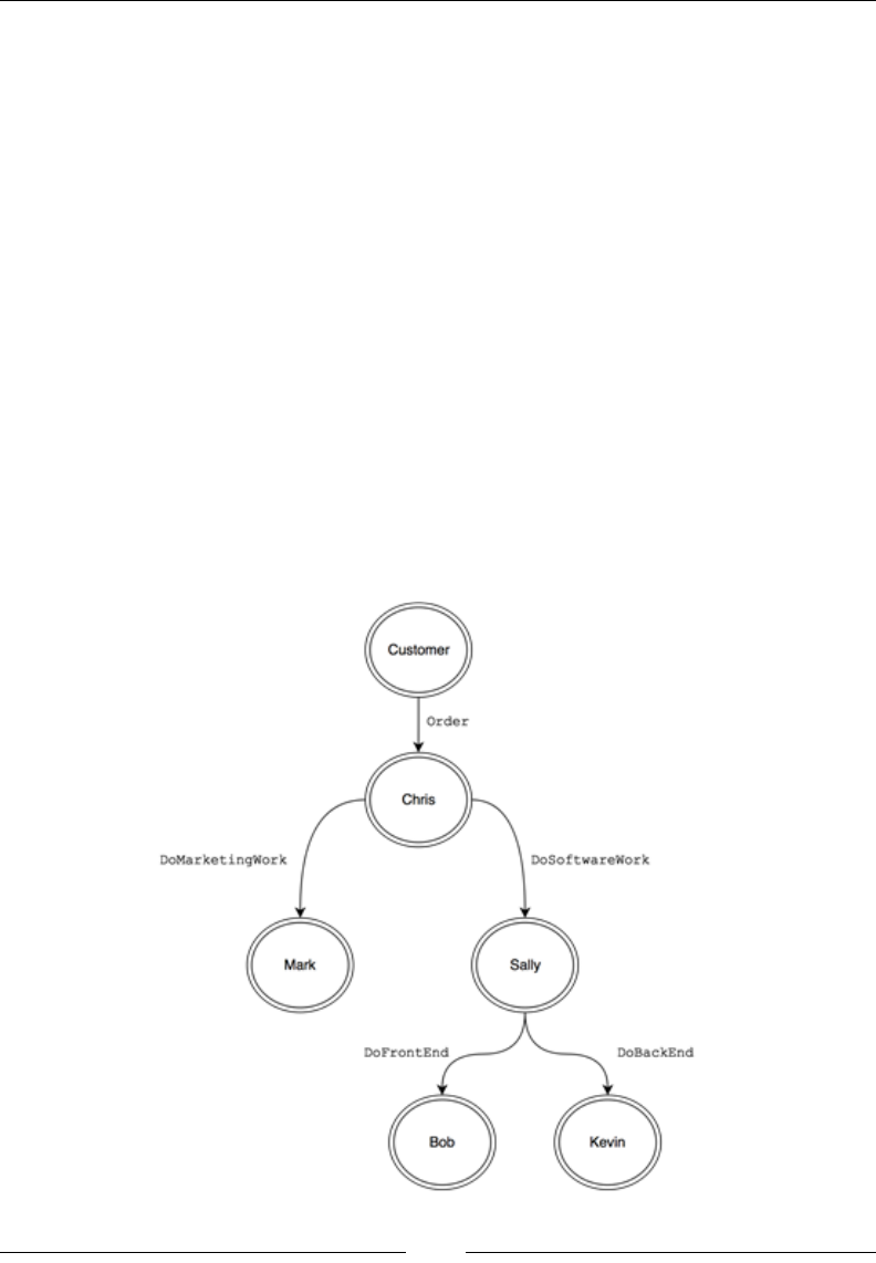
Chapter 9
[ 191 ]
Actors offer an elegant abstraction to encapsulate state. They are lightweight objects
that each perform a single task (possibly repeatedly) and communicate with each
other by passing messages. The internal state of an actor can only be changed from
within the actor itself. Importantly, actors only process messages one at a time,
effectively preventing race conditions.
By hiding program state inside actors, we can reason about the program more
effectively: if a bug is introduced that makes this state inconsistent, the culprit
will be localized entirely in that actor.
Actors as people
In the previous section, you learned that an actor encapsulates state, interacting with
the outside world through messages. Actors make concurrent programming more
intuitive because they behave a little bit like an ideal workforce.
Let's think of an actor system representing a start-up with ve people. There's
Chris, the CEO, and Mark, who's in charge of marketing. Then there's Sally, who
heads the engineering team. Sally has two minions, Bob and Kevin. As every good
organization needs an organizational chart, refer to the following diagram:

Concurrency with Akka
[ 192 ]
Let's say that Chris receives an order. He will look at the order, decide whether it
is something that he can process himself, and if not, he will forward it to Mark or
Sally. Let's assume that the order asks for a small program so Bob forwards the order
to Sally. Sally is very busy working on a backlog of orders so she cannot process
the order message straightaway, and it will just sit in her mailbox for a short while.
When she nally gets round to processing the order, she might decide to split the
order into several parts, some of which she will give to Kevin and some to Bob.
As Bob and Kevin complete items, they will send messages back to Sally to inform
her. When every part of the order is fullled, Sally will aggregate the parts together
and message either the customer directly or Chris with the results.
The task of keeping track of which jobs must be fullled to complete the order rests
with Sally. When she receives messages from Bob and Kevin, she must update
her list of tasks in progress and check whether every task related to this order is
complete. This sort of coordination would be more challenging with traditional
synchronize blocks: every access to the list of tasks in progress and to the list of
completed tasks would need to be synchronized. By embedding this logic in Sally,
who can only process a single message at a time, we can be sure that there will not be
race conditions.
Our start-up works well because each person is responsible for doing a single thing:
Chris either delegates to Mark or Sally, Sally breaks up orders into several parts and
assigns them to Bob and Kevin, and Bob and Kevin fulll each part. You might think
"hold on, all the logic is embedded in Bob and Kevin, the employees at the bottom of
the ladder who do all the actual work". Actors, unlike employees, are cheap, so if the
logic embedded in an actor gets too complicated, it is easy to introduce additional
layers of delegation until tasks get simple enough.
The employees in our start-up refuse to multitask. When they get a piece of work,
they process it completely and then move on to the next task. This means that they
cannot get muddled by the complexities of multitasking. Actors, by processing a
single message at a time, greatly reduce the scope for introducing concurrency errors
such as race conditions.
More importantly, by offering an abstraction that programmers can intuitively
understand—that of human workers—Akka makes reasoning about concurrency easier.

Chapter 9
[ 193 ]
Hello world with Akka
Let's install Akka. We add it as a dependency to our build.sbt le:
scalaVersion := "2.11.7"
libraryDependencies += "com.typesafe.akka" %% "akka-actor" %
"2.4.0"
We can now import Akka as follows:
import akka.actor._
For our rst foray into the world of actors, we will build an actor that echoes every
message it receives. The code examples for this section are in a directory called
chap09/hello_akka in the sample code provided with this book (https://github.
com/pbugnion/s4ds):
// EchoActor.scala
import akka.actor._
class EchoActor extends Actor with ActorLogging {
def receive = {
case msg:String =>
Thread.sleep(500)
log.info(s"Received '$msg'")
}
}
Let's pick this example apart, starting with the constructor. Our actor class must
extend Actor. We also add ActorLogging, a utility trait that adds the log attribute.
The Echo actor exposes a single method, receive. This is the actor's only way of
communicating with the external world. To be useful, all actors must expose a
receive method. The receive method is a partial function, typically implemented
with multiple case statements. When an actor starts processing a message, it will
match it against every case statement until it nds one that matches. It will then
execute the corresponding block.
Our echo actor accepts a single type of message, a plain string. When this message
gets processed, the actor waits for half a second and then echoes the message to the
log le.

Concurrency with Akka
[ 194 ]
Let's instantiate a couple of Echo actors and send them messages:
// HelloAkka.scala
import akka.actor._
object HelloAkka extends App {
// We need an actor system before we can
// instantiate actors
val system = ActorSystem("HelloActors")
// instantiate our two actors
val echo1 = system.actorOf(Props[EchoActor], name="echo1")
val echo2 = system.actorOf(Props[EchoActor], name="echo2")
// Send them messages. We do this using the "!" operator
echo1 ! "hello echo1"
echo2 ! "hello echo2"
echo1 ! "bye bye"
// Give the actors time to process their messages,
// then shut the system down to terminate the program
Thread.sleep(500)
system.shutdown
}
Running this gives us the following output:
[INFO] [07/19/2015 17:15:23.954] [HelloActor-akka.actor.default-
dispatcher-2] [akka://HelloActor/user/echo1] Received 'hello echo1'
[INFO] [07/19/2015 17:15:23.954] [HelloActor-akka.actor.default-
dispatcher-3] [akka://HelloActor/user/echo2] Received 'hello echo2'
[INFO] [07/19/2015 17:15:24.955] [HelloActor-akka.actor.default-
dispatcher-2] [akka://HelloActor/user/echo1] Received 'bye bye'
Note that the echo1 and echo2 actors are clearly acting concurrently: hello echo1
and hello echo2 are logged at the same time. The second message, passed to echo1,
gets processed after the actor has nished processing hello echo1.

Chapter 9
[ 195 ]
There are a few different things to note:
• To start instantiating actors, we must first create an actor system. There is
typically a single actor system per application.
• The way in which we instantiate actors looks a little strange. Instead of
calling the constructor, we create an actor properties object, Props[T]. We
then ask the actor system to create an actor with these properties. In fact,
we never instantiate actors with new: they are either created by calling the
actorOf method in the actor system or a similar method from within another
actor (more on this later).
We never call an actor's methods from outside that actor. The only way to interact
with the actor is to send messages to it. We do this using the tell operator, !. There
is thus no way to mess with an actor's internals from outside that actor (or at least,
Akka makes it difcult to mess with an actor's internals).
Case classes as messages
In our "hello world" example, we constructed an actor that is expected to receive a
string as message. Any object can be passed as a message, provided it is immutable.
It is very common to use case classes to represent messages. This is better than using
strings because of the additional type safety: the compiler will catch a typo in a case
class but not in a string.
Let's rewrite our EchoActor to accept instances of case classes as messages. We will
make it accept two different messages: EchoMessage(message) and EchoHello,
which just echoes a default message. The examples for this section and the next are in
the chap09/hello_akka_case_classes directory in the sample code provided with
this book (https://github.com/pbugnion/s4ds).
A common Akka pattern is to dene the messages that an actor can receive in the
actor's companion object:
// EchoActor.scala
object EchoActor {
case object EchoHello
case class EchoMessage(msg:String)
}

Concurrency with Akka
[ 196 ]
Let's change the actor denition to accept these messages:
class EchoActor extends Actor with ActorLogging {
import EchoActor._ // import the message definitions
def receive = {
case EchoHello => log.info("hello")
case EchoMessage(s) => log.info(s)
}
}
We can now send EchoHello and EchoMessage to our actors:
echo1 ! EchoActor.EchoHello
echo2 ! EchoActor.EchoMessage("We're learning Akka.")
Actor construction
Actor construction is a common source of difculty for people new to Akka. Unlike
(most) ordinary objects, you never instantiate actors explicitly. You would never
write, for instance, val echo = new EchoActor. In fact, if you try this, Akka raises
an exception.
Creating actors in Akka is a two-step process: you rst create a Props object, which
encapsulates the properties needed to construct an actor. The way to construct a
Props object differs depending on whether the actor takes constructor arguments.
If the constructor takes no arguments, we simply pass the actor class as a type
parameter to Props:
val echoProps = Props[EchoActor]
If we have an actor whose constructor does take arguments, we must pass these as
additional arguments when dening the Props object. Let's consider the following
actor, for instance:
class TestActor(a:String, b:Int) extends Actor { ... }
We pass the constructor arguments to the Props object as follows:
val testProps = Props(classOf[TestActor], "hello", 2)
The Props instance just embodies the conguration for creating an actor. It does
not actually create anything. To create an actor, we pass the Props instance to the
system.actorOf method, dened on the ActorSystem instance:
val system = ActorSystem("HelloActors")
val echo1 = system.actorOf(echoProps, name="hello-1")

Chapter 9
[ 197 ]
The name parameter is optional but is useful for logging and error messages. The
value returned by .actorOf is not the actor itself: it is a reference to the actor (it
helps to think of it as an address that the actor lives at) and has the ActorRef type.
ActorRef is immutable, but it can be serialized and duplicated without affecting the
underlying actor.
There is another way to create actors besides calling actorOf on the actor system:
each actor exposes a context.actorOf method that takes a Props instance as its
argument. The context is only accessible from within the actor:
class TestParentActor extends Actor {
val echoChild = context.actorOf(echoProps, name="hello-child")
...
}
The difference between an actor created from the actor system and an actor created
from another actor's context lies in the actor hierarchy: each actor has a parent. Any
actor created within another actor's context will have that actor as its parent. An
actor created by the actor system has a predened actor, called the user guardian, as
its parent. We will understand the importance of the actor hierarchy when we study
the actor lifecycle at the end of this chapter.
A very common idiom is to dene a props method in an actor's companion object
that acts as a factory method for Props instances for that actor. Let's amend the
EchoActor companion object:
object EchoActor {
def props:Props = Props[EchoActor]
// message case class definitions here
}
We can then instantiate the actor as follows:
val echoActor = system.actorOf(EchoActor.props)
Anatomy of an actor
Before diving into a full-blown application, let's look at the different components of
the actor framework and how they t together:
• Mailbox: A mailbox is basically a queue. Each actor has its own mailbox.
When you send a message to an actor, the message lands in its mailbox and
does nothing until the actor takes it off the queue and passes it through its
receive method.

Concurrency with Akka
[ 198 ]
• Messages: Messages make synchronization between actors possible. A
message can have any type with the sole requirement that it should be
immutable. In general, it is better to use case classes or case objects to gain
the compiler's help in checking message types.
• Actor reference: When we create an actor using val echo1 = system.
actorOf(Props[EchoActor]), echo1 has type ActorRef. An ActorRef is
a proxy for an actor and is what the rest of the world interacts with: when
you send a message, you send it to the ActorRef, not to the actor directly. In
fact, you can never obtain a handle to an actor directly in Akka. An actor can
obtain an ActorRef for itself using the .self method.
• Actor context: Each actor has a context attribute through which you can
access methods to create or access other actors and find information about
the outside world. We have already seen how to create new actors with
context.actorOf(props). We can also obtain a reference to an actor's
parent through context.parent. An actor can also stop another actor with
context.stop(actorRef), where actorRef is a reference to the actor that
we want to stop.
• Dispatcher: The dispatcher is the machine that actually executes the code in
an actor. The default dispatcher uses a fork/join thread pool. Akka lets us
use different dispatchers for different actors. Tweaking the dispatcher can be
useful to optimize the performance and give priority to certain actors. The
dispatcher that an actor runs on is accessible through context.dispatcher.
Dispatchers implement the ExecutionContext interface so they can be used
to run futures.
Follower network crawler
The end game for this chapter is to build a crawler to explore GitHub's follower
graph. We have already outlined how we can do this in a single-threaded manner
earlier in this chapter. Let's design an actor system to do this concurrently.
The moving parts in the code are the data structures managing which users have
been fetched or are being fetched. These need to be encapsulated in an actor to avoid
race conditions arising from multiple actors trying to change them concurrently. We
will therefore create a fetcher manager actor whose job is to keep track of which users
have been fetched and which users we are going to fetch next.
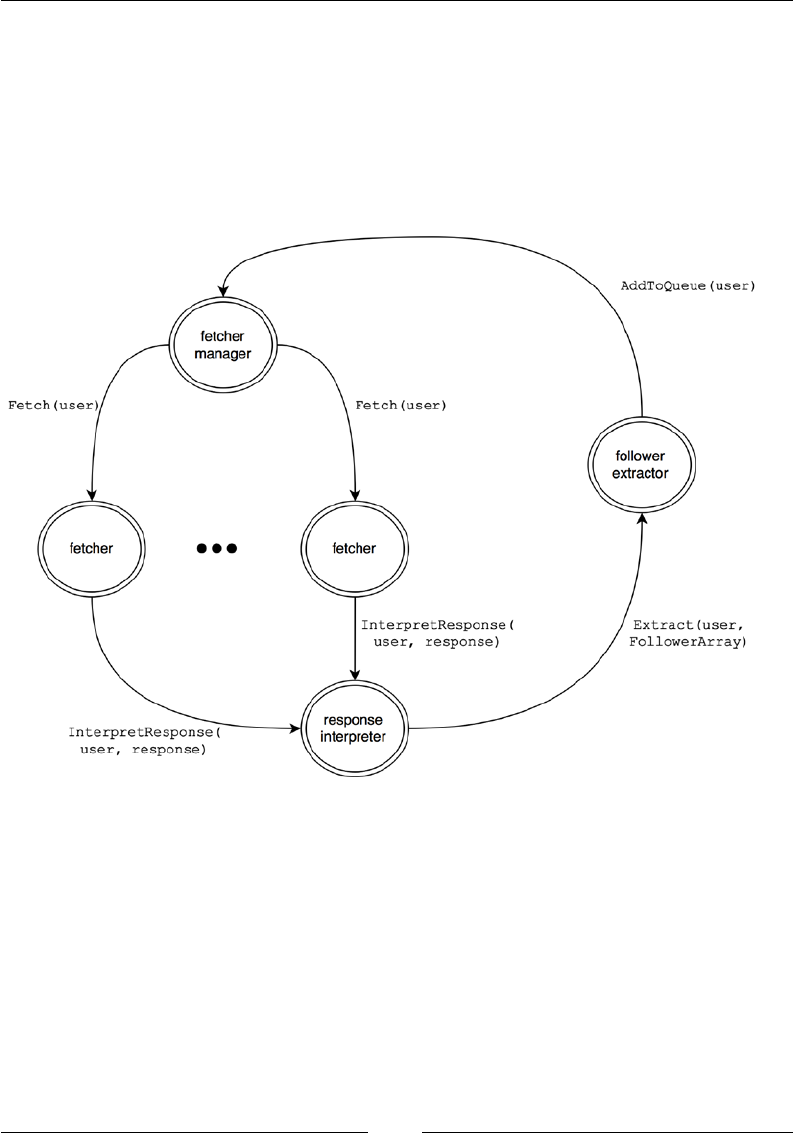
Chapter 9
[ 199 ]
The part of the code that is likely to be a bottleneck is querying the GitHub API. We
therefore want to be able to scale the number of workers doing this concurrently. We
will create a pool of fetchers, actors responsible for querying the API for the followers
of a particular user. Finally, we will create an actor whose responsibility is to
interpret the API's response. This actor will forward its interpretation of the response
to another actor who will extract the followers and give them to the fetcher manager.
This is what the architecture of the program will look like:
Actor system for our GitHub API crawler
Each actor in our program performs a single task: fetchers just query the GitHub
API and the queue manager just distributes work to the fetchers. Akka best practice
dictates giving actors as narrow an area of responsibility as possible. This enables
better granularity when scaling out (for instance, by adding more fetcher actors, we
just parallelize the bottleneck) and better resilience: if an actor fails, it will only affect
his area of responsibility. We will explore actor failure later on in this chapter.

Concurrency with Akka
[ 200 ]
We will build the app in several steps, exploring the Akka toolkit as we write
the program. Let's start with the build.sbt le. Besides Akka, we will mark
scalaj-http and json4s as dependencies:
// build.sbt
scalaVersion := "2.11.7"
libraryDependencies ++= Seq(
"org.json4s" %% "json4s-native" % "3.2.10",
"org.scalaj" %% "scalaj-http" % "1.1.4",
"com.typesafe.akka" %% "akka-actor" % "2.3.12"
)
Fetcher actors
The workhorse of our application is the fetcher, the actor responsible for fetching
the follower details from GitHub. In the rst instance, our actor will accept a single
message, Fetch(user). It will fetch the followers corresponding to user and log
the response to screen. We will use the recipes developed in Chapter 7, Web APIs, to
query the GitHub API with an OAuth token. We will inject the token through the
actor constructor.
Let's start with the companion object. This will contain the denition of the
Fetch(user) message and two factory methods to create the Props instances. You can
nd the code examples for this section in the chap09/fetchers_alone directory in the
sample code provided with this book (https://github.com/pbugnion/s4ds):
// Fetcher.scala
import akka.actor._
import scalaj.http._
import scala.concurrent.Future
object Fetcher {
// message definitions
case class Fetch(login:String)
// Props factory definitions
def props(token:Option[String]):Props =
Props(classOf[Fetcher], token)
def props():Props = Props(classOf[Fetcher], None)
}

Chapter 9
[ 201 ]
Let's now dene the fetcher itself. We will wrap the call to the GitHub API in a
future. This avoids a single slow request blocking the actor. When our actor receives
a Fetch request, it wraps this request into a future, sends it off, and can then process
the next message. Let's go ahead and implement our actor:
// Fetcher.scala
class Fetcher(val token:Option[String])
extends Actor with ActorLogging {
import Fetcher._ // import message definition
// We will need an execution context for the future.
// Recall that the dispatcher doubles up as execution
// context.
import context.dispatcher
def receive = {
case Fetch(login) => fetchUrl(login)
}
private def fetchUrl(login:String) {
val unauthorizedRequest = Http(
s"https://api.github.com/users/$login/followers")
val authorizedRequest = token.map { t =>
unauthorizedRequest.header("Authorization", s"token $t")
}
// Prepare the request: try to use the authorized request
// if a token was given, and fall back on an unauthorized
// request
val request = authorizedRequest.getOrElse(unauthorizedRequest)
// Fetch from github
val response = Future { request.asString }
response.onComplete { r =>
log.info(s"Response from $login: $r")
}
}
}

Concurrency with Akka
[ 202 ]
Let's instantiate an actor system and four fetchers to check whether our actor is
working as expected. We will read the GitHub token from the environment, as
described in Chapter 7, Web APIs, then create four actors and ask each one to fetch the
followers of a particular GitHub user. We wait ve seconds for the requests to get
completed, and then shut the system down:
// FetcherDemo.scala
import akka.actor._
object FetcherDemo extends App {
import Fetcher._ // Import the messages
val system = ActorSystem("fetchers")
// Read the github token if present.
val token = sys.env.get("GHTOKEN")
val fetchers = (0 until 4).map { i =>
system.actorOf(Fetcher.props(token))
}
fetchers(0) ! Fetch("odersky")
fetchers(1) ! Fetch("derekwyatt")
fetchers(2) ! Fetch("rkuhn")
fetchers(3) ! Fetch("tototoshi")
Thread.sleep(5000) // Wait for API calls to finish
system.shutdown // Shut system down
}
Let's run the code through SBT:
$ GHTOKEN="2502761..." sbt run
[INFO] [11/08/2015 16:28:06.500] [fetchers-akka.actor.default-
dispatcher-2] [akka://fetchers/user/$d] Response from tototoshi: Success
(HttpResponse([{"login":"akr4","id":10892,"avatar_url":"https://avatars.
githubusercontent.com/u/10892?v=3","gravatar_id":""...

Chapter 9
[ 203 ]
Notice how we explicitly need to shut the actor system down using system.
shutdown. The program hangs until the system is shut down. However, shutting
down the system will stop all the actors, so we need to make sure that they have
nished working. We do this by inserting a call to Thread.sleep.
Using Thread.sleep to wait until the API calls have nished to shut down the actor
system is a little crude. A better approach could be to let the actors signal back to the
system that they have completed their task. We will see examples of this pattern later
when we implement the fetcher manager actor.
Akka includes a feature-rich scheduler to schedule events. We can use the scheduler
to replace the call to Thread.sleep by scheduling a system shutdown ve seconds
in the future. This is preferable as the scheduler does not block the calling thread,
unlike Thread.sleep. To use the scheduler, we need to import a global execution
context and the duration module:
// FetcherDemoWithScheduler.scala
import scala.concurrent.ExecutionContext.Implicits.global
import scala.concurrent.duration._
We can then schedule a system shutdown by replacing our call to Thread.sleep
with the following:
system.scheduler.scheduleOnce(5.seconds) { system.shutdown }
Besides scheduleOnce, the scheduler also exposes a schedule method that lets you
schedule events to happen regularly (every two seconds, for instance). This is useful
for heartbeat checks or monitoring systems. For more information, read the API
documentation on the scheduler available at http://doc.akka.io/docs/akka/
snapshot/scala/scheduler.html.
Note that we are actually cheating a little bit here by not fetching every follower. The
response to the follower's query is actually paginated, so we would need to fetch
several pages to fetch all the followers. Adding logic to the actor to do this is not
terribly complicated. We will ignore this for now and assume that users are capped
at 100 followers each.

Concurrency with Akka
[ 204 ]
Routing
In the previous example, we created four fetchers and dispatched messages to them,
one after the other. We have a pool of identical actors among which we distribute
tasks. Manually routing the messages to the right actor to maximize the utilization
of our pool is painful and error-prone. Fortunately, Akka provides us with several
routing strategies that we can use to distribute work among our pool of actors.
Let's rewrite the previous example with automatic routing. You can nd the code
examples for this section in the chap09/fetchers_routing directory in the sample
code provided with this book (https://github.com/pbugnion/s4ds). We will
reuse the same denition of Fetchers and its companion object as we did in the
previous section.
Let's start by importing the routing package:
// FetcherDemo.scala
import akka.routing._
A router is an actor that forwards the messages that it receives to its children. The
easiest way to dene a pool of actors is to tell Akka to create a router and pass it a
Props object for its children. The router will then manage the creation of the workers
directly. In our example (we will only comment on the parts that differ from the
previous example in the text, but you can nd the full code in the fetchers_routing
directory with the examples for this chapter), we replace the custom Fetcher
creation code with the following:
// FetcherDemo.scala
// Create a router with 4 workers of props Fetcher.props()
val router = system.actorOf(
RoundRobinPool(4).props(Fetcher.props(token))
)
We can then send the fetch messages directly to the router. The router will route the
messages to the children in a round-robin manner:
List("odersky", "derekwyatt", "rkuhn", "tototoshi").foreach {
login => router ! Fetch(login)
}
We used a round-robin router in this example. Akka offers many different types of
routers, including routers with dynamic pool size, to cater to different types of load
balancing. Head over to the Akka documentation for a list of all the available routers,
at http://doc.akka.io/docs/akka/snapshot/scala/routing.html.

Chapter 9
[ 205 ]
Message passing between actors
Merely logging the API response is not very useful. To traverse the follower graph,
we must perform the following:
• Check the return code of the response to make sure that the GitHub API was
happy with our request
• Parse the response as JSON
• Extract the login names of the followers and, if we have not fetched them
already, push them into the queue
You learned how to do all these things in Chapter 7, Web APIs, but not in the context
of actors.
We could just add the additional processing steps to the receive method of our
Fetcher actor: we could add further transformations to the API response by future
composition. However, having actors do several different things, and possibly failing
in several different ways, is an anti-pattern: when we learn about managing the actor
life cycle, we will see that it becomes much more difcult to reason about our actor
systems if the actors contain several bits of logic.
We will therefore use a pipeline of three different actors:
• The fetchers, which we have already encountered, are responsible just for
fetching a URL from GitHub. They will fail if the URL is badly formatted or
they cannot access the GitHub API.
• The response interpreter is responsible for taking the response from the
GitHub API and parsing it to JSON. If it fails at any step, it will just log
the error (in a real application, we might take different corrective actions
depending on the type of failure). If it manages to extract JSON successfully,
it will pass the JSON array to the follower extractor.
• The follower extractor will extract the followers from the JSON array and
pass them on to the queue of users whose followers we need to fetch.
We have already built the fetchers, though we will need to modify them to forward
the API response to the response interpreter rather than just logging it.

Concurrency with Akka
[ 206 ]
You can nd the code examples for this section in the chap09/all_workers
directory in the sample code provided with this book (https://github.com/
pbugnion/s4ds).The rst step is to modify the fetchers so that, instead of logging
the response, they forward the response to the response interpreter. To be able to
forward the response to the response interpreter, the fetchers will need a reference
to this actor. We will just pass the reference to the response interpreter through the
fetcher constructor, which is now:
// Fetcher.scala
class Fetcher(
val token:Option[String],
val responseInterpreter:ActorRef)
extends Actor with ActorLogging {
...
}
We must also modify the Props factory method in the companion object:
// Fetcher.scala
def props(
token:Option[String], responseInterpreter:ActorRef
):Props = Props(classOf[Fetcher], token, responseInterpreter)
We must also modify the receive method to forward the HTTP response to the
interpreter rather than just logging it:
// Fetcher.scala
class Fetcher(...) extends Actor with ActorLogging {
...
def receive = {
case Fetch(login) => fetchFollowers(login)
}
private def fetchFollowers(login:String) {
val unauthorizedRequest = Http(
s"https://api.github.com/users/$login/followers")
val authorizedRequest = token.map { t =>
unauthorizedRequest.header("Authorization", s"token $t")
}
val request = authorizedRequest.getOrElse(unauthorizedRequest)
val response = Future { request.asString }
// Wrap the response in an InterpretResponse message and
// forward it to the interpreter.

Chapter 9
[ 207 ]
response.onComplete { r =>
responseInterpreter !
ResponseInterpreter.InterpretResponse(login, r)
}
}
}
The response interpreter takes the response, decides if it is valid, parses it to JSON, and
forwards it to a follower extractor. The response interpreter will need a reference to
the follower extractor, which we will pass in the constructor.
Let's start by dening the ResponseInterpreter companion. It will just contain the
denition of the messages that the response interpreter can receive and a factory to
create a Props object to help with instantiation:
// ResponseInterpreter.scala
import akka.actor._
import scala.util._
import scalaj.http._
import org.json4s._
import org.json4s.native.JsonMethods._
object ResponseInterpreter {
// Messages
case class InterpretResponse(
login:String, response:Try[HttpResponse[String]]
)
// Props factory
def props(followerExtractor:ActorRef) =
Props(classOf[ResponseInterpreter], followerExtractor)
}
The body of ResponseInterpreter should feel familiar: when the actor receives a
message giving it a response to interpret, it parses it to JSON using the techniques
that you learned in Chapter 7, Web APIs. If we parse the response successfully, we
forward the parsed JSON to the follower extractor. If we fail to parse the response
(possibly because it was badly formatted), we just log the error. We could recover
from this in other ways, for instance, by re-adding this login to the queue manager to
be fetched again:
// ResponseInterpreter.scala
class ResponseInterpreter(followerExtractor:ActorRef)

Concurrency with Akka
[ 208 ]
extends Actor with ActorLogging {
// Import the message definitions
import ResponseInterpreter._
def receive = {
case InterpretResponse(login, r) => interpret(login, r)
}
// If the query was successful, extract the JSON response
// and pass it onto the follower extractor.
// If the query failed, or is badly formatted, throw an error
// We should also be checking error codes here.
private def interpret(
login:String, response:Try[HttpResponse[String]]
) = response match {
case Success(r) => responseToJson(r.body) match {
case Success(jsonResponse) =>
followerExtractor ! FollowerExtractor.Extract(
login, jsonResponse)
case Failure(e) =>
log.error(
s"Error parsing response to JSON for $login: $e")
}
case Failure(e) => log.error(
s"Error fetching URL for $login: $e")
}
// Try and parse the response body as JSON.
// If successful, coerce the `JValue` to a `JArray`.
private def responseToJson(responseBody:String):Try[JArray] = {
val jvalue = Try { parse(responseBody) }
jvalue.flatMap {
case a:JArray => Success(a)
case _ => Failure(new IllegalStateException(
"Incorrectly formatted JSON: not an array"))
}
}
}
We now have two-thirds of our worker actors. The last link is the follower extractor.
This actor's job is simple: it takes the JArray passed to it by the response interpreter
and converts it to a list of followers. For now, we will just log this list, but when
we build our fetcher manager, the follower extractor will send messages asking the
manager to add the followers to its queue of logins to fetch.

Chapter 9
[ 209 ]
As before, the companion just denes the messages that this actor can receive and a
Props factory method:
// FollowerExtractor.scala
import akka.actor._
import org.json4s._
import org.json4s.native.JsonMethods._
object FollowerExtractor {
// Messages
case class Extract(login:String, jsonResponse:JArray)
// Props factory method
def props = Props[FollowerExtractor]
}
The FollowerExtractor class receives Extract messages containing a JArray of
information representing a follower. It extracts the login eld and logs it:
class FollowerExtractor extends Actor with ActorLogging {
import FollowerExtractor._
def receive = {
case Extract(login, followerArray) => {
val followers = extractFollowers(followerArray)
log.info(s"$login -> ${followers.mkString(", ")}")
}
}
def extractFollowers(followerArray:JArray) = for {
JObject(follower) <- followerArray
JField("login", JString(login)) <- follower
} yield login
}
Let's write a new main method to exercise all our actors:
// FetchNetwork.scala
import akka.actor._
import akka.routing._
import scala.concurrent.ExecutionContext.Implicits.global

Concurrency with Akka
[ 210 ]
import scala.concurrent.duration._
object FetchNetwork extends App {
import Fetcher._ // Import messages and factory method
// Get token if exists
val token = sys.env.get("GHTOKEN")
val system = ActorSystem("fetchers")
// Instantiate actors
val followerExtractor = system.actorOf(FollowerExtractor.props)
val responseInterpreter =
system.actorOf(ResponseInterpreter.props(followerExtractor))
val router = system.actorOf(RoundRobinPool(4).props(
Fetcher.props(token, responseInterpreter))
)
List("odersky", "derekwyatt", "rkuhn", "tototoshi") foreach {
login => router ! Fetch(login)
}
// schedule a shutdown
system.scheduler.scheduleOnce(5.seconds) { system.shutdown }
}
Let's run this through SBT:
$ GHTOKEN="2502761d..." sbt run
[INFO] [11/05/2015 20:09:37.048] [fetchers-akka.actor.default-
dispatcher-3] [akka://fetchers/user/$a] derekwyatt -> adulteratedjedi,
joonas, Psycojoker, trapd00r, tyru, ...
[INFO] [11/05/2015 20:09:37.050] [fetchers-akka.actor.default-
dispatcher-3] [akka://fetchers/user/$a] tototoshi -> akr4, yuroyoro,
seratch, yyuu, ...
[INFO] [11/05/2015 20:09:37.051] [fetchers-akka.actor.default-
dispatcher-3] [akka://fetchers/user/$a] odersky -> misto, gkossakowski,
mushtaq, ...
[INFO] [11/05/2015 20:09:37.052] [fetchers-akka.actor.default-
dispatcher-3] [akka://fetchers/user/$a] rkuhn -> arnbak, uzoice, jond3k,
TimothyKlim, relrod, ...

Chapter 9
[ 211 ]
Queue control and the pull pattern
We have now dened the three worker actors in our crawler application. The next
step is to dene the manager. The fetcher manager is responsible for keeping a queue
of logins to fetch as well as a set of login names that we have already seen in order to
avoid fetching the same logins more than once.
A rst attempt might involve building an actor that keeps a set of users that we
have already seen and just dispatches it to a round-robin router for fetchers when it
is given a new user to fetch. The problem with this approach is that the number of
messages in the fetchers' mailboxes would accumulate quickly: for each API query,
we are likely to get tens of followers, each of which is likely to make it back to a
fetcher's inbox. This gives us very little control over the amount of work piling up.
The rst problem that this is likely to cause involves the GitHub API rate limit: even
with authentication, we are limited to 5,000 requests per hour. It would be useful to
stop queries as soon as we hit this threshold. We cannot be responsive if each fetcher
has a backlog of hundreds of users that they need to fetch.
A better alternative is to use a pull system: the fetchers request work from a central
queue when they nd themselves idle. Pull systems are common in Akka when we
have a producer that produces work faster than consumers can process it (refer to
http://www.michaelpollmeier.com/akka-work-pulling-pattern/).
Conversations between the manager and fetchers will proceed as follows:
• If the manager goes from a state of having no work to having work, it sends a
WorkAvailable message to all the fetchers.
• Whenever a fetcher receives a WorkAvailable message or when it completes
an item of work, it sends a GiveMeWork message to the queue manager.
• When the queue manager receives a GiveMeWork message, it ignores the
request if no work is available or it is throttled. If it has work, it sends a
Fetch(user) message to the actor.
Let's start by modifying our fetcher. You can nd the code examples for this section
in the chap09/ghub_crawler directory in the sample code provided with this book
(https://github.com/pbugnion/s4ds). We will pass a reference to the fetcher
manager through the constructor. We need to change the companion object to add
the WorkAvailable message and the props factory to include the reference to
the manager:
// Fecther.scala
object Fetcher {
case class Fetch(url:String)

Concurrency with Akka
[ 212 ]
case object WorkAvailable
def props(
token:Option[String],
fetcherManager:ActorRef,
responseInterpreter:ActorRef):Props =
Props(classOf[Fetcher],
token, fetcherManager, responseInterpreter)
}
We also need to change the receive method so that it queries the FetcherManager
asking for more work once it's done processing a request or when it receives a
WorkAvailable message.
This is the nal version of the fetchers:
class Fetcher(
val token:Option[String],
val fetcherManager:ActorRef,
val responseInterpreter:ActorRef)
extends Actor with ActorLogging {
import Fetcher._
import context.dispatcher
def receive = {
case Fetch(login) => fetchFollowers(login)
case WorkAvailable =>
fetcherManager ! FetcherManager.GiveMeWork
}
private def fetchFollowers(login:String) {
val unauthorizedRequest = Http(
s"https://api.github.com/users/$login/followers")
val authorizedRequest = token.map { t =>
unauthorizedRequest.header("Authorization", s"token $t")
}
val request = authorizedRequest.getOrElse(unauthorizedRequest)
val response = Future { request.asString }
response.onComplete { r =>
responseInterpreter !
ResponseInterpreter.InterpretResponse(login, r)
fetcherManager ! FetcherManager.GiveMeWork
}
}
}

Chapter 9
[ 213 ]
Now that we have a working denition of the fetchers, let's build the
FetcherManager. This is the most complex actor that we have built so far, and,
before we dive into building it, we need to learn a bit more about the components of
the Akka toolkit.
Accessing the sender of a message
When our fetcher manager receives a GiveMeWork request, we will need to send
work back to the correct fetcher. We can access the actor who sent a message
using the sender method, which is a method of Actor that returns the ActorRef
corresponding to the actor who sent the message currently being processed. The
case statement corresponding to GiveMeWork in the fetcher manager is therefore:
def receive = {
case GiveMeWork =>
login = // get next login to fetch
sender ! Fetcher.Fetch(login)
...
}
As sender is a method, its return value will change for every new incoming message.
It should therefore only be used synchronously with the receive method. In
particular, using it in a future is dangerous:
def receive = {
case DoSomeWork =>
val work = Future { Thread.sleep(20000) ; 5 }
work.onComplete { result =>
sender ! Complete(result) // NO!
}
}
The problem is that when the future is completed 20 seconds after the message is
processed, the actor will, in all likelihood, be processing a different message so the
return value of sender will have changed. We will thus send the Complete message
to a completely different actor.

Concurrency with Akka
[ 214 ]
If you need to reply to a message outside of the receive method, such as when a
future completes, you should bind the value of the current sender to a variable:
def receive = {
case DoSomeWork =>
// bind the current value of sender to a val
val requestor = sender
val work = Future { Thread.sleep(20000) ; 5 }
work.onComplete { result => requestor ! Complete(result) }
}
Stateful actors
The behavior of the fetcher manager depends on whether it has work to give out to
the fetchers:
• If it has work to give, it needs to respond to GiveMeWork messages with a
Fetcher.Fetch message
• If it does not have work, it must ignore the GiveMeWork messages and, if
work gets added, it must send a WorkAvailable message to the fetchers
Encoding the notion of state is straightforward in Akka. We specify different
receive methods and switch from one to the other depending on the state. We will
dene the following receive methods for our fetcher manager, corresponding to
each of the states:
// receive method when the queue is empty
def receiveWhileEmpty: Receive = {
...
}
// receive method when the queue is not empty
def receiveWhileNotEmpty: Receive = {
...
}
Note that we must dene the return type of the receive methods as Receive.
To switch the actor from one method to the other, we can use context.
become(methodName). Thus, for instance, when the last login name is popped
off the queue, we can transition to using the receiveWhileEmpty method with
context.become(receiveWhileEmpty). We set the initial state by assigning
receiveWhileEmpty to the receive method:
def receive = receiveWhileEmpty

Chapter 9
[ 215 ]
Follower network crawler
We are now ready to code up the remaining pieces of our network crawler. The
largest missing piece is the fetcher manager. Let's start with the companion object.
As with the worker actors, this just contains the denitions of the messages that the
actor can receive and a factory to create the Props instance:
// FetcherManager.scala
import scala.collection.mutable
import akka.actor._
object FetcherManager {
case class AddToQueue(login:String)
case object GiveMeWork
def props(token:Option[String], nFetchers:Int) =
Props(classOf[FetcherManager], token, nFetchers)
}
The manager can receive two messages: AddToQueue, which tells it to add a
username to the queue of users whose followers need to be fetched, and GiveMeWork,
emitted by the fetchers when they are unemployed.
The manager will be responsible for launching the fetchers, response interpreter, and
follower extractor, as well as maintaining an internal queue of usernames and a set of
usernames that we have seen:
// FetcherManager.scala
class FetcherManager(val token:Option[String], val nFetchers:Int)
extends Actor with ActorLogging {
import FetcherManager._
// queue of usernames whose followers we need to fetch
val fetchQueue = mutable.Queue.empty[String]
// set of users we have already fetched.
val fetchedUsers = mutable.Set.empty[String]
// Instantiate worker actors
val followerExtractor = context.actorOf(
FollowerExtractor.props(self))
val responseInterpreter = context.actorOf(
ResponseInterpreter.props(followerExtractor))

Concurrency with Akka
[ 216 ]
val fetchers = (0 until nFetchers).map { i =>
context.actorOf(
Fetcher.props(token, self, responseInterpreter))
}
// receive method when the actor has work:
// If we receive additional work, we just push it onto the
// queue.
// If we receive a request for work from a Fetcher,
// we pop an item off the queue. If that leaves the
// queue empty, we transition to the 'receiveWhileEmpty'
// method.
def receiveWhileNotEmpty:Receive = {
case AddToQueue(login) => queueIfNotFetched(login)
case GiveMeWork =>
val login = fetchQueue.dequeue
// send a Fetch message back to the sender.
// we can use the `sender` method to reply to a message
sender ! Fetcher.Fetch(login)
if (fetchQueue.isEmpty) {
context.become(receiveWhileEmpty)
}
}
// receive method when the actor has no work:
// if we receive work, we add it onto the queue, transition
// to a state where we have work, and notify the fetchers
// that work is available.
def receiveWhileEmpty:Receive = {
case AddToQueue(login) =>
queueIfNotFetched(login)
context.become(receiveWhileNotEmpty)
fetchers.foreach { _ ! Fetcher.WorkAvailable }
case GiveMeWork => // do nothing
}
// Start with an empty queue.
def receive = receiveWhileEmpty
def queueIfNotFetched(login:String) {
if (! fetchedUsers(login)) {
log.info(s"Pushing $login onto queue")
// or do something useful...
fetchQueue += login

Chapter 9
[ 217 ]
fetchedUsers += login
}
}
}
We now have a fetcher manager. The rest of the code can remain the same, apart
from the follower extractor. Instead of logging followers names, it must send
AddToQueue messages to the manager. We will pass a reference to the manager at
construction time:
// FollowerExtractor.scala
import akka.actor._
import org.json4s._
import org.json4s.native.JsonMethods._
object FollowerExtractor {
// messages
case class Extract(login:String, jsonResponse:JArray)
// props factory method
def props(manager:ActorRef) =
Props(classOf[FollowerExtractor], manager)
}
class FollowerExtractor(manager:ActorRef)
extends Actor with ActorLogging {
import FollowerExtractor._
def receive = {
case Extract(login, followerArray) =>
val followers = extractFollowers(followerArray)
followers foreach { f =>
manager ! FetcherManager.AddToQueue(f)
}
}
def extractFollowers(followerArray:JArray) = for {
JObject(follower) <- followerArray
JField("login", JString(login)) <- follower
} yield login
}

Concurrency with Akka
[ 218 ]
The main method running all this is remarkably simple as all the code to instantiate
actors has been moved to the FetcherManager. We just need to instantiate the
manager and give it the rst node in the network, and it will do the rest:
// FetchNetwork.scala
import akka.actor._
object FetchNetwork extends App {
// Get token if exists
val token = sys.env.get("GHTOKEN")
val system = ActorSystem("GithubFetcher")
val manager = system.actorOf(FetcherManager.props(token, 2))
manager ! FetcherManager.AddToQueue("odersky")
}
Notice how we do not attempt to shut down the actor system anymore. We will just
let it run, crawling the network, until we stop it or hit the authentication limit. Let's
run this through SBT:
$ GHTOKEN="2502761d..." sbt "runMain FetchNetwork"
[INFO] [11/06/2015 06:31:04.614] [GithubFetcher-akka.actor.default-
dispatcher-2] [akka://GithubFetcher/user/$a] Pushing odersky onto queue
[INFO] [11/06/2015 06:31:05.563] [GithubFetcher-akka.actor.default-
dispatcher-4] [akka://GithubFetcher/user/$a] Pushing misto onto
queueINFO] [11/06/2015 06:31:05.563] [GithubFetcher-akka.actor.default-
dispatcher-4] [akka://GithubFetcher/user/$a] Pushing gkossakowski onto
queue
^C
Our program does not actually do anything useful with the followers that it retrieves
besides logging them. We could replace the log.info call to, for instance, store the
nodes in a database or draw the graph to screen.
Fault tolerance
Real programs fail, and they fail in unpredictable ways. Akka, and the Scala
community in general, favors planning explicitly for failure rather than trying to
write infallible applications. A fault tolerant system is a system that can continue
to operate when one or more of its components fails. The failure of an individual
subsystem does not necessarily mean the failure of the application. How does this
apply to Akka?

Chapter 9
[ 219 ]
The actor model provides a natural unit to encapsulate failure: the actor. When an
actor throws an exception while processing a message, the default behavior is for the
actor to restart, but the exception does not leak out and affect the rest of the system.
For instance, let's introduce an arbitrary failure in the response interpreter. We will
modify the receive method to throw an exception when it is asked to interpret the
response for misto, one of Martin Odersky's followers:
// ResponseInterpreter.scala
def receive = {
case InterpretResponse("misto", r) =>
throw new IllegalStateException("custom error")
case InterpretResponse(login, r) => interpret(login, r)
}
If you rerun the code through SBT, you will notice that an error gets logged. The
program does not crash, however. It just continues as normal:
[ERROR] [11/07/2015 12:05:58.938] [GithubFetcher-akka.actor.default-
dispatcher-2] [akka://GithubFetcher/user/$a/$b] custom error
java.lang.IllegalStateException: custom error
at ResponseInterpreter$
...
[INFO] [11/07/2015 12:05:59.117] [GithubFetcher-akka.actor.default-
dispatcher-2] [akka://GithubFetcher/user/$a] Pushing samfoo onto queue
None of the followers of misto will get added to the queue: he never made it past the
ResponseInterpreter stage. Let's step through what happens when the exception
gets thrown:
• The interpreter is sent the InterpretResponse("misto", ...) message.
This causes it to throw an exception and it dies. None of the other actors are
affected by the exception.
• A fresh instance of the response interpreter is created with the same Props
instance as the recently deceased actor.
• When the response interpreter has finished initializing, it gets bound to the
same ActorRef as the deceased actor. This means that, as far as the rest of the
system is concerned, nothing has changed.
• The mailbox is tied to ActorRef rather than the actor, so the new response
interpreter will have the same mailbox as its predecessor, without the
offending message.

Concurrency with Akka
[ 220 ]
Thus, if, for whatever reason, our crawler crashes when fetching or parsing the
response for a user, the application will be minimally affected—we will just not fetch
this user's followers.
Any internal state that an actor carries is lost when it restarts. Thus, if, for instance, the
fetcher manager died, we would lose the current value of the queue and visited users.
The risks associated with losing the internal state can be mitigated by the following:
• Adopting a different strategy for failure: we can, for instance, carry on
processing messages without restarting the actor in the event of failure.
Of course, this is of little use if the actor died because its internal state is
inconsistent. In the next section, we will discuss how to change the failure
recovery strategy.
• Backing up the internal state by writing it to disk periodically and loading
from the backup on restart.
• Protecting actors that carry critical state by ensuring that all "risky"
operations are delegated to other actors. In our crawler example, all the
interactions with external services, such as querying the GitHub API and
parsing the response, happen with actors that carry no internal state. As we
saw in the previous example, if one of these actors dies, the application is
minimally affected. By contrast, the precious fetcher manager is only allowed
to interact with sanitized inputs. This is called the error kernel pattern: code
likely to cause errors is delegated to kamikaze actors.
Custom supervisor strategies
The default strategy of restarting an actor on failure is not always what we want. In
particular, for actors that carry a lot of data, we might want to resume processing
after an exception rather than restarting the actor. Akka lets us customize this
behavior by setting a supervisor strategy in the actor's supervisor.
Recall that all actors have parents, including the top-level actors, who are children of
a special actor called the user guardian. By default, an actor's supervisor is his parent,
and it is the supervisor who decides what happens to the actor on failure.

Chapter 9
[ 221 ]
Thus, to change how an actor reacts to failure, you must set its parent's supervisor
strategy. You do this by setting the supervisorStrategy attribute. The default
strategy is equivalent to the following:
val supervisorStrategy = OneForOneStrategy() {
case _:ActorInitializationException => Stop
case _:ActorKilledException => Stop
case _:DeathPactException => Stop
case _:Exception => Restart
}
There are two components to a supervisor strategy:
• OneForOneStrategy determines that the strategy applies only to the actor
that failed. By contrast, we can use AllForOneStrategy, which applies the
same strategy to all the supervisees. If a single child fails, all the children will
be restarted (or stopped or resumed).
• A partial function mapping Throwables to a Directive, which is an
instruction on what to do in response to a failure. The default strategy, for
instance, maps ActorInitializationException (which happens if the
constructor fails) to the Stop directive and (almost all) other exceptions
to Restart.
There are four directives:
• Restart: This destroys the faulty actor and restarts it, binding the newborn
actor to the old ActorRef. This clears the internal state of the actor, which
may be a good thing (the actor might have failed because of some internal
inconsistency).
• Resume: The actor just moves on to processing the next message in its inbox.
• Stop: The actor stops and is not restarted. This is useful in throwaway actors
that you use to complete a single operation: if this operation fails, the actor is
not needed any more.
• Escalate: The supervisor itself rethrows the exception, hoping that its
supervisor will know what to do with it.
A supervisor does not have access to which of its children failed. Thus, if an actor has
children that might require different recovery strategies, it is best to create a set of
intermediate supervisor actors to supervise the different groups of children.

Concurrency with Akka
[ 222 ]
As an example of setting the supervisor strategy, let's tweak the FetcherManager
supervisor strategy to adopt an all-for-one strategy and stop its children when one of
them fails. We start with the relevant imports:
import akka.actor.SupervisorStrategy._
Then, we just need to set the supervisorStrategy attribute in the FetcherManager
denition:
class FetcherManager(...) extends Actor with ActorLogging {
...
override val supervisorStrategy = AllForOneStrategy() {
case _:ActorInitializationException => Stop
case _:ActorKilledException => Stop
case _:Exception => Stop
}
...
}
If you run this through SBT, you will notice that when the code comes across the
custom exception thrown by the response interpreter, the system halts. This is
because all the actors apart from the fetcher manager are now defunct.
Life-cycle hooks
Akka lets us specify code that runs in response to specic events in an actor's life,
through life-cycle hooks. Akka denes the following hooks:
• preStart(): This runs after the actor's constructor has finished but before
it starts processing messages. This is useful to run initialization code that
depends on the actor being fully constructed.
• postStop(): This runs when the actor dies after it has stopped processing
messages. This is useful to run cleanup code before terminating the actor.
• preRestart(reason: Throwable, message: Option[Any]): This is called
just after an actor receives an order to restart. The preRestart method
has access to the exception that was thrown and to the offending message,
allowing for corrective action. The default behavior of preRestart is to stop
each child and then call postStop.
• postRestart(reason:Throwable): This is called after an actor has restarted.
The default behavior is to call preStart().

Chapter 9
[ 223 ]
Let's use system hooks to persist the state of FetcherManager between runs of the
programs. You can nd the code examples for this section in the chap09/ghub_
crawler_fault_tolerant directory in the sample code provided with this book
(https://github.com/pbugnion/s4ds). This will make the fetcher manager fault-
tolerant. We will use postStop to write the current queue and set of visited users to
text les and preStart to read these text les from the disk. Let's start by importing
the libraries necessary to read and write les:
// FetcherManager.scala
import scala.io.Source
import scala.util._
import java.io._
We will store the names of the two text les in which we persist the state in the
FetcherManager companion object (a better approach would be to store them in a
conguration le):
// FetcherManager.scala
object FetcherManager {
...
val fetchedUsersFileName = "fetched-users.txt"
val fetchQueueFileName = "fetch-queue.txt"
}
In the preStart method, we load both the set of fetched users and the backlog of
users to fetch from the text les, and in the postStop method, we overwrite these
les with the new values of these data structures:
class FetcherManager(
val token:Option[String], val nFetchers:Int
) extends Actor with ActorLogging {
...
/** pre-start method: load saved state from text files */
override def preStart {
log.info("Running pre-start on fetcher manager")
loadFetchedUsers
log.info(
s"Read ${fetchedUsers.size} visited users from source"
)
loadFetchQueue

Concurrency with Akka
[ 224 ]
log.info(
s"Read ${fetchQueue.size} users in queue from source"
)
// If the saved state contains a non-empty queue,
// alert the fetchers so they can start working.
if (fetchQueue.nonEmpty) {
context.become(receiveWhileNotEmpty)
fetchers.foreach { _ ! Fetcher.WorkAvailable }
}
}
/** Dump the current state of the manager */
override def postStop {
log.info("Running post-stop on fetcher manager")
saveFetchedUsers
saveFetchQueue
}
/* Helper methods to load from and write to files */
def loadFetchedUsers {
val fetchedUsersSource = Try {
Source.fromFile(fetchedUsersFileName)
}
fetchedUsersSource.foreach { s =>
try s.getLines.foreach { l => fetchedUsers += l }
finally s.close
}
}
def loadFetchQueue {
val fetchQueueSource = Try {
Source.fromFile(fetchQueueFileName)
}
fetchQueueSource.foreach { s =>
try s.getLines.foreach { l => fetchQueue += l }
finally s.close
}
}
def saveFetchedUsers {
val fetchedUsersFile = new File(fetchedUsersFileName)
val writer = new BufferedWriter(

Chapter 9
[ 225 ]
new FileWriter(fetchedUsersFile))
fetchedUsers.foreach { user => writer.write(user + "\n") }
writer.close()
}
def saveFetchQueue {
val queueUsersFile = new File(fetchQueueFileName)
val writer = new BufferedWriter(
new FileWriter(queueUsersFile))
fetchQueue.foreach { user => writer.write(user + "\n") }
writer.close()
}
...
}
Now that we save the state of the crawler when it shuts down, we can put a better
termination condition for the program than simply interrupting the program once
we get bored. In production, we might halt the crawler when we have enough names
in a database, for instance. In this example, we will simply let the crawler run for
30 seconds and then shut it down.
Let's modify the main method:
// FetchNetwork.scala
import akka.actor._
import scala.concurrent.ExecutionContext.Implicits.global
import scala.concurrent.duration._
object FetchNetwork extends App {
// Get token if exists
val token = sys.env.get("GHTOKEN")
val system = ActorSystem("GithubFetcher")
val manager = system.actorOf(FetcherManager.props(token, 2))
manager ! FetcherManager.AddToQueue("odersky")
system.scheduler.scheduleOnce(30.seconds) { system.shutdown }
}

Concurrency with Akka
[ 226 ]
After 30 seconds, we just call system.shutdown, which stops all the actors
recursively. This will stop the fetcher manager, calling the postStop life cycle hook.
After one run of the program, I have 2,164 names in the fetched-users.txt le.
Running it again increases this number to 3,728 users.
We could improve fault tolerance further by making the fetcher manager dump the
data structures at regular intervals while the code runs. As writing to the disk (or to a
database) carries a certain element of risk (What if the database server goes down or
the disk is full?) it would be better to delegate writing the data structures to a custom
actor rather than endangering the manager.
Our crawler has one minor problem: when the fetcher manager stops, it stops the
fetcher actors, response interpreter, and follower extractor. However, none of the
users currently going through these actors are stored. This also results in a small
number of undelivered messages at the end of the code: if the response interpreter
stops before a fetcher, the fetcher will try to deliver to a non-existent actor. This only
accounts for a small number of users. To recover these login names, we can create
a reaper actor whose job is to coordinate the killing of all the worker actors in the
correct order and harvest their internal state. This pattern is documented in a blog
post by Derek Wyatt (http://letitcrash.com/post/30165507578/shutdown-
patterns-in-akka-2).
What we have not talked about
Akka is a very rich ecosystem, far too rich to do it justice in a single chapter.
There are some important parts of the toolkit that you will need, but we have not
covered them here. We will give brief descriptions, but you can refer to the Akka
documentation for more details:
• The ask operator, ?, offers an alternative to the tell operator, !, that we have
used to send messages to actors. Unlike "tell", which just fires a message to
an actor, the ask operator expects a response. This is useful when we need to
ask actors questions rather than just telling them what to do. The ask pattern
is documented at http://doc.akka.io/docs/akka/snapshot/scala/
actors.html#Ask__Send-And-Receive-Future.
• Deathwatch allows actors to watch another actor and receive a message
when it dies. This is useful for actors that might depend on another actor but
not be its direct supervisor. This is documented at http://doc.akka.io/
docs/akka/snapshot/scala/actors.html#Lifecycle_Monitoring_aka_
DeathWatch.

Chapter 9
[ 227 ]
• In our crawler, we passed references to actors explicitly through the
constructor. We can also look up actors using the actor hierarchy with a
syntax reminiscent of files in a filesystem at http://doc.akka.io/docs/
akka/snapshot/scala/actors.html#Identifying_Actors_via_Actor_
Selection.
• We briefly explored how to implement stateful actors with different receive
methods and using context.become to switch between them. Akka offers a
more powerful alternative, based on finite state machines, to encode a more
complex set of states and transitions: http://doc.akka.io/docs/akka/
snapshot/scala/fsm.html.
• We have not discussed distributing actor systems across several nodes in
this chapter. The message passing architecture works well with distributed
setups: http://doc.akka.io/docs/akka/2.4.0/common/cluster.html.
Summary
In this chapter, you learned how to weave actors together to tackle a difcult
concurrent problem. More importantly, we saw how Akka's actor framework
encourages us to think about concurrent problems in terms of many separate chunks
of encapsulated mutable data, synchronized through message passing. Akka makes
concurrent programming easier to reason about and more fun.
References
Derek Wyatt's book, Akka Concurrency, is a fantastic introduction to Akka. It should
denitely be the rst stop for anyone wanting to do serious Akka programming.
The LET IT CRASH blog (http://letitcrash.com) is the ofcial Akka blog, and
contains many examples of idioms and patterns to solve common issues.
[ 229 ]
Distributed Batch
Processing with Spark
In Chapter 4, Parallel Collections and Futures, we discovered how to use parallel
collections for "embarrassingly" parallel problems: problems that can be broken
down into a series of tasks that require no (or very little) communication between
the tasks.
Apache Spark provides behavior similar to Scala parallel collections (and much
more), but, instead of distributing tasks across different CPUs on the same computer,
it allows the tasks to be distributed across a computer cluster. This provides arbitrary
horizontal scalability, since we can simply add more computers to the cluster.
In this chapter, we will learn the basics of Apache Spark and use it to explore a set of
emails, extracting features with the view of building a spam lter. We will explore
several ways of actually building a spam lter in Chapter 12, Distributed Machine
Learning with MLlib.
Installing Spark
In previous chapters, we included dependencies by specifying them in a build.
sbt le, and relying on SBT to fetch them from the Maven Central repositories. For
Apache Spark, downloading the source code or pre-built binaries explicitly is more
common, since Spark ships with many command line scripts that greatly facilitate
launching jobs and interacting with a cluster.
Head over to http://spark.apache.org/downloads.html and download Spark
1.5.2, choosing the "pre-built for Hadoop 2.6 or later" package. You can also build
Spark from source if you need customizations, but we will stick to the pre-built
version since it requires no conguration.

Distributed Batch Processing with Spark
[ 230 ]
Clicking Download will download a tarball, which you can unpack with the
following command:
$ tar xzf spark-1.5.2-bin-hadoop2.6.tgz
This will create a spark-1.5.2-bin-hadoop2.6 directory. To verify that Spark works
correctly, navigate to spark-1.5.2-bin-hadoop2.6/bin and launch the Spark shell
using ./spark-shell. This is just a Scala shell with the Spark libraries loaded.
You may want to add the bin/ directory to your system path. This will let you
call the scripts in that directory from anywhere on your system, without having to
reference the full path. On Linux or Mac OS, you can add variables to the system
path by entering the following line in your shell conguration le (.bash_profile
on Mac OS, and .bashrc or .bash_profile on Linux):
export PATH=/path/to/spark/bin:$PATH
The changes will take effect in new shell sessions. On Windows (if you
use PowerShell), you need to enter this line in the profile.ps1 le in the
WindowsPowerShell folder in Documents:
$env:Path += ";C:\Program Files\GnuWin32\bin"
If this worked correctly, you should be able to open a Spark shell in any directory on
your system by just typing spark-shell in a terminal.
Acquiring the example data
In this chapter, we will explore the Ling-Spam email dataset (The original dataset
is described at http://csmining.org/index.php/ling-spam-datasets.html).
Download the dataset from http://data.scala4datascience.com/ling-spam.
tar.gz (or ling-spam.zip, depending on your preferred mode of compression),
and unpack the contents to the directory containing the code examples for this
chapter. The archive contains two directories, spam/ and ham/, containing the spam
and legitimate emails, respectively.

Chapter 10
[ 231 ]
Resilient distributed datasets
Spark expresses all computations as a sequence of transformations and actions on
distributed collections, called Resilient Distributed Datasets (RDD). Let's explore
how RDDs work with the Spark shell. Navigate to the examples directory and
open a Spark shell as follows:
$ spark-shell
scala>
Let's start by loading an email in an RDD:
scala> val email = sc.textFile("ham/9-463msg1.txt")
email: rdd.RDD[String] = MapPartitionsRDD[1] at textFile
email is an RDD, with each element corresponding to a line in the input le. Notice
how we created the RDD by calling the textFile method on an object called sc:
scala> sc
spark.SparkContext = org.apache.spark.SparkContext@459bf87c
sc is a SparkContext instance, an object representing the entry point to the Spark
cluster (for now, just our local machine). When we start a Spark shell, a context is
created and bound to the variable sc automatically.
Let's split the email into words using flatMap:
scala> val words = email.flatMap { line => line.split("\\s") }
words: rdd.RDD[String] = MapPartitionsRDD[2] at flatMap
This will feel natural if you are familiar with collections in Scala: the email RDD
behaves just like a list of strings. Here, we split using the regular expression \s,
denoting white space characters. Instead of using flatMap explicitly, we can also
manipulate RDDs using Scala's syntactic sugar:
scala> val words = for {
line <- email
word <- line.split("\\s")
} yield word
words: rdd.RDD[String] = MapPartitionsRDD[3] at flatMap

Distributed Batch Processing with Spark
[ 232 ]
Let's inspect the results. We can use .take(n) to extract the rst n elements of
an RDD:
scala> words.take(5)
Array[String] = Array(Subject:, tsd98, workshop, -, -)
We can also use .count to get the number of elements in an RDD:
scala> words.count
Long = 939
RDDs support many of the operations supported by collections. Let's use filter
to remove punctuation from our email. We will remove all words that contain any
non-alphanumeric character. We can do this by ltering out elements that match this
regular expression anywhere in the word: [^a-zA-Z0-9].
scala> val nonAlphaNumericPattern = "[^a-zA-Z0-9]".r
nonAlphaNumericPattern: Regex = [^a-zA-Z0-9]
scala> val filteredWords = words.filter {
word => nonAlphaNumericPattern.findFirstIn(word) == None
}
filteredWords: rdd.RDD[String] = MapPartitionsRDD[4] at filter
scala> filteredWords.take(5)
Array[String] = Array(tsd98, workshop, 2nd, call, paper)
scala> filteredWords.count
Long = 627
In this example, we created an RDD from a text le. We can also create RDDs from
Scala iterables using the sc.parallelize method available on a Spark context:
scala> val words = "the quick brown fox jumped over the dog".split(" ")
words: Array[String] = Array(the, quick, brown, fox, ...)
scala> val wordsRDD = sc.parallelize(words)
wordsRDD: RDD[String] = ParallelCollectionRDD[1] at parallelize at
<console>:23

Chapter 10
[ 233 ]
This is useful for debugging and for trialling behavior in the shell. The counterpart to
parallelize is the .collect method, which converts an RDD to a Scala array:
scala> val wordLengths = wordsRDD.map { _.length }
wordLengths: RDD[Int] = MapPartitionsRDD[2] at map at <console>:25
scala> wordLengths.collect
Array[Int] = Array(3, 5, 5, 3, 6, 4, 3, 3)
The .collect method requires the entire RDD to t in memory on the master node.
It is thus either used for debugging with a reduced dataset, or at the end of a pipeline
that trims down a dataset.
As you can see, RDDs offer an API much like Scala iterables. The critical difference is
that RDDs are distributed and resilient. Let's explore what this means in practice.
RDDs are immutable
You cannot change an RDD once it is created. All operations on RDDs either create
new RDDs or other Scala objects.
RDDs are lazy
When you execute operations like map and lter on a Scala collection in the
interactive shell, the REPL prints the values of the new collection to screen. The same
isn't true of Spark RDDs. This is because operations on RDDs are lazy: they are only
evaluated when needed.
Thus, when we write:
val email = sc.textFile(...)
val words = email.flatMap { line => line.split("\\s") }
We are creating an RDD, words that knows how to build itself from its parent RDD,
email, which, in turn, knows that it needs to read a text le and split it into lines.
However, none of the commands actually happen until we force the evaluation of
the RDDs by calling an action to return a Scala object. This is most evident if we try to
read from a non-existent text le:
scala> val inp = sc.textFile("nonexistent")
inp: rdd.RDD[String] = MapPartitionsRDD[5] at textFile

Distributed Batch Processing with Spark
[ 234 ]
We can create the RDD without a hitch. We can even dene further transformations
on the RDD. The program crashes only when these transformations are nally
evaluated:
scala> inp.count // number of lines
org.apache.hadoop.mapred.InvalidInputException: Input path does not
exist: file:/Users/pascal/...
The action .count is expected to return the number of elements in our RDD as an
integer. Spark has no choice but to evaluate inp, which results in an exception.
Thus, it is probably more appropriate to think of an RDD as a pipeline of operations,
rather than a more traditional collection.
RDDs know their lineage
RDDs can only be constructed from stable storage (for instance, by loading data
from a le that is present on every node in the Spark cluster), or through a set of
transformations based on other RDDs. Since RDDs are lazy, they need to know
how to build themselves when needed. They do this by knowing who their parent
RDD is, and what operation they need to apply to the parent. This is a well-dened
process since the parent RDD is immutable.
The toDebugString method provides a diagram of how an RDD is constructed:
scala> filteredWords.toDebugString
(2) MapPartitionsRDD[6] at filter at <console>:27 []
| MapPartitionsRDD[3] at flatMap at <console>:23 []
| MapPartitionsRDD[1] at textFile at <console>:21 []
| ham/9-463msg1.txt HadoopRDD[0] at textFile at <console>:21 []
RDDs are resilient
If you run an application on a single computer, you generally don't need to worry
about hardware failure in your application: if the computer fails, your application is
doomed anyway.
Distributed architectures should, by contrast, be fault-tolerant: the failure of a single
machine should not crash the entire application. Spark RDDs are built with fault
tolerance in mind. Let's imagine that one of the worker nodes fails, causing the
destruction of some of the data associated with an RDD. Since the Spark RDD knows
how to build itself from its parent, there is no permanent data loss: the elements that
were lost can just be re-computed when needed on another computer.

Chapter 10
[ 235 ]
RDDs are distributed
When you construct an RDD, for instance from a text le, Spark will split the RDD
into a number of partitions. Each partition will be entirely localized on a single
machine (though there is, in general, more than one partition per machine).
Many transformations on RDDs can be executed on each partition independently.
For instance, when performing a .map operation, a given element in the output RDD
depends on a single element in the parent: data does not need to be moved between
partitions. The same is true of .flatMap and .filter operations. This means that
the partition in the RDD produced by one of these operations depends on a single
partition in the parent RDD.
On the other hand, a .distinct transformation, which removes all duplicate
elements from an RDD, requires the data in a given partition to be compared to
the data in every other partition. This requires shufing the data across the nodes.
Shufing, especially for large datasets, is an expensive operation and should be
avoided if possible.
Transformations and actions on RDDs
The set of operations supported by an RDD can be split into two categories:
• Transformations create a new RDD from the current one. Transformations
are lazy: they are not evaluated immediately.
• Actions force the evaluation of an RDD, and normally return a Scala object,
rather than an RDD, or have some form of side-effect. Actions are evaluated
immediately, triggering the execution of all the transformations that make up
this RDD.
In the tables below, we give some examples of useful transformations and actions.
For a full, up-to-date list, consult the Spark documentation (http://spark.apache.
org/docs/latest/programming-guide.html#rdd-operations).
For the examples in these tables, we assume that you have created an RDD with:
scala> val rdd = sc.parallelize(List("quick", "brown", "quick", "dog"))

Distributed Batch Processing with Spark
[ 236 ]
The following table lists common transformations on an RDD. Recall that
transformations always generate a new RDD, and that they are lazy operations:
Transformation Notes Example (assuming rdd is { "quick",
"brown", "quick", "dog" })
rdd.map(func) rdd.map { _.size } // => { 5, 5,
5, 3 }
rdd.
filter(pred)
rdd.filter { _.length < 4 } //
=> { "dog" }
rdd.
flatMap(func)
rdd.flatMap { _.toCharArray } //
=> { 'q', 'u', 'i', 'c', 'k',
'b', 'r', 'o' … }
rdd.distinct() Remove duplicate
elements in RDD.
rdd.distinct // => { "dog",
"brown", "quick" }
rdd.
pipe(command,
[envVars])
Pipe through an
external program.
RDD elements are
written, line-by-
line, to the process's
stdin. The output
is read from
stdout.
rdd.pipe("tr a-z A-Z") // => {
"QUICK", "BROWN", "QUICK", "DOG"
}
The following table describes common actions on RDDs. Recall that actions always
generate a Scala type or cause a side-effect, rather than creating a new RDD. Actions
force the evaluation of the RDD, triggering the execution of the transformations
underpinning the RDD.
Action Nodes Example (assuming rdd is {
"quick", "brown", "quick",
"dog" })
rdd.first First element in the
RDD.
rdd.first // => quick
rdd.collect Transform the RDD
to an array (the
array must be able
to fit in memory on
the master node).
rdd.collect // =>
Array[String]("quick",
"brown", "quick", "dog")
rdd.count Number of elements
in the RDD.
rdd.count // => 4

Chapter 10
[ 237 ]
Action Nodes Example (assuming rdd is {
"quick", "brown", "quick",
"dog" })
rdd.countByValue Map of element to
the number of times
this element occurs.
The map must fit on
the master node.
rdd.countByValue // =>
Map(quick -> 2, brown ->
1, dog -> 1)
rdd.take(n) Return an array of
the first n elements
in the RDD.
rdd.take(2) // =>
Array(quick, brown)
rdd.
takeOrdered(n:Int)
(implicit ordering:
Ordering[T])
Top n elements in
the RDD according
to the element's
default ordering, or
the ordering passed
as second argument.
See the Scala docs
for Ordering
for how to define
custom comparison
functions (http://
www.scala-
lang.org/api/
current/index.
html#scala.
math.Ordering).
rdd.takeOrdered(2) // =>
Array(brown, dog)
rdd.takeOrdered(2)
(Ordering.by { _.size
}) // => Array[String] =
Array(dog, quick)
rdd.reduce(func) Reduce the RDD
according to the
specified function.
Uses the first
element in the
RDD as the base.
func should be
commutative and
associative.
rdd.map { _.size }.reduce
{ _ + _ } // => 18

Distributed Batch Processing with Spark
[ 238 ]
Action Nodes Example (assuming rdd is {
"quick", "brown", "quick",
"dog" })
rdd.
aggregate(zeroValue)
(seqOp, combOp)
Reduction for
cases where the
reduction function
returns a value of
type different to the
RDD's type. In this
case, we need to
provide a function
for reducing
within a single
partition (seqOp)
and a function for
combining the value
of two partitions
(combOp).
rdd.aggregate(0) ( _ +
_.size, _ + _ ) // => 18
Persisting RDDs
We have learned that RDDs only retain the sequence of operations needed to
construct the elements, rather than the values themselves. This, of course, drastically
reduces memory usage since we do not need to keep intermediate versions of our
RDDs in memory. For instance, let's assume we want to trawl through transaction
logs to identify all the transactions that occurred on a particular account:
val allTransactions = sc.textFile("transaction.log")
val interestingTransactions = allTransactions.filter {
_.contains("Account: 123456")
}
The set of all transactions will be large, while the set of transactions on the account
of interest will be much smaller. Spark's policy of remembering how to construct a
dataset, rather than the dataset itself, means that we never have all the lines of our
input le in memory at any one time.
There are two situations in which we may want to avoid re-computing the elements
of an RDD every time we use it:
• For interactive use: we might have detected fraudulent behavior on account
"123456", and we want to investigate how this might have arisen. We will
probably want to perform many different exploratory calculations on this
RDD, without having to re-read the entire log file every time. It therefore
makes sense to persist interestingTransactions.

Chapter 10
[ 239 ]
• When an algorithm re-uses an intermediate result, or a dataset. A canonical
example is logistic regression. In logistic regression, we normally use an
iterative algorithm to find the 'optimal' coefficients that minimize the loss
function. At every step in our iterative algorithm, we must calculate the loss
function and its gradient from the training set. We should avoid re-computing
the training set (or re-loading it from an input file) if at all possible.
Spark provides a .persist method on RDDs to achieve this. By calling .persist on
an RDD, we tell Spark to keep the dataset in memory next time it is computed.
scala> words.persist
rdd.RDD[String] = MapPartitionsRDD[3] at filter
Spark supports different levels of persistence, which you can tune by passing
arguments to .persist:
scala> import org.apache.spark.storage.StorageLevel
import org.apache.spark.storage.StorageLevel
scala> interestingTransactions.persist(
StorageLevel.MEMORY_AND_DISK)
rdd.RDD[String] = MapPartitionsRDD[3] at filter
Spark provides several persistence levels, including:
• MEMORY_ONLY: the default storage level. The RDD is stored in RAM. If the
RDD is too big to fit in memory, parts of it will not persist, and will need to
be re-computed on the fly.
• MEMORY_AND_DISK: As much of the RDD is stored in memory as possible. If
the RDD is too big, it will spill over to disk. This is only worthwhile if the
RDD is expensive to compute. Otherwise, re-computing it may be faster than
reading from the disk.
If you persist several RDDs and run out of memory, Spark will clear the least
recently used out of memory (either discarding them or saving them to disk,
depending on the chosen persistence level). RDDs also expose an unpersist
method to explicitly tell Spark than an RDD is not needed any more.

Distributed Batch Processing with Spark
[ 240 ]
Persisting RDDs can have a drastic impact on performance. What and how to
persist therefore becomes very important when tuning a Spark application. Finding
the best persistence level generally requires some tinkering, benchmarking and
experimentation. The Spark documentation provides guidelines on when to use
which persistence level (http://spark.apache.org/docs/latest/programming-
guide.html#rdd-persistence), as well as general tips on tuning memory usage
(http://spark.apache.org/docs/latest/tuning.html).
Importantly, the persist method does not force the evaluation of the RDD. It just
noties the Spark engine that, next time the values in this RDD are computed, they
should be saved rather than discarded.
Key-value RDDs
So far, we have only considered RDDs of Scala value types. RDDs of more complex
data types support additional operations. Spark adds many operations for key-value
RDDs: RDDs whose type parameter is a tuple (K, V), for any type K and V.
Let's go back to our sample email:
scala> val email = sc.textFile("ham/9-463msg1.txt")
email: rdd.RDD[String] = MapPartitionsRDD[1] at textFile
scala> val words = email.flatMap { line => line.split("\\s") }
words: rdd.RDD[String] = MapPartitionsRDD[2] at flatMap
Let's persist the words RDD in memory to avoid having to re-read the email le
from disk repeatedly:
scala> words.persist
To access key-value operations, we just need to apply a transformation to our RDD
that creates key-value pairs. Let's use the words as keys. For now, we will just use 1
for every value:
scala> val wordsKeyValue = words.map { _ -> 1 }
wordsKeyValue: rdd.RDD[(String, Int)] = MapPartitionsRDD[32] at map
scala> wordsKeyValue.first
(String, Int) = (Subject:,1)

Chapter 10
[ 241 ]
Key-value RDDs support several operations besides the core RDD operations.
These are added through an implicit conversion, using the "pimp my library"
pattern that we explored in Chapter 5, Scala and SQL through JDBC. These additional
transformations fall into two broad categories: by-key transformations and joins
between RDDs.
By-key transformations are operations that aggregate the values corresponding to
the same key. For instance, we can count the number of times each word appears in
our email using reduceByKey. This method takes all the values that belong to the
same key and combines them using a user-supplied function:
scala> val wordCounts = wordsKeyValue.reduceByKey { _ + _ }
wordCounts: rdd.RDD[(String, Int)] = ShuffledRDD[35] at reduceByKey
scala> wordCounts.take(5).foreach { println }
(university,6)
(under,1)
(call,3)
(paper,2)
(chasm,2)
Note that reduceByKey requires (in general) shufing the RDD, since not every
occurrence of a given key will be in the same partition:
scala> wordCounts.toDebugString
(2) ShuffledRDD[36] at reduceByKey at <console>:30 []
+-(2) MapPartitionsRDD[32] at map at <console>:28 []
| MapPartitionsRDD[7] at flatMap at <console>:23 []
| CachedPartitions: 2; MemorySize: 50.3 KB;
ExternalBlockStoreSize: 0.0 B; DiskSize: 0.0 B
| MapPartitionsRDD[3] at textFile at <console>:21 []
| CachedPartitions: 2; MemorySize: 5.1 KB;
ExternalBlockStoreSize: 0.0 B; DiskSize: 0.0 B
| ham/9-463msg1.txt HadoopRDD[2] at textFile at <console>:21 []
Note that key-value RDDs are not like Scala Maps: the same key can occur multiple
times, and they do not support O(1) lookup. A key-value RDD can be transformed to
a Scala map using the .collectAsMap action:
scala> wordCounts.collectAsMap
scala.collection.Map[String,Int] = Map(follow -> 2, famous -> 1...

Distributed Batch Processing with Spark
[ 242 ]
This requires pulling the entire RDD onto the main Spark node. You therefore need
to have enough memory on the main node to house the map. This is often the last
stage in a pipeline that lters a large RDD to just the information that we need.
There are many by-key operations, which we describe in the table below. For the
examples in the table, we assume that rdd is created as follows:
scala> val words = sc.parallelize(List("quick", "brown","quick", "dog"))
words: RDD[String] = ParallelCollectionRDD[25] at parallelize at
<console>:21
scala> val rdd = words.map { word => (word -> word.size) }
rdd: RDD[(String, Int)] = MapPartitionsRDD[26] at map at <console>:23
scala> rdd.collect
Array[(String, Int)] = Array((quick,5), (brown,5), (quick,5), (dog,3))
Transformation Notes Example (assumes rdd is { quick
-> 5, brown -> 5, quick -> 5,
dog -> 3 })
rdd.mapValues Apply an operation
to the values.
rdd.mapValues { _ * 2 } // =>
{ quick -> 10, brown -> 10,
quick -> 10, dog ->6 }
rdd.groupByKey Return a key-value
RDD in which values
corresponding
to the same key
are grouped into
iterables.
rdd.groupByKey // => {
quick -> Iterable(5, 5),
brown -> Iterable(5), dog ->
Iterable(3) }
rdd.
reduceByKey(func)
Return a key-value
RDD in which values
corresponding to
the same key are
combined using
a user-supplied
function.
rdd.reduceByKey { _ + _ } //
=> { quick -> 10, brown -> 5,
dog -> 3 }
rdd.keys Return an RDD of the
keys.
rdd.keys // => { quick,
brown, quick, dog }
rdd.values Return an RDD of the
values.
rdd.values // => { 5, 5, 5,
3 }

Chapter 10
[ 243 ]
The second category of operations on key-value RDDs involves joining different
RDDs together by key. This is somewhat similar to SQL joins, where the keys are the
column being joined on. Let's load a spam email and apply the same transformations
we applied to our ham email:
scala> val spamEmail = sc.textFile("spam/spmsgb17.txt")
spamEmail: org.apache.spark.rdd.RDD[String] = MapPartitionsRDD[52] at
textFile at <console>:24
scala> val spamWords = spamEmail.flatMap { _.split("\\s") }
spamWords: org.apache.spark.rdd.RDD[String] = MapPartitionsRDD[53] at
flatMap at <console>:26
scala> val spamWordCounts = spamWords.map {
_ -> 1 }.reduceByKey { _ + _ }
spamWordsCount: org.apache.spark.rdd.RDD[(String, Int)] = ShuffledRDD[55]
at reduceByKey at <console>:30
scala> spamWordCounts.take(5).foreach { println }
(banner,3)
(package,14)
(call,1)
(country,2)
(offer,1)
Both spamWordCounts and wordCounts are key-value RDDs for which the keys
correspond to unique words in the message, and the values are the number of times
that word occurs. There will be some overlap in keys between spamWordCounts and
wordCounts, since the emails will share many of the same words. Let's do an inner
join between those two RDDs to get the words that occur in both emails:
scala> val commonWordCounts = wordCounts.join(spamWordCounts)
res93: rdd.RDD[(String, (Int, Int))] = MapPartitionsRDD[58] at join at
<console>:41
scala> commonWordCounts.take(5).foreach { println }
(call,(3,1))
(include,(6,2))
(minute,(2,1))
(form,(1,7))
((,(36,5))

Distributed Batch Processing with Spark
[ 244 ]
The values in the RDD resulting from an inner join will be pairs. The rst element
in the pair is the value for that key in the rst RDD, and the second element is the
value for that key in the second RDD. Thus, the word call occurs three times in the
legitimate email and once in the spam email.
Spark supports all four join types. For instance, let's perform a left join:
scala> val leftWordCounts = wordCounts.leftOuterJoin(spamWordCounts)
leftWordCounts: rdd.RDD[(String, (Int, Option[Int]))] =
MapPartitionsRDD[64] at leftOuterJoin at <console>:40
scala> leftWordCounts.take(5).foreach { println }
(call,(3,Some(1)))
(paper,(2,None))
(chasm,(2,None))
(antonio,(1,None))
(event,(3,None))
Notice that the second element in our pair has type Option[Int], to accommodate
keys absent in spamWordCounts. The word paper, for instance, occurs twice in the
legitimate email and never in the spam email. In this case, it is more useful to have
zeros to indicate absence, rather than None. Replacing None with a default value is
simple with getOrElse:
scala> val defaultWordCounts = leftWordCounts.mapValues {
case(leftValue, rightValue) => (leftValue, rightValue.getOrElse(0))
}
org.apache.spark.rdd.RDD[(String, (Int, Option[Int]))] =
MapPartitionsRDD[64] at leftOuterJoin at <console>:40
scala> defaultwordCounts.take(5).foreach { println }
(call,(3,1))
(paper,(2,0))
(chasm,(2,0))
(antonio,(1,0))
(event,(3,0))

Chapter 10
[ 245 ]
The table below lists the most common joins on key-value RDDs:
Transformation Result (assuming rdd1 is { quick -> 1, brown ->
2, quick -> 3, dog -> 4 } and rdd2 is { quick
-> 78, brown -> 79, fox -> 80 })
rdd1.join(rdd2) { quick -> (1, 78), quick -> (3, 78), brown
-> (2, 79) }
rdd1.
leftOuterJoin(rdd2)
{ dog -> (4, None), quick -> (1, Some(78)),
quick -> (3, Some(78)), brown -> (2,
Some(79)) }
rdd1.
rightOuterJoin(rdd2)
{ quick -> (Some(1), 78), quick -> (Some(3),
78), brown -> (Some(2), 79), fox -> (None,
80) }
rdd1.
fullOuterJoin(rdd2)
{ dog -> (Some(4), None), quick -> (Some(1),
Some(78)), quick -> (Some(3), Some(78)),
brown -> (Some(2), Some(79)), fox -> (None,
Some(80)) }
For a complete list of transformations, consult the API documentation for
PairRDDFunctions, http://spark.apache.org/docs/latest/api/scala/index.
html#org.apache.spark.rdd.PairRDDFunctions.
Double RDDs
In the previous section, we saw that Spark adds functionality to key-value RDDs
through an implicit conversion. Similarly, Spark adds statistics functionality to RDDs
of doubles. Let's extract the word frequencies for the ham message, and convert the
values from integers to doubles:
scala> val counts = wordCounts.values.map { _.toDouble }
counts: rdd.RDD[Double] = MapPartitionsRDD[9] at map
We can then get summary statistics using the .stats action:
scala> counts.stats
org.apache.spark.util.StatCounter = (count: 397, mean: 2.365239, stdev:
5.740843, max: 72.000000, min: 1.000000)
Thus, the most common word appears 72 times. We can also use the .histogram
action to get an idea of the distribution of values:
scala> counts.histogram(5)
(Array(1.0, 15.2, 29.4, 43.6, 57.8, 72.0),Array(391, 1, 3, 1, 1))

Distributed Batch Processing with Spark
[ 246 ]
The .histogram method returns a pair of arrays. The rst array indicates the bounds
of the histogram bins, and the second is the count of elements in that bin. Thus, there
are 391 words that appear less than 15.2 times. The distribution of words is very
skewed, such that a histogram with regular-sized bin is not really appropriate. We
can, instead, pass in custom bins by passing an array of bin edges to the histogram
method. For instance, we might distribute the bins logarithmically:
scala> counts.histogram(Array(1.0, 2.0, 4.0, 8.0, 16.0, 32.0, 64.0,
128.0))
res13: Array[Long] = Array(264, 94, 22, 11, 1, 4, 1)
Building and running standalone
programs
So far, we have interacted exclusively with Spark through the Spark shell. In the
section that follows, we will build a standalone application and launch a Spark
program either locally or on an EC2 cluster.
Running Spark applications locally
The rst step is to write the build.sbt le, as you would if you were running a
standard Scala script. The Spark binary that we downloaded needs to be run against
Scala 2.10 (You need to compile Spark from source to run against Scala 2.11. This is
not difcult to do, just follow the instructions on http://spark.apache.org/docs/
latest/building-spark.html#building-for-scala-211).
// build.sbt file
name := "spam_mi"
scalaVersion := "2.10.5"
libraryDependencies ++= Seq(
"org.apache.spark" %% "spark-core" % "1.4.1"
)
We then run sbt package to compile and build a jar of our program. The jar will be
built in target/scala-2.10/, and called spam_mi_2.10-0.1-SNAPSHOT.jar. You
can try this with the example code provided for this chapter.

Chapter 10
[ 247 ]
We can then run the jar locally using the spark-submit shell script, available in the
bin/ folder in the Spark installation directory:
$ spark-submit target/scala-2.10/spam_mi_2.10-0.1-SNAPSHOT.jar
... runs the program
The resources allocated to Spark can be controlled by passing arguments to spark-
submit. Use spark-submit --help to see the full list of arguments.
If the Spark programs has dependencies (for instance, on other Maven packages),
it is easiest to bundle them into the application jar using the SBT assembly plugin.
Let's imagine that our application depends on breeze-viz. The build.sbt le now
looks like:
// build.sbt
name := "spam_mi"
scalaVersion := "2.10.5"
libraryDependencies ++= Seq(
"org.apache.spark" %% "spark-core" % "1.5.2" % "provided",
"org.scalanlp" %% "breeze" % "0.11.2",
"org.scalanlp" %% "breeze-viz" % "0.11.2",
"org.scalanlp" %% "breeze-natives" % "0.11.2"
)
SBT assembly is an SBT plugin that builds fat jars: jars that contain not only the
program itself, but all the dependencies for the program.
Note that we marked Spark as "provided" in the list of dependencies, which
means that Spark itself will not be included in the jar (it is provided by the Spark
environment anyway). To include the SBT assembly plugin, create a le called
assembly.sbt in the project/ directory, with the following line:
addSbtPlugin("com.eed3si9n" % "sbt-assembly" % "0.14.0")
You will need to re-start SBT for the changes to take effect. You can then create the
assembly jar using the assembly command in SBT. This will create a jar called spam_
mi-assembly-0.1-SNAPSHOT.jar in the target/scala-2.10 directory. You can run
this jar using spark-submit.

Distributed Batch Processing with Spark
[ 248 ]
Reducing logging output and Spark
conguration
Spark is, by default, very verbose. The default log-level is set to INFO. To avoid
missing important messages, it is useful to change the log settings to WARN. To
change the default log level system-wide, go into the conf directory in the directory
in which you installed Spark. You should nd a le called log4j.properties.
template. Rename this le to log4j.properties and look for the following line:
log4j.rootCategory=INFO, console
Change this line to:
log4j.rootCategory=WARN, console
There are several other conguration les in that directory that you can use to
alter Spark's default behavior. For a full list of conguration options, head over
to http://spark.apache.org/docs/latest/configuration.html.
Running Spark applications on EC2
Running Spark locally is useful for testing, but the whole point of using a distributed
framework is to run programs harnessing the power of several different computers.
We can set Spark up on any set of computers that can communicate with each other
using HTTP. In general, we also need to set up a distributed le system like HDFS,
so that we can share input les across the cluster. For the purpose of this example,
we will set Spark up on an Amazon EC2 cluster.
Spark comes with a shell script, ec2/spark-ec2, for setting up an EC2 cluster and
installing Spark. It will also install HDFS. You will need an account with Amazon
Web Services (AWS) to follow these examples (https://aws.amazon.com). You will
need the AWS access key and secret key, which you can access through the Account
/ Security Credentials / Access Credentials menu in the AWS web console. You
need to make these available to the spark-ec2 script through environment variables.
Inject them into your current session as follows:
$ export AWS_ACCESS_KEY_ID=ABCDEF...
$ export AWS_SECRET_ACCESS_KEY=2dEf...
You can also write these lines into the conguration script for your shell (your
.bashrc le, or equivalent), to avoid having to re-enter them every time you run
the setup-ec2 script. We discussed environment variables in Chapter 6, Slick – A
Functional Interface for SQL.

Chapter 10
[ 249 ]
You will also need to create a key pair by clicking on Key Pairs in the EC2 web
console, creating a new key pair and downloading the certicate le. I will assume
you named the key pair test_ec2 and the certicate le test_ec2.pem. Make
sure that the key pair is created in the N. Virginia region (by choosing the correct
region in the upper right corner of the EC2 Management console), to avoid having
to specify the region explicitly in the rest of this chapter. You will need to set access
permissions on the certicate le to user-readable only:
$ chmod 400 test_ec2.pem
We are now ready to launch the cluster. Navigate to the ec2 directory and run:
$ ./spark-ec2 -k test_ec2 -i ~/path/to/certificate/test_ec2.pem -s 2
launch test_cluster
This will create a cluster called test_cluster with a master and two slaves. The
number of slaves is set through the -s command line argument. The cluster will take
a while to start up, but you can verify that the instances are launching correctly by
looking at the Instances window in the EC2 Management Console.
The setup script supports many options for customizing the type of instances, the
number of hard drives and so on. You can explore these options by passing the
--help command line option to spark-ec2.
The life cycle of the cluster can be controlled by passing different commands to the
spark-ec2 script, such as:
# shut down 'test_cluster'
$ ./spark-ec2 stop test_cluster
# start 'test_cluster'
$ ./spark-ec2 -i test_ec2.pem start test_cluster
# destroy 'test_cluster'
$ ./spark-ec2 destroy test_cluster
For more detail on using Spark on EC2, consult the ofcial documentation at
http://spark.apache.org/docs/latest/ec2-scripts.html#running-
applications.

Distributed Batch Processing with Spark
[ 250 ]
Spam ltering
Let's put all we've learned to good use and do some data exploration for our spam
lter. We will use the Ling-Spam email dataset: http://csmining.org/index.php/
ling-spam-datasets.html. The dataset contains 2412 ham emails and 481 spam
emails, all of which were received by a mailing list on linguistics. We will extract the
words that are most informative of whether an email is spam or ham.
The rst steps in any natural language processing workow are to remove stop
words and lemmatization. Removing stop words involves ltering very common
words such as the, this and so on. Lemmatization involves replacing different forms
of the same word with a canonical form: both colors and color would be mapped to
color, and organize, organizing and organizes would be mapped to organize. Removing
stop words and lemmatization is very challenging, and beyond the scope of this
book (if you do need to remove stop words and lemmatize a dataset, your go-to
tool should be the Stanford NLP toolkit: http://nlp.stanford.edu/software/
corenlp.shtml). Fortunately, the Ling-Spam e-mail dataset has been cleaned and
lemmatized already (which is why the text in the emails looks strange).
When we do build the spam lter, we will use the presence of a particular word in an
email as the feature for our model. We will use a bag-of-words approach: we consider
which words appear in an email, but not the word order.
Intuitively, some words will be more important than others when deciding whether
an email is spam. For instance, an email that contains language is likely to be ham,
since the mailing list was for linguistics discussions, and language is a word unlikely
to be used by spammers. Conversely, words which are common to both message
types, for instance hello, are unlikely to be much use.
One way of quantifying the importance of a word in determining whether a message
is spam is through the Mutual Information (MI). The mutual information is the
gain in information about whether a message is ham or spam if we know that it
contains a particular word. For instance, the presence of language in a particular
email is very informative as to whether that email is spam or ham. Similarly, the
presence of the word dollar is informative since it appears often in spam messages
and only infrequently in ham messages. By contrast, the presence of the word
morning is uninformative, since it is approximately equally common in both spam
and ham messages. The formula for the mutual information between the presence of
a particular word in an email, and whether that email is spam or ham is:
() ( )
{}
{}
( )
()( )
2
,
,
,
, log
wordPresenttruefalse
class spam ham
PwordPresent class
MI word PwordPresent classPwordPresent Pclass
∈
∈
=⋅
∑

Chapter 10
[ 251 ]
where
( )
,
PwordPresent class
is the joint probability of an email containing a particular
word and being of that class (either ham or spam),
( )
PwordPresent is the probability
that a particular word is present in an email, and
()
Pclass
is the probability that any
email is of that class. The MI is commonly used in decision trees.
The derivation of the expression for the mutual information is
beyond the scope of this book. The interested reader is directed to
David MacKay's excellent Information Theory, Inference, and Learning
Algorithms, especially the chapter Dependent Random Variables.
A key component of our MI calculation is evaluating the probability that a word
occurs in spam or ham messages. The best approximation to this probability, given
our data set, is the fraction of messages a word appears in. Thus, for instance,
if language appears in 40% of messages, we will assume that the probability
( )
PlanguagePresent of language being present in any message is 0.4. Similarly, if 40%
of the messages are ham, and language appears in 50% of those, we will assume that
the probability of language being present in an email, and that email being ham is
( )
, 0.5 0.4 0.2PlanguagePresent ham =×=
.
Let's write a wordFractionInFiles function to calculate the fraction of messages in
which each word appears, for all the words in a given corpus. Our function will take,
as argument, a path with a shell wildcard identifying a set of les, such as ham/*,
and it will return a key-value RDD, where the keys are words and the values are the
probability that that word occurs in any of those les. We will put the function in an
object called MutualInformation.
We rst give the entire code listing for this function. Don't worry if this doesn't all
make sense straight-away: we explain the tricky parts in more detail just after the
code. You may nd it useful to type some of these commands in the shell, replacing
fileGlob with, for instance "ham/*":
// MutualInformation.scala
import org.apache.spark.{ SparkConf, SparkContext }
import org.apache.spark.SparkContext._
import org.apache.spark.rdd.RDD
object MutualInformation extends App {
def wordFractionInFiles(sc:SparkContext)(fileGlob:String)
:(RDD[(String, Double)], Long) = {
// A set of punctuation words that need to be filtered out.
val wordsToOmit = Set[String](
"", ".", ",", ":", "-", "\"", "'", ")",

Distributed Batch Processing with Spark
[ 252 ]
"(", "@", "/", "Subject:"
)
val messages = sc.wholeTextFiles(fileGlob)
// wholeTextFiles generates a key-value RDD of
// file name -> file content
val nMessages = messages.count()
// Split the content of each message into a Set of unique
// words in that message, and generate a new RDD mapping:
// message -> word
val message2Word = messages.flatMapValues {
mailBody => mailBody.split("\\s").toSet
}
val message2FilteredWords = message2Word.filter {
case(email, word) => ! wordsToOmit(word)
}
val word2Message = message2FilteredWords.map { _.swap }
// word -> number of messages it appears in.
val word2NumberMessages = word2Message.mapValues {
_ => 1
}.reduceByKey { _ + _ }
// word -> fraction of messages it appears in
val pPresent = word2NumberMessages.mapValues {
_ / nMessages.toDouble
}
(pPresent, nMessages)
}
}
Let's play with this function in the Spark shell. To be able to access this function from
the shell, we need to create a jar with the MutualInformation object. Write a build.
sbt le similar to the one presented in the previous section and package the code
into a jar using sbt package. Then, open a Spark shell with:
$ spark-shell --jars=target/scala-2.10/spam_mi_2.10-0.1-SNAPSHOT.jar

Chapter 10
[ 253 ]
This will open a Spark shell with our newly created jar on the classpath. Let's run our
wordFractionInFiles method on the ham emails:
scala> import MutualInformation._
import MutualInformation._
scala> val (fractions, nMessages) = wordFractionInFiles(sc)("ham/*")
fractions: org.apache.spark.rdd.RDD[(String, Double)] =
MapPartitionsRDD[13] at mapValues
nMessages: Long = 2412
Let's get a snapshot of the fractions RDD:
scala> fractions.take(5)
Array[(String, Double)] = Array((rule-base,0.002902155887230514), (re
union,4.1459369817578774E-4), (embarrasingly,4.1459369817578774E-4),
(mller,8.291873963515755E-4), (sapore,4.1459369817578774E-4))
It would be nice to see the words that come up most often in ham messages. We
can use the .takeOrdered action to take the top values of an RDD, with a custom
ordering. .takeOrdered expects, as its second argument, an instance of the type
class Ordering[T], where T is the type parameter of our RDD: (String, Double)
in this case. Ordering[T] is a trait with a single compare(a:T, b:T) method
describing how to compare a and b. The easiest way of creating an Ordering[T] is
through the companion object's by method, which denes a key by which to compare
the elements of our RDD.
We want to order the elements in our key-value RDD by the value and, since we want
the most common words, rather than the least, we need to reverse that ordering:
scala> fractions.takeOrdered(5)(Ordering.by { - _._2 })
res0: Array[(String, Double)] = Array((language,0.6737147595356551),
(university,0.6048922056384743), (linguistic,0.5149253731343284),
(information,0.45480928689883915), ('s,0.4369817578772803))
Unsurprisingly, language is present in 67% of ham emails, university in 60% of
ham emails and so on. A similar investigation on spam messages reveals that the
exclamation mark character ! is present in 83% of spam emails, our is present in 61%
and free in 57%.
We are now in a position to start writing the body of our application to calculate the
mutual information between each word and whether a message is spam or ham.
We will put the body of the code in the MutualInformation object, which already
contains the wordFractionInFiles method.

Distributed Batch Processing with Spark
[ 254 ]
The rst step is to create a Spark context:
// MutualInformation.scala
import org.apache.spark.{ SparkConf, SparkContext }
import org.apache.spark.SparkContext._
import org.apache.spark.rdd.RDD
object MutualInformation extends App {
def wordFractionInFiles(sc:SparkContext)(fileGlob:String)
:(RDD[(String, Double)], Long) = {
...
}
val conf = new SparkConf().setAppName("lingSpam")
val sc = new SparkContext(conf)
Note that we did not need to do this when we were using the Spark shell because the
shell comes with a pre-built context bound to the variable sc.
We can now calculate the conditional probabilities of a message containing a
particular word given that it is spam,
( )
|PwordPresent spam . This is just the fraction
of messages containing that word in the spam corpus. This, in turn, lets us infer
the joint probability of a message containing a certain word and being spam
()( )( )
, |PwordPresent spam P wordPresent spam P spam=×. We will do this for all four
combinations of classes: whether any given word is present or absent in a message,
and whether that message is spam or ham:
/* Conditional probabilities RDD:
word -> P(present | spam)
*/
val (pPresentGivenSpam, nSpam) = wordFractionInFiles(sc)("spam/*")
val pAbsentGivenSpam = pPresentGivenSpam.mapValues { 1.0 - _ }
val (pPresentGivenHam, nHam) = wordFractionInFiles(sc)("ham/*")
val pAbsentGivenHam = pPresentGivenHam.mapValues { 1.0 - _ }
// pSpam is the fraction of spam messages
val nMessages = nSpam + nHam
val pSpam = nSpam / nMessages.toDouble
// pHam is the fraction of ham messages

Chapter 10
[ 255 ]
val pHam = 1.0 - pSpam
/* pPresentAndSpam is a key-value RDD of joint probabilities
word -> P(word present, spam)
*/
val pPresentAndSpam = pPresentGivenSpam.mapValues {
_ * pSpam
}
val pPresentAndHam = pPresentGivenHam.mapValues { _ * pHam }
val pAbsentAndSpam = pAbsentGivenSpam.mapValues { _ * pSpam }
val pAbsentAndHam = pAbsentGivenHam.mapValues { _ * pHam }
We will re-use these RDDs in several places in the calculation, so let's tell Spark to
keep them in memory to avoid having to re-calculate them:
pPresentAndSpam.persist
pPresentAndHam.persist
pAbsentAndSpam.persist
pAbsentAndHam.persist
We now need to calculate the probabilities of words being present,
( )
PwordPresent
.
This is just the sum of pPresentAndSpam and pPresentAndHam, for each word. The
tricky part is that not all words are present in both the ham and spam messages.
We must therefore do a full outer join of those RDDs. This will give an RDD
mapping each word to a pair of Option[Double] values. For words absent in
either the ham or spam messages, we must use a default value. A sensible default is
()( ) ( )
| 0.5 /PwordPresent spam nSpam P spam=× for spam messages (a more rigorous
approach would be to use additive smoothing). This implies that the word would
appear once if the corpus was twice as large.
val pJoined = pPresentAndSpam.fullOuterJoin(pPresentAndHam)
val pJoinedDefault = pJoined.mapValues {
case (presentAndSpam, presentAndHam) =>
(presentAndSpam.getOrElse(0.5/nSpam * pSpam),
presentAndHam.getOrElse(0.5/nHam * pHam))
}
Note that we could also have chosen 0 as the default value. This complicates the
information gain calculation somewhat, since we cannot just take the log of a zero
value, and it seems unlikely that a particular word has exactly zero probability of
occurring in an email.

Distributed Batch Processing with Spark
[ 256 ]
We can now construct an RDD mapping words to
( )
PwordPresent , the probability
that a word exists in either a spam or a ham message:
val pPresent = pJoinedDefault.mapValues {
case(presentAndHam, presentAndSpam) =>
presentAndHam + presentAndSpam
}
pPresent.persist
val pAbsent = pPresent.mapValues { 1.0 - _ }
pAbsent.persist
We now have all the RDDs that we need to calculate the mutual information
between the presence of a word in a message and whether it is ham or spam.
We need to bring them all together using the equation for the mutual information
outlined earlier.
We will start by dening a helper method that, given an RDD of joint probabilities
P(X, Y) and marginal probabilities P(X) and P(Y), calculates
()
()
()()
,
, log PXY
PXY PXPY
⎛ ⎞
×⎜ ⎟
⎜ ⎟
⎝ ⎠.
Here, P(X) could, for instance, be the probability of a word being present in a
message
( )
PwordPresent and P(Y) would be the probability that that message is
spam,
()
P spam :
def miTerm(
pXYs:RDD[(String, Double)],
pXs:RDD[(String, Double)],
pY: Double,
default: Double // for words absent in PXY
):RDD[(String, Double)] =
pXs.leftOuterJoin(pXYs).mapValues {
case (pX, Some(pXY)) => pXY * math.log(pXY/(pX*pY))
case (pX, None) => default * math.log(default/(pX*pY))
}
We can use our function to calculate the four terms in the mutual information sum:
val miTerms = List(
miTerm(pPresentAndSpam, pPresent, pSpam, 0.5/nSpam * pSpam),
miTerm(pPresentAndHam, pPresent, pHam, 0.5/nHam * pHam),
miTerm(pAbsentAndSpam, pAbsent, pSpam, 0.5/nSpam * pSpam),
miTerm(pAbsentAndHam, pAbsent, pHam, 0.5/nHam * pHam)
)

Chapter 10
[ 257 ]
Finally, we just need to sum those four terms together:
val mutualInformation = miTerms.reduce {
(term1, term2) => term1.join(term2).mapValues {
case (l, r) => l + r
}
}
The RDD mutualInformation is a key-value RDD mapping each word to a measure
of how informative the presence of that word is in discerning whether a message is
spam or ham. Let's print out the twenty words that are most informative of whether
a message is ham or spam:
mutualInformation.takeOrdered(20)(Ordering.by { - _._2 })
.foreach { println }
Let's run this using spark-submit:
$ sbt package
$ spark-submit target/scala-2.10/spam_mi_2.10-0.1-SNAPSHOT.jar
(!,0.1479941771292119)
(language,0.14574624861510874)
(remove,0.11380645864246142)
(free,0.1073496947123657)
(university,0.10695975885487692)
(money,0.07531772498093084)
(click,0.06887598051593441)
(our,0.058950906866052394)
(today,0.05485248095680509)
(sell,0.05385519653184113)
(english,0.053509319455430575)
(business,0.05299311289740539)
(market,0.05248394151802276)
(product,0.05096229706182162)
(million,0.050233193237964546)
(linguistics,0.04990172586630499)
(internet,0.04974101556655623)
(company,0.04941817269989519)
(%,0.04890193809823071)
(save,0.04861393414892205)
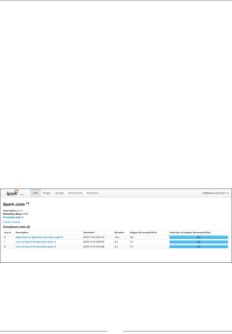
Distributed Batch Processing with Spark
[ 258 ]
Thus, we nd that the presence of words like language or free or ! carry the
most information, because they are almost exclusively present in either just spam
messages or just ham messages. A very simple classication algorithm could just
take the top 10 (by mutual information) spam words, and the top 10 ham words and
see whether a message contains more spam words or ham words. We will explore
machine learning algorithms for classication in more depth in Chapter 12, Distributed
Machine Learning with MLlib.
Lifting the hood
In the last section of this chapter, we will discuss, very briey, how Spark works
internally. For a more detailed discussion, see the References section at the end of
the chapter.
When you open a Spark context, either explicitly or by launching the Spark shell,
Spark starts a web UI with details of how the current task and past tasks have
executed. Let's see this in action for the example mutual information program we
wrote in the last section. To prevent the context from shutting down when the
program completes, you can insert a call to readLine as the last line of the main
method (after the call to takeOrdered). This expects input from the user, and will
therefore pause program execution until you press enter.
To access the UI, point your browser to 127.0.0.1:4040. If you have other instances
of the Spark shell running, the port may be 4041, or 4042 and so on.
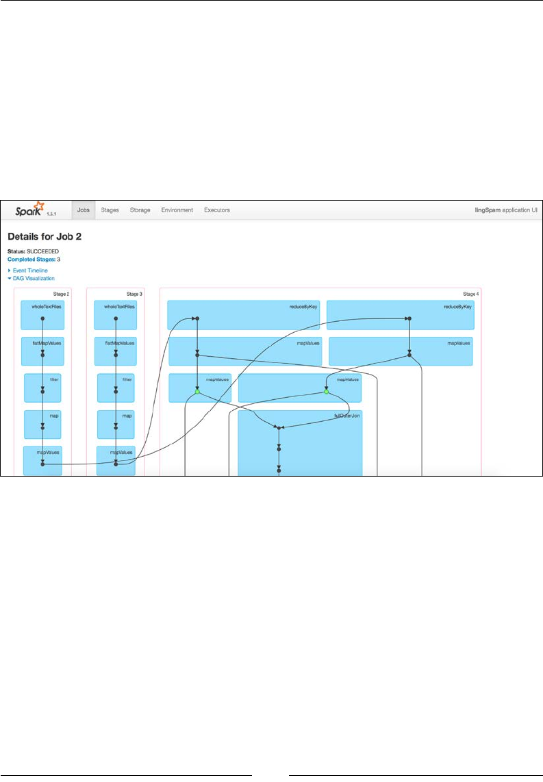
Chapter 10
[ 259 ]
The rst page of the UI tells us that our application contains three jobs. A job occurs
as the result of an action. There are, indeed, three actions in our application: the rst
two are called within the wordFractionInFiles function:
val nMessages = messages.count()
The last job results from the call to takeOrdered, which forces the execution of the
entire pipeline of RDD transformations that calculate the mutual information.
The web UI lets us delve deeper into each job. Click on the takeOrdered job in the
job table. You will get taken to a page that describes the job in more detail:
Of particular interest is the DAG visualization entry. This is a graph of the execution
plan to fulll the action, and provides a glimpse of the inner workings of Spark.
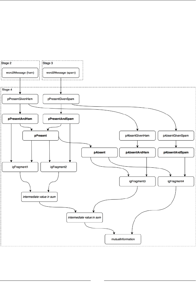
Distributed Batch Processing with Spark
[ 260 ]
When you dene a job by calling an action on an RDD, Spark looks at the RDD's
lineage and constructs a graph mapping the dependencies: each RDD in the lineage
is represented by a node, with directed edges going from this RDD's parent to itself.
This type of graph is called a directed acyclic graph (DAG), and is a data structure
useful for dependency resolution. Let's explore the DAG for the takeOrdered job in
our program using the web UI. The graph is quite complex, and it is therefore easy
to get lost, so here is a simplied reproduction that only lists the RDDs bound to
variable names in the program.

Chapter 10
[ 261 ]
As you can see, at the bottom of the graph, we have the mutualInformation RDD.
This is the RDD that we need to construct for our action. This RDD depends on the
intermediate elements in the sum, igFragment1, igFragment2, and so on. We can
work our way back through the list of dependencies until we reach the other end of
the graph: RDDs that do not depend on other RDDs, only on external sources.
Once the graph is built, the Spark engines formulates a plan to execute the job. The
plan starts with the RDDs that only have external dependencies (such as RDDs built
by loading les from disk or fetching from a database) or RDDs that already have
cached data. Each arrow along the graph is translated to a set of tasks, with each task
applying a transformation to a partition of the data.
Tasks are grouped into stages. A stage consists of a set of tasks that can all be
performed without needing an intermediate shufe.
Data shufing and partitions
To understand data shufing in Spark, we rst need to understand how data is
partitioned in RDDs. When we create an RDD by, for instance, loading a le from
HDFS, or reading a le in local storage, Spark has no control over what bits of data
are distributed in which partitions. This becomes a problem for key-value RDDs:
these often require knowing where occurrences of a particular key are, for instance to
perform a join. If the key can occur anywhere in the RDD, we have to look through
every partition to nd the key.
To prevent this, Spark allows the denition of a partitioner on key-value RDDs.
A partitioner is an attribute of the RDD that determines which partition a particular
key lands in. When an RDD has a partitioner set, the location of a key is entirely
determined by the partitioner, and not by the RDD's history, or the number of keys.
Two different RDDs with the same partitioner will map the same key to the same
partition.

Distributed Batch Processing with Spark
[ 262 ]
Partitions impact performance through their effect on transformations. There are two
types of transformations on key-value RDDs:
• Narrow transformations, like mapValues. In narrow transformations,
the data to compute a partition in the child RDD resides on a single
partition in the parent. The data processing for a narrow transformation
can therefore be performed entirely locally, without needing to communicate
data between nodes.
• Wide transformations, like reduceByKey. In wide transformations, the data
to compute any single partition can reside on all the partitions in the parent.
The RDD resulting from a wide transformation will, in general, have a
partitioner set. For instance, the output of a reduceByKey transformation are
hash-partitioned by default: the partition that a particular key ends up in is
determined by hash(key) % numPartitions.
Thus, in our mutual information example, the RDDs pPresentAndSpam and
pPresentAndHam will have the same partition structure since they both have the
default hash partitioner. All descendent RDDs retain the same keys, all the way
down to mutualInformation. The word language, for instance, will be in the
same partition for each RDD.
Why does all this matter? If an RDD has a partitioner set, this partitioner is retained
through all subsequent narrow transformations originating from this RDD. Let's
go back to our mutual information example. The RDDs pPresentGivenHam and
pPresentGivenSpam both originate from reduceByKey operations, and they
both have string keys. They will therefore both have the same hash-partitioner
(unless we explicitly set a different partitioner). This partitioner is retained as we
construct pPresentAndSpam and pPresentAndHam. When we construct pPresent,
we perform a full outer join of pPresentAndSpam and pPresentAndHam. Since
both these RDDs have the same partitioner, the child RDD pPresent has narrow
dependencies: we can just join the rst partition of pPresentAndSpam with the rst
partition of pPresentAndHam, the second partition of pPresentAndSpam with the
second partition of pPresentAndHam and so on, since any string key will be hashed
to the same partition in both RDDs. By contrast, without partitioner, we would
have to join the data in each partition of pPresentAndSpam with every partition of
pPresentAndSpam. This would require sending data across the network to all the
nodes holding pPresentAndSpam, a time-consuming exercise.
This process of having to send the data to construct a child RDD across the network,
as a result of wide dependencies, is called shufing. Much of the art of optimizing
a Spark program involves reducing shufing and, when shufing is necessary,
reducing the amount of shufing.

Chapter 10
[ 263 ]
Summary
In this chapter, we explored the basics of Spark and learned how to construct
and manipulate RDDs. In the next chapter, we will learn about Spark SQL and
DataFrames, a set of implicit conversions that allow us to manipulate RDDs in a
manner similar to pandas DataFrames, and how to interact with different data
sources using Spark.
Reference
• Learning Spark, by Holden Karau, Andy Konwinski, Patrick Wendell, and Matei
Zaharia, O'Reilly, provides a much more complete introduction to Spark that
this chapter can provide. I thoroughly recommend it.
• If you are interested in learning more about information theory, I recommend
David MacKay's book Information Theory, Inference, and Learning Algorithms.
• Information Retrieval, by Manning, Raghavan, and Schütze, describes how to
analyze textual data (including lemmatization and stemming). An online
• On the Ling-Spam dataset, and how to analyze it: http://www.aueb.gr/
users/ion/docs/ir_memory_based_antispam_filtering.pdf.
• This blog post delves into the Spark Web UI in more detail. https://
databricks.com/blog/2015/06/22/understanding-your-spark-
application-through-visualization.html.
• This blog post, by Sandy Ryza, is the first in a two-part series discussing Spark
internals, and how to leverage them to improve performance: http://blog.
cloudera.com/blog/2015/03/how-to-tune-your-apache-spark-jobs-
part-1/.
[ 265 ]
Spark SQL and DataFrames
In the previous chapter, we learned how to build a simple distributed application
using Spark. The data that we used took the form of a set of e-mails stored as text les.
We learned that Spark was built around the concept of resilient distributed datasets
(RDDs). We explored several types of RDDs: simple RDDs of strings, key-value
RDDs, and RDDs of doubles. In the case of key-value RDDs and RDDs of doubles,
Spark added functionality beyond that of the simple RDDs through implicit
conversions. There is one important type of RDD that we have not explored yet:
DataFrames (previously called SchemaRDD). DataFrames allow the manipulation
of objects signicantly more complex than those we have explored to date.
A DataFrame is a distributed tabular data structure, and is therefore very useful
for representing and manipulating structured data. In this chapter, we will rst
investigate DataFrames through the Spark shell, and then use the Ling-spam e-mail
dataset, presented in the previous chapter, to see how DataFrames can be integrated
in a machine learning pipeline.
DataFrames – a whirlwind introduction
Let's start by opening a Spark shell:
$ spark-shell
Let's imagine that we are interested in running analytics on a set of patients to
estimate their overall health level. We have measured, for each patient, their height,
weight, age, and whether they smoke.

Spark SQL and DataFrames
[ 266 ]
We might represent the readings for each patient as a case class (you might wish to
write some of this in a text editor and paste it into the Scala shell using :paste):
scala> case class PatientReadings(
val patientId: Int,
val heightCm: Int,
val weightKg: Int,
val age:Int,
val isSmoker:Boolean
)
defined class PatientReadings
We would, typically, have many thousands of patients, possibly stored in a database
or a CSV le. We will worry about how to interact with external sources later in this
chapter. For now, let's just hard-code a few readings directly in the shell:
scala> val readings = List(
PatientReadings(1, 175, 72, 43, false),
PatientReadings(2, 182, 78, 28, true),
PatientReadings(3, 164, 61, 41, false),
PatientReadings(4, 161, 62, 43, true)
)
List[PatientReadings] = List(...
We can convert readings to an RDD by using sc.parallelize:
scala> val readingsRDD = sc.parallelize(readings)
readingsRDD: RDD[PatientReadings] = ParallelCollectionRDD[0] at
parallelize at <console>:25
Note that the type parameter of our RDD is PatientReadings. Let's convert the
RDD to a DataFrame using the .toDF method:
scala> val readingsDF = readingsRDD.toDF
readingsDF: sql.DataFrame = [patientId: int, heightCm: int, weightKg:
int, age: int, isSmoker: boolean]

Chapter 11
[ 267 ]
We have created a DataFrame where each row corresponds to the readings for a
specic patient, and the columns correspond to the different features:
scala> readingsDF.show
+---------+--------+--------+---+--------+
|patientId|heightCm|weightKg|age|isSmoker|
+---------+--------+--------+---+--------+
| 1| 175| 72| 43| false|
| 2| 182| 78| 28| true|
| 3| 164| 61| 41| false|
| 4| 161| 62| 43| true|
+---------+--------+--------+---+--------+
The easiest way to create a DataFrame is to use the toDF method on an RDD. We
can convert any RDD[T], where T is a case class or a tuple, to a DataFrame. Spark
will map each attribute of the case class to a column of the appropriate type in the
DataFrame. It uses reection to discover the names and types of the attributes.
There are several other ways of constructing DataFrames, both from RDDs and from
external sources, which we will explore later in this chapter.
DataFrames support many operations for manipulating the rows and columns.
For instance, let's add a column for the Body Mass Index (BMI). The BMI is a
common way of aggregating height and weight to decide if someone is overweight or
underweight. The formula for the BMI is:
() ()
2
BMIweight kg height m=
Let's start by creating a column of the height in meters:
scala> val heightM = readingsDF("heightCm") / 100.0
heightM: sql.Column = (heightCm / 100.0)
heightM has data type Column, representing a column of data in a DataFrame.
Columns support many arithmetic and comparison operators that apply
element-wise across the column (similarly to Breeze vectors encountered in
Chapter 2, Manipulating Data with Breeze). Operations on columns are lazy: the
heightM column is not actually computed when dened. Let's now dene a
BMI column:
scala> val bmi = readingsDF("weightKg") / (heightM*heightM)
bmi: sql.Column = (weightKg / ((heightCm / 100.0) * (heightCm / 100.0)))

Spark SQL and DataFrames
[ 268 ]
It would be useful to add the bmi column to our readings DataFrame. Since
DataFrames, like RDDs, are immutable, we must dene a new DataFrame that is
identical to readingsDF, but with an additional column for the BMI. We can do this
using the withColumn method, which takes, as its arguments, the name of the new
column and a Column instance:
scala> val readingsWithBmiDF = readingsDF.withColumn("BMI", bmi)
readingsWithBmiDF: sql.DataFrame = [heightCm: int, weightKg: int, age:
int, isSmoker: boolean, BMI: double]
All the operations we have seen so far are transformations: they dene a pipeline of
operations that create new DataFrames. These transformations are executed when
we call an action, such as show:
scala> readingsWithBmiDF.show
+---------+--------+--------+---+--------+------------------+
|patientId|heightCm|weightKg|age|isSmoker| BMI|
+---------+--------+--------+---+--------+------------------+
| 1| 175| 72| 43| false|23.510204081632654|
| 2| 182| 78| 28| true| 23.54788069073783|
| 3| 164| 61| 41| false|22.679952409280194|
| 4| 161| 62| 43| true| 23.9188302920412|
+---------+--------+--------+---+--------+------------------+
Besides creating additional columns, DataFrames also support ltering rows that
satisfy a certain predicate. For instance, we can select all smokers:
scala> readingsWithBmiDF.filter {
readingsWithBmiDF("isSmoker")
}.show
+---------+--------+--------+---+--------+-----------------+
|patientId|heightCm|weightKg|age|isSmoker| BMI|
+---------+--------+--------+---+--------+-----------------+
| 2| 182| 78| 28| true|23.54788069073783|
| 4| 161| 62| 43| true| 23.9188302920412|
+---------+--------+--------+---+--------+-----------------+

Chapter 11
[ 269 ]
Or, to select everyone who weighs more than 70 kgs:
scala> readingsWithBmiDF.filter {
readingsWithBmiDF("weightKg") > 70
}.show
+---------+--------+--------+---+--------+------------------+
|patientId|heightCm|weightKg|age|isSmoker| BMI|
+---------+--------+--------+---+--------+------------------+
| 1| 175| 72| 43| false|23.510204081632654|
| 2| 182| 78| 28| true| 23.54788069073783|
+---------+--------+--------+---+--------+------------------+
It can become cumbersome to keep repeating the DataFrame name in an expression.
Spark denes the operator $ to refer to a column in the current DataFrame. Thus, the
filter expression above could have been written more succinctly using:
scala> readingsWithBmiDF.filter { $"weightKg" > 70 }.show
+---------+--------+--------+---+--------+------------------+
|patientId|heightCm|weightKg|age|isSmoker| BMI|
+---------+--------+--------+---+--------+------------------+
| 1| 175| 72| 43| false|23.510204081632654|
| 2| 182| 78| 28| true| 23.54788069073783|
+---------+--------+--------+---+--------+------------------+
The .filter method is overloaded. It accepts either a column of Boolean values, as
above, or a string identifying a Boolean column in the current DataFrame. Thus, to
lter our readingsWithBmiDF DataFrame to sub-select smokers, we could also have
used the following:
scala> readingsWithBmiDF.filter("isSmoker").show
+---------+--------+--------+---+--------+-----------------+
|patientId|heightCm|weightKg|age|isSmoker| BMI|
+---------+--------+--------+---+--------+-----------------+
| 2| 182| 78| 28| true|23.54788069073783|
| 4| 161| 62| 43| true| 23.9188302920412|
+---------+--------+--------+---+--------+-----------------+

Spark SQL and DataFrames
[ 270 ]
When comparing for equality, you must compare columns with the special
triple-equals operator:
scala> readingsWithBmiDF.filter { $"age" === 28 }.show
+---------+--------+--------+---+--------+-----------------+
|patientId|heightCm|weightKg|age|isSmoker| BMI|
+---------+--------+--------+---+--------+-----------------+
| 2| 182| 78| 28| true|23.54788069073783|
+---------+--------+--------+---+--------+-----------------+
Similarly, you must use !== to select rows that are not equal to a value:
scala> readingsWithBmiDF.filter { $"age" !== 28 }.show
+---------+--------+--------+---+--------+------------------+
|patientId|heightCm|weightKg|age|isSmoker| BMI|
+---------+--------+--------+---+--------+------------------+
| 1| 175| 72| 43| false|23.510204081632654|
| 3| 164| 61| 41| false|22.679952409280194|
| 4| 161| 62| 43| true| 23.9188302920412|
+---------+--------+--------+---+--------+------------------+
Aggregation operations
We have seen how to apply an operation to every row in a DataFrame to create
a new column, and we have seen how to use lters to build new DataFrames
with a sub-set of rows from the original DataFrame. The last set of operations on
DataFrames is grouping operations, equivalent to the GROUP BY statement in SQL.
Let's calculate the average BMI for smokers and non-smokers. We must rst tell
Spark to group the DataFrame by a column (the isSmoker column, in this case), and
then apply an aggregation operation (averaging, in this case) to reduce each group:
scala> val smokingDF = readingsWithBmiDF.groupBy(
"isSmoker").agg(avg("BMI"))
smokingDF: org.apache.spark.sql.DataFrame = [isSmoker: boolean, AVG(BMI):
double]

Chapter 11
[ 271 ]
This has created a new DataFrame with two columns: the grouping column and the
column over which we aggregated. Let's show this DataFrame:
scala> smokingDF.show
+--------+------------------+
|isSmoker| AVG(BMI)|
+--------+------------------+
| true|23.733355491389517|
| false|23.095078245456424|
+--------+------------------+
Besides averaging, there are several operators for performing the aggregation across
each group. We outline some of the more important ones in the table below, but,
for a full list, consult the Aggregate functions section of http://spark.apache.org/
docs/latest/api/scala/index.html#org.apache.spark.sql.functions$:
Operator Notes
avg(column) Group averages of the values in the specified
column.
count(column) Number of elements in each group in the specified
column.
countDistinct(column, ... ) Number of distinct elements in each group. This can
also accept multiple columns to return the count of
unique elements across several columns.
first(column), last(column) First/last element in each group
max(column), min(column) Largest/smallest element in each group
sum(column) Sum of the values in each group
Each aggregation operator takes either the name of a column, as a string, or an
expression of type Column. The latter allows aggregation of compound expressions.
If we wanted the average height, in meters, of the smokers and non-smokers in our
sample, we could use:
scala> readingsDF.groupBy("isSmoker").agg {
avg($"heightCm"/100.0)
}.show
+--------+-----------------------+
|isSmoker|AVG((heightCm / 100.0))|
+--------+-----------------------+

Spark SQL and DataFrames
[ 272 ]
| true| 1.715|
| false| 1.6949999999999998|
+--------+-----------------------+
We can also use compound expressions to dene the column on which to group. For
instance, to count the number of patients in each age group, increasing by decade,
we can use:
scala> readingsDF.groupBy(floor($"age"/10)).agg(count("*")).show
+-----------------+--------+
|FLOOR((age / 10))|count(1)|
+-----------------+--------+
| 4.0| 3|
| 2.0| 1|
+-----------------+--------+
We have used the short-hand "*" to indicate a count over every column.
Joining DataFrames together
So far, we have only considered operations on a single DataFrame. Spark also offers
SQL-like joins to combine DataFrames. Let's assume that we have another DataFrame
mapping the patient id to a (systolic) blood pressure measurement. We will assume we
have the data as a list of pairs mapping patient IDs to blood pressures:
scala> val bloodPressures = List((1 -> 110), (3 -> 100), (4 -> 125))
bloodPressures: List[(Int, Int)] = List((1,110), (3,100), (4,125))
scala> val bloodPressureRDD = sc.parallelize(bloodPressures)
res16: rdd.RDD[(Int, Int)] = ParallelCollectionRDD[74] at parallelize at
<console>:24
We can construct a DataFrame from this RDD of tuples. However, unlike when
constructing DataFrames from RDDs of case classes, Spark cannot infer column
names. We must therefore pass these explicitly to .toDF:
scala> val bloodPressureDF = bloodPressureRDD.toDF(
"patientId", "bloodPressure")
bloodPressureDF: DataFrame = [patientId: int, bloodPressure: int]
scala> bloodPressureDF.show

Chapter 11
[ 273 ]
+---------+-------------+
|patientId|bloodPressure|
+---------+-------------+
| 1| 110|
| 3| 100|
| 4| 125|
+---------+-------------+
Let's join bloodPressureDF with readingsDF, using the patient ID as the join key:
scala> readingsDF.join(bloodPressureDF,
readingsDF("patientId") === bloodPressureDF("patientId")
).show
+---------+--------+--------+---+--------+---------+-------------+
|patientId|heightCm|weightKg|age|isSmoker|patientId|bloodPressure|
+---------+--------+--------+---+--------+---------+-------------+
| 1| 175| 72| 43| false| 1| 110|
| 3| 164| 61| 41| false| 3| 100|
| 4| 161| 62| 43| true| 4| 125|
+---------+--------+--------+---+--------+---------+-------------+
This performs an inner join: only patient IDs present in both DataFrames are included
in the result. The type of join can be passed as an extra argument to join. For
instance, we can perform a left join:
scala> readingsDF.join(bloodPressureDF,
readingsDF("patientId") === bloodPressureDF("patientId"),
"leftouter"
).show
+---------+--------+--------+---+--------+---------+-------------+
|patientId|heightCm|weightKg|age|isSmoker|patientId|bloodPressure|
+---------+--------+--------+---+--------+---------+-------------+
| 1| 175| 72| 43| false| 1| 110|
| 2| 182| 78| 28| true| null| null|
| 3| 164| 61| 41| false| 3| 100|
| 4| 161| 62| 43| true| 4| 125|
+---------+--------+--------+---+--------+---------+-------------+

Spark SQL and DataFrames
[ 274 ]
Possible join types are inner, outer, leftouter, rightouter, or leftsemi. These
should all be familiar, apart from leftsemi, which corresponds to a left semi join.
This is the same as an inner join, but only the columns on the left-hand side are
retained after the join. It is thus a way to lter a DataFrame for rows which are
present in another DataFrame.
Custom functions on DataFrames
So far, we have only used built-in functions to operate on DataFrame columns. While
these are often sufcient, we sometimes need greater exibility. Spark lets us apply
custom transformations to every row through user-dened functions (UDFs). Let's
assume that we want to use the equation that we derived in Chapter 2, Manipulating
Data with Breeze, for the probability of a person being male, given their height and
weight. We calculated that the decision boundary was given by:
0.75 2.48 2.23f rescaledHeight rescaledWeight=−+×+×
Any person with f > 0 is more likely to be male than female, given their height
and weight and the training set used for Chapter 2, Manipulating Data with Breeze
(which was based on students, so is unlikely to be representative of the population
as a whole). To convert from a height in centimeters to the normalized height,
rescaledHeight, we can use this formula:
171
8.95
height
height height height
rescaledHeight
σ
−−
= =
Similarly, to convert a weight (in kilograms) to the normalized weight,
rescaledWeight, we can use:
65.7
13.4
weight
weight weight
weight
rescaledWeight
σ
−−
= =
The average and standard deviation of the height and weight are calculated from the
training set. Let's write a Scala function that returns whether a person is more likely
to be male, given their height and weight:
scala> def likelyMale(height:Int, weight:Int):Boolean = {
val rescaledHeight = (height - 171.0)/8.95

Chapter 11
[ 275 ]
val rescaledWeight = (weight - 65.7)/13.4
-0.75 + 2.48*rescaledHeight + 2.23*rescaledWeight > 0
}
To use this function on Spark DataFrames, we need to register it as a user-dened
function (UDF). This transforms our function, which accepts integer arguments, into
one that accepts column arguments:
scala> val likelyMaleUdf = sqlContext.udf.register(
"likelyMaleUdf", likelyMale _)
likelyMaleUdf: org.apache.spark.sql.UserDefinedFunction = UserDefinedFunc
tion(<function2>,BooleanType,List())
To register a UDF, we must have access to a sqlContext instance. The SQL context
provides the entry point for DataFrame operations. The Spark shell creates a SQL
context at startup, bound to the variable sqlContext, and destroys it when the shell
session is closed.
The rst argument passed to the register function is the name of the UDF (we will
use the UDF name later when we write SQL statements on the DataFrame, but you
can ignore it for now). We can then use the UDF just like the built-in transformations
included in Spark:
scala> val likelyMaleColumn = likelyMaleUdf(
readingsDF("heightCm"), readingsDF("weightKg"))
likelyMaleColumn: org.apache.spark.sql.Column = UDF(heightCm,weightKg)
scala> readingsDF.withColumn("likelyMale", likelyMaleColumn).show
+---------+--------+--------+---+--------+----------+
|patientId|heightCm|weightKg|age|isSmoker|likelyMale|
+---------+--------+--------+---+--------+----------+
| 1| 175| 72| 43| false| true|
| 2| 182| 78| 28| true| true|
| 3| 164| 61| 41| false| false|
| 4| 161| 62| 43| true| false|
+---------+--------+--------+---+--------+----------+

Spark SQL and DataFrames
[ 276 ]
As you can see, Spark applies the function underlying the UDF to every row in the
DataFrame. We are not limited to using UDFs to create new columns. We can also
use them in filter expressions. For instance, to select rows likely to correspond
to women:
scala> readingsDF.filter(
! likelyMaleUdf($"heightCm", $"weightKg")
).show
+---------+--------+--------+---+--------+
|patientId|heightCm|weightKg|age|isSmoker|
+---------+--------+--------+---+--------+
| 3| 164| 61| 41| false|
| 4| 161| 62| 43| true|
+---------+--------+--------+---+--------+
Using UDFs lets us dene arbitrary Scala functions to transform rows, giving
tremendous additional power for data manipulation.
DataFrame immutability and persistence
DataFrames, like RDDs, are immutable. When you dene a transformation on a
DataFrame, this always creates a new DataFrame. The original DataFrame cannot be
modied in place (this is notably different to pandas DataFrames, for instance).
Operations on DataFrames can be grouped into two: transformations, which result in
the creation of a new DataFrame, and actions, which usually return a Scala type or
have a side-effect. Methods like filter or withColumn are transformations, while
methods like show or head are actions.
Transformations are lazy, much like transformations on RDDs. When you generate
a new DataFrame by transforming an existing DataFrame, this results in the
elaboration of an execution plan for creating the new DataFrame, but the data
itself is not transformed immediately. You can access the execution plan with the
queryExecution method.
When you call an action on a DataFrame, Spark processes the action as if it were
a regular RDD: it implicitly builds a direct acyclic graph to resolve dependencies,
processing the transformations needed to build the DataFrame on which the action
was called.

Chapter 11
[ 277 ]
Much like RDDs, we can persist DataFrames in memory or on disk:
scala> readingsDF.persist
readingsDF.type = [patientId: int, heightCm: int,...]
This works in the same way as persisting RDDs: next time the RDD is calculated, it
will be kept in memory (provided there is enough space), rather than discarded. The
level of persistence can also be set:
scala> import org.apache.spark.storage.StorageLevel
import org.apache.spark.storage.StorageLevel
scala> readingsDF.persist(StorageLevel.MEMORY_AND_DISK)
readingsDF.type = [patientId: int, heightCm: int, ...]
SQL statements on DataFrames
By now, you will have noticed that many operations on DataFrames are inspired
by SQL operations. Additionally, Spark allows us to register DataFrames as tables
and query them with SQL statements directly. We can therefore build a temporary
database as part of the program ow.
Let's register readingsDF as a temporary table:
scala> readingsDF.registerTempTable("readings")
This registers a temporary table that can be used in SQL queries. Registering a
temporary table relies on the presence of a SQL context. The temporary tables are
destroyed when the SQL context is destroyed (when we close the shell, for instance).
Let's explore what we can do with our temporary tables and the SQL context. We can
rst get a list of all the tables currently registered with the context:
scala> sqlContext.tables
DataFrame = [tableName: string, isTemporary: boolean]
This returns a DataFrame. In general, all operations on a SQL context that return data
return DataFrames:
scala> sqlContext.tables.show
+---------+-----------+
|tableName|isTemporary|
+---------+-----------+
| readings| true|
+---------+-----------+

Spark SQL and DataFrames
[ 278 ]
We can query this table by passing SQL statements to the SQL context:
scala> sqlContext.sql("SELECT * FROM readings").show
+---------+--------+--------+---+--------+
|patientId|heightCm|weightKg|age|isSmoker|
+---------+--------+--------+---+--------+
| 1| 175| 72| 43| false|
| 2| 182| 78| 28| true|
| 3| 164| 61| 41| false|
| 4| 161| 62| 43| true|
+---------+--------+--------+---+--------+
Any UDFs registered with the sqlContext are available through the name given to
them when they were registered. We can therefore use them in SQL queries:
scala> sqlContext.sql("""
SELECT
patientId,
likelyMaleUdf(heightCm, weightKg) AS likelyMale
FROM readings
""").show
+---------+----------+
|patientId|likelyMale|
+---------+----------+
| 1| true|
| 2| true|
| 3| false|
| 4| false|
+---------+----------+
You might wonder why one would want to register DataFrames as temporary tables
and run SQL queries on those tables, when the same functionality is available directly
on DataFrames. The main reason is for interacting with external tools. Spark can run a
SQL engine that exposes a JDBC interface, meaning that programs that know how to
interact with a SQL database will be able to make use of the temporary tables.
We don't have the space to cover how to set up a distributed SQL engine in this
book, but you can nd details in the Spark documentation (http://spark.apache.
org/docs/latest/sql-programming-guide.html#distributed-sql-engine).

Chapter 11
[ 279 ]
Complex data types – arrays, maps, and
structs
So far, all the elements in our DataFrames were simple types. DataFrames support
three additional collection types: arrays, maps, and structs.
Structs
The rst compound type that we will look at is the struct. A struct is similar to a case
class: it stores a set of key-value pairs, with a xed set of keys. If we convert an RDD
of a case class containing nested case classes to a DataFrame, Spark will convert the
nested objects to a struct.
Let's imagine that we want to serialize Lords of the Ring characters. We might use
the following object model:
case class Weapon(name:String, weaponType:String)
case class LotrCharacter(name:String, val weapon:Weapon)
We want to create a DataFrame of LotrCharacter instances. Let's create some
dummy data:
scala> val characters = List(
LotrCharacter("Gandalf", Weapon("Glamdring", "sword")),
LotrCharacter("Frodo", Weapon("Sting", "dagger")),
LotrCharacter("Aragorn", Weapon("Anduril", "sword"))
)
characters: List[LotrCharacter] = List(LotrCharacter...
scala> val charactersDF = sc.parallelize(characters).toDF
charactersDF: DataFrame = [name: string, weapon: struct<name:string,weapo
nType:string>]
scala> charactersDF.printSchema
root
|-- name: string (nullable = true)
|-- weapon: struct (nullable = true)
| |-- name: string (nullable = true)

Spark SQL and DataFrames
[ 280 ]
| |-- weaponType: string (nullable = true)
scala> charactersDF.show
+-------+-----------------+
| name| weapon|
+-------+-----------------+
|Gandalf|[Glamdring,sword]|
| Frodo| [Sting,dagger]|
|Aragorn| [Anduril,sword]|
+-------+-----------------+
The weapon attribute in the case class was converted to a struct column in the
DataFrame. To extract sub-elds from a struct, we can pass the eld name to the
column's .apply method:
scala> val weaponTypeColumn = charactersDF("weapon")("weaponType")
weaponTypeColumn: org.apache.spark.sql.Column = weapon[weaponType]
We can use this derived column just as we would any other column. For instance,
let's lter our DataFrame to only contain characters who wield a sword:
scala> charactersDF.filter { weaponTypeColumn === "sword" }.show
+-------+-----------------+
| name| weapon|
+-------+-----------------+
|Gandalf|[Glamdring,sword]|
|Aragorn| [Anduril,sword]|
+-------+-----------------+
Arrays
Let's return to the earlier example, and assume that, besides height, weight, and age
measurements, we also have phone numbers for our patients. Each patient might
have zero, one, or more phone numbers. We will dene a new case class and new
dummy data:
scala> case class PatientNumbers(
patientId:Int, phoneNumbers:List[String])

Chapter 11
[ 281 ]
defined class PatientNumbers
scala> val numbers = List(
PatientNumbers(1, List("07929123456")),
PatientNumbers(2, List("07929432167", "07929234578")),
PatientNumbers(3, List.empty),
PatientNumbers(4, List("07927357862"))
)
scala> val numbersDF = sc.parallelize(numbers).toDF
numbersDF: org.apache.spark.sql.DataFrame = [patientId: int,
phoneNumbers: array<string>]
The List[String] array in our case class gets translated to an array<string>
data type:
scala> numbersDF.printSchema
root
|-- patientId: integer (nullable = false)
|-- phoneNumbers: array (nullable = true)
| |-- element: string (containsNull = true)
As with structs, we can construct a column for a specic index the array. For
instance, we can select the rst element in each array:
scala> val bestNumberColumn = numbersDF("phoneNumbers")(0)
bestNumberColumn: org.apache.spark.sql.Column = phoneNumbers[0]
scala> numbersDF.withColumn("bestNumber", bestNumberColumn).show
+---------+--------------------+-----------+
|patientId| phoneNumbers| bestNumber|
+---------+--------------------+-----------+
| 1| List(07929123456)|07929123456|
| 2|List(07929432167,...|07929432167|
| 3| List()| null|
| 4| List(07927357862)|07927357862|
+---------+--------------------+-----------+

Spark SQL and DataFrames
[ 282 ]
Maps
The last compound data type is the map. Maps are similar to structs inasmuch as
they store key-value pairs, but the set of keys is not xed when the DataFrame is
created. They can thus store arbitrary key-value pairs.
Scala maps will be converted to DataFrame maps when the DataFrame is
constructed. They can then be queried in a manner similar to structs.
Interacting with data sources
A major challenge in data science or engineering is dealing with the wealth of input
and output formats for persisting data. We might receive or send data as CSV les,
JSON les, or through a SQL database, to name a few.
Spark provides a unied API for serializing and de-serializing DataFrames to and
from different data sources.
JSON les
Spark supports loading data from JSON les, provided that each line in the JSON le
corresponds to a single JSON object. Each object will be mapped to a DataFrame row.
JSON arrays are mapped to arrays, and embedded objects are mapped to structs.
This section would be a little dry without some data, so let's generate some from
the GitHub API. Unfortunately, the GitHub API does not return JSON formatted
as a single object per line. The code repository for this chapter contains a script,
FetchData.scala which will download and format JSON entries for Martin
Odersky's repositories, saving the objects to a le named odersky_repos.json
(go ahead and change the GitHub user in FetchData.scala if you want). You can
also download a pre-constructed data le from data.scala4datascience.com/
odersky_repos.json.
Let's dive into the Spark shell and load this data into a DataFrame. Reading from a
JSON le is as simple as passing the le name to the sqlContext.read.json method:
scala> val df = sqlContext.read.json("odersky_repos.json")
df: DataFrame = [archive_url: string, assignees_url: ...]

Chapter 11
[ 283 ]
Reading from a JSON le loads data as a DataFrame. Spark automatically infers the
schema from the JSON documents. There are many columns in our DataFrame. Let's
sub-select a few to get a more manageable DataFrame:
scala> val reposDF = df.select("name", "language", "fork", "owner")
reposDF: DataFrame = [name: string, language: string, ...]
scala> reposDF.show
+----------------+----------+-----+--------------------+
| name| language| fork| owner|
+----------------+----------+-----+--------------------+
| dotty| Scala| true|[https://avatars....|
| frontend|JavaScript| true|[https://avatars....|
| scala| Scala| true|[https://avatars....|
| scala-dist| Scala| true|[https://avatars....|
|scala.github.com|JavaScript| true|[https://avatars....|
| scalax| Scala|false|[https://avatars....|
| sips| CSS|false|[https://avatars....|
+----------------+----------+-----+--------------------+
Let's save the DataFrame back to JSON:
scala> reposDF.write.json("repos_short.json")
If you look at the les present in the directory in which you are running the Spark
shell, you will notice a repos_short.json directory. Inside it, you will see les
named part-000000, part-000001, and so on. When serializing JSON, each
partition of the DataFrame is serialized independently. If you are running this on
several machines, you will nd parts of the serialized output on each computer.
You may, optionally, pass a mode argument to control how Spark deals with the case
of an existing repos_short.json le:
scala> import org.apache.spark.sql.SaveMode
import org.apache.spark.sql.SaveMode
scala> reposDF.write.mode(
SaveMode.Overwrite).json("repos_short.json")
Available save modes are ErrorIfExists, Append (only available for Parquet les),
Overwrite, and Ignore (do not save if the le exists already).

Spark SQL and DataFrames
[ 284 ]
Parquet les
Apache Parquet is a popular le format well-suited for storing tabular data. It is
often used for serialization in the Hadoop ecosystem, since it allows for efcient
extraction of specic columns and rows without having to read the entire le.
Serialization and deserialization of Parquet les is identical to JSON, with the
substitution of json with parquet:
scala> reposDF.write.parquet("repos_short.parquet")
scala> val newDF = sqlContext.read.parquet("repos_short.parquet")
newDF: DataFrame = [name: string, language: string, fo...]
scala> newDF.show
+----------------+----------+-----+--------------------+
| name| language| fork| owner|
+----------------+----------+-----+--------------------+
| dotty| Scala| true|[https://avatars....|
| frontend|JavaScript| true|[https://avatars....|
| scala| Scala| true|[https://avatars....|
| scala-dist| Scala| true|[https://avatars....|
|scala.github.com|JavaScript| true|[https://avatars....|
| scalax| Scala|false|[https://avatars....|
| sips| CSS|false|[https://avatars....|
+----------------+----------+-----+--------------------+
In general, Parquet will be more space-efcient than JSON for storing large
collections of objects. Parquet is also much more efcient at retrieving specic
columns or rows, if the partition can be inferred from the row. Parquet is thus
advantageous over JSON unless you need the output to be human-readable, or
de-serializable by an external program.
Standalone programs
So far, we have been using Spark SQL and DataFrames through the Spark shell. To use
it in standalone programs, you will need to create it explicitly, from a Spark context:
val conf = new SparkConf().setAppName("applicationName")
val sc = new SparkContext(conf)
val sqlContext = new org.apache.spark.sql.SQLContext(sc)

Chapter 11
[ 285 ]
Additionally, importing the implicits object nested in sqlContext allows the
conversions of RDDs to DataFrames:
import sqlContext.implicits._
We will use DataFrames extensively in the next chapter to manipulate data to get it
ready for use with MLlib.
Summary
In this chapter, we explored Spark SQL and DataFrames. DataFrames add a
rich layer of abstraction on top of Spark's core engine, greatly facilitating the
manipulation of tabular data. Additionally, the source API allows the serialization
and de-serialization of DataFrames from a rich variety of data les.
In the next chapter, we will build on our knowledge of Spark and DataFrames to
build a spam lter using MLlib.
References
DataFrames are a relatively recent addition to Spark. There is thus still a dearth of
literature and documentation. The rst port of call should be the Scala docs, available
at: http://spark.apache.org/docs/latest/api/scala/index.html#org.
apache.spark.sql.DataFrame.
The Scaladocs for operations available on the DataFrame Column type can be found
at: http://spark.apache.org/docs/latest/api/scala/#org.apache.spark.
sql.Column.
There is also extensive documentation on the Parquet le format: https://parquet.
apache.org.
[ 287 ]
Distributed Machine
Learning with MLlib
Machine learning describes the construction of algorithms that make predictions
from data. It is a core component of most data science pipelines, and is often seen
to be the component adding the most value: the accuracy of the machine learning
algorithm determines the success of the data science endeavor. It is also, arguably,
the section of the data science pipeline that requires the most knowledge from elds
beyond software engineering: a machine learning expert will be familiar, not just
with algorithms, but also with statistics and with the business domain.
Choosing and tuning a machine learning algorithm to solve a particular problem
involves signicant exploratory analysis to try and determine which features are
relevant, how features are correlated, whether there are outliers in the dataset, and so
on. Designing suitable machine learning pipelines is difcult. Add on an additional
layer of complexity resulting from the size of datasets and the need for scalability,
and you have a real challenge.
MLlib helps mitigate this difculty. MLlib is a component of Spark that provides
machine learning algorithms on top of the core Spark libraries. It offers a set of
learning algorithms that parallelize well over distributed datasets.
MLlib has evolved into two separate layers. MLlib itself contains the core algorithms,
and ml, also called the pipeline API, denes an API for gluing algorithms together and
provides a higher level of abstraction. The two libraries differ in the data types on
which they operate: the original MLlib predates the introduction of DataFrames, and
acts mainly on RDDs of feature vectors. The pipeline API operates on DataFrames.
In this chapter, we will study the newer pipeline API, diving into MLlib only when
the functionality is missing from the pipeline API.

Distributed Machine Learning with MLlib
[ 288 ]
This chapter does not try to teach the machine learning fundamentals behind the
algorithms that we present. We assume that the reader has a good enough grasp
of machine learning tools and techniques to understand, at least supercially,
what the algorithms presented here do, and we defer to better authors for in-depth
explanations of the mechanics of statistical learning (we present several references at
the end of the chapter).
MLlib is a rich library that is evolving rapidly. This chapter does not aim to give
a complete overview of the library. We will work through the construction of
a machine learning pipeline to train a spam lter, learning about the parts of
MLlib that we need along the way. Having read this chapter, you will have an
understanding of how the different parts of the library t together, and can use the
online documentation, or a more specialized book (see references at the end of this
chapter) to learn about the parts of MLlib not covered here.
Introducing MLlib – Spam classication
Let's introduce MLlib with a concrete example. We will look at spam classication
using the Ling-Spam dataset that we used in the Chapter 10, Distributed Batch
Processing with Spark. We will create a spam lter that uses logistic regression to
estimate the probability that a given message is spam.
We will run through examples using the Spark shell, but you will nd an analogous
program in LogisticRegressionDemo.scala among the examples for this chapter.
If you have not installed Spark, refer to Chapter 10, Distributed Batch Processing with
Spark, for installation instructions.
Let's start by loading the e-mails in the Ling-Spam dataset. If you have not done this
for Chapter 10, Distributed Batch Processing with Spark, download the data from data.
scala4datascience.com/ling-spam.tar.gz or data.scala4datascience.com/
ling-spam.zip, depending on whether you want a tar.gz le or a zip le, and
unpack the archive. This will create a spam directory and a ham directory containing
spam and ham messages, respectively.
Let's use the wholeTextFiles method to load spam and ham e-mails:
scala> val spamText = sc.wholeTextFiles("spam/*")
spamText: RDD[(String, String)] = spam/...
scala> val hamText = sc.wholeTextFiles("ham/*")
hamText: RDD[(String, String)] = ham/...

Chapter 12
[ 289 ]
The wholeTextFiles method creates a key-value RDD where the keys are the le
names and the values are the contents of the les:
scala> spamText.first
(String, String) =
(file:spam/spmsga1.txt,"Subject: great part-time summer job! ...")
scala> spamText.count
Long = 481
The algorithms in the pipeline API work on DataFrames. We must therefore convert
our key-value RDDs to DataFrames. We dene a new case class, LabelledDocument,
which contains a message text and a category label identifying whether a message is
spam or ham:
scala> case class LabelledDocument(
fileName:String,
text:String,
category:String
)
defined class LabelledDocument
scala> val spamDocuments = spamText.map {
case (fileName, text) =>
LabelledDocument(fileName, text, "spam")
}
spamDocuments: RDD[LabelledDocument] = MapPartitionsRDD[2] at map
scala> val hamDocuments = hamText.map {
case (fileName, text) =>
LabelledDocument(fileName, text, "ham")
}
hamDocuments: RDD[LabelledDocument] = MapPartitionsRDD[3] at map

Distributed Machine Learning with MLlib
[ 290 ]
To create models, we will need all the documents in a single DataFrame. Let's
therefore take the union of our two LabelledDocument RDDs, and transform that to
a DataFrame. The union method concatenates RDDs together:
scala> val allDocuments = spamDocuments.union(hamDocuments)
allDocuments: RDD[LabelledDocument] = UnionRDD[4] at union
scala> val documentsDF = allDocuments.toDF
documentsDF: DataFrame = [fileName: string, text: string, category:
string]
Let's do some basic checks to verify that we have loaded all the documents. We start
by persisting the DataFrame in memory to avoid having to re-create it from the raw
text les.
scala> documentsDF.persist
documentsDF.type = [fileName: string, text: string, category: string]
scala> documentsDF.show
+--------------------+--------------------+--------+
| fileName| text|category|
+--------------------+--------------------+--------+
|file:/Users/pasca...|Subject: great pa...| spam|
|file:/Users/pasca...|Subject: auto ins...| spam|
|file:/Users/pasca...|Subject: want bes...| spam|
|file:/Users/pasca...|Subject: email 57...| spam|
|file:/Users/pasca...|Subject: n't miss...| spam|
|file:/Users/pasca...|Subject: amaze wo...| spam|
|file:/Users/pasca...|Subject: help loa...| spam|
|file:/Users/pasca...|Subject: beat irs...| spam|
|file:/Users/pasca...|Subject: email 57...| spam|
|file:/Users/pasca...|Subject: best , b...| spam|
|... |
+--------------------+--------------------+--------+
scala> documentsDF.groupBy("category").agg(count("*")).show
+--------+--------+
|category|COUNT(1)|
+--------+--------+

Chapter 12
[ 291 ]
| spam| 481|
| ham| 2412|
+--------+--------+
Let's now split the DataFrame into a training set and a test set. We will use the test
set to validate the model that we build. For now, we will just use a single split,
training the model on 70% of the data and testing it on the remaining 30%. In the
next section, we will look at cross-validation, which provides more rigorous way to
check the accuracy of our models.
We can achieve this 70-30 split using the DataFrame's .randomSplit method:
scala> val Array(trainDF, testDF) = documentsDF.randomSplit(
Array(0.7, 0.3))
trainDF: DataFrame = [fileName: string, text: string, category: string]
testDF: DataFrame = [fileName: string, text: string, category: string]
The .randomSplit method takes an array of weights and returns an array of
DataFrames, of approximately the size specied by the weights. For instance, we
passed weights 0.7 and 0.3, indicating that any given row has a 70% chance of
ending up in trainDF, and a 30% chance of ending up in testDF. Note that this
means the split DataFrames are not of xed size: trainDF is approximately, but not
exactly, 70% the size of documentsDF:
scala> trainDF.count / documentsDF.count.toDouble
Double = 0.7013480815762184
If you need a xed size sample, use the DataFrame's .sample method to obtain
trainDF and lter documentDF for rows not in trainDF.
We are now in a position to start using MLlib. Our attempt at classication will
involve performing logistic regression on term-frequency vectors: we will count how
often each word appears in each message, and use the frequency of occurrence as a
feature. Before jumping into the code, let's take a step back and discuss the structure
of machine learning pipelines.
Pipeline components
Pipelines consist of a set of components joined together such that the DataFrame
produced by one component is used as input for the next component. The
components available are split into two classes: transformers and estimators.

Distributed Machine Learning with MLlib
[ 292 ]
Transformers
Transformers transform one DataFrame into another, normally by appending one or
more columns.
The rst step in our spam classication algorithm is to split each message into an
array of words. This is called tokenization. We can use the Tokenizer transformer,
provided by MLlib:
scala> import org.apache.spark.ml.feature._
import org.apache.spark.ml.feature._
scala> val tokenizer = new Tokenizer()
tokenizer: org.apache.spark.ml.feature.Tokenizer = tok_75559f60e8cf
The behavior of transformers can be customized through getters and setters.
The easiest way of obtaining a list of the parameters available is to call the
.explainParams method:
scala> println(tokenizer.explainParams)
inputCol: input column name (undefined)
outputCol: output column name (default: tok_75559f60e8cf__output)
We see that the behavior of a Tokenizer instance can be customized using two
parameters: inputCol and outputCol, describing the header of the column
containing the input (the string to be tokenized) and the output (the array of words),
respectively. We can set these parameters using the setInputCol and setOutputCol
methods.
We set inputCol to "text", since that is what the column is called in our training
and test DataFrames. We will set outputCol to "words":
scala> tokenizer.setInputCol("text").setOutputCol("words")
org.apache.spark.ml.feature.Tokenizer = tok_75559f60e8cf
In due course, we will integrate tokenizer into a pipeline, but, for now, let's just use
it to transform the training DataFrame, to verify that it works correctly.
scala> val tokenizedDF = tokenizer.transform(trainDF)
tokenizedDF: DataFrame = [fileName: string, text: string, category:
string, words: array<string>]
scala> tokenizedDF.show

Chapter 12
[ 293 ]
+--------------+----------------+--------+--------------------+
| fileName| text|category| words|
+--------------+----------------+--------+--------------------+
|file:/Users...|Subject: auto...| spam|[subject:, auto, ...|
|file:/Users...|Subject: want...| spam|[subject:, want, ...|
|file:/Users...|Subject: n't ...| spam|[subject:, n't, m...|
|file:/Users...|Subject: amaz...| spam|[subject:, amaze,...|
|file:/Users...|Subject: help...| spam|[subject:, help, ...|
|file:/Users...|Subject: beat...| spam|[subject:, beat, ...|
|... |
+--------------+----------------+--------+--------------------+
The tokenizer transformer produces a new DataFrame with an additional column,
words, containing an array of the words in the text column.
Clearly, we can use our tokenizer to transform any DataFrame with the correct
schema. We could, for instance, use it on the test set. Much of machine learning
involves calling the same (or a very similar) pipeline on different data sets. By
providing the pipeline abstraction, MLlib facilitates reasoning about complex
machine learning algorithms consisting of many cleaning, transformation, and
modeling components.
The next step in our pipeline is to calculate the frequency of occurrence of each
word in each message. We will eventually use these frequencies as features in our
algorithm. We will use the HashingTF transformer to transform from arrays of words
to word frequency vectors for each message.
The HashingTF transformer constructs a sparse vector of word frequencies from
input iterables. Each element in the word array gets transformed to a hash code. This
hash code is truncated to a value between 0 and a large number n, the total number
of elements in the output vector. The term frequency vector is just the number of
occurrences of the truncated hash.

Distributed Machine Learning with MLlib
[ 294 ]
Let's run through an example manually to understand how this works. We will
calculate the term frequency vector for Array("the", "dog", "jumped", "over",
"the"). Let's set n, the number of elements in the sparse output vector, to 16 for this
example. The rst step is to calculate the hash code for each element in our array. We
can use the built-in ## method, which calculates a hash code for any object:
scala> val words = Array("the", "dog", "jumped", "over", "the")
words: Array[String] = Array(the, dog, jumped, over, the)
scala> val hashCodes = words.map { _.## }
hashCodes: Array[Int] = Array(114801, 99644, -1148867251, 3423444,
114801)
To transform the hash codes into valid vector indices, we take the modulo of each
hash by the size of the vector (16, in this case):
scala> val indices = hashCodes.map { code => Math.abs(code % 16) }
indices: Array[Int] = Array(1, 12, 3, 4, 1)
We can then create a mapping from indices to the number of times that index
appears:
scala> val indexFrequency = indices.groupBy(identity).mapValues {
_.size.toDouble
}
indexFrequency: Map[Int,Double] = Map(4 -> 1.0, 1 -> 2.0, 3 -> 1.0, 12 ->
1.0)
Finally, we can convert this map to a sparse vector, where the value at each element
in the vector is the frequency with which this particular index occurs:
scala> import org.apache.spark.mllib.linalg._
import org.apache.spark.mllib.linalg._
scala> val termFrequencies = Vectors.sparse(16, indexFrequency.toSeq)
termFrequencies: linalg.Vector = (16,[1,3,4,12],[2.0,1.0,1.0,1.0])
Note that the .toString output for a sparse vector consists of three elements: the
total size of the vector, followed by two lists: the rst is a series of indices, and the
second is a series of values at those indices.

Chapter 12
[ 295 ]
Using a sparse vector provides a compact and efcient way of representing the
frequency of occurrence of words in the message, and is exactly how HashingTF
works under the hood. The disadvantage is that the mapping from words to indices
is not necessarily unique: truncating hash codes by the length of the vector will map
different strings to the same index. This is known as a collision. The solution is to
make n large enough that the frequency of collisions is minimized.
HashingTF is similar to building a hash table (for example, a Scala
map) whose keys are words and whose values are the number of times
that word occurs in the message, with one important difference: it
does not attempt to deal with hash collisions. Thus, if two words map
to the same hash, they will have the wrong frequency. There are two
advantages to using this algorithm over just constructing a hash table:
• We do not have to maintain a list of distinct words in memory.
• Each e-mail can be transformed to a vector independently of
all others: we do not have to reduce over different partitions
to get the set of keys in the map. This greatly eases applying
this algorithm to each e-mail in a distributed manner, since we
can apply the HashingTF transformation on each partition
independently.
The main disadvantage is that we must use machine learning algorithms
that can take advantage of the sparse representation efciently. This is
the case with logistic regression, which we will use here.
As you might expect, the HashingTF transformer takes, as parameters, the input
and output columns. It also takes a parameter dening the number of distinct hash
buckets in the vector. Increasing the number of buckets decreases the number
of collisions. In practice, a value between 18
2 262144
= and 20
2 1048576=
is
recommended.
scala> val hashingTF = (new HashingTF()
.setInputCol("words")
.setOutputCol("features")
.setNumFeatures(1048576))
hashingTF: org.apache.spark.ml.feature.HashingTF = hashingTF_3b78eca9595c
scala> val hashedDF = hashingTF.transform(tokenizedDF)

Distributed Machine Learning with MLlib
[ 296 ]
hashedDF: DataFrame = [fileName: string, text: string, category: string,
words: array<string>, features: vector]
scala> hashedDF.select("features").show
+--------------------+
| features|
+--------------------+
|(1048576,[0,33,36...|
|(1048576,[0,36,40...|
|(1048576,[0,33,34...|
|(1048576,[0,33,36...|
|(1048576,[0,33,34...|
|(1048576,[0,33,34...|
+--------------------+
Each element in the features column is a sparse vector:
scala> import org.apache.spark.sql.Row
import org.apache.spark.sql.Row
scala> val firstRow = hashedDF.select("features").first
firstRow: org.apache.spark.sql.Row = ...
scala> val Row(v:Vector) = firstRow
v: Vector = (1048576,[0,33,36,37,...],[1.0,3.0,4.0,1.0,...])
We can thus interpret our vector as: the word that hashes to element 33 occurs three
times, the word that hashes to element 36 occurs four times etc.
Estimators
We now have the features ready for logistic regression. The last step prior to
running logistic regression is to create the target variable. We will transform the
category column in our DataFrame to a binary 0/1 target column. Spark provides
a StringIndexer class that replaces a set of strings in a column with doubles. A
StringIndexer is not a transformer: it must rst be 'tted' to a set of categories to
calculate the mapping from string to numeric value. This introduces the second class
of components in the pipeline API: estimators.

Chapter 12
[ 297 ]
Unlike a transformer, which works "out of the box", an estimator must be tted to
a DataFrame. For our string indexer, the tting process involves obtaining the list
of unique strings ("spam" and "ham") and mapping each of these to a double. The
tting process outputs a transformer which can be used on subsequent DataFrames.
scala> val indexer = (new StringIndexer()
.setInputCol("category")
.setOutputCol("label"))
indexer: org.apache.spark.ml.feature.StringIndexer = strIdx_16db03fd0546
scala> val indexTransform = indexer.fit(trainDF)
indexTransform: StringIndexerModel = strIdx_16db03fd0546
The transformer produced by the tting process has a labels attribute describing
the mapping it applies:
scala> indexTransform.labels
Array[String] = Array(ham, spam)
Each label will get mapped to its index in the array: thus, our transformer maps ham
to 0 and spam to 1:
scala> val labelledDF = indexTransform.transform(hashedDF)
labelledDF: org.apache.spark.sql.DataFrame = [fileName: string, text:
string, category: string, words: array<string>, features: vector, label:
double]
scala> labelledDF.select("category", "label").distinct.show
+--------+-----+
|category|label|
+--------+-----+
| ham| 0.0|
| spam| 1.0|
+--------+-----+

Distributed Machine Learning with MLlib
[ 298 ]
We now have the feature vectors and classication labels in the correct format for
logistic regression. The component for performing logistic regression is an estimator:
it is tted to a training DataFrame to create a trained model. The model can then be
used to transform test DataFrames.
scala> import org.apache.spark.ml.classification.LogisticRegression
import org.apache.spark.ml.classification.LogisticRegression
scala> val classifier = new LogisticRegression().setMaxIter(50)
classifier: LogisticRegression = logreg_a5e921e7c1a1
The LogisticRegression estimator expects the feature column to be named
"features" and the label column (the target) to be named "label", by default.
There is no need to set these explicitly, since they match the column names set by
hashingTF and indexer. There are several parameters that can be set to control how
logistic regression works:
scala> println(classifier.explainParams)
elasticNetParam: the ElasticNet mixing parameter, in range [0, 1]. For
alpha = 0, the penalty is an L2 penalty. For alpha = 1, it is an L1
penalty. (default: 0.0)
fitIntercept: whether to fit an intercept term (default: true)
labelCol: label column name (default: label)
maxIter: maximum number of iterations (>= 0) (default: 100, current: 50)
regParam: regularization parameter (>= 0) (default: 0.0)
threshold: threshold in binary classification prediction, in range [0, 1]
(default: 0.5)
tol: the convergence tolerance for iterative algorithms (default: 1.0E-6)
...
For now, we just set the maxIter parameter. We will look at the effect of
other parameters, such as regularization, later on. Let's now t the classier to
labelledDF:
scala> val trainedClassifier = classifier.fit(labelledDF)
trainedClassifier: LogisticRegressionModel = logreg_353d18f6a5f0

Chapter 12
[ 299 ]
This produces a transformer that we can use on a DataFrame with a features
column. The transformer appends a prediction column and a probability
column. We can, for instance use trainedClassifier to transform labelledDF, the
training set itself:
scala> val labelledDFWithPredictions = trainedClassifier.transform(
labelledDF)
labelledDFWithPredictions: DataFrame = [fileName: string, ...
scala> labelledDFWithPredictions.select($"label", $"prediction").show
+-----+----------+
|label|prediction|
+-----+----------+
| 1.0| 1.0|
| 1.0| 1.0|
| 1.0| 1.0|
| 1.0| 1.0|
| 1.0| 1.0|
| 1.0| 1.0|
| 1.0| 1.0|
| 1.0| 1.0|
+-----+----------+
A quick way of checking the performance of our model is to just count the number of
misclassied messages:
scala> labelledDFWithPredictions.filter {
$"label" !== $"prediction"
}.count
Long = 1
In this case, logistic regression managed to correctly classify every message but
one in the training set. This is perhaps unsurprising, given the large number of
features and the relatively clear demarcation between the words used in spam
and legitimate e-mails.

Distributed Machine Learning with MLlib
[ 300 ]
Of course, the real test of a model is not how well it performs on the training set, but
how well it performs on a test set. To test this, we could just push the test DataFrame
through the same stages that we used to train the model, replacing estimators with
the tted transformer that they produced. MLlib provides the pipeline abstraction to
facilitate this: we wrap an ordered list of transformers and estimators in a pipeline.
This pipeline is then tted to a DataFrame corresponding to the training set. The
tting produces a PipelineModel instance, equivalent to the pipeline but with
estimators replaced by transformers, as shown in this diagram:
trainDF
fit
IndexerModel Tokenizer HashingTF
Classifier
ClassifierModel
Tokenizer HashingTF pipeline
fittedPipeline
Indexer
Let's construct the pipeline for our logistic regression spam lter:
scala> import org.apache.spark.ml.Pipeline
import org.apache.spark.ml.Pipeline
scala> val pipeline = new Pipeline().setStages(
Array(indexer, tokenizer, hashingTF, classifier)
)
pipeline: Pipeline = pipeline_7488113e284d
Once the pipeline is dened, we t it to the DataFrame holding the training set:
scala> val fittedPipeline = pipeline.fit(trainDF)
fittedPipeline: org.apache.spark.ml.PipelineModel = pipeline_089525c6f100

Chapter 12
[ 301 ]
When tting a pipeline to a DataFrame, estimators and transformers are treated
differently:
• Transformers are applied to the DataFrame and copied, as is, into the
pipeline model.
• Estimators are fitted to the DataFrame, producing a transformer. The
transformer is then applied to the DataFrame, and appended to the
pipeline model.
We can now apply the pipeline model to the test set:
scala> val testDFWithPredictions = fittedPipeline.transform(testDF)
testDFWithPredictions: DataFrame = [fileName: string, ...
This has added a prediction column to the DataFrame with the predictions of our
logistic regression model. To measure the performance of our algorithm, we calculate
the classication error on the test set:
scala> testDFWithPredictions.filter {
$"label" !== $"prediction"
}.count
Long = 20
Thus, our naive logistic regression algorithm, with no model selection, or
regularization, mis-classies 2.3% of e-mails. You may, of course, get slightly
different results, since the train-test split was random.
Let's save the training and test DataFrames, with predictions, as parquet les:
scala> import org.apache.spark.sql.SaveMode
import org.apache.spark.sql.SaveMode
scala> (labelledDFWithPredictions
.select("fileName", "label", "prediction", "probability")
.write.mode(SaveMode.Overwrite)
.parquet("transformedTrain.parquet"))
scala> (testDFWithPredictions
.select("fileName", "label", "prediction", "probability")
.write.mode(SaveMode.Overwrite)
.parquet("transformedTest.parquet"))

Distributed Machine Learning with MLlib
[ 302 ]
In spam classication, a false positive is considerably worse than a false
negative: it is much worse to classify a legitimate message as spam,
than it is to let a spam message through. To account for this, we could
increase the threshold for classication: only messages that score, for
instance, 0.7 or above would get classied as spam. This raises the
obvious question of choosing the right threshold. One way to do this
would be to investigate the false positive rate incurred in the test set for
different thresholds, and choosing the lowest threshold to give us an
acceptable false positive rate. A good way of visualizing this is to use
ROC curves, which we will investigate in the next section.
Evaluation
Unfortunately, the functionality for evaluating model quality in the pipeline API
remains limited, as of version 1.5.2. Logistic regression does output a summary
containing several evaluation metrics (available through the summary attribute on the
trained model), but these are calculated on the training set. In general, we want to
evaluate the performance of the model both on the training set and on a separate
test set. We will therefore dive down to the underlying MLlib layer to access
evaluation metrics.
MLlib provides a module, org.apache.spark.mllib.evaluation,
with a set of classes for assessing the quality of a model. We will use the
BinaryClassificationMetrics class here, since spam classication is a binary
classication problem. Other evaluation classes provide metrics for multi-class
models, regression models and ranking models.
As in the previous section, we will illustrate the concepts in the shell, but you will
nd analogous code in the ROC.scala script in the code examples for this chapter.
We will use breeze-viz to plot curves, so, when starting the shell, we must ensure that
the relevant libraries are on the classpath. We will use SBT assembly, as described
in Chapter 10, Distributed Batch Processing with Spark (specically, the Building and
running standalone programs section), to create a JAR with the required dependencies.
We will then pass this JAR to the Spark shell, allowing us to import breeze-viz. Let's
write a build.sbt le that declares a dependency on breeze-viz:
// build.sbt
name := "spam_filter"
scalaVersion := "2.10.5"
libraryDependencies ++= Seq(

Chapter 12
[ 303 ]
"org.apache.spark" %% "spark-core" % "1.5.2" % "provided",
"org.apache.spark" %% "spark-mllib" % "1.5.2" % "provided",
"org.scalanlp" %% "breeze" % "0.11.2",
"org.scalanlp" %% "breeze-viz" % "0.11.2",
"org.scalanlp" %% "breeze-natives" % "0.11.2"
)
Package the dependencies into a jar with:
$ sbt assembly
This will create a jar called spam_filter-assembly-0.1-SNAPSHOT.jar in the
target/scala-2.10/ directory. To include this jar in the Spark shell, re-start the
shell with the --jars command line argument:
$ spark-shell --jars=target/scala-2.10/spam_filter-assembly-0.1-SNAPSHOT.
jar
To verify that the packaging worked correctly, try to import breeze.plot:
scala> import breeze.plot._
import breeze.plot._
Let's load the test set, with predictions, which we created in the previous section and
saved as a parquet le:
scala> val testDFWithPredictions = sqlContext.read.parquet(
"transformedTest.parquet")
testDFWithPredictions: org.apache.spark.sql.DataFrame = [fileName:
string, label: double, prediction: double, probability: vector]
The BinaryClassificationMetrics object expects an RDD[(Double, Double)]
object of pairs of scores (the probability assigned by the classier that a particular
e-mail is spam) and labels (whether an e-mail is actually spam). We can extract this
RDD from our DataFrame:
scala> import org.apache.spark.mllib.linalg.Vector
import org.apache.spark.mllib.linalg.Vector
scala> import org.apache.spark.sql.Row
import org.apache.spark.sql.Row
scala> val scoresLabels = testDFWithPredictions.select(

Distributed Machine Learning with MLlib
[ 304 ]
"probability", "label").map {
case Row(probability:Vector, label:Double) =>
(probability(1), label)
}
org.apache.spark.rdd.RDD[(Double, Double)] = MapPartitionsRDD[3] at map
at <console>:23
scala> scoresLabels.take(5).foreach(println)
(0.9999999967713409,1.0)
(0.9999983827108793,1.0)
(0.9982059900606365,1.0)
(0.9999790713978142,1.0)
(0.9999999999999272,1.0)
We can now construct the BinaryClassificationMetrics instance:
scala> import org.apache.spark.mllib.evaluation.
BinaryClassificationMetrics
import mllib.evaluation.BinaryClassificationMetrics
scala> val bm = new BinaryClassificationMetrics(scoresLabels)
bm: BinaryClassificationMetrics = mllib.evaluation.BinaryClassificationMe
trics@254ed9ba
The BinaryClassificationMetrics objects contain many useful metrics for
evaluating the performance of a classication model. We will look at the receiver
operating characteristic (ROC) curve.
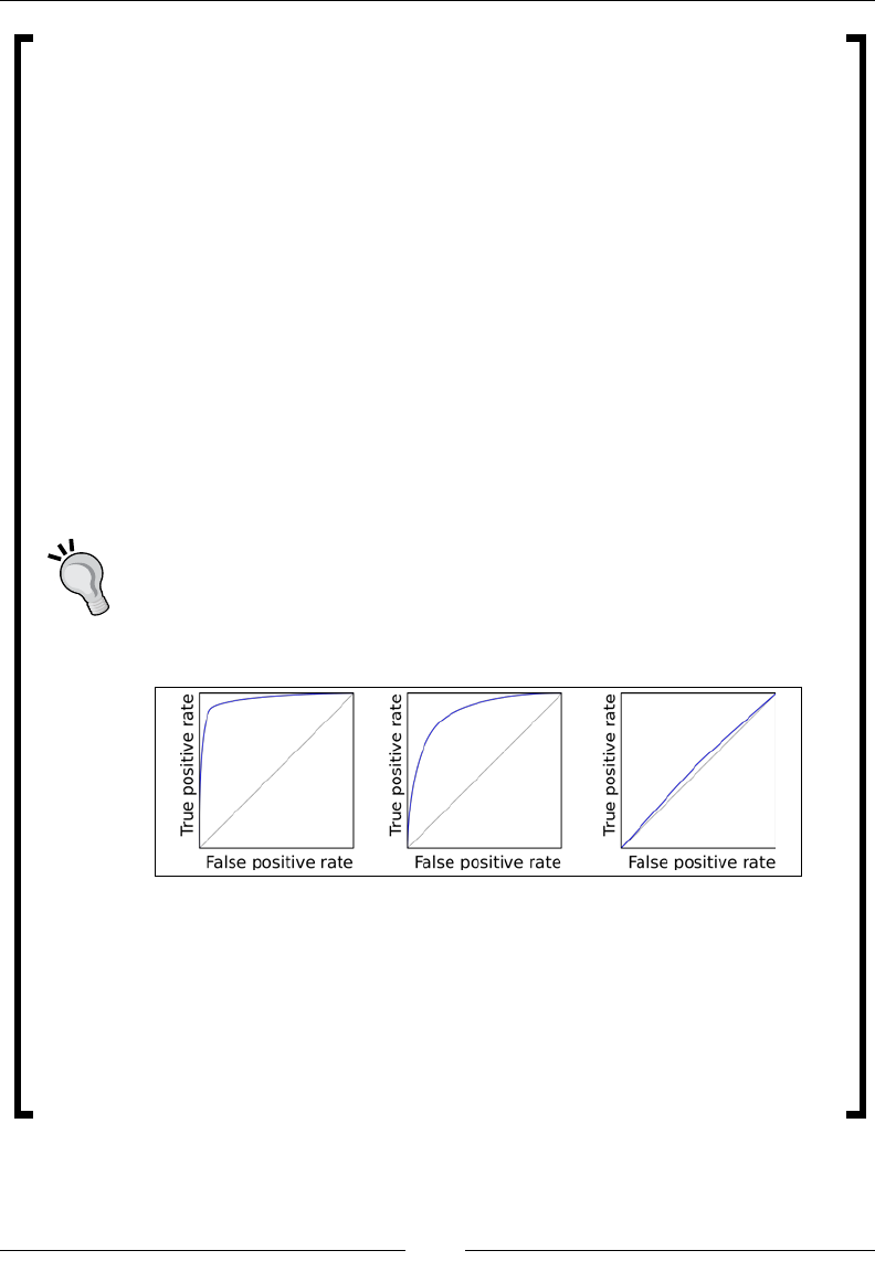
Chapter 12
[ 305 ]
ROC Curves
Imagine gradually decreasing, from 1.0, the probability threshold at
which we assume a particular e-mail is spam. Clearly, when the threshold
is set to 1.0, no e-mails will get classied as spam. This means that there
will be no false positives (ham messages which we incorrectly classify
as spam), but it also means that there will be no true positives (spam
messages that we correctly identify as spam): all spam e-mails will be
incorrectly identied as ham.
As we gradually lower the probability threshold at which we assume a
particular e-mail is spam, our spam lter will, hopefully, start identifying
a large fraction of e-mails as spam. The vast majority of these will, if our
algorithm is well-designed, be real spam. Thus, our rate of true positives
increases. As we gradually lower the threshold, we start classifying
messages about which we are less sure of as spam. This will increase the
number of messages correctly identied as spam, but it will also increase
the number of false positives.
The ROC curve plots, for each threshold value, the fraction of true
positives against the fraction of false positives. In the best case, the curve
is always 1: this happens when all spam messages are given a score of 1.0,
and all ham messages are given a score of 0.0. By contrast, the worst case
happens when the curve is a diagonal P(true positive) = P(false positive),
which occurs when our algorithm does no better than random. In general,
ROC curves fall somewhere in between, forming a convex shell above the
diagonal. The deeper this shell, the better our algorithm.
(left) ROC curve for a model performing much better than random: the
curve reaches very high true positive rates for a low false positive rate.
(middle) ROC curve for a model performing signicantly better than
random.
(right) ROC curve for a model performing only marginally better than
random: the true positive rate is only marginally larger than the rate
of false positives, for any given threshold, meaning that nearly half the
examples are misclassied.

Distributed Machine Learning with MLlib
[ 306 ]
We can calculate an array of points on the ROC curve using the .roc method on our
BinaryClassificationMetrics instance. This returns an RDD[(Double, Double)]
of (false positive, true positive) fractions for each threshold value. We can collect this as
an array:
scala> val rocArray = bm.roc.collect
rocArray: Array[(Double, Double)] = Array((0.0,0.0),
(0.0,0.16793893129770993), ...
Of course, an array of numbers is not very enlightening, so let's plot the ROC curve
with breeze-viz. We start by transforming our array of pairs into two arrays, one of
false positives and one of true positives:
scala> val falsePositives = rocArray.map { _._1 }
falsePositives: Array[Double] = Array(0.0, 0.0, 0.0, 0.0, 0.0, ...
scala> val truePositives = rocArray.map { _._2 }
truePositives: Array[Double] = Array(0.0, 0.16793893129770993,
0.19083969465...
Let's plot these two arrays:
scala> import breeze.plot._
import breeze.plot.
scala> val f = Figure()
f: breeze.plot.Figure = breeze.plot.Figure@3aa746cd
scala> val p = f.subplot(0)
p: breeze.plot.Plot = breeze.plot.Plot@5ed1438a
scala> p += plot(falsePositives, truePositives)
p += plot(falsePositives, truePositives)
scala> p.xlabel = "false positives"
p.xlabel: String = false positives
scala> p.ylabel = "true positives"
p.ylabel: String = true positives
scala> p.title = "ROC"
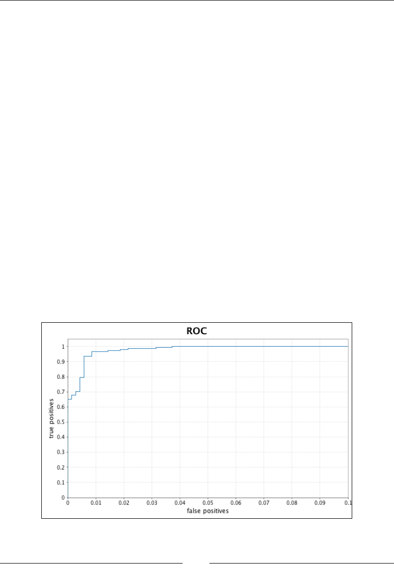
Chapter 12
[ 307 ]
p.title: String = ROC
scala> f.refresh
The ROC curve hits 1.0 for a small value of x: that is, we retrieve all true positives at
the cost of relatively few false positives. To visualize the curve more accurately, it is
instructive to limit the range on the x-axis from 0 to 0.1.
scala> p.xlim = (0.0, 0.1)
p.xlim: (Double, Double) = (0.0,0.1)
We also need to tell breeze-viz to use appropriate tick spacing, which requires going
down to the JFreeChart layer underlying breeze-viz:
scala> import org.jfree.chart.axis.NumberTickUnit
import org.jfree.chart.axis.NumberTickUnit
scala> p.xaxis.setTickUnit(new NumberTickUnit(0.01))
scala> p.yaxis.setTickUnit(new NumberTickUnit(0.1))
We can now save the graph:
scala> f.saveas("roc.png")
This produces the following graph, stored in roc.png:
ROC curve for spam classification with logistic regression.
Note that we have limited the false positive axis at 0.1

Distributed Machine Learning with MLlib
[ 308 ]
By looking at the graph, we see that we can lter out 85% of spam without a single
false positive. Of course, we would need a larger test set to really validate this
assumption.
A graph is useful to really understand the behavior of a model. Sometimes, however,
we just want to have a single measure of the quality of a model. The area under the
ROC curve can be a good such metric:
scala> bm.areaUnderROC
res21: Double = 0.9983061235861147
This can be interpreted as follows: given any two messages randomly drawn
from the test set, one of which is ham, and one of which is spam, there is a 99.8%
probability that the model assigned a greater likelihood of spam to the spam
message than to the ham message.
Other useful measures of model quality are the precision and recall for
particular thresholds, or the F1 score. All of these are provided by the
BinaryClassificationMetrics instance. The API documentation lists the
methods available: https://spark.apache.org/docs/latest/api/scala/index.
html#org.apache.spark.mllib.evaluation.BinaryClassificationMetrics.
Regularization in logistic regression
One of the dangers of machine learning is over-tting: the algorithm captures not
only the signal in the training set, but also the statistical noise that results from the
nite size of the training set.
A way to mitigate over-tting in logistic regression is to use regularization: we
impose a penalty for large values of the parameters when optimizing. We can do this
by adding a penalty to the cost function that is proportional to the magnitude of the
parameters. Formally, we re-write the logistic regression cost function (described in
Chapter 2, Manipulating Data with Breeze) as:
() ()
LR
n
Cost params Cost params params
λ
= +
where
LR
Cost
is the normal logistic regression cost function:
() ()( )
log exp 1
LR i i i
i
Cost params target params training params training=×⋅ − ⋅+
⎡ ⎤
⎣ ⎦
∑

Chapter 12
[ 309 ]
Here, params is the vector of parameters, i
training
is the vector of features for the ith
training example, and
i
target
is 1 if the ith training example is spam, and 0 otherwise.
This is identical to the logistic regression cost-function introduced in Chapter 2,
Manipulating data with Breeze, apart from the addition of the regularization term
n
params
λ
, the n
L
norm of the parameter vector. The most common value of n is
2, in which case
2
params is just the magnitude of the parameter vector:
2
2i
i
params params=∑
The additional regularization term drives the algorithm to reduce the magnitude of
the parameter vector. When using regularization, features must all have comparable
magnitude. This is commonly achieved by normalizing the features. The logistic
regression estimator provided by MLlib normalizes all features by default. This can
be turned off with the setStandardization parameter.
Spark has two hyperparameters that can be tweaked to control regularization:
• The type of regularization, set with the elasticNetParam parameter. A
value of 0 indicates 2
L
regularization.
• The degree of regularization (
λ
in the cost function), set with the regParam
parameter. A high value of the regularization parameter indicates a strong
regularization. In general, the greater the danger of over-fitting, the larger the
regularization parameter ought to be.
Let's create a new logistic regression instance that uses regularization:
scala> val lrWithRegularization = (new LogisticRegression()
.setMaxIter(50))
lrWithRegularization: LogisticRegression = logreg_16b65b325526
scala> lrWithRegularization.setElasticNetParam(0)
lrWithRegularization.type = logreg_1e3584a59b3a

Distributed Machine Learning with MLlib
[ 310 ]
To choose the appropriate value of
λ
, we t the pipeline to the training set and
calculate the classication error on the test set for several values of
λ
. Further on in
the chapter, we will learn about cross-validation in MLlib, which provides a much
more rigorous way of choosing hyper-parameters.
scala> val lambdas = Array(0.0, 1.0E-12, 1.0E-10, 1.0E-8)
lambdas: Array[Double] = Array(0.0, 1.0E-12, 1.0E-10, 1.0E-8)
scala> lambdas foreach { lambda =>
lrWithRegularization.setRegParam(lambda)
val pipeline = new Pipeline().setStages(
Array(indexer, tokenizer, hashingTF, lrWithRegularization))
val model = pipeline.fit(trainDF)
val transformedTest = model.transform(testDF)
val classificationError = transformedTest.filter {
$"prediction" !== $"label"
}.count
println(s"$lambda => $classificationError")
}
0 => 20
1.0E-12 => 20
1.0E-10 => 20
1.0E-8 => 23
For our example, we see that any attempt to add L2 regularization leads to a decrease
in classication accuracy.
Cross-validation and model selection
In the previous example, we validated our approach by withholding 30% of the data
when training, and testing on this subset. This approach is not particularly rigorous:
the exact result changes depending on the random train-test split. Furthermore, if we
wanted to test several different hyperparameters (or different models) to choose the
best one, we would, unwittingly, choose the model that best reects the specic rows
in our test set, rather than the population as a whole.
This can be overcome with cross-validation. We have already encountered
cross-validation in Chapter 4, Parallel Collections and Futures. In that chapter,
we used random subsample cross-validation, where we created the train-test
split randomly.

Chapter 12
[ 311 ]
In this chapter, we will use k-fold cross-validation: we split the training set into k
parts (where, typically, k is 10 or 3) and use k-1 parts as the training set and the last as
the test set. The train/test cycle is repeated k times, keeping a different part as test set
each time.
Cross-validation is commonly used to choose the best set of hyperparameters for
a model. To illustrate choosing suitable hyperparameters, we will go back to our
regularized logistic regression example. Instead of intuiting the hyper-parameters
ourselves, we will choose the hyper-parameters that give us the best cross-validation
score.
We will explore setting both the regularization type (through elasticNetParam)
and the degree of regularization (through regParam). A crude, but effective way
to nd good values of the parameters is to perform a grid search: we calculate the
cross-validation score for every pair of values of the regularization parameters
of interest.
We can build a grid of parameters using MLlib's ParamGridBuilder.
scala> import org.apache.spark.ml.tuning.{ParamGridBuilder,
CrossValidator}
import org.apache.spark.ml.tuning.{ParamGridBuilder, CrossValidator}
scala> val paramGridBuilder = new ParamGridBuilder()
paramGridBuilder: ParamGridBuilder = ParamGridBuilder@1dd694d0
To add hyper-parameters over which to optimize to the grid, we use the addGrid
method:
scala> val lambdas = Array(0.0, 1.0E-12, 1.0E-10, 1.0E-8)
Array[Double] = Array(0.0, 1.0E-12, 1.0E-10, 1.0E-8)
scala> val elasticNetParams = Array(0.0, 1.0)
elasticNetParams: Array[Double] = Array(0.0, 1.0)
scala> paramGridBuilder.addGrid(
lrWithRegularization.regParam, lambdas).addGrid(
lrWithRegularization.elasticNetParam, elasticNetParams)
paramGridBuilder.type = ParamGridBuilder@1dd694d0

Distributed Machine Learning with MLlib
[ 312 ]
Once all the dimensions are added, we can just call the build method on the builder
to build the grid:
scala> val paramGrid = paramGridBuilder.build
paramGrid: Array[org.apache.spark.ml.param.ParamMap] =
Array({
logreg_f7dfb27bed7d-elasticNetParam: 0.0,
logreg_f7dfb27bed7d-regParam: 0.0
}, {
logreg_f7dfb27bed7d-elasticNetParam: 1.0,
logreg_f7dfb27bed7d-regParam: 0.0
} ...)
scala> paramGrid.length
Int = 8
As we can see, the grid is just a one-dimensional array of sets of parameters to pass
to the logistic regression model prior to tting.
The next step in setting up the cross-validation pipeline is to dene a metric
for comparing model performance. Earlier in the chapter, we saw how to use
BinaryClassificationMetrics to estimate the quality of a model. Unfortunately,
the BinaryClassificationMetrics class is part of the core MLLib API, rather than
the new pipeline API, and is thus not (easily) compatible. The pipeline API offers
a BinaryClassificationEvaluator class instead. This class works directly on
DataFrames, and thus ts perfectly into the pipeline API ow:
scala> import org.apache.spark.ml.evaluation.
BinaryClassificationEvaluator
import org.apache.spark.ml.evaluation.BinaryClassificationEvaluator
scala> val evaluator = new BinaryClassificationEvaluator()
evaluator: BinaryClassificationEvaluator = binEval_64b08538f1a2
scala> println(evaluator.explainParams)
labelCol: label column name (default: label)
metricName: metric name in evaluation (areaUnderROC|areaUnderPR)
(default: areaUnderROC)
rawPredictionCol: raw prediction (a.k.a. confidence) column name
(default: rawPrediction)

Chapter 12
[ 313 ]
From the parameter list, we see that the BinaryClassificationEvaluator
class supports two metrics: the area under the ROC curve, and the area under
the precision-recall curve. It expects, as input, a DataFrame containing a label
column (the model truth) and a rawPrediction column (the column containing the
probability that an e-mail is spam or ham).
We now have all the parameters we need to run cross-validation. We rst build the
pipeline, and then pass the pipeline, the evaluator and the array of parameters over
which to run the cross-validation to an instance of CrossValidator:
scala> val pipeline = new Pipeline().setStages(
Array(indexer, tokenizer, hashingTF, lrWithRegularization))
pipeline: Pipeline = pipeline_3ed29f72a4cc
scala> val crossval = (new CrossValidator()
.setEstimator(pipeline)
.setEvaluator(evaluator)
.setEstimatorParamMaps(paramGrid)
.setNumFolds(3))
crossval: CrossValidator = cv_5ebfa1143a9d
We will now t crossval to trainDF:
scala> val cvModel = crossval.fit(trainDF)
cvModel: CrossValidatorModel = cv_5ebfa1143a9d
This step can take a fairly long time (over an hour on a single machine). This creates
a transformer, cvModel, corresponding to the logistic regression object with the
parameters that best represent trainDF. We can use it to predict the classication
error on the test DataFrame:
scala> cvModel.transform(testDF).filter {
$"prediction" !== $"label"
}.count
Long = 20
Cross-validation has therefore resulted in a model that performs identically to the
original, naive logistic regression model with no hyper-parameters. cvModel also
contains a list of the evaluation score for each set of parameter in the parameter grid:
scala> cvModel.avgMetrics
Array[Double] = Array(0.996427805316161, ...)

Distributed Machine Learning with MLlib
[ 314 ]
The easiest way to relate this to the hyper-parameters is to zip it with cvModel.
getEstimatorParamMaps. This gives us a list of (hyperparameter values, cross-validation
score) pairs:
scala> val params2score = cvModel.getEstimatorParamMaps.zip(
cvModel.avgMetrics)
Array[(ml.param.ParamMap,Double)] = Array(({
logreg_8f107aabb304-elasticNetParam: 0.0,
logreg_8f107aabb304-regParam: 0.0
},0.996427805316161),...
scala> params2score.foreach {
case (params, score) =>
val lambda = params(lrWithRegularization.regParam)
val elasticNetParam = params(
lrWithRegularization.elasticNetParam)
val l2Orl1 = if(elasticNetParam == 0.0) "L2" else "L1"
println(s"$l2Orl1, $lambda => $score")
}
L2, 0.0 => 0.996427805316161
L1, 0.0 => 0.996427805316161
L2, 1.0E-12 => 0.9964278053175655
L1, 1.0E-12 => 0.9961429402772803
L2, 1.0E-10 => 0.9964382546369551
L1, 1.0E-10 => 0.9962223090037103
L2, 1.0E-8 => 0.9964159754613495
L1, 1.0E-8 => 0.9891008277659763
The best set of hyper-parameters correspond to L2 regularization with a
regularization parameter of 1E-10, though this only corresponds to a tiny
improvement in AUC.
This completes our spam lter example. We have successfully trained a spam lter
for this particular Ling-Spam dataset. To obtain better results, one could experiment
with better feature extraction: we could remove stop words or use TF-IDF vectors,
rather than just term frequency vectors as features, and we could add additional
features like the length of messages, or even n-grams. We could also experiment
with non-linear algorithms, such as random forest. All of these steps would be
straightforward to add to the pipeline.

Chapter 12
[ 315 ]
Beyond logistic regression
We have concentrated on logistic regression in this chapter, but MLlib offers many
alternative algorithms that will capture non-linearity in the data more effectively.
The consistency of the pipeline API makes it easy to try out different algorithms
and see how they perform. The pipeline API offers decision trees, random forest
and gradient boosted trees for classication, as well as a simple feed-forward neural
network, which is still experimental. It offers lasso and ridge regression and decision
trees for regression, as well as PCA for dimensionality reduction.
The lower level MLlib API also offers principal component analysis for
dimensionality reduction, several clustering methods including k-means and latent
Dirichlet allocation and recommender systems using alternating least squares.
Summary
MLlib tackles the challenge of devising scalable machine learning algorithms
head-on. In this chapter, we used it to train a simple scalable spam lter. MLlib is
a vast, rapidly evolving library. The best way to learn more about what it can offer
is to try and port code that you might have written using another library (such as
scikit-learn).
In the next chapter, we will look at how to build web APIs and interactive
visualizations to share our results with the rest of the world.
References
The best reference is the online documentation, including:
• The pipeline API: http://spark.apache.org/docs/latest/ml-features.
html
• A full list of transformers: http://spark.apache.org/docs/latest/
mllib-guide.html#sparkml-high-level-apis-for-ml-pipelines
Advanced Analytics with Spark, by Sandy Ryza, Uri Laserson, Sean Owen and Josh Wills
provides a detailed and up-to-date introduction to machine learning with Spark.

Distributed Machine Learning with MLlib
[ 316 ]
There are several books that introduce machine learning in more detail than we can
here. We have mentioned The Elements of Statistical Learning, by Friedman, Tibshirani
and Hastie several times in this book. It is one of the most complete introductions to
the mathematical underpinnings of machine learning currently available.
Andrew Ng's Machine Learning course on https://www.coursera.org/
provides a good introduction to machine learning. It uses Octave/MATLAB as the
programming language, but should be straightforward to adapt to Breeze and Scala.
[ 317 ]
Web APIs with Play
In the rst 12 chapters of this book, we introduced basic tools and libraries for
anyone wanting to build data science applications: we learned how to interact with
SQL and MongoDB databases, how to build fast batch processing applications using
Spark, how to apply state-of-the-art machine learning algorithms using MLlib, and
how to build modular concurrent applications in Akka.
In the last chapters of this book, we will branch out to look at a web framework:
Play. You might wonder why a web framework would feature in a data science
book; surely such topics are best left to software engineers or web developers. Data
scientists, however, rarely exist in a vacuum. They often need to communicate results
or insights to stakeholders. As compelling as an ROC curve may be to someone
well versed in statistics, it may not carry as much weight with less technical people.
Indeed, it can be much easier to sell insights when they are accompanied by an
engaging visualization.
Many modern interactive data visualization applications are web applications
running in a web browser. Often, these involve D3.js, a JavaScript library for
building data-driven web pages. In this chapter and the next, we will look at
integrating D3 with Scala.
Writing a web application is a complex endeavor. We will split this task over this
chapter and the next. In this chapter, we will learn how to write a REST API that we
can use as backend for our application, or query in its own right. In the next chapter,
we will look at integrating front-end code with Play to query the API exposed by the
backend and display it using D3. We assume at least a basic familiarity with HTTP in
this chapter: you should have read Chapter 7, Web APIs, at least.

Web APIs with Play
[ 318 ]
Many data scientists or aspiring data scientists are unlikely to be familiar with the
inner workings of web technologies. Learning how to build complex websites or
web APIs can be daunting. This chapter therefore starts with a general discussion
of dynamic websites and the architecture of web applications. If you are already
familiar with server-side programming and with web frameworks, you can easily
skip over the rst few sections.
Client-server applications
A website works through the interaction between two computers: the client and
the server. If you enter the URL www.github.com/pbugnion/s4ds/graphs in a
web browser, your browser queries one of the GitHub servers. The server will look
though its database for information concerning the repository that you are interested
in. It will serve this information as HTML, CSS, and JavaScript to your computer.
Your browser is then responsible for interpreting this response in the correct way.
If you look at the URL in question, you will notice that there are several graphs
on that page. Unplug your internet connection and you can still interact with
the graphs. All the information necessary for interacting with the graphs was
transferred, as JavaScript, when you loaded that webpage. When you play with the
graphs, the CPU cycles necessary to make those changes happen are spent on your
computer, not a GitHub server. The code is executed client-side. Conversely, when
you request information about a new repository, that request is handled by a GitHub
server. It is said to be handled server-side.
A web framework like Play can be used on the server. For client-side code, we can
only use a language that the client browser will understand: HTML for the layout,
CSS for the styling and JavaScript, or languages that can compile to JavaScript, for
the logic.
Introduction to web frameworks
This section is a brief introduction to how modern web applications are designed. Go
ahead and skip it if you already feel comfortable writing backend code.
Loosely, a web framework is a set of tools and code libraries for building web
applications. To understand what a web framework provides, let's take a step back
and think about what you would need to do if you did not have one.
You want to write a program that listens on port 80 and sends HTML (or JSON or
XML) back to clients that request it. This is simple if you are serving the same le
back to every client: just load the HTML from le when you start the server, and
send it to clients who request it.

Chapter 13
[ 319 ]
So far, so good. But what if you now want to customize the HTML based on the
client request? You might choose to respond differently based on part of the URL
that the client put in his browser, or based on specic elements in the HTTP request.
For instance, the product page on amazon.com is different to the payment page. You
need to write code to parse the URL and the request, and then route the request to
the relevant handler.
You might now want to customize the HTML returned dynamically, based on
specic elements of the request. The page for every product on amazon.com follows
the same outline, but specic elements are different. It would be wasteful to store the
entire HTML content for every product. A better way is to store the details for each
product in a database and inject them into an HTML template when a client requests
information on that product. You can do this with a template processor. Of course,
writing a good template processor is difcult.
You might deploy your web framework and realize that it cannot handle the trafc
directed to it. You decide that handlers responding to client requests should run
asynchronously. You now have to deal with concurrency.
A web framework essentially provides the wires to bind everything together. Besides
bundling an HTTP server, most frameworks will have a router that automatically
routes a request, based on the URL, to the correct handler. In most cases, the handler
will run asynchronously, giving you much better scalability. Many frameworks
have a template processor that lets you write HTML (or sometimes JSON or XML)
templates intuitively. Some web frameworks also provide functionality for accessing
a database, for parsing JSON or XML, for formulating HTTP requests and for
localization and internationalization.
Model-View-Controller architecture
Many web frameworks impose program architectures: it is difcult to provide
wires to bind disparate components together without making some assumptions
about what those components are. The Model-View-Controller (MVC) architecture
is particularly popular on the Web, and it is the architecture the Play framework
assumes. Let's look at each component in turn:
• The model is the data underlying the application. For example, I expect
the application underlying GitHub has models for users, repositories,
organizations, pull requests and so on. In the Play framework, a model is
often an instance of a case class. The core responsibility of the model is to
remember the current state of the application.
• Views are representations of a model or a set of models on the screen.
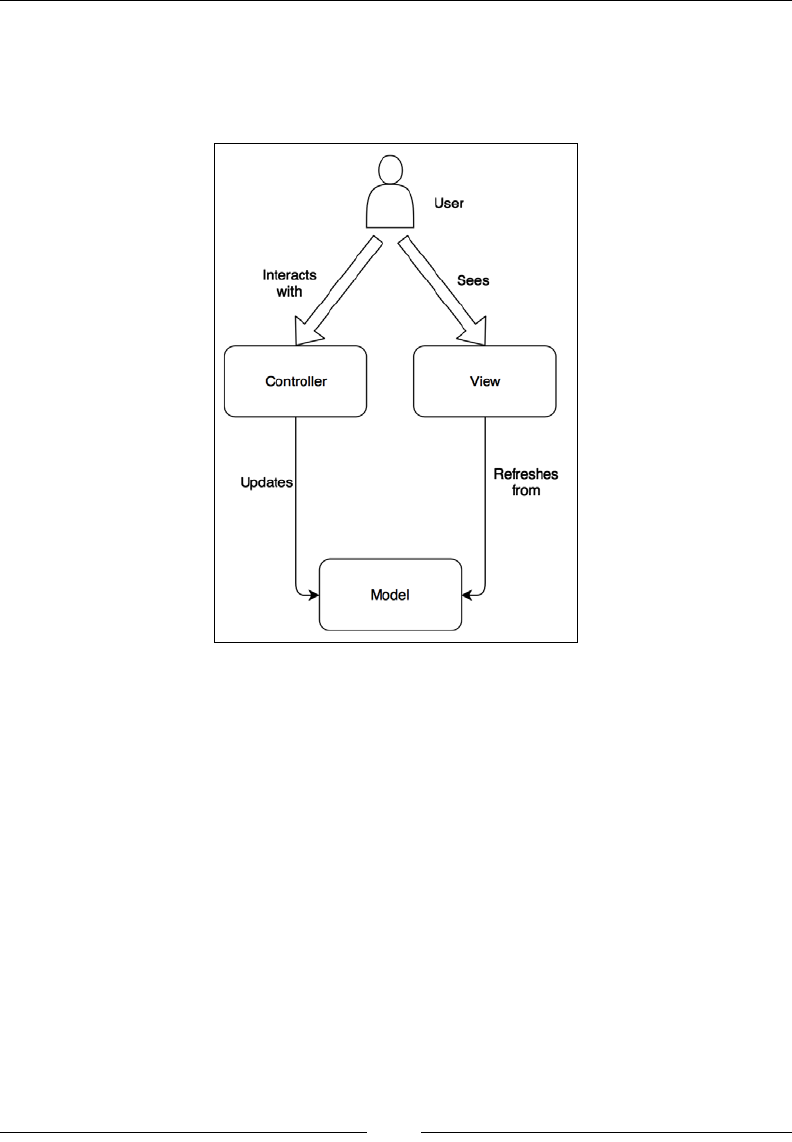
Web APIs with Play
[ 320 ]
• The controller handles client interactions, possibly changing the model.
For instance, if you star a project on GitHub, the controller will update the
relevant models. Controllers normally carry very little application state:
remembering things is the job of the models.
MVC architecture: the state of the application is provided by the model. The view provides
a visual representation of the model to the user, and the controller handles logic: what to do when
the user presses a button or submits a form.
The MVC framework works well because it decouples the user interface from the
underlying data and structures the ow of actions: a controller can update the model
state or the view, a model can send signals to the view to tell it to update, and the
view merely displays that information. The model carries no information related to
the user interface. This separation of concerns results in an easier mental model of
information ow, better encapsulation and greater testability.

Chapter 13
[ 321 ]
Single page applications
The client-server duality adds a degree of complication to the elegant MVC
architecture. Where should the model reside? What about the controller?
Traditionally, the model and the controller ran almost entirely on the server,
which just pushed the relevant HTML view to the client.
The growth in client-side JavaScript frameworks, such AngularJS, has resulted in a
gradual shift to putting more code in the client. Both the controller and a temporary
version of the model typically run client-side. The server just functions as a web API:
if, for instance, the user updates the model, the controller will send an HTTP request
to the server informing it of the change.
It then makes sense to think of the program running server-side and the one running
client-side as two separate applications: the server persists data in databases, for
instance, and provides a programmatic interface to this data, usually as a web service
returning JSON or XML data. The client-side program maintains its own model and
controller, and polls the server whenever it needs a new model, or whenever it needs
to inform the server that the persistent view of the model should be changed.
Taken to the extreme, this results in Single-Page Applications. In a single-page
application, the rst time the client requests a page from the server, he receives
the HTML and the JavaScript necessary to build the framework for the entire
application. If the client needs further data from the server, he will poll the server's
API. This data is returned as JSON or XML.
This might seem a little complicated in the abstract, so let's think how the Amazon
website might be structured as a single-page application. We will just concern
ourselves with the products page here, since that's complicated enough. Let's imagine
that you are on the home page, and you hit a link for a particular product. The
application running on your computer knows how to display products, for instance
through an HTML template. The JavaScript also has a prototype for the model, such as:
{
product_id: undefined,
product_name: undefined,
product_price: undefined,
...
}
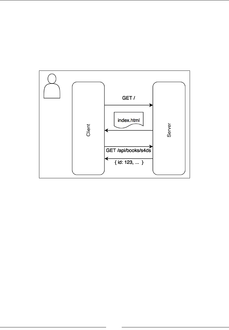
Web APIs with Play
[ 322 ]
What it's currently missing is knowledge of what data to put in those elds for the
product you have just selected: there is no way that information could have been
sent to your computer when the website loaded, since there was no way to know
what product you might click on (and sending information about every product
would be prohibitively costly). So the Amazon client sends a request to the server
for information on that product. The Amazon server replies with a JSON object (or
maybe XML). The client then updates its model with that information. When the
update is complete, an event is red to update the view:
Client-server communications in a single-page application: when the client first accesses
the website, it receives HTML, CSS and JavaScript files that contain the entire logic for
the application. From then on, the client only uses the server as an API when it requests
additional data. The application running in the user's web browser and the one running on the
server are nearly independent. The only coupling is through the structure of the API
exposed by the server.
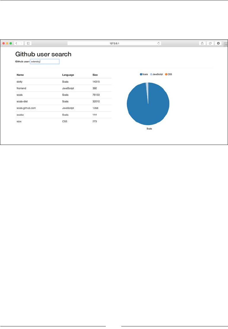
Chapter 13
[ 323 ]
Building an application
In this chapter and the next, we will build a single-page application that relies on an
API written in Play. We will build a webpage that looks like this:
The user enters the name of someone on GitHub and can view a list of their
repositories and a chart summarizing what language they use. You can nd the
application deployed at app.scala4datascience.com. Go ahead and give it a whirl.
To get a glimpse of the innards, type app.scala4datascience.com/api/repos/
odersky. This returns a JSON object like:
[{"name":"dotty","language":"Scala","is_fork":true,"size":14653},
{"name":"frontend","language":"JavaScript","is_fork":true,"size":392},
{"name":"legacy-svn-scala","language":"Scala","is_
fork":true,"size":296706},
...
We will build the API in this chapter, and write the front-end code in the next chapter.

Web APIs with Play
[ 324 ]
The Play framework
The Play framework is a web framework built on top of Akka. It has a proven track
record in industry, and is thus a reliable choice for building scalable web applications.
Play is an opinionated web framework: it expects you to follow the MVC architecture,
and it has a strong opinion about the tools you should be using. It comes bundled
with its own JSON and XML parsers, with its own tools for accessing external APIs,
and with recommendations for how to access databases.
Web applications are much more complex than the command line scripts we
have been developing in this book, because there are many more components: the
backend code, routing information, HTML templates, JavaScript les, images, and
so on. The Play framework makes strong assumptions about the directory structure
for your project. Building that structure from scratch is both mind-numbingly boring
and easy to get wrong. Fortunately, we can use Typesafe activators to bootstrap
the project (you can also download the code from the Git repository in https://
github.com/pbugnion/s4ds but I encourage you to start the project from a basic
activator structure and code along instead, using the nished version as an example).
Typesafe activator is a custom version of SBT that includes templates to get Scala
programmers up and running quickly. To install activator, you can either download
a JAR from https://www.typesafe.com/activator/download, or, on Mac OS,
via homebrew:
$ brew install typesafe-activator
You can then launch the activator console from the terminal. If you downloaded
activator:
$ ./path/to/activator/activator new
Or, if you installed via Homebrew:
$ activator new
This starts a new project in the current directory. It starts by asking what template
you want to start with. Choose play-scala. It then asks for a name for your
application. I chose ghub-display, but go ahead and be creative!
Let's explore the newly created project structure (I have only retained the most
important les):
├── app
│ ├── controllers
│ │ └── Application.scala

Chapter 13
[ 325 ]
│ └── views
│ ├── main.scala.html
│ └── index.scala.html
├── build.sbt
├── conf
│ ├── application.conf
│ └── routes
├── project
│ ├── build.properties
│ └── plugins.sbt
├── public
│ ├── images
│ │ └── favicon.png
│ ├── javascripts
│ │ └── hello.js
│ └── stylesheets
│ └── main.css
└── test
├── ApplicationSpec.scala
└── IntegrationSpec.scala
Let's run the app:
$ ./activator
[ghub-display] $ run
Head over to your browser and navigate to the URL 127.0.0.1:9000/. The page
may take a few seconds to load. Once it is loaded, you should see a default page that
says Your application is ready.
Before we modify anything, let's walk through how this happens. When you ask
your browser to take you to 127.0.0.1:9000/, your browser sends an HTTP request
to the server listening at that address (in this case, the Netty server bundled with
Play). The request is a GET request for the route /. The Play framework looks in
conf/routes to see if it has a route satisfying /:
$ cat conf/routes
# Home page
GET / controllers.Application.index
...

Web APIs with Play
[ 326 ]
We see that the conf/routes le does contain the route / for GET requests. The
second part of that line, controllers.Application.index, is the name of a Scala
function to handle that route (more on that in a moment). Let's experiment. Change
the route end-point to /hello. Refresh your browser without changing the URL.
This will trigger recompilation of the application. You should now see an error page:
The error page tells you that the app does not have an action for the route / any more.
If you navigate to 127.0.0.1:9000/hello, you should see the landing page again.
Besides learning a little of how routing works, we have also learned two things about
developing Play applications:
• In development mode, code gets recompiled when you refresh your browser
and there have been code changes
• Compilation and runtime errors get propagated to the web page
Let's change the route back to /. There is a lot more to say on routing, but it can wait
till we start building our application.
The conf/routes le tells the Play framework to use the method controllers.
Application.index to handle requests to /. Let's look at the Application.scala
le in app/controllers, where the index method is dened:
// app/controllers/Application.scala
package controllers
import play.api._
import play.api.mvc._
class Application extends Controller {
def index = Action {
Ok(views.html.index("Your new application is ready."))
}
}

Chapter 13
[ 327 ]
We see that controllers.Application.index refers to the method index in
the class Application. This method has return type Action. An Action is just a
function that maps HTTP requests to responses. Before explaining this in more
detail, let's change the action to:
def index = Action {
Ok("hello, world")
}
Refresh your browser and you should see the landing page replaced with "hello
world". By having our action return Ok("hello, world"), we are asking Play
to return an HTTP response with status code 200 (indicating that the request was
successful) and the body "hello world".
Let's go back to the original content of index:
Action {
Ok(views.html.index("Your new application is ready."))
}
We can see that this calls the method views.html.index. This might appear strange,
because there is no views package anywhere. However, if you look at the app/views
directory, you will notice two les: index.scala.html and main.scala.html. These
are templates, which, at compile time, get transformed into Scala functions. Let's
have a look at main.scala.html:
// app/views/main.scala.html
@(title: String)(content: Html)
<!DOCTYPE html>
<html lang="en">
<head>
<title>@title</title>
<!-- not so important stuff -->
</head>
<body>
@content
</body>
</html>

Web APIs with Play
[ 328 ]
At compile time, this template is compiled to a function main(title:String)
(content:Html) in the package views.html. Notice that the function package and
name comes from the template le name, and the function arguments come from the
rst line of the template. The template contains embedded @title and @content
values, which get lled in by the arguments to the function. Let's experiment with
this in a Scala console:
$ activator console
scala> import views.html._
import views.html._
scala> val title = "hello"
title: String = hello
scala> val content = new play.twirl.api.Html("<b>World</b>")
content: play.twirl.api.Html = <b>World</b>
scala> main(title)(content)
res8: play.twirl.api.HtmlFormat.Appendable =
<!DOCTYPE html>
<html lang="en">
<head>
<title>hello</title>
<!-- not so important stuff -->
</head>
<body>
<b>World</b>
</body>
</html>
We can call views.html.main, just like we would call a normal Scala function. The
arguments we pass in get embedded in the correct place, as dened by the template
in views/main.scala.html.

Chapter 13
[ 329 ]
This concludes our introductory tour of Play. Let's briey go over what we have
learnt: when a request reaches the Play server, the server reads the URL and the
HTTP verb and checks that these exist in its conf/routes le. It will then pass the
request to the Action dened by the controller for that route. This Action returns
an HTTP response that gets fed back to the browser. In constructing the response, the
Action may make use of a template, which, as far as it is concerned is just a function
(arguments list) => String or (arguments list) => HTML.
Dynamic routing
Routing, as we saw, is the mapping of HTTP requests to Scala handlers. Routes are
stored in conf/routes. A route is dened by an HTTP verb, followed by the end-
point, followed by a Scala function:
// verb // end-point // Scala handler
GET / controllers.Application.index
We learnt to add new routes by just adding lines to the routes le. We are not
limited to static routes, however. The Play framework lets us include wild cards in
routes. The value of the wild card can be passed as an argument to the controller.
To see how this works, let's create a controller that takes the name of a person as
argument. In the Application object in app.controllers, add:
// app/controllers/Application.scala
class Application extends Controller {
...
def hello(name:String) = Action {
Ok(s"hello, $name")
}
}
We can now dene a route handled by this controller:
// conf/routes
GET /hello/:name controllers.Application.hello(name)
If you now point your browser to 127.0.0.1:9000/hello/Jim, you will see hello,
Jim appear on the screen.
Web APIs with Play
[ 330 ]
Any string between : and the following / is treated as a wild card: it will match any
combination of characters. The value of the wild card can be passed to the controller.
Note that the wild card can appear anywhere in the URL, and there can be more than
one wild card. The following are all valid route denitions, for instance:
GET /hello/person-:name controllers.Application.hello(name)
// ... matches /hello/person-Jim
GET /hello/:name/picture controllers.Application.pictureFor(name)
// ... matches /hello/Jim/picture
GET /hello/:first/:last controllers.Application.hello(first, last)
// ... matches /hello/john/doe
There are many other options for selecting routes and passing arguments to
the controller. Consult the documentation for the Play framework for a full
discussion on the routing possibilities: https://www.playframework.com/
documentation/2.4.x/ScalaRouting.
URL design
It is generally considered best practice to leave the URL as simple
as possible. The URL should reect the hierarchical structure of the
information of the website, rather than the underlying implementation.
GitHub is a very good example of this: its URLs make intuitive sense.
For instance, the URL for the repository for this book is:
https://github.com/pbugnion/s4ds
To access the issues page for that repository, add /issues to the route.
To access the rst issue, add /1 to that route. These are called semantic
URLs (https://en.wikipedia.org/wiki/Semantic_URL).
Actions
We have talked about routes, and how to pass parameters to controllers. Let's now
talk about what we can do with the controller.
The method dened in the route must return a play.api.mvc.Action instance.
The Action type is a thin wrapper around the type Request[A] => Result, where
Request[A] identies an HTTP request and Result is an HTTP response.

Chapter 13
[ 331 ]
Composing the response
An HTTP response, as we saw in Chapter 7, Web APIs, is composed of:
• the status code (such as 200 for a successful response, or 404 for a
missing page)
• the response headers, a key-value list indicating metadata related to the
response
• The response body. This can be HTML for web pages, or JSON, XML or
plain text (or many other formats). This is generally the bit that we are really
interested in.
The Play framework denes a play.api.mvc.Result object that symbolizes a
response. The object contains a header attribute with the status code and the
headers, and a body attribute containing the body.
The simplest way to generate a Result is to use one of the factory methods in play.
api.mvc.Results. We have already seen the Ok method, which generates a response
with status code 200:
def hello(name:String) = Action {
Ok("hello, $name")
}
Let's take a step back and open a Scala console so we can understand how this works:
$ activator console
scala> import play.api.mvc._
import play.api.mvc._
scala> val res = Results.Ok("hello, world")
res: play.api.mvc.Result = Result(200, Map(Content-Type -> text/plain;
charset=utf-8))
scala> res.header.status
Int = 200
scala> res.header.headers
Map[String,String] = Map(Content-Type -> text/plain; charset=utf-8)
scala> res.body
play.api.libs.iteratee.Enumerator[Array[Byte]] = play.api.libs.iteratee.
Enumerator$$anon$18@5fb83873

Web APIs with Play
[ 332 ]
We can see how the Results.Ok(...) creates a Result object with status 200 and
(in this case), a single header denoting the content type. The body is a bit more
complicated: it is an enumerator that can be pushed onto the output stream when
needed. The enumerator contains the argument passed to Ok: "hello, world", in
this case.
There are many factory methods in Results for returning different status codes.
Some of the more relevant ones are:
• Action { Results.NotFound }
• Action { Results.BadRequest("bad request") }
• Action { Results.InternalServerError("error") }
• Action { Results.Forbidden }
• Action { Results.Redirect("/home") }
For a full list of Result factories, consult the API documentation for Results
(https://www.playframework.com/documentation/2.4.x/api/scala/index.
html#play.api.mvc.Results).
We have, so far, been limiting ourselves to passing strings as the content of the Ok
result: Ok("hello, world"). We are not, however, limited to passing strings. We
can pass a JSON object:
scala> import play.api.libs.json._
import play.api.libs.json._
scala> val jsonObj = Json.obj("hello" -> "world")
jsonObj: play.api.libs.json.JsObject = {"hello":"world"}
scala> Results.Ok(jsonObj)
play.api.mvc.Result = Result(200, Map(Content-Type -> application/json;
charset=utf-8))
We will cover interacting with JSON in more detail when we start building the
API. We can also pass HTML as the content. This is most commonly the case when
returning a view:
scala> val htmlObj = views.html.index("hello")
htmlObj: play.twirl.api.HtmlFormat.Appendable =
<!DOCTYPE html>

Chapter 13
[ 333 ]
<html lang="en">
<head>
...
scala> Results.Ok(htmlObj)
play.api.mvc.Result = Result(200, Map(Content-Type -> text/html;
charset=utf-8))
Note how the Content-Type header is set based on the type of content passed to Ok.
The Ok factory uses the Writeable type class to convert its argument to the body of the
response. Thus, any content type for which a Writeable type class exists can be used
as argument to Ok. If you are unfamiliar with type classes, you might want to read the
Looser coupling with type classes section in Chapter 5, Scala and SQL through JDBC.
Understanding and parsing the request
We now know how to formulate (basic) responses. The other half of the equation
is the HTTP request. Recall that an Action is just a function mapping Request =>
Result. We can access the request using:
def hello(name:String) = Action { request =>
...
}
One of the reasons for needing a reference to the request is to access parameters in
the query string. Let's modify the Hello, <name> example that we wrote earlier to,
optionally, include a title in the query string. Thus, a URL could be formatted as /
hello/Jim?title=Dr. The request instance exposes the getQueryString method
for accessing specic keys in the query string. This method returns Some[String]
if the key is present in the query, or None otherwise. We can re-write our hello
controller as:
def hello(name:String) = Action { request =>
val title = request.getQueryString("title")
val titleString = title.map { _ + " " }.getOrElse("")
Ok(s"Hello, $titleString$name")
}
Try this out by accessing the URL 127.0.0.1:9000/hello/Odersky?title=Dr in
your browser. The browser should display Hello, Dr Odersky.

Web APIs with Play
[ 334 ]
We have, so far, been concentrating on GET requests. These do not have a body.
Other types of HTTP request, most commonly POST requests, do contain a body.
Play lets the user pass body parsers when dening the action. The request body will be
passed through the body parser, which will convert it from a byte stream to a Scala
type. As a very simple example, let's dene a new route that accepts POST requests:
POST /hello controllers.Application.helloPost
We will apply the predened parse.text body parser to the incoming request body.
This converts the body of the request to a string. The helloPost controller looks like:
def helloPost = Action(parse.text) { request =>
Ok("Hello. You told me: " + request.body)
}
You cannot test POST requests easily in the browser. You can use cURL
instead. cURL is a command line utility for dispatching HTTP requests.
It is installed by default on Mac OS and should be available via the
package manager on Linux distributions. The following will send a
POST request with "I think that Scala is great" in the body:
$ curl --data "I think that Scala is great" --header
"Content-type:text/plain" 127.0.0.1:9000/hello
This prints the following line to the terminal:
Hello. You told me: I think that Scala is great
There are several types of built-in body parsers:
• parse.file(new File("filename.txt")) will save the body to a file.
• parse.json will parse the body as JSON (we will learn more about
interacting with JSON in the next section).
• parse.xml will parse the body as XML.
• parse.urlFormEncoded will parse the body as returned by submitting an
HTML form. The request.body attribute is a Scala map from String to
Seq[String], mapping each form element to its value(s).
For a full list of body parsers, the best source is the Scala API documentation for
play.api.mvc.BodyParsers.parse available at: https://www.playframework.
com/documentation/2.5.x/api/scala/index.html#play.api.mvc.
BodyParsers$parse$.

Chapter 13
[ 335 ]
Interacting with JSON
JSON, as we discovered in previous chapters, is becoming the de-facto language for
communicating structured data over HTTP. If you develop a web application or a
web API, it is likely that you will have to consume or emit JSON, or both.
In Chapter 7, Web APIs, we learned how to parse JSON through json4s. The Play
framework includes its own JSON parser and emitter. Fortunately, it behaves in
much the same way as json4s.
Let's imagine that we are building an API that summarizes information about
GitHub repositories. Our API will emit a JSON array listing a user's repositories
when queried about a specic user (much like the GitHub API, but with just a subset
of elds).
Let's start by dening a model for the repository. In Play applications, models are
normally stored in the folder app/models, in the models package:
// app/models/Repo.scala
package models
case class Repo (
val name:String,
val language:String,
val isFork: Boolean,
val size: Long
)
Let's add a route to our application that serves arrays of repos for a particular user.
In conf/routes, add the following line:
// conf/routes
GET /api/repos/:username controllers.Api.repos(username)
Let's now implement the framework for the controller. We will create a new
controller for our API, imaginatively called Api. For now, we will just have the
controller return dummy data. This is what the code looks like (we will explain the
details shortly):
// app/controllers/Api.scala
package controllers
import play.api._
import play.api.mvc._

Web APIs with Play
[ 336 ]
import play.api.libs.json._
import models.Repo
class Api extends Controller {
// Some dummy data.
val data = List[Repo](
Repo("dotty", "Scala", true, 14315),
Repo("frontend", "JavaScript", true, 392)
)
// Typeclass for converting Repo -> JSON
implicit val writesRepos = new Writes[Repo] {
def writes(repo:Repo) = Json.obj(
"name" -> repo.name,
"language" -> repo.language,
"is_fork" -> repo.isFork,
"size" -> repo.size
)
}
// The controller
def repos(username:String) = Action {
val repoArray = Json.toJson(data)
// toJson(data) relies on existence of
// `Writes[List[Repo]]` type class in scope
Ok(repoArray)
}
}
If you point your web browser to 127.0.0.1:9000/api/repos/odersky, you
should now see the following JSON object:
[{"name":"dotty","language":"Scala","is_fork":true,"size":14315},{"nam
e":"frontend","language":"JavaScript","is_fork":true,"size":392}]
The only tricky part of this code is the conversion from Repo to JSON. We call Json.
toJson on data, an instance of type List[Repo]. The toJson method relies on the
existence of a type class Writes[T] for the type T passed to it.

Chapter 13
[ 337 ]
The Play framework makes extensive use of type classes to dene how to convert
models to specic formats. Recall that we learnt how to write type classes in the
context of SQL and MongoDB. The Play framework's expectations are very similar:
for the Json.toJson method to work on an instance of type Repo, there must be a
Writes[Repo] implementation available that species how to transform Repo objects
to JSON.
In the Play framework, the Writes[T] type class denes a single method:
trait Writes[T] {
def writes(obj:T):Json
}
Writes methods for built-in simple types and for collections are already built into
the Play framework, so we do not need to worry about dening Writes[Boolean],
for instance.
The Writes[Repo] instance is commonly dened either directly in the controller, if it
is just used for that controller, or in the Repo companion object, where it can be used
across several controllers. For simplicity, we just embedded it in the controller.
Note how type-classes allow for separation of concerns. The model just denes the Repo
type, without attaching any behavior. The Writes[Repo] type class just knows how to
convert from a Repo instance to JSON, but knows nothing of the context in which it is
used. Finally, the controller just knows how to create a JSON HTTP response.
Congratulations, you have just dened a web API that returns JSON! In the next
section, we will learn how to fetch data from the GitHub web API to avoid constantly
returning the same array.
Querying external APIs and consuming
JSON
So far, we have learnt how to provide the user with a dummy JSON array of
repositories in response to a request to /api/repos/:username. In this section, we will
replace the dummy data with the user's actual repositories, dowloaded from GitHub.
In Chapter 7, Web APIs, we learned how to query the GitHub API using Scala's
Source.fromURL method and scalaj-http. It should come as no surprise that
the Play framework implements its own library for interacting with external
web services.

Web APIs with Play
[ 338 ]
Let's edit the Api controller to fetch information about a user's repositories from
GitHub, rather than using dummy data. When called with a username as argument,
the controller will:
1. Send a GET request to the GitHub API for that user's repositories.
2. Interpret the response, converting the body from a JSON object to a
List[Repo].
3. Convert from the List[Repo] to a JSON array, forming the response.
We start by giving the full code listing before explaining the thornier parts in detail:
// app/controllers/Api.scala
package controllers
import play.api._
import play.api.mvc._
import play.api.libs.ws.WS // query external APIs
import play.api.Play.current
import play.api.libs.json._ // parsing JSON
import play.api.libs.functional.syntax._
import play.api.libs.concurrent.Execution.Implicits.defaultContext
import models.Repo
class Api extends Controller {
// type class for Repo -> Json conversion
implicit val writesRepo = new Writes[Repo] {
def writes(repo:Repo) = Json.obj(
"name" -> repo.name,
"language" -> repo.language,
"is_fork" -> repo.isFork,
"size" -> repo.size
)
}
// type class for Github Json -> Repo conversion
implicit val readsRepoFromGithub:Reads[Repo] = (
(JsPath \ "name").read[String] and
(JsPath \ "language").read[String] and
(JsPath \ "fork").read[Boolean] and

Chapter 13
[ 339 ]
(JsPath \ "size").read[Long]
)(Repo.apply _)
// controller
def repos(username:String) = Action.async {
// GitHub URL
val url = s"https://api.github.com/users/$username/repos"
val response = WS.url(url).get() // compose get request
// "response" is a Future
response.map { r =>
// executed when the request completes
if (r.status == 200) {
// extract a list of repos from the response body
val reposOpt = Json.parse(r.body).validate[List[Repo]]
reposOpt match {
// if the extraction was successful:
case JsSuccess(repos, _) => Ok(Json.toJson(repos))
// If there was an error during the extraction
case _ => InternalServerError
}
}
else {
// GitHub returned something other than 200
NotFound
}
}
}
}
If you have written all this, point your browser to, for instance, 127.0.0.1:9000/
api/repos/odersky to see the list of repositories owned by Martin Odersky:
[{"name":"dotty","language":"Scala","is_fork":true,"size":14653},{"nam
e":"frontend","language":"JavaScript","is_fork":true,"size":392},...
This code sample is a lot to take in, so let's break it down.

Web APIs with Play
[ 340 ]
Calling external web services
The rst step in querying external APIs is to import the WS object, which denes
factory methods for creating HTTP requests. These factory methods rely on a reference
to an implicit Play application in the namespace. The easiest way to ensure this is the
case is to import play.api.Play.current, a reference to the current application.
Let's ignore the readsRepoFromGithub type class for now and jump straight to the
controller body. The URL that we want to hit with a GET request is "https://api.
github.com/users/$username/repos", with the appropriate value for $username.
We create a GET request with WS.url(url).get(). We can also add headers to an
existing request. For instance, to specify the content type, we could have written:
WS.url(url).withHeaders("Content-Type" ->
"application/json").get()
We can use headers to pass a GitHub OAuth token using:
val token = "2502761d..."
WS.url(url).withHeaders("Authorization" -> s"token $token").get()
To formulate a POST request, rather than a GET request, replace the nal .get()
with .post(data). Here, data can be JSON, XML or a string.
Adding .get or .post res the request, returning a Future[WSResponse]. You
should, by now, be familiar with futures. By writing response.map { r => ... },
we specify a transformation to be executed on the future result, when it returns. The
transformation veries the response's status, returning NotFound if the status code of
the response is anything but 200.
Parsing JSON
If the status code is 200, the callback parses the response body to JSON and converts
the parsed JSON to a List[Repo] instance. We already know how to convert from
a Repo object to JSON using the Writes[Repo] type class. The converse, going
from JSON to a Repo object, is a little more challenging, because we have to account
for incorrectly formatted JSON. To this effect, the Play framework provides the
.validate[T] method on JSON objects. This method tries to convert the JSON to an
instance of type T, returning JsSuccess if the JSON is well-formatted, or JsError
otherwise (similar to Scala's Try object). The .validate method relies on the
existence of a type class Reads[Repo]. Let's experiment with a Scala console:
$ activator console
scala> import play.api.libs.json._

Chapter 13
[ 341 ]
import play.api.libs.json._
scala> val s = """
{ "name": "dotty", "size": 150, "language": "Scala", "fork": true }
"""
s: String = "
{ "name": "dotty", "size": 150, "language": "Scala", "fork": true }
"
scala> val parsedJson = Json.parse(s)
parsedJson: play.api.libs.json.JsValue = {"name":"dotty","size":150,"lang
uage":"Scala","fork":true}
Using Json.parse converts a string to an instance of JsValue, the super-type for
JSON instances. We can access specic elds in parsedJson using XPath-like syntax
(if you are not familiar with XPath-like syntax, you might want to read Chapter 6,
Slick – A Functional Interface for SQL):
scala> parsedJson \ "name"
play.api.libs.json.JsLookupResult = JsDefined("dotty")
XPath-like lookups return an instance with type JsLookupResult. This takes two
values: either JsDefined, if the path is valid, or JsUndefined if it is not:
scala> parsedJson \ "age"
play.api.libs.json.JsLookupResult = JsUndefined('age' is undefined on
object: {"name":"dotty","size":150,"language":"Scala","fork":true})
To go from a JsLookupResult instance to a String in a type-safe way, we can use the
.validate[String] method:
scala> (parsedJson \ "name").validate[String]
play.api.libs.json.JsResult[String] = JsSuccess(dotty,)
The .validate[T] method returns either JsSuccess if the JsDefined instance
could be successfully cast to T, or JsError otherwise. To illustrate the latter, let's try
validating this as an Int:
scala> (parsedJson \ "name").validate[Int]
dplay.api.libs.json.JsResult[Int] = JsError(List((,List(ValidationError(L
ist(error.expected.jsnumber),WrappedArray())))))

Web APIs with Play
[ 342 ]
Calling .validate on an instance of type JsUndefined also returns in a JsError:
scala> (parsedJson \ "age").validate[Int]
play.api.libs.json.JsResult[Int] = JsError(List((,List(ValidationError
(List('age' is undefined on object: {"name":"dotty","size":150,
"language":"Scala","fork":true}),WrappedArray())))))
To convert from an instance of JsResult[T] to an instance of type T, we can use
pattern matching:
scala> val name = (parsedJson \ "name").validate[String] match {
case JsSuccess(n, _) => n
case JsError(e) => throw new IllegalStateException(
s"Error extracting name: $e")
}
name: String = dotty
We can now use .validate to cast JSON to simple types in a type-safe manner.
But, in the code example, we used .validate[Repo]. This works provided a
Reads[Repo] type class is implicitly available in the namespace.
The most common way of dening Reads[T] type classes is through a DSL
provided in import play.api.libs.functional.syntax._. The DSL works by
chaining operations returning either JsSuccess or JsError together. Discussing
exactly how this DSL works is outside the scope of this chapter (see, for instance,
the Play framework documentation page on JSON combinators: https://www.
playframework.com/documentation/2.4.x/ScalaJsonCombinators). We will
stick to discussing the syntax.
scala> import play.api.libs.functional.syntax._
import play.api.libs.functional.syntax._
scala> import models.Repo
import models.Repo
scala> implicit val readsRepoFromGithub:Reads[Repo] = (
(JsPath \ "name").read[String] and
(JsPath \ "language").read[String] and
(JsPath \ "fork").read[Boolean] and

Chapter 13
[ 343 ]
(JsPath \ "size").read[Long]
)(Repo.apply _)
readsRepoFromGithub: play.api.libs.json.Reads[models.Repo] = play.api.
libs.json.Reads$$anon$8@a198ddb
The Reads type class is dened in two stages. The rst chains together read[T]
methods with and, combining successes and errors. The second uses the apply
method of the companion object of a case class (or Tuple instance) to construct the
object, provided the rst stage completed successfully. Now that we have dened the
type class, we can call validate[Repo] on a JsValue object:
scala> val repoOpt = parsedJson.validate[Repo]
play.api.libs.json.JsResult[models.Repo] = JsSuccess(Repo(dotty,Scala,tr
ue,150),)
We can then use pattern matching to extract the Repo object from the JsSuccess
instance:
scala> val JsSuccess(repo, _) = repoOpt
repo: models.Repo = Repo(dotty,Scala,true,150)
We have, so far, only talked about validating single repos. The Play framework
denes type classes for collection types, so, provided Reads[Repo] is dened,
Reads[List[Repo]] will also be dened.
Now that we understand how to extract Scala objects from JSON, let's get back to
the code. If we manage to successfully convert the repositories to a List[Repo], we
emit it again as JSON. Of course, converting from GitHub's JSON representation
of a repository to a Scala object, and from that Scala object directly to our JSON
representation of the object, might seem convoluted. However, if this were a real
application, we would have additional logic. We could, for instance, store repos
in a cache, and try and fetch from that cache instead of querying the GitHub API.
Converting from JSON to Scala objects as early as possible decouples the code that
we write from the way GitHub returns repositories.
Asynchronous actions
The last bit of the code sample that is new is the call to Action.async, rather than
just Action. Recall that an Action instance is a thin wrapper around a Request
=> Result method. Our code, however, returns a Future[Result], rather than a
Result. When that is the case, use the Action.async to construct the action, rather
than Action directly. Using Action.async tells the Play framework that the code
creating the Action is asynchronous.

Web APIs with Play
[ 344 ]
Creating APIs with Play: a summary
In the last section, we deployed an API that responds to GET requests. Since this is a
lot to take in, let's summarize how to go about API creation:
1. Dene appropriate routes in /conf/routes, using wildcards in the URL
as needed.
2. Create Scala case classes in /app/models to represent the models used by
the API.
3. Create Write[T] methods to write models to JSON or XML so that they can
be returned by the API.
4. Bind the routes to controllers. If the controllers need to do more than a trivial
amount a work, wrap the work in a future to avoid blocking the server.
There are many more useful components of the Play framework that you are likely
to need, such as, for instance, how to use Slick to access SQL databases. We do not,
unfortunately, have time to cover these in this introduction. The Play framework has
extensive, well-written documentation that will ll the gaping holes in this tutorial.
Rest APIs: best practice
As the Internet matures, REST (representational state transfer) APIs are emerging as
the most reliable design pattern for web APIs. An API is described as RESTful if it
follows these guiding principles:
• The API is designed as a set of resources. For instance, the GitHub API
provides information about users, repositories, followers, etc. Each user, or
repository, is a specific resource. Each resource can be addressed through a
different HTTP end-point.
• The URLs should be simple and should identify the resource clearly. For
instance, api.github.com/users/odersky is simple and tells us clearly that
we should expect information about the user Martin Odersky.
• There is no world resource that contains all the information about the system.
Instead, top-level resources contain links to more specialized resources. For
instance, the user resource in the GitHub API contains links to that user's
repositories and that user's followers, rather than having all that information
embedded in the user resource directly.

Chapter 13
[ 345 ]
• The API should be discoverable. The response to a request for a specific
resource should contain URLs for related resources. When you query the
user resource on GitHub, the response contains the URL for accessing that
user's followers, repositories etc. The client should use the URLs provided by
the API, rather than attempting to construct them client-side. This makes the
client less brittle to changes in the API.
• There should be as little state maintained on the server as possible. For
instance, when querying the GitHub API, we must pass the authentication
token with every request, rather than expecting our authentication status to
be remembered on the server. Having each interaction be independent of the
history provides much better scalability: if any interaction can be handled by
any server, load balancing is much easier.
Summary
In this chapter, we introduced the Play framework as a tool for building web APIs.
We built an API that returns a JSON array of a user's GitHub repositories. In the
next chapter, we will build on this API and construct a single-page application to
represent this data graphically.
References
• This Wikipedia page gives information on semantic URLs:
https://en.wikipedia.org/wiki/Semantic_URL and
http://apiux.com/2013/04/03/url-design-restful-web-services/.
• For a much more in depth discussion of the Play framework, I suggest Play
Framework Essentials by Julien Richard-Foy.
• REST in Practice: Hypermedia and Systems Architecture, by Jim Webber, Savas
Parastatidis and Ian Robinson describes how to architect REST APIs.
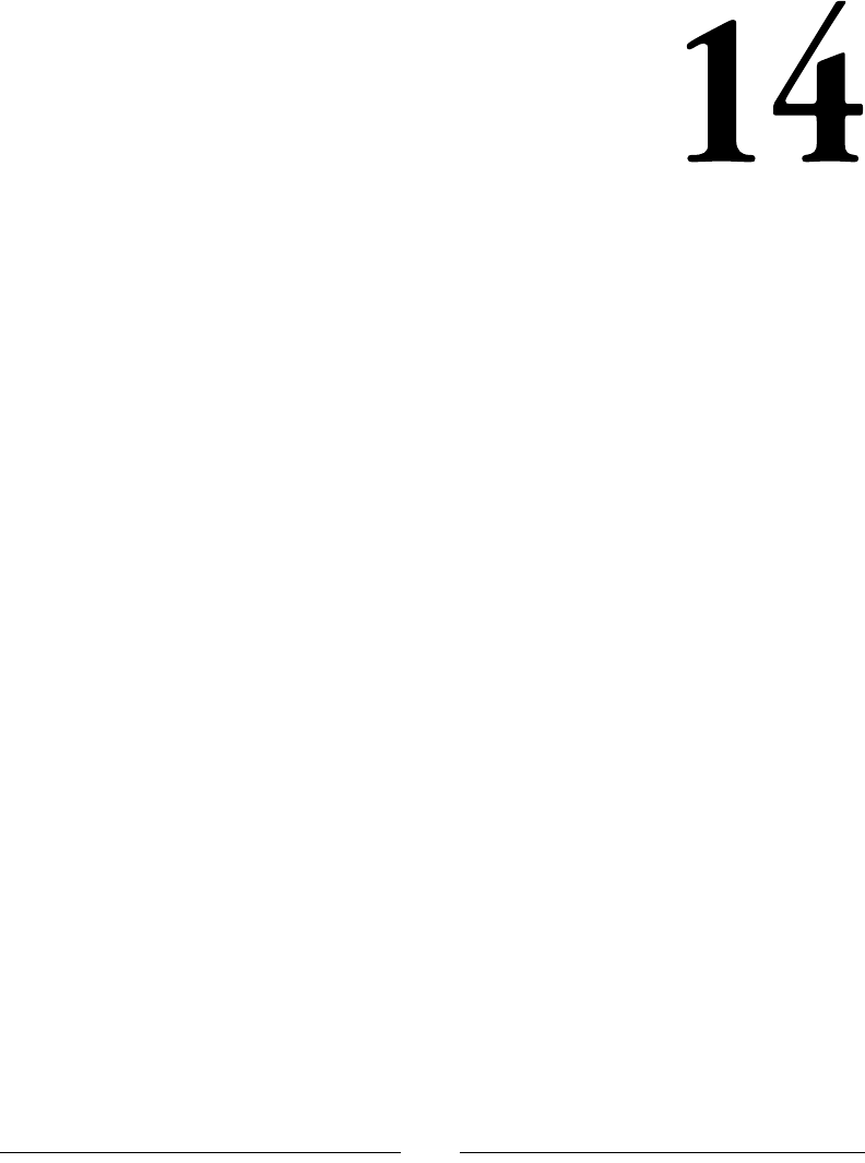
[ 347 ]
Visualization with D3 and the
Play Framework
In the previous chapter, we learned about the Play framework, a web framework
for Scala. We built an API that returns a JSON array describing a user's GitHub
repositories.
In this chapter, we will construct a fully-edged web application that displays a
table and a chart describing a user's repositories. We will learn to integrate D3.js,
a JavaScript library for building data-driven web pages, with the Play framework.
This will set you on the path to building compelling interactive visualizations that
showcase results obtained with machine learning.
This chapter assumes that you are familiar with HTML, CSS, and JavaScript.
We present references at the end of the chapter. You should also have read the
previous chapter.
Visualization with D3 and the Play Framework
[ 348 ]
GitHub user data
We will build a single-page application that uses, as its backend, the API developed
in the previous chapter. The application contains a form where the user enters the
login name for a GitHub account. The application queries the API to get a list of
repositories for that user and displays them on the screen as both a table and a pie
chart summarizing programming language use for that user:
To see a live version of the application, head over to
http://app.scala4datascience.com.
Do I need a backend?
In the previous chapter, we learned about the client-server model that underpins
how the internet works: when you enter a website URL in your browser, the server
serves HTML, CSS, and JavaScript to your browser, which then renders it in the
appropriate manner.
What does this all mean for you? Arguably the second question that you should
be asking yourself when building a web application is whether you need to do any
server-side processing (right after "is this really going to be worth the effort?"). Could
you just create an HTML web-page with some JavaScript?

Chapter 14
[ 349 ]
You can get away without a backend if the data needed to build the whole
application is small enough: typically a few megabytes. If your application is
larger, you will need a backend to transfer just the data the client currently needs.
Surprisingly, you can often build visualizations without a backend: while data
science is accustomed to dealing with terabytes of data, the goal of the data science
process is often condensing these huge data sets to a few meaningful numbers.
Having a backend also lets you include logic invisible to the client. If you need
to validate a password, you clearly cannot send the code to do that to the client
computer: it needs to happen out of sight, on the server.
If your application is small enough and you do not need to do any server-side
processing, stop reading this chapter, brush up on your JavaScript if you have to,
and forget about Scala for now. Not having to worry about building a backend will
make your life easier.
Clearly, however, we do not have that freedom for the application that we want
to build: the user could enter the name of anyone on GitHub. Finding information
about that user requires a backend with access to tremendous storage and querying
capacity (which we simulate by just forwarding the request to the GitHub API and
re-interpreting the response).
JavaScript dependencies through
web-jars
One of the challenges of developing web applications is that we are writing two
quasi-separate programs: the server-side program and the client-side program. These
generally require different technologies. In particular, for any but the most trivial
application, we must keep track of JavaScript libraries, and integrate processing the
JavaScript code (for instance, for minication) in the build process.

Visualization with D3 and the Play Framework
[ 350 ]
The Play framework manages JavaScript dependencies through web-jars. These are
just JavaScript libraries packaged as jars. They are deployed on Maven Central,
which means that we can just add them as dependencies to our build.sbt le. For
this application, we will need the following JavaScript libraries:
• Require.js, a library for writing modular JavaScript
• JQuery
• Bootstrap
• Underscore.js, a library that adds many functional constructs and
client-side templating.
• D3, the graph plotting library
• NVD3, a graph library built on top of D3
If you are planning on coding up the examples provided in this chapter, the easiest
will be for you to start from the code for the previous chapter (You can download
the code for Chapter 13, Web APIs with Play, from GitHub: https://github.com/
pbugnion/s4ds/tree/master/chap13). We will assume this as a starting point
here onwards.
Let's include the dependencies on the web-jars in the build.sbt le:
libraryDependencies ++= Seq(
"org.webjars" % "requirejs" % "2.1.22",
"org.webjars" % "jquery" % "2.1.4",
"org.webjars" % "underscorejs" % "1.8.3",
"org.webjars" % "nvd3" % "1.8.1",
"org.webjars" % "d3js" % "3.5.6",
"org.webjars" % "bootstrap" % "3.3.6"
)
Fetch the modules by running activator update. Once you have done this, you
will notice the JavaScript libraries in target/web/public/main/lib.
Towards a web application: HTML
templates
In the previous chapter, we briey saw how to construct HTML templates by
interleaving Scala snippets in an HTML le. We saw that templates are compiled
to Scala functions, and we learned how to call these functions from the controllers.

Chapter 14
[ 351 ]
In single-page applications, the majority of the logic governing what is actually
displayed in the browser resides in the client-side JavaScript, not in the server.
The pages served by the server contain the bare-bones HTML framework.
Let's create the HTML layout for our application. We will save this in views/index.
scala.html. The template will just contain the layout for the application, but will
not contain any information about any user's repositories. To fetch that information,
the application will have to query the API developed in the previous chapter. The
template does not take any parameters, since all the dynamic HTML generation will
happen client-side.
We use the Bootstrap grid layout to control the HTML layout. If you are not familiar
with Bootstrap layouts, consult the documentation at http://getbootstrap.com/
css/#grid-example-basic.
// app/views/index.scala.html
<!DOCTYPE html>
<html lang="en">
<head>
<title>Github User display</title>
<link rel="stylesheet" media="screen"
href="@routes.Assets.versioned("stylesheets/main.css")">
<link rel="shortcut icon" type="image/png"
href="@routes.Assets.versioned("images/favicon.png")">
<link rel="stylesheet" media="screen"
href=@routes.Assets.versioned("lib/nvd3/nv.d3.css") >
<link rel="stylesheet" media="screen"
href=@routes.Assets.versioned(
"lib/bootstrap/css/bootstrap.css")>
</head>
<body>
<div class="container">
<!-- Title row -->
<div class="row">
<h1>Github user search</h1>
</div>
<!-- User search row -->
<div class="row">
<label>Github user: </label>
<input type="text" id="user-selection">

Visualization with D3 and the Play Framework
[ 352 ]
<span id="searching-span"></span>
<hr />
</div>
<!-- Results row -->
<div id="response" class="row"></div>
</div>
</body>
</html>
In the HTML head, we link the CSS stylesheets that we need for the application.
Instead of specifying the path explicitly, we use the @routes.Assets.
versioned(...) function. This resolves to a URI corresponding to the location
where the assets are stored post-compilation. The argument passed to the function
should be the path from target/web/public/main to the asset you need.
We want to serve the compiled version of this view when the user accesses the route
/ on our server. We therefore need to add this route to conf/routes:
# conf/routes
GET / controllers.Application.index
The route is served by the index function in the Application controller. All this
controller needs to do is serve the index view:
// app/controllers/Application.scala
package controllers
import play.api._
import play.api.mvc._
class Application extends Controller {
def index = Action {
Ok(views.html.index())
}
}
Start the Play framework by running activator run in the root directory of the
application and point your web browser to 127.0.0.1:9000/. You should see the
framework for our web application. Of course, the application does not do anything
yet, since we have not written any of the JavaScript logic yet.

Chapter 14
[ 353 ]
Modular JavaScript through RequireJS
The simplest way of injecting JavaScript libraries into the namespace is to add them
to the HTML framework via <script>...</script> tags in the HTML header. For
instance, to add JQuery, we would add the following line to the head of the document:
<script src=@routes.Assets.versioned("lib/jquery/jquery.js")
type="text/javascript"></script>
While this works, it does not scale well to large applications, since every library
gets imported into the global namespace. Modern client-side JavaScript frameworks
such as AngularJS provide an alternative way of dening and loading modules that
preserve encapsulation.
We will use RequireJS. In a nutshell, RequireJS lets us encapsulate JavaScript
modules through functions. For instance, if we wanted to write a module example
that contains a function for hiding a div, we would dene the module as follows:
// example.js
define(["jquery", "underscore"], function($, _) {
// hide a div
function hide(div_name) {
$(div_name).hide() ;
}
// what the module exports.
return { "hide": hide }
}) ;
We encapsulate our module as a callback in a function called define. The define
function takes two arguments: a list of dependencies, and a function denition. The
define function binds the dependencies to the arguments list of the callback: in
this case, functions in JQuery will be bound to $ and functions in Underscore will
be bound to _. This creates a module which exposes whatever the callback function
returns. In this case, we export the hide function, binding it to the name "hide". Our
example module thus exposes the hide function.
To load this module, we pass it as a dependency to the module in which we want to
use it:
define(["example"], function(example) {
function hide_all() {

Visualization with D3 and the Play Framework
[ 354 ]
example.hide("#top") ;
example.hide("#bottom") ;
}
return { "hide_all": hide_all } ;
});
Notice how the functions in example are encapsulated, rather than existing in the
global namespace. We call them through example.<function-name>. Furthermore,
any functions or variables dened internally to the example module remain private.
Sometimes, we want JavaScript code to exist outside of modules. This is often the case
for the script that bootstraps the application. For these, replace define with require:
require(["jquery", "example"], function($, example) {
$(document).ready(function() {
example.hide("#header") ;
});
}) ;
Now that we have an overview of RequireJS, how do we use it in the Play
framework? The rst step is to add the dependency on the RequireJS web jar,
which we have done. The Play framework also adds a RequireJS SBT plugin
(https://github.com/sbt/sbt-rjs), which should be installed by default if you
used the play-scala activator. If this is missing, it can be added with the following
line in plugins.sbt:
// project/plugins.sbt
addSbtPlugin("com.typesafe.sbt" % "sbt-rjs" % "1.0.7")
We also need to add the plugin to the list of stages. This allows the plugin to
manipulate the JavaScript assets when packaging the application as a jar. Add the
following line to build.sbt:
pipelineStages := Seq(rjs)
You will need to restart the activator for the changes to take effect.
We are now ready to use RequireJS in our application. We can use it by adding the
following line in the head section of our view:
// index.scala.html
<html>
<head>

Chapter 14
[ 355 ]
...
<script
type="text/javascript"
src=@routes.Assets.versioned("lib/requirejs/require.js").url
data-main=@routes.Assets.versioned("javascripts/main.js").url>
</script>
</head>
...
</html>
When the view is compiled, this is resolved to tags like:
<script type="text/javascript"
data-main="/assets/javascripts/main.js"
src="/assets/lib/requirejs/require.min.js">
</script>
The argument passed to data-main is the entry point for our application. When
RequireJS loads, it will execute main.js. That script must therefore bootstrap our
application. In particular, it should contain a conguration object for RequireJS, to
make it aware of where all the libraries are.
Bootstrapping the applications
When we linked require.js to our application, we told it to use main.js as
our entry point. To test that this works, let's start by entering a dummy main.js.
JavaScript les in Play applications go in /public/javascripts:
// public/javascripts/main.js
require([], function() {
console.log("hello, JavaScript");
});
To verify that this worked, head to 127.0.0.1:9000 and open the browser console.
You should see "hello, JavaScript" in the console.

Visualization with D3 and the Play Framework
[ 356 ]
Let's now write a more useful main.js. We will start by conguring RequireJS, giving
it the location of modules we will use in our application. Unfortunately, NVD3, the
graph library that we use, does not play very well with RequireJS so we have to use
an ugly hack to make it work. This complicates our main.js le somewhat:
// public/javascripts/main.js
(function (requirejs) {
'use strict';
// -- RequireJS config --
requirejs.config({
// path to the web jars. These definitions allow us
// to use "jquery", rather than "../lib/jquery/jquery",
// when defining module dependencies.
paths: {
"jquery": "../lib/jquery/jquery",
"underscore": "../lib/underscorejs/underscore",
"d3": "../lib/d3js/d3",
"nvd3": "../lib/nvd3/nv.d3",
"bootstrap": "../lib/bootstrap/js/bootstrap"
},
shim: {
// hack to get nvd3 to work with requirejs.
// see this so question:
// http://stackoverflow.com/questions/13157704/how-to-integrate-
d3-with-require-js#comment32647365_13171592
nvd3: {
deps: ["d3.global"],
exports: "nv"
},
bootstrap : { deps :['jquery'] }
}
}) ;
})(requirejs) ;
// hack to get nvd3 to work with requirejs.
// see this so question on Stack Overflow:

Chapter 14
[ 357 ]
// http://stackoverflow.com/questions/13157704/how-to-integrate-d3-
with-require-js#comment32647365_13171592
define("d3.global", ["d3"], function(d3global) {
d3 = d3global;
});
require([], function() {
// Our application
console.log("hello, JavaScript");
}) ;
Now that we have the conguration in place, we can dig into the JavaScript part of
the application.
Client-side program architecture
The basic idea is simple: the user searches for the name of someone on GitHub in
the input box. When he enters a name, we re a request to the API designed earlier
in this chapter. When the response from the API returns, the program binds that
response to a model and emits an event notifying that the model has been changed.
The views listen for this event and refresh from the model in response.
Designing the model
Let's start by dening the client-side model. The model holds information regarding
the repos of the user currently displayed. It gets lled in after the rst search.
// public/javascripts/model.js
define([], function(){
return {
ghubUser: "", // last name that was searched for
exists: true, // does that person exist on github?
repos: [] // list of repos
} ;
});

Visualization with D3 and the Play Framework
[ 358 ]
To see a populated value of the model, head to the complete application example
on app.scala4datascience.com, open a JavaScript console in your browser,
search for a user (for example, odersky) in the application and type the following
in the console:
> require(["model"], function(model) { console.log(model) ; })
{ghubUser: "odersky", exists: true, repos: Array}
> require(["model"], function(model) {
console.log(model.repos[0]);
})
{name: "dotty", language: "Scala", is_fork: true, size: 14653}
These import the "model" module, bind it to the variable model, and then print
information to the console.
The event bus
We need a mechanism for informing the views when the model is updated, since the
views need to refresh from the new model. This is commonly handled through events
in web applications. JQuery lets us bind callbacks to specic events. The callback is
executed when that event occurs.
For instance, to bind a callback to the event "custom-event", enter the following in a
JavaScript console:
> $(window).on("custom-event", function() {
console.log("custom event received") ;
});
We can re the event using:
> $(window).trigger("custom-event");
custom event received

Chapter 14
[ 359 ]
Events in JQuery require an event bus, a DOM element on which the event is
registered. In this case, we used the window DOM element as our event bus, but any
JQuery element would have served. Centralizing event denitions to a single module
is helpful. We will, therefore, create an events module containing two functions:
trigger, which triggers an event (specied by a string) and on, which binds a
callback to a specic event:
// public/javascripts/events.js
define(["jquery"], function($) {
var bus = $(window) ; // widget to use as an event bus
function trigger(eventType) {
$(bus).trigger(eventType) ;
}
function on(eventType, f) {
$(bus).on(eventType, f) ;
}
return {
"trigger": trigger,
"on": on
} ;
});
We can now emit and receive events using the events module. You can test
this out in a JavaScript console on the live version of the application (at app.
scala4datascience.com). Let's start by registering a listener:
> require(["events"], function(events) {
// register event listener
events.on("hello_event", function() {
console.log("Received event") ;
}) ;
});
If we now trigger the event "hello_event", the listener prints "Received event":
> require(["events"], function(events) {
// trigger the event
events.trigger("hello_event") ;
}) ;

Visualization with D3 and the Play Framework
[ 360 ]
Using events allows us to decouple the controller from the views. The controller does
not need to know anything about the views, and vice-versa. The controller just needs
to emit a "model_updated" event when the model is updated, and the views need to
refresh from the model when they receive that event.
AJAX calls through JQuery
We can now write the controller for our application. When the user enters a name
in the text input, we query the API, update the model and trigger a model_updated
event.
We use JQuery's $.getJSON function to query our API. This function takes a
URL as its rst argument, and a callback as its second argument. The API call
is asynchronous: $.getJSON returns immediately after execution. All request
processing must, therefore, be done in the callback. The callback is called if the
request is successful, but we can dene additional handlers that are always called, or
called on failure. Let's try this out in the browser console (either your own, if you are
running the API developed in the previous chapter, or on app.scala4datascience.
com). Recall that the API is listening to the end-point /api/repos/:user:
> $.getJSON("/api/repos/odersky", function(data) {
console.log("API response:");
console.log(data);
console.log(data[0]);
}) ;
{readyState: 1, getResponseHeader: function, ...}
API response:
[Object, Object, Object, Object, Object, ...]
{name: "dotty", language: "Scala", is_fork: true, size: 14653}
getJSON returns immediately. A few tenths of a second later, the API responds, at
which point the response gets fed through the callback.
The callback only gets executed on success. It takes, as its argument, the JSON object
returned by the API. To bind a callback that is executed when the API request fails,
call the .fail method on the return value of getJSON:
> $.getJSON("/api/repos/junk123456", function(data) {
console.log("called on success");
}).fail(function() {
console.log("called on failure") ;

Chapter 14
[ 361 ]
}) ;
{readyState: 1, getResponseHeader: function, ...}
called on failure
We can also use the .always method on the return value of getJSON to specify a
callback that is executed, whether the API query was successful or not.
Now that we know how to use $.getJSON to query our API, we can write the
controller. The controller listens for changes to the #user-selection input eld.
When a change occurs, it res an AJAX request to the API for information on that
user. It binds a callback which updates the model when the API replies with a list
of repositories. We will dene a controller module that exports a single function,
initialize, that creates the event listeners:
// public/javascripts/controller.js
define(["jquery", "events", "model"], function($, events, model) {
function initialize() {
$("#user-selection").change(function() {
var user = $("#user-selection").val() ;
console.log("Fetching information for " + user) ;
// Change cursor to a 'wait' symbol
// while we wait for the API to respond
$("*").css({"cursor": "wait"}) ;
$.getJSON("/api/repos/" + user, function(data) {
// Executed on success
model.exists = true ;
model.repos = data ;
}).fail(function() {
// Executed on failure
model.exists = false ;
model.repos = [] ;
}).always(function() {
// Always executed
model.ghubUser = user ;
// Restore cursor
$("*").css({"cursor": "initial"}) ;
// Tell the rest of the application

Visualization with D3 and the Play Framework
[ 362 ]
// that the model has been updated.
events.trigger("model_updated") ;
});
}) ;
} ;
return { "initialize": initialize };
});
Our controller module just exposes the initialize method. Once the initialization
is performed, the controller interacts with the rest of the application through event
listeners. We will call the controller's initialize method in main.js. Currently, the
last lines of that le are just an empty require block. Let's import our controller and
initialize it:
// public/javascripts/main.js
require(["controller"], function(controller) {
controller.initialize();
});
To test that this works, we can bind a dummy listener to the "model_updated"
event. For instance, we could log the current model to the browser JavaScript console
with the following snippet (which you can write directly in the JavaScript console):
> require(["events", "model"],
function(events, model) {
events.on("model_updated", function () {
console.log("model_updated event received");
console.log(model);
});
});
If you then search for a user, the model will be printed to the console. We now have
the controller in place. The last step is writing the views.

Chapter 14
[ 363 ]
Response views
If the request fails, we just display Not found in the response div. This part is the
easiest to code up, so let's do that rst. We dene an initialize method that
generates the view. The view then listens for the "model_updated" event, which is
red by the controller after it updates the model. Once the initialization is complete,
the only way to interact with the response view is through "model_updated" events:
// public/javascripts/responseView.js
define(["jquery", "model", "events"],
function($, model, events) {
var failedResponseHtml =
"<div class='col-md-12'>Not found</div>" ;
function initialize() {
events.on("model_updated", function() {
if (model.exists) {
// success – we will fill this in later.
console.log("model exists")
}
else {
// failure – the user entered
// is not a valid GitHub login
$("#response").html(failedResponseHtml) ;
}
}) ;
}
return { "initialize": initialize } ;
});
To bootstrap the view, we must call the initialize function from main.js. Just add
a dependency on responseView in the require block, and call responseView.
initialize(). With these modications, the nal require block in main.js is:
// public/javascripts/main.js
require(["controller", "responseView"],
function(controller, responseView) {
controller.initialize();
responseView.initialize() ;
}) ;

Visualization with D3 and the Play Framework
[ 364 ]
You can check that this all works by entering junk in the user input to deliberately
cause the API request to fail.
When the user enters a valid GitHub login name and the API returns a list of
repos, we must display those on the screen. We display a table and a pie chart
that aggregates the repository sizes by language. We will dene the pie chart and
the table in two separate modules, called repoGraph.js and repoTable.js. Let's
assume those exist for now and that they expose a build method that accepts a
model and the name of a div in which to appear.
Let's update the code for responseView to accommodate the user entering a valid
GitHub user name:
// public/javascripts/responseView.js
define(["jquery", "model", "events", "repoTable", "repoGraph"],
function($, model, events, repoTable, repoGraph) {
// HTHML to inject when the model represents a valid user
var successfulResponseHtml =
"<div class='col-md-6' id='response-table'></div>" +
"<div class='col-md-6' id='response-graph'></div>" ;
// HTML to inject when the model is for a non-existent user
var failedResponseHtml =
"<div class='col-md-12'>Not found</div>" ;
function initialize() {
events.on("model_updated", function() {
if (model.exists) {
$("#response").html(successfulResponseHtml) ;
repoTable.build(model, "#response-table") ;
repoGraph.build(model, "#response-graph") ;
}
else {
$("#response").html(failedResponseHtml) ;
}
}) ;
}
return { "initialize": initialize } ;
});

Chapter 14
[ 365 ]
Let's walk through what happens in the event of a successful API call. We inject the
following bit of HTML in the #response div:
var successfulResponseHtml =
"<div class='col-md-6' id='response-table'></div>" +
"<div class='col-md-6' id='response-graph'></div>" ;
This adds two HTML divs, one for the table of repositories, and the other for the
graph. We use Bootstrap classes to split the response div vertically.
Let's now turn our attention to the table view, which needs to expose a single build
method, as described in the previous section. We will just display the repositories
in an HTML table. We will use Underscore templates to build the table dynamically.
Underscore templates work much like string interpolation in Scala: we dene a
template with placeholders. Let's try this in a browser console:
> require(["underscore"], function(_) {
var myTemplate = _.template(
"Hello, <%= title %> <%= name %>!"
) ;
});
This creates a myTemplate function which accepts an object with attributes title
and name:
> require(["underscore"], function(_) {
var myTemplate = _.template( ... );
var person = { title: "Dr.", name: "Odersky" } ;
console.log(myTemplate(person)) ;
});
Underscore templates thus provide a convenient mechanism for formatting an object
as a string. We will create a template for each row in our table, and pass the model
for each repository to the template:
// public/javascripts/repoTable.js
define(["underscore", "jquery"], function(_, $) {
// Underscore template for each row
var rowTemplate = _.template("<tr>" +
"<td><%= name %></td>" +
"<td><%= language %></td>" +
"<td><%= size %></td>" +
"</tr>") ;
// template for the table

Visualization with D3 and the Play Framework
[ 366 ]
var repoTable = _.template(
"<table id='repo-table' class='table'>" +
"<thead>" +
"<tr>" +
"<th>Name</th><th>Language</th><th>Size</th>" +
"</tr>" +
"</thead>" +
"<tbody>" +
"<%= tbody %>" +
"</tbody>" +
"</table>") ;
// Builds a table for a model
function build(model, divName) {
var tbody = "" ;
_.each(model.repos, function(repo) {
tbody += rowTemplate(repo) ;
}) ;
var table = repoTable({tbody: tbody}) ;
$(divName).html(table) ;
}
return { "build": build } ;
}) ;
Drawing plots with NVD3
D3 is a library that offers low-level components for building interactive
visualizations in JavaScript. By offering the low-level components, it gives a huge
degree of exibility to the developer. The learning curve can, however, be quite
steep. In this example, we will use NVD3, a library which provides pre-made graphs
for D3. This can greatly speed up initial development. We will place the code in the
le repoGraph.js and expose a single method, build, which takes, as arguments,
a model and a div and draws a pie chart in that div. The pie chart will aggregate
language use across all the user's repositories.

Chapter 14
[ 367 ]
The code for generating a pie chart is nearly identical to the example given in the
NVD3 documentation, available at http://nvd3.org/examples/pie.html. The
data passed to the graph must be available as an array of objects. Each object must
contain a label eld and a size eld. The label eld identies the language, and
the size eld is the total size of all the repositories for that user written in that
language. The following would be a valid data array:
[
{ label: "Scala", size: 1234 },
{ label: "Python", size: 4567 }
]
To get the data in this format, we must aggregate sizes across the repositories written
in a particular language in our model. We write the generateDataFromModel
function to transform the repos array in the model to an array suitable for NVD3.
The crux of the aggregation is performed by a call to Underscore's groupBy method,
to group repositories by language. This method works exactly like Scala's groupBy
method. With this in mind, the generateDataFromModel function is:
// public/javascripts/repoGraph.js
define(["underscore", "d3", "nvd3"],
function(_, d3, nv) {
// Aggregate the repo size by language.
// Returns an array of objects like:
// [ { label: "Scala", size: 1245},
// { label: "Python", size: 432 } ]
function generateDataFromModel(model) {
// Build an initial object mapping each
// language to the repositories written in it
var language2Repos = _.groupBy(model.repos,
function(repo) { return repo.language ; }) ;
// Map each { "language": [ list of repos ], ...}
// pairs to a single document { "language": totalSize }
// where totalSize is the sum of the individual repos.
var plotObjects = _.map(language2Repos,
function(repos, language) {
var sizes = _.map(repos, function(repo) {
return repo.size;
});
// Sum over the sizes using 'reduce'
var totalSize = _.reduce(sizes,

Visualization with D3 and the Play Framework
[ 368 ]
function(memo, size) { return memo + size; },
0) ;
return { label: language, size: totalSize } ;
}) ;
return plotObjects;
}
We can now build the pie chart, using NVD3's addGraph method:
// Build the chart.
function build(model, divName) {
var transformedModel = generateDataFromModel(model) ;
nv.addGraph(function() {
var height = 350;
var width = 350;
var chart = nv.models.pieChart()
.x(function (d) { return d.label ; })
.y(function (d) { return d.size ;})
.width(width)
.height(height) ;
d3.select(divName).append("svg")
.datum(transformedModel)
.transition()
.duration(350)
.attr('width', width)
.attr('height', height)
.call(chart) ;
return chart ;
});
}
return { "build" : build } ;
});
This was the last component of our application. Point your browser to
127.0.0.1:9000 and you should see the application running.
Congratulations! We have built a fully-functioning single-page web application.

Chapter 14
[ 369 ]
Summary
In this chapter, we learned how to write a fully-featured web application with the
Play framework. Congratulations on making it this far. Building web applications are
likely to push many data scientists beyond their comfort zone, but knowing enough
about the web to build basic applications will allow you to share your results in a
compelling, engaging manner, as well as facilitate communications with software
engineers and web developers.
This concludes our whistle stop tour of Scala libraries. Over the course of this book,
we have learned how to tackle linear algebra and optimization problems efciently
using Breeze, how to insert and query data in SQL databases in a functional manner,
and both how to interact with web APIs and how to create them. We have reviewed
some of tools available to the data scientist for writing concurrent or parallel
applications, from parallel collections and futures to Spark via Akka. We have
seen how pervasive these constructs are in Scala libraries, from futures in the Play
framework to Akka as the backbone of Spark. If you have read this far, pat yourself
on the back.
This books gives you the briefest of introduction to the libraries it covers, hopefully
just enough to give you a taste of what each tool is good for, what you could
accomplish with it, and how it ts in the wider Scala ecosystem. If you decide to use
any of these in your data science pipeline, you will need to read the documentation
in more detail, or a more complete reference book. The references listed at the end of
each chapter should provide a good starting point.
Both Scala and data science are evolving rapidly. Do not stay wedded to a particular
toolkit or concept. Remain on top of current developments and, above all, remain
pragmatic: nd the right tool for the right job. Scala and the libraries discussed
here will often be that tool, but not always: sometimes, a shell command or a short
Python script will be more effective. Remember also that programming skills are but
one aspect of the data scientist's body of knowledge. Even if you want to specialize
in the engineering side of data science, learn about the problem domain and the
mathematical underpinnings of machine learning.
Most importantly, if you have taken the time to read this book, it is likely that you
view programming and data science as more than a day job. Coding in Scala can be
satisfying and rewarding, so have fun and be awesome!

Visualization with D3 and the Play Framework
[ 370 ]
References
There are thousands of HTML and CSS tutorials dotted around the web. A simple
Google search will give you a much better idea of the resources available than any
list of references I can provide.
Mike Bostock's website has a wealth of beautiful D3 visualizations: http://bost.
ocks.org/mike/. To understand a bit more about D3, I recommend Scott Murray's
Interactive Data Visualization for the Web.
You may also wish to consult the references given in the previous chapter for
reference books on the Play framework and designing REST APIs.

[ 371 ]
Pattern Matching
and Extractors
Pattern matching is a powerful tool for control ow in Scala. It is often underused
and under-estimated by people coming to Scala from imperative languages.
Let's start with a few examples of pattern matching before diving into the theory.
We start by dening a tuple:
scala> val names = ("Pascal", "Bugnion")
names: (String, String) = (Pascal,Bugnion)
We can use pattern matching to extract the elements of this tuple and bind them to
variables:
scala> val (firstName, lastName) = names
firstName: String = Pascal
lastName: String = Bugnion
We just extracted the two elements of the names tuple, binding them to the variables
firstName and lastName. Notice how the left-hand side denes a pattern that the
right-hand side must match: we are declaring that the variable names must be a
two-element tuple. To make the pattern more specic, we could also have specied
the expected types of the elements in the tuple:
scala> val (firstName:String, lastName:String) = names
firstName: String = Pascal
lastName: String = Bugnion

Pattern Matching and Extractors
[ 372 ]
What happens if the pattern on the left-hand side does not match the right-hand side?
scala> val (firstName, middleName, lastName) = names
<console>:13: error: constructor cannot be instantiated to expected type;
found : (T1, T2, T3)
required: (String, String)
val (firstName, middleName, lastName) = names
This results in a compile error. Other types of pattern matching failures result in
runtime errors.
Pattern matching is very expressive. To achieve the same behavior without pattern
matching, you would have to do the following explicitly:
• Verify that the variable names is a two-element tuple
• Extract the first element and bind it to firstName
• Extract the second element and bind it to lastName
If we expect certain elements in the tuple to have specic values, we can verify this
as part of the pattern match. For instance, we can verify that the rst element of the
names tuple matches "Pascal":
scala> val ("Pascal", lastName) = names
lastName: String = Bugnion
Besides tuples, we can also match on Scala collections:
scala> val point = Array(1, 2, 3)
point: Array[Int] = Array(1, 2, 3)
scala> val Array(x, y, z) = point
x: Int = 1
y: Int = 2
z: Int = 3
Notice the similarity between this pattern matching and array construction:
scala> val point = Array(x, y, z)
point: Array[Int] = Array(1, 2, 3)
Syntactically, Scala expresses pattern matching as the reverse process to instance
construction. We can think of pattern matching as the deconstruction of an object,
binding the object's constituent parts to variables.

Appendix
[ 373 ]
When matching against collections, one is sometimes only interested in matching
the rst element, or the rst few elements, and discarding the rest of the collection,
whatever its length. The operator _* will match against any number of elements:
scala> val Array(x, _*) = point
x: Int = 1
By default, the part of the pattern matched by the _* operator is not bound to a
variable. We can capture it as follows:
scala> val Array(x, xs @ _*) = point
x: Int = 1
xs: Seq[Int] = Vector(2, 3)
Besides tuples and collections, we can also match against case classes. Let's start by
dening a case representing a name:
scala> case class Name(first: String, last: String)
defined class Name
scala> val name = Name("Martin", "Odersky")
name: Name = Name(Martin,Odersky)
We can match against instances of Name in much the same way we matched
against tuples:
scala> val Name(firstName, lastName) = name
firstName: String = Martin
lastName: String = Odersky
All these patterns can also be used in match statements:
scala> def greet(name:Name) = name match {
case Name("Martin", "Odersky") => "An honor to meet you"
case Name(first, "Bugnion") => "Wow! A family member!"
case Name(first, last) => s"Hello, $first"
}
greet: (name: Name)String

Pattern Matching and Extractors
[ 374 ]
Pattern matching in for comprehensions
Pattern matching is useful in for comprehensions for extracting items from a
collection that match a specic pattern. Let's build a collection of Name instances:
scala> val names = List(Name("Martin", "Odersky"),
Name("Derek", "Wyatt"))
names: List[Name] = List(Name(Martin,Odersky), Name(Derek,Wyatt))
We can use pattern matching to extract the internals of the class in a for-
comprehension:
scala> for { Name(first, last) <- names } yield first
List[String] = List(Martin, Derek)
So far, nothing terribly ground-breaking. But what if we wanted to extract the
surname of everyone whose rst name is "Martin"?
scala> for { Name("Martin", last) <- names } yield last
List[String] = List(Odersky)
Writing Name("Martin", last) <- names extracts the elements of names that
match the pattern. You might think that this is a contrived example, and it is, but the
examples in Chapter 7, Web APIs demonstrate the usefulness and versatility of this
language pattern, for instance, for extracting specic elds from JSON objects.
Pattern matching internals
If you dene a case class, as we saw with Name, you get pattern matching against the
constructor for free. You should be using case classes to represent your data as much
as possible, thus reducing the need to implement your own pattern matching. It is
nevertheless useful to understand how pattern matching works.
When you create a case class, Scala automatically builds a companion object:
scala> case class Name(first: String, last: String)
defined class Name
scala> Name.<tab>
apply asInstanceOf curried isInstanceOf toString tupled
unapply

Appendix
[ 375 ]
The method used (internally) for pattern matching is unapply. This method takes, as
argument, an object and returns Option[T], where T is a tuple of the values of the
case class.
scala> val name = Name("Martin", "Odersky")
name: Name = Name(Martin,Odersky)
scala> Name.unapply(name)
Option[(String, String)] = Some((Martin,Odersky))
The unapply method is an extractor. It plays the opposite role of the constructor: it
takes an object and extracts the list of parameters needed to construct that object.
When you write val Name(firstName, lastName), or when you use Name as a case
in a match statement, Scala calls Name.unapply on what you are matching against.
A value of Some[(String, String)] implies a pattern match, while a value of None
implies that the pattern fails.
To write custom extractors, you just need an object with an unapply method.
While unapply normally resides in the companion object of a class that you are
deconstructing, this need not be the case. In fact, it does not need to correspond to an
existing class at all. For instance, let's dene a NonZeroDouble extractor that matches
any non-zero double:
scala> object NonZeroDouble {
def unapply(d:Double):Option[Double] = {
if (d == 0.0) { None } else { Some(d) }
}
}
defined object NonZeroDouble
scala> val NonZeroDouble(denominator) = 5.5
denominator: Double = 5.5
scala> val NonZeroDouble(denominator) = 0.0
scala.MatchError: 0.0 (of class java.lang.Double)
... 43 elided
We dened an extractor for NonZeroDouble, despite the absence of a corresponding
NonZeroDouble class.

Pattern Matching and Extractors
[ 376 ]
This NonZeroDouble extractor would be useful in a match object. For instance, let's
dene a safeDivision function that returns a default value when the denominator
is zero:
scala> def safeDivision(numerator:Double,
denominator:Double, fallBack:Double) =
denominator match {
case NonZeroDouble(d) => numerator / d
case _ => fallBack
}
safeDivision: (numerator: Double, denominator: Double, fallBack: Double)
Double
scala> safeDivision(5.0, 2.0, 100.0)
Double = 2.5
scala> safeDivision(5.0, 0.0, 100.0)
Double = 100.0
This is a trivial example because the NonZeroDouble.unapply method is so simple,
but you can hopefully see the usefulness and expressiveness, if we were to dene a
more complex test. Dening custom extractors lets you dene powerful control ow
constructs to leverage match statements. More importantly, they enable the client
using the extractors to think about control ow declaratively: the client can declare
that they need a NonZeroDouble, rather than instructing the compiler to check
whether the value is zero.
Extracting sequences
The previous section explains extraction from case classes, and how to write custom
extractors, but it does not explain how extraction works on sequences:
scala> val Array(a, b) = Array(1, 2)
a: Int = 1
b: Int = 2
Rather than relying on an unapply method, sequences rely on an unapplySeq
method dened in the companion object. This is expected to return an
Option[Seq[A]]:
scala> Array.unapplySeq(Array(1, 2))
Option[IndexedSeq[Int]] = Some(Vector(1, 2))

Appendix
[ 377 ]
Let's write an example. We will write an extractor for Breeze vectors (which do
not currently support pattern matching). To avoid clashing with the DenseVector
companion object, we will write our unapplySeq in a separate object, called DV.
All our unapplySeq method needs to do is convert its argument to a Scala Vector
instance. To avoid muddying the concepts with generics, we will write this
implementation for [Double] vectors only:
scala> import breeze.linalg._
import breeze.linalg._
scala> object DV {
// Just need to convert to a Scala vector.
def unapplySeq(v:DenseVector[Double]) = Some(v.toScalaVector)
}
defined object DV
Let's try our new extractor implementation:
scala> val vec = DenseVector(1.0, 2.0, 3.0)
vec: breeze.linalg.DenseVector[Double] = DenseVector(1.0, 2.0, 3.0)
scala> val DV(x, y, z) = vec
x: Double = 1.0
y: Double = 2.0
z: Double = 3.0
Summary
Pattern matching is a powerful tool for control ow. It encourages the programmer
to think declaratively: declare that you expect a variable to match a certain pattern,
rather than explicitly tell the computer how to check that it matches this pattern. This
can save many lines of code and enhance clarity.

Pattern Matching and Extractors
[ 378 ]
Reference
For an overview of pattern matching in Scala, there is no better reference than
Programming in Scala, by Martin Odersky, Bill Venners, and Lex Spoon. An online
version of the rst edition is available at: https://www.artima.com/pins1ed/case-
classes-and-pattern-matching.html.
Daniel Westheide's blog covers slightly more advanced Scala constructs, and is a very
useful read: http://danielwestheide.com/blog/2012/11/21/the-neophytes-
guide-to-scala-part-1-extractors.html.
Module 2
Scala Data Analysis Cookbook
Navigate the world of data analysis, visualization, and machine learning
with over 100 hands-on Scala recipes

381
1
Getting Started
with Breeze
In this chapter, we will cover the following recipes:
fGetting Breeze—the linear algebra library
fWorking with vectors
fWorking with matrices
fVectors and matrices with randomly distributed values
fReading and writing CSV les
Introduction
This chapter gives you a quick overview of one of the most popular data analysis libraries in
Scala, how to get them, and their most frequently used functions and data structures.
We will be focusing on Breeze in this rst chapter, which is one of the most popular and
powerful linear algebra libraries. Spark MLlib, which we will be seeing in the subsequent
chapters, builds on top of Breeze and Spark, and provides a powerful framework for scalable
machine learning.
Getting Started with Breeze
382
Getting Breeze – the linear algebra library
In simple terms, Breeze (http://www.scalanlp.org) is a Scala library that extends the
Scala collection library to provide support for vectors and matrices in addition to providing a
whole bunch of functions that support their manipulation. We could safely compare Breeze
to NumPy (http://www.numpy.org/) in Python terms. Breeze forms the foundation of
MLlib—the Machine Learning library in Spark, which we will explore in later chapters.
In this rst recipe, we will see how to pull the Breeze libraries into our project using Scala
Build Tool (SBT). We will also see a brief history of Breeze to better appreciate why it
could be considered as the "go to" linear algebra library in Scala.
For all our recipes, we will be using Scala 2.10.4 along with Java 1.7. I
wrote the examples using the Scala IDE, but please feel free to use your
favorite IDE.
How to do it...
Let's add the Breeze dependencies into our build.sbt so that we can start playing with
them in the subsequent recipes. The Breeze dependencies are just two—the breeze (core)
and the breeze-native dependencies.
1. Under a brand new folder (which will be our project root), create a new le called
build.sbt.
2. Next, add the breeze libraries to the project dependencies:
organization := "com.packt"
name := "chapter1-breeze"
scalaVersion := "2.10.4"
libraryDependencies ++= Seq(
"org.scalanlp" %% "breeze" % "0.11.2",
//Optional - the 'why' is explained in the How it works
section
"org.scalanlp" %% "breeze-natives" % "0.11.2"
)
3. From that folder, issue a sbt compile command in order to fetch all your
dependencies.
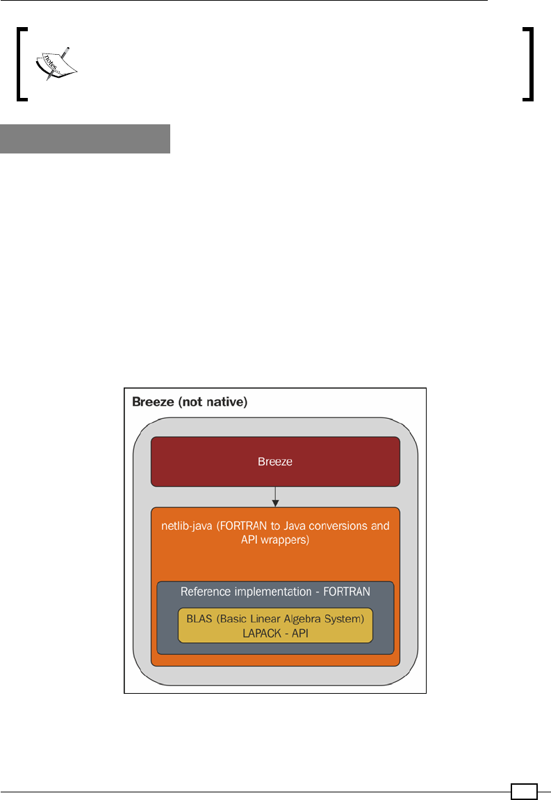
Chapter 1
383
You could import the project into your Eclipse using sbt eclipse
after installing the sbteclipse plugin https://github.com/
typesafehub/sbteclipse/. For IntelliJ IDEA, you just need to import
the project by pointing to the root folder where your build.sbt le is.
There's more...
Let's look into the details of what the breeze and breeze-native library dependencies we
added bring to us.
The org.scalanlp.breeze dependency
Breeze has a long history in that it isn't written from scratch in Scala. Without the native
dependency, Breeze leverages the power of netlib-java that has a Java-compiled version
of the FORTRAN Reference implementation of BLAS/LAPACK. The netlib-java also
provides gentle wrappers over the Java compiled library. What this means is that we could still
work without the native dependency but the performance won't be great considering the best
performance that we could leverage out of this FORTRAN-translated library is the performance
of the FORTRAN reference implementation itself. However, for serious number crunching with
the best performance, we should add the breeze-natives dependency too.
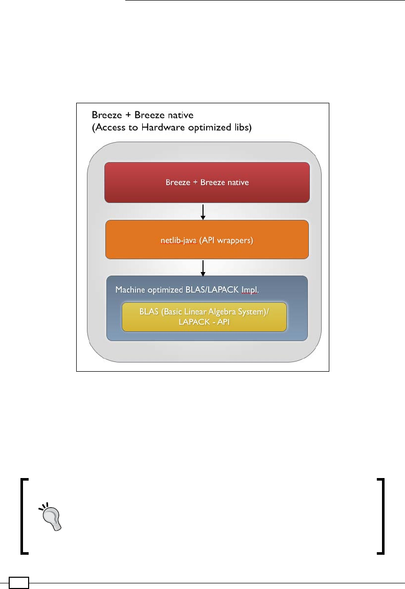
Getting Started with Breeze
384
The org.scalanlp.breeze-natives package
With its native additive, Breeze looks for the machine-specic implementations of the
BLAS/LAPACK libraries. The good news is that there are open source and (vendor provided)
commercial implementations for most popular processors and GPUs. The most popular open
source implementations include ATLAS (http://math-atlas.sourceforge.net) and
OpenBLAS (http://www.openblas.net/).
If you are running a Mac, you are in luck—Native BLAS libraries come out of the box on Macs.
Installing NativeBLAS on Ubuntu / Debian involves just running the following commands:
sudo apt-get install libatlas3-base libopenblas-base
sudo update-alternatives --config libblas.so.3
sudo update-alternatives --config liblapack.so.3
Downloading the example code
You can download the example code les from your account at
http://www.packtpub.com for all the Packt Publishing books you
have purchased. If you purchased this book elsewhere, you can visit
http://www.packtpub.com/support and register to have the
les e-mailed directly to you.
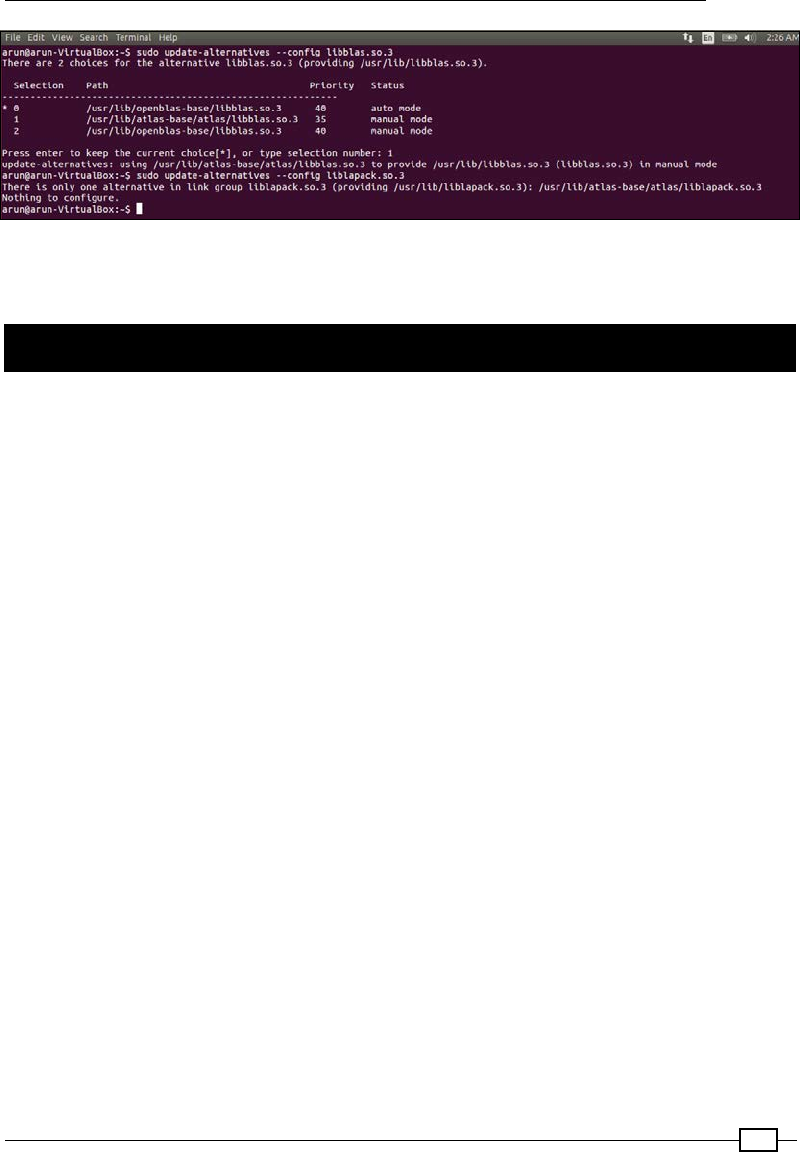
Chapter 1
385
For Windows, please refer to the installation instructions on https://github.com/
xianyi/OpenBLAS/wiki/Installation-Guide.
Working with vectors
There are subtle yet powerful differences between Breeze vectors and Scala's own scala.
collection.Vector. As we'll see in this recipe, Breeze vectors have a lot of functions that
are linear algebra specic, and the more important thing to note here is that Breeze's vector is
a Scala wrapper over netlib-java and most calls to the vector's API delegates the call to it.
Vectors are one of the core components in Breeze. They are containers of homogenous
data. In this recipe, we'll rst see how to create vectors and then move on to various data
manipulation functions to modify those vectors.
In this recipe, we will look at various operations on vectors. This recipe has been organized
in the form of the following sub-recipes:
fCreating vectors:
Creating a vector from values
Creating a zero vector
Creating a vector out of a function
Creating a vector of linearly spaced values
Creating a vector with values in a specific range
Creating an entire vector with a single value
Slicing a sub-vector from a bigger vector
Creating a Breeze vector from a Scala vector
fVector arithmetic:
Scalar operations
Calculating the dot product of a vector
Creating a new vector by adding two vectors together
Getting Started with Breeze
386
fAppending vectors and converting a vector of one type to another:
Concatenating two vectors
Converting a vector of int to a vector of double
fComputing basic statistics:
Mean and variance
Standard deviation
Find the largest value
Finding the sum, square root and log of all the values in the vector
Getting ready
In order to run the code, you could either use the Scala or use the Worksheet feature available
in the Eclipse Scala plugin (or Scala IDE) or in IntelliJ IDEA. The reason these options are
suggested is due to their quick turnaround time.
How to do it...
Let's look at each of the above sub-recipes in detail. For easier reference, the output of the
respective command is shown as well. All the classes that are being used in this recipe are
from the breeze.linalg package. So, an "import breeze.linalg._" statement at
the top of your le would be perfect.
Creating vectors
Let's look at the various ways we could construct vectors. Most of these construction
mechanisms are through the apply method of the vector. There are two different avors
of vector—breeze.linalg.DenseVector and breeze.linalg.SparseVector—the
choice of the vector depends on the use case. The general rule of thumb is that if you have
data that is at least 20 percent zeroes, you are better off choosing SparseVector but then
the 20 percent is a variant too.
Constructing a vector from values
fCreating a dense vector from values: Creating a DenseVector from values is just
a matter of passing the values to the apply method:
val dense=DenseVector(1,2,3,4,5)
println (dense) //DenseVector(1, 2, 3, 4, 5)

Chapter 1
387
fCreating a sparse vector from values: Creating a SparseVector from values is also
through passing the values to the apply method:
val sparse=SparseVector(0.0, 1.0, 0.0, 2.0, 0.0)
println (sparse) //SparseVector((0,0.0), (1,1.0), (2,0.0),
(3,2.0), (4,0.0))
Notice how the SparseVector stores values against the index.
Obviously, there are simpler ways to create a vector instead of just throwing all the data into
its apply method.
Creating a zero vector
Calling the vector's zeros function would create a zero vector. While the numeric types would
return a 0, the object types would return null and the Boolean types would return false:
val denseZeros=DenseVector.zeros[Double](5) //DenseVector(0.0,
0.0, 0.0, 0.0, 0.0)
val sparseZeros=SparseVector.zeros[Double](5) //SparseVector()
Not surprisingly, the SparseVector does not allocate any memory for the contents of
the vector. However, the creation of the SparseVector object itself is accounted for in
the memory.
Creating a vector out of a function
The tabulate function in vector is an interesting and useful function. It accepts a size
argument just like the zeros function but it also accepts a function that we could use to
populate the values for the vector. The function could be anything ranging from a random
number generator to a naïve index based generator, which we have implemented here.
Notice how the return value of the function (Int) could be converted into a vector of
Double by using the type parameter:
val
denseTabulate=DenseVector.tabulate[Double](5)(index=>index*index)
//DenseVector(0.0, 1.0, 4.0, 9.0, 16.0)
Creating a vector of linearly spaced values
The linspace function in breeze.linalg creates a new Vector[Double] of linearly
spaced values between two arbitrary numbers. Not surprisingly, it accepts three arguments—
the start, end, and the total number of values that we would like to generate. Please note
that the start and the end values are inclusive while being generated:
val spaceVector=breeze.linalg.linspace(2, 10, 5)
//DenseVector(2.0, 4.0, 6.0, 8.0, 10.0)

Getting Started with Breeze
388
Creating a vector with values in a specic range
The range function in a vector has two variants. The plain vanilla function accepts a start
and end value (start inclusive):
val allNosTill10=DenseVector.range(0, 10)
//DenseVector(0, 1, 2, 3, 4, 5, 6, 7, 8, 9)
The other variant is an overloaded function that accepts a "step" value:
val evenNosTill20=DenseVector.range(0, 20, 2)
// DenseVector(0, 2, 4, 6, 8, 10, 12, 14, 16, 18)
Just like the range function, which has all the arguments as integers, there is also a rangeD
function that takes the start, stop, and the step parameters as Double:
val rangeD=DenseVector.rangeD(0.5, 20, 2.5)
// DenseVector(0.5, 3.0, 5.5, 8.0, 10.5, 13.0, 15.5)
Creating an entire vector with a single value
Filling an entire vector with the same value is child's play. We just say HOW BIG is this vector
going to be and then WHAT value. That's it.
val denseJust2s=DenseVector.fill(10, 2)
// DenseVector(2, 2, 2, 2, 2, 2 , 2, 2, 2, 2)
Slicing a sub-vector from a bigger vector
Choosing a part of the vector from a previous vector is just a matter of calling the slice method
on the bigger vector. The parameters to be passed are the start index, end index, and an
optional "step" parameter. The step parameter adds the step value for every iteration until
it reaches the end index. Note that the end index is excluded in the sub-vector:
val allNosTill10=DenseVector.range(0, 10)
//DenseVector(0, 1, 2, 3, 4, 5, 6, 7, 8, 9)
val fourThroughSevenIndexVector= allNosTill10.slice(4, 7)
//DenseVector(4, 5, 6)
val twoThroughNineSkip2IndexVector= allNosTill10.slice(2, 9, 2)
//DenseVector(2, 4, 6)
Creating a Breeze Vector from a Scala Vector
A Breeze vector object's apply method could even accept a Scala Vector as a parameter and
construct a vector out of it:
val
vectFromArray=DenseVector(collection.immutable.Vector(1,2,3,4))
// DenseVector(Vector(1, 2, 3, 4))

Chapter 1
389
Vector arithmetic
Now let's look at the basic arithmetic that we could do on vectors with scalars and vectors.
Scalar operations
Operations with scalars work just as we would expect, propagating the value to each element
in the vector.
Adding a scalar to each element of the vector is done using the + function (surprise!):
val inPlaceValueAddition=evenNosTill20 +2
//DenseVector(2, 4, 6, 8, 10, 12, 14, 16, 18, 20)
Similarly the other basic arithmetic operations—subtraction, multiplication, and division
involves calling the respective functions named after the universally accepted symbols
(-, *, and /):
//Scalar subtraction
val inPlaceValueSubtraction=evenNosTill20 -2
//DenseVector(-2, 0, 2, 4, 6, 8, 10, 12, 14, 16)
//Scalar multiplication
val inPlaceValueMultiplication=evenNosTill20 *2
//DenseVector(0, 4, 8, 12, 16, 20, 24, 28, 32, 36)
//Scalar division
val inPlaceValueDivision=evenNosTill20 /2
//DenseVector(0, 1, 2, 3, 4, 5, 6, 7, 8, 9)
Calculating the dot product of two vectors
Each vector object has a function called dot, which accepts another vector of the same
length as a parameter.
Let's ll in just 2s to a new vector of length 5:
val justFive2s=DenseVector.fill(5, 2)
//DenseVector(2, 2, 2, 2, 2)
We'll create another vector from 0 to 5 with a step value of 1 (a fancy way of saying 0
through 4):
val zeroThrough4=DenseVector.range(0, 5, 1)
//DenseVector(0, 1, 2, 3, 4)

Getting Started with Breeze
390
Here's the dot function:
val dotVector=zeroThrough4.dot(justFive2s)
//Int = 20
It is to be expected of the function to complain if we pass in a vector of a different length
as a parameter to the dot product - Breeze throws an IllegalArgumentException if
we do that. The full exception message is:
Java.lang.IllegalArgumentException: Vectors must be the same
length!
Creating a new vector by adding two vectors together
The + function is overloaded to accept a vector other than the scalar we saw previously. The
operation does a corresponding element-by-element addition and creates a new vector:
val evenNosTill20=DenseVector.range(0, 20, 2)
//DenseVector(0, 2, 4, 6, 8, 10, 12, 14, 16, 18)
val denseJust2s=DenseVector.fill(10, 2)
//DenseVector(2, 2, 2, 2, 2, 2, 2, 2, 2, 2)
val additionVector=evenNosTill20 + denseJust2s
// DenseVector(2, 4, 6, 8, 10, 12, 14, 16, 18, 20)
There's an interesting behavior encapsulated in the addition though. Assuming you try to add
two vectors of different lengths, if the rst vector is smaller and the second vector larger, the
resulting vector would be the size of the rst vector and the rest of the elements in the second
vector would be ignored!
val fiveLength=DenseVector(1,2,3,4,5)
//DenseVector(1, 2, 3, 4, 5)
val tenLength=DenseVector.fill(10, 20)
//DenseVector(20, 20, 20, 20, 20, 20, 20, 20, 20, 20)
fiveLength+tenLength
//DenseVector(21, 22, 23, 24, 25)
On the other hand, if the rst vector is larger and the second vector smaller, it would result
in an ArrayIndexOutOfBoundsException:
tenLength+fiveLength
// java.lang.ArrayIndexOutOfBoundsException: 5

Chapter 1
391
Appending vectors and converting a vector of one type to
another
Let's briey see how to append two vectors and convert vectors of one numeric type
to another.
Concatenating two vectors
There are two variants of concatenation. There is a vertcat function that just vertically
concatenates an arbitrary number of vectors—the size of the vector just increases to the
sum of the sizes of all the vectors combined:
val justFive2s=DenseVector.fill(5, 2)
//DenseVector(2, 2, 2, 2, 2)
val zeroThrough4=DenseVector.range(0, 5, 1)
//DenseVector(0, 1, 2, 3, 4)
val concatVector=DenseVector.vertcat(zeroThrough4, justFive2s)
//DenseVector(0, 1, 2, 3, 4, 2, 2, 2, 2, 2)
No surprise here. There is also the horzcat method that places the second vector
horizontally next to the rst vector, thus forming a matrix.
val concatVector1=DenseVector.horzcat(zeroThrough4, justFive2s)
//breeze.linalg.DenseMatrix[Int]
0 2
1 2
2 2
3 2
4 2
While dealing with vectors of different length, the vertcat function happily
arranges the second vector at the bottom of the rst vector. Not surprisingly,
the horzcat function throws an exception:
java.lang.IllegalArgumentException, meaning all vectors must be
of the same size!
Getting Started with Breeze
392
Converting a vector of Int to a vector of Double
The conversion of one type of vector into another is not automatic in Breeze. However, there is
a simple way to achieve this:
val evenNosTill20Double=breeze.linalg.convert(evenNosTill20,
Double)
Computing basic statistics
Other than the creation and the arithmetic operations that we saw previously, there are
some interesting summary statistics operations that are available in the library. Let's look
at them now:
Needs import of breeze.linalg._ and breeze.numerics._. The
operations in the Other operations section aim to simulate the NumPy's
UFunc or universal functions.
Now, let's briey look at how to calculate some basic summary statistics for a vector.
Mean and variance
Calculating the mean and variance of a vector could be achieved by calling the
meanAndVariance universal function in the breeze.stats package. Note that
this needs a vector of Double:
meanAndVariance(evenNosTill20Double)
//MeanAndVariance(9.0,36.666666666666664,10)
As you may have guessed, converting an Int vector to a Double vector
and calculating the mean and variance for that vector could be merged
into a one-liner:
meanAndVariance(convert(evenNosTill20, Double))
Standard deviation
Calling the stddev on a Double vector could give the standard deviation:
stddev(evenNosTill20Double)
//Double = 6.0553007081949835
Find the largest value in a vector
The max universal function inside the breeze.linalg package would help us nd the
maximum value in a vector:
val intMaxOfVectorVals=max (evenNosTill20)
//18

Chapter 1
393
Finding the sum, square root and log of all the values
in the vector
The same as with max, the sum universal function inside the breeze.linalg package
calculates the sum of the vector:
val intSumOfVectorVals=sum (evenNosTill20)
//90
The functions sqrt, log, and various other universal functions in the breeze.numerics
package calculate the square root and log values of all the individual elements inside
the vector:
The Sqrt function
val sqrtOfVectorVals= sqrt (evenNosTill20)
// DenseVector(0.0, 1. 4142135623730951, 2.0, 2.449489742783178,
2.8284271247461903, 3.16227766016 83795, 3.4641016151377544,
3.7416573867739413, 4.0, 4.242640687119285)
The Log function
val log2VectorVals=log(evenNosTill20)
// DenseVector(-Infinity , 0.6931471805599453, 1.3862943611198906,
1.791759469228055, 2.079441541679 8357, 2.302585092994046,
2.4849066497880004, 2.6390573296152584, 2.77258872 2239781,
2.8903717578961645)
Working with matrices
As we discussed in the Working with vectors recipe, you could use the Eclipse or IntelliJ IDEA
Scala worksheets for a faster turnaround time.
How to do it...
There are a variety of functions that we have in a matrix. In this recipe, we will look at some
details around:
fCreating matrices:
Creating a matrix from values
Creating a zero matrix
Creating a matrix out of a function
Creating an identity matrix
Creating a matrix from random numbers
Creating from a Scala collection

Getting Started with Breeze
394
fMatrix arithmetic:
Addition
Multiplication (also element-wise)
fAppending and conversion:
Concatenating a matrix vertically
Concatenating a matrix horizontally
Converting a matrix of Int to a matrix of Double
fData manipulation operations:
Getting column vectors
Getting row vectors
Getting values inside the matrix
Getting the inverse and transpose of a matrix
fComputing basic statistics:
Mean and variance
Standard deviation
Finding the largest value
Finding the sum, square root and log of all the values in the matrix
Calculating the eigenvectors and eigenvalues of a matrix
Creating matrices
Let's rst see how to create a matrix.
Creating a matrix from values
The simplest way to create a matrix is to pass in the values in a row-wise fashion into the
apply function of the matrix object:
val simpleMatrix=DenseMatrix((1,2,3),(11,12,13),(21,22,23))
//Returns a DenseMatrix[Int]
1 2 3
11 12 13
21 22 23
Chapter 1
395
There's also a Sparse version of the matrix too—the Compressed Sparse Column Matrix
(CSCMatrix):
val sparseMatrix=CSCMatrix((1,0,0),(11,0,0),(0,0,23))
//Returns a SparseMatrix[Int]
(0,0) 1
(1,0) 11
(2,2) 23
Breeze's Sparse matrix is a Dictionary of Keys (DOK) representation with
(row, column) mapped against the value.
Creating a zero matrix
Creating a zero matrix is just a matter of calling the matrix's zeros function. The rst integer
parameter indicates the rows and the second parameter indicates the columns:
val denseZeros=DenseMatrix.zeros[Double](5,4)
//Returns a DenseMatrix[Double]
0.0 0.0 0.0 0.0
0.0 0.0 0.0 0.0
0.0 0.0 0.0 0.0
0.0 0.0 0.0 0.0
0.0 0.0 0.0 0.0
val compressedSparseMatrix=CSCMatrix.zeros[Double](5,4)
//Returns a CSCMatrix[Double] = 5 x 4 CSCMatrix
Notice how the SparseMatrix doesn't allocate any memory for the
values in the zero value matrix.

Getting Started with Breeze
396
Creating a matrix out of a function
The tabulate function in a matrix is very similar to the vector's version. It accepts a row and
column size as a tuple (in the example (5,4)). It also accepts a function that we could use to
populate the values for the matrix. In our example, we generated the values of the matrix by
just multiplying the row and column index:
val denseTabulate=DenseMatrix.tabulate[Double](5,4)((firstIdx,secondIdx)=
>firstIdx*secondIdx)
Returns a DenseMatrix[Double] =
0.0 0.0 0.0 0.0
0.0 1.0 2.0 3.0
0.0 2.0 4.0 6.0
0.0 3.0 6.0 9.0
0.0 4.0 8.0 12.0
The type parameter is needed only if you would like to convert the type of the matrix from
an Int to a Double. So, the following call without the parameter would just return an
Int matrix:
val denseTabulate=DenseMatrix.tabulate(5,4)((firstIdx,secondIdx)=>firstId
x*secondIdx)
0 1 2 3
0 2 4 6
0 3 6 9
0 4 8 12
Creating an identity matrix
The eye function of the matrix would generate an identity square matrix with the given
dimension (in the example's case, 3):
val identityMatrix=DenseMatrix.eye[Int](3)
Returns a DenseMatrix[Int]
1 0 0
0 1 0
0 0 1

Chapter 1
397
Creating a matrix from random numbers
The rand function in the matrix would generate a matrix of a given dimension (4 rows * 4
columns in our case) with random values between 0 and 1. We'll have an in-depth look into
random number generated vectors and matrices in a subsequent recipe.
val randomMatrix=DenseMatrix.rand(4, 4)
Returns DenseMatrix[Double]
0.09762565779429777 0.01089176285376725 0.2660579009292807
0.19428193961985674
0.9662568115400412 0.718377391997945 0.8230367668470933
0.3957540854393169
0.9080090988364429 0.7697780247035393 0.49887760321635066
0.26722019105654415
3.326843165250004E-4 0.447925644082819 0.8195838733418965
0.7682752255172411
Creating from a Scala collection
We could create a matrix out of a Scala array too. The constructor of the matrix accepts three
arguments—the rows, the columns, and an array with values for the dimensions. Note that the
data from the array is picked up to construct the matrix in the column rst order:
val vectFromArray=new DenseMatrix(2,2,Array(2,3,4,5))
Returns DenseMatrix[Int]
2 4
3 5
If there are more values than the number of values required by the dimensions of the matrix,
the rest of the values are ignored. Note how (6,7) is ignored in the array:
val vectFromArray=new DenseMatrix(2,2,Array(2,3,4,5,6,7))
DenseMatrix[Int]
2 4
3 5
However, if fewer values are present in the array than what is required by the dimensions of
the matrix, then the constructor call would throw an ArrayIndexOutOfBoundsException:
val vectFromArrayIobe=new DenseMatrix(2,2,Array(2,3,4))
//throws java.lang.ArrayIndexOutOfBoundsException: 3

Getting Started with Breeze
398
Matrix arithmetic
Now let's look at the basic arithmetic that we could do using matrices.
Let's consider a simple 3*3 simpleMatrix and a corresponding identity matrix:
val simpleMatrix=DenseMatrix((1,2,3),(11,12,13),(21,22,23))
//DenseMatrix[Int]
1 2 3
11 12 13
21 22 23
val identityMatrix=DenseMatrix.eye[Int](3)
//DenseMatrix[Int]
1 0 0
0 1 0
0 0 1
Addition
Adding two matrices will result in a matrix whose corresponding elements are summed up.
val additionMatrix=identityMatrix + simpleMatrix
// Returns DenseMatrix[Int]
2 2 3
11 13 13
21 22 24
Multiplication
Now, as you would expect, multiplying a matrix with its identity should give you the matrix
itself:
val simpleTimesIdentity=simpleMatrix * identityMatrix
//Returns DenseMatrix[Int]
1 2 3
11 12 13
21 22 23

Chapter 1
399
Breeze also has an alternative element-by-element operation that has the format of prexing
the operator with a colon, for example, :+,:-, :*, and so on. Check out what happens when
we do an element-wise multiplication of the identity matrix and the simple matrix:
val elementWiseMulti=identityMatrix :* simpleMatrix
//DenseMatrix[Int]
1 0 0
0 12 0
0 0 23
Appending and conversion
Let's briey see how to append two matrices and convert matrices of one numeric type
to another.
Concatenating matrices – vertically
Similar to vectors, matrix has a vertcat function, which vertically concatenates an arbitrary
number of matrices—the row size of the matrix just increases to the sum of the row sizes of
all matrices combined:
val vertConcatMatrix=DenseMatrix.vertcat(identityMatrix, simpleMatrix)
//DenseMatrix[Int]
1 0 0
0 1 0
0 0 1
1 2 3
11 12 13
21 22 23
Attempting to concatenate a matrix of different columns would, as expected, throw an
IllegalArgumentException:
java.lang.IllegalArgumentException: requirement failed: Not all
matrices have the same number of columns
Concatenating matrices – horizontally
Not surprisingly, the horzcat function concatenates the matrix horizontally—the column size
of the matrix increases to the sum of the column sizes of all the matrices:
val horzConcatMatrix=DenseMatrix.horzcat(identityMatrix, simpleMatrix)
// DenseMatrix[Int]
1 0 0 1 2 3

Getting Started with Breeze
400
0 1 0 11 12 13
0 0 1 21 22 23
Similar to the vertical concatenation, attempting to concatenate a matrix of a different row
size would throw an IllegalArgumentException:
java.lang.IllegalArgumentException: requirement failed: Not all
matrices have the same number of rows
Converting a matrix of Int to a matrix of Double
The conversion of one type of matrix to another is not automatic in Breeze. However, there is
a simple way to achieve this:
import breeze.linalg.convert
val simpleMatrixAsDouble=convert(simpleMatrix, Double)
// DenseMatrix[Double] =
1.0 2.0 3.0
11.0 12.0 13.0
21.0 22.0 23.0
Data manipulation operations
Let's create a simple 2*2 matrix that will be used for the rest of this section:
val simpleMatrix=DenseMatrix((4.0,7.0),(3.0,-5.0))
//DenseMatrix[Double] =
4.0 7.0
3.0 -5.0
Getting column vectors out of the matrix
The rst column vector could be retrieved by passing in the column parameter as 0 and using
:: in order to say that we are interested in all the rows.
val firstVector=simpleMatrix(::,0)
//DenseVector(4.0, 3.0)
Getting the second column vector and so on is achieved by passing the correct zero-indexed
column number:
val secondVector=simpleMatrix(::,1)
//DenseVector(7.0, -5.0)
Alternatively, you could explicitly pass in the columns to be extracted:
val firstVectorByCols=simpleMatrix(0 to 1,0)
//DenseVector(4.0, 3.0)

Chapter 1
401
While explicitly stating the range (as in 0 to 1), we have to be careful not to exceed the matrix
size. For example, the following attempt to select 3 columns (0 through 2) on a 2 * 2 matrix
would throw an ArrayIndexOutOfBoundsException:
val errorTryingToSelect3ColumnsOn2By2Matrix=simpleMatrix(0,0 to 2)
//java.lang.ArrayIndexOutOfBoundsException
Getting row vectors out of the matrix
If we would like to get the row vector, all we need to do is play with the row and column
parameters again. As expected, it would give a transpose of the column vector, which is
simply a row vector.
Like the column vector, we could either explicitly state our columns or pass in a wildcard (::)
to cover the entire range of columns:
val firstRowStatingCols=simpleMatrix(0,0 to 1)
//Transpose(DenseVector(4.0, 7.0))
val firstRowAllCols=simpleMatrix(0,::)
//Transpose(DenseVector(4.0, 7.0))
Getting the second row vector is achieved by passing the second row (1) and all the columns
(::) in that vector:
val secondRow=simpleMatrix(1,::)
//Transpose(DenseVector(3.0, -5.0))
Getting values inside the matrix
Assuming we are just interested in the values within the matrix, pass in the exact row and the
column number of the matrix. In order to get the rst row and rst column of the matrix, just
pass in the row and the column number:
val firstRowFirstCol=simpleMatrix(0,0)
//Double = 4.0
Getting the inverse and transpose of a matrix
Getting the inverse and the transpose of a matrix is a little counter-intuitive in Breeze. Let's
consider the same matrix that we dealt with earlier:
val simpleMatrix=DenseMatrix((4.0,7.0),(3.0,-5.0))
On the one hand, transpose is a function on the matrix object itself, like so:
val transpose=simpleMatrix.t
4.0 3.0
7.0 -5.0
Getting Started with Breeze
402
inverse, on the other hand is a universal function under the breeze.linalg package:
val inverse=inv(simpleMatrix)
0.12195121951219512 0.17073170731707318
0.07317073170731708 -0.0975609756097561
Let's do a matrix product to its inverse and conrm whether it is an identity matrix:
simpleMatrix * inverse
1.0 0.0
-5.551115123125783E-17 1.0
As expected, the result is indeed an identity matrix with rounding errors when doing oating
point arithmetic.
Computing basic statistics
Now, just like vectors, let's briey look at how to calculate some basic summary statistics
for a matrix.
This needs import of breeze.linalg._, breeze.numerics._
and, breeze.stats._. The operations in the "Other operations"
section aims to simulate the NumPy's UFunc or universal functions.
Mean and variance
Calculating the mean and variance of a matrix could be achieved by calling the
meanAndVariance universal function in the breeze.stats package. Note that
this needs a matrix of Double:
meanAndVariance(simpleMatrixAsDouble)
// MeanAndVariance(12.0,75.75,9)
Alternatively, converting an Int matrix to a Double matrix and calculating the mean and
variance for that Matrix could be merged into a one-liner:
meanAndVariance(convert(simpleMatrix, Double))

Chapter 1
403
Standard deviation
Calling the stddev on a Double vector could give the standard deviation:
stddev(simpleMatrixAsDouble)
//Double = 8.703447592764606
Next up, let's look at some basic aggregation operations:
val simpleMatrix=DenseMatrix((1,2,3),(11,12,13),(21,22,23))
Finding the largest value in a matrix
The (apply method of the) max object (a universal function) inside the breeze.linalg
package will help us do that:
val intMaxOfMatrixVals=max (simpleMatrix)
//23
Finding the sum, square root and log of all the values in the matrix
The same as with max, the sum object inside the breeze.linalg package calculates the
sum of all the matrix elements:
val intSumOfMatrixVals=sum (simpleMatrix)
//108
The functions sqrt, log, and various other objects (universal functions) in the breeze.
numerics package calculate the square root and log values of all the individual values
inside the matrix.
Sqrt
val sqrtOfMatrixVals= sqrt (simpleMatrix)
//DenseMatrix[Double] =
1.0 1.4142135623730951 1.7320508075688772
3.3166247903554 3.4641016151377544 3.605551275463989
4.58257569495584 4.69041575982343 4.795831523312719
Log
val log2MatrixVals=log(simpleMatrix)
//DenseMatrix[Double]
0.0 0.6931471805599453 1.0986122886681098
2.3978952727983707 2.4849066497880004 2.5649493574615367
3.044522437723423 3.091042453358316 3.1354942159291497

Getting Started with Breeze
404
Calculating the eigenvectors and eigenvalues of a matrix
Calculating eigenvectors is straightforward in Breeze. Let's consider our simpleMatrix from
the previous section:
val simpleMatrix=DenseMatrix((4.0,7.0),(3.0,-5.0))
Calling the breeze.linalg.eig universal function on a matrix returns a breeze.linalg.
eig.DenseEig object that encapsulate eigenvectors and eigenvalues:
val denseEig=eig(simpleMatrix)
This line of code returns the following:
Eig(
DenseVector(5.922616289332565, -6.922616289332565),
DenseVector(0.0, 0.0)
,0.9642892971721949 -0.5395744865143975 0.26485118719604456
0.8419378679586305)
We could extract the eigenvectors and eigenvalues by calling the corresponding functions on
the returned Eig reference:
val eigenVectors=denseEig.eigenvectors
//DenseMatrix[Double] =
0.9642892971721949 -0.5395744865143975
0.26485118719604456 0.8419378679586305
The two eigenValues corresponding to the two eigenvectors could be captured using the
eigenvalues function on the Eig object:
val eigenValues=denseEig.eigenvalues
//DenseVector[Double] = DenseVector(5.922616289332565,
-6.922616289332565)
Let's validate the eigenvalues and the vectors:
1. Let's multiply the matrix with the rst eigenvector:
val matrixToEigVector=simpleMatrix*denseEig.eigenvectors (::,0)
//DenseVector(5.7111154990610915, 1.568611955536362)
2. Then let's multiply the rst eigenvalue with the rst eigenvector. The resulting vector
will be the same with a marginal error when doing oating point arithmetic:
val vectorToEigValue=denseEig.eigenvectors(::,0) *
denseEig.eigenvalues (0)
//DenseVector(5.7111154990610915, 1.5686119555363618)

Chapter 1
405
How it works...
The same as with vectors, the initialization of the Breeze matrices are achieved by way of the
apply method or one of the various methods in the matrix's Object class. Various other
operations are provided by way of polymorphic functions available in the breeze.numeric,
breeze.linalg and breeze.stats packages.
Vectors and matrices with randomly
distributed values
The breeze.stats.distributions package supplements the random number generator
that is built into Scala. Scala's default generator just provides the ability to get the random
values one by one using the "next" methods. Random number generators in Breeze provide
the ability to build vectors and matrices out of these generators. In this recipe, we'll briey
see three of the most common distributions of random numbers.
In this recipe, we will cover at the following sub-recipes:
fCreating vectors with uniformly distributed random values
fCreating vectors with normally distributed random values
fCreating vectors with random values that have a Poisson distribution
fCreating a matrix with uniformly random values
fCreating a matrix with normally distributed random values
fCreating a matrix with random values that has a Poisson distribution
How it works...
Before we delve into how to create the vectors and matrices out of random numbers, let's
create instances of the most common random number distribution. All these generators are
under the breeze.stats.distributions package:
//Uniform distribution with low being 0 and high being 10
val uniformDist=Uniform(0,10)
//Gaussian distribution with mean being 5 and Standard deviation
being 1
val gaussianDist=Gaussian(5,1)
//Poission distribution with mean being 5
val poissonDist=Poisson(5)

Getting Started with Breeze
406
We could actually directly sample from these generators. Given any distribution we created
previously, we could sample either a single value or a sequence of values:
//Samples a single value
println (uniformDist.sample())
//eg. 9.151191360491392
//Returns a sample vector of size that is passed in as parameter
println (uniformDist.sample(2))
//eg. Vector(6.001980062275654, 6.210874664967401)
Creating vectors with uniformly distributed random values
With no generator parameter, the DenseVector.rand method accepts a parameter for
the length of the vector to be returned. The result is a vector (of length 10) with uniformly
distributed values between 0 and 1:
val uniformWithoutSize=DenseVector.rand(10)
println ("uniformWithoutSize \n"+ uniformWithoutSize)
//DenseVector(0.1235038023750481, 0.3120595941786264, 0.3575638744660876,
0.5640844223813524, 0.5336149399548831, 0.1338053814330793,
0.9099684427908603, 0.38690724148973166, 0.22561993631651522,
0.45120359622713657)
The DenseVector.rand method optionally accepts a distribution object and generates
random values using that input distribution. The following line generates a vector of 10
uniformly distributed random values that are within the range 0 and 10:
val uniformDist=Uniform(0,10)
val uniformVectInRange=DenseVector.rand(10, uniformDist)
println ("uniformVectInRange \n"+uniformVectInRange)
//DenseVector(1.5545833905907314, 6.172564377264846, 8.45578509265587,
7.683763574965107, 8.018688137742062, 4.5876187984930406,
3.274758584944064, 2.3873947264259954, 2.139988841403757,
8.314112884416943)
Creating vectors with normally distributed random values
In the place of the uniformDist generator, we could also pass the previously created
Gaussian generator, which is congured to yield a distribution that has a mean of 5 and
standard deviation of 1:
val gaussianVector=DenseVector.rand(10, gaussianDist)
println ("gaussianVector \n"+gaussianVector)

Chapter 1
407
//DenseVector(4.235655596913547, 5.535011377545014, 6.201428236839494,
6.046289604188366, 4.319709374229152,
4.2379652913447154, 2.957868021601233, 3.96371080427211,
4.351274306757224, 5.445022658876723)
Creating vectors with random values that have a Poisson
distribution
Similarly, by passing the previously created Poisson random number generator, a vector of
values that has a mean of 5 could be generated:
val poissonVector=DenseVector.rand(10, poissonDist)
println ("poissonVector \n"+poissonVector)
//DenseVector(5, 5, 7, 11, 7, 6, 6, 6, 6, 6)
We saw how easy it is to create a vector of random values. Now, let's proceed to create a
matrix of random values. Similar to DenseVector.rand to generate vectors with random
values, we'll use the DenseMatrix.rand function to generate a matrix of random values.
Creating a matrix with uniformly random values
The DenseMatrix.rand defaults to the uniform distribution and generates a matrix of
random values given the row and the column parameter. However, if we would like to have
a distribution within a range, then as in vectors, we could use the optional parameter:.
//Uniform distribution, Creates a 3 * 3 Matrix with random values from 0
to 1
val uniformMat=DenseMatrix.rand(3, 3)
println ("uniformMat \n"+uniformMat)
0.4492155777289115 0.9098840386699856 0.8203022252988292
0.0888975848853315 0.009677790736892788 0.6058885905934237
0.6201415814136939 0.7017492438727635 0.08404147915159443
//Creates a 3 * 3 Matrix with uniformly distributed random values with
low being 0 and high being 10
val uniformMatrixInRange=DenseMatrix.rand(3,3, uniformDist)
println ("uniformMatrixInRange \n"+uniformMatrixInRange)
7.592014659345548 8.164652560340933 6.966445294464401
8.35949395084735 3.442654641743763 3.6761640240938442
9.42626645215854 0.23658921372298636 7.327120138868571

Getting Started with Breeze
408
Creating a matrix with normally distributed random values
Just as in vectors, in place of the uniformDist generator, we could also pass the previously
created Gaussian generator to the rand function to generate a matrix of random values that
has a mean of 5 and standard deviation of 1:
//Creates a 3 * 3 Matrix with normally distributed random values
with mean being 5 and Standard deviation being 1
val gaussianMatrix=DenseMatrix.rand(3, 3,gaussianDist)
println ("gaussianMatrix \n"+gaussianMatrix)
5.724540885605018 5.647051873430568 5.337906135107098
6.2228893721489875 4.799561665187845 5.12469779489833
5.136960834730864 5.176410360757703 5.262707072950913
Creating a matrix with random values that has a Poisson
distribution
Similarly, by passing the previously created Poisson random number generator, a matrix
of random values that has a mean of 5 could be generated:
//Creates a 3 * 3 Matrix with Poisson distribution with mean being 5
val poissonMatrix=DenseMatrix.rand(3, 3,poissonDist)
println ("poissonMatrix \n"+poissonMatrix)
4 11 3
6 6 5
6 4 2
Reading and writing CSV les
Reading and writing a CSV le in Breeze is really a breeze. We just have two functions
in breeze.linalg package to play with. They are very intuitively named csvread
and csvwrite.
In this recipe, you'll see how to:
1. Read a CSV le into a matrix
2. Save selected columns of a matrix into a new matrix
3. Write the newly created matrix into a CSV le
4. Extract a vector out of the matrix
5. Write the vector into a CSV

Chapter 1
409
How it works...
There are just two functions that we need to remember in order to read and write data from
and to CSV les. The signatures of the functions are pretty straightforward too:
csvread(file, separator, quote, escape, skipLines)
csvwrite(file, mat, separator, quote, escape, skipLines)
Let's look at the parameters by order of importance:
ffile: java.io.File: Represents the le location.
fseparator: Defaults to a comma so as to represent a CSV. Could be overridden
when needed.
fskipLines: This is the number of lines to be skipped while reading the le.
Generally, if there is a header, we pass a skipLines=1.
fmat: While writing, this is the matrix object that is being written.
fquote: This defaults to double quotes. It is a character that implies that the value
inside is one single value.
fescape: This defaults to a backspace. It is a character used to escape
special characters.
Let's see these in action. For the sake of clarity, I have skipped the quote and the escape
parameter while calling the csvread and csvwrite functions. For this recipe, we will do
three things:
fRead a CSV le as a matrix
fExtract a sub-matrix out of the read matrix
fWrite the matrix
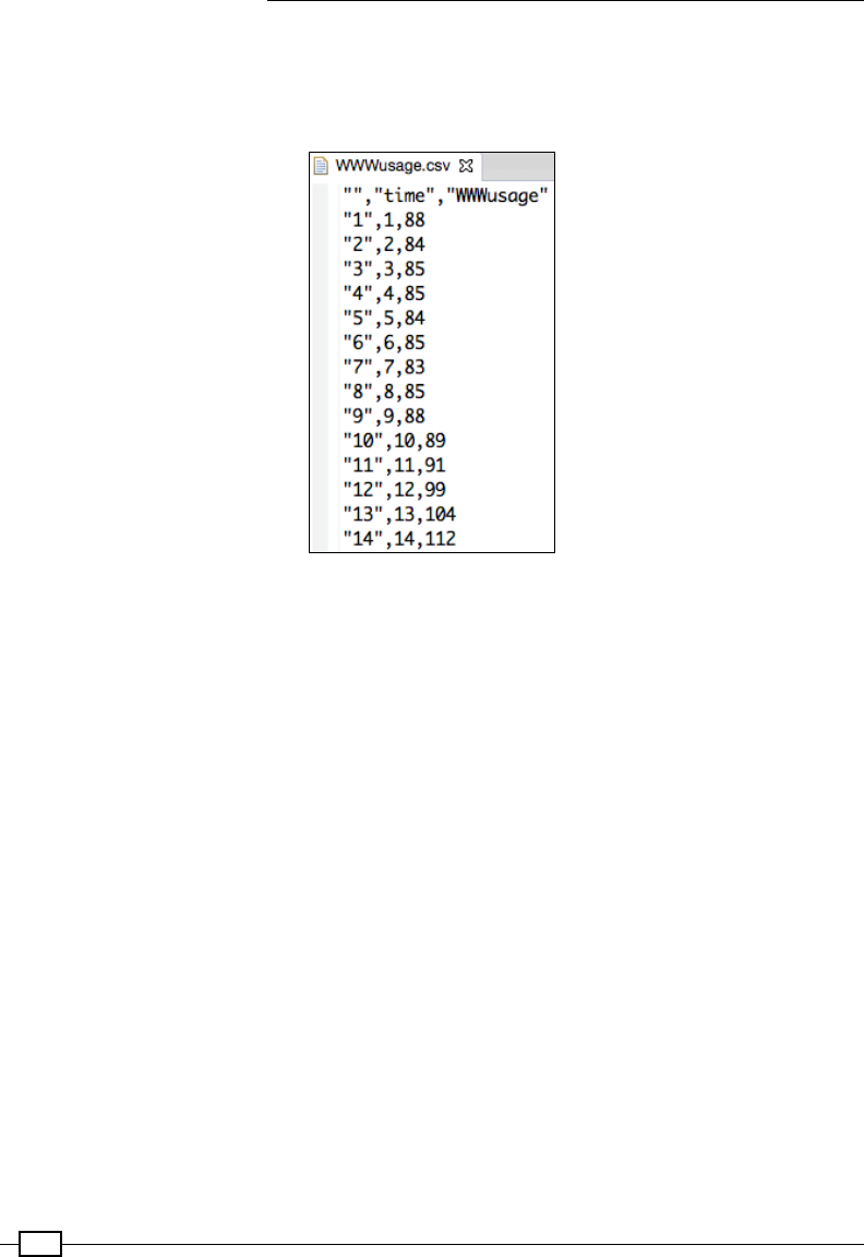
Getting Started with Breeze
410
Read the CSV as a matrix:
1. Let's use the csvread function to read a CSV le into a 100*3 matrix. We'll also skip
the header while reading and print 5 rows as a sample:
val usageMatrix=csvread(file=new File("WWWusage.csv"),
separator=',', skipLines=1)
//print first five rows
println ("Usage matrix \n"+ usageMatrix(0 to 5,::))
Output :
1.0 1.0 88.0
2.0 2.0 84.0
3.0 3.0 85.0
4.0 4.0 85.0
5.0 5.0 84.0
6.0 6.0 85.0
2. Extract a sub-matrix out of the read matrix:
For the sake of generating a submatrix let's skip the rst column and save the second
and the third column into a new matrix. Let's call it firstColumnSkipped:
val firstColumnSkipped= usageMatrix(::, 1 to
usageMatrix.cols-1)
//Sample some data so as to ensure we are fine
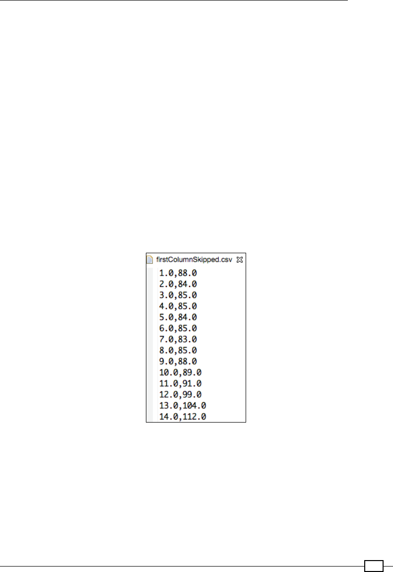
Chapter 1
411
println ("First Column skipped \n"+ firstColumnSkipped(0 to
5, ::))
Output :
1.0 88.0
2.0 84.0
3.0 85.0
4.0 85.0
5.0 84.0
6.0 85.0
3. Write the matrix:
As a nal step, let's write the firstColumnSkipped matrix to a new CSV le named
firstColumnSkipped.csv:
//Write this modified matrix to a file
csvwrite(file=new File ("firstColumnSkipped.csv"),
mat=firstColumnSkipped, separator=',')

413
2
Getting Started
with Apache Spark
DataFrames
In this chapter, we will cover the following recipes:
fGetting Apache Spark
fCreating a DataFrame from CSV
fManipulating DataFrames
fCreating a DataFrame from Scala case classes
Introduction
Apache Spark is a cluster computing platform that claims to run about 10 times faster than
Hadoop. In general terms, we could consider it as a means to run our complex logic over
massive amounts of data at a blazingly fast speed. The other good thing about Spark is that
the programs that we write are much smaller than the typical MapReduce classes that we write
for Hadoop. So, not only do our programs run faster but it also takes less time to write them.
Spark has four major higher level tools built on top of the Spark Core: Spark Streaming, Spark
MLlib (machine learning), Spark SQL (an SQL interface for accessing the data), and GraphX
(for graph processing). The Spark Core is the heart of Spark. Spark provides higher level
abstractions in Scala, Java, and Python for data representation, serialization, scheduling,
metrics, and so on.

Getting Started with Apache Spark DataFrames
414
At the risk of stating the obvious, a DataFrame is one of the primary data structures
used in data analysis. They are just like an RDBMS table that organizes all your attributes
into columns and all your observations into rows. It's a great way to store and play with
heterogeneous data. In this chapter, we'll talk about DataFrames in Spark.
Getting Apache Spark
In this recipe, we'll take a look at how to bring Spark into our project (using SBT) and how
Spark works internally.
The code for this recipe can be found at https://github.com/
arunma/ScalaDataAnalysisCookbook/blob/master/
chapter1-spark-csv/build.sbt.

Chapter 2
415
How to do it...
Let's now throw some Spark dependencies into our build.sbt le so that we can start
playing with them in subsequent recipes. For now, we'll just focus on three of them: Spark
Core, Spark SQL, and Spark MLlib. We'll take a look at a host of other Spark dependencies
as we proceed further in this book:
1. Under a brand new folder (which will be your project root), create a new le called
build.sbt.
2. Next, let's add the Spark libraries to the project dependencies.
3. Note that Spark 1.4.x requires Scala 2.10.x. This becomes the rst section of our
build.sbt:
organization := "com.packt"
name := "chapter1-spark-csv"
scalaVersion := "2.10.4"
val sparkVersion="1.4.1"
libraryDependencies ++= Seq(
"org.apache.spark" %% "spark-core" % sparkVersion,
"org.apache.spark" %% "spark-sql" % sparkVersion,
"org.apache.spark" %% "spark-mllib" % sparkVersion
)
Creating a DataFrame from CSV
In this recipe, we'll look at how to create a new DataFrame from a delimiter-separated
values le.
The code for this recipe can be found at https://github.com/
arunma/ScalaDataAnalysisCookbook/blob/master/
chapter1-spark-csv/src/main/scala/com/packt/
scaladata/spark/csv/DataFrameCSV.scala.
Getting Started with Apache Spark DataFrames
416
How to do it...
This recipe involves four steps:
1. Add the spark-csv support to our project.
2. Create a Spark Cong object that gives information on the environment that we are
running Spark in.
3. Create a Spark context that serves as an entry point into Spark. Then, we proceed
to create an SQLContext from the Spark context.
4. Load the CSV using the SQLContext.
5. CSV support isn't rst-class in Spark, but it is available through an external library
from Databricks. So, let's go ahead and add that to our build.sbt.
After adding the spark-csv dependency, our complete build.sbt looks like this:
organization := "com.packt"
name := "chapter1-spark-csv"
scalaVersion := "2.10.4"
val sparkVersion="1.4.1"
libraryDependencies ++= Seq(
"org.apache.spark" %% "spark-core" % sparkVersion,
"org.apache.spark" %% "spark-sql" % sparkVersion,
"com.databricks" %% "spark-csv" % "1.0.3"
)
6. SparkConf holds all of the information required to run this Spark "cluster." For this
recipe, we are running locally, and we intend to use only two cores in the machine—
local[2]. More details about this can be found in the There's more… section of
this recipe:
import org.apache.spark.SparkConf
val conf = new
SparkConf().setAppName("csvDataFrame").setMaster("local[2]")
When we say that the master of this run is "local," we mean that we
are running Spark on standalone mode. We'll see what "standalone"
mode means in the There's more… section.
Chapter 2
417
7. Initialize the Spark context with the Spark conguration. This is the core entry point
for doing anything with Spark:
import org.apache.spark.SparkContext
val sc = new SparkContext(conf)
The easiest way to query data in Spark is by using SQL queries:
import org.apache.spark.sql.SQLContext
val sqlContext=new SQLContext(sc)
8. Now, let's load our pipe-separated le. The students is of type org.apache.
spark.sql.DataFrame:
import com.databricks.spark.csv._
val students=sqlContext.csvFile(filePath="StudentData.csv",
useHeader=true, delimiter='|')
How it works...
The csvFile function of sqlContext accepts the full filePath of the le to be loaded.
If the CSV has a header, then the useHeader ag will read the rst row as column names.
The delimiter ag defaults to a comma, but you can override the character as needed.
Instead of using the csvFile function, we could also use the load function available in
SQLContext. The load function accepts the format of the le (in our case, it is CSV) and
options as Map. We can specify the same parameters that we specied earlier using Map,
like this:
val options=Map("header"->"true", "path"->"ModifiedStudent.csv")
val
newStudents=sqlContext.load("com.databricks.spark.csv",options)
There's more…
As we saw earlier, we now ran the Spark program in standalone mode. In standalone mode,
the Driver program (the brain) and the Worker nodes all get crammed into a single JVM.
In our example, we set master to local[2], which means that we intend to run Spark
in standalone mode and request it to use only two cores in the machine.
Spark can be run on three different modes:
fStandalone
fStandalone cluster, using its in-built cluster manager
fUsing external cluster managers, such as Apache Mesos and YARN
Getting Started with Apache Spark DataFrames
418
In Chapter 6, Scaling Up, we have dedicated explanations and recipes for how to run Spark
on inbuilt cluster modes on Mesos and YARN. In a clustered environment, Spark runs a Driver
program along with a number of Worker nodes. As the name indicates, the Driver program
houses the brain of the program, which is our main program. The Worker nodes have the
data and perform various transformations on it.
Manipulating DataFrames
In the previous recipe, we saw how to create a DataFrame. The next natural step, after
creating DataFrames, is to play with the data inside them. Other than the numerous functions
that help us to do that, we also nd other interesting functions that help us sample the data,
print the schema of the data, and so on. We'll take a look at them one by one in this recipe.
The code and the sample le for this recipe could be found at
https://github.com/arunma/ScalaDataAnalysisCookbook/
blob/master/chapter1-spark-csv/src/main/scala/com/
packt/scaladata/spark/csv/DataFrameCSV.scala.
How to do it...
Now, let's see how we can manipulate DataFrames using the following subrecipes:
fPrinting the schema of the DataFrame
fSampling data in the DataFrame
fSelecting specic columns in the DataFrame
fFiltering data by condition
fSorting data in the frame
fRenaming columns
fTreating the DataFrame as a relational table to execute SQL queries
fSaving the DataFrame as a le
Printing the schema of the DataFrame
After creating the DataFrame from various sources, we would obviously want to quickly check
its schema. The printSchema function lets us do just that. It prints our column names and
the data types to the default output stream:
1. Let's load a sample DataFrame from the StudentData.csv le:
//Now, lets load our pipe-separated file
//students is of type org.apache.spark.sql.DataFrame

Chapter 2
419
val
students=sqlContext.csvFile(filePath="StudentData.csv",
useHeader=true, delimiter='|')
2. Let's print the schema of this DataFrame:
students.printSchema
Output
root
|-- id: string (nullable = true)
|-- studentName: string (nullable = true)
|-- phone: string (nullable = true)
|-- email: string (nullable = true)
Sampling the data in the DataFrame
The next logical thing that we would like to do is to check whether our data got loaded into the
DataFrame correctly. There are a few ways of sampling the data in the newly created DataFrame:
fUsing the show method. This is the simplest way. There are two variants of the show
method, as explained here:
One with an integer parameter that specifies the number of rows to be
sampled.
The second is without the integer parameter. In it, the number of rows
defaults to 20.
The distinct quality about the show method as compared to the other functions that
sample data is that it displays the rows along with the headers and prints the output
directly to the default output stream (console):
//Sample n records along with headers
students.show (3)
//Sample 20 records along with headers
students.show ()
//Output of show(3)
+--+-----------+--------------+--------------------+
|id|studentName| phone| email|

Getting Started with Apache Spark DataFrames
420
+--+-----------+--------------+--------------------+
| 1| Burke|1-300-746-8446|ullamcorper.velit...|
| 2| Kamal|1-668-571-5046|pede.Suspendisse@...|
| 3| Olga|1-956-311-1686|Aenean.eget.metus...|
+--+-----------+--------------+--------------------+
fUsing the head method. This method also accepts an integer parameter representing
the number of rows to be fetched. The head method returns an array of rows. To print
these rows, we can pass the println method to the foreach function of the arrays:
//Sample the first 5 records
students.head(5).foreach(println)
If you are not a great fan of head, you can use the take function, which is common
across all Scala sequences. The take method is just an alias of the head method
and delegates all its calls to head:
//Alias of head
students.take(5).foreach(println)
//Output
[1,Burke,1-300-746-8446,ullamcorper.velit.in@ametnullaDonec.co.uk]
[2,Kamal,1-668-571-5046,pede.Suspendisse@interdumenim.edu]
[3,Olga,1-956-311-1686,Aenean.eget.metus@dictumcursusNunc.edu]
[4,Belle,1-246-894-6340,vitae.aliquet.nec@neque.co.uk]
[5,Trevor,1-300-527-4967,dapibus.id@acturpisegestas.net]
Selecting DataFrame columns
As you have seen, all DataFrame columns have names. The select function helps us pick
and choose specic columns from a previously existing DataFrame and form a completely
new one out of it:
fSelecting a single column: Let's say that you would like to select only the email
column from a DataFrame. Since DataFrames are immutable, the selection returns
a new DataFrame:
val emailDataFrame:DataFrame=students.select("email")
Chapter 2
421
Now, we have a new DataFrame called emailDataFrame, which has only the e-mail
as its contents. Let's sample and check whether that is true:
emailDataFrame.show(3)
//Output
+--------------------+
| email|
+--------------------+
|ullamcorper.velit...|
|pede.Suspendisse@...|
|Aenean.eget.metus...|
+--------------------+
fSelecting more than one column: The select function actually accepts an arbitrary
number of column names, which means that you can easily select more than one
column from your source DataFrame:
val studentEmailDF=students.select("studentName", "email")
The only requirement is that the string parameters that specify must
be a valid column name. Otherwise, an org.apache.spark.sql.
AnalysisException exception is thrown. The printSchema
function serves as a quick reference for the column names.
Let's sample and check whether we have indeed selected the studentName and
email columns in the new DataFrame:
studentEmailDF.show(3)
Output
+-----------+--------------------+
|studentName| email|
+-----------+--------------------+
| Burke|ullamcorper.velit...|
| Kamal|pede.Suspendisse@...|
| Olga|Aenean.eget.metus...|
+-----------+--------------------+

Getting Started with Apache Spark DataFrames
422
Filtering data by condition
Now that we have seen how to select columns from a DataFrame, let's see how to lter the
rows of a DataFrame based on conditions. For row-based ltering, we can treat the DataFrame
as a normal Scala collection and lter the data based on a condition. In all of these examples,
I have added the show method at the end for clarity:
1. Filtering based on a column value:
//Print the first 5 records that has student id more than 5
students.filter("id > 5").show(7)
Output
+--+-----------+--------------+--------------------+
|id|studentName| phone| email|
+--+-----------+--------------+--------------------+
| 6| Laurel|1-691-379-9921|adipiscing@consec...|
| 7| Sara|1-608-140-1995|Donec.nibh@enimEt...|
| 8| Kaseem|1-881-586-2689|cursus.et.magna@e...|
| 9| Lev|1-916-367-5608|Vivamus.nisi@ipsu...|
|10| Maya|1-271-683-2698|accumsan.convalli...|
|11| Emi|1-467-270-1337| est@nunc.com|
|12| Caleb|1-683-212-0896|Suspendisse@Quisq...|
+--+-----------+--------------+--------------------+
Notice that even though the id eld is inferenced as a String type, it does the
numerical comparison correctly. On the other hand, students.filter("email >
'c'") would give back all the e-mail IDs that start with a character greater than 'c'.
2. Filtering based on an empty column value. The following lter selects all students
without names:
students.filter("studentName =''").show(7)
Output
+--+-----------+--------------+--------------------+
|id|studentName| phone| email|
+--+-----------+--------------+--------------------+
|21| |1-598-439-7549|consectetuer.adip...|
|32| |1-184-895-9602|accumsan.laoreet@...|

Chapter 2
423
|45| |1-245-752-0481|Suspendisse.eleif...|
|83| |1-858-810-2204|sociis.natoque@eu...|
|94| |1-443-410-7878|Praesent.eu.nulla...|
+--+-----------+--------------+--------------------+
3. Filtering based on more than one condition. This lter shows all records whose
student names are empty or student name eld has a NULL string value:
students.filter("studentName ='' OR studentName = 'NULL'").show(7)
Output
+--+-----------+--------------+--------------------+
|id|studentName| phone| email|
+--+-----------+--------------+--------------------+
|21| |1-598-439-7549|consectetuer.adip...|
|32| |1-184-895-9602|accumsan.laoreet@...|
|33| NULL|1-105-503-0141|Donec@Inmipede.co.uk|
|45| |1-245-752-0481|Suspendisse.eleif...|
|83| |1-858-810-2204|sociis.natoque@eu...|
|94| |1-443-410-7878|Praesent.eu.nulla...|
+--+-----------+--------------+--------------------+
We are just limiting the output to seven records using the show(7) function.
4. Filtering based on SQL-like conditions.
This lter gets the entries of all students whose names start with the letter 'M'.
students.filter("SUBSTR(studentName,0,1) ='M'").show(7)
Output
+--+-----------+--------------+--------------------+
|id|studentName| phone| email|
+--+-----------+--------------+--------------------+
|10| Maya|1-271-683-2698|accumsan.convalli...|
|19| Malachi|1-608-637-2772|Proin.mi.Aliquam@...|
|24| Marsden|1-477-629-7528|Donec.dignissim.m...|
|37| Maggy|1-910-887-6777|facilisi.Sed.nequ...|
|61| Maxine|1-422-863-3041|aliquet.molestie....|
|77| Maggy|1-613-147-4380| pellentesque@mi.net|
|97| Maxwell|1-607-205-1273|metus.In@musAenea...|
+--+-----------+--------------+--------------------+

Getting Started with Apache Spark DataFrames
424
Sorting data in the frame
Using the sort function, we can order the DataFrame by a particular column:
1. Ordering by a column in descending order:
students.sort(students("studentName").desc).show(7)
Output
+--+-----------+--------------+--------------------+
|id|studentName| phone| email|
+--+-----------+--------------+--------------------+
|50| Yasir|1-282-511-4445|eget.odio.Aliquam...|
|52| Xena|1-527-990-8606|in.faucibus.orci@...|
|86| Xandra|1-677-708-5691|libero@arcuVestib...|
|43| Wynter|1-440-544-1851|amet.risus.Donec@...|
|31| Wallace|1-144-220-8159| lorem.lorem@non.net|
|66| Vance|1-268-680-0857|pellentesque@netu...|
|41| Tyrone|1-907-383-5293|non.bibendum.sed@...|
| 5| Trevor|1-300-527-4967|dapibus.id@acturp...|
|65| Tiger|1-316-930-7880|nec@mollisnoncurs...|
|15| Tarik|1-398-171-2268|turpis@felisorci.com|
+--+-----------+--------------+--------------------+
2. Ordering by more than one column (ascending):
students.sort("studentName", "id").show(10)
Output
+--+-----------+--------------+--------------------+
|id|studentName| phone| email|
+--+-----------+--------------+--------------------+
|21| |1-598-439-7549|consectetuer.adip...|
|32| |1-184-895-9602|accumsan.laoreet@...|
|45| |1-245-752-0481|Suspendisse.eleif...|
|83| |1-858-810-2204|sociis.natoque@eu...|
|94| |1-443-410-7878|Praesent.eu.nulla...|
|91| Abel|1-530-527-7467| urna@veliteu.edu|

Chapter 2
425
|69| Aiko|1-682-230-7013|turpis.vitae.puru...|
|47| Alma|1-747-382-6775| nec.enim@non.org|
|26| Amela|1-526-909-2605| in@vitaesodales.edu|
|16| Amena|1-878-250-3129|lorem.luctus.ut@s...|
+--+-----------+--------------+--------------------+
Alternatively, the orderBy alias of the sort function can be used to achieve this. Also,
multiple column orders could be specied using the DataFrame's apply method:
students.sort(students("studentName").desc, students("id").asc).show(10)
Renaming columns
If we don't like the column names of the source DataFrame and wish to change them
to something nice and meaningful, we can do that using the as function while selecting
the columns.
In this example, we rename the "studentName" column to "name" and retain the "email"
column's name as is:
val copyOfStudents=students.select(students("studentName").as("name"),
students("email"))
copyOfStudents.show()
Output
+--------+--------------------+
| name| email|
+--------+--------------------+
| Burke|ullamcorper.velit...|
| Kamal|pede.Suspendisse@...|
| Olga|Aenean.eget.metus...|
| Belle|vitae.aliquet.nec...|
| Trevor|dapibus.id@acturp...|
| Laurel|adipiscing@consec...|
| Sara|Donec.nibh@enimEt...|
Getting Started with Apache Spark DataFrames
426
Treating the DataFrame as a relational table
The real power of DataFrames lies in the fact that we can treat it like a relational table and
use SQL to query. This involves two simple steps:
1. Register the students DataFrame as a table with the name "students" (or any
other name):
students.registerTempTable("students")
2. Query it using regular SQL:
val dfFilteredBySQL=sqlContext.sql("select * from students where
studentName!='' order by email desc")
dfFilteredBySQL.show(7)
id studentName phone email
87 Selma 1-601-330-4409 vulputate.velit@p
96 Channing 1-984-118-7533 viverra.Donec.tem
4 Belle 1-246-894-6340 vitae.aliquet.nec
78 Finn 1-213-781-6969 vestibulum.massa@
53 Kasper 1-155-575-9346 velit.eget@pedeCu
63 Dylan 1-417-943-8961 vehicula.aliquet@
35 Cadman 1-443-642-5919 ut.lacus@adipisci
The lifetime of the temporary table is tied to the life of the SQLContext
that was used to create the DataFrame.
Joining two DataFrames
Now that we have seen how to register a DataFrame as a table, let's see how to perform SQL-
like join operations on DataFrames.
Inner join
An inner join is the default join and it just gives those results that are matching on both
DataFrames when a condition is given:
val students1=sqlContext.csvFile(filePath="StudentPrep1.csv",
useHeader=true, delimiter='|')
val students2=sqlContext.csvFile(filePath="StudentPrep2.csv",
useHeader=true, delimiter='|')

Chapter 2
427
val studentsJoin=students1.join(students2, students1("id")===students2("
id"))
studentsJoin.show(studentsJoin.count.toInt)
The output is as follows:
Right outer join
A right outer join shows all the additional unmatched rows that are available in the right-hand-
side DataFrame. We can see from the following output that the entry with ID 999 from the
right- hand-side DataFrame is now shown:
val studentsRightOuterJoin=students1.join(students2, students1("id")===st
udents2("id"), "right_outer")
studentsRightOuterJoin.show(studentsRightOuterJoin.count.toInt)

Getting Started with Apache Spark DataFrames
428
Left outer join
Similar to a right outer join, a left outer join returns not only the matching rows, but also the
additional unmatched rows of the left-hand-side DataFrame:
val studentsLeftOuterJoin=students1.join(students2, students1("id")===st
udents2("id"), "left_outer")
studentsLeftOuterJoin.show(studentsLeftOuterJoin.count.toInt)
Saving the DataFrame as a le
As the next step, let's save a DataFrame in a le store. The load function, which we used in
an earlier recipe, has a similar-looking counterpart called save.
This involves two steps:
1. Create a map containing the various options that you would like the save method to
use. In this case, we specify the lename and ask it to have a header:
val options=Map("header"->"true", "path"->"ModifiedStudent.csv")
To keep it interesting, let's choose column names from the source DataFrame.
In this example, we pick the studentName and email columns and change the
studentName column's name to just name.
val copyOfStudents=students.select(students("studentName").
as("name"), students("email"))
2. Finally, save this new DataFrame with the headers in a le named
ModifiedStudent.csv:
copyOfStudents.save("com.databricks.spark.csv", SaveMode.
Overwrite, options)
The second argument is a little interesting. We can choose Overwrite (as we did here),
Append, Ignore, or ErrorIfExists. Overwrite— as the name implies—overwrites the
le if it already exists, Ignore ignores writing if the le exists, ErrorIfExists complains
for pre-existence of the le, and Append continues writing from the last edit location.
Throwing an error is the default behavior.

Chapter 2
429
The output of the save method looks like this:
Creating a DataFrame from Scala case
classes
In this recipe, we'll see how to create a new DataFrame from Scala case classes.
The code for this recipe can be found at https://github.com/
arunma/ScalaDataAnalysisCookbook/blob/master/chapter1-
spark-csv/src/main/scala/com/packt/scaladata/spark/
csv/DataFrameFromCaseClasses.scala.
How to do it...
1. We create a new entity called Employee with the id and name elds, like this:
case class Employee(id:Int, name:String)
Similar to the previous recipe, we create SparkContext and SQLContext.
val conf = new SparkConf().setAppName("colRowDataFrame").
setMaster("local[2]")
//Initialize Spark context with Spark configuration. This is the
core entry point to do anything with Spark
val sc = new SparkContext(conf)

Getting Started with Apache Spark DataFrames
430
//The easiest way to query data in Spark is to use SQL queries.
val sqlContext=new SQLContext(sc)
2. We can source these employee objects from a variety of sources, such as an
RDBMS data source, but for the sake of this example, we construct a list of
employees, as follows:
val listOfEmployees =List(Employee(1,"Arun"), Employee(2,
"Jason"), Employee (3, "Abhi"))
3. The next step is to pass the listOfEmployees to the createDataFrame function
of SQLContext. That's it! We now have a DataFrame. When we try to print the schema
using the printSchema method of the DataFrame, we will see that the DataFrame has
two columns, with names id and name, as dened in the case class:
//Pass in the Employees into the `createDataFrame` function.
val empFrame=sqlContext.createDataFrame(listOfEmployees)
empFrame.printSchema
Output:
root
|-- id: integer (nullable = false)
|-- name: string (nullable = true)
As you might have guessed, the schema of the DataFrame is inferenced from the
case class using reection.
4. We can get a different name for the DataFrame—other than the names specied in
the case class—using the withColumnRenamed function, as shown here:
val empFrameWithRenamedColumns=sqlContext.createDataFrame(listOf
Employees).withColumnRenamed("id", "empId")
empFrameWithRenamedColumns.printSchema
Output:
root
|-- empId: integer (nullable = false)
|-- name: string (nullable = true)

Chapter 2
431
5. Let's query the DataFrame using Spark's rst-class SQL support. Before that, however,
we'll have to register the DataFrame as a table. The registerTempTable, as we saw
in the previous recipe, helps us achieve this. With the following command, we will have
registered the DataFrame as a table by name "employeeTable"
"employeeTable"
empFrameWithRenamedColumns.registerTempTable("employeeTable")
6. Now, for the actual query. Let's arrange the DataFrame in descending order of names:
val sortedByNameEmployees=sqlContext.sql("select * from
employeeTable order by name desc")
sortedByNameEmployees.show()
Output:
+-----+-----+
|empId| name|
+-----+-----+
| 2|Jason|
| 1| Arun|
| 3| Abhi|
+-----+-----+
How it works...
The createDataFrame function accepts a sequence of scala.Product. Scala case
classes extend from Product, and therefore it ts in the budget. That said, we can actually
use a sequence of tuples to create a DataFrame, since tuples implement Product too:
val mobiles=sqlContext.createDataFrame(Seq((1,"Android"), (2, "iPhone")))
mobiles.printSchema
mobiles.show()
Output:
//Schema
root
|-- _1: integer (nullable = false)
|-- _2: string (nullable = true)

Getting Started with Apache Spark DataFrames
432
//Data
+--+-------+
|_1| _2|
+--+-------+
| 1|Android|
| 2| iPhone|
+--+-------+
Of course, you can rename the column using withColumnRenamed.

433
3
Loading and Preparing
Data – DataFrame
In this chapter, we will cover the following recipes:
fLoading more than 22 features into classes
fLoading JSON into DataFrames
fStoring data as Parquet les
fUsing the Avro data model in Parquet
fLoading from RDBMS
fPreparing data in DataFrames
Introduction
In previous chapters, we saw how to import data from a CSV le to Breeze and Spark
DataFrames. However, almost all the time, the source data that is to be analyzed is available
in a variety of source formats. Spark, with its DataFrame API, provides a uniform API that
can be used to represent any source (or multiple sources). In this chapter, we'll focus on the
various input formats that we can load from in Spark. Towards the end of this chapter, we'll
also briey see some data preparation recipes.
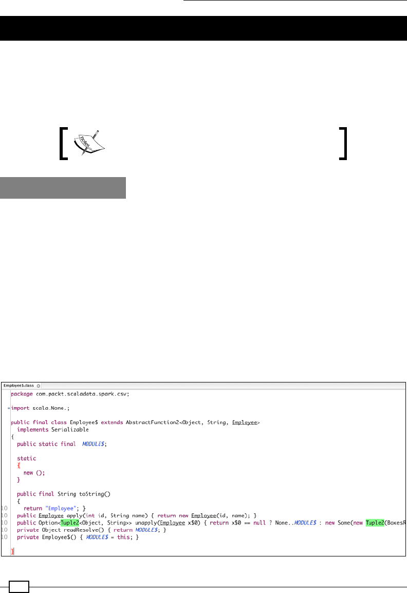
Loading and Preparing Data – DataFrame
434
Loading more than 22 features into classes
Case classes have an inherent limitation. They can hold only 22 attributes—Catch 22,
if you will. While a reasonable percentage of datasets would t in that budget, in many
cases, the limitation of 22 features in a dataset is a huge turnoff. In this recipe, we'll
take a sample Student dataset (http://archive.ics.uci.edu/ml/datasets/
Student+Performance), which has 33 features, and we'll see how we can work around this.
The 22-eld limit is resolved in Scala version 2.11.
However, Spark 1.4 uses Scala 2.10.
How to do it...
Case classes in Scala cannot go beyond encapsulating 22 elds because the companion
classes that are generated (during compilation) for these case classes cannot nd the
matching FunctionN and TupleN classes. Let's take the example of the Employee case
class that we created in Chapter 2, Getting Started with Apache Spark DataFrames:
case class Employee(id:Int, name:String)
When we look at its decompiled companion object, we notice that for the two constructor
parameters of the case class, the companion class uses Tuple2 and AbstractFunction2
in its unapply method, the method that gets invoked when we pattern-match against a
case class. The problem we face is that the Scala library has objects only until Tuple22 and
Function22 (probably because outside the data analysis world, having an entity object with
10 elds is not a great idea). However, there is a simple yet powerful workaround, and we will
be seeing it in this recipe.
Chapter 3
435
We saw in Chapter 2, Getting Started with Apache Spark DataFrames (in the Creating
a DataFrame from CSV recipe), that the requirement for creating a DataFrame using
SQLContext.createDataFrame from a collection of classes is that the class must
extend scala.Product. So, what we intend to do is write our own class that extends
from scala.Product.
This recipe consists of four steps:
1. Creating SQLContext from SparkContext and Config.
2. Creating a Student class that extends Product and overrides the necessary
functions.
3. Constructing an RDD of the Student classes from the sample dataset
(student-mat.csv).
4. Creating a DataFrame from the RDD, followed by printing the schema and
sampling the data.
Refer to the How it works… section of this recipe for a basic
introduction to RDD.
The code for this recipe can be found at https://github.com/
arunma/ScalaDataAnalysisCookbook/tree/master/
chapter3-data-loading.
Let's now cover these steps in detail:
1. Creating SQLContext: As with our recipes from the previous chapter, we construct
SparkContext from SparkConfig and then create an SQLContext from
SparkContext:
val conf=new
SparkConf().setAppName("DataWith33Atts").setMaster("local[2]")
val sc=new SparkContext(conf)
val sqlContext=new SQLContext(sc)
2. Creating the Student class: Our next step is to create a simple Scala class that
declares its constructor parameters, and make it extend Product.
Making a class extend Product requires us to override two functions from
scala.Product and one function from scala.Equals (which scala.Product,
in turn, extends from). The implementation of each of these functions is pretty
straightforward.
Refer to the API docs of Product (http://www.scala-lang.
org/api/2.10.4/index.html#scala.Product) and
Equals (http://www.scala-lang.org/api/2.10.4/
index.html#scala.Equals) for more details.

Loading and Preparing Data – DataFrame
436
Firstly, let's make our Student class declare its elds and extend Product:
class Student (school:String,
sex:String,
age:Int,
address:String,
famsize:String,
pstatus:String,
medu:Int,
fedu:Int,
mjob:String,
fjob:String,
reason:String,
guardian:String,
traveltime:Int,
studytime:Int,
failures:Int,
schoolsup:String,
famsup:String,
paid:String,
activities:String,
nursery:String,
higher:String,
internet:String,
romantic:String,
famrel:Int,
freetime:Int,
goout:Int,
dalc:Int,
walc:Int,
health:Int,
absences:Int,
g1:Int,
g2:Int,
g3:Int) extends Product{
Next, let's implement these three functions after briey looking at what they are
expected to do:
productArity():Int: This returns the size of the attributes. In our case,
it's 33. So, our implementation looks like this:
override def productArity: Int = 33

Chapter 3
437
productElement(n:Int):Any: Given an index, this returns the
attribute. As protection, we also have a default case, which throws
an IndexOutOfBoundsException exception:
@throws(classOf[IndexOutOfBoundsException])
override def productElement(n: Int): Any = n match {
case 0 => school
case 1 => sex
case 2 => age
case 3 => address
case 4 => famsize
case 5 => pstatus
case 6 => medu
case 7 => fedu
case 8 => mjob
case 9 => fjob
case 10 => reason
case 11 => guardian
case 12 => traveltime
case 13 => studytime
case 14 => failures
case 15 => schoolsup
case 16 => famsup
case 17 => paid
case 18 => activities
case 19 => nursery
case 20 => higher
case 21 => internet
case 22 => romantic
case 23 => famrel
case 24 => freetime
case 25 => goout
case 26 => dalc
case 27 => walc
case 28 => health
case 29 => absences
case 30 => g1
case 31 => g2
case 32 => g3
case _ => throw new
IndexOutOfBoundsException(n.toString())
}

Loading and Preparing Data – DataFrame
438
canEqual (that:Any):Boolean: This is the last of the three functions,
and it serves as a boundary condition when an equality check is being done
against this class:
override def canEqual(that: Any): Boolean =
that.isInstanceOf[Student]
3. Constructing an RDD of students from the student-mat.csv le: Now that we
have our Student class ready, let's convert the "student-mat.csv" input le
into a DataFrame:
val rddOfStudents=convertCSVToStudents("student-mat.csv", sc)
def convertCSVToStudents(filePath: String, sc: SparkContext):
RDD[Student] = {
val rddOfStudents: RDD[Student] = sc.textFile(filePath).
flatMap(eachLine => Student(eachLine))
rddOfStudents
}
As you can see, we have an apply method for Student that accepts a String and
returns an Option[Student]. We use flatMap to lter out None thereby resulting
in RDD[Student].
Let's look at the Student companion object's apply function. It's a very simple
function that takes a String, splits it based on semicolons into an array, and then
passes the parameters to the Student's constructor. The method returns None if
there is an error:
object Student {
def apply(str: String): Option[Student] = {
val paramArray = str.split(";").map(param =>
param.replaceAll("\"", "")) //Few values have extra double
quotes around it
Try(
new Student(paramArray(0),
paramArray(1),
paramArray(2).toInt,
paramArray(3),
paramArray(4),
paramArray(5),
paramArray(6).toInt,
paramArray(7).toInt,
paramArray(8),
Chapter 3
439
paramArray(9),
paramArray(10),
paramArray(11),
paramArray(12).toInt,
paramArray(13).toInt,
paramArray(14).toInt,
paramArray(15),
paramArray(16),
paramArray(17),
paramArray(18),
paramArray(19),
paramArray(20),
paramArray(21),
paramArray(22),
paramArray(23).toInt,
paramArray(24).toInt,
paramArray(25).toInt,
paramArray(26).toInt,
paramArray(27).toInt,
paramArray(28).toInt,
paramArray(29).toInt,
paramArray(30).toInt,
paramArray(31).toInt,
paramArray(32).toInt)) match {
case Success(student) => Some(student)
case Failure(throwable) => {
println (throwable.getMessage())
None
}
}
}
4. Creating a DataFrame, printing the schema, and sampling: Finally, we create
a DataFrame from RDD[Student]. Converting an RDD[T] to a DataFrame
of the same type is just a matter of calling the toDF() function. You are
required to import sqlContext.implicits._. Optionally, you can use
the createDataFrame method of sqlContext too.
The toDF() function is overloaded so as to accept custom
column names while converting to a DataFrame.

Loading and Preparing Data – DataFrame
440
We then print the schema using the DataFrame's printSchema() method and
sample data for conrmation using the show() method:
import sqlContext.implicits._
//Create DataFrame
val studentDFrame = rddOfStudents.toDF()
studentDFrame.printSchema()
studentDFrame.show()
The following is the output of the preceding code:
root
|-- school: string (nullable = true)
|-- sex: string (nullable = true)
|-- age: integer (nullable = false)
|-- address: string (nullable = true)
|-- famsize: string (nullable = true)
|-- pstatus: string (nullable = true)
|-- medu: integer (nullable = false)
|-- fedu: integer (nullable = false)
|-- mjob: string (nullable = true)
|-- fjob: string (nullable = true)
|-- reason: string (nullable = true)
|-- guardian: string (nullable = true)
|-- traveltime: integer (nullable = false)
|-- studytime: integer (nullable = false)
|-- failures: integer (nullable = false)
|-- schoolsup: string (nullable = true)
|-- famsup: string (nullable = true)
|-- paid: string (nullable = true)
|-- activities: string (nullable = true)
|-- nursery: string (nullable = true)
|-- higher: string (nullable = true)
|-- internet: string (nullable = true)
|-- romantic: string (nullable = true)
|-- famrel: integer (nullable = false)
|-- freetime: integer (nullable = false)
|-- goout: integer (nullable = false)
|-- dalc: integer (nullable = false)
|-- walc: integer (nullable = false)
|-- health: integer (nullable = false)
|-- absences: integer (nullable = false)
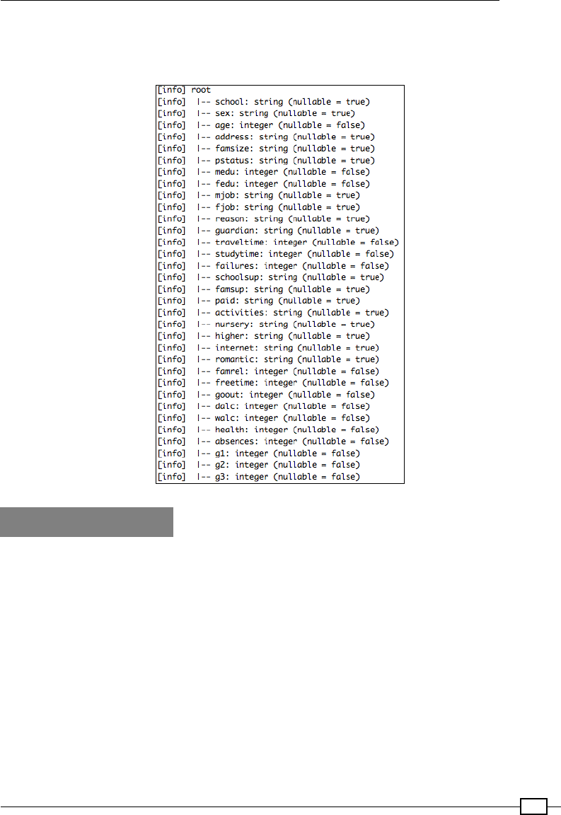
Chapter 3
441
|-- g1: integer (nullable = false)
|-- g2: integer (nullable = false)
|-- g3: integer (nullable = false)
How it works...
The foundation of Spark is the Resilient Distributed Dataset (RDD). From a programmer's
perspective, the composability of RDDs just like a regular Scala collection is a huge
advantage. An RDD wraps three vital (and two subsidiary) pieces of information that help in
the reconstruction of data. This enables fault tolerance. The other major advantage is that
while RDDs can be composed into hugely complex graphs using RDD operations, the entire
ow of data itself is not very difcult to reason with.
Other than optional optimization attributes (such as data location), at its core, RDD just
wraps three vital pieces of information:
fThe dependent/parent RDD (empty if not available)
fThe number of partitions
fThe function that needs to be applied to each element of the RDD
Loading and Preparing Data – DataFrame
442
In simple words, RDDs are just collections of data elements that can exist in the memory or
on the disk. These data elements must be serializable in order to have the capability to be
moved across multiple machines (or be serialized on the disk). The number of partitions or
blocks of data is primarily determined by the source of the input data (say, if the data is in
HDFS, then each block would translate to a single partition), but there are also other ways
of playing around with the number of partitions.
So, the number of partitions could be any of these:
fDictated by the input data itself, for example, the number of blocks in the case
of reading les from HDFS
fThe number set by the spark.default.parallelism parameter (set while
starting the cluster)
fThe number set by calling repartition or coalesce on the RDD itself
Note that currently, for all our recipes, we are running our Spark application in the self-
contained single JVM mode. While the programs work just ne, we are not yet exploiting
the distributed nature of the RDDs. In Chapter 6, Scaling Up, we'll explore how to bundle
and deploy our Spark application on a variety of cluster managers: YARN, Spark standalone
clusters, and Mesos.
There's more…
In the previous chapter, we created a DataFrame from a List of Employee case classes:
val listOfEmployees =List(Employee(1,"Arun"), Employee(2, "Jason"),
Employee (3, "Abhi"))
val empFrame=sqlContext.createDataFrame(listOfEmployees)
However, in this recipe, we loaded a le, converted them to RDD[String], transformed them
into case classes, and nally converted them into a DataFrame.
There are subtle, yet powerful, differences in these approaches. In the rst approach (converting
a List of case classes into a DataFrame), we have the entire collection in the memory of the
driver (we'll look at drivers and workers in Chapter 6, Scaling Up). Except for playing around
with Spark, for all practical purposes, we don't have our dataset as a collection of case classes.
We generally have it as a text le or read from a database. Also, requiring to hold the entire
collection in a single machine before converting it into a distributed dataset (RDD) will unfold
itself as a memory issue.
Chapter 3
443
In this recipe, we loaded an HDFS distributed le as an RDD[String] that is distributed
across a cluster of worker nodes, and then serialized each String into a case class, making
the RDD[String] into an RDD[Student]. So, each worker node that holds some partitions
of the dataset handles the computation around transforming RDD[String] to the case class,
while making the resulting dataset conform to a xed schema enforced by the case class
itself. Since the computation and the data itself are distributed, we don't need to worry about
a single machine requiring a lot of memory to store the entire dataset.
Loading JSON into DataFrames
JSON has become the most common text-based data representation format these days. In
this recipe, we'll see how to load data represented as JSON into our DataFrame. To make it
more interesting, let's have our JSON in HDFS instead of our local lesystem.
The Hadoop Distributed File System (HDFS) is a highly distributed lesystem that is both
scalable and fault tolerant. It is a critical part of the Hadoop ecosystem and is inspired by
the Google File System paper (http://research.google.com/archive/gfs.html).
More details about the architecture and communication protocols on HDFS can be found at
http://hadoop.apache.org/docs/r1.2.1/hdfs_design.html.
How to do it…
In this recipe, we'll see three subrecipes:
fHow to create a schema-inferenced DataFrame from JSON using
sqlContext.jsonFile
fAlternatively, if we prefer to preprocess the input le before parsing it into JSON, we'll
parse the input le as text and convert it into JSON using sqlContext.jsonRDD
fFinally, we'll take a look at declaring an explicit schema and using it to create
a DataFrame
Reading a JSON le using SQLContext.jsonFile
This recipe consists of three steps:
1. Storing our json (profiles.json) in HDFS: A copy of the data le is added to our
project repository, and it can be downloaded from https://github.com/arunma/
ScalaDataAnalysisCookbook/blob/master/chapter3-data-loading/
profiles.json:
hadoop fs -mkdir -p /data/scalada
hadoop fs -put profiles.json /data/scalada/profiles.json
hadoop fs -ls /data/scalada
-rw-r--r-- 1 Gabriel supergroup 176948 2015-05-16 22:13 /
data/scalada/profiles.json

Loading and Preparing Data – DataFrame
444
The following screenshot shows the HDFS le explorer available at
http://localhost:50070, which conrms that our upload is successful:
2. Creating contexts: We do the regular stuff—create SparkConfig, SparkContext,
and then SQLContext:
val conf = new
SparkConf().setAppName("DataFromJSON").setMaster("local[2]")
val sc = new SparkContext(conf)
val sqlContext = new SQLContext(sc)
3. Creating a DataFrame from JSON: In this step, we use the jsonFile function of
SQLContext to create a DataFrame. This is very similar to the sqlContext.
csvFile function that we used in Chapter 2, Getting Started with Apache Spark
DataFrames. There's just one thing that we need to watch out here; our .json
should be formatted as one line per record. It is unusual to store JSON as one line
per record considering that it is a structured format, but the jsonFile function
treats every single line as one record, failing to do which it would throw a scala.
MatchError error while parsing:
val
dFrame=sqlContext.jsonFile("hdfs://localhost:9000/data/scalada/
profiles.json")
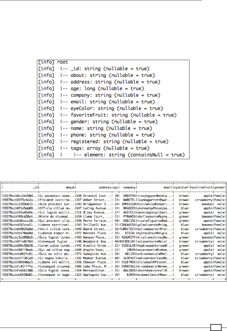
Chapter 3
445
That's it! We are done! Let's just print the schema and sample the data:
dFrame.printSchema()
dFrame.show()
The following screenshot shows the schema that is inferenced from the JSON le. Note that now
the age is resolved as long and tags are resolved as an array of string, as you can see here:
The next screenshot shows you a sample of the dataset:
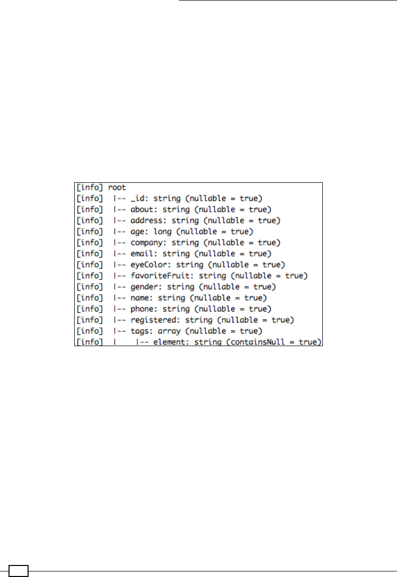
Loading and Preparing Data – DataFrame
446
Reading a text le and converting it to JSON RDD
In the previous section, we saw how we can directly import a textFile containing JSON
records as a DataFrame using sqlContext.jsonFile. Now, we'll see an alternate approach,
wherein we construct an RDD[String] from the same profiles.json le and then convert
them into a DataFrame. This has a distinct advantage from the previous approach—we can have
more control over the schema instead of relying on the one that is inferenced:
val strRDD=sc.textFile("hdfs://localhost:9000/data/scalada/profiles.
json")
val jsonDf=sqlContext.jsonRDD(strRDD)
jsonDf.printSchema()
The following is the output of the preceding command:
Explicitly specifying your schema
Using jsonRDD and letting it resolve the schema by itself is clean and simple. However,
it gives less control over the types; for example, the age eld must be Integer and not
Long. Similarly, the `registered` column is inferenced as a String while it is actually a
TimeStamp. In order to achieve this, let's go ahead and declare our own schema. The way we
do this is by constructing a StructType and StructField:
val profilesSchema = StructType(
Seq(
StructField("_id",StringType, true),
StructField("about",StringType, true),
StructField("address",StringType, true),
StructField("age",IntegerType, true),
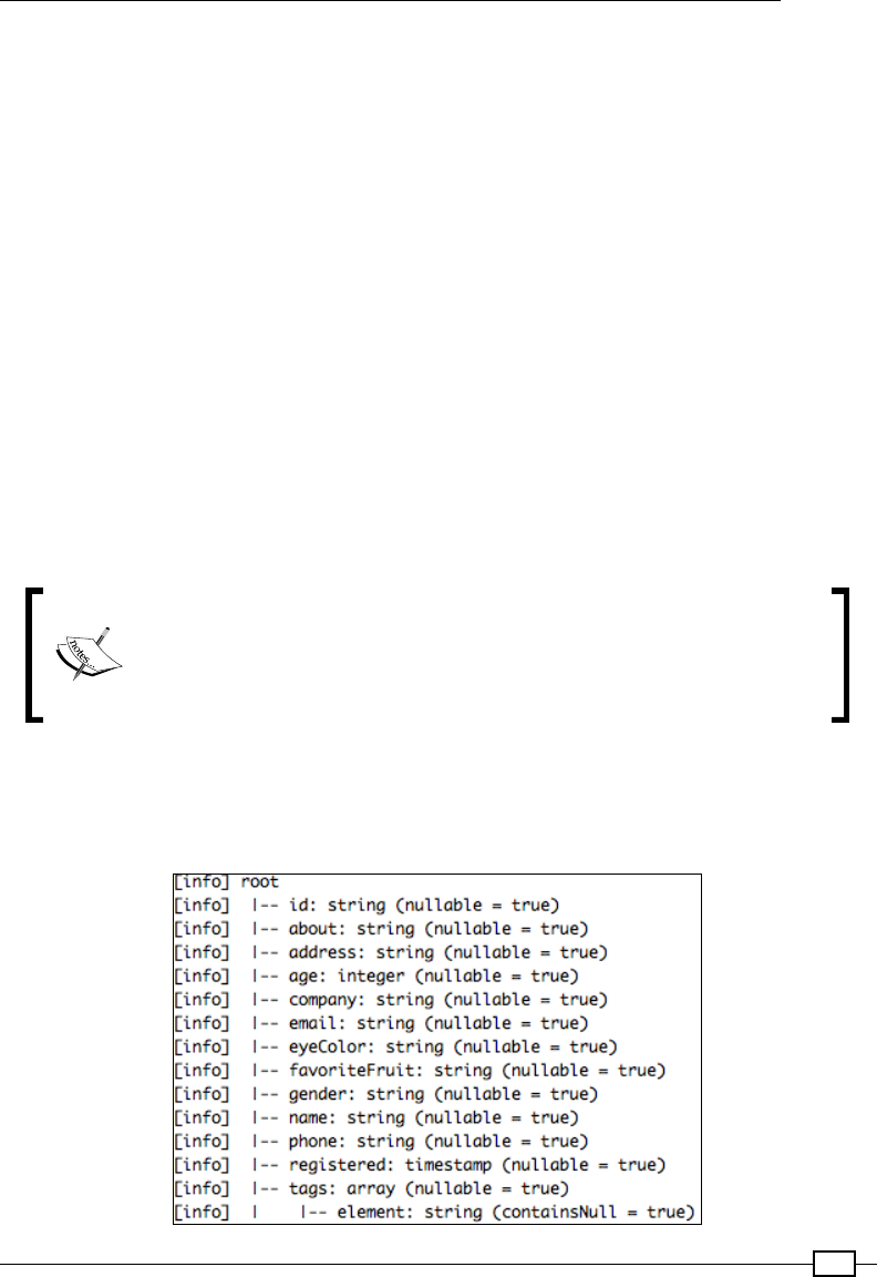
Chapter 3
447
StructField("company",StringType, true),
StructField("email",StringType, true),
StructField("eyeColor",StringType, true),
StructField("favoriteFruit",StringType, true),
StructField("gender",StringType, true),
StructField("name",StringType, true),
StructField("phone",StringType, true),
StructField("registered",TimestampType, true),
StructField("tags",ArrayType(StringType), true)
)
)
val jsonDfWithSchema=sqlContext.jsonRDD(strRDD, profilesSchema)
jsonDfWithSchema.printSchema() //Has timestamp
jsonDfWithSchema.show()
Another advantage of specifying our own schema is that all the columns
need not be specied in the StructType. We just need to specify the
columns that we are interested in, and only those columns will be available
in the target DataFrame. Also, any column that is declared in the schema
but is not available in the dataset will be lled in with null values.
The following is the output.
We can see that the registered feature is considered to have a timestamp data type and
age as integer:
Loading and Preparing Data – DataFrame
448
Finally, just for kicks, let's re a lter query based on the timestamp. This involves three steps:
1. Register the schema as a temporary table for querying, as has been done several
times in previous recipes. The following line of code registers a table by the name of
profilesTable:
jsonRDDWithSchema.registerTempTable("profilesTable")
2. Let's re away our lter query. The following query returns all proles that have been
registered after August 26, 2014. Since the registered eld is a timestamp, we
require an additional minor step of casting the parameter into a TimeStamp:
val filterCount = sqlContext.sql("select * from profilesTable
where registered> CAST('2014-08-26 00:00:00' AS TIMESTAMP)").count
3. Let's print the count:
println("Filtered based on timestamp count : " + filterCount)
//106
There's more…
If you aren't comfortable with having the schema in the code and would like to save the
schema in a le, it's just a one-liner for you:
import scala.reflect.io.File
import scala.io.Source
//Writes schema as JSON to file
File("profileSchema.json").writeAll(profilesSchema.json)
Obviously, you would want to reconstruct the schema from JSON, and that's also a one-liner:
val loadedSchema = DataType.fromJson(Source.fromFile("profileSchema.
json").mkString)
Let's check whether the loadedSchema and the profileSchema encapsulate the same
schema by doing an equality check on their json:
println ("ProfileSchema == loadedSchema :"+(loadedSchema.
json==profilesSchema.json))
The output is shown as follows:
ProfileSchema == loadedSchema :true
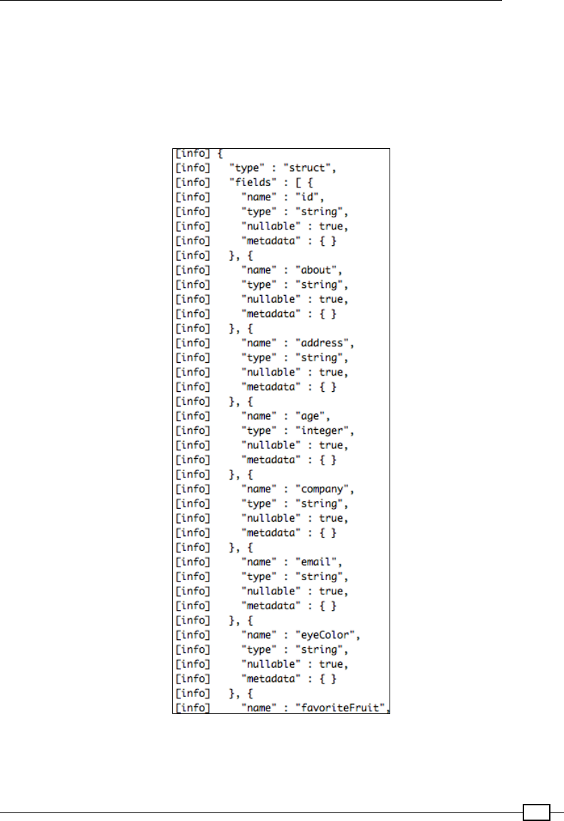
Chapter 3
449
If we would like to eyeball the json, we have a nice method called prettyJson that formats
the json:
//Print loaded schema
println(loadedSchema.prettyJson)
The output is as follows:
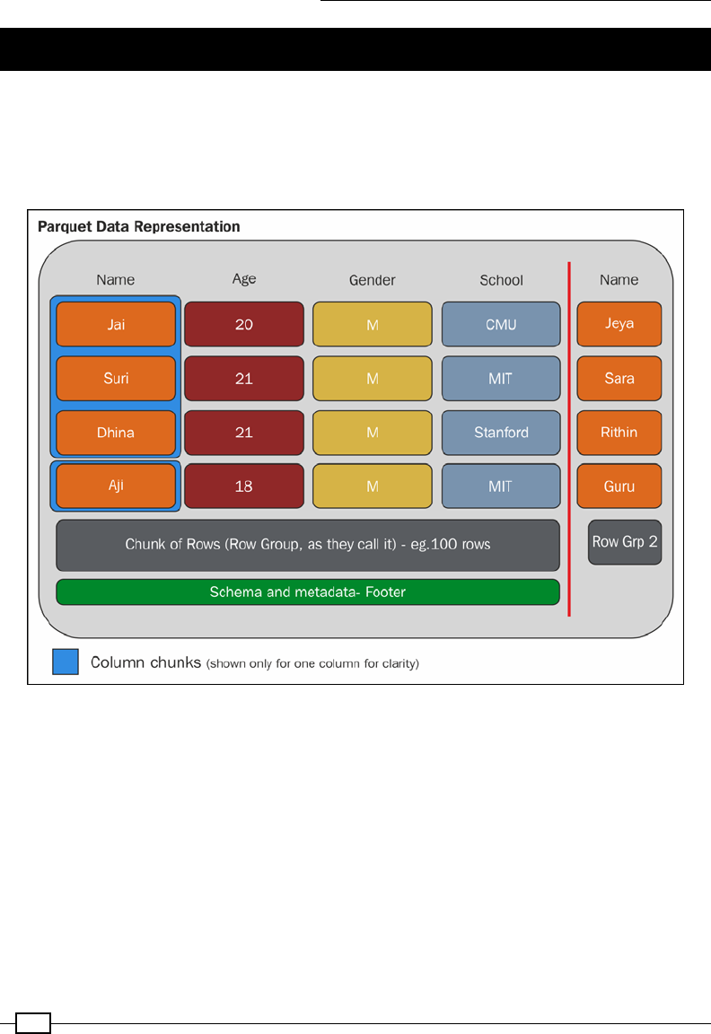
Loading and Preparing Data – DataFrame
450
Storing data as Parquet les
Parquet (https://parquet.apache.org/) is rapidly becoming the go-to data storage
format in the world of big data because of the distinct advantages it offers:
fIt has a column-based representation of data. This is better represented in a picture,
as follows:
As you can see in the preceding screenshot, Parquet stores data in chunks of
rows, say 100 rows. In Parquet terms, these are called RowGroups. Each of these
RowGroups has chunks of columns inside them (or column chunks). Column chunks
can hold more than a single unit of data for a particular column (as represented
in the blue box in the rst column). For example. Jai, Suri, and Dhina form a single
chunk even though they are composed of three single units of data for Name.
Another unique feature is that these column chunks (groups of a single column's
information) can be read independently. Let's consider the following image:
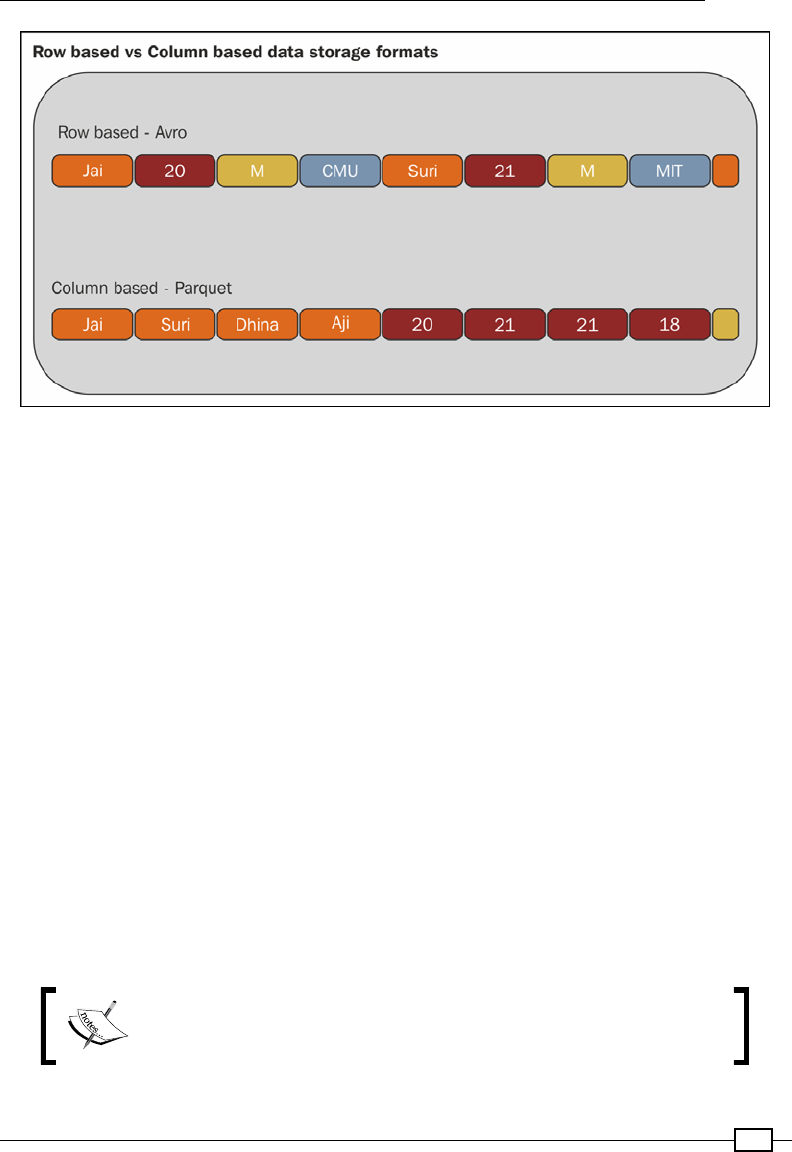
Chapter 3
451
We can see that the items of column data are stored next to each other in a
sequence. Since our queries are focused on just a few columns (a projection)
most of the time and not on the entire table, this storage mechanism enables
us to retrieve data much faster than reading the entire row data that is stored
and ltering for columns. Also, with Spark's in-memory computations, the memory
requirements are reduced in this way.
fThe second advantage is that there is very little that is needed for our transition from
the existing data models that we already use to represent the data. While Parquet
has its own native object model, we are pretty much free to choose Avro, ProtoBuf,
Thrift, and a variety of existing object models, and use an intermediate converter to
serialize our data in Parquet. Most of these converters are readily available at the
Parquet-MR project (https://github.com/Parquet/parquet-mr).
In this recipe, we'll cover the following steps:
1. Load a simple CSV le and convert it into a DataFrame.
2. Save it as a Parquet le.
3. Install Parquet tools.
4. Use the tools to inspect the Parquet le.
5. Enable compression for the Parquet le.
The entire code for this recipe can be found at https://github.
com/arunma/ScalaDataAnalysisCookbook/tree/master/
chapter3-data-loading-parquet.

Loading and Preparing Data – DataFrame
452
How to do it…
Before we dive into the steps, let's briey look at our build.sbt le, specically the library
dependencies and Avro settings (which we'll talk about in the following sections):
organization := "com.packt"
name := "chapter3-data-loading-parquet"
scalaVersion := "2.10.4"
val sparkVersion="1.4.1"
libraryDependencies ++= Seq(
"org.apache.spark" %% "spark-core" % sparkVersion,
"org.apache.spark" %% "spark-sql" % sparkVersion,
"org.apache.spark" %% "spark-mllib" % sparkVersion,
"org.apache.spark" %% "spark-hive" % sparkVersion,
"org.apache.avro" % "avro" % "1.7.7",
"org.apache.parquet" % "parquet-avro" % "1.8.1",
"com.twitter" %% "chill-avro" % "0.6.0"
)
resolvers ++= Seq(
"Apache HBase" at
"https://repository.apache.org/content/repositories/releases",
"Typesafe repository" at
"http://repo.typesafe.com/typesafe/releases/",
"Twitter" at "http://maven.twttr.com/"
)
fork := true
seq( sbtavro.SbtAvro.avroSettings : _*)
(stringType in avroConfig) := "String"
javaSource in sbtavro.SbtAvro.avroConfig <<= (sourceDirectory in
Compile)(_ / "java")
Now that we have build.sbt out of the way, let's go ahead and look at the code behind each
of the listed steps.
Chapter 3
453
Load a simple CSV le, convert it to case classes, and create a
DataFrame from it
We can actually create a DataFrame directly from CSV using the com.databricks/spark-
csv le, as we saw in Chapter 2, Getting Started with Apache Spark DataFrames, but for this
recipe, we'll just tokenize the CSV and create classes from it. The input CSV has a header
column. So, the conversion process involves skipping the rst row.
The class le that we will discuss in this section is the https://
github.com/arunma/ScalaDataAnalysisCookbook/blob/
master/chapter3-data-loading-parquet/src/main/
scala/com/packt/dataload/ParquetCaseClassMain.scala.
There are just two interesting things that you might notice in the code:
sqlContext.setConf("spark.sql.parquet.binaryAsString","true")
Some Parquet producing systems, such as Impala, binary encode the strings. In order to work
around this issue, we set the following conguration, which says that if it sees binary data,
it should be treated as a string:
Instead of using sqlContext.createDataFrame, we just use a toDF() on the
RDD[Student]. The SQLContext.Implicits object has a number of implicit conversions
that help us convert an RDD[T] to a DataFrame directly. The only requirement for us, as
expected, is to import the implicits:
import sqlContext.implicits._
The rest of the code is the same as we saw earlier:
val conf = new
SparkConf().setAppName("CaseClassToParquet").setMaster("local[2]")
val sc = new SparkContext(conf)
val sqlContext = new SQLContext(sc)
//Treat binary encoded values as Strings
sqlContext.setConf("spark.sql.parquet.binaryAsString","true")
import sqlContext.implicits._
//Convert each line into Student
val rddOfStudents = convertCSVToStudents("StudentData.csv", sc)
//Convert RDD[Student] to a Dataframe using sqlContext.implicits
val studentDFrame = rddOfStudents.toDF()
Loading and Preparing Data – DataFrame
454
The convertCSVToStudents method, which converts each line into a Student object,
looks like this:
def convertCSVToStudents(filePath: String, sc: SparkContext):
RDD[Student] = {
val rddOfStudents: RDD[Student]
=sc.textFile(filePath).flatMap(line => {
val data = line.split("\\|")
if (data(0) == "id") None else Some(Student(data(0),
data(1), data(2), data(3)))
})
rddOfStudents
}
Save it as a Parquet le
This is just a one-liner once we have the DataFrame. This can be done using either
the saveAsParquetFile or the save method. If you wish to save it in a Hive table
(https://hive.apache.org/), then there is also a saveAsTable method for you:
//Save DataFrame as Parquet using saveAsParquetFile
studentDFrame.saveAsParquetFile("studentPq.parquet")
//OR
//Save DataFrame as Parquet using the save method
studentDFrame.save("studentPq.parquet", "parquet",
SaveMode.Overwrite)
The save method allows the usage of SaveMode, which has the following
alternatives: Append, ErrorIfExists, Ignore, or Overwrite.
The save methods create a directory in the location that you specify (here, we simply store
it in our project directory). The directory holds the les that represent the serialized data.
It is not entirely human readable, but you may notice that the data of a single column is
stored together.
Just as we do for the rest of the recipes, let's read the le and sample the data for
conrmation:
//Read data for confirmation
val pqDFrame=sqlContext.parquetFile("studentPq.parquet")
pqDFrame.show()
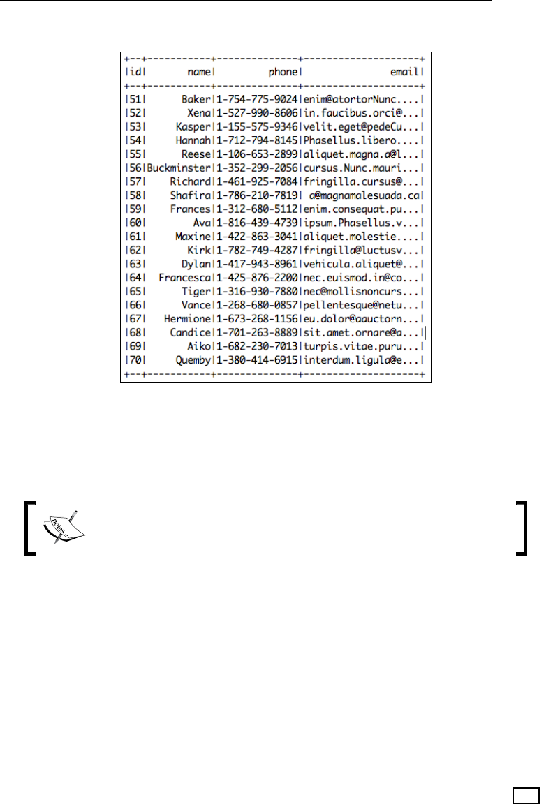
Chapter 3
455
The following is the output:
Install Parquet tools
Other than using the printSchema method of the DataFrame to inspect the schema, we can
use some interesting parquet tools provided as part of the parquet project to get a variety of
other information.
The parquet-tools is a subproject of Parquet and is available at
https://github.com/Parquet/parquet-mr/tree/master/
parquet-tools.
Since Spark 1.4.1 uses Parquet 1.6.0rc3, we'll need to download that version of the tools from
the Maven repository. The executables and the JARs can be downloaded as one bundle from
https://repo1.maven.org/maven2/com/twitter/parquet-tools/1.6.0rc3/
parquet-tools-1.6.0rc3-bin.tar.gz.
Using the tools to inspect the Parquet le
Let's put the tools into action. Specically, we'll do three things in this step:
fDisplay the schema in Parquet format
fDisplay the meta information that is stored in Parquet's footer

Loading and Preparing Data – DataFrame
456
fSample the data using head and cat
fDisplaying the schema: This can be achieved by calling the parquet-tools
command with schema and the parquet le as the parameter. As an example,
let's print the schema using one of the part les:
bash-3.2$ parquet-tools-1.6.0rc3/parquet-tools meta part-r-00000-
20a8b58c-fe1d-43e7-b148-f874b78eb5ec.gz.parquet
message root {
optional binary id (UTF8);
optional binary name (UTF8);
optional binary phone (UTF8);
optional binary email (UTF8);
}
We see that the schema is indeed available in Parquet format and is derived from our
case classes.
fDisplaying the meta information of a particular Parquet le: As we saw earlier,
meta information is stored in the footer. Let's print it to see it.
We see that the extra information has the schema that is specic to the data model
we used. This information is used when the data is deserialized. The meta parameter
of parquet-tools will help achieve this:
bash-3.2$ parquet-tools-1.6.0rc3/parquet-tools meta part-r-00000-
20a8b58c-fe1d-43e7-b148-f874b78eb5ec.gz.parquet
creator: parquet-mr version 1.6.0rc3 (build
d4d5a07ec9bd262ca1e93c309f1d7d4a74ebda4c)
extra: org.apache.spark.sql.parquet.row.metadata = {"type"
:"struct","fields":[{"name":"id","type":"string","nullable":true
,"metadata":{}},{"name":"name","type":"string","nullable":true,
[more]...
file schema: root
------------------------------------------------------------------
------------------------------------------------------------------
------------------------------------------------------------------
---
id: OPTIONAL BINARY O:UTF8 R:0 D:1
name: OPTIONAL BINARY O:UTF8 R:0 D:1
phone: OPTIONAL BINARY O:UTF8 R:0 D:1

Chapter 3
457
email: OPTIONAL BINARY O:UTF8 R:0 D:1
row group 1: RC:50 TS:3516
------------------------------------------------------------------
------------------------------------------------------------------
------------------------------------------------------------------
---
id: BINARY GZIP DO:0 FPO:4 SZ:140/326/2.33 VC:50
ENC:RLE,BIT_PACKED,PLAIN
name: BINARY GZIP DO:0 FPO:144 SZ:313/483/1.54 VC:50
ENC:RLE,BIT_PACKED,PLAIN
phone: BINARY GZIP DO:0 FPO:457 SZ:454/961/2.12 VC:50
ENC:RLE,BIT_PACKED,PLAIN
email: BINARY GZIP DO:0 FPO:911 SZ:929/1746/1.88 VC:50
ENC:RLE,BIT_PACKED,PLAIN
fSampling data using head and cat: Let's now have a sneak peek at the rst few
rows of the data. The head function will help us do that. It accepts an additional -n
parameter, where you can specify the number of records to be displayed:
bash-3.2$ parquet-tools-1.6.0rc3/parquet-tools head -n 2
part-r-00001.parquet
The preceding command will display only two rows because of the additional -n 2 parameter.
The following is the output of this command:
id = 1
name = Burke
phone = 1-300-746-8446
email = ullamcorper.velit.in@ametnullaDonec.co.uk
id = 2
name = Kamal
phone = 1-668-571-5046
email = pede.Suspendisse@interdumenim.edu
Optionally, if you wish to display all the records in the le, you can use the cat parameter with
the parquet-tools command:
parquet-tools cat part-r-00001.parquet
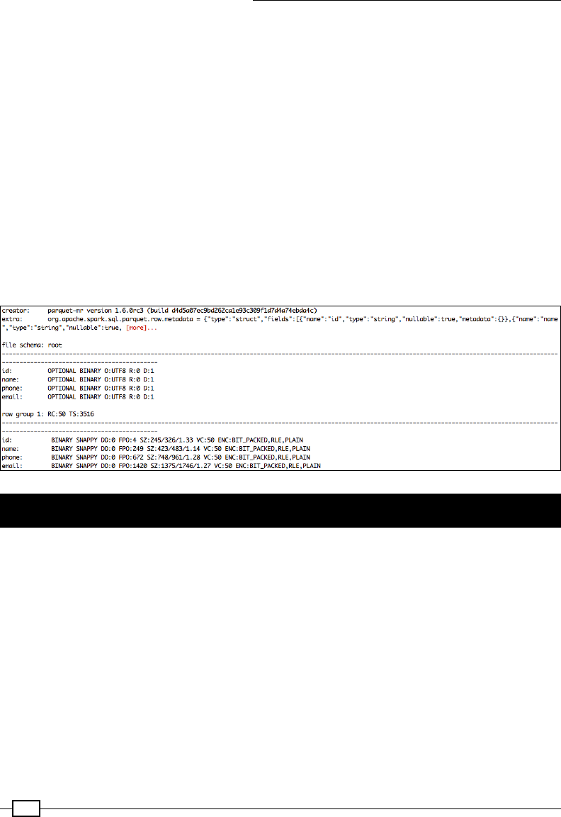
Loading and Preparing Data – DataFrame
458
Enable compression for the Parquet le
As you can see from the meta information, the data is gzipped by default. In order to
use Snappy compression, all that we need to do is set a conguration to our SQLContext
(actually the SQLConf of SQLContext). There's just one catch with regard to enabling
Lempel–Ziv–Oberhumer (LZO) compression—we are required to install native-lzo on all
the machines where this data is stored. Otherwise, we get a "native-lzo library not
available" error message.
Let's enable Snappy (http://google.github.io/snappy/) compression by passing the
conguration parameter of Parquet compression to Snappy:
sqlContext.setConf("spark.sql.parquet.compression.codec", "snappy")
After running the program, let's use the parquet-tools meta command to verify it:
parquet-tools meta part-r-00000-aee54b77-288e-44b2-8f36-53b38a489e8d.
snappy.parquet
Using the Avro data model in Parquet
Parquet is a kind of highly efcient columnar storage, but it is also relatively new. Avro
(https://avro.apache.org) is a widely used row-based storage format. This recipe
showcases how we can retain the older and exible Avro schema in our code but still use
the Parquet format during storage.
The Spark MR project (yes, the one that has the Parquet tools we saw in the previous recipe)
has converters for almost all the popular data formats. These model converters take your
format and convert it into Parquet format before causing it to persist.

Chapter 3
459
How to do it…
In this recipe, we'll use the Avro data model and serialize the data in a Parquet le. The recipe
involves the following steps:
1. Create the Avro Model.
2. Generate Avro objects using the sbt avro plugin.
3. Construct the RDD of your generated object (StudentAvro) from Students.csv.
4. Save the RDD[StudentAvro] in a Parquet le.
5. Read the le back for verication.
6. Use Parquet-tools to verify.
Creation of the Avro model
The Avro schema is dened using JSON. In our case, we'll just use the same Student.csv
as the input le. So, let's code the four elds— id, name, phone, and email—in the schema:
{"namespace": "studentavro.avro",
"type": "record",
"name": "StudentAvro",
"fields": [
{"name": "id", "type": ["string", "null"]},
{"name": "name", "type": ["string", "null"]},
{"name": "phone", "type": ["string", "null"]},
{"name": "email", "type": ["string", "null"]}
]
}
Probably, you are already familiar with Avro, or you have already understood the schema just
by taking a look at it, but let me bore you with some explanation of the schema anyway.
The namespace and name attributes in the JSON translate into our package name and class
name in our world, respectively. So, our generated class will have a fully qualied name as
studentavro.avro.StudentAvro. The "record" (of the type attribute) is one of the
complex types in Avro (http://avro.apache.org/docs/1.7.6/spec.html#schema_
complex). Let me rephrase this again. A record roughly translates to classes in Java/
Scala. It is at the topmost level in the schema hierarchy. A record can have multiple elds
encapsulated inside it, and these elds can be primitives (https://avro.apache.org/
docs/1.7.7/spec.html#schema_primitive) or other complex types. The last bit about
the type having an array of types is interesting ("type": ["string", "null"]). It just
means that the eld can be more than one type. In Avro terms, it is called a union.
Now that we are done with the schema, let's save this le with an extension of .avsc. I have
saved it as student.avsc in the src/main/avro directory.
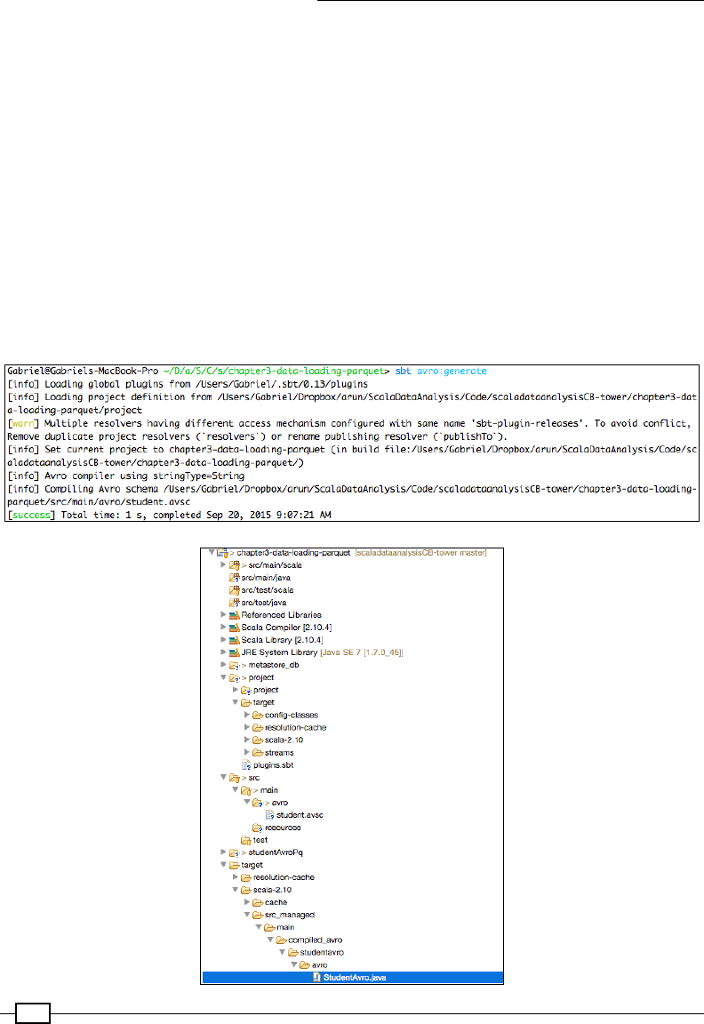
Loading and Preparing Data – DataFrame
460
Generation of Avro objects using the sbt-avro plugin
The next step is to generate a class from the schema. The reason we stored the avro
schema le in the src/main/avro folder is this: we'll be using an sbt-avro plugin
(https://github.com/cavorite/sbt-avro) to generate a Java class from the
schema. Conguring the plugin is as easy as conguring any other plugin for SBT:
fLet's add the plugin to project/plugins.sbt:
addSbtPlugin("com.cavorite" % "sbt-avro" % "0.3.2")
fAdd the default settings of the plugin to our build.sbt:
seq( sbtavro.SbtAvro.avroSettings : _*)
fLet's generate the Java class now. We can do this by calling sbt avro:generate.
You can see the generated Java le at target/scala-2.10/src_managed/
main/compiled_avro/studentavro/avro/StudentAvro.java.

Chapter 3
461
fWe also need the following library dependencies. Finally, let's perform an SBT compile
to compile the class so that the rest of the project picks up the generated Java le:
libraryDependencies ++= Seq(
"org.apache.spark" %% "spark-core" % sparkVersion,
"org.apache.spark" %% "spark-sql" % sparkVersion,
"org.apache.spark" %% "spark-mllib" % sparkVersion,
"org.apache.spark" %% "spark-hive" % sparkVersion,
"org.apache.avro" % "avro" % "1.7.7",
"org.apache.parquet" % "parquet-avro" % "1.8.1",
"com.twitter" %% "chill-avro" % "0.6.0"
)
sbt compile
Constructing an RDD of our generated object from Students.csv
This step is very similar to the previous recipe in the sense that we use the
convertCSVToStudents function to generate an RDD of the StudentAvro object. Also,
since this isn't a Scala class and the generated Java object comes up with a builder inside
it, we use the builder to construct the class uently (http://en.wikipedia.org/wiki/
Fluent_interface):
val conf = new
SparkConf().setAppName("AvroModelToParquet").setMaster("local[2]")
val sc = new SparkContext(conf)
val sqlContext = new SQLContext(sc)
sqlContext.setConf("spark.sql.parquet.binaryAsString", "true")
val rddOfStudents = convertCSVToStudents("StudentData.csv", sc)
//The CSV has a header row. Zipping with index and skipping the
first row
def convertCSVToStudents(filePath: String, sc: SparkContext):
RDD[StudentAvro] = {
val rddOfStudents:
RDD[StudentAvro]=sc.textFile(filePath).flatMap(eachLine => {
val data = eachLine.split("\\|")
if (data(0) == "id") None
else Some(StudentAvro.newBuilder()
.setId(data(0))
.setName(data(1))
.setPhone(data(2))
.setEmail(data(3)).build())
})
rddOfStudents
}

Loading and Preparing Data – DataFrame
462
Saving RDD[StudentAvro] in a Parquet le
This is a tricky step and involves multiple substeps. Let's decipher this step backwards.
We fall back to RDD[StudentAvro] in this example instead of a DataFrame because
DataFrames can be constructed only from an RDD of case classes (or classes that extend
Product, as we saw earlier in this chapter) or from RDD[org.apache.spark.sql.Row].
If you prefer to use DataFrames, you can read the CSV as an array of values, and
use RowFactory.create for each array of values. Once an RDD[Row] is available,
we can use sqlContext.createDataFrame to convert it to a DataFrame:
fIn order to save the RDD as a Hadoop SequenceFile, we can use
saveAsNewAPIHadoopFile. A sequence le is simply a text le that holds
key-value pairs. We could have chosen one of the Student attributes as a key,
but for the sake of it, let's have it as a Void in this example.
To represent a pair (key-value) in Spark, we use PairRDD (https://spark.
apache.org/docs/1.4.1/api/scala/index.html#org.apache.spark.
rdd.PairRDDFunctions). Not surprisingly, saveAsNewAPIHadoopFile is
available only for PairRDDs. To convert the existing RDD[StudentAvro] to a
PairRDD[Void,StudentAvro], we use the map function:
val pairRddOfStudentsWithNullKey = rddOfStudents.map(each
=> (null, each))
fSpark uses Java serialization by default to serialize the RDD to be distributed
across the cluster. However, the Avro model doesn't implement the serializable
interface, and hence it won't be able to leverage Java serialization. That's no reason
for worry, however, because Spark provides another 10x performant serialization
mechanism called Kryo. The only downside is that we need to explicitly register our
serialization candidates:
val conf = new
SparkConf().setAppName("AvroModelToParquet").setMaster("local[2]")
conf.set("spark.kryo.registrator",
classOf[StudentAvroRegistrator].getName)
conf.set("spark.serializer",
"org.apache.spark.serializer.KryoSerializer")
So, we say using the "spark.serializer" conguration that we intend to use
KryoSerializer, and that our registrator is StudentAvroRegistrator. As
you may expect, what the Registrator does is register our StudentAvro class as
a candidate for Kryo serialization. The twitter-chill project (https://github.
com/twitter/chill) provides a nice extension to delegate the Kryo serializer to
use the Avro serialization:
class StudentAvroRegistrator extends KryoRegistrator {
override def registerClasses(kryo: Kryo) {

Chapter 3
463
kryo.register(classOf[StudentAvro],
AvroSerializer.SpecificRecordBinarySerializer[StudentAvro])
}
}
fThe intent of this recipe is to write a Parquet le, but the data model (schema) is Avro.
Since we are going to write this down as a sequence le, we'll be using a bunch of
Hadoop APIs. The org.apache.hadoop.mapreduce.OutputFormat species
the output format of the le that we are going to write, and as expected, we use
ParquetOutputFormat (this is available in the parquet-hadoop subproject in
the parquet-mr project). There are two things that an OutputFormat requires:
The WriteSupport class, which knows how to convert the Avro data model
to the actual format. This is achieved with the following line:
ParquetOutputFormat.setWriteSupportClass(job,
classOf[AvroWriteSupport])
The schema needs to be written to the footer of the Parquet file too. The
schema of StudentAvro is accessible by using the getClassSchema
function. This line of code achieves that:
AvroParquetOutputFormat.setSchema(job, StudentAvro.
getClassSchema)
Now, what's that job parameter doing here in these two lines of code? The job
object is just an instance of org.apache.hadoop.mapreduce.Job:
val job = new Job()
When we call the setWriteSupportClass and setSchema methods of
ParquetOutputFormat and AvroParquetOutputFormat, the resulting
conguration is captured inside the JobConf encapsulated inside the Job object.
We'll be using this job conguration while saving the data in a sequence le.
fFinally, we save the le by calling saveAsNewAPIHadoopFile. The save method
requires a bunch of parameters, each of which we have already discussed. The rst
parameter is the lename, followed by the key and the value classes. The fourth is
the OutputFormat of the le, and nally comes the job conguration itself:
pairRddOfStudentsWithNullKey.saveAsNewAPIHadoopFile("studentAvro
Pq",
classOf[Void],
classOf[StudentAvro],
classOf[AvroParquetOutputFormat],
job.getConfiguration())

Loading and Preparing Data – DataFrame
464
We saw the entire program in bits and pieces, so for the sake of completion, let's see
it completely:
object ParquetAvroSchemaMain extends App {
val conf = new
SparkConf().setAppName("AvroModelToParquet").setMaster("local[2]")
conf.set("spark.kryo.registrator",
classOf[StudentAvroRegistrator].getName)
conf.set("spark.serializer",
"org.apache.spark.serializer.KryoSerializer")
val job = new Job()
val sc = new SparkContext(conf)
val sqlContext = new SQLContext(sc)
sqlContext.setConf("spark.sql.parquet.binaryAsString",
"true")
val rddOfStudents =
convertCSVToStudents("StudentData.csv", sc)
ParquetOutputFormat.setWriteSupportClass(job,
classOf[AvroWriteSupport])
AvroParquetOutputFormat.setSchema(job,
StudentAvro.getClassSchema)
val pairRddOfStudentsWithNullKey = rddOfStudents.map(each
=>
(null, each))
pairRddOfStudentsWithNullKey.saveAsNewAPIHadoopFile("studentAvro
Pq",
classOf[Void],
classOf[StudentAvro],
classOf[AvroParquetOutputFormat],
job.getConfiguration())
//The CSV has a header row. Zipping with index and
skipping the first row
def convertCSVToStudents(filePath: String, sc:
SparkContext):
RDD[StudentAvro] = {
val rddOfStudents:
RDD[StudentAvro]=sc.textFile(filePath).flatMap(eachLine =>
{
val data = eachLine.split("\\|")
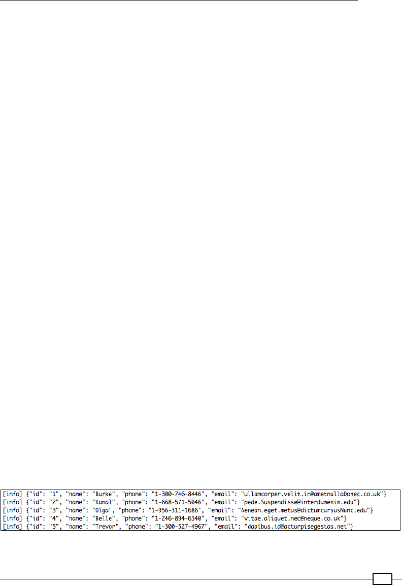
Chapter 3
465
if (data(0) == "id") None
else Some(StudentAvro.newBuilder()
.setId(data(0))
.setName(data(1))
.setPhone(data(2))
.setEmail(data(3)).build())
})
rddOfStudents
}
}
class StudentAvroRegistrator extends KryoRegistrator {
override def registerClasses(kryo: Kryo) {
kryo.register(classOf[StudentAvro],
AvroSerializer.SpecificRecordBinarySerializer[StudentAvro])
}
}
Reading the le back for verication
As always, let's read the le back for conrmation. The function to be called
for this is newAPIHadoopFile, which accepts a similar set of parameters as
saveAsNewAPIHadoopFile: the name of the le, InputFormat, the key class, the value
class, and nally the job conguration. Note that we are using newAPIHadoopFile instead
of the previously used the parquetFile method. This is because we are reading from a
Hadoop sequence le:
//Reading the file back for confirmation.
ParquetInputFormat.setReadSupportClass(job, classOf[AvroWriteSupport])
val readStudentsPair = sc.newAPIHadoopFile("studentAvroPq", classOf[Av
roParquetInputFormat[StudentAvro]], classOf[Void], classOf[StudentAvro],
job.getConfiguration())
val justStudentRDD: RDD[StudentAvro] = readStudentsPair.map(_._2)
val studentsAsString = justStudentRDD.collect().take(5).mkString("\n")
println(studentsAsString)
This is the output:
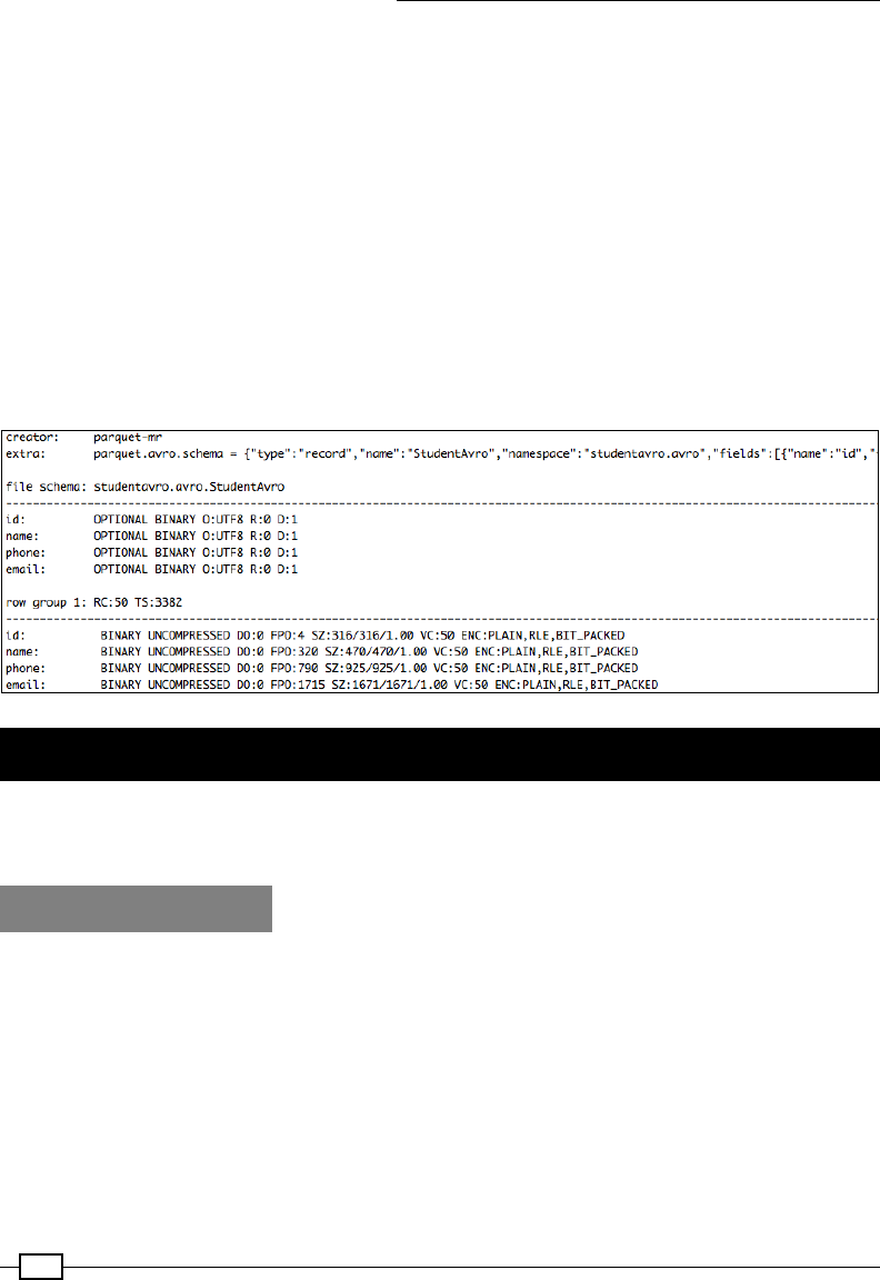
Loading and Preparing Data – DataFrame
466
Using Parquet tools for verication
We'll also use Parquet tools to conrm that the schema that is stored in the Parquet le is
indeed an avro schema:
/Users/Gabriel/Dropbox/arun/ScalaDataAnalysis/git/parquet-mr/parquet-
tools/target/parquet-tools-1.6.0rc3/parquet-tools meta /Users/Gabriel/
Dropbox/arun/ScalaDataAnalysis/Code/scaladataanalysisCB-tower/chapter3-
data-loading-parquet/studentAvroPq
Yup! Looks like it is! The extra section in meta does conrm that the avro schema is stored:
creator: parquet-mr
extra: parquet.avro.schema = {"type":"record","name":"StudentAvro",
"namespace":"studentavro.avro","fields":[{"name":"id","type":[{"type":"st
ring","avro.java.string":"Stri [more]...
Loading from RDBMS
As the nal recipe on loading, let's try to load data from an RDBMS data source, which is MySQL
in our case. This recipe assumes that you have already installed MySQL in your machine.
How to do it…
Let's go through the prerequisite steps rst. If you already have a MySQL table to play with,
you can safely ignore this step. We are just going to create a new database and a table and
load some sample data into it.
The prerequisite step (optional):
1. Creating a database and a table: This is achieved in MySQL by using the create
database and the create table DDL:
create database scalada;
use scalada

Chapter 3
467
CREATE TABLE student (
id varchar(20),
`name` varchar(200),
phone varchar(50),
email varchar(200),
PRIMARY KEY (id));
2. Loading data into the table: Let's dump some data into the table. I wrote a very
simple app to do this. Alternatively, you can use the load data infile command
if you have "local-infile=1" enabled on your server and the client. Refer to
https://dev.mysql.com/doc/refman/5.1/en/load-data.html for details
about this command.
As you can see, the program loads the Student.csv that we saw in Chapter
2, Getting Started with Apache Spark DataFrames, when we saw how to use
DataFrames with Spark using the databricks.csv connector. Then, for each line,
the data is inserted into the table using the plain old JDBC insert. As you might have
already gured out, we need to add the MySQL connector java dependency to our
build.sbt too:
"mysql" % "mysql-connector-java" % "5.1.34"
object LoadDataIntoMySQL extends App {
val conf = new
SparkConf().setAppName("LoadDataIntoMySQL").setMaster("local[2]")
val config=ConfigFactory.load()
val sc = new SparkContext(conf)
val sqlContext = new SQLContext(sc)
val students = sqlContext.csvFile(filePath =
"StudentData.csv", useHeader = true, delimiter = '|')
students.foreachPartition { iter=>
val conn =
DriverManager.getConnection(config.getString("mysql.connection.
url"))
val statement = conn.prepareStatement("insert into
scalada.student (id, name, phone, email) values (?,?,?,?)
")
for (eachRow <- iter) {
statement.setString(1, eachRow.getString(0))
statement.setString(2, eachRow.getString(1))
statement.setString(3, eachRow.getString(2))
statement.setString(4, eachRow.getString(3))
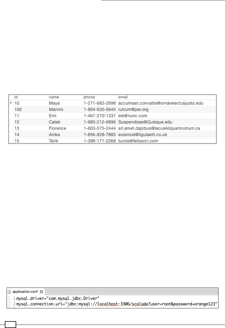
Loading and Preparing Data – DataFrame
468
statement.addBatch()
}
statement.executeBatch()
conn.close()
println ("All rows inserted successfully")
}
}
A "select * from scalada.student" on the MySQL client should conrm this, as
shown here:
Steps for loading RDBMS data into DataFrame:
The recommended approach to loading data from RDBMS databases is using the
SQLContext's load method:
1. Creating the Spark and SQLContext: You may have already become familiar with
this step by looking at the previous recipes:
val conf = new
SparkConf().setAppName("DataFromRDBMS").setMaster("local[2]")
val sc = new SparkContext(conf)
val sqlContext = new SQLContext(sc)
2. Constructing a map of options: This map is expected to have not only the driver
and the connection URL, but also the query to be invoked in order to load the data.
In this example, we'll store the parameter values in an external Typesafe config
le and load the values into our program.
The Typesafe application.conf is located at src/main/resources as per
standard SBT/Maven conventions. Here is a screenshot that shows the contents
of application.conf:

Chapter 3
469
Now let's look at the code that constructs the map:
val config = ConfigFactory.load()
val options = Map(
"driver" -> config.getString("mysql.driver"),
"url" -> config.getString("mysql.connection.url"),
"dbtable" -> "(select * from student) as student",
"partitionColumn" -> "id",
"lowerBound" -> "1",
"upperBound" -> "100",
"numPartitions"-> "2")
The rst three parameters are straightforward. The numPartitions species the
number of partitions for this job, and partitionColumn species the column
in the table based on which the job has to be partitioned. The lowerBound and
upperBound are values of the "id" eld. The amount of data to be handled by
a single partition is calculated using the number of partitions and the lower and
upper bounds.
3. Loading data from the table: The load function of SQLContext expects two
parameters. The rst one species that the source of the data is through "jdbc",
and the second parameter is the options that we constructed in step 2. Let's now
print the schema and show the rst 20 rows, as we always do:
val dFrame=sqlContext.load("jdbc", options)
dFrame.printSchema()
dFrame.show()
This is the output:
root
|-- id: string (nullable = false)
|-- name: string (nullable = true)
|-- phone: string (nullable = true)
|-- email: string (nullable = true)
|-- gender: string (nullable = true)
We see that the schema of the DataFrame is derived from the MySQL table denition by
examining the not nullable constraint of the id eld.
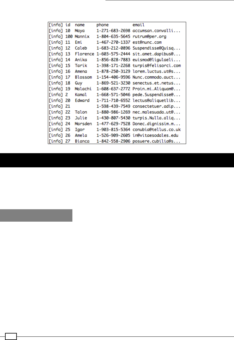
Loading and Preparing Data – DataFrame
470
The output is as follows:
Preparing data in Dataframes
Other than ltering, conversions, and transformations (with DataFrames which we saw
in Chapter 2, Getting Started with Apache Spark DataFrames) , let's see a few more data
preparation tricks in this recipe. We'll also be looking at specic data preparation in Chapter 5,
Learning from Data, where we will focus on using various machine learning algorithms.
How to do it...
While preprocessing data, we may be required to:
fMerge two different datasets
fPerform set operations on two datasets
fSort the DataFrame by casting an attribute value
fChoose a member from one dataset over another based on the predicate
fParse arbitrary date/time inputs
We'll use the StudentPrep1.csv and StudentPrep2.csv datasets for the rst four tasks,
and for the last one, we'll use StrangeDate.json, a JSON-based dataset. The CSV and the
JSON dataset are chosen primarily for convenience—the input data could be anything.
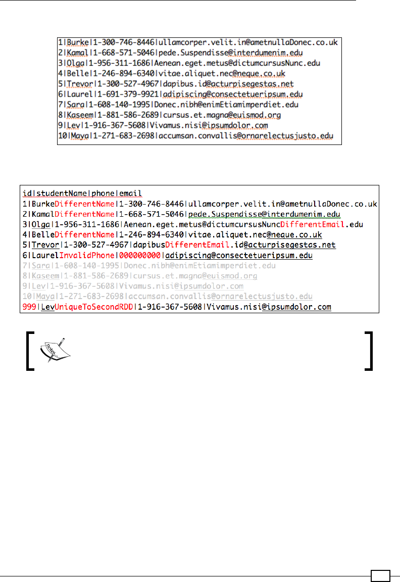
Chapter 3
471
The StudentPrep1.csv dataset is shown in this screenshot:
The StudentPrep2.csv dataset is shown in the following screenshot:
The code for this recipe can be found at https://github.com/
arunma/ScalaDataAnalysisCookbook/tree/master/
chapter3-data-loading.
Let's convert them into a DataFrame using the databricks/spark-csv library, which we
used in Chapter 2, Getting Started with Apache Spark DataFrames, when we talked about
loading DataFrames from CSV:
import com.databricks.spark.csv.CsvContext
val students1=sqlContext.csvFile(filePath="StudentPrep1.csv",
useHeader=true, delimiter='|')
val students2=sqlContext.csvFile(filePath="StudentPrep2.csv",
useHeader=true, delimiter='|')
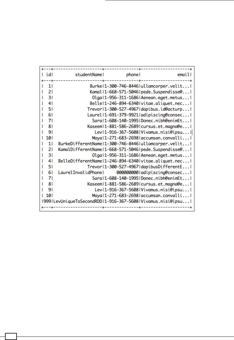
Loading and Preparing Data – DataFrame
472
1. Merging datasets: The DataFrame provides a convenient way to merge another
DataFrame—unionAll. The unionAll accepts another DataFrame as an argument.
Not surprisingly, the merged DataFrame maintains duplicates inside it:
val allStudents=students1.unionAll(students2)
allStudents.show(allStudents.count().toInt)
The output is shown as follows:
2. Performing set operations: Just like unionAll, the DataFrame has functions for
various set operations.
The intersection of two DataFrames would just entail calling the intersect function:
val intersection=students1.intersect(students2)
intersection.foreach(println)
[7,Sara,1-608-140-1995,Donec.nibh@enimEtiamimperdiet.edu]
[8,Kaseem,1-881-586-2689,cursus.et.magna@euismod.org]
[10,Maya,1-271-683-2698,accumsan.convallis@ornarelectusjusto.edu]
[9,Lev,1-916-367-5608,Vivamus.nisi@ipsumdolor.com]

Chapter 3
473
Deriving the difference of one DataFrame from another is done by calling the
except() function with another DataFrame as the parameter:
val subtraction=students1.except(students2)
subtraction.foreach(println)
Here is the output:
[6,Laurel,1-691-379-9921,adipiscing@consectetueripsum.edu]
[4,Belle,1-246-894-6340,vitae.aliquet.nec@neque.co.uk]
[2,Kamal,1-668-571-5046,pede.Suspendisse@interdumenim.edu]
[5,Trevor,1-300-527-4967,dapibus.id@acturpisegestas.net]
[3,Olga,1-956-311-1686,Aenean.eget.metus@dictumcursusNunc.edu]
[1,Burke,1-300-746-8446,ullamcorper.velit.in@ametnullaDonec.co.uk]
If there are duplicates in the data, the distinct function will ignore them and return
a DataFrame with only unique data:
val distinctStudents=allStudents.distinct
distinctStudents.foreach(println)
println(distinctStudents.count())
The following is the output:
[4,BelleDifferentName,1-246-894-6340,vitae.aliquet.nec@neque.
co.uk]
[1,Burke,1-300-746-8446,ullamcorper.velit.in@ametnullaDonec.co.uk]
[2,KamalDifferentName,1-668-571-5046,pede.Suspendisse@
interdumenim.edu]
[999,LevUniqueToSecondRDD,1-916-367-5608,Vivamus.nisi@ipsumdolor.
com]
[1,BurkeDifferentName,1-300-746-8446,ullamcorper.velit.in@
ametnullaDonec.co.uk]
[2,Kamal,1-668-571-5046,pede.Suspendisse@interdumenim.edu]
[3,Olga,1-956-311-1686,Aenean.eget.metus@dictumcursusNunc.edu]
[7,Sara,1-608-140-1995,Donec.nibh@enimEtiamimperdiet.edu]
[8,Kaseem,1-881-586-2689,cursus.et.magna@euismod.org]
[5,Trevor,1-300-527-4967,dapibus.id@acturpisegestas.net]
[4,Belle,1-246-894-6340,vitae.aliquet.nec@neque.co.uk]
[6,Laurel,1-691-379-9921,adipiscing@consectetueripsum.edu]
[6,LaurelInvalidPhone,000000000,adipiscing@consectetueripsum.edu]
[9,Lev,1-916-367-5608,Vivamus.nisi@ipsumdolor.com]
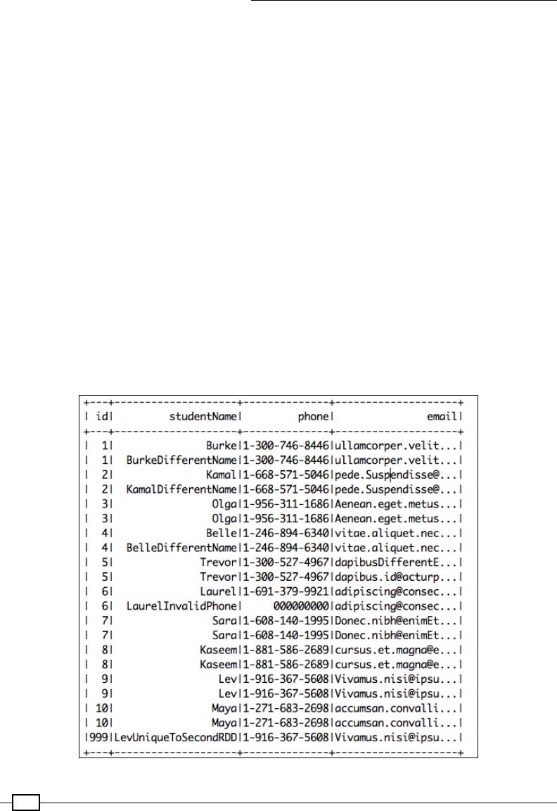
Loading and Preparing Data – DataFrame
474
[3,Olga,1-956-311-1686,Aenean.eget.metus@
dictumcursusNuncDifferentEmail.edu]
[5,Trevor,1-300-527-4967,dapibusDifferentEmail.id@acturpisegestas.
net]
[10,Maya,1-271-683-2698,accumsan.convallis@ornarelectusjusto.edu]
Count output:
17
3. Sorting the DataFrame by casting an attribute value: Sometimes, our DataFrame
inferences an integer attribute as a string. Since, DataFrames are immutable, the
correct way of converting an attribute from one type to another is by creating another
DataFrame. In this recipe, we'll not only cast one attribute type to another, but also
sort the DataFrame based on that attribute. The simplest way to achieve this is by
using the Spark SQL expression:
val sortedCols=allStudents.selectExpr("cast(id as int) as id",
"studentName", "phone", "email").sort("id")
println ("sorting")
sortedCols.show(sortedCols.count.toInt)
The output is shown here:

Chapter 3
475
4. Choosing a member from one dataset over another based on predicate: Let's
assume that for a given student ID across two different datasets, you would like to
pick only the one that has a longer name (or matches some predicate). The result
would be just one row per ID.
This involves three mini-steps:
1. Map the merged DataFrame (using unionAll) and spit out an RDD of
pairs with the key as the ID (or any other field based on which you would
like to merge):
val
idStudentPairs=allStudents.rdd.map(eachRow=>(eachRow.
getString(0),eachRow))
2. The next step is to use a function called reduceByKey. It accepts a function
that takes two rows and returns a single row. In our case, we simply write the
logic to choose the row with the longer name:
//Removes duplicates by id and holds on to the row with
the longest name
val idStudentPairs=allStudents.rdd.map(eachRow=>(eachRow.
getString(0),eachRow))
val longestNameRdd=idStudentPairs.reduceByKey((row1, row2)
=>
if (row1.getString(1).length()>row2.getString(1).
length()) row1 else row2
)
3. Let's print the output:
longestNameRdd.values.foreach(println)
The output is as follows:
[4,BelleDifferentName,1-246-894-6340,vitae.aliquet.nec@neque.
co.uk]
[8,Kaseem,1-881-586-2689,cursus.et.magna@euismod.org]
[6,LaurelInvalidPhone,000000000,adipiscing@consectetueripsum.edu]
[2,KamalDifferentName,1-668-571-5046,pede.Suspendisse@
interdumenim.edu]
[7,Sara,1-608-140-1995,Donec.nibh@enimEtiamimperdiet.edu]
[5,Trevor,1-300-527-4967,dapibusDifferentEmail.id@acturpisegestas.
net]
[9,Lev,1-916-367-5608,Vivamus.nisi@ipsumdolor.com]
[3,Olga,1-956-311-1686,Aenean.eget.metus@
dictumcursusNuncDifferentEmail.edu]
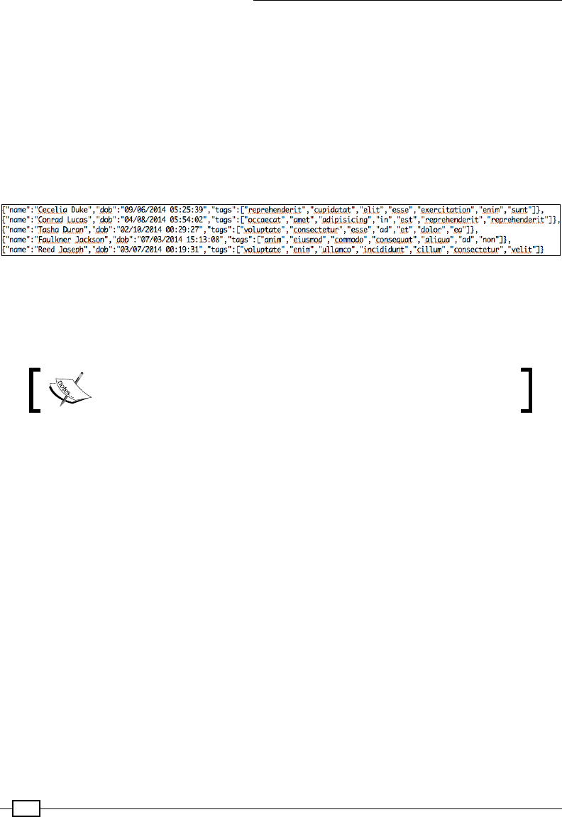
Loading and Preparing Data – DataFrame
476
[999,LevUniqueToSecondRDD,1-916-367-5608,Vivamus.nisi@ipsumdolor.
com]
[1,BurkeDifferentName,1-300-746-8446,ullamcorper.velit.in@
ametnullaDonec.co.uk]
[10,Maya,1-271-683-2698,accumsan.convallis@ornarelectusjusto.edu]
5. Parsing arbitary date/time inputs and convert an array into a comma-separated
string: While preparing the data, we see that, particularly, the date and time appear
in some crazy formats. As always, our aim is to standardize them. For this subrecipe,
we'll be using a JSON that looks like this:
As we saw in previous recipes, we could bring in this JSON as a DataFrame, but the
date format isn't ISO 8601, which means that it won't be considered as a timestamp
and would be treated as plain string. In this subrecipe, let's see how to convert a
string into a date format. This subrecipe involves four steps:
Performing arbitrary transformations is a work in progress
(https://issues.apache.org/jira/browse/SPARK-4190).
1. Import JSON as a text file:
val stringRDD = sc.textFile("StrangeDate.json")
2. Create a new org.joda.time.format.DateTimeFormat for the
specific pattern that our input is in:
val formatter = DateTimeFormat.forPattern("MM/dd/yyyy
HH:mm:ss")
3. We add json4s as our dependency in build.sbt:
"org.json4s" % "json4s-core_2.10" % "3.2.11",
"org.json4s" % "json4s-jackson_2.10" % "3.2.11"
4. For each line of the JSON string, parse, and convert the string to org.
json4s.JsonValue. The advantage of JsonValue is that we can
traverse the JSON object with XPath-like expressions.
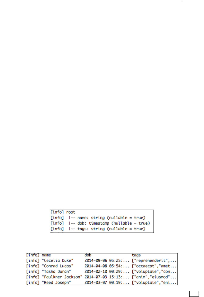
Chapter 3
477
Chaining the compact and render function will help us convert JsonValue to String.
In the following code, we extract the name eld as is, convert an array of tags into a
comma-separated string using the extract function, parse the date string using the
DateTimeFormat that we created earlier, and construct a Timestamp object. Finally,
we yield a case class called JsonDataModel out of the for comprehension that wraps
around the name, date, and tags:
case class JsonDateModel (name:String, dob:Timestamp, tags:String)
import org.json4s._
import org.json4s.jackson.JsonMethods._
implicit val formats = DefaultFormats
val dateModelRDD = for {
json <- stringRDD
jsonValue = parse(json)
name = compact(render(jsonValue \ "name"))
dateAsString=compact(render(jsonValue \ "dob")).replace("\"","")
date = new Timestamp(formatter.parseDateTime(dateAsString).
getMillis())
tags = render(jsonValue \ "tags").extract[List[String]].
mkString(",")
} yield JsonDateModel(name, date, tags)
After that, we construct a DataFrame out of this case class RDD and print the schema
to conrm:
import sqlContext.implicits._
val df=dateModelRDD.toDF()
df.printSchema()
df.show(df.count.toInt)
The output is as follows:
fSchema:
fData:

479
4
Data Visualization
In this chapter, we will cover the following recipes:
fVisualizing using Zeppelin
fCreating scatter plots with Bokeh-Scala
fCreating a time series MultiPlot with Bokeh-Scala
Introduction
In all honesty, free / open source data visualization tools in Scala aren't that rich compared to
those in other mature data analysis languages, such as R or Python. We might partly attribute
this to the lack of rich charting frameworks in Java, and visualization has never been a strong
point for big data analytics.
That said, Scala (or more specically the Hadoop world, including Spark) is catching up with
the presence of the Apache incubator project Zeppelin and the highly active Scala bindings
(https://github.com/bokeh/bokeh-scala) for the Bokeh project (http://bokeh.
pydata.org/en/latest/). With R becoming the rst-class citizen in Spark—with the
availability of SparkR DataFrames from 1.4 onwards—Spark gets additional visualization
from R other than the already existing Python APIs.
As a side note, all existing Java libraries are accessible from Scala. Hence, we are free to
borrow any visualization library from Java.
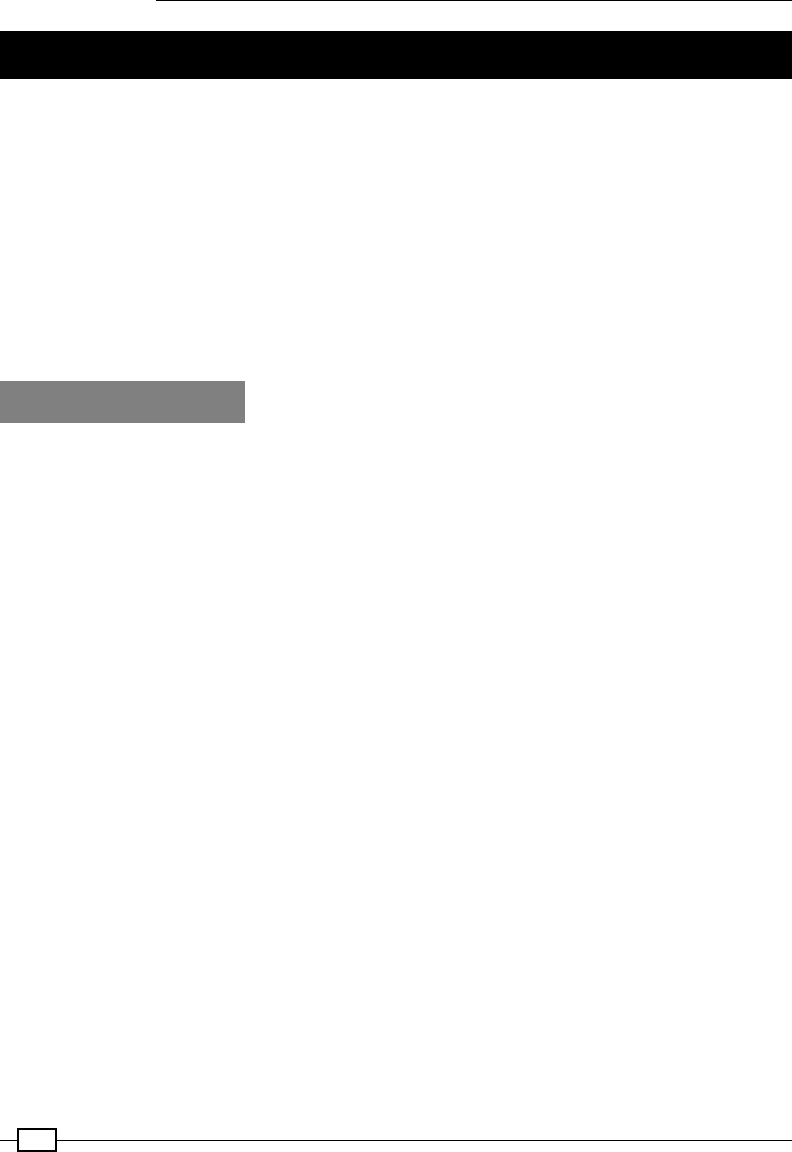
Data Visualization
480
Visualizing using Zeppelin
Apache Zeppelin is a nifty web-based tool that helps us visualize and explore large datasets.
From a technical standpoint, Apache Zeppelin is a web application on steroids. We aim to use
this application to render some neat, interactive, and shareable graphs and charts.
The interesting part of Zeppelin is that it has a bunch of built-in interpreters—ones that can
interpret and invoke all API functions in Spark (with a SparkContext) and Spark SQL (with a
SQLContext). The other interpreters that are built in are for Hive, Flink, Markdown, and Scala.
It also has the ability to run remote interpreters (outside of Zeppelin's own JVM) via Thrift. To
look at the list of built-in interpreters, you can go through conf/interpreter.json in the
zeppelin installation directory. Alternatively, you can view and customize the interpreters from
http://localhost:8080/#/interpreter once you start the zeppelin daemon.
How to do it...
In this recipe, we'll be using the built-in SparkContext and SQLContext inside Zeppelin
and transform data using Spark. At the end, we'll register the transformed data as a table
and use Spark SQL to query the data and visualize it.
The list of subrecipes in this section is as follows:
fInstalling Zeppelin
fCustomizing Zeppelin's server and websocket port
fVisualizing data on HDFS – parameterizing inputs
fUsing custom functions during visualization
fAdding external dependencies to Zeppelin
fPointing to an external Spark cluster
Installing Zeppelin
Zeppelin (http://zeppelin-project.org/) doesn't have a binary bundle yet. However,
just as its project site claims, it is pretty easy to build from source. We just ought to run one
command to install it on our local machine. At the end of this recipe, we'll take a look at how
to point our Zeppelin to an external Spark master:
git clone https://github.com/apache/incubator-zeppelin.git
cd incubator-zeppelin
mvn clean package -Pspark-1.4 -Dhadoop.version=2.2.0 -Phadoop-2.2
-DskipTests
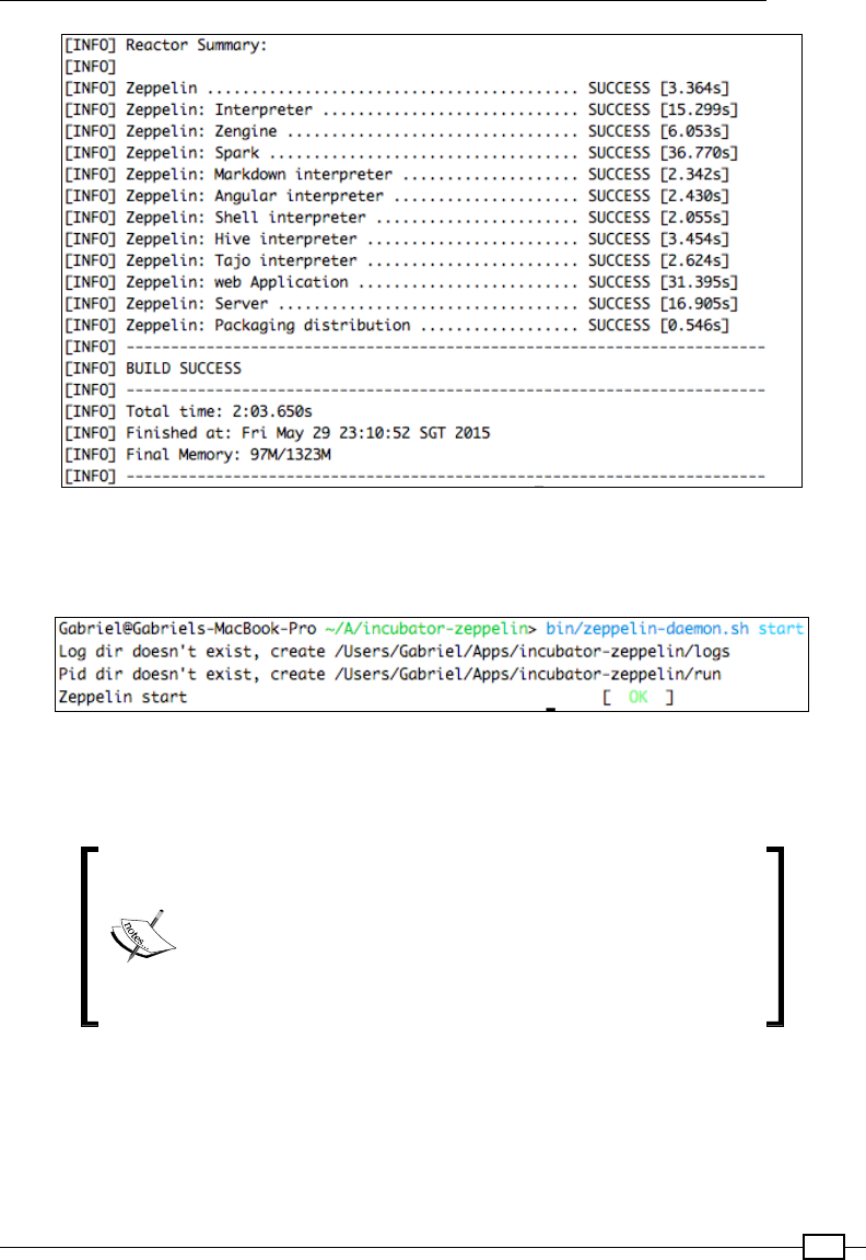
Chapter 4
481
Once built, we can start the Zeppelin daemon using the following command:
bin/zeppelin-daemon.sh start
To stop the daemon, we can use this command:
bin/zeppelin-daemon.sh stop
If you come across the following error, you can check with
rat.txt, only to nd that it complains about your data le:
Failed to execute goal org.apache.rat:apache-rat-
plugin:0.11:check (verify.rat) on project zeppelin: Too many
les with unapproved license: 3
Simply move your data le to a different location and initiate
the build again.
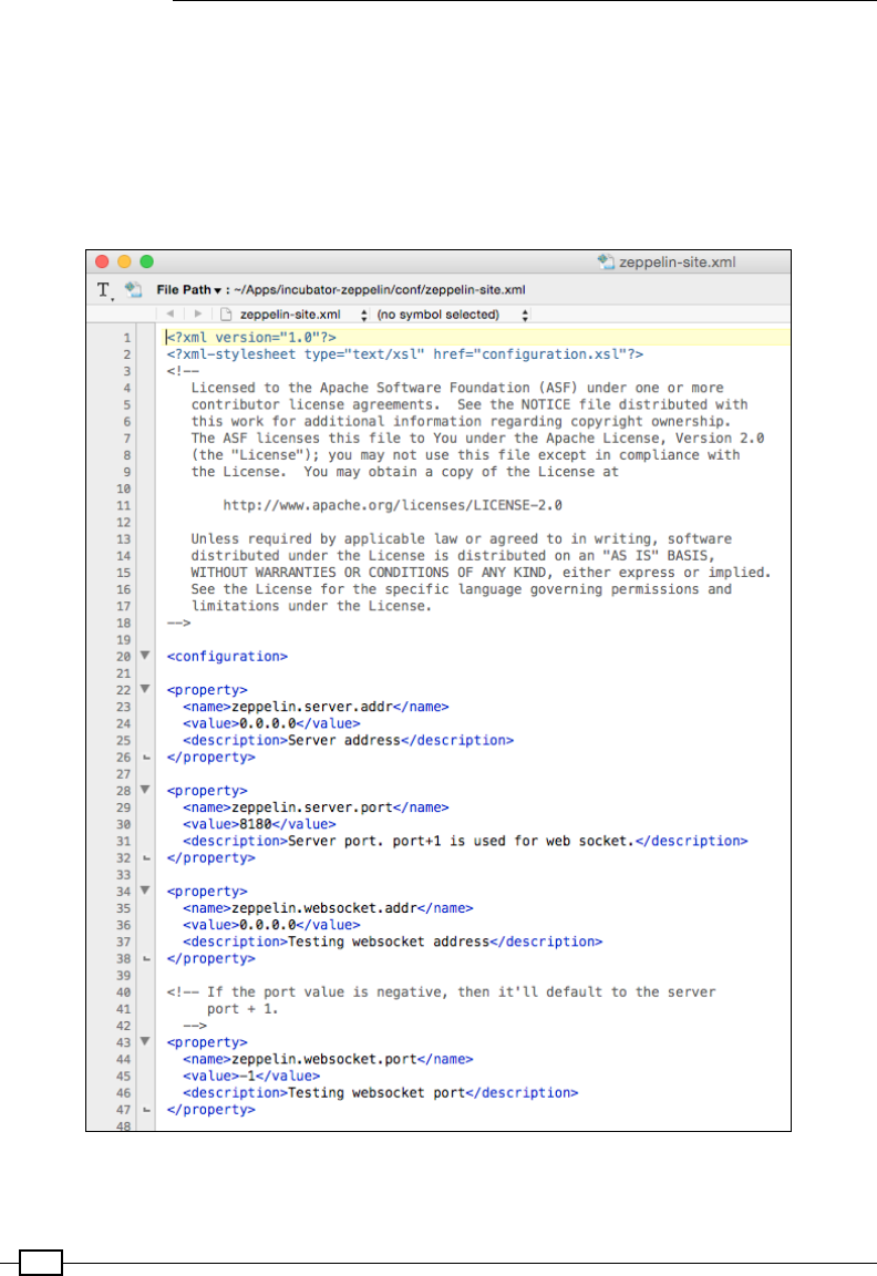
Data Visualization
482
Customizing Zeppelin's server and websocket port
Zeppelin runs on port 8080 by default, and it has a websocket port enabled at the +1
port (8081) by default. We can customize the port by copying conf/zeppelin-site.
xml.template to conf/zeppelin-site.xml and changing the ports and various other
properties, if necessary. Since the Spark standalone cluster master web UI also runs on 8080,
when we are running Zeppelin on the same machine as the Spark master, we have to change
the ports to avoid conicts.
1. For now, let's change the port to 8180. In order for this to take effect, let's restart
Zeppelin using bin/zeppelin-daemon restart
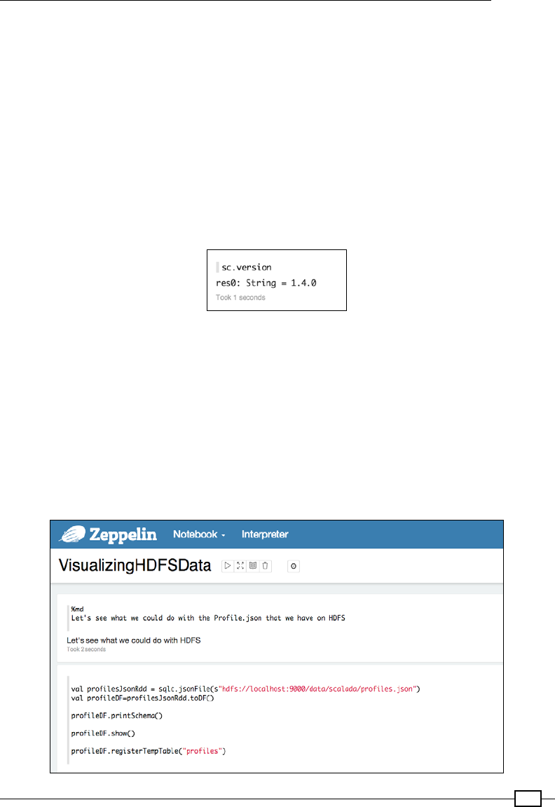
Chapter 4
483
Visualizing data on HDFS – parameterizing inputs
Once we start the daemon, we can point our browser to http://localhost:8080 (change
the port as per your modied port conguration) to view the Zeppelin UI. Zeppelin organizes
its contents as notes and paragraphs. A note is simply a list of all the paragraphs on a single
web page.
Using data from HDFS simply means that we point to the HDFS location instead of the local
lesystem location.
Before we consume the le from HDFS, let's quickly check the Spark version that Zeppelin
uses. This can be achieved by issuing sc.version on a paragraph. The sc is an implicit
variable representing the SparkContext inside Zeppelin, which simply means that we
need not programmatically create a SparkContext within Zeppelin.
Next, let's load the profiles.json sample data le, convert it into a DataFrame, and
print the schema and the rst 20 rows (show) for verication. Let's also nally register the
DataFrame as a table. Just like the implicit variable for SparkContext, SQLContext is
represented by the sqlc implicit variable inside Zeppelin:
val profilesJsonRdd = sqlc.jsonFile("hdfs://localhost:9000/data/scalada/
profiles.json")
val profileDF=profilesJsonRdd.toDF()
profileDF.printSchema()
profileDF.show()
profileDF.registerTempTable("profiles")
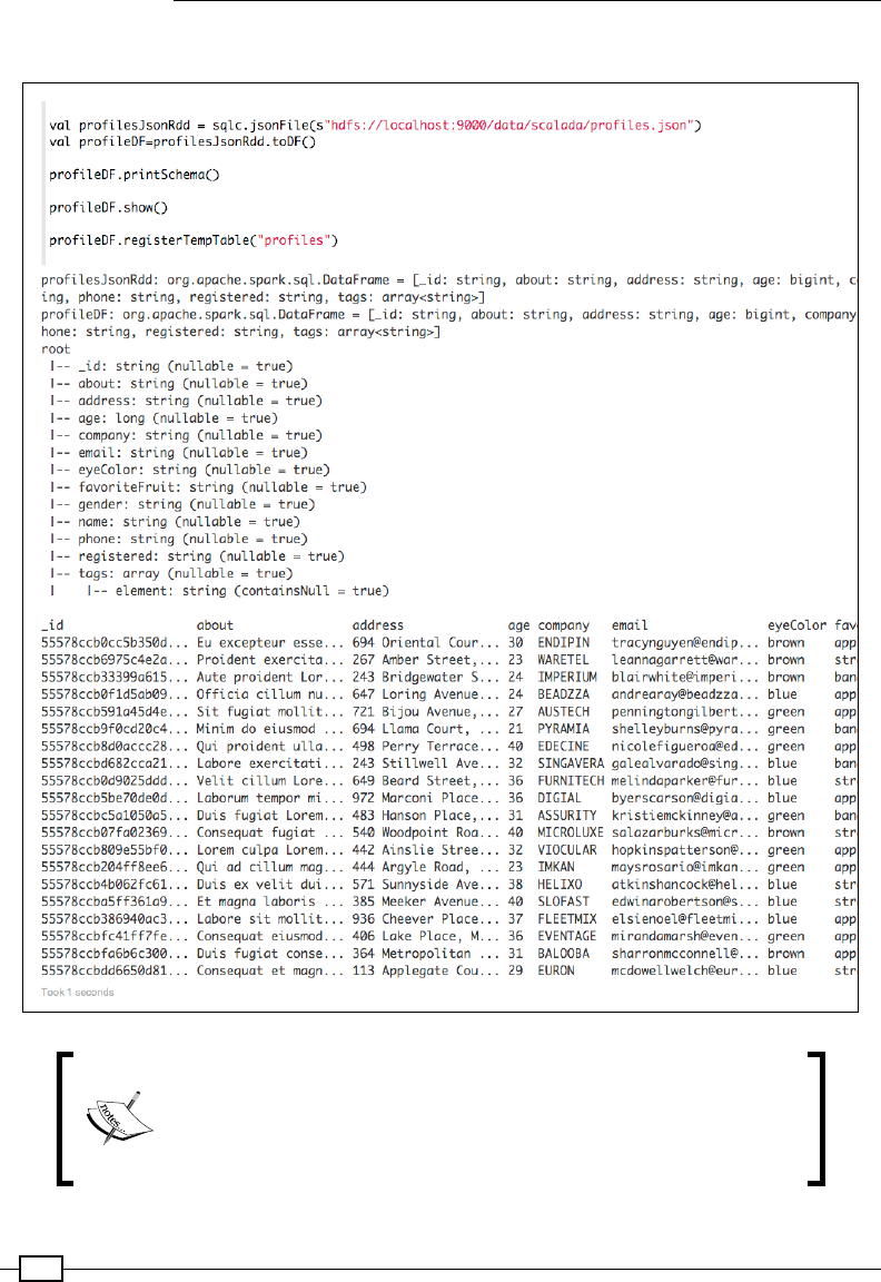
Data Visualization
484
The output looks like this:
Be careful not to explicitly create SQLContext or SparkContext.
If we create a SQLContext explicitly and register our temporary
tables to it, it won't be accessible from the SQL queries that we
execute. We'll get this error:
no such table List ([YOUR TEMP TABLE NAME])
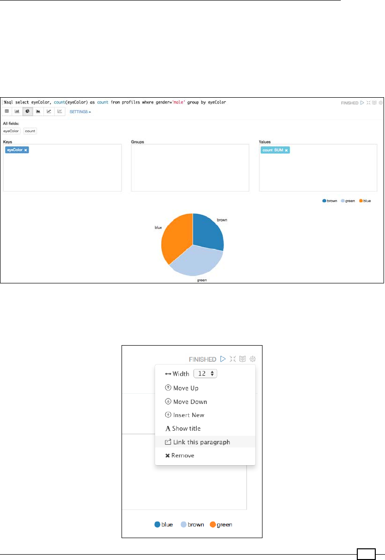
Chapter 4
485
Let's now run a simple query to understand eye colors and their counts for men in the dataset:
%sql select eyeColor, count(eyeColor) as count from profiles where
gender='male' group by eyeColor
The %sql at the beginning of the paragraph indicates to Zeppelin that we are about to
execute a Spark SQL query in this paragraph.
Now, if we wish to share this chart with someone or link it to an external website, we can do
so by clicking on the gear icon in this paragraph and then clicking on Link this paragraph,
as shown in the following screenshot:
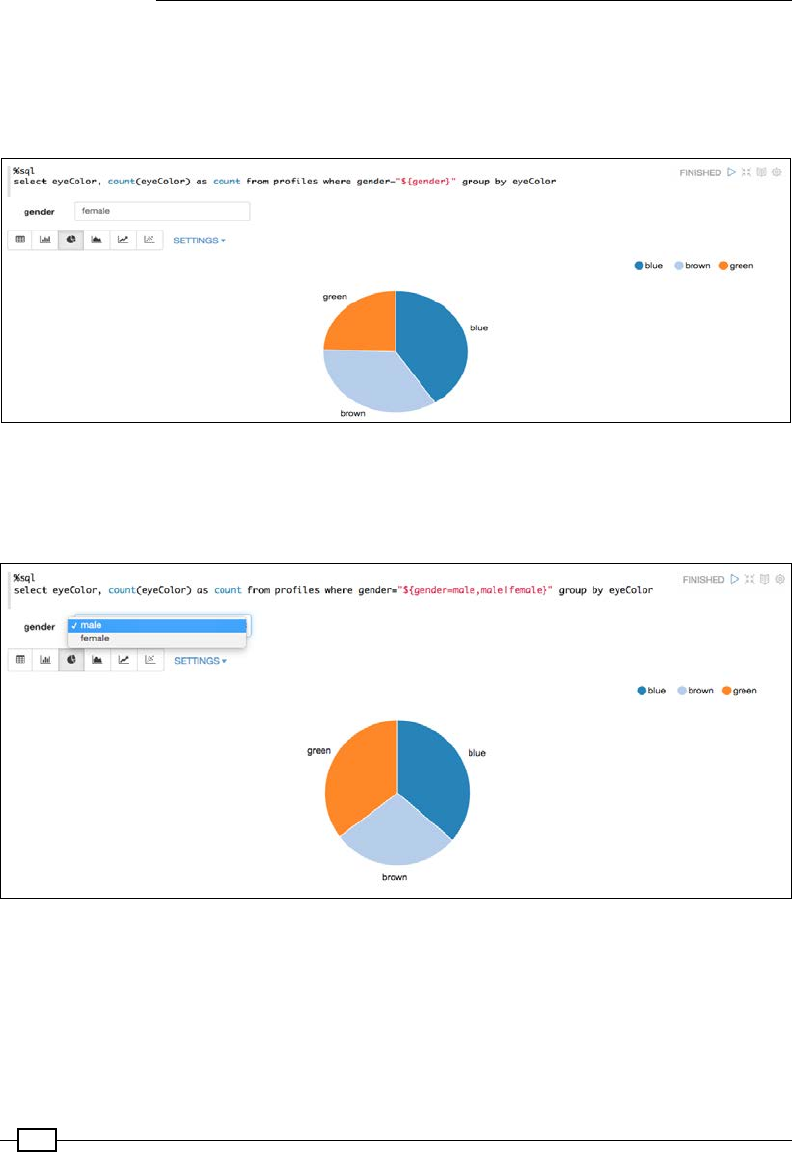
Data Visualization
486
We can actually parameterize the input for gender instead of altering our query every time.
This is achieved by the use of ${PARAMETER PLACEHOLDER}:
%sql select eyeColor, count(eyeColor) as count from profiles where
gender="${gender}" group by eyeColor
Finally, if parameterizing using free-form text isn't enough, we can use a dropdown instead:
%sql select eyeColor, count(eyeColor) as count from profiles where gender
="${gender=male,male|female}" group by eyeColor
Running custom functions
While Spark SQL doesn't support a range of functions as wide as ANSI SQL does, it has an
easy and powerful mechanism for registering a normal Scala function and using it inside the
SQL context.
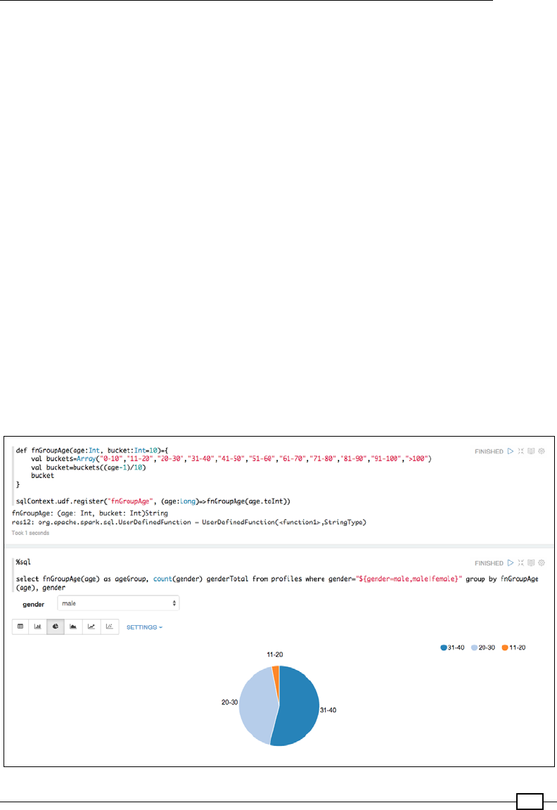
Chapter 4
487
Let's say we would like to nd out how many proles fall under each age group. We have
a simple function called ageGroup. Given an age, it returns a string representing the age
group:
def ageGroup(age: Long) = {
val buckets = Array("0-10", "11-20", "20-30", "31-40", "41-50", "51-
60", "61-70", "71-80", "81-90", "91-100", ">100")
buckets(math.min((age.toInt - 1) / 10, buckets.length - 1))
}
Now, in order to register this function to be used inside Spark SQL, all that we need to do is
give it a name and call the register method of the SQLContext's user-dened function object:
sqlc.udf.register("ageGroup", (age:Long)=>ageGroup(age.toInt))
Let's re our query and see the use of the function in action:
%sql select ageGroup(age) as group,
count(1) as total
from profiles
where gender='${gender=male,male|female}' group by ageGroup(age)
order by group
Here is the output:
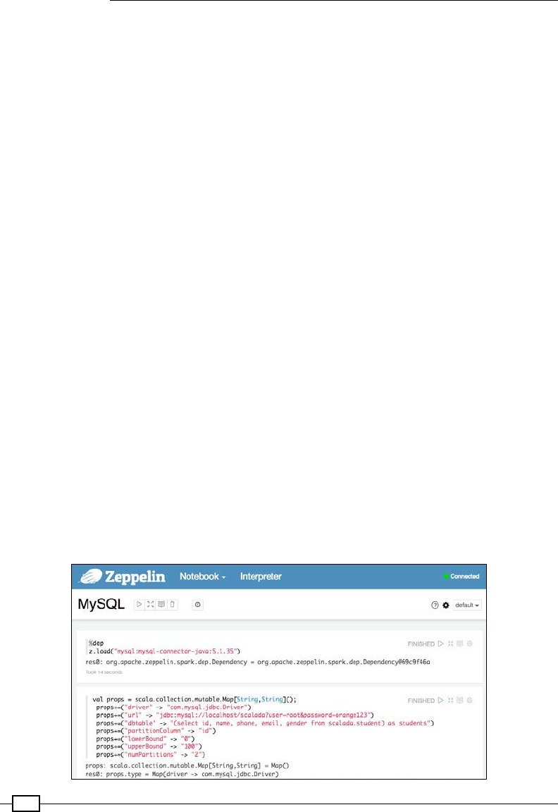
Data Visualization
488
Adding external dependencies to Zeppelin
Sooner or later, we would be depending on external libraries than that come bundled with
Zeppelin, say for an efcient CSV import or RDBMS data import. Let's see how to load a
MySQL database driver and visualize data from a table.
In order to load a mysql connector java driver, we just need to specify the group ID, artifact
ID, and version number, and the JAR gets downloaded from the maven repository. %dep
indicates that the paragraph adds a dependency, and the z implicit variable represents the
Zeppelin context:
%dep
z.load("mysql:mysql-connector-java:5.1.35")
If we would like to point to our enterprise Maven repository or some other custom repository,
we can add them by calling the addRepo method of the Zeppelin context available via the
same z implicit variable:
%dep
z.addRepo("RepoName").url("RepoURL")
Alternatively, we can load the jar from the local lesystem using the overloaded load
method:
%dep
z.load("/path/to.jar")
The only thing that we need to watch out for while using %dep is that the dependency paragraph
should be used before using the libraries that are being loaded. So, it is generally advised to
load the dependencies at the top of the Notebook.
Let's see the use in action:
fLoading the dependency:
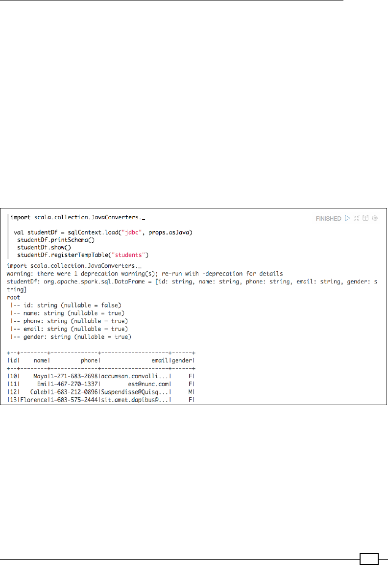
Chapter 4
489
Once we have loaded the dependencies, we need to construct the options required to
connect to the MySQL database:
val props = scala.collection.mutable.Map[String,String]();
props+=("driver" -> "com.mysql.jdbc.Driver")
props+=("url" -> "jdbc:mysql://localhost/scalada?user=root&passw
ord=orange123")
props+=("dbtable" -> "(select id, name, phone, email, gender
from scalada.student) as students")
props+=("partitionColumn" -> "id")
props+=("lowerBound" -> "0")
props+=("upperBound" -> "100")
props+=("numPartitions" -> "2")
fUsing the connection to create a DataFrame:
import scala.collection.JavaConverters._
val studentDf = sqlContext.load("jdbc", props.asJava)
studentDf.printSchema()
studentDf.show()
studentDf.registerTempTable("students")
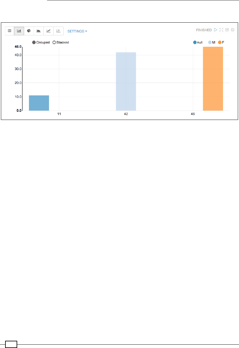
Data Visualization
490
fVisualizing the data:
Pointing to an external Spark cluster
Running Zeppelin with built-in Spark is all good, but in most of our cases, we'll be executing
the Spark jobs initiated by Zeppelin on a cluster of workers. Achieving this is pretty simple;
we need to congure Zeppelin to point its Spark master property to an external Spark master
URL. We'll be looking at how to install and run a Spark cluster on AWS, or a truly distributed
cluster, in a later chapter (Chapter 6, Scaling Up), but for this example, I have a simple and
standalone external Spark cluster running on my local machine. Please note that we will have
to run Zeppelin on a different port because of the Zeppelin UI port's conict with the Spark
standalone cluster master web UI over 8080:
For this example, let's download the Spark source for 1.4.1 and build it for Hadoop version 2.2:
build/mvn -Pyarn -Phadoop-2.2 -Dhadoop.version=2.2.0 -DskipTests clean
package
Similarly, let's download the zeppelin incubator and build it, specifying the Hadoop version
to be 2.2:
mvn clean install -Pspark-1.4 -Dhadoop.version=2.2.0 -Phadoop-2.2
-DskipTests -Pyarn
Let's bring up the Spark cluster. From inside your Spark source, execute this:
sbin/start-all.sh
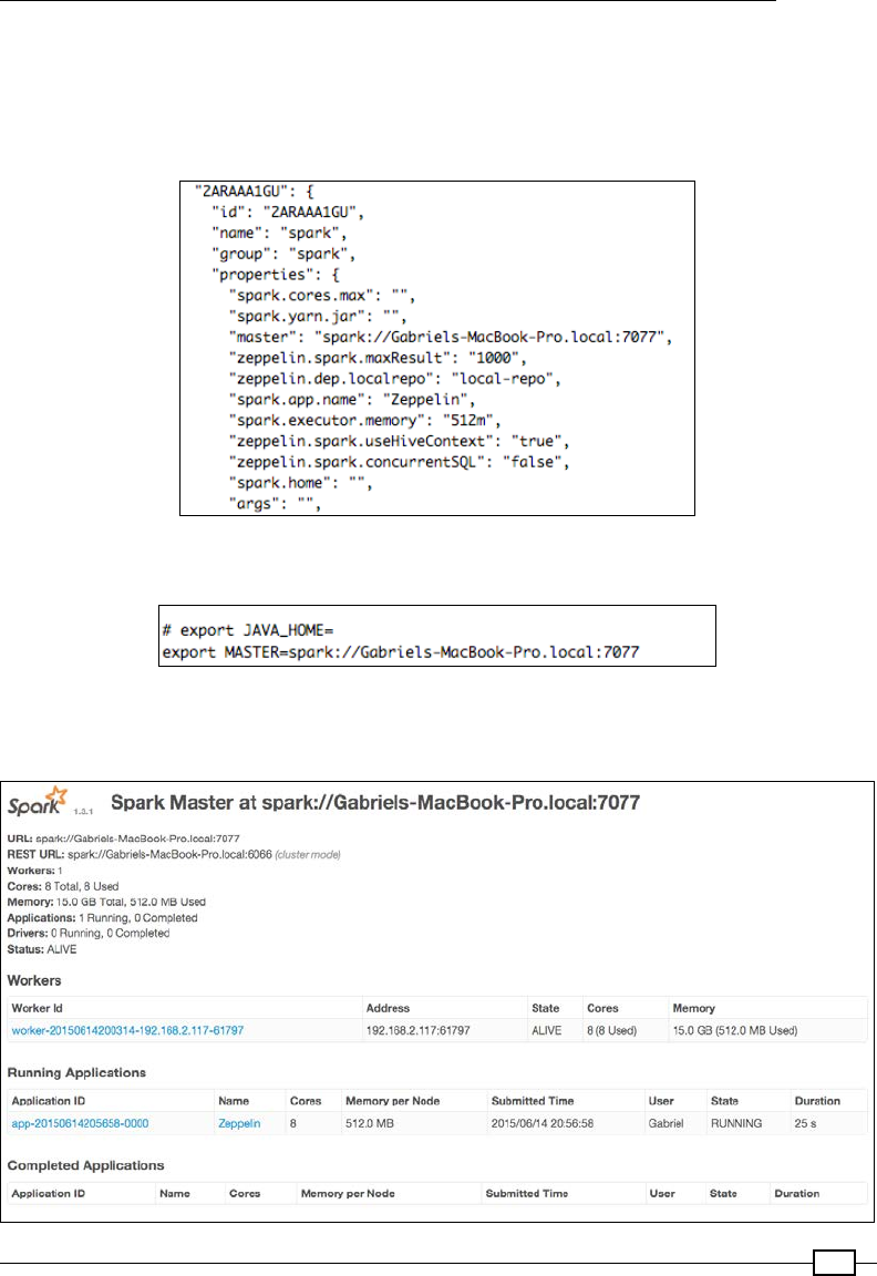
Chapter 4
491
Finally, let's modify conf/interpreter.json and conf/zeppelin-env.sh to point
the master property to the host on which the Spark VM is running. In this case, it will be
my localhost, with the port being 7077, which is the default master port.
1. The conf/interpreter.json le:
2. The conf/zeppelin-env.sh le:
Now, when we rerun Spark SQL from Zeppelin, we can see that the job runs on the external
Spark instance, as shown here:

Data Visualization
492
Creating scatter plots with Bokeh-Scala
While Zeppelin is powerful enough to quickly execute our Spark SQLs and visualize data, it is
still an evolving platform. In this section, we'll take a brief look at the most popular visualizing
framework in Python, called Bokeh, and use its (also fast evolving) Scala bindings to the
framework. Breeze also has a visualization API called breeze-viz, which is built on JFreeChart.
Unfortunately, at the time of writing this book, the API is not actively maintained, and therefore
we won't be discussing it here.
The power of Zeppelin lies in the ability to share and view graphics on the browser. This
is brought forth by the backing of the D3.js JavaScript visualization library. Bokeh is also
backed by another JavaScript visualization library, called BokehJS. The Scala bindings library
(bokeh-scala) not only gives an easier way to construct glyphs (lines, circles, and so on)
out of Scala objects, but also translates glyphs into a format that is understandable by the
BokehJS JavaScript components.
There is a warning here: the Bokeh-Scala bindings are still evolving and act at a lower level.
Sometimes, this is more cumbersome than its Python counterpart. That said, I am still sure
that we all would be able to appreciate the amazing graphs that we can create right out
of Scala.
How to do it...
In this recipe, we will be creating a scatter plot using iris data (https://archive.ics.
uci.edu/ml/datasets/Iris), which has the length and width attributes of owers
belonging to three different species of the same plant. Drawing a scatter plot on this dataset
involves a series of interesting substeps.
For the purpose of representing the iris data in a Breeze matrix, I have naïvely transformed the
species categories into numbers:
fIris setosa: 0
fIris versicolor: 1
fIris virginica: 2
This is available in irisNumeric.csv. Later, we'll see how we can load the original iris data
(iris.data) into a Spark DataFrame and use that as a source for plotting.
For the sake of clarity, let's dene what the various terms in Bokeh actually mean:
fGlyph: All geometric shapes that we can think of—circles, squares, lines, and so
on—are glyphs. This is just the UI representation and doesn't hold any data. All the
properties related to this object just help us modify the UI properties: color, x, y,
width, and so on.

Chapter 4
493
fPlot: A plot is like a canvas on which we arrange various objects relevant to the
visualization, such as the legend, x and y axes, grid, tools, and obviously, the core
of the graph—the data itself. We construct various accessory objects and nally add
them to the list of renderers in the plot object.
fDocument: The document is the component that does the actual rendering.
It accepts the plot as an argument, and when we call the save method in the
document, it uses all the child renderers in the plot object and constructs a JSON
from the wrapped elements. This JSON is eventually read by the BokehJS widgets to
render the data in a visually pleasing manner. More than one plot can be rendered
in the document by adding it to a grid plot (we'll look at how this is done in the next
recipe, Creating a time series MultiPlot with Bokeh-Scala).
A plot is a composition of multiple widgets/glyphs.
This consists of a series of steps:
1. Preparing our data.
2. Creating the Plot and Document objects.
3. Creating a point (marker object) and a renderer for it.
4. Setting the x and y axes' data range for the plot.
5. Drawing the x and the y axes.
6. Viewing the marker objects with varying colors.
7. Adding Grid lines.
8. Adding a legend to the plot.
Preparing our data
Bokeh plots require our data to be in a format that it understands, but it's really easy to do it.
All that we need to do is create a new source object that inherits from ColumnDataSource.
The other options are AjaxDataSource and RemoteDataSource.
So, let's overlay our Breeze data source on ColumnDataSource:
import breeze.linalg._
object IrisSource extends ColumnDataSource {
private val colormap = Map[Int, Color](0 -> Color.Red, 1 ->
Color.Green, 2 -> Color.Blue)
private val iris = csvread(file = new File("irisNumeric.csv"),
separator = ',')

Data Visualization
494
val sepalLength = column(iris(::, 0))
val sepalWidth = column(iris(::, 1))
val petalLength = column(iris(::, 2))
val petalWidth = column(iris(::, 3))
val species = column(iris(::, 4))
}
The rst line just reads irisNumeric.csv using the csvread function of the Breeze library.
The color map is something that we'll be using later while plotting. The purpose of this map is
to translate each species of ower into a different color. The nal piece is where we convert
the Breeze matrix into ColumnDataSource. As required by ColumnDataSource, we select
and map specic columns in the Breeze matrix to corresponding columns.
Creating Plot and Document objects
Let's have our image's title as Iris Petal Length vs Width and create a document
object so that we can save the nal HTML by the name IrisBokehBreeze.html. Since
we haven't specied the full path of the target le in the save method, the le will be saved
in the same directory as the project itself:
val plot = new Plot().title("Iris Petal Length vs Width")
val document = new Document(plot)
val file = document.save("IrisBokehBreeze.html")
println(s"Saved the chart as ${file.url}")
Creating a marker object
Our plot has neither data nor any glyphs. Let's rst create a marker object that marks the
data point. There are a variety of marker objects to choose from: Asterisk, Circle,
CircleCross, CircleX, Cross, Diamond, DiamondCross, InvertedTriangle,
PlainX, Square, SquareCross, SquareX, and Triangle.
Let's choose Diamond for our purpose:
val diamond = new Diamond()
.x(petalLength)
.y(petalWidth)
.fill_color(Color.Blue)
.fill_alpha(0.5)
.size(5)
val dataPointRenderer = new GlyphRenderer().data_source(IrisSource).
glyph(diamond)
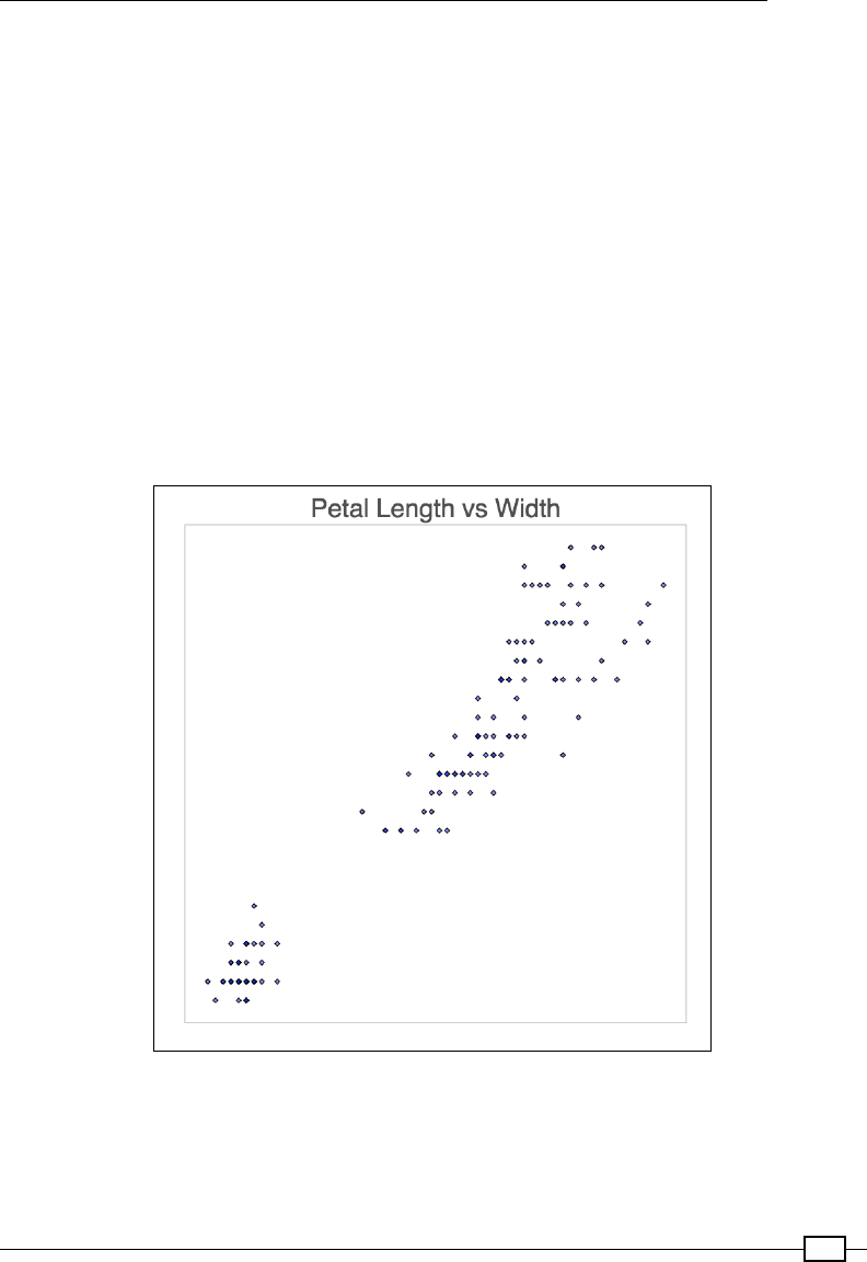
Chapter 4
495
While constructing the marker object, other than the UI attributes, we also say what the x and
the y coordinates for it are. Note that we have also mentioned that the color of this marker is
blue. We'll change that in a while using the color map.
Setting the X and Y axes' data range for the plot
The plot needs to know what the x and y data ranges of the plot are before rendering. Let's do
that by creating two DataRange objects and setting them to the plot:
val xRange = new DataRange1d().sources(petal_length :: Nil)
val yRange = new DataRange1d().sources(petal_width :: Nil)
plot.x_range(xRange).y_range(yRange)
Let's try and run the rst cut of this program.
The following is the output:
We see that this needs a lot of work to be done. Let's do it bit by bit.
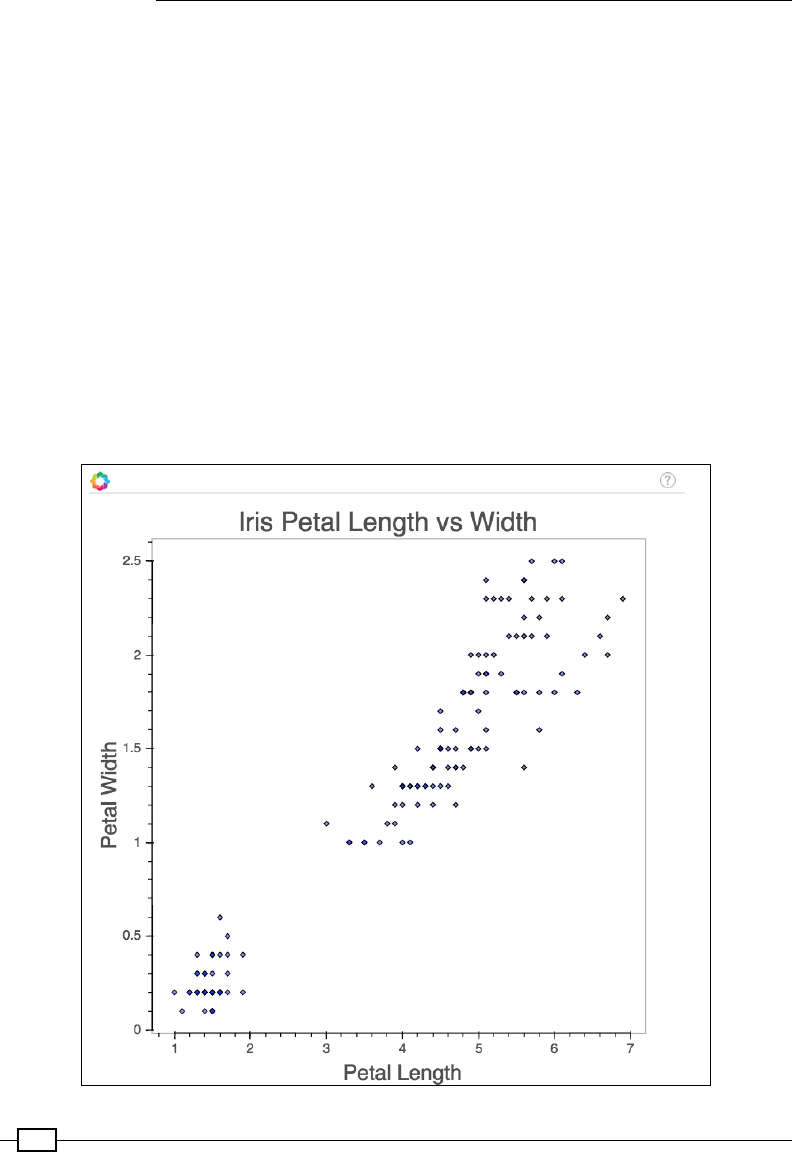
Data Visualization
496
Drawing the x and the y axes
Let's now draw the axes, set their bounds, and add them to the plot's renderers. We also need
to let the plot know which location each axis belongs to:
//X and Y Axis
val xAxis = new LinearAxis().plot(plot).axis_label("Petal Length").
bounds((1.0, 7.0))
val yAxis = new LinearAxis().plot(plot).axis_label("Petal Width").
bounds((0.0, 2.5))
plot.below <<= (listRenderer => (xAxis :: listRenderer))
plot.left <<= (listRenderer => (yAxis :: listRenderer))
//Add the renderer to the plot
plot.renderers := List(xAxis, yAxis, dataPointRenderer)
Here is the output:

Chapter 4
497
Viewing ower species with varying colors
All the data points are marked with blue as of now, but we would really like to differentiate the
species visually. This is a simple two-step process:
1. Add new derived data (speciesColor) into our ColumnDataSource to hold colors
that represent the species:
object IrisSource extends ColumnDataSource {
private val colormap = Map[Int, Color](0 -> Color.Red, 1
-> Color.Green, 2 -> Color.Blue)
private val iris = csvread(file = new
File("irisNumeric.csv"), separator = ',')
val sepalLength = column(iris(::, 0))
val sepalWidth = column(iris(::, 1))
val petalLength = column(iris(::, 2))
val petalWidth = column(iris(::, 3))
val speciesColor = column(species.value.map(v =>
colormap(v.round.toInt)))
}
So, we assign red to Iris setosa, green to Iris versicolor and blue to Iris virginica.
2. Modify the diamond marker to take this as input instead of accepting a static blue:
val diamond = new Diamond()
.x(petalLength)
.y(petalWidth)
.fill_color(speciesColor)
.fill_alpha(0.5)
.size(10)
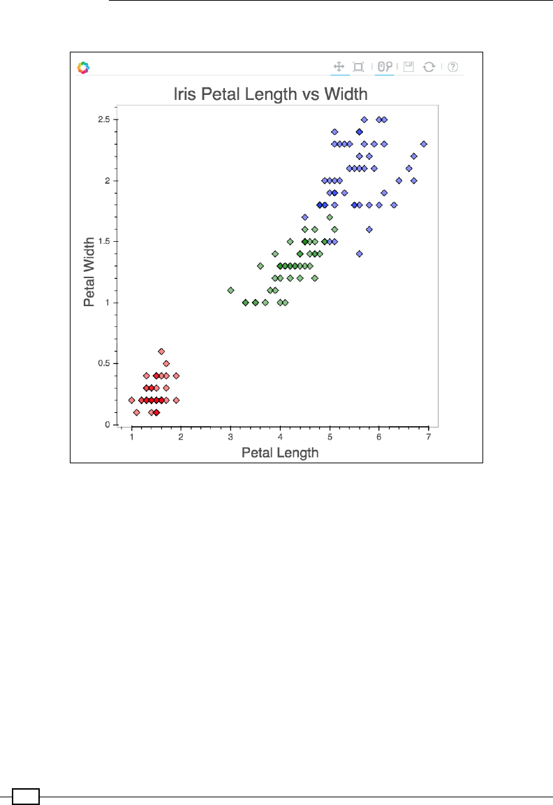
Data Visualization
498
The output is as follows:
It looks fairly okay now. Let's add some tools to the image. Bokeh has some nice tools that can
be attached to the image: BoxSelectTool, BoxZoomTool, CrosshairTool, HoverTool,
LassoSelectTool, PanTool, PolySelectTool, PreviewSaveTool, ResetTool,
ResizeTool, SelectTool, TapTool, TransientSelectTool, and WheelZoomTool.
Let's add a few of them to see them for fun:
val panTool = new PanTool().plot(plot)
val wheelZoomTool = new WheelZoomTool().plot(plot)
val previewSaveTool = new PreviewSaveTool().plot(plot)
val resetTool = new ResetTool().plot(plot)
val resizeTool = new ResizeTool().plot(plot)
val crosshairTool = new CrosshairTool().plot(plot)
plot.tools := List(panTool, wheelZoomTool, previewSaveTool, resetTool,
resizeTool, crosshairTool)
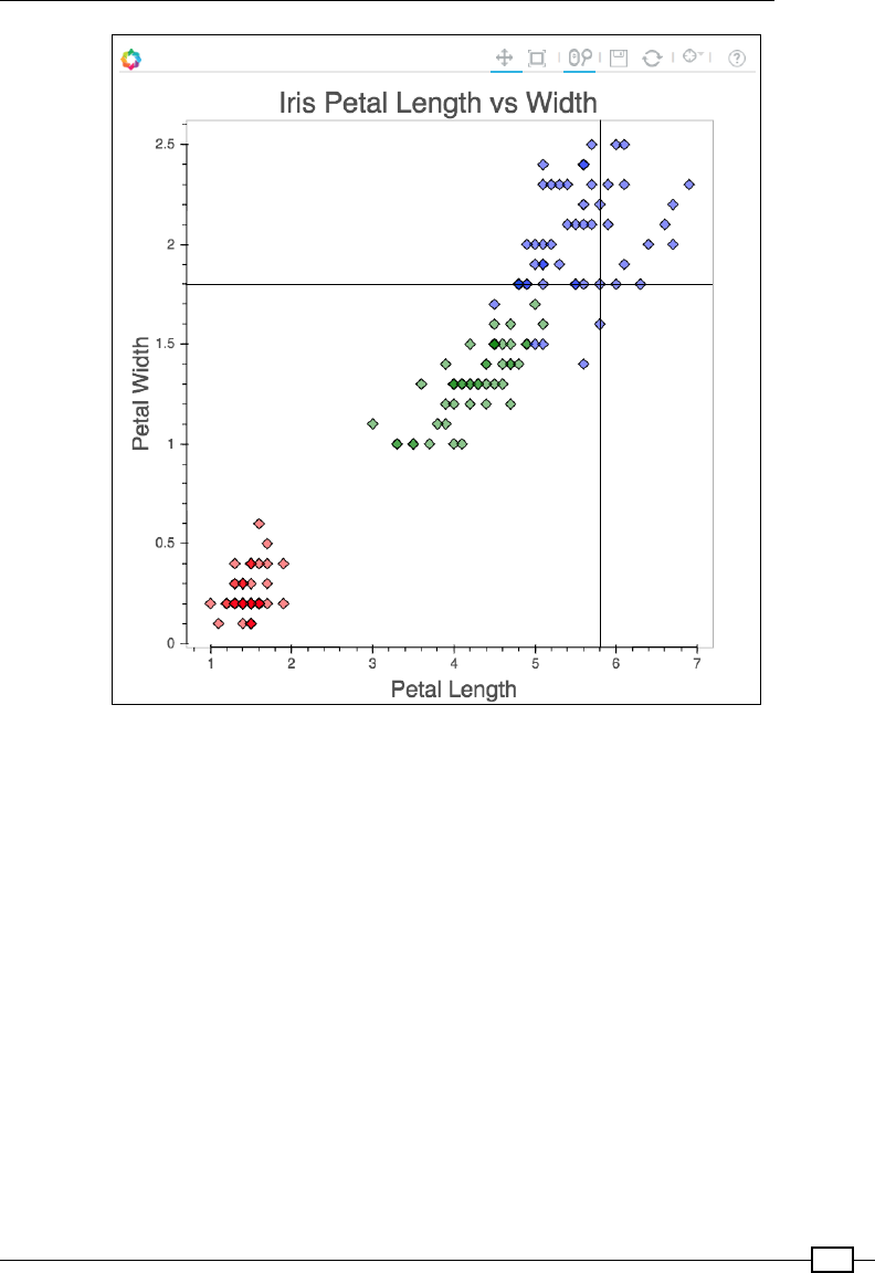
Chapter 4
499
Adding grid lines
While we have the crosshair tool, which helps us locate the exact x and y values of a particular
data point, it would be nice to have a data grid too. Let's add two data grids, one for the x axis
and one for the y axis:
val xAxis = new LinearAxis().plot(plot).axis_label("Petal Length").
bounds((1.0, 7.0))
val yAxis = new LinearAxis().plot(plot).axis_label("Petal Width").
bounds((0.0, 2.5))
val xgrid = new Grid().plot(plot).axis(xAxis).dimension(0)
val ygrid = new Grid().plot(plot).axis(yAxis).dimension(1)
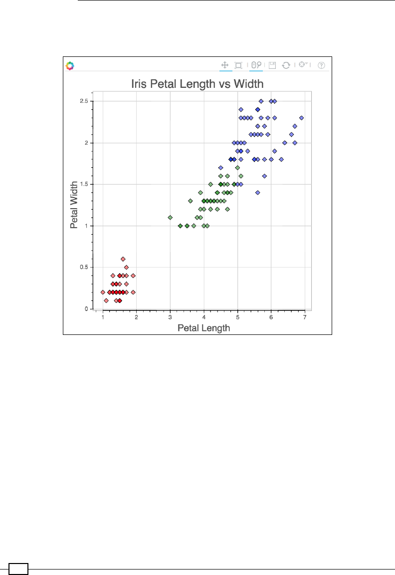
Data Visualization
500
Next, let's add the grids to the plot renderer list too:
plot.renderers := List(xAxis, yAxis, dataPointRenderer, xgrid, ygrid)
Adding a legend to the plot
This step is a bit tricky in the Scala binding of Bokeh due to the lack of high-level graphing
objects, such as scatter. For now, let's cook up our own legend. The legends property of
the Legend object accepts a list of tuples - a label and a GlyphRenderer pair. Let's explicitly
create three GlyphRenderer wrapping diamonds of three colors, which represent the
species. We then add them to the plot:
val setosa = new Diamond().fill_color(Color.Red).size(10).fill_alpha(0.5)
val setosaGlyphRnd=new GlyphRenderer().glyph(setosa)
val versicolor = new Diamond().fill_color(Color.Green).size(10).fill_
alpha(0.5)
val versicolorGlyphRnd=new GlyphRenderer().glyph(versicolor)
val virginica = new Diamond().fill_color(Color.Blue).size(10).fill_
alpha(0.5)
val virginicaGlyphRnd=new GlyphRenderer().glyph(virginica)
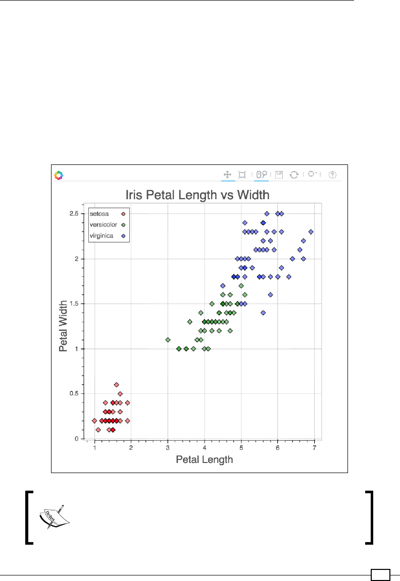
Chapter 4
501
val legends = List("setosa" -> List(setosaGlyphRnd),
"versicolor" -> List(versicolorGlyphRnd),
"virginica" -> List(virginicaGlyphRnd))
val legend = new Legend().orientation(LegendOrientation.TopLeft).
plot(plot).legends(legends)
plot.renderers := List(xAxis, yAxis, dataPointRenderer, xgrid, ygrid,
legend, setosaGlyphRnd, virginicaGlyphRnd, versicolorGlyphRnd)
The code for this recipe can be found at https://github.com/
arunma/ScalaDataAnalysisCookbook/blob/master/
chapter4-visualization/src/main/scala/com/
packt/scalada/viz/breeze.
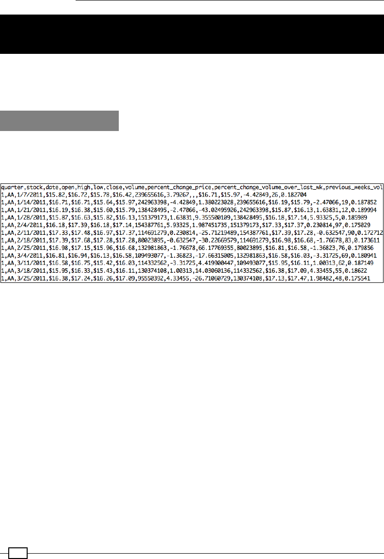
Data Visualization
502
Creating a time series MultiPlot with
Bokeh-Scala
In this second recipe on plotting using Bokeh, we'll see how to plot a time series graph
with a dataset borrowed from https://archive.ics.uci.edu/ml/datasets/
Dow+Jones+Index. We will also see how to plot multiple charts in a single document.
How to do it...
We'll be using only two elds from the dataset: the closing price of the stock at the end of the
week, and the last business day of the week. Our dataset is comma separated. Let's take a
look at some samples, as shown here:
Preparing our data
In contrast to the previous recipe, where we used the Breeze matrix to construct the
Bokeh ColumnDataSource, we'll use the Spark DataFrame to construct the source this
time. The getSource method accepts a ticker (MSFT-Microsoft and CAT-Caterpillar) and
a SQLContext. It runs a Spark SQL, fetches the data from the table, and constructs a
ColumnDataSource from it:
import org.joda.time.format.DateTimeFormat
object StockSource {
val formatter = DateTimeFormat.forPattern("MM/dd/yyyy");
def getSource(ticker: String, sqlContext: SQLContext) = {
val stockDf = sqlContext.sql(s"select stock, date, close from
stocks where stock= '$ticker'")
stockDf.cache()

Chapter 4
503
val dateData: Array[Double] =
stockDf.select("date").collect.map(eachRow =>
formatter.parseDateTime(eachRow.getString(0)).getMillis().toDouble)
val closeData: Array[Double] =
stockDf.select("close").collect.map(eachRow =>
eachRow.getString(0).drop(1).toDouble)
object source extends ColumnDataSource {
val date = column(dateData)
val close = column(closeData)
}
source
}
}
Earlier, we constructed SQLContext and registered the dataset as a table, like this:
val conf = new SparkConf().setAppName("csvDataFrame").
setMaster("local[2]")
val sc = new SparkContext(conf)
val sqlContext = new SQLContext(sc)
val stocks = sqlContext.csvFile(filePath = "dow_jones_index.data",
useHeader = true, delimiter = ',')
stocks.registerTempTable("stocks")
The only tricky thing that we do here is convert the date value into milliseconds. This is
because the Plot point requires a double. We use the Joda-Time API to achieve this.
Creating a plot
Let's go ahead and create the Plot object from the source:
//Create Plot
val plot = new Plot().title(ticker).x_range(xdr).y_range(ydr).width(800).
height(400)
Let's have our image's title as the ticker name of the stock and create a Document object so
that we can save the nal HTML by the name ClosingPrices.html:
val msDocument = new Document(microsoftPlot)
val msHtml = msDocument.save("ClosingPrices.html")

Data Visualization
504
Creating a line that joins all the data points
As we saw earlier with the Diamond marker, we'll have to pass the x and the y positions of
the data points. Also, we will need to wrap the Line glyph into a renderer so that we can
add it to Plot:
val line = new Line().x(date).y(close).line_color(color).line_width(2)
val lineGlyph = new GlyphRenderer().data_source(source).glyph(line)
Setting the x and y axes' data range for the plot
The plot needs to know what the x and y data ranges of the plot are before rendering.
Let's do that by creating two DataRange objects and setting them to the plot:
val xdr = new DataRange1d().sources(List(date))
val ydr = new DataRange1d().sources(List(close))
plot.x_range(xdr).y_range(ydr)
Drawing the axes and the grids
Drawing the axes and the grids is the same as before. We added some labels to the axis,
formatted the display of the x axis, and then added them to the Plot:
val xformatter = new DatetimeTickFormatter().formats(Map(DatetimeUnits.
Months -> List("%b %Y")))
val xaxis = new DatetimeAxis().plot(plot).formatter(xformatter).axis_
label("Month")
val yaxis = new LinearAxis().plot(plot).axis_label("Price")
plot.below <<= (xaxis :: _)
plot.left <<= (yaxis :: _)
val xgrid = new Grid().plot(plot).dimension(0).axis(xaxis)
val ygrid = new Grid().plot(plot).dimension(1).axis(yaxis)
Adding tools
As before, let's add some tools to the image—and to the plot:
//Tools
val panTool = new PanTool().plot(plot)
val wheelZoomTool = new WheelZoomTool().plot(plot)
val previewSaveTool = new PreviewSaveTool().plot(plot)
val resetTool = new ResetTool().plot(plot)
val resizeTool = new ResizeTool().plot(plot)
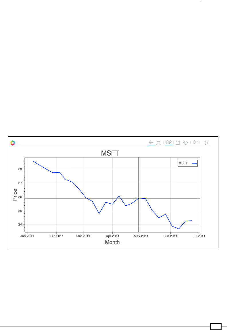
Chapter 4
505
val crosshairTool = new CrosshairTool().plot(plot)
plot.tools := List(panTool, wheelZoomTool, previewSaveTool,
resetTool, resizeTool, crosshairTool)
Adding a legend to the plot
Since we already have the Glyph renderer for the line, all we need to do is add it to the
legend. The properties of the line automatically propagate to the legend:
//Legend
val legends = List(ticker -> List(lineGlyph))
val legend = new Legend().plot(plot).legends(legends)
Next, let's add all the renderers that we created before to the plot:
plot.renderers <<= (xaxis :: yaxis :: xgrid :: ygrid :: lineGlyph ::
legend :: _)
As the nal step, let's try plotting multiple plots in the same document.
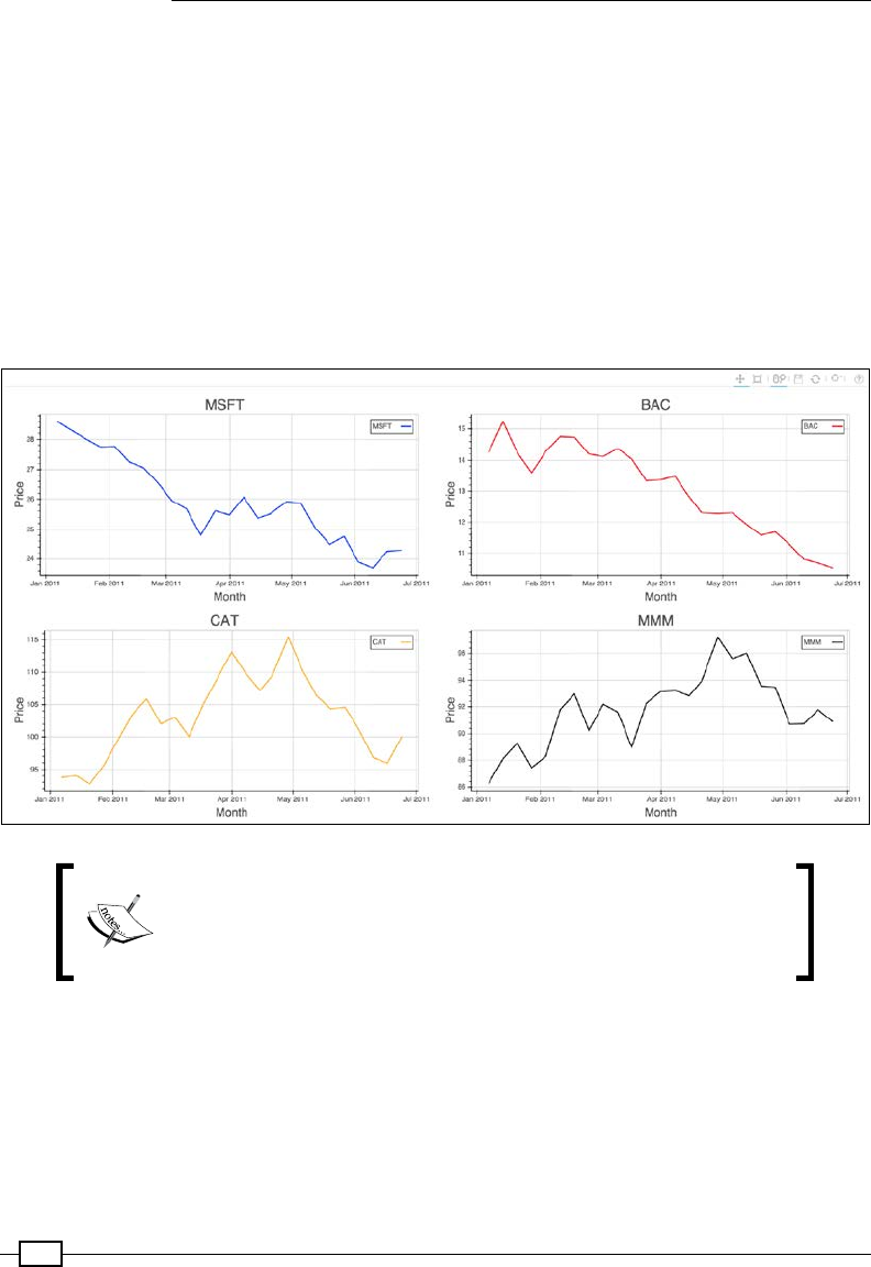
Data Visualization
506
Multiple plots in the document
Creating multiple plots in the same document is child's play. All that we need to do is create all
our plots and then add them into a grid. Finally, instead of passing our individual plot object
into the document, we pass in GridPlot:
val children = List(List(microsoftPlot, bofaPlot), List(caterPillarPlot,
mmmPlot))
val grid = new GridPlot().children(children)
val document = new Document(grid)
val html = document.save("DJClosingPrices.html")
The code for this recipe can be found at https://github.com/
arunma/ScalaDataAnalysisCookbook/blob/master/
chapter4-visualization/src/main/scala/com/
packt/scalada/viz/breeze.
In this chapter, we explored two methods of visualization and built some basic graphs and
charts using Scala. As I mentioned earlier, the visualization libraries in Scala are actively
being developed and cannot be compared to advanced visualizations that can be generated
using R or, for that sake, Tableau.

507
5
Learning from Data
In this chapter, we will cover the following recipes:
fPredicting continuous values using linear regression
fBinary classication using LogisticRegression and SVM
fBinary classication using LogisticRegression with the Pipeline API
fClustering using K-means
fFeature reduction using principal component analysis
Introduction
In previous chapters, we saw how to load, prepare, and visualize data. Now, let's start doing
some interesting stuff with it. In this chapter, we'll be looking into applying various machine
learning techniques on top of it. We'll look at a few examples for the two broad classications
of machine learning techniques: supervised and unsupervised learning. Before that, however,
let's briey see what these terms mean.
Supervised and unsupervised learning
If you are reading this book, you probably already know what supervised and unsupervised
learning are, but for the sake of completion, let's briey summarize what they mean. In
supervised learning, we train the algorithms with labeled data. Labeled data is nothing but
input data along with the outcome variable. For example, if our intention is to predict whether
a website is about news, we would be preparing a sample dataset of website content with
"news" and "not news" as labels. This dataset is called the training dataset.

Learning from Data
508
With supervised learning, our end goal is to use the training dataset and come up with a
function that maps our input variables to an output variable with least margin of error. We
call input variables (or x variables) features or explanatory variables, and the output variable
(also known as the y variable or label) the target or dependent variable. In the news website
example, the text content in the website would be the input variable and "news" or "not news"
would be the target variable. The function, along with its parameters (or weights or theta), is
our hypothesis, or model.
In the case of unsupervised learning, we aim to nd a structure within the data— groups and
relationships among these groups or the participants of a group. Unlike supervised learning,
we don't know any information about the data or even its subset. An example would be to see
whether there are similar buying patterns among a group of people (which helps cross-selling)
or to see which group of people is more likely to buy pizza from our newly opened store.
Gradient descent
With supervised learning, in order for the algorithm to learn the relationship between the input
and the output features, we provide a set of manually curated values for the target variable
(y) against a set of input variables (x). We call it the training set. The learning algorithm then
has to go over our training set, perform some optimization, and come up with a model that
has the least cost—deviation from the true values. So technically, we have two algorithms for
every learning problem: an algorithm that comes up with the function and (an initial set of)
weights for each of the x features, and a supporting algorithm (also called cost minimization
or optimization algorithm) that looks at our function parameters (feature weights) and tries to
minimize the cost as much as possible.
There are a variety of cost minimization algorithms, but one of the most popular is gradient
descent. Imagine gradient descent as climbing down a mountain. The height of the mountain
represents the cost, and the plain represents the feature weights. The highest point is your
function with the maximum cost, and the lowest point has the least cost. Therefore, our
intention is to walk down the mountain. What gradient descent does is as follows: for every
single step down the slope that it takes of a particular size (the step size), it goes through the
entire dataset (!) and updates all the values of the weights for x features. This goes on until
it reaches a state where the cost is the minimum. This avor of gradient descent, in which
it sees all of the data per iteration and updates all the parameters during every iteration, is
called batch gradient descent. The trouble with using this algorithm against the size of the
data that Spark aims to handle is that going through millions of rows per iteration is denitely
not optimal. So, Spark uses a variant of gradient descent, called Stochastic Gradient Descent
(SGD), wherein the parameters are updated for each training example as it looks at it one by
one. In this way, it starts making progress almost immediately, and therefore the computational
effort is considerably reduced. The SGD settings can be customized using the optimizer
attribute inside each of the ML algorithm. We'll look at this in detail in the recipes.
Chapter 5
509
In the following recipes, we'll be looking at linear regression, logistic regression, and
support vector machines as examples of supervised learning and K-means clustering,
as well as dimensionality reduction using Principal Component Analysis (PCA) as an
example of unsupervised learning. We'll also briey look at the Stanford NLP toolkit and
Scala NLP's Epic, popular natural language processing libraries, as examples of tting a
third-party library into Spark jobs.
Predicting continuous values using linear
regression
At the risk of stating the obvious, linear regression aims to nd the relationship between
an output (y) based on an input (x) using a mathematical model that is linear to the input
variables. The output variable, y, is a continuous numerical value. If we have more than one
input/explanatory variable (x), as in the example that we are going to see, we call it multiple
linear regression. The dataset that we'll use for this recipe, for lack of creativity, is lifted
from the UCI website at http://archive.ics.uci.edu/ml/machine-learning-
databases/wine-quality/. This dataset has 1599 instances of various red wines, their
chemical composition, and their quality. We'll use it to predict the quality of a red wine.
How to do it...
Let's summarize the steps:
1. Importing the data.
2. Converting each instance into a LabeledPoint.
3. Preparing the training and test data.
4. Scaling the features.
5. Training the model.
6. Predicting against the test data.
7. Evaluating the model.
8. Regularizing the parameters.
9. Mini batching.
The code for this recipe can be found at https://github.com/
arunma/ScalaDataAnalysisCookbook/tree/master/
chapter5-learning/src/main/scala/com/packt/
scalada/learning/LinearRegressionWine.scala.
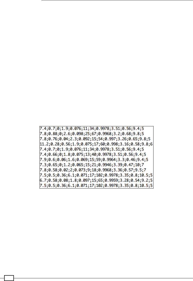
Learning from Data
510
"Step zero" of this process is the creation of SparkConfig and the SparkContext. There is
nothing fancy here:
val conf = new SparkConf().setAppName("linearRegressionWine").
setMaster("local[2]")
val sc = new SparkContext(conf)
Importing the data
We then import the semicolon-separated text le. We map each line into an Array[String]
by splitting each of them using semicolons. We end up with RDD[Array[String]]:
val rdd = sc.textFile("winequality-red.csv").map(line => line.split(";"))
Converting each instance into a LabeledPoint
As we discussed earlier, supervised learning requires training data to be provided. We are also
are required to test the model that we create for its accuracy against another set of data—the
test data. If we have two different datasets for this, we can import them separately and mark
them as a training set and a test set. In our example, we'll use a single dataset and split it into
training and test sets.
Each of our training samples has the following format: the last eld is the quality of the
wine, a rating from 1 to 10, and the rst 11 elds are the properties of the wine. So, from our
perspective, the quality of the wine is the y variable (the output) and the rest of them are x
variables (input). Now, let's represent this in a format that Spark understands—a LabeledPoint.
A LabeledPoint is a simple wrapper around the input features (our x variables) and our pre-
predicted value (y variable) for these x input values:
val dataPoints=rdd.map(row=>new LabeledPoint(row.last.toDouble,Vectors.
dense(row.take(row.length-1).map(str=>str.toDouble))))
The rst parameter to the constructor of the LabeledPoint is the label (y variable), and the
second parameter is a vector of input variables.

Chapter 5
511
Preparing the training and test data
As we discussed earlier, we can have two different independent datasets for training and
testing. However, it is a common practice to split the dataset into training and test datasets.
In this recipe, we will be splitting the dataset into training and test sets in the ratio of 80:20,
with each of the elements being selected randomly. This random shufing of data is one of
the prerequisites for better performance of the SGD too:
val dataSplit = dataPoints.randomSplit(Array(0.8, 0.2))
val trainingSet = dataSplit(0)
val testSet = dataSplit(1)
Scaling the features
Running a quick summary statistics reveals that our features aren't in the same range:
val featureVector = rdd.map(row => Vectors.dense(row.take(row.length-1).
map(str => str.toDouble)))
print(s"Max : ${stats.max}, Min : ${stats.min}, and Mean : ${stats.mean}
and Variance : ${stats.variance}")
println ("Min "+ stats.min)
println ("Max "+ stats.max)
Here is the output:
Min [4.6,0.12,0.0,0.9,0.012,1.0,6.0,0.99007,2.74,0.33,8.4]
Max [15.9,1.58,1.0,15.5,0.611,72.0,289.0,1.00369,4.01,2.0,14.9]
Variance : [3.031416388997815,0.0320623776515516,0.0379
4748313440582,1.987897132985963,0.002215142653300991,10
9.41488383305895,1082.1023725325845,3.56202945332629E-
6,0.02383518054541292,0.02873261612976197,1.135647395000472]
It is always recommended that the input variables have a mean of 0. This is easily achieved
with the help of the StandardScaler built into the Spark ML library itself. The one thing that
we have to watch out for here is that we have to scale the training and the test sets uniformly.
The way we do it is by creating a scaler for trainingSplit and using the same scaler to scale the
test set. Another side note is that feature scaling helps with faster convergence in SGD:
val scaler = new StandardScaler(withMean = true, withStd = true).
fit(trainingSet.map(dp => dp.features))
val scaledTrainingSet = trainingSet.map(dp => new LabeledPoint(dp.label,
scaler.transform(dp.features))).cache()
val scaledTestSet = testSet.map(dp => new LabeledPoint(dp.label, scaler.
transform(dp.features))).cache()

Learning from Data
512
Training the model
The next step is to use our training data to create a model. This just involves creating an
instance of LinearRegressionWithSGD and passing in a few parameters: one for the
LinearRegression algorithm and two for the SGD. The SGD parameters can be accessed
through the use of the optimizer attribute inside LinearRegressionWithSGD:
fsetIntercept: While predicting, we are more interested in the slope. This setting
will force the algorithm to nd the intercept too.
foptimizer.setNumIterations: This determines the number of iterations that
our algorithm needs to go through on the training set before nalizing the hypothesis.
An optimal number would be 10^6 divided by the number of instances in your
dataset. In our case, we'll set it to 1000.
fsetStepSize: This tells the gradient descent algorithm while it tries to reduce
the parameters how big a step it needs to take during every iteration. Setting this
parameter is really tricky because we would like the SGD to take bigger steps in the
beginning and smaller steps towards the convergence. Setting a xed small number
would slow down the algorithm, and setting a xed bigger number would not give us
a function that is a reasonable minimum. The way Spark handles our setStepSize
input parameter is as follows: it divides the input parameter by a root of the iteration
number. So initially, our step size is huge, and as we go further down, it becomes
smaller and smaller. The default step size parameter is 1.
val regression=new LinearRegressionWithSGD().setIntercept(true)
regression.optimizer.setNumIterations(1000).setStepSize(0.1)
//Let's create a model out of our training examples.
val model=regression.run(scaledTrainingSet)
Predicting against test data
This step is just a one-liner. We use the resulting model to predict the output (y) based on the
features of the test set:
val predictions:RDD[Double]=model.predict(scaledTestSet.map(point=>point.
features))
Evaluating the model
Let's evaluate our model against one of the most popular regression evaluation metrics—
mean squared error. Let's get the actual values that our test data has (the y variable
prepared manually) and then compare it with the predictions from our model:
val actuals:RDD[Double]=scaledTestSet.map(_.label)
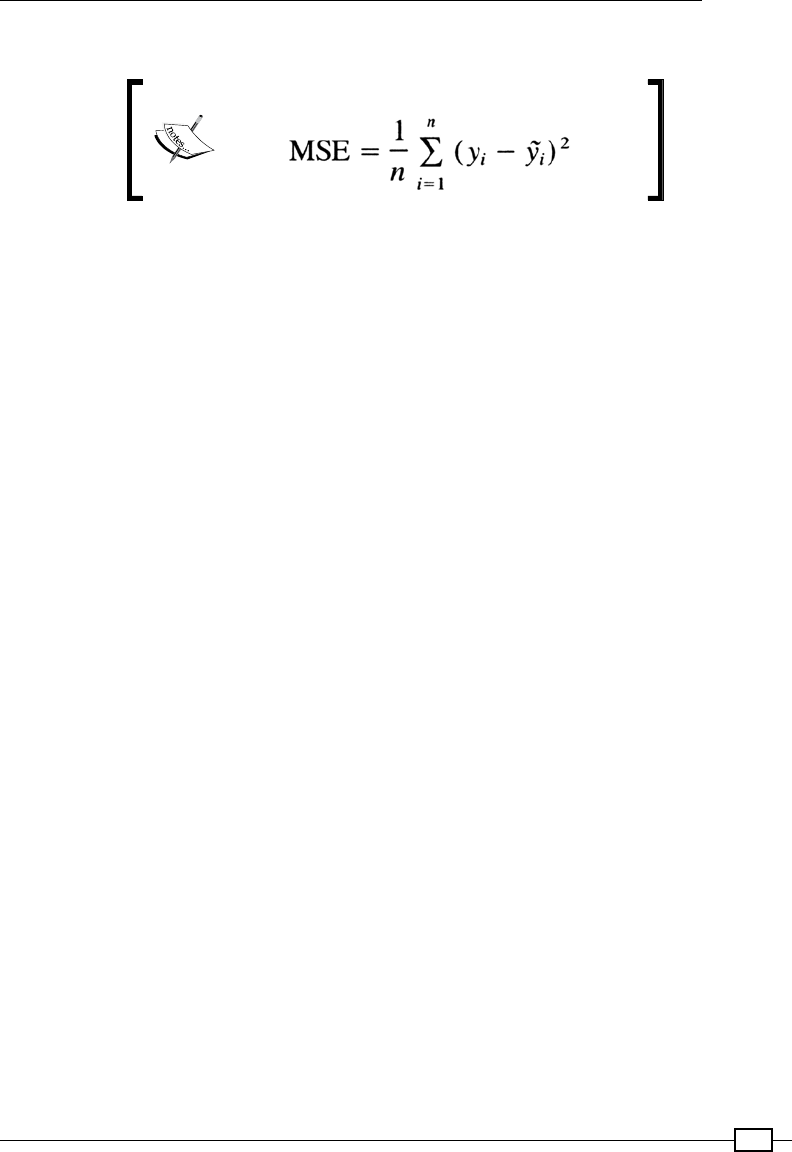
Chapter 5
513
Mean squared error
The mean squared error is given by this formula:
So, we take the difference between the actual and the predicted values (errors), square them,
and calculate the sum of them all. We then divide this sum by the number of values, thereby
calculating the mean:
val predictsAndActuals: RDD[(Double, Double)] = predictions.zip(actuals)
val sumSquaredErrors=predictsAndActuals.map{case (pred,act)=>
println (s"act, pred and difference $act, $pred ${act-pred}")
math.pow(act-pred,2)
}.sum()
val meanSquaredError = sumSquaredErrors / scaledTestSet.count
println(s"SSE is $sumSquaredErrors")
println(s"MSE is $meanSquaredError")
Here is the output:
SSE is 162.21647197365706
MSE is 0.49607483783992984
In our example, we selected all the features that are present in our dataset. Later, we'll take
a look at dimensionality reduction, which helps us reduce the number of features while still
maintaining the variance of the dataset at a reasonably higher level.
Regularizing the parameters
Before we see what regularization is, let's briey see what overtting is. A model is said to be
overt (or having high variance) when it memorizes the training set. The result of this is that
the algorithm fails to generalize and therefore performs badly with unseen datasets. One way
to solve the problem of overtting is to manually select the important features that will be
used to create the model, but for a large-dimensional dataset, it is hard to decide which ones
to keep and which ones to throw away.

Learning from Data
514
The other popular option is to retain all the features but reduce the magnitudes of the feature
weights. Thus, even with a model that is complex (with higher degree polynomials), if the
feature weights are really small, the resulting model would be simple. In other words, given
two equally (or almost equally) performing models, with one model being complex (with
higher degree polynomial) and the other model being simple, regularization chooses the
simple model. The reasoning behind this is that models with simple parameters have a
higher probability of predicting unseen data (also known as generalization).
The Spark MLlib comes with implementations for the most common L1 and L2 regularizations.
As a side note, LinearRegressionWithSGD, by default, uses a SimpleUpdater, which
does not regularize the parameters. Interestingly, Spark has implementations of regression
algorithms that are based on top of the L1 and L2 updaters; they are called the Lasso (that
uses the L1 updater) and Ridge (that uses the L2 updater by default).
While the L1 regularizer offers some feature selection when the dataset that we have is
sparse (or if the dataset's rows are smaller than the feature itself), most of the time, it is
recommended is to use the L2 regularizer. The new Pipeline API also has out-of-the-box
support for ElasticNet regularization, which uses both the L1 and L2 regularizations internally.
Now, let's go over the code:
def algorithm(algo: String, iterations: Int, stepSize: Int) = algo
match {
case "linear" => {
val algo = new LinearRegressionWithSGD()
algo.setIntercept(true).optimizer.setNumIterations(iterations).
setStepSize(stepSize)
algo
}
case "lasso" => {
val algo = new LassoWithSGD()
algo.setIntercept(true).optimizer.setNumIterations(iterations).
setStepSize(stepSize)
algo
}
case "ridge" => {
val algo = new RidgeRegressionWithSGD()
algo.setIntercept(true).optimizer.setNumIterations(iterations).
setStepSize(stepSize)
algo
}
}

Chapter 5
515
As discussed earlier, LassoWithSGD wraps an L1 updater and RidgeRegessionWithSGD
wraps an L2 updater. From a code perspective, all that we need to do is change the name
of the class. The optimizer (gradient descent) now accepts a regularization parameter that
penalizes larger parameters for the features. The default value of the regularization parameter
is 0.01 in Spark. A smaller regularization parameter would result in undertting, and a large
parameter would result in overtting.
The following output shows that regularizing the parameters has reduced our error values:
************** Printing metrics for Linear Regression with SGD
*****************
SSE is 132.39124792957116
MSE is 0.4124337941731189
************** Printing metrics for Lasso Regression with SGD
*****************
SSE is 132.3943810653321
MSE is 0.4124435547206608
************** Printing metrics for Ridge Regression with SGD
*****************
SSE is 132.44011034123344
MSE is 0.4125860135240917
Mini batching
Instead of going through our dataset one by one in the case of SGD, or seeing the entire
dataset for every iteration (in the case of batch gradient descent) while updating the
parameter vector, we can settle for something in the middle. With the mini batch fraction
parameter, for every single iteration, the SGD considers that fraction of the dataset to
process for the parameter update. Let's set the batch size to 5 percent:
algo.setIntercept(true).optimizer.setNumIterations(iterations).
setStepSize(stepSize).setRegParam(0.001).setMiniBatchFraction(0.05)
The results are as follows:
************** Printing metrics for Linear Regression with SGD
*****************
SSE is 112.96958667767147
MSE is 0.3574986920179477
SST is 183.05305027649794
Residual sum of squares is 0.38285875866568087
************** Printing metrics for Lasso Regression with SGD
*****************

Learning from Data
516
SSE is 112.95392101963424
MSE is 0.35744911715074124
SST is 183.05305027649794
Residual sum of squares is 0.3829443385454675
************** Printing metrics for Ridge Regression with SGD
*****************
SSE is 112.9218089913291
MSE is 0.3573474968080035
SST is 183.05305027649794
Residual sum of squares is 0.3831197632557175
The advantage that we get from using mini batches is that this obviously gives better
performance than plain SGD without batches. This is because with plain SGD, for every
iteration, only one example is considered to update the parameters. However, with mini
batches, we consider a batch of examples. That said, the improvement in the mean
squared error from the previous run is not the result of using batches, but just a feature
of SGD—roaming around the minima and not converging at a xed point.
Binary classication using
LogisticRegression and SVM
Unlike linear regression, wherein we predicted continuous values for the outcome (the y
variable), logistic regression and the Support Vector Machine (SVM) are used to predict
just one out of the n possibilities for the outcome (the y variable). If the outcome is one of
two possibilities, then the classication is called a binary classication.
Logistic regression, when used for binary classication, looks at each data point and estimates
the probability of that data point falling under the positive case. If the probability is less than a
threshold, then the outcome is negative (or 0); otherwise, the outcome is positive (or 1).
As with any other supervised learning techniques, we will be providing training examples
for logistic regression. We then add a bit of code for feature extraction and let the algorithm
create a model that encapsulates the probability of each of the features belonging to one of
the binary outcomes.
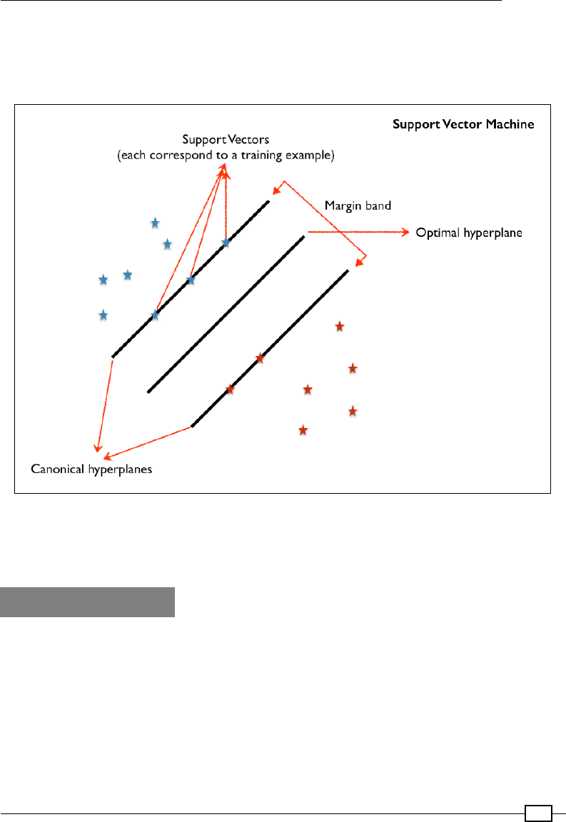
Chapter 5
517
What SVM tries to do is map all of the training data as points in the feature space.
The algorithm comes up with a hyperplane that separates the positive and negative
training examples in such a way that the distance (margin band) between them is
maximum. This is better illustrated with a diagram:
When a new and unseen data point comes up for prediction, the algorithm looks at that point
and tries to nd the closest point to the input data point. The label corresponding to that point
will be predicted as the label for the input point as well.
How to do it...
Both the implementations of LogisticRegression and SVM in Spark use L2 regularization by
default, but we are free to switch to L1 by setting the updater explicitly.
In this recipe, we'll classify a spam/ham dataset (https://archive.ics.uci.edu/ml/
datasets/SMS+Spam+Collection) against three variants of classication algorithms:
fLogistic regression with SGD as the optimization algorithm
fLogistic regression with BFGS as the optimization algorithm
fSupport vector machine with SGD as the optimization algorithm
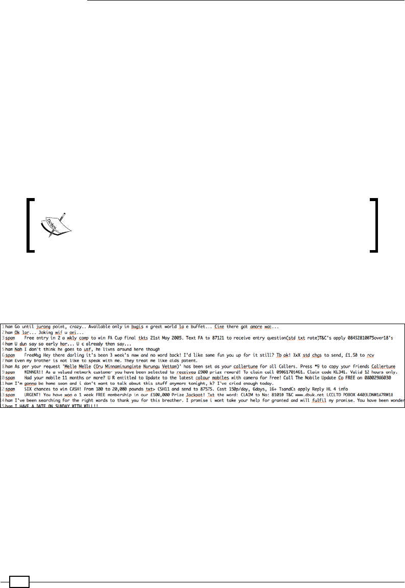
Learning from Data
518
The BFGS optimization algorithm provides the benets of converging to the minimum
faster than SGD. Also, for BFGS, we need not break our heads coming up with an optimal
learning rate.
Let's summarize the steps:
1. Importing the data.
2. Tokenizing the data and converting it into LabeledPoints.
3. Factoring the Inverse Document Frequency (IDF).
4. Preparing the training and test data.
5. Constructing the algorithm.
6. Training the model and predicting the test data.
7. Evaluating the model.
The code for this recipe can be found at https://github.com/
arunma/ScalaDataAnalysisCookbook/blob/master/
chapter5-learning/src/main/scala/com/packt/
scalada/learning/BinaryClassificationSpam.scala.
Importing the data
As usual, our input data is in the form of a text le—SMSSpamCollection. The data le looks
like this:
As we can see, the label and the data are separated by a tab. So, while reading each line,
we split the label and the content, and then populate a simple case class named Document.
This Document class is just a temporary placeholder. In the next step, we'll convert these
documents into LabeledPoints:
//Frankly, we could make this a tuple but this looks neat
case class Document(label: String, content: String)
val docs = sc.textFile("SMSSpamCollection").map(line => {
val words = line.split("\t")
Document(words.head.trim(), words.tail.mkString(" "))
})

Chapter 5
519
Tokenizing the data and converting it into LabeledPoints
For the tokenization, instead of relying on the tokenizer provided inside Spark, we'll see how
to plug in two external NLP libraries—the Stanford CoreNLP and Scala NLP's Epic libraries.
These are the two most popular NLP libraries: one from the Java world and the other from
Scala. However, one thing that we ought to watch out for while using external libraries is that
the instantiation of these APIs, and therefore the creation of heavyweight objects required for
the use of these APIs (such as a tokenizer), should be done at the partition level. If we do it at
the level of a closure, such as a map over RDD, we'll end up creating new instance of the API
object for every single instance of the data.
In the case of Epic, we just split the documents into sentences and then tokenize them into
words. We also add two more restrictions. Only those tokens that contain letters or digits will
be considered, and the tokens should be of at least two characters:
import epic.preprocess.TreebankTokenizer
import epic.preprocess.MLSentenceSegmenter
//Use Scala NLP - Epic
val labeledPointsUsingEpicRdd: RDD[LabeledPoint] =
docs.mapPartitions { docIter =>
val segmenter = MLSentenceSegmenter.bundled().get
val tokenizer = new TreebankTokenizer()
val hashingTf = new HashingTF(5000)
docIter.map { doc =>
val sentences = segmenter(doc.content)
val tokens = sentences.flatMap(sentence =>
tokenizer(sentence))
//consider only features that are letters or digits and
cut off all words that are less than 2 characters
val filteredTokens=tokens.toList.filter(token =>
token.forall(_.isLetterOrDigit)).filter(_.length() > 1)
new LabeledPoint(if (doc.label=="ham") 0 else 1,
hashingTf.transform(filteredTokens))
}
}.cache()
MLSentenceSegmenter splits the paragraph into sentences. The sentences are then split
into terms (or words) using the tokenizer. HashingTF creates a map of terms with their
frequency of occurrence. Finally, to construct a LabeledPoint for each document, we convert
these terms into a term frequency vector for that document using the transform function
of HashingTF. Also, we restrict the maximum number of interested terms to 5,000 by way
of setting the numFeatures in HashingTF.

Learning from Data
520
With Stanford CoreNLP, the process is a little more involved, in the sense that we reduce the
tokens to lemmas (https://en.wikipedia.org/wiki/Lemmatisation). In order to do
this, we create an NLP pipeline that splits sentences, tokenizes, and nally reduces the tokens
to lemmas:
def corePipeline(): StanfordCoreNLP = {
val props = new Properties()
props.put("annotators", "tokenize, ssplit, pos, lemma")
new StanfordCoreNLP(props)
}
def lemmatize(nlp: StanfordCoreNLP, content: String):
List[String] = {
//We are required to prepare the text as 'annotatable'
before we annotate :-)
val document = new Annotation(content)
//Annotate
nlp.annotate(document)
//Extract all sentences
val sentences =
document.get(classOf[SentencesAnnotation]).asScala
//Extract lemmas from sentences
val lemmas = sentences.flatMap { sentence =>
val tokens =
sentence.get(classOf[TokensAnnotation]).asScala
tokens.map(token =>
token.getString(classOf[LemmaAnnotation]))
}
//Only lemmas with letters or digits will be considered.
Also consider only those words which has a length of at least 2
lemmas.toList.filter(lemma =>
lemma.forall(_.isLetterOrDigit)).filter(_.length() > 1)
}
val labeledPointsUsingStanfordNLPRdd: RDD[LabeledPoint] =
docs.mapPartitions { docIter =>
val corenlp = corePipeline()
val stopwords = Source.fromFile("stopwords.txt").getLines()
val hashingTf = new HashingTF(5000)
docIter.map { doc =>
val lemmas = lemmatize(corenlp, doc.content)
//remove all the stopwords from the lemma list
lemmas.filterNot(lemma => stopwords.contains(lemma))

Chapter 5
521
//Generates a term frequency vector from the features
val features = hashingTf.transform(lemmas)
//example : List(until, jurong, point, crazy, available,
only, in, bugi, great, world, la, buffet, Cine, there, get, amore,
wat)
new LabeledPoint(
if (doc.label.equals("ham")) 0 else 1,
features)
}
}.cache()
Factoring the inverse document frequency
With HashingTF, we have a map of terms along with their frequency of occurrence in the
documents. Now, the problem with taking this metric is that common words such as "the"
and "a" get higher rankings compared to rare words. The inverse document frequency (IDF)
calculates the occurrences of a word in all the documents and gives higher weight to a term
that is uncommon. We'll now factor in the inverse document frequency so that we have
the TF-IDF score (https://en.wikipedia.org/wiki/Tf–idf) for each term. This is
easily achievable in Spark with the availability of org.apache.spark.mllib.feature.
IDFModel. We extract all term frequencies from LabeledPoints and pass them to the
transform function IDFModel to generate the TF-IDF:
val labeledPointsUsingStanfordNLPRdd=getLabeledPoints(docs,
"STANFORD")
val lpTfIdf=withIdf(labeledPointsUsingStanfordNLPRdd).cache()
def withIdf(lPoints: RDD[LabeledPoint]): RDD[LabeledPoint] = {
val hashedFeatures = labeledPointsWithTf.map(lp =>
lp.features)
val idf: IDF = new IDF()
val idfModel: IDFModel = idf.fit(hashedFeatures)
val tfIdf: RDD[Vector] = idfModel.transform(hashedFeatures)
val lpTfIdf= labeledPointsWithTf.zip(tfIdf).map {
case (originalLPoint, tfIdfVector) => {
new LabeledPoint(originalLPoint.label, tfIdfVector)
}
}
lpTfIdf
}
val lpTfIdf=withIdf(labeledPointsWithTf).cache()

Learning from Data
522
Prepare the training and test data
Our test data has a skewed distribution of spam and ham data. We just have to make sure
that when we split the data into training and test data into 80% and 20%, we rst split the
training and test data into two subsets and then split it into the 80:20 ratio. At the end of
this, the training data and test data will have a ratio of 4:1 spam and ham samples.
The spam and ham counts in our dataset are 747 and 4827, respectively:
//Split dataset
val spamPoints = lpTfIdf.filter(point => point.label ==
1).randomSplit(Array(0.8, 0.2))
val hamPoints = lpTfIdf.filter(point => point.label ==
0).randomSplit(Array(0.8, 0.2))
println ("Spam
count:"+(spamPoints(0).count)+"::"+(spamPoints(1).count))
println ("Ham count:"+(hamPoints(0).count)+"::"+(hamPoints(1).
count))
val trainingSpamSplit = spamPoints(0)
val testSpamSplit = spamPoints(1)
val trainingHamSplit = hamPoints(0)
val testHamSplit = hamPoints(1)
val trainingSplit = trainingSpamSplit ++ trainingHamSplit
val testSplit = testSpamSplit ++ testHamSplit
Constructing the algorithm
Now that we have our training and test sets, the next obvious step is to train a model out of
these examples. Let's create instances of the three variants of the algorithms that we would
like to experiment with:
val logisticWithSGD = getAlgorithm("logsgd", 100, 1, 0.001)
val logisticWithBfgs = getAlgorithm("logbfgs", 100, Double.Nan,
0.001)
val svmWithSGD = getAlgorithm("svm", 100, 1, 0.001)
def getAlgorithm(algo: String, iterations: Int, stepSize:
Double, regParam: Double) = algo match {
case "logsgd" => {
val algo = new LogisticRegressionWithSGD()

Chapter 5
523
algo.setIntercept(true).optimizer.setNumIterations(iterations).
setStepSize(stepSize).setRegParam(regParam)
algo
}
case "logbfgs" => {
val algo = new LogisticRegressionWithLBFGS()
algo.setIntercept(true).optimizer.setNumIterations(iterations).
setRegParam(regParam)
algo
}
case "svm" => {
val algo = new SVMWithSGD()
algo.setIntercept(true).optimizer.setNumIterations(iterations).
setStepSize(stepSize).setRegParam(regParam)
algo
}
}
We can notice that the stepSize parameter isn't set for logistic regression with BFGS.
Training the model and predicting the test data
Like linear regression, training and predicting the labels for the test set is just a matter of
calling the run and predict methods of the classication algorithm.
Soon after the prediction is done, the next logical step is to evaluate the model.
In order to generate metrics for this, we extract the predicted and the actual labels.
Our runClassification function trains the model using the training data and makes
predictions against the test data. It then zips the predicted and the actual outcomes
into a value called predictsAndActuals. This value is returned from the function.
The runClassification accepts a GeneralizedLinearAlgorithm as the parameter,
which is the parent of LinearRegressionWithSGD, LogisticRegressionWithSGD,
and SVMWithSGD:
val
logisticWithSGDPredictsActuals=runClassification(logisticWithSGD,
trainingSplit, testSplit)
val
logisticWithBfgsPredictsActuals=runClassification(logisticWithBfgs,
trainingSplit, testSplit)
val svmWithSGDPredictsActuals=runClassification(svmWithSGD,
trainingSplit, testSplit)

Learning from Data
524
def runClassification(algorithm: GeneralizedLinearAlgorithm[_ <:
GeneralizedLinearModel], trainingData:RDD[LabeledPoint],
testData:RDD[LabeledPoint]): RDD[(Double, Double)] = {
val model = algorithm.run(trainingData)
val predicted = model.predict(testData.map(point =>
point.features))
val actuals = testData.map(point => point.label)
val predictsAndActuals: RDD[(Double, Double)] =
predicted.zip(actuals)
predictsAndActuals
}
Evaluating the model
For generating the metrics, Spark has some inbuilt APIs. The two most common metrics used
to evaluate a classication model are the area under curve and the confusion matrix. The org.
apache.spark.mllib.evaluation.BinaryClassificationMetrics gives us the area
under the curve, and org.apache.spark.mllib.evaluation.MulticlassMetrics gives
us the confusion matrix. We also calculate the simple accuracy measure manually using the
values of predicated and actuals. The accuracy is simply the result of dividing the correctly
classied count of the test dataset by the total count of the test dataset. Refer to https://
en.wikipedia.org/wiki/Accuracy_and_precision#In_binary_classification
for more details:
def calculateMetrics(predictsAndActuals: RDD[(Double, Double)],
algorithm: String) {
val accuracy = 1.0*predictsAndActuals.filter(predActs => predActs._1
== predActs._2).count() / predictsAndActuals.count()
val binMetrics = new BinaryClassificationMetrics(predictsAndActuals)
println(s"************** Printing metrics for $algorithm
***************")
println(s"Area under ROC ${binMetrics.areaUnderROC}")
//println(s"Accuracy $accuracy")
val metrics = new MulticlassMetrics(predictsAndActuals)
val f1=metrics.fMeasure
println(s"F1 $f1")
println(s"Precision : ${metrics.precision}")
println(s"Confusion Matrix \n${metrics.confusionMatrix}")
println(s"************** ending metrics for $algorithm
*****************")
}

Chapter 5
525
As we can see from the output, LogisticRegressionWithSGD and SVMWithSGD have a
slightly bigger area under curve than LogisticRegressionWithBFGS, which means that
the two models perform a tad bit better.
This is a sample output (your output could vary):
************** Printing metrics for Logistic Regression with SGD
***************
Area under ROC 0.9208860759493671
Accuracy 0.9769585253456221
Confusion Matrix
927.0 0.0
25.0 133.0
************** ending metrics for Logistic Regression with SGD
*****************
************** Printing metrics for SVM with SGD ***************
Area under ROC 0.9318656156156157
Precision : 0.9784845650140318
Confusion Matrix
921.0 4.0
19.0 125.0
************** ending metrics for SVM with SGD *****************
************** Printing metrics for Logistic Regression with BFGS
***************
Area under ROC 0.8790559620074445
Accuracy 0.9596136962247586
Confusion Matrix
971.0 9.0
37.0 122.0
************** ending metrics for Logistic Regression with BFGS *********
*************************
Learning from Data
526
Binary classication using
LogisticRegression with Pipeline API
Earlier, with the spam example on binary classication, we saw how we prepared the data,
separated it into training and test data, trained the model, and evaluated it against test data
before we nally arrived at the metrics. This series of steps can be abstracted in a simplied
manner using Spark's Pipeline API.
In this recipe, we'll take a look at how to use the Pipeline API to solve the same classication
problem. Imagine the pipeline to be a factory assembly line where things happen one after
another. In our case, we'll pass our raw unprocessed data through various processors before
we nally feed the data into the classier.
How to do it...
In this recipe, we'll classify the same spam/ham dataset (https://archive.ics.uci.
edu/ml/datasets/SMS+Spam+Collection) rst using the plain Pipeline, and then
using a cross-validator to select the best model for us given a grid of parameters.
Let's summarize the steps:
1. Importing and splitting data as test and training sets.
2. Constructing the participants of the Pipeline.
3. Preparing a pipeline and training a model.
4. Predicting against test data.
5. Evaluating the model without cross-validation.
6. Constructing parameters for cross-validation.
7. Constructing a cross-validator and tting the best model.
8. Evaluating a model with cross-validation.
The code for this recipe can be found at https://github.com/
arunma/ScalaDataAnalysisCookbook/blob/master/
chapter5-learning/src/main/scala/com/packt/scalada/
learning/BinaryClassificationSpamPipeline.scala.

Chapter 5
527
Importing and splitting data as test and training sets
This process is a little different from the previous recipe, in the sense that we don't construct
LabeledPoint now. Instead of an RDD of LabeledPoint, the pipeline requires a DataFrame. So,
we convert each line of text into a Document object (with the label and the content) and then
convert RDD[Document] into a DataFrame by calling the toDF() function on the RDD:
case class Document(label: Double, content: String)
val docs = sc.textFile("SMSSpamCollection").map(line => {
val words = line.split("\t")
val label=if (words.head.trim()=="spam") 1.0 else 0.0
Document(label, words.tail.mkString(" "))
})
//Split dataset
val spamPoints = docs.filter(doc => doc.label==1.0).
randomSplit(Array(0.8, 0.2))
val hamPoints = docs.filter(doc => doc.label==0.0).
randomSplit(Array(0.8, 0.2))
println("Spam count:" + (spamPoints(0).count) + "::" + (spamPoints(1).
count))
println("Ham count:" + (hamPoints(0).count) + "::" + (hamPoints(1).
count))
val trainingSpamSplit = spamPoints(0)
val testSpamSplit = spamPoints(1)
val trainingHamSplit = hamPoints(0)
val testHamSplit = hamPoints(1)
val trainingSplit = trainingSpamSplit ++ trainingHamSplit
val testSplit = testSpamSplit ++ testHamSplit
import sqlContext.implicits._
val trainingDFrame=trainingSplit.toDF()
val testDFrame=testSplit.toDF()

Learning from Data
528
Construct the participants of the Pipeline
In order to arrange the pipeline, we need to construct its participants. There are three
unique participants (or pipeline stages) of this pipeline, and we have to line them up
in the right order:
fTokenizer: This disintegrates the sentence into tokens
fHashingTF: This creates a term frequency vector from the terms
fIDF: This creates an inverse document frequency vector from the terms
fVectorAssembler: This combines the TF-IDF vector and the label vector to form a
single vector, which will form the input features for the classication algorithm
fLogisticRegression: This is the classication algorithm itself
Let's construct these rst:
val tokenizer=new Tokenizer().setInputCol("content").
setOutputCol("tokens")
val hashingTf=new HashingTF().setInputCol(tokenizer.getOutputCol).
setOutputCol("tf")
val idf = new IDF().setInputCol(hashingTf.getOutputCol).
setOutputCol("tfidf")
val assembler = new VectorAssembler().setInputCols(Array("tfidf",
"label")).setOutputCol("features")
val logisticRegression=new LogisticRegression().
setFeaturesCol("features").setLabelCol("label").setMaxIter(10)
When RDD[Document] is run against the rst pipeline stage, that is, Tokenizer, the
"content" eld of the Document is taken as the input column, and the output of the
tokenizer is a bag of words that is captured in the "tokens" output column. HashingTF
takes the "tokens" and converts them into a TF vector. Notice that the input column of
HashingTF is the same as the output column from the previous stage. IDF takes the tf
vector and returns a tf-idf vector. VectorAssembler merges the tf-idf vector and
the label to form a single vector. This will be used as an input to the classication algorithm.
Finally, for the LogisticRegression stage, we specify the features column and the label column.
However, if the input DataFrame has a column named "label" with a Double type and
"features" of type Vector, there is no need to explicitly mention that. So, in our case, since
we have "label" as an attribute of the Document case class and the output column of the
HashingTF is named "features", there is no need for us to specify them explicitly. The
following code would work just ne:
val logisticRegression=new LogisticRegression().setMaxIter(10)

Chapter 5
529
Internally, this implementation of LogisticRegression constructs LabeledPoints for each
instance of the data, and uses some advanced optimization algorithms to derive a model
from the training data.
At every stage, each of these transformations occurs against the input DataFrame of that
particular stage, and the transformed DataFrame gets passed along until the nal stage.
Preparing a pipeline and training a model
As the next step, we just need to form a pipeline out of the various pipeline stages that we
constructed in the previous step. We then train a model by calling the pipeline.fit function:
val pipeline=new Pipeline()
pipeline.setStages(Array(tokenizer, hashingTf, logisticRegression))
val model=pipeline.fit(trainingDFrame)
If you are getting java.lang.IllegalArgumentException:
requirement failed: Column label must be of type
DoubleType but was actually StringType, it just means
that your label isn't of the Double type.
Predicting against test data
Using the newly constructed model to predict the data is just a matter of calling the transform
method of the model. Then, we also extract the actual label and the predicted value to
calculate the metrics:
val predictsAndActualsNoCV:RDD[(Double,Double)]=model.
transform(testDFrame).map(r => (r.getAs[Double]("label"), r.getAs[Double]
("prediction"))).cache
Evaluating a model without cross-validation
Cross-validation is a multiple-iteration model validation technique in which our training and
test sets are split into different partitions. The entire dataset is split into subsets, and for each
iteration, analysis is done on one subset and validation on a different subset. For this recipe,
we'll run the algorithm rst without cross-validation, and then with cross-validation.

Learning from Data
530
Firstly, we'll use the same validation metric and method that we used in the previous recipe.
We will simply calculate the area under the ROC curve, the precision, and the confusion matrix:
def calculateMetrics(predictsAndActuals: RDD[(Double, Double)],
algorithm: String) {
val accuracy = 1.0 * predictsAndActuals.filter(predActs =>
predActs._1 == predActs._2).count() / predictsAndActuals.count()
val binMetrics = new BinaryClassificationMetrics(predictsAndActuals)
println(s"************** Printing metrics for $algorithm
***************")
println(s"Area under ROC ${binMetrics.areaUnderROC}")
println(s"Accuracy $accuracy")
val metrics = new MulticlassMetrics(predictsAndActuals)
println(s"Precision : ${metrics.precision}")
println(s"Confusion Matrix \n${metrics.confusionMatrix}")
println(s"************** ending metrics for $algorithm
*****************")
}
A sample output of this pipeline without cross-validation is as follows:
************** Printing metrics for Without Cross validation
***************
Area under ROC 0.9676924738149228
Accuracy 0.9656357388316151
Confusion Matrix
993.0 36.0
4.0 131.0
************** ending metrics for Without Cross validation
*****************
Constructing parameters for cross-validation
Before we use the cross-validator to choose the best model that ts the data, we would want
to provide each of the parameters a set of alternate values that the validator can choose from.
The way we provide alternate values is in the form of a parameter grid:
val paramGrid=new ParamGridBuilder()
.addGrid(hashingTf.numFeatures, Array(1000, 5000, 10000))

Chapter 5
531
.addGrid(logisticRegression.regParam, Array(1, 0.1, 0.03, 0.01))
.build()
So, we say that the number of term frequency vectors that we want HashingTF to generate
could be one of 1,000, 5,000, and 10,000, and the regularization parameter for logistic
regression could be one of 1, 0.1, 0.03, and 0.01. Thus, in essence, we are passing a 3 x 4
matrix as the parameter grid.
Constructing cross-validator and t the best model
Next, we construct a cross-validator and pass in the following parameters:
fThe parameter grid that we constructed in the previous step.
fThe pipeline that we constructed in step 3.
fAn evaluator for the cross-validator to decide which model is better.
fThe number of folds. Say, if we set the number of folds to 10, the training data would
be split into 10 blocks. For each iteration (10 iterations), the rst block would be
selected as the cross-validation set, and the other nine would be the training sets:
val crossValidator=new CrossValidator()
.setEstimator(pipeline)
.setEvaluator(new BinaryClassificationEvaluator())
.setEstimatorParamMaps(paramGrid)
.setNumFolds(10)
We nally let the cross-validator run against the training dataset and derive the best model
out of it. Contrast the following line with pipeline.fit, where we skipped cross-validation:
val bestModel=crossValidator.fit(trainingDFrame)
Evaluating the model with cross-validation
Now, let's evaluate the model that is generated against the actual test data set (rather than
the test dataset that the cross-validator uses internally):
val predictsAndActualsWithCV:RDD[(Double,Double)]=bestModel.
transform(testDFrame).map(r => (r.getAs[Double]("label"), r.getAs[Double]
("prediction"))).cache
calculateMetrics(predictsAndActualsWithCV, "Cross validation")
A sample output of this pipeline with cross-validation is as follows:
************** Printing metrics for Cross validation ***************
Area under ROC 0.9968220338983051
Learning from Data
532
Accuracy 0.994579945799458
Confusion Matrix
938.0 6.0
0.0 163.0
************** ending metrics for Cross validation *****************
As we can see, the area under ROC is far better for this model than for any of our previously
generated models.
Clustering using K-means
Clustering is a class of unsupervised learning algorithms wherein the dataset is partitioned
into a nite number of clusters in such a way that the points within a cluster are similar to
each other in some way. This, intuitively, also means that the points of two different clusters
should be dissimilar.
K-means is one of the popular clustering algorithms, and in this recipe, we'll be looking at how
Spark implements K-means and how to use the algorithm to cluster a sample dataset. Since
the number of clusters is a crucial input for the K-means algorithm, we'll also see the most
common method of arriving at the optimal number of clusters for the data.
How to do it...
Spark provides two initialization modes for cluster center (centroid) initialization: the original
Lloyd's method (https://en.wikipedia.org/wiki/K-means_clustering), and a
parallelizable and scalable variant of K-means++ (https://en.wikipedia.org/wiki/K-
means%2B%2B). K-means++ itself is a variant of the original K-means and differs in the way
in which the initial centroids of the clusters are picked up. We can switch between the original
and the parallelized K-means++ versions by passing KMeans.RANDOM or KMeans.PARALLEL
as the initialization mode. Let's rst look at the details of the implementation.
KMeans.RANDOM
In the regular K-means (the KMeans.RANDOM initialization mode in the case of Spark), the
algorithm randomly selects k points (equal to the number of clusters that we expect to see)
and marks them as cluster centers (centroids). Then it iteratively does the following:
fIt marks all the points as belonging to a cluster based on the distance between a
point and its nearest centroid.
fThe mean of all the points in a cluster is calculated. This mean is now set as the new
centroid of that cluster.
fThe rest of the data points are reassigned their clusters based on this new centroid.

Chapter 5
533
Since we generally deal with more than one feature in a dataset, each instance of the data
and the centroids are vectors. In Spark, we represent them as org.apache.spark.mllib.
linalg.Vector.
KMeans.PARALLEL
Scalable K-means or K-means|| is a variant of K-means++. Let's look at what these variants
of K-means actually do.
K-means++
Instead of choosing all the centroids randomly, the K-means++ algorithm does the following:
1. It chooses the rst centroid randomly (uniform)
2. It calculates the distance squared of each of the rest of the points from the current
centroid
3. A probability is attached to each of these points based on how far they are. The farther
the centroid candidate is, the higher is its probability.
4. We choose the second centroid from the distribution that we have in step 3.
5. On the ith iteration, we have 1+i clusters. Find the new centroid by going over the
entire dataset and forming a distribution out of these points based on how far they
are from all the precomputed centroids.
These steps are repeated over k-1 iterations until k centroids are selected. K-means++ is
known for considerably increasing the quality of centroids. However, as we see, in order to
select the initial set of centroids, the algorithm goes through the entire dataset k times.
Unfortunately, with a large dataset, this becomes a problem.
K-means||
With K-means parallel (K-means||), for each iteration, instead of choosing a single point after
calculating the probability distribution of each of the points in the dataset, a lot more points
are chosen. In the case of Spark, the number of samples that are chosen per step is 2 * k.
Once these initial centroid candidates are selected, a K-means++ is run against these data
points (instead of going through the entire dataset).
Let's now look at the most important parameters that are passed to the algorithm.
Max iterations
There are worst-case scenarios for both random and parallel. In the case of random, since
the points in K-means are chosen at random, there is a distinct possibility that the model
identies two centroids from the same cluster. Say with k=3, there is a possibility of two
clusters becoming a part of a single cluster and a single cluster being separated into two.
A similar case applies to K-means++ with a bad choice of the initial set of centroids.
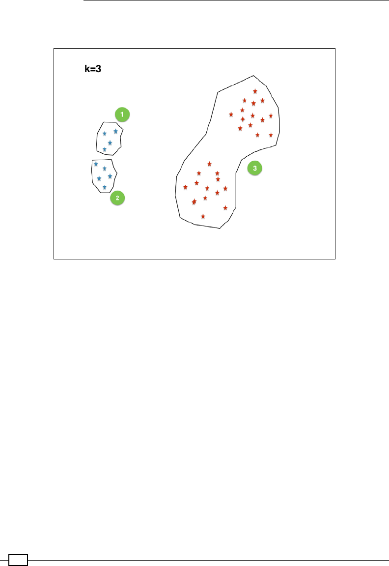
Learning from Data
534
The following gure proves that though we can see three clusters, a bad choice of centroids
separates a single cluster into two and makes two clusters one:
To solve this problem, we run the same algorithm with a different set of randomly initialized
centroids. This is determined by the maxIterations parameter. The distance between the
centroid and the points in the cluster is calculated (a mean squared difference in distances).
This will be the cost of the model. The iteration with the least cost is chosen and returned.
The metric that Spark uses to calculate the distance is the Euclidean distance.
Epsilon
How does the K-means algorithm know when to stop? There will always be a small distance that
the centroid can move if the clusters aren't separated by a huge margin. If all the centroids have
moved by a distance less than the epsilon parameter, it's the cue to the algorithm that it has
converged. In other words, the epsilon is nothing but a convergence threshold.
Now that we have the parameters that need to be passed to the K-means cluster out of the
way, let's look at the steps needed to run this algorithm to nd the clusters:
1. Importing the data and converting it into a vector.
2. Feature scaling the data.
3. Deriving the number of clusters.
4. Constructing the model.
5. Evaluating the model.
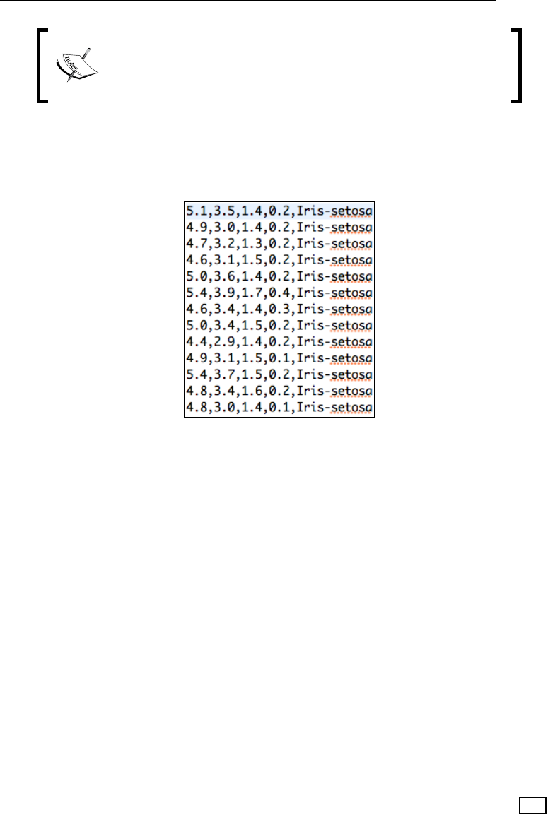
Chapter 5
535
The code for this recipe can be found at https://github.com/
arunma/ScalaDataAnalysisCookbook/blob/master/
chapter5-learning/src/main/scala/com/packt/
scalada/learning/KMeansClusteringIris.scala.
Importing the data and converting it into a vector
As usual, our input data is in the form of a text le—iris.data. Since we are clustering,
we can ignore the label (species) in the data. The data le looks like this:
val data = sc.textFile("iris.data").map(line => {
val dataArray = line.split(",").take(4)
Vectors.dense(dataArray.map(_.toDouble))
})
Feature scaling the data
When we look at the summary statistics of the data, the data looks alright, but it is always
advisable perform do feature scaling before running a K-means:
val stats = Statistics.colStats(data)
println("Statistics before scaling")
print(s"Max : ${stats.max}, Min : ${stats.min}, and Mean : ${stats.mean}
and Variance : ${stats.variance}")
Here is the statistics before scaling:
Max : [7.9,4.4,6.9,2.5]
Min : [4.3,2.0,1.0,0.1]

Learning from Data
536
Mean : [5.843333333333332,3.0540000000000003,3.7586666666666666,1.1986666
666666668]
Variance : [0.685693512304251,0.18800402684563744,3.113179418344516,0.582
4143176733783]
We run the data using StandardScaler and cache the resulting RDD. Since K-means
goes through the dataset multiple times, caching the data is strongly recommended to
avoid recomputation:
//Scale data
val scaler = new StandardScaler(withMean = true, withStd = true).
fit(data)
val scaledData = scaler.transform(data).cache()
The following is the statistics after scaling:
Max : [2.483698580557868,3.1042842692548858,1.7803768862629268,1.70518904
10833728]
Min : [-1.8637802962695154,-2.4308436996988485,-1.5634973589465175,-
1.4396268133736672], and Mean : [1.6653345369377348E-15,-
7.216449660063518E-16,-1.1102230246251565E-16,-3.3306690738754696E-16]
Variance : [0.9999999999999997,1.0000000000000007,1.0000000000000013,0.99
99999999999997]
Deriving the number of clusters
Many times, we already know the number of clusters that are there in the dataset. But at
times, if we aren't sure, the general method is to plot the number of clusters against the
cost and watch out for the point from which the cost stops falling drastically. If the data is
large, running the entire set of data just to obtain the number of clusters is computationally
expensive. Instead, we can take a random sample and come up with the k value. In this
example, we have taken a random 20% sample, but the sample percentage depends
entirely on your dataset:
//Take a sample to come up with the number of clusters
val sampleData = scaledData.sample(false, 0.2).cache()
//Decide number of clusters
val clusterCost = (1 to 7).map { noOfClusters =>
val kmeans = new KMeans()
.setK(noOfClusters)
.setMaxIterations(5)
.setInitializationMode(KMeans.K_MEANS_PARALLEL) //KMeans||
val model = kmeans.run(sampleData)
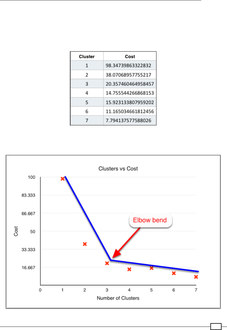
Chapter 5
537
(noOfClusters, model.computeCost(sampleData))
}
println ("Cluster cost on sample data")
clusterCost.foreach(println)
When we plot this, we can see that after cluster 3, the cost does not reduce drastically.
This point is called an Elbow bend, as shown here:

Learning from Data
538
Constructing the model
Now that we have gured out the number of clusters, let's run the algorithm against the entire
dataset:
//Let's do the real run for 3 clusters
val kmeans = new KMeans()
.setK(3)
.setMaxIterations(5)
.setInitializationMode(KMeans.K_MEANS_PARALLEL) //KMeans||
val model = kmeans.run(scaledData)
Evaluating the model
The last step is to evaluate the model by printing the cost of this model. The cost is nothing
but the square of the distance between all points in a cluster to its centroid. Therefore, a good
model must have the least cost:
//Cost
println("Total cost " + model.computeCost(scaledData))
printClusterCenters(model)
def printClusterCenters(model:KMeansModel) {
//Cluster centers
val clusterCenters: Array[Vector] = model.clusterCenters
println("Cluster centers")
clusterCenters.foreach(println)
}
Here is the output:
Total cost 34.98320617204239
Cluster centers
[-0.011357501034038157,-
0.8699705596441868,0.3756258413625911,0.3106129627676019]
[1.1635361185919766,0.1532643388373168,0.999796072473665,1.02619470887105
72]
[-1.0111913832028123,0.839494408624649,-1.3005214861029282,-
1.250937862106244]
Chapter 5
539
Feature reduction using principal
component analysis
Quoting the curse of dimensionality (https://en.wikipedia.org/wiki/Curse_of_
dimensionality), large number of features are computationally expensive. One way of
reducing the number of features is by manually choosing and ignoring certain features.
However, identication of the same features (represented differently) or highly correlated
features is laborious when we have a huge number of features. Dimensionality reduction
is aimed at reducing the number of features in the data while still retaining its variability.
Say, we have a dataset of housing prices and there are two features that represent the area of
the house in feet and meters; we can always drop one of these two. Dimensionality reduction
is very useful when dealing with text where the number of features easily runs into a few
thousands.
In this recipe, we'll be looking into Principal Component Analysis (PCA) as a means to reduce
the dimensions of data that is meant for both supervised and unsupervised learning.
How to do it...
As we have seen earlier, the only difference between the data for supervised and unsupervised
learning is that the training and the test data for supervised learning have labels attached to
them. This brings in a little complication, considering that we are interested only in reducing
the dimensions of the feature vector and would like to retain the labels as they are.
Dimensionality reduction of data for supervised learning
The only thing that we have to watch out for while reducing the dimensions of data to be used
as training data for supervised learning is that PCA must be applied on training data only. The
test set must not be used to extract the components. Using test data for PCA would bleed the
information in the test data into the components. This may result in higher accuracy numbers
while testing, but it could perform poorly on unseen production data.
The least number of components that can be chosen while maintaining a
sufciently high variance is facilitated by the singular value vector available in the
SingularValueDecomposion object. The singular values, available by calling the svd.s,
show the amount of variance captured by the components. The rst component will be the
most important (by contributing the highest variance), and the importance will slowly diminish.

Learning from Data
540
In order to come up with the probable number of dimensions, we can watch out for the
difference and the extent to which the singular values diminish. Alternatively, we can just
use simple heuristics and come up with a reasonable number if the features extend to a
few thousand:
val dimensionDecidingSample=new RowMatrix((trainingSplit.
randomSplit(Array(0.8,0.2))(1)).map(lp=>lp.features))
val svd = dimensionDecidingSample.computeSVD(500, computeU = false)
val sum = svd.s.toArray.sum
//Calculate the number of principal components which retains a variance
of 95%
val featureRange=(0 to 500)
val placeholder=svd.s.toArray.zip(featureRange).foldLeft(0.0) {
case (cum, (curr, component)) =>
val percent = (cum + curr) / sum
println(s"Component and percent ${component + 1} :: $percent ::::
Singular value is : $curr")
cum + curr
}
The steps that are involved are as follows:
1. Mean-normalizing the training data.
2. Extracting the principal components.
3. Preparing the labeled data.
4. Preparing the test data.
5. Classify and evaluate the metrics.
The code for this recipe can be found at https://github.com/
arunma/ScalaDataAnalysisCookbook/blob/master/
chapter5-learning/src/main/scala/com/packt/
scalada/learning/PCASpam.scala.

Chapter 5
541
Mean-normalizing the training data
It is highly recommended that the data be centered before running it by PCA. We achieve this
using the fit and transform functions of StandardScaler. However, since the scaler
in Spark accepts a DenseVector as the argument, we'll use the Vectors.dense factory
method to convert the features in the labeled point into a DenseVector:
val docs = sc.textFile("SMSSpamCollection").map(line => {
val words = line.split("\t")
Document(words.head.trim(), words.tail.mkString(" "))
}).cache()
val labeledPointsWithTf = getLabeledPoints(docs)
val lpTfIdf = withIdf(labeledPointsWithTf).cache()
//Split dataset
val spamPoints = lpTfIdf.filter(point => point.label ==
1).randomSplit(Array(0.8, 0.2))
val hamPoints = lpTfIdf.filter(point => point.label ==
0).randomSplit(Array(0.8, 0.2))
val trainingSpamSplit = spamPoints(0)
val trainingHamSplit = hamPoints(0)
val trainingData = trainingSpamSplit ++ trainingHamSplit
val unlabeledTrainData = trainingData.map(lpoint => Vectors.dense(lpoint.
features.toArray)).cache()
//Scale data - Does not support scaling of SparseVector.
val scaler = new StandardScaler(withMean = true, withStd = false).
fit(unlabeledTrainData)
val scaledTrainingData = scaler.transform(unlabeledTrainData).cache()

Learning from Data
542
Extracting the principal components
The computePrincipalComponents function is available in RowMatrix. So, we wrap
our scaled training data into a RowMatrix and then extract 100 principal components out
of it (as shown earlier, the number 100 is based on a run against a sample set of data and
on investigating the singular value vector of the SVD). Our training data is currently a 4419 x
5000 matrix—4419 instances of data * 5000 features restricted by us while generating the
term frequency using HashingTF. We then multiply this training matrix (4419 x 5000) by the
principal component matrix (5000 x 100) to arrive at a 4419 * 100 matrix—4419 instances
of data by 100 features (principal components). We can extract the feature vectors from this
matrix by calling the rows() function:
val trainMatrix = new RowMatrix(scaledTrainingData)
val pcomp: Matrix = trainMatrix.computePrincipalComponents(100)
val reducedTrainingData = trainMatrix.multiply(pcomp).rows.cache()
Preparing the labeled data
Now that we have reduced the data fty-fold, the next step that we have to take is to use this
reduced data in our algorithm to see how it fares. The classication algorithm (in this case,
LogisticRegressionWithBFGS) requires an RDD of LabeledPoints. To construct the
LabeledPoint, we extract the label from the original trainingData and the feature vector
from the dimension-reduced dataset:
val reducedTrainingSplit = trainingData.zip(reducedTrainingData).map {
case (labeled, reduced) => new LabeledPoint(labeled.label, reduced) }
Preparing the test data
Before predicting our test data against the algorithm, we need to bring the test data to the
same dimension as the training data. This is achieved by multiplying the principal components
with the test matrix. As discussed earlier, we just need to make sure that we don't compute
the principal components fresh here:
val unlabeledTestData=testSplit.map(lpoint=>lpoint.features)
val testMatrix = new RowMatrix(unlabeledTestData)
val reducedTestData=testMatrix.multiply(pcomp).rows.cache()
val reducedTestSplit=testSplit.zip(reducedTestData).map{case
(labeled,reduced) => new LabeledPoint (labeled.label, reduced)}

Chapter 5
543
Classify and evaluate the metrics
The nal step is to classify and evaluate the results of the algorithm. This step is the same
as the classication recipe that we saw earlier. From the output, we can see that we not
only reduced the number of features from 5,000 to 100, but also managed to maintain
the accuracy of the algorithm at the same levels:
val logisticWithBFGS = getAlgorithm(10, 1, 0.001)
val logisticWithBFGSPredictsActuals = runClassification(logisticWithBF
GS, reducedTrainingSplit, reducedTestSplit)
calculateMetrics(logisticWithBFGSPredictsActuals, "Logistic with BFGS")
def getAlgorithm(iterations: Int, stepSize: Double, regParam: Double) =
{
val algo = new LogisticRegressionWithLBFGS()
algo.setIntercept(true).optimizer.setNumIterations(iterations).
setRegParam(regParam)
algo
}
def runClassification(algorithm: GeneralizedLinearAlgorithm[_ <:
GeneralizedLinearModel], trainingData: RDD[LabeledPoint],
testData: RDD[LabeledPoint]): RDD[(Double, Double)] = {
val model = algorithm.run(trainingData)
println ("predicting")
val predicted = model.predict(testData.map(point => point.features))
val actuals = testData.map(point => point.label)
val predictsAndActuals: RDD[(Double, Double)] = predicted.
zip(actuals)
println (predictsAndActuals.collect)
predictsAndActuals
}
def calculateMetrics(predictsAndActuals: RDD[(Double, Double)],
algorithm: String) {
val accuracy = 1.0 * predictsAndActuals.filter(predActs =>
predActs._1 == predActs._2).count() / predictsAndActuals.count()
val binMetrics = new BinaryClassificationMetrics(predictsAndActuals)
println(s"************** Printing metrics for $algorithm
***************")
println(s"Area under ROC ${binMetrics.areaUnderROC}")
Learning from Data
544
println(s"Accuracy $accuracy")
val metrics = new MulticlassMetrics(predictsAndActuals)
println(s"Precision : ${metrics.precision}")
println(s"Confusion Matrix \n${metrics.confusionMatrix}")
println(s"************** ending metrics for $algorithm
*****************")
}
This is the output:
Compared to the area under the ROC at around the same levels (95%), we have considerably
reduced the time of the run by reducing the dimensions of the features ten-fold:
************** Printing metrics for Logistic with BFGS ***************
Area under ROC 0.9428948576675849
Accuracy 0.9829136690647482
Confusion Matrix
965.0 3.0
16.0 128.0
************** ending metrics for Logistic with BFGS *****************
Note that the entire code for this recipe can be found at https://
github.com/arunma/ScalaDataAnalysisCookbook/
blob/master/chapter5-learning/src/main/scala/
com/packt/scalada/learning/PCASpam.scala.
Dimensionality reduction of data for unsupervised learning
Unlike reducing the dimensions of data with labels, reducing the dimensionality of data for
unsupervised learning is very simple. We just apply the PCA to the entire dataset. This helps
a lot in improving the performance of algorithms such as K-means, where the entire set of
features has to be plotted on a higher dimension and the entire data must be visited multiple
times. A lesser number of features means a lesser number of dimensions and less data to be
held in the memory.
For this recipe, we use the Iris.data that we used for clustering earlier. The dataset
already has four features, and this isn't a great candidate for dimensionality reduction
as such. However, the process around reducing dimensions for unlabeled data is the
same as for any other dataset.
Chapter 5
545
The steps that are involved are as follows:
1. Mean-normalizing the training data.
2. Extracting the principal components.
3. Arriving at the number of components.
4. Evaluating the metrics.
The code for this recipe can be found at https://github.com/
arunma/ScalaDataAnalysisCookbook/blob/master/
chapter5-learning/src/main/scala/com/packt/
scalada/learning/PCAIris.scala.
Mean-normalizing the training data
As we saw earlier, scaling is a must before reducing dimensions:
val scaler = new StandardScaler(withMean = true, withStd = false).
fit(data)
val scaledData = scaler.transform(data).cache()
Extracting the principal components
As we saw earlier, to compute the principal components, we need to wrap our scaled training
data into a RowMatrix. We then multiply the matrix by the principal component matrix to
arrive at the reduced matrix. We can extract the feature vector from this matrix by calling the
rows() function:
val pcomp: Matrix = matrix.computePrincipalComponents(3)
val reducedData = matrix.multiply(pcomp).rows
Arriving at the number of components
While we would like to have the least number for the components, the other goal is to retain
the highest variance in the data. In this case, a run against three components was made, and
we could see that holding on to just two components out of the four, we retained 90% of the
variance. However, since we wanted at least 95%, 3 was chosen:
val svd = matrix.computeSVD(3)
val sum = svd.s.toArray.sum
svd.s.toArray.zipWithIndex.foldLeft(0.0) {

Learning from Data
546
case (cum, (curr, component)) =>
val percent = (cum + curr) / sum
println(s"Component and percent ${component + 1} :: $percent ::::
Singular value is : $curr")
cum + curr
}
The output is as follows:
Component and percent 1 :: 0.6893434455825798 :::: Singular value is :
25.089863978899867
Component and percent 2 :: 0.8544090583609627 :::: Singular value is :
6.0078525425063365
Component and percent 3 :: 0.9483881906752903 :::: Singular value is :
3.4205353829523646
Component and percent 4 :: 1.0 :::: Singular value
is : 1.878502340103494
Evaluating the metrics
After we have reduced the dimensions of the data from four to three (!?), for fun, we run the
data against a range of one to seven clusters to see the elbow bend. When we compare the
results of this with the K-means clustering without dimensionality reduction, the results looks
practically the same:
val clusterCost = (1 to 7).map { noOfClusters =>
val kmeans = new KMeans()
.setK(noOfClusters)
.setMaxIterations(5)
.setInitializationMode(KMeans.K_MEANS_PARALLEL) //KMeans||
val model = kmeans.run(reducedData)
(noOfClusters, model.computeCost(reducedData))
}
Here is the output:
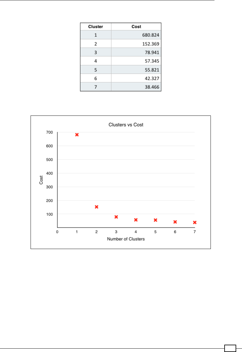
Chapter 5
547
The following screenshot shows the cost across various numbers of clusters:
Here is a screenshot that shows strikingly similar results for the elbow bend:
In this chapter, we rst saw the difference between supervised and unsupervised learning.
Then we explored a sample of machine learning algorithms in Spark: LinearRegression
for predicting continuous values, LogisticRegression and SVM for classication, K-means
for clustering, and nally PCA for dimensionality reduction. There are a plenty of other
algorithms in Spark, and more algorithms are being added to Spark with every version,
both batch and streaming.

549
6
Scaling Up
In this chapter, we will cover the following recipes:
fBuilding the Uber JAR
fSubmitting jobs to the Spark cluster (local)
fRunning the Spark standalone cluster on EC2
fRunning the Spark job on Mesos (local)
fRunning the Spark job on YARN (local)
Introduction
In this chapter, we'll be looking at how to bundle our Spark application and deploy it on various
distributed environments.
As we discussed earlier in Chapter 3, Loading and Preparing Data – DataFrame the foundation
of Spark is the RDD. From a programmer's perspective, the composability of RDDs such as a
regular Scala collection is a huge advantage. RDD wraps three vital (and two subsidiary) pieces
of information that help in reconstruction of data. This enables fault tolerance. The other major
advantage is that while the processing of RDDs could be composed into hugely complex graphs
using RDD operations, the entire ow of data itself is not very difcult to reason with.
Other than optional optimization attributes, such as data location, an RDD at its core wraps
only three vital pieces of information:
fThe dependent/parent RDD (empty if not available)
fThe number of partitions
fThe function that needs to be applied to each element of the RDD
Scaling Up
550
Spark spawns one task per partition. So, a partition is the basic unit of parallelism in Spark.
The number of partitions could be any of these:
fDictated by the number of blocks in the case of reading les
fA number set by the spark.default.parallelism parameter (set while starting
the cluster)
fA number set by calling repartition or coalesce on the RDD
So far, we have just run our Spark application in the self-contained single JVM mode. While
the programs work just ne, we have not yet exploited the distributed nature of the RDDs.
As always, all the code snippets for this chapter can be downloaded from
https://github.com/arunma/ScalaDataAnalysisCookbook/
tree/master/chapter6-scalingup.
Building the Uber JAR
The rst step for deploying our Spark application on a cluster is to bundle it into a single
Uber JAR, also known as the assembly JAR. In this recipe, we'll be looking at how to use
the SBT assembly plugin to generate the assembly JAR. We'll be using this assembly JAR
in subsequent recipes when we run Spark in distributed mode. We could alternatively set
dependent JARs using the spark.driver.extraClassPath property (https://spark.
apache.org/docs/1.3.1/configuration.html#runtime-environment). However,
for a large number of dependent JARs, this is inconvenient.
How to do it...
The goal of building the assembly JAR is to build a single, Fat JAR that contains all
dependencies and our Spark application. Refer to the following screenshot, which shows
the innards of an assembly JAR. You can see not only the application's les in the JAR,
but also all the packages and les of the dependent libraries:
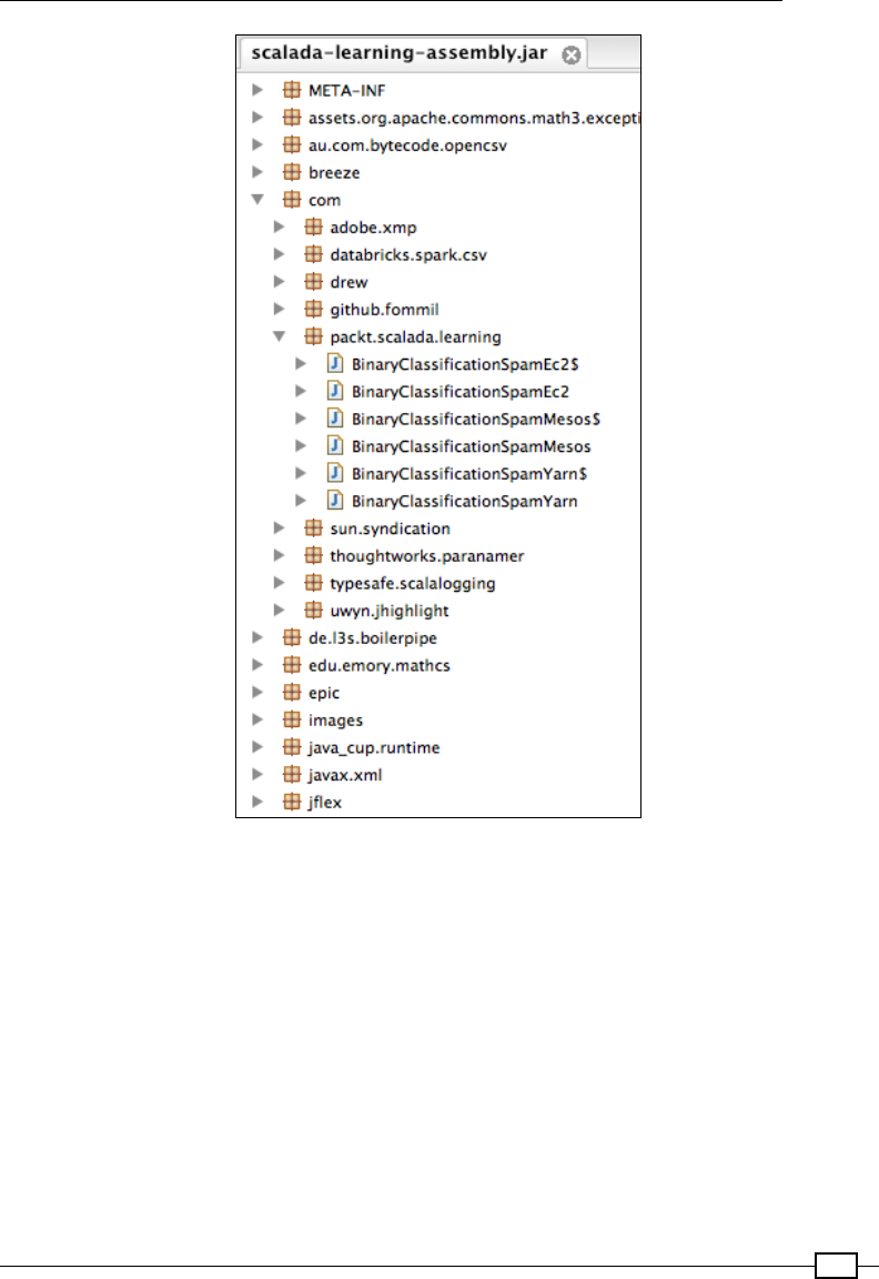
Chapter 6
551
The assembly JAR can easily be built in SBT using the SBT assembly plugin
(https://github.com/sbt/sbt-assembly).
In order to install the sbt-assembly plugin, let's add the following line to our
project/assembly.sbt:
addSbtPlugin("com.eed3si9n" % "sbt-assembly" % "0.13.0")
Next, the most common issue that we face while trying to build the assembly JAR (or Uber JAR)
is the problem of duplicates—duplicate transitive dependency JARs, or simply duplicate les
located at the same location (such as MANIFEST.MF) in different bundled JARs. The easiest
way to gure out is to install the sbt-dependency-graph plugin (https://github.com/
jrudolph/sbt-dependency-graph) and check which two trees bring in the conicting JAR.

Scaling Up
552
In order to add the sbt-dependency-graph plugin, let's add the following line to our
project/plugins.sbt:
addSbtPlugin("net.virtual-void" % "sbt-dependency-graph" %
"0.7.5")
Let's try to build the Uber JAR using sbt assembly. When we issue this command from the
root of the project, we get an error that tells us that we have duplicate les in our JAR.
Let's see an example of a duplicate error message that we might face:
deduplicate: different file contents found in the following:
/Users/Gabriel/.ivy2/cache/org.apache.xmlbeans/xmlbeans/jars/xmlbeans-
2.3.0.jar:org/w3c/dom/DOMStringList.class
/Users/Gabriel/.ivy2/cache/xml-apis/xml-apis/jars/xml-apis-1.4.01.
jar:org/w3c/dom/DOMStringList.class
deduplicate: different file contents found in the following:
/Users/Gabriel/.ivy2/cache/org.apache.xmlbeans/xmlbeans/jars/xmlbeans-
2.3.0.jar:org/w3c/dom/TypeInfo.class
/Users/Gabriel/.ivy2/cache/xml-apis/xml-apis/jars/xml-apis-1.4.01.
jar:org/w3c/dom/TypeInfo.class
deduplicate: different file contents found in the following:
/Users/Gabriel/.ivy2/cache/org.apache.xmlbeans/xmlbeans/jars/xmlbeans-
2.3.0.jar:org/w3c/dom/UserDataHandler.class
/Users/Gabriel/.ivy2/cache/xml-apis/xml-apis/jars/xml-apis-1.4.01.
jar:org/w3c/dom/UserDataHandler.class
This happens most commonly if:
fTwo different libraries in our sbt dependencies depend on the same external library
(or libraries that have bundled the classes with the same package)
fWe have explicitly stated the transitive dependency as a separate dependency in sbt
Whatever the case, it is always recommended to go through the entire dependency tree to
trim it down.
Transitive dependency stated explicitly in the SBT dependency
A simpler way is to export the dependency tree in an ASCII tree format and eyeball it to nd
the two instances where the xmlbeans JAR is referred to. The sbt dependency graph
plugin lets us do that. Once we have installed the plugin as per the instructions, we can
export and inspect the dependency tree:
sbt dependency-tree > deptree.txt
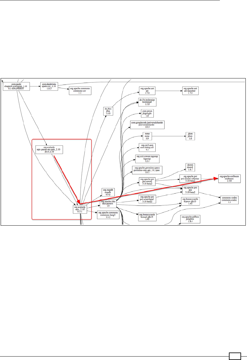
Chapter 6
553
The graph can also be visualized using a real graph (however, this lacks the text search
capabilities). The sbt dependency graph helps us analyze that too. We can export the
same tree as a .dot le using this code:
sbt dependency-dot > depdot.dot
It outputs a depdot.dot le in our target directory, which can be opened using Graphviz
(http://www.graphviz.org/). Refer to the following screenshot to see what the
visualization of a .dot le in Graphviz looks like:
As we can see in lines 96 and 573 of the dependency tree (refer to https://github.
com/arunma/ScalaDataAnalysisCookbook/blob/master/chapter6-scalingup/
depgraph_xmlbeans_duplicate.txt; its screenshot is given), there are two instances
of the import of xmlbeans: once in the tree that leads to org.scalanlp:epic-
parser-en-span_2.10:2015.2.19, and once in the tree that leads to org.
scalanlp:epic_2.10:0.3.1. If you notice the second level of the epic-parser library, you
will realize that it is the epic library itself.
So, we can resolve this error by removing scalanlp:epic_2.10:0.3.1 from the list of
dependencies in our build.sbt le.
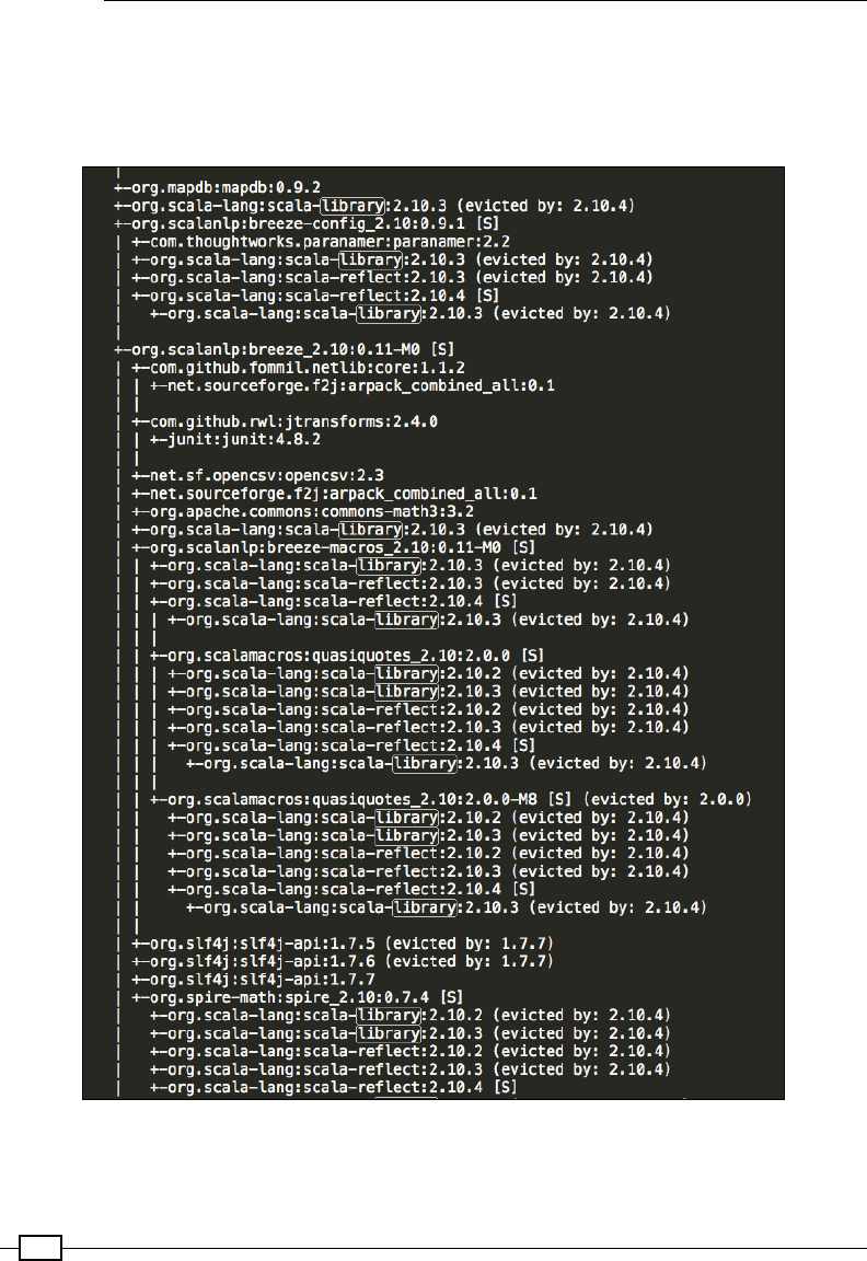
Scaling Up
554
Two different libraries depend on the same external library
Even after we have removed the epic library, we still see some issues with the xercesImpl
and xmlapi JARs. When we analyze the dependency tree, we see that two dependent
libraries of epic depend on xerces, the xml API and the scala library itself!

Chapter 6
555
We notice that the Epic library has a dependency on the Scala library, but we also know that
the Scala library should already be available on the master and the worker nodes. We can
exclude the Scala library altogether from getting bundled using the assemblyOption key:
assemblyOption in assembly := (assemblyOption in
assembly).value.copy(includeScala = false)
Next, in order to exclude the xml-apis library from the epic library, we use the
exclude function:
libraryDependencies ++= Seq(
"org.apache.spark" %% "spark-core" % sparkVersion % "provided",
"org.apache.spark" %% "spark-sql" % sparkVersion % "provided",
"org.apache.spark" %% "spark-mllib" % sparkVersion % "provided",
"com.databricks" %% "spark-csv" % "1.0.3",
("org.scalanlp" % "epic-parser-en-span_2.10" % "2015.2.19").
exclude("xml-apis", "xml-apis")
)
As for the rest of the conicting les, we can use the assembly plugin's merge strategy
to resolve the conict. Since we are merging contents of multiple JARs, there is a distinct
possibility of a similarly named le being available on the same path, for example,
MANIFEST.MF. The sbt-assembly plugin provides various strategies to resolve conicts
if the contents of the le in the same location don't match. The default strategy is to throw
an error, but we can customize the strategy to suit our needs.
In the merge strategy, we append the contents of application.conf if there are multiple
conf les in the JARs, use the rst matching class/le in the order of the class path for the
org.cyberneko.html package, and discard all the manifest les. For all others, we apply
the default strategy:
assemblyMergeStrategy in assembly := {
case "application.conf" =>
MergeStrategy.concat
case PathList("org", "cyberneko", "html", xs @ _*) =>
MergeStrategy.first
case m if m.toLowerCase.endsWith("manifest.mf") =>
MergeStrategy.discard
case f =>
(assemblyMergeStrategy in assembly).value(f)
}

Scaling Up
556
The entire build.sbt looks like this:
organization := "com.packt"
name := "chapter6-scalingup"
scalaVersion := "2.10.4"
val sparkVersion="1.4.1"
libraryDependencies ++= Seq(
"org.apache.spark" %% "spark-core" % sparkVersion % "provided",
"org.apache.spark" %% "spark-sql" % sparkVersion % "provided",
"org.apache.spark" %% "spark-mllib" % sparkVersion % "provided",
"com.databricks" %% "spark-csv" % "1.0.3",
("org.scalanlp" % "epic-parser-en-span_2.10" % "2015.2.19").
exclude("xml-apis", "xml-apis")
)
assemblyJarName in assembly := "scalada-learning-assembly.jar"
assemblyOption in assembly := (assemblyOption in
assembly).value.copy(includeScala = false)
assemblyMergeStrategy in assembly := {
case "application.conf" =>
MergeStrategy.concat
case PathList("org", "cyberneko", "html", xs @ _*) =>
MergeStrategy.first
case m if m.toLowerCase.endsWith("manifest.mf") =>
MergeStrategy.discard
case f =>
(assemblyMergeStrategy in assembly).value(f)
}
So nally, when we do an sbt assembly, scalada-learning-assembly.jar is created.
If you would like the JAR name to be picked up from the build.sbt le's name and version,
just delete the assemblyJarName key from build.sbt:
> sbt clean assembly
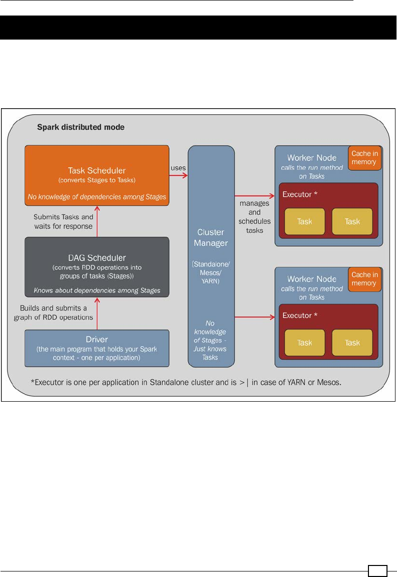
Chapter 6
557
Submitting jobs to the Spark cluster (local)
There are multiple components involved in running Spark in distributed mode. In the
self-contained application mode (the main program that we have run throughout this book
so far), all of these components run on a single JVM. The following diagram elaborates the
various components and their functions in running the Scala program in distributed mode:
As a rst step, the RDD graph that we construct using the various operations on our RDD
(map, lter, join, and so on) is passed to the Directed Acyclic Graph (DAG) scheduler. The
DAG scheduler optimizes the ow and converts all RDD operations into groups of tasks called
stages. Generally, all tasks before a shufe are wrapped into a stage. Consider operations
in which there is a one-to-one mapping between tasks; for example, a map or lter operator
yields one output for every input. If there is a map on an element on RDD followed by a lter,
they are generally pipelined (the map and the lter) to form a single task that can be executed
by a single worker, not to mention the benets of data locality. Relating this to our traditional
Hadoop MapReduce, where data is written to the disk at every stage, would help us really
appreciate the Spark lineage graph.
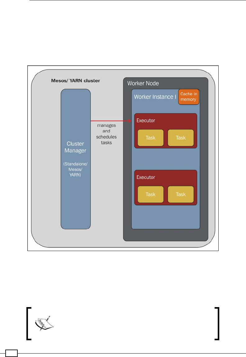
Scaling Up
558
These shufe-separated stages are then passed to the task scheduler, which splits them into
tasks and submits them to the cluster manager. Spark comes bundled with a simple cluster
manager that can receive the tasks and run it against a set of worker nodes. However, Spark
applications can also be run on popular cluster managers, such as Mesos and YARN.
With YARN/Mesos, we can run multiple executors on the same worker node. Besides, YARN
and Mesos can host non-Spark jobs in their cluster along with Spark jobs.
In the Spark standalone cluster, prior to Spark 1.4, the number of executors per worker
node per application was limited to 1. However, we could increase the number of worker
instances per worker node using the SPARK_WORKER_INSTANCES parameter. With Spark
1.4 (https://issues.apache.org/jira/browse/SPARK-1706), we are able to run
multiple executors on the same node, just as in Mesos/YARN.
If we intend to run multiple worker instances within a single
machine, we must ensure that we congure the SPARK_
WORKER_CORES property to limit the number of cores that
can be used by each worker. The default is all!
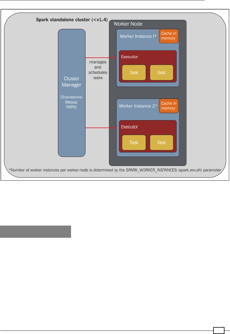
Chapter 6
559
In this recipe, we will be deploying the Spark application on a standalone cluster running on
a single machine. For all the recipes in this chapter, we'll be using the binary classication app
that we built in the previous chapter as a deployment candidate. This recipe assumes that you
have some knowledge of the concepts of HDFS and basic operations on them.
How to do it...
Submitting a Spark job to the local cluster involves the following steps:
1. Downloading Spark.
2. Running HDFS on pseudo-clustered mode.
3. Running the Spark master and slave locally.
4. Pushing data into HDFS.
5. Submitting the Spark application on the cluster.
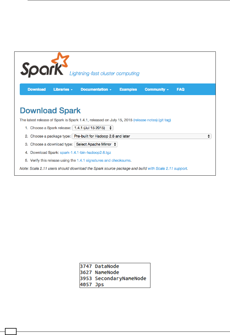
Scaling Up
560
Downloading Spark
Throughout this book, we have been using Spark version 1.4.1, as we can see in our
build.sbt. Now, let's head over to the download page (https://spark.apache.org/
downloads.html) and download the spark-1.4.1-bin-hadoop2.6.tgz bundle, as
shown here:
Running HDFS on Pseudo-clustered mode
Instead of loading the le from the local lesystem for our Spark application, let's have the le
stored away in HDFS. In order to do this, let's have a locally running Pseudo-distributed cluster
(https://hadoop.apache.org/docs/stable/hadoop-project-dist/hadoop-
common/SingleCluster.html#Pseudo-Distributed_Operation) of Hadoop 2.6.0.
After formatting our name node using bin/hdfs namenode -format and bringing up our
data node and name node using sbin/start-dfs.sh, let's conrm that all the processes
that we need are running properly. We do this using Jps. The following screenshot shows
what you are expected to see once you start the dfs daemon:
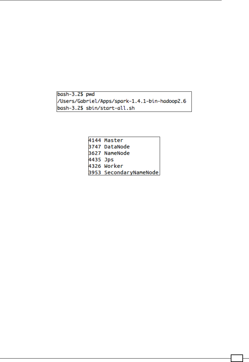
Chapter 6
561
Running the Spark master and slave locally
In order to submit our assembly JAR to a Spark cluster, we have to rst bring up the Spark
master and worker nodes.
All that we need to do to run Spark on the local machine is go to the downloaded (and
extracted) spark folder and run sbin/start-all.sh from the spark home directory.
This will bring up the Master and a Worker node of Spark. The Master's web UI is accessible
from port 8080. We use this port to check the status of the job. The default service port
of the Master is 7077. We'll be using this port to submit our assembly JAR as a job to the
Spark cluster.
Let's conrm the running of the Master and the Worker nodes using Jps:
Pushing data into HDFS
This just involves running the mkdir and put commands on HDFS:
bash-3.2$ hadoop fs -mkdir /scalada
bash-3.2$ hadoop fs -put /Users/Gabriel/Apps/SMSSpamCollection /scalada/
bash-3.2$ hadoop fs -ls /scalada
Found 1 items
-rw-r--r-- 1 Gabriel supergroup 477907 2015-07-18 16:59 /scalada/
SMSSpamCollection

Scaling Up
562
We can also conrm this via the HDFS web interface at 50070 and by going to Utilities |
Browse the le system, as shown here:
Submitting the Spark application on the cluster
Before we submit the Spark application to be run against the local cluster, let's change the
classication program (BinaryClassificationSpam) to point to the HDFS location:
val docs =
sc.textFile("hdfs://localhost:9000/scalada/SMSSpamCollection").
map(line => {
val words = line.split("\t")
Document(words.head.trim(), words.tail.mkString(" "))
})
By default, Spark 1.4.1 uses Hadoop 2.2.0. Now that we are trying to run the job on Hadoop
2.6.0, and are using the Spark binary prebuilt for Hadoop 2.6 and later, let's change build.
sbt to reect that:
libraryDependencies ++= Seq(
"org.apache.spark" %% "spark-core" % sparkVersion % "provided",
"org.apache.spark" %% "spark-sql" % sparkVersion % "provided",
"org.apache.spark" %% "spark-mllib" % sparkVersion % "provided",
"com.databricks" %% "spark-csv" % "1.0.3",
"org.apache.hadoop" % "hadoop-client" % "2.6.0",
("org.scalanlp" % "epic-parser-en-span_2.10" % "2015.2.19").
exclude("xml-apis", "xml-apis")
)
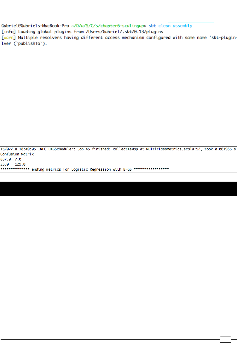
Chapter 6
563
Run sbt clean assembly to build the Uber JAR, like this:
./bin/spark-submit \
--class com.packt.scalada.learning.BinaryClassificationSpam \
--master spark://localhost:7077 \
--executor-memory 2G \
--total-executor-cores 2 \
<project root>/target/scala-2.10/scalada-learning-assembly.jar
Here is the output:
The following screenshot shows that we have successfully run our classication job on a Spark
cluster as against the standalone app that we used in the previous chapter:
Running the Spark Standalone cluster on EC2
The easiest way to create a Spark cluster and run our Spark jobs in a truly distributed mode
is Amazon EC2 instances. The ec2 folder inside the Spark installation directory wraps all the
scripts and libraries that we need to create a cluster. Let's quickly go through the steps that
entail the creation of our rst distributed cluster.
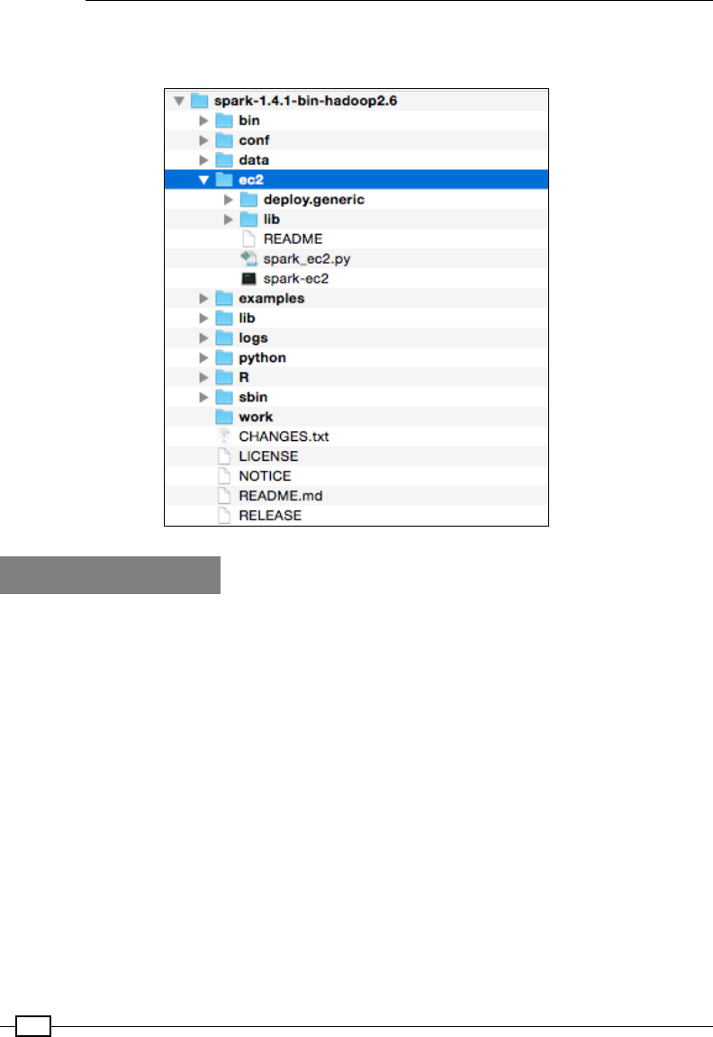
Scaling Up
564
This recipe assumes that you have a basic understanding of the Amazon EC2 ecosystem,
specically how to spawn a new EC2 instance.
How to do it...
We'll have to ensure that we have the access key and the Privacy Enhanced Mail (PEM)
les for AWS before proceeding with the steps. In fact, we are required to have these before
launching any EC2 instance if we intend to log in to the machines.
Creating the AccessKey and pem le
Instructions for creating a key pair and the pem key are available at http://docs.aws.
amazon.com/AWSEC2/latest/UserGuide/ec2-key-pairs.html. Anyway, the following
are the relevant screenshots.
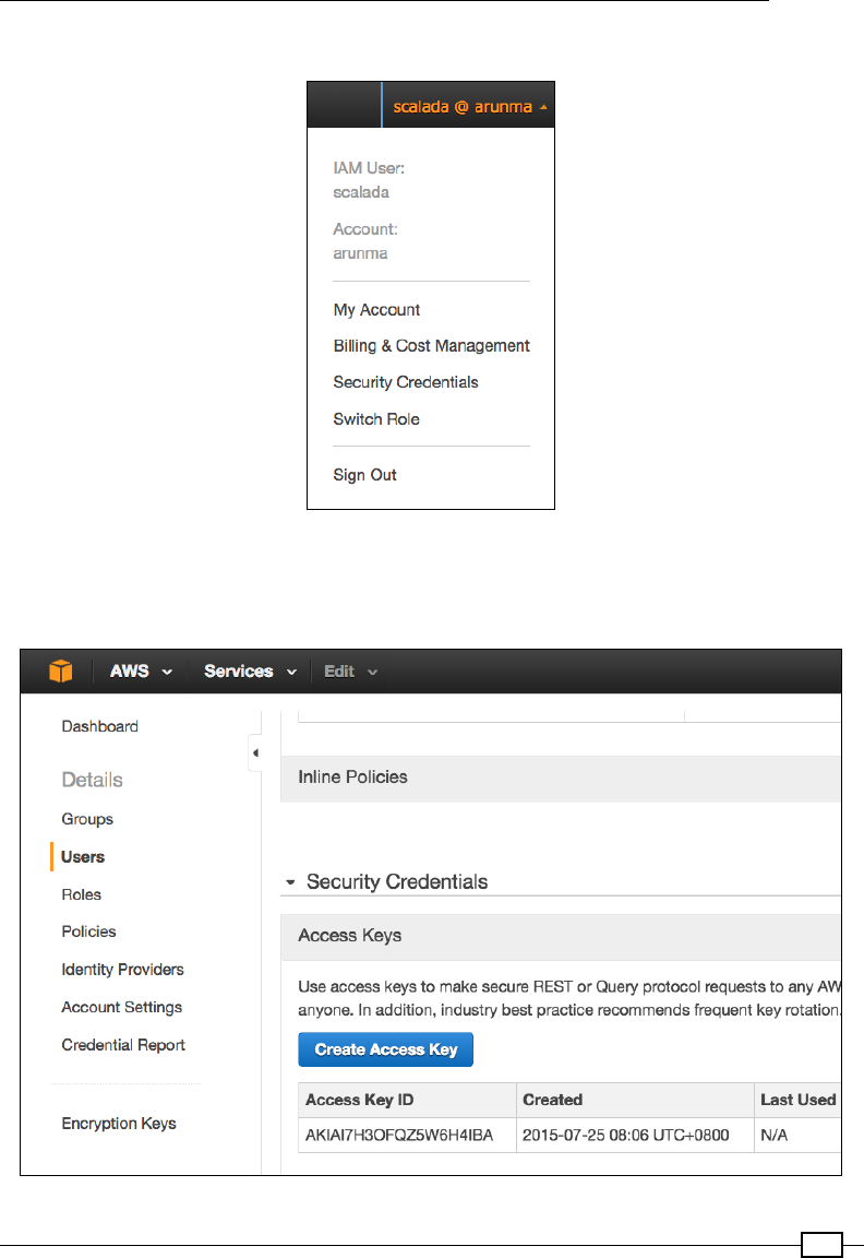
Chapter 6
565
Select Security Credentials from the user menu, like this:
Click on the Users menu and create an access key, as shown in the following screenshot.
Download the credentials. We'll be using this to create the EC2 instances for the Spark
master and the worker nodes:
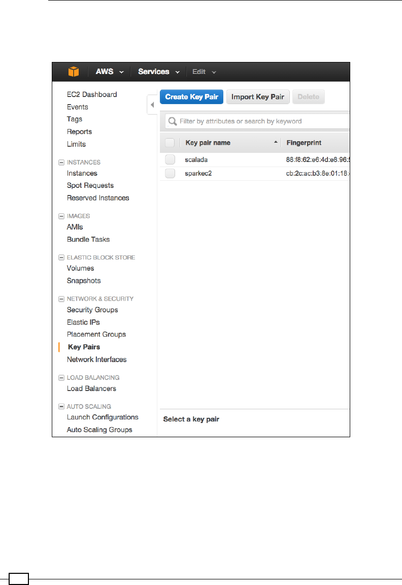
Scaling Up
566
The key pair can be created from inside the EC2 instances page using the Key Pairs menu, as
shown in the next screenshot. Your browser will automatically download the pem le once you
create a pair:
Once you have the pem le, ensure that the le permission for the pem le is 400. Otherwise,
an error message stating that your pem le's permissions are too open will be shown:
chmod 400 spark.pem
Launching and running our Spark application involves the following steps:
1. Setting the environment variables.
2. Running the launch script.
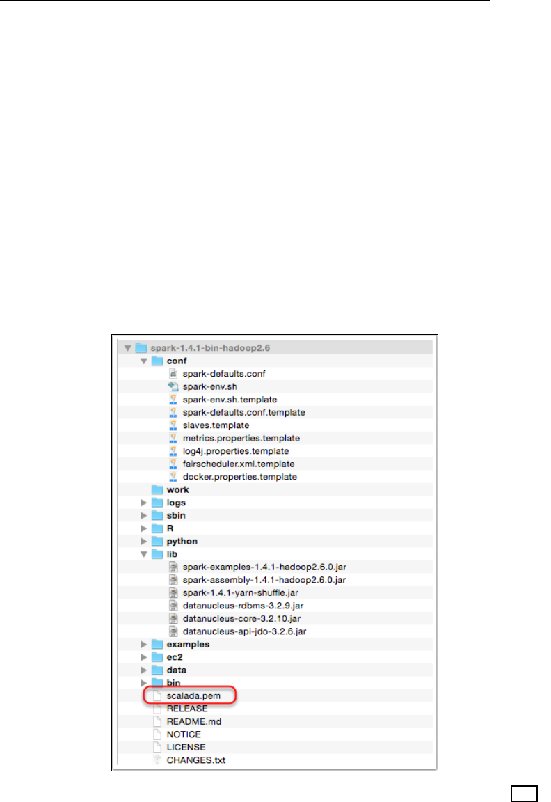
Chapter 6
567
3. Verifying installation.
4. Making changes to the code.
5. Transferring the data and job les.
6. Loading the dataset into HDFS.
7. Running the job.
8. Destroying the cluster.
Setting the environment variables
As the rst step, let's export the access and the secret access keys as environment variables.
The ec2 script for launching our instances will use these commands:
export AWS_ACCESS_KEY_ID=AKIAI7H3OFQZ5W6H4IBA
export AWS_SECRET_ACCESS_KEY=[YOUR SECRET ACCESS KEY]
I have also copied the pem le to the spark installation root directory, just to make the launch
command shorter (by not specifying the entire path of the pem le), as marked here:
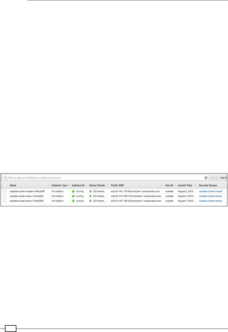
Scaling Up
568
Running the launch script
Now that we have the access key (and the secret key) exported and the pem le in the root
folder, let's spawn a new cluster:
cd spark-1.4.1-bin-hadoop2.6
./ec2/spark-ec2 --key-pair=scalada --identity-file=scalada.pem --slaves=2
--instance-type=m3.medium --hadoop-major-version=2 launch scalada-cluster
The parameters, as is clearly evident, represent the following:
fkey-pair: This is the name of the user to whom the access key and the secret
access key you exported as environment variables belong.
fidentity-file: This is the location of the pem le.
fslaves: This is the number of worker nodes.
finstance-type: This is one of the AWS instance types (http://aws.amazon.
com/ec2/instance-types/). M3 medium has one core and 3.75 GB in memory.
fhadoop-major-version: This is the version of Hadoop that we want Spark
to be bundled with. The spark version itself is derived from our local installation
(which is 1.4.1).
We can also conrm this from the EC2 console, as shown in the following screenshot:
Verifying installation
Let's log in to the Master to see the services that are running on each node:
ssh -i scalada.pem root@ec2-54-161-176-58.compute-1.amazonaws.com
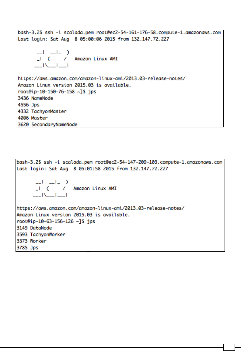
Chapter 6
569
Doing a jps on the master node shows that the Spark Master, the HDFS name node, and the
Secondary name node are running on the Spark master node, as depicted in this screenshot:
Similarly, on the worker nodes, we see that the Spark Worker and the HDFS data nodes are
running, as follows:
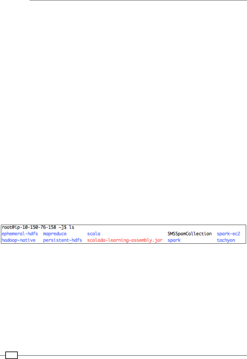
Scaling Up
570
Making changes to the code
There is a small change that is required in our code in order to make it run on this cluster—the
location of the dataset in HDFS. This, however, is not the recommended way of doing it, and
the URL should be sourced from an external conguration le:
val conf = new
SparkConf().setAppName("BinaryClassificationSpamEc2")
val sc = new SparkContext(conf)
val sqlContext = new SQLContext(sc)
val docs = sc.textFile("hdfs://ec2-54-159-166-156.compute-1.
amazonaws.com:9000/scalada/SMSSpamCollection").map(line => {
val words = line.split("\t")
Document(words.head.trim(), words.tail.mkString(" "))
})
Transferring the data and job les
As the next step, let's copy the dataset and the assembly JAR to the master node for
execution from the directory where you have the pem le:
scp -i scalada.pem <REPO_DIR>/chapter5-learning/SMSSpamCollection root@
ec2-54-161-176-58.compute-1.amazonaws.com:~/.
scp -i scalada.pem <REPO_DIR>/chapter6-scalingup/target/scala-2.10/
scalada-learning-assembly.jar root@ec2-54-161-176-58.compute-1.amazonaws.
com:~/.
An ls on the home folder of the master conrms this, as shown in the following screenshot:
Loading the dataset into HDFS
Now that we have uploaded our dataset to the master's local folder, let's push it to HDFS.
As we saw earlier when we veried the installation, the Spark EC2 script creates and runs
an HDFS cluster for us. Let's go to the ephemeral-hdfs folder in the root and format the
lesystem. Note that the les in this HDFS, as the name indicates, will be wiped off upon
restarting the cluster. Ideally, we should be installing a separate HDFS cluster on these nodes
instead of depending on the ephemeral installation that was created by the Spark EC2 script.
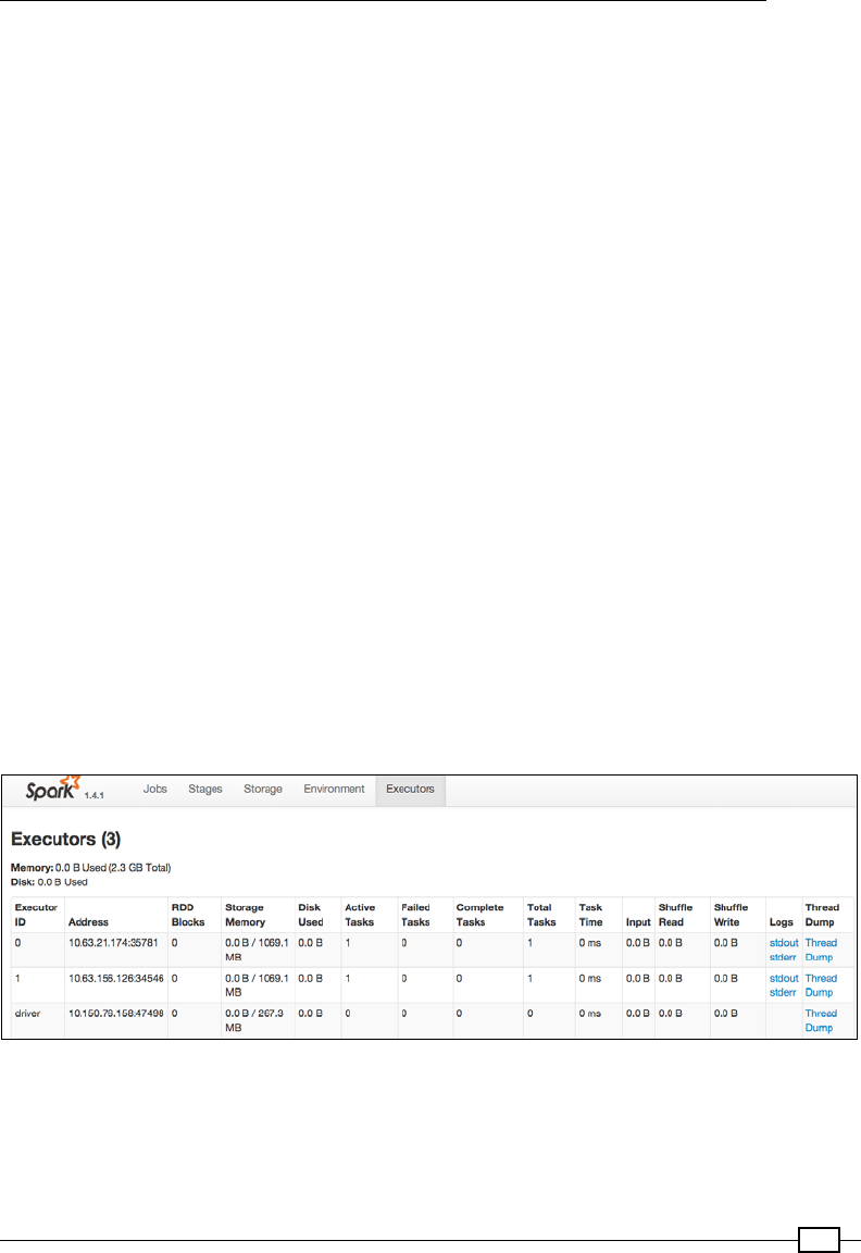
Chapter 6
571
Just as in our previous recipe, let's push the SMSSpamCollection dataset into the
/scalada folder in HDFS:
root@ip-10-150-76-158 ephemeral-hdfs] $ ./bin/hdfs namenode -format
root@ip-10-150-76-158 ephemeral-hdfs] $ ./bin/hadoop fs -mkdir /scalada
root@ip-10-150-76-158 ephemeral-hdfs] $ ./bin/hadoop fs -put ../
SMSSpamCollection /scalada/
root@ip-10-150-76-158 ephemeral-hdfs]$ ./bin/hadoop fs -ls /scalada
Found 1 items
-rw-r--r-- 3 root supergroup 477907 2015-08-08 05:24 /scalada/
SMSSpamCollection
Running the job
As with the previous recipe, we'll use the spark-submit script to submit the job to the cluster.
Let's enter the spark home directory (/root/spark) and execute the following lines:
./bin/spark-submit \
--class com.packt.scalada.learning.BinaryClassificationSpamEc2 \
--master spark://ec2-54-161-176-58.compute-1.amazonaws.com:7077 \
--executor-memory 2G \
--total-executor-cores 2 \
../scalada-learning-assembly.jar
We can see that the job runs on both worker nodes of the cluster, as shown in this screenshot:
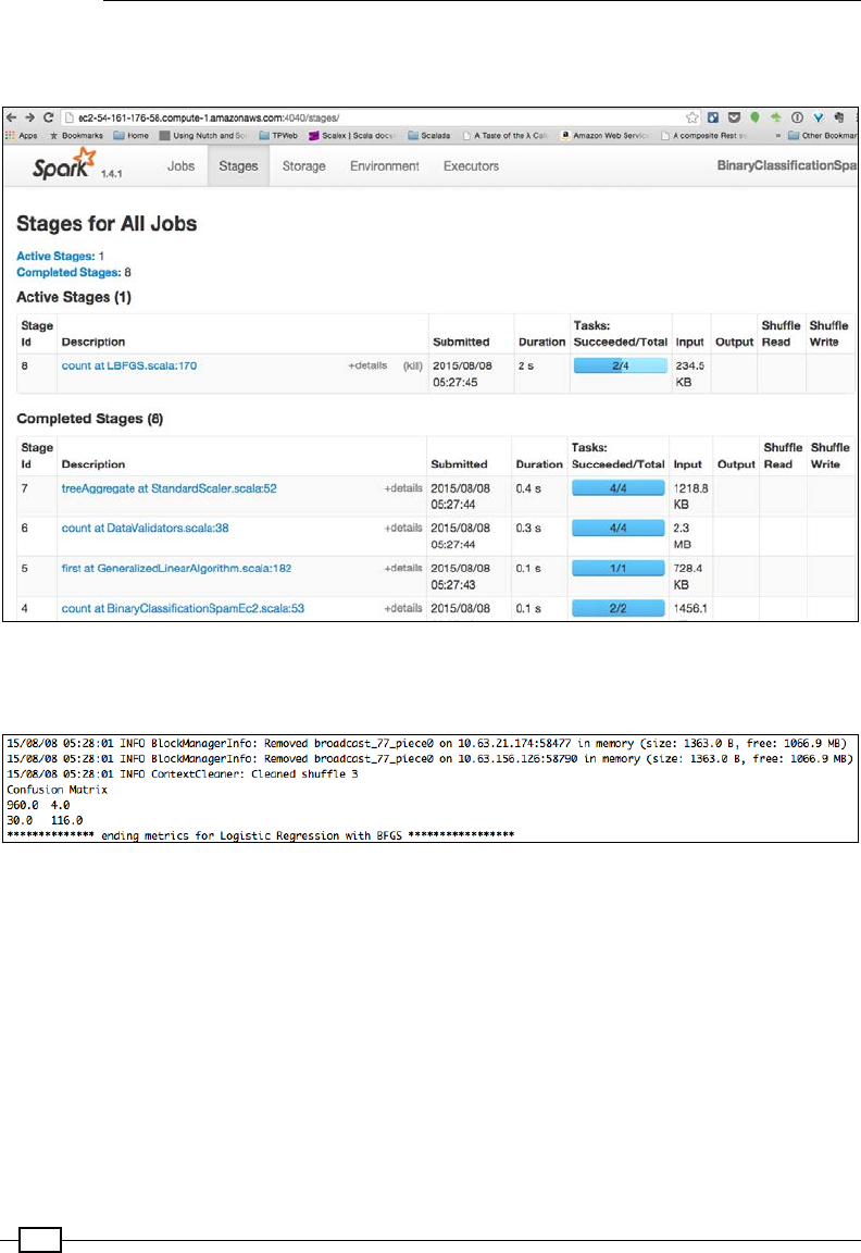
Scaling Up
572
We can also see the various stages of this Job from the Stages tab, as shown in the
following screenshot:
Not surprisingly, the accuracy measure is approximately the same, except that now we can
use this cluster to handle much bigger data.
Destroying the cluster
Finally, if you would like to destroy the cluster, you can use the same ec2 script with the
destroy action. From your local Spark installation directory, execute this line:
./ec2/spark-ec2 destroy scalada-cluster
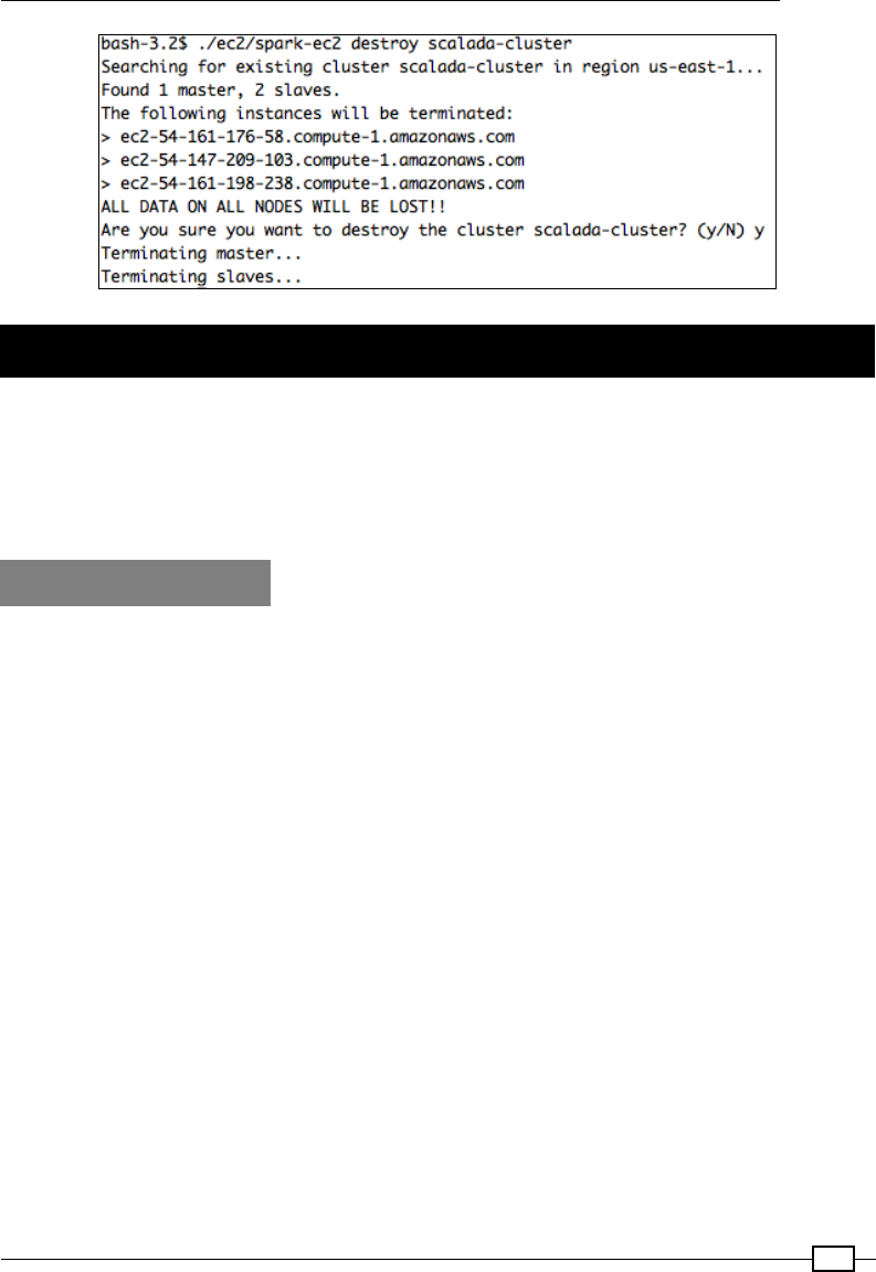
Chapter 6
573
Running the Spark Job on Mesos (local)
Unlike the Spark standalone cluster manager, which can run only Spark apps, Mesos is a
cluster manager that can run a wide variety of applications, including Python, Ruby, or Java EE
applications. It can also run Spark jobs. In fact, it is one of the popular go-to cluster managers
for Spark. In this recipe, we'll see how to deploy our Spark application on the Mesos cluster.
The prerequisite for this recipe is a running HDFS cluster.
How to do it...
Running a Spark job on Mesos is very similar to running it against the standalone cluster. It
involves the following steps:
1. Installing Mesos.
2. Starting the Mesos master and slave.
3. Uploading the Spark binary package and the dataset to HDFS.
4. Running the job.
Installing Mesos
Download Mesos on the local machine by following the instructions at http://mesos.
apache.org/gettingstarted/.
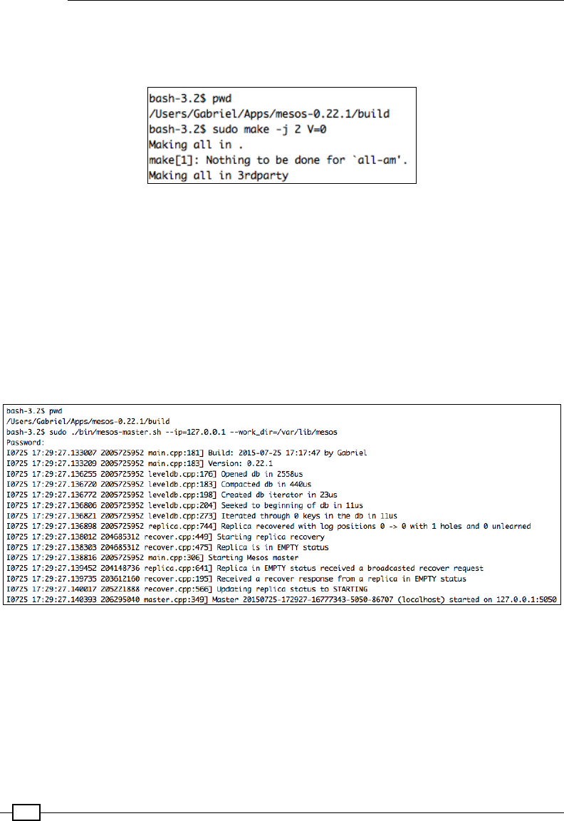
Scaling Up
574
After you have installed the OS-specic tools needed to build Mesos, you have to run the
congure and make commands (with root privileges) to build Mesos (this will take a long time)
unless you pass -j <number of cores> V=0 to your make command, as shown here:
As a side note, just like Spark, the ec2 folder inside the mesos installation directory provides
scripts to spawn a new EC2 mesos cluster.
Starting the Mesos master and slave
Now that we have Mesos installed, the next step is to start the Mesos master and slave:
bash-3.2$ pwd
/Users/Gabriel/Apps/mesos-0.22.1/build
bash-3.2$ sudo ./bin/mesos-master.sh --ip=127.0.0.1 --work_dir=/var/lib/
mesos
In another terminal window, let's bring up a worker node:
Gabriel@Gabriels-MacBook-Pro ~/A/m/build> pwd
/Users/Gabriel/Apps/mesos-0.22.1/build
Gabriel@Gabriels-MacBook-Pro ~/A/m/build> ./bin/mesos-slave.sh
--master=127.0.0.1:5050
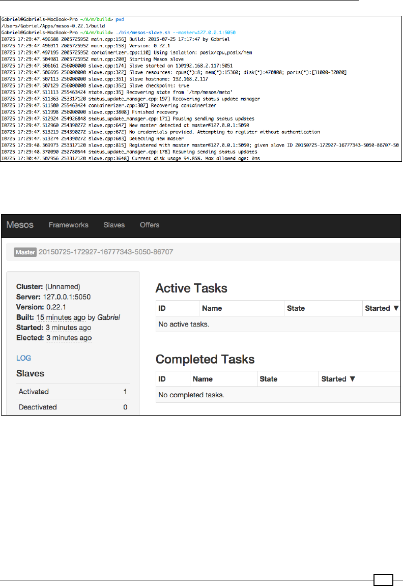
Chapter 6
575
We can now look at the Mesos status page at http://127.0.0.1:5050, and this is what
we will see:
Uploading the Spark binary package and the dataset to HDFS
Mesos requires that all worker nodes have Spark installed on the machines. We can achieve
this either by conguring the spark.mesos.executor.home property in the spark
conguration, or by simply uploading the entire Spark tar bundle to HDFS and making it
available to the Mesos workers:
./bin/hadoop fs -mkdir /scalada
./bin/hadoop fs -put /Users/Gabriel/Apps/spark-1.4.1-bin-hadoop2.6.tgz /
scalada/spark-1.4.1-bin-hadoop2.6.tgz
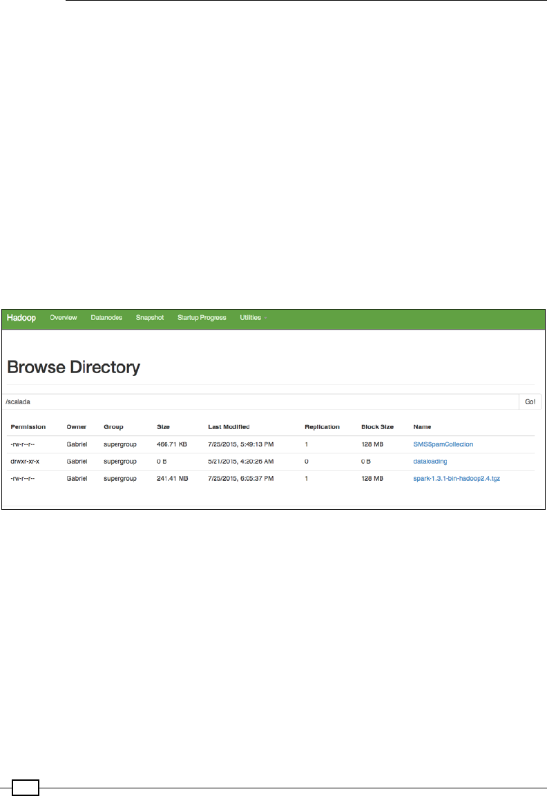
Scaling Up
576
Let's set the spark binary as the executor URI
export SPARK_EXECUTOR_URI=hdfs://localhost:9000/scalada/spark-1.4.1-bin-
hadoop2.6.tgz
Also, let's upload the dataset to HDFS:
./bin/hadoop fs -mkdir /scalada
./bin/hadoop fs -put /Users/Gabriel/Apps/SMSSpamCollection /scalada/
Running the job
There is one thing that we need to do before running the program itself— congure the
location of the libmesos native library. This le can be found in the /usr/local/lib
folder as libmesos.so or libmesos.dylib, depending on your operating system:
export MESOS_NATIVE_JAVA_LIBRARY=/usr/local/lib/libmesos-0.22.1.dylib
Now, let's use cd to enter the Spark installation directory, and then run the job:
cd /Users/Gabriel/Apps/spark-1.4.1-bin-hadoop2.6
export MESOS_NATIVE_JAVA_LIBRARY=/usr/local/lib/libmesos-0.22.1.dylib
./bin/spark-submit \
--class com.packt.scalada.learning.BinaryClassificationSpamMesos \
--master mesos://localhost:5050 \
--executor-memory 2G \
--total-executor-cores 2 \
<REPO_FOLDER>/chapter6-scalingup/target/scala-2.10/scalada-learning-
assembly.jar
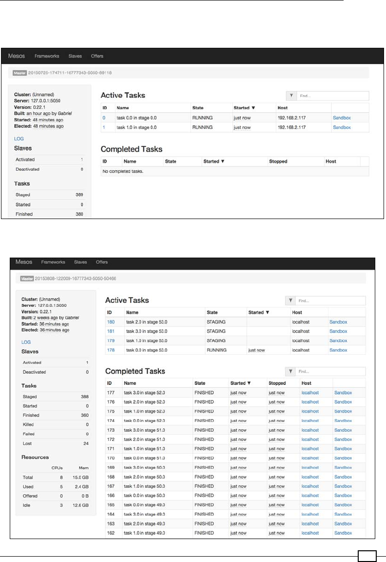
Chapter 6
577
As you can see in the following screenshot, the tasks run ne on this single-worker-node
cluster:
The next screenshot shows the list of tasks that are already completed:

Scaling Up
578
Running the Spark Job on YARN (local)
Hadoop has a long history, and in most cases, organizations have already invested in the
Hadoop infrastructure before they move their MR jobs to Spark. Unlike the Spark standalone
cluster manager, which can run only Spark jobs, and Mesos, which can run a variety of
applications, YARN runs Hadoop jobs as rst-class. At the same time, it can run Spark jobs
as well. This means that when a team decides to replace some of their MR jobs with Spark
jobs, they can use the same cluster manager to run Spark jobs. In this recipe, we'll see how
to deploy our Spark application on the YARN cluster manager.
How to do it...
Running a Spark job on YARN is very similar to running it against a Spark standalone cluster.
It involves the following steps:
1. Installing the Hadoop cluster.
2. Starting HDFS and YARN.
3. Pushing the Spark assembly and dataset to HDFS.
4. Running the Spark Job in the yarn-client mode.
5. Running the Spark Job in the yarn-cluster mode.
Installing the Hadoop cluster
While the setup of the cluster itself is beyond the scope of this recipe, for the sake of
completeness, let's quickly look at the relevant site XML congurations that were made while
setting up a single-node pseudo-distributed cluster on a local machine. Refer to http://
www.bogotobogo.com/Hadoop/BigData_hadoop_Install_on_ubuntu_single_
node_cluster.php for the complete details on how to set up a local YARN/HDFS cluster:
The core-site.xml le:
<configuration>
<property>
<name>fs.default.name</name>
<value>hdfs://localhost:54310</value>
</property>
</configuration>
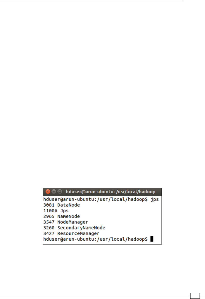
Chapter 6
579
The mapred-site.xml le:
<configuration>
<property>
<name>mapred.job.tracker</name>
<value>localhost:54311</value>
</property>
</configuration>
The hdfs-site.xml le:
<configuration>
<property>
<name>dfs.replication</name>
<value>1</value>
</property>
</configuration>
Starting HDFS and YARN
Once the setup of the cluster is done, let's format HDFS and start the cluster (dfs and yarn):
Format namenode:
hdfs namenode -format
Start both HDFS and YARN:
sbin/start-all.sh
Let's conrm that the services are running through jps, and this is what we should see:
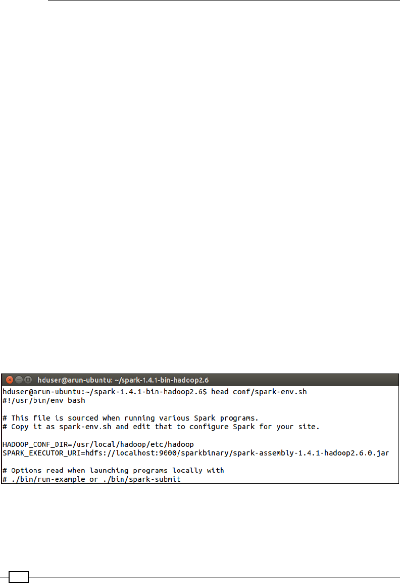
Scaling Up
580
Pushing Spark assembly and dataset to HDFS
Ideally, when we do a spark-submit, YARN should be able to pick our spark-assembly
JAR (or Uber JAR) and upload it to HDFS. However, this doesn't happen correctly and results
in the following error:
Error: Could not find or load main class org.apache.spark.deploy.yarn.
ExecutorLauncher
In order to work around this issue, let's upload our spark-assembly JAR manually to HDFS
and change our conf/spark-env.sh to reect the location. The Hadoop cong directory
should also be specied in spark-env.sh:
Uploading the spark assembly to HDFS.
hadoop fs -mkdir /sparkbinary
hadoop fs -put /Users/Gabriel/Apps/spark-1.4.1-bin-hadoop2.6/lib/spark-
assembly-1.4.1-hadoop2.6.0.jar /sparkbinary/
hadoop fs -ls /sparkbinary
Uploading the Spam dataset to HDFS:
hadoop fs -mkdir /scalada
hadoop fs -put ~/SMSSpamCollection /scalada/
hadoop fs -ls /scalada
Entries in spark-env.sh:
HADOOP_CONF_DIR=/usr/local/hadoop/etc/hadoop
SPARK_EXECUTOR_URI=hdfs://localhost:9000/sparkbinary/spark-assembly-
1.4.1-hadoop2.6.0.jar
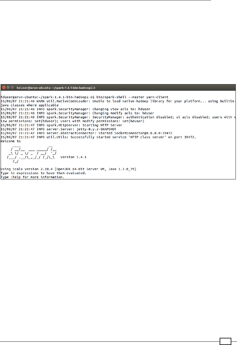
Chapter 6
581
Before we submit our Spark job to the YARN cluster, let's conrm that our setup is ne using
the Spark shell. The Spark shell is a wrapper arround the Scala REPL, with Spark libraries set
in the classpath. Conguring HADOOP_CONF_DIR to point to the Hadoop config directory
ensures that Spark will now use YARN to run its jobs. However, there are two modes in which
we can run the Spark job in YARN, namely yarn-client and yarn-cluster. Let's explore
both of them in this subrecipe. But before we do that, to validate our conguration, we'll
launch the Spark shell pointing the master to the yarn-client. After a rain of logs, we
should be able to see a Scala prompt. This conrms that our conguration is good:
bin/spark-shell --master yarn-client
Running a Spark job in yarn-client mode
Now that we have conrmed that the shell loads up ne against the YARN master, let's head
over to deploying our Spark job on YARN.
As we discussed earlier, there are two modes in which we can run a Spark application on
YARN: the yarn-client mode and the yarn-cluster mode. In the yarn-client mode,
the driver program resides on the client side and the YARN worker nodes are used only to
execute the job. All of the brain of the application resides in the client JVM that polls the
application master for the status. The application master does nothing except watching out
for failure of the executor nodes and reporting and requesting for resources accordingly to
the resource manager. This also means that the client (our driver JVM) needs to run as long
as the application executes:
./bin/spark-submit \
--class com.packt.scalada.learning.BinaryClassificationSpamYarn \
--master yarn-client \
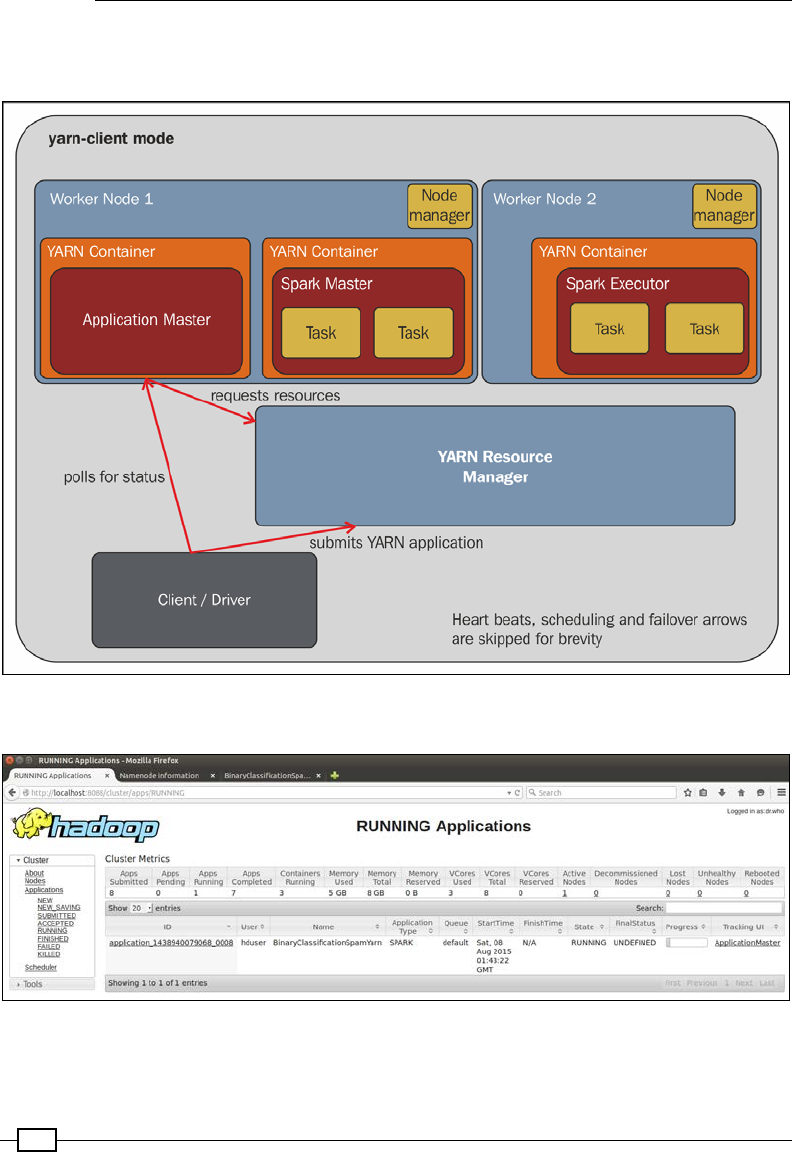
Scaling Up
582
--executor-memory 1G \
~/scalada-learning-assembly.jar
As we see from the YARN console, our job is running ne. Here is a screenshot that shows this:
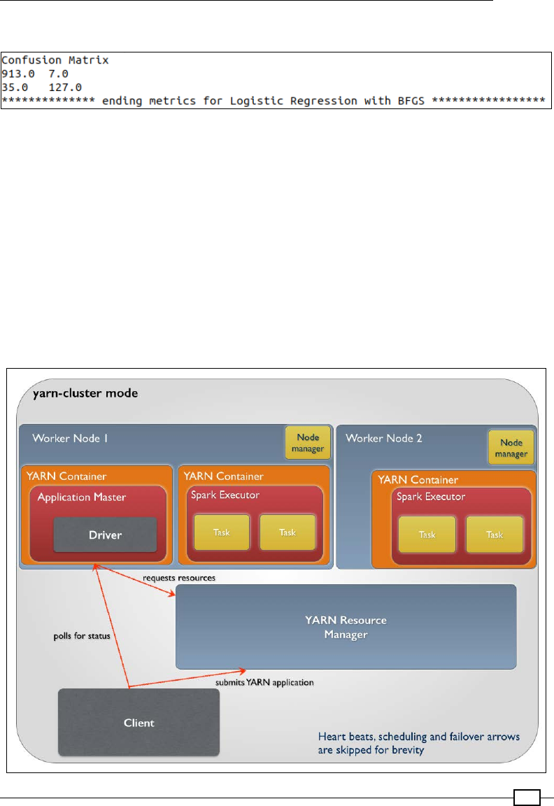
Chapter 6
583
Finally, we can see the output on the client JVM (the driver) itself:
Running Spark job in yarn-cluster mode
In the yarn-cluster mode, the client JVM doesn't do anything at all. In fact, it just submits
and polls the Application master for status. The driver program itself runs on the Application
master, which now has all the brains of the program. Unlike the yarn-client mode, the
user logs won't be displayed on the client JVM because the driver, which consolidates the
results, is executing inside the YARN cluster:
./bin/spark-submit \
--class com.packt.scalada.learning.BinaryClassificationSpamYarn \
--master yarn-cluster \
--executor-memory 1g \
~/scalada-learning-assembly.jar
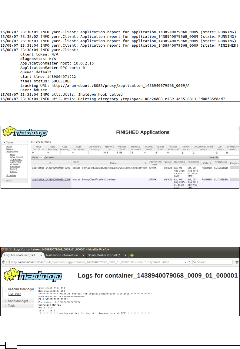
Scaling Up
584
As expected, the client JVM indicates that the job has run successfully. It doesn't, however,
show the user logs.
The following screenshot shows the nal status of our client and the cluster mode runs:
The actual output of this program is inside the Hadoop user logs. We can either go to the
logs directory of Hadoop, or check it out from the Hadoop console itself, when we click on
the application link and then on the logs link in the console.
As you can see in the following screenshot, the stdout le shows our embarrassing
println commands:

Chapter 6
585
In this chapter, we took an example Spark application and deployed it on a Spark standalone
cluster manager, YARN, and Mesos. Along the way, we touched upon the internals of these
cluster managers.
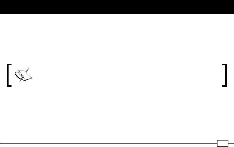
587
7
Going Further
In this chapter, we will cover the following recipes:
fUsing Spark Streaming to subscribe to a Twitter stream
fUsing Spark as an ETL tool (pulling data from ElasticSearch and publishing it
to Kafka)
fUsing StreamingLogisticRegression to classify a Twitter stream using Kafka
as a training stream
fUsing GraphX to analyze Twitter data
fWatching other Scala libraries of interest
Introduction
So far, the entire book has concentrated a little around Breeze and a lot around Spark,
specically DataFrames and machine learning. However, there are a whole lot of other
libraries, both in Java and Scala that could be leveraged while analyzing data from Scala.
This chapter goes a little more into Spark's other components, streaming and GraphX.
Note that each recipe in this chapter feeds into the next recipe.
All the code related to this chapter can be downloaded from
https://github.com/arunma/ScalaDataAnalysisCookbook/
tree/master/chapter7-goingfurther.
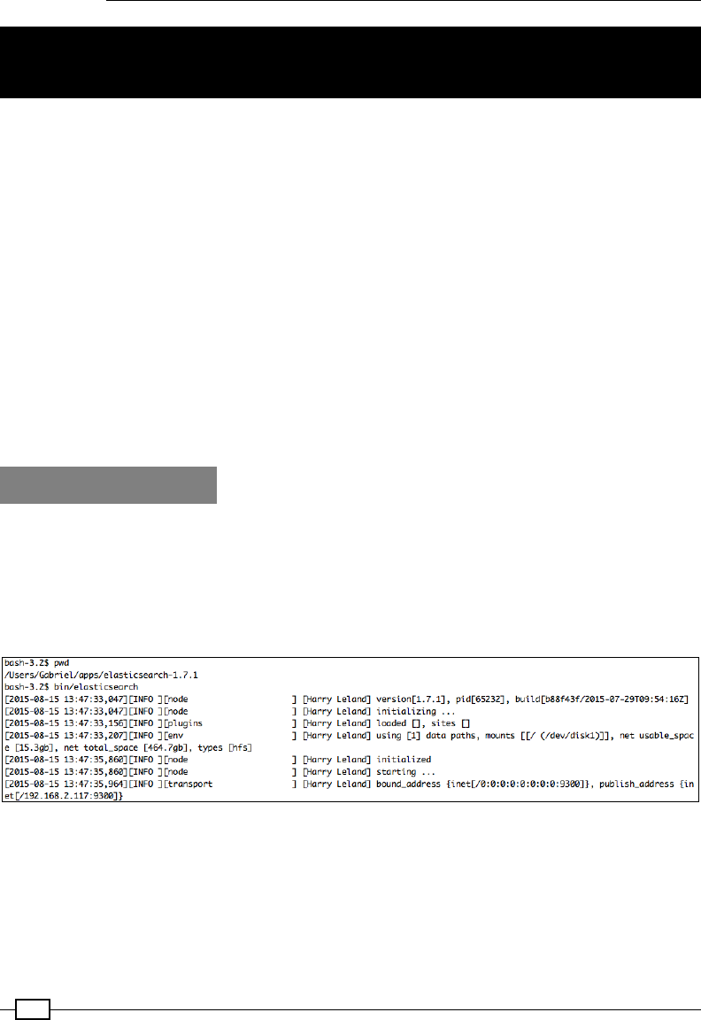
Going Further
588
Using Spark Streaming to subscribe to a
Twitter stream
Just like all the other components of Spark, Spark Streaming is also scalable and fault-tolerant,
it's just that it manages a stream of data instead of a large amount of data that Spark generally
does. The way that Spark Streaming approaches streaming is unique in the sense that it
accumulates streams into small batches called DStreams and then processes them as mini-
batches, an approach usually called micro-batching. The component that receives the stream
of data and splits it into time-bound windows of batches is called the receiver.
Once these batches are received, Spark takes these batches up, converts them into
RDDs, and processes the RDDs in the same way as static datasets. The regular framework
components such as the driver and executor stay the same. However, in terms of Spark
Streaming, a DStream or Discretized stream is just a continuous stream of RDDs. Also, just
like SQLContext served as an entry point to use SQL in Spark, there's StreamingContext
that serves as an entry point for Spark Streaming.
In this recipe, we will subscribe to a Twitter stream and index (store) the tweets into
ElasticSearch (https://www.elastic.co/).
How to do it...
The prerequisite to run this recipe is to have a running ElasticSearch instance on your machine.
1. Running ElasticSearch: Running an instance of ElasticSearch is as simple as it gets.
Just download the installable from https://www.elastic.co/downloads/
elasticsearch and run bin/elasticsearch. This recipe uses the latest
version 1.7.1.
2. Creating a Twitter app: In order to subscribe to tweets, Twitter requires us to create
a Twitter app. Let's quickly set up a Twitter app in order to get the consumer key and
the secret key. Visit https://apps.twitter.com/ using your login and click
Create New App.
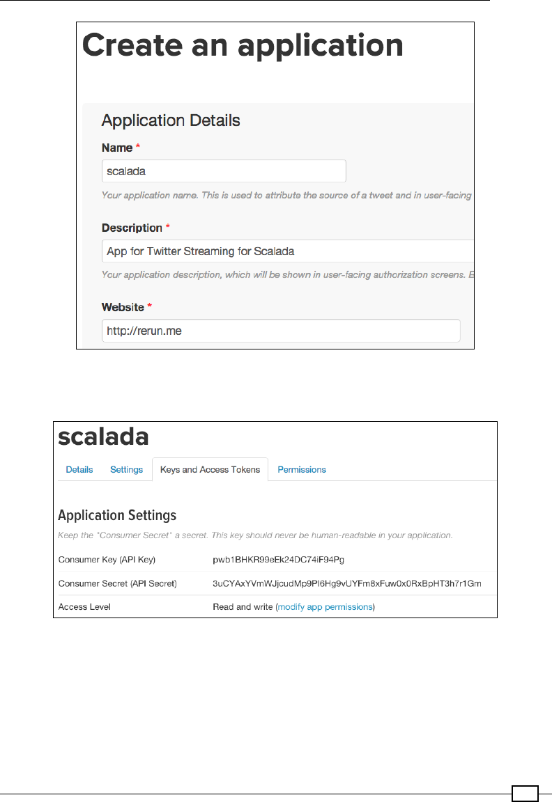
Chapter 7
589
We will be using the consumer key, consumer secret key, the access token, and the
access secret in our application.
3. Adding Spark Streaming and the Twitter dependency: There are two dependencies
that need to be added here, the spark-streaming and the spark-streaming-
twitter libraries:
"org.apache.spark" %% "spark-streaming" % sparkVersion %
"provided",
"org.apache.spark" %% "spark-streaming-twitter" %
sparkVersion

Going Further
590
4. Creating a Twitter stream: Creating a Twitter stream is super easy in Spark. We just
need to use TwitterUtils.createStream for this. TwitterUtils wraps around
the twitter4j library (http://twitter4j.org/en/index.html) to provide
rst-class support in Spark.
TwitterUtils.createStream expects a few parameters. Let's construct them
one by one.
StreamingContext: StreamingContext could be constructed by
passing in SparkContext and the time window of the batch:
val streamingContext=new StreamingContext(sc, Seconds
(5))
OAuthorization: The access and the consumer keys that comprise
the OAuth credentials need to be passed in order to subscribe to the
Twitter stream:
val builder = new ConfigurationBuilder()
.setOAuthConsumerKey(consumerKey)
.setOAuthConsumerSecret(consumerSecret)
.setOAuthAccessToken(accessToken)
.setOAuthAccessTokenSecret(accessTokenSecret)
.setUseSSL(true)
val twitterAuth = Some(new
OAuthAuthorization(builder.build()))
Filter criteria: You are free to skip this parameter if your intention is to
subscribe to (a sample of) the universe of the tweets. For this recipe,
we'll add some filter criteria to it:
val filter=List("fashion", "tech", "startup", "spark")
StorageLevel: This is where our received objects that come in batches
need to be stored. The default is memory with a capability to overflow to
disk. Once this is constructed, let's construct the Twitter stream itself:
val stream=TwitterUtils.createStream(streamingContext,
twitterAuth, filter, StorageLevel.MEMORY_AND_DISK)
5. Saving the stream to ElasticSearch: Writing the Tweets to ElasticSearch involves
three steps:
1. Adding the ElasticSearch-Spark dependency: Let's add the appropriate
version of ElasticSearch Spark to our build.sbt:
"org.elasticsearch" %% "elasticsearch-spark" % "2.1.0"

Chapter 7
591
2. Configuring the ElasticSearch server location in the Spark configuration:
ElasticSearch has a subproject called elasticsearch-spark that
makes ElasticSeach a first-class citizen in the Spark world. The org.
elasticsearch.spark package exposes some convenient functions that
convert a case class to JSON (deriving types) and indexes to ElasticSearch.
The package also provides some really cool implicits that provide functions
to save RDD into ElasticSearch and load data from ElasticSearch as an RDD.
We'll be looking at those functions shortly.
The ElasticSearch target node URL could be specied in the Spark
conguration. By default, it points to localhost and port 9200. If required,
we could customize it:
//Default is localhost. Point to ES node when required
val conf = new SparkConf()
.setAppName("TwitterStreaming")
.setMaster("local[2]")
.set(ConfigurationOptions.ES_NODES, "localhost")
.set(ConfigurationOptions.ES_PORT, "9200")
3. Converting the stream into a case class: If we are not interested in pushing
the data to ElasticSearch and are interested only in printing some values in
twitter4j.Status, stream.foreach will help us iterate through the
RDD[Status]. However, in this recipe, we will be extracting some data from
twitter4j.Status and pushing it to ElasticSearch. For this purpose, a
case class SimpleStatus is created. The reason why we are extracting
data out as a case class is that twitter4j.Status has way too much
information that we don't want to index:
case class SimpleStatus(id:String, content:String,
date:Date, hashTags:Array[String]=Array[String](),
urls:Array[String]=Array[String](),
user:String, userName:String,
userFollowerCount:Long)
The twitter4j.Status is converted to SimpleStatus using a convertToSimple
function that extracts only the required information:
def convertToSimple(status: twitter4j.Status): SimpleStatus = {
val hashTags: Array[String] =
status.getHashtagEntities().map(eachHT => eachHT.getText())
val urlArray = if (status.getURLEntities != null)
status.getURLEntities().foldLeft((Array[String]()))((r, c) => (r
:+ c.getExpandedURL())) else Array[String]()
val user = status.getUser()
Going Further
592
val utcDate = new
Date(dateTimeZone.convertLocalToUTC(status.getCreatedAt.getTime,
false))
SimpleStatus(id = status.getId.toString, content =
status.getText(), utcDate,
hashTags = hashTags, urls = urlArray,
user = user.getScreenName(), userName = user.getName,
userFollowerCount = user.getFollowersCount)
}
Once we map the twitter4j.Status to SimpleStatus, we now have a
RDD[SimpleStatus]. We can now iterate over the RDD[SimpleStatus] and push
every RDD to ElasticSearch's "spark" index. "twstatus" is the index type. In RDBMS
terms, an index is like a database schema and the index type is like a table:
stream.map(convertToSimple).foreachRDD { statusRdd =>
println(statusRdd)
statusRdd.saveToEs("spark/twstatus")
}
We could conrm the indexing by pointing to ElasticSearch's spark index using Sense,
a must-have Chrome plugin for ElasticSearch, or simply by performing a curl request:
curl -XGET "http://localhost:9200/spark/_search" -d'
{
"query": {
"match_all": {}
}
}'
The Sense plugin for Chrome can be downloaded from
the Chrome store at: https://chrome.google.
com/webstore/detail/sense-beta/lhjgkmll
caadmopgmanpapmpjgmfcfig?hl=en.
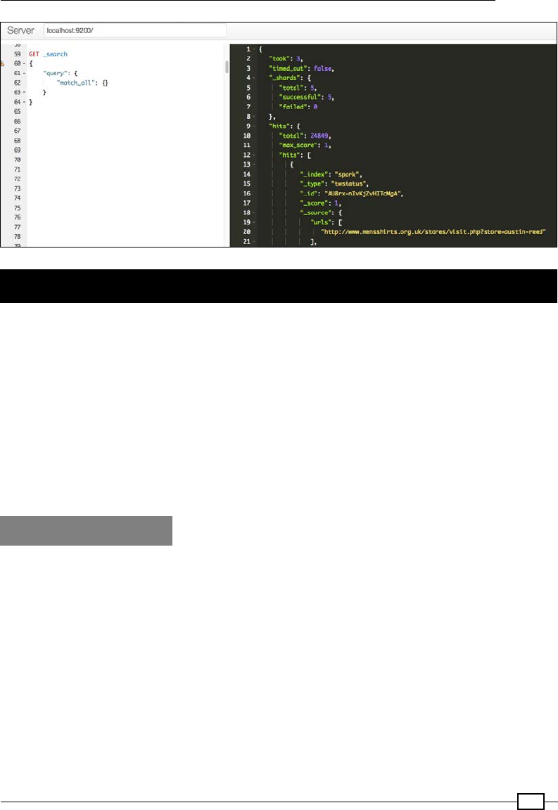
Chapter 7
593
Using Spark as an ETL tool
In the previous recipe, we subscribed to a Twitter stream and stored it in ElasticSearch.
Another common source of streaming is Kafka, a distributed message broker. In fact,
it's a distributed log of messages, which in simple terms means that there can be multiple
brokers that has the messages partitioned among them.
In this recipe, we'll be subscribing the data that we ingested into ElasticSearch in the previous
recipe and publishing the messages into Kafka. Soon after we publish the data to Kafka, we'll
be subscribing to Kafka using the Spark Stream API. While this is a recipe that demonstrates
treating ElasticSearch data as an RDD and publishing to Kafka using a KryoSerializer, the
true intent of this recipe is to run a streaming classication algorithm against Twitter, which is
our next recipe.
How to do it...
Let's look at the various steps involved in doing this.
1. Setting up Kafka: This recipe uses Kafka version 0.8.2.1 for Spark 2.10, which can
be downloaded from https://www.apache.org/dyn/closer.cgi?path=/
kafka/0.8.2.1/kafka_2.10-0.8.2.1.tgz.

Going Further
594
Once downloaded, let's extract, start the Kafka server, and create a Kafka topic
through three commands from inside our Kafka home directory:
1. Starting Zookeeper: Kafka uses Zookeeper (https://zookeeper.
apache.org/) to hold coordination information between Kafka servers.
It also holds the commit offset information of the data so that if a Kafka
node fails, it knows where to resume from. The Zookeeper data directory
and the client port (default 2181) is present in zookeeper.properties.
The zookeeper-server-start.sh expects this to be passed as a
parameter for it to start:
bin/zookeeper-server-start.sh config/zookeeper.properties
2. Starting the Kafka server: Again, in order to start Kafka, the configuration
file to be passed to it is server.properties. The server.properties,
among many things specifies the port on which the Kafka server listens
(9092) and the Zookeeper port it needs to connect to (2181). This is passed
to the kafka-server-start.sh startup script:
bin/kafka-server-start.sh config/server.properties
3. Creating a Kafka topic: In really simple terms, a topic can be compared
to a JMS topic with the difference that there could be multiple publishers
as well as a single subscriber in Kafka. Since we are running the Kafka in
a non-replicated and non-partitioned mode using just one Kafka server,
the topic named twtopic (Twitter topic) is created with a replication factor
of 1 and the number of partitions is 1 as well:
bin/kafka-topics.sh --create --zookeeper localhost:2181
--replication-factor 1 --partitions 1 --topic twtopic
2. Pulling data from ElasticSearch: The next step is to pull the data from ElasticSearch
and treat it as a Spark DataFrame other than the optional setting in Spark
conguration to point to the correct host and port. This is just a one-liner.
The conguration change (if needed) is:
//Default is localhost. Point to ES node when required
val conf = new SparkConf()
.setAppName("KafkaStreamProducerFromES")
.setMaster("local[2]")
.set(ConfigurationOptions.ES_NODES, "localhost")
.set(ConfigurationOptions.ES_PORT, "9200")
The following line queries the "spark/twstatus" index (that we published to in the
last recipe) for all documents and extracts the data into a DataFrame. Optionally, you
can pass in a query as a second argument (for example, "?q=fashion"):
val twStatusDf=sqlContext.esDF("spark/twstatus")
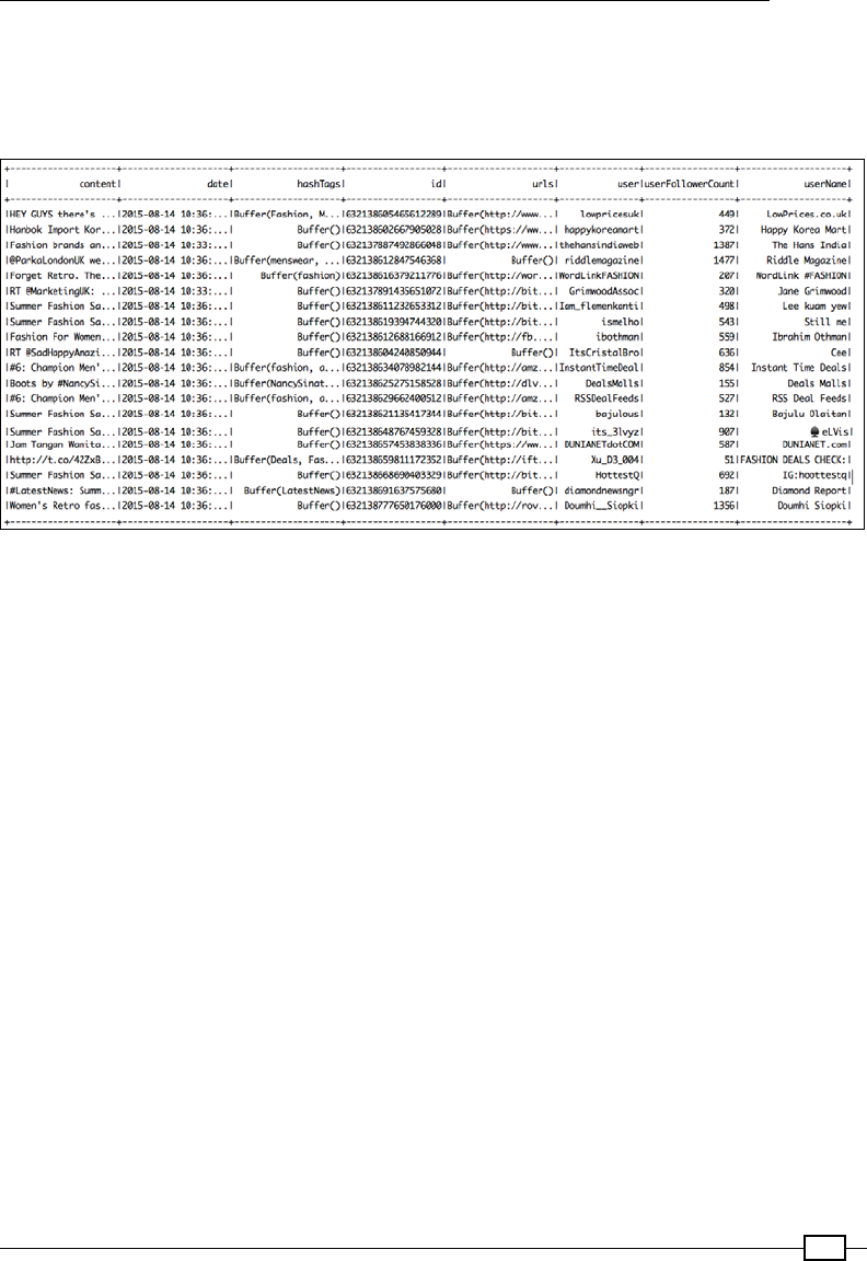
Chapter 7
595
Let's try to sample the DataFrame using show():
twStatusDf.show()
The output is:
3. Preparing data to be published to Kafka: Before we do this step, let's go over what
we aim to achieve from this step. Like we discussed at the beginning of the recipe,
we will be running a classication algorithm against streaming data in the next recipe.
As you know, any supervised learning algorithm requires a training dataset. Instead
of us manually curating the dataset, we will be doing that in a very primitive fashion
by marking all the tweets that have the word fashion in them as belonging to the
fashion class and the rest of the tweets as not belonging to the fashion class.
We will just take the content of the tweet and convert it into a case class called
LabeledContent (similar to LabeledPoint in Spark MLlib):
case class LabeledContent(label: Double, content:
Array[String])
LabeledContent only has two elds:
label: This indicates whether the tweet is about fashion or not (1.0 if the
tweet is on fashion and 0.0 if it is not)
content: This holds a space-tokenized version of the tweet itself
def convertToLabeledContentRdd(twStatusDf: DataFrame) = {
//Convert the content alone to a (label, content) pair
val labeledPointRdd = twStatusDf.map{row =>
val content =
row.getAs[String]("content").toLowerCase()
val tokens = content.split(" ") //A very primitive
space based tokenizer

Going Further
596
val labeledContent=if (content.contains("fashion"))
LabeledContent(1, tokens)
else LabeledContent(0, tokens)
println (labeledContent.label, content)
labeledContent
}
labeledPointRdd
}
4. Publishing data to Kafka using KryoSerializer: Now that we have the
publish candidate (LabeledContent) ready, let's publish it to the Kafka
topic. This involves just three lines.
Constructing the connection and transport properties: In properties,
we configure the Kafka server port location and register the serializer that
we use to serialize LabeledContent:
val properties = Map[String,
Object](ProducerConfig.BOOTSTRAP_SERVERS_CONFIG ->
"localhost:9092").asJava
Constructing the Kafka producer using the connection properties and
the key and value serializer: The next step is to construct a Kafka producer
using the properties we constructed earlier. The producer also needs
a key and a value serializer. Since we don't have a key for our message, we
fall back to Kafka's default, which fills in the hashcode by default, which we
aren't interested on receipt.
val producer = new KafkaProducer[String,
Array[Byte]](properties, new StringSerializer, new
ByteArraySerializer)
Sending data to the Kafka topic using the send method: We then serialize
LabeledContent using KryoSerializer and send it to the Kafka topic
"twtopic" (the one that we created earlier) using the producer.send
method. The only purpose of using a KryoSerializer here is to speed up
the serialization process:
val serializedPoint = KryoSerializer.serialize(lContent)
producer.send(new ProducerRecord[String,
Array[Byte]]("twtopic", serializedPoint))
For the KryoSerializer, we use Twitter's chill library (https://github.com/
twitter/chill), which provides an easier abstraction over the serialization
for Scala.

Chapter 7
597
The actual KryoSerializer is just ve lines of code:
object KryoSerializer {
private val kryoPool = ScalaKryoInstantiator.defaultPool
def serialize[T](anObject: T): Array[Byte] =
kryoPool.toBytesWithClass(anObject)
def deserialize[T](bytes: Array[Byte]): T =
kryoPool.fromBytes(bytes).asInstanceOf[T]
}
The dependency for Twitter chill that needs to be added to our build.sbt is:
"com.twitter" %% "chill" % "0.7.0"
The entire publishing method looks like this:
def publishToKafka(labeledPointRdd: RDD[LabeledContent])
{
labeledPointRdd.foreachPartition { iterator =>
val properties = Map[String, Object](ProducerConfig.
BOOTSTRAP_SERVERS_CONFIG ->
"localhost:9092", "serializer.class" ->
"kafka.serializer.DefaultEncoder").asJava
val producer = new KafkaProducer[String,
Array[Byte]](properties, new StringSerializer, new
ByteArraySerializer)
iterator.foreach { lContent =>
val serializedPoint =
KryoSerializer.serialize(lContent)
producer.send(new ProducerRecord[String,
Array[Byte]]("twtopic", serializedPoint))
}
}
}

Going Further
598
5. Conrming receipt in Kafka: We could conrm whether the data is in Kafka using
the JMX MBeans exposed by it. We'll use JConsole UI to explore MBeans. As you
can see, the count of the messages is 24849, which matches the ElasticSearch
document count (that was published in the previous recipe).
Using StreamingLogisticRegression to
classify a Twitter stream using Kafka
as a training stream
In the previous recipe, we published all the tweets that were stored in ElasticSearch to a
Kafka topic. In this recipe, we'll subscribe to the Kafka stream and train a classication
model out of it. We will later use this trained model to classify a live Twitter stream.

Chapter 7
599
How to do it...
This is a really small recipe that is composed of 3 steps:
1. Subscribing to a Kafka stream: There are two ways to subscribe to a Kafka stream
and we'll be using the DirectStream method, which is faster. Just like Twitter
streaming, Spark has rst-class support for subscribing to a Kafka stream. This is
achieved by adding the spark-streaming-kafka dependency. Let's add it to our
build.sbt le:
"org.apache.spark" %% "spark-streaming-kafka" %
sparkVersion
The subscription process is more or less the reverse of the publishing process even in
terms of the properties that we pass to Kafka:
val topics = Set("twtopic")
val kafkaParams = Map[String,
String]("metadata.broker.list" -> "localhost:9092")
Once the properties are constructed, we subscribe to twtopic using KafkaUtils.
createDirectStream:
val kafkaStream = KafkaUtils.createDirectStream[String,
Array[Byte], StringDecoder,
DefaultDecoder](streamingContext, kafkaParams,
topics).repartition(2)
With the stream at hand, let's reconstruct LabeledContent out of it. We can do that
through KryoSerializer's deserialize function:
val trainingStream = kafkaStream.map {
case (key, value) =>
val labeledContent =
KryoSerializer.deserialize(value).asInstanceOf[LabeledContent]
2. Training the classication model: Now that we are receiving the LabeledContent
objects from the Kafka stream, let's train our classication model out of them. We
will use StreamingLogisiticRegressionWithSGD for this, which as the name
indicates, is a streaming version of the LogisticRegressionWithSGD algorithm we saw
in Chapter 5, Learning from Data. In order to train the model, we have to construct
a LabeledPoint, which is a pair of labels (represented as a double) and a feature
vector. Since this is a text, we'll use the HashingTF's transform function to generate
the feature vector for us:
val hashingTf = new HashingTF(5000)
val kafkaStream = KafkaUtils.createDirectStream[String,
Array[Byte], StringDecoder,
DefaultDecoder](streamingContext, kafkaParams,
topics).repartition(2)

Going Further
600
val trainingStream = kafkaStream.map {
case (key, value) =>
val labeledContent =
KryoSerializer.deserialize(value).asInstanceOf[LabeledContent]
val vector =
hashingTf.transform(labeledContent.content)
LabeledPoint(labeledContent.label, vector)
}
trainingStream now is a stream of LabeledPoint, which we will be using to
train our model:
val model = new StreamingLogisticRegressionWithSGD()
.setInitialWeights(Vectors.zeros(5000))
.setNumIterations(25).setStepSize(0.1).setRegParam(0.001)
model.trainOn(trainingStream)
Since we specied the maximum number of features in our HashingTF to be 5000,
we set the initial weights to be 0 for all 5,000 features. The rest of the parameters
are the same as the regular LogisticRegressionWithSGD algorithm that trains on a
static dataset.
3. Classifying a live Twitter stream: Now that we have the model in hand, let's use
it to predict whether the incoming stream of tweets is about fashion or not. The
Twitter setup in this section is the same as the rst recipe where we subscribed
to a Twitter stream:
val filter = List("fashion", "tech", "startup", "spark")
val twitterStream =
TwitterUtils.createStream(streamingContext, twitterAuth,
filter, StorageLevel.MEMORY_AND_DISK)
The crucial part is the invocation of model.predictOnValues, which gives us the
predicted label. Once the prediction is made, we save them as text les in our local
directory. It's not the best way to do it and we will probably want to push this data to
some appendable data source instead.
val contentAndFeatureVector=twitterStream.map { status =>
val tokens=status.getText().toLowerCase().split(" ")
val vector=hashingTf.transform(tokens)
(status.getText(), vector)
}
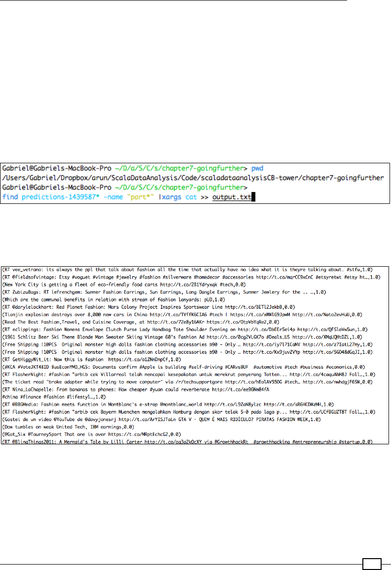
Chapter 7
601
val contentAndPrediction=model.predictOnValues(contentAndFeatu
reVector)
//Not the best way to store the results. Creates a whole
lot of files
contentAndPrediction.saveAsTextFiles("predictions",
"txt")
In order to consolidate the predictions that are spread over multiple les, a really
simple aggregation command was used:
find predictions* -name "part*" |xargs cat >> output.txt
Here is a sample of the prediction. The results are fairly okay considering the training
dataset itself was not classied in a very scientic way. Also, the tokenization is just
space-based, the data isn't scaled nor was the IDF used.

Going Further
602
Using GraphX to analyze Twitter data
GraphX is Spark's approach to graphs and computation against graphs. In this recipe, we will
see a preview of what is possible with the GraphX component in Spark.
How to do it...
Now that we have the Twitter data stored in the ElasticSearch index, we will perform the
following tasks on this data using a graph:
1. Convert the ElasticSearch data into a Spark Graph.
2. Sample vertices, edges, and triplets in the graph.
3. Find the top group of connected hashtags (connected component).
4. List all the hashtags in that component.
1. Converting the ElasticSearch data into a graph: This involves two steps:
1. Converting ElasticSearch data into a DataFrame: This step, like we saw in
an earlier recipe, is just a one-liner:
def convertElasticSearchDataToDataFrame(sqlContext:
SQLContext) = {
val twStatusDf = sqlContext.esDF("spark/twstatus")
twStatusDf
}
2. Converting DataFrame to a graph: Spark Graph construction requires an
RDD for a vertex and an RDD of edges. Let's construct them one by one.
Vertex RDD requires an RDD of a tuple representing a vertexId and a
vertex property. In our case, we'll just do a primitive hash code on the
hashTag as the vertex ID and hashTag itself as the property:
val verticesRdd:RDD[(Long,String)] = df.flatMap { tweet =>
val hashTags =
tweet.getAs[Buffer[String]]("hashTags")
hashTags.map { tag =>
val lowercaseTag = tag.toLowerCase()
val tagHashCode=lowercaseTag.hashCode().toLong
(tagHashCode, lowercaseTag)
}
}

Chapter 7
603
For the edges, we construct an RDD[Edge] , which wraps a pair of vertex IDs
and a property. In our case, we use the rst URL (if present) as a property to
the edge (we aren't using it for this recipe so an empty string should also be
ne). Since there is a possibility of multiple hashtags for a tweet, we use the
combinations function to choose pairs and then connect them together as
an edge:
val edgesRdd:RDD[Edge[String]] =df.flatMap { row =>
val hashTags = row.getAs[Buffer[String]]("hashTags")
val urls = row.getAs[Buffer[String]]("urls")
val topUrl=if (urls.length>0) urls(0) else ""
val combinations=hashTags.combinations(2)
combinations.map{ combs=>
val firstHash=combs(0).toLowerCase().hashCode.toLong
val
secondHash=combs(1).toLowerCase().hashCode.toLong
Edge(firstHash, secondHash, topUrl)
}
}
Finally, we construct the graph using both RDDs:
val graph=Graph(verticesRdd, edgesRdd)
2. Sampling vertices, edges, and triplets in the graph: Now that we have our
graph constructed, let's sample and see what the vertices, edges, and triplets
of the Graph look like. A triple is a representation of an edge and two vertices
connected by that edge:
graph.vertices.take(20).foreach(println)
Going Further
604
The output is:
graph.edges.take(20).foreach(println)
The output is:
graph.triplets.take(20).foreach(println)
Chapter 7
605
The output is:
3. Finding the top group of connected hashtags (connected component): As you
know, a graph is made of vertices and edges. A connected component of a graph
is just a part of the graph (a subgraph) whose vertices are connected to each other
by some edge. If there is a vertex that is not connected to another vertex directly or
indirectly through another vertex, then they are not connected and therefore don't
belong to the same connected component.
GraphX's graph.connectedComponents provides a graph of all the vertices
along with their component IDs:
val connectedComponents=graph.connectedComponents.cache()
Let's take the component ID with the maximum number of vertices and then extract
the vertices (and eventually the hashtags) that belong to that component:
val ccCounts:Map[VertexId,
Long]=connectedComponents.vertices.map{case (_, vertexId)
=> vertexId}.countByValue
//Get the top component Id and count
val topComponent:(VertexId,
Long)=ccCounts.toSeq.sortBy{case (componentId, count) =>
count}.reverse.head

Going Further
606
Since topComponent just has the component ID, in order to fetch the hashTags
of the top component, we need to have a representation that maps hashTag
to a component ID. This is achieved by joining the graph's vertices to the
connectedComponent vertices:
//RDD of HashTag-Component Id pair. Joins using vertexId
val
hashtagComponentRdd:VertexRDD[(String,VertexId)]=graph.vertices.
innerJoin(connectedComponents.vertices){ case
(vertexId, hashTag, componentId)=>
(hashTag, componentId)
}
Now that we have componentId and hashTag, let's lter only the hashTags for the
top component ID:
val topComponentHashTags=hashtagComponentRdd
.filter{ case (vertexId, (hashTag,
componentId)) => (componentId==topComponent._1)}
.map{case (vertexId, (hashTag,componentId)) =>
hashTag
}
topComponentHashTags
The entire method looks like this:
def getHashTagsOfTopConnectedComponent(graph:Graph[String,String])
:RDD[String]={
//Get all the connected components
val connectedComponents=graph.connectedComponents.cache()
import scala.collection._
val ccCounts:Map[VertexId,
Long]=connectedComponents.vertices.map{case (_, vertexId) =>
vertexId}.countByValue
//Get the top component Id and count
val topComponent:(VertexId,
Long)=ccCounts.toSeq.sortBy{case (componentId, count) =>
count}.reverse.head

Chapter 7
607
//RDD of HashTag-Component Id pair. Joins using
vertexId
val
hashtagComponentRdd:VertexRDD[(String,VertexId)]=graph.vertices.
innerJoin(connectedComponents.vertices){ case
(vertexId, hashTag, componentId)=>
(hashTag, componentId)
}
//Filter the vertices that belong to the top component alone
val topComponentHashTags=hashtagComponentRdd
.filter{ case (vertexId, (hashTag,
componentId)) => (componentId==topComponent._1)}
.map{case (vertexId, (hashTag,componentId)) =>
hashTag
}
topComponentHashTags
}
4. List all the hashtags in that component: Saving the hashTags to a le is as simple
as calling saveAsTextFile. The repartition(1) is done just so that we have a
single output le. Alternatively, you could use collect() to bring all the data to the
driver and inspect it:
def saveTopTags(topTags:RDD[String]){
topTags.repartition(1).saveAsTextFile("topTags.txt")
}
Going Further
608
The number of hashtags in the top connected component for our run was 7,320. This shows
that in our sample stream there are about 7,320 tags related to fashion that are interrelated.
They could be synonyms, closely related, or remotely related to fashion. A snapshot of the le
looks like this:
In this chapter, we briey touched upon Spark streaming, Streaming ML, and GraphX. Please
note that this is by no means an exhaustive recipe list for both topics and aims to just provide
a taste of what Streaming and GraphX in Spark could do.
Module 3
Scala for Machine Learning
Leverage Scala and Machine Learning to construct and study systems
that can learn from data

Getting Started
It is critical for any computer scientist to understand the different classes of machine
learning algorithms and be able to select the ones that are relevant to the domain of
their expertise and dataset. However, the application of these algorithms represents
a small fraction of the overall effort needed to extract an accurate and performing
model from input data. A common data mining workow consists of the following
sequential steps:
1. Loading the data.
2. Preprocessing, analyzing, and ltering the input data.
3. Discovering patterns, afnities, clusters, and classes.
4. Selecting the model features and the appropriate machine learning
algorithm(s).
5. Rening and validating the model.
6. Improving the computational performance of the implementation.
As we will emphasize throughout this book, each stage of the process is critical to
build the right model.
This rst chapter introduces you to the taxonomy of machine learning algorithms,
the tools and frameworks used in the book, and a simple application of logistic
regression to get your feet wet.
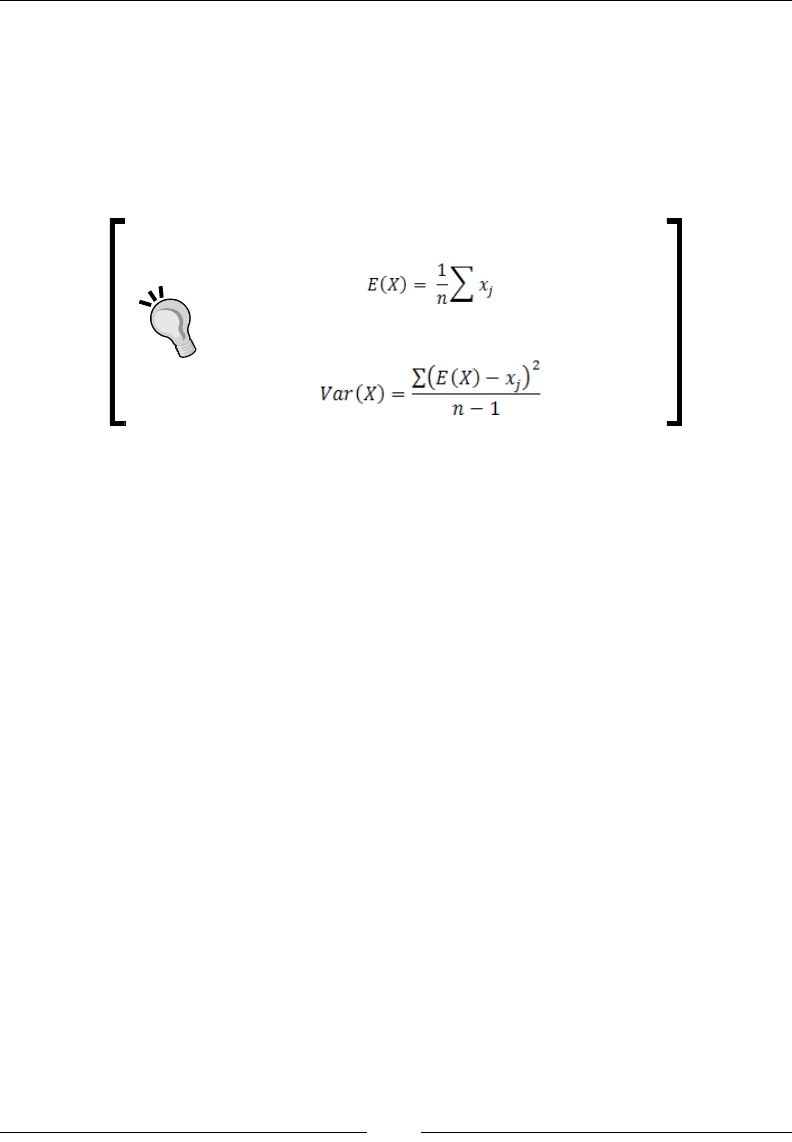
Getting Started
[ 612 ]
Mathematical notation for the curious
Each chapter contains a small section dedicated to the formulation of the algorithms
for those interested in the mathematical concepts behind the science and art of
machine learning. These sections are optional and dened within a tip box. For
example, the mathematical expression of the mean and the variance of a variable
X mentioned in a tip box will be as follows:
Mean value of a variable X = {x} is dened as:
The variance of a variable X = {x} is dened as:
Why machine learning?
The explosion in the number of digital devices generates an ever-increasing amount
of data. The best analogy I can nd to describe the need, desire, and urgency to
extract knowledge from large datasets is the process of extracting a precious metal
from a mine, and in some cases, extracting blood from a stone.
Knowledge is quite often dened as a model that can be constantly updated or
tweaked as new data comes into play. Models are obviously domain-specic ranging
from credit risk assessment, face recognition, maximization of quality of service,
classication of pathological symptoms of disease, optimization of computer networks,
and security intrusion detection, to customers' online behavior and purchase history.
Machine learning problems are categorized as classication, prediction, optimization,
and regression.
Classication
The purpose of classication is to extract knowledge from historical data. For
instance, a classier can be built to identify a disease from a set of symptoms. The
scientist collects information regarding the body temperature (continuous variable),
congestion (discrete variables HIGH, MEDIUM, and LOW), and the actual diagnostic
(u). This dataset is used to create a model such as IF temperature > 102 AND
congestion = HIGH THEN patient has the flu (probability 0.72), which
doctors can use in their diagnostic.

Chapter 1
[ 613 ]
Prediction
Once the model is extracted and validated against the past data, it can be used to
draw inference from the future data. A doctor collects symptoms from a patient,
such as body temperature and nasal congestion, and anticipates the state of
his/her health.
Optimization
Some global optimization problems are intractable using traditional linear and
non-linear optimization methods. Machine learning techniques improve the chances
that the optimization method converges toward a solution (intelligent search). You
can imagine that ghting the spread of a new virus requires optimizing a process
that may evolve over time as more symptoms and cases are uncovered.
Regression
Regression is a classication technique that is particularly suitable for a continuous
model. Linear (least square), polynomial, and logistic regressions are among the
most commonly used techniques to t a parametric model, or function, y= f (xj), to a
dataset. Regression is sometimes regarded as a specialized case of classication for
which the output variables are continuous instead of categorical.
Why Scala?
Like most functional languages, Scala provides developers and scientists with a
toolbox to implement iterative computations that can be easily woven dynamically
into a coherent dataow. To some extent, Scala can be regarded as an extension of
the popular MapReduce model for distributed computation of large amounts of data.
Among the capabilities of the language, the following features are deemed essential
to machine learning and statistical analysis.
Abstraction
Monoids and monads are important concepts in functional programming.
Monads are derived from the category and group theory allowing developers to
create a high-level abstraction as illustrated in Twitter's Algebird (https://github.
com/twitter/algebird) or Google's Breeze Scala (https://github.com/dlwh/
breeze) libraries.
A monoid denes a binary operation op on a dataset T with the property of closure,
identity operation, and associativity.

Getting Started
[ 614 ]
Let's consider the + operation is dened for a set T using the following
monoidal representation:
trait Monoid[T] {
def zero: T
def op(a: T, b: T): c
}
Monoids are associative operations. For instance, if ts1, ts2, and ts3 are three
time series, then the property ts1 + (ts2 + ts3) = (ts1 + ts2) + ts2 is true.
The associativity of a monoid operator is critical in regards to parallelization of
computational workows.
Monads are structures that can be seen either as containers by programmers or as
a generalization of Monoids. The collections bundled with the Scala standard library
(list, map, and so on) are constructed as monads [1:1]. Monads provide the ability
for those collections to perform the following functions:
1. Create the collection.
2. Transform the elements of the collection.
3. Flatten nested collections.
A common categorical representation of a monad in Scala is a trait, Monad,
parameterized with a container type M:
trait Monad[M[_]] {
def apply[T])(a: T): M[T]
def flatMap[T, U](m: M[T])(f: T=>M[U]): M[U]
}
Monads allow those collections or containers to be chained to generate a workow.
This property is applicable to any scientic computation [1:2].
Scalability
As seen previously, monoids and monads enable parallelization and chaining of
data processing functions by leveraging the Scala higher-order methods. In terms
of implementation, Actors are the core elements that make Scala scalable. Actors act
as coroutines, managing the underlying threads pool. Actors communicate through
passing asynchronous messages. A distributed computing Scala framework such
as Akka and Spark extends the capabilities of the Scala standard library to support
computation on very large datasets. Akka and Spark are described in detail in the
last chapter of this book [1:3].
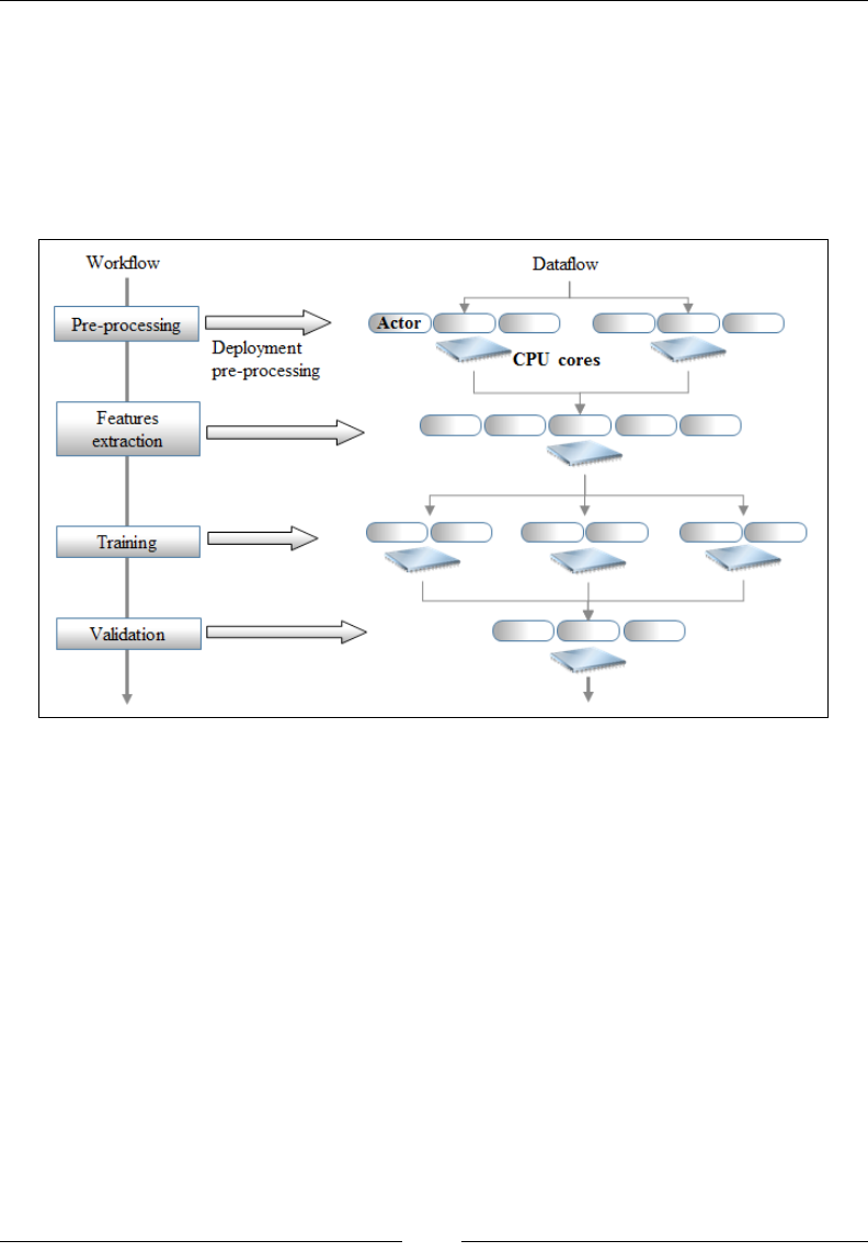
Chapter 1
[ 615 ]
In a nutshell, a workow is implemented as a sequence of activities or computational
tasks. Those tasks consist of high-order Scala methods such as flatMap, map, fold,
reduce, collect, join, or filter applied to a large collection of observations. Scala
allows these observations to be partitioned by executing those tasks through a cluster
of actors. Scala also supports message dispatching and routing of messages between
local and remote actors. The engineers can decide to execute a workow either locally
or distributed across CPU cores and servers with no code or very little code changes.
Deployment of a workflow as a distributed computation
In this diagram, a controller, that is, the master node, manages the sequence of
tasks 1 to 4 similar to a scheduler. These tasks are actually executed over multiple
worker nodes that are implemented by the Scala actors. The master node exchanges
messages with the workers to manage the state of the execution of the workow
as well as its reliability. High availability of these tasks is implemented through a
hierarchy of supervising actors.
Congurability
Scala supports dependency injection using a combination of abstract variables,
self-referenced composition, and stackable traits. One of the most commonly used
dependency injection patterns, the cake pattern, is used throughout this book to
create dynamic computation workows and plots.

Getting Started
[ 616 ]
Maintainability
Scala embeds Domain Specic Languages (DSL) natively. DSLs are syntactic layers
built on top of Scala native libraries. DSLs allow software developers to abstract
computation in terms that are easily understood by scientists. The most notorious
application of DSLs is the denition of the emulation of the syntax used in the
MATLAB program, which data scientists are familiar with.
Computation on demand
Lazy methods and values allow developers to execute functions and allocate
computing resources on demand. The Spark framework relies on lazy variables
and methods to chain Resilient Distributed Datasets (RDD).
Model categorization
A model can be predictive, descriptive, or adaptive.
Predictive models discover patterns in historical data and extract fundamental
trends and relationships between factors. They are used to predict and classify
future events or observations. Predictive analytics is used in a variety of elds
such as marketing, insurance, and pharmaceuticals. Predictive models are created
through supervised learning using a preselected training set.
Descriptive models attempt to nd unusual patterns or afnities in data by grouping
observations into clusters with similar properties. These models dene the rst level
in knowledge discovery. They are generated through unsupervised learning.
A third category of models, known as adaptive modeling, is generated through
reinforcement learning. Reinforcement learning consists of one or several
decision-making agents that recommend and possibly execute actions in
the attempt of solving a problem, optimizing an objective function, or
resolving constraints.

Chapter 1
[ 617 ]
Taxonomy of machine learning
algorithms
The purpose of machine learning is to teach computers to execute tasks without
human intervention. An increasing number of applications such as genomics, social
networking, advertising, or risk analysis generate a very large amount of data that
can be analyzed or mined to extract knowledge or provide insight into a process,
a customer, or an organization. Ultimately, machine learning algorithms consist
of identifying and validating models to optimize a performance criterion using
historical, present, and future data [1:4].
Data mining is the process of extracting or identifying patterns in a dataset.
Unsupervised learning
The goal of unsupervised learning is to discover patterns of regularities and
irregularities in a set of observations. The process known as density estimation
in statistics is broken down into two categories: discovery of data clusters and
discovery of latent factors. The methodology consists of processing input data to
understand patterns similar to the natural learning process in infants or animals.
Unsupervised learning does not require labeled data, and therefore, is easy to
implement and execute because no expertise is needed to validate an output.
However, it is possible to label the output of a clustering algorithm and use it for
future classication.
Clustering
The purpose of data clustering is to partition a collection of data into a number of
clusters or data segments. Practically, a clustering algorithm is used to organize
observations into clusters by minimizing the observations within a cluster and
maximizing the observations between clusters. A clustering algorithm consists
of the following steps:
1. Creating a model by making an assumption on the input data.
2. Selecting the objective function or goal of the clustering.
3. Evaluating one or more algorithms to optimize the objective function.
Data clustering is also known as data segmentation or data partitioning.
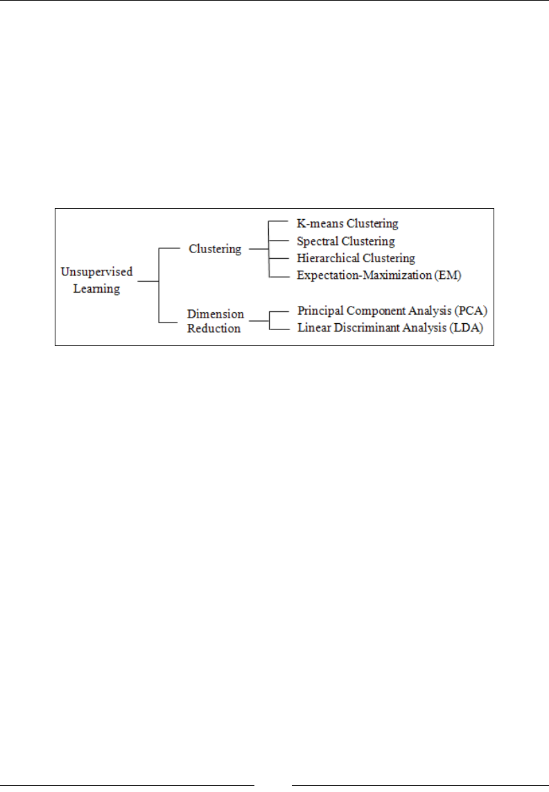
Getting Started
[ 618 ]
Dimension reduction
Dimension reduction techniques aim at nding the smallest but most relevant set
of features that models dataset reliability. There are many reasons for reducing the
number of features or parameters in a model, from avoiding overtting to reducing
computation costs.
There are many ways to classify the different techniques used to extract knowledge
from data using unsupervised learning. The following taxonomy breaks down these
techniques according to their purpose, although the list is far for being exhaustive, as
shown in the following diagram:
Supervised learning
The best analogy for supervised learning is function approximation or curve tting.
In its simplest form, supervised learning attempts to extract a relation or function f
x → y from a training set {x, y}. Supervised learning is far more accurate and reliable
than any other learning strategy. However, a domain expert may be required to label
(tag) data as a training set for certain types of problems.
Supervised machine learning algorithms can be broken into two categories:
• Generative models
• Discriminative models
Generative models
In order to simplify the description of statistics formulas, we adopt the following
simplication: the probability of an event X is the same as the probability of the
discrete random variable X to have a value x, p(X) = p(X=x). The notation of joint
probability (resp. conditional probability) becomes p(X, Y) = p(X=x, Y=y) (resp.
p(X|Y)=p(X=x | Y=y).
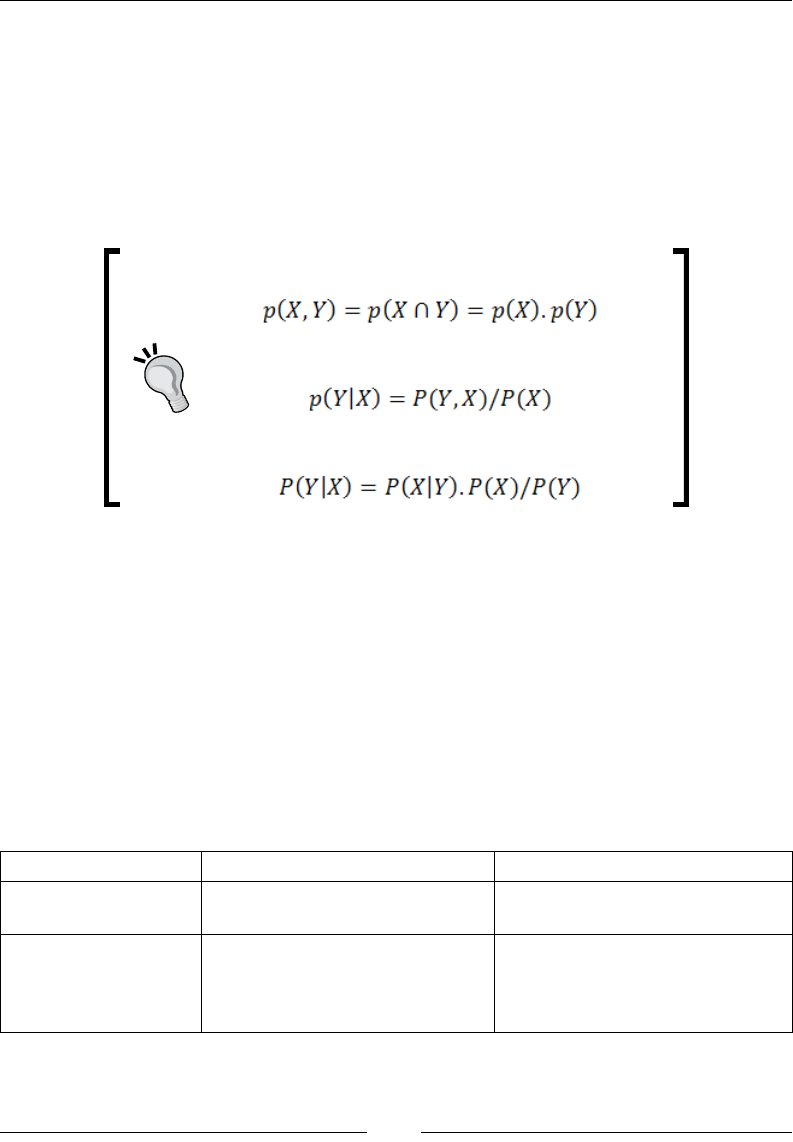
Chapter 1
[ 619 ]
Generative models attempt to t a joint probability distribution, p(X,Y), of two events
(or random variables), X and Y, representing two sets of observed and hidden (latent)
variables x and y. Discriminative models learn the conditional probability p(Y|X) of an
event or random variable Y of hidden variables y, given an event or random variable
X of observed variables x. Generative models are commonly introduced through the
Bayes' rule. The conditional probability of an event Y, given an event X, is computed
as the product of the conditional probability of the event X, given the event Y, and the
probability of the event X normalized by the probability of event Y [1:5].
Join probability (if X and Y are independent):
Conditional probability:
The Bayes' rule:
The Bayes' rule is the foundation of the Naïve Bayes classier, which is the topic of
Chapter 5, Naïve Bayes Classiers.
Discriminative models
Contrary to generative models, discriminative models compute the conditional
probability p(Y|X) directly, using the same algorithm for training and classication.
Generative and discriminative models have their respective advantages and
drawbacks. Novice data scientists learn to match the appropriate algorithm to each
problem through experimentation. Here is a brief guideline describing which type of
models makes sense according to the objective or criteria of the project:
Objective Generative models Discriminative models
Accuracy Highly dependent on the
training set.
Probability estimates tend to be
more accurate.
Modeling
requirements
There is a need to model both
observed and hidden variables,
which requires a significant
amount of training.
The quality of the training set
does not have to be as rigorous
as for generative models.
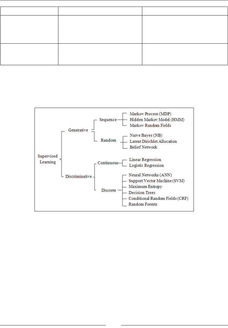
Getting Started
[ 620 ]
Objective Generative models Discriminative models
Computation cost This is usually low. For
example, any graphical method
derived from the Bayes' rule
has low overhead.
Most algorithms rely on
optimization of a convex
that introduces significant
performance overhead.
Constraints These models assume some
degree of independence among
the model features.
Most discriminative algorithms
accommodate dependencies
between features.
We can further rene the taxonomy of supervised learning algorithms by segregating
between sequential and random variables for generative models and breaking down
discriminative methods as applied to continuous processes (regression) and discrete
processes (classication):
Reinforcement learning
Reinforcement learning is not as well understood as supervised and unsupervised
learning outside the realms of robotics or game strategy. However, since the 90s,
genetic-algorithms-based classiers have become increasingly popular to solve
problems that require collaboration with a domain expert. For some types of
applications, reinforcement learning algorithms output a set of recommended
actions for the adaptive system to execute. In its simplest form, these algorithms
compute or estimate the best course of action. Most complex systems based on
reinforcement learning establish and update policies that can be vetoed by an expert.
The foremost challenge developers of reinforcement learning systems face is that the
recommended action or policy may depend on partially observable states and how to
deal with uncertainty.
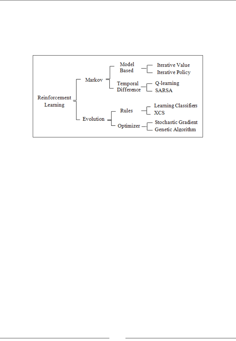
Chapter 1
[ 621 ]
Genetic algorithms are not usually considered part of the reinforcement learning
toolbox. However, advanced models such as learning classier systems use genetic
algorithms to classify and reward the rules and policies.
As with the two previous learning strategies, reinforcement learning models can be
categorized as Markovian or evolutionary:
This is a brief overview of machine learning algorithms with a suggested taxonomy.
There are almost as many ways to introduce machine learning as there are data and
computer scientists. We encourage you to browse through the list of references at the
end of the book and nd the documentation appropriate to your level of interest and
understanding.
Tools and frameworks
Before getting your hands dirty, you need to download and deploy a minimum set
of tools and libraries so as not to reinvent the wheel. A few key components have to
be installed in order to compile and run the source code described throughout the
book. We focus on open source and commonly available libraries, although you are
invited to experiment with equivalent tools of your choice. The learning curve for the
frameworks described here is minimal.
Java
The code described in the book has been tested with JDK 1.7.0_45 and JDK 1.8.0_25
on Windows x64 and MacOS X x64 . You need to install the Java Development Kit if
you have not already done so. Finally, the environment variables JAVA_HOME, PATH,
and CLASSPATH have to be updated accordingly.

Getting Started
[ 622 ]
Scala
The code has been tested with Scala 2.10.4. We recommend using Scala version
2.10.3 or higher and SBT 0.13 or higher. Let's assume that Scala runtime (REPL)
and libraries have been properly installed and environment variables SCALA_HOME
and PATH have been updated. The description and installation instructions of the
Scala plugin for Eclipse are available at http://scala-ide.org/docs/user/
gettingstarted.html.
You can also download the Scala plugin for Intellij IDEA from the JetBrains website
at http://confluence.jetbrains.com/display/SCA/.
The ubiquitous simple build tool (sbt) will be our primary building engine.
The syntax of the build le sbt/build.sbt conforms to version 0.13, and is
used to compile and assemble the source code presented throughout this book.
Apache Commons Math
Apache Commons Math is a Java library for numerical processing, algebra, statistics,
and optimization [1:6].
Description
This is a lightweight library that provides developers with a foundation of small,
ready-to-use Java classes that can be easily weaved into a machine learning problem.
The examples used throughout the book require version 3.3 or higher.
The main components of Apache Commons Math are:
• Functions, differentiation, and integral and ordinary differential equations
• Statistics distribution
• Linear and nonlinear optimization
• Dense and Sparse vectors and matrices
• Curve tting, correlation, and regression
For more information, visit http://commons.apache.org/proper/commons-math.
Licensing
We need Apache Public License 2.0; the terms are available at http://www.apache.
org/licenses/LICENSE-2.0.

Chapter 1
[ 623 ]
Installation
The installation and deployment of the Commons Math library are quite simple:
1. Go to the download page, http://commons.apache.org/proper/commons-
math/download_math.cgi.
2. Download the latest .jar les in the Binaries section, commons-math3-3.3-
bin.zip (for version 3.3, for instance).
3. Unzip and install the .jar les.
4. Add commons-math3-3.3.jar to classpath as follows:
°For Mac OS X, use the command export CLASSPATH=$CLASSPATH:/
Commons_Math_path/commons-math3-3.3.jar
°For Windows, navigate to System property | Advanced system
settings | Advanced | Environment variables…, then edit the
entry of the CLASSPATH variable
5. Add the commons-math3-3.3.jar le to your IDE environment if needed
(that is, for Eclipse, navigate to Project | Properties | Java Build Path |
Libraries | Add External JARs).
You can also download commons-math3-3.3-src.zip from the Source section.
JFreeChart
JFreeChart is an open source chart and plotting Java library, widely used in the Java
programmer community. It was originally created by David Gilbert [1:7].
Description
The library supports a variety of congurable plots and charts (scatter, dial, pie, area,
bar, box and whisker, stacked, and 3D). We use JFreeChart to display the output
of data processing and algorithms throughout the book, but you are encouraged to
explore this great library on your own, as time permits.
Licensing
It is distributed under the terms of the GNU Lesser General Public License (LGPL),
which permits its use in proprietary applications.

Getting Started
[ 624 ]
Installation
To install and deploy JFreeChart, perform the following steps:
1. Visit http://www.jfree.org/jfreechart.
2. Download the latest version from Source Forge at http://sourceforge.
net/projects/jfreechart/files.
3. Unzip and install the .jar le.
4. Add jfreechart-1.0.17.jar (for version 1.0.17) to classpath as follows:
°For Mac OS, update the classpath by using export
CLASSPATH=$CLASSPATH:/JFreeChart_path/ jfreechart-1.0.17.
jar
°For Windows, go to System property | Advanced system settings |
Advanced | Environment variables… and then edit the entry of the
CLASSPATH variable
5. Add the jfreechart-1.0.17.jar le to your IDE environment, if needed.
Other libraries and frameworks
Libraries and tools that are specic to a single chapter are introduced along with
the topic. Scalable frameworks are presented in the last chapter along with the
instructions to download them. Libraries related to the conditional random elds
and support vector machines are described in the respective chapters.
Why not use Scala algebra and numerical libraries
Libraries such as Breeze, ScalaNLP, and Algebird are great Scala
frameworks for linear algebra, numerical analysis, and machine
learning. They provide even the most seasoned Scala programmer
with a high-quality layer of abstraction. However, this book is
designed as a tutorial that allows developers to write algorithms
from the ground up using simple common Java libraries [1:8].
Source code
The Scala programming language is used to implement and evaluate the machine
learning techniques presented in this book. Only a subset of the source code used
to implement the techniques are presented in the book. The formal implementation
of these algorithms is available on the website of Packt Publishing (http://www.
packtpub.com).

Chapter 1
[ 625 ]
Downloading the example code
You can download the example code les for all Packt books you
have purchased from your account at http://www.packtpub.com.
If you purchased this book elsewhere, you can visit http://www.
packtpub.com/support and register to have the les e-mailed
directly to you.
Context versus view bounds
Most Scala classes discussed in the book are parameterized with the type
associated to the discrete/categorical value (Int) or continuous value (Double).
Context bounds would require that any type used by the client code has Int or
Double as upper bounds:
class MyClassInt[T <: Int]
class MyClassFloat[T <: Double]
Such a design introduces constraints on the client to inherit from simple types and to
deal with covariance and contravariance for container types [1:9].
For this book, view bounds are used instead of context bounds only where they
require an implicit conversion to the parameterized type to be dened:
Class MyClassFloat[T <% Double]
implicit def T2Double(t : T): Double
Presentation
For the sake of readability of the implementation of algorithms, all nonessential code
such as error checking, comments, exceptions, or imports are omitted. The following
code elements are discarded in the code snippet presented in the book:
• Code comments
• Validation of class parameters and method arguments:
class BaumWelchEM(val lambda: HMMLambda ...) {
require( lambda != null, "Lambda model is undefined")
• Exceptions and an exception handler:
try { .. }
catch {
case e: ArrayIndexOutOfBoundsException =>println(e.
toString)
}

Getting Started
[ 626 ]
• Nonessential annotation:
@inline def mean = ..
• Logging and debugging code:
m_logger.debug( …)
• Private and nonessential methods
Primitives and implicits
The algorithms presented in this book share the same primitive types, generic
operators, and implicit conversions.
Primitive types
For the sake of readability of the code, the following primitive types will be used:
type XY = (Double, Double)
type XYTSeries = Array[(Double, Double)]
type DMatrix[T] = Array[Array[T]]
type DVector[T] = Array[T]
type DblMatrix = DMatrix[Double]
type DblVector = Array[Double]
The types have the behavior (methods) of their primitive counterpart (array).
However, adding a new functionality to vectors, matrices, and time series requires
classes of their own right. These classes will be introduced in the next chapter.
Type conversions
Implicit conversion is an important feature of the Scala programming language
because it allows developers to specify a type conversion for an entire library
in a single place. Here are a few of the implicit type conversions used throughout
the book:
implicit def int2Double(n: Int): Double = n.toDouble
implicit def vectorT2DblVector[T <% Double](vt: DVector[T]): DblVector
= vt.map( t => t.toDouble)
implicit def double2DblVector(x: Double): DblVector = Array[Double](x)
implicit def dblPair2DbLVector(x: (Double, Double)): DblVector =
Array[Double](x._1,x._2)
implicit def dblPairs2DblRows(x: (Double, Double)): DblMatrix =
Array[Array[Double]](Array[Double](x._1, x._2))
...

Chapter 1
[ 627 ]
Library-specic conversion
The conversion between the primitive type listed here and
types introduced in a particular library (such as Apache
Commons Math) is declared in future chapters the rst
time those libraries are used.
Operators
Lastly, some operations are applied by multiple machine learning or preprocessing
algorithms. They need to be dened implicitly. The operation on a pair of a vector of
arbitrary type and vector of Double is dened as follows:
def Op[T <% Double](v: DVector[T], w: DblVector, op: (T, Double) =>
Double): DblVector =
v.zipWithIndex.map(x => op(x._1, w(x._2)))
It is also convenient to dene the following operators that are included in the Scala
standard library:
implicit def /(v: DblVector, n: Int):DblVector = v.map( x => x/n)
implicit def /(m: DblMatrix, col: Int, z: Double): DblMatrix = { (0
until m(n).size).foreach(i => m(n)(i) /= z) }
We won't have to redene the types, conversions, and operators from now on.
Immutability
It is usually a good idea to reduce the number of states of an object. Method
invocation transitions an object from one state to another. The larger the number
of methods or states, the more cumbersome the testing process becomes.
There is no point in creating a model that is not dened (trained). Therefore, making
the training of a model as part of the constructor of the class it implements makes a
lot of sense. Therefore, the only public methods of a machine learning algorithm are:
• Classication or prediction
• Validation
• Retrieval of model parameters (weights, latent variables, hidden states, and
so on), if needed

Getting Started
[ 628 ]
Performance of Scala iterators
The evaluation of the performance of Scala high-order iterative methods is beyond
the scope of this book. However, it is important to be aware of the trade-off of
each method.
The for loop construct is to be avoided as a counting iterator except if it is used
in conjunction with yield. It is designed to implement the for-comprehension
monad (map-atMap). The source code presented in this book uses the while
and foreach constructs.
Scala reducer methods reduce and fold are also frequently used for their efciency.
Let's kick the tires
This nal section introduces the key elements of the training and classication
workow. A test case using a simple logistic regression is used to illustrate each
step of the computational workow.
Overview of computational workows
In its simplest form, a computational workow to perform runtime processing of a
dataset is composed of the following stages:
1. Loading the dataset from les, databases, or any streaming devices.
2. Splitting the dataset for parallel data processing.
3. Preprocessing data using ltering techniques, analysis of variance, and
applying penalty and normalization functions whenever necessary.
4. Applying the model, either a set of clusters or classes to classify new data.
5. Assessing the quality of the model.
A similar sequence of tasks is used to extract a model from a training dataset:
1. Loading the dataset from les, databases, or any streaming devices.
2. Splitting the dataset for parallel data processing.
3. Applying ltering techniques, analysis of variance, and penalty and
normalization functions to the raw dataset whenever necessary.
4. Selecting the training, testing, and validation set from the cleansed input data.
5. Extracting key features, establishing afnity between a similar group of
observations using clustering techniques or supervised learning algorithms.
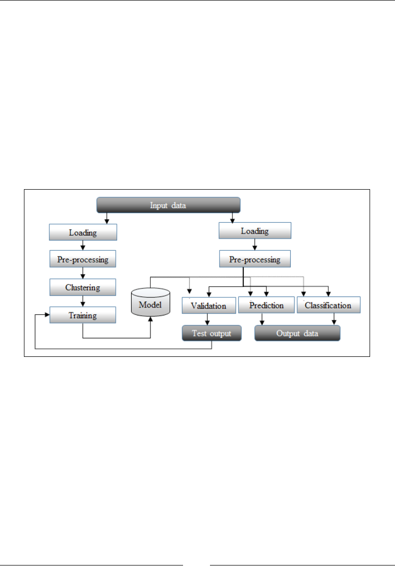
Chapter 1
[ 629 ]
6. Reducing the number of features to a manageable set of attributes to avoid
overtting the training set.
7. Validating the model and tuning the model by iterating steps 5, 6, and 7 until
the error meets criteria.
8. Storing the model into the le or database to be loaded for runtime
processing of new observations.
Data clustering and data classication can be performed independent of each other
or as part of a workow that uses clustering techniques as a preprocessing stage
of the training phase of a supervised learning algorithm. Data clustering does
not require a model to be extracted from a training set, while classication can be
performed only if a model has been built from the training set. The following image
gives an overview of training and classication:
A generic data flow for training and running a model
This diagram is an overview of a typical data mining processing pipeline.
The rst phase consists of extracting the model through clustering or training
of a supervised learning algorithm. The model is then validated against test data,
for which the source is the same as the training set but with different observations.
Once the model is created and validated, it can be used to classify real-time data
or predict future behavior. In reality, real-world workows are more complex
and require being dynamically congurable to allow experimentation of different
models. Several alternative classiers can be used to perform a regression and
different ltering algorithms are applied against input data depending of the
latent noise in the raw data.

Getting Started
[ 630 ]
Writing a simple workow
This book relies on nancial data to experiment with a different learning strategy.
The objective of the exercise is to build a model that can discriminate between
volatile and nonvolatile trading sessions. For this rst example, we select a simplied
version of the logistic regression as our classier as we treat a stock-price-volume
action as a continuous or pseudo-continuous process.
Logistic regression
Logistic regression is treated in depth in Chapter 6, Regression
and Regularization. The model treated in this example is a simple
binary classier using logistic regression for two-dimensional
observations.
The classication of trading sessions according to their volatility is as follows:
• Select a dataset
• Load the dataset
• Preprocess the dataset
• Display data
• Create the model through training
• Classify new data
Selecting a dataset
Throughout the book, we will rely on nancial data to evaluate and discuss the merit
of different data processing and machine learning methods. In this example, the data
is extracted from Yahoo! Finances using the CSV format with the following elds:
• Date
• Price at open
• Highest price in session
• Lowest price in session
• Price at session close
• Volume
• Adjust price at session close
Let's create a simple program that loads the content of the le, executes some simple
preprocessing functions, and creates a simple model. We selected the CSCO stock
price between January 1, 2012 and December 1, 2013 as our data input.

Chapter 1
[ 631 ]
Let's consider two variables, price and volume, as illustrated by the following
screenshot. The top graph displays the variation of the price of Cisco stock over time
and the bottom bar chart represents the daily trading volume on Cisco stock over time:
Price-Volume action for the Cisco stock
Loading the dataset
The rst step is loading the dataset from a local le. Typically, large datasets are
loaded from a database or distributed lesystem such as Hadoop Distributed File
System (HDFS), as shown here:
def load(fileName: String): Option[XYTSeries] = {
val src = Source.fromFile(fileName)
val fields = src.getLines.map( _.split(CSV_DELIM)).toArray //1
val cols = fields.drop(1) //2
val data = transform(cols)
src.close //3
Some(data)
}
The transform method will be described in the next section.
The data le is extracted through an invocation of the Source.fromFile static
method, and then the elds are extracted through a map (line 1). The header
(rst) row is removed with a call to drop (line 2).
Data extraction
The Source.fromFile.getLines.map invocation pipeline
method returns an iterator, which needs to be converted into an
array to store the information into memory.

Getting Started
[ 632 ]
The le has to be closed to avoid leaking of the le handle (line 3).
Code readability
A long pipeline of Scala high-order methods make the code and
underlying code quite difcult to read. It is recommended to break
down long chains of method calls. The following code is an example
of a long chain of method calls:
val cols = Source.fromFile.getLines.map(
_.split(CSV_DELIM).toArray.drop(1)
We can break down such method calls into several steps as follows:
val lines = Source.fromFile.getLines
val fields = lines.map(_.split(CSV_DELIM).toArray
val cols = fields.drop(1)
We strongly encourage you to consult the excellent guide Effective
Scala, written by Marius Eriksen from Twitter. This is denitively a
must read for any Scala developer [1:10].
Preprocessing the dataset
The next step is to normalize the data in the range [-0.5, 0.5] to be trained by the
logistic binary classier. It is time to introduce a non-sense statistics class.
Basic statistics
We select the computation of mean and standard deviation of the two time series as
the rst step of the preprocessing phase. The computation of these statistics can be
implemented by the reduce methods reduceLeft and foldLeft:
val mean = price.reduceLeft( _ + _ )/price.size
val s2 = price.foldLeft(0.0)((s,x) =>s+(x-mean)*(x-mean))
val stdDev = Math.sqrt(s2/(price.size-1) )
However, this implementation has one major drawback: the dataset (price in this
example) has to be traversed for each method (mean, stdDev, min, max, and so on).
One of the solutions is to create a class that computes the counters and the statistics
on demand using, once again, the lazy values:
class Stats[T <% Double](private values: DVector[T]) {
class _Stats(var minValue: Double, var maxValue: Double, var sum:
Double, var sumSqr: Double)
val stats = {
val _stats = new _Stats(Double.MaxValue, Double.MinValue, 0.0, 0.0)

Chapter 1
[ 633 ]
values.foreach(x => {
if(x < _stats.minValue) x else _stats.minValue
if(x > _stats.maxValue) x else _stats.maxValue
_stats.sum + x
_stats.sumSqr + x*x
})
_stats
}
lazy val mean = _stats.sum/values.size
lazy val variance = (_stats.sumSqr - mean*mean*values.size)/(values.
size-1)
lazy val stdDev = if(variance < ZERO_EPS) ZERO_EPS else Math.
sqrt(variance)
lazy val min = _stats.minValue
lazy val max = _stats.mazValue
}
We made the statistics object generic by using the view bounds T <% Double,
which assumes a conversion from type T to Double. By dening the statistics as tuple
counters (minimum value, maximum value, sum of values, and sum of square values)
and folding these values into a statistics object, we limit the number of invocations of
the foldLeft reducer method to 1, and therefore, avoid the recomputation of these
statistics for the existing dataset each time new data is added.
The code illustrates the use and benet of lazy values in Scala. The mean is computed
only if and when needed.
Normalization and Gauss distribution
Statistics are usually used to normalize data into a probability value [0, 1] as required
by most classication or clustering algorithms. It is logical to add the normalization
method to the Stats class, as we have already extracted the min and max values:
def normalize: DblVector = {
val range = max – min; values.map(x => (x - min)/range)
}
The same approach is used to compute the multivariate normal distribution:
def gauss: DblVector =
values.map(x =>{
val y=x-mean
INV_SQRT_2PI/stdDev*Math.exp(-0.5*y*y/stdDev)})
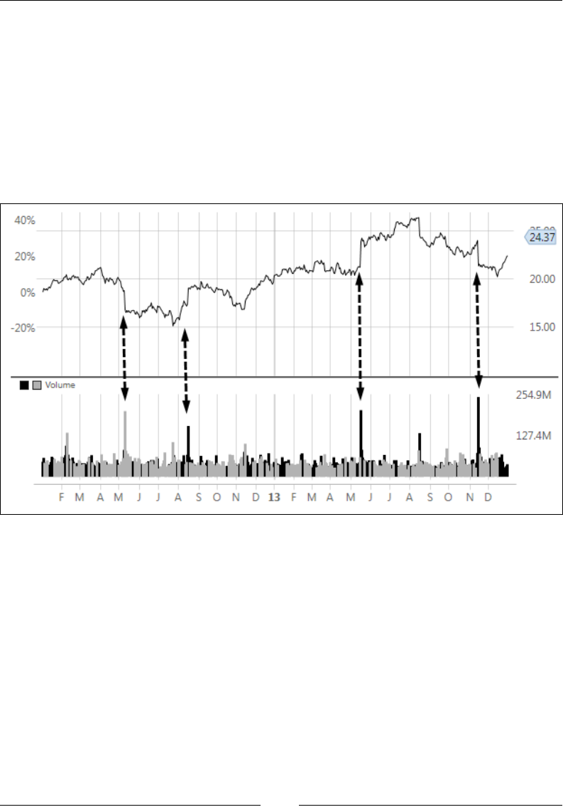
Getting Started
[ 634 ]
The price action chart has a very interesting characteristic. At a closer look, a
sudden change in price and increase in volume occurs about every three months
or so. Experienced investors will undoubtedly recognize that those price-volume
patterns are related to the release of quarterly earnings of Cisco. Such regular but
unpredictable patterns can be a source of concern or opportunity if risk can be
managed. The strong reaction of the stock price to the release of corporate earnings
may scare some long-term investors while enticing day traders.
The following graph visualizes the potential correlation between sudden price
change (volatility) and heavy trading volume:
Correlation price-volume action for the Cisco stock
Let's try to correlate the volatility of the stock price with volume. For the sake of this
exercise, we dene the volatility as the maximum variation of the stock price within
each trading session: the relative difference between the highest price during the
trading session and the lowest price during the session.
The YahooFinancials enumeration extracts historical stock prices and session
volume from a CSV le. For example, the volatility is extracted from the CSV
elds of each line in the CSV le as follows:
object YahooFinancials extends Enumeration {
type YahooFinancials = Value
val DATE, OPEN, HIGH, LOW, CLOSE, VOLUME, ADJ_CLOSE = Value

Chapter 1
[ 635 ]
val volatility = (fs: Array[String]) =>fs(HIGH.id).toDouble-fs(LOW.
id).toDouble
…
}
The transform method uses the YahooFinancials enumeration to generate the
input data for the model:
def transform(cols: Array[Array[String]]): XYTSeries = {
val volatility = Stats[Double](cols.map(YahooFinancials.
volatility)).normalize
val volume = Stats[Double](cols.map(YahooFinancials.volume)
).normalize
volatility.zip(volume)
}
The volatility and volume data is normalized using the Stats.normalize method
dened earlier.
Plotting data
Although charting is not the primary goal of this book, we thought that you will
benet from a brief introduction to JFreeChart. The skeleton code to generate a
scatter plot is rather simple. The most relevant code is the transformation of the
XYTSeries into graphical JFreeChart's XYSeries:
val xLegend = "Session Volatility"
val yLegend = "Session Volume"
def display(xy: XYTSeries, w: Int, h : Int): Unit = {
val series = new XYSeries("CSCO 2012-2013 Stock")
xy.foreach( x => series.add( x._1,x._2))
val seriesCollection = new XYSeriesCollection
seriesCollection.addSeries(series)
… // plot rendering code
val chart = ChartFactory.createScatterPlot(xLegend, xLegend,
yLegend, seriesCollection, PlotOrientation.VERTICAL, true, false,
false)
createFrame("Logistic Regression", chart)
}
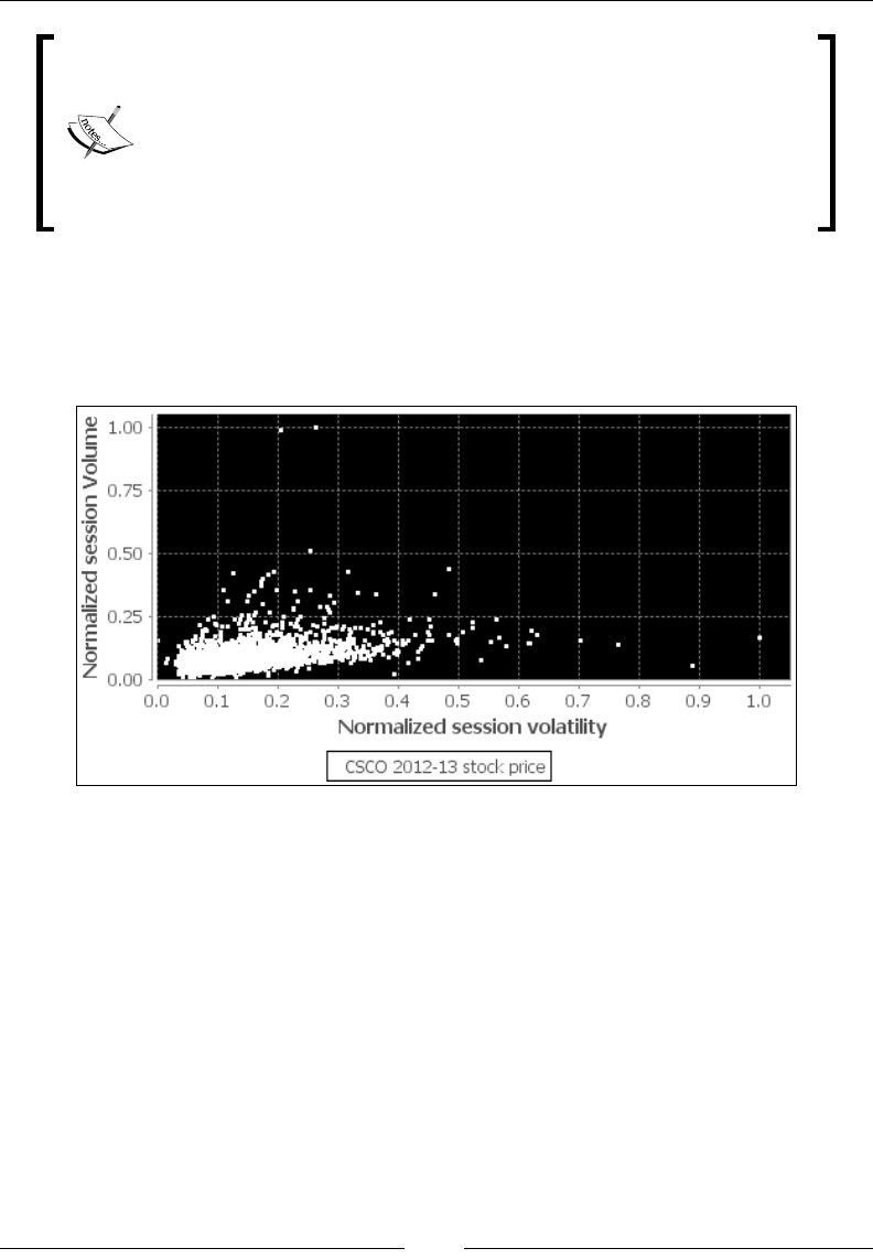
Getting Started
[ 636 ]
Visualization
The JFreeChart library is introduced as a robust charting tool. The
visualization of the results of a computation is beyond the scope of
this book. The code related to plots and charts is omitted from the
book in order to keep the code snippets concise and dedicated to
machine learning. In a few occasions, output data is formatted as a
CSV le to be simply imported into a spreadsheet.
Here is an example of a plot using the ScatterPlot.display method:
val plot = new ScatterPlot(("CSCO 2012-2013", "Session High - Low",
"Session Volume"), new BlackPlotTheme)
plot.display(volatility_vol.filter( _._1 < 0.5), 250, 340)
Scatter plot of volatility and volume for the Cisco stock
There is a level of correlation between session volume and session volatility. We can
use this information to classify trading sessions by their volatility.
Creating a model (learning)
The objective of the training is to build a model that can discriminate between
volatile and nonvolatile trading sessions. For the sake of the exercise, session
volatility has been dened as session price high and session price low coupled
with heavy trading volume, which constitute the two parameters of the model.

Chapter 1
[ 637 ]
Logistic regression is commonly used in statistics inference. The following
implementation of the binary logistic regression classier exposes a single method,
classify, to comply with our desire to reduce the complexity and life cycle of
objects. The model parameters, weights, are computed during training when the
LogBinRegression class/model is instantiated. As mentioned earlier, the sections
of the code nonessential to the understanding of the algorithm are omitted:
class LogBinRegression(val labels: DVector[(XY, Double)], val
maxIters: Int, val eta: Double, val eps: Double) {
val dim = 3
val weights = train
def classify(xy: XY): Option[(Boolean, Double)] = {
if(weights != None) {
val likelihood = sigmoid(w(0) + xy._1*w(1) + xy._2*w(2))
Some(likelihood > 0.5, likelihood)
}
else None
}
The training method, train, consists of iterating through the computation of the
weight using a simple descent gradient. The method computes the weights and
returns an option, so the model is either trained and ready for runtime classication
or nonexistent (None):
def train: Option[DblVector] = {
val w = Array.fill(dim)( x=> Random.nextDouble-1.0)
Range(0, maxIters).find(_ => {
val deltaW = labels.foldLeft(Array.fill(dim)(0.0))((dw, lbl) => {
val y = sigmoid(w(0) + w(1)*lbl._1._1 + w(2)*lbl._1._2)
dw.map(dx => dx + (lbl._2 - y)*(lbl._1._1 + lbl._1._2))
})
val nextW = Array.fill(dim)(0.0)
.zipWithIndex
.map(nw => w(nw._2)+eta*deltaW(nw._2))
val diff = Math.abs(nextW.sum - w.sum)
nextW.copyToArray(w); diff < eps
}) match {
case Some(iters) => Some(w)
case None => { … }
}
}
def sigmoid(x: Double):Double = 1.0/(1.0 + Math.exp(-x))

Getting Started
[ 638 ]
The iteration is encapsulated in the Scala find method that exists if the algorithm
converges (diff < eps). The model parameters, weights, are set to None if the
maximum number of iterations is reached.
The training method, train, iterates across the set of observations by computing
the gradient between the predicted and observed values. In our simplistic approach,
the gradient is computed as a linear function of the sigmoid of the sum of the
product of the weight and training observations. As for any optimization problem,
the initialization of the solution vector, weights, is critical. We choose to initialize
the weight with random values, although in practice, you would use a more
deterministic approach to initialize the model parameters.
In order to train the model, we need to label data. The process consists of tagging
every trading session as volatile and non volatile according to the observations
(relative session volatility and session volume). The labeling process is usually quite
cumbersome; therefore, let's generate the label automatically. A trading session is
considered volatile if a volatility and volume are both greater than 60 percent of the
maximum relative volatility and volume:
val labels = volatilityVol.zip(volatilityVol.map(x =>if( x._1>0.3 &&
x._2>0.3) 1.0 else 0.0))
Automated labeling
Although quite convenient, automated creation of training labels
is not without risk because it may mislabel singular observations.
This technique is used in this test for convenience but it is not
recommended unless a domain expert reviews the labels manually.
The model is created (trained) by a simple instantiation of the logistic binary classier:
val logit = new LogBinRegression(labels, 300, 0.00005, 0.02)
The training run is congured with a maximum of 300 iterations, a gradient slope of
0.00005, and convergence criteria of 0.02.
Classify the data
Finally, the model can be tested with a new fresh dataset, not related to the
training set:
Date,Open,High,Low,Close,Volume,Adj Close
3/9/2011,14.78,15.08,14.20,14.91,4.79E+08,14.88
11/17/2009,10.78,10.90,10.62,10.84,3901987,10.85

Chapter 1
[ 639 ]
It is just a matter of executing the classication method (exceptions, conditions on
method arguments, and returned values are omitted):
val testData = load("resources/data/chap1/CSCO2.csv")
logit.classify(testData(0)) match {
case Some(topCategory) => Display.show(topCategory)
case None => { … }
}
logit.classify(testData(1)) match {
case Some(topCategory) => Display.show(topCategory)
case None => { … }
}
The result of the classication is (true,0.516) for the rst sample and
(false,0.1180) for the second sample.
Validation
The simple classication, in this test case, is provided for illustrating
the runtime application of the model. It does not constitute a
validation of the model by any stretch of imagination. The next
chapter digs into validation metrics and methodology.
Summary
We hope you enjoyed this introduction to machine learning and how to leverage your
existing skills in Scala programming to create a simple regression program to predict
stock price/volume action. Here are the highlights of this introductory chapter:
• From monadic composition and high-order collection methods for
parallelization to congurability to reusability patterns, Scala is the
perfect t to implement and leverage data mining and machine learning
algorithms for large-scale projects
• There are many steps to create and apply a machine learning model
• The implementation of the logistic binary classier presented as part of the
test case is simple enough to encourage you to learn how to write and apply
more advanced machine learning algorithms
To the delight of Scala programming acionados, the next chapter will dig deeper
into building a exible workow by leveraging traits and dependency injection.

Hello World!
In the rst chapter, you were acquainted with some rudimentary concepts regarding
data processing, clustering, and classication. This chapter is dedicated to the
creation and maintenance of a exible end-to-end workow to train and classify
data. The rst section of the chapter introduces a data-centric (functional) approach
to create number-crunching applications.
You will learn how to:
• Apply the concept of monadic design to create dynamic workows
• Leverage some of Scala's advanced functional features, such as dependency
injection, to build portable computational workows
• Take into account the bias-variance trade-off in selecting a model
• Overcome overtting in modeling
• Break down data into training, test, and validation sets
• Implement model validation in Scala using precision, recall, and F score
Modeling
Data is the lifeline of any scientist, and the selection of data providers is critical in
developing or evaluating any statistical inference or machine learning algorithm.
A model by any other name
We briey introduced the concept of a model in the Model categorization section in
Chapter 1, Getting Started.

Hello World!
[ 642 ]
What constitutes a model? Wikipedia provides a reasonably good denition of a
model as understood by scientists [2:1]:
A scientic model seeks to represent empirical objects, phenomena, and physical
processes in a logical and objective way.
…
Models that are rendered in software allow scientists to leverage computational
power to simulate, visualize, manipulate and gain intuition about the entity,
phenomenon, or process being represented.
In statistics and the probabilistic theory, a model describes data that one might
observe from a system to express any form of uncertainty and noise. A model
allows us to infer rules, make predictions, and learn from data.
A model is composed of features, also known as attributes or variables, and a set of
relation between those features. For instance, the model represented by the function
f(x, y) = x.sin(2y) has two features, x and y, and a relation, f. These two features are
assumed to be independent. If the model is subject to a constraint such as f(x, y) < 20,
then the conditional independence is no longer valid.
An astute Scala programmer would associate a model to a monoid for which the set
is a group of observations and the operator is the function implementing the model.
If it walks like a monoid and quacks like a monoid, then it is a monoid.
Models come in a variety of shapes and forms:
• Parametric: This consists of functions and equations (for example,
y = sin(2t + w))
• Differential: This consists of ordinary and partial differential equations
(for example, dy = 2x.dx)
• Probabilistic: This consists of probability distributions (for example,
p (x|c) = exp (k.logx – x)/x!)
• Graphical: This consists of graphs that abstract out the conditional
independence between variables (for example, p(x,y|c) = p(x|c).p(y|c))
• Directed graphs: This consists of temporal and spatial relationships (for
example, a scheduler)
• Numerical method: This consists of nite elements and methods such as
Newton-Raphson
• Chemistry: This consists of formula and components (for example, H2O,
Fe + C12 = FeC13, and so on)

Chapter 2
[ 643 ]
• Taxonomy: This consists of a semantic denition and relationship of concepts
(for example, APG/Eudicots/Rosids/Huaceae/Malvales)
• Grammar and lexicon: This consists of a syntactic representation of
documents (for example, Scala programming language)
• Inference logic: This consists of a distribution pattern such as IF (stock
vol > 1.5 * average) AND rsi > 80 THEN…
Model versus design
The confusion between model and design is quite common in Computer Science,
the reason being that these terms have different meanings for different people
depending on the subject. The following metaphors should help with your
understanding of these two concepts:
• Modeling: This is describing something you know. A model makes the
assumption, which becomes an assertion if proven correct (for example,
the US population, p, increases by 1.2 percent a year, dp/dt= 1.012).
• Designing: This is manipulating representation for things you don't know.
Designing can be seen as the exploration phase of modeling (for example,
what are the features that contribute to the growth of the US population?
Birth rate? Immigration? Economic conditions? Social policies?).
Selecting a model's features
The selection of a model's features is the process of discovering and documenting
the minimum set of variables required to build the model. Scientists make the
assumption that data contains many redundant or irrelevant features. Redundant
features do not provide information already given by the selected features, and
irrelevant features provide no useful information.
Selecting features consists of two consecutive steps:
1. Searching for new feature subsets.
2. Evaluating these feature subsets using a scoring mechanism.
The process of evaluating each possible subset of features to nd the one that
maximizes the objective function or minimizes the error rate is computationally
intractable for large datasets. A model with n features requires 2n-1 evaluations.

Hello World!
[ 644 ]
Extracting features
An observation is a set of indirect measurements of hidden, also known as
latent, variables, which may be noisy or contain a high degree of correlation and
redundancies. Using raw observations in a classication task would very likely
produce inaccurate classes. Using all features from the observation also incurs
a high computation cost.
The purpose of extracting features is to reduce the number of variables or dimensions
of the model by eliminating redundant or irrelevant features. The features are extracted
by transforming the original set of observations into a smaller set at the risk of losing
some vital information embedded in the original set.
Designing a workow
A data scientist has many options in selecting and implementing a classication or
clustering algorithm.
Firstly, a mathematical or statistical model is to be selected to extract knowledge
from the raw input data or the output of a data upstream transformation. The
selection of the model is constrained by the following parameters:
• Business requirements such as accuracy of results
• Availability of training data and algorithms
• Access to a domain or subject-matter expert
Secondly, the engineer has to select a computational and deployment framework
suitable for the amount of data to be processed. The computational context is to
be dened by the following parameters:
• Available resources such as machines, CPU, memory, or I/O bandwidth
• Implementation strategy such as iterative versus recursive computation
or caching
• Requirements for the responsiveness of the overall process such as duration
of computation or display of intermediate results
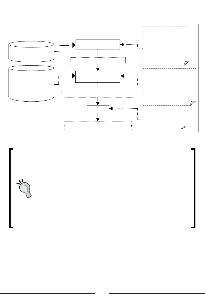
Chapter 2
[ 645 ]
The following diagram illustrates the selection process to dene the data
transformation for each computation in the workow:
Linear regression
Naive Bayes
SVM, HMM, CRF, ...
Concurrent maps
Hadoop/HDFS
In-memory databases
Akka,Spark
NoSQL, Streaming
Relational database
Model prameters
Code
Algorithm
weights=(0.783, 0.219, 0.498)
new LogBinRegression(label, n, eta, eps)
Logistic regression
Learning
Select a computational
framework
Select a statistical or
mathemathical model
Business requirements
Quality of labels
Data completeness
Nature of problem
Available expertise
Numerical libraries
....
Application Response time
Available memory, storage
Network bandwidth
Licensing constraints
Available servers, CPU cores
Redundancy
....
Observations
Labels
Context
....
Statistical and computation modeling for machine-learning applications
Domain expertise, data science, and software engineering
A domain or subject-matter expert is a person with authoritative
or credited expertise in a particular area or topic. A chemist is an
expert in the domain of chemistry and possibly related elds.
A data scientist solves problems related to data in a variety of elds
such as biological sciences, health care, marketing, or nances.
Data and text mining, signal processing, statistical analysis, and
modeling using machine learning algorithms are some of the
activities performed by a data scientist.
A software developer performs all the tasks related to creation of
software applications, including analysis, design, coding, testing,
and deployment.
The parameters of a data transformation may need to be recongured according to
the output of the upstream data transformation. Scala's higher-order functions are
particularly suitable for implementing congurable data transformations.

Hello World!
[ 646 ]
The computational framework
The objective is to create a framework exible and reusable enough to accommodate
different workows and support all types of machine learning algorithms from
preprocessing, data smoothing, and classication to validation.
Scala provides us with a rich toolbox that includes monadic design, design patterns,
and dependency injections using traits. The following diagram describes the three
levels of complexity for creating the framework:
Dependancy Injection (Cake pattern)
Pipe Operator
Monadic Data Transformation
Hierarchical design of a monadic workflow
The rst step is to dene a trait and a method that describes the transformation of
data by a computation unit (element of the workow).
The pipe operator
Data transformation is the foundation of any workow for processing and classifying
a dataset, training and validating a model, and displaying results.
The objective is to dene a symbolic representation of the transformation of different
types of data without exposing the internal state of the algorithm implementing the
data transformation. The pipe operator is used as the signature of a data transformation:
trait PipeOperator[-T, +U] {
def |> (data: T): Option[U]
}
F# reference
The notation |> as the signature of the transform or pipe operator
is borrowed from the F# language [2:2]. The data transformation
indeed implements a function, and therefore, has the same variance
signature as Function[-T, +R] of Scala.

Chapter 2
[ 647 ]
The |> operator transforms a data of the type T into a data of the type U and returns
an option to handle internal errors and exceptions.
Advanced Scala idioms
The next two sections introduce a monadic representation of the
data transformation and one implementation of the dependency
injection to create a dynamic workow as an alternative to the
delimited continuation pattern. Although these topics may interest
advanced Scala developers, they are not required to understand
any of the techniques or procedures described in this book.
Monadic data transformation
The next step is to create a monadic design to implement the pipe operator. Let's
use a monadic design to wrap _fct, a data transformation function (also known as
operator), with the most commonly used Scala higher-order methods:
class _FCT[+T](val _fct: T) {
def map[U](c: T => U): _FCT[U] = new _FCT[U]( c(_fct))
def flatMap[U](f: T =>_FCT[U]): _FCT[U] = f(_fct)
def filter(p: T =>Boolean): _FCT[T] = if( p(_fct) ) new _FCT[T](_
fct) else zeroFCT(_fct)
def reduceLeft[U](f: (U,T) => U)(implicit c: T=> U): U = f(c(_fct),
_fct)
def foldLeft[U](zero: U)(f: (U, T) => U)(implicit c: T=> U): U =
f(c(_fct), _fct)
def foreach(p: T => Unit): Unit = p(_fct)
}
The methods of the _FCT class represent a subset of the traditional Scala higher
methods for collections [2:3]. The _FCT class is to be used internally. Arguments
are validated by subclasses or containers.
Finally, the Transform class takes a PipeOperator instance as an argument and
automatically invokes its operator:
class Transform[-T, +U](val op: PipeOperator[T, U]) extends _
FCT[Function[T, Option[U]]](op.|>) {
def |>(data: T): Option[U] = _fct(data)
}

Hello World!
[ 648 ]
You may wonder about the reason behind the monadic representation of a data
transformation, Transform. You can create any algorithm by just implementing the
PipeOperator trait, after all. The reason is that Transform has a richer protocol
(methods) and enables developers to create a complex workow as an alternative to
the delimited continuation. The following code snippet illustrates a generic function
composition or data transformation composition using the monadic approach:
val op = new PipeOperator[Int, Double] {
def |> (n: Int):Option[Double] =Some(Math.sin(n.toDouble))
}
def g(f: Int =>Option[Double]): (Int=> Long) = {
(n: Int) => {
f(n) match {
case Some(x) => x.toLong
case None => -1L
}
}
}
val gof = new Transform[Int,Double](op).map(g(_))
This code extends op, an existing transformation, with another function, g. As stated
in the Presentation section under Source code in Chapter 1, Getting Started, code related
to exceptions, error checking, and validation of arguments is omitted (refer tothe
Format of code snippets section in Appendix A, Basic Concepts.
Dependency injection
This section presents the key constructs behind the Cake pattern. A workow
composed of congurable data transformations requires a dynamic modularization
(substitution) of the different stages of the workow. The Cake pattern is an advanced
class composition pattern that uses mix-in traits to meet the demands of a congurable
computation workow. It is also known as stackable modication traits [2:4].
This is not an in-depth analysis of the stackable trait injection and self-reference in
Scala. There are few interesting articles on dependencies injection that are worth a
look [2:5].
Java relies on packages tightly coupled with the directory structure and prex to
modularize the code base. Scala provides developers with a exible and reusable
approach to create and organize modules: traits. Traits can be nested, mixed with
classes, stacked, and inherited.

Chapter 2
[ 649 ]
Dependency injection is a fancy name for a reverse look up and binding to
dependencies. Let's consider a simple application that requires data preprocessing,
classication, and validation. A simple implementation using traits looks like this:
val myApp = new Classification with Validation with PreProcessing {
val filter = .. }
If, at a later stage, you need to use an unsupervised clustering algorithm instead of a
classier, then the application has to be rewired:
val myApp = new Clustering with Validation with PreProcessing { val
filter = .. }
This approach results in code duplication and lack of exibility. Moreover, the
filter class member needs to be redened for each new class in the composition
of the application. The problem arises when there is a dependency between traits
used in the composition of the application. Let's consider the case for which the lter
depends on the validation methodology.
Mixins linearization [2:6]
The linearization or invocation of methods between mixins
follows a right-to-left pattern:
• Trait B extends A
• Trait C extends A
• Class M extends N with C with B
The Scala compiler implements the linearization as follows:
M =>B => C => A => N
Although you can dene filter as an abstract value, it still has to be redened each
time a new validation type is introduced. The solution is to use the self type in the
denition of the newly composed PreProcessingWithValidation trait:
trait PreProcessiongWithValidation extends PreProcessing {
self: Validation =>
val filter = ..
}
The application can then be simply composed as:
val myApp = new Classification with PreProcessingWithValidation {
val validation: Validation
}

Hello World!
[ 650 ]
Overriding val with def
It is advantageous to override the declaration of a value with a denition
of a method with the same signature. Contrary to a value that locks the
implementation of the value, a method can return a different value for
each invocation:
trait PreProcessor { val validation = … }
trait MyValidator extends Validator { def validation
= … }
In Scala, a value declaration can be overridden by the method denition,
not vice versa.
Let's adapt and generalize this pattern to construct a boilerplate template in order to
create dynamic computational workows.
The rst step is to generate different modules to encapsulate different types of
data transformation.
Workow modules
The data transformation dened by the PipeOperator instance is dynamically
injected into the module by initializing the abstract value. Let's dene three
parameterized modules representing the preprocessing, processing, and
post-processing stages of a workow:
trait PreprocModule[-T, +U] { val preProc: PipeOperator[T, U] }
trait ProcModule[-T, +U] { val proc: PipeOperator[T, U] }
trait PostprocModule[-T, +U] { val postProc: PipeOperator[T, U] }
The modules (traits) contain only a single abstract value. One characteristic of the
Cake pattern is to enforce strict modularity by initializing the abstract values with
the type encapsulated in the module, as follows:
trait ProcModule[-T, +U] {
val proc: PipeOperator [T, U]
class Classification[-T, +U] extends PipeOperator [T,U] { }
}
One of the objectives in building the framework is allowing developers to create data
transformation (inherited from PipeOperator) independently from any workow.
Under these constraints, strict modularity is not an option.

Chapter 2
[ 651 ]
Scala traits versus Java packages
There is a major difference between Scala and Java in terms of
modularity. Java packages constrain developers into following a
strict syntax requirement; for instance, the source le has the same
name as the class it contains. Scala modules based on stackable traits
are far more exible.
The workow factory
The next step is to write the different modules into a workow. This is achieved
by using the self reference to the stack of the three traits dened in the previous
paragraph. Here is an implementation of the said self reference:
class WorkFlow[T, U, V, W] {
self: PreprocModule[T,U] with ProcModule[U,V] with
PostprocModule[V,W] =>
def |> (data: T): Option[W] = {
preProc |> data match {
case Some(input) => {
proc |> input match {
case Some(output) => postProc |> output
case None => { … }
}
}
case None => { … }
}
}
}
Quite simple indeed! If you need only two modules, you can either create a workow
with a stack of two traits or initialize the third with the PipeOperator identity:
def identity[T] = new PipeOperator[T,T] {
override def |> (data:T): Option[T] = Some(data)
}
Let's test the wiring with the following simple data transformations:
class Sampler(val samples: Int) extends PipeOperator[Double => Double,
DblVector] {
override def |> (f: Double => Double): Option[DblVector] =
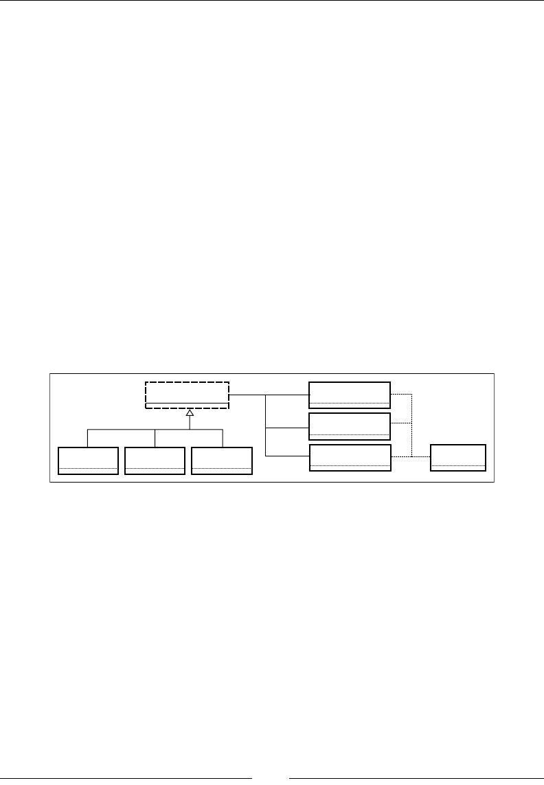
Hello World!
[ 652 ]
Some(Array.tabulate(samples)(n => f(n.toDouble/samples)) )
}
class Normalizer extends PipeOperator[DblVector, DblVector] {
override def |> (data: DblVector): Option[DblVector] =
Some(Stats[Double](data).normalize)
}
class Reducer extends PipeOperator[DblVector, Int] {
override def |> (data: DblVector): Option[Int] =
Range(0, data.size) find(data(_) == 1.0)
}
The rst operator, Sampler, samples a function, f, with a frequency 1/samples over
the interval [0, 1]. The second operator, Normalizer, normalizes the data over the
range [0, 1] using the Stats class introduced in the Basic statistics section in Chapter 1,
Getting Started. The last operator, Reducer, extracts the index of the large sample
(value 1.0) using the Scala collection method, find.
A picture is worth a thousand words; the following UML class diagram illustrates
the workow factory design pattern:
PipeOperator
Sampler Normalizer Reducer
PreprocModule
ProcModule
PostprocModule Workflow
preProc
proc
postProc
Finally, the workow is instantiated by dynamically initializing the abstract values,
preProc, proc, and postProc, with a transformation of the type PipeOperator as
long as the signature (input and output types) matches the parameterized types
dened in each module (lines marked as 1):
val dataflow = new Workflow[Double => Double, DblVector, DblVector,
Int]
with PreprocModule[Double => Double, DblVector]
with ProcModule[DblVector, DblVector]
with PostprocModule[DblVector, Int] {
val preProc: PipeOperator[Double => Double,DblVector] = new
Sampler(100) //1

Chapter 2
[ 653 ]
val proc: PipeOperator[DblVector,DblVector]= new Normalizer //1
val postProc: PipeOperator[DblVector,Int] = new Reducer//1
}
dataflow |> ((x: Double) => Math.log(x+1.0)+Random.nextDouble) match {
case Some(index) => …
Scala's strong type checking catches any inconsistent data types at compilation
time. It reduces the development cycle because runtime errors are more difcult
to track down.
Examples of workow components
It is difcult to build an example of workow using classes and algorithms
introduced later in the book. The modularization of the preprocessing and clustering
stages is briey described here to illustrate the encapsulation of algorithms described
throughout the book within a workow.
The preprocessing module
The following examples of a workow module use the time series class, XTSeries,
which is used throughout the book:
class XTSeries[T](label: String, arr: Array[T])
The XTSeries class takes an identier, a label, and an array of parameterized values,
arr, as parameters, and is formally described in Chapter 3, Data Preprocessing.
The preprocessing algorithms such as moving average or discrete Fourier lters
are encapsulated into a preprocessing module using a combination of abstract
value and inheritance:
trait PreprocessingModule[T] {
val preprocessor: Preprocessing[T] //1
abstract class Preprocessing[T] { //2
def execute(xt: XTSeries[T]): Unit
}
abstract class MovingAverage[T] extends Preprocessing[T] with
PipeOperator[XTSeries[T], XTSeries[Double]] { //3
override def execute(xt: XTSeries[T]): Unit = this |> xt match {
case Some(filteredData) => …

Hello World!
[ 654 ]
case None => …
}
}
class SimpleMovingAverage[@specialized(Double) T <% Double](period:
Int)(implicit num: Numeric[T]) extends MovingAverage[T] {
override def |> (xt: XTSeries[T]): Option[XTSeries[Double]] =
…
}
class DFTFir[T <% Double](g: Double=>Double) extends Preprocessing[T]
extends PreProcessing[T] with PipeOperator[XTSeries[T],
XTSeries[Double]] {
override def execute(xt: XTSeries[T]): Unit = this |> xt match {
case Some(filteredData) => …
case None => …
}
override def |> (xt: XTSeries[T]) : Option[XTSeries[Double]]
}
}
The preprocessing module, PreprocessingModule, denes preprocessor, an abstract
value, that is initialized at runtime (line 1). The PreProcessing class is dened as
a high-level abstract class with a generic execution function: execute (line 2). The
preprocessing algorithms; ltering techniques moving average, MovingAverage; and
discrete Fourier, DFTFir in this case, are dened as a class hierarchy with the base
type PreProcessing. Each ltering class also implements PipeOperator so it can be
weaved into a simpler data transformation workow (line 3).
The preprocessing algorithms are described in the next chapter.
The clustering module
The encapsulation of clustering techniques is the second example of a module for
dependency-injection-based workow:
trait ClusteringModule[T] {
type EMOutput = List[(Double, DblVector, DblVector)]
val clustering: Clustering[T]
abstract class Clustering[T] {

Chapter 2
[ 655 ]
def execute(xt: XTSeries[Array[T]]): Unit
}
class KMeans[T <% Double](K: Int, maxIters: Int, distance:
(DblVector, Array[T]) => Double)(implicit order: Ordering[T], m:
Manifest[T]) extends Clustering[T] with PipeOperator[XTSeries[Array
[T]], List[Cluster[T]]] {
override def |> (xt: XTSeries[Array[T]]): Option[List[Cluster[T]]]
override def execute(xt: XTSeries[Array[T]]): Unit = this |> xt
match {
case Some(clusters) => …
case None => …
}
}
class MultivariateEM[T <% Double](K: Int) extends Clustering[T] with
PipeOperator[XTSeries[Array[T]], EMOutput] {
override def |> (xt: XTSeries[Array[T]]): Option[EMOutput] =
override def execute(xt: XTSeries[Array[T]]): Unit = this |> xt
match {
case Some(emOutput) => …
case None => …
}
}
}
The ClusteringModule clustering module denes an abstract value, clustering,
which is initialized at runtime (line 1). The two clustering algorithms, KMeans and
Expectation-Maximization, MultivariateEM, inherits the Clustering base class.
The clustering technique can be used in:
• A dependency-injection-based workow by overriding execute
• A simpler data transformation ow by overriding PipeOperator (|>)
The clustering techniques are described in Chapter 4, Unsupervised Learning.

Hello World!
[ 656 ]
Dependency-injection-based workow versus data transformation
The data transformation PipeOperator trades exibility for simplicity.
The design proposed for preprocessing and clustering techniques allows
you to use both approaches. The techniques presented in the book
implement the basic data transformation, PipeOperator, in order to
keep the implementation of these techniques as simple as possible.
Assessing a model
Evaluating a model is an essential part of the workow. There is no point in creating
the most sophisticated model if you do not have the tools to assess its quality. The
validation process consists of dening some quantitative reliability criteria, setting
a strategy such as an N-Fold cross-validation scheme, and selecting the appropriate
labeled data.
Validation
The purpose of this section is to create a Scala class to be used in future chapters for
validating models. For starters, the validation process relies on a set of metrics to
quantify the tness of a model generated through training.
Key metrics
Let's consider a simple classication model with two classes dened as positive
(with respect to negative) represented with Black (with respect to White) color
in the following diagram. Data scientists use the following terminology:
• True positives (TP): These are observations that are correctly labeled as
belonging to the positive class (white dots on a dark background)
• True negatives (TN): These are observations that are correctly labeled as
belonging to the negative class (black dots on a light background)
• False positives (FP): These are observations incorrectly labeled as belonging
to the positive class (white dots on a dark background)
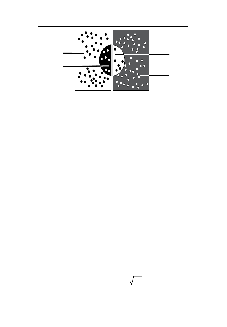
Chapter 2
[ 657 ]
• False negatives (FN): These are observations incorrectly labeled as belonging
to the negative class (black dots on a light background)
False negatives (FN)
True positives(TP)
True negatives (TN)
Flase positives (FP)
Categorization of validation results
This simplistic representation can be extended to classication problems that involve
more than two classes. For instance, false positives are dened as observations
incorrectly labeled that belong to any class other than the correct one. These four
factors are used for evaluating accuracy, precision, recall, and F and G measures:
• Accuracy: Represented as ac, this is the percentage of observations
correctly classied.
• Precision: Represented as p, this is the percentage of observations correctly
classied as positive in the group that the classier has declared positive.
• Recall: Represented as r, this is the percentage of observations labeled as
positive that are correctly classied.
• F-Measure or F-score F1: This is the score of a test's accuracy that strikes a
balance between precision and recall. It is computed as the harmonic mean
of the precision and recall with values ranging between 0 (worst score) and
1 (best score).
• G-measure: Represented as G, this is similar to the F-measure but is
computed as the geometric mean of precision p and recall r.
TP+TNTPTP
ac pr
TP+TN+FP+FNTP+FP TP+FN
===
2
1
pr
F G pr
pr
==
+

Hello World!
[ 658 ]
Implementation
Let's implement the validation formula using the same trait-based modular design
used in creating the preprocessor and classier modules. The Validation trait
denes the signature for the validation of a classication model: the computation
of the F1 statistics and the precision-recall pair:
trait Validation {
def f1: Double
def precisionRecall: (Double, Double)
}
Let's provide a default implementation of the Validation trait of the F1Validation
class. In the tradition of Scala programming, the class is immutable; it computes
the counters for TP, TN, FP, and FN when the class is instantiated. The class takes
two parameters:
• The array of actual versus expected class: actualExpected
• The target class for true positive observations: tpClass
class F1Validation(actualExpected: Array[(Int, Int)], tpClass:
Int) extends Validation {
val counts = actualExpected.foldLeft(new Counter[Label])((cnt,
oSeries) => cnt + classify(oSeries._1, oSeries._2))
lazy val accuracy = {
val num = counts(TP) + counts(TN)
num.toDouble/counts.foldLeft(0)( (s,kv) => s + kv._2)
}
lazy val precision = counts(TP).toDouble/(counts(TP) +
counts(FP))
lazy val recall = counts(TP).toDouble/(counts(TP) +
counters(FN))
override def f1: Double = 2.0*precision*recall/(precision +
recall)
override def precisionRecall: (Double, Double) = (precision,
recall)
def classify(actual: Int, expected: Int): Label = {
if(actual == expected) { if(actual == tpClass) TP else TN }
else { if (actual == tpClass) FP else FN }
}
}
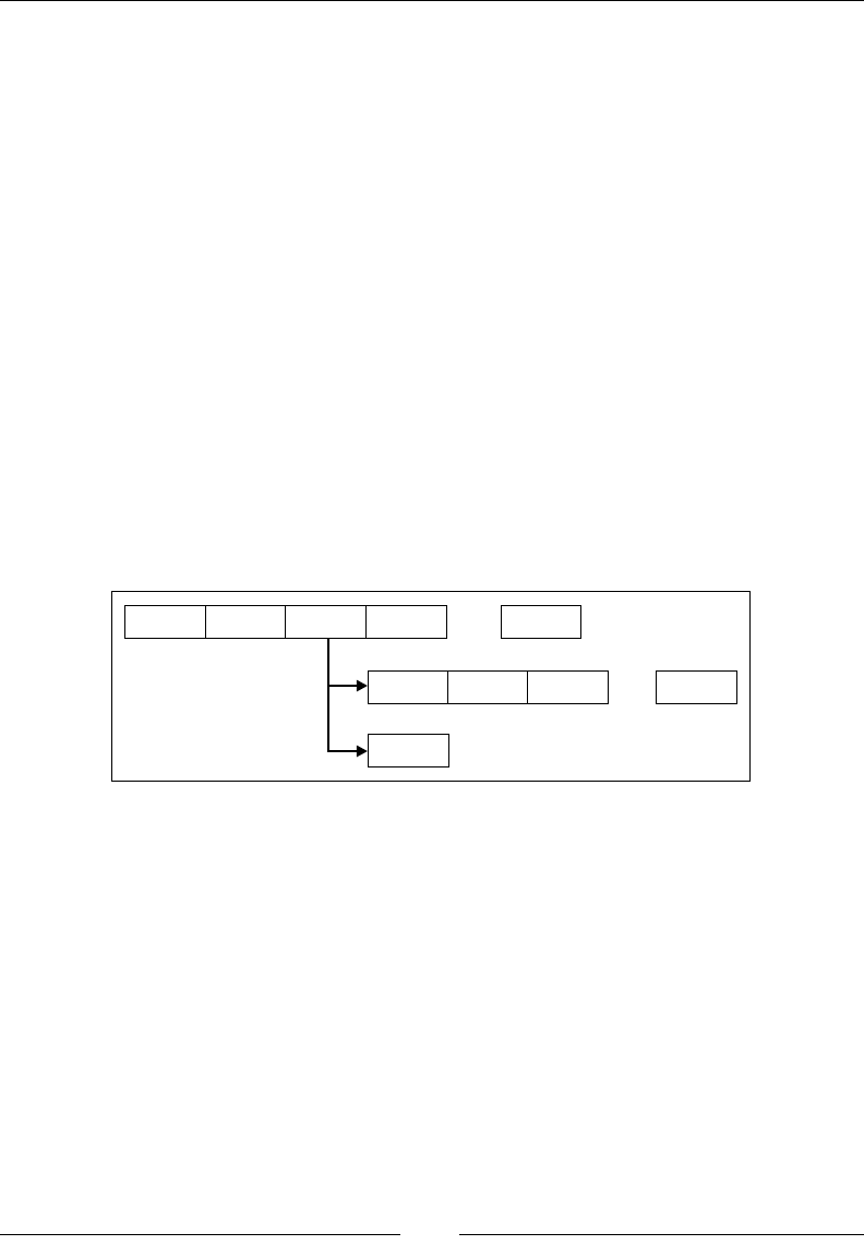
Chapter 2
[ 659 ]
The precision and recall variables are dened as lazy so they are computed only
once, when they are either accessed for the rst time or the f1 and precisionRecall
functions are invoked. The class is independent of the selected machine learning
algorithm, the training, the labeling process, and the type of observations.
Contrary to Java, which denes an enumerator as a class of types, Scala requires
enumerators to be singletons that inherit the functionality of the Enumeration class:
object Label extends Enumeration {
type Label = Value
val TP, TN, FP, FN = Value
}
K-fold cross-validation
It is quite common that the labeled dataset used for both training and validation is
not large enough. The solution is to break the original labeled dataset into K data
groups. The data scientist creates K training-validation datasets by selecting one
of the groups as a validation set then combining all other remaining groups into a
training set as illustrated in the next diagram. The process is known as the K-fold
cross validation [2:7].
S1 S2 S3 SK
S1 S2 S4 SK
S3
...
S4
...
Training
Validation
The third segment is used as validation data and all other dataset segments except S3
are combined into a single training set. This process is applied to each segment of the
original labeled dataset.

Hello World!
[ 660 ]
Bias-variance decomposition
There is an obvious challenge in creating a model that ts both the training set and
subsequent observations to be classied during the validation phase.
If the model tightly ts the observations selected for training, there is a high
probability that new observations may not be correctly classied. This is usually
the case when the model is complex. This model is characterized as having a
low bias with a high variance. Such a scenario can be attributed to the fact that
the scientist is overly condent that the observations he or she selected for training
are representative to the real world.
The probability of a new observation being classied as belonging to a positive class
increases as the selected model ts loosely the training set. In this case, the model is
characterized as having a high bias with a low variance.
The mathematical denition for the bias, variance, and mean squared error (MSE) of
the distribution are dened by the following formulas:
Variance and bias for a true model, θ:
$$
%
()
$
()
$$
( )
2
:varE E bias estimate
θθθ θθθθθ
⎡⎤
⎡⎤
=−=−
⎣⎦
⎢⎥
⎣⎦
Mean square error:
$
()
$
()
2
MSE var bias
θθ
=+
Let's illustrate the concept of bias, variance, and mean square error with an example.
At this stage, most of the machines learning techniques have not been introduced
yet. Therefore, the example will emulate a multiple models fEst: Double => Double
generated from non-overlapping training sets.
These models are evaluated against a test/validation datasets that are emulated by a
model, emul. The BiasVarianceEmulator emulator class takes the emulator function
and the size of the nValues validation test as parameters. It merely implements the
formula to compute the bias and variance for each of the fEst models:
class BiasVarianceEmulator[T <% Double](emul: Double => Double,
nValues: Int) {
def fit(fEst: List[Double => Double]): Option[XYTSeries] = {
val rf = Range(0, fEst.size)
val meanFEst = Array.tabulate(nValues)( x =>

Chapter 2
[ 661 ]
rf.foldLeft(0.0)((s, n) => s+fEst(n)(x))/fEst.size) // 1
val r = Range(0, nValues)
Some(fEst.map(fe => {
r.foldLeft(0.0, 0.0)((s, x) => {
val diff = (fe(x) - meanFEst(x))/ fEst.size // 2
(s._1 + diff*diff, s._2 + Math.abs(fe(x)-emul(x)))} )
}).toArray)
}
}
The fit method computes the variance and bias for each of the fEst models
generated from training. First, the mean of all the models are computed (line 1),
and then used in the computation of the variance and bias. The method returns
a tuple (variance, bias) for each of the fEst model.
Let's apply the emulator to three nonlinear regression models evaluated against
validation data:
2
sin20
, 0.0003. 0.18 1
5 5
x
x
y y x x and y x
⎛ ⎞
⎛⎞
⎜⎟
⎜ ⎟
⎝⎠
⎜ ⎟
== + =+
⎜ ⎟
⎜ ⎟
⎝ ⎠
The client code for the emulator consists of dening the emul emulator function,
and a list, fEst, of three models dened as tuples of (function, descriptor) of
type (Double=>Double, String). The fit method is call on the model functions
extracted through a map, as shown in the following code:
val emul = (x: Double) => 0.2*x*(1.0 + Math.sin(x*0.05))
val fEst = List[(Double=>Double, String)] (
((x: Double) => 0.2*x, "y=x/5"),
((x: Double) => 0.0003*x*x + 0.18*x, "y=3e-4.x^2-0.18x"),
((x: Double) =>0.2*x*(1+Math.sin(x*0.05),
"y=x(1+sin(x/20))/5"))
val emulator = new BiasVarianceEmulator[Double](emul, 200)
emulator.fit(fEst.map( _._1)) match {
case Some(varBias) => show(varBias)
case None => …
}
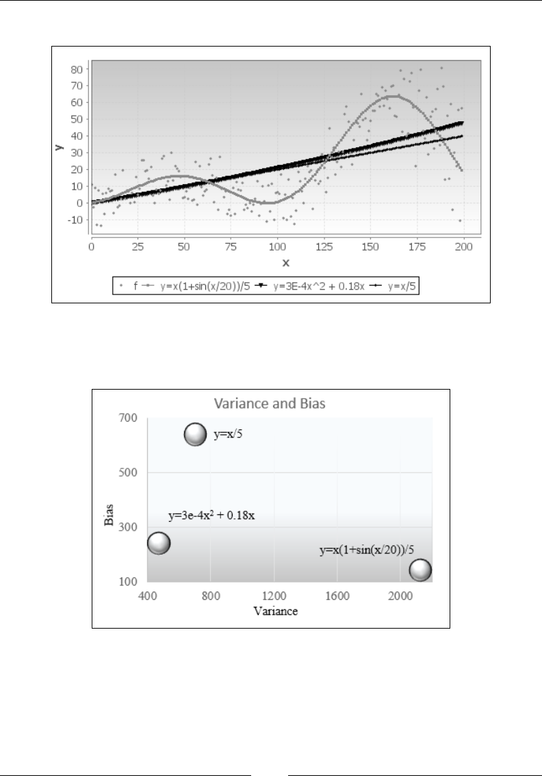
Hello World!
[ 662 ]
The JFreeChart library is used to display the test dataset and the three model functions.
Fitting models to dataset
The variance-bias trade-off is illustrated in the following scatter chart using the
absolute value of the bias:
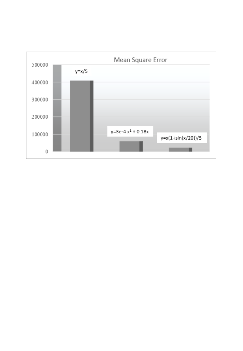
Chapter 2
[ 663 ]
The more complex the function, the lower the bias is. It is usually, but not always
related to, a high variance. The most complex function y=x (1+sin(x/20))/5 has by far
the highest variance and the lowest bias. The more complex model matches fairly
well with the training dataset. As expected, the mean square error reects the ability
of each of the three models to t the test data.
Mean square error bar chart
The low bias of the complex model reects in its ability to predict new observations
correctly. Its MSE is therefore low, as expected.
Complex models with low bias and high variance are known as overtting. Models
with high bias and low variance are characterized as undertting.
Overtting
The methodology presented in the example can be applied to any classication and
regression model. The list of models with low variance includes constant function
and models independent of the training set. High degree polynomial, complex
functions, and deep neural networks have high variance. Linear regression applied
to linear data has a low bias, while linear regression applied to nonlinear data has a
higher bias [2:8]

Hello World!
[ 664 ]
Overtting affects all aspects of the modeling process negatively, for example:
• It is a sure sign of an overly complex model, which is difcult to debug and
consumes computation resources
• It makes the model representing minor uctuations and noise
• It may discover irrelevant relationships between observed and latent features
• It has poor predictive performance
However, there are well-proven solutions to reduce overtting [2:9]:
• Increasing the size of the training set whenever possible
• Reducing noise in labeled and input data through ltering
• Decreasing the number of features using techniques such as principal
components analysis
• Modeling observable and latent noised using ltering techniques such as
Kalman or autoregressive models
• Reducing inductive bias in a training set by applying cross-validation
• Penalizing extreme values for some of the model's features using
regularization techniques
Summary
In this chapter, we established the framework for the different data processing units
that will be introduced in this book. There is a very good reason why the topics of
model validation and overtting are explored early on in this book. There is no point
in building models and selecting algorithms if we do not have a methodology to
evaluate their relative merits.
In this chapter, you were introduced to:
• The versatility and cleanness of the Cake pattern in Scala as an effective
scaffolding tool for data processing
• The concept of pipe operator for data conversion
• A robust methodology to validate machine learning models
• The challenge in tting models to both training and real-world data
The next chapter will address the problem of overtting by penalizing outliers,
modeling, and eliminating noise in data.

Data Preprocessing
Real-world data is usually noisy and inconsistent with missing observations.
No classication, regression, or clustering model can extract relevant information
from unprocessed data.
Data preprocessing consists of cleaning, ltering, transforming, and normalizing
raw observations using statistics in order to correlate features or groups of features,
identify trends and model, and lter out noise. The purpose of cleansing raw data
is twofold:
• Extract some basic knowledge from raw datasets
• Evaluate the quality of data and generate clean datasets for unsupervised or
supervised learning
You should not underestimate the power of traditional statistical analysis methods to
infer and classify information from textual or unstructured data.
In this chapter, you will learn how to:
• Apply commonly used moving average techniques to detect long-term
trends in a time series
• Identify market and sector cycles using discrete Fourier series
• Leverage the Kalman lter to extract the state of a dynamic system from
incomplete and noisy observations
Time series
The overwhelming majority of examples used to illustrate the different machine
algorithms in this book process time series or sequential, ordered, or unordered data.
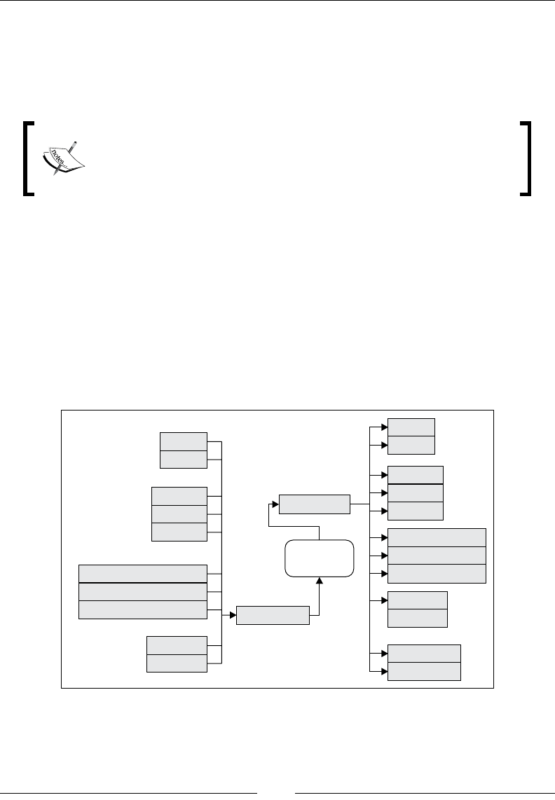
Data Preprocessing
[ 666 ]
Each library has its own container type to manipulate datasets. The challenge is
to dene all possible conversions between types from different libraries needed to
implement a large variety of machine learning models. Such a strategy may result in a
combinatorial explosion of implicit conversion. A solution consists of creating a generic
class to manage conversion from and to any type used by a third-party library.
Scala.collection.JavaConversions _
Scala provides a standard package to convert collection types from
Scala to Java and vice versa.
The generic data transformation, DT, can be used to transform any XTSeries time series:
class DT[T,U] extends PipeOperator[XTSeries[T], XTSeries[U]] {
override def |> : PartialFunction[XTSeries[T], XTSeries[U]]
}
Let's consider the simple case of using a Java library, the Apache Commons Math
framework, and JFreeChart for visualization, and dene a parameterized time series
class, XTSeries[T]. The \> data transformation converts a time series of values
of type T, XTSeries[T], into a time series of values of type U, XTSeries[U]. The
following diagram provides an overview of type conversion in data transformation:
Array2DRowRealMatrix
int[]
double[]
int[]
double[]
java
scala
org.apache.commons.math3
List[T]
Vector[T]
Array[T]
RealMatrix
RealVector
DblVector
DblMatrix
org.scalaml.core.Types
Values
KeyedValues
org.jfree.data
DblVector
DblMatrix
RealMatrix
RealVector
ArrayrealVector
List[U]
Vector[U]
Array[U]
XTSeries[U]
XTSeries[T]
Transform
|>

Chapter 3
[ 667 ]
Let's create the XTSeries class. As a container, the class should be an implementation
of the Scala higher-order collections functions such as map, foreach, or zip. The class
should support at least conversion to DblVector and DblMatrix types introduced in
the rst chapter.
Here is a partial implementation of the XTSeries class. Comments, exceptions,
argument validations, and debugging code are omitted in the code:
class XTSeries[T](label: String, arr: Array[T]) { // 1
def apply(n: Int): T = arr.apply(n)
@implicitNotFound("Undefined conversion to DblVector") // 2
def toDblVector(implicit f: T=>Double):DblVector =arr.map(f(_))
@implicitNotFound("Undefined conversion to DblMatrix") // 2
def toDblMatrix(implicit fv: T => DblVector): DblMatrix = arr.map(
fv( _ ) )
def + (n: Int, t: T)(implicit f: (T,T) => T): T = f(arr(n), t)
def head: T = arr.head //3
def drop(n: Int):XTSeries[T] = XTSeries(label,arr.drop(n))
def map[U: ClassTag](f: T => U): XTSeries[U] = XTSeries[U](label,
arr.map( x =>f(x)))
def foreach( f: T => Unit) = arr.foreach(f) //3
def sortWith(lt: (T,T)=>Boolean):XTSeries[T] = XTSeries[T](label,
arr.sortWith(lt))
def max(implicit cmp: Ordering[T]): T = arr.max //4
def min(implicit cmp: Ordering[T]): T = arr.min
…
}
The class takes an optional label and an invariant array of the parameterized type
T. The annotation @specialized (line 1) instructs the compiler to generate two
versions of the class:
• A generic XTSeries[T] class that exploits all the implicit conversions
required to perform operations on time series of a generic type
• An optimized XTSeries[Double] class that bypasses the conversion and
offers the client code with a faster implementation

Data Preprocessing
[ 668 ]
The conversion to DblVector (resp. DblMatrix) relies on the implicit conversion
of elements to type Double (resp. DblVector) (line 2). The @implicitNotFound
annotation instructs the compiler to omit an error if no implicit conversion is
detected. The conversion methods are used to implement the implicit conversion
introduced in the previous section. These methods are dened in the singleton
org.scalaml.core.Types.CommonsMath library. The following code shows the
implementation of the conversion methods:
object Types {
object CommonMath {
implicit def series2DblVector[T](xt: XTSeries[T])(implicit f:
T=>Double):DblVector = xt.toDblVector(f)
implicit def series2DblMatrix[T](xt: XTSeries[T])(implicit f:
T=>DblVector): DblMatrix = xt.toDblMatrix(f)
…
}
This code snippet exposes a subset of the Scala higher-order collections methods
(line 3) applied to the time series. The computation of the minimum and maximum
values in the time series required that the cmp ordering/compare method be dened
for the elements of the type T (line 4).
Let's put our versatile XTSeries class to use in creating a basic preprocessing data
transformation starting with the ubiquitous moving average techniques.
Moving averages
Moving averages provide data analysts and scientists with a basic predictive model.
Despite its simplicity, the moving average method is widely used in the technical
analysis of nancial markets to dene a dynamic level of support and resistance for
the price of a given security.
Let's consider a time series xt= x(t) and a function f(xt-p, xt-1) that reduces
the last p observations into a value or average. The prediction or
estimation of the observation at t+1 is dened by the following formula:
()
1
,...,
ttp t
xfx x
+−
=
%
Here, f is an average reducing function from the previous p data points.

Chapter 3
[ 669 ]
The simple moving average
Simple moving average, a smoothing method, is the simplest form of the moving
averages algorithms [3:1]. The simple moving average of period p estimates the value
at time t by computing the average value of the previous p observations using the
following formula:
The simple moving average of a time series {xt} with a period p is
computed as the average of the last p observations:
1t
t j
jt p
xx
p=−
=∑
%
The computation is implemented iteratively using the following
formula (1):
1;0
ttp
tt
xx
xx tp tp
p
−
−
−
=+ ∀≥ ∀≤
%%
Here,
t
x
%
is the estimate or simple moving average value at time t.
Let's build a class hierarchy of moving average algorithms, with the abstract
parameterized class MovingAverage[T <% Double] as its root. We use the generic
time series class, XTSeries[T], introduced in the rst section and the generic pipe
operator, |>, introduced in the previous chapter:
abstract class MovingAverage[T <% Double] extends
PipeOperator[XTSeries[T], XTSeries[Double]]
The pipe operator for the SimpleMovingAverage class implements the iterative
formula (1) for the computation of the simple moving average. The override
keyword is omitted:
class SimpleMovingAverage[@specialized(Double) T <% Double](val
period: Int)(implicit num: Numeric[T]) extends MovingAverage[T] {
def |> : PartialFunction[XTSeries[T], XTSeries[Double]] {
case xt: XTSeries[T] if(xt != null && xt.size > 0) => {
val slider = xt.take(data.size-period)
.zip(data.drop(period)) //1
val a0 = xt.take(period).toArray.sum/period //2
var a: Double = a0
val z = Array[Array[Double]](
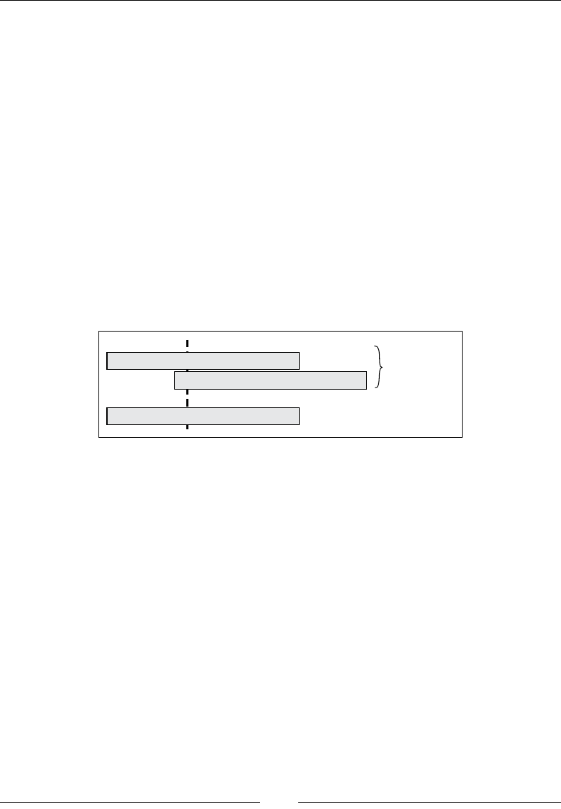
Data Preprocessing
[ 670 ]
Array.fill(period)(0.0), a, slider.map(x => {
a += (x._2 - x._1)/period
a})
).flatten //3
XTSeries[Double](z)
}
The class is parameterized for the type of elements of the input time series. After all,
we do not have control over the source of the input data. The type for the elements of
the output time series is Double.
The class has a type T and is specialized for the Double type for faster processing.
The implicitly dened num: Numeric[T] is required by the arithmetic operators
sum and / (line 2).
The implementation has a few interesting elements. First, the set of observations
is duplicated and the index in the clone is shifted by p observations before being
zipped with the original to the array of a pair of values: slider (line 1):
Moving averages
XXX..... XX................X
012p-1 pn-1
XXX..... X ................X
012p-1 n-1
0 0 ... . .0 ap... .. a ... .. a
in
Sliding pairs
The sliding algorithm to compute moving averages
The average value is initialized with the average of the rst p data points. The rst
p values of the trends are initialized as an array of p zero values. It is concatenated
with the rst average value and the array containing the remaining average values.
Finally, the array of three arrays is attened (flatten) into a single array containing
the average values (line 3).
The weighted moving average
The weighted moving average method is an extension of the simple moving average
by computing the weighted average of the last p observations [3:2]. The weights αj
are assigned to each of the last p data points xj, and are normalized by the sum of
the weights.

Chapter 3
[ 671 ]
The weighted moving average of a series {xt} with a period p and a
normalized weights distribution {αj} is given by the following formula (2):
1
;
0
11
p
t
tjp j j
jt p j
x x
p
αα
−
−
=−=
= =
∑∑
%
Here,
t
x
%
is the estimate or simple moving average value at time t.
The implementation of the WeightedMovingAverage class requires the computation
of the last p data points. There is no simple iterative formula to compute the
weighted moving average at time t+1 using the moving average at time t:
class WeightedMovingAverage[@specialized(Double) T <% Double](val
weights: DblVector) extends MovingAverage[T] {
def |> : PartialFunction[XTSeries[T], XTSeries[Double]] = {
case xt: XTSeries[T] if(xt != null && xt.size > 1) => {
val smoothed = Range(weights.size, xt.size).map(i => {
xt.toArray.slice(i- weights.size , i)
.zip(weights)
.foldLeft(0.0)((s, x) => s + x._1*x._2) }) //1
XTSeries[Double](Array.fill(weights.size)(0.0) ++ smoothed) //2
}
}
As with the simple moving average, the array of the initial p moving average
with the value 0 is concatenated (line 2) with the rst moving average value
and the remaining weighted moving average computed using a map (line 1). The
period for the weighted moving average is implicitly dened as weights.size.
The exponential moving average
The exponential moving average is widely used in nancial analysis and marketing
surveys because it favors the latest values. The older the value, the less impact it has
on the moving average value at time t [3:3].
The exponential moving average on a series {xt} and a smoothing
factor
α
is computed by the following iterative formula:
()
1 0
10; 0
ttt
xxxtxift
αα
−
=−+∀>=
%%
Here,
x
%
is the value of the exponential average at t.

Data Preprocessing
[ 672 ]
The implementation of the ExpMovingAverage class is rather simple. There are two
constructors, one for a user-dened smoothing factor and one for the Nyquist period,
p, used to compute the smoothing factor alpha = 2/(p+1):
class ExpMovingAverage[@specialized(Double) T <% Double](val alpha:
Double) extends MovingAverage[T] {
def |> : PartialFunction[XTSeries[T], XTSeries[Double]] = {
case xt: XTSeries[T] if(xt != null && xt.size > 1) => {
val alpha_1 = 1-alpha
var y: Double = data(0)
xt.map( x => {
val z = x*alpha + y*alpha_1; y=z; z })
}
}
}
The version of the constructor that uses the Nyquist period p is implemented using
the Scala apply method:
def apply[T <% Double](nyquist: Int): ExpMovingAverage[T] = new
ExpMovingAverage[T](2/( nyquist + 1))
Let's compare the results generated from these three moving averages methods
with the original price. We use a data source (with respect to sink), DataSource
(with respect to DataSink) to load the historical daily closing stock price of Bank
of America (BAC). The DataSource and DataSink classes are dened in the Data
extraction section in Appendix A, Basic Concepts. The comparison of results can be
done using the following code:
val p_2 = p >>1
val w = Array.tabulate(p)(n =>if(n==p_2) 1.0 else 1.0/(Math.
abs(n-p_2)+1)) //1
val weights = w map { _ / w.sum } //2
val src = DataSource("resources/data/chap3/BAC.csv, false)//3
val price = src |> YahooFinancials.adjClose //4
val sMvAve = SimpleMovingAverage(p)
val wMvAve = WeightedMovingAverage(weights)
val eMvAve = ExpMovingAverage(p)
val results = price :: sMvAve.|>(price) :: wMvAve.|>(price) ::
eMvAve.|>(price) :: List[XTSeries[Double]]() //5
Val outFile = "output/chap3/mvaverage" + p.toString + ".csv"
DataSink[Double]( outFile) |> results //6
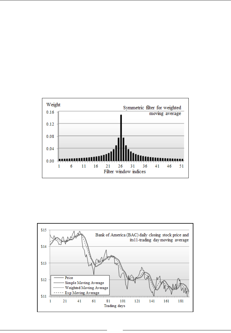
Chapter 3
[ 673 ]
The coefcients for the weighted moving average are generated (line 1) and
normalized (line 2). The trading data regarding the ticker symbol, BAC, is extracted
from the Yahoo! nances CSV le (line 3), YahooFinancials, using the adjClose
extractor (line 4). The smoothed data generated by each of the moving average
techniques are concatenated into a list of time series (line 5). Finally, the content is
formatted and dumped into a le, outFile, using a DataSink instance (line 6).
The weighted moving average method relies on a symmetric distribution of
normalized weights computed by a function passed as an argument of the generic
tabulate method. Note that the original price time series is generated if a specic
moving average cannot be computed. The following graph is an example of a
symmetric lter for weighted moving averages:
The three moving average techniques are applied to the price of the stock of Bank
of America (BAC) over 200 trading days. Both the simple and weighted moving
average uses a period of 11 trading days. The exponential moving average method
uses a scaling factor of 2/(11+1) = 0.1667.
11-day moving averages of the historical stock price of Bank of America
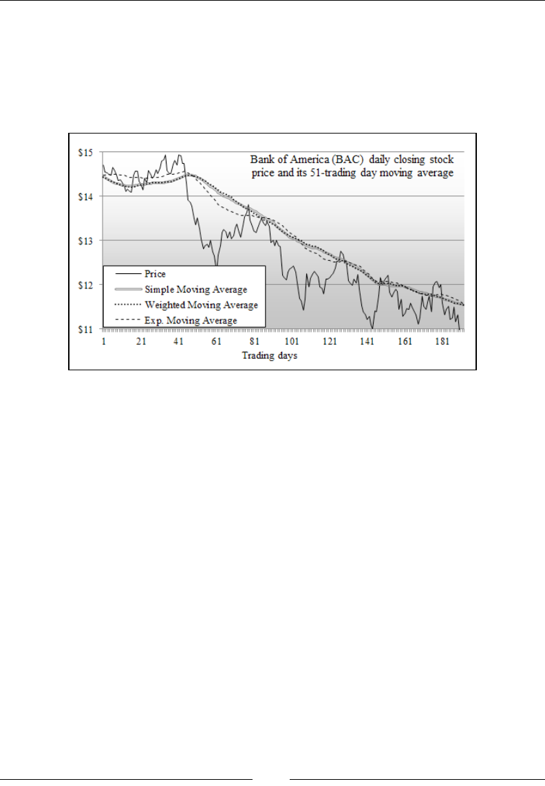
Data Preprocessing
[ 674 ]
The three techniques lter the noise out of the original historical price time series.
The exponential moving average reacts to a sudden price uctuation despite the fact
that the smoothing factor is low. If you increase the period to 51 trading days or two
calendar months, the simple and weighted moving averages generate a smoothed
time series compared to the exponential moving average with a smoothing factor
of 2/(p+1)= 0.038.
51-day moving averages of the historical stock price of Bank of America
You are invited to experiment further with different smooth factors and weight
distributions. You will be able to conrm the following basic rule: as the period of
the moving average increases, noise with decreasing frequencies is eliminated. In
other words, the window of allowed frequencies is shrinking. The moving average
acts as a low-band lter that allows only lower frequencies. Fine-tuning the period or
smoothing factor is time consuming. Spectral analysis, or more specically, Fourier
analysis, transforms the time series into a sequence of frequencies, which is a time
series in the frequency domain.

Chapter 3
[ 675 ]
Fourier analysis
The purpose of spectral density estimation is to measure the amplitude of a signal
or a time series according to its frequency [3:4]. The spectral density is estimated by
detecting periodicities in the dataset. A scientist can better understand a signal or
time series by analyzing its harmonics.
The spectral theory
Spectral analysis for time series should not be confused with
spectral theory, a subset of linear algebra that studies Eigenfunctions
on Hilbert and Banach spaces. Harmonic and Fourier analyses are
regarded as a subset of spectral theory.
The fast Fourier transform (FFT) is the most commonly used frequency analysis
algorithm [3:5]. Let's explore the concept behind the discrete Fourier series and
the Fourier transform as well as their benets as applied to nancial markets. The
Fourier analysis approximates any generic function as the sum of trigonometric
functions, sine and cosine. The decomposition in a basic trigonometric function is
known as a Fourier transform [3:6].
Discrete Fourier transform (DFT)
A time series {xk} can be represented as a discrete real-time domain function f, x=f(t).
In the 18th century, Jean Baptiste Joseph Fourier demonstrated that any continuous
periodic function f could be represented as a linear combination of sine and cosine
functions. The discrete Fourier transform (DFT) is a linear transformation that
converts a time series into a list of coefcients of a nite combination of complex or
real trigonometric functions, ordered by their frequencies.
The frequency ω of each trigonometric function denes one of the harmonics of the
signal. The space that represents signal amplitude versus frequency of the signal is
known as the frequency domain. The generic DFT transforms a time series into a
sequence of frequencies dened as complex numbers ω = a + j.φ (j2= -1), for which a
is the amplitude of the frequency and φ is the phase.

Data Preprocessing
[ 676 ]
This section is dedicated to the real DFT that converts a time series into an ordered
sequence of frequencies with real values.
Real discrete Fourier transform
A periodic function f can be represented as an innite combination of sine
and cosine functions:
() () ()
1 1
cos sin
2
o
k k
a
f t a nx b nx
∞ ∞
=+ =
∑∑
The Fourier cosine transform of a function f is dened as:
() ( )()
, cos 2
π
∞
−∞
=∫
c
Ffk kx f x dx
The discrete real cosine series of a function f(-x) = f(x) is dened as:
() ( ) () () ( )
23
0
1
0
2
cos cos .
2
N
k k
k
a
fx f x a kxwhere a f t kt dt
π
π
−
=
=−=+ =
∑∫
The Fourier sine transform of a function is dened as:
() ( )()
,sin 2
π
∞
−∞
=∫
s
Ffk kx f x dx
The discrete real sine series of a function f(-x) = f(x) is dened as:
() ( ) ( ) () ( )
23
10
2
sin sin .
N
k k
k
fx f x b kxwhereb f t kt dt
π
π
−
=
=−= =
∑∫
The computation of the Fourier trigonometric series is time consuming with an
asymptotic time complexity of O(n2). Several attempts have been made to make the
computation as effective as possible. The most common numerical algorithm used to
compute the Fourier series is the fast Fourier transform created by J. W. Cooley and
J. Tukey [3:7]. The algorithm, called Radix-2, recursively breaks down the Fourier
transform for a time series of N data points into any combination of N1 and N2 sized
segments such as N = N1 N2. Ultimately, the discrete Fourier transform is applied to
the deepest-nested segments.
The Cooley-Tukey algorithm
I encourage you to implement the Radix-2 Cooley-Tukey algorithm in
Scala using a tail recursion.

Chapter 3
[ 677 ]
The Radix-2 implementation requires that the number of data points is N=2n for
even functions (sine) and N = 2n+1 for cosine. There are two approaches to meet
this constraint:
• Reduce the actual number of points to the next lower radix, 2n < N
• Extend the original time series by padding it with 0 to the next higher radix,
N < 2n+1
Padding the original time series is the preferred option because it does not affect the
original set of observations.
Let's dene a base class, DTransform[T], for all the fast Fourier transforms,
parameterized with a view bounded to the Double type (Double, Float,
and so on). The rst step is to implement the padding method, common
to all the Fourier transforms:
trait DTransform[T] extends PipeOperator[XTSeries[T],
XTSeries[Double]] {
def padSize(xtSz: Int, even: Boolean=true): Int = {
val sz = if( even ) xtSz else xtSz-1
if( (sz & (sz-1)) == 0) 0
else {
var bitPos = 0
do {
bitPos += 1
} while( (sz >> bitPos) > 0)
(if(even) (1<<bitPos) else (1<<bitPos)+1) - xtSz
}
}
def pad(xt: XTSeries[T], even: Boolean=true)
(implicit f: T => Double): DblVector = {
val newSize = padSize(xt.size, even)
val arr: DblVector = xt
if( newSize > 0) arr ++ Array.fill(newSize)(0.0) else arr
}
}
The while loop
Scala developers prefer Scala higher-order methods on collection
to implement iterative computation. However, nothing prevents
you from using a traditional while loop if either readability or
performance is an issue.

Data Preprocessing
[ 678 ]
The fast implementation of the padding method, pad, consists of detecting the
number of observations, N, which is a power of 2 using the bit operator & by
evaluating whether N & (N-1) is null. The next highest radix is extracted by
computing the number of bits shift in N. The code illustrates the effective use of
implicit conversion to make the code readable. The arr: DblVector = series
conversion triggers a conversion dened in the XTSeries companion object.
The next step is to write the DFT class for the real discrete transforms, sine and cosine,
by subclassing DTransform. The purpose of the class is to select the appropriate
Fourier series, pad the time series to the next power of 2 if necessary, and invoke
the FastSineTransformer and FastCosineTransformer classes of the Apache
Commons Math library [3:8] introduced in the rst chapter:
class DFT[@specialized(Double) T<%Double] extends DTransform[T] {
def |> : PartialFunction[XTSeries[T], XTSeries[Double]] = {
case xt: XTSeries[T] if(xt != null && xt.length > 0) =>
XTSeries[Double](fwrd(xt)._2)
}
def fwrd(xt:XTSeries[T]): (RealTransformer, DblVector)= {
val rdt = if(Math.abs(xt.head) < DFT_EPS)
new FastSineTransformer(DstNormalization.STANDARD_DST_I)
else new FastCosineTransformer(DctNormalization.STANDARD_DCT_I)
(rdt, rdt.transform( pad(xt,xt.head==0.0),TransformType.FORWARD))
}
}
The discrete Fourier sine series requires that the rst value of the time series is 0.0.
This implementation automates the selection of the appropriate series by evaluating
series.head. This example uses the standard formulation of the cosine and sine
transformation, dened by the DctNormalization.STANDARD_DCT_I argument.
The orthogonal normalization, which normalizes the frequency by a factor of
1/sqrt(2(N-1), where N is the size of the time series, generates a cleaner frequency
spectrum for a higher computation cost.
@specialized
The @specialized(Double) annotation is used to instruct the
Scala compiler to generate a specialized and more efcient version of
the class for the type Double. The drawback of specialization is the
duplication of byte code as the specialized version coexists with the
parameterized classes [3:9].
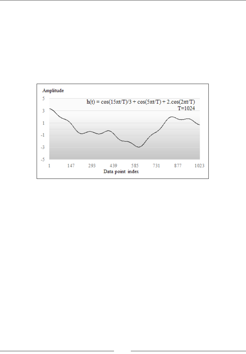
Chapter 3
[ 679 ]
In order to illustrate the different concepts behind DFTs, let's consider the case of a
time series generated by a sequence h of sinusoidal functions:
val _T= 1.0/1024
val h = (x:Double) =>2.0*Math.cos(2.0*Math.PI*_T*x) +
Math.cos(5.0*Math.PI*_T*x) + Math.cos(15.0*Math.PI*_T*x)/3
As the signal is synthetically created, we can select the size of the time series to avoid
padding. The rst value in the time series is not null, so the number of observations
is 2n+1. The data generated by the function h is plotted as follows:
Example of the sinusoidal time series
Let's extract the frequencies spectrum for the time series generated by the function h.
The data points are created by tabulating the function h. The frequencies spectrum
is computed with a simple invocation of the pipe operator on the instance of the
DFT class:
val rawOut = "output/chap3/raw.csv"
val smoothedOut = "output/chap3/smoothed.csv"
val values = Array.tabulate(1025)(x =>h(x/1025))
DataSink[Double](rawOut) |> values //1
val smoothed = DFT[Double] |> XTSeries[Double](values) //2
DataSink[Double]("output/chap3/smoothed.csv") |> smoothed
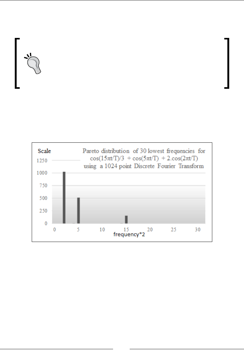
Data Preprocessing
[ 680 ]
The rst data sink (the type DataSink) stores the original time series into a CSV le
(line 1). The DFT instance extracts the frequencies spectrum and formats it as time
series (line 2). Finally, a second sink saves it into another CSV le.
Data sinks and spreadsheets
In this particular case, the results of the discrete Fourier
transform are dumped into a CSV le so that it can be loaded
into a spreadsheet. Some spreadsheets support a set of ltering
techniques that can be used to validate the result of the example.
A simpler alternative would be to use JFreeChart.
The spectrum of the time series, plotted for the rst 32 points, clearly shows three
frequencies at k=2, 5, and 15. This is expected because the original signal is composed
of three sinusoidal functions. The amplitude of these frequencies are 1024/1, 1024/2,
and 1024/6, respectively. The following plot represents the rst 32 harmonics for the
time series:
Frequency spectrum for a three-frequency sinusoidal
The next step is to use the frequencies spectrum to create a low-pass lter using DFT.
There are many algorithms to implement a low or pass band lter in the time domain
from autoregressive models to the Butterworth algorithm. However, the fast Fourier
transform is still a very popular technique to smooth signals and extract trends.

Chapter 3
[ 681 ]
Big Data
A DFT for a large time series can be very computation intensive.
One option is to treat the time series as a continuous signal and
sample it using the Nyquist frequency. The Nyquist frequency is
half of the sampling rate of a continuous signal.
DFT-based ltering
The purpose of this section is to introduce, describe, and implement a noise ltering
mechanism that leverages the discrete Fourier transform. The idea is quite simple:
the forward and inverse Fourier transforms are used sequentially to convert the
time series from the time domain to the frequency domain and back. The only input
you need to supply is a function G that modies the sequence of frequencies. This
operation is known as the convolution of the lter G and the frequencies spectrum.
A convolution is similar to an inner product of two time series in the frequencies
domain. Mathematically, the convolution is dened as follows:
Convolution
The convolution of two functions f and g is dened as:
() ( )
, .f g f t g x t dt
∞
−∞
<>= −
∫
DFT convolution
One important property of the Fourier transform is that convolution
of two signals is implemented as the inner product of their relative
spectrums:
()()()
Ff g FfFg∗=
Let's apply the property to the discrete Fourier transform. If a time
series {xi} has a frequency spectrum
{}
f
ω
and a lter f in a frequency
domain dened as
{}
g
ω
, then the convolution is dened as:
()
1
,,
0
N
xj fk j
Ff g
ωω
−
−
∗=∑
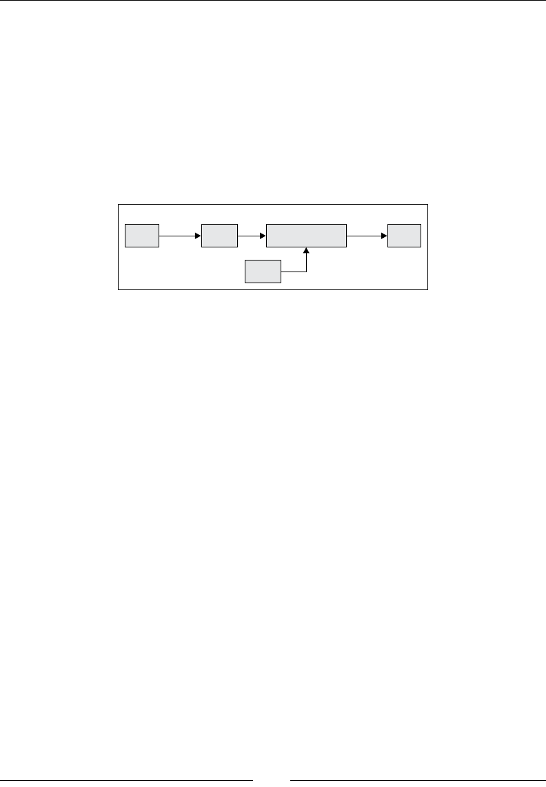
Data Preprocessing
[ 682 ]
Let's apply the convolution to our ltering problem. The ltering algorithm using the
discrete Fourier transform consists of ve steps:
1. Pad the time series to enable the discrete sine or cosine transform.
2. Generate the ordered sequence of frequencies using the forward transform.
3. Select the lter function g in the frequency domain and a cutoff frequency.
4. Convolute the sequence of frequency with the lter function g.
5. Generate the ltered signal in the time domain by applying the inverse DFT
transform to the convoluted frequencies.
Forward
Fourier
Transform
() () ()
F* F.G¥= ¥¥
()
G¥
()
ft ()
F¥ ()
f* t
Filter
Inverse
Fourier
Transform
Raw timeseries Filtered timeseries
wwww
w
Diagram of a discrete Fourier filter
The most commonly used low-pass lters are known as the sinc and sinc2
functions, dened as a rectangular function and a triangular function, respectively.
The simplest low-pass lter is implemented by a sinc function that returns 1 for
frequencies below a cutoff frequency, fC, and 0 if the frequency is higher:
def sinc(f: Double, fC: Double): Double = if(Math.abs(f) < fC) 1.0
else 0.0
def sinc2(f: Double, fC: Double): Double = if(f*f < fC) 1.0 else 0.0
The ltering computation is implemented as a data transformation (pipe operator
|>). The DFTFir class inherits from the DFT class in order to reuse the fwrd forward
transform function. As usual, exception and validation code is omitted. The
frequency domain function g is an attribute of the lter. The g function takes the
frequency cutoff value fC as the second argument. The two lters sinc and sinc2
dened in the previous section are examples of ltering functions.
class DFTFir[T <% Double](val g: (Double, Double) =>Double, val fC;
Double) extends DFT[T]
The pipe operator implements the ltering functionality:
def |> : PartialFunction[XTSeries[T], XTSeries[Double]] = {
case xt: XTSeries[T] if(xt != null && xt.size > 2) => {
val spectrum = fwrd(xt) //1
val cutOff = fC*spectrum._2.size
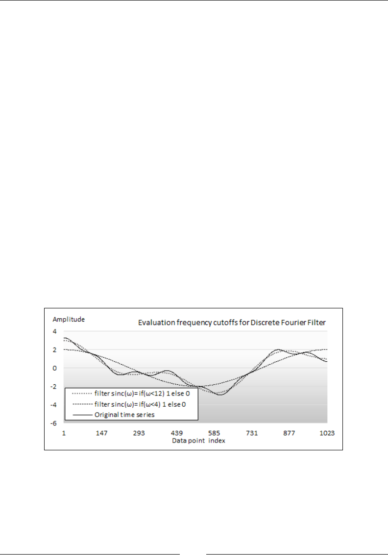
Chapter 3
[ 683 ]
val filtered = spectrum._2.zipWithIndex.map(x => x._1*g(x._2,
cutOff)) //2
XTSeries[Double](spectrum._1.transform(filtered, TransformType.
INVERSE)) //3
}
The ltering process follows three steps:
1. Computation of the discrete Fourier forward transformation
(sine or cosine), fwrd.
2. Apply the lter function through a Scala map method.
3. Apply the inverse transform on the frequencies.
Let's evaluate the impact of the cutoff values on the ltered data. The implementation
of the test program consists of invoking the DFT lter pipe operator and writing
results into a CSV le. The code reuses the generation function h introduced in the
previous paragraph:
val price = src |> YahooFinancials.adjClose
val filter = new DFTFir[Double](sinc, 4.0)
val filteredPrice = filter |> price
Filtering out the noise is accomplished by selecting the cutoff value between any of
the three harmonics with the respective frequencies of 2, 5, and 15. The original and
the two ltered time series are plotted on the following graph:
Plotting of the discrete Fourier filter-based smoothing
As you would expect, the low-pass lter with a cutoff value of 12 removes the noise
with the highest frequencies. The lter (with the cutoff value 4) cancels out the
second harmonic (low-frequency noise), leaving out only the main trend cycle.
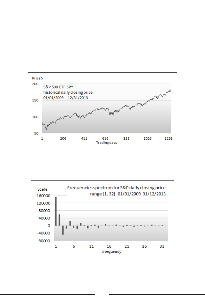
Data Preprocessing
[ 684 ]
Detection of market cycles
Using the discrete Fourier transform to generate the frequencies spectrum of a
periodical time series is easy. However, what about real-world signals such as
the time series representing the historical price of a stock?
The purpose of the next exercise is to detect, if any, the long term cycle(s) of the
overall stock market by applying the discrete Fourier transform to the quote of the
S&P 500 index between January 1, 2009, and December 31, 2013, as illustrated in the
following graph:
Historical S&P 500 index prices
The rst step is to apply the DFT to extract a spectrum for the S&P 500 historical
prices, as shown in the following graph, with the rst 32 harmonics:
Frequencies spectrum for historical S&P index
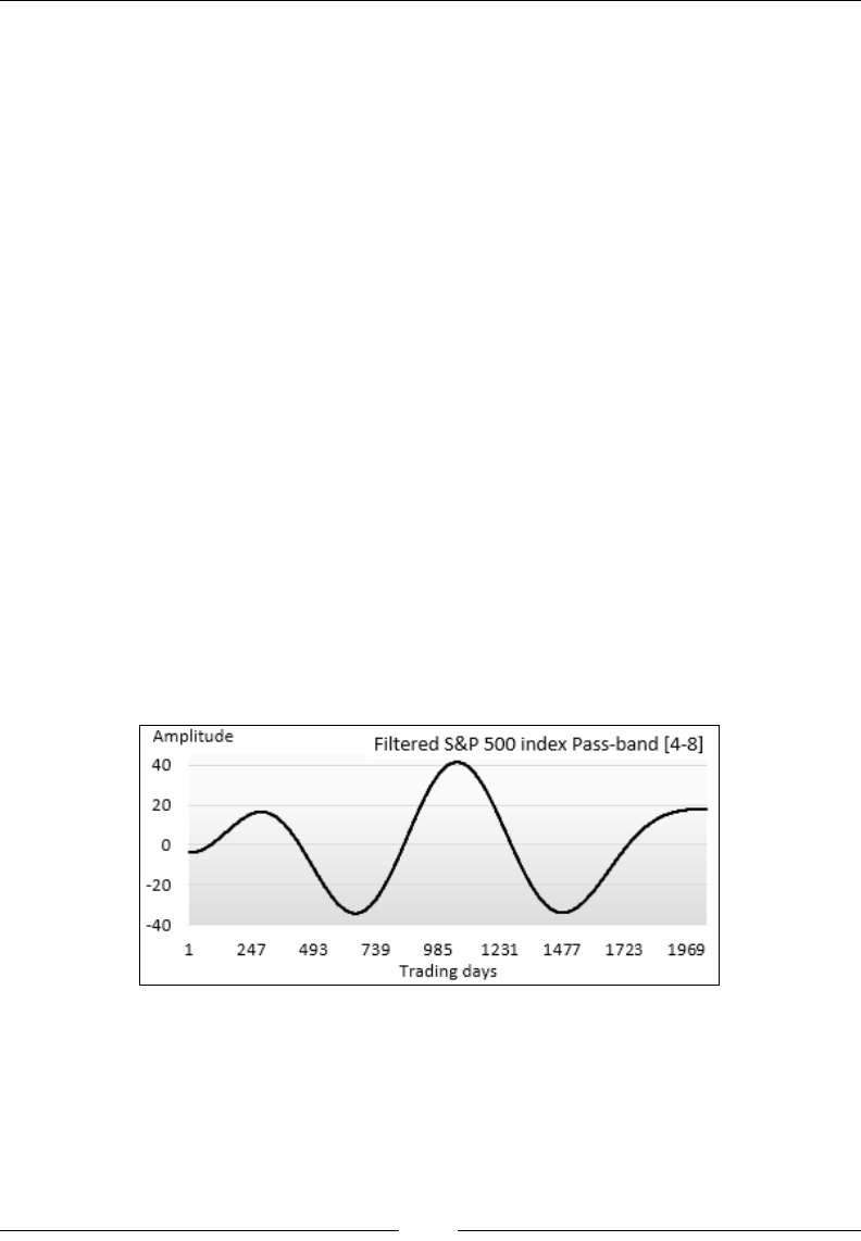
Chapter 3
[ 685 ]
The frequency domain chart highlights some interesting characteristics regarding the
S&P 500 historical prices:
• Both positive and negative amplitudes are present, as you would expect
in a time series with complex values. The cosine series contributes to the
positive amplitudes while the sine series affects both positive and negative
amplitudes, (cos(x+π) = sin(x)).
• The decay of the amplitude along the frequencies is steep enough to warrant
further analysis beyond the rst harmonic, which represents the main trend.
The next step is to apply a pass-band lter technique to the S&P 500 historical
data in order to identify short-term trends with lower periodicity.
A low-pass lter is limited to reduce or cancel out the noise in the raw data. In this
case, a passband lter using a range or window of frequencies is appropriate to
isolate the frequency or the group of frequencies that characterize a specic cycle.
The sinc function introduced in the previous section to implement a low-band lter
is modied to enforce the passband within a window, [w1, w2], as follows:
def sinc(f: Double, w: (Double, Double)): Double = if(Math.abs(f) >
w._1 && Math.abs(f) < w._2) 1.0 else 0.0
Let's dene a DFT-based pass-band lter with a window of width 4, w=(i, i +4), with
i ranging between 2 and 20. Applying the window [4, 8] isolates the impact of the
second harmonic on the price curve. As we eliminate the main upward trend with
frequencies less than 4, all ltered data varies within a short range relative to the
main trend. The following graph shows output of this lter:
The output of a pass-band DFT filter range 4-8 on the historical S&P index
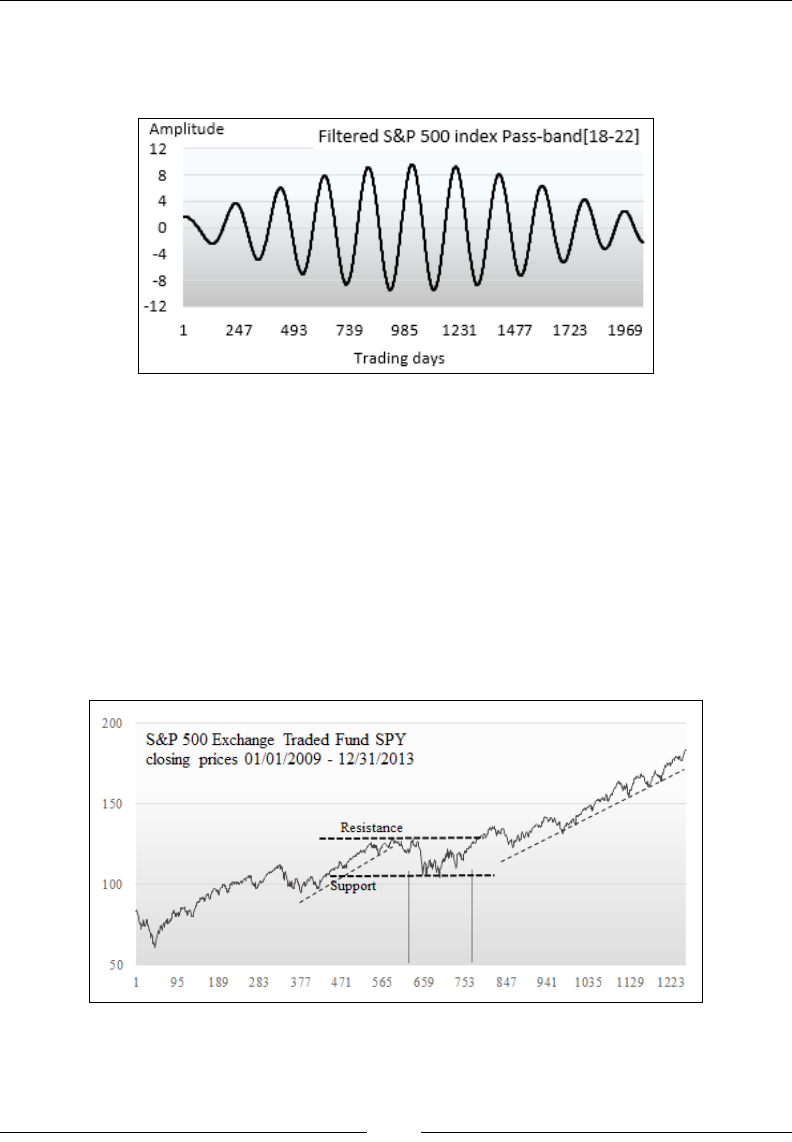
Data Preprocessing
[ 686 ]
In this case, we lter the S&P 500 index around the third group of harmonics with
frequencies ranging from 18 to 22; the signal is converted into a familiar sinusoidal
function, as shown here:
The output of a pass-band DFT filter range 18-22 on the historical S&P index
There is a possible rational explanation for the shape of the S&P 500 data ltered by
a passband with a frequency of 20, as illustrated in the previous plot; the S&P 500
historical data plot shows that the frequency of the uctuation in the middle of the
uptrend (trading sessions 620 to 770) increases signicantly. This phenomenon can
be explained by the fact that the S&P 500 index reaches a resistance level around the
trading session 545 when the existing uptrend breaks. A tug-of-war starts between
the bulls, betting the market nudges higher, and the bears, who are expecting a
correction. The back and forth between the traders ends when the S&P 500 index
breaks through its resistance and resumes a strong uptrend characterized by a high
amplitude and low frequency, as shown in the following graph:

Chapter 3
[ 687 ]
One of the limitations of using the Fourier transform to clean up data is that it requires
the data scientist to extract the frequencies spectrum and modify the lter on a regular
basis, as he or she is never sure that the most recent batch of data does not introduce
noise with a different frequency. The Kalman lter addresses this limitation.
The Kalman lter
The Kalman lter is a mathematical model that provides an accurate and recursive
computation approach to estimate the previous states and predict the future states of
a process for which some variables may be unknown. R. E. Kalman introduced it in
the early 60s to model dynamics systems and predict trajectory in aerospace [3:10].
Today, the Kalman lter is used to discover a relationship between two observed
variables that may or may not be associated with other hidden variables. In this
respect, the Kalman lter shares some similarities with the Hidden Markov models
(HMM) described in Chapter 6, Regression and Regularization [3:11].
The Kalman lter is used as:
• A predictor of the next data point from the current observation
• A lter that weeds out noise by processing the last two observations
• A smoother that computes trends from a history of observations
Smoothing versus ltering
Smoothing is an operation that removes high-frequency uctuations
from a time series or signal. Filtering consists of selecting a range of
frequencies to process the data. In this regard, smoothing is somewhat
similar to low-pass ltering. The only difference is that a low-pass
lter is usually implemented through linear methods.
Conceptually, the Kalman lter estimates the state of a system from noisy
observations. The Kalman lter has two characteristics:
• Recursive: A new state is predicted and corrected using the input of a
previous state
• Optimal: This is an optimal estimator because it minimizes the mean square
error of the estimated parameters (against actual values)

Data Preprocessing
[ 688 ]
The Kalman lter is one of the stochastic models that are used in adaptive
control [3:12].
Kalman and nonlinear systems
The Kalman lter estimates the internal state of a linear dynamic
system. However, it can be extended to a model nonlinear-state
space using linear or quadratic approximation functions. These
lters are known as, you guessed it, extended Kalman lters (EKF),
the theory of which is beyond the scope of this book.
The following section is dedicated to discrete Kalman lters for linear systems, as
applied to nancial engineering. A continuous signal can be converted to a time
series using the Nyquist frequency.
The state space estimation
The Kalman lter model consists of two core elements of a dynamic system—a
process that generates data and a measurement that collects data. These elements are
referred to as the state space model. Mathematically speaking, the state space model
consists of two equations:
• Transition equation: This describes the dynamics of the system including the
unobserved variables
• Measurement equation: This describes the relationship between the
observed and unobserved variables
The transition equation
Let's consider a system with a linear state xt of n variables and a control input vector
ut. The prediction of the state at time t is computed by a linear stochastic equation:
1ttt ttt
xAx Buw
−
=⋅+⋅+
• A is the square matrix of dimension n that represents the transition from
state x at t-1 to state x at t. The matrix is intrinsic to the dynamic system
under consideration.
• B is an n by n matrix that describes the control input model (external action
on the system or model). It is applied to the control vector u.
• w represents the noise generated by the system or from a probabilistic point
of view, the uncertainty on the model. It is known as the process white noise.
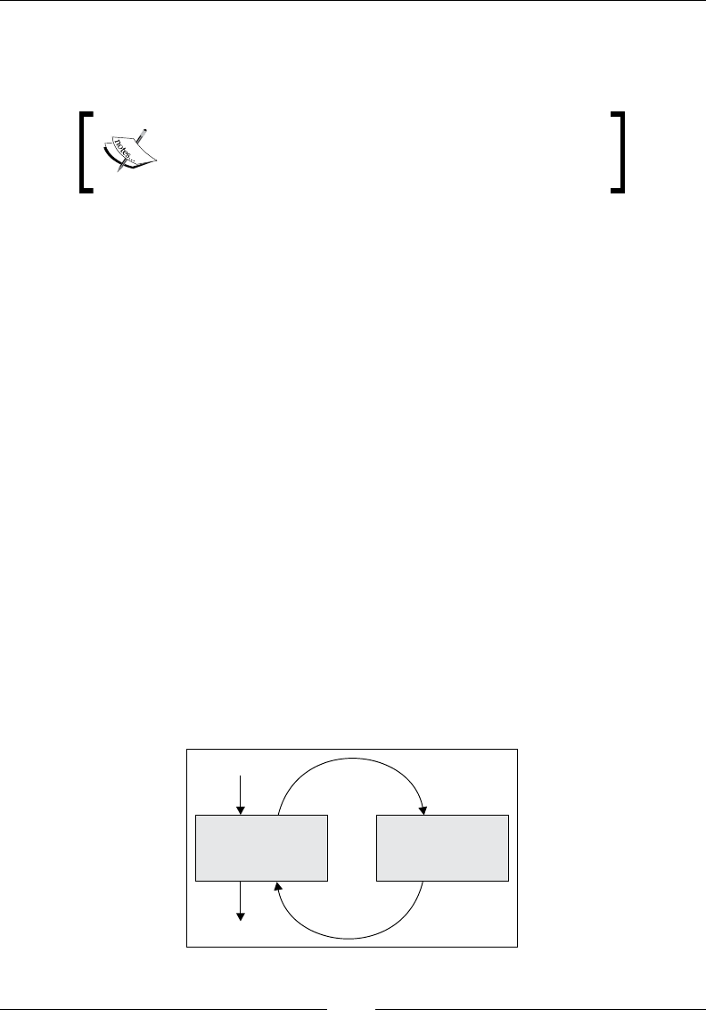
Chapter 3
[ 689 ]
The control input vector represents the external input (or control) to the state of the
system. Most systems, including our nancial example later in this chapter, have no
external input to the state of the model.
White and Gaussian noise
A white noise is a Gaussian noise, following a normal
distribution with zero mean.
The measurement equation
The measurement of m values zt of the state of the system is dened by the
following equation:
tttt
zHxv=⋅+
• H is a matrix m by n that models the dependency of the measurement to the
state of the system.
• v is the white noise introduced by the measuring devices. Similar to the
process noise, v follows a Gaussian distribution with zero mean and a
variance R, known as the measurement noise covariance.
The recursive algorithm
The set of equations for the discrete Kalman lter are implemented as recursive
computation with two distinct steps:
• The algorithm uses the transition equations to estimate the next observation
• The estimation is created with the actual measurement for this observation
The recursion is visualized in the following diagram:
Prediction
Estimate the internal
state of the system
Correction
Compute the internal
state of the system
Measurement
State
An overview diagram of the recursive Kalman algorithm

Data Preprocessing
[ 690 ]
Let's illustrate the prediction and correction phases in the context of ltering
nancial data, in a manner similar to the moving average and Fourier transform.
The objective is to extract the trend and the transitory component of the yield of the
10-year Treasury bond. The Kalman lter is particularly suitable for the analysis of
interest rates for two reasons:
• Yields are the results of multiple factors, some of which are not
directly observable
• Yields are inuenced by the policy of the Federal Reserve that can be easily
modeled by the control matrix
The 10-year Treasury bond has a higher trading volume than bonds with longer
maturity, making trends in interest rates a bit more reliable [3:13].
Applying the Kalman lter to clean raw data requires you to dene a model that
encompasses both observed and non-observed states. In the case of the trend analysis,
we can safely create our model with a two-variable state: the current yield xt and the
previous yield xt-1.
State in dynamic systems
The term "state" refers to the state of the dynamic system under
consideration. This is a different term for observation, data, or
value vector. A state or observation is a set of values, one for
each variable of the model.
This implementation of the Kalman lter uses the Apache Commons Math library,
which denes and manipulates specic types. The rst step is to dene the implicit
type conversion required to interface with the KalmanFilter class:
type DblMatrix = Array[Array[Double]]
type DblVector = Array[Double]
implicit def double2RealMatrix(x: DblMatrix): RealMatrix = new
Array2DRowRealMatrix(x)
implicit def double2RealRow(x: DblVector): RealMatrix = new
Array2DRowRealMatrix(x)
implicit def double2RealVector(x: DblVector): RealVector = new
ArrayRealVector(x)
The implicit type conversion has to be dened in the scope of the client code.

Chapter 3
[ 691 ]
The Kalman model assumes that process and measurement noise follow a Gaussian
distribution, also known as white noise. For the sake of maintainability, the generation
or simulation of the white noise is encapsulated in the QRNoise class with qr as the
tuple of scale factors for the process noise matrix Q and the measurement noise R. The
two create methods execute the user-dened noise function white:
class QRNoise(qr: XY, white: Double=> Double) {
def q = white(qr._1)
def r = white(qr._2)
def noisyQ = Array[Double](q,q)
def noisyR = Array[Double](r,r)
}
The easiest approach to manage the matrices and vectors used in the recursion is to
dene them as parameters of the main class, DKalman:
class DKalman(A:DblMatrix, B:DblMatrix, H:DblMatrix, P:DblMatrix)
(implicit val qrNoise: QRNoise) extends PipeOperator[XY,XY] {
val Q = new DblMatrix(A.size).map(_ => Array.fill(A.size)(qrNoise.
qr.1))
var x: RealVector = _
var filter: KalmanFilter =_
}
The matrix used in the prediction and correction phase is dened as an argument
of the DKalman class. The matrices for the covariance of the process noise Q and the
measurement noise R are also initialized during the instantiation of the Kalman lter
class. The key elements of the lter are now in place and it's time to implement the
prediction-correction cycle portion of the Kalman algorithm.
Prediction
The prediction phase consists of estimating the x state (yield of the bond) using the
transition equation. We assume that the Federal Reserve has no material effect on
the interest rates, making control input matrix B null. The transition equation can
be easily resolved using simple operations on matrices.
11 12
1 1 1 1
21 22
ˆ ˆ 00
ˆ ˆ 00
t t t t
t t t t
x x uw
aa
x x uw
aa
− − − −
⎡⎤ ⎡⎤ ⎡⎤⎡ ⎤
⎡⎤ ⎡⎤
=⋅+⋅+
⎢⎥ ⎢⎥ ⎢⎥⎢ ⎥
⎢⎥ ⎢⎥
⎣⎦
⎣⎦
⎣⎦ ⎣⎦ ⎣⎦⎣ ⎦
Visualization of the transition equation of the Kalman filter

Data Preprocessing
[ 692 ]
The purpose of this exercise is to evaluate the impact of the different parameters of
the transition matrix A in terms of smoothing.
The control input matrix B
In this example, the control matrix B is null because there is no known
deterministic external action on the yield of the 10-year Treasury bond.
However, the yield can be affected by unknown parameters that we
represent as hidden variables. The matrix B would be used to model
the decision of the Federal Reserve regarding asset purchases and
federal fund rates.
The mathematics behind the Kalman lter presented as reference to its
implementation in Scala use the same notation for matrices and vectors. It is
absolutely not a prerequisite to understand the Kalman lter and its implementation
in the next section. If you have a natural inclination toward linear algebra, the
following note describes the two equations for the prediction step.
The prediction step
The prediction of the state at time t+1 is computed by extrapolating the
state estimate:
'
1
ˆˆ
ttt tt
xAx Bu
−
=⋅+⋅
• A is the square matrix of dimension n that represents the
transition from state x at t-1 to state x at time t.
•
'
ˆt
x
is the predicted state of the system based on the current state
and the model A
• B is the vector of n dimension that describes the input to the state
The mean square error matrix P, which is to be minimized, is updated
through the following formula:
'
1
T
tttt t
PAPAQ
−
=⋅⋅+
• AT is the transpose of the state transition matrix.
• Q is the process white noise described as a Gaussian distribution
with a zero mean and a variance Q, known as the noise
covariance.
The state transition matrix is implemented using the matrix and vector classes
included in the Apache Commons Math library. The types of matrices and
vectors are automatically converted into RealMatrix and RealVector classes.
The implementation of the equation is as follows:
x = A.operate(x).add(qrNoise.noisyQ)

Chapter 3
[ 693 ]
The new state is predicted (or estimated), and then used as an input to the
correction step.
Correction
The second and last step of the recursive Kalman algorithm is the correction of the
estimated yield of the 10-year Treasury bond with the actual yield. In this example,
the white noise of the measurement is negligible. The measurement equation is
simple because the state is represented by the current and previous yield, and their
measurement z:
11 12
111
21 22
ˆ
ˆ
t t t
t t t
zxv
hh
zxv
hh
−−−
⎡⎤ ⎡⎤⎡⎤
⎡⎤
=⋅+
⎢⎥ ⎢⎥⎢⎥
⎢⎥
⎣⎦
⎣⎦ ⎣⎦⎣⎦
Visualization of the measurement equation of the Kalman filter
The sequence of mathematical equations of the correction phase consists of updating
the estimation of the state x using the actual values z, computing the Kalman gain K,
and estimating the matrix of the error covariance P.
Correction step
The state of the system x is estimated from the actual measurement
z through the following formula:
()
' ' '
ˆˆ ˆ ˆ
tt tt tttt tt
xxKzHxrzHx
=+ −⋅ =−⋅
• r is the residual between the predicted measurement and the
actual measured values
• K is the Kalman gain for the correction factor Kr
The Kalman gain is computed using the estimated error covariance
matrix
'
t
P
:
( )
1
' 'T T
ttt ttt t
KPHHPH R
−
=⋅⋅⋅+
• HT is the matrix transpose of H
Finally, the estimate of the error covariance matrix
'
t
P
is corrected to
the value Pt through the following formula:
()
' '
tdttt
PIKHP=−⋅ ⋅
• Id is the identity matrix.

Data Preprocessing
[ 694 ]
Kalman smoothing
It is time to put our knowledge of the transition and measurement equations to the
test. The Apache Commons Library denes two classes, DefaultProcessModel and
DefaultMeasurementModel, to encapsulate the components of the matrices and
vectors. The historical values for the yield of the 10-year Treasury bond is loaded
through the DataSource method and mapped to the smoothed series that is the
output of the lter.
def |> : PartialFunction[XTSeries[XY], XTSeries[XY]] = {
case xt: XTSeries[XY] if(xt.size> 0) => xt.map( y => {
initialize(Array[Double](y._1, y._2)) //1
val nState = newState //2
(nState(0), nState(1)) }) //3
…
The data transformation for the Kalman lter initializes the process and
measurement model for each data point (line 1), updates the state using the
transition and correction equations iteratively (line 2), and returns the ltered
series (line 3).
Exception handling
The code to catch and process exceptions thrown by the Apache
Commons Math library is omitted as the standard practice in the
book. As far as the execution of the Kalman lter is concerned, the
following exceptions have to be handled:
• NonSquareMatrixException
• DimensionMismatchException
• MatrixDimensionMismatchException
The model is a 2-step lag smoothing algorithm using a single smoothing factor α
with a state, St:
St = {xt+1, xt} with xt+1 = α.xt + (1- α).xt-1 and xt = xt
Following the Scala standard to return errors to the client code, the exceptions
thrown by the Commons Math API are caught and processed through the
Option monad. The iterative prediction and correction of the smoothed yields is
implemented by the newState method. The method iterates through four steps:
1. Filter an estimate of the state x at time t.
2. The new state is computed using the transition equation.
3. The measured value z of the state is computed using the measurement equation.
4. The original estimate x is corrected with the measured value.

Chapter 3
[ 695 ]
The newState method is dened as follows:
val PROCESS_NOISE_Q = 0.03
val PROCESS_NOISE_R = 0.1
val MEASUREMENT_NOISE = 0.4
def newState: DblVector = {
Range(0, maxIters) foreach( _ => {
filter.predict //1
val w = qrNoise.create(PROCESS_NOISE_Q, PROCESS_NOISE_R)
x = A.operate(x).add(qrNoise.noisyQ) //2
val v = qrNoise.create(MEASUREMENT_NOISE)
val z = H.operate(x).add(qrNoise.noisyR) //3
filter.correct(z) // 4
})
filter.getStateEstimation
}
The PROCESS_NOISE factor (with respect to MEASUREMENT_NOISE) used in the
creation of the process noise w and measurement noise v are somewhat arbitrary.
Their purpose is to simulate the white noise for the model. The newState method
returns the ltered state as a DblVector instance for this particular state.
The exit condition
In the code snippet for the newState method, the iteration for
specic data points exits when the maximum number of iterations
is reached. A more elaborate implementation consists of either
evaluating the matrix P at each iteration or estimation converged
within a predened range.
Experimentation
The objective is to smoothen the yield of the 10-year Treasury bond and quantify the
impact of the elements of the state-transition matrix A on the smoothing process. The
state equation updates the values of the state [xt, xt-1] using the previous state [xt-1, xt-2],
where x represents the yield at time t. This is accomplished by shifting the values of
the original time series {x0, ... xn} by 1 using the drop method, X1={x1, … xn}, creating
a copy of the original time series without the last element X2={x0, … xn-1} and zipping
X1 and X2. The resulting sequence of pair {(xk, xk-1)} is processed by the Kalman
algorithm, as shown in the following code:
implicit val qrNoise = QRNoise((0.2, 0.4), (m: Double) => m* (new
Random(System.currentTimeMillis)).nextGaussian) //1
val A: DblMatrix = ((0.9, 0.0), (0.0, 0.1))

Data Preprocessing
[ 696 ]
val B: DblMatrix = (0.0, 0.0)
val H: DblMatrix = (1.0, 1.0)
val P0: DblMatrix = ((0.4, 0.5), (0.4, 0.5))
val x0: DblVector = (175.0, 175.0)
val dKalman = new DKalman(A, B, H, P0) //2
val output = "output/chap3/kalman.csv"
val zt_1 = zSeries.drop(1)
val zt = zSeries.take(zSeries.size-1)
val filtered = dKalman |> XTSeries[(Double, Double)](zt_1.zip(zt)) //3
DataSink[Double](output) |> filtered.map(_._1) //4
The process and measurement noise qrNoise is implicitly initialized with the
respective factors, 0.2 and 0.4 (line 1). The Kalman lter is initialized with the
prediction-correction equation matrices A, B, H, and P0, and the initial state x0 (line 2).
A time series {(xi, xi-p)}i is generated by zipping two copies of the historical 10 Treasury
bond yield series, with the second one being shifted by p data. The Kalman lter is
applied to the time series of tuples and the result is dumped into an output le using
a DataSink instance (line 4)
The test is performed over a period of one year, and the results are plotted using a
basis point or 100th of a percentage. The quality of the output is evaluated using two
different values for the state transition matrix A: [0, 8, 0.2, 1.0, 0.0] and [0,5, 0.5, 1.0, 0.0].
Modeling state transition and noise
The state transition and the noise related to the process have to be
selected carefully. The resolution of the state equations relies on
the QR decomposition, which requires a non-negative denite
matrix. The implementation in the Apache common library throws a
NonPositiveDefiniteMatrixException if the principle is violated.
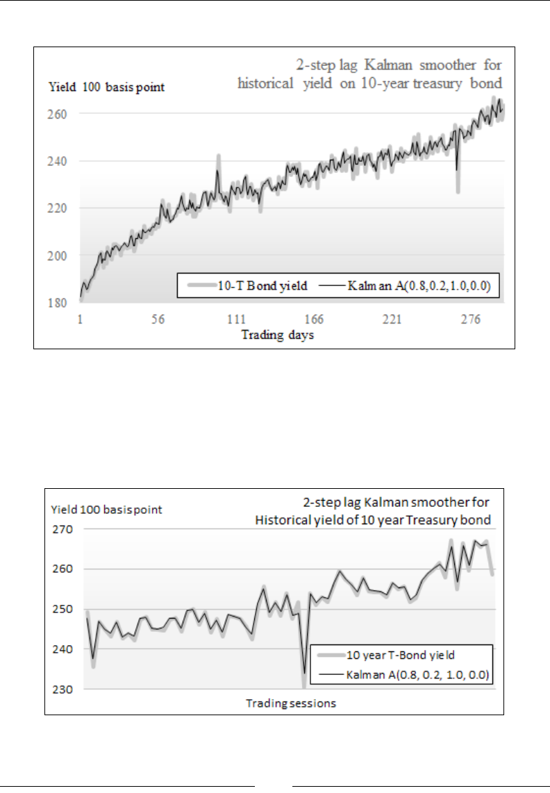
Chapter 3
[ 697 ]
The smoothed yield is plotted along the raw data as follows:
The output of the Kalman filter for the 10-year Treasury bond historical prices
Clearly, the yield time series has been smoothed. However, the amplitude of
the underlying trend is signicantly higher than any of the noise or the spikes.
Consequently, the Kalman lter has a limited impact. Let's analyze the data for a
shorter period during which the noise is the strongest, between the 190th and the
275th trading days.
The output of the Kalman filter for the 10-year Treasury bond prices 0.8-0.2
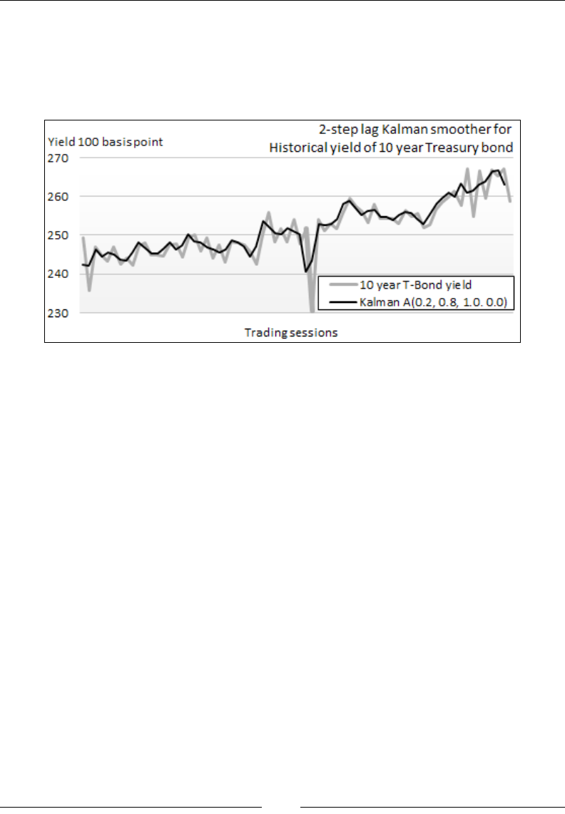
Data Preprocessing
[ 698 ]
The high frequency noise has been signicantly reduced without cancelling
the actual spikes. The distribution 0.8-0.2 takes into consideration the previous
state and favors the predicted value. Contrarily, a run with a state transition matrix
A [0.2, 0.8, 0.0, 1.0] that favors the latest measurement will preserve the noise, as seen
in the following graph:
The output of the Kalman filter for the 10-year Treasury bond price 0.2-0.8
The Kalman lter is a very useful and powerful tool in understanding the
distribution of the noise between the process and observation. Contrary to the
low or pass-band lters based on the fast Fourier transform, the Kalman lter
does not require computation of the frequencies spectrum or assume the range
of frequencies of the noise.
However, the linear Kalman lter has its limitations:
• The noise generated by both the process and the measurement has to
be Gaussian. Processes with non-Gaussian noise can be modeled with
techniques such as a Gaussian Sum lter or adaptive Gaussian mixture [3:14].
• It requires that the underlying process is linear. Researchers have been able
to formulate extensions to the Kalman lter, known as the extended Kalman
lter (EKF) to lter signals from non-linear dynamic systems, at the cost of
signicant computational complexity.

Chapter 3
[ 699 ]
Alternative preprocessing techniques
For the sake of space and your time, this chapter introduced and applied three
ltering and smoothing classes of algorithms. Moving averages, Fourier series, and
the Kalman lter are far from being the only techniques used in cleaning raw data.
The alternative techniques can be classied into two categories:
• Autoregressive models that encompass autoregressive moving average
(ARMA), autoregressive integrated moving average (ARIMA), generalized
autoregressive conditional heteroskedasticity (GARCH), and Box-Jenkins
that relies on some form of autocorrelation function
• Curve-tting algorithms that include the polynomial and geometric t
with the ordinary least squares method, non-linear least squares using
the Levenberg-Marquardt optimizer, and probability distribution tting
Summary
This completes the overview of the most commonly used data ltering and
smoothing techniques. There are other types of data preprocessing algorithms such
as normalization, analysis, and reduction of variance; the identication of missing
values is also essential to avoid the garbage-in garbage-out conundrum that plagues
so many projects that use machine learning for regression or classication.
Scala can be effectively used to make the code understandable and avoid cluttering
methods with unnecessary arguments.
The three techniques presented in this chapter, from the simplest moving averages
and Fourier transform to the more elaborate Kalman lter, go a long way in setting
up data for the next concepts introduced in the next chapter—unsupervised learning
and more specically, clustering.

Unsupervised Learning
Labeling a set of observations for classication or regression can be a daunting task,
especially in the case of a large feature set. In some cases, labeled observations are
either not available or not possible to create. In an attempt to extract some hidden
association or structures from observations, the data scientist relies on unsupervised
learning techniques to detect patterns or similarity in data.
The goal of unsupervised learning is to discover patterns of regularities and
irregularities in a set of observations. These techniques are also applied in reducing
the solution space or feature set similarly to the divide-and-conquer approach
commonly used in Computer Science.
There are numerous unsupervised algorithms; some are more appropriate to handle
dependent features while others generate more relevant groups in the case of hidden
features [4:1]. In this chapter, you will learn three of the most common unsupervised
learning algorithms:
• K-means: Clustering observed features
• Expectation-maximization (EM): Clustering observed and latent features
• Principal components analysis (PCA): Reducing the dimension of the model
Any of these algorithms can be applied to technical analysis or fundamental analysis.
Fundamental analysis of nancial ratios and technical analysis of price movements
are described in the Technical analysis section under Finances 101 in Appendix A,
Basic Concepts. The K-means algorithm is fully implemented in Scala while
expectation-maximization and principal components analysis leverage the
Apache Commons Math library.
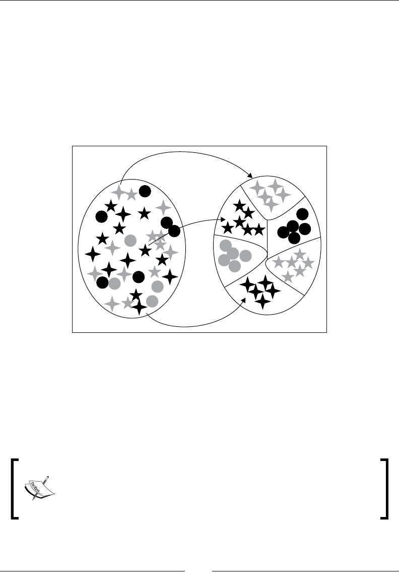
Unsupervised Learning
[ 702 ]
Clustering
Problems involving a large number of features for large datasets become quickly
intractable, and it is quite difcult to evaluate the independence between features.
Any computation that requires some level of optimization and, at a minimum,
computation of rst order derivatives requires a signicant amount of computing
power to manipulate high-dimension matrices. As with many engineering elds, a
divide-and-conquer approach to classifying very large datasets is quite effective. The
objective is to reduce continuous, innite, or very large datasets into a small group of
observations that share some common attributes.
Visualization of data clustering
This approach is known as vector quantization. Vector quantization is a method that
divides a set of observations into groups of similar size. The main benet of vector
quantization is that the analysis using a representative of each group is far simpler
than an analysis of the entire dataset [4:2].
Clustering, also known as cluster analysis, is a form of vector quantization that
relies on a concept of distance or similarity to generate groups known as clusters.
Learning vector quantization (LVQ)
Vector quantization should not be confused with learning vector
quantization. Learning vector quantization is a special case of articial
neural networks that relies on a winner-take-all learning strategy to
compress signals, images, or videos.

Chapter 4
[ 703 ]
This chapter introduces two of the most commonly applied clustering algorithms:
• K-means, which is used for quantitative types and minimizes the total error
(known as the reconstruction error) given the number of clusters and the
distance formula.
• Expectation-maximization (EM), which is a two-step probabilistic
approach that maximizes the likelihood estimates of a set of parameters.
EM is particularly suitable to handle missing data.
K-means clustering
K-means is a popular iterative clustering algorithm. The representative of each
cluster is computed as the center of the cluster, known as the centroid. The
similarity between observations within a single cluster relies on the concept
of distance between observations.
Measuring similarity
There are many ways to measure the similarity between observations. The most
appropriate measure has to be intuitive and avoid computational complexity.
This section reviews three similarity measures:
• The Manhattan distance
• The Euclidean distance
• Cosine of value observations
The Manhattan distance is dened by the absolute distance between two variables or
vectors, {xi} and {yi}, of the same size:
(, ) | |
ii
dxy x y=−
∑
The implementation is generic enough to compute the distance between two arrays
of elements of different types as long as an implicit conversion between each of these
types to Double values is already dened, as shown here:
def manhattan[T <% Double, U <% Double](x: Array[T], y: Array[U]):
Double = (x, y).zipped.foldLeft(0.0)((s, t) => s + Math.abs(t._1 -
t._2))

Unsupervised Learning
[ 704 ]
The ubiquitous Euclidean distance is dened as the square of the distance between
two vectors, {xi} and {yi}, of the same size:
2
(, ) ( )
ii
dxy x y
=−
∑
def euclidean[T <% Double, U <% Double](x: Array[T], y: Array[U]):
Double = Math.sqrt((x, y).zipped.foldLeft(0.0)((s, t) => { val d =
t._1 - t._2; s + d*d} ))
The cosine distance is dened as the cosine of an angle between two vectors, {xi} and
{yi}, of the same size:
221/ 2
(, ) ()
ii
ii
xy
dxy xy
=
∑
∑∑
In this implementation, the computation of the dot product and the norms for each
dataset is done simultaneously using the tuple within the fold method:
def cosine[T <% Double, U <% Double](x: Array[T], y: Array[U]): Double
= {
val zeros = (0.0, 0.0, 0.0)
val norms = (x, y).zipped.foldLeft(zeros)((s, t) =>
(s._1 + t._1*t._2, s._2 + t._1*t._1, s._3 + t._2*t._2))
norms._1/Math.sqrt(norms._2*norms._3)
}
Performance of zip
The scalar product of two vectors is one of the most common
operations. It is tempting to implement the dot product using the
generic zip method:
def dot (x:Array[Double], y:Array[Double]):
Array[Double] =
x.zip(y).map( x => f(x._1, x._2) )
An functional alternative is to use the Tuple2.
zipped method.
def dot(x:Array[Double], y:Array[Double]):
Array[Double] = (x, y).zipped map ( _ * _)
If readability is not a primary issue, you can always implement the
dot method with a while loop.

Chapter 4
[ 705 ]
Overview of the K-means algorithm
The main advantage of the K-means algorithm (and the reason for its popularity) is
its simplicity [4:3].
Let's consider K clusters {Ck} with means {mk}. The K-means algorithm is
indeed an optimization problem, the objective of which is to minimize
the reconstruction or the total error dened as the total sum of distance.
1
min(,)
k
ik
K
ik
CxC
dxm
∈
∑∑
The steps of the iterative algorithm are:
1. Initialize the centroids or means mk of the K clusters.
2. Assign observations to the nearest cluster given mk.
3. Iterate until no observations are reassigned to a cluster:
°Compute centroids mk that minimize the total error reconstruction for
the current assignment
°Reassign the observations given the new centroids mk
Step 1 – cluster conguration
The conguration of the K clusters consists of dening the following parameters for
the K-means algorithm: number of K clusters, the distance metrics, the maximum
number of iterations, and the initial value of the cluster's centroid.
Dening clusters
The rst step is to dene a cluster. A cluster is dened by the following parameters:
• Centroid: center
• The indices of the observations that belong to this cluster: members
The following code shows the denition of a cluster:
class Cluster[T <% Double](val center: DblVector) {
val members = new ListBuffer[Int]
The cluster is responsible for managing its members (data points) at any point of
the iterative computation of the K-means algorithm. It is assumed that a cluster
will never contain the same data points twice.

Unsupervised Learning
[ 706 ]
The constructor of the Cluster class is implemented by the apply method in
the companion object (for convenience, refer to the Class constructor template
section in Appendix A, Basic Concepts):
object Cluster {
def apply[T <% Double](c:DblVector):Cluster[T] = new Cluster[T](c)
}
At a minimum, a cluster should be able to manage its membership of observations,
update its center, and compute the variance or standard deviation of all its member
observations:
def += (n:Int): Unit = members.append(n)
def moveCenter(xt: XTSeries[Array[T]): Cluster[T] ={
val sums = members.map(xt(_).map(_.toDouble)).toList
.transpose
.map( _.sum)
Cluster[T](sums.map( _ / members.size).toArray)
}
def stdDev(xt: XTSeries[Array[T]], distance: (DblVector, Array[T]) =>
Double): Double = {
Stats[Double](members.map(xt( _))
.map( distance(center, _)).toArray).stdDev
}
The three important methods that dene the behavior of a cluster instance are
as follows:
• +=: Add a member (index of an observation in the original time series).
• moveCenter: Create a new cluster with the existing members and a new
centroid computed as the mean of all the observations contained in the cluster.
• stdDev: Compute the standard deviation (or density) of all the observations
contained in the cluster relative to its center. The distance between each
member and the centroid is extracted through a map, and then folded to
generate the statistics. The function to compute the distance between the
center and an observation is an argument of the method. The default
distance is Euclidean.

Chapter 4
[ 707 ]
Cluster selection
There are different ways to select the most appropriate cluster
when reassigning an observation (updating its membership).
In this implementation, we will select the cluster with the
larger spread or lowest density. An alternative is to select the
cluster with the largest membership.
Dening K-means
Let's declare the K-means algorithm class, KMeans, with its public methods.
The KMeans class takes the number of clusters, K, and the maximum number of
iterations, maxIters, as parameters. The implicit conversion of type T to a Double
is specied by the T <% Double view bound. The Ordering class has to be passed
implicitly as a parameter because it is required by the sortWith method in the
initialize and maxBy methods. The Manifest method is required to preserve the
type erasure for Array[T] in the JVM:
class KMeans[T <% Double](K: Int, maxIters: Int, distance:
(DblVector,Array[T]) => Double)(implicit order: Ordering[T],
m: Manifest[T]) extends PipeOperator[XTSeries[Array[T]],
List[Cluster[T]]] {
def |> : PartialFunction[XTSeries[Array[T]], List[Cluster[T]]]
def initialize(xt:XTSeries[Array[T]]): List[Cluster[T]]
As with other data processing units, the extraction of K-means clusters is
encapsulated by the pipe operator |>, so clustering can be integrated into a workow
using dependency injection described in the Dependency injection section in Chapter 2,
Hello World!. The initialization of the centroids of each of the K clusters is performed
by the private initialize method.
Initializing clusters
The initialization of the cluster centroids is important to ensure fast convergence of
K-means. Solutions range from the simple random generation of centroids to the
application of genetic algorithms to evaluate the tness of centroid candidates. We
selected an efcient and fast initialization algorithm developed by M. Agha and W.
Ashour [4:4].

Unsupervised Learning
[ 708 ]
The steps of the initialization are as follows:
1. Compute the standard deviation of the set of observations.
2. Select the dimension k {xk,0, xk,1 … xk,n} with maximum standard deviation.
3. Rank the observations by their increasing value of standard deviation for the
dimension k.
4. Divide the ranked observations set equally into K sets {Sm}.
5. Find the median values, size (Sm)/2.
6. Use the corresponding observations as centroids.
The initialization algorithm is implemented by the private initialize method:
def initialize(xt:XTSeries[Array[T]]): List[Cluster[T]]={
val stats = statistics(xt) //1
val maxSDevDim = Range(0,stats.size).maxBy (stats( _ ).stdDev)//2
val rankedObs = xt.zipWithIndex
.map(x=> (x._1(maxSDevDim), x._2)) //2
.sortWith( _._1 < _._1) //3
val halfSegSize = ((rankedObs.size>>1)/K).floor.toInt //4
val centroids = rankedObs.filter(isContained( _, halfSegSize,
rankedObs.size) ).map(n => xt(n._2)) //6
Range(0, K).foldLeft(List[Cluster[T]]())((xs, i) => Cluster[T]
(centroids(i)) :: xs) //7
}
Let's deconstruct the implementation of the Agha-Ashour algorithm in the
initialize method.
The statistics function is applied to the input time series to extract the standard
deviation for each dimension in the observations set (line 1). The dimension with
the maxSDevDim maximum variance or standard deviation is computed by using the
maxBy method on a Stats instance (line 2). Then, the observations are ranked by the
increasing value of the standard deviation, rankedObs (line 3).
The ordered sequence of observations is then broken into xt.size/K segments (line
4) and the indices of the centroids are selected as the midpoint (or median)
observations of those segments using the ltering condition, isContained:
def isContained(t: (T,Int), hSz: Int, dim: Int): Boolean =
((t._2 % hSz == 0) && (t._2 %(hSz<<1) != 0)

Chapter 4
[ 709 ]
The indices of the centroid in the time series are converted to actual observations
using a map method (line 6). Finally, the list of clusters is generated using a fold
(foldLeft) method on the range of cluster indices (0, K-1) (line 7).
Step 2 – cluster assignment
The second step in the K-means algorithm is the assignment of the observations
to the clusters for which the centroids have been initialized in step 1. This feat is
accomplished by the private assignToClusters method:
def assignToClusters(xt: XTSeries[Array[T]], clusters:
List[Cluster[T]], membership: Array[Int]): Int = {
xt.toArray
.zipWithIndex
.filter(x => { //1
val nearestCluster = getNearestCluster(clusters, x._1)//2
val reassigned = nearestCluster != membership(x._2)
clusters(nearestCluster) += x._2 //3
membership(x._2) = nearestCluster //4
reassigned
}).size
}
The core of the assignment of observations to each cluster is the lter on the time
series (line 1). The lter computes the index of the closest cluster and checks whether
the observation is to be reassigned (line 2). The observation at the index x._2 is
added to the nearest cluster, clusters(nearestCluster) (line 3). The current
membership of the observations is then updated (line 4).
The cluster closest to an observation data is computed by the getNearestCluster
method as follows:
def getNearestCluster(clusters: List[Cluster[T]], x:Array[T]): Int={
clusters.zipWithIndex..foldLeft((Double.MaxValue,0))((p,c) => {
val measure = distance(c._1.center, x)
if(measure < p._1) (measure, c._2) else p
})._2
A fold is used to extract from the list of clusters the cluster that is closest to the
observation x using the distance metric dened in the K-means constructor.

Unsupervised Learning
[ 710 ]
Step 3 – iterative reconstruction
The nal step is to implement the iterative computation of the reconstruction error.
In this implementation, the iteration terminates when no more observations are
reassigned to different clusters. As with other data processing units, the extraction
of K-means clusters is encapsulated by the pipe operator |>, so that clustering
can be integrated into a workow using dependency injection described in the
Dependency Injection section in Chapter 2, Hello World!.
The generation of the K clusters is executed by the data transformation |>:
def |> :PartialFunction[XTSeries[Array[T]], List[Cluster[T]]] = {
case xt: XTSeries[Array[T]] if(xt.size>2 && xt(0).size>0) => {
val clusters = initialize(xt) //1
if( clusters.isEmpty) List.empty
else {
val membership = Array.fill(xt.size)(0)
val reassigned = assignToClusters(xt,clusters,membership)//2
var newClusters: List[Cluster[T]] = List.empty
Range(0, maxIters).find( _ => {
newClusters = clusters.map( c => {
if( c.size > 0) c.moveCenter(xt, dimension(xt))
else clusters.filter( _.size > 0)
.maxBy( _.stdDev(xt, distance))
}) //3
assignToClusters(xt, newClusters, membership) == 0
}) match {
case Some(index) => newClusters
case None => { … }
} //4
}
}
As described in the algorithm overview section, the main method initializes the
membership for all the observations (line 1), creates and initializes the clusters, and
assigns the observations to clusters using the assignToClusters method (line 2).
The iteration updates the content of each cluster using the moveCenter method, by
assigning new observations to the cluster with the highest standard deviation (line 3).
The iterative loop exits when no more reassignment is needed (line 4).
Chapter 4
[ 711 ]
K-means algorithm exit condition
In some rare instances, the algorithm may reassign the same few
observations between clusters, preventing its convergence toward a
solution in a reasonable time. Therefore, it is recommended to add a
maximum number of iterations as an exit condition. If K-means does
not converge with the maximum number of iterations, then the cluster
centroids need to be reinitialized and the iterative process needs to be
executed once again.
The companion object for KMeans implements the apply constructor and the
computation of the stdDev standard deviation for each cluster. The default
constructor uses the Euclidean distance:
def apply[T <% Double](K: Int, maxIters: Int)(implicit order:
Ordering[T], m: Manifest[T]): KMeans[T] = new KMeans[T](K, maxIters,
euclidean)
def stdDev[T](c: List[Cluster[T]], xt: XTSeries[Array[T]]):
List[Double] = c.map( _.stdDev(xt))
The stdDev method computes the standard deviation of the distances between each
data point that belongs to a c cluster and its centroid.
Centroid versus mean
The terms centroid and mean refer to the same entity: the center of
a cluster. This chapter uses these two terms interchangeably.
Note that ordering a trait and Manifest have to be provided in the apply
constructor because there is no guarantee that such capabilities are provided
in runtime by the client code.
Curse of dimensionality
A model with a signicant number of features (high dimensions) requires a larger
number of observations in order to extract robust clusters. K-means clustering with
very small datasets, of size less than 50, produces models with high bias and a
limited number of clusters that are affected by the order of observations [4:5]. I have
been using the following simple empirical rule of thumb for a training set of size n,
expected K clusters, and N features: n < K.N.

Unsupervised Learning
[ 712 ]
Dimensionality versus size of training set
The issue with the dimensionality of models versus the number of
observations is not specic to unsupervised learning algorithms. All
supervised learning techniques face the same challenge to set up a
viable training plan.
Whichever empirical rule you follow, such a restriction is particularly an issue
for analyzing stocks using historical quotes. Let's consider our examples of using
technical analysis to categorize stocks according to their price behavior over a period
of 1 year (or approximately 250 trading days). The dimension of the problem is 250
(250 daily closing prices). The number of stocks (observations) would have exceeded
several hundred!
IBM price day 1, price day 2, ..., price day 250
GE price day 1, price day 2, ..., price day 250
GM price day 1, price day 2, ..., price day 250
Features
Observations
Price model for K-means clustering
There are options to get around this limitation and shrink the number of
observations; among them are:
• Sampling the trading data without losing a signicant amount of information
from the raw data, assuming the distribution of observations follows a
known probability density function.
• Smoothing the data to remove the noise as seen in Chapter 3, Data
Preprocessing, assuming the noise is Gaussian. In our test, a smoothing
technique will remove the price outliers for each stock and therefore reduce
the number of features (trading session). This approach differs from the
sampling approach because it does not require an assumption that the
dataset follows a known density function. On the other hand, the reduction
of features will be less signicant.
These approaches are workaround solutions at best, used for the sake of this tutorial,
but they are not recommended for actual commercial analytical applications. The
principal component analysis introduced in the last section of this chapter is one of
the most reliable dimension reduction techniques.
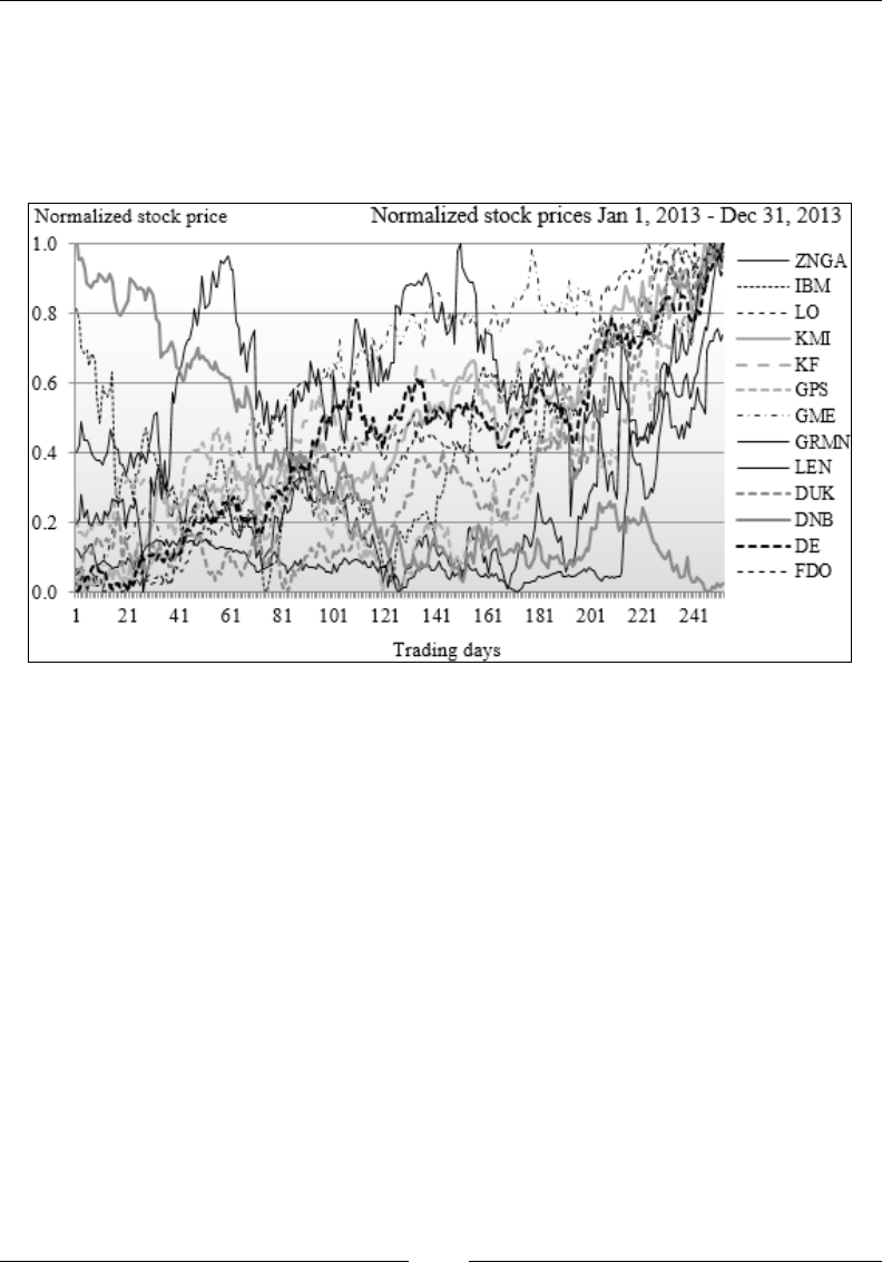
Chapter 4
[ 713 ]
Experiment
The objective is to extract clusters from a set of stock price actions during a period
of time between January 1 and Dec 31, 2013 as features. For this test, 127 stocks are
randomly selected from the S&P 500 list. The following chart visualizes the behavior
of the normalized price of a subset of these 127 stocks:
Price action of stocks used in K-means clustering
The key is to select the appropriate features prior to clustering and the time window
to operate on. It would make sense to consider the entire historical price over the
252 trading days as a feature. However, the number of observations (stocks) is too
limited to use the entire price range. The (SAMPLES = 50) observations are the stock
closing price for each trading session between the 80th and 130th days. The adjusted
daily closing prices are normalized using the minimum and maximum values.
First, let's create a simple function to execute the K-means algorithm:
Val MAX_ITERS = 150
def run(K: Int, obs: DblMatrix): Unit = {
val kmeans = KMeans[Double](K, MAX_ITERS) //1
val clusters = kmeans |> XTSeries[DblVector](obs) //2
clusters.foreach( _.center.foreach( show( _ ))) //3
clusters.map( _.stdDev(XTSeries[DblVector](obs, euclidean))).
foreach( show( _ ) ) //4
}

Unsupervised Learning
[ 714 ]
The KMeans class is rst initialized with a number of clusters, K, and a maximum
number of iterations, MAX_ITERS (line 1). These two parameters are domain and
problem specic. The clustering algorithm is executed (line 2) returning a list
of clusters. The clusters' centroid information is then displayed (line 3) and the
standard deviation is computed for each of the clusters for a given number of
clusters, K, and observations, obs (line 4).
Let's load the data from CSV les using the DataSource class (refer to the Data
extraction section in Appendix A, Basic Concepts):
final val path = "resources/data/chap4/"
val extractor = YahooFinancials.adjClose :: List[Array[String]
=>Double]() // 5
def symbols = DataSource.listSymbols(path) //6
final val START = 80
final val SAMPLES = 50
val normalize=true
val prices = symbols.map(s =>DataSource(s,path,normalize) |>
extractor) //7
prices.find(_.isEmpty) match { //8
case Some(noPrice) = { … }
case None => {
val values = prices. map(x => x(0))
.map(_.drop(START).take(SAMPLES))
args.map(_.toInt) foreach( run(_, values)) //9
}
}
As mentioned earlier, the cluster analysis applies to the closing price in the range
between the 80th and 130th trading day. The extractor is dened to extract the adjusted
closing price for a stock whose price information is retrieved from YahooFinancials
(line 5). The list of stock symbols is used to extract price information from CSV les
located at the path (line 6). For instance, the ticker symbol for General Electric Corp.
is GE and the trading data is located in GE.csv.
The 50 daily prices for each stock are extracted by an instance of DataSource (line
7). The run method introduced earlier is invoked either for each stock or as soon as
K-means fails through an exit condition in the find method (line 8). The normalized
data values.toArray for the specic time window is extracted by the combination
of calls to drop and take Scala array methods (line 9).
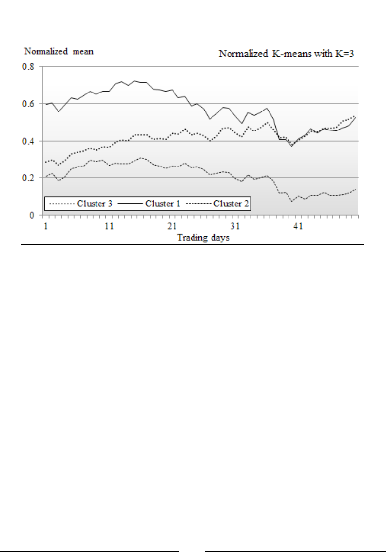
Chapter 4
[ 715 ]
The rst test run is executed with K=3 clusters. The mean (or centroid) vector for
each cluster is plotted as follows:
Chart of means of clusters using K-means K=3
The means vectors of the three clusters are quite distinctive. The top and bottom means
1 and 2 in the chart have the respective standard deviation of 0.34 and 0.27 and share a
very similar pattern. The difference between the elements of the 1 and 2 cluster mean
vectors is almost constant: 0.37. The cluster with a mean vector 3 represents the group
of stocks that behave like the stocks in cluster 2 at the beginning of the time period, and
behave like the stocks in cluster 1 towards the end of the time period.
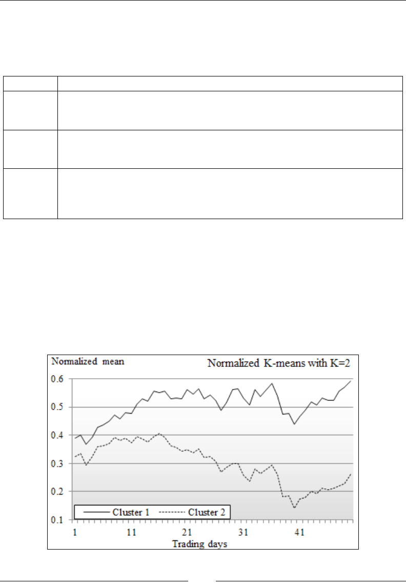
Unsupervised Learning
[ 716 ]
This behavior can be easily explained by the fact that the time window or trading
period, the 80th to 130th trading day, correspond to the shift in the monetary policy
of the federal reserve in regard to the quantitative easing program. Here is the list
of stocks for each of the clusters whose centroid values are displayed on the chart:
Cluster List of stocks
Cluster 1
AET, AHS, BBBY, BRCM, C, CB, CL, CLX, COH, CVX, CYH, DE, DG, DHI,
DO, DUK, EA, EBAY, EXC, EXP, FE, GLW, GPS, IBM, JCP, JNJ, JWN, K, KF,
KMI, KO, KRFT, LEN, LINC, LRCX, MSFT, NVMI, THC, XRT
Cluster 2
AA, AAPL, ADBE, ADSK, AFAM, AMZN, AU, BHI, BTU, CAT, CCL,
CCMP, COP, CSC, CU, DOW, EMR, ENTG, ETFC, FCX, FDX, FFIV, FISV,
FLIR, FLR, FLS, FTR, GLD, GRMN, GT, JCI, QCOM, QQQ, SIL, SLV, SLW
Cluster 3
ADM, ADP, AXP, BA, BBT, BEN, BK, BSX, CA, CBS, CCE, CELG, CHK, CI,
CME, CMG, CSCO, CVS, DAL, DD, DNB, EMC, EXPE, F, FDO, FITB, FMC,
GCI, GE, GM, GME, GS, HCA, JNPR, JPM, KLAC, LH, LLL, LM, LMT, LNC,
LO, MKSI, MU, NEM, TRW, TXN, UNH, WDC, XLF, XLNX, ZNGA
Let's evaluate the impact of the number of clusters K on the characteristics of
each cluster.
Tuning the number of clusters
We repeat the previous test on the 127 stocks and the same time window with the
number of clusters varying from 2 to 15.
The mean (or centroid) vector for each cluster is plotted as follows for K = 2:
Chart of means of clusters using K-means K=2
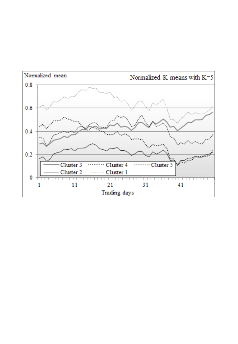
Chapter 4
[ 717 ]
The chart of the results of the K-means algorithms with 2 clusters shows that the
mean vector for the cluster labeled 2 is similar to the mean vector labeled 3 on
the chart with K = 3 clusters. However, the cluster with the mean vector 1 reects
somewhat the aggregation or summation of the mean vectors for the clusters 1 and 3
in the chart K =3. The aggregation effect explains why the standard deviation for the
cluster 1, 0.55, is twice as much as the standard deviation for the cluster 2, 0.28.
The mean (or centroid) vector for each cluster is plotted as follows for K = 5:
Chart of means of clusters using K-means K=5
In this chart, we can assess that the clusters 1 (with the highest mean), 2 (with the
lowest mean), and 3 are very similar to the clusters with the same labels in the chart
for K =3. The cluster with the mean vector 4 contains stocks whose behaviors are
quite similar to those in cluster 3, but in the opposite direction. In other words, the
stocks in cluster 3 and 4 reacted in opposite ways following the announcement of the
change in the monetary policy.
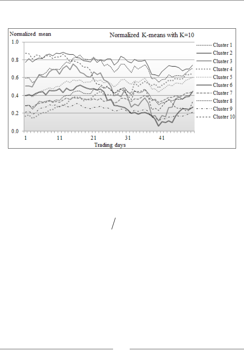
Unsupervised Learning
[ 718 ]
In the tests with high values of K, the distinction between the different clusters
becomes murky, as shown in the following chart for K = 10:
Chart of means of clusters using K-means K=10
The means for clusters 1, 2, and 3 seen in the rst chart for the case K = 3 are still
visible. It is fair to assume that these are very likely the most reliable clusters.
These clusters happened to have a low standard deviation or high density.
Let's dene the density of a cluster Cj with a centroid cj as the inverse of the
Euclidean distance between all members of each cluster and its mean (or centroid):
2
(C )1 ( )
j
j j
xC
dxc
∈
=−
∑
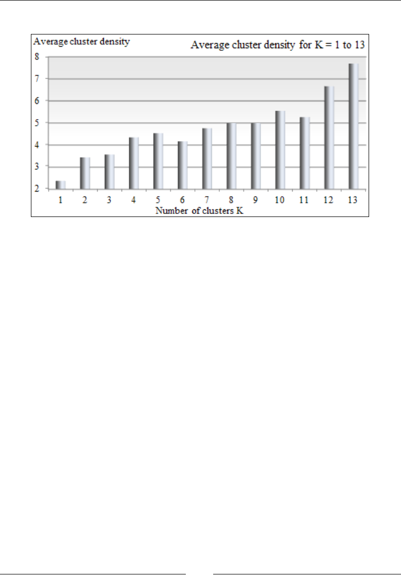
Chapter 4
[ 719 ]
The density of the cluster is plotted against the number of clusters with K = 1 to 13:
Bar chart of the average cluster density for K = 1 to 13
As expected, the average density of each cluster increases as K increases. From this
experiment, we can draw the simple conclusion that the density of each cluster does
not signicantly increase in the test runs for K =5 and beyond. You may observe that
the density does not always increase as the number of clusters increases (K = 6 to
K = 11). The anomaly can be explained by the following three factors:
• The original data is noisy
• The model is somewhat dependent on the initialization of the centroids
• The exit condition is too loose
Validation
There are several methodologies to validate the output of a K-means algorithm
from purity to mutual information [4:6]. One effective way to validate the output of
a clustering algorithm is to label each cluster and run those clusters through a new
batch of labeled observations. For example, if during one of these tests you nd that
one of the clusters CC contains most of the commodity-related stocks, then you can
select another commodity-related stock, SC, which is not part of the rst batch, and
run the entire clustering algorithm again. If SC is contained in CC, then the clustering
has performed as expected. If this is the case, you should run a new set of stocks,
some of which are commodity related, and measure the number of true positives, true
negatives, false positives, and false negatives. The precision, recall, and F1 measures
introduced in the Assessing a model section of Chapter 2, Hello World!, conrms whether
the tuning parameters and labels you selected for your cluster are indeed correct.

Unsupervised Learning
[ 720 ]
Validation
The quality of the clusters, as measured by the F1 statistics, depends
on the labeling of the cluster and the rule (that is, label a cluster with
the industry with the highest relative percentage of stocks in the
cluster) used to assign a label. This process is very subjective. The
only sure way to validate a validation methodology is to evaluate
several labeling schemes and select the one that generates the highest
F1 statistics.
We reviewed some of the tuning parameters that impact the quality of the results of
the K-means clustering. They are as follows:
• Initial selection of centroid
• Number of K clusters
In some cases, the similarity criterion (that is, Euclidean distance versus cosine value)
can have an impact on the cleanness or density of the clusters.
The nal and important consideration is the computational complexity of the
K-means algorithm. The previous sections of the chapter described some of the
performance issues with K-means and possible remedies.
Despite its many benets, the K-means algorithm does not handle missing data
or unobserved features very well. Features that depend on each other indirectly
may in fact depend on a common hidden (also known as latent) variable. The
expectation-maximization algorithm described in the next section addresses
some of these limitations.
Expectation-maximization (EM) algorithm
The expectation-maximization algorithm was originally introduced to estimate the
maximum likelihood in the case of incomplete data [4:7]. It is an iterative method to
compute the model features that maximize the likely estimate for observed values,
taking into account unobserved values.
The iterative algorithm consists of computing:
• The expectation, E, of the maximum likelihood for the observed data by
inferring the latent values (E-step)
• The model features that maximize the expectation E (M-step)
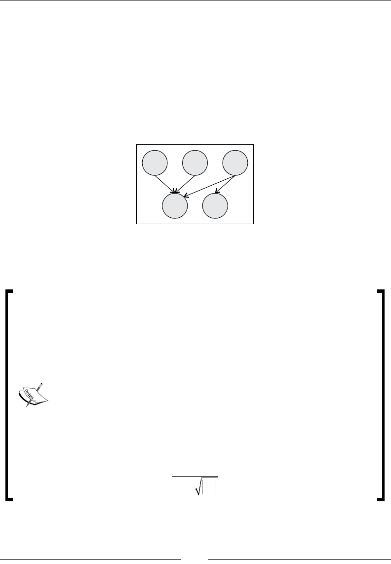
Chapter 4
[ 721 ]
The expectation-maximization algorithm is applied to solve clustering problems by
assuming that each latent variable follows a Normal or Gaussian distribution. This
is similar to the K-means algorithm for which the distance of each data point to the
center of each cluster follows a Gaussian distribution [4:8]. Therefore, a set of latent
variables is a mixture of Gaussian distributions.
Gaussian mixture model
Latent variables Z can be visualized as the behavior (or symptoms) of a model
(observed) X for which Z are the root causes of the behavior:
Z1Z2Z3
X1X2
Visualization of observed and latent features
The latent values Z follow a Gaussian distribution. For the statisticians among us, the
mathematics of a mixture model is described in the following information box.
The mixture model
If {xi} is a set of observed features associated with latent features {zk}, the
probability for the feature xi given zk has a value j:
(| )
ik
px Z j=
The probability p is called the base distribution. If we extend to the entire
model, θ= {xi, zk}, the conditional probability is dened as follows:
1
(|) (| )
J
ijik
j
px px Z j
θπ
=
= =
∑
The most widely used mixture model is the Gaussian mixture model
that represents the base distribution p as a Normal distribution and the
conditional probability as a weighted Normal multivariate distribution:
()
()()
1
/2
1
1
|
2
J
T
i j ij jij
d
jj
px ex x
θπ µ µ
π
− −
=
=−∑−
∑
∑

Unsupervised Learning
[ 722 ]
EM overview
As far as the implementation is concerned, the expectation-maximization algorithm
can be broken down into three stages:
1. The computation of the log likelihood for the model features given some
latent variables (LL).
2. The computation of the expectation of the log likelihood at iteration t (E-step).
3. The maximization of the expectation at iteration t (M-step).
Log likelihood
• LL: Let's consider a set of observed variables X={xi} and latent
variables Z={zi}. The log likelihood for X for given Z is:
()
()
log,|
ij
Lpxz
θ θ
=∑
• E-step: The expectation for the model variable θ at iteration t is
computed as:
() ()
,|,
t
t
QELX
θθ θ θ
⎡⎤
=⎣⎦
• M-step: The function Q is maximized for the model features θ as:
()
1argmax ,
t t
Q
θ
θθθ
+=
A formal, detailed, but short mathematical formulation of the EM algorithm can be
found in S. Borman's tutorial [4:9].
Implementation
Let's implement the three steps (LL, E-step, and M step) in Scala. The internal
calculations of the EM algorithm are a bit complex and overwhelming. You may
not benet much from the details of a specic implementation such as computation
of the eigenvalues of the covariance matrix of the expectation of the log likelihood.
This implementation hides some complexities by using the Apache Commons Math
library package [4:10].

Chapter 4
[ 723 ]
Inner workings of EM
You may want to download the source code for the implementation of
the EM algorithm in the Apache Commons Math library if you need to
understand the condition for which an exception is thrown.
First, let's dene convenient internal types:
type EM = MultivariateNormalMixtureExpectationMaximization
type EMOutput = List[(Double, DblVector, DblVector)]
import scala.collections.JavaConversions._ //1
The constructor of the MultivariateEM class uses the standard template for machine
learning algorithm classes:
• Parameterized view bound type
• Implementation of EM as a data transformation by extending PipeOperator
Here is an implementation of the constructor of MultivariateEM:
class MultivariateEM[T <% Double](K: Int) extends PipeOperator[XTSerie
s[Array[T]], EMOutput]
The Apache Commons Math Java implementation of the EM uses Java container
classes that need to be explicitly converted to Scala collections. Those conversions
are dened in the JavaConversions package (line 1).
The implementation of the EM algorithm in the data transformation |> operator uses
the Apache Commons Math MultivariateNormalMixture class for the Gaussian
mixture model and the MultivariateNormalMixtureExpectationMaximization
class for the EM algorithm:
def |> : PartialFunction[XTSeries[Array[T]], EMOutput] = {
case xt: XTSeries[Array[T]] if(xt.size>0 && dimension(xt)>0) =>{
val data: DblMatrix = xt //2
val multivariateEM = new EM(data)
val est = MultivariateNormalMixtureExpectationMaximization
.estimate(data, K)
multivariateEM.fit(est) //3
val newMixture = multivariateEM.getFittedModel //4
val components = newMixture.getComponents.toList //5
components.map(p => (p.getKey.toDouble, p.getValue.getMeans,
p.getValue.getStandardDeviations) ))//6
….

Unsupervised Learning
[ 724 ]
Let's look at the main |> method of the MultivariateEM wrapper class. The rst step
is to convert the time series into a primitive matrix of Double with observations and
historical quotes as rows and the stock symbols as columns (line 2).
The initial mixture of Gaussian distributions can be provided by the user or can
be extracted from the dataset as an estimate (line 3). The getFittedModel model
triggers the M-step (line 4).
The Apache library uses Java primitives that need to be converted to Scala types
using the package import scala.collection.JavaConversions. An instance
of java.util.List is converted to scala.collection.immutable.List using
toList, which invokes the asScalaIterator method of WrapAsScala, one of the
base traits of JavaConversions (line 5).
The <Double, MultivariateNormalDistribution> key-value pair, returned by
the call to getFittedModel by the Apache math method, is to be converted to a tuple
containing the mean and standard deviation for each cluster (line 6).
Third-party library exceptions
Scala does not enforce the declaration of exceptions as part of the
signature of a method. Therefore, there is no guarantee that all
types of exceptions will be caught locally. This problem occurs
when exceptions are thrown from a third-party library in two
scenarios:
• The documentation of the API does not list all the types of
exceptions
• The library is updated and a new type of exception is
added to a method
One easy workaround is to leverage the Scala exception-handling
mechanism:
Try {
..
} match {
case Success(results) => …
case Failure(exception) => ...
}

Chapter 4
[ 725 ]
Testing
Let's apply the MultivariateEM class to the clustering of the same 127 stocks used in
evaluating the K-means algorithm.
As discussed in the paragraph related to the curse of dimensionality, the number
of stocks (127) to analyze restricts the number of observations to be used by the EM
algorithm. A simple option is to lter out some of the noise of the stocks and apply a
basic sampling method. The maximum sampling rate is restricted by the frequencies
in the spectrum of noises of different types in the historical price of every stock.
Filtering and sampling
The preprocessing of the data using a combination of a simple
moving average and xed interval sampling prior to clustering is very
rudimentary in this example. For instance, we cannot assume that the
historical quotes of all the stocks share the same noise characteristics.
The noise pattern in the quotation of momentum and heavily traded
stocks is certainly different from blue-chip securities with a strong
ownership, and these stocks are held by large mutual funds.
The sampling rate should take into account the spectrum of frequency
of the noise. It should be set as at least twice the frequency of the noise
with the lowest frequency.
The object of the test is to evaluate the impact of the sampling rate, samplingRate,
and the number K of clusters used in the EM algorithm:
val extractor = YahooFinancials.adjClose :: List[Array[String]
=>Double]() //1
val period = 8
val samplingRate = 10
val smAv = SimpleMovingAverage[Double](period) //2
val obs = DataSource.listSymbols(path).map(sym => { //3
val xs = DataSource(sym, path, true) |> extractor //2
val values : XTSeries[Double] = XTSeries.|>(xs)).head //4
val filtered = smAv |> values
filtered.zipWithIndex //5
.drop(period+1).toArray //6
.filter( _._2%samplingRate==0)
.map( _._1)
})
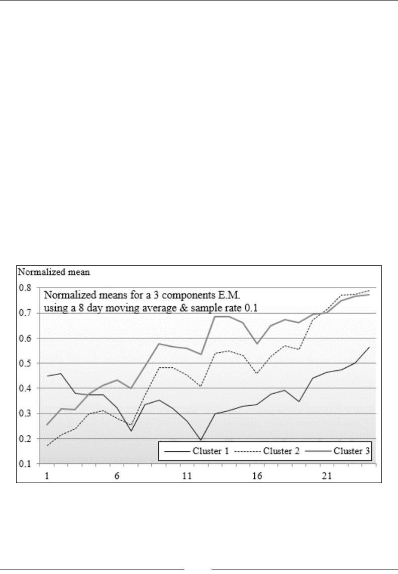
Unsupervised Learning
[ 726 ]
The rst step is to extract the historical quotes for all the stocks using the same
extractor as in the K-means test case (line 1).
The symbols of the stocks under consideration are extracted from the name of the
les in the path directory. The historical data is contained in the CSV le named
path/STOCK_NAME.csv (line 3). An implicit conversion is triggered by an assignment
of values of the type XTSeries[Double] (line 4). The simple moving average
algorithm zeroed out the rst period values in the smoothed data, filtered (line 5).
Those null values have to be dropped before applying the sampling (line 6).
The rst test is to execute the EM algorithm with K=3 clusters and a sampling period
of 10 on data smoothed by a simple moving average with a period of 8:
MultivariateEM[Double](K) |> XTSeries[DblVector](obs) foreach (…)
The driver prints the key (line 3), the mean (coordinates of the centroid vector) (line
4), and the standard deviation for each component (cluster).
The sampling of historical prices of the 127 stocks between January 1, 2013 and
December 31, 2013 with a frequency of 0.1 hertz produces 24 data points. The
following chart displays the mean or centroid of each of the 3 clusters:
Chart of the normalized means per cluster using EM K=3
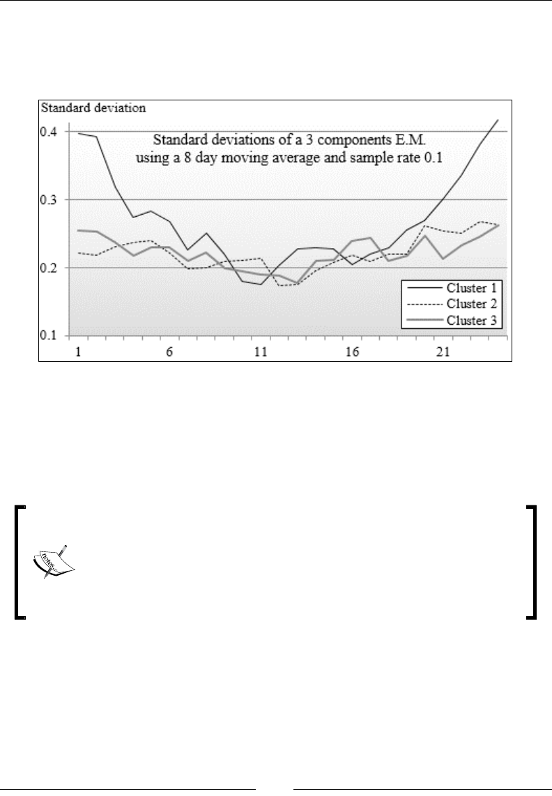
Chapter 4
[ 727 ]
The mean vectors of clusters 2 and 3 have similar patterns, which may suggest
that 2 components or clusters could provide a rst insight into the similarity within
groups of stocks. The following is a chart of the normalized standard deviation per
cluster using EM K = 3:
Chart of the normalized standard deviation per cluster using EM K=3
The distribution of the standard deviation along the mean vector of each cluster can
be explained by the fact that the price of stocks from a couple of industries went
down in synergy, while others went up as a semihomogenous group following the
announcement from the Federal Reserve that the monthly quantity of bonds purchased
as part of the quantitative easing program would be reduced in the near future.
Relation to K-means
You may wonder what is the relation between EM and K-means as
both techniques address the same problem. The K-means algorithm
assigns each observation uniquely to one and only one cluster. The
EM algorithm assigns an observation based on posterior probability.
K-means is a special case of the EM for Gaussian mixtures [4:11].

Unsupervised Learning
[ 728 ]
Online EM
Online learning is a powerful strategy for training a clustering model when dealing
with very large datasets. This strategy has regained interest from scientists lately.
The description of online EM is beyond the scope of this tutorial. However, you may
need to know that there are several algorithms available for online EM if you ever
have to deal with large datasets: batch EM, stepwise EM, incremental EM, and
Monte Carlo EM [4:12].
Dimension reduction
Without prior knowledge of the data domain, data scientists include all possible
features in their rst attempt to create a classication, prediction, or regression
model. After all, making assumptions is a poor and dangerous approach to reduce
the search space. It is not uncommon for a model to use hundreds of features, adding
complexity and signicant computation costs to build and validate the model.
Noise-ltering techniques reduce the sensitivity of the model to features that
are associated with sporadic behavior. However, these noise-related features
are not known prior to the training phase, and therefore, cannot be discarded.
As a consequence, training of the model becomes a very cumbersome and
time-consuming task.
Overtting is another hurdle that can arise from a large feature set. A training set of
limited size does not allow you to create a model with a large number of features.
Dimension reduction techniques alleviate these problems by detecting features that
have little inuence on the overall model behavior.
There are three approaches to reduce the number of features in a model:
• Statistical analysis solutions such as ANOVA for smaller feature sets
• Regularization and shrinking techniques, which are introduced in Chapter 6,
Regression and Regularization
• Algorithms that maximize the variance of the dataset by transforming the
covariance matrix
The next section introduces one of the most commonly used algorithms of the third
category—principal component analysis.
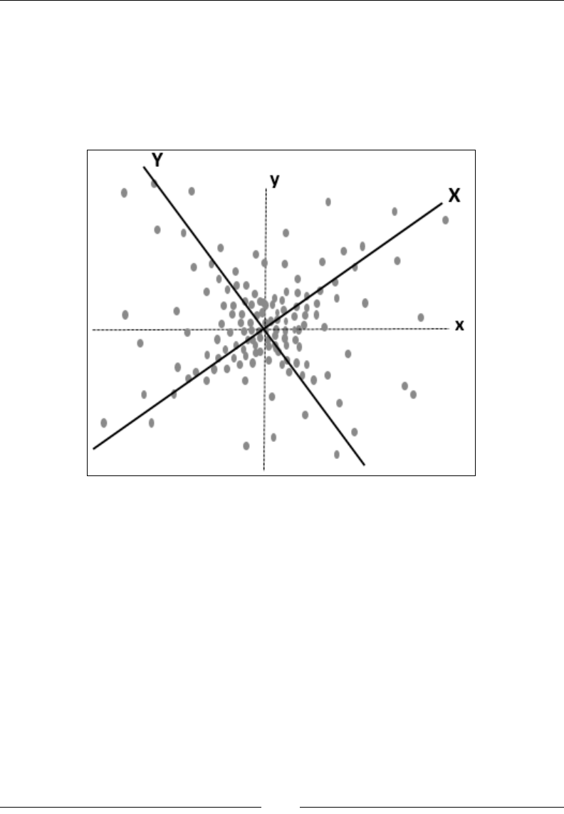
Chapter 4
[ 729 ]
Principal components analysis (PCA)
The purpose of principal components analysis is to transform the original set of
features into a new set of ordered features by decreasing the order of variance. The
original observations are transformed into a set of variables with a lower degree of
correlation. Let's consider a model with two features {x, y} and a set of observations
{xi, yi} plotted on the following chart:
Visualization of principal components for a 2-dimension model
The features x and y are converted into two variables X and Y (that is rotation) to
more appropriately match the distribution of observations. The variable with the
highest variance is known as the rst principal component. The variable with the
nth highest variance is known as the nth principal component.

Unsupervised Learning
[ 730 ]
Algorithm
I highly recommend the tutorial from Lindsay Smith [4:13] that describes the PCA
algorithm in a very concrete and simple way using a 2-dimension model.
PCA and covariance matrix
The covariance of two features X and Y with the observations set {xi, yi}
is dened as:
() ()()
1
,
1
i i
covXY xxyy
n
=−−
−
∑
Here,
x
and
y
are the respective mean values for the observations x
and y.
The covariance is computed from the zScore of each observation:
()
/
ii
xxx
σ
=−
For a model with n features, xi, the covariance matrix is dened as:
() ()
()
() ()
00 01
10 11
cov, cov,
cov,
cov, cov,
n
ij
nnn
xx xx
xx
xx xx
−
−−−
⎡ ⎤
⎢ ⎥
=⎢ ⎥
⎢ ⎥
⎣ ⎦
∑
L
M M
K
The transformation of x to X consists of computing the eigenvalues of
the covariance matrix:
()
',
T T
ij
WW cov X X and X W x∑=Σ= =
The eigenvalues are ranked by their decreasing order of variance and
the cumulative variance for each eigenvalue is computed. Finally,
the m top eigenvalues for which the cumulative of variance exceeds
a predened threshold (percentage of the trace of the matrix) are the
principal components or reduced feature set.
() ()
1
1: |,
m
ikk
k
Z X m cov x x Tr cov
=
⎧ ⎫
= >∈⋅
⎨ ⎬
⎩ ⎭
∑
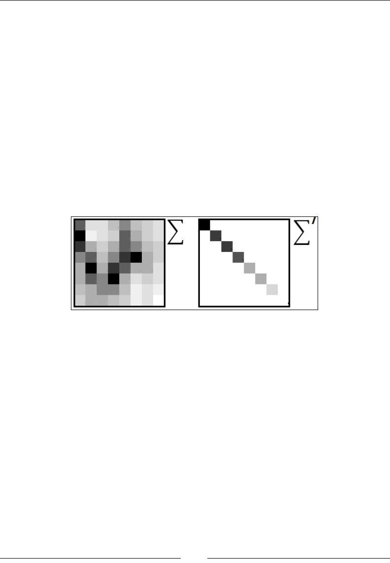
Chapter 4
[ 731 ]
The algorithm is implemented in ve steps:
1. Compute the zScore for the observations by standardizing the mean and
standard deviation.
2. Compute the covariance matrix Σ for the original set of observations.
3. Compute the new covariance matrix Σ' for the observations with the
transformed features by extracting the eigenvalues and eigenvectors.
4. Convert the matrix to rank eigenvalues by decreasing the order of variance.
The ordered eigenvalues are the principal components.
5. Select the principal components for which the total sum of variance exceeds a
threshold by as a percentage of the trace of the new covariance matrix.
The extraction of principal components by diagonalization of the covariance matrix
Σ is visualized in the following diagram. The color used to represent the covariance
value varies from white (lowest value) to black (highest value):
Visualization of the extraction of eigenvalues in PCA
The eigenvalues (variance of X) are ranked by the decreasing order of their values.
The PCA algorithm succeeds when the cumulative value of the last eigenvalues
(the right-bottom section of the diagonal matrix) becomes insignicant.
Implementation
PCA can be easily implemented by using the Apache Commons Math library
methods that compute the eigenvalues and eigenvectors. Once again, the main
routine is implemented as a pipe operator so that it can be used in a generic
workow as dened in the The Pipe Operator section under Designing a workow
in Chapter 2, Hello World!.
import types.ScalaMl._, types.CommonMath._, //2
def |> : PartialFunction[XTSeries[Array[T]], (DblMatrix, DblVector)]={
case xt: XTSeries[Array[T]] if(xt !=null && xt.size>1) => {

Unsupervised Learning
[ 732 ]
zScoring(xt) match {//1
case Some(obs) => {
val covariance = new Covariance(obs).getCovarianceMatrix //3
val transf = new EigenDecomposition(covariance)
val eigVectors = transf.getV //4
val eigValues = new ArrayRealVector(transf.getRealEigenvalues)
val cov = obs.multiply(eigVectors).getData
(cov, eigValues.toArray) //5
…
PCA requires that the original set of observations is standardized using the
z-score transformation. It is implemented using the XTSeries.zScoring function
introduced in the Normalization and Gauss distribution section in Chapter 1, Getting
Started (line 1).
The assignment forces the implicit conversion of a time series of features of the type
T into a matrix of the type Double. The implicit conversions between Scala primitives
and ScalaMl types such as DblMatrix (resp. between Apache Commons Math types
and Scala Ml) are dened in Types.ScalamMl, as mentioned in the Type conversions
section in Chapter 1, Getting Started (resp. Types.CommontMath in the Time series
section in Chapter 3, Data Preprocessing) (line 2). The covariance matrix is computed
based on the zScore created from the original observations (line 3). The eigenvectors,
eigVectors, are computed using the getV method in the Apache Commons Math
EigenDecomposition class. The eigenvalues, eigValues, are extracted as principal
components (line 4).
Finally, the data transformation returns the tuple (covariance matrix, array of
eigenvalues) (line 5).
Test case
Let's apply the PCA algorithm to extract a subset of the features that represents
some of the nancial metrics ratios of 34 S&P 500 companies. The metrics under
consideration are:
• Trailing Price-to-Earnings ratio (PE)
• Price-to-Sale ratio (PS)
• Price-to-Book ratio (PB)
• Return on Equity (ROE)
• Operation Margin (OM)
The nancial metrics are described in the Terminology section under Finances 101 in
Appendix A, Basic Concepts.
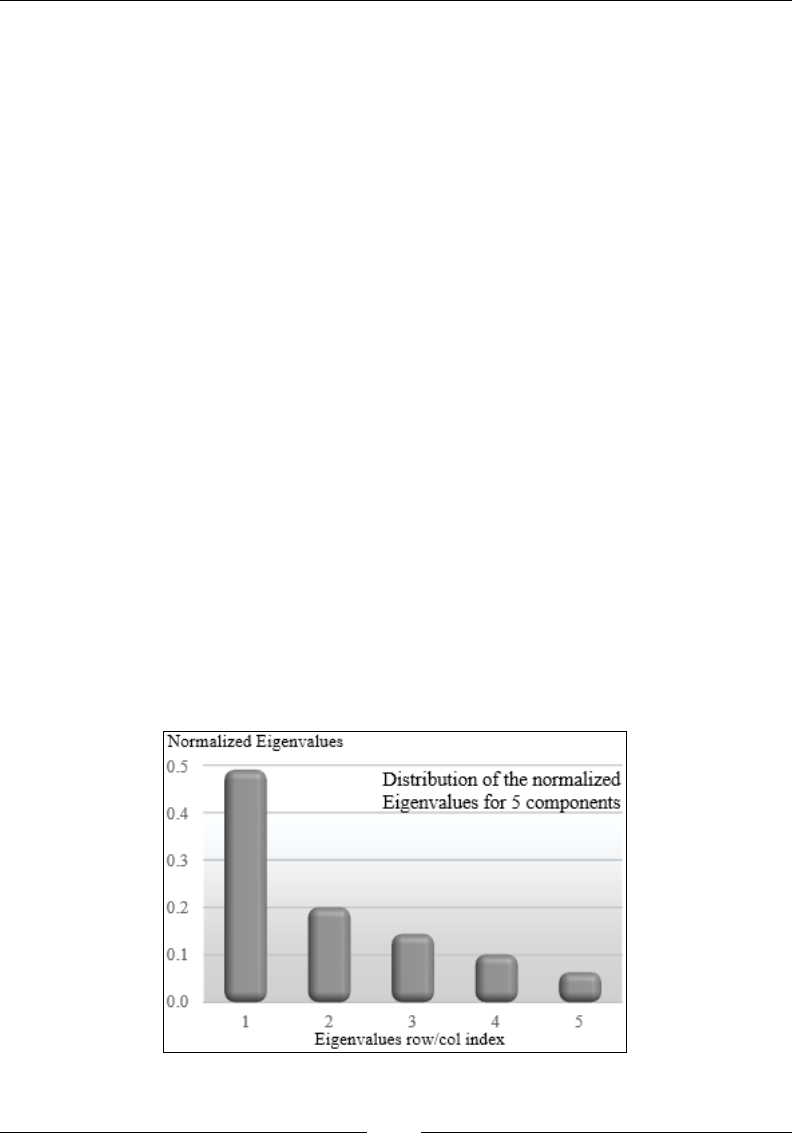
Chapter 4
[ 733 ]
The input data is specied with the following format as a tuple: the ticker symbol
and an array of ve nancial ratios, PE, PS, PB, ROE, and OM:
val data = Array[(String, DblVector)] (
// Ticker PE PS PB ROE OM
("QCOM", Array[Double](20.8, 5.32, 3.65, 17.65,29.2)),
("IBM", Array[Double](13, 1.22, 12.2, 88.1,19.9)),
…
)
The client code that executes the PCA algorithm is dened simply as follows:
val pca = new PCA[Double] //1
val input = data.map( _._2.take(3))
val cov = pca |> XTSeries[DblVector](input) //2
Display.show(toString(cov), logger) //3
Once the PCA class is instantiated (line 1), the eigenvalues and covariance matrix,
cov, are computed (line 2), and then displayed using the utility singleton Display
that formats messages and appends to the logger (line 3).
Evaluation
The rst test on the 34 nancial ratios uses a model that has ve dimensions.
As expected, the algorithm produces a list of ve ordered eigenvalues.
2.5321, 1.0350, 0.7438, 0.5218, 0.3284
Let's plot the relative value of the eigenvalues (that is, relative importance of each
feature) on a bar chart:
Distribution of eigenvalues in PCA for 5 dimensions
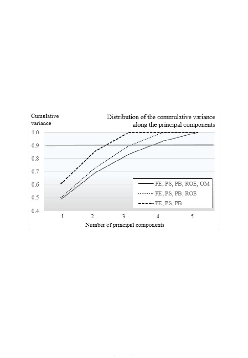
Unsupervised Learning
[ 734 ]
The chart shows that 3 out of 5 features account for 85 percent of total variance
(trace of the transformed covariance matrix). I invite you to experiment with
different combinations of these features. The selection of a subset of the existing
features is as simple as applying Scala's take or drop methods:
Val numFeatures = 4
val ts = XTSeries[DblVector](data.map(_._2.take(numFeatures)))
Let's plot the cumulative eigenvalues for the three different model congurations:
• Five features: PE, PS, PB, ROE, and OM
• Four features: PE, PS, PB, and ROE
• Three features: PE, PS, and PB
Distribution of eigenvalues in PCA for 3, 4, and 5 features
The chart displays the cumulative value of eigenvalues that are the variance of the
transformed features Xi. If we apply a threshold of 90 percent to the cumulative
variance, then the number of principal components for each test model is as follows:
• {PE, PS, PB}: 2
• {PE, PS, PB, ROE}:3
• {PE, PS, PB, ROE, OM}: 3
In conclusion, the PCA algorithm reduced the dimension of the model by 33 percent
for the 3-feature model, 25 percent for the 4-feature model, and 40 percent for the
5-feature model for a threshold of 90 percent.

Chapter 4
[ 735 ]
Cross-validation of PCA
Like any other unsupervised learning technique, the resulting principal
components have to be validated through a one or K-fold cross-validation
using a regression estimator such as partial least square regression
(PLSR) or the predicted residual error sum of squares (PRESS). For
those not afraid of statistics, I recommend Fast Cross-validation in Robust
PCA by S. Engelen and M. Hubert [4:14]. You need to be aware, however,
that the implementation of these regression estimators is not simple.
The principal components can be validated through a 1-fold or K-fold cross-validation,
by performing some type of regression estimators or EM on the same dataset. The
validation of the PCA is beyond the scope and space allocated to this chapter.
Principal components analysis is a special case of the more general factor analysis.
The later class of algorithm does not require the transformation of the covariance
matrix to be orthogonal.
Other dimension reduction techniques
Although quite popular, the principal components analysis is far from being the
only dimension reduction method. Here are some alternative techniques, listed
as reference: factor analysis, principal factor analysis, maximum likelihood factor
analysis, independent component analysis (ICA), Random projection, nonlinear
PCA, nonlinear ICA, Kohonen's self-organizing maps, neural networks, and
multidimensional scaling, just to name a few [4:15].
Performance considerations
The three unsupervised learning techniques share the same limitation—a high
computational complexity.
K-means
The K-means has the computational complexity of O(iKnm), where i is the number of
iterations, K the number of clusters, n the number of observations, and m the number
of features. The algorithm can be improved through the use of other techniques by
using the following techniques:
• Reducing the average number of iterations by seeding the centroid using an
algorithm such as initialization by ranking the variance of the initial cluster
as described at the beginning of this chapter.

Unsupervised Learning
[ 736 ]
• Using a parallel implementation of K-means and leveraging a large-scale
framework such as Hadoop or Spark.
• Reducing the number of outliers and possible features by ltering out the
noise with a smoothing algorithm such as a discrete Fourier transform or a
Kalman lter.
• Decreasing the dimensions of the model by following a two-step process: a
rst pass with a smaller number of clusters K and/or a loose exit condition
regarding the reassignment of data points. The data points close to each
centroid are aggregated into a single observation. A second pass is then run
on a smaller set of observations.
EM
The computational complexity of the expectation-maximization algorithm for each
iteration (E + M steps) is O(m2n), where m is the number of hidden or latent variables
and n is the number of observations.
A partial list of suggested performance improvement includes:
• Filtering of raw data to remove noise and outliers
• Using a sparse matrix on a large feature set to reduce the complexity of the
covariance matrix, if possible
• Applying the Gaussian mixture model (GMM) wherever possible: the
assumption of Gaussian distribution simplies the computation of the
log likelihood
• Using a parallel data processing framework such as Apache Hadoop or Spark
as explained in the Apache Spark section in Chapter 12, Scalable Frameworks
• Using a kernel method to reduce the estimate of covariance in the E-step
PCA
The computational complexity of the extraction of the principal components is O(m2n
+ n3), where m is the number of features and n the number of observations. The rst
term represents the computational complexity for computing the covariance matrix.
The last term reects the computational complexity of the eigenvalue decomposition.

Chapter 4
[ 737 ]
The list of potential performance improvements or alternative solutions for
PCA includes:
• Assuming that the variance is Gaussian
• Using a sparse matrix to compute eigenvalues for problems with large
feature sets and missing data
• Investigating alternatives to PCA to reduce the dimension of a model such
as the discrete Fourier transform (DFT) or singular value decomposition
(SVD) [4:16]
• Using the PCA in conjunction with EM (a research)
• Deploying a dataset on a parallel data processing framework such as Apache
Spark or Hadoop as explained in the Apache Spark section in Chapter 12,
Scalable Frameworks
Summary
This completes the overview of three of the most commonly used unsupervised
learning techniques:
• K-means for clustering fully observed features of a model with
reasonable dimensions
• Expectation-maximization for clustering a combination of observed and
latent features
• Principal components analysis to transform and extract the most critical
features in terms of variance
The key point to remember is that unsupervised learning techniques are used:
• By themselves to extract structures and associations from
unlabelled observations
• As a preprocessing stage to supervised learning in reducing the number
of features prior to the training phase
In the next chapter, we will address the second use case, and cover supervised
learning techniques starting with generative models.

Naïve Bayes Classiers
This chapter introduces the most common and simple generative classiers—Naïve
Bayes. As a reminder, generative classiers are supervised learning algorithms
that attempt to t a joint probability distribution, p(X,Y), of two events X and Y,
representing two sets of observed and hidden (or latent) variables, x and y.
In this chapter, you will learn, and hopefully appreciate, the simplicity of the Naïve
Bayes technique through a concrete example. Then, you will build a Naïve Bayes
classier to predict stock price movement, given some prior technical indicators
in the analysis of nancial markets.
Finally, you will apply Naïve Bayes to text mining by predicting stock prices,
using nancial news feed and press releases.
Probabilistic graphical models
Let's start with a refresher course in basic statistics.
Given two events or observations, X and Y, the joint probability of X and Y
is dened as
()( )
,pXY pX Y=∩
. If the observations X and Y are not related, an
assumption known as conditional independence, then p(X,Y) = p(X).p(Y). The
conditional probability of event Y, given X, is dened as p(Y|X)=p(X,Y)/p(X).
These two denitions are quite simple. However, probabilistic reasoning can be
difcult to read in the case of large numbers of variables and sequences of conditional
probabilities. As a picture is worth a thousand words, researchers introduced graphical
models to describe a probabilistic relation between random variables [5:1].
There are two categories of graphs, and therefore, graphical models:
• Directed graphs such as Bayesian networks
• Undirected graphs such as conditional random elds (refer to the Conditional
random elds section in Chapter 7, Sequential Data Models)
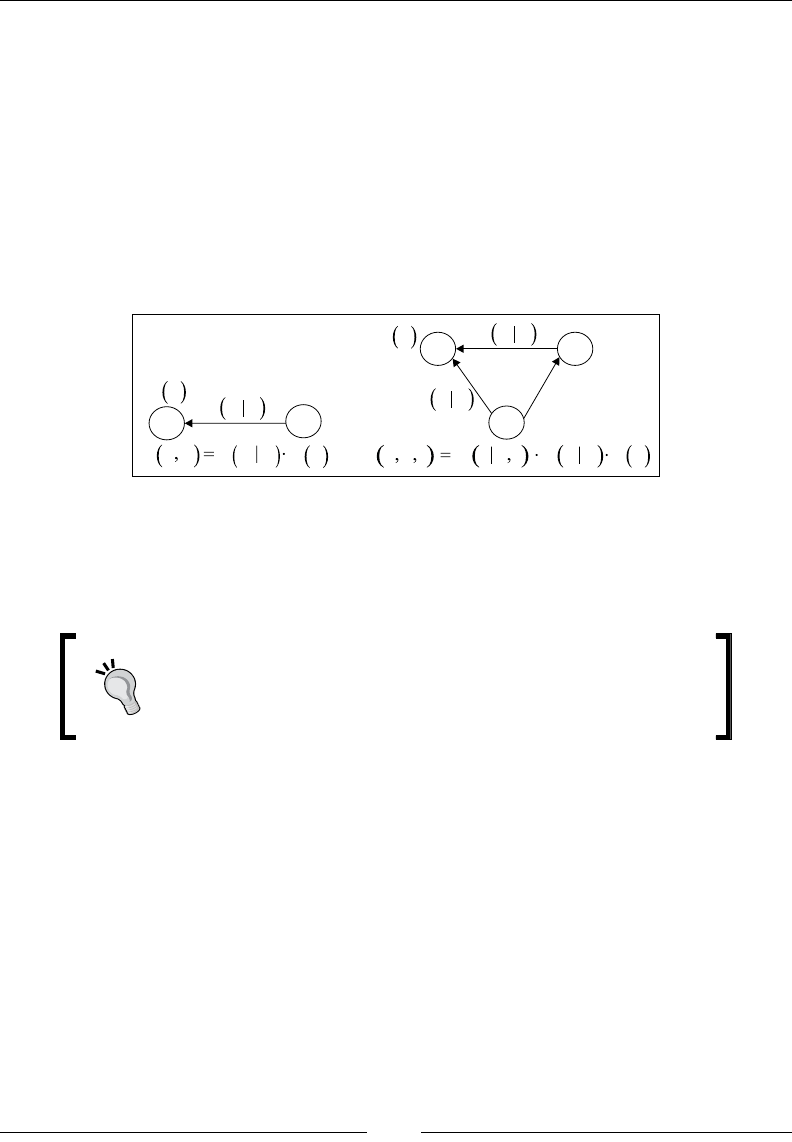
Naïve Bayes Classiers
[ 740 ]
Directed graphical models are directed acyclic graphs that have been introduced to:
• Provide a simple way to visualize a probabilistic model
• Describe the conditional dependence (or independence) between variables
• Represent statistical inference in terms of graphical manipulation
A Bayesian network is a directed graphical model dening a join probability over a
set of variables [5:2].
The two join probabilities, p(X,Y) and p(X,Y,Z), can be graphically modeled using
Bayesian networks, as follows:
XY
YX
Z
pXY
p
ppp
p
p
pp
ppp
XXX
XX
X
XXXX
YYY
Y
Y
Y
Z
ZZ
X
Examples of probabilistic graphical models
The conditional probability p(Y|X) is represented by an arrow directed from the
output (or symptoms) Y to the input (or cause) X. Elaborate models can be described
as a large directed graph between variables.
Metaphor for graphical models
From a software engineering perspective, graphical models
visualize probabilistic equations the same way the UML class
diagram visualizes object-oriented source code.
Here is an example of a real-world Bayesian network; the functioning of a
smoke detector:
1. A re may generate smoke.
2. Smoke may trigger an alarm.
3. A depleted battery may trigger an alarm.
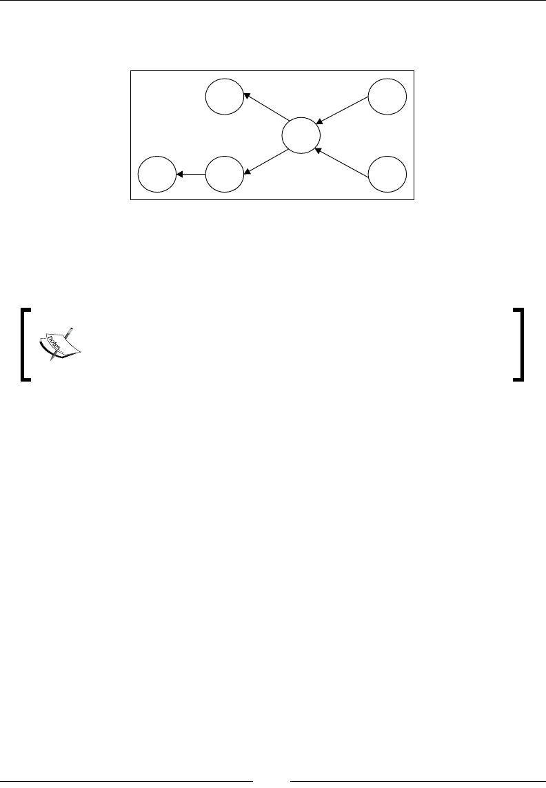
Chapter 5
[ 741 ]
4. The alarm may alert the homeowner.
5. The alarm may alert the re department.
Alarm
Smoke
Battery
Fire
Home
owner
Fire
dept
A Bayesian network for smoke detectors
This representation may be a bit counterintuitive, as the vertices are directed from
the symptoms (or output) to the cause (or input). Directed graphical models are
used in many different models, besides Bayesian networks [5:3].
Plate models
There are several alternate representations of probabilistic models,
besides the directed acyclic graph, such as the plate model commonly
used for the latent Dirichlet allocation (LDA) [5:4].
The Naïve Bayes models are probabilistic models based on the Bayes's theorem
under the assumption of features independence, as mentioned in the Generative
models section in Chapter 1, Getting Started.
Naïve Bayes classiers
This conditional independence between X features is an essential requirement for the
Naïve Bayes classier. It also restricts its applicability. The Naïve Bayes classication
is better understood through simple, concrete examples [5:5].
Introducing the multinomial Naïve Bayes
Let's consider the problem of how to predict change in interest rates. The rst step is
to list the factors that potentially may trigger or cause an increase or decrease in the
interest rates. For the sake of illustrating Naïve Bayes, we will select the consumer
price index (CPI), change in the Federal fund rate (FDF) and the gross domestic
product (GDP) as a rst set of features. The terminology is described in the
Terminology section under Finances 101 in Appendix A, Basic Concepts.
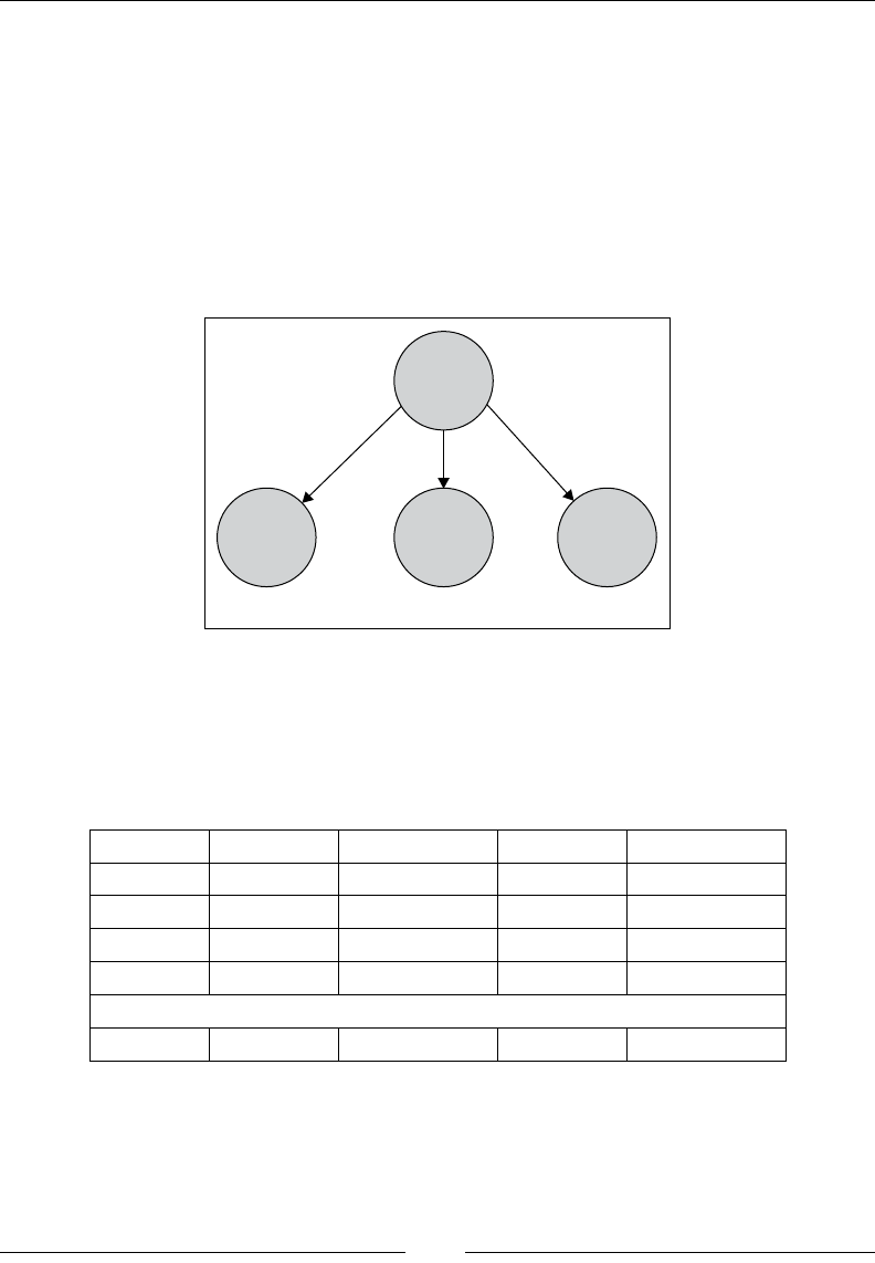
Naïve Bayes Classiers
[ 742 ]
The use case is to predict direction of the change in the yield of the 1-year Treasury
bill (1yTB), taking into account the change in the current CPI, FDF, and GDP.
The objective is, therefore, to create a predictive model using a combination
of these three features.
It is assumed that there is no available nancial investment expert who can supply
rules or policies to predict interest rates. Therefore, the model depends highly on the
historical data. Intuitively, if one feature is always increasing when the yield of the
1-year Treasury bill increases, then we can conclude that there is a strong correlation
of causal relationship between the features and the output variation in interest rates.
Change in
1yTB
Output
(labeled data)
Change in
GDP
Change in
FDF
Change in
CPI
Model features
The Naïve Bayes model for predicting the change in the yield of the 1-year T-bill
The correlation (or cause-effect relationship) is derived from historical data. The
methodology consists of counting the number of times each feature either increases
(UP) or decreases (DOWN), and recording the corresponding output (or labeled
data), as illustrated in the following table:
ID GDP FDF CPI 1yTB
1 UP DOWN UP UP
2 UP UP UP UP
3 DOWN UP DOWN DOWN
4 UP DOWN DOWN DOWN
…
256 DOWN DOWN UP DOWN
Chapter 5
[ 743 ]
First, let's tabulate the number of occurrence of each change {UP, DOWN} for the
three features and the output value (the 1-year Treasury bill):
Number GDP FDF CPI 1yTB
UP 169 184 175 159
DOWN 97 72 81 97
Total 256 256 256 256
UP/Total 0.66 0.72 0.68 0.625
Next, let's compute the number of positive directions for each of the features when
the yield 1-year Treasury bill increases (159 occurrences):
Number GDP Fed funds CPI
UP 110 136 127
DOWN 49 23 32
Total 159 159 159
UP/Total 0.69 0.85 0.80
For this table, we conclude that the yield of the 1-year Treasury bill increases when
the GDP is increasing (69 percent of the time), the rate of the Federal funds increases
(85 percent of the time) and the CPI increases (80 percent of the time).
Let's formalize the Naïve Bayes model before turning these ndings into a
probabilistic model.
Formalism
Let's start by clarifying the terminology used in the Bayesian model:
• Class prior probability or class prior is the probability of a class
• Likelihood is the probability of an observation given a class, also known as
the probability of the predictor given a class
• Evidence is the probability of observations occurring, also known as the
prior probability of the predictor
• Posterior probability is the probability of an observation x being in a
given class
No model can be simpler! The log likelihood, log(p(x|C), is commonly used instead
of the likelihood, p(x|C), (probability of an observation given a class) in order to
reduce the impact of the features y that have a low likelihood, p(y|C).

Naïve Bayes Classiers
[ 744 ]
The objective of the Naïve Bayes classication of a new observation, is to compute
the class that has the higher log likelihood. The mathematical notation for the Naïve
Bayes model is also straightforward.
The posterior probability,
()
|
j
pC x
:
()
()()
()
|
|j j
j
pxC pC
pC x
px
⋅
=
• x = {xi} (0, n-1), with a set of n features
• {Cj}, a set of classes with their class prior p(Cj)
•
()
px
, the evidence of new observation
• p(x| Cj), the likelihood for each feature
Posterior probability,
()
|
j
pC x
, with conditional independence:
() ( )()
1
0
| |
−
=
=⋅
∏
n
jjj j
i
pC x px C pC
• xi are independent and the probabilities are normalized
for evidence p(x) = 1
Log-likelihood:
() ( ) ()
1
0
log| log| log
n
jij j
i
pC x px C pC
−
=
= +
∑
Naïve Bayes classication:
()
( )
Carg max log |
m j
j
pC x
=
This particular use case has a major drawback—the GDP statistics are provided
quarterly, while the CPI data is made available once a month and a change in the
FDF rate is rather infrequent.
The frequentist perspective
The ability to compute the posteriori probability depends on the formulation of the
likelihood using historical data. A simple solution is to count the occurrences of
observations for each class and compute the frequency.
Let's consider the rst example that predicts the direction of change in the yield of
the 1-year Treasury bill given changes in the GDP, FDF, and CPI.
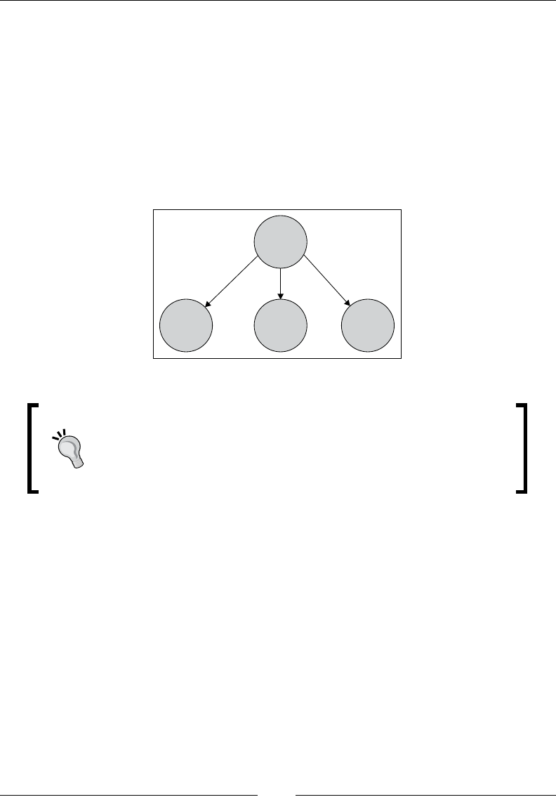
Chapter 5
[ 745 ]
The results are expressed with simple probabilistic formulas and a directed
graphical model:
P(GDP=UP|1yTB=UP) = 110/159
P(1yTB=UP) = num occurrences (1yTB=UP)/total num of
occurrences=159/256
p(1yTB=UP|GDP=UP,FDF=UP,CPI=UP) = p(GDP=UP|1yTB=UP) x
p(FDF=UP|1yTB=UP) x
p(CPI=UP|1yTB=UP) x
p(1yTB=UP) = 0.69 x 0.85 x
0.80 x 0.625
1yTB=UP
GDP=UP
P=0.69
FD=UP
P=0.85
CPI=UP
P=0.80
The Bayesian network for the prediction of the change of the yield of the 1-year Treasury bill
Overtting
The Naïve Bayes model is not immune to overtting, in case the
number of observations is not large enough relative to the number
of features. One approach to address this problem is to perform a
feature selection, using the mutual information exclusion [5:6].
This problem is not a good candidate for a Bayesian classication for two reasons:
• The training set is not large enough to compute accurate prior probabilities
and generate a stable model; decades of quarterly GDP data is needed to
train and validate the model
• The features have different rates of change, which predominately favor the
feature with the highest frequency; in this case, the CPI
Let's select another use case for which a large historical data set is available and can
be automatically labeled.
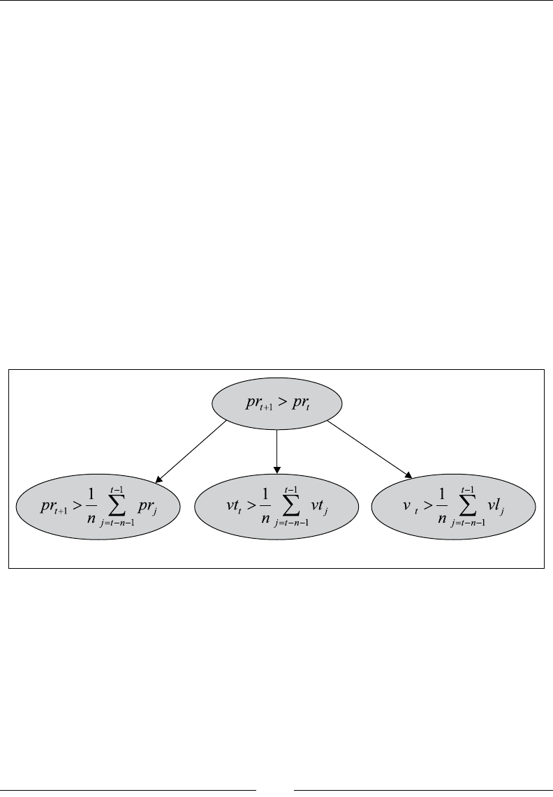
Naïve Bayes Classiers
[ 746 ]
The predictive model
The predictive model is the second use case that consists of predicting the direction
of the closing price of a stock, pr(t+1) = {UP, DOWN}, at trading day t+1, given the
history of its direction of the price, volume, and volatility for the previous t days,
pr(i),i=1,t. The features volume and volatility have been already used in the Creating
a model (learning) section under Let's kick the tires in Chapter 1, Getting Started.
Therefore, the three features under consideration are:
• The closing price, pr(t), of the last trading session, t, is above or below the
average closing price over the n previous trading days, [t-n, t]
• The volume of the last trading day, vl(t), is above or below the average
volume of the n previous trading days
• The volatility on the last trading day, vt(t), is above or below the average
volatility of the previous n trading days
The directed graphic model can be expressed using one output variable (price at
session t+1 is greater than price at session t) and three features: price condition (1),
volume condition (2), and volatility condition (3).
Output
(labeled data)
Price condition Volatility condition Volume condition
l
A Bayesian model for predicting the future direction of the stock price
This model works under the assumption that there is at least one observation, and
ideally few observations for each feature and for each labeled output.
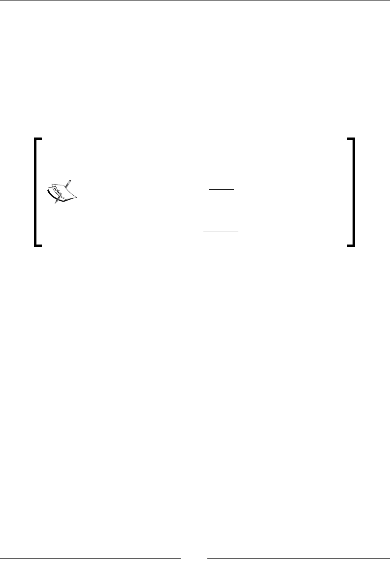
Chapter 5
[ 747 ]
The zero-frequency problem
It is possible that the training set does not contain any data actually observed for a
feature for a specic label or class. In this case, the mean is 0/N = 0, and therefore, the
likelihood is null, making classication unfeasible. The case for which there are only
few observations for a feature in a given class is also an issue, as it skews the likelihood.
There are a couple of correcting or smoothing formulas for unobserved features
or features with a low number of occurrences that address this issue, such as the
Laplace and Lidstone smoothing formula.
The smoothing factor for counters
Laplace smoothing of the mean k/N out of N observations
of features of dimension n:
1
'
µ
+
=
+
k
Nn
Lidstone smoothing with a factor
α
:
'
α
µα
+
=
+⋅
k
Nn
The two formulas are commonly used in natural language processing applications,
for which occurrence of a specic word or tag is a feature [5:7].
Implementation
I think it is time to write some Scala code and toy around with Naïve Bayes.
Let's start with an overview of the software components.
Software design
Our implementation of the Naïve Bayes classier uses the following components:
• A generic model, NaiveBayesModel, of the type Model, which is initialized
through training during the instantiation of the class.
• A model for the binomial classication, BinNaiveBayesModel, which
subclasses NaiveBayesModel. The model consists of a density function of
the type Density, and a pair of positive and negative Likelihood instances.
• A model for the multinomial classication MultiNaiveBayesModel.
• The predictive or classication routine is implemented as a data
transformation extending the PipeOperator trait.
• The NaiveBayes classier class has two parameters: a smoothing function
such as Laplace and a labeled training set of the XTSeries type.
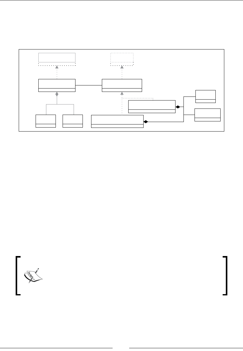
Naïve Bayes Classiers
[ 748 ]
The principle of software architecture applied to the implementation of classiers is
described in the Design template for classiers section in Appendix A, Basic Concepts.
The key software components of the Naïve Bayes classier are described in the
following UML class diagram:
NaiveBayes
density
smoothing xt
model
PipeOperator Model
NaiveBayesModel
Double XTSeries Multi BayesModelNaive
Likelihood
Density
Bin BayesModelNaive
1
2+
1
11
1likelihoodSet
The UML class diagram for the Naïve Bayes classifier
Training
The objective of the training phase is to build a model consisting of the likelihood for
each feature and the class prior. The likelihood for a feature is identied as:
• The number of occurrences k of this features for N > k observations in case of
binary features or counters
• The mean value for all the observations for this features in the case of
numeric or continuous features
It is assumed for the sake of this test case that the features, technical analysis
indicators price, volume, and volatility are conditionally independent. This
assumption is not actually correct.
Conditional dependency
Recent models, known as Hidden Naïve Bayes (HNB), relax the
restrictions on the independence between features. The HNB
algorithm uses conditional mutual information to describe the
interdependency between some of the features [5:8].

Chapter 5
[ 749 ]
Let's write the code to train the multinomial Naïve Bayes. The rst step is to dene
the likelihood for each feature using historical data. The Likelihood class has the
following attributes:
• The label for the observation, label
• An array of tuple Laplace or Lidstone smoothed mean and standard
deviation, muSigma
• The prior class prior that computes p(c)
As with any code snippet presented in this book, the validation of class parameters and
method arguments are omitted in order to keep the code readable. The Likelihood
class is dened as follows:
type Density = (Double*) => Double //1
type XYTSeries = Array[(Double, Double)]
val MINLOGARG = 1e-32
val MINLOGVALUE = -MINLOGARG
class Likelihood[T <% Double](val label: Int, val muSigma: XYTSeries,
prior: Double) { //2
def score(obs: Array[T], density: Density): Double =
(obs, muSigma).zipped
.foldLeft(0.0)((post, xms) => {
val mean = xms._2._1
val stdDev = xms._2._2
val _obs = xms._1
val prob = density(mean, stdDev, _obs)
post + Math.log(if(prob< MINLOGARG) MINLOGVALUE else prob)
}) + Math.log(prior) //3
}
The functions of the Density type compute the probability density for the values of
a feature (line 1). The method takes an undened number of arguments: the mean,
the standard deviation, and the input value for the Gaussian distribution, the mean
and input value {0, 1} for the Bernoulli distribution. The default probability density
function is the normal distribution implemented by Stats.gauss.

Naïve Bayes Classiers
[ 750 ]
The parameterized, view-bounded class, Likelihood, has two purposes:
• Dene the model extracted from training (likelihood for each feature and the
class prior) in the constructor (line 2)
• Compute the score of a new observation as part of the classication process
score (line 3). The computation of the log of the likelihood uses a density
method of the type Density, which is an argument of the score method. As
seen in the next section, the density can be either a Gaussian or a Bernoulli
distribution. The score method uses the Scala's zipped method to merge the
observation values with the labeled output.
The next step is to dene the BinNaiveBayesModel model for a two-class
classication scheme. The two-class model consists of the two Likelihood instances:
positives for the label UP (value==1) and negatives for the label DOWN (value==
0). In order to make the model generic, we created NaiveBayesModel, an abstract
class that can be extended as needed to support both the Binomial and Multinomial
Naïve Bayes models, as follows:
abstract class NaiveBayesModel [T <% Double](density: Density) {
def classify(values: DblVector): Int
}
class BinNaiveBayesModel [T <% Double](positives: Likelihood,
negatives: Likelihood, density: Density) extends NaiveBayesModel [T](
density) {
override def classify(x: Array[T]): Int =
if (positives.score(x,density) > negatives.score(x,density)) 1
else 0
}
The classication is executed by the classify method called by the |> operator in
the Naïve Bayes classier. It returns 1 for the class containing the positive cases and
0 for the negative.
Model validation
The parameters of the Naïve Bayes model (likelihood) are computed
through training and the model value is instantiated regardless of
whether the model is actually validated in this example. A commercial
application would require the model to be validated using a
methodology such as the K-fold validation and F1 measure. (Refer to
the Design template for classiers section in Appendix A, Basic Concepts.)

Chapter 5
[ 751 ]
The multinomial Naïve Bayes model, dened by the MultiNaiveBayesModel class is
very similar to the BinNaiveBayesModel class:
class MultiNaiveBayesModel[T <% Double](likelihoodXs:
List[Likelihood[T]], density: Density) extends NaiveBayesModel[T]
(density) {
override def classify(x: Array[T]): Int =
likelihoodXs.sortWith( (p1,p2) => p1.score(x, density) >
p2.score(x, density)).head.label
}
The multinomial Naïve Bayes model differs from the binomial version in the
following ways:
• The likelihood is dened as a list, likelihoodXs (one likelihood per class)
• The runtime classication sorts the class by the log likelihood (sortWith),
selects the class with the highest score, and returns the class ID
Finally, the Naïve Bayes classier is implemented by the NaiveBayes class. It
implements the training and runtime classication using the Naïve Bayes formula.
Any supervised learning model needs to be validated. In order to force the developer
to dene a validation for any new supervised learning technique, the class inherits
from the Supervised trait that declares the validation method, validate:
trait Supervised[T] {
def validate(xt: XTSeries[(Array[T],Int)], tpClass:Int): Double
}
The validate method takes a labeled time series xt as an array of tuples
(observation, class label) and the tpClass index that contains the true positives
(that is, increase in the stock price) outcome. The method returns an F1-measure.
Besides inheriting the Supervised trait, the NaiveBayes class inherits the
PipeOperator trait so that it can be integrated into a generic workow as
one of the computation units.
The attributes of the multinomial Naïve Bayes are as follows:
• The smoothing formula (Laplace, Lidstone, and so on): smoothing
• The labeled training set dened as a time series: xt
• The probability density function: density

Naïve Bayes Classiers
[ 752 ]
The NaiveBayes class is dened as follows:
Class NaiveBayes[T <% Double](smoothing: Double, xt:
XTSeries[(Array[T], Int)], density: Density) extends PipeOperator[XTSe
ries[Array[T]], Array[Int]] with Supervised[T] {
val model = BinNaiveBayesModel[T](train(1),train(0),density) //1
def train(label:Int)(implicit f: Array[T] => DblVector):
Likelihood[T] = { //2
val xi = xt.toArray
val values= xi.filter( _._2 == label).map(x => f(x._1) )
val dim = xi(0)._1.size
val vt = XTSeries[DblVector](values.toArray) //3
val muStdDev = statistics(vt).map(stat =>
(stat.lidstoneMean(smoothing, dim), stat.stdDev))
Likelihood(label, muStdDev, values.size.toDouble/xi.size) //4
}
…
The classier uses the binomial Naïve Bayes model, BinNaiveBayesModel (line 1).
The training process is implemented in the constructor by invoking the private
train method (line 2). The method relies on an implicit conversion, f: Array[T]
=> DblVector, because of the Array type erasure. The main reason for this is to hide
the details of the model and its training from the client code. We cannot assume that
the user of the model is the same person as the creator of the model.
Training and class instantiation
There are several benets of allowing the instantiation of the Naïve
Bayes mode only once when it is trained. It prevents the client code from
invoking the algorithm on an untrained or partially trained model, and it
reduces the number of states of the model (untrained and trained). It is an
elegant way to hide the details of the training of the model from the user.
The train method takes the labeled observations (observations or label) as input.
The vt time series is extracted (line 3) and the likelihoods are calculated by counting
the positive and negative labels, computing the mean, corrected with the Lidstone
smoothing formula (line 4). The lidstoneMean method and standard deviation,
stdDev, use the statistics method of the XTSeries singleton instance.
The NaiveBayes class also dened the runtime classication method |> and the
F1-validation methods. Both methods are described in the next section.
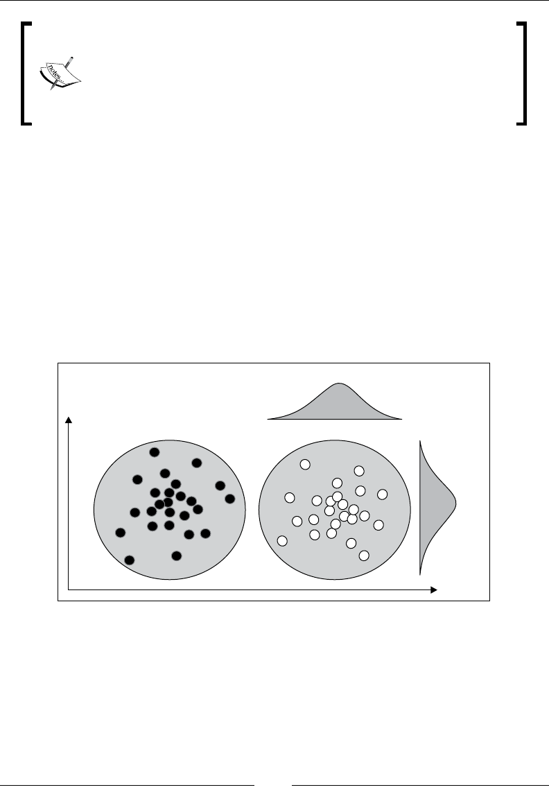
Chapter 5
[ 753 ]
Handling missing data
Naïve Bayes has a no-nonsense approach to handling missing data.
You just ignore the attribute in the observations for which the value
is missing. In this case, the prior for this particular attribute for these
observations is not computed. This workaround is obviously made
possible because of the conditional independence between features.
Classication
The likelihood and class prior that have been computed through training is used for
validating the model and classifying new observations.
The score represents the log of likelihood estimate (or the posterior probability),
which is computed as the summation of the log of the Gaussian distribution using
the mean and standard deviation, extracted from the training phase and the log of
the likelihood class.
The Naïve Bayes classication using Gaussian distribution is illustrated using two
classes, C1 and C2, and a model with two features (x and y):
C1C2
Gaussian distribution
of feature x
Gaussian distribution
of feature y
y
x
Illustration of the Gaussian Naive Bayes using a 2-dimensional model
The Gaussian mixture is particularly suited for modeling datasets for which
the features have large sets of discrete values or are continuous variables. The
conditional probabilities for the feature x is described by the normal probability
density function [5:9].

Naïve Bayes Classiers
[ 754 ]
Naïve Bayes classication using Gaussian density
For a Lidstone or Laplace smoothed mean µ' and a standard deviation σ,
the log likelihood of a posterior probability is dened as:
()
()
()
2
1
2
0
'
1
log| log log
2
2
Nj
j j
i
x
pC x epC
µ
σ
πσ
−
=
⎛ ⎞
−−
⎜ ⎟
=−+
⎜ ⎟
⎝ ⎠
∑
In this example, we used the Gaussian distribution as our probability density
function as dened in the Stats object, which was introduced in Chapter 2, Hello
World!. The implementation of the computation of the Gaussian probability density
is quite simple, shown as follows:
object Stats {
final val INV_SQRT_2PI = 1.0/Math.sqrt(2.0*Math.PI)
def gauss(mu: Double, sigma: Double, x:Double) : Double = {
val y = x - mu
INV_SQRT_2PI/sigma * Math.exp(-0.5*y*y/sigma*sigma)
}
def gauss(x: Double*): Double = gauss(x(0), x(1), x(2))
…
}
The second version of the Gaussian density is required to handle the Density type:
(Double, Double, Double) => Double.
Finally, the classication method is implemented as the pipe operator |> of the
NaiveBayes class. The classication model and the density function are provided
at runtime as attributes of the class:
def |> : PartialFunction[XTSeries[Array[T]], Array[Int]] = {
case xt: XTSeries[Array[T]] if(xt != null && xt.size > 0 && model !=
None) => xt.toArray.map( model.classify( _))}
Labeling
The most critical element in the training of a supervised learning algorithm is the
creation of labeled data. Fortunately, in this case, the label (or expected class) can
be automatically generated. The objective is to predict the direction of the price of
a stock for the next trading day, taking into account the average price, volume, and
volatility over the last n days.

Chapter 5
[ 755 ]
The rst step is to extract the average price, volume, and volatility for each
stock during the period of Jan 1, 2000 and Dec 31, 2014 with daily and weekly
closing prices. Let's use the simple moving average to compute these averages
for the [t-n, t] window.
First, the extractor function extracts the closing, high, and low prices, and volume
for each trading day, using the toDouble and % operators described in the Data
extraction and Data sources section in Appendix A, Basic Concepts, as follows:
val extractor = toDouble(CLOSE) //stock closing price
:: ratio(HIGH, LOW) //volatility (HIGH-LOW)/HIGH
:: toDouble(VOLUME) //daily stock trading volume
::List[Array[String] =>Double]()
Secondly, the data source extractor outputs the four statistics for each stock (line
1) for which the average for a window period is computed (line 3) using a simple
moving average mv (line 2):
val xs = DataSource(symbol, path, true) |> extractor //1
val mv = SimpleMovingAverage(period) //2
val ratios = xs.map(x => { //3
val xt = mv get x,toArray
val zValues = x.drop(period).zip(xt.drop(period))
zValues.map(z => if(z._1 > z._2) 1 else 0).toArray //4
})
var prev = xs(0)(period)
val label = xs(0).drop(period+1).map( x => { //5
val y = if( x > prev) 1 else 0
prev = x; y
}).toArray
ratios.transpose.take(label.size).zip(label) //6
The Scala's drop method is used to shift the time series to compute the average of the
three variables: price, toDouble(CLOSE); volume, toDouble(VOLUME); and volatility,
ratio(HIGH, LOW) (line 4). The labeled data, direction of the price action for the
next trading day, is added to the three ratios (line 5). Finally, the array is transposed
to extract the list of tuples (list of UP/DOWN values for each feature and price
direction for next trading day/labeled data) (line 6).
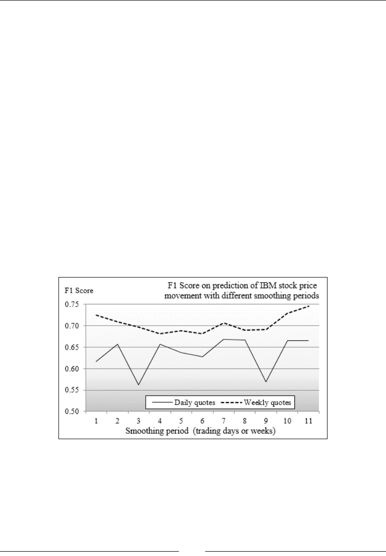
Naïve Bayes Classiers
[ 756 ]
The labeled data extracted from the input CSV le is used in the training and
validation of the time series using the Naïve Bayes classier:
val trainValidRatio = 0.8
val period = 10
val labels = XTSeries[(Array[Int], Int)](input.map(x =>
(x._1.toArray, x._2)).toArray) //7
val numObsToTrain = (trainValidRatio*labels.size).floor.toInt //8
val nb = NaiveBayes[Int](labels.take(numObsToTrain)) //9
validate(labels.drop(numObsForTrains+1), nb) //10
The original labeled dataset, labels, is split between training and validation labeled
data (line 7) using the trainValidRatio ratio (line 8). The NaiveBayes constructor
initializes the model through training (line 9). Finally, the validate method returns
the F1 measure for the validation test (line 10).
Results
The next chart plots the value of the F1 measure of the predictor of the direction of
the IBM stock using price, volume, and volatility over the previous n trading days,
with n varying from 1 to 12 trading days:
A graph of the F1-measure for the validation of the Naïve Bayes model

Chapter 5
[ 757 ]
The preceding chart illustrates the impact of the value of the averaging period
(number of trading days) on the quality of the multinomial Naïve Bayesian
prediction, using the value of stock price, volatility, and volume relative to their
average over the averaging period.
From this experiment, we conclude that:
• The prediction of the stock movement using the average price, volume, and
volatility is not very good. The F1 measure for the models using weekly (with
respect to daily) closing prices varies between 0.68 and 0.74 (with respect to
0.56 and 0.66).
• The prediction using weekly closing prices is more accurate than the
prediction using the daily closing prices. In this particular example, the
distribution of the weekly closing prices is more reective of an intermediate
term trend than the distribution of daily prices.
• The prediction is somewhat independent of the period used to average
the features.
Multivariate Bernoulli classication
The previous example uses the Gaussian distribution for features that are essentially
binary, {UP=1, DOWN=0}, to represent the change in value. The mean value is
computed as the ratio of the number of observations for which xi = UP over the total
number of observations.
As stated in the rst section, the Gaussian distribution is more appropriate for either
continuous features or binary features for very large labeled datasets. The example is
the perfect candidate for the Bernoulli model.
Model
The Bernoulli model differs from Naïve Bayes classier in that it penalizes the
features x, which do not have any observations; the Naïve Bayes classier ignores
them [5:10].
The Bernoulli mixture model
For a feature function fi, with fi = 1 if the feature is observed, and a value
of 0 if the feature is not observed:
() ()
()
()
( )
( )
1
0
||11 |
−
=
=⋅+−−
∏
n
ij kkj kkj
k
pfC f px C f px C

Naïve Bayes Classiers
[ 758 ]
Implementation
The implementation of the Bernoulli model consists of modifying the Likelihood.
score scoring function by using the Bernoulli density dened in the Stats object:
object Stats {
def bernoulli(mean: Double, p: Int): Double = mean*p +
(1-mean)*(1-p)
def bernoulli(x: Double*): Double = bernoulli(x(0), x(1).toInt)
…
The rst version of the Bernoulli algorithm is the direct implementation of the
mathematical formula. The second version uses the signature of the Density
(Double*) => Double type.
The mean value is the same as in the Gaussian version. The binary feature is
implemented as an Int type with the value UP =1 (with respect to DOWN= 0) for the
upward (with respect to downward) direction of the nancial technical indicator.
Naïve Bayes and text mining
The multinomial Naïve Bayes classier is particularly suited for text mining.
Naïve Bayes is used to classify the following entities:
• E-mails as legitimate versus spam
• Business news stories
• Movie reviews and scoring
• Technical papers as per eld of expertise
This third use case consists of predicting the direction of a stock, Tesla Motors Inc,
(ticker symbol: TSLA) give the nancial news. The features are the frequency of
occurrence of some specic terms related to the stock. It is unclear how fast the
investor or trader reacts to the news and inuence, if any, of the value of a stock.
Therefore, the delayed response time, as depicted in the following chart, should
be a feature of the proposed model:
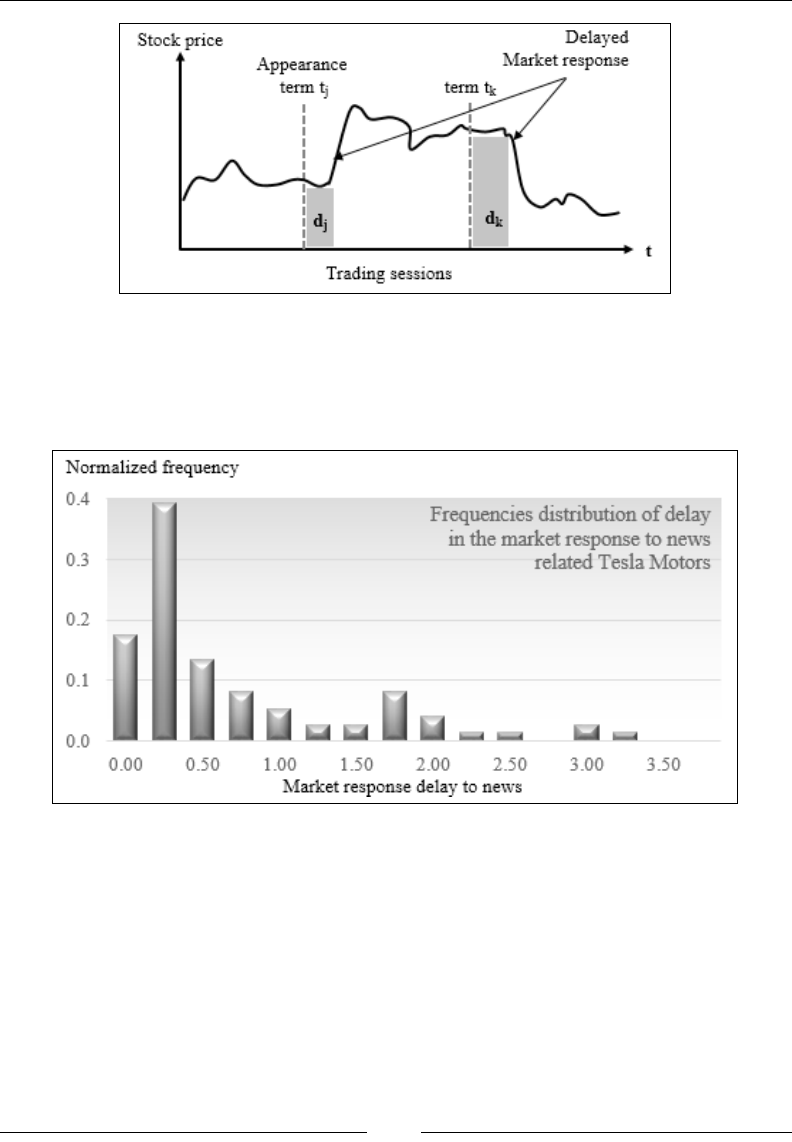
Chapter 5
[ 759 ]
The feature market response delay would play a role in the training, only if the
variance of the observations is signicant. The distribution of the frequencies of the
delay in the market response to any newsworthy articles regarding TSLA shows that
the stock prices react within the same day in 82 percent of the case, as seen here:
The frequency peak for a market response delay of 1.75 days can be explained by the
fact that some news are released over the weekend and investors have to wait till the
following Monday to impact the stock price. The second challenge is to assign any
shift of stock price to a specic news release, taking into account that some news can
be redundant and simultaneous.
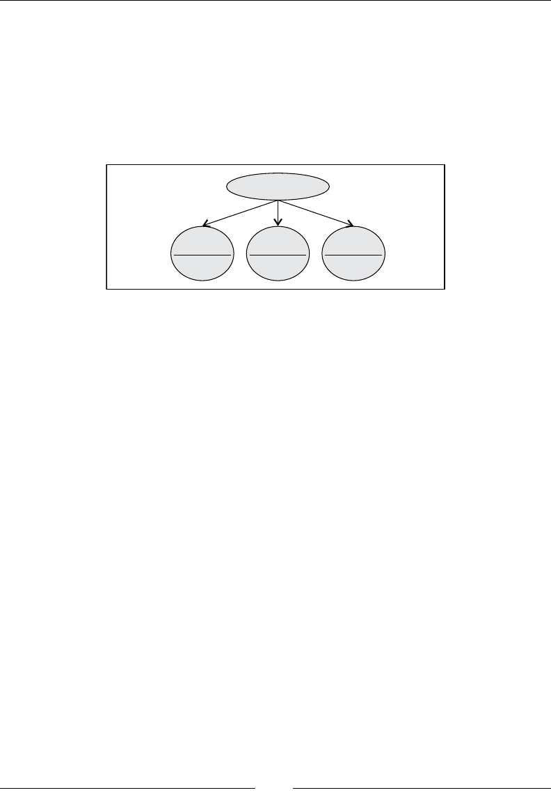
Naïve Bayes Classiers
[ 760 ]
Therefore, the model features for predicting the stock price, prt+1, are the relative
frequency, fi, of occurrence of a term Ti within a time window [t-n, t], where t and n
are trading days.
The following graphical model formally describes the causal relation or conditional
dependency of the direction of the stock price between two consecutive trading
sessions t and t+1, given the relative frequency of appearance of some terms in
the media:
Relative
frequency
of term T0
Output
(labelled data)
Relative
frequency
of term Tj
pr pr
tt+1 >
St
tn-0
ft()
Sft
0()
St
tn i-ft()
Sft
i() Sft
j()
St
t-n j
ft()
The Bayesian model for the prediction of stock movement given financial news
For this exercise, the observation sets are the corpus of news feeds and articles
released by the most prominent nancial news organizations, such as Bloomberg
or CNBC. The rst step is to devise a methodology to extract and select the most
relevant terms associated with a specic stock.
Basics of information retrieval
A full discussion of information retrieval and text mining is beyond the scope of this
book [5:11]. For the sake of simplicity, the model will rely on a very simple model for
extracting relevant terms and computing their relative frequency. The following 10-
step sequence of actions describe one of numerous methodologies to extract the most
relevant terms from a corpus:
1. Create or extract the timestamp for each news article.
2. Extract the title, paragraph, and sentences of each article using a
Markovian classier.
3. Extract the terms from each sentence using regular expressions.
4. Correct terms for typos using a dictionary and metric such as the
Levenstein distance.
5. Remove the nonstop words.
6. Perform stemming and lemmatization.

Chapter 5
[ 761 ]
7. Extract bags of words and generate a list of n-grams (as a sequence of n terms).
8. Apply a tagging model build using a maximum entropy or conditional
random eld to extract nouns and adjectives (such as NN, NNP, and so on).
9. Match the terms against a dictionary that supports senses, hyponyms, and
synonyms, such as WordNet.
10. Disambiguate word sense using DBpedia [5:12].
Text extraction from the web
The methodology discussed in this section does not include
the process of searching and extracting news and articles
from the Web that requires additional steps such as searching,
crawling, and scraping [5:13].
Implementation
Let's apply the text mining methodology template to predict the direction of a stock,
given the nancial news. The algorithm relies on a sequence of 8 simple steps:
1. Extracting all news with a reference to a specic stock or company in the
news feed.
2. Extracting the timestamp or date of the article using a regular expression.
3. Grouping all the news articles related to the stock for a specic date t into a
document Dt.
4. Ordering the documents Dt as per the timestamp.
5. Extracting the terms {Ti,D} from each sentence of the document Dt and
ranking them by their relative frequency.
6. Aggregating the terms {Tt,i} for all the documents sharing the same release
date t.
7. Computing the relative frequency, rtf, of each term, {Tt,i}, for the date t, as the
ratio of number of its occurrences in all the articles released at t to the total
number of its occurrences of the term in the entire corpus.
8. Normalizing the relative frequency for the average number of articles per
date, nrtf.

Naïve Bayes Classiers
[ 762 ]
The relative term frequency for term ti with nia occurrences in
article a released on the date Dt is given as:
()
a
aDti
ia
a Corpus i
n
ntrf tn
∈
∈
∑
=∑
The relative term frequency normalized by the average number
of articles per day, Na/D is given as:
()
()
/
i
i
rtft
ntrf
t
Na D
=
Extraction of terms
First, let's dene the features set for the nancial terms as the NewsArticles class
parameterized for the date type T. For the sake of simplicity, the type of date value is
explicitly viewbounded to Long. The NewsArticles class is a container of the news
articles and press releases relevant to a specic stock. At its core, a news article is
dened by its release or publication, and the list of tuple of terms and their relative
frequency. The NewsArticles class is dened as follows:
@implicitNotFound("NewsArticles. Ordering not explicitly defined")
class NewsArticles[T <% Long](implicit val order: Ordering[T]) {
val articles = new HashMap[T, Map[String, Double]]
…
}
The @implicitNotFound annotation
I recommend using the implicitNotFound annotation for
every implicit class and method parameter. A declaration
may be obvious to one software developer but not obvious to
another developer.
The NewsArticles class uses the mutable HashMap data structure to manage the set
of articles. An article is dened by:
• Its release date (type T)
• Its map of tuples {term contained in the article, relative frequency (or weight) of the
term}, wTerms
The weight of a term is computed as the ratio of the number of occurrences of this
term in the article, to the total number of occurrences in the entire corpus of articles
related to the stock.

Chapter 5
[ 763 ]
The implicit Ordering class parameter is required for sorting.
The map articles is populated with the overloaded operator +=:
def += (date: T, wTerms: Map[String, Double]): Unit = { //1
def merge(m1: Map[String, Double], m2: Map[String, Double]):
Map[String, Double] = { //2
(m1.keySet ++ m2.keySet).foldLeft(new HashMap[String, Double])((m,
x) => {
var wt = 0.0
if(m1.contains(x)) wt += m1(x)
if(m2.contains(x)) wt += m2(x)
m.put(x, wt)
m
}).toMap
}
articles.put(date, if( articles.contains(date))
merge(articles(date), wTerms) else wTerms) //3
}
The += method adds new sets (mutable hash map) of pairs (terms, relative
frequency), wTerms, released at a specic date, to the existing map of news articles
(line 1). The terms related to different articles from the same date are merged using
the local merge function (line 2). Finally, the list of key-value pairs (term, frequency)
is ordered by their timestamp of the type T.
The second method, toOrderedArray, consists of ordering the articles per their
release date:
def toOrderedArray: Array[(T, Map[String, Double])] = articles.
toArray.sortWith( _._1 < _._1)
Scoring of terms
The scoring of the terms is actually performed by the TermsScore class,
parameterized by date and the score method:
class TermsScore[T <% Long](toDate: String =>T, toWords: String =>
Array[String], lexicon: Map[String, String])(implicit val order:
Ordering[T]) {
def score(corpus: Corpus): Option[NewsArticles[T]]
}

Naïve Bayes Classiers
[ 764 ]
The TermsScore class parameterized for the type of release date has three parameters:
• A toDate function to extract the date from each news article. The function can
be implemented as a regular expression or a group of regular expressions.
• A toWords function to extract the nonstop terms from the content of the
article. The function can be quite elaborate, as described in the previous
section. It may require creating classiers to extract sentences, n-grams,
and tags.
• A lexicon function that simulates the lemmatization and stemming of the
most common terms. The lexicon function is implemented as a map that
attaches a semantic equivalent to each term as a poor man's lemmatization.
For example, "China", "Chinese", and "Shanghai" are semantically associated
to the term "China".
The type for date T is view bounded by the Long type because it is assumed that any
date can be potentially converted into time in milliseconds. The Ordering[T] class is
provided as an implicit attribute to order the news articles as per their release date.
The relative frequency of a term t is computed arbitrarily, as the ratio of the number
of occurrences of t for a specic date to the total number of terms.
Let's look at the scoring method:
type Corpus = (String, String, String) //1
def score(corpus: Corpus): Option[NewsArticles[T]] = { //2
val docs = rank(corpus)
val cnts = docs.map(doc => (doc._1,count(doc._3)) )//3
val totals = cnts
.map(_._2) //4
.foldLeft(Counter[String])((s,cnt)=>s ++ cnt)
val articles = NewsArticles[T]
cnts.foreach(cnt =>articles +=(cnt._1,(cnt._2/totals).toMap))
articles
…
The score method processes the training set or corpus of the news articles related to
a stock and returns a set of NewsArticles instances.
The corpus type (line 1) denes the three essential components of a news article:
a timestamp, a title, and a body or content. The rank method (line 2) extracts the
release date from each news article and orders them as per increasing date.

Chapter 5
[ 765 ]
The frequency of terms is computed for each document or group of news articles
associated with a date (line 3) using the count method. The count method matches
each term extracted from the news article to the entries of the lexicon map. The
counters of the Counter: Map[String, Int] type collect the number of occurrences
of each term. The next instruction (line 4) aggregates the counts for the entire corpus
that is used to compute the relative frequencies (line 5).
The rank method uses a sequence of Scala methods map and sortWith to order the
articles as per date (line 6):
def rank(corpus: Corpus): Option[CorpusType[T]] = {
corpus.map(doc => (toDate(doc._1.trim), doc._2, doc._3)))
.sortWith( _._1 < _._1) //6
}
The scoring method is protected by a Scala exception handler (line 7). Finally, the
count method matches a term with an entry in the lexicon and updates the count
if a match is found (line 8):
def count(term: String): Counter[String] =
toWords(term).foldLeft(new Counter[String])((cnt, w) =>
if( lexicon.contains(w)) cnt + lexicon(w) //8
else cnt
)
Testing
For testing purpose, let's select the news articles mentioning Tesla Motors and its
ticker symbol TSLA over a period of two months.
Retrieving textual information
First, you need to dene the three parameters of the scoring TermsScore class:
toDate, toWords, and lexicon.
The private toDate method converts a string into a date dened as a Long data type:
def toDate(date: String): Long = {
val idx1 = date.indexOf(".")
val idx2 = date.lastIndexOf(".")
if(idx1 != -1 && idx2 != -1)
(date.substring(0, idx1) + date.substring(idx1+1, idx2)).toLong
else -1L
}

Naïve Bayes Classiers
[ 766 ]
The toWords method uses simple regular expressions, regExpr, to replace
any punctuation into a . character (line 1), used as a word delimiter (line 2).
All words shorter than three characters are discounted (line 3):
def toWords(txt: String): Array[String] = {
val regExpr = "['|,|.|?|!|:|\"]"
txt.trim.toLowerCase
.replace(regExpr,"&@") //1
.split("&@") //2
.filter(_.length > 2) //3
}
Finally, the lexicon contains the terms that need to be monitored. In this particular
period of time, the news media were looking for any announcement regarding Tesla
Motors' foray into the Chinese market, issues with the batteries, and any plan to
deploy electrical vehicle charger stations. The set of terms regarding these issues is
limited, and therefore, the lexicon can be built manually:
val LEXICON = Map[String, String](
"tesla"->"Tesla","tsla"->"TSLA","china"->"China","chinese"->
"China", ....)
The semantic analysis
This example uses a very primitive semantic map (lexicon) for the
sake of illustrating the benets and inner workings of the multinomial
Naïve Bayes algorithm. Commercial applications involving sentiment
analysis or topic analysis require a deeper understanding of semantic
associations and extraction of topics using advanced generative models,
such as the latent Dirichlet allocation.
The client code to train and validate the model executes the entire workow,
from extracting and scoring the news articles and press releases to generating
the normalized labeled data and computing the F1 measure.
The output (or labeled data) TSLA_QUOTES consists of the stock price for Tesla Motors:
val TSLA_QUOTES = Array[Double](250.56, 254.84, … )

Chapter 5
[ 767 ]
The rst step is to load and clean all the articles (corpus) dened in the pathname
directory (line 1). This task is performed by the DocumentsSource class (described
in the Extraction of documents section under Scala programming in Appendix A,
Basic Concepts):
val corpus: Corpus = DocumentsSource(pathName) |> { //1
val ts = new TermsScore[Long](toDate, toWords, LEXICON)
ts.score(corpus) match { //2
case Some(terms) => {
var prevQ = 0.0
val diff = TSLA_QUOTES.map( q => {
val delta = if(q > prevQ) 1 else 0
prevQ = q; delta
})
val columns = LEXICON.values.foldLeft(new HashSet[String])((hs,
key) => {hs.add(key); hs}).toArray
val fqLabels = terms.toOrderedArray //3
.zip(diff) //4
.map( x => (x._1._2, x._2))
.map(lbl =>(columns //5
.map(f =>if( lbl._1.contains(f) ) lbl._1(f)
else 0.0), lbl._2))
val xt = XTSeries[(Array[Double], Int)](fqLabels)
val nb = NaiveBayes[Double](xt) //6
….
Next, the TermsScore.score method extracts and scores the more relevant terms
from the corpus, using the normalized relative frequency dened in steps 7 and 8
of the information retrieval process (line 2). The terms are then ordered by date
(line 3) and zipped with the labels (direction of the next trading day's stock price)
(line 4). The lexicon is used to generate the nal labeled observations (features = terms
relative frequency, label= direction of stock price) (line 5). Finally, the model is built by
invoking the NaiveBayes.apply constructor (line 6), which consists of running the
algorithm through the training set.
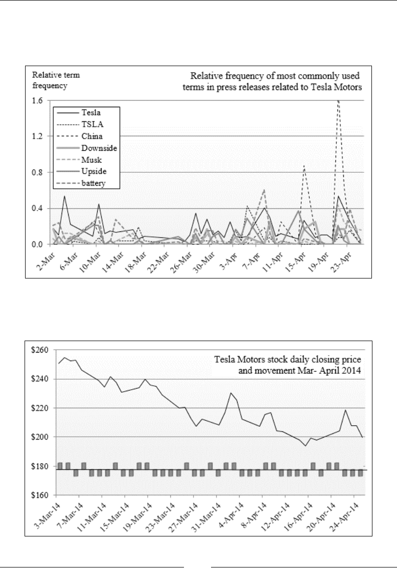
Naïve Bayes Classiers
[ 768 ]
Evaluation
The following chart describes the frequency of occurrences of some of the terms
related to either Tesla Motors or its stock ticker TSLA:
Plot of the relative frequency of a partial list of stock-related terms
The next chart plots the labeled data, which is the direction of the stock price for the
day following the press release(s) or news article(s):
Plot of the stock price and movement for Tesla Motors stock
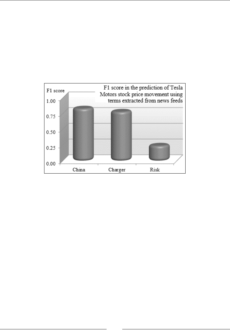
Chapter 5
[ 769 ]
This chart displays the historical price of the stock TSLA with the direction (UP or
DOWN). The classication of 15 percent of the labeled data selected for validation has
an F1 measure of 0.71. You need to keep in mind that no preprocessing or clustering
was performed to isolate the most relevant features/keywords. The keywords were
selected according the frequency of their occurrence in the nancial news.
It is fair to assume that some of the keywords have a more signicant impact on
the direction of the stock price than others. One simple but interesting exercise is to
record the value of the F1 score for a validation for which only the observations that
have a high number of occurrences of a specic keyword are used, as shown here:
Bar chart representing predominant keywords in predicting TSLA stock movement
The bar chart shows that the terms China, representing all the mentions of the
activities of Tesla Motors in China, and Charger, which covers all the references to
the charging stations, have a signicant positive impact on the direction of the stock
with a probability averaging 75 percent. The terms under the category Risk have a
negative impact on the direction of the stock with a probability of 68 percent, or a
positive impact of the direction of the stock with a probability of 32 percent. Within
the remaining eight categories, 72 percent of them were unusable as a predictor of
the direction of the stock price.
This approach can be used for selecting features as an alternative to mutual
information for using more elaborate classiers. However, it should not be regarded
as the primary methodology for the features selection, but instead as a by-product
of the Naïve Bayes in case a very small number of features (less than 10 percent) are
predominant in the model. This result can always be validated by computing the
principal components, for which the normalized cumulative variance (eigenvalues)
of the most predominant features is 90 percent or more.

Naïve Bayes Classiers
[ 770 ]
Pros and cons
The examples selected in this chapter do not do justice to the versatility and accuracy
of the Naïve Bayes family of classiers.
Naïve Bayes classiers are simple and robust generative classiers that rely on prior
conditional probabilities to extract a model from a training dataset. The Naïve Bayes
has its benets, as mentioned here:
• Simple implementation and easy to parallelize
• Very low computational complexity: O((n+c)*m), where m is the number of
features, C the number of classes, and n the number of observations
• Handles missing data
• Supports incremental updates, insertions, and deletions
However, Naïve Bayes is not a silver bullet. It has the following disadvantages:
• The assumption of the independence of features is not practical in the
real world
• It requires a large training set to achieve reasonable accuracy
• It contains a zero-frequency problem for counters
Summary
There is a reason why the Naïve Bayes model is the rst supervised learning
technique you learned: it is simple and robust. As a matter of fact, this is the rst
technique that should come to mind when you are considering creating a model
from a labeled dataset, as long as the features are conditionally independent.
This chapter also introduced you to the basics of text mining as an application of
Naïve Bayes.
Despite all its benets, the Naïve Bayes classier assumes that the features are
conditionally independent, a limitation that cannot be always overcome. In the
case of document classication, Naïve Bayes assumes incorrectly that terms
are semantically independent: the two entities' age and date of birth are highly
correlated. The discriminative classiers described in the next few chapters
attempt to address some of the Naïve Bayes's disadvantages [5:14].
However, this chapter does not address temporal dependencies, sequence of events,
or conditional dependencies between observed and hidden features. These types of
dependencies necessitate a different approach to modeling that is the subject of the
next chapter.

Regression and
Regularization
In the rst chapter, we briey introduced the binary logistic regression (binomial
logistic regression for a single variable) as our rst test case. The purpose was to
illustrate the concept of discriminative classication. There are many more regression
models, starting with the ubiquitous ordinary least-square linear regression and the
logistic regression [6:1].
The purpose of regression is to minimize a loss function, with the residual sum
of squares (RSS) being one that is commonly used. The problem of overtting
described in the Overtting section of Chapter 2, Hello World!, can be addressed by
adding a penalty term to the loss function. The penalty term is an element of the
larger concept of regularization.
The rst section of this chapter will describe and implement the linear least-squares
regression. The second section will introduce the concept of regularization with an
implementation of the Ridge regression.
Finally, the logistic regression will be revisited in detail from the perspective of a
classication model.
Linear regression
Linear regression is by far the most widely used, or at least the most commonly
known, regression method. The terminology is usually associated with the concept of
tting a model to data. Linear regression can be implemented using the least squares
method. Practically, the least squares method entails the minimization of the sum of
the squares of the error between the observed data and the actual model.

Regression and Regularization
[ 772 ]
The least squares problems fall into two categories:
• Ordinary least squares
• Nonlinear least squares
One-variate linear regression
Let's start with the simplest form of linear regression, which is the single variable
regression, in order to introduce the terms and concepts behind linear regression.
In its simplest interpretation, the one-variate linear regression consists of tting a
line to a set of data points {x, y}.
Single variable linear regression is given by the following formula:
()
( )
()
2
1
01
,
0
ˆargmin ||
n
jj
wr
j
wyfxw fxwww
x
−
=
=−=+⋅
∑
Here, w1 is the slope, w0 is the intercept, f is the linear function that
minimizes the RSS, and (xj, yj) is a set of n observations.
The RSS is also known as the sum of squared errors (SSE). The mean squared error
(MSE) for n observations is dened as the ratio RSS/n.
Terminology
The terminology used in the scientic literature regarding regression
is a bit confusing at times. Regression weights are also known as
regression coefcients or regression parameters. The weights are
referred to as w in formulas and the source code throughout the
chapter, although β is also used in reference books.
Implementation
Let's create a parameterized class SingleLinearRegression[T] to implement
the formula described in the previous section. The class implements the data
transformation PipeOperator (refer to the Design template for classiers section
in Appendix A, Basic Concepts).
class SingleLinearRegression[T <% Double](xt: XTSeries[(T, T)])
(implicit g: Double => T) extends PipeOperator[Double, T] {
type XY = (Double, Double)
…
}

Chapter 6
[ 773 ]
Model instantiation
The model parameters are computed through training and the value
model is instantiated regardless of whether the model is actually
validated. A commercial application requires the model to be validated
using a methodology such as the K-fold validation. (Refer to the Design
template for classiers section Appendix A, Basic Concepts.)
The application code must provide an implicit conversion g from Double to the
class type parameter, T. The training generates the model dened as the regression
weights, the tuple (slope, intercept), in the case of single variable linear regression:
val model: Option[XY] = {
val data = xt.toArray
.map(x => Array[Double](x._1, x._2)) //1
val regr = new SimpleRegression(true)
regr.addData(data) //2
Some((regr.getSlope, regr.getIntercept)) //3
}
The tuple of regression weights or coefcients for the model are computed using
the SimpleRegression class from the stats.regression package of the Apache
Commons Math library. The time series is converted to a matrix of double values,
data (line 1), which is used to initialize the instance of SimpleRegression (line 2). The
model is initialized with the slope and intercept computed during the training (line 3).
private vs. private[this]
A private value or variable can be accessed only by all the instances
of a class. A value declared private[this] can be manipulated
only by this instance. For example, the value model can be accessed
only by this instance of SingleLinearRegression.
Test case
For our rst test case, we compute the single variate linear regression of the price of
the copper ETF (the ticker symbol: CU) over a period of 6 months (January 1, 2013 to
June 30, 2013):
val price = DataSource(path, false, true, 1) |> adjClose //1
val xy = price.zipWithIndex
.map(x => (x._2.toDouble, x._1.toDouble)) //2
val linRegr = SingleLinearRegression(xy) //3
val w1 = linRegr.slope
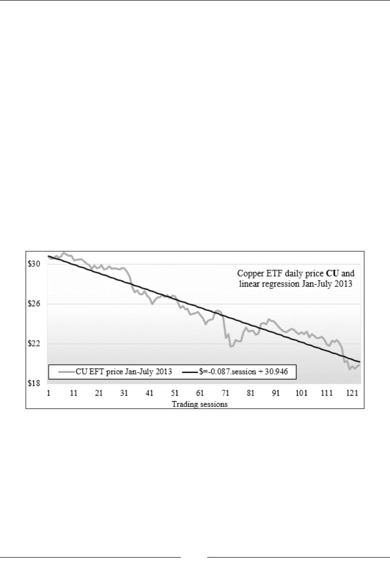
Regression and Regularization
[ 774 ]
val w0 = linRegr.intercept
if( w1 != None ) //4
Display.show(lsErr(xy.toArray, w1.get, w0.get), logger)
…
The closing price for the CU ETF is extracted from a CSV le (line 1) using a
DataSource instance (refer to the Data extraction section Appendix A, Basic Concepts).
The 2-dimension time series is generated by converting the indexes of the time series
into the x values using the zipWithIndex Scala method (line 2). The regression
model, linRegr, is trained during instantiation of the SingleLinearRegression
class (line 3). Once the model is created successfully, the least squared error lsErr
of the predicted values and the actual values is computed, as follows:
def lsErr(xyt: Array[XY], w1: Double, w0: Double): Double =
Math.sqrt(xyt.foldLeft(0.0)((err, xy) => {
val diff = xy._2 – w1*xy._1 – w0; err + diff*diff
})/xyt.size)
The original stock price and the linear regression equation are plotted in the
following chart:
Single variable linear regression – Copper ETF daily price
Although the single variable linear regression is convenient, it is limited to scalar
time series. Let's consider the case of multiple variables.

Chapter 6
[ 775 ]
Ordinary least squares (OLS) regression
The ordinary least squares regression computes the parameters w of a linear
function, y = f(x0, x2 … xd), by minimizing the residual sum of squares. The
optimization problem is solved by performing vector and matrix operations
(transposition, inversion, and substitution).
Minimization of the loss function is given by the following formula:
()
( )
()
2
1 1
0 1
ˆargmin ||
n D
jj dd
w
i d
wyfxw fxw wx
− −
= =
=−=
∑ ∑
where wj:0,D is the D regression (or model) parameters (or weights),
(xi, yi)i:0,n-1 is n observations of vector x and output value y, and f is
the linear multivariate function, y = f(x0, x1, …,xd, ..).
There are several methodologies to minimize the residual sum of squares (RSS) for a
linear regression:
• Resolution of the set of n equations with d variables (weights) using the
QR decomposition of the n by d matrix representing the time series of n
observations of vector of d dimension (d features) with n > d [6:2]
• Singular value decomposition on the observations-features matrix, in the
case where the dimension d exceeds the number of observations n [6:3]
• Gradient descent [6:4]
• Stochastic gradient descent [6:5]
An overview of these matrix decompositions and optimization techniques can
be found in the Linear algebra and Summary of optimization techniques sections in
Appendix A, Basic Concepts.
The QR decomposition generates the smallest relative error MSE for the most
common least squares problem. The technique is used in our implementation
of the least squares regression.
Design
The following implementation of the least squares regression leverages the Apache
Commons Math library implementation of the ordinary least squares regression [6:6].
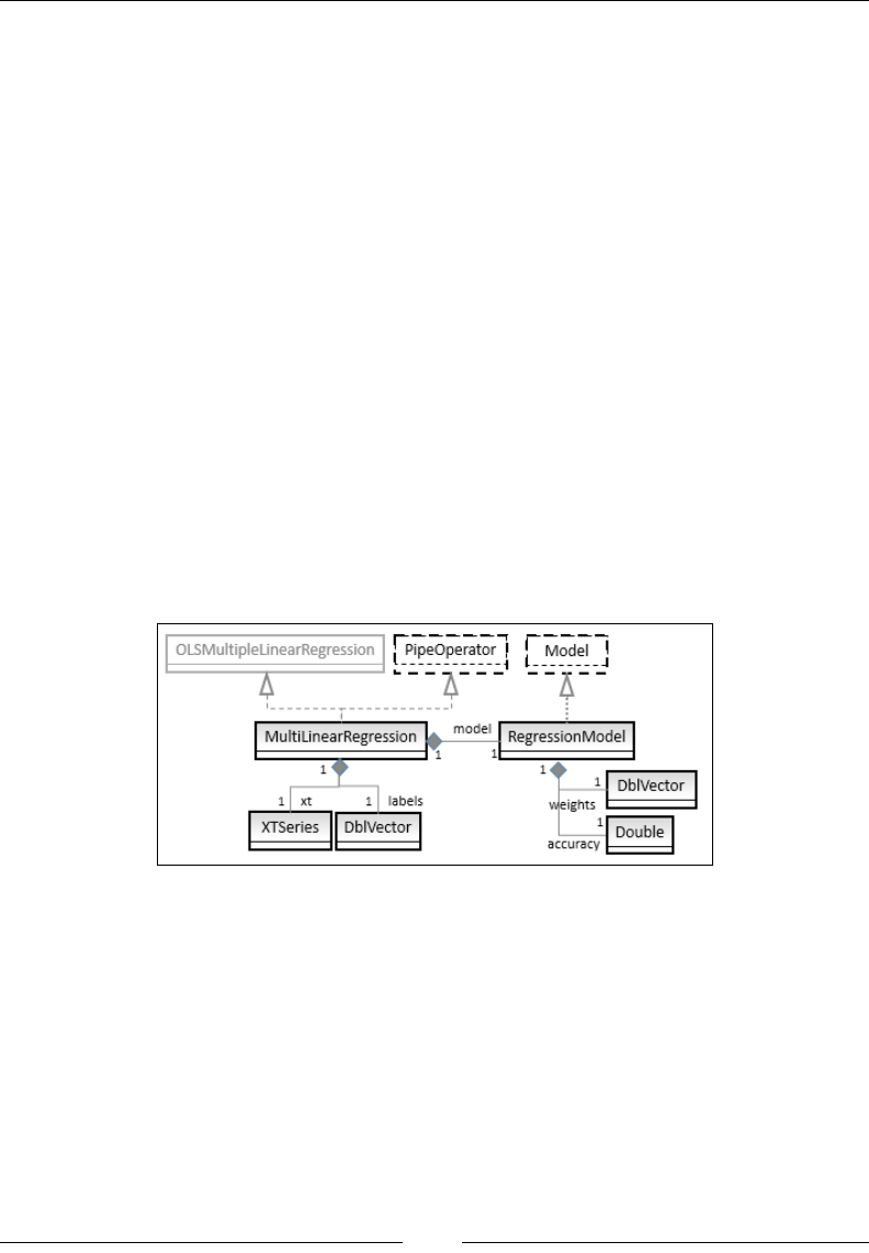
Regression and Regularization
[ 776 ]
Let's create a class, MultiLinearRegression, which inherits the implementation
of the ordinary least square computation of the Apache Commons Math library
OLSMultipleLinearRegression. The class is dened as a data transformation
implementing the PipeOperator, as follows:
class MultiLinearRegression[T <% Double](xt: XTSeries[Array[T]],
y: DblVector) extends OLSMultipleLinearRegression with
PipeOperator[Array[T], Double]
The parameterized class takes the following two parameters:
• The time series of the variables vector xt (input matrix)
• The labeled output values, y, used in training
The model for the linear regression is dened by its weights (or parameters) and its
residual sum of squares, rss. The RSS is included in the model because it provides
the client code with important information regarding the accuracy of the underlying
technique used to minimize the loss function:
case class RegressionModel(val weights: DblVector, val rss: Double)
The relationship between the different components of the least squares regression is
described in the following UML class diagram:
Implementation
The training is performed during the instantiation of the class MultiLinearRegression
(refer to the Design template for classiers section in Appendix A, Basic Concepts):
val model: Option[RegressionModel] = {
newSampleData(labels, xt.toDblMatrix) //1
val weights = estimateRegressionParameters
val wRss =(weights, calculateResidualSumOfSquares) //2
Some(RegressionModel(wRss._1, wRss._2))
}

Chapter 6
[ 777 ]
The least squares algorithm is initialized with the feature observations,
xt, and the target data, labels, using the newSampleData method of
OLSMultipleLinearRegression (line 1).
The model weights are retrieved using estimateRegressionParameters (similarly,
rss using calculateResidualSumOfSquares) (line 2).
Exception handling
Wrapping up invocation of methods in a third party with a Scala
exception handler matters for a couple of reasons: it makes debugging
easier by segregating your code from the third party and it allows your
code to recover from the exception by re-executing the same function with
alternative third-party library methods, whenever possible.
The predictive algorithm for the ordinary least squares regression is implemented by
the data transformation |>. The method predicts the output value given model and
an input value x:
def |> : PartialFunction[Feature, Double] = {
case x: Feature if(model!=None && x.size==model.get.size-1) =>{
val w = model.get.weights
x.zip(w.drop(1)).foldLeft(w(0))((s, z) => s + z._1*z._2))
}
}
The predictive value is computed by zipping the weight w1 to wn with the input vector
x and then folding the zipped array.
Test case 1 – trending
Trending consists of extracting the long-term movement in a time series. Trend lines can be
identied using a multivariate least squares regression. The objective of this rst test
is to evaluate the ltering capability of the ordinary least squares regression.
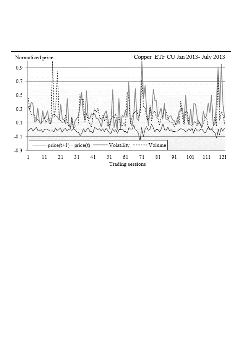
Regression and Regularization
[ 778 ]
The regression is performed on the relative price variation of the Copper ETF (ticker
symbol: CU). The selected features are volatility and volume, and the label or target
variable is the price change between two consecutive trading sessions y. The volume,
volatility, and price variation for CU between January 1, 2013 and June 30, 2013 are
plotted in the following chart:
Chart for price variation, volatility, and trading volume for Copper ETF
Let's write the client code to compute the multivariate linear regression, price change
= w0 + volatility.w1 + volume.w2:
val path = "resources/data/chap6/CU.csv"
val src = DataSource(path, true, true, 1) //2
val price = (src |> YahooFinancials.adjClose).toArray //1
val volatility = src |> YahooFinancials.volatility //1
val volume = src |> YahooFinancials.volume //1
val deltaPrice = price.drop(1)
.zip(price.take(price.size -1))
.map(z => z._1 - z._2) ) //3
val data = volatility.zip(volume)
.map(z => Array[Double](z._1, z._2))
val features = XTSeries[DblVector](data.dropRight(1)) //4
val regression = MultiLinearRegression[Double](features, deltaPrice)
//5
regression.weights match {
case Some(w) => Display.show(w, logger)
…
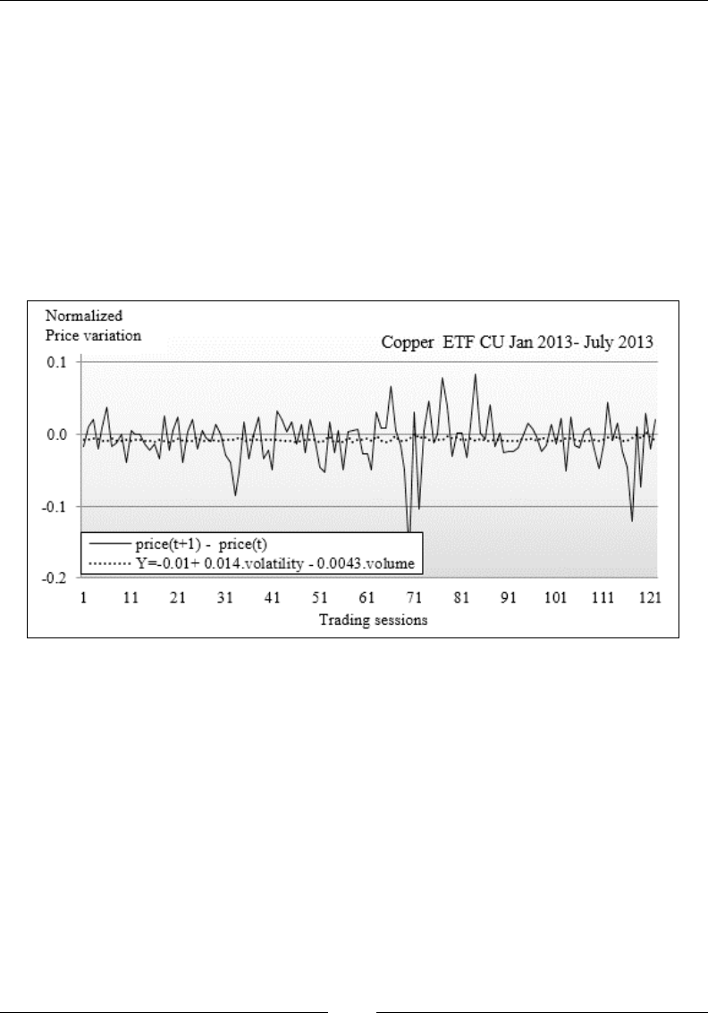
Chapter 6
[ 779 ]
The daily session adjusted closing price, the session volatility, and the session
volume for the CU ETF is extracted from a CSV le (line 1) using the DataSource
transformation (line 2). The array, priceChange, which is the daily price change
between two consecutive trading sessions is computed by duplicating, shifting,
and zipping the session closing prices (line 3). The features are computed by
zipping volatility and the volume time series (line 4). The regression model is
trained by instantiating the MultiLinearRegression class (line 5) and the
model weights are displayed using an auxiliary display method (to the logger
or standard output) (line 6).
The original price change time series and the data predicted by the regression are
plotted in the following chart:
Price variation and the least squares regression for copper ETF according to volatility and volume
The least squares regression model is dened by the linear function for the
estimation of price variation as follows:
price(t+1)-price(t) = -0.01 + 0.014 volatility – 0.0042.volume
The estimated price change (the dotted line in the preceding chart) represents
the long term trend from which the noise is ltered out. In other words, the least
squares regression operates as a simple low-pass lter as an alternative to some of
the ltering techniques such as discrete Fourier transform or the Kalman lter for
dynamic systems (refer to Chapter 3, Data Preprocessing) [6:7].
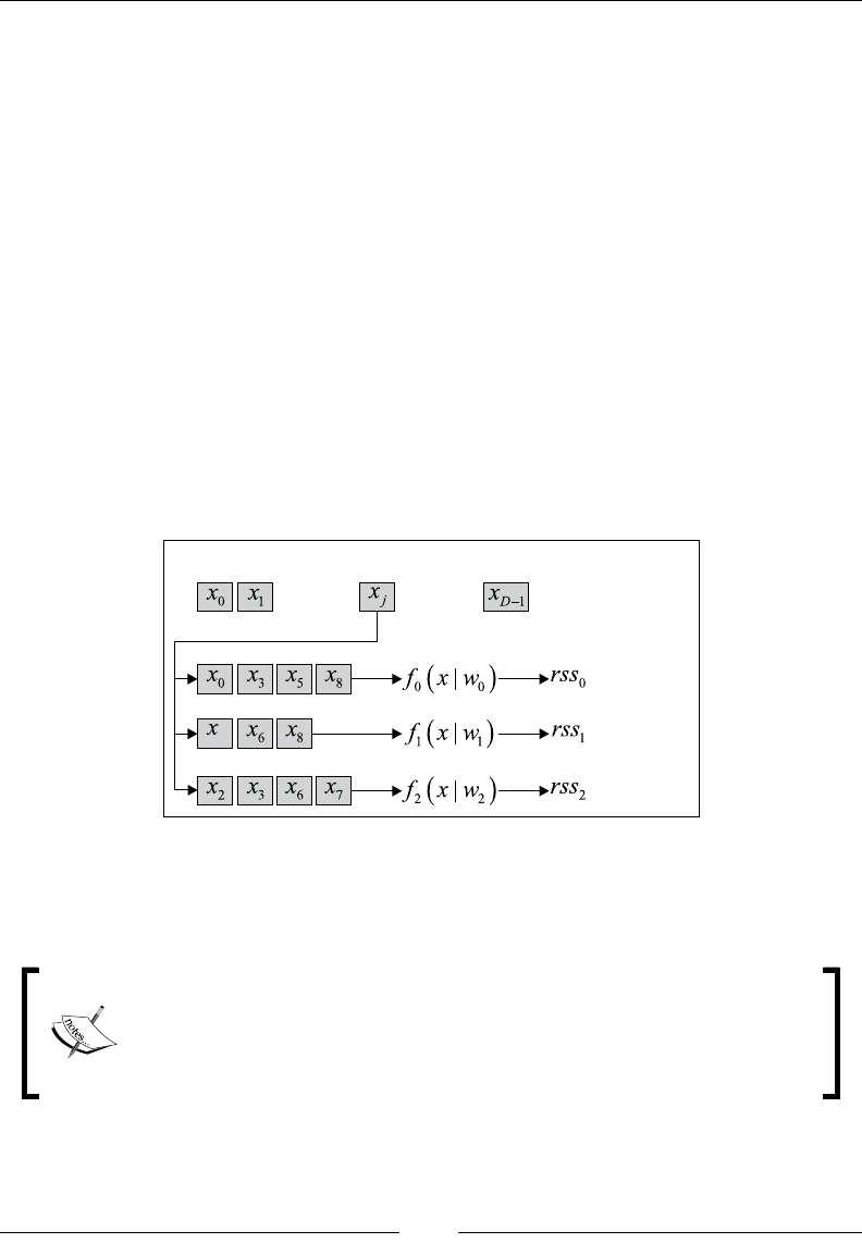
Regression and Regularization
[ 780 ]
Although trend detection is an interesting application of the least squares regression,
the method has limited ltering capabilities for time series [6:8]:
• It is sensitive to outliers
• It put a greater weight to the rst and last few observations that need to
be discarded
• As a deterministic method, it does not support noise analysis (distribution,
frequencies, and so on)
Test case 2 – features selection
The second test case is related to features selection. The objective is to discover which
subset of initial features generates the most accurate regression model, that is, the
model with the smallest residual sum of squares (RSS) on the training set.
Let's consider an initial set of D features {xi}. The objective is to estimate the subset of
features {xi
d} that are the most relevant to the set of observations using a least squares
regression. Each subset of features is associated to an fj(x|wj) model:
Model 0
Model 1
Model 2
Original set of features
4
... ...
The OLS can be used to select the model parameters w if the original set of features
is small. Performing the regression of each subset of a large original features set is
not practical.
The features selection can be expressed mathematically as follows:
()
( )
()
21
1
0
0 1
argmin | |
j
j
D
n
jj jjd d
fi d
fyfxw fxww wx
−
−
= =
⎧ ⎫
⎪ ⎪
=−=+
⎨ ⎬
⎪ ⎪
⎩ ⎭
∑ ∑
(
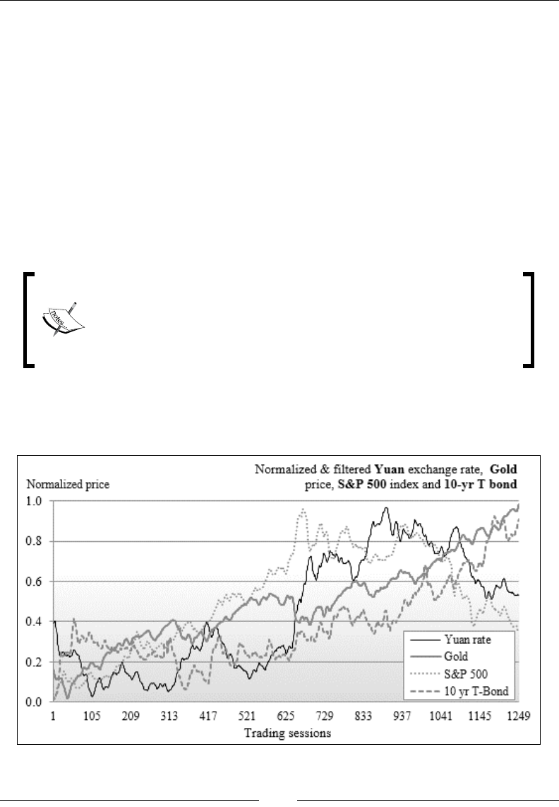
Chapter 6
[ 781 ]
Let's consider the following four nancial time series over the period from January 1,
2009 to December 31, 2013:
• The exchange rate of Chinese Yuan to US Dollar
• The S&P 500 index
• The spot price of gold
• The 10-year treasury bond price
The problem is to estimate which combination of the three variables S&P 500 index,
gold price, and 10-year treasury bond price is the most correlated to the exchange
rate of the Yuan. For practical reasons, we use the Exchange Trade Funds CYN as the
proxy for the Yuan/US dollar exchange rate (similarly, SPY, GLD, and TLT for S&P
500 index, the spot price of gold, and the 10-year treasury bond price respectively).
Automation of features extraction
The code in this section implements an ad hoc extraction of features
with an arbitrary xed set of models. The process can be easily
automated with an optimizer (gradient descent, genetic algorithm,
and so on) using 1/RSS as the objective function to be maximized.
The number of models to evaluate is relatively small, so an ad hoc approach
to compute the RSS for each combination is acceptable. Have a look at the
following graph:
Graph of the Chinese Yuan exchange rate, gold, 10-year treasury bond price, and S&P 500 index

Regression and Regularization
[ 782 ]
The getRss method implements the computation of the RSS value given a set of
observations xt and labeled values y:
def getRss(xt: XTSeries[DblVector], y: DblVector): String = {
val regression = MultiLinearRegression[Double](xt, y) //1
val buf = new StringBuilder
regression.weights.get
.zipWithIndex //2
.foreach(w => {
if(w._2 == 0) buf.append(w._1)
else buf.append(s" + ${w._1}.x${w._2}") //3
buf.append(s"RSS: ${(regression.rss.get}").toString
}
The getRss method merely trains the model by instantiating the multilinear
regression class (line 1), indexes the array of weights (line 2), and creates a text
representation of the linear regression equation (line 3).
Once the regression model is trained during the instantiation of the
MultiLinearRegression class, the coefcients of the regression weights and
the RSS value are printed. The rss method is invoked for any combination of the
variables ETF, GLD, SPY, and TLT against the label CNY:
val symbols = Array[String]("CNY", "GLD", "SPY", "TLT")
val smoothingPeriod = 16
val movAvg = SimpleMovingAverage[Double](smoothingPeriod) //4
val input= symbols.map(s=>DataSource(path+s+".csv",true,true, 1))
.map( _ |> YahooFinancials.adjClose ) //5
.map(x=> movAvg |> XTSeries[Double](x))
val features = input.drop(1)
val featuresList = List[(String, DblMatrix)](
("CNY=f(SPY,GLD,TLT)", features.map( _.toArray).transpose),//6
("CNY=f(GLD,TLT)", features.drop(1).map( _.toArray).transpose),
…
}
featuresList.foreach(x => Display.show(x._1 +
getRss(XTSeries[DblVector](x._2), input(0)), logger)) //7
The dataset is large (1,260 trading sessions) and noisy enough to warrant ltering using
a simple moving average with a period of 16 trading sessions, movAvg (line 4). The time
series are extracted from CSV les using the DataSource class, then smoothed using
a sequence of Array.map invocations (line 5). The rst map extracts the content of
the les associated to the stock ticker symbol, assuming that the names of the les
are formatted as path/symbol.csv.
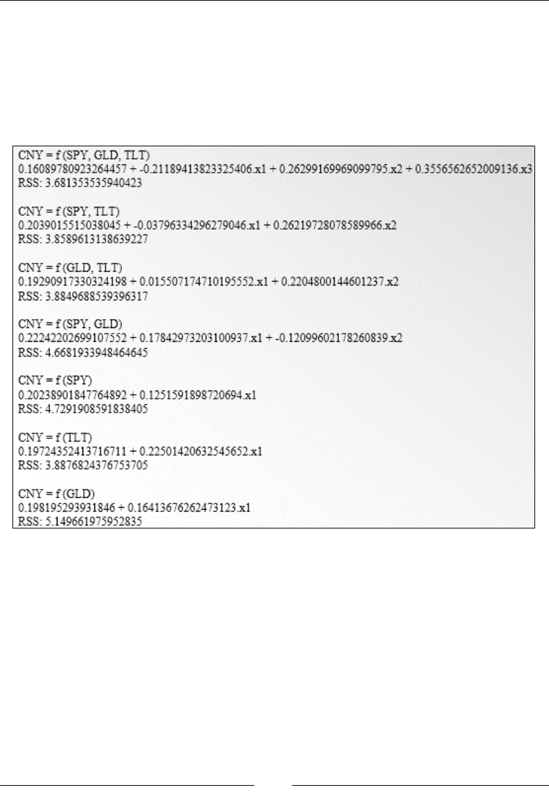
Chapter 6
[ 783 ]
For the sake of simplicity, the option type returned by the pipe operator is not validated.
The rst model using the three variables SPY, GLD, and TLT is created by transposing
them by the xt.size matrix (line 6). The RSS value is computed by invoking the rss
method (line 7). The second model using two variables, SPY and TLT, is created by
ltering out the GLD time series. The process is repeated for all other models. Have a
look at the following screenshot:
The output results clearly show that the three variable regression CNY=f(SPY, GLD,
TLT) is the most accurate or ttest model for the CNY time series, followed by CNY
=f(SPY, TLT). Therefore, the feature selection process generates the features set,
{SPY, GLD, TLT}.
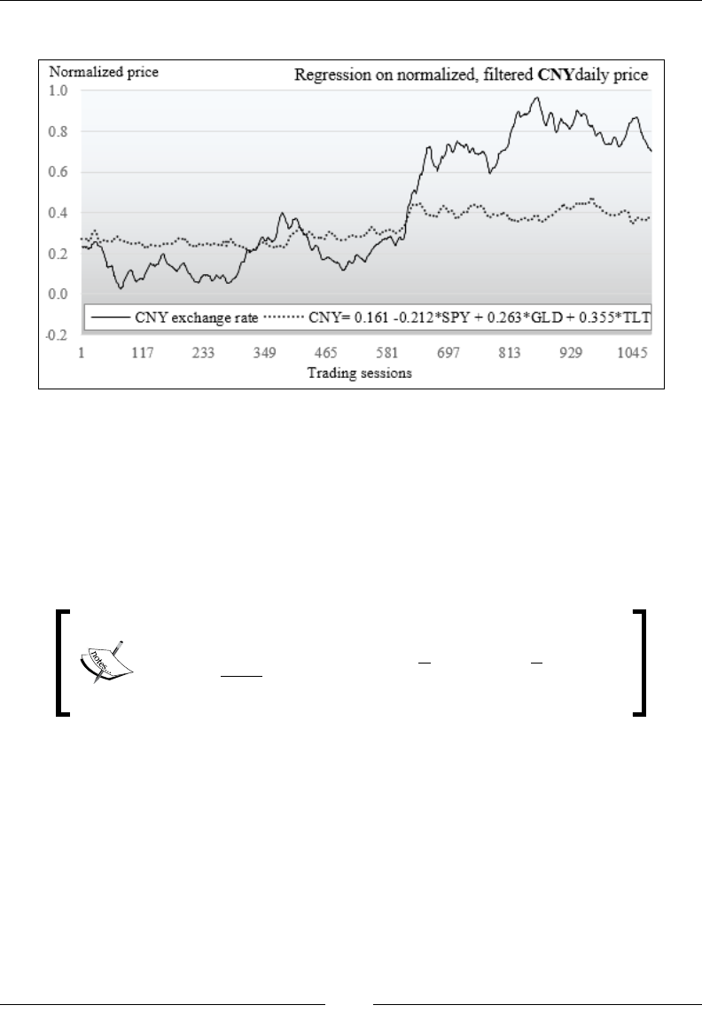
Regression and Regularization
[ 784 ]
Let's plot the model against the raw data:
Ordinary least regression on the Chinese Yuan ETF (CNY)
The regression model smoothed the original CNY time series. It weeded out all but the
most signicant price variation.
However, the RSS does not always provide an accurate visualization of the tness
of the regression model. The tness of the regression model is commonly assessed
using r2 statistics. The r2 value is a number that indicates how well data ts a
statistical model.
RSS and r2 statistics are related by the following formulae:
()
( )
2
1
2
0
1 |
n
j j
i f
RSS
r TSS y f x w f f
TSS
−
=
=−=−=
∑ ∑
The implementation of the computation of the r2 statistics is fairly simple. For each
model fj, the rssSum method computes the tuple {rss, sum of predicted values}:
def rssSum(xt: XTSeries[DblVector], y: DblVector): XY = {
val regression = MultiLinearRegression[Double](xt, y)
(regression.rss.get,
xt.toArray.zip(y).foldLeft(0.0)(s,x) =>
val d = (x._2 - (regression |> x._1))
s + d*d
})
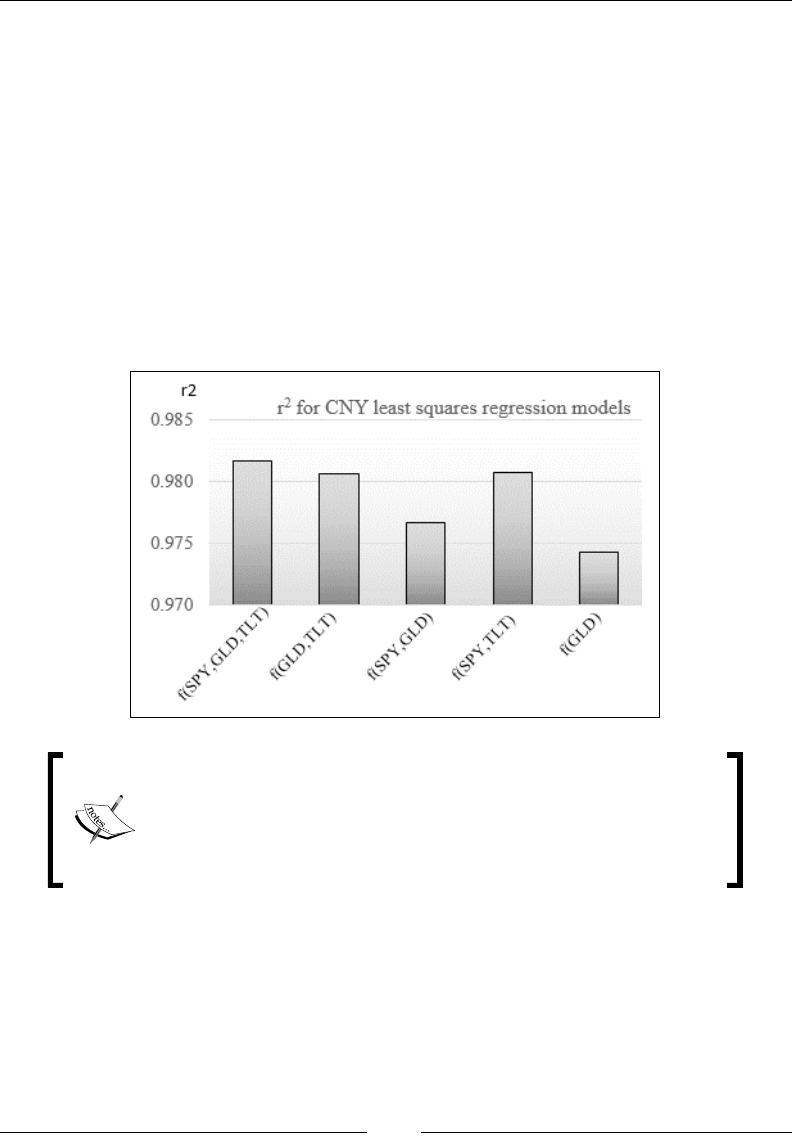
Chapter 6
[ 785 ]
Finally, the process is repeated for each model and the sum of the predicted values
for each model is summed (line 8), averaged (line 9), and then used in the r2 formula
(line 10):
var xsRss = new ListBuffer[Double]()
val tss = featuresList.foldLeft(0.0)((s, x) => { //8
val _tss = rssSum(XTSeries[DblVector](x._2), input(0))
xsRss.append(_tss._1)
s + _tss._2 //9
})/xsRss.size
xsRss.map( 1.0 - _/tss) //10
The graph plotting the r2 value for each model conrms that the three features model
is the most accurate:
General linear regression
The concept of linear regression is not restricted to polynomial
tting models such as y = w0 + w1.x + w2.x2 + …+ wnxn. Regression
models can also be dened as a linear combination of basis
functions as ϕj: y = w0 + w1.ϕ1(x) + w2ϕ2(x) + … + wn.ϕn(x) [6:9].

Regression and Regularization
[ 786 ]
Regularization
The ordinary least squares method for nding the regression parameters is a specic
case of the maximum likelihood. Therefore, regression models are subject to the same
challenge in terms of overtting as any other discriminative model. You are already
aware that regularization is used to reduce model complexity and avoid overtting
as stated in the Overtting section of Chapter 2, Hello World!.
Ln roughness penalty
Regularization consists of adding a penalty function J(w) to the loss function (or
RSS in the case of a regressive classier) in order to prevent the model parameters
(or weights) from reaching high values. A model that ts a training set very well
tends to have many features variable with relatively large weights. This process is
known as shrinkage. Practically, shrinkage involves adding a function with model
parameters as an argument to the loss function:
()
( )
()
1
2
0
ˆargmin |
d
n
ii
w
i
wyfxw Jw
λ
−
=
⎧ ⎫
=−+
⎨ ⎬
⎩ ⎭
∑
The penalty function is completely independent from the training set {x,y}. The
penalty term is usually expressed as a power to the function of the norm of the
model parameters (or weights), wd. For a model of D dimensions, the generic
Lp-norm is dened as follows:
()
/
1
1
qp
D
q p
pq d
p
d
Jw w w
−
=
⎡⎤
==
⎢⎥
⎣⎦
∑
Notation
Regularization applies to parameters or weights associated
to an observation. In order to be consistent with our notation,
w0 being the intercept value, the regularization applies to the
parameters w1,…, wd.
The two most commonly used penalty functions for regularization are L1 and L2.

Chapter 6
[ 787 ]
Regularization in machine learning
The regularization technique is not specic to the linear or logistic
regression. Any algorithm that minimizes the residual sum of
squares, such as a support vector machine or feed-forward neural
network, can be regularized by adding a roughness penalty
function to the RSS.
The L1 regularization applied to the linear regression is known as the Lasso
regularization. The Ridge regression is a linear regression that uses the L2
regularization penalty.
You may wonder which regularization makes sense for a given training set. In
a nutshell, L2 and L1 regularization differ in terms of computation efciency,
estimation, and features selection: [6:10] [6:11]
• Model estimation: L1 generates a sparser estimation of the regression
parameters than L2. For a large nonsparse dataset, L2 has a smaller
estimation error than L1.
• Feature selection: L1 is more effective in reducing the regression weights
for features with high value than L2. Therefore, L1 is a reliable features
selection tool.
• Overtting: Both L1 and L2 reduce the impact of overtting. However, L1 has
a signicant advantage in overcoming overtting (or excessive complexity of
a model); for the same reason, it is more appropriate for selecting features.
• Computation: L2 is conducive to a more efcient computation model. The
summation of the loss function and the L2 penalty, w2, is a continuous and
differentiable function for which the rst and second derivative can be
computed (convex minimization). The L1 term is the summation of |wi|
and therefore not differentiable.
Terminology
The ridge regression is sometimes called the penalized least
squares regression. The L2 regularization is also known as
the weight decay.
Let's implement the ridge regression, and then evaluate the impact of the L2-norm
penalty factor.

Regression and Regularization
[ 788 ]
The ridge regression
The ridge regression is a multivariate linear regression with an L2-norm penalty term:
( )
2
122 2
022
0 1
ˆargmin
d
n D
T
Ridge d
w
j d
wyw wx w w w
λ
−
= =
=−− + =
∑ ∑
The computation of the ridge regression parameters requires the resolution of a
system of linear equations similar to the linear regression.
The matrix representation of the ridge regression closed form is
as follows:
()
ˆ
.
T T
Ridge
XX Iw Xy
λ
−=
I is the identity matrix and uses the QR decomposition:
()
1
.0 0
T T
Ridge y
R R
XX IQ w Q
λ
−
⎡⎤
−=⎢⎥
⎣⎦
Implementation
The implementation of the ridge regression adds the L2 regularization term to the
multiple linear regression computation of the Apache Commons Math library.
The methods of RidgeRegression have the same signature as their ordinary least
squares counterparts. However, the class has to inherit the abstract base class,
AbstractMultipleLinearRegression, in the Apache Commons Math library
and override the generation of the QR decomposition to include the penalty term:
class RidgeRegression[T <% Double](xt: XTSeries[Array[T]], y:
DblVector, lambda: Double) extends AbstractMultipleLinearRegression
with PipeOperator[Array[T], Double] {
var qr: QRDecomposition = _
val model: Option[RegressionModel] = …
…

Chapter 6
[ 789 ]
Besides the input time series xt and the labels y, the ridge regression requires the
lambda factor of the L2 penalty term. The instantiation of the class trains the model.
The steps to create the ridge regression models are as follows:
1. Extract the Q and R matrices for the input values, newXSampleData (line 1).
2. Compute the weights using calculateBeta dened in the base class (line 2).
3. Return the tuple regression weights, calculateBeta, and the residuals,
calculateResiduals.
Consider the following code:
val model: Option[(DblVector, Double)] = {
this.newXSampleData(xt.toDblMatrix) //1
newYSampleData(y)
val _rss = calculateResiduals.toArray.map(x => x*x).sum
val wRss = (calculateBeta.toArray, _rss) //2
Some(RegressionModel(wRss._1, wRss._2))
}
The QR decomposition in the base class, AbstractMultipleLinearRegression,
does not include the penalty term (line 3); the identity matrix with the lambda factor
in the diagonal has to be added to the matrix to be decomposed (line 4):
override protected def newXSampleData(x: DblMatrix): Unit = {
super.newXSampleData(x) //3
val xtx: RealMatrix = getX
val nFeatures = xt(0).size
Range(0, nFeatures)
.foreach(i =>xtx.setEntry(i,i,xtx.getEntry(i,i)+lambda)) //4
qr = new QRDecomposition(xtx)
}
The regression weights are computed by resolving the system of linear equations using
substitution on the Q.R matrices. It overrides calculateBeta from the base class:
override protected def calculateBeta: RealVector =
qr.getSolver().solve(getY())

Regression and Regularization
[ 790 ]
The test case
The objective of the test case is to identify the impact of the L2 penalization on the
RSS value and then compare the predicted values with the original values.
Let's consider the rst test case related to the regression on the daily price variation of
the Copper ETF (symbol: CU) using the stock daily volatility and volume as features.
The implementation of the extraction of observations is identical to that of the least
squares regression:
val lambda = 0.5
val src = DataSource(path, true, true, 1)
val price = src |> YahooFinancials.adjClose
val volatility = src |> YahooFinancials.volatility
val volume = src |> YahooFinancials.volume //1
val deltaPrice = XTSeries[Double](price.drop(1)
.zip(price.take(_price.size -1))
.map( z => z._1 - z._2)) //2
val data = volatility.zip(volume)
.map(z => Array[Double](z._1, z._2)) //3
val features = XTSeries[DblVector](data.dropRight(1))
val regression = new RidgeRegression[Double](features, deltaPrice,
lambda) //4
regression.rss match {
case Some(rss) => Display.show(rss, logger)
…
The observed data, that is, the ETF daily price and the features (volatility
and volume) are extracted from the src source (line 1). The daily price change
deltaPrice is computed using a combination of Scala take and drop methods (line
2). The features vector is created by zipping volatility and volume (line 3). The
model is created by instantiating the RidgeRegression class (line 4). The RSS value,
rss, is nally displayed (line 5).
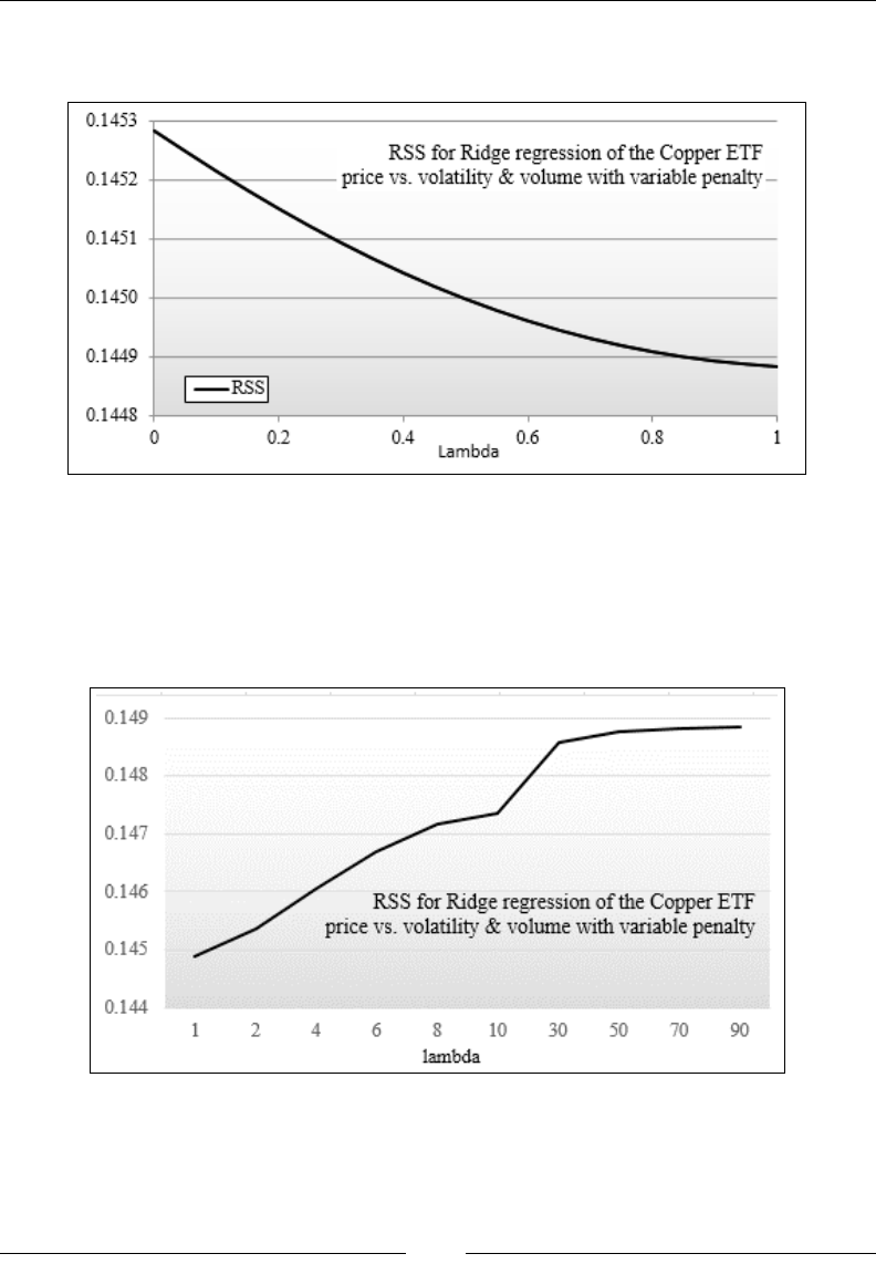
Chapter 6
[ 791 ]
The RSS value, rss, is plotted for different values of lambda less than 1.0, as shown
in the following chart:
Graph of RSS versus Lambda for Copper ETF
The residual sum of squares decreases as λ increases. The curve seems to be
reaching for a minimum around λ = 1. The case of λ = 0 corresponds to the
least squares regression.
Next, let's plot the RSS value for λ varying between 1 and 100:
Graph of RSS versus large-value Lambda for Copper ETF
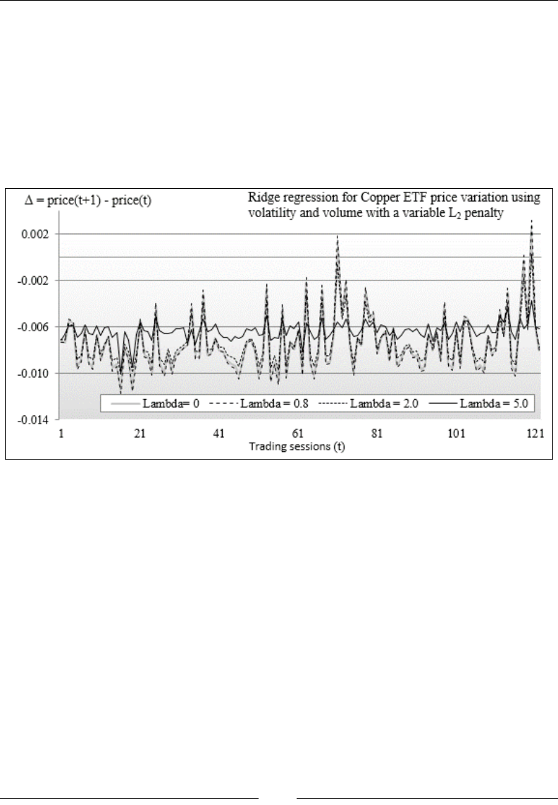
Regression and Regularization
[ 792 ]
This time around, the value of RSS increases with λ before reaching a maximum
of λ > 60. This behavior is consistent with other ndings [6:12]. As λ increases, the
overtting gets more expensive and therefore, the RSS value increases.
The regression weights can be simply outputted as follows:
regression.weights.get
Let's plot the predicted price variation of the Copper ETF using the ridge regression
with different values of lambda (λ):
The graph of ridge regression on Copper ETF price variation with variable lambda
The original price variation of the Copper ETF, Δ = price(t+1)-price(t), is plotted
as λ = 0. The predicted values for λ = 0.8 is very similar to the original data. The
predicted values for λ = 2 follow the pattern of the original data with a reduction
of large variations (peaks and troves). The predicted values for λ = 5 correspond to
a smoothed dataset. The pattern of the original data is preserved but the magnitude
of the price variation is signicantly reduced.
The logistic regression, briey introduced in the Let's kick the tires section of Chapter 1,
Getting Started, is the next logical regression model to discuss. The logistic regression
relies on optimization methods. Let's go through a short refreshment course in
optimization before diving into the logistic regression.

Chapter 6
[ 793 ]
Numerical optimization
This section briey introduces the different optimization algorithms that can
be applied to minimize the loss function, with or without a penalty term. These
algorithms are described in greater detail in the Summary of optimization techniques
section in Appendix A, Basic Concepts.
First, let's dene the least squares problem. The minimization of the loss function
consists of nullifying the rst order derivatives, which in turn generates a system of
D equations (also known as gradient equations), D being the number of regression
weights (parameters). The weights are iteratively computed by solving the system of
equations using a numerical optimization algorithm.
The denition of the least squares-based loss function is as follows:
() () ( )
1
0
|
n
iii
i
Lw r w y f x w
−
=
==−
∑
The generation of gradient equations with a Jacobian J matrix (refer to
the Jacobian and Hessian matrices section in Appendix A, Basic Concepts)
after minimization of the loss function L is described as follows:
() ()
()
1
0
0
n
i
iid id
id
rw
rwJ J w
w
−
=
∂
==−∂
∑
Iterative approximation using the Taylor series is described as follows:
()
()
()
()
()
()
()
1
0
|
||~
d
k
Di
k k
i i
jd w
fxw
fxw ffxw ww
−
=
∂
− −
∂
∑
Normal equations using the matrix notation and the Jacobian matrix is
described as follows:
()
() ()
()
() ()
()
1 1kk kk
T T
ii
JJ w w J y y
+ +
−=−

Regression and Regularization
[ 794 ]
The logistic regression is a nonlinear function. Therefore, it requires the nonlinear
minimization of the sum of least squares. The optimization algorithms for the
nonlinear least squares problems can be divided into the following two categories:
• Newton (or 2nd order techniques): These algorithms calculate the second
order derivatives (the Hessian matrix) to compute the regression weights
that nullify the gradient. The two most common algorithms in this category
are the Gauss-Newton and the Levenberg-Marquardt methods (refer to the
Nonlinear least squares minimization section in Appendix A, Basic Concepts). Both
algorithms are included in the Apache Commons Math library.
• Quasi-Newton (or 1st order techniques): First order algorithms do not
compute but estimate the second order derivatives of the least squares
residuals from the Jacobian matrix. These methods can minimize any
real-valued functions, not just the least squares summation. This
category of algorithms includes the Davidon-Fletcher-Powell and the
Broyden-Fletcher-Goldfarb-Shannon methods (refer to the Quasi-Newton
algorithms section in Appendix A, Basic Concepts).
The logistic regression
Despite its name, the logistic regression is a classier. As a matter of fact, the logistic
regression is one of the most used discriminative learning techniques because of its
simplicity and its ability to leverage a large variety of optimization algorithms. The
technique is used to quantify the relationship between an observed target variable y
and a set of variables x that it depends on. Once the model is created (trained), it is
used to classify real-time data.
A logistic regression can be either binomial (two classes) or multinomial (three and
more classes). In a binomial classication, the observed outcome is dened as {true,
false}, {0, 1}, or {-1, +1}.
The logit function
The conditional probability in a linear regression model is a linear function of its
weights [6:13]. The logistic regression model addresses the nonlinear regression
problem by dening the logarithm of the conditional probability as a linear function
of its parameters.
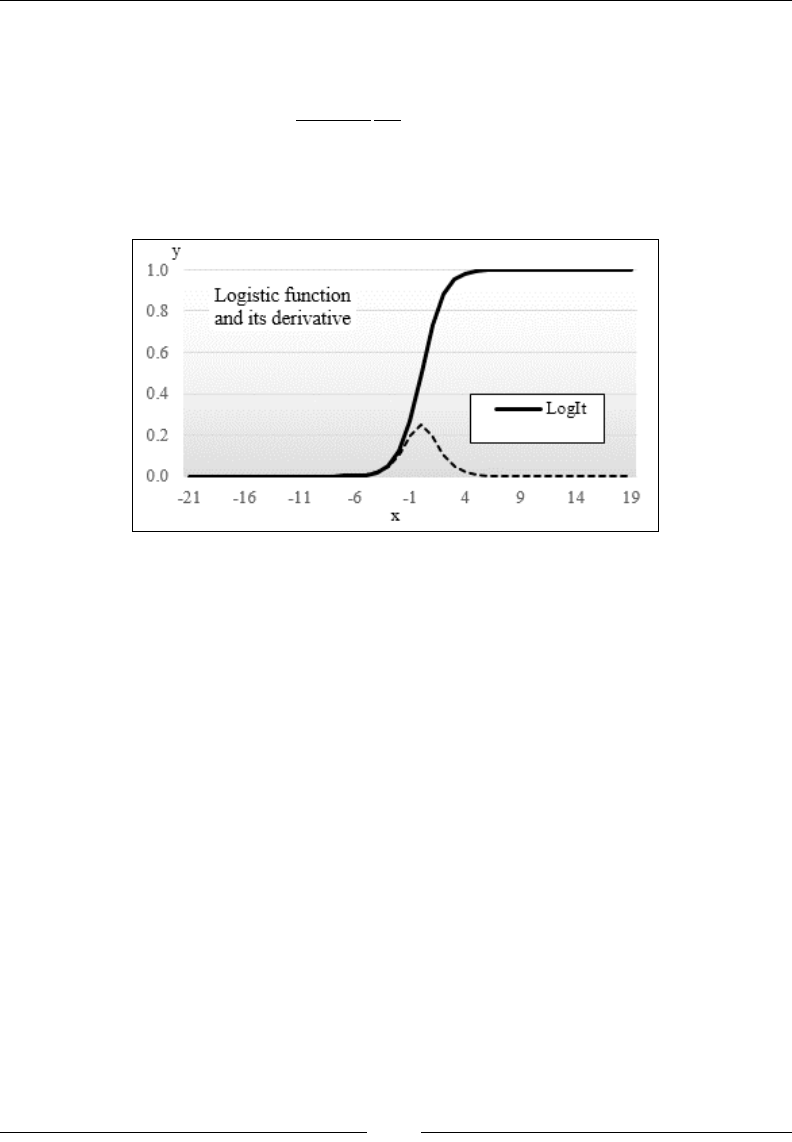
Chapter 6
[ 795 ]
First, let's introduce the logistic function and its derivative, which are dened
as follows:
()
()
() ()
()
1
1
1x
df
fx fx fx
dx
e−
= = −
−
Have a look at the following graph:
The graph of the logistic function and its derivative
The remainder of this section is dedicated to the application of the multivariate
logistic regression to a binary classication (two classes).
Binomial classication
The logistic regression is popular for several reasons; some are as follows:
• It is available with most statistical software packages and open source libraries
• Its S-shape describes the combined effect of several explanatory variables
• Its range of values [0, 1] is intuitive from a probabilistic perspective
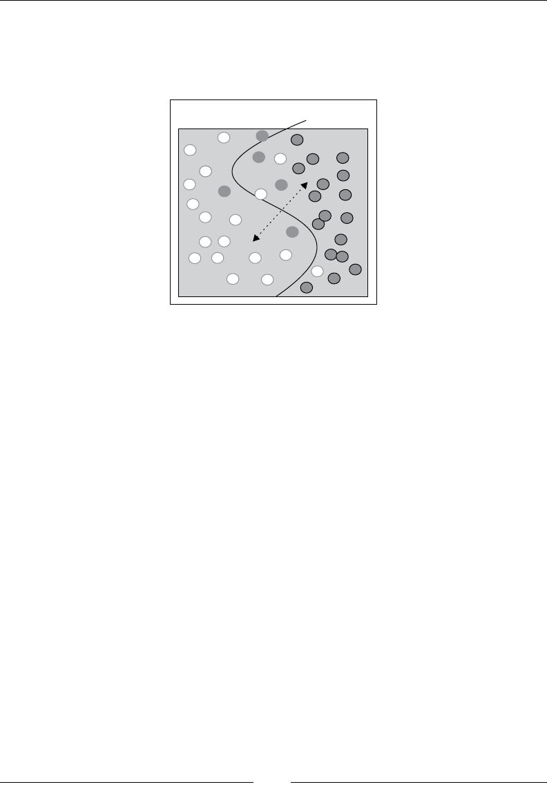
Regression and Regularization
[ 796 ]
Let's consider the classication problem using two classes. As discussed in the
Validation section of Chapter 2, Hello World!, even the best classier produces false
positives and false negatives. The training procedure for a binomial classication is
illustrated in the following diagram:
Hyperplane
Class 2
Class 1
Illustration of the binomial classification for a 2-dimension dataset
The purpose of the training is to compute the hyperplane that separates the
observations into two categories or classes. Mathematically speaking, a hyperplane
in an n-dimensional space (number of features) is a subspace of n-1 dimensions. The
separating hyperplane of a three-dimension space is a curved surface. The separating
hyperplane of a two-dimension problem (plane) is a line. In our preceding example,
the hyperplane segregates/separates a training set into two very distinct classes (or
groups), class 1 and class 2, in an attempt to reduce the overlap (false positive and
false negative).
The equation of the hyperplane is dened as the logistic function of the dot product of the
regression parameters (or weights) and features.
The logistic function accentuates the difference between the two groups of training
observations, separated by the hyperplane. It pushes the observations away from
the separating hyperplane towards either of the classes.
Chapter 6
[ 797 ]
In the case of two classes, c1 and c2 with their respective probabilities, p(C=c1|
X=xi|w) = p(xi|w) and p(C=c2 |X= xi|w) = 1- p(xi|w), where w is the model
parameters set or weights in the case of the logistic regression, the following
functions can be dened:
The log likelihood:
() ( )
1
0
log|
N
i
i
Lw px w
−
=
=∑
Conditional probabilities using the logit function:
[]
()
12
1, , |
1
T
T
wx
T
dwx
e
xxxx pxw
e
= =
+
L
The log likelihood for the binomial logistic regression:
()
()
{}
1
0
log1 0,1
T
i
N
wx
T
ii
i
Lw ywx e y
−
=
=−+∈
∑
First order derivative for the log likelihood:
()
()
( )
1
0
|
N
ij ii
i
j
Lw
xy pxw
w
−
=
∂
=−
∂∑
Let's implement the logistic regression without a penalty term using the Apache
Commons Math library. The library contains several least squares optimizers,
allowing you to specify the minimizing algorithm, optimizer, for the loss function
in the logistic regression class LogisticRegression:
class LogisticRegression[T <% Double](xt: XTSeries[Array[T]],
labels: Array[Int], optimizer: LogisticRegressionOptimizer) extends
PipeOperator[Array[T], Int]{
val model: Option[RegressionModel] = { … }
…
}

Regression and Regularization
[ 798 ]
The parameters of the logistic regression class are the multivariate time series (features)
xt, the target or labeled data, labels, and the optimizer algorithm used to minimize
the loss function or residual sum of squares. In the case of the binomial logistic
regression, labels are assigned the values of 1 for one class and 0 for the other.
The purpose of the training is to determine the regression coefcient, model._1,
which minimizes the loss function. The residual sum of squares (RSS) is computed
as model._2.
Target values
There is no specic rule to assign the two values to the observed
data for the binomial logistic regression: {-1, +1}, {0, 1}, or {false,
true}. The values pair {0, 1} is convenient because it allows the
developer to reuse the code for multinomial logistic regression
using normalized class values.
For convenience, the denition and the conguration of the optimizer are
encapsulated in the LogisticRegressionOptimizer class.
Software design
The implementation of the logistic regression uses the following components:
• RegressionModel of the Model type, which is initialized through training
during the instantiation of the classier. We reuse the RegressionModel
type introduced in the Linear regression section.
• The predictive or classication routine is implemented as a data
transformation |> extending the PipeOperator trait.
• The logistic regression class, LogisticRegression, has three parameters: the
least squares optimizer of the type LogisticRegresssionOptimizer (used
in training), a features set XTSeries, and a label vector DblVector.
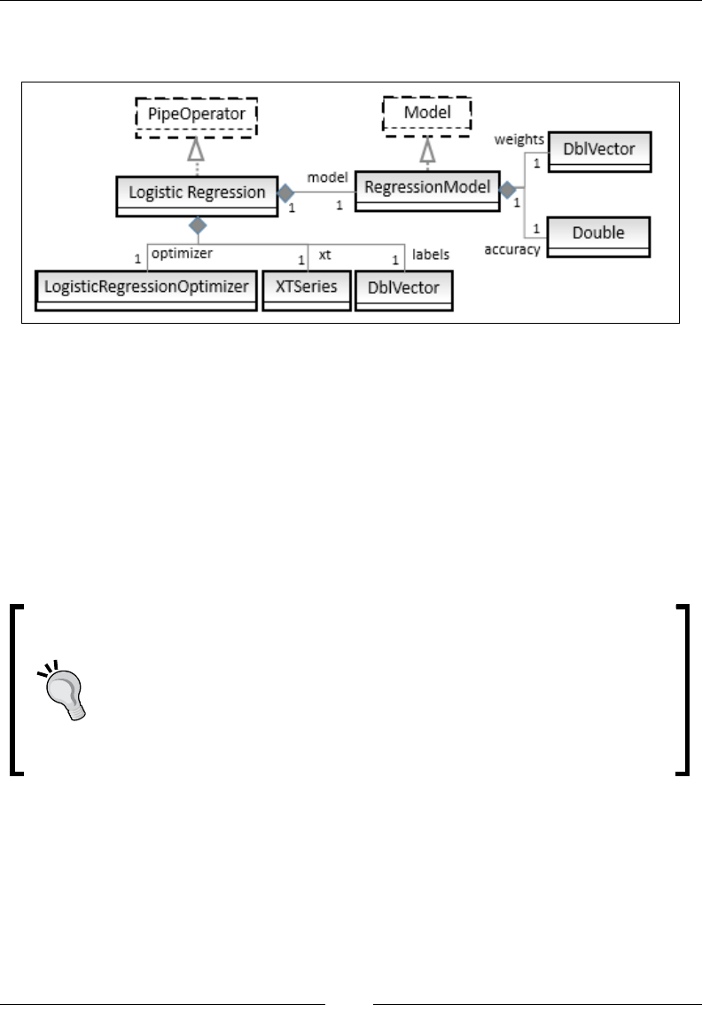
Chapter 6
[ 799 ]
The key software components of the logistic regression are described in the following
UML class diagram:
The UML class diagram for the logistic regression
The training workow
Our implementation of the training of the logistic regression model leverages either
the Gauss-Newton or the Levenberg-Marquardt nonlinear least squares optimizers,
(refer to the Nonlinear least squares minimization section in Appendix A, Basic Concepts)
packaged with the Apache Commons Math library.
The training of the logistic regression is performed by the train method:
val model: Option[RegressionModel] = train
Handling exceptions from the Apache Commons Math library
The training of the logistic regression using the Apache Commons
Math library requires handling ConvergenceException,
DimensionMismatchException, TooManyEvaluationsException,
TooManyIterationsException, and MathRuntimeException.
Debugging is greatly facilitated by understanding the context of these
exceptions in the Apache library source code.
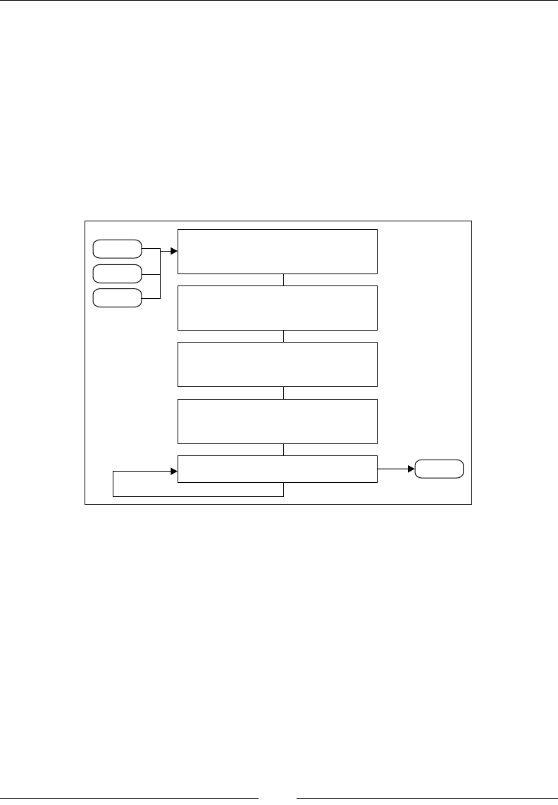
Regression and Regularization
[ 800 ]
The implementation of the training method, train, relies on the following ve steps:
1. Select and congure the least squares optimizer.
2. Dene the logit function and its Jacobian.
3. Specify the convergence and exit criteria.
4. Compute the residuals using the least squares problem builder.
5. Run the optimizer.
The workow and the Apache Commons Math classes used in the training of the
logistic regression are visualized by the following ow diagram:
1.Configure Least Squares minimizer
LogisticRegressionOptimizer
2.Define logit&its Jacobian
MultivariateJacobianFunction
3.Define the exit conditions
ConvergenceChe kerc
4.Build least squares problem
LeastSquaresBuilder
5.Execute minimization
iterates
optimizer
labels
Xt
model
The workflow for training the logistic regression using Apache Commons Math
The rst four steps are required by the Apache Commons Math library to initialize
the conguration of the logistic regression prior to the minimization of the loss
function. Let's start with the conguration of the least squares optimizer.
Conguring the least squares optimizer
In this step, you have to specify the algorithm to minimize the residual of the sum of
squares. The LogisticRegressionOptimizer class is responsible for conguring the
optimizer. The class has the following two purposes:
• Encapsulating the conguration parameters for the optimizer
• Invoking the LeastSquaresOptimizer interface dened in the Apache
Commons Math library

Chapter 6
[ 801 ]
Consider the following code:
class LogisticRegressionOptimizer(maxIters: Int, maxEvals: Int,eps:
Double, lsOptimizer: LeastSquaresOptimizer){
def optimize(lsProblem: LeastSquaresProblem): Optimum = lsOptimizer.
optimize(lsProblem)
}}
The conguration of the logistic regression optimizer is dened using the maximum
number of iterations (maxIters), the maximum number of evaluations (maxEval)
for the logistic function and its derivative, the convergence criteria (eps) on the
residual sum of squares, and the instance of the least squares problem (org.apache.
commons.math3.fitting.leastsquares.LeastSquaresProblem).
Computing the Jacobian matrix
The next step consists of computing the value of the logistic function and its rst
order partial derivatives with respect to the weights by overriding the value method
of the fitting.leastsquares.MultivariateJacobianFunction interface:
final val initWeight = 0.5
val weights0 = Array.fill(xt(0) +1)(initWeight) //1
val lrJacobian = new MultivariateJacobianFunction {
override def value(w:RealVector):Pair[RealVector,RealMatrix] ={
val _w = w.toArray
val gradient = xt.toArray
.map( g => { //2
val expn = g.zip(_w.drop(1))
.foldLeft(_w(0))((s,z) => s + z._1*z._2)
val logIt = 1.0/(1.0 + Math.exp(-expn)) //3
(logIt, logIt *(1- logIt)) //4
})
val jacobian = Array.ofDim[Double](xt.size, weights0.size)//5
xt.toArray.zipWithIndex.foreach(xi => { //6
val df: Double = gradient(xi._2)._2
Range(0, xi._1.size).foreach(j =>
jacobian(xi._2)(j+1) = xi._1(j)*df)
jacobian(xi._2)(0) = 1.0 //7
})
(new ArrayRealVector(gradient.map(_._1)),
new Array2DRowRealMatrix(jacobian)) //8
}
}
The regression weights, weights0, are initialized with the arbitrary value of 0.5.

Regression and Regularization
[ 802 ]
The value method uses the primitives types RealVector, RealMatrix,
ArrayRealVector, and Array2DRowRealMatrix dened in the org.apache.
commons.math3.linear Apache Commons Math package.
It takes the regression weight, w, and computes the gradient (line 2) of the logistic
function for each data point and returns the value of logit (line 3) and its derivative
(line 4) as a tuple. The Jacobian matrix is created (line 5), and then initialized with
logit and its derivative (line 6). The rst element of each column of the Jacobian
matrix is set to 1.0 to take into account the intercept (line 7). Finally, the vector of the
logit values for each observation and the Jacobian matrix are returned (line 8) as a
tuple to comply with the return type of the function value.
Dening the exit conditions
The third step denes the exit condition for the optimizer. It is accomplished by
overriding the converged method of the parameterized org.apache.commons.
math3.optim.ConvergenceChecker interface:
val exitCheck = new ConvergenceChecker[PointVectorValuePair] {
override def converged(iteration: Int, prev: PointVectorValuePair,
current:PointVectorValuePair): Boolean = {
val delta = prev.getValue
.zip(current.getValue)
.foldLeft(0.0)((s, z) =>{
val d = z._1 - z._2
s + diff*diff
})
Math.sqrt(delta)<optimizer.eps && iteration>=optimizer.maxIters
}
}
This implementation computes the convergence or exit condition as follows:
• Either the L2-norm of the difference between the weights of the current
iteration and the weights of the previous iteration, delta, is smaller
than the convergence criteria, eps
• Or the iteration exceeds the maximum number of iterations that
maxIters allowed

Chapter 6
[ 803 ]
Dening the least squares problem
The Apache Commons Math least squares optimizer package requires all the
input to the nonlinear least squares minimizer to be dened as an instance of
LeastSquareProblem generated by the factory LeastSquareBuilder class:
val builder = new LeastSquaresBuilder
val diagWeights0 = Array.fill(xt.size)(1.0) //1
val wMatrix = MatrixUtils.createRealDiagonalMatrix(diagWeights0)
val lsp = builder.model(lrJacobian) //2
.weight(wMatrix)
.target(labels) //7
.checkerPair(exitCheck) //5
.maxEvaluations(optimizer.maxEvals) //3
.start(weights0) //6
.maxIterations(optimizer.maxIters) //4
.build
The diagonal elements of the weights matrix are initialized to 1.0 (line 1). Besides
the initialization of the model with the Jacobian matrix, lrJacobian (line 2), the
maximum number of evaluations (line 3), maximum number of iterations (line 4),
and the exit condition (line 5) are also initialized.
The regression weights are initialized as 0.5 (weights0) (line 6). Finally, the labeled
or target values are initialized (line 7).
Minimizing the loss function
The training is executed with a simple call to the least squares minimizer, lsp:
val optimum = optimizer.optimize(lsp)
(optimum.getPoint.toArray, optimum.getRMS)
The regression coefcients (or weights) and the residuals mean square (RMS) are
returned by invoking the getPoint method on the optimum class of the Apache
Commons Math library.

Regression and Regularization
[ 804 ]
Test
Let's test our implementation of the binomial multivariate logistic regression using
the example of the Copper ETF price variation versus volatility and volume, used
in the previous two sections. The only difference is that we need to dene the target
values as 0 if the ETF price decreases between two consecutive trading sessions, and
1 otherwise. Therefore, the deltaPrice vector used in the linear and ridge regression
is to be modied to support the binary outcome:
val deltaPrice = prices.drop(1).zip(prices).dropRight(1))
.map(p => if(p._1>p._2) 1 else 0)
Executing the test case is just a matter of instantiating the LogisticRegression class
with the appropriate conguration parameters. The implementation reuses the code
already dened for the least squares and ridge regression to load data from CSV les
(src, price, volatility, and volume) and normalize the observations:
val MAXITERS = 80; val MAXEVALS = 1000; val EPS = 1e-4
val lsOptimizer = LogisticRegressionOptimizer(MAXITERS, MAXEVALS, EPS,
new LevenbergMarquardtOptimizer)
val xt = XTSeries[DblVector](features)
val regression = new LogisticRegression[Double](xt, deltaPrice,
lsOptimizer)
val rms = regression.rms.get
val weights = regression.weights.get
In this example, the Levenberg-Marquardt algorithm is used to minimize the
loss function.
Levenberg-Marquardt parameters
The driver code uses the LevenbergMarquardtOptimizer
with the default tuning parameters conguration to keep the
implementation simple. However, the algorithm has a few important
parameters, such as relative tolerance for cost and matrix inversion,
that are worth tuning for commercial applications (refer to the
Levenberg-Marquardt section in Appendix A, Basic Concepts).
The execution of the test produces the following results:
• Residual mean square is 0.497
• Weights are -0.124 for intercept, 0.453 for ETF volatility, and -0.121 for
ETF volume
The last step is the classication of the real-time data.

Chapter 6
[ 805 ]
Classication
As mention earlier and despite its name, the binomial logistic regression is a binary
classier. The classication method is implemented as a data transformation by
overriding the pipe operator:
type Feature = Array[T]
final val MARGIN = 0.01
def |> : PartialFunction[Feature, Int] = { //1
case x: Feature if(model!=None && model.get.size-1==x.size) =>{
val w = _model.get.weights
val dot = x.zip(w.drop(1))
.foldLeft(w(0))((s,xw) => s + xw._1*xw._2)//2
if(logit(dot) > 0.5 + MARGIN) 1 else 0 //3
}
}
The classication method, |>, checks if the number of model parameters (weights)
is equal to the number of features plus 1 (line 1) and throws an exception if the test
fails. The dot product of the weights and the features is computed using a fold.
Finally, the method returns 1 (class 1, which signies that the price variation of the
ETF is positive) if the value of the sigmoid is greater than 0.5. It returns 0 otherwise
(class 2, which signies that the price variation of the ETF is negative) (line 3).
Class identication
The class that the new data x belongs to is determined by the
logit(dot) > 0.5 test, where dot is the product of the features
and the regression weights (w0+w1.volatility + w2.volume). This
test is equivalent to dot > 0.0. You may nd either condition in
the literature.
Let's apply the classication to the original training set, features, to validate our
model (weights):
val predicted = features.map(x => regression |> x)
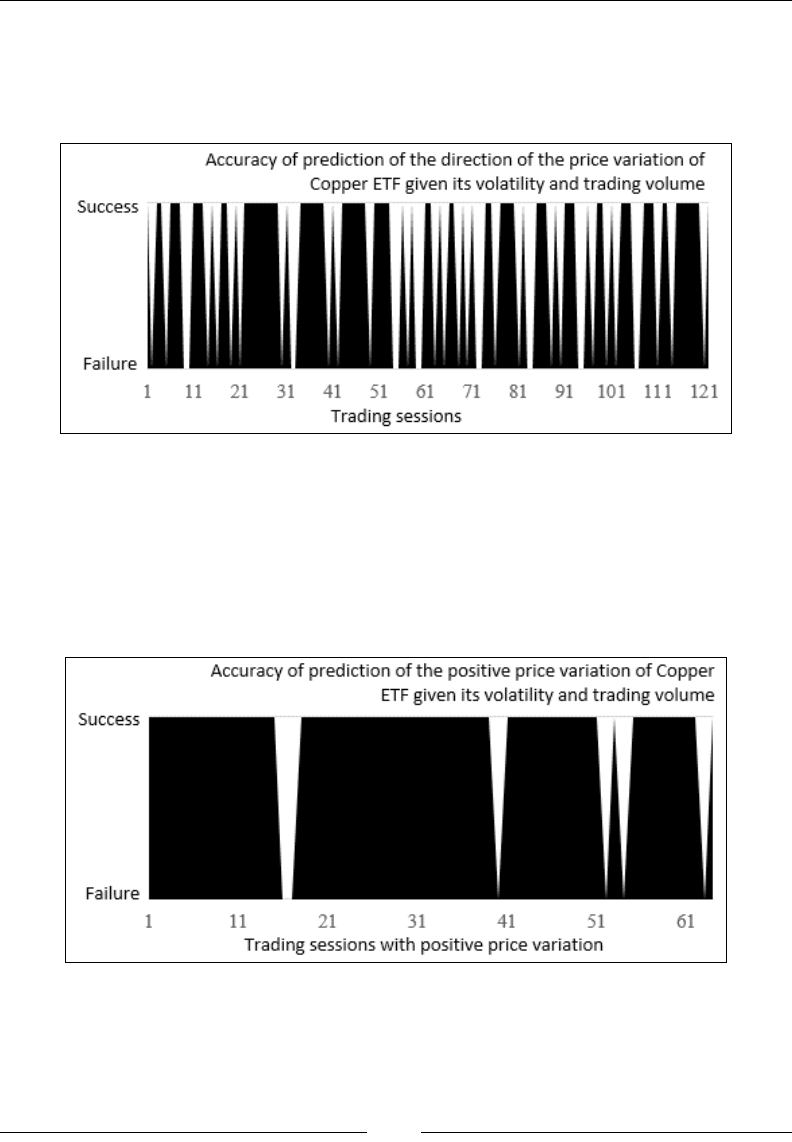
Regression and Regularization
[ 806 ]
The direction of the price variation of the Copper ETF, price(t+1) – price(t), is
compared to the direction predicted by the logistic regression. The result is plotted
with the success value if the positive or negative direction is correctly classied,
otherwise, it is plotted with the failure value:
The logistic regression was able to classify 78 out of 121 trading sessions
(65 percent accuracy).
Now, let's use the logistic regression to predict the positive price variation for the
Copper ETF, given its volatility and trading volume. This trading or investment
strategy is known as being long on the market. This use case ignores the trading
sessions for which the price was either at or declined:
The logistic regression was able to correctly predict the positive price variation for
58 out of 64 trading sessions (90.6 percent accuracy). What is the difference between
the rst and second test cases?
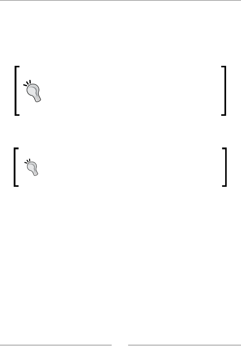
Chapter 6
[ 807 ]
In the rst case, the separating hyperplane equation, w0 + w1.volatility +
w2.volume, is used to segregate both the features generating either positive or
negative price variation. The overall accuracy of the classication is negatively
impacted by the overlap of the features from the two classes.
In the second case, the classier has to consider only the observations located on one
side of the hyperplane equation, without taking into account the false negatives.
Impact of rounding errors
Under some circumstances, the generation of the rounding errors
during the computation of the Jacobian matrix has an impact
on the accuracy of the separating hyperplane equation: w0 +
w1.volatility + w2.volume. This negatively impacts the
prediction of both the positive and negative price variation.
The accuracy of the binary classier can be further improved by considering the
positive variation of price as price(t+1) – price(t) > EPS.
Validation methodology
The validation set is generated by randomly selecting data points
from the original labeled set. A formal validation requires the
use of a K-fold validation methodology to compute the recall,
precision, and F1 measure for the logistic regression model.
Summary
This concludes the description and implementation of linear and logistic regression
and the concept of regularization to reduce overtting. Your rst analytical projects
using machine learning will (or did) likely involve a regression model of some type.
Regression models, along with the Naïve Bayes classication, are the most understood
techniques for those without a deep knowledge of statistics or machine learning.
At the completion of this chapter, you hopefully have a grasp on the following:
• The concept of linear and nonlinear least squares-based optimization
• The implementation of ordinary least square regression as well as
logistic regression
• The impact of regularization with an implementation of the Ridge regression

Regression and Regularization
[ 808 ]
The logistic regression is also the foundation of the conditional random elds
introduced in the next chapter and articial neural networks in Chapter 9,
Articial Neural Networks.
Contrary to the Naïve Bayes models (refer to Chapter 5, Naïve Bayes Classiers), the
least squares or logistic regression does not impose the condition that the features
have to be independent. However, the regression models do not take into account
the sequential nature of a time series such as asset pricing. The next chapter, Chapter 7,
Sequential Data Models, describes two classiers that take into account the time
dependency in a time series.

Sequential Data Models
The universe of Markov models is vast and encompasses computational concepts
such as the Markov decision process, discrete Markov, Markov chain Monte Carlo
for Bayesian networks, and hidden Markov models.
Markov processes, and more specically, the hidden Markov model (HMM), are
commonly used in speech recognition, language translation, text classication,
document tagging, and data compression and decoding.
The rst section of this chapter introduces and describes the hidden Markov model
with the full implementation of the three canonical forms of the hidden Markov model
using Scala. This section details the different dynamic programming techniques used
in the evaluation, decoding, and training of the hidden Markov model. The design of
the classier follows the same pattern as the logistic and linear regression.
The second and last section of the chapter is dedicated to a discriminative (labels
conditional to observation) alternative to the hidden Markov model: conditional
random elds. The open source CRF Java library authored by Sunita Sarawagi from
the Indian Institute of Technology, Bombay, is used to create a predictive model
using conditional random elds [7:1].
Markov decision processes
This rst section also describes the basic concepts you need to know in order to
understand, develop, and apply the hidden Markov model. The foundation of
the Markovian universe is the concept known as the Markov property.
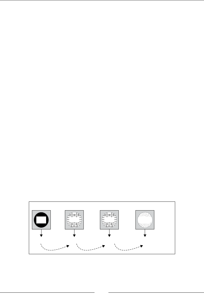
Sequential Data Models
[ 810 ]
The Markov property
The Markov property is a characteristic of a stochastic process where the conditional
probability distribution of a future state depends on the current state and not on its
past states. In this case, the transition between the states occurs at a discrete time,
and the Markov property is known as the discrete Markov chain.
The rst-order discrete Markov chain
The following example is taken from Introduction to Machine Learning by
E. Alpaydin [7:2].
Let's consider the following use case. N balls of different colors are hidden in N
boxes (one each). The balls can have only three colors {Blue, Red, and Green}. The
experimenter draws the balls one by one. The state of the discovery process is
dened by the color of latest ball drawn from one of the boxes: S0 = Blue, S1 = Red,
and S2 = Green.
Let {π0, π1, π2} be the initial probabilities for having an initial set of color in each
of the boxes.
Let qt denote the color of the ball drawn at the time t. The probability of drawing
a ball of color Sk at the time k after drawing a ball of the color Sj at the time j is
dened as p(qt= Sk| qt-1= Sj) = ajk. The probability to draw a red ball in the rst attempt
is p(qt0= S1) = π1. The probability to draw a blue ball in the second attempt is p(q0= S1)
p(q1= S0|q0= S1) = π1 a10. The process is repeated to create a sequence of the state {St} =
{Red, Blue, Blue, Green, …} with the following probability:
p(q0= S1).p(q1= S0|q0= S1).p(q2= S0|q1= S0).p(q3= S2|q2= S0)… = π1.a10.a00.a02…
The sequence of states/colors can be represented as follows:
Box0Box1Box2Box3
1a10 11
a00a10 a10
a00
a02 1
red blue
blue blue green ...
pp
pp
Illustration of the ball and boxes example

Chapter 7
[ 811 ]
Let's estimate the probabilities p using historical data (learning phase):
1. The estimation of the probability to draw a red ball (S1) in the rst attempt is
π1, which is computed as the number of sequences starting with S1 (red) / total
number of balls.
2. The estimation of the probability of retrieving a blue ball in the second
attempt is a10, the number of sequences for which a blue ball is drawn after a
red ball / total number of sequences, and so on.
Nth-order Markov
The Markov property is popular mainly because of its simplicity.
As you will discover while studying the Hidden Markov model,
having a state solely dependent on the previous state allows us to
apply efcient dynamic programming techniques. However, some
problems require dependencies between more than two states.
These models are known as Markov random elds.
Although the discrete Markov process can be applied to trial and error types
of applications, its applicability is limited to solving problems for which the
observations do not depend on hidden states. Hidden Markov models are a
commonly applied technique to meet such a challenge.
The hidden Markov model (HMM)
The hidden Markov model has numerous applications related to speech recognition,
face identication (biometrics), and pattern recognition in pictures and video [7:3].
A hidden Markov model consists of a Markov process (also known as a Markov chain)
for observations with a discrete time. The main difference with the Markov processes
is that the states are not observable. A new observation is emitted with a probability
known as the emission probability each time the state of the system or model changes.
There are now two sources of randomness:
• Transition between states
• Emission of an observation when a state is given
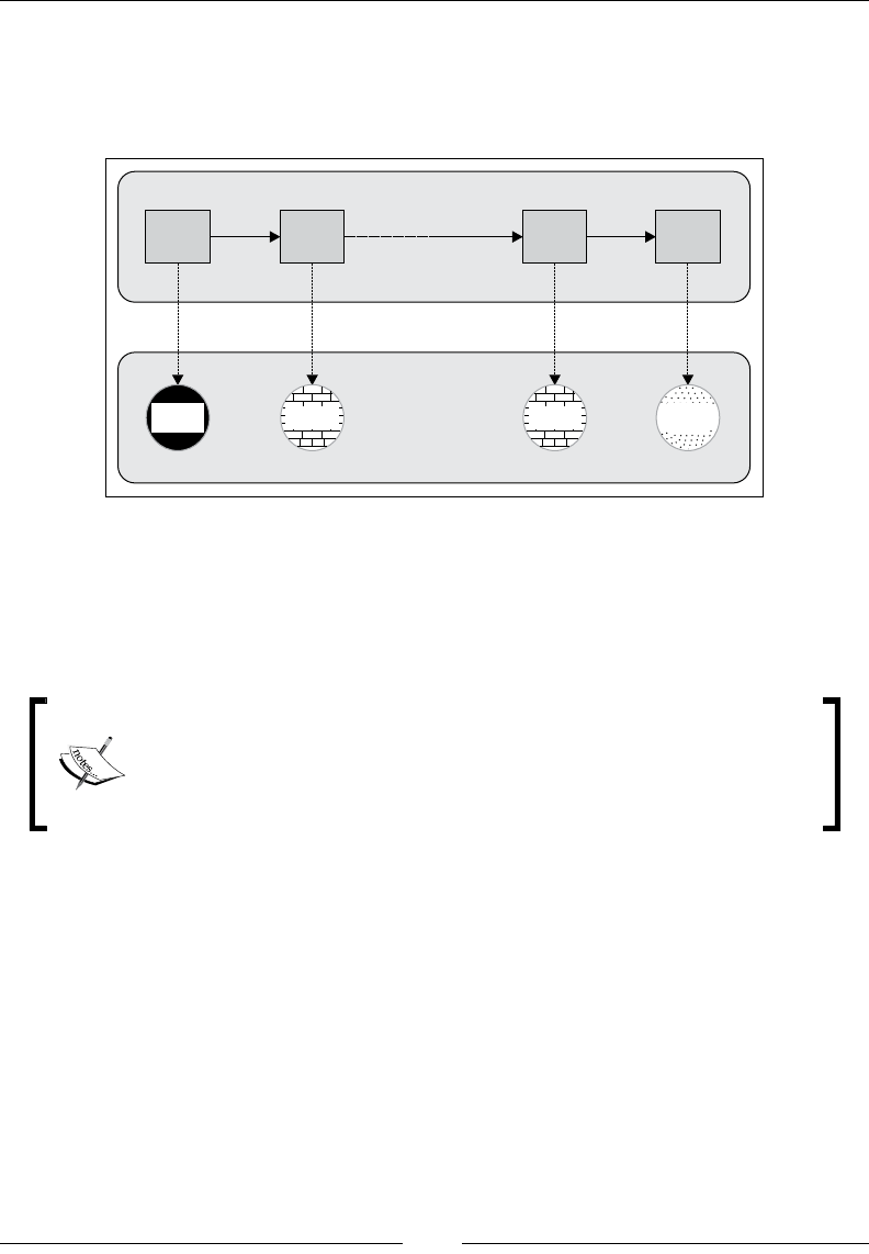
Sequential Data Models
[ 812 ]
Let's reuse the boxes and balls example. If the boxes are hidden states (non-observable),
then the user draws the balls whose color is not visible. The emission probability is the
probability bik =p(ot= colork| qt=Si) to retrieve a ball of the color k from a hidden box I, as
described in the following diagram:
bk0 bml bmi bnj
Box1
aji
Box0Boxj
Boxi
Hidden boxes (states)
a10
Observed colors
Color
m
Color
kColor
mColor
n
The hidden Markov model for the balls and boxes example
In this example, we do not assume that all the boxes contain balls of different colors.
We cannot make any assumptions on the order as dened by the transition aij. The
HMM does not assume that the number of colors (observations) is identical to the
number of boxes (states).
Time invariance
Contrary to the Kalman lter, for example, the hidden Markov model
requires that the transition elements, aji, are independent of time. This
property is known as stationary or homogeneous restriction.
It must be kept in mind that the observations, in this case the color of the balls, are
the only tangible data available to the experimenter. From this example, we can
conclude that a formal HMM has three components:
• A set of observations
• A sequence of hidden states
• A model that maximizes the joint probability of the observations and hidden
states, known as the Lambda model
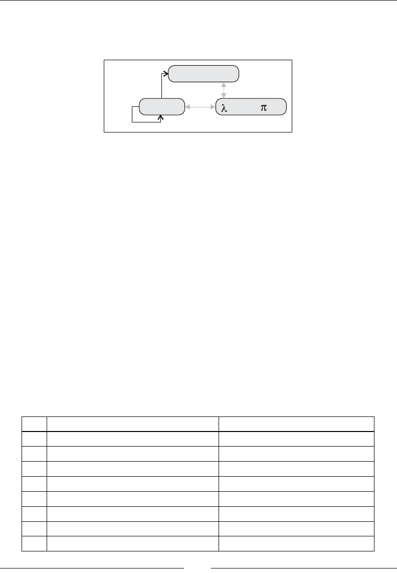
Chapter 7
[ 813 ]
A Lambda model, λ, is composed of initial probabilities π, the probabilities of state
transitions as dened by the matrix A, and the probabilities of states emitting one or
more observations:
A=aki
B=bji
Observations Oj
-model=( ,A,B)
States S
i
Visualization of the HMM key components
This diagram illustrates that, given a sequence of observations, HMM tackles three
problems known as canonical forms:
• CF1—evaluation: Evaluate the probability of a given sequence of
observations Ot, given a model λ = (π, A, B)
• CF2—training: Identify (or learn) a model λ = (π, A, B) given a set of
observations O
• CF3—decoding: Estimate the state sequence Q with the highest probability to
generate a given set of observations O and a model λ
The solution to these three problems uses dynamic programming techniques.
However, we need to clarify the notations prior to diving into the mathematical
foundation of the hidden Markov model.
Notation
One of the challenges of describing the hidden Markov model is the mathematical
notation that sometimes differs from author to author. From now on, we will use
the following notation:
Description Formulation
NThe number of hidden states
SA finite set of N hidden states S = {S0, S1, … SN-1}
MThe number of observation symbols
qtThe state at time or step t
QTime sequence of states Q = {q0, q1, … qn-1} = Q0:n-1
TThe number of observations
otThe observation at time t
OA finite sequence of T observations O = {o0, o1, … oT-1} = O0:T-1
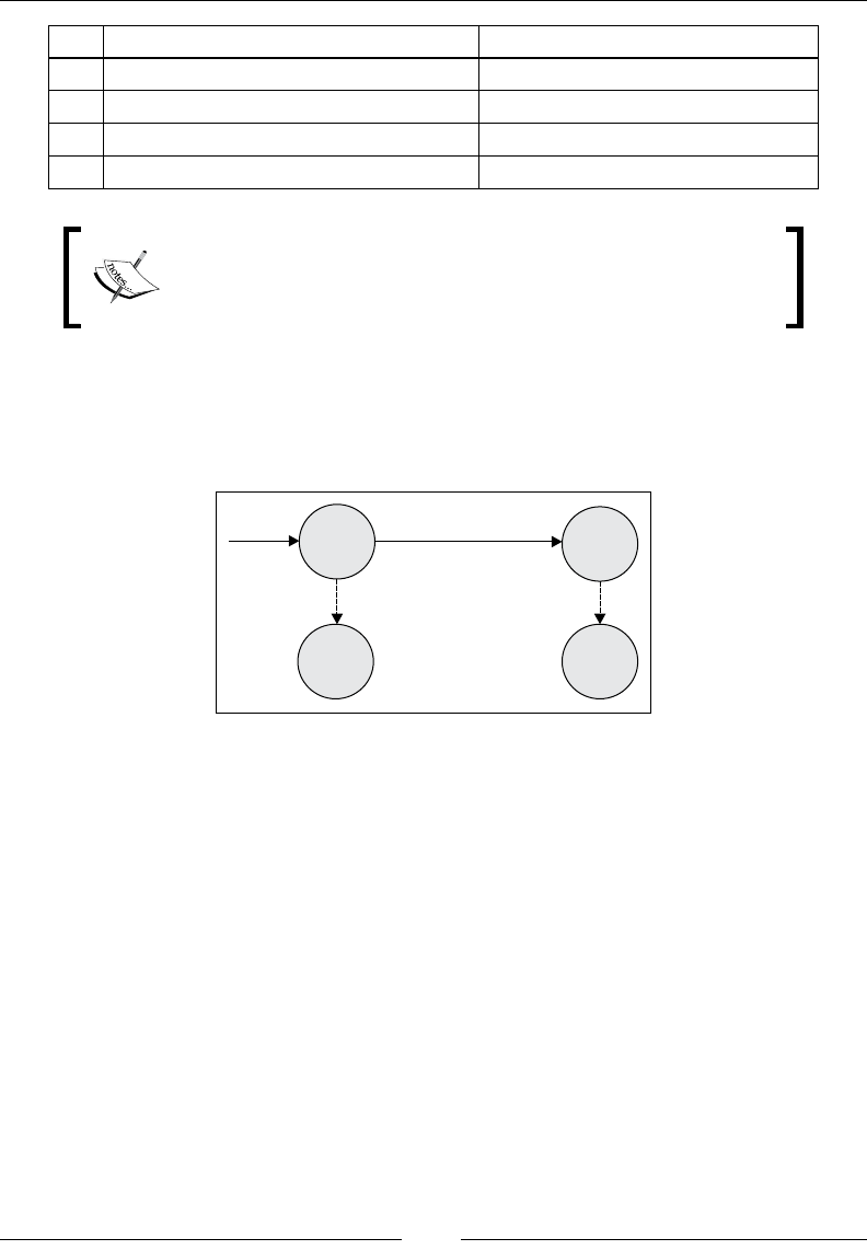
Sequential Data Models
[ 814 ]
Description Formulation
AThe state transition probability matrix aji = p(qt+1=Si| qt=Sj)
BThe emission probability matrix bjk = p(ot=Ok| qt=Sj)
πThe initial state probability vector πi = p(q0=Sj)
λThe hidden Markov model λ = (π, A, B)
Variance in notation
Some authors use the symbol z to represent the hidden states
instead of q and x to represent the observations O.
For convenience, let's simplify the notation of the sequence of observations and states
using the following condensed form: p(O0:T, qt| λ) = p(O0, O1, … OT, qt| λ). It is quite
common to visualize a hidden Markov model with a lattice of states and observations
similar to our description of the boxes and balls examples, as shown here:
transition aji
observations
emission bki bmj
qt+1=Sj
qti
=S
ot+1=Om
ot=Ok
The formal HMM-directed graph
The state Si is observed as Ok at time t, before being transitioned to the state Sj
observed as Om at the time t+1. The rst step in the creation of our HMM is the
denition of the class that implements the lambda model λ = (π, A, B) [7:4].
The lambda model
The three canonical forms of the hidden Markov model rely heavily on manipulation
and operations on matrices and vectors. For convenience, let's dene an HMMConfig
class that contains the dimensions used in the HMM:
class HMMConfig(val _T: Int, val _N: Int, val _M: Int) extends Config
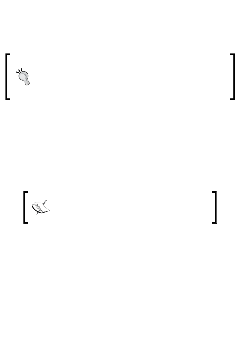
Chapter 7
[ 815 ]
The input parameters for the class are:
• _T: The number of observations
• _N: The number of hidden states
• _M: The number of observation symbols or features
Consistency with mathematical notation
The implementation uses _T (with respect to _N, _M) to represent
programmatically the number of observations T (with respect to hidden
states N and features M). As a general rule, the implementation reuses
the mathematical symbols as much as possible. Although the practice
does not always make the code elegant, it improves its readability.
The HMMConfig companion object denes the operations on ranges of index of matrix
rows and columns. The foreach, foldLeft, and maxBy methods are regularly used
in each of the three canonical forms:
object HMMConfig {
def foreach(i: Int, f: Int => Unit): Unit = Range(0, i).foreach(f)
def foldLeft(i: Int, f: (Double, Int) => Double, zero:Double) =
Range(0, i).foldLeft(zero)(f)
def maxBy(i: Int, f: Int => Double): Int = Range(0,i).maxBy(f)
…
}
Notation
The λ model in HMM should not be confused with the
regularization factor discussed in the Ln roughness penalty
section in Chapter 6, Regression and Regularization.
As mentioned earlier, the lambda model is dened as a tuple of the transition
probability matrix A, emission probability matrix B, and the initial probability π. It
is easily implemented as a case class, HMMLambda, using the Matrix class dened in
the Matrix class section in Appendix A, Basic Concepts. The simplest constructor for the
HMMLambda class is invoked in the case where the state-transition probability matrix,
the emission probability matrix, and the initial states are known, as shown here:
class HMMLambda(val A: Matrix[Double], val B: Matrix[Double], var pi:
DblVector, val numObs: Int) {
def getT: Int = numObs
def getN: Int = A.nRows
def getM: Int = B.nCols
val d1 = numObs -1
…
}
Sequential Data Models
[ 816 ]
The implementation reects the mathematical notation, with pi being the initial
state probability, A the state transition matrix, and B the emission matrix. The
numObs value is the number of observations in the sequence. The getT, getN, and
getM methods are used to keep the implementation consistent with the initial
conguration, HMMConfig. The section related to the training of HMM introduces
a different constructor for HMMLambda using the conguration as a parameter.
The initial probabilities are unknown, and therefore, initialized with a random
generator of values [0, 1].
Normalization
Input states and observations data may have to be normalized and
converted to probabilities before initializing the matrices A and B.
The two other components of the HMM are the sequence of observations and the
sequence of hidden states.
HMM execution state
The canonical forms of the HMM are implemented through dynamic programming
techniques. These techniques rely on variables that dene the state of the execution
of the HMM for any of the canonical forms:
• Alpha (the forward variable): The probability of observing the rst t <
T observations for a specic state at Si for the observation t, αt(i) = p(O0:t,
qt=Si|λ)
• Beta (the backward variable): The probability of observing the remainder of
the sequence qt for a specic state βt(i) =p(Ot+1:T-1|qt=Si,λ)
• Gamma: The probability of being in a specic state given a sequence of
observations and a model γt(i) =p(qt=Si|O0:T-1, λ)
• Delta: The sequence to have the highest probability path for the rst i
observations dened for a specic test δt(i)
• Qstar: The optimum sequence q* of states Q0:T-1
• DiGamma: The probability of being in a specic state at t and another
dened state at t+1 given the sequence of observations and the model
γt(i,j) =p(qt=Si,qt+1=Sj|O0:T-1, λ)

Chapter 7
[ 817 ]
Each of the parameters is described in the section related to each canonical form. Let's
create a class HMMState that encapsulates the variables used in the implementation of
the three canonical cases.
For convenience, all the parameters related to the three canonical cases and listed in
the previous notation section are encapsulated into a single outer class, HMMState:
class HMMState(lambda: HMMLambda, maxIters:Int) extends Config {
val delta = Matrix[Double]( lambda.getT, lambda.get N) // δt(i)
object QStar { … } //q*
object DiGamma { … } // γt(i, j)
object Gamma { … } // γt(i)
}
Once again, we use the same notation as for the conguration of the HMM; lambda.
getT, being the number of observations, and lambda.getN, the number of hidden
states. The HMM state parameters have self-descriptive names that strictly follow
the notation introduced earlier. The
λ
model, the HMM state, and the sequence of
observations are all the elements needed to implement the three canonical cases.
The Gamma and DiGamma singletons are used and described in the evaluation
canonical form. The DiGamma singleton is described as part of the Viterbi algorithm
to extract the sequence of states with the highest probability given a
λ
model and a
set of observations.
The execution of any of the three canonical forms relies on dynamic programming
techniques (refer to the Overview of dynamic programming section in Appendix A,
Basic Concepts) [7:5]. The simplest of the dynamic programming techniques is
a single traversal of the observations/state chain.
Therefore, it makes sense to dene a base class, HMMModel, that has all the algorithms
that manipulate the
λ
model, lambda, and the observed states, obs:
abstract class HMMModel(lambda: HMMLambda, obs: Array[Int])
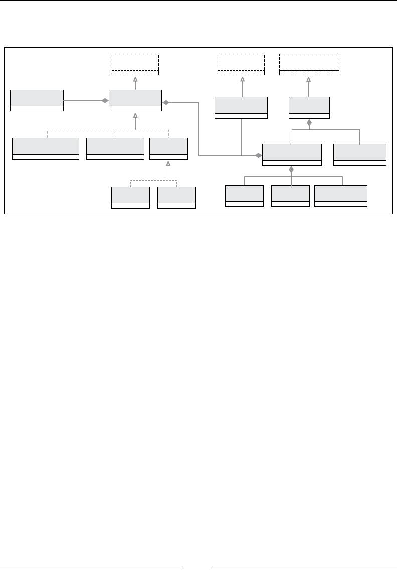
Sequential Data Models
[ 818 ]
The list of dynamic-programming-related algorithms used in any of the three canonical
forms is visualized through the class hierarchy of our implementation of the HMM:
obs
config
lambda
state
AB pi
form
lambda
11
1
1
1
11
11
Model Config PipeOperator
Array[Int] HMMModel HMMConfig HMM
BaumWelchEM VirtebiPath Pass
Matrix Matrix
Beta
Alpha
HMMLambda HMMForm
DblVector
Scala classes' hierarchy for HMM (UML class diagram)
Each class is described as needed in the description of the three canonical forms
of HMM. It is time to dive into the implementation details of each of the canonical
forms, starting with the evaluation.
Evaluation (CF-1)
The objective is to compute the probability (or likelihood) of the observed sequence
Ot given a
λ
model. A dynamic programming technique is used to break down the
probability of the sequence of observations into two probabilities:
()()( )
0: 1 0:t 1: 1
|| |
λα λ λ
−+−
⋅
TtT
pO pO pO
The likelihood is computed by marginalizing over all the hidden states [7:6]{Si}:
()( )
1
0: 10: 1
0
|,q S |
N
TTti
i
pO pO
λ λ
−
− −
=
= =
∑
Chapter 7
[ 819 ]
If we use the notation introduced in the previous chapter for alpha and beta variables,
the probability for the observed sequence Ot given a
λ
model can be expressed as:
()()()
0: 1
|
Ttt
i
pO ii
λαβ
−
=⋅
∑
The product of the probabilities α and β can potentially underow. Therefore, it is
recommended to use the log of the probabilities instead of the probabilities.
Alpha class (the forward variable)
The computation of the probability of observing a specic sequence given a sequence
of hidden states and a
λ
model relies on a two-pass algorithm. The alpha algorithm
consists of the following steps:
1. Compute the initial alpha value [M1]. The value is then normalized by the
sum of alpha values across all the hidden states [M2].
2. Compute the alpha value iteratively for the time 0 to time t, then normalize
by the sum of alpha values for all states [M3].
3. The nal step is the computation of the log of the probability of observing the
sequence [M4].
Performance consideration
A direct computation of the probability of observing a specic
sequence requires 2TN2 multiplications. The iterative alpha and
beta classes reduce the number of multiplications to N2T.
For those with some inclination toward mathematics, computation of the alpha
matrix is dened in the following information box. Each formula has an identier
[Mx], which is referenced in the Scala source code implementing it.

Sequential Data Models
[ 820 ]
Alpha-class (forward variable)
• M1: Initialization:
() ( )
0 0ii
ibO
απ
=⋅
• M2: Normalization of initial values:
() () ()
1
0 0 0
0
ˆ/
N
j
ii i
αα
α
−
=
=∑
• M3: Normalized summation:
() ( ) ( ) () () ()
1 1
1
0 0
ˆ
1/
N N
t t ji it t tt tt
j i
ijabOciiic
αα
ααα
− −
−
= =
= = = ⋅
∑ ∑
• M4: Probability of observing a sequence given a lambda model
and states:
() ()
1
1
00
1
log| logˆ
T
N
jit
pO i
λα
−
−
==
⎛⎞
=−⎜⎟
⎜⎟
∑
⎝⎠
∑
Let's look at the implementation of the alpha class in Scala, using the referenced
number of the mathematical expressions of the alpha class. The alpha and beta
values have to be normalized [M3], and therefore, we dene a base class, Pass,
for the alpha and beta algorithms that implements the normalization:
class Pass(_lambda: HMMLambda, _obs: Array[Int]) extends HMMModel(_
lambda, _obs) { //1
var alphaBeta: Matrix[Double] = _
val ct = Array.fill(lambda.getT)(0.0) //2
def normalize(t: Int): Unit = {
ct.update(t, foldLeft(lambda.getN, (s, n) => s + alphaBeta(t,
n))) //3
alphaBeta /= (t, ct(t))
}
}
As with any algorithm used in the hidden Markov model, the Pass base class of the
alpha and beta classes is a composition of the attributes of the model (HMMLambda), the
computation parameters (HMMParams), and the sequence of observations obs (line 1).
The alphaBeta matrix represents either the alpha or beta matrix manipulated in the
subclasses (line 2). The scale factor, ct, is computed as the summation of the alpha or
beta row matrix over all the states using a fold (line 3).

Chapter 7
[ 821 ]
Computation efciency
Scala's reduce, fold, and foreach methods are far more
efcient iterators than the for loop. You need to keep in mind that
the main purpose of the for loop in Scala is the monadic chaining
of map and flatMap operations.
The computation of the alpha variable in the Alpha class follows the same
computation ow as dened in the mathematical expression:
class Alpha(lambda: HMMLambda, obs: Array[Int]) extends Pass(lambda,
obs)
The alpha value is initialized [M1] (line 4), then normalized [M2] using the current
sequence order (line 5). The value of alpha is then updated [M3] by summation of
the previous alpha value at t-1 and the transition from the state j to the state i (line 6),
as shown here:
Import HMMConfig._
val alpha = {
alphaBeta = lambda.initAlpha(obs) //4
normalize(0) //5
sumUp //6
}
def sumUp: Double = { //[M2]
foreach(lambda.getT, t => {
updateAlpha(t) //7
normalize(t) //8
})
foldLeft(lambda.getN, (s, k) => s + alphaBeta(lambda.dim_1, k))
}
def updateAlpha(t: Int): Unit =
HMMConfig.foreach(lambda.getN, i =>
alphaBeta += (t,i,lambda.alpha(alphaBeta(t-1,i),i,obs(t)))
)
}
The value of alpha is updated by the updateAlpha method (line 7) before
normalization (line 8). The implementation that relies on the fold method
is omitted, but can be easily written.

Sequential Data Models
[ 822 ]
Finally, the computation of the logarithm of the probability to observe a specic
sequence, given the sequence of states and a predened
λ
model, [M4] can be
performed by the following code (line 9):
def logProb: Double = foldLeft(lambda.getT, (s, t)
=> s + Math.log(ct(t)), Math.log(alpha))//9
The method computes the logarithm of the probability instead of the probability
itself. The summation of the logarithm of probabilities is less likely to cause an
underow than the product of probabilities.
Beta class (the backward variable)
The recursive computation of beta values is similar to the Alpha class except that the
iteration executes backward on the sequence of states.
The implementation of Beta is similar to the alpha class:
1. Compute [M5] and normalize [M6] the value of beta at t=0 across states.
2. Compute and normalize iteratively the beta at the time T-1 to t updated from
its value at t+1 [M7].
Beta class (the backward variable)
• M5: Initialization of beta: βT-1(t)=1
• M6: Normalization of initial beta values:
() () ( )
1
1 1 1
0
ˆ/
N
T T T
j
ii j
ββ
β
−
− − −
=
=∑
• M7: Normalized summation of beta:
() ( ) ( ) () () ()
1 1
1 1
0 0
ˆ
1/
N N
t t ij jt t t t tt
j j
ijabOc jiic
ββ
βββ
− −
+ +
= =
=⋅⋅ = = ⋅
∑ ∑

Chapter 7
[ 823 ]
The denition of the class for the Beta class is identical to the Alpha class:
class Beta(lambdaB: HMMLambda, _obs: Array[Int]) extends Pass(lambdaB,
_obs)
The implementation of the Beta class is similar to the Alpha class with computation
(line 1) and normalization (line 2) of beta at t=0. As expected, the summation routine
sumUp (line 3) is implemented as updating and normalizing beta at the time t, as
shown here:
val complete = { //4
alphaBeta = Matrix[Double](lambda.getT, lambda.getN)
alphaBeta += (lambda.dim_1, 1.0) //1
normalize(lambda.dim_1) //2
sumUp; true
}
def sumUp: Unit = //3
(lambda.getT-2 to 0 by -1).foreach( t =>{
updateBeta(t)
normalize(t)
})
def updateBeta(t: Int): Unit =
foreach(lambda.config.getN, i => {
alphaBeta += (t, i, lambda.beta(alphaBeta(t+1, i), i, obs(t+1)))
})
The recursive method updates and normalizes the beta matrix by traversing the
sequence of observations backward from before the last observation to the rst.
Contrary to the Alpha class, the Beta class does not generate an output value.
Therefore, we need to ag the state of the class using a ready Boolean value,
which is set to true if the instantiation succeeds and false otherwise.

Sequential Data Models
[ 824 ]
Constructors
The alpha and beta values are computed within the constructors
of their respective class, so no public or protected method needs
to verify if these values are already computed. The design pattern
reduces the complexity of implementation by ensuring that a class
instance has only one state: computation completed.
What is the value of a model if it cannot be created? The next canonical form CF2
leverages dynamic programming and recursive functions to extract the
λ
model.
Training (CF-2)
The objective of this canonical form is to extract the
λ
model given a set of
observations and a sequence of states. It is similar to the training of a classier.
The simple dependency of a current state on the previous state enables an
implementation using an iterative procedure, known as the Baum-Welch
estimator or expectation-maximization (EM).
Baum-Welch estimator (EM)
At its core, the algorithm has three steps and an iterative method, similar to the
evaluation canonical form:
1. Compute the probability π (the gamma value at t=0) [M9].
2. Compute and normalize the state's transition probabilities matrix A [M10].
3. Compute and normalize the matrix of emission probabilities B [M11].
4. Repeat steps 2 and 3 until the change of likelihood is insignicant.
The algorithm uses the digamma and summation gamma variables dened in the
HMMConfig class.

Chapter 7
[ 825 ]
The Baum-Welch algorithm
• M8: Joint probability of the state qi at t and qj at t+1:
()
( )
1
,,|0,
ttit j
ij pq Sq S
γ
λ
+
== =
()
() ()()
() ()
11
1
0
,tijjtt
tN
tt
j
iab O j
ij
ii
α β
γ
αβ
++
−
=
=∑
• M9: The initial probabilities vector:
() () ( )
1
0
0
ˆ,
N
i t t
j
ii ij
πγ
γγ
−
=
= = ∑
• M10: Update of the transition probabilities matrix:
()
()
()
1
0
1
0
,
ˆ
T
t
t
ij T
t
t
ij
a
i
γ
γ
−
=
−
=
=
∑
∑
• M11: Update of the emission probabilities matrix :
()
()
0
0
1
0
ˆ
j
t
t
ij T
t
t
i
b
i
γ
γ
=
−
=
=
∑
∑
The Baum-Welch algorithm requires the following three inputs:
• The
λ
model, _lambda, initialized with random values uniformly distributed
• The current state of the training, state
• The labeled observed data, _obsIdx

Sequential Data Models
[ 826 ]
The implementation of the Baum-Welch algorithm illustrates the elegance and
conciseness of the Scala programming language. The constructor requires a fourth
parameter to describe the minimum rate of change of the estimate of the likelihood
between iterative calls, as shown in the following code snippet:
class BaumWelchEM config: HMMConfig, obs: Array[Int], numIters:
Int,eps: Double) extends HMMModel(HMMLambda(config), obs) {
val state = HMMState(lambda, numIters)
}
The
λ
model has to be initialized with the conguration parameters (number of
observations, number of states, and number of symbols). The matrices A and B and
the initial state probabilities pi are initialized with a uniform random generator
[0, 1], Matrix.fillRandom, as shown here:
object HMMLambda {
def apply(config: HMMConfig): HMMLambda = {
val A = Matrix[Double](config._N)
A.fillRandom(0.0)
val B = Matrix[Double](config._N, config._M)
B.fillRandom(0.0)
val pi = Array.fill(config._N)(Random.nextDouble)
new HMMLambda(A, B, pi, config._T)
}
The maximum likelihood, maxLikelihood, is computed as part of the constructor to
ensure a consistent state:
var likelihood = frwrdBckwrdLattice
Range(0, state.maxIters) find( _ => {
lambda.estimate(state, obs) //1
val _likelihood = frwrdBckwrdLattice //2
val diff = likelihood - _likelihood //3
likelihood = _likelihood
diff < eps //4
}) match {
case Some(index) => maxLikelihood
…
The computation of the likelihood requires the estimation of the transition matrix A
and emission matrix B (line 1). The training process iterates by traversing the lattice
forward and backward until the likelihood reaches a local or global maximum. The
λ
model is updated using the estimate method (line 1). The method computes the
likelihood of the sequence of states (line 2) and then compares it with the likelihood
computed in the previous iteration (line 3). The method exits if the difference between
two consecutive likelihood values meets the convergence criteria eps (line 4).
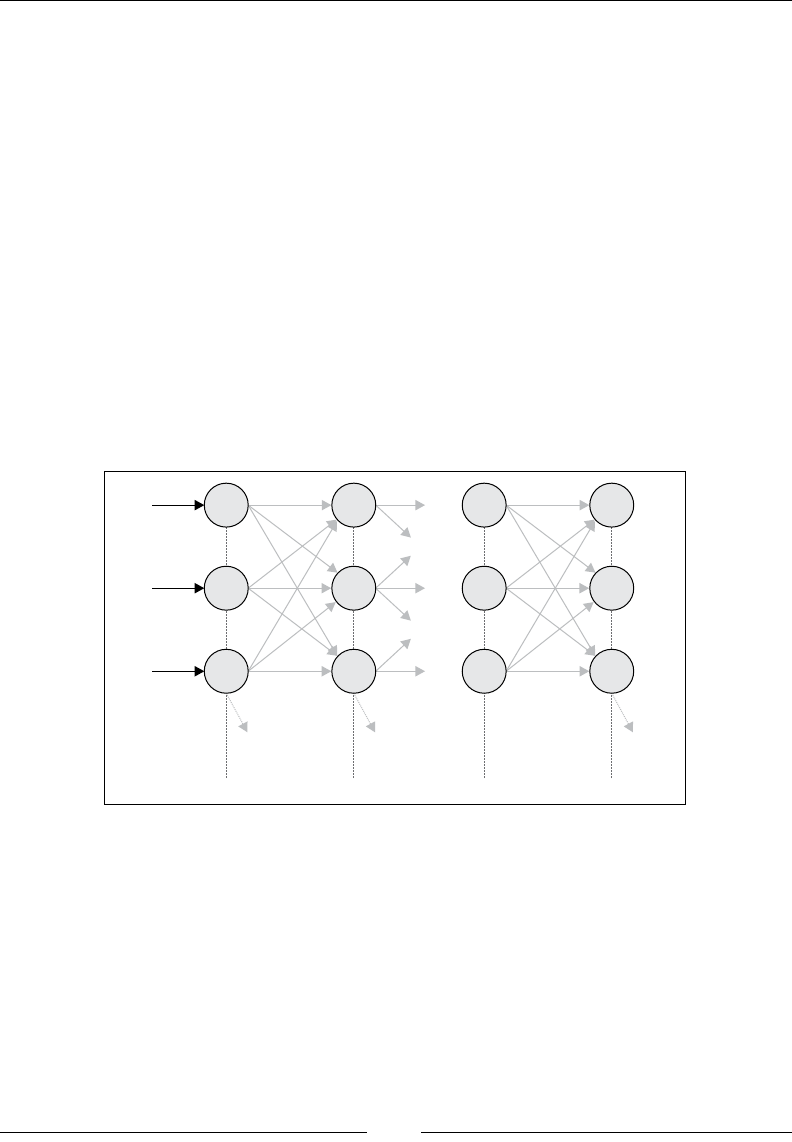
Chapter 7
[ 827 ]
The estimate method of the HMMLambda class updates the
λ
model (A, B, and pi):
def estimate(state: HMMState, obsIdx: Array[Int]): Unit = {
pi = Array.tabulate(config._N)(i => state.Gamma(0, i) )
HMMConfig.foreach(config._N, i => {
var denominator = state.Gamma.fold(dim_1, i)
HMMConfig.foreach(config._N, k =>
A += (i, k, state.DiGamma.fold(dim_1, i, k)/denominator)
)
denominator = state.Gamma.fold(config._T, i)
HMMConfig.foreach(config._N, k => B += (i, k, state.Gamma.
fold(config._T, i, k, obsIdx)/denominator))
})
The core of the Baum-Welch expectation maximization is the iterative forward and
backward update of the lattice of states and observations between time t and t+1.
The lattice-based iterative computation is illustrated in the following diagram:
pi
pN-1
p0
t=0 t=1 t-1 t
O0O1Ot
a0,0 a0,0
q0
qi
qN-1
q0
qi
qN-1
q0
qi
qN-1
q0
qi
qN-1
aN-1, N-1 bN-1, 1
aN-1, N-1 bN-1, 1
Visualization of HMM graph lattice for the Baum-Welch algorithm
The iteration across the lattice is implemented by the frwrdBckwrdLattice method
(line 2). The lattice is traversed ahead using the Alpha instance class (line 1), and
backward using the Beta instance class (line 2):
def frwrdBckwrdLattice: Double = {
val _alpha = Alpha(lambda, obs).alpha //1
val _beta = Beta(lambda, obs) //2
val a = _alpha.alphaBeta
val b = _beta.alphaBeta

Sequential Data Models
[ 828 ]
Gamma.update(a, b) //3
DiGamma.update(a, b, A, B, obs) //4
_alpha.alpha
}
The method returns the alpha coefcient and computes the new values for the Gamma
(line 3) vector and DiGamma (line 4) matrix. These HMMState methods are omitted for
the sake of clarity.
Decoding (CF-3)
This last canonical form consists of extracting the most likely sequence of states {qt}
given a set of observations Ot and a
λ
model. Solving this problem requires, once
again, a recursive algorithm.
The Viterbi algorithm
The extraction of the best state sequence (the sequence of state that has the highest
probability) is very time consuming. An alternative consists of applying a dynamic
programming technique to nd the best sequence {qt} through iteration. The
algorithm is known as the Viterbi algorithm. Given a sequence of states {qt} and
sequence of observations {oj}, the probability δt(i) for any sequence to have the
highest probability path for the rst T observations is dened for the state Si [7:7].
The Viterbi algorithm
M12: Denition of delta function:
()
{}
( )
0:T1 0: 1
:0, 1
max,|
tiT
qj T
ipqSO
δ λ
− −
−
= =
M13: Initialization of delta:
() ( ) ()
000 0
ii
ibO i i
δπ
ψ
= = ∀
M14: Recursive computation of delta:
() () ( )
( )
() ()
()
1 1
max arg max
t t ij jt t tij
i i
iiabO i ia
δδ ψ δ
− −
=⋅⋅ =⋅
M15: Computation of the optimum state sequence Q:
()
()
11 argmax
ttt t T
i
qqq i
ψ δ
∗∗∗
++
= =

Chapter 7
[ 829 ]
The constructor of the Viterbi algorithm, ViterbiPath, is similar to the algorithms
of the rst two canonical forms, and therefore, inherits HMMInference. The purpose
of the Viterbi algorithm is to compute the optimum sequence given a set of
observations and a
λ
model by maximizing the delta, maxDelta:
class ViterbiPath(_lambda: HMMLambda, _state: HMMState, _obs:
Array[Int]) extends HMMInference(_lambda, _state, _obs) {
val maxDelta = recurse(lambda.getT, 0)
…
}
The recursive method that implements [M14] and [M15] steps is invoked by
the constructor:
def recurse(t: Int, j: Int): Double = {
var maxDelta = initial((t, j)) //1
if( maxDelta == -1.0) {
if(t != obs.size) {
maxDelta = maxBy(lambda.getN, //2 [M14]
s => recurse(t-1, s)* lambda.A(s, j)* lambda.B(j, obs(t))
)
val idx =maxBy(lambda.getT, i =>recurse(t-1 ,i)*lambda.A(i,j))
//3 [M14]
state.psi += (t, j, idx) //4
state.delta += (t, j, maxDelta) //5
}
else { //6
maxDelta = 0.0
val index =maxBy(lambda.getN, i => {
val delta = recurse(t-1 ,i)
if( delta > maxDelta) maxDelta = delta
delta
})
state.QStar.update(t, index) //7
}
}
maxDelta
}

Sequential Data Models
[ 830 ]
Once initialized (line 1), the maximum value of delta, maxDelta, is computed
recursively by applying the formula [M14] at each state, s, using Scala's maxBy method
(line 2). Next, the index of the column of the transition matrix A corresponding to the
maximum of delta is computed (line 3). The last step is to update the matrix psi (line
4) (with respect to delta (line 5)). Once the step t reaches the maximum number of
observation labels (line 6), the optimum sequence of states q* is computed [M15] (line 7).
Ancillary methods are omitted.
This implementation of the decoding form of the hidden Markov model completes
the description of the hidden Markov model and its implementation in Scala. Now,
let's put this knowledge into practice.
Putting it all together
The main class HMM implements the three canonical forms. A view bound to an
array of integers is used to parameterize the HMM class. We assume that a time
series of continuous or pseudocontinuous values is converted (or categorized)
into discrete symbol values.
The @specialized annotation ensures that the byte code is generated for the
Array[Int] primitive without executing the conversion implicitly declared by the
bound view. The HMM can be potentially used as part of a computation workow,
and therefore, has to implement the pipe operator (PipeOperator).
There are two different constructors for the HMM class. The rst constructor uses the
λ
model as input (evaluation (CF1) and decoding (CF3)):
class HMM[@specialized T <% Array[Int]](lambda: HMMLambda, form:
HMMForm, maxIters: Int) (implicit f: DblVector => T) extends
PipeOperator[T, HMMPredictor] {
val state = HMMState(lambda, maxIters)
….
}
The HMMForm enumerator is used to specify the canonical form of the HMM solution:
object HMMForm extends Enumeration {
type HMMForm = Value
val EVALUATION,DECODING = Value
}

Chapter 7
[ 831 ]
The conversion of DblVector to a type T is required only if the evaluation and
decoding canonical form uses actual observation values as argument. The f function is
then used to discretize the double values into a sequence of index of the observations.
The HMMPredictor type consists of a tuple log probability (or likelihood) of
observations and index of sequence of observations:
type HMMPredictor = (Double, Array[Int])
The HMM has three canonical forms instead of the two forms of most classiers.
The second canonical form, training, is implemented by dening a second
constructor for the HMM class, as follows:
object HMM {
def apply[T <% Array[Int]](config: HMMConfig, obs: Array[Int],
form: HMMForm, maxIters: Int, eps: Double)
(implicit f: DblVector => T): HMM[T] = {
val baumWelchEM = new BaumWelchEM(config, obs, maxIters, eps)
new HMM[T](baumWelchEM.lambda, form, maxIters)
}
}
The decode (with respect to evaluate) method implements the third (with respect
to the rst) canonical form of HMM. Both methods take a sequence of indices for
observations as an argument.
def decode(obsIdx: Array[Int]): HMMPredictor = (ViterbiPath(lambda,
state, obsIdx).maxDelta, state.QStar())
def evaluate(obsIdx: Array[Int]): HMMPredictor = (-Alpha(lambda,
obsIdx).logProb, obsIdx)
}
The data transformation |> encapsulates the evaluation and decoding forms in
order to preserve its meaning. The observation, obs, is automatically converted
into a sequence of indices to each observation (line 1) by the DblVector => T
discretization function, which is an implicit parameter of the HMM class.
def |> : PartialFunction[DblVector, HMMPredictor] = {
case obs: DblVector if(obs != null && obs.size > 2) => {
form match {
case EVALUATION => evaluate(obs) //1
case DECODING => decode(obs) //1
}
…

Sequential Data Models
[ 832 ]
Normalized probabilities input
You need to make sure that the input probabilities for the
λ
model for
evaluation and decoding canonical forms are normalized—the sum of
the probabilities of all the states for the π vector and A and B matrices are
equal to 1. This validation code is omitted in the example code.
Test case
Our test case is to train an HMM to predict the sentiment of investors as measured
by the weekly sentiment survey of the members of the American Association of
Individual Investors (AAII) [7:8]. The goal is to compute the transition probabilities
matrix A, the emission probabilities matrix B, and the steady state probability
distribution π, given the observations and hidden states (training canonical form).
We assume that the change in investor sentiments is independent of time, as required
by the hidden Markov model.
The AAII sentiment survey grades the bullishness on the market in terms of percentage:
The weekly AAII market sentiment (reproduced by courtesy from AAII)
The sentiment of investors is known as a contrarian indicator of the future direction
of the stock market. Refer to the Terminology section in Appendix A, Basic Concepts.
Let's select the ratio of percentage of investors that are bullish over the percentage of
investors that are bearish. The ratio is then normalized. The following table lists this:
Time Bullish Bearish Neutral Ratio Normalized ratio
t00.38 0.15 0.47 2.53 1.0
t10.41 0.25 0.34 1.68 0.53
t20.25 0.35 0.40 0.71 0.0
….

Chapter 7
[ 833 ]
The sequence of non-normalized observations (ratio of bullish sentiment over bearish
sentiment) is dened in a CSV le as follows:
final val OBS_PATH = "resources/data/chap7/obs.csv"
final val NUM_SYMBOLS = 6
final val NUM_STATES = 5
final val EPS = 1e-3
final val MAX_ITERS = 250
val srcObs = Source.fromFile(OBS_PATH)
val obs = srcObs.getLines.map(_.toDouble)).toSeq //1
val config = new HMMConfig(obs.size, NUM_STATES, NUM_SYMBOLS)
val min = obs.min
val delta = obs.max - min
val obsSeq = obs.map( x => (x - min)/delta) //2
.map(x =>(x*NUM_SYMBOLS).floor.toInt) //3
HMM[Array[Int]](config,obsSeq,EVALUATION,MAX_ITERS,EPS) match {
case Some( hmm) => //4
Display.show(s"Lambda: ${hmm.getModel.toString}", logger)
…
}
The sequence of observations is loaded from the CSV le (line 1) before
being normalized (line 2). The discretization converts the normalized bullish
sentiment/bearish sentiment ratio in six levels (integers) [0,-5] (line 3). The
instantiation of the HMM class for the ratio levels (Array[Int]) generates the
λ
model (A, B, and pi) (line 4).
The following is a state-transition matrix:
A 1 2 3 4 5
1 0.090 0.026 0.056 0.046 0.150
2 0.094 0.123 0.074 0.058 0.0
3 0.093 0.169 0.087 0.061 0.056
4 0.033 0.342 0.017 0.031 0.147
5 0.386 0.47 0.314 0.541 0.271

Sequential Data Models
[ 834 ]
The emission matrix is as follows:
B123456
1 0.203 0.313 0.511 0.722 0.264 0.307
2 0.149 0.729 0.258 0.389 0.324 0.471
3 0.305 0.617 0.427 0.596 0.189 0.186
4 0.207 0.312 0.351 0.653 0.358 0.442
5 0.674 0.520 0.248 0.294 0.259 0.03
The hidden Markov model for time series
analysis
The evaluation form of the hidden Markov model is very suitable for ltering data
for discrete states. Contrary to time series lters such as the Kalman lter introduced
in the The Kalman lter section in Chapter 3, Data Preprocessing, HMM requires data
to be somewhat stationary in order to create a reliable model. However, the hidden
Markov model overcomes some of the limitations of analytical time series analysis.
Filters and smoothing techniques assume that the noise (frequency mean, variance,
and covariance) is known and usually follows a Gaussian distribution. The hidden
Markov model does not have such a restriction. Moreover, moving averaging
techniques, discrete Fourier transforms, and generic Kalman lters require the states
to be continuous with linear dependencies, although the extended Kalman lter can
approximate nonlinear states.
Conditional random elds
The conditional random eld (CRF) is a discriminative machine learning algorithm
introduced by John Lafferty, Andrew McCallum, and Fernando Pereira [7:9] at the
turn of the century as an alternative to the HMM. The algorithm was originally
developed to assign labels to a set of observation sequences as found.
Let's consider a concrete example to understand the conditional relation between the
observations and the label data.

Chapter 7
[ 835 ]
Introduction to CRF
Let's consider the problem of detecting a foul during a soccer game using a
combination of video and audio. The objective is to assist the referee and analyze
the behavior of the players to determine whether an action on the eld is dangerous
(red card), inappropriate (yellow card), in doubt to be replayed, or legitimate. The
following image is an example of segmentation of a video frame for image processing:
The analysis of the video consists of segmenting each video frame and extracting
image features such as colors or edges [7:10]. A simple segmentation scheme
consists of breaking down each video frame into tiles or groups of pixels indexed by
their coordinates on the screen. A time sequence is then created for each tile Sij, as
represented in the following image:
0123t
Sij0Sij3Sijt
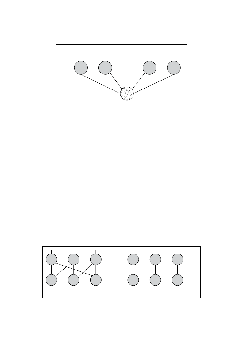
Sequential Data Models
[ 836 ]
The image segment Sij is one of the labels that are associated with multiple
observations. The same features extraction process applies to the audio associated with
the video. The relation between the video/image segment and the hidden state of the
altercation between the soccer players is illustrated by the following model graph:
Y0Y1Yn-2 Yn-1
Features
X={color, texture, edge, ...}
Sequences of labels (type of interaction)
Y= {legitimate, in-doubt, inappropriate, dangerous}
Undirected graph representation of CRF for soccer infraction detection
Conditional random elds (CRFs) are discriminative models that can be regarded
as a structured output extension of the logistic regression. CRFs address the problem
of labeling a sequence of data such as assigning a tag to each word in a sentence.
The objective is to estimate the correlation among the output (observed) values Y
conditional on the input values (features) X.
The correlation between the output and input values is described as a graph
(also known as a graph-structured CRF). A good example of graph-structured CRF
are cliques. Cliques are sets of connected nodes in a graph for which each vertex
has an edge connecting it to every other vertex in the clique.
Such models are complex and their implementation is challenging. Most real-world
problems related to time series or ordered sequences of data can be solved as a
correlation between a linear sequence of observations and a linear sequence of input
data much like HMM. Such a model is known as the linear chain structured graph
CRF or linear chain CRF for short.
Example non-linear CRF
time time
Linear chain CRF
Y0Y1Y2
X0X1X2
Y0Y1Y2
X0X1X2
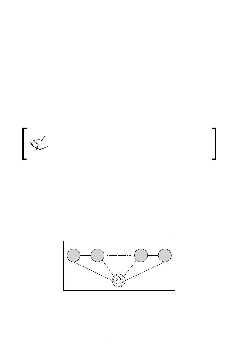
Chapter 7
[ 837 ]
One main advantage of the linear chain CRF is that the maximum likelihood, p(Y|X,
w), can be estimated using dynamic programming techniques such as the Viterbi
algorithm used in the HMM. From now on, the section focuses exclusively on the
linear chain CRF to stay consistent with the HMM described in the previous section.
Linear chain CRF
Let's consider a random variable X={xi}0:n-1 representing n observations and a random
variable Y representing a corresponding sequence of labels Y={yj}0:n-1. The hidden
Markov model estimates the joint probability p(X,Y) as any generative model
requires the enumeration of all the sequences of observations.
If each element of Y, yj obeys the rst order of the Markov property, then (Y, X) is a
CRF. The likelihood is dened as a conditional probability p(Y|X, w), where w is the
model parameters vector.
Observation dependencies
The purpose of CRF models is to estimate the maximum
likelihood of p(Y|X, w). Therefore, independence between
observations X is not required.
A graphical model is a probabilistic model for which a graph denotes the conditional
independence between random variables (vertices). The conditional and joint
probabilities of random variables are represented as edges. The graph for generic
conditional random elds can indeed be complex. The most common and simplistic
graph is the linear chain CRF.
A rst order linear chain conditional random eld can be visualized as an undirected
graphical model, which illustrates the conditional probability of a label Yj given a set
of observations X:
Observed features
Labeled sequence
p(Y |X)
0
p(Y |X)
1
p(Y |X)
n-1
X={x }
j
Y0Y1Yn-2 Yn-1
Linear, conditional, random field undirected graph

Sequential Data Models
[ 838 ]
The Markov property simplies the conditional probabilities of Y, given X, by
considering only the neighbor labels p(Y1|X, Yj j ≠1) = p(Y1|X, Y0, Y2) and p(Yi|X, Yj j
≠i) = p(Yi|X, Yi-1, Yi+1).
The conditional random elds introduce a new set of entities and a new terminology:
• Potential functions (fi): These are strictly positive, real value functions that
represent a set of constraints on the congurations of random variables. They
do not have any obvious probabilistic interpretation.
• Identity potential functions: These are potential functions I(x, t) that take
1 if the condition on the feature x at time t is true, and 0 otherwise.
• Transition feature functions: Simply known as feature functions, ti, are
potential functions that take a sequence of features {Xi}, the previous label
Yt-1, the current label Yt, and an index i. The transition feature function
outputs a real value function. In a text analysis, a transition feature function
would be dened by a sentence as a sequence of observed features, the
previous word, the current word, and a position of a word in a sentence. Each
transition feature function is assigned a weight that is similar to the weights
or parameters in the logistic regression. Transition feature functions play
a similar role as the state transition factors aij in HMM but without a direct
probabilistic interpretation.
• State feature functions sj are potential functions that take the sequence of
features {Xi}, the current label Yi, and the index i. They play a similar role
as the emission factors in the HMM.
A CRF denes the log probability of a particular label sequence Y, given a sequence
of observations X as the normalized product of the transition feature and state
feature functions. In other words, the likelihood of a particular sequence Y,
given the observed features X, is a logistic regression.
The mathematical notation to compute the conditional probabilities in the case of a
rst order linear chain CRF is described in the following information box.

Chapter 7
[ 839 ]
CRF conditional distribution
• The log probability of a label's sequence y, given an
observation x:
() ()()
1 1
1 1
0 0
log,, ,,x,i ,x,i
K K
ii i ciiii jj i
i j
fy yxi w wt yy sy
µ
− −
− −
= =
=+ +
∑∑
• Transition feature functions with I(a) = 1 if a true, 0 otherwise:
()()()()
111 2
,,,i III0
ii i i i
ty yx y l y l x
− −
==⋅=⋅=
• Using the notation:
()
()
() ()
1 1
1
0 0
, , , log | , ,y
K K
ijjj jj
j j
Fyx f y yxi pyx wFx
λα
− −
−
= =
=∑ ∑
• Conditional distribution of labels y, given x, using the Markov
property:
()
()
()
() ()
1
0
11
,y
00
1
|, ,y
−
=
−−
==
∑
= = ∑∑
K
jj
j
NK
wF x
jj
ij
pyxw ezx wF x
Zx
The weights wj are sometimes referred as
λ
in scientic papers, which may confuse
the reader. W is used to avoid any confusion with the
λ
regularization factor.
Now, let's get acquainted with the conditional random elds algorithm and its
implementation by Sunita Sarawagi.
CRF and text analytics
Most of the examples used to demonstrate the capabilities of conditional random
elds are related to text mining, intrusion detection, or bioinformatics. Although
these applications have a great commercial merit, they are not suitable as an
introductory test case because they usually require a lengthy description of the
model and the training process.

Sequential Data Models
[ 840 ]
The feature functions model
For our example, we will select a simple problem: how to collect and aggregate
an analyst's recommendation on any given stock from different sources with
different formats.
Analysts at brokerage rms and investment funds routinely publish the list
of recommendations or rating for any stock. These analysts used different
rating schemes from buy/hold/sell; A, B, C rating; and stars rating to market
perform/neutral/market underperform. For this example, the rating is normalized
as follows:
• 0 for a strong sell, (or F or 1 star rating)
• 1 for sell (D, 2 stars, marker underperform)
• 2 for neutral (C, hold, 3 stars, market perform, and so on)
• 3 for buy (B, 4 stars, market overperform, and so on)
• 4 from strong buy (A, 5 stars, highly recommended, and so on)
Here is an example of recommendations by stock analysts:
Macquarie upgraded AUY from Neutral to Outperform rating
Raymond James initiates Ainsworth Lumber as Outperform
BMO Capital Markets upgrades Bear Creek Mining to Outperform
Goldman Sachs adds IBM to its conviction list
The objective is to extract the name of the nancial institution that publishes the
recommendation or rating, the stock rated, the previous rating, if available, and
the new rating. The output can be inserted into a database for further trend analysis,
prediction, or simply the creation of reports.
Scope of the application
Ratings from analysts are updated every day through different protocols
(feed, emails, blogs, web pages, and so on). The data has to be extracted
from HTML, JSON, plain text, or XML format before being processed. In
this exercise, we assume that the input has already been converted into
plain text (ASCII) using a regular expression or another classier.

Chapter 7
[ 841 ]
The rst step is to dene the labels Y representing the categories or semantics
of the rating. A segment or sequence is dened as a recommendation sentence.
After reviewing the different recommendations, we are able to specify the following
seven labels:
• Source of the recommendation (Goldman Sachs and so on)
• Action (upgrades, initiates, and so on)
• Stock (either the company name or the stock ticker symbol)
• From (optional keyword)
• Rating (optional previous rating)
• To
• Rating (new rating for the stock)
The training set is generated from the raw data by tagging the different components
of the recommendation. The rst (or initiate) rating for a stock does not have the elds
4 and 5 dened.
For example:
Citigroup // Y(0) = 1
upgraded // Y(1)
Macys // Y(2)
from // Y(3)
Buy // Y(4)
to // Y(5)
Strong Buy //Y(6) = 7
Tagging
Tagging a word may have a different meaning depending on the
context. In natural language processing (NLP), tagging refers to the
process of assigning an attribute (adjective, pronoun, verb, proper
name, and so on) to a word in a sentence [7:11].

Sequential Data Models
[ 842 ]
A training sequence can be visualized with the following undirected graph:
upgraded
Citigroup Macys from Buy to Strong Buy
Source Action Stock From Rating To Rating
Y0Y1Y2Y3Y4Y5Y6
X0X1X2X3X4X5X6
Labels
Observations
An example of a recommendation as a CRF training sequence
You may wonder why we need to tag the "From" and "To" labels in the creation of
the training set. The reason is that these keywords may not always be stated and/or
their positions in the recommendation differ from one source to another.
Software design
The implementation of the conditional random elds follows the design template
for classier, as explained in the Design template for classiers section in Appendix A,
Basic Concepts.
Its key components are as follows:
• A CrfModel model of the type Model is initialized through training during
the instantiation of the classier.
• The predictive or classication routine is implemented as a data
transformation that implements the PipeOperator trait.
• The conditional random eld classier, Crf, has four parameters: the number
of labels (or number of features), nLabels; conguration of type CrfConfig;
the sequence of delimiters of the type CrfSeqDelimiter; and the labeled (or
tagged) observations taggedObs.
• The CrfRecommendation class is required by the CRF library to implement
the DataSequence interface. The class is used to recommend (or estimate) the
next label.
• CrfSeqIter implements the DataIter iteration interface to traverse the
labeled data sequence during training, as required by the CRF library.
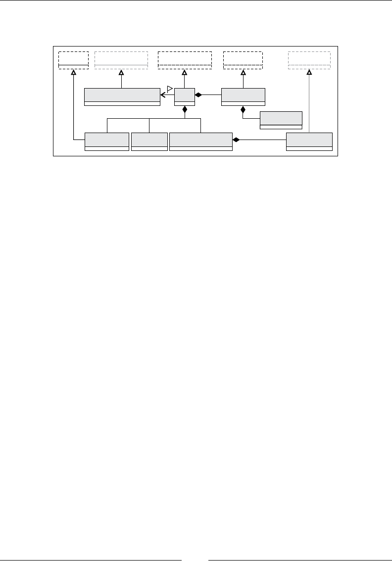
Chapter 7
[ 843 ]
The key software components of the conditional random elds are described in the
following UML class diagram:
CrfRecommendation Crf CrfModel
CrfConfig String CrfSeqDelimiter CrfSeqlter
DblVector
Config DataSequence PipeOperator Model Datalter
model
config taggedObs delims weights
11
11
delims
111
UML class diagram for the conditional random fields
The DataSequence and DataIter interfaces are grayed out to indicate that these are
dened in the IITB's CRF Java library.
Implementation
The test case uses the IITB's CRF Java implementation from the Indian Institute of
Technology at Bombay by Sunita Sarawagi. The JAR les can be downloaded from
Source Forge (http://sourceforge.net/projects/crf/).
The library is available as JAR les and source code. Some of the functionality,
such as the selection of a training algorithm, is not available through the API. The
components (JAR les) of the library are as follows:
• CRF for the implementation of the CRF algorithm
• LBFGS for limited-memory Broyden-Fletcher-Goldfarb-Shanno nonlinear
optimization of convex functions (used in training)
• CERN Colt library for manipulation of a matrix
• GNU generic hash container for indexing
The training of the conditional random eld for sequences requires dening a few
key interfaces:
• DataSequence to specify the mechanism to access observations and labels for
training and test data
• DataIter to iterate through the sequence of data created using the
DataSequence interface
• FeatureGenerator to aggregate all the features types
These interfaces have default implementations bundled in the CRF Java library [7:12].

Sequential Data Models
[ 844 ]
The scope of the IITB CRF Java library evaluation
The CRF library has been evaluated with three simple text
analytics test cases. Although the library is certainly robust enough
to illustrate the internal workings of the CRF, I cannot vouch for
its scalability or applicability in other elds of interest such as
bioinformatics or process control.
Building the training set
The rst step is to implement the structure of the training sequence, which
implements the DataIter interface. The training le consists of a pair of les:
• Raw recommendations (such as Raymond James upgrades Gentiva Health
Services from Underperform to Market perform)
• Tagged recommendations (such as Raymond James [1] upgrades [2] Gentiva
Health Services [3], from [4] Underperform [5] to [6] Market perform [7])
Let's dene the model for the CRF classier. As mentioned earlier, the model for the
CRF is similar to the logistic regression model and consists of the weights parameter:
class CrfModel(val weights: DblVector) extends Model
The tagged recommendations le requires a delimiter class, CrfSeqDelimiter.
It delineates the sequence of observations using the following parameters:
• obsDelim is a regular expression to break down data input into a sequence
of observations
• labelsDelim generates a sequence of labels from the data input
• trainingDelim generates a sequence of training tuples from the training set
The CrfSeqDelimiter class is dened as follows:
class CrfSeqDelimiter(val obsDelim: String, val labelsDelim: String,
val trainingDelim:String)
The main purpose of the IITB CRF Java library's DataIter interface is to dene
the methods to iterate through a sequence of data, tags, or observations. The three
methods are as follows:
• hasNext tests if the sequence has another entry
• next returns the next data or entry in the sequence and increments the
iterator cursor
• startScan initializes the DataIter iterator

Chapter 7
[ 845 ]
The CrfSeqIter sequence iterator uses the iitb.segment.DataCruncher class to
read a training set from a le (a le with tagged words):
class CrfSeqIter(val nLabels: Int, val input: String, val delim:
SeqDelimiter) extends DataIter {
lazy val trainData = DataCruncher.readTagged(nLabels, input, input,
delim.obsDelim, delim.labelsDelim, delim.trainingDelim, new labelMap)
override def hasNext: Boolean = trainData.hasNext
override def next: DataSequence = trainData.next
override def startScan: Unit = trainData.startScan
}
The trainData training set is initialized only once when any of the DataIter
overridden methods is invoked. The class is merely an adapter to the generation
of the training set.
Generating tags
The second step consists of selecting the mechanism and class to generate the
features observations. The extraction of the features from any data set requires
implementation of the FeatureGenerator interface in order to access all the
features observations from any kind of features.
Our problem is a simple linear tagging of data sequences (recommendations
from analysts). Therefore, we can use the iitb.Model.FeatureGenImpl default
implementation. Our tagging class, TaggingGenerator makes FeatureGenImpl
as a subclass and species the model specication as a CompleteModel. The IITB
CRF library supports both linear chain model of CompleteModel with a single edge
iterator and the nested chain CRF model of the type NestedModel with a nested
edge iterator. The complete model does not make any assumption regarding the
independence between labels Y:
val addFeature = true
class TaggingGenerator (val nLabels: Int) extends FeatureGenImpl(new
CompleteModel(nLabels),nLabels,addFeature)
The class is dened within the scope of the Crf class and does not have to be exposed
to the client code. The last parameter of FeatureGenImpl, addFeature, is set as true
to allow the tags of dictionary to be built iteratively during the training.

Sequential Data Models
[ 846 ]
Extracting data sequences
The CrfTrainingSet class implements the DataSequence interface. It is used to
access all the raw analyst's recommendations and rating regarding stocks. The class
needs to implement the following methods:
• set_y to assign a label index to a position k
• y to retrieve a label y at position y
• x to retrieve an observed feature vector at position k
• length to retrieve the number of entries in the sequence
The CrfTrainingSet class can be implemented as follows:
class CrfTrainingSet(val nLabels: Int, val entry: String, val delim:
String) extends DataSequence {
val words = entry.split(delim)
val map = new Array[Int](nLabels)
override def set_y(k: Int, label: Int): Unit = map(k) = label
override def y(k: Int): Int = map(k)
override def length: Int = words.size
override def x(k: Int): Object = words(k)
}
The class takes an analyst's recommendation regarding a stock, entry, as an input
and breaks it down into words, using the delimiter or regular expression, delim.
CRF control parameters
The execution of the CRF algorithm is controlled by a wide variety of conguration
parameters. For the sake of simplicity, we use the default conguration parameters,
CrfConfig, to control the execution of the learning algorithm, with the exception of
the following four variables:
• Initialization of the weights, w0, using either a predened or a random value
between 0 and 1 (default 0)
• Maximum number of iterations used in the computation of the weights
during the learning phase maxIters (default 50)
• The scaling factor lamdba for the L2 penalty function, used to reduce
observations with a high value (default 1.0)
• Convergence criteria, eps, used in computing the optimum values for the
weights wj (default 1e-4)
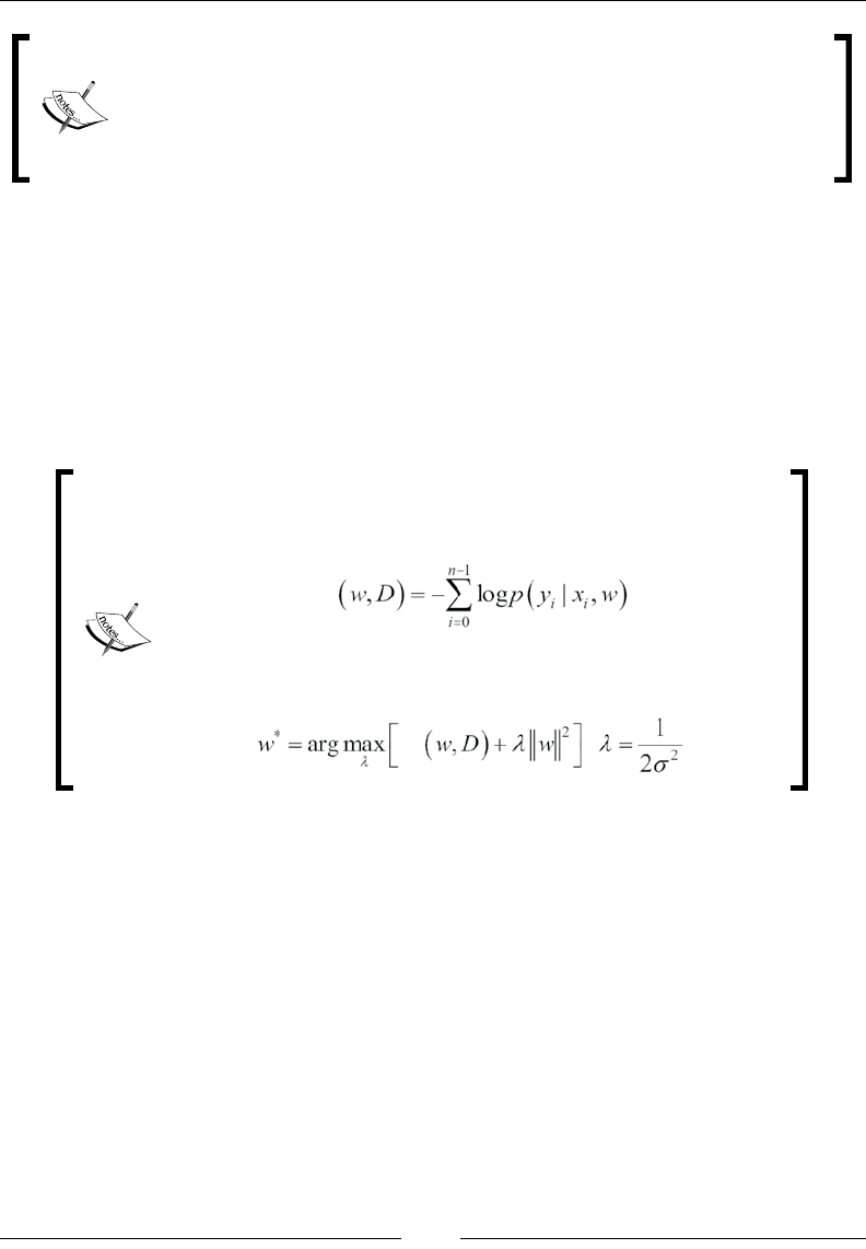
Chapter 7
[ 847 ]
Advanced conguration
The CRF model of the iitb library is highly congurable. It allows
developers to specify a state-label undirected graph with any combination
of at and nested dependencies between states. The source code includes
several training algorithms such as the exponential gradient.
The test case does not assume any dependence between states:
class CrfConfig(w0: Double, maxIters: Int, lambda: Double, eps:
Double) extends Config
Putting it all together
The objective of the training is to compute the weights wj that maximize the
conditional log-likelihood without the L2 penalty function.
Conditional log-likelihood for a linear chain CRF training set,
()
{}
0: 1
,
ii
n
Dxy−
=
is given as follows:
!
Learning: Maximization of loss function and L2 penalty is given
as follows:
!
Maximizing the log-likelihood function
!
is equivalent to minimizing the loss
with L2 penalty. The function is convex, and therefore, any variant gradient
descent (greedy) algorithm can be applied iteratively.
The Crf class implements the learning, train, and classification methods. Like
any other classiers, Crf implements the PipeOperator trait; so, the classication
can be included in a workow. The class also implements the Supervised trait to
force the developer to dene a validation routine for the CRF:
class Crf(nLabels: Int, config: CrfConfig, delims: SeqDelimiter,
taggedObs: String) extends PipeOperator[String, Double] with
Supervised[String] {
val features = new TaggingGenerator(nLabels) //1
lazy val crf = new CRF(nLabels, features, config.params) //2
val model: Option[CrfModel] = {

Sequential Data Models
[ 848 ]
features.train(seqIter) //3
Some(new CrfModel(crf.train(seqIter))) //4
}
…
The computation of the CRF weights during training uses either methods dened in
IITB's CRF library or methods described in the previous sections.
Once the features have been extracted from the data sequence input le (line 1), the
CRF algorithm is instantiated (line 2) with the number of labels, extracted features,
and the conguration. The model is trained using the iterator for features seqIter
(line 3), and then returns a CrfModel instance (vector of weights) (line 4) if training
succeeds, None otherwise.
The predictive method implements the data transformation operator, |>. It takes a
new observation (analyst's recommendation on a stock) and returns the maximum
likelihood, as shown here:
def |> : PartialFunction[String, Double] = {
case obs: String if(obs.length > 1 && model != None) => {
val dataSeq = new CrfTrainingSet(nLabels,obs,delims.obsDelim)
crf.apply(dataSeq)
}
}
The data transformation implements the Viterbi algorithm to extract the best sequence
of labels for a newly observed recommendation, obs. It invokes the apply method of
the iitb.crf.CRF class. The code to validate the arguments/parameters of the class
and methods are omitted along with the exception handler for the sake of readability.
Tests
The client code to execute the test consists of dening the number of labels (tags for
recommendation), the L2 penalty factor, LAMBDA, and the delimiting string:
val LAMBDA = 0.5; val EPS = 1e-3
val NLABELS = 9; val MAX_ITERS = 100; val W0 = 0.7
val PATH = "resources/data/chap7/rating"
val config = CrfConfig(W0, MAX_ITERS, LAMBDA, EPS)
val delimiters = CrfSeqDelimiter(",\t/ -():.;'?#`&_", "//", "\n")
Crf(NLABELS, config, delimiters, PATH).weights match {
case Some(weights) => weights
case None => { … }
}
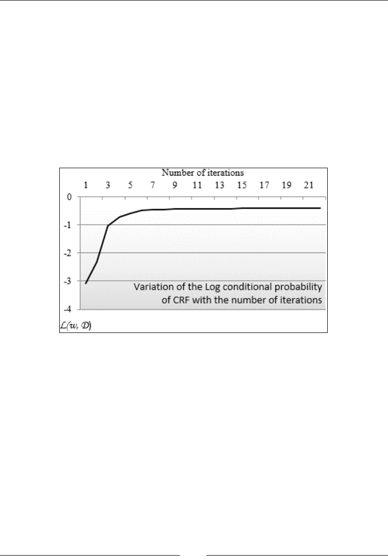
Chapter 7
[ 849 ]
For these tests, the initial value for the weights (with respect to the maximum number
of iterations for the maximization of the log likelihood, and the convergence criteria)
are set to 0.7 (with respect to 100 and 1e-3). The delimiters for labels sequence, observed
features sequence, and the training set are customized for the format of input data les,
rating.raw and rating.tagged.
The training convergence prole
The rst training run discovered 136 features from 34 analyst's stock recommendations.
The algorithm converged after 21 iterations. The value of the log of the likelihood for
each of those iterations is plotted to illustrate the convergence toward a solution of
optimum w:
Visualization of the log conditional probability of CRF during training
The training phase converges fairly quickly toward a solution. It can be explained
by the fact that there is little variation in the six-eld format of the analyst's
recommendations. A loose or free-style format would have required a larger
number of iterations during training to converge.
Impact of the size of the training set
The second test evaluates the impact of the size of the training set on the convergence
of the training algorithm. It consists of computing the difference Δw of the model
parameters (weights) between two consecutive iterations {wi}t+1 and {wi}t:
()
1
1
0
D
tt
ii
i
www
−+
=
=−
∑
△
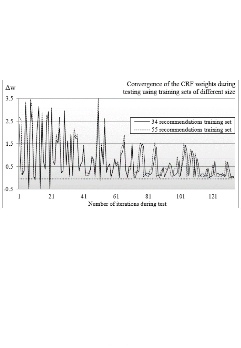
Sequential Data Models
[ 850 ]
The test is run on 163 randomly chosen recommendations using the same model but
with two different training sets:
• 34 analyst stock recommendations
• 55 stock recommendations
The larger training set is a super set of the 34 recommendations set. The following
graph illustrates the comparison of features generated with 34 and 55 CRF training
sequences:
The disparity between the test runs using two different size of training set is very
small. This can be easily explained by the fact that there is a small variation in the
format between the analyst's recommendations.
Impact of the L2 regularization factor
The third test evaluates the impact of the L2 regularization penalty on the convergence
toward the optimum weights/features. The test is similar to the rst test with different
value of
λ
. The following charts plot log [p(Y|X, w)] for different values of
λ
= 1/σ2
(02, 0.5, and 0.8):
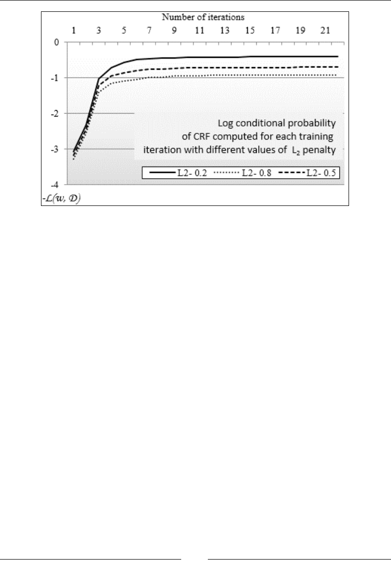
Chapter 7
[ 851 ]
Impact of the L2 penalty on convergence of the CRF training algorithm
The log of the conditional probability decreases or the conditional probability
increases with the number of iterations. The lower the L2 regularization factor,
the higher the conditional probability.
The variation of the analysts' recommendations within the training set is fairly small,
which limits the risk of overtting. A free-style recommendation format would have
been more sensitive to overtting.
Comparing CRF and HMM
The cost/benet analysis of discriminative models relative to generative models applies
to the comparison of the conditional random eld with the hidden Markov model.
Contrary to the hidden Markov model, the conditional random eld does not
require the observations to be independent (conditional probability). The conditional
random eld can be regarded as a generalization of the HMM by extending the
transition probabilities to arbitrary feature functions that can depend on the input
sequence. HMM assumes the transition probabilities matrix to be constant.
HMM learns the transition probabilities aij on its own by providing more training
data. The HMM can be regarded as a special case of CRF where the probabilities
used in the state transition are constant.

Sequential Data Models
[ 852 ]
Performance consideration
The time complexity for decoding and evaluating canonical forms of the hidden
Markov model for N states and T observations is O(N2T). The training of HMM
using the Baum-Welch algorithm is O(N2TM), where M is the number of iterations.
There are several options to improve the performance of HMM:
• Avoid multiplication by 0 in the emission probabilities matrix by using
sparse matrices or keeping tab of the null entries
• Try to train HMM on a relevant subset of the training data, particularly in the
case of tagging
The training of the linear chain conditional random elds is implemented using
the same dynamic programming techniques as HMM implementation (Viterbi,
forward-backward passes). Its time complexity for training T data sequence, N
labels y, and M weights/features
λ
is O(MTN2). The time complexity of the training
of a CRF can be reduced by distributing the computation of the log likelihood and
gradient over multiple nodes [7:13].
Summary
In this chapter, we had a closer look at modeling sequences of observations with
hidden states with the two most commonly used algorithms:
• Generative hidden Markov model (HMM) to maximize p(X,Y)
• Discriminative conditional random eld (CRF) to maximize log p(Y|X)
HMM is a special form of Bayes Network and requires the observations to be
independent. Under these circumstances, the HMM is fairly easy to estimate,
which is not the case for CRF.
You learned how to implement three dynamic programming techniques, Viterbi,
Baum-Welch, and alpha/beta algorithms in Scala. These algorithms are routinely
used to solve optimization problems and should be an essential component of your
algorithmic toolbox.

Kernel Models and Support
Vector Machines
This chapter introduces kernel functions, binary support vectors classiers, one-class
support vector machines for anomaly detection, and support vector regression.
In the Binomial classication section of Chapter 6, Regression and Regularization, you
learned the concept of hyperplanes used to segregate observations from the training
set and estimate the linear decision boundary. The logistic regression has at least one
limitation: it requires that the datasets are linearly separated using a dened function
(sigmoid). This limitation is especially an issue for high-dimension problems (large
number of features that are highly nonlinearly dependent). Support vector machines
(SVMs) overcome this limitation by estimating the optimal separating hyperplane
using kernel functions.
In this chapter, you will discover the following topics:
• The impact of some of the SVM conguration parameters and the kernel
method on the accuracy of the classication
• How to apply the binary support vector classier to estimate the risk for a
public company to curtail or eliminate its dividend
• How the support vector regression compares to the linear regression
Support vector machines are formulated as a convex optimization problem. Therefore,
the mathematical foundation of these algorithms is described for reference.
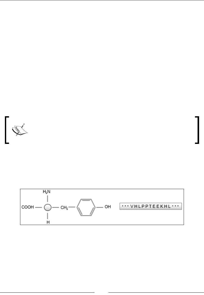
Kernel Models and Support Vector Machines
[ 854 ]
Kernel functions
Every machine learning model introduced in this book so far assumes that
observations are represented by a feature vector of a xed size. However, some
real-world applications such as text mining or genomics do not lend themselves
to this restriction. The critical element of the process of classication is to dene a
similarity or a distance between two observations. Kernel functions allow developers
to compute the similarity between observations without the need to encode them in
feature vectors [8:1].
Overview
The concept of kernel methods may be a bit odd at rst to a novice. It is usually
better understood by using a concrete example. Let's consider the example of the
classication of proteins. Proteins have different lengths and composition, but it
does not prevent scientists from classifying them [8:2].
Proteins:
Proteins are polymers of amino acids joined together by peptide bonds.
They are composed of a carbon atom bonded to a hydrogen atom,
another amino acid, or a carboxyl group.
A protein is represented using a traditional molecular notation to which biochemists
are familiar. Geneticists describe proteins in terms of a sequence of characters known
as the protein sequence annotation. The sequence annotation encodes the structure
and composition of the protein. The following picture illustrates the molecular (left)
and encoded (right) representation of a protein:
Sequence annotation of a protein
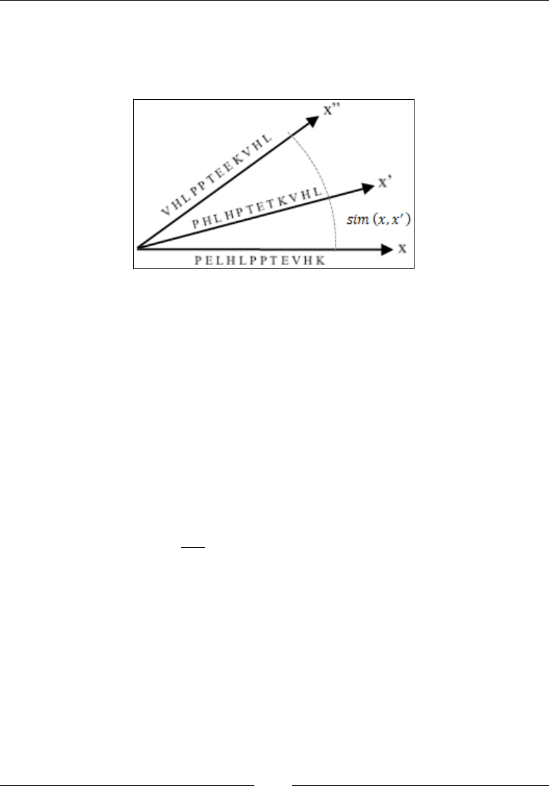
Chapter 8
[ 855 ]
The classication and the clustering of a set of proteins require the denition of a
similarity factor or distance used to evaluate and compare the proteins. For example,
the similarity between three proteins can be dened as a normalized dot product of
their sequence annotation:
Similarity between the sequence annotations of three proteins
You do not have to represent the entire sequence annotation of the proteins as a
feature vector in order to establish that they belong to the same class. You only need
to compare each element of each sequence, one by one, and compute the similarity.
For the same reason, the estimation of the similarity does not require the two
proteins to have the same length.
In this example, we do not have to assign a numerical value to each element of the
annotation. Let's represent an element of the protein annotation as its character c
and position p (for example: K, 4). The dot product of the two protein annotations x
and x' of the respective lengths n and n' can be dened as the number of identical
elements (character and position) between the two annotations divided by the
maximum length between the two annotations:
()
()( ) ()
'''
1
1
'''max ,'
mx
cp cp
i
simx x cc p pmx nn
mx =
==∩==
∑
The computation of the similarity for the three proteins produces the result as
sim(x,x')=6/12 = 0.50, sim(x,x'')=3/13 =0.23, sim(x',x'')= 4/13= 0.31.
Another similar aspect is that the similarity of two identical annotations is 1.0 and
the similarity of two completely different annotations is 0.0.

Kernel Models and Support Vector Machines
[ 856 ]
Visualization of similarity:
It is usually more convenient to use a radial representation to
visualize the similarity between features, as in the example of
proteins' annotations. The distance d(x,x') = 1/sim(x,x') is visualized
as the angle or cosine between two features. The cosine metric is
commonly used in text mining.
In this example, the similarity is known as a kernel function in the space of the
sequence annotation of proteins.
Common discriminative kernels
Although the measure of similarity is very useful to understand the concept
of a kernel function, kernels have a broader denition. A kernel K(x, x') is a
symmetric, non-negative real function that takes two real arguments (values
of two features). There are many different types of kernel functions, among
which the most common are:
• The linear kernel (dot product): This is useful in the case of very
high-dimensional data where problems can be expressed as a linear
combination of the original features
• The polynomial kernel: This extends the linear kernel for a combination of
features that are not completely linear
• The radial basis function (RBF): This is the most commonly applied kernel.
It is appropriate where the labeled or target data is noisy and requires some
level of regularization
• The sigmoid kernel: This is used in conjunction with neural networks
• The laplacian kernel: This is a variant of RBF with a higher regularization
impact on training data
• The log kernel: This is used in image processing
RBF terminology
In this presentation and the library used in its implementation,
the radial basis function is a synonym to the Gaussian kernel
function. However, RBF also refers to the family of exponential
kernel functions that encompasses Gaussian, Laplacian, and
exponential functions.

Chapter 8
[ 857 ]
The simple linear model for regression consists of the dot product of the regression
parameters (weights) and the input data (refer to the Ordinary least squares (OLS)
regression section of Chapter 6, Regression and Regularization).
The model is in fact the linear combination of weights and linear combination of
inputs. The concept can be extended by dening a general regression model as the
linear combination of nonlinear functions, known as basis functions:
() ()
0
1
|:R R
D
dd d
d
fxw w w x
φφ
=
=+ →
∑
The most commonly used basis functions are the power and Gaussian functions.
The kernel function is described as the dot product of the two vectors of the basis
function φ(x).φ(x') of two features vector x and x'. A partial list of kernel methods is
as follows:
The generic kernel:
()()() ()()
1
,' ' '
D
dd
d
Kxx x x x x
φφ φφ
=
=⋅=∑
The linear kernel:
()
1
,' ' '
D
T
ii
d
Kx
xxx xx
=
==⋅
∑
The polynomial kernel with the slope γ, degree n, and constant c:
()
()
,' ' 0, 0
n
T
Kxx xx c c
γγ
=+>≤
The sigmoid kernel with the slope γ and constant c:
()
()
,' tanh '0,0
T
Kxx xx c c
γγ
=+>≤
The radial basis function kernel with the slope γ:
()
2
'
,' 0
xx
Kxx e
γγ
−−
=>
The laplacian kernel with the slope γ:
()
'
,' 0
xx
Kxx e
γ
γ
−−
=>
The log kernel with the degree n:
()
()
,' log1 '
n
Kxx xx=−+−

Kernel Models and Support Vector Machines
[ 858 ]
The list of discriminative kernel functions described earlier is just a subset of the
kernel methods universe. Other types of kernels include:
• Probabilistic kernels: These are kernels derived from generative models.
Probabilistic models such as Gaussian processes can be used as a kernel
function [8:3].
• Smoothing kernels: This is the nonparametric formulation, averaging
density with the nearest neighbor observations [8:4].
• Reproducible Kernel Hilbert Spaces: This is the dot product of nite or
innite basis functions [8:5].
The kernel functions play a very important role in support vector machines for
nonlinear problems.
The support vector machine (SVM)
A support vector machine (SVM) is a linear discriminative classier that attempts
to maximize the margin between classes during training. This approach is similar to
the denition of a hyperplane through the training of the logistic regression (refer to
the Binomial classication section of Chapter 6, Regularization and Regression). The main
difference is that the support vector machine computes the optimum separating
hyperplane between groups or classes of observations. The hyperplane is indeed the
equation that represents the model generated through training.
The quality of the SVM depends on the distance, known as margin, between the
different classes of observations. The accuracy of the classier increases as the
margin increases.
The linear SVM
First, let's apply the support vector machine to extract a linear model (classier or
regression) for a labeled set of observations. There are two scenarios for dening a
linear model. The labeled observations are as follows:
• Naturally segregated in the features space (the separable case)
• Intermingled with overlap (the nonseparable case)
It is easy to understand the concept of an optimal separating hyperplane in cases the
observations are naturally segregated.
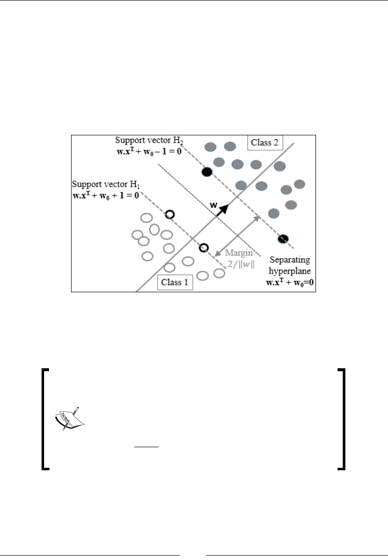
Chapter 8
[ 859 ]
The separable case (hard margin)
The concept of separating a training set of observations with a hyperplane is better
explained with a 2-dimensional (x, y) set of observations with two classes, C1 and C2.
The label y has the value -1 or +1.
The equation for the separating hyperplane is dened by the linear equation,
y=w.xT+w0, which sits in the midpoint between the boundary data points for class
C1 (H1: w.xT + w0 + 1=0) and class C2 (H2: w.xT + w0 - 1). The planes H1 and H2 are the
support vectors:
Support vector machine – separable case
In the separable case, the support vectors fully segregate the observations into two
distinct classes. The margin between the two support vectors is the same for all the
observations and is known as the hard margin.
Support vectors equation w is represented as:
()
0
1
T
i
ywx w i+≥∀
Hard margin optimization problem is given by:
()
0
,
min 1
2
o
T
T
i
ww
ww
subject to ywx w i
⎧⎫
+≥∀
⎨⎬
⎩⎭
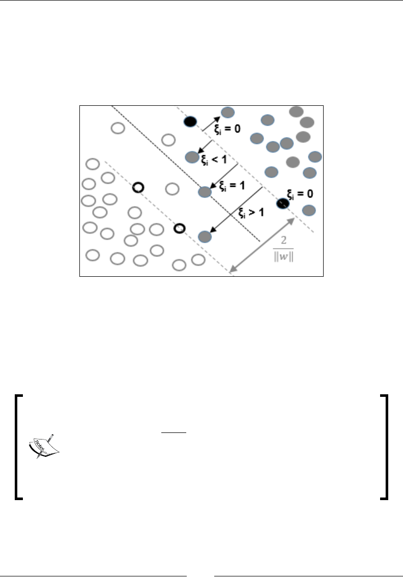
Kernel Models and Support Vector Machines
[ 860 ]
The nonseparable case (soft margin)
In the nonseparable case, the support vectors cannot completely segregate
observations through training. They merely become linear functions that penalize
the few observations or outliers that are located outside (or beyond) their respective
support vector, H1 or H2. The penalty variable ξ, also known as the slack variable,
increases if the outlier is further away from the support vector:
A support vector machine – the nonseparable case
The observations that belong to the appropriate (or own) class do not have to be
penalized. The condition is similar to the hard margin, which means that the slack
ξ is null. Observations that belong to the class but located beyond its support vector
are penalized; the slack ξ increases as the observations get closer to the support
vector of the other class and beyond. The margin is then known as a soft margin
because the separating hyperplane is enforced through a slack variable.
Optimization of the soft-margin for a linear SVM with C formulation:
()
1
,0
0
min2
0, 1
T
n
i
wi
T
i i
ww c
ywx w i
ξξ
ξ
ξ
−
=
⎧ ⎫
+
⎨ ⎬
⎩ ⎭
≥+≥− ∀
∑
C is the penalty (or inversed regularization) factor.
Chapter 8
[ 861 ]
You may wonder how the minimization of the margin error is related to the loss
function and the penalization factor introduced for the ridge regression (refer to the
Numerical optimization section of Chapter 6, Regularization and Regression). The second
factor in the formula corresponds to the ubiquitous loss function. You will certainly
recognize the rst term as the L2 regularization penalty with λ=1/2C.
The problem can be reformulated as the minimization of a function known as the
primal problem [8:6].
Primal problem formulation of the support vector classier:
()
0
1
0
,w 0
min 1
2
Tn
T
ii i
wi
ww cLL ywxw
−
=
⎧ ⎫
+=−+
⎨ ⎬
⎩ ⎭
∑
The C penalty factor can be thought of as the inverse of the L2 regularization factor.
The loss function L is then known as the hinge loss. The formulation of the margin
using the C penalty (or cost) parameter is known as the C-SVM formulation. C-SVM
is sometimes called the C-Epsilon SVM formulation for the nonseparable case.
The υ-SVM (or Nu-SVM) is an alternative formulation to the C-SVM. The
formulation is more descriptive than C-SVM; υ represents the upper bound of
the training observations that are poorly classied and the lower bound of the
observations on the support vectors [8:7].
υ-SVM formulation of a linear SVM:
()
1
,, 0
0
1
min2
0,
Tn
i
wp i
T
i i i
ww pun
ywx w p i
ξξ
ξ
ξ
−
=
⎧ ⎫
−
⎨ ⎬
⎩ ⎭
≥+≥− ∀
∑
Here, ρ is a margin factor used as a optimization variable.
The C-SVM formulation is used throughout the chapters for the binary, one class
support vector classier as well as the support vector regression.
Sequential Minimal Optimization
The optimization problem consists of the minimization of a quadratic
objective function (w2) subject to N linear constraints, N being the number
of observations. The time complexity of the algorithm is O(N3). A more
efcient algorithm, known as Sequential Minimal Optimization (SMO)
has been introduced to reduce the time complexity to O(N2).
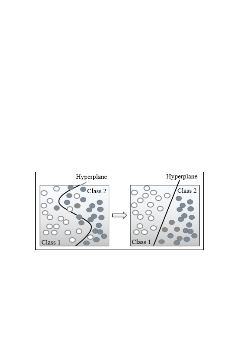
Kernel Models and Support Vector Machines
[ 862 ]
The nonlinear SVM
So far, it has been assumed that the separating hyperplane, and therefore, the
support vectors, are linear functions. Unfortunately, such assumptions are not
always correct in the real world.
Max-margin classication
Support vector machines are known as large or maximum margin classiers.
The objective is to maximize the margin between the support vectors with hard
constraints for separable (similarly, soft constraints with slack variables for
nonseparable) cases.
The model parameters {wi} are rescaled during optimization to guarantee that
the margin is at least 1. Such algorithms are known as maximum (or large)
margin classiers.
The problem of tting a nonlinear model into the labeled observations using support
vectors is not an easy task. A better alternative consists of mapping the problem to
a new, higher dimensional space using a nonlinear transformation. The nonlinear
separating hyperplane becomes a linear plane in the new space, as illustrated in the
following diagram:
Illustration of the Kernel trick in an SVM
The nonlinear SVM is implemented using a basis function, ϕ(x). The formulation
of the nonlinear C-SVM is very similar to the linear case. The only difference is the
constraint along the support vector, using the basis function, φ:
()
( )
0
10
T
iii
yw x w i
φξξ
+≥− ≥ ∀
Chapter 8
[ 863 ]
The minimization of wT.ϕ(x) in the preceding equation requires the computation of
the inner product ϕ(x)T.ϕ(x). The inner product of the basis functions is implemented
using one of the kernel functions introduced in the rst section. The optimization of
the preceding convex problem computes the optimal hyperplane w* as the kernelized
linear combination of the training samples, y.ϕ(x), and Lagrange multipliers. This
formulation of the optimization problem is known as the SVM dual problem. The
description of the dual problem is mentioned as a reference and is well beyond the
scope of this book [8:8 ].
Optimal hyperplane for the SVM dual problem:
()
1
*
0
n
ii i
i
wyx
αφ
−
=
=∑
Hard margin formulation for the SVM dual problem:
()
( )
()
()
()()
1
0 0
0
,
,1
n
T
i i ii i
i
i i
yw xw y yKxxw
Kxx x x i
φ α
φφ
−
=
⎛ ⎞
⋅+= +≥
⎜ ⎟
⎝ ⎠
=∀
∑
The kernel trick
The transformation (x,x') => K(x,x') maps a nonlinear problem into a linear problem
in a higher dimensional space. It is known as the kernel trick.
Let's consider, for example, the polynomial kernel dened in the rst section with a
degree d=2 and coefcient of C0=1 in a two-dimension space. The polynomial kernel
function on two vectors, x=[x1, x2] and z=[x'1, x'2], is decomposed into a linear function
in a dimension 6 space:
()
()
()( )
() ( ) () ( ) () ( )
() () () ()
2
2 2
'''' ' '
11 22 1122 11 22
11 22 33
2
2 2 13 24 1
,' 1'
12 22
' ' '
1, 2, 2,
T
Kxxxx
xx xx xxxxxx xx
xx xx xx
xxxxxxx
φφ φφ φφ
φφ
φ φ
=+
=+ ++ + +
=⋅+⋅+⋅+
== = =
L
L

Kernel Models and Support Vector Machines
[ 864 ]
Support vector classier (SVC)
Support vector machines can be applied to classication, anomalies detection, and
regression problems. Let's dive into the support vector classiers rst.
The binary SVC
The rst classier to be evaluated is the binary (2-class) support vector classier.
The implementation uses the LIBSVM library created by Chih-Chung Chang and
Chih-Jen Lin from the National Taiwan University [8:9].
LIBSVM
The library was originally written in C and ported to Java. It can be downloaded
from http://www.csie.ntu.edu.tw/~cjlin/libsvm as a .zip or tar.gzip le.
The library includes the following classier modes:
• Support vector classiers (C-SVC, υ-SVC, and one-class SVC)
• Support vector regression (υ-SVR and ε-SVR)
• RBF, linear, sigmoid, polynomial, and precomputed kernels
LIBSVM has the distinct advantage of using Sequential Minimal Optimization
(SMO), which reduces the time complexity of a training of n observations to O(n2).
LIBSVM documentation covers both the theory and implementation of hard and soft
margins and is available at http://www.csie.ntu.edu.tw/~cjlin/papers/guide/
guide.pdf.
Why LIBSVM?
There are alternatives to the LIBSVM library for learning and
experimenting with SVM. David Soergel from the University of
Berkeley refactored and optimized the Java version [8:10]. Thorsten
Joachims' SVMLight [8:11] Spark/MLlib 1.0 includes two Scala
implementations of SVM using resilient distributed datasets (refer to
the Apache Spark section of Chapter 12, Scalable Frameworks). However,
LIBSVM is the most commonly used SVM library.
The implementation of the different support vector classiers and the support vector
regression in LIBSVM is broken down into the following ve Java classes:
• svm_model: This denes the parameters of the model created during training
• svm_node: This models the element of the sparse matrix Q, used in the
maximization of the margins

Chapter 8
[ 865 ]
• svm_parameters: This contains the different models for support vector
classiers and regressions, the ve kernels supported in LIBSVM with
their parameters, and the weights vectors used in cross-validation
• svm_problem: This congures the input to any of the SVM algorithm (number
of observations, input vector data x as a matrix, and the vector of labels y)
• svm: This implements algorithms used in training, classication, and regression
The library also includes template programs for training, prediction, and
normalization of datasets.
The LIBSVM Java code
The Java version of LIBSVM is a direct port of the original C code.
It does not support generic types and is not easily congurable
(the code uses switch statements instead of polymorphism). For
all its limitations, LIBSVM is a fairly well-tested and robust Java
library for SVM.
Let's create a Scala wrapper to the LIBSVM library to improve its exibility and ease
of use.
Software design
The implementation of the support vector machine algorithm uses the design
template for classiers (refer to the Design template for classier section in Appendix A,
Basic Concepts).
The key components of the implementation of an SVM are as follows:
• A model SVMModel of the type Model, which is initialized through training
during the instantiation of the classier. The model class is an adapter to the
svm_model structure dened in LIBSVM.
• A predictive or classication routine is implemented as a data transformation
extending the PipeOperator trait.
• The support vector machine class SVM has three parameters: the conguration
wrapper of the type SVMConfig, the features/time series of the type
XTSeries, and the target or labeled values DblVector.
• The conguration (the type SVMConfig) consists of three distinct elements:
SVMExecution that denes the execution parameters such as maximum
number of iterations or convergence criteria, SVMKernel that species the
kernel function used during training, and SVMFormulation that denes
the formula (C, epsilon, or nu) used to compute a nonseparable case for
the support vector classier and regression.
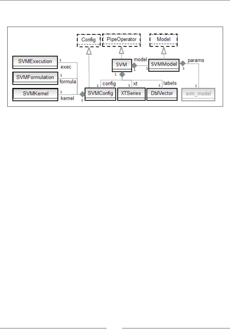
Kernel Models and Support Vector Machines
[ 866 ]
The key software components of the support vector machine are described in the
following UML class diagram:
Conguration parameters
LIBSVM exposes a large number of parameters for the conguration and execution
of any of the SVM algorithms. Any SVM algorithm is congured with three
categories of parameters, which are as follows:
• Formulation (or type) of the SVM algorithms (multiclass classier, one-class
classier, regression, and so on) using the SVMFormulation class
• The kernel function used in the algorithm (the RBF kernel, Sigmoid kernel,
and so on) using the SVMKernel class
• Training and execution parameters (convergence criteria, number of folds for
cross-validation, and so on) using the SVMExecution class
SVM Formulation
The instantiation of the conguration consists of initializing the LIBSVM parameter,
param, by the SVM type, kernel, and the execution context selected by the user.
Each of the SVM parameters case class extends the generic trait, SVMConfigItem:
trait SVMConfigItem { def update(param: svm_parameter): Unit }
The classes inherited from SVMConfigItem are responsible for updating the list of
the SVM parameters, svm_parameter, dened in LIBSVM. The update method
encapsulates the conguration of the LIBSVM.

Chapter 8
[ 867 ]
The formulation of the SVM algorithm is dened by classes implementing the
SVMFormulation trait:
sealed trait SVMFormulation extends SVMConfigItem {
def update(param: svm_parameter): Unit
}
The list of formulation for the SVM (C, nu, and eps for regression) is completely
dened and known. Therefore, the hierarchy should not be altered and the
SVMFormulation trait has to be declared sealed. Here is an example of the SVM
formulation class, CSVCFormulation, which denes the C-SVM model:
class CSVCFormulation (c: Double) extends SVMFormulation {
override def update(param: svm_parameter): Unit = {
param.svm_type = svm_parameter.C_SVC
param.C = c
}
}
The other SVM formulation classes, NuSVCFormulation, OneSVCFormulation,
and SVRFormulation, implement the υ-SVM, 1-SVM, and ε-SVM respectively
for regression models.
The SVM kernel function
Next, you need to specify the kernel functions by dening and implementing the
SVMKernel trait:
sealed trait SVMKernel extends SVMConfigItem {
def update(param: svm_parameter): Unit
}
Once again, there are a limited number of kernel functions supported in LIBSVM.
Therefore, the hierarchy of kernel functions is sealed. The following code snippet
congures the radius basis function kernel, RbfKernel, as an example of denition
of the kernel denition class:
class RbfKernel(gamma: Double) extends SVMKernel {
override def update(param: svm_parameter): Unit = {
param.kernel_type = svm_parameter.RBF
param.gamma = gamma
…

Kernel Models and Support Vector Machines
[ 868 ]
The fact that the LIBSVM Java byte code library is not very extensible does not
prevent you from dening a new kernel function in the LIBSVM source code.
For example, the Laplacian kernel can be added with the following steps:
1. Create a new kernel type in svm_parameter, such as svm_parameter.
LAPLACE = 5.
2. Add the kernel function name to kernel_type_table in the svm class.
3. Add kernel_type != svm_parameter.LAPLACE to the svm_check_
parameter method.
4. Add the implementation of the kernel function for two values in svm.
kernel_function (java code):
case svm_parameter.LAPLACE:
double sum = 0.0;
for(int k = 0; k < x[i].length; k++) {
final double diff = x[i][k].value - x[j][k].value;
sum += diff*diff;
}
return Math.exp(-gamma*Math.sqrt(sum));
5. Add the implementation of the Laplace kernel function in the svm.k_function
method by modifying the existing implementation of RBF (distanceSqr).
6. Rebuild the libsvm.jar le
SVM execution
The SVMExecution class denes the conguration parameters for the execution
of the training of the model, namely, the convergence factor, eps for the optimizer,
the size of the cache cacheSize, and the number of folds, nFolds used during
cross-validation:
class SVMExecution(cacheSize: Int, eps: Double, nFolds: Int) extends
SVMConfigItem {
override def update(param: svm_parameter): Unit = {
param.cache_size = cacheSize
param.eps = eps
}
}
The cross-validation is performed only if the nFolds value is greater than 1.

Chapter 8
[ 869 ]
SVM implementation
We are nally ready to create the conguration class, SVMConfig, which hides and
manages all of the different conguration parameters:
class SVMConfig(formula: SVMFormulation, kernel: SVMKernel,exec:
SVMExecution) {
val param = new svm_parameter
formula.update(param)
kernel.update(param)
exec.update(param)
}
The instantiation of SVMConfig initialized the internal LIBSVM list of conguration
parameters through a sequence of update calls.
Next, let's implement the rst support vector classier for the two-class problems.
As with any other data transformation, the parameterized class SVM implements the
PipeOperator, as follows:
class SVM[T <% Double](config: SVMConfig, xt: XTSeries[Array[T]],
labels: DblVector) extends PipeOperator[Array[T], Double] {
type Feature = Array[T]
type SVMNodes = Array[Array[svm_node]]
This class has the same parameters as other classiers presented in the previous
chapters: a conguration, config, an input time series, xt, and labeled data, labels.
The types are added for convenience. The internal types, Feature and SVMNodes, are
added for convenience.
The LIBSVIM type, svm_node, is the indexed value of an element of the feature
vector in a particular observation:
public class svm_node implements java.io.Serializable {
public int index;
public double value;
}
The type SVMNodes dened in the scope of SVM class is the representation of
a two-dimensional array of features vector elements by observations. The next
step is to implement the training procedure. The training is executed during the
instantiation of the SVM class. The SVM model, SVMModel, is dened as a tuple or
pair (svmmodel, accuracy) with the following:
• The svmmodel is the model dened in LIBSVM
• accuracy computed during an N-folds cross-validation if the number of
folds, nFolds, has been set as one of the parameters of SVMExecution

Kernel Models and Support Vector Machines
[ 870 ]
Consider the following code:
class SVMModel(val svmmodel: svm_model, val accuracy: Double) extends
Model
The instantiation of SVC is hidden from the client code. It is executed during the
instantiation of the class, so a client code does not have to be aware of the LIBSVM
types. Consider the following code:
val model: Option[SVMModel] = {
val problem = new svm_problem //1
problem.l = xt.size;
problem.y = labels
problem.x = new SVMNodes(xt.size)
val dim = dimension(xt)
xt.zipWithIndex.foreach( xt_i => { //2
val svm_col = new Array[svm_node](dim)
xt_i._1.zipWithIndex
.foreach(xi => {
val node = new svm_node
node.index= xi._2
node.value = xi._1
svm_col(xi._2) = node
})
problem.x(xt_i._2) = svm_col
})
Some(svm.svm_train(problem, config.param, accuracy(problem))//3
}
The rst step in the creation of the model is to dene the SVM problem, problem,
in the context of LIBSVM (line 1): length of the time series, labeled data, and input
observations. The time series has to be converted into the LIBSVM internal class,
svm_nodes (line 2), to complete the initialization of the problem. The Scala method,
zipWithIndex, is used to access the index of each observation (time series entry).
Finally, the model and the computed accuracy are returned as a tuple (line 3) after
processing by the svm_train training method.

Chapter 8
[ 871 ]
The accuracy is the ratio of true positive plus the true negative over the size of the
test sample (refer to the Key metrics section of Chapter 2, Hello World!). It is computed
through cross-validation only if the number of folds is initialized in the SVMExecution
conguration class as greater than 1. Practically, the accuracy is computed by
invoking the cross-validation method, svm_cross_validation, in the LIBSVM
package, and then computing the ratio of the number of predicted values that match
the labels over the total number of observations. Here is the essential part of the
implementation of accuracy(problem: svm_problem):
val target = new Array[Double](labels.size)
svm.svm_cross_validation(problem, config.param, config.exec.nFolds,
target)
val rawAccuracy = target.zip(labels)
.filter(z => Math.abs(z._1-z._2) < config.eps)
rawAccuracy.size.toDouble/labels.size
The Scala filter weeds out the observations that were poorly predicted.
This minimalist implementation is good enough to start exploring the support
vector classier.
C-penalty and margin
The rst evaluation consists of understanding the impact of the penalty factor C to
the margin in the generation of the classes. Let's implement the computation of the
margin. The margin is dened as 2/||w|| and implemented as a method of the SVC
class, as follows:
def margin: Option[Double] = model match {
case Some(m) => {
val wNorm = m.svmmodel.sv_coef(0)
.foldLeft(0.0)((s, r) => s + r*r) //1
if(wNorm < config.eps) None
else Some(2.0/Math.sqrt(wNorm)) //2
}
…
}
The rst instruction (line 1) computes the sum of the squares, wNorm, of the residuals
r = y – f(x|w). The margin (line 2) is ultimately computed if the sum of squares is
signicant enough to avoid rounding errors.

Kernel Models and Support Vector Machines
[ 872 ]
The margin is evaluated using an articially generated time series and labeled data.
First, we dene the method to evaluate the margin for a specic value of the penalty
(inversed regularization) factor C:
def evalMargin(observations: DblMatrix, labels: DblVector, c: Double):
Unit = {
val config = SVMConfig(CSVCFormulation(c), RbfKernel(GAMMA)) //3
val xt = XTSeries[DblVector](observations)
val svc = SVM[Double](config, xt, labels)
svc.margin match {
case Some(margin) => Display.show("Margin $margin", logger)
…
This test uses the default execution parameters, cache_size= 25000 and eps=1e-15.
Therefore, the 3rd value of SVMCong, exec, is not specied in the SVMConfig.
apply constructor (line 3).The method is invoked iteratively to evaluate the impact
of the penalty factor on the margin extracted from the training of the model. The test
uses a synthetic time series to highlight the relation between C and the margin. The
synthetic time series consists of the following two training sets of an equal size, N:
• First training set: data points generated as y = x(1 + r/5) for the label 1, r
being a randomly generated number over the range [0,1]
• Second training set: randomly generated data point y = r for the label of -1
Consider the following code:
def generate: (DblMatrix, DblVector) = {
val z = Array.tabulate(N)(i =>
Array[Double](i, i*(1.0 + 0.2*Random.nextDouble))
) ++
Array.tabulate(N)(i =>Array[Double](i, i*Random.nextDouble))
(z, Array.fill(N)(1.0) ++ Array.fill(N)(-1.0))
}
The evalMargin method is executed for a predened value of gamma and the value
C ranging from 0 to 5:
val gamma =0.8; val N = 100
val values = generate
Range(0, 50).foreach(i =>evalMargin(values._1, values._2, i*0.1))
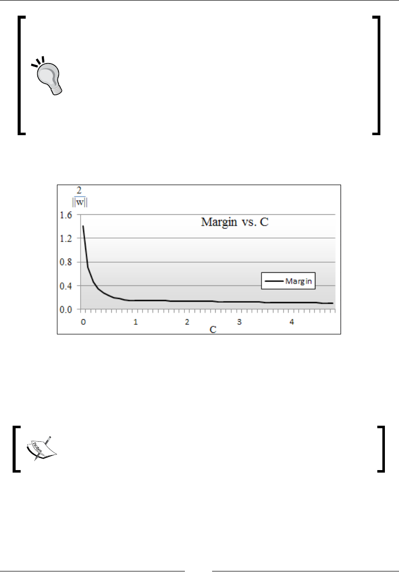
Chapter 8
[ 873 ]
val vs. nal val
There is a difference between a val and a nal val. A nonnal value
can be overridden in a subclass. Overriding a nal value produces a
compiler error, as follows:
class A {val x = 5; final val y = 8 }
class B extends A {
override val x = 9 // OK
override val y = 10 // Error
}
The following chart illustrates the relation between the penalty, or cost factor, C and
the margin:
The margin value versus C-penalty for an SVC
As expected, the value of the margin decreases as the penalty term C increases. The
C penalty factor is related to the L2 regularization factor λ as C ~ 1/λ. A model with
a large value of C has a high variance and a low bias, while a small value of C will
produce lower variance and a higher bias.
Optimizing C-penalty
The optimal value for C is usually evaluated through cross-validation,
by varying C in incremental powers of 2: 2n, 2n+1 … [8:12].

Kernel Models and Support Vector Machines
[ 874 ]
Kernel evaluation
The next test consists of comparing the impact of the kernel function on the accuracy
of the prediction. Once again, a synthetic time series is generated to highlight the
contribution of each kernel.
First, the prediction method for the SVM class is implemented by overriding the pipe
operator data transformation, |>:
def |> : PartialFunction[Feature, Double] = {
case x: Feature if(x != null && x.size==dimension(xt) && model
!= None && model.get.accuracy >= 0.0) =>
svm.svm_predict(model.get.svmmodel, toNodes(x))
}
The prediction model relies on the svm_predict LIBSVM to compute the output
value. It takes two parameters: svmmodel and an array of svm_nodes (line 1). The
conversion of a feature from the type DblVector to an array of the svm_nodes
LIBSVM is performed by the toNodes method:
def toNodes(x: Feature): Array[svm_node] =
x.zipWithIndex
.foldLeft(new ArrayBuffer[svm_node])((xs, f) => { //2
val node = new svm_node
node.index = f._2
node.value = f._1
xs.append(node)
xs
}).toArray
A fold is used to construct the array of svm_nodes from the feature vector, x. The
nodes (elements of the sparse matrix of the svm_node LIBSVM) are generated from
the new observation x (line 1). The model extracted from the training of the model
(instantiation of SVM) and the sparse matrix nodes are the input to the LIBSVM
predictor, svm_predict (line 2).
The predictor is used by the test code for evaluating the different kernel functions.
Let's create a method to evaluate and compare these kernel functions. All we need
is the following:
• A training set, observations, by features of the type DblMatrix
• A test set, test, of the type DblMatrix
• A set of labels for the training set, taking the value 0 or 1
• A kernel function kF

Chapter 8
[ 875 ]
Consider the following code:
def evalKernel(features: DblMatrix, test: DblMatrix, labels:
DblVector, kF: SVMKernel): Double = {
val config = SVMConfig(new CSVCFormulation(C), kF) //3
val xt = XTSeries[DblVector](features)
val svc = SVM[Double](config, xt, labels) //4
val successes = test.zip(labels)
.count(tl => {
Try((svc |> tl._1) == tl._2)
match { case Success(n) => true
case Failure(e) => false }
})
successes.toDouble/test.size //6
}
The support vector classier, svc, is congured with the default execution parameters
and the C-formulation (line 3), and trained (instantiated) with the observed features,
xt and the output, labels (line 4).
Once trained, svc is used to predict the value for a test sample extracted from
the original dataset (line 5). Finally, the number of successful test observations is
counted and the accuracy is computed as the ratio of the successful prediction over
the size of the test sample (line 6).
In order to compare the different kernels, let's generate three datasets of the
size 2N for a binomial classication using the following random generator,
y = variance*x – mean:
def genData(variance: Double, mean: Double): DblMatrix =
val adjVariance1 = variance*Random.nextDouble - mean
val adjVariance2 = variance*Random.nextDouble - mean
Array.fill(N)(Array[Double]( adjVariance, adjVariance2))
}
A training set is then created as the aggregate of two classes of data points:
• Random data points (x,y) with variance a and mean 1-b with label 0.0
• Random data points with variance a and mean b-1 with label 1.0
Consider the following code
val trainingSet = genData(a,b) ++ genData(a,1-b)
val labels = Array.fill(N)(0.0) ++ Array.fill(N)(1.0)
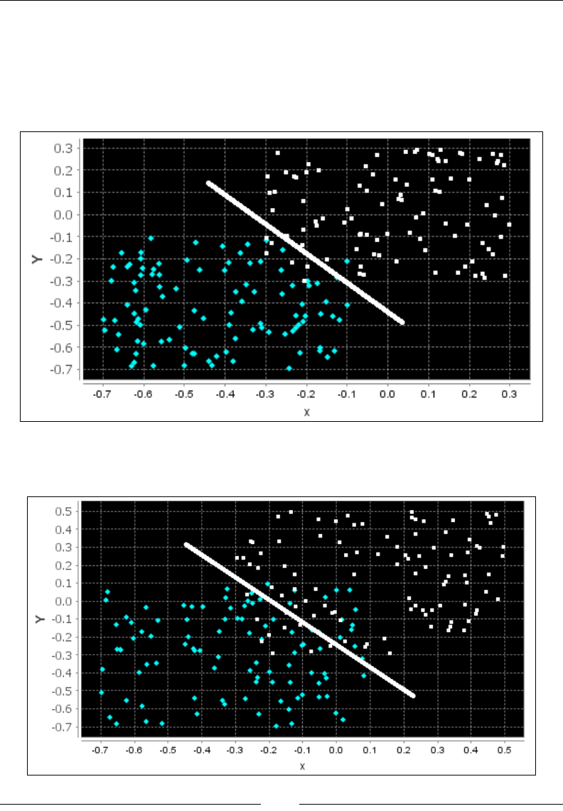
Kernel Models and Support Vector Machines
[ 876 ]
The parameters a and b are selected from two groups of training data points with
various degree of separation to illustrate the separating hyperplane.
The following chart describes the high margin; the rst training set generated with
the parameters a = 0.6 and b = 0.3 illustrates the highly separable classes with a
clean and distinct hyperplane:
The following chart describes the medium margin; the parameters a = 0.8 and
b = 0.3 generate two groups of observations with some overlap:
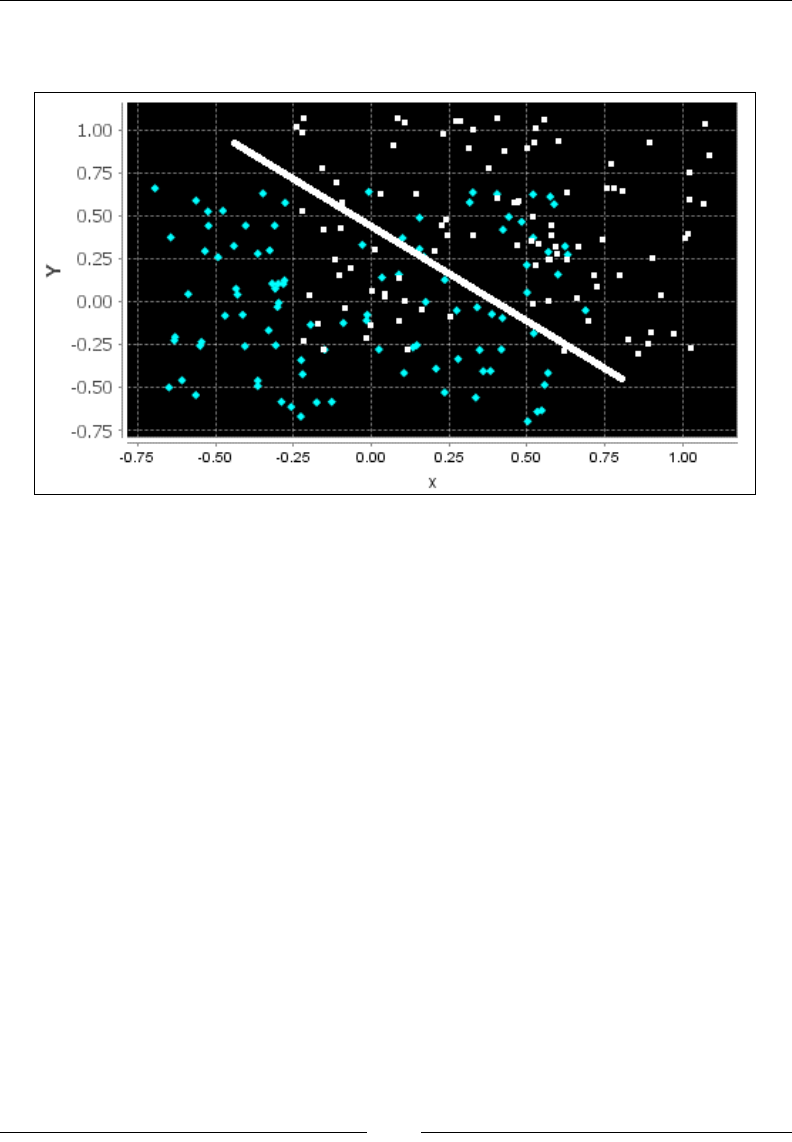
Chapter 8
[ 877 ]
The following chart describes the low margin; the two groups of observations in this
last training are generated with a = 1.4 and b = 0.3 and show a signicant overlap:
The test set is generated in a similar fashion as the training set, as they are extracted
from the same data source:
val EPS = 0.0001; val C = 1.0; val GAMMA = 0.8
val N = 100; val COEF0 = 0.5; val DEGREE = 2
val a = 1.4; val b = 0.3 //3 sets of values
val trainSet = genData(a, b) ++ genData(a, 1-b)
val testSet = genData(a, b) ++ genData(a, 1-b)
val labels = Array.fill(N)(0.0) ++ Array.fill(N)(1.0)
val result =
evalKernel(trainSet,testSet, labels, RbfKernel(GAMMA)) ::
evalKernel(trainSet,testSet, labels, SigmoidKernel(GAMMA)) ::
evalKernel(trainSet,testSet, labels, LinearKernel) ::
evalKernel(trainSet,testSet, labels, PolynomialKernel(GAMMA, COEF0,
DEGREE)) :: List[Double]()
The value of the kernel function parameters are arbitrary selected from text books.
The evalKernel method dened earlier is applied to the three training sets: high
margin (a = 1.4), medium margin (a = 0.8), and low margin (a = 0.6) with
each of the four kernels (RBF, sigmoid, linear, and polynomial).
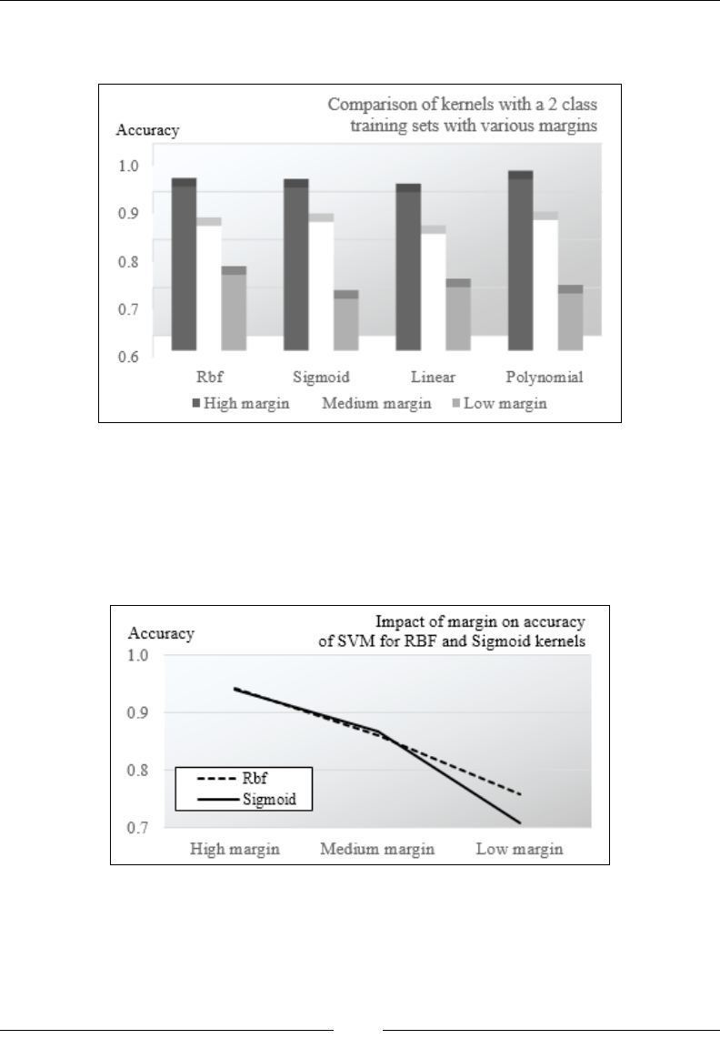
Kernel Models and Support Vector Machines
[ 878 ]
The accuracy is assessed by counting the number of observations correctly classied
for all of the classes for each invocation of the predictor, |>:
Comparative chart of kernel functions
Although the different kernel functions do not differ in terms of the impact on the
accuracy of the classier, you can observe that the RBF and polynomial kernels
produce slightly more accurate results. As expected, the accuracy decreases as
the margin decreases. A decreasing margin is a sign that the cases are not easily
separable, affecting the accuracy of the classier:

Chapter 8
[ 879 ]
Test case design
The test to compare the different kernel methods is highly
dependent on the distribution or mixture of data in the training
and test sets. The synthetic generation of data in this test case is
used for the purpose of illustrating the margin between classes of
observations. Real-world datasets may produce different results.
In summary, there are four steps in creating a SVC-based model:
1. Select a features set.
2. Select the C-penalty (inverse regularization).
3. Select the kernel function.
4. Tune the kernel parameters.
As mentioned earlier, this test case relies on synthetic data to illustrate the concept
of margin and compare kernel methods. Let's use the support vector classier for
a real-world nancial application.
Application to risk analysis
The purpose of the test case is to evaluate the risk for a company to curtail or
eliminate its quarterly or yearly dividend. The features selected are nancial
metrics relevant to a company's ability to generate cash ow and pay out its
dividends over the long term.
Features and labels
We need to select any subset of the following nancial technical analysis metrics
(refer to the Terminology section in Appendix A, Basic Concepts):
• Relative change in stock prices over the last 12 months
• Long-term debt-equity ratio
• Dividend coverage ratio
• Annual dividend yield
• Operating prot margin
• Short interest (ratio of shares shorted over the oat)
• Cash per share-share price ratio
• Earnings per share trend

Kernel Models and Support Vector Machines
[ 880 ]
The earnings trend has the following values:
• -2, if earnings per share decline by more than 15 percent over the last
12 months
• -1, if earnings per share decline between 5 percent and 15 percent
• 0, if earning per share is maintained within 5 percent
• +1, if earnings per share increase between 5 percent and 15 percent
• +2, if earnings per share increase by more than 15 percent
The features are normalized with values 0 and 1.
The labeled output, dividend changes, is categorized as follows:
• -1, if dividend is cut by more than 5 percent
• 0, if dividend is maintained within 5 percent
• +1, if dividend is increased by more than 5 percent
Let's combine two of these three labels {-1, 0, 1} to generate two classes for the
binary SVC:
• Class C1 = stable or decreasing dividends and class C2 = increasing dividends;
represented by dividendsA
• Class C1 = decreasing dividends and class C2 = stable or increasing dividends;
represented by dividendsB
The different tests are performed with a xed set of conguration parameters C and
GAMMA and a 2-fold validation conguration:
val path = "resources/data/chap8/dividendsA.csv"
val C = 1.0; val GAMMA = 0.5; val EPS = 1e-3; val NFOLDS = 2
val extractor = relPriceChange :: debtToEquity :: dividendCoverage
:: cashPerShareToPrice :: epsTrend :: dividendTrend
:: List[Array[String] =>Double]() //1

Chapter 8
[ 881 ]
The components of the extractor are functions that convert a set of elds in the input
.csv le into double oating point values:
val xs = DataSource(path, true, false, 1) |> extractor
val config = SVMConfig(new CSVCFormulation(C),
RbfKernel(GAMMA),
SVMExecution(EPS, NFOLDS))
val features = XTSeries.transpose(xs.take(xs.size-1))//2
val svc = SVM[Double](config, features, xs.last)
svc.accuracy match { //3
case Some(acc) => Display.show(s"Accuracy: $acc", logger)
case None => { … }
}
The different elds are extracted from the dividendsA.csv le using the DataSource
extractor with a lter (line 1). The purpose of the test A is to create a separating
hyperplane (the predictive model) for dividendsA, that is, companies that cut or
maintained their dividends and the companies that increased their dividends. The last
eld in the extractor is the labeled output. The observed features time series is created
from all the elds extracted from the .csv le except the last. The time series has to
be transposed to use the format required by LIBSVM (line 2). Once the support vector
classier is created, you can retrieve the accuracy of the cross-validation (line 3).
LIBSVM scaling
LIBSVM supports feature normalization known as scaling, prior
to training. The main advantage of scaling is to avoid attributes
in greater numeric ranges dominating those in smaller numeric
ranges. Another advantage is to avoid numerical difculties
during the calculation. In our examples, we use the normalization
of the time series, XTSeries.normalize. Therefore, the scaling
ag in LIBSVM is disabled.
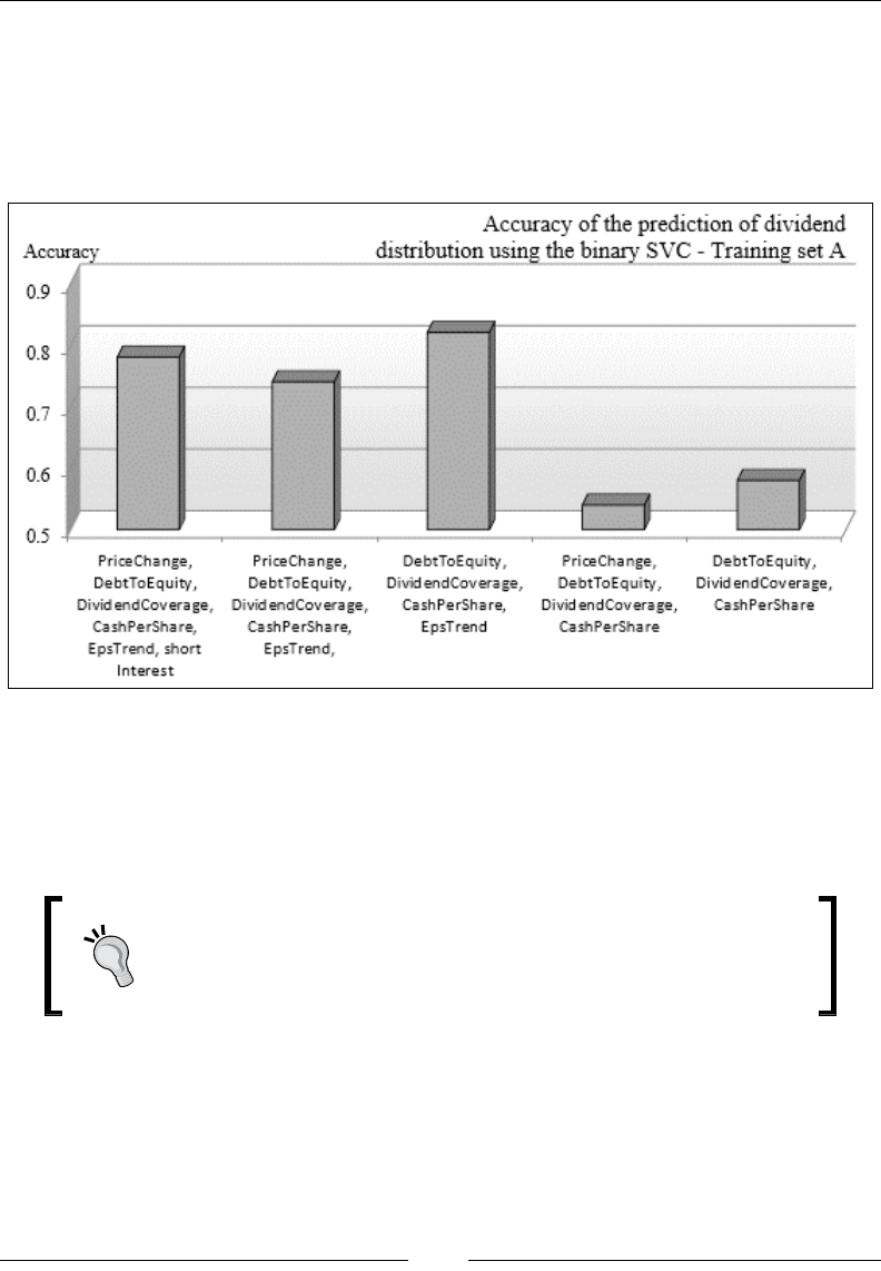
Kernel Models and Support Vector Machines
[ 882 ]
The test is repeated with a different set of features and consists of comparing the
accuracy of the support vector classier for different features sets. The features
sets are selected from the content of the .csv le by assembling the extractor with
different congurations, as follows:
val extractor = … :: dividendTrend :: List[Array[String] =>Double]()
The test demonstrates that the selection of the proper features set is the most critical
step in applying the support vector machine, and any other model for that matter,
to classication problems. In this particular case, the accuracy is also affected by the
small size of the training set. The increase in the number of features also reduces the
contribution of each specic feature to the loss function.
N-fold cross-validation
The cross-validation in this test example uses only 2 folds because
the number of observations is small, and you want to make sure
that any class contains at least a few observations.
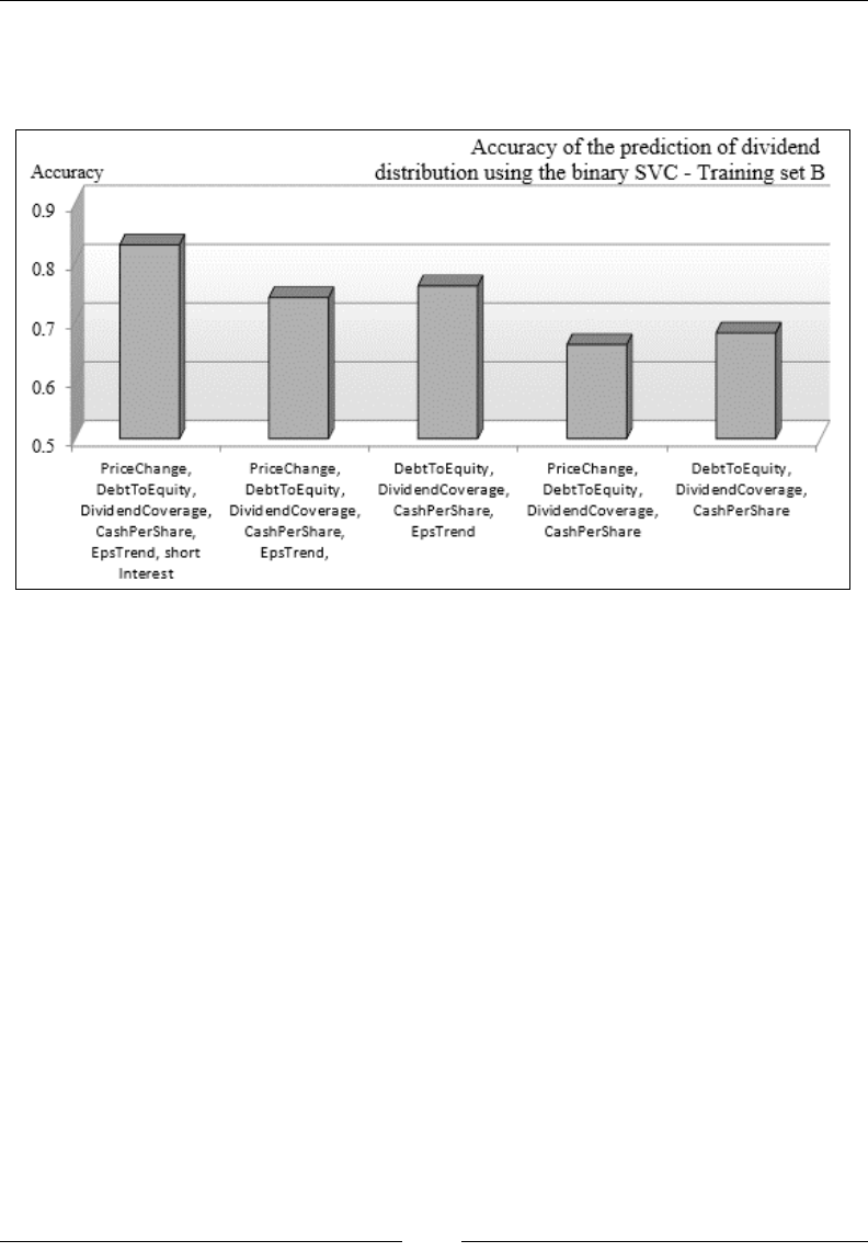
Chapter 8
[ 883 ]
The same process is repeated for the test B whose purpose is to classify companies
with decreasing dividends and companies with stable or increasing dividends, as
shown in the following graph:
The difference in terms of accuracy of prediction between the rst three features
set and the last two features set in the preceding graph is more pronounced in test
A than test B. In both tests, the feature eps (earning per share) trend improves the
accuracy of the classication. It is a particularly good predictor for companies with
increasing dividends.
The problem of predicting the distribution (or not) dividends can be restated as
evaluating the risk of a company to dramatically reduce its dividends.
What about the risk a company entails to eliminate its dividend altogether? Such
a scenario is rare, and those cases are actually outliers. A one-class support vector
classier can be used to detect outliers or anomalies [8:13].
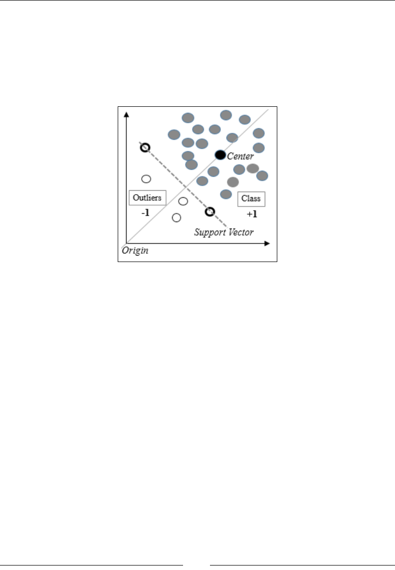
Kernel Models and Support Vector Machines
[ 884 ]
Anomaly detection with one-class SVC
The design of the one-class SVC is an extension of the binary SVC. The main
difference is that a single class contains most of the baseline (or normal) observations
and the other class is replaced by a reference point known as the SVC origin. The
outliers (or abnormal) observations reside beyond (or outside) the support vector of
the single class:
Illustration of the one-class SVC
The outlier observations have a labeled value of -1, while the remaining training
sets are labeled +1. In order to create a relevant test, we add four more companies
that have drastically cut their dividends (ticker symbols WLT, RGS, MDC, NOK,
and GM). The dataset includes the stock prices and nancial metrics recorded prior
to the cut in dividends.
The implementation of this test case is very similar to the binary SVC driver code,
except for the following:
• The classier uses the Nu-SVM formulation, OneSVFormulation
• The labeled data is generated by assigning -1 to companies that have
eliminated their dividend and +1 for all other companies
The test is executed against the dataset resources/data/chap8/dividends2.csv.
First, we need to dene the formulation for the one-class SVM:
class OneSVCFormulation(nu: Double) extends SVMFormulation {
override def update(param: svm_parameter): Unit = {
param.svm_type = svm_parameter.ONE_CLASS
param.nu = nu
}
}

Chapter 8
[ 885 ]
The test code is similar to the execution code for the binary SVC. The only difference
is the denition of the output labels; -1 for companies eliminating dividends and +1
for all other companies:
val NU = 0.2; val GAMMA = 0.5; val NFOLDS = 2
val path = "resources/data/chap8/dividends2.csv"
val xs = DataSource(path, true, false, 1) |> extractor
val config = SVMConfig(new OneSVCFormulation(NU),
RbfKernel(GAMMA),
SVMExecution(EPS, NFOLDS))
val features = XTSeries.transpose(xs.dropRight(1))
val svc = SVM[Double](config, features, xs.last.map( filter (_)))
svc.accuracy match {
case Some(acc) => Display.show("Accuracy: $acc", logger)
case None => { … }
}
The test is executed with the following features: relPriceChange, debtToEquity,
dividendCoverage, cashPerShareToPrice, and epsTrend.
The model is generated with the accuracy of 0.821. This level of accuracy should not
be a surprise; the outliers (companies that completely eliminated their dividends) are
added to the original dividend .csv le. These outliers differ signicantly from the
baseline observations (companies who have reduced, maintained, or increased their
dividend) in the original input le.
Where the labeled observations are available, the one-class support vector machine is
an excellent alternative to clustering techniques.
Denition of anomaly
The results generated by a one-class support vector classier depend
heavily on the subjective denition of an outlier. The test case
assumes that the companies that eliminate their dividends have
unique characteristics that set them apart, and are different even from
companies who have cut, maintained, or increased their dividend.
There is no guarantee that this assumption is indeed always valid.
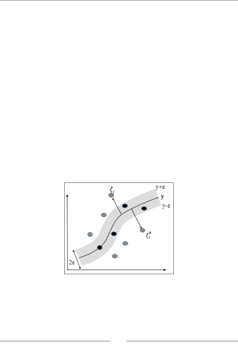
Kernel Models and Support Vector Machines
[ 886 ]
Support vector regression (SVR)
Most of the applications using support vector machines are related to classication.
However, the same technique can be applied to regression problems. Luckily, as
with classication, LIBSVM supports two formulations for support vector regression:
•
∈
-VR (sometimes called C-SVR)
• υ-SVR
For the sake of consistency with the two previous cases, the following test uses the
∈
(or C) formulation of the support vector regression.
Overview
The SVR introduces the concept of error insensitive zone and insensitive error, ε.
The insensitive zone denes a range of values around the predictive values, y(x).
The penalization component C does not affect the data point {xi,yi} that belongs to
the insensitive zone [8:14].
The following diagram illustrates the concept of an error insensitive zone, using a
single variable feature x and an output y. In the case of a single variable feature, the
error insensitive zone is a band of width 2ε. Ε is known as the insensitive error. The
insensitive error plays a similar role to the margin in the SVC.

Chapter 8
[ 887 ]
For the mathematically inclined, the maximization of the margin for nonlinear
models introduces a pair of slack variables. As you may remember, the C-support
vector classiers use a single slack variable. The preceding diagram illustrates the
minimization formula.
ε SVR:
()
()
*
1
*
,, 0
*
0
min2
i
Tn
ii
wi
T
i i i i
ww c
wxwy
i
ξξ ξξ
ξφ εξ
−
=
⎧ ⎫
++
⎨ ⎬
⎩ ⎭
−∈− ≤ +−≤+∀
∑
Here, ε is the insensitive error function.
The ε-SVR regression equation:
() ( )
1
0
0
ˆ ˆ
,
n
ii
i
yx Kxx w
α
−
=
= +
∑
Let's reuse the SVM class to evaluate the capability of the SVR, compared to
the linear regression (refer to the Ordinary least squares (OLS) regression section
of Chapter 6, Regression and Regularization).
SVR versus linear regression
This test consists of reusing the example on single-variate linear regression (refer to
the One-variate linear regression section of Chapter 6, Regression and Regularization). The
purpose is to compare the output of the linear regression with the output of the SVR
for predicting the value of a stock price or an index. We select the S&P 500 exchange
traded fund, SPY, which is a proxy for the S&P 500 index.
The model consists of the following:
• One labeled output: SPY-adjusted daily closing price
• One single variable feature set: the index of the trading session (or index of
the values SPY)
The implementation follows a familiar pattern:
1. Dene the conguration parameters for the SVR (the C cost/penalty function,
GAMMA coefcient for the RBF kernel, EPS for the convergence criteria, and
EPSILON for the regression insensitive error).
2. Extract the labeled data (the SPY price) from the data source (DataSource),
which is the Yahoo nancials CSV-formatted data le.

Kernel Models and Support Vector Machines
[ 888 ]
3. Create the linear Regression, SingleLinearRegression, with the index
of the trading session as the single variable feature and the SPY-adjusted
closing price as the labeled output.
4. Create the observations as a time series of indexes, xt
5. Instantiate the SVR with the index of trading session as features, and the SPY
adjusted closing price as the labeled output
6. Run the prediction methods for both SVR and the linear regression and
compare the results of the linear regression and SVR
val path = "resources/data/chap8/SPY.csv"
val C = 1; val GAMMA = 0.8; val EPS = 1e-3; val EPSILON = 0.1 //1
val price = DataSource(path, false, true, 1) |> adjClose //2
val priceIdx = price.zipWithIndex
.map(x => (x._1.toDouble, x._2.toDouble))
val linRg = SingleLinearRegression(priceIdx) //3
val config = SVMConfig(new SVRFormulation(C, EPSILON),
RbfKernel(GAMMA)) //3
val labels = price.toArray
val xt = XTSeries[DblVector](
Array.tabulate(labels.size)(Array[Double](_))) //4
val svr = SVM[Double](config, xt, labels) //5
collect(svr, linRg, price) //6
The collect method invokes the predictive method for the support vector
regression (line 7) and the linear regression model (line 8), and then buffers
the results along with the original observation, price (line 9).
def collect(svr: SVM_Double,
lin: SingleLinearRegression[Double],
price: DblVector): Array[XYTSeries] = {
val collector = Array.fill(3)(new ArrayBuffer[XY]
Range(1, price.size-2).foldLeft(collector)( (xs, n) => {
xs(0).append((n, (svr |> n.toDouble).get)) //7
xs(1).append((n, (lin |> n).get)) //8
xs(2).append((n, price(n))) //9
xs
}).map( _.toArray)
}
The types XY=(Double, Double) and XYTSeries=Array[(Double, Double)] have
already been dened in the Primitive types section of Chapter 1, Getting Started.
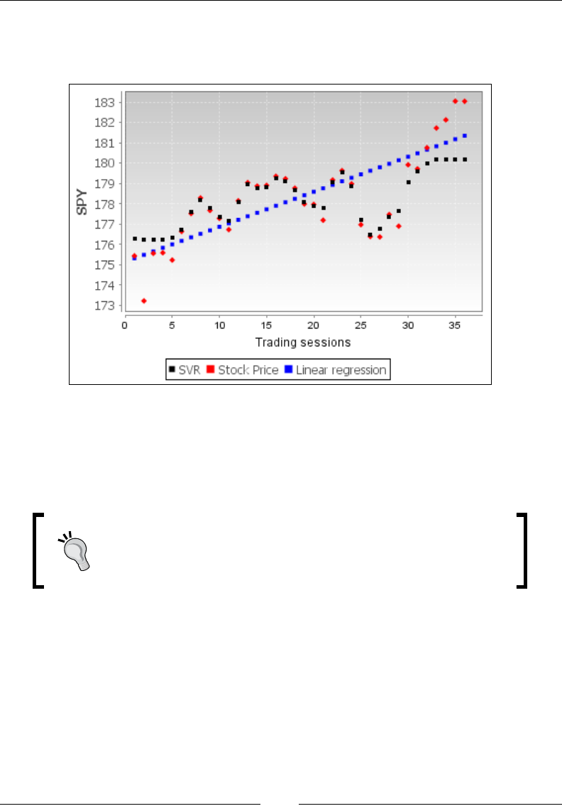
Chapter 8
[ 889 ]
The results are displayed in the following graph, generated using the JFreeChart
library. The code to plot the data is omitted because it is not essential to the
understanding of the application.
Comparative plot linear regression and SVR
The support vector regression provides a more accurate prediction than the linear
regression model. You can also observe that the L2 regularization term of the SVR
penalizes the data points (the SPY price) with a high deviation from the mean of
the price. A lower value of C will increase the L2-norm penalty factor as λ =1/C.
SVR and L2 regularization
You are invited to run the use case with a different value of C
to quantify the impact of the L2 regularization on the predictive
values of the SVR.
There is no need to compare SVR with the logistic regression as the logistic
regression is a classier. However, SVM is related to the logistic regression;
the hinge loss in SVM is similar to the loss in the logistic regression [8:15].

Kernel Models and Support Vector Machines
[ 890 ]
Performance considerations
You may have already observed that the training of a support vector regression
model on a large data set is time consuming. The performance of the support
vector machine depends on the type of optimizer (for example, sequential minimal
optimization) selected to maximize the margin during training.
• A linear model (SVM without kernel) has an asymptotic time complexity
O(N) for training N labeled observations.
• Nonlinear models rely on kernel methods formulated as a quadratic
programming problem with an asymptotic time complexity of O(N3)
• An algorithm that uses sequential minimal optimization techniques
such as index caching or elimination of null values (as in LIBSVM), has
an asymptotic time complexity of O(N2) with the worst case scenario
(quadratic optimization) of O(N3)
• Sparse problems for very large training sets (N > 10,000) also have an
asymptotic time of O(N2)
The time and space complexity of the kernelized support vector machine has been
receiving a great deal of attention [8:16] [8:17].
Summary
This concludes our investigation of kernel and support vector machines. Support
vector machines have become a robust alternative to logistic regression and neural
networks for extracting discriminative models from large training sets.
Apart from the unavoidable references to the mathematical foundation of maximum
margin classiers such as SVM, you should have developed a basic understanding
of the power and complexity of the tuning and conguration parameters of the
different variants of SVM.
As with other discriminative models, the selection of the optimization method for
SVMs has a critical impact not only on the quality of the model, but also on the
performance (time complexity) of the training and cross-validation process.
The next chapter will describe the third most commonly used discriminative
supervised model—articial neural networks.

Articial Neural Networks
The popularity of neural networks surged in the 90s. They were seen as the silver
bullet to a vast number of problems. At its core, a neural network is a nonlinear
statistical model that leverages the logistic regression to create a nonlinear distributed
model. The concept of articial neural networks is rooted in biology, with the desire
to simulate key functions of the brain and replicate its structure in terms of neurons,
activation, and synapses.
In this chapter, you will move beyond the hype and learn:
• The concept and elements of the multilayer perceptron (MLP)
• How to train a neural network using error backpropagation
• The evaluation and tuning of MLP conguration parameters
• Full Scala implementation of the MLP classier
• How to apply MLP to extract correlation models for currency exchange rates
Feed-forward neural networks (FFNN)
The idea behind articial neural networks was to build mathematical and
computational models of the natural neural network in the brain. After all, the brain is
a very powerful information processing engine that surpasses computers in domains
such as learning, inductive reasoning, prediction and vision, and speech recognition.
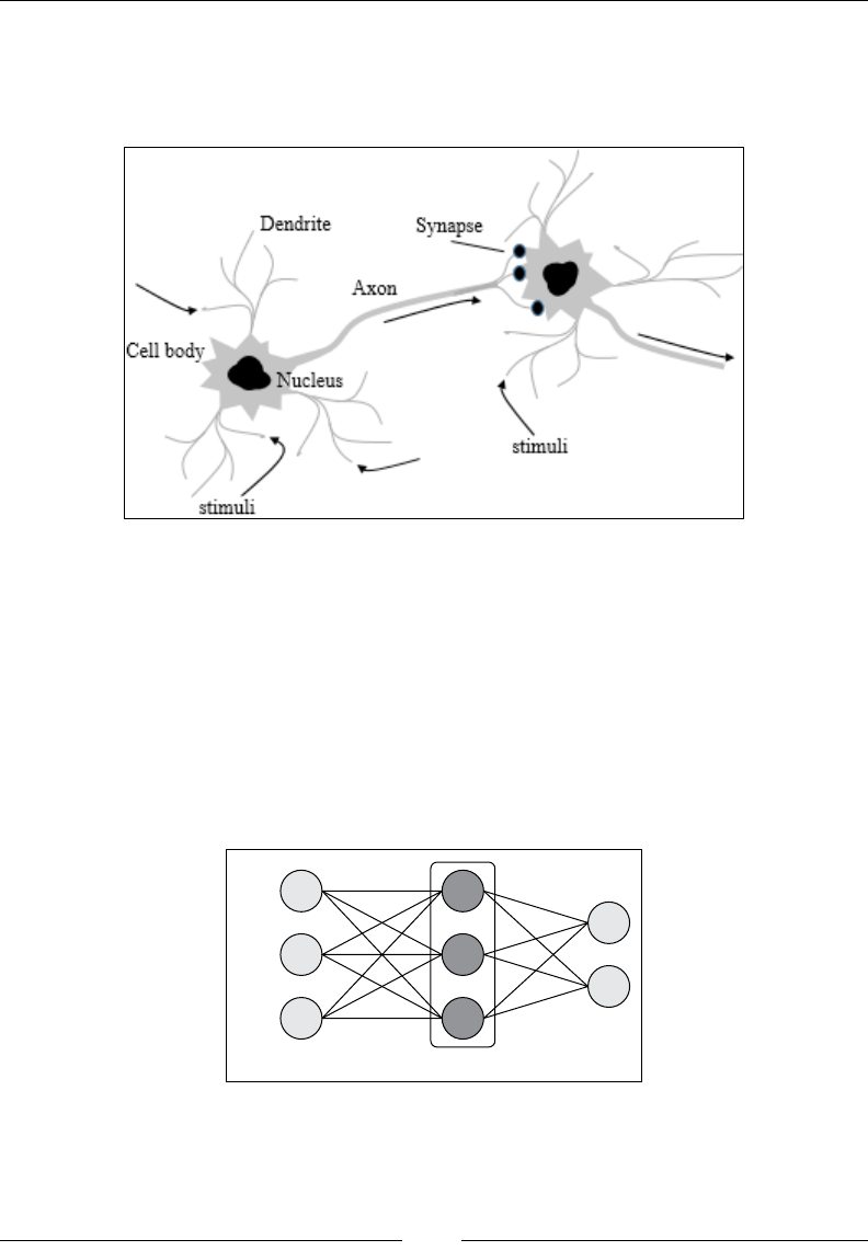
Articial Neural Networks
[ 892 ]
The Biological background
In biology, a neural network is composed of groups of neurons interconnected
though synapses [9:1], as shown in the following image:
Neuroscientists have been especially interested in understanding how the billions of
neurons in the brain can interact to provide human beings with parallel processing
capabilities. The 60s saw a new eld of study emerging, known as connectionism.
Connectionism marries cognitive psychology, articial intelligence, and neuroscience.
The goal was to create a model for mental phenomena. Although there are many forms
of connectionism, the neural network models have become the most popular and the
most taught of all connectionism models [9:2].
Biological neurons communicate through electrical charges known as stimuli.
This network of neurons can be represented as a simple schematic, as follows:
Connection
Neuron
layer
Synapse

Chapter 9
[ 893 ]
This representation categorizes groups of neurons as layers. The terminology used
to describe the natural neural networks has a corresponding nomenclature for the
articial neural network.
The biological neural network The artificial neuron network
Axon Connection
Dendrite Connection
Synapse Weight
Potential Weighted sum
Threshold Bias weight
Signal, Stimulus Activation
Group of neurons Layer of neurons
In the biological world, stimuli do not propagate in any specic direction
between neurons. An articial neural network can have the same degree of
freedom. The articial neural networks most commonly used by data scientists,
have a predened direction: from the input layer to output layers. These neural
networks are known as FFNN.
The mathematical background
In the previous chapter, you learned that support vector machines have the ability to
formulate the training of a model as a nonlinear optimization for which the objective
function is convex. A convex objective function is fairly straightforward to implement.
The drawback is that the kernelization of the SVM may result in a large number of
basis functions (or model dimensions). Refer to the The Kernel trick section under The
support vector machine (SVM) in Chapter 8, Kernel Models and Support Vector Machines.
One solution is to reduce the number of basis functions through parameterization, so
these functions can adapt to different training sets. Such an approach can be modeled
as a FFNN, known as the multilayer perceptron [9:3].
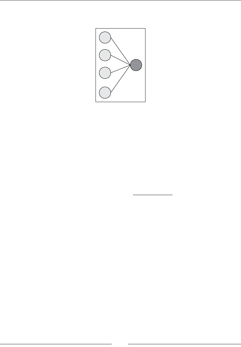
Articial Neural Networks
[ 894 ]
The linear regression can be visualized as a simple connectivity model using neurons
and synapses, as follows:
.
.
.
+1
X1
X2
Xn
W0
W1
W2
Wn
Y
A two-layer neural network
The feature x0=+1 is known as the bias input (or bias element), which corresponds to
the intercept in the classic linear regression.
As with support vector machines, linear regression is appropriate for observations
that can be linearly separable. The real world is usually driven by a nonlinear
phenomena. Therefore, the logistic regression is naturally used to compute the
output of the perceptron. For a set of input variable x = {xi}0,n and the weights
w={wi}1,n, the output y is computed as:
()
()
0
0
1
1
T
T
wwx
ywwx
e
σ
−+
=+=
+
An FFNN can be regarded as a stack of layers of logistic regression with the output
layer as a linear regression.
The value of the variables in each hidden layer is computed as the sigmoid of the dot
product of the connection weights and the output of the previous layer. Although
interesting, the theory behind articial neural networks is beyond the scope of this
book [9:4].
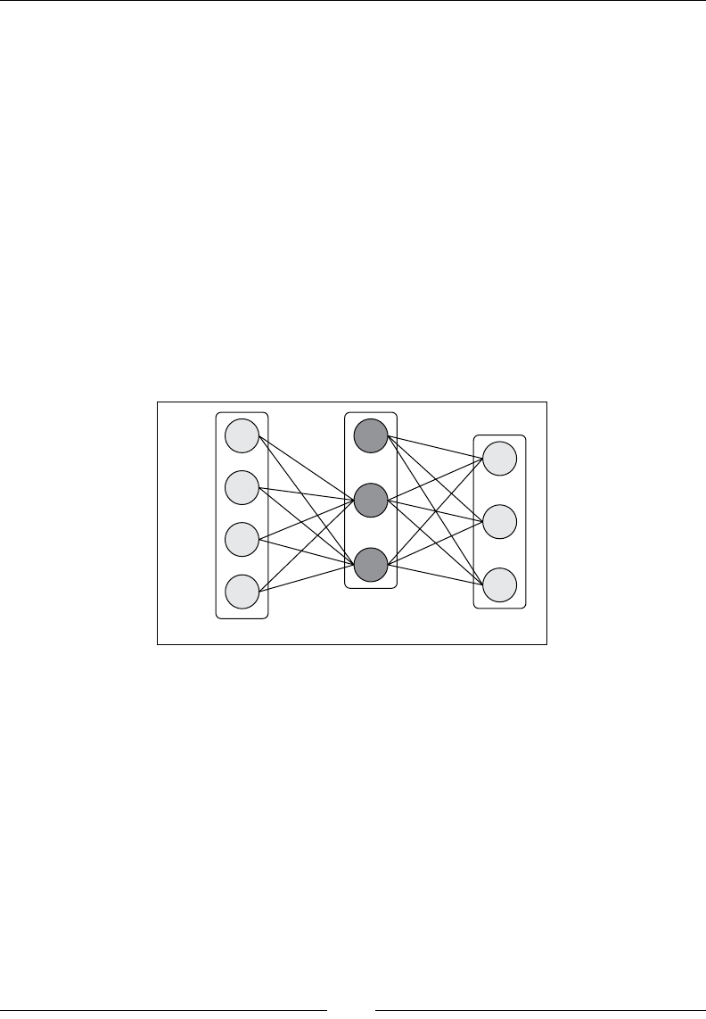
Chapter 9
[ 895 ]
The multilayer perceptron (MLP)
The perceptron is a basic processing element that performs binary classication by
mapping a scalar or vector to a binary (or XOR) value {true, false} or {-1, +1}. The
original perceptron algorithm was dened as a single layer of neurons for which each
value xi of the feature vector is processed in parallel and generates a single output y.
The perceptron was later extended to encompass the concept of an activation function.
The single layer perceptrons are limited to process a single linear combination
of weights and input values. Scientists found out that adding intermediate
layers between the input and output layers enable them to solve more complex
classication problems. These intermediate layers are known as hidden layers
because they interface only with other perceptrons. Hidden nodes can be accessed
only through the input layer.
From now on, we will use a three-layered perceptron to investigate and illustrate the
properties of neural networks, as shown here:
+1
z1
zm
+1
X1
X2
Xn
.
.
.
.
.
..
.
.
Input layer
Hidden layer
Output layer
y0
y1
yp
wij
vij
Synapse
Bias
Neuron
A three-layered perceptron
The three-layered perceptron requires two sets of weights: wij to process the output
of the input layer to the hidden layer and vij between the hidden layer and the output
layer. The intercept value w0, in both linear and logistic regression, is represented
with +1 in the visualization of the neural network (w0.1 + w1.x1+w2.x2+ …).
Articial Neural Networks
[ 896 ]
FFNN with no hidden layer
A FFNN without a hidden layer is similar to a linear statistical
model. The only transformation or connection between the
input and output layer is actually a linear regression. A linear
regression is a more efcient alternative to the FFNN without
a hidden layer.
The description of the MLP components and their implementations rely on the
following stages:
1. Overview of the software design.
2. Description of the MLP model components.
3. Implementation of the four-step training cycle.
4. Denition and implementation of the training strategy and the
resulting classier.
Terminology
Articial neural networks encompass a large variety of learning
algorithms, the multilayer perceptron being one of them. Perceptrons
are indeed components of a neural network organized as input,
output, and hidden layers. This chapter is dedicated to the multilayer
perceptron with hidden layers. The terms "neural network" and
"multilayer perceptron" are used interchangeably.
The activation function
The perceptron is represented as a linear combination of weights, wi, and input
values, xi, processed by the output unit activation function h, as shown here:
$
()
0 0
1
n
T
ii
i
yhw wx hw wx
=
⎛⎞
=+ =+
⎜⎟
⎝⎠
∑
The output activation function h has to be continuous and differentiable for a range
of value of the weights. It takes different forms depending on the problems to be
solved, as mentioned here:
• Identity for the output layer of the binary classication or regression problem
• Sigmoid,
σ
, for hidden layers

Chapter 9
[ 897 ]
• Softmax for the multinomial classication
• Hyperbolic tangent, tanh, for classication using zero mean
The Softmax formula is described in the next section.
The network architecture
The output layer and hidden layers have a computational capability (dot product of
weights, inputs, and activation functions). The input layer does not transform data.
An n-layer neural network is a network with n computational layers. Its architecture
consists of the following components:
• 1 input layer
• (n-1) hidden layer
• 1 output layer
A fully connected neural network has all its input nodes connected to hidden layer
neurons. Networks are characterized as partially connected neural networks if one
or more of their input variables are not processed. This chapter deals with a fully
connected neural network.
Partially connected networks
Partially connected networks are not as complex as they seem.
They can be generated from fully connected networks by
setting some of the weights to zero.
The structure of the output layer is highly dependent on the type of problems
(regression or classication) you need to solve, also known as the objective of the
neural network. The type of problem at hand denes the number of output nodes
[9:5], for example:
• A one-variate regression has one output node whose value is a real
number [0, 1]
• A multivariate regression with n variables has n real output nodes
• A binary classication has one binary output node {0, 1} or {-1, +1}
• A multinomial or K-class classication has K binary output nodes
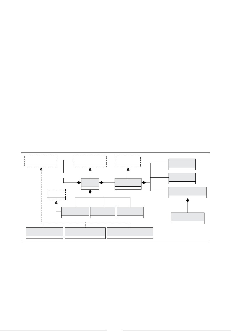
Articial Neural Networks
[ 898 ]
Software design
The implementation of the MLP classier follows the same pattern as previous
classiers (refer to the Design template for classiers section in Appendix A, Basic Concepts):
• A model MLPModel of the type Model is initialized through training
during the initialization of the classier. The model is composed of a
layer of neurons of the type MLPLayer, connected by synapses of the
type MLPSynapse contained by a connector of the type MLPConnection.
• All of the conguration parameters are encapsulated into a single
conguration class, MLPConfig.
• The predictive or classication routine is implemented as a data
transformation, extending the PipeOperator trait.
• The multilayer perceptron class, MLP, takes three parameters: conguration
instance, a features set or time series of the XTSeries class, and a labeled
dataset of the type DblMatrix.
The software components of the multilayer perceptron are described in the following
UML class diagram:
MLPObjective PipeOperator Model Array[Int]
MLPRegression MLPBinClassifier MLPMultiClassifier
MLPSynapse
MLPConnection
MLPLayer
Config
MLPConfig XTSeries DblMatrix
MLP MLPModel
topology
layers
connections
synapses
model
config xt labels
objective
1
111
11
1
1
1+
1
1+
1+
A UML class diagram for the multilayer perceptron
The class diagram is a convenient navigation map to understand the role and relation
of the Scala classes used to build an MLP. Let's start with the implementation of the
MLP model and its components.

Chapter 9
[ 899 ]
Model denition
The purpose of the model is to completely dene the network architecture. It is
implemented by the MLPModel parameterized class, which is responsible for creating
and managing the different components of the network, layers, and connections as
well as the topology.
Let's establish a simple naming convention for the layers of neurons as follows:
• The input layer, inLayer, consists of nInputs neurons
• A hidden layer, hidLayer, has nHiddens neurons
• The output layer, outLayer, has nOutputs neurons
The instantiation of the class requires a minimum set of three parameters:
class MLPModel[T <% Double](config: MLPConfig, nInputs: Int, nOutputs:
Int) extends Model {
val layers: Array[MLPLayer]
val connections: Array[MLPConnection]
val topology: Array[Int]
}
Besides the config conguration, the model class has two parameters: the number
of input features, {x}, nInputs; and the number of output values, {y}, nOutputs.
These three parameters are all you need to initialize the topology of the network.
A model has the following attributes:
• Multiple layers of the type MLPLayers
• Multiple connections of the type MLPConnection
• A topology array that wires these layers and connections
The topology is dened as an array of number of nodes per layer, starting with the
input nodes. The array indices follow the forward path within the network. The size
of the input layer is automatically generated from the observations as the size of the
features vector. The size of the output layer is automatically extracted from the size
of the output vector:
val topology = Array[Int](nInputs) ++ config.hidLayers ++
Array[Int](nOutputs)
The sequence of hidden layers, hidLayers, is dened as an array of number of
neurons (or nodes) per hidden layers:
val hidLayers: Array[Int]
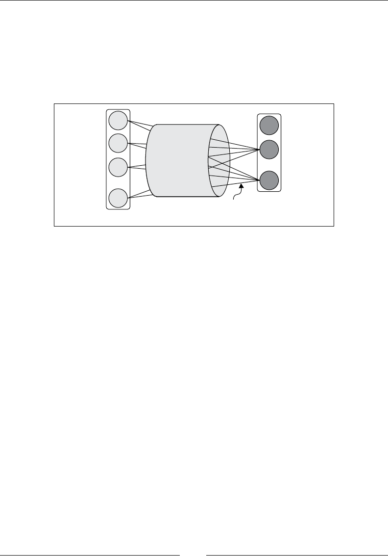
Articial Neural Networks
[ 900 ]
This is an attribute of the MLPConfiguration class described in the next section.
For instance, the topology of a neural network with three input variables, one
output variable, and two hidden layers of three neurons each is specied as
Array[Int](4, 3, 3, 1).
The following diagram visualizes the interaction between the different components
of a model: MLPLayer, MLPConnection, and MLPSynapse:
MLPConnection
Bias element
MLPLayer
source
Bias element
MLPLayer
destination
+1
x1
x
2
xn
+1
z1
zm
.
.
.
.
.
.
MLPSynapse
(w (w ))
ij ij
D
Components of the MLP model
Layers
First, let's start with the denition of the layer class, MLPLayer, which is completely
specied by its position in the network and the number of nodes it contains:
class MLPLayer(val id: Int, val len: Int) {
val output = new DblVector(len) //1
val delta = new DblVector(len) //2
...output.update(0, 1.0) //3
The id parameter is the order of the layer (0 for input, 1 for the rst hidden
layer,…, n-1 for the output layer) in the network. The len value is the number of
elements or nodes, including the bias element, in this layer. The output vector for
the layer (line 1) is an uninitialized vector of values updated during the forward
propagation, except for the rst value (bias element), which is set to 1 (line 3). The
delta vector associated to the output vector (line 2) is updated through the error
backpropagation algorithm, described in the next section.
The output values, except the bias element, is initialized using the set method:
def set(x: DblVector): Unit = x.copyToArray(output,1)

Chapter 9
[ 901 ]
Synapses
A synapse is dened as a pair of real values:
• The weight of the connection from the neuron i of the previous layer to the
neuron j, wij
• The weights adjustment (or gradient of weights),
∆
wij
Its type is dened as MLPSynapse, as shown here:
type MLPSynapse = (Double, Double)
Connections
A connection between two consecutive layers implements the matrix of synapses, the
(wij,
∆
wij) pairs. The MLPConnection instance is created with the following parameters:
• Conguration parameters, config
• The source layer, sometimes known as the ingress layer, src
• The destination (or egress) layer, dst
The MLPConnection class is dened as follows:
class MLPConnection(config: MLPConfig, src: MLPLayer, dst: MLPLayer)
The last step in the initialization of the MLP algorithm is the selection of the initial
(usually random) values of the weights (synapse). The following code snippet
initializes the weights for non-bias neurons as random values in the range [0, beta]
with beta <= 1.0.
The weight for the bias is obviously dened as w0=+1, and its weight adjustment is
initialized as
∆
w0 = 0, as shown here:
Val beta = 0.1
val synapses = Array.tabulate(dst.len)(n =>
if(n > 0) Array.fill(src.len)((beta*Random.nextDouble, 0.0))
else Array.fill(src.len)((1.0, 0.0))
)
Random initialization of weights
The range [0, beta] of initial random values is domain specic. Some
problems require a very small range, less than 1e-3, while others use the
probability space [0, 1]. The initial values impact the number of epochs
required to converge toward an optimal set of weights. [9:6]
Articial Neural Networks
[ 902 ]
Once the topology, synapses, layers, and connections of the MLP algorithm are
dened, the initialization of the MLPModel model is straightforward:
val layers = topology.zipWithIndex
.map(t => MLPLayer(t._2, t._1+1))
val connections = Range(0, layers.size-1).map(n =>
new MLPConnection(config, layers(n), layers(n+1))).toArray
The layers are created by traversing the network topology and instantiating each
layer with its proper index and number of elements. The connections are instantiated
by selecting two consecutive layers of index n (with respect to n+1) as source (with
respect to destination).
Encapsulation and the model factory
The model components: connections, layers, and synapses are
implemented as top-level classes for clarity sake. However, there is
no need for the model to expose its inner workings to the client code.
These components should be declared as an inner class to the model.
Moreover, the model is responsible for creating its topology. A factory
design pattern would be perfectly appropriate to instantiate an
MLPModel instance dynamically [9:7].
Once initialized, the MLP model is ready to be trained using a combination of
forward propagation, output error back propagation, and iterative adjustment
of weights and gradients of weights.
Training cycle/epoch
The training of the model processes the training observations multiple times.
A training cycle or iteration is known as an epoch. The ve steps of the training
cycle are as follows:
1. Forward propagation of the input value for a specic epoch.
2. Compute the sum of squared errors.
3. Backpropagation of the output error.
4. Recomputation of the synapse weight and gradient of weight.
5. Evaluate the convergence criteria and exit if criteria is met
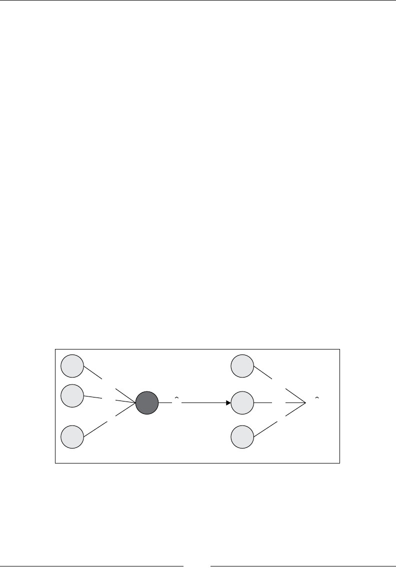
Chapter 9
[ 903 ]
The computation of the network weights during training could use the difference
between labeled data and actual output for each layer. But this solution is not feasible,
because the output of the hidden layers is unknown. The solution is to propagate the
error on the output values backward through the hidden layers. This approach is not
that different than the beta (or backward) pass in the hidden Markov model, covered
in the Beta class (the backward variable) section in Chapter 7, Sequential Data Models.
The error at the output layer for p neurons can be computed in either of the
following ways:
• Sum of the squared of errors (SSE): Calculated for each output, yk
• Mean squared error (MSE): Calculated as MSE= SSE/p
We select the sum of the squared errors to initialize the error back-propagation
algorithm.
Step 1 – input forward propagation
As mentioned earlier, the output values of a hidden layer are computed as a logistic
function (the activation function) of the dot product of the weights wij and the input
values xi.
In the following diagram, the MLP algorithm computes the linear product of the
weights wij and input xi for the hidden layer. The product is then processed by the
activation function
σ
(sigmoid or hyperbolic tangent). The output values zj are then
combined with the weights vij of the output layer. The output layer doesn't have an
activation function.
Predicted Predicted
Hidden layer Output layer
s
+1
x1
xn
+1
zj
zm
Zj
...
.. ...
W0j
W1j
Wnj
V0k
Yk
Vjk
Wmk
The mathematical formulation of the output of a neuron j is dened as a composition
of the activation function and the dot product of the weights wij and input values xi.
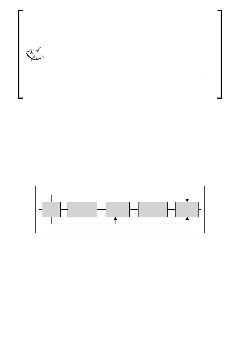
Articial Neural Networks
[ 904 ]
Computation of the output y for the output layer:
$
0
1
m
kj j
k
j
yv vz
=
=+
∑
Estimation of the output values for binary classication with
an activation function
σ
:
01
0
1
1
1
n
ij i
i
n
jij iwwx
i
zwwx
e
σ
=
−−
=
⎛ ⎞
=+ =
⎜ ⎟ ∑
⎝ ⎠
+
∑
$
As seen in the network architecture section, the output values for the multinomial
(or multiclass) classication with more than two classes are normalized using an
exponential function (softmax).
The computational model
The computation of the output values y from the input x is known as the input
forward propagation. For the sake of simplicity, we represent the forward propagation
between layers with the following block diagram. Such a representation will be quite
convenient for the design and implementation of the MLP.
forwardPropagation
Input
x1:n
Connection
wij
Hidden
z1:m
Connection
vij
Output
y1:p
connectionForwardPropagation
A computation model of input forward propagation
This diagram illustrates a computational model for the input forward propagation,
as the programmatic relation between the source and destination layers and their
connectivity. The input x is propagated forward through each connection.
The connectionForwardPropagation method computes the dot product of the
weights and the input values, and applies the activation function in the case of hidden
layers, for each connection. Therefore, it is a member of the MLPConnection class.
The forward propagation of input values across the entire network is managed by
the MLP algorithm itself.

Chapter 9
[ 905 ]
The forward propagation of the input value is used in the classication or
prediction y =f(x). It depends on the value weights wij and vij that need to be
estimated through training. As you may have guessed, the weights dene the
model of a neural network similar to the regression models. Let's look at the
connectionForwardPropagation method of the MLPConnection class:
def connectionForwardPropagation: Unit = {
val synps= synapses.drop(1)
val _output = synps.map(x => { //1
val sum = x.zip(src.output)
.foldLeft(0.0)((s, xy) => s + xy._1._1*xy._2)
if(!isOutLayer) config.activation(sum) //2
else sum
})
val out = if(isOutLayer) mlpObjective(_output) else _output //3
out.copyToArray(dst.output, 1)
}
The rst step is to compute the linear dot product of the _output output of
the current source layer, src, for this connection, and the weights, w (line 1).
The activation method, the implementation of which is described in the next
paragraph, is applied to the dot product, dot (line 2). If the destination layer of the
connection is the output layer, then the output values are processed according to the
mlpObjective objective of the algorithm (line 3).
Objective
In the The network architecture section, you learned that the structure of the output
layer depends on the type of problems that need to be resolved, or objective of the
algorithm. Let's encapsulate the different objectives (binary, multiclass classiers,
and regression) into an MLPObjective hierarchy (nested in MLP companion object)
and the transformation of the output values, y, using a simple apply method:
trait MLPObjective { def apply(y: DblVector): DblVector }
The output of the apply method is used to compute the sum of squared errors
during training, after the forward propagation of features. The binary (2 class)
classier requires a single output without any transformation because the values
are either 0 or 1.
class MLPBinClassifier extends MLPObjective {
override def apply(y: DblVector): DblVector = output
}

Articial Neural Networks
[ 906 ]
The MLPMultiClassifier multiclass classier objective class used the softmax
method to boost the output with the highest value, as shown here:
class MLPMultiClassifier extends MLPObjective {
override def apply(y:DblVector):DblVector = softmax(y.drop(1))
def softmax(y: DblVector): DblVector = { …}
}
The softmax method is applied to the actual output value, not the bias. Therefore,
the rst node y(0)=+1 has to be dropped before applying the softmax normalization.
Softmax
In case of a classication problem with K classes (K > 2), the output has to be
converted into a probability [0, 1]. For problems that require a large number of
classes, there is a need to boost the output yk with the highest value (or probability).
This process is known as the exponential normalization or softmax [9:8].
Softmax formula for multinomial (K > 2) classication is as follows:
$
$
$
k
i
y
ky
i
e
y
e
−
−
=∑
Here is the simple implementation of the softmax method of the
MLPMultiClassifier class:
def softmax(y: DblVector): DblVector = {
val softmaxValues = new DblVector(y.size)
val expY = y.map( Math.exp(_))//1
val expYSum = expY.sum
expY.map( _ /expYSum).copyToArray(softmaxValues, 1) //2
softmaxValues
}
First, the output values are transformed to exponential, expY (line 1). The exponentially
transformed outputs are then normalized by their sum, expYSum, to generate the array
of softmaxValues output (line 2). Once again, you do not have to update the bias
element y(0).
The second step in the training phase is the back propagation of the output error.

Chapter 9
[ 907 ]
Step 2 – sum of squared errors
Once the input features are propagated across the neural network, the sum of
squared errors, sse, for the output layer of the MPLayer type is computed at
each epoch, as follows:
def sse(labels: DblVector): Double = {
var _sse = 0.0
output.drop(1) //1
.zipWithIndex
.foreach(on => {
val err = labels(on._2) - on._1 //2
delta.update(on._2+1, on._1* (1.0- on._1)*err) //3
_sse += err*err
})
_sse*0.5 //4
}
As expected, the computation of the sum of squared errors requires the labeled
values, labels, and the objective method as arguments. The vector output values,
output, stripped of the bias node (line 1) is used to compute the difference, err,
between the label and the actual output (line 2). The delta value (line 3), described
in the next section, is used in the back-propagation algorithm to adjust the weights
of the output and hidden layers. Note that the sum of squares, _sse, is divided by 2
(line 4), so its derivative is err.
Step 3 – error backpropagation
The error backpropagation is an algorithm that estimates the error for the hidden
layer in order to compute the change in weights of the network. It takes the sum of
squared errors on the output as input.
Terminology
Some authors refer to the backpropagation as a training methodology
for an MLP, which applies the gradient descent to the output error
dened as either the sum of squared errors, or the mean squared error.
In this chapter, we keep the narrower denition of backpropagation as
the backward computation of the sum of squared errors.
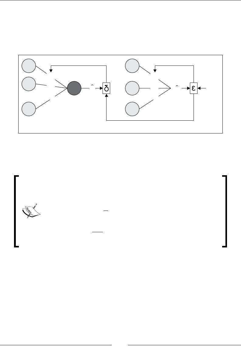
Articial Neural Networks
[ 908 ]
Error propagation
The objective of the training of a perceptron is to minimize the sum of squared
errors at the output layer. The error
k
ε
for each output neuron, yk, is computed as the
difference between a predicted output value and label output value. This approach
does not work for the hidden layers zj because the label value is unknown.
Predicted Predicted
Hidden layer Output layer
s
+1
x1
xn
+1
zj
zm
Zj
...
W0j
W1j
Wnj
V0k
yk
Vjk
Vmk
...
yk
Dwij Dvjk
Expected
The partial derivative of the sum of squared output error over each weight of the
output layer is computed as the composition of the derivative of the square function,
and the derivative of the dot product of weights and the input z.
Derivative of the output SSE over the weighs of the output layer:
0
2
1
1
ˆ
1
2
T
kkkk
p
k
k
m
jk
j
k
yy yv
vz
z
v
ε
εε
εε
=
=
=−=− −
=
∂=−
∂
∑
∑
As mentioned earlier, the computation of the partial derivative of the sum of squared
error over the weights of the hidden layer is a bit tricky. Fortunately, the partial
derivative can be broken down into the following three pieces using the output layer
values and the output of the hidden layer:
• Derivative of sum of squared error
ε
over the output value yk
• Derivative of the output value yk over the hidden value zj knowing that the
derivative of a sigmoid
σ
is
σ
(1 -
σ
)
• Derivative of the output of the hidden layer zj over the weights wij
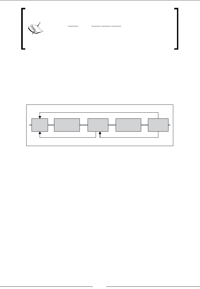
Chapter 9
[ 909 ]
Derivative of error over the weights of the hidden layer:
()
1 1
1
p p
j
k
jj
k k
ij kj ij
jkj j
z
yx
wyzw
zz
εε δ
δε
= =
∂
∂
∂∂
= = −
∂∂∂∂
=−
∑∑
The computational model
The computational model for the error backpropagation algorithm is very similar to
the forward propagation of the input. The main difference is that the propagation
of the derivative delta
δ
is performed from the output layer to the input layer. The
following diagram illustrates the computational model of the backpropagation in the
case of two hidden layers zs and zt:
backPropagation
Connection
wt
ij
Hidden
zt
1:m t
j
d
Connection
vjk
Output
y1:p e
connectionBackPropagation
Hidden
zs
1:m s
j
d
The connectionBackPropagation method propagates the error back to the previous
layer. It is a member of the MLPConnection class. The backpropagation of the output
error across the entire network is managed by the MLP class.
It implements the two set of equations where synapses (j)(i)._1 are the weights
wji, dst.delta is the vector of error derivative in the destination or next layer, and
src.delta is the error derivative on the outputs in the source (or antecedent) layer,
as shown here:
def connectionBackpropagation: Unit =
Range(1, src.len).foreach(i => {
val dot = Range(1, dst.len).foldLeft(0.0)((s, j) =>
s + synapses(j)(i)._1*dst.delta(j)) //1
src.delta(i) = src.output(i)*(1.0 - src.output(i))*dot//2
})
The dot product of the synapse weights and the errors of the destination layers
(line 1) is used to compute the delta on the source (or previous layer) layers (line 2).
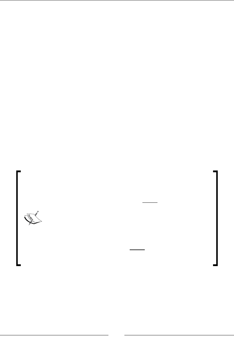
Articial Neural Networks
[ 910 ]
Step 4 – synapse/weights adjustment
The connection weights
∆
v and
∆
w are adjusted by computing the sum of the
derivative of the error, over the weights scaled with a learning factor. The gradient
of weights are then used to compute the error of the output of the source layer [9:9].
Momentum factor for gradient descent
The simplest algorithm to update the weights is the gradient descent [9:10].
The gradient descent is a very simple and robust algorithm. However, it is
slower in converging toward a global minimum than the conjugate gradient or
the quasi-Newton method (refer to the Summary of optimization techniques section
in Appendix A, Basic Concepts).
There are several methods available to speed up the convergence of the gradient
descent toward a minimum: momentum factor and adaptive learning coefcient [9:11].
Large variations of the weights (or large value of the gradient of weights) cause
the gradient descent to require more training iteration in order to converge. This
is particularly true for a training strategy known as online training. The training
strategies are discussed in the next section. The momentum factor
α
is used for
the remaining section of the chapter.
The computation of neural network weights using gradient
descent is as follows:
() ()
()
1
t
tt j
ij ij
ij
ww w
ε
η
+∂
=−∂
The computation of neural network weights using gradient
descent method with momentum coefcient
α
is as follows:
() ()
() ()
1
t
tt j t
ij ij ij
ij
ww w
w
ε
ηα
+∂
=−+∆
∂
The basic gradient descent algorithm is selected by setting the momentum factor
α
to zero.

Chapter 9
[ 911 ]
Implementation
The fourth step of the training phase is to adjust each connection's synapses
(w,
∆
w). This task is performed by the connectionUpdate method of the
MLPConnection class:
def connectionUpdate: Unit =
Range(1, dst.len).foreach(i => {
val delta = dst.delta(i) //1
Range(0, src.len).foreach(j => {
val _output = src.output(j) //2
val oldSynapse = synapses(i)(j)
val grad = config.eta*delta*_output //3
val deltaWeight = grad + config.alpha* oldSynapse._2 //4
synapses(i)(j) = (oldSynapse._1 + deltaWeight, grad) //5
})
})
The connectionUpdate method computes the error of each destination neuron (line 1).
The _output output of each neuron source (line 2) is used in the computation of the
grad gradient (line 3). The weight is then adjusted for a momentum (line 4) as per the
mathematical formulation. Finally, the synapses for source and destination layers are
updated (line 5).
The adjustable learning rate
The computation of the new weights of a connection for
each new epoch can be further improved by making the
learning adjustable.
Step 5 – convergence criteria
The convergence criterion consists of evaluating the sum of squared errors against a
predetermined threshold eps. It is common to normalize the sum of squared errors
by the number of observations.
Conguration
The MLPConfig conguration of the multilayer perceptron consists of the denition
of the network conguration with hidden layers, the learning parameters, the
training parameters, and the activation function:
Class MLPConfig(val alpha: Double, val eta: Double, val hidLayers:
Array[Int], val numEpochs: Int,val eps: Double,val activation:
Double=>Double) extends Config

Articial Neural Networks
[ 912 ]
For the sake of readability, the name of the conguration parameters matches the
symbols dened in the mathematical formulation:
• alpha: This is the momentum factor.
• eta: This is the learning rate (xed or adaptive).
• hidLayers: This is an array of size of hidden layers (for example, two hidden
layers of two and four elements are specied as Array[Int](2,4)).
• numEpochs: This is the maximum number of epochs allowed for training the
neural network.
• eps: This is the convergence criteria used as an exit condition for the training
of the neural network, error < eps.
• activation: This is the activation function used for nonlinear regression
applied to hidden layers. The default function is the sigmoid.
Putting all together
The ve steps of the training cycle have been implemented for each connection or
matrix of synapses (weights, gradient of weights). The management of the cycle is
performed by the algorithm dened by the MLP class, as shown here:
class MLP[T <% Double](config: MLPConfig, xt: XTSeries[Array[T]],
labels: DblMatrix)(implicit val mlpObjective: MLP.MLPObjective)
extends PipeOperator[Array[T], DblVector] {
val model: Option[MLPModel]
def |> : PartialFunction[Array[T], DblVector]
}
The MLP algorithm takes the following parameters:
• config: The conguration of the algorithm
• xt: The time series of features used to train the model
• labels: The labeled output values for training purpose
• mlpObjective: The implicit objective of the algorithm (a type of problem)
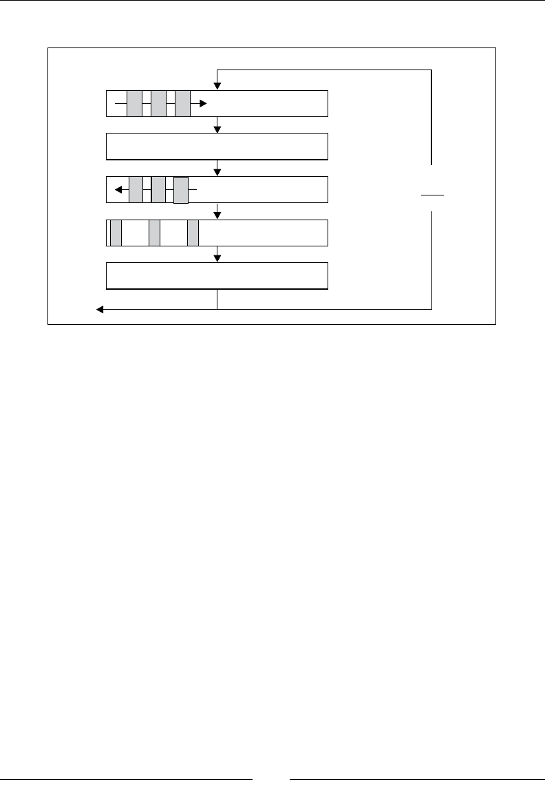
Chapter 9
[ 913 ]
The ve steps of the training cycle or epoch is summarized in the following diagram:
w=w- w+w
() ()
()
()t+1
ij
t
ij ij
t
jt
ij
h
e
aD
sse
if (sse<eps)
Sum of squared errors
Backpropagation
Weights adjustment
Exit condition
dd e
xzyForward propagation
Dwij Dvjk
weights YesNo
epoch t
epoch t+1
6
6
Let's apply the ve steps of a training epoch in a trainEpoch method of the
MLPModel class using a simple the foreach Scala iterator, as shown here:
def trainEpoch(x: DblVector, y: DblVector): Double = {
inLayer.set(x)
connections.foreach( _.connectionForwardPropagation) //1
val _sse = sse(y) //2
val bckIterator = connections.reverseIterator
bckIterator.foreach( _.connectionBackpropagation) //3
connections.foreach( _.connectionUpdate) //4
_sse
}
You can certainly recognize the rst four stages of the training cycle: forward
propagation of the input, x (line 1), computation of the sum of squared errors,
_sse (line 2), the back propagation of the error (line 3), and the recomputation
of the weight and gradient of weight associated with each synapse (line 4).
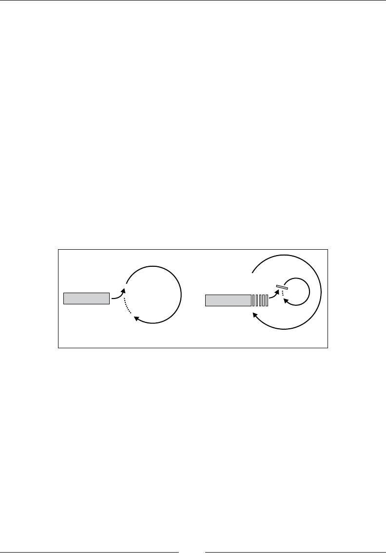
Articial Neural Networks
[ 914 ]
Training strategies and classication
Once the training cycle or epoch is dened, it is merely a matter of dening and
implementing a strategy to create a model using a sequence of data or time series.
Online versus batch training
One important remaining issue is nding a strategy to conduct the training of time
series, as ordered sequences of data. There are two strategies to create an MLP model
for time series:
• Batch training: The entire time series is processed at once as a single input to
the neural network. The weights (synapses) are updated at each epoch using
the sum of squared errors on the output of the time series. The training exits
once the sum of the squared errors meets the convergence criteria.
• Online training: The observations are fed to the neural network one at a time.
Once the time series has been processed, the total of the sum of the squared
error (sse) for the time series for all the observations are computed. If the exit
condition is not met, the observations are reprocessed by the network.
Observations
Time series
Epoch
Batch training Online training
Time series
Exit
condition
Epoch
An illustration on online and batch training
An online training is faster than batch training because the convergence criterion has
to be met for each data point, possibly resulting in a smaller number of epochs [9:12].
Techniques such as the momentum factor, which is described earlier, or any adaptive
learning scheme improve the performance of the online training process further.
The online training strategy is applied to a nancial time series for the remainder of
this chapter.

Chapter 9
[ 915 ]
Regularization
There are two approaches to nd the most appropriate network architecture for a
given classication or regression problem; they are:
• Destructive tuning: Starting with a large network, then removing nodes,
synapses, and hidden layers that have no impact on the sum of squared errors
• Constructive tuning: Starting with a small network, then incrementally adding
the nodes, synapses, and hidden layers that reduce the output error
The destructive tuning strategy removes the synapses by zeroing out their weights.
This is commonly accomplished by using regularization.
You have seen that regularization is a powerful technique to address overtting
in the case of the linear and logistic regression in the The ridge regression section in
Chapter 6, Regression and Regularization. Neural networks can benet from adding a
regularization term to the sum of squared errors. The larger the regularization factor
is, the more likely some weights will be reduced to zero, thus reducing the scale of
the network [9:13].
Model instantiation
The model instance is created (trained) during the instantiation of the multilayer
perceptron. The model is created by iterating the training cycle over all the data
points of the time series xt, and through multiple epochs until the total sum of
squared errors is smaller than the threshold eps, as in the following code:
var converged = false
val model: Option[MLPModel] = {
val _model = new MLPModel(config, xt(0).size, labels(0).size)
(mlpObjective) //1
val errScale = 1.0/(labels(0).size*xt.size) //4
converged = Range(0, config.numEpochs).find( _ => {
xt.toArray.zip(labels)
.foldLeft(0.0)((s, xtlbl) =>
s + _model.trainEpoch(xtlbl._1, xtlbl._2) //2
)*errScale < config.eps //3
}) != None
_model
}

Articial Neural Networks
[ 916 ]
The model is rst initialized (line 1). The rst four stages of the MLP training cycle
are executed by the MLPModel.trainEpoch method described in the previous
section (line 2). The method returns the sum of squared errors for each observation
in the time series. The sum of squared errors for the observations are summed, then
evaluated against the convergence criterion, eps (line 3). The sum of squared errors is
normalized for the size of the time series and the size of the output vector (line 5). The
implementation uses the Scala method, find, to exit from the iterative loop before the
maximum number of epochs, config.numEpochs, is reached.
The exit condition
In this implementation a ag, converged, is set to indicate that the
execution of the training has not converged before the maximum
number of epochs has been reached; however, the model is still
instantiated nevertheless. It allows the client code to evaluate the
pattern of the sum of squared errors in regard to a local minimum.
Once the model is created during the instantiation of the multilayer perceptron, it is
available to predict the class of a new observation.
Prediction
The prediction method of the MLPModel class, getOutput, takes a new observation
(feature vector) as argument and returns the output by using the forward
propagation algorithm:
def getOutput(x: DblVector): DblVector = {
inLayer.set(x)
connections.foreach( _.connectionForwardPropagation)
outLayer.output
}
The classication method is implemented as the data transformation |>. It returns
the predicted value, normalized as a probability if the model was successfully
trained; None, otherwise:
def |> : PartialFunction[Array[T], DblVector] = {
case x: Array[T] if(model!=None && x.size == dimension(xt)) =>
model.get.getOutput(x))
}
Our MLP class is now ready to tackle some classication challenges.

Chapter 9
[ 917 ]
Evaluation
Before applying our multilayer perceptron to understand uctuations in the currency
market exchanges, let's get acquainted with some of the key learning parameters
introduced in the rst section.
Impact of learning rate
The purpose of the rst exercise is to evaluate the impact of the learning rate,
η
, on
the convergence of the training epoch, as measured by the sum of the squared errors
of all output variables. The observations x (with respect to the labeled output, y) are
synthetically generated using several noisy patterns: functions f1, f2, and noise,
as follows:
val noise = () => NOISE_RATIO*Random.nextDouble
val f1 = (x: Double) => x*(1.0 + noise())
val f2 = (x: Double) => x*x*(1.0 + noise())
def vec1(x: Double): DblVector = Array[Double](f1(x), noise(), f2(x),
noise())
def vec2(x: Double): DblVector = Array[Double](noise(), noise())
val x = XTSeries[DblVector](Array.tabulate(TEST_SIZE)(vec1(_)))
val y = XTSeries[DblVector](Array.tabulate(TEST_SIZE)(vec2(_)))
The x and y values are normalized [0, 1]. The test is run with a sample of size
TEST_SIZE data points over a maximum of 250 epochs, a single hidden layer of
ve neurons with no softmax transformation and the following MLP parameters:
val NUM_EPOCHS = 250; val EPS = 1.0e-4
val HIDDENLAYER = Array[Int](5)
val ALPHA = 0.9; val TEST_SIZE = 40
val features = XTSeries.normalize(x).get
val labels = XTSeries.normalize(y).get.toArray
val config = MLPConfig(ALPHA, _eta, SIZE_HIDDEN_LAYER, NUM_EPOCHS,
EPS)
implicit val mlpObjective = new MLP.MLPBinClassifier
val mlp = MLP[Double](config, features, labels)
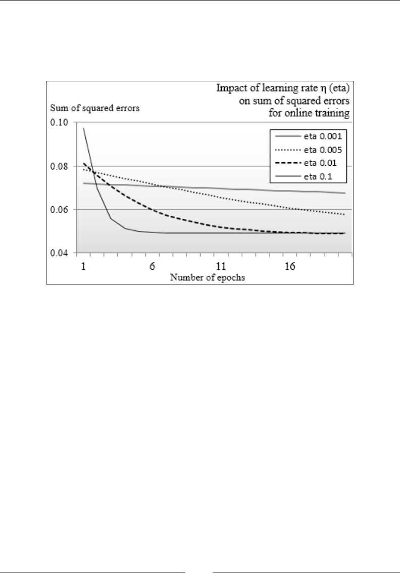
Articial Neural Networks
[ 918 ]
The objective of the algorithm, mlpObjective, has to be implicitly dened prior to
the instantiation of the MLP class.
The test is performed with a different learning rate, eta. For clarity's sake, the graph
displays the sum of squared errors for the rst 22 epochs.
Impact of the learning rate on the MLP training
The chart illustrates that the MLP model training converges a lot faster with a larger
value of learning rate. You need to keep in mind, however, that a very steep learning
rate may lock the training process into a local minimum for the sum of squared
errors generating weights with lesser accuracy. The same conguration parameters
are used to evaluate the impact of the momentum factor on the convergence of the
gradient descent algorithm.
Impact of the momentum factor
Let's quantify the impact of the momentum factor,
α
, on the convergence of the
training process toward an optimal model (synapse weights). The total sum of
squared errors for the entire time series is plotted for the rst ve epochs in the
following graph:
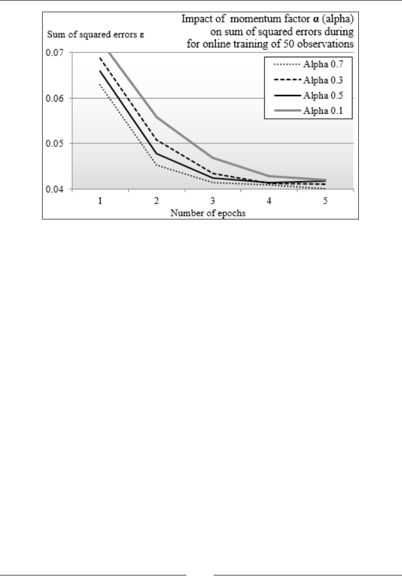
Chapter 9
[ 919 ]
Impact of the momentum factor on the MLP training
The graph shows that the rate the sum of squared errors declines as the momentum
factor increases. In other words, the momentum factor has a positive although limited
impact on the convergence of the gradient descent.
Let's apply our newfound knowledge regarding neural networks and the classication
of variables, that impact the exchange rate of certain currency.
Test case
Neural networks have been used in nancial applications from risk management in
mortgage applications and hedging strategies for commodities pricing, to predictive
modeling of the nancial markets [9:14].
The objective of the test case is to understand the correlation factors between the
exchange rate of some currencies, the spot price of gold and the S&P 500 index.
For this exercise, we will use the following exchange-traded funds (ETFs) as
proxies for exchange rate of currencies:
• FXA: Rate of an Australian dollar in US dollar
• FXB: Rate of a British pound in US dollar
• FXE: Rate of an Euro in US dollar
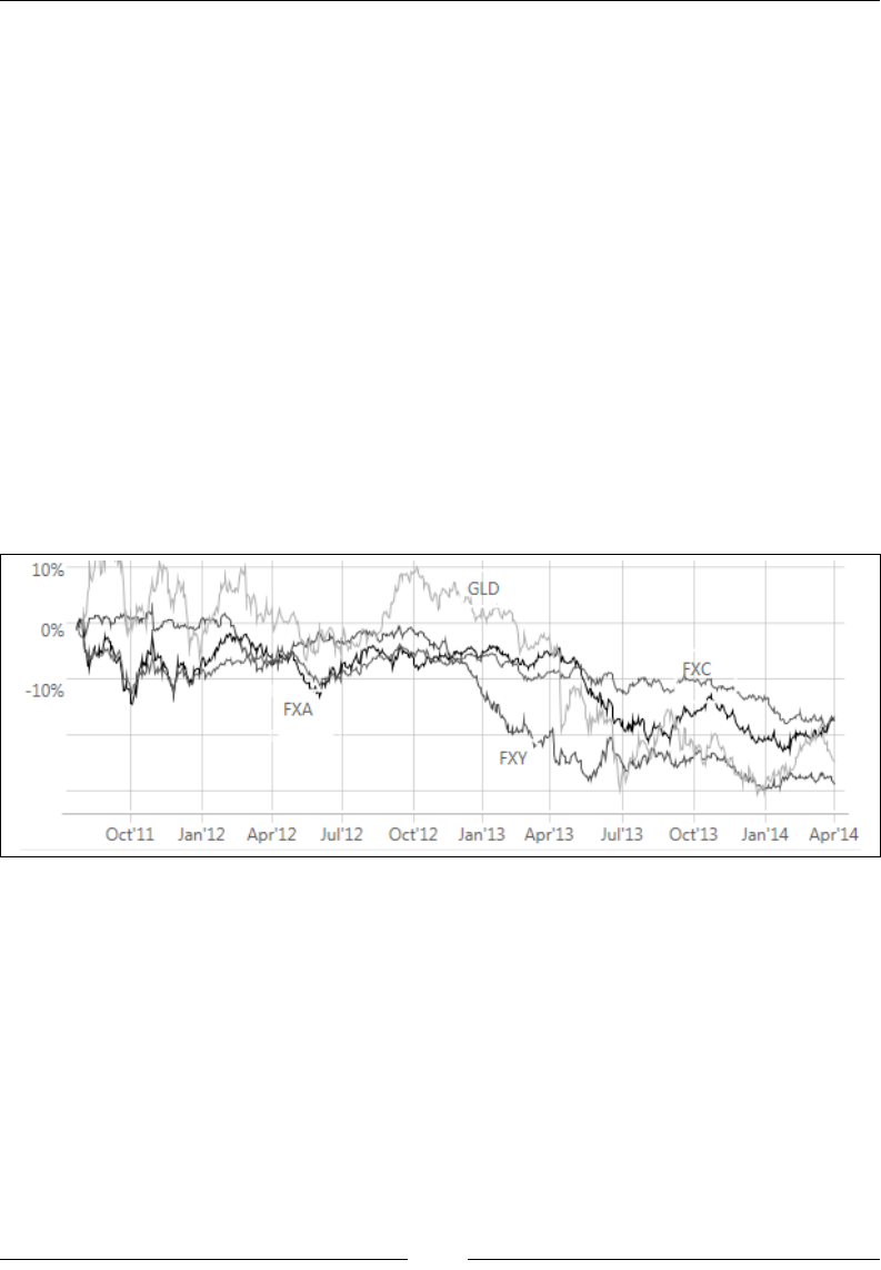
Articial Neural Networks
[ 920 ]
• FXC: Rate of a Canadian dollar in US dollar
• FXF: Rate of a Swiss franc in US dollar
• FXY: Rate of a Japanese yen in US dollar
• CYB: Rate of a Chinese yuan in US dollar
• SPY: S&P 500 index
• GLD: The price of gold in US dollar
Practically, the problem to solve is to extract one or more regressive models that link
one ETFs y with a basket of other ETFs {xi} y=f(xi). For example, is there a relation
between the exchange rate of the Japanese yen (FXY) and a combination of the spot
price for gold (GLD), exchange rate of the Euro in US dollar (FXE) and the exchange
rate of the Australian dollar in US dollar (FXA), and so on? If so, the regression f will
be dened as FXY = f (GLD, FXE, FXA).
The following two charts visualize the uctuation between currencies over
a period of two and a half years. The rst chart displays an initial group of
potentially correlated ETFs:
An example of correlated currency-based ETFs
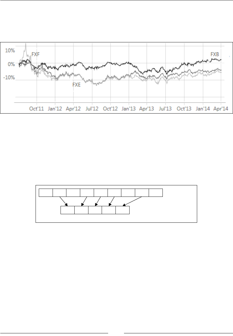
Chapter 9
[ 921 ]
The second chart displays another group of currency-related ETFs that shares
a similar price action behavior. Neural networks do not provide any analytical
representation of their internal reasoning; therefore, a visual correlation can be
extremely useful to novice engineers in validating their models.
An example of correlated currency-based ETFs
A very simple approach for nding any correlation between the movement of the
currency exchange rates and the gold spot price, is to select one ticker symbol as the
target and a subset of other currency-based ETFs as features.
Let's consider the following problem: nding the correlation between the price
of FXE and a range of currencies FXB, CYB, FXA, and FXC, as illustrated in the
following diagram:
Ticker symbols
GLD FXE FXY FXB CYB FXA SPY FXF FXC
FXE FXB CYB FXA FXF
target Features
Indexed study
The mechanism to generate features from ticker symbols
Implementation
The rst step is to dene the conguration parameter for the MLP classier,
is as follows:
val path = "resources/data/chap9/"
val ALPHA = 0.5; val ETA = 0.03
val NUM_EPOCHS = 250; val EPS = 1.0e-6
var hidLayers = Array[Int](7, 7) //1
var config = MLPConfig(ALPHA, ETA, hidLayers, NUM_EPOCHS, EPS)

Articial Neural Networks
[ 922 ]
Besides the learning parameters, the network is initialized with two congurations:
• One hidden layer with four nodes
• Two hidden layers of four neurons each (line 1)
Next, let's create the search space of the prices of all the ETFs used in the analysis:
val symbols = Array[String]("FXE", "FXA", "SPY", "GLD", "FXB", "FXF",
"FXC", "FXY", "CYB") //2
The closing prices of all the ETFs over a period of three years are extracted from the
Google Financial tables, using the GoogleFinancials extractor (line 3) for a basket
of ETFs (line 2):
val prices = symbols.map(s =>DataSource(s"$path$s.csv",true))
.map( _ |> GoogleFinancials.close) //3
.map( _.toArray)
The next step consists of implementing the mechanism to extract the target and the
features from a basket of ETFs, or studies introduced in the previous paragraph. Let's
consider the following study as the list of ETF ticker symbols (line 4):
val study = Array[String]("FXE", "FXF", "FXB", "CYB") //4
The rst element of the study, FXE, is the labeled output; the remaining three
elements are observed features. For this study, the network architecture has three
input variables {FXF, FXB, CYB} and one output variable FXE:
val obs = study.map(s =>index.get(s).get).map( prices( _ )) //5
val features = obs.drop(1).transpose //6
val target = Array[DblVector](obs(0)).transpose //7
The set of observations is built using an index (line 5). By convention, the rst
observation is selected as the label data and the remaining studies as the features for
training. As the observations are loaded as an array of time series, the time features
of series is computed through transpose (line 6). The single output variable,
target, has to be converted into a matrix before transposition (line 7).
Ultimately, the model is built through instantiation of the MLP class:
val THRESHOLD = 0.08
implicit val mlpObjective = new MLP. MLPBinClassifier
val mlp = MLP[Double](config, features, target)
mlp.accuracy(THRESHOLD)

Chapter 9
[ 923 ]
The objective type, mlpObjective, is implicitly dened as an MLP binary classier,
MLPBinClassifier. The square root of the sum of squares of the difference between
the predicted output generated by the MLP and the target value is computed
and compared to a predened threshold. The accuracy value is computed as
the percentage of data points, whose prediction matches the target value within
a range < THRESHOLD:
val nCorrects = xt.toArray.zip(labels).foldLeft(0)((s, xtl) => {
val output = model.get.getOutput(xtl._1) //8
val _sse = xtl._2.zip(output.drop(1))
.foldLeft(0.0)((err,tp) => {
val diff= tp._1 - tp._2
err + diff*diff
}) //9
val error = Math.sqrt(_sse)/(output.size-1) //10
if(error < threshold) s + 1
else s
})
nCorrects.toDouble/xt.size
The implementation of the computation of the accuracy, as in the previous code
snippet, retrieves the values of the output layer (line 8). The error value (line 10)
is computed as the square root of the sum of squared errors, _sse (line 9). Finally, a
prediction is considered correct if it is equal to the labeled output, within the margin
error, threshold.
Models evaluation
The test consists of evaluating six different models to determine which ones provide
the most reliable correlation. It is critical to ensure that the result is somewhat
independent of the architecture of the neural network. Different architectures are
evaluated as part of the test.
The following charts compare the models for two architectures:
• Two hidden layers with four nodes each
• Three hidden layers with eight (with respect to ve and six) nodes
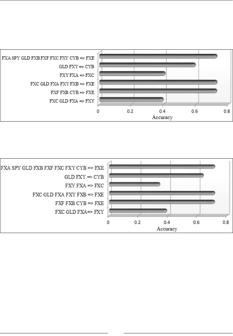
Articial Neural Networks
[ 924 ]
This rst chart visualizes the accuracy of the six regression models with an
architecture consisting of a variable number of inputs [2, 7], one output variable, and
two hidden layers of four nodes each. The features (ETF symbols) are listed on the
left-hand side of the arrow => along the y-axis. The symbol on the right-hand side of
the arrow is the expected output value:
Accuracy of MLP with two hidden layers of four nodes each
The next chart displays the accuracy of the six regression models for an architecture
with three hidden layers of eight, ve, and six nodes, respectively:
Accuracy of MLP with three hidden layers with 8, 5, and 6 nodes, respectively
The two network architectures shared a lot of similarity: in both cases, the most
accurate regression models are as follows:
• FXE = f (FXA, SPY, GLD, FXB, FXF, FXD, FXY, CYB)
• FXE = g (FXC, GLD, FXA, FXY, FXB)
• FXE = h (FXF, FXB, CYB)
On the other hand, the prediction the Canadian dollar to US dollar's exchange rate
(FXC) using the exchange rate for the Japanese yen (FXY) and the Australian dollar
(FXA) is poor with both conguration.
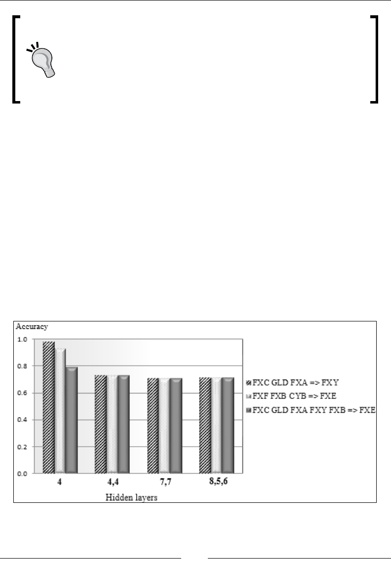
Chapter 9
[ 925 ]
The empirical evaluation
These empirical tests use a simple accuracy metric. A formal
comparison of the regression models would systematically analyze
every combination of input and output variables. The evaluation
would also compute the precision, the recall, and the F1 score for each
of those models (refer to the Key metrics section under Validation in the
Assessing a model section in Chapter 2, Hello World!.
Impact of hidden layers architecture
The next test consists of evaluating the impact of the hidden layer(s) of conguration
on the accuracy of three models: (FXF, FXB, CYB => FXE), (FCX, GLD, FXA =>FXY),
and (FXC, GLD, FXA, FXY, FXB => FXE). For this test, the accuracy is computed by
selecting a subset of the training data as a test sample, for the sake of convenience.
The objective of the test is to compare different network architectures using some
metrics, not to estimate the absolute accuracy of each model.
The four network congurations are as follows:
• A single hidden layer with four nodes
• Two hidden layers with four nodes each
• Two hidden layers with seven nodes each
• Three hidden layer with eight, ve, and six nodes
Impact of hidden layers architecture on the MLP accuracy
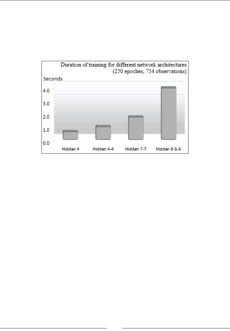
Articial Neural Networks
[ 926 ]
The complex neural network architecture with two or more hidden layers generates
weights with similar accuracy. The four-node single hidden layer architecture
generates the highest accuracy. The computation of the accuracy using a formal
cross-validation technique would generate a lower accuracy number.
Finally, we look at the impact of the complexity of the network on the duration of the
training, as in the following graph:
Impact of hidden layers architecture on duration of training
Not surprisingly, the time complexity increases signicantly with the number of
hidden layers and number of nodes.
Benets and limitations
The advantages and disadvantages of neural networks depend on which other
machine learning methods they are compared to. However, neural-network-based
classiers, particularly the multilayer perceptron using error backpropagation, have
some obvious advantages, such as:
• The mathematical foundation of a neural network does not require expertise
in dynamic programming or linear algebra, beyond the basic gradient
descent algorithm.
• A neural network can perform tasks that a linear algorithm cannot.

Chapter 9
[ 927 ]
• MLP is usually reliable for highly dynamic and nonlinear processes.
Contrary to the support vector machines, they do not require us to
increase the problem dimension through kernelization.
• MLP does not make any assumption on linearity, variable independence,
or normality.
• The execution of training of the MLP lends itself to concurrent processing
quite well for online training. In most architecture, the algorithm can
continue even if a node in the network fails.
However, as with any machine learning algorithm, neural networks have their
detractors. Among the most documented limitations are as follows:
• MLP models are black boxes for which the association between features and
classes may not be easily described.
• MLP requires a lengthy training process, especially using the batch strategy.
For example, a two-layer network has a time complexity (number of
multiplications) of O(n.m.p.N.e) for n input variables, m hidden neurons,
p output values, N observations, and e epochs. It is not uncommon that a
solution emerges after thousands of epochs. The online training strategy
using momentum factor tends to converge faster and require a smaller
number of epochs than the batch process.
• Tuning the conguration parameters, such as learning rate, selection of the
activation method, application of softmax transformation, or momentum
factor, can turn into a lengthy process.
• Estimating the minimum size of the training set to get accurate results is
not obvious.
• A neural network cannot be incrementally retrained. Any new labeled data
requires an entirely new training cycle.

Articial Neural Networks
[ 928 ]
Summary
This concludes not only the journey inside the multilayer perceptron, but also the
introduction of the supervised learning algorithms. In this chapter, you learned:
• The components and architecture of a neural networks
• The stages of the training cycle of a backpropagation multilayer perceptron
• How to implement an MLP from the ground up in Scala
• The numerous conguration parameters and options to use MLP as a
classier and regression
• To evaluate the impact of the learning rate and the gradient descent
momentum factor on the convergence of the sum of squared errors
during training
• How to apply a multilayer perceptron to the nancial analysis of the
uctuation of currencies
The next chapter will introduce the concept of genetic algorithms with a full
implementation in Scala. Although, strictly speaking, genetic algorithms do not
belong to the family of machine learning algorithms, they play a crucial role in the
optimization of nonlinear, nondifferentiable problems and the selection of strong
classiers within ensembles.

Genetic Algorithms
This chapter introduces the concept of evolutionary computing. Algorithms derived
from the theory of evolution are particularly efcient in solving large combinatorial
or NP problems. Evolutionary computing has been pioneered by John Holland
[10:1] and David Goldberg [10:2]. Their ndings should be of interest to anyone
eager to learn about the foundation of genetic algorithms (GA) and articial life.
This chapter covers the following topics:
• The origin of evolutionary computing
• The theoretical foundation of genetic algorithms
• Advantages and limitations of genetic algorithms
From a practical perspective, you will learn how to:
• Apply genetic algorithms to leverage technical analysis of market price and
volume movement to predict future returns
• Evaluate or estimate the search space
• Encode solutions in the binary format using either hierarchical or
at addressing
• Tune some of the genetic operators
• Create and evaluate tness functions
Evolution
The theory of evolution, enunciated by Charles Darwin, describes the morphological
adaptation of living organisms [10:3].

Genetic Algorithms
[ 930 ]
The origin
The Darwinian process consists of optimizing the morphology of organisms to adapt
to the harshest environments—hydrodynamic optimization for shes, aerodynamic
for birds, or stealth skills for predators. The following diagram shows a gene:
The population of organisms varies over time. The number of individuals within
a population changes, sometimes dramatically. These variations are usually
associated with the abundance or lack of predators and prey as well as the changing
environment. Only the ttest organisms within the population can survive over time
by adapting quickly to sudden changes in living environments and new constraints.
NP problems
NP stands for nondeterministic polynomial time. The NP problems concept relates
to the theory of computation and more precisely, time and space complexity. The
categories of NP problems are as follows:
• P-problems (or P decision problems): For these problems, the resolution
on a deterministic Turing machine (computer) takes a deterministic
polynomial time.
• NP problems: These problems can be resolved in a polynomial time on
nondeterministic machines.
• NP-complete problems: These are NP-hard problems that are reduced to NP
problems for which the solution takes a deterministic polynomial time. These
types of problems may be difcult to solve but their solution can be validated.

Chapter 10
[ 931 ]
• NP-hard problems: These problems have solutions that may not be found in
polynomial time.
Computational complexity
NP-hard
NP-complete
NP
P
Problems such as the traveling salesman, oor shop scheduling, the computation of
a graph K-minimum spanning tree, map coloring, or cyclic ordering have a search
execution time that is a nondeterministic polynomial, ranging from n! to 2n for a
population of n elements [10:4].
NP problems cannot always be solved using analytical methods because of the
computation overhead—even in the case of a model, it relies on differentiable
functions. Genetic algorithms were invented by John Holland in the 1970s, and
they derived their properties from the Theory of Evolution of Darwin to tackle
NP and NP-complete problems.
Evolutionary computing
A living organism consists of cells that contain identical chromosomes. Chromosomes
are strands of DNA and serve as a model for the whole organism. A chromosome
consists of genes that are blocks of DNA and encode a specic protein.
Recombination (or crossover) is the rst stage of reproduction. Genes from parents
generate the whole new chromosome (offspring) that can be mutated. During
mutation, one or more elements, also known as individual bases of the DNA strand
or chromosomes, are changed. These changes are mainly caused by errors that occur
when the genes from parents are being passed on to their offspring. The success of an
organism in its life measures its tness [10:5].
Genetic algorithms use reproduction to evolve a solution for a problem that is similar
to unsupervised learning, for which a class or clusters are identied through an
iterative or optimization methodology.

Genetic Algorithms
[ 932 ]
Genetic algorithms and machine learning
The practical purpose of a genetic algorithm as an optimization technique is to solve
problems by nding the most relevant or ttest solution among a set or group of
solutions. Genetic algorithms have many applications in machine learning, as follows:
• Discrete model parameters: Genetic algorithms are particularly effective in
nding the set of discrete parameters that maximizes the log likelihood. For
example, the colorization of a black and white movie relies on a large but
nite set of transformations from shades of grey to the RGB color scheme.
The search space is composed of the different transformations and the
objective function is the quality of the colorized version of the movie.
• Reinforcement learning: Systems that select the most appropriate rules
or policies to match a given data set rely on genetic algorithms to evolve
the set of rules over time. The search space or population is the set of
candidate rules, and the objective function is the credit or reward for an
action triggered by these rules (refer to the Introduction section of Chapter 11,
Reinforcement Learning).
• Neural network architecture: A genetic algorithm drives the evaluation of
different congurations of networks. The search space consists of different
combinations of hidden layers and the size of those layers. The tness or
objective function is the sum of the squared errors.
• Ensemble learning [10:6]: A genetic algorithm can weed out the weak learners
among a set of classiers in order to improve the quality of the prediction.
Genetic algorithm components
Genetic algorithms have the following three components:
• Genetic encoding (and decoding): This is the conversion of a solution
candidate and its components into the binary format (an array of bits
or a string of 0 and 1 characters)
• Genetic operations: This is the application of a set of operators to extract the
best (most genetically t) candidates (chromosomes)
• Genetic tness function: This is the evaluation of the ttest candidate using
an objective function
Encodings and the tness function are problem dependent. Genetic operators are not.
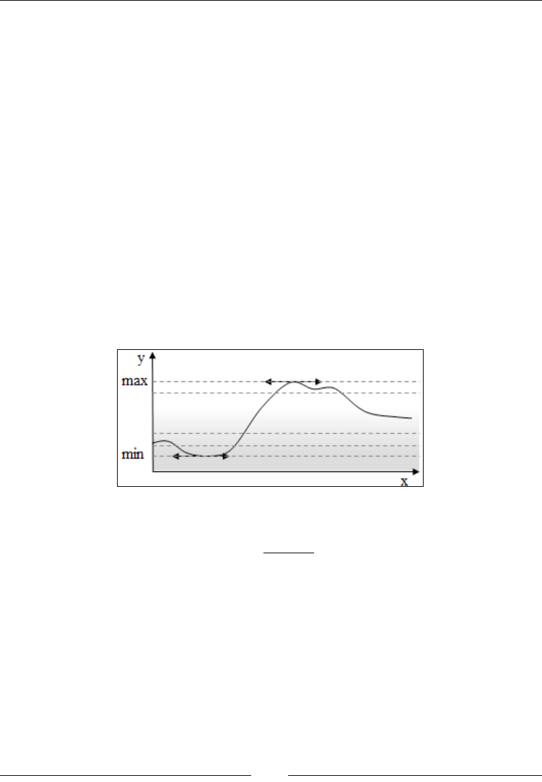
Chapter 10
[ 933 ]
Encodings
Let's consider the optimization problem in machine learning that consists of
maximizing the log likelihood or minimizing the loss function. The goal is to
compute the parameters or weights, w={wi}, that minimize or maximize a function
f(w). In the case of a nonlinear model, variables may depend on other variables,
which make the optimization problem particularly challenging.
Value encoding
The genetic algorithm manipulates variables as bits or bit strings. The conversion
of a variable into a bit string is known as encoding. In the case where the variable is
continuous, the conversion is known as discretization. Each type of variable has a
unique encoding scheme, as follows:
• Boolean values are easily encoded with 1 bit: 0 for false and 1 for true.
• Continuous variables are discretized in a fashion similar to the conversion of
an analog to a digital signal. Let's consider the function with a maximum max
(similarly min for minimum) over a range of values, encoded with n=16 bits:
The step size of the discretization is computed as:
step
max-min
=
2
n
The step size of the discretization of the sine y = sin(x) in 16 bits is 1.524e-5.
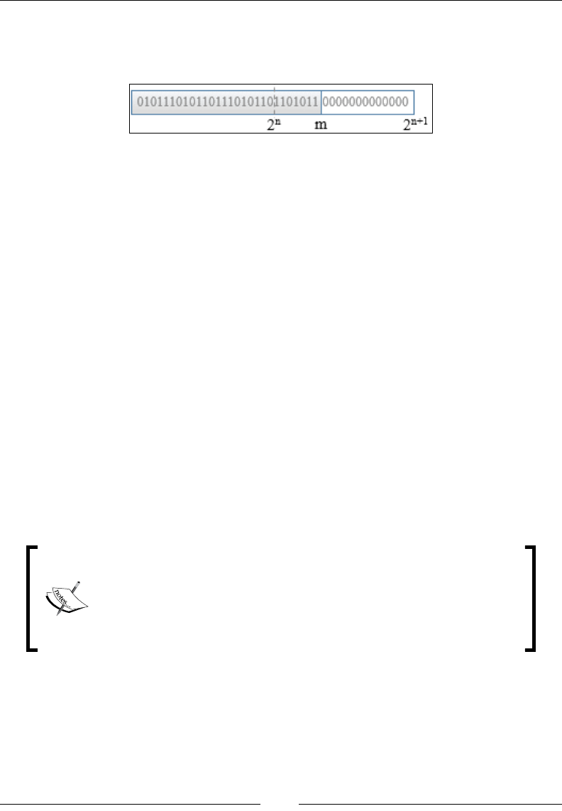
Genetic Algorithms
[ 934 ]
• Discrete or categorical variables are a bit more challenging to encode to bits. At
a minimum, all the discrete values have to be accounted for. However, there is
no guarantee that the number of variables will coincide with the bits boundary:
In this case, the next exponent, n+1, dened the minimum number of bits
required to represent the set of values: n = log2(m).toInt + 1. A discrete
variable with 19 values requires 5 bits. The remaining bits are set to an
arbitrary value (0, NaN,…) depending on the problem. This procedure is
known as padding.
Encoding is as much art as it is science. For each encoding function, you need a
decoding function to convert the bits representation back to actual values.
Predicate encoding
A predicate for a variable x is a relation dened as x operator [target], for instance,
unit cost < [9$], temperature = [82F], or Movie rating is [3 stars].
The simplest encoding scheme for predicates is as follows:
• Variables are encoded as category or type (for example, temperature,
barometric pressure, and so on) because there is a nite number of
variables in any model
• Operators are encoded as discrete type
• Values are encoded as either discrete or continuous values
Encoding format for predicates
There are many approaches for encoding a predicate in a bits
string. For instance, the format {operator, left-operand, right-operand}
is useful because it allows you to encode a binary tree. The entire
rule, IF predicate THEN action, can be encoded with the action being
represented as a discrete or categorical value.
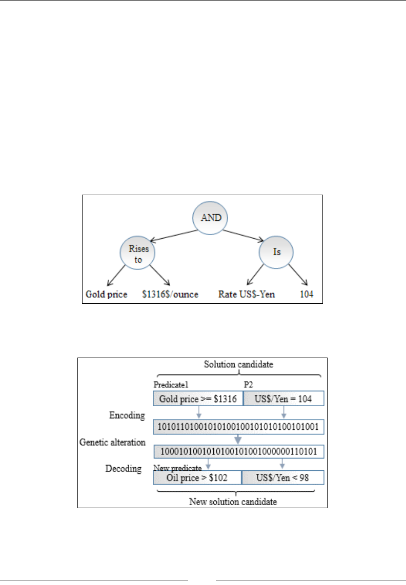
Chapter 10
[ 935 ]
Solution encoding
The solution encoding approach describes the solution to a problem as an unordered
sequence of predicates. Let's consider the following rule:
IF {Gold price rises to [1316$/ounce]} AND
{US$/Yen rate is [104]}).
THEN {S&P 500 index is [UP]}
In this example, the search space is dened by two levels:
• Boolean operators (for example, AND) and predicates
• Each predicate is dened as a tuple {variable, operator, target value}
The tree representation for the search space is shown in the following diagram:
The bits string representation is decoded back to its original format for
further computation:
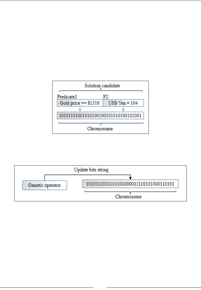
Genetic Algorithms
[ 936 ]
The encoding scheme
There are two approaches to encode such a candidate solution or chain of predicates:
• Flat coding of a chromosome
• Hierarchical coding of a chromosome as a composition of genes
Flat encoding
The at encoding approach consists of encoding the set of predicates into a single
chromosome (bits string) representing a specic solution candidate to the optimization
problem. The identity of the predicates is not preserved:
An overview of flat addressing
A genetic operator manipulates the bits of the chromosome regardless of whether the
bits refer to a particular predicate:
Chromosome encoding with flat addressing
Hierarchical encoding
In this conguration, the characteristic of each predicate is preserved during the
encoding process. Each predicate is converted into a gene represented by a bit string.
The genes are aggregated to form the chromosome. An extra eld is added to the
bits string or chromosome for the selection of the gene. This extra eld consists of the
index or the address of the gene:
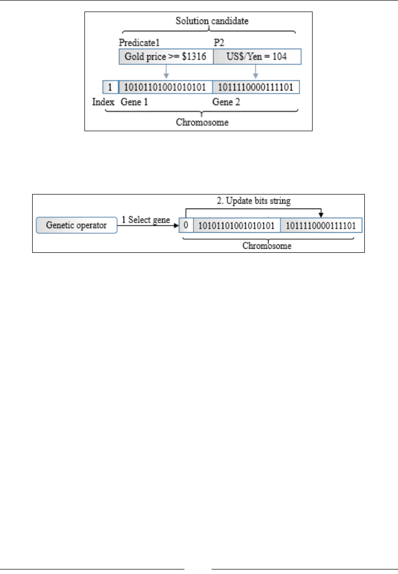
Chapter 10
[ 937 ]
An overview of hierarchical addressing
A generic operator selects the predicate it needs to manipulate rst. Once the target
gene is selected, the operator updates the bits string associated to the gene, as follows:
A chromosome with hierarchical addressing
The next step is to dene the genetic operators that manipulate or update the bits
string representing either a chromosome or individual genes.
Genetic operators
The implementation of the reproduction cycle attempts to replicate the natural
reproduction process [10:7]. The reproduction cycle that controls the population
of chromosomes consists of three genetic operators:
• Selection: This operator ranks chromosomes according to a tness function
or criteria. It eliminates the weakest or less-t chromosomes and controls the
population growth.
• Crossover: This operator pairs chromosomes to generate offspring
chromosomes. These offspring chromosomes are added to the population
along with their parent chromosomes.
• Mutation: This operator introduces minor alteration in the genetic code
(bits string representation) to prevent the successive reproduction cycles
from electing the same ttest chromosome. In optimization terms, this
operator reduces the risk of the genetic algorithm converging quickly
towards a local maximum or minimum.
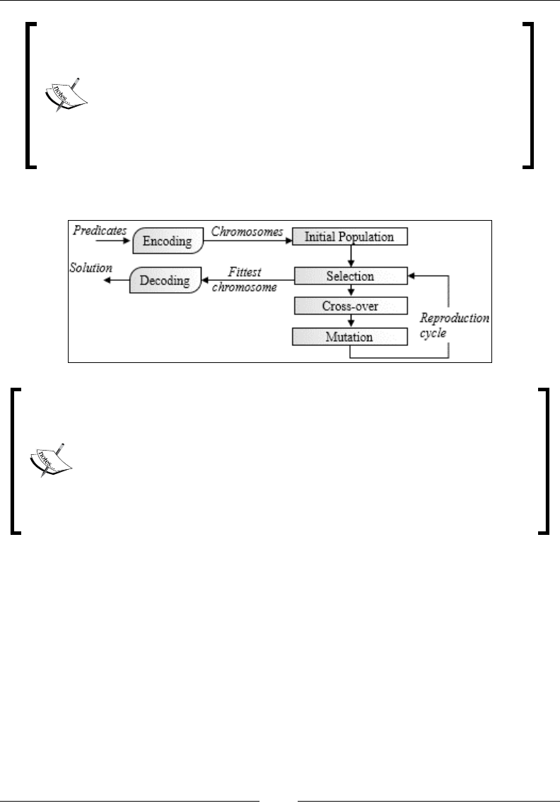
Genetic Algorithms
[ 938 ]
Transposition operator
Some implementations of genetic algorithms use a fourth operator,
genetic transposition, in case the tness function cannot be very
well dened and the initial population is very large. Although
additional genetic operators could potentially reduce the odds of
nding a local maximum or minimum, the inability to describe
the tness criteria or the search space is a sure sign that a genetic
algorithm may not be the most suitable tool.
The following diagram gives an overview of the genetic algorithm workow:
Initialization
The initialization of the search space (a set of potential solutions
to a problem) in any optimization procedure is challenging, and
genetic algorithms are no exception. In the absence of bias or
heuristics, the reproduction initializes the population with randomly
generated chromosomes. However, it is worth the effort to extract the
characteristics of a population. Any well-founded bias introduced during
initialization facilitates the convergence of the reproduction process.
Each of these genetic operators has at least one congurable parameter that has to be
estimated and/or tuned. Moreover, you will likely need to experiment with different
tness functions and encoding schemes in order to increase your odds of nding a
ttest solution (or chromosome).
Selection
The purpose of the genetic selection phase is to evaluate, rank, and weed out the
chromosomes (that is, the solution candidates) that are not a good t for the problem.
The selection procedure relies on a tness function to score and rank candidate
solutions through their chromosomal representation. It is a common practice to
constrain the growth of the population of chromosomes by setting a limit to the size
of the population.

Chapter 10
[ 939 ]
There are several methodologies to implement the selection process from scaled
relative tness, Holland roulette wheel, and tournament selection to rank-based
selection [10:8].
Relative tness degradation
As the initial population of chromosomes evolves, the chromosomes
tend to get more and more similar to each other. This phenomenon is
a healthy sign that the population is actually converging. However,
for some problems, you may need to scale or magnify the relative
tness to preserve a meaningful difference in the tness score
between the chromosomes [10:9].
The following implementation relies on rank-based selection using either a tness or
untness function to score chromosomes.
The selection process consists of the following steps:
1. Apply the tness/untness function to each chromosome j in
the population, fj
2. Compute the total tness/untness score for the entire population, ∑fj
3. Normalize the tness/untness score of each chromosome by the sum of the
tness/untness scores of all the chromosomes, fj = fi/Σfj
4. Sort the chromosomes by their descending tness score or ascending
untness score
5. Compute the cumulative tness/untness score for each chromosome,
j fj = fj + ∑fk
6. Generate the selection probability (for the rank-based formula) as a random
value, p ε [0,1]
7. Eliminate the chromosome, k, having a low tness score fk < p or high
untness cost, fk > p
8. Reduce the size of the population further if it exceeds the maximum allowed
number of chromosomes.
Natural selection
You should not be surprised by the need to control the size
of population of chromosomes. After all, nature does not
allow any species to grow beyond a certain point in order
to avoid depleting natural resources. The predator-prey
process modeled by the Lotka-Volterra equation [10:10]
keeps the population of each species in check.
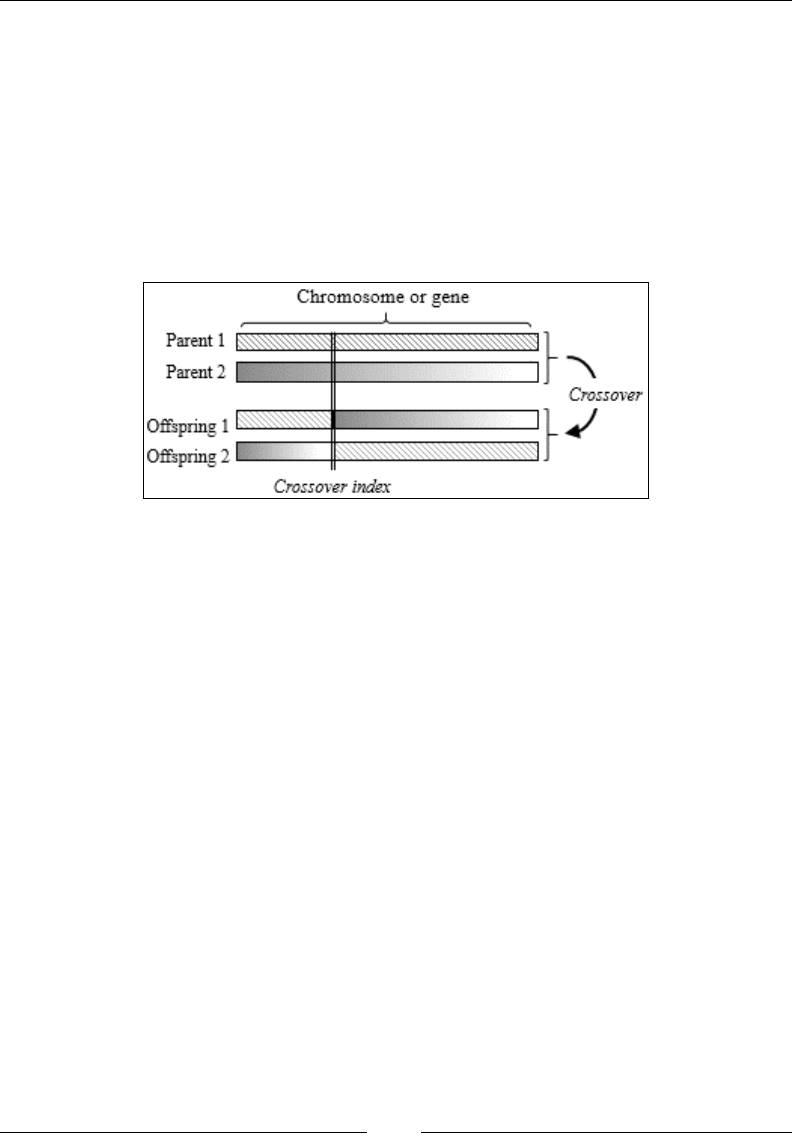
Genetic Algorithms
[ 940 ]
Crossover
The purpose of the genetic crossover is to expand the current population of
chromosomes in order to intensify the competition among the solution candidates.
The crossover phase consists of reprogramming chromosomes from one generation to
the next. There are many different variations of crossover techniques. The algorithm
for the evolution of the population of chromosomes is independent of the crossover
technique. Therefore, the case study uses the simpler one-point crossover. The
crossover swaps sections of the two-parent chromosomes to produce two offspring
chromosomes, as illustrated in the following diagram:
A chromosome's crossover
An important element in the crossover phase is the selection and pairing of parent
chromosomes. There are different approaches for selecting and pairing the parent
chromosomes that are the most suitable for reproduction:
• Selecting only the n ttest chromosomes for reproduction
• Pairing chromosomes ordered by their tness (or untness) value
• Pairing the ttest chromosome with the least-t chromosome, the second
ttest chromosome with the second least-t chromosome, and so on
It is a common practice to rely on a specic optimization problem to select the most
appropriate selection method as it is highly domain dependent.
The crossover phase that uses hierarchical addressing as the encoding scheme
consists of the following steps:
1. Extract pairs of chromosomes from the population.
2. Generate a random probability p ϵ [0,1].
3. Compute the index ri of the gene for which the crossover is applied
as ri = p.num_genes, where num_genes are the number of genes in
a chromosome.
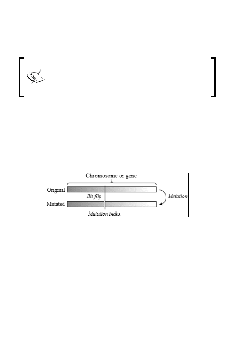
Chapter 10
[ 941 ]
4. Compute the index of the bit in the selected gene for which the crossover is
applied as xi=p.gene_length, where gene_length is the number of bits in the gene.
5. Generate two offspring chromosomes by interchanging strands
between parents.
6. Add the two offspring chromosomes to the population.
Preserving parent chromosomes
You may wonder why the parents are not removed from
the population once the offspring chromosomes are created.
This is because there is no guarantee that any of the offspring
chromosomes are a better t.
Mutation
The objective of genetic mutation is preventing the reproduction cycle from
converging towards a local optimum by introducing a pseudo-random alteration
to the genetic material. The mutation procedure inserts a small variation in
a chromosome to maintain some level of diversity between generations. The
methodology consists of ipping one bit in the bits string representation of the
chromosome, as illustrated in the following diagram:
The chromosome mutation
The mutation is the simplest of the three phases in the reproduction process. In the
case of hierarchical addressing, the steps are as follows:
1. Select the chromosome to be mutated.
2. Generate a random probability p ϵ[0,1].
3. Compute the index mi of the gene to be mutated using the formula
mi = p.num_genes.
4. Compute the index of the bit in the gene to be mutated xi=p.genes_length.
5. Perform a ip XOR operation on the selected bit.

Genetic Algorithms
[ 942 ]
The tuning issue
The tuning of a genetic algorithm can be a daunting task.
A plan including a systematic design experiment for
measuring the impact of the encoding, tness function,
crossover, and mutation ratio is necessary to avoid lengthy
evaluation and self-doubt.
Fitness score
The tness function is the centerpiece of the selection process. There are three
categories of tness functions:
• The xed tness function: In this function, the computation of the tness
value does not vary during the reproduction process
• The evolutionary tness function: In this function, the computation of the
tness value morphs between each selection according to predened criteria
• An approximate tness function: In this function, the tness value cannot be
computed directly using an analytical formula [10:11]
Our implementation of the genetic algorithm uses a xed tness function.
Implementation
As mentioned earlier, the genetic operators are independent of the problem to be
solved. Let's implement all the components of the reproduction cycle. The tness
function and the encoding scheme are highly domain specic.
In accordance with the principles of object-oriented programming, the software
architecture denes the genetic operators using a top-down approach: starting
with the population, then each chromosome, down to each gene.
Software design
The implementation of the genetic algorithm uses a design that is similar to
the template for classiers (refer to the Design template for classier section in
Appendix A, Basic Concepts).
The key components of the implementation of the genetic algorithm are as follows:
• The Population class denes the current set of solution candidates
or chromosomes.
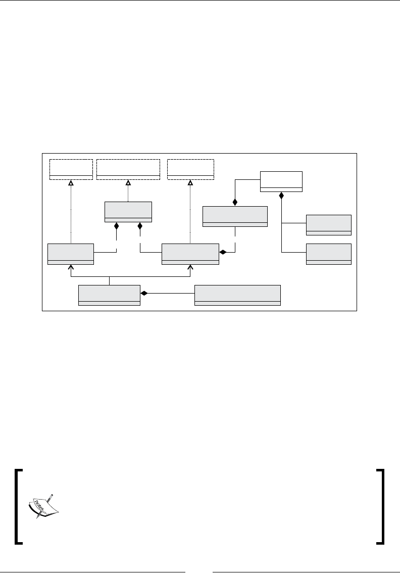
Chapter 10
[ 943 ]
• The GASolver class implements the GA solver and has two components: a
conguration object of the type GAConfig and the initial population. This
class denes a data transformation by implementing the PipeOperator trait.
• The conguration class GAConfig consists of the GA execution and
reproduction conguration parameters.
• The reproduction (of the type Reproduction) controls the reproduction cycle
between consecutive generations of chromosomes through the mate method.
The following UML class diagram describes the relation between the different
components of the genetic algorithm:
Reproduction Chromosome[T]=>()
Operator
Double
PopulationGAConfig
GASolver Chromosome
Gene
Config PipeOperator Model
mate
score
code
op
value
config population chromosomes
1
1+
1
11
11
11
1
1
1
1+
UML class diagram of genetic algorithm components
Let's start by dening the key classes that control the genetic algorithm.
Key components
The parameterized class Population (with the subtype Gene) contains the set or
pool of chromosomes. A population contains chromosomes that are a sequence
or list of element of the type inherited from Gene. A Pool is a mutable array in
order to avoid excessive duplication of the Chromosome instances associated with
immutable collections.
A case for mutability
It is a good Scala programming practice to stay away from mutable
collections. However, in this case, the number of chromosomes can
be very large. Most implementations of genetic algorithms update the
population potentially three times per reproduction cycle, generating
a large number of objects and taxing the Java garbage collector.

Genetic Algorithms
[ 944 ]
The Population class takes two parameters:
• limit: This is the maximum size of the population
• chromosomes: This is the pool of chromosomes dening the current population
A reproduction cycle executes the following sequence of three genetic operators on
a population: select for selection across all the chromosomes of the population, +-
for crossover of all the chromosomes, and ^ for the mutation of each chromosome.
Consider the following code:
type Pool[T <: Gene] = ArrayBuffer[Chromosome[T]]
class Population[T <: Gene](limit: Int, val chromosomes: Pool[T]) {
def select(score: Chromosome[T] => Unit, cutOff: Double)
def +- (xOver: Double)
def ^ (mu: Double)
…
The limit value species the maximum size of the population during optimization.
It denes the hard limit or constraints on the population growth.
The chromosome is the second level of containment in the genotype hierarchy.
The Chromosome class takes a list of genes as parameter (code). The signature of the
crossover and mutation methods, +- and ^, are similar to their implementation in the
Population class except for the fact that the crossover and mutable parameters are
passed as indices relative to the list of genes and each gene. The section dedicated to
the genetic crossover describes the GeneticIndices class:
class Chromosome[T <: Gene](val code: List[T]) {
var unfitness: Double = 1e+5*(1 + Random.nextDouble)
def +- (that: Chromosome[T], idx: GeneticIndices):
(Chromosome[T],Chromosome[T])
def ^ (idx: GeneticIndices): Chromosome[T]
…
The algorithm assigns the tting score an unfitness value in this implementation
to enable the ranking of the population and ultimately the selection of the ttest
chromosomes.
Fitness vs. untness
The machine learning algorithms used the loss function or
its variant as an objective function to be minimized. This
implementation of the GA uses untness scores to be consistent
with the concept of minimization of cost, loss, or penalty function.

Chapter 10
[ 945 ]
Finally, the reproduction process executes the genetic operators on each gene:
class Gene(val id: String, val target: Double, op: Operator)(implicit
discr: Discretization) {
val bits: BitSet
…
def +- (index: Int, that: Gene): Gene
def ^ (index: Int): Unit
}
The Gene class takes four parameters:
• id: This is the identier of the gene. It is usually the name of the variable
represented by the gene.
• target: This is the target value or threshold to be converted or discretized
into a bit string.
• op: This is the operator that is applied to the target value.
• discr: This is the discretization class that converts a double value to an
integer to be converted into bits and vice versa.
The discretization is implemented as a case class:
case class Discretization(toInt: Double => Int,toDouble: Int =>
Double) {
def this(R: Int) =
this((x: Double) => (x*R).floor.toInt, (n: Int) => n/R)
}
The rst function, toInt, converts a real value to an integer and toDouble
converts the integer back to a real value. The discretization and inverse functions
are encapsulated into a class to reduce the risk of inconsistency between the two
opposite conversion functions.
The instantiation of a gene converts the predicate representation into a bit string (bits
of the type java.util.BitSet) using the discretization function Discretization.
toInt. The bit string is decoded by the decode method of the Gene companion object.
The Operator trait denes the signature of any operator. Each domain-specic
problem requires a unique set of operations: Boolean, numeric, or string manipulation:
trait Operator {
def id: Int
def apply(id: Int): Operator
}

Genetic Algorithms
[ 946 ]
The preceding operator has two methods: an identier id and an apply method that
converts an index to an operator.
Selection
The rst genetic operator of the reproduction cycle is the selection process. The
select method of the Population class implements the steps of the selection
phase to the population of chromosomes in the most efcient manner, as follows:
def select(score: Chromosome[T] => Unit, cutOff: Double) = {
val cumul = chromosomes.foldLeft(0.0)((s,x) =>{
score(xy); s + xy.unfitness} ) //1
chromosomes foreach( _ /= cumul) //2
val newChromosomes = chromosomes.sortWith(_.unfitness < _.unfitness)
//3
val cutOffSize = (cutOff*newChromosomes.size).floor.toInt //4
val newPopSize = if(limit<cutOffSize) limit else cutOffSize //5
chromosomes.clear //6
chromosomes ++= newChromosomes.take(newPopSize) //7
}
The select method computes the cumulative sum of an untness value, cumul,
for the entire population (line 1). It normalizes the untness of each chromosome
(line 2), orders the population by decreasing value (line 3), and applies a soft limit
function on population growth, cutOff (line 4). The next step reduces the size of
the population to the lowest of the two limits: the hard limit, limit, or the soft limit,
cutOffSize (line 5). Finally, the current population is cleared (line 6) and updated
with the next generation (line 7).
Even population size
The next phase in the reproduction cycle is the crossover, which
requires the pairing of parent chromosomes. It makes sense to
pad the population so that its size is an even integer.
The scoring function score takes a chromosome as parameter and updates its
unfitness value for this chromosome.

Chapter 10
[ 947 ]
Controlling population growth
The natural selection process controls or manages the growth of the population of
species. The genetic algorithm uses two mechanisms:
• The absolute maximum size of the population (hard limit).
• The incentive to reduce the population as the optimization progresses
(soft limit). This incentive (or penalty) on the population growth is dened
by the cutOff value used during selection (the select method).
The cutoff value is computed through a user-dened function, softLimit, of the
type Int => Double, provided as a conguration parameter (softLimit(cycle:
Int) => a.cycle +b).
GA conguration
The four congurations and tuning parameters required by the genetic
algorithm are:
• xover: This is the crossover ratio (or probability) and has a value
in the interval [0, 1].
• mu: This is the mutation ratio with a value in the interval [0, 1].
• maxCycles: This is the maximum number of reproduction cycles.
• softLimit: This is the soft constraint on the population growth. The constraint
function takes the number of iterations as argument and returns the maximum
number of chromosomes allowed in the population.
Consider the following code:
class GAConfig(val xover: Double,val mu: Double,val maxCycles: Int,val
softLimit: Int => Double) extends Config
Crossover
As mentioned earlier, the genetic crossover operator couples two chromosomes to
generate two offspring chromosomes that compete with all the other chromosomes
in the population, including their own parents, in the selection phase of the next
reproduction cycle.
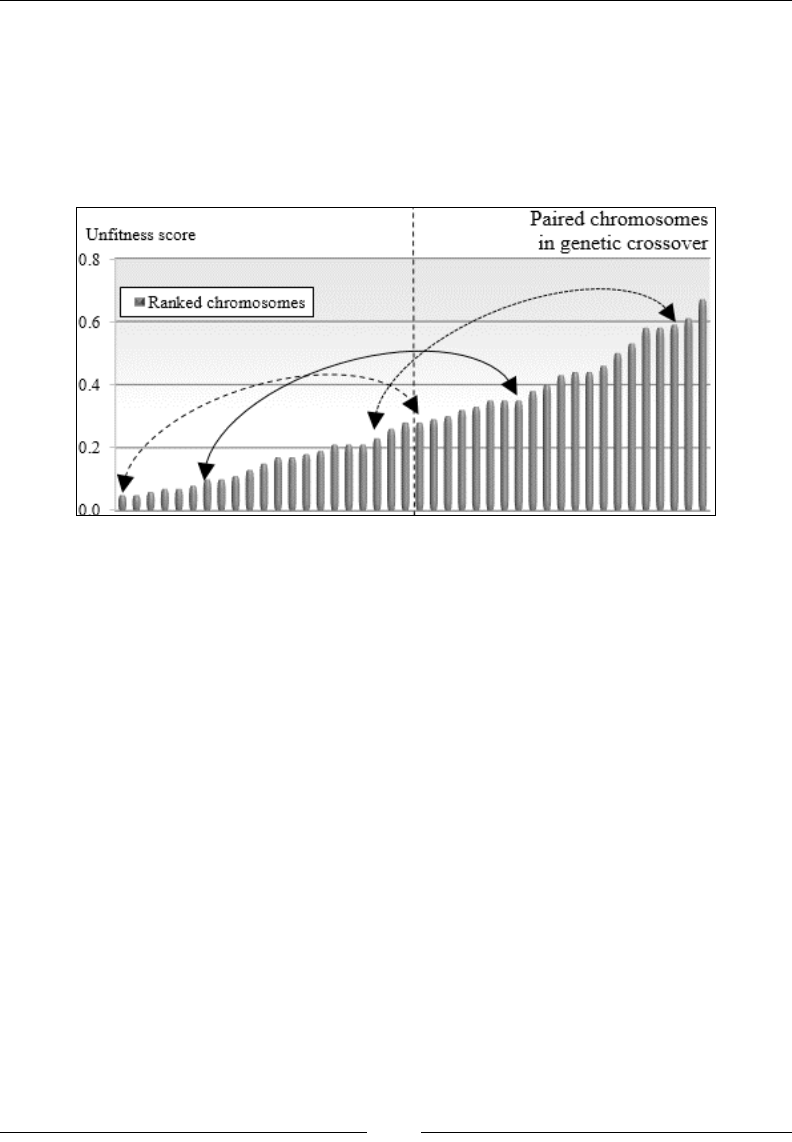
Genetic Algorithms
[ 948 ]
Population
We use the notation +- as the implementation of the crossover operator in Scala. There
are several options to select pairs of chromosomes for crossover. This implementation
ranks the chromosomes by their tness value and then divides the population into two
halves. Finally, it pairs the chromosomes of identical rank from each half as illustrated
in the following diagram:
Pairing of chromosomes within a population prior to crossover
The crossover implementation, +-, selects the parent chromosome candidates for
crossover using the pairing scheme described earlier. Consider the following code:
def +- (xOver: Double): Unit = {
if( size > 1) {
val mid = size>>1
val bottom = chromosomes.slice(mid, size) //1
val gIdx = geneticIndices(xOver) //5
val offSprings = chromosomes.take(mid)
.zip(bottom) //2
.map(p => p._1 +-(p._2, gIdx))
.unzip //3
chromosomes ++= offSprings._1 ++ offSprings._2 //4
}
}
This method splits the population into two subpopulations of equal size (line 1)
and applies the Scala zip method (line 2) to generate the set of pairs of offspring
chromosomes (line 3). The crossover operator, +-, is applied to each chromosome
pair to produce an array of pairs of offspring. Finally, the crossover method adds
offspring chromosomes to the existing population (line 4). The crossover value,
xOver, is a probability randomly generated over the interval [config.xOver, 1].

Chapter 10
[ 949 ]
The geneticIndices method (line 5) computes the relative indices of the crossover
bit in the chromosomes and genes:
case class GeneticIndices(val chOpIdx: Int, val geneOpIdx: Int)
def geneticIndices(prob: Double): GeneticIndices = {
var idx = (prob*chromosomeSize).floor.toInt
val chIdx = if(idx==0) 1
else if(idx == chromosomeSize) chromosomeSize-1 else idx
idx = (prob*geneSize).floor.toInt
val gIdx = if(idx == 0) 1
else if(idx == geneSize) geneSize-1 else idx
GeneticIndices(chIdx, gIdx)
}
The GeneticIndices case class denes two indices of the bit whenever a crossover or
a mutation occurs. The rst index, chOpIdx, is the absolute index of the bit affected by
the genetic operation in the chromosome. The second index, geneOpIdx, is the index
of the bit within the gene subjected to crossover or mutation. The geneticIndices
method of the Population class computes the two indices from a randomly generated
value, prob, selected over the interval [config.xover, 1] for crossover and
[config.mu, 1] for mutation.
Chromosomes
First, we need to dene the Chromosome class, which takes a list of genes, code
(for genetic code), as the parameter:
class Chromosome[T <: Gene](val code: List[T])
The implementation of the crossover for a pair of chromosomes using hierarchical
encoding follows two steps:
• Find the gene on each chromosome that corresponds to the crossover index,
gIdx.chOpIdx, and then swap the remaining genes
• Split and splice the gene crossover at xoverIdx
Consider the following code:
def +-(that: Chromosome[T], gIdx: GeneticIndices): (Chromosome[T],
Chromosome[T]) = {
val xoverIdx = gIdx.chOpIdx //6
val xGenes = spliceGene(gIdx, that.code(xoverIdx) ) //7
val offSprng1 = code.slice(0, xoverIdx) ::: xGenes._1 :: that.code.
drop(xoverIdx+1) //8

Genetic Algorithms
[ 950 ]
val offSprng2 = that.code.slice(0, xoverIdx) ::: xGenes._2 :: code.
drop(xoverIdx+1)
(Chromosome[T](offSprng1), Chromosome[T](offSprng2)//9
}
The crossover method computes the index of the bit that denes the crossover
(xoverIdx) in each parent chromosome (line 6). The genes this.code(xoverIdx)
and that.code(xoverIdx) are swapped and spliced by the spliceGene method
to generate a spliced gene (line 7).
def spliceGene(gIdx: GeneticIndices, thatCode: T): (T, T) = {
((this.code(gIdx.chOpIdx) +- (thatCode, gIdx)),
(thatCode +- (code(gIdx.chOpIdx), gIdx)) )
}
The offspring chromosomes are gathered by collating the rst xOverIdx genes of the
parent chromosome, the crossover gene, and the remaining genes of the other parent
(line 8). The method returns the pair of offspring chromosomes (line 9).
Genes
The crossover is applied to a gene through the +-method of the Gene class. The
exchange of bits between the two genes this and that uses the BitSet Java class
to rearrange the bits after the permutation:
def +- (that: Gene, idx: GeneticIndices): Gene = {
val clonedBits = cloneBits(bits) //10
Range(gIdx.geneOpIdx, bits.size).foreach(n =>
if( that.bits.get(n) ) clonedBits.set(n)
else clonedBits.clear(n)
) //11
val valOp = decode(clonedBits) //12
Gene(id, valOp._1, valOp._2)
}
The bits of the gene are cloned (line 10) and then spliced by exchanging their bits
along the crossover point xOverIdx (line 11). The cloneBits function duplicates
a bit string, which is then converted into a (target value, operator) tuple using the
decode method (line 12). We omit these two methods because they are not critical
to the understanding of the algorithm.

Chapter 10
[ 951 ]
Mutation
The mutation of the population uses the same algorithmic approach as the
crossover operation.
Population
The mutation operator ^ invokes the same operator for all the chromosomes in the
population and then adds the mutated chromosomes to the existing population,
so that they can compete with the original chromosomes. We use the notation ^ to
dene the mutation operator to remind the reader that the mutation is implemented
by ipping one bit:
def ^ (mu: Double): Unit =
chromosomes ++= chromosomes.map(_ ^ geneticIndices(mu))
The mutation parameter mu is used to compute the absolute index of the mutating
gene, geneticIndices(mu).
Chromosomes
The implementation of the mutation operator ^ on a chromosome consists of
mutating the gene of the index gIdx.chOpIdx (line 1) and then updating the list of
genes in the chromosome (line 2). The method returns a new chromosome (line 3)
that will compete with the original chromosome:
def ^ (gIdx: GeneticIndices): Chromosome[T] = { //1
val mutated = code(gIdx.chOpIdx) ^ gIdx
val xs = Range(0, code.size).map(i =>
if(i==gIdx.chOpIdx) mutated else code(i)).toList //2
Chromosome[T](xs) //3
}
Genes
Finally, the mutation operator ips (XOR) the bit at the index gIdx.geneOpIdx:
def ^ (gIdx: GeneticIndices): Gene = {
val clonedBits = cloneBits(bits) //4
clonedBits.flip(idx.geneOpIdx) //5
val valOp = decode(clonedBits) //6
Gene(id, valOp._1, valOp._2) //7
}

Genetic Algorithms
[ 952 ]
The ^ method mutates the cloned bit string, clonedBits (line 4) by ipping the bit at
the index gIdx.geneOpIdx (line 5). It decodes and converts the mutated bit string by
converting it into a (target value, operator) tuple (line 6). The last step creates a new
gene from the target-operator tuple (line 7).
The reproduction cycle
Let's wrap the reproduction cycle into a Reproduction class that uses the scoring
function score:
class Reproduction[T <: Gene](score: Chromosome[T] => Unit)
The reproduction function, mate, implements the sequence or workow of the three
genetic operators: select for the selection, +- (xover) for the crossover, and ^ (mu)
for the mutation:
def mate(population: Population[T], config: GAConfig, cycle: Int):
Boolean = population.size match {
case 0 | 1 | 2=> false
case _ => {
population.select(score, config.softLimit(cycle))
population +- (1.0 - Random.nextDouble*config.xover)
population ^ (1.0 - Random.nextDouble*config.mu)
true
}
}
This method returns true if the size of the population is larger than 2. The last
element of the puzzle is the exit condition. There are two options for estimating
that the reproducing cycle is converging:
• Greedy: In this approach, the objective is to evaluate whether the n ttest
chromosomes have not changed in the last m reproduction cycles
• Loss function: This approach is similar to the convergence criteria for the
training of supervised learning
A simple exit condition describes the state, of the type GAState, of the genetic
algorithm at each reproduction cycle:
def converge(population: Population[T], cycle: Int): GAState = {
if(population == null) GA_FAILED
else if(iters >= config.cycles)
GA_NO_CONVERGENCE(s"failed after $cycle cycles")
…

Chapter 10
[ 953 ]
Let's dene the state of the genetic algorithm as a case class of the super
type GAState:
sealed abstract class GAState(val description: String)
case class GA_FAILED(val _description: String) extends GAState(_
description)
object GA_RUNNING extends GAState("Running")
case class GA_NO_CONVERGENCE(val _desc: String) extends GAState(_desc)
…
The last class GASolver manages the reproduction cycle and evaluates the exit
condition or the convergence criteria:
class GASolver[T <: Gene](config: GAConfig, score: Chromosome[T]
=>Unit) extends PipeOperator[Population[T], Population[T]] {
var state: GAState = GA_NOT_RUNNING
This class implements the data transformation |>, which transforms a population to
another one, given a conguration, config and a scoring method, score, as follows:
def |> : PartialFunction[Population[T], Population[T]] = {
case population: Population[T] if(population.size > 1) => {
val reproduction = Reproduction[T](score)
state = GA_RUNNING
Range(0, config.maxCycles).find(n => { //1
reproduction.mate(population, config, n) match { //2
case true => converge(population, n) != GA_RUNNING //3
case false => { …. }
}
}) match {
case Some(n) => population
…
The reproduction cycle is controlled by the find function (line 1) that tests whether
an error occurs during the reproduction, mate (line 2), before the convergence
criteria (line 3) are applied.
GA for trading strategies
Let's apply our fresh expertise in genetic algorithms to evaluate different strategies to
trade securities using trading signals. Knowledge in trading strategies is not required
to understand the implementation of a GA. However, you may want to get familiar
with the foundation and terminology of technical analysis of securities and nancial
markets, described briey in the Technical analysis section in Appendix A, Basic Concepts.
Genetic Algorithms
[ 954 ]
The problem is to nd the best trading strategy to predict the increase or decrease of the
price of a security given a set of trading signals. A trading strategy is dened as a set of
trading signals tsj that are triggered or red when a variable x= {xj}, derived from
nancial metrics such as the price of the security or the daily or weekly trading
volume, either exceeds or equals or is below a predened target value, αj (refer to
the Trading signals and strategy section in Appendix A, Basic Concepts).
The number of variables that can be derived from price and volume can be very
large. Even the most seasoned nancial professionals face two challenges:
• Selecting a minimal set of trading signals that are relevant to a given data
set (minimize a cost or untness function)
• Tuning those trading signals with heuristics derived from personal
experience and expertise
Alternative to GA
The problem described earlier can certainly be solved using
one of the machine learning algorithms introduced in the
previous chapters. It is just a matter of dening a training set
and formulating the problem as minimizing the loss function
between the predictor and the training score.
The following table lists the trading classes with their counter part in the
'genetic world':
Generic classes Corresponding securities trading classes
Operator SOperator
Gene Signal
Chromosome Strategy
Population StrategiesFactory
Denition of trading strategies
A chromosome is the genetic encoding of a trading strategy. A factory class,
StrategyFactory, assembles the components of a trading strategy: operators,
untness function and signals.

Chapter 10
[ 955 ]
Trading operators
Let's extend the Operator trait with the SOperator class to dene the operations
we need to trigger the signals. The SOperator instance has a single parameter: its
identier, _id. The class overrides the id () method to retrieve the ID (similarly, the
class overrides the apply method to convert an ID into an SOperator instance):
class SOperator(val _id: Int) extends Operator {
override def id: Int = _id
override def apply(idx: Int): SOperator = new SOperator(idx)
}
The operators used by trading signals are the logical operators: <, >, and =,
as follows:
object LESS_THAN extends SOperator(1)
object GREATER_THAN extends SOperator(2)
…
Each operator is associated with a scoring function by the map operatorFuncMap.
The function computes the untness of the signal against a real value or a time series:
val operatorFuncMap = Map[Operator, (Double, Double) =>Double](
LESS_THAN -> ((x: Double, target: Double) => target - x),
GREATER_THAN -> ((x: Double, target: Double) => x -target),
… )
The select method of Population computes the untness value of a signal by
quantifying the truthfulness of the predicate. For instance, the untness value for
a trading signal, x > 10, is penalized as 5 – 10 = -5 for x = 5 and credited as 14 – 10
= 4 if x = 14. In this regard, the untness value is similar to the cost or loss in a
discriminative machine learning algorithm.
The cost/untness function
Let's consider the following trading strategy dened as a set of two signals to predict
the sudden relative decrease Δp of the price of a security:
• Relative volume vm with a condition vm < α
• Relative volatility vl with the condition vl > β
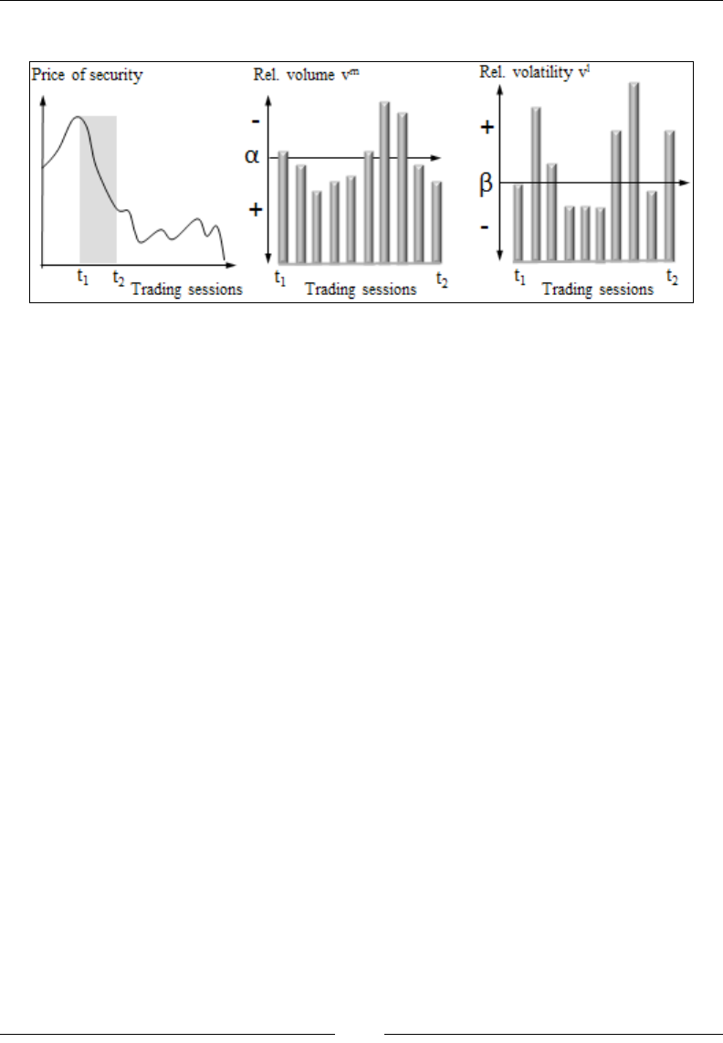
Genetic Algorithms
[ 956 ]
Have a look at the following graphs:
As the goal is to model a sudden crash in stock price, we should reward the trading
strategies that predict the steep decrease in the stock price and penalize the strategies
that work well only with a small decrease or increase in stock price. For the case of
the trading strategy with two signals, relative volume vm and relative volatility vl,
n trading sessions, the cost or untness function C, and given a relative variation of
stock price and a penalization w = -Δp:
()( )( )
1
0
,,|,
tt
n
ml m l
tt t t
t
wp
Cpv v vw v w
αβ α β
−
=
=−∆
=−+−
∑
Trading signals
Let's subclass the Gene class to dene the trading signal:
class Signal(_id: String, _target: Double, _op: Operator,xt:
DblVector, weights: DblVector)(implicit discr: Discretization) extends
Gene(_id, _target, _op)
The Signal class takes the identier for the feature, the target value, an operator
op, the time series xt of the type DblVector, and the weights associated to each data
point of the time series xt. The main purpose of the Signal class is to compute its
score. The chromosome updates its untness by summing the score or weighted
score of the signals it contains.
The score of the trading signal is simply the summation of the penalty or truthfulness
of the signal for each entry of the time series, ts:
def score: Double = sumScore(operatorFuncMap.get(op).get)
def sumScore(f: (Double, Double) => Double): Double = xt.foldLeft(0.0)
((s, x) => s + f(x, target))
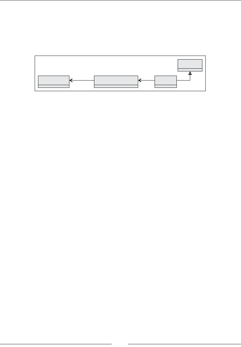
Chapter 10
[ 957 ]
Trading strategies
A trading strategy is an unordered list of trading signals. It makes sense to create
a factory class to generate the trading strategies. The StrategyFactory class
creates strategies of the type List[Signal] from an existing pool of signals of
the subtype Gene:
strategy StrategyFactoryList[Signal] Signal
Gene
+=
The StrategyFactory class has two arguments: the number of signals, nSignals, in
a trading strategy and the implicit discretization instance:
class StrategyFactory(nSignals: Int)(implicit discr: Discretization){
val signals = new ListBuffer[Signal]
lazy val strategies: Pool[Signal]
…
The += method adds the trading signals to the factor. The StrategyFactory class
generates all possible sequences of signals as trading strategies. The += method takes
ve arguments: the identier (id), target, operation (op) to qualify the class as a
Gene, the times series xt for scoring the signals, and the weights associated to the
overall cost function:
def += (id: String, target: Double, op: Operator, xt:
XTSeries[Double], weights: DblVector): Unit =
signals.append(Signal(id, target, op, xt.toArray, weights) )
The StrategyFactory class denes strategies as lazy values to avoid
unnecessary regeneration of the pool on demand:
lazy val strategies: Pool[Signal] = {
implicit val ordered = Signal.orderedSignals //7
val xss = new Pool[Signal] //1
val treeSet = new TreeSet[Signal] ++= signals.toList //2
val subsetsIterator = treeSet.subsets(nSignals) //3
while( subsetsIterator.hasNext) { //4
val subset = subsetsIterator.next
val signalList: List[Signal] = subset.toList //5
xss.append(Chromosome[Signal](signalList)) //6
} xss
}
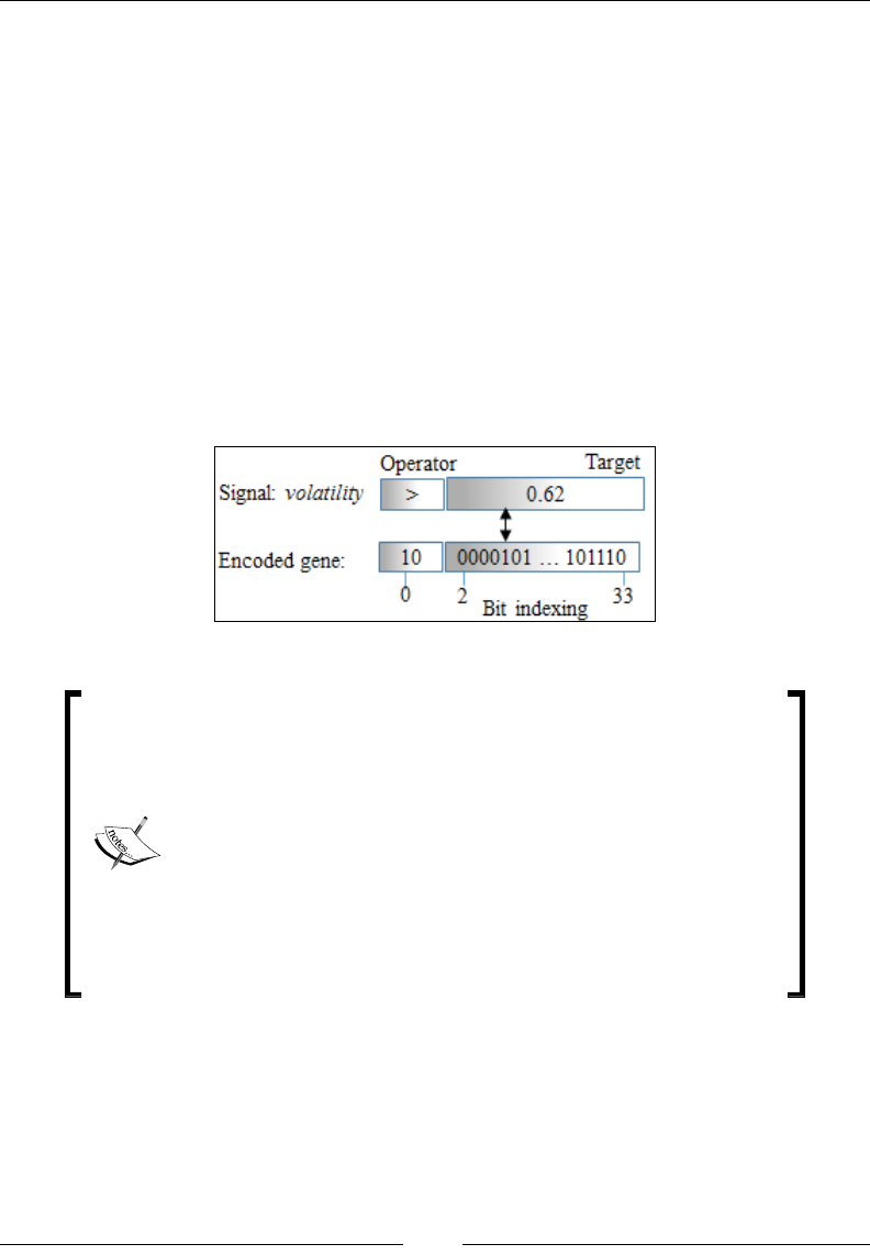
Genetic Algorithms
[ 958 ]
The implementation of the strategies value creates Pool (line 1) by converting the
list of signals to a treeset (line 2). It breaks down the tree set into unique subtrees
of nSignals nodes each (line 3). It instantiates a subsetsIterator iterator (line 3)
to traverse the sequence of subtrees (line 4) and converts them into a list (line 5) as
arguments of the new chromosome (trading strategy) (line 6). The procedure to order
the signals, orderedSignals, in the tree set has to be implicitly dened (line 7):
val orderedSignals = Ordering.by((signal: Signal) => signal.id)
Signal encoding
The encoding of trading predicates is the most critical element of the genetic
algorithm. In our example, we encode a predicate as a tuple (target value, operator).
Let's consider the simple predicate volatility > 0.62. The discretization converts the
value 0.62 into 32 bits for the instance and a 2-bit representation for the operator:
Encoding price volatility as a gene
IEEE-732 encoding
The threshold value for predicates is converted into an integer
(the type Int or Long). The IEEE-732 binary representation
of oating point values makes the bit addressing required
to apply genetic operators quite challenging. A simple
conversion consists of the following:
encoding e: (x: Double) => (x*100000).toInt
decoding d: (x: Int) => x*1e-5
All values are normalized; so, there is no risk of overowing
the 32-bit representation.
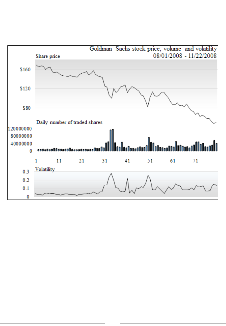
Chapter 10
[ 959 ]
Test case
The goal is to evaluate which trading strategy was the most relevant (ttest) during
the crash of the stock market in fall 2008. Let's consider the stock price of one of the
nancial institutions, Goldman Sachs, as a proxy of the sudden market decline:
Goldman-Sachs fall 2008
Besides the variation of the price of the stock between two consecutive trading
sessions (deltaPrice), the model uses the following parameters:
• deltaVolume: This is the relative variation of the volume between two
consecutive trading sessions
• deltaVolatility: This is the relative variation of volatility between two
consecutive trading sessions
• relVolatility: This is the relative volatility within a trading session
• relCloseOpen: This is the relative difference of the stock opening and
closing price

Genetic Algorithms
[ 960 ]
The execution of the genetic algorithm requires the following steps:
1. Extraction of model parameters or variables.
2. Generation of the initial population of trading strategies.
3. Setting up the GA conguration parameters with the maximum number of
reproduction cycles allowed, the crossover and mutation ratio, and the soft
limit function for population growth.
4. Instantiating the GA algorithm with the scoring/untness function.
5. Extracting the ttest trading strategy that can best explain the sharp decline
in the price of Goldman Sachs stocks.
Data extraction
The rst step is to extract the model parameters as illustrated for the variation of the
stock price between two consecutive trading sessions:
val path = "resources/data/chap10/GS.csv"
val src = DataSource(path, false, true, 1)
val price = src |> YahooFinancials.adjClose
val deltaPrice = price.drop(1)
.zip(price.dropRight(1))
.map(p => (1.0 – p._2/p._1))
The extraction of relative variation in volume and volatility is similar to the extraction
of the relative variation of the stock price.
Initial population
The next step consists of generating the initial population of strategies that compete
to become relevant to the decline of the price of stocks of Goldman Sachs. The factory
is initialized with a set of signals:
val NUM_SIGNALS_PER_STRATEGY = 3
val factory = new StrategyFactory(NUM_SIGNALS_PER_STRATEGY)
factory += ("Delta_volume", 1.1, GREATER_THAN, deltaVolume,
deltaPrice)
factory += ("Rel_volatility", 1.3, GREATER_THAN, relVolatility.
drop(1), deltaPrice)
…
The test code generates population by retrieving the pool of strategies:
val limit = factory.strategies.size // 1 <<4
val population = Population[Signal](limit, factory.strategies)

Chapter 10
[ 961 ]
The maximum size of the population (hard limit) is arbitrarily set as 16 times the
number of the initial trading strategies (line 1).
At this stage, we need to instantiate a Discretization instance:
val R=1024.0
implicit val digitize = new Discretization(R)
Conguration
The four conguration parameters for the GA are the maximum number of
reproduction cycles (MAX_CYCLES) allowed in the execution, the crossover (XOVER),
the mutation ratio (MU), and the soft limit function (softLimit) to control the
population growth:
val XOVER = 0.2; val MU = 0.6; val MAX_CYCLES = 250
val CUTOFF_SLOPE = -0.003; val CUTOFF_INTERCEPT = 1.003
val softLimit = (n: Int) => CUTOFF_SLOPE*n + CUTOFF_INTERCEPT
val config = GAConfig(XOVER, MUTATE, MAX_NUM_ITERS, softLimit)
The soft limit is implemented as a linearly decreasing function of the number of
cycles (n) to retrain the growth of the population as the execution of the genetic
algorithm progresses.
GA instantiation
Let's implement the chromosome scoring function using the formula introduced
in the cost/untness section. The trading strategy/chromosome scoring function
sums up the score for each gene and updates it:
val scoring = (chr: Chromosome[Signal]) => {
val signals: List[Gene] = chr.code
chr.unfitness = signals.foldLeft(0.0)((s, x) => s + x.score)
}
The conguration config and the scoring function, scoring, are all you need to
create and execute the solver gaSolver:
val gaSolver = GASolver[Signal](config, scoring)

Genetic Algorithms
[ 962 ]
GA execution
The execution of the genetic algorithm transforms an initial population to a very
small group of the NFITS ttest trading strategies:
val NFITS = 2
val best = gaSolver |> population
best.fittest(NFITS)
.getOrElse(ArrayBuffer.empty)
.foreach(ch => Display.show(s"Best: ${ch.toString(" ")}", logger))
…
Tests
The cost function C and the untness score of each trading strategy are weighted for
the rate of decline of the price of the Goldman Sachs stock. Let's run two tests:
• Evaluation of the genetic algorithm with an unweighted score function
• Evaluation of the conguration of the genetic algorithm with the
weighted score
The unweighted score
The test uses three different sets of crossover and mutation ratios: (0.6, 0.2), (0.3, 0.1),
and (0.2, 0.6). The best trading strategy for each scenario are as follows:
• 0.6-0.2: For this, Delta_volume > 1.10, Rel_close-Open > 0.75, and
Rel_volatility > 0.97 with average chromosome unfitness = 0.025
• 0.3-0.1: For this, Delta_volatility > 0.9, Rel_close-Open < 0.8, and
Rel_volatility > 1.77 with unfitness = 0.100
• 0.2-0.6: For this, Delta_volatility > 0.9 Delta_volume > 33.09, and
Rel_volatility > 1.09 with unfitness = 0.099
The ttest trading strategy for each case does not differ much from the initial
population for one or several of the following reasons:
• The initial guess for the trading signals was good
• The size of the initial population is too small to generate genetic diversity
• The test does not take into account the rate of decline of the stock price
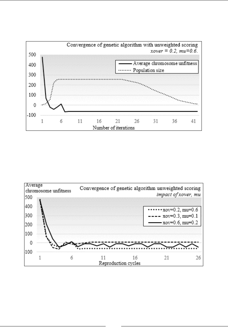
Chapter 10
[ 963 ]
Let's examine the behavior of the genetic algorithm during execution. We are
particularly interested in the convergence of the average chromosome untness
score. The average chromosome untness is the ratio of the total untness score for
the population over the size of the population: Have a look at the following graph:
The GA converges quite quickly and then stabilizes. The size of the population
increases through crossover and mutation operations until it reaches the maximum
of 256 trading strategies. The soft limit or constraint on the population size kicks in
after 23 trading cycles. The test is run again with a different values of crossover and
mutation ratio, as shown in the following graph:
The prole of the execution of the genetic algorithm is not overly affected by the
different values of crossover and mutation ratios. The chromosome untness score
for the high crossover ratio, 0.6, oscillates as the execution progresses. In some cases,
the untness score between chromosomes is so small that the GA recycles the same
few trading strategies.
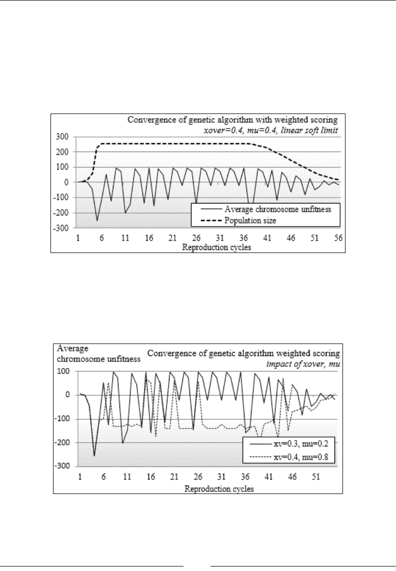
Genetic Algorithms
[ 964 ]
The quick decline in the untness of the chromosomes is consistent with the fact that
some of the ttest strategies were part of the initial population. It should, however,
raise some concerns that the GA locked on a local minimum early on.
The weighted score
The execution of a test that is similar to the previous one with the weighted untness
scoring formula produces some interesting results, as shown in the following graph:
The prole for the size of the population is similar to the test using unweighted
untness. However, the average chromosome untness does not stabilize as the
optimization goes on until the size of the population is reduced by the soft limit
function. This phenomenon is conrmed by running the test using different
congurations, as shown in the following graph:

Chapter 10
[ 965 ]
The weighting function adds the rate of decline of the stock price into the scoring
of the untness. The formula to compute the cost/untness of a trading strategy is
not a linear function; its complexity increases the odds of the genetic algorithm not
converging properly, which is conrmed with extra runs with different values of the
crossover and mutation ratios.
The possible solutions to the convergence problem are as follows:
• Make the weighting function additive (less complex)
• Increase the size and diversity of the initial population
Advantages and risks of genetic
algorithms
It should be clear by now that genetic algorithms provide scientists with a powerful
toolbox with which to optimize problems that:
• Are poorly understood.
• May have more than one good enough solutions.
• Have discrete, discontinuous, and non-differentiable functions.
• Can be easily integrated with the rules engine and knowledge bases (for
example, learning classiers systems).
• Do not require deep domain knowledge. The genetic algorithm generates
new solution candidates through genetic operators. The initial population
does not have to contain the ttest solution.
• Do not require knowledge of numerical methods such as the Newton-
Raphson, conjugate gradient, or BFGS as optimization techniques, which
frighten those with little inclination for mathematics.
However, evolutionary computation is not suitable for problems for which:
• A tness function cannot be clearly dened
• Finding the global minimum or maximum is essential to the problem
• The execution time has to be predictable
• The solution has to be provided in real time or pseudo-real time

Genetic Algorithms
[ 966 ]
Summary
Are you hooked on evolutionary computation, genetic algorithms in particular, and
their benets, limitations as well as some of the common pitfalls? If the answer is
yes, then you may nd learning classier systems, introduced in the next chapter,
fascinating. This chapter dealt with the following topics:
• Key concepts in evolutionary computing
• The key components and operators of genetic operators
• The pitfalls in dening a tness or untness score using a nancial trading
strategy as a backdrop
• The challenge of encoding predicates in the case of trading strategies
• Advantages and risks of genetic algorithms
• The process for building a genetic algorithm forecasting tool from the
bottom up
The genetic algorithm is an important element of a special class of reinforcement
learning introduced in the Learning classier systems section of the next chapter.

Reinforcement Learning
This chapter presents the concept of reinforcement learning, which is widely
used in gaming and robotics. The second part of this chapter is dedicated to
learning classier systems, which combine reinforcement learning techniques with
evolutionary computing introduced in the previous chapter. Learning classiers
are an interesting breed of algorithms that are not commonly included in literature
dedicated to machine learning. I highly recommend you to read the seminal book on
reinforcement learning by R. Sutton and A. Barto [11:1] if you are interested to know
about the origin, purpose, and scientic foundation of reinforcement learning.
In this chapter, you will learn the following:
• Basic concepts behind reinforcement learning
• Detailed implementation of the Q-learning algorithm
• A simple approach to manage and balance an investment portfolio using
reinforcement learning
• An introduction to learning classier systems
• A simple implementation of extended learning classiers
The section on learning classier systems (LCS) is mainly informative and does not
include a test case.
Introduction
The need of an alternative to traditional learning techniques arose with the design of
the rst autonomous systems.

Reinforcement Learning
[ 968 ]
The problem
Autonomous systems are semi-independent systems that perform tasks with a high
degree of autonomy. Autonomous systems touch every facet of our life, from robots
and self-driving cars to drones. Autonomous devices react to the environment in
which they operate. The reaction or action requires the knowledge of not only the
current state of the environment but also the previous state(s).
Autonomous systems have specic characteristics that challenge traditional
methodologies of machine learning, as listed here:
• Autonomous systems have poorly dened domain knowledge because of the
sheer number of possible combinations of states.
• Traditional non-sequential supervised learning is not a practical option
because of the following:
°Training consumes significant computational resources, which are
not always available on small autonomous devices
°Some learning algorithms are not suitable for real-time prediction
°The models do not capture the sequential nature of the data feed
• Sequential data models such as hidden Markov models require training
sets to compute the emission and state transition matrices (as explained
in the The hidden Markov model (HMM) section in Chapter 7, Sequential Data
Models), which are not always available. However, a reinforcement learning
algorithm benets from a hidden Markov model in case some of the states
are unknown. These algorithms are known as behavioral hidden Markov
models [11:2].
• Genetic algorithms are an option if the search space can be constrained
heuristically. However, genetic algorithms have unpredictable response
time, which makes them impractical for real-time processing.
A solution – Q-learning
Reinforcement learning is an algorithmic approach to understanding and ultimately
automating goal-based decision-making. Reinforcement learning is also known
as control learning. It differs from both supervised and unsupervised learning
techniques from the knowledge acquisition standpoint: autonomous, automated
systems or devices learn from direct, real-time interaction with their environment.
There are numerous practical applications of reinforcement learning from robotics,
navigation agents, drones, adaptive process control, game playing, and online
learning, to schedule and routing problems.

Chapter 11
[ 969 ]
Terminology
Reinforcement learning introduces a new terminology as listed here, quite different
from that of older machine learning techniques:
• Environment: The environment is any system that has states and
mechanisms to transition between states. For example, the environment
for a robot is the landscape or facility it operates in.
• Agent: The agent is an automated system that interacts with the environment.
• State: The state of the environment or system is the set of variables or
features that fully describe the environment.
• Goal or absorbing state or terminal state: A goal state is the state that
provides a higher discounted cumulative rewards than any other state.
It is a constraint on the training process that prevents the best policy from
being dependent on the initial state.
• Action: An action denes the transition between states. The agent is
responsible for performing or at least recommending an action. Upon
execution of the action, the agent collects a reward or punishment from
the environment.
• Policy: The policy denes the action to be selected and executed for any state
of the environment.
• Best policy. This is the policy generated through training. It denes the
model in Q-learning and is constantly updated with any new episode.
• Reward: A reward quanties the positive or negative interaction of the
agent with the environment. Rewards are essentially the training set for
the learning engine.
• Episode: This denes the number of steps necessary to reach the goal state
from an initial state. Episodes are also known as trials.
• Horizon: The horizon is the number of future steps or actions used in the
maximization of the reward. The horizon can be innite, in which case the
future rewards are discounted in order for the value of the policy to converge.
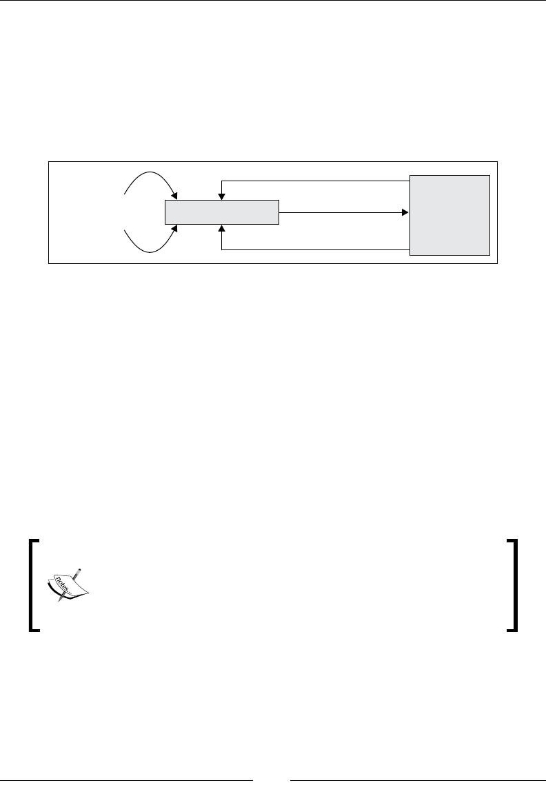
Reinforcement Learning
[ 970 ]
Concept
The key component in reinforcement learning is a decision-making agent that
reacts to its environment by selecting and executing the best course of actions and
being rewarded or penalized for it [11:3]. You can visualize these agents as robots
navigating through an unfamiliar terrain or a maze. Robots use reinforcement
learning as part of their reasoning process after all. The following diagram gives
the overview architecture of the reinforcement learning agent:
2. Compute best
course of action(s) Learning agent
1. Retrieve state
3. Perform action
4. Get reward
Environment
The agent collects the state of the environment, selects, and then executes the most
appropriate action. The environment responds to the action by changing its state and
rewarding or punishing the agent for the action.
The four steps of an episode or learning cycle are as follows:
1. The learning agent either retrieves or is notied of a new state of
the environment.
2. The agent evaluates and selects the action that may provide the
highest reward.
3. The agent executes the action.
4. The agent collects the reward or penalty and applies it to calibrate the
learning algorithm.
Reinforcement versus supervision
The training process in reinforcement learning rewards features
that maximize a value or return. Supervised learning rewards
features that meet a predened labeled value. Supervised learning
can be regarded as forced learning.
The action of the agent modies the state of the system, which in turn noties the agent
of the new operational condition. Although not every action will trigger a change in
the state of the environment, the agent collects the reward or penalty nevertheless. At
its core, the agent has to design and execute a sequence of actions to reach its goal. This
sequence of actions is modeled using the ubiquitous Markov decision process (refer to
the Markov decision processes section in Chapter 7, Sequential Data Models.)

Chapter 11
[ 971 ]
Dummy actions
It is important to design the agent so that actions may not
automatically trigger a new state of the environment. It is easy to
think about a scenario in which the agent triggers an action just to
evaluate its reward without affecting the environment signicantly.
A good metaphor for such a scenario is the rollback of the action.
However, not all environments support such a dummy action, and the
agent may have to run Monte-Carlo simulations to try out an action.
Value of policy
Reinforcement learning is particularly suited to problems for which long-term
rewards can be balanced against short-term rewards. A policy enforces the trade-off
between short-term and long-term rewards. It guides the behavior of the agent by
mapping the state of the environment to its actions. Each policy is evaluated through
a variable known as the value of policy.
Intuitively, the value of a policy is the sum of all the rewards collected as a result
of the sequence of actions taken by the agent. In practice, an action over the policy
farther in the future obviously has a lesser impact than the next action from state St
to state St+1. In other words, the impact of future actions on the current state has to be
discounted by a factor, known as the discount coefcient for future rewards < 1.
State transition matrix
The state transition matrix has have been introduced
in the The hidden Markov model section in Chapter 7,
Sequential Data Models.
The optimum policy,
π
*, is the agent's sequence of actions that maximizes the future
reward discounted to the current time.
The following table introduces the mathematical notation of each component of
reinforcement learning:
Notation Description
S = {si}States of the environment
A = {ai}Actions on the environment
Πt = p(at|st)Policy (or strategy) of the agent
Vπ(st)Value of the policy at the state
pt =p(st+1|st,at)State transition probabilities from state st to state st+1
Reinforcement Learning
[ 972 ]
Notation Description
rt= p(rt+1|st,st+1,at)Reward of an action at for a state st
RtExpected discounted long term return
γCoefficient to discount the future rewards
The purpose is to compute the maximum expected reward, Rt, from any starting
state, sk, as the sum of all discounted rewards to reach the current state, st. The value
V
π
of a policy
π
at state st is the maximum expected reward Rt given the state st.
The value of a policy π at state st with reward rj in
previous state sj:
() { }
1
0
|s
k
ttk
k
ttt
Rr
Vs
ER
π
γ
+∞
++
=
=
=
∑
Bellman optimality equations
The problem of nding the optimal policies is indeed a nonlinear optimization
problem whose solution is iterative (dynamic programming). The expression of
the value function
V
π
of a policy
π
can be formulated using the Markovian state
transition probabilities pt.
Value of state st using the transition probability
() ()
( )
{ }
() ()
max
ttkk k
aA k
t t
Vs pr V s
Vs V s
π π
π
π
π γ
∈
∗
= + ⋅
=
∑∑
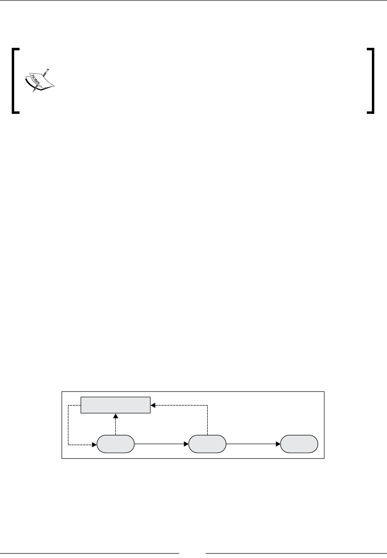
Chapter 11
[ 973 ]
V*(st) is the optimal value of state st across all the policies. The equations are known
as the Bellman optimality equations.
The curse of dimensionality
The number of states for a high-dimension problem (large-feature
vector) becomes quickly insolvable. A workaround is to approximate
the value function and reduce the number of states by sampling. The
application test case introduces a very simple approximation function.
If the environment model, state, action, and rewards, as well as transition between
states, are completely dened, the reinforcement learning technique is known as
model-based learning. In this case, there is no need to explore a new sequence of
actions or state transitions. Model-based learning is similar to playing a board game
in which all combinations of steps necessary to win are completely known.
However, most practical applications using sequential data do not have a complete,
denitive model. Learning techniques that do not depend on a fully dened and
available model are known as model-free techniques. These techniques require
exploration to nd the best policy for any given state. The remaining sections in this
chapter deal with model-free learning techniques, and more specically the temporal
difference algorithm.
Temporal difference for model-free learning
Temporal difference is a model-free learning technique that samples the
environment. It is a commonly used approach to solve the Bellman equations
iteratively. The absence of a model requires a discovery or exploration of the
environment. The simplest form of exploration is to use the value of the next state
and the reward dened from the action to update the value of the current state, as
described in the following diagram:
Action
Adjust V*(s )
t
V(s )
t
Action
V(s )
t+1 V(s )
t+2
t+1
a
t
a
Illustration of the temporal difference algorithm
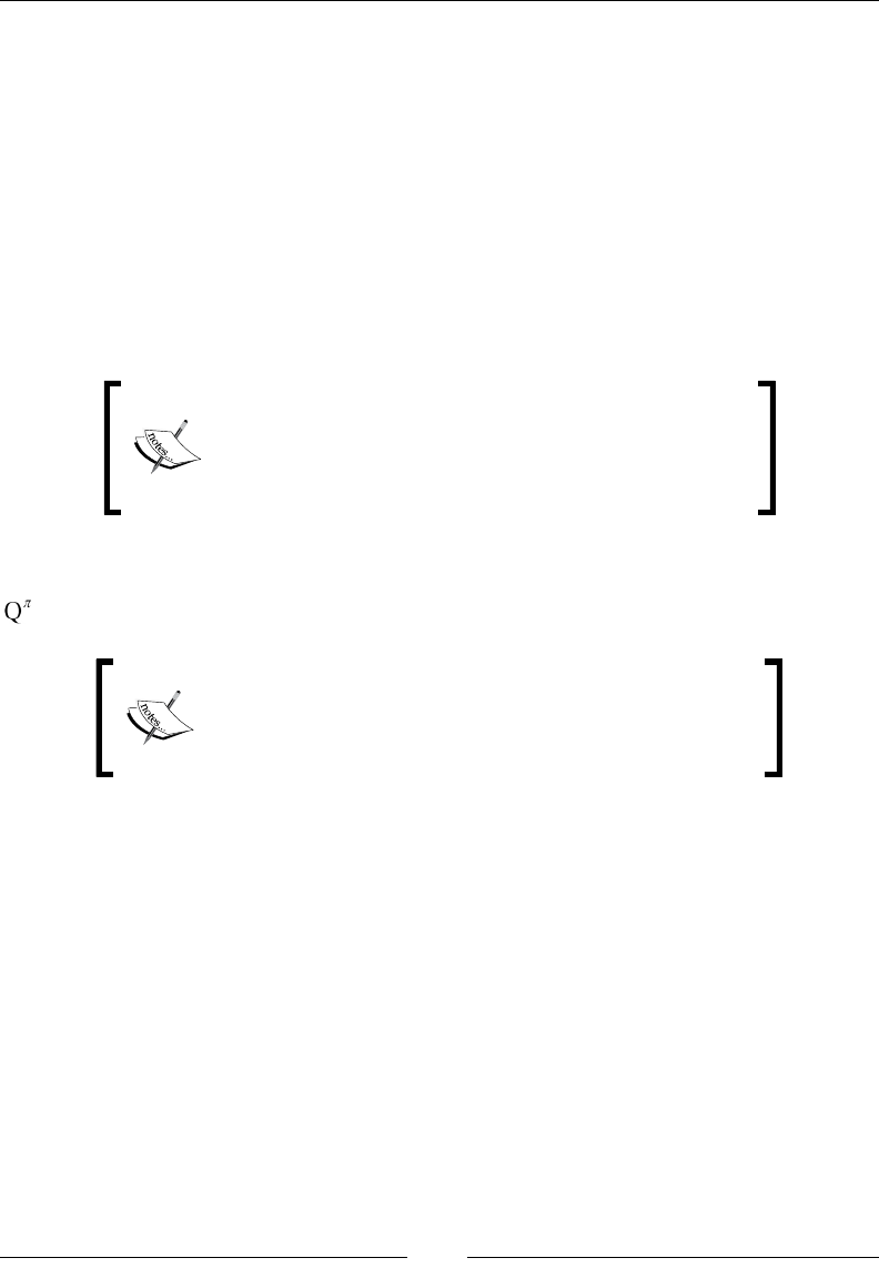
Reinforcement Learning
[ 974 ]
The iterative feedback loop used to adjust the value action on the state plays a role
similar to back propagation of errors in articial neural networks or minimization of
the loss function in supervised learning. The adjustment algorithm has to:
• Discount the estimate value of the next state using the discount rate
γ
• Strike a balance between the impacts of the current state and the next state on
updating the value at time t using the learning rate
α
The iterative formulation of the rst Bellman equation predicts
V
π
(st), the value
function of state st from the value function of the next state st+1. The difference
between the predicted value and the actual value is known as the temporal
difference error abbreviated as
δ
t.
Formula for tabular temporal difference:
() ()
() ()
1 1
ˆ
tt t t
ttt
rVsVs
Vs
Vs
π π
δγ
αδ
+ +
=+ −
=+
An alternative to evaluating a policy using the value of the state,
V
π
(st), is to use the
value of taking an action on a state st known as the value of action (or action-value)
(st, at).
Value of action at state st
()( )
,|,
ttt ttt
QQsa ERsa
ππ
==
There are two methods to implement the temporal difference algorithm:
• On-policy: This is the value for the next best action that uses the policy
• Off-policy: This is the value for the next best action that does not use the policy
Let's consider the temporal difference algorithm using an off-policy method and its
most commonly used implementation: Q-learning.
Action-value iterative update
Q-learning is a model-free learning technique using an off-policy method. It
optimizes the action-selection policy by learning an action-value function. Like
any machine learning technique that relies on convex optimization, the Q-learning
algorithm iterates through actions and states using the quality function, as described
in the following mathematical formulation.
Chapter 11
[ 975 ]
The algorithm predicts and discounts the optimum value of action, max{Qt}, for the
current state st and action at on the environment to transition to state st+1.
Similar to genetic algorithms that reuse the population of chromosomes in the
previous reproduction cycle to produce offspring, the Q-learning technique strikes
a balance between the new value of the quality function Qt+1 and the old value Qt
using the learning rate,
α
. Q-learning applies temporal difference techniques to
the Bellman equation for an off-policy methodology.
Q-learning action-value updating formula:
()
1
111
ˆmax,
tt t tt t
a
QQ r Qsa Q
ππ π π
αγ
+
+++
⎡ ⎤
=+ + −
⎢ ⎥
⎣ ⎦
A value 1 for the learning rate
α
discards the previous state, while a value 0 discards
learning. A value 1 for the discount rate
γ
uses long-term rewards only, while a
value 0 uses the short-term reward only.
Q-learning estimates the cumulative reward discounted for future actions.
Q-learning as reinforcement learning
Q-learning qualies as a reinforcement learning technique
because it does not strictly require labeled data and training.
Moreover, the Q-value does not have to be a continuous,
differentiable function.
Let's apply our hard-earned knowledge of reinforcement learning to management
and optimization of a portfolio of exchange-traded funds.
Implementation
Let us implement the Q-learning algorithm in Scala.
Software design
The key components of the implementation of the Q-learning algorithm are
as follows:
• The QLearning class implements training and prediction methods. It
denes a data transformation by implementing the PipeOperator trait.
The constructor has three arguments: a conguration of type QLConfig,
a search space of type QLSpace, and a mutable policy of type QLPolicy.
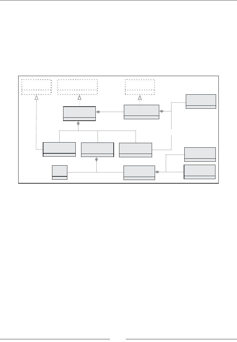
Reinforcement Learning
[ 976 ]
• The QLSpace class has two components: a sequence of states of type QLState
and the ID of one or more goal states within the sequence.
• A state, QLState, contains a sequence of QLAction instances used in its
transition to another state.
• The model of type QLModel is generated through training. It contains the best
policy and the accuracy for a model.
The following diagram shows the ow of the Q-learning algorithm:
Config PipeOperator Model
Qlearning model
Double
QLConfig
Int goallds states QLState actions
qlSpace
T
accuracy
1
1+
prop
config
qlPolicy
QLSpace QLPolicy
QLAction
1+ 1+
1
1
11
1
1
1
1
1
1
QLModel
bestPolicy
States and actions
The QLAction class species the transition of one state with ID from to another state
with ID to, as shown here:
class QLAction[T <% Double](val from: Int, val to: Int)
Actions have a Q value (or action-value), a reward, and a probability. The
implementation denes these three values in three separate matrices: Q for
the action values, R for rewards, and P for probabilities, in order to stay
consistent with the mathematical formulation.
A state of type QLState is fully dened by its ID, the list of actions to transition
to some other states, and a property prop of parameterized type, as shown in the
following code:
class QLState[T](val id: Int, val actions: List[QLAction[T]=List.
empty, val prop: T])

Chapter 11
[ 977 ]
The state might not have any actions. This is usually the case of the goal or absorbing
state. In this case, the list is empty. The parameterized prop property is a placeholder
for any information, heuristic about the state, or any action performed by the state.
The next step consists of creating the graph or search space.
Search space
The search space is the container responsible for any sequence of states. The QLSpace
class takes the following parameters:
• The sequence of all the possible states
• The ID of one or several states that have been selected as goals
Why multiple goals?
There is absolutely no requirement that a state space
must have a single goal. You can describe a solution to a
problem as reaching a threshold or meeting one of several
conditions. Each condition can be dened as a state goal.
The QLSpace class can be implemented as follows:
class QLSpace[T](states: Seq[QLState[T]], goals: Array[Int]) {
val statesMap = states.map(st => (st.id, st)).toMap //1
val goalStates = new HashSet[Int]() ++ goals //2
def maxQ(state: QLState[T], policy: QLPolicy[T]): Double //3
def init(r: Random) = states(r.nextInt(states.size-1)) //4
def nextStates(st: QLState[T]): List[QLState[T]] //5
…
}
The instantiation of the QLSpace class generates a map, statesMap, to retrieve the
state using its id (line 1) and the set of goals, goalStates (line 2). Furthermore,
the maxQ method computes the maximum action-value, maxQ, for a state given a
policy (line 3), the init method selects an initial state for training episodes (line 4),
and nally, the nextStates method retrieves the list of states resulting from the
execution of all the actions associated to the st state (line 5).

Reinforcement Learning
[ 978 ]
The search space is actually created by the instance factory dened in the QLSpace
companion object, as shown here:
def apply[T](numStates: Int, goals: Array[Int], features: Set[T],
neighbors: (Int, Int) => List[Int]): QLSpace[T] = {
val states = features
.zipWithIndex
.map(x => {
val actions = neighbors(x._2, numStates)
.map(j => QLAction[T](x._2,j))
.filter(x._2 != _.to)
QLState[T](x._2, actions, x._1
})
new QLSpace[T](states.toArray, goals)
}
The apply method creates a list of states using the features set as input. Each
state creates its list of actions. The user-dened function, neighbors, constrains
the number of actions assigned to each state. The test case describes a very simple
implementation of the neighbors function, which is dened in the conguration.
Policy and action-value
Each action has an action-value, a reward, and a potentially probability. The
probability variable is introduced to model simply the hindrance or adverse
condition for an action to be executed. If the action does not have any external
constraint, the probability is 1. If the action is not allowed, the probability is 0.
Dissociating policy from states
The action and states are the edges and vertices of the search space
or search graph. The policy dened by the action-value, rewards,
and probabilities is completely dissociated from the graph. The
Q-learning algorithm initializes the reward matrix and updates the
action-value matrix independently of the structure of the graph.
The QLData class is a container for three variables: reward, probability, and value
for the Q-value, as shown here:
class QLData(var reward: Double = 1.0, var probability: Double = 1.0
var value: Double = 0.0) {
def estimate: Double = value*probability
}

Chapter 11
[ 979 ]
The estimate method adjusts the Q-value, value, with the probability to reect any
external condition that can impede the action.
Mutable data
You might wonder why the QLData class uses variables instead of
values as recommended by the best Scala coding practices [11:4].
An instance of an immutable class would be created for each action
or state transition. The training of the Q-learning model entails
iterating across several episodes, each episode being dened as
a multiple iteration. For instance, the training of a model with
400 states for 10 episodes of 100 iterations can potentially create
160 million instances of QLData. Although not quite elegant,
mutability reduces the load on the JVM garbage collector.
Next, let us create a simple schema or class, QLInput, to initialize the reward and
probability associated with each action as follows:
class QLInput(val from: Int, val to: Int, val reward: Double =1.0, val
probability: Double =1.0)
The rst two arguments are the identiers for the source state, from, and target state,
to, for this specic action. The last two arguments are the reward, collected at the
completion of the action, and its probability. There is no need to provide an entire
matrix. Actions have a reward of 1 and a probability of 1 by default. You only need
to create an input for actions that have either a higher reward or a lower probability.
The number of states and a sequence of input dene the policy of type QLPolicy. It
is merely a data container, as shown here:
class QLPolicy[T](numStates: Int, input: Array[QLInput]) {
val qlData = {
val data = Array.tabulate(numStates)(v =>
Array.fill(numStates)(new QLData[T]))
input.foreach(i => {
data(i.from)(i.to).reward = i.reward //1
data(i.from)(i.to).probability = i.probability //2
})
data
}
…

Reinforcement Learning
[ 980 ]
The constructor initializes the qlData matrix of type QLData with the input data,
reward (line 1) and probability (line 2). The QLPolicy class denes the methods of
the element in the reward (line 3), probability, and Q-learning action-value (line 4)
matrices as follows:
def R(from: Int, to: Int): Double = qlData(from)(to).reward //3
def Q(from: Int, to: Int): Double = qlData(from)(to).value //4
The Q-learning training
The QLearning class encapsulates the Q-learning algorithm, and more specically
the action-value updating equation. It implements PipeOperator to the prediction
used as a transformation between states, as shown here:
class QLearning[T](config: QLConfig, qlSpace: QLSpace[T],qlPolicy:
QLPolicy[T]) extends PipeOperator[QLState[T], QLState[T]]
The constructor takes the following parameters:
• Conguration of the algorithm, config
• Search space, qlSpace
• Policy, qlPolicy
The model is generated or trained during the instantiation of the class (refer to the
Design template for classier section in Appendix A, Basic Concepts.)
The conguration denes the learning rate, alpha; the discount rate, gamma the
maximum number of states (or length) of an episode, episodeLength; the number
of episodes used in training, numEpisodes; the minimum coverage of the state
transition/actions during training to select the best policy, minCoverage; and the
search constraint function, neighbors, as shown here:
class QLConfig(val alpha: Double, val gamma: Double, val
episodeLength: Int, val numEpisodes: Int, val minCoverage: Double, val
neighbors: (Int, Int) => List[Int]) extends Config
Let us look at the computation of the best policy during training. First, we need to
dene a model class, QLModel, with the best policy and its state-transition coverage
of training as parameters:
class QLModel[T](val bestPolicy: QLPolicy[T], val coverage:Double)

Chapter 11
[ 981 ]
The creation of model consists of executing multiple episodes to extract the best policy.
Each episode starts with a randomly selected state, as shown in the following code:
val model: Option[QLModel[T]] = {
val r = new Random(System.currentTimeMillis) //1
val rg = Range(0, config.numEpisodes)
val cnt =rg.foldLeft(0)((s, _) => s+(if(train(r)) 1 else 0))//2
val accuracy = cnt.toDouble/config.numEpisodes
if( accuracy > config.minCoverage )
Some(new QLModel[T](qlPolicy, coverage)) //3
else None
}
The model initialization code creates a random number generator (line 1), and
iterates the generation of the best policy starting from a randomly selected state
config.numEpisodes times (line 2). The transition coverage is computed as the
percentage of times the search ends with the goal state (line 3). The initialization
succeeds only if the accuracy exceeds a threshold value, config.minCoverage,
specied in the conguration.
Quality of the model
The implementation uses the coverage to measure the quality of
the model or best policy. The F1 measure (refer to the Assessing
a model section in Chapter 2, Hello World!), is not appropriate
because there are no false positives.
The train method does the heavy lifting at each episode. It triggers the search by
selecting the initial state using a random generator r with a new seed, as shown in
the following code:
def train(r: Random): Boolean = {
r.setSeed(System.currentTimeMillis*Random.nextInt)
qlSpace.isGoal(search((qlSpace.init(r), 0))._1)
}
The implementation of search for the goal state(s) from any random states is a
textbook implementation of the Scala tail recursion.

Reinforcement Learning
[ 982 ]
Tail recursion to the rescue
Tail recursion is a very effective construct to apply an operation to every item of a
collection [11:5]. It optimizes the management of the function stack frame during
the recursion. The annotation triggers a validation of the condition necessary for the
compiler to optimize the function calls, as shown here:
@scala.annotation.tailrec
def search(st: (QLState[T], Int)): (QLState[T], Int) = {
val states = qlSpace.nextStates(st._1) //1
if( states.isEmpty || st._2 >= config.episodeLength ) st //2
else {
val state = states.maxBy(s => qlPolicy.R(st._1.id,s.id ))//3
if( qlSpace.isGoal(state) ) (state, st._2) //4
else {
val r = qlPolicy.R(st._1.id, state.id)
val q = qlPolicy.Q(st._1.id, state) //5
val nq = q + config.alpha*(r + config.gamma *
qlSpace.maxQ(state, qlPolicy) - q)//6
qlPolicy.setQ(st._1.id, state.id, nq) //7
search((state, st._2))
}
}
}
Let us dive into the implementation for the Q action-value updating equation. The
recursion uses the tuple (state, iteration number in the episode) as argument. First,
the recursion invokes the nextStates method of QLSpace to retrieve all the states
associated with the current state, st, through its actions, as shown here:
def nextStates(st: QLState[T]): List[QLState[T]] =
st.actions.map(ac => statesMap.get(ac.to).get )
The search completes and returns the current state if either the length of the episode
(maximum number of states visited) is reached or the goal is reached or there is no
further state to transition to (line 2). Otherwise the recursion computes the state to
which the transition generates the higher reward R from the current policy (line 3).
The recursion returns the state with the highest reward if it is one of the goal states
(line 4). The method retrieves the current q action value and r reward matrices from
the policy, and then applies the equation to update the action-value (line 6). The
method updates the action-value Q with the new value nq (line 7).

Chapter 11
[ 983 ]
The action-value updating equation requires the computation of the maximum
action-value associated with the current state, which is performed by the maxQ
method of the QLSpace class:
def maxQ(state: QLState[T], policy: QLPolicy[T]): Double = {
val best = states.filter( _ != state)
.maxBy(st => policy.EQ(state.id, st.id))
policy.EQ(state.id, best.id)
}
Reachable goal
The algorithm does not require the goal state to be reached for every
episode. After all, there is no guarantee that the goal will be reached
from any randomly selected state. It is a constraint on the algorithm
to follow a positive gradient of the rewards when transitioning
between states within an episode. The goal of the training is to
compute the best possible policy or sequence of states from any given
initial state. You are responsible for validating the model or best
policy extracted from the training set, independent from the fact that
the goal state is reached for every episode.
Prediction
The last functionality of the QLearning class is the prediction using the model
created during training. The method predicts a state from an existing state.
def |> : PartialFunction[QLState[T], QLState[T]] = {
case state: QLState[T] if(state != null && model != None)
=> nextState(state, 0)._1
}
The data transformation |> computes the best outcome, nextState, given a state
using another tail recursion, as follows:
@scala.annotation.tailrec
def nextState(st: (QLState[T], Int)): (QLState[T], Int) = {
val states = qlSpace.nextStates(st._1)
if( states.isEmpty || st._2 >= config.episodeLength) st
else nextState( (states.maxBy(s =>
model.get.bestPolicy.R(st._1.id, s.id)), st._2+1))
}
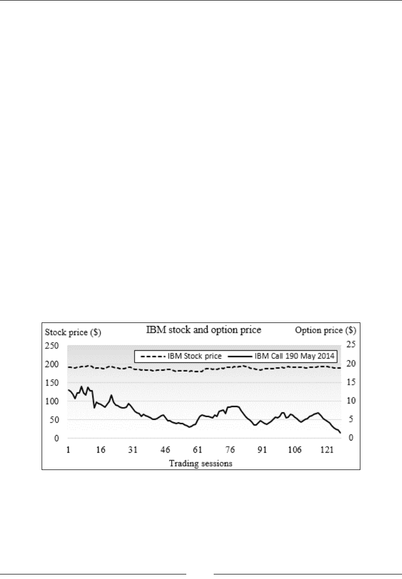
Reinforcement Learning
[ 984 ]
The prediction ends when no more states are available or the maximum number of
iterations within the episode is exceeded. You can dene a more sophisticated exit
condition. The challenge is that there is no explicit error or loss variable/function
that can be used except the temporal difference error. The prediction returns either
the best possible state, or None if the model cannot be created during training.
Option trading using Q-learning
The Q-learning algorithm is used in many nancial and market trading applications
[11:6]. Let us consider the problem of computing the best strategy to trade certain
types of options given some market conditions and trading data.
The Chicago Board Options Exchange (CBOE) offers an excellent online tutorial
on options [11:7]. An option is a contract giving the buyer the right but not the
obligation to buy or sell an underlying asset at a specic price on or before a certain
date (refer to the Options trading section under Finances 101 in Appendix A, Basic
Concepts.) There are several option pricing models, the Black-Scholes stochastic
partial differential equations being the most recognized [11:8].
The purpose of the exercise is to predict the price of an option on a security for N
days in the future according to the current set of observed features derived from the
time to expiration, price of the security, and volatility. Let's focus on the call options
of a given security, IBM. The following chart plots the daily price of IBM stock and
its derivative call option for May 2014 with a strike price of $190:
The price of an option depends on the following parameters:
• Time to expiration of the option (time decay)
• The price of the underlying security
• The volatility of returns of the underlying asset
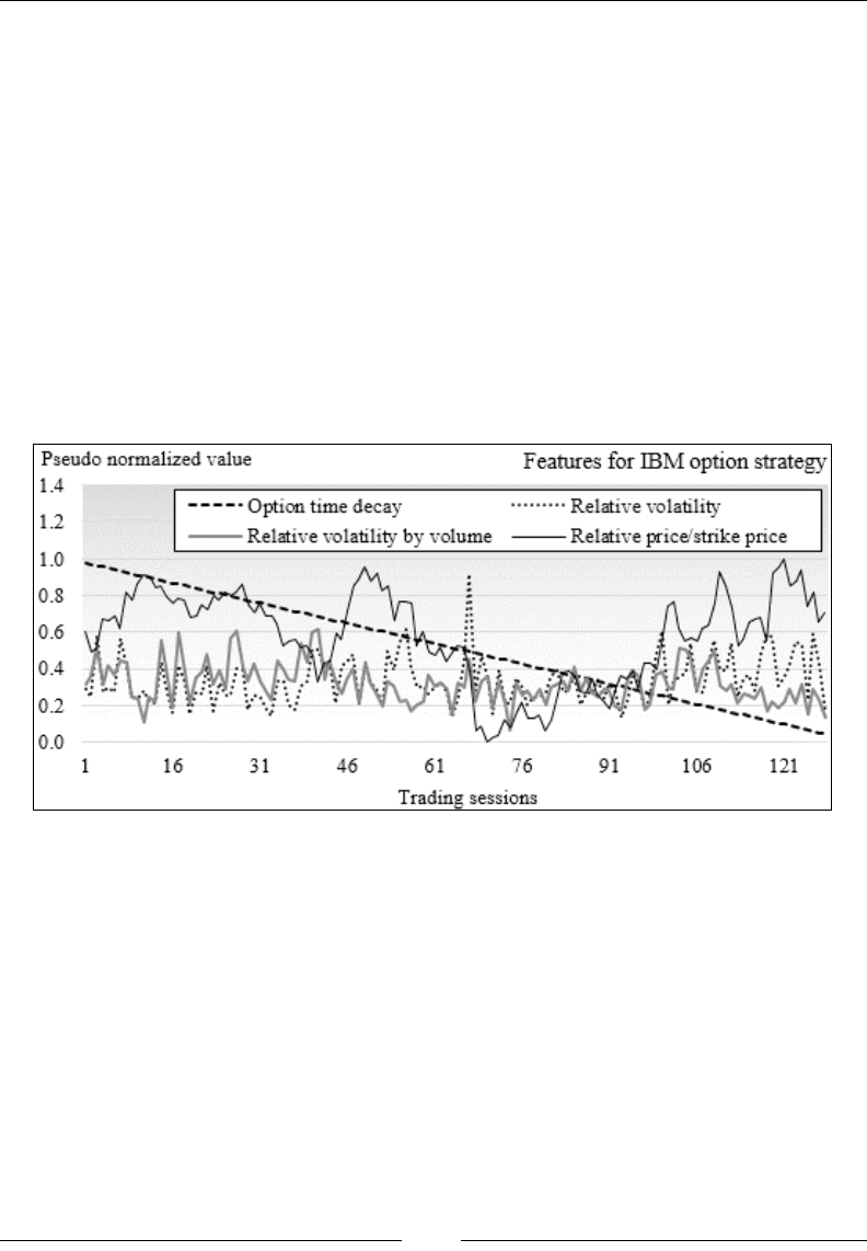
Chapter 11
[ 985 ]
Pricing model usually does not take into account the variation in trading volume of
the underlying security. So it would be quite interesting to include it in our model.
Let us dene the state of an option using the following four normalized features:
• Time decay: This is the time to expiration once normalized over [0, 1].
• Relative volatility: This is the relative variation of the price of the underlying
security within a trading session. It is different from the more complex
volatility of returns dened in the Black-Scholes model, for example.
• Volatility relative to volume: This is the relative volatility of the price of the
security adjusted for its trading volume.
• Relative difference between the current price and strike price: This measures
the ratio of the difference between price and strike price to the strike price.
The following graph shows the four normalized features for IBM option strategy:
The implementation of the option trading strategy using Q-learning consists of the
following steps:
1. Describing the property of an option
2. Dening the function approximation
3. Specifying the constraints on the state transition
Option property
Let us select N =2 as the number of days in the future for our prediction. Any
longer-term prediction is quite unreliable because it falls outside the constraint
of the discrete Markov model. Therefore, the price of the option two days in the
future is the value of the reward—prot or loss.

Reinforcement Learning
[ 986 ]
The OptionProperty class encapsulates the four attributes of an option as follows:
class OptionProperty(timeToExp: Double, relVolatility: Double,
volatilityByVol: Double, relPriceToStrike: Double) {
val toArray = Array[Double](timeToExp, relVolatility,
volatilityByVol, relPriceToStrike)
}
Modular design
The implementation avoids subclassing the QLState class to
dene the features of our option pricing model. The state of the
option is a parameterized prop parameter for the state class.
Option model
The OptionModel class is a container and a factory for the properties of the option.
It creates the list of option properties, propsList, by accessing the data source of the
four features introduced earlier. It takes the following parameters:
• The symbol of the security.
• The strike price for the option, strikePrice.
• The source of data, src.
• The minimum time decay or time to expiration, minTDecay. Out-of-the-money
options expire worthless and in-the-money options have very different price
behavior as they get closer to the expiration date (refer to the Options trading
section in Appendix A, Basic Concepts). Therefore, the last minTDecay trading
sessions prior to the expiration date are not used in the training of the model.
• The number of steps (or buckets), nSteps, used in approximating the values
of each feature. For instance, an approximation of four steps creates four
buckets [0, 25], [25, 50], ]50, 75], and [75, 100].
The implementation of the OptionModel class is as follows:
class OptionModel(symbol: String, strikePrice: Double, src:
DataSource, minExpT: Int, nSteps: Int) {
val propsList = {
val volatility = normalize((src |> relVolatility).get.toArray
val rVolByVol = normalize((src |> volatilityByVol).get.toArray
val priceToStrike = normalize(price.map(p => 1.0-strikePrice/p)
volatility.zipWithIndex //1
.foldLeft(List[OptionProperty]())((xs, e) => {
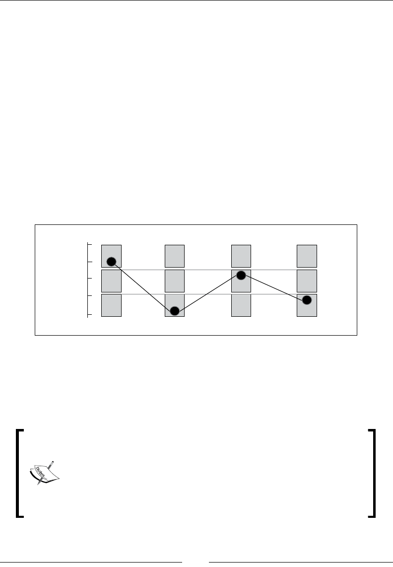
Chapter 11
[ 987 ]
val normDecay = (e._2+minExpT).toDouble/(price.size+minExpT) //2
new OptionProperty(normDecay, e._1, volByVol(e._2),priceToStrik
e(e._2)) :: xs
}).drop(2).reverse
}
The factory uses the zipWithIndex Scala method to model the index of the trading
sessions (line 1). All feature values are normalized over the interval [0, 1], including
the time decay (or time to expiration) of the normDecay option (line 2).
Function approximation
The four properties of the option are continuous values, normalized as a probability
[0, 1]. The states in the Q-learning algorithm are discrete and require a discretization
or categorization known as a function approximation, although a function
approximation scheme can be quite elaborate [11:9]. Let us settle for a simple linear
categorization as illustrated in the following diagram:
Option property (2,0,1,0)
Normalized
value
Bucket
timeToEXP relVolatility volatilityByVol relPriceToStrike
1
0
The function approximation denes the number of states. In this example, a function
approximation that converts a normalized value into three intervals or buckets
generates 34 = 81 states or potentially 38-34 = 6480 actions! The maximum number
of states for l buckets function approximation and n features is ln with a maximum
number of l2n-ln actions.
Function approximation guidelines
The design of the function to approximate the state of options has to
address the following two conicting requirements:
• Accuracy demands a fine-grained approximation
• Limited computation resources restrict the number of states,
and therefore, level of approximation

Reinforcement Learning
[ 988 ]
The approximate method of the OptionModel class converts the normalized value of
each option property of features into an array of bucket indices. It returns a map of
prot and loss for each bucket keyed on the array of bucket indices, as shown in the
following code:
def approximate(y: DblVector): Map[Array[Int], Double] = {
val mapper = new HashMap[Int, Array[Int]] //1
val acc = new NumericAccumulator //2
propsList.map( _.toArray)
.map( toArrayInt( _ )) //3
.map(ar => {
val enc = encode(ar) //4
mapper.put(enc, ar)
enc })
.zip(y)
.foldLeft(acc)((acc,t) => {acc += (t._1,t._2);acc})//5
acc.map(kv => (kv._1, kv._2._2/kv._2._1)) //6
.map(kv => (mapper(kv._1), kv._2)).toMap
}
The method creates a mapper instance to index the array of buckets (line 1). An
accumulator, acc, of type NumericAccumulator extends Map[Int, (Int, Double)]
and computes the tuple (number of occurrences of features on each buckets, the sum
of increase or decrease of the option price) (line 2). The toArrayInt method converts
the value of each option property (timeToExp, relVolatility, and so on) into the
index of the appropriate bucket (line 3). The array of indices is then encoded (line
4) to generate the id or index of a state. The method updates the accumulator with
the number of occurrences and the total prot and loss for a trading session for the
option (line 5). It nally computes the reward on each action by averaging the prot
and loss on each bucket (line 6).
def toArrayInt(feature: DblVector): Array[Int] =
feature.map(x => (nSteps*x).floor.toInt)
Constrained state-transition
Each state is potentially connected to any other state through actions. There are two
methodologies to reduce search space or number of actions/transitions:
• Static constraint denes the actions/transition when the model is instantiated.
The state transition map is xed for the entire life cycle of the model.
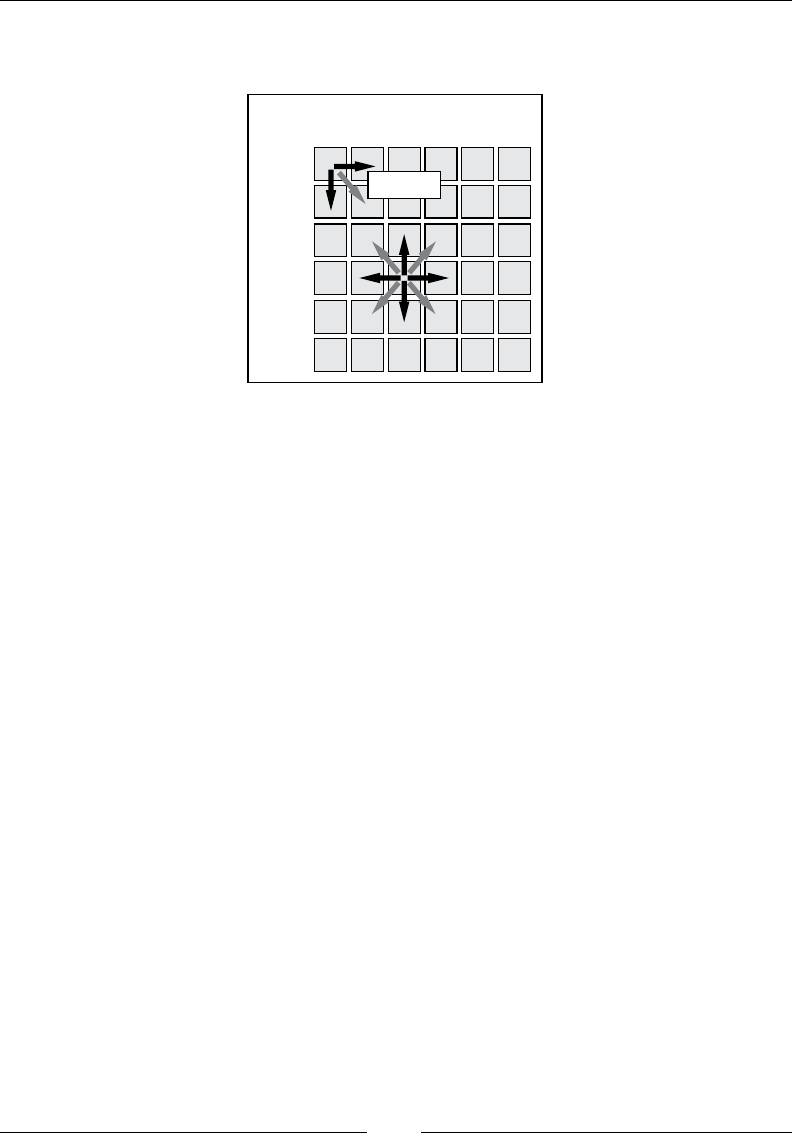
Chapter 11
[ 989 ]
• Dynamic constraint relies on the probability of an action to prevent or hinder
state transitions.
States
S1
Sn-1
States
Sn-1
S0
S0
S1
Actions
The implementation of the static constraint avoids the unnecessary creation of a large
number of QLAction object at the expense of the inability to modify the search space
during training. The test case uses the static constraint as dened in the neighbors
function passed as a parameter of the QLSpace class:
val RADIUS = 4
val neighbors = (idx: Int, numStates: Int) => {
def getProximity(idx: Int, radius: Int): List[Int] = {
val idx_max = if(idx + radius >= numStates) numStates-1 else idx+
radius
val idx_min = if(idx < radius) 0 else idx - radius
Range(idx_min, idx_max+1).filter( _ != idx)
.foldLeft(List[Int]())((xs, n) => n :: xs)
}
getProximity(idx, RADIUS).toList
}
The neighbors function restrains the number of actions to up to RADIUS*2 states,
depending on the ID, idx, of the state. The function is implemented as a closure: it
requires the value numStates to be dened within the function or in its outer scope.
Putting it all together
The nal piece of the puzzle is the code that congures and executes the Q-learning
algorithm on one or several options on a security, IBM:
val stockPricePath = "resources/data/chap11/IBM.csv"
val optionPricePath = "resources/data/chap11/IBM_O.csv"

Reinforcement Learning
[ 990 ]
val MIN_TIME_EXP = 6; val APPROX_STEP = 3; val NUM_FEATURES = 4
val ALPHA = 0.4; val DISCOUNT = 0.6; val NUM_EPISODES = 202520
val src = DataSource(stockPricePath, false, false, 1) //1
val ibmOption = new OptionModel("IBM", 190.0, src, MIN_TIME_EXP,
APPROX_STEP) //2
DataSource(optionPricePath, false, false, 1) extract match {
case Some(v) => initializeModel (ibmOption, v)
…
}
The client code instantiates the option model, ibmOption, for the IBM stock
(line 1). It invokes the initializeModel method once the historical price of
the option is downloaded through the appropriate data source (line 2). The
initializeModel method does all the work as shown in the following code:
def initializeModel(ibmOption: OptionModel, oPrice: DblVector):
QLearning[Array[Int]] {
val fMap = ibmOption.approximate(oPrice) //3
val input = new ArrayBuffer[QLInput]
val profits = fMap.values.zipWithIndex
profits.foreach(v1 =>
profits.foreach( v2 =>
input.append(new QLInput(v1._2, v2._2, v2._1-v1._1))))//4
val goal = input.maxBy( _.reward).to
val config = new QLConfig(ALPHA, DISCOUNT, EPISODE_LEN, NUM_
EPISODES, MIN_ACCURACY, getNeighbors)
QLearning[Array[Int]](config, fMap , goal, input.toArray, fMap.
keySet)
}
The initializeModel method generates the approximation map, fMap (line 3),
which contains the prot and loss for each state. Next, the method initializes the
input to the policy by computing the reward as the difference of the prot/loss of
the source v1 and the destination v2 of each action (line 4). The goal is initialized as
the action with the highest reward (line 5). The last step is the instantiation of the
QLearning class that executes the training.
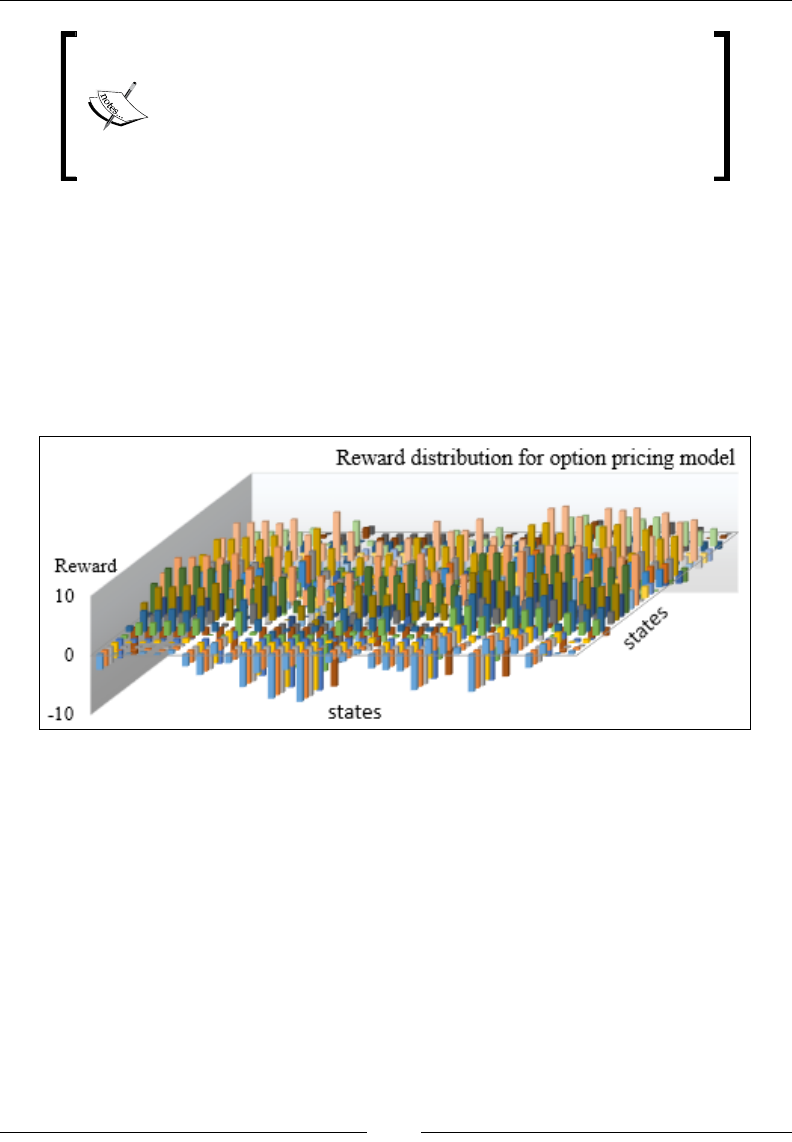
Chapter 11
[ 991 ]
The anti-goal state
The goal state is the state with the highest assigned reward.
It is a heuristic to reward a strategy for good performance.
However, it is conceivable and possible to dene an anti-goal
state with the highest assigned penalty or the lowest assigned
reward to guide the search away from some condition.
Evaluation
Besides the function approximation, the size of the training set has an impact on the
number of states. A well-distributed or large training set provides at least one value for
each bucket created by the approximation. In this case, the training set is quite small
and only 34 out of 81 buckets have actual values. As result, the number of states is 34.
The initialization of the Q-learning model generates the following reward matrix:
The graph visualizes the distribution of the rewards computed from the prot and
loss of the option. The xy plane represents the actions between states. The states'
IDs are listed on x and y axes. The z-axis measures the actual value of the reward
associated with each action.
The reward reects the uctuation in the price of the option. The price of an option
has a higher volatility than the price of the underlying security.
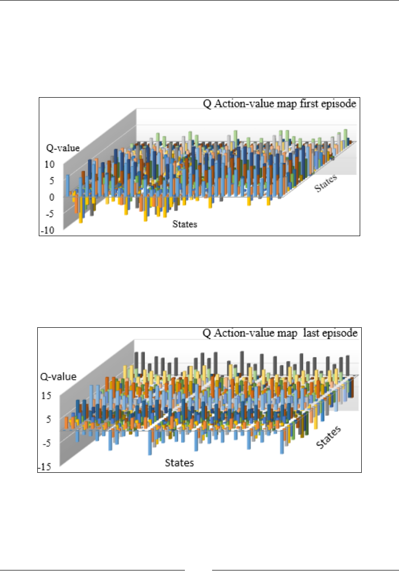
Reinforcement Learning
[ 992 ]
The xy reward matrix R is rather highly distributed. Therefore, we select a small
value for the learning rate, 0.4, to reduce the impact of the previous state on the
new state. The value for the discount rate, 0.6, accommodates the fact that the
number of states is limited. There is no reason to compute the future discounted
reward using a long sequence of states. The training of the policies generates the
following action-value matrix Q of 34 states by 34 states after the rst episode:
The distribution of the action-values between states at the end of the rst episode
reects the distribution of the reward across state-to-state action. The rst episode
consists of a sequence of nine states from an initial randomly selected state to
the goal state. The action-value map is compared with the map generated after
20 episodes in the following graph:

Chapter 11
[ 993 ]
The action-value map at the end of the last episode shows some clear patterns. Most
of the rewarding actions transition from a large number of states (X-axis) to a smaller
number of states (Y-axis). The chart illustrates the following issues with the small
training sample:
• The small size of the training set forces us to use an approximate
representation of each feature. The purpose is to increase the odds that most
buckets have at least one data point.
• However, a loose function approximation tends to group quite different
states into the same bucket.
• The bucket with a very low number can potentially mischaracterize one
property or feature of a state.
Pros and cons of reinforcement learning
Reinforcement learning algorithms are ideal for the following problems:
• Online learning
• The training data is small or non-existent
• A model is non-existent or poorly dened
• Computation resources are limited
However, these techniques perform poorly in the following cases:
• The search space (number of possible actions) is large causing the maintenance
of the states, action graph, and rewards matrix become challenging
• The execution is not always predictable in terms of scalability and performance
Learning classier systems
J. Holland introduced the concept of learning classier systems (LCS) more than 30
years ago as an extension to evolutionary computing [11:10]:
Learning classier systems are a kind of rule-based system with general
mechanisms for processing rules in parallel, for adaptive generation of new rules,
and for testing the effectiveness of new rules.
However, the concept started to get the attention of computer scientists only a few
years ago, with the introduction of several variants of the original concept, including
extended learning classier systems (XCS). Learning classier systems are interesting
because they combine rules, reinforcement learning, and genetic algorithms.
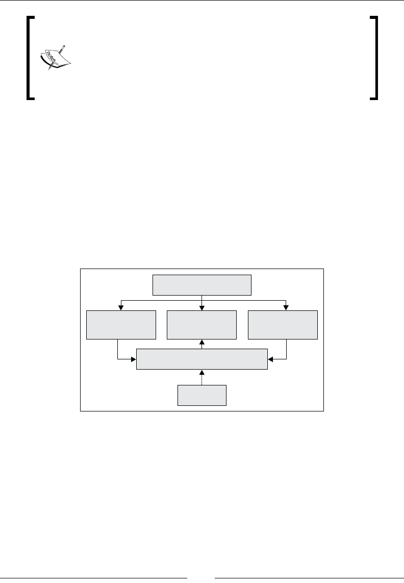
Reinforcement Learning
[ 994 ]
Disclaimer
The implementation of the extended learning classier is
presented for informational purposes only. Validating XCS
against a known and labeled population of rules is a very
signicant endeavor. The source code snippet is presented only
to illustrate the different components of the XCS algorithm.
Introduction to LCS
Learning classier systems merge the concepts of reinforcement learning, rule-based
policies, and evolutionary computing. This unique class of learning algorithms
represents the merger of the following research elds [11:11]:
• Reinforcement learning
• Genetic algorithms and evolutionary computing
• Supervised learning
• Rule-based knowledge encoding
Rules
Evolutionary
Computing
Reinforcement
Learning
Supervised
Learning
Machine Learning
Learning Classifier Systems
Diagram of the scientific disciplines required for learning classifier systems
Learning classier systems are an example of complex adaptive systems. A learning
classier system has the following four components:
• A population of classiers or rules that evolves over time. In some cases,
a domain expert creates a primitive set of rules (core knowledge). In other
cases, the rules are randomly generated prior to the execution of the learning
classier system.

Chapter 11
[ 995 ]
• A genetic algorithm-based discovery engine that generates new classiers
or rules from the existing population. This component is also known as the
rules discovery module. The rules rely on the same pattern of evolution
of organisms introduced in the previous chapter. The rules are encoded as
strings or bit strings to represent a condition (predicate) and action.
• A performance or evaluation function that measures the positive or negative
impact of the actions from the ttest classiers or policies.
• A reinforcement learning component that rewards or punishes the classiers
that contribute to the action, as seen in the previous section. The rules that
contribute to an action that improves the performance of the system are
rewarded, while those that degrade the performance of the system are
punished. This component is also known as the credit assignment module.
Why LCS
Learning classier systems are particularly appropriate to problems in which the
environment is constantly changing, and are the combination of learning strategy
and an evolutionary approach to build and maintain a knowledge base [11:12].
Supervised learning methods alone can be effective on large datasets, but they
require either a signicant amount of labeled data or a reduced set of features
to avoid overtting. Such constraints may not be practical in the case of
ever-changing environments.
The last 20 years have seen the introduction of many variants of learning classier
systems that belong to the following two categories:
• Systems for which accuracy is computed from the correct predictions and
that apply the discovery to a subset of those correct classes. They incorporate
elements of supervised learning to constrain the population of classiers.
These systems are known to follow the Pittsburgh approach.
• Systems that explore all the classiers and apply rule accuracy in the genetic
selection of the rules. Each individual classier is a rule. These systems are
known to follow the Michigan approach.
The rest of this section is dedicated to the second type of learning classiers—more
specically extended learning classier systems. In a context of LCS, the term
classier refers to the predicate or rule generated by the system. From this point on,
the term "rule" replaces the term classier to avoid confusion with the more common
denition of classication.

Reinforcement Learning
[ 996 ]
Terminology
Each domain of research has its own terminology and LCS is no exception.
The terminology of LCS consists of the following terms:
• Environment: Environment variables in the context of reinforcement learning.
• Agent: An agent used in reinforcement learning.
• Predicate: A clause or fact using the format: variable- operator- value,
and usually implemented as (operator, variable value); for example,
Temperature- exceeds - 87F or ('Temperature', 87F), Hard drive – failed or
('Status hard drive', FAILED), and so on. It is encoded as a gene in order
to be processed by the genetic algorithm.
• Compound predicate: Composition of several predicates and Boolean logic
operators, which is usually implemented as a logical tree (for example,
((predicate1 AND predicate2) OR predicate3 is implemented as OR (AND
(predicated 1, predicate 2), predicate3). It uses a chromosome representation.
• Action: A mechanism that alters the environment by modifying the value
of one or several of its parameters using a format (type of action, target),
for example, change thermostat settings, replace hard drive, and so on.
• Rule: A formal rst-order logic formula using the format IF compound
predicate THEN sequence of action, for example, IF gold price < $1140 THEN
sell stock of oil and gas producing companies.
• Classier: A rule in the context of an LCS.
• Rule tness or score: This is identical to the denition of the tness or score
in the genetic algorithm. In the context of an LCS, it is the probability of a
rule to be invoked and red in response of change in environment.
• Sensors: Environment variables monitored by agent, for example,
temperature and hard drive status.
• Input data stream: Flow of data generated by sensors. It is usually associated
with online training.
• Rule matching: Mechanism to match a predicate or compound predicate
with a sensor.
• Covering: The process of creating new rules to match a new condition
(sensor) in the environment. It generates the rules by either using a random
generator or mutating existing rules.
• Predictor: An algorithm to nd the action with the maximum number of
occurrences within a set of matching rules.
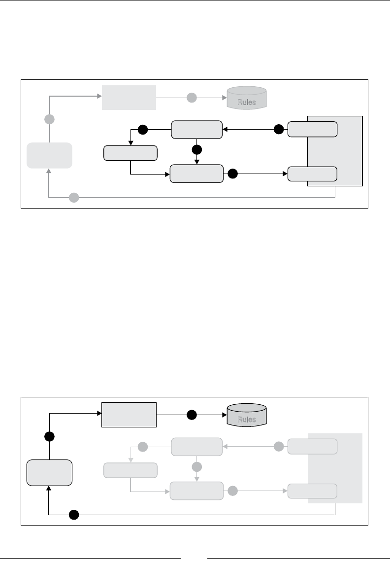
Chapter 11
[ 997 ]
Extended learning classier systems (XCS)
Similar to reinforcement learning, the XCS algorithm has an exploration phase and
an exploitation phase. The exploitation process consists of leveraging the existing
rules to inuence the target environment in a protable or rewarding manner.
Reward
Update
Fitness New rule
Feedback
Genetic
Algorithm
Evolution
Matching Data
stream
Predictor
Environment
Rules
Sensor
Action
5
6
1
2
4
3
7
Exploitation component of the XCS algorithm
The following list describes each numbered block:
• 1: Sensors acquire new data or events from the system.
• 2: Rules for which the condition matches the input event are searched and
extracted from the current population.
• 3: A new rule is created if no match is found in the existing population.
This process is known as covering.
• 4: The chosen rules are ranked by their tness values, and the rules with
the highest predicted outcome are used to trigger the action.
The purpose of exploration components is to increase the rule base as a population
of the chromosomes that encode these rules.
Reward
Updated
Fitness New rule
Feedback
Genetic
Algorithm
Evolution
Matching Data
stream
Predictor
Environment
Rules
Sensor
Action
5
6
1
2
4
3
7
Exploration components of the XCS algorithm

Reinforcement Learning
[ 998 ]
The following list describes each numbered block of the block diagram:
• 5: Once the action is performed, the system rewards the rules for which the
action has been executed. The reinforcement learning module assigns credit
to these rules.
• 6: Rewards are used to update the rule tness, applying evolutionary
constraints to the existing population.
• 7: The genetic algorithm updates the existing population of classiers/rules
using operators such as crossover and mutation.
XCS components
This section describes the key classes of the XCS. The implementation leverages
the existing design of the genetic algorithm and the reinforcement learning.
It is easier to understand the inner workings of the XCS algorithm with a
concrete application.
Application to portfolio management
Portfolio management and trading have beneted from the application of extended
learning classiers [11:13]. The use case is the management of a portfolio of
exchange-traded funds (ETFs) in an ever-changing nancial environment. Contrary
to stocks, exchange traded funds are representative of an industry-specic group of
stocks or the nancial market at large. Therefore, the price of these ETFs is affected
by the following macroeconomic changes:
• Gross domestic product
• Ination
• Geopolitical events
• Interest rates
Let's select the value of the 10-year Treasury yield as a proxy for the macroeconomic
conditions, for the sake of simplicity.

Chapter 11
[ 999 ]
The portfolio has to be constantly adjusted in response to any specic change in the
environment or market condition that affects the total value of the portfolio, and can
be done referring to the following table:
XCS component Portfolio management
Environment Portfolio of securities defined by its composition, total value,
and the yield of the 10-year Treasury bond
Action Change in the composition of the portfolio
Reward Profit and loss of the total value of the portfolio
Input data stream Feed of stock and bond price quotation
Sensor Trading information regarding securities in the portfolio such
as price, volume, volatility, or yield, and the yield on the-10
year Treasury bond
Predicate Change in composition of the portfolio
Action Rebalancing a portfolio by buying and selling securities
Rule Association of trading data with the rebalancing of a portfolio
The rst step is to create an initial set of rules regarding the portfolio. This initial set
can be created randomly, much like the initial population of a genetic algorithm, or
be dened by a domain expert.
The XCS initial population
Rules or classiers are dened and/or rened through evolution.
Therefore, there is no absolute requirement for the domain expert
to set up a comprehensive knowledge base. In fact, rules can be
randomly generated at the start of the training phase. However,
seeding the XCS initial population with a few relevant rules
improves the odds of having the algorithm converge quickly.
The reader is invited to initialize the population of rules with as many relevant
and nancially sound trading rules as possible. Over time, the execution of the
XCS algorithm will conrm whether or not the initial rules are indeed appropriate.
The following diagram describes the application of the XCS algorithm to the
composition of a portfolio of ETFs, such as VWO, TLT, IWC, and so on, with the
following components:
• The population of trading rules
• An algorithm to match rules and compute the prediction
• An algorithm to extract the actions sets
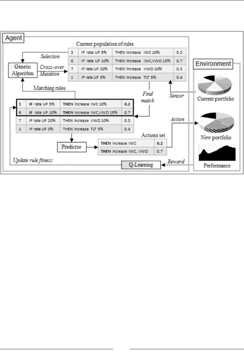
Reinforcement Learning
[ 1000 ]
• The Q-learning module to assign credit or reward to the selected rules
• The genetic algorithm to evolve the population of rules
Overview of XCS algorithm to optimize portfolio allocation
The agent responds to the change in the allocation of ETFs in the portfolio by
matching one of the existing rules.
Let's build the XCS agent from the ground.
XCS core data
There are three types of data that are manipulated by the XCS agent:
• Signal: This is the trading signal
• XcsAction: This is the action on the environment
• XcsSensor: This is the sensor or data from the environment
The XcsAction class was introduced for the evaluation of the genetic algorithm
in the Trading signals section in Chapter 10, Genetic Algorithms. The agent creates,
modies, and deletes actions. It makes sense to dene these actions as mutable
genes, as follows:
class XcsAction(val sensorid: String, val target: Double)(implicit val
discr: Discretization) extends Gene(sensorid, target, EQUAL)

Chapter 11
[ 1001 ]
The XcsAction class has the identier of the sensor, sensorId, and the target value
as parameters. For example, the action to increase the number of shares of ETF, VWO
in the portfolio to 80 is denes as follows:
Val vwoTo80 = new XcsAction("VWO", 80.0)
The only type of action allowed in this scheme is setting a value using the EQUAL
operator. You can create actions that support other operators, such as += used to
increase an existing value. These operators need to implement the operator trait,
explained in the Trading operators section in Chapter 10, Genetic Algorithms.
A discretization instance has to be implicitly dened in order to encode the
target value.
Finally, the XcsSensor class encapsulates the sensorId identier for the variable
and value of the sensor, as shown here:
case class XcsSensor(val sensorId: String, val value: Double)
val new10ytb = new XcsSensor("10yTBYield", 2.76)
Setters and getters
In this simplistic scenario, the sensors retrieve a new value
from an environment variable. The action sets a new value to
an environment variable. You can think of a sensor as a get
method of an environment class and an action as a set method
with variable/sensor ID and value as arguments.
XCS rules
The next step consists of dening a rule as a pair of two genes: a signal and an action,
as shown in the following code:
class XcsRule(val signal: Signal, val action: XcsAction)
The rule: r1: IF(yield 10-year TB > 2.84%) THEN reduce VWO shares to 240 is
implemented as follows:
val signal = new Signal("10ytb", 2.84, GREATER_THAN)
val action = new XcsAction("vwo", 240)
val r1 = new XcsRule(signal, action)
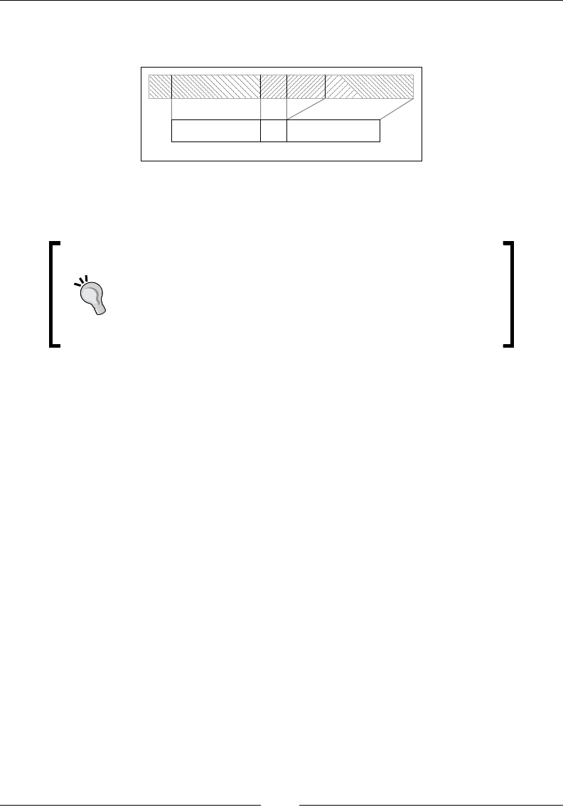
Reinforcement Learning
[ 1002 ]
The agent encodes the rule as a chromosome using 2 bits to represent the operator
and 32 bits for values, as shown in the following diagram:
10010...1010 01 001110...0110
032
>
34 65
2.85 vwo 240
rl
In this implementation, there is no need to encode the type of action as the agent uses
only one type of action—set. A complex action requires encoding of its type.
Knowledge encoding
This example uses very simple rules with a single predicate
as the condition. Real-world domain knowledge is usually
encoded using complex rules with multiple clauses. It is
highly recommended that you break down complex rules
into multiple basic rules of classiers.
Matching a rule to a new sensor consists of matching the sensor to the signal.
The algorithm matches the new new10ytb sensor against the signal in the current
population of s10ytb1 and s10ytb2 rules that uses the same sensor or variable
10ytb, as follows:
val new10ytb = new XcsSensor("10ytb", 2.76)
val s10ytb1 = Signal("10ytb", 2.5, GREATER_THAN)
val s10ytb2 = Signal("10ytb", 2.2, LESS_THAN)
val r23: XcsRule(s10ytb1, act12)
val r34: XcsRule(s10ytb2, act17)
…
In this case, the agent selects the rule r23 but not r34 in the existing population. The
agent then adds the act12 action to the list of possible actions. The agent lists all the
rules that match the sensor: r23, r11, and r46, as shown in the following code:
val r23: XcsRule(s10yTB1, act12)
val r11: XcsRule(s10yTB6, act6)
val r46: XcsRule(s10yTB7, act12)

Chapter 11
[ 1003 ]
The action with the most references, act12, is executed. The Q-learning algorithm
computes the reward from the prot or loss incurred by the portfolio following the
execution of the selected rules r23 and r46. The agent uses the reward to adjust the
tness of r23 and r46, before the genetic selection in the next reproduction cycle.
These two rules will reach and stay in the top tier of the rules in the population, until
either a new genetic rule modied through crossover and mutation or a rule created
through covering, triggers a more rewarding action on the environment.
Covering
The purpose of the covering phase is to generate new rules if no rule matches the
input or sensor. The cover method of an XcsCover singleton generates a new
XcsRule instance given a sensor and an existing set of actions, as shown here:
def cover(sensor: XcsSensor, actions: List[XcsAction]) (implicit
discr: Discretization): List[XcsRule] = {
actions.foldLeft(List[XcsRule]()) ((xs, act) => {
val rIdx = Random.nextInt(Signal.numOperators)
val signal = new Signal(sensor.id, sensor.value, new
SOperator(rIdx))
new XcsRule(signal, XcsAction(act, Random)) :: xs
})
}
You might wonder why the cover method uses a set of actions as arguments knowing
that covering consists of creating new actions. The method mutates (operator ^) an
existing action to create a new one instead of using a random generator. This is one of
the advantages of dening an action as a gene. The mutation is executed by one of the
constructors of XcsAction, as follows:
def apply(action: XcsAction, r: Random): XcsAction =
(action ^ r.nextInt(XCSACTION_SIZE))
The index of the operator type, rIdx, is a random value in the interval [0, 3] because
a signal uses four types of operators: None, >, <, and =.
Example of implementation
The Xcs class has the following purposes:
• gaSolver: This is the selection and generation of genetically modied rules
• qlLearner: This is the rewarding and scoring the rules

Reinforcement Learning
[ 1004 ]
• Xcs: These are the rules for matching, covering, and generation of action
class Xcs(config: XcsConfig, population: Population[Signal],
score: Chromosome[Signal]=> Unit, input: Array[QLInput]) extends
PipeOperator[XcsSensor, List[XcsAction]] {
val gaSolver = GASolver[Signal](config.gaConfig, score)
val featuresSet: Set[Chromosome[Signal]] = population.
chromosomes.toSet
val qLearner = QLearning[Chromosome[Signal]](config.qlConfig,
computeNumStates(input), extractGoals(input), input, featuresSet)
…
}
The XCS algorithm is initialized with a conguration, config, an initial set of rules,
population, a tness function, score, and an input to the Q-learning policy generate
reward matrix for qlLearner. The goals and number of states are extracted from the
input to the policy of the Q-learning algorithm.
In this implementation, the generic algorithm, gaSolver, is mutable. It is instantiated
along with the Xcs container class. The Q-learning algorithm uses the same design,
as any classier, as immutable. The model of Q-learning is the best possible policy to
reward rules. Any changes in the number of states or the rewarding scheme require a
new instance of the learner.
Benets and limitation of learning
classier systems
Learning classier systems and XCS in particular, hold many promises, which are
as follows:
• They allow non-scientists and domain experts to describe the knowledge
using familiar Boolean constructs and inferences such as predicates and rules
• They provide analysts with an overview of the knowledge base and its
coverage by distinguishing between the need for exploration and exploitation
of the knowledge base

Chapter 11
[ 1005 ]
However, the scientic community has been slow to recognize the merits of these
techniques. The wider adoption of learning classier systems is hindered by the
following factors:
• Sheer complexity of the conguration of the algorithm because of the large
number of parameters for exploration and exploitation.
• Lack of a unied theory to validate the concept of evolutionary policies or
rules. After all, these algorithms are the merger of standalone techniques.
The accuracy and performance of the execution of LCSes depend on each
component as well as the interaction between components.
• An execution that is not always predictable in terms of scalability
and performance.
• Too many variants of LCS.
Summary
Reinforcement learning algorithms are sometimes overlooked by the software
engineering community. Let's hope that this chapter provides adequate answers
to the following questions:
• What is reinforcement learning?
• What are the different the different types of algorithms that qualify as
reinforcement learning?
• How can we implement the Q-learning algorithm in Scala?
• How can we apply Q-learning to the optimization of option trading?
• What are the pros and cons of using reinforcement learning?
• What are learning classier systems?
• What are the key components of the XCS algorithm?
• What are the potentials and limitations of learning classier systems?
This concludes the introduction of the last category of learning techniques. The
ever-increasing amount of data that surrounds us requires data processing and
machine learning algorithms to be highly scalable. This is the subject of the next
and the nal chapter.

Scalable Frameworks
The advent of social networking, interactive media, and deep analysis has caused
the amount of data processed daily to skyrocket. For data scientists, it's no longer
just a matter of nding the most appropriate and accurate algorithm to mine data;
it is also about leveraging multi-core CPU architectures and distributed computing
frameworks to solve problems in a timely fashion. After all, how valuable is a data
mining application if the model does not scale?
There are many options available to Scala developers to build classication and
regression applications for very large datasets. This chapter covers the Scala parallel
collections, Actor model, Akka framework, and Apache Spark in-memory clusters.
The following are the topics addressed in this chapter:
• Introduction to Scala parallel collections
• Evaluation of performance of a parallel collection on multicore CPU
• The actor model and reactive systems.
• Clustered and reliable distributed computing using Akka
• Design of computational workow using Akka routers
• Introduction to Apache Spark clustering and its design principles
• Using Spark MLlib for clustering
• Relative performance tuning and evaluation of Spark
• Benets and limitations of the Apache Spark framework

Scalable Frameworks
[ 1008 ]
Overview
The support for distributing and concurrent processing is provided by different
stacked frameworks and libraries. Scala concurrent and parallel collections classes
leverage the threading capabilities of the Java virtual machine. Akka.io implements
a reliable action model originally introduced as part of the Scala standard library.
The Akka framework supports remote actors, routing, and load balancing protocol;
dispatchers, clusters, events, and congurable mailboxes management; and support
for different transport modes, supervisory strategies and typed actors. Apache
Spark's resilient distributed datasets with advanced serialization, caching, and
partitioning capabilities leverage Scala and Akka libraries.
The following stack representation illustrates the interdependencies between
frameworks:
Partitioner, Accumulator: org.apache.spark
Broadcast: org.apache.spark.broadcast
Resilient datasets: org.apache.spark.rdd
Caching: org.apache.spark
Listeners: org.apache.spark.scheduler._
Serialization: org.apache.spark.serializer
Spark
Scheduler: scala.actors.scheduler
Concurrency: scala.concurrent
Parallel collections: scala.collection.parallel
Scala
Threads, executors: java.util.concurrent*
Actors, Supervisors: akka.actors._
Remote actors: akka.remote
Type actors: akka.actors._
Mailbox management: akka.mailbox._
Clusters: akka.cluster._
Dispatchers: akka.dispatch
Events management: akka.event._
Routing, Broadcast: akka.routing
Persistency: akka.persistence._
Akka
Stack representation of Scalable frameworks using Scala
Each layer adds a new functionality to the previous one to increase scalability.
The Java virtual machine runs as a process within a single host. Scala concurrent
classes support effective deployment of an application by leveraging multicore CPU
capabilities without the need to write multithreaded applications. Akka extends
the Actor paradigm to clusters with advanced messaging and routing options.
Finally, Apache Spark leverages Scala higher-order collection methods and the Akka
implementation of the Actor model to provide large-scale data processing systems
with better performance and reliability, through its resilient distributed datasets and
in-memory persistency.

Chapter 12
[ 1009 ]
Scala
The Scala standard library offers a rich set of tools, such as parallel collections and
concurrent classes to scale number-crunching applications. Although these tools are
very effective in processing medium-sized datasets, they are unfortunately quite
often discarded by developers in favor of more elaborate frameworks.
Controlling object creation
Although code optimization and memory management is beyond the scope of
this chapter, it is worthwhile to remember that a few simple steps can be taken to
improve the scalability of an application. One of the most frustrating challenges in
using Scala to process large datasets is the creation of a large number of objects and
the load on the garbage collector.
A partial list of remedial actions is as follows:
• Limiting unnecessary duplication of objects in an iterated function by using a
mutable instance
• Using lazy values and Stream classes to create objects as needed
• Leveraging efcient collections such as bloom lters or skip lists
• Running javap to decipher the generation of byte code by the JVM
Parallel collections
The Scala standard library includes parallelized collections, whose purpose is to
shield developers from the intricacies of concurrent thread execution and race
condition. Parallel collections are a very convenient approach to encapsulate
concurrency constructs to a higher level of abstraction [12:1].
There are two ways to create parallel collections in Scala:
• Converting an existing collection into a parallel collection of the same
semantic using the par method, for example, List[T].par: ParSeq[T],
Array[T].par: ParArray[T], Map[K,V].par: ParMap[K,V], and so on
• Using the collections classes from the collection.parallel, parallel.
immutable, or parallel.mutable packages, for example, ParArray, ParMap,
ParSeq, ParVector, and so on

Scalable Frameworks
[ 1010 ]
Processing a parallel collection
A parallel collection does lend itself to concurrent processing until a pool of threads
and a tasks scheduler are assigned to it. Fortunately, Scala parallel and concurrent
packages provide developers with a powerful toolbox to map partitions or segments
of collection to tasks running on different CPU cores. The components are as follows:
• TaskSupport: This trait inherits the generic Tasks trait. It is responsible for
scheduling the operation on the parallel collection. There are three concrete
implementations of TaskSupport.
• ThreadPoolTaskSupport: This uses the threads pool in an older version of
the JVM.
• ExecutionContextTaskSupport: This uses ExecutorService, which
delegates the management of tasks to either a thread pool or the
ForkJoinTasks pool.
• ForkJoinTaskSupport: This uses the fork-join pools of type java.util.
concurrent.FortJoinPool introduced in Java SDK 1.6. In Java, a fork-join
pool is an instance of ExecutorService that attempts to run not only the
current task but also any of its subtasks. It executes the ForkJoinTask
instances that are lightweight threads.
The following example implements the generation of random exponential value
using a parallel vector and ForkJoinTaskSupport:
val rand = new ParVector[Float]
Range(0, MAX).foreach(n =>rand.updated(n, n*Random.nextFloat))//1
rand.tasksupport = new ForkJoinTaskSupport(new ForkJoinPool(16))
val randExp = vec.map( Math.exp(_) )//2
The parallel vector of random probabilities, rand, is created and initialized by the
main task (line 1), but the conversion to a vector of exponential value, randExp,
is executed by a pool of 16 concurrent tasks (line 2).
Preserving order of elements
Operations that traverse a parallel collection using an iterator
preserve the original order of the element of the collection.
Iterator-less methods such as foreach or map do not
guarantee that the order of the elements that are processed
will be preserved.

Chapter 12
[ 1011 ]
Benchmark framework
Scala library benchmark
The Scala standard library has a trait, testing.Benchmark,
for testing using the command line [12:2]. All you need to do
is to insert your function or code in the run method:
object test with Benchmark { def run { /* fill
the blank /* }
The main purpose of parallel collections is to improve the performance of execution
through concurrency. First, let us create a parameterized class, Benchmark, to evaluate
the performance of operations on a parallel array, v, relative to an array, u, as follows:
class ParArrayBenchmark[U](u: Array[U], v: ParArray[U], times:Int)
Next, you need to create a method, timing, that computes the ratio of the duration of
a given operation on a parallel collection over the duration of the same operation on
a single threaded collection, as shown here:
def timing(g: Int => Unit ): Long = {
var startTime = System.currentTimeMillis
Range(0, times).foreach(g)
System.currentTimeMillis - startTime
}
This method measures the time it takes to process a user-dened function,
g, times times.
Let's compare the parallelized and default array on the map and reduce methods
of Benchmark as follows
def map(f: U => U)(nTasks: Int): Unit = {
val pool = new ForkJoinPool(nTasks)
v.tasksupport = new ForkJoinTaskSupport(pool)
val duration = timing(_ => u.map(f)).toDouble //3
val ratio = timing( _ => v.map(f))/duration //4
Display.show(s"$nTasks, $ratio", logger)
}

Scalable Frameworks
[ 1012 ]
The user has to dene the mapping function, f, and the number of concurrent tasks,
nTasks, available to execute a map transformation on the array u (line 3) and its
parallelized counterpart v (line 4). The reduce method follows the same design as
shown in the following code:
def reduce(f: (U,U) => U)(nTasks: Int): Unit = {
val pool = new ForkJoinPool(nTasks)
v.tasksupport = new ForkJoinTaskSuppor(pool)
val duration = timing(_ => u.reduceLeft(f)).toDouble
val ratio = timing( _ => v.reduceLeft(f) )/duration
Display.show(s"$nTasks, $ratio", logger)
}
The same template can be used for other higher Scala methods, such as filter.
The absolute timing of each operation is completely dependent on the environment.
It is far more useful to record the ratio of the duration of execution of operation on
the parallelized array, over the single thread array.
The benchmark class, ParMapBenchmark, used to evaluate ParHashMap is similar to
the benchmark for ParArray, as shown in the following code:
class ParMapBenchmark[U](val u: Map[Int, U], val v: ParMap[Int, U],
times: Int)
For example, the filter method of ParMapBenchmark evaluates the performance of
the parallel map v relative to single threaded map u. It applies the ltering condition
to the values of each map as follows:
def filter(f: U => Boolean)(nTasks: Int): Unit = {
val pool = new ForkJoinPool(nTasks)
v.tasksupport = new ForkJoinTaskSupport(pool)
val duration = timing(_ => u.filter(e => f(e._2))).toDouble
val ratio = timing( _ => v.filter(e => f(e._2)))/duration
Display.show(s"$nTasks, $ratio", logger)
}
Performance evaluation
The rst performance test consists of creating a single-threaded and a parallel array
of random values and executing the evaluation methods, map and reduce, on using
an increasing number of tasks, as follows:
val sz = 1000000
val data = Array.fill(sz)(Random.nextDouble)
val pData = ParArray.fill(sz)(Random.nextDouble)
val times: Int = 50
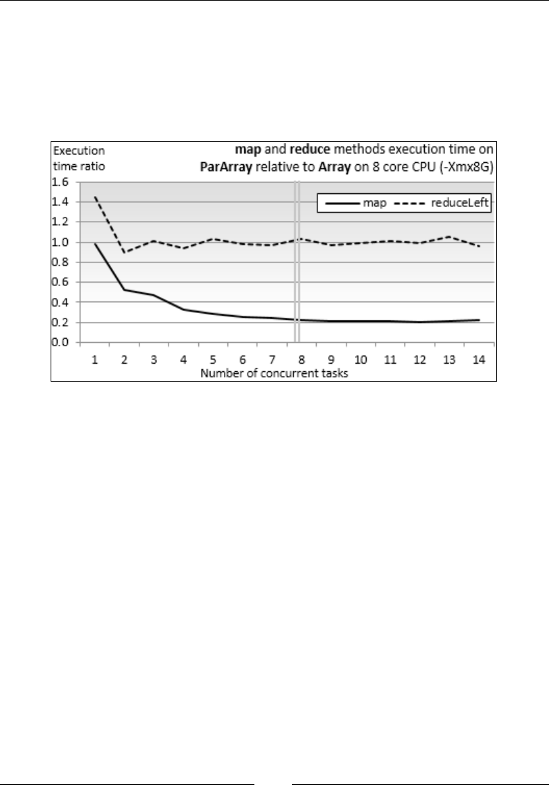
Chapter 12
[ 1013 ]
val bench1 = new ParArrayBenchmark[Double](data, pData, times)
val mapper = (x: Double) => Math.sin(x*0.01) + Math.exp(-x)
Range(1, 16).foreach(n => bench1.map(mapper)(n))
val reducer = (x: Double, y: Double) => x+y
Range(1, 16).foreach(n => bench1.reduce(reducer)(n))
The following graph shows the output of the performance test:
The test executes the mapper and reducer functions 1 million times on an 8-core
CPU with 8 GB of available memory on JVM.
The results are not surprising in the following respects:
• The reducer doesn't take advantage of the parallelism of the array. The
reduction of ParArray has a small overhead in the single-task scenario
and then matches the performance of Array.
• The performance of the map function benets from the parallelization of the
array. The performance levels off when the number of tasks allocated equals
or exceeds the number of CPU core.
The second test consists of comparing the behavior of two parallel collections,
ParArray and ParHashMap, on two methods, map and filter, using a conguration
identical to the rst test as follows:
val sz = 1000000
val mData = new HashMap[Int, Double]
Range(0, sz).foreach(n => mData.put(n, Random.nextDouble)) //1
val mParData = new ParHashMap[Int, Double]
Range(0, sz).foreach(n => mParData.put(n, Random.nextDouble))
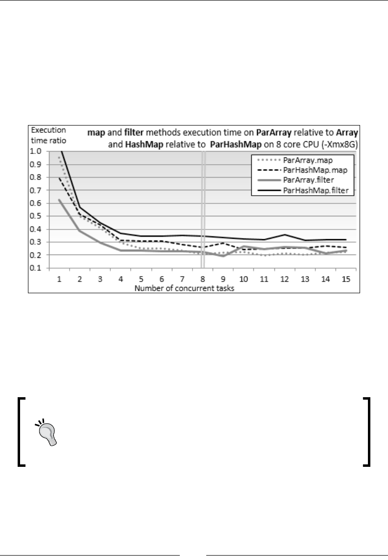
Scalable Frameworks
[ 1014 ]
val bench2 = new ParMapBenchmark[Double](mData, mParData, times)
Range(1, 16).foreach(n => bench2.map(mapper)(n)) //2
val filterer = (x: Double) => (x > 0.8)
Range(1, 16).foreach(n => bench2.filter(filterer)(n)) //3
The test initializes a HashMap instance and its parallel counter ParHashMap with 1
million random values (line 1). The benchmark, bench2, processes all the elements
of these hash maps with the mapper instance introduced in the rst test (line 2) and
a ltering function, filterer (line 3), with 16 tasks. The output is as shown here:
The impact of the parallelization of collections is very similar across methods and
across collections. It's important to notice that the performance of the parallel
collections levels off at around four times the single thread collections for ve
concurrent tasks and above. Core parking is partially responsible for this behavior.
Core parking disables a few CPU cores in an effort to conserve power, and in the
case of singe application, consumes almost all CPU cycles.
Further performance evaluation
The purpose of the performance test was to highlight the benets
of using Scala parallel collections. You should experiment further
with collections other than ParArray and ParHashMap and other
higher-order methods to conrm the pattern.
Clearly, a four-times increase in performance is nothing to complain about. That
being said, parallel collections are limited to single host deployment. If you cannot
live with such a restriction and still need a scalable solution, the Actor model
provides a blueprint for highly distributed applications.
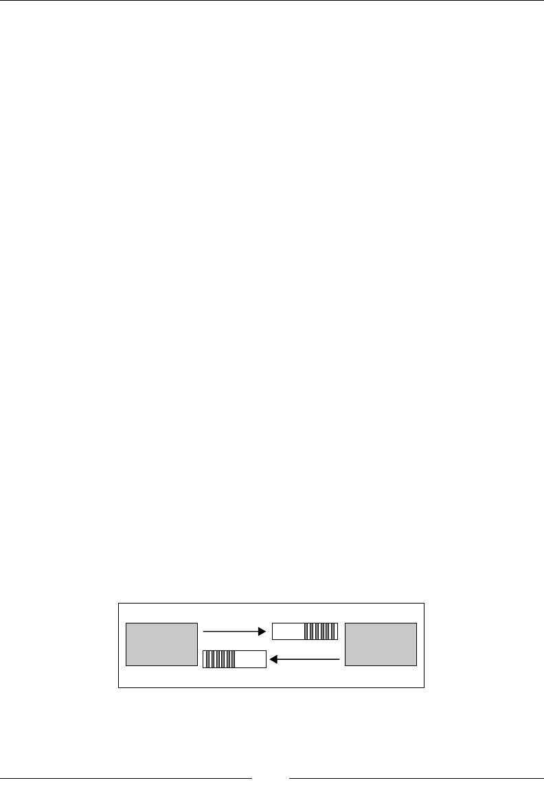
Chapter 12
[ 1015 ]
Scalability with Actors
Traditional multithreaded applications rely on accessing data located in shared
memory. The mechanism relies on synchronization monitors such as locks, mutexes,
or semaphores to avoid deadlocks and inconsistent mutable states. Even for the
most experienced software engineer, debugging multithreaded applications is not
a simple endeavor.
The second problem with shared memory threads in Java is the high computation
overhead caused by continuous context switches. Context switching consists of
saving the current stack frame delimited by the base and stack pointers into the
heap memory and loading another stack frame.
These restrictions and complexities can be avoided by using a concurrency model
that relies on the following key principles:
• Immutable data structures
• Asynchronous communication
The Actor model
The Actor model, originally introduced in the Erlang programming language,
addresses these issues [12:3]. The purpose of using the Actor model is twofold:
• It distributes the computation over as many cores and servers as possible
• It reduces or eliminates race conditions and deadlocks which are very
prevalent in Java development
The model consists of the following components:
• Independent processing units known as Actors. Actors communicate by
exchanging messages asynchronously instead of sharing states.
• Immutable messages are sent to queues, known as mailboxes, before being
processed by each actor one at a time.
Actor A Actor B
Mailbox
Mailbox
Message
Representation of messaging between actors

Scalable Frameworks
[ 1016 ]
There are two message-passing mechanisms:
• Fire-and-forget or tell: Sends the immutable message asynchronously to
the target or receiving actor, and returns immediately without blocking.
The syntax is as follows:
targetActorRef ! message
• Send-and-receive or ask: Sends a message asynchronously, but returns
a Future instance that denes the expected reply from the target actor
val future = targetActorRef ? message
The generic construct for the Actor message handler is somewhat similar to the
Runnable.run() method in Java, as shown in the following code:
while( true ){
receive { case msg1: MsgType => handler }
}
The receive keyword is in fact a partial function of type PartialFunction[Any,
Unit] [12:4]. The purpose is to avoid forcing developers to handle all possible
message types. The Actor consuming messages may very well run on a separate
component or even application, than the Actor producing these messages. It not
always easy to anticipate the type of messages an Actor has to process in a future
version of an application.
A message whose type is not matched is merely ignored. There is no need to throw
an exception from within the Actor's routine. Implementations of the Actor model
strive to avoid the overhead of context switching and creation of threads [12:5].
I/O blocking operations
Although it is highly recommended not to use Actors for
blocking operations such as I/O, there are circumstances that
require the sender to wait for a response. The reader needs to
be mindful that blocking an underlying thread inside the Actor
might starve other Actors from CPU cycles. It is recommended
to either congure the runtime system to use a large thread pool,
or to allow the thread pool to be resized by setting the actors.
enableForkJoin property as false.

Chapter 12
[ 1017 ]
Partitioning
A dataset is dened as a Scala collection, for example, List, Map, and so on.
Concurrent processing requires the following steps:
1. Breaking down a dataset into multiple subdatasets.
2. Processing each dataset independently and concurrently.
3. Aggregating all the resulting datasets.
These steps are dened through a monad associated with a collection in the
Abstraction section under Why Scala? in Chapter 1, Getting Started.
1. The apply method creates the subcollection or partitions for the rst step, for
example, def apply[T](a: T): List[T].
2. A map-like operation denes the second stage. The last step relies on the
monoidal associativity of the Scala collection, for example, def ++ (a:
List[T], b: List[T](: List[T] = a ++ b.
3. The aggregation, such as reduce, fold, sum, and so on, consists of attening
all the subresults into a single output, for example, val xs: List(…) =
List(List(..), List(..)).flatten.
The methods that can be parallelized are map, flatMap, filter, find, and filterNot.
The methods that cannot be completely parallelized are reduce, fold, sum, combine,
aggregate, groupBy, and sortWith.
Beyond actors – reactive programming
The Actor model is an example of the reactive programming paradigm. The concept
is that functions and methods are executed in response to events or exceptions.
Reactive programming combines concurrency with event-based systems [12:6].
Advanced functional reactive programming constructs rely on composable futures
and continuation-passing style (CPS). An example of a Scala reactive library can be
found at https://github.com/ingoem/scala-react.
Akka
The Akka framework extends the original Actor model in Scala by adding extraction
capabilities such as support for typed Actor, message dispatching, routing, load
balancing, and partitioning, as well as supervision and congurability [12:7].
The Akka framework can be downloaded from the www.akka.io website, or through
the Typesafe Activator at http://www.typesafe.com/platform.

Scalable Frameworks
[ 1018 ]
Akka simplies the implementation of Actor by encapsulating some of the details of
Scala Actor in the akka.actor.Actor and akka.actor.ActorSystem classes.
The three methods you want to override are as follows:
• preStart: This is an optional method, invoked to initialize all the necessary
resources such as le or database connection before the Actor is executed
• receive: This method denes the Actor's behavior and returns a partial
function of type PartialFunction[Any, Unit]
• postStop: This is an optional method to clean up resources such as releasing
memory, closing database connections, and socket or le handles
Typed versus untyped actors
Untyped actors can process messages of any type. If the type
of the message is not matched by the receiving actor, it is
discarded. Untyped actors can be regarded as contract-less
actors. They are the default actors in Scala.
Typed actors are similar to Java remote interfaces. They
respond to a method invocation. The invocation is declared
publicly, but the execution is delegated asynchronously to
the private instance of the target actor [12:8].
Akka offers a variety of functionalities to deploy concurrent applications. Let us create
a generic template for a master Actor and worker Actors to transform a dataset using
any preprocessing or classication algorithm inherited from the PipeOperator trait, as
explained in the The pipe operator section under Designing a workow in Chapter 2, Hello
World!. The master Actor manages the worker actors in one of the following ways:
• Individual actors
• Clusters through a router or a dispatcher
The router is a very simple example of Actor supervision. Supervision strategies
in Akka are an essential component to make the application fault-tolerant [12:9].
A supervisor Actor manages the operations, availability, and life cycle of its children,
known as subordinates. The supervision among actors is organized as a hierarchy.
Supervision strategies are categorized as follows:
• One-for-one strategy: This is the default strategy. In case of a failure of one
of the subordinates, the supervisor executes a recovery, restart, or resume
action for that subordinate only.
• All-for-one strategy: The supervisor executes a recovery or remedial action
on all its subordinates in case one of the Actors fails.

Chapter 12
[ 1019 ]
Master-workers
The rst model to evaluate is the traditional master-slaves or master-workers
design for computation workow. In this design, the worker Actors are initialized
and managed by the master Actor which is responsible for controlling the iterative
process, state, and termination condition of the algorithm. The orchestration of the
distributed tasks is performed through message passing.
The design principle
It is highly recommended that you segregate the implementation
of the computation or domain-specic logic from the actual
implementation of the worker and master Actors.
Messages exchange
The rst step in implementing the master-worker design is to dene the different
classes of messages exchanged between the master and each worker, to control
the execution of the iterative procedure. The implementation of the master-worker
design is as follows:
type DblSeries = XTSeries[Double]
sealed abstract class Message(val id: Int)
case class Start(i: Int =0) extends Message(i) //1
case class Activate(i: Int, xt: DblSeries extends Message(i) //2
case class Completed(i: Int, xt: DblSeries) extends Message(i) //3
Let's dene the messages that control the execution of the algorithm. We need at
least the following message types or case classes:
1. Start is sent by the client code to the master to start the computation.
2. Activate is sent by the master to the workers to activate the computation.
This message contains the time series, xt, to be processed by the worker Actors.
3. Completed is sent by each worker back to sender. It contains the variance of
the data in the group.
4. The master stops a worker using a PoisonPill message. The different
approaches to terminate an actor are described in the The Master actor section.
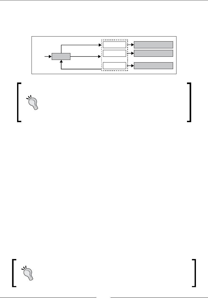
Scalable Frameworks
[ 1020 ]
The hierarchy of the Message class is sealed to prevent third-party developers from
adding another message type. The worker responds to the activate message by
executing a data transformation of type inherited from PipeOperator. The messages
exchanged between master and worker actors are shown in the following diagram:
PipeOperator.I>
PipeOperator.I>
PipeOperator.I>
Worker 1
Worker 2
Master
Start
Worker N
Terminate/PoisonPill
Activate
Complete
Messages as case classes
The actor retrieves the messages queued in its mailbox by
managing each message instance (copy, matching, and so
on). Therefore, the message type has to be dened as a case
class. Otherwise, the developer will have to override the
equals and hashCode methods.
Worker actors
The worker actors are responsible for transforming each partition created by the
master Actor, as follows:
class Worker(id: Int, fct: PipeOperator[DblSeries, DblSeries]) extends
Actor { //1
override def receive = {
case msg: Activate => {
msg.sender ! Completed(msg.id+id, transform(msg.xt)) //2
context.stop(self)
}
case _ => Display.show("Unknown message", logger)
}
def transform(xt: DblSeries): DblSeries = fct |>
}
The Worker class constructor takes the fct data transformation as an argument
(line 1). The worker launches the processing or transformation of the msg.xt data
upon arrival of the Activate message (line 2). It returns the Completed message
to the master once the data transformation, transform, is completed.
The design principle
It is highly recommended that you segregate the implementation
of the computation or domain-specic logic from the actual
implementation of the worker and master Actors.

Chapter 12
[ 1021 ]
The workow controller
In the Scalability section in Chapter 1, Getting Started, we introduced the concepts
of workow and controller, to manage the training and classication process as
a sequence of transformation on time series. Let's dene an abstract class for all
controller actors, Controller, with the following three key parameters:
• A time series, xt, to be a process
• A data transformation, fct, of type PipeOperator
• A partitioning method, partitioner, to break down a time series for
concurrent processing
The Controller class can be dened as follows:
abstract class Controller(val xt: DblSeries, val fct:
PipeOperator[DblSeries, DblSeries],val partitioner: Partitioner)
extends Actor
The workow controller is responsible for splitting the time series into several
partitions and assigning each partition to a dedicated worker Actor. A helper class,
Partitioner, implements the partitioning of the dataset as follows:
class Partitioner(val numPartitions: Int) {
def split(xt: DblSeries): Array[Int] = {
val sz = (xt.size.toDouble/numPartitions).floor.toInt
val indices = Array.tabulate(numPartitions)(i=>(i+1)*sz)
indices.update(numPartitions -1, xt.size)
indices
}
}
The split method breaks down a time series, xt, into numPartitions partitions,
and returns the index of each partition relative to the original time series.
The master Actor
Let's dene a master Actor class, Master. The three methods to override are
as follows:
• preStart is a method invoked to initialize all the necessary resources such as
le or database connection before the actor executes
• receive is a partial function that dequeues and processes the messages from
the mail box
• postStop cleans up resources such as releasing memory and closing
database connections, sockets, or le handles

Scalable Frameworks
[ 1022 ]
The Master class can be dened as follows:
abstract class Master(xt: DblSeries, fct: PipeOperator[DblSeries,
DblSeries], partitioner: Partitioner) extends Controller(xt,fct,
partitioner) {
val workers = List.tabulate(partitioner.numPartitions)(n =>
context.actorOf(Props(new Worker(n, fct)))) //4
val aggregator = new ListBuffer[DblVector] //5
override def preStart: Unit = {} //6
override def postStop: Unit = {} //7
override def receive
The Master class has the following parameters:
• xt: This is the time series to transform
• fct: This is the transformation function
• partitioner: This is the instance of time series partitioning
The worker actors are created through the actorOf factory method of the
ActorSystem context (line 4). A list buffer, aggregator, collects and reduces
the results from each worker (line 5). The preStart method implements any
initialization required to process the messages (line 6). The postStop method
releases all the resources allocated to process the messages (line 7).
The receive message handler processes only two types of messages: Start from the
client code and Completed from the workers, as shown in the following code:
override def receive = {
case Start => split //8
case msg: Completed => { //10
if(aggregator.size >= partitioner.numPartitions-1) { //12
aggregate //14
//13 workers.foreach( _ ! PoisonPill)
context.stop(self) //15
}
aggregator.append(msg.xt.toArray) //11
}
}
def aggregate: Seq[Double]
def split: Unit = {
val partIdx = partitioner.split(xt)

Chapter 12
[ 1023 ]
workers.zip(partIdx).foreach(w =>
w._1 ! Activate(0, xt.slice(w._2-partIdx(0), w._2))) //9
}
The Start message triggers the split of the input time series into partitions (line
8), which are then dispatched to each worker with the Activate message (line 9).
Each worker sends a Completed message back to master upon the completion of
their task (line 10). The master aggregates the results from the each worker (line 11).
Once every worker has completed its task (line 12), the master terminates all the
workers, through a PoisonPill message in case the worker actors do not terminate
themselves (line 13). The master aggregate the results (line 14) before it terminates
itself through a request to its context to stop it (line 15).
The aggregate method can be dened as a parameter either of the Master class or of
one of its subclasses.
The previous code snippet uses two different approaches to terminate an actor. There
are four different methods of shutting down an actor, as mentioned here:
• actorSystem.shutdown: This method is used by the client to shut down the
parent actor system
• actor ! PoisonPill: This method is used by the client to send a poison pill
message to the actor
• context.stop(self): This method is used by the Actor to shut itself down
within its context
• context.stop(childActorRef): This method is used by the Actor to shut
itself down through its reference
Master with routing
The previous design makes sense only if each worker has a unique characteristic
that requires direct communication with the master. This is not the case in most
applications. The communication and internal management of the worker can be
delegated to a router. The implementation of the master routing capabilities is very
similar to the previous design, as shown in the following code:
abstract class MasterWithRouter(xt: DblSeries, fct:
PipeOperator[DblSeries, DblSeries], partitioner: Partitioner) extends
Controller(xt, fct, partitioner) {
val router = context.actorOf(Props(new Worker(0, fct))
.withRouter(RoundRobinPool(partitioner.numPartitions,
supervisorStrategy = this.supervisorStrategy)))
…

Scalable Frameworks
[ 1024 ]
The only difference is that the context.actorOf factory creates an extra actor,
router, along with the workers. This particular implementation relies on
round-robin assignment of the message by the router to each worker. Akka
supports several routing mechanisms that select a random actor, or the actor
with the smallest mailbox, or the rst to respond to a broadcast, and so on.
Routing supervision
The router actor is a parent of the worker actors. It is by
design a supervisor of the worker actors, which are its
children actors. Therefore, the router is responsible for the
life cycle of the worker actors which includes their creation,
restarting, and termination.
The implementation of the receive message handler is almost identical to the
message handler in the master without routing capabilities, except that the
partitioning (line 1) is delegated to the router instead of being applied to each
individual worker, as follows:
override def receive = {
case msg: Start => split
case msg: Completed => {
if(aggregator.size >= partitioner.numPartitions-1) {
aggregate
context.stop(self) //2
}
aggregator.append(msg.xt.toarray)
}
}
def split: Unit = {
val indices = partitioner.split(xt)
indices.foreach(n =>
router ! Activate(xt.slice(n - indices(0), n))) //1
}
The supervising router terminates itself automatically once all its child actors are
terminated (line 2).
Distributed discrete Fourier transform
Let's select the discrete Fourier transform (DFT) on a time series, xt, as our data
transformation. We discussed it in the Discrete Fourier transform (DFT) section in
Chapter 3, Data Preprocessing. The testing code is exactly the same, whether the
master has routing capabilities or not.

Chapter 12
[ 1025 ]
First, let's dene a master controller, DFTMaster, dedicated to the execution of the
distributed discrete Fourier transform, as follows:
class DFTMaster(xt: XTSeries[Double], partitioner: Partitioner)
extends Master(xt, DFT[Double], partitioner) {
override def aggregate: Seq[Double] =
aggregator.transpose.map( _.sum).toSeq
}
The aggregate method aggregates or reduces the results of the discrete Fourier
transform (frequencies distribution) from each worker. In the case of the discrete
Fourier transform, the aggregate method transposes the list of frequencies
distribution then summed the amplitude for each frequency, as shown here:
val NUM_WORKERS = 4
val NUM_DATAPOINTS = 1000000
val h = (x:Double) =>2.0*Math.cos(Math.PI*0.005*x) +
Math.cos(Math.PI*0.05*x) +
0.5*Math.cos(Math.PI*0.2*x) +
0.3* Random.nextDouble //1
val xt = XTSeries[Double](Array.tabulate(NUM_DATAPOINTS)(h(_)))
val partitioner = new Partitioner(NUM_WORKERS) //2
implicit val actorSystem = ActorSystem("system") //3
val master = actorSystem.actorOf(Props(new DFTMaster(xt,
partitioner)), "DFTMaster") //4
master ! Start //5
Thread.sleep(15000)
actorSystem.shutdown //6
The input time series is synthetically generated by the noisy function, h (line 1).
The function h has three distinct harmonics, 0.005, 0.05, and 0.2, so the results of
the transformation can be easily validated. A partitioner instance is created for
NUM_WORKERS worker Actors (line 2). The Actor system, ActorSystem, is instantiated
(line 3) and the master Actor is generated through the Akka ActorSytem.actorOf
factory. The main program sends a Start message to the master to trigger the
distributed computation of the discrete Fourier transform. The main program has
to sleep for a period of time long enough to allow the master to complete its task.
Finally, the main program shuts down the actor system (line 6).
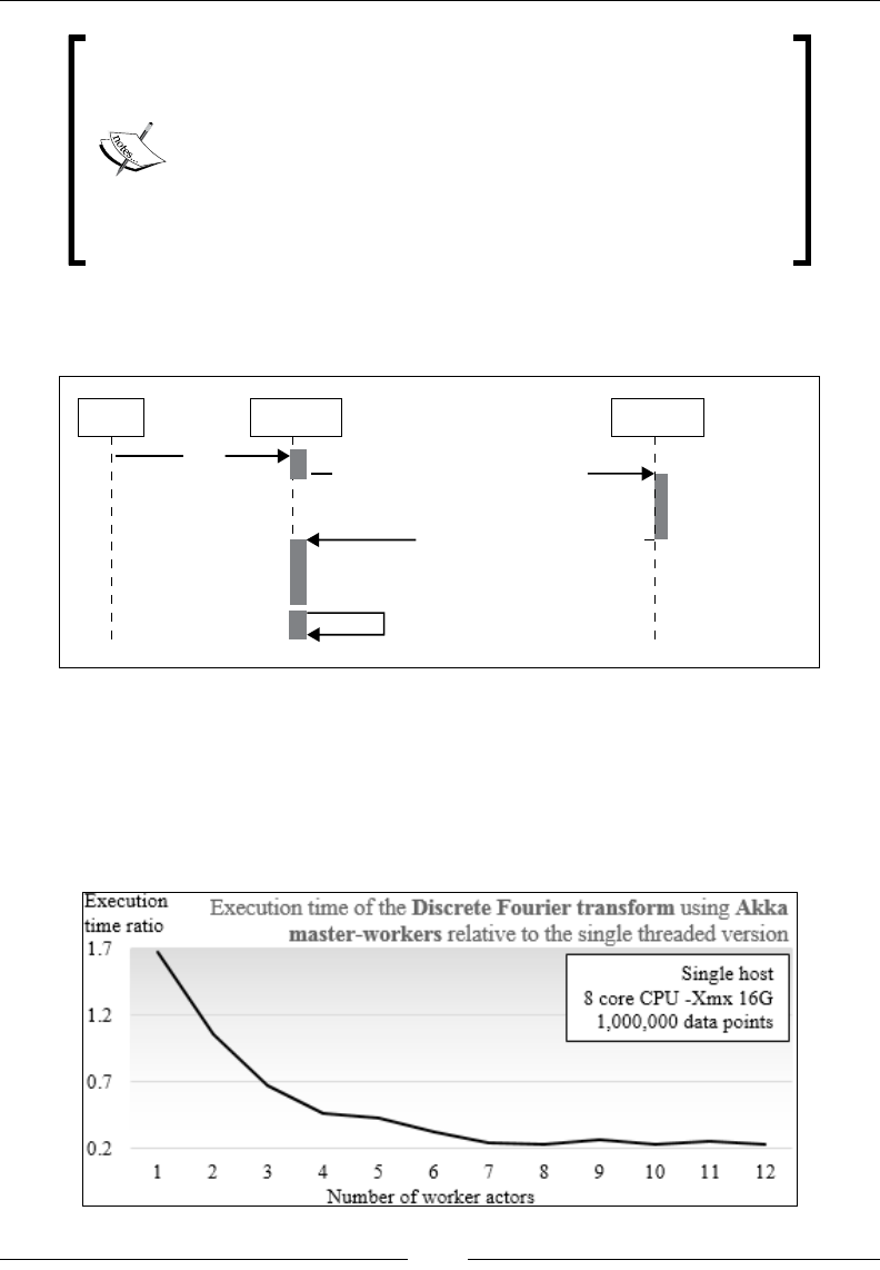
Scalable Frameworks
[ 1026 ]
Actor instantiation
Although the scala.actor.Actor class can be instantiated
using the constructor, akka.actor.Actor is instantiated
using a context, ActorSystem; a factory, actorOf; and
a conguration object, Props. This second approach has
several benets, including decoupling the deployment of the
actor from its functionality and enforcing a default supervisor
or parent for the Actor, in this case ActorSystem.
The following sequential diagram illustrates the message exchange between the main
program, master, and worker Actors:
Worker
transform
msg: Completed(id, results)
context.stop(self)
aggregate
msg: Activate(id,partition)
Master.main
Start
context.stop(self)
Sequential diagram for the normalization of cross-validation groups
The purpose of the test is to evaluate the performance of the computation of the
discrete Fourier transform using the Akka framework relative to the original
implementation, without actors. As with the Scala parallel collections, the absolute
timing for the transformation depends on the host and the conguration, as shown
in the following graph:

Chapter 12
[ 1027 ]
The single-threaded version of the discrete Fourier transform is signicantly faster
than the implementation using the Akka master-worker model with a single worker
actor. The cost of partitioning and the aggregating (or reducing) the results adds a
signicant overhead to execution of the Fourier transform. However, the master-
worker model is far more efcient with three or more worker actors.
Limitations
The master-worker implementation has a few problems:
• In the message handler of the master Actor, there is no guarantee that the
poison pill will be consumed by all the workers before the master stops.
• The main program has to sleep for a period of time long enough to allow the
master and workers to complete their tasks. There is no guarantee that the
computation will be completed when the main program awakes.
• There is no mechanism to handle failure in delivering or processing messages.
The culprit is the exclusive use of the re-and-forget mechanism to exchange
data between master and workers. The send-and-receive protocol and futures
are remedies to these problems.
Futures
A future is an object, more specically a monad, used to retrieve the results of
concurrent operations, in a non-blocking fashion. The concept is very similar to a
callback supplied to a worker, which invokes it when the task is completed. Futures
hold a value that might or might not become available in the future when a task is
completed, successful or not [12:10].
There are two options to retrieve results from futures:
• Blocking execution using scala.concurrent.Await
• Callback functions, onComplete, onSuccess, and onFailure
Which future?
A Scala environment provides developers with two different
Future classes: scala.actor.Future and scala.
concurrent.Future. The actor.Future class is used to write
continuation-passing style workows in which the current actor
is blocked until the value of the future is available. Instances of
type scala.concurrent.Future used in this chapter are the
equivalent of java.concurrent.Future in Scala.

Scalable Frameworks
[ 1028 ]
The Actor life cycle
Let's reimplement the normalization of cross-validation groups by their variance,
which we introduced in the previous section, using futures to support concurrency.
The rst step is to import the appropriate classes for execution of the main actor and
futures, as follows:
import akka.actor.{Actor, ActorSystem, ActorRef, Props}
import akka.util.Timeout
import scala.concurrent.{Await, Future}
The Actor classes are provided by the package akka.actor, instead of the scala.
actor._ package because of Akka's extended actor model. The future-related classes,
Future and Await, are imported from the scala.concurrent package, which is
similar to the java.concurrent package. The akka.util.Timeout class is used to
specify the maximum duration the actor has to wait for the completion of the futures.
There are two options for a parent actor or the main program to manage the futures
it creates:
• Blocking: The parent actor or main program stops execution until all futures
have completed their tasks.
• Callback: The parent actor or the main program initiates the futures during
execution. The future tasks are performed concurrently with the parent actor,
that is then notied when each future task is completed.
Blocking on futures
The following design consists of blocking the actor that launches the futures until
all the futures have been completed, either returning with a result or throwing
an exception. Let's modify the master Actor into a class, TransformFutures, that
manages futures instead of workers or routing actors, as follows:
abstract class TransformFutures(xt: DblSeries,
fct: PipeOperator[DblSeries, DblSeries],
partitioner: Partitioner)(implicit timeout: TimeOut)
extends Controller(xt,fct, partitioner) { //1
override def receive = {
case Start => compute(transform) //2
case _ => Display.error("Message not recognized", logger)
}
def aggregate(results: Array[DblSeries]): Seq[Double]
…
}

Chapter 12
[ 1029 ]
The TransformFutures class requires the same parameters as the Master actor: a
time series, xt; a data transformation, fct; and partitioner. The timeout parameter
is an implicit argument of the Await.result method, and therefore, needs to be
declared as an argument (line 1). The only message, Start, triggers the computation
of the data transformation of each future, and then the aggregation of the results
(line 2). The transform and compute methods have the same semantics as those in
the master-workers design.
The generic message handler
You may have read or even written examples of actors that have
generic case _ => handlers in the message loop for debugging
purposes. The message loop takes a partial function as argument.
Therefore, no error or exception is thrown in case the message
type is not recognized. There is no need for such a handler aside
from one for debugging purposes. Message types should inherit
from a sealed abstract class or a sealed trait in order to prevent a
new message type from being added by mistake.
Let's have a look at the transform method. Its main purpose is to instantiate, launch,
and return an array of futures responsible for the transformation of the partitions, as
shown in the following code:
def transform: Array[Future[DblSeries]] = {
val partIdx = partitioner.split(xt)
val partitions = partIdx.map(n =>
XTSeries[Double](xt.slice(n - partIdx(0), n).toArray)) //3
val futures = new Array[Future[DblSeries]](partIdx.size) //4
partitions.zipWithIndex.foreach(pi => {
futures(pi._2) = Future[DblSeries] { fct |> pi._1 }
})
futures
}
First, the transform method splits the input time series into several partitions
(line 3), similar to the master Actor in the previous section. An array of futures
(one future per partition) is created (line 4). Each future executes the data
transformation, fct, to the partition assigned to the future (line 5) as the
worker Actor did in the previous section.
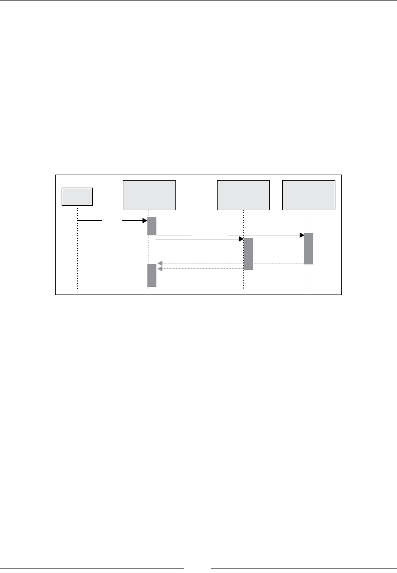
Scalable Frameworks
[ 1030 ]
The compute method has the same purpose as the aggregate method in the
master-workers design. The execution of the Actor is blocked until the Await class
method (line 6) scala.concurrent.Await.result returns the result of each future
computation. In the case of the discrete Fourier transform, the list of frequencies is
transposed before the amplitude of each frequency is summed (7), as follows:
def compute(futures: Array[Future[DblSeries]]): Seq[Double] = {
val results = futures.map(Await.result(_, timeout.duration))
aggregate(results)
}
The following sequential diagram illustrates the blocking design and the activities
performed by the Actor and the futures:
main Transform
Futures
Future
[DblSeries]
split
fct.|>
Await.result
aggregate
Future
[DblSeries]
fct.|>
Start
transform
Sequential diagram for actor blocking on future results
Handling future callbacks
Callbacks are an excellent alternative to having the actor blocks on futures, as they
can simultaneously execute other functions concurrently with the future execution.
There are two simple ways to implement the callback function:
• Future.onComplete
• Future.onSuccess and Future.onFailure
The onComplete callback function takes a function of type Try[T] => U as argument
with an implicit reference to the execution context, as shown in the following code:
val f: Future[T] = future { executeSomeTask }
f onComplete {
case Success(s) => { … }
case Failure(e) => { … }
}
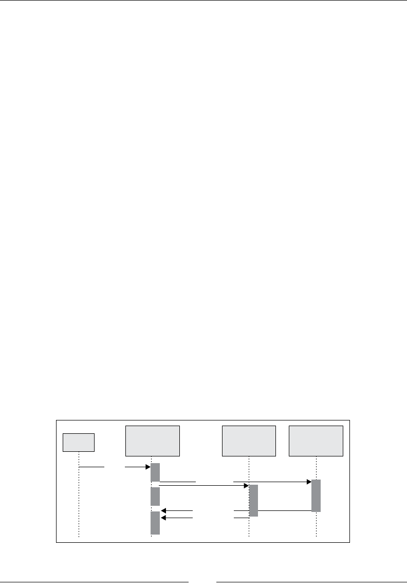
Chapter 12
[ 1031 ]
You can surely recognize the {Try, Success, Failure} monad.
An alternative implementation is to invoke the onSuccess and onFailure methods
that use partial functions as arguments to implement the callbacks, as follows:
f onFailure { case e: Exception => { … } }
f onSuccess { case t => { … } }
The only difference between blocking one future data transformation and handling
callbacks is the implementation of the compute method or reducer. The class
denition, message handler, and initialization of futures are identical, as shown
in the following code:
def compute(futures: Array[Future[DblSeries]]): Seq[Double] = {
val aggregation = new ArrayBuffer[DblSeries]
futures.foreach(f => {
f onSuccess { //1
case data: DblSeries => aggregation.append(data)
}
f onFailure { //2
case e: Exception => aggregation.append(XTSeries.empty)
}
})
if( aggregation.find( _.isEmpty) == None) //3
aggregate(aggregation.toArray)//4
else Seq.empty
}
Each future calls the master Actor back with either the result of the data
transformation, the onSuccess message (line 1), or an exception, the OnFailure
message (line 2). If every future succeeds (line 3), the values of every frequency for
all the partitions are summed (line 4). The following sequential diagram illustrates
the handling of the callback in the master Actor:
main Transform
Futures
Future
[DblSeries]
split
fct.|>
Other tasks
aggregate
Future
[DblSeries]
fct.|>
Start
transform
onSuccess
onFailure
Sequential diagram for actor handling future result with Callbacks

Scalable Frameworks
[ 1032 ]
Execution context
The Futures method requires that the execution context
be implicitly provided by the developer. There are three
different ways to dene the execution context:
• Import the context:
import ExecutionContext.Implicits.global
• Create an instance of the context within the actor
(or actor context):
implicit val ec = ExecutionContext.
fromExecutorService( … )
• Define the context when instantiating the future:
val f= Future[T] ={ } (ec)
Putting all together
Let's reuse the discrete Fourier transform. The client code uses the same synthetically
created time series as with the master-worker test model.
The rst step is to create a transform future for the discrete Fourier transform,
DFTTransformFuture, as follows:
class DFTTransformFutures(xt: DblSeries, partitioner: Partitioner)
(implicit timeout: Timeout)
extends TransformFutures(xt, DFT[Double], partitioner) {
override def aggregate(xt: Array[DblSeries]): Seq[Double] =
xt.map(_.toArray).transpose.map(_.sum).toSeq
}
The only purpose of the DFTTransformFuture class is to dene the aggregation
method, aggregate, for the discrete Fourier transform, as follows:
import akka.pattern.ask
val duration = Duration(10000, "millis")
implicit val timeout = new Timeout(duration)
implicit val actorSystem = ActorSystem("system")
val xt = XTSeries[Double](Array.tabulate(NUM_DATAPOINTS)(h(_)))
val partitioner = new Partitioner(NUM_WORKERS)
val master = actorSystem.actorOf(Props(new DFTTransformFutures(xt,
partitioner)), "DFTTransform") //1
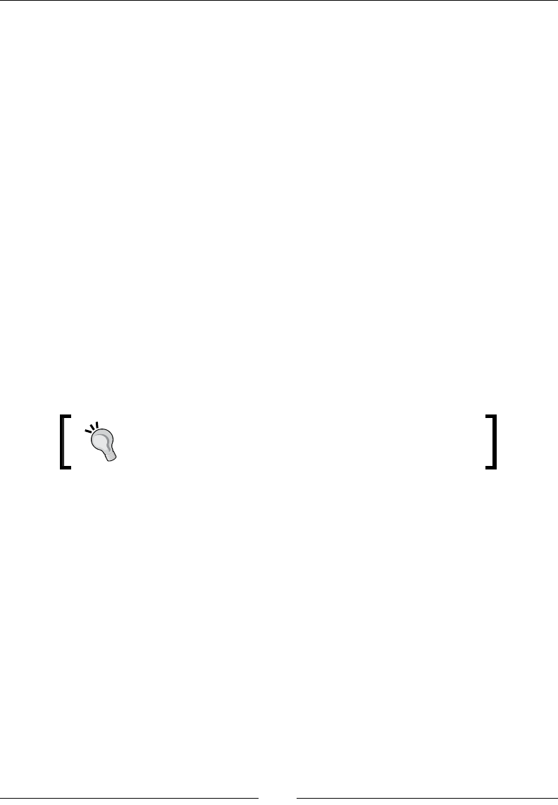
Chapter 12
[ 1033 ]
val future = master ? Start //2
Await.result(future, timeout.duration) //3
actorSystem.shutdown //4
The master Actor is initialized as of the TransformFutures type with the input time
series, xt; discrete Fourier transform, DFT; and partitioner as arguments (line 1).
The program creates a future instance, by sending (ask) the Start message to
master. The program blocks until the completion of the future (line 3), and then
shuts down the Akka actor system (line 4).
Apache Spark
Apache Spark is a fast and general-purpose cluster computing system, initially
developed as AMPLab / UC Berkley as part of the Berkeley Data Analytics Stack
(BDAS), http://en.wikipedia.org/wiki/UC_Berkeley. It provides high-level
APIs for the following programming languages that make large, concurrent parallel
jobs easy to write and deploy [12:11]:
• Scala: http://spark.apache.org/docs/latest/api/scala/index.html
• Java: http://spark.apache.org/docs/latest/api/java/index.html
• Python: http://spark.apache.org/docs/latest/api/python/index.html
Link to latest information
The URLs as any reference to Apache Spark may change
in future versions.
The core element of Spark is Resilient Distributed Dataset (RDD), which is a
collection of elements partitioned across the nodes of a cluster and/or CPU cores of
servers. An RDD can be created from a local data structure such as list, array, or hash
table, from the local le system or the Hadoop Distributed File System (HDFS).
The operations on an RDD in Spark are very similar to the Scala higher-order
methods. These operations are performed concurrently over each partition.
Operations on RDD can be classied as follows:
• Transformation: This operation converts, manipulates, and lters the
elements of an RDD on each partition
• Action: This operation aggregates, collects, or reduces the elements of the
RDD from all partitions
An RDD can persist, be serialized, and be cached for future computation.

Scalable Frameworks
[ 1034 ]
Spark is written in Scala and built on top of Akka libraries. Spark relies on the
following mechanisms to distribute and partition RDDs:
• Hadoop/HDFS for the distributed and replicated les system
• Mesos for management of cluster and shared pool of data nodes
The Spark ecosystem can be represented as stacks of technology and framework,
as seen in the following diagram:
Spark-based applications
MLlib
MLBase Graphx Streaming SparkSQL
Spark framework/RDD
Akka framework
Scala standard library
Hadoop HDFS
Mesos cluster manager
JVM
Operating System
Spark framework ecosystem
The Spark ecosystem has grown to support some machine-learning algorithms out of
the box, MLlib; a SQL-like interface to manipulate datasets with relational operators,
SparkSQL; a library for distributed graphs, GraphX; and a streaming library [12:12].
Why Spark
The authors of Spark attempt to address the limitations of Hadoop in terms of
performance and real-time processing by implementing in-memory iterative
computing, which is critical to most discriminative machine-learning algorithms.
Numerous benchmark tests have been performed and published to evaluate the
performance improvement of Spark relative to Hadoop. In the case of iterative
algorithms, the time per iteration can be reduced by a ratio of 1:10 or more.
Spark provides a large array of prebuilt transforms and actions that go well beyond
the basic map-reduce paradigm. Those methods on RDDs are a natural extension of
the Scala collections, making code migration seamless for Scala developers.

Chapter 12
[ 1035 ]
Finally, Apache Spark supports fault-tolerant operations by allowing RDDs to persist
both in memory and in the lesystems. Persistency enables automatic recovery
from node failures. The resiliency of Spark relies on the supervisory strategy of
the underlying Akka actors, the persistency of their mailboxes, and the replication
schemes of HDFS.
Design principles
The performance of Spark relies on four core design principles [12:13]:
• In-memory persistency
• Laziness in scheduling tasks
• Transform and actions applied to RDDs
• Implementation of shared variables
In-memory persistency
The developer can decide to persist and/or cache an RDD for future usage. An RDD
may persist in memory only or on disk only—in memory if available, or on disk
otherwise as deserialized or serialized Java objects. For instance, an RDD, rdd,
can be cached through serialization through a simple statement, as shown in the
following code:
rdd.persist(StorageLevel.MEMORY_ONLY_SER).cache
Kryo serialization
Java serialization through the Serializable interface is
notoriously slow. Fortunately, the Spark framework allows the
developer to specify a more efcient serialization mechanism such
as the Kryo library.
Laziness
Scala supports lazy values natively. The left side of the assignment, which can either
be a value, object reference, or method, is performed once, that is, the rst time it is
invoked, as shown in the following code:
class Pipeline {
lazy val x = { println("x"); 1.5}
lazy val m = { println("m"); 3}
val n = { println("n"); 6}
def f = (m <<1)

Scalable Frameworks
[ 1036 ]
def g(j: Int) = Math.pow(x, j)
}
val pipeline = new Pipeline //1
…
pipeline.g(pipeline.f) //2
The order of the variables printed is n, m, and then x. The instantiation of the
Pipeline class initializes n but not m or x. At a later stage, the g method is called,
which in turn invokes the f method. The f method initializes the value m it needs,
then g initializes x to compute its power to m<<1.
Spark applies the same principle to RDDs by executing the transformation only
when an action is performed. In other words, Spark postpones memory allocation,
parallelization, and computation until the driver code gets the result through the
execution of an action. The cascading effect of invoking all these transformations
backwards is performed by the direct acyclic graph scheduler.
Transforms and Actions
Spark is implemented in Scala, so you should not be too surprised that the most
relevant Scala higher methods on collections are supported in Spark. The rst table
describes the transformation methods using Spark, as well as their counterparts in
the Scala standard library. We use the (K, V) notation for (key, value) pairs.
Spark Scala Description
map(f) map(f) Transforms an RDD by executing the f function on
each element of the collection.
filter(f) filter(f) Transforms an RDD by selecting the element for
which the f function returns true.
flatMap(f) flatMap(f) Transforms an RDD by mapping each element to a
sequence of output items.
mapPartitions(f) Executes the map method separately on each
partition.
sample Samples a fraction of the data with or without a
replacement using a random generator.
groupByKey groupBy Called on (K,V) to generate a new (K, Seq(V)) RDD.
union union Creates a new RDD as union of this RDD and the
argument.
distinct distinct Eliminates duplicate elements from this RDD.
reduceByKey(f) reduce Aggregates or reduces the value corresponding to
each key using the f function.

Chapter 12
[ 1037 ]
Spark Scala Description
sortByKey sortWith Reorganizes (K,V) in an RDD by the ascending,
descending, or otherwise specified order of the
keys, K.
join Joins an RDD (K,V) with an RDD (K,W) to generate
a new RDD (K, (V,W)).
coGroup Implements a join operation but generates an RDD
(K, Seq(V), Seq(W)).
Action methods trigger the collection or the reduction of the datasets from all
partitions back to the driver, as listed here:
Spark Scala Description
reduce(f) reduce(f) Aggregates all the elements of the RDD across all the
partitions and returns a Scala object to the driver.
collect collect Collects and returns all the elements of the RDD
across all the partitions as a list in the driver.
count count Returns the number of elements in the RDD to the
driver.
first head Returns the first element of the RDD to the driver.
take(n) take(n) Returns the first n elements of the RDD to the driver
.
takeSample Returns an array of random elements from the RDD
back to the driver.
saveAsTextFile Writes the elements of the RDD as a text file in either
the local files system or HDFS.
countByKey Generates a (K, Int) RDD with the original keys, K,
and the count of values for each key.
foreach foreach Executes a T=> Unit function on each elements of the
RDD.
Scala methods such as fold, find, drop, flatten, min, max, and sum are not
currently implemented in Spark. Other Scala methods such as zip have to be
used carefully, as there is no guarantee that the order of the two collections in
zip is maintained between partitions.
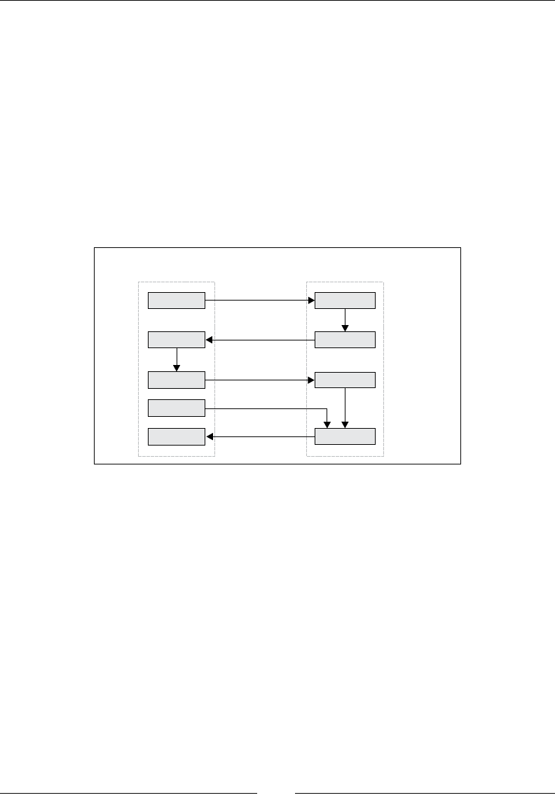
Scalable Frameworks
[ 1038 ]
Shared variables
In a perfect world, variables are immutable and local to each partition to avoid
race conditions. However, there are circumstances where variables have to be
shared without breaking the immutability provided by Spark. To this extent, Spark
duplicates shared variables and copies them to each partition of the dataset. Spark
supports the following types of shared variables:
• Broadcast values: These values encapsulate and forward data to all
the partitions
• Accumulator variables: These variables act as summations or reference counters
The four design principles can be summarized in the following diagram:
Spark Driver
Spark Partitions
Data nodes
Data
4. computation
1. parallelize
3. action
(reducer)
5. parallelize
6. broadcast
7. action
2. transform (mapper)
RDD
Data
Data
Data
RDD
RDD
RDD
Variable
Interaction between Spark driver and RDDs
The preceding diagram illustrates the most common interaction between the Spark
driver and its workers, as listed in the following steps:
1. The input data, residing in either memory as a Scala collection or HDFS as
a text le, is parallelized and partitioned into an RDD
2. A transformation function is applied on each element of the dataset across all
the partitions
3. An action is performed to reduce and collect the data back to the driver
4. The data is processed locally within the driver
5. A second parallelization is performed to distribute computation through
the RDDs
6. A variable is broadcast to all the partitions as an external parameter of the
last RDD transformation

Chapter 12
[ 1039 ]
7. Finally, the last action aggregates and collects the nal result back in
the driver
If you look closely, the management of datasets and RDDs by the Spark driver is not
very different from that by Akka master and worker actors of futures.
Experimenting with Spark
Spark's in-memory computation for iterative computing makes it an excellent
candidate to distribute the training of machine learning models, implemented
with dynamic programming or optimization algorithms. Spark runs on Windows,
Linux, and Mac OS operating systems. It can be deployed either in local mode for a
single host, or master mode for a distributed environment. The version of the Spark
framework used is 1.1.
Scala- and Java SE-compatible versions
At the time of writing, the version of Spark 1.0.0 required Java
1.7+ and Scala 2.10.2 or 2.10.3. Spark 1.1 is compatible with
both Java 1.7 and 1.8 and Scala 2.10.4 and 2.11.1.
Deploying Spark
The easiest way to learn Spark is to deploy a localhost in standalone mode. You can
either deploy a precompiled version of Spark from the website, or build the JAR les
using the simple build tool (sbt) or maven [12:14] as follows:
1. Go to the download page at http://spark.apache.org/downloads.html.
2. Choose a package type (Hadoop distribution). The Spark framework relies
on HDFS to run in cluster mode; therefore, you need to select a distribution
of Hadoop, or an open source distribution, MapR or Cloudera.
3. Download and decompress the package.
4. If you are interested in the latest functionality added to the framework, check
out the newest source code at https://github.com/apache/spark.git.
5. Next, you need to build, or assemble, the Apache Spark libraries from the
top-level directory using either Maven or sbt:
°Maven: Set the following maven options to support build,
deployment, and execution:
MAVEN_OPTS="-Xmx4g -XX:MaxPermSize=512M
-XX:ReservedCodeCacheSize=512m"
mvn –DskipTests clean package
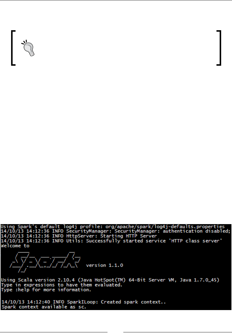
Scalable Frameworks
[ 1040 ]
°Simple build tool: Use the following command:
sbt/sbt assembly
Installation instructions
The directory and name of artifacts used in Spark will undoubtedly
change over time. Please refer to the documentation and installation
guide for the latest version of Spark.
Using Spark shell
Use any of the following methods to use the Spark shell:
• The shell is an easy way to get your feet wet with Spark-resilient distributed
datasets (RDD). To launch the shell locally, execute ./bin/spark-shell –
master local[8] to execute the shell on an 8-core localhost.
• To launch a Spark application locally, connect with the shell and execute the
following command line:
./bin/spark-submit --class application_class --master local[4]
--executor-memory 12G --jars myApplication.jar –class myApp.class
The command launches the application, myApplication, with the main
method, myApp.main, on a 4-core CPU local host, and 12 GB of memory.
• To launch the same Spark application remotely, connect with the shell
execute the following command line:
./bin/spark-submit --class application_class --master
spark://162.198.11.201:7077 –total-executor-cores 80 --executor-
memory 12G --jars myApplication.jar –class myApp.class
Partial screenshot of Spark shell

Chapter 12
[ 1041 ]
Potential pitfalls with Spark shell
Depending on your environment, you might need to disable
logging information into the console by reconguring conf/
log4j.properties. The Spark shell might also conict with the
declaration of classpath in the prole or the environment variables
list. In this case, it has to be replaced by ADD_JARS as environment
variable as ADD_JARS = path1/jar1, path2/jar2.
MLlib
MLlib is a scalable machine learning library built on top of Spark. As of version 1.0,
the library is a work in progress.
The main components of the library are as follows:
• Classication algorithms, including logistic regression, Naïve Bayes, and
support vector machines
• Clustering limited to K-means in version 1.0
• L1 and L1 regularization
• Optimization techniques such as gradient descent, logistic gradient and
stochastic gradient descent, and L-BFGS.
• Linear algebra such as singular value decomposition
• Data generator for K-means, logistic regression, and support vector machines
The machine learning bytecode is conveniently included in the Spark assembly JAR
le built with the simple build tool.
RDD generation
The transformation and actions are performed on RDDs. Therefore, the rst step is
to create a mechanism to facilitate the generation of RDDs from a time series. Let's
create an RDDSource singleton with a convert method that transforms a time series,
xt, into an RDD, as shown here:
def convert(xt: XTSeries[DblVector], rddConfig: RDDConfig)(implicit
sc: SparkContext): RDD[DblVector] = {
val rdd: = sc.parallelize(xt.toArray
.map(new DenseVector( _ ))) //1
rdd.persist(rddConfig.persist) //2
if( rddConfig.cache) rdd.cache //3
rdd
}

Scalable Frameworks
[ 1042 ]
The last parameter, rddConfig, species the conguration for the RDD. In this
example, the conguration of the RDD consists of enabling/disabling cache and
selecting the persistency model, as follows:
case class RDDConfig(val cache: Boolean, val persist: StorageLevel)
It is fair to assume that SparkContext has already been implicitly dened in a
manner quite similar to ActorSystem in the Akka framework.
The generation of the RDD is performed in the following steps:
1. Create an RDD by using the parallelize method of the context and converting
into a vector (SparseVector or DenseVector) (line 1)
2. Specify the persistency model or the storage level if the default level needs to
be overridden for the RDD (line 2)
3. Specify whether the RDD has to persist in memory (line 3)
Alternative for the creation of an RDD
An RDD can be generated from data loaded from either
the local lesystems or HDFS using the SparkContext.
textFile method that returns an RDD of string.
Once the RDD is created, it can be used as an input for any algorithm dened as a
sequence of transformation and actions. Let's experiment with the implementation of
the K-means algorithm in Spark/MLlib.
K-means using Spark
The rst step is to create a SparkKMeansConfig class to dene the conguration of
the Apache Spark K-means algorithm, as follows:
class SparkKMeansConfig(K: Int, maxIters: Int, numRuns: Int =1) {
val kmeans: KMeans = {
val kmeans = new KMeans
kmeans.setK(K) //4
kmeans.setMaxIterations(maxIters) //5
kmeans.setRuns(numRuns) //6
kmeans
}
}

Chapter 12
[ 1043 ]
The minimum set of initialization parameters for MLlib K-means algorithm is
as follows:
• Number of clusters, K (line 4)
• Maximum number iterations for the reconstruction of the total error,
maxIters (line 5)
• The number of training runs, numRuns (line 6)
The SparkKMeans class wraps the Spark KMeans into a data transformation of type
PipeOperator so that it can be used in a computation workow. The class follows
the design template for classier as explained in the Design template for classiers
section in Appendix A, Basic Concepts.
class SparkKMeans(config: SparkKMeansConfig, rddConfig: RDDConfig, xt:
XTSeries[DblVector])(implicit sc: SparkContext)
extends PipeOperator[DblVector, Int] {
val model = config.kmeans.run(RDDSource.convert(xt, rddConfig))
…
}
The constructor takes three arguments: the Apache Spark KMeans conguration,
config; the RDD conguration, rddConfig; and the input time series to clustering,
xt. The generation of model merely consists of converting the time series xt into an
RDD using rddConfig and invoking MLlib KMeans.run. Once created, the clusters
(KMeansModel) are available for predicting new observation, obs, as follows:
def |> : PartialFunction[DblVector, Int] = {
case x: DblVector if(x!= null && x.size>0 && model != null) =>
model.predict(new DenseVector(x))
}
The prediction method, |>, returns the index of the cluster of observations.
Finally, let's write a simple client program to exercise the SparkKMeans model using
the trading volume of each trading session, and the volatility of the price of the stock
during the session:
val K = 8; val MAXITERS = 100; val NRUNS = 16
val PATH = "resources/data/chap12/CSCO.csv"
val CACHE = true
val extractors = List[Array[String] => Double](
YahooFinancials.volatility, YahooFinancials.volume) //7
)
val input = DataSource(PATH, true) |> extractors //8
val volatilityVol = input(0).zip(input(1)) //9

Scalable Frameworks
[ 1044 ]
.map(x => Array[Double](x._1, x._2))
implicit val sc = new SparkContext("Local","SparkKMeans") //10
val config = new SparkKMeansConfig(K, MAXITERS, NRUNS)
val rddConfig = RDDConfig(CACHE , StorageLevel.MEMORY_ONLY)
val xt = XTSeries[DblVector](volatilityVol)
val sparkKMeans = SparkKMeans(config, rddConfig, xt) //11
val obs = Array[Double](0.23, 0.67)
val clusterId = sparkKMeans |> obs//12
Display.show(s"cluster = $clusterId", logger)
The rst step is to dene the variable to be extracted from the CSV le (line 7). The
spark context is created (line 10) once the volatility and volume are extracted (line 8)
and zipped (line 9). The K-means wrapper, sparkKMeans, is initialized (line 11). The
nal step consists of correctly predicting the cluster for a new observation (line 12).
Performance evaluation
Let's execute the normalization of the cross-validation group on an 8-core CPU
machine with 32 GB of RAM. The data is partitioned with a ratio of two partitions
per CPU core.
Meaningful performance test
The scalability test should be performed with a large number of
data points (normalized volatility, normalized volume), in excess
of 1 million in order to be meaningful.
The actual values of the data points have no bearing on the overall performance of
the Spark cluster.
Tuning parameters
The performance of a Spark application depends greatly on the conguration
parameters. Selecting the appropriate value for those conguration parameters in
Spark can be overwhelming—there are 54 conguration parameters as of the last
count. Fortunately, the majority of those parameters have relevant default values.
However, there are few parameters that deserve your attention, including:
• Number of cores available to execute transformation and actions on RDDs:
config.cores.max.

Chapter 12
[ 1045 ]
• Memory available for the execution of the transformation and actions spark.
executor.memory. Setting the value as 60 percent of the maximum JVM heap
is a generally a good compromise.
• Number of concurrent tasks to use across all the partitions for shufe-related
operations, they use key such as reduceByKey: spark.default.parallelism.
The recommended formula is parallelism = total number of cores x 2. The value
of the parameter can be overridden with the spark.reduceby.partitions
parameter for specic RDD reducers.
• Flag to compress serialized RDD partition for MEMORY_ONLY_SER: spark.
rdd.compress. The purpose is to reduce memory footprints at the cost of
extra CPU cycles.
• Maximum size of message containing the results of an action sent to the
spark.akka.frameSize driver. This value has to be increased if a collection
may potentially generate a large size array.
• Flag to compress large size broadcasted spark.broadcast.compress
variables. It is usually recommended.
Tests
The purpose of the test is to evaluate how the execution time is related to the size
of the training set. The test executes K-means from MLlib library on the volatility
and trading session volume on Bank of America (BAC) stock over the following
periods: 3 months, 6 months, 12 months, 24 months, 48 months, 60 month, 72 month,
96 months, and 120 months.
The following conguration is used to perform the training of the K-means: 10
clusters, 30 maximum iterations, and 3 runs. The test is run on a single host with
8-CPU cores and 32 GB RAM.
The test was conducted with the following values of parameters:
• StorageLevel = MEMORY_ONLY
• spark.executor.memory=12G
• spark.default.parallelism = 48
• spark.akka.frameSize = 20
• spark.broadcast.compress=true
• No serialization
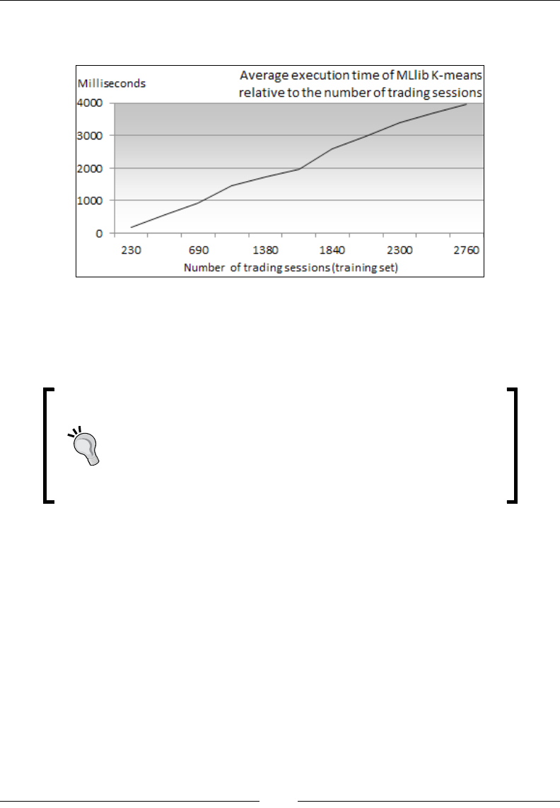
Scalable Frameworks
[ 1046 ]
The rst step after executing a test for a specic dataset is to log in to the Spark
monitoring console at http://host_name:4040/stages:
Average duration of K-means clustering versus size of trading data in months
Obviously, each environment produces somewhat different performance results,
but conrms that the time complexity of the Spark K-means is a linear function
of the training set.
Evaluation in distributed environment
A Spark deployment on multiple hosts would add latency
of the TCP communication to the overall execution time.
The latency is related to the collection of the results of the
clustering back to the Spark driver, which is negligible and
independent of the size of the training set.
Performance considerations
This test barely scratches the surface of the capabilities of Apache Spark. The
following are the lessons learned from personal experience in order to avoid the
most common performance pitfalls when deploying Spark 1.1:
• Get acquainted with the most common Spark conguration parameters
regarding partitioning, storage level, and serialization.
• Avoid serializing complex or nested objects unless you use an effective Java
serialization library such as Kryo.
• Look into dening your own partitioning function to reduce large key-value
pair datasets. The convenience of reduceByKey has its price. The ratio of
number of partitions to number of cores has an impact on the performance of
a reducer using key.

Chapter 12
[ 1047 ]
• Avoid unnecessary actions such as collect, count, or lookup. An action
reduces the data residing in the RDD partitions, and then forwards it to the
Spark driver. The Spark driver (or master) program runs on a single JVM
with limited resources.
• Relies on shared or broadcast variables whenever necessary. Broadcast
variables, for instance, improve the performance of operations on multiple
datasets with very different sizes. Let us consider the common case of joining
two datasets of very different sizes. Broadcasting the smaller dataset to each
partition of the RDD of the larger dataset is far more efcient than converting
the smaller dataset into an RDD and executing a join operation between the
two datasets.
• Use an accumulator variable for summation as it is faster than using a reduce
action on an RDD.
Pros and cons
An increasing number of organizations are adopting Spark as their distributed data
processing platform for real-time, or pseudo real-time operations. There are several
reasons for the fast adoption of Spark:
• Supported by a large and dedicated community of developers [12:15]
• In-memory persistency is ideal for iterative computation found in machine
learning and statistical inference algorithms
• Excellent performance and scalability that can be extended with the
Streaming module
• Apache Spark leverages Scala functional capabilities and a large number of
open source Java libraries
• Spark can leverage the Mesos cluster manager, which reduces the complexity
of dening fault-tolerance and load balancing between worker nodes
• Spark is to be integrated with commercial Hadoop vendors such as Cloudera
However, no platform is perfect and Spark is no exception. The most common
complaints or concerns regarding Spark are:
• Creating a Spark application can be intimidating for a developer with no
prior knowledge of functional programming.
• The integration with the database has been somewhat lagging, relying
heavily on Hive. The Spark development team has started to address
these limitations with the introduction of SparkSQL.

Scalable Frameworks
[ 1048 ]
0xdata Sparkling Water
Sparkling water is an initiative to integrate 0xdata H2O with Spark and complement
MLlib [12:16]. H2O from 0xdata is a very fast, open source, in-memory platform
for machine learning for very large datasets, http://0xdata.com/product/. The
framework is worth mentioning for the following reasons:
• It has a Scala API
• It is fully dedicated to machine learning and predictive analytics
• It leverages both the frame data representation of H2O and in-memory
clustering of Spark
H2O has an extensive implementation of the generalized linear model and gradient
boosted classication, among other goodies. Its data representation consists of
hierarchical data frames. A data frame is a container of vectors potentially shared
with other frames. Each vector is composed of data chunks, which themselves are
containers of data elements [12:17]. At the time of writing, Sparkling Water is in
beta version.
Summary
This completes the introduction of the most common scalable frameworks built
using Scala. It is quite challenging to describe frameworks such as Akka and Spark,
as well as new computing models such as Actors, Futures, and RDDs, in a few pages.
This chapter should be regarded as an invitation to further explore the capabilities of
those frameworks in both a single host and a large deployment environment.
In this last chapter, we learned:
• The benets of asynchronous concurrency
• The essentials of the actor model, composing futures with blocking or
callback modes
• How to implement a simple Akka cluster to squeeze performance of
distributed applications
• The ease and blazing performance of Spark's resilient distributed datasets
and the in-memory persistency approach

Basic Concepts
Machine learning algorithms make signicant use of linear algebra and optimization
techniques. Describing the concepts and the implementation of linear algebra, calculus,
and optimization algorithms in detail would have added signicant complexity to the
book and distracted the reader from the essence of machine learning.
This appendix lists a set of basic elements of linear algebra and optimization
mentioned throughout the book. It also summarizes the coding practices that have
been covered, and acquaints the reader with basic knowledge of nancial analysis.
Scala programming
The following is a partial list of coding practices and design techniques used
throughout the book.
List of libraries
The libraries directory contains the JAR les related to the third-party libraries or
frameworks used in this book. Not all libraries are needed for every chapter. The list
is as follows:
• Apache Commons Math 3.3 in Chapter 3, Data Preprocessing; Chapter 4,
Unsupervised Learning; and Chapter 6, Regression and Regularization
• JFChart 1.0.1 in Chapter 1, Getting Started; Chapter 2, Hello World!; Chapter 5,
Naïve Bayes Classiers; and Chapter 9, Articial Neural Networks
• Iitb CRF 0.2 (including L-BFGS and Colt libraries) in Chapter 7, Sequential
Data Models
• LIBSVM 0.1.6 in Chapter 8, Kernel Models and Support Vector Machines
• Akka framework 2.2.4 in Chapter 12, Scalable Frameworks
• Apache Spark/MLlib 1.1 in Chapter 12, Scalable Frameworks

Basic Concepts
[ 1050 ]
Note for Spark developers
The Scala library and compiler JAR les bundled with the assembly
JAR le of Apache Spark contain a version of the Scala standard
library and compiler JAR le that may conict with an existing
Scala library (for example, Eclipse default ScalaIDE library).
Format of code snippets
For the sake of readability of the implementation of algorithms, all non-essential
pieces of code such as error checking, comments, exceptions, or imports have been
omitted. The following code elements have been discarded in the code snippets presented in
the book:
• Comments:
// The MathRuntime exception has to be caught here!
• Validation of class parameters and method arguments:
class BaumWelchEM(val lambda: HMMLambda ...) {
require( lambda != null, "Lambda model is undefined")
• Class qualiers such as nal, private, and so on:
final protected class MLP[T <% Double] …
• Method qualiers and access controls (nal, private, and so on):
final def inputLayer: MLPLayer
private def recurse: Unit =
• Java-style exceptions:
try { … }
catch { case e: ArrayIndexOutOfBoundsException => … }
if (y < EPS)
throw new IllegalStateException( … )
• Scala-style exceptions:
Try(process(args)) match {
case Success(results) => …
case Failure(e) => …
}
• Non-essential annotations:
@inline def mean = { … }

Appendix A
[ 1051 ]
• Logging and debugging code:
m_logger.debug( …)
Console.println( … )
• Auxiliary methods not essential to the understanding of an algorithm
Encapsulation
One important objective while creating an API is reducing access to supporting or
helper classes. There are two options to encapsulate helper classes, as follows:
• Package scope: In this, the supporting classes are rst-level classes with
protected access
• Class or object scope: In this, the supported classes are nested in the
main class
The algorithms presented in this book follow the rst encapsulation pattern.
Class constructor template
The constructors of a class are dened in the companion object using apply and the
class has package scope (protected):
protected class MyClass[T](val x: X, val y: Y,…) { … }
object MyClass {
def apply[T](x: X, y:Y, ..): MyClass[T] = new MyClass(x,y,..)
final val y0 = ..
def apply[T](x: , ..): MyClass[T] = new MyClass(x, y0, …)
}
For example, the conguration of the support vector machine classier is dened
as follows:
protected class SVMConfig(val formulation: SVMFormulation, val kernel:
SVMKernel, val svmExec: SVMExecution) extends Config
Its constructors are dened as follows:
object SVMConfig {
val DEFAULT_CACHE = 25000
val DEFAULT_EPS = 1e-15
…
def apply(svmType: SVMFormulation, kernel: SVMKernel, svmExec:
SVMExecution): SVMConfig = new SVMConfig(svmType, kernel, svmExec)

Basic Concepts
[ 1052 ]
def apply(svmType: SVMFormulation, kernel: SVMKernel): SVMConfig
= new SVMConfig(svmType, kernel, new SVMExecution(DEFAULT_CACHE,
DEFAULT_EPS, -1))
}
Companion objects versus case classes
In the preceding example, the constructors are explicitly dened in the companion
object. Although the invocation of the constructor is very similar to the instantiation
of case classes, there is a major difference—the Scala compiler generates several
methods to manipulate an instance as regular data (equals, copy, hash, and so on).
Case classes should be reserved for single-state data objects, that is, objects with
no methods.
Enumerations versus case classes
It is not uncommon to read or hear discussions regarding the relative merit of
enumerations and pattern matching with case classes in Scala [A:1]. As a very
general guideline, enumeration values can be regarded as lightweight case
classes or case classes can be considered as heavyweight enumeration values.
Let's take an example of a Scala enumeration that consists of evaluating the uniform
distribution of scala.util.Random:
object MyEnum extends Enumeration {
type TMyEnum = Value
val A, B, C = Value
}
import MyEnum._
val counters = Array.fill(MyEnum.maxId+1)(0)
Range(0, 1000).foreach( _ => Random.nextInt(10) match {
case 3 => counters(A.id) += 1
…
case _ => { }
})
The previous pattern matching is very similar to the switch statement of Java.

Appendix A
[ 1053 ]
Let's consider the following example of pattern matching using case classes that
selects a mathematical formula according to the input:
package MyPackage {
sealed abstract class MyEnum(val level: Int)
case class A extends MyEnum(3) { def f =(x:Double) => 23*x}
…
}
import MyPackage._
def compute(myEnum: MyEnum, x: Double): Double = myEnum match {
case a: A => a.f(x)
…
}
The previous pattern matching is performed using the default equals method, whose
byte code is automatically set for each case class. This approach is far more exible
than simple enumeration, at the cost of extra computation cycles.
The advantages of using enumerations over case classes are as follows:
• Enumerations involve less code for a single attribute comparison
• Enumerations are more readable, especially for Java developers
The advantages of using case classes are as follows:
• Case classes are data objects and support more attributes than
enumeration IDs
• Pattern matching is optimized for sealed classes as the Scala compiler is
aware of the number of cases
In a nutshell, you should use enumeration for single value constants and case
classes to match data objects.
Overloading
Contrary to C++, Scala does not actually overload operators. Here is the meaning
of the operators used in code snippets:
• +=: This adds an element to a collection or container.
• +: This sums two elements of the same type.
• |>: This transforms a collection of data. It is also known as pipe operator.
The type of output collections and elements can be different from that of
the input.
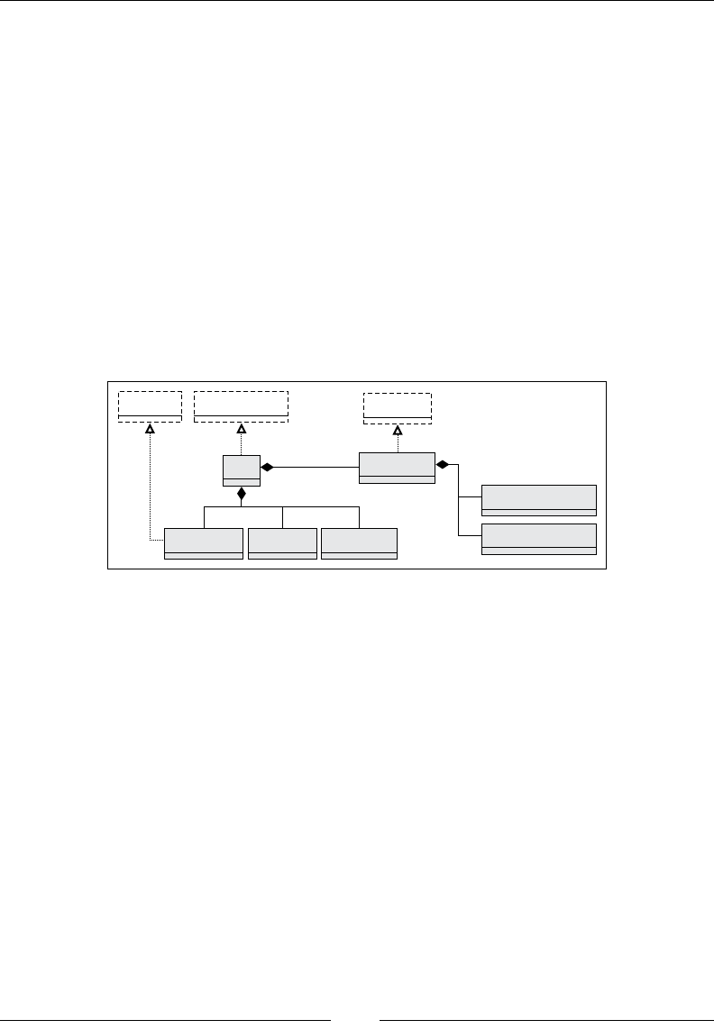
Basic Concepts
[ 1054 ]
Design template for classiers
The machine learning algorithms described in this book use the following
design pattern:
• A model instance that implements the Model trait is created through training
during the initialization of the classier
• All conguration parameters are encapsulated into a single conguration
class inheriting the Config trait
• The predictive or classication routine is implemented as a data
transformation extending the PipeOperator trait
• The classier takes at least three parameters: conguration instance,
a features set or time series, and a labeled dataset
Have a look at the following diagram:
XComponent2
XComponent1
Config Model
XModel
X
XConfig XTSeries DblVector
PipeOperator
model
config xt labels
1
1+
11
1
1+
11
1
A generic UML class diagram for classifiers
For example, the key components of the support vector machine package are
as follows:
final protected class SVM[T <% Double](val config: SVMConfig, val xt:
XTSeries[Array[T]], val labels: DblVector)
extends PipeOperator[Array[T], Double] {
val model: Option[SVMModel] = { … }
override def |> (x: Feature): Option[Double] = { prediction }
…
}
final protected class SVMConfig(val formulation: SVMFormulation, val
kernel: SVMKernel, val svmExec: SVMExecution) extends Config
protected class SVMModel(val params: (svm_model, Double)) extends
Model
Appendix A
[ 1055 ]
The two data inputs required to train a model are the conguration of the classier
(config) and the training set (xt and labels). Once trained and validated, the
model is available for prediction or classication.
This design has the main advantage of reducing the life cycle of the classier;
a model is either dened, available for classication, or is not created.
Implementation considerations
The validation phase is omitted in most of the practical
examples throughout this book for the sake of readability.
Data extraction
A CSV le is the most common format used to store historical nancial data. It is the
default format used to import data throughout this book:
type Fields = Array[String]
class DataSource(pathName: String,
normalize: Boolean,
reverseOrder: Boolean,
headerLines: Int = 1,
srcFilter: Option[Fields=>Boolean])
extends PipeOperator[List[Fields =>Double], List[DblVector]]
The parameters for the DataSource class are as follows:
• pathName: This is the relative pathname of a data le to be loaded if the
argument is a le, or the directory containing multiple input data les. Most
of the les are CSV les.
• normalize: This is a ag to specify if the data has to be normalized
over [0, 1].
• reverseOrder: This is a ag to specify whether the order of the data in the
le has to be reversed—for example, time series—if its value is true.
• headerLines: This species the number of lines for column headers
and comments.
• srcFilter: This is a lter or condition for some of the row elds to skip the
data set, for example, missing data or incorrect format.

Basic Concepts
[ 1056 ]
The most important method of DataSource is the following data transformation
from a le to a typed time series (XTSeries[T]) implemented as the pipe operator
method. The method takes the extractor from a row of literal values to Double
oating-point values:
def |> : PartialFunction[List[Fields=>Double],List[DblVector]] ={
case extr: List[Fields=>Double] if(extr!=null && extr.size>0)=>
load match { //1
case Some(data) => {
if( normalize) // 2
extr.map(t=>Stats[Double](data._2.map(t(_))) //3
.normalize) //4
else extr.map(t => data._2.map(t(_)))
}
…
}
The data is loaded from the le and converted into a list of vectors using the
extractor, extr (line 1). The data is normalized if required (line 2) by converting
each literal to a oating point value and a Stats object is created (line 3). Finally,
the Stats instance normalizes the sequence of oating-point values (line 4).
A second data transformation consists of transforming a single literal per row to
create a time series of single variables:
def |> (extr: Fields => Double): Option[XTSeries[Double]]
Data sources
The examples in this book rely on three different sources of nancial data using
CSV format:
• YahooFinancials for Yahoo schema for historical stock and ETF price
• GoogleFinancials for Google schema for historical stock and ETF price
• Fundamentals for fundamental nancial analysis ratio (CSV le)
Let's illustrate the extraction from a data source using YahooFinancials as
an example:
object YahooFinancials extends Enumeration {
type YahooFinancials = Value
val DATE, OPEN, HIGH, LOW, CLOSE, VOLUME, ADJ_CLOSE = Value
val adjClose = ((s: Fields) => s(ADJ_CLOSE.id).toDouble)
…

Appendix A
[ 1057 ]
def toDouble(v: Value): Fields => Double =
(s: Fields) => s(v.id).toDouble
def vol: Fields => Double = (s: Fields) => {
s(HIGH.id).toDouble/s(LOW.id).toDouble -1.0) * s(VOLUME.id).
toDouble)
}
…
}
Let's look at an example of application of a DataSource transformation: loading
historical stock data from the Google nance website. The data is downloaded
as a CSV-formatted le. The rst step is to specify the column name using an
enumeration singleton, YahooFinancials:
object GoogleFinancials extends Enumeration {
type GoogleFinancials = Value
val DATE, OPEN, HIGH, LOW, CLOSE, VOLUME = Value
val close = ((s: Fields) => s(CLOSE.id).toDouble)//5
…
}
Each column is associated with an extractor function (line 5). Consider the
following code:
val symbols = Array[String]("CSCO", ...) //6
val prices = symbols
.map(s => DataSource(path+s+".csv",true,true,1))//7
.map( _ |> YahooFinancials.close ) //8
The list of stocks for which the historical data has to be downloaded is dened as
an array of symbols (line 6). Each symbol is associated with a CSV le (for example,
CSCO is associated with resources/CSCO.csv) (line 7). Finally, the YahooFinancials
extractor for the close price is invoked (line 8).
Extraction of documents
The DocumentsSource class is responsible for extracting the date, title, and content
of a list of text documents or text les. This class does not support HTML documents:
class DocumentsSource(val pathName: String)

Basic Concepts
[ 1058 ]
The extraction of terms is performed by the data transformation |>, as follows:
def |> : Corpus = {
filesList.map( fName => {
val src = Source.fromFile(pathName + fName) //1
val fieldIter = src.getLines //2
val date = nextField(fieldIter)
val title = nextField (fieldIter)
val content = fieldIter.foldLeft(new StringBuilder)((b, str)
=> b.append(str.trim)) //3
src.close //4
if(date == None || title == None)
throw new IllegalStateException( … ) //6
(date.get, title.get, content.toString) //5
})
}
This method loads the text les for each lename in the list, filesList (line 1).
It gets a reference to the document lines iterator, fieldIter (line 2). The iterator is
used to extract (line 3) and return the tuple (document date, document title, document
content) (line 5) once the le handle is closed (line 4). An IllegalStateException
is thrown and caught if the text le is malformed. The nextField method moves the
iterator forward to the next non-null line:
def nextField(iter: Iterator[String]): Option[String] =
iter.find(s=> (s != null && s.length > 1)
Matrix class
Some discriminative learning models require operations performed on rows and
columns of the matrix. The parameterized Matrix class facilitates the read/write
operations on columns and rows:
class Matrix[@specialized(Double, Int) T: ClassTag](val nRows: Int,
val nCols: Int, val data:Array[T])(implicit f: T => Double){
def apply(i: Int, j: Int): T = data(i*nCols+j)
def cols(i: Int): Array[T] = {
(i until data.size by nCols)
.map(data(_)).toArray
}
...
def += (i: Int, j : Int, t: T): Unit = data(i*nCols +j) = t
def += (iRow: Int, t: T): Unit = {
val i = iRow*nCols

Appendix A
[ 1059 ]
Range(0, nCols).foreach(k => data(i + k) =t)
}
def /= (iRow: Int, t: T)(implicit g: Double => T): Unit = {
val i = iRow*nCols
Range(0, nCols).foreach(k => data(i + k) /= t)
}
}
The apply method returns an element. Similarly, the cols method returns a column.
The write methods consist of updating an element or a column of elements (+=) with a
value and dividing the elements of a column by a value (/=). The matrix is specialized
with the type Double in order to generate a dedicated byte code for this type.
The generation of the transpose matrix is performed by the transpose method.
It is an alternative to the Scala methods Array.transpose and List.transpose:
def transpose: Matrix[T] = {
val m = Matrix[T](nCols, nRows)
Range(0, nRows).foreach(i => {
val col = i*nCols
Range(0, nCols).foreach(j => m += (j, i, data(col+j)))
})
m
}
The constructors of the Matrix class are dened by its companion object:
def apply[T: ClassTag](nR: Int, nC: Int, data: Array[T])
(implicit f: T => Double): Matrix[T] =
new Matrix(nRows, nCols, data)
Mathematics
This section describes very briey some of the mathematical concepts used in
this book.
Linear algebra
Many algorithms used in machine learning such as minimization of a convex
loss function, principal component analysis, or least squares regression invariably
involve manipulation and transformation of matrices. There are many good books
on the subject, from the inexpensive [A:2] to the sophisticated [A:3].

Basic Concepts
[ 1060 ]
QR Decomposition
QR decomposition (or QR factorization) is the decomposition of a matrix A into a
product of an orthogonal matrix Q and upper triangular matrix R. So, A=QR and
QTQ=I [A:4].
The decomposition is unique if A is a real, square, and invertible matrix. In the case
of a rectangle matrix A, m by n with m > n, the decomposition is implemented as
the dot product of two vectors of matrix A = [Q1, Q2].[R1, R2]T, where Q1 is an m by n
matrix, Q2 is an m by n matrix, R1 is an n by n upper triangular matrix, and R2 is an m
by n null matrix.
QR decomposition is a reliable method of solving a large system of linear equations
in which the number of equations (rows) exceeds the number of variables (columns).
Its asymptotic computational time complexity for a training set of m dimensions and
n observations is O(mn2-n3/3).
It is used to minimize the loss function for ordinary least squares regression (refer to the
Ordinary least squares (OLS) regression section of Chapter 6, Regression and Regularization).
LU factorization
LU factorization is a technique used to solve a matrix equation A.x = b where A
is a non-singular matrix and x and b are two vectors. The technique consists of
decomposing the original matrix A as the product of simple matrices A = A1A2…An.
It is of two types as follows:
• Basic LU factorization: This denes A as the product of a unit lower
triangular matrix L and a upper triangular matrix U. So, A = LU.
• LU factorization with pivot: This denes A as the product of a permutation
matrix P, a unit lower triangular matrix L, and an upper triangular matrix U.
So, A = PLU.
LDL decomposition
LDL decomposition for real matrices denes a real positive matrix A as the product
of a lower unit triangular matrix L, a diagonal matrix D, and the transposed matrix of
L, that is LT. So, A = LDLT.
Cholesky factorization
The Cholesky factorization or Cholesky decomposition of real matrices is a special
case of LU factorization [A:4]. It decomposes a positive denite matrix A into a
product of a lower triangular matrix L and its conjugate transpose LT. So, A = LLT.

Appendix A
[ 1061 ]
The asymptotic computational time complexity for the Cholesky factorization is
O(mn2), where m is the number of features (model parameters) and n is the number
of observations. Cholesky factorization is used in the linear least squares Kalman
lter (refer to the The recursive algorithm section of Chapter 3, Data Preprocessing.
Singular value decomposition
The singular value decomposition (SVD) of real matrices denes an m by n real
matrix A as the product of an m square real unitary matrix U, an m by n rectangular
diagonal matrix Σ, and the transpose VT matrix of a real matrix. So, A=UΣVT.
The columns of the matrices U and V are the orthogonal bases and the value of
the diagonal matrix Σ is a singular value [A:4]. The asymptotic computational time
complexity for the singular value decomposition for n observations and m features
is O(mn2-n3). Singular value decomposition is used to minimize the total least squares
and solve homogeneous linear equations.
Eigenvalue decomposition
The Eigen decomposition of a real square matrix A is the canonical factorization
as Ax = λx.
λ is the eigenvalue (scalar) corresponding to the vector x. The n by n matrix A is
then dened as A = QDQT. Q is the square matrix that contains the eigenvectors
and D is the diagonal matrix whose elements are the eigenvalues associated to the
eigenvectors [A:5], [A:6]. Eigen decomposition is used in Principal Components
Analysis (refer to the Principal components analysis (PCA) section of Chapter 4,
Unsupervised Learning).
Algebraic and numerical libraries
There are many more open source algebraic libraries available to developers as
APIs besides Apache Commons Math, which is used in Chapter 3, Data preprocessing;
Chapter 5, Naïve Bayes Classiers, and Chapter 6, Regression and Regularization, and
Apache Spark/MLlib used in Chapter 12, Scalable Frameworks. They are as follows:
• jBlas 1.2.3 (Java) created by Mikio Braun under the BSD revised license.
This library provides Java and Scala developers a high-level Java interface to
BLAS and LAPACK. It is available at https://github.com/mikiobraun/
jblas.
• Colt 1.2.0 (Java) is a high-performance scientic library developed at CERN
under the European Organization for Nuclear Research license. It is available
at http://acs.lbl.gov/ACSSoftware/colt/.
Basic Concepts
[ 1062 ]
• AlgeBird 2.10 (Scala) developed at Twitter under Apache Public License 2.0.
It denes concepts of abstract linear algebra using monoids and monads.
This library is an excellent example of high-level functional programming
using Scala. It is available at https://github.com/twitter/algebird.
• Breeze 0.8 (Scala) is a numerical processing library using Apache Public
License 2.0 originally created by David Hall. It is a component of the
ScalaNLP suite of machine learning and numerical computing libraries,
and it is available at http://www.scalanlp.org/.
The Apache Spark/MLlib framework bundles jBlas, Colt, and Breeze. The Iitb
framework for conditional random elds uses Colt linear algebra components.
Alternative to Java/Scala libraries
If your application or project needs a high-performance
numerical processing tool under limited resources (CPU, RAM
memory, and so on), and if portability is not a constraint, then
using a C- or C++-compiled library is an excellent alternative.
The binary functions can be accessed through the Java Native
Interface (JNI).
First order predicate logic
Propositional logic is the formulation of axioms or propositions. There are several
formal representations of propositions:
• Noun-VERB-Adjective: "Variance of the stock price EXCEEDS 0.76"
or "Minimization of the loss function DOES NOT converge"
• Entity-value = Boolean: " Variance of the stock price GREATER+THAN
0.76 = true" or "Minimization of the loss function converge = false"
• Variable op value: "Variance_stock_price > 0.76" or
"Minimization_loss_function != converge"
Propositional logic is subject to the rules of Boolean calculus. Let's consider three
propositions P, Q, and R and three Boolean operators NOT, AND, OR. So the
following rules apply:
• NOT (NOT P) = P
• P AND false = false, P AND true = P, P OR false = P, P OR true
= P
• P AND Q = Q AND P, P OR Q = Q OR P
• P AND (Q AND R) = (P AND Q) AND R

Appendix A
[ 1063 ]
First-order predicate logic, also known as rst-order predicate calculus, is the
quantication of propositional logic [A:7]. The most common formulations of
the rst order logic are as follows:
• IF P THEN action rules
• Existential operators
First order logic is used to describe the classiers in learning classier systems. Refer
to the XCS rules section of Chapter 11, Reinforcement Learning for more information.
Jacobian and Hessian matrices
Let's consider a function with n variables xi and m outputs yj such that
f: { xi } -> {yj =fj(x)}.
The Jacobian matrix [A:8] is the matrix of the rst order partial derivatives of the
output values of a continuous, differential function:
()
1 1
1
1
n
m m
n
ff
xx
Jf
ff
xx
∂∂
⎡ ⎤
⎢ ⎥
∂∂
⎢ ⎥
=⎢ ⎥
⎢ ⎥
∂∂
⎢ ⎥
⎢ ⎥
∂∂
⎣ ⎦
L
MOM
L
The Hessian matrix is the square matrix of the second order of partial derivatives of
a continuous, twice differentiable function:
()
2 2
2
1 1
2 2
2
1
n
n n
f f
xxx
Hf
f f
xx x
⎡ ⎤
∂∂
⎢ ⎥
∂∂∂
⎢ ⎥
⎢ ⎥
=⎢ ⎥
∂∂
⎢ ⎥
⎢ ⎥
∂∂ ∂
⎣ ⎦
L
MOM
L
An example is as follows:
() () ()
2 2
22
,2, 2
− −
−
⎡⎤
⎡ ⎤
=+ = −=⎢⎥
⎣ ⎦ ⎣⎦
y y
y
yx
fxy xy e Jf xy xe Hf xe
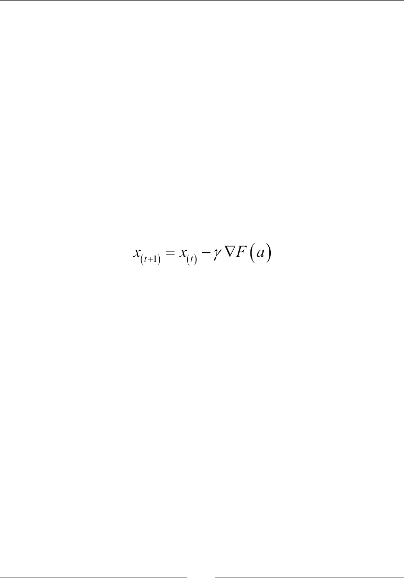
Basic Concepts
[ 1064 ]
Summary of optimization techniques
The same comments regarding linear algebra algorithms apply to optimization.
Treating such techniques in depth would have rendered the book impractical.
However, optimization is critical to the efciency and, to a lesser extent, the
accuracy of the machine learning algorithms. Some basic knowledge in this
eld goes a long way to build practical solutions for large data sets.
Gradient descent methods
Steepest descent
The steepest descent (or gradient descent) method is one of the simplest techniques
used to nd a local minimum of any continuous, differentiable function F or the
global minimum of any dened, differentiable, and convex function [A:9]. The value
of a vector or data point xt+1 at the iteration t + 1 is computed from the previous value
xt using the gradient
D
F of function F and the slope γ:
The steepest gradient algorithm is used for solving systems of non-linear equations
and minimization of the loss function in the logistic regression (refer to the Numerical
optimization section of Chapter 6, Regression and Regularization), in support vector
classiers (refer to the The nonlinear SVM section of Chapter 8, Kernel Models and
Support Vector Machines), and in multilayer perceptrons (refer to the The multilayer
perceptron (MLP) section of Chapter 9, Articial Neural Networks).
Conjugate gradient
The conjugate gradient solves unconstrained optimization problems and systems of
linear equations. It is an alternative to the LU factorization for positive, denite, and
symmetric square matrices. The solution x* to the equation Ax = b is expanded as the
weighted summation of n basis orthogonal directions pi (or conjugate directions):
1
*
0
;0
n
ii ij
i
Ax bpxbpp
α
−
=
=→=⋅=
∑
The solution x* is extracted by computing the ith conjugate vector pi and then
computing the coefcients αi.

Appendix A
[ 1065 ]
Stochastic gradient descent
The stochastic gradient method is a variant of the steepest descent method that
minimizes the convex function by dening the objective function F as the sum of
differentiable, basis functions fi:
() () ()
1 1
1
0 0
,
α
− −
+
= =
= = −∇
∑ ∑
n n
itt i
i i
Fx f x x x f x
The solution xt+1 at iteration t+1 is computed from the value xt at iteration t, the step
size (or learning rate) α, and the sum of the gradient of the basis functions [A:10].
The stochastic gradient descent is usually faster than other gradient descent or
quasi-Newton methods in converging towards a solution for convex functions.
The stochastic gradient descent method is used in logistic regression, support
vector machines, and back-propagation neural networks.
Stochastic gradient is particularly suitable for discriminative models with large
datasets [A:11]. Spark/MLlib makes extensive use of the stochastic gradient method.
Quasi-Newton algorithms
Quasi-Newton algorithms are variations of Newton's method of nding the value
of a vector or data point that maximizes or minimizes a function F whose rst order
derivative is null [A:12].
Newton's method is a well-known and simple optimization method used to nd the
solution to equations F(x) = 0 for which F is continuous and differentiable up to the
second order. It relies on the Taylor series expansion to approximate the function F
with a quadratic approximation on the variable ∆x = xt+1-xt, to compute the value at
the next iteration using the rst order F' and second order F" derivatives:
()()() ()
()
()
1
'
'. " "
t
t t ttt
t
Fx
Fx x Fx F x x F x x x Fx
+
+∆−≈∆+→=−
Contrary to Newton's method, quasi-Newton methods do not require that the
second order derivative, Hessian matrix of the objective function be computed.
It just has to be approximated [A:13]. There are several approaches to approximate
the computation of the Hessian matrix.
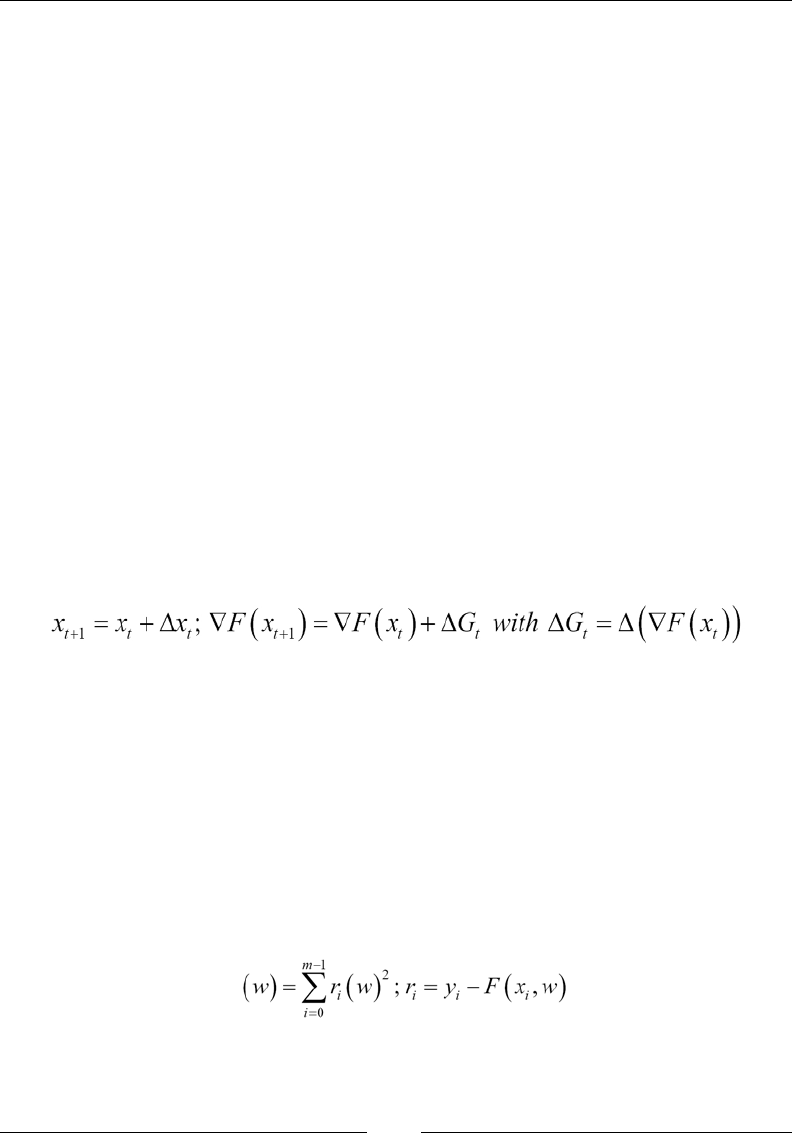
Basic Concepts
[ 1066 ]
BFGS
The Broyden-Fletcher-Goldfarb-Shanno (BGFS) method is a quasi-Newton iterative
numerical method to solve unconstrained nonlinear problems. The Hessian matrix
Ht+1 at an iteration t+1 is approximated using the value of the previous iteration t as
Ht+1=Ht + Ut + Vt applied to the Newton equation for the direction pt:
()
1
,
tt ttttt
Hp F x x x p
α
+
=−∇ =+
The BFGS method is used in minimization of the cost function for the conditional
random eld, and L1 and L2 regression.
L-BFGS
The performance of the BFGS algorithm can be improved by caching the
intermediate computation in memory in order to approximate the Hessian
matrix. The obvious drawback is that the memory becomes a limiting factor
in the scalability of the optimizer.
The Limited memory Broyden-Fletcher-Goldfarb-Shanno algorithm or L-BFGS is
a variant of BFGS that uses a minimum amount of computer RAM. The algorithm
maintains the last m incremental updates of the values ∆xt and the gradient ∆Gt at
iteration t, and then computes those values for the next step t+1:
It is supported by the Apache Commons Math 3.3 and above, Apache Spark/MLlib 1.0
and above, Colt 1.0 and above, and Iiitb CRF libraries. L-BFGS is used in minimization
of the loss function in conditional random elds. For more information, refer to the
Conditional random elds section of Chapter 7, Sequential Data Models.
Nonlinear least squares minimization
Let's consider the classic minimization of the least squares of a nonlinear function
y = F(x, w) with wi parameters for observations {y, xi}. The objective is to minimize
the sum of the squares of residuals ri:
L
Appendix A
[ 1067 ]
Gauss-Newton
The Gauss-Newton technique is a generalization of Newton's method. The technique
solves nonlinear least squares by updating the parameters wt+1 at iteration t+1 using
the rst order derivative, or Jacobian:
() ()
()
()
()
1
1
it
tt t
iij
rw
ww rw
w
−
+
∂
=−∂
The Gauss-Newton algorithm is used in logistic regression. For more information,
refer to the The logistic regression section of Chapter 6, Regression and Regularization.
Levenberg-Marquardt
The Levenberg-Marquardt algorithm is an alternative to the Gauss-Newton technique
for solving nonlinear least squares and curve tting problems. The method consists
of adding the gradient or Jacobian terms to the residuals ri to approximate the least
squares error:
The Levenberg-Marquardt algorithm is used in the training of logistic regression.
For more information, refer to the The logistic regression section of Chapter 6, Regression
and Regularization.
Lagrange multipliers
The Lagrange multipliers methodology is an optimization technique to nd the local
optima of a multivariate function, subject to equality constraints [A:14]. The problem
is stated as maximize f(x) subject to g(x) = c, where c is a constant and x is a variable or
features vector.
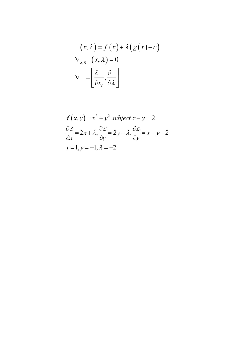
Basic Concepts
[ 1068 ]
This methodology introduces a new variable λ to integrate the constraint g into
a function, known as the Lagrange function
!
(x, λ). Let's note
D
!
, which is the
gradient of
!
over the variables xi and λ. The Lagrange multipliers are computed
by maximizing
!
:
!
! !
!
!
An example is as follows:
Lagrange multipliers are used in minimizing the loss function in the non-separable
case of linear support vector machines. For more information, refer to The nonseparable
case (soft margin) section of Chapter 8, Kernel Models and Support Vector Machines.
Overview of dynamic programming
The purpose of dynamic programming is to break down an optimization problem
into a sequence of steps known as substructures [A:15]. There are two types of
problems for which dynamic programming is suitable.
The solution of a global optimization problem can be broken down into optimal
solutions for its subproblems. The solutions of the subproblems are known as
optimal substructures. Greedy algorithms or the computation of the minimum
span of a graph are examples of decomposition into optimal substructures. Such
algorithms can be implemented either recursively or iteratively.
The solution of the global problem is applied recursively to the subproblems if the
number of subproblems is small. This approach is known as dynamic programming
using overlapping substructures. Forward-backward passes on hidden Markov
models, the Viterbi algorithm (refer to the The Viterbi algorithm section of Chapter 7,
Sequential Data Models), or the back-propagation of error in a multilayer perceptron
(refer to the Step 3 – error backpropagation section of Chapter 9, Articial Neural
Networks) are good examples of overlapping substructures.

Appendix A
[ 1069 ]
The mathematical formulation of dynamic programming solutions is specic to the
problem it attempts to solve. Dynamic programming techniques are also commonly
used in mathematical puzzles such as the Tower of Hanoi.
Finances 101
The exercises presented throughout this book are related to historical nancial
data and require the reader to have some basic understanding of nancial markets
and reports.
Fundamental analysis
Fundamental analysis is a set of techniques to evaluate a security—stock, bond,
currency, or commodity—that entails attempting to measure its intrinsic value
by examination related to both macro and micro, nancial and economy reports.
Fundamental analysis is usually applied to estimate the optimal price of a stock
using a variety of nancial ratios.
Numerous nancial metrics are used throughout this book. Here are the denitions
of the most commonly used metrics [A:16]:
• Earnings per share (EPS): This is the ratio of net earnings to the number of
outstanding shares.
• Price/Earnings ratio (PE): This is the ratio of the market price per share to
earnings per share.
• Price/Sales ratio (PS): This is the ratio of market price per share over gross
sales or revenue.
• Price/Book value ratio (PB): This is the ratio of market price per share over
total balance sheet value per share.
• Price to Earnings/Growth (PEG): This is the ratio of price/earnings per share
(PE) over annual growth of earnings per share.
• Operating income: This is the difference between the operating revenue and
operating expenses.
• Net sales: This is the difference between the revenue or gross sales and cost
of goods or cost of sales.
• Operating prot margin: This is the ratio of the operating income over
net sales.
• Net prot margin: This is the ratio of net prot over net sales (or net revenue).
• Short interest: This is the quantity of shares sold short and not yet covered.

Basic Concepts
[ 1070 ]
• Short interest ratio: This is the ratio of the short interest over total number of
shares oated.
• Cash per share: This is the ratio of the value of cash per share over market
price per share.
• Pay-out ratio: This is the percentage of the primary/basic earnings per share
excluding extraordinary items paid to common stockholders in the form of
cash dividends.
• Annual dividend yield: This is the ratio of sum of dividends paid during the
previous 12-month rolling period, over the current stock price. Regular and
extra dividends are included.
• Dividend coverage ratio: This is the ratio of income available to common
stockholders, excluding extraordinary items, for the most recent trailing
twelve months, to gross dividends paid to common shareholders, expressed
as percent.
• Gross Domestic Product (GDP): This is the aggregate measure of the
economic output of a country. It actually measures the sum of value added
by the production of goods and delivery of services.
• consumer price index (CPI): This is an indicator that measures the change in
the price of an arbitrary basket of goods and services used by the Bureau of
Labor Statistics to evaluate the inationary trend.
• Federal Fund rate: This is the interest rate at which banks trade balances held
at the Federal Reserve. The balances are called Federal Funds.
Technical analysis
Technical analysis is a methodology used to forecast the direction of the price of any given
security through the study of past market information derived from price and volume. In
simpler terms, it is the study of price activity and price patterns in order to identify
trade opportunities [A:17]. The price of a stock, commodity, bond, or nancial future
reects all the information publicly known about that asset as processed by the
market participants.
Terminology
• Bearish or bearish position: A bear position attempts to prot by betting that
the prices of the security will fall.
• Bullish or bullish position: A bull position attempts to prot by betting that
the price of the security will rise.
• Long position: This is the same as bullish.

Appendix A
[ 1071 ]
• Neutral position: A neutral position attempts to prot by betting the price of
the security will not change signicantly.
• Oscillator: An oscillator is a technical indicator that measures the price
momentum of a security using some statistical formulae.
• Overbought: A security is overbought when its price rises too fast as
measured by one or several trading signals or indicators.
• Oversold: A security is oversold when its price drops too fast as measured
by one or several trading signals or indicators.
• Relative strength index (RSI): The RSI is an oscillator that computes the
average of number of trading sessions for which the closing price is higher
than the opening price over the average of number of trading sessions
for which the closing price is lower than the opening price. The value is
normalized over [0, 1] or [0, 100%].
• Resistance: A resistance level is the upper limit of the price range of a
security. The price falls back as soon as it reaches the resistance level.
• Short position: This is the same as bearish.
• Support: A support level is the lower limit of the price range of a security
over a period of time. The price bounces back as soon as it reaches the
support level.
• Technical indicator: A technical indicator is a variable derived from the price
of a security and possibly its trading volume.
• Trading range: The trading range for a security over a period of time is the
difference between the highest and lowest price for this period of time.
• Trading signal: A signal is triggered when a technical indicator reaches a
predened value, upwards or downwards.
• Volatility: This is the variance or standard deviation of the price of a security
over a period of time.
Trading signals and strategy
The purpose is to create a set variable x, derived from price and volume; x = f (price,
volume) then generate predicates, x op c, where op is a Boolean operator, such as >
or =. The op operator compares the value of x to a predetermined threshold c.
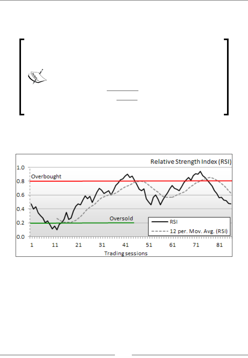
Basic Concepts
[ 1072 ]
Let's consider one of the most common technical indicators derived from price: the
relative strength index RSI, or the normalized RSI; nRSI, whose formulation is provided
here for reference:
The RSI for a period of T sessions, with opening price po, and
closing price pc is given by:
() ()
( )
1
0
0
100
100 /100
1
T
T c
t
TTT
T
T
Uptpt
RSI nRSI RSI
U
TU
−
=
=>
=−=
+−
∑
A trading signal is a predicate using a technical indicator nRSI(t) < 0.2. In trading
terminology, a signal is emitted for any time period, t, for which the predicate is true.
Have a look at the following graph:
Traders do not usually rely on a single trading signal to make a rational decision.
As an example, if G is the price of gold, I10 is the current rate of the 10-year Treasury
bond, and RSIsp500 is the relative strength index of the S&P 500 index, then we
can conclude that the increase in the exchange rate of the US$ to the Japanese Yen
maximizes for the trading strategy: {G < $1170 and I10 > 3.9% and RSIsp500 > 0.6 and
RSIsp500 < 0.8}.
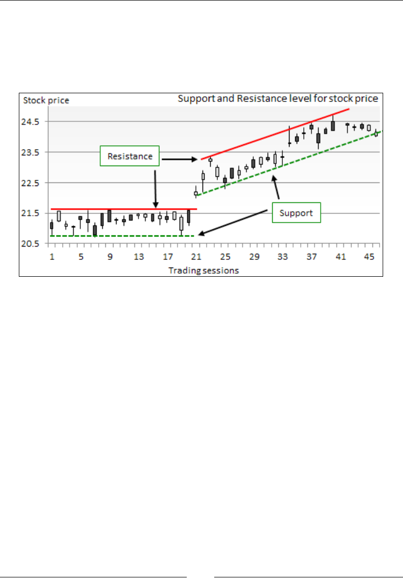
Appendix A
[ 1073 ]
Price patterns
Technical analysis assumes that historical prices contain some recurring albeit noisy
patterns that can be discovered using the statistical method. The most common
patterns used in the book are the trend, support, and resistance levels [A:18], as
illustrated in the following chart:
Illustration of trend, support, and resistance levels in technical analysis
Options trading
An option is a contract that gives the buyer the right but not the obligation to buy or
sell a security at a specic price on or before a certain date [A:19].
The two types of options are calls and puts:
• A call gives the holder the right to buy a security at a certain price within a
specic period of time. Buyers of calls expect that the price of the security
will increase substantially over the strike price before the option expires.
• A put option gives the holder the right to sell a security at a certain price
within a specic period of time. Buyers of puts expect that the price of the
stock will fall below the strike price before the option expires.
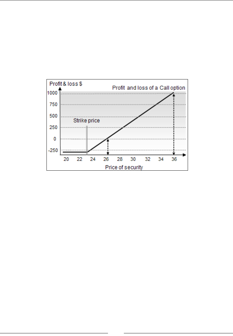
Basic Concepts
[ 1074 ]
Let's consider a call option contract on 100 shares at a strike price of $ 23 for a total
cost of $ 270 ($ 2.7 per option). The maximum loss the holder of the call can incur
is the loss of premium or $270 when the option expires. However, the prot can be
potentially almost unlimited. If the price of the security reaches $ 36 when the call
option expires, the owner will have a prot of ($ 36 - $ 23)*100 - $ 270 = $ 1030. The
return on investment is 1030/270 = 380 percent. Buying and then selling the stock
would have generated a return on investment of 36/24 - 1= 50 percent. This example
is simple and does not take into account transaction fee or margin cost [A:20]. Have a
look at the following graph:
.
Financial data sources
There are numerous sources of nancial data available to experiment with machine
learning and validation models [A:21].
• Yahoo nances (stocks, ETFs, and indices) available at
http://finance.yahoo.com
• Google nances (stocks, ETFs, and indices) available at
https://www.google.com/finance
• NASDAQ (stocks, ETFs, and indices) available at http://www.nasdaq.com
• European Central Bank (European bonds and notes) available at
http://www.ecb.int
• TrueFx (forex) available at http://www.truefx.com
• Quandl (economics and nancials statistics) available at
http://www.quantl.com
• Dartmouth University (portfolio and simulation) available at
http://mba.tuck.dartmouth.edu

Appendix A
[ 1075 ]
Suggested online courses
• Practical Machine Learning. J. Leek, R. Peng, B. Caffo. Johns Hopkins
University, available at https://www.coursera.org/jhu
• Probabilistic Graphical Models. D. Koller. Stanford University, available at
https://www.coursera.org/course/pgm
• Machine Learning. A. Ng. Stanford University, available at
https://www.coursera.org/course/ml
References
• [A:1] Daily scala: Enumeration. J. Eichar. 2009, available at http://daily-
scala.blogspot.com/2009/08/enumerations.html
• [A:2] Matrices and Linear Transformations 2nd edition. C. Cullen. Dover Books
on Mathematics. 1990
• [A:3] Linear Algebra: A Modern Introduction. D Poole. BROOKS/COLE
CENGAGE Learning. 2010
• [A:4] Matrix decomposition for regression analysis. D. Bates. 2007, available
at http://www.stat.wisc.edu/courses/st849-bates/lectures/
Orthogonal.pdf
• [A:5] Eigenvalues and Eigenvectors of Symmetric Matrices. I. Mateev. 2013,
available at http://www.slideshare.net/vanchizzle/eigenvalues-and-
eigenvectors-of-symmetric-matrices
• [A:6] Linear Algebra Done Right 2nd edition (§5 Eigenvalues and Eigenvectors).
S Axler. Springer. 2000
• [A:7] First Order Predicate Logic. S. Kaushik. CSE India Institute of
Technology. Delhi, available at http://www.cse.iitd.ac.in/~saroj/LFP/
LFP_2013/L4.pdf
• [A:8] Matrix Recipes. J. Movellan. 2005, available at http://www.math.
vt.edu/people/dlr/m2k_svb11_hesian.pdf
• [A:9] Gradient descent. Wikipedia: the free encyclopedia. Wikimedia
foundation, available at http://en.wikipedia.org/wiki/Gradient_
descent
• [A:10] Large Scale Machine Learning: Stochastic Gradient Descent Convergence.
A. Ng. Stanford University, available at https://class.coursera.org/ml-
003/lecture/107

Basic Concepts
[ 1076 ]
• [A:11] Large-Scala Machine Learning with Stochastic Gradient Descent. L
Bottou. 2010, available at http://leon.bottou.org/publications/pdf/
compstat-2010.pdf
• [A:12] Overview of Quasi-Newton optimization methods. Dept. Computer
Science. University of Washington, available at https://homes.
cs.washington.edu/~galen/files/quasi-newton-notes.pdf
• [A:13] Lecture 2-3: Gradient and Hessian of Multivariate Function. M.
Zibulevsky. 2013, available at http://www.youtube.com
• [A:14] Introduction to the Lagrange Multiplier. ediwm.com, video available at
http://www.noodle.com/learn/details/334954/introduction-to-the-
lagrange-multiplier
• [A:15] A brief introduction to Dynamic Programming (DP). A. Kasibhatla.
Nanocad Lab, available at http://nanocad.ee.ucla.edu/pub/Main/
SnippetTutorial/Amar_DP_Intro.pdf
• [A:16] Financial ratios. Wikipedia, available at http://en.wikipedia.org/
wiki/Financial_ratio
• [A:17] Getting started in Technical Analysis (§1 Charts: Forecasting Tool or
Folklore?). J Schwager. John Wiley & Sons. 1999
• [A:18] Getting started in Technical Analysis (§4 Trading Ranges, Support &
Resistance). J Schwager. John Wiley & Sons. 1999
• [A:19] Options: a personal seminar (§1 Options: An Introduction, What is an
Option). S. Fullman, New York Institute of Finance. Simon Schuster. 1992
• [A:20] Options: a personal seminar (§2 Purchasing Options). S. Fullman. New
York Institute of Finance. Simon Schuster. 1992
• [A:21] List of nancial data feeds. Wikipedia, the free encyclopedia. Wikimedia
foundation, available at http://en.wikipedia.org/wiki/List_of_
financial_data_feeds

[ 1077 ]
Bibliography
This Learning path is a blend of text and projects, all packaged up keeping your
journey in mind. It includes content from the following Packt books:
• Scala for Data Science, Pascal Bugnion
• Scala Data Analysis Cookbook, Arun Manivannan
• Scala for Machine Learning, Patrick R. Nicolas

Thank you for buying
Scala: Guide for Data Science Professionals
About Packt Publishing
Packt, pronounced 'packed', published its rst book, Mastering phpMyAdmin for Effective
MySQL Management, in April 2004, and subsequently continued to specialize in publishing
highly focused books on specic technologies and solutions.
Our books and publications share the experiences of your fellow IT professionals in adapting
and customizing today's systems, applications, and frameworks. Our solution-based books
give you the knowledge and power to customize the software and technologies you're using
to get the job done. Packt books are more specic and less general than the IT books you have
seen in the past. Our unique business model allows us to bring you more focused information,
giving you more of what you need to know, and less of what you don't.
Packt is a modern yet unique publishing company that focuses on producing quality,
cutting-edge books for communities of developers, administrators, and newbies alike.
For more information, please visit our website at www.packtpub.com.
Writing for Packt
We welcome all inquiries from people who are interested in authoring. Book proposals should
be sent to author@packtpub.com. If your book idea is still at an early stage and you would
like to discuss it rst before writing a formal book proposal, then please contact us; one of our
commissioning editors will get in touch with you.
We're not just looking for published authors; if you have strong technical skills but no writing
experience, our experienced editors can help you develop a writing career, or simply get some
additional reward for your expertise.
Please check www.PacktPub.com for information on our titles
