Short Guide
User Manual: Pdf
Open the PDF directly: View PDF ![]() .
.
Page Count: 145 [warning: Documents this large are best viewed by clicking the View PDF Link!]
- Title Page
- Thank you!
- Preface
- Things You Need to Know
- Typesetting Text
- Typesetting Mathematical Formulae
- Specialities
- Producing Mathematical Graphics
- Customising LaTeX
- Bibliography
- Index


ii
Copyright ©1995-2002 Tobias Oetiker and all the Contributers to LShort. All
rights reserved.
This document is free; you can redistribute it and/or modify it under the terms
of the GNU General Public License as published by the Free Software Foundation;
either version 2 of the License, or (at your option) any later version.
This document is distributed in the hope that it will be useful, but WITHOUT
ANY WARRANTY; without even the implied warranty of MERCHANTABILITY
or FITNESS FOR A PARTICULAR PURPOSE. See the GNU General Public
License for more details.
You should have received a copy of the GNU General Public License along with
this document; if not, write to the Free Software Foundation, Inc., 675 Mass Ave,
Cambridge, MA 02139, USA.
Thank you!
Much of the material used in this introduction comes from an Austrian in-
troduction to L
A
T
EX 2.09 written in German by:
Hubert Partl <partl@mail.boku.ac.at>
Zentraler Informatikdienst der Universität für Bodenkultur Wien
Irene Hyna <Irene.Hyna@bmwf.ac.at>
Bundesministerium für Wissenschaft und Forschung Wien
Elisabeth Schlegl <noemail>
in Graz
If you are interested in the German document, you can find a version
updated for L
A
T
EX 2εby Jörg Knappen at
CTAN:/tex-archive/info/lshort/german

iv Thank you!
While preparing this document, I asked for reviewers on comp.text.tex.
I got a lot of response. The following individuals helped with corrections,
suggestions and material to improve this paper. They put in a big effort to
help me get this document into its present shape. I would like to sincerely
thank all of them. Naturally, all the mistakes you’ll find in this book are
mine. If you ever find a word that is spelled correctly, it must have been one
of the people below dropping me a line.
Rosemary Bailey, Marc Bevand, Friedemann Brauer, Jan Busa,
Markus Brühwiler, Pietro Braione, David Carlisle, José Carlos Santos,
Neil Carter, Mike Chapman, Pierre Chardaire, Christopher Chin, Carl Cerecke,
Chris McCormack, Wim van Dam, Jan Dittberner, Michael John Downes,
Matthias Dreier, David Dureisseix, Elliot, Hans Ehrbar, Daniel Flipo, David Frey,
Hans Fugal, Robin Fairbairns, Jörg Fischer, Erik Frisk, Mic Milic Frederickx,
Frank, Kasper B. Graversen, Arlo Griffiths, Alexandre Guimond, Andy Goth,
Cyril Goutte, Greg Gamble, Frank Fischli, Neil Hammond,
Rasmus Borup Hansen, Joseph Hilferty, Björn Hvittfeldt, Martien Hulsen,
Werner Icking, Jakob, Eric Jacoboni, Alan Jeffrey, Byron Jones, David Jones,
Johannes-Maria Kaltenbach, Michael Koundouros, Andrzej Kawalec,
Sander de Kievit, Alain Kessi, Christian Kern, Jörg Knappen, Kjetil Kjernsmo,
Maik Lehradt, Rémi Letot, Flori Lambrechts, Johan Lundberg, Alexander Mai,
Hendrik Maryns, Martin Maechler, Aleksandar S Milosevic, Henrik Mitsch,
Claus Malten, Kevin Van Maren, Richard Nagy, Philipp Nagele,
Lenimar Nunes de Andrade, Manuel Oetiker, Urs Oswald, Demerson Andre Polli,
Maksym Polyakov Hubert Partl, John Refling, Mike Ressler, Brian Ripley,
Young U. Ryu, Bernd Rosenlecher, Chris Rowley, Risto Saarelma,
Hanspeter Schmid, Craig Schlenter, Gilles Schintgen, Baron Schwartz,
Christopher Sawtell, Miles Spielberg, Geoffrey Swindale, Laszlo Szathmary,
Boris Tobotras, Josef Tkadlec, Scott Veirs, Didier Verna, Fabian Wernli,
Carl-Gustav Werner, David Woodhouse, Chris York, Fritz Zaucker, Rick Zaccone,
and Mikhail Zotov.
Preface
L
A
T
EX [1] is a typesetting system that is very suitable for producing scientific
and mathematical documents of high typographical quality. It is also suitable
for producing all sorts of other documents, from simple letters to complete
books. L
A
T
EX uses T
EX [2] as its formatting engine.
This short introduction describes L
A
T
EX 2εand should be sufficient for
most applications of L
A
T
EX. Refer to [1,3] for a complete description of the
L
A
T
EX system.
This introduction is split into 6 chapters:
Chapter 1 tells you about the basic structure of L
A
T
EX 2εdocuments. You
will also learn a bit about the history of L
A
T
EX. After reading this
chapter, you should have a rough understanding how L
A
T
EX works.
Chapter 2 goes into the details of typesetting your documents. It explains
most of the essential L
A
T
EX commands and environments. After reading
this chapter, you will be able to write your first documents.
Chapter 3 explains how to typeset formulae with L
A
T
EX. Many examples
demonstrate how to use one of L
A
T
EX’s main strengths. At the end
of the chapter are tables listing all mathematical symbols available in
L
A
T
EX.
Chapter 4 explains indexes, bibliography generation and inclusion of EPS
graphics. It introduces creation of PDF documents with pdfL
A
T
EX and
presents some handy extension packages.
Chapter 5 shows how to use L
A
T
EX for creating graphics. Instead of draw-
ing a picture with some graphics program, saving it to a file and then
including it into L
A
T
EX you describe the picture and have L
A
T
EX draw
it for you.
Chapter 6 contains some potentially dangerous information about how to
alter the standard document layout produced by L
A
T
EX. It will tell you
how to change things such that the beautiful output of L
A
T
EX turns ugly
or stunning, depending on your abilities.

vi Preface
It is important to read the chapters in order—the book is not that big, after
all. Be sure to carefully read the examples, because a lot of the information
is in the examples placed throughout the book.
L
A
T
EX is available for most computers, from the PC and Mac to large UNIX
and VMS systems. On many university computer clusters you will find that
a L
A
T
EX installation is available, ready to use. Information on how to access
the local L
A
T
EX installation should be provided in the Local Guide [5]. If you
have problems getting started, ask the person who gave you this booklet.
The scope of this document is not to tell you how to install and set up a
L
A
T
EX system, but to teach you how to write your documents so that they
can be processed by L
A
T
EX.
If you need to get hold of any L
A
T
EX related material, have a look at one
of the Comprehensive T
EX Archive Network (CTAN) sites. The homepage is
at http://www.ctan.org. All packages can also be retrieved from the ftp
archive ftp://www.ctan.org and its various mirror sites all over the world.
They can be found e.g. at ftp://ctan.tug.org (US), ftp://ftp.dante.de
(Germany), ftp://ftp.tex.ac.uk (UK). If you are not in one of these coun-
tries, choose the archive closest to you.
You will find other references to CTAN throughout the book, especially
pointers to software and documents you might want to download. Instead of
writing down complete urls, I just wrote CTAN: followed by whatever location
within the CTAN tree you should go to.
If you want to run L
A
T
EX on your own computer, take a look at what is
available from CTAN:/tex-archive/systems.
If you have ideas for something to be added, removed or altered in this
document, please let me know. I am especially interested in feedback from
L
A
T
EX novices about which bits of this intro are easy to understand and
which could be explained better.
Tobias Oetiker <oetiker@ee.ethz.ch>
Department of Information Technology and
Electrical Engineering, Swiss Federal Institute of Technology
The current version of this document is available on
CTAN:/tex-archive/info/lshort
Contents
Thank you! iii
Preface v
1 Things You Need to Know 1
1.1 The Name of the Game ..................... 1
1.1.1 T
EX............................ 1
1.1.2 L
A
T
EX........................... 1
1.2 Basics ............................... 2
1.2.1 Author, Book Designer, and Typesetter ........ 2
1.2.2 Layout Design ...................... 2
1.2.3 Advantages and Disadvantages ............. 3
1.3 L
A
T
EX Input Files ......................... 4
1.3.1 Spaces ........................... 4
1.3.2 Special Characters .................... 4
1.3.3 L
A
T
EX Commands ..................... 5
1.3.4 Comments ......................... 6
1.4 Input File Structure ....................... 6
1.5 A Typical Command Line Session ................ 7
1.6 The Layout of the Document .................. 9
1.6.1 Document Classes .................... 9
1.6.2 Packages .......................... 9
1.6.3 Page Styles ........................ 11
1.7 Files You Might Encounter ................... 11
1.8 Big Projects ............................ 13
2 Typesetting Text 15
2.1 The Structure of Text and Language . . . . . . . . . . . . . . 15
2.2 Line Breaking and Page Breaking ................ 17
2.2.1 Justified Paragraphs ................... 17
2.2.2 Hyphenation ....................... 18
2.3 Ready-Made Strings ....................... 19
2.4 Special Characters and Symbols ................. 19

viii CONTENTS
2.4.1 Quotation Marks ..................... 19
2.4.2 Dashes and Hyphens ................... 20
2.4.3 Tilde (∼)......................... 20
2.4.4 Degree Symbol (◦).................... 20
2.4.5 The Euro Currency Symbol (€)............. 21
2.4.6 Ellipsis (. . . ) ....................... 22
2.4.7 Ligatures ......................... 22
2.4.8 Accents and Special Characters ............. 22
2.5 International Language Support ................. 23
2.5.1 Support for Portuguese ................. 25
2.5.2 Support for French .................... 27
2.5.3 Support for German ................... 27
2.5.4 Support for Korean .................... 28
2.5.5 Support for Cyrillic .................... 31
2.6 The Space Between Words .................... 32
2.7 Titles, Chapters, and Sections .................. 33
2.8 Cross References ......................... 35
2.9 Footnotes ............................. 35
2.10 Emphasized Words ........................ 36
2.11 Environments ........................... 36
2.11.1 Itemize, Enumerate, and Description . . . . . . . . . . 37
2.11.2 Flushleft, Flushright, and Center . . . . . . . . . . . . 37
2.11.3 Quote, Quotation, and Verse . . . . . . . . . . . . . . 38
2.11.4 Abstract .......................... 38
2.11.5 Printing Verbatim .................... 39
2.11.6 Tabular .......................... 39
2.12 Floating Bodies .......................... 41
2.13 Protecting Fragile Commands .................. 44
3 Typesetting Mathematical Formulae 45
3.1 General .............................. 45
3.2 Grouping in Math Mode ..................... 47
3.3 Building Blocks of a Mathematical Formula . . . . . . . . . . 47
3.4 Math Spacing ........................... 51
3.5 Vertically Aligned Material ................... 52
3.6 Phantoms ............................. 54
3.7 Math Font Size .......................... 54
3.8 Theorems, Laws, . . . ....................... 55
3.9 Bold Symbols ........................... 57
3.10 List of Mathematical Symbols .................. 58

CONTENTS ix
4 Specialities 65
4.1 Including Encapsulated PostScript Graphics . . . . . . . . 65
4.2 Bibliography ........................... 67
4.3 Indexing .............................. 68
4.4 Fancy Headers .......................... 69
4.5 The Verbatim Package ...................... 70
4.6 Downloading and Installing L
A
T
EX Packages . . . . . . . . . . 71
4.7 Working with pdfL
A
T
EX..................... 72
4.7.1 PDF Documents for the Web . . . . . . . . . . . . . . 73
4.7.2 The Fonts ......................... 73
4.7.3 Using Graphics ...................... 75
4.7.4 Hypertext Links ..................... 76
4.7.5 Problems with Links ................... 78
4.7.6 Problems with Bookmarks ................ 78
4.8 Creating Presentations with pdfscreen ............. 80
5 Producing Mathematical Graphics 85
5.1 Overview ............................. 85
5.2 The picture Environment .................... 86
5.2.1 Basic Commands ..................... 86
5.2.2 Line Segments ...................... 87
5.2.3 Arrows ........................... 88
5.2.4 Circles ........................... 89
5.2.5 Text and Formulas .................... 90
5.2.6 The \multiput and the \linethickness command . . 90
5.2.7 Ovals. The \thinlines and the \thicklines command 91
5.2.8 Multiple Use of Predefined Picture Boxes . . . . . . . 92
5.2.9 Quadratic Bézier Curves ................. 93
5.2.10 Catenary ......................... 94
5.2.11 Rapidity in the Special Theory of Relativity . . . . . . 95
5.3 X
Y
-pic ............................... 95
6 Customising L
A
T
E
X99
6.1 New Commands, Environments and Packages . . . . . . . . . 99
6.1.1 New Commands .....................100
6.1.2 New Environments ....................101
6.1.3 Extra Space ........................101
6.1.4 Commandline L
A
T
EX...................102
6.1.5 Your Own Package ....................103
6.2 Fonts and Sizes ..........................103
6.2.1 Font Changing Commands ................103
6.2.2 Danger, Will Robinson, Danger . . . . . . . . . . . . . 106
6.2.3 Advice ...........................106
6.3 Spacing ..............................107

x CONTENTS
6.3.1 Line Spacing .......................107
6.3.2 Paragraph Formatting ..................107
6.3.3 Horizontal Space .....................108
6.3.4 Vertical Space .......................109
6.4 Page Layout ............................110
6.5 More Fun With Lengths .....................112
6.6 Boxes ...............................113
6.7 Rules and Struts .........................115
Bibliography 117
Index 119
List of Figures
1.1 A Minimal L
A
T
EX File. ...................... 7
1.2 Example of a Realistic Journal Article. ............. 7
4.1 Example fancyhdr Setup. ..................... 70
4.2 Example pdfscreen input file ................... 81
6.1 Example Package. ........................103
6.2 Page Layout Parameters. .....................111
List of Tables
1.1 Document Classes. ........................ 9
1.2 Document Class Options. .................... 10
1.3 Some of the Packages Distributed with L
A
T
EX. . . . . . . . . . 12
1.4 The Predefined Page Styles of L
A
T
EX. . . . . . . . . . . . . . . 12
2.1 A bag full of Euro symbols .................... 21
2.2 Accents and Special Characters. ................. 23
2.3 Preamble for Portuguese documents. . . . . . . . . . . . . . . 26
2.4 Special commands for French. .................. 27
2.5 German Special Characters. ................... 28
2.6 Bulgarian, Russian, and Ukrainian ............... 32
2.7 Float Placing Permissions. .................... 42
3.1 Math Mode Accents. ....................... 58
3.2 Lowercase Greek Letters. ..................... 58
3.3 Uppercase Greek Letters. .................... 58
3.4 Binary Relations. ......................... 59
3.5 Binary Operators. ........................ 59
3.6 BIG Operators. .......................... 60
3.7 Arrows. .............................. 60
3.8 Delimiters. ............................. 60
3.9 Large Delimiters. ......................... 60
3.10 Miscellaneous Symbols. ...................... 61
3.11 Non-Mathematical Symbols. ................... 61
3.12 AMS Delimiters. ......................... 61
3.13 AMS Greek and Hebrew. ..................... 61
3.14 AMS Binary Relations. ...................... 62
3.15 AMS Arrows. ........................... 62
3.16 AMS Negated Binary Relations and Arrows. . . . . . . . . . . 63
3.17 AMS Binary Operators. ..................... 63
3.18 AMS Miscellaneous. ....................... 64
3.19 Math Alphabets. ......................... 64
4.1 Key Names for graphicx Package. ................ 66

xiv LIST OF TABLES
4.2 Index Key Syntax Examples. .................. 69
6.1 Fonts. ...............................104
6.2 Font Sizes. .............................104
6.3 Absolute Point Sizes in Standard Classes. . . . . . . . . . . . 105
6.4 Math Fonts. ............................105
6.5 T
EX Units. ............................109
Chapter 1
Things You Need to Know
The first part of this chapter presents a short overview of the philosophy and
history of L
A
T
E
X 2ε. The second part focuses on the basic structures of a L
A
T
E
X
document. After reading this chapter, you should have a rough knowledge of
how L
A
T
E
X works, which you will need to understand the rest of this book.
1.1 The Name of the Game
1.1.1 T
E
X
T
EX is a computer program created by Donald E. Knuth [2]. It is aimed
at typesetting text and mathematical formulae. Knuth started writing the
T
EX typesetting engine in 1977 to explore the potential of the digital printing
equipment that was beginning to infiltrate the publishing industry at that
time, especially in the hope that he could reverse the trend of deteriorating
typographical quality that he saw affecting his own books and articles. T
EX
as we use it today was released in 1982, with some slight enhancements added
in 1989 to better support 8-bit characters and multiple languages. T
EX is
renowned for being extremely stable, for running on many different kinds of
computers, and for being virtually bug free. The version number of T
EX is
converging to πand is now at 3.14159.
T
EX is pronounced “Tech,” with a “ch” as in the German word “Ach” or
in the Scottish “Loch.” In an ASCII environment, T
EX becomes TeX.
1.1.2 L
A
T
E
X
L
A
T
EX is a macro package that enables authors to typeset and print their
work at the highest typographical quality, using a predefined, professional
layout. L
A
T
EX was originally written by Leslie Lamport [1]. It uses the T
EX
formatter as its typesetting engine. These days L
A
T
EX is maintained by Frank
Mittelbach.

2 Things You Need to Know
L
A
T
EX is pronounced “Lay-tech” or “Lah-tech.” If you refer to L
A
T
EX in
an ASCII environment, you type LaTeX. L
A
T
EX 2εis pronounced “Lay-tech
two e” and typed LaTeX2e.
1.2 Basics
1.2.1 Author, Book Designer, and Typesetter
To publish something, authors give their typed manuscript to a publishing
company. One of their book designers then decides the layout of the docu-
ment (column width, fonts, space before and after headings, . . .). The book
designer writes his instructions into the manuscript and then gives it to a
typesetter, who typesets the book according to these instructions.
A human book designer tries to find out what the author had in mind
while writing the manuscript. He decides on chapter headings, citations,
examples, formulae, etc. based on his professional knowledge and from the
contents of the manuscript.
In a L
A
T
EX environment, L
A
T
EX takes the role of the book designer and
uses T
EX as its typesetter. But L
A
T
EX is “only” a program and therefore
needs more guidance. The author has to provide additional information to
describe the logical structure of his work. This information is written into
the text as “L
A
T
EX commands.”
This is quite different from the WYSIWYG1approach that most modern
word processors, such as MS Word or Corel WordPerfect, take. With these
applications, authors specify the document layout interactively while typing
text into the computer. They can see on the screen how the final work will
look when it is printed.
When using L
A
T
EX it is not normally possible to see the final output while
typing the text, but the final output can be previewed on the screen after
processing the file with L
A
T
EX. Then corrections can be made before actually
sending the document to the printer.
1.2.2 Layout Design
Typographical design is a craft. Unskilled authors often commit serious
formatting errors by assuming that book design is mostly a question of
aesthetics—“If a document looks good artistically, it is well designed.” But
as a document has to be read and not hung up in a picture gallery, the read-
ability and understandability is much more important than the beautiful
look of it. Examples:
•The font size and the numbering of headings have to be chosen to make
the structure of chapters and sections clear to the reader.
1What you see is what you get.

1.2 Basics 3
•The line length has to be short enough not to strain the eyes of the
reader, while long enough to fill the page beautifully.
With WYSIWYG systems, authors often generate aesthetically pleasing
documents with very little or inconsistent structure. L
A
T
EX prevents such
formatting errors by forcing the author to declare the logical structure of his
document. L
A
T
EX then chooses the most suitable layout.
1.2.3 Advantages and Disadvantages
When people from the WYSIWYG world meet people who use L
A
T
EX, they
often discuss “the advantages of L
A
T
EX over a normal word processor” or the
opposite. The best thing you can do when such a discussion starts is to keep
a low profile, since such discussions often get out of hand. But sometimes
you cannot escape . . .
So here is some ammunition. The main advantages of L
A
T
EX over normal
word processors are the following:
•Professionally crafted layouts are available, which make a document
really look as if “printed.”
•The typesetting of mathematical formulae is supported in a convenient
way.
•Users only need to learn a few easy-to-understand commands that spec-
ify the logical structure of a document. They almost never need to
tinker with the actual layout of the document.
•Even complex structures such as footnotes, references, table of con-
tents, and bibliographies can be generated easily.
•Free add-on packages exist for many typographical tasks not directly
supported by basic L
A
T
EX. For example, packages are available to in-
clude PostScript graphics or to typeset bibliographies conforming to
exact standards. Many of these add-on packages are described in The
L
A
T
E
X Companion [3].
•L
A
T
EX encourages authors to write well-structured texts, because this
is how L
A
T
EX works—by specifying structure.
•T
EX, the formatting engine of L
A
T
EX 2ε, is highly portable and free.
Therefore the system runs on almost any hardware platform available.
L
A
T
EX also has some disadvantages, and I guess it’s a bit difficult for me to
find any sensible ones, though I am sure other people can tell you hundreds
;-)
4 Things You Need to Know
•L
A
T
EX does not work well for people who have sold their souls . . .
•Although some parameters can be adjusted within a predefined docu-
ment layout, the design of a whole new layout is difficult and takes a
lot of time.2
•It is very hard to write unstructured and disorganized documents.
•Your hamster might, despite some encouraging first steps, never be
able to fully grasp the concept of Logical Markup.
1.3 L
A
T
E
X Input Files
The input for L
A
T
EX is a plain ASCII text file. You can create it with any
text editor. It contains the text of the document, as well as the commands
that tell L
A
T
EX how to typeset the text.
1.3.1 Spaces
“Whitespace” characters, such as blank or tab, are treated uniformly as
“space” by L
A
T
EX. Several consecutive whitespace characters are treated
as one “space.” Whitespace at the start of a line is generally ignored, and a
single line break is treated as “whitespace.”
An empty line between two lines of text defines the end of a paragraph.
Several empty lines are treated the same as one empty line. The text below
is an example. On the left hand side is the text from the input file, and on
the right hand side is the formatted output.
It does not matter whether you
enter one or several spaces
after a word.
An empty line starts a new
paragraph.
It does not matter whether you enter one or
several spaces after a word.
An empty line starts a new paragraph.
1.3.2 Special Characters
The following symbols are reserved characters that either have a special
meaning under L
A
T
EX or are not available in all the fonts. If you enter them
directly in your text, they will normally not print, but rather coerce L
A
T
EX
to do things you did not intend.
#$%^&_{}~\
2Rumour says that this is one of the key elements that will be addressed in the upcoming
L
A
T
E
X3 system.
1.3 L
A
T
E
X Input Files 5
As you will see, these characters can be used in your documents all the
same by adding a prefix backslash:
\# \$ \% \^{} \& \_ \{ \} \~{} #$%ˆ&_{}˜
The other symbols and many more can be printed with special commands
in mathematical formulae or as accents. The backslash character \can not
be entered by adding another backslash in front of it (\\); this sequence is
used for line breaking.3
1.3.3 L
A
T
E
X Commands
L
A
T
EX commands are case sensitive, and take one of the following two for-
mats:
•They start with a backslash \and then have a name consisting of
letters only. Command names are terminated by a space, a number or
any other ‘non-letter.’
•They consist of a backslash and exactly one non-letter.
L
A
T
EX ignores whitespace after commands. If you want to get a space
after a command, you have to put either {} and a blank or a special spacing
command after the command name. The {} stops L
A
T
EX from eating up all
the space after the command name.
I read that Knuth divides the
people working with \TeX{} into
\TeX{}nicians and \TeX perts.\\
Today is \today.
I read that Knuth divides the people working
with T
EX into T
EXnicians and T
EXperts.
Today is 4th April 2004.
Some commands need a parameter, which has to be given between curly
braces { } after the command name. Some commands support optional pa-
rameters, which are added after the command name in square brackets [ ].
The next examples use some L
A
T
EX commands. Don’t worry about them;
they will be explained later.
You can \textsl{lean} on me! You can lean on me!
Please, start a new line
right here!\newline
Thank you!
Please, start a new line right here!
Thank you!
3Try the $\backslash$ command instead. It produces a ‘\’.
6 Things You Need to Know
1.3.4 Comments
When L
A
T
EX encounters a %character while processing an input file, it ignores
the rest of the present line, the line break, and all whitespace at the beginning
of the next line.
This can be used to write notes into the input file, which will not show
up in the printed version.
This is an % stupid
% Better: instructive <----
example: Supercal%
ifragilist%
icexpialidocious
This is an example: Supercalifragilisticexpi-
alidocious
The %character can also be used to split long input lines where no whites-
pace or line breaks are allowed.
For longer comments you could use the comment environment provided
by the verbatim package. This means, to use the comment environment you
have to add the command \usepackage{verbatim} to the preamble of your
document.
This is another
\begin{comment}
rather stupid,
but helpful
\end{comment}
example for embedding
comments in your document.
This is another example for embedding com-
ments in your document.
Note that this won’t work inside complex environments, like math for
example.
1.4 Input File Structure
When L
A
T
EX 2εprocesses an input file, it expects it to follow a certain struc-
ture. Thus every input file must start with the command
\documentclass{...}
This specifies what sort of document you intend to write. After that, you
can include commands that influence the style of the whole document, or
you can load packages that add new features to the L
A
T
EX system. To load
such a package you use the command
\usepackage{...}
When all the setup work is done,4you start the body of the text with
the command
4The area between \documentclass and \begin{document}is called the preamble.

1.5 A Typical Command Line Session 7
\begin{document}
Now you enter the text mixed with some useful L
A
T
EX commands. At
the end of the document you add the
\end{document}
command, which tells L
A
T
EX to call it a day. Anything that follows this
command will be ignored by L
A
T
EX.
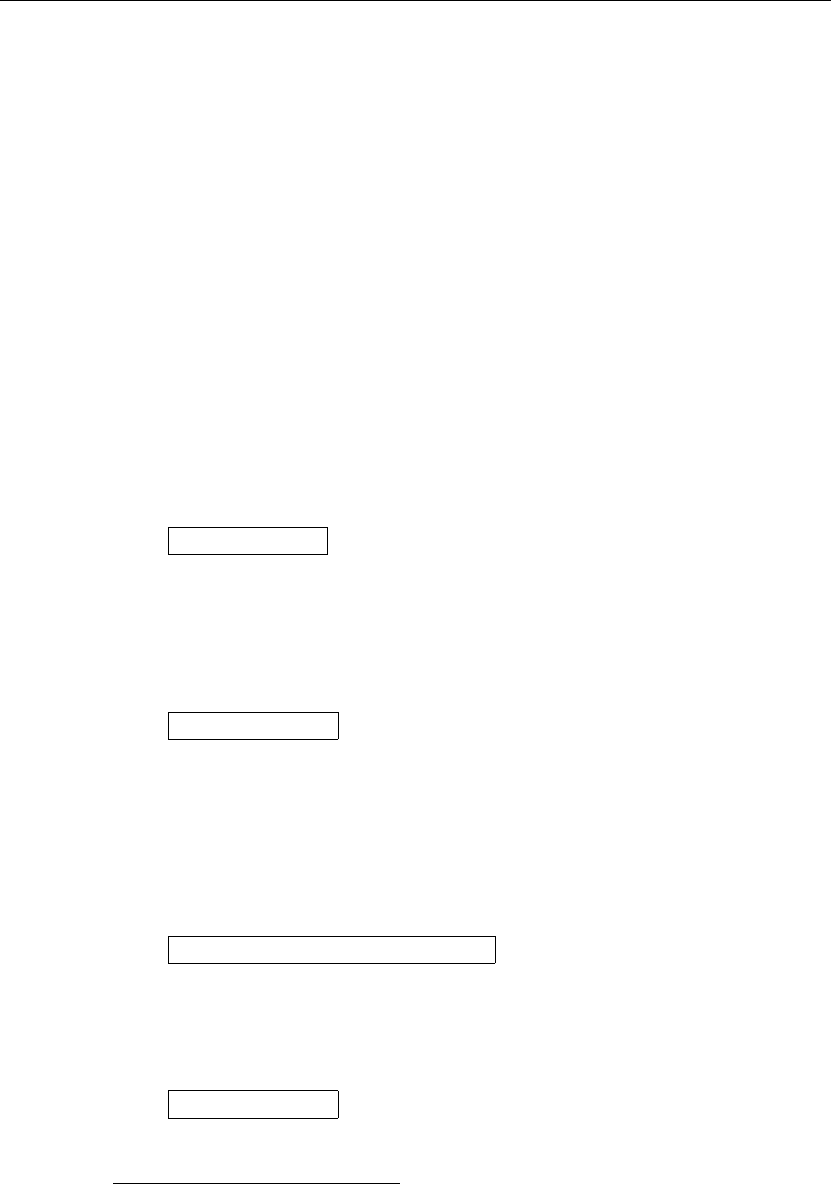
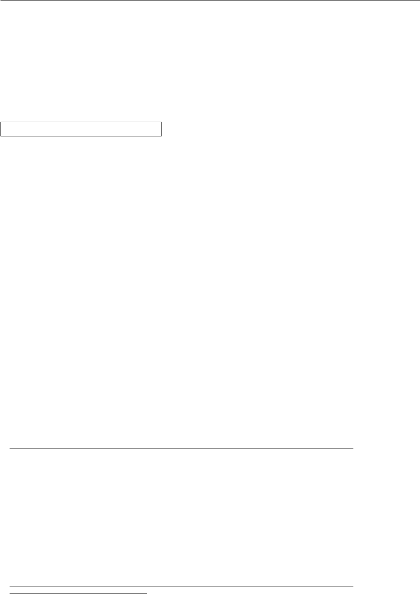
Figure 1.1 shows the contents of a minimal L
A
T
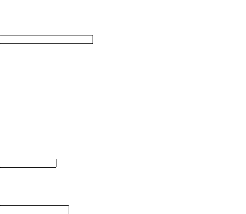
EX 2εfile. A slightly more
complicated input file is given in Figure 1.2.
1.5 A Typical Command Line Session
I bet you must be dying to try out the neat small L
A
T
EX input file shown
on page 7. Here is some help: L
A
T
EX itself comes without a GUI or fancy
buttons to press. It is just a program that crunches away at your input file.
Some L
A
T
EX installations feature a graphical front-end where you can click
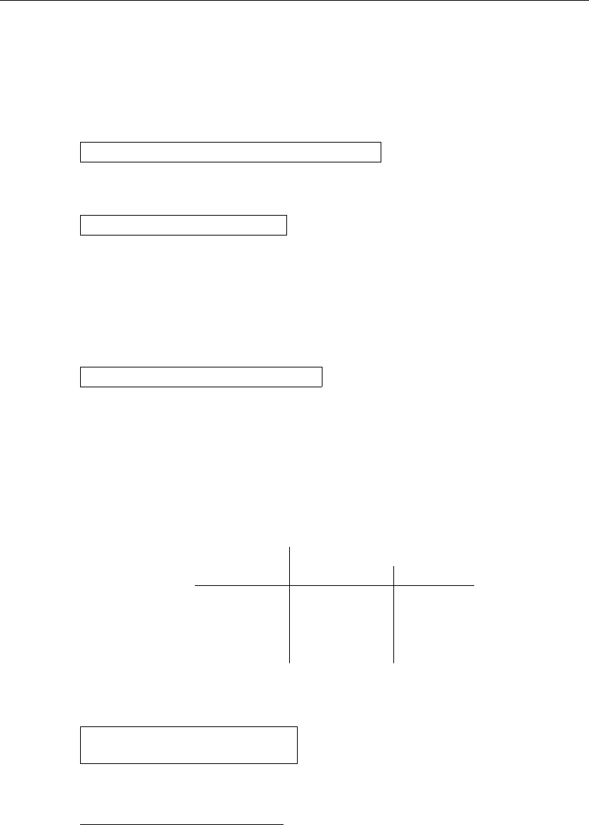
\documentclass{article}
\begin{document}
Small is beautiful.
\end{document}
Figure 1.1: A Minimal L
A
T
EX File.
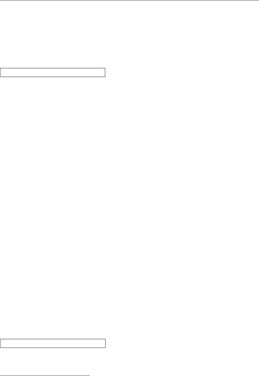
\documentclass[a4paper,11pt]{article}
% define the title
\author{H.~Partl}
\title{Minimalism}
\begin{document}
% generates the title
\maketitle
% insert the table of contents
\tableofcontents
\section{Some Interesting Words}
Well, and here begins my lovely article.
\section{Good Bye World}
\ldots{} and here it ends.
\end{document}
Figure 1.2: Example of a Realistic Journal Article.
8 Things You Need to Know
L
A
T
EX into compiling your input file. On other systems there might be some
typing involved, so here is how to coax L
A
T
EX into compiling your input file
on a text based system. Please note: this description assumes that a working
L
A
T
EX installation already sits on your computer.5
1. Edit/Create your L
A
T
EX input file. This file must be plain ASCII text.
On Unix all the editors will create just that. On Windows you might
want to make sure that you save the file in ASCII or Plain Text format.
When picking a name for your file, make sure it bears the extension
.tex.
2. Run L
A
T
EX on your input file. If successful you will end up with a .dvi
file. It may be necessary to run L
A
T
EX several times to get the table
of contents and all internal references right. When your input file has
a bug L
A
T
EX will tell you about it and stop processing your input file.
Type ctrl-D to get back to the command line.
latex foo.tex
3. Now you may view the DVI file. There are several ways to do that.
You can show the file on screen with
xdvi foo.dvi &
This only works on Unix with X11. If you are on Windows you might
want to try yap (yet another previewer).
You can also convert the dvi file to PostScript for printing or viewing
with Ghostscript.
dvips -Pcmz foo.dvi -o foo.ps
If you are lucky your L
A
T
EX system even comes with the dvipdf tool,
which allows you to convert your .dvi files straight into pdf.
dvipdf foo.dvi
5This is the case with most well groomed Unix Systems, and . . . Real Men use Unix,
so . . . ;-)
1.6 The Layout of the Document 9
1.6 The Layout of the Document
1.6.1 Document Classes
The first information L
A
T
EX needs to know when processing an input file is
the type of document the author wants to create. This is specified with the
\documentclass command.
\documentclass[options]{class}
Here class specifies the type of document to be created. Table 1.1 lists the
document classes explained in this introduction. The L
A
T
EX 2εdistribution
provides additional classes for other documents, including letters and slides.
The options parameter customises the behaviour of the document class. The
options have to be separated by commas. The most common options for the
standard document classes are listed in Table 1.2.
Example: An input file for a L
A
T
EX document could start with the line
\documentclass[11pt,twoside,a4paper]{article}
which instructs L
A
T
EX to typeset the document as an article with a base
font size of eleven points, and to produce a layout suitable for double sided
printing on A4 paper.
1.6.2 Packages
While writing your document, you will probably find that there are some
areas where basic L
A
T
EX cannot solve your problem. If you want to include
graphics, coloured text or source code from a file into your document, you
Table 1.1: Document Classes.
article for articles in scientific journals, presentations, short reports,
program documentation, invitations, . . .
report for longer reports containing several chapters, small books, PhD
theses, . . .
book for real books
slides for slides. The class uses big sans serif letters. You might want
to consider using FoilT
EXainstead.
amacros/latex/contrib/supported/foiltex

10 Things You Need to Know
Table 1.2: Document Class Options.
10pt,11pt,12pt Sets the size of the main font in the document. If
no option is specified, 10pt is assumed.
a4paper,letterpaper, . . . Defines the paper size. The default size
is letterpaper. Besides that, a5paper,b5paper,
executivepaper, and legalpaper can be specified.
fleqn Typesets displayed formulae left-aligned instead of centred.
leqno Places the numbering of formulae on the left hand side
instead of the right.
titlepage,notitlepage Specifies whether a new page should be
started after the document title or not. The article class does
not start a new page by default, while report and book do.
onecolumn,twocolumn Instructs L
A
T
EX to typeset the document in
one column or two columns.
twoside, oneside Specifies whether double or single sided output
should be generated. The classes article and report are single
sided and the book class is double sided by default. Note that
this option concerns the style of the document only. The option
twoside does not tell the printer you use that it should actually
make a two-sided printout.
landscape Changes the layout of the document to print in landscape
mode.
openright, openany Makes chapters begin either only on right
hand pages or on the next page available. This does not work
with the article class, as it does not know about chapters. The
report class by default starts chapters on the next page available
and the book class starts them on right hand pages.
1.7 Files You Might Encounter 11
need to enhance the capabilities of L
A
T
EX. Such enhancements are called
packages. Packages are activated with the
\usepackage[options]{package}
command, where package is the name of the package and options is a list of
keywords that trigger special features in the package. Some packages come
with the L
A
T
EX 2εbase distribution (See Table 1.3). Others are provided
separately. You may find more information on the packages installed at your
site in your Local Guide [5]. The prime source for information about L
A
T
EX
packages is The L
A
T
E
X Companion [3]. It contains descriptions on hundreds
of packages, along with information of how to write your own extensions to
L
A
T
EX 2ε.
1.6.3 Page Styles
L
A
T
EX supports three predefined header/footer combinations—so-called page
styles. The style parameter of the
\pagestyle{style}
command defines which one to use. Table 1.4 lists the predefined page styles.
It is possible to change the page style of the current page with the com-
mand
\thispagestyle{style}
A description how to create your own headers and footers can be found
in The L
A
T
E
X Companion [3] and in section 4.4 on page 69.
1.7 Files You Might Encounter
When you work with L
A
T
EX you will soon find yourself in a maze of files
with various extensions and probably no clue. The following list explains
the various file types you might encounter when working with T
EX. Please
note that this table does not claim to be a complete list of extensions, but
if you find one missing that you think is important, please drop me a line.
.tex L
A
T
EX or T
EX input file. Can be compiled with latex.
.sty L
A
T
EX Macro package. This is a file you can load into your L
A
T
EX
document using the \usepackage command.
.dtx Documented T
EX. This is the main distribution format for L
A
T
EX style
files. If you process a .dtx file you get documented macro code of the
L
A
T
EX package contained in the .dtx file.

12 Things You Need to Know
Table 1.3: Some of the Packages Distributed with L
A
T
EX.
doc Allows the documentation of L
A
T
EX programs.
Described in doc.dtxaand in The L
A
T
E
X Companion [3].
exscale Provides scaled versions of the math extension font.
Described in ltexscale.dtx.
fontenc Specifies which font encoding L
A
T
EX should use.
Described in ltoutenc.dtx.
ifthen Provides commands of the form
‘if. . . then do. . . otherwise do. . . .’
Described in ifthen.dtx and The L
A
T
E
X Companion [3].
latexsym To access the L
A
T
EX symbol font, you should use the
latexsym package. Described in latexsym.dtx and in The
L
A
T
E
X Companion [3].
makeidx Provides commands for producing indexes. Described in
section 4.3 and in The L
A
T
E
X Companion [3].
syntonly Processes a document without typesetting it.
inputenc Allows the specification of an input encoding such as
ASCII, ISO Latin-1, ISO Latin-2, 437/850 IBM code pages,
Apple Macintosh, Next, ANSI-Windows or user-defined one.
Described in inputenc.dtx.
aThis file should be installed on your system, and you should be able to
get a dvi file by typing latex doc.dtx in any directory where you have write
permission. The same is true for all the other files mentioned in this table.
Table 1.4: The Predefined Page Styles of L
A
T
EX.
plain prints the page numbers on the bottom of the page, in the middle
of the footer. This is the default page style.
headings prints the current chapter heading and the page number in
the header on each page, while the footer remains empty. (This is
the style used in this document)
empty sets both the header and the footer to be empty.

1.8 Big Projects 13
.ins The installer for the files contained in the matching .dtx file. If you
download a L
A
T
EX package from the net, you will normally get a .dtx
and a .ins file. Run L
A
T
EX on the .ins file to unpack the .dtx file.
.cls Class files define what your document looks like. They are selected
with the \documentclass command.
.fd Font description file telling L
A
T
EX about new fonts.
The following files are generated when you run L
A
T
EX on your input file:
.dvi Device Independent File. This is the main result of a L
A
T
EX compile
run. You can look at its content with a DVI previewer program or you
can send it to a printer with dvips or a similar application.
.log Gives a detailed account of what happened during the last compiler
run.
.toc Stores all your section headers. It gets read in for the next compiler
run and is used to produce the table of content.
.lof This is like .toc but for the list of figures.
.lot And again the same for the list of tables.
.aux Another file that transports information from one compiler run to the
next. Among other things, the .aux file is used to store information
associated with cross-references.
.idx If your document contains an index. L
A
T
EX stores all the words that
go into the index in this file. Process this file with makeindex. Refer
to section 4.3 on page 68 for more information on indexing.
.ind The processed .idx file, ready for inclusion into your document on the
next compile cycle.
.ilg Logfile telling what makeindex did.
1.8 Big Projects
When working on big documents, you might want to split the input file into
several parts. L
A
T
EX has two commands that help you to do that.
\include{filename}
You can use this command in the document body to insert the contents of
another file named filename.tex. Note that L
A
T
EX will start a new page before
processing the material input from filename.tex.
14 Things You Need to Know
The second command can be used in the preamble. It allows you to
instruct L
A
T
EX to only input some of the \included files.
\includeonly{filename,filename,. . . }
After this command is executed in the preamble of the document, only
\include commands for the filenames that are listed in the argument of
the \includeonly command will be executed. Note that there must be no
spaces between the filenames and the commas.
The \include command starts typesetting the included text on a new
page. This is helpful when you use \includeonly, because the page breaks
will not move, even when some included files are omitted. Sometimes this
might not be desirable. In this case, you can use the
\input{filename}
command. It simply includes the file specified. No flashy suits, no strings
attached.
To make L
A
T
EX quickly check your document you can use the syntonly
package. This makes L
A
T
EX skim through your document only checking for
proper syntax and usage of the commands, but doesn’t produce any (DVI)
output. As L
A
T
EX runs faster in this mode you may save yourself valuable
time. Usage is very simple:
\usepackage{syntonly}
\syntaxonly
When you want to produce pages, just comment out the second line (by
adding a percent sign).

Chapter 2
Typesetting Text
After reading the previous chapter, you should know about the basic stuff of
which a L
A
T
E
X 2εdocument is made. In this chapter I will fill in the remaining
structure you will need to know in order to produce real world material.
2.1 The Structure of Text and Language
By Hanspeter Schmid < hanspi@schmid-werren.ch>
The main point of writing a text (some modern DAAC1literature excluded),
is to convey ideas, information, or knowledge to the reader. The reader will
understand the text better if these ideas are well-structured, and will see and
feel this structure much better if the typographical form reflects the logical
and semantical structure of the content.
L
A
T
EX is different from other typesetting systems in that you just have
to tell it the logical and semantical structure of a text. It then derives the
typographical form of the text according to the “rules” given in the document
class file and in various style files.
The most important text unit in L
A
T
EX (and in typography) is the para-
graph. We call it “text unit” because a paragraph is the typographical form
that should reflect one coherent thought, or one idea. You will learn in the
following sections how you can force line breaks with e.g. \\, and paragraph
breaks with e.g. leaving an empty line in the source code. Therefore, if a new
thought begins, a new paragraph should begin, and if not, only line breaks
should be used. If in doubt about paragraph breaks, think about your text
as a conveyor of ideas and thoughts. If you have a paragraph break, but
the old thought continues, it should be removed. If some totally new line of
thought occurs in the same paragraph, then it should be broken.
Most people completely underestimate the importance of well-placed
paragraph breaks. Many people do not even know what the meaning of
1Different At All Cost, a translation of the Swiss German UVA (Um’s Verrecken An-
ders).

16 Typesetting Text
a paragraph break is, or, especially in L
A
T
EX, introduce paragraph breaks
without knowing it. The latter mistake is especially easy to make if equa-
tions are used in the text. Look at the following examples, and figure out
why sometimes empty lines (paragraph breaks) are used before and after the
equation, and sometimes not. (If you don’t yet understand all commands
well enough to understand these examples, please read this and the following
chapter, and then read this section again.)
% Example 1
\ldots when Einstein introduced his formula
\begin{equation}
e = m \cdot c^2 \; ,
\end{equation}
which is at the same time the most widely known
and the least well understood physical formula.
% Example 2
\ldots from which follows Kirchhoff’s current law:
\begin{equation}
\sum_{k=1}^{n} I_k = 0 \; .
\end{equation}
Kirchhoff’s voltage law can be derived \ldots
% Example 3
\ldots which has several advantages.
\begin{equation}
I_D = I_F - I_R
\end{equation}
is the core of a very different transistor model. \ldots
The next smaller text unit is a sentence. In English texts, there is a
larger space after a period that ends a sentence than after one that ends an
abbreviation. L
A
T
EX tries to figure out which one you wanted to have. If
L
A
T
EX gets it wrong, you must tell it what you want. This is explained later
in this chapter.
The structuring of text even extends to parts of sentences. Most lan-
guages have very complicated punctuation rules, but in many languages (in-
cluding German and English), you will get almost every comma right if you
remember what it represents: a short stop in the flow of language. If you
are not sure about where to put a comma, read the sentence aloud and take

2.2 Line Breaking and Page Breaking 17
a short breath at every comma. If this feels awkward at some place, delete
that comma; if you feel the urge to breathe (or make a short stop) at some
other place, insert a comma.
Finally, the paragraphs of a text should also be structured logically at a
higher level, by putting them into chapters, sections, subsections, and so on.
However, the typographical effect of writing e.g. \section{The Structure
of Text and Language} is so obvious that it is almost self-evident how these
high-level structures should be used.
2.2 Line Breaking and Page Breaking
2.2.1 Justified Paragraphs
Books are often typeset with each line having the same length. L
A
T
EX inserts
the necessary line breaks and spaces between words by optimizing the con-
tents of a whole paragraph. If necessary, it also hyphenates words that would
not fit comfortably on a line. How the paragraphs are typeset depends on
the document class. Normally the first line of a paragraph is indented, and
there is no additional space between two paragraphs. Refer to section 6.3.2
for more information.
In special cases it might be necessary to order L
A
T
EX to break a line:
\\ or \newline
starts a new line without starting a new paragraph.
\\*
additionally prohibits a page break after the forced line break.
\newpage
starts a new page.
\linebreak[n],\nolinebreak[n],\pagebreak[n]and \nopagebreak[n]
do what their names say. They enable the author to influence their actions
with the optional argument n, which can be set to a number between zero
and four. By setting nto a value below 4, you leave L
A
T
EX the option of
ignoring your command if the result would look very bad. Do not confuse
these “break” commands with the “new” commands. Even when you give
a “break” command, L
A
T
EX still tries to even out the right border of the
page and the total length of the page, as described in the next section. If
18 Typesetting Text
you really want to start a “new line”, then use the corresponding command.
Guess its name!
L
A
T
EX always tries to produce the best line breaks possible. If it cannot
find a way to break the lines in a manner that meets its high standards, it
lets one line stick out on the right of the paragraph. L
A
T
EX then complains
(“overfull hbox”) while processing the input file. This happens most often
when L
A
T
EX cannot find a suitable place to hyphenate a word.2You can
instruct L
A
T
EX to lower its standards a little by giving the \sloppy command.
It prevents such over-long lines by increasing the inter-word spacing—even
if the final output is not optimal. In this case a warning (“underfull hbox”)
is given to the user. In most such cases the result doesn’t look very good.
The command \fussy brings L
A
T
EX back to its default behaviour.
2.2.2 Hyphenation
L
A
T
EX hyphenates words whenever necessary. If the hyphenation algorithm
does not find the correct hyphenation points, you can remedy the situation
by using the following commands to tell T
EX about the exception.
The command
\hyphenation{word list }
causes the words listed in the argument to be hyphenated only at the points
marked by “-”. The argument of the command should only contain words
built from normal letters, or rather signs that are considered to be normal
letters by L
A
T
EX. The hyphenation hints are stored for the language that
is active when the hyphenation command occurs. This means that if you
place a hyphenation command into the preamble of your document it will
influence the English language hyphenation. If you place the command after
the \begin{document} and you are using some package for national language
support like babel, then the hyphenation hints will be active in the language
activated through babel.
The example below will allow “hyphenation” to be hyphenated as well as
“Hyphenation”, and it prevents “FORTRAN”, “Fortran” and “fortran” from
being hyphenated at all. No special characters or symbols are allowed in the
argument.
Example:
\hyphenation{FORTRAN Hy-phen-a-tion}
2Although L
A
T
E
X gives you a warning when that happens (Overfull hbox) and displays
the offending line, such lines are not always easy to find. If you use the option draft in
the \documentclass command, these lines will be marked with a thick black line on the
right margin.
2.3 Ready-Made Strings 19
The command \- inserts a discretionary hyphen into a word. This also
becomes the only point hyphenation is allowed in this word. This command is
especially useful for words containing special characters (e.g. accented char-
acters), because L
A
T
EX does not automatically hyphenate words containing
special characters.
I think this is: su\-per\-cal\-%
i\-frag\-i\-lis\-tic\-ex\-pi\-%
al\-i\-do\-cious
I think this is: supercalifragilisticexpialido-
cious
Several words can be kept together on one line with the command
\mbox{text}
It causes its argument to be kept together under all circumstances.
My phone number will change soon.
It will be \mbox{0116 291 2319}.
The parameter
\mbox{\emph{filename}} should
contain the name of the file.
My phone number will change soon. It will
be 0116 291 2319.
The parameter filename should contain the
name of the file.
\fbox is similar to \mbox, but in addition there will be a visible box
drawn around the content.
2.3 Ready-Made Strings
In some of the examples on the previous pages, you have seen some very
simple L
A
T
EX commands for typesetting special text strings:
Command Example Description
\today 4th April 2004 Current date in the current language
\TeX T
EX The name of your favorite typesetter
\LaTeX L
A
T
EX The Name of the Game
\LaTeXe L
A
T
EX 2εThe current incarnation of L
A
T
EX
2.4 Special Characters and Symbols
2.4.1 Quotation Marks
You should not use the "for quotation marks as you would on a typewriter.
In publishing there are special opening and closing quotation marks. In
L
A
T
EX, use two ‘s (grave accent) for opening quotation marks and two ’s
(vertical quote) for closing quotation marks. For single quotes you use just
one of each.
20 Typesetting Text
‘‘Please press the ‘x’ key.’’ “Please press the ‘x’ key.”
Yes I know the rendering is not ideal, it’s really a back-tick or grave
accent for opening quotes and vertical quote for closing, despite what the
font chosen might suggest.
2.4.2 Dashes and Hyphens
L
A
T
EX knows four kinds of dashes. You can access three of them with different
numbers of consecutive dashes. The fourth sign is actually not a dash at
all—it is the mathematical minus sign:
daughter-in-law, X-rated\\
pages 13--67\\
yes---or no? \\
$0$, $1$ and $-1$
daughter-in-law, X-rated
pages 13–67
yes—or no?
0,1and −1
The names for these dashes are: ‘-’ hyphen, ‘–’ en-dash, ‘—’ em-dash and
‘−’ minus sign.
2.4.3 Tilde (∼)
A character often seen in web addresses is the tilde. To generate this in
L
A
T
EX you can use \~ but the result: ˜ is not really what you want. Try this
instead:
http://www.rich.edu/\~{}bush \\
http://www.clever.edu/$\sim$demo
http://www.rich.edu/˜bush
http://www.clever.edu/∼demo
2.4.4 Degree Symbol (◦)
The following example shows how to print a degree symbol in L
A
T
EX:
It’s $-30\,^{\circ}\mathrm{C}$.
I will soon start to
super-conduct.
It’s −30 ◦C. I will soon start to super-
conduct.
The textcomp package makes the degree symbol also available as \textcelsius.
2.4 Special Characters and Symbols 21
2.4.5 The Euro Currency Symbol (€)
When writing about money these days, you need the Euro symbol. Many
current fonts contain a Euro symbol. After loading the textcomp package in
the preamble of your document
\usepackage{textcomp}
you can use the command
\texteuro
to access it.
If your font does not provide its own Euro symbol or if you do not like
the font’s Euro symbol, you have two more choices:
First the eurosym package. It provides the official Euro symbol:
\usepackage[official]{eurosym}
If you prefer a Euro symbol that matches your font, use the option gen
in place of the official option.
If the Adobe Eurofonts are installed on your system (they are available
for free from ftp://ftp.adobe.com/pub/adobe/type/win/all) you can use
either the package europs and the command \EUR (for a Euro symbol that
matches the current font) or the package eurosans and the command \euro
(for the “official Euro”).
The marvosym package also provides many different symbols, including
a Euro, under the name \EUR. It’s disadvantag is that it does not provide
slanted and bold variants of the Euro symbol.
Table 2.1: A bag full of Euro symbols
package command roman sans-serif typewriter
eurosym \euro e e e
[gen]eurosym \euro ACACAC
europs \EUR e c d
eurosans \euro € € €
marvosym \EUR ¤ ¤ ¤
22 Typesetting Text
2.4.6 Ellipsis (. . . )
On a typewriter, a comma or a period takes the same amount of space as
any other letter. In book printing, these characters occupy only a little space
and are set very close to the preceding letter. Therefore, you cannot enter
‘ellipsis’ by just typing three dots, as the spacing would be wrong. Instead,
there is a special command for these dots. It is called
\ldots
Not like this ... but like this:\\
New York, Tokyo, Budapest, \ldots
Not like this ... but like this:
New York, Tokyo, Budapest, . . .
2.4.7 Ligatures
Some letter combinations are typeset not just by setting the different letters
one after the other, but by actually using special symbols.
ff fi fl ffi. . . instead of ff fi fl ffi . . .
These so-called ligatures can be prohibited by inserting an \mbox{} between
the two letters in question. This might be necessary with words built from
two words.
\Large Not shelfful\\
but shelf\mbox{}ful
Not shelfful
but shelfful
2.4.8 Accents and Special Characters
L
A
T
EX supports the use of accents and special characters from many lan-
guages. Table 2.2 shows all sorts of accents being applied to the letter o.
Naturally other letters work too.
To place an accent on top of an i or a j, its dots have to be removed.
This is accomplished by typing \i and \j.
H\^otel, na\"\i ve, \’el\‘eve,\\
sm\o rrebr\o d, !‘Se\~norita!,\\
Sch\"onbrunner Schlo\ss{}
Stra\ss e
Hôtel, naïve, élève,
smørrebrød, ¡Señorita!,
Schönbrunner Schloß Straße
2.5 International Language Support 23
2.5 International Language Support
When you write documents in languages other than English, there are three
areas where L
A
T
EX has to be configured appropriately:
1. All automatically generated text strings3have to be adapted to the new
language. For many languages, these changes can be accomplished by
using the babel package by Johannes Braams.
2. L
A
T
EX needs to know the hyphenation rules for the new language. Get-
ting hyphenation rules into L
A
T
EX is a bit more tricky. It means re-
building the format file with different hyphenation patterns enabled.
Your Local Guide [5] should give more information on this.
3. Language specific typographic rules. In French for example, there is a
mandatory space before each colon character (:).
If your system is already configured appropriately, you can activate the
babel package by adding the command
\usepackage[language]{babel}
after the \documentclass command. A list of the languages built into your
L
A
T
EX system will be displayed every time the compiler is started. Babel
will automatically activate the appropriate hyphenation rules for the lan-
guage you choose. If your L
A
T
EX format does not support hyphenation in
the language of your choice, babel will still work but will disable hyphen-
ation, which has quite a negative effect on the appearance of the typeset
document.
3Table of Contents, List of Figures, . . .
Table 2.2: Accents and Special Characters.
ò\‘o ó\’o ô\^o õ\~o
¯o \=o ˙o \.o ö\"o ç\c c
˘o \u o ˇo \v o ő\H o ¸o \c o
o
.\d o o
¯\b o oo \t oo
œ\oe Œ\OE æ\ae Æ\AE
å\aa Å\AA
ø\o Ø\O ł\l Ł\L
ı\i \j ¡!‘ ¿?‘
24 Typesetting Text
Babel also specifies new commands for some languages, which simplify
the input of special characters. The German language, for example, contains
a lot of umlauts (äöü). With babel, you can enter an ö by typing "o instead
of \"o.
If you call babel with multiple languages
\usepackage[languageA,languageB]{babel}
you have to use the command
\selectlanguage{languageA}
to set the current language.
Most of the modern computer systems allow you to input letter of na-
tional alphabets directly from the keyboard. In order to handle variety of
input encoding used for different groups of languages and/or on different
computer platforms L
A
T
EX employs the inputenc package:
\usepackage[encoding]{inputenc}
When using this package, you should consider that other people might
not be able to display your input files on their computer, because they use a
different encoding. For example, the German umlaut ä on OS/2 is encoded
as 132, on Unix systems using ISO-LATIN 1 it is encoded as 228, while
in cyrillic encoding cp1251 for Windows this letter does not exist at all;
therefore you should use this feature with care. The following encodings
may come in handy, depending on the type of system you are working on4
Operating encodings
system western latin cyrillic
Mac applemac macukr
Unix latin1 koi8-ru
Windows ansinew cp1251
DOS, OS/2 cp850 cp866nav
If you use multilingual document with conflicting input encodings, you
might want to switch to unicode with the help of ucs package.
\usepackage{ucs}
\usepackage[utf8]{inputenc}
will enable you to create L
A
T
EX input files in utf8, a multi-byte encoding in
which each character can be encoded in as little as one byte and as many as
4To learn more about supported input encodings for Latin-based and Cyrillic-based
languages, read the documentation for inputenc.dtx and cyinpenc.dtx respectively. Sec-
tion 4.6 tells how to produce package documentation.
2.5 International Language Support 25
four bytes.
Font encoding is a different matter. It defines at which position inside a
T
EX-font each letter is stored. Multiple input encodings could be mapped
into one font encoding, which reduces number of required font sets. Font
encodings are handled through fontenc package:
\usepackage[encoding]{fontenc}
where encoding is font encoding. It is possible to load several encodings
simultaneously.
The default L
A
T
EX font encoding is OT1, the encoding of the original
Computer Modern T
EX font. It containins only the 128 characters of the 7-
bit ASCII character set. When accented characters are required, T
EX creates
them by combining a normal character with an accent. While the resulting
output looks perfect, this approach stops the automatic hyphenation from
working inside words containing accented characters. Besides, some of latin
letters could not be created by combining a normal character with an accent,
to say nothing about letters of non-latin alphabets, such as Greek or Cyrillic.
To overcome these shortcomings, several 8-bit CM-like font sets were cre-
ated. Extended Cork (EC) fonts in T1 encoding contains letters and punctu-
ation characters for most of the European languages based on Latin script.
The LH font set contains letters necessary to typeset documents in languages
using Cyrillic script. Because of the large number of Cyrillic glyphs, they are
arranged into four font encodings—T2A,T2B,T2C, and X2.5The CB bundle
contains fonts in LGR encoding for the composition of Greek text.
By using these fonts you can improve/enable hyphenation in non-English
documents. Another advantage of using new CM-like fonts is that they
provide fonts of CM families in all weights, shapes, and optically scaled font
sizes.
2.5.1 Support for Portuguese
By Demerson Andre Polli <polli@linux.ime.usp.br>
To enable hyphenation and change all automatic text to Portuguese, use the
command:
\usepackage[portuguese]{babel}
Or if you are in Brazil, substitute the language for brazilian.
5The list of languages supported by each of these encodings could be found in [11].
26 Typesetting Text
Table 2.3: Preamble for Portuguese documents.
\usepackage[portugese]{babel}
\usepackage[latin1]{inputenc}
\usepackage[T1]{fontenc}
As there are a lot of accents in Portuguese you might want to use
\usepackage[latin1]{inputenc}
to be able to input them correctly as well as
\usepackage[T1]{fontenc}
to get the hyphenation right.
See table 2.3 for the preamble you need to write in the Portuguese lan-
guage. Note that we are using the latin1 input encoding here, so this will
not work on a Mac or on DOS. Just use the appropriate encoding for your
system.
2.5 International Language Support 27
2.5.2 Support for French
By Daniel Flipo <daniel.flipo@univ-lille1.fr>
Some hints for those creating French documents with L
A
T
EX: you can load
French language support with the following command:
\usepackage[frenchb]{babel}
Note that, for historical reasons, the name of babel’s option for French is
either frenchb or francais but not french.
This enables French hyphenation, if you have configured your L
A
T
EX sys-
tem accordingly. It also changes all automatic text into French: \chapter
prints Chapitre, \today prints the current date in French and so on. A set
of new commands also becomes available, which allows you to write French
input files more easily. Check out table 2.4 for inspiration.
Table 2.4: Special commands for French.
\og guillemets \fg{} « guillemets »
M\up{me}, D\up{r} Mme, Dr
1\ier{}, 1\iere{}, 1\ieres{} 1er, 1re, 1res
2\ieme{} 4\iemes{} 2e4es
\No 1, \no 2 No1, no2
20~\degres C, 45\degres 20 °C, 45°
\bsc{M. Durand} M. Durand
\nombre{1234,56789} 1 234,567 89
You will also notice that the layout of lists changes when switching to
the French language. For more information on what the frenchb option
of babel does and how you can customize its behaviour, run L
A
T
EX on file
frenchb.dtx and read the produced file frenchb.dvi.
2.5.3 Support for German
Some hints for those creating German documents with L
A
T
EX: you can load
German language support with the following command:
\usepackage[german]{babel}
This enables German hyphenation, if you have configured your L
A
T
EX
system accordingly. It also changes all automatic text into German. Eg.

28 Typesetting Text
“Chapter” becomes “Kapitel.” A set of new commands also becomes avail-
able, which allows you to write German input files more quickly even when
you don’t use the inputenc package. Check out table 2.5 for inspiration.
With inputenc, all this becomes moot, but your text also is locked in a
particular encoding world.
Table 2.5: German Special Characters.
"a ä"s ß
"‘ „"’ “
"< or \flqq «"> or \frqq »
\flq ‹\frq ›
\dq "
In German books you often find French quotation marks («guillemets»).
German typesetters, however, use them differently. A quote in a German
book would look like »this«. In the German speaking part of Switzerland,
typesetters use «guillemets» the same way the French do.
A major problem arises from the use of commands like \flq: If you use
the OT1 font (which is the default font) the guillemets will look like the math
symbol “”, which turns a typesetter’s stomach. T1 encoded fonts, on the
other hand, do contain the required symbols. So if you are using this type of
quote, make sure you use the T1 encoding. (\usepackage[T1]{fontenc})
2.5.4 Support for Korean6
To use L
A
T
EX for typesetting Korean, we need to solve three problems:
1. We must be able to edit Korean input files. Korean input files must
be in plain text format, but because Korean uses its own character set
outside the repertoire of US-ASCII, they will look rather strange with
a normal ASCII editor. The two most widely used encodings for Ko-
rean text files are EUC-KR and its upward compatible extension used
in Korean MS-Windows, CP949/Windows-949/UHC. In these encod-
ings each US-ASCII character represents its normal ASCII character
similar to other ASCII compatible encodings such as ISO-8859-x, EUC-
JP, Shift_JIS, and Big5. On the other hand, Hangul syllables, Han-
jas (Chinese characters as used in Korea), Hangul Jamos, Hirakanas,
6Considering a number of issues Korean L
A
T
E
X users have to cope with. This section
was written by Karnes KIM on behalf of the Korean lshort translation team. It was
translated into English by SHIN Jungshik and shortened by Tobi Oetiker

2.5 International Language Support 29
Katakanas, Greek and Cyrillic characters and other symbols and let-
ters drawn from KS X 1001 are represented by two consecutive octets.
The first has its MSB set. Until the mid-1990’s, it took a consider-
able amount of time and effort to set up a Korean-capable environ-
ment under a non-localized (non-Korean) operating system. You can
skim through the now much-outdated http://jshin.net/faq to get
a glimpse of what it was like to use Korean under non-Korean OS in
mid-1990’s. These days all three major operating systems (Mac OS,
Unix, Windows) come equipped with pretty decent multilingual sup-
port and internationalization features so that editing Korean text file
is not so much of a problem anymore, even on non-Korean operating
systems.
2. T
EX and L
A
T
EX were originally written for scripts with no more than
256 characters in their alphabet. To make them work for languages
with considerably more characters such as Korean7or Chinese, a sub-
font mechanism was developed. It divides a single CJK font with thou-
sands or tens of thousands of glyphs into a set of subfonts with 256
glyphs each. For Korean, there are three widely used packages; HL
A
T
EX
by UN Koaunghi, hL
A
T
EXp by CHA Jaechoon and the CJK package
by Werner Lemberg.8HL
A
T
EX and hL
A
T
EXp are specific to Korean and
provide Korean localization on top of the font support. They both can
process Korean input text files encoded in EUC-KR. HL
A
T
EX can even
process input files encoded in CP949/Windows-949/UHC and UTF-8
when used along with Λ,Ω.
The CJK package is not specific to Korean. It can process input files
7Korean Hangul is an alphabetic script with 14 basic consonants and 10 basic vowels
(Jamos). Unlike Latin or Cyrillic scripts, the individual characters have to be arranged
in rectangular clusters about the same size as Chinese characters. Each cluster represents
a syllable. An unlimited number of syllables can be formed out of this finite set of vow-
els and consonants. Modern Korean orthographic standards (both in South Korea and
North Korea), however, put some restriction on the formation of these clusters. Therefore
only a finite number of orthographically correct syllables exist. The Korean Charac-
ter encoding defines individual code points for each of these syllables (KS X 1001:1998
and KS X 1002:1992). So Hangul, albeit alphabetic, is treated like the Chinese and
Japanese writing systems with tens of thousands of ideographic/logographic characters.
ISO 10646/Unicode offers both ways of representing Hangul used for modern Korean by
encoding Conjoining Hangul Jamos (alphabets: http://www.unicode.org/charts/PDF/
U1100.pdf) in addition to encoding all the orthographically allowed Hangul syllables in
modern Korean (http://www.unicode.org/charts/PDF/UAC00.pdf). One of the most
daunting challenges in Korean typesetting with L
A
T
E
X and related typesetting system is
supporting Middle Korean—and possibly future Korean—syllables that can be only rep-
resented by conjoining Jamos in Unicode. It is hoped that future T
E
X engines like Ωand
Λwill eventually provide solutions to this so that some Korean linguists and historians
will defect from MS Word that already has a pretty good support for Middle Korean.
8They can be obtained at language/korean/HLaTeX/
language/korean/CJK/ and http://knot.kaist.ac.kr/htex/
30 Typesetting Text
in UTF-8 as well as in various CJK encodings including EUC-KR and
CP949/Windows-949/UHC, it can be used to typeset documents with
multilingual content (especially Chinese, Japanese and Korean). The
CJK package has no Korean localization such as the one offered by
HL
A
T
EX and it does not come with as many special Korean fonts as
HL
A
T
EX.
3. The ultimate purpose of using typesetting programs like T
EX and
L
A
T
EX is to get documents typeset in an ‘aesthetically’ satisfying way.
Arguably the most important element in typesetting is a set of well-
designed fonts. The HL
A
T
EX distribution includes UHC PostScript
fonts of 10 different families and Munhwabu9fonts (TrueType) of 5
different families. The CJK package works with a set of fonts used by
earlier versions of HL
A
T
EX and it can use Bitstream’s cyberbit True-
Type font.
To use the HL
A
T
EX package for typesetting your Korean text, put the
following declaration into the preamble of your document:
\usepackage{hangul}
This command turns the Korean localization on. The headings of chap-
ters, sections, subsections, table of content and table of figures are all trans-
lated into Korean and the formatting of the document is changed to follow
Korean conventions. The package also provides automatic “particle selec-
tion.” In Korean, there are pairs of post-fix particles grammatically equiv-
alent but different in form. Which of any given pair is correct depends on
whether the preceding syllable ends with a vowel or a consonant. (It is a bit
more complex than this, but this should give you a good picture.) Native
Korean speakers have no problem picking the right particle, but it cannot
be determined which particle to use for references and other automatic text
that will change while you edit the document. It takes a painstaking effort to
place appropriate particles manually every time you add/remove references
or simply shuffle parts of your document around. HL
A
T
EX relieves its users
from this boring and error-prone process.
In case you don’t need Korean localization features but just want to
typeset Korean text, you can put the following line in the preamble, instead.
\usepackage{hfont}
For more details on typesetting Korean with HL
A
T
EX, refer to the HL
A
T
E
X
Guide. Check out the web site of the Korean T
EX User Group (KTUG) at
9Korean Ministry of Culture

2.5 International Language Support 31
http://www.ktug.or.kr/. There is also a Korean translation of this manual
available.
2.5.5 Support for Cyrillic
By Maksym Polyakov <polyama@myrealbox.com>
Version 3.7h of babel includes support for the T2* encodings and for type-
setting Bulgarian, Russian and Ukrainian texts using Cyrillic letters.
Support for Cyrillic is based on standard L
A
T
EX mechanisms through the
fontenc and inputenc packages. But, if you are going to use Cyrillics in math
mode, you need to load mathtext package before fontenc:10
\usepackage{mathtext}
\usepackage[T1,T2A]{fontenc}
\usepackage[koi8-ru]{inputenc}
\usepackage[english,bulgarian,russian,ukranian]{babel}
Generally, babel will authomatically choose the default font encoding, for
the above three languages this is T2A. However, documents are not restricted
to a single font encoding. For multi-lingual documents using Cyrillic and
Latin-based languages it makes sense to include latin font encoding explicitly.
babel will take care of switching to the appropriate font encoding when a
different language is selected within the document.
In addition to enabling hyphenations, translating automatically gener-
ated text strings, and activating some language specific typographic rules
(like \frenchspacing), babel provides some commands allowing typesetting
according to the standards of Bulgarian, Russian, or Ukrainian languages.
For all three languages, language specific punctuation is provided: The
cyrillic dash for the text (it is little narrower than latin dash and surrounded
by tiny spaces), a dash for direct speech, quotes, and commands to facilitate
hyphenation, see Table 2.6.
The Russian and Ukrainian options of babel define the commands \Asbuk
and \asbuk, which act like \Alph and \alph, but produce capital and small
letters of Russian or Ukrainian alphabets (whichever is the active language
of the document). The Bulgarian option of babel provides the commands
\enumBul and \enumLat (\enumEng), which make \Alph and \alph produce
letters of either Bulgarian or Latin (English) alphabets. The default be-
haviour of \Alph and \alph for the Bulgarian language option is to produce
letters from the Bulgarian alphabet.
10If you use A
M
S-L
A
T
E
X packages, load them before fontenc and babel as well.
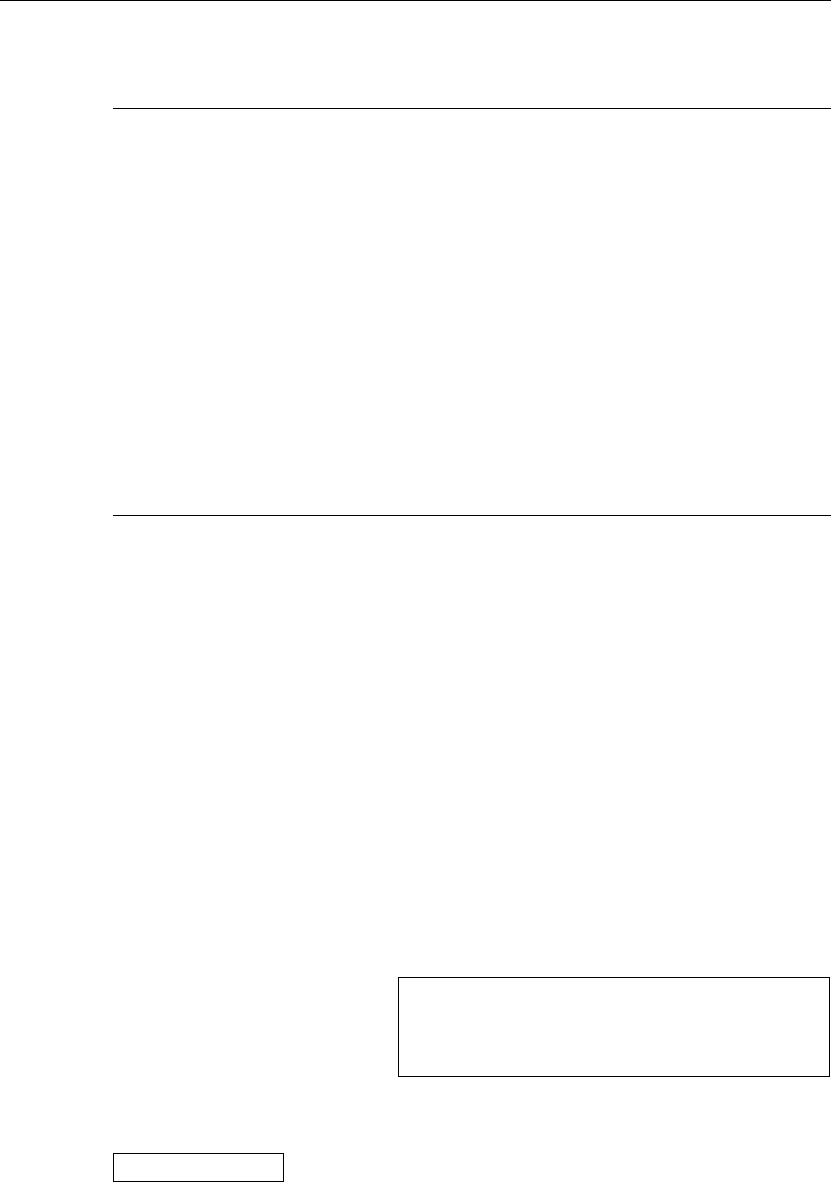
32 Typesetting Text
Table 2.6: The extra definitions made by Bulgarian, Russian, and Ukrainian
options of babel
"| disable ligature at this position.
"- an explicit hyphen sign, allowing hyphenation in the rest of the word.
"--- Cyrillic emdash in plain text.
"--~ Cyrillic emdash in compound names (surnames).
"--* Cyrillic emdash for denoting direct speech.
"" like |"-|, but producing no hyphen sign (for compound words with
hyphen, e.g. |x-""y| or some other signs as “disable/enable”).
"~ for a compound word mark without a breakpoint.
"= for a compound word mark with a breakpoint, allowing hyphenation
in the composing words.
", thinspace for initials with a breakpoint in following surname.
"‘ for German left double quotes (looks like ,,).
"’ for German right double quotes (looks like “).
"< for French left double quotes (looks like <<).
"> for French right double quotes (looks like >>).
2.6 The Space Between Words
To get a straight right margin in the output, L
A
T
EX inserts varying amounts
of space between the words. It inserts slightly more space at the end of a
sentence, as this makes the text more readable. L
A
T
EX assumes that sentences
end with periods, question marks or exclamation marks. If a period follows
an uppercase letter, this is not taken as a sentence ending, since periods after
uppercase letters normally occur in abbreviations.
Any exception from these assumptions has to be specified by the author.
A backslash in front of a space generates a space that will not be enlarged. A
tilde ‘~’ character generates a space that cannot be enlarged and additionally
prohibits a line break. The command \@ in front of a period specifies that
this period terminates a sentence even when it follows an uppercase letter.
Mr.~Smith was happy to see her\\
cf.~Fig.~5\\
I like BASIC\@. What about you?
Mr. Smith was happy to see her
cf. Fig. 5
I like BASIC. What about you?
The additional space after periods can be disabled with the command
\frenchspacing
which tells L
A
T
EXnot to insert more space after a period than after ordinary
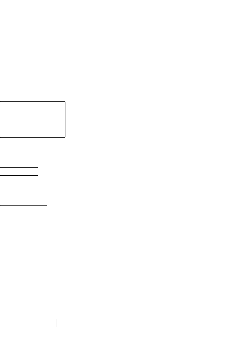
2.7 Titles, Chapters, and Sections 33
character. This is very common in non-English languages, except bibliogra-
phies. If you use \frenchspacing, the command \@ is not necessary.
2.7 Titles, Chapters, and Sections
To help the reader find his or her way through your work, you should divide
it into chapters, sections, and subsections. L
A
T
EX supports this with special
commands that take the section title as their argument. It is up to you to
use them in the correct order.
The following sectioning commands are available for the article class:
\section{...}
\subsection{...}
\subsubsection{...}
\paragraph{...}
\subparagraph{...}
If you want to split your document in parts without influencing the sec-
tion or chapter numbering you can use
\part{...}
When you work with the report or book class, an additional top-level
sectioning command becomes available
\chapter{...}
As the article class does not know about chapters, it is quite easy to add
articles as chapters to a book. The spacing between sections, the numbering
and the font size of the titles will be set automatically by L
A
T
EX.
Two of the sectioning commands are a bit special:
•The \part command does not influence the numbering sequence of
chapters.
•The \appendix command does not take an argument. It just changes
the chapter numbering to letters.11
L
A
T
EX creates a table of contents by taking the section headings and page
numbers from the last compile cycle of the document. The command
\tableofcontents
expands to a table of contents at the place it is issued. A new document
has to be compiled (“L
A
T
EXed”) twice to get a correct table of contents.
11For the article style it changes the section numbering.
34 Typesetting Text
Sometimes it might be necessary to compile the document a third time.
L
A
T
EX will tell you when this is necessary.
All sectioning commands listed above also exist as “starred” versions. A
“starred” version of a command is built by adding a star *after the command
name. This generates section headings that do not show up in the table
of contents and are not numbered. The command \section{Help}, for
example, would become \section*{Help}.
Normally the section headings show up in the table of contents exactly
as they are entered in the text. Sometimes this is not possible, because the
heading is too long to fit into the table of contents. The entry for the table of
contents can then be specified as an optional argument in front of the actual
heading.
\chapter[Title for the table of contents]{A long
and especially boring title, shown in the text}
The title of the whole document is generated by issuing a
\maketitle
command. The contents of the title have to be defined by the commands
\title{...},\author{...} and optionally \date{...}
before calling \maketitle. In the argument to \author, you can supply
several names separated by \and commands.
An example of some of the commands mentioned above can be found in
Figure 1.2 on page 7.
Apart from the sectioning commands explained above, L
A
T
EX 2εintro-
duced three additional commands for use with the book class. They are
useful for dividing your publication. The commands alter chapter headings
and page numbering to work as you would expect it in a book:
\frontmatter should be the very first command after \begin{document}.
It will switch page numbering to Roman numerals and sections be non-
enumerated. As if you were using the starred sectioning commands (eg
\chapter*{Preface}) but the sections will still show up in the table
of contents.
\mainmatter comes right before the first chapter of the book. It turns on
Arabic page numbering and restarts the page counter.
\appendix marks the start of additional material in your book. After this
command chapters will be numbered with letters.
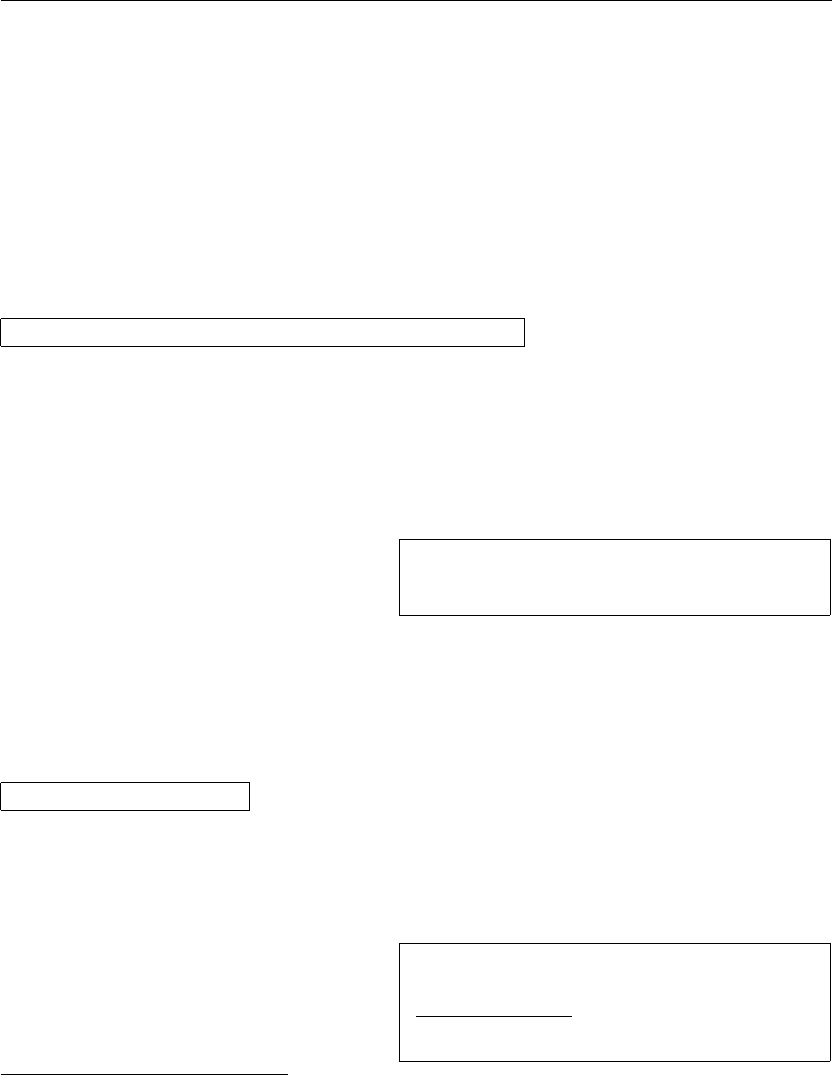
2.8 Cross References 35
\backmatter should be inserted before the very last items in your book,
such as the bibliography and the index. In the standard document
classes, this has no visual effect.
2.8 Cross References
In books, reports and articles, there are often cross-references to figures,
tables and special segments of text. L
A
T
EX provides the following commands
for cross referencing
\label{marker},\ref{marker}and \pageref{marker }
where marker is an identifier chosen by the user. L
A
T
EX replaces \ref by
the number of the section, subsection, figure, table, or theorem after which
the corresponding \label command was issued. \pageref prints the page
number of the page where the \label command occurred.12 As with the
section titles, the numbers from the previous run are used.
A reference to this subsection
\label{sec:this} looks like:
‘‘see section~\ref{sec:this} on
page~\pageref{sec:this}.’’
A reference to this subsection looks like: “see
section 2.8 on page 35.”
2.9 Footnotes
With the command
\footnote{footnote text }
a footnote is printed at the foot of the current page. Footnotes should always
be put13 after the word or sentence they refer to. Footnotes referring to a
sentence or part of it should therefore be put after the comma or period.14
Footnotes\footnote{This is
a footnote.} are often used
by people using \LaTeX.
Footnotesaare often used by people using
L
A
T
EX.
aThis is a footnote.
12Note that these commands are not aware of what they refer to. \label just saves the
last automatically generated number.
13“put” is one of the most common English words.
14Note that footnotes distract the reader from the main body of your document. After
all, everybody reads the footnotes—we are a curious species, so why not just integrate
everything you want to say into the body of the document?15
15A guidepost doesn’t necessarily go where it’s pointing to :-).
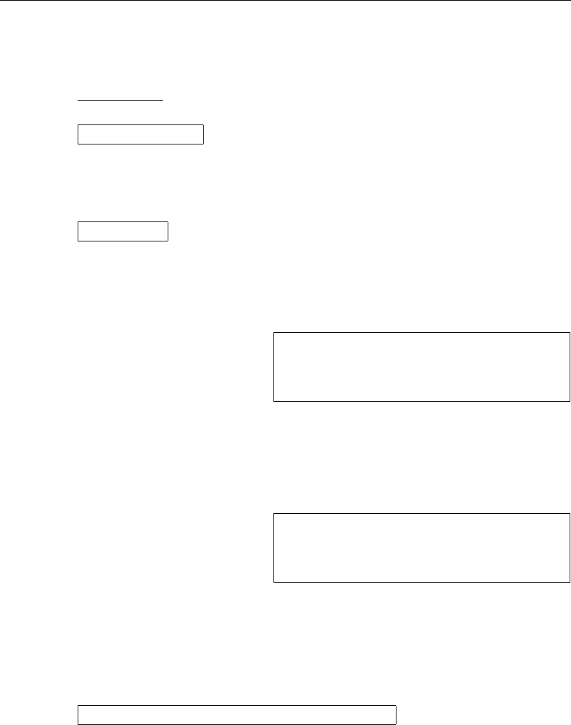
36 Typesetting Text
2.10 Emphasized Words
If a text is typed using a typewriter, important words are emphasized by
underlining them.
\underline{text}
In printed books, however, words are emphasized by typesetting them in
an italic font. L
A
T
EX provides the command
\emph{text}
to emphasize text. What the command actually does with its argument
depends on the context:
\emph{If you use
emphasizing inside a piece
of emphasized text, then
\LaTeX{} uses the
\emph{normal} font for
emphasizing.}
If you use emphasizing inside a piece of em-
phasized text, then L
A
T
E
X uses the normal
font for emphasizing.
Please note the difference between telling L
A
T
EX to emphasize something
and telling it to use a different font:
\textit{You can also
\emph{emphasize} text if
it is set in italics,}
\textsf{in a
\emph{sans-serif} font,}
\texttt{or in
\emph{typewriter} style.}
You can also emphasize text if it is set in ital-
ics, in a sans-serif font, or in typewriter
style.
2.11 Environments
\begin{environment }text \end{environment }
Where environment is the name of the environment. Environments can be
nested within each other as long as the correct nesting order is maintained.
\begin{aaa}...\begin{bbb}...\end{bbb}...\end{aaa}
In the following sections all important environments are explained.
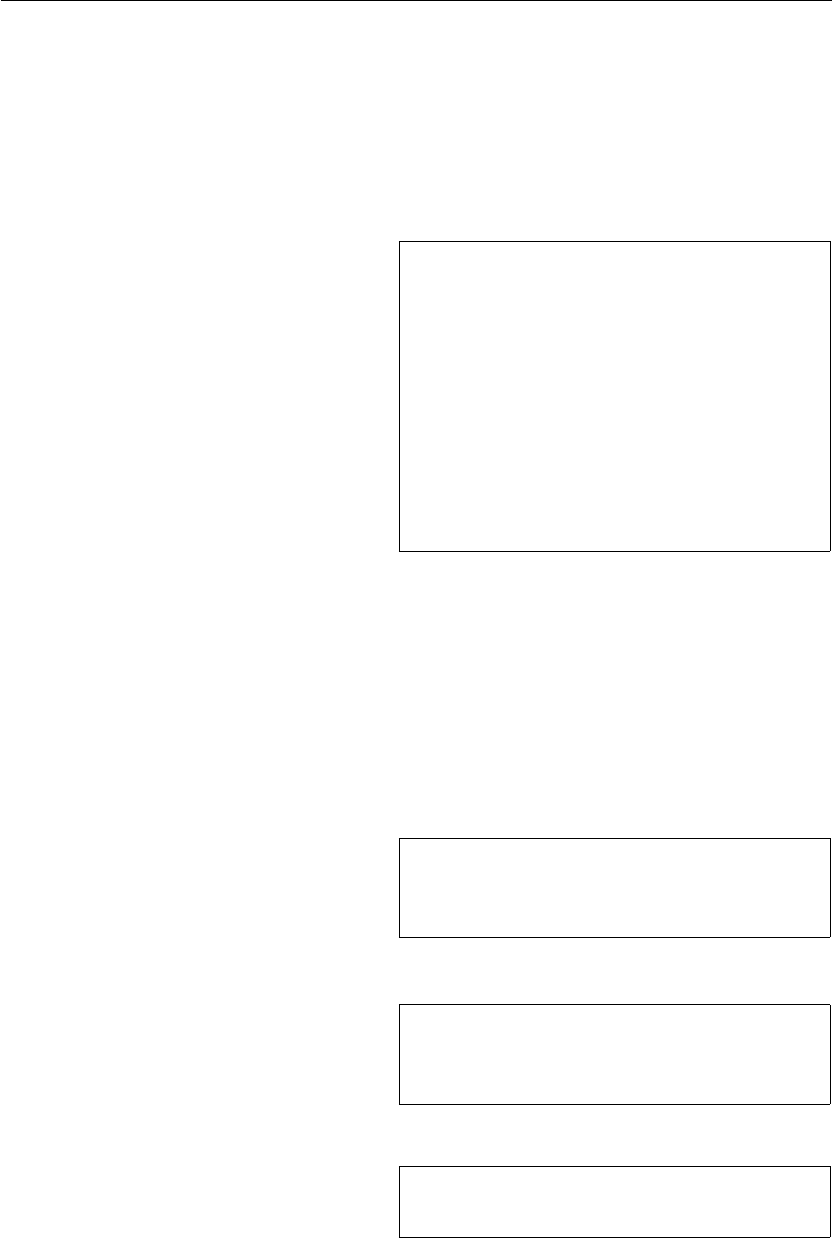
2.11 Environments 37
2.11.1 Itemize, Enumerate, and Description
The itemize environment is suitable for simple lists, the enumerate envi-
ronment for enumerated lists, and the description environment for descrip-
tions.
\flushleft
\begin{enumerate}
\item You can mix the list
environments to your taste:
\begin{itemize}
\item But it might start to
look silly.
\item[-] With a dash.
\end{itemize}
\item Therefore remember:
\begin{description}
\item[Stupid] things will not
become smart because they are
in a list.
\item[Smart] things, though, can be
presented beautifully in a list.
\end{description}
\end{enumerate}
1. You can mix the list environments to
your taste:
•But it might start to look silly.
- With a dash.
2. Therefore remember:
Stupid things will not become smart
because they are in a list.
Smart things, though, can be
presented beautifully in a list.
2.11.2 Flushleft, Flushright, and Center
The environments flushleft and flushright generate paragraphs that are
either left- or right-aligned. The center environment generates centred text.
If you do not issue \\ to specify line breaks, L
A
T
EX will automatically deter-
mine line breaks.
\begin{flushleft}
This text is\\ left-aligned.
\LaTeX{} is not trying to make
each line the same length.
\end{flushleft}
This text is
left-aligned. L
A
T
EX is not trying to make
each line the same length.
\begin{flushright}
This text is right-\\aligned.
\LaTeX{} is not trying to make
each line the same length.
\end{flushright}
This text is right-
aligned. L
A
T
EX is not trying to make each
line the same length.
\begin{center}
At the centre\\of the earth
\end{center}
At the centre
of the earth
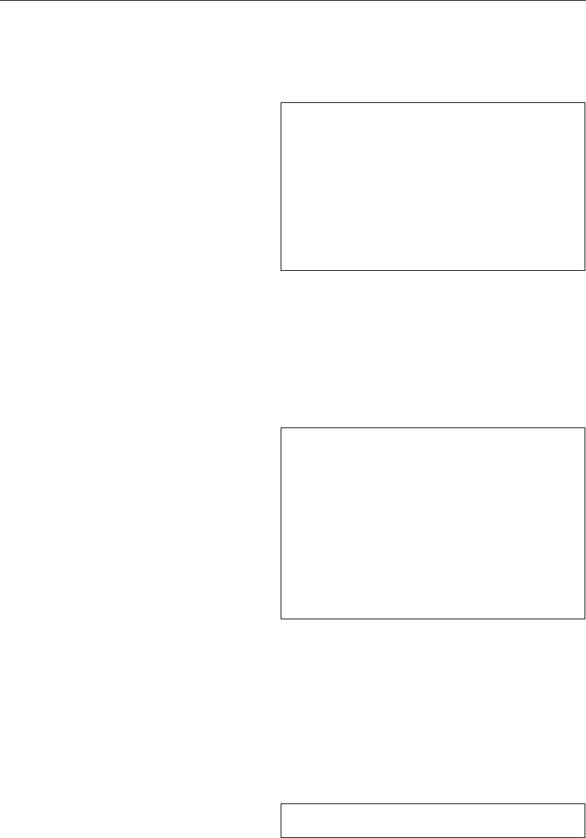
38 Typesetting Text
2.11.3 Quote, Quotation, and Verse
The quote environment is useful for quotes, important phrases and examples.
A typographical rule of thumb
for the line length is:
\begin{quote}
On average, no line should
be longer than 66 characters.
\end{quote}
This is why \LaTeX{} pages have
such large borders by default and
also why multicolumn print is
used in newspapers.
A typographical rule of thumb for the line
length is:
On average, no line should be
longer than 66 characters.
This is why L
A
T
EX pages have such large bor-
ders by default and also why multicolumn
print is used in newspapers.
There are two similar environments: the quotation and the verse envi-
ronments. The quotation environment is useful for longer quotes going over
several paragraphs, because it indents the first line of each paragraph. The
verse environment is useful for poems where the line breaks are important.
The lines are separated by issuing a \\ at the end of a line and an empty
line after each verse.
I know only one English poem by
heart. It is about Humpty Dumpty.
\begin{flushleft}
\begin{verse}
Humpty Dumpty sat on a wall:\\
Humpty Dumpty had a great fall.\\
All the King’s horses and all
the King’s men\\
Couldn’t put Humpty together
again.
\end{verse}
\end{flushleft}
I know only one English poem by heart. It is
about Humpty Dumpty.
Humpty Dumpty sat on a wall:
Humpty Dumpty had a great
fall.
All the King’s horses and all
the King’s men
Couldn’t put Humpty together
again.
2.11.4 Abstract
In scientific publications it is customary to start with an abstract which gives
the reader a quick overview of what to expect. L
A
T
EX provides the abstract
environment for this purpose. Normally abstract is used in documents
typeset with the article document class.
\begin{abstract}
The abstract abstract.
\end{abstract}
The abstract abstract.
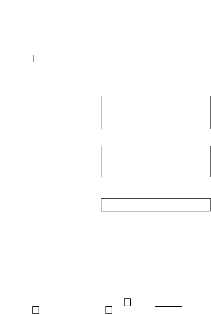
2.11 Environments 39
2.11.5 Printing Verbatim
Text that is enclosed between \begin{verbatim} and \end{verbatim} will
be directly printed, as if typed on a typewriter, with all line breaks and
spaces, without any L
A
T
EX command being executed.
Within a paragraph, similar behavior can be accessed with
\verb+text+
The +is just an example of a delimiter character. You can use any character
except letters, *or space. Many L
A
T
EX examples in this booklet are typeset
with this command.
The \verb|\ldots| command \ldots
\begin{verbatim}
10 PRINT "HELLO WORLD ";
20 GOTO 10
\end{verbatim}
The \ldots command . . .
10 PRINT "HELLO WORLD ";
20 GOTO 10
\begin{verbatim*}
the starred version of
the verbatim
environment emphasizes
the spaces in the text
\end{verbatim*}
the␣starred␣version␣of
the␣␣␣␣␣␣verbatim
environment␣emphasizes
the␣spaces␣␣␣in␣the␣text
The \verb command can be used in a similar fashion with a star:
\verb*|like this :-) | like␣␣␣this␣:-)␣
The verbatim environment and the \verb command may not be used
within parameters of other commands.
2.11.6 Tabular
The tabular environment can be used to typeset beautiful tables with
optional horizontal and vertical lines. L
A
T
EX determines the width of the
columns automatically.
The table spec argument of the
\begin{tabular}[pos]{table spec}
command defines the format of the table. Use an lfor a column of left-
aligned text, rfor right-aligned text, and cfor centred text; p{width }
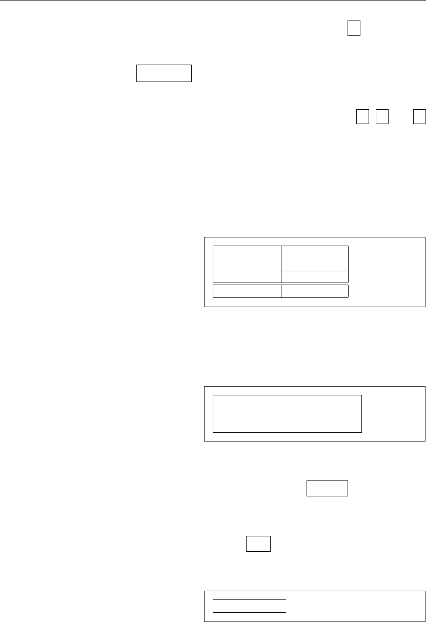
40 Typesetting Text
for a column containing justified text with line breaks, and |for a vertical
line.
If the text in a column is too wide for the page, L
A
T
EX won’t automatically
wrap it. Using p{width }you can define a special type of column which
will wrap-around the text as in a normal paragraph.
The pos argument specifies the vertical position of the table relative to
the baseline of the surrounding text. Use either of the letters t,band c
to specify table alignment at the top, bottom or center.
Within a tabular environment, &jumps to the next column, \\ starts
a new line and \hline inserts a horizontal line. You can add partial lines
by using the \cline{j-i}, where j and i are the column numbers the line
should extend over.
\begin{tabular}{|r|l|}
\hline
7C0 & hexadecimal \\
3700 & octal \\ \cline{2-2}
11111000000 & binary \\
\hline \hline
1984 & decimal \\
\hline
\end{tabular}
7C0 hexadecimal
3700 octal
11111000000 binary
1984 decimal
\begin{tabular}{|p{4.7cm}|}
\hline
Welcome to Boxy’s paragraph.
We sincerely hope you’ll
all enjoy the show.\\
\hline
\end{tabular}
Welcome to Boxy’s paragraph.
We sincerely hope you’ll all en-
joy the show.
The column separator can be specified with the @{...} construct. This
command kills the inter-column space and replaces it with whatever is be-
tween the curly braces. One common use for this command is explained
below in the decimal alignment problem. Another possible application is to
suppress leading space in a table with @{} .
\begin{tabular}{@{} l @{}}
\hline
no leading space\\
\hline
\end{tabular}
no leading space
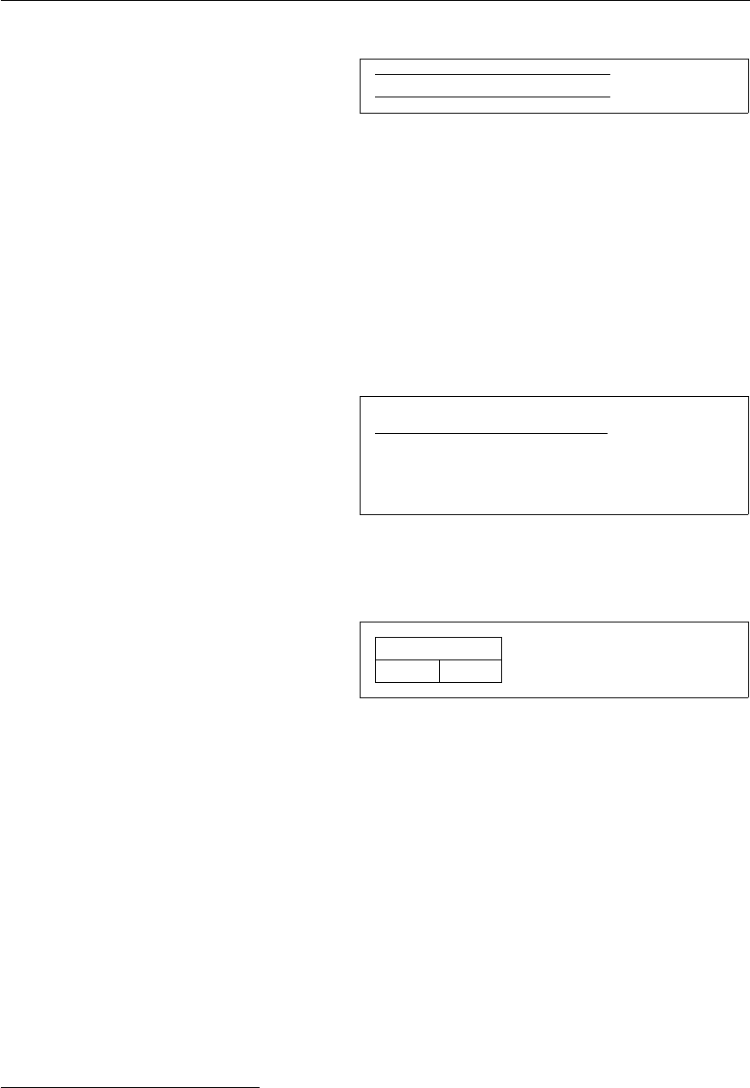
2.12 Floating Bodies 41
\begin{tabular}{l}
\hline
leading space left and right\\
\hline
\end{tabular}
leading space left and right
Since there is no built-in way to align numeric columns to a decimal
point,16 we can “cheat” and do it by using two columns: a right-aligned inte-
ger and a left-aligned fraction. The @{.} command in the \begin{tabular}
line replaces the normal inter-column spacing with just a “.”, giving the ap-
pearance of a single, decimal-point-justified column. Don’t forget to replace
the decimal point in your numbers with a column separator (&)! A column
label can be placed above our numeric “column” by using the \multicolumn
command.
\begin{tabular}{c r @{.} l}
Pi expression &
\multicolumn{2}{c}{Value} \\
\hline
$\pi$ & 3&1416 \\
$\pi^{\pi}$ & 36&46 \\
$(\pi^{\pi})^{\pi}$ & 80662&7 \\
\end{tabular}
Pi expression Value
π3.1416
ππ36.46
(ππ)π80662.7
\begin{tabular}{|c|c|}
\hline
\multicolumn{2}{|c|}{Ene} \\
\hline
Mene & Muh! \\
\hline
\end{tabular}
Ene
Mene Muh!
Material typeset with the tabular environment always stays together on
one page. If you want to typeset long tables, you might want to have a look
at the supertabular and the longtabular environments.
2.12 Floating Bodies
Today most publications contain a lot of figures and tables. These elements
need special treatment, because they cannot be broken across pages. One
method would be to start a new page every time a figure or a table is too
large to fit on the present page. This approach would leave pages partially
empty, which looks very bad.
The solution to this problem is to ‘float’ any figure or table that does not
fit on the current page to a later page, while filling the current page with
16If the ‘tools’ bundle is installed on your system, have a look at the dcolumn package.
42 Typesetting Text
body text. L
A
T
EX offers two environments for floating bodies; one for tables
and one for figures. To take full advantage of these two environments it is
important to understand approximately how L
A
T
EX handles floats internally.
Otherwise floats may become a major source of frustration, because L
A
T
EX
never puts them where you want them to be.
Let’s first have a look at the commands L
A
T
EX supplies for floats:
Any material enclosed in a figure or table environment will be treated
as floating matter. Both float environments support an optional parameter
\begin{figure}[placement specifier]or \begin{table}[placement specifier ]
called the placement specifier. This parameter is used to tell L
A
T
EX about the
locations to which the float is allowed to be moved. A placement specifier is
constructed by building a string of float-placing permissions. See Table 2.7.
A table could be started with the following line e.g.
\begin{table}[!hbp]
The placement specifier [!hbp] allows L
A
T
EX to place the table right here
(h) or at the bottom (b) of some page or on a special floats page (p), and all
this even if it does not look that good (!). If no placement specifier is given,
the standard classes assume [tbp].
L
A
T
EX will place every float it encounters according to the placement
specifier supplied by the author. If a float cannot be placed on the current
page it is deferred either to the figures or the tables queue.17 When a new
page is started, L
A
T
EX first checks if it is possible to fill a special ‘float’ page
17These are FIFO—‘first in first out’—queues!
Table 2.7: Float Placing Permissions.
Spec Permission to place the float . . .
hhere at the very place in the text where it occurred. This is
useful mainly for small floats.
tat the top of a page
bat the bottom of a page
pon a special page containing only floats.
!without considering most of the internal parametersa, which
could stop this float from being placed.
Note that pt and em are T
EX units. Read more on this in table 6.5 on page
109.
aSuch as the maximum number of floats allowed on one page.
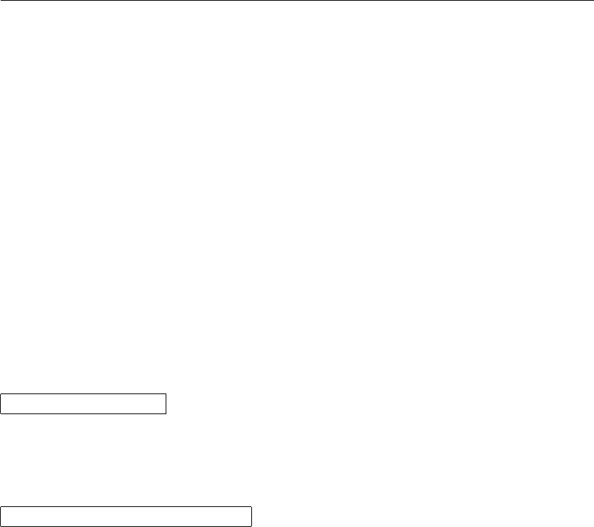
2.12 Floating Bodies 43
with floats from the queues. If this is not possible, the first float on each
queue is treated as if it had just occurred in the text: L
A
T
EX tries again to
place it according to its respective placement specifiers (except ‘h,’ which is
no longer possible). Any new floats occurring in the text get placed into the
appropriate queues. L
A
T
EX strictly maintains the original order of appearance
for each type of float. That’s why a figure that cannot be placed pushes all
further figures to the end of the document. Therefore:
If L
A
T
EX is not placing the floats as you expected, it is often only
one float jamming one of the two float queues.
While it is possible to give L
A
T
EX single-location placement specifiers,
this causes problems. If the float does not fit in the location specified it
becomes stuck, blocking subsequent floats. In particular, you should never,
ever use the [h] option—it is so bad that in more recent versions of L
A
T
EX,
it is automatically replaced by [ht].
Having explained the difficult bit, there are some more things to mention
about the table and figure environments. With the
\caption{caption text }
command, you can define a caption for the float. A running number and the
string “Figure” or “Table” will be added by L
A
T
EX.
The two commands
\listoffigures and \listoftables
operate analogously to the \tableofcontents command, printing a list of
figures or tables, respectively. These lists will display the whole caption, so if
you tend to use long captions you must have a shorter version of the caption
for the lists. This is accomplished by entering the short version in brackets
after the \caption command.
\caption[Short]{LLLLLoooooonnnnnggggg}
With \label and \ref, you can create a reference to a float within your
text.
The following example draws a square and inserts it into the document.
You could use this if you wanted to reserve space for images you are going
to paste into the finished document.
Figure~\ref{white} is an example of Pop-Art.
\begin{figure}[!hbp]
\makebox[\textwidth]{\framebox[5cm]{\rule{0pt}{5cm}}}
\caption{Five by Five in Centimetres.\label{white}}
\end{figure}

44 Typesetting Text
In the example above, L
A
T
EX will try really hard (!) to place the figure right
here (h).18 If this is not possible, it tries to place the figure at the bottom (b)
of the page. Failing to place the figure on the current page, it determines
whether it is possible to create a float page containing this figure and maybe
some tables from the tables queue. If there is not enough material for a
special float page, L
A
T
EX starts a new page, and once more treats the figure
as if it had just occurred in the text.
Under certain circumstances it might be necessary to use the
\clearpage or even the \cleardoublepage
command. It orders L
A
T
EX to immediately place all floats remaining in the
queues and then start a new page. \cleardoublepage even goes to a new
right-hand page.
You will learn how to include PostScript drawings into your L
A
T
EX 2ε
documents later in this introduction.
2.13 Protecting Fragile Commands
Text given as arguments of commands like \caption or \section may show
up more than once in the document (e.g. in the table of contents as well
as in the body of the document). Some commands fail when used in the
argument of \section-like commands. These commands are called frag-
ile commands—for example, \footnote or \phantom. These fragile com-
mands need protection (don’t we all?). You can protect them by putting the
\protect command in front of them.
\protect only refers to the command that follows right behind, not even
to its arguments. In most cases a superfluous \protect won’t hurt.
\section{I am considerate
\protect\footnote{and protect my footnotes}}
18assuming the figure queue is empty.

Chapter 3
Typesetting Mathematical
Formulae
Now you are ready! In this chapter, we will attack the main strength of T
E
X:
mathematical typesetting. But be warned, this chapter only scratches the sur-
face. While the things explained here are sufficient for many people, don’t despair
if you can’t find a solution to your mathematical typesetting needs here. It is
highly likely that your problem is addressed in AMS-L
A
T
E
X1
3.1 General
L
A
T
EX has a special mode for typesetting mathematics. Mathematics can be
typeset inline within a paragraph, or the paragraph can be broken to typeset
it separately. Mathematical text within a paragraph is entered between \(
and \), between $and $, or between \begin{math} and \end{math}.
Add $a$ squared and $b$ squared
to get $c$ squared. Or, using
a more mathematical approach:
$c^{2}=a^{2}+b^{2}$
Add asquared and bsquared to get csquared.
Or, using a more mathematical approach:
c2=a2+b2
\TeX{} is pronounced as
\(\tau\epsilon\chi\).\\[6pt]
100~m$^{3}$ of water\\[6pt]
This comes from my
\begin{math}\heartsuit\end{math}
T
EX is pronounced as τ χ.
100 m3of water
This comes from my ♥
1The American Mathematical Society has produced a powerful extension to L
A
T
E
X.
Many of the examples in this chapter make use of this extension. It is provided with all
recent T
E
X distributions. If yours is missing it, go to macros/latex/required/amslatex.

46 Typesetting Mathematical Formulae
When you want your larger mathematical equations or formulae to be set
apart from the rest of the paragraph, it is preferable to display them, rather
than to break the paragraph apart. To do this, you can either enclose them
in \[ and \], or between \begin{displaymath} and \end{displaymath}.
Add $a$ squared and $b$ squared
to get $c$ squared. Or, using
a more mathematical approach:
\begin{displaymath}
c^{2}=a^{2}+b^{2}
\end{displaymath}
or you can type less with:
\[a+b=c\]
Add asquared and bsquared to get csquared.
Or, using a more mathematical approach:
c2=a2+b2
or you can type less with:
a+b=c
If you want L
A
T
EX to enumerate your equations, you can use the equation
environment. You can then \label an equation number and refer to it
somewhere else in the text by using \ref or \eqref:
\begin{equation} \label{eq:eps}
\epsilon > 0
\end{equation}
From (\ref{eq:eps}), we gather
\ldots{}From \eqref{eq:eps} we
do the same.
> 0(3.1)
From (3.1), we gather . . . From (3.1) we do
the same.
Note the difference in typesetting style between equations that are type-
set and those that are displayed:
$\lim_{n \to \infty}
\sum_{k=1}^n \frac{1}{k^2}
= \frac{\pi^2}{6}$
limn→∞ Pn
k=1
1
k2=π2
6
\begin{displaymath}
\lim_{n \to \infty}
\sum_{k=1}^n \frac{1}{k^2}
= \frac{\pi^2}{6}
\end{displaymath}
lim
n→∞
n
X
k=1
1
k2=π2
6
There are differences between math mode and text mode. For example,
in math mode:
1. Most spaces and line breaks do not have any significance, as all spaces
are either derived logically from the mathematical expressions, or have
to be specified with special commands such as \,,\quad or \qquad.
2. Empty lines are not allowed. Only one paragraph per formula.
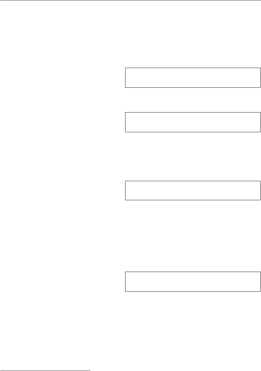
3.2 Grouping in Math Mode 47
3. Each letter is considered to be the name of a variable and will be
typeset as such. If you want to typeset normal text within a formula
(normal upright font and normal spacing) then you have to enter the
text using the \textrm{...} commands (see also section 3.7 on page
54).
\begin{equation}
\forall x \in \mathbf{R}:
\qquad x^{2} \geq 0
\end{equation} ∀x∈R:x2≥0(3.2)
\begin{equation}
x^{2} \geq 0\qquad
\textrm{for all }x\in\mathbf{R}
\end{equation}
x2≥0for all x∈R(3.3)
Mathematicians can be very fussy about which symbols are used: it
would be conventional here to use ‘blackboard bold’, which is obtained using
\mathbb from the package amsfonts or amssymb. The last example becomes
\begin{displaymath}
x^{2} \geq 0\qquad
\textrm{for all }x\in\mathbb{R}
\end{displaymath}
x2≥0for all x∈R
3.2 Grouping in Math Mode
Most math mode commands act only on the next character, so if you want
a command to affect several characters, you have to group them together
using curly braces: {...}.
\begin{equation}
a^x+y \neq a^{x+y}
\end{equation}
ax+y6=ax+y(3.4)
3.3 Building Blocks of a Mathematical Formula
This section describes the most important commands used in mathematical
typesetting. Take a look at section 3.10 on page 58 for a detailed list of
commands for typesetting mathematical symbols.
Lowercase Greek letters are entered as \alpha,\beta,\gamma, ...,
uppercase letters are entered as \Gamma,\Delta, . . . 2
2There is no uppercase Alpha defined in L
A
T
E
X 2εbecause it looks the same as a normal
roman A. Once the new math coding is done, things will change.

48 Typesetting Mathematical Formulae
$\lambda,\xi,\pi,\mu,\Phi,\Omega$ λ, ξ, π, µ, Φ,Ω
Exponents and Subscripts can be specified using the ^and the _
character.
$a_{1}$ \qquad $x^{2}$ \qquad
$e^{-\alpha t}$ \qquad
$a^{3}_{ij}$\\
$e^{x^2} \neq {e^x}^2$
a1x2e−αt a3
ij
ex26=ex2
The square root is entered as \sqrt; the nth root is generated with
\sqrt[n]. The size of the root sign is determined automatically by L
A
T
EX.
If just the sign is needed, use \surd.
$\sqrt{x}$ \qquad
$\sqrt{ x^{2}+\sqrt{y} }$
\qquad $\sqrt[3]{2}$\\[3pt]
$\surd[x^2 + y^2]$
√xpx2+√y3
√2
√[x2+y2]
The commands \overline and \underline create horizontal lines di-
rectly over or under an expression.
$\overline{m+n}$ m+n
The commands \overbrace and \underbrace create long horizontal
braces over or under an expression.
$\underbrace{ a+b+\cdots+z }_{26}$ a+b+··· +z
| {z }
26
To add mathematical accents such as small arrows or tilde signs to vari-
ables, you can use the commands given in Table 3.1 on page 58. Wide hats
and tildes covering several characters are generated with \widetilde and
\widehat. The ’symbol gives a prime.
\begin{displaymath}
y=x^{2}\qquad y’=2x\qquad y’’=2
\end{displaymath} y=x2y0= 2x y00 = 2
Vectors often are specified by adding small arrow symbols on top of
a variable. This is done with the \vec command. The two commands
\overrightarrow and \overleftarrow are useful to denote the vector from
Ato B.

3.3 Building Blocks of a Mathematical Formula 49
\begin{displaymath}
\vec a\quad\overrightarrow{AB}
\end{displaymath} a −−→
AB
Usually you don’t typeset an explicit dot sign to indicate the multiplica-
tion operation; however sometimes it is written to help the reader’s eyes in
grouping a formula. You should use \cdot in these cases:
\begin{displaymath}
v = {\sigma}_1 \cdot {\sigma}_2
{\tau}_1 \cdot {\tau}_2
\end{displaymath}
v=σ1·σ2τ1·τ2
Names of log-like functions are often typeset in an upright font, and
not in italics as variables are, so L
A
T
EX supplies the following commands to
typeset the most important function names:
\arccos \cos \csc \exp \ker \limsup \min
\arcsin \cosh \deg \gcd \lg \ln \Pr
\arctan \cot \det \hom \lim \log \sec
\arg \coth \dim \inf \liminf \max \sin
\sinh \sup \tan \tanh
\[\lim_{x \rightarrow 0}
\frac{\sin x}{x}=1\] lim
x→0
sin x
x= 1
For the modulo function, there are two commands: \bmod for the binary
operator “amod b” and \pmod for expressions such as “x≡a(mod b).”
$a\bmod b$\\
$x\equiv a \pmod{b}$
amod b
x≡a(mod b)
A built-up fraction is typeset with the \frac{...}{...} command.
Often the slashed form 1/2is preferable, because it looks better for small
amounts of ‘fraction material.’
$1\frac{1}{2}$~hours
\begin{displaymath}
\frac{ x^{2} }{ k+1 }\qquad
x^{ \frac{2}{k+1} }\qquad
x^{ 1/2 }
\end{displaymath}
11
2hours
x2
k+ 1 x2
k+1 x1/2
To typeset binomial coefficients or similar structures, you can use the
command \binom from the amsmath package.
50 Typesetting Mathematical Formulae
\begin{displaymath}
\binom{n}{k}\qquad\mathrm{C}_n^k
\end{displaymath} n
kCk
n
For binary relations it may be useful to stack symbols over each other.
\stackrel puts the symbol given in the first argument in superscript-like
size over the second, which is set in its usual position.
\begin{displaymath}
\int f_N(x) \stackrel{!}{=} 1
\end{displaymath} ZfN(x)!
= 1
The integral operator is generated with \int, the sum operator with
\sum, and the product operator with \prod. The upper and lower limits
are specified with ^and _like subscripts and superscripts. 3
\begin{displaymath}
\sum_{i=1}^{n} \qquad
\int_{0}^{\frac{\pi}{2}} \qquad
\prod_\epsilon
\end{displaymath}
n
X
i=1 Zπ
2
0Y
To get more control over the placement of indices in complex expressions,
amsmath provides two additional tools: the \substack command and the
subarray environment:
\begin{displaymath}
\sum_{\substack{0<i<n \\ 1<j<m}}
P(i,j) =
\sum_{\begin{subarray}{l} i\in I\\
1<j<m
\end{subarray}} Q(i,j)
\end{displaymath}
X
0<i<n
1<j<m
P(i, j) = X
i∈I
1<j<m
Q(i, j)
T
EX provides all sorts of symbols for braces and other delimiters (e.g. [h k l).
Round and square braces can be entered with the corresponding keys and
curly braces with \{, but all other delimiters are generated with special
commands (e.g. \updownarrow). For a list of all delimiters available, check
Table 3.8 on page 60.
\begin{displaymath}
{a,b,c}\neq\{a,b,c\}
\end{displaymath}
a, b, c 6={a, b, c}
3A
M
S-L
A
T
E
X in addition has multi-line super-/subscripts
3.4 Math Spacing 51
If you put the command \left in front of an opening delimiter or \right
in front of a closing delimiter, T
EX will automatically determine the correct
size of the delimiter. Note that you must close every \left with a corre-
sponding \right, and that the size is determined correctly only if both are
typeset on the same line. If you don’t want anything on the right, use the
invisible ‘\right.’!
\begin{displaymath}
1 + \left( \frac{1}{ 1-x^{2} }
\right) ^3
\end{displaymath}
1 + 1
1−x23
In some cases it is necessary to specify the correct size of a mathematical
delimiter by hand, which can be done using the commands \big,\Big,\bigg
and \Bigg as prefixes to most delimiter commands.4
$\Big( (x+1) (x-1) \Big) ^{2}$\\
$\big(\Big(\bigg(\Bigg($\quad
$\big\}\Big\}\bigg\}\Bigg\}$\quad
$\big\|\Big\|\bigg\|\Bigg\|$
(x+ 1)(x−1)2
o)
There are several commands to enter three dots into a formula. \ldots
typesets the dots on the baseline and \cdots sets them centred. Besides
that, there are the commands \vdots for vertical and \ddots for diagonal
dots. You can find another example in section 3.5.
\begin{displaymath}
x_{1},\ldots,x_{n} \qquad
x_{1}+\cdots+x_{n}
\end{displaymath}
x1, . . . , xnx1+··· +xn
3.4 Math Spacing
If the spaces within formulae chosen by T
EX are not satisfactory, they can be
adjusted by inserting special spacing commands. There are some commands
for small spaces: \, for 3
18 quad ( ), \: for 4
18 quad ( ) and \; for 5
18 quad
( ). The escaped space character \␣ generates a medium sized space and
\quad ( ) and \qquad ( ) produce large spaces. The size of a \quad
corresponds to the width of the character ‘M’ of the current font. The \!
command produces a negative space of −3
18 quad ( ).
4These commands do not work as expected if a size changing command has been used,
or the 11pt or 12pt option has been specified. Use the exscale or amsmath packages to
correct this behaviour.
52 Typesetting Mathematical Formulae
\newcommand{\ud}{\mathrm{d}}
\begin{displaymath}
\int\!\!\!\int_{D} g(x,y)
\, \ud x\, \ud y
\end{displaymath}
instead of
\begin{displaymath}
\int\int_{D} g(x,y)\ud x \ud y
\end{displaymath}
ZZD
g(x, y) dxdy
instead of
Z ZD
g(x, y)dxdy
Note that ‘d’ in the differential is conventionally set in roman.
AMS-L
A
T
EX provides another way for fine-tuning the spacing between
multiple integral signs, namely the \iint,\iiint,\iiiint, and \idotsint
commands. With the amsmath package loaded, the above example can be
typeset this way:
\newcommand{\ud}{\mathrm{d}}
\begin{displaymath}
\iint_{D} \, \ud x \, \ud y
\end{displaymath} ZZD
dxdy
See the electronic document testmath.tex (distributed with AMS-L
A
T
EX)
or Chapter 8 of The L
A
T
E
X Companion [3] for further details.
3.5 Vertically Aligned Material
To typeset arrays, use the array environment. It works somewhat similar
to the tabular environment. The \\ command is used to break the lines.
\begin{displaymath}
\mathbf{X} =
\left( \begin{array}{ccc}
x_{11} & x_{12} & \ldots \\
x_{21} & x_{22} & \ldots \\
\vdots & \vdots & \ddots
\end{array} \right)
\end{displaymath}
X=
x11 x12 . . .
x21 x22 . . .
.
.
..
.
....
The array environment can also be used to typeset expressions that have
one big delimiter by using a “.” as an invisible \right delimiter:
\begin{displaymath}
y = \left\{ \begin{array}{ll}
a & \textrm{if $d>c$}\\
b+x & \textrm{in the morning}\\
l & \textrm{all day long}
\end{array} \right.
\end{displaymath}
y=
aif d>c
b+xin the morning
lall day long
3.5 Vertically Aligned Material 53
Just as with the tabular environment, you can also draw lines in the
array environment, e.g. separating the entries of a matrix:
\begin{displaymath}
\left(\begin{array}{c|c}
1 & 2 \\
\hline
3 & 4
\end{array}\right)
\end{displaymath}
1 2
3 4
For formulae running over several lines or for equation systems, you can
use the environments eqnarray, and eqnarray* instead of equation. In
eqnarray each line gets an equation number. The eqnarray* does not num-
ber anything.
The eqnarray and the eqnarray* environments work like a 3-column
table of the form {rcl}, where the middle column can be used for the equal
sign, the not-equal sign, or any other sign you see fit. The \\ command
breaks the lines.
\begin{eqnarray}
f(x) & = & \cos x \\
f’(x) & = & -\sin x \\
\int_{0}^{x} f(y)dy &
= & \sin x
\end{eqnarray}
f(x) = cos x(3.5)
f0(x) = −sin x(3.6)
Zx
0
f(y)dy = sin x(3.7)
Notice that the space on either side of the the equal signs is rather large.
It can be reduced by setting \setlength\arraycolsep{2pt}, as in the next
example.
Long equations will not be automatically divided into neat bits. The
author has to specify where to break them and how much to indent. The
following two methods are the most common ways to achieve this.
{\setlength\arraycolsep{2pt}
\begin{eqnarray}
\sin x & = & x -\frac{x^{3}}{3!}
+\frac{x^{5}}{5!}-{}
\nonumber\\
& & {}-\frac{x^{7}}{7!}+{}\cdots
\end{eqnarray}}
sin x=x−x3
3! +x5
5! −
−x7
7! +··· (3.8)
54 Typesetting Mathematical Formulae
\begin{eqnarray}
\lefteqn{ \cos x = 1
-\frac{x^{2}}{2!} +{} }
\nonumber\\
& & {}+\frac{x^{4}}{4!}
-\frac{x^{6}}{6!}+{}\cdots
\end{eqnarray}
cos x= 1 −x2
2! +
+x4
4! −x6
6! +··· (3.9)
The \nonumber command tells L
A
T
EX not to generate a number for this
equation.
It can be difficult to get vertically aligned equations to look right with
these methods; the package amsmath provides a more powerful set of alter-
natives. (see align,flalign,gather,multline and split environments).
3.6 Phantoms
We can’t see phantoms, but they still occupy some space in many people’s
minds. L
A
T
EX is no different. We can use this for some interesting spacing
tricks.
When vertically aligning text using ^and _L
A
T
EX is sometimes just a
little bit too helpful. Using the \phantom command you can reserve space
for characters that do not show up in the final output. The easiest way to
understand this is to look at the following examples.
\begin{displaymath}
{}^{12}_{\phantom{1}6}\textrm{C}
\qquad \textrm{versus} \qquad
{}^{12}_{6}\textrm{C}
\end{displaymath}
12
6C versus 12
6C
\begin{displaymath}
\Gamma_{ij}^{\phantom{ij}k}
\qquad \textrm{versus} \qquad
\Gamma_{ij}^{k}
\end{displaymath}
Γk
ij versus Γk
ij
3.7 Math Font Size
In math mode, T
EX selects the font size according to the context. Super-
scripts, for example, get typeset in a smaller font. If you want to typeset
part of an equation in roman, don’t use the \textrm command, because the
font size switching mechanism will not work, as \textrm temporarily escapes
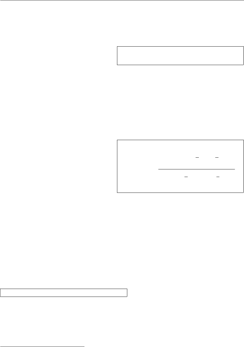
3.8 Theorems, Laws, . . . 55
to text mode. Use \mathrm instead to keep the size switching mechanism ac-
tive. But pay attention, \mathrm will only work well on short items. Spaces
are still not active and accented characters do not work.5
\begin{equation}
2^{\textrm{nd}} \quad
2^{\mathrm{nd}}
\end{equation}
2nd 2nd (3.10)
Sometimes you still need to tell L
A
T
EX the correct font size. In math
mode, this is set with the following four commands:
\displaystyle (123), \textstyle (123), \scriptstyle (123) and
\scriptscriptstyle (123).
Changing styles also affects the way limits are displayed.
\begin{displaymath}
\mathop{\mathrm{corr}}(X,Y)=
\frac{\displaystyle
\sum_{i=1}^n(x_i-\overline x)
(y_i-\overline y)}
{\displaystyle\biggl[
\sum_{i=1}^n(x_i-\overline x)^2
\sum_{i=1}^n(y_i-\overline y)^2
\biggr]^{1/2}}
\end{displaymath}
corr(X, Y ) =
n
X
i=1
(xi−x)(yi−y)
n
X
i=1
(xi−x)2
n
X
i=1
(yi−y)21/2
This is an examples with larger brackets than \left[ \right] provides.
The \biggl and \biggr commands are used for left and right brackets re-
spectively.
3.8 Theorems, Laws, . . .
When writing mathematical documents, you probably need a way to typeset
“Lemmas”, “Definitions”, “Axioms” and similar structures. L
A
T
EX supports
this with the command
\newtheorem{name}[counter ]{text}[section]
The name argument is a short keyword used to identify the “theorem.”
With the text argument you define the actual name of the “theorem,” which
will be printed in the final document.
The arguments in square brackets are optional. They are both used to
specify the numbering used on the “theorem.” Use the counter argument to
5The A
M
S-L
A
T
E
X (amsmath) package makes the \textrm command work with size
changing.
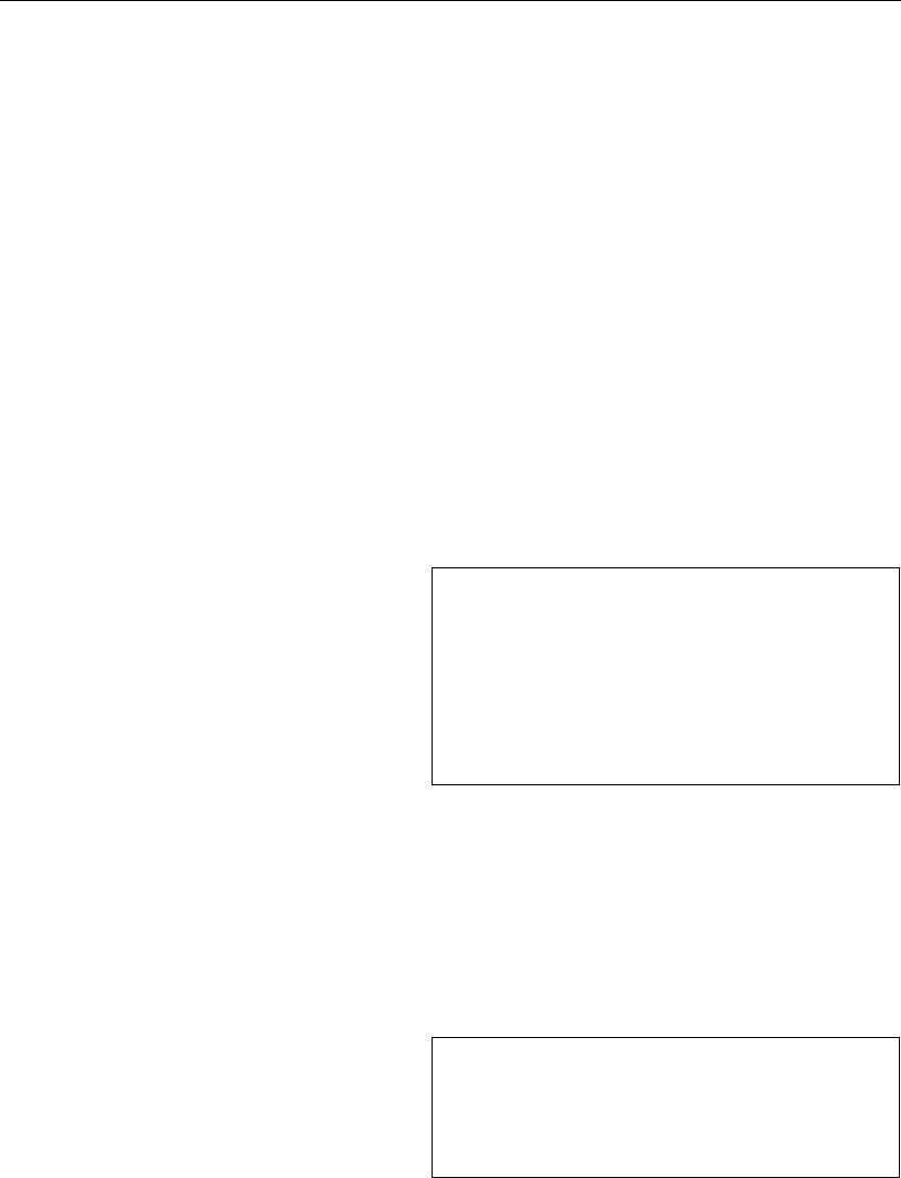
56 Typesetting Mathematical Formulae
specify the name of a previously declared “theorem.” The new “theorem”
will then be numbered in the same sequence. The section argument allows
you to specify the sectional unit within which the “theorem” should get its
numbers.
After executing the \newtheorem command in the preamble of your doc-
ument, you can use the following command within the document.
\begin{name}[text]
This is my interesting theorem
\end{name}
This should be enough theory. The following examples should remove
any remaining doubt, and make it clear that the \newtheorem environment
is way too complex to understand.
% definitions for the document
% preamble
\newtheorem{law}{Law}
\newtheorem{jury}[law]{Jury}
%in the document
\begin{law} \label{law:box}
Don’t hide in the witness box
\end{law}
\begin{jury}[The Twelve]
It could be you! So beware and
see law~\ref{law:box}\end{jury}
\begin{law}No, No, No\end{law}
Law 1 Don’t hide in the witness box
Jury 2 (The Twelve) It could be you! So
beware and see law 1
Law 3 No, No, No
The “Jury” theorem uses the same counter as the “Law” theorem, so it
gets a number that is in sequence with the other “Laws.” The argument in
square brackets is used to specify a title or something similar for the theorem.
\flushleft
\newtheorem{mur}{Murphy}[section]
\begin{mur}
If there are two or more
ways to do something, and
one of those ways can result
in a catastrophe, then
someone will do it.\end{mur}
Murphy 3.8.1 If there are two or more
ways to do something, and one of those ways
can result in a catastrophe, then someone
will do it.
The “Murphy” theorem gets a number that is linked to the number of
the current section. You could also use another unit, for example chapter or
subsection.
3.9 Bold Symbols 57
3.9 Bold Symbols
It is quite difficult to get bold symbols in L
A
T
EX; this is probably intentional
as amateur typesetters tend to overuse them. The font change command
\mathbf gives bold letters, but these are roman (upright) whereas mathe-
matical symbols are normally italic. There is a \boldmath command, but
this can only be used outside mathematics mode. It works for symbols too.
\begin{displaymath}
\mu, M \qquad \mathbf{M} \qquad
\mbox{\boldmath $\mu, M$}
\end{displaymath}
µ, M Mµ, M
Notice that the comma is bold too, which may not be what is required.
The package amsbsy (included by amsmath) as well as the bm from the
tools bundle make this much easier as they include a \boldsymbol command.
\begin{displaymath}
\mu, M \qquad
\boldsymbol{\mu}, \boldsymbol{M}
\end{displaymath}
µ, M µ,M

58 Typesetting Mathematical Formulae
3.10 List of Mathematical Symbols
The following tables demonstrate all the symbols normally accessible from
math mode.
To use the symbols listed in Tables 3.12–3.16,6the package amssymb must
be loaded in the preamble of the document and the AMS math fonts must
be installed on the system. If the AMS package and fonts are not installed
on your system, have a look at
macros/latex/required/amslatex. An even more comprehensive list of
symbols can be found at info/symbols/comprehensive.
Table 3.1: Math Mode Accents.
ˆa\hat{a} ˇa\check{a} ˜a\tilde{a} ´a\acute{a}
`a\grave{a} ˙a\dot{a} ¨a\ddot{a} ˘a\breve{a}
¯a\bar{a} a \vec{a} b
A\widehat{A} e
A\widetilde{A}
Table 3.2: Lowercase Greek Letters.
α\alpha θ\theta ooυ\upsilon
β\beta ϑ\vartheta π\pi φ\phi
γ\gamma ι\iota \varpi ϕ\varphi
δ\delta κ\kappa ρ\rho χ\chi
\epsilon λ\lambda \varrho ψ\psi
ε\varepsilon µ\mu σ\sigma ω\omega
ζ\zeta ν\nu ς\varsigma
η\eta ξ\xi τ\tau
Table 3.3: Uppercase Greek Letters.
Γ\Gamma Λ\Lambda Σ\Sigma Ψ\Psi
∆\Delta Ξ\Xi Υ\Upsilon Ω\Omega
Θ\Theta Π\Pi Φ\Phi
6These tables were derived from symbols.tex by David Carlisle and subsequently
changed extensively as suggested by Josef Tkadlec.

3.10 List of Mathematical Symbols 59
Table 3.4: Binary Relations.
You can negate the following symbols by prefixing them with a \not com-
mand.
<<>>==
≤\leq or \le ≥\geq or \ge ≡\equiv
\ll \gg .
=\doteq
≺\prec \succ ∼\sim
\preceq \succeq '\simeq
⊂\subset ⊃\supset ≈\approx
⊆\subseteq ⊇\supseteq ∼
=\cong
<\sqsubset a=\sqsupset a1\Join a
v\sqsubseteq w\sqsupseteq \bowtie
∈\in 3\ni ,\owns ∝\propto
`\vdash a\dashv |=\models
|\mid k\parallel ⊥\perp
\smile \frown \asymp
::/∈\notin 6=\neq or \ne
aUse the latexsym package to access this symbol
Table 3.5: Binary Operators.
++−-
±\pm ∓\mp \triangleleft
·\cdot ÷\div \triangleright
×\times \\setminus \star
∪\cup ∩\cap ∗\ast
t\sqcup u\sqcap ◦\circ
∨\vee ,\lor ∧\wedge ,\land •\bullet
⊕\oplus \ominus \diamond
\odot \oslash ]\uplus
⊗\otimes \bigcirc q\amalg
4\bigtriangleup 5\bigtriangledown †\dagger
\lhd a\rhd a‡\ddagger
\unlhd a\unrhd ao\wr

60 Typesetting Mathematical Formulae
Table 3.6: BIG Operators.
P\sum S\bigcup W\bigvee L\bigoplus
Q\prod T\bigcap V\bigwedge N\bigotimes
`\coprod F\bigsqcup J\bigodot
R\int H\oint U\biguplus
Table 3.7: Arrows.
←\leftarrow or \gets ←− \longleftarrow ↑\uparrow
→\rightarrow or \to −→ \longrightarrow ↓\downarrow
↔\leftrightarrow ←→ \longleftrightarrow l\updownarrow
⇐\Leftarrow ⇐=\Longleftarrow ⇑\Uparrow
⇒\Rightarrow =⇒\Longrightarrow ⇓\Downarrow
⇔\Leftrightarrow ⇐⇒ \Longleftrightarrow m\Updownarrow
7→ \mapsto 7−→ \longmapsto %\nearrow
←\hookleftarrow →\hookrightarrow &\searrow
\leftharpoonup \rightharpoonup .\swarrow
\leftharpoondown \rightharpoondown -\nwarrow
\rightleftharpoons ⇐⇒ \iff (bigger spaces) ;\leadsto a
aUse the latexsym package to access this symbol
Table 3.8: Delimiters.
(())↑\uparrow ⇑\Uparrow
[[or \lbrack ]]or \rbrack ↓\downarrow ⇓\Downarrow
{\{ or \lbrace }\} or \rbrace l\updownarrow m\Updownarrow
h\langle i\rangle ||or \vert k\| or \Vert
b\lfloor c\rfloor d\lceil e\rceil
//\\backslash . (dual. empty)
Table 3.9: Large Delimiters.
\lgroup
\rgroup
\lmoustache
\rmoustache
\arrowvert w
w\Arrowvert
\bracevert

3.10 List of Mathematical Symbols 61
Table 3.10: Miscellaneous Symbols.
. . . \dots ··· \cdots .
.
.\vdots ...\ddots
\hbar ı\imath \jmath \ell
<\Re =\Im ℵ\aleph ℘\wp
∀\forall ∃\exists 0\mho a∂\partial
0’0\prime ∅\emptyset ∞\infty
∇\nabla 4\triangle 2\Box a3\Diamond a
⊥\bot >\top ∠\angle √\surd
♦\diamondsuit ♥\heartsuit ♣\clubsuit ♠\spadesuit
¬\neg or \lnot \flat \natural \sharp
aUse the latexsym package to access this symbol
Table 3.11: Non-Mathematical Symbols.
These symbols can also be used in text mode.
†\dag §\S ©\copyright ®\textregistered
‡\ddag ¶\P £\pounds %\%
Table 3.12: AMS Delimiters.
p\ulcorner q\urcorner x\llcorner y\lrcorner
|\lvert |\rvert k\lVert k\rVert
Table 3.13: AMS Greek and Hebrew.
\digamma κ\varkappa \beth ג\gimel \daleth

62 Typesetting Mathematical Formulae
Table 3.14: AMS Binary Relations.
\lessdot \gtrdot +\doteqdot or \Doteq
6\leqslant >\geqslant :\risingdotseq
0\eqslantless 1\eqslantgtr ;\fallingdotseq
5\leqq =\geqq P\eqcirc
≪\lll or \llless ≫\ggg or \gggtr $\circeq
.\lesssim &\gtrsim ,\triangleq
/\lessapprox '\gtrapprox l\bumpeq
≶\lessgtr ≷\gtrless m\Bumpeq
Q\lesseqgtr R\gtreqless ∼\thicksim
S\lesseqqgtr T\gtreqqless ≈\thickapprox
4\preccurlyeq <\succcurlyeq \approxeq
2\curlyeqprec 3\curlyeqsucc v\backsim
-\precsim %\succsim w\backsimeq
\precapprox \succapprox \vDash
j\subseteqq k\supseteqq \Vdash
b\Subset c\Supset \Vvdash
<\sqsubset =\sqsupset \backepsilon
∴\therefore ∵\because ∝\varpropto
\shortmid \shortparallel G\between
`\smallsmile a\smallfrown t\pitchfork
C\vartriangleleft B\vartriangleright J\blacktriangleleft
E\trianglelefteq D\trianglerighteq I\blacktriangleright
Table 3.15: AMS Arrows.
L99 \dashleftarrow 99K \dashrightarrow (\multimap
⇔\leftleftarrows ⇒\rightrightarrows \upuparrows
\leftrightarrows \rightleftarrows \downdownarrows
W\Lleftarrow V\Rrightarrow \upharpoonleft
\twoheadleftarrow \twoheadrightarrow \upharpoonright
\leftarrowtail \rightarrowtail \downharpoonleft
\leftrightharpoons \rightleftharpoons \downharpoonright
\Lsh \Rsh \rightsquigarrow
"\looparrowleft #\looparrowright !\leftrightsquigarrow
\curvearrowleft \curvearrowright
\circlearrowleft \circlearrowright

3.10 List of Mathematical Symbols 63
Table 3.16: AMS Negated Binary Relations and Arrows.
≮\nless ≯\ngtr \varsubsetneqq
\lneq \gneq \varsupsetneqq
\nleq \ngeq \nsubseteqq
\nleqslant \ngeqslant \nsupseteqq
\lneqq \gneqq \nmid
\lvertneqq \gvertneqq ∦\nparallel
\nleqq \ngeqq \nshortmid
\lnsim \gnsim \nshortparallel
\lnapprox \gnapprox \nsim
⊀\nprec \nsucc \ncong
\npreceq \nsucceq \nvdash
\precneqq \succneqq \nvDash
\precnsim \succnsim \nVdash
\precnapprox \succnapprox \nVDash
\subsetneq \supsetneq \ntriangleleft
\varsubsetneq \varsupsetneq \ntriangleright
\nsubseteq \nsupseteq \ntrianglelefteq
\subsetneqq \supsetneqq \ntrianglerighteq
\nleftarrow \nrightarrow \nleftrightarrow
\nLeftarrow \nRightarrow \nLeftrightarrow
Table 3.17: AMS Binary Operators.
u\dotplus \centerdot |\intercal
\ltimes \rtimes \divideontimes
d\Cup or \doublecup e\Cap or \doublecap \smallsetminus
Y\veebar Z\barwedge [\doublebarwedge
\boxplus \boxminus \circleddash
\boxtimes \boxdot }\circledcirc
h\leftthreetimes i\rightthreetimes ~\circledast
g\curlyvee f\curlywedge

64 Typesetting Mathematical Formulae
Table 3.18: AMS Miscellaneous.
\hbar \hslash k\Bbbk
\square \blacksquare s\circledS
M\vartriangle N\blacktriangle {\complement
O\triangledown H\blacktriangledown \Game
♦\lozenge \blacklozenge F\bigstar
∠\angle ]\measuredangle ^\sphericalangle
\diagup \diagdown 8\backprime
\nexists \Finv ∅\varnothing
ð\eth 0\mho
Table 3.19: Math Alphabets.
Example Command Required package
ABCDEabcde1234 \mathrm{ABCDE abcde 1234}
ABCDEabcde1234 \mathit{ABCDE abcde 1234}
ABCDEabcde \mathnormal{ABCDE abcde 1234}
ABCDE \mathcal{ABCDE abcde 1234}
A BC D E \mathscr{ABCDE abcde 1234} mathrsfs
ABCDEabcde1234 \mathfrak{ABCDE abcde 1234} amsfonts or amssymb
ABCDE \mathbb{ABCDE abcde 1234} amsfonts or amssymb

Chapter 4
Specialities
When putting together a large document, L
A
T
E
X will help you with some special
features like index generation, bibliography management, and other things. A
much more complete description of specialities and enhancements possible with
L
A
T
E
X can be found in the L
A
T
E
X Manual [1]and The L
A
T
E
X Companion [3].
4.1 Including Encapsulated PostScript Graphics
L
A
T
EX provides the basic facilities to work with floating bodies, such as im-
ages or graphics, with the figure and table environments.
There are also several ways to generate the actual graphics with basic
L
A
T
EX or a L
A
T
EX extension package, but most users find them quite difficult
to understand, so this manual will not explain them. Please refer to The
L
A
T
E
X Companion [3] and the L
A
T
E
X Manual [1] for more information on
that subject.
A much easier way to get graphics into a document is to generate them
with a specialised software package1and then include the finished graphics
into the document. Here again, L
A
T
EX packages offer many ways to do this,
but this introduction will only discuss the use of Encapsulated PostScript
(EPS) graphics, because it is quite easy to do and widely used. In order
to use pictures in the EPS format, you must have a PostScript printer2
available for output.
A good set of commands for inclusion of graphics is provided in the
graphicx package by D. P. Carlisle. It is part of a whole family of packages
called the “graphics” bundle.3
1Such as XFig, CorelDraw!, Freehand, Gnuplot, . . .
2Another possibility to output PostScript is the GhostScript program available
from support/ghostscript. Windows and OS/2 users might want to look for GSview.
3macros/latex/required/graphics
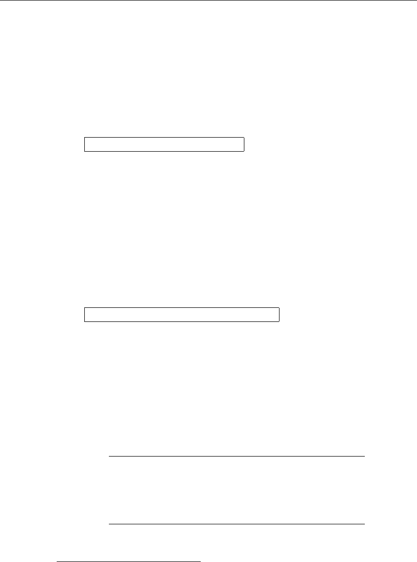
66 Specialities
Assuming you are working on a system with a PostScript printer avail-
able for output and with the graphicx package installed, you can use the
following step by step guide to include a picture into your document:
1. Export the picture from your graphics program in EPS format.4
2. Load the graphicx package in the preamble of the input file with
\usepackage[driver]{graphicx}
where driver is the name of your “dvi to postscript” converter program.
The most widely used program is called dvips. The name of the driver
is required, because there is no standard on how graphics are included
in T
EX. Knowing the name of the driver, the graphicx package can
choose the correct method to insert information about the graphics
into the .dvi file, so that the printer understands it and can correctly
include the .eps file.
3. Use the command
\includegraphics[key=value, . . . ]{file}
to include file into your document. The optional parameter accepts a
comma separated list of keys and associated values. The keys can be
used to alter the width, height and rotation of the included graphic.
Table 4.1 lists the most important keys.
Table 4.1: Key Names for graphicx Package.
width scale graphic to the specified width
height scale graphic to the specified height
angle rotate graphic counterclockwise
scale scale graphic
4If your software can not export into EPS format, you can try to install a PostScript
printer driver (such as an Apple LaserWriter, for example) and then print to a file with
this driver. With some luck this file will be in EPS format. Note that an EPS must not
contain more than one page. Some printer drivers can be explicitly configured to produce
EPS format.
4.2 Bibliography 67
The following example code may help to clarify things:
\begin{figure}
\begin{center}
\includegraphics[angle=90, width=0.5\textwidth]{test}
\end{center}
\caption{A caption, explaining that this is a test.}
\end{figure}
It includes the graphic stored in the file test.eps. The graphic is first
rotated by an angle of 90 degrees and then scaled to the final width of 0.5
times the width of a standard paragraph. The aspect ratio is 1.0, because
no special height is specified. The width and height parameters can also be
specified in absolute dimensions. Refer to Table 6.5 on page 109 for more
information. If you want to know more about this topic, make sure to read
[9] and [13].
4.2 Bibliography
You can produce a bibliography with the thebibliography environment.
Each entry starts with
\bibitem[label ]{marker }
The marker is then used to cite the book, article or paper within the
document.
\cite{marker}
If you do not use the label option, the entries will get enumerated au-
tomatically. The parameter after the \begin{thebibliography} command
defines how much space to reserve for the number of labels. In the example
below, {99} tells L
A
T
EX to expect that none of the bibliography item numbers
will be wider than the number 99.
Partl~\cite{pa} has
proposed that \ldots
\begin{thebibliography}{99}
\bibitem{pa} H.~Partl:
\emph{German \TeX},
TUGboat Volume~9, Issue~1 (1988)
\end{thebibliography}
Partl [1] has proposed that . . .
Bibliography
[1] H. Partl: German T
E
X, TUGboat Vol-
ume 9, Issue 1 (1988)
68 Specialities
For larger projects, you might want to check out the BibT
EX program.
BibT
EX is included with most T
EX distributions. It allows you to main-
tain a bibliographic database and then extract the references relevant to
things you cited in your paper. The visual presentation of BibT
EX gener-
ated bibliographies is based on a style sheets concept that allows you to
create bibliographies following a wide range of established designs.
4.3 Indexing
A very useful feature of many books is their index. With L
A
T
EX and the
support program makeindex,5an index can be generated quite easily. This
introduction will only explain the basic index generation commands. For a
more in-depth view, please refer to The L
A
T
E
X Companion [3].
To enable the indexing feature of L
A
T
EX, the makeidx package must be
loaded in the preamble with:
\usepackage{makeidx}
and the special indexing commands must be enabled by putting the
\makeindex
command into the input file preamble.
The content of the index is specified with
\index{key}
commands, where key is the index entry. You enter the index commands
at the points in the text that you want the final index entries to point to.
Table 4.2 explains the syntax of the key argument with several examples.
When the input file is processed with L
A
T
EX, each \index command
writes an appropriate index entry, together with the current page number,
to a special file. The file has the same name as the L
A
T
EX input file, but
a different extension (.idx). This .idx file can then be processed with the
makeindex program.
makeindex filename
The makeindex program generates a sorted index with the same base file
name, but this time with the extension .ind. If now the L
A
T
EX input file
5On systems not necessarily supporting filenames longer than 8 characters, the program
may be called makeidx.
4.4 Fancy Headers 69
Table 4.2: Index Key Syntax Examples.
Example Index Entry Comment
\index{hello} hello, 1 Plain entry
\index{hello!Peter} Peter, 3 Subentry under ‘hello’
\index{Sam@\textsl{Sam}} Sam, 2 Formatted entry
\index{Lin@\textbf{Lin}} Lin, 7 Same as above
\index{Jenny|textbf} Jenny, 3Formatted page number
\index{Joe|textit} Joe, 5Same as above
\index{eolienne@\’eolienne} éolienne, 4 Handling of accents
is processed again, this sorted index gets included into the document at the
point where L
A
T
EX finds
\printindex
The showidx package that comes with L
A
T
EX 2εprints out all index entries
in the left margin of the text. This is quite useful for proofreading a document
and verifying the index.
Note that the \index command can affect your layout if not used care-
fully.
My Word \index{Word}. As opposed
to Word\index{Word}. Note the
position of the full stop.
My Word . As opposed to Word. Note the
position of the full stop.
4.4 Fancy Headers
The fancyhdr package,6written by Piet van Oostrum, provides a few sim-
ple commands that allow you to customize the header and footer lines of
your document. If you look at the top of this page, you can see a possible
application of this package.
The tricky problem when customising headers and footers is to get things
like running section and chapter names in there. L
A
T
EX accomplishes this
with a two-stage approach. In the header and footer definition, you use
the commands \rightmark and \leftmark to represent the current section
and chapter heading, respectively. The values of these two commands are
overwritten whenever a chapter or section command is processed.
6Available from macros/latex/contrib/supported/fancyhdr.

70 Specialities
\documentclass{book}
\usepackage{fancyhdr}
\pagestyle{fancy}
% with this we ensure that the chapter and section
% headings are in lowercase.
\renewcommand{\chaptermark}[1]{\markboth{#1}{}}
\renewcommand{\sectionmark}[1]{\markright{\thesection\ #1}}
\fancyhf{} % delete current setting for header and footer
\fancyhead[LE,RO]{\bfseries\thepage}
\fancyhead[LO]{\bfseries\rightmark}
\fancyhead[RE]{\bfseries\leftmark}
\renewcommand{\headrulewidth}{0.5pt}
\renewcommand{\footrulewidth}{0pt}
\addtolength{\headheight}{0.5pt} % make space for the rule
\fancypagestyle{plain}{%
\fancyhead{} % get rid of headers on plain pages
\renewcommand{\headrulewidth}{0pt} % and the line
}
Figure 4.1: Example fancyhdr Setup.
For ultimate flexibility, the \chapter command and its friends do not
redefine \rightmark and \leftmark themselves. They call yet another com-
mand (\chaptermark,\sectionmark, or \subsectionmark) that is respon-
sible for redefining \rightmark and \leftmark.
If you want to change the look of the chapter name in the header line,
you need only “renew” the \chaptermark command.
Figure 4.1 shows a possible setup for the fancyhdr package that makes the
headers look about the same as they look in this booklet. In any case, I sug-
gest you fetch the documentation for the package at the address mentioned
in the footnote.
4.5 The Verbatim Package
Earlier in this book, you got to know the verbatim environment. In this
section, you are going to learn about the verbatim package. The verbatim
package is basically a re-implementation of the verbatim environment that
works around some of the limitations of the original verbatim environment.
This by itself is not spectacular, but the implementation of the verbatim
package added new functionality, which is why I am mentioning the package
4.6 Downloading and Installing L
A
T
E
X Packages 71
here. The verbatim package provides the
\verbatiminput{filename}
command, which allows you to include raw ASCII text into your document
as if it were inside a verbatim environment.
As the verbatim package is part of the ‘tools’ bundle, you should find it
pre-installed on most systems. If you want to know more about this package,
make sure to read [10].
4.6 Downloading and Installing L
A
T
E
X Packages
Most L
A
T
EX installations come with a large set of pre-installed style packages,
but many more are available on the net. The main place to look for style
packages on the Internet is CTAN (http://www.ctan.org/).
Packages such as geometry,hyphenat, and many others are typically made
up of two files: a file with the extension .ins and another with the extension
.dtx. There will often be a readme.txt with a brief description of the
package. You should of course read this file first.
In any event, once you have copied the package files onto your machine,
you still have to process them in a way that (a) tells your T
EX distribution
about the new style package and (b) gives you the documentation. Here’s
how you do the first part:
1. Run L
A
T
EX on the .ins file. This will extract a .sty file.
2. Move the .sty file to a place where your distribution can find it. Usu-
ally this is in your .../localtexmf /tex/latex subdirectory (Win-
dows or OS/2 users should feel free to change the direction of the
slashes).
3. Refresh your distribution’s file-name database. The command depends
on the L
A
T
EXdistribution you use: teTeX, fpTeX – texhash; web2c –
maktexlsr; MikTeX – initexmf -update-fndb or use the GUI.
Now you can extract the documentation from the .dtx file:
1. Run L
A
T
EX on the .dtx file. This will generate a .dvi file. Note
that you may have to run L
A
T
EX several times before it gets the cross-
references right.
2. Check to see if L
A
T
EX has produced a .idx file among the various files
you now have. If you do not see this file, then you may proceed to
step 5.

72 Specialities
3. In order to generate the index, type the following:
makeindex -s gind.ist name
(where name stands for the main-file name without any extension).
4. Run L
A
T
EX on the .dtx file once again.
5. Last but not least, make a .ps or .pdf file to increase your reading
pleasure.
Sometimes you will see that a .glo (glossary) file has been produced.
Run the following command between step 4and 5:
makeindex -s gglo.ist -o name.gls name.glo
Be sure to run L
A
T
EX on the .dtx one last time before moving on to step 5.
4.7 Working with pdfL
A
T
E
X
By Daniel Flipo <Daniel.Flipo@univ-lille1.fr>
PDF is a hypertext document format. Much like in a web page, some words
in the document are marked as hyperlinks. They link to other places in the
document or even to other documents. If you click on such a hyperlink you
get transported to the destination of the link. In the context of L
A
T
EX, this
means that all occurrences of \ref and \pageref become hyperlinks. Addi-
tionally, the table of contents, the index and all the other similar structures
become collections of hyperlinks.
Most web pages you find today are written in HTML (HyperText Markup
Language). This format has two significant disadvantages when writing sci-
entific documents:
1. Including mathematical formulae into HTML documents is not gener-
ally supported. While there is a standard for it, most browsers used
today do not support it, or lack the required fonts.
2. Printing HTML documents is possible, but the results vary widely
between platforms and browsers. The results are miles removed from
the quality we have come to expect in the L
A
T
EX world.
There have been many attempts to create translators from L
A
T
EX to
HTML. Some were even quite successful in the sense that they are able
to produce legible web pages from a standard L
A
T
EX input file. But all of
them cut corners left and right to get the job done. As soon as you start
using more complex L
A
T
EX features and external packages things tend to
fall apart. Authors wishing to preserve the unique typographic quality of
their documents even when publishing on the web turn to PDF (Portable
Document Format), which preserves the layout of the document and permits
hypertext navigation. Most modern browsers come with plugins that allow
the direct display of PDF documents.

4.7 Working with pdfL
A
T
E
X 73
Even though there are DVI and PS viewers for almost every platform,
you will find that acrobat reader and xpdf for viewing PDF documents are
more widely deployed. So providing PDF versions of your documents will
make them much more accessible to your potential readers.
4.7.1 PDF Documents for the Web
The creation of a PDF file from L
A
T
EX source is very simple, thanks to the
pdfT
EX program developed by Hàn Th´
ê Thành. pdfT
EX produces PDF
output where normal T
EX produces DVI. There is also a pdfL
A
T
EX, which
produces PDF output from L
A
T
EX sources.
Both pdfT
EX and pdfL
A
T
EX are installed automatically by most modern
T
EX distributions, such as teT
EX, fpT
EX, MikT
EX, T
EXLive and CMacT
EX.
To produce a PDF instead of DVI, it is sufficient to replace the com-
mand latex file.tex by pdflatex file.tex. On systems where L
A
T
EX
is not called from the command line, you may find a special button in the
T
EXControlCenter.
In L
A
T
EX you can define the the paper size with an optional documentclass
argument such as a4paper or letterpaper. This works in pdfL
A
T
EX too,
but on top of this pdfT
EX also needs to know the physical size of the paper
to determine the physical size of the pages in the pdf file. If you use the
hyperref package (see page 76), the papersize will be adjusted automatically.
Otherwise you have to do this manually by putting the following lines into
the preamble of the document:
\pdfpagewidth=\paperwidth
\pdfpageheight=\paperheight
The following section will go into more detail regarding the differences
between normal L
A
T
EX and pdfL
A
T
EX. The main differences concern three
areas: the fonts to use, the format of images to include, and the manual
configuration of hyperlinks.
4.7.2 The Fonts
pdfL
A
T
EX can deal with all sorts of fonts (PK bitmaps, TrueType, PostScript
type 1. . . ) but the normal L
A
T
EX font format, the bitmap PK fonts produce
very ugly results when the document is displayed with Acrobat Reader. It
is best to use PostScript Type 1 fonts exclusively to produce documents
that display well. Modern TeX installations will be setup so that this hap-
pens automatically. Best is to try. If it works for you, just skip this whole
paragraph.
The PostScript Type 1 implementation of the Computer Modern and
AMSFonts was produced by Blue Sky Research and Y&Y, Inc., who then
transferred copyright to the American Mathematical Society. The fonts were

74 Specialities
made publicly available in early 1997 and currently come with most of T
EX
distributions.
However, if you are using L
A
T
EX to create documents in languages other
than English, you might want to use EC, LH, or CB fonts (see the discussion
about OT1 fonts on the page 25). Vladimir Volovich has created the cm-super
font bundle which covers the entire EC/TC, EC Concrete, EC Bright and
LH font sets. It is available from CTAN:/fonts/ps-type1/cm-super and is
included with T
EXLive7 and MikT
EX. Similar type 1 CB Greek fonts created
by Apostolos Syropoulos are available at CTAN:/tex-archive/fonts/greek/cb.
Unfortunately, both of these font sets are not of the same typographic quality
as the Type1 CM fonts by Blue Sky/Y&Y. They were automatically hinted,
and the document might look not as neat on the screen as the ones using
Blue Sky/Y&Y type 1 CM fonts, on high resolution output devices they
produce results identical to the original bitmap EC/LH/CB fonts.
If you are creating document in one of Latin-based languages, you have
several other options.
•You might want to use aeguill package, aka Almost European Computer
Modern with Guillemets. Just put the line \usepackage{aeguill} into
the preamble of your document, to enable AE virtual fonts instead of
EC fonts.
•Alternatively, you can use mltex package, but this only works when
your pdfT
EX has been compiled with the mltex option.
The AE virtual fontset, like the MlT
EX system, makes T
EX believe it has
a full 256 character fontset at its disposal by creating most of the missing
letters from characters of the CM font and rearranging them in the EC order,
this allows to use the excellent type 1 format CM fonts available on most
systems. As the font is now in T1 encoding, hyphenation will work well in
Latin-based European languages. The only disadvantage of this approach is
that the artificial AE characters do not work with Acrobat Reader’s Find
function, so you cannot search for words with accented characters in your
final PDF file.
For the Russian language a similar solution is to use C1 virtual fonts
available at ftp://ftp.vsu.ru/pub/tex/font-packs/c1fonts. These fonts
combine the standard CM type 1 fonts from Bluesky collection and CMCYR
type 1 fonts from Paradissa and BaKoMa collection, all available on CTAN.
Because Paradissa fonts contain only Russian letters, C1 fonts are missing
other Cyrillic glyphs.
Another solution is to switch to other PostScript type 1 fonts. Ac-
tually, some of them are even included with every copy of Acrobat Reader.
Because these fonts have different character sizes, the text layout on your
pages will change. Generally these other fonts will use more space than the
CM fonts, which are very space-efficient. Also, the overall visual coherence

4.7 Working with pdfL
A
T
E
X 75
of your document will suffer because Times, Helvetica and Courier (the pri-
mary candidates for such a replacement job) have not been designed to work
in harmony in a single document.
Two ready-made font sets are available for this purpose: pxfonts, which
is based on Palatino as its main text body font, and the txfonts package,
which is based on Times. To use them it is sufficient to put the following
lines into the preamble of your document:
\usepackage[T1]{fontenc}
\usepackage{pxfonts}
Note: you may find lines like
Warning: pdftex (file eurmo10): Font eurmo10 at ... not found
in the .log file after compiling your input file. They mean that some font
used in the document has not been found. You really have to fix these
problems, as the resulting PDF document may not display the pages with
the missing characters at all.
This whole font business, especially the lack of a good EC fontset equiv-
alent in quality to the CM font in type 1 format, is occupying the minds of
many people, so new solutions are cropping up all the time.
4.7.3 Using Graphics
Including graphics into a document works best with the graphicx package
(see page 65). By using the special driver option pdftex the package will
work with pdfL
A
T
EX as well:
\usepackage[pdftex]{color,graphicx}
In the sample above I have included the color option, as using color in doc-
uments displayed on the web comes quite naturally.
So much for the good news. The bad news is that graphics in Encapsu-
lated PostScript format do not work with PdfL
A
T
EX. If you don’t define a
file extension in the \includegraphics command, graphicx will go looking
for a suitable file on its own, depending on the setting of the driver op-
tion. For pdftex this is formats .png,.pdf,.jpg,.mps (METAPOST), and
.tif—but not .eps.
The simple way out of this problem is to just convert your EPS files into
PDF format using the epstopdf utility found on many systems. For vector
graphics (drawings) this is a great solution. For bitmaps (photos, scans) this
is not ideal, because the PDF format natively supports the inclusion of PNG
and JPEG images. PNG is good for screenshots and other images with few
colors. JPEG is great for photos, as it is very space-efficient.

76 Specialities
It may even be desirable not to draw certain geometric figures, but rather
describe the figure with a specialized command language, such as META-
POST, which can be found in most T
EX distributions, and comes with its
own extensive manual.
4.7.4 Hypertext Links
The hyperref package will take care of turning all internal references of your
document into hyperlinks. For this to work properly some magic is necessary,
so you have to put \usepackage[pdftex]{hyperref} as the last command
into the preamble of your document.
Many options are available to customize the behaviour of the hyperref
package:
•either as a comma separated list after the pdftex option
\usepackage[pdftex]{hyperref}
•or on individual lines with the command \hypersetup{options}.
The only required option is pdftex; the others are optional and allow
you to change the default behaviour of hyperref.7In the following list the
default values are written in an upright font.
bookmarks (=true,false )show or hide the bookmarks bar when display-
ing the document
unicode (=false,true )allows to use characters of non-latin based lan-
guages in Acrobat’s bookmarks
pdftoolbar (=true,false )show or hide Acrobat’s toolbar
pdfmenubar (=true,false )show or hide Acrobat’s menu
pdffitwindow (=true,false )adjust the initial magnification of the pdf
when displayed
pdftitle (={text}) define the title that gets displayed in the Document
Info window of Acrobat
pdfauthor (={text}) the name of the PDF’s author
pdfnewwindow (=true,false )define if a new window should get opened
when a link leads out of the current document
7It is worth noting that the hyperref package is not limited to work with pdfT
E
X. It
can also be configured to embed PDF-specific information into the DVI output of normal
L
A
T
E
X, which then gets put into the PS file by dvips and is finally picked up by Adobe
Distiller when it is used to turn the PS file into PDF.

4.7 Working with pdfL
A
T
E
X 77
colorlinks (=false,true )surround the links by color frames (false) or
colors the text of the links (true). The color of these links can be
configured using the following options (default colors are shown):
linkcolor (=red) color of internal links (sections, pages, etc.),
citecolor (=green) color of citation links (bibliography)
filecolor (=magenta) color of file links
urlcolor (=cyan) color of URL links (mail, web)
If you are happy with the defaults, use
\usepackage[pdftex]{hyperref}
To have the bookmark list open and links in color (the =true values are
optional):
\usepackage[pdftex,bookmarks,colorlinks]{hyperref}
When creating PDFs destined for printing, colored links are not a good
thing as they end up in gray in the final output, making it difficult to read.
You can use color frames, which are not printed:
\usepackage{hyperref}
\hypersetup{colorlinks=false}
or make links black:
\usepackage{hyperref}
\hypersetup{colorlinks,%
citecolor=black,%
filecolor=black,%
linkcolor=black,%
urlcolor=black,%
pdftex}
When you just want to provide information for the Document Info sec-
tion of the PDF file:
\usepackage[pdfauthor={Pierre Desproges}%
pdftitle={Des femmes qui tombent},%
pdftex]{hyperref}
In addition to the automatic hyperlinks for cross references, it is possible
to embed explicit links using
\href{url}{text}
The code

78 Specialities
The \href{http://www.ctan.org}{CTAN} website.
produces the output “CTAN”; a click on the word “CTAN” will take you to
the CTAN website.
If the destination of the link is not a URL but a local file, you can use
the \href command:
The complete document is \href{manual.pdf}{here}
Which produces the text “The complete document is here”. A click on the
word “here” will open the file manual.pdf. (The filename is relative to the
location of the current document).
The author of an article might want her readers to easily send email
messages by using the \href command inside the \author command on the
title page of the document:
\author{Mary Oetiker $<$\href{mailto:mary@oetiker.ch}%
{mary@oetiker.ch}$>$
Note that I have put the link so that my email address appears not only in
the link but also on the page itself. I did this because the link
\href{mailto:mary@oetiker.ch}{Mary Oetiker}
would work well within Acrobat, but once the page is printed the email
address would not be visible anymore.
4.7.5 Problems with Links
Messages like the following:
! pdfTeX warning (ext4): destination with the same identifier
(name{page.1}) has been already used, duplicate ignored
appear when a counter gets reinitialized, for example by using the command
\mainmatter provided by the book document class. It resets the page num-
ber counter to 1 prior to the first chapter of the book. But as the preface of
the book also has a page number 1 all links to “page 1” would not be unique
anymore, hence the notice that “duplicate has been ignored.”
The counter measure consists of putting plainpages=false into the hy-
perref options. This unfortunately only helps with the page counter. An
even more radical solution is to use the option hypertexnames=false, but
this will cause the page links in the index to stop working.
4.7.6 Problems with Bookmarks
The text displayed by bookmarks does not always look like you expect it to
look. Because bookmarks are “just text,” much fewer characters are available
for bookmarks than for normal L
A
T
EX text. Hyperref will normally notice
such problems and put up a warning:

4.7 Working with pdfL
A
T
E
X 79
Package hyperref Warning:
Token not allowed in a PDFDocEncoded string:
You can now work around this problem by providing a text string for the
bookmarks, which replaces the offending text:
\texorpdfstring{T
E
X text}{Bookmark Text}
Math expressions are a prime candidate for this kind of problem:
\section{\texorpdfstring{$E=mc^2$}%
{E\ =\ mc\texttwosuperior}}
which turns \section{$E=mc^2$} to “E=mc2” in the bookmark area.
Color changes also do not travel well into bookmarks:
\section{\textcolor{red}{Red !}}
produces the string “redRed!”. The command \textcolor gets ignored but
its argument (red) gets printed.
If you use
\section{\texorpdfstring{\textcolor{red}{Red !}}{Red\ !}}
the result will be much more legible.
Source Compatibility Between L
A
T
E
X and pdfL
A
T
E
X
Ideally your document would compile equally well with L
A
T
EX and pdfL
A
T
EX.
The main problem in this respect is the inclusion of graphics. The simple
solution is to systematically drop the file extension from \includegraphics
commands. They will then automatically look for a file of a suitable format
in the current directory. All you have to do is create appropriate versions of
the graphics files. L
A
T
EX will look for .eps, and pdfL
A
T
EX will try to include
a file with the extension .png,.pdf,.jpg,.mps or .tif (in that order).
For the cases where you want to use different code for the PDF version
of your document, you can add:
\newif\ifPDF
\ifx\pdfoutput\undefined\PDFfalse
\else\ifnum\pdfoutput > 0\PDFtrue
\else\PDFfalse
\fi
\fi
as the very first few lines of your document. This defines a special command
that will allow you to easily write conditional code:

80 Specialities
\ifPDF
\usepackage[T1]{fontenc}
\usepackage{aeguill}
\usepackage[pdftex]{graphicx,color}
\usepackage[pdftex]{hyperref}
\else
\usepackage[T1]{fontenc}
\usepackage[dvips]{graphicx}
\usepackage[dvips]{hyperref}
\fi
In the example above I have included the hyperref package even in the non-
PDF version. The effect of this is to make the \href command work in
all cases, which saves me from wrapping every occurrence into a conditional
statement.
Note that in recent T
EX distributions (T
EXLive for example), the choice
between pdftex and dvips when calling graphicx and color will happen auto-
matically according to the settings made automatically in the configuration
files graphics.cfg and color.cfg.
4.8 Creating Presentations with pdfscreen
By Daniel Flipo <Daniel.Flipo@univ-lille1.fr>
You can present the results of your scientific work on a blackboard, with
transparencies, or directly from your laptop using some presentation soft-
ware.
pdfL
A
T
EX combined with the pdfscreen package allows you to create pre-
sentations in PDF, equally as colorful and lively as is possible with Power-
Point, but much more portable because Acrobat Reader is available on many
more systems.
The pdfscreen class uses graphicx,color and hyperref with options adapted
to screen presentations.
To create this type of document you normally work within the article
class. Figure 4.2 shows an example input file. First you have to load the
pdfscreen package together with appropriate options:
screen for screen presentation. Use print to create a printable version.
panelright put a navigation panel on the right side of the screen. If the
panel should be on the left side use panelleft. If you do not want
panels use nopanel.
french or some other supported language will render the text on the nav-
igation buttons appropriately. This option is independent of the op-
tions set with the babel package. If your language is not supported by

4.8 Creating Presentations with pdfscreen 81
\documentclass[pdftex,12pt]{article}
%%% misc extensions %%%%%%%%%%%%%%%%%%%%%%%%%%%%%%%%%%%%%
\usepackage[latin1]{inputenc}
\usepackage[english]{babel}
\usepackage[T1]{fontenc}
\usepackage{aeguill}
%%% pdfscreen %%%%%%%%%%%%%%%%%%%%%%%%%%%%%%%%%%%%%%%%%%%
\usepackage[screen,panelleft,chocolate]{pdfscreen}
% Screen Format
\panelwidth=25mm
%% height width
\screensize{150mm}{200mm}
%% left right top bottom
\marginsize{42mm}{8mm}{10mm}{10mm}
% Color or image for background
\overlayempty
\definecolor{mybg}{rgb}{1,0.9,0.7}
\backgroundcolor{mybg}
% Logo
\emblema{MyLogo}
%%% For PPower4 (post-processor) %%%%%%%%%%%%%%%%%%%%%%%%
\usepackage{pause}
%%%%%%%%%%%%%%%%%%%%%%%%%%%%%%%%%%%%%%%%%%%%%%%%%%%%%%%%%
\begin{document}
\begin{slide}
\begin{itemize}
\item Good News\dots \pause
\item Bad News
\end{itemize}
\end{slide}
\end{document}
Figure 4.2: Example pdfscreen input file
82 Specialities
pdfscreen, you still can localize navigation panel buttons by using file
pdfscreen.cfg, see pdfscreen.cfg..specimen for an example.
chocolate color scheme for the navigation panel. Other choices are gray,
orange,palegreen,bluelace and blue, which is the default.
Then you configure the display format. Because the presentation will al-
ways scale to the real size of the screen when displayed, this can be used to
configure the overall font size:
\panelwidth defines the width of the navigation panel
\screensize{width}{height}define the width and height of the screen in-
cluding the navigation panel.
\marginsize{left}{right}{top}{bottom}defines the margins of the docu-
ment. In the example the document is not centered because the section
numbers are kept in the left margin.
It is possible to use a background image in any of the image formats
supported by pdfT
EX using the command
\overlay{image}
or if you prefer a plain background you can define its color using
\background{color }
Finally if you want to place the logo of your organization into the navi-
gation panel use the command
\emblema{logo}
If you believe in the presentational power of successive exposure of your
bullet points you may want to make use of the pause package. It provides the
command \pause. You can place this command right into the flow of your
text wherever you want Acrobat to pause the display of your document. The
pause package is part of the ppower4 (P4:Pdf Presentation Post-Processor )
system, which can post-process pdf output from pdfT
EX and make it sing
and dance and beg for food. On the command line it looks like this:
ppower4 xy.pdf xyz.pdf
To control what goes onto a single slide, use the environment \begin{slide}
...\end{slide}. The content of each slide will get displayed centered verti-
cally on its page.
Compiling the example above, will end in an error message:

4.8 Creating Presentations with pdfscreen 83
! pdfTeX warning (dest): name{contents} has been
referenced but does not exist, replaced by a fixed one
This is because there is a button in the navigation panel that wants to
point to the table of contents, because this example does not contain a
\tableofcontents command the resolution of the link fails.
If you want the table of contents to be displayed right inside the navi-
gation panel, you can use the option paneltoc when calling pdfscreen. This
will only produce satisfactory results if your presentation has very few and
short entries in the table of contents. You may want to provide short titles
for your section headings in square brackets.
This short introduction only scratches the surface of what is possible with
pdfscreen and PPower4. Both come with their own extensive documentation.
Chapter 5
Producing Mathematical
Graphics
Most people use L
A
T
E
X for typesetting their text. But as the non content and
structure oriented approach to authoring is so convenient, L
A
T
E
X also offers a,
if somewhat restricted, possibility for producing graphical output from textual
descriptions. Furthermore, quite a number of L
A
T
E
X extensions have been created
in order to overcome these restrictions. In this section, you will learn about a
few of them.
5.1 Overview
The picture environment allows programming pictures directly in L
A
T
EX. A
detailed description can be found in the L
A
T
E
X Manual [1]. On the one hand,
there are rather severe constraints, as the slopes of line segments as well as
the radii of circles are restricted to a narrow choice of values. On the other
hand, the picture environment of L
A
T
EX 2εbrings with it the \qbezier
command, “q” meaning “quadratic”. Many frequently used curves such as
circles, ellipses, or catenaries can be satisfactorily approximated by quadratic
Bézier curves, although this may require some mathematical toil. If, in
addition, a programming language like Java is used to generate \qbezier
blocks of L
A
T
EX input files, the picture environment becomes quite powerful.
Although programming pictures directly in L
A
T
EX is severely restricted,
and often rather tiresome, there are still reasons for doing so. The documents
thus produced are “small” with respect to bytes, and there are no additional
graphics files to be dragged along.
Packages like epic and eepic (described, for instance, in The L
A
T
E
X Com-
panion [3]), or pstricks help to eliminate the restrictions hampering the orig-
inal picture environment, and greatly strengthen the graphical power of
L
A
T
EX.
86 Producing Mathematical Graphics
While the former two packages just enhance the picture environment,
the pstricks package has its own drawing environment, pspicture. The power
of pstricks stems from the fact that this package makes extensive use of
PostScript possibilities. In addition, numerous packages have been written
for specific purposes. One of them is X
Y
-pic, described at the end of this
chapter. A wide variety of these packages is described in detail in The L
A
T
E
X
Graphics Companion [4] (not to be confused with The L
A
T
E
X Companion [3]).
Perhaps the most powerful graphical tool related with L
A
T
EX is MetaPost,
the twin of Donald E. Knuth’s METAFONT.MetaPost has the very powerful and
mathematically sophisticated programming language of METAFONT. Contrary
to METAFONT, which generates bitmaps, MetaPost generates encapsulated
PostScript files, which can be imported in L
A
T
EX. For an introduction,
see A User’s Manual for MetaPost [15], or the tutorial on [17].
A very thorough discussion of L
A
T
EX and T
EX strategies for graphics (and
fonts) can be found in T
E
X Unbound [16].
5.2 The picture Environment
By Urs Oswald <osurs@bluewin.ch>
5.2.1 Basic Commands
Apicture environment1is created with one of the two commands
\begin{picture}(x, y). . . \end{picture}
or
\begin{picture}(x, y)(x0, y0). . . \end{picture}
The numbers x, y, x0, y0refer to \unitlength, which can be reset any
time (but not within a picture environment) with a command such as
\setlength{\unitlength}{1.2cm}
The default value of \unitlength is 1pt. The first pair, (x, y), effects the
reservation, within the document, of rectangular space for the picture. The
optional second pair, (x0, y0), assigns arbitrary coordinates to the bottom
left corner of the reserved rectangle.
1Believe it or not, the picture environment works out of the box, with standard L
A
T
E
X 2ε
no package loading necessary.
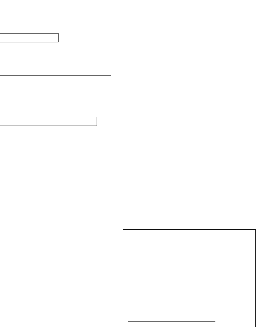
5.2 The picture Environment 87
Most drawing commands have one of the two forms
\put(x, y){object }
or
\multiput(x, y)(∆x, ∆y){n}{object }
Bézier curves are an exception. They are drawn with the command
\qbezier(x1, y1)(x2, y2)(x3, y3)
5.2.2 Line Segments
\setlength{\unitlength}{5cm}
\begin{picture}(1,1)
\put(0,0){\line(0,1){1}}
\put(0,0){\line(1,0){1}}
\put(0,0){\line(1,1){1}}
\put(0,0){\line(1,2){.5}}
\put(0,0){\line(1,3){.3333}}
\put(0,0){\line(1,4){.25}}
\put(0,0){\line(1,5){.2}}
\put(0,0){\line(1,6){.1667}}
\put(0,0){\line(2,1){1}}
\put(0,0){\line(2,3){.6667}}
\put(0,0){\line(2,5){.4}}
\put(0,0){\line(3,1){1}}
\put(0,0){\line(3,2){1}}
\put(0,0){\line(3,4){.75}}
\put(0,0){\line(3,5){.6}}
\put(0,0){\line(4,1){1}}
\put(0,0){\line(4,3){1}}
\put(0,0){\line(4,5){.8}}
\put(0,0){\line(5,1){1}}
\put(0,0){\line(5,2){1}}
\put(0,0){\line(5,3){1}}
\put(0,0){\line(5,4){1}}
\put(0,0){\line(5,6){.8333}}
\put(0,0){\line(6,1){1}}
\put(0,0){\line(6,5){1}}
\end{picture}
!!!!!!!!!!!!!!
!
""""""""""""""
"
##############
#
%%%%%%%%%%%%%%
%
((((((((((((((
(
,,,,,,,,,,,,,,
,
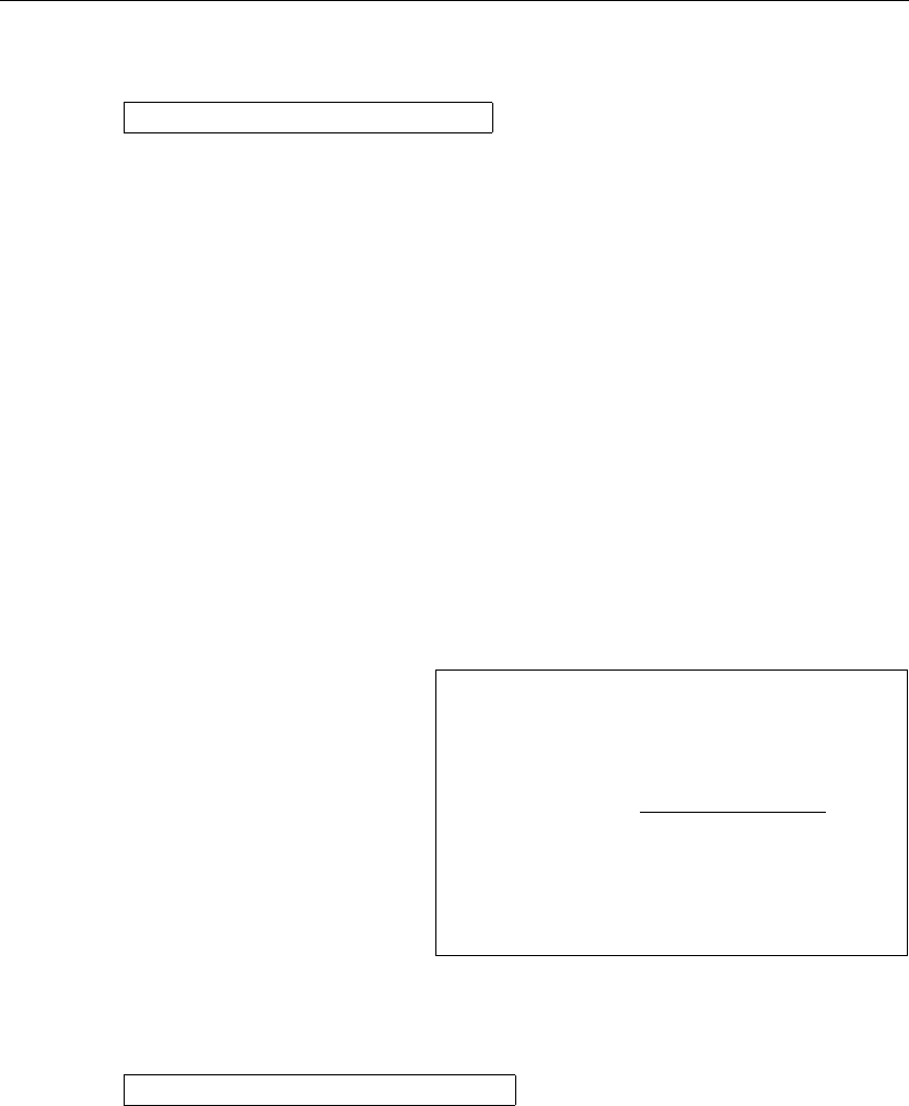
88 Producing Mathematical Graphics
Line segments are drawn with the command
\put(x, y){\line(x1, y1){length}}
The \line command has two arguments:
1. a direction vector,
2. a length.
The components of the direction vector are restricted to the integers
−6,−5, . . . , 5,6,
and they have to be coprime (no common divisor except 1). The figure
illustrates all 25 possible slope values in the first quadrant. The length is
relative to \unitlength. The length argument is the vertical coordinate in
the case of a vertical line segment, the horizontal coordinate in all other
cases.
5.2.3 Arrows
\setlength{\unitlength}{1mm}
\begin{picture}(60,40)
\put(30,20){\vector(1,0){30}}
\put(30,20){\vector(4,1){20}}
\put(30,20){\vector(3,1){25}}
\put(30,20){\vector(2,1){30}}
\put(30,20){\vector(1,2){10}}
\thicklines
\put(30,20){\vector(-4,1){30}}
\put(30,20){\vector(-1,4){5}}
\thinlines
\put(30,20){\vector(-1,-1){5}}
\put(30,20){\vector(-1,-4){5}}
\end{picture}
-
:
1
*
X
X
X
X
X
X
X
X
Xy
C
C
C
C
C
CO
Arrows are drawn with the command
\put(x, y){\vector(x1, y1){length}}
For arrows, the components of the direction vector are even more nar-
rowly restricted than for line segments, namely to the integers
−4,−3, . . . , 3,4.
Components also have to be coprime (no common divisor except 1). Notice
the effect of the \thicklines command on the two arrows pointing to the
upper left.

5.2 The picture Environment 89
5.2.4 Circles
\setlength{\unitlength}{1mm}
\begin{picture}(60, 40)
\put(20,30){\circle{1}}
\put(20,30){\circle{2}}
\put(20,30){\circle{4}}
\put(20,30){\circle{8}}
\put(20,30){\circle{16}}
\put(20,30){\circle{32}}
\put(40,30){\circle{1}}
\put(40,30){\circle{2}}
\put(40,30){\circle{3}}
\put(40,30){\circle{4}}
\put(40,30){\circle{5}}
\put(40,30){\circle{6}}
\put(40,30){\circle{7}}
\put(40,30){\circle{8}}
\put(40,30){\circle{9}}
\put(40,30){\circle{10}}
\put(40,30){\circle{11}}
\put(40,30){\circle{12}}
\put(40,30){\circle{13}}
\put(40,30){\circle{14}}
\put(15,10){\circle*{1}}
\put(20,10){\circle*{2}}
\put(25,10){\circle*{3}}
\put(30,10){\circle*{4}}
\put(35,10){\circle*{5}}
\end{picture}
bej
&%
'$
&%
'$behjm
"!
#
"!
#
&%
'$
r u x z}
The command
\put(x, y){\circle{diameter}}
draws a circle with center (x, y)and diameter (not radius) diameter. The
picture environment only admits diameters up to approximately 14 mm,
and even below this limit, not all diameters are possible. The \circle*
command produces disks (filled circles).
As in the case of line segments, one may have to resort to additional pack-
ages, such as eepic or pstricks. For a thorough description of these packages,
see The L
A
T
E
X Graphics Companion [4].
There is also a possibility within the picture environment. If one is not
afraid of doing the necessary calculations (or leaving them to a program),
arbitrary circles and ellipses can be patched together from quadratic Bézier
curves. See Graphics in L
A
T
E
X 2ε[17] for examples and Java source files.
90 Producing Mathematical Graphics
5.2.5 Text and Formulas
\setlength{\unitlength}{1cm}
\begin{picture}(6,5)
\thicklines
\put(1,0.5){\line(2,1){3}}
\put(4,2){\line(-2,1){2}}
\put(2,3){\line(-2,-5){1}}
\put(0.7,0.3){$A$}
\put(4.05,1.9){$B$}
\put(1.7,2.95){$C$}
\put(3.1,2.5){$a$}
\put(1.3,1.7){$b$}
\put(2.5,1.05){$c$}
\put(0.3,4){$F=
\sqrt{s(s-a)(s-b)(s-c)}$}
\put(3.5,0.4){$\displaystyle
s:=\frac{a+b+c}{2}$}
\end{picture}
H
H
H
H
H
H
A
B
C
a
b
c
F=ps(s−a)(s−b)(s−c)
s:= a+b+c
2
As this example shows, text and formulas can be written into a picture
environment with the \put command in the usual way.
5.2.6 The \multiput and the \linethickness command
\setlength{\unitlength}{2mm}
\begin{picture}(30,20)
\linethickness{0.075mm}
\multiput(0,0)(1,0){31}%
{\line(0,1){20}}
\multiput(0,0)(0,1){21}%
{\line(1,0){30}}
\linethickness{0.15mm}
\multiput(0,0)(5,0){7}%
{\line(0,1){20}}
\multiput(0,0)(0,5){5}%
{\line(1,0){30}}
\linethickness{0.3mm}
\multiput(5,0)(10,0){3}%
{\line(0,1){20}}
\multiput(0,5)(0,10){2}%
{\line(1,0){30}}
\end{picture}
The command
\multiput(x, y)(∆x, ∆y){n}{object }
has 4 arguments: the starting point, the translation vector from one ob-
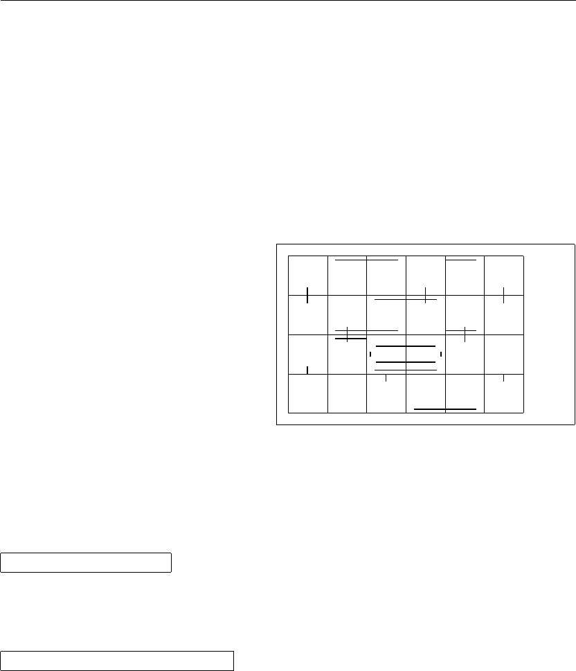
5.2 The picture Environment 91
ject to the next, the number of objects, and the object to be drawn. The
\linethickness command applies to horizontal and vertical line segments,
but neither to oblique line segments, nor to circles. It does, however, apply
to quadratic Bézier curves!
5.2.7 Ovals. The \thinlines and the \thicklines command
\setlength{\unitlength}{1cm}
\begin{picture}(6,4)
\linethickness{0.075mm}
\multiput(0,0)(1,0){7}%
{\line(0,1){4}}
\multiput(0,0)(0,1){5}%
{\line(1,0){6}}
\thicklines
\put(2,3){\oval(3,1.8)}
\thinlines
\put(3,2){\oval(3,1.8)}
\thicklines
\put(2,1){\oval(3,1.8)[tl]}
\put(4,1){\oval(3,1.8)[b]}
\put(4,3){\oval(3,1.8)[r]}
\put(3,1.5){\oval(1.8,0.4)}
\end{picture}
'
&
$
%
'
&
$
%
'
& %
$
%
The command
\put(x, y){\oval(w, h)}
or
\put(x, y){\oval(w, h)[position]}
produces an oval centered at (x, y)and having width wand height h. The
optional position arguments b,t,l,rrefer to “top”, “bottom”, “left”, “right”,
and can be combined, as the example illustrates.
Line thickness can be controlled by two kinds of commands:
\linethickness{length}on the one hand, \thinlines and \thicklines
on the other. While \linethickness{length}applies only to horizontal and
vertical lines (and quadratic Bézier curves), \thinlines and \thicklines
apply to oblique line segments as well as to circles and ovals.
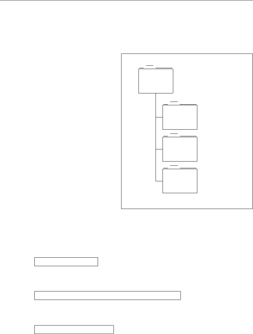
92 Producing Mathematical Graphics
5.2.8 Multiple Use of Predefined Picture Boxes
\setlength{\unitlength}{0.5mm}
\begin{picture}(120,168)
\newsavebox{\foldera}% declaration
\savebox{\foldera}
(40,32)[bl]{% definition
\multiput(0,0)(0,28){2}
{\line(1,0){40}}
\multiput(0,0)(40,0){2}
{\line(0,1){28}}
\put(1,28){\oval(2,2)[tl]}
\put(1,29){\line(1,0){5}}
\put(9,29){\oval(6,6)[tl]}
\put(9,32){\line(1,0){8}}
\put(17,29){\oval(6,6)[tr]}
\put(20,29){\line(1,0){19}}
\put(39,28){\oval(2,2)[tr]}
}
\newsavebox{\folderb}% declaration
\savebox{\folderb}
(40,32)[l]{% definition
\put(0,14){\line(1,0){8}}
\put(8,0){\usebox{\foldera}}
}
\put(34,26){\line(0,1){102}}
\put(14,128){\usebox{\foldera}}
\multiput(34,86)(0,-37){3}
{\usebox{\folderb}}
\end{picture}
A picture box can be declared by the command
\newsavebox{name}
then defined by
\savebox{name}(width,height)[position]{content}
and finally arbitrarily often be drawn by
\put(x, y)\usebox{name}
The optional position parameter has the effect of defining the ‘anchor
point’ of the savebox. In the example it is set to bl which puts the anchor
point into the bottom left corner of the savebox. The other position specifiers
are top and right.
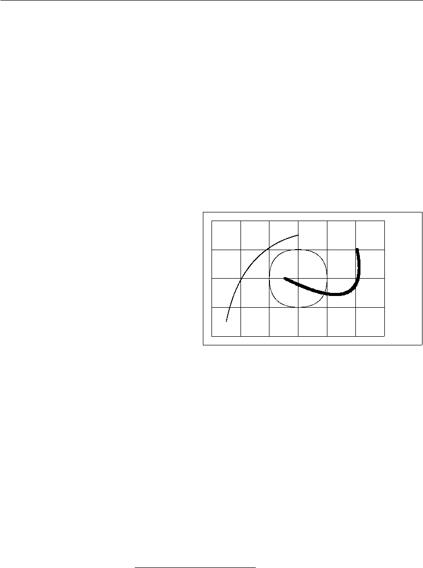
5.2 The picture Environment 93
The name argument refers to a L
A
T
EX storage bin and therefore is of a
command nature (which accounts for the backslashes in the current exam-
ple). Boxed pictures can be nested: In this example, \foldera is used within
the definition of \folderb.
The \oval command had to be used as the \line command does not
work if the segment length is less than about 3 mm.
5.2.9 Quadratic Bézier Curves
\setlength{\unitlength}{1cm}
\begin{picture}(6,4)
\linethickness{0.075mm}
\multiput(0,0)(1,0){7}
{\line(0,1){4}}
\multiput(0,0)(0,1){5}
{\line(1,0){6}}
\thicklines
\put(0.5,0.5){\line(1,5){0.5}}
\put(1,3){\line(4,1){2}}
\qbezier(0.5,0.5)(1,3)(3,3.5)
\thinlines
\put(2.5,2){\line(2,-1){3}}
\put(5.5,0.5){\line(-1,5){0.5}}
\linethickness{1mm}
\qbezier(2.5,2)(5.5,0.5)(5,3)
\thinlines
\qbezier(4,2)(4,3)(3,3)
\qbezier(3,3)(2,3)(2,2)
\qbezier(2,2)(2,1)(3,1)
\qbezier(3,1)(4,1)(4,2)
\end{picture}
HHHHHHHH
H
D
D
D
D
D
D
D
D
As this example illustrates, splitting up a circle into 4 quadratic Bézier
curves is not satisfactory. At least 8 are needed. The figure again shows the
effect of the \linethickness command on horizontal or vertical lines, and of
the \thinlines and the \thicklines commands on oblique line segments.
It also shows that both kinds of commands affect quadratic Bézier curves,
each command overriding all previous ones.
Let P1= (x1, y1), P2= (x2, y2)denote the end points, and m1, m2the
respective slopes, of a quadratic Bézier curve. The intermediate control point
S= (x, y)is then given by the equations
x=m2x2−m1x1−(y2−y1)
m2−m1
,
y=yi+mi(x−xi) (i= 1,2).
(5.1)
See Graphics in L
A
T
E
X 2ε[17] for a Java program which generates the neces-
sary \qbezier command line.

94 Producing Mathematical Graphics
5.2.10 Catenary
\setlength{\unitlength}{1.3cm}
\begin{picture}(4.3,3.6)(-2.5,-0.25)
\put(-2,0){\vector(1,0){4.4}}
\put(2.45,-.05){$x$}
\put(0,0){\vector(0,1){3.2}}
\put(0,3.35){\makebox(0,0){$y$}}
\qbezier(0.0,0.0)(1.2384,0.0)
(2.0,2.7622)
\qbezier(0.0,0.0)(-1.2384,0.0)
(-2.0,2.7622)
\linethickness{.075mm}
\multiput(-2,0)(1,0){5}
{\line(0,1){3}}
\multiput(-2,0)(0,1){4}
{\line(1,0){4}}
\linethickness{.2mm}
\put( .3,.12763){\line(1,0){.4}}
\put(.5,-.07237){\line(0,1){.4}}
\put(-.7,.12763){\line(1,0){.4}}
\put(-.5,-.07237){\line(0,1){.4}}
\put(.8,.54308){\line(1,0){.4}}
\put(1,.34308){\line(0,1){.4}}
\put(-1.2,.54308){\line(1,0){.4}}
\put(-1,.34308){\line(0,1){.4}}
\put(1.3,1.35241){\line(1,0){.4}}
\put(1.5,1.15241){\line(0,1){.4}}
\put(-1.7,1.35241){\line(1,0){.4}}
\put(-1.5,1.15241){\line(0,1){.4}}
\put(-2.5,-0.25){\circle*{0.2}}
\end{picture}
-x
6
y
v
In this figure, each symmetric half of the catenary y= cosh x−1is
approximated by a quadratic Bézier curve. The right half of the curve ends
in the point (2,2.7622), the slope there having the value m= 3.6269. Using
again equation (5.1), we can calculate the intermediate control points. They
turn out to be (1.2384,0) and (−1.2384,0). The crosses indicate points of
the real catenary. The error is barely noticeable, being less than one percent.
This example points out the use of the optional argument of the
\begin{picture} command. The picture is defined in convenient “mathe-
matical” coordinates, whereas by the command
\begin{picture}(4.3,3.6)(-2.5,-0.25)
its lower left corner (marked by the black disk) is assigned the coordinates
(−2.5,−0.25).

5.3 X
Y
-pic 95
5.2.11 Rapidity in the Special Theory of Relativity
\setlength{\unitlength}{1cm}
\begin{picture}(6,4)(-3,-2)
\put(-2.5,0){\vector(1,0){5}}
\put(2.7,-0.1){$\chi$}
\put(0,-1.5){\vector(0,1){3}}
\multiput(-2.5,1)(0.4,0){13}
{\line(1,0){0.2}}
\multiput(-2.5,-1)(0.4,0){13}
{\line(1,0){0.2}}
\put(0.2,1.4)
{$\beta=v/c=\tanh\chi$}
\qbezier(0,0)(0.8853,0.8853)
(2,0.9640)
\qbezier(0,0)(-0.8853,-0.8853)
(-2,-0.9640)
\put(-3,-2){\circle*{0.2}}
\end{picture}
-χ
6
β=v/c = tanh χ
u
The control points of the two Bézier curves were calculated with formu-
las (5.1). The positive branch is determined by P1= (0,0), m1= 1 and
P2= (2,tanh 2), m2= 1/cosh22. Again, the picture is defined in mathe-
matically convenient coordinates, and the lower left corner is assigned the
mathematical coordinates (−3,−2) (black disk).
5.3 X
Y
-pic
By Alberto Manuel Brandão Simões <albie@alfarrabio.di.uminho.pt>
xy is a special package for drawing diagrams. To use it, simply add the
following line to the preamble of your document:
\usepackage[options]{xy}
options is a list of functions from X
Y
-pic you want to load. These options
are primarily useful when debugging the package. I recommend you pass the
all option, making L
A
T
EX load all the X
Ycommands.
X
Y
-pic diagrams are drawn over a matrix-oriented canvas, where each
diagram element is placed in a matrix slot:
\begin{displaymath}
\xymatrix{A & B \\
C & D }
\end{displaymath}
A B
C D
96 Producing Mathematical Graphics
The \xymatrix command must be used in math mode. Here, we specified
two lines and two columns. To make this matrix a diagram we just add
directed arrows using the \ar command.
\begin{displaymath}
\xymatrix{ A \ar[r] & B \ar[d] \\
D \ar[u] & C \ar[l] }
\end{displaymath}
A//B
D
OO
C
oo
The arrow command is placed on the origin cell for the arrow. The
arguments are the direction the arrow should point to (up, down, right and
left).
\begin{displaymath}
\xymatrix{
A \ar[d] \ar[dr] \ar[r] & B \\
D & C }
\end{displaymath}
A
@
@
@
@
@
@
@//B
D C
To make diagonals, just use more than one direction. In fact, you can
repeat directions to make bigger arrows.
\begin{displaymath}
\xymatrix{
A \ar[d] \ar[dr] \ar[drr] & & \\
B & C & D }
\end{displaymath}
A
@
@
@
@
@
@
@
''
P
P
P
P
P
P
P
P
P
P
P
P
P
P
B C D
We can draw even more interesting diagrams by adding labels to the
arrows. To do this, we use the common superscript and subscript operators.
\begin{displaymath}
\xymatrix{
A \ar[r]^f \ar[d]_g &
B \ar[d]^{g’} \\
D \ar[r]_{f’} & C }
\end{displaymath}
Af//
g
B
g0
Df0//C
As shown, you use these operators as in math mode. The only difference
is that that superscript means “on top of the arrow,” and subscript means
“under the arrow.” There is a third operator, the vertical bar: |It causes
text to be placed in the arrow.
5.3 X
Y
-pic 97
\begin{displaymath}
\xymatrix{
A \ar[r]|f \ar[d]|g &
B \ar[d]|{g’} \\
D \ar[r]|{f’} & C }
\end{displaymath}
Af//
g
B
g0
Df0//C
To draw an arrow with a hole in it, use \ar[...]|\hole.
In some situations, it is important to distinguish between different types
of arrows. This can be done by putting labels on them, or changing their
appearance:
\shorthandoff{"}
\begin{displaymath}
\xymatrix{
\bullet\ar@{->}[rr] && \bullet\\
\bullet\ar@{.<}[rr] && \bullet\\
\bullet\ar@{~)}[rr] && \bullet\\
\bullet\ar@{=(}[rr] && \bullet\\
\bullet\ar@{~/}[rr] && \bullet\\
\bullet\ar@{^{(}->}[rr] && \bullet\\
\bullet\ar@2{->}[rr] && \bullet\\
\bullet\ar@3{->}[rr] && \bullet\\
\bullet\ar@{=+}[rr] && \bullet
}
\end{displaymath}
\shorthandon{"}
•//•
•oo•
•_
?
/o
/o
/o
/o
/o
/o
/o •
••
•
/o
/o
/o
/o
/o
/o
/o •
•//•
•+3•
•_*4•
•
_•
Notice the difference between the following two diagrams:
\begin{displaymath}
\xymatrix{
\bullet \ar[r]
\ar@{.>}[r] &
\bullet
}
\end{displaymath}
•////•
98 Producing Mathematical Graphics
\begin{displaymath}
\xymatrix{
\bullet \ar@/^/[r]
\ar@/_/@{.>}[r] &
\bullet
}
\end{displaymath}
•((66•
The modifiers between the slashes define how the curves are drawn. X
Y
-
pic offers many ways to influence the drawing of curves; for more information,
check X
Y
-pic documentation.
Chapter 6
Customising L
A
T
E
X
Documents produced with the commands you have learned up to this point will
look acceptable to a large audience. While they are not fancy-looking, they obey
all the established rules of good typesetting, which will make them easy to read
and pleasant to look at.
However, there are situations where L
A
T
E
X does not provide a command or
environment that matches your needs, or the output produced by some existing
command may not meet your requirements.
In this chapter, I will try to give some hints on how to teach L
A
T
E
X new tricks
and how to make it produce output that looks different from what is provided
by default.
6.1 New Commands, Environments and Packages
You may have noticed that all the commands I introduce in this book are
typeset in a box, and that they show up in the index at the end of the book.
Instead of directly using the necessary L
A
T
EX commands to achieve this, I
have created a package in which I defined new commands and environments
for this purpose. Now I can simply write:
\begin{lscommand}
\ci{dum}
\end{lscommand}
\dum
In this example, I am using both a new environment called lscommand,
which is responsible for drawing the box around the command, and a new
command named \ci, which typesets the command name and makes a corre-
sponding entry in the index. You can check this out by looking up the \dum
command in the index at the back of this book, where you’ll find an entry
for \dum, pointing to every page where I mentioned the \dum command.
100 Customising L
A
T
E
X
If I ever decide that I do not like the commands to be typeset in a box
any more, I can simply change the definition of the lscommand environment
to create a new look. This is much easier than going through the whole
document to hunt down all the places where I have used some generic L
A
T
EX
commands to draw a box around some word.
6.1.1 New Commands
To add your own commands, use the
\newcommand{name}[num]{definition}
command. Basically, the command requires two arguments: the name of
the command you want to create, and the definition of the command. The
num argument in square brackets is optional and specifies the number of
arguments the new command takes (up to 9 are possible). If missing it
defaults to 0, i.e. no argument allowed.
The following two examples should help you to get the idea. The first
example defines a new command called \tnss. This is short for “The Not
So Short Introduction to L
A
T
EX 2ε.” Such a command could come in handy
if you had to write the title of this book over and over again.
\newcommand{\tnss}{The not
so Short Introduction to
\LaTeXe}
This is ‘‘\tnss’’ \ldots{}
‘‘\tnss’’
This is “The not so Short Introduction to
L
A
T
EX 2ε” . . . “The not so Short Introduction
to L
A
T
EX 2ε”
The next example illustrates how to define a new command that takes
one argument. The #1 tag gets replaced by the argument you specify. If you
wanted to use more than one argument, use #2 and so on.
\newcommand{\txsit}[1]
{This is the \emph{#1} Short
Introduction to \LaTeXe}
% in the document body:
\begin{itemize}
\item \txsit{not so}
\item \txsit{very}
\end{itemize}
•This is the not so Short Introduction
to L
A
T
EX 2ε
•This is the very Short Introduction to
L
A
T
EX 2ε
L
A
T
EX will not allow you to create a new command that would overwrite
an existing one. But there is a special command in case you explicitly want
this: \renewcommand. It uses the same syntax as the \newcommand command.
In certain cases you might also want to use the \providecommand com-
mand. It works like \newcommand, but if the command is already defined,
L
A
T
EX 2εwill silently ignore it.
6.1 New Commands, Environments and Packages 101
There are some points to note about whitespace following L
A
T
EX com-
mands. See page 5for more information.
6.1.2 New Environments
Just as with the \newcommand command, there is a command to create your
own environments. The \newenvironment command uses the following syn-
tax:
\newenvironment{name}[num]{before}{after }
Again \newenvironment can have an optional argument. The material
specified in the before argument is processed before the text in the envi-
ronment gets processed. The material in the after argument gets processed
when the \end{name}command is encountered.
The example below illustrates the usage of the \newenvironment com-
mand.
\newenvironment{king}
{\rule{1ex}{1ex}%
\hspace{\stretch{1}}}
{\hspace{\stretch{1}}%
\rule{1ex}{1ex}}
\begin{king}
My humble subjects \ldots
\end{king}
My humble subjects . . .
The num argument is used the same way as in the \newcommand com-
mand. L
A
T
EX makes sure that you do not define an environment that al-
ready exists. If you ever want to change an existing command, you can
use the \renewenvironment command. It uses the same syntax as the
\newenvironment command.
The commands used in this example will be explained later. For the
\rule command see page 115, for \stretch go to page 108, and more infor-
mation on \hspace can be found on page 108.
6.1.3 Extra Space
When creating a new environemnt you may easily get bitten by extra spaces
creaping in, which can potentially have fatal effects. For example when you
want to create a title environemnt which supresses its own indentation as well
as the one on the following paragraph. The \ignorespaces command in the
begin block of the environment will make it ignore any space after executing
the begin block. The end block is a bit more tricky as special processing
occurs at the end of an environment. With the \ignorespacesafterend
102 Customising L
A
T
E
X
L
A
T
EX will issue an \ignorespaces after the special ‘end’ processing has
occured.
\newenvironment{simple}%
{\noindent}%
{\par\noindent}
\begin{simple}
See the space\\to the left.
\end{simple}
Same\\here.
See the space
to the left.
Same
here.
\newenvironment{correct}%
{\noindent\ignorespaces}%
{\par\noindent\ignorespacesafterend}
\begin{correct}
No space\\to the left.
\end{correct}
Same\\here.
No space
to the left.
Same
here.
6.1.4 Commandline L
A
T
E
X
If you work on a Unix like OS, you might be using Makefiles to build your
L
A
T
EX projects. In that connection it might be interesting to produce dif-
ferent versions of the same document by calling L
A
T
EX with commandline
parameters. If you add the following structure to your document:
\usepackage{ifthen}
\ifthenelse{\equal{\blackandwhite}{true}}{
% "black and white" mode; do something..
}{
% "color" mode; do something different..
}
Now you can call L
A
T
EX like this:
latex ’\newcommand{\blackandwhite}{true}\input{test.tex}’
First the command \blackandwhite gets defined and then the actual file
is read with input. By setting \blackandwhite to false the color version of
the document would be produced.
6.2 Fonts and Sizes 103
6.1.5 Your Own Package
If you define a lot of new environments and commands, the preamble of your
document will get quite long. In this situation, it is a good idea to create
a L
A
T
EX package containing all your command and environment definitions.
You can then use the \usepackage command to make the package available
in your document.
% Demo Package by Tobias Oetiker
\ProvidesPackage{demopack}
\newcommand{\tnss}{The not so Short Introduction to \LaTeXe}
\newcommand{\txsit}[1]{The \emph{#1} Short
Introduction to \LaTeXe}
\newenvironment{king}{\begin{quote}}{\end{quote}}
Figure 6.1: Example Package.
Writing a package basically consists of copying the contents of your doc-
ument preamble into a separate file with a name ending in .sty. There is
one special command,
\ProvidesPackage{package name}
for use at the very beginning of your package file. \ProvidesPackage tells
L
A
T
EX the name of the package and will allow it to issue a sensible error
message when you try to include a package twice. Figure 6.1 shows a small
example package that contains the commands defined in the examples above.
6.2 Fonts and Sizes
6.2.1 Font Changing Commands
L
A
T
EX chooses the appropriate font and font size based on the logical struc-
ture of the document (sections, footnotes, . . . ). In some cases, one might
like to change fonts and sizes by hand. To do this, you can use the com-
mands listed in Tables 6.1 and 6.2. The actual size of each font is a design
issue and depends on the document class and its options. Table 6.3 shows
the absolute point size for these commands as implemented in the standard
document classes.
{\small The small and
\textbf{bold} Romans ruled}
{\Large all of great big
\textit{Italy}.}
The small and bold Romans ruled all of
great big Italy.
104 Customising L
A
T
E
X
One important feature of L
A
T
EX 2εis that the font attributes are indepen-
dent. This means that you can issue size or even font changing commands,
and still keep the bold or slant attribute set earlier.
In math mode you can use the font changing commands to temporarily
exit math mode and enter some normal text. If you want to switch to another
font for math typesetting you need another special set of commands; refer
to Table 6.4.
In connection with the font size commands, curly braces play a significant
role. They are used to build groups. Groups limit the scope of most L
A
T
EX
commands.
He likes {\LARGE large and
{\small small} letters}. He likes large and small letters.
The font size commands also change the line spacing, but only if the
paragraph ends within the scope of the font size command. The closing
curly brace }should therefore not come too early. Note the position of the
\par command in the next two examples. 1
1\par is equivalent to a blank line
Table 6.1: Fonts.
\textrm{...} roman \textsf{...} sans serif
\texttt{...} typewriter
\textmd{...} medium \textbf{...} bold face
\textup{...} upright \textit{...} italic
\textsl{...} slanted \textsc{...} small caps
\emph{...} emphasized \textnormal{...} document font
Table 6.2: Font Sizes.
\tiny tiny font
\scriptsize very small font
\footnotesize quite small font
\small small font
\normalsize normal font
\large large font
\Large larger font
\LARGE very large font
\huge huge
\Huge largest

6.2 Fonts and Sizes 105
Table 6.3: Absolute Point Sizes in Standard Classes.
size 10pt (default) 11pt option 12pt option
\tiny 5pt 6pt 6pt
\scriptsize 7pt 8pt 8pt
\footnotesize 8pt 9pt 10pt
\small 9pt 10pt 11pt
\normalsize 10pt 11pt 12pt
\large 12pt 12pt 14pt
\Large 14pt 14pt 17pt
\LARGE 17pt 17pt 20pt
\huge 20pt 20pt 25pt
\Huge 25pt 25pt 25pt
Table 6.4: Math Fonts.
\mathrm{...} Roman Font
\mathbf{...} Boldface Font
\mathsf{...} Sans Serif Font
\mathtt{...} Typewriter Font
\mathit{...} Italic Font
\mathcal{...} CALLIGRAPHIC FONT
\mathnormal{...} Normal F ont
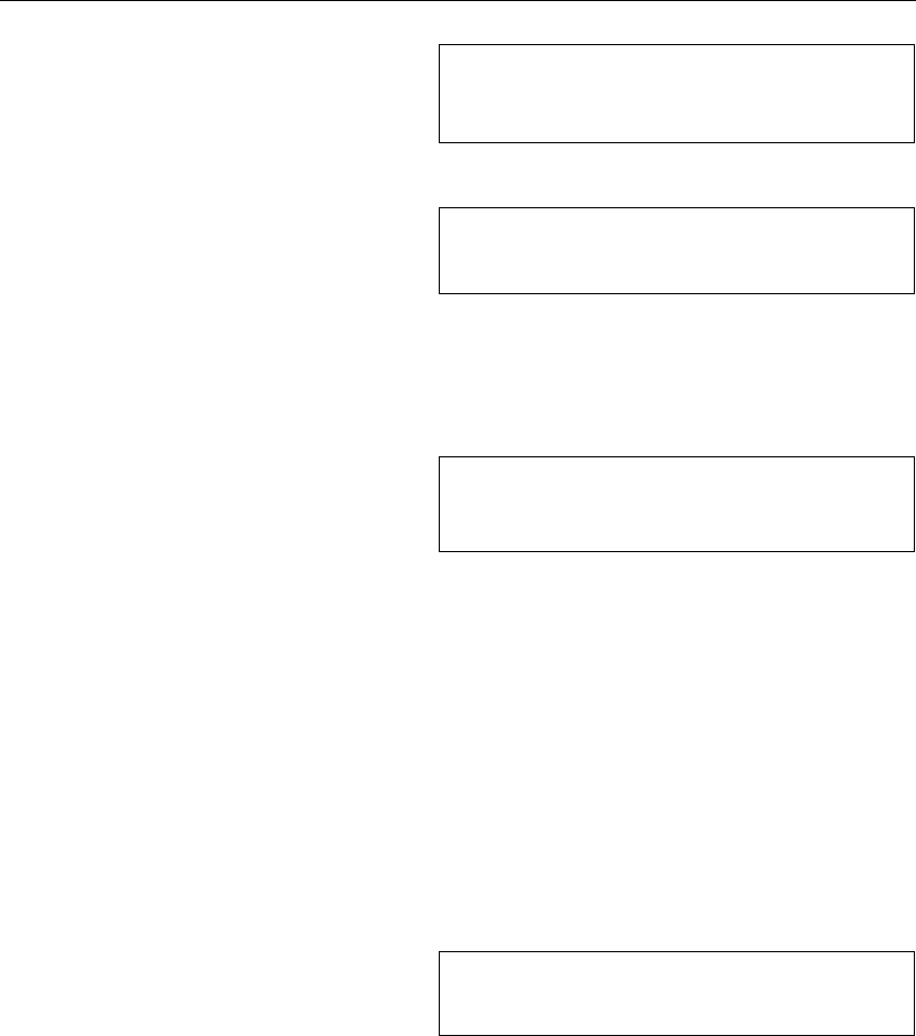
106 Customising L
A
T
E
X
{\Large Don’t read this! It is not
true. You can believe me!\par}
Don’t read this! It is not true.
You can believe me!
{\Large This is not true either.
But remember I am a liar.}\par This is not true either. But re-
member I am a liar.
If you want to activate a size changing command for a whole paragraph
of text or even more, you might want to use the environment syntax for font
changing commands.
\begin{Large}
This is not true.
But then again, what is these
days \ldots
\end{Large}
This is not true. But then again,
what is these days . . .
This will save you from counting lots of curly braces.
6.2.2 Danger, Will Robinson, Danger
As noted at the beginning of this chapter, it is dangerous to clutter your
document with explicit commands like this, because they work in opposition
to the basic idea of L
A
T
EX, which is to separate the logical and visual markup
of your document. This means that if you use the same font changing com-
mand in several places in order to typeset a special kind of information, you
should use \newcommand to define a “logical wrapper command” for the font
changing command.
\newcommand{\oops}[1]{\textbf{#1}}
Do not \oops{enter} this room,
it’s occupied by a \oops{machine}
of unknown origin and purpose.
Do not enter this room, it’s occupied by a
machine of unknown origin and purpose.
This approach has the advantage that you can decide at some later
stage that you want to use some visual representation of danger other than
\textbf, without having to wade through your document, identifying all the
occurrences of \textbf and then figuring out for each one whether it was
used for pointing out danger or for some other reason.
6.2.3 Advice
To conclude this journey into the land of fonts and font sizes, here is a little
word of advice:
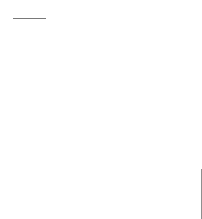
6.3 Spacing 107
Remember!The MOREfonts you use in adocument,the
more readable and beautiful it becomes.
6.3 Spacing
6.3.1 Line Spacing
If you want to use larger inter-line spacing in a document, you can change
its value by putting the
\linespread{factor}
command into the preamble of your document. Use \linespread{1.3} for
“one and a half” line spacing, and \linespread{1.6} for “double” line spac-
ing. Normally the lines are not spread, so the default line spread factor
is 1.
Note that the effect of the \linespread command is rather drastic and
not appropriate for published work. So if you have a good reason for changing
the line spacing you might want to use the command:
\setlength{\baselineskip}{1.5\baselineskip}
{\setlength{\baselineskip}%
{1.5\baselineskip}
This paragraph is typeset with the
baseline skip set to 1.5 of what
it was before. Note the par command
at the end of the paragraph.\par}
This paragraph has a clear purpose,
it shows that after the curly brace
has been closed, everything is back
to normal.
This paragraph is typeset with the baseline
skip set to 1.5 of what it was before. Note the
par command at the end of the paragraph.
This paragraph has a clear purpose, it shows
that after the curly brace has been closed,
everything is back to normal.
6.3.2 Paragraph Formatting
In L
A
T
EX, there are two parameters influencing paragraph layout. By placing
a definition like
\setlength{\parindent}{0pt}
\setlength{\parskip}{1ex plus 0.5ex minus 0.2ex}
in the preamble of the input file, you can change the layout of paragraphs.
These two commands increase the space between two paragraphs while set-
ting the paragraph indent to zero.
108 Customising L
A
T
E
X
The plus and minus parts of the length above tell T
EX that it can com-
press and expand the inter paragraph skip by the amount specified, if this
is necessary to properly fit the paragraphs onto the page.
In continental Europe, paragraphs are often separated by some space and
not indented. But beware, this also has its effect on the table of contents.
Its lines get spaced more loosely now as well. To avoid this, you might want
to move the two commands from the preamble into your document to some
place after the \tableofcontents or to not use them at all, because you’ll
find that most professional books use indenting and not spacing to separate
paragraphs.
If you want to indent a paragraph that is not indented, you can use
\indent
at the beginning of the paragraph.2Obviously, this will only have an effect
when \parindent is not set to zero.
To create a non-indented paragraph, you can use
\noindent
as the first command of the paragraph. This might come in handy when you
start a document with body text and not with a sectioning command.
6.3.3 Horizontal Space
L
A
T
EX determines the spaces between words and sentences automatically. To
add horizontal space, use:
\hspace{length}
If such a space should be kept even if it falls at the end or the start of
a line, use \hspace* instead of \hspace. The length in the simplest case is
just a number plus a unit. The most important units are listed in Table 6.5.
This\hspace{1.5cm}is a space
of 1.5 cm. This is a space of 1.5 cm.
The command
\stretch{n}
generates a special rubber space. It stretches until all the remaining space
2To indent the first paragraph after each section head, use the indentfirst package in
the ‘tools’ bundle.
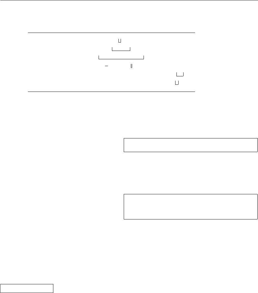
6.3 Spacing 109
Table 6.5: T
EX Units.
mm millimetre ≈1/25 inch
cm centimetre = 10 mm
in inch =25.4 mm
pt point ≈1/72 inch ≈1
3mm
em approx width of an ‘M’ in the current font
ex approx height of an ‘x’ in the current font
on a line is filled up. If two \hspace{\stretch{n}} commands are issued
on the same line, they grow according to the stretch factor.
x\hspace{\stretch{1}}
x\hspace{\stretch{3}}x x x x
When using horizontal space together with text, it may make sense to
make the space adjust its size relative to the size of the current font. This
can be done by using the text-relative units em and ex:
{\Large{}big\hspace{1em}y}\\
{\tiny{}tin\hspace{1em}y}
big y
tin y
6.3.4 Vertical Space
The space between paragraphs, sections, subsections, . . . is determined au-
tomatically by L
A
T
EX. If necessary, additional vertical space between two
paragraphs can be added with the command:
\vspace{length}
This command should normally be used between two empty lines. If the
space should be preserved at the top or at the bottom of a page, use the
starred version of the command, \vspace*, instead of \vspace.
The \stretch command, in connection with \pagebreak, can be used to
typeset text on the last line of a page, or to centre text vertically on a page.
Some text \ldots
\vspace{\stretch{1}}
This goes onto the last line of the page.\pagebreak
110 Customising L
A
T
E
X
Additional space between two lines of the same paragraph or within a
table is specified with the
\\[length]
command.
With \bigskip and \smallskip you can skip a predefined amount of
vertical space without having to worry about exact numbers.
6.4 Page Layout
L
A
T
EX 2εallows you to specify the paper size in the \documentclass com-
mand. It then automatically picks the right text margins, but sometimes
you may not be happy with the predefined values. Naturally, you can change
them. Figure 6.2 shows all the parameters that can be changed. The figure
was produced with the layout package from the tools bundle.3
WAIT! . . . before you launch into a “Let’s make that narrow page a bit
wider” frenzy, take a few seconds to think. As with most things in L
A
T
EX,
there is a good reason for the page layout to be as it is.
Sure, compared to your off-the-shelf MS Word page, it looks awfully
narrow. But take a look at your favourite book4and count the number of
characters on a standard text line. You will find that there are no more than
about 66 characters on each line. Now do the same on your L
A
T
EX page.
You will find that there are also about 66 characters per line. Experience
shows that the reading gets difficult as soon as there are more characters on
a single line. This is because it is difficult for the eyes to move from the end
of one line to the start of the next one. This is also why newspapers are
typeset in multiple columns.
So if you increase the width of your body text, keep in mind that you
are making life difficult for the readers of your paper. But enough of the
cautioning, I promised to tell you how you do it . . .
L
A
T
EX provides two commands to change these parameters. They are
usually used in the document preamble.
The first command assigns a fixed value to any of the parameters:
\setlength{parameter}{length}
The second command adds a length to any of the parameters:
\addtolength{parameter}{length}
This second command is actually more useful than the \setlength com-
3macros/latex/required/tools
4I mean a real printed book produced by a reputable publisher.
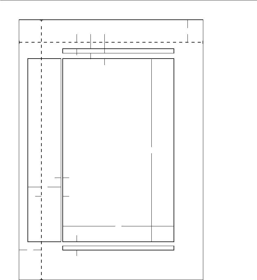
6.4 Page Layout 111
Header
Body
Footer
Margin
Notes
i
8
-
i
7
?
6
i
1
-
-i
3i
10
-
- i
9
6
?
i
11
i
2
?
6
i
4
6
?i
5
6
?i
6
6
?
1 one inch + \hoffset 2 one inch + \voffset
3 \oddsidemargin = 22pt 4 \topmargin = 22pt
or \evensidemargin
5 \headheight = 13pt 6 \headsep = 19pt
7 \textheight = 595pt 8 \textwidth = 360pt
9 \marginparsep = 7pt 10 \marginparwidth = 106pt
11 \footskip = 27pt \marginparpush = 5pt (not shown)
\hoffset = 0pt \voffset = 0pt
\paperwidth = 597pt \paperheight = 845pt
Figure 6.2: Page Layout Parameters.
112 Customising L
A
T
E
X
mand, because you can now work relative to the existing settings. To add
one centimetre to the overall text width, I put the following commands into
the document preamble:
\addtolength{\hoffset}{-0.5cm}
\addtolength{\textwidth}{1cm}
In this context, you might want to look at the calc package. It allows
you to use arithmetic operations in the argument of \setlength and other
places where you can enter numeric values into function arguments.
6.5 More Fun With Lengths
Whenever possible, I avoid using absolute lengths in L
A
T
EX documents. I
rather try to base things on the width or height of other page elements. For
the width of a figure this could be \textwidth in order to make it fill the
page.
The following 3 commands allow you to determine the width, height and
depth of a text string.
\settoheight{variable}{text}
\settodepth{variable}{text}
\settowidth{variable}{text}
The example below shows a possible application of these commands.
\flushleft
\newenvironment{vardesc}[1]{%
\settowidth{\parindent}{#1:\ }
\makebox[0pt][r]{#1:\ }}{}
\begin{displaymath}
a^2+b^2=c^2
\end{displaymath}
\begin{vardesc}{Where}$a$,
$b$ -- are adjoin to the right
angle of a right-angled triangle.
$c$ -- is the hypotenuse of
the triangle and feels lonely.
$d$ -- finally does not show up
here at all. Isn’t that puzzling?
\end{vardesc}
a2+b2=c2
Where: a,b– are adjoin to the right angle of
a right-angled triangle.
c– is the hypotenuse of the triangle
and feels lonely.
d– finally does not show up here at
all. Isn’t that puzzling?
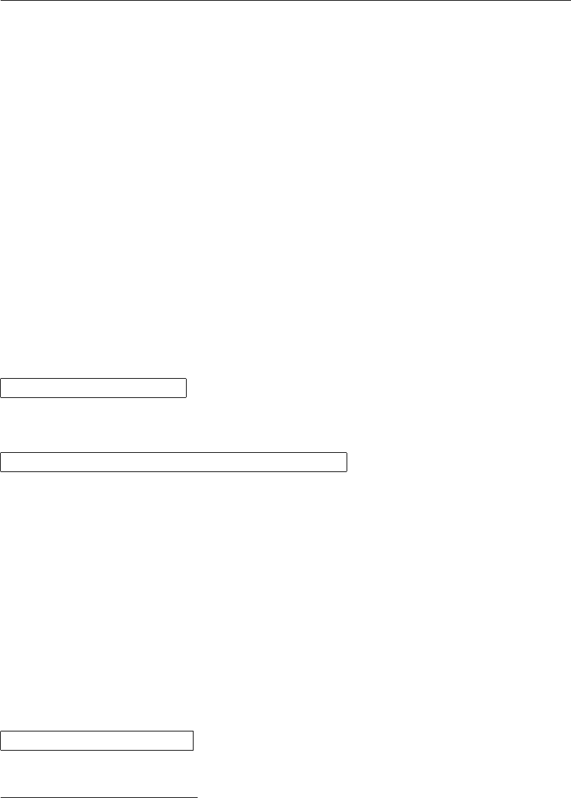
6.6 Boxes 113
6.6 Boxes
L
A
T
EX builds up its pages by pushing around boxes. At first, each letter is
a little box, which is then glued to other letters to form words. These are
again glued to other words, but with special glue, which is elastic so that a
series of words can be squeezed or stretched as to exactly fill a line on the
page.
I admit, this is a very simplistic version of what really happens, but the
point is that T
EX operates on glue and boxes. Letters are not the only things
that can be boxes. You can put virtually everything into a box, including
other boxes. Each box will then be handled by L
A
T
EX as if it were a single
letter.
In the past chapters you have already encountered some boxes, although
I did not tell you. The tabular environment and the \includegraphics,
for example, both produce a box. This means that you can easily arrange
two tables or images side by side. You just have to make sure that their
combined width is not larger than the textwidth.
You can also pack a paragraph of your choice into a box with either the
\parbox[pos]{width}{text}
command or the
\begin{minipage}[pos]{width}text \end{minipage}
environment. The pos parameter can take one of the letters c, t or bto
control the vertical alignment of the box, relative to the baseline of the
surrounding text. width takes a length argument specifying the width of the
box. The main difference between a minipage and a \parbox is that you
cannot use all commands and environments inside a parbox, while almost
anything is possible in a minipage.
While \parbox packs up a whole paragraph doing line breaking and ev-
erything, there is also a class of boxing commands that operates only on
horizontally aligned material. We already know one of them; it’s called
\mbox. It simply packs up a series of boxes into another one, and can be
used to prevent L
A
T
EX from breaking two words. As you can put boxes inside
boxes, these horizontal box packers give you ultimate flexibility.
\makebox[width][pos]{text}
width defines the width of the resulting box as seen from the outside.5Be-
5This means it can be smaller than the material inside the box. You can even set
the width to 0pt so that the text inside the box will be typeset without influencing the
surrounding boxes.
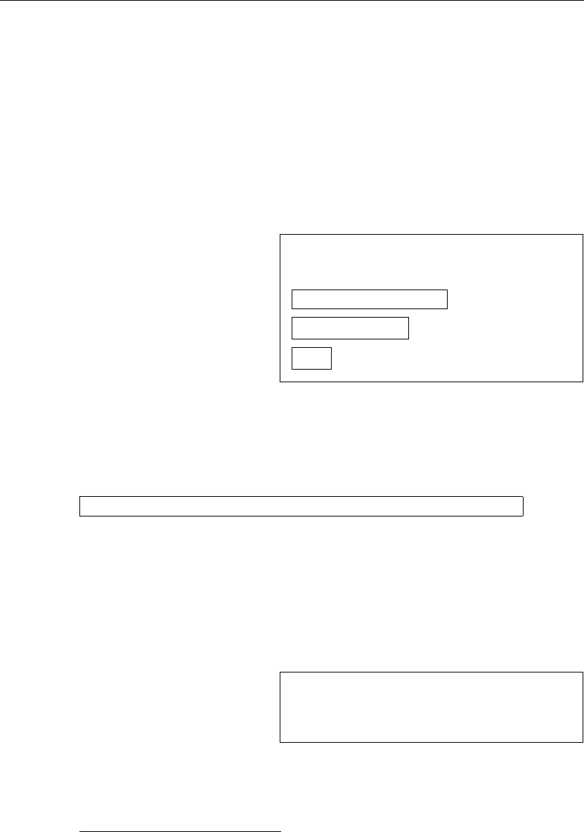
114 Customising L
A
T
E
X
sides the length expressions, you can also use \width,\height,\depth, and
\totalheight in the width parameter. They are set from values obtained
by measuring the typeset text. The pos parameter takes a one letter value:
center, flushleft, flushright, or spread the text to fill the box.
The command \framebox works exactly the same as \makebox, but it
draws a box around the text.
The following example shows you some things you could do with the
\makebox and \framebox commands.
\makebox[\textwidth]{%
c e n t r a l}\par
\makebox[\textwidth][s]{%
s p r e a d}\par
\framebox[1.1\width]{Guess I’m
framed now!} \par
\framebox[0.8\width][r]{Bummer,
I am too wide} \par
\framebox[1cm][l]{never
mind, so am I}
Can you read this?
central
spread
Guess I’m framed now!
Bummer, I am too wide
never mind, so am ICan you read this?
Now that we control the horizontal, the obvious next step is to go for the
vertical.6No problem for L
A
T
EX. The
\raisebox{lift}[extend-above-baseline][extend-below-baseline]{text}
command lets you define the vertical properties of a box. You can use
\width,\height,\depth, and \totalheight in the first three parameters,
in order to act upon the size of the box inside the text argument.
\raisebox{0pt}[0pt][0pt]{\Large%
\textbf{Aaaa\raisebox{-0.3ex}{a}%
\raisebox{-0.7ex}{aa}%
\raisebox{-1.2ex}{r}%
\raisebox{-2.2ex}{g}%
\raisebox{-4.5ex}{h}}}
he shouted but not even the next
one in line noticed that something
terrible had happened to him.
Aaaaaaarg
h
he shouted but not even
the next one in line noticed that something
terrible had happened to him.
6Total control is only to be obtained by controlling both the horizontal and the vertical
. . .
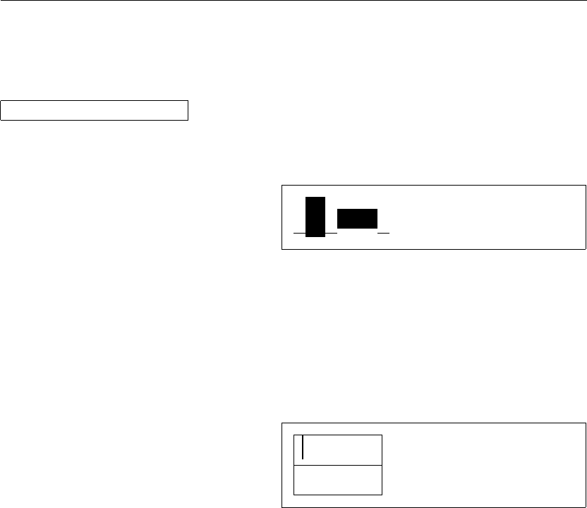
6.7 Rules and Struts 115
6.7 Rules and Struts
A few pages back you may have noticed the command
\rule[lift]{width}{height}
In normal use it produces a simple black box.
\rule{3mm}{.1pt}%
\rule[-1mm]{5mm}{1cm}%
\rule{3mm}{.1pt}%
\rule[1mm]{1cm}{5mm}%
\rule{3mm}{.1pt}
This is useful for drawing vertical and horizontal lines. The line on the title
page, for example, has been created with a \rule command.
A special case is a rule with no width but a certain height. In professional
typesetting, this is called a strut. It is used to guarantee that an element
on a page has a certain minimal height. You could use it in a tabular
environment to make sure a row has a certain minimum height.
\begin{tabular}{|c|}
\hline
\rule{1pt}{4ex}Pitprop \ldots\\
\hline
\rule{0pt}{4ex}Strut\\
\hline
\end{tabular}
Pitprop . . .
Strut
The End.
Bibliography
[1] Leslie Lamport. L
A
T
E
X: A Document Preparation System. Addison-
Wesley, Reading, Massachusetts, second edition, 1994, ISBN 0-201-
52983-1.
[2] Donald E. Knuth. The T
E
Xbook, Volume A of Computers and Type-
setting, Addison-Wesley, Reading, Massachusetts, second edition, 1984,
ISBN 0-201-13448-9.
[3] Michel Goossens, Frank Mittelbach and Alexander Samarin. The L
A
T
E
X
Companion. Addison-Wesley, Reading, Massachusetts, 1994, ISBN 0-
201-54199-8.
[4] Michel Goossens, Sebastian Rahtz and Frank Mittelbach. The L
A
T
E
X
Graphics Companion. Addison-Wesley, Reading, Massachusetts, 1997,
ISBN 0-201-85469-4.
[5] Each L
A
T
EX installation should provide a so-called L
A
T
E
X Local Guide,
which explains the things that are special to the local system. It should
be contained in a file called local.tex. Unfortunately, some lazy sysops
do not provide such a document. In this case, go and ask your local
L
A
T
EX guru for help.
[6] L
A
T
EX3 Project Team. L
A
T
E
X 2εfor authors. Comes with the L
A
T
EX 2ε
distribution as usrguide.tex.
[7] L
A
T
EX3 Project Team. L
A
T
E
X 2εfor Class and Package writers. Comes
with the L
A
T
EX 2εdistribution as clsguide.tex.
[8] L
A
T
EX3 Project Team. L
A
T
E
X 2εFont selection. Comes with the L
A
T
EX 2ε
distribution as fntguide.tex.
[9] D. P. Carlisle. Packages in the ‘graphics’ bundle. Comes with the ‘graph-
ics’ bundle as grfguide.tex, available from the same source your L
A
T
EX
distribution came from.
[10] Rainer Schöpf, Bernd Raichle, Chris Rowley. A New Implementation
of L
A
T
E
X’s verbatim Environments. Comes with the ‘tools’ bundle as

118 BIBLIOGRAPHY
verbatim.dtx, available from the same source your L
A
T
EX distribution
came from.
[11] Vladimir Volovich, Werner Lemberg and L
A
T
EX3 Project Team. Cyrillic
languages support in L
A
T
E
X. Comes with the L
A
T
EX 2εdistribution as
cyrguide.tex.
[12] Graham Williams. The TeX Catalogue is a very complete listing of
many T
EX and L
A
T
EX related packages. Available online from CTAN:
/tex-archive/help/Catalogue/catalogue.html
[13] Keith Reckdahl. Using EPS Graphics in L
A
T
E
X 2εDocuments, which
explains everything and much more than you ever wanted to know about
EPS files and their use in L
A
T
EX documents. Available online from
CTAN:/tex-archive/info/epslatex.ps
[14] Kristoffer H. Rose. X
Y
-pic User’s Guide. Downloadable from CTAN
with X
Y
-pic distribution
[15] John D. Hobby. A User’s Manual for MetaPost. Downloadable from
http://cm.bell-labs.com/who/hobby/
[16] Alan Hoenig. T
E
X Unbound. Oxford University Press, 1998, ISBN 0-
19-509685-1; 0-19-509686-X (pbk.)
[17] Urs Oswald. Graphics in L
A
T
E
X 2ε, containing some Java source files
for generating arbitrary circles and ellipses within the picture en-
vironment, and MetaPost - A Tutorial. Both downloadable from
http://www.ursoswald.ch
Index
Symbols
\!,51
",19
"’,32
"-,32
"---,32
"<,32
"=,32
">,32
"‘,32
$,45
\(,45
\),45
\,,46,51
-, 20
−,20
\-,19
–, 20
—, 20
., space after, 32
..., 22
\:,51
\;,51
\@,32
\[,46
\\,17,37,38,40,110
\\*,17
\],46
~,32
A
A4 paper, 10
A5 paper, 10
å, 23
abstract,38
accent, 22
acrobat reader, 73
acute, 23
\addtolength,110
advantages of L
A
T
EX, 3
æ, 23
aeguill,74
\Alph,31
\alph,31
amsbsy,57
amsfonts,47,64
amsmath,49–52,54,55,57
amssymb,47,58
\and,34
ansinew,24
\appendix,33,34
applemac,24
\ar,96
\arccos,49
\arcsin,49
\arctan,49
\arg,49
array,52,53
arrow symbols, 48
article class, 9
\Asbuk,31
\asbuk,31
\author,34,78
B
B5 paper, 10
babel,18,23,31,32
\background,82
\backmatter,35
backslash, 5
\backslash,5
base font size, 10

120 INDEX
\begin,36,86,94
\bibitem,67
bibliography, 67
\Big,51
\big,51
\Bigg,51
\bigg,51
\biggl,55
\biggr,55
\bigskip,110
\binom,49
blackboard bold, 47
bm,57
\bmod,49
bold face, 104
bold symbols, 47,57
\boldmath,57
\boldsymbol,57
book class, 9
braces, 50
brazilian, 25
C
calc,112
\caption,43,44
\cdot,49
\cdots,51
center,37
\chapter,33
\chaptermark,70
\ci,99
\circle,89
\circle*,89
\cite,67
CJK package, 29
\cleardoublepage,44
\clearpage,44
\cline,40
color,80
coloured text, 9
comma, 22
commands, 5
\!,51
\(,45
\),45
\,,46,51
\-,19
\:,51
\;,51
\@,32
\[,46
\\,17,37,38,40,110
\\*,17
\],46
\addtolength,110
\Alph,31
\alph,31
\and,34
\appendix,33,34
\ar,96
\arccos,49
\arcsin,49
\arctan,49
\arg,49
\Asbuk,31
\asbuk,31
\author,34,78
\background,82
\backmatter,35
\backslash,5
\begin,36,86,94
\bibitem,67
\Big,51
\big,51
\Bigg,51
\bigg,51
\biggl,55
\biggr,55
\bigskip,110
\binom,49
\bmod,49
\boldmath,57
\boldsymbol,57
\caption,43,44
\cdot,49
\cdots,51
\chapter,33
\chaptermark,70

INDEX 121
\ci,99
\circle,89
\circle*,89
\cite,67
\cleardoublepage,44
\clearpage,44
\cline,40
\cos,49
\cosh,49
\cot,49
\coth,49
\csc,49
\date,34
\ddots,51
\deg,49
\depth,114
\det,49
\dim,49
\displaystyle,55
\documentclass,9,13,18
\dq,28
\dum,99
\emblema,82
\emph,36,104
\end,36,86
\enumBul,31
\enumEng,31
\enumLat,31
\eqref,46
\EUR,21
\euro,21
\exp,49
\fbox,19
\flq,28
\flqq,28
\foldera,93
\folderb,93
\footnote,35,44
\footskip,111
\frac,49
\framebox,114
\frenchspacing,31–33
\frontmatter,34
\frq,28
\frqq,28
\fussy,18
\gcd,49
\headheight,111
\headsep,111
\height,114
\hline,40
\hom,49
\href,77,78,80
\hspace,101,108
\hyphenation,18
\idotsint,52
\ignorespaces,101,102
\ignorespacesafterend,101
\iiiint,52
\iiint,52
\iint,52
\include,13,14
\includegraphics,66,75,79,
113
\includeonly,14
\indent,108
\index,68,69
\inf,49
\input,14
\int,50
\item,37
\ker,49
\label,35,46
\LaTeX,19
\LaTeXe,19
\ldots,22,51
\left,51
\leftmark,69,70
\lg,49
\lim,49
\liminf,49
\limsup,49
\line,88,93
\linebreak,17
\linespread,107
\linethickness,90,91,93
\listoffigures,43
\listoftables,43

122 INDEX
\ln,49
\log,49
\mainmatter,34,78
\makebox,113,114
\makeindex,68
\maketitle,34
\marginparpush,111
\marginparsep,111
\marginparwidth,111
\marginsize,82
\mathbb,47
\mathrm,55
\max,49
\mbox,19,22,113
\min,49
\multicolumn,41
\multiput,87,90
\newcommand,100
\newenvironment,101
\newline,17
\newpage,17
\newsavebox,92
\newtheorem,55,56
\noindent,108
\nolinebreak,17
\nonumber,54
\nopagebreak,17
\not,59
\oddsidemargin,111
\oval,91,93
\overbrace,48
\overlay,82
\overleftarrow,48
\overline,48
\overrightarrow,48
\pagebreak,17
\pageref,35,72
\pagestyle,11
\panelwidth,82
\paperheight,111
\paperwidth,111
\par,104
\paragraph,33
\parbox,113
\parindent,107
\parskip,107
\part,33
\pause,82
\phantom,44,54
\pmod,49
\Pr,49
\printindex,69
\prod,50
\protect,44
\providecommand,100
\ProvidesPackage,103
\put,87–92
\qbezier,85,87,93
\qquad,46,51
\quad,46,51
\raisebox,114
\ref,35,46,72
\renewcommand,100
\renewenvironment,101
\right,51,52
\right.,51
\rightmark,69,70
\rule,101,115
\savebox,92
\screensize,82
\scriptscriptstyle,55
\scriptstyle,55
\sec,49
\section,33,44
\sectionmark,70
\selectlanguage,24
\setlength,86,107,110,112
\settodepth,112
\settoheight,112
\settowidth,112
\sin,49
\sinh,49
\sloppy,18
\smallskip,110
\sqrt,48
\stackrel,50
\stretch,101,108
\subparagraph,33

INDEX 123
\subsection,33
\subsectionmark,70
\substack,50
\subsubsection,33
\sum,50
\sup,49
\tableofcontents,33,83
\tan,49
\tanh,49
\TeX,19
\texorpdfstring,79
\textcelsius,20
\texteuro,21
\textheight,111
\textrm,55
\textstyle,55
\textwidth,111
\thicklines,88,91,93
\thinlines,91,93
\thispagestyle,11
\title,34
\tnss,100
\today,19
\topmargin,111
\totalheight,114
\underbrace,48
\underline,36,48
\unitlength,86,88
\usebox,92
\usepackage,11,21,23–25,
103
\vdots,51
\vec,48
\vector,88
\verb,39
\verbatiminput,71
\vspace,109
\widehat,48
\widetilde,48
\width,114
\xymatrix,96
comment,6
comments, 6
\cos,49
\cosh,49
\cot,49
\coth,49
cp1251,24
cp850,24
cp866nav,24
cross-references, 35
\csc,49
curly braces, 5,104
D
dash, 20
\date,34
dcolumn,41
\ddots,51
decimal alignment, 41
\deg,49
degree symbol, 20
delimiters, 50
\depth,114
description,37
\det,49
Deutsch, 27
diagonal dots, 51
\dim,49
dimensions, 108
displaymath,46
\displaystyle,55
doc,12
document font size, 10
document title, 10
\documentclass,9,13,18
dotless ı and , 23
double line spacing, 107
double sided, 10
\dq,28
\dum,99
E
eepic,85,89
ellipsis, 22
em-dash, 20
\emblema,82
\emph,36,104

124 INDEX
empty,11
en-dash, 20
Encapsulated PostScript,65,75
encodings
font
LGR,25
OT1,25
T1,25,31
T2*,31
T2A,25,31
T2B,25
T2C,25
X2,25
input
ansinew,24
applemac,24
cp1251,24
cp850,24
cp866nav,24
koi8-ru,24,31
latin1,24
macukr,24
utf8,24
\end,36,86
\enumBul,31
\enumEng,31
enumerate,37
\enumLat,31
environments
abstract,38
array,52,53
center,37
comment,6
description,37
displaymath,46
enumerate,37
eqnarray,53
equation,46
figure,42,43
flushleft,37
flushright,37
itemize,37
lscommand,99
math,45
minipage,113
parbox,113
picture,85,86,89,90
pspicture,86
quotation,38
quote,38
subarray,50
table,42,43
tabular,39,113
thebibliography,67
verbatim,39,70,71
verse,38
epic,85
eqnarray,53
\eqref,46
equation,46
equation system, 53
\EUR,21
\euro,21
europs,21
eurosans,21
eurosym,21
executive paper, 10
\exp,49
exponent, 48
exscale,12,51
extension, 11
.aux,13
.cls,13
.dtx,11
.dvi,13,66
.eps,66
.fd,13
.idx,13,68
.ilg,13
.ind,13,68
.ins,13
.lof,13
.log,13
.lot,13
.sty,11,71
.tex,8,11
.toc,13

INDEX 125
F
fancyhdr,69,70
\fbox,19
figure,42,43
file types, 11
floating bodies, 42
\flq,28
\flqq,28
flushleft,37
flushright,37
foiltex, 9
\foldera,93
\folderb,93
font, 103
\footnotesize,104
\Huge,104
\huge,104
\LARGE,104
\Large,104
\large,104
\mathbf,105
\mathcal,105
\mathit,105
\mathnormal,105
\mathrm,105
\mathsf,105
\mathtt,105
\normalsize,104
\scriptsize,104
\small,104
\textbf,104
\textit,104
\textmd,104
\textnormal,104
\textrm,104
\textsc,104
\textsf,104
\textsl,104
\texttt,104
\textup,104
\tiny,104
font encoding, 12
font encodings, 25
LGR,25
OT1,25
T1,25,31
T2*,31
T2A,25,31
T2B,25
T2C,25
X2,25
font size, 103,104
fontenc,12,25,31
footer, 11
\footnote,35,44
\footnotesize,104
\footskip,111
formulae, 45
\frac,49
fraction, 49
fragile commands, 44
\framebox,114
French, 27
\frenchspacing,31–33
\frontmatter,34
\frq,28
\frqq,28
\fussy,18
G
\gcd,49
geometry,71
German, 24,27
GhostScript, 65
graphics, 9,65
graphicx,65,75,80
grave, 23
Greek letters, 47
grouping, 104
H
HL
A
T
EX, 29
hL
A
T
EXp, 29
header, 11
\headheight,111
textttheadings, 11
\headsep,111
\height,114

126 INDEX
\hline,40
\hom,49
horizontal
brace, 48
dots, 51
line, 48
space, 108
\href,77,78,80
\hspace,101,108
\Huge,104
\huge,104
hyperref,73,76,80
hypertext, 72
hyphen, 20
hyphenat,71
\hyphenation,18
I
\idotsint,52
ifthen,12
\ignorespaces,101,102
\ignorespacesafterend,101
\iiiint,52
\iiint,52
\iint,52
\include,13,14
\includegraphics,66,75,79,113
\includeonly,14
\indent,108
indentfirst,108
index, 68
\index,68,69
\inf,49
\input,14
input encodings
ansinew,24
applemac,24
cp1251,24
cp850,24
cp866nav,24
koi8-ru,24,31
latin1,24
macukr,24
utf8,24
input file, 7
inputenc,12,24,31
\int,50
integral operator, 50
international, 23
italic, 104
\item,37
itemize,37
K
\ker,49
Knuth, Donald E., 1
koi8-ru,24,31
Korean, 28
Korean font
UHC font, 30
Korean input files, 28
L
\label,35,46
Lamport, Leslie, 1
language, 23
\LARGE,104
\Large,104
\large,104
\LaTeX,19
L
A
T
EX3, 4
\LaTeXe,19
latexsym,12
latin1,24
layout,110
\ldots,22,51
\left,51
left aligned, 37
\leftmark,69,70
legal paper, 10
letter paper, 10
\lg,49
LGR,25
ligature, 22
\lim,49
\liminf,49
\limsup,49
\line,88,93

INDEX 127
line break, 17
line spacing, 107
\linebreak,17
\linespread,107
\linethickness,90,91,93
\listoffigures,43
\listoftables,43
\ln,49
\log,49
long equations, 53
longtabular,41
lscommand,99
M
macukr,24
\mainmatter,34,78
\makebox,113,114
makeidx,12,68
makeidx package, 68
\makeindex,68
makeindex program, 68
\maketitle,34
\marginparpush,111
\marginparsep,111
\marginparwidth,111
margins, 110
\marginsize,82
marvosym,21
math,45
math font size, 54
math spacing, 51
\mathbb,47
\mathbf,105
\mathcal,105
mathematical
accents, 48
delimiter, 51
functions, 49
minus, 20
mathematics, 45
\mathit,105
\mathnormal,105
\mathrm,55,105
mathrsfs,64
\mathsf,105
mathtext,31
\mathtt,105
\max,49
\mbox,19,22,113
METAPOST,75,76
\min,49
minipage,113
minus sign, 20
Mittelbach, Frank, 1
mltex, 74
mltex,74
modulo function, 49
\multicolumn,41
\multiput,87,90
N
\newcommand,100
\newenvironment,101
\newline,17
\newpage,17
\newsavebox,92
\newtheorem,55,56
\noindent,108
\nolinebreak,17
\nonumber,54
\nopagebreak,17
\normalsize,104
\not,59
O
\oddsidemargin,111
œ, 23
one column, 10
option, 9
optional parameters, 5
OT1,25
\oval,91,93
\overbrace,48
overfull hbox, 18
\overlay,82
\overleftarrow,48
\overline,48
\overrightarrow,48

128 INDEX
P
package, 6,9,99
packages
aeguill,74
amsbsy,57
amsfonts,47,64
amsmath,49–52,54,55,57
amssymb,47,58
babel,18,23,31,32
bm,57
calc,112
color,80
dcolumn,41
doc,12
eepic,85,89
epic,85
europs,21
eurosans,21
eurosym,21
exscale,12,51
fancyhdr,69,70
fontenc,12,25,31
geometry,71
graphicx,65,75,80
hyperref,73,76,80
hyphenat,71
ifthen,12
indentfirst,108
inputenc,12,24,31
latexsym,12
layout,110
longtabular,41
makeidx,12,68
marvosym,21
mathrsfs,64
mathtext,31
mltex,74
pause,82
pdfscreen,80,82,83
pstricks,85,86,89
pxfonts,75
showidx,69
supertabular,41
syntonly,12,14
textcomp,20,21
txfonts,75
ucs,24
verbatim,6,70,71
xy,95
page layout, 110
page style, 11
empty,11
headings,11
plain,11
\pagebreak,17
\pageref,35,72
\pagestyle,11
\panelwidth,82
paper size, 10,73,110
\paperheight,111
\paperwidth,111
\par,104
paragraph, 15
\paragraph,33
parameter, 5
\parbox,113
parbox,113
\parindent,107
\parskip,107
\part,33
pause,82
\pause,82
PDF, 72
pdfL
A
T
EX, 73,80
pdfscreen,80,82,83
pdfL
A
T
EX, 73
pdfT
EX, 73
period, 22
\phantom,44,54
picture,85,86,89,90
placement specifier, 42
plain,11
\pmod,49
Português, 25
Portuguese, 25
PostScript,3,8,30,44,65,66,
73,74,86
Encapsulated, 65,75

INDEX 129
\Pr,49
preamble, 6
prime, 48
\printindex,69
\prod,50
product operator, 50
\protect,44
\providecommand,100
\ProvidesPackage,103
pspicture,86
pstricks,85,86,89
\put,87–92
pxfonts,75
Q
\qbezier,85,87,93
\qquad,46,51
\quad,46,51
quotation,38
quotation marks, 19
quote,38
R
\raisebox,114
\ref,35,46,72
\renewcommand,100
\renewenvironment,101
report class, 9
reserved characters, 4
\right,51,52
right-aligned, 37
\right.,51
\rightmark,69,70
roman, 104
\rule,101,115
S
sans serif, 104
\savebox,92
Scandinavian letters, 23
\screensize,82
\scriptscriptstyle,55
\scriptsize,104
\scriptstyle,55
\sec,49
\section,33,44
\sectionmark,70
\selectlanguage,24
\setlength,86,107,110,112
\settodepth,112
\settoheight,112
\settowidth,112
showidx,69
\sin,49
single sided, 10
\sinh,49
slanted, 104
slides class, 9
\sloppy,18
\small,104
small caps, 104
\smallskip,110
space, 4
special character, 22
\sqrt,48
square brackets, 5
square root, 48
\stackrel,50
\stretch,101,108
structure, 6
strut, 115
subarray,50
\subparagraph,33
subscript, 48
\subsection,33
\subsectionmark,70
\substack,50
\subsubsection,33
\sum,50
sum operator, 50
\sup,49
superscript, 50
supertabular,41
syntonly,12,14
T
T1,25,31
T2*,31
T2A,25,31

130 INDEX
T2B,25
T2C,25
table, 39
table,42,43
table of contents, 33
\tableofcontents,33,83
tabular,39,113
\tan,49
\tanh,49
\TeX,19
\texorpdfstring,79
\textbf,104
\textcelsius,20
textcomp,20,21
\texteuro,21
\textheight,111
\textit,104
\textmd,104
\textnormal,104
\textrm,55,104
\textsc,104
\textsf,104
\textsl,104
\textstyle,55
\texttt,104
\textup,104
\textwidth,111
thebibliography,67
\thicklines,88,91,93
\thinlines,91,93
\thispagestyle,11
three dots, 51
tilde, 20,48
tilde ( ~), 32
\tiny,104
title, 10,34
\title,34
\tnss,100
\today,19
\topmargin,111
\totalheight,114
two column, 10
txfonts,75
U
ucs,24
umlaut, 23
\underbrace,48
underfull hbox, 18
\underline,36,48
\unitlength,86,88
units, 108,109
upright, 104
URL, 20
\usebox,92
\usepackage,11,21,23–25,103
utf8,24
V
\vdots,51
\vec,48
\vector,88
vectors, 48
\verb,39
verbatim,6,70,71
verbatim,39,70,71
\verbatiminput,71
verse,38
vertical dots, 51
vertical space, 109
\vspace,109
W
whitespace, 4
after commands, 5
at the start of a line, 4
\widehat,48
\widetilde,48
\width,114
Word, 69
www, 20
WYSIWYG, 2,3
X
X2,25
xpdf, 73
xy,95
\xymatrix,96

INDEX 131
