Sisyphe User Manual En V6p3
sisyphe_user_manual_en_v6p3
User Manual: Pdf
Open the PDF directly: View PDF ![]() .
.
Page Count: 76
- Introduction
- Running a sedimentological computation
- Hydrodynamics parameters
- Sediment parameters
- Bedload transport
- Suspended load
- Bed evolution equation
- Wave effects
- Sand grading effects
- Cohesive sediment properties
- Cohesive bed structure
- Erosion and deposition rates
- Bed Evolution
- Mass conservation
- Consolidation algorithm
- Closure equations for permeability and effective stress
- Mixed sediments processes

Accessibility: Internal : EDF SA
Special mention:
Declassification:
Front page Page I of III
EDF SA 2014
EDF R&D
NATIONAL HYDRAULICS AND ENVIRONMENT LABORATORY
NUMERICAL AND PHYSICAL MODELLING IN RIVER AND COASTAL HYDRODYNAMICS
6 quai Watier - 78401 CHATOU CEDEX, +33 (1) 30 87 79 46
January 13 2014
Front Page
Sisyphe v6.3 User's Manual
Pablo TASSI
Catherine VILLARET
H-P74-2012-02004-EN 1.0
SISYPHE is the state of the art sediment transport and bed evolution module of the TELEMAC-
MASCARET modelling system.
SISYPHE can be used to model complex morphodynamics processes in diverse environments, such
as coastal, rivers, lakes and estuaries
, for different flow rates, sediment size classes and sediment
transport modes.
In SISYPHE, sediment transport processes are grouped as bed-load, suspended-load or total-load,
with an extensive library of bed-load transport relations.
SISYPHE is applicable to non-cohesive sediments that can be uniform (single-sized) or non-uniform
(multiple-sized), cohesive sediments (multi-layer consolidation models), as well as sand-mud mixtures.
A number of physically-based processes are incorporated into
SISYPHE, such as the influence of
secondary currents to precisely capture the complex flow field induced by channel curvature, the effect
of bed slope associated with the influence of gravity, b
ed roughness predictors, and areas of
inerodible bed, among others.
For currents only, SISYPHE can be tighly coupled to the depth-
averaged shallow water module
TELEMAC-2D or to the three-dimensional Reynolds-averaged Navier-Stokes module TELEMAC-3D.
In order to account for the effect of waves or combined
waves and currents, SISYPHE can be
internally coupled to the waves module TOMAWAC.
SISYPHE can be easily expanded and custo
mized to particular requirements by modifying friendly,
easy to read fortran files. To help the community of users and developers, SISYPHE includes a large
number of examples, verification and validation tests for a range of applications.

EDF R&D
Sisyphe v6.3 User's Manual
H-P74-2012-02004-EN
Version 1.0
Accessibility: Internal : EDF SA
Page II of III
EDF SA 2014
Validation workflow
Author Pablo TASSI 12/09/13
Reviewer Nicole GOUTAL 12/19/13
Approval Charles BODEL 01/05/14
Pre-diffusion
Recipient
Business code

EDF R&D
Sisyphe v6.3 User's Manual
H-P74-2012-02004-EN
Version 1.0
Accessibility: Internal : EDF SA
Page III of III
EDF SA 2014
Diffusion list
Group
P7-LNHE Chefs
P7-LNHE Chefs groupe
P73-MAHTRHYS
P74-SIMPHY
Recipient Entity / Structure Diffusion

EDF R&D Reference manual
Sisyphe 6.3
H-P74-2012-02004-EN
Version 1.0
AVERTISSEMENT / CAUTION
Optionnal, EDF publications only
L’acc`
es `
a ce document, ainsi que son utilisation, sont strictement limit´
es aux personnes express´
ement
habilit´
ees par EDF.
EDF ne pourra ˆ
etre tenu responsable, au titre d’une action en responsabilit´
e contractuelle, en res-
ponsabilit´
e d´
elictuelle ou de tout autre action, de tout dommage direct ou indirect, ou de quelque
nature qu’il soit, ou de tout pr´
ejudice, notamment, de nature financier ou commercial, r´
esultant de
l’utilisation d’une quelconque information contenue dans ce document.
Les donn´
ees et informations contenues dans ce document sont fournies ”en l’´
etat” sans aucune
garantie expresse ou tacite de quelque nature que ce soit.
Toute modification, reproduction, extraction d’´
el´
ements, r´
eutilisation de tout ou partie de ce
document sans autorisation pr´
ealable ´
ecrite d’EDF ainsi que toute diffusion externe `
a EDF du pr´
esent
document ou des informations qu’il contient est strictement interdite sous peine de sanctions.
-------
The access to this document and its use are strictly limited to the persons expressly authorized to
do so by EDF.
EDF shall not be deemed liable as a consequence of any action, for any direct or indirect da-
mage, including, among others, commercial or financial loss arising from the use of any information
contained in this document.
This document and the information contained therein are provided ”as are” without any war-
ranty of any kind, either expressed or implied.
Any total or partial modification, reproduction, new use, distribution or extraction of elements
of this document or its content, without the express and prior written consent of EDF is strictly
forbidden. Failure to comply to the above provisions will expose to sanctions.
Accessibility : Interne : EDF SA Page 1 sur 73 c
EDF SA 2013


EDF R&D Reference manual
Sisyphe 6.3
H-P74-2012-02004-EN
Version 1.0
Table des mati`
eres
1 Introduction ............................................... 6
2 Running a sedimentological computation ............................. 8
2.1 Input files .............................................. 8
2.2 Steering file ............................................. 8
2.3 Coupling hydrodynamics and morphodynamics ....................... 8
2.4 Boundary conditions file ....................................... 11
2.5 Fortran files .............................................. 11
2.6 Parallel computing .......................................... 12
3 Hydrodynamics parameters ...................................... 13
3.1 Current induced bed shear stresses .............................. 13
3.2 Bed roughness ............................................. 14
3.3 Skin friction .............................................. 16
4 Sediment parameters .......................................... 18
4.1 Sediment properties ........................................ 18
4.2 Shields parameter ......................................... 18
4.3 Settling velocities ......................................... 19
4.4 Transport rate ........................................... 19
5 Bedload transport ............................................ 21
5.1 Bedload transport formulae .................................. 21
5.2 Sediment transport formulae .................................. 21
5.3 Bed slope effect ............................................ 23
5.4 Sediment Slide ............................................ 24
5.5 Bedload transport in curved channels ............................... 25
6 Suspended load ............................................. 26
6.1 Main assumptions .......................................... 26
6.2 Two-dimensional sediment transport equation .......................... 26
6.3 Convection velocity .......................................... 27
6.4 Numerical treatments ........................................ 27
6.5 Equilibrium concentrations ..................................... 29
6.6 Initial and boundary conditions for sediment concentrations ................. 30
7 Bed evolution equation ........................................ 31
7.1 Bedload ................................................ 31
7.2 Boundary conditions ....................................... 31
7.3 Treatment of rigid beds and tidal flats ............................ 32
7.4 Tidal flats .............................................. 32
Accessibility : Interne : EDF SA Page 3 sur 73 c
EDF SA 2013

EDF R&D Reference manual
Sisyphe 6.3
H-P74-2012-02004-EN
Version 1.0
7.5 Bed evolution for suspension .................................. 33
8 Wave effects ............................................... 34
8.1 Introduction ............................................. 34
8.2 Wave-induced bottom friction .................................... 35
8.3 Wave-induced ripples ........................................ 36
8.4 Wave-induced sediment transport ................................. 37
8.5 Internal coupling waves-currents and sediment transport ................... 40
9 Sand grading effects .......................................... 41
9.1 Sediment bed composition ..................................... 41
9.2 Sediment transport of sediment mixtures ............................. 42
10 Cohesive sediment properties .................................... 47
10.1 Introduction ............................................. 47
10.2 Effect of floculation ....................................... 47
10.3 Consolidation process ....................................... 48
11 Cohesive bed structure ........................................ 48
11.1 Multi-layer model ......................................... 48
11.2 Initialization ............................................ 50
12 Erosion and deposition rates ..................................... 51
12.1 Erosion flux ............................................. 51
12.2 Deposition flux ........................................... 52
13 Bed Evolution .............................................. 53
14 Mass conservation ........................................... 54
15 Consolidation algorithm ....................................... 54
15.1 Multi-layer empirical algorithm ................................ 56
15.2 Multi-layer iso-pycnal Gibson’s model ............................ 57
15.3 Vertical grid Gibson’s model .................................... 58
16 Closure equations for permeability and effective stress ..................... 59
17 Mixed sediments processes ...................................... 63
17.1 Mixte sediment bed composition ................................. 63
17.2 Erosion/deposition of sand-mud sediment bed ........................ 63
17.3 Critical erosion shear stress of sand mud mixture .................... 63
17.4 Iterative procedure ........................................ 65
17.5 Definition scheme of sand-mud mixture in Sisyphe ..................... 65
17.6 Suspended sediment transport equation .............................. 66
17.7 Fortran subroutines for mixed sediment transport ........................ 68
Accessibility : Interne : EDF SA Page 4 sur 73 c
EDF SA 2013

EDF R&D Reference manual
Sisyphe 6.3
H-P74-2012-02004-EN
Version 1.0
Conventions
In this document, the following conventions are used :
– The names of the different modules are written in caps and small caps
– File names are written in sans serif font
– Keywords, variables, subroutines, etc. are written in monospaced ‘‘typewriter’’ font
Accessibility : Interne : EDF SA Page 5 sur 73 c
EDF SA 2013

EDF R&D Reference manual
Sisyphe 6.3
H-P74-2012-02004-EN
Version 1.0
1 Introduction
Sisyphe is a sediment transport and morphodynamic model which is part of the hydroinforma-
tics finite element and finite volume system Telemac-Mascaret. In Sisyphe , sediment transport
rates, split into bedload and suspended load, are calculated at each node as a function of various
flow (velocity, water depth, wave height, etc.) and sediment (grain diameter, relative density, settling
velocity, etc.) parameters. The bedload is calculated by using a classical sediment transport formula
from the literature. The suspended load is determined by solving an additional transport equa-
tion for the depth-averaged suspended sediment concentration. The bed evolution equation (Exner
equation) can be solved by using either a finite element or a finite volume formulation.
Sisyphe is applicable to non-cohesive sediments (uniform or graded), cohesive sediments as well
as sand-mud mixtures. The sediment composition is represented by a finite number of classes, each
characterized by its mean diameter, grain density and settling velocity. Sediment transport processes
can also include the effect of bottom slope, rigid beds, secondary currents and slope failure. For
cohesive sediments, the effect of bed consolidation can be accounted for.
Sisyphe can be applied to a large variety of hydrodynamic flow conditions including rivers,
estuaries and coastal applications. For the later, the effects of waves superimposed to a tidal current
can be included. The bed shear stress, decomposed into skin friction and form drag, can be calculated
either by imposing a friction coefficient (Strickler, Nikuradse, Manning, Ch´
ezy or user defined) or
by a bed-roughness predictor.
In Sisyphe , the relevant hydrodynamic variables can be either imposed in the model (chaining
method) or calculated by a hydrodynamic computation (internal coupling) by using one of the
hydrodynamic modules of the Telemac system (modules Telemac-2d, Telemac-3dor Tomawac )
or an external hydrodynamic model.
Sisyphe can be run on Unix, Linux or Windows. The latest release of Sisyphe (release 6.3) uses
the version 6.3 of the Bief finite element library (Telemac system library). The reader can refer to
the specific documentation for pre- and post-processing tools, e.g. [10].
Outline of the manual
This document is organized in three parts, as follows. In the first part (Part I), the main steps
to run a sedimentological computation are given in Section 2. In Sections 3and 4, a description of
the main sediment and hydrodynamics parameters such that total bed shear stress, skin friction,
etc. is presented. In the second part (Part II), specific aspects of non-cohesive sediment transport
modelling are give. In Section 5the bedload is presented. In Section 6, the suspended load transport
is introduced. Details on bed evolution for bedload and suspended-load are given in Section 7.
Section 8presents the influence of the effect of waves on the sediment transport. In Section 9, sand
grading effects are introduced. Finally, in Part III numerical aspects of cohesive and mixed (sand-
mud) sediment transport modelling are introduced.
Accessibility : Interne : EDF SA Page 6 sur 73 c
EDF SA 2013


EDF R&D Reference manual
Sisyphe 6.3
H-P74-2012-02004-EN
Version 1.0
2 Running a sedimentological computation
2.1 Input files
The minimum set of input files to run a Sisyphe simulation includes the steering file (format ascii
file cas), the geometry file (format selafin slf), and the boundary conditions file (format ascii file cli).
Additional or optional input files include the fortran file, the reference file, the results file, etc.
2.2 Steering file
The steering file contains the necessary information for running a computation, including the
physical and numerical parameters that are different from the default values. Like any other modules
of the Telemac system, the model parameters can be specified in the (obligatory) Sisyphe steering
file. The following essential information (input/output) must be specified in the steering file :
– Input and output files
– Physical parameters (sand diameter, cohesive or not, settling velocity, etc.)
– Main sediment transport processes (transport mechanism and formulae, etc.)
– Additional sediment transport processes (secondary currents, slope effect, etc.)
– Numerical options and parameters (numerical scheme, options for solvers, etc.)
2.3 Coupling hydrodynamics and morphodynamics
We describe here two methods for linking the hydrodynamic and the morphodynamic models :
by chaining (the flow is obtained from a previous hydrodynamic simulation assuming a fixed bed)
or by internal coupling (both the flow and bed evolution are updated at each time step).
2.3.1 Chaining method
–Principle
For this method, both models (hydrodynamic and morphodynamic) are running indepen-
dently. During the first hydrodynamic simulation, the bed is assumed to be fixed. Then, in
the subsequent morphodynamic step, the flow rate and free surface are read from the previous
hydrodynamic results file. The chaining method is only justified for relatively simple flows,
due to the difference in time-scales between the hydrodynamics and the bed evolution. For
unsteady tidal flow, Sisyphe can be used in unsteady mode, that means that the flow field is
linearly interpolated between two time steps of the hydrodynamic file. For steady flows, the
last time step of the hydrodynamic file is used and the flow rate and free surface is assumed
to be constant while the bed evolves.
–Flow updating
At each time step, the flow velocity is updated by assuming that both the flow rate and free
surface elevation are conserved. In the case of deposition, the flow velocity is locally increased,
whereas in the case of erosion, the flow velocity decreases.
This schematic updating does not take into account any deviation of the flow. It is only suitable
for simple flows and assuming relatively small bed evolutions. The morphodynamic compu-
tation is stopped when the bed evolution reaches a certain percent of the initial water depth.
This methodology is not longer valid when the bed evolution becomes greater than a signifi-
cant percentage of the water depth, specified by the user. At this point, it is recommended to
stop the morphodynamic calculation and to recalculate the hydrodynamic variables.
–Mass continuity
With this simple method, the sediment mass continuity may not be satisfied because of po-
tential losses due to changes in the flow depth as the bed evolves. Furthermore, it can also be
Accessibility : Interne : EDF SA Page 8 sur 73 c
EDF SA 2013

EDF R&D Reference manual
Sisyphe 6.3
H-P74-2012-02004-EN
Version 1.0
responsible of numerical instabilities.
When the flow is steady (STEADY CASE = YES), only the last record of the previous result
file will be used. Otherwise (STEADY CASE = NO), the TIDE PERIOD and NUMBER OF TIDES OR
FLOODS will be used to specify the sequence to be read on the hydrodynamic file. Hydrodyna-
mics records are interpolated at each time step of the sedimentological computation.
Important
An error may occur when the TIDE PERIOD is not a multiple of the graphic printout
period of the hydrodynamic file (hydrodynamic file is not long enough). In an uns-
teady case, the keyword STARTING TIME OF THE HYDROGRAM gives the first time step to
be read. If the starting time is not specified, the last period of the hydrogram will be used
for the sedimentological computation.
–Steering and fortran files
For uncoupled mode, the Sisyphe steering file should specify :
– The time steps, graphical or listing output, final time
– The hydrodynamic file as yielded by Telemac-2dor Telemac-3d(HYDRODYNAMIC FILE) or
by the subroutine condim sisyphe.f.
– For waves only : the wave parameters can be either calculated by a wave propagation code
(Tomawac ), or defined directly in Sisyphe (condim sisyphe.f). The effect of waves on bed
forms and associated bed roughness coefficient can be accounted with keyword : EFFECT OF
WAVES = YES.
– A restart from a previous Sisyphe model run, by setting COMPUTATION CONTINUED = YES and
specification of sedimentological results in PREVIOUS SEDIMENTOLOGICAL COMPUTATION
– Flow options : steady or unsteady options, flow period
– Friction options : Selects the type of formulation used for the bottom friction.
Keywords
For time step, final time and output :
–TIME STEP, NUMBER OF TIME STEPS
–GRAPHIC PRINTOUT PERIOD
–LISTING VARIABLES FOR GRAPHIC PRINTOUTS
For hydrodynamics (imposed flow and updated) :
–HYDRODYNAMIC FILE
–STEADY CASE =NO, default option
–TIDE PERIOD = 44640, default option
–STARTING TIME OF THE HYDROGRAM = 0., default option
–NUMBER OF TIDES OR FLOODS = 1, default option
–CRITICAL EVOLUTION RATIO = 0.1, default value
–LAW OF BOTTOM FRICTION = 3, default value
–FRICTION COEFFICIENT = 50, default value
For waves :
–WAVE FILE, WAVE EFFECTS
Important
In the case of internal coupling, the friction coefficient is selected in the Telemac-2dor
Telemac-3dsteering file except when BED ROUGHNESS PREDICTION is set to YES.
2.3.2 Internal coupling
–Principle
Sisyphe can be internally coupled to the hydrodynamic model, Telemac-2dor Telemac-3d.Si-
syphe is internally coupled with the hydrodynamic model without any exchange of data files.
The data to be exchanged between the two programs is now directly shared in the memory,
Accessibility : Interne : EDF SA Page 9 sur 73 c
EDF SA 2013

EDF R&D Reference manual
Sisyphe 6.3
H-P74-2012-02004-EN
Version 1.0
instead of being written and read in a file.
At each time step, the hydrodynamics variables (velocity field, water depth and bed shear
stress) are transferred into the morphodynamic model, which sends back the updated bed ele-
vation to the hydrodynamic model.
–Time step and coupling period
The internal coupling method is more time consuming than the chaining method. Various
techniques can be set up to reduce the CPU time (e.g. parallel processors). In certain cases, the
use of a coupling period >1 allows the bed load transport rates and resulting bed evolution
not to be re-calculated at every time step. For suspended load, a convection-diffusion equation
needs to be solved. This transport equation obeys the same Courant number criteria on the
time step than the hydrodynamics and therefore needs to be solved at each time step (COUPLING
PERIOD = 1).
The time step of Sisyphe is equal to the time step of Telemac-2dor Telemac-3dmultiplied by
the COUPLING PERIOD. The graphic and listing printout periods are the same as in the Telemac
computation.
The Telemac-2dand Telemac-3dsteering files must specify the type of coupling, the name of
the Sisyphe steering file, and the coupling period. In addition, the Fortran file of Sisyphe must
be sometimes specified in the Telemac steering file (if for example there is no Fortran file for
Telemac-2dor Telemac-3dsteering file).
Keywords
For internal coupling, the following keywords need to be specified in the Telemac-2dor
Telemac-3dsteering files :
–COUPLING WITH = SISYPHE
–COUPLING PERIOD =1, default value
–NAME OF SISYPHE STEERING FILE
All computational parameters (time step, duration, printout, option for friction) need to be
specified in the Telemac-2dor Telemac-3dsteering file, but are no longer used by Sisyphe .
The values of time step, bottom shear stress, etc. are transferred directly to Sisyphe .
For long term simulations, it is possible to use the keyword MORPHOLOGICAL FACTOR (in order
to speed-up the computational time. This method allows to increase the time step used for the
morphological simulations. Further details can be found in [40].
Keywords
For internal coupling, the following keywords need to be specified in the Sisyphe steering
file :
–MORPHOLOGICAL FACTOR =1, default value
Obsolete keywords
For the new version of Sisyphe , the following keywords are obsolete :
Important
The following keywords are no longer in use is (Sisyphe ) steering file :
–TIME STEP
–GRAPHIC PRINTOUT PERIOD
–LISTING PRINTOUT PERIOD
–LAW OF BOTTOM FRICTION
–FRICTION COEFFICIENT
–VARIABLE TIME STEP (DTVAR)
–COMPUTATION METHOD (lengthening of the tide, remplaced by MORPHOLOGICAL FACTOR
–FILTERING COEFFICIENT
–NON EQUILIBRIUM BED LOAD (NOEQBED)
–GRAIN FEEDING (LGRAFED)
Accessibility : Interne : EDF SA Page 10 sur 73 c
EDF SA 2013

EDF R&D Reference manual
Sisyphe 6.3
H-P74-2012-02004-EN
Version 1.0
2.4 Boundary conditions file
The format of the boundary condition file is the same as for Telemac-2dor Telemac-3d. This
ascii file can be created by a mesh generator (for example, BlueKenue [10]) and modified using a
text editor. Each line is related to a point along the edge of the mesh. Boundary points are listed in
the file in the following way : First the domain outline points, proceeding counterclockwise from the
lower left corner, then the islands proceeding clockwise, also from the lower left corner.
The edge points are numbered like the file lines ; the numbering first describes the domain outline
in the counterclockwise direction from lower left point (X+Y minimum), then the islands in the
clockwise direction.
For Telemac-2dor Telemac-3d, the information contained in the hydrodynamics boundary
condition file includes :
(1) (2) (3) (4) ... (8) (9)
LIHBOR LIUBOR LIVBOR QBOR ... LITBOR TBOR
Further details for the boundary condition file for Sisyphe are given in Chapter 5(bedload) and
Chapter 6(suspended load).
2.5 Fortran files
Programming can be necessary for particular applications by modifying a user’s subroutine from
the sources. When a subroutine(s) is necessary for a particular case, a Fortran file (keyword FORTRAN
FILE) needs to be specified in the Telemac-2dor Telemac-3dsteering file. Some typically used
subroutines are briefly described below :
–Coordinates modification : corrxy.f was designed for carry-out, at the beginning of a compu-
tation, a modification of the nodes coordinates, e.g. for a scaling-up (shifting from a small-scale
model to a full size), a rotation or a translation. This subroutine is empty by default and pro-
vides, in the form of a comment, an example of programmed change of scale and origin.
–Time variable or space variable friction : strche.f is used for defining a space-variable or
time variable friction coefficient. By default, the value given for the FRICTION COEFFICIENT
keyword in the steering file is imposed throughout the domain. The corstr subroutine is for
imposing a time-variable friction coefficient, which can be computed as a function of liquid
flow, water depth, etc.
–Definition of rigid areas : noerod.f is used for specifying the rigid areas. The depths of non-
erodable areas (array ZR) are imposed in this subroutine.
–New sand transport formula :qsform.f can be used to program a sediment transport for-
mula that is different from those already implemented in Sisyphe . The keyword BED-LOAD
TRANSPORT FORMULA should be set to 0.
–Declaration of private variables : subroutines nomvar.f and predes.f. In the standard version
of Sisyphe , it is possible to output a number of computed variables. In some cases, the user
may want to compute variables and write them into the results file (so far, the number of
these variables is limited to four). Likewise, each variable is identified by one or several letters
in the keyword VARIABLES FOR GRAPHIC PRINTOUTS. The new variables are then identified by
letters A,G,Land Owhich, respectively, correspond to numbers 23, 24, 25 and 26. In the data
structure, these four variables correspond to the PRIVE%ADR(1)%P%R(X),PRIVE%ADR(2)%P%R(X),
PRIVE%ADR(3)%P%R(X) and PRIVE%ADR(4)%P%R(X) arrays (where Xis the number of grid points)
that can be used in several programming stages. The new variables are programmed in two
steps :
– Firstly, the names of these new variables should be set by completing the nomvar.f subrou-
tine, which consists of two equivalent structures for English and French languages. Each
structure sets the names of variables of the results file to be generated, then the names of
variables to be read again in the previous computation file in case of a reactivation. This su-
Accessibility : Interne : EDF SA Page 11 sur 73 c
EDF SA 2013

EDF R&D Reference manual
Sisyphe 6.3
H-P74-2012-02004-EN
Version 1.0
broutine can also be amended when, for instance, the French version of Sisyphe being used,
one wants to make a reactivation on a file generated by the English version. If so, the TEXTPR
array of the subroutine French part shall contain the English names of the variables.
– Secondly, the PREDES subroutine is to be amended for entering the computation(s) of the
new variable(s) thereinto. Besides, the LEO and IMP variables are provided for determining
whether, at the time step being considered, the variable should be printed in the monitoring
listing or in the results file.
Important
In the case of internal coupling, the Sisyphe fortran file can be specified in the Telemac-2d
or Telemac-3dsteering file instead. This is necessary if the fortran file is not present for the
hydrodynamics.
2.6 Parallel computing
For running simulations in parallel mode, the user must specify the keyword PARALLEL PROCESSORS
in the Telemac-2dor Telemac-3dsteering file (for internal coupling simulations).
Accessibility : Interne : EDF SA Page 12 sur 73 c
EDF SA 2013

EDF R&D Reference manual
Sisyphe 6.3
H-P74-2012-02004-EN
Version 1.0
3 Hydrodynamics parameters
3.1 Current induced bed shear stresses
3.1.1 Coupled mode
The bed shear stress is one of the most important hydrodynamics parameters regarding sediment
transport applications. The current-generated bed shear stress is used in 2D in the shallow water
momentum equation and in 3D as the bottom boundary condition for the velocity profile. When
Sisyphe is internally coupled with Telemac-2d, the bed shear stress term τ0= (τx,τy)is calculated
at each time step from the classical quadratic dependency on the depth–averaged velocity :
τx,y=1
2ρCd(u,v)|u|, (1)
where (u,v)are the depth-averaged velocity components along the x−and y−Cartesian direc-
tions, respectively ; |u|=|(u,v)|=√u2+v2the velocity module ; and friction coefficient Cd. The
magnitude of the bed shear stress τ0can be related to the friction velocity u∗, defined by :
τ0=ρu2
∗. (2)
Sisyphe coupled with Telemac-2d
When the model is coupled with Telemac-2d, the flow variables and the values of the friction
coefficients (and therefore, the bed shear stresses) are provided by Telemac-2d. The bed shear
stress and resulting bedload transport rates are assumed to be in the direction of the mean flow
velocity, except when the sediment transport formulation accounts for :
– deviation correction (bed slope effect), see §5.3
– secondary currents, see §5.5
Sisyphe coupled with Telemac-3d
When Sisyphe is coupled with Telemac-3d, the bed shear stress is aligned with the near bed
velocity in order to account for possible flow deviations. The magnitude of the bed shear stress
is still related to the depth-averaged velocity, except if the Nikuradse friction law is applied.
In this case, the friction velocity is related to the near bed flow velocity u(z1)by assuming a
logarithmic velocity profile near the bed :
u(z1) = u∗
κln z1
z0(3)
where z0is expressed as a function of the Nikuradse bed roughness (z0=ks/30), with ksthe
grain roughness height, z1is the distance of the first vertical plane from the bed level ; and
κ=0.4 is the von K´
arm´
an constant. For flat beds, the roughness height has been shown to be
approximately ks≈3d50 [29], with d50 the grain size with 50% of the material finer by weight.
3.1.2 Uncoupled mode
The quadratic friction coefficient Cd, which is used to calculate the total bed shear stress, can
be calculated after the selected friction law. Different options, which are consistent with Telemac-
2doptions are available in Sisyphe and depend on the choice of the keywords LAW FOR BOTTOM
FRICTION and on the value of the FRICTION COEFFICIENT. Similar keywords are available in order
to account for the effect of the friction for Telemac-2d, Telemac-3dand Sisyphe .
Accessibility : Interne : EDF SA Page 13 sur 73 c
EDF SA 2013
EDF R&D Reference manual
Sisyphe 6.3
H-P74-2012-02004-EN
Version 1.0
– Ch´
ezy coefficient Ch(KFROT = 2)
Cd=2g
C2
h
(4)
– Strickler coefficient St(KFROT = 3)
Cd=2g
S2
t
1
h1/3 (5)
– Manning friction Ma(KFROT = 4)
Cd=2g
h1/3 M2
a(6)
– Nikuradse bed roughness ks(KFROT = 5)
Cd=2"κ
log(12h
ks)#2
, (7)
Keywords
In the Sisyphe steering file, for the uncoupled mode the total bed shear stress is calculated
based on :
–LAW OF BOTTOM FRICTION (KFROT =3, default option)
–BOTTOM FRICTION COEFFICIENT (St=50, default value)
Important
In the case of internal coupling with Telemac-2dor Telemac-3d, the friction keywords pro-
vided in the Sisyphe steering file are not longer used.
3.2 Bed roughness
3.2.1 Role of bed forms
A natural sediment bed is generally covered with bed forms, in general characterized by their
length λdand height ηd. The presence of bed forms modifies the boundary layer flow structure, with
the formation of recirculation cells and depressions in the lee of bed forms. Depending on the flow
and sediment transport rates, the size of bed forms ranges from a few centimeters for ripples to
tens of meters for dunes or bars. The dimension of dunes scales with the water depth h, such that
ηd≈0.4hand λd≈6−10h. In most cases, large scale models do not resolve the small to medium
scale bed forms (ripples, mega-ripples) which need therefore to be parameterized by increading the
friction coefficient. To determine bed roughness, there are two options available in Sisyphe . The
simplest one is to impose the friction coefficient based on friction laws. As in most applications the
bed roughness is unknown, an alternative is to predict the value of the bed roughness as a function
of flow and sediment parameters using a bed roughness predictor.
Important
In coupled mode, the bed roughness predicted by Sisyphe is sent to the hydrodynamics model
in order to avoid inconsistencies between hydrodynamics and morphodynamics simulations.
3.2.2 Bed roughness predictor
Different options are programmed in Sisyphe to predict the total bed roughness through the asso-
ciated keywords BED ROUGHNESS PREDICTION and BED ROUGHNESS PREDICTOR OPTION. It is recalled
Accessibility : Interne : EDF SA Page 14 sur 73 c
EDF SA 2013

EDF R&D Reference manual
Sisyphe 6.3
H-P74-2012-02004-EN
Version 1.0
that the bed friction option of Sisyphe is not used in the case of internal coupling with Telemac-2d
or Telemac-3d.
If the keyword BED ROUGHNESS PREDICTION is activated (= YES), the following options are avai-
lable via the keyword BED ROUGHNESS PREDICTOR OPTION :
– For IKS = 1 : the bed is assumed to be flat ks=k0
s=αd50, with αa constant (assumed to be
equal to 3). The αparameter can be changed according to the keyword RATIO BETWEEN SKIN
FRICTION AND MEAN DIAMETER.
–IKS = 2 : the bed is assumed to be covered by ripples.
– For currents only, the ripple bed roughness is function of the mobility number Ψ=U2/(s−
1)gd50, see [54] :
kr=d50(85 −65 tanh(0.015(Ψ−150))) for Ψ<250
20d50 otherwise
– For waves and combined waves and currents, bedform dimensions are calculated as a func-
tion of wave parameters following the method of Wiberg and Harris [60]. The wave-induced
bedform bed roughness kris calculated as a function of the wave-induced bedform height
ηr:
kr=max(k0
s,ηr). (8)
Then,
ks=k0
s+kr. (9)
–IKS = 3 : for currents only, the van Rijn’s total bed roughness predictor has been implemen-
ted [27,54]. The total bed roughness can be decomposed into a grain roughness k0
s, a small-scale
ripple roughness kr, a mega-ripple component kmr, and a dune roughness kd:
ks=k0
s+qk2
r+k2
mr +k2
d. (10)
Both small scale ripples and grain roughness have an influence on the sediment transport laws,
while the mega-ripples and dune roughness only contribute to the hydrodynamic model (total
friction). In Equation (10), the general expression for megaripple roughness kmr is given by :
kmr =0.00002 ftsh(1−exp−0.05Ψ)(550 −Ψ),
with
fts =d50/(1.5dsand)for d50 <1.5dsand
1 otherwise
and the general expression for dune roughness kdis estimed by :
kd=0.00008 fts h(1−exp−0.02Ψ)(600 −Ψ).
Keywords
In Sisyphe steering file, the bed roughness prediction is calculated based on :
–BED ROUGHNESS PREDICTION, (= NO default option)
–BED ROUGHNESS PREDICTOR OPTION (IKS = 1 : Flat bed (default option), IKS = 2 : Rippled
bed, IKS = 3 : Dunes and mega ripples (van Rijn’s method))
–RATIO BETWEEN SKIN FRICTION AND MEAN DIAMETER = 3, default option. If = 0 use skin
friction prediction from Van Rijn (2007) for currents or the Wiberg and Harris method for
waves.
Accessibility : Interne : EDF SA Page 15 sur 73 c
EDF SA 2013

EDF R&D Reference manual
Sisyphe 6.3
H-P74-2012-02004-EN
Version 1.0
3.3 Skin friction
3.3.1 Bed shear stress decomposition
In the presence of bedforms, the total bed shear stress can be expressed as the sum of two
components :
τ0=τ0
0+τ00
0(11)
where τ0is the total bed shear stress, τ0
0is the grain (or skin) shear stress, and τ00
0is the form shear
stress. The local skin friction component determines the bedload transport rate and the equilibrium
concentration for the suspension. The total friction velocity determines the turbulence eddy viscosi-
ty/diffusivity vertical distribution in 3D models, and therefore determines both the velocity vertical
profile and the mean concentration profile.
Bedload transport rates are calculated as a function of the local skin friction component τ0
0. The
total bed shear stress issued from the hydrodynamics model needs to be corrected in the morpho-
dynamics model as follows :
τ0
0=µτ0, (12)
where µis a correction factor for skin friction. Physically, the skin bed roughness should be smaller
than the total bed roughness (i.e. µ≤1). However, in most cases the hydrodynamic friction does
not represent the physical bottom friction : the coefficient µis generally used as a calibration coef-
ficient in hydrodynamics models. It is adjusted by comparing simulation results with observations
of the time-varying free surface and velocity field. Therefore, its model value integrates various ne-
glected processes (side wall friction, possible errors in the bathymetry and input data). Under those
conditions, a correction factor µ>1 can be admitted.
3.3.2 Correction factor for skin friction
Different methods are programmed in Sisyphe in order to calculate the bedform correction factor
µ, according to the keyword SKIN FRICTION CORRECTION :
–ICR = 0 : no correction, the total friction issued from Telemac is directly used for sand trans-
port calculations (µ=1).
–ICR = 1 : the skin roughness is assumed to be proportional to the sand grain diameter like
in the case of flat beds (k0
s∼d50). The proportionality coefficient is specified by the keyword
RATIO BETWEEN SKIN FRICTION AND MEAN DIAMETER, defined as :
µ=C0
d
Cd
, (13)
where Cdet C0
dare both quadratic friction coefficients related to total friction and skin fric-
tion,respectively. Cdis obtained from Telemac-2dor Telemac-3dand C0
dis calculated from k0
s,
as follows :
C0
d=2"κ
log(12h
k0
s)#2
(14)
–ICR = 2 the bedform predictor is used to calculate the bedform roughness krin order to ac-
count for the effect of ripples. Both krand k0
sshould influence the transport rates. It is assumed
that :
µ=C00.75
dC0.25
r
Cd
, (15)
where the quadratic friction Crdue to bedforms is calculated as a function of kr.
Accessibility : Interne : EDF SA Page 16 sur 73 c
EDF SA 2013


EDF R&D Reference manual
Sisyphe 6.3
H-P74-2012-02004-EN
Version 1.0
4 Sediment parameters
4.1 Sediment properties
Fine sediment particles of grain size d50 <60µm present complex cohesive properties which
affect the sediment transport processes. For non-cohesive sediments (median diameter d50 >60µm),
the grain diameter and grain density ρsare the key parameters which determine its resistance to
erosion and sediment transport rate.
In Part II, we consider non-cohesive sediments either characterized by one single value for the
grain size d50 and grain density ρsor represented by a number of classes for sand grading.
In Part III, we deal with cohesive sediments (d50 <60µm) : the grain diameter is no longer the key
sediment parameter and the settling velocity now depends on the flocculation state of suspension,
whereas the critical bed shear strength depends on the consolidation state of the sediment bed.
Keywords
The physical properties of the sediment are always defined in the Sisyphe steering file using
the following keywords :
–COHESIVE SEDIMENTS (= NO , default option)
–NUMBER OF SIZE-CLASSES OF BED MATERIAL (NSICLA= 1, default option)
–SEDIMENT DIAMETERS (d50 >60µm for non-cohesive sediments)
–SEDIMENT DENSITY (ρs=2650 kgm−3, default value)
4.2 Shields parameter
The critical Shields number or dimensionless critical shear stress Θcis defined by :
Θc=τc
g(ρs−ρ)d50
(16)
where τcis the critical shear stress for sediment incipient motion. Values of Θccan be either specified
in the Sisyphe steering file by use of keyword SHIELDS PARAMETERS or calculated by the model as a
function of non-dimensional grain diameter D∗:
D∗=d[(ρs/ρ−1)g/ν2]1/3. (17)
The critical Shields number is implemented in the subroutine init sediment.f as follows :
Θc=
0.24D−1
∗,D∗≤4
0.14D−0.64
∗, 4 <D∗≤10
0.04D−0.10
∗, 10 <D∗≤20
0.013D0.29
∗, 20 <D∗≤150
0.045, 150 ≤D∗
where τcand d50 are in N m−2and in m, respectively. If the value of the Shields number is not
specified in the steering file, Sisyphe computes the value according the Equation (4.2) as a function
of the non-dimensional grain diameter D∗. For multi-grain sizes, the Shields parameter needs to be
specified for each class.
Keywords
–SHIELDS PARAMETERS
Accessibility : Interne : EDF SA Page 18 sur 73 c
EDF SA 2013
EDF R&D Reference manual
Sisyphe 6.3
H-P74-2012-02004-EN
Version 1.0
Attention
For multiple grain size (NSICLA > 1), Θcis an array which allows to use different values for
each class of material.
4.3 Settling velocities
The settling velocity wsis an important parameter for suspended sediment transport. It can
be either specified or calculated by the model as a function of the grain diameter. The van Rijn
formula [52,53] which is valid for non-cohesive spherical particles and dilute suspensions, has been
implemented in Sisyphe as follows :
ws=
(s−1)gd2
50
18ν, if d50 ≤10−4
10ν
d50
s1+0.01 (s−1)gd3
50
18ν2−1
, if 10−4≤d50 ≤10−3
1.1q(s−1)gd50, otherwise
with s=ρs/ρ0is the relative density, νis the fluid viscosity and gis gravity.
Keywords
–SETTLING VELOCITIES
Attention
The default value is not given. If the user does not give a value, the subroutine vitchu.f
computes their value as a function of the grain size, the relative density and the fluid viscosity.
4.4 Transport rate
When the current-induced bed shear stress exceeds the critical threshold value coarse sediment
particles start to move as bedload, while the finer particles are transported in suspension. The total
sediment load Qtincludes a bedload Qband suspended load Qscomponents :
Qt=Qb+Qs. (18)
Bedload occurs in a very thin high concentrated near-bed layer, where inter-particle interactions
develop. In Sisyphe , we assume the classical delimitation between bedload and suspended load.
The interface between the bedload and suspended load is located at z=Zre f :
– In the thin high-concentrated bedload layer (z<Zre f ) inter-particle interactions and flow-
turbulent interactions strongly modify the flow structure. Equilibrium conditions are however
a reliable assumption to relate the bed-load to the current induced bed shear stress.
– In the upper part of the flow (z>Zre f ), for dilute suspension clear flow concepts still apply, and
the sediment grains can be regarded as a passive scalar which follows the mean and turbulent
flow velocity, with an additional settling velocity term.
Accessibility : Interne : EDF SA Page 19 sur 73 c
EDF SA 2013


EDF R&D Reference manual
Sisyphe 6.3
H-P74-2012-02004-EN
Version 1.0
5 Bedload transport
5.1 Bedload transport formulae
For currents only (no wave effects), a large number of semi-empirical formulae can be found
in the literature to calculate the bedload transport rate. Sisyphe offers the choice among different
bedload formulae including the Meyer-Peter and M¨
uller, Engelund-Hansen and Einstein-Brown for-
mulae.
Most sediment transport formulae assume threshold conditions for the onset of erosion (e.g.
Meyer-Peter and M ¨
uller, van Rijn and Hunziker). Other formulae are based on similar energy
concept (e.g. Engelund-Hansen) or can be derived from a statistical approach (e.g. Einstein-Brown,
Bijker, etc.). The non-dimensional current-induced sand transport rate Φs, is expressed as :
Φs=Qb
qg(s−1)d3
ch
(19)
with ρsthe sediment density ; s=ρs/ρthe relative density ; dthe characteristic sand grain diameter
(=dch for uniform grains) ; and gthe gravity. The characteristic sand grain diameter can be chosen as
d50 initially. As presented next, the non-dimensional sand transport rate Φsis, in general, expressed
as a function of the non-dimensional skin friction or Shields parameter θ0, defined by :
θ0=µτ0
(ρs−ρ)gdch
, (20)
with the correction factor for skin friction µand the bottom shear stress τ0.
5.2 Sediment transport formulae
The choice of a transport formula depends on the selected value of the model parameter ICF, as
defined in the steering file by the keyword BED-LOAD TRANSPORT FORMULA. By setting ICF = 0, the
user can program a specific transport formula through the subroutine qsform.f.
Keywords
–BED-LOAD TRANSPORT FORMULA (default option : Meyer-Peter-M¨
uller formula ICF=1)
–ICF = 1 (Meyer-Peter-M ¨
uller formula) : this classical bed-load formula has been validated for
coarse sediments in the range (0.4 mm <d50 <29 mm). It is based on the concept of initial
entrainment :
Φb=0 if θ0<θc
αmpm (θ0−θc)3/2 otherwise
with αmpm a coefficient (=8 by default), θcthe critical Shields parameter (=0.047 by default).
The coefficient αmpm can be modified in the steering file by the keyword MPM COEFFICIENT (=
8.0 by default). The characteristic sand grain diameter was originally chosen to d64 by Meyer-
Peter and M ¨
uller.
–ICF = 2 (Einstein-Brown formula) : this bed-load formula is recommended for gravel (d50 >2
mm) and large bed shear stress θ>θc. The solid transport rate (see [17]) is expressed as :
Φb=F(D∗)f(θ0), (21)
with
F(D∗) = 2
3+36
D∗0.5
−36
D∗0.5
, (22)
Accessibility : Interne : EDF SA Page 21 sur 73 c
EDF SA 2013
EDF R&D Reference manual
Sisyphe 6.3
H-P74-2012-02004-EN
Version 1.0
and
f(θ0) = 2.15 exp(−0.391/θ0)if θ0≤0.2
40 θ03otherwise
where the non-dimensional diameter D∗is defined according to Equation (17).
–ICF = 3 or 30 (Engelund-Hansen formula) : this formula predicts the total load (bedload +
suspended load). It is recommended for fine sediments, in the range 0.2 mm <d50 <1 mm but
beware that the use of a total load formula is only suitable under equilibrium conditions (quasi-
steady and uniform flow). The two different forms of the same equation are programmed in
Sisyphe :
–ICF = 30 corresponds to the original formula, where the transport rate is related to the skin
friction without threshold :
Φs=0.1 θ05/2 (23)
–ICF = 3 corresponds to the version modified by Chollet and Cunge [12] to account for the
effects of sand dunes. The transport rate is related to the total bed shear stress as :
Φs=0.1
Cd
ˆ
θ5/2, (24)
where the dimensionless bed shear stress ˆ
θis calculated as a function of the dimensionless
skin friction θ0:
ˆ
θ=
0 if θ0<0.06 (flat bed regime - no transport)
p2.5(θ0−0.06)if 0.06 <θ0<0.384 (dune regime)
1.065θ00.176 if 0.384 <θ0<1.08 (transition regime)
θ0if θ0>1.08 (flat bed regime - upper regime)
Attention
To avoid the suspended load to be calculated twice, in the case of coupling between
bedload and suspended load (SUSPENSION = YES), the total load formula (ICF = 3 or
30) should not be used.
–ICF = 7 (van Rijn’s formula) : this formula was proposed by van Rijn [51] to calculate the
bedload transport rate for particles of size 0.2 mm <d50 <2 mm :
Φb=0.053D−0.3
∗θp−θcr
θcr 2.1
. (25)
Attention
Other sediment transport formulae, described in Chapters 8and 9, have been programmed in
Sisyphe to account for the effects of waves (cf. Bijker, Bailard, Dibajnia and Watanabe, etc.) or
sand grading (cf. Hunziker). The Bijker’s formula (ICF = 4) is a total load formula (bedload
+suspended load) that can also be used to account for currents only.
5.2.1 Validity range of sediment transport formulae
Most sediment transport formulae are based on experiments performed under fluvial, unidi-
rectional flows. These formulae shown a rapid variation of the bedload transport prediction, as a
function of the mean flow intensity. Therefore, an increasing of the current velocity by 10% will
result, depending on the formula being used, in an increasing of the transport rate of over 30%
(Meyer-Peter), 60% (Engelund-Hansen) or almost 80% (Einstein-Brown). Therefore, any error made
when calculating the hydrodynamics will be significantly amplified by the sediment transport rates
estimates. On the other hand, under variable flow conditions (e.g. tidal regime), the average trans-
port will be highly influenced by the stronger currents and will not be directly related to the mean
flow.
Accessibility : Interne : EDF SA Page 22 sur 73 c
EDF SA 2013

EDF R&D Reference manual
Sisyphe 6.3
H-P74-2012-02004-EN
Version 1.0
The validity range of the different formulae is briefly summarized in Table 1.
Formula Meyer-Peter& M ¨
uller Einstein-Brown Engelund-Hansen van Rijn
IFC 1 2 3 or 30 7
Mode of transport bedload bedload total load bedload
Validity range (d50) 0.4 −29 mm 0.25 −32 mm 0.19 −0.93 mm 0.20 −2.0 mm
Table 1 – Validity range of some of the sand transport formulae programmed in Sisyphe (for currents
only).
5.3 Bed slope effect
The effect of a sloping bottom is to increase the bedload transport rate in the downslope direction,
and to reduce it in the upslope bedload direction. In Sisyphe , a correction factor can be applied
to both the magnitude and direction of the solid transport rate, before solving the bed evolution
equation. The bed slope effect is activated if the keyword SLOPE EFFECT is present in the Sisyphe
steering file.
Two different formulations for both effects are available depending on the choice of the keywords
FORMULA FOR SLOPE EFFECT, which chooses the magnitude correction and FORMULA FOR DEVIATION,
which chooses the direction correction. At the open boundaries the slope effect is disarmed due to
stability reasons.
5.3.1 Correction of the magnitude of bedload transport rate (formula for slope
effect)
–SLOPEFF = 1 : this correction method is based on the Koch and Flokstra’s formula [31]. The
solid transport rate intensity Qb0is multiplied by a factor 1 −β∂Zf/∂s, thus :
Qb=Qb01−β∂Zf
∂s, (26)
with sthe coordinate in the current direction and βan empirical factor, which can be specified
with the associated keyword BETA (default value = 1.3). This effect of bed slope is then similar
to adding a diffusion term in the bed evolution equation. It tends to smooth the results and is
often used to reduce unstabilities.
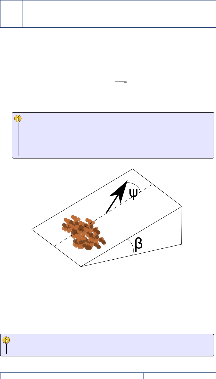
–SLOPEFF=2 : this correction is based on the method of Soulsby (1997), in which the threshold
bed shear stress θco is modified as a function of the bed slope χ, the angle of repose of the
sediment φs, modified in the Sisyphe steering file with the keyword FRICTION ANGLE OF THE
SEDIMENT (= 40◦by default), and the angle of the current to the upslope direction ψ:
θc
θco
=cos ψsin χ+ (cos2χtan2φs−sin2ψsin2χ)0.5
tan φs, (27)
with θcthe modified threshold bed shear stress. Be aware that this formula effected the results
with threshold bedload formulae (like Meyer-Peter and M ¨
uller) only.
5.3.2 Correction of the direction of bedload transport rate (formula for de-
viation)
The change in the direction of solid transport is taken into account by the formula :
tan α=tan δ−T∂Zf
∂n, (28)
where αis the direction of solid transport in relation to the flow direction, δis the direction of
bottom stress in relation to the flow direction, and nis the coordinate along the axis perpendi-
cular to the flow.
Accessibility : Interne : EDF SA Page 23 sur 73 c
EDF SA 2013
EDF R&D Reference manual
Sisyphe 6.3
H-P74-2012-02004-EN
Version 1.0
–DEVIA = 1 : according to Koch and Flochstra, the coefficient Tdepends exclusively on the
Shields parameter
T=4
6θ(29)
–DEVIA = 2 : the deviation is calculated based on Talmon et al. [44] and depends on the Shields
parameter and an empirical coefficient β2
T=1
β2√θ(30)
The empirical coefficient β2can be modified by the keyword PARAMETER FOR DEVIATION (=
0.85 by default). For rivers could be achieved satisfying results by using a higher value of
β2=1.5.
Keywords
–SLOPE EFFECT (= NO, default option)
–FORMULA FOR SLOPE EFFECT (SLOPEFF = 1, default option)
–FORMULA FOR DEVIATION (DEVIA = 1, default option)
–FRICTION ANGLE OF THE SEDIMENT (φs=40◦, default value)
–BETA (β=1.3, default value)
–PARAMETER FOR DEVIATION (β2=0.85, default value)
Figure 1 – Sloping bed : general slope (adapted from [42]).
5.4 Sediment Slide
An iterative algorithm prevents the bed slope to become greater than the maximum friction angle
(θs≈32◦−40◦). This option is activated by use of key word SEDIMENT SLIDE. Further details can be
found in the Die-Moran’s thesis [15].
Keywords
–SEDIMENT SLIDE,= NO, default value
–FRICTION ANGLE OF SEDIMENT = 40◦, default value
Accessibility : Interne : EDF SA Page 24 sur 73 c
EDF SA 2013
EDF R&D Reference manual
Sisyphe 6.3
H-P74-2012-02004-EN
Version 1.0
5.5 Bedload transport in curved channels
The bedload movement direction deviates from the main flow direction due to helical flow ef-
fect [65]. Different authors proposed empirical formulas for evaluating this deviation. The Engelund
formula [19], based on the assumption that the bottom shear stress, the bed roughness and the mean
water depth are constant in the cross-section, is
tan δ=7h
r(31)
where δis the angle between the bedload movement and main flow direction, hthe mean water
depth and rthe local radius of curvature. Yalin and Ferrera da Silva [64] have showed that δis
proportional to h/r. The local radius rcan be computed based on the the cross sectional variation of
the free surface [19] :
r=−ρα0U2
g∂Zs
∂y
,
with α0a coefficient (α0≈0.75 for very rough beds and α0≈1.0 for smooth beds).
Keywords
–SECONDARY CURRENTS (= NO, default option)
–SECONDARY CURRENTS ALPHA COEFFICIENT (= 1.0, default option)
Attention
This option should only be activated when the flow is calculated by a depth-averaged model.
Accessibility : Interne : EDF SA Page 25 sur 73 c
EDF SA 2013

EDF R&D Reference manual
Sisyphe 6.3
H-P74-2012-02004-EN
Version 1.0
6 Suspended load
6.1 Main assumptions
6.1.1 Vertical concentration profile
We assume a Rouse profile for the vertical concentration distribution, which is theoretically valid
in uniform steady flow conditions :
C(z) = Cre f z−h
z
a
a−hR
, (32)
where Ris the Rouse number defined by :
R=ws
κu∗, (33)
with ws>0 the vertical-settling sediment velocity, κthe von Karman constant (κ=0.4), u∗the
friction velocity corresponding to the total bed shear stress, and athe reference elevation above the
bed elevation.
6.2 Two-dimensional sediment transport equation
The two-dimensional (2D) sediment transport equation for the depth-averaged suspended-load
concentration C=C(x,y,t)is obtained by integrating the 3D sediment transport equation over the
suspended-load zone. By applying the Leibniz integral rule, adopting suitable boundary conditions
and assuming that the bedload zone is very thin, the depth-integrated suspended-load transport
equation is obtained :
∂hC
∂t+∂(hUC)
∂x+∂(hVC)
∂y=∂
∂xhes∂C
∂x+∂
∂yhes∂C
∂y+E−D, (34)
with h=Zs−Zf≈Zs−Zzre f the water depth, assuming that the bedload layer thickness is very
thin, (U,V)are the depth-averaged velocity components in the x−and y−directions, respectively.
The net sediment flux E−Dis determined based on the concept of equilibrium concentration,
see [11] :
(E−D)Zre f =wsCeq −Cre f (35)
where Ceq is the equilibrium near-bed concentration and Cre f is the near-bed concentration, calcula-
ted at the interface between the bed-load and the suspended load, z=Zre f . The reference elevation
Zre f corresponds to the interface between bedload and suspended load.
Equation (34), can be expressed in its non-conservative form as :
∂C
∂t+U∂C
∂x+V∂C
∂y
| {z }
advection
=1
h∂
∂xhes∂C
∂x+∂
∂yhes∂C
∂y
| {z }
diffusion
+E−D
h, (36)
where Uand Vare the depth-averaged convective flow velocities in the x−and y−directions,
respectively.
Keywords
–SUSPENSION = NON, default value
Accessibility : Interne : EDF SA Page 26 sur 73 c
EDF SA 2013
EDF R&D Reference manual
Sisyphe 6.3
H-P74-2012-02004-EN
Version 1.0
Attention
In Equation (34), the net sediment flux E−Dis expressed in ms−1. For consistency with
bedload units, expressed in m2s−1), concentration is dimensionless. However, the user can
choose concentration by mass per unit volume of the mixture (kg m−3) by using the keyword
MASS CONCENTRATION. The relation between concentration by volume and concentration by
mass is Cm(kg m−3) = ρsC.
6.3 Convection velocity
In Equation (34) it is supposed that Qsx=hUC and Qsy=hVC. A straightforward treatment
of the advection terms would imply the definition of an advection velocity and replacement of the
depth-averaged velocities in Eq. (34). For the x−component :
Qsx=hUconvC
A correction factor is introduced in Sisyphe , defined by :
Fconv =Uconv
U
The convection velocity should be smaller than the mean flow velocity (Fconv ≤1) since sediment
concentrations are mostly transported in the lower part of the water column where velocities are
smaller. We further assume an exponential profile concentration profile which is a reasonable ap-
proximation of the Rouse profile, and a logarithmic velocity profile, in order to establish the follo-
wing analytical expression for Fconv :
Fconv =−I2−ln B
30 I1
I1ln eB
30 ,
with B=ks/h=Zre f /hand
I1=Z1
B(1−u)
uR
du,I2=Z1
Bln u(1−u)
uR
du.
A similar treatment is done for the y−component. For further details, see [27].
Keywords
–CORRECTION ON CONVECTION VELOCITY (= NO, default option)
6.4 Numerical treatments
6.4.1 Treatment of the diffusion terms
According to the choice of the parameter OPDTRA of the keyword OPTION FOR THE DIFFUSION OF
TRACER, the diffusion terms in (36) can be simplified as follows :
–OPDTRA = 1 : the diffusion term is solved in the form ∇·(εs∇T)
–OPDTRA = 2 : the diffusion term is solved in the form 1
h∇·(hεs∇T)
The value of the dispersion coefficient esdepends on the choice of the parameter OPTDIF of the
keyword OPTION FOR THE DISPERSION :
–OPTDIF = 1 : the values of the constant longitudinal and transversal dispersivity coefficients
(T1 and T2 respectively) are provided with the keywords DISPERSION ALONG THE FLOW and
DISPERSION ACROSS THE FLOW
Accessibility : Interne : EDF SA Page 27 sur 73 c
EDF SA 2013

EDF R&D Reference manual
Sisyphe 6.3
H-P74-2012-02004-EN
Version 1.0
–OPTDIF = 2 : the values of the longitudinal and transversal dispersion coefficients are compu-
ted with the Elder model T1=αlu∗hand T2=αtu∗h, where the coefficients αland αtcan be
provided with the keywords DISPERSION ALONG THE FLOW and DISPERSION ACROSS THE FLOW.
–OPTDIF = 3 : the values of the dispersion coefficients are provide by Telemac-2d
The diffusion term can also be set to zero with keyword DIFFUSION = NO (YES is the option by
default).
Attention
Different schemes are available for solving the non-linear advection terms depending on the
choice of the parameter the classical characteristics schemes. To the diffusive schemes SUPG
and PSI, it is recommended to use conservative schemes.
6.4.2 Treatment of the advection terms
The choice of the numerical scheme is based on keyword TYPE OF ADVECTION. The following
numerical methods are available in Sisyphe :
–Method of characteristics (1)
– Unconditionally stable and monotonous
– Diffusive for small time steps
– Not mass conservative
–Method Streamline Upwind Petrov Galerkin SUPG (2)
– Courant number criteria
– Not mass conservative
– Less diffusive for small time steps
–Conservative N-scheme (similar to finite volumes) (3, 4)
– Solves the continuity equation under its conservative form
– Recommended when the correction on convection velocity is
accounted for
– Courant number limitation (sub-iterations are included to reduce the time step
– Numerical schemes 13 and 14 are the same as 3and 4but here adapted to the presence of tidal
flats based on positive water depth algorithm
–Distributive schemes (PSI)
– like scheme 4, but the fluxes are corrected according to the tracer value : this relaxes the
courant number criteria and it is also less diffusive than scheme 4and 14
– The CPU time is however increased
– This method should not applied for tidal flats
Attention
It is recommended to use scheme 4or 14 (if tidal flats are present) as a good compromise
(accuracy/computational time)
Keywords
–TETA SUSPENSION (= 1, default option)
–TYPE OF ADVECTION (= 1, default option)
–SOLVER FOR SUSPENSION (= 3, conjugate gradient by default option)
–PRECONDITIONING FOR SUSPENSION (= NO, default option)
–SOLVER ACCURACY FOR SUSPENSION (1.0 ×10⁻⁸, default option)
–MAXIMUM NUMBER OF ITERATIONS FOR SOLVER FOR SUSPENSION (= 50, default option)
–OPTION FOR THE DISPERSION (= 1, constant dispersion coefficient by default option)
–DISPERSION ALONG THE FLOW (1.0 ×10⁻², default option)
–DISPERSION ACROSS THE FLOW (1.0 ×10⁻², default option)
Accessibility : Interne : EDF SA Page 28 sur 73 c
EDF SA 2013

EDF R&D Reference manual
Sisyphe 6.3
H-P74-2012-02004-EN
Version 1.0
6.5 Equilibrium concentrations
6.5.1 Erosion and deposition rates
For non-cohesive sediments, the net sediment flux E−Dis determined based on the concept of
equilibrium concentration, see [11] :
(E−D)Zre f =wsCeq −Cre f (37)
where Ceq is the equilibrium near-bed concentration and Cre f is the near-bed concentration, calcula-
ted at the interface between the bed-load and the suspended load, z=Zre f . The reference elevation
Zre f corresponds to the interface between bedload and suspended load. For flat beds, the bed-load
layer thickness is proportional to the grain size, whereas when the bed is rippled, the bedload layer
thickness scales with the equilibrium bed roughness (kr). The definition of the reference elevation
needs also to be consistent with the choice of the equilibrium near-bed concentration formula.
The keyword REFERENCE CONCENTRATION FORMULA access to four differents semi-empirical for-
mulas :
–ICQ= 1 : Zyserman and Fredsoe formula
Ceq =0.331(θ0−θc)1.75
1+0.72(θ0−θc)1.75 , (38)
where θcis the critical Shields parameter and θ0=µθ ,the non-dimensional skin friction which
is related to the Shields parameter, by use of the ripple correction factor.
According to Zyserman and Fredsoe, the reference elevation should be set to Zre f =2d50. In
Sisyphe we take Zre f =k0
s, where k0
sis the skin bed roughness for flat bed (k0
s≈d50) , the
default value of proportionality factor is KSPRATIO =3).
–ICQ= 2 : Bijker (1992) formula The equilibrium concentration corresponds to the volume concen-
tration at the top of the bed-load layer. It can related to the bed load transport rate :
Ceq =Qs
bZre f u∗, (39)
with an empirical factor b=6.34.
According to Bijker, Zre f =kr.
Attention
The near bed concentration computed with the Bijker formula is related to the bedload.
Therefore, this option cannot be used without bedload transport (BED-LOAD = YES). Fur-
thermore, both bedload and suspended load transport must be calculated at each time
step, with the keyword PERIOD OF COUPLING set equal to 1.
–ICQ= 3 : van Rijn formula
Ceq =0.015d50
(τp/τc−1)3/2
Zre f D0.3
∗
, (40)
The concentration is defined at Zre f =max(ks/2; 0.01m)
–ICQ= 4 : Soulsby-van Rijn formula
For details, we refer to the reference [42].
6.5.2 Ratio between the reference and depth-averaged concentration
By depth-integration of the Rouse profile (41), the following relation can be established between
the mean (depth-averaged) concentration and the reference concentration :
Cre f =FC,
Accessibility : Interne : EDF SA Page 29 sur 73 c
EDF SA 2013
EDF R&D Reference manual
Sisyphe 6.3
H-P74-2012-02004-EN
Version 1.0
where :
F−1=Zre f
hRZ1
Zre f /h1−u
uR
du. (41)
In Sisyphe , we use the following approximate expression for F:
F−1=1
(1−Z)BR1−B(1−R), for R6=1
F−1=−Blog B, for R=1,
with B=Zre f /h.
Keywords
–REFERENCE CONCENTRATION FORMULA =1, default value
6.6 Initial and boundary conditions for sediment concentrations
6.6.1 Initial conditions
The initial values of volume concentration for each class can be either imposed in the subroutine
condim susp.f or specified in the steering file through the keyword INITIAL SUSPENSION CONCENTRATIONS.
Attention
It will not be used if EQUILIBRIUM INFLOW CONCENTRATION = YES.
6.6.2 Boundary conditions
For boundary conditions, the concentration of each class can be specified in the steering file
through keyword CONCENTRATION PER CLASS AT BOUNDARIES. To avoid unwanted erosion or sedi-
mentation at the entrance of the domain, it may be also convenient to use keyword EQUILIBRIUM
INFLOW CONCENTRATION = YES to specify the value of the concentration at inflow, according to the
choice of the REFERENCE CONCENTRATION FORMULA. The depth-averaged equilibrium concentration is
then calculated assuming equilibrium concentration at the bed and a Rouse profile correction for the
Ffactor. Input concentrations can be also directly specified in the subroutine conlit.f. In conlit.f,
it is assumed that LIEBOR = LICBOR.
Accessibility : Interne : EDF SA Page 30 sur 73 c
EDF SA 2013

EDF R&D Reference manual
Sisyphe 6.3
H-P74-2012-02004-EN
Version 1.0
7 Bed evolution equation
7.1 Bedload
To calculate the bed evolution , Sisyphe solves the Exner equation :
(1−n)∂Zf
∂t+∇·Qb=0, (42)
where nis the non-cohesive bed porosity (specified by the keyword NON COHESIVE BED POROSITY,=
0.40 by default), Zfthe bottom elevation, and Qb(m2s−1) the solid volume transport (bedload) per
unit width.
Equation (42) states that the variation of sediment bed thickness can be derived from a simple
mass balance and it is valid for equilibrium conditions.
7.2 Boundary conditions
From v6.2, as a general case the user has to specify two different boundary conditions files :
a conlim file for the hydrodynamics module (e.g., for Telemac-2d) and a different conlim file for
Sisyphe . This allows the user to apply different conditions for a tracer in Telemac-2dand for bed
evolution or concentration in Sisyphe . However, in most simple applications, the same boundary
condition can be used.
In the sediment transport boundary condition file, the following boundary condition types can
be imposed on the open boundaries :
Imposed bed evolution
For this case, LIEBOR=5 (KENT) and LIQBOR=4 (KSORT) for boundaries with prescribed variation
of elevation. For example, if the user wants to define a boundary with a fixed bed elevation (zero
evolution), the conlim file should look like :
(not used) LIQBOR (not used) ... LIEBOR EBOR
(4) 4 (5) ... 5 0.
Imposed sediment transport rates
For this case, LIEBOR = 4 (KSORT) and LIQBOR = 5 (KENT). For example, if the user wants to define
a boundary with an imposed transport rate =1.0 ×10⁻⁵m2s−1, the conlim file should look like :
(not used) LIQBOR (not used) Q2BOR ... LIEBOR EBOR
(-) 5 (-) 1.E-5 ... 4 0.
For this case, a boundary condition file for Sisyphe is needed. LIHBOR is actually not used but is now
available for users. LIQBOR is the boundary condition on solid discharge. Q2BOR is the prescribed
solid discharge given at boundary points, and expressed in m2s−1.
Alternatively, the user can give the width-integrated values of the imposed sediment transport
along the boundaries by using the keyword PRESCRIBED SOLID DISCHARGES, which is in m3s−1.
When the keyword PRESCRIBED SOLID DISCHARGES is given it supersedes Q2BOR, which is then taken
as a constant profile.
For non-uniform sediment distribution, the imposed values of transport rate are distributed to
every class with the help of the fractions (array AVAIL), this is done for EBOR and QBOR in conlis.f
and may be changed.
Accessibility : Interne : EDF SA Page 31 sur 73 c
EDF SA 2013

EDF R&D Reference manual
Sisyphe 6.3
H-P74-2012-02004-EN
Version 1.0
Keywords
–BEDLOAD = YES (default option)
–NON COHESIVE BED POROSITY (default option = 0.4).
7.3 Treatment of rigid beds and tidal flats
Non-erodable beds are treated numerically by limiting bedload erosion and letting incoming
sediment pass over. The problem of rigid beds is conceptually trivial but numerically complex.
For finite elements the minimum water depth algorithm allows a natural treatment of rigid
beds, see [25]. The sediment is managed as a layer with a depth that must remain positive, and
the Exner equation is solved similarly to the shallow water continuity equation in the subroutine
positive depths.f.
For finite volume schemes, the treatment must be explicitly specified and different options are
available with the keyword OPTION FOR THE TREATMENT OF NON ERODABLE BEDS :
Keywords
–OPTION FOR THE TREATMENT OF NON ERODABLE BEDS (= 0, default option)
–= 0 : erodable bottoms everywhere (default option)
–= 1 : minimisation of the solid discharge
–= 2 : nul solid discharge
–= 3 : minimisation of the solid discharge in FINITE ELEMENTS / MASS-LUMPING
–= 4 : minimisation of the solid discharge in FINITE VOLUMES
Attention
For the finite element method, the treatment of rigid bed is implicitly done by the numerical
scheme and previous options are now obsolete.
The space location and position of the rigid bed can be changed in the subroutine noerod.f. By
default, the position of the rigid bed is located at z=−100m.
7.4 Tidal flats
Tidal flats are areas of the computational domain where the water depth can become zero during
the simulation.
For finite elements the minimum water depth algorithm allows a natural treatment of tidal flats,
see [25] and the Exner equation is solved similarly to the shallow water continuity equation in the
subroutine positive depths.f.
For finite volume schemes, tidal flats can be treated with the keyword TIDAL FLATS. The compa-
nion keyword OPTION FOR THE TREATMENT OF TIDAL FLATS allows to choose between two different
approaches :
–OPTBAN = 1 : is the default option, and the equations are solved everywhere. The water depth
is set to a minimum value, controlled by the keyword MINIMAL VALUE OF THE WATER HEIGHT,
with a default value = 1.D-3m.
–OPTBAN = 2 : this option removes from the computational domain the elements with points
that present a water depth less than a minimum value. This option should be avoided because
it is not exactly mass-conservative.
Accessibility : Interne : EDF SA Page 32 sur 73 c
EDF SA 2013

EDF R&D Reference manual
Sisyphe 6.3
H-P74-2012-02004-EN
Version 1.0
Keywords
–TIDAL FLATS (= YES, default option)
–MINIMAL VALUE OF THE WATER HEIGHT (= 1.D-3m, default value)
–OPTION FOR THE TREATMENT OF TIDAL FLATS (OPTBAN = 1, default option)
Attention
For the finite element method, the treatment of tidal flats is implicitly done by the numerical
scheme and previous options are now obsolete.
7.5 Bed evolution for suspension
By considering only suspended load sediment transport, the bed evolution is function of the net
vertical sediment flux at the interface between the bedload and the suspended load given by :
(1−n)∂Zf
∂t+ (E−D)z=Zre f =0 (43)
with Zfthe bed elevation, Zre f the interface between the bedload and suspended load, and nthe
bed porosity. Once the flow variables are determined by solving the hydrodynamics and suspended
sediment transport equations, changes of bed level are computed from Equation (43) for the cell
coincident to the bed, calculating at each time step the net sediment flux E−Dat the bedload-
suspended load interface (z=Zre f ), as explained later. Further details on the derivation of the mass
balance equation (43) and coupling strategies can be found in [65].
Accessibility : Interne : EDF SA Page 33 sur 73 c
EDF SA 2013

EDF R&D Reference manual
Sisyphe 6.3
H-P74-2012-02004-EN
Version 1.0
8 Wave effects
8.1 Introduction
In coastal zones, the effect of waves superimposed to a mean current (wave-induced or tidal),
modifies the bed structure. Due to the reduced thickness of the bed boundary layer, the bottom
shear stress increases largely and the resulting sand transport rate could be in many cases of one
order of magnitude greater than in the case of currents alone. Furthermore, the wave-generated
ripples may also have a strong effect on the bed roughness and sand transport mechanisms. In
Sisyphe , these effects can be incorporated into the numerical simulations when the keyword EFFECT
OF WAVES is activated.
To compute sediment transport rates due to the action of waves, the wave height, period and
direction need to be specified. This information can be provided from a fortran file, by the subroutine
condim sisyphe.f, from a file containing the variables computed previously by the wave module,
e.g. Tomawac , or by internal coupling.
The wave orbital velocity U0is calculated by Sisyphe by assuming the validity of the linear
theory :
U0=Hsω
2 sinh(kh),
where Hsis the significant wave height, ω=2π/Tpis the intrinsic angular frequency, k=2π/L
is the wave number, with Lthe wave length. The wave number is calculated from the dispersion
relation (neglecting surface tension and amplitude effects) as :
ω2=gk tanh(kh).
8.1.1 Wave information
The wave information, required as input parameters for the morphodynamic model, are the
significant wave height Hs, the peak wave period Tpand the wave direction θw. If θwis not provided,
Sisyphe assumes the default value θw=90◦, which means that the direction of propagation of the
wave is parallel to the x-axis. When using the Bailard’s transport formula, this variable must be
always provided.
If the wave field is given from a file containing the variables computed previously on the same
mesh by the wave module, e.g. Tomawac , the keyword WAVE FILE must be specified in the Sisyphe
steering file. This file must contain the significant wave height Hs(HM0), the wave peak period Tp
(TPR5) and mean wave direction θwrelative to y-axis (DMOY).
Attention
For the keyword WAVE FILE, variables are given by the last record of the file.
If the currents and wave field is provided from a file containing the variables computed pre-
viously on the same mesh by the currents and wave modules, e.g. Telemac-2dand Tomawac ,
respectively, the keyword HYDRODYNAMIC FILE must be specified in the Sisyphe steering file. This
file must contain the hydrodynamic variables (water height and velocity field) as well as the wave
variables : significant wave height Hs(HM0), wave peak period Tp(TPR5) and mean wave direction
θwrelative to y-axis (DMOY). The users has also the choice of provide the wave variables from the
subroutine condim sisyphe.f.
Attention
For the keyword HYDRODYNAMIC FILE, the variables are given by the last record of the file if
the case is steady or by the time steps describing the tide or flood for the unsteady case.
Accessibility : Interne : EDF SA Page 34 sur 73 c
EDF SA 2013

EDF R&D Reference manual
Sisyphe 6.3
H-P74-2012-02004-EN
Version 1.0
8.2 Wave-induced bottom friction
8.2.1 Wave-induced bottom friction
The maximum stress due to waves is calculated at each time step as a function of the wave-orbital
velocity Uwby using the quadratic friction coefficient fwdue to waves :
τw=1
2ρfwU2
w.
The wave friction factor fwis calculated as a function of the orbital amplitude on the bed A0=Uw/ω
and the bed roughness ks:
fw=fw(A0/ks),
In Sisyphe , the formula proposed by Swart et al. [43] is provided :
fw=
exp −6.0 +5.2 A0
ks−0.19, if A0/ks>1.57
0.30, otherwise
8.2.2 Wave-current interaction
For combined waves and currents, the wave-induced (mean and maximum) bottom stresses can
be of one order of magnitude larger than in the case of currents alone. Different models can be found
in the literature to calculate the wave and current bottom stresses τcw, as a function of the bottom
shear stress due to currents only τcand the maximum shear stress due to waves only τw. Following
Bijker [7] :
τcw =τc+1
2τw. (44)
The mean τmean and maximum τmax shear stresses can be computed following the Soulsby’s
method [42]. Non-dimensional variables are defined :
X=τ0
τ0+τw;Y=τmean
τ0+τw;Z=τmax
τ0+τw
They can be parameterized as :
Y=X(1+bXp(1−X)q),
Z=1+aXm(1−X)n
The various model coefficients (a,b,m,n,p,q) are empirical functions of friction coefficients fwand
CD, and the wave-current angle φ:
a= (a1+a2|cos φ|I) + (a3+a4|cos φ|I)log10 2fw
CD,
b= (b1+b2|cos φ|J) + (b3+b4|cos φ|J)log10 2fw
CD,
......
with similar expressions for m,n,p, and q. The fitted constants (ai,bi,mi,ni,pi,qi,Iand J) depend
on the turbulence model selected. Table 2shows the coefficients used in Sisyphe corresponding to
the model of Huynh-Thanh and Temperville [28] for I=0.82, J=2.7.
Accessibility : Interne : EDF SA Page 35 sur 73 c
EDF SA 2013

EDF R&D Reference manual
Sisyphe 6.3
H-P74-2012-02004-EN
Version 1.0
i aibiminipiqi
1−0.07 0.27 0.72 0.78 −0.75 0.89
2 1.87 0.51 −0.33 −0.23 0.13 0.40
3−0.34 −0.10 0.08 0.12 0.12 0.50
4−0.12 −0.24 0.34 −0.12 0.02 −0.28
Table 2 – Constants issued from the turbulence model of Huynh-Thanh and Temperville [28], see
also Soulsby [42], page 91.
8.2.3 Friction coefficient under combined waves and currents
The characteristic shear stress −→
τcw(t), is related to the time-averaged mean velocity :
−→
τcw(t)=ρfcw −−→
U(t)
2,
where −−→
U(t)
2=U2
c+1
2U2
w
According to Camenen [8], the characteristic shear stress is taken as a weighted average between
τmean and τmax :−→
τcw(t)=Xτmean + (1−X)τmax,
which is equivalent to : −→
τcw(t)=Yτc+Zτw.
Finally, the expression for the wave-current interaction factor is :
fcw =Yτc+Zτw
U2
c+1
2U2
w
. (45)
This expression is used by Bailard [2] and Dibajnia and Watanabe [14] to compute sand transport
rates.
8.3 Wave-induced ripples
Equilibrium ripples are generally observed outside the surf zone. Their dimensions can be pre-
dicted as a function of waves (orbital velocity U0and wave period T=2π/ω), for a given uniform
sediment diameter d50. In Sisyphe , the procedure of Wiberg and Harris has been implemented [60].
This formulation is only applicable to oscillatory flow conditions and does not account for the effect
of a superimposed mean current.
Ripples can be classified into three types depending on the value of the ratio of wave orbital
diameter to mean grain diameter D0/d50, with D0=2U0/ω. The ripples wave length λand height
η, can be estimated as follows :
– Under moderate wave conditions (orbital regime), the ripple dimensions are proportional to
D0:
λ=0.62D0,η=0.17λ.
– For larger waves (anorbital regime), ripple dimensions scale with the sand grain diameter :
λ=535 d50,
η=λexp −0.095 log D0
η2
+0.042 log D0
η−2.28!.
Accessibility : Interne : EDF SA Page 36 sur 73 c
EDF SA 2013

EDF R&D Reference manual
Sisyphe 6.3
H-P74-2012-02004-EN
Version 1.0
The effect of ripples is to increase the bed roughness. Based on the Bijker’s formula, in Sisyphe it is
assumed that :
ks=max (η, 3d50).
Following Tanaka and Dang [49], the effect of the mean current superimposed to the waves is
accounted by introducing a correction factor αto the orbital velocity :
α=1+0.81 tanh(0.3S2/3
∗)2.5 U
Uw1.9
,
with S∗=d50p(s−1)gd50/4ν.
8.4 Wave-induced sediment transport
The effect of waves modifies the sand transport rates when it is superimposed to currents. This
effect can be accounted by using one of the following wave sand transport formula implemented
in Sisyphe , namely the Bijker’s formula [7], the Soulsby-van Rijn’s formula [42], the Bailard’s for-
mula [2] and the Dibajnia and Watanabe’s formula [14].
The keyword BED-LOAD TRANSPORT FORMULA allows the user to choose :
–ICF = 4 : the Bijker’s formula (1968) can be used to determine the total transport rate Qs
(bed-load + suspension), with its two components the bedload Qsc and the suspended load
Qss computed separately. For bedload transport, Bijker extended the steady bed-load formula
proposed by Frijlink (1952), by adding the wave effects. In non-dimensional form, the bedload
transport rate is :
Φb=bθ0.5
cexp −0.27 1
µθcw ,
where θcis the non-dimensional shear stress due to currents alone, θcw is the non-dimensional
shear stress due to wave-current interaction, and µis a correction factor which accounts for the
effect of ripples. The shear stress under combined wave and current is calculated by Equation
(44).
In the original formulation, the coefficient b=5. Recent studies showed that b=2 provides
better results when comparing with field and experimental data. By default, in Sisyphe b=
2 but this value can be modified with the keyword B VALUE FOR THE BIJKER FORMULA. The
ripple factor correction µis calculated in the same way as in the Meyer-Peter-Mueller formula
for currents only.
The suspended load transport is solved in a simplified manner, by assuming the concentration
profile to be in equilibrium. The inertia effects are not modeled and it is assumed that no
exchange takes place with the bed load layer.
After depth-integration and by assuming a Rouse profile for the concentration and a logarith-
mic velocity profile for the mean velocity profile, the suspended load can be written as :
Qss =Qsc I,
where
I=1.83 ×0.216 BA−1
(1−B)AZ1
B1−y
yA
ln 33y
Bdy,
with
A=Ws
κu∗,u∗=rτcw
ρ,B=ks/h.
Accessibility : Interne : EDF SA Page 37 sur 73 c
EDF SA 2013

EDF R&D Reference manual
Sisyphe 6.3
H-P74-2012-02004-EN
Version 1.0
–ICF = 5 : Soulsby-van Rijn formula, the transport rate due to the combined action of waves
and current is provided by the following equation :
Qb,s=Ab,sU"U2+20.018
CD
U2
00.5
−Ucr#2.4
.
This formula can be applied to estimate the components of the total sand transport rate (bed-
load Qband suspended load Qs), and it is suitable for beds covered by ripples. The bedload
and suspended load coefficients Ab,sare computed as :
Ab=0.005h(d50/h)1.2
((s−1)gd50)1.2
As=0.012d50D−0.6
∗
((s−1)gd50)1.2 ,
where Uis the depth-averaged current velocity, U0is the RMS orbital velocity of waves, and
CDis the quadratic drag coefficient due to current alone. This formula has been validated
assuming a rippled bed roughness with ks=0.18 m. The critical entrainment velocity Ucr is
given by the expression :
Ucr =
0.19d0.1
50 log10 4h
D90 , if 0.1mm ≤d50 ≤0.5mm
8.5d0.6
50 log10 4h
D90 , if 0.5mm ≤d50 ≤2.0mm.
The diameter D90, characteristic of the coarser grains, is specified with the keyword D90. The
validity range for the Soulsby-van Rijn formula is h= [1−20]m, U= [0.5 −5]ms−1, and
d50 = [0.1 −2.0]mm.
–ICF = 8 : the Bailard’s formula is based on the energetic approach. The bedload and the sus-
pended load components of the sand transport rate are expressed respectively as the third- and
fourth-order momentum of the near-bed time-varying velocity field −−→
U(t), as follows :
Qb=fcw
g(s−1)
ec
tan ϕ−→
U
2−→
U
Qs=fcw
g(s−1)
es
Ws−→
U
3−→
U,
with fcw the friction coefficient which accounts for wave-current interactions, es=0.02, ec=0.1
empirical factors, ϕsediment friction angle (tan ϕ=0.63) and <·>time-averaged over a
wave-period.
Under combined wave and currents, the time-varying velocity vector −−→
U(t)is composed of a
mean component Ucand an oscillatory component of amplitude U0, assuming linear waves ; φ
is the angle between the current and the wave direction, φcis the angle between the mean cur-
rent direction and the x−axis, and φwis the angle between the wave direction of propagation
and the x-axis. The time-varying velocity field verifies :
−−→
U(t) = Ucexpiφc+U0cos ωtexpiφw.
For the third-order term, one can derive an analytical expression in the general case, whereas
for the fourth-order momentum, we have to assume the waves and currents to be co-linear (φ=
0), in order to find an analytical expression. For the general case of a non-linear non-colinear
wave, we would have to integrate numerically the fourth-order velocity term [8]. However, this
method has showed to be inefficient. Expressions for the third and fourth-order terms are given
below :
Accessibility : Interne : EDF SA Page 38 sur 73 c
EDF SA 2013

EDF R&D Reference manual
Sisyphe 6.3
H-P74-2012-02004-EN
Version 1.0
– Third-order term :
−→
U
2−→
U=−→
Uc(U2
c+1
2U2
0) + −→
U0(−→
Uc·−→
U0)
−→
U
2−→
Ux
=U3
c+UcU2
0(1+1
2cos 2φ)cos φc−1
2UcU2
0sin 2φsin φc
−→
U
2−→
Uy
=U3
c+UcU2
0(1+1
2cos 2φ)sin φc+1
2UcU2
0sin 2φcos φc
– Fourth-order term :
−→
U
3−→
Ux
=1
8(24U2
0U2
c+8U4
c+3U4
0)cos φc
−→
U
3−→
Uy
=1
8(24U2
0U2
c+8U4
c+3U4
0)sin φc
–ICF = 9 : the Dibajnia and Watanabe (1992) formula is an unsteady formula, which accounts
for inertia effects. The sand transport rate is calculated by the expression :
−→
Qs
Wsd50
=α−→
Γ
|Γ|1−β, (46)
with α=0.0001 and β=0.55 empirical model coefficients and −→
Γthe difference between the
amounts of sediments transported in the onshore and offshore directions. This formula is used
to estimate the intensity of the solid transport rate, the direction is assumed to follow the mean
current direction. In the wave direction, the time-varying velocity is given by :
U(t) = Uccos φ+U0sin ωt,
ris defined by the asymmetry parameter :
r=U0
Uccos φ.
The wave cycle is decomposed into two parts :
1. During the first part of the wave-cycle (0 <t<T1), the velocities are directed onshore
(U(t)>0).
2. During the second part (T2=T−T1), the velocities are negatives (U(t)<0).
The sand transport rate in the wave direction is :
ΓX0=u1T1(Ω3
1+Ω03
2)−u2T2(Ω3
2+Ω03
1)
(u1+u2)T
where Ω1and Ω2represent the amount of sand transported in the onshore and offshore di-
rections which will be deposited before flow reversal, respectively, Ω0
1and Ω0
2represent the
remaining part which stay in suspension after flow reversal. The inertia of sediment depends
on the ratio d50/ws, and represented by parameter ωi:
ωi=u2
i
2(s−1)gWsTi
,
with
u2
i=2
TiZu>or<0u2dt,
and two different cases :
Accessibility : Interne : EDF SA Page 39 sur 73 c
EDF SA 2013
EDF R&D Reference manual
Sisyphe 6.3
H-P74-2012-02004-EN
Version 1.0
1. All sediment is deposited before flow reversal ωi≤ωcrit
Ωi=ωi
2WsTi
d50
,Ω0
i=0
2. Part of the sediment stays in suspension after flow reversal ωi≥ωcrit
Ωi=ωcrit
2WsTi
d50
,Ω0
i= (ωi−ωcrit)2WsTi
d50
.
The critical value of ωcrit is calculated as function of the wave-current non-dimensional friction :
Θcw =<τcw >
ρ
1
(s−1)gd50
.
According to Temperville et Guiza :
ωcrit =
0.03, if Θcw ≤0.2
1−p1−((Θcw −0.2)/0.58)2, if 0.2 ≤Θcw ≤0.4
0.8104pΘcw −0.4225, if 0.4 ≤Θcw ≤1.5
0.7236pΘcw −0.3162, otherwise
Attention
In Sisyphe , the solid discharge is assumed to be oriented in the direction of the mean current.
The possible deviation of the transport in the direction of waves, which can be important in
the near shore zone due to non-linear effects, is not accounted for.
8.5 Internal coupling waves-currents and sediment transport
The internal coupling waves-currents and sediment transport is implemented in the Telemac-
Mascaret system. The keyword COUPLING WITH = ’TOMAWAC, SISYPHE’ (in the Telemac-2d steering
file) is used to internally couple with Tomawac and Sisyphe .
The coupling period with Tomawac and Sisyphe can be controlled with the keywords COUPLING
PERIOD FOR TOMAWAC and COUPLING PERIOD FOR SISYPHE, respectively.
In the Telemac-2dcas file, the keyword WAVE DRIVEN CURRENTS = YES allows to incorporate the
effect of waves in the hydrodynamic simulation.
In the Sisyphe cas file, the keyword EFFECT OF WAVES = YES is used to consider the effect of the
waves on the solid transport formula. In Sisyphe , the implemented bedload transport formulae that
consider the combined effect of currents and waves are Bijker (=4), Soulsby-van Rijn (=5), Bailard
(=8) and Dibajnia and Watanabe (=9). Formulae 4, 5 and 8consider bedload and suspended load
transport. Formula 9considers total transport.
Accessibility : Interne : EDF SA Page 40 sur 73 c
EDF SA 2013

EDF R&D Reference manual
Sisyphe 6.3
H-P74-2012-02004-EN
Version 1.0
9 Sand grading effects
9.1 Sediment bed composition
9.1.1 Granulometry distribution
The number of classes of bed material is specified in the steering file with the keyword NUMBER
OF SIZE-CLASSES OF BED MATERIAL and is limited to NSICLA ≤20. For uniform sediments, the
granulometry distribution is represented by one single value NSICLA =1 for the whole domain. The
mean grain diameter and corresponding settling velocity are defined in the steering file.
For sediment mixtures, the granulometry distribution is discretized in a number of classes. Each
class of sediment 1 < j < NSICLA is defined by its mean diameter d50(j) and volume fraction in
the mixture at every node AVAI(j). The characteristics of each class of sediment, such as the Shields
number θc(i) or the settling velocity ws(i) for each class can be specified in the steering file or
calculated by the model as for a single sediment class.
The percent of each class of material need to verify :
∑
j=1,NSICLA
AVAI(j) = 1 and 0 ≤AVAI(j)≤1. (47)
The initial bed composition can be defined in the steering file for uniform bed. For complex
bed configurations, e.g. spatial variation, vertical structure, etc., the user subroutine init compo.f is
used to define the initial state. The mean diameter dm,ACLADM, is calculated as :
dm=∑
j=1,NSICLA
AVAI(j)d50(j). (48)
9.1.2 Bed structure
The bed is stratified into a number of layers NOMBLAY that enables vertical variations of the se-
diment bed composition. The percentage of each class jof material, AVAI(i,j,k) as well as the
thickness of each layer Esare defined at each point iand for each layer k.
The composition of transported material is computed using the composition of the upper layer,
see below the definition of active layer. The initial composition of the bed (number of layers, thickness
of each layer Es, composition of each layer AVAI are specified in user’s subroutine init compo.f.
The subroutine init avail.f verifies if the structure of the initial bed composition is compatible
with the position of the rigid bed, as defined in user’s subroutine noerod.f :
Zf(i)−Zr(i) = ∑
k=1,NOMBLAY
Es(k). (49)
In general, the thickness of the bed is taken to be large (by default, 100 m), so the bottom layer
thickness of the last layer (nearest to the rigid bed) needs to be increased.
Assuming the porosity nof each class to be identical and constant, the total mass of sediments
per unit area is :
Ms(i) = ∑
k=1,NOMBLAY
ρsEs(k)(n−1). (50)
In each layer, the percent of each class AVAI, which is defined as the volume of each class of
material per the total volume of material, is considered to be a constant. For each layer and at each
point of the domain, the following constraints need to be satisfied :
Accessibility : Interne : EDF SA Page 41 sur 73 c
EDF SA 2013

EDF R&D Reference manual
Sisyphe 6.3
H-P74-2012-02004-EN
Version 1.0
∑
j=1,NSICLA
AVAI(i,k,j) = 1 and 0 ≤AVAI(i,k,j)≤1.
Keywords
The initial sediment bed composition is defined by :
–NUMBER OF SIZE-CLASSES OF BED MATERIAL :NSICLA = 1, by default
–SEDIMENT DIAMETERS :FDM = .01, by default
–SETTLING VELOCITIES : if XWC is not given, the subroutine vitchu sisyphe.f is used to
compute the settling velocity based on the Stokes, Zanke or Van Rijn formulae as a function
of the grain size
–SHIELDS PARAMETERS : for multi grain size, the Shields parameter needs to be specified for
each class. If only one value is specified, the shields parameter will be considered constant
for all classes. The default option, no Shields parameter given in steering file, is to calculate
the Shields parameter as a function of the sand grain diameter, see logical CALAC.
–INITIAL FRACTION FOR PARTICULAR SIZE CLASS :AVA0 = 1.;0.;0.;..., by default
For more than one-size classes, the user should specify NSICLA values for the mean diameter,
initial fraction, etc. For example, for a mixture of two classes :
Example
–NUMBER OF SIZE-CLASSES OF BED MATERIAL = 2
–SEDIMENT DIAMETERS = 0.5; 0.5
–SETTLING VELOCITIES = 0.10; 0.05
–SHIELDS PARAMETERS = 0.045; 0.01
–INITIAL FRACTION FOR PARTICULAR SIZE CLASS = 0.5; 0.5
Attention
When using a (manually modified) sedimentological restart pay attention, that the following
restrictions are valid :
∑
j=1,NSICLA
AVAI(j) = 1 and 0 ≤AVAI(j)≤1 (51)
Zf(i)−Zr(i) = ∑
k=1,NOMBLAY
Es(k)(52)
9.2 Sediment transport of sediment mixtures
The method programmed in Sisyphe for the treatment of mixtures of sediment with variable
grain sizes is classical and based on previous models from the literature (as for example the 1D
model Sedicoup developed at Sogreah). There are two layer concepts implemented in Sisyphe .
The classical active layer model based on Hirano’s concept [23] and a newly developed continuous
vertical sorting model (C-VSM), implemented by Merkel and Kopmann (BAW) [36].
9.2.1 Active layer and stratum
Since only a relatively thin layer is envolved in the transport, the upper part (active part) of the
bed is therefore divided into a thin active layer and an active stratum. The composition of the active
layer is used to calculate the composition of transported material and the intensity of transport rates
Accessibility : Interne : EDF SA Page 42 sur 73 c
EDF SA 2013

EDF R&D Reference manual
Sisyphe 6.3
H-P74-2012-02004-EN
Version 1.0
for each class of sediment :
Qs=∑
j=1,NSICLA
AVAI(i,1,j)Qs(j), (53)
where AVAI(i,1,j) is the percentage of the class jin the active layer.
The active stratum is the layer that will exchange sediment with the active layer in order to keep
the active layer to a fixed (either constant or calculated) size. In case of high erosion depth, the active
stratum becomes thinner and thinner, since it will be merged with the stratum lying underneath.
The active layer thickness concept is not well defined and depends on the flow and sediment
transport characteristics [52]. According to Yalin [63], it is proportional to the sand diameter of the
upper layer. The active later thickness generally scales with the bed roughness, which is typically of
the order of a few grain diameters for flat beds up to few centimeters in the case of rippled beds. In
the presence of dunes, the active layer thickness should be half the dune height [39].
In Sisyphe , the active layer thickness is an additional parameter of the model, called ELAY0, which
can be estimated by calibration and specified by the user in the steering file by keyword ACTIVE
LAYER THICKNESS. With the option CONSTANT ACTIVE LAYER THICKNESS = NON, it is possible to use
a space and time varying active layer thickness during the simulation. In Sisyphe it is assumed that
ELAY0 = 3dm, with dmthe mean diameter of the active layer. Using the continuous vertical sorting
model, more formulae for calculating the active layer thickness are available.
The erosion rate is restricted by the total amount of sediments in the active layer, which there-
fore acts as a rigid bed. The same method applied for rigid bed is applicable for the active layer
formulation.
Attention
When dealing with graded sediment and thin thickness active layers, it is advised to use finite
elements combined with the positive depth algorithm, as used for the treatment of rigid bed,
in order to avoid numerical problems such as negative sediment fractions. The error message
EROSION GREATER THAN ONE LAYER THICKNESS can also appear in the listing file when the
erosion is greater than the active layer thickness. If the sedimentation is greater than the active
layer thickness the error message DEPOSITION MORE THAN ONE LAYER THICKNESS appear in the
listing as well. In both cases it is strongly recommended to reduce the time step. Otherwise
the calculation of the fractions is not valid anymore.
9.2.2 Continuous vertical sorting model
The C-VSM overcomes many limitations of the classical layer implementation of Hirano (HR-
VSM). Even though it is a different way to manage the grain sorting, it is just another interpretation
of Hirano’s original idea with fewer simplifications. So still an active layer is defined but the grain
distribution in this layer is computed for each time step from a depth dependent bookkeeping model
for each grain size fraction with unlimited numerical resolution for each horizontal node. The new
model does not overcome the need to carefully calibrate the same input parameters as all other
models, but the new interpretation has the following advantages :
– It is possible to keep minor but prominent grain mixture variations even after a high number of
time steps. Smearing effects and bookkeeping accuracy is defined by user defined thresholds
or the computational resources, rather than through a fix value.
– Various functions for the impact depth of the shear stress can be chosen to the projects de-
mands. The result is a much more accurate vertical grain sorting, which results in better pro-
gnoses for bed roughness, bed forms and erosion stability.
A couple of new keywords must be set in your Sisyphe steering file. The full C-VSM output can
be found in the new Selafin files VSPRES & VSPHYD in the tmp-folders. As the higher resolution
Accessibility : Interne : EDF SA Page 43 sur 73 c
EDF SA 2013

EDF R&D Reference manual
Sisyphe 6.3
H-P74-2012-02004-EN
Version 1.0
of the C-VSM needs resources, you can reduce the printout period, or suppress the output at all.
The common Sisyphe result files only show the averaged values for the active layer. Even more disk
space can be saved, if only few points are printed out as .VSP.CSV files in the subfolder /VSP/. We
recommend using between 200 and 1000 vertical sections. More will not improve the accuracy much,
and less will lead to increasing data management, as the profile compression algorithms are called
more often.
Keywords
The initial sediment bed composition is defined by :
–VERTICAL GRAIN SORTING MODEL = 1
–0 = Layer = HR-VSM (Hirano +Ribberink as until Sisyphe v6p1)
–1 = C-VSM
–C-VSM MAXIMUM SECTIONS = 100
– Should be at least 4 +4×Number of fractions,
– better >100, tested up to 10000
–C-VSM FULL PRINTOUT PERIOD = 1000
–0 => GRAPHIC PRINTOUT PERIOD
– Anything greater 0 => Sets an own printout period for the CVSP
– Useful to save disk space
–C-VSM PRINTOUT SELECTION = 0|251|3514|...|...
– Add any 2D Mesh Point numbers for .CSV-Ascii output of the CVSP
– Add 0for full CVSP output as Selafin3D files (called VSPRES +VSPHYD)
– All files are saved to your working folder and in /VSP &/LAY folders below
–C-VSM DYNAMIC ALT MODEL = 5
– Model for dynamic active layer thickness approximation
–0= constant (Use Keyword : ACTIVE LAYER THICKNESS)
–1= Hunziker & Guenther
ALT =5dMAX
–2= Fredsoe & Deigaard (1992)
ALT =2τB
(1−n)g(ρS−ρ)tan Φ
–3= van RIJN (1993)
ALT =0.3D0.7
∗
τB−τC
τB
0.5
d50
–4= Wong (2006)
ALT =5τB
(ρS−ρ)gd −0.0549)0.56d50
–5= Malcharek (2003)
ALT =d90
1−nmax(1, τB
τC
)
–6 = 3*d50 within last time steps ALT’
ALT =3d50
9.2.3 General formulation
Bedload transport rates are computed separately for each class using classical sediment transport
formulae, corrected for sand grading effects. The Exner equation is then solved for each class of
sediment. The individual bed evolution due to each class of bed material is then summed to give
the global evolution due to bedload. Similarly, the suspended transport equation is solved for each
class of sediment and the resulting bed evolution for each class is then summed to give the global
Accessibility : Interne : EDF SA Page 44 sur 73 c
EDF SA 2013

EDF R&D Reference manual
Sisyphe 6.3
H-P74-2012-02004-EN
Version 1.0
evolution due to the suspended load.
At each time step, the bed evolution due to bedload and to suspension transport is used to
compute the new bed structure. The algorithm which determines the new bed composition considers
two possibilities, namely deposit or erosion, and ensures mass conservation for each individual class
of material. The algorithm is explained in [22].
9.2.4 Hiding exposure
In order to calculate bedload sediment transport rates for each class of sediment, it is necessary to
consider the effect of hiding exposure. That means that in a sediment mixture, bigger particles will
be more exposed to the flow than the smaller ones and therefore, prediction of sediment transport
rates with classical sediment transport formulas, need to be corrected by use of a hiding-exposure
correction factor. In Sisyphe , the keyword HIDING FACTOR FOR PARTICULAR SIZE CLASS sets the
value of hiding factor for a particular size class and the keyword HIDING FACTOR FORMULA allows
the user to choose among different formulations. Two formulas, Egiazaroff [16] and Ashida & Mi-
chiue [1], have been written based on the Meyer-Peter and M¨
uller formula. Both formulas modify
the critical Shields parameter that will be used in the Meyer-Peter formula. Therefore they only can
be combined useful with threshold formulae. The formula of Karim and Kennedy [30] can be used
in combination with any bedload transport predictor. This formula modifies directly the bedload
transport rate.
–HIDFAC = 1 : formulation of Egiazaroff
θcr =0.047ζi, with ζi=log(19)
log(19Di/Dm)2
–HIDFAC = 2 : formulation of Ashida & Michiue
–HIDFAC = 4 : formulation of Karim et al.
Keywords
Sand grading effects are defined by :
–HIDING FACTOR FORMULA : if HIDFAC = 0 (by default), the user needs to give HIDING FACTOR
FOR PARTICULAR SIZE CLASS
–ACTIVE LAYER THICKNESS := 10000, by default
–CONSTANT ACTIVE LAYER THICKNESS := YES, by default
–NUMBER OF BED LOAD MODEL LAYERS :NOMBLAY = 2, by default
9.2.5 Sediment transport formula
The formula of Hunziker [26] is an adaptation of the Meyer-Peter M¨
uller formula for fractional
transport. The volumetric sediment transport per sediment class is given by :
Φb=5pi[ζi(µθi−θcm)]3/2 if µθi>θcr, (54)
with pithe fraction of class iin the active layer, θithe Shields parameter, θcm =θcr (Dmo/Dm)0.33 the
corrected critical Shields parameter, θcr the critical Shields parameter (θcr =0.047), ξi=(Di/Dm)−α
the hiding factor, Dithe grain size of class i,Dmthe mean grain size of the surface layer (m),
Dmo the mean grain size of the under layer (m), and αa constant. The critical Shields parameter is
calculated as a function of the dimensionless mean grain size D∗. It should be noted that according
to Hunziker, stability problems may occur outside the parameter range α≤2.3 and Di/Dm≥0.25.
Hunziker developed an own hiding-exposure formula corresponding to his bed load formula.
Accessibility : Interne : EDF SA Page 45 sur 73 c
EDF SA 2013


EDF R&D Reference manual
Sisyphe 6.3
H-P74-2012-02004-EN
Version 1.0
10 Cohesive sediment properties
10.1 Introduction
Fine cohesive sediments are predominant in most estuaries, basins and reservoirs. The prediction
of cohesive sediment transport, often associated with pollutants, is crucial regarding environmental
issues.
Cohesive properties appear for fine particles (silts and clay), with diameter less than a limiting
value of about 60 µm, depending on the physico-chemical properties of the fluid and salinity. Fine
cohesive sediments are transported in suspension (no bed-load) and transport processes strongly
depend on the state of floculation of the suspension and consolidation of the bed.
The erosion rate mainly depends on the degree of consolidation of the sediment bed, while the
settling velocity depends on the state of floculation and aggregates properties.
Attention
The separation value at 60µm to discriminate non-cohesive from cohesive sediment is conven-
tional (UK classification). The value is different depending on the country (63µm in Nether-
lands, 75µm in USA as pointed by Winterwerp and Van Kesteren [61]). Moreover, aggregation
of flocs can lead to the formation of macro-flocs larger than 100µm.
Keywords
In Sisyphe , the simplest case of uniform and cohesive sediments is characterized by one single
value for the primary grain size D50 and density ρs=2650 kg/m3for quartz particles, which
is transported in suspension (no bedload).
In the Sisyphe steering file, the physical properties of the sediment are defined :
–COHESIVE SEDIMENT = YES (= NO, default option)
–SEDIMENT DIAMETERS (D50 >0.00006 m, for non-cohesive sediment)
–SEDIMENT DENSITY (ρs=2650 Kg/m3, default value)
Both key words SUSPENDED LOAD = YES,BED LOAD = NO are set automatically, in order to be
consistent with the selected type of sediment, when COHESIVE SEDIMENT = YES
–SUSPENDED LOAD = YES (= NO, default option)
–BED LOAD = NO (= YES, default option)
10.2 Effect of floculation
For cohesive sediments (D50 <60µm), the primary grain diameter and density no longer control
the transport rates. Due to electro-static attractive forces (van der Waals), individual particles tend to
form flocs. Their size can be an order of magnitude greater than the initial particle diameter, while
the density decreases : the floc characterictics (size and density, as well as its fractal dimension) are
more relevant to compute the settling velocity.
The settling velocity of cohesive particles therefore depends on the suspended sediment concen-
tration as well as on other physico-chemical properties (pH, salinity, cations for instance) of the
suspension which influence the flocculation process. The effect of turbulence level determines also
the floculation state. The critical bed shear strength depends on the consolidation state or age of the
sediment bed (Migniot, 1968).
Floculation can be modelled using process based models (cf. Mc Anally [34]). The settling velocity
is generally one order of magnitude greater than the settling velocity based on the individual particle
size, as a result of flocculation.
The flocculation process is not yet programmed in Sisyphe and the settling velocity should be
specified by the user as a calibration parameter. More physically based relations will be implemented
Accessibility : Interne : EDF SA Page 47 sur 73 c
EDF SA 2013

EDF R&D Reference manual
Sisyphe 6.3
H-P74-2012-02004-EN
Version 1.0
in a future release of the code.
Keywords
–SETTLING VELOCITIES
Attention
The settling velocity needs to be specified, if not, it will be calculated by the Stokes law as a
function of the individual particle diameter in subroutine vitchu sisyphe.f. As a result of
flocculation, the settling velocity can be approximately an order of magnitude greater.
10.3 Consolidation process
Once the sedimentation process is achieved, a sediment bed is formed. For non-cohesive bed, no
evolution with time will be observed if no erosion or further sedimentation occurs. For cohesive bed,
the concentration will increase with time as the result of self-weight consolidation or compaction.
Two stages, namely the primary and secondary consolidation are classically considered to explain
the progressive compaction of the cohesive sediment bed with time. As the formed bed resulting
from the sedimentation of mud is very soft, it tends to compact under its self-weight. During this
process, the void ratio tends to diminish so that pore water is expulsed upward as a result of water
incompressibility. The dynamic of this primary stage of consolidation is therefore controlled by
the permeability of the bed. At the end of the primary consolidation, the excess pore pressure is
fully dissipated (Figure 2) but the cohesive bed records further compaction. This secondary stage
of consolidation is no longer related to pore pressure but rather to the solid skeleton property. The
secondary consolidation is considered as a result of time effect (viscous or ageing) in the stress-strain
relationship of the soil. Two effects of time are currently considered in modern soil mechanic : the
creep of the soil (viscous behaviour of cohesive geomaterial) and ageing (thixotropy of mud). Even
through the dynamic of the secondary consolidation is much slower than the primary consolidation,
this stage is important for long term prediction.
Keywords
–MUD CONSOLIDATION = NON, by default
11 Cohesive bed structure
11.1 Multi-layer model
Cohesive sediment beds are generally non-uniform : as a result of self-weight consolidation, the
bed becomes stratified, with density increasing with distance from the surface. The top layer is
generally made of freshly deposited soft mud, while the bottom consolidated layers present higher
resistance to erosion. The vertical stratification of the cohesive bed is therefore a key issue, which
controls the amount of material to be put in suspension.
In Sisyphe , cohesive sediment bed can be represented by a fixed number NCOUCH TASS of layers.
The number of layers is fixed with maximum number up to 20. Each layer is characterized by its
concentration and resitance to erosion. The concentration of each layer (Cs(j))is generally constant
and specified by keyword MUD CONCENTRATION PER LAYER expressed in kg/m3. It may also vary in
space and time (see consolidation model 3). The resistance of each layer is specified by keyword
CRITICAL EROSION SHEAR STRESS OF THE MUD expressed in N/m2.
Each layer j(1 ≤j≤NCOUCH TASS) is defined by its concentration Cs, thickness Esand mass
Accessibility : Interne : EDF SA Page 48 sur 73 c
EDF SA 2013
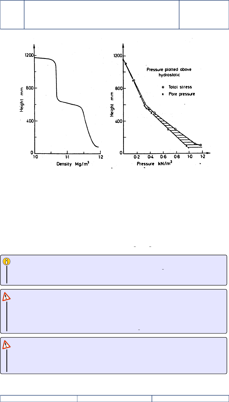
EDF R&D Reference manual
Sisyphe 6.3
H-P74-2012-02004-EN
Version 1.0
Figure 2 – Vertical variation of density and effective stress within the cohesive sediment bed.
per surface area Ms, which depends on both layer concentration and thickness, such that
Ms(i,j) = Cs(j)Es(i,j)
where Msis the mass per unit surface area (Kg/m2), Csis the concentration (kg/m3) and Esthe
layer thickness.
For specific applications, the bed concentrations Cs(i,j)can also vary from one point to another.
The initial distribution can be specified in subroutine init compo coh.f.
Keywords
–NUMBER OF LAYERS OF THE CONSOLIDATION MODEL :NCOUCH TASS (default value =1)
should be less than the maximum number of layers (NLAYMAX = 20)
–MUD CONCENTRATION PER LAYER, in Kg/m3:Cs(default value =50)
Attention
The keywords NUMBER OF BED LOAD MODEL LAYERS and NUMBER OF LAYERS OF THE
CONSOLIDATION MODEL are essentially the same except that the default values are different.
For cohesive sediments, it is possible to have only one uniform layer, whereas for sand grading
algorithm we need at least 2 layers (the active layer and the substratum). The subroutine
lecdon.f specifies at the end NOMBLAY =NCOUCH TASS
Attention
Due to the default value of NOMBLAY for sand grading effects (NOMBLAY =2). For uni-
form beds both keywords need to be specified :
–NUMBER OF BED LOAD MODEL LAYERS = 1
–NUMBER OF LAYERS OF THE CONSOLIDATION MODEL = 1
Accessibility : Interne : EDF SA Page 49 sur 73 c
EDF SA 2013
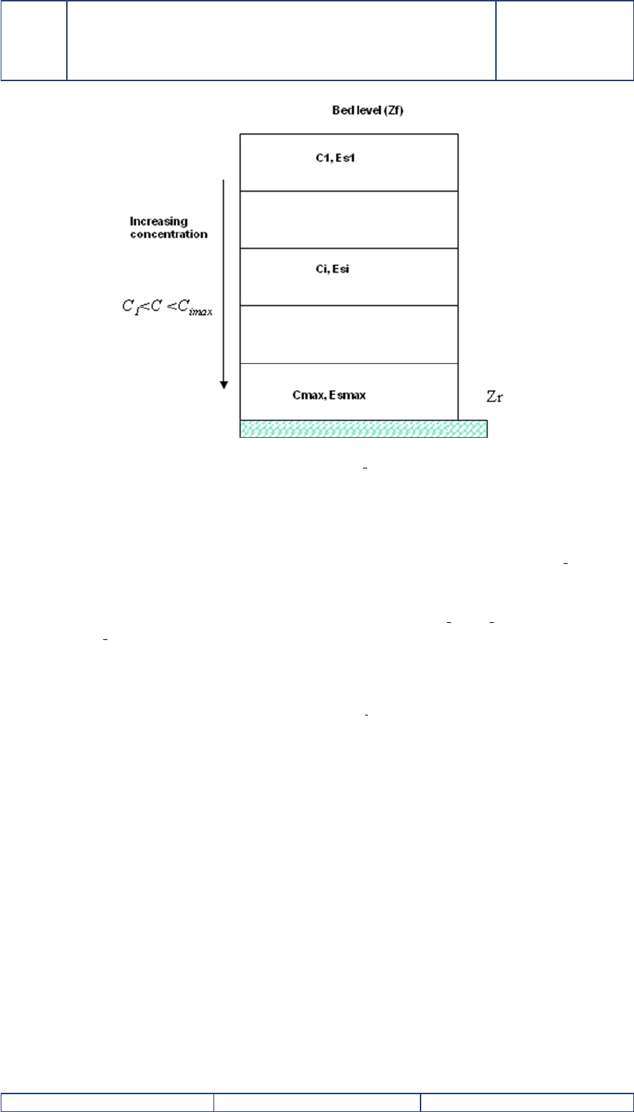
EDF R&D Reference manual
Sisyphe 6.3
H-P74-2012-02004-EN
Version 1.0
Figure 3 – Multi-layer bed structure (NCOUCH TASS is the number of layers)
11.2 Initialization
The initial concentration for the suspended load can be either imposed within condim susp.f or
specified in the steering file through the keyword INITIAL SUSPENSION CONCENTRATIONS initializes
the value of the volume concentration for each class.
The initial layer thicknesses are specified in user-subroutine init compo coh.f. It is called by
subroutine init mixte.f which just checks if the sum of all layers is equal to the total bed thickness
as specified by the initial bathymetry Zfand rigid bed Zr:
Zf(i)−Zr(i) = ∑
j=1,NCOUCH TASS
Es(i,j)(55)
where iis the number of point, jthe number of layer, Zfthe bed level and Zrthe non-erodible bed
level.
Accessibility : Interne : EDF SA Page 50 sur 73 c
EDF SA 2013

EDF R&D Reference manual
Sisyphe 6.3
H-P74-2012-02004-EN
Version 1.0
12 Erosion and deposition rates
The erosion and deposition rates are needed to solve the net sediment flux present in the
advection-diffusion equation 34, see Chapter 6. In this equation, the erosion term is treated explicitly
while the deposition term is treated implicitly.
Attention
The sediment concentration is assumed to be uniform over the depth, which is a reasonable
assumption for fine cohesive sediments (ws<< u∗).
12.1 Erosion flux
Erosion fluxes can be calculated using the Partheniades classical formula which is programmed
in Sisyphe : erosion flux are related to the excess of applied bed shear stress to the bed shear strength
at the bed surface. When the bed is stratified, it is necessary to take into account the vertical increase
of bed shear strength as the bed gets eroded.
Uniform bed
The classical Partheniades formula is applied for cohesive sediments. Assuming the bed to be
uniform (NCOUCH TASS = 1) :
E=
M u∗
u∗e2
−1!, if u∗>u∗e
0, otherwise
where u∗eis the critical erosion velocity and u∗is the friction velocity related to skin friction, defined
as :
u∗=sτ0
ρ
with τ0the bed shear stress corrected for skin friction and ρthe fluid density.
The Partheniades coefficient Mis a dimensional coefficient. It is specified in the steering file with
units given in kg/m2/s. The erosion rate is expressed in m/s, by converting the Mcoefficient to
m/s (subroutine lecdon.f).
Non uniform bed
In the multi-layer model, the critical erosion shear stress increases as the mud concentration
increases (see Migniot, 1968).
In the multi-layer model (NCOUCH TASS > 1), each layer is characterized by its density and critical
bed shear stress. The erosion rate of each layer E(j)decreases with distance from the surface.
For each layer jand at each time step, the erosion rate E(j)is calculated as a function of the
difference between the applied bed shear stress and the critical bed shear strength, using (4). For
each E(j)>0, the layer is erodible.
The erosion flux Eis determined as the mean erosion rate, averaged over the eroded depth :
E=1
∆zer Z∆zer
0E(z)dz =1
ρsdt Zdt
0dMs
where dMsis the eroded mass per unit surface area (Kg/m2), ∆zer is the maximum depth to be
eroded, E(z)is the erosion flux (m/s) at distance zfrom the bed interface, and dt the time step.
Accessibility : Interne : EDF SA Page 51 sur 73 c
EDF SA 2013

EDF R&D Reference manual
Sisyphe 6.3
H-P74-2012-02004-EN
Version 1.0
Iterative procedure
The potential depth to be eroded is estimated using the iterative procedure described below and
programmed in subroutine suspension erosion coh.f.
At each time step, the top layer is first eroded if E(1)>0. Once it is empty, the next layer is
eroded etc... For each erodible layer jwith erosion rate (E(j)>0), the time interval dt(j)to erode it
completely is estimated by a simple mass balance from the mass of the layer Ms(j):
dt(j) = Ms(j)
ρsE(j)=Es(j)Cs(j)
ρsE(j)
For the first layer (j=1), there are two possibilities :
–dt(1)>dt : layer 1 is emptied partially, such that −Cs(1)dEs(1) = ρsdtE(j)
–dt(1)<dt : layer 1 is emptied completly, and the next (second) layer can be eroded, such that
dEs(1) = −Es(1).
The last (non-empty) layer (noted jmax) to be eroded is obtained by emptying all successive top layers
until :
jmax −1
∑
j=1
dt(j)<dt <
jmax
∑
j=1
dt(j)
For jmax, the time left to erode the last layer is
dtmax =dt −
jmax −1
∑
j=1
dt(j)
The mass potentially eroded during this process is
Ms=
jmax −1
∑
j=1
Ms(j) + ρsE(jmax)dtmax
The erosion flux (m/s) is therefore estimated as follows :
E=Ms
ρsdt
Keywords
–COHESIVE SEDIMENTS (= YES, default option)
–PARTHENIADES CONSTANT (M=10−3Kg/m2, default option)
–CRITICAL EROSION SHEAR STRESS OF THE MUD (τce =0.01 N/m2, default option)
12.2 Deposition flux
The deposition flux is calculated as a function of the near bed concentration. In the case of
fine cohesive sediments (ws<< u∗where wsis the settling velocity, and u∗, the turbulent friction
velocity), the bed concentration is approximately equal to the depth-averaged concentration. The
deposition flux can be treated as an implicit term, whereas the erosion flux is explicit.
D=
0 if u∗>u∗d
wsC 1−u∗
u∗d2!otherwise
Accessibility : Interne : EDF SA Page 52 sur 73 c
EDF SA 2013

EDF R&D Reference manual
Sisyphe 6.3
H-P74-2012-02004-EN
Version 1.0
where Cis the depth-averaged concentration, ws, the settling velocity, and u∗d, the critical deposition
velocity which represents the limiting shear velocity, above which the sediment flocs are broken and
resuspended.
Keywords
–CRITICAL SHEAR VELOCITY FOR MUD DEPOSITION (u∗d=1000 m/s, default option)
–SETTLING VELOCITIES (by default, wsis calculated by the model based on the Stokes law
and individual particle diameter)
13 Bed Evolution
The bed evolution for cohesive sediments is solved with the Equation (43), see Chapter 6.
Uniform bed
The uniform bed (NCOUCH TASS =1) is characterized by a single density Cs=Cs(1). The bed
evolution at each time step is therefore :
dZf=ρs(D−E)dt
Cs
(dZf<0 for net erosion and dZf>0 for net deposition).
Non-uniform beds
For non-uniform beds (NCOUCH TASS >1), two different cases occur.
– In the case of net deposition (D−E>0), sediment is deposited in the first top layer of density
Cs(1):
dZf=dEs(1) = ρs(D−E)dt
Cs(1)>0
– In the case of net erosion (E−D>0), sediment is eroded layer by layer (dEs(j)<0), until the
eroded mass balances the net eroded flux. The last layer to be eroded jmax is determined in
order to satisfy :
jmax −1
∑
j=1
Mn
s(j)<ρs(E−D)dt <
jmax
∑
j=1
Mn
s(j)
Top layers are emptied (dEs(j) = −Es(j)for j=1 to jmax −1) ; the last layer is eroded up to a
the depth dEs(jmax)<0 in order to satisfy mass conservation :
jmax −1
∑
j=1
Mn
s(j)−dEs(jmax)Cs(jmax)
| {z }
eroded mass
=ρs(E−D)dt
The variation of bed elevation is therefore :
dZf=− jmax −1
∑
j=1
En
s(j)!+dEs(jmax)<0
The thickness and mass of each layer are updated at the end of each time step (n+1), from their
initial values (n) :
for j= (1, jmax −1)En+1
ss(j) = 0
Mn+1
s(j) = 0
Accessibility : Interne : EDF SA Page 53 sur 73 c
EDF SA 2013

EDF R&D Reference manual
Sisyphe 6.3
H-P74-2012-02004-EN
Version 1.0
and
f or j =jmax En+1
s(jmax) = En
s(jmax) + dEs(jmax)
Mn+1
s(jmax) = En+1
s(jmax)Cs(jmax)
Underneath layers (from jmax +1 to NCOUCH TASS) are not eroded and keep their thickness
and mass.
14 Mass conservation
The subroutine suspension bilan coh.f calculates at each time step the mass of sediments in
the computational domain and ensures that the sum of the different components is compensated by
the fluxes at the liquid boundaries. The mass of sediment in suspension M1is given by :
M1=ρsyc(x,y,z)δv=ρsx
S
C(x,y)hδs
with Cthe depth-averaged volume concentration of sediment in suspension, hthe water depth and
Sthe surface of the computational domain.
In finite elements, each 2D variable is decomposed on basis function φi:
M1=ρs∑
i=1,Npoin
Cihixφiδs=ρs∑
i=1,Npoin
CihiSi
with Sithe integral of basis function. The mass of sediment in the bed M2is expressed as :
M2=yCsδv=xZZ f
Zr Csδzδs
with Csthe sediment bed mass concentration, Zfthe bed level and Zrthe non erodible bed level.
After discretization of the bed layers into layers of variable thickness Esand concentration Cs
M2=x ∑
j=1,Nomblay
Ms(j)!δs=∑
i=1,Npoin ∑
j=1,Nomblay
Ms(j)!i
Si
where Msi is the total mass per surface area at node i.
Keywords
–MASS-BALANCE (= NON, default option)
15 Consolidation algorithm
In Sisyphe , the effect of consolidation is modeled through physical as well as empirically-based
models. In a so-called iso-pycnal scheme, the bed is represented by a number of layers of increasing
concentration. The concentration of each layer is fixed, while their thickness varies in time as the
bed undergoes erosion/deposition/consolidation. This scheme is used in a semi-empirical model,
originally developed by Villaret and Walther [58]. A new scheme developed by Van [35] is based on
the Gibson’s theory. An other third scheme has been implemented which is similar to the Gibson
consolidation model developed in Telemac-3dby LeNormand et al. [32]. In this third model, the
bed is discretised in layers of given thicknesses and time-varying concentrations. This third model
has been shown to be unstable and CPU time-consuming (cf. [35]).
Accessibility : Interne : EDF SA Page 54 sur 73 c
EDF SA 2013

EDF R&D Reference manual
Sisyphe 6.3
H-P74-2012-02004-EN
Version 1.0
Consolidation theroy
1. Most consolidation theories describe the primary consolidation since they are based on the
theory by Terzaghi (1923) [50].
2. The theory by Terzaghi relates the deformation of the bed to the permeability and the effec-
tive (or solid) stress which is defined as the difference between the total stress and the pore
pressure (principle of effective stress [50]). It corresponds to the stress that is transmitted di-
rectly through the contacts between solid particles. It is also called osmotic pressure by some
authors. Been and Sills (1981) evidenced the progressive increase of effective stress during the
consolidation process.
3. The theory by Terzaghi was originally formulated for infinitesimal strains so that permeability
and compressibility could be assumed constant. The theory was extended for large deforma-
tions by Gibson et al. [20,21] as pointed out by Been and Sills [6].
As an illustration of the process in the water column, Figure 3 proposes a schematic represen-
tation of both, the sedimentation and the consolidation. In the right side of Figure 3, we present
the validity range of the Kynch theory of sedimentation and of the Gibson theory of large strain
consolidation. Both theories are unified by Toorman [47,48] which pointed out the fact that Gibson
model can also describe the sedimentation of particle depending on the choice of closure equations.
The general model (Equations 56,57 and 58) proposed by Gibson et al. [20,21] represents the
different stages of consolidation. This equation is based on a two-phase approach by considering
continuity and motion equations for both fluid and solid phase to obtain the general equation that
reads in material coordinate ζwhich represents the volume of solids :
∂e
∂t+ ρs−ρf
ρf!d
de k
1+e∂e
∂ζ +∂
∂ζ k
gρf(1+e)
dσ0
de
∂e
∂ζ !=0, (56)
where eis the void ratio, kthe hydraulic permeability (in m/s) and σ0the effective (or solid) stress.
The Gibson equation can be also written in Eulerian framework as :
∂e
∂t+ (1+e)2 ρs−ρf
ρf!∂
∂zk
(1+e)2+(1+e)2
gρf
∂
∂zk
1+e
∂σ0
∂z=0 (57)
This equation is equivalent to :
∂φ
∂t−∂
∂z" k(s−1)φ+k
γf
∂σ0
∂z!φ#=0 (58)
where φstands for the sediment volume concentration, kthe hydraulic permeability, sthe density
ratio between sediment and fluid (=ρs/ρf), γfthe unit weight of fluid (=gρf,gbeing the acceleration
of gravity), zthe vertical coordinate (positive upward), and tthe time.
The equation of Gibson has been widely used in various numerical consolidation models [3,6,
47,48] as well as compared with the experimental results. It has been implemented in Telemac-3d
by LeNormand et al. [32] or coupled with Telemac-2dby Thiebot [45]. Their method of resolution
has been adapted to Sisyphe by Van [35].
The main difficulty in using the Gibson model is related to the choice for closing the problem.
Two closure equations, for the permeability kand for the effective stress σ0, is indeed required to
obtain the time evolution of vertical concentration profiles. However, the formulation of these closure
equations remains an open problem and a shared protocol to determine their parameter values are
still lacking as reported by Toorman [47,48], Bartholomeeusen et al. [3] and Van [35].
Accessibility : Interne : EDF SA Page 55 sur 73 c
EDF SA 2013
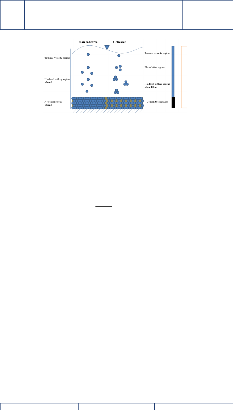
EDF R&D Reference manual
Sisyphe 6.3
H-P74-2012-02004-EN
Version 1.0
Figure 4 – Diagram of different processes involved in the settling transport (left : non-cohesive,
right : cohesive).
15.1 Multi-layer empirical algorithm
Time evolution
The consolidation effect is reproduced by assuming that the vertical flux of sediment from layer
jto underneath layer j+1 is proportional to the mass of sediments, Ms(kg/m2), contained in the
layer j.
dMs(j)
dt =aiMs(j)(59)
The transfer mass coefficients aj(in s−1) are specified in the steering file (MASS TRANSFER PER
LAYER). They correspond to a characteristic timescale to transfer mass from one layer to another.
This multilayer consolidation model is not related to Gibson equation so that it should be consi-
dered as empirical. Despite its apparent simplicity, it can qualitatively reproduce an increase of mud
bed deposit with time, while ensuring mass conservation (transfer coefficient of the last bottom layer
is zero). The model results are highly sensitive to the specified values of the mass transfer coefficients
aiwhich are however difficult to calibrate. The main advantage of this iso-pycnal formulation relies
in the fact that no vertical grid is required to compute the concentration evolution of the different
layers.
Discretization
The vertical resolution of semi-empirical equation (59) is based on the multi-layer iso-pycnal
model with fixed concentrations. The consolidation is then reproduced by mass transfer between
layers of the model. The transfer coefficients are fixed for each layer.
The set of mass-transfer coefficients a(j)in (s−1) are selected by calibration, in order to find best
agreement of time-varying concentration profiles between model and experiment. Physically, they
represent the inverse of the residence time per layer. The values a(j)are found to decrease from
top to bottom, as the time scale of consolidation (or residence time) increases. The mass transfer of
the last layer is set to zero, in order to insure no mass loss at the rigid bed level (impermeability
condition).
Accessibility : Interne : EDF SA Page 56 sur 73 c
EDF SA 2013

EDF R&D Reference manual
Sisyphe 6.3
H-P74-2012-02004-EN
Version 1.0
Keywords
–COHESIVE SEDIMENT = YES (= NO, default option)
–MUD CONSOLIDATION = YES (= NO, default option)
–CONSOLIDATION MODEL = 1, default option
–NUMBER OF LAYERS OF THE CONSOLIDATION MODEL (NOMBLAY=10 by default, maximum value
is 20 )
–MUD CONCENTRATION PER LAYER (in kg/m3,E=50.; 100.; ... by default)
–MASS TRANSFER PER LAYER (=5.0E−5, ..., 0., by default)
15.2 Multi-layer iso-pycnal Gibson’s model
15.2.1 Theoretical background
The previous equation presents the advantage of not using a vertical mesh. However it is not
physically based model since it neglects the Gibson theory. Improvement of this category of model
was proposed by Sanchez [41] and Thiebot [45]. In these formulations, the sediment flux from one
layer to the other is given not in term of empirical mass transfer coefficient (ai) but in term of
theoretical flux which is given by the Gibson theory.
15.2.2 Numerical discretization
The model originally developed by Sanchez [41] and Thiebot [45] is a 1DV sedimentation-
consolidation multi-layer model, based on an original technique to solve Gibson equation. The ad-
vantage of this representation (Equation 60) if compared with previous one (Equation 59) relies on
the right hand side term which relates the mass of sediments, Msi(kg), to the net flux entering or
leaving the layer. This equation enables therefore to consider the flux of sedimentation and consoli-
dation as provided by the Gibson theory.
dMsi
dt = (Fi(t)−Fi+1(t))∆tπr2(60)
In Equation 60, a circular shape (of radius r) is assumed for the surface. Equivalently, Equation 61
is expressed in term of layer thickness Esi(m), recalling Msi= Csiπr2Esi.. This last expression
becomes independent on the settling column geometry.
dEsi
dt =Fi(t)−Fi+1(t)
Csi
(61)
The concentration of the different bed layers Cs(i)is fixed. As the sedimentation and consolida-
tion progress, the sediment is transferred to the more concentrated layers, and the thickness of these
layers increase as well.
Accessibility : Interne : EDF SA Page 57 sur 73 c
EDF SA 2013
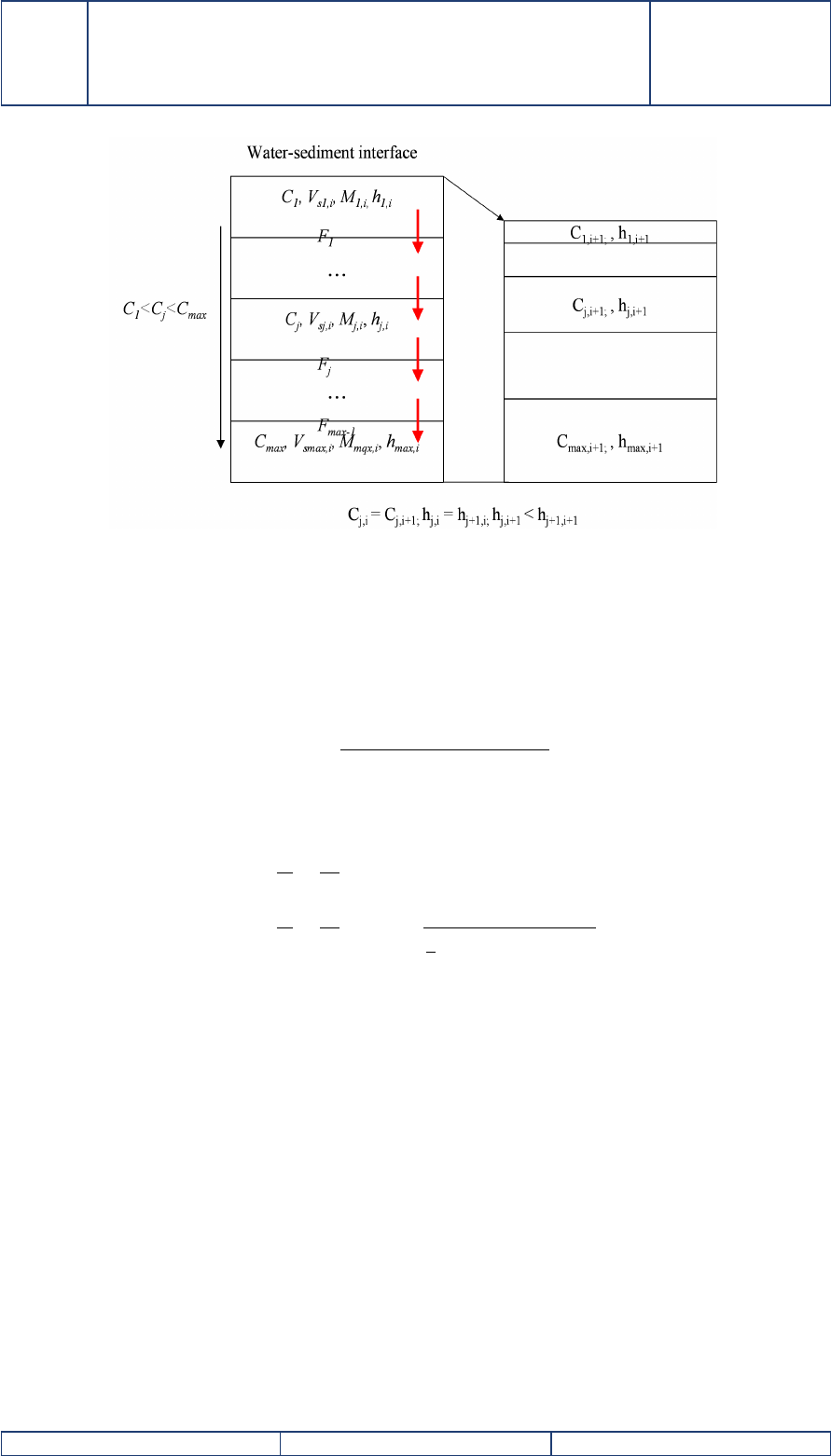
EDF R&D Reference manual
Sisyphe 6.3
H-P74-2012-02004-EN
Version 1.0
The mass conservation is ensured by requiring at each moment, in each layer, the equality bet-
ween the mass contained in a layer at time t+∆tand the mass present in this layer at time tin which
the outgoing mass was removed and the incoming mass was added (means the mass that crossed
the upper and lower sections respectively during the time ∆t). The outgoing and incoming masses
are taken into account by sediment flux noted Fi(t).
Fi(t) = (Vs,i(t)−Vs,i−1(t))Ci−1Ci
Ci−1−Ci
(62)
where Vs,iis the falling velocity of the layer i, and can be defined as :
Vs,i(Ci) =
k(Ci)Ci 1
ρs−1
ρf!, if Ci≤Cgel
k(Ci)Ci 1
ρs−1
ρf!+k(Ci)σ0(Ci−1)−σ0(Ci)
1
2(Epi−1(t) + Epi(t))
, otherwise
(63)
where kis the permeability, σ0is the effective stress, Cgel the transition concentration between
sedimentation and consolidation schemes (see Camenen & Pham Van Bang [9]).
15.3 Vertical grid Gibson’s model
Vertical-grid models propose a natural resolution of the Gibson equation as a vertical grid is used
to compute the concentration at each point. This category of model uses common techniques (finite
difference or finite volume or finite element methods) for resolving partial differential equations.
As they use a vertical grid, the connection with Sisyphe which is depth integrated model is not
straightforward.
In the new version of Sisyphe , such a category of model is also available. Strictly speaking,
the original Gibson model (in material coordinate) used in Telemac-3dwhich was developed by
Lenormant et al. [32] is connected to Sisyphe .
The finite difference method is used. The implicit scheme leads to a tridiagonal matrix that is
solved by using a classical double sweep algorithm. More details are given in Telemac-3duser
Accessibility : Interne : EDF SA Page 58 sur 73 c
EDF SA 2013

EDF R&D Reference manual
Sisyphe 6.3
H-P74-2012-02004-EN
Version 1.0
guide, LeNormand et al. [32] and Van [35].
16 Closure equations for permeability and effective stress
All of the Gibson based models, i.e. Multi-layer iso-pycknal Gibson’s model (section 15.2) and
vertical grid Gibson model (section 15.3), requires two closure equations. The Multi-layer empirical
model (section 15.1) only needs closure on ai, the mass transfer coefficients.
In this section, some available empirical formula are detailed. In general, a decreasing (or increa-
sing) function of solid concentration is considered for permeability K(or effective solid stress). These
expressions are logarithmic or exponential or power law functions (see Bartholomeeusen et al. [3]).
16.0.1 Closure equations
–Bed permeability k
Bartholomeeusen et al. [3] introduced typical functions, in the form of either power or expo-
nential, to relate the permeability kwith the void ratio e:
k=
A1eA2
A1φ−A2
s
exp(−A1+A2e)
The value of these coefficients A1and A2depend on grain size distribution, organic content,
activity and pore size distribution.
–Effective stress σ0
The similar way can be opted in the determination of σ0(e)(σ0(C),σ0(φ)), which gives :
(e=−B1σ0B2+B3
σ0=B1φB2
s
or e=B1(σ0+B2)−B3
σ0=exp(B4+B5e)
According to Winterwerp & van Kesteren (2004), the validity range of the power-type func-
tions (e.g. k=A1eA2,σ0=B1φB2
s) is much larger than that of the exponential-type functions.
Moreover, there is a physical insight in the formulation of the power-type functions. Therefore,
it is recommended to use power-type functions. However, two different power functions for
permeability may be necessary to represent the two separate processes : sedimentation and
consolidation.
16.0.2 Determination of parameters
No standard is found in the literature to recommend a specific methodology for calibrating the
empirical functions for both permeability and effective stress. Most of study reported some fitting
exercice on settling curve, i.e. the position of supernatant/suspension interface. They considered
mostly the least square technique for the adjustment to experimental results. However as stated
by Toorman [48] a more relevant adjustment is offered when concentration profiles are available
from Gamma-ray techniques (see Been and Sills [6] or Bartholomeeusen et al. [3]), X-ray technique
(Villaret et al. [59]) or MRI techniques (Pham Van Bang et al. [38]). In such a situation, the density or
concentration profile are adjusted on the measurement for different time. A specific procedure has
been recently proposed by Thiebot et al. [46], also based on least square method.
The user should consider the previous method (adjustment on settling curve or on concentration
profile) as conventional even through no shared procedure has been internationality recognized as
the best one (as previously discussed in 10.3). An recent alternative was successfully applied to
Gironde mud (Van [35]).
Accessibility : Interne : EDF SA Page 59 sur 73 c
EDF SA 2013

EDF R&D Reference manual
Sisyphe 6.3
H-P74-2012-02004-EN
Version 1.0
16.0.3 Space-time based method to determine parameters of closure equations
The new methodology to determine parameters is based on space-time analysis of data. It re-
quires data on time evolution of concentration (vertical) profile. If such an information is not avai-
lable, the proposed method becomes useless. If only the supernatant/suspension interface position
is detailed by data, the user should consider the classical fitting method.
If the space-time resolved data is available, this new methodology could be applied easily. The
method is based on a theoretical framework which is an advantage to help during the calibration
procedure. From time evolution of concentration profiles which are provided by non-intrusive tech-
niques (here the X-ray technique), the procedure uses self-similar analytical solutions to determine
the closure equation relative to the convection (or sedimentation) part and to the diffusion (or conso-
lidation) part of Gibson equation.
∂φ
∂t−∂
∂z[V(φ)φ]−∂
∂zD(φ)∂φ
∂z=0
where V(φ) = K(s−1)φand D(φ) = Kφ/γfdσ0/dφin order to match with Gibson equation 58 in
Eulerian coordinate.
Considering a separation regime between sedimentation and consolidation (or between convec-
tion and diffusion), self-similar solutions are obtained for each regime. The separation between both
problems is justified by the fact that effective stress should be zero for a suspension since there is no
direct contact between particles.
16.0.4 Determination of closure equation for the sedimentation
If the concentration of the suspension is lower than a given threshold (the so-called gelling point
for cohesive sediment), the inter-particle contacts are negligible, i.e. there is no solid (or effective)
stress (Camenen & Pham Van Bang [9]). In such a situation the Gibson equation (58) is simply
reduced to the equation of Kynch :
∂φ
∂t−∂
∂z[V(φ)φ]=0 (64)
where φ=C/ρsis the volume fraction of solids, V(φ)is the settling velocity of the suspension at
concentration φthat is equal to K(s−1)φ.
Considering the self-similar variable ζ=z/tand similarity solution U, i.e. φ(z,t) = U(ζ), equa-
tion 64 leads to :
d f
dU −ζdU
dζ=0
where fis the solid (or sedimentation) flux, which is equal to −V(φ)φ.
The method is equivalent to the so-called method of characteristics (Leveque [33]). The iso-
concentration pattern presents different straight lines in the space-time (z−t)plot. The slopes of
iso-concentration straight lines in the z−tplane are measured to obtain the first derivative of the
solid flux. The sedimentation flux proposed for the Gironde mud (Villaret et al. [59] ; Van [35]) is
given by equations 65 or 66. The first derivative of this closure equation is straightforward [59] : the
determination and validation of its parameters (Vst,φgel,n) has been presented in details in the test
case of settling column of Gironde mud :
f(φ) = Vst(1−φ) 1−φ
φgel !n
φfor φ<φgel (65)
Accessibility : Interne : EDF SA Page 60 sur 73 c
EDF SA 2013

EDF R&D Reference manual
Sisyphe 6.3
H-P74-2012-02004-EN
Version 1.0
and
f(C) = Vst(1−C
ρs
) 1−C
Cgel !nC
ρsfor C<Cgel (66)
where Vst is the Stokes velocity of an equivalent sphere, φgel (Cgel)is the gelling concentration,
nis an exponent. Both parameters have physical meanings in terms of rheology (Pham Van Bang
et al. [38]). Indeed, φgel(Cgel)is the concentration value from which the effective viscosity of the
suspension diverges. And n is a parameter describing the transition from suspension to a structured
bed. It is worth noting that the so-called Richardson & Zaki empirical model is recovered by setting
φgel =1.
16.0.5 Determination of closure equation for the consolidation
Still considering separation regime between sedimentation (convective problem) and consolida-
tion (diffusion problem), for cohesive sediment and concentration larger than the gelling point, the
effective solid stress build up. The diffusion term is no longer negligible and becomes the leading
term in the Gibson equation. For concentration larger than the gel point, the convective part is an-
nihilated in the proposed formulation so that only the diffusion term remains. As this term takes
origin from the competition between the seepage flow through a porous media and the effective
stress of the solid skeleton (Camenen & Pham Van Bang [9]), the diffusion is expressed by an ex-
pression with the permability Kand the effective stress (dσ0/dφ). The problem is now related to the
non-linearity of the diffusion :
∂φ
∂t−∂
∂zD(φ)∂φ
∂z=0 (67)
where D(φ)is the non linear diffusion term, equal to Kφ(dσ0/dφ)/γfin order to match with
(58).
The power law is assumed for the diffusion coefficient. Indeed, if we consider a power law for the
permeability and a power law for the effective stress, the diffusion coefficient will also be a power
function of concentration. Here the possible time dependence of the effective stress is investigated
so that the secondary consolidation is also taken into consideration (cf. 10.3). As a result, the non
linear diffusion coefficient is assumed to depend on both concentration and time by an empirical
power law, i.e. D(φ) = D0φatb. Here the time dependence of the consolidation is introduced to
mimic the thixotropic behaviour of mud. Introducing as a self-similar variable, χ=z/tθwith θ=
(1+b)/(2+a)and the similarity solution h, i.e. φ(z,t) = h(χ)/tθin equation (67) leads to :
∂φ
∂t−∂
∂zD0φatb∂φ
∂z=0→d
dχha(χ)dh
dχ−θχh(χ)=0
The similarity solution his obtained after integration of the previous ODE equation (see Van [35]).
The parameter Mis a constant whose value corresponds to the total mass of sediment in the system.
h(χ) =
M−a(1+b)χ2
2(2+a)1/a
for χ∈"0, −2M(2+a)
a(1+b)1/2#
0 for χ≥−2M(2+a)
a(1+b)1/2
In order to find out the closure equation for effective stress, from the above equations, it is
needed to determine the two variables : a,b. This procedure will be presented in detail in test case
Tassement 2, with a given experimental result of settling column.
Accessibility : Interne : EDF SA Page 61 sur 73 c
EDF SA 2013

EDF R&D Reference manual
Sisyphe 6.3
H-P74-2012-02004-EN
Version 1.0
Keywords
–COHESIVE SEDIMENT = YES (= NO, default option)
–MUD CONSOLIDATION = YES (= NO, default option)
–CONSOLIDATION MODEL = 2
–GEL CONCENTRATION = CONC GEL
–PERMEABILITY COEFFICIENT = COEF N
–NUMBER OF LAYERS OF THE CONSOLIDATION MODEL = NOMBLAY (<20)
–MUD CONCENTRATION PER LAYER
Accessibility : Interne : EDF SA Page 62 sur 73 c
EDF SA 2013
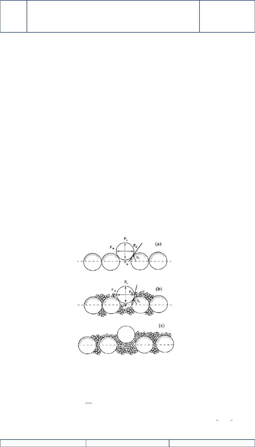
EDF R&D Reference manual
Sisyphe 6.3
H-P74-2012-02004-EN
Version 1.0
17 Mixed sediments processes
17.1 Mixte sediment bed composition
A sand-mud mixture is composed of two classes of bed sediments : The first class (noted 1)
is non-cohesive and represented by its grain diameter D1and can be transported as bed-load or
suspended load. The settling velocity ws1is a function of the relative sediment density (s=1.65)
and grain diameter D1. So far we assume only suspended load, which implies that the model is
devoted to mixtures of fine sand grains and mud.
The second class (noted 2) is cohesive, grain diameter D2less than 60 mm. The settling velocity
ws2is a function of flocs properties which differs from the individual cohesive particles, and needs
to be specified. The mass concentration is the mass of sediments per volume occupied by the mud
component (solid particles +water).
17.2 Erosion/deposition of sand-mud sediment bed
The erosion/deposition fluxes depend on the mass percentage % of each class in the surface layer
(Panagiotopoulos et al., 1997). If the mass percent of the mud class is greater than 50%, the bed is
considered as pure cohesive and the erosion/deposition laws follow the Partheniades classical law
(see below for the calculation of the bed shear strength in a sand/mud mixture).
If the mass fraction of mud percentage is less than 30%, the bed is considered as non-cohesive,
and has little effect on the bed shear strength. If the mass fraction of mud percent is greater than
30%, the bed is considered as cohesive. The rate of erosion is based on the Partheniades erosion law,
where the critical bed shear strength of the mud class depends on the consolidation state. Different
regimes can be considered depending on the volume content of each class, as pictured below :
Figure 5 – (a) Sand regime ( f2<30%) ; (b) Intermediate ; (c) Mud-dominated regime ( f2>50%).
17.3 Critical erosion shear stress of sand mud mixture
The mean bed shear strength (τce) of the sand/mud mixtures depends on the mass percentage %
of mud f2at the surface and depends on the layer. The proposed framework is based on the work
of Waeles (2005). The bed shear strength is calculated in the subroutine suspension flux mixte.f
Accessibility : Interne : EDF SA Page 63 sur 73 c
EDF SA 2013
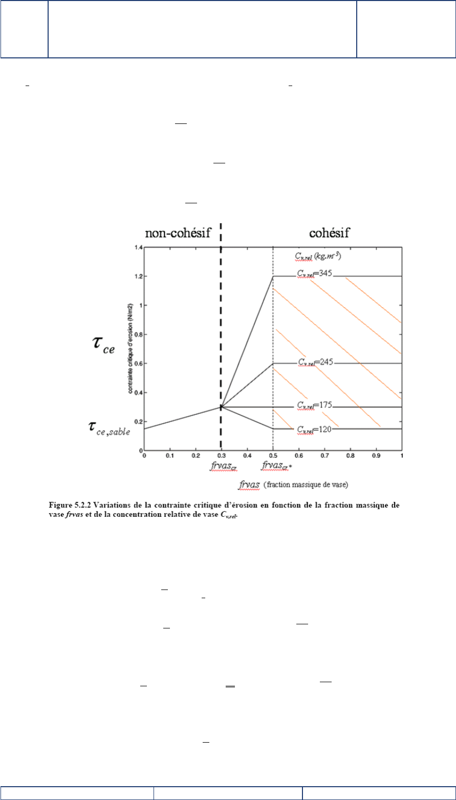
EDF R&D Reference manual
Sisyphe 6.3
H-P74-2012-02004-EN
Version 1.0
(TOCE MIXTE, for τce). For each layer (K), the expression of TOCE MIXTE depends of the mass percent
of mud in the layer :
– For f2<30%, τce =τce(1)for pure sand, based on
τce =τce(1) = Θcgd50(s−1)(68)
– For f2>50%, τce =τce(2)for pure mud as a function of bed layer concentration
τce =τce(2)(69)
– In the intermediate range (30% <f2<50%) :
τce =f1τce(1) + f2τce(2)(70)
Figure 6 – Mixed sediment bed structure.
The potential erosion flux depends on the composition of the bed layer. The first step is to deter-
mine a mean erosion rate per layer E(FLUER LOC) :
– For f2<30% (sand dominant) : we use the equilibrium concentration concept :
E=E1=ws1Ceq, for τbτce
0, otherwise (71)
– For f2>50% (mud dominant) : the Partheniades erosion law can be applied :
E=
E2=Mτ0
τce 2−1for τb>τce
0 otherwise
– For 30% <f2<50% (intermediate range) : the mean erosion rate is an average value of the
erosion classes of both classes :
E=f1E1+f2E2
Accessibility : Interne : EDF SA Page 64 sur 73 c
EDF SA 2013

EDF R&D Reference manual
Sisyphe 6.3
H-P74-2012-02004-EN
Version 1.0
17.4 Iterative procedure
The next step is to calculate the mean erosion flux for both classes of bed material. The underlying
assumption is that the eroded depth is the same for both classes. This is done iteratively, by checking
layer by layer (starting from the top) how much sediment there is in the layer and how much time
it would take to empty that layer entirely : This procedure is necessary because the bed is stratified
and the eroded depth is unknown.
At the start of time step (t0), the first layer whose thickness is non-zero is eroded, at a given rate
e(j). For each erodible layer jwith E(j)>0, the time interval dt(j)to erode completely layer jis
estimated based on the mass of the layer :
dt(j) = dMs(j)
ρsE(j)=dEs(j)Cs(j)
ρsE(j),
where the potential erosion rate E(j)decreases and tends to zero as jincreases. The last (non-empty)
layer (noted jmax) to be eroded is obtained by emptying all successive top layers until :
jmax−1
∑
j=1
dt(j)<Dt <
jmax
∑
j=1
dt(j).
For jmax, the time left to erode the last layer is Dtmax =Dt −∑jmax−1
j=1Dt(j). The total (mud and sand)
mass potentially eroded during this process is :
Ms=
jmax−1
∑
j=1
Ms(j) + ρsE(jmax)Dtmax.
The mean mass erosion flux of the sand-mud mixture Es(Kg/m/s) is therefore estimated as
Es=Ms
Dt .
Here we assume that both mud and sand are eroded simultaneously to the same depth, therefore
the eroded volume flux of each phases is differentiated by their mass percent :
E1=Ms1
ρsDt ,E2=Ms2
ρsDt .
17.5 Definition scheme of sand-mud mixture in Sisyphe
17.5.1 Assumptions
In this framework, the sand particles are assumed to be fully embedded in the cohesive frame-
work. So this is valid for cohesive dominant regime. The density of individual primary or sand
particles is assumed to be constant and equal to ρs=2650 kg/m3
Accessibility : Interne : EDF SA Page 65 sur 73 c
EDF SA 2013
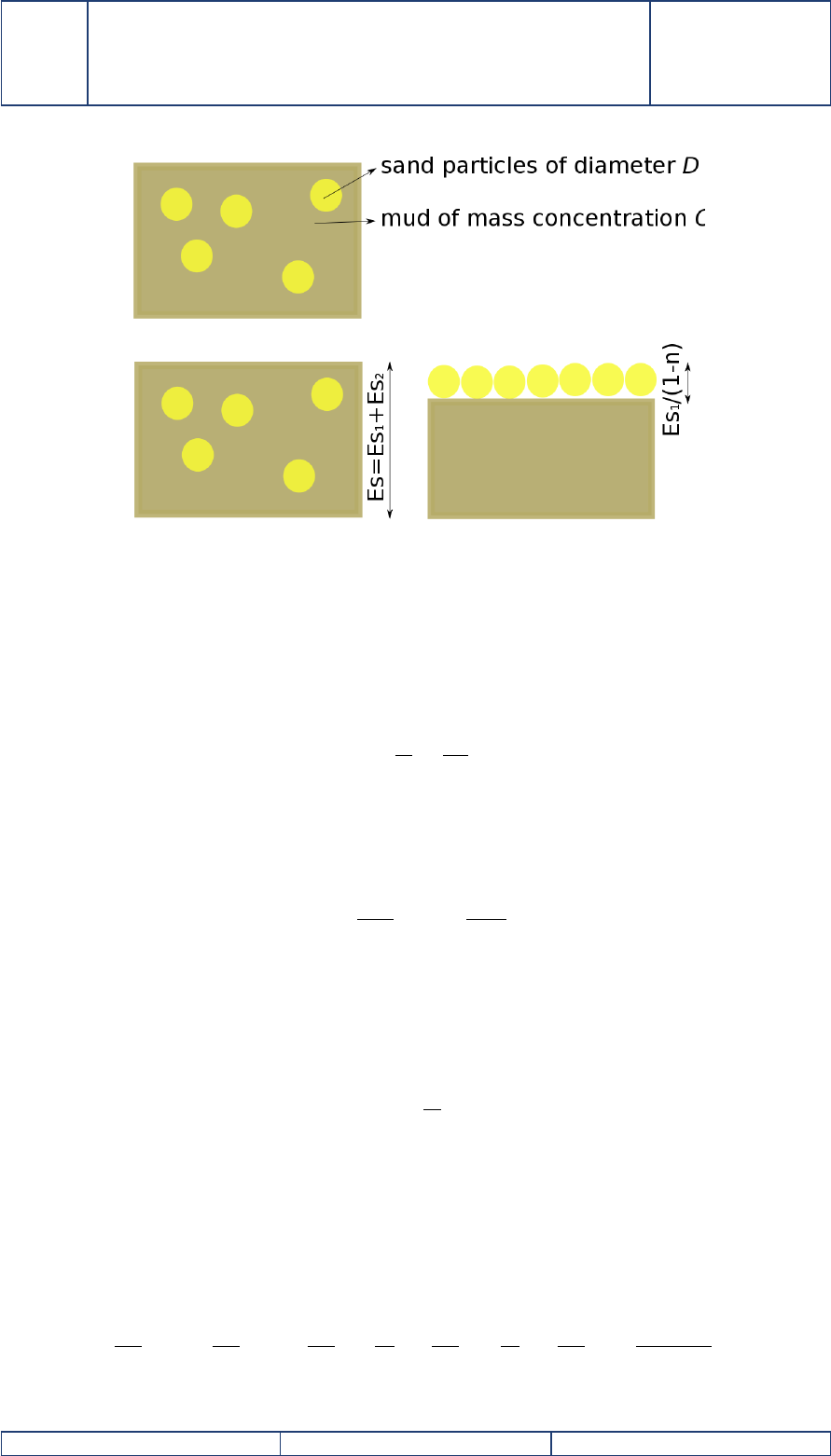
EDF R&D Reference manual
Sisyphe 6.3
H-P74-2012-02004-EN
Version 1.0
Figure 7 – Critical erosion shear stress of sand-mud mixture (from Waeles [62]).
17.5.2 Bed structure
The sand-mud mixture is characterized by the volume percent of each class :
Pi=Vi
Vt
=Esi
Et,
where Viis the volume occupied by the sand or mud particles i=1, 2, Vt=V1+V2, is the total
volume, Esi=piEs is the volume per unit surface area of phase iand corresponds to the vertical
thickness of each phase (voids are not included), and Etis the total volume (sand +mud) per unit
surface area Et=E1+E2. It is also useful to define the mass percent of each class, for sand f1and
for mud f2:
f1=ρsV1
Mt;f2=C2V2
Mt,
where C2is the mud density, which varies with distance for the bed surface and Mtthe total mass
of the sand-mud mixture :
Mt=C2V2+ρsV1.
Once sediment particles have been put in suspension, they are transported independently, by
solving for each class a transport equation for the volume solid concentrations, defined as :
Ci=Vi
Vt,
with Vt=V1+V2+Vwater. The volume and density of suspended cohesive flocs vary as a result of
flocculation, so what is conserved here is the volume of primary constitutive particles of density ρs.
17.6 Suspended sediment transport equation
Both sand and mud are treated separately and independently. We solve here the volume 2D (
depth integrated) concentrations of the primary particles, assuming constant density ρs:
∂Ci
∂t+Uconv ∂Ci
∂x+Vconv ∂Ci
∂y=∂
∂xes∂Ci
∂x+∂
∂yes∂Ci
∂y+(Ei−Di)
h
Accessibility : Interne : EDF SA Page 66 sur 73 c
EDF SA 2013
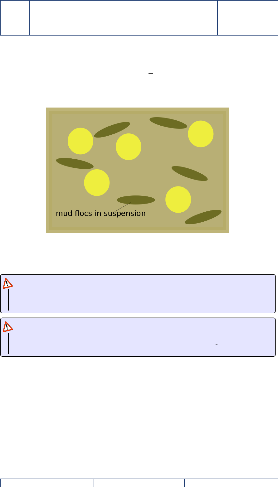
EDF R&D Reference manual
Sisyphe 6.3
H-P74-2012-02004-EN
Version 1.0
– For sand : D1=ws1CF1, with F1the ratio between the near bed concentration and depth-
averaged concentration.
– For mud :
D2=(ws2C1−τ
τd, for τ≤τd
0 otherwise
with τdthe critical bed shear stress for deposition.
Figure 8 – Mixed sediment in suspension.
Attention
In the subroutines, the definitions of Sisyphe variables are : horizontal point index : I; layer
index : K; number of classes of bed material (NSICLA = 2) ; J=1: sand ; J=2: mud ; grain
sizes : FDM(J) and number of bed layers : COUCH TASS.
Attention
For pure mud, the bed shear strength increases as the concentration of the mud increases
while consolidation is taking place. Mud concentration per layer : CONC VASE (K) (Kg/m3) ;
critical erosion shear stress per layer : TOCE VASE(K) (N/m2).
Accessibility : Interne : EDF SA Page 67 sur 73 c
EDF SA 2013

EDF R&D Reference manual
Sisyphe 6.3
H-P74-2012-02004-EN
Version 1.0
Keywords
To enable the mixed sediment transport in Sisyphe , the following keywords should be speci-
fied in the steering file :
–MIXED SEDIMENT = YES (= NO, default option)
–COHESIVE SEDIMENTS = YES (= NO, default option. In Sisyphe , the first sediment class is
always sand and the second is mud)
–NUMBER OF SIZE-CLASSES OF BED MATERIAL = 2 (NSICLA)
–INITIAL FRACTION FOR PARTICULAR SIZE CLASS = f1;f2(example : =0.80; 0.20)
–SEDIMENT DIAMETERS = D1, D2 (for non-cohesive sediments D1>6.0E-5, for cohesive sedi-
ments D1<6.0E-5, example with 300 µm for sand and 60 µm for mud : =0.0003; 0.00006)
–SEDIMENT DENSITY = 2650 (the sediment density is only for sand, while the mud density is
defined in the keyword MUD CONCENTRATION PER LAYER)
–SETTLING VELOCITIES = ws1,ws2(example =4.E−02; 1.E−02, if this one is active, only
one value is taken for calculation. It is corrected later in the subroutine)
–INITIAL SUSPENSION CONCENTRATIONS (example =0.0002; 0.0002)
–NUMBER OF LAYERS OF THE CONSOLIDATION MODEL (NOMBLAY = 10, default option)
–MUD CONCENTRATION PER LAYER (in kg/m3,CONC VASE= 50.; 100.;..., default option)
–CRITICAL EROSION SHEAR STRESS OF THE MUD (example =0.5; 10.0)
17.7 Fortran subroutines for mixed sediment transport
–INIT SEDIMENT : This subroutine initializes the bed composition (by calling INIT MIXTE for
mixed sediment transport) and calculates the settling velocity, if not present in the steering
file Moreover, shields parameter and CRITICAL EROSION SHEAR STRESS OF THE SAND known
as TOCE SABLE is calculated in this subroutine as well.
–INIT MIXTE : This subroutine calls INIT COMPO COH to initialize the composition of the sediment
bed and also check the thickness of each bed layer. The initial masses of sand and mud are
also calculated here. It can be seen that XMVS is the sand density defined in the steering file
while CONC(I,J) is the mud density of each bed layer defined in the steering file to known as
MUD CONCENTRATION PER LAYER. For this subroutine, the density of the sand is assumed to be
constant (XMVS) and the following variables are defined :
– Mass per unit surface area of the sand : MS SABLE(I,K) (Kg/m2)
– Mass per unit surface of the mud : MS VASE(I,K) (Kg/m2)
– Total Mass per layer : MS TOTAL(I,K) = MS SABLE(I,K) + MS VASE(I,K)
– Mass percent of each phase per layer : Fs(I,K,1) = MS SABLE(I,K)/MS TOTAL(I,K) and
Fs(I,K,2) = MS VASE(I,K)/MS TOTAL(I,K)
– Initial mass of the sand bed : MASS0
– Initial mass of the mud bed : MASV0
–INIT COMPO COH : This subroutine initializes fraction distribution of sand and mud. The thick-
ness of each bed layer is also defined here. For this simulation, there are two bed layers defined
in this subroutine as the sum of the thickness of mud per layer (EPAI VASE) and the thickness of
sand per layer (EPAI SABLE). The modification is made for reading sand fraction from data file.
We do not take into account the porosity of sand, because we assume the void to be entirely
filled up by the fine particles. This may be wrong when the mud percent % is lower than the
void ratio (in case of bedload layer for example). Up to 6.3, the present the mixte sediment
formulation is only valid assuming the sand grains to be imbedded in the cohesive frame.
– Release 6.3 : the thickness of each sand layer corresponds here to the volume occupied by
the sand particles, per unit surface area.
– Bed layer thickness for sand : EPAI SABLE(K) (m)
– Bed layer thickness for mud (m) : EPAI VASE(K) (m)
– Bed layer thickness (mud and sand) : ES(I,K) = EPAI SABLE (K) + EPAI VASE (K)
– Volume percent of each phase : AVAIL(I,K,1) = EPAI SABLE(K)/ES(I,K) and AVAIL(I,K,2)
= EPAI VASE(K)/ES(I,K)
– Future release : introduce a test on AVAIL (only correct if AVAIL(I,K,2) > void ratio of ≈0.4
Accessibility : Interne : EDF SA Page 68 sur 73 c
EDF SA 2013

EDF R&D Reference manual
Sisyphe 6.3
H-P74-2012-02004-EN
Version 1.0
(=1-XKV))
–SUSPENSION COMPUTATION : This is the main subroutine for the computation of the suspension
load and the bed elevation. It has the following steps :
1. COMPUTES THE REFERENCE ELEVATION --> ZREF
2. ADVECTION VELOCITY --> UCONV, VCONV, TAKING INTO ACCOUNT THE VERTICAL PROFILE
OF CONCENTRATIONS AND VELOCITIES
3. EROSION FLUX : FLUER In this part, the subroutine SUSPENSION FLUX MIXTE is called to
compute the suspension for the sand and mud mixture.
4. DEPOSITION FLUX : FLUDPT =WC*T2 This subroutine calls SUSPENSION DEPOT to compute
the sand and mud deposition.
5. DIFFIN A SPECIFIC TREATMENT IS DONE IF THE ADVECTION METHOD IS THE CHARACTERISTICS:
FREE OUTPUTS ARE TREATED LIKE DIRICHLET. THIS SPECIFIC TREATMENT IS CANCELLED
HERE BY SENDING A MODIFIED VALUE FOR RESOL.
6. BOUNDARY CONDITIONS : CBORCONC V The keyword IMP INFLOW C is found here for control-
ling the calculation of equilibrium concentration at open boundaries.
7. SOLVING TRANSPORT EQUATION IF METHOD OF CHARACTERISTICS
8. SOURCE AND SINK TERMS (IMPLICIT SOURCE TERM FOR THE DEPOSITION T9 AND EXPLICIT
SOURCE TERM WITHOUT PUNCTUAL SOURCES T11)
9. ADVECTION-DISPERSION STEP CONFIGURATION OF ADVECTION
10. BED EVOLUTION DUE TO NET EROSION/DEPOSITION FLUX The subroutine SUSPENSION EVOL
is called from here to calculate the bed evolution.
Accessibility : Interne : EDF SA Page 69 sur 73 c
EDF SA 2013

EDF R&D Reference manual
Sisyphe 6.3
H-P74-2012-02004-EN
Version 1.0
R´
ef´
erences
[1] Ashida K. and Mishiue M., 1973. Studies on bed load transport rate in alluvial streams, Trans JSCE,
vol.4.
[2] Bailard J., 1981. An energetics total load transport model for a plane sloping beach. Journal of
Geophysical Research, 86, C11, 10938-10954.
[3] Bartholomeeusen, G., Sills, G.C., Znidarcic, D., van Kesteren, W., Merckelbach, L.M., Pyke, R.,
Carrier, W.D., Lin, H., Penumadu, D., Winterwerp, H., Masala, S. and Chan, D., 2002, Sidere :
numerical prediction of large strain consolidation, G´
eotechnique 52, No. 9, 639-648.
[4] Begnudelli L., Valiani A. and Sanders B.F., 2010. A balanced treatment of secondary currents,
turbulence and dispersion in a depth-integrated hydrodynamic and bed deformation model for
channel bends. Advances in Water Resources, 33(1).
[5] Belleudy P., 2000. Numerical simulation of sediment mixture deposition, part 1 : analysis of a
flume experiment, Journal of Hydraulic Research, Vol.38, N◦6.
[6] Been, K. and Sills, G.C., 1981, Self weight consolidation of Soft Soils : an Experimental and Theoretical
Study. Geotechnique, Volume 31, No.4, pp. 519-535.
[7] Bijker E.W., 1968. Mechanics of sediment transport by the combination of waves and current. In
Design and Reliability of Coastal Structures, 23rd Int. Conf. on Coastal Engineering, 147-173.
[8] Camenen B., 2002. Mod´elisation num´erique du transport s´edimentaire sur une plage sableuse. Ph.D
thesis, Universit´
e Joseph Fourier, Grenoble 1.
[9] Camenen B. & Pham Van Bang D., 2011. Modelling the settling of suspended sediments for concen-
trations close to the gelling concentration, Cont. Shelf Res., 31, S106-S116.
[10] Blue Kenue : Tutorial Manual for the Mesher in BlueKenue. Canadian Hydraulics Centre (CHC)
of the National Research Council, 2013.
[11] Celik I., Rodi W., 1988. Modelling Suspended Sediment Transport in non- equilibrium situa-
tions, Journal of Hydraulic Eng., Vol. 114, N◦10.
[12] Chollet J.P. and Cunge J.A., 1980. New interpretation of some headlooss - flow velocity relation-
ship for deformable bed, J. Hydr. Eng., 17 (1).
[13] Davies A.G. and Villaret C., 2004. Modelling the effect of wave-induced ripples on littoral sand trans-
port. EDF-LNHE Report HP-75/03/029/A.
[14] Dibajnia M., Watanabe A., 1992. Sheet flow under non-linear waves and currents. Proc. of the Intl.
Conf. on Coast Eng., 2015-2029.
[15] Die-Moran A., 2012. Physical and Numerical modelling investigation of induced bank erosion as a
sediment transport restoration strategy for trained rivers. The case of the Old Rhine (France). Universit´
e
Paris-Est.
[16] Egiazaroff I.V., 1965 : Calculation of non-uniform sediment concentrations, J. of Hydr. Div. ASCE,
vol. 91, N◦4, pp. 225-248.
[17] Einstein H.A. (1950). The bed load function for sediment transportation in open channel flow. US Dep.
Of Agriculture, Techn. Bull.
[18] Engelund F. and Hansen E., 1967. A monograph on sediment transport in alluvial streams. Techn.
Univers. Of Denmark, Copenhagen, Denmark.
[19] Engelund F., 1974. Flow and bed topography in channel bends. J. Hydraul. Div. Am. Soc. Civ. Eng.,
100, 1631-1648.
Accessibility : Interne : EDF SA Page 70 sur 73 c
EDF SA 2013

EDF R&D Reference manual
Sisyphe 6.3
H-P74-2012-02004-EN
Version 1.0
[20] Gibson, R.E., Englund, G. L. and Hussey, M. J. L., 1967, The theory of one dimensional consolidation
of saturated clay, I. Finite Non-Linear Consolidation of Thin Homogeneous Layers. Geotechnique, pp.
261-273.
[21] Gibson, R.E., Schiffman, R.L. and Cargill, K.W., 1981, The theory of One dimensional Consolida-
tion of Saturated Clays, II. Finite Nonlinear Consolidation of Thick Homogeneous Layers. Canadian
Geotechnical Journal, Vol. 18, pp. 280-293.
[22] Gonzales de Linares M., 2002. Graded sediment in Sisyphe. Rapport EDF-LNHE, HP-75/2002/68.
[23] Hirano, M., 1970. On phenomena of river-bed lowering and armouring below reservoirs. In Proc. 14th
Hydraul. Lecture Meeting, 13-14 Feb., Civ. Eng. Ass. Hydr. Committee, Hatsumei Kaikan.
[24] Hervouet J.-M., Hydrodynamics of free surface flows : modelling with finite element methods, John
Wiley & Sons, 2007.
[25] Hervouet J.M., Razafindrakoto E., Villaret C., 2011. Dealing with dry zones in free surface flows, a
new class of advection scheme. IAHR conference, July 2011.
[26] Hunziker R.P., 1995. Fraktionsweiser Geschuebetransport, Ph.D. thesis, Mitteeilungen Nr 138 deer
Versuchanstalt fur Wasserbau, Hydrologie und Glaziologie, ETH Zurich, Switzerland.
[27] Huybrechts N., Villaret C., Hervouet JM, 2010. Comparison between 2D and 3D modelling of sedi-
ment transport : application to the dune evolution. Proceedings of the RiverFlow conference.
[28] Huynh-Thanh and Temperville A., 1991. A numerical model of the rough turbulent boundary layer
in combined wave and current interaction. In Sand Transport in Rivers Estuaries and the Sea, eds
RL Soulsby and R. Bettess, pp. 93-100, Balkema, Rotterdam.
[29] Julien P. (2010). Erosion and sedimentation, second edition. Cambridge University Press, Cam-
bridge.
[30] Karim M.F. and Kennedy J.F., 1982. A computer based flow and sediment routing. IIH Report N◦250
Modelling for streams and its application to the Missouri River, University of Iowa, Iowa City,
IA.
[31] Koch F.G. and Flokstra C., 1981. Bed level computations for curved alluvial channels, XIXth Congress
of the International Association for Hydraulic Research, New Delhi India.
[32] Lenormant, C., Lepeintre, F., Teisson, C., Malcherek, A., Markofsky, M., and Zielke, W., 1993,
Three dimensional modelling of estuarine processes. In MAST Days and Euromar Market, Project
Reports Volume 1.
[33] Leveque, Randal J., 2002, Finite-Volime Methods for Hyperbolics Problems, Cambridge Texts in
Applied Mathematics, ISBN 0-511-04219-1 eBook.
[34] Mc Anally, W.H., 1999. Aggregation and deposition of fine estuarial sediment Floculation. Ph.D.
Thesis, Univ of Fla, Gainesville, Fla.
[35] Van, L.A., 2012. Mod´elisation du transport de s´ediments mixtes sable-vase et application `a la morpho-
dynamique de l’estuaire de la Gironde (France). Ph.D. thesis, Universit´
e Paris-Est.
[36] Merkel U.H. and Kopmann R., 2012. Continuous vertical grain sorting for Telemac & Sisyphe v6p2,
Proceedings of the XIX Telemac-Mascaret User Conference. Oxford, UK.
[37] Meyer-Peter E. and Muller R., 1948. Formulae for bed-load transport. Int. IARH Congress, Stock-
holm, Sweden.
[38] Pham Van Bang D., Ovarlez G., Tocquer L., 2007. Density and structural effects on the rheological
characteristics of mud. La Houille Blanche, 2, 85-93.
Accessibility : Interne : EDF SA Page 71 sur 73 c
EDF SA 2013

EDF R&D Reference manual
Sisyphe 6.3
H-P74-2012-02004-EN
Version 1.0
[39] Ribberink J., 1987. Mathematical modelling of one-dimensional morphological changes in rivers with
non-uniform sediment. PhD thesis, Delft University.
[40] Roelvink J.A., Coastal morphodynamic evolution techniques, Coastal Engineering, 2006, 53, 277-287.
[41] Sanchez, M., 1992, Mod´elisation dans un estuaire `a mare : Rˆole du bouchon vaseux dans la tenue des
sols sous marins. PhD thesis. University of Nantes (232 pages).
[42] Soulsby R., 1997. Dynamics of marine sands. Thomas Thelford Edition.
[43] Swart D.H., 1976. Offshore sediment transport and equilibrium beach profiles. Delft Hydraulics Pu-
blication 131, Delft University, The Netherlands.
[44] Talmon, A.M., Striksma, N. and van Mierlo, M.C.L.M. (1995). Laboratory measurements of the
direction of sediment tranport on transverse alluvial-bed slopes. Journal of Hydraulics Research,
33, 495-517.
[45] Thi´
ebot J., 2008, Mod´elisation num´erique des processus gouvernant la formation et la d´egradation des
massif vaseux. PhD thesis ENGREF, University of Caen, 130 pp.
[46] Thiebot, J., Guillou, S., Brun-Cottan, J-C., 2011, An optimisation method for determining permea-
bility and effective stress relationships of consolidating cohesive sediment deposits, Continental Shelf
Research 31 (2011) S117-S123.
[47] Toorman E. A., 1996, Sedimentation and self-weight consolidation : general unifying theory,
G´
eotechnique 46, N◦1, pp. 101-113.
[48] Toorman, E.A., 1999. Sedimentation and self-weight consolidation : constitutive equations and nume-
rical modelling. G´
eotechnique, 49(6) :709-726.
[49] Tanaka, H. and Dang, V.T., 1996. Geometry of sand ripples due to combined wave-current flows.
J. of Waterway, Port, Coastal and Ocean Engineering, ASCE, 122 (6), 298-300.
[50] Terzaghi, K. 1923. Die Berechnung des Durchlassigkeitsziffer des Tones aus des Verlauf des hydrody-
namischen Spannungerscheinungen, Sitz. Akad. Wissen. Wien, Math. Naturwiss. Kl., Abt IIa, 132,
125-138.
[51] van Rijn L.C., 1984. Sediment transport - Part I : bed load - Part II : suspended load, J. of
Hydraulic Division, Proc. ASCE, 110, HY10, 1431-56, HY11, 1613-41.
[52] van Rijn L.C., 1987. Mathematical modelling of morphological processes in the case of suspended sedi-
ment transport, Doctoral Thesis, Faculty of civil engineering, Delft University of technology).
[53] van Rijn L.C., 1993. Principles of Sediment Transport in Rivers, Estuaries and Coastal Seas. Aqua
Publications.
[54] van Rijn, L.C., 2007 Unified view of sediment transport by currents and waves. 1. Initiation of
motion, bed roughness, and bed-load transport. Journal of Hydraulic Engineering, 133, 6, 649-667.
[55] Villaret C., 2001. Prise en compte des fonds non-´erodables dans le logiciel Sisyphe, Rapport EDF-LNH,
HP-75/02/045/B.
[56] Villaret C., 2001. Mod´elisation du transport solide par la formule de Bijker-Etude de sensibilit´e et tests
validation. Rapport EDF R&D LNHE HP-75/2001/66/A.
[57] Villaret C. and Davies A.G., 2004. Numerical modeling of littoral sand transport. ICCE Conference,
Portugal, September.
[58] Villaret C., Walther R., 2008. Numerical modeling of the Gironde estuary. Physics of Estuaries and
Coastal Sediments, Liverpool, August 2008.
Accessibility : Interne : EDF SA Page 72 sur 73 c
EDF SA 2013

EDF R&D Reference manual
Sisyphe 6.3
H-P74-2012-02004-EN
Version 1.0
[59] Villaret C., Van L.A., Huybrechts N., Pham Van Bang D., Boucher O. 2010. Consolidation effects
on morphodynamics modelling : application to the Gironde estuary. La Houille Blanche, N◦6-2010,
15-24.
[60] Wiberg P.L. and Harris C.K., 1994. Ripple geometry in wave-dominated environments. Journal
of Geophysical Research 99 (C1), 775-789.
[61] Winterwerp J.C. and van Kesteren W.G.M., 2004. Introduction to the Physics of Cohesive Sediment
Dynamics in the Marine Environment. Elsevier, 576 pages.
[62] Waeles B., 2005. Detachment and transport of slay sand gravel mixtures by channel flows. Ph.D. thesis,
University of Caen.
[63] Yalin, MS, 1977. Mechanics of sediment transport. Pergamon Press, Oxford.
[64] Yalin M.S. and Ferrera da Silva A.M.F., 2001. Fluvial Processes. IAHR monograph Delft Hydrau-
lics.
[65] Wu W., 2008. Computational River Dynamics. Taylor and Francis Group, London, UK.
[66] Zyserman J.A. and Fredsoe J. 1994. Data analysis of bed concentration of suspended sediment,
Journal of Hydraulic Engineering, ASCE, Vol. 120, N◦9, pp 1021-1042.
Accessibility : Interne : EDF SA Page 73 sur 73 c
EDF SA 2013
