Ssm Manual

ssm_manual

User Manual: Pdf

Open the PDF directly: View PDF .
Page Count: 44

State Space Models Manual

Jyh-Ying Peng1, John A. D. Aston2

1Institute of Information Science, Academia Sinica∗

2Department of Statistics, University of Warwick

July 1, 2011

∗Address for Correspondence:

Institute of Information Science,

Academia Sinica

128 Academia Road, Sec 2

Taipei 115, Taiwan

email: jypeng@iis.sinica.edu.tw

2 Peng & Aston

Contents

1 Introduction 4

2 How to Cite State Space Models Toolbox 4

3 The State Space Model Equations 4

3.1 LinearGaussianmodels.......................................... 4

3.2 Non-Gaussianmodels........................................... 5

3.3 Nonlinearmodels............................................. 5

4 The State Space Algorithms 5

4.1 Kalmanﬁlter ............................................... 6

4.2 Statesmoother .............................................. 7

4.3 Disturbancesmoother........................................... 8

4.4 Simulationsmoother ........................................... 8

5 Getting Started 9

5.1 Preliminaries ............................................... 9

5.2 Modelconstruction ............................................ 9

5.3 Modelandstateestimation ........................................ 9

6 SSM Classes 10

6.1 ClassSSMAT............................................... 10

6.2 ClassSSDIST............................................... 11

6.3 ClassSSFUNC .............................................. 11

6.4 ClassSSPARAM ............................................. 12

6.5 ClassSSMODEL ............................................. 12

7 SSM Functions 14

8 Data Analysis Examples 14

8.1 Structuraltimeseriesmodels....................................... 15

8.1.1 Univariateanalysis........................................ 15

8.1.2 Bivariateanalysis......................................... 20

8.2 ARMAmodels .............................................. 21

8.3 Cubicsplinesmoothing.......................................... 22

8.4 Poisson distribution error model . . . . . . . . . . . . . . . . . . . . . . . . . . . . . . . . . . . . . 24

8.5 t-distributionmodels ........................................... 25

8.6 Hillmer-Tiaodecomposition ....................................... 26

A Predeﬁned Model Reference 28

B Class Reference 31

B.1 SSMAT .................................................. 31

B.1.1 Subscripted reference and assignment . . . . . . . . . . . . . . . . . . . . . . . . . . . . . . 31

B.1.2 Classmethods .......................................... 31

SSM Toolbox for Matlab 3

B.2 SSDIST .................................................. 32

B.2.1 Subscripted reference and assignment . . . . . . . . . . . . . . . . . . . . . . . . . . . . . . 33

B.2.2 Classmethods .......................................... 33

B.2.3 Predeﬁned non-Gaussian distributions . . . . . . . . . . . . . . . . . . . . . . . . . . . . . . 33

B.3 SSFUNC ................................................. 34

B.3.1 Subscripted reference and assignment . . . . . . . . . . . . . . . . . . . . . . . . . . . . . . 34

B.3.2 Classmethods .......................................... 34

B.4 SSPARAM ................................................ 35

B.4.1 Subscripted reference and assignment . . . . . . . . . . . . . . . . . . . . . . . . . . . . . . 35

B.4.2 Classmethods .......................................... 35

B.5 SSMODEL ................................................ 36

B.5.1 Subscripted reference and assignment . . . . . . . . . . . . . . . . . . . . . . . . . . . . . . 36

B.5.2 ClassMethods .......................................... 36

C Function Reference 37

C.1 User-deﬁnedupdatefunctions ...................................... 37

C.2 Dataanalysisfunctions .......................................... 38

C.3 Stockelementfunctions.......................................... 40

C.4 Miscellaneoushelperfunctions...................................... 43

C.5 TRAMO model selection and Hillmer-Tiao decomposition . . . . . . . . . . . . . . . . . . . . . . . 43

4 Peng & Aston

1 Introduction

State Space Models (SSM) is a MATLAB toolbox for doing time series analysis using general state space models

and the Kalman ﬁlter [1]. The goal of this software package is to provide users with an intuitive, convenient and

efﬁcient way to do general time series modeling within the state space framework. Speciﬁcally, it seeks to provide

users with easy construction and combination of arbitrary models without having to explicitly deﬁne every component

of the model, and to maximize transparency in their data analysis usage so no special consideration is needed for

any individual model. This is achieved through the uniﬁcation of all state space models and their extension to non-

Gaussian and nonlinear special cases. The user creation of custom models is also implemented to be as general,

ﬂexible and efﬁcient as possible. Thus, there are often multiple ways of deﬁning a single model and choices as

to the parametrization versus initialization and to how the model update functions are implemented. Stock model

components are also provided to ease user extension to existing predeﬁned models. Functions that implement standard

algorithms such as the Kalman ﬁlter and state smoother, log likelihood calculation and parameter estimation will work

seamlessly across all models, including any user deﬁned custom models.

These features are implemented through object-oriented programming primitives provided by MATLAB and

classes in the toolbox are deﬁned to conform to MATLAB conventions whenever possible. The result is a highly

integrated toolbox with support for general state space models and standard state space algorithms, complemented by

the built-in matrix computation and graphic plotting capabilities of MATLAB.

2 How to Cite State Space Models Toolbox

Please cite the following paper if you use this software in your research:

Jyh-Ying Peng and John A.D. Aston. The State Space Models toolbox for MATLAB. Journal of Statistical Software,

41(6):1-26, May 2011. Software available at http://sourceforge.net/projects/ssmodels.

3 The State Space Model Equations

This section presents a summary of the basic deﬁnition of models supported by SSM. Currently SSM implements the

Kalman ﬁlter and related algorithms for model and state estimation, hence non-Gaussian or nonlinear models need

to be approximated by linear Gaussian models prior to or during estimation. However the approximation is done

automatically and seamlessly by the respective routines, even for user-deﬁned non-Gaussian or nonlinear models.

The following notation for various sequences will be used throughout the paper:

ytp×1Observation sequence

εtp×1Observation disturbance (Unobserved)

αtm×1State sequence (Unobserved)

ηtr×1State disturbance (Unobserved)

3.1 Linear Gaussian models

SSM supports linear Gaussian state space model in the form

yt=Ztαt+εt,ε

t∼N(0,H

t),

αt+1 =ct+Ttαt+Rtηt,η

t∼N(0,Q

t),

α1∼N(a1,P

1),t=1,...,n.

(1)

SSM Toolbox for Matlab 5

Thus the matrices Zt,c

t,T

t,R

t,H

t,Q

t,a

1,P

1are required to deﬁne a linear Gaussian state space model. The matrix

Ztis the state to observation linear transformation, for univariate models it is a row vector. The matrix ctis the same

size as the state vector, and is the “constant” in the state update equation, although it can be dynamic or dependent

on model parameters. The square matrix Ttdeﬁnes the time evolution of states. The matrix Rttransforms general

disturbance into state space, and exists to allow for more varieties of models. Htand Qtare Gaussian variance matrices

governing the disturbances, and a1and P1are the initial conditions. The matrices and their dimensions are listed:

Ztp×mState to observation transform matrix

ctm×1State update constant

Ttm×mState update transform matrix

Rtm×rState disturbance transform matrix

Htp×pObservation disturbance variance

Qtr×rState disturbance variance

a1m×1Initial state mean

P1m×mInitial state variance

3.2 Non-Gaussian models

SSM supports non-Gaussian state space models in the form

yt∼p(yt|θt),θ

t=Ztαt,

αt+1 =ct+Ttαt+Rtηt,η

t∼Qt=p(ηt),

α1∼N(a1,P

1),t=1,...,n.

(2)

The sequence θtis the signal and Qtis a non-Gaussian distribution (e.g. heavy-tailed distribution). The non-Gaussian

observation disturbance can take two forms: an exponential family distribution

Ht=p(yt|θt)=expyT

tθt−bt(θt)+ct(yt),−∞ <θ

t<∞,(3)

or a non-Gaussian additive noise

yt=θt+εt,ε

t∼Ht=p(εt).(4)

With model combination it is also possible for Htand Qtto be a combination of Gaussian distributions (represented

by variance matrices) and various non-Gaussian distributions.

3.3 Nonlinear models

SSM supports nonlinear state space models in the form

yt=Zt(αt)+εt,ε

t∼N(0,H

t),

αt+1 =ct+Tt(αt)+Rtηt,η

t∼N(0,Q

t),

α1∼N(a1,P

1),t=1,...,n.

(5)

Ztand Ttare functions that map m×1vectors to p×1and m×1vectors respectively. With model combination it

is also possible for Ztand Ttto be a combination of linear functions (matrices) and nonlinear functions.

4 The State Space Algorithms

This section summarizes the core algorithms implemented in SSM, starting with the Kalman ﬁlter. Normally the initial

conditions a1and P1should be given for these algorithms, but the exact diffuse initialization implemented permits

6 Peng & Aston

elements of either to be unknown, and derived implicitly from the ﬁrst few observations. The unknown elements in a1

are set to 0, and the corresponding diagonal entry in P1is set to ∞, this represents an improper prior which reﬂects the

lack of knowledge about that particular element a priori. See [1] for details. To keep variables ﬁnite in the algorithms

we deﬁne another initial condition P∞,1with elements

(P∞,1)i,j =0,if (P1)i,j <∞,

1,if (P1)i,j =∞,(6)

and set inﬁnite elements of P1to 0. All the state space algorithms supports exact diffuse initialization.

For non-Gaussian and nonlinear models linear Gaussian approximations are performed by linearization of the

loglikelihood equation and model matrices respectively, and the Kalman ﬁlter algorithms can then be used on the

resulting approximation models.

4.1 Kalman ﬁlter

Given the observation yt, the model and initial conditions a1,P

1,P

∞,1, Kalman ﬁlter outputs at=E(αt|y1:t−1)

and Pt= Var(αt|y1:t−1), the one step ahead state prediction and prediction variance. Theoretically the diffuse state

variance P∞,t will only be non-zero for the ﬁrst couple of time points (usually the number of diffuse elements, but may

be longer depending on the structure of Zt), after which exact diffuse initialization is completed and normal Kalman

ﬁlter is applied. Here ndenotes the length of observation data, and ddenotes the number of time points where the

state variance remains diffuse.

The normal Kalman ﬁlter recursion (for t>d) are as follows:

vt=yt−Ztat,

Ft=ZtPtZT

t+Ht,

Kt=TtPtZT

tF−1

Lt=Tt−KtZt,

at+1 =ct+Ttat+Ktvt,

Pt+1 =TtPtLT

t+RtQtRT

The exact diffuse initialized Kalman ﬁlter recursion (for t≤d) is divided into two cases, when F∞,t =ZtP∞,tZT

tis

nonsingular:

vt=yt−Ztat,

F(1)

t=(ZtP∞,tZT

t)−1,

F(2)

t=−F(1)

t(ZtPtZT

t+Ht)F(1)

Kt=TtP∞,tZT

tF(1)

K(1)

t=Tt(PtZT

tF(1)

t+P∞,tZT

tF(2)

t),

Lt=Tt−KtZt,

L(1)

t=−K(1)

tZt,

at+1 =ct+Ttat+Ktvt,

Pt+1 =TtP∞,tL(1)T

t+TtPtLT

t+RtQtRT

P∞,t+1 =TtP∞,tLT

SSM Toolbox for Matlab 7

and when F∞,t =0:

vt=yt−Ztat,

Ft=ZtPtZT

t+Ht,

Kt=TtPtZT

tF−1

Lt=Tt−KtZt,

at+1 =ct+Ttat+Ktvt,

Pt+1 =TtPtLT

t+RtQtRT

P∞,t+1 =TtP∞,tTT

4.2 State smoother

Given the Kalman ﬁlter outputs, the state smoother outputs ˆαt=E(αt|y1:n)and Vt= Var(αt|y1:n), the smoothed

state mean and variance given the whole observation data, by backwards recursion.

To start the backwards recursion, ﬁrst set rn=0and Nn=0, where rtand Ntare the same size as atand Pt

respectively. The normal backwards recursion (for t>d) is then

rt−1=ZT

tF−1

tvt+LT

trt,

Nt−1=ZT

tF−1

tZt+LT

tNtLt,

ˆαt=at+Ptrt−1,

Vt=Pt−PtNt−1Pt.

For the exact diffuse initialized portion (t≤d) set additional diffuse variables r(1)

d=0and N(1)

d=N(2)

d=0

corresponding to rdand Ndrespectively, the backwards recursion is

r(1)

t−1=ZT

tF(1)

tvt+LT

tr(1)

t+L(1)T

trt,

rt−1=LT

trt,

N(2)

t−1=ZT

tF(2)

tZt+LT

tN(2)

tLt+LT

tN(1)

tL(1)

+L(1)T

tN(1)

tLt+L(1)T

tNtL(1)

N(1)

t−1=ZT

tF(1)

tZt+LT

tN(1)

tLt+L(1)T

tNtLt,

Nt−1=LT

tNtLt,

ˆαt=at+Ptrt−1+P∞,tr(1)

t−1,

Vt=Pt−PtNt−1Pt−(P∞,tN(1)

t−1Pt)T

−P∞,tN(1)

t−1Pt−P∞,tN(2)

t−1P∞,t,

if F∞,t is nonsingular, and

r(1)

t−1=TT

tr(1)

rt−1=ZT

tF−1

tvt+LT

trt,

N(2)

t−1=TT

tN(2)

tTt,

N(1)

t−1=TT

tN(1)

tLt,

Nt−1=ZT

tF−1

tZt+LT

tNtLt,

ˆαt=at+Ptrt−1+P∞,tr(1)

t−1,

8 Peng & Aston

Vt=Pt−PtNt−1Pt−(P∞,tN(1)

t−1Pt)T

−P∞,tN(1)

t−1Pt−P∞,tN(2)

t−1P∞,t,

if F∞,t =0.

4.3 Disturbance smoother

Given the Kalman ﬁlter outputs, the disturbance smoother outputs ˆεt=E(εt|y1:n),Var(εt|y1:n),ˆηt=E(ηt|y1:n)

and Var(ηt|y1:n). Calculate the sequence rtand Ntby backwards recursion as before, the disturbance can then be

estimated by

ˆηt=QtRT

trt,

Var(ηt|y1:n)=Qt−QtRT

tNtRtQt,

ˆεt=Ht(F−1

tvt−KT

trt),

Var(εt|y1:n)=Ht−Ht(F−1

t+KT

tNtKt)Ht,

if t>dor F∞,t =0, and

ˆηt=QtRT

trt,

Var(ηt|y1:n)=Qt−QtRT

tNtRtQt,

ˆεt=−HtKT

trt,

Var(εt|y1:n)=Ht−HtKT

tNtKtHt,

if t≤dand F∞,t is nonsingular.

4.4 Simulation smoother

The simulation smoother randomly generates an observation sequence ˜ytand the underlying state and disturbance

sequences ˜αt,˜�tand ˜ηtconditional on the model and observation data yt. The algorithm is as follows (each step is

performed for all time points t):

1. Draw random samples of the state and observation disturbances:

ε+

t∼N(0,H

t),

η+

t∼N(0,Q

t).

2. Draw random samples of the initial state:

α+

1∼N(a1,P

1).

3. Generate state sequences α+

tand observation sequences y+

tfrom the random samples.

4. Use disturbance smoothing to obtain

ˆεt=E(εt|y1:n),

ˆηt=E(ηt|y1:n),

ˆε+

t=E(ε+

t|y+

1:n),

ˆη+

t=E(η+

t|y+

1:n).

SSM Toolbox for Matlab 9

5. Use state smoothing to obtain

ˆαt=E(αt|y1:n),

ˆα+

t=E(α+

t|y+

1:n).

6. Calculate

˜αt=ˆαt−ˆα+

t+α+

˜εt=ˆεt−ˆε+

t+ε+

˜ηt=ˆηt−ˆη+

t+η+

7. Generate ˜ytfrom the output.

5 Getting Started

The easiest and most frequent way to start using SSM is by constructing predeﬁned models, as opposed to creating a

model from scratch. This section presents some examples of simple time series analysis using predeﬁned models, the

complete list of available predeﬁned models can be found in Appendix A.

5.1 Preliminaries

Some parts of SSM is programmed in c for maximum efﬁciency, before using SSM, go to the subfolder csrc and

execute the script mexall to compile and distribute all needed c mex functions.

5.2 Model construction

To create an instance of a predeﬁned model, call the functions ssm *where the wildcard is the short name for the

model, with arguments as necessary. For example:

•model = ssm llm creates a local level model.

•model = ssm arma(p, q) creates an ARMA(p, q)model.

The resulting variable model is a SSMODEL object and can be displayed just like any other MATLAB variables.

To set or change the model parameters, use model.param, which is a row vector that behaves like a MATLAB

matrix except its size cannot be changed. The initial conditions usually defaults to exact diffuse initialization, where

model.a1 is zero, and model.P1 is ∞on the diagonals, but can likewise be changed. Models can be combined

by horizontal concatenation, where only the observation disturbance model of the ﬁrst one will be retained. The class

SSMODEL will be presented in detail in later sections.

5.3 Model and state estimation

With the model created, estimation can be performed. SSM expects the data yto be a matrix of dimensions p×n, where

nis the data size (or time duration). The model parameters are estimated by maximum likelihood, the SSMODEL

class method estimate performs the estimation. For example:

•model1 = estimate(y, model0) estimates the model and stores the result in model1, where the pa-

rameter values of model0 is used as initial value.

10 Peng & Aston

•[model1 logL] = estimate(y, model0, psi0, [], optname1,

optvalue1, optname2, optvalue2, ...) estimates the model with psi0 as the initial parameters

using option settings speciﬁed with option value pairs, and returns the resulting model and loglikelihood.

After the model is estimated, state estimation can be performed, this is done by the SSMODEL class method

kalman and statesmo, which is the Kalman ﬁlter and state smoother respectively.

•[a P] = kalman(y, model) applies the Kalman ﬁlter on yand returns the one-step-ahead state predic-

tion and variance.

•[alphahat V] = statesmo(y, model) applies the state smoother on yand returns the expected state

mean and variance.

The ﬁltered and smoothed state sequences aand alphahat are m×n+1 and m×nmatrices respectively, and the

ﬁltered and smoothed state variance sequences Pand Vare m×m×n+1 and m×m×nmatrices respectively, except

if m=1, in which case they are squeezed and transposed.

6 SSM Classes

SSM is composed of various MATLAB classes each of which represents speciﬁc parts of a general state space model.

The class SSMODEL represents a state space model, and is the most important class of SSM. It embeds the classes

SSMAT,SSDIST,SSFUNC and SSPARAM, all designed to facilitate the construction and usage of SSMODEL for

general data analysis. Consult Appendix B for complete details about these classes.

6.1 Class SSMAT

The class state space matrix (SSMAT) forms the basic components of a state space model, they can represent linear

transformations that map vectors to vectors (the Zt,Ttand Rtmatrices), or variance matrices of Gaussian disturbances

(the Htand Qtmatrices).

The ﬁrst data member of class SSMAT is mat, which is a matrix that represents the stationary part of the state

space matrix, and is often the only data member that is needed to represent a state space matrix. For dynamic state

space matrices, the additional data members dmmask and dvec are needed. dmmask is a logical matrix the same

size as mat, and speciﬁes elements of the state space matrix that varies with time, these elements arranged in a column

in column-wise order forms the columns of the matrix dvec, thus nnz(dmmask) is equal to the number of rows in

dvec, and the number of columns of dvec is the number of time points speciﬁed for the state space matrix. This is

designed so that the code

mat(dmmask) = dvec(:, t);

gets the value of the state space matrix at time point t.

Now these are the constant part of the state space matrix, in that they do not depend on model parameters. The

logical matrix mmask speciﬁes which elements of the stationary mat is dependent on model parameters (variable),

while the logical column vector dvmask speciﬁes the variable elements of dvec. Functions that update the state space

matrix take the model parameters as input argument, and should output results so that the following code correctly

updates the state space matrix:

mat(mmask) = func1(psi);

dvec(dvmask, :) = func2(psi);

SSM Toolbox for Matlab 11

where func1 update the stationary part, and func2 updates the dynamic part. The class SSMAT is designed to

represent the “structure” and current value of a state space matrix, thus the update functions are not part of the class

and will be described in detail in later sections.

Objects of class SSMAT behaves like a matrix to a certain extent, calling size returns the size of the stationary

part, concatenations horzcat,vertcat and blkdiag can be used to combine SSMAT with each other and ordi-

nary matrices, and same for plus. Data members mat and dvec can be read and modiﬁed provided the structure of

the state space matrix stays the same, parenthesis indexing can also be used.

6.2 Class SSDIST

The class state space distributions (SSDIST) is a child class of SSMAT, and represents non-Gaussian distributions for

the observation and state disturbances (Htand Qt). Since disturbances are vectors, it’s possible to have both elements

with Gaussian distributions, and elements with different non-Gaussian distributions. Also in order to use the Kalman

ﬁlter, non-Gaussian distributions are approximated by Gaussian noise with dynamic variance. Thus the class SSDIST

needs to keep track of multiple non-Gaussian distributions and also their corresponding disturbance elements, so that

the individual Gaussian approximations can be concatenated in the correct order.

As non-Gaussian distributions are approximated by dynamic Gaussian distribution in SSM, its representation need

only consist of data required in the approximation process, namely the functions that take disturbance samples as input

and outputs the dynamic Gaussian variance. Also a function that outputs the probability of the disturbance samples

is needed for loglikelihood calculation. These functions are stored in two data members matf and logpf, both cell

arrays of function handles. A logical matrix diagmask is needed to keep track of which elements each non-Gaussian

distribution governs, where each column of diagmask corresponds to each distribution. Elements not speciﬁed in

any columns are therefore Gaussian. Lastly a logical vector dmask of the same length as matf and logpf speciﬁes

which distributions are variable, for example, t-distributions can be variable if the variance and degree of freedom are

model parameters. The update function func for SSDIST objects should be deﬁned to take parameter values as input

arguments and output a cell matrix of function handles such that

distf = func(psi);

[matf{dmask}] = distf{:, 1};

[logpf{dmask}] = distf{:, 2};

correctly updates the non-Gaussian distributions.

In SSM most non-Gaussian distributions such as exponential family distributions and some heavy-tailed noise

distributions are predeﬁned and can be constructed similarly to predeﬁned models, these can then be inserted in stock

components to allow for non-Gaussian disturbance generalizations.

6.3 Class SSFUNC

The class state space functions (SSFUNC) is another child class of SSMAT, and represents nonlinear functions that

transform vectors to vectors (Zt,Ttand Rt). As with non-Gaussian distribution it is possible to “concatenate” non-

linear functions corresponding to different elements of the state vector and destination vector. The dimension of input

and output vector and which elements they corresponds to will have to be kept track of for each nonlinear function,

and their linear approximations are concatenated using these information.

Both the function itself and its derivative are needed to calculate the linear approximation, these are stored in

data members fand df, both cell arrays of function handles. horzmask and vertmask are both logical matrices

where each column speciﬁes the elements of the input and output vector for each function, respectively. In this

12 Peng & Aston

way the dimensions of the approximating matrix for the ith function can be determined as nnz(vertmask(:,

i)) ×nnz(horzmask(:, i)). The logical vector fmask speciﬁes which functions are variable with respect to

model parameters. The update function func for SSFUNC objects should be deﬁned to take parameter values as input

arguments and output a cell matrix of function handles such that

funcf = func(psi);

[f{fmask}] = funcf{:, 1};

[df{fmask}] = funcf{:, 2};

correctly updates the nonlinear functions.

6.4 Class SSPARAM

The class state space parameters (SSPARAM) stores and organizes the model parameters, each model parameter has

a name, value, transform and possible constraints. Transforms are necessary because most model parameters have a

restricted domain, but most numerical optimization routines generally operate over the whole real line. For example

a variance parameter σ2are suppose to be positive, so if σ2is optimized directly there’s the possibility of error, but

by deﬁning ψ= log(σ2)and optimizing ψinstead, this problem is avoided. Model parameter transforms are not

restricted to single parameters, sometimes a group of parameters need to be transformed together, the same goes for

constraints. Hence the class SSPARAM also keeps track of parameter grouping.

Like SSMAT,SSPARAM objects can be treated like a row vector of parameters to a certain extent. Speciﬁcally, it is

possible to horizontally concatenate SSPARAM objects as a means of combining parameter groups. Other operations

on SSPARAM objects include getting and setting the parameter values and transformed values. The untransformed

values are the original parameter values meaningful to the model deﬁned, and will be referred to as param in code

examples; the transformed values are meant only as input to optimization routines and have no direct interpretation in

terms of the model, they are referred to as psi in code examples, but the user will rarely need to use them directly if

predeﬁned models are used.

6.5 Class SSMODEL

The class state space model (SSMODEL) represents state space models by embedding SSMAT,SSDIST,SSFUNC

and SSPARAM objects and also keeping track of update functions, parameter masks and general model component

information. The basic constituent elements of a model is described earlier as Z,T,R,H,Q,c,a1 and P1.Z,Tand

Rare vector transformations, the ﬁrst two can be SSFUNC or SSMAT objects, but the last one can only be a SSMAT

object. Hand Qgovern the disturbances and can be SSDIST or SSMAT objects. c,a1 and P1 can only be SSMAT

objects. These form the “constant” part of the model speciﬁcation, and is the only part needed in Kalman ﬁlter and

related state estimation algorithms.

The second part of SSMODEL concerns the update functions and model parameters, general speciﬁcations for the

model estimation process. func and grad are cell arrays of update functions and their gradient for the basic model

elements respectively. It is possible for a single function to update multiple parts of the model and these information

are stored in the data member A,alength(func) ×18 adjacency matrix. Each row of Arepresents one update

function, and each column represents one updatable element. The 18 updatable model elements in order are

H Z T R Q c a1 P1 Hd Zd Td Rd Qd cd Hng Qng Znl Tnl

where the dsufﬁx means dynamic, ng means non-Gaussian and nl means nonlinear. It is therefore possible for a

function that updates Zto output [vec dsubvec funcf] updating the stationary part of Z, dynamic part of Zand

the nonlinear functions in Zrespectively. The row in Afor this function would be

SSM Toolbox for Matlab 13

H Z T R Q c a1 P1 Hd Zd Td Rd Qd cd Hng Qng Znl Tnl

010000 0 0 0 1 0 0 0 0 0 0 1 0

Any function can update any combination of these 18 elements, the only restriction is that the output should follow

the order set in Awith possible omissions.

On the other hand Aalso allows many functions to update a single model element, this is the main mechanism that

enables smooth model combination. Suppose T1 of model 1is updated by func1, and T2 of model 2by func2,

combination of models 1and 2requires block diagonal concatenation of T1 and T2:T = blkdiag(T1, T2). It

is easy to see that the vertical concatenation of the output of func1 and func2 correctly updates the new matrix T

as follows

vec1 = func1(psi);

vec2 = func2(psi);

T.mat(T.mmask) = [vec1; vec2];

This also holds for horizontal concatenation, but for vertical concatenation of more than one column this would fail,

luckily this case never occurs when combining state space models, so can be safely ignored. The updates of dynamic,

non-Gaussian and nonlinear elements can also be combined in this way, in fact, the whole scheme of the update

functions are designed with combinable output in mind. For an example adjacency matrix A

H Z T R Q c a1 P1 Hd Zd Td Rd Qd cd Hng Qng Znl Tnl

func1 1 0 1 0 1 0 0 0 0 0 0 0 0 0 0 0 1 0

func2 0 0 1 0 0 0 0 0 0 1 0 0 0 0 0 0 0 0

func3 0 1 1 0 1 0 0 0 0 1 0 0 0 0 0 0 1 0

model update would then proceed by ﬁrst invoking the three update functions

[Hvec1 Tvec1 Qvec1 Zfuncf1] = func1(psi);

[Tvec2 Zdsubvec2] = func2(psi);

[Zvec3 Tvec3 Qvec3 Zdsubvec3 Zfuncf3] = func3(psi);

and then update the various elements

H.mat(H.mmask) = Hvec1;

Z.mat(Z.mmask) = Zvec3;

T.mat(T.mmask) = [Tvec1; Tvec2; Tvec3];

Q.mat(Q.mmask) = [Qvec1; Qvec3];

Z.dvec(Z.dvmask, :) = [Zdsubvec2; Zdsubvec3];

Z.f(Z.fmask) = [Zfuncf1{:, 1}; Zfuncf3{:, 1}];

Z.df(Z.fmask) = [Zfuncf1{:, 2}; Zfuncf3{:, 2}];

Now to facilitate model construction and alteration, functions that need adjacency matrix Aas input actually

expects another form based on strings. Each of the 18 elements shown earlier is represented by the corresponding

strings, ’H’,’Qng’,’Zd’, . . . etc., and each row of Ais a single string in a cell array of strings, where each string is

a concatenation of various elements in any order. This form (a cell array of strings) is called “adjacency string” and is

used in all functions that require an adjacency matrix as input.

The remaining data members of SSMODEL are psi and pmask.psi is a SSPARAM object that stores the model

parameters, and pmask is a cell array of logical row vectors that speciﬁes which parameters are required by each up-

date function. So each update function are in fact provided a subset of model parameters funci(psi.value(pmask{i})).

It is trivial to combine these two data members when combining models.

14 Peng & Aston

In summary the class SSMODEL can be divided into two parts, a “constant” part that corresponds to an instance

of a theoretical state space model given all model parameters, which is the only part required to run Kalman ﬁlter

and related state estimation routines, and a “variable” part that keeps track of the model parameters and how each

parameter effects the values of various model elements, which is used (in addition to the “constant” part) in model

estimation routines that produce parameter estimates. This division is the careful separation of the “structure” of a

model and its “instantiation” given model parameters, and allows logical separation of various structural elements

of the model (with the classes SSMAT,SSDIST and SSFUNC) to facilitate model combination and usage, without

compromising the ability to efﬁciently deﬁne and combine complex model update mechanisms.

7 SSM Functions

There are several types of functions in SSM besides class methods, these are data analysis functions, stock element

functions and various helper functions. Most data analysis functions are Kalman ﬁlter related and implemented as

SSMODEL methods, but for the user this is transparent since class methods and functions are called in the same way

in MATLAB. Examples for data analysis functions include kalman,statesmo and loglik, all of which uses the

kalman ﬁlter and outputs the ﬁltered states, smoothed states and loglikelihood respectively. These and similar functions

take three arguments, the data y, which must be p×n, where pis the number of variables in the data and nthe data

size, the model model,aSSMODEL object, and optional analysis option name value pairs (see function setopt in

Appendix C.4), where settings such as tolerance can be speciﬁed. The functions linear and gauss calculates the

linear Gaussian approximation models, and requires y,model and optional initial state estimate alpha0 as input

arguments. The function estimate runs numerical optimization routines for model estimation; model updates,

necessary approximations and loglikelihood calculations are done automatically in the procedure, input arguments

are y,model and initial parameter estimate psi0, the function outputs the maximum likelihood model. There are

also some functions speciﬁc to ARIMA-type models, such as Hillmer-Tiao decomposition [2] and TRAMO model

selection [3].

Stock element functions create predeﬁned models and components, they range from the general to the speciﬁc.

These functions have names of the form (element) (description), for example, the function mat arma

creates matrices for the ARMA model. Currently there are ﬁve types of stock element functions: ssm *creates state

space models (SSMODELs), fun *creates model update functions, mat *creates matrix structures, dist *creates

non-Gaussian distributions (SSDISTs), and x*creates stock regression variables such as trading day variables.

Miscellaneous helper functions provide additional functionality unsuitable to be implemented in the previous two

categories. The most important of which is the function setopt, which speciﬁes the global options or settings

structure that is used by almost every data analysis function. One time overrides of individual options are possible for

each function call, and each option can be individually speciﬁed, examples of possible options include tolerance and

verbosity. Other useful functions include ymarray which generates a year, month array from starting year, starting

month and number of months and is useful for functions like x td and x ee which take year, month arrays as input.

8 Data Analysis Examples

Many of the data analysis examples are based on the data in the book by Durbin and Koopman [1], to facilitate easy

comparison and understanding of the method used here.

SSM Toolbox for Matlab 15

8.1 Structural time series models

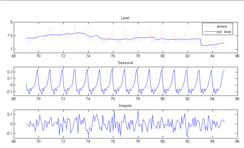
In this example data on road accidents in Great Britain [4] is analyzed using structural time series models following

[1]. The purpose the the analysis is to assess the effect of seat belt laws on road accident casualties, with individual

monthly ﬁgures for drivers, front seat passengers and rear seat passengers. The monthly price of petrol and average

number of kilometers traveled will be used as regression variables. The data is from January 1969 to December 1984.

8.1.1 Univariate analysis

The drivers series will be analyzed with univariate structural time series model, which consists of local level compo-

nent µt, trigonometric seasonal component γt, regression component (on price of petrol) and intervention component

(introduction of seat belt law) βxt. The model equation is

yt=µt+γt+βxt+εt,(7)

where εtis the observation noise. The following code example constructs this model:

lvl = ssm_llm;

seas = ssm_seasonal(’trig1’, 12);

intv = ssm_intv(n, ’step’, 170);

reg = ssm_reg(petrol, ’price of petrol’);

bstsm = [lvl seas intv reg];

bstsm.name = ’Basic structural time series model’;

bstsm.param = [10 0.1 0.001];

The MATLAB display for object bstsm is

bstsm =

Basic structural time series model

==================================

p=1

m = 14

r = 12

n = 192

Components (5):

==================

[Gaussian noise]

p=1

[local polynomial trend]

d=0

[seasonal]

subtype = trig1

s = 12

[intervention]

subtype = step

16 Peng & Aston

tau = 170

[regression]

variable = price of petrol

H matrix (1, 1)

-------------------

10.0000

Z matrix (1, 14, 192)

----------------------

Stationary part:

110101010101DYNDYN

Dynamic part:

Columns 1 through 9

000000000

-2.2733 -2.2792 -2.2822 -2.2939 -2.2924 -2.2968 -2.2655 -2.2626 -2.2655

Columns 10 through 18

000000000

-2.2728 -2.2757 -2.2828 -2.2899 -2.2956 -2.3012 -2.3165 -2.3192 -2.3220

...

Columns 181 through 189

111111111

-2.1390 -2.1646 -2.1565 -2.1597 -2.1644 -2.1648 -2.1634 -2.1646 -2.1707

Columns 190 through 192

111

-2.1502 -2.1539 -2.1536

T matrix (14, 14)

-------------------

SSM Toolbox for Matlab 17

Columns 1 through 9

100000000

0 0.8660 0.5000 0 0 0 0 0 0

0 -0.5000 0.8660 0 0 0 0 0 0

0 0 0 0.5000 0.8660 0 0 0 0

0 0 0 -0.8660 0.5000 0 0 0 0

0 0 0 0 0 0.0000 1 0 0

0 0 0 0 0 -1 0.0000 0 0

0 0 0 0 0 0 0 -0.5000 0.8660

0 0 0 0 0 0 0 -0.8660 -0.5000

000000000

Columns 10 through 14

00000

-0.8660 0.5000 0 0 0

-0.5000 -0.8660 0 0 0

0 0 -1 0 0

00010

00001

R matrix (14, 12)

-------------------

100000000000

010000000000

001000000000

000100000000

000010000000

000001000000

000000100000

000000010000

000000001000

000000000100

18 Peng & Aston

000000000010

000000000001

000000000000

Q matrix (12, 12)

-------------------

Columns 1 through 9

0.100000000000

0 0.0010 0 0 0 0 0 0 0

0 0 0.0010 0 0 0 0 0 0

0 0 0 0.0010 0 0 0 0 0

0 0 0 0 0.0010 0 0 0 0

0 0 0 0 0 0.0010 0 0 0

0 0 0 0 0 0 0.0010 0 0

0 0 0 0 0 0 0 0.0010 0

0 0 0 0 0 0 0 0 0.0010

000000000

Columns 10 through 12

000

0.0010 0 0

0 0.0010 0

0 0 0.0010

P1 matrix (14, 14)

-------------------

Inf0000000000000

0Inf000000000000

00Inf00000000000

000Inf0000000000

0000Inf000000000

SSM Toolbox for Matlab 19

00000Inf00000000

000000Inf0000000

0000000Inf000000

00000000Inf00000

000000000Inf0000

0000000000Inf000

00000000000Inf00

000000000000Inf0

0000000000000Inf

Adjacency matrix (3 functions):

-----------------------------------------------------------------------------

Function H Z T R Q c a1 P1 Hd Zd Td Rd Qd cd Hng Qng Znl Tnl

fun_var/psi2var 1 0 0 0 0 0 0 0 0 0 0 0 0 0 0 0 0 0

fun_var/psi2var 0 0 0 0 1 0 0 0 0 0 0 0 0 0 0 0 0 0

fun_dupvar/psi2dupvar1 0 0 0 0 1 0 0 0 0 0 0 0 0 0 0 0 0 0

Parameters (3)

------------------------------------

Name Value

epsilon var 10

zeta var 0.1

omega var 0.001

The constituting components of the model and the model matrices are all displayed, note that Zis dynamic with the

intervention and regression variables, and matrices cand a1 are omitted if they are zero, also Hand Qtake on values

determined by the parameters set.

With the model constructed, estimation can proceed with the code:

[bstsm logL] = estimate(y, bstsm);

[alphahat V] = statesmo(y, bstsm);

irr = disturbsmo(y, bstsm);

ycom = signal(alphahat, bstsm);

ylvl = sum(ycom([1 3 4], :), 1);

yseas = ycom(2, :);

The estimated model parameters are [0.0037862 0.00026768 1.162e-006], which can be obtained by dis-

playing bstsm.param, the loglikelihood is 175.7790. State and disturbance smoothing is performed with the

estimated model, and the smoothed state is transformed into signal components by signal. Because p=1, the out-

put ycom is M×n, where Mis the number of signal components. The level, intervention and regression are summed as

the total data level, separating seasonal inﬂuence. Using MATLAB graphic functions the individual signal components

and data are visualized:

subplot(3, 1, 1), plot(time, y, ’r:’, ’DisplayName’, ’drivers’), hold all,

plot(time, ylvl, ’DisplayName’, ’est. level’), hold off,

title(’Level’), ylim([6.875 8]), legend(’show’);

20 Peng & Aston

Figure 1: Driver casualties estimated by basic structural time series model

subplot(3, 1, 2), plot(time, yseas), title(’Seasonal’), ylim([-0.16 0.28]);

subplot(3, 1, 3), plot(time, irr), title(’Irregular’), ylim([-0.15 0.15]);

The graphical output is shown in ﬁgure 1. The coefﬁcient for the intervention and regression is deﬁned as part of the

state vector in this model, so they can be obtained from the last two elements of the smoothed state vector (due to the

order of component concatenation) at the last time point. Coefﬁcient for the intervention is alphahat(13, n) =

-0.23773, and coefﬁcient for the regression (price of petrol) is alphahat(14, n) = -0.2914. In this way

diagnostics of these coefﬁcient estimates can also be obtained by the smoothed state variance V.

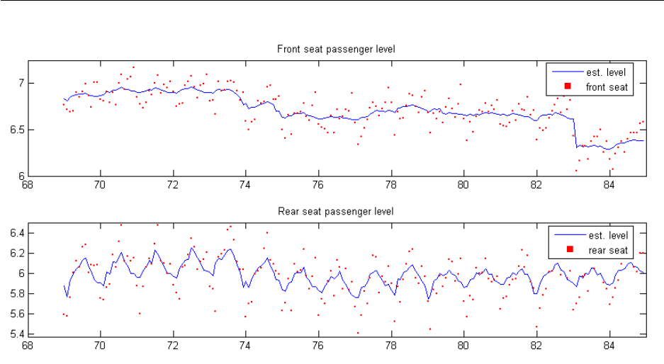
8.1.2 Bivariate analysis

The front seat passenger and rear seat passenger series will be analyzed together using bivariate structural time series

model, with components as before. Speciﬁcally, separate level and seasonal components are deﬁned for both series, but

the disturbances are assumed to be correlated. To reduce the number of parameters estimated the seasonal component

is assumed to be ﬁxed, so that the total number of parameters is six. We also include regression on the price of petrol

and kilometers traveled, and intervention for only the ﬁrst series, since the seat belt law only effects the front seat

passengers. The following is the model construction code:

bilvl = ssm_mvllm(2);

biseas = ssm_mvseasonal(2, [], ’trig fixed’, 12);

biintv = ssm_mvintv(2, n, {’step’ ’null’}, 170);

bireg = ssm_mvreg(2, [petrol; km]);

bistsm = [bilvl biseas biintv bireg];

bistsm.name = ’Bivariate structural time series model’;

The model is then estimated with carefully chosen initial values, and state smoothing and signal extraction proceeds

as before:

SSM Toolbox for Matlab 21

Figure 2: Passenger casualties estimated by bivariate structural time series model

[bistsm logL] = estimate(y2, bistsm, [0.0054 0.0086 0.0045 0.00027 0.00024 0.00023]);

[alphahat V] = statesmo(y2, bistsm);

y2com = signal(alphahat, bistsm);

y2lvl = sum(y2com(:,:, [1 3 4]), 3);

y2seas = y2com(:,:, 2);

When p>1the output from signal is of dimension p×n×M, where Mis the number of components. The

level, regression and intervention are treated as one component of data level as before, separated from the seasonal

component. The components estimated for the two series is plotted:

subplot(2, 1, 1), plot(time, y2lvl(1, :), ’DisplayName’, ’est. level’), hold all,

scatter(time, y2(1, :), 8, ’r’, ’s’, ’filled’, ’DisplayName’, ’front seat’), hold off,

title(’Front seat passenger level’), xlim([68 85]), ylim([6 7.25]), legend(’show’);

subplot(2, 1, 2), plot(time, y2lvl(2, :), ’DisplayName’, ’est. level’), hold all,

scatter(time, y2(2, :), 8, ’r’, ’s’, ’filled’, ’DisplayName’, ’rear seat’), hold off,

title(’Rear seat passenger level’), xlim([68 85]), ylim([5.375 6.5]), legend(’show’);

The graphical output is shown in ﬁgure 2. The intervention coefﬁcient for the front passenger series is obtained by

alphahat(25, n) = -0.30025, the next four elements are the coefﬁcients of the regression of the two series

on the price of petrol and kilometers traveled.

8.2 ARMA models

In this example the difference of the number of users logged on an internet server [5] is analyzed by ARMA models,

and model selection via BIC and missing data analysis are demonstrated. To select an appropriate ARMA(p, q)model

for the data various values for pand qare tried, and the BIC of the estimated model for each is recorded, the model

with the lowest BIC value is chosen.

forp=0:5

forq=0:5

[arma logL output] = estimate(y, ssm_arma(p, q), 0.1);

22 Peng & Aston

BIC(p+1, q+1) = output.BIC;

end

[m i] = min(BIC(:));

arma = estimate(y, ssm_arma(mod(i-1, 6), floor((i-1)/6)), 0.1);

The BIC values obtained for each model is as follows:

q=0 q=1 q=2 q=3 q=4 q=5

p=0 6.3999 5.6060 5.3299 5.3601 5.4189 5.3984

p=1 5.3983 5.2736 5.3195 5.3288 5.3603 5.3985

p=2 5.3532 5.3199 5.3629 5.3675 5.3970 5.4436

p=3 5.2765 5.3224 5.3714 5.4166 5.4525 5.4909

p=4 5.3223 5.3692 5.4142 5.4539 5.4805 5.4915

p=5 5.3689 5.4124 5.4617 5.5288 5.5364 5.5871

The model with the lowest BIC is ARMA(1,1), second lowest is ARMA(3,0), the former model is chosen for subse-

quent analysis.

Next missing data is simulated by setting some time points to NaN, model and state estimation can still proceed

normally with missing data present.

y([6 16 26 36 46 56 66 72 73 74 75 76 86 96]) = NaN;

arma = estimate(y, arma, 0.1);

yf = signal(kalman(y, arma), arma);

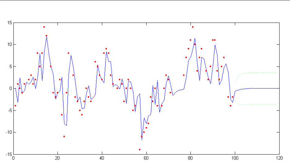
Forecasting is equivalent to treating future data as missing, thus the data set yis appended with as many NaN

values as the steps ahead to forecast. Using the previous estimated ARMA(1,1) model the Kalman ﬁlter will then

effectively predict future data points.

[a P v F] = kalman([y repmat(NaN, 1, 20)], arma);

yf = signal(a(:, 1:end-1), arma);

conf50 = 0.675*realsqrt(F); conf50(1:n) = NaN;

plot(yf), hold all, plot([yf+conf50; yf-conf50]’, ’g:’),

scatter(1:length(y), y, 10, ’r’, ’s’, ’filled’), hold off, ylim([-15 15]);

The plot of the forecast and its conﬁdence interval is shown in ﬁgure 3. Note that if the Kalman ﬁlter is replaced with

the state smoother, the forecasted values will still be the same.

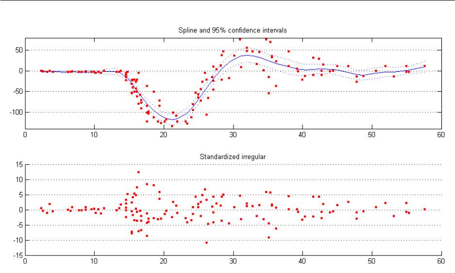
8.3 Cubic spline smoothing

The general state space formulation can also be used to do cubic spline smoothing, by putting the cubic spline into

an equivalent state space form, and accounting for the continuous nature of such smoothing procedures. Here the

continuous acceleration data of a simulated motorcycle accident [6] is smoothed by the cubic spline model, which is

predeﬁned.

spline = estimate(y, ssm_spline(delta), [1 0.1]);

[alphahat V] = statesmo(y, spline);

conf95 = squeeze(1.96*realsqrt(V(1, 1, :)))’;

[eps eta epsvar] = disturbsmo(y, spline);

SSM Toolbox for Matlab 23

Figure 3: Forecast using ARMA(1,1) model with 50% conﬁdence interval

The smoothed data and standardized irregular is plotted and shown in ﬁgure 4.

subplot(2, 1, 1), plot(time, alphahat(1, :), ’b’), hold all,

plot(time, [alphahat(1, :) + conf95; alphahat(1, :) - conf95], ’b:’),

scatter(time, y, 10, ’r’, ’s’, ’filled’), hold off,

title(’Spline and 95% confidence intervals’), ylim([-140 80]),

set(gca,’YGrid’,’on’);

subplot(2, 1, 2), scatter(time, eps./realsqrt(epsvar), 10, ’r’, ’s’, ’filled’),

title(’Standardized irregular’), set(gca,’YGrid’,’on’);

It is seen from ﬁgure 4 that the irregular may be heteroscedastic, an easy ad hoc solution is to model the changing

variance of the irregular by a continuous version of the local level model. Assume the irregular variance is σ2

εh2

tat

time point tand h1=1, then we model the absolute value of the smoothed irregular abs(eps) with htas its level.

The continuous local level model with level htneeds to be constructed from scratch.

contllm = ssmodel(’’, ’continuous local level’, ...

0, 1, 1, 1, ssmat(0, [], true, zeros(1, n), true), ...

’Qd’, {@(X) exp(2*X)*delta}, {[]}, ssparam({’zeta var’}, ’1/2 log’));

contllm = [ssm_gaussian contllm];

alphahat = statesmo(abs(eps), estimate(abs(eps), contllm, [1 0.1]));

h2 = (alphahat/alphahat(1)).ˆ2;

h2 is then the relative magnitude of the noise variance h2

tat each time point, which can be used to construct a custom

dynamic observation noise model as follows.

hetnoise = ssmodel(’’, ’Heteroscedastic noise’, ...

ssmat(0, [], true, zeros(1, n), true), zeros(1, 0), [], [], [], ...

’Hd’, {@(X) exp(2*X)*h2}, {[]}, ssparam({’epsilon var’}, ’1/2 log’));

hetspline = estimate(y, [hetnoise spline], [1 0.1]);

[alphahat V] = statesmo(y, hetspline);

24 Peng & Aston

Figure 4: Cubic spline smoothing of motorcycle acceleration data

conf95 = squeeze(1.96*realsqrt(V(1, 1, :)))’;

[eps eta epsvar] = disturbsmo(y, hetspline);

The smoothed data and standardized irregular with heteroscedastic assumption is shown in ﬁgure 5, it is seen that the

conﬁdence interval shrank, especially at the start and end of the series, and the irregular is slightly more uniform.

In summary the motorcycle series is ﬁrst modeled by a cubic spline model with Gaussian irregular assumption,

then the smoothed irregular magnitude itself is modeled with a local level model. Using the irregular level estimated

at each time point as the relative scale of irregular variance, a new heteroscedastic irregular continuous model is

constructed with the estimated level built-in, and plugged into the cubic spline model to obtain new estimates for the

motorcycle series.

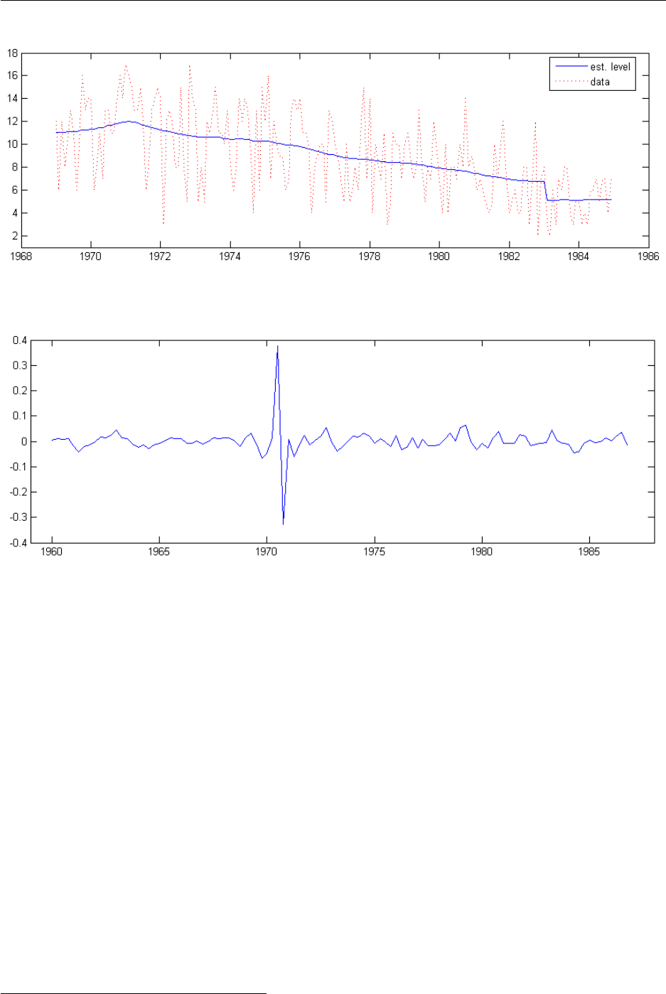
8.4 Poisson distribution error model

The road accident casualties and seat belt law data analyzed in section 8.1 also contains a monthly van driver casualties

series. Due to the smaller numbers of van driver casualties the Gaussian assumption is not justiﬁed in this case,

previous methods cannot be applied. Here a poisson distribution is assumed for the data, the mean is exp(θt)and the

observation distribution is

log p(yt|θt)=θT

tyt−exp(θt)−log yt!

The signal θtin turn is modeled with the structural time series model. The total model is then constructed by con-

catenating a poisson distribution model with a standard structural time series model, the former model will replace the

default Gaussian noise model.

pbstsm = [ssm_poisson ssm_llm ...

ssm_seasonal(’dummy fixed’, 12) ssm_intv(n, ’step’, 170)];

pbstsm.name = ’Poisson basic STSM’;

SSM Toolbox for Matlab 25

Figure 5: Cubic spline smoothing of motorcycle acceleration data with heteroscedastic noise

Model estimation will automatically calculate the Gaussian approximation to the poisson model. Since this is an

exponential family distribution the data ytalso need to be transformed to ˜yt, which is stored in the output argument

output, and used in place of ytfor all functions implementing linear Gaussian (Kalman ﬁlter related) algorithms.

The following is the code for model and state estimation

[pbstsm logL output] = estimate(y, pbstsm, 0.0006, [], ’fmin’, ’bfgs’, ’disp’, ’iter’);

[alphahat V] = statesmo(output.ytilde, pbstsm);

thetacom = signal(alphahat, pbstsm);

Note that the original data yis input to the model estimation routine, which also calculates the transform ytilde.

The model estimated then has its Gaussian approximation built-in, and will be treated by the state smoother as a linear

Gaussian model, hence the transformed data ytilde needs to be used as input. The signal components thetacom

obtained from the smoothed state alphahat is the components of θt, the mean of ycan then be estimated by

exp(sum(thetacom, 1)).

The exponentiated level exp(θt)with the seasonal component eliminated is compared to the original data in ﬁgure

6. The effect of the seat belt law can be clearly seen.

thetalvl = thetacom(1, :) + thetacom(3, :);

plot(time, exp(thetalvl), ’DisplayName’, ’est. level’), hold all,

plot(time, y, ’r:’, ’DisplayName’, ’data’), hold off, ylim([1 18]), legend(’show’);

8.5 t-distribution models

In this example another kind of non-Gaussian models, t-distribution models is used to analyze quarterly demand for

gas in UK [7]. A structural time series model with a t-distribution heavy-tailed observation noise is constructed similar

to the last section, and model estimation and state smoothing performed.

tstsm = [ssm_t ssm_llt ssm_seasonal(’dummy’, 4)];

26 Peng & Aston

Figure 6: Van driver casualties and estimated level

Figure 7: t-distribution irregular

tstsm = estimate(y, tstsm, [0.0018 4 7.7e-10 7.9e-6 0.0033], [], ’fmin’, ’bfgs’);

[alpha irr] = fastsmo(y, tstsm);

plot(time, irr), title(’Irregular component’), xlim([1959 1988]), ylim([-0.4 0.4]);

Since t-distribution is not an exponential family distribution, data transformation is not necessary, and yis used

throughout. A plot of the irregular in ﬁgure 7 shows that potential outliers with respect to the Gaussian assumption

has been detected by the use of heavy-tailed distribution.

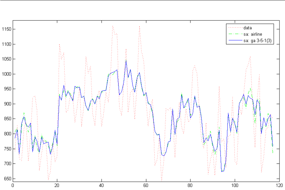
8.6 Hillmer-Tiao decomposition

In this example seasonal adjustment is performed by the Hillmer-Tiao decomposition [2] of airline models. The data

(Manufacturing and reproducing magnetic and optical media, U.S. Census Bureau) is ﬁtted with the airline model, then

the estimated model is Hillmer-Tiao decomposed into an ARIMA components model with trend and seasonal compo-

nents. The same is done for the generalized airline model1[8], and the seasonal adjustment results are compared. The

following are the code to perform seasonal adjustment with the airline model:

air = estimate(y, ssm_airline, 0.1);

aircom = ssmhtd(air);

1Currently renamed Frequency Speciﬁc ARIMA model.

SSM Toolbox for Matlab 27

Figure 8: Seasonal adjustment with airline and generalized airline models

ycom = signal(statesmo(y, aircom), aircom);

airseas = ycom(2, :);

aircom is the decomposed ARIMA components model corresponding to the estimated airline model, and airseas

is the seasonal component, which will be subtracted out of the data yto obtain the seasonal adjusted series. ssmhtd

automatically decompose ARIMA type models into trend, seasonal and irregular components, plus any extra MA

components as permissible.

The same seasonal adjustment procedure is then done with the generalized airline model, using parameter estimates

from the airline model as initial parameters:

param0 = air.param([1 2 2 3]); param0(1:3) = -param0(1:3); param0(2:3) = param0(2:3).ˆ(1/12);

ga = estimate(y, ssm_genair(3, 5, 3), param0);

gacom = ssmhtd(ga);

ycom = signal(statesmo(y, gacom), gacom);

gaseas = ycom(2, :);

The code creates a generalized airline 3-5-1 model, Hillmer-Tiao decomposition produces the same components as for

the airline model since the two models have the same order. From the code it can be seen that the various functions

work transparently across different ARIMA type models. Figure 8 shows the comparison between the two seasonal

adjustment results.

References

[1] J. Durbin and S. J. Koopman. Time Series Analysis by State Space Methods. Oxford University Press, New York,

2001.

28 Peng & Aston

[2] S. C. Hillmer and G. C. Tiao. An arima-model-based approach to seasonal adjustment. J. Am. Stat. Assoc.,

77:63–70, 1982.

[3] V. Gomez and A. Maravall. Automatic modelling methods for univariate series. In D. Pena, G. C. Tiao, and R. S.

Tsay, editors, A Course in Time Series Analysis. John Wiley & Sons, New York, 2001.

[4] A. C. Harvey and J. Durbin. The effects of seat belt legislation on british road casualties: A case study in structural

time series modelling. J. Roy. Stat. Soc. A, 149:187–227, 1986.

[5] S. Makridakis, S. C. Wheelwright, and R. J. Hyndman. Forecasting: Methods and Applications, 3rd Ed. John

Wiley and Sons, New York, 1998.

[6] B. W. Silverman. Some aspects of the spline smoothing approach to non-parametric regression curve ﬁtting. J.

Roy. Stat. Soc. B, 47:1–52, 1985.

[7] S. J. Koopman, A. C. Harvey, J. A. Doornik, and N. Shephard. STAMP 6.0: Structural Time Series Analyser,

Modeller and Predictor. Timberlake Consultants, London, 2000.

[8] J.A.D. Aston, D.F. Findley, T.S. McElroy, K.C. Wills, and D.E.K. Martin. New arima models for seasonal time

series and their application to seasonal adjustment and forecasting. Research Report Series, US Census Bureau,

2007.

A Predeﬁned Model Reference

The predeﬁned models can be organized into two categories, observation disturbance models and normal models. The

former contains only speciﬁcation of the observation disturbance, and is used primarily for model combination; the

latter contains all other models, and can in turn be partitioned into structural time series models, ARIMA type models,

and other models.

The following is a list of each model and function name.

•Observation disturbance models

– Gaussian noise: ssm gaussian([p, cov]) or ssm normal([p, cov])

pis the number of variables, default 1.

cov is true if they are correlated, default true.

– Null noise: ssm null([p])

pis the number of variables, default 1.

– Poisson error: ssm poisson

– Binary error: ssm binary

– Binomial error: ssm binomial(k)

kis the number of trials, can be a scalar or row vector.

– Negative binomial error: ssm negbinomial(k)

kis the number of trials, can be a scalar or row vector.

– Exponential error: ssm exp

– Multinomial error: ssm multinomial(h, k)

his the number of cells.

kis the number of trials, can be a scalar or row vector.

SSM Toolbox for Matlab 29

– Exponential family error: ssm expfamily(b, d2b, id2bdb, c)

p(y|θ)=expyTθ−b(θ)+c(y)

bis the function b(θ).

d2b is ¨

b(θ), the second derivative of b(θ).

id2bdb is ¨

b(θ)−1˙

b(θ).

cis the function c(y).

– t-distribution noise: ssm t([nu])

nu is the degree of freedom, will be estimated as model parameter if not speciﬁed.

– Gaussian mixture noise: ssm mix

– General error noise: ssm err

•Structural time series models

– Integrated random walk: ssm irw(d)

dis the order of integration.

– Local polynomial trend: ssm lpt(d)

dis the order of the polynomial.

– Local level model: ssm llm

– Local level trend: ssm llt

– Seasonal components: ssm seasonal(type, s)

type can be ’dummy’,’dummy fixed’,’h&s’,’trig1’,’trig2’ or ’trig fixed’.

sis the seasonal period.

– Cycle component: ssm cycle

– Regression components: ssm reg(x[, varname])

– Dynamic regression components: ssm dynreg(x[, varname])

xis a m×nmatrix, mis the number of regression variables.

varname is the name of the variables.

– Intervention components: ssm intv(n, type, tau)

nis the total time duration.

type can be ’step’,’pulse’,’slope’ or ’null’.

tau is the onset time.

– Constant components: ssm const

– Trading day variables: ssm td(y, m, N, td6)

’td6’ is set to true to use six variables.

– Length-of-month variables: ssm lom(y, m, N)

– Leap-year variables: ssm ly(y, m, N)

– Easter effect variables: ssm ee(y, m, N, d)

yis the starting year.

mis the starting month.

Nis the total number of months.

dis the number of days before Easter.

30 Peng & Aston

– Structural time series models: ssm stsm(lvl, seas, s[, cycle, x])

lvl is ’level’ or ’trend’.

seas is the seasonal type (see seasonal components).

sis the seasonal period.

cycle is true if there’s a cycle component in the model, default false.

xis explanatory (regression) variables (see regression components).

– Common levels models: ssm commonlvls(p, A ast, a ast)

yt=0

a∗+Ir

A∗µ∗

t+εt

µ∗

t+1 =µ∗

t+η∗

pis the number of variables (length of yt).

A ast is A∗,a(p−r)×rmatrix.

a ast is a∗,a(p−r)×1vector.

– Multivariate local level models: ssm mvllm(p[, cov])

– Multivariate local level trend: ssm mvllt(p[, cov])

– Multivariate seasonal components: ssm mvseasonal(p, cov, type, s)

– Multivariate cycle component: ssm mvcycle(p[, cov])

pis the number of variables.

cov is a logical vector that is true for each correlated disturbances, default all true.

Other arguments are the same as the univariate versions.

– Multivariate regression components: ssm mvreg(p, x[, dep])

dep is a p×mlogical matrix that speciﬁes dependence of data variables on regression variables.

– Multivariate intervention components: ssm mvintv(p, n, type, tau)

– Multivariate structural time series models: ssm mvstsm(p, cov, lvl, seas, s[, cycle,

x, dep])

cov is a logical vector that speciﬁes the covariance structure of each component in turn.

•ARIMA type models

– ARMA models: ssm arma(p, q, mean)

– ARIMA models: ssm arima(p, d, q, mean)

– Multiplicative seasonal ARIMA models: ssm sarima(p, d, q, P, D, Q, s, mean)

– Seasonal sum ARMA models: ssm sumarma(p, q, D, s, mean)

– SARIMA with Hillmer-Tiao decomposition: ssm sarimahtd(p, d, q, P, D, Q, s, gauss)

pis the order of AR.

dis the order of I.

qis the order of MA.

Pis the order of seasonal AR.

Dis the order of seasonal I.

Qis the order of seasonal MA.

sis the seasonal period.

mean is true if the model has mean.

gauss is true if the irregular component is Gaussian.

SSM Toolbox for Matlab 31

– Airline models: ssm airline([s])

sis the period, default 12.

– Frequency speciﬁc SARIMA models: ssm freqspec(p, d, q, P, D, nparam, nfreq, freq)

– Frequency speciﬁc airline models: ssm genair(nparam, nfreq, freq)

nparam is the number of parameters, 3or 4.

nfreq is the size of the largest subset of frequencies sharing the same parameter.

freq is an array containing the members of the smallest subset.

– ARIMA component models: ssm arimacom(d, D, s, phi, theta, ksivar)

The arguments match those of the function htd, see its description for details.

•Other models

– Cubic spline smoothing (continuous time): ssm spline(delta)

delta is the time duration of each data point.

– 1/f noise models (approximated by AR): ssm oneoverf(m)

mis the order of the approximating AR process.

B Class Reference

B.1 SSMAT

The class SSMAT represents state space matrices, can be stationary or dynamic. SSMAT can be horizontally, vertically,

and block diagonally concatenated with each other, as well as with ordinary matrices. Parenthesis reference can also

be used, where two or less indices indicate the stationary part, and three indices indicates a 3-d matrix with time as the

third dimension.

B.1.1 Subscripted reference and assignment

.mat RA2Stationary part of SSMAT Assignment cannot change size.

.mmask R Variable mask A logical matrix the same size as mat.

.n R Time duration Is equal to size(dvec, 2).

.dmmask R Dynamic mask A logical matrix the same size as mat.

.d R Number of dynamic elements Is equal to size(dvec, 1).

.dvec RA Dynamic vector sequence A d×nmatrix. Assignment cannot change d.

.dvmask R Dynamic vector variable mask A d×1logical vector.

.const R True if SSMAT is constant A logical scalar.

.sta R True if SSMAT is stationary A logical scalar.

(i, j) RA Stationary part of SSMAT Assignment cannot change size.

(i, j, t) RA SSMAT as a 3-d matrix Assignment cannot change size.

B.1.2 Class methods

•ssmat

SSMAT constructor.

SSMAT(m[, mmask]) creates a SSMAT.mcan be a 2-d or 3-d matrix, where the third dimension is time.

2R - reference, A - assignment.

32 Peng & Aston

mmask is a 2-d logical matrix masking the variable part of matrix, which can be omitted or set to [] for

constant SSMAT.

SSMAT(m, mmask, dmmask[, dvec, dvmask]) creates a dynamic SSMAT.mis a 2-d matrix forming

the stationary part of the SSMAT.mmask is a logical matrix masking the variable part of matrix, which can

be set to [] for constant SSMAT.dmmask is a logical matrix masking the dynamic part of SSMAT.dvec is

annz(dmmask) ×nmatrix, dvec(:, t) is the values for the dynamic part at time t(m(dmmask) =

dvec(:, t) for time t), default is a nnz(dmmask) ×1zero matrix. dvmask is a nnz(dmmask) ×1

logical vector masking the variable part of dvec.

•isconst

ISCONST(·3)returns true if the stationary part of SSMAT is constant.

•isdconst

ISDCONST(·)returns true if the dynamic part of SSMAT is constant.

•issta

ISSTA(·)returns true if SSMAT is stationary.

•size

[ ... ] = SIZE(·, ...) is equivalent to [ ... ] = SIZE(·.mat, ...).

•getmat

GETMAT(·)returns SSMAT as a matrix if stationary, or as a cell array of matrices if dynamic.

•getdvec

GETDVEC(·, mmask) returns the dynamic elements speciﬁed in matrix mask mmask as a vector sequence.

•getn

GETN(·)returns the time duration of SSMAT.

•setmat

SETMAT(·, vec) updates the variable stationary matrix, vec must have size nnz(mmask) ×1.

•setdvec

SETDVEC(·, dsubvec) updates the variable dynamic vector sequence, dsubvec must have nnz(dvmask)

rows.

•plus

SSMAT addition.

B.2 SSDIST

The class SSDIST represents state space distributions, a set of non-Gaussian distributions that governs a disturbance

vector (which can also have Gaussian elements), and is a child class of SSMAT.SSDIST are constrained to be square

matrices, hence can only be block diagonally concatenated, any other types of concatenation will ignore the non-

Gaussian distribution part. Predeﬁned non-Gaussian distributions can be constructed via the SSDIST constructor.

3An instance of the class in question.

SSM Toolbox for Matlab 33

B.2.1 Subscripted reference and assignment

.nd R Number of distributions A scalar.

.type R Type of each distribution A 0-1 row vector.

.matf R Approximation functions A cell array of functions.

.logpf R Log probability functions A cell array of functions.

.diagmask R Non-Gaussian masks A size(mat, 1) ×nd logical matrix.

.dmask R Variable mask for the distributions A 1×nd logical vector.

.const R True if SSDIST is constant A logical scalar.

B.2.2 Class methods

•ssdist

SSDIST constructor.

SSDIST(type[, matf, logpf, n, p]) creates a single univariate non-Gaussian distribution. type is

0 for exponential family distributions and 1 for additive noise distributions. matf is the function that generates

the approximated Gaussian variance matrix given observations and signal or disturbances. logpf is the function

that calculates the log probability of observations given observation and signal or disturbances. If the last two

arguments are omitted, then the SSDIST is assumed to be variable. SSDIST with multiple non-Gaussian

distributions can be formed by constructing a SSDIST for each and then block diagonally concatenating them.

•isdistconst

ISDISTCONST(·)returns true if the non-Gaussian part of SSDIST is constant.

•setdist

SETDIST(·, distf) updates the non-Gaussian distributions. distf is a cell matrix of functions.

•setgauss

SETGAUSS(·, eps) or

[·ytilde] = SETGAUSS(·, y, theta) calculates the approximating Gaussian covariance, the ﬁrst

form is used if there are no exponential family distributions, and the data yneed to be transformed into ytilde

in the second form if there are.

•logprobrat

LOGPROBRAT(·, N, eps) or

LOGPROBRAT(·, N, y, theta, eps) calculates the log probability ratio between the original non-Gaussian

distribution and the approximating Gaussian distribution of the observations, it is used when calculating the

non-Gaussian loglikelihood by importance sampling. The ﬁrst form is used if there are no exponential family

distributions. Nis the number of importance samples.

B.2.3 Predeﬁned non-Gaussian distributions

•Poisson distribution: dist poisson

•Binary distribution: dist binary

•Binomial distribution: dist binomial(k)

•Negative binomial distribution: dist negbinomial(k)

kis the number of trials, can be a scalar or row vector.

34 Peng & Aston

•Exponential distribution: dist exp

•Multinomial distribution: dist multinomial(h, k)

his the number of cells.

kis the number of trials, can be a scalar or row vector.

•General exponential family distribution: dist expfamily(b, d2b, id2bdb, c)

p(y|θ)=expyTθ−b(θ)+c(y)

bis the function b(θ).

d2b is ¨

b(θ), the second derivative of b(θ).

id2bdb is ¨

b(θ)−1˙

b(θ).

cis the function c(y).

B.3 SSFUNC

The class SSFUNC represents state space functions, a set of nonlinear functions that describe state vector transfor-

mations, and is a child class of SSMAT. Since linear transformations in SSM are represented by left multiplication of

matrices, it is only possible for nonlinear functions (and hence it’s matrix approximation) to be either block diagonally

or horizontally concatenated. The former concatenation method produces multiple resulting output vectors, whereas

the latter produces the sum of the output vectors of all functions as output. Vertical concatenation will ignore the

nonlinear part of SSFUNC.

B.3.1 Subscripted reference and assignment

.nf R Number of functions A scalar.

.f R The nonlinear functions A cell array of functions.

.df R Derivative of each function A cell array of functions.

.horzmask R Nonlinear function output masks A size(mat, 1) ×nf logical matrix.

.vertmask R Nonlinear function input masks A size(mat, 2) ×nf logical matrix.

.fmask R Variable mask for the functions A 1×nf logical vector.

.const R True if SSFUNC is constant A logical scalar.

B.3.2 Class methods

•ssfunc

SSFUNC constructor.

SSFUNC(p, m[, f, df]) creates a single nonlinear function. pis the input vector dimension and mis

the output vector dimension. Hence the approximating linear matrix will be p×m.fand df is the nonlinear

function and its derivative. fmaps m×1vectors and time tto p×1vectors, and df maps m×1vectors and

time tto p×mmatrices. If fand df are not both provided, the SSFUNC is assumed to be variable. SSFUNC

with multiple functions can be constructed by deﬁning individual SSFUNC for each function, and concatenating

them.

•isfconst

ISFCONST(·)returns true if the nonlinear part of SSFUNC is constant.

SSM Toolbox for Matlab 35

•getfunc

GETFUNC(·, x, t) returns f(x, t), the transform of xat time t.

•getvertmask

GETVERTMASK(·)returns vertmask.

•setfunc

SETFUNC(·, funcf) updates the nonlinear functions. funcf is a cell matrix of functions.

•setlinear

[·c] = SETLINEAR(·, alpha) calculates the approximating linear matrix, cis an additive constant in

the approximation.

B.4 SSPARAM

The class SSPARAM represents state space model parameters. SSPARAM can be seen as a row vector of parameter

values, hence they are combined by horizontal concatenation with a slight difference, as described below.

B.4.1 Subscripted reference and assignment

.w R Number of parameters A scalar.

.name R Parameter names A cell array of strings.

.value RA Transformed parameter values A 1×wvector. Assignment cannot change size.

B.4.2 Class methods

•ssparam

SSPARAM constructor.

SSPARAM(w[, transform, group]) creates a SSPARAM with wparameters.

SSPARAM(name[, transform, group]) creates a SSPARAM with parameter names name, which is a

cell array of strings.

transform is a cell array of strings describing transforms used for each parameter.

group is a row vector that speciﬁes the number of parameters included in each parameter subgroup, and

transform is of the same length which speciﬁes transforms for each group.

•get

GET(·)returns the untransformed parameter values.

•set

SET(·, value) sets the untransformed parameter values.

•remove

REMOVE(·, mask) removes the parameters speciﬁed by mask.

•horzcat

[·pmask] = HORZCAT(·1,·2, ...) combines multiple SSPARAM into one, and optionally generates a

cell array of parameter masks pmask, masking each original parameter sets with respect to the new combined

parameter set.

36 Peng & Aston

B.5 SSMODEL

The class SSMODEL represents state space models and embeds all the previous classes. SSMODEL can be combined

by horizontal or block diagonal concatenation. The former is the basis for additive model combination, where the

observation is the sum of individual signals. The latter is an independent combination in which the observation is the

vertical concatenation of the individual signals, which obviously needs to be further combined or changed to be useful.

Only SSMODEL objects are used directly in data analysis functions, knowledge of embedded objects are needed only

when deﬁning custom models. For a list of predeﬁned models see appendix A.

B.5.1 Subscripted reference and assignment

.name RA Model name A string.

.Hinfo R Observation disturbance info A structure.

.info R Model component info A cell array of structures.

.p R Model observation dimension A scalar.

.m R Model state dimension A scalar.

.r R Model state disturbance dimension A scalar.

.n R Model time duration A scalar. Value is 1for stationary models.

.H R Observation disturbance A SSMAT or SSDIST.

.Z R State to observation transform A SSMAT or SSFUNC.

.T R State update transform A SSMAT or SSFUNC.

.R R Disturbance to state transform A SSMAT.

.Q R State disturbance A SSMAT or SSDIST.

.c R State update constant A SSMAT.

.a1 RA Initial state mean A stationary SSMAT, can assign matrices.

.P1 RA Initial state variance A stationary SSMAT, can assign matrices.

.sta R True for stationary SSMODEL A logical scalar.

.linear R True for linear SSMODEL A logical scalar.

.gauss R True for Gaussian SSMODEL A logical scalar.

.w R Number of parameters A scalar.

.paramname R Parameter names A cell array of strings.

.param RA Parameter values A 1×wvector. Assignment cannot change w.

.psi RA Transformed parameter values A 1×wvector. Assignment cannot change w.

.q R Number of initial diffuse elements A scalar.

B.5.2 Class Methods

•ssmodel

SSMODEL constructor.

SSMODEL(info, H, Z, T, R, Q) creates a constant state space model with complete diffuse initial-

ization and c=0.SSMODEL(info, H, Z, T, R, Q, A, func, grad, psi[, pmask, P1,

a1, c]) create a state space model. info is a string or a free form structure with ﬁeld ’type’ describing the

model component. His a SSMAT or SSDIST.Zis a SSMAT or SSFUNC.Tis a SSMAT or SSFUNC.Ris a

SSMAT.Qis a SSMAT or SSDIST.Ais a cell array of strings or a single string, each corresponding to func,

a cell array of functions or a single function. Each string of Ais a concatenation of some of ’H’,’Z’,’T’,

’R’,’Q’,’c’,’a1’,’P1’,’Hd’,’Zd’,’Td’,’Rd’,’Qd’,’cd’,’Hng’,’Qng’,’Znl’,’Tnl’,

SSM Toolbox for Matlab 37

representing each part of each element of SSMODEL. For example, ’Qng’ speciﬁes the non-Gaussian part of

Q, and ’Zd’ speciﬁes the dynamic part of Z. A complicated example of a string in Ais

[’H’ repmat(’ng’, 1, gauss) repmat(’T’, 1, p+P>0) ’RQP1’],

which is the adjacency string for a possibly non-Gaussian ARIMA components model. func is a cell array of

functions that updates model matrices. If multiple parts of the model are updated the output for each part must

be ordered as for the adjacency matrix, but parts not updated can be skipped, for example, a function that updates

H,Tand Qmust output [Hvec Tvec Qvec] in this order. grad is the derivative of func, each of which can

be [] if not differentiable. For the example function above the gradient function would output [Hvec Tvec

Qvec Hgrad Tgrad Qgrad] in order. psi is a SSPARAM.pmask is a cell array of parameter masks for

the corresponding functions, can be omitted or set to [] if there’s only one update function (which presumably

uses all parameters). P1 and a1 are both stationary SSMAT.cis a SSMAT. All arguments expecting SSMAT

can also take numeric matrices.

•isgauss

ISGAUSS(·)is true for Gaussian SSMODEL.

•islinear

ISLINEAR(·)is true for linear SSMODEL.

•issta

ISSTA(·)is true for stationary SSMODEL. Note that all SSFUNC are implicitly assumed to be dynamic, but

are treated as stationary by this and similar functions.

•set

SET(·, A, M, func, grad, psi, pmask) changes one speciﬁc element of SSMODEL.Ais an adja-

cency string, specifying which elements the function or functions func updates. Ais a adjacency string as

described earlier, corresponding to func.Mshould be the new value for one of H,Z,T,R,Q,c,a1 or P1, and A

is constrained to contain only references to that element. grad is the same type as func and is its gradient, set

individual functions to 0 if gradient does not exist or needed. psi is a SSPARAM that stores all the parameters

used by functions in func, and pmask is the parameter mask for each function.

•setparam

SETPARAM(·, psi, transformed) sets the parameters for SSMODEL. If transformed is true, psi

is the new value for the transformed parameters, else psi is the new value for the untransformed parameters.

C Function Reference

C.1 User-deﬁned update functions

This section details the format of update functions for various parts of classes SSMAT,SSDIST and SSFUNC.

•Stationary part

vec = func(psi) updates the stationary part of SSMAT.vec must be a column vector such that mat(mmask)

= vec would correctly update the stationary matrix mat given parameters psi.

38 Peng & Aston

•Dynamic part

dsubvec = func(psi) updates the dynamic part of SSMAT.dsubvec must be a matrix such that dvec(dvmask,

1:size(dsubvec, 2)) = dsubvec would correctly update the dynamic vector sequence dvec given

parameters psi.

•Non-Gaussian part

distf = func(psi) updates the non-Gaussian part of SSDIST.distf must be a cell matrix of function

handles such that [matfdmask] = distf:, 1 and [logpfdmask] = distf:, 2 would correctly

update the distributions given parameters psi.

•Nonlinear part

funcf = func(psi) updates the nonlinear part of SSFUNC.funcf must be a cell matrix of function

handles such that [ffmask] = funcf:, 1 and [dffmask] = funcf:, 2 would correctly update the

nonlinear functions given parameters psi.

Note that an update function can return more than one of the four kind of output, thus updating multiple part of a

SSMODEL, but the order of the output arguments must follow the convention: stationary part of H,Z,T,R,Q,c,a1,

P1, dynamic part of H,Z,T,R,Q,c, non-Gaussian part of H,Q, nonlinear part of Z,T, with possible omissions.

C.2 Data analysis functions

Most functions in this section accepts analysis settings options, speciﬁed as option name and option value pairs (e.g.

(’disp’, ’off’)). These groups of arguments are speciﬁed at the end of each function that accepts them, and

are represented by opt in this section.

•batchsmo

[alphahat epshat etahat] = BATCHSMO(y, model[, opt]) performs batch smoothing of mul-

tiple data sets. yis the data of dimension p×n×N, where nis the data length and Nis the number of data

sets, there must be no missing values. model is a SSMODEL. The output is respectively the smoothed state,

smoothed observation disturbance and smoothed state disturbance, each of dimensions m×n×N,p×n×N

and r×n×N. This is equivalent to doing fastsmo on each data set.

•disturbsmo

[epshat etahat epsvarhat etavarhat] = DISTURBSMO(y, model[, opt]) performs dis-

turbance smoothing. yis the data of dimension p×n, and model is a SSMODEL. The output is respectively

the smoothed observation disturbance (p×n), smoothed state disturbance (r×n), smoothed observation dis-

turbance variance (p×p×nor 1×nif p=1) and smoothed state disturbance variance (r×r×nor 1×n

if r=1).

•estimate

[model logL output] = ESTIMATE(y, model[, param0, alpha0, opt]) estimates the pa-

rameters of model starting from the initial parameter value param0.yis the data of dimension p×n, and

model is a SSMODEL.param0 can be empty if the current parameter values of model is used as initial value,

and a scalar param0 sets all parameters to the same value. Alternatively param0 can be a logical row vec-

tor specifying which parameters to estimate, or a 2×wmatrix with the ﬁrst row as initial value and second

row as estimated parameter mask. The initial state sequence estimate alpha0 is needed only when model is

non-Gaussian or nonlinear. output is a structure that contains optimization routine information, approximated

observation sequence ˜yif non-Gaussian or nonlinear, and the AIC and BIC of the output model.

SSM Toolbox for Matlab 39

•fastsmo

[alphahat epshat etahat] = fastsmo(y, model[, opt]) performs fast smoothing. yis the

data of dimension p×n, and model is a SSMODEL. The output is respectively the smoothed state (m×n),

smoothed observation disturbance (p×n), and smoothed state disturbance (r×n).

•gauss

[model ytilde] = GAUSS(y, model[, alpha0, opt]) calculates the Gaussian approximation.

yis the data of dimension p×n, and model is a SSMODEL.alpha0 is the initial state sequence estimate and

can be empty or omitted.

•kalman

[a P v F] = KALMAN(y, model[, opt]) performs Kalman ﬁltering. yis the data of dimension p×

n, and model is a SSMODEL. The output is respectively the ﬁltered state (m×n+1), ﬁltered state variance

(m×m×n+1, or 1×n+1 if m=1), one-step prediction error (innovation) (p×n), one-step prediction variance

(p×p×n, or 1×nif p=1).

•linear

[model ytilde] = LINEAR(y, model[, alpha0, opt]) calculates the linear approximation. y

is the data of dimension p×n, and model is a SSMODEL.alpha0 is the initial state sequence estimate and

can be empty or omitted.

•loglik

LOGLIK(y, model[, ytilde, opt]) returns the log likelihood of model given y.yis the data of

dimension p×n, and model is a SSMODEL.ytilde is the approximating observation ˜yand is needed for

some non-Gaussian or nonlinear models.

•sample

[y alpha eps eta] = SAMPLE(model, n[, N]) generates observation samples from model.model

is a SSMODEL,nspeciﬁes the sampling data length, and Nspeciﬁes how many sets of data to generate. yis

the sampled data of dimension p×n×N,alpha,eps,eta are respectively the corresponding sampled state

(m×n×N), observation disturbance (p×n×N), and state disturbance (r×n×N).

•signal

SIGNAL(alpha, model) generates the signal for each component according to the state sequence and

model speciﬁcation. alpha is the state of dimension m×n, and model is a SSMODEL. The output is a cell

array of data each with dimension p×n, or a M×nmatrix where Mis the number of components if p=1.

•simsmo

[alphatilde epstilde etatilde] = SIMSMO(y, model, N[, antithetic, opt]) gen-

erates observation samples from model conditional on data y.yis the data of dimension p×n, and model

is a SSMODEL.antithetic should be set to 1if antithetic variables are used. The output is respectively the

sampled state sequence (m×n×N), sampled observation disturbance (p×n×N), and sampled state disturbance

(r×n×N).

•statesmo

[alphahat V] = STATESMO(y, model[, opt]) performs state smoothing. yis the data of dimen-

sion p×n, and model is a SSMODEL. The output is respectively the smoothed state (m×n), smoothed state

variance (m×m×n, or 1×nif p=1). If only the ﬁrst output argument is speciﬁed, fast state smoothing is

automatically performed instead.

40 Peng & Aston

•oosforecast

[yf err SS] = OOSFORECAST(y, model, n1, h) performs out-of-sample forecast. yis the data

of dimension p×n,model is a SSMODEL,n1 is the number of time points to exclude at the end, and his the

number of steps ahead to forecast, which can be an array. The output yf is the forecast obtained, err is the

forecast error, and SS is the forecast error cumulative sum of squares.

C.3 Stock element functions

•fun arma

[fun grad param] = FUN ARMA(p, q) creates matrix update functions for ARMA models.

•fun cycle

[fun grad param] = FUN CYCLE() creates matrix update functions for cycle components.

•fun dupvar

[fun grad param] = FUN DUPVAR(p, cov, d[, name]) creates matrix update functions for du-

plicated variances.

•fun genair

[fun grad param] = FUN GENAIR(nparam, nfreq, freq) creates matrix update functions for

generalized airline models.

•fun homovar

[fun grad param] = FUN HOMOVAR(p, cov, q[, name]) creates matrix update functions for ho-

mogeneous variances.

•fun interlvar

[fun grad param] = FUN INTERLVAR(p, q, cov[, name]) creates matrix update functions for

q-interleaved variances.

•fun mvcycle

[fun grad param] = FUN MVCYCLE(p) creates matrix update functions for multivariate cycle compo-

nent.

•fun oneoverf

[fun grad param] = FUN ONEOVERF(m) creates matrix update functions for 1/f noise.

•fun sarimahtd

[fun grad param] = FUN SARIMAHTD(p, d, q, P, D, Q, s, gauss) creates matrix update

functions for SARIMA with Hillmer-Tiao decomposition and non-Gaussian irregular.

•fun sarma

[fun grad param] = FUN SARMA(p, q, P, Q, s) creates matrix update functions for seasonal

ARMA models.

•fun spline

[fun grad param] = FUN SPLINE(delta) creates matrix update functions for the cubic spline mod-

els.

•fun t

[fun grad param] = FUN T([nu]) creates update functions for the t-distribution.

SSM Toolbox for Matlab 41

•fun var

[fun grad param] = FUN VAR(p, cov[, name]) creates matrix update functions for variances.

•fun wvar

[fun grad param] = FUN WVAR(p, s[, name]) creates matrix update functions for W structure

variances.

•mat arima

[Z T R P1 Tmmask Rmmask P1mmask] = MAT ARIMA(p, d, q, mean) creates base matrices for

ARIMA models.

•mat arma

[Z T R P1 Tmmask Rmmask P1mmask] = MAT ARMA(p, q, mean) or

[T R P1 Tmmask Rmmask P1mmask] = MAT ARMA(p, q, mean) creates base matrices for ARMA

models.

•mat commonlvls

[Z T R a1 P1] = MAT COMMONLVLS(p, A, a) creates base matrices for common levels models.

•mat dummy

[Z T R] = MAT DUMMY(s[, fixed]) creates base matrices for dummy seasonal component.

•mat dupvar

[m mmask] = MAT DUPVAR(p, cov, d) creates base matrices for duplicated variances.

•mat homovar

[H Q Hmmask Qmmask] = MAT HOMOVAR(p, cov, q) creates base matrices for homogeneous vari-

ances.

•mat hs

[Z T R] = MAT HS(s) creates base matrices for Harrison and Stevens seasonal component.

•mat interlvar

[m mmask] = MAT INTERLVAR(p, q, cov) creates base matrices for q-interleaved variances.

•mat lpt

[Z T R] = MAT LPT(d, stochastic) creates base matrices for local polynomial trend or integrated

random walk models.

•mat mvcycle

[Z T Tmmask R] = MAT MVCYCLE(p) creates base matrices for multivariate cycle components.

•mat mvdummy

[Z T R] = MAT MVDUMMY(p, s[, fixed]) creates base matrices for multivariate dummy seasonal

components.

•mat mvhs

[Z T R] = MAT MVHS(p, s) creates base matrices for multivariate Harrison and Stevens seasonal com-

ponents.

42 Peng & Aston

•mat mvintv

[Z Zdmmask Zdvec T R] = MAT MVINTV(p, n, type, tau) creates base matrices for multivari-

ate intervention components.

•mat mvllt

[Z T R] = MAT MVLLT(p) creates base matrices for multivariate local level trend models.

•mat mvreg

[Z Zdmmask Zdvec T R] = MAT MVREG(p, x, dep) creates base matrices for multivariate regres-

sion components.

•mat mvtrig

[Z T R] = MAT MVTRIG(p, s[, fixed]) creates base matrices for multivariate trigonometric sea-

sonal components.

•mat reg

[Z Zdmmask Zdvec T R] = MAT REG(x[, dyn]) creates base matrices for regression components.

•mat sarima

[Z T R P1 Tmmask Rmmask P1mmask] = MAT SARIMA(p, d, q, P, D, Q, s, mean) or

[Z T R P1 Rmmask P1mmask] = MAT SARIMA(p, d, q, P, D, Q, s, mean) creates base ma-

trices for SARIMA models.

•mat sarimahtd

[Z T R Qmat P1 Tmmask Rmmask Qmmask P1mmask] = MAT SARIMAHTD(p, d, q, P, D,

Q, s) creates base matrices for SARIMA with Hillmer-Tiao decomposition.

•mat spline

[Z T Tdmmask Tdvec R] = MAT (delta) creates base matrices for the cubic spline model.

•mat sumarma

[Z T R P1 Tmmask Rmmask P1mmask] = MAT SUMARMA(p, q, D, s, mean) creates base ma-

trices for sum integrated ARMA models.

•mat trig

[Z T R] = MAT TRIG(s[, fixed]) creates base matrices for trigonometric seasonal components.

•mat var

[m mmask] = MAT VAR(p, cov) creates base matrices for variances.

•mat wvar

[m mmask] = MAT WVAR(p, s) creates base matrices for W structure variances.

•x ee

X EE(Y, M, d) generates Easter effect variable.

•x intv

X INTV(n, type, tau) generates intervention variables.

•x ly

X LY(Y, M) generates leap-year variable.

SSM Toolbox for Matlab 43

•x td

X TD(Y, M, td6) generates trading day variables.

C.4 Miscellaneous helper functions

•setopt

SETOPT(optname1, optvalue1, optname2, optvalue2, ...) sets the global analysis settings

and returns a structure containing the new settings, thus a call with no arguments just returns the current settings.

The available options are: ’disp’ can be set to ’off’,’notify’,’final’ or ’iter’.tol is the

tolerance. fmin is the minimization algorithm to use (’bfgs’ or ’simplex’). maxiter is the maximum

number of iterations. nsamp is the number of samples to use in simulation. Note that the same form of argument

sequence can be used at the end of most data analysis functions to specify one time overrides.

•ymarray

[Y M] = YMARRAY(y, m, N) generates an array of years and months from speciﬁed starting year y, start-

ing month m, and number of months N.

C.5 TRAMO model selection and Hillmer-Tiao decomposition

•arimaselect

[p d q mean] = ARIMASELECT(y) or

[p d q P D Q mean] = ARIMASELECT(y, s) performs TRAMO model selection. yis the data of

dimension p×n, and sis the seasonal period. The ﬁrst form selects among ARIMA models with or without a

mean. The second form selects among SARIMA models with or without a mean.

•armadegree

[p q] = ARMADEGREE(y[, mean, mr]) or

[p q P Q] = ARMADEGREE(y, s[, mean, mr, ms]) determines the degrees of ARMA or SARMA

from observation y.yis the data of dimension p×n, and sis the seasonal period. mean is true if models with

mean are used for the selection. mr and ms is the largest degree to consider for regular ARMA and seasonal

ARMA respectively.

•diffdegree

[d mean] = DIFFDEGREE(y[, ub, tsig]) or

[d D mean] = DIFFDEGREE(y, s[, ub, tsig]) performs unit root detection. The ﬁrst form only

considers regular differencing. yis the data of dimension p×n,sis the seasonal period, ub is the threshold

for unit roots, default is [0.97 0.88], and tsig is the t-value threshold for mean detection, default is 1.5.

•loglevel

LOGLEVEL(y, s) or

LOGLEVEL(y, p, q) or

LOGLEVEL(y, p, d, q[, P, D, Q, s]) determines the log level speciﬁcation with respect to various

models. yis the observation data, sis the seasonal period. The output is 1if no logs are needed, else 0. The

ﬁrst form uses the airline model with speciﬁed seasonal period, second form uses ARMA models, and the third

form uses SARIMA models.

44 Peng & Aston

•htd

[theta ksivar] = HTD(d, D, s, Phi, Theta[, etavar]) performs Hillmer-Tiao decompo-

sition. dis the order of regular differencing, Dis the order of seasonal differencing, sis the seasonal period,

Phi is a cell array of increasing order polynomials representing autoregressive factors for each component,

Theta is an increasing order polynomial representing the moving average factor, etavar is the disturbance

variance. The output theta is a cell array of decomposed moving average factors for each component, and

ksivar is the corresponding disturbance variance for each component (including the irregular variance at the

end).

•ssmhtd

SSMHTD(model) performs Hillmer-Tiao decomposition on SSMODEL model and returns an ARIMA com-

ponent model. This is a wrapper for the function htd.

Ssm Manual

ssm_manual

Navigation menu

Versions of this User Manual:

Views

Navigation