Tensorflow Manual Cn

tensorflow_manual_cn

User Manual: Pdf

Open the PDF directly: View PDF .
Page Count: 438 [warning: Documents this large are best viewed by clicking the View PDF Link!]

起步
基础教程
运作方式
Python API
C++ API
资源
其他

TensorFlow 指南

2016 年1月28 日

第一章起步 11

1.1 Introduction || 简介 . . . . . . . . . . . . . . . . . . . . . . . . . . . . . . . . . . . . 12

1.2 Download and Setup || 下载与安装 . . . . . . . . . . . . . . . . . . . . . . . . . . 14

1.2.1 Requirements ｜安装需求 ........................... 14

1.2.2 Overview | 安装总述 . . . . . . . . . . . . . . . . . . . . . . . . . . . . . . . 14

1.2.3 Pip Installatioin | Pip 安装 . . . . . . . . . . . . . . . . . . . . . . . . . . . . 15

1.2.4 Virtualenv installation | 基于 Virtualenv 安装 . . . . . . . . . . . . . . . . 16

1.2.5 Docker Installation . . . . . . . . . . . . . . . . . . . . . . . . . . . . . . . . 18

1.2.6 Test the TensorFlow installation | 测试 TensorFlow 安装 . . . . . . . . . . 19

1.2.7 Installing from source . . . . . . . . . . . . . . . . . . . . . . . . . . . . . . 19

1.2.8 Train your ﬁrst TensorFlow neural net model | 训练第一个 TensorFlow

模型 . . . . . . . . . . . . . . . . . . . . . . . . . . . . . . . . . . . . . . . . . 23

1.2.9 Common Problems | 常见问题 . . . . . . . . . . . . . . . . . . . . . . . . . 23

1.3 Basic Usage || 使用基础 ................................. 26

1.3.1 Overview | 总览 . . . . . . . . . . . . . . . . . . . . . . . . . . . . . . . . . . 26

1.3.2 The computation graph | 计算图 . . . . . . . . . . . . . . . . . . . . . . . . 27

1.3.3 Interactive Usage | 交互式使用 . . . . . . . . . . . . . . . . . . . . . . . . . 29

1.3.4 Tensors | 张量 . . . . . . . . . . . . . . . . . . . . . . . . . . . . . . . . . . . 30

1.3.5 Variables | 变量 . . . . . . . . . . . . . . . . . . . . . . . . . . . . . . . . . . 30

1.3.6 Fetches | 取回 . . . . . . . . . . . . . . . . . . . . . . . . . . . . . . . . . . . 31

1.3.7 Feeds | 供给 . . . . . . . . . . . . . . . . . . . . . . . . . . . . . . . . . . . . 32

第二章基础教程 33

2.1 MNIST 机器学习入门 . . . . . . . . . . . . . . . . . . . . . . . . . . . . . . . . . . 37

2.1.1 The MNIST Data | MNIST 数据集 . . . . . . . . . . . . . . . . . . . . . . . 38

2.1.2 Softmax 回归介绍 . . . . . . . . . . . . . . . . . . . . . . . . . . . . . . . . 40

2.1.3 实现回归模型 . . . . . . . . . . . . . . . . . . . . . . . . . . . . . . . . . . . 43

2.1.4 训练模型 . . . . . . . . . . . . . . . . . . . . . . . . . . . . . . . . . . . . . . 46

2.1.5 Evaluating Our Model || 评估我们的模型 . . . . . . . . . . . . . . . . . . . 48

2.2 Deep MNIST for Experts || 深入 MNIST . . . . . . . . . . . . . . . . . . . . . . . . 50

4目录

2.2.1 Setup | 安装 . . . . . . . . . . . . . . . . . . . . . . . . . . . . . . . . . . . . 50

2.2.2 Build a Softmax Regression Model || 构建 Softmax 回归模型 . . . . . . . 52

2.2.3 Train the Model | 训练模型 . . . . . . . . . . . . . . . . . . . . . . . . . . . 54

2.2.4 Build a Multilayer Convolutional Network | 构建多层卷积网络模型 . . . 55

2.3 TensorFlow Mechanics 101 ............................... 60

2.3.1 教程使用的文件 . . . . . . . . . . . . . . . . . . . . . . . . . . . . . . . . . 60

2.3.2 准备数据 . . . . . . . . . . . . . . . . . . . . . . . . . . . . . . . . . . . . . . 60

2.3.3 构建图表（Build the Graph）......................... 61

2.3.4 训练模型 . . . . . . . . . . . . . . . . . . . . . . . . . . . . . . . . . . . . . . 64

2.3.5 评估模型 . . . . . . . . . . . . . . . . . . . . . . . . . . . . . . . . . . . . . . 66

2.4 卷积神经网络 . . . . . . . . . . . . . . . . . . . . . . . . . . . . . . . . . . . . . . . 68

2.4.1 Overview . . . . . . . . . . . . . . . . . . . . . . . . . . . . . . . . . . . . . . 68

2.4.2 Code Organization . . . . . . . . . . . . . . . . . . . . . . . . . . . . . . . . 69

2.4.3 CIFAR-10 模型 ................................... 70

2.4.4 开始执行并训练模型 . . . . . . . . . . . . . . . . . . . . . . . . . . . . . . 73

2.4.5 评估模型 . . . . . . . . . . . . . . . . . . . . . . . . . . . . . . . . . . . . . . 75

2.4.6 在多个 GPU 板卡上训练模型 ......................... 76

2.4.7 下一步 . . . . . . . . . . . . . . . . . . . . . . . . . . . . . . . . . . . . . . . 77

2.5 Vector Representations of Words . . . . . . . . . . . . . . . . . . . . . . . . . . . . 78

2.5.1 亮点 ......................................... 78

2.5.2 动机:为什么需要学习 Word Embeddings? . . . . . . . . . . . . . . . . . . 78

2.5.3 处理噪声对比训练 . . . . . . . . . . . . . . . . . . . . . . . . . . . . . . . . 79

2.5.4 Skip-gram 模型 . . . . . . . . . . . . . . . . . . . . . . . . . . . . . . . . . . 82

2.5.5 建立图形 . . . . . . . . . . . . . . . . . . . . . . . . . . . . . . . . . . . . . . 83

2.5.6 训练模型 . . . . . . . . . . . . . . . . . . . . . . . . . . . . . . . . . . . . . . 84

2.5.7 嵌套学习结果可视化 . . . . . . . . . . . . . . . . . . . . . . . . . . . . . . 84

2.5.8 嵌套学习的评估:类比推理 . . . . . . . . . . . . . . . . . . . . . . . . . . . 84

2.5.9 优化实现 . . . . . . . . . . . . . . . . . . . . . . . . . . . . . . . . . . . . . . 84

2.5.10 总结 . . . . . . . . . . . . . . . . . . . . . . . . . . . . . . . . . . . . . . . . 85

2.6 循环神经网络 . . . . . . . . . . . . . . . . . . . . . . . . . . . . . . . . . . . . . . . 86

2.6.1 介绍 ......................................... 86

2.6.2 语言模型 . . . . . . . . . . . . . . . . . . . . . . . . . . . . . . . . . . . . . . 86

2.6.3 教程文件 . . . . . . . . . . . . . . . . . . . . . . . . . . . . . . . . . . . . . . 86

2.6.4 下载及准备数据 . . . . . . . . . . . . . . . . . . . . . . . . . . . . . . . . . 86

2.6.5 模型 ......................................... 86

2.6.6 编译并运行代码 . . . . . . . . . . . . . . . . . . . . . . . . . . . . . . . . . 88

2.6.7 除此之外？ . . . . . . . . . . . . . . . . . . . . . . . . . . . . . . . . . . . . 88

2.7 Sequence-to-Sequence Models . . . . . . . . . . . . . . . . . . . . . . . . . . . . 89

目录 5

2.7.1 Sequence-to-Sequence Basics . . . . . . . . . . . . . . . . . . . . . . . . . 89

2.7.2 TensorFlow seq2seq Library . . . . . . . . . . . . . . . . . . . . . . . . . . 90

2.7.3 Neural Translation Model . . . . . . . . . . . . . . . . . . . . . . . . . . . . 91

2.7.4 Let’s Run It . . . . . . . . . . . . . . . . . . . . . . . . . . . . . . . . . . . . 93

2.7.5 What Next? . . . . . . . . . . . . . . . . . . . . . . . . . . . . . . . . . . . . 94

2.8 偏微分方程 . . . . . . . . . . . . . . . . . . . . . . . . . . . . . . . . . . . . . . . . 95

2.8.1 基本设置 . . . . . . . . . . . . . . . . . . . . . . . . . . . . . . . . . . . . . . 95

2.8.2 定义计算函数 . . . . . . . . . . . . . . . . . . . . . . . . . . . . . . . . . . . 95

2.8.3 定义偏微分方程 ................................. 95

2.8.4 开始仿真 . . . . . . . . . . . . . . . . . . . . . . . . . . . . . . . . . . . . . . 96

2.9 MNIST 数据下载 ..................................... 97

2.9.1 教程文件 . . . . . . . . . . . . . . . . . . . . . . . . . . . . . . . . . . . . . . 97

2.9.2 准备数据 . . . . . . . . . . . . . . . . . . . . . . . . . . . . . . . . . . . . . . 97

第三章运作方式 101

3.0.1 Variables: 创建，初始化，保存，和恢复 . . . . . . . . . . . . . . . . . . 102

3.0.2 TensorFlow 机制 101 . . . . . . . . . . . . . . . . . . . . . . . . . . . . . . . 102

3.0.3 TensorBoard: 学习过程的可视化 . . . . . . . . . . . . . . . . . . . . . . . 102

3.0.4 TensorBoard: 图的可视化 . . . . . . . . . . . . . . . . . . . . . . . . . . . . 102

3.0.5 数据读入 . . . . . . . . . . . . . . . . . . . . . . . . . . . . . . . . . . . . . . 102

3.0.6 线程和队列 . . . . . . . . . . . . . . . . . . . . . . . . . . . . . . . . . . . . 102

3.0.7 添加新的 Op . . . . . . . . . . . . . . . . . . . . . . . . . . . . . . . . . . . . 102

3.0.8 自定义数据的 Readers . . . . . . . . . . . . . . . . . . . . . . . . . . . . . . 103

3.0.9 使用 GPUs . . . . . . . . . . . . . . . . . . . . . . . . . . . . . . . . . . . . . 103

3.0.10 共享变量 Sharing Variables . . . . . . . . . . . . . . . . . . . . . . . . . . . 103

3.1 变量:创建、初始化、保存和加载 . . . . . . . . . . . . . . . . . . . . . . . . . . 104

3.1.1 变量创建 . . . . . . . . . . . . . . . . . . . . . . . . . . . . . . . . . . . . . . 104

3.1.2 变量初始化 . . . . . . . . . . . . . . . . . . . . . . . . . . . . . . . . . . . . 104

3.1.3 保存和加载 . . . . . . . . . . . . . . . . . . . . . . . . . . . . . . . . . . . . 105

3.2 共享变量 . . . . . . . . . . . . . . . . . . . . . . . . . . . . . . . . . . . . . . . . . . 108

3.2.1 问题 . . . . . . . . . . . . . . . . . . . . . . . . . . . . . . . . . . . . . . . . . 108

3.2.2 变量作用域实例 . . . . . . . . . . . . . . . . . . . . . . . . . . . . . . . . . 109

3.2.3 变量作用域是怎么工作的？ . . . . . . . . . . . . . . . . . . . . . . . . . . 110

3.2.4 使用实例 . . . . . . . . . . . . . . . . . . . . . . . . . . . . . . . . . . . . . . 112

3.3 TensorBoard: 可视化学习　 . . . . . . . . . . . . . . . . . . . . . . . . . . . . . . 113

3.3.1 数据序列化　 . . . . . . . . . . . . . . . . . . . . . . . . . . . . . . . . . . . 113

3.3.2 启动 TensorBoard 　. . . . . . . . . . . . . . . . . . . . . . . . . . . . . . . 114

3.4 TensorBoard: 图表可视化 . . . . . . . . . . . . . . . . . . . . . . . . . . . . . . . . 115

6目录

3.4.1 名称域（Name scoping）和节点（Node）. . . . . . . . . . . . . . . . . 115

3.4.2 交互 . . . . . . . . . . . . . . . . . . . . . . . . . . . . . . . . . . . . . . . . . 118

3.5 数据读取 . . . . . . . . . . . . . . . . . . . . . . . . . . . . . . . . . . . . . . . . . . 120

3.5.1 目录 . . . . . . . . . . . . . . . . . . . . . . . . . . . . . . . . . . . . . . . . . 120

3.5.2 供给数据 . . . . . . . . . . . . . . . . . . . . . . . . . . . . . . . . . . . . . . 120

3.5.3 从文件读取数据 . . . . . . . . . . . . . . . . . . . . . . . . . . . . . . . . . 121

3.5.4 预取数据 . . . . . . . . . . . . . . . . . . . . . . . . . . . . . . . . . . . . . . 126

3.5.5 多输入管道 . . . . . . . . . . . . . . . . . . . . . . . . . . . . . . . . . . . . 127

3.6 线程和队列 . . . . . . . . . . . . . . . . . . . . . . . . . . . . . . . . . . . . . . . . 128

3.6.1 队列使用概述 . . . . . . . . . . . . . . . . . . . . . . . . . . . . . . . . . . . 128

3.6.2 Coordinator . . . . . . . . . . . . . . . . . . . . . . . . . . . . . . . . . . . . 128

3.6.3 QueueRunner . . . . . . . . . . . . . . . . . . . . . . . . . . . . . . . . . . . 129

3.6.4 异常处理 . . . . . . . . . . . . . . . . . . . . . . . . . . . . . . . . . . . . . . 130

3.7 增加一个新 Op . . . . . . . . . . . . . . . . . . . . . . . . . . . . . . . . . . . . . . 131

3.7.1 内容 . . . . . . . . . . . . . . . . . . . . . . . . . . . . . . . . . . . . . . . . . 131

3.7.2 定义 Op 的接口 . . . . . . . . . . . . . . . . . . . . . . . . . . . . . . . . . . 132

3.7.3 为Op 实现 kernel . . . . . . . . . . . . . . . . . . . . . . . . . . . . . . . . 132

3.7.4 生成客户端包装器 . . . . . . . . . . . . . . . . . . . . . . . . . . . . . . . . 133

3.7.5 检查 Op 能否正常工作 . . . . . . . . . . . . . . . . . . . . . . . . . . . . . 134

3.7.6 验证条件 . . . . . . . . . . . . . . . . . . . . . . . . . . . . . . . . . . . . . . 134

3.7.7 Op 注册 . . . . . . . . . . . . . . . . . . . . . . . . . . . . . . . . . . . . . . 135

3.7.8 GPU 支持 . . . . . . . . . . . . . . . . . . . . . . . . . . . . . . . . . . . . . 147

3.7.9 使用 Python 实现梯度 . . . . . . . . . . . . . . . . . . . . . . . . . . . . . . 147

3.7.10 在Python 中实现一个形状函数 . . . . . . . . . . . . . . . . . . . . . . . . 148

3.8 自定义数据读取 . . . . . . . . . . . . . . . . . . . . . . . . . . . . . . . . . . . . . 150

3.8.1 主要内容 . . . . . . . . . . . . . . . . . . . . . . . . . . . . . . . . . . . . . . 150

3.8.2 编写一个文件格式读写器 . . . . . . . . . . . . . . . . . . . . . . . . . . . 150

3.8.3 编写一个记录格式 Op . . . . . . . . . . . . . . . . . . . . . . . . . . . . . 153

3.9 使用 GPUs . . . . . . . . . . . . . . . . . . . . . . . . . . . . . . . . . . . . . . . . . 155

3.9.1 支持的设备 . . . . . . . . . . . . . . . . . . . . . . . . . . . . . . . . . . . . 155

3.9.2 记录设备指派情况 . . . . . . . . . . . . . . . . . . . . . . . . . . . . . . . . 155

3.9.3 手工指派设备 . . . . . . . . . . . . . . . . . . . . . . . . . . . . . . . . . . . 155

3.9.4 在多 GPU 系统里使用单一 GPU . . . . . . . . . . . . . . . . . . . . . . . . 156

3.9.5 使用多个 GPU . . . . . . . . . . . . . . . . . . . . . . . . . . . . . . . . . . 156

第四章 Python API 159

4.1 Overview . . . . . . . . . . . . . . . . . . . . . . . . . . . . . . . . . . . . . . . . . . 160

4.2 Building Graphs . . . . . . . . . . . . . . . . . . . . . . . . . . . . . . . . . . . . . . 161

目录 7

4.2.1 Contents . . . . . . . . . . . . . . . . . . . . . . . . . . . . . . . . . . . . . . 161

4.2.2 Core graph data structures . . . . . . . . . . . . . . . . . . . . . . . . . . . 161

4.2.3 Tensor types . . . . . . . . . . . . . . . . . . . . . . . . . . . . . . . . . . . . 176

4.2.4 Utility functions . . . . . . . . . . . . . . . . . . . . . . . . . . . . . . . . . 179

4.2.5 Graph collections . . . . . . . . . . . . . . . . . . . . . . . . . . . . . . . . 182

4.2.6 Deﬁning new operations . . . . . . . . . . . . . . . . . . . . . . . . . . . . 183

4.3 Constants, Sequences, and Random Values . . . . . . . . . . . . . . . . . . . . . . 193

4.3.1 Contents . . . . . . . . . . . . . . . . . . . . . . . . . . . . . . . . . . . . . . 193

4.3.2 Constant Value Tensors . . . . . . . . . . . . . . . . . . . . . . . . . . . . . 194

4.3.3 Sequences . . . . . . . . . . . . . . . . . . . . . . . . . . . . . . . . . . . . . 197

4.3.4 Random Tensors . . . . . . . . . . . . . . . . . . . . . . . . . . . . . . . . . 198

4.4 Variables . . . . . . . . . . . . . . . . . . . . . . . . . . . . . . . . . . . . . . . . . . 203

4.4.1 Contents . . . . . . . . . . . . . . . . . . . . . . . . . . . . . . . . . . . . . . 203

4.4.2 Variables . . . . . . . . . . . . . . . . . . . . . . . . . . . . . . . . . . . . . . 204

4.4.3 Variable helper functions . . . . . . . . . . . . . . . . . . . . . . . . . . . . 209

4.4.4 Saving and Restoring Variables . . . . . . . . . . . . . . . . . . . . . . . . . 211

4.4.5 Sharing Variables . . . . . . . . . . . . . . . . . . . . . . . . . . . . . . . . . 217

4.4.6 Sparse Variable Updates . . . . . . . . . . . . . . . . . . . . . . . . . . . . . 221

4.5 Tensor Transformations . . . . . . . . . . . . . . . . . . . . . . . . . . . . . . . . . 227

4.5.1 Contents . . . . . . . . . . . . . . . . . . . . . . . . . . . . . . . . . . . . . . 227

4.5.2 Casting . . . . . . . . . . . . . . . . . . . . . . . . . . . . . . . . . . . . . . . 228

4.5.3 Shapes and Shaping . . . . . . . . . . . . . . . . . . . . . . . . . . . . . . . 231

4.5.4 Slicing and Joining . . . . . . . . . . . . . . . . . . . . . . . . . . . . . . . . 235

4.6 Math ............................................245

4.6.1 Contents . . . . . . . . . . . . . . . . . . . . . . . . . . . . . . . . . . . . . . 245

4.6.2 Arithmetic Operators . . . . . . . . . . . . . . . . . . . . . . . . . . . . . . 248

4.6.3 Basic Math Functions . . . . . . . . . . . . . . . . . . . . . . . . . . . . . . 250

4.6.4 Matrix Math Functions . . . . . . . . . . . . . . . . . . . . . . . . . . . . . 256

4.6.5 Complex Number Functions . . . . . . . . . . . . . . . . . . . . . . . . . . 262

4.6.6 Reduction . . . . . . . . . . . . . . . . . . . . . . . . . . . . . . . . . . . . . 264

4.6.7 Segmentation . . . . . . . . . . . . . . . . . . . . . . . . . . . . . . . . . . . 269

4.6.8 Sequence Comparison and Indexing . . . . . . . . . . . . . . . . . . . . . 274

4.7 Control Flow . . . . . . . . . . . . . . . . . . . . . . . . . . . . . . . . . . . . . . . 280

4.7.1 Contents . . . . . . . . . . . . . . . . . . . . . . . . . . . . . . . . . . . . . . 280

4.7.2 Control Flow Operations . . . . . . . . . . . . . . . . . . . . . . . . . . . . 281

4.7.3 Logical Operators . . . . . . . . . . . . . . . . . . . . . . . . . . . . . . . . 283

4.7.4 Comparison Operators . . . . . . . . . . . . . . . . . . . . . . . . . . . . . 284

4.7.5 Debugging Operations . . . . . . . . . . . . . . . . . . . . . . . . . . . . . 289

8目录

4.8 Images . . . . . . . . . . . . . . . . . . . . . . . . . . . . . . . . . . . . . . . . . . . 292

4.8.1 Contents . . . . . . . . . . . . . . . . . . . . . . . . . . . . . . . . . . . . . . 292

4.8.2 Encoding and Decoding . . . . . . . . . . . . . . . . . . . . . . . . . . . . . 293

4.8.3 Resizing . . . . . . . . . . . . . . . . . . . . . . . . . . . . . . . . . . . . . . 297

4.8.4 Cropping . . . . . . . . . . . . . . . . . . . . . . . . . . . . . . . . . . . . . 300

4.8.5 Flipping and Transposing . . . . . . . . . . . . . . . . . . . . . . . . . . . . 304

4.8.6 Image Adjustments . . . . . . . . . . . . . . . . . . . . . . . . . . . . . . . 306

4.9 Sparse Tensors . . . . . . . . . . . . . . . . . . . . . . . . . . . . . . . . . . . . . . 310

4.9.1 Contents . . . . . . . . . . . . . . . . . . . . . . . . . . . . . . . . . . . . . . 310

4.9.2 Sparse Tensor Representation . . . . . . . . . . . . . . . . . . . . . . . . . 310

4.9.3 Sparse to Dense Conversion . . . . . . . . . . . . . . . . . . . . . . . . . . 313

4.9.4 Manipulation . . . . . . . . . . . . . . . . . . . . . . . . . . . . . . . . . . . 315

4.10 Inputs and Readers . . . . . . . . . . . . . . . . . . . . . . . . . . . . . . . . . . . 320

4.10.1 Contents . . . . . . . . . . . . . . . . . . . . . . . . . . . . . . . . . . . . . . 320

4.10.2 Placeholders . . . . . . . . . . . . . . . . . . . . . . . . . . . . . . . . . . . 321

4.10.3 Readers . . . . . . . . . . . . . . . . . . . . . . . . . . . . . . . . . . . . . . 322

4.10.4 Converting . . . . . . . . . . . . . . . . . . . . . . . . . . . . . . . . . . . . 337

4.10.5 Queues . . . . . . . . . . . . . . . . . . . . . . . . . . . . . . . . . . . . . . 342

4.10.6 Dealing with the ﬁlesystem . . . . . . . . . . . . . . . . . . . . . . . . . . . 347

4.10.7 Input pipeline . . . . . . . . . . . . . . . . . . . . . . . . . . . . . . . . . . 348

4.11 Data IO (Python functions) . . . . . . . . . . . . . . . . . . . . . . . . . . . . . . . 356

4.11.1 Contents . . . . . . . . . . . . . . . . . . . . . . . . . . . . . . . . . . . . . . 356

4.11.2 Data IO (Python Functions) . . . . . . . . . . . . . . . . . . . . . . . . . . 356

4.12 Neural Network . . . . . . . . . . . . . . . . . . . . . . . . . . . . . . . . . . . . . 358

4.12.1 Contents . . . . . . . . . . . . . . . . . . . . . . . . . . . . . . . . . . . . . . 358

4.12.2 Activation Functions . . . . . . . . . . . . . . . . . . . . . . . . . . . . . . 360

4.12.3 Convolution . . . . . . . . . . . . . . . . . . . . . . . . . . . . . . . . . . . 363

4.12.4 Pooling . . . . . . . . . . . . . . . . . . . . . . . . . . . . . . . . . . . . . . 367

4.12.5 Normalization . . . . . . . . . . . . . . . . . . . . . . . . . . . . . . . . . . 369

4.12.6 Losses . . . . . . . . . . . . . . . . . . . . . . . . . . . . . . . . . . . . . . . 371

4.12.7 Classiﬁcation . . . . . . . . . . . . . . . . . . . . . . . . . . . . . . . . . . . 371

4.12.8 Embeddings . . . . . . . . . . . . . . . . . . . . . . . . . . . . . . . . . . . 373

4.12.9 Evaluation . . . . . . . . . . . . . . . . . . . . . . . . . . . . . . . . . . . . 374

4.12.10 Candidate Sampling . . . . . . . . . . . . . . . . . . . . . . . . . . . . . . 375

4.13 Running Graphs . . . . . . . . . . . . . . . . . . . . . . . . . . . . . . . . . . . . . 384

4.13.1 Contents . . . . . . . . . . . . . . . . . . . . . . . . . . . . . . . . . . . . . . 384

4.13.2 Session management . . . . . . . . . . . . . . . . . . . . . . . . . . . . . . 385

4.13.3 Error classes . . . . . . . . . . . . . . . . . . . . . . . . . . . . . . . . . . . 389

目录 9

4.14 Training . . . . . . . . . . . . . . . . . . . . . . . . . . . . . . . . . . . . . . . . . . 396

4.14.1 Contents . . . . . . . . . . . . . . . . . . . . . . . . . . . . . . . . . . . . . . 396

4.14.2 Optimizers . . . . . . . . . . . . . . . . . . . . . . . . . . . . . . . . . . . . 398

4.14.3 Gradient Computation . . . . . . . . . . . . . . . . . . . . . . . . . . . . . 407

4.14.4 Gradient Clipping . . . . . . . . . . . . . . . . . . . . . . . . . . . . . . . . 409

4.14.5 Decaying the learning rate . . . . . . . . . . . . . . . . . . . . . . . . . . . 413

4.14.6 Moving Averages . . . . . . . . . . . . . . . . . . . . . . . . . . . . . . . . . 414

4.14.7 Coordinator and QueueRunner . . . . . . . . . . . . . . . . . . . . . . . . 417

4.14.8 Summary Operations . . . . . . . . . . . . . . . . . . . . . . . . . . . . . . 422

4.14.9 Adding Summaries to Event Files . . . . . . . . . . . . . . . . . . . . . . . 426

4.14.10 Training utilities . . . . . . . . . . . . . . . . . . . . . . . . . . . . . . . . 429

第五章 C++ API 431

第六章资源 433

第七章其他 435

10 目录

第一章起步

12 第一章起步

1.1 Introduction || 简介

Let’s get you up and running with TensorFlow!

本章的目的是让你了解和运行 TensorFlow！

But before we even get started, let’s peek at what TensorFlow code looks like in the

Python API, so you have a sense of where we’re headed.

在开始之前，让我们先看一段使用 Python API 撰写的 TensorFlow 示例代码，让你

对将要学习的内容有初步的印象.

Here’s a little Python program that makes up some data in two dimensions, and then

ﬁts a line to it.

下面这段短小的 Python 程序将把一些数据放入二维空间，再用一条线来拟合这些

数据．

 

1import tensorflow as tf

2import numpy as np

4# Create 100 phony x, y data points in NumPy, y = x * 0.1 + 0.3

5x_data = np.random.rand(100).astype("float32")

6y_data = x_data * 0.1 + 0.3

8# Try to find values for W and b that compute y_data = W * x_data + b

9# (We know that W should be 0.1 and b 0.3, but Tensorflow will

10 # figure that out for us.)

11 W = tf.Variable(tf.random_uniform([1], −1.0, 1.0))

12 b = tf.Variable(tf.zeros([1]))

13 y = W * x_data + b

15 # Minimize the mean squared errors.

16 loss = tf.reduce_mean(tf.square(y −y_data))

17 optimizer = tf.train.GradientDescentOptimizer(0.5)

18 train = optimizer.minimize(loss)

20 # Before starting , initialize the variables. We will 'run' this first

21 init = tf.initialize_all_variables()

23 # Launch the graph.

24 sess = tf.Session()

25 sess.run(init)

27 # Fit the line.

28 for step in xrange(201):

29 sess.run(train)

30 if step % 20 == 0:

31 print(step, sess.run(W), sess.run(b))

33 # Learns best fit is W: [0.1], b: [0.3]

 

The ﬁrst part of this code builds the data ﬂow graph. TensorFlow does not actually run

any computation until the session is created and the run function is called.

以上代码的第一部分构建了数据的流向图 (ﬂow graph)．在一个 session 被建立并

且run()函数被运行前，TensorFlow 不会进行任何实质的计算．

To whet your appetite further, we suggest you check out what a classical machine

1.1 INTRODUCTION ||

简介 13

learning problem looks like in TensorFlow. In the land of neural networks the most "classic"

classical problem is the MNIST handwritten digit classiﬁcation. We offer two introductions

here, one for machine learning newbies, and one for pros. If you’ve already trained dozens

of MNIST models in other software packages, please take the red pill. If you’ve never even

heard of MNIST, deﬁnitely take the blue pill. If you’re somewhere in between, we suggest

skimming blue, then red.

为了进一步激发你的学习欲望,我们想让你先看一下 TensorFlow 是如何解决一个

经典的机器学习问题的．在神经网络领域，最为经典的问题莫过于 MNIST 手写数字分

类．为此，我们准备了两篇不同的教程,分别面向初学者和专家．如果你已经使用其它软

件训练过许多 MNIST 模型，请参阅高级教程 (红色药丸)．如果你以前从未听说过 MNIST

，请先阅读初级教程 (蓝色药丸)．如果你的水平介于这两类人之间,我们建议你先快速

浏览初级教程，然后再阅读高级教程．

If you’re already sure you want to learn and install TensorFlow you can skip these and

charge ahead. Don’t worry, you’ll still get to see MNIST – we’ll also use MNIST as an example

in our technical tutorial where we elaborate on TensorFlow features.

如果你已下定决心准备学习和安装 TensorFlow ，你可以略过这些文字，直接阅读

后面的章节1．不用担心，你仍然会看到 MNIST — 在阐述 TensorFlow 的特性时，我们还

会使用 MNIST 作为一个样例．

1推荐随后阅读内容：1下载与安装，2基本使用，3 TensorFlow 101.

14 第一章起步

1.2 Download and Setup || 下载与安装

You can install TensorFlow either from our provided binary packages or from the github

source.

您可以使用我们提供的二进制包，或者源代码，安装 TensorFlow.

1.2.1 Requirements ｜安装需求

The TensorFlow Python API currently supports Python 2.7 and Python 3.3+ from source.

TensorFlow Python API 目前支持 Python 2.7 和python 3.3 以上版本．

The GPU version (Linux only) currently requires the Cuda Toolkit 7.0 and CUDNN 6.5

V2. Please see Cuda installation.

支持 GPU 运算的版本 (仅限 Linux) 需要 Cuda Toolkit 7.0 和CUDNN 6.5 V2. 具体请

参考Cuda 安装．

1.2.2 Overview | 安装总述

We support different ways to install TensorFlow:

TensorFlow 支持通过以下不同的方式安装：

•Pip Install:Install TensorFlow on your machine, possibly upgrading previously in-

stalled Python packages. May impact existing Python programs on your machine.

•Pip 安装:在你的机器上安装 TensorFlow，可能会同时更新之前安装的 Python 包，

并且影响到你机器当前可运行的 Python 程序．

•Virtualenv Install:Install TensorFlow in its own directory, not impacting any existing

Python programs on your machine.

•Virtualenv 安装:在一个独立的路径下安装 TensorFlow，不会影响到你机器当前运

行的 Python 程序．

•Docker Install:Run TensorFlow in a Docker container isolated from all other pro-

grams on your machine.

•Docker 安装:在一个独立的 Docker 容器中安装 TensorFlow，并且不会影响到你机

器上的任何其他程序．

1.2 DOWNLOAD AND SETUP ||

下载与安装 15

If you are familiar with Pip, Virtualenv, or Docker, please feel free to adapt the instruc-

tions to your particular needs. The names of the pip and Docker images are listed in the

corresponding installation sections.

如果你已经很熟悉 Pip、Virtualenv、Docker 这些工具的使用，请利用教程中提供

的代码，根据你的需求安装 TensorFlow．你会在下文的对应的安装教程中找到 Pip 或

Docker 安装所需的镜像．

If you encounter installation errors, see common problems for some solutions.

如果你遇到了安装错误，请参考章节常见问题寻找解决方案．

1.2.3 Pip Installatioin | Pip 安装

Pip is a package management system used to install and manage software packages

written in Python.

Pip 是一个用于安装和管理 Python 软件包的管理系统．

The packages that will be installed or upgraded during the pip install are listed in the

REQUIRED_PACKAGES section of setup.py

安装依赖包 (REQUIRED_PACKAGES section of setup.py)列出了 pip 安装时将会被安

装或更新的库文件．

Install pip (or pip3 for python3) if it is not already installed:

如果 pip 尚未被安装，请使用以下代码先安装 pip(如果你使用的是 Python 3 请安

装pip3 ):

 

1# Ubuntu/Linux 64−bit

2$ sudo apt−get install python−pip python−dev

 

 

1# Mac OS X

2$ sudo easy_install pip

 

Install TensorFlow:

安装 TensorFlow:

 

1# Ubuntu/Linux 64−bit, CPU only:

2$ sudo pip install −−upgrade https://storage.googleapis.com/

tensorflow/linux/cpu/tensorflow−0.6.0−cp27−none−linux_x86_64.whl

 

 

1# Ubuntu/Linux 64−bit, GPU enabled:

2$ sudo pip install −−upgrade https://storage.googleapis.com/

tensorflow/linux/gpu/tensorflow−0.6.0−cp27−none−linux_x86_64.whl

 

 

1# Mac OS X, CPU only:

2$ sudo easy_install −−upgrade six

3$ sudo pip install −−upgrade https://storage.googleapis.com/

tensorflow/mac/tensorflow−0.6.0−py2−none−any.whl

 

For Python 3:

基于 Python 3 的TensorFlow 安装:

 

1# Ubuntu/Linux 64−bit, CPU only:

16 第一章起步

2$ sudo pip3 install −−upgrade https://storage.googleapis.com/

tensorflow/linux/cpu/tensorflow−0.6.0−cp34−none−linux_x86_64.whl

 

 

1# Ubuntu/Linux 64−bit, GPU enabled:

2$ sudo pip3 install −−upgrade https://storage.googleapis.com/

tensorflow/linux/gpu/tensorflow−0.6.0−cp34−none−linux_x86_64.whl

 

 

1# Mac OS X, CPU only:

2$ sudo easy_install −−upgrade six

3$ sudo pip3 install −−upgrade https://storage.googleapis.com/

tensorflow/mac/tensorflow−0.6.0−py3−none−any.whl

 

You can now test your installation.

至此你可以测试安装是否成功．

1.2.4 Virtualenv installation | 基于 Virtualenv 安装

Virtualenv is a tool to keep the dependencies required by different Python projects

in separate places. The Virtualenv installation of TensorFlow will not override pre-existing

version of the Python packages needed by TensorFlow.

Virtualenv 是一个管理在不同位置存放和调用 Python 项目所需依赖库的工具．Ten-

sorFlow 的Virtualenv 安装不会覆盖先前已安装的 TensorFlow Python 依赖包．

With Virtualenv the installation is as follows:

基于Virtualenv的安装分为以下几步:

•Install pip and Virtualenv.

•Create a Virtualenv environment.

•Activate the Virtualenv environment and install TensorFlow in it.

•After the install you will activate the Virtualenv environment each time you want to

use TensorFlow.

•安装 pip 和Virtualenv.

•建立一个 Virtualenv 环境.

•激活这个 Virtualenv 环境，并且在此环境下安装 TensorFlow.

•安装完成之后，每次你需要使用 TensorFlow 之前必须激活这个 Virtualenv 环境.

Install pip and Virtualenv:

安装 pip 和Virtualenv：

 

1# Ubuntu/Linux 64−bit

2$ sudo apt−get install python−pip python−dev python−virtualenv

 

1.2 DOWNLOAD AND SETUP ||

下载与安装 17

 

1# Mac OS X

2$ sudo easy_install pip

3$ sudo pip install −−upgrade virtualenv

 

etcCreate a Virtualenv environment in the directory ~/tensorflow:

在~/tensorflow路径下建立一个 Virtualenv 环境：

 

1$ virtualenv −−system−site−packages ~/tensorflow

 

Activate the environment and use pip to install TensorFlow inside it:

激活 Virtualenv 环境并使用 pip 在该环境下安装 TensorFlow：

 

1$ source ~/tensorflow/bin/activate # If using bash

2$ source ~/tensorflow/bin/activate.csh # If using csh

3(tensorflow)$ # Your prompt should change

5# Ubuntu/Linux 64−bit, CPU only:

6(tensorflow)$ pip install −−upgrade https://storage.googleapis.com/

tensorflow/linux/cpu/tensorflow−0.5.0−cp27−none−linux_x86_64.whl

8# Ubuntu/Linux 64−bit, GPU enabled:

9(tensorflow)$ pip install −−upgrade https://storage.googleapis.com/

tensorflow/linux/gpu/tensorflow−0.5.0−cp27−none−linux_x86_64.whl

11 # Mac OS X, CPU only:

12 (tensorflow)$ pip install −−upgrade https://storage.googleapis.com/

tensorflow/mac/tensorflow−0.5.0−py2−none−any.whl

 

and again for python3:

 

1$ source ~/tensorflow/bin/activate # If using bash

2$ source ~/tensorflow/bin/activate.csh # If using csh

3(tensorflow)$ # Your prompt should change

5# Ubuntu/Linux 64−bit, CPU only:

6(tensorflow)$ pip install −−upgrade https://storage.googleapis.com/

tensorflow/linux/cpu/tensorflow−0.6.0−cp34−none−linux_x86_64.whl

8# Ubuntu/Linux 64−bit, GPU enabled:

9(tensorflow)$ pip install −−upgrade https://storage.googleapis.com/

tensorflow/linux/gpu/tensorflow−0.6.0−cp34−none−linux_x86_64.whl

11 # Mac OS X, CPU only:

12 (tensorflow)$ pip3 install −−upgrade https://storage.googleapis.com/

tensorflow/mac/tensorflow−0.6.0−py3−none−any.whl

 

With the Virtualenv environment activated, you can now test your installation.

在Virtualenv 环境被激活时，您可以测试安装．

When you are done using TensorFlow, deactivate the environment.

当您无需使用 TensorFlow 时，取消激活该环境．

 

1(tensorflow)$ deactivate

2$# Your prompt should change back

 

To use TensorFlow later you will have to activate the Virtualenv environment again:

如果需要再次使用 TensorFlow 您需要先再次激活 Virtualenv 环境:

 

1$ source ~/tensorflow/bin/activate # If using bash.

18 第一章起步

2$ source ~/tensorflow/bin/activate.csh # If using csh.

3(tensorflow)$ # Your prompt should change.

4# Run Python programs that use TensorFlow.

5...

6# When you are done using TensorFlow, deactivate the environment.

7(tensorflow)$ deactivate

 

1.2.5 Docker Installation

Docker is a system to build self contained versions of a Linux operating system running

on your machine. When you install and run TensorFlow via Docker it completely isolates the

installation from pre-existing packages on your machine.

We provide 4 Docker images:

•b.gcr.io/tensorflow/tensorflow: TensorFlow CPU binary image.

•b.gcr.io/tensorflow/tensorflow:latest−devel:CPU Binary image plus source code.

•b.gcr.io/tensorflow/tensorflow:latest−gpu:TensorFlow GPU binary image.

•b.gcr.io/tensorflow/tensorflow:latest−devel−gpu:GPU Binary image plus source code.

We also have tags with latest replaced by a released version (eg 0.6.0−gpu).

With Docker the installation is as follows:

• Install Docker on your machine.

• Create a Docker group to allow launching containers without sudo.

• Launch a Docker container with the TensorFlow image. The image gets downloaded

automatically on ﬁrst launch.

See installing Docker for instructions on installing Docker on your machine.

After Docker is installed, launch a Docker container with the TensorFlow binary image

as follows.

 

1$ docker run −it b.gcr.io/tensorflow/tensorflow

 

If you’re using a container with GPU support, some additional ﬂags must be passed to

expose the GPU device to the container. For the default conﬁg, we include a script in the

repo with these ﬂags, so the command-line would look like:

 

1$ path/to/repo/tensorflow/tools/docker/docker_run_gpu.sh b.gcr.io/

tensorflow/tensorflow:gpu

 

You can now test your installation within the Docker container.

1.2 DOWNLOAD AND SETUP ||

下载与安装 19

1.2.6 Test the TensorFlow installation | 测试 TensorFlow 安装

(Optional, Linux) Enable GPU Support

If you installed the GPU version of TensorFlow, you must also install the Cuda Toolkit 7.0

and CUDNN 6.5 V2. Please see Cuda installation.

如果您安装了 GPU 版本的 TensorFlow, 您还需要安装 Cuda Toolkit 7.0 和CUDNN 6.5 V2．

请参阅Cuda 安装．

You also need to set the LD_LIBRARY_PATH and CUDA_HOME environment variables. Con-

sider adding the commands below to your ~/.bash_profile.These assume your CUDA in-

stallation is in /usr/local/cuda:

您需要在先环境变量中设置LD_LIBRARY_PATH 和CUDA_HOME．您可以在~/.bash_profile

中追加一下命令，假设您的 CUDA 安装位置为/usr/local/cuda:

 

1export LD_LIBRARY_PATH="$LD_LIBRARY_PATH:/usr/local/cuda/lib64"

2export CUDA_HOME=/usr/local/cuda

 

Run TensorFlow from the Command Line | 从命令行运行 TensorFlow

See common problems if an error happens.

如果遇到任何报错，请参考常见问题．

Open a terminal and type the following:

打开终端，输入以下指令：

 

1$ python

2...

3>>> import tensorflow as tf

4>>> hello = tf.constant('Hello,␣TensorFlow!')

5>>> sess = tf.Session()

6>>> print(sess.run(hello))

7Hello, TensorFlow!

8>>> a = tf.constant(10)

9>>> b = tf.constant(32)

10 >>> print(sess.run(a + b))

11 42

12 >>>

 

Run a TensorFlow demo model | 运行一个 TensorFlow 的演示模型

All TensorFlow packages, including the demo models, are installed in the Python li-

brary. The exact location of the Python library depends on your system, but is usually one

of:

所有版本的 TensorFlow 的Python 库中包都附带了一些演示模型．具体位位置取决

于您的系统，它们通常会在以下位置出现：

 

1/usr/local/lib/python2.7/dist−packages/tensorflow

2/usr/local/lib/python2.7/site−packages/tensorflow

 

20 第一章起步

You can ﬁnd out the directory with the following command: 您可以用以下指令找到

它的路径：

 

1$ python −c'import␣site;␣print("\n".join(site.getsitepackages()))'

 

The simple demo model for classifying handwritten digits from the MNIST dataset is in

the sub-directory models/image/mnist/convolutional.py. You can run it from the command

line as follows:

在子目录models/image/mnist/convolutional.py可以找到一个使用 MNIST 数据集进

行手写数字识别的简单案例．您可以使用以下指令在命令行中直接运行：

 

1# Using 'python −m' to find the program in the python search path:

2$ python −m tensorflow.models.image.mnist.convolutional

3Extracting data/train−images−idx3−ubyte.gz

4Extracting data/train−labels−idx1−ubyte.gz

5Extracting data/t10k−images−idx3−ubyte.gz

6Extracting data/t10k−labels−idx1−ubyte.gz

7...etc...

9# You can alternatively pass the path to the model program file to

the python interpreter.

10 $ python /usr/local/lib/python2.7/dist−packages/tensorflow/models/

image/mnist/convolutional.py

11 ...

 

1.2.7 Installing from source

When installing from source you will build a pip wheel that you then install using pip.

You’ll need pip for that, so install it as described above.

Clone the TensorFlow repository

 

1$ git clone −−recurse−submodules https://github.com/tensorflow/

tensorflow

 

−−recurse−submodules is required to fetch the protobuf library that TensorFlow depends on.

Installation for Linux

Install Bazel Follow instructions here to install the dependencies for Bazel. Then down-

load bazel version 0.1.1 using the installer for your system and run the installer as mentioned

there:

 

1$ chmod +x PATH_TO_INSTALL.SH

2$ ./PATH_TO_INSTALL.SH −−user

 

Remember to replace PATH_TO_INSTALL.SH with the location where you downloaded the

installer.

Finally, follow the instructions in that script to place bazel into your binary path.

1.2 DOWNLOAD AND SETUP ||

下载与安装 21

Install other dependencies  

1$ sudo apt−get install python−numpy swig python−dev

 

Conﬁgure the installation Run the conﬁgure script at the root of the tree. The conﬁgure

script asks you for the path to your python interpreter and allows (optional) conﬁguration

of the CUDA libraries (see below).

This step is used to locate the python and numpy header ﬁles.

 

1$ ./configure

2Please specify the location of python. [Default is /usr/bin/python]:

 

Optional: Install CUDA (GPUs on Linux) In order to build or run TensorFlow with GPU

support, both Cuda Toolkit 7.0 and CUDNN 6.5 V2 from NVIDIA need to be installed.

TensorFlow GPU support requires having a GPU card with NVidia Compute Capability

>= 3.5. Supported cards include but are not limited to:

• NVidia Titan

• NVidia Titan X

• NVidia K20

• NVidia K40

Download and install Cuda Toolkit 7.0

https://developer.nvidia.com/cuda-toolkit-70

Install the toolkit into e.g. /usr/local/cuda

Download and install CUDNN Toolkit 6.5

https://developer.nvidia.com/rdp/cudnn-archive

Uncompress and copy the cudnn ﬁles into the toolkit directory. Assuming the toolkit is

installed in /usr/local/cuda:

 

1tar xvzf cudnn−6.5−linux−x64−v2.tgz

2sudo cp cudnn−6.5−linux−x64−v2/cudnn.h /usr/local/cuda/include

3sudo cp cudnn−6.5−linux−x64−v2/libcudnn* /usr/local/cuda/lib64

 

Conﬁgure TensorFlow’s canonical view of Cuda libraries

When running the conﬁgure script from the root of your source tree, select the option

Y when asked to build TensorFlow with GPU support.

 

1$ ./configure

2Please specify the location of python. [Default is /usr/bin/python]:

3Do you wish to build TensorFlow with GPU support? [y/N] y

4GPU support will be enabled for TensorFlow

6Please specify the location where CUDA 7.0 toolkit is installed.

Refer to

22 第一章起步

7README.md for more details. [default is: /usr/local/cuda]: /usr/local

/cuda

9Please specify the location where CUDNN 6.5 V2 library is installed.

Refer to

10 README.md for more details. [default is: /usr/local/cuda]: /usr/local

/cuda

12 Setting up Cuda include

13 Setting up Cuda lib64

14 Setting up Cuda bin

15 Setting up Cuda nvvm

16 Configuration finished

 

This creates a canonical set of symbolic links to the Cuda libraries on your system. Ev-

ery time you change the Cuda library paths you need to run this step again before you invoke

the bazel build command.

Build your target with GPU support

From the root of your source tree, run:

 

1$ bazel build −c opt −−config=cuda //tensorflow/cc:

tutorials_example_trainer

3$ bazel−bin/tensorflow/cc/tutorials_example_trainer −−use_gpu

4# Lots of output. This tutorial iteratively calculates the major

eigenvalue of

5# a 2x2 matrix, on GPU. The last few lines look like this.

6000009/000005 lambda = 2.000000 x = [0.894427 −0.447214] y =

[1.788854 −0.894427]

7000006/000001 lambda = 2.000000 x = [0.894427 −0.447214] y =

[1.788854 −0.894427]

8000009/000009 lambda = 2.000000 x = [0.894427 −0.447214] y =

[1.788854 −0.894427]

 

Note that "–conﬁg=cuda" is needed to enable the GPU support.

Enabling Cuda 3.0

TensorFlow ofﬁcially supports Cuda devices with 3.5 and 5.2 compute capabilities. In

order to enable earlier Cuda devices such as Grid K520, you need to target Cuda 3.0. This

can be done through TensorFlow unofﬁcial settings with "conﬁgure".

 

1$ TF_UNOFFICIAL_SETTING=1 ./configure

3# Same as the official settings above

5WARNING: You are configuring unofficial settings in TensorFlow.

Because some

6external libraries are not backward compatible , these settings are

largely

7untested and unsupported.

9Please specify a list of comma−separated Cuda compute capabilities

you want to

10 build with. You can find the compute capability of your device at:

11 https://developer.nvidia.com/cuda−gpus.

12 Please note that each additional compute capability significantly

increases

13 your build time and binary size. [Default is:"3.5,5.2"]: 3.0

1.2 DOWNLOAD AND SETUP ||

下载与安装 23

15 Setting up Cuda include

16 Setting up Cuda lib64

17 Setting up Cuda bin

18 Setting up Cuda nvvm

19 Configuration finished

 

Known issues

Although it is possible to build both Cuda and non-Cuda conﬁgs under the same source

tree, we recommend to run ¨

bazel clean ¨

when switching between these two conﬁgs in the

same source tree.

You have to run conﬁgure before running bazel build. Otherwise, the build will fail with

a clear error message. In the future, we might consider making this more conveninent by in-

cluding the conﬁgure step in our build process, given necessary bazel new feature support.

Installation for Mac OS X

We recommend using homebrew to install the bazel and SWIG dependencies, and in-

stalling python dependencies using easyinst al lor pi p.

Dependencies Follow instructions here to install the dependencies for Bazel. You can then

use homebrew to install bazel and SWIG:

 

1$ brew install bazel swig

 

You can install the python dependencies using easyinst al lor pi p.U si ng e as yinst al l,r un

 

1$ sudo easy_install −U six

2$ sudo easy_install −U numpy

3$ sudo easy_install wheel

 

We also recommend the ipython enhanced python shell, so best install that too:

 

1$ sudo easy_install ipython

 

Conﬁgure the installation Run the configure script at the root of the tree. The conﬁgure

script asks you for the path to your python interpreter.

This step is used to locate the python and numpy header ﬁles.

 

1$ ./configure

2Please specify the location of python. [Default is /usr/bin/python]:

3Do you wish to build TensorFlow with GPU support? [y/N]

 

Create the pip package and install

 

1$ bazel build −c opt //tensorflow/tools/pip_package:build_pip_package

3# To build with GPU support:

4$ bazel build −c opt −−config=cuda //tensorflow/tools/pip_package:

build_pip_package

24 第一章起步

6$ bazel−bin/tensorflow/tools/pip_package/build_pip_package /tmp/

tensorflow_pkg

8# The name of the .whl file will depend on your platform.

9$ pip install /tmp/tensorflow_pkg/tensorflow−0.5.0−cp27−none−

linux_x86_64.whl

 

1.2.8 Train your ﬁrst TensorFlow neural net model | 训练第一个 TensorFlow 模

型

Starting from the root of your source tree, run:

从根目录开始运行一下指令：

 

1$ cd tensorflow/models/image/mnist

2$ python convolutional.py

3Succesfully downloaded train−images−idx3−ubyte.gz 9912422 bytes.

4Succesfully downloaded train−labels−idx1−ubyte.gz 28881 bytes.

5Succesfully downloaded t10k−images−idx3−ubyte.gz 1648877 bytes.

6Succesfully downloaded t10k−labels−idx1−ubyte.gz 4542 bytes.

7Extracting data/train−images−idx3−ubyte.gz

8Extracting data/train−labels−idx1−ubyte.gz

9Extracting data/t10k−images−idx3−ubyte.gz

10 Extracting data/t10k−labels−idx1−ubyte.gz

11 Initialized!

12 Epoch 0.00

13 Minibatch loss: 12.054, learning rate: 0.010000

14 Minibatch error: 90.6%

15 Validation error: 84.6%

16 Epoch 0.12

17 Minibatch loss: 3.285, learning rate: 0.010000

18 Minibatch error: 6.2%

19 Validation error: 7.0%

20 ...

21 ...

 

1.2.9 Common Problems | 常见问题

GPU-related issues | GPU 有关问题

If you encounter the following when trying to run a TensorFlow program:

 

1ImportError: libcudart.so.7.0: cannot open shared object file: No

such file or directory

 

Make sure you followed the the GPU installation instructions.

Pip installation issues | Pip 安装中的问题

Can't␣find␣setup.py If, during pip install, you encounter an error like:

 

1...

2IOError: [Errno 2] No such file or directory: '/tmp/pip−o6Tpui−build/

setup.py'

 

Solution: upgrade your version of pip:

1.2 DOWNLOAD AND SETUP ||

下载与安装 25

 

1pip install −−upgrade pip

 

This may require sudo, depending on how pip is installed.

SSLError: SSL_VERIFY_FAILED If, during pip install from a URL, you encounter an error

like:

 

1...

2SSLError: [SSL: CERTIFICATE_VERIFY_FAILED] certificate verify failed

 

Solution: Download the wheel manually via curl or wget, and pip install locally.

Linux issues

If you encounter:

 

1...

2"__add__","__radd__",

4SyntaxError: invalid syntax

 

Solution: make sure you are using Python 2.7.

Mac OS X: ImportError: No module named copyreg

On Mac OS X, you may encounter the following when importing tensorﬂow.

 

1>>> import tensorflow as tf

2...

3ImportError: No module named copyreg

 

Solution: TensorFlow depends on protobuf, which requires the Python package six

−1.10.0. Apple’s default Python installation only provides six−1.4.1.

You can resolve the issue in one of the following ways:

• pgrade the Python installation with the current version of six:

 

1$ sudo easy_install −U six

 

• Install TensorFlow with a separate Python library:

–Virtualenv

–Docker

Install a separate copy of Python via Homebrew or MacPorts and re-install TensorFlow

in that copy of Python.

26 第一章起步

Mac OS X: TypeError: __init__() got an unexpected keyword argument ’syntax’

On Mac OS X, you may encounter the following when importing tensorﬂow.

 

1>>> import tensorflow as tf

2Traceback (most recent call last):

3File "<stdin>", line 1, in <module>

4File "/usr/local/lib/python2.7/site−packages/tensorflow/__init__.py

", line 4, in <module>

5from tensorflow.python import *

6File "/usr/local/lib/python2.7/site−packages/tensorflow/python/

__init__.py", line 13, in <module>

7from tensorflow.core.framework.graph_pb2 import *

8...

9File "/usr/local/lib/python2.7/site−packages/tensorflow/core/

framework/tensor_shape_pb2.py", line 22, in <module>

10 serialized_pb=_b('\n,tensorflow/core/framework/tensor_shape.proto

\x12\ntensorflow\"d\n\x10TensorShapeProto\x12−\n\x03\x64im\x18\x02

␣\x03(\x0b\x32␣.tensorflow.TensorShapeProto.Dim\x1a!\n\x03\x44im\

x12\x0c\n\x04size\x18\x01␣\x01(\x03\x12\x0c\n\x04name\x18\x02␣\x01

(\tb\x06proto3')

11 TypeError: __init__() got an unexpected keyword argument 'syntax'

 

This is due to a conﬂict between protobuf versions (we require protobuf 3.0.0). The

best current solution is to make sure older versions of protobuf are not installed, such as:

 

1$ pip install −−upgrade protobuf

 

原文：Download and Setup

1.3 BASIC USAGE ||

使用基础 27

1.3 Basic Usage || 使用基础

To use TensorFlow you need to understand how TensorFlow:

•Represents computations as graphs.

•Executes graphs in the context of Sessions.

•Represents data as tensors.

•Maintains state with Variables.

•Uses feeds and fetches to get data into and out of arbitrary operations.

使用 TensorFlow 之前你需要了解关于 TensorFlow 的以下基础知识:

•使用图(graphs)来表示计算.

•在会话 (Session)中执行图.

•使用张量 (tensors)来代表数据.

•通过变量 (Variables)维护状态.

•使用供给 (feeds)和取回 (fetches)将数据传入或传出任何操作.

1.3.1 Overview | 总览

TensorFlow is a programming system in which you represent computations as graphs.

Nodes in the graph are called ops (short for operations). An op takes zero or more Tensors,

performs some computation, and produces zero or more Tensors. A Tensor is a typed multi-

dimensional array. For example, you can represent a mini-batch of images as a 4-D array of

ﬂoating point numbers with dimensions [batch, height, width, channels].

TensorFlow 是一个以图(graphs)来表示计算的编程系统,图中的节点被称之为 op (op-

eration 的缩写). 一个 op 获得零或多个张量 (tensors)执行计算,产生零或多个张量。张量

是一个按类型划分的多维数组。例如,你可以将一小组图像集表示为一个四维浮点数数

组,这四个维度分别是[batch, height, width, channels]。

A TensorFlow graph is a description of computations. To compute anything, a graph

must be launched in a Session. A Session places the graph ops onto Devices, such as CPUs

or GPUs, and provides methods to execute them. These methods return tensors produced

by ops as numpy ndarray objects in Python, and as tensorflow::Tensor instances in C and

C++.

TensorFlow 的图是一种对计算的抽象描述。在计算开始前,图必须在会话 (Session

())中被启动.会话将图的 op 分发到如 CPU 或GPU 之类的设备 (Devices())上,同时提供

执行 op 的方法。这些方法执行后,将产生的张量 (tensor)返回。在 Python 语言中,将返

回numpy的ndarray 对象;在C和C++ 语言中,将返回tensorflow::Tensor实例。

28 第一章起步

1.3.2 The computation graph | 计算图

TensorFlow programs are usually structured into a construction phase, that assembles

a graph, and an execution phase that uses a session to execute ops in the graph.

通常，TensorFlow 编程可按两个阶段组织起来:构建阶段和执行阶段;前者用于组

织计算图，而后者利用 session 中执行计算图中的 op 操作。

For example, it is common to create a graph to represent and train a neural network in

the construction phase, and then repeatedly execute a set of training ops in the graph in the

execution phase.

例如,在构建阶段创建一个图来表示和训练神经网络，然后在执行阶段反复执行一

组op 来实现图中的训练。

TensorFlow can be used from C, C++, and Python programs. It is presently much easier

to use the Python library to assemble graphs, as it provides a large set of helper functions

not available in the C and C++ libraries.

TensorFlow 支持 C、C++、Python 编程语言。目前, TensorFlow 的Python 库更加易

用,它提供了大量的辅助函数来简化构建图的工作,而这些函数在 C和C++ 库中尚不被

支持。

The session libraries have equivalent functionalities for the three languages.

这三种语言的会话库 (session libraries) 是一致的.

Building the graph | 构建计算图

To build a graph start with ops that do not need any input (source ops), such as Con-

stant, and pass their output to other ops that do computation.

刚开始基于 op 建立图的时候一般不需要任何的输入源 (source op)，例如输入常量

(Constance)，再将它们传递给其它 op 执行运算。

The ops constructors in the Python library return objects that stand for the output of

the constructed ops. You can pass these to other ops constructors to use as inputs.

Python 库中的 op 构造函数返回代表已被组织好的 op 作为输出对象，这些对象可

以传递给其它 op 构造函数作为输入。

The TensorFlow Python library has a default graph to which ops constructors add

nodes. The default graph is sufﬁcient for many applications. See the Graph class docu-

mentation for how to explicitly manage multiple graphs.

TensorFlow Python 库有一个可被 op 构造函数加入计算结点的默认图 (default graph)。

对大多数应用来说，这个默认图已经足够用了。阅读 Graph 类文档来了解如何明晰的管

理多个图.

 

1import tensorflow as tf

3# Create a Constant op that produces a 1x2 matrix. The op is

4# added as a node to the default graph.

1.3 BASIC USAGE ||

使用基础 29

6# The value returned by the constructor represents the output

7# of the Constant op.

8matrix1 = tf.constant([[3., 3.]])

10 # Create another Constant that produces a 2x1 matrix.

11 matrix2 = tf.constant([[2.],[2.]])

13 # Create a Matmul op that takes 'matrix1' and 'matrix2' as inputs.

14 # The returned value, 'product', represents the result of the matrix

15 # multiplication.

16 product = tf.matmul(matrix1 , matrix2)

 

The default graph now has three nodes: two constant() ops and one matmul() op. To

actually multiply the matrices, and get the result of the multiplication, you must launch the

graph in a session.

默认图现在拥有三个节点，两个constant() op，一个matmul() op. 为了真正进行矩

阵乘法运算，得到乘法结果,你必须在一个会话 (session) 中载入动这个图。

Launching the graph in a session | 在会话中载入图

Launching follows construction. To launch a graph, create a Session object. Without

arguments the session constructor launches the default graph.

See the Session class for the complete session API.

构建过程完成后就可运行执行过程。为了载入之前所构建的图，必须先创建一个

会话对象 (Session object)。会话构建器在未指明参数时会载入默认的图。

完整的会话 API 资料，请参见会话类 (Session object)。

 

1# Launch the default graph.

2sess = tf.Session()

4# To run the matmul op we call the session 'run()' method, passing '

product'

5# which represents the output of the matmul op. This indicates to

the call

6# that we want to get the output of the matmul op back.

8# All inputs needed by the op are run automatically by the session.

They

9# typically are run in parallel.

10 #

11 # The call 'run(product)' thus causes the execution of threes ops in

the

12 # graph: the two constants and matmul.

13 #

14 # The output of the op is returned in 'result' as a numpy `ndarray `

object.

15 result = sess.run(product)

16 print(result)

17 # ==> [[ 12.]]

19 # Close the Session when we're done.

20 sess.close()

 

Sessions should be closed to release resources. You can also enter a Session with a

"with" block. The Session closes automatically at the end of the with block.

30 第一章起步

会话在完成后必须关闭以释放资源。你也可以使用"with"句块开始一个会话，该会

话将在"with"句块结束时自动关闭。

 

1with tf.Session() as sess:

2result = sess.run([product])

3print(result)

 

The TensorFlow implementation translates the graph deﬁnition into executable op-

erations distributed across available compute resources, such as the CPU or one of your

computer’s GPU cards. In general you do not have to specify CPUs or GPUs explicitly. Ten-

sorFlow uses your ﬁrst GPU, if you have one, for as many operations as possible.

TensorFlow 事实上通过一个“翻译”过程，将定义的图转化为不同的可用计算资源

间实现分布计算的操作，如 CPU 或是显卡 GPU。通常不需要用户指定具体使用的 CPU

或GPU，TensorFlow 能自动检测并尽可能的充分利用找到的第一个 GPU 进行运算。

If you have more than one GPU available on your machine, to use a GPU beyond the

ﬁrst you must assign ops to it explicitly. Use with...Device statements to specify which CPU

or GPU to use for operations:

如果你的设备上有不止一个 GPU，你需要明确指定 op 操作到不同的运算设备以调

用它们。使用with...Device语句明确指定哪个 CPU 或GPU 将被调用:

 

1with tf.Session() as sess:

2with tf.device("/gpu:1"):

3matrix1 = tf.constant([[3., 3.]])

4matrix2 = tf.constant([[2.],[2.]])

5product = tf.matmul(matrix1 , matrix2)

6...

 

Devices are speciﬁed with strings. The currently supported devices are:

"/cpu:0": The CPU of your machine.

"/gpu:0": The GPU of your machine, if you have one.

"/gpu:1": The second GPU of your machine, etc.

See Using GPUs for more information about GPUs and TensorFlow.

使用字符串指定设备，目前支持的设备包括:

"/cpu:0"：计算机的 CPU；

"/gpu:0"：计算机的第一个 GPU，如果可用；

"/gpu:1"：计算机的第二个 GPU，以此类推。

关于使用 GPU 的更多信息，请参阅 GPU 使用。

1.3.3 Interactive Usage | 交互式使用

The Python examples in the documentation launch the graph with a Session and use

the Session.run() method to execute operations.

For ease of use in interactive Python environments, such as IPython you can instead

use the InteractiveSession class, and the Tensor.eval() and Operation.run() methods. This

avoids having to keep a variable holding the session.

1.3 BASIC USAGE ||

使用基础 31

文档中的 Python 示例使用一个会话 Session 来启动图,并调用 Session.run() 方法

执行操作。

考虑到如IPython这样的交互式 Python 环境的易用,可以使用InteractiveSession 代

替Session类,使用 Tensor.eval()和Operation.run() 方法代替 Session.run().这样可以避

免使用一个变量来持有会话.

 

1# Enter an interactive TensorFlow Session.

2import tensorflow as tf

3sess = tf.InteractiveSession()

5x = tf.Variable([1.0, 2.0])

6a = tf.constant([3.0, 3.0])

8# Initialize 'x' using the run() method of its initializer op.

9x.initializer.run()

11 # Add an op to subtract 'a' from 'x'. Run it and print the result

12 sub = tf.sub(x, a)

13 print(sub.eval())

14 # ==> [−2. −1.]

16 # Close the Session when we're done.

17 sess.close()

 

1.3.4 Tensors | 张量

TensorFlow programs use a tensor data structure to represent all data – only tensors

are passed between operations in the computation graph. You can think of a TensorFlow

tensor as an n-dimensional array or list. A tensor has a static type, a rank, and a shape. To

learn more about how TensorFlow handles these concepts, see the Rank, Shape, and Type

reference.

TensorFlow 程序使用 tensor 数据结构来代表所有的数据,计算图中,操作间传递的

数据都是 tensor. 你可以把 TensorFlow 的张量看作是一个 n维的数组或列表.一个 tensor

包含一个静态类型 rank, 和一个 shape. 想了解 TensorFlow 是如何处理这些概念的,参见

Rank, Shape, 和Type]。

1.3.5 Variables | 变量

Variables maintain state across executions of the graph. The following example shows

a variable serving as a simple counter. See Variables for more details.

变量维持了图执行过程中的状态信息。下面的例子演示了如何使用变量实现一个

简单的计数器，更多细节详见变量章节。

 

1# Create a Variable, that will be initialized to the scalar value 0.

2#建立一个变量，用 0初始化它的值

3state = tf.Variable(0, name="counter")

5# Create an Op to add one to `state`.

7one = tf.constant(1)

32 第一章起步

8new_value = tf.add(state , one)

9update = tf.assign(state , new_value)

11 # Variables must be initialized by running an `init` Op after having

12 # launched the graph. We first have to add the `init` Op to the

graph.

13 init_op = tf.initialize_all_variables()

15 # Launch the graph and run the ops.

16 with tf.Session() as sess:

17 # Run the 'init' op

18 sess.run(init_op)

19 # Print the initial value of 'state'

20 print(sess.run(state))

21 # Run the op that updates 'state' and print 'state '.

22 for _in range(3):

23 sess.run(update)

24 print(sess.run(state))

26 # output:

28 # 0

29 # 1

30 # 2

31 # 3

 

The assign() operation in this code is a part of the expression graph just like the add()

operation, so it does not actually perform the assignment until run() executes the expres-

sion.

代码中assign()操作是图所描绘的表达式的一部分,正如add()操作一样.所以在调

用run()执行表达式之前,它并不会真正执行赋值操作.

TYou typically represent the parameters of a statistical model as a set of Variables. For

example, you would store the weights for a neural network as a tensor in a Variable. During

training you update this tensor by running a training graph repeatedly.

通常会将一个统计模型中的参数表示为一组变量.例如,你可以将一个神经网络的

权重作为某个变量存储在一个 tensor 中.在训练过程中,通过重复运行训练图,更新这个

tensor.

1.3.6 Fetches | 取回

To fetch the outputs of operations, execute the graph with a run() call on the Session

object and pass in the tensors to retrieve. In the previous example we fetched the single

node state, but you can also fetch multiple tensors:

为了取回操作的输出内容,可以在使用 Session 对象的 run() 调用执行图时,传入一

些tensor, 这些 tensor 会帮助你取回结果.在之前的例子里,我们只取回了单个节点state,

但是你也可以取回多个 tensor:

 

1input1 = tf.constant(3.0)

2input2 = tf.constant(2.0)

3input3 = tf.constant(5.0)

4intermed = tf.add(input2 , input3)

5mul = tf.mul(input1, intermed)

1.3 BASIC USAGE ||

使用基础 33

7with tf.Session() as sess:

8result = sess.run([mul, intermed])

9print(result)

11 # output:

12 # [array([ 21.], dtype=float32), array([ 7.], dtype=float32)]

 

All the ops needed to produce the values of the requested tensors are run once (not

once per requested tensor).

需要获取的多个 tensor 值，在 op 的一次运行中一起获得（而不是逐个去获取 ten-

sor）。

1.3.7 Feeds | 供给

The examples above introduce tensors into the computation graph by storing them in

Constants and Variables. TensorFlow also provides a feed mechanism for patching a tensor

directly into any operation in the graph.

上述示例在计算图中引入了 tensor, 以常量 (Constants)或变量 (Variables)的形式

存储. TensorFlow 还提供给 (feed)机制,该机制可临时替代图中的任意操作中的 tensor

可以对图中任何操作提交补丁,直接插入一个 tensor.

A feed temporarily replaces the output of an operation with a tensor value. You supply

feed data as an argument to a run() call. The feed is only used for the run call to which it

is passed. The most common use case involves designating speciﬁc operations to be "feed"

operations by using tf.placeholder() to create them:

feed 使用一个 tensor 值临时替换一个操作的输出结果.你可以提供 feed 数据作为

run() 调用的参数.feed 只在调用它的方法内有效,方法结束, feed 就会消失.最常见的用

例是将某些特殊的操作指定为"feed" 操作,标记的方法是使用tf.placeholder()为这些操

作创建占位符.

 

1input1 = tf.placeholder(tf.float32)

2input2 = tf.placeholder(tf.float32)

3output = tf.mul(input1, input2)

5with tf.Session() as sess:

6print(sess.run([output], feed_dict={input1:[7.], input2:[2.]}))

8# output:

9# [array([ 14.], dtype=float32)]

 

Aplaceholder() operation generates an error if you do not supply a feed for it. See the

MNIST fully-connected feed tutorial (source code) for a larger-scale example of feeds.

如果没有正确供给,placeholder() 操作将会产生一个错误提示.关于 feed 的规模更

大的案例，参见MNIST 全连通 feed 教程以及其源代码。

原文：Basic Usage

34 第一章起步

第二章基础教程

36 第二章基础教程

综述

MNIST For ML Beginners || MNIST 机器学习入门

If you’re new to machine learning, we recommend starting here. You’ll learn about a

classic problem, handwritten digit classiﬁcation (MNIST), and get a gentle introduction to

multiclass classiﬁcation.

如果你是机器学习领域的新手,我们推荐你从本文开始阅读.本文通过讲述一个经

典的问题,手写数字识别 (MNIST), 让你对多类分类 (multiclass classiﬁcation) 问题有直观

的了解.

Deep MNIST for Experts || 深入 MNIST

If you’re already familiar with other deep learning software packages, and are already

familiar with MNIST, this tutorial with give you a very brief primer on TensorFlow.

如果你已经对其它深度学习软件比较熟悉,并且也对 MNIST 很熟悉,这篇教程能够

引导你对 TensorFlow 有初步了解.

View Tutorial | 阅读该教程

TensorFlow Mechanics 101 ||

This is a technical tutorial, where we walk you through the details of using TensorFlow

infrastructure to train models at scale. We use again MNIST as the example.

这是一篇技术教程,详细介绍了如何使用 TensorFlow 架构训练大规模模型.本文继

续使用 MNIST 作为例子.

View Tutorial | 阅读该教程

Convolutional Neural Networks

An introduction to convolutional neural networks using the CIFAR-10 data set. Convo-

lutional neural nets are particularly tailored to images, since they exploit translation invari-

ance to yield more compact and effective representations of visual content.

这篇文章介绍了如何使用 TensorFlow 在CIFAR-10 数据集上训练卷积神经网络.卷

积神经网络是为图像识别量身定做的一个模型.相比其它模型,该模型利用了平移不变

性(translation invariance), 从而能够更更简洁有效地表示视觉内容.

View Tutorial

Vector Representations of Words

This tutorial motivates why it is useful to learn to represent words as vectors (called

word embeddings). It introduces the word2vec model as an efﬁcient method for learning

embeddings. It also covers the high-level details behind noise-contrastive training methods

(the biggest recent advance in training embeddings).

本文让你了解为什么学会使用向量来表示单词,即单词嵌套 (word embedding), 是

一件很有用的事情.文章中介绍的 word2vec 模型,是一种高效学习嵌套的方法.本文还

涉及了对比噪声 (noise-contrastive) 训练方法的一些高级细节,该训练方法是训练嵌套领

域最近最大的进展.

View Tutorial

Recurrent Neural Networks

An introduction to RNNs, wherein we train an LSTM network to predict the next word

in an English sentence. (A task sometimes called language modeling.)

一篇 RNN 的介绍文章,文章中训练了一个 LSTM 网络来预测一个英文句子的下一个

单词 (该任务有时候被称作语言建模).

View Tutorial

Sequence-to-Sequence Models

A follow on to the RNN tutorial, where we assemble a sequence-to-sequence model for

machine translation. You will learn to build your own English-to-French translator, entirely

machine learned, end-to-end.

RNN 教程的后续,该教程采用序列到序列模型进行机器翻译.你将学会构建一个完

全基于机器学习,端到端的英语-法语翻译器.

View Tutorial

Mandelbrot Set

TensorFlow can be used for computation that has nothing to do with machine learning.

Here’s a naive implementation of Mandelbrot set visualization.

TensorFlow 可以用于与机器学习完全无关的其它计算领域.这里实现了一个原生的

Mandelbrot 集合的可视化程序.

View Tutorial

Partial Differential Equations

As another example of non-machine learning computation, we offer an example of a

naive PDE simulation of raindrops landing on a pond.

这是另外一个非机器学习计算的例子,我们利用一个原生实现的偏微分方程,对雨

滴落在池塘上的过程进行仿真.

View Tutorial

MNIST Data Download

Details about downloading the MNIST handwritten digits data set. Exciting stuff.

一篇关于下载 MNIST 手写识别数据集的详细教程.

View Tutorial

Image Recognition

How to run object recognition using a convolutional neural network trained on Ima-

geNet Challenge data and label set.

如何利用受过训练的 ImageNet 挑战数据和标签集卷积神经网络来运行物体识别。

View Tutorial

We will soon be releasing code for training a state-of-the-art Inception model.

Deep Dream Visual Hallucinations

Building on the Inception recognition model, we will release a TensorFlow version of

the Deep Dream neural network visual hallucination software.

38 第二章基础教程

我们也将公布一个训练高级的 Iception 模型所用的代码。

COMING SOON

2.1 MNIST

机器学习入门 39

2.1 MNIST 机器学习入门

This tutorial is intended for readers who are new to both machine learning and Ten-

sorFlow. If you already know what MNIST is, and what softmax (multinomial logistic) re-

gression is, you might prefer this faster paced tutorial. Be sure to install TensorFlow before

starting either tutorial.

本教程的目标读者是对机器学习和 TensorFlow 都不太了解的新手．如果你已经了

解MNIST 和softmax 回归 (softmax regression) 的相关知识，你可以阅读这个快速上手教

程．

When one learns how to program, there’s a tradition that the ﬁrst thing you do is print

"Hello World." Just like programming has Hello World, machine learning has MNIST.

当我们开始学习编程的时候，第一件事往往是学习打印“Hello World”．就好比编

程入门有 Hello World，机器学习入门有 MNIST．

MNIST is a simple computer vision dataset. It consists of images of handwritten digits

like these:

MNIST 是一个入门级的计算机视觉数据集，它包含各种手写数字图片：

图2.1:

It also includes labels for each image, telling us which digit it is. For example, the labels

for the above images are 5, 0, 4, and 1.

它也包含每一张图片对应的标签，告诉我们这个是数字几．比如，上面这四张图片

的标签分别是 5,0,4,1．

In this tutorial, we’re going to train a model to look at images and predict what dig-

its they are. Our goal isn’t to train a really elaborate model that achieves state-of-the-art

performance – although we’ll give you code to do that later! – but rather to dip a toe into

using TensorFlow. As such, we’re going to start with a very simple model, called a Softmax

Regression.

在此教程中，我们将训练一个机器学习模型用于预测图片里面的数字．我们的目

的不是要设计一个世界一流的复杂模型---尽管我们会在之后给你源代码去实现一流的

预测模型---而是要介绍下如何使用 TensorFlow．所以，我们这里会从一个很简单的数学

模型开始，它叫做 Softmax Regression．

The actual code for this tutorial is very short, and all the interesting stuff happens in

just three lines. However, it is very important to understand the ideas behind it: both how

TensorFlow works and the core machine learning concepts. Because of this, we are going to

40 第二章基础教程

very carefully work through the code.

对应这个教程的实现代码很短，而且真正有意思的内容只包含在三行代码里面．但

是，去理解包含在这些代码里面的设计思想是非常重要的：TensorFlow 工作流程和机器

学习的基本概念．因此，这个教程会很详细地介绍这些代码的实现原理．

2.1.1 The MNIST Data | MNIST 数据集

The MNIST data is hosted on Yann LeCun’s website. For your convenience, we’ve in-

cluded some python code to download and install the data automatically. You can either

download the code and import it as below, or simply copy and paste it in.

MNIST 数据集的官网是Yann LeCun’s website．在这里，我们提供了一份 python 源

代码用于自动下载和安装这个数据集．你可以下载这段代码，然后用下面的代码导入到

你的项目里面，也可以直接复制粘贴到你的代码文件里面．

 

1import input_data

2mnist = input_data.read_data_sets("MNIST_data/", one_hot=True)

 

The downloaded data is split into three parts, 55,000 data points of training data (mnist

.train), 10,000 points of test data (mnist.test), and 5,000 points of validation data (mnist

.validation). This split is very important: it’s essential in machine learning that we have

separate data which we don’t learn from so that we can make sure that what we’ve learned

actually generalizes!

下载下来的数据集可被分为三部分：55000 行训练用点数据集（mnist.train），10000

行测试数据集 (mnist.test)，以及 5000 行验证数据集（mnist.validation）．这样的切分

很重要：在机器学习模型设计时必须有一个单独的测试数据集不用于训练而是用来评

估这个模型的性能，从而更加容易把设计的模型推广到其他数据集上（泛化）．

As mentioned earlier, every MNIST data point has two parts: an image of a handwritten

digit and a corresponding label. We will call the images "xs" and the labels "ys". Both the

training set and test set contain xs and ys, for example the training images are mnist.train.

images and the train labels are mnist.train.labels.

正如前面提到的一样，每一个 MNIST 数据单元有两部分组成：一张包含手写数字

的图片和一个对应的标签．我们把这些图片设为“xs”，把这些标签设为“ys”．训练数

据集和测试数据集都包含 xs 和ys，比如训练数据集的图片是mnist.train.images ，训练

数据集的标签是mnist.train.labels．

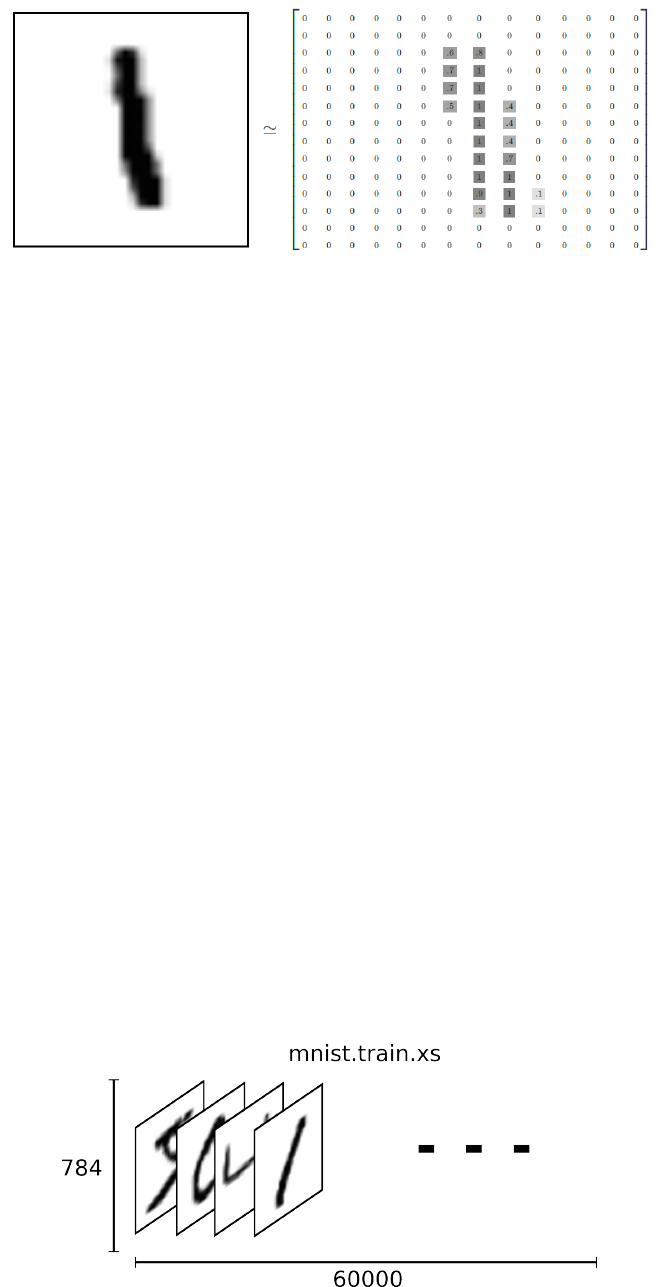
Each image is 28 pixels by 28 pixels. We can interpret this as a big array of numbers:

每一张图片包含 28 ×28 像素．我们可以用一个数字数组来表示这张图片：

We can ﬂatten this array into a vector of 28 ×28 =784 numbers. It doesn’t matter how

we ﬂatten the array, as long as we’re consistent between images. From this perspective, the

MNIST images are just a bunch of points in a 784-dimensional vector space, with a very rich

structure (warning: computationally intensive visualizations).

2.1 MNIST

机器学习入门 41

图2.2:

我们把这个数组展开成一个向量，长度是 28 ×28 =784．如何展开这个数组（数字

间的顺序）不重要，只要保持各个图片采用相同的方式展开．从这个角度来看，MNIST

数据集的图片就是在 784 维向量空间里面的点,并且拥有比较复杂的结构 (注意:此类数

据的可视化是计算密集型的)．

Flattening the data throws away information about the 2D structure of the image. Isn’t

that bad? Well, the best computer vision methods do exploit this structure, and we will in

later tutorials. But the simple method we will be using here, a softmax regression, won’t.

展平图片的数字数组会丢失图片的二维结构信息．这显然是不理想的，最优秀的

计算机视觉方法会挖掘并利用这些结构信息，我们会在后续教程中介绍．但是在这个教

程中我们忽略这些结构，所介绍的简单数学模型，softmax 回归 (softmax regression)，不

会利用这些结构信息．

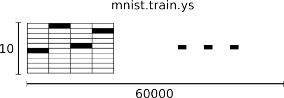
The result is that mnist.train.images is a tensor (an n-dimensional array) with a shape

of [55000, 784]. The ﬁrst dimension indexes the images and the second dimension indexes

the pixels in each image. Each entry in the tensor is the pixel intensity between 0 and 1, for

a particular pixel in a particular image.

因此，在 MNIST 训练数据集中，mnist.train.images是一个形状为 [55000, 784] 的

张量，第一个维度数字用来索引图片，第二个维度数字用来索引每张图片中的像素点．

在此张量里的每一个元素，都表示某张图片里的某个像素的强度值，值介于 0和1之间．

图2.3:

42 第二章基础教程

The corresponding labels in MNIST are numbers between 0 and 9, describing which

digit a given image is of. For the purposes of this tutorial, we’re going to want our labels as

"one-hot vectors". A one-hot vector is a vector which is 0 in most dimensions, and 1 in a

single dimension. In this case, the nth digit will be represented as a vector which is 1 in the

nth dimensions. For example, 3 would be [0, 0,0, 1,0, 0,0, 0,0,0]. Consequently, mnist.train

.labels is a [55000, 10] array of ﬂoats.

相对应的 MNIST 数据集的标签是介于 0到9的数字，用来描述给定图片里表示

的数字．为了用于这个教程，我们使标签数据是"one-hot vectors"．一个 one-hot 向量

除了某一位的数字是 1以外其余各维度数字都是 0．所以在此教程中，数字 n将表示

成一个只有在第 n维度（从 0开始）数字为 1的10 维向量．比如，标签 0将表示成

([1,0,0,0,0,0,0,0,0,0,0])．因此，mnist.train.labels是一个 [55000, 10] 的数字矩阵．

图2.4:

We’re now ready to actually make our model!

现在，我们准备开始真正的建模之旅！

2.1.2 Softmax 回归介绍

We know that every image in MNIST is a digit, whether it’s a zero or a nine. We want

to be able to look at an image and give probabilities for it being each digit. For example, our

model might look at a picture of a nine and be 80% sure it’s a nine, but give a 5% chance to

it being an eight (because of the top loop) and a bit of probability to all the others because

it isn’t sure.

我们知道 MNIST 数据集的每一张图片都表示一个 (0 到9的)数字．那么，如果模

型若能看到一张图就能知道它属于各个数字的对应概率就好了。比如，我们的模型可能

看到一张数字"9" 的图片，就判断出它是数字"9" 的概率为 80%，而有 5% 的概率属于数

字"8"（因为 8和9都有上半部分的小圆），同时给予其他数字对应的小概率（因为该图

像代表它们的可能性微乎其微）．

This is a classic case where a softmax regression is a natural, simple model. If you want

to assign probabilities to an object being one of several different things, softmax is the thing

to do. Even later on, when we train more sophisticated models, the ﬁnal step will be a layer

of softmax.

2.1 MNIST

机器学习入门 43

这是能够体现 softmax 回归自然简约的一个典型案例．softmax 模型可以用来给

不同的对象分配概率．在后文，我们训练更加复杂的模型时，最后一步也往往需要用

softmax 来分配概率．

A softmax regression has two steps: ﬁrst we add up the evidence of our input being in

certain classes, and then we convert that evidence into probabilities.

softmax 回归（softmax regression）分两步：首先对输入被分类对象属于某个类的

“证据”相加求和，然后将这个“证据”的和转化为概率.

To tally up the evidence that a given image is in a particular class, we do a weighted

sum of the pixel intensities. The weight is negative if that pixel having a high intensity is

evidence against the image being in that class, and positive if it is evidence in favor.

我们使用加权的方法来累积计算一张图片是否属于某类的“证据”。如果图片的像

素强有力的体现该图不属于某个类，则权重为负数，相反如果这个像素拥有有利的证据

支持这张图片属于这个类，那么权值为正．

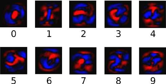
The following diagram shows the weights one model learned for each of these classes.

Red represents negative weights, while blue represents positive weights.

下面的图片显示了一个模型学习到的图片上每个像素对于特定数字类的权值．红

色代表负权值，蓝色代表正权值．

图2.5:

We also add some extra evidence called a bias. Basically, we want to be able to say that

some things are more likely independent of the input. The result is that the evidence for a

class igiven an input xis:

我们也需要引入额外的“证据”，可称之为偏置量 (bias）。总的来说，我们希望它

代表了与所输入向无关的判断证据．因此对于给定的输入图片 x代表某数字 i的总体证

据可以表示为:

evi dencei=

Wi,jxj+bi(2.1)

where Wiis the weights and biis the bias for class i, and jis an index for summing over the

pixels in our input image x. We then convert the evidence tallies into our predicted proba-

44 第二章基础教程

bilities y using the "softmax" function:

其中，Wi代表权重，bi代表第 i类的偏置量，j代表给定图片 x的像素索引用于像素求

和．然后用 softmax 函数可以把这些证据转换成概率 y:

y=so f t max(evi dence) (2.2)

Here softmax is serving as an "activation" or "link" function, shaping the output of our lin-

ear function into the form we want – in this case, a probability distribution over 10 cases.

You can think of it as converting tallies of evidence into probabilities of our input being in

each class. It’s deﬁned as:

这里的 softmax 可以看成是一个激励（activation）函数或是链接（link）函数，把我们定

义的线性函数的输出转换成我们想要的格式，也就是关于 10 个数字类的概率分布．因

此，给定一张图片，它对于每一个数字的吻合度可以被 softmax 函数转换成为一个概率

值．softmax 函数可以定义为：

so f t max(x)=nor mal i ze(exp(x)) (2.3)

If you expand that equation out, you get:

展开等式右边的子式，可以得到：

so f t max(x)i=exp(xi)

jexp(xj)(2.4)

But it’s often more helpful to think of softmax the ﬁrst way: exponentiating its inputs and

then normalizing them. The exponentiation means that one more unit of evidence in-

creases the weight given to any hypothesis multiplicatively. And conversely, having one less

unit of evidence means that a hypothesis gets a fraction of its earlier weight. No hypothesis

ever has zero or negative weight. Softmax then normalizes these weights, so that they add

up to one, forming a valid probability distribution. (To get more intuition about the softmax

function, check out the section on it in Michael Nieslen’s book, complete with an interactive

visualization.)

但是更多的时候把 softmax 模型函数定义为第一种形式：把输入值当成幂指数求值，再

正则化这些结果值．这个幂运算表示，更大的证据对应更大的假设模型（hypothesis）里

面的乘数权重值．反之，拥有更少的证据意味着在假设模型里面拥有更小的乘数系数．

假设模型里的权值不可以是 0值或者负值．Softmax 然后会正则化这些权重值，使它们

的总和等于 1，以此构造一个有效的概率分布．（更多的关于 Softmax 函数的信息，可以

参考 Michael Nieslen 的书里面的这个部分，其中有关于 softmax 的可交互式的可视化解

释．）

2.1 MNIST

机器学习入门 45

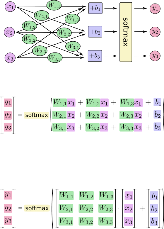
You can picture our softmax regression as looking something like the following, al-

though with a lot more xs. For each output, we compute a weighted sum of the xs, add a

bias, and then apply softmax.

对于 softmax 回归模型可以用下面的图解释，对于输入的 xs 加权求和，再分别加上一个

偏置量，最后再输入到 softmax 函数中：

If we write that out as equations, we get:

如果把它写成一个方程，可以得到：

We can "vectorize" this procedure, turning it into a matrix multiplication and vector addi-

tion. This is helpful for computational efﬁciency. (It’s also a useful way to think.)

我们也可以用向量表示这个计算过程：用矩阵乘法和向量相加．这有助于提高计算效率

（也是一种更有效的思考方式）．

More compactly, we can just write:

更进一步，可以写成更加紧凑的方式：

y=so f t max(Wx+b) (2.5)

2.1.3 实现回归模型

To do efﬁcient numerical computing in Python, we typically use libraries like NumPy

that do expensive operations such as matrix multiplication outside Python, using highly

efﬁcient code implemented in another language. Unfortunately, there can still be a lot of

overhead from switching back to Python every operation. This overhead is especially bad

46 第二章基础教程

if you want to run computations on GPUs or in a distributed manner, where there can be a

high cost to transferring data.

为了在 python 中高效的进行数值计算，我们通常会调用（如 NumPy）外部函数库，

把类似矩阵乘法这样的复杂运算使用其他外部语言实现．不幸的是，从外部计算切换回

Python 的每一个操作，仍然是一个很大的开销．如果你用 GPU 来进行外部计算，这样

的开销会更大．用分布式的计算方式，也会花费更多的资源用来传输数据．

TensorFlow also does its heavy lifting outside python, but it takes things a step fur-

ther to avoid this overhead. Instead of running a single expensive operation independently

from Python, TensorFlow lets us describe a graph of interacting operations that run entirely

outside Python. (Approaches like this can be seen in a few machine learning libraries.)

TensorFlow 也把复杂的计算放在 python 之外完成，但是为了避免前面说的那些开

销，它做了进一步完善．TensorFlow 不单独地运行单一的复杂计算，而是让我们可以先

用图描述一系列可交互的计算操作，然后全部一起在 Python 之外运行．（这样类似的运

行方式，可以在不少的机器学习库中看到．）

To use TensorFlow, we need to import it.

使用 TensorFlow 之前，首先导入它：

 

1import tensorflow as tf

 

We describe these interacting operations by manipulating symbolic variables. Let’s

create one:

我们通过操作符号变量来描述这些可交互的操作单元，可以用下面的方式创建一

个：

 

1x = tf.placeholder("float", [None, 784])

 

xisn’t a speciﬁc value. It’s a placeholder, a value that we’ll input when we ask TensorFlow

to run a computation. We want to be able to input any number of MNIST images, each

ﬂattened into a 784-dimensional vector. We represent this as a 2-D tensor of ﬂoating-point

numbers, with a shape [None, 784]. (Here None means that a dimension can be of any

length.)

x不是一个特定的值，而是一个占位符placeholder，我们在 TensorFlow 运行计算时输入

这个值．我们希望能够输入任意数量的 MNIST 图像，每一张图展平成 784 维的向量．我

们用 2维的浮点数张量来表示这些图，这个张量的形状是 [None，784]．（这里的None表

示此张量的第一个维度可以是任何长度的．）

We also need the weights and biases for our model. We could imagine treating these

like additional inputs, but TensorFlow has an even better way to handle it: Variable. A

Variable is a modiﬁable tensor that lives in TensorFlow’s graph of interacting operations.

It can be used and even modiﬁed by the computation. For machine learning applications,

one generally has the model parameters be Variables.

我们的模型也需要权重值和偏置量，当然我们可以把它们当做是另外的输入（使用

2.1 MNIST

机器学习入门 47

占位符），但 TensorFlow 有一个更好的方法来表示它们：Variable．一个Variable代表一

个可修改的张量，存在在 TensorFlow 的用于描述交互性操作的图中．它们可以用于计

算输入值，也可以在计算中被修改．对于各种机器学习应用，一般都会有模型参数，可

以用Variable表示．

 

1W = tf.Variable(tf.zeros([784,10]))

2b = tf.Variable(tf.zeros([10]))

 

We create these Variables by giving tf.Variable the initial value of the Variable: in this

case, we initialize both W and b as tensors full of zeros. Since we are going to learn Wand b,

it doesn’t matter very much what they initially are.

我们赋予tf.Variable 不同的初值来创建不同的Variable：在这里，我们都用全为零

的张量来初始化W和b．因为我们要学习W和b的值，它们的初值可以随意设置．

Notice that W has a shape of [784, 10] because we want to multiply the 784-dimensional

image vectors by it to produce 10-dimensional vectors of evidence for the difference classes.

bhas a shape of [10] so we can add it to the output.

注意，W的维度是[784，10]，因为我们想要用 784 维的图片向量乘以它以得到一个

10 维的证据值向量，每一位对应不同数字类．b的形状是[10]，所以我们可以直接把它

加到输出上面．

We can now implement our model. It only takes one line!

现在，可以实现我们的模型了，只需以下一行代码：

 

1y = tf.nn.softmax(tf.matmul(x,W) + b)

 

First, we multiply xby Wwith the expression tf.matmul(x, W). This is ﬂipped from

when we multiplied them in our equation, where we had Wx, as a small trick to deal with x

being a 2D tensor with multiple inputs. We then add b, and ﬁnally apply tf.nn.softmax.

首先，我们用tf.matmul(X，W)表示 x乘以 W，对应之前等式里面的 Wx，这里 x是

一个 2维张量拥有多个输入．然后再加上 b，把和输入到tf.nn.softmax函数里面．

That’s it. It only took us one line to deﬁne our model, after a couple short lines of

setup. That isn’t because TensorFlow is designed to make a softmax regression particularly

easy: it’s just a very ﬂexible way to describe many kinds of numerical computations, from

machine learning models to physics simulations. And once deﬁned, our model can be run

on different devices: your computer’s CPU, GPUs, and even phones!

至此，我们先用了几行简短的代码来设置变量，然后只用了一行代码来定义我们的

模型．TensorFlow 不仅仅可以使 softmax 回归模型计算变得特别简单，它也用这种非常

灵活的方式来描述其他各种数值计算，从机器学习模型对物理学模拟仿真模型．一旦被

定义好之后，我们的模型就可以在不同的设备上运行：计算机的 CPU，GPU，甚至是手

机！

48 第二章基础教程

2.1.4 训练模型

In order to train our model, we need to deﬁne what it means for the model to be good.

Well, actually, in machine learning we typically deﬁne what it means for a model to be bad,

called the cost or loss, and then try to minimize how bad it is. But the two are equivalent.

为了训练我们的模型，我们首先需要定义一个指标来评估这个模型是好的．其实，

在机器学习，我们通常定义指标来表示一个模型是坏的，这个指标称为成本（cost）或

损失（loss），然后尽量最小化这个指标．但是，这两种方式是相同的．

One very common, very nice cost function is "cross-entropy." Surprisingly, cross-entropy

arises from thinking about information compressing codes in information theory but it

winds up being an important idea in lots of areas, from gambling to machine learning. It’s

deﬁned:

一个非常常见的，非常漂亮的成本函数是“交叉熵”(cross-entropy)．交叉熵产生于信

息论里面的信息压缩编码技术，但是它后来演变成为从博弈论到机器学习等其他领域

里的重要技术手段．它的定义如下：

Hy′(y)=−

y′

il og (yi) (2.6)

where yis our predicted probability distribution, and y′is the true distribution (the one-

hot vector we’ll input). In some rough sense, the cross-entropy is measuring how inefﬁcient

our predictions are for describing the truth. Going into more detail about cross-entropy is

beyond the scope of this tutorial, but it’s well worth understanding.

y是我们预测的概率分布,y′是实际的分布（我们输入的 one-hot vector)．比较粗糙的理

解是，交叉熵是用来衡量我们的预测用于描述真相的低效性．更详细的关于交叉熵的解

释超出本教程的范畴，但是你很有必要好好理解它．

To implement cross-entropy we need to ﬁrst add a new placeholder to input the cor-

rect answers:

为了计算交叉熵，我们首先需要添加一个新的占位符用于输入正确值：

 

1y = tf.placeholder("float", [None,10])

 

Then we can implement the cross-entropy −y′l og (y),

然后我们可以用 −y′l og (y)计算交叉熵:

 

1cross_entropy = −tf.reduce_sum(y_*tf.log(y))

 

First, tf.log computes the logarithm of each element of y. Next, we multiply each

element of y_ with the corresponding element of tf.log(y). Finally, tf.reduce_sum adds all

the elements of the tensor.

首先，用 tf.log 计算 y的每个元素的对数．接下来，我们把y_的每一个元素和tf.

log(y_)的对应元素相乘．最后，用tf.reduce_sum计算张量的所有元素的总和．

2.1 MNIST

机器学习入门 49

Note that this isn’t just the cross-entropy of the truth with a single prediction, but the

sum of the cross-entropies for all the images we looked at. In this example, we have 100

images in each batch: how well we are doing on 100 data points is a much better description

of how good our model is than a single data point.

值得注意的是，这里的交叉熵不仅仅用来衡量单一的一对预测和真实值，而是所有

100 幅图片的交叉熵的总和．对于 100 个数据点的预测表现比单一数据点的表现能更好

地描述我们的模型的性能．

Now that we know what we want our model to do, it’s very easy to have TensorFlow

train it to do so. Because TensorFlow knows the entire graph of your computations, it can

automatically use the backpropagation algorithm to efﬁciently determine how your vari-

ables affect the cost you ask it minimize. Then it can apply your choice of optimization

algorithm to modify the variables and reduce the cost.

现在我们知道我们需要我们的模型做什么啦，用 TensorFlow 来训练它是非常容易

的．因为 TensorFlow 拥有一张描述你各个计算单元的图，它可以自动地使用反向传播

算法 (backpropagation algorithm)来有效地确定你的变量是如何影响你想要最小化的那

个成本值的．然后，TensorFlow 会用你选择的优化算法来不断地修改变量以降低成本．

 

1train_step = tf.train.GradientDescentOptimizer(0.01).minimize(

cross_entropy)

 

In this case, we ask TensorFlow to minimize cross_entropy using the gradient descent

algorithm with a learning rate of 0.01. Gradient descent is a simple procedure, where Ten-

sorFlow simply shifts each variable a little bit in the direction that reduces the cost. But

TensorFlow also provides many other optimization algorithms: using one is as simple as

tweaking one line.

在这里，我们要求 TensorFlow 用梯度下降算法（gradient descent algorithm）以 0.01

的学习速率最小化交叉熵．梯度下降算法（gradient descent algorithm）是一个简单的

学习过程，TensorFlow 只需将每个变量一点点地往使成本不断降低的方向移动．当然

TensorFlow 也提供了其他许多优化算法：只要简单地调整一行代码就可以使用其他的

算法．

What TensorFlow actually does here, behind the scenes, is it adds new operations

to your graph which implement backpropagation and gradient descent. Then it gives you

back a single operation which, when run, will do a step of gradient descent training, slightly

tweaking your variables to reduce the cost.

TensorFlow 在这里实际上所做的是，它会在后台给描述你的计算的那张图里面增

加一系列新的计算操作单元用于实现反向传播算法和梯度下降算法．然后，它返回给你

的只是一个单一的操作，当运行这个操作时，它用梯度下降算法训练你的模型，微调你

的变量，不断减少成本．

Now we have our model set up to train. One last thing before we launch it, we have to

add an operation to initialize the variables we created:

50 第二章基础教程

现在，我们已经设置好了我们的模型．在运行计算之前，我们需要添加一个操作来

初始化我们创建的变量：

 

1init = tf.initialize_all_variables()

 

We can now launch the model in a Session, and run the operation that initializes the vari-

ables:

现在我们可以在一个 Session 里面启动我们的模型，并且初始化变量：

 

1sess = tf.Session()

2sess.run(init)

 

Let’s train – we’ll run the training step 1000 times!

然后开始训练模型，这里我们让模型循环训练 1000 次！

 

1for iin range(1000):

2batch_xs, batch_ys = mnist.train.next_batch(100)

3sess.run(train_step , feed_dict={x: batch_xs , y_: batch_ys})

 

Each step of the loop, we get a "batch" of one hundred random data points from our

training set. We run train_step feeding in the batches data to replace the placeholders.

该循环的每个步骤中，我们都会随机抓取训练数据中的 100 个批处理数据点，然后

我们用这些数据点作为参数替换之前的占位符来运行train_step．

Using small batches of random data is called stochastic training – in this case, stochas-

tic gradient descent. Ideally, we’d like to use all our data for every step of training because

that would give us a better sense of what we should be doing, but that’s expensive. So, in-

stead, we use a different subset every time. Doing this is cheap and has much of the same

beneﬁt.

使用一小部分的随机数据来进行训练被称为随机训练 (stochastic training)---在这里

更确切的说是随机梯度下降训练．理想情况下，我们希望用我们所有的数据来进行每一

步的训练，因为这能给我们更好的训练结果，但显然这需要很大的计算开销．所以，每

一次训练我们可以使用不同的数据子集，这样做既可以减少计算开销，又可以最大化地

学习到数据集的总体特性．

2.1.5 Evaluating Our Model || 评估我们的模型

How well does our model do?

那么我们的模型性能如何呢？

Well, ﬁrst let’s ﬁgure out where we predicted the correct label. tf.argmax is an extremely

useful function which gives you the index of the highest entry in a tensor along some axis.

For example, tf.argmax(y,1) is the label our model thinks is most likely for each input, while

tf.argmax(y_,1) is the correct label. We can use tf.equal to check if our prediction matches

the truth.

首先让我们找出那些预测正确的标签．tf.argmax()是一个非常有用的函数，它能给

你在一个张量里沿着某条轴的最高条目的索引值．比如，tf.argmax(y,1)是模型认为每个

2.1 MNIST

机器学习入门 51

输入最有可能对应的那些标签，而tf.argmax(y_,1)代表正确的标签．我们可以用tf.equal

来检测我们的预测是否真实标签匹配．

 

1correct_prediction = tf.equal(tf.argmax(y,1), tf.argmax(y_,1))

 

That gives us a list of booleans. To determine what fraction are correct, we cast to

ﬂoating point numbers and then take the mean. For example, [True, False, True, True]

would become [1,0,1,1] which would become 0.75.

这行代码会给我们一组布尔值．为了确定正确预测项的比例，我们可以把布尔值转

换成浮点数，然后取平均值．例如，[True, False, True, True]会变成[1,0,1,1]，取平均

值后得到 0.75 .

 

1accuracy = tf.reduce_mean(tf.cast(correct_prediction , "float"))

 

Finally, we ask for our accuracy on our test data.

最后，我们计算所学习到的模型在测试数据集上面的正确率．

 

1print sess.run(accuracy , feed_dict={x: mnist.test.images, y_: mnist.

test.labels})

 

This should be about 91%.

最终结果值应该大约是 91%．

Is that good? Well, not really. In fact, it’s pretty bad. This is because we’re using a very

simple model. With some small changes, we can get to 97%/. The best models can get to

over 99.7% accuracy! (For more information, have a look at this list of results)

这个结果好吗？嗯，并不太好．事实上，这个结果是很差的．这是因为我们仅仅使

用了一个非常简单的模型．不过，做一些小小的改进，我们就可以得到 97% 的正确率．

最好的模型甚至可以获得超过 99.7% 的准确率！（想了解更多信息，请参考这个结果对

比列表．)

What matter is that we learned from this model. Still, if you’re feeling a bit down about

these results, check out the next tutorial where we do a lot better, and learn how to build

more sophisticated models using TensorFlow!

比结果更重要的是，我们从这个模型中学习到的设计思想．不过，如果你仍然对这

里的结果有点失望，可以查看下个教程，在那里你将学到如何用 FensorFlow 构建更加

复杂的模型以获得更好的性能！

原文地址：MNIST For ML Beginners

52 第二章基础教程

2.2 Deep MNIST for Experts || 深入 MNIST

TensorFlow is a powerful library for doing large-scale numerical computation. One

of the tasks at which it excels is implementing and training deep neural networks. In this

tutorial we will learn the basic building blocks of a TensorFlow model while constructing a

deep convolutional MNIST classiﬁer.

TensorFlow 是一个善于大规模数值计算的强大库件。它的一个强项就是训练并实

现深度神经网络 (deep neural networks)。在本小节中，我们将会学习 TensorFlow 模型构

建的基本方法，并以此构建一个深度卷积 MNIST 分类器。

This introduction assumes familiarity with neural networks and the MNIST dataset. If

you don’t have a background with them, check out the introduction for beginners. Be sure

to install TensorFlow before starting.

本教程假设您已经熟悉神经网络和 MNIST 数据集。如果你尚未了解，请查看新手

指南。再开始学习前请确保您已安装 TensorFlow。

2.2.1 Setup | 安装

Before we create our model, we will ﬁrst load the MNIST dataset, and start a Tensor-

Flow session.

在创建模型之前，我们会先加载 MNIST 数据集，然后启动一个 TensorFlow 会话。

Load MNIST Data | 加载 MINIST 数据

For your convenience, we’ve included a script which automatically downloads and im-

ports the MNIST dataset. It will create a directory 'MNIST_data' in which to store the data

ﬁles.

为了方便起见，我们已经准备了一个脚本来自动下载和导入 MNIST 数据集。它会

自动创建一个'MNIST_data'的目录来存储数据。

 

1import input_data

2mnist = input_data.read_data_sets('MNIST_data', one_hot=True)

 

Here mnist is a lightweight class which stores the training, validation, and testing sets

as NumPy arrays. It also provides a function for iterating through data minibatches, which

we will use below.

此处的 mnist 是一个以 NumPy 数组形式存储训练、验证和测试数据的轻量级类。我

们将在之后使用到它提供的一个函数功能，用于迭代按批处理数据。

Start TensorFlow InteractiveSession | 开始 TensorFlow 交互会话

Tensorﬂow relies on a highly efﬁcient C++ backend to do its computation. The con-

nection to this backend is called a session. The common usage for TensorFlow programs is

to ﬁrst create a graph and then launch it in a session.

2.2 DEEP MNIST FOR EXPERTS ||

深入

MNIST

Tensorﬂow 基于一个高效的 C++ 后台模块进行运算。与这个后台模块的连接叫做会

话(session)。TensorFlow 编程的常规流程是先创建一个图，然后在 session 中加载它。

Here we instead use the convenient InteractiveSession class, which makes TensorFlow

more ﬂexible about how you structure your code. It allows you to interleave operations

which build a computation graph with ones that run the graph. This is particularly con-

venient when working in interactive contexts like IPython. If you are not using an Interac-

tiveSession, then you should build the entire computation graph before starting a session

and launching the graph.

这里，我们使用更加方便的交互会话 (InteractiveSession) 类，它可以让您更加灵活

地构建代码。交互会话能让你在运行图的时候，插入一些构建计算图的操作。这能给使

用交互式文本 shell 如iPython 带来便利。如果你没有使用 InteractiveSession 的话，你需

要在开始 session 和加载图之前，构建整个计算图。

 

1import tensorflow as tf

2sess = tf.InteractiveSession()

 

Computation Graph | 计算图

To do efﬁcient numerical computing in Python, we typically use libraries like NumPy

that do expensive operations such as matrix multiplication outside Python, using highly

efﬁcient code implemented in another language. Unfortunately, there can still be a lot of

overhead from switching back to Python every operation. This overhead is especially bad

if you want to run computations on GPUs or in a distributed manner, where there can be a

high cost to transferring data.

为了高效地在 Python 里进行数值计算，我们一般会使用像 NumPy 这样用其他语言

编写的库件，在 Python 外用其它执行效率高的语言完成这些高运算开销操作（如矩阵

运算）。但是，每一步操作依然会需要切换回 Python 带来很大开销。特别的，这种开销

会在 GPU 运算或是分布式集群运算这类高数据传输需求的运算形式上非常高昂。

TensorFlow also does its heavy lifting outside Python, but it takes things a step fur-

ther to avoid this overhead. Instead of running a single expensive operation independently

from Python, TensorFlow lets us describe a graph of interacting operations that run entirely

outside Python. This approach is similar to that used in Theano or Torch.

TensorFlow 将高运算量计算放在 Python 外进行，同时更进一步设法避免上述的额

外运算开销。不同于在 Python 中独立运行运算开销昂贵的操作，TensorFlow 让我们可

以独立于 Python 以外以图的形式描述交互式操作。这与 Theano、Torch 的做法很相似。

The role of the Python code is therefore to build this external computation graph, and

to dictate which parts of the computation graph should be run. See the Computation Graph

section of Basic Usage for more detail.

因此，这里 Python 代码的角色是构建其外部将运行的计算图，并决定计算图的哪

一部分将被运行。更多的细节和基本使用方法请参阅计算图章节。

54 第二章基础教程

2.2.2 Build a Softmax Regression Model || 构建 Softmax 回归模型

In this section we will build a softmax regression model with a single linear layer. In

the next section, we will extend this to the case of softmax regression with a multilayer con-

volutional network.

在这小节里，我们将会构建一个包含单个线性隐层的 softmax 回归模型。我们将在

下一小结把它扩展成多层卷积网络 softmax 回归模型。

Placeholder | 占位符

We start building the computation graph by creating nodes for the input images and

target output classes.

我们先从创建输入图像和输出类别的节点来创建计算图。

 

1x = tf.placeholder("float", shape=[None, 784])

2y_ = tf.placeholder("float", shape=[None, 10])

 

Here xand yaren’t speciﬁc values. Rather, they are each a placeholder — a value that

we’ll input when we ask TensorFlow to run a computation.

这里的x和y并不代表具体值，他们是一个占位符 (placeholder) — 当TensorFlow 运

行时需要赋值的变量。

The input images xwill consist of a 2d tensor of ﬂoating point numbers. Here we assign

it a shape of [None, 784], where 784 is the dimensionality of a single ﬂattened MNIST image,

and None indicates that the ﬁrst dimension, corresponding to the batch size, can be of any

size. The target output classes y_ will also consist of a 2d tensor, where each row is a one-hot

10-dimensional vector indicating which digit class the corresponding MNIST image belongs

to.

输入图片x是由浮点数值组成的 2维张量 (tensor)。这里，我们定义它为[None, 784]

的shape，其中784是单张展开的 MNIST 图片的维度数。None对应shape的第一个维度，代

表了这批输入图像的数量，可能是任意值。目标输出类y_也是一个 2维张量，其中每一

行为一个 10 维向量代表对应 MNIST 图片的所属数字的类别。

The shape argument to placeholder is optional, but it allows TensorFlow to automati-

cally catch bugs stemming from inconsistent tensor shapes.

虽然placeholder的shape参数是可选的，但有了它，TensorFlow 能够自动捕捉因数据

维度不一致导致的错误。

Variables | 变量

We now deﬁne the weights Wand biases bfor our model. We could imagine treat-

ing these like additional inputs, but TensorFlow has an even better way to handle them:

Variable. A Variable is a value that lives in TensorFlow’s computation graph. It can be used

2.2 DEEP MNIST FOR EXPERTS ||

深入

MNIST

and even modiﬁed by the computation. In machine learning applications, one generally has

the model parameters be Variables.

我们现在为模型定义权重W和偏置b。它们可以被视作是额外的输入量，但是 Ten-

sorFlow 有一个更好的方式来处理：Variable。一个Variable代表着在 TensorFlow 计算图

中的一个值，它是能在计算过程中被读取和修改的。在机器学习的应用过程中，模型参

数一般用Variable来表示。

 

1W = tf.Variable(tf.zeros([784,10]))

2b = tf.Variable(tf.zeros([10]))

 

We pass the initial value for each parameter in the call to tf.Variable. In this case,

we initialize both Wand bas tensors full of zeros. Wis a 784 ×10 matrix (because we have

784 input features and 10 outputs) and bis a 10-dimensional vector (because we have 10

classes).

我们在调用tf.Variable的时候传入初始值。在这个例子里，我们把W和b都初始化为

零向量。W是一个 784 ×10 的矩阵（因为我们有 784 个特征和 10 个输出值）。b是一个 10

维的向量（因为我们有 10 个分类）。

Before Variables can be used within a session, they must be initialized using that ses-

sion. This step takes the initial values (in this case tensors full of zeros) that have already

been speciﬁed, and assigns them to each Variable. This can be done for all Variables at

once.

Variable需要在session之前初始化，才能在session中使用。初始化需要初始值（本

例当中是全为零）传入并赋值给每一个Variable。这个操作可以一次性完成。

 

1sess.run(tf.initialize_all_variables())

 

Predicted Class and Cost Function | 预测分类与损失函数

We can now implement our regression model. It only takes one line! We multiply the

vectorized input images xby the weight matrix W, add the bias b, and compute the softmax

probabilities that are assigned to each class.

现在我们可以实现我们的 regression 模型了。这只需要一行！我们把图片x和权重

矩阵W相乘，加上偏置b，然后计算每个分类的 softmax 概率值。

 

1y = tf.nn.softmax(tf.matmul(x,W) + b)

 

The cost function to be minimized during training can be speciﬁed just as easily. Our

cost function will be the cross-entropy between the target and the model’s prediction.

在训练中最小化损失函数同样很简单。我们这里的损失函数用目标分类和模型预

测分类之间的交叉熵。

 

1cross_entropy = −tf.reduce_sum(y_*tf.log(y))

 

Note that tf.reduce_sum sums across all images in the minibatch, as well as all classes.

We are computing the cross entropy for the entire minibatch.

56 第二章基础教程

注意，tf.reduce_sum把minibatch里的每张图片的交叉熵值都加起来了。我们计算的

交叉熵是指整个minibatch的。

2.2.3 Train the Model | 训练模型

Now that we have deﬁned our model and training cost function, it is straightforward

to train using TensorFlow. Because TensorFlow knows the entire computation graph, it can

use automatic differentiation to ﬁnd the gradients of the cost with respect to each of the

variables. TensorFlow has a variety of builtin optimization algorithms. For this example, we

will use steepest gradient descent, with a step length of 0.01, to descend the cross entropy.

我们已经定义好了模型和训练的时候用的损失函数，接下来使用 TensorFlow 来训

练。因为 TensorFlow 知道整个计算图，它会用自动微分法来找到损失函数对于各个变

量的梯度。TensorFlow 有大量内置优化算法，这个例子中，我们用快速梯度下降法让交

叉熵下降，步长为 0.01。

 

1train_step = tf.train.GradientDescentOptimizer(0.01).minimize(

cross_entropy)

 

What TensorFlow actually did in that single line was to add new operations to the com-

putation graph. These operations included ones to compute gradients, compute parameter

update steps, and apply update steps to the parameters.

这一行代码实际上是用来往计算图上添加一个新操作，其中包括计算梯度，计算每

个参数的步长变化，并且计算出新的参数值。

The returned operation train_step, when run, will apply the gradient descent updates

to the parameters. Training the model can therefore be accomplished by repeatedly running

train_step.

train_step这个操作，用梯度下降来更新权值。因此，整个模型的训练可以通过反

复地运行train_step来完成。

 

1for iin range(1000):

2batch = mnist.train.next_batch(50)

3train_step.run(feed_dict={x: batch[0], y_: batch[1]})

 

Each training iteration we load 50 training examples. We then run the train_step op-

eration, using feed_dict to replace the placeholder tensors xand y_ with the training exam-

ples. Note that you can replace any tensor in your computation graph using feed_dict — it’s

not restricted to just placeholders.

每一步迭代，我们都会加载 50 个训练样本，然后执行一次train_step，使用feed_dict

，用训练数据替换placeholder向量x和y_。注意，在计算图中，你可以用feed_dict来替代

任何张量，并不仅限于替换placeholder。

Evaluate the Model | 评估模型

How well did our model do?

2.2 DEEP MNIST FOR EXPERTS ||

深入

MNIST

我们的模型效果怎样？

First we’ll ﬁgure out where we predicted the correct label. tf.argmax is an extremely

useful function which gives you the index of the highest entry in a tensor along some axis.

For example, tf.argmax(y,1) is the label our model thinks is most likely for each input, while

tf.argmax(y_,1) is the true label. We can use tf.equal to check if our prediction matches

the truth.

首先，要先知道我们哪些 label 是预测正确了。tf.argmax是一个非常有用的函数。它

会返回一个张量某个维度中的最大值的索引。例如，tf.argmax(y,1)表示我们模型对每

个输入的最大概率分类的分类值。而 tf.argmax(y_,1)表示真实分类值。我们可以用tf.

equal来判断我们的预测是否与真实分类一致。

 

1correct_prediction = tf.equal(tf.argmax(y,1), tf.argmax(y_,1))

 

That gives us a list of booleans. To determine what fraction are correct, we cast to

ﬂoating point numbers and then take the mean. For example, [True, False, True, True]

would become [1,0,1,1] which would become 0.75.

这里返回一个布尔数组。为了计算我们分类的准确率，我们将布尔值转换为浮点数

来代表对、错，然后取平均值。例如：[True, False, True, True]变为[1,0,1,1]，计算出

平均值为0.75。

 

1accuracy = tf.reduce_mean(tf.cast(correct_prediction , "float"))

 

Finally, we can evaluate our accuracy on the test data. This should be about 91% cor-

rect.

最后，我们可以计算出在测试数据上的准确率，大概是 91%。

 

1print accuracy.eval(feed_dict={x: mnist.test.images, y_: mnist.test.

labels})

 

2.2.4 Build a Multilayer Convolutional Network | 构建多层卷积网络模型

Getting 91% accuracy on MNIST is bad. It’s almost embarrassingly bad. In this section,

we’ll ﬁx that, jumping from a very simple model to something moderately sophisticated: a

small convolutional neural network. This will get us to around 99.2% accuracy — not state

of the art, but respectable.

在MNIST 上只有 91% 正确率，实在太糟糕。在这个小节里，我们用一个稍微复杂

的模型：卷积神经网络来改善效果。这会达到大概 99.2% 的准确率。虽然不是最高，但

是还是比较让人满意。

Weight Initialization | 权重初始化

To create this model, we’re going to need to create a lot of weights and biases. One

should generally initialize weights with a small amount of noise for symmetry breaking, and

58 第二章基础教程

to prevent 0 gradients. Since we’re using ReLU neurons, it is also good practice to initial-

ize them with a slightly positive initial bias to avoid "dead neurons." Instead of doing this

repeatedly while we build the model, let’s create two handy functions to do it for us.

在创建模型之前，我们先来创建权重和偏置。一般来说，初始化时应加入轻微噪声，

来打破对称性，防止零梯度的问题。因为我们用的是 ReLU，所以用稍大于 0的值来初

始化偏置能够避免节点输出恒为 0的问题（dead neurons）。为了不在建立模型的时候

反复做初始化操作，我们定义两个函数用于初始化。

 

1def weight_variable(shape):

2initial = tf.truncated_normal(shape, stddev=0.1)

3return tf.Variable(initial)

5def bias_variable(shape):

6initial = tf.constant(0.1, shape=shape)

7return tf.Variable(initial)

 

Convolution and Pooling | 卷积和池化

TensorFlow also gives us a lot of ﬂexibility in convolution and pooling operations. How

do we handle the boundaries? What is our stride size? In this example, we’re always going

to choose the vanilla version. Our convolutions uses a stride of one and are zero padded so

that the output is the same size as the input. Our pooling is plain old max pooling over 2×2

blocks. To keep our code cleaner, let’s also abstract those operations into functions.

TensorFlow 在卷积和池化上有很强的灵活性。我们怎么处理边界？步长应该设多

大？在这个实例里，我们会一直使用 vanilla 版本。我们的卷积使用 1步长（stride size），

0边距（padding size）的模板，保证输出和输入是同一个大小。我们的池化用简单传统

的2×2大小的模板做 max pooling。为了代码更简洁，我们把这部分抽象成一个函数。

 

1def conv2d(x, W):

2return tf.nn.conv2d(x, W, strides=[1, 1, 1, 1], padding='SAME')

4def max_pool_2x2(x):

5return tf.nn.max_pool(x, ksize=[1, 2, 2, 1], strides=[1, 2, 2,

1], padding='SAME')

 

First Convolutional Layer | 第一层卷积

We can now implement our ﬁrst layer. It will consist of convolution, followed by max

pooling. The convolutional will compute 32 features for each 5 ×5 patch. Its weight tensor

will have a shape of [5, 5, 1, 32]. The ﬁrst two dimensions are the patch size, the next is

the number of input channels, and the last is the number of output channels. We will also

have a bias vector with a component for each output channel.

现在我们可以开始实现第一层了。它由一个卷积接一个 max pooling 完成。卷积在

每个 5×5的patch 中算出 32 个特征。权重是一个[5, 5, 1, 32]的张量，前两个维度是

2.2 DEEP MNIST FOR EXPERTS ||

深入

MNIST

patch 的大小，接着是输入的通道数目，最后是输出的通道数目。输出对应一个同样大

小的偏置向量。

 

1W_conv1 = weight_variable([5, 5, 1, 32])

2b_conv1 = bias_variable([32])

 

To apply the layer, we ﬁrst reshape xto a 4d tensor, with the second and third dimen-

sions corresponding to image width and height, and the ﬁnal dimension corresponding to

the number of color channels.

为了用这一层，我们把x变成一个 4d 向量，第 2、3维对应图片的宽高，最后一维代

表颜色通道。

 

1x_image = tf.reshape(x, [−1,28,28,1])

 

We then convolve x_image with the weight tensor, add the bias, apply the ReLU func-

tion, and ﬁnally max pool.

我们把x_image和权值向量进行卷积相乘，加上偏置，使用 ReLU 激活函数，最后 max

pooling。

 

1h_conv1 = tf.nn.relu(conv2d(x_image, W_conv1) + b_conv1)

2h_pool1 = max_pool_2x2(h_conv1)

 

Second Convolutional Layer | 第二层卷积

In order to build a deep network, we stack several layers of this type. The second layer

will have 64 features for each 5 ×5 patch.

为了构建一个更深的网络，我们会把几个类似的层堆叠起来。第二层中，每个 5x5

的patch 会得到 64 个特征。

 

1W_conv2 = weight_variable([5, 5, 32, 64])

2b_conv2 = bias_variable([64])

4h_conv2 = tf.nn.relu(conv2d(h_pool1, W_conv2) + b_conv2)

5h_pool2 = max_pool_2x2(h_conv2)

 

Densely Connected Layer | 密集连接层

Now that the image size has been reduced to 7 ×7, we add a fully-connected layer

with 1024 neurons to allow processing on the entire image. We reshape the tensor from the

pooling layer into a batch of vectors, multiply by a weight matrix, add a bias, and apply a

ReLU.

现在，图片降维到 7×7，我们加入一个有 1024 个神经元的全连接层，用于处理整

个图片。我们把池化层输出的张量 reshape 成一些向量，乘上权重矩阵，加上偏置，使

用ReLU 激活。

 

1W_fc1 = weight_variable([7 * 7 * 64, 1024])

2b_fc1 = bias_variable([1024])

60 第二章基础教程

4h_pool2_flat = tf.reshape(h_pool2, [−1, 7*7*64])

5h_fc1 = tf.nn.relu(tf.matmul(h_pool2_flat , W_fc1) + b_fc1)

 

Dropout

To reduce overﬁtting, we will apply dropout before the readout layer. We create a place-

holder for the probability that a neuron’s output is kept during dropout. This allows us to

turn dropout on during training, and turn it off during testing. TensorFlow’s tf.nn.dropout

op automatically handles scaling neuron outputs in addition to masking them, so dropout

just works without any additional scaling.

为了减少过拟合，我们在输出层之前加入 dropout。我们用一个 placeholder 来代表

一个神经元在 dropout 中被保留的概率。这样我们可以在训练过程中启用 dropout，在

测试过程中关闭 dropout。TensorFlow 的tf.nn.dropout操作会自动处理神经元输出值的

scale。所以用 dropout 的时候可以不用考虑 scale。

 

1keep_prob = tf.placeholder("float")

2h_fc1_drop = tf.nn.dropout(h_fc1 , keep_prob)

 

Readout Layer | 输出层

Finally, we add a softmax layer, just like for the one layer softmax regression above.

最后，我们添加一个 softmax 层，就像前面的单层 softmax regression 一样。

 

1W_fc2 = weight_variable([1024, 10])

2b_fc2 = bias_variable([10])

4y_conv=tf.nn.softmax(tf.matmul(h_fc1_drop , W_fc2) + b_fc2)

 

Train and Evaluate the Model | 训练和评估模型

How well does this model do? To train and evaluate it we will use code that is nearly

identical to that for the simple one layer SoftMax network above. The differences are that:

we will replace the steepest gradient descent optimizer with the more sophisticated ADAM

optimizer; we will include the additional parameter keep_prob in feed_dict to control the

dropout rate; and we will add logging to every 100th iteration in the training process.

这次效果又有多好呢？我们用前面几乎一样的代码来测测看。只是我们会用更加复

杂的 ADAM 优化器来做梯度最速下降，在 feed_dict 中加入额外的参数 keep_prob 来控

制dropout 比例。然后每 100 次迭代输出一次日志。

 

1cross_entropy = −tf.reduce_sum(y_*tf.log(y_conv))

2train_step = tf.train.AdamOptimizer(1e−4).minimize(cross_entropy)

3correct_prediction = tf.equal(tf.argmax(y_conv ,1), tf.argmax(y_,1))

4accuracy = tf.reduce_mean(tf.cast(correct_prediction , "float"))

5sess.run(tf.initialize_all_variables())

6for iin range(20000):

7batch = mnist.train.next_batch(50)

8if i%100 == 0:

9train_accuracy = accuracy.eval(feed_dict={

10 x:batch[0], y_: batch[1], keep_prob: 1.0})

2.2 DEEP MNIST FOR EXPERTS ||

深入

MNIST

11 print "step␣%d,␣training␣accuracy␣%g"%(i, train_accuracy)

12 train_step.run(feed_dict={x: batch[0], y_: batch[1], keep_prob:

0.5})

14 print "test␣accuracy␣%g"%accuracy.eval(feed_dict={

15 x: mnist.test.images, y_: mnist.test.labels , keep_prob: 1.0})

 

The ﬁnal test set accuracy after running this code should be approximately 99.2%.

以上代码，在最终测试集上的准确率大概是 99.2%。

We have learned how to quickly and easily build, train, and evaluate a fairly sophisti-

cated deep learning model using TensorFlow.

目前为止，我们已经学会了用 TensorFlow 来快速和简易地搭建、训练和评估一个

复杂一点儿的深度学习模型。

原文地址：Deep MNIST for Experts

62 第二章基础教程

2.3 TensorFlow Mechanics 101

Code:tensorﬂow/examples/tutorials/mnist/

代码地址:tensorﬂow/g3doc/tutorials/mnist/

The goal of this tutorial is to show how to use TensorFlow to train and evaluate a simple

feed-forward neural network for handwritten digit classiﬁcation using the (classic) MNIST

data set. The intended audience for this tutorial is experienced machine learning users in-

terested in using TensorFlow.

本篇教程的目的，是向大家展示如何利用 TensorFlow 使用（经典）MNIST 数据集

训练并评估一个用于识别手写数字的简易前馈神经网络（feed-forward neural network）。

我们的目标读者是有兴趣使用 TensorFlow 的机器学习资深人士。

These tutorials are not intended for teaching Machine Learning in general.

因此，撰写该系列教程并不是为了教大家机器学习领域的基础知识。

Please ensure you have followed the instructions to install TensorFlow.

在学习本教程之前，请确保您已按照安装 TensorFlow 教程中的要求，完成了安装。

2.3.1 教程使用的文件

本教程引用如下文件：

只需要直接运行 fully_connected_feed.py 文件，就可以开始训练：

python fully_connected_feed.py

2.3.2 准备数据

MNIST 是机器学习领域的一个经典问题，指的是让机器查看一系列大小为 28 ×28

像素的手写数字灰度图像，并判断这些图像代表 0–9 中的哪一个数字。

图2.6:

更多相关信息，请查阅 Yann LeCun 网站中关于 MNIST 的介绍或者 Chris Olah 对

MNIST 的可视化探索。

下载

在run\_training()方法的一开始，input\_data.read\_data\_sets()函数会确保你的

本地训练文件夹中，已经下载了正确的数据，然后将这些数据解压并返回一个含有DataSet

实例的字典。

2.3 TENSORFLOW MECHANICS 101

 

1data_sets = input_data.read_data_sets(FLAGS.train_dir , FLAGS.

fake_data)

 

Add table here2

输入与占位符

placeholder_inputs()函数将生成两个tf.placeholder 操作，定义传入图表中的 shape

参数，shape 参数中包括batch_size值，后续还会将实际的训练用例传入图表。

 

1images_placeholder = tf.placeholder(tf.float32, shape=(batch_size,

IMAGE_PIXELS))

2labels_placeholder = tf.placeholder(tf.int32, shape=(batch_size))

 

在训练循环（training loop）的后续步骤中，传入的整个图像和标签数据集会被切片，

以符合每一个操作所设置的 batch_size值，占位符操作将会填补以符合这个batch_size

值。然后使用feed_dict参数，将数据传入sess.run()函数。

2.3.3 构建图表（Build the Graph）

在为数据创建占位符之后，就可以运行mnist.py文件，经过三阶段的模式函数操作：

inference()，loss()\lstinline，和training()。图表就构建完成了。

1. inference() ——尽可能地构建好图表，满足促使神经网络向前反馈并做出预测的

要求。

2. loss() ——往 inference 图表中添加生成损失（loss）所需要的操作（ops）。

3. training() ——往损失图表中添加计算并应用梯度（gradients）所需的操作。

推理（Inference）

inference()函数会尽可能地构建图表，做到返回包含了预测结果（output predic-

tion）的 Tensor。

它接受图像占位符为输入，在此基础上借助 ReLu(Rectiﬁed Linear Units) 激活函数，

构建一对完全连接层（layers），以及一个有着十个节点（node）、指明了输出 logtis 模型

的线性层。

每一层都创建于一个唯一的tf.name_scope之下，创建于该作用域之下的所有元素都

将带有其前缀。

 

1with tf.name_scope('hidden1') as scope:

 

1fake_data标记是用于单元测试的，读者可以不必理会。

2了解更多数据有关信息，请查阅此系列教程的 [数据下载](mnist/download/index.md) 部分.

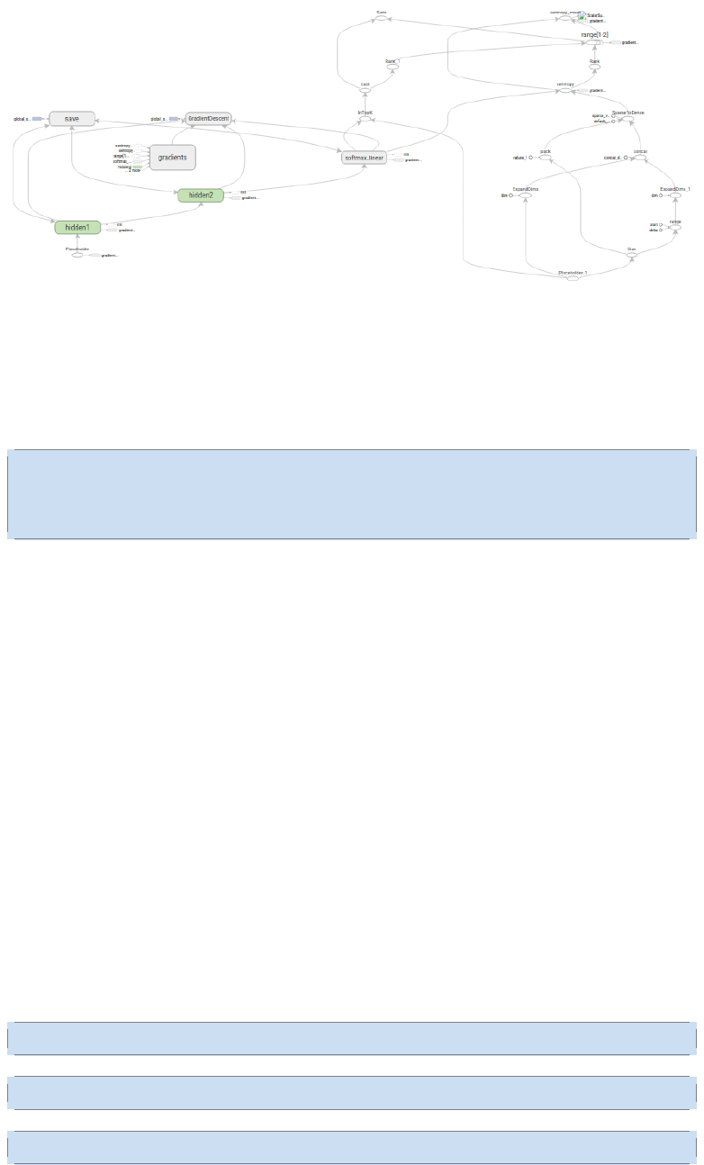
64 第二章基础教程

图2.7:

在定义的作用域中，每一层所使用的权重和偏差都在tf.Variable 实例中生成，并

且包含了各自期望的 shape。

 

1weights = tf.Variable(tf.truncated_normal([IMAGE_PIXELS ,

hidden1_units], stddev=1.0 / math.sqrt(float(IMAGE_PIXELS))), name

='weights')

2biases = tf.Variable(tf.zeros([hidden1_units]), name='biases')

 

例如，当这些层是在hidden1作用域下生成时，赋予权重变量的独特名称将会是"hidden1

/weights"。

每个变量在构建时，都会获得初始化操作（initializer ops）。

在这种最常见的情况下，通过tf.truncated_normal 函数初始化权重变量，给赋予

的shape 则是一个二维 tensor，其中第一个维度代表该层中权重变量所连接（connect

from）的单元数量，第二个维度代表该层中权重变量所连接到的（connect to）单元数

量。对于名叫hidden1的第一层，相应的维度则是[IMAGE_PIXELS, hidden1_units]，因为权

重变量将图像输入连接到了hidden1层。tf.truncated_normal初始函数将根据所得到的均

值和标准差，生成一个随机分布。

然后，通过tf.zeros 函数初始化偏差变量（biases），确保所有偏差的起始值都是 0，

而它们的 shape 则是其在该层中所接到的（connect to）单元数量。

图表的三个主要操作，分别是两个tf.nn.relu 操作，它们中嵌入了隐藏层所需的tf.

matmul ；以及 logits 模型所需的另外一个tf.matmul。三者依次生成，各自的tf.Variable实

例则与输入占位符或下一层的输出 tensor 所连接。

 

1hidden1 = tf.nn.relu(tf.matmul(images, weights) + biases)

 

 

1hidden2 = tf.nn.relu(tf.matmul(hidden1 , weights) + biases)

 

 

1logits = tf.matmul(hidden2, weights) + biases

 

最后，程序会返回包含了输出结果的 ‘logits‘Tensor。

2.3 TENSORFLOW MECHANICS 101

损失（Loss）

loss()函数通过添加所需的损失操作，进一步构建图表。

首先，labels_placeholer中的值，将被编码为一个含有 1-hot values 的Tensor。例如，

如果类标识符为“3”，那么该值就会被转换为：[0, 0, 0, 1, 0, 0, 0, 0, 0, 0]

 

1batch_size = tf.size(labels)

2labels = tf.expand_dims(labels , 1)

3indices = tf.expand_dims(tf.range(0, batch_size, 1), 1)

4concated = tf.concat(1, [indices , labels])

5onehot_labels = tf.sparse_to_dense(

6concated, tf.pack([batch_size , NUM_CLASSES]), 1.0, 0.0)

 

之后，又添加一个tf.nn.softmax_cross_entropy_with_logits 操作3，用来比较inference

()函数与 1-hot 标签所输出的 logits Tensor。

 

1cross_entropy = tf.nn.softmax_cross_entropy_with_logits(logits,

onehot_labels , name='xentropy')

 

然后，使用tf.reduce_mean 函数，计算 batch 维度（第一维度）下交叉熵（cross entropy）

的平均值，将将该值作为总损失。

 

1loss = tf.reduce_mean(cross_entropy, name='xentropy_mean')

 

最后，程序会返回包含了损失值的 Tensor。

训练

training()函数添加了通过梯度下降（gradient descent）将损失最小化所需的操作。

首先，该函数从loss()函数中获取损失 Tensor，将其交给[tf.scalar_summary] ，后

者在与SummaryWriter（见下文）配合使用时，可以向事件文件（events ﬁle）中生成汇总

值（summary values）。在本篇教程中，每次写入汇总值时，它都会释放损失 Tensor 的

当前值（snapshot value）。

 

1tf.scalar_summary(loss.op.name, loss)

 

接下来，我们实例化一个[tf.train.GradientDescentOptimizer] ，负责按照所要求的

学习效率（learning rate）应用梯度下降法（gradients）。

 

1optimizer = tf.train.GradientDescentOptimizer(FLAGS.learning_rate)

 

之后，我们生成一个变量用于保存全局训练步骤（global training step）的数值，并

使用minimize() 函数更新系统中的三角权重（triangle weights）、增加全局步骤的操作。

根据惯例，这个操作被称为train_op，是 TensorFlow 会话（session）诱发一个完整训练

步骤所必须运行的操作（见下文）。

 

1global_step = tf.Variable(0, name='global_step', trainable=False)

2train_op = optimizer.minimize(loss, global_step=global_step)

 

3交叉熵是信息理论中的概念，可以让我们描述如果基于已有事实，相信神经网络所做的推测最坏会

导致什么结果。更多详情，请查阅博文《可视化信息理论》(http://colah.github.io/posts/2015-09-Visual-

Information/)

66 第二章基础教程

最后，程序返回包含了训练操作（training op）输出结果的 Tensor。

2.3.4 训练模型

一旦图表构建完毕，就通过fully_connected_feed.py文件中的用户代码进行循环地

迭代式训练和评估。

图表 (The Graph)

在run_training()这个函数的一开始，是一个 Python 语言中的with命令，这个命令

表明所有已经构建的操作都要与默认的[`tf.Graph`] 全局实例关联起来。

 

1with tf.Graph().as_default():

 

tf.Graph实例是一系列可以作为整体执行的操作。TensorFlow 的大部分场景只需要

依赖默认图表一个实例即可。

利用多个图表的更加复杂的使用场景也是可能的，但是超出了本教程的范围。

会话 (The Session)

完成全部的构建准备、生成全部所需的操作之后，我们就可以创建一个tf.Session

，用于运行图表。

 

1sess = tf.Session()

 

另外，也可以利用with代码块生成Session，限制作用域：

 

1with tf.Session() as sess:

 

Session函数中没有传入参数，表明该代码将会依附于（如果还没有创建会话，则会

创建新的会话）默认的本地会话。

生成会话之后，所有tf.Variable实例都会立即通过调用各自初始化操作中的sess.

run() 函数进行初始化。

 

1init = tf.initialize_all_variables()

2sess.run(init)

 

sess.run() 方法将会运行图表中与作为参数传入的操作相对应的完整子集。在初次

调用时，init操作只包含了变量初始化程序tf.group 。图表的其他部分不会在这里，而

是在下面的训练循环运行。

训练循环

完成会话中变量的初始化之后，就可以开始训练了。

训练的每一步都是通过用户代码控制，而能实现有效训练的最简单循环就是：

 

1for step in xrange(max_steps):

2sess.run(train_op)

 

2.3 TENSORFLOW MECHANICS 101

但是，本教程中的例子要更为复杂一点，原因是我们必须把输入的数据根据每一步

的情况进行切分，以匹配之前生成的占位符。

向图表提

执行每一步时，我们的代码会生成一个反馈字典（feed dictionary），其中包含对应

步骤中训练所要使用的例子，这些例子的哈希键就是其所代表的占位符操作。

fill_feed_dict函数会查询给定的DataSet，索要下一批次batch_size的图像和标签，

与占位符相匹配的 Tensor 则会包含下一批次的图像和标签。

 

1images_feed , labels_feed = data_set.next_batch(FLAGS.batch_size)

 

然后，以占位符为哈希键，创建一个 Python 字典对象，键值则是其代表的反馈

Tensor。

 

1feed_dict = {

2images_placeholder: images_feed ,

3labels_placeholder: labels_feed ,

 

这个字典随后作为feed_dict参数，传入sess.run()函数中，为这一步的训练提供输

入样例。

检查状态

在运行sess.run()函数时，要在代码中明确其需要获取的两个值：[train_op, loss]。

 

1for step in xrange(FLAGS.max_steps):

2feed_dict = fill_feed_dict(data_sets.train, images_placeholder ,

labels_placeholder)

3_, loss_value = sess.run([train_op , loss], feed_dict=feed_dict)

 

因为要获取这两个值，sess.run()会返回一个有两个元素的元组。其中每一个Tensor

对象，对应了返回的元组中的 numpy 数组，而这些数组中包含了当前这步训练中对应

Tensor 的值。由于train_op并不会产生输出，其在返回的元祖中的对应元素就是None，所

以会被抛弃。但是，如果模型在训练中出现偏差，loss Tensor 的值可能会变成NaN，所

以我们要获取它的值，并记录下来。

假设训练一切正常，没有出现NaN，训练循环会每隔 100 个训练步骤，就打印一行简

单的状态文本，告知用户当前的训练状态。

 

1if step % 100 == 0:

2print 'Step␣%d:␣loss␣=␣%.2f␣(%.3f␣sec)' % (step, loss_value ,

duration)

 

状态可视化为了释放[TensorBoard] 所使用的事件文件（events ﬁle），所有的即时数据

（在这里只有一个）都要在图表构建阶段合并至一个操作（op）中。

 

1summary_op = tf.merge_all_summaries()

 

在创建好会话（session）之后，可以实例化一个tf.train.SummaryWriter ，用于写入

包含了图表本身和即时数据具体值的事件文件。

 

1summary_writer = tf.train.SummaryWriter(FLAGS.train_dir , graph_def=

sess.graph_def)

 

68 第二章基础教程

最后，每次运行summary_op时，都会往事件文件中写入最新的即时数据，函数的输

出会传入事件文件读写器（writer）的add_summary()函数。。

 

1summary_str = sess.run(summary_op, feed_dict=feed_dict)

2summary_writer.add_summary(summary_str , step)

 

事件文件写入完毕之后，可以就训练文件夹打开一个 TensorBoard，查看即时数据

的情况。

** 注意 **：了解更多如何构建并运行 TensorBoard 的信息，请查看相关教程Tensorboard：

训练过程可视化。

保存检查点 (checkpoint) 为了得到可以用来后续恢复模型以进一步训练或评估的检查

点文件（checkpoint ﬁle），我们实例化一个tf.train.Saver

 

1saver = tf.train.Saver()

 

在训练循环中，将定期调用saver.save() 方法，向训练文件夹中写入包含了当前所

有可训练变量值得检查点文件。

 

1saver.save(sess, FLAGS.train_dir , global_step=step)

 

这样，我们以后就可以使用saver.restore() 方法，重载模型的参数，继续训练。

 

1saver.restore(sess, FLAGS.train_dir)

 

2.3.5 评估模型

每隔一千个训练步骤，我们的代码会尝试使用训练数据集与测试数据集，对模型进

行评估。do_eval函数会被调用三次，分别使用训练数据集、验证数据集合测试数据集。

 

1print 'Training␣Data␣Eval:'

2do_eval(sess, eval_correct, images_placeholder , labels_placeholder ,

data_sets.train)

3print 'Validation␣Data␣Eval:'

4do_eval(sess, eval_correct, images_placeholder , labels_placeholder ,

data_sets.validation)

2.3 TENSORFLOW MECHANICS 101

5print 'Test␣Data␣Eval:'

6do_eval(sess, eval_correct , images_placeholder , labels_placeholder ,

data_sets.test)

 

>注意，更复杂的使用场景通常是，先隔绝data_sets.test测试数据集，只有在大量

的超参数优化调整（hyperparameter tuning）之后才进行检查。但是，由于 MNIST 问题

比较简单，我们在这里一次性评估所有的数据。

构建评估图表（Eval Graph）

在打开默认图表（Graph）之前，我们应该先调用get_data(train=False)函数，抓取

测试数据集。

 

1test_all_images , test_all_labels = get_data(train=False)

 

在进入训练循环之前，我们应该先调用mnist.py文件中的evaluation函数，传入的

logits 和标签参数要与loss函数的一致。这样做事为了先构建 Eval 操作。

 

1eval_correct = mnist.evaluation(logits , labels_placeholder)

 

evaluation函数会生成tf.nn.in_top_k 操作，如果在 k个最有可能的预测中可以发现

真的标签，那么这个操作就会将模型输出标记为正确。在本文中，我们把 k的值设置为

1，也就是只有在预测是真的标签时，才判定它是正确的。

 

1eval_correct = tf.nn.in_top_k(logits , labels, 1)

 

评估图表的输出（Eval Output）

之后，我们可以创建一个循环，往其中添加feed_dict，并在调用sess.run()函数时

传入eval_correct操作，目的就是用给定的数据集评估模型。

 

1for step in xrange(steps_per_epoch):

2feed_dict = fill_feed_dict(data_set,

3images_placeholder,

4labels_placeholder)

5true_count += sess.run(eval_correct, feed_dict=feed_dict)

 

true_count变量会累加所有in_top_k操作判定为正确的预测之和。接下来，只需要将

正确测试的总数，除以例子总数，就可以得出准确率了。

 

1precision = float(true_count) / float(num_examples)

2print '␣␣Num␣examples:␣%d␣␣Num␣correct:␣%d␣␣Precision␣@␣1:␣%0.02f' %

(

3num_examples, true_count , precision)

 

原文：TensorFlow Mechanics 101 翻译：bingjin 校对：LichAmnesia

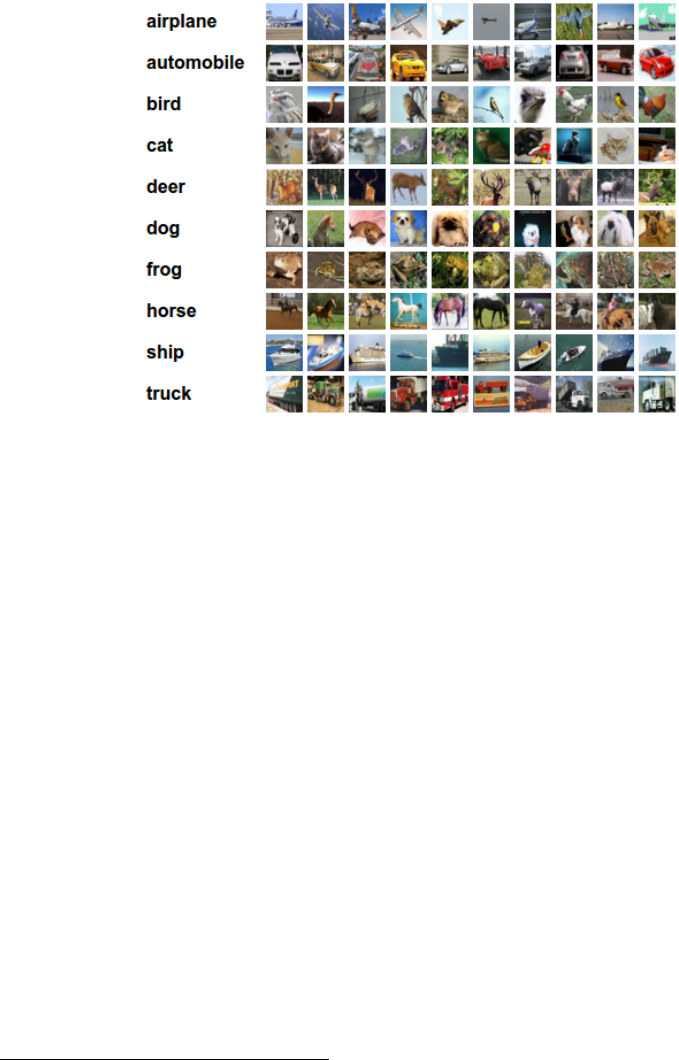
70 第二章基础教程

2.4 卷积神经网络

2.4.1 Overview

对CIFAR-10 数据集的分类是机器学习中一个公开的基准测试问题，其任务是对一

组32x32RGB 的图像进行分类，这些图像涵盖了 10 个类别：airplane,automobile,bird,

cat,deer,dog,frog,horse,ship,和truck.4

图2.8:

想了解更多信息请参考CIFAR-10 page，以及 Alex Krizhevsky 写的技术报告。

目标

本教程的目标是建立一个用于识别图像的相对较小的卷积神经网络，在这一过程

中，本教程会：

•着重于建立一个规范的网络组织结构，训练并进行评估；

•为建立更大规模更加复杂的模型提供一个范例

选择 CIFAR-10 是因为它的复杂程度足以用来检验 TensorFlow 中的大部分功能，并

可将其扩展为更大的模型。与此同时由于模型较小所以训练速度很快，比较适合用来测

试新的想法，检验新的技术。

本教程的重点

CIFAR-10 教程演示了在 TensorFlow 上构建更大更复杂模型的几个种重要内容：

4This tutorial is intended for advanced users of TensorFlow and assumes expertise and experience in ma-

chine learning

2.4

卷积神经网络 71

•相关核心数学对象，如卷积、修正线性激活、最大池化以及局部响应归一化；

•训练过程中一些网络行为的可视化，这些行为包括输入图像、损失情况、网络行

为的分布情况以及梯度；

•算法学习参数的移动平均值的计算函数，以及在评估阶段使用这些平均值提高预

测性能；

•实现了一种机制，使得学习率随着时间的推移而递减；

•为输入数据设计预存取队列，将磁盘延迟和高开销的图像预处理操作与模型分离

开来处理；

我们也提供了模型的多 GUP 版本，用以表明：

•可以配置模型后使其在多个 GPU 上并行的训练

•可以在多个 GPU 之间共享和更新变量值

我们希望本教程给大家开了个头，使得在 Tensorﬂow 上可以为视觉相关工作建立

更大型的 Cnns 模型

模型架构

本教程中的模型是一个多层架构，由卷积层和非线性层 (nonlinearities) 交替多次排

列后构成。这些层最终通过全连通层对接到 softmax 分类器上。这一模型除了最顶部的

几层外，基本跟 Alex Krizhevsky 提出的模型一致。

在一个 GPU 上经过几个小时的训练后，该模型达到了最高 86% 的精度。细节请查

看下面的描述以及代码。模型中包含了 1,068,298 个学习参数，分类一副图像需要大概

19.5M 个乘加操作。

2.4.2 Code Organization

本教程的代码位于tensorﬂow/models/image/cifar10/.

72 第二章基础教程

[c]@ll@

文

件

作

用cifar10_input

.py

读

取

本

地

CIFAR-

的

二

进

制

文

件

格

式

的

内

容。

cifar10

.py

建

立

CIFAR-

的

模

型。

cifar10_train

.py

在

CPU

或

GPU

上

训

练

CIFAR-

的

模

型。

cifar10_multi_gpu_train

.py

在

多

GPU

上

训

练

CIFAR-

的

模

型。

cifar10_eval

.py

评

估

CIFAR-

模

型

的

预

测

性

能。

2.4.3 CIFAR-10 模型

CIFAR-10 网络模型部分的代码位于cifar10.py。完整的训练图中包含约 765 个操作，

但是通过下面的模块来构造训练图可以最大限度的提高代码复用率:

1. 模型输入:包括inputs() 、distorted\_inputs()等一些操作，分别用于读取 CIFAR

的图像并进行预处理，做为后续评估和训练的输入；

2. 模型预测:包括inference()等一些操作，用于进行统计计算，比如在提供的图像

进行分类；adds operations that perform inference, i.e. classiﬁcation, on supplied

images.

3. 模型训练:包括loss() 和train()等一些操作，用于计算损失、计算梯度、进行变

量更新以及呈现最终结果。

模型输入

输入模型是通过 inputs() 和distorted\_inputs()函数建立起来的，这 2个函数会

从CIFAR-10 二进制文件中读取图片文件，由于每个图片的存储字节数是固定的，因此

可以使用tf.FixedLengthRecordReader函数。更多的关于Reader类的功能可以查看Reading

Data。

图片文件的处理流程如下：

2.4

卷积神经网络 73

•图片会被统一裁剪到 24x24 像素大小，裁剪中央区域用于评估或随机裁剪用于训

练；

•图片会进行近似的白化处理，使得模型对图片的动态范围变化不敏感。

对于训练，我们另外采取了一系列随机变换的方法来人为的增加数据集的大小：

•对图像进行随机的左右翻转；

•随机变换图像的亮度；

•随机变换图像的对比度；

可以在Images页的列表中查看所有可用的变换，对于每个原始图我们还附带了一

个image_summary，以便于在 TensorBoard 中查看。这对于检查输入图像是否正确十分有

用。

从磁盘上加载图像并进行变换需要花费不少的处理时间。为了避免这些操作减慢

训练过程，我们在 16 个独立的线程中并行进行这些操作，这 16 个线程被连续的安排在

一个 TensorFlow队列中。

模型预测

模型的预测流程由inference()构造，该函数会添加必要的操作步骤用于计算预测值

的logits，其对应的模型组织方式如下所示：

74 第二章基础教程

[c]@ll@

Layer

名

称

描

述conv1 实

现卷

积

以

及

rec-

ti-

ﬁed

lin-

ear

acti-

va-

tion.

pool1 max

pool-

ing.

norm1 局

部

响

应

归

一

化.

conv2 卷

积

and

rec-

ti-

ﬁed

lin-

ear

acti-

va-

tion.

norm2 局

部

响

应

归

一

化.

pool2 max

pool-

ing.

local3

基

于

修

正

线

性

激

活

的

全

连

接

层.

local4基

于

修

正

线

性

激

活

的

全

连

接

层.

softmax

_linear

进

行

线

性

变

换

以

输

出

log-

its.

这里有一个由 TensorBoard 绘制的图形，用于描述模型建立过程中经过的步骤：

练习:inference的输出是未归一化的 logits，尝试使用tf.softmax()修改网络

架构后返回归一化的预测值。

inputs() 和inference() 函数提供了评估模型时所需的所有构件，现在我们把讲解

的重点从构建一个模型转向训练一个模型。

练习:inference() 中的模型跟cuda-convnet中描述的 CIFAR-10 模型有些许不

同，其差异主要在于其顶层不是全连接层而是局部连接层，可以尝试修改网

络架构来准确的复制全连接模型。

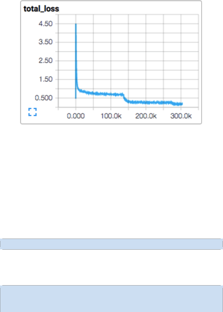
2.4

卷积神经网络 75

模型训练

训练一个可进行 N维分类的网络的常用方法是使用多项式逻辑回归,又被叫做 soft-

max 回归。Softmax 回归在网络的输出层上附加了一个softmax nonlinearity，并且计算

归一化的预测值和 label 的1-hot encoding的交叉熵。在正则化过程中，我们会对所有

学习变量应用权重衰减损失。模型的目标函数是求交叉熵损失和所有权重衰减项的和，

loss()函数的返回值就是这个值。

在TensorBoard 中使用scalar_summary来查看该值的变化情况：

图2.9: CIFAR-10 Loss

我们使用标准的梯度下降算法来训练模型（也可以在Training中看看其他方法），其

学习率随时间以指数形式衰减。

train() 函数会添加一些操作使得目标函数最小化，这些操作包括计算梯度、更新

学习变量（详细信息请查看GradientDescentOptimizer）。train() 函数最终会返回一个用

以对一批图像执行所有计算的操作步骤，以便训练并更新模型。

2.4.4 开始执行并训练模型

我们已经把模型建立好了，现在通过执行脚本cifar10\_train.py来启动训练过程。

 

1python cifar10_train.py

 

注意:当第一次在 CIFAR-10 教程上启动任何任务时，会自动下载 CIFAR-10 数据集，

该数据集大约有 160M 大小，因此第一次运行时泡杯咖啡小栖一会吧。

你应该可以看到如下类似的输出:

 

1Filling queue with 20000 CIFAR images before starting to train. This

will take a few minutes.

22015−11−04 11:45:45.927302: step 0, loss = 4.68 (2.0 examples/sec;

64.221 sec/batch)

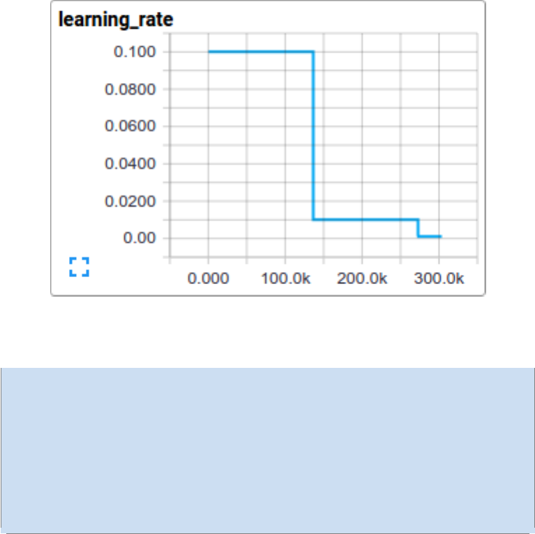
76 第二章基础教程

图2.10: CIFAR-10 Learning Rate Decay

32015−11−04 11:45:49.133065: step 10, loss = 4.66 (533.8 examples/sec;

0.240 sec/batch)

42015−11−04 11:45:51.397710: step 20, loss = 4.64 (597.4 examples/sec;

0.214 sec/batch)

52015−11−04 11:45:54.446850: step 30, loss = 4.62 (391.0 examples/sec;

0.327 sec/batch)

62015−11−04 11:45:57.152676: step 40, loss = 4.61 (430.2 examples/sec;

0.298 sec/batch)

72015−11−04 11:46:00.437717: step 50, loss = 4.59 (406.4 examples/sec;

0.315 sec/batch)

8...

 

脚本会在每 10 步训练过程后打印出总损失值，以及最后一批数据的处理速度。下

面是几点注释：

•第一批数据会非常的慢（大概要几分钟时间），因为预处理线程要把 20,000 个待处

理的 CIFAR 图像填充到重排队列中；

•打印出来的损失值是最近一批数据的损失值的均值。请记住损失值是交叉熵和权

重衰减项的和；

•上面打印结果中关于一批数据的处理速度是在 Tesla K40C 上统计出来的，如果你

运行在 CPU 上，性能会比此要低；

练习:当实验时，第一阶段的训练时间有时会非常的长，长到足以让人生

厌。可以尝试减少初始化时初始填充到队列中图片数量来改变这种情况。

在cifar10.py中搜索NUM\_EXAMPLES\_PER\_EPOCH\_FOR\_TRAIN并修改之。

cifar10\_train.py 会周期性的在检查点文件中保存模型中的所有参数，但是不会对

模型进行评估。cifar10\_eval.py会使用该检查点文件来测试预测性能（详见下面的描

述：评估模型）。

2.4

卷积神经网络 77

如果按照上面的步骤做下来，你应该已经开始训练一个 CIFAR-10 模型了。恭喜你!

cifar10\_train.py输出的终端信息中提供了关于模型如何训练的一些信息，但是我

们可能希望了解更多关于模型训练时的信息，比如：

*损失是真的在减小还是看到的只是噪声数据？

*为模型提供的图片是否合适？

*梯度、激活、权重的值是否合理？

*当前的学习率是多少？

TensorBoard提供了该功能，可以通过cifar10\_train.py中的SummaryWriter周期性的

获取并显示这些数据。

比如我们可以在训练过程中查看local3的激活情况，以及其特征维度的稀疏情况：

相比于总损失，在训练过程中的单项损失尤其值得人们的注意。但是由于训练中使

用的数据批量比较小，损失值中夹杂了相当多的噪声。在实践过程中，我们也发现相比于

原始值，损失值的移动平均值显得更为有意义。请参阅脚本ExponentialMovingAverage了

解如何实现。

2.4.5 评估模型

现在可以在另一部分数据集上来评估训练模型的性能。脚本文件cifar10\_eval.py

对模型进行了评估，利用 inference()函数重构模型，并使用了在评估数据集所有 10,000

张CIFAR-10 图片进行测试。最终计算出的精度为 1:N，N= 预测值中置信度最高的一项

与图片真实 label 匹配的频次。(It calculates the precision at 1: how often the top prediction

matches the true label of the image)。

为了监控模型在训练过程中的改进情况，评估用的脚本文件会周期性的在最新的

检查点文件上运行，这些检查点文件是由cifar10\_train.py产生。

 

1python cifar10_eval.py

 

注意：不要在同一块 GPU 上同时运行训练程序和评估程序，因为可能会导

致内存耗尽。尽可能的在其它单独的 GPU 上运行评估程序，或者在同一块

GPU 上运行评估程序时先挂起训练程序。

你可能会看到如下所示输出:

 

12015−11−06 08:30:44.391206: precision @ 1 = 0.860

2...

 

评估脚本只是周期性的返回 precision@1 (The script merely returns the precision @ 1

periodically)--在该例中返回的准确率是 86%。cifar10\_eval.py 同时也返回其它一些可

以在 TensorBoard 中进行可视化的简要信息。可以通过这些简要信息在评估过程中进一

步的了解模型。

训练脚本会为所有学习变量计算其移动均值,评估脚本则直接将所有学习到的模型

参数替换成对应的移动均值。这一替代方式可以在评估过程中提升模型的性能。

78 第二章基础教程

练习:通过 precision @ 1 测试发现，使用均值参数可以将预测性能提高约 3%，

在cifar10\_eval.py中尝试修改为不采用均值参数的方式，并确认由此带来

的预测性能下降。

2.4.6 在多个 GPU 板卡上训练模型

现代的工作站可能包含多个 GPU 进行科学计算。TensorFlow 可以利用这一环境在

多个 GPU 卡上运行训练程序。

在并行、分布式的环境中进行训练，需要对训练程序进行协调。对于接下来的描述，

术语模型拷贝（model replica）特指在一个数据子集中训练出来的模型的一份拷贝。

如果天真的对模型参数的采用异步方式更新将会导致次优的训练性能，这是因为我

们可能会基于一个旧的模型参数的拷贝去训练一个模型。但与此相反采用完全同步更新

的方式，其速度将会变得和最慢的模型一样慢 (Conversely, employing fully synchronous

updates will be as slow as the slowest model replica.)。

在具有多个 GPU 的工作站中，每个 GPU 的速度基本接近，并且都含有足够的内存

来运行整个 CIFAR-10 模型。因此我们选择以下方式来设计我们的训练系统：

•在每个 GPU 上放置单独的模型副本；

•等所有 GPU 处理完一批数据后再同步更新模型的参数；

下图示意了该模型的结构：:

可以看到，每一个 GPU 会用一批独立的数据计算梯度和估计值。这种设置可以非

常有效的将一大批数据分割到各个 GPU 上。

这一机制要求所有 GPU 能够共享模型参数。但是众所周知在 GPU 之间传输数据非

常的慢，因此我们决定在 CPU 上存储和更新所有模型的参数 (对应图中绿色矩形的位

置)。这样一来，GPU 在处理一批新的数据之前会更新一遍的参数。

图中所有的 GPU 是同步运行的。所有 GPU 中的梯度会累积并求平均值 (绿色方框

部分)。模型参数会利用所有模型副本梯度的均值来更新。

在多个设备中设置变量和操作

在多个设备中设置变量和操作时需要做一些特殊的抽象。

我们首先需要把在单个模型拷贝中计算估计值和梯度的行为抽象到一个函数中。在

代码中，我们称这个抽象对象为 “tower’’。对于每一个 “tower’’ 我们都需要设置它的两个

属性：

*在一个 tower 中为所有操作设定一个唯一的名称。tf.name_scope()通过添加一个范围

前缀来提供该唯一名称。比如，第一个 tower 中的所有操作都会附带一个前缀tower\_0，

示例：tower\_0/conv1/Conv2D；

2.4

卷积神经网络 79

•在一个 tower 中运行操作的优先硬件设备。tf.device() 提供该信息。比如，在第

一个 tower 中的所有操作都位于 device(\textquotesingle{/gpu:0') 范围中，暗含的

意思是这些操作应该运行在第一块 GPU 上；

为了在多个 GPU 上共享变量，所有的变量都绑定在 CPU 上，并通过tf.get_variable

()访问。可以查看Sharing Variables以了解如何共享变量。

启动并在多个 GPU 上训练模型

如果你的机器上安装有多块 GPU，你可以通过使用cifar10\_multi\_gpu\_train.py

脚本来加速模型训练。该脚本是训练脚本的一个变种，使用多个 GPU 实现模型并行训

练。

 

1python cifar10_multi_gpu_train.py −−num_gpus=2

 

训练脚本的输出如下所示：

 

1Filling queue with 20000 CIFAR images before starting to train. This

will take a few minutes.

22015−11−04 11:45:45.927302: step 0, loss = 4.68 (2.0 examples/sec;

64.221 sec/batch)

32015−11−04 11:45:49.133065: step 10, loss = 4.66 (533.8 examples/sec;

0.240 sec/batch)

42015−11−04 11:45:51.397710: step 20, loss = 4.64 (597.4 examples/sec;

0.214 sec/batch)

52015−11−04 11:45:54.446850: step 30, loss = 4.62 (391.0 examples/sec;

0.327 sec/batch)

62015−11−04 11:45:57.152676: step 40, loss = 4.61 (430.2 examples/sec;

0.298 sec/batch)

72015−11−04 11:46:00.437717: step 50, loss = 4.59 (406.4 examples/sec;

0.315 sec/batch)

8...

 

需要注意的是默认的 GPU 使用数是 1，此外，如果你的机器上只有一个 GPU，那么

所有的计算都只会在一个 GPU 上运行，即便你可能设置的是 N个。

练习:cifar10\_train.py中的批处理大小默认配置是 128。尝试在 2个GPU

上运行cifar10\_multi\_gpu\_train.py脚本，并且设定批处理大小为 64，然后

比较 2种方式的训练速度。

2.4.7 下一步

恭喜你!你已经完成了 CIFAR-10 教程。如果你对开发和训练自己的图像分类系统感

兴趣，我们推荐你新建一个基于该教程的分支，并修改其中的内容以建立解决您问题的

图像分类系统。

练习:下载Street View House Numbers (SVHN) 数据集。新建一个 CIFAR-10 教

程的分支，并将输入数据替换成 SVHN。尝试改变网络结构以提高预测性能。

原文：Convolutional Neural Networks 翻译：oskycar 校对：KK4SBB

80 第二章基础教程

2.5 Vector Representations of Words

In this tutorial we look at the word2vec model by Mikolov et al. This model is used for

learning vector representations of words, called "word embeddings".

在本教程我们来看一下Mikolovet al中提到的 word2vec 模型。该模型是用于学习文

字的向量表示，称之为"wordembedding"。

2.5.1 亮点

本教程旨在意在展现出在 TensorfLow 中构建 word2vec 模型有趣、本质的部分。

•我们从我们为何需要使用向量表示文字开始。

•我们通过直观地例子观察模型背后的本质，以及它是如何训练的（通过一些数学

方法评估）。

•同时我们也展示了 TensorFlow 对该模型的简单实现。

•最后，我们着眼于让给这个简单版本的模型表现更好。

我们会在教程的推进中循序渐进地解释代码，但是如果你更希望直入主题，可以在

tensorﬂow/g3doc/tutorials/word2vec/word2vec_basic.py查看到一个最简单的实现。这个

基本的例子提供的代码可以完成下载一些数据，简单训练后展示结果。一旦你觉得已经

完全掌握了这个简单版本，你可以查看 tensorﬂow/models/embedding/word2vec.py，这

里提供了一些更复杂的实现，同时也展示了 TensorFlow 的一些更进阶的特性，比如如

何更高效地使用线程将数据送入文本模型，再比如如何在训练中设置检查点等等。

但是首先，让我们来看一下为何需要学习 word embeddings。如果你对 word em-

beddings 相关内容已经是个专家了，那么请安心跳过本节内容，直接深入细节干一些脏

活吧。

2.5.2 动机:为什么需要学习 Word Embeddings?

通常图像或音频系统处理的是由图片中所有单个原始像素点强度值或者音频中功

率谱密度的强度值，把它们编码成丰富、高纬度的向量数据集。对于物体或语音识别这

一类的任务，我们所需的全部信息已经都存储在原始数据中（显然人类本身就是依赖

原始数据进行日常的物体或语音识别的）。然后，自然语言处理系统通常将词汇作为离

散的单一符号，例如"cat" 一词或可表示为Id537 ，而"dog" 一词或可表示为Id143。这些

符号编码毫无规律，无法提供不同词汇之间可能存在的关联信息。换句话说，在处理关

于"dogs" 一词的信息时，模型将无法利用已知的关于"cats" 的信息（例如，它们都是动

物，有四条腿，可作为宠物等等）。可见，将词汇表达为上述的独立离散符号将进一步

导致数据稀疏，使我们在训练统计模型时不得不寻求更多的数据。而词汇的向量表示将

克服上述的难题。

2.5 VECTOR REPRESENTATIONS OF WORDS

图2.11:

向量空间模型 (VSMs) 将词汇表达（嵌套）于一个连续的向量空间中，语义近似的

词汇被映射为相邻的数据点。向量空间模型在自然语言处理领域中有着漫长且丰富的

历史，不过几乎所有利用这一模型的方法都依赖于分布式假设，其核心思想为出现于上

下文情景中的词汇都有相类似的语义。采用这一假设的研究方法大致分为以下两类：基

于技术的方法 (如，潜在语义分析)，和预测方法 (如，神经概率化语言模型).

其中它们的区别在如下论文中又详细阐述Baroni etal.，不过简而言之：基于计数的

方法计算某词汇与其邻近词汇在一个大型语料库中共同出现的频率及其他统计量，然

后将这些统计量映射到一个小型且稠密的向量中。预测方法则试图直接从某词汇的邻

近词汇对其进行预测，在此过程中利用已经学习到的小型且稠密的嵌套向量。

Word2vec 是一种可以进行高效率词嵌套学习的预测模型。其两种变体分别为：连续

词袋模型（CBOW）及 Skip-Gram 模型。从算法角度看，这两种方法非常相似，其区别为

CBOW 根据源词上下文词汇（"the cat sits on the"）来预测目标词汇（例如，"mat"），而

Skip-Gram 模型做法相反，它通过目标词汇来预测源词汇。Skip-Gram 模型采取 CBOW

的逆过程的动机在于：CBOW 算法对于很多分布式信息进行了平滑处理（例如将一整

段上下文信息视为一个单一观察量）。很多情况下，对于小型的数据集，这一处理是有

帮助的。相形之下，Skip-Gram 模型将每个“上下文---目标词汇”的组合视为一个新观

察量，这种做法在大型数据集中会更为有效。本教程余下部分将着重讲解 Skip-Gram 模

型。

2.5.3 处理噪声对比训练

神经概率化语言模型通常使用极大似然法 (ML) 进行训练，其中通过softmaxfunction

来最大化当提供前一个单词 h(代表"history")，后一个单词的概率 wt(代表"target")，

P(wt|h)=so f t max(score(wt,h)) (2.7)

=exp{scor e(wt,h)}

W or d w ′i nV oc ab exp{score(w′,h)} (2.8)

当scor e(wt,h)计算了文字 wt和上下文 h的相容性（通常使用向量积）。我们使用

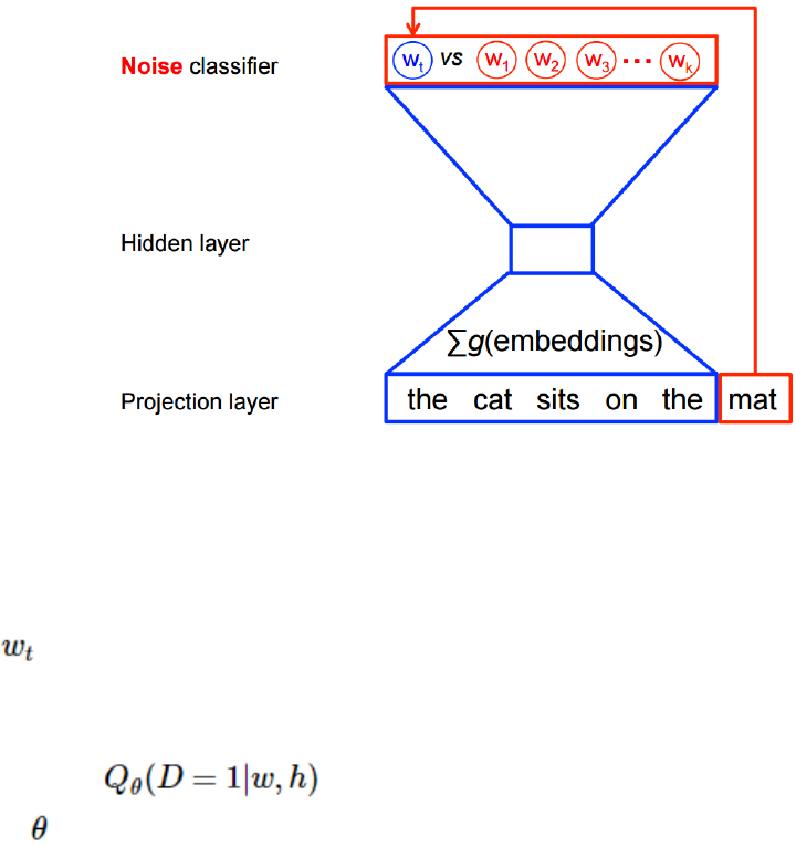
82 第二章基础教程

对数似然函数来训练训练集的最大值，比如通过：

JML =logP(wt|h) (2.9)

=scor e(wt,h)−log( 

W or d w ′inV ocab

exp{scor e(w′,h)}) (2.10)

这里提出了一个解决语言概率模型的合适的通用方法。然而这个方法实际执行起

来开销非常大，因为我们需要去计算并正则化当前上下文环境 h中所有其他 V单词 w′

的概率得分，在每一步训练迭代中。

图2.12:

从另一个角度来说，当使用 word2vec 模型时，我们并不需要对概率模型中的所有

特征进行学习。而 CBOW 模型和 Skip-Gram 模型为了避免这种情况发生，使用一个二分

类器（逻辑回归）在同一个上下文环境里从 k虚构的 (噪声)单词区分出真正的目标单词

。我们下面详细阐述一下 CBOW 模型，对于 Skip-Gram 模型只要简单地做相反的操

作即可。

从数学角度来说，我们的目标是对每个样本最大化：

其中代表的是数据集在当前上下文 h，根据所学习的嵌套向

量，目标单词 w使用二分类逻辑回归计算得出的概率。在实践中，我们通过在噪声

分布中绘制比对文字来获得近似的期望值（通过计算蒙特卡洛平均值）。

当真实地目标单词被分配到较高的概率，同时噪声单词的概率很低时，目标函数

也就达到最大值了。从技术层面来说，这种方法叫做负抽样，而且使用这个损失函数

在数学层面上也有很好的解释：这个更新过程也近似于 softmax 函数的更新。这在计算

上将会有很大的优势，因为当计算这个损失函数时，只是有我们挑选出来的 k个噪声

单词，而没有使用整个语料库 V。这使得训练变得非常快。我们实际上使用了与noise-

contrastiveestimation(NCE)介绍的非常相似的方法，这在 TensorFlow 中已经封装了一个

很便捷的函数tf.nn.nce_loss()。

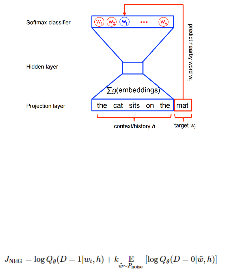
2.5 VECTOR REPRESENTATIONS OF WORDS

图2.13:

图2.14:

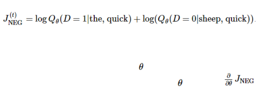
84 第二章基础教程

让我们在实践中来直观地体会它是如何运作的！

2.5.4 Skip-gram 模型

下面来看一下这个数据集

"the␣quick␣brown␣fox␣jumped␣over␣the␣lazy␣dog"

我们首先对一些单词以及它们的上下文环境建立一个数据集。我们可以以任何合

理的方式定义 ‘上下文’，而通常上这个方式是根据文字的句法语境的（使用语法原理的

方式处理当前目标单词可以看一下这篇文献 Levy et al.，比如说把目标单词左边的内容

当做一个“上下文”，或者以目标单词右边的内容，等等。现在我们把目标单词的左右

单词视作一个上下文，使用大小为 1的窗口，这样就得到这样一个由 (上下文,目标

单词)组成的数据集：

([the, brown], quick), ([quick, fox], brown), ([brown, jumped],

fox), ...

前文提到 Skip-Gram 模型是把目标单词和上下文颠倒过来，所以在这个问题中，举

个例子，就是用’quick’ 来预测 ‘the’ 和‘brown’ ，用 ‘brown’ 预测 ‘quick’ 和‘brown’ 。因此

这个数据集就变成由 (输入,输出)组成的：

(quick, the), (quick, brown), (brown, quick), (brown, fox), ...

目标函数通常是对整个数据集建立的，但是本问题中要对每一个样本（或者是一个

batch_size 很小的样本集，通常设置为 16 <= batch_size <= 512）在同一时

间执行特别的操作，称之为随机梯度下降 (SGD)。我们来看一下训练过程中每一步的执

行。

假设用 t表示上面这个例子中 quick 来预测 the 的训练的单个循环。用 num_noise

定义从噪声分布中挑选出来的噪声（相反的）单词的个数，通常使用一元分布，P(w)。

为了简单起见，我们就定 num_noise=1，用 sheep 选作噪声词。接下来就可以计算

每一对观察值和噪声值的损失函数了，每一个执行步骤就可表示为：

图2.15:

整个计算过程的目标是通过更新嵌套参数来逼近目标函数（这个这个例子中就

是使目标函数最大化）。为此我们要计算损失函数中嵌套参数的梯度，比如，

(幸好 TensorFlow 封装了工具函数可以简单调用!)。对于整个数据集，当梯度下降的过程

中不断地更新参数，对应产生的效果就是不断地移动每个单词的嵌套向量，直到可以把

真实单词和噪声单词很好得区分开。

我们可以把学习向量映射到 2维中以便我们观察，其中用到的技术可以参考 t-SNE

2.5 VECTOR REPRESENTATIONS OF WORDS

降纬技术。当我们用可视化的方式来观察这些向量，就可以很明显的获取单词之间语义

信息的关系，这实际上是非常有用的。当我们第一次发现这样的诱导向量空间中，展示

了一些特定的语义关系，这是非常有趣的，比如文字中 male-female，gender 甚至还有

country-capital 的关系,如下方的图所示 (也可以参考 Mikolov et al., 2013论文中的例子)。

这也解释了为什么这些向量在传统的 NLP 问题中可作为特性使用，比如用在对一

个演讲章节打个标签，或者对一个专有名词的识别 (看看如下这个例子 Collobert et al.或

者Turian et al.)。

不过现在让我们用它们来画漂亮的图表吧！

2.5.5 建立图形

这里谈得都是嵌套，那么先来定义一个嵌套参数矩阵。我们用唯一的随机值来初始

化这个大矩阵。

[] embeddings = tf.Variable( tf.randomuni f or m([vocabul ar ysi ze,embeddi ngsi ze],−1.0,1.0))

对噪声-比对的损失计算就使用一个逻辑回归模型。对此，我们需要对语料库中的

每个单词定义一个权重值和偏差值。(也可称之为输出权重与之对应的输入嵌套值)。定

义如下。

[] ncewei g ht s=t f .V ar i abl e(t f .tr uncatednor mal([vocabul ar ysi ze,embeddi ngsi ze],st ddev=1.0/math.sqr t(embeddi ngsi ze)))ncebi ases=t f .V ar i able(t f .zer os([vocabul ar ysi ze]))

我们有了这些参数之后，就可以定义 Skip-Gram 模型了。简单起见，假设我们已经把

语料库中的文字整型化了，这样每个整型代表一个单词 (细节请查看 tensorﬂow/g3doc/tutorials/word2vec/word2vec_basic.py)。

Skip-Gram 模型有两个输入。一个是一组用整型表示的上下文单词，另一个是目标单词。

给这些输入建立占位符节点，之后就可以填入数据了。

[] 建立输入占位符 traininput s=t f .pl acehol der (t f .i nt 32, shape=[batchsi ze])t r ai nlabel s=t f .pl acehol der (t f .i nt32, shape=[batchsi ze,1])

然后我们需要对批数据中的单词建立嵌套向量，TensorFlow 提供了方便的工具函

数。

[] embed = tf.nn.embeddinglookup(embedd ing s,t r ai ninput s)

好了，现在我们有了每个单词的嵌套向量，接下来就是使用噪声-比对的训练方式

来预测目标单词。

[] 计算 NCE 损失函数,每次使用负标签的样本. loss = tf.reducemean(t f .nn.nceloss(ncewei g ht s,ncebi ases,embed,tr ai nlabel s,numsampl ed,vocabul ar ysi ze))

我们对损失函数建立了图形节点，然后我们需要计算相应梯度和更新参数的节点，

比如说在这里我们会使用随机梯度下降法，TensorFlow 也已经封装好了该过程。

[] 使用 SGD 控制器. optimizer = tf.train.GradientDescentOptimizer(learningrate=1.0).mi ni mi ze(l oss)

86 第二章基础教程

2.5.6 训练模型

训练的过程很简单，只要在循环中使用 feed_dict 不断给占位符填充数据，同

时调用 session.run即可。

[] for inputs, labels in generatebatch(...) : f eeddict={tr ai ni nginput s :i nput s,t r ai ni nglabel s :l abel s},curloss=sessi on.r un([opt imi zer,loss], f eeddic t=f eeddi ct)

完整地例子可参考 tensorﬂow/g3doc/tutorials/word2vec/word2vec_basic.py.

2.5.7 嵌套学习结果可视化

使用 t-SNE 来看一下嵌套学习完成的结果。

Et voila! 与预期的一样，相似的单词被聚类在一起。对 word2vec 模型更复杂的实现

需要用到 TensorFlow 一些更高级的特性，具体是实现可以参考 tensorﬂow/models/em-

bedding/word2vec.py。

2.5.8 嵌套学习的评估:类比推理

词嵌套在 NLP 的预测问题中是非常有用且使用广泛地。如果要检测一个模型是否

是可以成熟地区分词性或者区分专有名词的模型，最简单的办法就是直接检验它的预

测词性、语义关系的能力，比如让它解决形如 king is to queen as father is

to ? 这样的问题。这种方法叫做类比推理，可参考Mikolov and colleagues，数据集下

载地址为: https://word2vec.googlecode.com/svn/trunk/questions-words.txt。

To see how we do this evaluation 如何执行这样的评估，可以看 build_eval_graph()

和eval() 这两个函数在下面源码中的使用 tensorﬂow/models/embedding/word2vec.py.

超参数的选择对该问题解决的准确性有巨大的影响。想要模型具有很好的表现，需

要有一个巨大的训练数据集，同时仔细调整参数的选择并且使用例如二次抽样的一些

技巧。不过这些问题已经超出了本教程的范围。

2.5.9 优化实现

以上简单的例子展示了 TensorFlow 的灵活性。比如说，我们可以很轻松得用现成

的tf.nn.sampled_softmax_loss() 来代替 tf.nn.nce_loss() 构成目标函

数。如果你对损失函数想做新的尝试，你可以用 TensorFlow 手动编写新的目标函数

的表达式，然后用控制器执行计算。这种灵活性的价值体现在，当我们探索一个机器学

习模型时，我们可以很快地遍历这些尝试，从中选出最优。

一旦你有了一个满意的模型结构，或许它就可以使实现运行地更高效（在短时间

内覆盖更多的数据）。比如说，在本教程中使用的简单代码，实际运行速度都不错，因

为我们使用 Python 来读取和填装数据，而这些在 TensorFlow 后台只需执行非常少的工

作。如果你发现你的模型在输入数据时存在严重的瓶颈，你可以根据自己的实际问题自

行实现一个数据阅读器，参考新的数据格式。对于 Skip-Gram 模型，我们已经完成了如

下这个例子 tensorﬂow/models/embedding/word2vec.py。

2.5 VECTOR REPRESENTATIONS OF WORDS

如果 I/O 问题对你的模型已经不再是个问题，并且想进一步地优化性能，或许你

可以自行编写 TensorFlow 操作单元，详见添加一个新的操作。相应的，我们也提供了

Skip-Gram 模型的例子 tensorﬂow/models/embedding/word2vec_optimized.py。请自行

调节以上几个过程的标准，使模型在每个运行阶段有更好地性能。

2.5.10 总结

在本教程中我们介绍了 word2vec 模型,它在解决词嵌套问题中具有良好的性能。我

们解释了使用词嵌套模型的实用性，并且讨论了如何使用 TensorFlow 实现该模型的高

效训练。总的来说，我们希望这个例子能够让向你展示 TensorFlow 可以提供实验初期

的灵活性，以及在后期优化模型时对模型内部的可操控性。

原文地址：Vector Representation of Words 翻译：btpeter 校对：waiwaizheng

88 第二章基础教程

2.6 循环神经网络

2.6.1 介绍

可以在 this great article 查看循环神经网络 (RNN) 以及 LSTM 的介绍。

2.6.2 语言模型

此教程将展示如何在高难度的语言模型中训练循环神经网络。该问题的目标是获

得一个能确定语句概率的概率模型。为了做到这一点，通过之前已经给出的词语来预测

后面的词语。我们将使用 PTB(Penn Tree Bank) 数据集，这是一种常用来衡量模型的基

准，同时它比较小而且训练起来相对快速。

语言模型是很多有趣难题的关键所在，比如语音识别，机器翻译，图像字幕等。它

很有意思---可以参看 here。

本教程的目的是重现 Zaremba et al., 2014 的成果，他们在 PTB 数据集上得到了很棒

的结果。

2.6.3 教程文件

本教程使用的下面文件的目录是 models/rnn/ptb:

[c]@ll@ 文件作用ptb\_word\_lm.py 在PTB 数据集上训练一个语言模型.reader.py 读

取数据集.

2.6.4 下载及准备数据

本教程需要的数据在 data/ 路径下，来源于 Tomas Mikolov 网站上的 PTB 数据集http

://www.fit.vutbr.cz/\textasciitilde{imikolov/rnnlm/simple-examples.tgz。

该数据集已经预先处理过并且包含了全部的 10000 个不同的词语，其中包括语句结

束标记符，以及标记稀有词语的特殊符号 (\textless{unk>) 。我们在 reader.py 中转换

所有的词语，让他们各自有唯一的整型标识符，便于神经网络处理。

2.6.5 模型

LSTM

模型的核心由一个 LSTM 单元组成，其可以在某时刻处理一个词语，以及计算语句

可能的延续性的概率。网络的存储状态由一个零矢量初始化并在读取每一个词语后更

新。而且，由于计算上的原因，我们将以 batch\_size 为最小批量来处理数据。

基础的伪代码就像下面这样：

[] lstm = rnncel l .B asi cLST MC el l(l st msi ze)LST M .st at e=t f .zer os([bat chsi ze,l st m.st at esi ze])

loss = 0.0 for currentbatchofwor d si nw or d sindat ase t :.out put ,st at e=l st m(cur r entbatchofwor d s,s t ate)

2.6

循环神经网络 89

LSTM 输出可用于产生下一个词语的预测 logits = tf.matmul(output, softmaxw)+so f tmaxbpr obabi l i ti es=t f .nn.so f tmax(l og i t s)l oss+=loss functi on(pr obabi l i ti es,t ar g etwor d s)

截断反向传播

为使学习过程易于处理，通常的做法是将反向传播的梯度在（按时间）展开的步

骤上照一个固定长度 (num\_steps)截断。通过在一次迭代中的每个时刻上提供长度为

num\_steps 的输入和每次迭代完成之后反向传导，这会很容易实现。

一个简化版的用于计算图创建的截断反向传播代码：

[] 一次给定的迭代中的输入占位符. words = tf.placeholder(tf.int32, [batchsi ze,numsteps])

lstm = rnncel l .B asi cLST MC el l(l st msi ze)LST M.i ni ti alst at e=st at e=t f .zer os([bat chsi ze,l st m.st at esi ze])

for i in range(len(numsteps)) : .out put ,st at e=l stm(w or d s[:,i], st ate)

其余的代码. ...

ﬁnalst at e=s t at e

下面展现如何实现迭代整个数据集：

[] 一个 numpy 数组，保存每一批词语之后的 LSTM 状态. numpyst at e=i ni ti alst at e.ev al()t ot alloss=0.0f or cur rentbat chofwor d si nwor d sindat aset :numpyst at e,cur r entloss=session.r un([f i nalst at e,loss],LST M .f eeddict={i ni ti alst at e :numpyst at e,w or d s :cur r entbatchofwor d s})t ot alloss+=cur r entloss

输入

在输入 LSTM 前，词语 ID 被嵌入到了一个密集的表示中 (查看矢量表示教程)。这

种方式允许模型高效地表示词语，也便于写代码：

[] embeddingmat r i x[voc abul ar ysi ze,embeddi ngsi ze]wor dembedding s=t f .nn.embeddi nglookup(embeddi ngmat r i x,wordid s)

嵌入的矩阵会被随机地初始化，模型会学会通过数据分辨不同词语的意思。

损失函数

我们想使目标词语的平均负对数概率最小

图2.16:

实现起来并非很难，而且函数 sequence\_loss\_by\_example 已经有了，可以直接使

用。

论文中的典型衡量标准是每个词语的平均困惑度（perplexity），计算式为

图2.17:

同时我们会观察训练过程中的困惑度值（perplexity）。

90 第二章基础教程

多个 LSTM 层堆叠

要想给模型更强的表达能力，可以添加多层 LSTM 来处理数据。第一层的输出作为

第二层的输入，以此类推。

类MultiRNNCell 可以无缝的将其实现：

[] lstm = rnncel l .B asi cLST MC el l(l st msi ze)st ackedlstm=r nncel l .Mul t i RN NC ell ([l st m]∗numberoflayer s)

initialst at e=st at e=st ackedlstm.zer ost at e(bat chsi ze,t f .f l oat32)f or i i nr ang e(l en(numst eps)) :.out put ,st at e=st ackedlstm(w or d s[:,i], st at e)

其余的代码. ...

ﬁnalst at e=s t ate

2.6.6 编译并运行代码

首先需要构建库，在 CPU 上编译：

bazel build -c opt tensorflow/models/rnn/ptb:ptb_word_lm

如果你有一个强大的 GPU，可以运行：

bazel build -c opt --config=cuda tensorflow/models/rnn/ptb:ptb_word_lm

运行模型：

bazel-bin/tensorflow/models/rnn/ptb/ptb_word_lm \

--data_path=/tmp/simple-examples/data/ --alsologtostderr --model small

教程代码中有 3个支持的模型配置参数：“small’’，“medium” 和“large’’。它们指的

是LSTM 的大小，以及用于训练的超参数集。

模型越大，得到的结果应该更好。在测试集中 small 模型应该可以达到低于 120 的

困惑度（perplexity），large 模型则是低于 80，但它可能花费数小时来训练。

2.6.7 除此之外？

还有几个优化模型的技巧没有提到，包括：

•随时间降低学习率,

• LSTM 层间 dropout.

继续学习和更改代码以进一步改善模型吧。

原文：Recurrent Neural Networks 翻译：Warln 校对：HongyangWang

2.7 SEQUENCE-TO-SEQUENCE MODELS

2.7 Sequence-to-Sequence Models

Recurrent neural networks can learn to model language, as already discussed in the

RNN Tutorial (if you did not read it, please go through it before proceeding with this one).

This raises an interesting question: could we condition the generated words on some in-

put and generate a meaningful response? For example, could we train a neural network to

translate from English to French? It turns out that the answer is yes.

This tutorial will show you how to build and train such a system end-to-end. You can

start by running this binary.

bazel run -c opt <...>/models/rnn/translate/translate.py

--data_dir [your_data_directory]

It will download English-to-French translation data from the WMT’15 Website prepare

it for training and train. It takes about 20GB of disk space, and a while to download and

prepare (see later for details), so you can start and leave it running while reading this tutorial.

This tutorial references the following ﬁles from models/rnn.

[c]@ll@ File

What’s

it? seq2seq.pyLibrary

for

build-

ing

sequence-

to-

sequence

mod-

els.

translate/seq2seq_model.pyNeural

trans-

la-

tion

sequence-

to-

sequence

model.

translate/data_utils.pyHelper

func-

tions

for

prepar-

ing

trans-

la-

tion

data.

translate/translate.pyBinary

that

trains

and

runs

the

trans-

la-

tion

model.

2.7.1 Sequence-to-Sequence Basics

A basic sequence-to-sequence model, as introduced in Cho et al., 2014, consists of two

recurrent neural networks (RNNs): an encoder that processes the input and a decoder that

generates the output. This basic architecture is depicted below.

Each box in the picture above represents a cell of the RNN, most commonly a GRU cell

or an LSTM cell (see the RNN Tutorial for an explanation of those). Encoder and decoder

can share weights or, as is more common, use a different set of parameters. Mutli-layer

cells have been successfully used in sequence-to-sequence models too, e.g. for translation

Sutskever et al., 2014.

92 第二章基础教程

In the basic model depicted above, every input has to be encoded into a ﬁxed-size state

vector, as that is the only thing passed to the decoder. To allow the decoder more direct

access to the input, an attention mechanism was introduced in Bahdanu et al., 2014. We

will not go into the details of the attention mechanism (see the paper), sufﬁce it to say that

it allows the decoder to peek into the input at every decoding step. A multi-layer sequence-

to-sequence network with LSTM cells and attention mechanism in the decoder looks like

this.

2.7.2 TensorFlow seq2seq Library

As you can see above, there are many different sequence-to-sequence models. Each of

these models can use different RNN cells, but all of them accept encoder inputs and decoder

inputs. This motivates the interfaces in the TensorFlow seq2seq library (models/rnn/seq2seq.py).

The basic RNN encoder-decoder sequence-to-sequence model works as follows.

[] outputs, states = basicrnnseq2seq(encoderinput s,decoderinput s,cel l)

In the above call, encoder_inputs are a list of tensors representing inputs to the en-

coder, i.e., corresponding to the letters A, B, C in the ﬁrst picture above. Similarly, decoder_inputs

are tensors representing inputs to the decoder, GO, W, X, Y, Z on the ﬁrst picture.

The cell argument is an instance of the models.rnn.rnn_cell.RNNCell class

that determines which cell will be used inside the model. You can use an existing cell, such

as GRUCell or LSTMCell, or you can write your own. Moreover, rnn_cell provides

wrappers to construct multi-layer cells, add dropout to cell inputs or outputs, or to do other

transformations, see the RNN Tutorial for examples.

The call to basic_rnn_seq2seq returns two arguments: outputs and states.

Both of them are lists of tensors of the same length as decoder_inputs. Naturally, outputs

correspond to the outputs of the decoder in each time-step, in the ﬁrst picture above that

would be W, X, Y, Z, EOS. The returned states represent the internal state of the decoder

at every time-step.

In many applications of sequence-to-sequence models, the output of the decoder at

time t is fed back and becomes the input of the decoder at time t+1. At test time, when

decoding a sequence, this is how the sequence is constructed. During training, on the other

hand, it is common to provide the correct input to the decoder at every time-step, even if the

decoder made a mistake before. Functions in seq2seq.py support both modes using the

feed_previous argument. For example, let’s analyze the following use of an embedding

RNN model.

[] outputs, states = embeddingrnnseq2seq(encoderinput s,decoderinput s,cel l ,numencodersymbol s,numdecodersymbol s,out putpr o j ect ion=None,f eedpr evi ous=F al se)

In the embedding_rnn_seq2seq model, all inputs (both encoder_inputs and

decoder_inputs) are integer-tensors that represent discrete values. They will be embed-

2.7 SEQUENCE-TO-SEQUENCE MODELS

ded into a dense representation (see the Vectors Representations Tutorial for more details on

embeddings), but to construct these embeddings we need to specify the maximum number

of discrete symbols that will appear: num_encoder_symbols on the encoder side, and

num_decoder_symbols on the decoder side.

In the above invocation, we set feed_previous to False. This means that the de-

coder will use decoder_inputs tensors as provided. If we set feed_previous to True,

the decoder would only use the ﬁrst element of decoder_inputs. All other tensors from

this list would be ignored, and instead the previous output of the encoder would be used.

This is used for decoding translations in our translation model, but it can also be used dur-

ing training, to make the model more robust to its own mistakes, similar to Bengio et al.,

2015.

One more important argument used above is output_projection. If not speciﬁed,

the outputs of the embedding model will be tensors of shape batch-size by num_decoder_symbols

as they represent the logits for each generated symbol. When training models with large out-

put vocabularies, i.e., when num_decoder_symbols is large, it is not practical to store

these large tensors. Instead, it is better to return smaller output tensors, which will later be

projected onto a large output tensor using output_projection. This allows to use our

seq2seq models with a sampled softmax loss, as described in Jean et. al., 2015.

In addition to basic_rnn_seq2seq and embedding_rnn_seq2seq there are a

few more sequence-to-sequence models in seq2seq.py, take a look there. They all have

similar interfaces, so we will not describe them in detail. We will use embedding_attention_seq2seq

for our translation model below.

2.7.3 Neural Translation Model

While the core of the sequence-to-sequence model is constructed by the functions in

models/rnn/seq2seq.py, there are still a few tricks that are worth mentioning that are

used in our translation model in models/rnn/translate/seq2seq_model.py.

Sampled softmax and output projection

For one, as already mentioned above, we want to use sampled softmax to handle large

output vocabulary. To decode from it, we need to keep track of the output projection. Both

the sampled softmax loss and the output projections are constructed by the following code

in seq2seq_model.py.

[] if numsampl es>0andnumsampl es<sel f .t ar g e tvocabsi ze :w=t f .g e tvar i able("pr o jw",[si ze,sel f .t ar g e tvocabsi ze])wt=t f .tr anspose(w)b=t f .g e tvar i abl e("pr o jb",[sel f .t ar g e tvocabsi ze])out putpr o j ec ti on=(w,b)

def sampledloss(i nput s,l abel s) : l abel s=t f .reshape(l abel s, [−1,1])r etur nt f .nn.sampl edso f tmaxloss(wt,b,i nput s,l abel s,numsamples,sel f .t ar g e tvocabsi ze)

First, note that we only construct a sampled softmax if the number of samples (512 by

94 第二章基础教程

default) is smaller that the target vocabulary size. For vocabularies smaller than 512 it might

be a better idea to just use a standard softmax loss.

Then, as you can see, we construct an output projection. It is a pair, consisting of a

weight matrix and a bias vector. If used, the rnn cell will return vectors of shape batch-size by

size, rather than batch-size by target_vocab_size. To recover logits, we need to mul-

tiply by the weight matrix and add the biases, as is done in lines 124-126 in seq2seq_model.py.

[] if outputpr o j ec ti oni snot None:sel f .out put s[b]=[t f .matmul(out put ,out putpr o j ect i on[0])+out putpr o j ec ti on[1] f or ...]

Bucketing and padding

In addition to sampled softmax, our translation model also makes use of bucketing,

which is a method to efﬁciently handle sentences of different lengths. Let us ﬁrst clarify

the problem. When translating English to French, we will have English sentences of dif-

ferent lengths L1 on input, and French sentences of different lengths L2 on output. Since

the English sentence is passed as encoder_inputs, and the French sentence comes as

decoder_inputs (preﬁxed by a GO symbol), we should in principle create a seq2seq

model for every pair (L1, L2+1) of lengths of an English and French sentence. This would re-

sult in an enormous graph consisting of many very similar subgraphs. On the other hand, we

could just pad every sentence with a special PAD symbol. Then we’d need only one seq2seq

model, for the padded lengths. But on shorter sentence our model would be inefﬁcient,

encoding and decoding many PAD symbols that are useless.

As a compromise between contructing a graph for every pair of lengths and padding

to a single length, we use a number of buckets and pad each sentence to the length of the

bucket above it. In translate.py we use the following default buckets.

[] buckets = [(5, 10), (10, 15), (20, 25), (40, 50)]

This means that if the input is an English sentence with 3 tokens, and the correspond-

ing output is a French sentence with 6 tokens, then they will be put in the ﬁrst bucket and

padded to length 5 for encoder inputs, and length 10 for decoder inputs. If we have an En-

glish sentence with 8 tokens and the corresponding French sentence has 18 tokens, then

they will not ﬁt into the (10, 15) bucket, and so the (20, 25) bucket will be used, i.e. the En-

glish sentence will be padded to 20, and the French one to 25.

Remember that when constructing decoder inputs we prepend the special GO symbol

to the input data. This is done in the get_batch() function in seq2seq_model.py,

which also reverses the input English sentence. Reversing the inputs was shown to improve

results for the neural translation model in Sutskever et al., 2014. To put it all together, imag-

ine we have the sentence “I go.”, tokenized as ["I", "go", "."] as input and the sen-

tence “Je vais.” as output, tokenized ["Je", "vais", "."]. It will be put in the (5,

10) bucket, with encoder inputs representing [PAD PAD "." "go" "I"] and decoder

2.7 SEQUENCE-TO-SEQUENCE MODELS

inputs [GO "Je" "vais" "." EOS PAD PAD PAD PAD PAD].

2.7.4 Let’s Run It

To train the model described above, we need to a large English-French corpus. We will

use the 10ˆ9-French-English corpus from the WMT’15 Website for training, and the 2013

news test from the same site as development set. Both data-sets will be downloaded to

data_dir and training will start, saving checkpoints in train_dir, when this command

is run.

bazel run -c opt <...>/models/rnn/translate:translate

--data_dir [your_data_directory] --train_dir [checkpoints_directory]

--en_vocab_size=40000 --fr_vocab_size=40000

It takes about 18GB of disk space and several hours to prepare the training corpus. It

is unpacked, vocabulary ﬁles are created in data_dir, and then the corpus is tokenized

and converted to integer ids. Note the parameters that determine vocabulary sizes. In the

example above, all words outside the 40K most common ones will be converted to an UNK

token representing unknown words. So if you change vocabulary size, the binary will re-map

the corpus to token-ids again.

After the data is prepared, training starts. Default parameters in translate are set to

quite large values. Large models trained over a long time give good results, but it might take

too long or use too much memory for your GPU. You can request to train a smaller model as

in the following example.

bazel run -c opt <...>/models/rnn/translate:translate

--data_dir [your_data_directory] --train_dir [checkpoints_directory]

--size=256 --num_layers=2 --steps_per_checkpoint=50

The above command will train a model with 2 layers (the default is 3), each layer with

256 units (default is 1024), and will save a checkpoint every 50 steps (the default is 200). You

can play with these parameters to ﬁnd out how large a model can be to ﬁt into the memory

of your GPU.

During training, every steps_per_checkpoint steps the binary will print out statis-

tics from recent steps. With the default parameters (3 layers of size 1024), ﬁrst messages look

like this.

global step 200 learning rate 0.5000 step-time 1.39 perplexity 1720.62

eval: bucket 0 perplexity 184.97

eval: bucket 1 perplexity 248.81

eval: bucket 2 perplexity 341.64

96 第二章基础教程

eval: bucket 3 perplexity 469.04

global step 400 learning rate 0.5000 step-time 1.38 perplexity 379.89

eval: bucket 0 perplexity 151.32

eval: bucket 1 perplexity 190.36

eval: bucket 2 perplexity 227.46

eval: bucket 3 perplexity 238.66

You can see that each step takes just under 1.4 seconds, the perplexity on the train-

ing set and the perplexities on the development set for each bucket. After about 30K steps,

we see perplexities on short sentences (bucket 0 and 1) going into single digits. Since the

training corpus contains ~22M sentences, one epoch (going through the training data once)

takes about 340K steps with batch-size of 64. At this point the model can be used for trans-

lating English sentences to French using the --decode option.

bazel run -c opt <...>/models/rnn/translate:translate --decode

--data_dir [your_data_directory] --train_dir [checkpoints_directory]

Reading model parameters from /tmp/translate.ckpt-340000

> Who is the president of the United States?

Qui est le président des États-Unis ?

2.7.5 What Next?

The example above shows how you can build your own English-to-French translator,

end-to-end. Run it and see how the model performs for yourself. While it has reasonable

quality, the default parameters will not give you the best translation model. Here are a few

things you can improve.

First of all, we use a very promitive tokenizer, the basic_tokenizer function in

data_utils. A better tokenizer can be found on the WMT’15 Website. Using that tok-

enizer, and a larger vocabulary, should improve your translations.

Also, the default parameters of the translation model are not tuned. You can try chang-

ing the learning rate, decay, or initializing the weights of your model in a different way. You

can also change the default GradientDescentOptimizer in seq2seq_model.py to

a more advanced one, such as AdagradOptimizer. Try these things and see how they

improve your results!

Finally, the model presented above can be used for any sequence-to-sequence task,

not only for translation. Even if you want to transform a sequence to a tree, for example to

generate a parsing tree, the same model as above can give state-of-the-art results, as demon-

strated in Vinyals & Kaiser et al., 2015. So you can not only build your own translator, you

can also build a parser, a chat-bot, or any program that comes to your mind. Experiment!

2.8

偏微分方程 97

2.8 偏微分方程

TensorFlow 不仅仅是用来机器学习，它更可以用来模拟仿真。在这里，我们将通过

模拟仿真几滴落入一块方形水池的雨点的例子，来引导您如何使用 TensorFlow 中的偏

微分方程来模拟仿真的基本使用方法。

注：本教程最初是准备做为一个 IPython 的手册。>译者注:关于偏微分方

程的相关知识，译者推荐读者查看网易公开课上的《麻省理工学院公开课：

多变量微积分》课程。

2.8.1 基本设置

首先,我们需要导入一些必要的引用。

[] 导入模拟仿真需要的库 import tensorﬂow as tf import numpy as np

导入可视化需要的库 import PIL.Image from cStringIO import StringIO from IPython.display

import clearout put,I mag e,d i spl ay

然后，我们还需要一个用于表示池塘表面状态的函数。

[] def DisplayArray(a, fmt=’jpeg’, rng=[0,1]): """Display an array as a picture.""" a = (a -

rng[0])/ﬂoat(rng[1] - rng[0])*255 a = np.uint8(np.clip(a, 0, 255)) f = StringIO() PIL.Image.fromarray(a).save(f,

fmt) display(Image(data=f.getvalue()))

最后，为了方便演示，这里我们需要打开一个 TensorFlow 的交互会话（interactive

session）。当然为了以后能方便调用，我们可以把相关代码写到一个可以执行的 Python

文件中。

[] sess = tf.InteractiveSession()

2.8.2 定义计算函数

[] def makeker nel (a) : """Tr ans f or ma2Dar r a yi ntoaconvol uti onker nel"""a=np.asar r a y(a)a=a.r eshape(l i st (a.shape)+[1,1])r etur nt f .const ant (a,dt y pe=1)

def simpleconv(x,k) : """Asi mpl i f i ed2Dconvolut ionoper at ion"""x=t f .expanddi ms(t f .expanddi ms(x,0),−1)y=t f .nn.d ept hwi seconv2d(x,k, [1,1,1,1], padd ing =′S AME ′)retur n y[0,:, :,0]

def laplace(x): """Compute the 2D laplacian of an array""" laplacek=makeker nel ([[0.5,1.0,0.5],[1.0,−6.,1.0],[0.5,1.0,0.5]])retur nsimpl econv(x,l apl acek)

2.8.3 定义偏微分方程

首先,我们需要创建一个完美的 500 Œ 500 的正方形池塘,就像是我们在现实中找到

的一样。

[] N = 500

然后，我们需要创建了一个池塘和几滴将要坠入池塘的雨滴。

[] Initial Conditions – some rain drops hit a pond

Set everything to zero uini t =np.zer os([N,N],d t ype="f loat 32")utini t =np.zer os([N,N],dt ype="f l oat32")

98 第二章基础教程

Some rain drops hit a pond at random points for n in range(40): a,b = np.random.randint(0,

N, 2) uini t[a,b]=np.r andom.uni f or m()

DisplayArray(uini t,r ng =[−0.1,0.1])

图2.18: jpeg

现在，让我们来指定该微分方程的一些详细参数。

[] Parameters: eps – time resolution damping – wave damping eps = tf.placeholder(tf.ﬂoat32,

shape=()) damping = tf.placeholder(tf.ﬂoat32, shape=())

Create variables for simulation state U = tf.Variable(uini t)Ut=t f .V ar i abl e(utini t )

Discretized PDE update rules U=U+eps∗U tUt=Ut+eps∗(l apl ace(U)−d ampi ng ∗U t )

Operation to update the state step = tf.group( U.assign(U),Ut.assi g n(U t))

2.8.4 开始仿真

为了能看清仿真效果，我们可以用一个简单的 for 循环来远行我们的仿真程序。

[] Initialize state to initial conditions tf.initializeallvar i ables().r un()

Run 1000 steps of PDE for i in range(1000): Step simulation step.run({eps: 0.03, damp-

ing: 0.04}) Visualize every 50 steps if i clearout put ()Di spl a y Ar r a y(U.eval (),r ng =[−0.1,0.1])

图2.19: jpeg

看！！雨点落在池塘中,和现实中一样的泛起了涟漪。

原文链接:http://tensorflow.org/tutorials/pdes/index.md 翻

译:[@wangaicc](https://github.com/wangaicc) 校对:[@tensorﬂy](https://github.com/tensorﬂy)

2.9 MNIST

数据下载 99

2.9 MNIST 数据下载

源码:tensorﬂow/g3doc/tutorials/mnist/

本教程的目标是展示如何下载用于手写数字分类问题所要用到的（经典）MNIST

数据集。

2.9.1 教程文件

本教程需要使用以下文件：

[c]@ll@

文

件

目

的input_data.py下

载

用

于

训

练

和

测

试

的

MNIST

数

据

集

的

源

码

2.9.2 准备数据

MNIST 是在机器学习领域中的一个经典问题。该问题解决的是把 28x28 像素的灰

度手写数字图片识别为相应的数字，其中数字的范围从 0到9.

图2.20: MNIST Digits

更多详情,请参考 Yann LeCun’s MNIST page 或Chris Olah’s visualizations of MNIST.

下载

Yann LeCun’s MNIST page 也提供了训练集与测试集数据的下载。

100 第二章基础教程

[c]@ll@

文

件

内

容train-images-idx3-ubyte.gz训

练

集

图

片-

55000

张

训

练

图

片,

5000

张

验

证

图

片

train-labels-idx1-ubyte.gz训

练

集

图

片

对

应

的

数

字

标

签

t10k-images-idx3-ubyte.gz测

试

集

图

片-

10000

张

图

片

t10k-labels-idx1-ubyte.gz测

试

集

图

片

对

应

的

数

字

标

签

在input_data.py 文件中,maybe_download() 函数可以确保这些训练数据下

载到本地文件夹中。

文件夹的名字在 fully_connected_feed.py 文件的顶部由一个标记变量指定，

你可以根据自己的需要进行修改。### 解压与重构

这些文件本身并没有使用标准的图片格式储存，并且需要使用 input_data.py

文件中 extract_images() 和extract_labels() 函数来手动解压（页面中有相

关说明）。

图片数据将被解压成 2维的 tensor：[image index, pixel index] 其中每一

项表示某一图片中特定像素的强度值,范围从 [0, 255] 到[-0.5, 0.5]。“image

index’’ 代表数据集中图片的编号,从0到数据集的上限值。“pixel index’’ 代表该图片中像

素点得个数,从0到图片的像素上限值。

以train-*开头的文件中包括 60000 个样本，其中分割出 55000 个样本作为训练

集，其余的 5000 个样本作为验证集。因为所有数据集中 28x28 像素的灰度图片的尺寸

为784，所以训练集输出的 tensor 格式为 [55000, 784]。

数字标签数据被解压称 1维的 tensor: [image index]，它定义了每个样本数值

的类别分类。对于训练集的标签来说，这个数据规模就是:[55000]。

数据集对象

底层的源码将会执行下载、解压、重构图片和标签数据来组成以下的数据集对象:

2.9 MNIST

数据下载 101

[c]@ll@ 数据集目的 data_sets.train 55000 组图片和标签,用于训练。data_sets.validation

5000 组图片和标签,用于迭代验证训练的准确性。data_sets.test 10000 组图片和

标签,用于最终测试训练的准确性。

执行 read_data_sets() 函数将会返回一个 DataSet 实例，其中包含了以上

三个数据集。函数 DataSet.next_batch() 是用于获取以 batch_size 为大小的

一个元组，其中包含了一组图片和标签，该元组会被用于当前的 TensorFlow 运算会话

中。

[] imagesfeed,l abel s feed=d at aset.nextbat ch(F L AGS.bat chsi ze)

原文地址：MNIST Data Download 翻译：btpeter 校对：waiwaizheng

102 第二章基础教程

第三章运作方式

103

104 第三章运作方式

综述 Overview

3.0.1 Variables: 创建，初始化，保存，和恢复

TensorFlow Variables 是内存中的容纳 tensor 的缓存。这一小节介绍了用它们在模

型训练时 (during training) 创建、保存和更新模型参数 (model parameters) 的方法。

参看教程

3.0.2 TensorFlow 机制 101

用MNIST 手写数字识别作为一个小例子，一步一步的将使用 TensorFlow 基础架构

(infrastructure) 训练大规模模型的细节做详细介绍。

参看教程

3.0.3 TensorBoard: 学习过程的可视化

对模型进行训练和评估时，TensorBoard 是一个很有用的可视化工具。此教程解释

了创建和运行 TensorBoard 的方法，和使用摘要操作 (Summary ops) 的方法，通过添加

摘要操作 (Summary ops)，可以自动把数据传输到 TensorBoard 所使用的事件文件。

参看教程

3.0.4 TensorBoard: 图的可视化

此教程介绍了在 TensorBoard 中使用可视化工具的方法，它可以帮助你理解张量流

图的过程并 debug。

参看教程

3.0.5 数据读入

此教程介绍了把数据传入 TensorSlow 程序的三种主要的方法：Feeding, Reading 和

Preloading.

参看教程

3.0.6 线程和队列

此教程介绍 TensorFlow 中为了更容易进行异步和并发训练的各种不同结构 (con-

structs)。

参看教程

3.0.7 添加新的 Op

TensorFlow 已经提供一整套节点操作 (）operation)，你可以在你的 graph 中随意使

用它们，不过这里有关于添加自定义操作 (custom op) 的细节。

105

参看教程。

3.0.8 自定义数据的 Readers

如果你有相当大量的自定义数据集合，可能你想要对 TensorFlow 的Data Readers

进行扩展，使它能直接以数据自身的格式将其读入。

参看教程。

3.0.9 使用 GPUs

此教程描述了用多个 GPU 构建和运行模型的方法。

参看教程

3.0.10 共享变量 Sharing Variables

当在多 GPU 上部署大型的模型，或展开复杂的 LSTMs 或RNNs 时，在模型构建代

码的不同位置对许多相同的变量（Variable）进行读写常常是必须的。设计变量作用域

（Variable Scope）机制的目的就是为了帮助上述任务的实现。

参看教程。

原文：How-to

翻译：Terence Cooper

校对：lonlonago

106 第三章运作方式

3.1 变量:创建、初始化、保存和加载

当训练模型时，用变量来存储和更新参数。变量包含张量 (Tensor) 存放于内存的缓

存区。建模时它们需要被明确地初始化，模型训练后它们必须被存储到磁盘。这些变量

的值可在之后模型训练和分析是被加载。

本文档描述以下两个 TensorFlow 类。点击以下链接可查看完整的 API 文档：

• tf.Variable 类

• tf.train.Saver 类

3.1.1 变量创建

当创建一个变量时，你将一个张量作为初始值传入构造函数 Variable()。TensorFlow

提供了一系列操作符来初始化张量，初始值是常量或是随机值。

 

1# Create two variables.

2weights = tf.Variable(tf.random_normal([784, 200], stddev=0.35), name

="weights")

3biases = tf.Variable(tf.zeros([200]), name="biases")

 

调用 tf.Variable() 添加一些操作 (Op, operation) 到graph：

•一个 Variable 操作存放变量的值。

•一个初始化 op 将变量设置为初始值。这事实上是一个 tf.assign 操作。

•初始值的操作，例如示例中对 biases 变量的 zeros 操作也被加入了 graph。

tf.Variable的返回值是 Python 的tf.Variable类的一个实例。

3.1.2 变量初始化

变量的初始化必须在模型的其它操作运行之前先明确地完成。最简单的方法就是

添加一个给所有变量初始化的操作，并在使用模型之前首先运行那个操作。

你或者可以从检查点文件中重新获取变量值，详见下文。

使用tf.initialize_all_variables()添加一个操作对变量做初始化。记得在完全构

建好模型并加载之后再运行那个操作。

 

1# Create two variables.

2weights = tf.Variable(tf.random_normal([784, 200], stddev=0.35),

3name="weights")

4biases = tf.Variable(tf.zeros([200]), name="biases")

5...

6# Add an op to initialize the variables.

7init_op = tf.initialize_all_variables()

9# Later, when launching the model

10 with tf.Session() as sess:

11 # Run the init operation.

12 sess.run(init_op)

13 ...

3.1

变量

创建、初始化、保存和加载 107

14 # Use the model

15 ...

 

由另一个变量初始化

你有时候会需要用另一个变量的初始化值给当前变量初始化。由于tf.initialize_all_variables

()是并行地初始化所有变量，所以在有这种需求的情况下需要小心。

用其它变量的值初始化一个新的变量时，使用其它变量的initialized_value()属性。

你可以直接把已初始化的值作为新变量的初始值，或者把它当做 tensor 计算得到一个

值赋予新变量。

 

1# Create a variable with a random value.

2weights = tf.Variable(tf.random_normal([784, 200], stddev=0.35),name=

"weights")

3# Create another variable with the same value as 'weights'.

4w2 = tf.Variable(weights.initialized_value(), name="w2")

5# Create another variable with twice the value of 'weights'

6w_twice = tf.Variable(weights.initialized_value() * 0.2, name="

w_twice")

 

自定义初始化

tf.initialize_all_variables()函数便捷地添加一个 op 来初始化模型的所有变量。

你也可以给它传入一组变量进行初始化。详情请见 Variables Documentation，包括检查

变量是否被初始化。

3.1.3 保存和加载

最简单的保存和恢复模型的方法是使用 tf.train.Saver 对象。构造器给 graph 的所有

变量，或是定义在列表里的变量，添加save和restoreops。saver对象提供了方法来运行

这些 ops，定义检查点文件的读写路径。

Checkpoint Files

Variables are saved in binary ﬁles that, roughly, contain a map from variable names to

tensor values.

When you create a Saver object, you can optionally choose names for the variables in

the checkpoint ﬁles. By default, it uses the value of the Variable.name property for each

variable.

保存变量

用tf.train.Saver()创建一个Saver来管理模型中的所有变量。

 

1# Create some variables.

2v1 = tf.Variable(..., name="v1")

3v2 = tf.Variable(..., name="v2")

108 第三章运作方式

4...

5# Add an op to initialize the variables.

6init_op = tf.initialize_all_variables()

8# Add ops to save and restore all the variables.

9saver = tf.train.Saver()

11 # Later, launch the model, initialize the variables , do some work,

save the

12 # variables to disk.

13 with tf.Session() as sess:

14 sess.run(init_op)

15 # Do some work with the model.

16 ..

17 # Save the variables to disk.

18 save_path = saver.save(sess, "/tmp/model.ckpt")

19 print "Model␣saved␣in␣file:␣", save_path

 

恢复变量

用同一个Saver对象来恢复变量。注意，当你从文件中恢复变量时，不需要事先对

它们做初始化。

 

1# Create some variables.

2v1 = tf.Variable(..., name="v1")

3v2 = tf.Variable(..., name="v2")

4...

5# Add ops to save and restore all the variables.

6saver = tf.train.Saver()

8# Later, launch the model, use the saver to restore variables from

disk, and

9# do some work with the model.

10 with tf.Session() as sess:

11 # Restore variables from disk.

12 saver.restore(sess, "/tmp/model.ckpt")

13 print "Model␣restored."

14 # Do some work with the model

15 ...

 

选择存储和恢复哪些变量

如果你不给tf.train.Saver()传入任何参数，那么saver将处理graph中的所有变量。

其中每一个变量都以变量创建时传入的名称被保存。

有时候在检查点文件中明确定义变量的名称很有用。举个例子，你也许已经训练

得到了一个模型，其中有个变量命名为"weights"，你想把它的值恢复到一个新的变量"

params"中。

有时候仅保存和恢复模型的一部分变量很有用。再举个例子，你也许训练得到了一

个5层神经网络，现在想训练一个 6层的新模型，可以将之前 5层模型的参数导入到新

模型的前 5层中。

你可以通过给tf.train.Saver()构造函数传入 Python 字典，很容易地定义需要保持

的变量及对应名称：键对应使用的名称，值对应被管理的变量。

3.1

变量

创建、初始化、保存和加载 109

注意：

You can create as many saver objects as you want if you need to save and restore

different subsets of the model variables. The same variable can be listed in mul-

tiple saver objects, its value is only changed when the saver restore() method is

run.

If you only restore a subset of the model variables at the start of a session, you

have to run an initialize op for the other variables. See tf.initialize_variables

() for more information.

如果需要保存和恢复模型变量的不同子集，可以创建任意多个 saver 对象。同一个

变量可被列入多个 saver 对象中，只有当 saver 的restore()函数被运行时，它的值才会

发生改变。

如果你仅在 session 开始时恢复模型变量的一个子集，你需要对剩下的变量执行初

始化 op。详情请见tf.initialize_variables()。

 

1# Create some variables.

2v1 = tf.Variable(..., name="v1")

3v2 = tf.Variable(..., name="v2")

4...

5# Add ops to save and restore only 'v2' using the name "my_v2"

6saver = tf.train.Saver({"my_v2": v2})

7# Use the saver object normally after that.

8...

 

110 第三章运作方式

3.2 共享变量

你可以在怎么使用变量中所描述的方式来创建，初始化，保存及加载单一的变量.但

是当创建复杂的模块时，通常你需要共享大量变量集并且如果你还想在同一个地方初始

化这所有的变量,我们又该怎么做呢.本教程就是演示如何使用 tf.variable_scope()

和tf.get_variable() 两个方法来实现这一点.

3.2.1 问题

假设你为图片过滤器创建了一个简单的模块，和我们的卷积神经网络教程模块相似,

但是这里包括两个卷积（为了简化实例这里只有两个）.如果你仅使用 tf.Variable

变量,那么你的模块就如怎么使用变量里面所解释的是一样的模块.

[] def myimag e fi l ter (i nputimag es) : conv1wei g ht s=t f .V ar i able(t f .r andomnor mal ([5,5,32,32]),name="conv1wei g ht s")conv1bi ases=t f .V ar i abl e(t f .zer os([32]),name="conv1bi ase s")conv1=t f .nn.conv2d(i nputimag es,conv1wei g ht s,str ides=[1,1,1,1], p ad di ng =′S AME ′)rel u1=t f .nn.r el u(conv1+conv1bi ases)

conv2wei g ht s=t f .V ar i abl e(t f .r andomnor mal([5,5,32,32]),name="conv2wei g ht s")conv2bi ases=t f .V ar i able(t f .zer os([32]), name="conv2bi ases")conv2=t f .nn.conv2d(r elu1,conv2wei g ht s,st r ides=[1,1,1,1], padd ing =′S AME′)r et ur nt f .nn.r el u(conv2+conv2bi ases)

你很容易想到，模块集很快就比一个模块变得更为复杂，仅在这里我们就有了四个

不同的变量：conv1_weights,conv1_biases,conv2_weights,和conv2_biases.

当我们想重用这个模块时问题还在增多.假设你想把你的图片过滤器运用到两张不同的

图片，image1 和image2.你想通过拥有同一个参数的同一个过滤器来过滤两张图片，

你可以调用 my_image_filter() 两次，但是这会产生两组变量.

[] First call creates one set of variables. result1 = myimag e fi l ter (i mag e1)Anot her se ti scr eatedi nthesecondc al l.r esul t 2=myimag e fi l ter (i ma g e2)

通常共享变量的方法就是在单独的代码块中来创建他们并且通过使用他们的函数.

如使用字典的例子：

[] variablesdict={"conv1wei g ht s": t f .V ar i able(t f .r andomnor mal ([5,5,32,32]),name="conv1wei g ht s")"conv1bi ases": t f .V ar i abl e(t f .zer os([32]),name="conv1bi ases")...etc....}

def myimag e fi l ter (inputimag e s,v ar i able sdi ct ) : conv1=t f .nn.conv2d(i nputimag es,v ar i ablesdic t["conv1wei g ht s"],str ides=[1,1,1,1], p ad di ng =′S AME ′)rel u1=t f .nn.r el u(conv1+var i ablesdict["conv1bi ases"])

conv2 = tf.nn.conv2d(relu1, variablesdic t["conv2wei g ht s"],str ides=[1,1,1,1], p ad di ng =′S AME ′)retur nt f .nn.relu(conv2+var i abl esdi ct["conv2bi ases"])

The 2 calls to myimag e fi l ter ()now uset hesame var i abl esr esul t 1=myimag e fi l t er (i mag e1, var i ablesdict)r esul t2=m yimag e fi l ter (i mag e2, var i abl esdi ct)

虽然使用上面的方式创建变量是很方便的，但是在这个模块代码之外却破坏了其

封装性：

•在构建试图的代码中标明变量的名字，类型，形状来创建.

•当代码改变了，调用的地方也许就会产生或多或少或不同类型的变量.

解决此类问题的方法之一就是使用类来创建模块，在需要的地方使用类来小心地

管理他们需要的变量.一个更高明的做法,不用调用类，而是利用 TensorFlow 提供了变

量作用域机制，当构建一个视图时,很容易就可以共享命名过的变量.

3.2

共享变量 111

3.2.2 变量作用域实例

变量作用域机制在 TensorFlow 中主要由两部分组成：

•tf.get_variable(<name>, <shape>, <initializer>):通过所给的名

字创建或是返回一个变量.

•tf.variable_scope(<scope_name>):通过 tf.get_variable() 为变量

名指定命名空间.

方法 tf.get_variable() 用来获取或创建一个变量，而不是直接调用 tf.Variable.

它采用的不是像 ‘tf.Variable 这样直接获取值来初始化的方法.一个初始化就是一个方法，

创建其形状并且为这个形状提供一个张量.这里有一些在 TensorFlow 中使用的初始化变

量：

•tf.constant_initializer(value) 初始化一切所提供的值,

•tf.random_uniform_initializer(a, b) 从a到b均匀初始化,

•tf.random_normal_initializer(mean, stddev) 用所给平均值和标准差

初始化均匀分布.

为了了解 tf.get_variable() 怎么解决前面所讨论的问题,让我们在单独的方

法里面创建一个卷积来重构一下代码，命名为 conv_relu：

[] def convrel u(input ,ker nelshape,bi asshape) :Cr eat ev ar i ablenamed"wei g ht s".wei g ht s=t f .g e tvar i abl e("wei g ht s", ker nelshape,i ni ti al i zer =t f .r andomnor malini ti al i zer ())Cr eat ev ar i abl enamed"bi ases".bi ases=t f .g e tvar i able("bi ases", bi asshape,i ni t i al i zer =t f .const antinti al i zer (0.0))conv=t f .nn.conv2d(i nput ,wei g ht s,str i des=[1,1,1,1], pad di ng =′S AME ′)retur nt f .nn.r el u(conv+bi ase s)

这个方法中用了"weights" 和"biases" 两个简称.而我们更偏向于用 conv1 和

conv2 这两个变量的写法,但是不同的变量需要不同的名字.这就是 tf.variable_scope()

变量起作用的地方.他为变量指定了相应的命名空间.

[] def myimag e fi l ter (inputimag e s) : wi t ht f .v ar i abl escope("conv1") :V ar i ablescr eatedher ewil lbenamed"conv1/w ei g ht s","conv1/bi ases".r elu1=convrel u(inputimag e s,[5,5,32,32],[32])wi t ht f .v ar i abl escope("conv2") :V ar i abl escr eat ed her ew illbenamed"conv2/w ei g ht s", "conv2/bi ases".ret ur nconvrelu(r elu1,[5,5,32,32],[32])

现在，让我们看看当我们调用 my_image_filter() 两次时究竟会发生了什么.

result1 = my_image_filter(image1)

result2 = my_image_filter(image2)

# Raises ValueError(... conv1/weights already exists ...)

就像你看见的一样，tf.get_variable() 会检测已经存在的变量是否已经共享.

如果你想共享他们，你需要像下面使用的一样，通过 reuse_variables() 这个方法

来指定.

with tf.variable_scope("image_filters") as scope:

result1 = my_image_filter(image1)

scope.reuse_variables()

result2 = my_image_filter(image2)

112 第三章运作方式

用这种方式来共享变量是非常好的，轻量级而且安全.

3.2.3 变量作用域是怎么工作的？

理解 tf.get_variable()

为了理解变量作用域，首先完全理解 tf.get_variable() 是怎么工作的是很有

必要的.通常我们就是这样调用 tf.get_variable 的.

[] v = tf.getvar i abl e(name,shape,d t y pe,i ni t i al i zer )

此调用做了有关作用域的两件事中的其中之一，方法调入.总的有两种情况.

•情况 1: 当tf.get_variable_scope().reuse == False 时，作用域就是

为创建新变量所设置的.

这种情况下，v将通过 tf.Variable 所提供的形状和数据类型来重新创建.创建

变量的全称将会由当前变量作用域名 +所提供的名字所组成,并且还会检查来确保没

有任何变量使用这个全称.如果这个全称已经有一个变量使用了，那么方法将会抛出

ValueError 错误.如果一个变量被创建,他将会用 initializer(shape) 进行初始

化.比如：

[] with tf.variablescope(" f oo") :v=t f .g etvar i abl e("v", [1])asser t v.name=="f oo/v: 0"

•情况 1：当 tf.get_variable_scope().reuse == True 时，作用域是为重

用变量所设置

这种情况下，调用就会搜索一个已经存在的变量，他的全称和当前变量的作用域名

+所提供的名字是否相等.如果不存在相应的变量，就会抛出 ValueError 错误.如果

变量找到了，就返回这个变量.如下：

[] with tf.variablescope(" f oo") :v=t f .g etvar i abl e("v", [1])wi tht f .var i abl escope("f oo",reuse=Tr ue) :v1=t f .g e tvar i able("v", [1])asser t v1==v

tf.variable_scope() 基础

知道 tf.get_variable() 是怎么工作的,使得理解变量作用域变得很容易.变

量作用域的主方法带有一个名称，它将会作为前缀用于变量名,并且带有一个重用标签

来区分以上的两种情况.嵌套的作用域附加名字所用的规则和文件目录的规则很类似：

[] with tf.variablescope(" f oo") :w i tht f .var i ablescope("bar ") :v=t f .g e tvar i able("v", [1])as ser t v.name=="f oo/bar /v: 0"

当前变量作用域可以用 tf.get_variable_scope() 进行检索并且 reuse 标

签可以通过调用 tf.get_variable_scope().reuse_variables() 设置为 True

3.2

共享变量 113

[] with tf.variablescope(" f oo") :v=t f .g e tvar i abl e("v",[1])t f .g e tvar i abl escope().r eusevar i able s()v1=t f .g e tvar i able("v", [1])asser t v1==v

注意你不能设置 reuse 标签为 False.其中的原因就是允许改写创建模块的方

法.想一下你前面写得方法 my_image_filter(inputs).有人在变量作用域内调用

reuse=True 是希望所有内部变量都被重用.如果允许在方法体内强制执行 reuse=False，

将会打破内部结构并且用这种方法使得很难再共享参数.

即使你不能直接设置 reuse 为False ,但是你可以输入一个重用变量作用域,然后

就释放掉,就成为非重用的变量.当打开一个变量作用域时,使用 reuse=True 作为参

数是可以的.但也要注意，同一个原因，reuse 参数是不可继承.所以当你打开一个重用

变量作用域，那么所有的子作用域也将会被重用.

[] with tf.variablescope("r oot") :At st ar t ,the scopei snot reusi ng .asser t t f .g e tvar i ablescope().reuse==F al se wi t ht f .v ar i abl escope(" f oo") :Op ened asub −scope,st i ll not r eusi ng .asser t t f .g etvar i abl escope().reuse==F al se wi t ht f .var i abl escope(" f oo",r euse=Tr ue) :E x pl i ci t l yopened ar eu si ng scope.asser t t f .g e tvar i ablescope().reuse==Tr uew i tht f .var i ablescope("bar ") :Now sub −scopei nher i t st her euse f l ag .asser t t f .g e tvar i ablescope().reuse==T r ueE xi t ed t her eusi ng scope,backtoanon −r eusi ng one.asser t t f .g e tvar i ablescope().reuse==F al se

获取变量作用域

在上面的所有例子中，我们共享参数只因为他们的名字是一致的，那是因为我们开

启一个变量作用域重用时刚好用了同一个字符串.在更复杂的情况，他可以通过变量作

用域对象来使用，而不是通过依赖于右边的名字来使用.为此,变量作用域可以被获取并

使用，而不是仅作为当开启一个新的变量作用域的名字.

[] with tf.variablescope(" f oo")as f ooscope :v=t f .g e tvar i able("v", [1])wi t ht f .v ar i abl escope(f ooscope)w=t f .g e tvar i abl e("w",[1])w i tht f .var i ablescope(f ooscope,r euse=Tr ue)v1=t f .g e tvar i abl e("v",[1])w1=t f .g e tvar i able("w", [1])as ser t v1==v asser t w 1==w

当开启一个变量作用域，使用一个预先已经存在的作用域时，我们会跳过当前变量

作用域的前缀而直接成为一个完全不同的作用域.这就是我们做得完全独立的地方.

[] with tf.variablescope(" f oo")as f ooscope :asser t f ooscope.name=="f oo"wi t ht f .var i abl escope("bar ")wi tht f .var i abl escope("baz")asotherscope :asser totherscope.name=="bar /baz"wi t ht f .var i abl escope(f ooscope)as f ooscope2 :asser t f ooscope2.name=="f oo"Not chang ed .

变量作用域中的初始化器

使用 tf.get_variable() 允许你重写方法来创建或者重用变量,并且可以被外

部透明调用.但是如果我们想改变创建变量的初始化器那要怎么做呢？是否我们需要为

所有的创建变量方法传递一个额外的参数呢？那在大多数情况下，当我们想在一个地方

并且为所有的方法的所有的变量设置一个默认初始化器，那又改怎么做呢？为了解决

这些问题，变量作用域可以携带一个默认的初始化器.他可以被子作用域继承并传递给

tf.get_variable() 调用.但是如果其他初始化器被明确地指定,那么他将会被重写.

[] with tf.variablescope(" f oo",i ni t i ali zer =t f .const antini t i al i zer (0.4)) :v=t f .g e tvar i abl e("v",[1])asser t v.ev al ()==0.4De f aul ti ni ti al i zer asset above.w=t f .g e tvar i able("w", [1],ini t i al i zer =t f .const antini ti al i zer (0.3)) :asser t w.eval ()==0.3Speci f i ci ni ti al i zer over r i de sthed e f aul t.wi t ht f .v ar i abl escope("bar ") :v=t f .g e tvar i able("v",[1])as ser t v.eval ()==0.4Inher i tedde f aul ti ni t i al i zer.w i tht f .v ar i ablescope("baz",i ni ti al i zer =t f .const antini ti al i zer (0.2)) :v=t f .g e tvar i able("v",[1])as ser t v.eval ()==0.2Chang ed de f aul ti ni t i al i zer.

114 第三章运作方式

在tf.variable_scope() 中ops 的名称

我们讨论 tf.variable_scope 怎么处理变量的名字.但是又是如何在作用域中

影响到其他 ops 的名字的呢？ops 在一个变量作用域的内部创建，那么他应该是共享他的

名字，这是很自然的想法.出于这样的原因，当我们用 with tf.variable_scope("name")

时，这就间接地开启了一个 tf.name_scope("name").比如：

[] with tf.variablescope(" f oo") :x=1.0+t f .g etvar i abl e("v",[1])asser t x.op.name=="f oo/add"

名称作用域可以被开启并添加到一个变量作用域中,然后他们只会影响到 ops 的名

称,而不会影响到变量.

[] with tf.variablescope(" f oo") :w i tht f .namescope("bar ") :v=t f .g etvar i abl e("v",[1])x=1.0+v asser t v.name=="f oo/v: 0"asser t x.op.name=="f oo/bar /add"

当用一个引用对象而不是一个字符串去开启一个变量作用域时，我们就不会为 ops

改变当前的名称作用域.

3.2.4 使用实例

这里有一些指向怎么使用变量作用域的文件.特别是，他被大量用于时间递归神经

网络和sequence-to-sequence 模型,

File | What’s in it? — | — models/image/cifar10.py |图像中检测对象的模型.

models/rnn/rnn_cell.py |时间递归神经网络的元方法集.models/rnn/seq2seq.py

|为创建 sequence-to-sequence 模型的方法集.原文：Sharing Variables 翻译：nb312校

对：Wiki

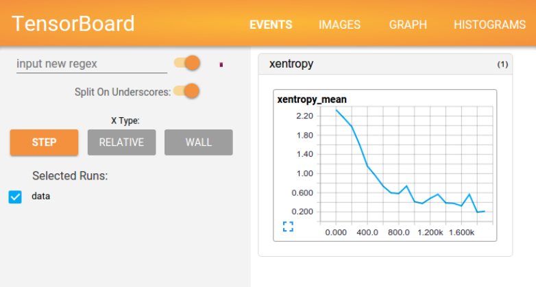
3.3 TENSORBOARD:

可视化学习　 115

3.3 TensorBoard: 可视化学习　

TensorBoard 涉及到的运算，通常是在训练庞大的深度神经网络中出现的复杂而又

难以理解的运算。

为了更方便 TensorFlow 程序的理解、调试与优化，我们发布了一套叫做 TensorBoard

的可视化工具。你可以用 TensorBoard 来展现你的 TensorFlow 图像，绘制图像生成的定

量指标图以及附加数据。

当TensorBoard 设置完成后，它应该是这样子的：

图3.1: MNIST TensorBoard

3.3.1 数据序列化　

TensorBoard 通过读取 TensorFlow 的事件文件来运行。TensorFlow 的事件文件包括

了你会在 TensorFlow 运行中涉及到的主要数据。下面是 TensorBoard 中汇总数据（Sum-

mary data）的大体生命周期。

首先，创建你想汇总数据的 TensorFlow 图，然后再选择你想在哪个节点进行汇总

(summary) 操作。

比如，假设你正在训练一个卷积神经网络，用于识别 MNISt 标签。你可能希望记录学

习速度 (learning rate) 的如何变化，以及目标函数如何变化。通过向节点附加scalar_summary操

作来分别输出学习速度和期望误差。然后你可以给每个 scalary_summary 分配一个有意

义的标签，比如 'learning rate' 和'loss function'。

或者你还希望显示一个特殊层中激活的分布，或者梯度权重的分布。可以通过分别

附加 histogram_summary 运算来收集权重变量和梯度输出。

所有可用的 summary 操作详细信息，可以查看summary_operation文档。

在TensorFlow 中，所有的操作只有当你执行，或者另一个操作依赖于它的输出时才

116 第三章运作方式

会运行。我们刚才创建的这些节点（summary nodes）都围绕着你的图像：没有任何操

作依赖于它们的结果。因此，为了生成汇总信息，我们需要运行所有这些节点。这样的

手动工作是很乏味的，因此可以使用tf.merge_all_summaries来将他们合并为一个操作。

然后你可以执行合并命令，它会依据特点步骤将所有数据生成一个序列化的 Summary

protobuf 对象。最后，为了将汇总数据写入磁盘，需要将汇总的 protobuf 对象传递

给tf.train.Summarywriter。

SummaryWriter 的构造函数中包含了参数 logdir。这个 logdir 非常重要，所有事

件都会写到它所指的目录下。此外，SummaryWriter 中还包含了一个可选择的参数

GraphDef。如果输入了该参数，那么 TensorBoard 也会显示你的图像。

现在已经修改了你的图，也有了 SummaryWriter，现在就可以运行你的神经网络

了！如果你愿意的话，你可以每一步执行一次合并汇总，这样你会得到一大堆训练数

据。这很有可能超过了你想要的数据量。你也可以每一百步执行一次合并汇总，或者如

下面代码里示范的这样。

[] mergedsummar yop=t f .mer g eal lsummar i es()summar ywr i t er =t f .tr ai n.Summar yW r i t er (′/t mp/mni stlog s′,sess.g r aph)t ot alstep=0whi letr ai ni ng :t ot alstep+=1sessi on.r un(tr ai ni ngop)i f t ot alstepsummar ystr =sessi on.r un(mer g edsummar yop)summar ywr i ter.ad dsummar y(summar yst r,t ot alstep)

现在已经准备好用 TensorBoard 来可视化这些数据了。

3.3.2 启动 TensorBoard 　

输入下面的指令来启动 TensorBoard

python tensorflow/tensorboard/tensorboard.py --logdir=path/to/log-directory

这里的参数 logdir 指向 SummaryWriter 序列化数据的存储路径。如果 logdir

目录的子目录中包含另一次运行时的数据，那么 TensorBoard 会展示所有运行的数据。

一旦 TensorBoard 开始运行，你可以通过在浏览器中输入 localhost:6006 来查看

TensorBoard。

如果你已经通过 pip 安装了 TensorBoard，你可以通过执行更为简单地命令来访问

TensorBoard

tensorboard --logdir=/path/to/log-directory

进入 TensorBoard 的界面时，你会在右上角看到导航选项卡，每一个选项卡将展现

一组可视化的序列化数据集。对于你查看的每一个选项卡，如果 TensorBoard 中没有数

据与这个选项卡相关的话，则会显示一条提示信息指示你如何序列化相关数据。

更多更详细的关于如何使用 graph 选项来显示你的图像的信息。参见 TensorBoard:

图表可视化

原文地址：TensorBoard:Visualizing Learning 翻译：thylaco1eo 校对：lucky521

3.4 TENSORBOARD:

图表可视化 117

3.4 TensorBoard: 图表可视化

TensorFlow 图表计算强大而又复杂，图表可视化在理解和调试时显得非常有帮助。

下面是一个运作时的可式化例子。

‘‘一个 TensorFlow 图表的可视化”) 一个 TensorFlow 图表的可视化。

为了显示自己的图表，需将 TensorBoard 指向此工作的日志目录并运行，点击图表顶

部窗格的标签页，然后在左上角的菜单中选择合适的运行。想要深入学习关于如何运行

TensorBoard 以及如何保证所有必要信息被记录下来，请查看 Summaries 和TensorBoard.

3.4.1 名称域（Name scoping）和节点（Node）

典型的 TensorFlow 可以有数以千计的节点，如此多而难以一下全部看到，甚至无

法使用标准图表工具来展示。为简单起见，我们为变量名划定范围，并且可视化把该信

息用于在图表中的节点上定义一个层级。默认情况下，只有顶层节点会显示。下面这个

例子使用tf.name_scope在hidden 命名域下定义了三个操作:

[] import tensorﬂow as tf

with tf.namescope(′hi dden′)asscope :a=t f .const ant (5,name=′al pha′)W=t f .V ar i abl e(t f .r andomuni f or m([1,2],−1.0,1.0),name=′wei g ht s′)b=t f .V ar i able(t f .zer os([1]),name=′bi ases′)

结果是得到了下面三个操作名:

•hidden/alpha

•hidden/weights

•hidden/biases

默认地，三个操作名会折叠为一个节点并标注为 hidden。其额外细节并没有丢失，

你可以双击，或点击右上方橙色的 +来展开节点，然后就会看到三个子节点 alpha，

weights 和biases 了。

这有一个生动的例子，例中有一个更复杂的节点，节点处于其初始和展开状态。

</td>

</td>

顶级名称域的初始视图<code>pool_1</code>，点击右上方橙色的<code>+</code>按钮或双击节点来展开。

</td>

118 第三章运作方式

展开的<code>pool_1</code>名称域视图，点击右上方橙色的<code>-</code>按钮或双击节点来收起此名称域。

</td>

通过名称域把节点分组来得到可读性高的图表很关键的。如果你在构建一个模型，

名称域就可以用来控制可视化结果。你的名称域越好，可视性就越好。

上面的图像例子说明了可视化的另一方面，TensorFlow 图表有两种连接关系：数据

依赖和控制依赖。数据依赖显示两个操作之间的 tensor 流程，用实心箭头指示，而控制依

赖用点线表示。在已展开的视图 (上面的右图)中，除了用点线连接的 CheckNumerics

和control_dependency 之外，所有连接都是数据依赖的。

还有一种手段用来简化布局。大多数 TensorFlow 图表有一部分节点，这部分节点

和其他节点之间有很多连接。比如，许多节点在初始化阶段可能会有一个控制依赖，而

绘制所有 init 节点的边缘和其依赖可能会创造出一个混乱的视图。

为了减少混乱，可视化把所有 high-degree 节点分离到右边的一个从属区域，而不

会绘制线条来表示他们的边缘。线条也不用来表示连接了，我们绘制了小节点图标来指

示这些连接关系。分离出从属节点通常不会把关键信息删除掉，因为这些节点和内构功

能是相关的。

</td>

</td>

节点<code>conv_1</code>被连接到<code>save</code>，注意其右边<code>save</code>节点图标。

</td>

<code>save</code> has a high degree, 并会作为从属节点出现，与<code>conv_1</code>的连接作为一个节点图标显示在其左边。为了继续减少杂乱，既然<code>save</code>有很多连接，我们则只显示前5个，而把其余的缩略为<code>... 12 more</code>。

</td>

最后一个结构上的简化法叫做序列折叠（series collapsing）。序列基序（Sequential

motifs）是拥有相同结构并且其名称结尾的数字不同的节点，它们被折叠进一个单独的

节点块（stack）中。对长序列网络来说，序列折叠极大地简化了视图，对于已层叠的节

点，双击会展开序列。

</td>

3.4 TENSORBOARD:

图表可视化 119

</td>

一个节点序列的折叠视图。

</td>

视图的一小块,双击后展开。

</td>

最后，针对易读性的最后一点要说到的是，可视化为常节点和摘要节点使用了特别

的图标，总结起来有下面这些节点符号：

[c]@ll@

符

号

意

义High-

level

节

点

代

表

一

个

名

称

域，

双

击

则

展

开

一

个

高

层

节

点。

彼

此

之

间

不

连

接

的

有

限

个

节

点

序

列。

彼

此

之

间

相

连

的

有

限

个

节

点

序

列。

一

个

单

独

的

操

作

节

点。

一

个

常

量

结

点。

一

个

摘

要

节

点。

120 第三章运作方式

显

示

各

操

作

间

的

数

据

流

边。

显

示

各

操

作

间

的

控

制

依

赖

边。

引

用

边，

表

示

出

度

操

作

节

点

可

以

使

入

度

ten-

sor

发

生

变

化。

3.4.2 交互

通过平移和缩放来导航图表，点击和拖动用于平移，滚动手势用于缩放。双击一个

节点或点击其 +按钮来展开代表一组操作的名称域。右下角有一个小地图可以在缩放

和平移时方便的改变当前视角。

要关闭一个打开的节点，再次双击它或点击它的-按钮，你也可以只点击一次来选

中一个节点，节点的颜色会加深，并且会看到节点的详情，其连接到的节点会在可视化

右上角的详情卡片显现。

</td>

</td>

3.4 TENSORBOARD:

图表可视化 121

详情卡片展示<code>conv2</code>名称域的详细信息，名称域中操作节点的输入和输出被结合在一起，适用于不显示属性的名称域。

</td>

详情卡片展示<code>DecodeRaw</code>操作节点，除了输入和输出，卡片也会展示与当前节点相关的设备和属性。

</td>

选择对于 high-degree 节点的理解也很有帮助，选择任意节点，则与它的其余连接

相应的节点也会选中，这使得在进行例如查看哪一个节点是否已保存等操作时非常容

易。

点击详情卡片中的一个节点名称时会选中该节点，必要的话，视角会自动平移以使

该节点可见。

最后，使用图例上方的颜色菜单，你可以给你的图表选择两个颜色方案。默认的结

构视图下，当两个 high-level 节点颜色一样时，其会以相同的彩虹色彩出现，而结构唯

一的节点颜色是灰色。还有一个视图则展示了不同的操作运行于什么设备之上。名称域

被恰当的根据其中的操作节点的设备片件来着色。

下图是一张真实图表的图解：

</td>

</td>

结构视图：灰色节点的结构是唯一的。橙色的<code>conv1</code>和<code>conv2</code>节点有相同的结构,其他颜色的节点也类似。

</td>

设备视图：名称域根据其中的操作节点的设备片件来着色，在此紫色代表GPU，绿色代表CPU。

</td>

原文:TensorBoard: Graph Visualization 翻译: [@Warln](https://github.com/Warln) 校

对:lucky521

122 第三章运作方式

3.5 数据读取

TensorFlow 程序读取数据一共有 3种方法:

•供给数据 (Feeding)：在 TensorFlow 程序运行的每一步，让 Python 代码来供给数

据。

•从文件读取数据：在 TensorFlow 图的起始，让一个输入管线从文件中读取数据。

•预加载数据：在 TensorFlow 图中定义常量或变量来保存所有数据 (仅适用于数据

量比较小的情况)。

3.5.1 目录

数据读取

•供给数据 (Feeding)

•从文件读取数据

•文件名,乱序 (shufﬂing), 和最大训练迭代数 (epoch limits)

•文件格式

•预处理

•批处理

•使用 QueueRunner 创建预读线程

•对记录进行过滤或者为每个纪录创建多个样本

•序列化输入数据 (Sparse input data)

•预加载数据

•多管线输入

3.5.2 供给数据

TensorFlow 的数据供给机制允许你在 TensorFlow 运算图中将数据注入到任一张量

中。因此，python 运算可以把数据直接设置到 TensorFlow 图中。

通过给 run() 或者 eval() 函数输入 feed_dict 参数，可以启动运算过程。

[] with tf.Session(): input = tf.placeholder(tf.ﬂoat32) classiﬁer = ... print classiﬁer.eval(feeddi ct ={i nput :mypyt honpr epr ocessi ng fn()})

虽然你可以使用常量和变量来替换任何一个张量，但是最好的做法应该是使用placeholder

op节点。设计 placeholder 节点的唯一的意图就是为了提供数据供给 (feeding) 的方

3.5

数据读取 123

法。placeholder 节点被声明的时候是未初始化的，也不包含数据，如果没有为它供

给数据，则 TensorFlow 运算的时候会产生错误，所以千万不要忘了为 placeholder

提供数据。

可以在tensorflow/g3doc/tutorials/mnist/fully_connected_feed.py找

到使用 placeholder 和MNIST 训练的例子，MNIST tutorial也讲述了这一例子。

3.5.3 从文件读取数据

一共典型的文件读取管线会包含下面这些步骤：

1. 文件名列表

2. 可配置的文件名乱序 (shufﬂing)

3. 可配置的最大训练迭代数 (epoch limit)

4. 文件名队列

5. 针对输入文件格式的阅读器

6. 纪录解析器

7. 可配置的预处理器

8. 样本队列

文件名,乱序 (shufﬂing), 和最大训练迭代数 (epoch limits)

可以使用字符串张量 (比如 ["file0", "file1"],[("file%d" % i) for i

in range(2)]，[("file%d" % i) for i in range(2)])或者tf.train.match_filenames_once

函数来产生文件名列表。

将文件名列表交给tf.train.string_input_producer 函数.string_input_producer

来生成一个先入先出的队列，文件阅读器会需要它来读取数据。

string_input_producer 提供的可配置参数来设置文件名乱序和最大的训练

迭代数，QueueRunner 会为每次迭代 (epoch) 将所有的文件名加入文件名队列中，如

果shuffle=True 的话，会对文件名进行乱序处理。这一过程是比较均匀的，因此它

可以产生均衡的文件名队列。

这个 QueueRunner 的工作线程是独立于文件阅读器的线程，因此乱序和将文件

名推入到文件名队列这些过程不会阻塞文件阅读器运行。

文件格式

根据你的文件格式，选择对应的文件阅读器，然后将文件名队列提供给阅读器的

read 方法。阅读器的 read 方法会输出一个 key 来表征输入的文件和其中的纪录 (对

124 第三章运作方式

于调试非常有用)，同时得到一个字符串标量，这个字符串标量可以被一个或多个解析

器，或者转换操作将其解码为张量并且构造成为样本。

CSV 文件从CSV 文件中读取数据，需要使用TextLineReader和decode_csv 操作，

如下面的例子所示：

[] ﬁlenamequeue=t f .tr ai n.str inginputpr od ucer ([" f i le0.csv","f i le1.csv"])

reader = tf.TextLineReader() key, value = reader.read(ﬁlenamequeue)

Default values, in case of empty columns. Also speciﬁes the type of the decoded result.

recordde f aul t s=[[1], [1],[1], [1],[1]]col 1,col2, col 3,col 4,col5=t f .decodecsv(val ue,r ecor dde f aul t s=r ecor dde f aul t s)f eatur es=t f .concat(0,[col1,col2, col 3,col 4])

with tf.Session() as sess: Start populating the ﬁlename queue. coord = tf.train.Coordinator()

threads = tf.train.startqueuerunner s(coor d=coord)

for i in range(1200): Retrieve a single instance: example, label = sess.run([features,

col5])

coord.requeststop()coor d .j oi n(t hr e ad s)

每次 read 的执行都会从文件中读取一行内容，decode_csv 操作会解析这一行

内容并将其转为张量列表。如果输入的参数有缺失，record_default 参数可以根据

张量的类型来设置默认值。

在调用 run 或者 eval 去执行 read 之前，你必须调用 tf.train.start_queue_runners

来将文件名填充到队列。否则 read 操作会被阻塞到文件名队列中有值为止。

固定长度的记录从二进制文件中读取固定长度纪录，可以使用tf.FixedLengthRecordReader的tf.decode_raw操

作。decode_raw 操作可以讲一个字符串转换为一个 uint8 的张量。

举例来说，the CIFAR-10 dataset的文件格式定义是：每条记录的长度都是固定的，一

个字节的标签，后面是 3072 字节的图像数据。uint8 的张量的标准操作就可以从中获取图

像片并且根据需要进行重组。例子代码可以在tensorflow/models/image/cifar10/cifar10_input.py找

到，具体讲述可参见教程.

标准 TensorFlow 格式另一种保存记录的方法可以允许你讲任意的数据转换为 Tensor-

Flow 所支持的格式，这种方法可以使 TensorFlow 的数据集更容易与网络应用架构相匹

配。这种建议的方法就是使用 TFRecords 文件，TFRecords 文件包含了tf.train.Example

协议内存块 (protocol buffer)(协议内存块包含了字段 Features)。你可以写一段代码获

取你的数据，将数据填入到 Example 协议内存块 (protocol buffer)，将协议内存块序列

化为一个字符串，并且通过tf.python_io.TFRecordWriter class写入到 TFRecords

文件。tensorflow/g3doc/how_tos/reading_data/convert_to_records.py就

是这样的一个例子。

从TFRecords 文件中读取数据，可以使用tf.TFRecordReader的tf.parse_single_example解

析器。这个 parse_single_example 操作可以将 Example 协议内存块 (protocol

buffer) 解析为张量。MNIST 的例子就使用了 convert_to_records 所构建的数据。

3.5

数据读取 125

请参看tensorflow/g3doc/how_tos/reading_data/fully_connected_reader.py,

您也可以将这个例子跟 fully_connected_feed 的版本加以比较。

预处理

你可以对输入的样本进行任意的预处理，这些预处理不依赖于训练参数，你可以

在tensorflow/models/image/cifar10/cifar10.py找到数据归一化，提取随机

数据片，增加噪声或失真等等预处理的例子。

批处理

在数据输入管线的末端，我们需要有另一个队列来执行输入样本的训练，评价和推

理。因此我们使用tf.train.shuffle_batch 函数来对队列中的样本进行乱序处理

示例:

def read_my_file_format(filename_queue):

reader = tf.SomeReader()

key, record_string = reader.read(filename_queue)

example, label = tf.some_decoder(record_string)

processed_example = some_processing(example)

return processed_example, label

def input_pipeline(filenames, batch_size, num_epochs=None):

filename_queue = tf.train.string_input_producer(

filenames, num_epochs=num_epochs, shuffle=True)

example, label = read_my_file_format(filename_queue)

# min_after_dequeue defines how big a buffer we will randomly sample

# from -- bigger means better shuffling but slower start up and more

# memory used.

# capacity must be larger than min_after_dequeue and the amount larger

# determines the maximum we will prefetch. Recommendation:

# min_after_dequeue + (num_threads + a small safety margin) *batch_size

min_after_dequeue = 10000

capacity = min_after_dequeue + 3 *batch_size

example_batch, label_batch = tf.train.shuffle_batch(

[example, label], batch_size=batch_size, capacity=capacity,

min_after_dequeue=min_after_dequeue)

return example_batch, label_batch

如果你需要对不同文件中的样子有更强的乱序和并行处理，可以使用tf.train.shuffle_batch_join

函数.示例:

126 第三章运作方式

def read_my_file_format(filename_queue):

# Same as above

def input_pipeline(filenames, batch_size, read_threads, num_epochs=None):

filename_queue = tf.train.string_input_producer(

filenames, num_epochs=num_epochs, shuffle=True)

example_list = [read_my_file_format(filename_queue)

for _ in range(read_threads)]

min_after_dequeue = 10000

capacity = min_after_dequeue + 3 *batch_size

example_batch, label_batch = tf.train.shuffle_batch_join(

example_list, batch_size=batch_size, capacity=capacity,

min_after_dequeue=min_after_dequeue)

return example_batch, label_batch

在这个例子中，你虽然只使用了一个文件名队列，但是 TensorFlow 依然能保证多

个文件阅读器从同一次迭代 (epoch) 的不同文件中读取数据，知道这次迭代的所有文件

都被开始读取为止。（通常来说一个线程来对文件名队列进行填充的效率是足够的）

另一种替代方案是：使用tf.train.shuffle_batch 函数,设置 num_threads

的值大于 1。这种方案可以保证同一时刻只在一个文件中进行读取操作 (但是读取速度

依然优于单线程)，而不是之前的同时读取多个文件。这种方案的优点是：*避免了两个

不同的线程从同一个文件中读取同一个样本。*避免了过多的磁盘搜索操作。

你一共需要多少个读取线程呢？函数 tf.train.shuffle_batch*为Tensor-

Flow 图提供了获取文件名队列中的元素个数之和的方法。如果你有足够多的读取线程，

文件名队列中的元素个数之和应该一直是一个略高于 0的数。具体可以参考TensorBoard:

可视化学习.

创建线程并使用 QueueRunner 对象来预取

简单来说：使用上面列出的许多 tf.train 函数添加QueueRunner到你的数据流

图中。在你运行任何训练步骤之前，需要调用tf.train.start_queue_runners函

数，否则数据流图将一直挂起。tf.train.start_queue_runners 这个函数将会启

动输入管道的线程，填充样本到队列中，以便出队操作可以从队列中拿到样本。这种情

况下最好配合使用一个tf.train.Coordinator，这样可以在发生错误的情况下正确

地关闭这些线程。如果你对训练迭代数做了限制，那么需要使用一个训练迭代数计数

器，并且需要被初始化。推荐的代码模板如下：

[] Create the graph, etc. initop=t f .i ni ti al i zeallvar i ables()

Create a session for running operations in the Graph. sess = tf.Session()

Initialize the variables (like the epoch counter). sess.run(initop)

3.5

数据读取 127

Start input enqueue threads. coord = tf.train.Coordinator() threads = tf.train.startqueuerunner s(sess=sess,coord=coor d)

try: while not coord.shouldst op() : Runtr ai ni ng st epsor whatever sess.r un(tr ai nop)

except tf.errors.OutOfRangeError: print ’Done training – epoch limit reached’ ﬁnally:

When done, ask the threads to stop. coord.requeststop()

Wait for threads to ﬁnish. coord.join(threads) sess.close()

疑问:这是怎么回事?首先，我们先创建数据流图，这个数据流图由一些流水线的阶段

组成，阶段间用队列连接在一起。第一阶段将生成文件名，我们读取这些文件名并且把

他们排到文件名队列中。第二阶段从文件中读取数据（使用 Reader），产生样本，而

且把样本放在一个样本队列中。根据你的设置，实际上也可以拷贝第二阶段的样本，使

得他们相互独立，这样就可以从多个文件中并行读取。在第二阶段的最后是一个排队操

作，就是入队到队列中去，在下一阶段出队。因为我们是要开始运行这些入队操作的线

程，所以我们的训练循环会使得样本队列中的样本不断地出队。

在tf.train 中要创建这些队列和执行入队操作，就要添加tf.train.QueueRunner到

一个使用tf.train.add_queue_runner函数的数据流图中。每个 QueueRunner

负责一个阶段，处理那些需要在线程中运行的入队操作的列表。一旦数据流图构造成功，

tf.train.start_queue_runners函数就会要求数据流图中每个 QueueRunner

去开始它的线程运行入队操作。

如果一切顺利的话，你现在可以执行你的训练步骤，同时队列也会被后台线程来

填充。如果您设置了最大训练迭代数，在某些时候，样本出队的操作可能会得到一

个tf.OutOfRangeError的错误。这其实是 TensorFlow 的‘‘文件结束’’（EOF）————

这就意味着已经达到了最大训练迭代数，已经没有更多可用的样本了。

最后一个因素是Coordinator。这是负责在收到任何关闭信号的时候，让所有的

线程都知道。最常用的是在发生异常时这种情况就会呈现出来，比如说其中一个线程在

运行某些操作时出现错误（或一个普通的 Python 异常）。

想要了解更多的关于 threading, queues, QueueRunners, and Coordinators 的内容可

以看这里.

疑问:在达到最大训练迭代数的时候如何清理关闭线程?想象一下，你有一个模型并且

设置了最大训练迭代数。这意味着，生成文件的那个线程将只会在产生 OutOfRange

错误之前运行许多次。该 QueueRunner 会捕获该错误，并且关闭文件名的队列，最

后退出线程。关闭队列做了两件事情：

•如果还试着对文件名队列执行入队操作时将发生错误。任何线程不应该尝试去这

样做，但是当队列因为其他错误而关闭时，这就会有用了。

•任何当前或将来出队操作要么成功（如果队列中还有足够的元素）或立即失败（发

生OutOfRange 错误）。它们不会防止等待更多的元素被添加到队列中，因为上

面的一点已经保证了这种情况不会发生。

128 第三章运作方式

关键是，当在文件名队列被关闭时候，有可能还有许多文件名在该队列中，这样

下一阶段的流水线（包括 reader 和其它预处理）还可以继续运行一段时间。一旦文件

名队列空了之后，如果后面的流水线还要尝试从文件名队列中取出一个文件名（例如，

从一个已经处理完文件的 reader 中），这将会触发 OutOfRange 错误。在这种情况

下，即使你可能有一个 QueueRunner 关联着多个线程。如果这不是在 QueueRunner 中

的最后那个线程，OutOfRange 错误仅仅只会使得一个线程退出。这使得其他那些正

处理自己的最后一个文件的线程继续运行，直至他们完成为止。（但如果假设你使用

的是tf.train.Coordinator，其他类型的错误将导致所有线程停止）。一旦所有的

reader 线程触发 OutOfRange 错误，然后才是下一个队列，再是样本队列被关闭。

同样，样本队列中会有一些已经入队的元素，所以样本训练将一直持续直到样本

队列中再没有样本为止。如果样本队列是一个RandomShuffleQueue，因为你使用

了shuffle_batch 或者 shuffle_batch_join，所以通常不会出现以往那种队列

中的元素会比 min_after_dequeue 定义的更少的情况。然而，一旦该队列被关闭，

min_after_dequeue 设置的限定值将失效，最终队列将为空。在这一点来说，当实

际训练线程尝试从样本队列中取出数据时，将会触发 OutOfRange 错误，然后训练线

程会退出。一旦所有的培训线程完成，tf.train.Coordinator.join会返回，你就

可以正常退出了。

筛选记录或产生每个记录的多个样本

举个例子，有形式为 [x, y, z] 的样本，我们可以生成一批形式为 [batch,

x, y, z] 的样本。如果你想滤除这个记录（或许不需要这样的设置），那么可以设置

batch 的大小为 0；但如果你需要每个记录产生多个样本，那么 batch 的值可以大于 1。然

后很简单，只需调用批处理函数（比如：shuffle_batch or shuffle_batch_join）

去设置 enqueue_many=True 就可以实现。

稀疏输入数据

SparseTensors 这种数据类型使用队列来处理不是太好。如果要使用 SparseTensors

你就必须在批处理之后使用tf.parse_example 去解析字符串记录 (而不是在批处理

之前使用 tf.parse_single_example)。

3.5.4 预取数据

这仅用于可以完全加载到存储器中的小的数据集。有两种方法：

•存储在常数中。

•存储在变量中，初始化后，永远不要改变它的值。

使用常数更简单一些，但是会使用更多的内存（因为常数会内联的存储在数据流图

数据结构中，这个结构体可能会被复制几次）。

3.5

数据读取 129

[] trainingdat a=...tr ai ni nglabel s=...w i tht f .Session() :i nputdat a=t f .cons t ant (tr ai ni ngdat a)i nputlabel s=t f .const ant (tr ai ni nglabel s)...

要改为使用变量的方式，您就需要在数据流图建立后初始化这个变量。

[] trainingdat a=...t r ai ni nglabel s=...wi tht f .Session()assess :d at aini t i al i zer =t f .pl acehol der (d t ype=tr ai ni ngdat a.d t ype,shape=t r ai ni ngdat a.shape)l abelini ti al i zer =t f .pl acehol der (d t y pe=tr aini nglabel s.d t ype,shape=tr ai ni nglabel s.shape)i nputdat a=t f .V ar i able(d at aini t al i zer,t r ai nabl e=F al se,col lect i ons=[])i nputlabel s=t f .V ar i able(l abelini t al i zer,tr ai nabl e=F al se,col l ecti ons=[])...sess.r un(i nputdat a.i ni t i al i zer,f eeddict={d a t aini t i al i zer :t r ai ni ngdat a})sess.r un(i nputlabel s.i ni t i al i zer,f eeddic t={l abelini t i ali zer :tr ai ni nglables})

设定 trainable=False 可以防止该变量被数据流图的 GraphKeys.TRAINABLE_VARIABLES

收集,这样我们就不会在训练的时候尝试更新它的值；设定 collections=[] 可以防

止GraphKeys.VARIABLES 收集后做为保存和恢复的中断点。

无论哪种方式，tf.train.slice_input_producer function函数可以被用

来每次产生一个切片。这样就会让样本在整个迭代中被打乱，所以在使用批处理的

时候不需要再次打乱样本。所以我们不使用 shuffle_batch 函数，取而代之的是

纯tf.train.batch 函数。如果要使用多个线程进行预处理，需要将 num_threads

参数设置为大于 1的数字。

在tensorflow/g3doc/how_tos/reading_data/fully_connected_preloaded.py

中可以找到一个 MNIST 例子，使用常数来预加载。另外使用变量来预加载的例子在tensorflow/g3doc/how_tos/reading_data/fully_connected_preloaded_var.py，

你可以用上面 fully_connected_feed 和fully_connected_reader 的描述来

进行比较。

3.5.5 多输入管道

通常你会在一个数据集上面训练，然后在另外一个数据集上做评估计算 (或称为

“eval”)。这样做的一种方法是，实际上包含两个独立的进程：

•训练过程中读取输入数据，并定期将所有的训练的变量写入还原点文件）。

•在计算过程中恢复还原点文件到一个推理模型中，读取有效的输入数据。

这两个进程在下面的例子中已经完成了：the example CIFAR-10 model，有以下几个

好处：

• eval 被当做训练后变量的一个简单映射。

•你甚至可以在训练完成和退出后执行 eval。

您可以在同一个进程的相同的数据流图中有训练和 eval，并分享他们的训练后的变

量。参考the shared variables tutorial.

原文地址：Reading data 翻译：volvet and zhangkom 校对：

130 第三章运作方式

3.6 线程和队列

在使用 TensorFlow 进行异步计算时，队列是一种强大的机制。

正如 TensorFlow 中的其他组件一样，队列就是 TensorFlow 图中的节点。这是一种

有状态的节点，就像变量一样：其他节点可以修改它的内容。具体来说，其他节点可以

把新元素插入到队列后端 (rear)，也可以把队列前端 (front) 的元素删除。

为了感受一下队列，让我们来看一个简单的例子。我们先创建一个 ‘‘先入先出’’ 的

队列（FIFOQueue），并将其内部所有元素初始化为零。然后，我们构建一个 TensorFlow

图，它从队列前端取走一个元素，加上 1之后，放回队列的后端。慢慢地，队列的元素

的值就会增加。

Enqueue、EnqueueMany 和Dequeue 都是特殊的节点。他们需要获取队列指针，

而非普通的值，如此才能修改队列内容。我们建议您将它们看作队列的方法。事实上，

在Python API 中，它们就是队列对象的方法（例如 q.enqueue(...)）。

现在你已经对队列有了一定的了解，让我们深入到细节. . .

3.6.1 队列使用概述

队列，如 FIFOQueue 和RandomShuffleQueue，在 TensorFlow 的张量异步计

算时都非常重要。

例如，一个典型的输入结构：是使用一个 RandomShuffleQueue 来作为模型训

练的输入：

•多个线程准备训练样本，并且把这些样本推入队列。

•一个训练线程执行一个训练操作，此操作会从队列中移除最小批次的样本（mini-

batches)。

这种结构具有许多优点，正如在Reading data how to中强调的，同时，Reading data

how to也概括地描述了如何简化输入管道的构造过程。

TensorFlow 的Session 对象是可以支持多线程的，因此多个线程可以很方便地使

用同一个会话（Session）并且并行地执行操作。然而，在 Python 程序实现这样的并行

运算却并不容易。所有线程都必须能被同步终止，异常必须能被正确捕获并报告，回话

终止的时候，队列必须能被正确地关闭。

所幸 TensorFlow 提供了两个类来帮助多线程的实现：tf.Coordinator和tf.QueueRunner。

从设计上这两个类必须被一起使用。Coordinator 类可以用来同时停止多个工作线程

并且向那个在等待所有工作线程终止的程序报告异常。QueueRunner 类用来协调多个

工作线程同时将多个张量推入同一个队列中。

3.6.2 Coordinator

Coordinator 类用来帮助多个线程协同工作，多个线程同步终止。其主要方法有：

3.6

线程和队列 131

•should_stop():如果线程应该停止则返回 True。

•request_stop(<exception>):请求该线程停止。

•join(<list of threads>):等待被指定的线程终止。

首先创建一个 Coordinator 对象，然后建立一些使用 Coordinator 对象的线

程。这些线程通常一直循环运行，一直到 should_stop() 返回 True 时停止。任何线

程都可以决定计算什么时候应该停止。它只需要调用 request_stop()，同时其他线

程的 should_stop() 将会返回 True，然后都停下来。

[] 线程体：循环执行，直到 ‘Coordinator‘收到了停止请求。如果某些条件为真，

请求 ‘Coordinator‘去停止其他线程。 def MyLoop(coord): while not coord.shouldstop() :

...dosome thi ng ...i f ...somecondi t ion... :coor d.r equestst op()

Main code: create a coordinator. coord = Coordinator()

Create 10 threads that run ’MyLoop()’ threads = [threading.Thread(target=MyLoop, args=(coord))

for i in xrange(10)]

Start the threads and wait for all of them to stop. for t in threads: t.start() coord.join(threads)

显然，Coordinator 可以管理线程去做不同的事情。上面的代码只是一个简单的例

子，在设计实现的时候不必完全照搬。Coordinator 还支持捕捉和报告异常,具体可以参

考Coordinator class的文档。

3.6.3 QueueRunner

QueueRunner 类会创建一组线程，这些线程可以重复的执行 Enquene 操作，他

们使用同一个 Coordinator 来处理线程同步终止。此外，一个 QueueRunner 会运行一个

closer thread，当 Coordinator 收到异常报告时，这个 closer thread 会自动关闭队列。

您可以使用一个 queue runner，来实现上述结构。首先建立一个 TensorFlow 图表，这

个图表使用队列来输入样本。增加处理样本并将样本推入队列中的操作。增加 training

操作来移除队列中的样本。

[] example = ...ops to create one example... Create a queue, and an op that enqueues

examples one at a time in the queue. queue = tf.RandomShufﬂeQueue(...) enqueueop=queue.enqueue(exampl e)Cr eat eat r ai ni ng g r aphthat st ar t sb yd eq ueui ng abat cho f exampl es.i nput s=queue.dequeuemany(batchsi ze)tr ai nop=...use′i nput s′tobuild thetr ai ni ng par t o f t heg r aph...

在Python 的训练程序中，创建一个 QueueRunner 来运行几个线程，这几个线

程处理样本，并且将样本推入队列。创建一个 Coordinator，让 queue runner 使用

Coordinator 来启动这些线程，创建一个训练的循环，并且使用 Coordinator 来控

制QueueRunner 的线程们的终止。

# Create a queue runner that will run 4 threads in parallel to enqueue

# examples.

qr = tf.train.QueueRunner(queue, [enqueue_op] *4)

132 第三章运作方式

# Launch the graph.

sess = tf.Session()

# Create a coordinator, launch the queue runner threads.

coord = tf.train.Coordinator()

enqueue_threads = qr.create_threads(sess, coord=coord, start=True)

# Run the training loop, controlling termination with the coordinator.

for step in xrange(1000000):

if coord.should_stop():

break

sess.run(train_op)

# When done, ask the threads to stop.

coord.request_stop()

# And wait for them to actually do it.

coord.join(threads)

3.6.4 异常处理

通过 queue runners 启动的线程不仅仅只处理推送样本到队列。他们还捕捉和处理

由队列产生的异常，包括 OutOfRangeError 异常，这个异常是用于报告队列被关闭。

使用 Coordinator 的训练程序在主循环中必须同时捕捉和报告异常。下面是对上面

训练循环的改进版本。

[] try: for step in xrange(1000000): if coord.shouldstop() : breaksess.r un(tr ai nop)except E xcep ti on,e:Repor t excepti onst ot hecoor dinator.coor d.r equestst op(e)

Terminate as usual. It is innocuous to request stop twice. coord.requeststop()coor d.j oi n(t hr ead s)

原文地址：Threading and Queues 翻译：zhangkom 校对：volvet

3.7

增加一个新

133

3.7 增加一个新 Op

预备知识:

•对C++ 有一定了解.

•已经下载 TensorFlow 源代码并有能力编译它.

如果现有的库没有涵盖你想要的操作,你可以自己定制一个.为了使定制的 Op 能够

兼容原有的库,你必须做以下工作:

•在一个 C++ 文件中注册新 Op. Op 的注册与实现是相互独立的.在其注册时描述了

Op 该如何执行.例如,注册 Op 时定义了 Op 的名字,并指定了它的输入和输出.

•使用 C++ 实现 Op. 每一个实现称之为一个 “kernel”, 可以存在多个 kernel, 以适配不

同的架构 (CPU, GPU 等)或不同的输入/输出类型.

•创建一个 Python 包装器（wrapper）.这个包装器是创建 Op 的公开 API. 当注册 Op

时,会自动生成一个默认默认的包装器.既可以直接使用默认包装器,也可以添加

一个新的包装器.

• (可选)写一个函数计算 Op 的梯度.

• (可选)写一个函数,描述 Op 的输入和输出 shape. 该函数能够允许从 Op 推断

shape.

•测试 Op, 通常使用 Pyhton。如果你定义了梯度，你可以使用 Python 的GradientChecker来

测试它。

3.7.1 内容

增加一个新 Op

•定义 Op 的接口

•为Op 实现 kernel

•生成客户端包装器

•Python Op 包装器

•C++ Op 包装器

•检查 Op 能否正常工作

•验证条件

•Op 注册

134 第三章运作方式

•属性

•属性类型

•多态

•输入和输出

•向后兼容性

•GPU 支持

•使用 Python 实现梯度

•使用 Python 实现 shape 函数

3.7.2 定义 Op 的接口

向TensorFlow 系统注册来定义 Op 的接口.在注册时,指定 Op 的名称,它的输入 (类

型和名称)和输出 (类型和名称), 和所需要任何属性的文档说明.

为了让你有直观的认识,创建一个简单的 Op 作为例子.该Op 接受一个 int32 类

型tensor 作为输入,输出这个 tensor 的一个副本,副本与原 tensor 唯一的区别在于第

一个元素被置为 0. 创建文件 tensorflow/core/user_ops/zero_out.cc,并调用

REGISTER_OP 宏来定义 Op 的接口.

#include "tensorflow/core/framework/op.h"

REGISTER_OP("ZeroOut")

.Input("to_zero: int32")

.Output("zeroed: int32");

ZeroOut Op 接受 32 位整型的 tensor to_zero 作为输入,输出 32 位整型的 tensor

zeroed.

命名的注意事项: Op 的名称必须是为唯一的,并使用驼峰命名法.以下划线 _

开始的名称保留为内部使用.

3.7.3 为Op 实现 kernel

在定义接口之后,提供一个或多个 Op 的实现.为这些 kernel 的每一个创建一个对应

的类,继承 OpKernel,覆盖 Compute 方法.Compute 方法提供一个类型为 OpKernelContext*

的参数 context,用于访问一些有用的信息,例如输入和输出的 tensor.

将kernel 添加到刚才创建的文件中, kernel 看起来和下面的代码类似:

3.7

增加一个新

135

#include "tensorflow/core/framework/op_kernel.h"

using namespace tensorflow;

class ZeroOutOp : public OpKernel {

public:

explicit ZeroOutOp(OpKernelConstruction*context) : OpKernel(context) {}

void Compute(OpKernelContext*context) override {

// 获取输入 tensor.

const Tensor& input_tensor = context->input(0);

auto input = input_tensor.flat<int32>();

// 创建一个输出 tensor.

Tensor*output_tensor = NULL;

OP_REQUIRES_OK(context, context->allocate_output(0, input_tensor.shape(),

&output_tensor));

auto output = output_tensor->template flat<int32>();

// 设置 tensor 除第一个之外的元素均设为 0.

const int N = input.size();

for (int i = 1; i < N; i++) {

output(i) = 0;

}

// 尽可能地保留第一个元素的值.

if (N > 0) output(0) = input(0);

}

};

实现 kernel 后,将其注册到 TensorFlow 系统中.注册时,可以指定该 kernel 运行时的

多个约束条件.例如可以指定一个 kernel 在CPU 上运行,另一个在 GPU 上运行.

将下列代码加入到 zero_out.cc 中,注册 ZeroOut op:

REGISTER_KERNEL_BUILDER(Name("ZeroOut").Device(DEVICE_CPU), ZeroOutOp);

一旦创建和重新安装了 TensorFlow, Tensorﬂow 系统可以在需要时引用和使用该

Op.

3.7.4 生成客户端包装器

Python Op 包装器

当编译 TensorFlow 时,所有放在 tensorflow/core/user_ops 目录下的 Op 会

自动在 bazel-genfiles/tensorflow/python/ops/gen_user_ops.py 文件中

生成 Python Op 包装器.通过以下声明,把那些 Op 引入到 tensorflow/python/user_ops/user_ops.py

中:

136 第三章运作方式

[] from tensorﬂow.python.ops.genuseropsi mpor t∗

你可以选择性将部分函数替换为自己的实现.为此,首先要隐藏自动生成的代码,在

tensorflow/python/BUILD 文件中,将其名字添加到 "user_ops" 的hidden 列

表.

[] tfgenopwr apperpy(name="userops",hi dden=["F ac t",],requi r eshape functions=F al se,)

紧接着 "Fact" 列出自己的 Op. 然后,在tensorflow/python/user_ops/user_ops.py

中添加你的替代实现函数.通常,替代实现函数也会调用自动生成函数来真正把 Op 添

加到图中.被隐藏的自动生成函数位于 gen_user_ops 包中,名称多了一个下划线前缀

(“_”). 例如:

[] def myfact() : """Op."""r e tur ng enuserops.fact()

C++ Op 包装器

当编译 TensorFlow 时,所有 tensorflow/core/user_ops 文件夹下的 Op 会自

动创建 C++ Op 包装器.例如,tensorflow/core/user_ops/zero_out.cc 中的 Op

会自动在 bazel-genfiles/tensorflow/cc/ops/user_ops.{h,cc} 中生成包

装器.

tensorflow/cc/ops/standard_ops.h 通过下述申明,导入用户自定义 Op 自

动生成的包装器.

#include "tensorflow/cc/ops/user_ops.h"

3.7.5 检查 Op 能否正常工作

验证已经成功实现 Op 的方式是编写测试程序.创建文件 tensorflow/python/kernel_tests/zero_out_op_test.py,

包含以下内容:

[] import tensorﬂow as tf class ZeroOutTest(tf.test.TestCase): def testZeroOut(self): with

self.testsessi on() : r esul t =t f .userops.zer oout ([5,4,3,2,1])sel f .asser t Al l E qual (re sul t .eval(),[5,0,0,0,0])

然后运行测试:

$ bazel test tensorflow/python:zero_out_op_test

3.7.6 验证条件

上述示例假定 Op 能够应用在任何 shape 的tensor 上.如果只想应用到 vector 上呢?

这意味需要在上述 OpKernel 实现中添加相关的检查.

void Compute(OpKernelContext*context) override {

// 获取输入 tensor

3.7

增加一个新

137

const Tensor& input_tensor = context->input(0);

OP_REQUIRES(context, TensorShapeUtils::IsVector(input_tensor.shape()),

errors::InvalidArgument("ZeroOut expects a 1-D vector."));

// ...

}

OP_REQUIRES 断言的输入是一个 vector, 如果不是 vector, 将设置 InvalidArgument

状态并返回.OP_REQUIRES 宏有三个参数:

•context:可以是一个 OpKernelContext 或OpKernelConstruction 指针

(参见 tensorflow/core/framework/op_kernel.h), 其SetStatus() 方

法将被使用到.

•检查条件:tensorflow/core/public/tensor_shape.h 中有一些验证 ten-

sor shape 的函数.

•条件不满足时产生的错误:错误用一个 Status 对象表示,参见 tensorflow/core/public/status.h.

Status 包含一个类型 (通常是 InvalidArgument,但也可以是任何类型)和一

个消息.构造一个错误的函数位于 tensorflow/core/lib/core/errors.h

中.

如果想要测试一个函数返回的 Status 对象是否是一个错误,可以使用 OP_REQUIRES_OK.

这些宏如果检测到错误,会直接跳出函数,终止函数执行.

3.7.7 Op 注册

属性

Op 可以有属性,属性的值在 Op 添加到图中时被设置.属性值用于配置 Op, 在kernel

实现中, Op 注册的输入和输出类型中,均可访问这些属性值.尽可能地使用输入代替属

性,因为输入的灵活性更高,例如可以在执行步骤中中被更改,可以使用 feed 等等.属性

可用于实现一些输入无法做到的事情,例如影响 Op 签名 (即输入输出的数量和类型)的

配置或只读配置可以通过属性实现.

下:

<name> 必须以字母开头,可以由数字,字母,下划线组成.<attr-type-expr> 是

一个类型表达式,形式如下:

例如,如果想要 ZeroOut Op 保存一个用户索引,指示该 Op 不仅仅只有一个元素,

你可以注册 Op 如下:

138 第三章运作方式

REGISTER_OP("ZeroOut")

.Attr("preserve_index: int")

.Input("to_zero: int32")

.Output("zeroed: int32");

你的 kernel 可以在构造函数里,通过 context 参数访问这个属性:

class ZeroOutOp : public OpKernel {

public:

explicit ZeroOutOp(OpKernelConstruction *context) : OpKernel(context) {

// 获取欲保存的索引值

OP_REQUIRES_OK(context,

context->GetAttr("preserve_index", &preserve_index_));

// 检查 preserve_index 是否为正

OP_REQUIRES(context, preserve_index_ >= 0,

errors::InvalidArgument("Need preserve_index >= 0, got ",

preserve_index_));

}

void Compute(OpKernelContext*context) override {

// ...

}

private:

int preserve_index_;

};

该值可以在 Compute 方法中被使用:

void Compute(OpKernelContext*context) override {

// ...

// 检查 preserve_index 范围是否合法

OP_REQUIRES(context, preserve_index_ < input.dimension(0),

errors::InvalidArgument("preserve_index out of range"));

// 设置输出 tensor 所有的元素值为 0

const int N = input.size();

for (int i = 0; i < N; i++) {

output_flat(i) = 0;

}

// 保存请求的输入值

output_flat(preserve_index_) = input(preserve_index_);

}

3.7

增加一个新

139

为了维持向后兼容性,将一个属性添加到一个已有的 Op 时,必须指定一个默

认值:

REGISTER_OP("ZeroOut")

.Attr("preserve_index: int = 0")

.Input("to_zero: int32")

.Output("zeroed: int32");

属性类型

属性可以使用下面的类型:

•string:任何二进制字节流 (UTF8 不是必须的).

•int:一个有型整数.

•float:一个浮点数.

•bool:真或假.

•type:DataType 非引用类型之一.

•shape:一个 TensorShapeProto.

•tensor:一个 TensorProto.

•list(<type>):<type> 列表,其中 <type> 是上述类型之一.注意 list(list(<type>))

是无效的.

权威的列表以 op_def_builder.cc:FinalizeAttr 为准.

默认值和约束条件属性可能有默认值,一些类型的属性可以有约束条件.为了定义一

个有约束条件的属性,你可以使用下列的 <attr-type-expr> 形式:

•{'<string1>', '<string2>'}:属性值必须是一个字符串,取值可以为 <string1>

或<string2>.值的语法已经暗示了值的类型为 string,已经暗示了.下述语句

模拟了一个枚举值:

REGISTER_OP("EnumExample")

.Attr("e: {’apple’, ’orange’}");

•{<type1>, <type2>}:值是 type 类型,且必须为 <type1> 或<type2> 之一,

当然 <type1> 和<type2> 必须都是有效的 tensor 类型.你无须指定属性的类型

为type,而是通过 {...} 语句给出一个类型列表.例如,在下面的例子里,属性 t

的类型必须为 int32,float,或bool:

140 第三章运作方式

REGISTER_OP("RestrictedTypeExample")

.Attr("t: {int32, float, bool}");

•这里有一些常见类型约束条件的快捷方式:

•numbertype:限制类型为数字类型,即非 string 非bool 的类型.

•realnumbertype:与numbertype 区别是不支持复杂类型.

•quantizedtype:与numbertype 区别是只支持量化数值 (quantized number

type).

这些类型的列表在 tensorflow/core/framework/types.h 文件中通过函数

定义 (如NumberTypes()). 本例中属性 t必须为某种数字类型:

REGISTER_OP("NumberType")

.Attr("t: numbertype");

对于这个 Op:

[] tf.numberty pe(t=t f .i nt32)t f .numberty pe(t=t f .bool)

•int >= <n>:值必须是一个整数,且取值大于等于 <n>,<n> 是一个自然数.

例如,下列 Op 注册操作指定了属性 a的取值至少为 2.

REGISTER_OP("MinIntExample")

.Attr("a: int >= 2");

•list(<type>) >= <n>:一个 <type> 类型列表,列表长度必须大于等于 <n>.

例如,下面的 Op 注册操作指定属性 a是一个列表,列表中的元素类型是 int32 或

float 列表长度至少为 3.

REGISTER_OP("TypeListExample")

.Attr("a: list({int32, float}) >= 3");

通过添加 = <default> 到约束条件末尾,给一个属性设置默认值 (使其在自动生

成的代码里变成可选属性), 如下:

REGISTER_OP("AttrDefaultExample")

.Attr("i: int = 0");

默认值支持的语法将在最终 GraphDef 定义的 protobuf 表示中被使用.

下面是给所有类型赋予默认值的例子:

3.7

增加一个新

141

REGISTER_OP("AttrDefaultExampleForAllTypes")

.Attr("s: string = ’foo’")

.Attr("i: int = 0")

.Attr("f: float = 1.0")

.Attr("b: bool = true")

.Attr("ty: type = DT_INT32")

.Attr("sh: shape = { dim { size: 1 } dim { size: 2 } }")

.Attr("te: tensor = { dtype: DT_INT32 int_val: 5 }")

.Attr("l_empty: list(int) = []")

.Attr("l_int: list(int) = [2, 3, 5, 7]");

请特别注意那些类型值里面包含的 DT_*名称.

多态

Type Polymorphism 对于那些可以使用不同类型输入或产生不同类型输出的 Op, 可以

一个 OpKernel.

例如,除了 int32 外,想要 ZeroOut Op 支持 float,注册代码如下:

REGISTER_OP("ZeroOut")

.Attr("T: {float, int32}")

.Input("to_zero: <b>T</b>")

.Output("zeroed: <b>T</b>");

这段 Op 注册代码现在指定了输入的类型必须为 float 或int32,而且既然输入和

输出制定了同样的类型 T,输出也同样如此.

一个命名建议:{#naming} 输入,输出,和属性通常使用 snake_case 命名法.唯

一的例外是属性被用作输入类型或是输入类型的一部分.当添加到图中时,

这些属性可以被推断出来,因此不会出现在 Op 的函数里.例如,最后一个

ZeroOut 定义生成的 Python 函数如下:

[] def zeroout(t ozer o,name=None) :"""... :t ozer o : ‘Tensor ‘. :‘f l oat32‘,‘i nt32‘.name : ().

返回值:一个 ‘Tensor‘, 类型和 ‘tozer o‘."""

如果输入的 to_zero 是一个 int32 的tensor, 然后 T将被自动设置为 int32

(实际上是 DT_INT32). 那些推导出的属性的名称字母全大写或采用驼峰命

名法.

下面是一个输出类型自动推断的例子,读者可以对比一下:

142 第三章运作方式

REGISTER_OP("StringToNumber")

.Input("string_tensor: string")

.Output("output: out_type")

.Attr("out_type: {float, int32}");

.Doc(R"doc(

Converts each string in the input Tensor to the specified numeric type.

)doc");

在这种情况下,用户需要在生成的 Python 代码中指定输出类型.

[] def stringtonumber(str i ngtensor,outty pe=None,name=None) :"""Tensor

参数: stringtensor : ‘st r i ng ‘‘Tensor ‘.outtype : ‘t f .DT ype‘,‘t f .f l oat32, t f .i nt 32‘.‘t f .f l oat32‘.name : ().

返回值:一个 ‘outty pe‘‘Tensor ‘."""

#include "tensorflow/core/framework/op_kernel.h"

class ZeroOutInt32Op : public OpKernel {

// 和之前一样

};

class ZeroOutFloatOp : public OpKernel {

public:

explicit ZeroOutFloatOp(OpKernelConstruction *context)

: OpKernel(context) {}

void Compute(OpKernelContext *context) override {

// 获取输入 tensor

const Tensor& input_tensor = context->input(0);

auto input = input_tensor.flat<float>();

// 创建一个输出 tensor

Tensor *output = NULL;

OP_REQUIRES_OK(context,

context->allocate_output(0, input_tensor.shape(), &output));

auto output_flat = output->template flat<float>();

// 设置输出 tensor 的所有元素为 0

const int N = input.size();

for (int i = 0; i < N; i++) {

output_flat(i) = 0;

}<br/>

// 保留第一个输入值

if (N > 0) output_flat(0) = input(0);

}

};

3.7

增加一个新

143

// 注意, TypeConstraint<int32>("T") 意味着属性 "T" (在上面 Op 注册代码中

// 定义的)必须是 "int32", 才能实例化.

REGISTER_KERNEL_BUILDER(

Name("ZeroOut")

.Device(DEVICE_CPU)

.TypeConstraint<int32>("T"),

ZeroOutOpInt32);

REGISTER_KERNEL_BUILDER(

Name("ZeroOut")

.Device(DEVICE_CPU)

.TypeConstraint<float>("T"),

ZeroOutFloatOp);

为了保持向后兼容性,你在为一个已有的 op 添加属性时,必须指定一个默认

值:

REGISTER_OP("ZeroOut")

.Attr("T: {float, int32} = DT_INT32")

.Input("to_zero: T")

.Output("zeroed: T")

如果需要添加更多类型,例如 double:

REGISTER_OP("ZeroOut")

.Attr("T: {float, double, int32}")

.Input("to_zero: T")

.Output("zeroed: T");

为了避免为新增的类型写冗余的 OpKernel 代码,通常可以写一个 C++ 模板作为替

代.当然,仍然需要为每一个重载版本定义一个 keneral 注册 (REGISTER\_KERNEL\_BUILDER

调用).

template <typename T>;

class ZeroOutOp : public OpKernel {

public:

explicit ZeroOutOp(OpKernelConstruction*context) : OpKernel(context) {}

void Compute(OpKernelContext*context) override {

// 获取输入 tensor

const Tensor& input_tensor = context->input(0);

auto input = input_tensor.flat<T>();

// 创建一个输出 tensor

144 第三章运作方式

Tensor*output = NULL;

OP_REQUIRES_OK(context,

context->allocate_output(0, input_tensor.shape(), &output));

auto output_flat = output->template flat<T>();

// 设置输出 tensor 的所有元素为 0

const int N = input.size();

for (int i = 0; i < N; i++) {

output_flat(i) = 0;

}

// Preserve the first input value

if (N > 0) output_flat(0) = input(0);

}

};

};<br/>

// 注意, TypeConstraint<int32>("T") 意味着属性 "T" (在上面 Op 注册代码中

// 定义的)必须是 "int32", 才能实例化. </b>

REGISTER_KERNEL_BUILDER(

Name("ZeroOut")

.Device(DEVICE_CPU)

.TypeConstraint<int32>("T"),

ZeroOutOp<int32>);

REGISTER_KERNEL_BUILDER(

Name("ZeroOut")

.Device(DEVICE_CPU)

.TypeConstraint<float>("T"),

ZeroOutOp<float>);

REGISTER_KERNEL_BUILDER(

Name("ZeroOut")

.Device(DEVICE_CPU)

.TypeConstraint<double>("T"),

ZeroOutOp<double>);

如果有很多重载版本,可以将注册操作通过一个宏来实现.

#include "tensorflow/core/framework/op_kernel.h"

#define REGISTER_KERNEL(type) \

REGISTER_KERNEL_BUILDER( \

Name("ZeroOut").Device(DEVICE_CPU).TypeConstraint<type>("T"), \

ZeroOutOp<type>)

3.7

增加一个新

145

REGISTER_KERNEL(int32);

REGISTER_KERNEL(float);

REGISTER_KERNEL(double);

#undef REGISTER_KERNEL

取决于注册 kernel 使用哪些类型,你可能可以使用tensorflow/core/framework/register_types.h

提供的宏:

#include "tensorflow/core/framework/op_kernel.h"

#include "tensorflow/core/framework/register_types.h"

REGISTER_OP("ZeroOut")

.Attr("T: realnumbertype")

.Input("to_zero: T")

.Output("zeroed: T");

template <typename T>

class ZeroOutOp : public OpKernel { ... };

#define REGISTER_KERNEL(type) \

REGISTER_KERNEL_BUILDER( \

Name("ZeroOut").Device(DEVICE_CPU).TypeConstraint<type>("T"), \

ZeroOutOp<type>)

TF_CALL_REAL_NUMBER_TYPES(REGISTER_KERNEL);

#undef REGISTER_KERNEL

列表输入和输出除了能够使用不同类型的 tensor 作为输入或输出, Op 还支持使用多

个tensor 作为输入或输出.

在接下来的例子里,属性 T存储了一个类型列表,并同时作为输入 in 和输出 out

的类型.输入和输出均为指定类型的 tensor 列表.既然输入和输出的类型均为 T,它们的

tensor 数量和类型是一致的.

REGISTER_OP("PolymorphicListExample")

.Attr("T: list(type)")

.Input("in: T")

.Output("out: T");

可以为列表中可存放的类型设置约束条件.在下一个例子中,输入是 float 和

double 类型的 tensor 列表.例如,这个 Op 可接受的输入类型为 (float, double,

float) 的数据,且在此情况下,输出类型同样为 (float, double, float).

REGISTER_OP("ListTypeRestrictionExample")

.Attr("T: list({float, double})")

146 第三章运作方式

.Input("in: T")

.Output("out: T");

如果想要一个列表中的所有 tensor 是同一类型,你需要写下列代码:

REGISTER_OP("IntListInputExample")

.Attr("N: int")

.Input("in: N *int32")

.Output("out: int32");

这段代码接受 int32 tensor 列表,并用一个 int 属性 N来指定列表的长度.

这也可用于类型推断.在下一个例子中,输入是一个 tensor 列表,长度为 "N",类型

为"T",输出是单个 "T" 的tensor:

REGISTER_OP("SameListInputExample")

.Attr("N: int")

.Attr("T: type")

.Input("in: N *T")

.Output("out: T");

默认情况下, tensor 列表的最小长度为 1. 这个约束条件可以通过为指定的属性增加

一个 ">=" 约束来变更:

REGISTER_OP("MinLengthIntListExample")

.Attr("N: int >= 2")

.Input("in: N *int32")

.Output("out: int32");

同样的语法也适用于 "list(type)" 属性:

REGISTER_OP("MinimumLengthPolymorphicListExample")

.Attr("T: list(type) >= 3")

.Input("in: T")

.Output("out: T");

输入和输出

总结一下上述内容,一个 Op 注册操作可以指定多个输入和输出:

REGISTER_OP("MultipleInsAndOuts")

.Input("y: int32")

.Input("z: float")

.Output("a: string")

.Output("b: int32");

3.7

增加一个新

147

每一个输入或输出形式如下:

其中,<name> 以字母打头,且只能由数字,字母和下划线组成.<io-type-expr>

可以是下列类型表达式之一:

•<type>,一个合法的输入类型,如float,int32,string.这可用于指定给定类

型的单个 tensor.

参见合法 Tensor 类型列表.

REGISTER_OP("BuiltInTypesExample")

.Input("integers: int32")

.Input("complex_numbers: scomplex64");

•<attr-type>,一个属性和一个类型 type 或类型列表 list(type)(可能包含

类型限制). 该语法可实现多态 Op.

REGISTER_OP("PolymorphicSingleInput")

.Attr("T: type")

.Input("in: T);

REGISTER_OP("RestrictedPolymorphicSingleInput")

.Attr("T: {int32, int64}")

.Input("in: T);

将属性的类型设置为 list(type) 将允许你接受一个序列的 tensor.

REGISTER_OP("ArbitraryTensorSequenceExample")

.Attr("T: list(type)")

.Input("in: T")

.Output("out: T");

REGISTER_OP("RestrictedTensorSequenceExample")

.Attr("T: list({int32, int64})")

.Input("in: T")

.Output("out: T");

注意,输入和输出均为 T,意味着输入和输出的类型与数量均相同.

•<number> *<type>,一组拥有相同类型的 tensor, <number> 是一个 int 类型

属性的名称.<type> 可以是一个类似于 int32 和float 的特定类型,或者一个

type 类型属性的名字.前者的例子如下,该例子接受一个 int32 tensor 列表作为

Op 输入:

148 第三章运作方式

REGISTER_OP("Int32SequenceExample")

.Attr("NumTensors: int")

.Input("in: NumTensors *int32")

后者的例子如下,该例子接受一个泛型 tensor 列表作为 Op 输入:

REGISTER_OP("SameTypeSequenceExample")

.Attr("NumTensors: int")

.Attr("T: type")

.Input("in: NumTensors *T")

• Tensor 的引用表示为 Ref(<type>),其中 <type> 是上述类型之一.

一个命名建议:当使用属性表示一个输入的类型时,该类型可以被推断出来.

实现该特性,将需要推断的类型用大写名称表示 (如T或N), 其它的输入,输

出,和属性像使用函数参数一样使用这些大写名称.参见之前的命名建议章

节查看更多细节.

更多细节参见 tensorflow/core/framework/op_def_builder.h.

向后兼容性

通常,对规范的改变必须保持向后兼容性: Op 使用新规范后,需保证使用旧规范构

造的序列化 GraphDef 仍能正确工作.

下面是几种保持向后兼容性的方式:

1. 任何添加到 Op 的新属性必须有默认值,且默认值下的行为有明确定义.将一个非

多态的操作变为多态操作,你必须为新的类型属性赋予默认值,以保持原始的函数

签名.例如,有如下操作:

REGISTER_OP("MyGeneralUnaryOp")

.Input("in: float")

.Output("out: float");

可以通过下述方式将其变为多态,且保持向后兼容性:

REGISTER_OP("MyGeneralUnaryOp")

.Input("in: T")

.Output("out: T")

.Attr("T: numerictype = float");

3.7

增加一个新

149

1. 放宽一个属性的约束条件是安全的.例如,你可以将 {int32, int64} 变为

{int32, int64, float},或者,将{"apple", "orange"} 变为 {"apple", "banana",

"orange"}.

2. 通过给 Op 名称添加一些项目中唯一的标识作为前缀,来为新建的 Op 添加命名空

间.命名空间可以预防你的 Op 与TensorFlow 未来版本里的内置 Op 产生命名冲突.

3. 超前计划!尝试着去预测 Op 未来的的用途,超前设计,毕竟,一些签名的变更无法

保证兼容性 (例如,增加新的输入,或将原来的单元素输入变成一个列表).

如果不能以兼容的方式改变一个操作,那就创建一个全新的操作,来实现所需功能.

3.7.8 GPU 支持

你可以实现不同的 OpKernel, 将其中之一注册到 GPU, 另一个注册到 GPU, 正如为

不同的类型注册 kernel一样.tensorflow/core/kernels/ 中有一些 GPU 支持的例

子.注意,一些 kernel 的CPU 版本位于 .cc 文件, GPU 版本位于 _gpu.cu.cc 文件,共

享的代码位于 .h 文件.

例如,pad op 除了 GPU kernel 外的其它代码均在 tensorflow/core/kernels/pad_op.cc

中. GPU kernel 位于 tensorflow/core/kernels/pad_op_gpu.cu.cc,共享的一

个模板类代码定义在 tensorflow/core/kernels/pad_op.h.需要注意的事情是,

即使使用 pad 的GPU 版本时,仍然需要将 "paddings" 输入放置到内存中.为了实现

这一点,将输入或输出标记为必须保存在内存中,为kernel 注册一个 HostMemory() 调

用.如下:

#define REGISTER_GPU_KERNEL(T) \

REGISTER_KERNEL_BUILDER(Name("Pad") \

.Device(DEVICE_GPU) \

.TypeConstraint<T>("T") \

.HostMemory("paddings"), \

PadOp<GPUDevice, T>)

3.7.9 使用 Python 实现梯度

给定一个 Op 组成的图, TensorFlow 使用自动微分 (反向传播)来添加新的 Op 以表

示梯度运算,同时不影响已有的 Op (参见梯度运算). 为了使自动微分能够与新的 Op 协

同工作,必须注册一个梯度函数,从Op 的输入计算梯度,并返回代表梯度值的输出.

数学上,如果一个 Op 计算 $y = f(x)$, 注册的梯度 Op 通过以下链式法则,将$∂/∂y$$∂/∂x$.

∂

∂x=

∂

∂y

∂x=

∂

∂y

∂f

∂x.

在ZeroOut 的例子中,输入中只有一个项会影响输出,所以,代表输入的梯度值的

tensor 也只有一个输入项.如下所示:

150 第三章运作方式

[] from tensorﬂow.python.framework import ops from tensorﬂow.python.ops import

arrayops f r omtensor f l ow.py thon.opsi mpor t sp ar seops

@ops.RegisterGradient("ZeroOut") def zer ooutgr ad(op,g r ad ) : """‘zer oout‘.

参数: op: 欲进行微分的 ‘zeroout“‘,Op.g r ad : ‘zer oout‘Op.

返回:代表输入 ‘zeroout‘."""tozer o=op.i nput s[0]shape=ar r a yops.shape(t ozer o)i ndex=ar r a yops.zer osli ke(shape)f i r stgr ad=ar r a yops.r eshape(g r ad ,[−1])[0]t ozer ogr ad =spar seops.spar setodense(i ndex,shape,f i r stgr ad,0)r etur n[tozer ogr ad]Tensor ,

使用 ops.RegisterGradient 注册梯度函数需要注意的一些细节:

•对于仅有一个输出的 Op, 梯度函数使用 Operation op 和一个 Tensor grad 作

为参数,并从 op.inputs[i],op.outputs[i],和grad 构建新的 Op. 属性的信

息可以通过 op.get_attr 获取.

•如果 Op 有多个输出,梯度函数将使用 op 和grads 作为参数,其中,grads 是一个

梯度 Op 的列表,为每一个输出计算梯度.梯度函数的输出必须是一个 Tensor 对

象列表,对应到每一个输入的梯度.

•如果没有为一些输入定义梯度,譬如用作索引的整型,这些输入返回的梯度为 None.

举一个例子,如果一个 Op 的输入为一个浮点数 tensor x和一个整型索引 i,那么梯

度函数将返回 [x_grad, None].

•如果梯度对于一个 Op 来说毫无意义,使用 ops.NoGradient("OpName") 禁用

自动差分.

注意当梯度函数被调用时,作用的对象是数据流图中的 Op, 而不是 tensor 数据本身.

因此,只有在图运行时,梯度运算才会被其它 tensorﬂow Op 的执行动作所触发.

3.7.10 在Python 中实现一个形状函数

TensorFlow Python API 有一个 ‘‘形状推断”功能,可以不执行图就获取 tensor 的形

状信息.形状推断功能藉由每一个 Op 类型注册的 ‘‘形状函数”来支持,该函数有两个

规则:假设所有输入的形状必须是兼容的,以及指定输出的形状.一个形状函数以一个

Operation 作为输入,返回一个 TensorShape 对象列表 (每一个输出一个对象). 使用

tf.RegisterShape 装饰器注册形状函数.例如,上文定义的 ZeroOut Op 的形状函

数如下:

[] @tf.RegisterShape("ZeroOut"): def zer ooutshape(op) : """Z er oOutOp.

这是 ZeroOut 形状函数的无约束版本,为每一个输出产生的形状和对应的输入一样.

""" return [op.inputs[0].getshape()]

一个形状函数也可以约束输入的形状.下面是ZeroOut 形状函数的 vector 输入约

束版本:

[] @tf.RegisterShape("ZeroOut"): def zer ooutshape(op) : """Z er oOutOp.

3.7

增加一个新

151

这是 ZeroOut 形状函数的约束版本,要输入的 rank 必须是 1 (即使一个 vector). """

inputshape=op.i nput s[0].g e tshape().wi thrank(1)ret ur n[inputshape]

如果 Op 是多输入的多态 Op,使用操作的属性来决定需要检查的形状数量:

@tf.RegisterShape("IntListInputExample")

def _int_list_input_example_shape(op):

""" "IntListInputExample" Op 的形状函数.

所有的输入和输出是同大小的矩阵.

"""

output_shape = tf.TensorShape(None)

for input in op.inputs:

output_shape = output_shape.merge_with(input.get_shape().with_rank(2))

return [output_shape]

既然形状推断是一个可选的特性,且tensor 的形状可能动态变化,形状函数必须足

够健壮,能够处理任意输入形状信息缺失的情形.merge_with 方法能够帮助调用者

判断两个形状是否是一样的,即使两个形状的信息不全,该函数同样有效.所有的标准

Python Op 的形状函数都已经定义好了,并且已经有很多不同的使用示例.

原文：Adding a New Op 翻译：[@doc001](https://github.com/PFZheng) 校对：

[@ZHNathanielLee](https://github.com/ZHNathanielLee)

152 第三章运作方式

3.8 自定义数据读取

基本要求:

•熟悉 C++ 编程。

•确保下载 TensorFlow 源文件,并可编译使用。

我们将支持文件格式的任务分成两部分：

•文件格式:我们使用 Reader Op 来从文件中读取一个 record (可以使任意字符串)。

•记录格式:我们使用解码器或者解析运算将一个字符串记录转换为 TensorFlow 可

以使用的张量。

例如，读取一个 CSV 文件，我们使用一个文本读写器，然后是从一行文本中解析

CSV 数据的运算。

3.8.1 主要内容

自定义数据读取

•编写一个文件格式读写器

•编写一个记录格式 Op

3.8.2 编写一个文件格式读写器

Reader 是专门用来读取文件中的记录的。TensorFlow 中内建了一些读写器 Op 的实

例：

•tf.TFRecordReader (代码位于 kernels/tf_record_reader_op.cc)

•tf.FixedLengthRecordReader (代码位于 kernels/ﬁxed_length_record_reader_op.cc)

•tf.TextLineReader (代码位于 kernels/text_line_reader_op.cc)

你可以看到这些读写器的界面是一样的，唯一的差异是在它们的构造函数中。最重

要的方法是 Read。它需要一个行列参数，通过这个行列参数，可以在需要的时候随时

读取文件名 (例如：当 Read Op 首次运行，或者前一个 Read‘ 从一个文件中读取最后一

条记录时)。它将会生成两个标量张量：一个字符串和一个字符串关键值。

新创建一个名为 SomeReader 的读写器，需要以下步骤：

1. 在C++ 中,定义一个 tensorﬂow::ReaderBase的子类，命名为 “SomeReader”.

2. 在C++ 中，注册一个新的读写器 Op 和Kernel，命名为 “SomeReader’’。

3.8

自定义数据读取 153

3. 在Python 中,定义一个 tf.ReaderBase 的子类，命名为 “SomeReader’’。

你可以把所有的 C++ 代码放在 tensorflow/core/user_ops/some_reader_op.cc

文件中.读取文件的代码将被嵌入到 C++ 的ReaderBase 类的迭代中。这个 ReaderBase

类是在 tensorﬂow/core/kernels/reader_base.h 中定义的。你需要执行以下的方法：

• OnWorkStartedLocked：打开下一个文件

• ReadLocked：读取一个记录或报告 EOF/error

• OnWorkFinishedLocked：关闭当前文件

• ResetLocked：清空记录，例如：一个错误记录

以上这些方法的名字后面都带有 “Locked’’，表示 ReaderBase 在调用任何一个方法

之前确保获得互斥锁，这样就不用担心线程安全（虽然只保护了该类中的元素而不是全

局的）。

对于 OnWorkStartedLocked, 需要打开的文件名是 current_work() 函数的返回

值。此时的 ReadLocked 的数字签名如下:

Status ReadLocked(string*key, string*value, bool*produced, bool*at_end)

如果 ReadLocked 从文件中成功读取了一条记录，它将更新为：

• *key：记录的标志位，通过该标志位可以重新定位到该记录。可以包含从 cur-

rent_work() 返回值获得的文件名，并追加一个记录号或其他信息。

• *value：包含记录的内容。

• *produced：设置为 true。

当你在文件（EOF）末尾，设置 *at_end 为true ，在任何情况下，都将返回 Status::OK()。

当出现错误的时候，只需要使用 tensorﬂow/core/lib/core/errors.h 中的一个辅助功能就

可以简单地返回，不需要做任何参数修改。

接下来你讲创建一个实际的读写器 Op。如果你已经熟悉了添加新的 Op 那会很有

帮助。主要步骤如下：

•注册 Op。

•定义并注册 OpKernel。

要注册 Op，你需要用到一个调用指令定义在 tensorﬂow/core/framework/op.h中的

REGISTER_OP。

读写器 Op 没有输入，只有 Ref(string) 类型的单输出。它们调用 SetIsStateful()，并

有一个 container 字符串和 shared_name 属性.你可以在一个 Doc 中定义配置或包含文

档的额外属性。例如：详见 tensorﬂow/core/ops/io_ops.cc等：

154 第三章运作方式

#include "tensorflow/core/framework/op.h"

REGISTER_OP("TextLineReader")

.Output("reader_handle: Ref(string)")

.Attr("skip_header_lines: int = 0")

.Attr("container: string = ’’")

.Attr("shared_name: string = ’’")

.SetIsStateful()

.Doc(R"doc(

A Reader that outputs the lines of a file delimited by ’\n’.

)doc");

要定义一个 OpKernel，读写器可以使用定义在tensorﬂow/core/framework/reader_op_kernel.h中

的ReaderOpKernel 的递减快捷方式，并运行一个叫 SetReaderFactory 的构造函数。定义

所需要的类之后，你需要通过 REGISTER_KERNEL_BUILDER(. . . ) 注册这个类。

一个没有属性的例子：

#include "tensorflow/core/framework/reader_op_kernel.h"

class TFRecordReaderOp : public ReaderOpKernel {

public:

explicit TFRecordReaderOp(OpKernelConstruction*context)

: ReaderOpKernel(context) {

Env*env = context->env();

SetReaderFactory([this, env]() { return new TFRecordReader(name(), env); });

}

};

REGISTER_KERNEL_BUILDER(Name("TFRecordReader").Device(DEVICE_CPU),

TFRecordReaderOp);

一个带有属性的例子：

#include "tensorflow/core/framework/reader_op_kernel.h"

class TextLineReaderOp : public ReaderOpKernel {

public:

explicit TextLineReaderOp(OpKernelConstruction*context)

: ReaderOpKernel(context) {

int skip_header_lines = -1;

OP_REQUIRES_OK(context,

context->GetAttr("skip_header_lines", &skip_header_lines));

OP_REQUIRES(context, skip_header_lines >= 0,

errors::InvalidArgument("skip_header_lines must be >= 0 not ",

3.8

自定义数据读取 155

skip_header_lines));

Env*env = context->env();

SetReaderFactory([this, skip_header_lines, env]() {

return new TextLineReader(name(), skip_header_lines, env);

});

}

};

REGISTER_KERNEL_BUILDER(Name("TextLineReader").Device(DEVICE_CPU),

TextLineReaderOp);

最后一步是添加 Python 包装器，你需要将 tensorﬂow.python.ops.io_ops 导入到 ten-

sorﬂow/python/user_ops/user_ops.py，并添加一个 io_ops.ReaderBase的衍生函数。

from tensorflow.python.framework import ops

from tensorflow.python.ops import common_shapes

from tensorflow.python.ops import io_ops

class SomeReader(io_ops.ReaderBase):

def __init__(self, name=None):

rr = gen_user_ops.some_reader(name=name)

super(SomeReader, self).__init__(rr)

ops.NoGradient("SomeReader")

ops.RegisterShape("SomeReader")(common_shapes.scalar_shape)

你可以在 tensorﬂow/python/ops/io_ops.py中查看一些范例。

3.8.3 编写一个记录格式 Op

一般来说，这是一个普通的 Op，需要一个标量字符串记录作为输入，因此遵循添

加Op 的说明。你可以选择一个标量字符串作为输入，并包含在错误消息中报告不正确

的格式化数据。

用于解码记录的运算实例：

•tf.parse_single_example (and tf.parse_example)

•tf.decode_csv

•tf.decode_raw

请注意，使用多个 Op 来解码某个特定的记录格式也是有效的。例如，你有一张以字

符串格式保存在 tf.train.Example 协议缓冲区的图像文件。根据该图像的格式，你可能从

tf.parse_single_example 的Op 读取响应输出并调用 tf.decode_jpeg，tf.decode_png，或者

tf.decode_raw。通过读取 tf.decode_raw 的响应输出并使用tf.slice 和tf.reshape 来提取数

156 第三章运作方式

据是通用的方法。>原文：Custom Data Readers 翻译：[@derekshang](https://github.com/derekshang)

校对：Wiki

3.9

使用

GPUS

157

3.9 使用 GPUs

3.9.1 支持的设备

在一套标准的系统上通常有多个计算设备. TensorFlow 支持 CPU 和GPU 这两种设

备.我们用指定字符串 strings 来标识这些设备.比如:

•"/cpu:0":机器中的 CPU

•"/gpu:0":机器中的 GPU, 如果你有一个的话.

•"/gpu:1":机器中的第二个 GPU, 以此类推. . .

如果一个 TensorFlow 的operation 中兼有 CPU 和GPU 的实现,当这个算子被指派

设备时, GPU 有优先权.比如 matmul 中CPU 和GPU kernel 函数都存在.那么在 cpu:0

和gpu:0 中,matmul operation 会被指派给 gpu:0 .

3.9.2 记录设备指派情况

为了获取你的 operations 和Tensor 被指派到哪个设备上运行,用log_device_placement

新建一个 session,并设置为 True.

[] 新建一个 graph. a = tf.constant([1.0, 2.0, 3.0, 4.0, 5.0, 6.0], shape=[2, 3], name=’a’) b

= tf.constant([1.0, 2.0, 3.0, 4.0, 5.0, 6.0], shape=[3, 2], name=’b’) c = tf.matmul(a, b) 新建 ses-

sion with logdevi cepl acementTr ue.sess=t f .Sessi on(con f i g =t f .Con f i g Pr ot o(logdevi cepl acement =Tr ue))op.pr i nt sess.r un(c)

你应该能看见以下输出:

Device mapping:

/job:localhost/replica:0/task:0/gpu:0 -> device: 0, name: Tesla K40c, pci bus

id: 0000:05:00.0

b: /job:localhost/replica:0/task:0/gpu:0

a: /job:localhost/replica:0/task:0/gpu:0

MatMul: /job:localhost/replica:0/task:0/gpu:0

[[ 22. 28.]

[ 49. 64.]]

3.9.3 手工指派设备

如果你不想使用系统来为 operation 指派设备,而是手工指派设备,你可以用 with

tf.device 创建一个设备环境,这个环境下的 operation 都统一运行在环境指定的设备

上.

[] 新建一个 graph. with tf.device(’/cpu:0’): a = tf.constant([1.0, 2.0, 3.0, 4.0, 5.0, 6.0],

shape=[2, 3], name=’a’) b = tf.constant([1.0, 2.0, 3.0, 4.0, 5.0, 6.0], shape=[3, 2], name=’b’) c =

158 第三章运作方式

tf.matmul(a, b) 新建 session with logdevi cepl acement Tr ue.sess=t f .Sessi on(con f i g =t f .Con f i g Pr ot o(logdevi cepl acement =Tr ue))op.pr i nt sess.r un(c)

你会发现现在 a和b操作都被指派给了 cpu:0.

Device mapping:

/job:localhost/replica:0/task:0/gpu:0 -> device: 0, name: Tesla K40c, pci bus

id: 0000:05:00.0

b: /job:localhost/replica:0/task:0/cpu:0

a: /job:localhost/replica:0/task:0/cpu:0

MatMul: /job:localhost/replica:0/task:0/gpu:0

[[ 22. 28.]

[ 49. 64.]]

3.9.4 在多 GPU 系统里使用单一 GPU

如果你的系统里有多个 GPU, 那么 ID 最小的 GPU 会默认使用.如果你想用别的

GPU, 可以用下面的方法显式的声明你的偏好:

[] 新建一个 graph. with tf.device(’/gpu:2’): a = tf.constant([1.0, 2.0, 3.0, 4.0, 5.0, 6.0],

shape=[2, 3], name=’a’) b = tf.constant([1.0, 2.0, 3.0, 4.0, 5.0, 6.0], shape=[3, 2], name=’b’) c =

tf.matmul(a, b) 新建 session with logdevi cepl acement Tr ue.sess=t f .Sessi on(con f i g =t f .Con f i g Pr ot o(logdevi cepl acement =Tr ue))op.pr i nt sess.r un(c)

如果你指定的设备不存在,你会收到 InvalidArgumentError 错误提示:

InvalidArgumentError: Invalid argument: Cannot assign a device to node ’b’:

Could not satisfy explicit device specification ’/gpu:2’

[[Node: b = Const[dtype=DT_FLOAT, value=Tensor<type: float shape: [3,2]

values: 1 2 3...>, _device="/gpu:2"]()]]

为了避免出现你指定的设备不存在这种情况,你可以在创建的 session 里把参数

allow_soft_placement 设置为 True,这样 tensorFlow 会自动选择一个存在并且支

持的设备来运行 operation.

[] 新建一个 graph. with tf.device(’/gpu:2’): a = tf.constant([1.0, 2.0, 3.0, 4.0, 5.0, 6.0],

shape=[2, 3], name=’a’) b = tf.constant([1.0, 2.0, 3.0, 4.0, 5.0, 6.0], shape=[3, 2], name=’b’) c =

tf.matmul(a, b) 新建 session with logdevi cepl acement Tr ue.sess=t f .Sessi on(con f i g =t f .Con f i g Pr ot o(all owso f tpl acement=Tr ue,l ogdevi cepl acement=Tr ue))op.pr i nt sess.r un(c)

3.9.5 使用多个 GPU

如果你想让 TensorFlow 在多个 GPU 上运行,你可以建立 multi-tower 结构,在这个

结构里每个 tower 分别被指配给不同的 GPU 运行.比如:

3.9

使用

GPUS

159

#新建一个 graph.

c = []

for d in [’/gpu:2’, ’/gpu:3’]:

with tf.device(d):

a = tf.constant([1.0, 2.0, 3.0, 4.0, 5.0, 6.0], shape=[2, 3])

b = tf.constant([1.0, 2.0, 3.0, 4.0, 5.0, 6.0], shape=[3, 2])

c.append(tf.matmul(a, b))

with tf.device(’/cpu:0’):

sum = tf.add_n(c)

#新建session with log_device_placement并设置为True.

sess = tf.Session(config=tf.ConfigProto(log_device_placement=True))

#运行这个op.

print sess.run(sum)

你会看到如下输出:

Device mapping:

/job:localhost/replica:0/task:0/gpu:0 -> device: 0, name: Tesla K20m, pci bus

id: 0000:02:00.0

/job:localhost/replica:0/task:0/gpu:1 -> device: 1, name: Tesla K20m, pci bus

id: 0000:03:00.0

/job:localhost/replica:0/task:0/gpu:2 -> device: 2, name: Tesla K20m, pci bus

id: 0000:83:00.0

/job:localhost/replica:0/task:0/gpu:3 -> device: 3, name: Tesla K20m, pci bus

id: 0000:84:00.0

Const_3: /job:localhost/replica:0/task:0/gpu:3

Const_2: /job:localhost/replica:0/task:0/gpu:3

MatMul_1: /job:localhost/replica:0/task:0/gpu:3

Const_1: /job:localhost/replica:0/task:0/gpu:2

Const: /job:localhost/replica:0/task:0/gpu:2

MatMul: /job:localhost/replica:0/task:0/gpu:2

AddN: /job:localhost/replica:0/task:0/cpu:0

[[ 44. 56.]

[ 98. 128.]]

cifar10 tutorial 这个例子很好的演示了怎样用 GPU 集群训练.

原文:using_gpu 翻译:[@lianghyv](https://github.com/lianghyv) 校对:Wiki

160 第三章运作方式

�

第四章 Python API

161

162 第四章

PYTHON API

4.1 Overview

TensorFlow has APIs available in several languages both for constructing and executing

a TensorFlow graph. The Python API is at present the most complete and the easiest to use,

but the C++ API may offer some performance advantages in graph execution, and supports

deployment to small devices such as Android.

Over time, we hope that the TensorFlow community will develop front ends for lan-

guages like Go, Java, JavaScript, Lua R, and perhaps others. With SWIG, it’s relatively easy to

develop a TensorFlow interface for your favorite language.

Note: Many practical aspects of usage are covered in the Mechanics tab, and some

additional documentation not speciﬁc to any particular language API is available in the Re-

sources tab.

4.2 BUILDING GRAPHS

163

4.2 Building Graphs

4.2.1 Contents

Building Graphs

•Core graph data structures

•class tf.Graph

•class tf.Operation

•class tf.Tensor

•Tensor types

•class tf.DType

•tf.as_dtype(type_value)

•Utility functions

•tf.device(dev)

•tf.name_scope(name)

•tf.control_dependencies(control_inputs)

•tf.convert_to_tensor(value, dtype=None, name=None)

•tf.get_default_graph()

•tf.import_graph_def(graph_def, input_map=None, return_elements=None, name=None

, op_dict=None)

•Graph collections

•tf.add_to_collection(name, value)

•tf.get_collection(key, scope=None)

•class tf.GraphKeys

•Deﬁning new operations

•class tf.RegisterGradient

•tf.NoGradient(op_type)

•class tf.RegisterShape

•class tf.TensorShape

•class tf.Dimension

•tf.op_scope(values, name, default_name)

•tf.get_seed(op_seed)

Classes and functions for building TensorFlow graphs.

4.2.2 Core graph data structures

164 第四章

PYTHON API

class tf.Graph

A TensorFlow computation, represented as a dataﬂow graph.

AGraph contains a set of Operation objects, which represent units of computation; and

Tensor objects, which represent the units of data that ﬂow between operations.

A default Graph is always registered, and accessible by calling tf.get_default_graph().

To add an operation to the default graph, simply call one of the functions that deﬁnes a new

Operation:

 

1c = tf.constant(4.0)

2assert c.graph is tf.get_default_graph()

 

Another typical usage involves the Graph.as_default() context manager, which over-

rides the current default graph for the lifetime of the context:

[] g = tf.Graph() with g.asde f aul t () : De f i neo per at i onsand t ensor si n‘g‘.c=t f .const ant (30.0)asser t c.g r aphi sg

Important note: This class is not thread-safe for graph construction. All operations

should be created from a single thread, or external synchronization must be provided. Un-

less otherwise speciﬁed, all methods are not thread-safe.

tf.Graph.__init__() Creates a new, empty Graph.

tf.Graph.as_default() Returns a context manager that makes this Graph the default graph.

This method should be used if you want to create multiple graphs in the same process.

For convenience, a global default graph is provided, and all ops will be added to this graph

if you do not create a new graph explicitly. Use this method the with keyword to specify that

ops created within the scope of a block should be added to this graph.

The default graph is a property of the current thread. If you create a new thread, and

wish to use the default graph in that thread, you must explicitly add a with g.as_default():

in that thread’s function.

The following code examples are equivalent:

[] 1. Using Graph.asde f aul t () : g=t f .Gr aph()w i thg .asde f aul t () :c=t f .const ant (5.0)asser t c.g r aphi sg

2. Constructing and making default: with tf.Graph().asde f aul t ()asg :c=t f .const ant (5.0)asser t c.g r aphi sg

Returns: A context manager for using this graph as the default graph.

4.2 BUILDING GRAPHS

165

tf.Graph.as_graph_def(from_version=None) Returns a serialized GraphDef representation

of this graph.

The serialized GraphDef can be imported into another Graph (using import_graph_def())

or used with the C++ Session API.

This method is thread-safe.

Args:

•from_version: Optional. If this is set, returns a GraphDef containing only the nodes

that were added to this graph since its version property had the given value.

Returns: AGraphDef protocol buffer.

tf.Graph.finalize() Finalizes this graph, making it read-only.

After calling g.finalize(), no new operations can be added to g. This method is used to

ensure that no operations are added to a graph when it is shared between multiple threads,

for example when using a QueueRunner.

tf.Graph.finalized True if this graph has been ﬁnalized.

tf.Graph.control_dependencies(control_inputs) Returns a context manager that speci-

ﬁes control dependencies.

Use with the with keyword to specify that all operations constructed within the context

should have control dependencies on control_inputs. For example:

[] with g.controldependencies([a,b,c]) : ‘d‘and‘e‘wi llonl yr una f ter ‘a‘,‘b‘, and‘c‘haveexecuted.d=...e=...

Multiple calls to control_dependencies() can be nested, and in that case a new Operation

will have control dependencies on the union of control_inputs from all active contexts.

[] with g.controldependencies([a,b]) : Op sd ecl ar ed her er una f t er ‘a‘and‘b‘.w i t hg .contr oldependencies([c,d]) :Opsdecl ar ed her er una f t er ‘a‘, ‘b‘,‘c‘, and‘d‘.

N.B. The control dependencies context applies only to ops that are constructed within

the context. Merely using an op or tensor in the context does not add a control dependency.

The following example illustrates this point:

[] WRONG def myfunc(pr ed,tensor ) : t=t f .matmul(t ensor,tensor )wi t ht f .contr oldepend encies([pr ed ]) :T hemat mul opi scr eated out si det hecont ext,sonocont r ol de pendenc y wi ll be add ed .ret ur nt

RIGHT def myfunc(pr ed,tensor ) : wi tht f .contr oldependenci es([pr ed]) :T hematmul opi scre at edi nthecontext,soacontr ol dependenc y wi ll be add ed .ret ur nt f .mat mul (tensor,tensor )

166 第四章

PYTHON API

Args:

•control_inputs: A list of Operation or Tensor objects, which must be executed or com-

puted before running the operations deﬁned in the context.

Returns: A context manager that speciﬁes control dependencies for all operations

constructed within the context.

Raises:

•TypeError: If control_inputs is not a list of Operation or Tensor objects.

tf.Graph.device(device_name_or_function) Returns a context manager that speciﬁes the

default device to use.

The device_name_or_function argument may either be a device name string, a device

function, or None:

• If it is a device name string, all operations constructed in this context will be assigned

to the device with that name.

• If it is a function, it will be treated as function from Operation objects to device name

strings, and invoked each time a new Operation is created. The Operation will be

assigned to the device with the returned name.

• If it is None, the default device will be cleared.

For example:

[] with g.device(’/gpu:0’): All operations constructed in this context will be placed

on GPU 0. with g.device(None): All operations constructed in this context will have no

assigned device.

Deﬁnes a function from ‘Operation‘ to device string. def matmulongpu(n) : i f n.t y pe=="M at Mul ":retur n"/g pu : 0"el se:r etur n"/cpu : 0"

with g.device(matmulongpu) : Al loper ati onso f t y pe"M at Mul "constr uc ted i nt hi scont ex t wi l l bepl aced onGPU 0; al lot her oper at i onswi l lbepl aced onC PU 0.

Args:

•device_name_or_function: The device name or function to use in the context.

Returns: A context manager that speciﬁes the default device to use for newly created

ops.

4.2 BUILDING GRAPHS

167

tf.Graph.name_scope(name) Returns a context manager that creates hierarchical names for

operations.

A graph maintains a stack of name scopes. A with name_scope(...): statement pushes

a new name onto the stack for the lifetime of the context.

The name argument will be interpreted as follows:

• A string (not ending with ‘/’) will create a new name scope, in which name is appended

to the preﬁx of all operations created in the context. If name has been used before, it

will be made unique by calling self.unique_name(name).

• A scope previously captured from a with g.name_scope(...) as scope: statement

will be treated as an “absolute” name scope, which makes it possible to re-enter exist-

ing scopes.

• A value of None or the empty string will reset the current name scope to the top-level

(empty) name scope.

For example:

[] with tf.Graph().asde f aul t ()asg :c=t f .const ant (5.0,name="c")asser t c1.name=="c"c1=t f .const ant (6.0,name="c")asser tc1.name=="c1"

Creates a scope called "nested" with g.namescope("nested")asscope :nest edc=t f .const ant (10.0,name="c")asser tnestedc.name=="nest ed/c"

Creates a nested scope called "inner". with g.namescope("i nner ") :nestedinnerc=t f .const ant (20.0,name="c")asser tnestedinnerc.name=="nested/i nner /c"

Create a nested scope called "inner1".w i t hg .namescope("i nner ") :nestedinner1c=t f .cons t ant (30.0,name="c")asser tnest edinner1c.name=="nested/i nner1/c"

Treats ‘scope‘ as an absolute name scope, and switches to the "nested/" scope. with

g.namescope(scope) : nestedd=t f .const ant (40.0,name="d")asser t nestedd.name=="nested/d"

with g.namescope("") :e=t f .const ant (50.0,name="e")asser t e.name=="e"

The name of the scope itself can be captured by with g.name_scope(...) as scope:,

which stores the name of the scope in the variable scope. This value can be used to name an

operation that represents the overall result of executing the ops in a scope. For example:

[] inputs = tf.constant(...) with g.namescope(′mylayer ′)asscope :w ei g ht s=t f .V ar i abl e(...,name="wei g ht s")bi ase s=t f .V ar i able(...,name="bi ases")a f f i ne=t f .matmul(i nput s,wei g ht s)+bi asesout put =t f .nn.relu(a f f i ne,name=scope)

Args:

•name: A name for the scope.

Returns: A context manager that installs name as a new name scope.

AGraph instance supports an arbitrary number of “collections” that are identiﬁed by

name. For convenience when building a large graph, collections can store groups of related

objects: for example, the tf.Variable uses a collection (named tf.GraphKeys.VARIABLES) for

all variables that are created during the construction of a graph. The caller may deﬁne ad-

ditional collections by specifying a new name.

168 第四章

PYTHON API

tf.Graph.add_to_collection(name, value) Stores value in the collection with the given

name.

Args:

•name: The key for the collection. For example, the GraphKeys class contains many stan-

dard names for collections.

•value: The value to add to the collection.

tf.Graph.get_collection(name, scope=None) Returns a list of values in the collection with

the given name.

Args:

•key: The key for the collection. For example, the GraphKeys class contains many stan-

dard names for collections.

•scope: (Optional.) If supplied, the resulting list is ﬁltered to include only items whose

name begins with this string.

Returns: The list of values in the collection with the given name, or an empty list if

no value has been added to that collection. The list contains the values in the order under

which they were collected.

tf.Graph.as_graph_element(obj, allow_tensor=True, allow_operation=True) Returns the

object referred to by obj, as an Operation or Tensor.

This function validates that obj represents an element of this graph, and gives an infor-

mative error message if it is not.

This function is the canonical way to get/validate an object of one of the allowed types

from an external argument reference in the Session API.

This method may be called concurrently from multiple threads.

4.2 BUILDING GRAPHS

169

Args:

•obj: A Tensor, an Operation, or the name of a tensor or operation. Can also be any

object with an _as_graph_element() method that returns a value of one of these types.

•allow_tensor: If true, obj may refer to a Tensor.

•allow_operation: If true, obj may refer to an Operation.

Returns: The Tensor or Operation in the Graph corresponding to obj.

Raises:

•TypeError: If obj is not a type we support attempting to convert to types.

•ValueError: If obj is of an appropriate type but invalid. For example, an invalid string.

•KeyError: If obj is not an object in the graph.

tf.Graph.get_operation_by_name(name) Returns the Operation with the given name.

This method may be called concurrently from multiple threads.

Args:

•name: The name of the Operation to return.

Returns: The Operation with the given name.

Raises:

•TypeError: If name is not a string.

•KeyError: If name does not correspond to an operation in this graph.

tf.Graph.get_tensor_by_name(name) Returns the Tensor with the given name.

This method may be called concurrently from multiple threads.

Args:

•name: The name of the Tensor to return.

170 第四章

PYTHON API

Returns: The Tensor with the given name.

Raises:

•TypeError: If name is not a string.

•KeyError: If name does not correspond to a tensor in this graph.

tf.Graph.get_operations() Return the list of operations in the graph.

You can modify the operations in place, but modiﬁcations to the list such as insert-

s/delete have no effect on the list of operations known to the graph.

This method may be called concurrently from multiple threads.

Returns: A list of Operations.

tf.Graph.get_default_device() Returns the default device.

Returns: A string.

tf.Graph.seed

tf.Graph.unique_name(name) Return a unique Operation name for “name”.

Note: You rarely need to call uniquename()di r ectl y.Mosto f thetimeyou j ustneedtocreat e“w i t hg .namescope()′′bl ock st og ener ate st r uct ur ed name s.

unique_name is used to generate structured names, separated by “/”, to help identify

Operations when debugging a Graph. Operation names are displayed in error messages

reported by the TensorFlow runtime, and in various visualization tools such as TensorBoard.

Args:

•name: The name for an Operation.

Returns: A string to be passed to create_op() that will be used to name the operation

being created.

4.2 BUILDING GRAPHS

171

tf.Graph.version Returns a version number that increases as ops are added to the graph.

tf.Graph.create_op(op_type, inputs, dtypes, input_types=None, name=None, attrs=None,

op_def=None, compute_shapes=True) Creates an Operation in this graph.

This is a low-level interface for creating an Operation. Most programs will not call this

method directly, and instead use the Python op constructors, such as tf.constant(), which

add ops to the default graph.

Args:

•op_type: The Operation type to create. This corresponds to the OpDef.name ﬁeld for the

proto that deﬁnes the operation.

•inputs: A list of Tensor objects that will be inputs to the Operation.

•dtypes: A list of DType objects that will be the types of the tensors that the operation

produces.

•input_types: (Optional.) A list of DTypes that will be the types of the tensors that the

operation consumes. By default, uses the base DType of each input in inputs. Opera-

tions that expect reference-typed inputs must specify input_types explicitly.

•name: (Optional.) A string name for the operation. If not speciﬁed, a name is generated

based on op_type.

•attrs: (Optional.) A list of AttrValue protos for the attr ﬁeld of the NodeDef proto that

will represent the operation.

•op_def: (Optional.) The OpDef proto that describes the op_type that the operation will

have.

•compute_shapes: (Optional.) If True, shape inference will be performed to compute the

shapes of the outputs.

Raises:

•TypeError: if any of the inputs is not a Tensor.

Returns: An Operation object.

172 第四章

PYTHON API

tf.Graph.gradient_override_map(op_type_map) EXPERIMENTAL: A context manager for

overriding gradient functions.

This context manager can be used to override the gradient function that will be used

for ops within the scope of the context.

For example:

[] @tf.RegisterGradient("CustomSquare") def customsquar egr ad(op,i nput s) : ...

with tf.Graph().asde f aul t ()asg :c=t f .const ant (5.0)s1=t f .square(c)U sest hed e f aul t g r ad i ent f or t f .square.w i t hg .g r ad i entover r i demap({"Square":"Cust omSquar e"}) :s2=t f .squar e(s2)Usescust omsquar egr ad t oc omput e the g r ad i ent o f s2.

Args:

•op_type_map: A dictionary mapping op type strings to alternative op type strings.

Returns: A context manager that sets the alternative op type to be used for one or

more ops created in that context.

Raises:

•TypeError: If op_type_map is not a dictionary mapping strings to strings.

class tf.Operation

Represents a graph node that performs computation on tensors.

An Operation is a node in a TensorFlow Graph that takes zero or more Tensor objects as

input, and produces zero or more Tensor objects as output. Objects of type Operation are

created by calling a Python op constructor (such as tf.matmul()) or Graph.create_op().

For example c = tf.matmul(a, b) creates an Operation of type "MatMul" that takes ten-

sors aand bas input, and produces cas output.

After the graph has been launched in a session, an Operation can be executed by pass-

ing it to Session.run().op.run() is a shortcut for calling tf.get_default_session().run(op).

tf.Operation.name The full name of this operation.

tf.Operation.type The type of the op (e.g. "MatMul").

4.2 BUILDING GRAPHS

173

tf.Operation.inputs The list of Tensor objects representing the data inputs of this op.

tf.Operation.control_inputs The Operation objects on which this op has a control de-

pendency.

Before this op is executed, TensorFlow will ensure that the operations in self.control_inputs

have ﬁnished executing. This mechanism can be used to run ops sequentially for perfor-

mance reasons, or to ensure that the side effects of an op are observed in the correct order.

Returns: A list of Operation objects.

tf.Operation.outputs The list of Tensor objects representing the outputs of this op.

tf.Operation.device The name of the device to which this op has been assigned, if any.

Returns: The string name of the device to which this op has been assigned, or None

if it has not been assigned to a device.

tf.Operation.graph The Graph that contains this operation.

tf.Operation.run(feed_dict=None, session=None) Runs this operation in a Session.

Calling this method will execute all preceding operations that produce the inputs needed

for this operation.

N.B. Before invoking Operation.run(), its graph must have been launched in a session,

and either a default session must be available, or session must be speciﬁed explicitly.

Args:

•feed_dict: A dictionary that maps Tensor objects to feed values. See Session.run() for

a description of the valid feed values.

•session: (Optional.) The Session to be used to run to this operation. If none, the

default session will be used.

174 第四章

PYTHON API

tf.Operation.get_attr(name) Returns the value of the attr of this op with the given name.

Args:

•name: The name of the attr to fetch.

Returns: The value of the attr, as a Python object.

Raises:

•ValueError: If this op does not have an attr with the given name.

tf.Operation.traceback Returns the call stack from when this operation was constructed.

Other Methods

tf.Operation.__init__(node_def, g, inputs=None, output_types=None, control_inputs=None

, input_types=None, original_op=None, op_def=None) Creates an Operation.

NOTE: This constructor validates the name of the Operation (passed as “nodede f .name′′).V al i dOper at i onname smat cht he f ol l ow i ng r eg ul ar expr essi on :

[A-Za-z0-9.][A-Za-z0-9.−/]∗

Args:

•node_def: graphpb2.NodeDe f .NodeDe f f or theOper ati on.Used f or at t r i but eso f g r aphpb2.NodeDe f ,t y pic all y“name′′,“op′′,and“devi ce′′.T he“i nput′′at t r i but ei si r r el ev ant her easi t w i ll becomputed w heng ener at ing t hemod el .g:

Gr aph.T he par ent g r aph.

•• inputs: list of Tensor objects. The inputs to this Operation.

•output_types: list of typespb2.D at aT y pe.Li st o f thet y peso f theTensor scomputedby t hi soper ati on.T heleng tho f t hi sl i sti ndi catest henumber o f out putend poi nt so f t heOper ati on.control_inputs :

li st o f oper at i onsor tensor s f r omwhichtohaveacontr ol dependenc y.

•• input_types: List of typespb2.D at aT y per epr esent i ng t het y peso f t heTensor saccept edb yt heOper at ion.B yde f aul t uses[x.d t ype.basedt y pe f or xi ni nput s].Oper ati onst hat expectre f er ence−

t y ped i nput smust speci f y thesee xpl ici t l y.original_op :Opti onal .Used toassoci at et henewOper at ionwi thanexi st ingOper at ion(f or example,ar epl ic awi t ht heop that w asr epl i cat ed ).

•• op_def: Optional. The opde fpb2.OpDe f pr ot ot hat descr i be st heop t y pe that t hi sOper at i onr epr esent s.

Raises:

•TypeError: if control inputs are not Operations or Tensors, or if nodede f i snot aNod eDe f ,or i f g i snot aGr aph,or i f i nput sar enot Tensor s,or i f i nput sand i nputty pesar eincompatibl e.ValueError :

i f thenod ede f namei snot v al i d.

•

4.2 BUILDING GRAPHS

175

tf.Operation.node_def Returns a serialized NodeDef representation of this operation.

Returns: ANodeDef protocol buffer.

tf.Operation.op_def Returns the OpDef proto that represents the type of this op.

Returns: An OpDef protocol buffer.

tf.Operation.values() DEPRECATED: Use outputs.

class tf.Tensor

Represents a value produced by an Operation.

ATensor is a symbolic handle to one of the outputs of an Operation. It does not hold the

values of that operation’s output, but instead provides a means of computing those values

in a TensorFlow Session.

This class has two primary purposes:

1. A Tensor can be passed as an input to another Operation. This builds a dataﬂow con-

nection between operations, which enables TensorFlow to execute an entire Graph

that represents a large, multi-step computation.

2. After the graph has been launched in a session, the value of the Tensor can be com-

puted by passing it to Session.run().t.eval() is a shortcut for calling tf.get_default_session

().run(t).

In the following example, c,d, and eare symbolic Tensor objects, whereas result is a

numpy array that stores a concrete value:

[] Build a dataﬂow graph. c = tf.constant([[1.0, 2.0], [3.0, 4.0]]) d = tf.constant([[1.0, 1.0],

[0.0, 1.0]]) e = tf.matmul(c, d)

Construct a ‘Session‘ to execut the graph. sess = tf.Session()

Execute the graph and store the value that ‘e‘ represents in ‘result‘. result = sess.run(e)

176 第四章

PYTHON API

tf.Tensor.dtype The DType of elements in this tensor.

tf.Tensor.name The string name of this tensor.

tf.Tensor.value_index The index of this tensor in the outputs of its Operation.

tf.Tensor.graph The Graph that contains this tensor.

tf.Tensor.op The Operation that produces this tensor as an output.

tf.Tensor.consumers() Returns a list of Operations that consume this tensor.

Returns: A list of Operations.

tf.Tensor.eval(feed_dict=None, session=None) Evaluates this tensor in a Session.

Calling this method will execute all preceding operations that produce the inputs needed

for the operation that produces this tensor.

N.B. Before invoking Tensor.eval(), its graph must have been launched in a session,

and either a default session must be available, or session must be speciﬁed explicitly.

Args:

•feed_dict: A dictionary that maps Tensor objects to feed values. See Session.run() for

a description of the valid feed values.

•session: (Optional.) The Session to be used to evaluate this tensor. If none, the default

session will be used.

Returns: A numpy array corresponding to the value of this tensor.

4.2 BUILDING GRAPHS

177

tf.Tensor.get_shape() Returns the TensorShape that represents the shape of this tensor.

The shape is computed using shape inference functions that are registered for each

Operation type using tf.RegisterShape. See TensorShape for more details of what a shape

represents.

The inferred shape of a tensor is used to provide shape information without having to

launch the graph in a session. This can be used for debugging, and providing early error

messages. For example:

[] c = tf.constant([[1.0, 2.0, 3.0], [4.0, 5.0, 6.0]])

print c.getshape()==>Tensor Shape([Di mensi on(2), Di mension(3)])

d = tf.constant([[1.0, 0.0], [0.0, 1.0], [1.0, 0.0], [0.0, 1.0]])

print d.getshape()==>Tensor Shape([Di mensi on(4),Di mensi on(2)])

Raises a ValueError, because ‘c‘ and ‘d‘ do not have compatible inner dimensions. e =

tf.matmul(c, d)

f = tf.matmul(c, d, transposea=Tr ue,t r ansposeb=Tr ue)

print f.getshape()==>Tensor Shape([Di mensi on(3),Di mensi on(4)])

In some cases, the inferred shape may have unknown dimensions. If the caller has

additional information about the values of these dimensions, Tensor.set_shape() can be

used to augment the inferred shape.

Returns: ATensorShape representing the shape of this tensor.

tf.Tensor.set_shape(shape) Updates the shape of this tensor.

This method can be called multiple times, and will merge the given shape with the cur-

rent shape of this tensor. It can be used to provide additional information about the shape

of this tensor that cannot be inferred from the graph alone. For example, this can be used to

provide additional information about the shapes of images:

[] ,i mag edat a=t f .T F Recor dRead er (...).read(...)i mag e=t f .i mag e.decodepng (i mag edat a,channel s=3)

The height and width dimensions of ‘image‘ are data dependent, and cannot be com-

puted without executing the op. print image.getshape()==>Tensor Shape([Dimensi on(None),Di mensi on(None),Di mensi on(3)])

We know that each image in this dataset is 28 x 28 pixels. image.setshape([28,28,3])pr i nt i mag e.g etshape()==>Tensor Shape([Dimensi on(28),Di mensi on(28),Di mensi on(3)])

Args:

•shape: A TensorShape representing the shape of this tensor.

Raises:

•ValueError: If shape is not compatible with the current shape of this tensor.

178 第四章

PYTHON API

Other Methods

tf.Tensor.__init__(op, value_index, dtype) Creates a new Tensor.

Args:

•op: An Operation.Operation that computes this tensor.

•value_index: An int. Index of the operation’s endpoint that produces this tensor.

•dtype: A types.DType. Type of data stored in this tensor.

Raises:

•TypeError: If the op is not an Operation.

tf.Tensor.device The name of the device on which this tensor will be produced, or None.

4.2.3 Tensor types

class tf.DType

Represents the type of the elements in a Tensor.

The following DType objects are deﬁned:

•tf.float32: 32-bit single-precision ﬂoating-point.

•tf.float64: 64-bit double-precision ﬂoating-point.

•tf.bfloat16: 16-bit truncated ﬂoating-point.

•tf.complex64: 64-bit single-precision complex.

•tf.int8: 8-bit signed integer.

•tf.uint8: 8-bit unsigned integer.

•tf.int32: 32-bit signed integer.

•tf.int64: 64-bit signed integer.

4.2 BUILDING GRAPHS

179

•tf.bool: Boolean.

•tf.string: String.

•tf.qint8: Quantized 8-bit signed integer.

•tf.quint8: Quantized 8-bit unsigned integer.

•tf.qint32: Quantized 32-bit signed integer.

In addition, variants of these types with the _ref sufﬁx are deﬁned for reference-typed

tensors.

The tf.as_dtype() function converts numpy types and string type names to a DType

object.

tf.DType.is_compatible_with(other) Returns True if the other DType will be converted to

this DType.

The conversion rules are as follows:

 

1DType(T) .is_compatible_with(DType(T)) == True

2DType(T) .is_compatible_with(DType(T).as_ref) == True

3DType(T).as_ref.is_compatible_with(DType(T)) == False

4DType(T).as_ref.is_compatible_with(DType(T).as_ref) == True

 

Args:

•other: A DType (or object that may be converted to a DType).

Returns: True if a Tensor of the other DType will be implicitly converted to this DType.

tf.DType.name Returns the string name for this DType.

tf.DType.base_dtype Returns a non-reference DType based on this DType.

tf.DType.is_ref_dtype Returns True if this DType represents a reference type.

180 第四章

PYTHON API

tf.DType.as_ref Returns a reference DType based on this DType.

tf.DType.is_integer Returns whether this is a (non-quantized) integer type.

tf.DType.is_quantized Returns whether this is a quantized data type.

tf.DType.as_numpy_dtype Returns a numpy.dtype based on this DType.

tf.DType.as_datatype_enum Returns a types_pb2.DataType enum value based on this DType

Other Methods

tf.DType.__init__(type_enum) Creates a new DataType.

NOTE(mrry): In normal circumstances, you should not need to construct a DataType

object directly. Instead, use the types.asdt ype()f unction.

Args:

•type_enum: A types_pb2.DataType enum value.

Raises:

•TypeError: If type_enum is not a value types_pb2.DataType.

tf.DType.max Returns the maximum representable value in this data type.

Raises:

•TypeError: if this is a non-numeric, unordered, or quantized type.

4.2 BUILDING GRAPHS

181

tf.DType.min Returns the minimum representable value in this data type.

Raises:

•TypeError: if this is a non-numeric, unordered, or quantized type.

tf.as_dtype(type_value)

Converts the given type_value to a DType.

Args:

•type_value: A value that can be converted to a tf.DType object. This may currently be

atf.DType object, a DataType enum, a string type name, or a numpy.dtype.

Returns: ADType corresponding to type_value.

Raises:

•TypeError: If type_value cannot be converted to a DType.

4.2.4 Utility functions

tf.device(dev)

Wrapper for Graph.device() using the default graph.

See Graph.name_scope() for more details.

Args:

•device_name_or_function: The device name or function to use in the context.

Returns: A context manager that speciﬁes the default device to use for newly created

ops.

tf.name_scope(name)

Wrapper for Graph.name_scope() using the default graph.

See Graph.name_scope() for more details.

182 第四章

PYTHON API

Args:

•name: A name for the scope.

Returns: A context manager that installs name as a new name scope in the default

graph.

tf.control_dependencies(control_inputs)

Wrapper for Graph.control_dependencies() using the default graph.

See Graph.control_dependencies() for more details.

Args:

•control_inputs: A list of Operation or Tensor objects, which must be executed or com-

puted before running the operations deﬁned in the context.

Returns: A context manager that speciﬁes control dependencies for all operations

constructed within the context.

tf.convert_to_tensor(value, dtype=None, name=None)

Converts the given value to a Tensor.

This function converts Python objects of various types to Tensor objects. It accepts

Tensor objects, numpy arrays, Python lists, and Python scalars. For example:

[] import numpy as np array = np.random.rand((32, 100, 100))

def myfunc(ar g ) : ar g =t f .conver ttotensor (ar g ,dt ype=t f .f l oat 32)r etur nt f .matmul(ar g ,ar g )+ar g

The following calls are equivalent. value1=m y func(t f .const ant ([[1.0,2.0],[3.0,4.0]]))val ue2=m y func([[1.0,2.0],[3.0,4.0]])val ue3=m y func(np.ar r ay([[1.0,2.0],[3.0,4.0]], d t ype=np.f loat32))

This function can be useful when composing a new operation in Python (such as my_func

in the example above). All standard Python op constructors apply this function to each of

their Tensor-valued inputs, which allows those ops to accept numpy arrays, Python lists,

and scalars in addition to Tensor objects.

Args:

•value: An object whose type has a registered Tensor conversion function.

4.2 BUILDING GRAPHS

183

•dtype: Optional element type for the returned tensor. If missing, the type is inferred

from the type of value.

•name: Optional name to use if a new Tensor is created.

Returns: ATensor based on value.

Raises:

•TypeError: If no conversion function is registered for value.

•RuntimeError: If a registered conversion function returns an invalid value.

tf.get_default_graph()

Returns the default graph for the current thread.

The returned graph will be the innermost graph on which a Graph.as_default() context

has been entered, or a global default graph if none has been explicitly created.

N.B. The default graph is a property of the current thread. If you create a new thread,

and wish to use the default graph in that thread, you must explicitly add a with g.as_default

(): in that thread’s function.

Returns: The default Graph being used in the current thread.

tf.import_graph_def(graph_def, input_map=None, return_elements=None, name=None, op_dict

=None)

Imports the TensorFlow graph in graph_def into the Python Graph.

This function provides a way to import a serialized TensorFlow GraphDef protocol buffer,

and extract individual objects in the GraphDef as Tensor and Operation objects. See Graph.

as_graph_def() for a way to create a GraphDef proto.

Args:

•graph_def: A GraphDef proto containing operations to be imported into the default

graph.

•input_map: A dictionary mapping input names (as strings) in graph_def to Tensor ob-

jects. The values of the named input tensors in the imported graph will be re-mapped

to the respective Tensor values.

184 第四章

PYTHON API

•return_elements: A list of strings containing operation names in graph_def that will be

returned as Operation objects; and/or tensor names in graph_def that will be returned

as Tensor objects.

•name: (Optional.) A preﬁx that will be prepended to the names in graph_def. Defaults

to "import".

•op_dict: (Optional.) A dictionary mapping op type names to OpDef protos. Must con-

tain an OpDef proto for each op type named in graph_def. If omitted, uses the OpDef

protos registered in the global registry.

Returns: A list of Operation and/or Tensor objects from the imported graph, corre-

sponding to the names in ‘returnel ement s′.

Raises:

•TypeError: If graph_def is not a GraphDef proto, input_map\textquotesingle{ is not a dictio-

nary mapping strings toTensorobjects, orreturnel ement s‘i snot al i s to f st r i ng s.ValueError :

I f input_map,or return_elementscont ai nsname st hat donot appe ar i ngraph_def,or graph_defi snot wel l −

f or med (e.g.i tr e f er st oanunknowntensor ).

4.2.5 Graph collections

•

tf.add_to_collection(name, value)

Wrapper for Graph.add_to_collection() using the default graph.

See Graph.add_to_collection() for more details.

Args:

•name: The key for the collection. For example, the GraphKeys class contains many stan-

dard names for collections.

•value: The value to add to the collection.

tf.get_collection(key, scope=None)

Wrapper for Graph.get_collection() using the default graph.

See Graph.get_collection() for more details.

4.2 BUILDING GRAPHS

185

Args:

•key: The key for the collection. For example, the GraphKeys class contains many stan-

dard names for collections.

•scope: (Optional.) If supplied, the resulting list is ﬁltered to include only items whose

name begins with this string.

Returns: The list of values in the collection with the given name, or an empty list if

no value has been added to that collection. The list contains the values in the order under

which they were collected.

class tf.GraphKeys

Standard names to use for graph collections.

The standard library uses various well-known names to collect and retrieve values as-

sociated with a graph. For example, the tf.Optimizer subclasses default to optimizing the

variables collected under tf.GraphKeys.TRAINABLE_VARIABLES if none is speciﬁed, but it is

also possible to pass an explicit list of variables.

The following standard keys are deﬁned:

•VARIABLES: the Variable objects that comprise a model, and must be saved and re-

stored together. See tf.all_variables() for more details.

•TRAINABLE_VARIABLES: the subset of Variable objects that will be trained by an opti-

mizer. See tf.trainable_variables() for more details.

•SUMMARIES: the summary Tensor objects that have been created in the graph. See tf.

merge_all_summaries() for more details.

•QUEUE_RUNNERS: the QueueRunner objects that are used to produce input for a computa-

tion. See tf.start_queue_runners() for more details.

4.2.6 Deﬁning new operations

class tf.RegisterGradient

A decorator for registering the gradient function for an op type.

186 第四章

PYTHON API

This decorator is only used when deﬁning a new op type. For an op with minputs and

ninputs, the gradient function is a function that takes the original Operation and n Tensor

objects (representing the gradients with respect to each output of the op), and returns m

Tensor objects (representing the partial gradients with respect to each input of the op).

For example, assuming that operations of type "Sub" take two inputs xand y, and return

a single output x−y, the following gradient function would be registered:

[] @tf.RegisterGradient("Sub") def subgr ad (unusedop,g r ad ) : r et ur ng r ad,t f .N eg (g r ad)

The decorator argument op_type is the string type of an operation. This corresponds to

the OpDef.name ﬁeld for the proto that deﬁnes the operation.

tf.RegisterGradient.__init__(op_type) Creates a new decorator with op_type as the Op-

eration type.

Args:

•op_type: The string type of an operation. This corresponds to the OpDef.name ﬁeld for

the proto that deﬁnes the operation.

tf.NoGradient(op_type)

Speciﬁes that ops of type op_type do not have a deﬁned gradient.

This function is only used when deﬁning a new op type. It may be used for ops such as

tf.size() that are not differentiable. For example:

[] tf.NoGradient("Size")

Args:

•op_type: The string type of an operation. This corresponds to the OpDef.name ﬁeld for

the proto that deﬁnes the operation.

Raises:

•TypeError: If op_type is not a string.

4.2 BUILDING GRAPHS

187

class tf.RegisterShape

A decorator for registering the shape function for an op type.

This decorator is only used when deﬁning a new op type. A shape function is a func-

tion from an Operation object to a list of TensorShape objects, with one TensorShape for each

output of the operation.

For example, assuming that operations of type "Sub" take two inputs xand y, and re-

turn a single output x−y, all with the same shape, the following shape function would be

registered:

[] @tf.RegisterShape("Sub") def subshape(op) : retur n[op.i nput s[0].g e tshape().mer g ewi t h(op.i nput s[1].g etshape())]

The decorator argument op_type is the string type of an operation. This corresponds to

the OpDef.name ﬁeld for the proto that deﬁnes the operation. - - -

tf.RegisterShape.__init__(op_type) Saves the “opty pe′′ast heOper at iont y pe.

class tf.TensorShape

Represents the shape of a Tensor.

ATensorShape represents a possibly-partial shape speciﬁcation for a Tensor. It may be

one of the following:

•Fully-known shape: has a known number of dimensions and a known size for each

dimension.

•Partially-known shape: has a known number of dimensions, and an unknown size for

one or more dimension.

•Unknown shape: has an unknown number of dimensions, and an unknown size in all

dimensions.

If a tensor is produced by an operation of type "Foo", its shape may be inferred if there

is a registered shape function for "Foo". See tf.RegisterShape() for details of shape func-

tions and how to register them. Alternatively, the shape may be set explicitly using Tensor.

set_shape().

tf.TensorShape.merge_with(other) Returns a TensorShape combining the information in

self and other.

The dimensions in self and other are merged elementwise, according to the rules de-

ﬁned for Dimension.merge_with().

188 第四章

PYTHON API

Args:

•other: Another TensorShape.

Returns: ATensorShape containing the combined information of self and other.

Raises:

•ValueError: If self and other are not compatible.

tf.TensorShape.concatenate(other) Returns the concatenation of the dimension in self

and other.

N.B. If either self or other is completely unknown, concatenation will discard informa-

tion about the other shape. In future, we might support concatenation that preserves this

information for use with slicing.

Args:

•other: Another TensorShape.

Returns: ATensorShape whose dimensions are the concatenation of the dimensions

in self and other.

tf.TensorShape.ndims Returns the rank of this shape, or None if it is unspeciﬁed.

tf.TensorShape.dims Returns a list of Dimensions, or None if the shape is unspeciﬁed.

tf.TensorShape.as_list() Returns a list of integers or None for each dimension.

4.2 BUILDING GRAPHS

189

tf.TensorShape.is_compatible_with(other) Returns True iff self is compatible with other

Two possibly-partially-deﬁned shapes are compatible if there exists a fully-deﬁned shape

that both shapes can represent. Thus, compatibility allows the shape inference code to rea-

son about partially-deﬁned shapes. For example:

• TensorShape(None) is compatible with all shapes.

• TensorShape([None, None]) is compatible with all two-dimensional shapes, such as

TensorShape([32, 784]), and also TensorShape(None). It is not compatible with, for

example, TensorShape([None]) or TensorShape([None, None, None]).

• TensorShape([32, None]) is compatible with all two-dimensional shapes with size 32

in the 0th dimension, and also TensorShape([None, None]) and TensorShape(None).

It is not compatible with, for example, TensorShape([32]), TensorShape([32, None, 1])

or TensorShape([64, None]).

• TensorShape([32, 784]) is compatible with itself, and also TensorShape([32, None]),

TensorShape([None, 784]), TensorShape([None, None]) and TensorShape(None). It is

not compatible with, for example, TensorShape([32, 1, 784]) or TensorShape([None]).

The compatibility relation is reﬂexive and symmetric, but not transitive. For example,

TensorShape([32, 784]) is compatible with TensorShape(None), and TensorShape(None) is

compatible with TensorShape([4, 4]), but TensorShape([32, 784]) is not compatible with

TensorShape([4, 4]).

Args:

•other: Another TensorShape.

Returns: True iff self is compatible with other.

tf.TensorShape.is_fully_defined() Returns True iff self is fully deﬁned in every dimen-

sion.

tf.TensorShape.with_rank(rank) Returns a shape based on self with the given rank.

This method promotes a completely unknown shape to one with a known rank.

190 第四章

PYTHON API

Args:

•rank: An integer.

Returns: A shape that is at least as speciﬁc as self with the given rank.

Raises:

•ValueError: If self does not represent a shape with the given rank.

tf.TensorShape.with_rank_at_least(rank) Returns a shape based on self with at least the

given rank.

Args:

•rank: An integer.

Returns: A shape that is at least as speciﬁc as self with at least the given rank.

Raises:

•ValueError: If self does not represent a shape with at least the given rank.

tf.TensorShape.with_rank_at_most(rank) Returns a shape based on self with at most the

given rank.

Args:

•rank: An integer.

Returns: A shape that is at least as speciﬁc as self with at most the given rank.

Raises:

•ValueError: If self does not represent a shape with at most the given rank.

tf.TensorShape.assert_has_rank(rank) Raises an exception if self is not compatible with

the given rank.

4.2 BUILDING GRAPHS

191

Args:

•rank: An integer.

Raises:

•ValueError: If self does not represent a shape with the given rank.

tf.TensorShape.assert_same_rank(other) Raises an exception if self and other do not

have compatible ranks.

Args:

•other: Another TensorShape.

Raises:

•ValueError: If self and other do not represent shapes with the same rank.

tf.TensorShape.assert_is_compatible_with(other) Raises exception if self and other do

not represent the same shape.

This method can be used to assert that there exists a shape that both self and other

represent.

Args:

•other: Another TensorShape.

Raises:

•ValueError: If self and other do not represent the same shape.

tf.TensorShape.assert_is_fully_defined() Raises an exception if self is not fully deﬁned

in every dimension.

Raises:

•ValueError: If self does not have a known value for every dimension.

192 第四章

PYTHON API

Other Methods

tf.TensorShape.__init__(dims) Creates a new TensorShape with the given dimensions.

Args:

•dims: A list of Dimensions, or None if the shape is unspeciﬁed.

•DEPRECATED: A single integer is treated as a singleton list.

tf.TensorShape.as_dimension_list() DEPRECATED: use asli st ().

tf.TensorShape.num_elements() Returns the total number of elements, or none for incom-

plete shapes.

class tf.Dimension

Represents the value of one dimension in a TensorShape. - - -

tf.Dimension.__init__(value) Creates a new Dimension with the given value.

tf.Dimension.assert_is_compatible_with(other) Raises an exception if other is not com-

patible with this Dimension.

Args:

•other: Another Dimension.

Raises:

•ValueError: If self and other are not compatible (see iscompatibl ewi th).

4.2 BUILDING GRAPHS

193

tf.Dimension.is_compatible_with(other) Returns true if other is compatible with this Di-

mension.

Two known Dimensions are compatible if they have the same value. An unknown Di-

mension is compatible with all other Dimensions.

Args:

•other: Another Dimension.

Returns: True if this Dimension and other are compatible.

tf.Dimension.merge_with(other) Returns a Dimension that combines the information in

self and other.

Dimensions are combined as follows:

Dimension(n) .mergewi th(Di mension(n)) ==Di mension(n)Di mensi on(n).mer g ewi t h(Dimensi on(None)) ==

Dimensi on(n)Dimension(None).mer g ewi th(Dimensi on(n)) ==Dimensi on(n)Dimension(None).mer g ewi th(Dimensi on(None)) ==

Dimensi on(None)Dimensi on(n).mer g ewi th(Dimensi on(m))r ai se sV al ueEr r or f or n!=

Args:

•other: Another Dimension.

Returns: A Dimension containing the combined information of self and other.

Raises:

•ValueError: If self and other are not compatible (see iscompatibl ewi th).

tf.Dimension.value The value of this dimension, or None if it is unknown.

194 第四章

PYTHON API

tf.op_scope(values, name, default_name)

Returns a context manager for use when deﬁning a Python op.

This context manager validates that the given values are from the same graph, ensures

that that graph is the default graph, and pushes a name scope.

For example, to deﬁne a new Python op called my_op:

[] def myop(a,b,c,name=None) :wi t ht f .opscope([a,b,c],name,"M yOp")asscope :a=t f .conver ttotensor (a,name="a")b=t f .conver ttotensor (b,name="b")c=t f .conver ttotensor (c,name="c")De f i ne somecomput at iont hatuses‘a‘,‘b‘, and‘c‘.r etur n f ooop(...,name=scope)

Args:

•values: The list of Tensor arguments that are passed to the op function.

•name: The name argument that is passed to the op function.

•default_name: The default name to use if the name argument is None.

Returns: A context manager for use in deﬁning a Python op.

tf.get_seed(op_seed)

Returns the local seeds an operation should use given an op-speciﬁc seed.

Given operation-speciﬁc seed, op_seed, this helper function returns two seeds derived

from graph-level and op-level seeds. Many random operations internally use the two seeds

to allow user to change the seed globally for a graph, or for only speciﬁc operations.

For details on how the graph-level seed interacts with op seeds, see set_random_seed.

Args:

•op_seed: integer.

Returns: A tuple of two integers that should be used for the local seed of this opera-

tion.

4.3 CONSTANTS, SEQUENCES, AND RANDOM VALUES

195

4.3 Constants, Sequences, and Random Values

4.3.1 Contents

Constants, Sequences, and Random Values

•Constant Value Tensors

•tf.zeros(shape, dtype=tf.float32, name=None)

•tf.zeros_like(tensor, dtype=None, name=None)

•tf.ones(shape, dtype=tf.float32, name=None)

•tf.ones_like(tensor, dtype=None, name=None)

•tf.fill(dims, value, name=None)

•tf.constant(value, dtype=None, shape=None, name='Const')

•Sequences

•tf.linspace(start, stop, num, name=None)

•tf.range(start, limit, delta=1, name='range')

•Random Tensors

•Examples:

•tf.random_normal(shape, mean=0.0, stddev=1.0, dtype=tf.float32,

seed=None, name=None)

•tf.truncated_normal(shape, mean=0.0, stddev=1.0, dtype=tf.float32,

seed=None, name=None)

•tf.random_uniform(shape, minval=0.0, maxval=1.0, dtype=tf.float32,

seed=None, name=None)

•tf.random_shuffle(value, seed=None, name=None)

•tf.set_random_seed(seed)

1Note: Functions taking Tensor arguments can also take anything accepted by tf.converttotensor.

196 第四章

PYTHON API

4.3.2 Constant Value Tensors

TensorFlow provides several operations that you can use to generate constants.

tf.zeros(shape, dtype=tf.float32, name=None)

Creates a tensor with all elements set to zero.

This operation returns a tensor of type dtype with shape shape and all elements set

to zero.

For example:

[] tf.zeros([3, 4], int32) ==> [[0, 0, 0, 0], [0, 0, 0, 0], [0, 0, 0, 0]]

Args:

•shape: Either a list of integers, or a 1-D Tensor of type int32.

•dtype: The type of an element in the resulting Tensor.

•name: A name for the operation (optional).

Returns: ATensor with all elements set to zero.

tf.zeros_like(tensor, dtype=None, name=None)

Creates a tensor with all elements set to zero.

Given a single tensor (tensor), this operation returns a tensor of the same type and

shape as tensor with all elements set to zero. Optionally, you can use dtype to specify a

new type for the returned tensor.

For example:

[] ’tensor’ is [[1, 2, 3], [4, 5, 6]] tf.zeroslike(tensor )==>[[0,0,0],[0,0,0]]

Args:

•tensor: A Tensor.

•dtype: A type for the returned Tensor. Must be float32,float64,int8,int16,

int32,int64,uint8, or complex64.

•name: A name for the operation (optional).

4.3 CONSTANTS, SEQUENCES, AND RANDOM VALUES

197

Returns: ATensor with all elements set to zero.

tf.ones(shape, dtype=tf.float32, name=None)

Creates a tensor with all elements set to 1.

This operation returns a tensor of type dtype with shape shape and all elements set

to 1.

For example:

[] tf.ones([2, 3], int32) ==> [[1, 1, 1], [1, 1, 1]]

Args:

•shape: Either a list of integers, or a 1-D Tensor of type int32.

•dtype: The type of an element in the resulting Tensor.

•name: A name for the operation (optional).

Returns: ATensor with all elements set to 1.

tf.ones_like(tensor, dtype=None, name=None)

Creates a tensor with all elements set to 1.

Given a single tensor (tensor), this operation returns a tensor of the same type and

shape as tensor with all elements set to 1. Optionally, you can specify a new type (dtype)

for the returned tensor.

For example:

[] ’tensor’ is [[1, 2, 3], [4, 5, 6]] tf.oneslike(t ensor )==>[[1,1,1],[1,1,1]]

Args:

•tensor: A Tensor.

•dtype: A type for the returned Tensor. Must be float32,float64,int8,int16,

int32,int64,uint8, or complex64.

•name: A name for the operation (optional).

Returns: ATensor with all elements set to 1.

198 第四章

PYTHON API

tf.fill(dims, value, name=None)

Creates a tensor ﬁlled with a scalar value.

This operation creates a tensor of shape dims and ﬁlls it with value.

For example:

# output tensor shape needs to be [2, 3]

# so ’dims’ is [2, 3]

fill(dims, 9) ==> [[9, 9, 9]

[9, 9, 9]]

Args:

•dims: A Tensor of type int32. 1-D. Represents the shape of the output tensor.

•value: A Tensor. 0-D (scalar). Value to ﬁll the returned tensor.

•name: A name for the operation (optional).

Returns: ATensor. Has the same type as value.

tf.constant(value, dtype=None, shape=None, name='Const')

Creates a constant tensor.

The resulting tensor is populated with values of type dtype, as speciﬁed by arguments

value and (optionally) shape (see examples below).

The argument value can be a constant value, or a list of values of type dtype. If

value is a list, then the length of the list must be less than or equal to the number of ele-

ments implied by the shape argument (if speciﬁed). In the case where the list length is less

than the number of elements speciﬁed by shape, the last element in the list will be used to

ﬁll the remaining entries.

The argument shape is optional. If present, it speciﬁes the dimensions of the resulting

tensor. If not present, then the tensor is a scalar (0-D) if value is a scalar, or 1-D otherwise.

If the argument dtype is not speciﬁed, then the type is inferred from the type of value.

For example:

“‘python # Constant 1-D Tensor populated with value list. tensor = tf.constant([1, 2, 3,

4, 5, 6, 7]) => [1 2 3 4 5 6 7]

# Constant 2-D tensor populated with scalar value -1. tensor = tf.constant(-1.0, shape=[2,

3]) => [[-1. -1. -1.][-1. -1. -1.]] “‘

4.3 CONSTANTS, SEQUENCES, AND RANDOM VALUES

199

Args:

•value: A constant value (or list) of output type dtype.

•dtype: The type of the elements of the resulting tensor.

•shape: Optional dimensions of resulting tensor.

•name: Optional name for the tensor.

Returns: A Constant Tensor.

4.3.3 Sequences

tf.linspace(start, stop, num, name=None)

Generates values in an interval.

A sequence of num evenly-spaced values are generated beginning at start. If num >

1, the values in the sequence increase by stop - start / num - 1, so that the last

one is exactly stop.

For example:

tf.linspace(10.0, 12.0, 3, name="linspace") => [ 10.0 11.0 12.0]

Args:

•start: A Tensor. Must be one of the following types: float32,float64. First

entry in the range.

•stop: A Tensor. Must have the same type as start. Last entry in the range.

•num: A Tensor of type int32. Number of values to generate.

•name: A name for the operation (optional).

Returns: ATensor. Has the same type as start. 1-D. The generated values.

200 第四章

PYTHON API

tf.range(start, limit, delta=1, name='range')

Creates a sequence of integers.

This operation creates a sequence of integers that begins at start and extends by

increments of delta up to but not including limit.

For example:

# ’start’ is 3

# ’limit’ is 18

# ’delta’ is 3

tf.range(start, limit, delta) ==> [3, 6, 9, 12, 15]

Args:

•start: A 0-D (scalar) of type int32. First entry in sequence.

•limit: A 0-D (scalar) of type int32. Upper limit of sequence, exclusive.

•delta: A 0-D Tensor (scalar) of type int32. Optional. Default is 1. Number that

increments start.

•name: A name for the operation (optional).

Returns: An 1-D int32 Tensor.

4.3.4 Random Tensors

TensorFlow has several ops that create random tensors with different distributions. The

random ops are stateful, and create new random values each time they are evaluated.

The seed keyword argument in these functions acts in conjunction with the graph-

level random seed. Changing either the graph-level seed using set_random_seed or the

op-level seed will change the underlying seed of these operations. Setting neither graph-

level nor op-level seed, results in a random seed for all operations. See set_random_seed

for details on the interaction between operation-level and graph-level random seeds.

Examples:

[] Create a tensor of shape [2, 3] consisting of random normal values, with mean -1

and standard deviation 4. norm = tf.randomnor mal ([2,3],mean=−1, stddev=4)

Shufﬂe the ﬁrst dimension of a tensor c = tf.constant([[1, 2], [3, 4], [5, 6]]) shuff =

tf.randomshu f f l e(c)

Each time we run these ops, different results are generated sess = tf.Session() print

sess.run(norm) print sess.run(norm)

4.3 CONSTANTS, SEQUENCES, AND RANDOM VALUES

201

Set an op-level seed to generate repeatable sequences across sessions. c = tf.constant([[1,

2], [3, 4], [5, 6]]) sess = tf.Session() norm = tf.randomnor mal (c,seed=1234)pr i nt sess.r un(nor m)pr i nt sess.r un(nor m)

Another common use of random values is the intialization of variables. Also see the

Variables How To.

[] Use random uniform values in [0, 1) as the initializer for a variable of shape [2, 3]. The

default type is ﬂoat32. var = tf.Variable(tf.randomuni f or m([2,3]), name="var ")i ni t =t f .ini ti al i zeallvar i ables()

sess = tf.Session() sess.run(init) print sess.run(var)

tf.random_normal(shape, mean=0.0, stddev=1.0, dtype=tf.float32,

seed=None, name=None)

Outputs random values from a normal distribution.

Args:

•shape: A 1-D integer Tensor or Python array. The shape of the output tensor.

•mean: A 0-D Tensor or Python value of type dtype. The mean of the normal distri-

bution.

•stddev: A 0-D Tensor or Python value of type dtype. The standard deviation of the

normal distribution.

•dtype: The type of the output.

•seed: A Python integer. Used to create a random seed for the distribution. See

set_random_seed for behavior.

•name: A name for the operation (optional).

Returns: A tensor of the speciﬁed shape ﬁlled with random normal values.

tf.truncated_normal(shape, mean=0.0, stddev=1.0, dtype=tf.float32,

seed=None, name=None)

Outputs random values from a truncated normal distribution.

The generated values follow a normal distribution with speciﬁed mean and standard

deviation, except that values whose magnitude is more than 2 standard deviations from the

mean are dropped and re-picked.

202 第四章

PYTHON API

Args:

•shape: A 1-D integer Tensor or Python array. The shape of the output tensor.

•mean: A 0-D Tensor or Python value of type dtype. The mean of the truncated nor-

mal distribution.

•stddev: A 0-D Tensor or Python value of type dtype. The standard deviation of the

truncated normal distribution.

•dtype: The type of the output.

•seed: A Python integer. Used to create a random seed for the distribution. See

set_random_seed for behavior.

•name: A name for the operation (optional).

Returns: A tensor of the speciﬁed shape ﬁlled with random truncated normal values.

tf.random_uniform(shape, minval=0.0, maxval=1.0, dtype=tf.float32,

seed=None, name=None)

Outputs random values from a uniform distribution.

The generated values follow a uniform distribution in the range [minval, maxval).

The lower bound minval is included in the range, while the upper bound maxval is ex-

cluded.

Args:

•shape: A 1-D integer Tensor or Python array. The shape of the output tensor.

•minval: A 0-D Tensor or Python value of type dtype. The lower bound on the range

of random values to generate.

•maxval: A 0-D Tensor or Python value of type dtype. The upper bound on the range

of random values to generate.

•dtype: The type of the output.

•seed: A Python integer. Used to create a random seed for the distribution. See

set_random_seed for behavior.

•name: A name for the operation (optional).

4.3 CONSTANTS, SEQUENCES, AND RANDOM VALUES

203

Returns: A tensor of the speciﬁed shape ﬁlled with random uniform values.

tf.random_shuffle(value, seed=None, name=None)

Randomly shufﬂes a tensor along its ﬁrst dimension.

The tensor is shufﬂed along dimension 0, such that each value[j] is mapped to one

and only one output[i]. For example, a mapping that might occur for a 3x2 tensor is:

[] [[1, 2], [[5, 6], [3, 4], ==> [1, 2], [5, 6]] [3, 4]]

Args:

•value: A Tensor to be shufﬂed.

•seed: A Python integer. Used to create a random seed for the distribution. See

set_random_seed for behavior.

•name: A name for the operation (optional).

Returns: A tensor of same shape and type as value, shufﬂed along its ﬁrst dimen-

sion.

tf.set_random_seed(seed)

Sets the graph-level random seed.

Operations that rely on a random seed actually derive it from two seeds: the graph-level

and operation-level seeds. This sets the graph-level seed.

Its interactions with operation-level seeds is as follows:

1. If neither the graph-level nor the operation seed is set: A random seed is used for this

op.

2. If the graph-level seed is set, but the operation seed is not: The system deterministi-

cally picks an operation seed in conjunction with the graph-level seed so that it gets a

unique random sequence.

3. If the graph-level seed is not set, but the operation seed is set: A default graph-level

seed and the speciﬁed operation seed are used to determine the random sequence.

4. If both the graph-level and the operation seed are set: Both seeds are used in conjunc-

tion to determine the random sequence.

204 第四章

PYTHON API

To illustrate the user-visible effects, consider these examples:

To generate different sequences across sessions, set neither graph-level nor op-level

seeds:

[] a = tf.randomuni f or m([1])b=t f .r andomnor mal ([1])

print "Session 1" with tf.Session() as sess1: print sess1.run(a) generates ’A1’ print sess1.run(a)

generates ’A2’ print sess1.run(b) generates ’B1’ print sess1.run(b) generates ’B2’

print "Session 2" with tf.Session() as sess2: print sess2.run(a) generates ’A3’ print sess2.run(a)

generates ’A4’ print sess2.run(b) generates ’B3’ print sess2.run(b) generates ’B4’

To generate the same repeatable sequence for an op across sessions, set the seed for

the op:

[] a = tf.randomuni f or m([1], seed=1)b=t f .r andomnor mal ([1])

Repeatedly running this block with the same graph will generate the same sequence of

values for ’a’, but different sequences of values for ’b’. print "Session 1" with tf.Session() as

sess1: print sess1.run(a) generates ’A1’ print sess1.run(a) generates ’A2’ print sess1.run(b)

generates ’B1’ print sess1.run(b) generates ’B2’

print "Session 2" with tf.Session() as sess2: print sess2.run(a) generates ’A1’ print sess2.run(a)

generates ’A2’ print sess2.run(b) generates ’B3’ print sess2.run(b) generates ’B4’

To make the random sequences generated by all ops be repeatable across sessions, set

a graph-level seed:

[] tf.setrandomseed(1234)a=t f .r andomuni f or m([1])b=t f .r and omnor mal ([1])

Repeatedly running this block with the same graph will generate different sequences of

’a’ and ’b’. print "Session 1" with tf.Session() as sess1: print sess1.run(a) generates ’A1’ print

sess1.run(a) generates ’A2’ print sess1.run(b) generates ’B1’ print sess1.run(b) generates

’B2’

print "Session 2" with tf.Session() as sess2: print sess2.run(a) generates ’A1’ print sess2.run(a)

generates ’A2’ print sess2.run(b) generates ’B1’ print sess2.run(b) generates ’B2’

Args:

•seed: integer.

4.4 VARIABLES

205

4.4 Variables

Note: Functions taking Tensor arguments can also take anything accepted by tf.convert_to_tensor

4.4.1 Contents

Variables

•Variables

•class tf.Variable

•Variable helper functions

•tf.all_variables()

•tf.trainable_variables()

•tf.initialize_all_variables()

•tf.initialize_variables(var_list, name=textquotesingle {}inittextquotesingle {})

•tf.assert_variables_initialized(var_list=None)

•Saving and Restoring Variables

•class tf.train.Saver

•tf.train.latest_checkpoint(checkpoint_dir, latest_filename=None)

•tf.train.get_checkpoint_state(checkpoint_dir, latest_filename=None)

•tf.train.update_checkpoint_state(save_dir, model_checkpoint_path, all_model_checkpoint_paths

=None, latest_filename=None)

•Sharing Variables

•tf.get_variable(name, shape=None, dtype=tf.float32, initializer=None, trainable

=True, collections=None)

•tf.get_variable_scope()

•tf.variable_scope(name_or_scope, reuse=None, initializer=None)

•tf.constant_initializer(value=0.0)

•tf.random_normal_initializer(mean=0.0, stddev=1.0, seed=None)

206 第四章

PYTHON API

•tf.truncated_normal_initializer(mean=0.0, stddev=1.0, seed=None)

•tf.random_uniform_initializer(minval=0.0, maxval=1.0, seed=None)

•tf.uniform_unit_scaling_initializer(factor=1.0, seed=None)

•tf.zeros_initializer(shape, dtype=tf.float32)

•Sparse Variable Updates

•tf.scatter_update(ref, indices, updates, use_locking=None, name=None)

•tf.scatter_add(ref, indices, updates, use_locking=None, name=None)

•tf.scatter_sub(ref, indices, updates, use_locking=None, name=None)

•tf.sparse_mask(a, mask_indices, name=None)

•class tf.IndexedSlices

4.4.2 Variables

class tf.Variable

See the Variables How To for a high level overview.

A variable maintains state in the graph across calls to run(). You add a variable to the

graph by constructing an instance of the class Variable.

The Variable() constructor requires an initial value for the variable, which can be a

Tensor of any type and shape. The initial value deﬁnes the type and shape of the variable.

After construction, the type and shape of the variable are ﬁxed. The value can be changed

using one of the assign methods.

If you want to change the shape of a variable later you have to use an assign Op with

validate\_shape=False.

Just like any Tensor, variables created with Variable() can be used as inputs for other

Ops in the graph. Additionally, all the operators overloaded for the Tensor class are carried

over to variables, so you can also add nodes to the graph by just doing arithmetic on vari-

ables.

[] import tensorﬂow as tf

Create a variable. w = tf.Variable(<initial-value>, name=<optional-name>)

Use the variable in the graph like any Tensor. y = tf.matmul(w, ...another variable or

tensor...)

The overloaded operators are available too. z = tf.sigmoid(w + b)

4.4 VARIABLES

207

Assign a new value to the variable with ‘assign()‘ or a related method. w.assign(w + 1.0)

w.assignadd(1.0)

When you launch the graph, variables have to be explicitly initialized before you can

run Ops that use their value. You can initialize a variable by running its initializer op, restor-

ing the variable from a save ﬁle, or simply running an assign Op that assigns a value to the

variable. In fact, the variable initializer op is just an assign Op that assigns the variable’s

initial value to the variable itself.

[] Launch the graph in a session. with tf.Session() as sess: Run the variable initializer.

sess.run(w.initializer) ...you now can run ops that use the value of ’w’...

The most common initialization pattern is to use the convenience function initialize_all_variables

() to add an Op to the graph that initializes all the variables. You then run that Op after

launching the graph.

[] Add an Op to initialize all variables. initop=t f .i ni t i al i zeal lvar i ables()

Launch the graph in a session. with tf.Session() as sess: Run the Op that initializes all

variables. sess.run(initop)...youcannowr unanyOpthatusesvar i abl ev alues...

If you need to create a variable with an initial value dependent on another variable, use

the other variable’s initialized_value(). This ensures that variables are initialized in the

right order.

All variables are automatically collected in the graph where they are created. By default,

the constructor adds the new variable to the graph collection GraphKeys.VARIABLES. The

convenience function all_variables() returns the contents of that collection.

When building a machine learning model it is often convenient to distinguish betwen

variables holding the trainable model parameters and other variables such as a global step

variable used to count training steps. To make this easier, the variable constructor supports

atrainable=\textless{bool> parameter. If True, the new variable is also added to the graph

collection GraphKeys.TRAINABLE_VARIABLES. The convenience function trainable_variables

() returns the contents of this collection. The various Optimizer classes use this collection

as the default list of variables to optimize.

Creating a variable.

tf.Variable.__init__(initial_value, trainable=True, collections=None, validate_shape

=True, name=None) Creates a new variable with value initial_value.

The new variable is added to the graph collections listed in collections, which defaults

to {[GraphKeys.VARIABLES].

If trainable is True the variable is also added to the graph collection GraphKeys.TRAINABLE_VARIABLES

208 第四章

PYTHON API

This constructor creates both a variable Op and an assign Op to set the variable to its

initial value.

Args:

•initial_value: A Tensor, or Python object convertible to a Tensor. The initial value for

the Variable. Must have a shape speciﬁed unless validate_shape is set to False.

•trainable: If True, the default, also adds the variable to the graph collection GraphKeys

.TRAINABLE_VARIABLES. This collection is used as the default list of variables to use by

the Optimizer classes.

•collections: List of graph collections keys. The new variable is added to these collec-

tions. Defaults to {[GraphKeys.VARIABLES].

•validate_shape: If False, allows the variable to be initialized with a value of unknown

shape. If True, the default, the shape of initial_value must be known.

•name: Optional name for the variable. Defaults to \textquotesingle{Variable' and gets

uniquiﬁed automatically.

Returns: A Variable.

Raises:

•ValueError: If the initial value does not have a shape and validate_shape is True.

tf.Variable.initialized_value() Returns the value of the initialized variable.

You should use this instead of the variable itself to initialize another variable with a

value that depends on the value of this variable.

[] Initialize ’v’ with a random tensor. v = tf.Variable(tf.truncatednor mal([10,40]))Use‘i ni t i al i zedval ue‘t og uar ant eet hat ‘v‘hasbeeni ni t i al i zedbe f or ei t sval uei sused toi ni t i al i ze‘w‘.T her andomval uesar epi ckedonl yonce.w=t f .V ar i able(v.i ni ti al i zedval ue()∗2.0)

Returns: ATensor holding the value of this variable after its initializer has run.

Changing a variable value.

tf.Variable.assign(value, use_locking=False) Assigns a new value to the variable.

This is essentially a shortcut for assign(self,\ value).

4.4 VARIABLES

209

Args:

•value: A Tensor. The new value for this variable.

•use\_locking: If True, use locking during the assignment.

Returns: ATensor that will hold the new value of this variable after the assignment

has completed.

tf.Variable.assign_add(delta, use_locking=False) Adds a value to this variable.

This is essentially a shortcut for assign\_add(self,\ delta).

Args:

•delta: A Tensor. The value to add to this variable.

•use\_locking: If True, use locking during the operation.

Returns: ATensor that will hold the new value of this variable after the addition has

completed.

tf.Variable.assign_sub(delta, use_locking=False) Subtracts a value from this variable.

This is essentially a shortcut for assign\_sub(self,\ delta).

Args:

•delta: A Tensor. The value to subtract from this variable.

•use\_locking: If True, use locking during the operation.

Returns: ATensor that will hold the new value of this variable after the subtraction

has completed.

tf.Variable.scatter_sub(sparse_delta, use_locking=False) Subtracts IndexedSlices from

this variable.

This is essentially a shortcut for scatter\_sub(self,\ sparse\_delta.indices,\ sparse

\_delta.values).

210 第四章

PYTHON API

Args:

•sparse\_delta:IndexedSlices to be subtracted from this variable.

•use\_locking: If True, use locking during the operation.

Returns: ATensor that will hold the new value of this variable after the scattered

subtraction has completed.

Raises:

•ValueError: if sparse\_delta is not an IndexedSlices.

tf.Variable.count_up_to(limit) Increments this variable until it reaches limit.

When that Op is run it tries to increment the variable by 1. If incrementing the variable

would bring it above limit then the Op raises the exception OutOfRangeError.

If no error is raised, the Op outputs the value of the variable before the increment.

This is essentially a shortcut for count\_up\_to(self,\ limit).

Args:

•limit: value at which incrementing the variable raises an error.

Returns: ATensor that will hold the variable value before the increment. If no other

Op modiﬁes this variable, the values produced will all be distinct.

tf.Variable.eval(session=None) In a session, computes and returns the value of this vari-

able.

This is not a graph construction method, it does not add ops to the graph.

This convenience method requires a session where the graph containing this variable

has been launched. If no session is passed, the default session is used. See the Session class

for more information on launching a graph and on sessions.

[] v = tf.Variable([1, 2]) init = tf.initializeal lvar i ables()

with tf.Session() as sess: sess.run(init) Usage passing the session explicitly. print v.eval(sess)

Usage with the default session. The ’with’ block above makes ’sess’ the default session. print

v.eval()

4.4 VARIABLES

211

Args:

•session: The session to use to evaluate this variable. If none, the default session is

used.

Returns: A numpy ndarray with a copy of the value of this variable.

Properties.

tf.Variable.name The name of this variable.

tf.Variable.dtype The DType of this variable.

tf.Variable.get_shape() The TensorShape of this variable.

Returns: ATensorShape.

tf.Variable.device The device of this variable.

tf.Variable.initializer The initializer operation for this variable.

tf.Variable.graph The Graph of this variable.

tf.Variable.op The Operation of this variable.

4.4.3 Variable helper functions

TensorFlow provides a set of functions to help manage the set of variables collected in

the graph.

212 第四章

PYTHON API

tf.all_variables()

Returns all variables collected in the graph.

The Variable() constructor automatically adds new variables to the graph collection

GraphKeys.VARIABLES. This convenience function returns the contents of that collection.

Returns: A list of Variable objects.

tf.trainable_variables()

Returns all variables created with trainable=True.

When passed trainable=True, the Variable() constructor automatically adds new vari-

ables to the graph collection GraphKeys.TRAINABLE\_VARIABLES. This convenience function

returns the contents of that collection.

Returns: A list of Variable objects.

tf.initialize_all_variables()

Returns an Op that initializes all variables.

This is just a shortcut for initialize\_variables(all\_variables())

Returns: An Op that initializes all variables in the graph.

tf.initialize_variables(var_list, name=textquotesingle {}inittextquotesingle {})

Returns an Op that initializes a list of variables.

After you launch the graph in a session, you can run the returned Op to initialize all

the variables in var\_list. This Op runs all the initializers of the variables in var\_list in

parallel.

Calling initialize\_variables() is equivalent to passing the list of initializers to Group

().

If var\_list is empty, however, the function still returns an Op that can be run. That

Op just has no effect.

4.4 VARIABLES

213

Args:

•var\_list: List of Variable objects to initialize.

•name: Optional name for the returned operation.

Returns: An Op that run the initializers of all the speciﬁed variables.

tf.assert_variables_initialized(var_list=None)

Returns an Op to check if variables are initialized.

When run, the returned Op will raise the exception FailedPreconditionError if any of

the variables has not yet been initialized.

Note: This function is implemented by trying to fetch the values of the variables. If

one of the variables is not initialized a message may be logged by the C++ runtime. This is

expected.

Args:

•var\_list: List of Variable objects to check. Defaults to the value of all\_variables()

Returns: An Op, or None if there are no variables.

4.4.4 Saving and Restoring Variables

class tf.train.Saver

Saves and restores variables.

See Variables for an overview of variables, saving and restoring.

The Saver class adds ops to save and restore variables to and from checkpoints. It also

provides convenience methods to run these ops.

Checkpoints are binary ﬁles in a proprietary format which map variable names to ten-

sor values. The best way to examine the contents of a checkpoint is to load it using a Saver.

Savers can automatically number checkpoint ﬁlenames with a provided counter. This

lets you keep multiple checkpoints at different steps while training a model. For example

you can number the checkpoint ﬁlenames with the training step number. To avoid ﬁlling

up disks, savers manage checkpoint ﬁles automatically. For example, they can keep only the

N most recent ﬁles, or one checkpoint for every N hours of training.

214 第四章

PYTHON API

You number checkpoint ﬁlenames by passing a value to the optional global\_step ar-

gument to save():

[] saver.save(sess, ’my-model’, globalstep=0)==>f i l ename :′m y −model −0′...saver.save(sess,′my −model′,g l obalst ep=1000)==>f i l ename :′my −model −1000′

Additionally, optional arguments to the Saver() constructor let you control the prolif-

eration of checkpoint ﬁles on disk:

•max\_to\_keep indicates the maximum number of recent checkpoint ﬁles to keep. As

new ﬁles are created, older ﬁles are deleted. If None or 0, all checkpoint ﬁles are kept.

Defaults to 5 (that is, the 5 most recent checkpoint ﬁles are kept.)

•keep\_checkpoint\_every\_n\_hours: In addition to keeping the most recent max\_to\

_keep checkpoint ﬁles, you might want to keep one checkpoint ﬁle for every N hours

of training. This can be useful if you want to later analyze how a model progressed

during a long training session. For example, passing keep\_checkpoint\_every\_n\

_hours=2 ensures that you keep one checkpoint ﬁle for every 2 hours of training. The

default value of 10,000 hours effectively disables the feature.

Note that you still have to call the save() method to save the model. Passing these

arguments to the constructor will not save variables automatically for you.

A training program that saves regularly looks like:

[] ... Create a saver. saver = tf.train.Saver(...variables...) Launch the graph and

train, saving the model every 1,000 steps. sess = tf.Session() for step in xrange(1000000):

sess.run(..trainingop..)i f st e p Ap pend t he st epnumber t ot hec heck poi nt name :saver.save(sess,′my −model ′,g l obalst ep=st ep)

In addition to checkpoint ﬁles, savers keep a protocol buffer on disk with the list of

recent checkpoints. This is used to manage numbered checkpoint ﬁles and by latest\

_checkpoint(), which makes it easy to discover the path to the most recent checkpoint. That

protocol buffer is stored in a ﬁle named ‘checkpoint’ next to the checkpoint ﬁles.

If you create several savers, you can specify a different ﬁlename for the protocol buffer

ﬁle in the call to save().

tf.train.Saver.__init__(var_list=None, reshape=False, sharded=False, max_to_keep=5,

keep_checkpoint_every_n_hours=10000.0, name=None, restore_sequentially=False, saver_def

=None, builder=None) Creates a Saver.

The constructor adds ops to save and restore variables.

var\_list speciﬁes the variables that will be saved and restored. It can be passed as a

dict or a list:

4.4 VARIABLES

215

• A dict of names to variables: The keys are the names that will be used to save or restore

the variables in the checkpoint ﬁles.

• A list of variables: The variables will be keyed with their op name in the checkpoint

ﬁles.

For example:

[] v1 = tf.Variable(..., name=’v1’) v2 = tf.Variable(..., name=’v2’)

Pass the variables as a dict: saver = tf.train.Saver({’v1’: v1, ’v2’: v2})

Or pass them as a list. saver = tf.train.Saver([v1, v2]) Passing a list is equivalent to

passing a dict with the variable op names as keys: saver = tf.train.Saver({v.op.name: v for v

in [v1, v2]})

The optional reshape argument, if True, allows restoring a variable from a save ﬁle

where the variable had a different shape, but the same number of elements and type. This

is useful if you have reshaped a variable and want to reload it from an older checkpoint.

The optional sharded argument, if True, instructs the saver to shard checkpoints per

device.

Args:

•var\_list: A list of Variables or a dictionary mapping names to Variables. If None,

defaults to the list of all variables.

•reshape: If True, allows restoring parameters from a checkpoint where the variables

have a different shape.

•sharded: If True, shard the checkpoints, one per device.

•max\_to\_keep: maximum number of recent checkpoints to keep. Defaults to 10,000

hours.

•keep\_checkpoint\_every\_n\_hours: How often to keep checkpoints. Defaults to 10,000

hours.

•name: string. Optional name to use as a preﬁx when adding operations.

•restore\_sequentially: A Bool, which if true, causes restore of different variables to

happen sequentially within each device. This can lower memory usage when restor-

ing very large models.

•saver\_def: Optional SaverDef proto to use instead of running the builder. This is

only useful for specialty code that wants to recreate a Saver object for a previously

built Graph that had a Saver. The saver_def proto should be the one returned by the

as_saver_def() call of the Saver that was created for that Graph.

216 第四章

PYTHON API

•builder: Optional SaverBuilder to use if a saver_def was not provided. Defaults to

BaseSaverBuilder().

Raises:

•TypeError: If var\_list is invalid.

•ValueError: If any of the keys or values in var\_list is not unique.

tf.train.Saver.save(sess, save_path, global_step=None, latest_filename=None) Saves

variables.

This method runs the ops added by the constructor for saving variables. It requires a

session in which the graph was launched. The variables to save must also have been initial-

ized.

The method returns the path of the newly created checkpoint ﬁle. This path can be

passed directly to a call to restore().

Args:

•sess: A Session to use to save the variables.

•save\_path: string. Path to the checkpoint ﬁlename. If the saver is sharded, this is the

preﬁx of the sharded checkpoint ﬁlename.

•global\_step: If provided the global step number is appended to save\_path to create

the checkpoint ﬁlename. The optional argument can be a Tensor, a Tensor name or

an integer.

•latest\_filename: Optional name for the protocol buffer ﬁle that will contains the

list of most recent checkpoint ﬁlenames. That ﬁle, kept in the same directory as the

checkpoint ﬁles, is automatically managed by the saver to keep track of recent check-

points. Defaults to ‘checkpoint’.

Returns: A string: path at which the variables were saved. If the saver is sharded, this

string ends with: ‘-?????-of-nnnnn’ where ‘nnnnn’ is the number of shards created.

Raises:

•TypeError: If sess is not a Session.

4.4 VARIABLES

217

tf.train.Saver.restore(sess, save_path) Restores previously saved variables.

This method runs the ops added by the constructor for restoring variables. It requires a

session in which the graph was launched. The variables to restore do not have to have been

initialized, as restoring is itself a way to initialize variables.

The save\_path argument is typically a value previously returned from a save() call, or

a call to latest\_checkpoint().

Args:

•sess: A Session to use to restore the parameters.

•save\_path: Path where parameters were previously saved.

Other utility methods.

tf.train.Saver.last_checkpoints List of not-yet-deleted checkpoint ﬁlenames.

You can pass any of the returned values to restore().

Returns: A list of checkpoint ﬁlenames, sorted from oldest to newest.

tf.train.Saver.set_last_checkpoints(last_checkpoints) Sets the list of not-yet-deleted

checkpoint ﬁlenames.

Args:

•last\_checkpoints: a list of checkpoint ﬁlenames.

Raises:

•AssertionError: if the list of checkpoint ﬁlenames has already been set.

tf.train.Saver.as_saver_def() Generates a SaverDef representation of this saver.

Returns: ASaverDef proto.

218 第四章

PYTHON API

tf.train.latest_checkpoint(checkpoint_dir, latest_filename=None)

Finds the ﬁlename of latest saved checkpoint ﬁle.

Args:

•checkpoint\_dir: Directory where the variables were saved.

•latest\_filename: Optional name for the protocol buffer ﬁle that contains the list of

most recent checkpoint ﬁlenames. See the corresponding argument to Saver.save().

Returns: The full path to the latest checkpoint or None if no checkpoint was found.

tf.train.get_checkpoint_state(checkpoint_dir, latest_filename=None)

Returns CheckpointState proto from the “checkpoint” ﬁle.

If the “checkpoint” ﬁle contains a valid CheckpointState proto, returns it.

Args:

•checkpoint\_dir: The directory of checkpoints.

•latest\_filename: Optional name of the checkpoint ﬁle. Default to ‘checkpoint’.

Returns: A CheckpointState if the state was available, None otherwise.

tf.train.update_checkpoint_state(save_dir, model_checkpoint_path, all_model_checkpoint_paths

=None, latest_filename=None)

Updates the content of the ‘checkpoint’ ﬁle.

This updates the checkpoint ﬁle containing a CheckpointState proto.

Args:

•save\_dir: Directory where the model was saved.

•model\_checkpoint\_path: The checkpoint ﬁle.

•all\_model\_checkpoint\_paths: list of strings. Paths to all not-yet-deleted check-

points, sorted from oldest to newest. If this is a non-empty list, the last element

must be equal to model_checkpoint_path. These paths are also saved in the Check-

pointState proto.

•latest\_filename: Optional name of the checkpoint ﬁle. Default to ‘checkpoint’.

4.4 VARIABLES

219

Raises:

•RuntimeError: If the save paths conﬂict.

4.4.5 Sharing Variables

TensorFlow provides several classes and operations that you can use to create variables

contingent on certain conditions.

tf.get_variable(name, shape=None, dtype=tf.float32, initializer=None, trainable=True

, collections=None)

Gets an existing variable with these parameters or create a new one.

This function preﬁxes the name with the current variable scope and performs reuse

checks. See the Variable Scope How To for an extensive description of how reusing works.

Here is a basic example:

[] with tf.variablescope(" f oo") :v=g e tvar i able("v",[1])v.name =="f oo/v: 0"w=g e tvar i able("w", [1])w.name =="f oo/w: 0"wi t ht f .v ar i abl escope("f oo",r euse=Tr ue)v1=g etvar i able("v")T hesameasv above.

If initializer is None (the default), the default initializer passed in the constructor is used.

If that one is None too, a UniformUnitScalingInitializer will be used.

Args:

•name: the name of the new or existing variable.

•shape: shape of the new or existing variable.

•dtype: type of the new or existing variable (defaults to DT\_FLOAT).

•initializer: initializer for the variable if one is created.

•trainable: If True also add the variable to the graph collection GraphKeys.TRAINABLE\

_VARIABLES (see variables.Variable).

•collections: List of graph collections keys to add the Variable to. Defaults to {[GraphKeys.VARIABLES]

(see variables.Variable).

Returns: The created or existing variable.

Raises:

•ValueError: when creating a new variable and shape is not declared, or when violating

reuse during variable creation. Reuse is set inside variable\_scope.

220 第四章

PYTHON API

tf.get_variable_scope()

Returns the current variable scope.

tf.variable_scope(name_or_scope, reuse=None, initializer=None)

Returns a context for variable scope.

Variable scope allows to create new variables and to share already created ones while

providing checks to not create or share by accident. For details, see the Variable Scope How

To, here we present only a few basic examples.

Simple example of how to create a new variable:

[] with tf.variablescope(" f oo") :w i tht f .var i ablescope("bar ") :v=t f .g e tvar i able("v", [1])as ser t v.name=="f oo/bar /v: 0"

Basic example of sharing a variable:

[] with tf.variablescope(" f oo") :v=g e tvar i able("v",[1])wi t ht f .v ar i abl escope("f oo",r euse=Tr ue) :v1=t f .g etvar i able("v", [1])asser t v1==v

Sharing a variable by capturing a scope and setting reuse:

[] with tf.variablescope(" f oo")asscope.v=g e tvar i able("v", [1])scope.r eusevar i ables()v1=t f .g e tvar i able("v", [1])asser t v1==v

To prevent accidental sharing of variables, we raise an exception when getting an exist-

ing variable in a non-reusing scope.

[] with tf.variablescope(" f oo")asscope.v=g e tvar i able("v", [1])v1=t f .g e tvar i able("v",[1])Rai sesV al ueEr r or ("...v al r ead yexi st s...").

Similarly, we raise an exception when trying to get a variable that does not exist in reuse

mode.

[] with tf.variablescope(" f oo",r euse=Tr ue) :v=g e tvar i abl e("v",[1])Rai sesV al ueEr r or ("...vdoesnot exi st s...").

Note that the reuse ﬂag is inherited: if we open a reusing scope, then all its sub-scopes

become reusing as well.

Args:

•name\_or\_scope:string or VariableScope: the scope to open.

•reuse:True or None; if True, we go into reuse mode for this scope as well as all sub-

scopes; if None, we just inherit the parent scope reuse.

•initializer: default initializer for variables within this scope.

Yields: A scope that can be to captured and reused.

4.4 VARIABLES

221

Raises:

•ValueError: when trying to reuse within a create scope, or create within a reuse scope,

or if reuse is not None or True.

•TypeError: when the types of some arguments are not appropriate.

tf.constant_initializer(value=0.0)

Returns an initializer that generates Tensors with a single value.

Args:

•value: A Python scalar. All elements of the initialized variable will be set to this value.

Returns: An initializer that generates Tensors with a single value.

tf.random_normal_initializer(mean=0.0, stddev=1.0, seed=None)

Returns an initializer that generates Tensors with a normal distribution.

Args:

•mean: a python scalar or a scalar tensor. Mean of the random values to generate.

•stddev: a python scalar or a scalar tensor. Standard deviation of the random values to

generate.

•seed: A Python integer. Used to create random seeds. See set_random_seed for behav-

ior.

Returns: An initializer that generates Tensors with a normal distribution.

tf.truncated_normal_initializer(mean=0.0, stddev=1.0, seed=None)

Returns an initializer that generates a truncated normal distribution.

These values are similar to values from a random_normal_initializer except that values

more than two standard deviations from the mean are discarded and re-drawn. This is the

recommended initializer for neural network weights and ﬁlters.

222 第四章

PYTHON API

Args:

•mean: a python scalar or a scalar tensor. Mean of the random values to generate.

•stddev: a python scalar or a scalar tensor. Standard deviation of the random values to

generate.

•seed: A Python integer. Used to create random seeds. See set_random_seed for behav-

ior.

Returns: An initializer that generates Tensors with a truncated normal distribution.

tf.random_uniform_initializer(minval=0.0, maxval=1.0, seed=None)

Returns an initializer that generates Tensors with a uniform distribution.

Args:

•minval: a python scalar or a scalar tensor. lower bound of the range of random values

to generate.

•maxval: a python scalar or a scalar tensor. upper bound of the range of random values

to generate.

•seed: A Python integer. Used to create random seeds. See set_random_seed for behav-

ior.

Returns: An initializer that generates Tensors with a uniform distribution.

tf.uniform_unit_scaling_initializer(factor=1.0, seed=None)

Returns an initializer that generates tensors without scaling variance.

When initializing a deep network, it is in principle advantageous to keep the scale of

the input variance constant, so it does not explode or diminish by reaching the ﬁnal layer.

If the input is xand the operation x\ *\ W, and we want to initialize Wuniformly at random,

we need to pick Wfrom

[-sqrt(3) / sqrt(dim), sqrt(3) / sqrt(dim)]

4.4 VARIABLES

223

to keep the scale intact, where dim\ =\ W.shape{[0] (the size of the input). A similar

calculation for convolutional networks gives an analogous result with dim equal to the prod-

uct of the ﬁrst 3 dimensions. When nonlinearities are present, we need to multiply this by a

constant factor. See https://arxiv.org/pdf/1412.6558v3.pdf for deeper mo-

tivation, experiments and the calculation of constants. In section 2.3 there, the constants

were numerically computed: for a linear layer it’s 1.0, relu: ~1.43, tanh: ~1.15.

Args:

•factor: Float. A multiplicative factor by which the values will be scaled.

•seed: A Python integer. Used to create random seeds. See set_random_seed for behav-

ior.

Returns: An initializer that generates tensors with unit variance.

tf.zeros_initializer(shape, dtype=tf.float32)

An adaptor for zeros() to match the Initializer spec.

4.4.6 Sparse Variable Updates

The sparse update ops modify a subset of the entries in a dense Variable, either over-

writing the entries or adding / subtracting a delta. These are useful for training embedding

models and similar lookup-based networks, since only a small subset of embedding vectors

change in any given step.

Since a sparse update of a large tensor may be generated automatically during gra-

dient computation (as in the gradient of tf.gather), an IndexedSlices class is provided that

encapsulates a set of sparse indices and values. IndexedSlices objects are detected and han-

dled automatically by the optimizers in most cases.

tf.scatter_update(ref, indices, updates, use_locking=None, name=None)

Applies sparse updates to a variable reference.

This operation computes

# Scalar indices

ref[indices, ...] = updates[...]

224 第四章

PYTHON API

# Vector indices (for each i)

ref[indices[i], ...] = updates[i, ...]

# High rank indices (for each i, ..., j)

ref[indices[i, ..., j], ...] = updates[i, ..., j, ...]

This operation outputs ref after the update is done. This makes it easier to chain oper-

ations that need to use the reset value.

If indices contains duplicate entries, lexicographically later entries override earlier en-

tries.

Requires updates.shape\ =\ indices.shape\ +\ ref.shape{[1:].

Args:

•ref: A mutable Tensor. Should be from a Variable node.

•indices: A Tensor. Must be one of the following types: int32,int64. A tensor of indices

into the ﬁrst dimension of ref.

•updates: A Tensor. Must have the same type as ref. A tensor of updated values to store

in ref.

•use\_locking: An optional bool. Defaults to True. If True, the assignment will be pro-

tected by a lock; otherwise the behavior is undeﬁned, but may exhibit less contention.

•name: A name for the operation (optional).

Returns: Same as ref. Returned as a convenience for operations that want to use the

updated values after the update is done.

tf.scatter_add(ref, indices, updates, use_locking=None, name=None)

Adds sparse updates to a variable reference.

This operation computes

# Scalar indices

ref[indices, ...] += updates[...]

# Vector indices (for each i)

ref[indices[i], ...] += updates[i, ...]

4.4 VARIABLES

225

# High rank indices (for each i, ..., j)

ref[indices[i, ..., j], ...] += updates[i, ..., j, ...]

This operation outputs ref after the update is done. This makes it easier to chain oper-

ations that need to use the reset value.

Duplicate entries are handled correctly: if multiple indices reference the same loca-

tion, their contributions add.

Requires updates.shape\ =\ indices.shape\ +\ ref.shape{[1:].

Args:

•ref: A mutable Tensor. Must be one of the following types: float32,float64,int64,

int32,uint8,int16,int8,complex64,qint8,quint8,qint32. Should be from a Variable

node.

•indices: A Tensor. Must be one of the following types: int32,int64. A tensor of indices

into the ﬁrst dimension of ref.

•updates: A Tensor. Must have the same type as ref. A tensor of updated values to add

to ref.

•use\_locking: An optional bool. Defaults to False. If True, the addition will be pro-

tected by a lock; otherwise the behavior is undeﬁned, but may exhibit less contention.

•name: A name for the operation (optional).

Returns: Same as ref. Returned as a convenience for operations that want to use the

updated values after the update is done.

tf.scatter_sub(ref, indices, updates, use_locking=None, name=None)

Subtracts sparse updates to a variable reference.

# Scalar indices

ref[indices, ...] -= updates[...]

# Vector indices (for each i)

ref[indices[i], ...] -= updates[i, ...]

# High rank indices (for each i, ..., j)

ref[indices[i, ..., j], ...] -= updates[i, ..., j, ...]

226 第四章

PYTHON API

This operation outputs ref after the update is done. This makes it easier to chain oper-

ations that need to use the reset value.

Duplicate entries are handled correctly: if multiple indices reference the same loca-

tion, their (negated) contributions add.

Requires updates.shape\ =\ indices.shape\ +\ ref.shape{[1:].

Args:

•ref: A mutable Tensor. Must be one of the following types: float32,float64,int64,

int32,uint8,int16,int8,complex64,qint8,quint8,qint32. Should be from a Variable

node.

•indices: A Tensor. Must be one of the following types: int32,int64. A tensor of indices

into the ﬁrst dimension of ref.

•updates: A Tensor. Must have the same type as ref. A tensor of updated values to

subtract from ref.

•use\_locking: An optional bool. Defaults to False. If True, the subtraction will be pro-

tected by a lock; otherwise the behavior is undeﬁned, but may exhibit less contention.

•name: A name for the operation (optional).

Returns: Same as ref. Returned as a convenience for operations that want to use the

updated values after the update is done.

tf.sparse_mask(a, mask_indices, name=None)

Masks elements of IndexedSlices.

Given an IndexedSlices instance a, returns another IndexedSlices that contains a sub-

set of the slices of a. Only the slices at indices speciﬁed in mask\_indices are returned.

This is useful when you need to extract a subset of slices in an IndexedSlices object.

For example:

[] ‘a‘ contains slices at indices [12, 26, 37, 45] from a large tensor with shape [1000, 10]

a.indices => [12, 26, 37, 45] tf.shape(a.values) => [4, 10]

‘b‘ will be the subset of ‘a‘ slices at its second and third indices, so we want to mask of

its ﬁrst and last indices (which are at absolute indices 12, 45) b = tf.sparsemask(a,[12,45])

b.indices => [26, 37] tf.shape(b.values) => [2, 10]

4.4 VARIABLES

227

Args:

•a: An IndexedSlices instance.

•mask\_indices: Indices of elements to mask.

•name: A name for the operation (optional).

Returns: The masked IndexedSlices instance.

class tf.IndexedSlices

A sparse representation of a set of tensor slices at given indices.

This class is a simple wrapper for a pair of Tensor objects:

•values: A Tensor of any dtype with shape {[D0, D1, ..., Dn].

•indices: A 1-D integer Tensor with shape {[D0].

An IndexedSlices is typically used to represent a subset of a larger tensor dense of shape

{[LARGE0, D1, .. , DN] where LARGE0\ \textgreater{> D0. The values in indices are the

indices in the ﬁrst dimension of the slices that have been extracted from the larger tensor.

The dense tensor dense represented by an IndexedSlices slices has

[] dense[slices.indices[i], :, :, :, ...] = slices.values[i, :, :, :, ...]

The IndexedSlices class is used principally in the deﬁnition of gradients for operations

that have sparse gradients (e.g. tf.gather).

Contrast this representation with SparseTensor, which uses multi-dimensional indices

and scalar values.

tf.IndexedSlices.__init__(values, indices, dense_shape=None) Creates an IndexedSlices

tf.IndexedSlices.values ATensor containing the values of the slices.

tf.IndexedSlices.indices A 1-D Tensor containing the indices of the slices.

228 第四章

PYTHON API

tf.IndexedSlices.dense_shape A 1-D Tensor containing the shape of the corresponding

dense tensor.

tf.IndexedSlices.name The name of this IndexedSlices.

tf.IndexedSlices.dtype The DType of elements in this tensor.

tf.IndexedSlices.device The name of the device on which values will be produced, or

None.

tf.IndexedSlices.op The Operation that produces values as an output.

4.5 TENSOR TRANSFORMATIONS

229

4.5 Tensor Transformations

Note: Functions taking Tensor arguments can also take anything accepted by tf.convert_to_tensor

4.5.1 Contents

Tensor Transformations

•Casting

•tf.string_to_number(string_tensor, out_type=None, name=None)

•tf.to_double(x, name=textquotesingle {}ToDoubletextquotesingle {})

•tf.to_float(x, name=textquotesingle {}ToFloattextquotesingle {})

•tf.to_bfloat16(x, name=textquotesingle {}ToBFloat16textquotesingle {})

•tf.to_int32(x, name=textquotesingle {}ToInt32textquotesingle {})

•tf.to_int64(x, name=textquotesingle {}ToInt64textquotesingle {})

•tf.cast(x, dtype, name=None)

•Shapes and Shaping

•tf.shape(input, name=None)

•tf.size(input, name=None)

•tf.rank(input, name=None)

•tf.reshape(tensor, shape, name=None)

•tf.squeeze(input, squeeze_dims=None, name=None)

•tf.expand_dims(input, dim, name=None)

•Slicing and Joining

•tf.slice(input_, begin, size, name=None)

•tf.split(split_dim, num_split, value, name=textquotesingle {}splittextquotesingle

{})

•tf.tile(input, multiples, name=None)

•tf.pad(input, paddings, name=None)

230 第四章

PYTHON API

•tf.concat(concat_dim, values, name=textquotesingle {}concattextquotesingle {})

•tf.pack(values, name=textquotesingle {}packtextquotesingle {})

•tf.unpack(value, num=None, name=textquotesingle {}unpacktextquotesingle {})

•tf.reverse_sequence(input, seq_lengths, seq_dim, name=None)

•tf.reverse(tensor, dims, name=None)

•tf.transpose(a, perm=None, name=textquotesingle {}transposetextquotesingle {})

•tf.gather(params, indices, name=None)

•tf.dynamic_partition(data, partitions, num_partitions, name=None)

•tf.dynamic_stitch(indices, data, name=None)

4.5.2 Casting

TensorFlow provides several operations that you can use to cast tensor data types in

your graph.

tf.string_to_number(string_tensor, out_type=None, name=None)

Converts each string in the input Tensor to the speciﬁed numeric type.

(Note that int32 overﬂow results in an error while ﬂoat overﬂow results in a rounded

value.)

Args:

•string_tensor: A Tensor of type string.

•out_type: An optional tf.DType from: tf.float32, tf.int32. Defaults to tf.float32. The

numeric type to interpret each string in stringtensor as.name :Aname f or theoper at ion(opti onal ).

Returns: ATensor of type out_type. A Tensor of the same shape as the input stringtensor.

•

tf.to_double(x, name=textquotesingle {}ToDoubletextquotesingle {})

Casts a tensor to type float64.

4.5 TENSOR TRANSFORMATIONS

231

Args:

•x: A Tensor or SparseTensor.

•name: A name for the operation (optional).

Returns: ATensor or SparseTensor with same shape as xwith type float64.

Raises:

•TypeError: If xcannot be cast to the float64.

tf.to_float(x, name=textquotesingle {}ToFloattextquotesingle {})

Casts a tensor to type float32.

Args:

•x: A Tensor or SparseTensor.

•name: A name for the operation (optional).

Returns: ATensor or SparseTensor with same shape as xwith type float32.

Raises:

•TypeError: If xcannot be cast to the float32.

tf.to_bfloat16(x, name=textquotesingle {}ToBFloat16textquotesingle {})

Casts a tensor to type bfloat16.

Args:

•x: A Tensor or SparseTensor.

•name: A name for the operation (optional).

Returns: ATensor or SparseTensor with same shape as xwith type bfloat16.

232 第四章

PYTHON API

Raises:

•TypeError: If xcannot be cast to the bfloat16.

tf.to_int32(x, name=textquotesingle {}ToInt32textquotesingle {})

Casts a tensor to type int32.

Args:

•x: A Tensor or SparseTensor.

•name: A name for the operation (optional).

Returns: ATensor or SparseTensor with same shape as xwith type int32.

Raises:

•TypeError: If xcannot be cast to the int32.

tf.to_int64(x, name=textquotesingle {}ToInt64textquotesingle {})

Casts a tensor to type int64.

Args:

•x: A Tensor or SparseTensor.

•name: A name for the operation (optional).

Returns: ATensor or SparseTensor with same shape as xwith type int64.

Raises:

•TypeError: If xcannot be cast to the int64.

tf.cast(x, dtype, name=None)

Casts a tensor to a new type.

The operation casts x(in case of Tensor) or x.values (in case of SparseTensor) to dtype.

For example:

[] tensor ‘a‘ is [1.8, 2.2], dtype=tf.ﬂoat tf.cast(a, tf.int32) ==> [1, 2] dtype=tf.int32

4.5 TENSOR TRANSFORMATIONS

233

Args:

•x: A Tensor or SparseTensor.

•dtype: The destination type.

•name: A name for the operation (optional).

Returns: ATensor or SparseTensor with same shape as x.

Raises:

•TypeError: If xcannot be cast to the dtype.

4.5.3 Shapes and Shaping

TensorFlow provides several operations that you can use to determine the shape of a

tensor and change the shape of a tensor.

tf.shape(input, name=None)

Returns the shape of a tensor.

This operation returns a 1-D integer tensor representing the shape of input.

For example:

 

1# 't' is [[[1, 1, 1], [2, 2, 2]], [[3, 3, 3], [4, 4, 4]]]

2shape(t) ==> [2, 2, 3]

 

Args:

•input: A Tensor.

•name: A name for the operation (optional).

Returns: ATensor of type int32.

tf.size(input, name=None)

Returns the size of a tensor.

This operation returns an integer representing the number of elements in input.

For example:

 

1# 't' is [[[1, 1,, 1], [2, 2, 2]], [[3, 3, 3], [4, 4, 4]]]]

2size(t) ==> 12

 

234 第四章

PYTHON API

Args:

•input: A Tensor.

•name: A name for the operation (optional).

Returns: ATensor of type int32.

tf.rank(input, name=None)

Returns the rank of a tensor.

This operation returns an integer representing the rank of input.

For example:

 

1# 't' is [[[1, 1, 1], [2, 2, 2]], [[3, 3, 3], [4, 4, 4]]]

2# shape of tensor 't' is [2, 2, 3]

3rank(t) ==> 3

 

Note: The rank of a tensor is not the same as the rank of a matrix. The rank of a tensor

is the number of indices required to uniquely select each element of the tensor. Rank is also

known as “order”, “degree”, or “ndims.”

Args:

•input: A Tensor.

•name: A name for the operation (optional).

Returns: ATensor of type int32.

tf.reshape(tensor, shape, name=None)

Reshapes a tensor.

Given tensor, this operation returns a tensor that has the same values as tensor with

shape shape.

If shape is the special value {[-1], then tensor is ﬂattened and the operation outputs a

1-D tensor with all elements of tensor.

If shape is 1-D or higher, then the operation returns a tensor with shape shape ﬁlled

with the values of tensor. In this case, the number of elements implied by shape must be the

same as the number of elements in tensor.

For example:

4.5 TENSOR TRANSFORMATIONS

235

 

1# tensor 't' is [1, 2, 3, 4, 5, 6, 7, 8, 9]

2# tensor 't' has shape [9]

3reshape(t, [3, 3]) ==> [[1, 2, 3]

4[4, 5, 6]

5[7, 8, 9]]

7# tensor 't' is [[[1, 1], [2, 2]]

8# [[3, 3], [4, 4]]]

9# tensor 't' has shape [2, 2]

10 reshape(t, [2, 4]) ==> [[1, 1, 2, 2]

11 [3, 3, 4, 4]]

13 # tensor 't' is [[[1, 1, 1],

14 # [2, 2, 2]],

15 # [[3, 3, 3],

16 # [4, 4, 4]],

17 # [[5, 5, 5],

18 # [6, 6, 6]]]

19 # tensor 't' has shape [3, 2, 3]

20 # pass '[−1]' to flatten 't'

21 reshape(t, [−1]) ==> [1, 1, 1, 2, 2, 2, 3, 3, 3, 4, 4, 4, 5, 5, 5, 6,

6, 6]

 

Args:

•tensor: A Tensor.

•shape: A Tensor of type int32. Deﬁnes the shape of the output tensor.

•name: A name for the operation (optional).

Returns: ATensor. Has the same type as tensor.

tf.squeeze(input, squeeze_dims=None, name=None)

Removes dimensions of size 1 from the shape of a tensor.

Given a tensor input, this operation returns a tensor of the same type with all dimen-

sions of size 1 removed. If you don’t want to remove all size 1 dimensions, you can remove

speciﬁc size 1 dimensions by specifying squeeze_dims.

For example:

 

1# 't' is a tensor of shape [1, 2, 1, 3, 1, 1]

2shape(squeeze(t)) ==> [2, 3]

 

Or, to remove speciﬁc size 1 dimensions:

 

1# 't' is a tensor of shape [1, 2, 1, 3, 1, 1]

2shape(squeeze(t, [2, 4])) ==> [1, 2, 3, 1]

 

236 第四章

PYTHON API

Args:

•input: A Tensor. The input to squeeze.

•squeeze_dims: An optional list of ints. Defaults to {[]. If speciﬁed, only squeezes

the dimensions listed. The dimension index starts at 0. It is an error to squeeze a

dimension that is not 1.

•name: A name for the operation (optional).

Returns: ATensor. Has the same type as input. Contains the same data as input, but

has one or more dimensions of size 1 removed.

tf.expand_dims(input, dim, name=None)

Inserts a dimension of 1 into a tensor’s shape.

Given a tensor input, this operation inserts a dimension of 1 at the dimension index dim

of input’s shape. The dimension index dim starts at zero; if you specify a negative number

for dim it is counted backward from the end.

This operation is useful if you want to add a batch dimension to a single element. For

example, if you have a single image of shape {[height, width, channels], you can make it a

batch of 1 image with expand_dims(image, 0), which will make the shape {[1, height, width,

channels].

Other examples:

 

1# 't' is a tensor of shape [2]

2shape(expand_dims(t, 0)) ==> [1, 2]

3shape(expand_dims(t, 1)) ==> [2, 1]

4shape(expand_dims(t, −1)) ==> [2, 1]

6# 't2' is a tensor of shape [2, 3, 5]

7shape(expand_dims(t2, 0)) ==> [1, 2, 3, 5]

8shape(expand_dims(t2, 2)) ==> [2, 3, 1, 5]

9shape(expand_dims(t2, 3)) ==> [2, 3, 5, 1]

 

This operation requires that:

−1−input.dims() \textless{= dim <= input.dims()

This operation is related to squeeze(), which removes dimensions of size 1.

Args:

•input: A Tensor.

•dim: A Tensor of type int32. 0-D (scalar). Speciﬁes the dimension index at which to

expand the shape of input.

•name: A name for the operation (optional).

4.5 TENSOR TRANSFORMATIONS

237

Returns: ATensor. Has the same type as input. Contains the same data as input, but

its shape has an additional dimension of size 1 added.

4.5.4 Slicing and Joining

TensorFlow provides several operations to slice or extract parts of a tensor, or join mul-

tiple tensors together.

tf.slice(input_, begin, size, name=None)

Extracts a slice from a tensor.

This operation extracts a slice of size size from a tensor input starting at the location

speciﬁed by begin. The slice size is represented as a tensor shape, where size{[i] is the

number of elements of the ’i’th dimension of input that you want to slice. The starting lo-

cation (begin) for the slice is represented as an offset in each dimension of input. In other

words, begin{[i] is the offset into the ’i’th dimension of input that you want to slice from.

begin is zero-based; size is one-based. If size{[i] is -1, all remaining elements in di-

mension i are included in the slice. In other words, this is equivalent to setting:

size{[i] = input.dimsi ze(i)−be g i n[i]

This operation requires that:

0 \textless{= begin[i] <= begin[i] + size[i] <= Di for i in [0, n]

For example:

 

1# 'input' is [[[1, 1, 1], [2, 2, 2]],

2# [[3, 3, 3], [4, 4, 4]],

3# [[5, 5, 5], [6, 6, 6]]]

4tf.slice(input, [1, 0, 0], [1, 1, 3]) ==> [[[3, 3, 3]]]

5tf.slice(input, [1, 0, 0], [1, 2, 3]) ==> [[[3, 3, 3],

6[4, 4, 4]]]

7tf.slice(input, [1, 0, 0], [2, 1, 3]) ==> [[[3, 3, 3]],

8[[5, 5, 5]]]

 

Args:

•input_: A Tensor.

•begin: An int32 or int64 Tensor.

•size: An int32 or int64 Tensor.

•name: A name for the operation (optional).

Returns: ATensor the same type as input.

238 第四章

PYTHON API

tf.split(split_dim, num_split, value, name=textquotesingle {}splittextquotesingle {})

Splits a tensor into num_split tensors along one dimension.

Splits value along dimension split_dim into num_split smaller tensors. Requires that

num_split evenly divide value.shape{[splitdim].

For example:

[] ’value’ is a tensor with shape [5, 30] Split ’value’ into 3 tensors along dimension 1

split0, split1, split2 = tf.split(1, 3, value) tf.shape(split0) ==> [5, 10]

Args:

•split_dim: A 0-D int32 Tensor. The dimension along which to split. Must be in the

range {[0, rank(value)).

•num_split: A 0-D int32 Tensor. The number of ways to split.

•value: The Tensor to split.

•name: A name for the operation (optional).

Returns: num_split Tensor objects resulting from splitting value.

tf.tile(input, multiples, name=None)

Constructs a tensor by tiling a given tensor.

This operation creates a new tensor by replicating input multiples times. The output

tensor’s i’th dimension has input.dims(i) * multiples{[i] elements, and the values of input

are replicated multiples{[i] times along the ’i’th dimension. For example, tiling {[a b c d]

by {[2] produces {[a b c d a b c d].

Args:

•input: A Tensor. 1-D or higher.

•multiples: A Tensor of type int32. 1-D. Length must be the same as the number of

dimensions in input

•name: A name for the operation (optional).

Returns: ATensor. Has the same type as input.

4.5 TENSOR TRANSFORMATIONS

239

tf.pad(input, paddings, name=None)

Pads a tensor with zeros.

This operation pads a input with zeros according to the paddings you specify. paddings

is an integer tensor with shape {[Dn, 2], where n is the rank of input. For each dimension

D of input,paddings{[D, 0] indicates how many zeros to add before the contents of input in

that dimension, and paddings{[D, 1] indicates how many zeros to add after the contents of

input in that dimension.

The padded size of each dimension D of the output is:

paddings(D, 0) + input.dim_size(D) + paddings(D, 1)

For example:

 

1# 't' is [[1, 1], [2, 2]]

2# 'paddings' is [[1, 1]], [2, 2]]

3# rank of 't' is 2

4pad(t, paddings) ==> [[0, 0, 0, 0, 0]

5[0, 0, 0, 0, 0]

6[0, 1, 1, 0, 0]

7[[0, 2, 2, 0, 0]

8[0, 0, 0, 0, 0]]

 

Args:

•input: A Tensor.

•paddings: A Tensor of type int32.

•name: A name for the operation (optional).

Returns: ATensor. Has the same type as input.

tf.concat(concat_dim, values, name=textquotesingle {}concattextquotesingle {})

Concatenates tensors along one dimension.

Concatenates the list of tensors values along dimension concat_dim. If values{[i].shape

= [D0, D1, ... Dconcatdi m(i),...Dn], theconcat enat ed re sul thasshape

 

1[D0, D1, ... Rconcat_dim , ...Dn]

 

where

 

1Rconcat_dim = sum(Dconcat_dim(i))

 

That is, the data from the input tensors is joined along the concat_dim dimension.

The number of dimensions of the input tensors must match, and all dimensions except

concat_dim must be equal.

240 第四章

PYTHON API

For example:

[] t1 = [[1, 2, 3], [4, 5, 6]] t2 = [[7, 8, 9], [10, 11, 12]] tf.concat(0, [t1, t2]) ==> [[1, 2, 3], [4, 5,

6], [7, 8, 9], [10, 11, 12]] tf.concat(1, [t1, t2]) ==> [[1, 2, 3, 7, 8, 9], [4, 5, 6, 10, 11, 12]]

tensor t3 with shape [2, 3] tensor t4 with shape [2, 3] tf.shape(tf.concat(0, [t3, t4])) ==>

[4, 3] tf.shape(tf.concat(1, [t3, t4])) ==> [2, 6]

Args:

•concat_dim: 0-D int32 Tensor. Dimension along which to concatenate.

•values: A list of Tensor objects or a single Tensor.

•name: A name for the operation (optional).

Returns: ATensor resulting from concatenation of the input tensors.

tf.pack(values, name=textquotesingle {}packtextquotesingle {})

Packs a list of rank-Rtensors into one rank-(R+1) tensor.

Packs tensors in values into a tensor with rank one higher than each tensor in values

and shape {[len(values)] + values[0].shape. The output satisﬁes output{[i, ...] = values[i][...].

This is the opposite of unpack. The numpy equivalent is

 

1tf.pack([x, y, z]) = np.asarray([x, y, z])

 

Args:

•values: A list of Tensor objects with the same shape and type.

•name: A name for this operation (optional).

Returns:

•output: A packed Tensor with the same type as values.

4.5 TENSOR TRANSFORMATIONS

241

tf.unpack(value, num=None, name=textquotesingle {}unpacktextquotesingle {})

Unpacks the outer dimension of a rank-Rtensor into rank-(R−1) tensors.

Unpacks num tensors from value along the ﬁrst dimension. If num is not speciﬁed (the

default), it is inferred from value’s shape. If value.shape{[0] is not known, ValueError is

raised.

The ith tensor in output is the slice value{[i, ...]. Each tensor in output has shape value

.shape{[1:].

This is the opposite of pack. The numpy equivalent is

 

1tf.unpack(x, n) = list(x)

 

Args:

•value: A rank R \textgreater{ 0Tensor to be unpacked.

•num: An int. The ﬁrst dimension of value. Automatically inferred if None (the default).

•name: A name for the operation (optional).

Returns: The list of Tensor objects unpacked from value.

Raises:

•ValueError: If num is unspeciﬁed and cannot be inferred.

tf.reverse_sequence(input, seq_lengths, seq_dim, name=None)

Reverses variable length slices in dimension seq_dim.

This op ﬁrst slices input along the ﬁrst dimension, and for each slice i, reverses the ﬁrst

seq_lengths{[i] elements along the dimension seq_dim.

The elements of seq_lengths must obey seq_lengths{[i] < input.dims[seqdim], andseq_lengthsmustbeavect or o f l eng t hinput.dims(0).

The output slice ialong dimension 0 is then given by input slice i, with the ﬁrst seq_lengths

{[i] slices along dimension seq_dim reversed.

For example:

 

1# Given this:

2seq_dim = 1

3input.dims = (4, ...)

4seq_lengths = [7, 2, 3, 5]

6# then slices of input are reversed on seq_dim, but only up to

seq_lengths:

7output[0, 0:7, :, ...] = input[0, 7:0:−1, :, ...]

8output[1, 0:2, :, ...] = input[1, 2:0:−1, :, ...]

242 第四章

PYTHON API

9output[2, 0:3, :, ...] = input[2, 3:0:−1, :, ...]

10 output[3, 0:5, :, ...] = input[3, 5:0:−1, :, ...]

12 # while entries past seq_lens are copied through:

13 output[0, 7:, :, ...] = input[0, 7:, :, ...]

14 output[1, 2:, :, ...] = input[1, 2:, :, ...]

15 output[2, 3:, :, ...] = input[2, 3:, :, ...]

16 output[3, 2:, :, ...] = input[3, 2:, :, ...]

 

Args:

•input: A Tensor. The input to reverse.

•seq_lengths: A Tensor of type int64. 1-D with length input.dims(0) and max(seq_lengths

) \textless{ input.dims(seqdi m)seq_dim :Anint.T hedi mensi onwhi chi spar t i al l yr ever sed.

•• name: A name for the operation (optional).

Returns: ATensor. Has the same type as input. The partially reversed input. It has

the same shape as input.

tf.reverse(tensor, dims, name=None)

Reverses speciﬁc dimensions of a tensor.

Given a tensor, and a bool tensor dims representing the dimensions of tensor, this op-

eration reverses each dimension i of tensor where dims{[i] is True.

tensor can have up to 8 dimensions. The number of dimensions of tensor must equal

the number of elements in dims. In other words:

rank(tensor) = size(dims)

For example:

 

1# tensor 't' is [[[[ 0, 1, 2, 3],

2# [ 4, 5, 6, 7],

3# [ 8, 9, 10, 11]],

4# [[12, 13, 14, 15],

5# [16, 17, 18, 19],

6# [20, 21, 22, 23]]]]

7# tensor 't' shape is [1, 2, 3, 4]

9# 'dims' is [False, False, False, True]

10 reverse(t, dims) ==> [[[[ 3, 2, 1, 0],

11 [ 7, 6, 5, 4],

12 [ 11, 10, 9, 8]],

13 [[15, 14, 13, 12],

14 [19, 18, 17, 16],

15 [23, 22, 21, 20]]]]

17 # 'dims' is [False, True, False, False]

18 reverse(t, dims) ==> [[[[12, 13, 14, 15],

19 [16, 17, 18, 19],

4.5 TENSOR TRANSFORMATIONS

243

20 [20, 21, 22, 23]

21 [[ 0, 1, 2, 3],

22 [ 4, 5, 6, 7],

23 [ 8, 9, 10, 11]]]]

25 # 'dims' is [False, False, True, False]

26 reverse(t, dims) ==> [[[[8, 9, 10, 11],

27 [4, 5, 6, 7],

28 [0, 1, 2, 3]]

29 [[20, 21, 22, 23],

30 [16, 17, 18, 19],

31 [12, 13, 14, 15]]]]

 

Args:

•tensor: A Tensor. Must be one of the following types: uint8,int8,int32,bool,float32,

float64. Up to 8-D.

•dims: A Tensor of type bool. 1-D. The dimensions to reverse.

•name: A name for the operation (optional).

Returns: ATensor. Has the same type as tensor. The same shape as tensor.

tf.transpose(a, perm=None, name=textquotesingle {}transposetextquotesingle {})

Transposes a. Permutes the dimensions according to perm.

The returned tensor’s dimension i will correspond to the input dimension perm{[i]. If

perm is not given, it is set to (n-1. . .0), where n is the rank of the input tensor. Hence by

default, this operation performs a regular matrix transpose on 2-D input Tensors.

For example:

[] ’x’ is [[1 2 3] [4 5 6]] tf.transpose(x) ==> [[1 4] [2 5] [3 6]]

Equivalently tf.transpose(x perm=[0, 1]) ==> [[1 4] [2 5] [3 6]]

’perm’ is more useful for n-dimensional tensors, for n > 2 ’x’ is [[[1 2 3] [4 5 6]] [[7 8

9] [10 11 12]]] Take the transpose of the matrices in dimension-0 tf.transpose(b, perm=[0,

2, 1]) ==> [[[1 4] [2 5] [3 6]]

[[7 10] [8 11] [9 12]]]

Args:

•a: A Tensor.

•perm: A permutation of the dimensions of a.

•name: A name for the operation (optional).

244 第四章

PYTHON API

Returns: A transposed Tensor.

tf.gather(params, indices, name=None)

Gather slices from params according to indices.

indices must be an integer tensor of any dimension (usually 0-D or 1-D). Produces an

output tensor with shape indices.shape + params.shape{[1:] where:

 

1# Scalar indices

2output[:, ..., :] = params[indices, :, ... :]

4# Vector indices

5output[i, :, ..., :] = params[indices[i], :, ... :]

7# Higher rank indices

8output[i, ..., j, :, ... :] = params[indices[i, ..., j], :, ..., :]

 

If indices is a permutation and len(indices) == params.shape{[0] then this operation

will permute params accordingly.

Args:

•params: A Tensor.

•indices: A Tensor. Must be one of the following types: int32,int64.

•name: A name for the operation (optional).

Returns: ATensor. Has the same type as params.

tf.dynamic_partition(data, partitions, num_partitions, name=None)

Partitions data into num_partitions tensors using indices from partitions.

For each index tuple js of size partitions.ndim, the slice data{[js, ...] becomes part

of outputs{[partitions[js]]. The slices with partitions{[js] = i are placed in outputs{[i] in

lexicographic order of js, and the ﬁrst dimension of outputs{[i] is the number of entries in

partitions equal to i. In detail,

 

1outputs[i].shape = [sum(partitions == i)] + data.shape[partitions.

ndim:]

3outputs[i] = pack([data[js, ...] for js if partitions[js] == i])

 

data.shape must start with partitions.shape.

For example:

4.5 TENSOR TRANSFORMATIONS

245

 

1# Scalar partitions

2partitions = 1

3num_partitions = 2

4data = [10, 20]

5outputs[0] = [] # Empty with shape [0, 2]

6outputs[1] = [[10, 20]]

8# Vector partitions

9partitions = [0, 0, 1, 1, 0]

10 num_partitions = 2

11 data = [10, 20, 30, 40, 50]

12 outputs[0] = [10, 20, 50]

13 outputs[1] = [30, 40]

 

Args:

•data: A Tensor.

•partitions: A Tensor of type int32. Any shape. Indices in the range {[0, numpar t i ti ons).num_partitions :

Anintt hati s\textgreater{ =1.T henumber o f p ar t i t i onst oout put .

•• name: A name for the operation (optional).

Returns: A list of num_partitions Tensor objects of the same type as data.

tf.dynamic_stitch(indices, data, name=None)

Interleave the values from the data tensors into a single tensor.

Builds a merged tensor such that

 

1merged[indices[m][i, ..., j], ...] = data[m][i, ..., j, ...]

 

For example, if each indices{[m] is scalar or vector, we have

 

1# Scalar indices

2merged[indices[m], ...] = data[m][...]

4# Vector indices

5merged[indices[m][i], ...] = data[m][i, ...]

 

Each data{[i].shape must start with the corresponding indices{[i].shape, and the rest

of data{[i].shape must be constant w.r.t. i. That is, we must have data{[i].shape = in-

dices[i].shape + constant. In terms of this constant, the output shape is

 

1merged.shape = [max(indices)] + constant

 

Values are merged in order, so if an index appears in both indices{[m][i] and indices

{[n][j] for (m,i) \textless{ (n,j) the slice data{[n][j] will appear in the merged result.

For example:

246 第四章

PYTHON API

 

1indices[0] = 6

2indices[1] = [4, 1]

3indices[2] = [[5, 2], [0, 3]]

4data[0] = [61, 62]

5data[1] = [[41, 42], [11, 12]]

6data[2] = [[[51, 52], [21, 22]], [[1, 2], [31, 32]]]

7merged = [[1, 2], [11, 12], [21, 22], [31, 32], [41, 42],

8[51, 52], [61, 62]]

 

Args:

•indices: A list of at least 2 Tensor objects of type int32.

•data: A list with the same number of Tensor objects as indices of Tensor objects of the

same type.

•name: A name for the operation (optional).

Returns: ATensor. Has the same type as data.

4.6 MATH

247

4.6 Math

Note: Functions taking Tensor arguments can also take anything accepted by tf.convert_to_tensor.

4.6.1 Contents

Math

•Arithmetic Operators

•tf.add(x, y, name=None)

•tf.sub(x, y, name=None)

•tf.mul(x, y, name=None)

•tf.div(x, y, name=None)

•tf.mod(x, y, name=None)

•Basic Math Functions

•tf.add_n(inputs, name=None)

•tf.abs(x, name=None)

•tf.neg(x, name=None)

•tf.sign(x, name=None)

•tf.inv(x, name=None)

•tf.square(x, name=None)

•tf.round(x, name=None)

•tf.sqrt(x, name=None)

•tf.rsqrt(x, name=None)

•tf.pow(x, y, name=None)

•tf.exp(x, name=None)

•tf.log(x, name=None)

•tf.ceil(x, name=None)

•tf.floor(x, name=None)

•tf.maximum(x, y, name=None)

248 第四章

PYTHON API

•tf.minimum(x, y, name=None)

•tf.cos(x, name=None)

•tf.sin(x, name=None)

•Matrix Math Functions

•tf.diag(diagonal, name=None)

•tf.transpose(a, perm=None, name='transpose')

•tf.matmul(a, b, transpose_a=False, transpose_b=False, a_is_sparse=False,

b_is_sparse=False, name=None)

•tf.batch_matmul(x, y, adj_x=None, adj_y=None, name=None)

•tf.matrix_determinant(input, name=None)

•tf.batch_matrix_determinant(input, name=None)

•tf.matrix_inverse(input, name=None)

•tf.batch_matrix_inverse(input, name=None)

•tf.cholesky(input, name=None)

•tf.batch_cholesky(input, name=None)

•Complex Number Functions

•tf.complex(real, imag, name=None)

•tf.complex_abs(x, name=None)

•tf.conj(in_, name=None)

•tf.imag(in_, name=None)

•tf.real(in_, name=None)

•Reduction

•tf.reduce_sum(input_tensor, reduction_indices=None, keep_dims=False,

name=None)

•tf.reduce_prod(input_tensor, reduction_indices=None, keep_dims=False,

name=None)

4.6 MATH

249

•tf.reduce_min(input_tensor, reduction_indices=None, keep_dims=False,

name=None)

•tf.reduce_max(input_tensor, reduction_indices=None, keep_dims=False,

name=None)

•tf.reduce_mean(input_tensor, reduction_indices=None, keep_dims=False,

name=None)

•tf.reduce_all(input_tensor, reduction_indices=None, keep_dims=False,

name=None)

•tf.reduce_any(input_tensor, reduction_indices=None, keep_dims=False,

name=None)

•tf.accumulate_n(inputs, shape=None, tensor_dtype=None, name=None)

•Segmentation

•tf.segment_sum(data, segment_ids, name=None)

•tf.segment_prod(data, segment_ids, name=None)

•tf.segment_min(data, segment_ids, name=None)

•tf.segment_max(data, segment_ids, name=None)

•tf.segment_mean(data, segment_ids, name=None)

•tf.unsorted_segment_sum(data, segment_ids, num_segments, name=None)

•tf.sparse_segment_sum(data, indices, segment_ids, name=None)

•tf.sparse_segment_mean(data, indices, segment_ids, name=None)

•Sequence Comparison and Indexing

•tf.argmin(input, dimension, name=None)

•tf.argmax(input, dimension, name=None)

•tf.listdiff(x, y, name=None)

•tf.where(input, name=None)

•tf.unique(x, name=None)

•tf.edit_distance(hypothesis, truth, normalize=True, name='edit_distance')

•tf.invert_permutation(x, name=None)

250 第四章

PYTHON API

4.6.2 Arithmetic Operators

TensorFlow provides several operations that you can use to add basic arithmetic oper-

ators to your graph.

tf.add(x, y, name=None)

Returns x + y element-wise.

NOTE: Add supports broadcasting. AddN does not.

Args:

•x: A Tensor. Must be one of the following types: float32,float64,int8,

int16,int32,complex64,int64.

•y: A Tensor. Must have the same type as x.

•name: A name for the operation (optional).

Returns: ATensor. Has the same type as x.

tf.sub(x, y, name=None)

Returns x - y element-wise.

Args:

•x: A Tensor. Must be one of the following types: float32,float64,int32,

complex64,int64.

•y: A Tensor. Must have the same type as x.

•name: A name for the operation (optional).

Returns: ATensor. Has the same type as x.

tf.mul(x, y, name=None)

Returns x * y element-wise.

4.6 MATH

251

Args:

•x: A Tensor. Must be one of the following types: float32,float64,int8,

int16,int32,complex64,int64.

•y: A Tensor. Must have the same type as x.

•name: A name for the operation (optional).

Returns: ATensor. Has the same type as x.

tf.div(x, y, name=None)

Returns x / y element-wise.

Args:

•x: A Tensor. Must be one of the following types: float32,float64,int32,

complex64,int64.

•y: A Tensor. Must have the same type as x.

•name: A name for the operation (optional).

Returns: ATensor. Has the same type as x.

tf.mod(x, y, name=None)

Returns element-wise remainder of division.

Args:

•x: A Tensor. Must be one of the following types: int32,int64,float32,float64.

•y: A Tensor. Must have the same type as x.

•name: A name for the operation (optional).

Returns: ATensor. Has the same type as x.

252 第四章

PYTHON API

4.6.3 Basic Math Functions

TensorFlow provides several operations that you can use to add basic mathematical

functions to your graph.

tf.add_n(inputs, name=None)

Add all input tensors element wise.

Args:

•inputs: A list of at least 1 Tensor objects of the same type in: float32,float64,

int64,int32,uint8,int16,int8,complex64,qint8,quint8,qint32.

Must all be the same size and shape.

•name: A name for the operation (optional).

Returns: ATensor. Has the same type as inputs.

tf.abs(x, name=None)

Computes the absolute value of a tensor.

Given a tensor of real numbers x, this operation returns a tensor containing the abso-

lute value of each element in x. For example, if x is an input element and y is an output

element, this operation computes $y = |x|$.

See tf.complex_abs() to compute the absolute value of a complex number.

Args:

•x: A Tensor of type float,double,int32, or int64.

•name: A name for the operation (optional).

Returns: ATensor the same size and type as xwith absolute values.

tf.neg(x, name=None)

Computes numerical negative value element-wise.

I.e., $y = -x$.

4.6 MATH

253

Args:

•x: A Tensor. Must be one of the following types: float32,float64,int32,

complex64,int64.

•name: A name for the operation (optional).

Returns: ATensor. Has the same type as x.

tf.sign(x, name=None)

Returns an element-wise indication of the sign of a number.

y = sign(x) = -1 if x < 0; 0 if x == 0; 1 if x > 0.

Args:

•x: A Tensor. Must be one of the following types: float32,float64,int32,

int64.

•name: A name for the operation (optional).

Returns: ATensor. Has the same type as x.

tf.inv(x, name=None)

Computes the reciprocal of x element-wise.

I.e., $y = 1 / x$.

Args:

•x: A Tensor. Must be one of the following types: float32,float64,int32,

complex64,int64.

•name: A name for the operation (optional).

Returns: ATensor. Has the same type as x.

254 第四章

PYTHON API

tf.square(x, name=None)

Computes square of x element-wise.

I.e., $y = x * x = xˆ2$.

Args:

•x: A Tensor. Must be one of the following types: float32,float64,int32,

complex64,int64.

•name: A name for the operation (optional).

Returns: ATensor. Has the same type as x.

tf.round(x, name=None)

Rounds the values of a tensor to the nearest integer, element-wise.

For example:

[] ’a’ is [0.9, 2.5, 2.3, -4.4] tf.round(a) ==> [ 1.0, 3.0, 2.0, -4.0 ]

Args:

•x: A Tensor of type float or double.

•name: A name for the operation (optional).

Returns: ATensor of same shape and type as x.

tf.sqrt(x, name=None)

Computes square root of x element-wise.

I.e., $y = px=xˆ{1/2}$.

Args:

•x: A Tensor. Must be one of the following types: float32,float64,int32,

complex64,int64.

•name: A name for the operation (optional).

4.6 MATH

255

Returns: ATensor. Has the same type as x.

tf.rsqrt(x, name=None)

Computes reciprocal of square root of x element-wise.

I.e., $y = 1 / px$.

Args:

•x: A Tensor. Must be one of the following types: float32,float64,int32,

complex64,int64.

•name: A name for the operation (optional).

Returns: ATensor. Has the same type as x.

tf.pow(x, y, name=None)

Computes the power of one value to another.

Given a tensor xand a tensor y, this operation computes $xˆy$ for corresponding

elements in xand y. For example:

# tensor ’x’ is [[2, 2]], [3, 3]]

# tensor ’y’ is [[8, 16], [2, 3]]

tf.pow(x, y) ==> [[256, 65536], [9, 27]]

Args:

•x: A Tensor of type float,double,int32,complex64, or int64.

•y: A Tensor of type float,double,int32,complex64, or int64.

•name: A name for the operation (optional).

Returns: ATensor.

tf.exp(x, name=None)

Computes exponential of x element-wise. $y = eˆx$.

256 第四章

PYTHON API

Args:

•x: A Tensor. Must be one of the following types: float32,float64,int32,

complex64,int64.

•name: A name for the operation (optional).

Returns: ATensor. Has the same type as x.

tf.log(x, name=None)

Computes natural logrithm of x element-wise.

I.e., $y = log_ex$.

Args:

•x: A Tensor. Must be one of the following types: float32,float64,int32,

complex64,int64.

•name: A name for the operation (optional).

Returns: ATensor. Has the same type as x.

tf.ceil(x, name=None)

Returns element-wise smallest integer in not less than x.

Args:

•x: A Tensor. Must be one of the following types: float32,float64.

•name: A name for the operation (optional).

Returns: ATensor. Has the same type as x.

tf.floor(x, name=None)

Returns element-wise largest integer not greater than x.

4.6 MATH

257

Args:

•x: A Tensor. Must be one of the following types: float32,float64.

•name: A name for the operation (optional).

Returns: ATensor. Has the same type as x.

tf.maximum(x, y, name=None)

Returns the max of x and y (i.e. x > y ? x : y) element-wise, broadcasts.

Args:

•x: A Tensor. Must be one of the following types: float32,float64,int32,

int64.

•y: A Tensor. Must have the same type as x.

•name: A name for the operation (optional).

Returns: ATensor. Has the same type as x.

tf.minimum(x, y, name=None)

Returns the min of x and y (i.e. x < y ? x : y) element-wise, broadcasts.

Args:

•x: A Tensor. Must be one of the following types: float32,float64,int32,

int64.

•y: A Tensor. Must have the same type as x.

•name: A name for the operation (optional).

Returns: ATensor. Has the same type as x.

tf.cos(x, name=None)

Computes cos of x element-wise.

258 第四章

PYTHON API

Args:

•x: A Tensor. Must be one of the following types: float32,float64,int32,

complex64,int64.

•name: A name for the operation (optional).

Returns: ATensor. Has the same type as x.

tf.sin(x, name=None)

Computes sin of x element-wise.

Args:

•x: A Tensor. Must be one of the following types: float32,float64,int32,

complex64,int64.

•name: A name for the operation (optional).

Returns: ATensor. Has the same type as x.

4.6.4 Matrix Math Functions

TensorFlow provides several operations that you can use to add basic mathematical

functions for matrices to your graph.

tf.diag(diagonal, name=None)

Returns a diagonal tensor with a given diagonal values.

Given a diagonal, this operation returns a tensor with the diagonal and everything

else padded with zeros. The diagonal is computed as follows:

Assume diagonal has dimensions [D1,. . ., Dk], then the output is a tensor of rank 2k

with dimensions [D1,. . . , Dk, D1,. . . , Dk] where:

output[i1,..., ik, i1,..., ik] = diagonal[i1, ..., ik] and 0 ev-

erywhere else.

For example:

4.6 MATH

259

# ’diagonal’ is [1, 2, 3, 4]

tf.diag(diagonal) ==> [[1, 0, 0, 0]

[0, 2, 0, 0]

[0, 0, 3, 0]

[0, 0, 0, 4]]

Args:

•diagonal: A Tensor. Must be one of the following types: float32,float64,

int32,int64. Rank k tensor where k is at most 3.

•name: A name for the operation (optional).

Returns: ATensor. Has the same type as diagonal.

tf.transpose(a, perm=None, name='transpose')

Transposes a. Permutes the dimensions according to perm.

The returned tensor’s dimension i will correspond to the input dimension perm[i].

If perm is not given, it is set to (n-1. . . 0), where n is the rank of the input tensor. Hence by

default, this operation performs a regular matrix transpose on 2-D input Tensors.

For example:

[] ’x’ is [[1 2 3] [4 5 6]] tf.transpose(x) ==> [[1 4] [2 5] [3 6]]

Equivalently tf.transpose(x perm=[0, 1]) ==> [[1 4] [2 5] [3 6]]

’perm’ is more useful for n-dimensional tensors, for n > 2 ’x’ is [[[1 2 3] [4 5 6]] [[7 8

9] [10 11 12]]] Take the transpose of the matrices in dimension-0 tf.transpose(b, perm=[0,

2, 1]) ==> [[[1 4] [2 5] [3 6]]

[[7 10] [8 11] [9 12]]]

Args:

•a: A Tensor.

•perm: A permutation of the dimensions of a.

•name: A name for the operation (optional).

Returns: A transposed Tensor.

260 第四章

PYTHON API

tf.matmul(a, b, transpose_a=False, transpose_b=False, a_is_sparse=False,

b_is_sparse=False, name=None)

Multiplies matrix aby matrix b, producing a*b.

The inputs must be two-dimensional matrices, with matching inner dimensions, pos-

sibly after transposition.

Both matrices must be of the same type. The supported types are: float,double,

int32,complex64.

Either matrix can be transposed on the ﬂy by setting the corresponding ﬂag to True.

This is False by default.

If one or both of the matrices contain a lot of zeros, a more efﬁcient multiplication

algorithm can be used by setting the corresponding a_is_sparse or b_is_sparse ﬂag

to True. These are False by default.

For example:

[] 2-D tensor ‘a‘ a = tf.constant([1, 2, 3, 4, 5, 6], shape=[2, 3]) => [[1. 2. 3.] [4. 5. 6.]] 2-D

tensor ‘b‘ b = tf.constant([7, 8, 9, 10, 11, 12], shape=[3, 2]) => [[7. 8.] [9. 10.] [11. 12.]] c =

tf.matmul(a, b) => [[58 64] [139 154]]

Args:

•a:Tensor of type float,double,int32 or complex64.

•b:Tensor with same type as a.

•transpose_a: If True,ais transposed before multiplication.

•transpose_b: If True,bis transposed before multiplication.

•a_is_sparse: If True,ais treated as a sparse matrix.

•b_is_sparse: If True,bis treated as a sparse matrix.

•name: Name for the operation (optional).

Returns: ATensor of the same type as a.

tf.batch_matmul(x, y, adj_x=None, adj_y=None, name=None)

Multiplies slices of two tensors in batches.

Multiplies all slices of Tensor x and y(each slice can be viewed as an element of

a batch), and arranges the individual results in a single output tensor of the same batch

size. Each of the individual slices can optionally be adjointed (to adjoint a matrix means

4.6 MATH

261

to transpose and conjugate it) before multiplication by setting the adj_x or adj_y ﬂag to

True, which are by default False.

The input tensors xand yare 3-D or higher with shape [..., r_x, c_x] and

[..., r_y, c_y].

The output tensor is 3-D or higher with shape [..., r_o, c_o], where:

r_o = c_x if adj_x else r_x

c_o = r_y if adj_y else c_y

It is computed as:

out[..., :, :] = matrix(x[..., :, :]) *matrix(y[..., :, :])

Args:

•x: A Tensor. Must be one of the following types: float32,float64,int32,

complex64. 3-D or higher with shape [..., r_x, c_x].

•y: A Tensor. Must have the same type as x. 3-D or higher with shape [..., r_y,

c_y].

•adj_x: An optional bool. Defaults to False. If True, adjoint the slices of x. De-

faults to False.

•adj_y: An optional bool. Defaults to False. If True, adjoint the slices of y. De-

faults to False.

•name: A name for the operation (optional).

Returns: ATensor. Has the same type as x. 3-D or higher with shape [..., r_o,

c_o]

tf.matrix_determinant(input, name=None)

Calculates the determinant of a square matrix.

Args:

•input: A Tensor. Must be one of the following types: float32,float64. A

tensor of shape [M, M].

•name: A name for the operation (optional).

262 第四章

PYTHON API

Returns: ATensor. Has the same type as input. A scalar, equal to the determinant

of the input.

tf.batch_matrix_determinant(input, name=None)

Calculates the determinants for a batch of square matrices.

The input is a tensor of shape [..., M, M] whose inner-most 2 dimensions form

square matrices. The output is a 1-D tensor containing the determinants for all input sub-

matrices [..., :, :].

Args:

•input: A Tensor. Must be one of the following types: float32,float64. Shape

is [..., M, M].

•name: A name for the operation (optional).

Returns: ATensor. Has the same type as input. Shape is [...].

tf.matrix_inverse(input, name=None)

Calculates the inverse of a square invertible matrix. Checks for invertibility.

Args:

•input: A Tensor. Must be one of the following types: float32,float64. Shape

is [M, M].

•name: A name for the operation (optional).

Returns: ATensor. Has the same type as input. Shape is [M, M] containing the

matrix inverse of the input.

tf.batch_matrix_inverse(input, name=None)

Calculates the inverse of square invertible matrices. Checks for invertibility.

The input is a tensor of shape [..., M, M] whose inner-most 2 dimensions form

square matrices. The output is a tensor of the same shape as the input containing the inverse

for all input submatrices [..., :, :].

4.6 MATH

263

Args:

•input: A Tensor. Must be one of the following types: float32,float64. Shape

is [..., M, M].

•name: A name for the operation (optional).

Returns: ATensor. Has the same type as input. Shape is [..., M, M].

tf.cholesky(input, name=None)

Calculates the Cholesky decomposition of a square matrix.

The input has to be symmetric and positive deﬁnite. Only the lower-triangular part of

the input will be used for this operation. The upper-triangular part will not be read.

The result is the lower-triangular matrix of the Cholesky decomposition of the input.

Args:

•input: A Tensor. Must be one of the following types: float64,float32. Shape

is [M, M].

•name: A name for the operation (optional).

Returns: ATensor. Has the same type as input. Shape is [M, M].

tf.batch_cholesky(input, name=None)

Calculates the Cholesky decomposition of a batch of square matrices.

The input is a tensor of shape [..., M, M] whose inner-most 2 dimensions form

square matrices, with the same constraints as the single matrix Cholesky decomposition

above. The output is a tensor of the same shape as the input containing the Cholesky de-

compositions for all input submatrices [..., :, :].

Args:

•input: A Tensor. Must be one of the following types: float64,float32. Shape

is [..., M, M].

•name: A name for the operation (optional).

264 第四章

PYTHON API

Returns: ATensor. Has the same type as input. Shape is [..., M, M].

4.6.5 Complex Number Functions

TensorFlow provides several operations that you can use to add complex number func-

tions to your graph.

tf.complex(real, imag, name=None)

Converts two real numbers to a complex number.

Given a tensor real representing the real part of a complex number, and a tensor

imag representing the imaginary part of a complex number, this operation computes com-

plex numbers elementwise of the form $a + bj$, where arepresents the real part and b

represents the imag part.

The input tensors real and imag must be the same shape.

For example:

# tensor ’real’ is [2.25, 3.25]

# tensor ‘imag‘ is [4.75, 5.75]

tf.complex(real, imag) ==> [[2.25 + 4.74j], [3.25 + 5.75j]]

Args:

•real: A Tensor of type float.

•imag: A Tensor of type float.

•name: A name for the operation (optional).

Returns: ATensor of type complex64.

tf.complex_abs(x, name=None)

Computes the complex absolute value of a tensor.

Given a tensor xof complex numbers, this operation returns a tensor of type float

that is the absolute value of each element in x. All elements in xmust be complex numbers

of the form $a + bj$. The absolute value is computed as $ pa2+b2$.

For example:

# tensor ’x’ is [[-2.25 + 4.75j], [-3.25 + 5.75j]]

tf.complex_abs(x) ==> [5.25594902, 6.60492229]

4.6 MATH

265

Args:

•x: A Tensor of type complex64.

•name: A name for the operation (optional).

Returns: ATensor of type float32.

tf.conj(in_, name=None)

Returns the complex conjugate of a complex number.

Given a tensor in of complex numbers, this operation returns a tensor of complex

numbers that are the complex conjugate of each element in in. The complex numbers

in in must be of the form $a + bj$, where ais the real part and bis the imaginary part.

The complex conjugate returned by this operation is of the form $a - bj$.

For example:

# tensor ’in’ is [-2.25 + 4.75j, 3.25 + 5.75j]

tf.conj(in) ==> [-2.25 - 4.75j, 3.25 - 5.75j]

Args:

•in_: A Tensor of type complex64.

•name: A name for the operation (optional).

Returns: ATensor of type complex64.

tf.imag(in_, name=None)

Returns the imaginary part of a complex number.

Given a tensor in of complex numbers, this operation returns a tensor of type float

that is the imaginary part of each element in in. All elements in in must be complex num-

bers of the form $a + bj$, where ais the real part and bis the imaginary part returned by

this operation.

For example:

# tensor ’in’ is [-2.25 + 4.75j, 3.25 + 5.75j]

tf.imag(in) ==> [4.75, 5.75]

266 第四章

PYTHON API

Args:

•in_: A Tensor of type complex64.

•name: A name for the operation (optional).

Returns: ATensor of type float32.

tf.real(in_, name=None)

Returns the real part of a complex number.

Given a tensor in of complex numbers, this operation returns a tensor of type float

that is the real part of each element in in. All elements in in must be complex numbers of

the form $a + bj$, where ais the real part returned by this operation and bis the imaginary

part.

For example:

# tensor ’in’ is [-2.25 + 4.75j, 3.25 + 5.75j]

tf.real(in) ==> [-2.25, 3.25]

Args:

•in_: A Tensor of type complex64.

•name: A name for the operation (optional).

Returns: ATensor of type float32.

4.6.6 Reduction

TensorFlow provides several operations that you can use to perform common math

computations that reduce various dimensions of a tensor.

tf.reduce_sum(input_tensor, reduction_indices=None, keep_dims=False,

name=None)

Computes the sum of elements across dimensions of a tensor.

Reduces input_tensor along the dimensions given in reduction_indices. Un-

less keep_dims is true, the rank of the tensor is reduced by 1 for each entry in reduction_indices.

If keep_dims is true, the reduced dimensions are retained with length 1.

4.6 MATH

267

If reduction_indices has no entries, all dimensions are reduced, and a tensor

with a single element is returned.

For example:

[] ’x’ is [[1, 1, 1]] [1, 1, 1]] tf.reducesum(x)==>6t f .r ed ucesum(x,0)==>[2,2,2]t f .r educesum(x,1)==>[3,3]t f .r educesum(x,1, keepdims=Tr ue)==>[[3],[3]]t f .r ed ucesum(x,[0,1])==>6

Args:

•input_tensor: The tensor to reduce. Should have numeric type.

•reduction_indices: The dimensions to reduce. If None (the defaut), reduces all

dimensions.

•keep_dims: If true, retains reduced dimensions with length 1.

•name: A name for the operation (optional).

Returns: The reduced tensor.

tf.reduce_prod(input_tensor, reduction_indices=None, keep_dims=False,

name=None)

Computes the product of elements across dimensions of a tensor.

Reduces input_tensor along the dimensions given in reduction_indices. Un-

less keep_dims is true, the rank of the tensor is reduced by 1 for each entry in reduction_indices.

If keep_dims is true, the reduced dimensions are retained with length 1.

If reduction_indices has no entries, all dimensions are reduced, and a tensor

with a single element is returned.

Args:

•input_tensor: The tensor to reduce. Should have numeric type.

•reduction_indices: The dimensions to reduce. If None (the defaut), reduces all

dimensions.

•keep_dims: If true, retains reduced dimensions with length 1.

•name: A name for the operation (optional).

Returns: The reduced tensor.

268 第四章

PYTHON API

tf.reduce_min(input_tensor, reduction_indices=None, keep_dims=False,

name=None)

Computes the minimum of elements across dimensions of a tensor.

Reduces input_tensor along the dimensions given in reduction_indices. Un-

less keep_dims is true, the rank of the tensor is reduced by 1 for each entry in reduction_indices.

If keep_dims is true, the reduced dimensions are retained with length 1.

If reduction_indices has no entries, all dimensions are reduced, and a tensor

with a single element is returned.

Args:

•input_tensor: The tensor to reduce. Should have numeric type.

•reduction_indices: The dimensions to reduce. If None (the defaut), reduces all

dimensions.

•keep_dims: If true, retains reduced dimensions with length 1.

•name: A name for the operation (optional).

Returns: The reduced tensor.

tf.reduce_max(input_tensor, reduction_indices=None, keep_dims=False,

name=None)

Computes the maximum of elements across dimensions of a tensor.

Reduces input_tensor along the dimensions given in reduction_indices. Un-

less keep_dims is true, the rank of the tensor is reduced by 1 for each entry in reduction_indices.

If keep_dims is true, the reduced dimensions are retained with length 1.

If reduction_indices has no entries, all dimensions are reduced, and a tensor

with a single element is returned.

Args:

•input_tensor: The tensor to reduce. Should have numeric type.

•reduction_indices: The dimensions to reduce. If None (the defaut), reduces all

dimensions.

•keep_dims: If true, retains reduced dimensions with length 1.

•name: A name for the operation (optional).

4.6 MATH

269

Returns: The reduced tensor.

tf.reduce_mean(input_tensor, reduction_indices=None, keep_dims=False,

name=None)

Computes the mean of elements across dimensions of a tensor.

Reduces input_tensor along the dimensions given in reduction_indices. Un-

less keep_dims is true, the rank of the tensor is reduced by 1 for each entry in reduction_indices.

If keep_dims is true, the reduced dimensions are retained with length 1.

If reduction_indices has no entries, all dimensions are reduced, and a tensor

with a single element is returned.

For example:

[] ’x’ is [[1., 1. ]] [2., 2.]] tf.reducemean(x)==>1.5t f .r educemean(x,0)==>[1.5,1.5]t f .r educemean(x,1)==>[1.,2.]

Args:

•input_tensor: The tensor to reduce. Should have numeric type.

•reduction_indices: The dimensions to reduce. If None (the defaut), reduces all

dimensions.

•keep_dims: If true, retains reduced dimensions with length 1.

•name: A name for the operation (optional).

Returns: The reduced tensor.

tf.reduce_all(input_tensor, reduction_indices=None, keep_dims=False,

name=None)

Computes the “logical and” of elements across dimensions of a tensor.

Reduces input_tensor along the dimensions given in reduction_indices. Un-

less keep_dims is true, the rank of the tensor is reduced by 1 for each entry in reduction_indices.

If keep_dims is true, the reduced dimensions are retained with length 1.

If reduction_indices has no entries, all dimensions are reduced, and a tensor

with a single element is returned.

For example:

[] ’x’ is [[True, True]] [False, False]] tf.reduceall(x)==>F al se t f .r ed uceall (x,0)==>[F al se,F al se]t f .reduceal l(x,1)==>[Tr ue,F al se]

270 第四章

PYTHON API

Args:

•input_tensor: The boolean tensor to reduce.

•reduction_indices: The dimensions to reduce. If None (the defaut), reduces all

dimensions.

•keep_dims: If true, retains reduced dimensions with length 1.

•name: A name for the operation (optional).

Returns: The reduced tensor.

tf.reduce_any(input_tensor, reduction_indices=None, keep_dims=False,

name=None)

Computes the “logical or” of elements across dimensions of a tensor.

Reduces input_tensor along the dimensions given in reduction_indices. Un-

less keep_dims is true, the rank of the tensor is reduced by 1 for each entry in reduction_indices.

If keep_dims is true, the reduced dimensions are retained with length 1.

If reduction_indices has no entries, all dimensions are reduced, and a tensor

with a single element is returned.

For example:

[] ’x’ is [[True, True]] [False, False]] tf.reduceany(x)==>Tr uet f .r educeany(x,0)==>[Tr ue,Tr ue]t f .r ed uceany(x,1)==>[Tr ue,F al se]

Args:

•input_tensor: The boolean tensor to reduce.

•reduction_indices: The dimensions to reduce. If None (the defaut), reduces all

dimensions.

•keep_dims: If true, retains reduced dimensions with length 1.

•name: A name for the operation (optional).

Returns: The reduced tensor.

4.6 MATH

271

tf.accumulate_n(inputs, shape=None, tensor_dtype=None, name=None)

Returns the element-wise sum of a list of tensors.

Optionally, pass shape and tensor_dtype for shape and type checking, otherwise,

these are inferred.

For example:

[] tensor ’a’ is [[1, 2], [3, 4] tensor ‘b‘ is [[5, 0], [0, 6]] tf.accumulaten([a,b,a])==>[[7,4],[6,14]]

Explicitly pass shape and type tf.accumulaten([a,b,a], shape=[2,2], t ensordt ype=t f .i nt32)==>[[7,4], [6,14]]

Args:

•inputs: A list of Tensor objects, each with same shape and type.

•shape: Shape of elements of inputs.

•tensor_dtype: The type of inputs.

•name: A name for the operation (optional).

Returns: ATensor of same shape and type as the elements of inputs.

Raises:

•ValueError: If inputs don’t all have same shape and dtype or the shape cannot

be inferred.

4.6.7 Segmentation

TensorFlow provides several operations that you can use to perform common math

computations on tensor segments. Here a segmentation is a partitioning of a tensor along

the ﬁrst dimension, i.e. it deﬁnes a mapping from the ﬁrst dimension onto segment_ids.

The segment_ids tensor should be the size of the ﬁrst dimension, d0, with consecutive

IDs in the range 0to k, where k<d0. In particular, a segmentation of a matrix tensor is a

mapping of rows to segments.

For example:

[] c = tf.constant([[1,2,3,4], [-1,-2,-3,-4], [5,6,7,8]]) tf.segmentsum(c,t f .const ant ([0,0,1]))==>[[0000][5678]]

272 第四章

PYTHON API

tf.segment_sum(data, segment_ids, name=None)

Computes the sum along segments of a tensor.

Read the section on Segmentation for an explanation of segments.

Computes a tensor such that $output_i = _j d at a_j$wher esumi sover jsuchthatsegment_ids[j] == i.

Args:

•data: A Tensor. Must be one of the following types: float32,float64,int32,

int64,uint8,int16,int8.

•segment_ids: A Tensor. Must be one of the following types: int32,int64. A

1-D tensor whose rank is equal to the rank of data’s ﬁrst dimension. Values should

be sorted and can be repeated.

•name: A name for the operation (optional).

Returns: ATensor. Has the same type as data. Has same shape as data, except for

dimension_0 which has size k, the number of segments.

tf.segment_prod(data, segment_ids, name=None)

Computes the product along segments of a tensor.

Read the section on Segmentation for an explanation of segments.

Computes a tensor such that $output_i = _j d at a_j$wher ethepr od uct i sover jsucht hatsegment_ids[j] == i.

Args:

•data: A Tensor. Must be one of the following types: float32,float64,int32,

int64,uint8,int16,int8.

•segment_ids: A Tensor. Must be one of the following types: int32,int64. A

1-D tensor whose rank is equal to the rank of data’s ﬁrst dimension. Values should

be sorted and can be repeated.

•name: A name for the operation (optional).

Returns: ATensor. Has the same type as data. Has same shape as data, except for

dimension_0 which has size k, the number of segments.

4.6 MATH

273

tf.segment_min(data, segment_ids, name=None)

Computes the minimum along segments of a tensor.

Read the section on Segmentation for an explanation of segments.

Computes a tensor such that $output_i = min_j(d at a_j)$wher emini sover jsucht hatsegment_ids[j] == i.

Args:

•data: A Tensor. Must be one of the following types: float32,float64,int32,

int64,uint8,int16,int8.

•segment_ids: A Tensor. Must be one of the following types: int32,int64. A

1-D tensor whose rank is equal to the rank of data’s ﬁrst dimension. Values should

be sorted and can be repeated.

•name: A name for the operation (optional).

Returns: ATensor. Has the same type as data. Has same shape as data, except for

dimension_0 which has size k, the number of segments.

tf.segment_max(data, segment_ids, name=None)

Computes the maximum along segments of a tensor.

Read the section on Segmentation for an explanation of segments.

Computes a tensor such that $output_i = max_j(d at a_j)$wheremaxi sover jsuchthat segment_ids[j] == i.

Args:

•data: A Tensor. Must be one of the following types: float32,float64,int32,

int64,uint8,int16,int8.

•segment_ids: A Tensor. Must be one of the following types: int32,int64. A

1-D tensor whose rank is equal to the rank of data’s ﬁrst dimension. Values should

be sorted and can be repeated.

•name: A name for the operation (optional).

Returns: ATensor. Has the same type as data. Has same shape as data, except for

dimension_0 which has size k, the number of segments.

274 第四章

PYTHON API

tf.segment_mean(data, segment_ids, name=None)

Computes the mean along segments of a tensor.

Read the section on Segmentation for an explanation of segments.

Computes a tensor such that $output_i = jd at a jN$wher emeani sover jsuchthat segment_ids[j] == iand Ni s the tot al numbe r o f v al ue ssummed .

Args:

•data: A Tensor. Must be one of the following types: float32,float64,int32,

int64,uint8,int16,int8.

•segment_ids: A Tensor. Must be one of the following types: int32,int64. A

1-D tensor whose rank is equal to the rank of data’s ﬁrst dimension. Values should

be sorted and can be repeated.

•name: A name for the operation (optional).

Returns: ATensor. Has the same type as data. Has same shape as data, except for

dimension_0 which has size k, the number of segments.

tf.unsorted_segment_sum(data, segment_ids, num_segments, name=None)

Computes the sum along segments of a tensor.

Read the section on Segmentation for an explanation of segments.

Computes a tensor such that $output_i = _j d at a_j$wher esumi sover jsuchthatsegment_ids[j] == i.Unli keSegmentSum,segment_idsneed not besor t ed andneednot cover al l v al ue si nt he f ul l r ang eo f v al i d v al ues.

If the sum is empty for a given segment ID i,output[i] = 0.

num_segments should equal the number of distinct segment IDs.

Args:

•data: A Tensor. Must be one of the following types: float32,float64,int32,

int64,uint8,int16,int8.

•segment_ids: A Tensor. Must be one of the following types: int32,int64. A

1-D tensor whose rank is equal to the rank of data’s ﬁrst dimension.

•num_segments: A Tensor of type int32.

•name: A name for the operation (optional).

4.6 MATH

275

Returns: ATensor. Has the same type as data. Has same shape as data, except for

dimension_0 which has size num_segments.

tf.sparse_segment_sum(data, indices, segment_ids, name=None)

Computes the sum along sparse segments of a tensor.

Read the section on Segmentation for an explanation of segments.

Like SegmentSum, but segment_ids can have rank less than data’s ﬁrst dimen-

sion, selecting a subset of dimension_0, speciﬁed by indices.

For example:

c = tf.constant([[1,2,3,4], [-1,-2,-3,-4], [5,6,7,8]])

# Select two rows, one segment.

tf.sparse_segment_sum(c, tf.constant([0, 1]), tf.constant([0, 0]))

==> [[0 0 0 0]]

# Select two rows, two segment.

tf.sparse_segment_sum(c, tf.constant([0, 1]), tf.constant([0, 1]))

==> [[ 1 2 3 4]

[-1 -2 -3 -4]]

# Select all rows, two segments.

tf.sparse_segment_sum(c, tf.constant([0, 1, 2]), tf.constant([0, 0, 1]))

==> [[0 0 0 0]

[5 6 7 8]]

# Which is equivalent to:

tf.segment_sum(c, tf.constant([0, 0, 1]))

Args:

•data: A Tensor. Must be one of the following types: float32,float64,int32,

int64,uint8,int16,int8.

•indices: A Tensor of type int32. A 1-D tensor. Has same rank as segment_ids.

•segment_ids: A Tensor of type int32. A 1-D tensor. Values should be sorted and

can be repeated.

•name: A name for the operation (optional).

276 第四章

PYTHON API

Returns: ATensor. Has the same type as data. Has same shape as data, except for

dimension_0 which has size k, the number of segments.

tf.sparse_segment_mean(data, indices, segment_ids, name=None)

Computes the mean along sparse segments of a tensor.

Read the section on Segmentation for an explanation of segments.

Like SegmentMean, but segment_ids can have rank less than data’s ﬁrst dimen-

sion, selecting a subset of dimension_0, speciﬁed by indices.

Args:

•data: A Tensor. Must be one of the following types: float32,float64.

•indices: A Tensor of type int32. A 1-D tensor. Has same rank as segment_ids.

•segment_ids: A Tensor of type int32. A 1-D tensor. Values should be sorted and

can be repeated.

•name: A name for the operation (optional).

Returns: ATensor. Has the same type as data. Has same shape as data, except for

dimension_0 which has size k, the number of segments.

4.6.8 Sequence Comparison and Indexing

TensorFlow provides several operations that you can use to add sequence comparison

and index extraction to your graph. You can use these operations to determine sequence

differences and determine the indexes of speciﬁc values in a tensor.

tf.argmin(input, dimension, name=None)

Returns the index with the smallest value across dimensions of a tensor.

Args:

•input: A Tensor. Must be one of the following types: float32,float64,int64,

int32,uint8,int16,int8,complex64,qint8,quint8,qint32.

4.6 MATH

277

•dimension: A Tensor of type int32. int32, 0 <= dimension < rank(input). De-

scribes which dimension of the input Tensor to reduce across. For vectors, use di-

mension = 0.

•name: A name for the operation (optional).

Returns: ATensor of type int64.

tf.argmax(input, dimension, name=None)

Returns the index with the largest value across dimensions of a tensor.

Args:

•input: A Tensor. Must be one of the following types: float32,float64,int64,

int32,uint8,int16,int8,complex64,qint8,quint8,qint32.

•dimension: A Tensor of type int32. int32, 0 <= dimension < rank(input). De-

scribes which dimension of the input Tensor to reduce across. For vectors, use di-

mension = 0.

•name: A name for the operation (optional).

Returns: ATensor of type int64.

tf.listdiff(x, y, name=None)

Computes the difference between two lists of numbers.

Given a list xand a list y, this operation returns a list out that represents all numbers

that are in xbut not in y. The returned list out is sorted in the same order that the numbers

appear in x(duplicates are preserved). This operation also returns a list idx that represents

the position of each out element in x. In other words:

out[i] = x[idx[i]] for i in [0, 1, ..., len(out) - 1]

For example, given this input:

x = [1, 2, 3, 4, 5, 6]

y = [1, 3, 5]

This operation would return:

out ==> [2, 4, 6]

idx ==> [1, 3, 5]

278 第四章

PYTHON API

Args:

•x: A Tensor. 1-D. Values to keep.

•y: A Tensor. Must have the same type as x. 1-D. Values to remove.

•name: A name for the operation (optional).

Returns: A tuple of Tensor objects (out, idx).

•out: A Tensor. Has the same type as x. 1-D. Values present in xbut not in y.

•idx: A Tensor of type int32. 1-D. Positions of xvalues preserved in out.

tf.where(input, name=None)

Returns locations of true values in a boolean tensor.

This operation returns the coordinates of true elements in input. The coordinates

are returned in a 2-D tensor where the ﬁrst dimension (rows) represents the number of true

elements, and the second dimension (columns) represents the coordinates of the true ele-

ments. Keep in mind, the shape of the output tensor can vary depending on how many true

values there are in input. Indices are output in row-major order.

For example:

# ’input’ tensor is [[True, False]

# [True, False]]

# ’input’ has two true values, so output has two coordinates.

# ’input’ has rank of 2, so coordinates have two indices.

where(input) ==> [[0, 0],

[1, 0]]

# ‘input‘ tensor is [[[True, False]

# [True, False]]

# [[False, True]

# [False, True]]

# [[False, False]

# [False, True]]]

# ’input’ has 5 true values, so output has 5 coordinates.

# ’input’ has rank of 3, so coordinates have three indices.

where(input) ==> [[0, 0, 0],

4.6 MATH

279

[0, 1, 0],

[1, 0, 1],

[1, 1, 1],

[2, 1, 1]]

Args:

•input: A Tensor of type bool.

•name: A name for the operation (optional).

Returns: ATensor of type int64.

tf.unique(x, name=None)

Finds unique elements in a 1-D tensor.

This operation returns a tensor ycontaining all of the unique elements of xsorted in

the same order that they occur in x. This operation also returns a tensor idx the same size

as xthat contains the index of each value of xin the unique output y. In other words:

y[idx[i]] = x[i] for i in [0, 1,...,rank(x) - 1]

For example:

# tensor ’x’ is [1, 1, 2, 4, 4, 4, 7, 8, 8]

y, idx = unique(x)

y ==> [1, 2, 4, 7, 8]

idx ==> [0, 0, 1, 2, 2, 2, 3, 4, 4]

Args:

•x: A Tensor. 1-D.

•name: A name for the operation (optional).

Returns: A tuple of Tensor objects (y, idx).

•y: A Tensor. Has the same type as x. 1-D.

•idx: A Tensor of type int32. 1-D.

280 第四章

PYTHON API

tf.edit_distance(hypothesis, truth, normalize=True, name='edit_distance')

Computes the Levenshtein distance between sequences.

This operation takes variable-length sequences (hypothesis and truth), each pro-

vided as a SparseTensor, and computes the Levenshtein distance. You can normalize

the edit distance by length of truth by setting normalize to true.

For example, given the following input:

[] ’hypothesis’ is a tensor of shape ‘[2, 1]‘ with variable-length values: (0,0) = ["a"] (1,0)

= ["b"] hypothesis = tf.SparseTensor( [[0, 0, 0], [1, 0, 0]], ["a", "b"] (2, 1, 1))

’truth’ is a tensor of shape ‘[2, 2]‘ with variable-length values: (0,0) = [] (0,1) = ["a"]

(1,0) = ["b", "c"] (1,1) = ["a"] truth = tf.SparseTensor( [[0, 1, 0], [1, 0, 0], [1, 0, 1], [1, 1, 0]] ["a",

"b", "c", "a"], (2, 2, 2))

normalize = True

This operation would return the following:

[] ’output’ is a tensor of shape ‘[2, 2]‘ with edit distances normalized by ’truth’ lengths.

output ==> [[inf, 1.0], (0,0): no truth, (0,1): no hypothesis [0.5, 1.0]] (1,0): addition, (1,1): no

hypothesis

Args:

•hypothesis: A SparseTensor containing hypothesis sequences.

•truth: A SparseTensor containing truth sequences.

•normalize: A bool. If True, normalizes the Levenshtein distance by length of

truth.

•name: A name for the operation (optional).

Returns: A dense Tensor with rank R-1, where R is the rank of the SparseTensor

inputs hypothesis and truth.

Raises:

•TypeError: If either hypothesis or truth are not a SparseTensor.

tf.invert_permutation(x, name=None)

Computes the inverse permutation of a tensor.

This operation computes the inverse of an index permutation. It takes a 1-D integer

tensor x, which represents the indices of a zero-based array, and swaps each value with its

4.6 MATH

281

index position. In other words, for an ouput tensor yand an input tensor x, this operation

computes the following:

y[x[i]] = i for i in [0, 1, ..., len(x) - 1]

The values must include 0. There can be no duplicate values or negative values.

For example:

# tensor ‘x‘ is [3, 4, 0, 2, 1]

invert_permutation(x) ==> [2, 4, 3, 0, 1]

Args:

•x: A Tensor of type int32. 1-D.

•name: A name for the operation (optional).

Returns: ATensor of type int32. 1-D.

282 第四章

PYTHON API

4.7 Control Flow

Note: Functions taking Tensor arguments can also take anything accepted by tf.convert_to_tensor.

4.7.1 Contents

Control Flow

•Control Flow Operations

•tf.identity(input, name=None)

•tf.tuple(tensors, name=None, control_inputs=None)

•tf.group(*inputs, **kwargs)

•tf.no_op(name=None)

•tf.count_up_to(ref, limit, name=None)

•Logical Operators

•tf.logical_and(x, y, name=None)

•tf.logical_not(x, name=None)

•tf.logical_or(x, y, name=None)

•tf.logical_xor(x, y, name='LogicalXor')

•Comparison Operators

•tf.equal(x, y, name=None)

•tf.not_equal(x, y, name=None)

•tf.less(x, y, name=None)

•tf.less_equal(x, y, name=None)

•tf.greater(x, y, name=None)

•tf.greater_equal(x, y, name=None)

•tf.select(condition, t, e, name=None)

•tf.where(input, name=None)

•Debugging Operations

•tf.is_finite(x, name=None)

4.7 CONTROL FLOW

283

•tf.is_inf(x, name=None)

•tf.is_nan(x, name=None)

•tf.verify_tensor_all_finite(t, msg, name=None)

•tf.check_numerics(tensor, message, name=None)

•tf.add_check_numerics_ops()

•tf.Assert(condition, data, summarize=None, name=None)

•tf.Print(input_, data, message=None, first_n=None, summarize=None,

name=None)

4.7.2 Control Flow Operations

TensorFlow provides several operations and classes that you can use to control the ex-

ecution of operations and add conditional dependencies to your graph.

tf.identity(input, name=None)

Return a tensor with the same shape and contents as the input tensor or value.

Args:

•input: A Tensor.

•name: A name for the operation (optional).

Returns: ATensor. Has the same type as input.

tf.tuple(tensors, name=None, control_inputs=None)

Group tensors together.

This creates a tuple of tensors with the same values as the tensors argument, ex-

cept that the value of each tensor is only returned after the values of all tensors have been

computed.

control_inputs contains additional ops that have to ﬁnish before this op ﬁnishes,

but whose outputs are not returned.

284 第四章

PYTHON API

This can be used as a “join” mechanism for parallel computations: all the argument

tensors can be computed in parallel, but the values of any tensor returned by tuple are

only available after all the parallel computations are done.

Tensorflow Manual Cn