User Guide
User Manual: Pdf
Open the PDF directly: View PDF ![]() .
.
Page Count: 132 [warning: Documents this large are best viewed by clicking the View PDF Link!]
- Contents
- 1 Introduction
- 2 Installation
- 3 Theoretical background
- 4 Overview of rheoTool
- 5 Tutorials
- 5.1 rheoFoam
- 5.1.1 General guidelines
- 5.1.2 A note on coded FunctionObjects
- 5.1.3 Case 1: flow between parallel plates
- 5.1.4 Case 2: lid-driven cavity flow
- 5.1.5 Case 3: flow in a 4:1 planar contraction
- 5.1.6 Case 4: flow around a confined cylinder
- 5.1.7 Case 5: bifurcation in a 2D cross-slot flow
- 5.1.8 Case 6: blood flow simulation in a real-model aneurysm
- 5.2 rheoTestFoam
- 5.3 rheoInterFoam
- 5.4 rheoEFoam
- 5.4.1 General guidelines
- 5.4.2 Case I: EDF of power-law and PTT fluids in a microchannel
- 5.4.3 Case II: induced-charge electroosmosis around a cylinder
- 5.4.4 Case III: charge transport across an ion-selective membrane
- 5.4.5 Case IV: electrokinetic instabilities in a flow-focusing device
- 5.4.6 Case V: electrokinetic mixer
- 5.4.7 Case VI: electro-elastic instabilities in cross-shaped geometries
- 5.1 rheoFoam
- Appendix A Parameters and variables in rheoTool
- Bibliography
User Guide
Version 2.0
February 9, 2018

License
This document is licensed under
Creative Commons Attribution-NonCommercial-NoDerivs 3.0 Unported License
http://creativecommons.org/licenses/by-nc-nd/3.0/legalcode
Acknowledgments
The work leading to the preparation of this document has received funding from
the European Research Council under the European Union’s Seventh Framework
Programme (FP7/2007-2013)/ERC Grant agreement no307499. The
collaboration with Professor Fernando T. Pinho (University of Porto, Portugal),
Professor Paulo J. Oliveira (University of Beira Interior, Portugal) and Dr
Alexandre Afonso (University of Porto, Portugal) in the development of
numerical methods for computational rheology is also acknowledged.
Disclaimer
This offering is not approved nor endorsed by ESI-Group, the producer of the
OpenFOAM R
software and owner of the OpenFOAM R
trademark.
The recommendations expressed in this document are those of the authors and
are not necessarily the views of, or endorsement by, third parties named in this
document.
RheoTool, where this guide is included, is distributed in the hope that it will be
useful, but WITHOUT ANY WARRANTY. See the GNU General Public
License (http://www.gnu.org/licenses/) for more details.
Trademarks
Linux is a registered trademark of Linus Torvalds.
OpenFOAM is a registered trademark of ESI Group.
Paraview is a registered trademark of Kitware.
Typeset in L
A
T
EX.
c
2016-2018 Francisco Pimenta, Manuel A. Alves
Contents
1 Introduction 1
1.1 Motivation................................ 1
1.2 Guideorganization ........................... 2
1.3 Changelog................................ 3
1.4 Citing rheoTool ............................. 4
1.5 Contacts................................. 4
2 Installation 5
2.1 Folderorganization........................... 5
2.2 Compatibility with OpenFOAM R
and foam-extend versions . . . . 6
2.3 System requirements . . . . . . . . . . . . . . . . . . . . . . . . . . 6
2.4 Downloading Eigen library . . . . . . . . . . . . . . . . . . . . . . . 6
2.5 Installing rheoTool ........................... 7
2.6 Differences between versions . . . . . . . . . . . . . . . . . . . . . . 8
3 Theoretical background 10
3.1 Governingequations .......................... 10
3.2 Stabilization of viscoelastic fluid flow simulations . . . . . . . . . . 11
3.2.1 The both-sides-diffusion (BSD) technique . . . . . . . . . . . 11
3.2.2 The log-conformation tensor approach . . . . . . . . . . . . 11
3.3 Coupling algorithms . . . . . . . . . . . . . . . . . . . . . . . . . . 13
3.3.1 Pressure-velocity coupling . . . . . . . . . . . . . . . . . . . 13
3.3.2 Stress-velocity coupling . . . . . . . . . . . . . . . . . . . . . 14
3.4 High-resolution schemes . . . . . . . . . . . . . . . . . . . . . . . . 15
3.5 Electrically-driven flow models . . . . . . . . . . . . . . . . . . . . . 16
3.5.1 Poisson-Nernst-Planck model . . . . . . . . . . . . . . . . . 16
3.5.2 Splitting the electric potential . . . . . . . . . . . . . . . . . 17
3.5.3 Poisson-Boltzmann model . . . . . . . . . . . . . . . . . . . 18
3.5.4 Debye-H¨uckel model . . . . . . . . . . . . . . . . . . . . . . 18
3.5.5 Slipmodel............................ 19
3.5.6 Ohmic (leaky dielectric) model . . . . . . . . . . . . . . . . 20
4 Overview of rheoTool 22
4.1 The constitutiveEquations library ................... 22
4.1.1 Available GNF and viscoelastic models . . . . . . . . . . . . 22
4.1.2 A note on FENE-type models . . . . . . . . . . . . . . . . . 26
4.1.3 Multi-mode modeling . . . . . . . . . . . . . . . . . . . . . . 28
ii

CONTENTS iii
4.1.4 Analysis of a code sample . . . . . . . . . . . . . . . . . . . 28
4.1.5 Advanced settings . . . . . . . . . . . . . . . . . . . . . . . . 34
4.1.6 Adding new viscoelastic or GNF models . . . . . . . . . . . 34
4.2 The EDFModels library ........................ 35
4.2.1 Available EDF models . . . . . . . . . . . . . . . . . . . . . 35
4.2.2 The potentials splitting approach and multi-species model-
ing in the PNP, PB and DH models . . . . . . . . . . . . . . 37
4.2.3 Electrokinetic coupling loop in the PNP model . . . . . . . . 37
4.2.4 Analysis of a code sample . . . . . . . . . . . . . . . . . . . 37
4.2.5 Adding new EDF models . . . . . . . . . . . . . . . . . . . . 44
4.3 Solvers.................................. 45
4.3.1 rheoFoam ............................ 46
4.3.2 rheoTestFoam .......................... 53
4.3.3 rheoInterFoam ......................... 55
4.3.4 rheoEFoam ........................... 56
4.4 Boundaryconditions .......................... 57
4.4.1 linearExtrapolation ....................... 57
4.4.2 zeroIonicFlux .......................... 58
4.4.3 boltzmannEquilibrium ...................... 58
4.4.4 inducedPotential ........................ 58
4.4.5 slipSmoluchowski ........................ 59
4.4.6 slipSigmaDependent ...................... 59
4.4.7 A note on wall boundary conditions for pressure . . . . . . . 59
4.5 Utilities ................................. 61
4.5.1 GaussDefCmpw schemes for convective terms . . . . . . . . 61
4.5.2 Generic post-processing: ppUtil ................ 63
4.5.3 writeEfield ............................ 65
5 Tutorials 66
5.1 rheoFoam ................................ 67
5.1.1 General guidelines . . . . . . . . . . . . . . . . . . . . . . . 67
5.1.2 A note on coded FunctionObjects ............... 72
5.1.3 Case 1: flow between parallel plates . . . . . . . . . . . . . . 73
5.1.4 Case 2: lid-driven cavity flow . . . . . . . . . . . . . . . . . 74
5.1.5 Case 3: flow in a 4:1 planar contraction . . . . . . . . . . . . 76
5.1.6 Case 4: flow around a confined cylinder . . . . . . . . . . . . 79
5.1.7 Case 5: bifurcation in a 2D cross-slot flow . . . . . . . . . . 81
5.1.8 Case 6: blood flow simulation in a real-model aneurysm . . . 84
5.2 rheoTestFoam .............................. 87
5.2.1 General guidelines . . . . . . . . . . . . . . . . . . . . . . . 87
5.2.2 Case I: Herschel-Bulkley model . . . . . . . . . . . . . . . . 90
5.2.3 Case II: FENE-CR model . . . . . . . . . . . . . . . . . . . 91
5.3 rheoInterFoam ............................. 94
5.3.1 General guidelines . . . . . . . . . . . . . . . . . . . . . . . 94
5.3.2 Case 1: impacting drop . . . . . . . . . . . . . . . . . . . . . 95
5.3.3 Case 2: planar die swell . . . . . . . . . . . . . . . . . . . . 97

CONTENTS iv
5.4 rheoEFoam ............................... 99
5.4.1 General guidelines . . . . . . . . . . . . . . . . . . . . . . . 99
5.4.2 Case I: EDF of power-law and PTT fluids in a microchannel 102
5.4.3 Case II: induced-charge electroosmosis around a cylinder . . 106
5.4.4 Case III: charge transport across an ion-selective membrane 108
5.4.5 Case IV: electrokinetic instabilities in a flow-focusing device 110
5.4.6 Case V: electrokinetic mixer . . . . . . . . . . . . . . . . . . 114
5.4.7 Case VI: electro-elastic instabilities in cross-shaped geometries116
Appendix A Parameters and variables in rheoTool 119
Bibliography 124
Chapter 1
Introduction
1.1 Motivation
The open-source OpenFOAM R
toolbox can be used as a versatile finite-volume
solver for CFD simulations in general polyhedral grids. A number of constitutive
equations for Generalized Newtonian Fluids (GNF) are already available in the
toolbox for a long time. More recently, Favero et al. [1] created a library containing
a wide range of constitutive equations to model viscoelastic fluids, along with a
solver named viscoelasticFluidFoam which makes use of this library. However,
viscoelasticFluidFoam presents stability issues in certain conditions, such as, for
example, in the simulation of high Weissenberg number (Wi) flows or when there
is no solvent viscosity contribution (e.g. in the upper-convected Maxwell model).
In Ref. [2], we attempted to minimize those issues by modifying critical points
in the viscoelasticFluidFoam solver and in the handling of viscoelastic models. The
modified solver was tested in benchmark flows and second-order accuracy, both in
space and time, was observed, in addition to an enhanced stability [2]. The package
that we present in this document – rheoTool – implements the method described
in [2].
Afterwards, the capability to simulate electrically-driven flows was added to
rheoTool [3] and is available since version 2.0.
rheoTool is more than a collection of solvers and libraries. In addition to robust
solvers for the simulation of pressure- and electrically-driven flows of both GNF
and viscoelastic fluids, we provide also tutorials and utilities that can be useful for
the users starting to apply the OpenFOAM R
toolbox in the simulation of complex
fluid flows. In particular, some of the distinguishing features of rheoTool are:
•both GNF and viscoelastic models can be selected on run time and applied to
single-phase laminar flows. A solver for two-phase flows is also being devel-
oped and an experimental (but fully functional) version is already available.
•the log-conformation tensor methodology [4] is available for a wide range
of viscoelastic models. This minimizes the numerical instabilities frequently
observed for high Weissenberg number flows.
•a stress-velocity coupling term can be selected on run time in order to avoid
1

CHAPTER 1. Introduction 2
checkerboard fields under specific conditions, such as in the simulation of the
Upper-Convected Maxwell (UCM) model in strong extensional flows.
•high-resolution schemes for convective terms are available in a component-
wise and deferred correction approach, avoiding numerical instabilities (see
Ref. [2] for details). Additional schemes were added to the newly created
library, which are not available by default in the OpenFOAM R
toolbox.
•a solver (rheoTestFoam) is provided to compute the relevant material func-
tions of each GNF/viscoelastic model included in the library. The user can
select any canonical flow to be tested (shear flow, extensional flow, etc.).
•a number of models for electrically-driven flows is available and can be cou-
pled with any rheological model. Mixed pressure- and electrically-driven
flows are also allowed.
•transient flow solvers use the SIMPLEC algorithm for pressure-velocity cou-
pling, instead of the PISO implementation. Large time-steps can be used
without decoupling problems, and the use of under-relaxation is not required
(except for pressure in some problems using non-orthogonal grids).
•the tool is provided with a user-guide (this document) and a selected set of
tutorials reproducing relevant benchmark or real-life flow problems.
•rheoTool is available for both 1OpenFOAM R
and 2foam-extend versions.
1.2 Guide organization
The remainder of this guide is organized as follows:
•Chapter 2describes the basic steps to install rheoTool.
•Chapter 3provides a succinct overview of the theory behind the governing
equations being solved. More details can be found in Refs. [2,3,5].
•Chapter 4presents an overview of the functionalities available in rheoTool,
and discusses technical details about the code implementation.
•Chapter 5contains several tutorials, guiding the reader into the use of
rheoTool.
The language and the content used in this guide assumes that the reader has a
basic knowledge on the use of the OpenFOAM R
toolbox and is familiar with the
finite-volume method applied to CFD problems. Thus, it is out the scope of this
document to serve as an introduction on those subjects.
Although rheoTool is available for different OpenFOAM R
and foam-extend
versions, Chapters 4and 5use OpenFOAM R
version 2.2.2 to describe the contents.
1http://openfoam.org/
2http://www.extend-project.de/

CHAPTER 1. Introduction 3
However, the small differences among different versions should not be an obstacle
to the readers using any other version.
The readers interested in the theory behind rheoTool are strongly encouraged
to first read Refs. [2] and [3] before this guide.
1.3 Changelog
Version 2.0
Released on 09/02/2018.
Electrically-driven flows
•Add: solvers, libraries, utilities and tutorials for electrically-driven flows.
Constitutive equations
•Add: the Rolie-Poly viscoelastic model has been added to the library of
constitutive equations. Both the stress and log-conformation versions are
available.
•Add: the (single-equation) eXtended Pom-Pom viscoelastic model has been
added to the library of constitutive equations. Both the stress and log-
conformation versions are available.
•Change: sPTT models have been generalized to their full form by replacing
the upper-convected derivative by the Gordon-Schowalter derivative. It is
now possible to simulate PTT models with non-affine deformation, in both
the stress and log-conformation versions.
•Change: the stabilization method in viscoelastic simulations has been made
general and run time selectable: none,BSD or coupling.
•Change: a verification step has been added to the WhiteMetznerLog model
in order to prevent its incorrect use (see the note in the table displaying the
constitutive equations).
Post-Processing
•Add: class ppUtil for post-processing purposes has been added to the versions
for OpenFOAM R
and the one existing for foam-extend has been modified.
Enable the use of multiple ppUtil in simultaneous.
•Fix: sampling error was fixed for the tutorials of versions of40 and fe40.
Multiphase flows
•Change: (fvc::grad(U)&fvc::grad(etaS()*alpha)) has been replaced by
fvc::div(etaS()*alpha*dev2(T(fvc::grad(U)))) for the use in multi-
phase flows (constitutiveEq.C).

CHAPTER 1. Introduction 4
•Fix: call to constrainPressure() in rheoInterFoam, version of40, has been
corrected for the SIMPLEC algorithm (pEqn.H). Added a section in the user-
guide on how to use properly the fixedFluxPressure BC with rheoInterFoam
in versions of222 and fe40.
•Add: tutorials on the die swell problem.
Generic
•Change/Fix: code cleanup and bug fix (BC evaluation of the explicit fvc::
div(phi,X) operator) in class GaussDefCmpw.
•Change/Add: replace boundary condition extST by the Type-independent
linearExtrapolation boundary condition (no backward compatibility). Added
optional second-order regression.
•Change: major update of the user guide to include electrically-driven flows.
Other changes were made in its content and organization, and some typos
were corrected.
•Change: ensure compatibility with foam-extend 4.0 and OpenFOAM R
v4.1.
Version 1.0
Released on 6/12/2016.
Initial version.
1.4 Citing rheoTool
If you found rheoTool useful and want to cite it in your work, the following BibTex
entry can be used for that purpose:
@misc{rheoTool,
author = "F. Pimenta and M.A. Alves",
title = "rheoTool",
howpublished = "\url{https://github.com/fppimenta/rheoTool}",
year = "2016"}
Since the underlying theory of rheoTool has been mainly presented in technical
papers (Refs. [2] and [3]), these can also be used for citation purposes.
1.5 Contacts
rheoTool is under continuous development and new features will be added in the
future. If you have any suggestions, comments or doubts regarding the tool, or if
you found a bug or error, feel free to contact us:
RF. Pimenta: fpimenta@fe.up.pt
RM.A. Alves: mmalves@fe.up.pt

Chapter 2
Installation
2.1 Folder organization
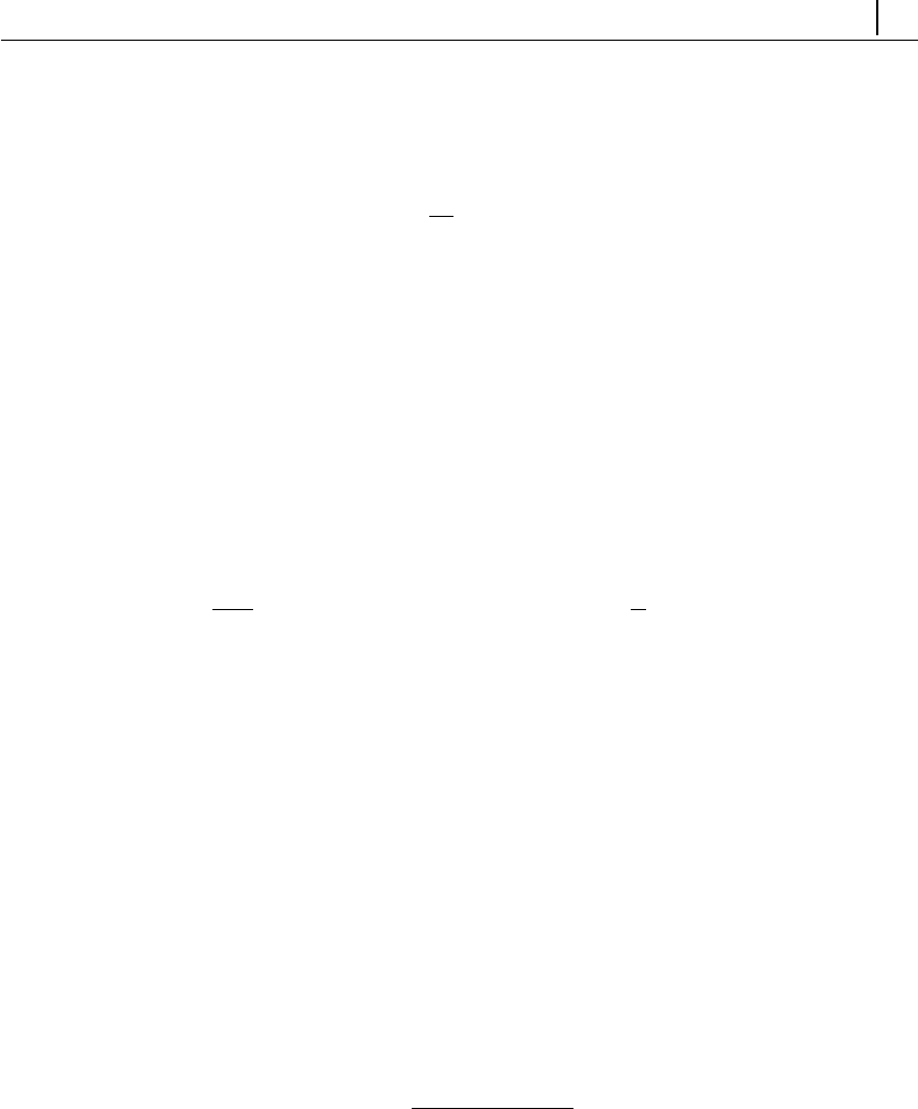
The structure of rheoTool cloned or downloaded from the GitHub repository (ht
tps://github.com/fppimenta/rheoTool) is depicted in Fig. 2.1.
rheoTool of222
of40
fe40
doc
src
tutorials
libs
solvers
(…)
(…)
(…)
(…)
(…)
Figure 2.1: Directory organization of rheoTool.
The top-level directory of rheoTool contains the versions available for different
OpenFOAM R
(of ) and foam-extend (fe) versions (see next section for compati-
bility issues). The folder doc/, containing the user-guide, is also in the top-level
directory. Inside the folder for each version, there are two directories: src/, where
the source-code can be found, and tutorials/, containing several tutorial cases
showing the use of rheoTool. The src/ directory is further subdivided in a di-
rectory with the applications (solvers/) and another one containing libraries
(libs/).
After cloning/downloading rheoTool, the user is free to remove from the top-
level directory all the versions not needed and keep only the one(s) of interest.
5

CHAPTER 2. Installation 6
2.2 Compatibility with OpenFOAM R
and foam-
extend versions
The development and testing of rheoTool was mainly performed in OpenFOAM R
version 2.2.2 (we will change to version 4.0/4.1 in a near future). However, an
effort has been made to release rheoTool also running under other (more recent)
versions of OpenFOAM R
and foam-extend. Thus, compatible versions of rheoTool
are provided for:
•OpenFOAM R
v2.2.2 (of222/).
•OpenFOAM R
v4.0, v4.1 (of40/).
•foam-extend 4.0 (fe40/).
Note that the list above includes the versions which were effectively tested. This
means that a given version of rheoTool may be compatible with other OpenFOAM R
or foam-extend versions not included in this list. The versions above were tested
in a Ubuntu (12.04 or 16.04) environment, but other operating systems running
OpenFOAM R
can eventually support some version of rheoTool. However, the
installation is only described here for a Linux OS.
2.3 System requirements
Only standard requirements are needed to install rheoTool:
•a compatible and functional version of OpenFOAM R
or foam-extend should
be already installed.
•the machine should be connected to the Internet.
After ensuring that these conditions are fulfilled, the user is ready to start the
installation, which includes two major steps: downloading (no install) the open-
source Eigen library [6] and installing rheoTool.
2.4 Downloading Eigen library
In the top-level directory of rheoTool, open a terminal and check that file etc/bash
rc of your installed OpenFOAM R
or foam-extend version has been sourced. This is
particularly relevant if you have defined alias for different versions of OpenFOAMR
or foam-extend. If this is the case, be sure that the alias pointing to the desired
version has been typed. Shortly, you should only advance to the next step if a
command like ∼$icoFoam -help is recognized in the terminal. Note that in
this document we use the prepending ∼$ for any instruction to be typed in the
command line (thus, ∼$icoFoam -help means that you only type icoFoam
-help). If this check is successful, run the script downloadEigen in that terminal:

CHAPTER 2. Installation 7
∼$./downloadEigen
This script downloads Eigen version 3.2.9 (other versions close to that would
also work adequately) from the Internet (using wget), extracts it and moves it to
directory:
$WM PROJECT USER DIR/ThirdParty/Eigen3.2.9
Eigen is used in rheoTool for computation of eigenvalues and eigenvectors and
there is no need to install the library, since the inclusion of the required headers
is enough for our purposes.
However, its location in the system must defined and exported. This is achieved
by attributing to variable EIGEN_RHEO – the one used and recognized by rheoTool –
the actual path of Eigen. The command to do so has been displayed to the terminal
after running script downloadEigen (if everything was ok) and looks like:
∼$echo "export EIGEN_RHEO=/home/user/OpenFOAM/user-4.0/ThirdParty
/Eigen3.2.9">>/home/user/.bashrc
Do not copy this command, it is just an example of what is displayed to the
screen. Instead, copy-paste and run the command appearing in your terminal.
If, for some reason, the user wants to move Eigen to another directory (or
already has an Eigen version in another directory), then move Eigen to its final
location (if already not) and define variable EIGEN_RHEO accordingly. Note that
Eigen only needs to be installed once per system. Even if the user has
installed multiple versions of rheoTool in the same system, the above procedure
only needs to be run once (for the first version being installed), as long as the
directory containing Eigen since the first installation is not deleted, or renamed.
2.5 Installing rheoTool
While Eigen needs to be saved in a specified directory to avoid any change in
the code (because an absolute path is used), the folder containing rheoTool can be
saved and compiled in any location on your machine. Nevertheless, a location with
writing permission is recommended, otherwise you will need to use sudo mode to
run all the commands. A good location for rheoTool is, for example, directory
$WM PROJECT USER DIR, which is defined by default when OpenFOAM R
or
foam-extend is installed.
After you move rheoTool to its final location, open a new terminal (to
ensure that your system ~/.bashrc is sourced and contains the path of Eigen)
in the top-level directory of rheoTool (ensuring that the OpenFOAM R
or foam-
extend environment has been sourced, as previously) and enter the directory with
the version of rheoTool that is compatible with your OpenFOAM R
or foam-extend
version, and then go to directory src/. For example, for OpenFOAM R
v2.2.2, it
would be:
∼$cd of222/src
Now, run the script Allwmake to build the libraries and applications of rheoTool:
∼$./Allwmake

CHAPTER 2. Installation 8
Both the libraries and applications installed with rheoTool can be cleaned by
running the script Allwclean.
Since the user will probably not need the remaining versions of rheoTool that
remain in the top-level directory, they can simply be deleted, if already not.
To check if the installation succeeded, the user should try to run one of the
tutorials of Chapter 5.
2.6 Differences between versions
In order to make rheoTool compatible with each OpenFOAM R
/foam-extend ver-
sion, several modifications were required at the programming level for each case.
On the other hand, the user-interface remained almost unchanged among the dif-
ferent versions. The main exception is on the codedStream FunctionObjects and
coded boundary conditions, which are used in the tutorials of Chapter 5. Indeed,
while these functionalities are available in OpenFOAM R
, it is not the case for
foam-extend. Thus, the coded boundary conditions and the utilities implemented
as codedStream FunctionObjects in OpenFOAM R
versions had to be assembled
and compiled in a library for the foam-extend version.
A second point to be taken into account is that rheoTool may perform differ-
ently in each OpenFOAM R
/foam-extend version, as it may happen with any other
default solver of OpenFOAM R
/foam-extend. This is naturally a consequence of
the evolution of the core machinery of OpenFOAM R
/foam-extend, transversal to
many solvers and libraries. Fortunately, in most of the cases the differences will
be small. All the discussion in this guide, including the results presented for the
tutorials in Chapter 5, is for OpenFOAMR
v2.2.2, as aforementioned. Taking
this version as reference, the following issues were detected in the tests that we
performed:
•there is some difference in the results for non-orthogonal grids, between of222
and the other two versions tested. This issue can be observed, for example,
in the tutorial of section 5.1.6, where the drag coefficient in a cylinder is
computed. The difference is originated by a change which has been intro-
duced since version 2.3.x in the computation of the cell-to-face distance at
the boundaries, that is used, for example, in the fvm::laplacian() operator.
The change can be found in file src/finiteVolume/fvMesh/fvPatches/fv
Patch/fvPatch.C, in the function fvPatch::delta(), where the newer versions
only account for the normal component of the cell-to-face vector.
•in general, a tutorial of rheoTool for versions of40 or of222 may be run either
in serial or parallel while keeping the same numerical settings. However, in
the tests using version fe40, it was observed that parallel runs are less stable
than serial runs, usually requiring a lower time-step or some under-relaxation
of the velocity (sometimes as low as 0.97).
Although the main development of rheoTool has been made using OpenFOAM R
v2.2.2 for historical reasons, in general we recommend new users to prefer more re-
cent distributions of OpenFOAM R
, since several improvements and bug fixes have

CHAPTER 2. Installation 9
been made since v2.2.2 (released in 2013). This is especially true for multiphase
flows.

Chapter 3
Theoretical background
The equations governing pressure- and electrically-driven flows of incompressible,
complex fluids are discussed in this Chapter, along with some important aspects
related with their discretization in the finite-volume framework. Since a thorough
discussion on this subject can be found in Refs. [2,3], some intermediate steps are
skipped and only the more relevant equations are presented.
3.1 Governing equations
The basic equations governing isothermal, single-phase, transient flows, under lam-
inar conditions, for incompressible fluids, establish mass conservation (Eq. 3.1) and
momentum balance (Eq. 3.2),
∇·u= 0 (3.1)
ρ∂u
∂t +u·∇u=−∇p+∇·τ0+f(3.2)
where uis the velocity vector, tis the time, pis the pressure, τ0is the extra-stress
tensor and fis any external body-force, such as the electric force discussed in
Section 3.5. To simulate viscoelastic fluid flows, it is a common approach to split
the total extra-stress tensor in a solvent contribution (τs) and a polymeric contri-
bution (τ), τ0=τ+τs. In order to have a closed set of equations, a constitutive
equation is required for each tensor contribution, which can be generally written
as in Eqs. (3.3) and (3.4), for a wide range of models,
τs=ηs( ˙γ)(∇u+∇uT) (3.3)
f(τ)τ+λ( ˙γ)∇
τ+h(τ) = ηp( ˙γ)(∇u+∇uT) (3.4)
In Eqs. (3.3) and (3.4), ηsis the solvent viscosity, ηpis the polymeric viscosity
coefficient, λis the relaxation time, ˙γis the shear-rate, f(τ) is a general scalar
function depending on an invariant of τ,h(τ) is a tensor-valued function depend-
ing on τand ∇
τ=∂τ
∂t +u·∇τ−τ·∇u− ∇uT·τrepresents the upper-convected
10
CHAPTER 3. Theoretical background 11
time derivative, which renders the models frame-invariant. Some models use the
Gordon-Schowalter derivative (
τ=∇
τ+ζ(τ·D+D·τ), with D=1
2(∇u+∇uT))
instead of the upper-convected derivative, in order to take non-affine deformation
into account (controlled by parameter ζ). In rheoTool, this is the case of PTT-
type models. Other constitutive models exist, which can also make use of the
lower-convected time derivative, but those are not explored here. The constitu-
tive equation for a GNF is limited to Eq. (3.3), since elasticity is not considered
(τ0=τs). In Table 4.1 presented in the next Chapter, Eqs. (3.3) and (3.4) are
specified for several GNF and viscoelastic models.
Eqs. (3.1)–(3.4) represent the standard system of equations to be solved. How-
ever, due to numerical stability issues in viscoelastic fluid flow simulations, the
system is rarely solved in that form. Indeed, several techniques are available for
stabilization purposes (see, for instance, Ref. [7] for a comparison between the
most popular techniques) and the ones used in rheoTool are addressed next.
3.2 Stabilization of viscoelastic fluid flow simu-
lations
3.2.1 The both-sides-diffusion (BSD) technique
The both-sides-diffusion (BSD) is a technique already incorporated in the vis-
coelasticFluidFoam solver [1]. It consists in adding a diffusive term on both sides
of momentum equation (Eq. 3.2), with the difference that one of them (left-hand
side) is added implicitly, while the other one (right-hand side) is added explicitly.
Once steady-state is reached, both terms cancel each other exactly. Such method
increases the ellipticity of the momentum equation and, as such, has a stabiliz-
ing effect, mostly when there is no solvent contribution in the extra-stress tensor.
Incorporating the terms arising from the both-sides-diffusion in the momentum
equation, and making use of Eq. (3.3), then
ρ∂u
∂t +u·∇u− ∇·(ηs+ηp)∇u=−∇p− ∇·(ηp∇u) + ∇·τ+f(3.5)
Note that the added diffusive terms are scaled by the polymeric viscosity (ηp),
which is a common choice in the literature (e.g. Ref. [7]), although not mandatory.
In order to simplify the reading, the possible dependence of the viscosity and
relaxation time on the shear-rate will be dropped in the respective symbols, as
already done in Eq. (3.5), although this relation still holds to keep generality.
3.2.2 The log-conformation tensor approach
The log-conformation tensor approach consists in a change of variable when evolv-
ing in time the polymeric extra-stress and it was devised to tackle the numerical
instability faced at high Weissenberg number flows [4,8].
CHAPTER 3. Theoretical background 12
The polymeric extra-stress tensor is related with the conformation tensor (A).
For the Oldroyd-B model, for example, this relation is expressed as (see Table 4.1
for several viscoelastic models)
τ=ηp
λ(A−I) (3.6)
In the log-conformation tensor methodology, a new tensor (Θ) is defined as
the natural logarithm of the conformation tensor
Θ= ln(A) = Rln(Λ)RT(3.7)
In Eq. (3.7), the conformation tensor was diagonalized (A=RΛRT) because it
is positive definite, where Ris a matrix containing in its columns the eigenvectors
of Aand Λis a matrix whose diagonal elements are the respective eigenvalues
resulting from the decomposition of A. Eq. (3.4) written in terms of (Θ) becomes
[4]
∂Θ
∂t +u·∇Θ=ΩΘ −ΘΩ + 2B+1
λg(Θ) (3.8)
where g(Θ) is a model-specific tensorial function depending on Θ(see Table 4.1
for other viscoelastic models) and
B=R
mxx 0 0
0myy 0
0 0 mzz
RT(3.9)
Ω=R
0ωxy ωxz
−ωxy 0ωyz
−ωxz −ωyz 0
RT(3.10)
M=R∇uTRT=
mxx mxy mxz
myx myy myz
mzx mzy mzz
(3.11)
ωij =Λjmij +Λimji
Λj−Λi
(3.12)
After solving Eq. (3.8), Θis diagonalized in the form
Θ=RΛΘRT(3.13)
and the conformation tensor is recovered by the inverse relation of Eq. (3.7)
A= exp(Θ) = Rexp(ΛΘ)RT(3.14)
Finally, the polymeric extra-stress tensor can be computed from A(Eq. 3.6)
and used in the momentum equation.
Note that for PTT-type models, which may include non-affine deformation
through the Gordon-Schowalter derivative, the tensor M(Eq. 3.11) is computed
differently: M=R∇uT−ζDRT.

CHAPTER 3. Theoretical background 13
It is worth to mention that the log-conformation approach can be considered
a particular case of the kernel-conformation method [9]. However, from our expe-
rience, the log kernel is frequently the optimal kernel (in terms of robustness and
accuracy) for generic problems, so that only this one is widely used in rheoTool.
Nevertheless, for the Oldroyd-B model, the rootkkernel [9] and the square-root
transformation [10] are also included in rheoTool for demonstration purposes.
3.3 Coupling algorithms
3.3.1 Pressure-velocity coupling
Although the OpenFOAM R
toolbox is already able to solve linear systems of
equations in a coupled way, most of the solvers still rely on segregated solutions
(this is a rule for transient solvers). In segregated solvers, the equations for each
variable are solved sequentially. Even for a fully-implicit method, if the coupling
between variables is weak, then numerical divergence is prone to occur.
In the OpenFOAM R
toolbox, common algorithms for pressure-velocity cou-
pling are SIMPLE and SIMPLEC for steady-state solvers and either PISO or
PIMPLE (a combination of SIMPLE(C) and PISO) for transient solvers. From
the benchmark cases performed in Ref. [2], it was observed that SIMPLEC was
particularly suitable for transient viscoelastic fluid flows at low Reynolds numbers,
regarding stability and accuracy.
The continuity equation, implicit in the pressure variable, derived for SIM-
PLEC (a more detailed derivation is presented in Ref. [2]) leads to
∇·1
aP−H1
(∇p)P=∇·H
aP
+1
aP−H1−1
aP(∇p∗)P(3.15)
where aPare the diagonal coefficients from the momentum equation, H1=−P
nb
anb
is an operator representing the negative sum of the off-diagonal coefficients from
momentum equation, H=−P
nb
anbu∗
nb +bis an operator containing the off-
diagonal contributions, plus source terms (except the pressure gradient) of the
momentum equation and p∗is the pressure field known from the previous time-
step or iteration. Accordingly, the equation to correct the velocity after obtaining
the continuity-compliant pressure field from Eq. (3.15) is
u=H
aP
+1
aP−H1−1
aP(∇p∗)P−1
aP−H1
(∇p)P(3.16)
Importantly, in order to avoid the onset of checkerboard fields, the pressure
gradient terms involved in the computation of face velocities, i.e., in Eqs. (3.15)
and (3.16), are directly evaluated using the pressure on the cells straddling the face,
in a Rhie-Chow-like procedure (more details in Ref. [2]). Nonetheless, when Eq.
(3.16) is used to correct the cell-centered velocity field, the pressure gradient terms
are computed ”in the usual way”, for example using Green-Gauss integration.

CHAPTER 3. Theoretical background 14
Rhie-Chow methods used to avoid checkerboard fields, as the one described
in the previous paragraph, are known to be affected by the use of small time-
steps and they also present time-step dependency on steady-state results [11].
In OpenFOAM R
solvers, a common strategy to avoid such effects is to add a
corrective term to face-interpolated velocities, through functions ddtPhiCorr() or
ddtCorr(). Recently, in foam-extend the time-step dependency was solved in a
different way, by removing the transient term contribution from the aPcoefficients
of the momentum equation [12]. However, this approach may be problematic when
used with the SIMPLEC algorithm, since a division by zero is prone to happen.
In rheoTool, we keep using the added corrective term, although, as mentioned in
Ref. [2], this term can be improved in order to more efficiently avoid the small
time-step dependency of steady-state solutions.
3.3.2 Stress-velocity coupling
Stress-velocity decoupling problems can arise for similar reasons as those described
for pressure-velocity: the cell-centered velocity loses the influence of the forces
(either polymeric extra-stress or pressure gradient) of its direct neighborhood (cells
sharing a face in common). This usually happens in the interpolation from cell-
centered to face-centered fields. In the case of polymeric extra-stresses, it is the
divergence term (∇·τ) in the momentum equation, when τis linearly interpolated
from cell centers to face centers, which can be responsible for the decoupling.
In Ref. [2], we described a new stress-velocity coupling method, where the
polymeric extra-stresses at face centers are computed as
τf=τf+ηph∇u|f+(∇u)T|f−∇u|f+(∇u)T|fi (3.17)
where terms with an overbar are linearly interpolated from cell-centered values,
while the remaining velocity gradients are directly evaluated from the cell-centered
velocities straddling the face. When the definition of τfin Eq. (3.17) is inserted in
the momentum equation with the both-sides-diffusion terms already present (Eq.
3.5), then we obtain
ρ∂u
∂t +u·∇u− ∇·(ηs+ηp)∇u=−∇p− ∇·ηp∇u+∇·τ+f(3.18)
where the term ∇·ηp∇uis a ”special second-order derivative” (different from
the laplacian operator of OpenFOAM R
), defined as the divergence of the velocity
gradient, where the velocity gradient at the faces is obtained by linear interpolation
of the velocity gradient evaluated on the cell centers. More details are presented
in Ref. [2], where it is shown that with mesh refinement Eq. (3.17) approaches
τf=τfand the additional terms cancel out. Note that when inserting Eq. (3.17)
in the momentum equation (resulting in Eq. 3.18), we drop the transpose velocity
gradients for simplicity, since continuity imposes ∇·∇uT=0.

CHAPTER 3. Theoretical background 15
3.4 High-resolution schemes
The discretization of convective terms within the finite-volume framework leads to
ZV
(u·∇φ) dV=X
f
φf(uf·Sf) = X
f
φfFf(3.19)
where φis a generic variable being advected, Sfis the face-area vector and Ffis
the volumetric flux crossing face f. While fluxes are known at the faces from the
Rhie-Chow-like interpolation (Eq. 3.16), φat face centers need to be interpolated
from known values at cell centers. OpenFOAMR
offers a wide range of schemes to
perform such interpolation, from upwind – an unconditionally stable scheme, but
only first-order accurate –, to central differences – a conditionally stable, second-
order accurate scheme. A good compromise between both extremes is provided
by High-Resolution Schemes (HRSs). When represented in a Normalized Variable
Diagram (NVD), several HRSs are piecewise-linear functions and can be defined
using the Normalized Weighting Factor (NWF) approach [13]:
e
φf=αe
φC+β(3.20)
where the following definitions hold
e
φf=φf−φU
φD−φU
(3.21a)
e
φC=φC−φU
φD−φU
(3.21b)
In Eq. (3.20), αand βare scalars specific to each HRS and they can be functions
of e
φC. Subscripts in Eqs. (3.21a,b) have the following meaning: for a given face,
cell C is the cell from which the flux comes (upstream), cell D (downstream) is the
cell to which the flux goes and cell U (far-upstream) is the cell upstream to cell C.
In a general unstructured mesh, cell U cannot be identified unequivocally, and φU
in Eqs. (3.21a,b) can be evaluated as [14]
φU=φD−2(∇φ)C·dCD (3.22)
where dCD is the vector connecting the center of cells C and D. For a deferred
correction implementation of HRSs, the upwind part of the HRS is discretized
implicitly, while the remaining (difference between the HRS and the upwind differ-
encing scheme) is discretized explicitly (cf. Ref. [2]), which, using Eqs. (3.20-3.22),
results in
φf= [φC]implicit + [(α−1)φC+βφD+ (1 −α−β)(φD−2(∇φ)C·dCD)]explicit (3.23)
Handling the HRSs in a deferred correction approach avoids, in some cases,
numerical instabilities introduced by the central-differencing component of the
HRS. Additionally, in Ref. [2] it was observed that the usual methodology of
OpenFOAM R
to apply HRSs to non-scalar variables (tensors and vectors) can
locally introduce numerical instabilities in some viscoelastic flow problems. This

CHAPTER 3. Theoretical background 16
methodology consists in using a frame-invariant quantity for non-scalar variables,
such as the squared magnitude for vectors, or the trace (or double-dot product)
for tensors, to compute the αand βparameters in Eq. (3.23). It was observed
that such artificial instabilities can be significantly damped with a component-wise
handling of non-scalar variables [2], at the cost of losing frame-invariance, which
however is very weak and vanishes with grid refinement. Accordingly, non-scalar
variables are split into its components and Eq. (3.23) is applied independently to
each one of them. Note that this approach still generates one single matrix of co-
efficients for such variables, since the upwind differencing scheme coefficients are
common to all the components (they only depend on the flux). The differentiation
between components is only introduced in the explicit part of Eq. (3.23), generat-
ing a different source term for each individual tensor/vector component. This is
possible due to the use of a deferred correction approach.
3.5 Electrically-driven flow models
Consider now that the fluid under analysis is a weak electrolyte subjected to an
electric field. In such conditions, the momentum equation (Eq. 3.2) should include
the contribution from an electric body-force,
f=fE=∇·εEE −kEk2
2I=ρEE−kEk2
2∇ε(3.24)
where Eis the electric field, ε=ε0εRis the electric permittivity and ρEis the
charge density (per unit volume). In order to close the system of equations for
electrically-driven flows (EDFs), additional relations must be provided to compute
the terms in Eq. (3.24). Some options, the ones available in rheoTool, are presented
next. Note that when referring generically to EDFs, we do not exclude the possi-
bility of having any other external forcing (for example due to an imposed pressure
difference), in addition to the electric forcing. When only an electric forcing exists,
we call this flow as pure EDF.
The second term of Eq. (3.24) is only non-zero for a system of two fluids, each
having a different electric permittivity.
3.5.1 Poisson-Nernst-Planck model
In the absence of magnetic effects, the electric potential (Ψ) can be computed by
Gauss’ law
∇·(ε∇Ψ) = −ρE(3.25)
where the electric field is E=−∇Ψin electrostatics. By definition, the charge
density is
ρE=F
N
X
i=1
zici(3.26)
CHAPTER 3. Theoretical background 17
where Fis Faraday’s constant, ziis the charge valence of specie iand ciis the
concentration of specie i(mol/m3). The sum is over the Ncharged species in
the electrolyte. The standard law governing the transport of charged species in a
weak electrolyte, under the action of an electric field and neglecting any reaction,
is embodied by the Nernst-Planck equation,
dci
dt +u·∇ci=∇·(Di∇ci) + ∇·
Di
ezi
kT ∇Ψ
| {z }
uM,i
ci
(3.27)
which closes the system of equations for an EDF. In Eq. (3.27), Dis the diffu-
sion coefficient, eis the elementary charge, kis Boltzmann’s constant and Tis
the absolute temperature. The last term of Eq. (3.27), representing the transport
of charged species due to an electric field, can be though as a standard convec-
tive term driven by an electromigration velocity (uM,i). However, it may also be
considered as the Laplacian operator applied to field Ψ, with a space and time
varying diffusion coefficient, Diezi
kT ci(this last approach is used in rheoTool for
discretization purposes).
The so-called Poisson-Nernst-Planck model (henceforth PNP model) is con-
stituted by Eqs. (3.25)-(3.27) and, coupled with the continuity and momentum
equations, is applicable to a wide range of EDFs. However, the coexistence of dif-
ferent scales of time and length in EDFs may originate a stiff system of equations
when the PNP model is used. As such, several simplified models can be derived to
mitigate these numerical issues, as described next. Note that the PNP model does
not take into account molecular crowding effects (e.g., the number of ions near a
surface may grow unbounded), so care must be taken when using it to simulate
electrolytes of mild to high ionic strength.
In the PNP model, the electric-related unknowns are ciand Ψ. Due to the
convective term in Eq. (3.27), there is a two-way coupling between the PNP and
the momentum equations.
3.5.2 Splitting the electric potential
Before proceeding to the derivation of other EDF models, we introduce here a
useful approach to simulate EDF problems. In the PNP model, a single electric
potential variable has been used, Ψ. However, in certain situations this can pose
some difficulties when defining the boundary conditions to solve the Poisson equa-
tion. A common approach to avoid such issues is the decomposition of the electric
potential in two variables: the externally imposed electric potential, φExt, and the
intrinsic electric potential, ψ, such that Ψ=φExt +ψ[3]. Following this approach,
Gauss’ law is also decomposed in two equations,
∇·(ε∇φExt) = 0 (3.28a)
∇·(ε∇ψ) = −ρE(3.28b)
CHAPTER 3. Theoretical background 18
An additional simplification which can be used simultaneously with the split-
ting approach is to consider fE=−ρE∇φExt in the momentum equation, i.e., the
intrinsic electric potential contribution is ignored in the electric field definition.
This can be justified by stating that this extra force not accounted for directly is
balanced by a pressure gradient, which mutually cancel each other in the momen-
tum equation [3], under the assumption that it would not affect the flow.
The splitting approach will be used in the derivation of the next two models.
3.5.3 Poisson-Boltzmann model
If we assume that the ions follow a Boltzmann equilibrium, then the PNP model
can be simplified to the so-called Poisson-Boltzmann model (henceforth PB model),
for which Gauss’ law reads
∇·(ε∇ψ) = −F
N
X
i=1
zici,0exp −ezi
kT (ψ−ψ0)(3.29)
with ci,0being a reference concentration of specie i, where the intrinsic poten-
tial is ψ0. Without loss of generality, we will assume that ci,0is the bulk ionic
concentration, where the intrinsic potential is ψ0= 0.
Note that the right hand-side of Eq. (3.29) represents (minus) the charge den-
sity for the PB model. Thus, Eq. (3.29) provides the definition of Eq. (3.28b) for
the PB model, under the splitting approach.
For this model, the only electric-related unknowns are the two electric poten-
tials, ψand φExt, computed from Eqs. (3.28a) and (3.29). Furthermore, as can
be seen from Eq. (3.29), there is no influence of flow variables in the PB model
(one-way coupling).
In order to increase the implicitness of Eq. (3.29), its source term can be lin-
earized by expansion in Taylor series up to the first-derivative, transforming the
equation into
∇·(ε∇ψ) + ψF
N
X
i=1
(aibi)∗=−F
N
X
i=1
(ai)∗+ψ∗F
N
X
i=1
(aibi)∗(3.30)
with bi=−ezi
kT and ai=zici,0exp (biψ). All the terms of Eq. (3.30) with a star are
evaluated explicitly.
3.5.4 Debye-H¨uckel model
Considering the PB model, if we further simplify Eq. (3.29) assuming low electric
potentials, ezi
kT ψ1 , then
∇·(ε∇ψ) = −F
N
X
i=1
zici,01−ezi
kT ψ(3.31)
which is the equation governing the electric potential distribution in the so-called
Debye-H¨uckel model (henceforth DH model).

CHAPTER 3. Theoretical background 19
As for the PB model, the only electric-related unknowns are the two electric
potentials, ψand φExt, computed from Eqs. (3.28a) and (3.31). Also, there is no
influence of flow variables in the DH model (one-way coupling).
3.5.5 Slip model
A common characteristic of electrokinetic problems is the spontaneous formation
of an electric double layer (EDL) near a charged surface, upon contact with an
electrolyte. The thickness of the EDL can be approximated by the Debye length
(λD), a physical parameter appearing when solving the Poisson equation for the
electric potential,
λD=v
u
u
u
t
εkT
F e
N
P
i=1
z2
ici,0
(3.32)
In several practical applications, the charge density is mainly located in the
EDL region, while the bulk electrolyte is neutral. If the Debye length is much
smaller than the characteristic dimension of the system (λD
W1) and assuming a
smooth, laminar flow inside the EDL, then it is possible to approximate the EDL
effect by a slip velocity at the surface, avoiding the need to solve the flow inside the
EDL. Such a case would be, for example, the pumping of a Newtonian electrolyte
(λD∼ O(10−9m)) in a microchannel of arbitrary shape (W∼ O(10−6m)), by
electroosmosis, at low voltage ( ez
kT ψ1) – the last conditions is usually relaxed.
The Helmholtz-Smoluchowski theory is frequently used to approximate the slip
velocity in such conditions,
uSch =µE(3.33)
where µ=−εζ
η0is the electroosmotic mobility (ζis usually the surface zeta-
potential). Thus, when Eq. (3.33) is used as a boundary condition for velocity
in the momentum equation, both the electroosmotic mobility and the electric field
at the surface must be known. The electroosmotic mobility is assumed to be known
a priori – it can be a fixed value over all the surface or have a known distribution.
On the other hand, the electric field on the surface must be computed, making use
of the initial assumption that no free charge exists in the bulk electrolyte, thus
Ψ=φExt +ψ=φExt, and
∇·(ε∇Ψ) = 0 (3.34)
When the slip model is used, the electric body-force is not included in the
momentum equation – electric effects contribute uniquely via the slip boundary
condition on the wall.
Note that slip models do not resolve any phenomena occurring in the EDL.
Thus, this approach is highly inaccurate for some flows, even though the condition
λD
W1 is satisfied. For example, this kind of model is unable to predict the high
values of shear-rate typically found in EDLs, which can trigger elastic instabilities
CHAPTER 3. Theoretical background 20
for complex fluid flows [15] – using a slip model would simply retrieve a smooth
flow in such cases.
3.5.6 Ohmic (leaky dielectric) model
The so-called Ohmic model [16] is particularly useful to simulate fluids of different
conductivities, although a generalized Ohmic model has been recently proposed
for different types of problems [17]. The model can be derived from the PNP
equations, rewritten in terms of the conductivity and free-charge density, and
assuming additionally instantaneous charge relaxation and electroneutrality [16].
The interested reader is directed to Ref. [16] for the full derivation of the Ohmic
model. Here, only the final equations are presented. Furthermore, and contrarily
to what was done for the previous models, we will restrict our analysis to a binary
electrolyte, i.e., an electrolyte composed of only one positive and one negative
species, with z+=−z−=z, but no restrictions in the relation between D+and
D−.
First, let’s start defining the conductivity (σ) and free-charge density (ρE) for
a binary electrolyte,
σ=F2z2
RT (D+c++D−c−) (3.35)
ρE=F z(c+−c−) (3.36)
where Ris the universal gas constant. Imposing the conservation of each variable
leads to (after the assumptions mentioned above; more details in Ref. [16])
∂σ
∂t +u·∇σ=Deff∇2σ(3.37)
∇·(σ∇Ψ) = 0 (3.38)
where the effective diffusivity is Deff =2D−D+
D−+D+. The conductivity is transported
through Eq. (3.37), while Eq. (3.38), derived from the conservation of charge-
density (then simplified on the basis of electroneutrallity), is actually used to
compute the distribution of electric potential. The electric force entering the mo-
mentum equation assumes its standard form, taking into account that the charge
density can be expressed as ρE=−∇·(ε∇Ψ) from Gauss’ law, then
fE=ρEE=∇·(ε∇Ψ)∇Ψ(3.39)
In order to close the Ohmic model, the EDL effect is commonly represented
by a slip velocity, which avoids detailing the flow inside the EDL using a very
fine mesh. Since the zeta-potential of a surface depends generally on the ionic
conductivity, a σ-dependent slip velocity is typically used [16], such as
uSch(σ) = µ0σ
σ0m
E(3.40)

CHAPTER 3. Theoretical background 21
where µ0=−εζ0
η0is a reference electroosmotic mobility, at a reference conduc-
tivity (σ0), and mis an exponent governing the power-law dependence of the
zeta-potential on the conductivity (m∈[−0.5,−0.3] is in agreement with several
works, e.g. [16]). Note that Ein Eq. (3.40) is the electric potential at the surface
where the slip velocity is computed.
Chapter 4
Overview of rheoTool
In the previous Chapter, the main theoretical points behind rheoTool were briefly
discussed. This Chapter focus on the numerical implementation of the governing
equations in the OpenFOAM R
environment, providing an overview of the func-
tionalities available in rheoTool.
4.1 The constitutiveEquations library
4.1.1 Available GNF and viscoelastic models
The constitutiveEquations library is a main component of rheoTool, since it con-
tains all the viscoelastic and GNF constitutive equations, which can be called from
the solvers. It was derived from the viscoelasticTransportModels library [1]. How-
ever, instead of restricting the library to viscoelastic models, we also extend it to
include GNF models, most of them already present in OpenFOAM R
. This was
done in order to allow accessing both classes of models from a single library, hence
from a single solver.
The models available in the constitutiveEquations library are displayed in Table
4.1, along with the respective expressions to be used in Eqs. (3.3), (3.4), (3.6) and
(3.8).
22

CHAPTER 4. Overview of rheoTool 23
Table 4.1: Available constitutive models in the constitutiveEquations library.
GNF models
Model 1TypeName ηs( ˙γ)
Newtonian Newtonian η
2(Bounded) Power-Law PowerLaw max(ηmin,min(ηmax, k ˙γn−1))
Carreau-Yasuda CarreauYasuda η∞+ (η0−η∞)[1 + (k˙γ)a]n−1
a
2(Bounded) Herschel-Bulkley HerschelBulkley min η0, τ0˙γ−1+k˙γn−1
1Corresponds to the name entry identifying the model in the source code.
2In the Power-Law and Herschel-Bulkley models special care is taken to avoid division by zero when ˙γis zero or very
small and n−1<0. For ˙γ < VSMALL, the value ˙γ=VSMALL is used in the computation of the shear viscosity
(VSMALL = 10−300 for versions using double precision).
Notes:
•˙γ=q˙
γ:˙
γ
2, with ˙
γ=∇u+∇uT.
•Iis the identity tensor and D
Dt(φ) = ∂φ
∂t +u·∇φrepresents the material derivative of the generic variable φ.
•∇
τ=∂τ
∂t +u·∇τ−τ·∇u− ∇uT·τis the upper-convected derivative of τ.
•
τ=∇
τ+ζ(τ·D+D·τ) is the Gordon-Schowalter derivative of τ, with D=1
2(∇u+∇uT).
23

CHAPTER 4. Overview of rheoTool 24
Continuation of Table 4.1
Viscoelastic models solved in the standard extra-stress or conformation tensor variables
Model TypeName ηs( ˙γ)ηp( ˙γ)λ( ˙γ) Constitutive Equation
Oldroyd-B Oldroyd-B ηsηpλτ+λ∇
τ=ηp(∇u+∇uT)
WhiteMetzner
(Carreau-Yasuda) WhiteMetznerCY ηsηp[1 + (K˙γ)a]n−1
aλ[1 + (L˙γ)b]m−1
bτ+λ( ˙γ)∇
τ=ηp( ˙γ)(∇u+∇uT)
Giesekus Giesekus ηsηpλτ+λ∇
τ+αλ
ηp(τ·τ) = ηp(∇u+∇uT)
PTT linear PTTlinear ηsηpλh1 + ελ
ηptr(τ)iτ+λ
τ=ηp(∇u+∇uT)
PTT exponential PTTexp ηsηpλe
ελ
ηptr(τ)τ+λ
τ=ηp(∇u+∇uT)
FENE-CR FENE-CR ηsηpλh1 + λD
Dt1
fiτ+λ
f∇
τ=ηp(∇u+∇uT)
where f=L2+λ
ηptr(τ)
L2−3
FENE-P FENE-P ηsηpλ
τ+λ
f∇
τ=aηp
f(∇u+∇uT)−D
Dt1
f[λτ+aηpI]
where f=L2+λ
aηptr(τ)
L2−3and a=L2
L2−3
3Rolie-Poly Rolie-Poly ηsηpλD
λD∇
A=−(A−I)−2kλD
λR1−p3/tr(A)A+βtr(A)
3δ(A−I)
where k=3−χ2
χ2
max 1−1
χ2
max
1−χ2
χ2
max 3−1
χ2
max and χ=qtr(A)
3
eXtended Pom-Pom XPomPom ηsηpλB
fτ+λB∇
τ+αλB
ηp(τ·τ) + ηp
λB(f−1) I=ηp(∇u+∇uT)
where f= 2λB
λSe2
q(Λ−1) 1−1
Λ+1
Λ2h1−α
3
tr(τ·τ)
(ηP/λB)2iand Λ=q1 + tr(τ)
3ηP/λB
3See Ref. [18]. This model is exclusively solved in the conformation tensor variable, which is then converted to τusing, τ=ηp
λDk(A−I).
24

CHAPTER 4. Overview of rheoTool 25
Continuation of Table 4.1
‡Viscoelastic models solved with the log-conformation approach
Model TypeName Θ¸τ4,5Constitutive Equation
6Oldroyd-B Oldroyd-BLog τ=ηp
λ(eΘ−I)Υ=1
λe−Θ−I
7WhiteMetzner
(Carreau-Yasuda) WhiteMetznerCYLog τ=ηp
λ(eΘ−I)Υ=1
λ( ˙γ)e−Θ−I
Giesekus GiesekusLog τ=ηp
λ(eΘ−I)Υ=1
λhe−Θ−I−αeΘe−Θ−I2i
PTT linear PTTlinearLog τ=ηp
λ(1−ζ)(eΘ−I)Υ=1
λn1 + ε
1−ζtr(eΘ)−3o(e−Θ−I)
PTT exponential PTTexpLog τ=ηp
λ(1−ζ)(eΘ−I)Υ=1
λeε
1−ζ(tr(eΘ)−3)(e−Θ−I)
FENE-CR FENE-CRLog τ=ηpf
λ(eΘ−I)Υ=f
λe−Θ−I, where f=L2
L2−tr(eΘ)
FENE-P FENE-PLog τ=ηp
λ(feΘ−aI)Υ=1
λae−Θ−fI, where a=L2
L2−3and f=L2
L2−tr(eΘ)
8Rolie-Poly Rolie-PolyLog τ=ηp
λDk(eΘ−I)Υ=−1
λDe−Θ(eΘ−I)+2kλD
λR1−p3/tr(eΘ)eΘ+βtr(eΘ)
3δ(eΘ−I)
eXtended Pom-Pom XPomPomLog τ=ηp
λB(eΘ−I)
Υ=−1
λBe−Θ(f−2α)eΘ+αeΘeΘ+ (α−1)I
where f= 2λB
λSe2
q(Λ−1) 1−1
Λ+1
Λ21−α−α
3tr(eΘ(eΘ−2I))and Λ=qtr(eΘ)
3
‡The solvent viscosity, the polymeric viscosity coefficient and the relaxation time for the models solved in variable Θare the same as those for the models solved in
variable τor A, in the previous page.
4For the shortness of notation, we have introduced the operator: Υ=∂Θ
∂t +u·∇Θ−(ΩΘ −ΘΩ)−2B.
5The following equivalences hold true: eΘ=A=RΛRTand e−Θ=A−1=RΛ−1RT.
6For this model, we also included the square-root conformation approach [10] (TypeName: Oldroyd-BSqrt) and the rootkkernel approach [9] (TypeName: Oldroyd-
BRootk), for demonstration purposes.
7This log-conformation tensor approach of the White-Metzner model is only applicable when ηp( ˙γ)
λ( ˙γ)=ηp
λis constant, i.e., for K=L,a=band n=m. The
version based on the extra-stress tensor variable is more general and does not have this restriction.
8The expression for kis the same as for the model solved in variable A, in the previous page, considering that A=eΘ.
25

CHAPTER 4. Overview of rheoTool 26
In a footnote of Table 4.1, the (invariant) shear-rate used to compute shear-rate
dependent variables was defined as
˙γ=r˙
γ:˙
γ
2=√2D:D,with ˙
γ=∇u+∇uTand D=1
2˙
γ(4.1)
In the code, the shear-rate is returned by function strainRate() as
strainRate() = sqrt(2.0)*mag(symm(fvc::grad(U())))
and it is equivalent to Eq. (4.1). Indeed,
symm(fvc::grad(U())) =1
2∇u+∇uT=1
2˙
γ=D
thus,
sqrt(2.0)*mag(symm(fvc::grad(U()))) =√2q1
2˙
γ:1
2˙
γ=q˙
γ:˙
γ
2=√2D:D
which is equal to Eq. (4.1) – the definitions of operators symm(),mag() and :
(double contraction) can be found in the OpenFOAM R
programmers’ guide. Note
that the invariant computed in Eq. (4.1) is actually the magnitude of the rate-of-
strain tensor, which is usually called shear rate or strain rate for shear-dominated
or extensional-dominated flows, respectively.
All the viscoelastic models can be solved in the standard extra-stress tensor
τ(Eq. 3.4) or using the log-conformation approach (Eq. 3.8). The selection is
made in dictionary constitutiveProperties, which should be located inside the
folder constant/ of the case (see more details in section 5.1.1). For the Oldroyd-
B model, we provide two additional methods for demonstration purposes. One
of them (TypeName: Oldroyd-BSqrt) consists in solving the constitutive equation
using the square-root of the conformation tensor, according to Ref. [10]. The
second approach (TypeName: Oldroyd-BRootk) allows to apply a general rootk
kernel, as described in Ref. [9]. Both can be used in 2D or 3D simulations, as
any other model in the library. Since both models are only illustrative, their
implementation and theory are not described in this guide, although both can be
easily understood after a close inspection of the source code and taking as reference
the literature cited for each one. Furthermore, tutorials for both methodologies
are included in rheoTool (see the tutorial of Section 5.1.7).
4.1.2 A note on FENE-type models
The Finite Extendable Non-linear Elastic (FENE) models were originally devel-
oped based on the representation of polymer molecules by elastic dumbbells [5].
In such analysis, the end-to-end vector for each molecule is naturally related with
the conformation tensor, such that the constitutive equations for this family of
models is frequently written and handled as a function of the conformation tensor.
The polymeric contribution to the momentum equation is then accounted for by
transforming the conformation tensor (A) in the extra-stress tensor (τ), using the
relations in Table 4.1 (for the models expressed in the log-conformation approach,
considering that eΘ=A). The same applies for the Roly-Polie model.
CHAPTER 4. Overview of rheoTool 27
In order to write the constitutive equation for FENE-type models as a function
of τ, some terms arise, which may compromise the numerical stability. Further-
more, the computational cost to evaluate the resulting expression is higher than
for the original model. As such, some authors simplify the constitutive equation
by neglecting certain terms [19]. For the FENE-CR and FENE-P models, the
complete constitutive equation written as a function of Aand τand the modified
formulation in τare:
•FENE-CR
–Complete in A:
λ∇
A=−f(tr(A))(A−I), where f(tr(A)) = L2
L2−tr(A)
–Complete in τ(see Table 4.1):
h1 + λD
Dt1
fiτ+λ
f∇
τ=ηp(∇u+∇uT), where f=L2+λ
ηptr(τ)
L2−3
–Modified in τ(usually known as FENE-MCR):
τ+λ
f∇
τ=ηp(∇u+∇uT), where f=L2+λ
ηptr(τ)
L2−3
•FENE-P
–Complete in A:
λ∇
A=−[f(tr(A))A−aI], where f(tr(A)) = L2
L2−tr(A)and a=L2
L2−3
–Complete in τ(see Table 4.1):
τ+λ
f∇
τ=aηp
f(∇u+∇uT)−D
Dt1
f[λτ+aηpI], where f=L2+λ
aηptr(τ)
L2−3
and a=L2
L2−3
–Modified in τ:
τ+λ
f∇
τ=aηp
f(∇u+∇uT), where f=L2+λ
aηptr(τ)
L2−3and a=L2
L2−3
In rheoTool, all the formulations are available and can be used (see Section
5.1.1 to know how to select each one). The steady material functions evaluated
for canonical flows are the same for all the formulations. However, this is not true
when evaluating the transient material functions: the modified formulations have
a different behavior comparing with the complete ones, which are themselves simi-
lar. For a generic flow, the complete formulations, either in Aor τ, should provide
similar results, since they are mathematically equivalent. Due to discretization
errors and stability issues, this may not be true. Regarding the modified formula-
tions, they are not expected to behave exactly as the complete ones, even in the
limit of highly refined grids.

CHAPTER 4. Overview of rheoTool 28
From our experience, we strongly recommend using the formulations written
and solved as a function of Afor FENE-type models. Those are the most sta-
ble, the most accurate regarding the original theory presented in [5] and the ones
for which there is direct correspondence with the models solved with the log-
conformation approach, since those were derived from the constitutive equations
written as a function of the conformation tensor. Note that the FENE-CR and
FENE-P models available in the viscoelasticTransportModels library of viscoelas-
ticFluidFoam [1] are expressed in the modified form presented above.
4.1.3 Multi-mode modeling
Similarly to the viscoelasticTransportModels library [1], the constitutiveEquations
library also supports multi-mode modeling for viscoelastic models. In such cases,
the total extra-stress tensor is the sum of the extra-stress tensor resulting from
each kth mode
τ0=
N
X
k=1 τk+τk
s(4.2)
In practice, this is achieved by assembling and solving one constitutive equa-
tion for each kth mode, that is, Eq. (3.3) – solvent contribution – and Eq. (3.4)
or (3.8) – polymer contribution – are built and solved Ntimes each time-step. A
warning should be made at this point, since this approach is probably not the most
conventional. Indeed, τsin Eq. (4.2) is commonly placed outside the summation
symbol, since multiple modes are only assigned to the polymeric contribution. To
achieve this in rheoTool, and considering the expression for τsin Eq. (3.3), the
user must split the ”single-solvent viscosity” by the Nmodes consid-
ered, in any way, such that this ”single-solvent viscosity” is recovered summing
all these Nvalues in Eq. (4.2).
4.1.4 Analysis of a code sample
For the readers still initiating their journey in OpenFOAM R
, we will explore in this
section the implementation of the Oldroyd-B constitutive model, solved with the
log-conformation tensor approach. This example will establish the link between
part of the theory described in Chapter 3and its implementation in the source
code.
The source code displayed in Listing 4.1 is taken from file src/libs/constitut
iveEquations/constitutiveEqs/Oldroyd-B/Oldroyd-BLog/Oldroyd_BLog.C.
Let’s analyze the most important lines:
•lines 1-91: this section initializes the variables used in the constitutive model.
In terms of field variables, we have (lines 23-84): tau (τ), theta (Θ), eigVals
(Λ) and eigVecs (R). All those fields must be defined by the user when
starting a simulation, except eigVals and eigVecs , which can be defined
or not. If defined (typical of a restart from a previous simulation), they are
used in the first time-step; otherwise, they are both initialized as the identity

CHAPTER 4. Overview of rheoTool 29
tensor/matrix, corresponding to a null extra-stress tensor (τ). Afterwards,
the fluid properties are read from a dictionary (lines 85-88), along with the
stabilization method selected by the user (line 90): none, BSD or the stress-
velocity coupling described in Section 3.3.2.
•lines 94-151: this section implements the member function correct(), whose
purpose is to update the polymeric extra-stress field, by evolving Θaccord-
ing to the constitutive equation. From line 96 to 105, variables M,Ωand
B, defined in Eqs. (3.9)–(3.11), are computed. The function decomposeG-
radU() is a member function of the base class constitutiveEq (find it in the
file constitutiveEq.C), since it is used by all the models based on the
log-conformation tensor approach. Then, in lines 107-140, the constitutive
equation (Eq. 3.8) is built and solved, after which Θis diagonalized to com-
pute its eigenvectors/eigenvalues (line 144). The function doing this task
(calcEig()) is also a member function of the class constitutiveEq and the al-
gorithm being used by default for that purpose is the QR method provided
by the Eigen library [6]. Another method is also available, as discussed in
Section 4.1.5. Note that the eigenvalues retrieved by function (calcEig())
are already exponentiated, so that they correspond to Λ= exp(ΛΘ). Fi-
nally, with the currently computed eigenvectors/eigenvalues, the polymeric
extra-stress tensor (τ) is recovered from the conformation tensor (line 148),
according to the relation established in Eqs. (3.6) and (3.14) (check Table
4.1 for other models), and will be used in the divTau() function described
below.
•in the viscoelasticTransportModels library [1] each model was in charge to
define its own contribution to the momentum equation, i.e., the term (∇·τ0).
In the constitutiveEquations library there is a default definition of this term
in the base class. In fact, the function divTau() is now defined in class
constitutiveEq and can be found in file constitutiveEq.C, Listing 4.2. This
function starts by distinguishing between GNF and viscoelastic models in
line 7. For a GNF model (lines 8-14), the extra-stress contribution is ∇·τ0=
∇·η( ˙γ)∇u+∇u·∇η( ˙γ), divided by the density to be compliant with the
usual strategy of OpenFOAM R
for single-phase, incompressible fluid flows.
Note that the second term is included to account for a shear-rate dependent
viscosity coefficient. By definition, a GNF fluid has no elasticity, thus τ=0.
For a viscoelastic fluid (lines 17-49), the output depends on the stabilization
method selected (see function checkForStab() in constitutiveEq.C for the
correspondence between indexes and the method): if none, there is no added
stabilization and ∇·τ=∇·τ−∇·ηs∇u; if BSD, then the both-sides-diffusion
technique is used and ∇·τ=∇·τ− ∇·ηp∇u+∇·(ηs+ηp)∇u(Eq. 3.5);
otherwise (if coupling), the stress-velocity coupling technique of Eq. (3.17)
is used and ∇·τ=∇·τ− ∇·ηp∇u+∇·(ηs+ηp)∇u. Note that using the
coupling stabilization is the method recommended for most of the cases,
being the one used by default if no information is provided by the user.
However, some cases may require the use of no stabilization, as for example
the simulation of multimode models with ηPηS– the amount of artificial

CHAPTER 4. Overview of rheoTool 30
diffusion may mask the real phenomena in transient simulations. For the
cases using stabilization, the explicit behavior effects on transient results
can be minimized by performing inner iterations at each time-step, a subject
discussed later in this guide (see Section 4.3.1). In file consitutiveEq.C, a
function divTauS() is also included, which retrieves part of the extra-stress
contribution to the momentum equation, when solving two-phase flows (this
topic will be discussed later).
1#include "Oldroyd_BLog.H"
#include "addToRunTimeSelectionTable.H"
3
// **************Static Data Members ********
*****//
5
namespace Foam
7{
defineTypeNameAndDebug(Oldroyd_BLog, 0);
9addToRunTimeSelectionTable(constitutiveEq, Oldroyd_BLog,
dictionary);
}
11
// ****************Constructors *********
*****//
13
Foam::Oldroyd_BLog::Oldroyd_BLog
15 (
const word& name,
17 const volVectorField& U,
const surfaceScalarField& phi,
19 const dictionary& dict
)
21 :
constitutiveEq(name, U, phi),
23 tau_
(
25 IOobject
(
27 "tau" + name,
U.time().timeName(),
29 U.mesh(),
IOobject::MUST_READ,
31 IOobject::AUTO_WRITE
),
33 U.mesh()
),
35 theta_
(
37 IOobject
(
39 "theta" + name,
U.time().timeName(),
41 U.mesh(),
IOobject::MUST_READ,
43 IOobject::AUTO_WRITE

CHAPTER 4. Overview of rheoTool 31
),
45 U.mesh()
),
47 eigVals_
(
49 IOobject
(
51 "eigVals" + name,
U.time().timeName(),
53 U.mesh(),
IOobject::READ_IF_PRESENT,
55 IOobject::AUTO_WRITE
),
57 U.mesh(),
dimensionedTensor
59 (
"I",
61 dimless,
pTraits<tensor>::I
63 ),
zeroGradientFvPatchField<tensor>::typeName
65 ),
eigVecs_
67 (
IOobject
69 (
"eigVecs" + name,
71 U.time().timeName(),
U.mesh(),
73 IOobject::READ_IF_PRESENT,
IOobject::AUTO_WRITE
75 ),
U.mesh(),
77 dimensionedTensor
(
79 "I",
dimless,
81 pTraits<tensor>::I
),
83 zeroGradientFvPatchField<tensor>::typeName
),
85 rho_(dict.lookup("rho")),
etaS_(dict.lookup("etaS")),
87 etaP_(dict.lookup("etaP")),
lambda_(dict.lookup("lambda")),
89 {
checkForStab(dict);
91 }
93 // ***************Member Functions ********
*****//
void Foam::Oldroyd_BLog::correct()
95 {
// Decompose grad(U).T()
97
volTensorField L = fvc::grad(U());

CHAPTER 4. Overview of rheoTool 32
99
dimensionedScalar c1( "zero", dimensionSet(0, 0, -1, 0, 0, 0,
0), 0.);
101 volTensorField B = c1 *eigVecs_;
volTensorField omega = B;
103 volTensorField M = (eigVecs_.T() & L.T() & eigVecs_);
105 decomposeGradU(M, eigVals_, eigVecs_, omega, B);
107 // Solve the constitutive Eq in theta = log(c)
109 dimensionedTensor Itensor
(
111 "Identity",
dimensionSet(0, 0, 0, 0, 0, 0, 0),
113 tensor::I
);
115
fvSymmTensorMatrix thetaEqn
117 (
fvm::ddt(theta_)
119 + fvm::div(phi(), theta_)
==
121 symm
(
123 (omega&theta_)
- (theta_&omega)
125 + 2.0 *B
+ (1.0/lambda_)
127 *(
eigVecs_ &
129 (
inv(eigVals_)
131 - Itensor
)
133 & eigVecs_.T()
)
135 )
137 );
139 thetaEqn.relax();
thetaEqn.solve();
141
// Diagonalization of theta
143
calcEig(theta_, eigVals_, eigVecs_);
145
// Convert from theta to tau
147
tau_ = (etaP_/lambda_) *symm( (eigVecs_ & eigVals_ & eigVecs_
.T()) - Itensor);
149
tau_.correctBoundaryConditions();

CHAPTER 4. Overview of rheoTool 33
151 }
Listing 4.1: Source code for the Oldroyd-BLog constitutive model
(Oldroyd BLog.C)
1tmp<fvVectorMatrix> constitutiveEq::divTau
(
3const volVectorField& U
)const
5{
7if (isGNF())
{
9return
(
11 fvm::laplacian( eta()/rho(), U, "laplacian(eta,U)")
+ (fvc::grad(U) & fvc::grad(eta()/rho()))
13 );
}
15 else
{
17 if (stabMeth_ == 0) // none
{
19
return
21 (
fvc::div(tau()/rho(), "div(tau)")
23 + fvm::laplacian(etaS()/rho(), U, "laplacian(eta,U
)")
);
25
}
27 else if (stabMeth_ == 1) // BSD
{
29
return
31 (
fvc::div(tau()/rho(), "div(tau)")
33 - fvc::laplacian(etaP()/rho(), U, "laplacian(eta,U
)")
+ fvm::laplacian( (etaP()+ etaS())/rho(), U, "
laplacian(eta,U)")
35 );
37 }
else // coupling
39 {
41 return
(
43 fvc::div(tau()/rho(), "div(tau)")
- (etaP()/rho()) *fvc::div(fvc::grad(U))
45 + fvm::laplacian( (etaP() + etaS())/rho(), U, "
laplacian(eta,U)")
);
47

CHAPTER 4. Overview of rheoTool 34
}
49 }
}
Listing 4.2: Source code of the virtual function divTau() defined in file
constitutiveEq.C
4.1.5 Advanced settings
As aforementioned, the eigenvectors/eigenvalues used in the models based on the
log-conformation approach are computed, by default, using the QR algorithm pro-
vided by the Eigen library [6]. However, there is also the possibility to use an
iterative Jacobi method [20]. While both options offer good accuracy and stabil-
ity, the QR algorithm was seen to be slightly faster and this is the reason of being
the default option. Switching between either methods is not run time selectable,
but hard-coded, instead. This can be controlled in member function calcEig()
of class constitutiveEq, located in file constitutiveEq.C. The Jacobi method
can be selected by uncommenting the currently commented block (// Eigen de-
composition using the iterative jacobi algorithm) and commenting the block (//
Eigen decomposition using a QR algorithm of Eigen library), i.e., all the remain-
ing lines inside the function. The source-code of jacobi() function is located in
utils/jacobi.H. Note that, independently of which method is used in func-
tion calcEig(), this function will return the eigenvectors of the input tensor, and
the exponential of the eigenvalues of the same tensor. After re-compiling the
library with those modifications, all the log-conformation-based models will be
affected by those changes.
4.1.6 Adding new viscoelastic or GNF models
For the users with minimal programming skills in OpenFOAM R
, adding new vis-
coelastic or GNF models should be a straightforward task. The main steps are:
•copy-paste the folder of an existing model (that we will call template model)
in directory src/libs/constitutiveEquations/constitutiveEqs
/for viscoelastic models, or src/libs/constitutiveEquations/con
stitutiveEqs/GNF/ for GNF models. Rename the folder and the files
inside it (.C and .H files) with the new model’s name. Remove the .dep
file inside the folder, as well as the folder for the log-implementation (if not
needed), in case of viscoelastic models.
•inside the source .C and header .H files, find-replace the old model’s name
by the new one (e.g. Ctrl +Hin gedit). This is to change the name of the
class, which is usually equal to the name given to the respective source file.
However, it is a good idea to always check first the name given to the class
of the template model.
•add the source code of the new model to the compilation list of the library.
For that, edit file src/libs/constitutiveEquations/Make/files

CHAPTER 4. Overview of rheoTool 35
by adding the path for the source code (see the entries for the other models
already there).
•make a first compilation of the new model, by running the script Allwmake
in directory src/. Note that, until this point, the source code of the new
model is the one from the original template model, where only the name of
the class has been changed. Thus, the model should compile without errors.
If not, something wrong occurred in the previous steps.
•the last step is to change the source code of the model in order to implement
the desired constitutive equation. Typically, the changes will be in three
main places: (i) the header file, where the new variables and parameters
of the model have to be declared (delete the ones from the template model
that are not needed); (ii) the constructor in the source file, where those new
entries should be added and initialized (delete the ones not needed); (iii)
function correct(), which is aimed to either update the viscosity (GNF) or
the polymeric extra-stresses (viscoelastic model). Note that you may also
need to define functions divTau() and divTauS() for your new model, if the
ones defined and used by default in the base class (see constitutiveEq.C)
are not adequate. After all the changes on the code had been completed,
compile again by running script Allwmake.
If all the steps listed above were successfully executed, then the new model
is now available to all the solvers of rheoTool. In order to use library constitu-
tiveEquations in any solver other than the ones provided with rheoTool, the user
should:
•add the header #include ”constitutiveModel.H” to the main solver.
•create a constitutiveModel object by calling the constructor, with the correct
arguments, for example: constitutiveModel constEq(U, phi).
•add the library constitutiveEquations to the Make/options, and specify its
path (check the Make/options of the solvers in rheoTool for an example).
4.2 The EDFModels library
4.2.1 Available EDF models
The list of runtime selectable EDF models is presented in Table 4.2.
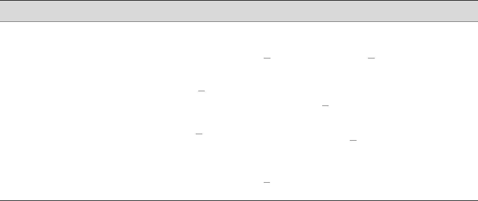
Table 4.2: Available models for electrically-driven flows in the EDFModels library. The last column indicates the section in the user guide where
the model has been described.
Model 1TypeName 2,3,4fE5Governing Equations Section
Poisson-Nernst-Planck
(PNP) NernstPlanck −F
N
P
i=1
zici(∇Ψ−Ea)
∇·(ε∇φExt) = 0
∇·(ε∇ψ) = −F
N
P
i=1
zici
∂ci
∂t +u·∇ci=∇·(Di∇ci) + ∇·Diezi
kT ∇Ψci
Section 3.5.1
Poisson-Boltzmann
(PB) PoissonBoltzmann −F
N
P
i=1
zici,0exp −ezi
kT ψ(∇Ψ−Ea)
∇·(ε∇φExt) = 0
∇·(ε∇ψ) + ψF
N
P
i=1
(aibi)∗=−F
N
P
i=1
(ai)∗+ψ∗F
N
P
i=1
(aibi)∗
with bi=−ezi
kT and ai=zici,0exp (biψ)
Section 3.5.3
Debye-H¨uckel
(DH) DebyeHuckel −F
N
P
i=1
zici,01−ezi
kT ψ(∇Ψ−Ea)
∇·(ε∇φExt) = 0
∇·(ε∇ψ) = −F
N
P
i=1
zici,01−ezi
kT ψSection 3.5.4
Slip velocity slipSmoluchowski 0∇·(ε∇φExt) = 0 Section 3.5.5
Ohmic Ohmic [∇·(ε∇φExt)] (∇φExt −Ea)
∂σ
∂t +u·∇σ=Deff∇2σ
∇·(σ∇φExt) = 0
Section 3.5.6
1Corresponds to the name entry identifying the model in the source code.
2fEis the electric body-force entering the momentum equation.
3Eais an optional argument - a single vector - representing a uniform electric field.
4When the splitting of potentials approach is selected for the PNP, PB and DH models, the user may choose to use (∇φExt −Ea), instead of (∇Ψ−Ea). Recall that the splitting
of potentials is given by Ψ=φExt +ψ(cf. Section 3.5.2).
5For the PNP, PB and DH models, the equations are presented according to the splitting of potentials approach, which is optional. When a single electric potential is intended to
be used, then replace ψby Ψand ignore the equations in terms of φExt.
36

CHAPTER 4. Overview of rheoTool 37
4.2.2 The potentials splitting approach and multi-species
modeling in the PNP, PB and DH models
The possibility of splitting the electric potential into two variables, as described
in Section 3.5.2, is available for the PNP, PB and DH models. When used, one
Poisson equation for ψand one Laplace equation for φExt are solved, as shown in
Table 4.2. In practice, the choice between using one or two potentials is achieved
in the following way: if only one potential ( psi ⇔Ψ) is present in the starting-
time folder, then it is assumed than a unique potential is to be used, while if two
potentials (phiE ⇔φExt and psi ⇔ψ) are defined, then the splitting approach is
assumed. Under the splitting approach, the user still has the option to include or
not the contribution of the intrinsic potential in the electric field definition of the
body-force entering the momentum equation. The choice is through the variable
psiContrib, which should be defined in a dictionary, as explained later in Section
5.4.1.
All the PNP, PB and DH models support multi-species modeling, with an ar-
bitrary number of species, each having different properties (charge valence, and
diffusivity, when it applies). On the other hand, the Ohmic model is only imple-
mented for a binary, symmetric electrolyte, although the two species may have
different diffusion coefficients.
4.2.3 Electrokinetic coupling loop in the PNP model
The PNP model has a loop for the coupling between the Nernst-Planck equations
(ionic concentration) and the Poisson equation (electric potential). This loop was
seen to be required to keep the second-order accuracy in time of the PNP model
[3]. Furthermore, it also allows the use of higher time-steps, while ensuring the
conservation of ions. Although it is allowed to select one single iteration for this
loop, we recommend the use of at least two iterations in any generic case. Moreover,
two coupling iterations is the default behavior for this model if no information is
provided by the user.
4.2.4 Analysis of a code sample
As previously done in Section 4.1.4 for the constitutiveEquations library, in this
Section we analyze a piece of code from the EDFModels library in order to illustrate
the connection between the code and the theory previously discussed. However,
we should note that the differences, at the code level, between the different models
of the EDFModels library are bigger than in the constitutiveEquations library, as
can be deduced from Table 4.2.
The piece of code selected for that purpose, Listing 4.3, represents the imple-
mentation of the PNP model and can be found in src/libs/EDFModels/mod
els/NernstPlanck/NernstPlanck.C. Let’s start the analysis to the most
important parts:
•lines 11-33: this is the constructor of a subclass (NPSpecie), nested in the
main class (NernstPlanck). Remember that the PNP, PB and DH models
CHAPTER 4. Overview of rheoTool 38
were all presented in a multi-species formulation, which is the form avail-
able in the code. The NPSpecie subclass is exactly each specie of the PNP
model. For each new specie, we can see the initialization of the following
attributes (members): the concentration field (ci), the charge valence (zi)
and the diffusivity (Di). The NernstPlanck class may have Ninstances of
the NPSpecie subclass, as much as defined by the user.
•lines 35-107: this is the constructor of the main class, where the several
fields and variables are initialized. The call to function checkForPhiE() in
line 44, which is implemented in the base class (see EDFEquation.C), is
checking for the existence of field phiE in the folder corresponding to the
starting time. If it is found, the code will interpret that the electric potential
should be split into 2 variables (phiE ⇔φExt and psi ⇔ψ), otherwise, the
code will consider that only a single potential should be used (psi ⇔Ψ).
This is how we identify if the splitting of potentials approach should be used.
We also highlight lines 89-107, where each specie of the PNP model is being
constructed and saved in a P trList <>, named species .
•lines 110-156: as suggested by the function’s name (Fe), these lines im-
plement the function returning the electric body-force for the momentum
equation. The charge density (rhoE) is computed in lines 114-120 (compare
with Eq. 3.26), and multiplied by the electric field in lines 122-155 (compare
with Eq. 3.24 and Table 4.2). The computation of the electric field may
include, or not, the contribution from the intrinsic potential, as discussed in
Section 3.5.2 – this is a user selection. Furthermore, the vector extraE is
an extra, uniform electric field, which can be optionally defined by the user
(see Table 4.2 and its footnotes).
•lines 158-252: it is inside this function, named correct(), that the electric-
related equations are solved for. The function is generally prepared to use
the splitting approach, in which case three equations are solved: the Laplace
equation for the external potential (lines 172-186), the Poisson equation for
the intrinsic (or full, unique) potential (lines 188-218) and the Nernst-Planck
transport equation for each ionic specie (220-250) – all these equations can
be seen in Table 4.2. Each equation is inserted in a while loop controlled by
the number of cycles and by the initial residual of the equation solved for.
This is to optionally converge the explicit terms inside each equation, for
each inner-iteration. In addition, and as discussed in Section 4.2.3, all the
equations are solved inside an electrokinetic coupling loop (lines 161-251),
whose number of iterations is controlled by variable nIterPNP , that is read
from dictionary fvSolution (line 86). If the variable is not specified by
the user, 2 iterations are carried out by default.
All the other EDF models also have the functions Fe() and correct() in their
structure, which are defined according to the given model. We believe that the
readers/users will easily understand those functions by reading the comments in-
cluded in the code, and by comparing the code with Table 4.2.

CHAPTER 4. Overview of rheoTool 39
#include "NernstPlanck.H"
2#include "addToRunTimeSelectionTable.H"
4// *********Static Data Members ********//
namespace Foam
6{
defineTypeNameAndDebug(NernstPlanck, 0);
8addToRunTimeSelectionTable(EDFEquation, NernstPlanck, dictionary);
}
10
// **********Constructors **********//
12 Foam::NernstPlanck::NPSpecie::NPSpecie
(
14 const word& name,
const surfaceScalarField& phi,
16 const dictionary& dict
)
18 :
ci_
20 (
IOobject
22 (
name,
24 phi.time().timeName(),
phi.mesh(),
26 IOobject::MUST_READ,
IOobject::AUTO_WRITE
28 ),
phi.mesh()
30 ),
zi_(dict.lookup("z")),
32 Di_(dict.lookup("D"))
{}
34
// **********Constructors **********//
36 Foam::NernstPlanck::NernstPlanck
(
38 const word& name,
const surfaceScalarField& phi,
40 const dictionary& dict
)
42 :
EDFEquation(name, phi),
44 solvePhiE_(checkForPhiE(name, phi)),
psi_
46 (
IOobject
48 (
"psi" + name,
50 phi.time().timeName(),
phi.mesh(),
52 IOobject::MUST_READ,
IOobject::AUTO_WRITE
54 ),
phi.mesh()
56 ),
phiE_

CHAPTER 4. Overview of rheoTool 40
58 (
IOobject
60 (
"phiE" + name,
62 phi.time().timeName(),
phi.mesh(),
64 IOobject::READ_IF_PRESENT,
solvePhiE_ == false ? (IOobject::NO_WRITE) : (IOobject::
AUTO_WRITE)
66 ),
phi.mesh(),
68 dimensionedScalar
(
70 "zero",
psi_.dimensions(),
72 pTraits<scalar>::zero
),
74 zeroGradientFvPatchField<scalar>::typeName
),
76 relPerm_(dict.lookup("relPerm")),
T_(dict.lookup("T")),
78 extraE_(dict.lookupOrDefault<dimensionedVector>("extraEField",
dimensionedVector("0", dimensionSet(1, 1, -3, 0, 0, -1, 0),
vector::zero))),
psiContrib_(dict.lookupOrDefault<bool>("psiContrib", true)),
80 phiEEqRes_(phi.mesh().solutionDict().subDict("electricControls").
subDict("phiEEqn").lookupOrDefault<scalar>("residuals", 1e-7)),
psiEqRes_(phi.mesh().solutionDict().subDict("electricControls").
subDict("psiEqn").lookupOrDefault<scalar>("residuals", 1e-7)),
82 ciEqRes_(phi.mesh().solutionDict().subDict("electricControls").
subDict("ciEqn").lookupOrDefault<scalar>("residuals", 1e-7)),
maxIterPhiE_(phi.mesh().solutionDict().subDict("electricControls").
subDict("phiEEqn").lookupOrDefault<scalar>("maxIter", 50)),
84 maxIterPsi_(phi.mesh().solutionDict().subDict("electricControls").
subDict("psiEqn").lookupOrDefault<scalar>("maxIter", 50)),
maxIterCi_(phi.mesh().solutionDict().subDict("electricControls").
subDict("ciEqn").lookupOrDefault<scalar>("maxIter", 50)),
86 nIterPNP_(phi.mesh().solutionDict().subDict("electricControls").
lookupOrDefault<int>("nIterPNP", 2)),
species_(),
88 nSpecies_(0)
{
90 PtrList<entry> specEntries(dict.lookup("species"));
nSpecies_ = specEntries.size();
92 species_.setSize(nSpecies_);
94 forAll (species_, specI)
{
96 species_.set
(
98 specI,
new NPSpecie
100 (
specEntries[specI].keyword(),
102 phi,
specEntries[specI].dict()
104 )

CHAPTER 4. Overview of rheoTool 41
);
106 }
}
108
// ******** Member Functions * *********//
110 Foam::tmp<Foam::volVectorField> Foam::NernstPlanck::Fe() const
{
112 volScalarField rhoE( psi_ *dimensionedScalar("norm", epsilonK_.
dimensions()/dimArea, 0.) );
114 forAll (species_, i)
{
116 rhoE
+= (
118 species_[i].zi()*species_[i].ci()*FK_
);
120 }
122 if (solvePhiE_)
{
124 if (psiContrib_)
{
126 return
(
128 -rhoE *( fvc::grad(phiE_+psi_) - extraE_)
);
130 }
else
132 {
return
134 (
-rhoE *( fvc::grad(phiE_) - extraE_)
136 );
}
138 }
else
140 {
if (psiContrib_)
142 {
return
144 (
-rhoE *( fvc::grad(psi_) - extraE_)
146 );
}
148 else
{
150 return
(
152 -rhoE *(-extraE_)
);
154 }
}
156 }
158 void Foam::NernstPlanck::correct()
{
160
CHAPTER 4. Overview of rheoTool 42
// Electrokinetic coupling loop
162 for (int j=0; j<nIterPNP_; j++)
{
164
Info << "PNP Coupling iteration: " << j << endl;
166
scalar res=GREAT;
168 scalar iter=0;
170 //- Equation for the external potential (loop for the case
// of non-orthogonal grids)
172 if (solvePhiE_)
{
174 while (res > phiEEqRes_ && iter < maxIterPhiE_)
{
176 fvScalarMatrix phiEEqn
(
178 fvm::laplacian(phiE_)
);
180
phiEEqn.relax();
182 res=phiEEqn.solve().initialResidual();
184 iter++;
}
186 }
188 //- Equation for the intrinsic potential
190 res=GREAT;
iter=0;
192
volScalarField souE(psi_ *dimensionedScalar("norm1",dimless/dimArea
,0.));
194
forAll (species_, i)
196 {
souE +=
198 (
-species_[i].zi()*species_[i].ci()*FK_
200 /(relPerm_*epsilonK_)
);
202 }
204 while (res > psiEqRes_ && iter < maxIterPsi_)
{
206
fvScalarMatrix psiEqn
208 (
fvm::laplacian(psi_)
210 ==
souE
212 );
214 psiEqn.relax();
res=psiEqn.solve().initialResidual();
216

CHAPTER 4. Overview of rheoTool 43
iter++;
218 }
220 //- Nernst-Planck equation for each ionic specie
222 forAll (species_, i)
{
224 res=GREAT;
iter=0;
226
volScalarField& ci = species_[i].ci();
228
dimensionedScalar cf(species_[i].Di() *eK_ *species_[i].zi() / (kbK_
*T_) );
230
while (res > ciEqRes_ && iter < maxIterCi_)
232 {
234 fvScalarMatrix ciEqn
(
236 fvm::ddt(ci)
+fvm::div(phi(), ci, "div(phi,ci)")
238 ==
fvm::laplacian(species_[i].Di(), ci, "laplacian(D,ci)")
240 +fvc::laplacian(ci*cf, phiE_+psi_, "laplacian(elecM)")
);
242
ciEqn.relax(phi().mesh().equationRelaxationFactor("ci"));
244 res=ciEqn.solve(phi().mesh().solver("ci")).initialResidual();
246 ci = Foam::max( dimensionedScalar("lowerLimit",ci.dimensions(), 0.),
ci );
iter++;
248
}
250 }
}
252 }
Listing 4.3: Source code of the Poisson-Nernst-Planck model in file
NernstPlanck.C.

CHAPTER 4. Overview of rheoTool 44
4.2.5 Adding new EDF models
The steps required to add new EDF models are similar to the ones described
previously, in Section 4.1.6, for GNF and viscoelastic models. The main steps are:
•copy-paste the folder of an existing model (that we will call template model)
in directory src/libs/EDFModels/models/. Rename the folder and
the files inside it (.C and .H files) with the new model’s name. Remove the
.dep file inside the folder. We recommend to use model slipSmoluchowski as
template, since it is the simplest one and does not contain other sub-classes,
which would also need to be renamed in the next step.
•inside the source .C and header .H files, find-replace the old model’s name
by the new one (e.g. Ctrl +Hin gedit). This is to change the name of the
class, which is usually equal to the name given to the respective source file.
However, it is a good idea to always check first the name given to the class
of the template model.
•add the source code of the new model to the compilation list of the library.
For that, edit file src/libs/EDFModels/Make/files by adding the
path for the source code (see the entries for the other models already there).
•make a first compilation of the new model, by running the script Allwmake
in directory src/. Note that, until this point, the source code of the new
model is the one from the original template model, where only the name of
the class has been changed. Thus, the model should compile without errors.
If not, something wrong occurred in the previous steps.
•the last step is to change the source code of the model in order to implement
the desired EDF model. Depending on the characteristics of the new model,
several parts of the source and header files might need to be changed. Our
recommendation is to look to the closest model among the ones available.
After all the changes on the code had been completed, compile again by
running script Allwmake.
If all the steps listed above were successfully executed, then the new model is
now available to solver rheoEFoam (only). In order to use library EDFModels in
any solver other than rheoEFoam, the user should:
•add the header #include ”EDFModel.H” to the main solver.
•create an EDFModel object by calling the constructor with the correct ar-
guments, for example: EDFModel elecM(phi).
•add the library EDFModels to the Make/options, and specify its path
(check the Make/options of rheoEFoam for an example).

CHAPTER 4. Overview of rheoTool 46
Table 4.3: Brief description of the solvers available in rheoTool.
Name Description
rheoFoam
Transient solver for pressure-driven, single-phase, lam-
inar, isothermal flows. Selection of rheology is general
among all the available GNF and viscoelastic models.
rheoInterFoam
Transient solver for pressure-driven, two-phase, lami-
nar, isothermal flows, using the volume-of-fluid (VOF)
approach. Selection of rheology for each phase is
general among all the available GNF and viscoelastic
models.
rheoTestFoam
Application to compute steady and transient material
properties for any of the available GNF and viscoelas-
tic models.
rheoEFoam
Transient solver for electrically-driven, single-phase,
laminar, isothermal flows. Mixed electric-/pressure-
driven flows are also allowed. Selection of rheology is
general among all the available GNF and viscoelastic
models.
4.3.1 rheoFoam
The solver rheoFoam implements the transient, incompressible Navier-Stokes equa-
tions for single-phase flows of GNF or viscoelastic fluids. Figure 4.1 displays the
solving sequence.
The solver has three main loops: L1, which is advancing the time; L2, which is
an inner-loop used to converge the solution at each time-step; and L3, a loop which
can be enabled for non-orthogonal grids, in order to update (inside each time-step
and each inner-iteration) the explicit correction of the pressure Laplacian, avoiding
stability problems and reducing the error in transient computations. More than
understanding each step identified in Fig. 4.1, we want to help the reader to identify
them in the source code and relate them with the theory presented in the previous
Chapter. With this purpose in mind, we will do a tour to the source code of
the solver and the most important points will be discussed, skipping the lines not
essential to understand the algorithm.
The solver rheoFoam is composed of one main file (rheoFoam.C) and four as-
sociated header files (createFields.H,createPPutil.H,UEqn.H,pEqn.
H,CEqn.H), which can be found in directory src/solvers/rheoFoam/. All
the header files are included from the main .C file. We will start by digging into
rheoFoam.C, whose source code is displayed in Listing 4.4.
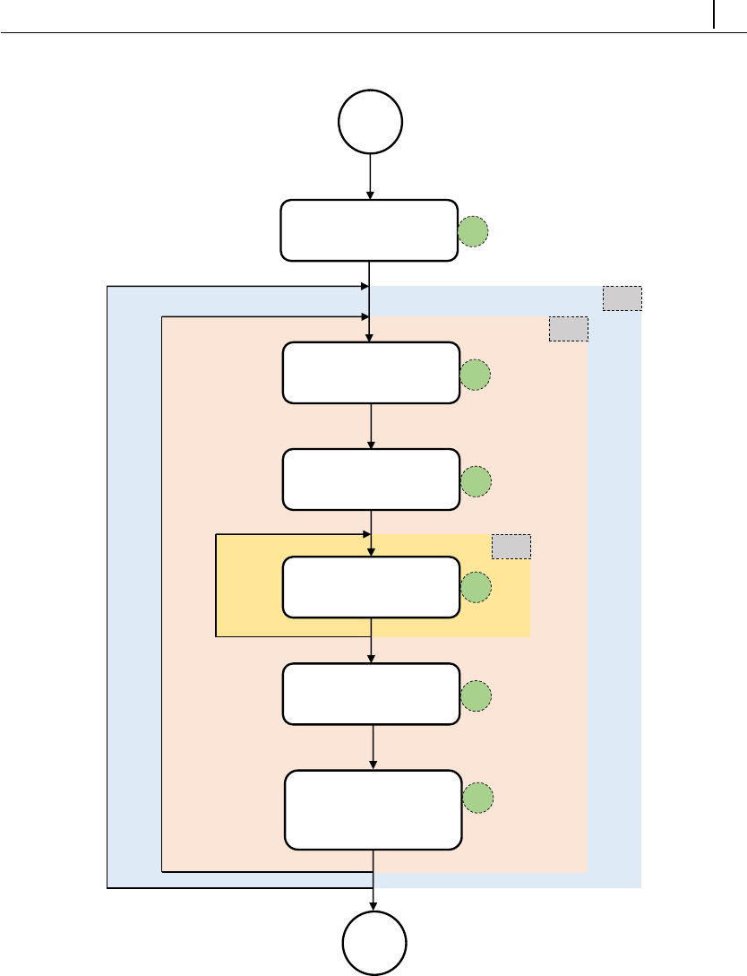
CHAPTER 4. Overview of rheoTool 47
Solve the constitutive
equation
Solve the momentum
equation
Solve the pressure
(continuity) equation
Correct cell velocities
and face fluxes
Initialize fields and
variables
End
Start
Inner loop: i = i + 1
Time loop: t = t + Δt
Non-orthogonality
corrector
loop
S2
S3
S4
S5
S1
L1
L2
L3
createField.H
rheoFoam.C
UEqn.H
pEqn.H
pEqn.H
Solve the transport
equation for a scalar
(optional)
S6
CEqn.H
Figure 4.1: Solving sequence of rheoFoam.
•lines 1-5: those # include lines load classes used by OpenFOAMR
for stan-
dard tasks, transversal to most of the OpenFOAM R
solvers.
•line 6: this # include is providing access to a library of post-processing
utilities, that we discuss later in Section 4.5.2.
•line 7: this # include allows the solver to access the models defined in the

CHAPTER 4. Overview of rheoTool 48
constitutiveEquations library.
•lines 13-21: fields, variables, controls and the mesh are created (step S1 of
Fig. 4.1). Lines 16 and 18 point to the header files createFields.H and
createPPutil.H, respectively, located in the same directory as rheoFo
am.C. The later is responsible for the creation of post-processing utilities.
•lines 27-65: represents the time loop, i.e., L1 of Fig. 4.1. The solver will
keep running until the final specified time is reached or once the residuals of
the solved variables drop below some tolerance (this dual criterion is specific
of class simpleControl).
•lines 31-33: those includes allow automatic time-step adjustment, based on
the maximum Courant number specified by the user. This control can be
switched off by the user (more details in Section 5.1.1).
•lines 36-55: this is the inner loop, L2, of Fig. 4.1. Inside this loop, all
the conservation equations are solved nInIter times inside the same time-
step. This reduces the explicitness of the method, which exists, for example,
in the non-linear convective term of the momentum equation, in the both-
sides-diffusion technique and in several terms of the constitutive equation
(for a given equation, only the terms introduced through a fvm:: operator
are implicit). Furthermore, these iterations also strengthen the coupling
between velocity and pressure.
•line 43: the function correct() of the constitutive model is called. As seen
before, this function updates variable τby solving the constitutive equa-
tion(s).
•line 46: the momentum equation is solved. The header file UEqn.H (Listing
4.5) will be explored later.
•line 47: the pressure equation is solved. The header file pEqn.H (Listing
4.6) will be explored later.
•line 51-54: the equation for a passive scalar is optionally solved, depending
on a user-defined selection (more details in Section 5.1.1). The header file
CEqn.H (Listing 4.7) will be explored later.
•lines 57-58: this is where the post-processing utilities are evaluated, if any
has been selected by the user.
#include "fvCFD.H"
2#include "IFstream.H"
#include "OFstream.H"
4#include "simpleControl.H"
#include "fvIOoptionList.H"
6#include "ppUtilInterface.H"
#include "constitutiveModel.H"
8

CHAPTER 4. Overview of rheoTool 49
// ******************************//
10
int main(int argc, char *argv[])
12 {
#include "setRootCase.H"
14 #include "createTime.H"
#include "createMesh.H"
16 #include "createFields.H"
#include "createFvOptions.H"
18 #include "createPPutil.H"
#include "initContinuityErrs.H"
20
simpleControl simple(mesh);
22 // ****************************//
24 Info<< "\nStarting time loop\n" << endl;
26 // --- Time loop ---
while (simple.loop())
28 {
Info<< "Time = " << runTime.timeName() << nl << endl;
30
#include "readTimeControls.H"
32 #include "CourantNo.H"
#include "setDeltaT.H"
34
// --- Inner loop iterations ---
36 for (int i=0; i<nInIter; i++)
{
38 Info<< "Iteration " << i << nl << endl;
40 // --- Pressure-velocity SIMPLEC corrector
{
42 // ---- Solve constitutive equation ----
constEq.correct();
44
// ---- Solve U and p ----
46 #include "UEqn.H"
#include "pEqn.H"
48 }
50 // --- Passive Scalar transport
if (sPS)
52 {
#include "CEqn.H"
54 }
}
56
//- Post-processing
58 postProc.update();
60 runTime.write();
62 Info<< "ExecutionTime = " << runTime.elapsedCpuTime() << "
s"
<< " ClockTime = " << runTime.elapsedClockTime() << "

CHAPTER 4. Overview of rheoTool 50
s"
64 << nl << endl;
}
66
Info<< "End\n" << endl;
68
return 0;
70 }
Listing 4.4: Source code of rheoFoam.C.
The source code in file createFields.H will not be discussed, since it mainly
contains standard declaration/initialization of fields and variables. However, it is
worth mentioning the creation of a constitutiveModel object, named constEq, which
stores the data of the constitutive equation selected.
According to the SIMPLEC algorithm, the momentum equation is first solved
to obtain an estimated velocity field, using the pressure field of the previous inner-
iteration or time-step. Then, we solve for the pressure field enforcing continuity.
Finally, using the correct pressure field, the previously estimated velocity is cor-
rected, both on faces and cell centers. This is what is being executed in UEqn.H
and pEqn.H. We follow the discussion by analyzing the content of UEqn.H, whose
code is displayed in Listing 4.5.
•lines 3-10: this is where the momentum equation is built. We can identify
the transient term in line 5, the convective term in line 6, an extra momen-
tum source term in line 8 (term fin Eqs. 3.5 and 3.18) and the extra-stress
divergence in line 9 (∇·τ0), containing both the solvent and the polymeric
contributions (remember the output of divTau() function, analyzed in Sec-
tion 4.1.4).
•line 16: the momentum equation is solved considering the pressure gradi-
ent contribution, where the pressure field from the last time-step or inner-
iteration is used. This term was not added before in order for operator H
obtained from the momentum equation to be free of such contribution, as
discussed in Section 3.3.1. This is required to avoid the onset of checkerboard
fields, since a traditional Rhie-Chow interpolation is not used (cf. Ref. [2]).
// Momentum predictor
2
tmp<fvVectorMatrix> UEqn
4(
fvm::ddt(U)
6+ fvm::div(phi, U)
==
8fvOptions(U)
+ constEq.divTau(U)
10 );
12 UEqn().relax();
14 fvOptions.constrain(UEqn());
CHAPTER 4. Overview of rheoTool 51
16 solve(UEqn() == -fvc::grad(p));
18 fvOptions.correct(U);
Listing 4.5: Source code of UEqn.H.
After having a guessed (non-conservative) velocity field, we will see how it is
used inside pEqn.H (Listing 4.6):
•lines 1-19: variables required to solve the pressure equation (Eq. 3.15) are
assembled. The sequence of steps can be easily understood, keeping in mind
that UEqn().A() retrieves diagonal coefficients (aP) and that UEqn().H()
and UEqn().H1() stand for operators Hand H1, respectively. As previously
discussed in Section 3.3.1, pressure gradient terms entering the definition of
face fluxes (line 18) are directly evaluated on cell faces to avoid checkerboard
fields. Also, in line 9 there is the addition of the corrective term for time-step
dependency, described in Section 3.3.1.
•lines 24-39: this is the non-orthogonality corrector loop (L3 ) displayed in
Fig. 4.1. The goal is similar to the one of the inner loop: minimizing the
explicitness of the algorithm. At this point, the reader may be asking why
do this loop exists if the inner loop is already there doing a similar task?
To clarify this point, it should be noted that the non-orthogonality corrector
loop only makes sense to exist for non-orthogonal meshes. For those meshes,
the laplacian operator in line 28 is not completely handled in an implicit
way, but an explicit corrective term is added. For highly non-orthogonal
meshes, this term has an important contribution and, due to being explicit,
the pressure resulting from solving line 37 will not be continuity-compliant,
which can afterwards introduce continuity problems and lead the simulation
to diverge. For this reason, in such cases the implicitness of the Laplacian
term is increased by continuously solving that equation with the updated
pressure-field, and the fluxes are only corrected at the last iteration of this
loop (lines 35-38). Is the non-orthogonal corrector loop absolutely necessary
when dealing with non-orthogonal meshes? No, as long as the simulation
does not diverge and if only steady-state results are required. Otherwise,
this loop should be active. For a number of cases, doing 2-3 non-orthogonal
iterations keeps the solver stable, without the need of under-relaxing the pres-
sure. Even if only one non-orthogonal correction is performed, the Laplacian
term should still be discretized with the corrective term to keep the accuracy
in non-orthogonal meshes.
•lines 28,33: the pressure equation (Eq. 3.15) is assembled (line 28) and
solved (line 33).
•line 37: this is the equation which corrects the face fluxes (Eq. 3.16 interpo-
lated to the faces). Again, pressure gradient terms are directly evaluated on
cell faces: the snGrad() operator in line 18, when building phiHbyA, and the
one coming from the laplacian() operator in line 28, from which the flux()
operator is derived.

CHAPTER 4. Overview of rheoTool 52
•line 47: this is the equation which corrects the cell-centered velocity field
(Eq. 3.16).
volScalarField rAU(1.0/UEqn().A());
2volVectorField HbyA("HbyA", U);
HbyA = rAU*UEqn().H();
4
surfaceScalarField phiHbyA
6(
"phiHbyA",
8(fvc::interpolate(HbyA) & mesh.Sf())
+ fvc::ddtPhiCorr(rAU, U, phi)
10 );
12 fvOptions.relativeFlux(phiHbyA);
adjustPhi(phiHbyA, U, p);
14
tmp<volScalarField> rAtU(rAU);
16
rAtU = 1.0/(1.0/rAU - UEqn().H1());
18 phiHbyA += fvc::interpolate(rAtU() - rAU)*fvc::snGrad(p)*mesh.
magSf();
HbyA -= (rAU - rAtU())*fvc::grad(p);
20
UEqn.clear();
22
// Non-orthogonal pressure corrector loop
24 while (simple.correctNonOrthogonal())
{
26 fvScalarMatrix pEqn
(
28 fvm::laplacian(rAtU(), p, "laplacian(p|(ap-H1))") ==
fvc::div(phiHbyA)
);
30
pEqn.setReference(pRefCell, pRefValue);
32
pEqn.solve();
34
if (simple.finalNonOrthogonalIter())
36 {
phi = phiHbyA - pEqn.flux();
38 }
}
40
#include "continuityErrs.H"
42
// Explicitly relax pressure for momentum corrector
44 p.relax();
46 // Momentum corrector
U = HbyA - rAtU()*fvc::grad(p);
48 U.correctBoundaryConditions();
fvOptions.correct(U);
Listing 4.6: Source code of pEqn.H.
CHAPTER 4. Overview of rheoTool 53
After pEqn.H is executed, both the pressure and the face fluxes are continuity-
compliant, but not the cell-centered velocity field. The conservative fluxes can now
be used to solve any transport equation. In rheoFoam, we offer the possibility to
solve a transport equation for a passive scalar. The governing equation, included
in file CEqn.H, is simply a convection-diffusion transport equation, as can be seen
in lines 5-11 of Listing 4.7.
1// Transport of passive scalar
3dimensionedScalar D_ = cttProperties.subDict("
passiveScalarProperties").lookup("D");
5fvScalarMatrix CEqn
(
7fvm::ddt(C)
+ fvm::div(phi, C)
9==
fvc::laplacian(D_,C)
11 );
13 CEqn.relax();
CEqn.solve();
15
if (U.time().outputTime())
17 {
C.write();
19 }
Listing 4.7: Source code of CEqn.H.
4.3.2 rheoTestFoam
The main purpose of solver rheoTestFoam is to evaluate the behavior of the con-
stitutive models for a user-defined ∇utensor. At the same time, it can also be
envisaged as a basic debugging tool to check for the correct implementation of the
constitutive models, since an analytical or semi-analytical solution usually exists,
which can be used for comparison.
Shortly, rheoTestFoam solves for the solvent and polymeric constitutive equa-
tions, Eqs. (3.3) and (3.4), respectively, for a prescribed ∇utensor, assuming
homogeneous flow conditions (∇·τ=0;u·∇τ=0). Since there are no approx-
imations related with spatial discretization, the resulting steady-state solution
τ0=τ+τsis exact, and OpenFOAM R
is simply acting as a nonlinear matrix
solver. To obtain unsteady solutions, the temporal discretization introduces nu-
merical errors during the transient period, which can be reduced using a small
time-step.
The computational domain used with this solver is composed of a single cell: a
cube with unitary edge length (1 m). The boundary conditions for uare internally
manipulated inside the code, in order to get the tensor ∇udefined by the user,
Fig. 4.2. Thus, the default mesh and boundary conditions should not
be changed by the user when working with rheoTestFoam. We note that the
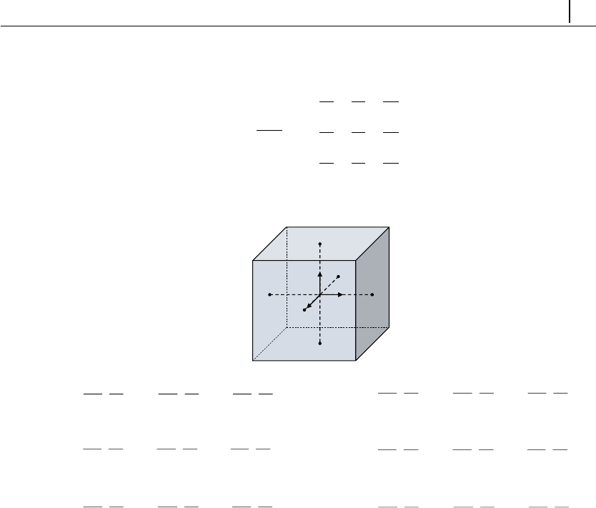
CHAPTER 4. Overview of rheoTool 54
following definition holds in this guide (and in OpenFOAM R
, in general):
(∇u)ij =∂uj
∂xi
=
∂u
∂x
∂v
∂x
∂w
∂x
∂u
∂y
∂v
∂y
∂w
∂y
∂u
∂z
∂v
∂z
∂w
∂z
(4.3)
y
z
x
x+
x-
z+
z-
y-
y+
2
,
2
,
2321 y
y
u
y
y
u
y
y
uz
y
x
y
u
2
,
2
,
2321 x
x
u
x
x
u
x
x
uz
y
x
x
u
2
,
2
,
2321 z
z
u
z
z
u
z
z
uz
y
x
z
u
2
,
2
,
2321 y
y
u
y
y
u
y
y
uz
y
x
y
u
2
,
2
,
2321 x
x
u
x
x
u
x
x
uz
y
x
x
u
2
,
2
,
2321 z
z
u
z
z
u
z
z
uz
y
x
z
u
Figure 4.2: Boundary conditions manipulation in the single-cell mesh used with
rheoTestFoam. The constants currently used to represent the cell-centered velocity
are κ1=κ2=κ3= 0, although any other values could be used. The edge length
of the cubic cell is set to δx =δy =δz = 1m.
Two operation modes are available with this solver:
•ramp mode: the user defines a list of ∇utensors and the solver will retrieve
the steady solution for each entry. In this mode, the solver automatically
selects the ideal time-step value to be used and the steady-state is also auto-
matically detected (either the relative variation of the extra-stress magnitude
drops below 10-8, or after a predefined number of time-steps has been ex-
ceeded – this last condition is used to avoid infinite loops).
•transient mode: the user defines one single ∇utensor and the solver will
return the evolution over time of the monitored variables. In this case,
both the time-step and the end time are controlled by the user. This mode
allows to determine the transient material functions of the constitutive model
selected.
As default behavior, rheoTestFoam writes a file named Report containing all
the components of the total extra-stress tensor, τ0(remember that τ0=τ+τsis

CHAPTER 4. Overview of rheoTool 55
the total extra-stress tensor, including both solvent and polymeric contributions).
In ramp mode, also the status (Converged or Exceed Niter) is returned, along
with the relative error. The user can compute any relevant material function from
the tensor components retrieved. If for some reason the status Exceed Niter is
retrieved for any ∇uentry in ramp mode, we recommend to run rheoTestFoam in
transient mode for that same ∇u, using a small time-step – at convergence, the
steady material properties will be obtained. This may happens, for example, when
using a multimode model with very different modes, for which the automatic time-
stepping procedure fails to choose a stable time-step for the given ∇u. On the
other hand, some viscoelastic models are naturally unbounded under certain flow
conditions, such as the UCM and Oldroyd-B models for W i ≥0.5 in extensional
flow. Care should be taken for such situations, since the solver will most likely
retrieve a non-physical solution close to those limits and eventually diverge.
Note that rheoTestFoam is only adapted to work optimally in ramp mode
with the models implemented in the extra-stress tensor variable, which excludes
the models solved with the log-conformation approach or with the conformation
tensor (FENE-type). However, the material functions for a given model are the
same independently of the variable in which it is solved for, as long as all the terms
are accounted for. Thus, it is possible to extract the material functions of all the
models provided in rheoTool.
In a future release of rheoTool, we anticipate that the solver rheoTestFoam will
be able to fit the available constitutive models to experimental data input by the
user and return the best-fit model, along with the best-fit parameters (λ, η, ...).
This will allow to run simulations with a numerical model reproducing properly
the material functions of real fluids.
4.3.3 rheoInterFoam
Section 4.3.3 is under development.
The solver rheoInterFoam is a generalization of rheoFoam for two-phase flows, us-
ing the Volume of Fluid (VOF) method of OpenFOAM R
to represent the interface
between the two phases.
Currently, rheoInterFoam solves a constitutive equation for each phase and the
extra-stress tensor contributing to the momentum equation is the weighted aver-
age of the extra-stress tensor for each phase, where the weighing is ensured by the
indicator function used in VOF. This approach allows to have phases represented
by different constitutive equations, although this is possibly not the most accurate
and stable way to do the computations. Additionally, the SIMPLEC algorithm
used for single-phase flows may need to be improved when used in rheoInterFoam.
Other aspects are still under test, which makes the current version of rheoInter-
Foam still experimental. Nonetheless, this version is fully functional.

CHAPTER 4. Overview of rheoTool 56
4.3.4 rheoEFoam
The solver rheoEFoam is the extension of rheoFoam to electrically-driven flows –
note the additional Ein the solver name, which points to its Electric component.
Thus, with no surprise, both solvers share the same basic structure and only
minor differences exist between both at the code level. For this reason, we will
not discuss again the common parts. Instead, we refer the reader to Section
4.3.1 to eventually recall the structure of rheoFoam and in this Section we only
highlight the main differences introduced in rheoEFoam. Note that rheoEFoam
allows the combination of both electrically- and pressure-driven flows with no
restrictions. Pure pressure-driven flows can be also simulated with rheoEFoam, for
which the solver becomes functionally equivalent to rheoFoam, although directly
using rheoFoam is the more efficient option in these situations.
Starting by the file createFields.H, there is an extra line for the creation
of the electric model, as shown in Listing 4.8.
1// Create the electric model
EHDEKModel elecM(phi);
Listing 4.8: Line in the file createFields.H of rheoEFoam, where the
electric model is created.
In file rheoEFoam.C, the header # include ”EDFModel.H” has been added in
order to enable the use of the EDFModels library, whose path had also to be added
to file Make/options. The other change is in the inner-iteration loop, which
now starts by solving the electric-related equations (line 11, Listing 4.9), calling
the function correct() of the electric model (recall an example of that function in
lines 188-281 of Listing 4.3). The user may also choose to not solve the equations
governing the fluid flow (see the if condition in line 13 of Listing 4.9). This is
useful when only the electric component of the problem is of interest.
// --- Inner loop iterations ---
2
for (int i=0; i<nInIter; i++)
4{
6Info<< "Inner iteration: " << i << nl << endl;
8// --- Pressure-velocity SIMPLEC corrector
{
10 // ---- Update electric terms ----
elecM.correct();
12
if (solveFluid)
14 {
// ---- Solve constitutive equation ----
16 constEq.correct();
18 // ---- Solve U and p ----
#include "UEqn.H"
20 #include "pEqn.H"
}
22 }

CHAPTER 4. Overview of rheoTool 57
24 // --- Passive Scalar transport
if (sPS)
26 {
#include "CEqn.H"
28 }
30 }
Listing 4.9: Inner-iteration loop of rheoEFoam (source code:
rheoEFoam.C).
Finally, the last change at the code level is in file UEqn.H, containing the
momentum equation, which has been modified to include the electric body-force
(line 8, Listing 4.10) – it can be a null vector, depending on the EDF model
selected.
tmp<fvVectorMatrix> UEqn
2(
fvm::ddt(U)
4+ fvm::div(phi, U)
==
6fvOptions(U)
+ constEq.divTau(U)
8+ elecM.Fe()/constEq.rho()
);
Listing 4.10: Momentum-balance equation in rheoEFoam (source code:
UEqn.H).
4.4 Boundary conditions
4.4.1 linearExtrapolation
TypeName:linearExtrapolation
Type: fixed-value (any type field).
Formula:Tij, f =Tij, P + (∇Tij)P·dPf, where Tij is the ij component of the
generic field T(scalar, vector or tensor), indices f and P represent the boundary
face and the cell owning that face, respectively, and dPf is the vector connecting
their geometrical centers.
Description: linear extrapolation of each field component from boundary cells
to boundary faces. Shortly, this boundary condition starts by computing the gradi-
ent of each component at the center of the cell owning the boundary face (using the
previous iteration/time-step known values on the boundary face). Then, with both
the value and the gradient of each component at those locations, the components
at the boundary faces are estimated by linear extrapolation. The discretization
scheme to compute the gradients enrolled in the process is run time selectable
and can be adjusted in dictionary fvSchemes, through the entry linExtrapGrad
followed by the selected scheme, in the gradSchemes subDict. In general, using

CHAPTER 4. Overview of rheoTool 58
linear extrapolation for the polymeric extra-stress tensor on walls should be pre-
ferred in relation to a zero-gradient boundary condition, which has a lower order
of accuracy [2].
Since version 2.0, an optional second-order accurate linear regression [21] can
be selected by adding the entry useRegression true to the dictionary defining the
BC, i.e., below keyword type, for example. If not present, the solver will execute
by default the linear extrapolation defined above.
4.4.2 zeroIonicFlux
TypeName:zeroIonicFlux
Type: fixed-gradient (scalar).
Formula:∇ci|f·nf=−ci,f ezi
kT ∇Ψ|f·nf, with ci,f =ci,P exp −ezi
kT (ψf−ψP).
Indices f and P represent the boundary face and the cell owning that face (see the
definition of the other variables in Section 3.5.1).
Description: imposing a no-flux condition for an ionic specie, in the Poisson-
Nernst-Planck model. This boundary condition results from the balance of diffu-
sion and electromigration at the patch, assuming that a no-penetration condition
holds there. The expression being used has been derived from a Robin-type bound-
ary condition [3].
4.4.3 boltzmannEquilibrium
TypeName:boltzmannEquilibrium
Type: fixed-value (scalar).
Formula:ci,f =ci,0 exp ezi
kT (ψf−ψ0), where ci,0 is the reference concentration
(user-defined) at which the intrinsic electric potential is ψ0(user-defined; see the
definition of the other variables in Section 3.5.1). A common choice is to set ci,0
as the bulk concentration of ions and ψ0= 0.
Description: ionic concentration derived from the assumption of Boltzmann
equilibrium near the patch. This boundary condition is intended to be used when
the electric potential is split, in which case only the intrinsic potential is used
in the formula. This boundary condition does not guarantee the zero-flux of a
given specie in all the situations, and, in general, it is not accurate for transient
simulations.
4.4.4 inducedPotential
TypeName:inducedPotential
Type: fixed-value (scalar).

CHAPTER 4. Overview of rheoTool 59
Formula:ψf=−φExt,f +ψFix +
1
Nf
P
f=1 |Sf|
Nf
P
f=1
φExt,f|Sf|, where ψFix is the bias
voltage (user-defined) of the patch, i.e., the electric potential of the surface in the
absence of an external electric field.
Description: intrinsic potential induced in a conducting surface placed over
an electric field and having a bias voltage [22]. The last term in the formula
represents the area-averaged external electric potential over the surface. This
boundary condition can be used with the Poisson-Boltzmann and Debye-H¨uckel
models, under the potentials splitting approach.
4.4.5 slipSmoluchowski
TypeName:slipSmoluchowski
Type: fixed-value (vector).
Formula:uSch,f =µ(−∇φExt,f), where µis the electroosmotic mobility (user-
defined), as defined in Section 3.5.5.
Description: slip velocity derived from the Helmholtz-Smoluchowski theory
(Section 3.5.5). Although this boundary condition can be used with any EDF
model for which φExt is defined, it is primarily intended to be used with the slip
model.
4.4.6 slipSigmaDependent
TypeName:slipSigmaDependent
Type: fixed-value (vector).
Formula:uSch,f =µ0σf
σ0m(−∇φExt,f), as defined in Section 3.5.6. Parame-
ters µ0,σ0and mare user-defined.
Description: slip velocity derived from the Helmholtz-Smoluchowski theory
for a space-variable conductivity field (Section 3.5.6). This boundary condition
can be used with the Ohmic model.
4.4.7 A note on wall boundary conditions for pressure
In the simulation of incompressible flows, it is a common approach to assign a zero-
gradient boundary condition for the pressure at walls. This approach is efficient to
ensure no-penetration in the wall (continuity equation), but it results in a lower-
order approximation for the pressure gradient in the momentum equation and, in
some cases, it may significantly unbalance the remaining sources of momentum.
A more general approach is to derive the pressure gradient at the boundary from
the continuity equation, by enforcing the no-penetration condition. Indeed, if Eq.
CHAPTER 4. Overview of rheoTool 60
(3.16) is interpolated to the faces of a bounding wall, then setting the velocity, or
more correctly the flux, to zero (no-penetration condition) results in
uf·n= 0 ⇒(∇p)f·n= (aP−H1)Hf
aP
+1
aP−H1−1
aP(∇p∗)f·n(4.4)
Eq. (4.4) is generic since it does not depend on a specific form of the momentum
equation. It can also be seen that if both sides of Eq. (4.4) are forced to be zero –
the zero-gradient approach –, the equality is still satisfied and the no-penetration
condition is still valid. The advantage in using Eq. (4.4) is that the resulting
normal pressure gradient is going to effectively balance the remaining local forces
in the momentum equation. In practice, the difference between using Eq. (4.4) or
the zero-gradient approximation is only noticeable when the stresses at the wall are
significant (high Hf
aP), as for example in EDFs, where a strong electric force normal
to the wall may exists. In the tutorials provided with rheoTool, the zero-gradient
approximation is frequently used.
Since OpenFOAM R
version 4.0, the boundary equation embodied by Eq. (4.4)
is available by default under the name fixedFluxExtrapolatedPressure. However,
this boundary condition may not be usable in some cases, as for example in cases
with a zero velocity assigned to all boundaries. In such cases, there is a conflict
created by function adjustPhi() when it attempts to artificially adjust the fluxes.
This issue can be avoided by commenting the line where function adjustPhi() is
called in the code (typically inside file pEqn.H), provided the user is sure that
the set of boundary conditions under use verifies continuity. This limitation in the
boundary condition might be eventually solved in future releases of OpenFOAM R
.
Importantly, in multiphase flows with non-zero surface tension and/or gravity
effects, the zero-gradient condition for pressure is generally incorrect. Indeed, for
such flows it is usual to compute the fluxes in two steps in OpenFOAM R
, i.e., the
term Hf
aPin Eq. (4.4) is built in two steps. The last step adds the flux contribution
from surface-tension and gravity without enforcing a null contribution at the wall.
Thus, in general the right hand-side of Eq. (4.4) is non-null in these cases and sim-
ply setting (∇p)f·n= 0 creates a local mass imbalance. The boundary conditions
fixedFluxPressure (available in OpenFOAM R
and foam-extend) and fixedFluxEx-
trapolatedPressure (only available in OpenFOAM R
starting from version 4.0) solve
this issue by equating the normal pressure gradient to this extra flux, and they
should be employed in such situations. In addition, for rheoTool versions running
OpenFOAM R
v2.2.2 or foam-extend, when the SIMPLEC algorithm is selected
for pressure-velocity coupling, the fixedFluxPressure BC requires that the entry
Dp is defined and set to ”rAtU ” (check the tutorials provided). This is not needed
for the PIMPLE coupling algorithm, or when using OpenFOAM R
v4.x.

CHAPTER 4. Overview of rheoTool 61
4.5 Utilities
4.5.1 GaussDefCmpw schemes for convective terms
The component-wise and deferred correction handling of HRSs, described in Sec-
tion 3.4, is included as a library in rheoTool. If the installation procedure pre-
sented in Chapter 2has been followed, this new class of schemes will only be
available when using the family of solvers provided with rheoTool. However, there
are several ways to make the schemes available to any solver of OpenFOAMR
.
One option (not requiring compilation) is to include this library (libgauss
DefCmpwConvectionSchemes.so) as a lib entry of controlDict in the
case directory. Another option is to compile the class inside library finiteVol-
ume, which is included by most OpenFOAMR
solvers. To access this class from
a specific solver, lgaussDefCmpwConvectionSchemes should be added to
the Make/options file of that solver, along with its path. We note that the
component-wise and deferred correction handling of HRSs improved significantly
the stability of viscoelastic fluid flow simulations [2], but its performance and ad-
vantage when used in other type of flows need to be tested (by no way we argue
that this is a magic bullet for all purposes).
The new group of HRSs is accessible from class GaussDefCmpw and its use
is similar to the standard HRSs of OpenFOAM R
. For example, the CUBISTA
scheme can be used by simply defining in dictionary fvSchemes:GaussDefCmpw
cubista; in front of the divergence term being discretized (remember that keywords
in OpenFOAM R
are case-sensitive). To obtain a list of all the schemes available,
simply type GaussDefCmpw; without any additional argument and you will ob-
tain all the possibilities, listed in Table 4.4. There is a scheme named none, which
corresponds to removing the convective term from the equation being discretized.
Note that all the limiters implemented in class GaussDefCmpw are totally inde-
pendent from the already existing limiters of OpenFOAM R
and all are defined
in file limiters.H. For example, you will have now GaussDefCmpw minmod
and Gauss Minmod, which are two different schemes, or, actually, two different
implementations of the same high-resolution scheme.
Details on the implementation of this class of schemes will not be presented in
this guide, although the interested reader will easily find the analogy between the
equations presented in Section 3.4 and the source code in files gaussDefCmpwCo
nvectionScheme.C and limiters.H. Nevertheless, for documentation pur-
poses, we summarize next the operations being executed by each member function
of class GaussDefCmpw:
•phifDefC(): depending on the boolean value of onlyDCphi, this function
returns either the interpolated variable on the faces – Eq. (3.23), with all the
terms explicitly evaluated –, or the deferred correction to the upwind scheme
– only the explicit term of Eq. (3.23).
•lims(): this function retrieves three variables: alpha, is a list containing αfor
each interval of the function defined in Eq. (3.20); beta is a list containing β
for each interval of the function defined in Eq. (3.20); bounds is a list of e
φC
CHAPTER 4. Overview of rheoTool 62
Table 4.4: Available High-Resolution schemes for convective terms in class gauss-
DefCmpw. The schemes are defined using the NWF approach (Eq. 3.20).
Scheme 1TypeName 2Equation
Upwind upwind [α, β] = [1,0]
CUBISTA cubista [α, β] =
[1,0] ˜
φC≤0∨˜
φC≥1
[7/4,0] 0 <˜
φC<3/8
[3/4,3/8] 3/8≤˜
φC≤3/4
[1/4,3/4] 3/4<˜
φC<1
MINMOD minmod [α, β] =
[1,0] ˜
φC≤0∨˜
φC≥1
[3/2,0] 0 <˜
φC<1/2
[1/2,1/2] 1/2≤˜
φC<1
SMART smart [α, β] =
[1,0] ˜
φC≤0∨˜
φC≥1
[3,0] 0 <˜
φC<1/6
[3/4,3/8] 1/6≤˜
φC≤5/6
[0,1] 5/6<˜
φC<1
WACEB waceb [α, β] =
[1,0] ˜
φC≤0∨˜
φC≥1
[2,0] 0 <˜
φC<3/10
[3/4,3/8] 3/10 ≤˜
φC≤5/6
[0,1] 5/6<˜
φC<1
SUPERBEE superbee [α, β] =
[1,0] ˜
φC≤0∨˜
φC≥1
[1/2,1/2] 0 <˜
φC<1/2
[3/2,0] 1/2≤˜
φC≤2/3
[0,1] 2/3<˜
φC<1
3no convection none –
1Corresponds to the name entry identifying the scheme in the source code.
2See Eq. (3.20).
3When this option is used, the convective term is deleted.
values, for which there is a change of branch in the function defined in Eq.
(3.20). Thus, function lims() defines Eq. (3.20) for the selected scheme.
•fvmDiv(): this function also exists for Gauss schemes and returns the matrix
of coefficients and the source term resulting from the discretization of the
implicit convective operator fvm::div(). Function phifDefC() is called from
here, whenever the selected scheme is different from upwind or none. Note
that both Gauss and GaussDefCmpw classes implement the upwind scheme
in the same way – it is the only scheme for which this happens.
•fvcDiv(): evaluates explicitly the operator fvc::div().
•interpolate(): returns face-interpolated values, by simpling calling phifDefC(),

CHAPTER 4. Overview of rheoTool 63
with the adequate boolean value.
•flux(): returns the field interpolated on face centers multiplied by the flux
on each face (phi).
The class GaussDefCmpw easily allows modifying or adding a new piecewise-
linear HRS, by simply adding a new instance or modifying an existing one in
function lims(), in file limiters.H. It is also possible to include HRSs not
defined as piecewise-linear functions, although this also requires modifying function
phifDefC().
4.5.2 Generic post-processing: ppUtil
In version 1.0 of rheoTool for OpenFOAM R
versions, the computation and writing
of quantities of interest after and/or during the simulations of the tutorial cases
was mainly exemplified by the use of coded FunctionObjects. The reader will easily
notice this throughout Chapter 5, where we even included a short Section devoted
to those utilities (Section 5.1.2). On the other hand, the same tasks accomplished
by such coded FunctionObjects were assembled in a library for the rheoTool version
running in foam-extend, since coded FunctionObjects are not available there. While
we recognize that coded FunctionObjects are a very useful tool, it is also true that
they do not allow the efficient execution of some advanced tasks. Therefore, since
rheoTool version 2.0 we generalized the post-processing dedicated library already
present for foam-extend versions to all rheoTool versions, while still keeping the
examples making use of coded FunctionObjects.
The post-processing library is named libpostProcessingRheoTool and it can
be found in directory src/libs/postProcessing/postProcUtils/. The
base class is named ppUtil and it is accessible from all the solvers included in
rheoTool through the ppUtilInterface class. Creating a new ppUtil is straightfor-
ward for a user with some knowledge on OpenFOAM R
programming:
•copy and paste the folder of an already existing ppUtil and give it a new
name of your choice. Delete the .dep file in that folder.
•find &replace the old name of the ppUtil by the name that you gave to the
folder. This should be done for both the .C and .H files (there are several
ways to do it automatically, for example, Ctrl +Hin gedit).
•modify the source code in order to do what you want.
•add the source file that was just created to the list of files for compilation in
the Make/file of the library.
•run the Allwmake script in src/ to compile, and it should be ready to use.
Several ppUtil can be used simultaneously in a given simulation. They should
be defined in subDict PostProcessing, located in dictionary fvSolution. Each
ppUtil should be provided as a different entry of group functions, as shown in
Listing 4.11. In this example, two ppUtil are selected and a name is given to each
one (ciMonitor and jMonitor; any name can be attributed).

CHAPTER 4. Overview of rheoTool 64
1PostProcessing
{
3
functions
5(
7ciMonitor
{
9funcType calcBalance;
enabled true;
11 evaluateInterval 100;
}
13
jMonitor
15 {
funcType calcJpatch;
17 ListOfPatches
(
19 "cylinder"
);
21 enabled true;
evaluateInterval 100;
23 }
25 );
27 }
Listing 4.11: Example of a PostProcessing subDict.
For each ppUtil selected, at least three keywords must be defined:
•funcType: should specify the TypeName of the given ppUtil. To obtain a full
list of all the available utilities, simply insert any random letter.
•enabled: should be true or false and it determines whether the ppUtil is
active or not;
•evaluateInterval: should be any integer value >0 and corresponds to the
number of time-steps between consecutive calls to the given ppUtil. Cur-
rently, the execution interval can be only controlled by the number of time-
steps.
When a given ppUtil is active and programmed to write some quantity (or
several) of interest, a folder named rheoToolPP/startTimeName/ppUtilN
ame/ is created in the case directory and the output is forwarded to there.
The class ppUtil not only allows to create case-specific post-processing tools,
as it also offers the possibility to build generic post-processing applications. In
Table 4.5 we present some generic ppUtil which are included in rheoTool and that
can be useful in a number of cases.
CHAPTER 4. Overview of rheoTool 65
Table 4.5: General-purpose ppUtil available in rheoTool.
TypeName Description
calcWSS
Computes the wall shear-stress magnitude for any con-
stitutive equation: W SSmag =|n·τ0−nn·τ0·n|
(Pa), where we remember that τ0represents
the total extra-stress tensor (see Section 3.1).
This ppUtil is used in the tutorial of Section 5.1.8.
calcJpatch
Computes the surface-averaged current density, for each
ionic specie, in the patches specified by the user:
Ji=ziF
|Spatch|
Nf
P
f=1 ci,fuf−Di∇ci,f −Diezi
kT ci,f∇Ψf·Sf(A/m2).
This ppUtil is only meaningful for the PNP model (an ex-
ample can be found in the tutorial of Section 5.4.4).
calcBalance
Computes the average concentration for each ionic specie:
ci=1
Vdomain
NC
P
j=1
ci,jVj(mol/m3). It also retrieves the net, surface-
averaged flux of each ionic specie through all the domain
boundaries (equivalent to run calcJpatch for all the bound-
aries, sum the fluxes and divide by ziF). This ppUtil is only
meaningful for the PNP model (an example can be found in
the tutorial of Section 5.4.3).
4.5.3 writeEfield
By default, the solver rheoEFoam does not write the electric field to the time
directories. The purpose of utility writeEfield is to read the electric potential
variable(s) and write the electric field, for each time directory. This means that
this utility can only be called after the simulation has been run. The utility sums
up all the electric potential variables available in the directories: Ψ(psi), φExt
(phiE) and/or ψ(psi).
The utility can be used by typing writeEfield in the terminal, without any
other requirements, except that at least one electric potential variable must exist
in the time directories. In addition, the time directories can not be decomposed
among processors (reconstruct the case if it is decomposed).
Note that the electric field can be also computed from the electric potential
in most of the visualization software, as for example Paraview, since a simple
differentiation operation is required.
Chapter 5
Tutorials
In this Chapter, we provide a step-by-step guide on how to use the solvers of
rheoTool. For each solver, general guidelines are first discussed, regarding the new
fields and dictionaries required by that application. Then, specific tutorials are
presented, which will illustrate the application of rheoTool to relevant problems.
These tutorials cover the full process to obtain results, from the mesh generation
to the post-processing stage.
The approach used in this Chapter assumes that the reader is familiar with
the typical folder organization of OpenFOAM R
cases and has basic knowledge on
how to run simulations in OpenFOAM R
.
oSome of the tutorials included in rheoTool, and described in this Chap-
ter, make use of either coded FunctionObjects or codedFixedValue func-
tionalities of OpenFOAM R
, which allow to use run time compilable code
from within the case directory. In some (older) versions of OpenFOAM R
(e.g. v2.2.2), those features are not allowed to be executed by default and
an error reporting this problem is retrieved. The instructions to change
the default behavior are displayed in the error description printed in the
screen. Shortly, the user should switch on variable allowSystemOperations
in file etc/controlDict located in the OpenFOAM R
installation di-
rectory.
The tutorials in this Chapter are mainly intended for learning purposes.
It is not our primary goal to obtain highly accurate results with such
examples, but solely to show how to run the solvers, preferably using
fast-running cases. Higher accuracy can be obtained in all the cases by
increasing the resolution in space and time.
66

CHAPTER 5. Tutorials 67
5.1 rheoFoam
5.1.1 General guidelines
Before proceeding, we note that the sequence of operations required to prepare a
case in OpenFOAM R
does not need to be ordered as presented next (constant/
¸0/ ¸system/). This sequence was organized in such a way to be (hopefully)
logic and easy to follow and execute.
|constant/
Inside folder constant/ there are two main components of the simulation: the
mesh, in folder polyMesh/, and the dictionary constitutiveProperties,
which is a dictionary specific of rheoTool. Since the mesh is an element required
by almost all OpenFOAM R
solvers, it will not be discussed here and we assume
that a valid mesh already exists in folder polyMesh/.
The dictionary constitutiveProperties used by rheoFoam includes in-
formation about the constitutive model and the passive scalar transport which can
optionally be activated in the simulation (Listing 5.1).
1parameters
{
3type Oldroyd-BLog;
5rho rho [1 -3 0 0 0 0 0] 1.;
etaS etaS [1 -1 -1 0 0 0 0] 0.01;
7etaP etaP [1 -1 -1 0 0 0 0] 0.99;
lambda lambda [0 0 1 0 0 0 0] 1.;
9
stabilization coupling;
11 }
13 passiveScalarProperties
{
15 solvePassiveScalar off;
D D[02-10000]1e-9;
17 }
Listing 5.1: Example of a constitutiveProperties dictionary used
with rheoFoam.
The dictionary constitutiveProperties has two different sub-dictionaries
(subDict), which must necessarily exist: parameters, with information on the
constitutive model, and passiveScalarProperties, related with the scalar-transport
equation.
Regarding subDict parameters, in line 3 we define the TypeName of the consti-
tutive model to be used, which can be found in Table 4.1. In the example displayed
in Listing 5.1, we are using the Oldroyd-B model, solved with the log-conformation
approach (Oldroyd-B +Log). If we would like to use the same model without solv-
ing it with the log-conformation approach (solving the constitutive equation for
the extra-stress tensor), then the type would be simply Oldroyd-B – this naming
rule is valid for all viscoelastic models. Lines 5 to 8 specify the fluid properties

CHAPTER 5. Tutorials 68
required by the constitutive model being solved. The density is a property com-
mon to all models (it is not related with the constitutive equation) and should
always be present, while the model-dependent properties can be checked in Table
4.1. Anyway, if some required parameter is not specified, the solver will retrieve
an error complaining for its absence.
The reader might be surprised with the unphysical parameters displayed in
Listing 5.1 (even just being an example), particularly the density of the fluid,
which is not realistic for any known viscoelastic liquid. The use of a unitary
density (ρ= 1 kg/m3) and many other unitary variables is simply to facilitate the
calculations. In the tutorials presented next, we frequently make use of this kind
of approach, since the computation of dimensionless parameters does not require
physically realistic quantities.
At line 10, the stabilization method is selected (recall that C++ is case-
sensitive): none for no stabilization; BSD to use the both-sides-diffusion technique;
coupling to use the stress-velocity coupling discussed in Section (3.3.2). Note that
this option is only meaningful for viscoelastic models.
For multi-mode viscoelastic models, the TypeName is multimode and lines 3-
10 need to be included for each mode, enclosed in a dictionary identified with the
mode’s name. An example is provided in the tutorials (tutorials/rheoFoam
/OtherTests/).
For the FENE-type models not using the log-conformation approach, several
formulations are available, as discussed in Section 4.1.2. The selection between
them is also performed in subDict parameters. If nothing is specified, FENE mod-
els are evaluated using the (complete) formulation in A. In order to solve the
complete formulation in τ, the keyword solveInTau should be defined and set to
true. If the modified formulation in τis intended, both solveInTau and modified-
Form keywords should be defined and set to true. Some examples are provided in
the tutorials (tutorials/rheoFoam/OtherTests/). Note that the selection
between the available formulations of FENE-type models is not achieved by spec-
ifying different TypeNames for each one: the TypeName is the same for all the
formulations within the same model (FENE-CR or FENE-P) and the selection is
based on the keywords just described.
Focusing now on subDict passiveScalarProperties, only two entries are present.
In line 15, the user can select to solve (on, true or yes), or not (off, false or
no), the transport equation of a passive scalar. If the equation is solved, then
line 16 should specify the diffusion coefficient and field C(the name of the scalar
being transported) should be defined in the folder corresponding to the start-time.
Otherwise, none of these two actions is required. Importantly, if the option to solve
the transport equation is enabled, but field Cis not provided, then rheoFoam will
solve a transport equation (you can confirm it on the solver output) for a scalar not
present in the domain (its concentration will remain null over all the simulation
time), since this is how the field is internally initialized when there is no entry for
it in the start-time folder.
|0/
At this point, both the mesh and the fluid are defined and some decisions have
been made about the numerical method. It is now time to create and define the
CHAPTER 5. Tutorials 69
initial and boundary conditions for the variables used in the simulation, which will
depend on the constitutive equation selected. At least three scenarios are possible:
•GNF fluid: those cases only require defining pressure (divided by the den-
sity), p(in this guide represented by p
ρ), and velocity, U(in this guide rep-
resented by u) fields. For all the GNF models, except for the Newtonian
case, the solver will automatically write the shear-rate dependent viscosity
at subsequent times.
•viscoelastic model using the standard extra-stress approach: those
cases require defining pressure (divided by the density), p, velocity, U, and
the polymeric extra-stress field, tau (in this guide represented by τ). The
novelty relative to the GNF cases is in variable tau, which is of type symmTen-
sor. All the three variables will be automatically written at future times.
When a multi-mode viscoelastic model is used, each mode owns a vari-
able tau, which should be present in folder 0/. The name given to each
variable should be consistent with the names attributed to each mode in
constitutiveProperties, i.e., this name should be appended at the
end of name tau. For example, having defined mode names M1 and M2,
then the names for the respective tau should be tauM1 and tauM2.
•viscoelastic model using the log-conformation approach: comparing
with the previous case, it requires defining the additional variable theta,
which represents the natural logarithm of the conformation tensor (in this
guide represented by Θ), which is also a symmTensor. In order to define
boundary conditions for theta, we suggest the reader to take a look at
Eqs. (3.6) and (3.7). For example, if the polymeric extra-stress (tau) is a
null tensor, then variable theta is also a null tensor. At subsequent times,
the solver will automatically write fields p,U,tau,theta and both the
eigenvectors, eigVecs (in this guide represented by R), and eigenvalues,
eigVals (in this guide represented by Λ), which are obtained from the di-
agonalization of the conformation tensor. Note that the fields eigVecs and
eigVals do not need to be present to start a simulation, although they are
read if they are present (for example, to restart a simulation from the exact
point where it finished). For a multi-mode model, the same considerations
previously described apply, including for variable theta.
When using FENE-type models solved in the conformation tensor, without
the logarithmic transformation (see Section 4.1.2), the conformation tensor field
(A) can be optionally defined in folder 0/, being read by the solver in that case.
However, if not defined, the solver automatically initializes the conformation tensor
field from τ, that should always be present. Independently of being or not present
in the starting time folder, field Awill be written to the case directory for the
remaining of the simulation.
For any of the previous cases, if the option to solve the transport equation of
a passive scalar has been enabled, then a field Cshould also be present in folder
0/. The utility setFields of OpenFOAM R
can be particularly helpful to initialize

CHAPTER 5. Tutorials 70
this field, since it allows to assign different values of Cin different regions of the
domain.
|system/
The last steps before starting the simulation are related with the dictionaries
located in folder system/, which mainly control the numerical method. In par-
ticular, we will focus our attention on the following dictionaries: controlDict,
fvSchemes and fvSolution. All the three dictionaries must be present for
the simulation to run, as required by most of the OpenFOAMR
solvers. Since
most of the entries in those dictionaries are transversal to both rheoFoam and any
OpenFOAM R
solver, we will limit our description to the new features introduced
by rheoFoam.
In controlDict dictionary, the options allowing to automatically control
the time-step by imposing a Courant number limit are available in rheoFoam and
can be used (following the same principles of other OpenFOAM R
solvers). Those
options are adjustTimeStep (on/off ), maxCo (the value of the limiting Courant
number) and maxDeltaT (the maximum admissible time-step). Furthermore, and
although not being a feature exclusive of rheoFoam,coded functionObjects can
be defined in controlDict and used with rheoFoam to extract and monitor
quantities of interest (this is not possible in foam-extend). This kind of functions
are frequently used in the tutorials of this Chapter.
Regarding dictionary fvSchemes, we remember that GaussDefCmpw schemes
(Section 4.5.1) are available for selection and can be used to discretize any convec-
tive term with the generic form div(phi,variable), where variable is either U,tau,
theta or C. Still in the divSchemes subDict, the term div(grad(U)) is part of the
stress-velocity coupling algorithm (see line 44 of Listing 4.2) and should (always)
be discretized using a central differencing scheme (Gauss linear), if used. In the
gradSchemes subDict, the entry linExtrapGrad is for the gradient of the tensor
components when using linear extrapolation of polymeric extra-stress at a given
boundary, as discussed in Section 4.4.1. Apart from this, the remaining entries in
fvSchemes should be familiar to the user and the selection of appropriate dis-
cretization schemes for each one is essential to keep the numerical method accurate
and stable.
The dictionary fvSolution is the only remaining to be adjusted before run-
ning the simulation. In subDict solvers, the matrix solver for each equation being
solved should be specified (remember that there will be Nequations to solve for
theta/tau in a model using Nmodes; wildcard characters are useful in those
cases). If the user forgets to specify any, the solver will retrieve an error message
asking for it. Only the pressure equation results in a symmetric matrix of coeffi-
cients, while all the others generate non-symmetric matrices. The only exception
is the momentum equation without the convective term included, which also re-
sults in a symmetric matrix. This should be taken into account when selecting
the type of matrix solver, since some are specific for some type of matrices. In the
SIMPLE subDict, there is a new entry specific of rheoFoam, which is nInIter. This
variable was defined in Section 4.3.1 and controls the number of inner-iterations
(see Fig. 4.1). If not defined, the solver will execute 1 inner-iteration as the de-
fault behavior. Still in the SIMPLE subDict, the entry residualControl allows the

CHAPTER 5. Tutorials 71
solver to automatically stop the simulation once the residuals for all the speci-
fied variables drop below the prescribed value. This is mainly a characteristic of
steady-state solvers of OpenFOAM R
and it can be also used in rheoFoam. How-
ever, if the goal is to run rheoFoam until the endTime specified in controlDict,
simply leave this entry empty. The last subDict in fvSolution is the relaxation-
Factors, that determines the amount of explicit (fields) and implicit (equations)
under-relaxation for each field or equation. When using the SIMPLEC algorithm
for pressure-velocity coupling, as a rule of thumb, the pressure does not need to be
explicitly under-relaxed to correct the velocity (see Ref. [2]). The only exception
occurs for non-orthogonal grids, where a small amount of under-relaxation may
eventually be needed for pressure. The under-relaxation factor, ranging between
1 (no under-relaxation) and 0 (total under-relaxation, pressure does not evolve in
time), is case-specific and should be as high as possible (it can be conditioned by
stability issues). Regarding implicit under-relaxation (equations), it only makes
sense to be used with steady-state solvers, where the absence of a time-derivative
term requires under-relaxation for stability reasons. Since rheoFoam is by default
a transient solver, where time-derivatives are present in all the transport equa-
tions, implicit under-relaxation is not needed. In practice, it is possible to run
rheoFoam without those time-derivatives by selecting a default steady-state dis-
cretization scheme in the ddtSchemes subDict of fvSchemes and, by this way,
rheoFoam will run as a typical steady-state solver of OpenFOAM R
, requiring im-
plicit under-relaxation. However, in some situations (viscoelastic models solved
with the log-conformation approach) the user will probably face stability issues,
due to the poor diagonal dominance of the base matrix of coefficients. For this
reason, unless the user is experienced and knows what is doing, we strongly recom-
mend to use rheoFoam in transient mode. Note that, if it exists, the steady-state
will be reached after some time of a transient simulation (typically after several
relaxation times, of the order of 10 or above for higher Wi, for viscoelastic models).
If the transient analysis is not important, a high Courant number (1) can be
defined to reach this state faster, as long as the computations remain stable.
In all the tutorials presented next, a steady-state is reached for the range of
parameters used in the examples. However, in none of them we use the residuals
as the termination criteria. Indeed, we prefer to set a very long endTime and
monitor a relevant variable at sensitive points over time. It can be the extra-stress
near a singular point, the drag coefficient over a surface, a vortex length, or any
other relevant quantity for the problem at hand. This is usually achieved either
through a probe (when the variable exists within the solver) or a ppUtil or coded
FunctionObject (when the variable does not exist within the solver and needs to be
computed), in dictionary controlDict. The termination criteria is then based
on this variable. Of course, we have set the endTime in the tutorials based on
that analysis. The residuals displayed on the screen should not be used alone as
the termination criteria.
As mentioned in Section 4.5.2, the PostProcessing subDict enabling the use of
the ppUtil class is also defined in dictionary fvSolution. A detailed discussion
on this subject can be found in Section 4.5.2.

CHAPTER 5. Tutorials 72
5.1.2 A note on coded FunctionObjects
Most of the tutorials presented next use a coded FunctionObject. This is a run
time compilable code, executing run time functions coded by the user, which can
be defined in dictionary controlDict.
These functions allow to access almost all the data of the case, from field vari-
ables to information about the mesh. The frequency at which they are evaluated
can be controlled using the keywords outputControl and outputInterval. It is also
possible to disable these functions by setting the keyword enabled to off.
The coded FunctionObjects included in the tutorials are usually divided in
three sections: a section which reads data, a section which computes quantities of
interest from this data and a writing section. Usually, we create a dynamic list
to accommodate the data to be written, so that any extra quantity can be easily
added to the list. This also eases the writing step. The meaning of each column
of the data being written is usually displayed as a comment in the source code of
the coded FunctionObject, being of course dependent on the tutorial case.
Among the several possibilities to write the variables computed by coded Func-
tionObjects, we chose to use a .sh executable, named writeData. This executable
simply receives as arguments the name of the file to write to (the user can change
it in the codedStream functionObjects), along with the data to be written, both
provided by a system call from the coded FunctionObject. If the executable is not
present in the case directory, but it is being called by the FunctionObject, a warn-
ing is displayed in the terminal informing about this situation (it is also possible
to copy this script to a location loaded by default in each OpenFOAM R
session,
in order to avoid the need of having it in the case directory). Keep in mind that
this .sh executable only writes to a file the data it receives as argument, so that it
is unlikely that the user would need to change it.
One main advantage of coded FunctionObjects is that they are case-specific,
instead of solver-specific, which means that the code of the solver does not need
to be changed. They are probably also a good entry point to start programming
in OpenFOAM R
, since the compilation steps are automatically handled.
Note for foam-extend users: as mentioned in Section 2.6,coded objects
are not available in foam-extend. For these versions, functions executing the same
tasks as the coded objects are available in a dedicated post-processing library, as
discussed in Section 4.5.2.
The boundary conditions implemented in OpenFOAM R
versions as coded func-
tions were added to library libBCRheoTool.so in the foam-extend version.
For most of the tutorials presented next, the commands required to
run them are specified. It is instructive for the less experienced users
to type each one in the command line, in order to exactly know what is
being done. However, in the directory for each tutorial we also provide a
script named Allrun that automatically runs all these commands. On
the other hand, the script Allclean also included cleans the directory,
deleting everything that has been created.
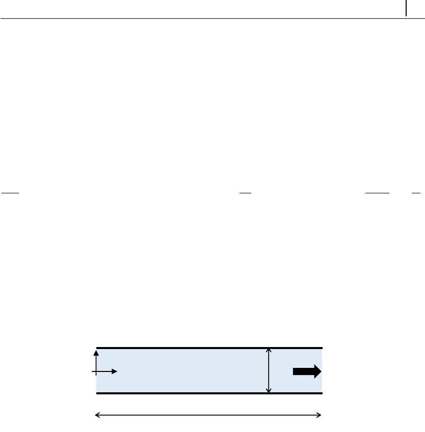
CHAPTER 5. Tutorials 73
5.1.3 Case 1: flow between parallel plates
Itutorials/rheoFoam/Channel/Oldroyd-BLog/
!Overview
In this tutorial, the flow between two infinite parallel plates is simulated for
an Oldroyd-B fluid. Although apparently simple, this case can pose formidable
difficulties using the UCM and Oldroyd-B models at high Weissenberg number
flows [23]. This example also shows that the log-conformation approach is effective
in solving this stability issue, while retrieving the predicted analytical profiles.
Following Ref. [24], the Reynolds number for this problem is defined as Re =
ρUw
η0and the Weissenberg number as W i =λU
w(1 −β), where β=ηs
ηs+ηp=ηs
η0.
The case reproduced in the tutorial is for Re = 0 (the convective term in the
momentum equation is suppressed), W i = 0.99 and β= 0.01.
!Geometry & Mesh
The geometry is a planar channel (two parallel plates) with half-width w, Fig.
5.1. The mesh is composed of 50 cells in the x-direction and 60 cells in the y-
direction, uniformly distributed in both directions.
inlet
outlet
walls
y
x
2w
40w
walls
Figure 5.1: Planar channel geometry.
!Boundary conditions
This flow is 2D, being solved in the xy-plane. A uniform velocity profile (U)
is set at the inlet, along with zero-gradient for pressure and polymeric extra-
stress components. At the outlet, fully-developed flow conditions are assumed
(zero-gradient for all variables, except pressure, which is fixed to a constant value,
p= 0). A no-slip boundary condition is assigned at the walls (velocity is null,
polymeric extra-stress components are linearly extrapolated and a zero-gradient is
assumed for pressure in the normal direction to the wall).
!Command-line
1–Build the mesh:
∼$blockMesh
2–Run the solver:
∼$rheoFoam
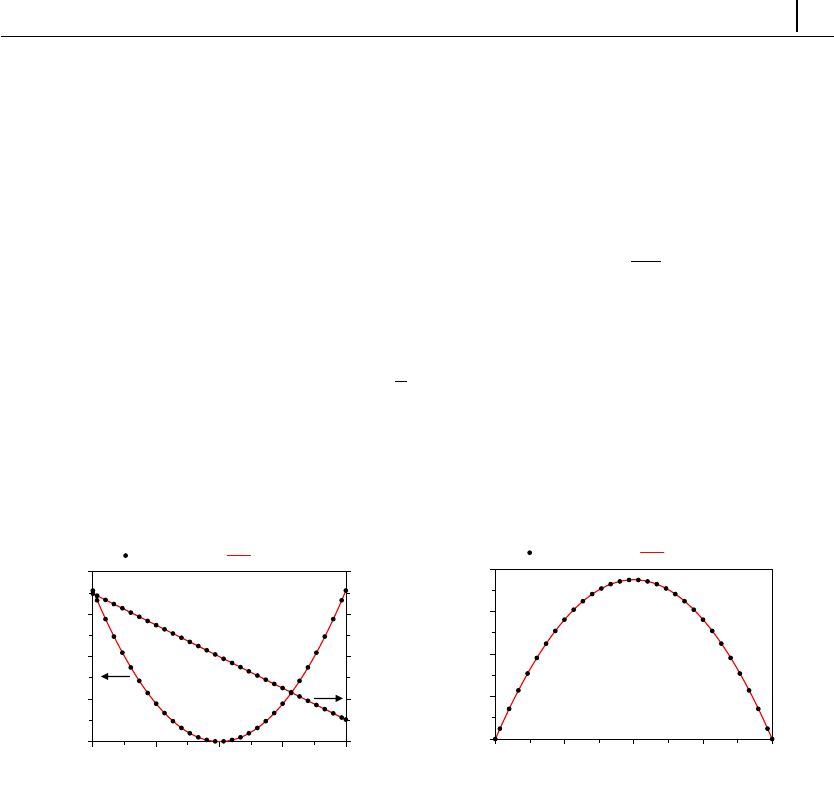
CHAPTER 5. Tutorials 74
3–Extract profiles for uand τalong line x= 35:
∼$sample
!Results
Figure 5.2 presents the fully-developed profiles at line x= 35. The variables
were normalized as follows: length is normalized with w, time with w/U, velocity
with Uand polymeric components of the extra-stress with η0U
w, as in Ref. [24].
A good agreement is observed between the numerical results and the analytical
solution written in dimensionless form [24]:
ux=3
21−y2
τxy =−3(1 −β)y
τxx = 18W i(1 −β)y2
-4
-2
0
2
4
0
5
10
15
20
-1 -0.5 0 0.5 1
τxy
τxx
y
Numerical Analytical
(a)
0.0
0.4
0.8
1.2
1.6
-1 -0.5 0 0.5 1
u
y
Numerical Analytical
(b)
Figure 5.2: (a) Polymeric extra-stress components and (b) velocity, at x= 35,
for Re = 0, W i = 0.99 and β= 0.01.
The user can test the solver with a UCM fluid (β= 0) and confirm that an
accurate solution is still achieved, without facing any numerical issue. However,
running the same cases without the log-conformation approach leads to numerical
divergence (try it!).
This tutorial probes a point in the flow over time (to check for convergence),
which has been specified in controlDict dictionary. The data is written to a
directory named probes/, whose location in the case directory depends on the
OpenFOAM R
version.
5.1.4 Case 2: lid-driven cavity flow
Itutorials/rheoFoam/Cavity/Oldroyd-BLog/
!Overview
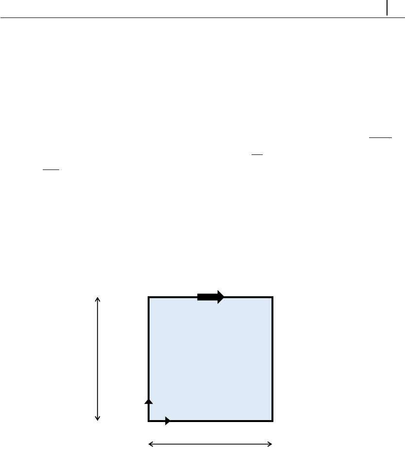
CHAPTER 5. Tutorials 75
The flow in a lid-driven cavity is a common benchmark for numerical solvers,
for both Newtonian and viscoelastic fluids, being one of the mostly used geometries
for such purposes. One reason explaining the popularity is its simple geometry: a
square in 2D or a cube in 3D.
For viscoelastic fluids, stress boundary layers develop at the walls and, at high
Deborah numbers, the flow becomes time-dependent. A similar behavior is ob-
served with Newtonian fluids at high Reynold numbers.
The case reproduced in this tutorial is for an Oldroyd-B fluid with β=ηs
ηs+ηp=
0.5. The Deborah number is defined here as De =λU
L, while the Reynolds number
is Re =ρUL
η0. In this tutorial, we set De = 1 and Re = 0.01, so that the creeping
flow assumption is still adequate, notwithstanding the finite Re.
!Geometry & Mesh
The planar lid-driven cavity is simply a square, with side length L, Fig. 5.3.
The coordinate axis is located at the bottom-left corner. The mesh consists of one
single block with 127 cells uniformly distributed in both directions.
fixedWalls
fixedWalls
fixedWalls
movingLid
L
L
y
x
Figure 5.3: Geometry for the lid-driven cavity flow.
!Boundary conditions
The flow is assumed to be 2D, being solved in the xy-plane. For the three
stationary walls, a no-slip boundary condition is assigned, with null velocity, lin-
early extrapolated polymeric extra-stresses and zero normal gradient for pressure.
At the moving lid wall, the same boundary conditions are used for pressure and
polymeric extra-stresses. Regarding the velocity, a time-space dependent condi-
tion is employed in order to impose a smooth start of the flow, and to avoid a local
singularity with infinite acceleration at the top-right and top-left corners [8]:
Ulid(x, t)=8U[1 + tanh {8(t−0.5)}]x2(1 −x)2(5.1)
CHAPTER 5. Tutorials 76
Eq. (5.1) is directly implemented as a codedFixedValue boundary condition in
file 0/U. The variables were normalized as follows: length is normalized with L,
time with L/U, velocity with U, and polymeric extra-stresses with η0U
L.
!Command-line
1–Build the mesh:
∼$blockMesh
2–Run the solver:
∼$rheoFoam
3–Extract profiles for uand τalong lines x= 0.5 and y= 0.75:
∼$sample
!Results
Figure 5.4 presents spatial profiles for the x-component of the velocity and for
Θxy, along with the evolution over time of the volume-averaged ”kinetic energy”,
defined as
Ek=1
2VtZ|u|2dV=1
2Vt
N
X
k=1 |uk|2Vk=1
2N
N
X
k=1 |uk|2(5.2)
where Nis the number of cells of the mesh and Vt=NVkfor a uniform mesh.
A good agreement is observed between the results obtained by rheoFoam and the
reference data [8], which shows the good accuracy of the solver, both in space and
time. The contour maps for the components of Θare also provided in Fig. 5.5,
together with the flow streamlines.
The ”kinetic energy” is written on run time to the case directory, using a coded
FunctionObject, defined in dictionary controlDict. The reader can check in
this function how Eq. (5.2) has been implemented.
5.1.5 Case 3: flow in a 4:1 planar contraction
Itutorials/rheoFoam/Contraction41/Oldroyd-BLog/
!Overview
The 4:1 planar contraction is another traditional benchmark flow problem for
viscoelastic fluid flow solvers. The existence of singular points at the re-entrant
corners, where stresses grow exponentially as the corner is approached, make this
problem challenging from a numerical perspective.
This tutorial reproduces the work that we developed in Ref. [2] using an early
version of rheoFoam, where an Oldroyd-B fluid (β=1
9) was studied for De = 0−12.
The constitutiveProperties dictionary is adjusted to reproduce the case
for De = 1 and Re = 0.01.
!Geometry & Mesh
The geometry for this case is reproduced in Fig. 5.6. The mesh corresponds to
mesh M1 of Ref. [2].
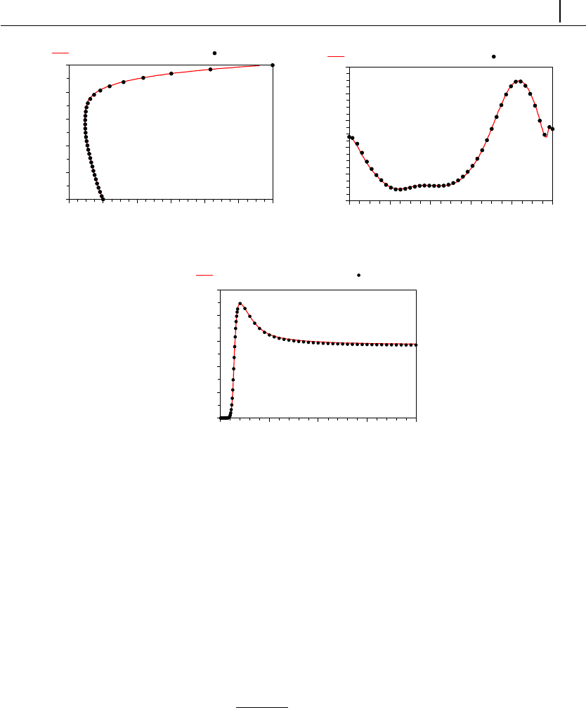
CHAPTER 5. Tutorials 77
0
0.2
0.4
0.6
0.8
1
-0.2 0 0.2 0.4 0.6 0.8 1
y
u (0.5, y)
Fattal & Kupferman (2005) rheoFoam
(a)
-0.4
0
0.4
0.8
1.2
1.6
0 0.2 0.4 0.6 0.8 1
ϴxy (x, 0.75)
x
Fattal & Kupferman (2005) rheoFoam
(b)
0
0.004
0.008
0.012
0.016
0.02
0 2 4 6 8
Ek
t
Fattal & Kupferman (2005) rheoFoam
(c)
Figure 5.4: (a) Velocity profile along line x= 0.5 (at t= 8), (b) Θxy profile along
line y= 0.5 (at t= 8) and (c) evolution of the average ”kinetic energy” over time.
All the results are for Re = 0.01, De = 1 and β= 0.5.
!Boundary conditions
The boundary conditions used are described in Ref. [2]. It is worth mentioning
that the time-varying inlet velocity is implemented as a codedFixedValue boundary
condition in file 0/U. The function is implemented as
u(t) = (1−cos(πt)
fac dirN t≤tlim
Uav t > tlim
(5.3)
where Uav and dirN are vectors, and fac and tlim are scalar parameters. For
Uav = (0.25,0,0), dirN = (1,0,0), fac = 8 and tlim = 1, this generates an inlet
velocity profile aligned with the x-axis and whose magnitude increases from 0, at
t= 0, to 0.25, at t= 1.
!Command-line
1–Build the mesh:
∼$blockMesh
2–Run the solver:
∼$rheoFoam
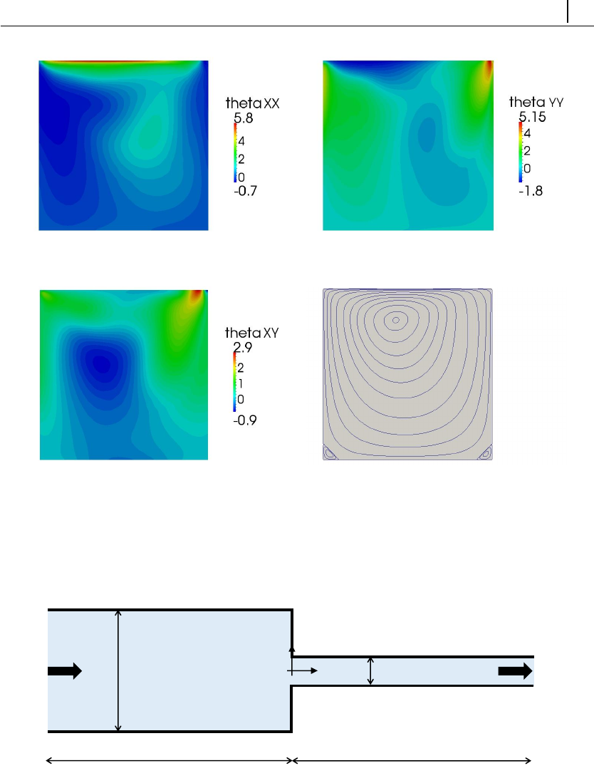
CHAPTER 5. Tutorials 78
(a) (b)
(c) (d)
Figure 5.5: Contours of (a) Θxx, (b) Θyy and (c) Θxy. In (d), the streamlines are
plotted. All the results are for Re = 0.01, De = 1, β= 0.5 and t= 8.
inlet
outlet
2H
100H
wall_vortdown
wall_vorttop
wall_liptop
wall_lipdown
walls
walls
100H
8H
y
x
Figure 5.6: Geometry for the 4:1 planar contraction.
3–Extract uand τat the cell centers immediately upstream and downstream of
vertical line x= 0:
∼$sample
!Results
The results obtained with mesh M1 can be found in Ref. [2].
Acoded FunctionObject returns the points where the wall-parallel velocity com-

CHAPTER 5. Tutorials 79
ponent changes of sign (for both the walls near to the upper lip and corner vortices).
Those points are delimiting the lip and corner vortices (if present). The user can
easily add two extra coded FunctionObjects for the vortices in the lower-half of the
contraction.
5.1.6 Case 4: flow around a confined cylinder
Itutorials/rheoFoam/Cylinder/Oldroyd-BLog/
!Overview
The planar flow past a confined cylinder is another traditional benchmark prob-
lem in computational rheology. Since this flow has no singular points and because
extra-stresses can grow significantly in the wake of the cylinder, this problem is
particularly well-suited to test the accuracy and stability of numerical methods.
Furthermore, it is also a good problem to test the non-orthogonality handling by
the algorithms, both in terms of accuracy and stability, since the grids used for
this problem usually require some degree of non-orthogonality.
The Oldroyd-B model is used in this tutorial, since a reasonable amount of
data is available in the literature for comparison purposes. The Reynolds number
for this flow is defined as Re =ρUR
η0and the Weissenberg number as W i =λU
R. In
order to establish comparable conditions with Refs. [25,26], the solvent viscosity
ratio (β) is fixed at 0.59, the blockage ratio (diameter of cylinder/width of the
channel) is 50 % and Re = 0 (the convective term in the momentum equation is
removed). The case at W i = 0.7 is simulated in this tutorial.
!Geometry & Mesh
The geometry used in this case is composed of a channel with a cylinder of
radius Rvertically centered between its walls – spaced apart 4R–, and placed at
a distance of 20Rfrom the inlet, Fig. 5.7. The length of the channel downstream
of the cylinder is 60R. The mesh for this geometry is composed of 8 blocks (upper-
half), with a high cell-density near the wall of the cylinder. The minimum cell
length in the radial direction of the cylinder is 0.0049R, while in the tangential
direction it is 0.0053R.
!Boundary conditions
The flow is assumed to be 2D, being solved in the xy-plane. At the inlet, a
uniform velocity profile with magnitude Uis imposed, the polymeric extra-stresses
are null and zero-gradient is assigned to pressure. Channel and cylinder walls are
static (velocity is null, polymeric extra-stresses are linearly extrapolated to the
walls and a zero-gradient is imposed for pressure). At the outlet, fully-developed
conditions are assumed: zero-gradient for all variables, except pressure, which is
fixed to a constant value, p= 0.
!Command-line
1–Create half of the mesh:
∼$blockMesh
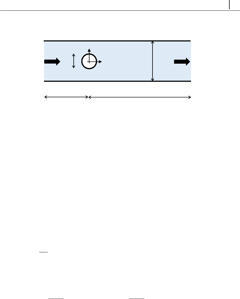
CHAPTER 5. Tutorials 80
walls
walls
inlet
outlet
cylinder
60R
4R
2R
y
x
20R
Figure 5.7: Cylinder vertically centered in a planar channel with 50 % blockage
ratio.
2–Reflect the half-mesh using plane xz as mirror, to obtain the full mesh:
∼$mirrorMesh -noFunctionObjects
3–Run the solver:
∼$rheoFoam
!Results
Figure 5.8 presents the contour plots for the first normal stress difference and
for the velocity magnitude (with superimposed streamlines), at Re = 0, W i = 0.7
and β= 0.59, using the Oldroyd-B model with the log-conformation approach.
Note that the velocity is normalized with U, time with R/Uand polymeric extra-
stresses with η0U
R. The drag coefficient obtained in such conditions is Cd= 117.357,
which is in reasonable agreement with Cd= 117.323 [26] and Cd= 117.315 [25].
Refining the mesh would further increase the accuracy of the numerical solution.
The drag coefficient was computed as
Cd=1
η0Uh Z
SpI+τ0·ˆ
i·dS=1
η0Uh
Nf
X
k=1
Sf·pfI+τ0
f·ˆ
i
where Sfis a vector normal to each face of the cylinder boundary, whose magnitude
is equal to the face’s area, his the depth of the cylinder in the neutral (empty)
direction and ˆ
iis a unitary vector aligned with the streamwise direction. The drag
coefficient is retrieved on run time by a coded FunctionObject, which can be found
in controlDict dictionary.
It should be noted that, although the mesh displays some amount of non-
orthogonality (run checkMesh to confirm it), the non-orthogonality corrector loop
is not used (this is to say that only one iteration is performed) and the explicit
pressure under-relaxation factor is kept relatively high (0.9). These features show
the enhanced stability of the solver. However, to study for example the time
evolution of the drag coefficient, the use of the non-orthogonality corrector loop,
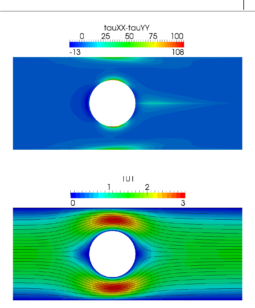
CHAPTER 5. Tutorials 81
(a)
(b)
Figure 5.8: (a) First-normal stress difference and (b) velocity magnitude contours
with superimposed streamlines, at t= 15, for W i = 0.7, Re = 0 and β= 0.59.
combined with inner iterations, is suggested in order to increase the time accuracy
(by decreasing the explicitness of the method). For a high-enough number of
iterations in the non-orthogonal correction loop, under-relaxation of pressure may
eventually be avoided.
5.1.7 Case 5: bifurcation in a 2D cross-slot flow
Itutorials/rheoFoam/CrossSlot/Oldroyd-BLog/

CHAPTER 5. Tutorials 82
!Overview
While the previous tutorials were based on traditional benchmark flow prob-
lems, the case selected for this tutorial is a recent benchmark: the 2D cross-slot
flow [27]. For sufficiently high Deborah numbers, the flow in such geometry be-
comes asymmetric (steady or unsteady) [27]. At the stagnation point generated
by the two opposite-flowing streams, fluid elements can remain for a virtually in-
finite amount of time. Because the local strain-rate is non-zero, the accumulated
strain is high (theoretically infinite at the stagnation point), and this is especially
problematic for models based on springs with an infinite extension – the tensile
normal stress grows exponentially over time near that point. Thus, a singular
point exists in this case, although not being located at a wall, as commonly seen
in other geometries with singularities.
In directory tutorials/rheoFoam/CrossSlot/, there are four tutorials
for this case, each one using a different model or solution method. The tutorial
described here is the one solving the Oldroyd-B model with the log-conformation
approach (Oldroyd-BLog/). The remaining cases are: Oldroyd-BRootk/,
which solves the Oldroyd-B model using the rootkkernel, with k= 8; Oldroyd-B
Sqrt/, which solves the Oldroyd-B model using the square-root transformation
approach; and PTTlinearLog/, which solves the linear PTT model with the
log-conformation approach. All the tutorials with the Oldroyd-B model are for
the same conditions: De = 0.33, Re = 0 and β= 0 (UCM fluid). The tutorial
solving the linear PTT model is for De = 0.6, Re = 0, β= 1/9, ε= 0.02 and
ζ= 0 (simplified PTT). This group of tutorials also solves the transport equation
of a passive scalar, exemplifying how this extra-feature can be used.
The dimensionless numbers for this problem are defined as: Re =ρU W
η0,W i =
λU
W,β=ηs
η0and P e =W U
D. The P´eclet number (Pe) is only relevant for the scalar
transport equation and Dis the diffusion coefficient of the passive tracer. We set
P e = 500 in all the cases (representative, for example, of rhodamine-B in water
flowing in a 200 µm wide channel, at 1 mm/s).
!Geometry & Mesh
The cross-slot geometry for this tutorial is depicted in Fig. 5.9. It consists of
four identical arms (width W; length 10W), where the two vertically opposite arms
are inlets and the remaining are outlets. Each arm is meshed as a single block
with 60 cells in the streamwise direction (cells are compressed near the origin)
and 51 cells uniformly distributed in the transverse direction. As a consequence,
the central square block, (x, y)∈[−0.5W, 0.5W], has 51x51 uniformly spaced
cells. The use of an odd number of cells in both directions of the central square
generates a cell exactly centered at the stagnation point, which is advantageous
for the post-processing of quantities of interest at this location.
!Boundary conditions
The flow is assumed to be 2D, being solved in the xy-plane. At both inlets, a
uniform velocity profile is specified, with magnitude Uand pointing to the origin,
so that those two streams are flowing in opposite directions. The polymeric extra-
stresses are null and for pressure a zero-gradient is used. The walls are stationary,
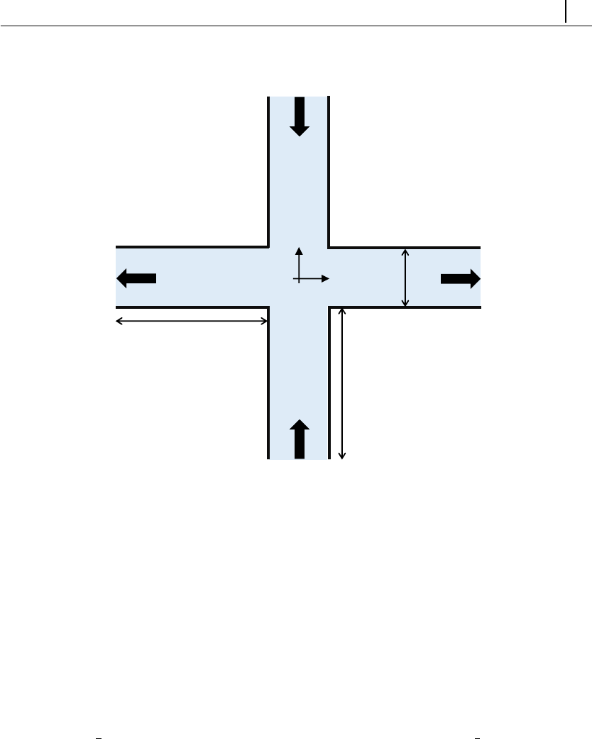
CHAPTER 5. Tutorials 83
y
x
walls
walls
walls
walls
inlet_south
outlet_west
outlet_east
9.5W
inlet_north
9.5W
W
Figure 5.9: Cross-slot geometry composed of 4 arms with two balanced inlets
and two outlets.
thus velocity is null, polymeric extra-stresses are linearly extrapolated and the
pressure is assumed to not change in the normal direction. Fully-developed flow
conditions are assigned at the outlets: null normal gradient for all variables, except
pressure, which is fixed at p= 0.
A passive scalar (tracer field C) is added to the problem, which requires the
assignment of initial and boundary conditions. We impose a continuous injection
of Cat inlet north (C= 1), while no tracer is injected at inlet south (C= 0).
In the remaining boundaries, we impose null normal gradient (meaning no flux of
Cacross the walls and fully-developed flow conditions at both outlets). At time
t= 0, when the simulation is started, the y-positive portion of the cross-slot is
filled with the tracer (C= 1, y > 0∧t= 0).
!Command-line
1–Build the mesh:
∼$blockMesh
2–Create field Cby copying one already present, which is not initialized in the
interior domain:
∼$cp 0/C.org 0/C
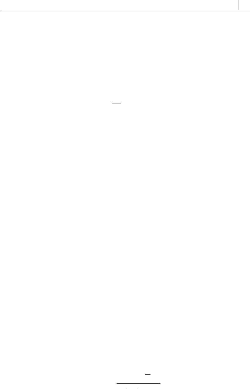
CHAPTER 5. Tutorials 84
3–Initialize field Cin the interior domain (C= 1, y > 0∧t= 0):
∼$setFields
4–Run the solver:
∼$rheoFoam
!Results
The contours for some important variables are displayed in Fig. 5.10, for Re =
0, W i = 0.33, β= 0 (UCM model) and P e = 500. The variables are normalized
with U(velocity), W/U (time) and η0U
W(stresses).
The local Weissenberg number at the origin, defined in Ref. [27] as the product
of the relaxation time by the velocity gradient magnitude at the stagnation point
streamlines, is W i0= 0.523, which is close to the benchmark value obtained in
a similar mesh, W i0= 0.509 (Ref. [27], for mesh M1). The local Weissenberg
number at the origin is retrieved by the solver to the case directory, through a
coded FunctionObject that can be found in dictionary controlDict.
The importance of stress-velocity coupling in this case can be evaluated by re-
running the tutorial with either BSD only or no stabilization method (stabilization
=none or BSD, in dictionary constitutiveProperties).
Checkerboard fields easily develop in such conditions (this is a critical case due to
the use of a UCM fluid).
Note that this tutorial makes use of a variable time-step, controlled by a maxi-
mum Courant number fixed at 0.4. This strategy is used because only steady-state
results are of interest. This is also the reason to use a high tolerance in the sparse
matrix solvers, in fvSolution dictionary – the steady asymmetry in the flow
develops faster with these conditions, since the transient numerical error is higher.
5.1.8 Case 6: blood flow simulation in a real-model aneurysm
Itutorials/rheoFoam/Aneurysm/HerschelBulkley/
!Overview
The tutorial presented in this Section addresses the simulation of blood flow in
a real-model aneurysm. Contrarily to the previous tutorials, this case is based on
a 3D polyhedral (non-orthogonal) mesh and uses a GNF model. Furthermore, the
flow is simulated for a moderate Reynolds number, which will test the robustness
of the solver for such conditions, where inertia already plays an important role.
The Herschel-Bulkley model was selected to simulate the blood rheology, fol-
lowing Ref. [28]. The generalized Reynolds number for this model, assuming τ0= 0
– the power-law limit –, is [28]:
ReGN =ρ(2Rin1)nU2−n
k3n+1
4nn8n−1
This tutorial simulates the flow at ReGN = 420.
!Geometry & Mesh
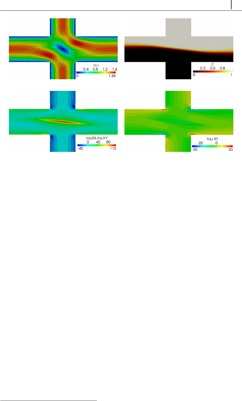
CHAPTER 5. Tutorials 85
(a) (b)
(c) (d)
Figure 5.10: (a) Velocity magnitude contours with superimposed streamlines, (b)
contours of C, (c) first-normal stress difference and (d) τxy contours, for Re = 0,
W i = 0.33, β= 0 and P e = 500.
The STL file of the aneurysm surface was downloaded from a repository with
real-model aneurysms [29], extracted from 3D rotational angiographies of diseased
patients. From the list of available models, case ID C0005 was selected, which
refers to an aneurysm in the internal carotid artery (ICA).
The surface is composed of one main entry vessel (in1, the ICA), which bi-
furcates into two smaller vessels (out1 and out2 ), Fig. 5.11a. The aneurysm is
located near the bifurcation point. Due to the long extension of vessels upstream
and downstream of the aneurysm in the original STL file, all the vessels were
shortened and a cylindrical extension was connected to each one, in order to min-
imize entry/exit effects in the region near the aneurysm. The locations where
those connections were established are highlighted in Fig. 5.11a using red arrows.
The transition length between the tube connectors and the vessels is typically 10
% of the vessel radius and the radius of those tubes is equal to the equivalent
radius of the vessels at the connection point. The radius of each inlet/outlet is:
Rin1 = 1.66 mm, Rout1 = 1.17 mm and Rout2 = 0.95 mm.
The mesh was built using 1cfMesh, a meshing tool available in foam-extend
since version 3.2. The maximum cell size was limited to 5 mm and boundary
cell layers were generated near to the vessel walls in order to accurately solve the
gradients developed there, Fig. 5.11b. The mesh provided with this tutorial has
around 280 kcells.
!Boundary conditions
The boundary conditions and fluid properties used in this tutorial are based in
1http://cfmesh.com/
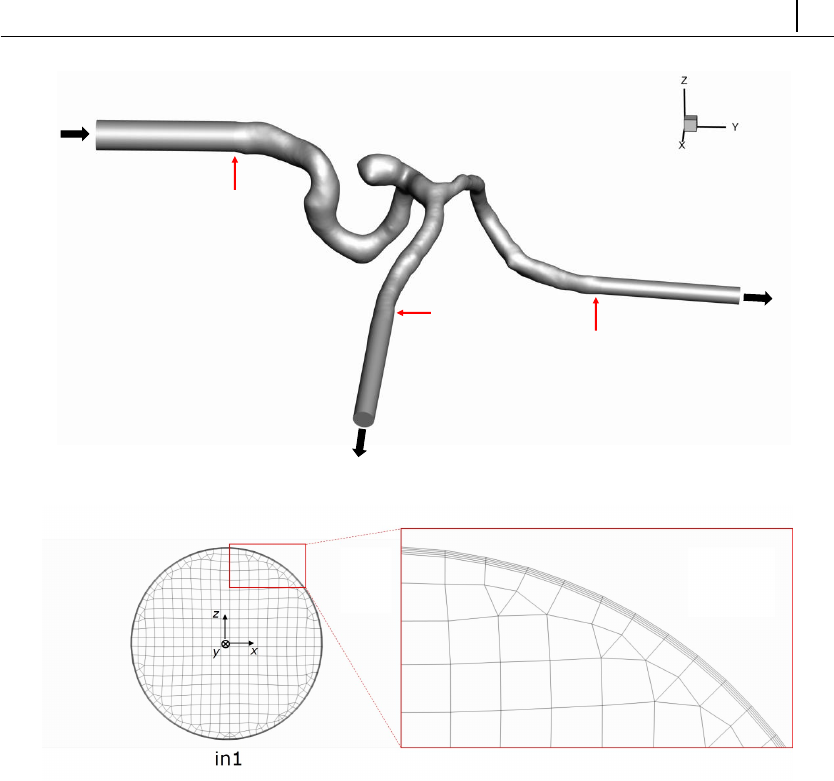
CHAPTER 5. Tutorials 86
in1
out2
walls
out1
(a)
(b)
Figure 5.11: (a) Geometry of the aneurysm considered in the tutorial. Red
arrows point to the transition regions between the aneurysm and the cylindrical
extensions. The radius of each inlet/outlet is: Rin1 = 1.66 mm, Rout1 = 1.17 mm
and Rout2 = 0.95 mm. (b) Detailed view of the mesh on patch in1, zooming the
cell layers near the wall. The reference axis for the geometry is centered on patch
in1, with the normal vector of the patch pointing in the negative direction of the
y-axis.
Ref. [28], where also ICA aneurysms were studied. Accordingly, blood is modeled
with a Herschel-Bulkley model, with τ0= 0.0175 Pa, k= 8.9721 ×10⁻³Pa.sn,
n= 0.8601 and η0= 0.15 Pa.s. Note that η0(see Table 4.1) is a parameter
characteristic of the model implementation in rheoTool, which limits the viscosity
for low strain-rate values – otherwise it would generate infinite values at points
with zero shear-rate. A relatively high value was attributed to η0in order to not
affect the results. Furthermore, a density of 1050 kg/m3is considered.
For this fluid model, a fully-developed velocity profile is imposed at the inlet
(in1 ), along with a null pressure gradient. For small τ0, we can use (approximately)
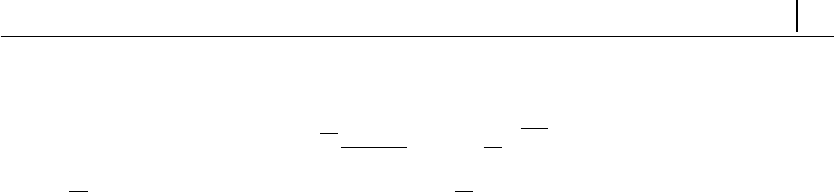
CHAPTER 5. Tutorials 87
the fully-developed velocity profile for a power-law fluid:
U=U3n+ 1
n+ 1 1−r
Rn+1
n(5.4)
where Uis the mean velocity. In our case, Uis constant over time, thus steady
conditions are simulated, instead of the cardiac cycle (this is to shorten the simu-
lation time, since transient solutions would require a lower time-step, leading to a
higher computational time). Regarding the walls, a no-slip boundary condition is
imposed. At the outlets, the pressure is fixed to zero and the velocity is assumed
to be fully-developed (zero gradient for velocity). Since the Reynolds number used
in the tutorial is well below the critical value for transition to the turbulent regime,
no special conditions need to be defined regarding turbulence modeling.
!Command-line
The mesh is already built and can be found in folder polyMesh/.
1–Decompose the case among 2 processors to speed-up the computations (with
2 processors, it takes around 1h to reach convergence in a laptop with an Intel
i5-3210M processor, 2.5 GHz):
∼$decomposePar
2–Run the solver in parallel, using 2 processors:
∼$mpirun -np 2 rheoFoam -parallel
3–Reconstruct the last time-step of the case for post-processing:
∼$reconstructPar -latestTime
!Results
The results obtained at ReGN = 420 are displayed in Fig. 5.12, where both the
streamlines and the wall shear-stress magnitude (WSSmag) contours are shown.
The wall shear-stress magnitude is computed through a ppUtil (described in Sec-
tion 4.5.2), whose settings can be found in dictionary fvSolution, under subDict
PostProcessing.
This tutorial is defined to run with an adjustable time-step, controlled by a
maximum Courant number fixed at 50. The high Courant number is to quickly
achieve the steady-state, without the need to cancel the time-derivatives. The
non-orthogonality corrector loop was turned on, with 1 iteration per time-step
(the pressure is also under-relaxed with a factor of 0.9), in order to avoid possible
numerical issues due to non-orthogonality. The convergence can be monitored by
a probe located at one of the exit vessels, downstream of the aneurysm.
5.2 rheoTestFoam
5.2.1 General guidelines
In Section 4.3.2,rheoTestFoam was presented as a testing application for the con-
stitutive models implemented in rheoTool, being not a general-purpose solver. For
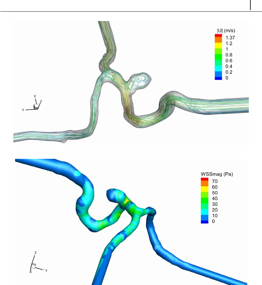
CHAPTER 5. Tutorials 88
(a)
(b)
Figure 5.12: (a) Streamlines (colored with the velocity magnitude) and (b) wall
shear-stress magnitude contours, at steady-state and for ReGN = 420.
this reason, some of the steps usually required to setup a generic simulation in
OpenFOAM R
are not necessary with rheoTestFoam, while, on the other hand,
extra-inputs need to be specified.
|constant/
One main difference of rheoTestFoam cases regarding, for example, rheoFoam
cases is in the mesh: the user should always use the same single-cell unitary mesh
when working with rheoTestFoam. Thus, changing the mesh from case to case is
unnecessary and not recommended.
The dictionary constitutiveProperties is composed of two subDict: pa-
rameters and rheoTestFoamParameters, as displayed in Listing 5.2. The entries in
parameters have exactly the same meaning as previously discussed for rheoFoam.

CHAPTER 5. Tutorials 89
However, there are two entries which remain inactive in rheoTestFoam:rho and
stabilization. Remember from Section 4.3.2 that rheoTestFoam is only solving the
constitutive equations for a given ∇utensor, thus those two parameters related
with the momentum equation are useless. Nevertheless, they should be present
(with any assigned value) to avoid a run time error. rheoTestFoamParameters is
a subDict specific of rheoTestFoam, in the same way as passiveScalarProperties is
a particular subDict of rheoFoam. The keyword ramp stands for the operation
mode (see Section 4.3.2): ramp (true) or transient (false). The other two entries
define tensor ∇u, since we consider ∇u=gammaEpsilonDotL[i]·gradU, where
iis the index representing each entry of list gammaEpsilonDotL. If ramp =false,
the mode is transient and only one entry is expected in gammaEpsilonDotL – the
solver is testing the transient behavior of the constitutive model, for a (single)
given ∇u. On the other hand, in ramp mode (ramp =true), gammaEpsilonDotL
may have as many entries as defined by the user and steady-state variables will be
returned by the solver for each entry. Any combination of components is admissi-
ble for gradU, although only some correspond to canonical rheometric flows. The
one displayed in Listing 5.2 is for a pure-shear flow: u= ( ˙γy, 0,0), where ˙γis the
gammaEpsilonDotL value.
1parameters
{
3type Oldroyd-B;
5etaS etaS [1 -1 -1 0 0 0 0] 1.;
etaP etaP [1 -1 -1 0 0 0 0] 1.;
7lambda lambda [0 0 1 0 0 0 0] 0.1;
9// Place-holder variables in rheoTestFoam
stabilization none;
11 rho rho [1 -3 0 0 0 0 0] 0.;
}
13
rheoTestFoamParameters
15 {
ramp false;
17
gradU (0. 0. 0.
19 1. 0 0.
0. 0. 0.);
21
gammaEpsilonDotL
23 (
1.
25 );
}
Listing 5.2: Example of a constitutiveProperties dictionary used
with rheoTestFoam.
|0/
When using rheoTestFoam, the same fields as for rheoFoam should be present
in folder 0/. However, any value can be assigned to their internal/boundary fields,

CHAPTER 5. Tutorials 90
since the solver will internally manipulate those values (only for velocity) in order
to fulfill the specified ∇u(Fig. 4.2). Shortly, both the mesh and folder 0/
provided in the tutorials can be readily applied to any fluid, without
any change.
|system/
When running rheoTestFoam in ramp mode, the user does not have control
on deltaT (time-step), nor on the endTime. The time step is automatically set
based on the relaxation time and strain-rate values for viscoelastic fluids or is sim-
ply set to 1 s for GNF models (in this case, the value is not important since no
equation is solved implicitly). The endTime in ramp mode is not important, since
the stopping criteria is based on an hard-coded threshold for the residuals and for
the number of iterations. On the other hand, in transient mode, both variables
should be specified by the user in controlDict. Regarding the discretization
schemes (fvSchemes dictionary), only time-derivatives and grad(U) are used by
the solver. The discretization of grad(U) should be kept as Gauss linear, while
any valid time-scheme can be selected (except steady-state), although in ramp
mode this should not make any difference, since we are looking for steady-state
solutions. In dictionary fvSolution, the matrix solvers required by the consti-
tutive equations must be defined and the number of inner-iterations may also be
controlled if running in transient mode. Note that since the mesh has only one
cell, a good time accuracy can be achieved by selecting a small time-step, without
compromising the CPU time (in general, simulations will be always fast). The use
of under-relaxation is not needed, as long as time-derivatives are not disabled in
fvSchemes (this is our recommendation).
5.2.2 Case I: Herschel-Bulkley model
Itutorials/rheoTestFoam/HerschelBulkley/
!Overview
This tutorial illustrates the behavior of the Herschel-Bulkley model used in
tutorial Case 6 to model the blood rheology (Section 5.1.8). A steady shear flow
is considered for this purpose.
!Geometry & Mesh
The geometry used with rheoTestFoam is always the same (see Sections 5.2.1
and 4.3.2). The mesh is already built (do not change it).
!Boundary conditions
The boundary conditions to be used with rheoTestFoam are always the same
(see Sections 5.2.1 and 4.3.2). Folder 0/ should not be changed.
!Command-line
1–Run the solver:
∼$rheoTestFoam
The file Report is created in the case directory, which contains the results.
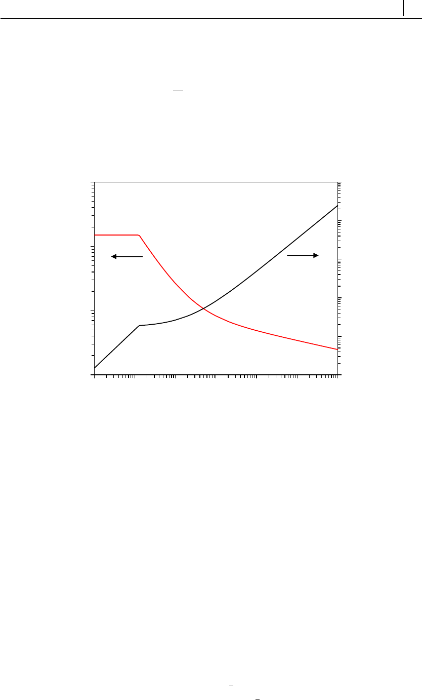
CHAPTER 5. Tutorials 91
!Results
For a GNF model, only the ramp mode of rheoTestFoam makes sense to be
used, since thixotropy is not considered in any of the GNF models implemented.
A steady shear flow is used, thus ∂u
∂y is the only non-zero component of tensor ∇u.
For the range of shear-rates between 0.01 s-1 and 10000 s-1, the Herschel-Bulkley
model behavior is displayed in Fig. 5.13. The model predicts a shear-thinning
behavior for ˙γ > ˙γ0, where ˙γ0is the critical strain-rate at which η=η0. For the
parameters defined in this example, ˙γ0= 0.13 s−1.
0.001
0.01
0.1
1
10
100
0.001
0.01
0.1
1
0.01 0.1 1 10 100 1000 10000
τ'xy (Pa)
η(Pa.s)
Shear-rate (s-1)
Figure 5.13: Shear viscosity and τ0
xy (the only non-zero component of the sym-
metric extra-stress tensor) as a function of the shear-rate, in a steady shear
flow, for the Herschel-Bulkley model with parameters: τ0= 0.0175 Pa, k=
8.9721 ×10⁻³Pa.sn,n= 0.8601 and η0= 0.15 Pa.s.
5.2.3 Case II: FENE-CR model
Itutorials/rheoTestFoam/FENE-CR/
!Overview
This tutorial exemplifies the use of rheoTestFoam, both in transient and ramp
modes, with a constitutive equation for a viscoelastic fluid. The FENE-CR model
is selected and its behavior will be assessed for uniaxial extensional flow.
The uniaxial extensional flow may be described by the following velocity gra-
dient
∇u= ˙ε
1 0 0
0−1
20
0 0 −1
2

CHAPTER 5. Tutorials 92
where ˙εis the extensional rate. The Weissenberg number, W i =λ˙ε, is the di-
mensionless group controlling the rate of stretch induced in the fluid and it was
varied between 0.01 and 100, by increasing the extensional rate from 0.01 to 100
s-1. The fluid properties used in the FENE-CR model are: ηs= 0.1 Pa.s, ηp= 0.9
Pa.s, λ= 1 s and different values of L2were tested (10, 100 and 1000). In such
conditions, the extensional viscosity, defined as ηE=τ0
xx−τ0
yy
˙ε, is given by [19]
ηE= 3ηs+ηp2
1−2λ˙ε/f +1
1 + λ˙ε/f (5.5)
where fis the solution of the cubic equation
(L2−3)f3−(λ˙ε)(L2−3) + L2f2
−2(λ˙ε)2(L2−3) −(λ˙ε)L2+ 6(λ˙ε)2f+ 2(λ˙ε)2L2= 0 (5.6)
!Geometry & Mesh
The geometry used with rheoTestFoam is always the same (see Sections 5.2.1
and 4.3.2). The mesh is already built (do not change it).
!Boundary conditions
The boundary conditions to be used with rheoTestFoam are always the same
(see Sections 5.2.1 and 4.3.2). Folder 0/ should not be changed.
!Command-line
As it is, the tutorial will run in ramp mode.
1–Run the solver:
∼$rheoTestFoam
Take a look to file Report created in the case directory, which contains the results.
!Results
The results computed by rheoTestFoam, and displayed in Fig. 5.14a, show
that the FENE-CR model is correctly implemented, since the difference to the
analytical solution is negligible.
In addition to the ”steady” results in Fig. 5.14a, also the transient evolution
of the extensional viscosity (commonly denoted as η+
Ein the literature) can be
obtained with rheoTestFoam. For that purpose, simply switch the keyword ramp
(in constitutiveProperties) from true to false and define the desired ex-
tensional rate as the first entry of list gammaEpsilonDotL (the remaining entries
can be left, since they will not be read). The results obtained for Wi = 2, 5 and
10 are displayed in Fig. 5.14b.
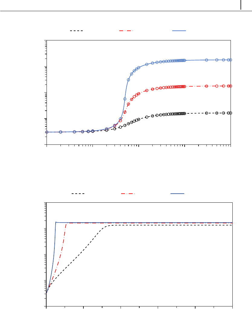
CHAPTER 5. Tutorials 93
1
10
100
1000
10000
0.01 0.1 1 10 100
ηE/η0
λε ̇
L2 = 10 L2 = 100 L2 = 1000
(a)
0.1
1
10
100
1000
0 1 2 3 4 5
ηE+/η0
t/λ
Wi = 2 Wi = 5 Wi = 10
(b)
Figure 5.14: (a) Steady extensional viscosity (ηE) as a function of W i =λ˙ε, for
different values of L2(points represent the numerical results of rheoTestFoam and
the lines correspond to the analytical solution of Eq. 5.5); (b) transient extensional
viscosity η+
Efor different Wi, at fixed L2= 100. The remaining parameters of the
FENE-CR model are ηs= 0.1 Pa.s and ηp= 0.9 Pa.s.
CHAPTER 5. Tutorials 94
5.3 rheoInterFoam
Section 5.3 is under development.
5.3.1 General guidelines
Since most of the steps required to set up a case for rheoInterFoam are the same
as for rheoFoam, only the major differences will be pointed out.
|constant/
The dictionary constitutiveProperties should contain the same infor-
mation as detailed for rheoFoam (Section 5.1.1), for each phase. The principle is
the same as for the default two-phase solvers of OpenFOAM R
(e.g. interFoam),
where each phase owns a dictionary defining its physical properties. Importantly,
subDict passiveScalarProperties, related with the transport of a passive
scalar, is general for the two phases and should only be defined once, outside each
phase. Finally, the surface tension between the two phases – parameter sigma –
should also be present.
Note that when using default names phase1 and phase2 for each phase, without
specifying the name of the phases in a wordList, then it is automatically assumed
that the phases are labeled 1and 2, respectively. Recent versions of OpenFOAMR
have a slightly different behavior regarding phases labeling.
|0/
In folder 0/, the internal and boundary field for the indicator (color) function
used by the VOF method should be defined. The indicator has a value of 1 for
one of the phases and 0 for the other phase. Ideally, and assuming that bound-
ary conditions were correctly assigned, the indicator should remain bounded in
this range. The name given to the file representing the indicator field should be
consistent with the naming in dictionary constitutiveProperties. If the
default names phase1 and phase2 were used, then the indicator function should
be named alpha1. If other name was used instead, then the indicator would be
named alpha suffixed with that name, without spaces in-between (recent versions of
OpenFOAM R
require a separation point). Although there are always two phases,
only one indicator field should be defined, since the indicator for the other phase
is computed from this one. In opposition to what is done in rheoFoam, the pres-
sure field used by rheoInterFoam is not divided by the density, thus retaining its
natural units (Pa.s).
Given that a constitutive equation is being defined and solved individually for
each phase, variables tau and theta should be labeled (suffixed) with the re-
spective phase name. Considering a viscoelastic model for each phase and default
naming of phases, we would have tau1,theta1 and tau2,theta2. If a mul-
timode mode model is assigned to a given phase, then the name of each mode
should also be appended.

CHAPTER 5. Tutorials 95
|system/
The main novelty comparing to rheoFoam is that when using rheoInterFoam
the user has the possibility to choose between PIMPLE and SIMPLEC for pressure-
velocity coupling. This is controled in dictionary fvSolution, in subDict PIM-
PLE, where the keyword SIMPLEC can be assigned to true or false. Independently
of the choice, the momentum equation is always solved. The variable nCorrectors
works in its usual way (looping the pressure equation) and the variable nInIter
assumes the same function as nOuterCorrectors. In a future release of rheoIn-
terFoam, this workflow will most likely change. There are currently these two
options because it is still not clear which one is more advantageous. Still in dictio-
nary fvSolution, other keywords must be assigned in subDict PIMPLE, which
are related with the VOF method and that the reader can found in the tutorials.
In dictionary fvSchemes, the discretization schemes for the two phases should
be defined, as well as the discretization schemes related with the VOF method,
which can also be found in the tutorials.
Besides the Courant number, the solvers using VOF, as rheoInterFoam, can
also restrict the time-step based on an interface Courant number, which should be
defined in dictionary controlDict.
The dictionary setFields, used to initialize parts of the domain with speci-
fied values, should also be present in folder system/ whenever used.
5.3.2 Case 1: impacting drop
Itutorials/rheoInterFoam/ImpactingDrop/Oldroyd-BLog/
!Overview
In this tutorial, a liquid drop composed of a viscoelastic fluid falls under gravity
and its shape (the drop width, more precisely) is monitored before and after the
drop impacts a rigid plate. Under such conditions, the drop width oscillates after
the impact. This problem has been used in the literature as a benchmark case for
viscoelastic two-phase flow solvers (e.g. [30,31]).
The configuration adopted in the tutorial reproduces the conditions in Ref.
[30], where an axisymmetric geometry has been used. The dimensionless numbers
governing the flow are: F r =U0
√gD ,Re =ρU0D
η0,W i =λU0
Dand β=ηs
ηs+ηp, where U0
is the initial velocity of the drop, gis the gravitational acceleration, Dis the drop
diameter, ρis the fluid density, η0is the total viscosity (polymer plus solvent) and
λis the relaxation time (all these fluid properties are for the drop phase). The
problem was simulated for F r = 2.26, Re = 5, W i = 1 and β= 0.1. Note that the
surface tension is set to zero and we assign low (but finite) density and viscosity
values to the fluid surrounding the drop.
!Geometry & Mesh
The geometry is composed by a plate on its bottom, while the other patches
simply act as open boundaries, representing the atmosphere. Axisymmetry is
considered around the y-axis. All the dimensions are expressed as a function of
the drop diameter, Fig. 5.15. The domain is big enough so that we can neglect
the influence of the open boundaries location in the results.
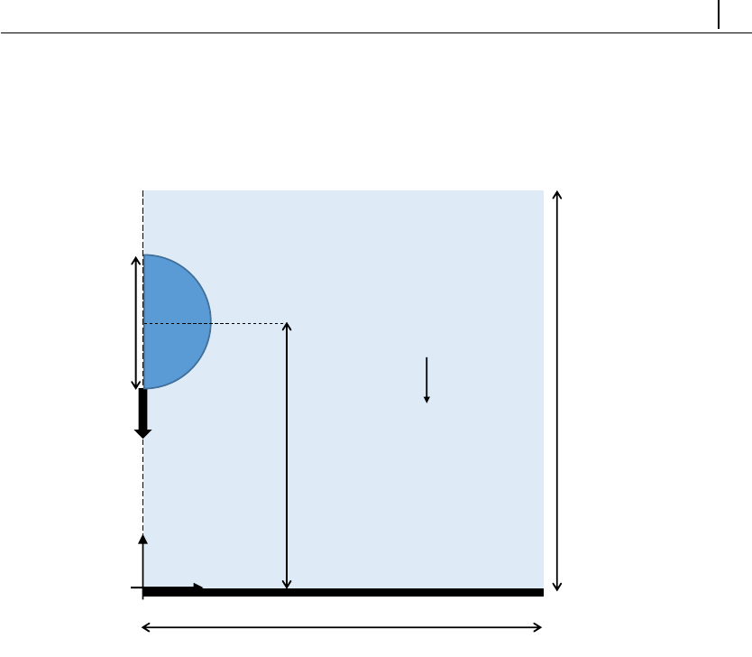
CHAPTER 5. Tutorials 96
The domain is meshed uniformly with 120 cells in both the radial and axial
directions.
axis
atmosphere
y
r
D
3D
plate
3D
2D
atmosphere
phase 2
phase 1
U0
g
Figure 5.15: Geometry for the impacting drop problem.
!Boundary conditions
At the plate, no-slip boundary conditions are imposed with a null velocity,
linearly extrapolated polymeric extra-stress components and zero normal gradient
for the indicator field. We assign a fixedFluxPressure BC to the pressure, as
discussed in Section 4.4.7, for multiphase flows. The patches representing the
open boundaries (atmosphere) are assumed to not interfere with the dynamics of
the drop, so that zero-gradient is assumed for all variables, except the pressure,
which is fixed at p= 0.
Following Ref. [30], the drop has an initial velocity U0, in the vertical direction
(pointing downwards), and its center of mass is at a distance 2Dfrom the plate.
!Command-line
1–Build the mesh:
∼$blockMesh
2–Initialize the indicator and velocity fields in the drop region:
∼$cp 0/alpha1.org 0/alpha1
∼$cp 0/U.org 0/U
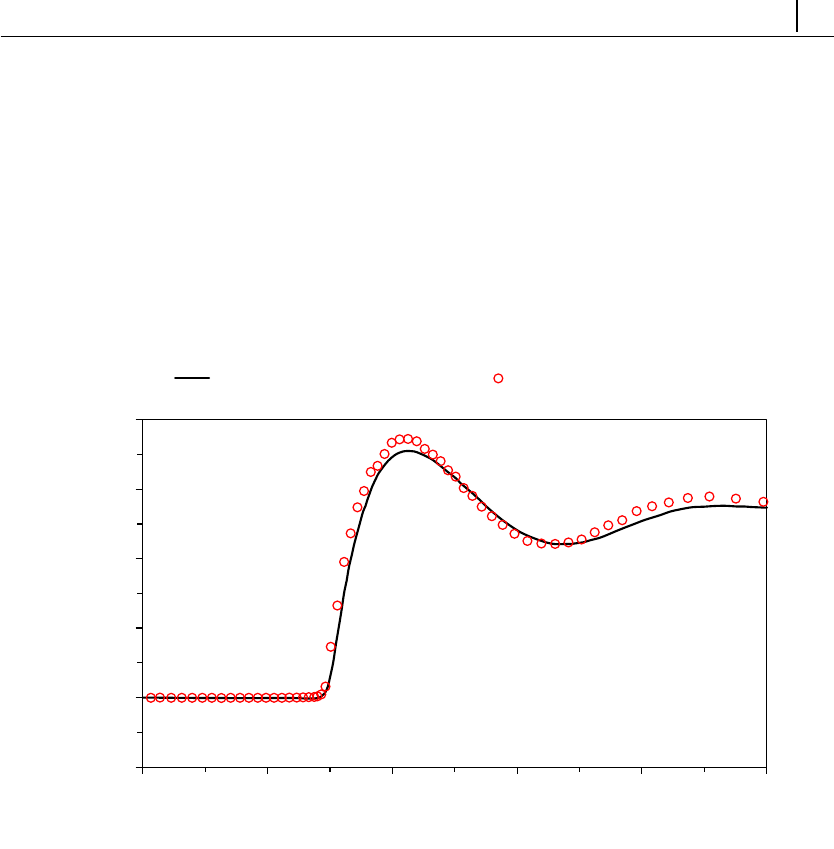
CHAPTER 5. Tutorials 97
∼$setFields
3–Run the solver:
∼$rheoInterFoam
!Results
The evolution of the drop width over time is plotted in Fig. 5.16. The width
is normalized with D(its initial diameter) and time with D/U0. The evolution of
the drop width over time is written to a file by a coded FunctionObject.
0.8
1
1.2
1.4
1.6
1.8
0 1 2 3 4 5
W
t
Figueiredo et al. (2016) rheoInterFoam
Figure 5.16: Evolution of the drop width over time for F r = 2.26, Re = 5,
W i = 1 and β= 0.1. The profile obtained with rheoInterFoam is compared with
the data of Figueiredo et al. [30].
5.3.3 Case 2: planar die swell
Itutorials/rheoInterFoam/DieSwell/
!Overview
A significant number of plastic objects that we use in our everyday life are pro-
duced by extrusion of molten polymers. In this process, the polymeric phase can
swell significantly at the exit of the die due to the development of normal stresses.
Predicting the amount of swell is important for the processing. Moreover, undesir-
able sharkskin defects in the extrudate surface can occur under certain conditions,
and the ability to predict such conditions can potentially reduce industrial wastes.
This tutorial presents the swell of non-Newtonian fluids flowing through a pla-
nar rectangular die. The three cases provided reproduce the results obtained in
Ref. [32] using rheoTool, for mesh M1 and three different fluids: Carreau-Yasuda
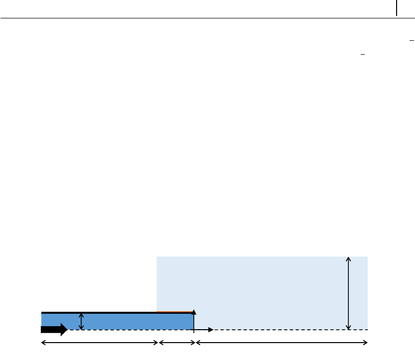
CHAPTER 5. Tutorials 98
fluid with n= 0.3 (directory CarreauYasuda/); Oldroyd-B fluid with β=1
9
and W i = 2 (directory Oldroyd-BLog/); Giesekus fluid with β=1
9,α= 0.5
and W i = 4 (directory GiesekusLog/). The viscoelastic fluid models are solved
with the log-conformation approach. Note that both gravity and surface-tension
effects are neglected in this tutorial. In addition, only the steady-state solution is
of interest.
!Geometry & Mesh
The geometry for this case is displayed in Fig. 5.17. The mesh corresponds to
mesh M1 of Ref. [32]. Note that this is a kind of stick-slip configuration, which
represents a die with negligible wall thickness. Accordingly, patch wallOut overlaps
part of the wallIn patch.
y
x
H
32.5H
40H
4H
2.5H
inlet
outlet
atmosphere
atmosphere
symmetry
phase 2
phase 1
wallIn
wallOut
Figure 5.17: Geometry for the planar die swell tutorial.
!Boundary conditions
The boundary conditions used are described in Ref. [32]. In order to avoid the
definition of an analytical solution at the inlet, a long entrance channel is used.
!Command-line
1–Build the mesh:
∼$blockMesh
2–Initialize the color function field:
∼$cp 0/alpha1.org 0/alpha1
∼$setFields
3–Run the solver:
∼$rheoInterFoam
!Results

CHAPTER 5. Tutorials 99
The results obtained with mesh M1 can be found in Ref. [32]. The users of
the foam-extend version (fe40 ) will notice an instability in the extrudate surface
close to the die exit, which eventually vanishes with time. Such instability is not
present in the OpenFOAM R
versions.
Several methods can be used to compute the amount of swell far from the die
exit. Assuming that the free-surface of the extrudate corresponds to α= 0.5, for
α∈[0,1], this isoline can be directly extracted with Paraview. Another option
is to extract the profile of the color function (α) over a vertical line far from
the die exit, using the sample utility of OpenFOAM R
. Then, the value α= 0.5
can be simply interpolated from the nearest values. A more complex, still more
versatile option is to code a ppUtil function (Section 4.5.2) retrieving in run time
the maximum free-surface position in a predefined region. This would also allow to
check for convergence of the free-surface position. Slight differences can be found
among the results from the different methods.
5.4 rheoEFoam
5.4.1 General guidelines
The first steps to set up a case for rheoEFoam are the same as for rheoFoam
(Section 5.1.1). After that, the hydrodynamic component of the problem will be
ready, and only the electric component will remain to be defined – this is the
subject of this section.
|constant/
The electricProperties dictionary should be added to folder constant
/. It contains most of the information about the EDF model to be used, as shown
in Listing 5.3, illustrating an example for the PNP model.
parameters
2{
type NernstPlanck;
4
T T[0001000]298;
6relPerm relPerm [ 0 0 0 0 0 0 0 ] 80.1;
8psiContrib true;
extraEField extraEField [ 1 1 -3 0 0 -1 0 ] (5000 0
0);
10
species
12 (
cCation
14 {
z z[0000000]1;
16 D D[02-10000]1e-9;
}
18
cAnion
20 {
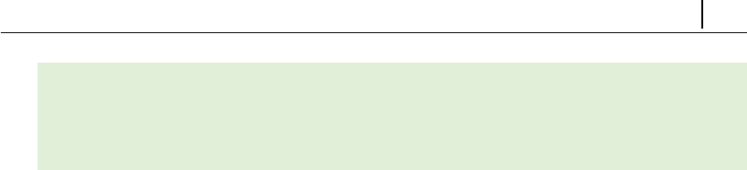
CHAPTER 5. Tutorials 100
z z[0000000]-1;
22 D D[02-10000]1e-9;
}
24 );
}
Listing 5.3: Example of a electricProperties dictionary used with
rheoEFoam – the settings displayed are for the PNP model.
The electric properties in dictionary electricProperties are defined in-
side a subDict named parameters (line 1, Listing 5.3). The EDF model is selected
through keyword type, where the TypeName of any model in Table 4.2 can be used
(the user may type any random word to get the list of all available EDF models).
Apart from the type keyword, all the remaining entries are model-specific. In the
case of the PNP model in Listing 5.3,Tis the absolute temperature and relPerm
corresponds to the relative permittivity (dielectric constant) of the electrolyte, εR,
such that ε=εRε0, where ε0is the vacuum permittivity. In line 8, the entry
psiContrib set to true indicates that variable psi (either Ψor ψ) should con-
tribute to the electric field used in the definition of the electric body-force. The
default behavior, i.e., if the entry is not defined, is psiContrib = true. The next
line (line 9) is also optional and allows the user to define an additional uniform
electric field, extraEField (units are in SI, as always). This electric field will only
enter in the computation of the electric body-force in the momentum equation
(fE=ρE(E+extraEField); extraEField corresponds to vector Eain Table
4.2). Then, from line 11 to 24 each specie of the electrolyte is defined. In the
example, only two species are modeled: cCation and cAnion, each having its own
charge valence (z) and diffusivity (D). Note that the charge valence is a signed
integer: positive for cations and negative for anions. The user can add as many
species as desired to the list, for the model under analysis. The name given to
each specie is user-defined, but consistence must be kept when further defining the
respective fields, as explained next.
The example in Listing 5.3 should not be generalized to all the EDF models, as
stated before. The best way for the user to know how the electricProperties
dictionary should look like for a given EDF model is to analyze a tutorial provided
for that model (at least one tutorial is provided for each model).
|0/
In addition to the fields related with the hydrodynamics (pressure, velocity and
eventually extra-stress), when using rheoEFoam for EDFs, the fields specific to the
given EDF model should be specified in folder 0/ (or the equivalent starting time
folder when different from 0).
For the PNP model illustrated in Listing 5.3, we need to define 3 or 4 fields,
depending if we use one single electric potential or two, respectively. In the first
case, the fields would be psi (in this guide represented by Ψ), cCation and cAni
on (in this guide represented by ci). In the second case, field psi would be replaced
by psi (in this guide represented by ψ) and phiE (in this guide represented by
φExt). Note that although having the same name in both cases, field psi has
different meanings for each one: it is either the total, unique electric potential (Ψ),

CHAPTER 5. Tutorials 101
or the intrinsic electric potential (ψ) – in practice, the Poisson equation to be solved
is different in each case. The selection between both cases is made through variable
phiE: when present, psi is considered the intrinsic electric potential, ψ. It is
important to highlight that the fields representing the concentration of each specie
(in mol/m3) should keep the name defined in dictionary electricProperties,
in a one-to-one correspondence for each specie. These names are user-defined, in
opposition to the names for the electric potential variables, which are fixed: psi
and phiE.
The PNP model is the only to require the definition of fields for the concentra-
tion of each ionic specie. The other EDF models only require the electric potential
(one or two variables, depending on the model and on the user’s choice) to be
defined. The exception is the Ohmic model, which also requires a field for the
conductivity (sigma, in this guide represented by σ). Still for this model, only
one electric potential variable may exist and its name should be phiE. In case of
doubt, checking the tutorials is always a good starting point.
|system/
Since additional equations are solved for EDFs (comparing to pressure-driven
flows), the discretization schemes for the terms entering these equations need to
be defined, as well as the sparse matrix solvers and respective settings.
The discretization schemes are defined in dictionary fvSchemes. The new
entries to add to the dictionary are model-dependent and can be found in the
tutorials. If the discretization scheme for any term is missing, an error will be
retrieved complaining for it.
Regarding dictionary fvSolution, keep in mind when defining the matrix
solvers for the new fields that Poisson-type equations require, in general, a sym-
metric matrix solver, while generic transport equations (including advection) are
usually handled with an asymmetric matrix solver. Regarding under-relaxation,
our recommendations are the same as the ones expressed for rheoFoam: by default,
do not use under-relaxation, except, eventually for pressure in non-orthogonal
grids, if needed. Note that the Nernst-Planck equations for each specie in the
PNP model are collectively solved under the name ci, instead of the name given
to the specie (this should be taken into account when defining the matrix solver
and the under-relaxation factors).
Still in dictionary fvSolution, a new subDict needs to be defined for EDFs,
named electricControls, Listing 5.4. In the code sample analyzed in Section 4.2.4,
we have seen that each equation of a given EDF model is solved inside a while loop,
controlled by a maximum allowable number of iterations and the initial residual
of the equation being solved (the loop is exited when the first of the two criteria
is met). These loops are intended to converge explicit terms inside each equation,
since this can be critical for some EDFs. Thus, the controlling parameters of
these cycles – the maximum number of iterations and the threshold residual – are
defined in subDict electricControls. This needs to be done for each equation, or
default values are assumed otherwise (maxIter: 50; residuals: 10−7). For non-
stiff problems and when the mesh non-orthogonality is kept low, 1 iteration can
be enough. When the PNP model is used, the number of electrokinetic coupling
iterations (see Section 4.2.3) can also be defined in this subDict, as shown in line 3

CHAPTER 5. Tutorials 102
of Listing 5.4 (if not defined, nIterP NP = 2 is assumed by default). As mentioned
in Section 4.2.3, we recommend a minimum of 2 electrokinetic coupling iterations
for any generic case using this model.
1electricControls
{
3nIterPNP 2;
5phiEEqn
{
7residuals 1e-7;
maxIter 1;
9}
11 psiEqn
{
13 residuals 1e-7;
maxIter 1;
15 }
17 ciEqn
{
19 residuals 1e-7;
maxIter 1;
21 }
}
Listing 5.4: Example of an electricControls subDict in dictionary
fvSolution – the settings displayed are for the PNP model.
5.4.2 Case I: EDF of power-law and PTT fluids in a mi-
crochannel
Our first tutorial for rheoEFoam is aimed to predict the velocity profile for a purely
EDF of a power-law fluid (Part A) and for the mixed pressure-/electrically-driven
flow of a linear PTT fluid (Part B) in a slit microchannel. The numerical profiles
are compared with analytical solutions.
○Part A - Power-law fluid
Itutorials/rheoEFoam/channelEDF/PowerLaw/PoissonBoltzmann
!Overview
The analytical solution for the EDF of a power-law fluid in a slit microchannel
can be found in Ref. [33] for a generic flow behavior index (n) of the power-law
model, under the Debye-H¨uckel approximation. For fully-developed flow condi-
tions, the velocity profiles depend on nand on ˜κ=κH =H
λD=q2(zH)2ec0F
εkT ,
where λDis the Debye length for a binary, symmetric electrolyte, as defined in
Eq. (3.32), and His the channel half-width. Although we will only present results
for the PB model, we also provide the corresponding cases for the PNP and DH

CHAPTER 5. Tutorials 103
models – as you will see, the results are indistinguishable between the models, for
the conditions simulated.
!Geometry & Mesh
The geometry is a 2D (slit) microchannel with half-width H, Fig. 5.18. Due
to the periodic boundary conditions assumed on the inlet/outlet, the mesh has
one single cell in the x-direction and 300 non-uniformly distributed cells in the
y-direction, normal to the applied electric field.
inlet
outlet
walls
y
x
H
symmetry
E
Figure 5.18: Planar channel geometry.
!Boundary conditions
The flow is 2D in the xy-plane. At both the inlet and outlet, periodicity is
imposed. Thus, we assume from the beginning that this condition will retrieve the
fully developed profiles for an infinitely long microchannel. A symmetry condition
is imposed at y= 0. The walls are impermeable (u=0and zero-gradient for
pressure) and have a fixed intrinsic electric potential. Due to the simple geometry
of the channel, the flow is generated by imposing a uniform electric field through-
out the channel, parallel to the walls (E). Therefore, there is no need to solve
for the external electric potential variable (phiE ): the electric field is directly im-
posed through the extraEfield entry of dictionary electricProperties. These
boundary conditions hold for both the PB and DH models. In order to use the PNP
model, a boundary condition must be defined at the wall for the ionic species. Since
Boltzmann equilibrium holds and only the steady-solution is sought, the easiest
way is to simply compute the ionic concentration from the potential distribution
(check the boltzmannEquilibrium boundary condition described in Section 4.4.3).
The flow is initially at rest and the intrinsic electric potential is zero.
!Command-line
1–Build the mesh:
∼$blockMesh
2–Run the solver:
∼$rheoEFoam
3–Extract the profile of ualong the vertical direction:
∼$sample -latestTime
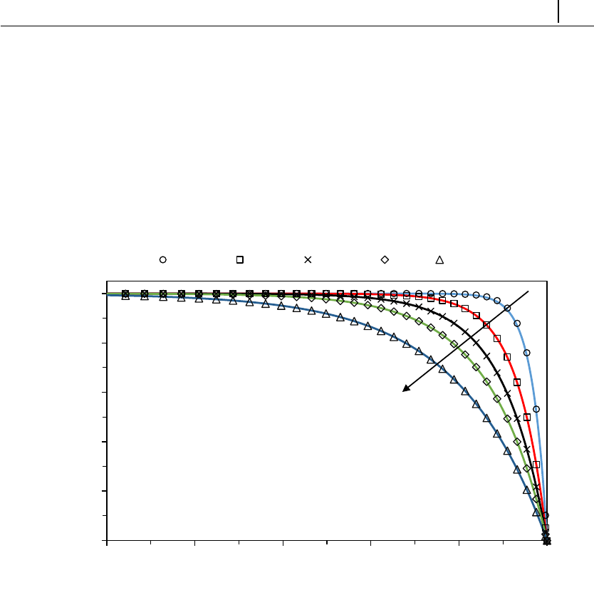
CHAPTER 5. Tutorials 104
!Results
The velocity profiles over the y-direction are depicted in Fig. 5.19 for varying n
= 0.25, 0.5, 0.75, 1 and 1.5, at fixed ˜κ= 15. The velocity profiles are normalized
by the velocity at the centerline of the channel, while the spatial coordinate is
normalized by the channel half-width. The numerical results reproduce accurately
the analytical solution [33] and show that shear-thinning fluids (n < 1) display an
apparently compressed EDL, while the opposite is observed for shear-thickening
fluids (n > 1).
0.0
0.2
0.4
0.6
0.8
1.0
0.5 0.6 0.7 0.8 0.9 1
|u|
y
n=0.25 n=0.5 n=0.75 n=1 n=1.5
n
Figure 5.19: Velocity magnitude over the direction transverse to the applied
electric field for a power-law fluid with different flow behavior index, at fixed
˜κ= 15. The points represent numerical values, while the lines are the analytical
solution [33]. Note that the x-scale has been truncated and only represents one-
quarter of the channel width (this is to have a zoomed view near the wall).
As aforementioned, the same results would be obtained with the PNP and DH
models and the user may confirm that from the cases provided. All the cases
are prepared for n= 0.75 (this can be easily changed in dictionary constitu
tiveProperties) and will converge in the total time of simulation defined in
controlDict. However, we should note that for low n, where n= 0.25 can be
included, the simulation will take a much longer time to reach the steady-state,
because of the low viscosity that develops near the wall, where the shear-rate
attains very high values (it becomes even worse for higher ˜κ). Furthermore, care
should be taken in defining the upper and lower bounds for the viscosity (check
the power-law model implementation in Table 4.1), since stringent bounds may
influence the numerical solution.
○Part B - linear PTT fluid
CHAPTER 5. Tutorials 105
Itutorials/rheoEFoam/channelEDF/PTTlinear/DebyeHuckel
!Overview
Afonso et al. [34] derived an analytical expression for the mixed pressure-
/electrically-driven flow of simplified (ζ= 0) linear PTT fluids in slit channels
with an homogeneous zeta-potential at the walls, under the Debye-H¨uckel approx-
imation. For creeping flow conditions (Re = 0), the velocity profiles depend on
Γ=−H2
ψ0|∇p|
|E|(ratio between pressure and electric forcing), ˜κ=κH =H
λD=
q2(zH)2ec0F
εkT and √εDe =√ελκU, where εis the extensibility parameter of the
PTT model, U=−ψ0|E|
η0is the Helmholtz–Smoluchowski velocity and ψ0is the
zeta-potential at the wall. Both ∇pand Eonly have a single non-zero component,
in our case, the x-component. Note that in this tutorial we use exceptionally to
represent the electric permittivity (instead of ε), in order to distinguish it from ε
that we use to represent the extensibility parameter of the PTT model.
In this tutorial, we analyze the effect of varying Γ, while keeping the remaining
dimensionless parameters fixed.
!Geometry & Mesh
The geometry is similar to the one used in Part A for the power-law fluid ex-
ample. However, the physical dimensions are different and, importantly, we do not
consider periodicity between the inlet and outlet. Instead, the flow is also solved
in the x-direction. We note that this is not mandatory and that cyclic conditions
would also provide the right solution. However, considering the full channel in the
x-direction eases the definition of the pressure gradient, at the expanse of having a
higher number of cells in the mesh. Several options would allow to keep the cyclic
patches and to impose directly the pressure gradient in the momentum equation,
as the fvOptions tool, but we consider them less straightforward than our choice
(at least for less experienced users).
!Boundary conditions
The boundary conditions are similar to the ones used in Part A, with some
modifications required by the use of a viscoelastic model and due to the different
conditions assigned to patches inlet and outlet. Since pressure gradients are al-
lowed, we fix the pressure at the outlet and adjust the inlet pressure as required
to get the desired Γ. Remember that in rheoEFoam field prepresents the pressure
divided by the density. A zero-gradient condition is imposed for the remaining
variables at those two patches. Regarding the wall, the polymeric extra-stresses
are linearly extrapolated.
!Command-line
1–Build the mesh:
∼$blockMesh
2–Run the solver:
∼$rheoEFoam
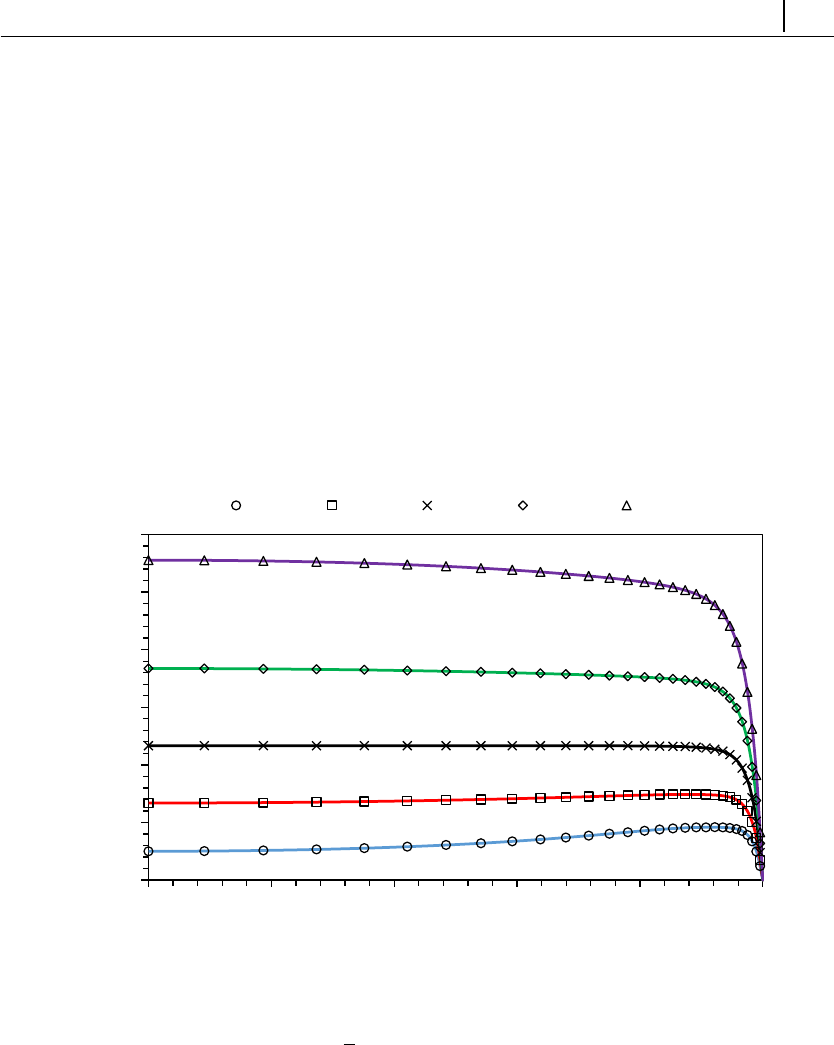
CHAPTER 5. Tutorials 106
3–Extract the profile of ualong the vertical direction for the latest time (the
x-position of the sampling line should not be important):
∼$sample -latestTime
!Results
Fig. 5.20 shows the velocity profiles under different forcing ratios. The velocity
is normalized by the Helmholtz–Smoluchowski velocity (U, defined above), while
the spatial coordinate is normalized by the channel half-width. Note that for a
Newtonian case and Γ= 0 (pure EDF), the (normalized) velocity profile at the
centerline would have a value very close to 1 (the higher ˜κ, the closer it is) and
we can see that this value is significantly higher for a linear PTT fluid due to
shear-thinning.
The parameters provided in the tutorial are for Γ= 4.
0
5
10
15
20
25
30
0 0.2 0.4 0.6 0.8 1
|u|
y
Γ=4
Γ=2
Γ=0
Γ=-2
Γ=-4
Figure 5.20: Velocity magnitude along the direction transverse to the applied
electric field and pressure gradient for a simplified linear PTT fluid, at different
forcing ratios Γ, for ˜κ= 20 and √εDe = 4. The points represent numerical values,
while the lines are the analytical solution [34].
5.4.3 Case II: induced-charge electroosmosis around a cylin-
der
Itutorials/rheoEFoam/ICEO/NernstPlanck
!Overview
This tutorial analyzes the DC induced-charge electroosmosis (ICEO) around a
conducting cylinder. We have investigated this problem in Ref. [3] and we present
in this tutorial the setup used for ˜
V= 0.01 and ˜κ= 10, in mesh M1.
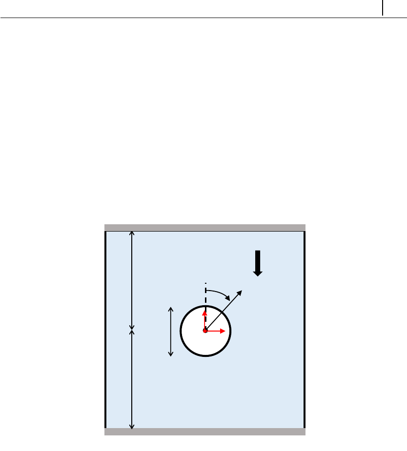
CHAPTER 5. Tutorials 107
In directory tutorials/rheoEFoam/ICEO/, the same case is available un-
der different EDF models (PNP, PB and DH). For the conditions aforementioned,
all give similar results in steady-state. The case for the PNP model uses one po-
tential (Ψ), while the remaining cases are solved under the splitting approach for
the electric potential (both φExt and ψare defined). For the last ones, you can
also see the use of the inducedPotential boundary condition described in Section
4.4.4.
!Geometry & Mesh
The geometry used in this tutorial is displayed in Fig. 5.21, being the same as
in Ref. [3]. The mesh corresponds to mesh M1 of that work, and more details on
the problem definition can be found therein.
elecNorth
wallWest
cylinder
50R
2R
θ
elecSouth
wallEast
50R
E
r
x
y
Figure 5.21: Metallic cylinder placed over an electric field. The surrounding
domain is square (edge size: 100R) and the cylinder lays on its center. The cylin-
drical coordinate system (r, θ) is plotted in black, while the Cartesian coordinate
system (x, y) is represented in red (remember that OpenFOAMR
uses the Carte-
sian system for computations).
!Boundary conditions
The boundary conditions are described in detail in Ref. [3]. It is worth to note
that the boundary conditions of this tutorial, for the PNP model, are different be-
tween the versions of rheoTool. Indeed, we set a zeroGradient BC for the pressure
at the cylinder surface in versions of222 and fe40. However, in version of40 we
use the more accurate fixedFluxExtrapolatedPressure BC, which is not available in
the other versions (see Section 4.4.7). In order to keep the code of rheoEFoam
unchanged, this BC applied in the specific context of this problem – the pressure
field needs an internal reference value/point, because no Dirichlet BC is defined

CHAPTER 5. Tutorials 108
for it – requires that at least one of the remaining boundaries does not fix the ve-
locity (u=0is used in of222 and fe40 ). A simple workaround to this situation,
which would allow to keep the no-slip BC in all the boundaries (without violating
continuity), would be to comment the line where function adjustPhi() is called in
rheoEFoam (file pEqn.H). In practice, both the methods retrieve similar solu-
tions, since the bounding domain is significantly larger than the cylinder radius.
In addition, the major difference between using zeroGradient (of222 and fe40 )
or fixedFluxExtrapolatedPressure (of40 ) for the pressure on the cylinder surface
is essentially observed in the velocity values in the first 2–3 cells adjacent to the
cylinder (more evident at θ= 0 and 180◦). Farther away from the surface, the ef-
fect is barely detected. The differences are more noticeable at higher voltages, but
they vanish with mesh refinement, since this compensates the low-order accuracy
of the zeroGradient BC.
!Command-line
1–Build the mesh:
∼$blockMesh
2–Run the solver:
∼$rheoEFoam
3–Extract profiles of ualong the line θ= 45◦:
∼$sample -latestTime
!Results
You may find the following relation useful in converting the velocity from the
Cartesian base where it is computed, to the cylindrical base used in Ref. [3] to
display the results:
Ur
Uθ=sin(θ) cos(θ)
cos(θ)−sin(θ)Ux
Uy(5.7)
Note that two ppUtil (cf. Section 4.5.2) are used in this tutorial, returning
both the global balance of ions (calcBalance) and the current density through the
cylinder surface (calcJpatch). The latter allows to verify, in this specific case, that
the no-flux boundary conditions for the two ionic species is working as expected,
since a quasi-null current density is retrieved at the boundary where it is assigned.
5.4.4 Case III: charge transport across an ion-selective mem-
brane
Itutorials/rheoEFoam/selecMembrane/NernstPlanck
!Overview
This tutorial presents the charge transport across an ion-selective membrane
and will show the development of the so-called electroconvective instabilities (e.g.
[35]). We addressed this EDF in Ref. [3] and we present in this tutorial the setup
used for ˜
V= 120, in mesh M1. The case is adjusted to run until ˜
t= 0.01, but this
time can be easily increased in controlDict.
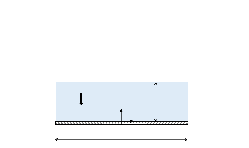
CHAPTER 5. Tutorials 109
!Geometry & Mesh
The geometry for this tutorial is displayed in Fig. 5.22, being the same as in
Ref. [3]. The mesh corresponds to mesh M1 of that work, and more details on the
problem definition can be found therein.
cyc0
reservoir
H
membrane
cyc1
E
6H
y
x
Figure 5.22: Planar reservoir with an ion-selective membrane (only permeable
to cations) on its bottom.
!Boundary conditions
The boundary conditions were described in detail in Ref. [3]. For the users
of OpenFOAM R
v4.x, if the fixedFluxExtrapolatedPressure is intended to be used
at the membrane boundary – this is the most correct option –, then the function
adjustPhi() must be disabled in solver rheoEFoam, as discussed in Section 4.4.7
and in the previous tutorial (again, because no Dirichlet BC is used for pressure,
which automatically enables function adjustPhi()). Since this would require a
permanent change in the solver, we have chosen to use a zeroGradient BC in
replacement. The degree of approximation, as well as the differences between the
two approaches, are the same as for the tutorial in the previous Section (see the
comments therein).
!Command-line
This tutorial is slightly different from the previous ones regarding the command-
line sequence to run. This is because the problem is first solved in a 1D configura-
tion and the resulting solution is then disturbed and used as the starting solution
of the 2D configuration. Thus, we recommend to use directly the Allrun script
to run this tutorial, although we also explain next the main steps accomplished by
that script.
Firstly, in the directory of the main case you will find a folder named so
lution1D/. This is where the 1D problem is solved – script Allrun inside
this folder is the first call of the Allrun in the main directory. Computing the
1D solution is relatively straightforward in what respects the commands to be
executed, since it only requires building the mesh (blockMesh) and running the
solver (rheoEFoam). You may note that the hydrodynamic component of the
solver is switched off through the solveFluid keyword in dictionary fvSolution,

CHAPTER 5. Tutorials 110
which is set to false. Thus, only the Poisson and Nernst-Planck equations are being
solved. Furthermore, we note that underelaxation is being used to compute the 1D
solution in order to enable the use of high time-steps. Under the current settings,
the lower the voltage on patch reservoir, the higher the time for the 1D solution to
converge (the endTime should be increased accordingly in these situations). Our
criteria for convergence relies in the monitor for the current density.
After the 1D solution is computed, the resulting fields are mapped to the 2D
domain (also created with blockMesh beforehand), using the mapFields utility
available by default in OpenFOAM R
. Then, the fields for the cationic and an-
ionic concentration are locally disturbed by a 1 % random perturbation. This is
accomplished by a pre-processing utility named rndPerturbation, which has been
specifically created for this task and that can be found in directory src/libs/p
reProcessing/rndPerturbation/. The case is ready to be run with rheoE-
Foam, noticing that now solveFluid = true.
While the case is running, a ppUtil (cf. Section 4.5.2) is simultaneously being
executed (calcJpatch), which retrieves the surface-averaged current density over
time on both the reservoir and membrane patches (Fig. 5.22).
!Results
The current density can be plotted over time and the contours of charge density
can be computed and visualized in Paraview (these are just some suggestions).
The electric field intensity can be controlled by changing the voltage in file
solution1D/0/psi, under the entry for patch reservoir. Note that any change
in the initial/boundary conditions of any field must be done in the files inside folder
solution1D due to the mapping procedure. By running the Allrun script in
the main folder, the 1D solution will be always computed first.
5.4.5 Case IV: electrokinetic instabilities in a flow-focusing
device
Itutorials/rheoEFoam/EKI/Ohmic
!Overview
This tutorial aims to reproduce qualitatively the electrokinetic instabilities aris-
ing in a flow-focusing device, when electrolytes of different conductivity join at the
converging region. The problem has been extensively studied in Ref. [36], both
experimentally and theoretically.
The use of the Ohmic model is illustrated in this tutorial, which also includes
the transport of a passive, neutral scalar.
As shown by Posner et al. [36], the dynamics of the problem is essentially
governed by three dimensionless numbers: the electric Rayleigh number, RaE=
εE2
ah2
ηD , the conductivity ratio γ=σW
σSand the voltage ratio β=VW
VS. The indices
refer to the north (N), south (S), west (W) and outlet (O) arms of the flow-focusing
device and h= 0.8His the channel depth. Furthermore, an apparent electric field
is computed as Ea=VN−VO
LN+LO, where the denominator of Earepresents the summed
distance of the north and east arms (distance between the ends of each arm, passing
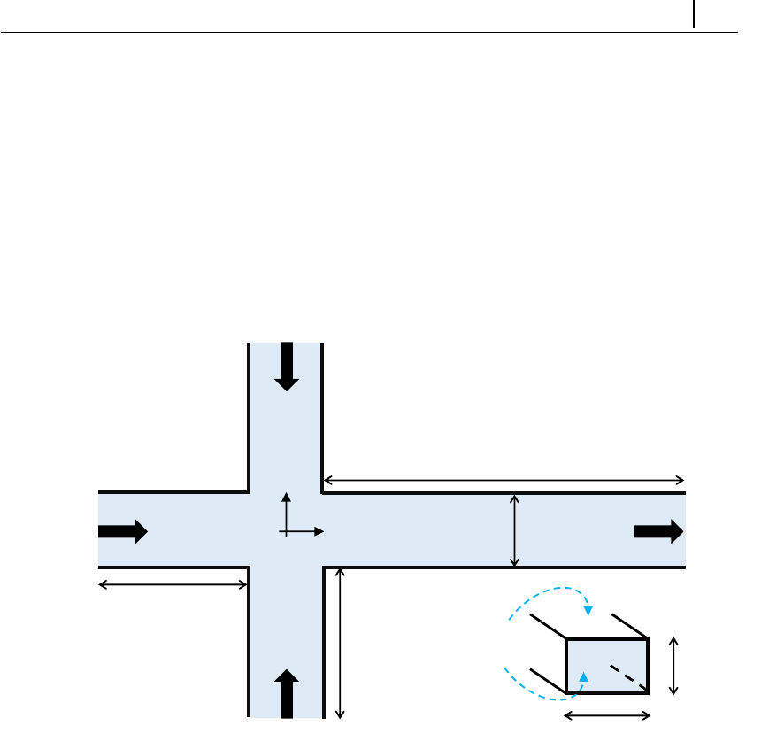
CHAPTER 5. Tutorials 111
by the center of the geometry: LN+LO= 24Hin this tutorial). The parameters
of the tutorial are chosen in order to simulate RaE= 839, γ= 10 and β= 1.05.
!Geometry & Mesh
The geometry is a 3D flow-focusing device (Fig. 5.23) composed of three con-
verging inlets and one outlet. The width and the depth of the channel are uniform
over all the geometry: 2Hand 0.8H, respectively. The inlet arms (west, south
and north) are all 8Hlong, while the outlet arm (east) is 16Hlong.
y
x
walls
walls
walls
walls
inletSouth
intletWest
outlet
7H
inletNorth
7H
2H
15H
2H
0.8H
frontAndBack
Figure 5.23: Three-dimensional flow-focusing device.
The geometry is divided into 12 blocks for meshing purposes. The dimen-
sions of the cells at the junction corners are approximately: (∆x, ∆y, ∆z)≈
(0.1,0.1,0.07)H.
!Boundary conditions
Since the Ohmic model is used in this simulation, we have to define boundary
conditions for pressure, velocity, electric potential and conductivity. We consider
that all the arms are open to the atmosphere, thus p= 0 and a zero-gradient is
assumed for the velocity. At inletNorth and inletSouth, the conductivity of the
fluid entering those arms is the same, but ten times lower than the conductivity of
the fluid entering inletWest (γ= 10). A passive scalar (neutral dye) is also entering
the geometry through inletWest, only. A zero-gradient condition is imposed for
both the conductivity and the passive-scalar concentration at the outlet. At the
walls we assume zero-gradient for all variables, except the velocity. As discussed
in Section 3.5.6, the Ohmic model is usually complemented with a conductivity-
dependent slip velocity (Eq. 3.40). In this tutorial, we use m=−0.3 for the

CHAPTER 5. Tutorials 112
power-law index (see Section 4.4.6). Regarding the electric potential, the outlet
is grounded, while the potential at inletNorth and inletSouth are the same, being
adjusted in order to impose the desired RaE. The potential at inletWest is set
according to β.
Note that the passive-scalar (dye) has a diffusivity which is one order of magni-
tude lower than the diffusivity of the ions (conductivity), in agreement with typical
real conditions.
!Command-line
1–Build the mesh:
∼$blockMesh
2–Create fields Cand sigma by copying the ones already present, but which are
not initialized in the interior domain:
∼$cp 0/C.org 0/C
∼$cp 0/sigma.org 0/sigma
3–Initialize fields Cand sigma in the interior domain (C= 1 ∧σ=σWfor
x < −Hand t= 0):
∼$setFields
4–Run the solver:
∼$rheoFoam
5–Post-process in Paraview (hint: slice the channel at the midplane in the z-
direction and plot the contours of C):
∼$paraFoam
!Results
The contours for the passive-scalar are displayed in Fig. 5.24 at the mid-plane
in z, for different RaE. The reader will probably note similarities between these
instabilities and von-K´arm´an vortex streets.
The patterns are qualitatively similar to those obtained in Ref. [36] (see Fig. 4
therein, although our RaEis defined differently from the one used in that work).
The periodicity or the chaotic behavior of the instabilities can be further evaluated
by looking to the probes of Cand U.
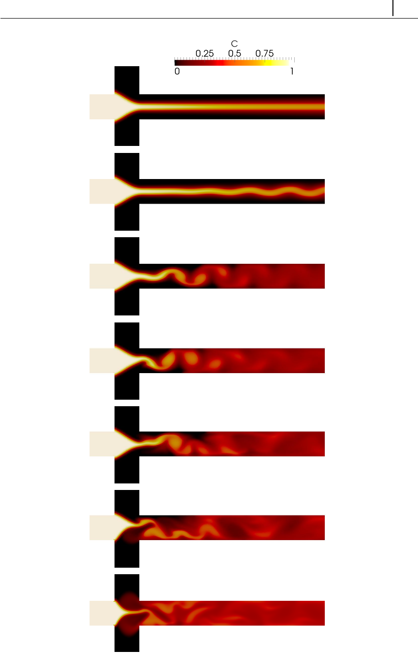
CHAPTER 5. Tutorials 113
RaE= 579
RaE= 481
RaE= 629
RaE= 839
RaE= 1424
RaE= 2164
RaE= 6239
Figure 5.24: Instantaneous contours of Cat the mid-plane in zfor different RaE
(γ= 10 and β= 1.05). The case provided in the tutorial is for RaE= 839 and
the remaining ones can be easily obtained by simply scaling the applied voltage
(phiE) at the inlets (see the definition of RaE).
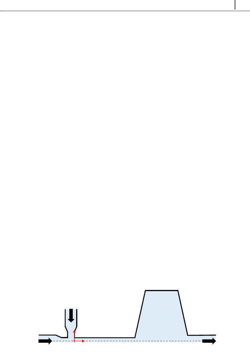
CHAPTER 5. Tutorials 114
Note that we do not used exactly the same parameters as in Posner et al. [36],
since our purpose was solely to illustrate the qualitative behavior of electrokinetic
instabilities, through a fast-running case. The large time-step used (Courant-
controlled, with Co = 1.5) is also inadequate to capture accurately the transient
behavior of this case.
5.4.6 Case V: electrokinetic mixer
Itutorials/rheoEFoam/EKmixer/slipSmoluchowski
!Overview
The main purpose of this tutorial is to illustrate the use of the slipSmoluchowski
EDF model (see Section 3.5.5 and Table 4.2). Although simple, this model is very
useful to simulate Newtonian fluid flows in complex geometries, being accurate for
thin EDL and low intrinsic potentials. In addition, in this tutorial we also use AC
fields, combined with the transport of a passive-scalar.
The case that we propose is an electrokinetic-based micromixer, inspired on the
work of Coleman et al. [37]. In that work, the authors showed that a flow-focusing
geometry followed by an expansion can achieve a good degree of mixing between
two fluids, under AC-driven injection.
Note that this tutorial does not reproduce exactly the same geometrical dimen-
sions, nor the same operating conditions of Ref. [37].
!Geometry & Mesh
The 2D electrokinetic mixer is shown in Fig. 5.25 (the user can check the
dimensions by opening the mesh in Paraview or by inspecting the corresponding
blockMeshDict file). The device consists of a flow-focusing region where one
fluid is injected through inletWest and the other fluid is injected in inletNorth.
The geometry is made symmetric relative to the x-axis and an expansion region
exists downstream to the flow-focusing, which is where the mixing mainly occurs.
symmetry
walls
inletWest
inletNorth
outlet
y
x
Figure 5.25: Electrokinetic mixer similar to the device used by Coleman et
al. [37].
!Boundary conditions
We consider a purely EDF, thus p= 0 at both inlets and outlet boundaries, and
a zero-gradient condition is simultaneously assigned to the velocity. Regarding the

CHAPTER 5. Tutorials 115
externally applied potential, it is fixed at 0 V in the outlet and a custom sinusoidal
boundary condition is imposed at each inlet,
φExt(t) = φExt, DC +φExt, AC sin(2πft +θ) (5.8)
As long as φExt(t)>0 at each inlet, there is a unidirectional net flow of fluid
in the region x > 0, although the fluid can move both forward and backward in
the region x≤0, which constitutes the injecting mechanism of the mixer [37].
By changing φExt, DC, φExt, AC, f and/or θat each inlet, different degrees of mixing
can be achieved. At the wall, zero-gradient is considered for pressure and electric
potential and the Helmholtz-Smoluchowski equation (Eq. 3.33) is used for the slip
velocity.
A passive-scalar is injected at inletWest and the purpose of the mixer is pre-
cisely to achieve the perfect mixing of the passive-scalar stream (inletWest), with
the stream devoid of that scalar (inletNorth) – perfect mixing means C= 0.5 for
a passive-scalar in the range [0,1]. Note that, as stated in Ref. [37], the operating
conditions can be also tuned in order to obtain a pre-defined degree of mixture
different than a 0.5/0.5 stream at the outlet.
!Command-line
Since the list of commands to run is rather extensive, we recommend the user
to simply run the script Allrun. The commands executed by Allrun that might
seem new, regarding what has been done in the previous tutorials, are topoSet and
refineMesh. Those commands select the cells in the expansion region and perform
a refinement in the y-direction, respectively.
!Results
Fig. 5.26 shows the contours of the passive-scalar when either the stream devoid
of C, or rich in C, are injected. Both snapshots were taken after the system has
reached a periodic state. As can be seen, the conditions defined ensure a good
mixing between the streams, since C≈0.5 at the outlet.
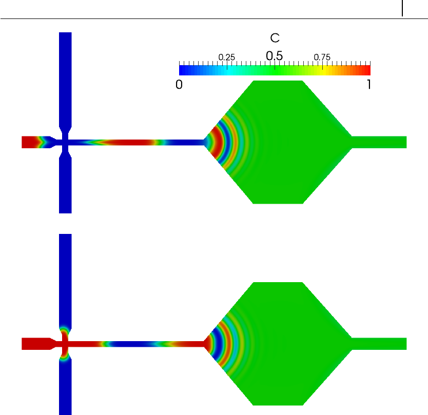
CHAPTER 5. Tutorials 116
(a)
(b)
Figure 5.26: Snapshots of the passive scalar concentration field at different in-
stants: (a) injecting the phase devoid of C(inletNorth) and (b) injecting the phase
rich in C(inletWest). Note that the geometry has been reflected relative to the x-
axis (in Paraview) for presentation purposes – only the upper-half of the geometry
is simulated.
The user can play with the several degrees of freedom of the electric potential
boundary conditions in order to achieve different degrees of mixing. Note that the
time-step used in the tutorial has been adjusted to obtain results in a reasonable
amount time, but it should be lowered to achieve higher accuracy in time. Such
a high time-step, as well as the ”coarse” mesh used, would not be possible to use
if, for instance, the full PNP model was used instead – the simulation would most
likely diverge due to stability issues.
5.4.7 Case VI: electro-elastic instabilities in cross-shaped
geometries
Itutorials/rheoEFoam/EEI/PoissonBoltzmann/
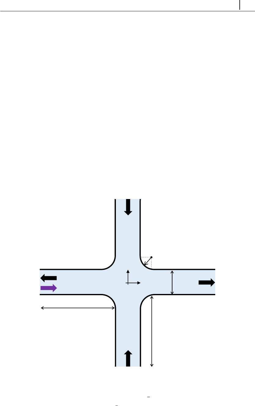
CHAPTER 5. Tutorials 117
!Overview
The electrically-driven flow of high-molecular weight polyacrylamide solutions
in cross-slot and flow-focusing devices was seen to become unstable after a thresh-
old electric potential is exceeded [38]. This tutorial addresses the numerical simula-
tion of such phenomena, as presented in Ref. [38]. This tutorial merges electrically-
driven flows with viscoelastic fluid models, where the electric charge distribution
is computed by the Poisson-Boltzmann model and the extra-stress tensor of the
viscoelastic fluid is evolved using the Oldroyd-B model (β= 0.4). The settings
of the tutorial reproduce the case with ∆V= 160 V, W iB= 2.06, W iκ= 103
(CrossSlot/) and ∆V= 160 V, W iB= 1.03, W iκ= 154 (FlowFocusing/)
of Ref. [38]. The physical time of the simulations is tf= 0.5 s = 10λ.
!Geometry & Mesh
The geometry for this case is displayed in Fig. 5.27. Both the geometry and
the mesh correspond to the ones used in Ref. [38]. The flow is assumed to be 2D,
being solved in the xy-plane. Note that the patch names for the cross-slot and
flow-focusing geometries differ in the west arm, which is either an outlet or an
inlet (Fig. 5.27).
y
x
walls
walls
walls
walls
49H
49H
2H
0.2H
outlet_east
inlet_south
inlet_north
outlet_west
inlet_west
Figure 5.27: Cross-slot and flow-focusing geometries. In the west arm, the black
arrow is for the cross-slot configuration (outlet west) and the purple arrow is for
the flow-focusing configuration (inlet west). In the tutorial, H= 5 ×10⁻⁵m.
!Boundary conditions

CHAPTER 5. Tutorials 118
The boundary conditions used are described in Ref. [38]. The tutorials also
include the transport of a passive tracer. Note that the pressure extrapolation
boundary condition at the wall is replaced by a zero-gradient condition in versions
of222 and fe40, since it is not available therein.
!Command-line
Before presenting the command line sequence, it is worth to note that the
mesh for this case is built in a slightly different way. Indeed, the blockMesh
application only builds one-quarter of the geometry/mesh, the one in the first
quadrant (+,+). The remaining of the geometry/mesh is built by 2 sequential
mirroring operations (mirrorMesh): first using the Oyz plane and then using
the Oxz plane. Afterwards, patches should be renamed accordingly, which requires
selecting, spliting and removing faces of already existing patches (topoSet) and
creation of new ones (createPatch).
1–Build the mesh:
∼$blockMesh
∼$cp system/mirrorMeshDict0 system/mirrorMeshDict
∼$mirrorMesh
∼$cp system/mirrorMeshDict1 system/mirrorMeshDict
∼$mirrorMesh
∼$topoSet
∼$createPatch -overwrite
2–Initialize field Cin the interior domain:
∼$cp 0/C.org 0/C
∼$setFields
3–Run the solver:
∼$rheoEFoam
!Results
The dye patterns (field C) of the unstable flows can be visualized in Paraview.

Appendix A
Parameters and variables in
rheoTool
Table A.1: List of some relevant parameters and variables used by rheoTool and
correspondence with the nomenclature used in this guide.
Name in
the guide
Name in
the code
Dimensions
[kg m s K mol A cd] Definition
αalpha [0 0 0 0 0 0 0]
Anisotropy parameter of
Giesekus and eXtended Pom-
Pom models (scalar)
αalpha [0 0 0 0 0 0 0] Parameter of the piecewise-linear
HRS functions (scalar)
αalpha [0 0 0 0 0 0 0] Indicator/Color function of the
VOF method (scalar)
AA[0 0 0 0 0 0 0] Conformation tensor (symmTen-
sor)
aa[0 0 0 0 0 0 0]
Dimensionless parameter of
Carreau-Yasuda and White-
Metzner models (scalar)
aa[0 0 0 0 0 0 0] Variable of FENE-P model
(scalar)
-AK [0 0 0 0 -1 0 0] Avogrado’s constant (scalar)
βbeta [0 0 0 0 0 0 0] Parameter of the piecewise-linear
HRS functions (scalar)
βbeta [0 0 0 0 0 0 0] CCR coefficient of Rolie-Poly
model (scalar)
119

APPENDIX A. Parameters and variables in rheoTool 120
bb[0 0 0 0 0 0 0] Dimensionless parameter of
White-Metzner model (scalar)
-b[0 0 0 0 0 0 0]
Square-root conformation tensor
of Ref. [10], for the Oldroyd-BSqrt
model (symmTensor)
χmax chiMax [0 0 0 0 0 0 0] Maximum stretch ratio in Rolie-
Poly model (scalar)
-C[0 0 0 0 0 0 0] Passive scalar (scalar)
ci-[0 -3 0 0 1 0 0] Concentration of specie iin
mol/m3(scalar)
c0c0 [0 -3 0 0 1 0 0] Reference ionic concentration
(scalar)
δdelta [0 0 0 0 0 0 0] Exponent of Rolie-Poly model
(scalar)
DD[0 2 -1 0 0 0 0]
Diffusion coefficient in the the
passive scalar transport equation
(scalar)
DiDi [0 2 -1 0 0 0 0] Diffusion coefficient of ionic
specie i(scalar)
µelecMobility [-1 0 2 0 0 1 0] Electroosmotic mobility (scalar)
µ0elecMobility0 [-1 0 2 0 0 1 0] Electroosmotic mobility at a ref-
erence conductivity (scalar)
εepsilon [0 0 0 0 0 0 0] Extensibility parameter of PTT-
type models (scalar)
ε–[-1 -3 4 0 0 2 0] Electric permittivity (scalar)
ε0epsilonK [-1 -3 4 0 0 2 0] Electric permittivity of vacuum
(scalar)
ηeta [1 -1 -1 0 0 0 0] Newtonian viscosity (scalar)
η( ˙γ)eta [1 -1 -1 0 0 0 0] Shear-rate dependent viscosity
from a GNF model (scalar)
η0eta0 [1 -1 -1 0 0 0 0] Zero shear-rate viscosity (scalar)
η0eta0 [1 -1 -1 0 0 0 0] Limiting viscosity in the
Herschel-Bulkley model (scalar)
APPENDIX A. Parameters and variables in rheoTool 121
η∞etaInf [1 -1 -1 0 0 0 0] Infinite shear-rate viscosity
(scalar)
ηmax etaMax [1 -1 -1 0 0 0 0] Upper bound for the viscosity in
the power-law model (scalar)
ηmin etaMin [1 -1 -1 0 0 0 0] Lower bound for the viscosity in
the power-law model (scalar)
ηpetaP [1 -1 -1 0 0 0 0] Polymeric viscosity coefficient
(scalar)
ηsetaS [1 -1 -1 0 0 0 0] Solvent viscosity (scalar)
ΛeigVals [0 0 0 0 0 0 0] Eigenvalues obtained in the diag-
onalization of A(tensor)
ReigVecs [0 0 0 0 0 0 0]
Eigenvectors obtained in the di-
agonalization of Θand A(ten-
sor)
eeK [0 0 1 0 0 1 0] Elementary charge (scalar)
EaextraEField [1 1 -3 0 0 -1 0] Constant and uniform extra elec-
tric field (vector)
ff[0 0 0 0 0 0 0] Variable of FENE-type models
(scalar)
FFK [0 0 1 0 -1 1 0] Faraday’s constant (scalar)
kk[1 -1 -1 0 0 0 0] Consistency index of power-law
model (scalar)
kk[0 0 1 0 0 0 0] Time-scale in the Carreau-
Yasuda model (scalar)
KK[0 0 1 0 0 0 0] Time-scale for ηpin the White-
Metzner model (scalar)
kkbK [1 2 -2 -1 0 0 0] Boltzmann’s constant (scalar)
λlambda [0 0 1 0 0 0 0] Relaxation time (scalar)
λBlambdaB [0 0 1 0 0 0 0] Relaxation time of the backbone
tube orientation (scalar)
λDlambdaD [0 0 1 0 0 0 0] Reptation time (scalar)
λRlambdaR [0 0 1 0 0 0 0] Rouse or stretch time (scalar)
λSlambdaS [0 0 1 0 0 0 0] Relaxation time for the tube
stretch (scalar)

APPENDIX A. Parameters and variables in rheoTool 122
LL[0 0 1 0 0 0 0] Time-scale for λin the White-
Metzner model (scalar)
L2L2 [0 0 0 0 0 0 0] Extensibility parameter of
FENE-type models (scalar)
mm[0 0 0 0 0 0 0] Dimensionless parameter of
White-Metzner model (scalar)
mm[0 0 0 0 0 0 0]
Power-law exponent for
the conductivity-dependent
Helmholtz-Smoluchowski veloc-
ity (scalar)
nn[0 0 0 0 0 0 0]
Flow behavior index for shear-
rate dependent viscosity models
(scalar)
φExt phiE [1 2 -3 0 0 -1 0] Externally-applied electric po-
tential (scalar)
Ψpsi [1 2 -3 0 0 -1 0] Total electric potential (scalar)
ψpsi [1 2 -3 0 0 -1 0] Intrinsic electric potential
(scalar)
pp[1 -1 -2 0 0 0 0] Pressure, in rheoInterFoam
(scalar)
p
ρp[0 2 -2 0 0 0 0]
Pressure divided by the den-
sity, in rheoFoam and rheoEFoam
(scalar)
u·Sphi [0 3 -1 0 0 0 0] Face fluxes (scalar)
qq[0 0 0 0 0 0 0] Amount of arms at the end of the
polymer backbone (scalar)
ρrho [1 -3 0 0 0 0 0] Density (scalar)
ρE-[0 -3 1 0 0 1 0] Charge density (per unit volume)
(scalar)
εRrelPerm [0 0 0 0 0 0 0] Relative electric permittivity or
dielectric constant (scalar)
σsigma [-1 -3 3 0 0 2 0] Electric conductivity (scalar)
σ0sigma0 [-1 -3 3 0 0 2 0] Reference electric conductivity
(scalar)
˙γstrainRate() [0 0 -1 0 0 0 0] Shear-rate (scalar)

APPENDIX A. Parameters and variables in rheoTool 123
τtau [1 -1 -2 0 0 0 0] Polymeric extra-stress tensor
(symmTensor)
τ0tau0 [1 -1 -2 0 0 0 0] Yield stress (scalar)
-tauMF [1 -1 -2 0 0 0 0]
Polymeric extra-stress ten-
sor weighted by the indicator
function in rheoInterFoam
(symmTensor)
Θtheta [0 0 0 0 0 0 0] Natural logarithm of the confor-
mation tensor (symmTensor)
TT[0 0 0 1 0 0 0] Absolute temperature (scalar)
uU[0 1 -1 0 0 0 0] Velocity (vector)
ζzeta [0 0 0 0 0 0 0] Slip parameter of PTT-type
models (scalar)
zizi [0 0 0 0 0 0 0] Charge valence of specie i
(scalar)
Bibliography
[1] J. Favero, A. Secchi, N. Cardozo, and H. Jasak, “Viscoelastic fluid analysis
in internal and in free surface flows using the software OpenFOAM,” Com-
puters & Chemical Engineering, vol. 34, no. 12, pp. 1984 – 1993, 2010. 10th
International Symposium on Process Systems Engineering, Salvador, Bahia,
Brasil, 16-20 August 2009.
[2] F. Pimenta and M. Alves, “Stabilization of an open-source finite-volume
solver for viscoelastic fluid flows,” Journal of Non-Newtonian Fluid Mechan-
ics, vol. 239, pp. 85 – 104, 2017.
[3] F. Pimenta and M. Alves, “Simulation of electrically-driven flows using
OpenFOAM R
,” arXiv:1802.02843, 2018.
[4] R. Fattal and R. Kupferman, “Constitutive laws for the matrix-logarithm
of the conformation tensor,” Journal of Non-Newtonian Fluid Mechanics,
vol. 123, no. 2–3, pp. 281 – 285, 2004.
[5] R. Bird and O. Hassager, Dynamics of Polymeric Liquids: Fluid mechanics,
vol. 1-2 of Dynamics of Polymeric Liquids. Wiley, 1987.
[6] G. Guennebaud, B. Jacob, et al., “Eigen v3.” http://eigen.tuxfamil
y.org, 2010.
[7] X. Chen, H. Marschall, M. Sch¨afer, and D. Bothe, “A comparison of stabilisa-
tion approaches for finite-volume simulation of viscoelastic fluid flow,” Inter-
national Journal of Computational Fluid Dynamics, vol. 27, no. 6-7, pp. 229–
250, 2013.
[8] R. Fattal and R. Kupferman, “Time-dependent simulation of viscoelastic flows
at high weissenberg number using the log-conformation representation,” Jour-
nal of Non-Newtonian Fluid Mechanics, vol. 126, no. 1, pp. 23 – 37, 2005.
[9] A. Afonso, F. Pinho, and M. Alves, “The kernel-conformation constitutive
laws,” Journal of Non-Newtonian Fluid Mechanics, vol. 167–168, pp. 30 – 37,
2012.
[10] N. Balci, B. Thomases, M. Renardy, and C. R. Doering, “Symmetric fac-
torization of the conformation tensor in viscoelastic fluid models,” Journal of
Non-Newtonian Fluid Mechanics, vol. 166, no. 11, pp. 546 – 553, 2011. XVIth
International Workshop on Numerical Methods for Non-Newtonian Flows.
124

BIBLIOGRAPHY 125
[11] ˇ
Z. Tukovi´c and H. Jasak, “A moving mesh finite volume interface tracking
method for surface tension dominated interfacial fluid flow,” Computers &
Fluids, vol. 55, pp. 70 – 84, 2012.
[12] H. Jasak, “Pressure-velocity coupling in FOAM, Consistent derivation for
steady and transient flow solvers.” OFW11, Guimar˜aes, Portugal, 2016.
[13] F. Moukalled, A. A. Aziz, and M. Darwish, “Performance comparison of the
NWF and DC methods for implementing high-resolution schemes in a fully
coupled incompressible flow solver,” Applied Mathematics and Computation,
vol. 217, no. 11, pp. 5041 – 5054, 2011.
[14] H. Jasak, H. Weller, and A. Gosman, “High resolution NVD differencing
scheme for arbitrarily unstructured meshes,” International Journal for Nu-
merical Methods in Fluids, vol. 31, no. 2, pp. 431 – 449, 1999.
[15] A. Afonso, F. Pinho, and M. Alves, “Electro-osmosis of viscoelastic fluids
and prediction of electro-elastic flow instabilities in a cross slot using a finite-
volume method,” Journal of Non-Newtonian Fluid Mechanics, vol. 179–180,
pp. 55 – 68, 2012.
[16] C.-H. Chen, H. Lin, S. K. Lele, and J. G. Santiago, “Convective and abso-
lute electrokinetic instability with conductivity gradients,” Journal of Fluid
Mechanics, vol. 524, pp. 263–303, 2005.
[17] A. Persat and J. G. Santiago, “An ohmic model for electrokinetic flows of
binary asymmetric electrolytes,” Current Opinion in Colloid & Interface Sci-
ence, vol. 24, pp. 52 – 63, 2016.
[18] K. K. Kabanemi and J.-F. H´etu, “Nonequilibrium stretching dynamics of
dilute and entangled linear polymers in extensional flow,” Journal of Non-
Newtonian Fluid Mechanics, vol. 160, no. 2–3, pp. 113 – 121, 2009.
[19] P. J. Oliveira, “Asymmetric flows of viscoelastic fluids in symmetric planar
expansion geometries,” Journal of Non-Newtonian Fluid Mechanics, vol. 114,
no. 1, pp. 33 – 63, 2003.
[20] W. H. Press, B. P. Flannery, S. A. Teukolsky, and W. T. Vetterling, “Nu-
merical recipes (FORTRAN version),” Press Syndicate of the University of
Cambridge, Cambridge, UK, 1989.
[21] F. Habla, A. Woitalka, S. Neuner, and O. Hinrichsen, “Development of a
methodology for numerical simulation of non-isothermal viscoelastic fluid
flows with application to axisymmetric 4:1 contraction flows,” Chemical En-
gineering Journal, vol. 207, no. Supplement C, pp. 772 – 784, 2012. 22nd
International Symposium on Chemical Reaction Engineering (ISCRE 22).
[22] Z. Wu and D. Li, “Mixing and flow regulating by induced-charge electrokinetic
flow in a microchannel with a pair of conducting triangle hurdles,” Microflu-
idics and Nanofluidics, vol. 5, no. 1, pp. 65–76, 2008.

BIBLIOGRAPHY 126
[23] S. Xue and G. W. Barton, “An unstructured finite volume method for vis-
coelastic flow simulations with highly truncated domains,” Journal of Non-
Newtonian Fluid Mechanics, vol. 233, pp. 48 – 60, 2016. Papers presented at
the Rheology Symposium in honor of Prof. R. I. Tanner on the occasion of
his 82nd birthday, in Vathi, Samos, Greece.
[24] Y. Na and J. Y. Yoo, “A finite volume technique to simulate the flow of a
viscoelastic fluid,” Computational Mechanics, vol. 8, no. 1, pp. 43–55, 1991.
[25] M. A. Hulsen, R. Fattal, and R. Kupferman, “Flow of viscoelastic fluids past a
cylinder at high weissenberg number: Stabilized simulations using matrix log-
arithms,” Journal of Non-Newtonian Fluid Mechanics, vol. 127, no. 1, pp. 27
– 39, 2005.
[26] M. Alves, F. Pinho, and P. Oliveira, “The flow of viscoelastic fluids past a
cylinder: finite-volume high-resolution methods,” Journal of Non-Newtonian
Fluid Mechanics, vol. 97, no. 2–3, pp. 207 – 232, 2001.
[27] F. Cruz, R. Poole, A. Afonso, F. Pinho, P. Oliveira, and M. Alves, “A new
viscoelastic benchmark flow: Stationary bifurcation in a cross-slot,” Journal
of Non-Newtonian Fluid Mechanics, vol. 214, pp. 57 – 68, 2014.
[28] A. Valencia, A. Zarate, M. Galvez, and L. Badilla, “Non-newtonian blood
flow dynamics in a right internal carotid artery with a saccular aneurysm,”
International Journal for Numerical Methods in Fluids, vol. 50, no. 6, pp. 751–
764, 2006.
[29] Aneurisk-Team, “AneuriskWeb project website, http://ecm2.mathcs.e
mory.edu/aneuriskweb.” Web Site, 2012.
[30] R. Figueiredo, C. Oishi, A. Afonso, I. Tasso, and J. Cuminato, “A two-phase
solver for complex fluids: Studies of the weissenberg effect,” International
Journal of Multiphase Flow, vol. 84, pp. 98 – 115, 2016.
[31] C. Oishi, F. Martins, M. Tom´e, and M. Alves, “Numerical simulation of drop
impact and jet buckling problems using the extended pom–pom model,” Jour-
nal of Non-Newtonian Fluid Mechanics, vol. 169–170, pp. 91 – 103, 2012.
[32] R. Comminal, F. Pimenta, J. H. Hattel, M. A. Alves, and J. Spangenberg,
“Numerical simulation of the planar extrudate swell of pseudoplastic and vis-
coelastic fluids with the streamfunction and the VOF methods,” Journal of
Non-Newtonian Fluid Mechanics, vol. 252, pp. 1 – 18, 2018.
[33] C. Zhao and C. Yang, “An exact solution for electroosmosis of non-
newtonian fluids in microchannels,” Journal of Non-Newtonian Fluid Me-
chanics, vol. 166, no. 17–18, pp. 1076 – 1079, 2011.
[34] A. Afonso, M. Alves, and F. Pinho, “Analytical solution of mixed electro-
osmotic/pressure driven flows of viscoelastic fluids in microchannels,” Journal
of Non-Newtonian Fluid Mechanics, vol. 159, no. 1–3, pp. 50 – 63, 2009.

BIBLIOGRAPHY 127
[35] C. L. Druzgalski, M. B. Andersen, and A. Mani, “Direct numerical simulation
of electroconvective instability and hydrodynamic chaos near an ion-selective
surface,” Physics of Fluids, vol. 25, no. 11, p. 110804, 2013.
[36] J. D. Posner and J. G. Santiago, “Convective instability of electrokinetic flows
in a cross-shaped microchannel,” Journal of Fluid Mechanics, vol. 555, pp. 1–
42, 05 2006.
[37] J. T. Coleman, J. McKechnie, and D. Sinton, “High-efficiency electrokinetic
micromixing through symmetric sequential injection and expansion,” Lab
Chip, vol. 6, pp. 1033–1039, 2006.
[38] F. Pimenta and M. Alves, “Electro-elastic instabilities in cross-shaped mi-
crochannels,” Submitted for publication, 2018.
