VELMA 2.0 User Manual Current
User Manual: Pdf
Open the PDF directly: View PDF ![]() .
.
Page Count: 180 [warning: Documents this large are best viewed by clicking the View PDF Link!]
- The Simulator Configuration file specifies the Names of all other input data files.
- The Simulator Configuration file specifies the Location of all other input data files.
- ESRI Grid ASCII (.asc)
- Comma-Separated Value (.csv)
- Simple Text Files (.txt)
- The Flat-Processed DEM File
- The Cover Species ID Map File
- The Cover Species Age Map File
- The Soil Parameters ID Map File
- The Precipitation Driver Data File
- The Air Temperature Driver Data File
- The Observed Runoff Data File
- The Observed Stream Chemistry Data File
- Required Input Files
- Configuration Steps
- Specify Startup Parameters
- Specify Input Parameters
- Click an underlined hyperlink to jump to configuration instructions
- 0.0 All Configuration Parameters
- 1.0 Input Data Location
- 2.0 Results Data Location
- 3.0 Spatial Dimensions and DEM File
- 4.0 Soil Types
- 4.0 Soil Types
- Important Information for Sections 5.0 – 25.0 of the All Parameters TOC
- 5.0 Cover Types
- 6.0 Weather Model
- 7.0 Initialize Uniform Water Amount per Cell
- 8.0 Chemistry Pools (Dissolved C and N)
- 9.0 Nitrogen Deposition
- 10.0 Transpiration
- 11.0 Plant Uptake
- 12.0 Plant Mortality
- 13.0 Decomposition
- 14.0 Nitrogen-Fixation
- 15.0 Nitrification
- 16.0 Denitrification
- 17.0 Simulation Run Schedule
- 18.0 Years to Compute Nash-Sutcliffe for Runoff
- 19.0 Observed Data Files
- 20.0 Simulation-End Data Capture for Spin-up Initialization Use
- 21.0 Simulation-Start Initialization from Spin-up Data
- 22.0 Cell Data Writer Items
- 23.0 Spatial Data Writer Items
- 24.0 Disturbance Items
- 25.0 Runtime Chart Display Scale
- 0.0 – All Configuration Parameters (link to All Parameters TOC)
- 1.0 – Input Data Location (link to All Parameters TOC)
- 2.0 – Results Data Location (link to All Parameters TOC)
- 3.0 – Spatial Dimensions and DEM File (link to All Parameters TOC)
- 4.0 – Soil Types (link to All Parameters TOC)
- IMPORTANT INFORMATION FOR SECTIONS 5.0 – 25.0 OF THE ALL PARAMETERS TOC (link to All Parameters TOC)
- 5.0 – Cover Types (link to All Parameters TOC)
- 6.0 – Weather Model (link to All Parameters TOC)
- A Summary Description of the Snow Model’s Behavior
- You Must Explicitly Specify Activation of the Spatial Weather Model
- You Must Provide the Weather Model with Rain and Air Temperature Driver Files
- You Must Provide Files of Coefficients for Precipitation and Air Temperature Calculations
- The Spatial and Default Weather Model Both Employ the Same Snow Model
- 7.0 – Initialize Uniform Water Amount per Cell (link to All Parameters TOC)
- 8.0 – Chemistry Pools (Dissolved C and N) (link to All Parameters TOC)
- 9.0 - 9.1.1 – Nitrogen Deposition (link to All Parameters TOC)
- 10.0 – Transpiration (link to All Parameters TOC)
- 11.0 Plant Uptake (link to All Parameters TOC)
- 12.0 Plant Mortality (link to All Parameters TOC)
- 13.0 Decomposition (link to All Parameters TOC)
- 14.0 Nitrogen-Fixation (link to All Parameters TOC)
- 15.0 Nitrification (link to All Parameters TOC)
- 16.0 Denitrification (link to All Parameters TOC)
- 17.0 – Simulation Run Schedule (link to All Parameters TOC)
- The Forcing Start and End Years Specify When a Simulation CAN Run
- The Simulation Start and End Years Specify When a Simulation WILL Run
- The Loops Parameter Specifies How Many Times the Simulation Repeats a Run
- Use the All Parameters Outline Selector to Focus on the Simulation Run Schedule Parameters
- You Can Also Review and Set Some of these Values in the Run Parameters Tab
- 18.0 – Years to Compute Nash-Sutcliffe for Runoff (link to All Parameters TOC)
- The VELMA Simulator Calculates a Nash-Sutcliffe Value for Runoff
- Set the Observed Runoff Source File
- Set the Years to Simulation the Nash-Sutcliffe
- The VELMA Simulator Writes the Nash-Sutcliffe Coefficient for Runoff to an Output File
- The Computed Nash-Sutcliffe Value is Only as Accurate as the Observed Data
- 19.0 – Observed Data Files (link to All Parameters TOC)
- 20.0 – Simulation-End Data Capture for Spin-up Initialization Use (link to All Parameters TOC)
- 21.0 – Simulation-Start Initialization from Spin-up Data (link to All Parameters TOC)
- (1) Create a common simulation configuration base .xml document
- (2) Make two copies of the base simulation configuration .xml document
- (3) Modify the Spin up configuration to save spatial data state at the end of its simulation run
- (4) Modify the Actual configuration to initialize its spatial data state at simulation start.
- (5) Run the Spin up simulation to completion.
- (6) Run the Actual simulation to completion.
- 22.0 – Cell Data Writer Items (link to All Parameters TOC)
- Cell Data Writers Allow You to Gather Simulation Results for a Specific Grid Location
- Adding a Cell Data Writer to a Simulation Configuration
- Configuring a Cell Data Writer’s Parameters
- A Cell Data Writer has only 3 parameters, but they must all be set correctly: none are optional.
- Cell Data Writer Output is A Comma-Separated Values File
- Cell Data Writers and Spatial Data Writers are Different, but Complementary
- 23.0 – Spatial Data Writer Items (link to All Parameters TOC)
- Spatial Data Writers Report a Simulation Result for Every Cell in the Simulation Grid
- Adding a Spatial Data Writer to a Simulation Configuration
- Configuring a Spatial Data Writer’s Parameters
- The Spatial Data Sources Parameter Specifies What Data Is Written
- The Three “InitializeActive…” Parameters Specify When Data Is Written
- You May Emphasize the Watershed Cells, or Not
- You May Reduce the Dimensions of the Results Grid File
- Spatial Data Writer Output is a Grid ASCII File
- Spatial Data Writers and Spatial Data Writers are Different, but Complementary
- Table of Spatial Data Sources
- 24.0 – Disturbance Items (link to All Parameters TOC)
- 25.0 – Runtime Chart Display Scale (link to All Parameters TOC)
- Different runtime display charts use different subsets of the display parameters. Unfortunately, nothing listed under “All Parameters 25.0 Runtime Chart Display Scale” indicates which display parameters belong to a particular runtime display chart. T...
- For example, if you want to adjust VELMA’s “Annual Plot” display for soil humus, you would find “Annual Plot” under the “Display Selector Name” column in the table below, copy “maxHumusDayDisplay” and paste it in the “Parameter” search window in the V...
- (Link to All Parameters Table of Contents)
- (Link to All Parameters Table of Contents)
- Add the New Disturbance Parameters to the Simulation Configuration
- Configure the New Disturbance Parameters
- (Link to All Parameters Table of Contents)
- (Link to All Parameters Table of Contents)
- Where are VELMA Simulator Results Located?
- What Results are Available after a VELMA Simulation is Run?
- (Link to All Parameters Table of Contents)
- (Link to All Parameters Table of Contents)
- (Link to All Parameters Table of Contents)
- Start JPDEM
- Loading DEM Data Into JPDEM
- Flat Processing DEM Data In JPDEM
- Saving Flat-Processed DEM Data From JPDEM To a File
- II. Watershed Delineation

1
VELMA Version 2.0
User Manual and Technical Documentation
September 17, 2014
U.S. Environmental Protection Agency
Office of Research and Development
National Health and Environmental Effects Research Laboratory
Western Ecology Division
Corvallis, Oregon 97333
Robert B. McKane (mckane.bob@epa.gov)1
Allen Brookes (brookes.allen@epa.gov)1
Kevin Djang (djang.kevin@epa.gov)2
Marc Stieglitz (marc.stieglitz@ce.gatech.edu)3
Alex G. Abdelnour (abdelnouralex@gmail.com)3,5
Feifei Pan (feifei.Pan@unt.edu)3,4
Jonathan J. Halama (halama.jonathan@epa.gov)1
Paul B. Pettus (pettus.paul@epa.gov)1
Donald L. Phillips (phillips.donald@epa.gov)1
1U.S. Environmental Protection Agency, Western Ecology Division, Corvallis, OR 97333
2CSC, Corvallis, OR 97333
3School of Civil & Environmental Engineering, Georgia Institute of Technology, Atlanta, GA 30332
4Current address: Department of Geography, University of North Texas, Denton, TX 76203
5Current address: McKinsey & Company, 133 Peachtree Street, N.E., Atlanta, GA 30303

2
ACKNOWLEDGEMENTS
The information in this document has been funded in part by the U.S. Environmental Protection Agency. It
has been subjected to the agency’s peer and administrative review, and it has been approved for
publication as an EPA document. This research was additionally supported in part by NSF grants 0439620,
0436118, and 0922100. We thank our many colleagues who have contributed data and advice during the
course of developing VELMA and its applications: Sherri Johnson, Barbara Bond, Mark Harmon, Fred
Swanson, Julia Jones, Suzanne Remillard, Theresa Valentine, and Don Henshaw with the H.J. Andrews Long
Term Ecological Research (LTER) program; John Blair, John Briggs, and Loretta Johnson with the Konza
Prairie LTER program; Don Weller and Tom Jordan, Smithsonian Environmental Research Center; Bill
Peterjohn, West Virginia University; Larry Band, University of North Carolina; Irena Creed, University of
Western Ontario; George Ice, Oregon State University; Ed Rastetter and Bonnie Kwiatkowski, Ecosystems
Center, Marine Biological Laboratory; Brenda Groskinsky, Don Phillips, Jana Compton, Renee Brooks, and
many others at the U.S. Environmental Protection Agency.
DISCLAIMER
Neither the United States Environmental Protection Agency (USEPA) nor the Georgia Institute of Technology
(GT) makes any warranty or assume any legal liability or responsibility for the accuracy, completeness, or
usefulness of any information, product, or process described herein. Reference to any special commercial
products, process, or service by trade name, trademark, manufacturer, or otherwise, does not necessarily constitute
or imply endorsement, recommendation, or favoring by the USEPA or GT. The views and opinions of the authors
do not necessarily reflect those of the USEPA or GIT.
3
Table of Contents
I. Introduction .............................................................................................................................................6
II. Changes in VELMA Version 2.0 ............................................................................................................8
III. How to Use This Manual .......................................................................................................................9
IV. Required Input Data Files for VELMA Simulations ...........................................................................11
Details of Specific File Formats .............................................................................................................13
Details of Specific Input Data Files .......................................................................................................14
V. Creating a Simulator Configuration (New VELMA Application)........................................................18
Start the JVelma GUI .............................................................................................................................19
Using the GUI ........................................................................................................................................21
Using the GUI to Specify Startup and Input Parameters .......................................................................23
Overview of the All Parameters Table of Contents (TOC) ...................................................................26
All Parameters TOC ..............................................................................................................................26
VI. Steps for Configuring All Parameters TOC Sections 0.0 – 25.0 .........................................................29
0.0 All Configuration Parameters .........................................................................................................29
1.0 Input Data Location ........................................................................................................................30
2.0 Results Data Location ....................................................................................................................31
2.1 Results Data Directory Name .....................................................................................................31
2.2 Results Directory Logfile Names ...............................................................................................32
3.0 Spatial Dimensions and DEM File .................................................................................................33
3.1 DEM Row and Column Counts ..................................................................................................34
3.2 DEM Cell Size ............................................................................................................................34
3.3 Watershed Outlet ........................................................................................................................34
4.0 Soil Types .......................................................................................................................................35
4.1 Soil ID Map File .........................................................................................................................35
4.2 Soil IDs and Names ....................................................................................................................36
4.3 Soil Depth Values .......................................................................................................................37
4.4 Soil Ks Values ............................................................................................................................38
4.5 Soil Other Hydrologic Parameters ..............................................................................................40
Important Information for Sections 5.0 – 25.0 of the All Parameters TOC ...........................................41
5.0 Cover Types ...................................................................................................................................43
5.1 Cover ID Map File......................................................................................................................44
5.2 Cover Age Map File ...................................................................................................................45
5.3 Cover IDs and Names .................................................................................................................44
5.4 Cover Carbon-To-Nitrogen Ratios .............................................................................................46
4
5.5 Cover Uniform-Cell Initialization Amounts ..............................................................................46
5.6 Cover Gale-Grigal Root Parameters ...........................................................................................47
5.7 Cover Leaf Stem and Root Pool Parameters ..............................................................................49
6.0 Weather Model ...............................................................................................................................53
6.1 Weather Rain Driver File ...........................................................................................................54
6.2 Weather Air Temperature Driver File ........................................................................................54
6.3.1 Weather Model Coefficients Files (Only Spatial Weather) ....................................................55
6.4 Latitude/Longitude .....................................................................................................................60
6.5 Solar Radiation ...........................................................................................................................60
6.6 Soil Layer Temperature ..............................................................................................................60
7.0 Initialize Uniform Water Amount per Cell ....................................................................................61
8.0 Chemistry Pools (Dissolved C and N) ...........................................................................................62
8.1 Chemistry Amounts for uniform cell-initialization ....................................................................62
8.2 Chemistry Water Loss Fractions ................................................................................................63
9.0 Nitrogen Deposition .......................................................................................................................64
9.1 Nitrogen Deposition Model Selection ........................................................................................64
10.0 Transpiration ...............................................................................................................................65
10.1 Core PET and ET Parameters ..................................................................................................66
10.2 ET Recovery On/Off? ..............................................................................................................66
10.3 Transpiration Limiter On/Off? .................................................................................................67
11.0 Plant Uptake .................................................................................................................................69
11.1 Plant Uptake NH4-specific .......................................................................................................70
11.2 Plant Uptake NO3-specific .......................................................................................................70
11.3 Plant Uptake GEM Temperature Component ..........................................................................71
11.4 Plant Update NPP Distribution Fractions .................................................................................72
11.5 Plant Uptake Phenology ...........................................................................................................73
12.0 Plant Mortality ..............................................................................................................................74
12.1 Plant Mortality Logistic or Linear? ..........................................................................................74
12.2 Plant Mortality Phenology ........................................................................................................77
13.0 Decomposition .............................................................................................................................77
13.1 Decomposition Nitrogen-To-DON Fraction ............................................................................78
13.2 Decomposition CO2 Respiration Fraction ...............................................................................78
13.3 Decomposition Microbe Efficiency .........................................................................................78
13.4 Decomposition Cover-Specific Parameters ..............................................................................79
14.0 Nitrogen-Fixation .........................................................................................................................80
14.1 Nitrogen-Fixation On/Off? .......................................................................................................82
5
15.0 Nitrification ..................................................................................................................................82
15.1 Nitrification On/Off? ................................................................................................................83
16.0 Denitrification ..............................................................................................................................85
16.1 Denitrification On/Off? ............................................................................................................86
17.0 Simulation Run Schedule .............................................................................................................88
18.0 Years to Compute Nash-Sutcliffe for Runoff ..............................................................................90
19.0 Observed Data Files .....................................................................................................................91
20.0 Simulation-End Data Capture for Spin-up Initialization Use ......................................................92
21.0 Simulation-Start Initialization from Spin-up Data .......................................................................92
22.0 Cell Data Writer Items .................................................................................................................94
23.0 Spatial Data Writer Items .............................................................................................................96
23.1 Spatial Data Writer Items by Model Type ...............................................................................96
23.2 Spatial Data Writer Items Data Sources ...................................................................................97
23.3 Spatial Data Writer Items Core Scheduling .............................................................................98
23.4 Spatial Data Writer Items Output Map Size .............................................................................98
24.0 Disturbance Items .......................................................................................................................102
24.1 Disturbance Items by Model Type .........................................................................................108
24.2 Disturbance Items Core Scheduling .......................................................................................111
24.3 Disturbance Items Spatial Specifiers (Raster Rally) ..............................................................109
25.0 Runtime Chart Display Scale ....................................................................................................114
Appendix 1: Overview of VELMA’s Leaf-Stem-Root (LSR) Plant Biomass Submodel .......................121
Appendix 2: Initializing a Spatial Data Pool Using an ASCII Grid ........................................................133
Appendix 3: Creating Initial ASCII Grid Chemistry Spatial Data Pools ................................................136
Appendix 4: Overview of VELMA Simulator Output ............................................................................141
Appendix 5: Generating daily temperature and precipitation grids for running VELMA ......................144
Appendix 6.1: VELMA version 1.0, Part 1 of 2, HYDROLOGICAL Model Description .....................163
Appendix 6.2: VELMA version 1.0, Part 2 of 2, BIOGEOCHEMICAL Model Description .................169
Appendix 7: Creating Flat-Processed DEM Data For The VELMA Simulator and Determining Outlet
and Watershed Delineation ......................................................................................................................177

6
I. Introduction
VELMA – Visualizing Ecosystems for Land Management Assessments – is a spatially distributed, eco-
hydrological model that links a land surface hydrology model with a terrestrial biogeochemistry model for
simulating the integrated responses of vegetation, soil, and water resources to interacting stressors. For example,
VELMA can simulate how changes in climate and land use interact to affect soil water storage, surface and
subsurface runoff, vertical drainage, evapotranspiration, vegetation and soil carbon and nitrogen dynamics, and
transport of nitrate, ammonium, and dissolved organic carbon and nitrogen to water bodies. VELMA differs from
other existing eco-hydrology models in its simplicity, flexibility, and theoretical foundation. The model has a
user-friendly Graphics User Interface (GUI) for easy input of model parameter values. In addition, advanced
visualization of simulation results can enhance understanding of results and underlying concepts. VELMA’s
visualization and interactivity features are packaged in an open-source, open-platform programming environment
(Java / Eclipse). The development team for VELMA version 2.0 includes Dr. Bob McKane and coworkers at the
U.S. Environmental Protection Agency’s Western Ecology Division, Dr. Marc Stieglitz and coworkers at the
Georgia Institute of Technology, and Dr. Feifei Pan at the University of North Texas.
1.1. Application of VELMA to Various Ecosystems
VELMA’s hydrological and biogeochemical submodels have been verified for simulating the effects of changes
in climate and land use on streamflow, stream chemistry, and ecosystem carbon and nitrogen dynamics
(Abdelnour et al. 2011, 2013; http://onlinelibrary.wiley.com/doi/10.1029/2010WR010165/full;
http://onlinelibrary.wiley.com/doi/10.1029/2012WR012994/full). To date, we have calibrated VELMA for a
wide range of major ecosystem types across North America, focusing primarily on data-rich sites in the National
Science Foundation’s Long Term Ecological Research (LTER) network (http://www.lternet.edu/lter-sites). These
ecosystem types include temperate forest LTER sites in Oregon, New Hampshire, and North Carolina; the Konza
Prairie LTER in Kansas; agricultural watersheds in the Chesapeake Bay and Willamette River Basin; and the
arctic tundra LTER in Alaska.
1.2. Decision Support
We developed VELMA to help support two recent sustainability initiatives by the EPA Office of Research and
Development: the Safe and Sustainable Waters Research Program (SSWR) and the Sustainable and Healthy
Communities Research Program (SHC). Our goal is to provide comprehensive decision support tools that can
help communities, tribes, land managers and policy makers address present needs without compromising the
ability of society and the environment to meet the economic, social and environmental needs of future
generations. Key decision support goals are to (1) assess the effectiveness of natural and engineered green
infrastructure for protecting water quality of streams and estuaries, and (2) quantify the ecosystem goods
and services that ecosystems provide for humans.
VELMA was recently redesigned (version 2.0, described herein) to better address both these goals. Green
infrastructure (GI) involves the establishment of riparian buffers (streamside vegetation), cover crops, constructed
wetlands, and other measures to intercept, store and transform nutrients, toxics and other contaminants that might
otherwise reach surface and ground waters. GI enhancements have also strengthened model capabilities for
quantifying how alternative land use and policy scenarios affect tradeoffs among important ecosystem services –
that is, the capacity of an ecosystem to provide clean water, flood control, food and fiber, climate (greenhouse
gas) regulation, fish and wildlife habitat, among others (Millennium Ecosystem Assessment 2005). Model
development has been guided by the principle of parsimony to enable VELMA to efficiently address multiple
spatial and temporal scales – plots to basins, days to centuries.
While VELMA has already proven useful for quantifying how such ecosystem services interact and respond in
concert to environmental changes (http://eco.confex.com/eco/2012/webprogram/Paper37040.html;
http://eco.confex.com/eco/2010/techprogram/P25975.HTM), it is important to also quantify the economic and
social impacts associated with such changes. Therefore, we are collaborating with Oregon State University to
link VELMA with ENVISION, a well-established decision support tool that integrates landscape GIS layers,
ecological models, economic valuation models, and user-defined stressor scenarios

7
(http://envision.bioe.orst.edu/). The recently completed Envision-VELMA linkage is described in our SHC
2.1.4.2 product for September 2014.
To date, we have prototyped ENVISION for the 30,000 km2 Willamette River Basin in Oregon to examine how
alternative scenarios (2010 – 2060) of land use and human population growth affect "bundled" ecosystem
services. This work examines the capacity of the landscape to support projected increases in human populations
under alternative growth plans (smart growth, unmanaged growth, and status quo) and consequent trade-offs in
provisioning of agricultural and forest products, clean supplies of water, carbon sequestration, and habitat for
wildlife populations (Bolte et al. in review; Bolte et al. 2011, http://www.thesolutionsjournal.com/node/1019).
1.3. Products and Impacts
The major product of this research will be a set of broadly applicable decision support tools that enable
communities, client offices and other stakeholders to (1) assess the effectiveness of green infrastructure options
for protecting water quality, (2) quantify tradeoffs among ecosystem goods and services associated with
alternative land use decision scenarios, and (3) generate community sustainability indicators and their trajectories
to help communities balance environmental, economic and social criteria over timescales relevant to immediate
needs and long-term (decades to centuries) planning goals.
Using a participatory planning and outreach approach that integrates researchers, stakeholders and decision
makers, we will address several questions pertinent to community sustainability:
• Can methodologies be developed to quantify and value ecosystem services, so that this natural capital can
be better accounted for in decisions that affect the supply of the goods and services upon which human
well-being depends?
• What are the uncertainties associated with various decision options? Is there an optimal “decision path”
for restoring the natural capital needed to sustainably support communities dependent on resource-based
economies, such as the agricultural, forest, and fishing industries?
• Can those factors that have the greatest potential to improve future trajectories of ecosystem services and
human well-being be identified? For example, what green and grey infrastructure improvements, carbon
and nitrogen management practices, and growth and development policies can most effectively be
managed to attain a sustainable and desirable future?
The linkage of VELMA and ENVISION is intended to provide stakeholders with a user-friendly, visual interface
for exploring the consequences of alternative climate and land use scenarios on ecosystem service tradeoffs.
Outputs will be computer-generated visualizations of predicted changes in multiple ecosystem services, both in
biophysical and economic terms. Our overall goal is to provide a framework for integrated assessments that
identify policy and management strategies for entire ecosystems and the bundled services they provide, rather
than piecemeal assessments of individual services.
1.4. References
Abdelnour, A., M. Stieglitz, F. Pan, and R. McKane (2011) Catchment hydrological responses to forest harvest
amount and spatial pattern, Water Resources Research, 47, W09521, doi:10.1029/2010WR010165.
Abdelnour, A., R. McKane, M. Stieglitz, F. Pan, and Y. Cheng (2013) Effects of harvest on carbon and nitrogen
dynamics in a Pacific Northwest forest catchment, Water Resources Research, 49,
doi:10.1029/2012WR012994.
Abdelnour, A., R. McKane, M. Stieglitz and F. Pan. Catchment biogeochemical responses to forest harvest
amount and spatial pattern. Submitted to Water Resources Research.
Bolte, J., R. McKane, D. Phillips, N. Schumaker, D. White, A. Brookes, C. Burdick and D. Olszyk (in review),
An extensible decision support system for evaluating ecosystem services under alternative future scenarios – a
Willamette River Basin case study. EPA publication number ORD-002136
Bolte, J., R. McKane, D. Phillips, N. Schumaker, D. White, A. Brookes, and D. Olszyk (2011) In Oregon, the
EPA calculates nature’s worth now and in the future. Solutions 2(6): 35-41.
McKane, R., A. Abdelnour, A. Brookes, C. Burdick, K. Djang, T.E. Jordan, B. Kwiatkowski, F. Pan, W.T.
Peterjohn, M. Stieglitz and D.E. Weller (2012) Identifying green infrastructure BMPs for reducing nitrogen

8
export to a Chesapeake Bay agricultural stream: model synthesis and extension of experimental data. The
Ecological Society of America 97th Annual Meeting, Portland, OR, August 2012.
McKane, R., M. Stieglitz, A. Abdelnour, F. Pan, B. Bond, S. Johnson (2010) An integrated eco-hydrologic
modeling framework for assessing the effects of interacting stressors on multiple ecosystem services. The
Ecological Society of America 95th Annual Meeting, Pittsburgh, PA, August 2010.
MEA, Millennium Ecosystem Assessment (2005) Ecosystems and human well-being: synthesis. Island,
Washington, DC.
II. Changes in VELMA Version 2.0
The original version of VELMA (henceforth referred to as version 1.0 or v1.0) has been previously described
(Abdelnour et al. 2011, 2013). VELMA version 2.0 (v2.0), described herein, includes a number of important
changes that are designed to facilitate green infrastructure and ecosystem service applications of interest to
communities, tribes, land managers and policy makers. In summary, this required:
- Enhancements to the hydrological and biogeochemical submodels to better simulate effects of green
infrastructure management practices on the fate and transport of water, nutrients and toxics across
multiple spatial and temporal scales – plots to basins, days to centuries (details below).
- A new graphical-user-interface (GUI) to assist novice and experienced model users in scenario
development, model calibration, and visualization and interpretation of results.
- Rewriting the program code in Java / Eclipse to facilitate debugging and open source (community) model
development. The version 1.0 Processing code is no longer supported.
- A new user manual (this document) that provides a step-by-step guide to setting up and applying VELMA
v2.0.
Details follow on changes to the hydrological and biogeochemical submodels in VELMA v2.0:
1) Hydrological submodel:
a. Evapotranspiration (ET) submodel revised to include
i. effect of leaf biomass (surrogate for leaf area); replaces submodel for simulating effect of
stand age on ET (Abdelnour et al. 2011)
ii. effect of stand age on ET in forest systems
2) Biogeochemical submodel:
a. Single land cover simulator revised to include multiple land cover types within watersheds
b. Plant Soil Model (PSM) approach for simulating plant biomass in aggregate (Stieglitz et al. 2006;
Abdelnour et al. 2013) replaced by a Leaf-Stem-Root (LSR) submodel that simulates carbon (C)
and nitrogen (N) dynamics for leaves, aboveground stems belowground stems, and fine roots (<2
mm diameter).
c. Decomposition submodel replaced by Potter et al. (1993) submodel and further adapted to work
with LSR submodel.
d. New plant biomass mortality submodel based on changes in NPP/mortality ratio during
succession
e. Plant nitrogen uptake submodel modified to include fine root biomass dynamics
f. Nitrification and denitrification submodels revised based on unpublished corrections to Del
Grosso et al. (2001)

9
g. New nitrogen fixation submodel
h. New atmospheric nitrogen deposition submodel that accounts for time lag between dry deposition
on leaf surfaces and subsequent precipitation-driven transfer to plant-available soil nitrogen pools
i. Improved disturbance submodel and GUI for scheduling and simulating effects of fertilization,
harvest, grazing and fire on ecohydrological processes
3) New spatial climate simulator that includes effects of elevation, slope and aspect on pixel-specific
temperature and precipitation
4) Supporting submodels
a. DEM processor (PDEM) rewritten in Java with new GUI
b. New Python software (VELMA Raster Rally GIS toolbox) for preparing spatial data files (DEM,
land cover, plant biomass, nutrient pools and soil type maps) for VELMA initialization
References
Abdelnour, A., Stieglitz, M., Pan, F., & McKane, R. 2011. Catchment hydrological responses to forest harvest amount and
spatial pattern. Water Resources Research 47(9).
Abdelnour, A., B McKane, R., Stieglitz, M., Pan, F., & Cheng, Y. (2013). Effects of harvest on carbon and
nitrogen dynamics in a Pacific Northwest forest catchment. Water Resources Research 49:1292-1313.
McKane, R.B., A. Abdelnour, A. F. Brookes, C. A. Burdick, K. Djang, T. Jordan, B. Kwiatkowski, F. Pan, W.
Peterjohn, M. Stieglitz, and D. Weller. 2012. Identifying green infrastructure BMPs for reducing nitrogen export
to a Chesapeake Bay agricultural stream: model synthesis and extension of experimental data. Presented at
Ecological Society of America, Portland, OR, August 05 - 10, 2012.
McKane, R.B. 2014. Using VELMA to Quantify and Visualize the Effectiveness of Green Infrastructure Options
for Protecting Water Quality. Seminar slide presentation for EPA-ORD Green Infrastructure Seminar Series, July
30, 2014.
III. How to Use This Manual
This user manual and its supporting documents are written and organized for several types of VELMA user
groups:
Group 1: User describes questions and goals, VELMA team does the rest.
Example: EPA client offices (Regional offices, Office of Water, etc.) requiring information
on potential effects of a change in policy on water quality and other environmental
endpoints. VELMA team functions as user types 3 and 4, below, to address client questions
and goals.
Group 2: User assembles GIS data, creates scenarios, runs simulations, analyzes data; VELMA team
calibrates hydrology & biogeochemistry submodels and supplies initial input files
(parameter values and, if necessary, initial GIS data and climate drivers).
Example: federal and state land management agencies, watershed councils and other
community groups with sufficient expertise.
Group 3: User works independently to assemble model input files, calibrate parameters, and analyze
model output.
Example: academics and other professionals with expertise in hydrology, biogeochemistry
and GIS methods.

10
Group 4: User works independently, as for (3), and modifies the program code and ecohydrological
equations. Suggested code modifications can be submitted to the VELMA development
team, who will review and may incorporate proposed modifications into updated model
versions.
Example: academics and other professionals with expertise in hydrology, biogeochemistry,
GIS methods, and computer programming and software design.
This user manual is a reasonably complete “how to” for operating VELMA v2.0. However, rather than getting
immediately bogged down in details, we recommend that all users begin with a quick example and condensed
version of the user manual.
Use these steps:
1. Open the “VELMA v2.0” subfolder located inside the “VELMA Model” folder
2. Open the PDF “VELMA 2.0 Quick Example”. This condensed version (12 pages) of the complete User
Manual (176 pages) will guide you through a quick example of how to start VELMA and run it for a pre-
configured set of input files and parameters located in the path\folder named “VELMA Model\VELMA
v2.0\BlueRiver_Example”. This application is for a headwater forest catchment at the HJ Andrews
Experimental Forest in western Oregon (Abdelnour et al. 2011, 2013). The Quick Example PDF will
walk you through the remaining steps, below.
3. Confirm that you have either a Java 7 JRE installed and accessible on your machine.
4. Start the VELMA GUI.
5. Load the example Simulation Configuration File.
6. Set the Location of the Simulation Configuration’s Input Data Files.
7. Set the Location Where the VELMA Simulator Will Writer Results Files.
8. Save Your Parameter Changes.
9. Click the Start Button to Start a Simulation Run.
10. Look in the Specified initialOutputDataLocationRoot Results Directory for Results.
These are the most basic steps for using VELMA. All user groups can benefit from the details included in the
complete User Manual (this document), although persons in each group likely will have a different approach to
using the manual.
For example, if you are a Group 2 VELMA user interested in investigating watershed responses to climate
change, you could develop and apply climate scenarios of your own design by following instructions in section IV
in this manual. You could then apply your scenarios to an existing VELMA application – for example, the
“BlueRiver_Example” located in the “VELMA v20” folder with this User Manual. Our hope is that some Group
2 users will make the jump to Group 3 as they gain experience with VELMA and modeling methods in general.
If you are a Group 3 or Group 4 VELMA user interested in developing new simulator configurations (VELMA
applications), you may want to step through all or most of the remainder of this manual. There are a fair number
of steps, but we’ve tried to organize these in a logical way. In particular, “Chapter VI – Steps for Configuring All
Parameters TOC Sections 0.0 – 25.0” is our attempt to break up the parameterization process into manageable
pieces. Each section and its subsections are focused on parameters associated with a particular ecosystem
component or process.
If you are a Group 4 “super-user” interested in developing new algorithms or other features for VELMA, please
contact the authors of this user manual. We will be happy to provide instructions for accessing the VELMA
program code through an open source (Subversion / SVN) site where you can download the current release, and
later upload your proposed enhancements. Our intent is to make VELMA an open-source community model that
is freely accessible and will improve over time.
Before beginning, we recommend that all users become familiar with two “box and arrow” figures describing
VELMA’s hydrological and biogeochemical pools and fluxes. The first figure is located in Appendix 6.2 section
A3 from Abdelnour et al. (2013). It describes the original (VELMA v1.0) model structure and nicely captures the
interaction of hydrological and biogeochemical processes in VELMA. The second is Figure 1 on page 43 under
“Important Information for Sections 5.0 – 25.0 of the All Parameters TOC”. It describes VELMA v2.0’s Plant
Soil Model (PSM) submodel, for which a Leaf-Stem-Root (LSR) submodel has replaced the single (aggregate)
11
plant biomass pool in VELMA v1.0. Together, these figures will give users a good sense of how the model
works, and how each section of the User Manual relates to the others.
IV. Required Input Data Files for VELMA
Simulations
The primary input file for a given simulation run is an XML file of initialization parameters known as
the simulator configuration file1 (often abbreviated as the “simconfig” or “the XML” file). In addition
to the simulator configuration file, the following data files must be complete and available for the
VELMA Simulator to run:
FILE
TYPE
CONTAINS
Flat-Processed DEM
Spatial / Grid ASCII (.asc)
Elevation in meters
Cover Species ID Map
Spatial / Grid ASCII (.asc)
Cover Species ID integers
Cover Species Age Map
Spatial / Grid ASCII (.asc)
Cover Species age in years
Soil Parameters ID Map
Spatial / Grid ASCII (.asc)
Soil Parameterization ID integers
Precipitation Driver Data
Temporal / (.csv or .txt)
Precipitation per in mm
Air Temperature Driver Data
Temporal / (.csv or .txt)
Air Temperature in degrees C
If your simulation is using the optional spatially-explicit weather model, the following files must also be
complete and available:
FILE
TYPE
CONTAINS
Head Index Map
Spatial / ESRI Grid ASCII (.asc)
Heat index values
Precipitation Coefficients
Tabular (.csv)
Coefficient values
Air Temperature Coefficients
Tabular (.csv)
Coefficient values
Finally, the following files are not required for the VELMA Simulator to run, but providing them for a
simulation run is recommended. Their availability allows the simulator to provide more run-time
information and some additional results data. (E.g. The VELMA Simulator can only compute a Nash-
Sutcliffe coefficient value for a simulation run’s runoff data if the Observed Runoff data file was
provided as part of the input data).
FILE
TYPE
CONTAINS
Observed Runoff
Temporal (.csv or .txt)
Observed runoff in mm
Observed Stream Chemistry
Temporal Tabular (.csv)
Observed chemistry values
1 “Simulator Configuration” and “Simulation Configuration” are both used as the term for this primary file. The former
emphasizes the fact that the file’s contents configure the simulator, while the latter emphasizes the (equally true) fact that
the file’s contents form a particular configuration of a given simulation scenario.

12
The Simulator Configuration file specifies the Names of all other input data files.
When you run a VELMA Simulation, the simulator engine is given the simulator configuration file. The
first thing the simulator engine does is initialize itself, using the key-value pairs in the file. Each of the
required or optional files mentioned above is present as a key-value pair in the simulator configuration
file.
FILE CONFIGURATION ID KEY
Flat-Processed DEM /calibration/VelmaInputs.properties/input_dem
Cover Species ID Map /calibration/VelmaInputs.properties/coverSpeciesIndexMapFileName
Cover Species Age Map /calibration/VelmaInputs.properties/coverAgeMapFileName
Soil Parameters ID Map /calibration/VelmaInputs.properties/soilParametersIndexMapFileName
Precipitation Driver Data /weather/SpatialWeatherModel/rainDriverDataFileName
Air Temperature Driver
Data
/weather/SpatialWeatherModel/airTemperatureDriverDataFileName
Head Index Map /weather/SpatialWeatherModel/heatIndexMapFileName
Precipitation
Coefficients
/weather/SpatialWeatherModel/rainCoefficientDataFileName
Air Temperature
Coefficients
/weather/SpatialWeatherModel/airTemperatureCoefficientsDataFileName
Observed Runoff /calibration/VelmaInputs.properties/input_runoff
Observed Stream
Chemistry
/calibration/VelmaInputs.properties/input_stream_chem
ID keys for required input data files must have the name of an existing, valid and readable file2
specified, while optional input data files ID keys may be left blank.
2 Sometimes just the name and extension of the file will do, sometimes the fully-specified path must be included as part of
the name, and sometimes the path is optional. This unfortunately-confusing state of affairs exists due the history of the
Simulator’s development. For the input data files discussed here, supply only the name and extension as an ID Key’s value.

13
The Simulator Configuration file specifies the Location of all other input data files.
The simulation configuration specifies the location of a directory (a.k.a. “folder”) and the VELMA
simulator engine looks in that directory for the input data files specified by the appropriate ID Keys (as
listed in the previous table). The simulation configuration uses two, separate ID Keys to specify one
fully-qualified path + directory name:
Location Path /startups/VelmaStartups.properties/inputDataLocationRootName
Directory Name /startups/VelmaStartups.properties/inputDataLocationDirName
The fully-qualified location of input data files is Location Path + “/” + Directory Name.
For example, the following ID Key values:
ID Key Value
/startups/VelmaStartups.properties/inputDataLocationRootName
C:/MyVELMA_InputData
/startups/VelmaStartups.properties/inputDataLocationDirName
LittleMtn_Watershed
… indicate that the VELMA simulator should look for input data files in this directory:
C:\MyVELMA_InputData\LittleMtn_Watershed
IMPORTANT NOTE
The example above uses Microsoft Window file system “back slash” separators, however you should
ALWAYS use “forward slash” (a.k.a. Unix-style) separators when specifying path name values for the
simulator configuration’s ID Keys.
Given the fully-qualified input data location in the example above, suppose the LittleMtn_Watershed’s
DEM file name (for ID Key /calibration/VelmaInputs.properties/input_dem) was specified as:
LittleMtn_30m_DEM.asc
The VELMA simulator would attempt to open and read elevation data from the file:
C:\MyVELMA_InputData\LittleMtn_Watershed\LittleMtn_30m_DEM.asc
Details of Specific File Formats
Broadly speaking, the VELMA simulator needs two types of input or driver data: Spatial and Temporal.
A spatial data value is something associated with a particular cell location. A temporal data value is
something associated with a particular time step of a simulation run. Spatial data is nearly always input
from files in ESRI Grid ASCII format (.asc), while temporal data is input from files with either comma-
separated value format (.csv), or simple text files (.txt)
ESRI Grid ASCII (.asc)
A raster GIS file format specified by ESRI. See this Wikipedia article for an overview:
“ESRI grid”
http://en.wikipedia.org/wiki/ESRI_grid

14
Comma-Separated Value (.csv)
An informal, de-facto standard format that represents tabular data in a file as a sequence of lines (rows)
of comma-separated values (columns). There is no formal standard for CSV data, but good overviews
are provided by this Wikipedia article:
“Comma-separated values”
http://en.wikipedia.org/wiki/Comma-separated_value
And this RFC document:
“RFC 4180 – Common Format and MIME Type for Comma-Separated Values (CSV) Files”
http://tools.ietf.org/html/rfc4180
Simple Text Files (.txt)
These are plain-text files of the sort created by Microsoft’s Text Editor, or by saving a Microsoft Word
document as “Plain Text”.
Details of Specific Input Data Files
The Flat-Processed DEM File
A spatial data file (.asc) containing elevation values (in meters) for every cell in the simulation area.
The term “Flat-Processed” indicates that the contents of the file have been pre-processed by the JPDEM
flat-processing utility. The DEM file is the “master” film for a simulation run: all other spatially-
explicit data is assumed to have the same row, column, cell size and x, y offset values as the DEM file.
See “Appendix 7: Creating Flat-Processed DEM Data For The VELMA Simulator and Determining
Outlet and Watershed Delineation” for details on the use of the JPDEM.jar program to flat process a
DEM file.
The Cover Species ID Map File
A spatial data file (.asc) containing cover species ID numbers for every cell in the simulation area. The
ID numbers must be integers, and must correspond to one or more of the simulator configuration’s
/cover/…/uniqueId ID Key values.
The Cover Species Age Map File
A spatial data file (.asc) containing ages (in years) for every cell in the simulation area. The age of a
given cell in the file represents that cell’s cover species’ age in years at the simulation start year
(specified in the simulator configuration by the /calibration/VelmaInputs.properties/syear ID Key’s
value).
The Soil Parameters ID Map File
A spatial data file (.asc) containing Soil Parameterization ID numbers for every cell in the simulation
area. The ID numbers must be integers, and must correspond to one or more of the simulator
configuration’s /soil/…/uniqueId ID Key values .

15
The Precipitation Driver Data File
A temporal data file containing a rain value in millimeters for each day of the simulation.
The data is formatted as one value per line in the file, and the file should have as many lines as there are
days between the simulator configuration’s specified forcing_start and forcing_end values.
For example, if the simulation configuration has the following values specified:
ID Key Value
/calibration/VelmaInputs.properties/forcing_start 2000
/calibration/VelmaInputs.properties/forcing_end 2001
/weather/SpatialWeatherModel/rainDriverDataFileName MyRainData.csv
… the VELMA simulator will expect the file MyRainData.csv to contain exactly 731 lines of data (366
days + 365 days for years 2000 + 2001) one value per line. The first five lines of the file might look like
this:
29.6500000
67.1500000
14.4000000
28.3250000
33.4000000
[ … ]
Notice that although MyRainData.csv is a .csv (comma-separated values) file, it has no header row, and
no commas (because there is only one “column” of data). Notice also that there is leading whitespace in
front of the data values; leading whitespace is not required, and is ignored.
Because there is no difference between a single-column, no-header-row, comma-separated values (.csv)
file, and a simple plain text (.txt), the VELMA simulator will accept either a .csv or .txt file extension
for the precipitation driver file, although the .csv extension is preferred.
The Air Temperature Driver Data File
A temporal data file containing a value in centigrade for mean daily temperature (i.e., the average of
daily Tmin and Tmax) for each day of the simulation. The data is formatted according to the same rules
as the precipitation driver data file; one value per line, one line per possible simulation day.
The Heat Index Map File
A spatial data file (.asc) containing a heat index value for every cell in the simulation area. The heat
index value is computed from elevation, slope and other factors.
The Heat Index Map File is only required when the spatially-explicit weather model is used. Otherwise,
the file may be left unspecified in the simulator configuration.
The Precipitation Coefficients File
A comma-separated values (.csv) file containing a table of coefficients for the spatial weather model’s
precipitation equation. The file must contain 13 rows of 6 comma-separated values (columns) each.
The first row is a header row, and the remaining 12 rows provide values for the equation’s a, b, c, d and
e coefficients for each month of the year.
Here is an example table of values:

16
and here are the lines from the corresponding .csv data file:
month,a,b,c,d,e
1,259.751,0.011833,5.24E-05,-3.94717,-0.09685
2,241.5404,0.006131,6.10E-05,-5.15183,0.892817
3,210.8037,0.037236,4.62E-05,-4.20577,0.951439
4,96.40946,0.080534,7.44E-06,-1.44569,1.250961
5,88.34944,0.014202,3.06E-05,-0.20094,1.259266
6,53.51838,0.048195,9.53E-06,0.873204,1.297879
7,13.08702,0.023576,2.49E-06,0.686924,0.685529
8,21.89397,7.78E-05,6.23E-06,-0.00893,0.199088
9,70.03036,0.007598,2.39E-05,-0.00868,0.959202
10,124.4332,-0.00302,3.59E-05,-1.16562,0.890761
11,316.075,0.072349,4.32E-05,-4.40543,1.247633
12,290.7049,0.034712,4.62E-05,-4.46288,0.495517
The Precipitation Coefficients File is only required when the spatially-explicit weather model is used.
Otherwise, the file may be left unspecified in the simulator configuration.
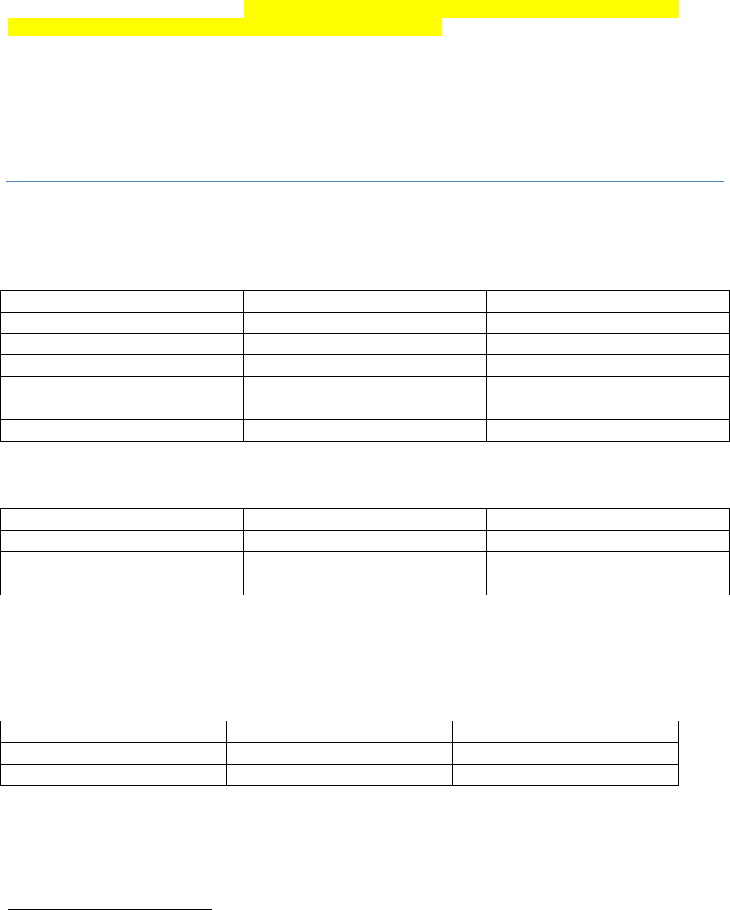
The Air Temperature Coefficients File
A comma-separated values (.csv) file containing a table of coefficients for the spatial weather model’s
air temperature equation. The file must contain 13 rows of 10 comma-separated values (columns) each.
The first row is a header row, and the remaining 12 rows provide values for the equation’s a,..,j and x
coefficients for each month of the year.
Here is an example table of values:
17
and here are the lines from the corresponding .csv data file:
month,b,c,d,e,g,h,i,j,x
1,0.007047,0.018444,2.75E-06,-1.12696,-0.00434,0.012177,-1.60E-05,6.606466,679.15
2,0.006148,0.065628,2.75E-06,1.024448,-0.00545,0.037565,-1.50E-05,8.958362,684.28
3,0.001492,0.041412,1.47E-06,5.402304,-0.00656,0.039723,-5.70E-06,11.03547,699.67
4,-0.00239,0.053357,2.53E-07,10.24696,-0.00697,0.043574,6.13E-06,13.99039,818.03
5,0.004219,0.059169,1.86E-06,8.916032,-0.00707,0.056038,-1.20E-05,16.80074,698.66
6,-0.00222,0.046785,-1.30E-06,16.98087,-0.00684,0.078366,1.33E-05,20.81386,827.75
7,-0.00123,0.004955,-2.50E-06,19.38073,-0.00633,0.073345,-1.90E-06,23.54351,814.57
8,-0.00023,0.00407,-2.60E-06,18.81907,-0.00585,0.092057,9.03E-06,23.53079,836.26
9,0.001476,-0.0342,-2.30E-06,14.80655,-0.00612,0.047614,7.60E-06,20.83291,791.89
10,-0.00023,0.018716,-1.20E-06,11.70249,-0.00641,0.112236,-8.60E-06,16.77907,819.27
11,0.002002,0.014029,-2.60E-07,3.771477,-0.00556,0.027117,-1.40E-05,9.412401,745.95
12,0.00697,0.047469,2.59E-06,-1.28579,-0.00399,0.007256,-1.70E-05,6.096779,674.34
The Air Temperature Coefficients File is only required when the spatially-explicit weather model is
used. Otherwise, the file may be left unspecified in the simulator configuration.
The Observed Runoff Data File
An (optional, but recommended) temporal data file containing a runoff value in millimeters for each day
of the simulation. The data is formatted according to the same rules as the precipitation driver data file;
one value per line, one line per possible simulation day. The VELMA simulator engine can run without
an observed runoff data file, but the Nash-Sutcliffe coefficient value automatically computed as part of
the simulation results will be invalid if the observed runoff data is unavailable.
The Observed Stream Chemistry Data File
An optional temporal data file containing observed DON, NH4, DOC and NO3 loss values for each day
of the simulation. The data is formatted as four comma-separated values per line, one line per possible
simulation day. The first five lines of an observed stream chemistry data file might look like this:
0.000409543,7.73582E-05,0.013059883,9.10096E-06
4.76427E-05,9.52854E-06,0.002572705,0
9.50966E-05,2.8529E-05,0.006276374,4.75483E-06
4.76506E-05,4.76506E-06,0.002001324,0
4.76506E-05,4.76506E-06,0.001620119,0
[ … ]
In this example snippet, the first day’s observed loss values would be:
DON = 0.000409543

18
NH4 = 7.73582E-05
DOC = 0.013059883
NO3 = 9.10096E-06
Note that, like the Observed Runoff data file, there is no header row (initial line of column header titles)
in the observed stream chemistry file.
V. Creating a Simulator Configuration
(New VELMA Application)
Required Input Files
The following simulation data input files must be available prior to creating a new VELMA application:
1. JPDEM flat-processed Grid ASCII (.asc) DEM map file. (see JPDEM user guide in Appendix 7)
2. Cover Species ID Grid ASCII map (.asc) file.
3. Cover Species Age Grid ASCII map (.asc) file.
4. Soil Parameters ID Grid ASCII map (.asc) file.
5. Daily Rainfall driver data file (.txt or .csv) file.
6. Daily Air Temperature data file (.txt or .csv) file.
Configuration Steps
With the above files available, perform the following steps:
1. Start the JVelma graphical user interface (GUI)
2. Create a New Simulator Configuration
3. Specify Startup Parameters
4. Specify Input Parameters
5. Specify Weather Parameters
6. Add and Specify Parameters for Each Cover Species
7. Add and Specify Parameters for Each Soil Parameterization
Additional details for these steps appear in the following pages.

19
Start the JVelma GUI
To start the JVelma GUI, open a Windows command prompt, and launch the GUI via Java and the
JVelma.jar file.
Here is an example of the form the startup command takes:
C:\> java –Xmx1024m –jar C:\Some\full\Path\JVelma.jar
Of course, replace C:\Some\full\Path\ with the actual, fully-qualified path name of the location where
your copy of the JVelma.jar file resides.
Here are a couple of screen captures showing actual command lines for starting JVelma:
(In the above screen-capture, the double-quotes around the fully-qualified path+name of the JVelma.jar
file are required because the text of the path contains whitespace.)
(When there is no whitespace in the entire path the double-quotes are not required.)
The “-Xmx1024m” command line option specifies the amount of memory available to the JVelma GUI
and simulator. The value 1024 is in Megabytes, so this command line allocates a 1 Gigabyte memory
space for the JVelma GUI and simulator to run in. You can allocate more memory than 1 GB (e.g. the
option “-Xmx4096m” would allocate 4 GB) but if you allocate more memory than your computer can
make available, JVelma will fail to start properly.
20
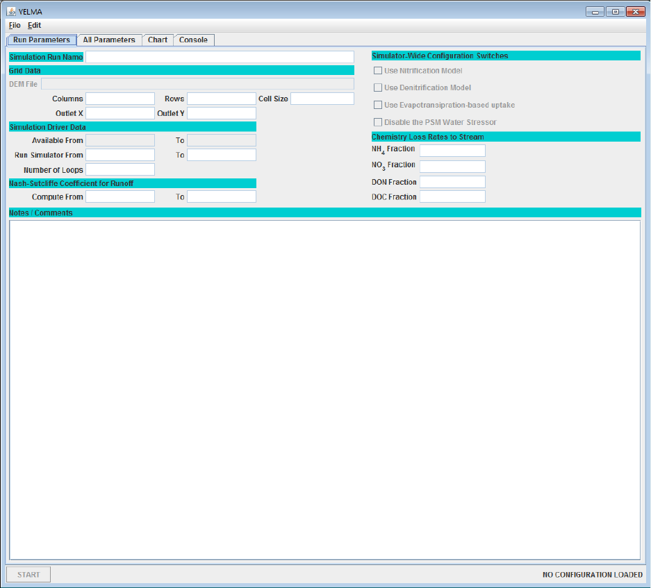
Once you type in the command line and press the enter key, the JVelma GUI should begin running.
Initially, the GUI looks like this:
21
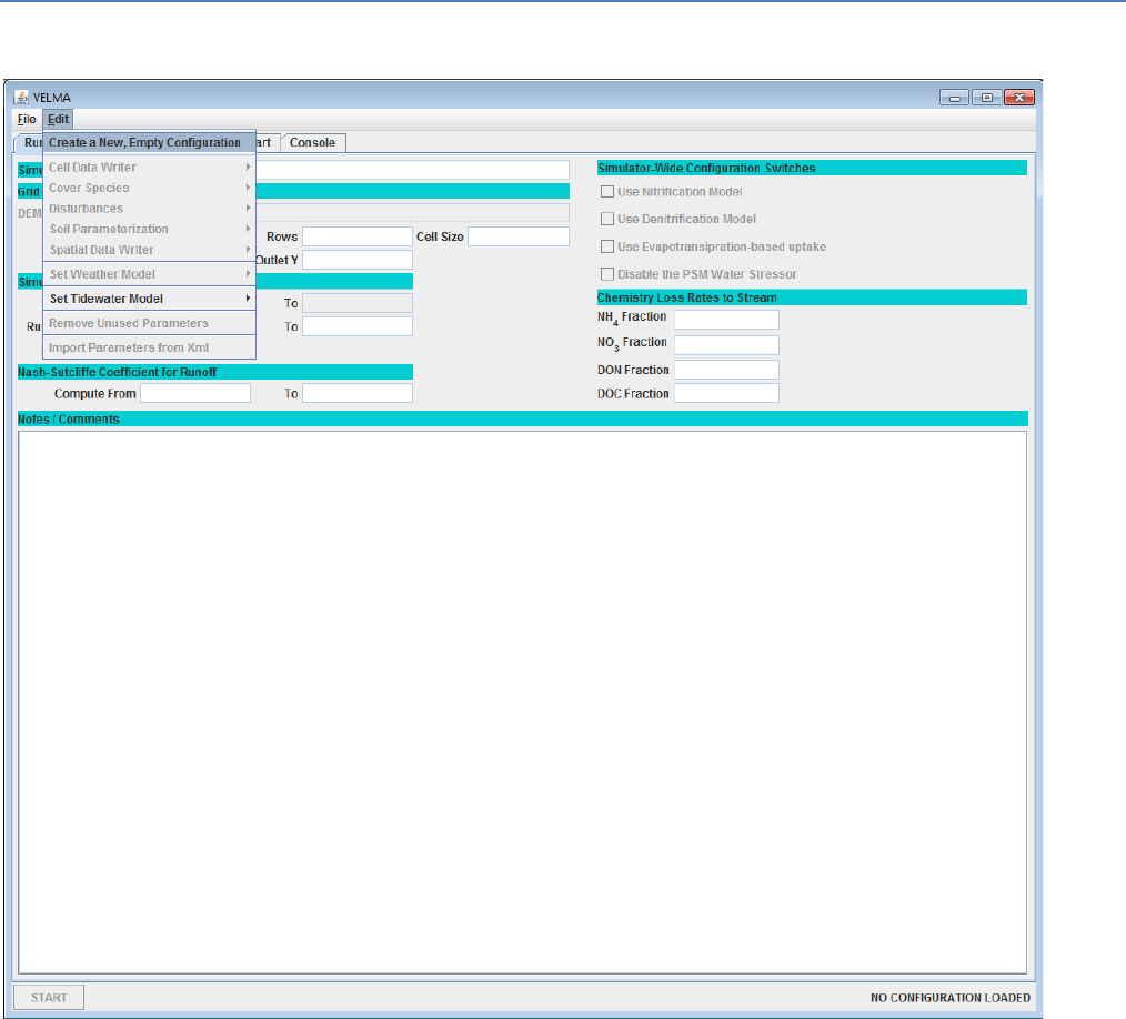
Using the GUI
Click the Edit menu’s Create a New, Empty Configuration item:
Clicking this item creates a new, empty simulation configuration in the JVelma GUI and opens the All
Parameters table view. The All Parameters table lists the Group, Item and Parameter keys and the
current value of all the parameters used by a single VELMA simulation run. When we speak of the
“Simulation Configuration”, this list of parameters is what we’re speaking of.

22
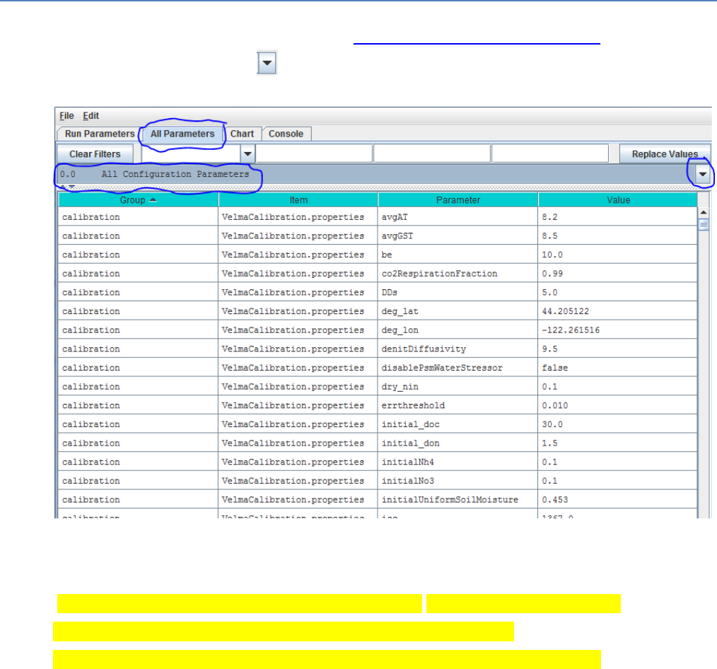
For demonstration purposes, here is an annotated screen-captured snapshot of the All Parameters table
for an existing simulator configuration (cells under the Value column will be blank for new simulator
configurations):
In addition to filtering by an arbitrary text string, the filter field at the top of the table can be set to any of
several pre-composed filtering expressions.
For example, In the All Parameters table, click “Clear Filters” at the left of side of the filter fields, then
click the drop-down button ( ) on the right side of the leftmost filter field to display a drop-down
menu (see demonstration, below).
23
Using the GUI to Specify Startup and Input Parameters
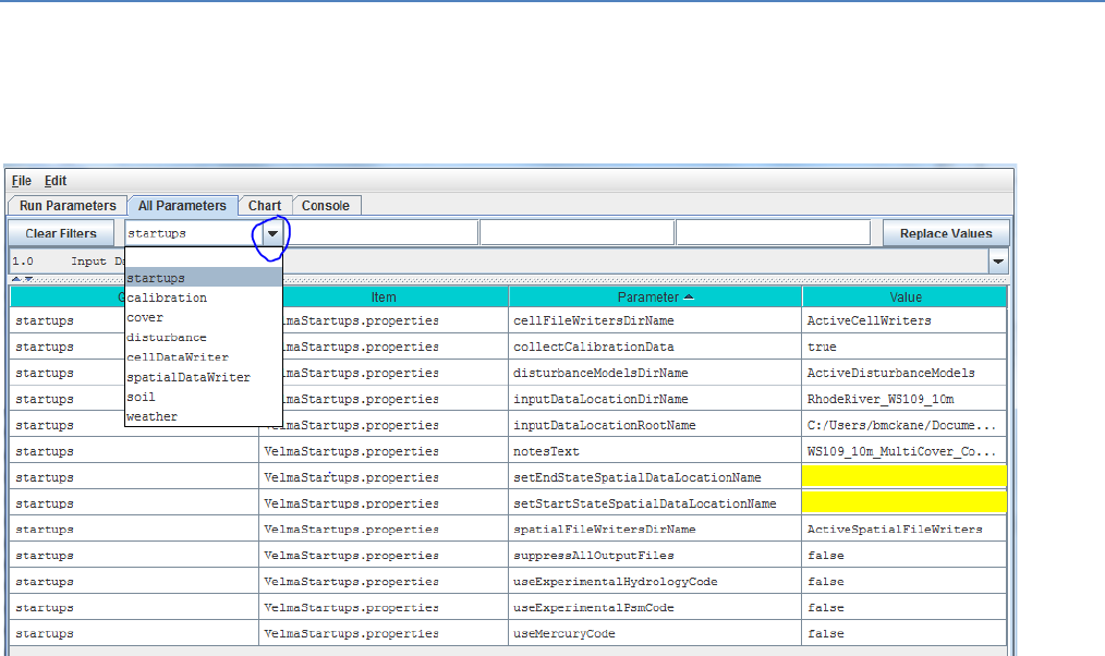
Specify Startup Parameters
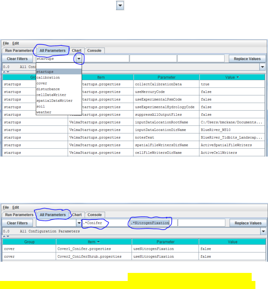
In the All Parameters table, click the first (leftmost) filter field’s drop-down button and select “startups”
from the drop-down list:
The resulting display shows 13 “startups” parameters under the 3rd column. For now, we will focus on 2
startup parameters that VELMA uses to locate simulation input files at the start of a simulation. You will
need to specify a valid value in the 4th column for these:
inputDataLocationDirName The name of the directory containing your simulation input
data files
inputDataLocationRootName The fully-qualified path above the directory name you
specified for inputDataLocationDirName
Specify Input Parameters
Under the All Parameters menu tab, in the 2nd filter field to the left of the “Clear Filters” button, type
“VelmaInputs” (case sensitive, without the double-quotes):
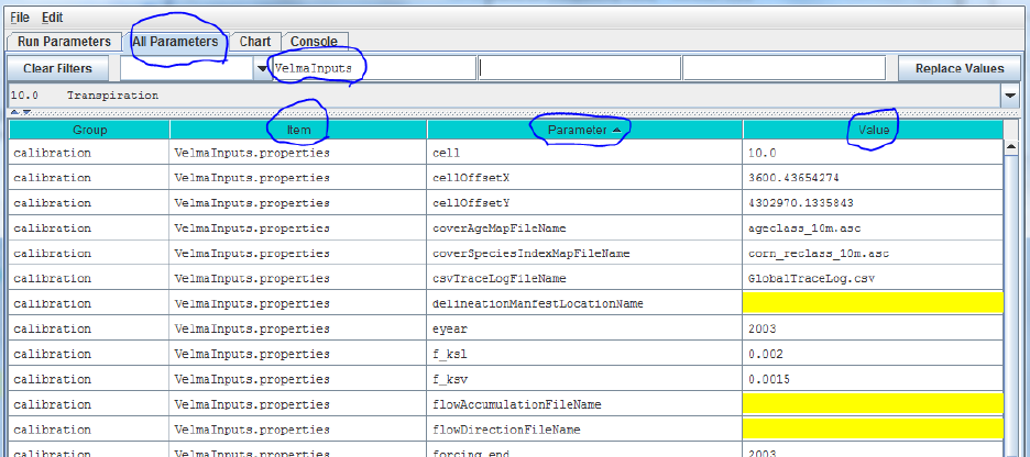
24
In the displayed subset of configuration parameters, enter values for the following parameters:
input_dem The name (plus extension, “.asc”) of this simulation’s DEM
spatial data file. The simulator will look for the file in the
directory specified by the inputDataLocationDirName + “/” +
inputDataLocationRootName that you specified as Startups
parameters.
cell The width of a cell in the DEM grid (should match the “cellsize”
header value in the DEM Grid ASCII file and will be a value in
meters).
ncol The number of columns in the DEM grid (should match the
DEM Grid ASCII file’s ncols header value).
nrow The number of rows in the DEM grid (should match the DEM
Grid ASCII file’s nrows header value).
cellOffsetX Horizontal (column) offset of the DEM's zeroth pixel in meters.
cellOffsetY Vertical (row) offset of the DEM's zeroth pixel in meters.
outx The zero-based x-coordinate (column index) of the outlet cell for
this simulation’s watershed.
outy The zero-based y-coordinate (row index) of the outlet cell for
this simulation’s watershed.
coverAgeMapFileName The name (and “.asc” extension) of this simulation’s cover
species age spatial data map.
coverSpeciesIndexMapFileName The name (and “.asc” extension) of this simulation’s cover
species ID spatial data map.
soilParametersIndexMapFileName The name (and “.asc” extension) of this simulation’s soil
parameterizations ID spatial data map.
forcing_start The first year (inclusive) of temporal data available for
simulation runs.
forcing_end The last year (inclusive) of temporal data available for
simulation runs.
25
syear The starting year of the simulation run.
eyear The ending year of the simulation run.
input_runoff The name of the observed runoff data for simulation runs.
(Specifying this file is optional, but highly recommended.)
input_stream_chem The name of the observed stream chemistry data for simulation
runs. (Specifying this file is optional, but highly recommended.)
run_index The name of the directory where the VELMA simulation will
save simulation results files.
initializeOutputDataLocationRoot The fully-qualified path above the directory name you specified
for the run_index.
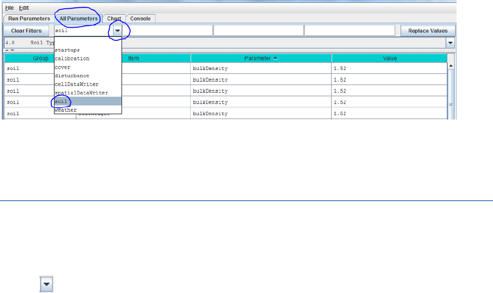
The drop-down filter field menu above the “Group” column can also be used to add and specify
parameters for the other parameter categories listed: cover, disturbance, cellDataWriter,
spatialDataWriter, soil, and weather:
However, we recommend that you use the “All Parameters Table of Contents” described in the next
section to configure these and other subsets of parameters.
Overview of the All Parameters Table of Contents (TOC)
The “All Parameters Table of Contents” (TOC) provides users with a logical sequence of steps for
creating a new simulator configuration, or for quickly locating and calibrating parameters for existing
configurations.
To access the All Parameter TOC, click the GUI’s “All Parameters” tab, then click the drop-down
button ( ) located on the right side of the 4-window filter field (don’t confuse this button with the one
located next to the leftmost filter field):
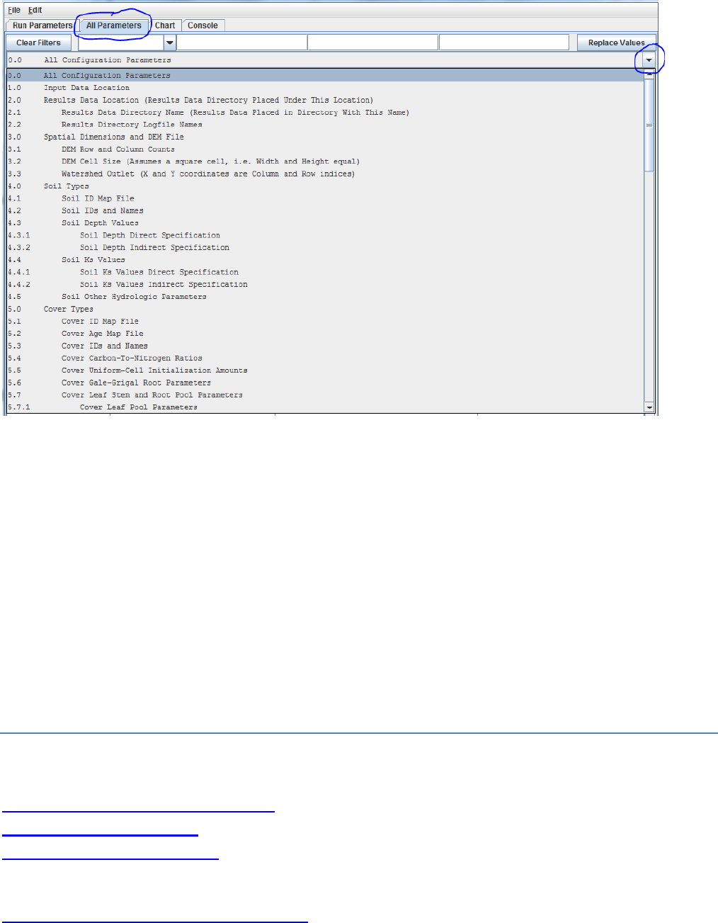
26
That drop-down menu that appears is designed to organize subsets of model parameters in a “Table of
Contents” format. The screenshot above shows the first page of the All Parameters TOC. Additional
pages can be viewed by holding your mouse cursor over the TOC and scrolling down.
In all, the TOC includes 26 main sections (0.0 – 25.0), each of which addresses a particular simulation
configuration procedure.
The All Parameters TOC is designed to:
− Provide a structured step-by-step guide for building a new simulator configuration.
− Help users quickly make specific adjustments to an existing simulator configuration, for
example, to change the directory path and/or folder name for input and output files, or to
calibrate a particular subset of parameters for a hydrological or biogeochemical process.
All Parameters Table of Contents
Click an underlined hyperlink to jump to configuration instructions
0.0 All Configuration Parameters
1.0 Input Data Location
2.0 Results Data Location
2.1 Results Data Directory Name
2.2 Results Directory Logfile Names
3.0 Spatial Dimensions and DEM File
3.1 DEM Row and Column Counts
3.2 DEM Cell Size (Assumes a square cell, i.e. Width and Height equal)

27
3.3 Watershed Outlet (X and Y coordinates are Column and Row indices)
4.0 Soil Types
4.1 Soil ID Map File
4.2 Soil IDs and Names
4.3 Soil Depth Values
4.3.1 Soil Depth Direct Specification
4.3.2 Soil Depth Indirect Specification
4.4 Soil Ks Values
4.4.1 Soil Ks Values Direct Specification
4.4.2 Soil Ks Values Indirect Specification
4.5 Soil Other Hydrologic Parameters
4.0 Soil Types
4.1 Soil ID Map File
Important Information for Sections 5.0 – 25.0 of the All Parameters TOC
5.0 Cover Types
5.1 Cover ID Map File
5.2 Cover Age Map File
5.3 Cover IDs and Names
5.4 Cover Carbon-To-Nitrogen Ratios
5.5 Cover Uniform-Cell Initialization Amounts
5.6 Cover Gale-Grigal Root Parameters
5.7 Cover Leaf Stem and Root Pool Parameters
5.7.1 Cover Leaf Pool Parameters
5.7.2 Cover Above-Ground Stem Pool Parameters
5.7.3 Cover Below-Ground Stem Pool Parameters
5.7.4 Cover Root Pool Parameters
6.0 Weather Model
6.1 Weather Rain Driver File
6.2 Weather Air Temperature Driver File
6.3.1 Weather Model Coefficients Files (Only Spatial Weather)
6.4 Latitude/Longitude
6.5 Solar Radiation
6.6 Soil Layer Temperature
7.0 Initialize Uniform Water Amount per Cell
8.0 Chemistry Pools (Dissolved C and N)
8.1 Chemistry Amounts for uniform cell-initialization
8.2 Chemistry Water Loss Fractions
9.0 Nitrogen Deposition
9.1 Nitrogen Deposition Model Selection (useExperimental=true HIGHLY RECOMMENDED)
9.1.1 Nitrogen Deposition Parameters
9.1.2 Old (DEPRECATED) Nitrogen Deposition Parameters
10.0 Transpiration
10.1 Core PET and ET Parameters
10.2 ET Recovery On/Off ?
10.2.1 ET Recovery Parameters
10.3 Transpiration Limiter On/Off ?
10.3.1 Transpiration Parameters

28
11.0 Plant Uptake
11.1 Plant Uptake NH4-specific
11.2 Plant Uptake NO3-specific
11.3 Plant Uptake GEM Temperature Component
11.4 Plant Update NPP Distribution Fractions
11.5 Plant Uptake Phenology
12.0 Plant Mortality
12.1 Plant Mortality Logistic or Linear ?
12.1.1 Plant Mortality Logistic Parameters
12.1.1.1 Plant Mortality Leaf Logistic Parameters
12.1.1.2 Plant Mortality Above-Ground Stem Logistic Parameters
12.1.1.3 Plant Mortality Below-Ground Stem Logistic Parameters
12.1.1.4 Plant Mortality Root Logistic Parameters
12.2 Plant Mortality Phenology
13.0 Decomposition
13.1 Decomposition Nitrogen-To-DON Fraction
13.2 Decomposition CO2 Respiration Fraction
13.3 Decomposition Microbe Efficiency
13.4 Decomposition Cover-Specific Parameters
14.0 Nitrogen-Fixation
14.1 Nitrogen-Fixation On/Off ?
15.0 Nitrification
15.1 Nitrification On/Off ?
15.1.1 Nitrification Function Type
15.1.2 Nitrification Soil-Specific Parameters
16.0 Denitrification
16.1 Denitrification On/Off ?
16.1.1 Denitrification Core Parameters
16.1.2 Denitrification Soil-Specific Parameters
17.0 Simulation Run Schedule
18.0 Years to Compute Nash-Sutcliffe for Runoff
19.0 Observed Data Files
20.0 Simulation-End Data Capture for Spin-up Initialization Use
21.0 Simulation-Start Initialization from Spin-up Data
22.0 Cell Data Writer Items
23.0 Spatial Data Writer Items
23.1 Spatial Data Writer Items by Model Type
23.2 Spatial Data Writer Items Data Sources
23.3 Spatial Data Writer Items Core Scheduling
23.4 Spatial Data Writer Items Output Map Size
24.0 Disturbance Items
24.1 Disturbance Items by Model Type
24.2 Disturbance Items Core Scheduling
24.3 Disturbance Items Spatial Specifiers (Raster Rally)
25.0 Runtime Chart Display Scale
29
VI. Steps for Configuring All Parameters TOC
Sections 0.0 – 25.0
0.0 – All Configuration Parameters (link to All Parameters TOC)
Using the drop-down button ( ) on the right side of the filter field, select All Configuration
Parameters from the All Parameters menu.
This view displays all Groups, Items, Parameters and Values for a simulator configuration in a
single, scrollable view. To see a pop-up description of any Group, Item or Parameter in any
cell, hover the mouse cursor over the cell.
Alternatively, these descriptions are summarized here in an Excel file located here:
Filename: VELMA 2.0_Description of Calibration Parameters.xlsx
Folder location: VELMA Model\Supporting Documents\Excel Calibration Files
The All Configuration Parameters view contains an overwhelming amount of
information, but the user has some search options for organizing and selecting
things of interest. Experienced users may find that any of the first three search
options, below, are useful for finding a specific parameter of interest in an existing
simulator configuration.
Option 1 – For some purposes it is useful to use the All Configuration Parameters view to locate,
sort and select parameters of interest. For example, you can sort columns by double clicking the
Group, Item, Parameter or Value column headers (turquois). You can also right click a
particular cell and select “Set Column Filter to cellname”, which will display values for the
30
selected item across all cover types, soil types, disturbance type, etc. For example, this is useful
if your watershed has more than one cover or soil type.
Option 2 – Use the drop-down button ( ) on the right side of the first filter field (above
Group) to select from the list of model configuration categories: startups, calibration, cover,
disturbance, cellDataWriter, spatailDataWriter, soil, and weather (the meaning and use of
these categories will be explained below, under sections 1.0 to 25.0).
Option 3 – Type a search string in the filter fields located above any of the four turquois column
headers. Suppose you want to make sure the nitrogen fixation subroutine is turned off for a
coniferous cover type. As the screenshot below shows, by typing “.*Conifer in the “Item” filter
field and “.*NitrogenFixation” in the “Parameter” filter field. This search verified that the
“useNitrogenFixation” parameter is turned off (false).
Option 4 (recommended) – Although experienced users may find Options 1 - 3 handy for quickly
locating specific Items, Parameters or Values, we recommend that all users stick with using
sections 1.0 – 25.0 of the All Parameters TOC when configuring a new VELMA application.
These sections collectively contain the same information listed under “All Configuration
Parameters”, but in a sequence of steps organized to assist users in building new simulator
configurations or editing existing ones. Details follow.
31
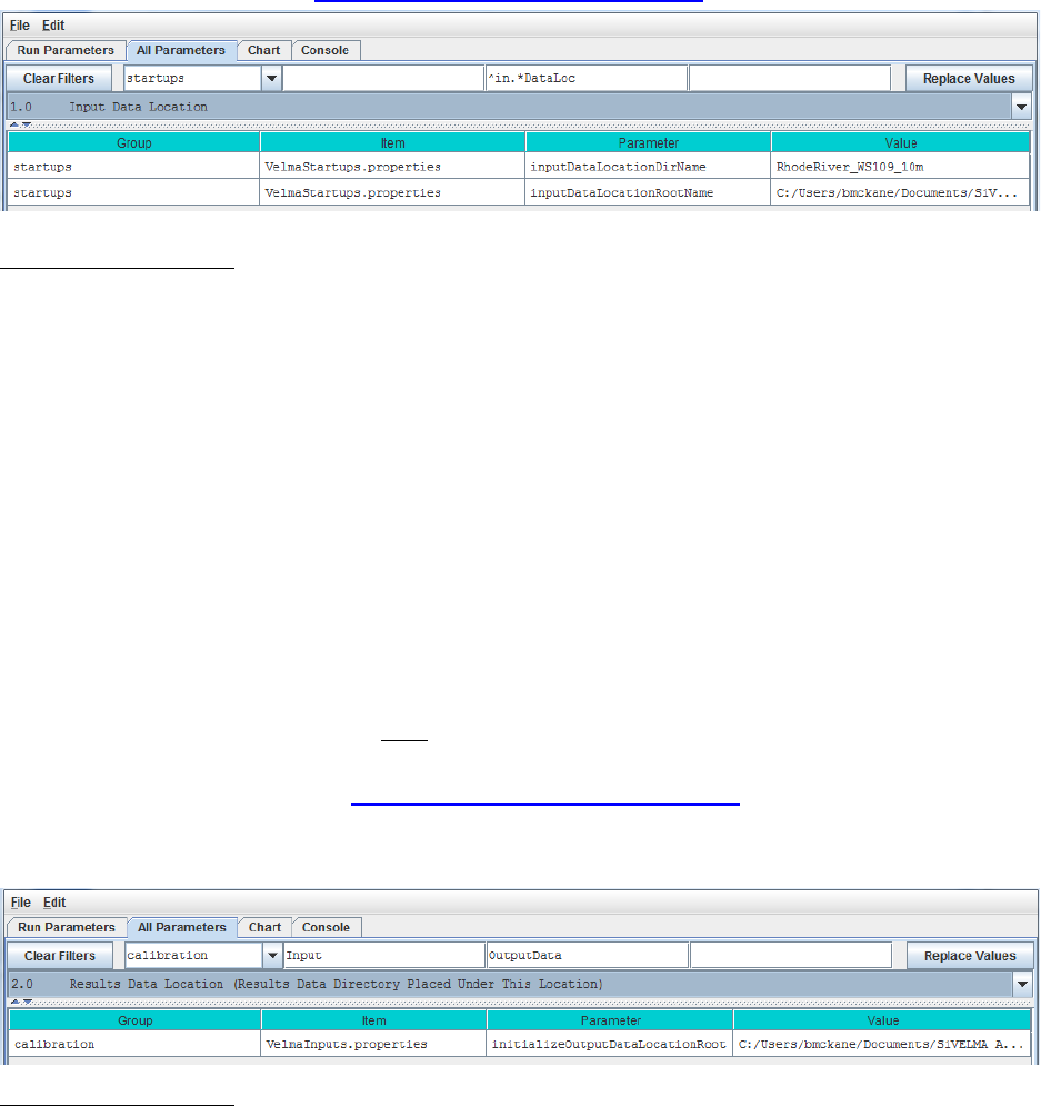
1.0 – Input Data Location (link to All Parameters TOC)
Parameter Definitions
inputDataLocationDirName The name of a subdirectory of the
inputDataLocationRootName directory that
contains the set of input data for a specific
simulation run. When left unspecified or
commented-out defaults to "". (I.e. VELMA will
look for input data in the
inputDataLocationRootName directory itself)
inputDataLocationRootName Fully-qualified path to the directory containing
input data directories. When left unspecified or
commented-out defaults to the "../data/"
subdirectory of VELMA's installation directory.
For the inputDataLocationRootName parameter, specify a directory name for the folder that
contains the set of input data for a given simulation configuration. The
inputDataLocationRootName is the path to that directory.
2.0 – Results Data Location (link to All Parameters TOC)
For the initializeOutputDataLocationRoot parameter, specify the root directory under which
VELMA will place simulation output files for a particular model run.
Parameter Definitions
initializeOutputDataLocationRoot Root directory under which to place per-simulation-run
directories. If this property is left unspecified per-
simulation-run directories for output files will be placed
underneath a default root created in the ../data
subdirectory of the VELMA simulator's installation
directory. When specified this property must be a fully-
qualified path name. Whitespace in the name does not
have to be escape-delimited or double-quoted and the "/"
can (and should!) be used as the path separator for both
Unix and Windows paths. EXAMPLE:
initializeOutputDataLocationRoot = C:/My
VelmaResults/VelmaResultsRoot For the above example
subdirectories for each VELMA simulator run are placed
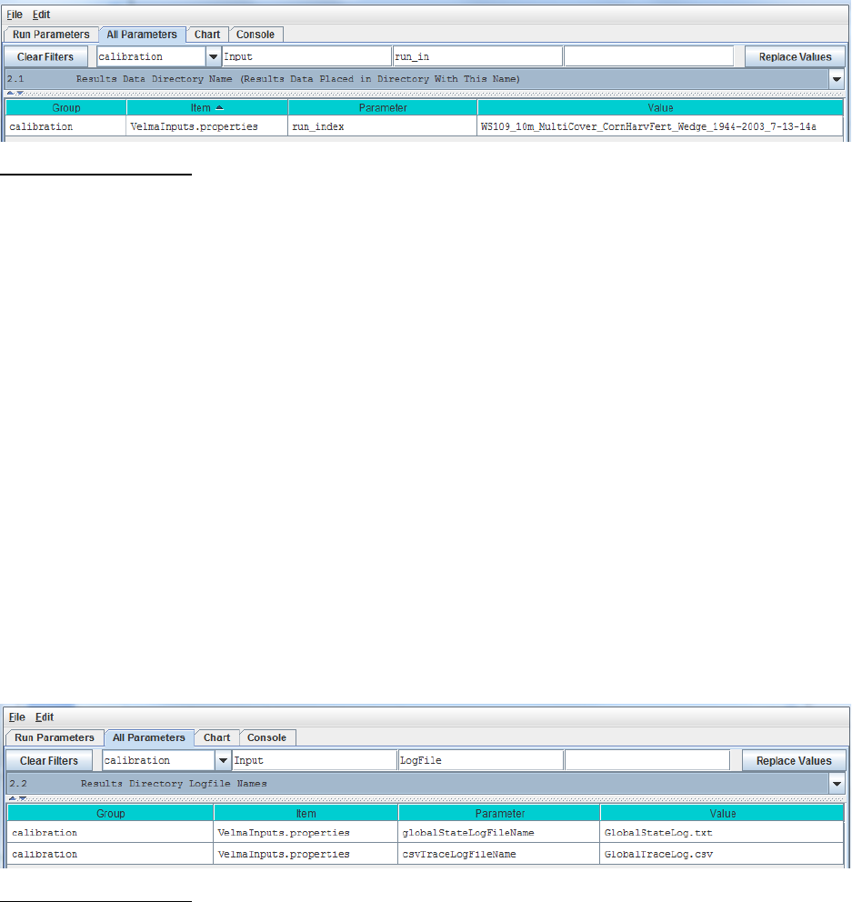
32
underneath the directory "C:/My
VelmaResults/VelmaResultsRoot/"
2.1 – Results Data Directory Name (Results data placed in directory with this name)
Specify a unique simulation filename in the value column for the run_index parameter.
Parameter Definitions
run_index Watershed Name (used as core name for the simulation model run data
files).
Use this parameter to specify a unique name for each simulation run that you do. For example, a
useful run_index name might include the watershed name, date and other identifiers that will
make it easier to determine when a simulation configuration was built and how it differs from
others. VELMA will use the run_index name to create:
- the Simulation Run Name listed in the upper left corner of the Run Parameters GUI
- the .XML file name that VELMA writes when the user saves a configuration file (“Ctrl-S”,
or “File/Save Configuration To VELMA XML File” using the menu at the top of the Run
Parameters GUI). This XML file contains all parameter names and values for the saved
configuration. VELMA will not save this information if the user does not save it in an
XML file;
- the name of the subdirectory (along with the full path) to which model output data files are
written.
2.2 – Results Directory Logfile Names
Specify a filename in the Value column for the globalStateLogFilename parameter.
Parameter Definitions
globalStateLogFilename The name of the global log file. The Global log file records
console messages emitted during a simulation run. When left
blank ("") or commented-out no global log file is created.
csvTraceLogFilename The name of the trace log file. The trace log file records any low-
level debugging messages emitted during a simulation run.
When left blank ("") or commented-out no trace log file is
created.

33
VELMA will use the globalStateLogFilename to record the stream of runtime console messages
(see Console tab) generated during a simulation run. This is optional, but we recommend
creating a globalStateFileName to help identify any problems with the simulator configuration
file. For example, the console messages recorded in the globalStateLogFilename provide a
complete, sequential log of runtime information about successful or unsuccessful loading of
input files, activation of disturbance events (harvest, fertilization, etc.), saving results to output
directories/files, and so on.
///// IMPORTANT NOTE /////
For important additional details on configuring, saving and understanding simulator
results, please see Appendix 4: Overview of VELMA Simulator Output.
3.0 – Spatial Dimensions and DEM File (link to All Parameters TOC)
The VELMA simulator requires a DEM file in order to run a simulation. The simulator also
assumes that all other spatial data files (discussed below) contain spatial data with the same
overall (row and column) and cell (pixel) size dimensions as the DEM file. We highly
recommend that the DEM used for VELMA simulations be pre-processed using the JPDEM
software, rather than by other available “flat-processor” software (see Appendix 7).The VELMA
simulation configuration parameter that specifies the name of the DEM file is:
input_dem example: SmallWatershed_10m.asc
The VELMA simulation configuration parameters that define the DEM file’s location are:
InputDataLocationRootName example: CoastalSite
and
inputDataLocationDirName example: C:\VelmaInputData
Note that:
- Input_dem and inputDataLocationRootName are single file or directory names, while
inputDataLocationDirName specifies a complete directory path.)
- When a simulation is started, the DEM data is loaded from
inputDataLocationRootName/inputDataLocationDirName/input_dem
- The DEM File’s Dimensions are NOT Set Automatically by the Simulator or GUI
- The VELMA simulator does not read the DEM file’s dimensions from the DEM file’s
header!
As part of parameterizing a VELMA simulation configuration, you must manually determine
(usually by viewing the DEM file’s header rows with a text editor) the DEM file dimensions, and
set the corresponding VELMA simulation parameters (usually by using the JVelma GUI)
This table lists the header rows of a DEM (Grid ASCII) file and the corresponding VELMA
simulation parameters:
Grid ASCII Header Item
VELMA Simulation Configuration Parameter
ncols
Ncol
nrows
Nrow
xllcorner
cellOffsetX
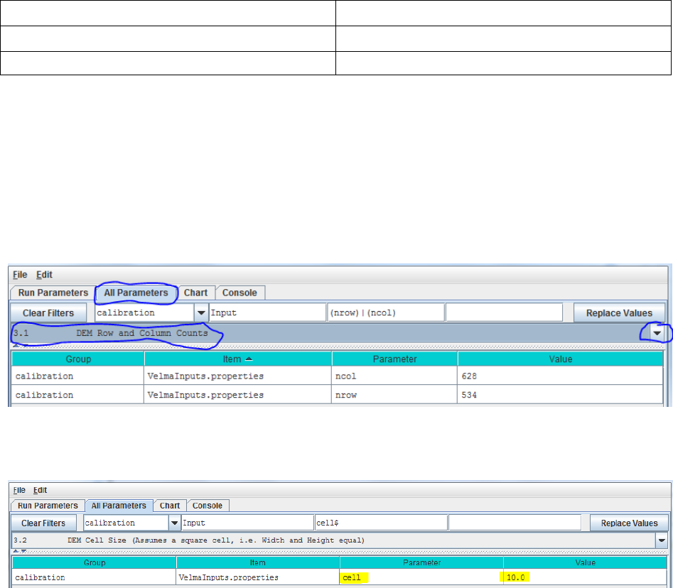
34
yllcorner
cellOffsetY
cellsize
cell
nodata_value
Sections 3.1 – 3.3 provide details on configuring these parameters for a DEM file.
Note: if you change the DEM file that a simulation is configured to use (i.e. you change the
DEM filename for the input_dem parameter) then you must ensure that all of the parameters
above are updated as well.
3.1 – DEM Row and Column Counts
Specify values for the ncol and nrow parameters based on the DEM grid ASCII header items in
the table above.
3.2 – DEM Cell Size (Assumes a square cell, i.e. Width and Height equal)
Specify the value of the cell parameter.
This describes the xy-dimension in meters of individual cells in the DEM grid ASCII file. In this
example, each cell is 10x10 meters. The choice of DEM cell size will depend upon the set of
questions a user wishes to address. For example, applications focusing on the effect of riparian
buffer width on nutrient export to streams may require relatively small cells (e.g., 10 meters),
compared to applications focusing on ecosystem carbon dynamics (e.g., 100 meters). Obviously,
an application’s total number of cells (and consequent simulation time) increases with the square
of the ratio of alternative cell sizes – e.g., (100/10)2 = 100 times more cells for 10m versus 100m
cell sizes. In any case, the specified cell size must be consistent with the DEM cell size. That is,
the user cannot arbitrarily adjust the cell size parameter without telling VELMA to load a DEM
having the same cell size (see All Parameters 3.0). Furthermore, the DEM used must be “flat-
processed” for the specified cell size using the JPDEM tool. The executable JPDEM.jar, a
JPDEM user manual, and background information (Pan et al. 2012) can be found here: VELMA
Model\JPDEM_DEM Processor. The JPDEM user manual is also included in Appendix 7 of this
manual.
3.3 – Watershed Outlet (X and Y coordinates are Column and Row indices)
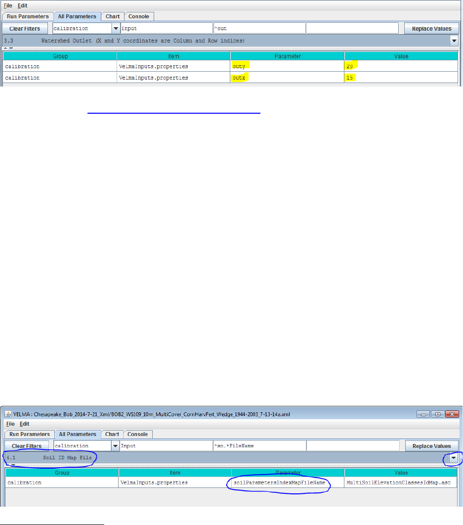
35
Specify the value of the outx and outy parameters. These describe the watershed outlet cell’s X
and Y coordinates (column index) relative to the DEM upper-left corner. The watershed outlet
cell coordinates are determined using the JPDEM tool.
4.0 – Soil Types (link to All Parameters TOC)
VELMA requires information on key soil properties affecting hydrological and biogeochemical
processes within a study watershed. Whether single or multiple soil types are modeled within a
watershed, you will need to establish a soil type map and specify parameter values for a set of
soil properties associated with each soil type. The following steps will accomplish this:
− Establish a soil ID map describing the assignment of soil type IDs for every cell
within the delineated watershed. See section 4.1 for details.
− Specify soil ID parameter names and values corresponding to those appearing in the
soil ID map. See section 4.2 for details.
− Specify soil depth values for the entire soil column and for each of four soil layers
within the column. See section 4.3 for details.
− Specify soil hydraulic conductivity values controlling infiltration rate (Ks), and depth
dependent changes in vertical and lateral macropore flow, Ksv and Ksl, respectively.
See section 4.4 for details.
4.1 – Soil ID Map File
The Soil ID Map File is specified by the soilParametersIndexMapFileName parameter. You can
view and set it by selecting “4.1 Soil ID Map File” in the All Parameters outline drop-down
selector:
Parameter Definitions
soilParametersIndexMapFileName The file name of a spatial-explicit map of Soil
Parameters uniqueIds. The data in this map file
specifies the Soil Parameterization of a given pixel in
the DEM map.
The file specified for the soilParametersIndexMapFileName is assumed to be a Grid ASCII
(“.asc”) map file with the same row and column dimensions as the simulation configuration’s
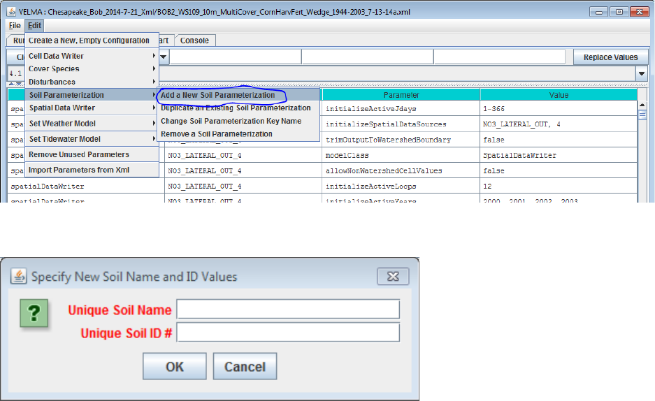
36
DEM file. Its contents should be integer values. Each cell’s integer value should be the ID
number of a soil type.
Suppose the specified soil index map file contains three distinct integers for this map: 100, 105
and 110. The VELMA simulation will expect the simulation configuration to include 3 soil
parameterizations.
4.2 – Soil IDs and Names
Adding a Soil Parameterization to a simulation configuration using the following steps.
Click the Edit Soil Parameterizations “Add a New Soil Parameterization” menu item:
Clicking “Add a New Soil Parameterization” opens the Soil Parameterization Name and ID
dialog which looks like this:
Enter a name and ID number for your new Soil Parameterization.
The name must be unique (i.e. no other Soil Parameterization already specified for this
simulation configuration can share the name you specify) and we recommend avoiding
whitespace and punctuation characters (e.g. “(“ and “)”) apart from the underbar (“_”) character,
which can be used instead of whitespace.
The ID number must be an integer, not already specified for any existing Soil Parameterization,
and must match one of the integers that appears in the Soil ID Map File.
As an example: Suppose we are adding the first Soil Parameterization (“100”) for the
hypothetical Soil ID Map File mentioned above, and that ID “100” identifies cells that contain
loamy sand.
Acceptable names (it’s guaranteed unique because it’s the first Soil Parameterization we’re
adding) might be: “Loamy_Sand” or “Soil_100_LoamySand”, or something similar.
However, the only acceptable ID value is “100” – because the Unique Soil ID # of this
parameterization is what keys it to those particular cells in the Soil ID Map File.
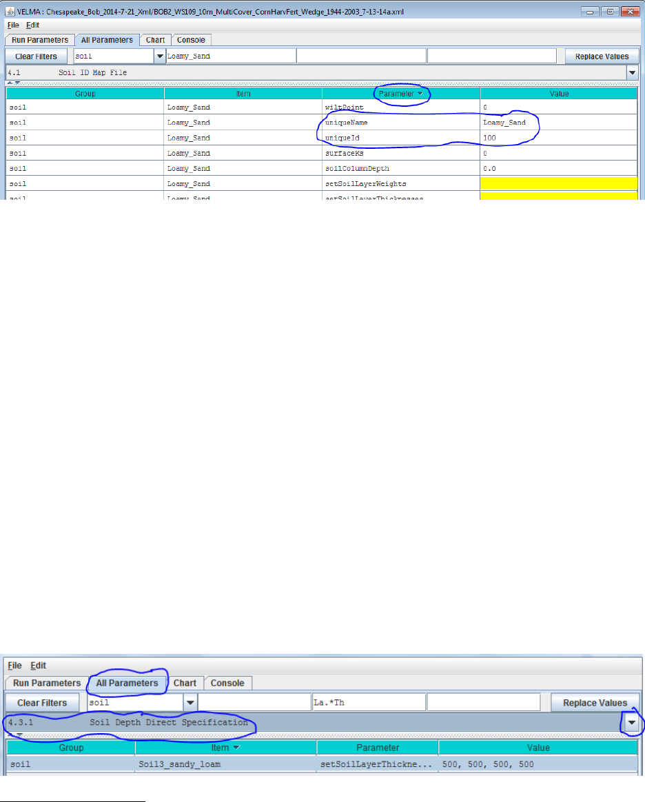
37
Once you’ve entered valid name and ID values in the Name and ID dialog, click the OK button.
When you click OK, the VELMA GUI adds a new Soil Parameterization to the simulation
configuration, and sets the All Parameters tab’s filters to display only the parameters of the
newly-added Soil Parameterization. Assuming we named our new Soil Parameterization
“Loamy_Sand”, with ID = “100”, this is what the All Parameters tab would look like after
clicking OK:
We did one other thing to get the above display: notice that the “Parameter” column is circled,
and has a “down-arrow” indicating “descending-sort”. After clicking OK to add the new Soil
Parameterization, we clicked the “Parameter” header field (twice), which sorts the table of
properties on that column.
Now go to All Parameters 4.3 and 4.4 where parameter values for each soil name/ID will need to
be specified for total soil column depth, thickness of each of four soil layers, and hydrologic
parameters affecting vertical and lateral flow.
4.3 – Soil Depth Values
There are two methods, direct or indirect, that can be used to specify soil layer depths. The
direct and indirect methods have their own distinct set of parameters that are available to each
soil type specified for a given simulation configuration. Each method has its advantages. Thus,
it is up to the user to decide which one to use. Either the direct or indirect set of parameters can
be applied to a specified soil type, independent of which set is applied in other specified soil
types.
4.31 – Soil Depth Direct Specification
The direct method (optional) for setting a soil type’s layer thicknesses uses a comma-separated
list of values for the setSoilLayerThicknesses parameter in millimeters for of each of 4 soil
layers. For example: "500, 500, 500, 1500" (without the quote-marks) specifies the soil type’s 4
layers as being 500 mm, 500 mm 500 mm, and 1500 mm thick, from layer 1 to layer 4,
respectively.
Parameter Definitions
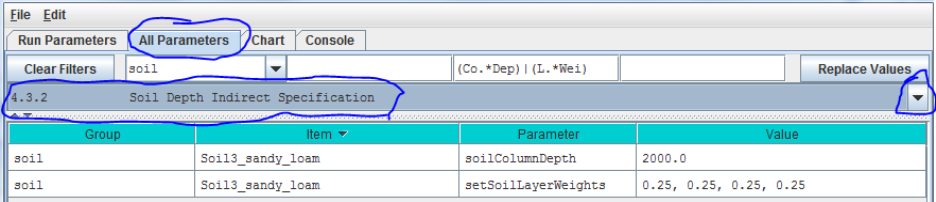
38
setSoilLayerThicknesses A comma-separated list of values specifying the thickness of
each soil layer in millimeters. For example: "500 750 1000
1500" (without the quote-marks) specifies the soil's 4 layers
as being 500 mm 750 mm 1000 mm and 1500 mm thick
from layer 1 to layer 4 respectively. NOTE: This list of
values may be left unspecified. When
setSoilLayerThickness is unspecified the soil's layer
thicknesses are set by the combination of the
soilColumnDepth and setSoilLayerWeights parameters.
When setSoilLayerThickness is specified the
soilColumnDepth and setSoilLayerWeights parameters are
ignored.
Thus, for the direct method, VELMA internally calculates the value for the soilColumnDepth
parameter from the setSoilLayerThicknesses values specified for layers 1, 2, 3 and 4. When
setSoilLayerThicknesses is not specified (left blank), the indirect method must be used to
specify the soil layer thicknesses and soil column depth (see All Parameters 4.32).
4.32 – Soil Depth Indirect Specification
As an alternative to the direct method described under All Parameters 4.31, you can instead use
the indirect method for specifying a soil type’s total soil column depth (parameter =
soilColumnDepth, in millimeters) and soil layer depth (parameter = setSoilLayerWeights, which
is equal to the fraction “soil layer thickness / soil column depth”.
In this example the soil type named “SoilWedge1” has soilColumnDepth = 2000 mm, and
setSoilLayerWeights = 0.25, 0.25, 0.25, 0.25 for layers 1, 2, 3 and 4, respectively. VELMA
uses these values during a simulation to compute each soil layer’s thickness (in millimeters) as:
layerThickness[iLayer] = soilColumnDepth * soilLayerWeight[iLayer].
Thus, the parameter values shown in the above example translate to soil layer thicknesses of 500
mm, 500 mm, 500 mm, and 500 mm for each layer.
When setColumnDepth and setSoilLayerWeights are not specified (left blank), the direct method
must be used to specify the soil layer thicknesses and soil column depth (see All Parameters
4.31).
4.4 – Soil Ks Values
VELMA simulates vertical and lateral water drainage using a logistic function that is intended to
capture the breakthrough characteristics of soil water movement. The logistic function provides
a simple way (3 parameters) to capture the fast “switching” from low to high flow as water
storage within a soil layer approaches field capacity. VELMA offers two alternative methods,
direct or indirect, for specifying these parameters. However, because the direct method is still
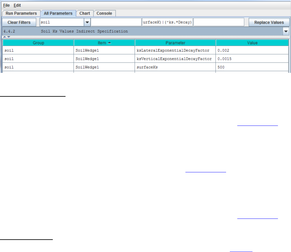
39
under development, we recommend that users use the indirect method (see All Parameters
4.4.2).
4.4.1 – Soil Ks Values Direct Specification
Under development – please use the indirect method described in the next section.
4.4.2 – Soil Ks Values Indirect Specification
We refer to this method as an “indirect" because VELMA internally uses the specified soil Ks
parameter values to calculate the actual soil lateral and vertical hydraulic conductivity (Ks)
values used during the simulation run. You must specify values for 3 parameters for each soil
type (in this example, “SoilWedge1” refers to a particular soil type / map unit).
Parameter Definitions
surfaceKs saturated hydraulic conductivity (Ks, mm/day) at
the soil surface. For equations and
parameterization information see Appendix 6.1
(Abdelnour et al. 2011).
ksVerticalExponentialDecayFactor vertical Ks exponential decay factor (unitless)
controlling the rate of decrease in vertical flow
with depth. For equations and parameterization
information see Appendix 6.1 (Abdelnour et al.
2011).
ksLateralExponentialDecayFactor lateral Ks exponential decay factor (unitless)
controlling the exponential rate of decrease in
lateral flow with depth. . For equations and
parameterization information see Appendix 6.1
(Abdelnour et al. 2011).
Calibration Notes
As a starting point, we recommend using the texture-specific values listed in Table 1 for
“Surface Ks” and other physical characteristics of soil. Note that all the values in Table 1can
vary significantly as a result of compaction, presence of hard pans, and other factors.
Based on the parameter values specified, VELMA computes the Ks lateral and Ks vertical flows
(mm/day) per each soil layer as
ksLateral[ilayer] = surfaceKs * −∗ ∑[]∗0.5
ksVertial[ilayer] = surfaceKs * −∗ ∑[]∗0.5

40
Iterative calibration of the user-specified parameter values is generally required to obtain a good
fit between simulated and observed stream discharge (mm/day) at the watershed outlet. At the
end of each simulation, VELMA calculates a Nash-Sutcliffe efficiency coefficient to assess the
goodness-of-fit and reports the results in a simulation output file named
“NashSutcliffeCoefficients.txt”.
See http://en.wikipedia.org/wiki/Nash%E2%80%93Sutcliffe_model_efficiency_coefficient for a
general overview of the Nash-Sutcliffe efficiency coefficient and its application. Quoting that
website:
“Nash–Sutcliffe efficiencies can range from −∞ to 1. An efficiency of 1 (E = 1)
corresponds to a perfect match of modeled discharge to the observed data. An efficiency
of 0 (E = 0) indicates that the model predictions are as accurate as the mean of the
observed data, whereas an efficiency less than zero (E < 0) occurs when the observed
mean is a better predictor than the model.”
In general, a Nash-Sutcliffe coefficient of 0.7 is considered a good fit between simulated and
observed discharge. A value of 0.8 or greater is excellent, particularly for spatially-distributed
ecohydrological models like VELMA that simulate the processes and flow paths by which water
arrives at the watershed outlet (empirical models do not have this requirement).
Advanced users can consult Appendix 6.1 (Abdelnour et al. 2011) for additional details
concerning soil Ks equations, parameters and calibration.
4.5 – Soil Other Hydrologic Parameters
VELMA simulates the effect of several soil physical properties on water retention, rates of
drainage and other hydrological processes. These physical properties and their associated
parameter names are
− Soil porosity (parameter name = porosityFraction): the fraction of void space (v/v) in a
soil.
− Soil field capacity (parameter name = fieldCapacity): the amount of soil moisture (v/v)
held in soil after excess water has drained away and the rate of downward movement has
materially decreased
− Wilt Point (parameter name = wiltPoint): the minimal point of soil moisture (v/v) the
plant requires not to wilt.
− Bulk density (parameter name = bulkDensity): the dry weight of soil per unit volume of
soil (g/cm3).
The following table provides typical values for these parameters for 11 soil texture classes
(surface Ks, described above in All Parameters 4.4, is included here as well). The values listed
are offered here as a starting point for model initialization. However, users should be aware that
these values can vary dramatically as a result of compaction, presence of hard pans, and other
factors.
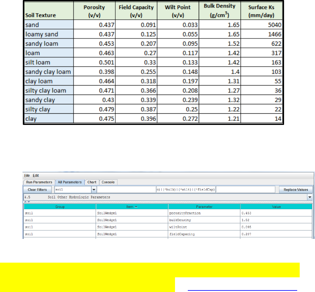
41
Table 1. Physical characteristics of major soil texture classes (Pan et al. 2009, VELMA v1.0
user manual)
For each soil type in a watershed (we recommend just one texture type per soil type / mapping
unit), you will need to specify values for porosity, field capacity, wilt point and bulk density.
Use the All Parameters drop-down menu to select “4.5 Soil Other Hydrologic Parameters (only
one of six soil types is shown in the truncated screenshot below):
IMPORTANT INFORMATION FOR SECTIONS 5.0 – 25.0
OF THE ALL PARAMETERS TOC (link to All Parameters TOC)
VELMA version 2.0 simulates plant biomass and detritus much differently than VELMA version 1.0.
Version 1.0 used a simplified Plant Soil Model (PSM, Stieglitz et al. 2006) to simulate plant biomass in
each cell in aggregate – that is, leaves, stems and roots were lumped together in a single biomass pool
(Abdelnour et al. 2011). This lumped approach greatly simplified the structure and application of the
model. Version 1.0 successfully simulates important aspects of catchment hydrology and
biogeochemistry (e.g., Abdelnour et al. 2011, 2013), but it does not simulate effects associated with
phenological changes and disturbances that disproportionately affect specific plant tissues – for
example, leaf growth and senescence, defoliation events, selective removal of high or low C/N tissues
via harvest or grazing, etc. These effects can have important implications for assessments involving
water quality and quantity, carbon sequestration and other ecosystem services.
To address such effects, VELMA version 2.0 simulates nitrogen pools and fluxes for four plant tissue
types: leaves, aboveground stems, belowground stems (>2 mm diameter), and fine roots (< 2 mm

42
diameter). This new Leaf-Stem-Root (LSR) submodel includes live (biomass) and dead (detritus) pools
for each of the four plant tissue types.
A carbon/nitrogen (C/N) ratio must be specified for each plant tissue type so that VELMA can estimate
carbon pools and fluxes corresponding to modeled nitrogen pools and fluxes. Although the model
parameterization allows different C/N values for the biomass and detritus pools of the same tissue type,
at present, the plant biomass and detritus pools for each tissue type must have the same C/N ratio to
maintain mass balance of C and N pools. Specification of distinct C/N ratios per tissue type will be
addressed in future versions.
Several other features have been built into the LSR submodel.
1) A new nonlinear mortality subroutine simulates the loss of live plant biomass to detritus for all
four tissues. See All Parameters section 12.0 for details. This replaces the mortality subroutine
in VELMA version 1.0 described in Appendix 1, section A1.2.3.
2) A modified version of the decomposition subroutine of Potter et al. (1993) is used to decompose
detritus (leaf, stem and root) to humus (unidentifiable dead material). See All Parameters
section 13.0 for details. This replaces the decomposition subroutine in VELMA version 1.0
described in Appendix 1, section A1.2.
3) The “ET recovery” subroutine (Abdelnour et al. 2011) has been revised to use leaf biomass,
rather than stand age, to simulate effects of forest regrowth on ET and streamflow. This
subroutine can be applied to any cover type. See All Parameters section 13.0 for details. This
replaces the decomposition subroutine in VELMA version 1.0 described in Appendix 6.2,
section B2.
4) A new subroutine describing age-related declines in transpiration of forest stands has been
added. Aboveground plant biomass is used as a proxy for stand age. See All Parameters section
10.3 for details.
The figure on the next page illustrates the structure of the new LSR submodel and its integration into the
overall Plant Soil Model. Additional Details on the LSR model structure, equations and parameters can
be found in "Appendix 1: Overview of VELMA’s Leaf-Stem-Root (LSR) Plant Biomass Submodel”.
We recommend reviewing this material before proceeding further, focusing on the LSR model structure
and equations describing the various LSR nitrogen and carbon pools and fluxes.
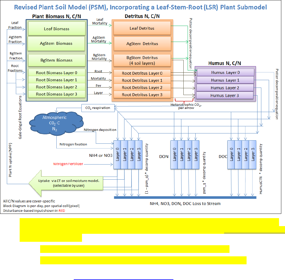
43
Figure 1.
The User Manual package includes slides for a seminar describing the effectiveness of riparian
buffers for protecting water quality in the Chesapeake Bay (please contact mckane.bob@epa.gov
if you have questions):
Filename: McKane_VELMA overview_OSU 2April2014_final.pptx
Folder location: VELMA Model\Supporting Documents\VELMA Pubs & Talks
5.0 – Cover Types (link to All Parameters TOC)
VELMA version 2.0 includes two major changes to the vegetation submodel:
(1) Multiple cover types (forest, grassland, agricultural crops, etc.) within a watershed
can now be modeled. The version 1.0 convention of one cover type per grid cell is
maintained.
(2) Plant biomass for each cover type is modeled using four plant tissues – leaves,
aboveground stems, belowground stems, and roots – rather than as a single biomass
pool.
Sections 5.1 – 5.3, below, discuss procedures for initializing a simulator configuration for one or
more cover types.
Sections 5.4 through 5.7, below, discuss procedures for initializing a simulator configuration for
the four plant biomass pools.
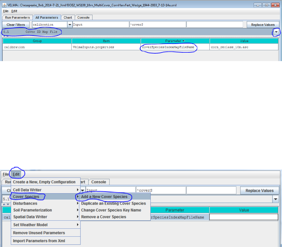
44
5.1 – Cover ID Map File
The VELMA program requires a set of Cover Species parameters for each Cover ID number that
occurs in the Cover ID Map File. Each Cover ID corresponds to a distinct, user-defined Cover
Species (cover type) – for example, hardwood forest, grassland, corn cropland, and so forth.
This section describes the Cover ID map file and associated parameter specifications.
The Cover ID Map File is specified by the coverSpeciesIndexMapFileName parameter. You can
view and set it by selecting “All Parameters 5.1 Cover ID Map File” from the All Parameters
outline drop-down menu:
The file specified for the coverSpeciesIndexMapFileName is assumed to be a grid ASCII (“.asc”)
map file with the same row and column dimensions as the simulation configuration’s DEM file.
Its contents should be integer values. Each cell’s integer value should be the ID number of a
cover type.
Suppose the specified cover index map file contains three distinct integers: 5, 7 and 9. For this
map, the VELMA simulation will expect the simulation configuration to include 3 Cover
Species.
You will need to add a new Cover Species to a simulation configuration using the following
steps:
(1) Click Edit Cover Species “Add a New Cover Species” menu item. This will cause a
pop-up menu to appear (see step 2).
5.3 – Cover IDs and Names
[Note: All Parameters 5.2 – Cover Age Map File has been moved below section 5.3 to reflect
the required workflow]
Picking up from All Parameters 5.2, step (2)…
(2) Enter a name and ID number for your new Cover Species.
The name must be unique (i.e. no other Cover Species already specified for this simulation
configuration can share the name you specify) and we recommend avoiding whitespace and
punctuation characters (e.g. “(“ and “)”) apart from the underbar (“_”) character, which can
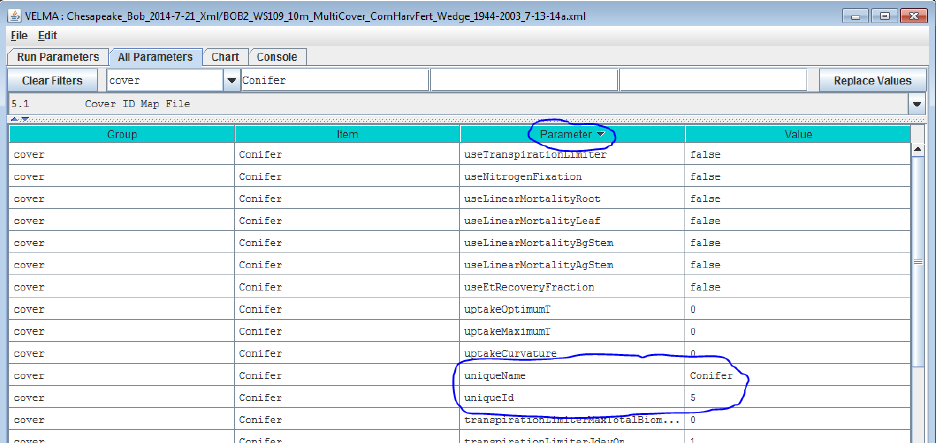
45
be used instead of whitespace.
The ID number must be an integer, not already specified for any existing Cover Species, and
must match one of the integers that appears in the Cover ID Map File.
As an example:
Suppose we are adding the first Cover Species (“5”) for the hypothetical Cover ID Map File
mentioned above, and that ID “5” identifies cells that contain Conifers.
Acceptable names (guaranteed unique because this is the first Cover Species we’re adding)
might be: “Conifer” or “Cover_5_Conifer”, or something similar.
However, the only acceptable ID value is “5” – because the Unique Cover ID # of this
parameterization is what keys it to those particular cells in the Cover ID Map File.
(3) Once you’ve entered valid name and ID values in the Name and ID dialog, click the OK
button.
When you click OK, the VELMA GUI adds a new Cover Species Parameterization to the
simulation configuration, and sets the All Parameters tab’s filters to display only the
parameters of the newly-added Cover Species. Assuming we named our new Cover Species
“Conifer”, with ID = “5”, this is what the All Parameters tab would look like after clicking
OK:
We did one other thing to get the above display: notice that the “Parameter” column is circled,
and has a “down-arrow” indicating “descending-sort”. After clicking OK to add the new Cover
Species, we clicked the “Parameter” header field (twice), which sorts the table of properties on
that column.
5.2 – Cover Age Map File
[Note: section 5.2 appears after section 5.3 to reflect the required workflow for developing a
Cover Age Map file and associated parameter values]
To enable scheduling of disturbance events during a simulation (per All Parameters section
24.0), VELMA needs to keeps track of changes in the age (years) of vegetation from one
calendar year to another, or as a result of disturbances that can reset stand age to 0 (e.g., by
clearcutting) or to some other age (e.g., by selective thinning of old trees that establishes
understory vegetation as the new dominant age class). Note that cover age maps can be can be
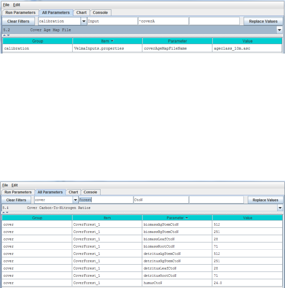
46
applied to cover types other than forests, e.g., rangeland vegetation that may have a more diverse
mixt of species than vegetation recovering from a recent fire.
After you have established a Cover ID Map file (section 5.1) and specified Cover IDs and names
for each Cover Species (section 5.3, above!), you will need to set up a Cover Age Map file and
specify the file name.
The Cover Age Map file name is specified by the coverAgeMapFileName parameter. You can
view and set it by selecting “All Parameters 5.2 Cover Age Map File” from the All Parameters
outline drop-down menu:
The file specified for the coverAgeMapFileName is assumed to be a grid ASCII (“.asc”) map file
with the same row and column dimensions as the simulation configuration’s DEM file. Its
contents should be integer values reflecting the age of vegetation (Cover Species) occupying
each grid cell. Each cell’s integer value should be the ID number of a Cover Species. For
example, an age of 0 could be assigned to row crops (corn, soybeans, etc.). Cells in a forest
landscape might range in age from 0 (newly burned or planted) to many centuries. The VELMA
team has used biomass-to-age and tree height-to-age relationships to establish Cover Age Maps.
5.4 – Cover Carbon-To-Nitrogen Ratios
This section is concerned with initializing plant tissue C/N ratios for plant biomass and detritus
associated with leaves, aboveground stems (AgStem), belowground stems (BgStem) and roots.
Thus, a total of eight C/N (CtoN) ratios must be specified for each cover type. Only one cover
type (CoverForest_1) is displayed for the example below. In addition, a C/N ratio must be
specified for the humus pool.
5.5 – Cover Uniform-Cell Initialization Amounts
Using the All Parameters drop-down menu, select “5.5 Cover Uniform-Cell Initialization
Amounts”. The parameters shown are used to specify initial pool sizes (g C / m2) that VELMA
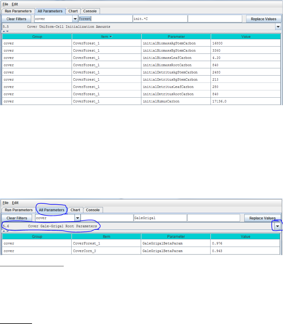
47
requires at the start of each simulation run. Values must be specified for all plant biomass pools,
detritus pools and humus pool associated with each cover type. The example below shows just
one cover type, but the same list of 9 parameters repeats for each additional cover type that has
been has been for the simulation configuration.
“Cover Uniform-Cell Initialization Amounts” refers to the fact that all grid cells assigned to a
particular cover type will have the same initial values for plant biomass, detritus and humus.
Obviously this method will not work for watersheds where there is significant spatial variability
in pool sizes (e.g., where forest stands vary in age). In these situations, you can use All
Parameters menu item “24.3 Disturbance Items Spatial Specifiers” to establish spatially variable
initialization amounts for any or all pools.
5.6 – Cover Gale-Grigal Root Parameter
Select section 5.6 from the All Parameters drop-down menu to specify Gale-Grigal root
parameter values for each cover type in your watershed:
Parameter Definitions
GaleGrigalBetaParam The Beta term for this cover type’s root vertical
distribution. For the root distribution function of
Gale Grigal (1987): roots[D] = 1 - B^D, where
B = GaleGrigalBetaParam value (assigned here)
D = layer depth
References
Gale, M. R., & Grigal, D. F. (1987). Vertical root distributions of northern tree species in relation
to successional status. Canadian Journal of Forest Research, 17(8), 829-834.
Jackson, R. B., Canadell, J., Ehleringer, J. R., Mooney, H. A., Sala, O. E., & Schulze, E. D.
(1996). A global analysis of root distributions for terrestrial biomes. Oecologia, 108(3), 389-411.

48
Calibration Notes:
VELMA uses the method of Gale and Grigal (1987) to vertically distribute a cover type’s
specified total root biomass. This results in an exponentially decreasing amount of root biomass
per soil layer. See Appendix 6.2 section A1.2.6 (Abdelnour et al. 2013) for a description of
VELMA’s implementation of the Gale-Grigal root distribution function.
Jackson et al. (1996) used the Gale-Grigal method to characterize rooting patterns for terrestrial
biomes globally. In the absence of measured data to calibrate GaleGrigalBetaParam for your
site’s cover types, we recommend consulting Jackson et al.’s Table 1and Figure 1:
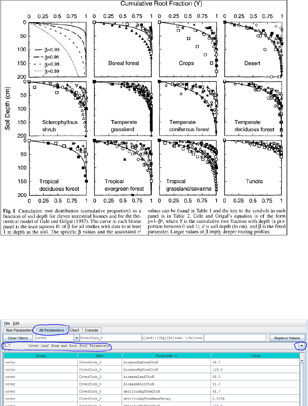
49
5.7 – Cover Leaf Stem and Root Pool Parameters
Select section 5.7 from the All Parameters drop-down menu to specify leaf stem and root pool
parameter values for each cover type in your watershed (do this for each cover type):

50
Parameters in this section cover the Leaf, Stem and Root pool C/N ratios, initial values, mortality
parameterizations and uptake fractions. Because each biomass or detritus leaf, stem and root
pool has its own set of parameters for these subjects, this list of parameters is relatively
extensive.
Parameter Definitions
biomassLeafCtoN The Carbon-to-Nitrogen ratio of the cover type’s
Leaf biomass pool.
biomassAgStemCtoN The Carbon-to-Nitrogen ratio of the cover type’s
AgStem biomass pool.
biomassBgStemCtoN The Carbon-to-Nitrogen ratio of the cover type’s
BgStem biomass pool.
biomassRootCtoN The Carbon-to-Nitrogen ratio of the cover type’s
Root biomass pool. (All layers of this pool use the
same CtoN ratio value.)
detritusLeafCtoN The Carbon-to-Nitrogen ratio of the cover type’s
Leaf detritus pool.
detritusAgStemCtoN The Carbon-to-Nitrogen ratio of the cover type’s
AgStem detritus pool.
detritusBgStemCtoN The Carbon-to-Nitrogen ratio of the cover type’s
BgStem detritus pool. (All layers of this pool use
the same CtoN ratio value.)
detritusRootCtoN The Carbon-to-Nitrogen ratio of the cover type’s
Root detritus pool. (All layers of this pool use the
same CtoN ratio value.)
detritusLeafNmaxDecay Maximum decay rate for Potter decomposition of
Leaf detritus pool’s Nitrogen amount.
detritusAgStemNmaxDecay Maximum decay rate for Potter decomposition of
AgStem detritus pool’s Nitrogen amount.
detritusBgStemNmaxDecay Maximum decay rate for Potter decomposition of
BgStem detritus pool’s Nitrogen amount.
detritusRootNmaxDecay Maximum decay rate for Potter decomposition of
Root detritus pool’s Nitrogen amount.
initialBiomassLeafCarbon The amount of biomass (in grams of Carbon)
placed in the Leaf biomass pool of each cell of this
cover type at initialization start.
initialBiomassAgStemCarbon The amount of biomass (in grams of Carbon)
placed in the AgStem biomass pool of each cell of
this cover type at initialization start.
initialBiomassBgStemCarbon The amount of biomass (in grams of Carbon)
placed in the BgStem biomass pool of each cell of
this cover type at initialization start.

51
initialBiomassRootCarbon The amount of biomass (in grams of Carbon)
placed in the Root biomass pool of each cell of
this cover type at initialization start.
initialDetritusLeafCarbon The amount of detritus (in grams of Carbon)
placed in the Leaf detritus pool of each cell of this
cover type at initialization start.
initialDetritusAgStemCarbon The amount of detritus (in grams of Carbon)
placed in the AgStem detritus pool of each cell of
this cover type at initialization start.
initialDetritusBgStemCarbon The amount of detritus (in grams of Carbon)
placed in the BgStem detritus pool of each cell of
this cover type at initialization start.
initialDetritusRootCarbon The amount of detritus (in grams of Carbon)
placed in the Root detritus pool of each cell of this
cover type at initialization start.
etRecoveryFractionMinimumLeafBiomassC
The minimum amount of leaf biomass (in gC/m^2)
required to compute an ET recovery fraction.
Whenever leaf biomass is less than this amount,
the ET recovery fraction is forced to the
etRecoverFractionMinimumValue.
See Section 10.2.1 ET Recovery Parameters.
mortalityLeafAnnualFraction The fraction of the Leaf biomass Pool annual
mortality amount actually subtracted from that
pool per day of senescence. The default value for
this fraction is 1.0 (i.e. the full per-day amount)
and the valid range is [0.0 to 1.0]. Warning! Users
unfamiliar with this parameter's behavior should
leave it set to the default value of 1.0.
mortalityLeafDenominatorCoefficient The mortality equation’s denominator coefficient
value for the biomass Leaf pool.
mortalityLeafExponentialCoefficient The mortality equation’s exponential coefficient
value for the biomass Leaf pool.
mortalityLeafNumeratorCoefficient The mortality equation’s numerator coefficient
value for biomass Leaf pool.
mortalityAgStemAnnualFraction The fraction of the AgStem biomass Pool annual
mortality amount actually subtracted from that
pool per day of senescence. The default value for
this fraction is 1.0 (i.e. the full per-day amount)
and the valid range is [0.0 to 1.0]. Warning! Users
unfamiliar with this parameter's behavior should
leave it set to the default value of 1.0.
mortalityAgStemDenominatorCoefficient
The mortality equation’s denominator coefficient
value for the biomass AgStem pool.
mortalityAgStemExponentialCoefficient
The mortality equation’s exponential coefficient
value for the biomass AgStem pool.
52
mortalityAgStemNumeratorCoefficient The mortality equation’s numerator coefficient
value for the biomass AgStem pool.
mortalityBgStemAnnualFraction The fraction of the BgStem biomass Pool annual
mortality amount actually subtracted from that
pool per day of senescence. The default value for
this fraction is 1.0 (i.e. the full per-day amount)
and the valid range is [0.0 to 1.0]. Warning! Users
unfamiliar with this parameter's behavior should
leave it set to the default value of 1.0.
mortalityBgStemDenominatorCoefficient
The mortality equation’s denominator coefficient
value for the biomass BgStem pool.
mortalityBgStemExponentialCoefficient
The mortality equation’s exponential coefficient
value for the biomass BgStem pool.
mortalityBgStemNumeratorCoefficient The mortality equation’s numerator coefficient
value for the biomass BgStem pool.
mortalityRootAnnualFraction The fraction of the Leaf biomass Pool annual
mortality amount actually subtracted from that
pool per day of senescence. The default value for
this fraction is 1.0 (i.e. the full per-day amount)
and the valid range is [0.0 to 1.0]. Warning! Users
unfamiliar with this parameter's behavior should
leave it set to the default value of 1.0.
mortalityRootDenominatorCoefficient The mortality equation’s denominator coefficient
value for the biomass Root pool.
mortalityRootExponentialCoefficient The mortality equation’s exponential coefficient
value for the biomass Root pool.
mortalityRootNumeratorCoefficient The mortality equation’s numerator coefficient
value for the biomass Root pool.
useLinearMortalityLeaf When true, leaf mortality is computed using a
simple linear function. When false (default)
mortality is computed via a logistic function.
useLinearMortalityAgStem When true, AgStem mortality is computed using a
simple linear function. When false (default)
mortality is computed via a logistic function.
useLinearMortalityBgStem When true, BgStem mortality is computed using a
simple linear function. When false (default)
mortality is computed via a logistic function.
useLinearMortalityRoot When true, Root mortality is computed using a
simple linear function. When false (default)
mortality is computed via a logistic function.
nppToBiomassLeafNfraction The fraction of total daily NPP for a cell of this
cover type allotted to the biomass Leaf pool.
nppToBiomassRootNfraction The fraction of total daily NPP for a cell of this
cover type allotted to the biomass Root pool.
nppToBiomassAgStemNfraction The fraction of daily NPP ALOTTED TO STEM
POOLS for a cell of this cover type allotted to the

53
biomass AgStem pool. The remaining NPP
allotted to stem pools goes to the biomass BgStem
pool. NOTE: Total daily NPP is reduced by the
fractions for leaf and root pools first. Any
remainder is the daily NPP allotted to stem pools.
Calibration Notes
At this stage (section 5.7) of your simulation configuration, don’t try to specify values for all the
parameters listed above. For now, just focus on the initial C and N pools for plant biomass and
detritus (highlighted in yellow, above). To specify initial C and N stocks (g/m2) for these pools,
we recommend that you consult Appendix 1 for an overview of VELMA’s LSR submodel and it
C and N pools and fluxes. Filling in C and N values for the various pools shown would be a
good start. Remember to document data sources as you go.
Methods for specifying parameter values for NPP (plant uptake) allocation, plant biomass
mortality, and detritus decay (decomposition) rates, and NPP are discussed in subsequent
sections:
− N uptake (NPP): Section 11.0
− Mortality: Section 12.0
− Decomposition: Section 13.0
5.7.1 – Cover Leaf Pool Parameter
Select section 5.7.1 from the All Parameters drop-down menu to specify cover-specific
parameter values for leaf biomass and detritus. See 5.7 above for the parameter descriptions.
5.7.2 – Cover Above-Ground Stem Pool Parameters
Select section 5.7.1 from the All Parameters drop-down menu to specify cover-specific
parameter values for aboveground stem biomass and detritus. See 5.7 above for the parameter
descriptions.
5.7.3 – Cover Below-Ground Stem Pool Parameters
Select section 5.7.1 from the All Parameters drop-down menu to specify cover-specific
parameter values for belowground stem biomass and detritus. See 5.7 above for the parameter
descriptions.
5.7.4 – Cover Root Pool Parameters
Select section 5.7.1 from the All Parameters drop-down menu to specify cover-specific
parameter values for root biomass and detritus. See 5.7 above for the parameter descriptions.
6.0 – Weather Model (link to All Parameters TOC)
The Default Weather Model provides uniform precipitation and air temperature values for all
cells of a simulation’s delineated watershed for each day of a simulation run, and includes a
simple snow model.
A Default Weather Model is Provided Automatically in New Simulation Configurations
When you create a new simulation configuration in the VELMA GUI (Edit “Create a New,
Empty Configuration”), it automatically contains parameters for the default weather model. This
weather model’s modelClass, uniqueName and uniqueId parameters are preset to valid, default
values. You may change those values if you wish, but there is no need to do so and we advise
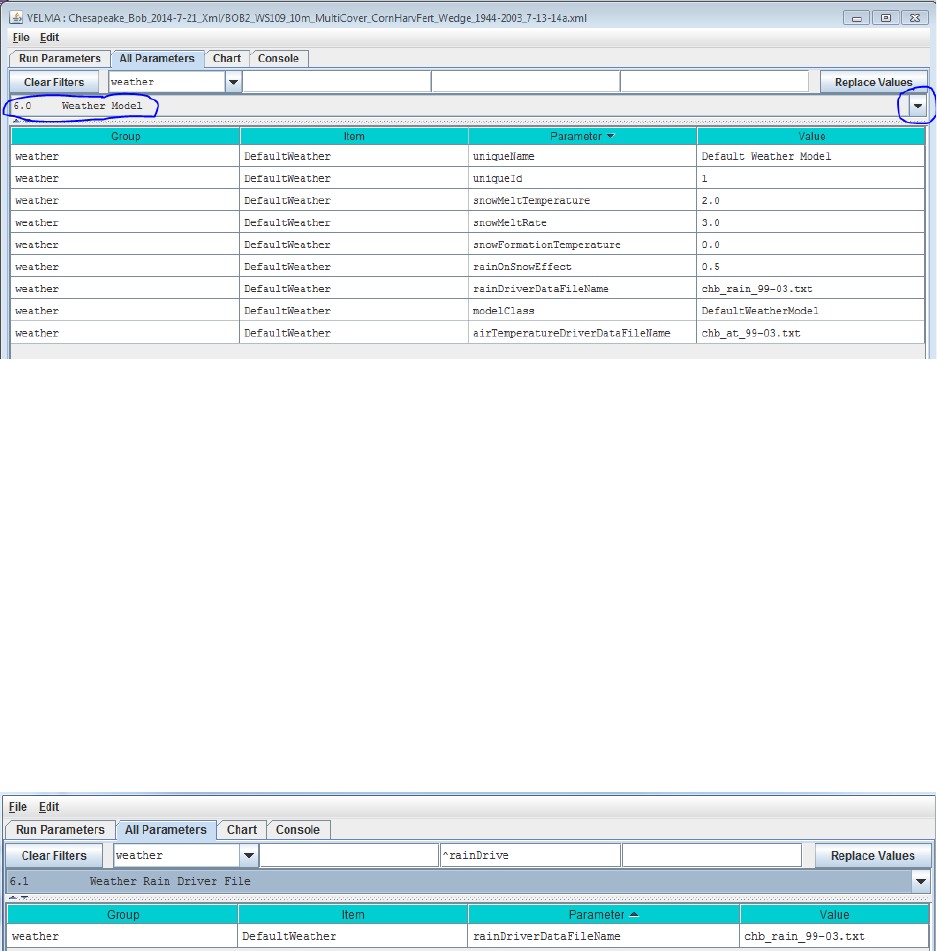
54
you to leave them alone. You must provide the model with the names of data files for
precipitation and air temperature driver data, and parameterize the snow model.
You can focus the All Parameters tab’s parameters table to various aspects of the simulation
configuration’s weather model by selecting them in the tab’s drop-down selector.
To view the complete core weather model parameterization, select “6.0 Weather Model”:
You Must Provide the Weather Model with Rain and Air Temperature Driver Files.
The rain and air temperature driver files share the same format requirements: one floating-point
value per line, with exactly one line for each day between the first day of the year specified by
the simulation configuration’s forcing_start value, and the last day of the year specified by the
simulation configuration’s forcing_end value. For example, if a forcing start/end range of [2000
to 2001] would require each driver file to have 731 lines of data (corresponding to 366 + 365
days per year, accounting for the leap year), with one value per line.
You may omit the path of the driver file names you specify. The Velma simulator then assumes
the file’s location is specified by the simulation configuration’s input data location settings (set
the outline selection to “1.0 Input Data Selection” to review or set the input location). You may
also provide a fully-qualified path + name for a driver file. If you do, be sure to use “/”
(forward-slash) characters as path-separators.
Select “6.1 Weather Rain Driver File” to focus the parameters table on the weather model’s
rainDriverDataFileName parameter.
Each value in this file represents a day’s precipitation (in millimeters) at each cell in simulation’s
the delineated watershed. Because of the snow model, some of this precipitation may be rain,
and some may be snow. The parameterization of the snow model determines the amounts of
both.
Select “6.2 Weather Air Temperature Driver File” to focus the parameters table on the weather
model’s airTemperatureDriverFileName.
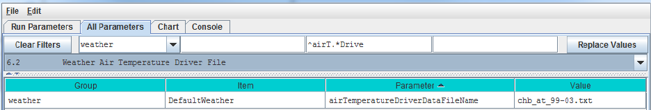
55
Each value in this file represents a day’s average air temperature (in degrees Centigrade) at each
cell in the simulation’s delineated watershed.
The Snow Model Determines the Rain / Snow Mixture for the Precipitation Driver Value
The four parameters of the snow model determine how much of a given day’s precipitation falls
as rain or as snow, and how fast snow on the ground is converted to surface water.
snowFormationTemperature
The air temperature (in degrees C) below which the
day’s precipitation is counted as snow. At and above this
temperature, it is counted as rain.
snowMeltTemperature
The temperature above which any available snow begins
to melt.
snowMeltRate
The rate at which melting snow becomes surface water.
rainOnSnowEffect
Used in conjunction with the
snowMeltRate
to determine
the amount of snow that melts into surface water.
A Summary Description of the Snow Model’s Behavior
For each day of a simulation run, the daily air temperature and precipitation values are taken
together with the above snow model parameters and daily values are calculated for the following:
Rain, Snow, Snow Depth and Snow Melt.
When air temperature is at or above the snowFormationTemperature, all the day’s precipitation is
counted as rain and becomes the day’s Rain value. If the air temperature is also greater than the
snowMeltTemperature, the amount of snow that melts is calculated using the following equation:
snowMeltRate * (airT - snowMeltTemperature) + rainOnSnowEffect * rain
where airT and rain are the day’s air temperature and precipitation values respectively.
If there has been snow deposited into the Snow Depth value on previous simulation days (see
below) the amount of snow melted is “deducted” from that value and becomes additional “rain”
for the day. If the melted amount that is computed exceeds the amount of snow depth, the entire
amount (but no more) is “deducted”.
When air temperature is below the snowFormationTemperature parameter, all the day’s
precipitation is counted as snow and becomes the day’s Snow value. The day’s Snow mount is
also added to the Snow Depth value.
6.3.1 – Weather Model Coefficients Files (Only Spatial Weather)
VELMA’s default weather model (described under section 6.0 – 6.2) does not address spatial
variations in temperature and precipitation associated with topographic features – elevation,
slope, aspect and cold air drainages.
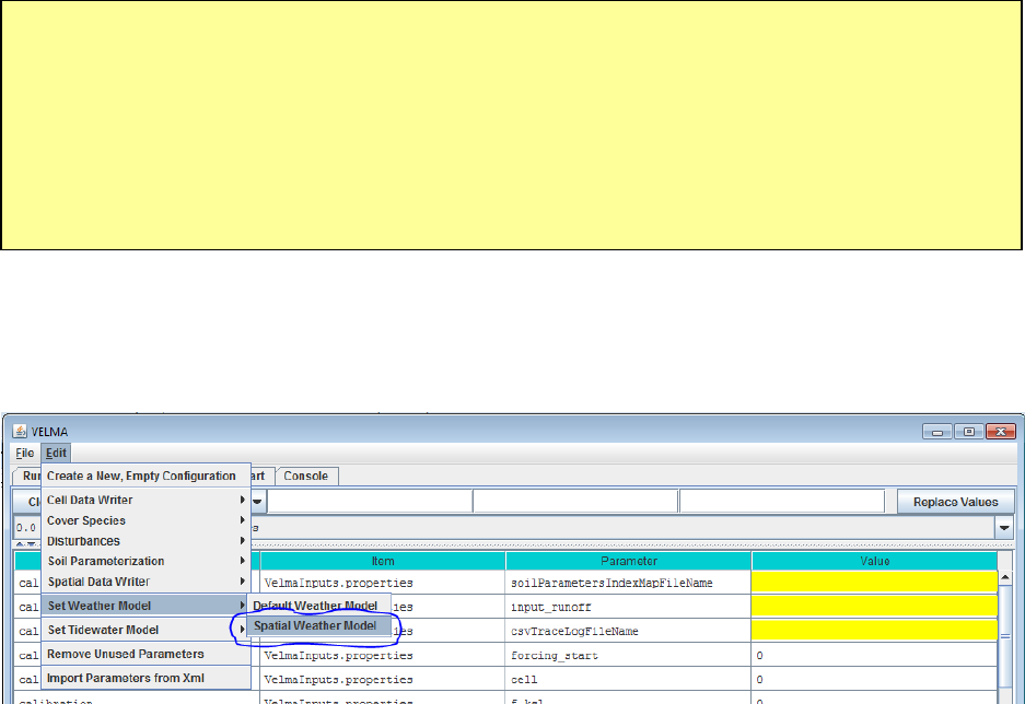
56
VELMA’s optional Spatial Weather Model provides differing precipitation and air temperature
values for each cell of a simulation’s delineated watershed for each day of a simulation run. It
includes the same simple snow model as the Default Weather Model.
You Must Explicitly Specify Activation of the Spatial Weather Model
When you create a new simulation configuration, the VELMA GUI automatically adds a Default
Weather Model parameters group to it. If you wish to use the Spatial Weather Model instead,
Click the Edit “Set Weather Model “Spatial Weather Model” menu item:
When you set the weather model to “Spatial Weather Model”, the VELMA GUI removes any
pre-existing weather model parameters and adds the parameters group for the Spatial Weather
Model.
You can focus the All Parameters tab’s parameters table to various aspects of the simulation
configuration’s weather model by selecting them in the tab’s outline drop-down selector.
The VELMA GUI automatically provides valid default values for the Spatial Weather Model’s
uniqueId, uniqueName and modelClass parameters. You may leave these as they are initially set.
To view the complete core weather model parameterization, select “6.0 Weather Model”:
CAUTION!
The Spatial Weather Model is still somewhat experimental and undergoing testing and
refinement.
Also, it requires more effort to configure/parameterize than the Default Weather Model.
For both of these reasons, we currently recommend using only the Default Weather Model
unless you must have the more complex behavior that the Spatial Weather Model provides,
e.g, for mountainous terrain.
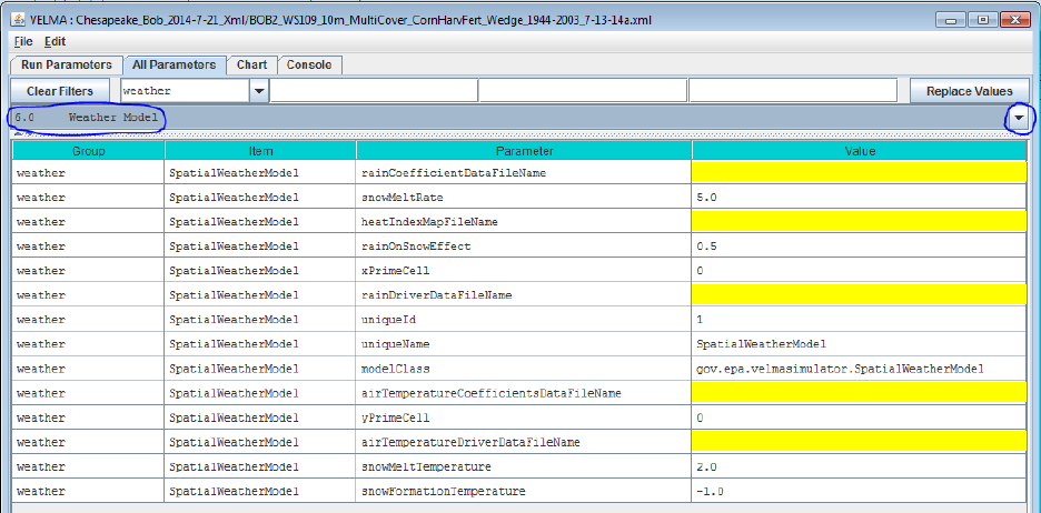
57
You Must Provide the Weather Model with Rain and Air Temperature Driver Files
The Spatial Weather Model derives daily rain and air temperature values for every cell in the
simulation watershed by applying functions to the daily rain and air temperature values of one
specific cell (the “Primary” or “Prime” Cell) within the watershed. You must provide the data
file names for rain and air temperature data observed for this Prime Cell, as well as its x-and-y
coordinates as part of the Spatial Weather Model’s parameterization.
Set the xPrimeCell and yPrimeCell parameter’s values to the Prime Cell’s x (column) and y
(row) location.
Set the rainDriverDataFileName and airTemperatureDriverDataFileName to the file names of
the precipitation and air temperature files, respectively.
You may omit the path of the driver file names you specify. The Velma simulator then assumes
the file’s location is specified by the simulation configuration’s input data location settings (set
the outline selection to “1.0 Input Data Selection” to review or set the input location). You may
also provide a fully-qualified path + name for a driver file. If you do, be sure to use “/”
(forward-slash) characters as path-separators.
The rain and air temperature driver files share the same format requirements: one floating-point
value per line, with exactly one line for each day between the first day of the year specified by
the simulation configuration’s forcing_start value, and the last day of the year specified by the
simulation configuration’s forcing_end value. For example, if a forcing start/end range of [2000
to 2001] would require each driver file to have 731 lines of data, with one value per line.
You Must Provide Files of Coefficients for Precipitation and Air Temperature Calculations
The Spatial Weather Model calculates the day’s precipitation and air temperature values for a
given cell location by applying a precipitation or air temperature function to the day’s driver
precipitation or air temperature value. These functions map/modify the “seed” value at the
Prime Cell to derive a value for the other cells. The functions take into account the cell’s
elevation, flow accumulation and heat index values, and the equations involved require per-
month coefficients for each term of their equations.

58
You must provide the file names (or optionally full path + names) of one file for rain
(precipitation) equation coefficients and one file of air temperature coefficients.
The Precipitation Coefficients File
A comma-separated values (.csv) file containing a table of coefficients for the spatial weather
model’s precipitation equation. The file must contain 13 rows of 6 comma-separated values
(columns) each.
The first row is a header row, and the remaining 12 rows provide values for the equation’s a, b,
c, d and e coefficients for each month of the year.
Here is an example table of values:
and here are the lines from the corresponding .csv data file:
month,a,b,c,d,e
1,259.751,0.011833,5.24E-05,-3.94717,-0.09685
2,241.5404,0.006131,6.10E-05,-5.15183,0.892817
3,210.8037,0.037236,4.62E-05,-4.20577,0.951439
4,96.40946,0.080534,7.44E-06,-1.44569,1.250961
5,88.34944,0.014202,3.06E-05,-0.20094,1.259266
6,53.51838,0.048195,9.53E-06,0.873204,1.297879
7,13.08702,0.023576,2.49E-06,0.686924,0.685529
8,21.89397,7.78E-05,6.23E-06,-0.00893,0.199088
9,70.03036,0.007598,2.39E-05,-0.00868,0.959202
10,124.4332,-0.00302,3.59E-05,-1.16562,0.890761
NOTE
Determining the values for precipitation and air temperature coefficients requires
detailed knowledge of the equations defining the Spatial Weather Model’s behavior.
For additional information concerning theory and procedures for developing statistical
coefficients for VELMA’s spatial climate model see Appendix 5: Generating daily
temperature and precipitation grids for running VELMA: development of statistical
models based on monthly PRISM data.
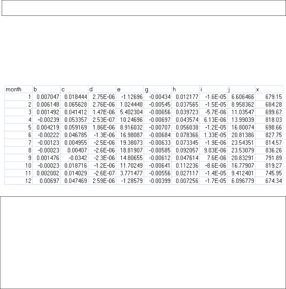
59
11,316.075,0.072349,4.32E-05,-4.40543,1.247633
12,290.7049,0.034712,4.62E-05,-4.46288,0.495517
The Air Temperature Coefficients File
A comma-separated values (.csv) file containing a table of coefficients for the spatial weather
model’s air temperature equation. The file must contain 13 rows of 10 comma-separated values
(columns) each.
The first row is a header row, and the remaining 12 rows provide values for the equation’s a – j
and x coefficients for each month of the year.
Here is an example table of values:
And here are the lines from the corresponding .csv data file:
month,b,c,d,e,g,h,i,j,x
1,0.007047,0.018444,2.75E-06,-1.12696,-0.00434,0.012177,-1.60E-05,6.606466,679.15
2,0.006148,0.065628,2.75E-06,1.024448,-0.00545,0.037565,-1.50E-05,8.958362,684.28
3,0.001492,0.041412,1.47E-06,5.402304,-0.00656,0.039723,-5.70E-06,11.03547,699.67
4,-0.00239,0.053357,2.53E-07,10.24696,-0.00697,0.043574,6.13E-06,13.99039,818.03
5,0.004219,0.059169,1.86E-06,8.916032,-0.00707,0.056038,-1.20E-05,16.80074,698.66
6,-0.00222,0.046785,-1.30E-06,16.98087,-0.00684,0.078366,1.33E-05,20.81386,827.75
7,-0.00123,0.004955,-2.50E-06,19.38073,-0.00633,0.073345,-1.90E-06,23.54351,814.57
8,-0.00023,0.00407,-2.60E-06,18.81907,-0.00585,0.092057,9.03E-06,23.53079,836.26
9,0.001476,-0.0342,-2.30E-06,14.80655,-0.00612,0.047614,7.60E-06,20.83291,791.89
10,-0.00023,0.018716,-1.20E-06,11.70249,-0.00641,0.112236,-8.60E-06,16.77907,819.27
11,0.002002,0.014029,-2.60E-07,3.771477,-0.00556,0.027117,-1.40E-05,9.412401,745.95
12,0.00697,0.047469,2.59E-06,-1.28579,-0.00399,0.007256,-1.70E-05,6.096779,674.34
The Spatial and Default Weather Model Both Employ the Same Snow Model
Parameterization of the Spatial Weather Model’s snow (sub)model is exactly the same as that of
the Default Weather Model’s. See the Default Weather Model’s documentation for the details.
The difference between the two is that the Spatial Weather Model first calculates the
precipitation and air temperature values for the specific cell before applying the snow model’s
mechanism to determine the day’s rain, snow, snow depth and snow melt values. In contrast, the
Default Weather Model presents the same (driver) precipitation and air temperature values to the
snow model at every cell location in the simulation’s watershed.
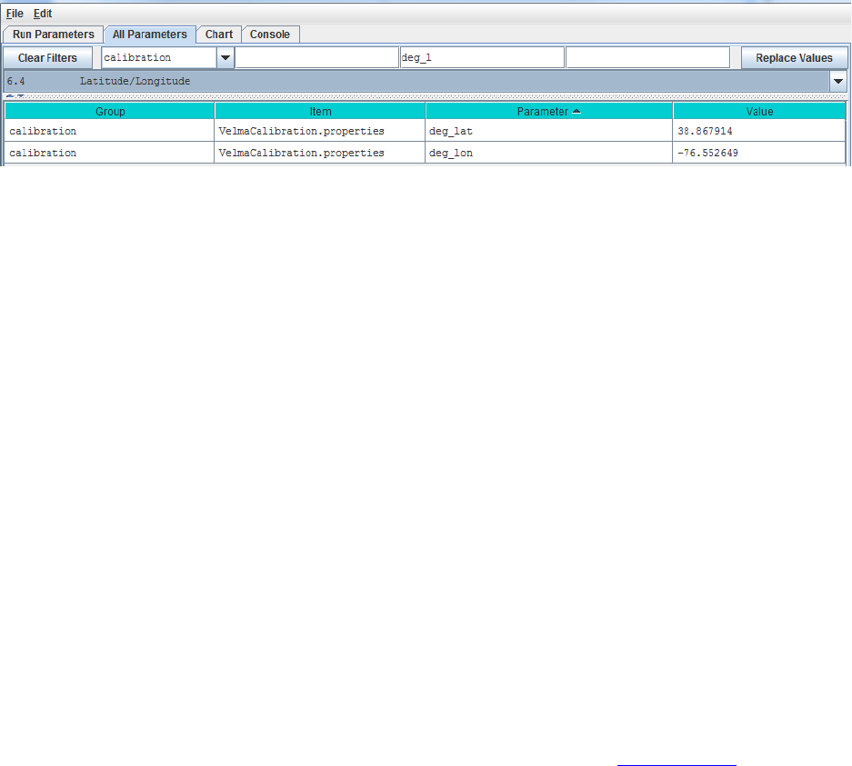
60
6.4 – Latitude/Longitude
The VELMA simulator computes a daily solar radiation value for the latitude and longitude
specified by the deg_lat and deg_lon parameter values. Set the values of these parameters to the
latitude and longitude of your simulation configuration’s location. Use decimal degrees, NOT
“degrees, minutes, seconds” format for the values. For example:
6.5 – Solar Radiation
In addition to latitude and longitude, VELMA’s solar radiation equation requires values for the
following parameters:
isc
Solar Constant.
sr1
Constant parameter 1 of solar radiation uptake function.
sr2
Constant parameter 2 of solar radiation uptake function.
srth
Solar radiation threshold.
The VELMA GUI automatically provides default values for each of these parameters; these may
be acceptable for your simulation location.
NOTE: Solar radiation parameters are intended for use in computing plant nitrogen uptake and
snow melt. Although these modeling capabilities are under development, VELMA 2.0 currently
does not include them. That being the case you may leave the solar radiation parameters set to
their default values without affecting your simulation run results.
6.6 – Soil Layer Temperature
Soil temperature is used in many of VELMA’s subroutines, for example, to compute rates of soil
organic matter decomposition, plant nitrogen uptake, nitrification, and many other temperature
sensitive processes. Documentation describing the equations and methods for computing
subsurface temperature per VELMA’s four soil layers can be found in Appendix 6.2 section
A1.1.
For the soil temperature subroutine to work properly for your simulation site, you need to:
− provide a daily mean air temperature file (see “Required Input Data Files for VELMA
Simulations”)
− specify values for total soil depth and soil bulk density (see All Parameters sections 4.3
and 4.5, respectively)
− and specify the average annual air temperature for your site (avgAT), as follows:
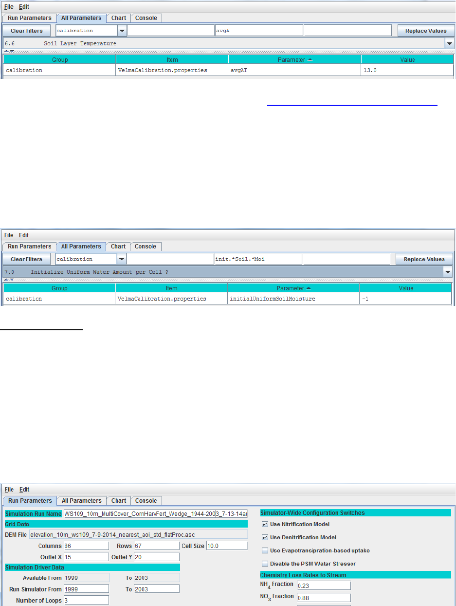
61
7.0 – Initialize Uniform Water Amount per Cell (link to All Parameters TOC)
Because soil moisture can vary significantly in space and time, it would be extremely difficult to
specify realistic soil moisture amounts for every soil layer in every cell within a watershed. A
more practical method is to specify a uniform amount of initial soil moisture for all layers and
cells, and then allow these initial values to adjust to realistic levels during a “spin up” period of
years prior to the simulated years of interest.
By default, VELMA set the initial water content of all cells and layers to the field capacity value
specified for each soil type. , i.e., when the parameter initialUniformSoilMoisture is set to its
default value of -1 (if it is set to any other value, reset it to -1).
Calibration Notes
We recommend using this default option, and that you also discard the first year of simulation
results, and possibly more, until soil moisture levels have sufficient time to “spin up” to your
site’s observed conditions. Shallow soils may adjust within a year or two, whereas deep soils
may require decades before simulated groundwater tables reach observed levels. You will need
to experiment with this to determine how many spin-up years are required.
To set up a spin-up period, you can instruct VELMA to perform one or more simulation “loops”
for the set of years included in the climate input files. To do this, specify the desired “Number of
Loops” in Run Parameters tab of the simulator’s GUI. For the example shown below, 3 loops
are specified, meaning that the 5 years (1999 – 2003) of available climate driver data will be
repeated (looped) 3 times for this simulation.
Thus, VELMA will generate 3 loops x 5 years = 15 years of model output, for which the first 2
loops (10 spin-up years) can be discarded.

62
An alternative method to accomplish the same thing would be to edit the temperature and
precipitation driver files, such that a copy of the years you want to use for spin-up purposes
appears at the beginning of the original climate record (remember to rename the edited climate
driver files to reflect the spin-up number of years).
8.0 – Chemistry Pools (Dissolved C and N) (link to All Parameters TOC)
VELMA simulates ecosystem inputs, outputs and internal cycling of four pools of dissolved
nitrogen and carbon in soil: ammonium (NH4), nitrate (NO3), dissolved organic nitrogen (DON)
and dissolved organic carbon (DOC).
Sections 8.1 and 8.2, below, describe the specification of initial pools and calibration of
parameters controlling leaching losses to streams. Subsequent sections describe additional
processes affecting inputs and outputs from these dissolved C and N pools.
8.1 – Chemistry Amounts for uniform cell-initialization
Initial soil pools (g N / m2 or g C / m2) of NH4, NO3, DON and DOC can be viewed and
specified by selecting “8.1 Chemistry Amounts for uniform cell-initialization” from the All
Parameters drop-down menu. The values specified should represent the sum of all 4 soil layers
(total soil column) averaged across the watershed.
Parameter Definitions
initial_doc Initial DOC pool amount (per cell) in gC/m2
initial_don Initial DON pool amount (per cell) in gN/m2.
initial_Nh4 Initial NH4 pool amount (per cell) in gN/m2.
initial_No3 Initial NO3 pool amount (per cell) in gN/m2.
Calibration Notes
On day 1 of a simulation, VELMA will use the specified parameter values to calculate the
fraction of each nutrient’s total pool to allocate to each of the four soil layers. This is done
uniformly for all grid cells on day 1.
With some effort, VELMA can be calibrated to simulate spatial variability in C, N, H2O pools
and fluxes. With a well-calibrated parameter set, initially uniform nutrient pool values will begin
to adjust and, after a sufficient spin-up time, more closely match spatial and temporal patterns of
observed nutrient pools (McKane 2014).
Section 7.0 describes methods for setting up an appropriate spin-up period for allowing
initialized soil moisture levels to adjust to a site’s biophysical conditions. The same spin-up
method applies for all model pools and fluxes, including stream chemistry.
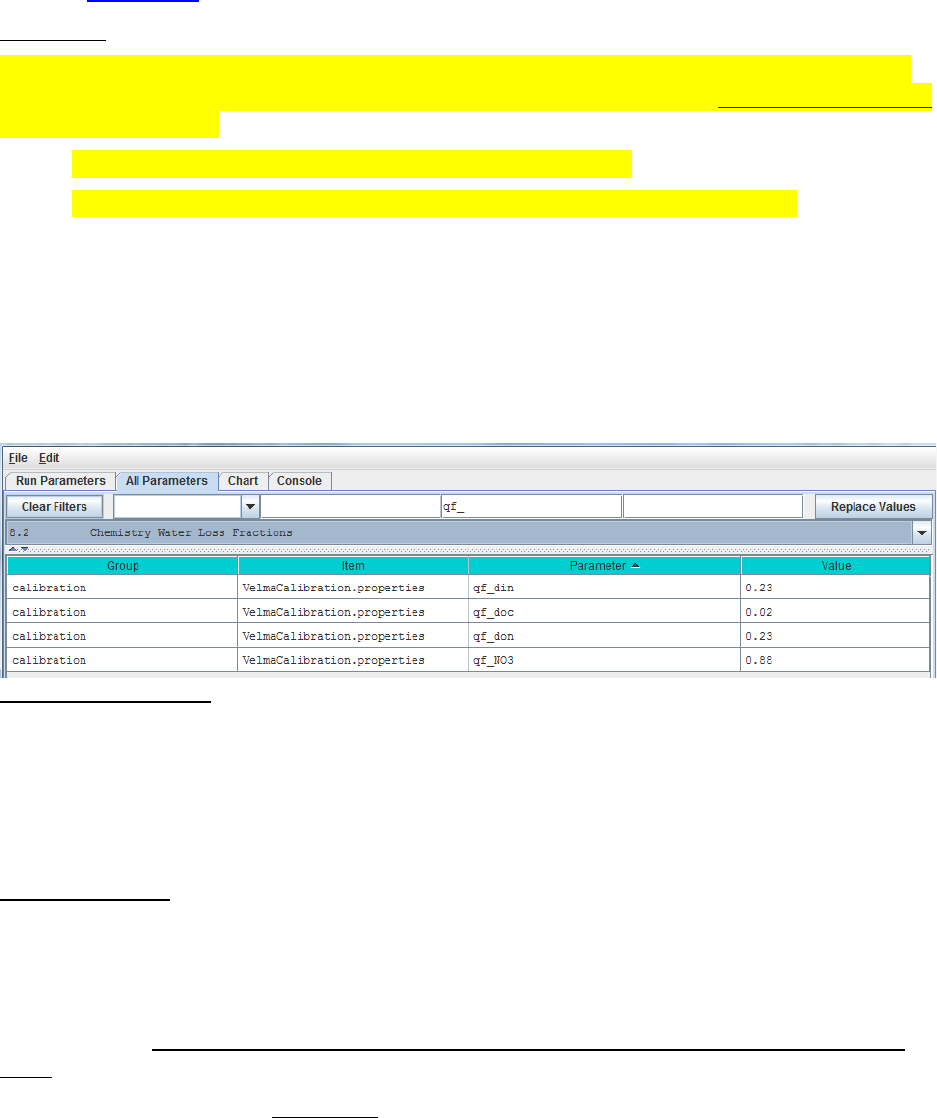
63
Alternatively, you can use a more advanced method for specifying initial nutrient pool values
that consider spatial variability in soil types, and cover species type and age. Details can be
found in Appendix 3: Creating Initial ASCII Grid Chemistry Spatial Data Pools.
References
The User Manual package includes slides for a seminar describing the effectiveness of riparian
buffers for protecting water quality in the Chesapeake Bay (please contact mckane.bob@epa.gov
if you have questions):
Filename: McKane_ORD GI webinar_7-30-14 Final.pptx
Folder location: VELMA Model\Supporting Documents\VELMA Pubs & Talks
8.2 – Chemistry Water Loss Fractions
In VELMA, transport of dissolved nutrients within the soil column, and ultimately to the stream,
is a function of vertical and lateral water drainage, the size of the nutrient pool, and a specified
loss fraction (qf) parameter.
The nutrient loss fraction parameters can be viewed and specified by selecting “8.2 Chemistry
Water Loss Fractions” from the All Parameters drop-down menu.
Parameter Definitions
qf_din NH4 loss due to horizontal and vertical water flow range [0.0 1.0].
qf_doc DOC loss due to horizontal and vertical water flow range [0.0 1.0].
qf_don DON loss due to horizontal and vertical water flow range [0.0 1.0].
qf_NO3 NO3 loss due to horizontal and vertical water flow range [0.0 1.0].
Calibration Notes
The “qf” parameters for specifying nutrient loss fractions are very important for achieving a
good fit between simulated and observed stream chemistry data (Abdelnour et al. 2013).
However, when you are calibrating these and any other parameters, keep in mind that it is fairly
easy to specify qf values that provide a good fit between simulated and observed stream
chemistry data, even when the source soil nutrient pools are poorly calibrated (too large or too
small.
Achieving a well-calibrated ecosystem model is an iterative process, requiring numerous
simulation runs until a set of parameters values is identified that simultaneously provides a good
fit between simulated and observed data for plants, soils and streams, i.e., all C, N and H2O pools
and fluxes for which good quality observed data are available (recognizing that complete
validation is an ideal never reached).
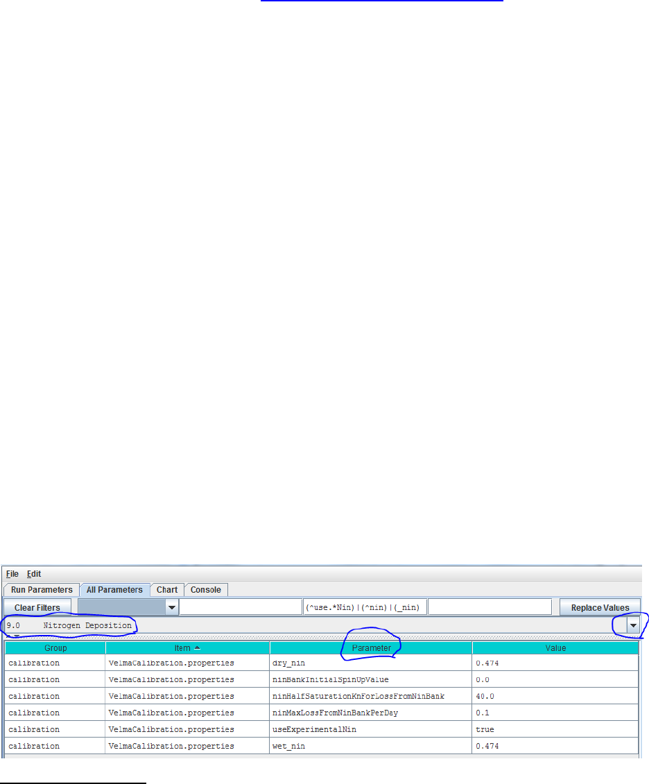
64
9.0 - 9.1.1 – Nitrogen Deposition (link to All Parameters TOC)
Atmospheric inputs of wet and dry nitrogen deposition can make a significant contribution to
ecosystem nitrogen budgets, especially in regions influenced by industry and agricultural. It is
important to estimate the timing and amounts of wet and dry nitrogen deposition, and its
availability for plant uptake and other ecohydrological processes. Such estimates are
complicated by time lags associated with dry deposition of nitrogen on leaves and other surfaces,
and subsequent flushing into the soil during precipitation events.
VELMA version 1.0 modeled daily atmospheric inputs of wet and dry deposition as a function of
the annual atmospheric input and the fraction of annual rain that occurs at a given day.
VELMA version 2.0 models atmospheric nitrogen deposition based on the following
assumptions:
1) The daily rate of atmospheric N deposition (wet + dry) is the same every day of the year,
i.e., annual total N deposition/365 = daily N deposition
2) Daily N deposition (Nin) accumulates on leaves & other surfaces (NinBank) until a liquid
precipitation (rain + snowmelt) event.
3) Precipitation events wash a fraction of NinBank (throughfall N) into the surface soil
layer’s inorganic N pool. This fraction (0-1) varies as a nonlinear (asymptotic) function
of leaf biomass and daily precipitation amount, such that grid cells having higher leaf
biomass have disproportionately lower throughfall N at lower amounts of precipitation.
Furthermore, N stored in NinBank becomes depleted past a certain upper threshold
(asymptote) of daily precipitation. Thus, the main difference between this method and
VELMA version 1.0 is that it can account for observed nonlinear threshold behavior of
throughfall as a function of leaf area and precipitation amount.
4) Currently, daily Nin is composed of NH4 + NO3 deposition, and Nin transferred from the
NinBank to the surface soil layer is to the ammonium pool in Layer0 (NH4 and NO3 will
be modeled separately in a future version of VELMA).
Parameters for the experimental (but preferred) nitrogen deposition subroutine can be viewed
and specified by selecting “9.0 Nitrogen Deposition” from the All Parameters drop-down menu:
Parameter Definitions
wet_nin Wet nitrogen deposition factor in gNm^2 per year
dry_nin Dry nitrogen deposition factor in gNm^2 per year
ninBankInitialSpinUpValue N-deposition initialization value. When this initialization
value is zero a simulation run’s first year is used to “spin
up” the Michaelis-Menten-based N-deposition model. The
N-deposition values computed for that first year (and

65
subsequent values calculated from them) are unlikely to be
accurate. However if a correct value is known this
initialization parameter may be set to it. The value should
be the daily average N-deposition value for a single cell of
the current simulation. If the value is unknown or cannot be
reliably deduced ahead of simulation start leave this value
zero and incur the first-year spin-up (see Calibration notes,
below)
ninHalfSaturationKnForLossFromNinBank N-deposition Michaelis-Menten kinetics Kn
constant.
ninMaxLossFromNinBankPerDay N-Deposition Michaelis-Menten kinetics maximum
useExperimentalNin When set to “true” N-deposition is computed using a
banked Michaelis-Menten-based equation. When set to
“false” N-deposition is computed using the VELMA
version 1.0 linear equation. Use of the older equation is
deprecated. The default value for this parameter is “true”.
Calibration Notes
For the reasons mentioned under assumption #3, above, we recommend using the experimental
(VELMA version 2.0) nitrogen deposition subroutine rather than that used in VELMA version
1.0.
We have prepared a DRAFT Excel spreadsheet that you may choose to use to parameterize the
experimental nitrogen deposition subroutine (please contact mckane.bob@epa.gov if you have
questions):
Filename: VELMA 2.0_Nitrogen Deposition Calibrator_7-26-13 v3.xlsx
Folder location: VELMA Model\Supporting Documents\Excel Calibration Files
9.1.2 Old (DEPRECATED) Nitrogen Deposition Parameters
Use of the VELMA version 1.0 nitrogen deposition subroutine is discouraged. Please see section
9.0.
10.0 – Transpiration (link to All Parameters TOC)
Evapotranspiration (ET) is the sum of evaporation and plant transpiration. ET equations and
parameters in VELMA version 2.0 are the same as for version 1.0 (see Abdelnour et al. 2011),
except for the following:
− The ET recovery function has been replaced with a new subroutine that models post-
disturbance changes in ET based on leaf biomass dynamics.
− A new subroutine models age-related declines in transpiration for forest systems.
See details in subsections 10.1 – 10.3.1.

66
10.1 – Core PET and ET Parameters
Core parameters for calibrating VELMA’s PET and ET submodels can be found by selecting
section 10.1 from the All Parameters drop-down menu:
Parameter definitions (see Abdelnour et al. 2011 for equations and additional explanation):
roair Air density in g/m^3
be ET coefficient used in the logistic equation that computes ET
from PET
temperaturePetOff PET is only active when air temperature is > than this value (in
degrees C)
petParam1 First term of PET Hamon Equation: petParam1 * petParam2 *
gS.roair * (esat / 1000.0f)
petParam2 Second term of PET Hamon Equation: petParam1 * petParam2
* gS.roair * (esat / 1000.0f)
notranspirationPetFraction The fraction of PET available outside of this a cover
species/type’s growing season range [0.0 - 1.0].
10.2 – ET Recovery On/Off ?
Select section 10.2 from the All Parameters drop-down menu to turn the ET recovery function on
(true) or off (false):
10.2.1 – ET Recovery Parameters
Select section 10.2.1 from the All Parameters drop-down menu to specify ET recovery parameter
values for each cover type in your watershed (just one cover shown below):
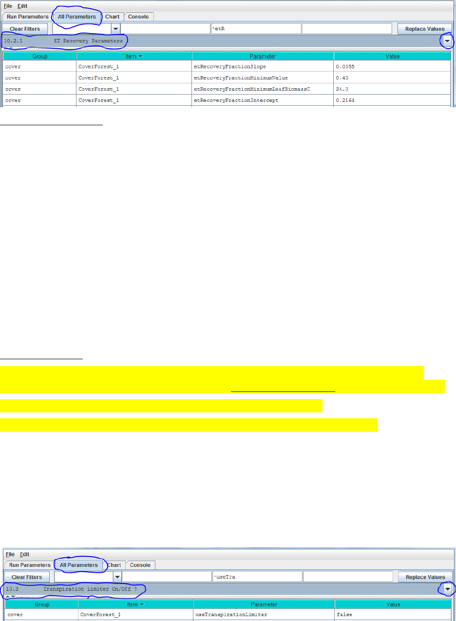
67
Parameter Definitions
etRecoverFractionSlope The value of the ET recovery fraction's linear
equation slope component.
etRecoverFractionMinimumValue The ET recovery fraction is forced to this value
when the current leaf biomass is less than the
value specified for
etRecoveryFractionLeafBiomassMinimum or
when the calculated ET recovery fraction is less
than zero.
etRecoverFractionMinimumLeafBiomassC The minimum amount of leaf biomass (in gC/m^2)
required to compute an ET recovery fraction.
Whenever leaf biomass is less than this amount
the ET recovery fraction is forced to the
etRecoverFractionMinimumValue.
etRecoverFractionIntercept The value of the ET recovery fraction's linear
equation intercept component.
Calibration Notes
We have prepared a DRAFT Excel spreadsheet that you may choose to use to calibrate ET
recovery parameters for your site (please contact mckane.bob@epa.gov if you have questions):
Filename: VELMA 2.0_ET Recovery Calibrator_HJA_12-1-13.xlsx
Folder location: VELMA Model\Supporting Documents\Excel Calibration Files
10.3 – Transpiration Limiter On/Off?
Studies in the Pacific Northwest have shown that young forests transpire significantly more
water than old forests (McDowell et al. 2002; Moore et al. 2004). VELMA version 2.0 has a
new subroutine to address age-related declines in transpiration by forest vegetation.
Select section 10.3 from the All Parameters drop-down menu to turn the Transpiration Limiter
subroutine on (true) or off (false):
Parameter definition:
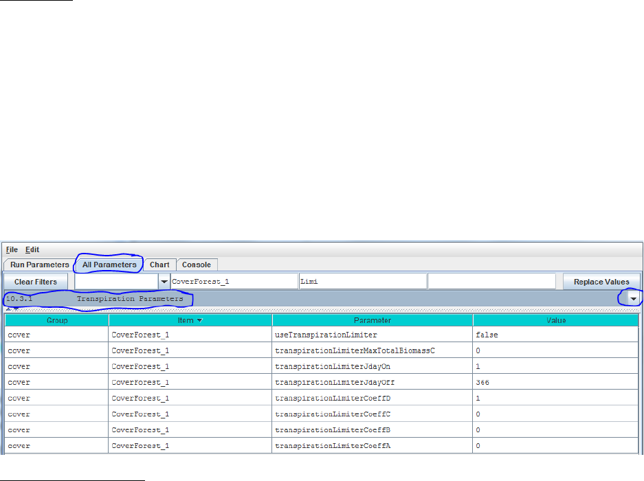
68
useTranspirationLimiter When set false (default value) the transpiration limiter fraction
value is forced to 1.0 (Which effectively means "No age-related
limitation" i.e. the limiter is OFF.) When set true the
transpiration limiter fraction is computed based on its jday and
coefficients settings.
See section 10.4 for parameters and calibration information.
References
McDowell, N. G., Phillips, N., Lunch, C., Bond, B. J., & Ryan, M. G. (2002). An investigation
of hydraulic limitation and compensation in large, old Douglas-fir trees. Tree Physiology,
22(11), 763-774.
Moore, G. W., Bond, B. J., Jones, J. A., Phillips, N., & Meinzer, F. C. (2004). Structural and
compositional controls on transpiration in 40-and 450-year-old riparian forests in western
Oregon, USA. Tree physiology, 24(5), 481-491.
10.3.1 – Transpiration Parameters
Select section 10.3.1 from the All Parameters drop-down menu to specify parameter values for
the Transpiration Limiter subroutine used to describe age-related declines in transpiration by
forest vegetation:
Parameter Definitions
useTranspirationLimiter When set false (default value) the transpiration
limiter fraction value is forced to 1.0 (Which
effectively means "No limiting at all" i.e. the
limiter is OFF.) When set true the transpiration
limiter fraction is computed based on its jday and
coefficients settings.
transpirationLimiterMaxTotalBiomassC Upper limit of total biomass amount (in gC/m^2)
for transpiration limiter fraction computation.
When total biomass amount in a cell exceeds this
max value the transpiration limiter faction value is
forced to the transpirationLimiterCoeffD
parameter's value.
transpirationLimiterJdayOn Transpiration reduction occurs on the Julian day
specified by this "on" parameter and continues on
every day of the year up to and including the day

69
specified by the paired "off" parameter. I.e.
transpiration reduction occurs in the range
[transpirationLimiterJdayOn
transpirationLimiterJdayOff]
transpirationLimiterJdayOff Transpiration reduction occurs on the Julian day
specified by this "off" parameter and does not
occur for any days of the year remaining after it.
I.e. transpiration reduction occurs in the range
[transpirationLimiterJdayOn
transpirationLimiterJdayOff]
transpirationLimiterCoeffA The A coefficient in the Transpiration Limiter
Fraction equation: A / (1 + B * exp(C *
totalBiomassC)) + D
transpirationLimiterCoeffB The B coefficient in the Transpiration Limiter
Fraction equation: A / (1 + B * exp(C *
totalBiomassC)) + D
transpirationLimiterCoeffC The C coefficient in the Transpiration Limiter
Fraction equation: A / (1 + B * exp(C *
totalBiomassC)) + D
transpirationLimiterCoeffD The D coefficient in the Transpiration Limiter
Fraction equation: A / (1 + B * exp(C *
totalBiomassC)) + D
Calibration Notes
The transpiration limiter subroutine is experimental and we do not recommend using it at this
time.
11.0 Plant Uptake (link to All Parameters TOC)
The VELMA v1.0 subroutine for plant nitrogen uptake is described by Abdelnour et al. (2011).
VELMA v2.0 generally follows the same subroutine, but includes important changes to several
components affecting nitrogen uptake:
− Uptake of NH4 and NO3 is now modeled explicitly, using pool-specific Michaelis-
Menten equations.
− The temperature response function for plant N uptake is now based on a quadratic
equation described by Rastetter et al. (1991).
− In VELMA v1.0 a constant root fraction parameter was applied to total plant biomass to
indirectly simulate effects of successional changes in root biomass on N uptake.
VELMA v2.0 includes a leaf-stem-root (LSR) subroutine that explicitly models root
biomass dynamics and consequent effects on NH4 and NO3 uptake.
− Simulated total N uptake per day is allocated to leaf, stem and root tissues according to
specified fractions per tissue.
− Phenological controls on plant nitrogen uptake constrain when nitrogen uptake can occur.
− The nonlinear (Weibull) function in VELMA v1.0 for simulating the effect of forest stand
age on N uptake has been removed. This and other age-related effects in VELMA v2.0
are now modeled as a consequence of successional changes in the availabilities of
nitrogen and water.
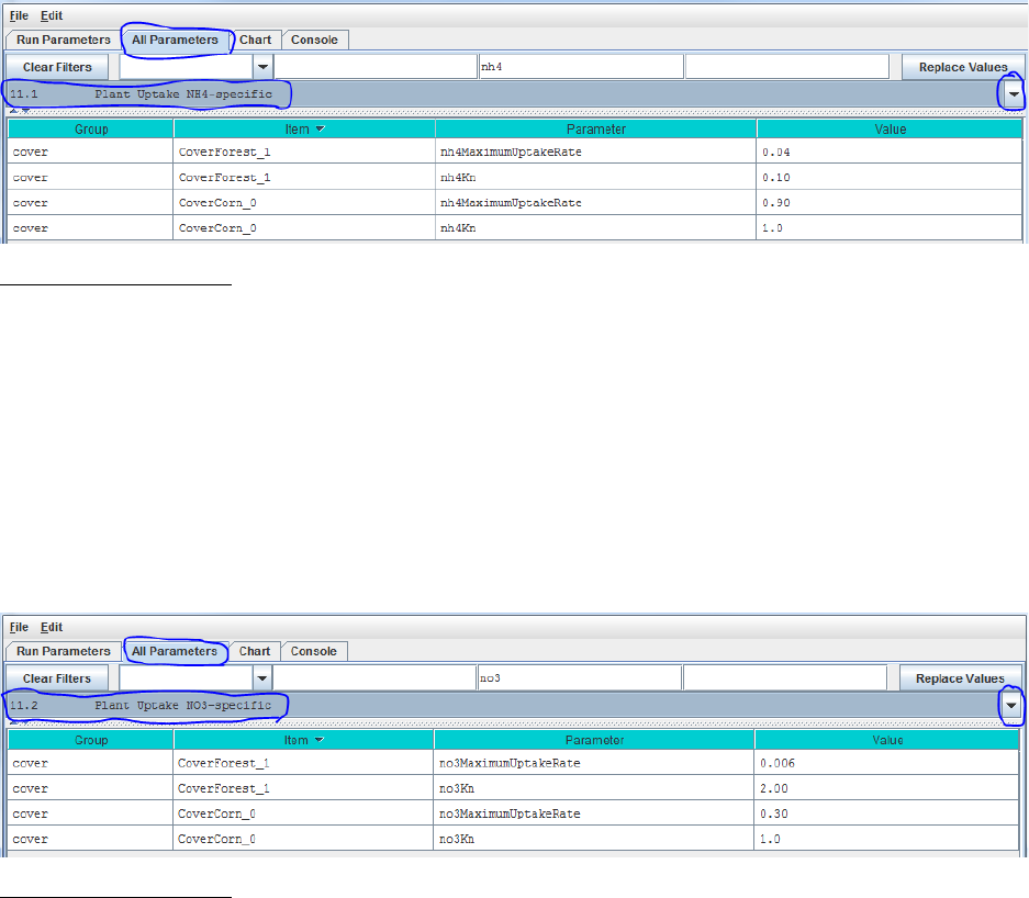
70
− The VELMA v2.0 plant N uptake subroutine must be set up and calibrated for each cover
species/types within a watershed.
Details are provided in subsections 11.1 – 11.5.
11.1 – Plant Uptake NH4-specific
Select “11.1 Plant Uptake NH4-specific” from the All Parameters drop-down menu to specify
parameter values controlling NH4 uptake per cover species/type. Note that two cover types
(forest and corn) are shown here to emphasize that parameters must be specified for each cover
type within a watershed (true for all of section 11).
Parameter Definitions
nh4MaximumUptakeRate Cover-specific maximum rate of NH4 uptake for biomass
uptake equation.
nh4Kn Half saturation constant kn for Michaelis Menton NH4 uptake
in gN/m^2.
See calibration notes for section 11.2.
11.2 – Plant Uptake NO3-specific
Select “11.2 Plant Uptake NO3-specific” from the All Parameters drop-down menu to specify
parameter values controlling NO3 uptake per cover species/type:
Parameter Definitions
no3MaximumUptakeRate Cover-specific maximum rate of NO3 uptake for biomass
uptake equation.
no3Kn Half saturation constant, kn, for Michaelis-Menten NO3
uptake in gN/m^2.
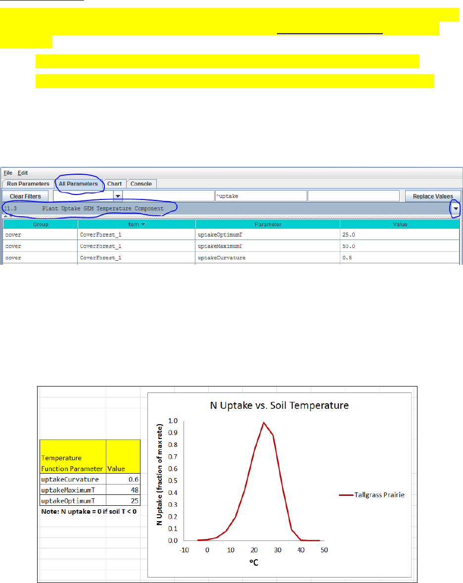
71
Calibration Notes
We have prepared a DRAFT Excel spreadsheet that you may choose to use to calibrate NH4 and
NO3 plant uptake parameters for your site (please contact mckane.bob@epa.gov if you have
questions):
Filename: VELMA 2.0_Nitrogen Uptake Calibrator (CHB Forest)_9-24-13.xlsx
Folder location: VELMA2.0Software/SupportingDocuments/ExcelCalibrationFiles
11.3 – Plant Uptake GEM Temperature Component
Select “11.3 Plant Uptake GEM Temperature Component” from the All Parameters drop-down
menu to specify parameter values for the temperature response function affecting NH4 and NO3
uptake (specify per cover type):
Parameter definitions (see Rastetter et al. (1991) for a description of the General Ecosystem
Model (GEM) temperature function and parameters for simulating plant nitrogen uptake):
uptakeOptimumT Optimal temperature (oC) plant uptake of NH4 and NO3
uptakeMaximumT Maximum temperature (oC) plant uptake of NH4 and NO3
uptakeCurvature Curvature parameter of GEM temperature function.
An example:
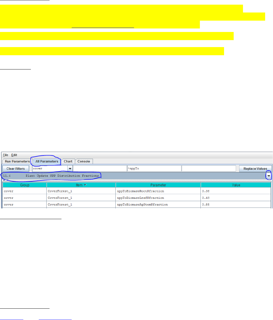
72
Calibration Notes
We have prepared a DRAFT Excel spreadsheet that you may choose to use to calibrate
temperature response functions for plant N uptake and other temperature sensitive processes in
VELMA. (please contact mckane.bob@epa.gov if you have questions):
Filename: VELMA 2.0_Temperature & Moisture Response Functions_9-8-14.xlsx
Folder location: VELMA Model\Supporting Documents\Excel Calibration Files
References
Rastetter, E. B., Ryan, M. G., Shaver, G. R., Melillo, J. M., Nadelhoffer, K. J., Hobbie, J. E., &
Aber, J. D. (1991). A general biogeochemical model describing the responses of the C and N
cycles in terrestrial ecosystems to changes in CO2, climate, and N deposition. Tree
Physiology, 9(1-2), 101-126.
11.4 – Plant Uptake NPP Distribution Fractions
Select “11.4 Plant Uptake NPP Distribution Fractions” from the All Parameters drop-down menu
to specify parameter values controlling how daily total N uptake (a.k.a, “NPP” in VELMA) is
allocated to leaf, aboveground stem, belowground stem, and root biomass:
Parameter Definitions
nppToBiomassRootNfraction The fraction (0.0 -1.0) of total plant uptake of nitrogen (NH4 +
NO3) per day allocated to the root biomass N pool.
nppToBiomassLeafNfraction The fraction (0.0 -1.0) of total plant uptake of nitrogen (NH4 +
NO3) per day allocated to the leaf biomass N pool.
nppToBiomassAgStemNfraction The fraction (0.0 -1.0) of total plant uptake of nitrogen (NH4 +
NO3) per day allocated to the AgStem biomass N pool.
Note that “nppToBiomassBgStemfraction” does not need to be specified because VELMA
internally calculates it by difference.
Calibration Notes
Figure 1 and Appendix 1 provides conceptual diagrams and equations describing how N uptake
(NPP) is allocated among the four LSR plant tissues.
To calibrate the N allocation parameters described in this section, we recommend constructing an
annual plant biomass N budget(s) for all four LSR tissues per cover type. Observed data and
estimates can usually be found in the literature for this. For example:
− Leaf litterfall data can be used to estimate annual leaf NPP, usually as dry weight or
carbon, so you will also need C/N data to calculate annual N uptake.
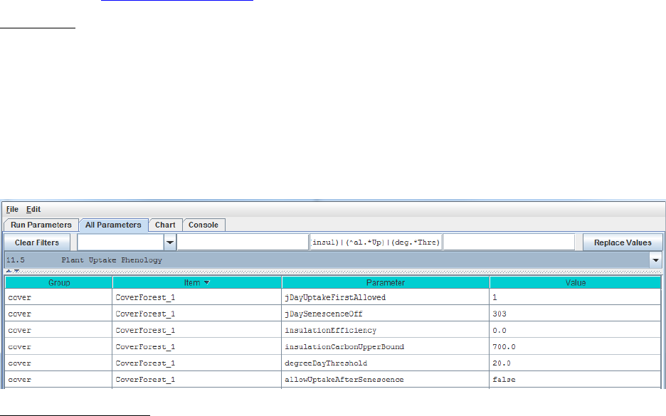
73
− Data for above- and belowground stem biomass growth can be obtained from tree-
ring data and allometric biomass equations for forest cover types, or from
“destructive” biomass harvest methods in grasslands or agricultural plots.
− Production estimates for fine roots exist for many cover types, and are based on a
variety of methods – e.g., see Nadelhoffer, K. J., & Raich, J. W. (1992).
Please contact mckane.bob@epa.gov if you have questions.
References
Nadelhoffer, K. J., & Raich, J. W. (1992). Fine root production estimates and belowground
carbon allocation in forest ecosystems. Ecology, 1139-1147
11.5 – Plant Uptake Phenology
Select “11.5 Plant Uptake Phenology” from the All Parameters drop-down menu to specify
parameter values affecting when plant N uptake begins and ends during the year (per cover
type):
Parameter Definitions
jDayUptakeFirstAllowed The first Julian day of the year on which uptake is possible for
this Cover. Uptake will NEVER happen before the specified
day. Use this parameter to delay uptake until the daily
photoperiod is sufficient for the given Cover. This parameter
specifies the first day of the year when uptake can occur not
necessarily the first day when uptake will occur. On and after
the day specified by this parameter uptake will occur
whenever the degree day parameterization allows it to begin.
jDaySenescenceOff The Julian Day of the year when this cover species biomass
stops senescing (Note: any value >= 367 results in biomass
NOT senescing through the end of the
year.nppToBiomassAgStemNfraction The fraction (0.0 -1.0)
of total plant uptake of nitrogen (NH4 + NO3) per day allocated
to the AgStem biomass N pool.
insulationEfficiency Insulating efficiency of available litter range [0.0 1.0] (this
affects soil temperature and, therefore, plant N uptake). NOTE:
Set this value to zero to disable insulation effects on degree-
day calculation.
insulationCarbonUpperBound Quantity of above-ground litter beyond which there is no
additional insulating effect in gC/m^2 (this affects soil
temperature and, therefore, plant N uptake).

74
degreeDayThreshold Allow biomass uptake only when accumulated degree day
value >= degreeDayThreshold.
allowUptakeAfterSenescence When set true (default) uptake takes place before
jDaySenescenceOn and resumes after jDaySenescenceOff.
When set "false" uptake occurs ONLY before
jDaySenescenceOn
12.0 Plant Mortality (link to All Parameters TOC)
VELMA v.2.0 has a new plant biomass mortality function, replacing the linear mortality function
in v1.0 (Abdelnour et al. 2011). The new mortality function was initially developed for forest
vegetation but we have found that it applies just as well to other cover types, including
nonwoody species such as grasslands and agricultural crops.
The mortality function is based on the following observations and assumptions:
− The ratio of mortality/NPP during succession is nonlinear. For example, in regrowing
forest stands, observed increases in stem biomass require that stem NPP exceeds stem
mortality until steady state is reached.
− A logistic function provides sufficient flexibility to capture temporal changes in the
relationship between mortality and NPP during succession. Specifically, a logistic
function is used to describe nonlinear changes in a tissue’s litterfall/NPP ratio vs. stand
age, where “tissue” can represent leaf, aboveground stem, belowground stem, or root
biomass. In practice, total plant biomass (or aboveground stem biomass) serves as a
proxy for stand age.
− For example, using VELMA’s parameter naming convention,
mortalityAgStemCarbon / nppAgStemCarbon = C / (1 + A * exp^(-B * plantBiomassCarbon))
− Rearranging,
mortalityAgStemCarbon = nppAgStemCarbon * C / (1 + A * exp^(-B * plantBiomassCarbon))
For example, the figures below show results obtained by applying the logistic mortality function
to a riparian hardwood forest. The left figure shows changes in the ratio of belowground stem
mortality/NPP vs. total stem biomass (proxy for stand age). The right figure shows simulated
temporal changes in simulated belowground stem biomass and total plant biomass. Adjustment
of the mortality function parameters can be used to flatten or steepen the asymptotic trends in
biomass, according to chronosequence data. The mortality function must be applied to all four
of VELMA’s plant tissues (results for leaf, aboveground stem and fine root biomass are not
shown here).
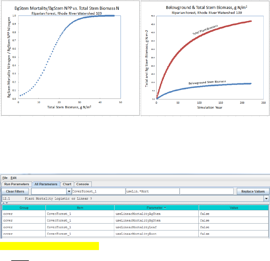
75
12.1 – Plant Mortality Logistic or Linear?
Select “12.1 Plant Mortality Logistic or Linear ?” from the All Parameters drop-down menu to
specify whether you wish to use the logistic (recommended) or linear functions for simulating
plant biomass mortality:
///// IMPORTANT NOTE /////
We do not recommend using the old linear model for simulating plant biomass mortality.
Therefore, make sure all four of the parameters shown above are set = false. When that is the
case, plant biomass mortality is computed using the logistic function. You will need to do this
for all cover types included in your watershed.
12.1.1 – Plant Mortality Logistic Parameters
Select “12.1.1 Plant Mortality Logistic Parameters” from the All Parameters drop-down menu to
specify parameter values affecting biomass mortality for each of VELMA’s four plant tissue
types. Parameter specifications are required for each cover type.
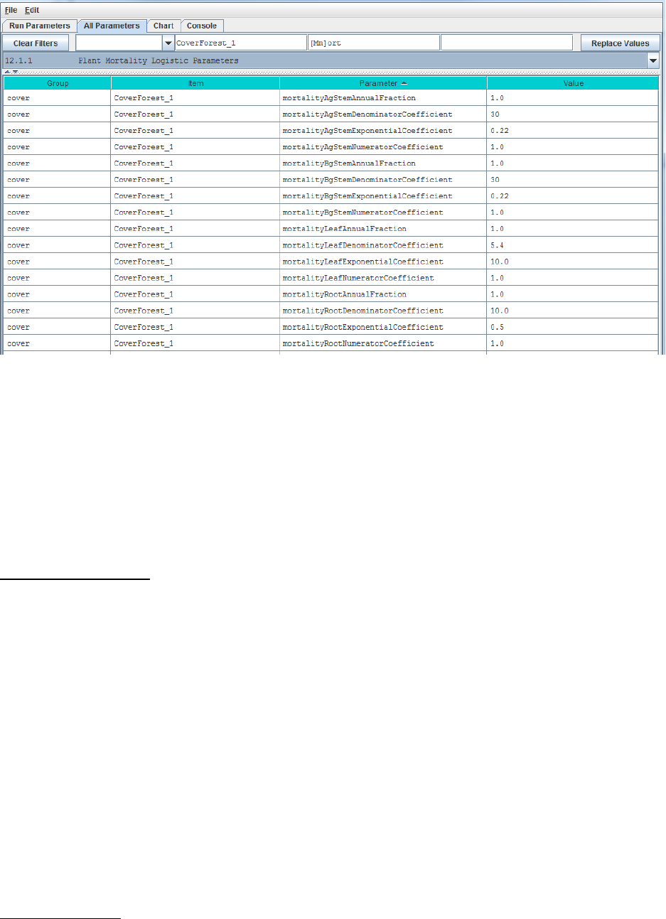
76
Reference to mortality coefficients in the parameter definitions, below, refer to the following
plant mortality logistic function. Using AgStem as an example:
AgStem Mortality = AgStem NPP * C / (1 + A * exp^(-B * Tissue N)),
where,
AgStem Mortality & AgStem NPP are computed internally by VELMA in g N m-2 d-1
A = mortalityAgStemDenominatorCoefficient
B = mortalityAgStemExponentialCoefficient
C = mortalityAgStemNumeratorCoefficient
Parameter Definitions
mortalityAgStemAnnualFraction The fraction of a tissue’s simulated
annual mortality that gets subtracted
from the corresponding biomass pool per
day during the specified period of
senescence. The default value for this
fraction is 1.0 (i.e. the full per-day
amount) and the valid range is [0.0 to
1.0] Warning! Users unfamiliar with
this parameter's behavior should leave
it set to the default value of 1.0.
mortalityAgStemDenominatorCoefficient Parameter “A” in the equation above.
mortalityAgStemExponentialCoefficient Parameter “B” in the equation above.
above.mortalityAgStemNumeratorCoefficient Parameter “C” in the equation above.
Note: the 4 preceding parameters repeat for the other tissues – i.e., “Leaf”, “BgStem” or “Root”
appear in place of “AgStem” in the parameter names above. These
Calibration Notes
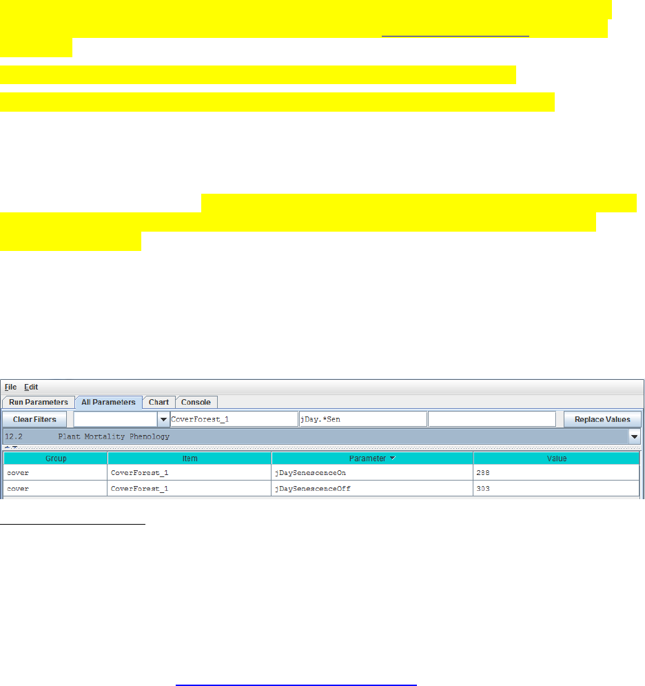
77
We have prepared a DRAFT Excel spreadsheet that you may choose to use to calibrate plant
logistic mortality parameters for your site (please contact mckane.bob@epa.gov if you have
questions):
Filename: VELMA 2.0_Biomass Mortality Calibrator_CHB_9-24-13 v3.xlsx
Folder location: VELMA2.0Software/SupportingDocuments/ExcelCalibrationFiles
12.1.1.1 through 12.1.1.4 – Plant Mortality Logistic Parameters for Leaf, AgStem, BgStem and
Root Biomass
See section 12.1, above, for mortality parameter definitions and calibration information.
Although 12.1 complete list However, to avoid mistakes, we recommend that you use sections
12.1.1.1 through 12.1.1.4 in the All Parameters drop-down menu to specify tissue-specific
mortality parameters. For example, use the All Parameters drop-down menu to select section
12.1.1.1 to display and specify leaf logistic mortality parameters. Parameters for aboveground
stem, belowground stem and roots appear under the following 3 subsections.
12.2 – Plant Mortality Phenology
Select “12.2 Plant Mortality Phenology” from the All Parameters drop-down menu to specify
parameter values for the beginning and end dates for plant biomass mortality.
Parameter Definitions
jDaySenescenceOn The Julian Day of the year when this cover species biomass begins
senescing. (Note: Set >= 367 to "deactivate" senescence for this
cover species.)
jDaySenescenceOff The Julian Day of the year when this cover species biomass stops
senescing (Note: any value >= 367 results in biomass NOT
senescing through the end of the year.
13.0 Decomposition (link to All Parameters TOC)
Decomposition of soil organic matter is a key process in VELMA, controlling the rate at which
dead organic C and N pools (detritus and humus) are converted to inorganic C and N pools (CO2,
NH4, NO3, DON and DOC).
VELMA v2.0 has a new decomposition model based on Potter et al. (1993). In the Potter model,
microbially-mediated decomposition of plant and soil organic residues produces CO2, such that
CO2i = Ci * ki * Ws * Ts * (1-Me), where
− i = a specified soil organic matter pool (in VELMA, plant tissue detritus or humus)
− CO2i = carbon dioxide released by the decomposition of pool i
− Ci = carbon content (gC/m2) of pool i
− ki = maximum decay rate constant of pool i
− Ws = scalar constant (0-2.8) for the effect of soil moisture content on decomposition
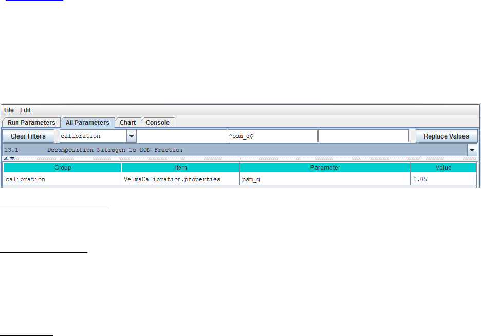
78
− Ts = scalar constant (0-1) for the effect of temperature on decomposition
− Me = carbon assimilation efficiency (0 – 1) of microbes
We made several modifications to the Potter model for VELMA v2.0:
− We modified the Potter decomposition equation, above, to apply it to detritus and
humus N pools rather than C pools. The difference in the C/N ratios of donor and
recipient pools are used to estimate total carbon decomposed. Specified fractions of
the total carbon decomposed are converted to CO2 and DOC. Similarly, a specified
fraction of total decomposed N is converted to DON.
− We replaced Potter’s scalar constant for soil temperature (Ts) with a nonlinear
function describing the fraction (0 – 1) of the maximum decay rate (Ki) versus soil
temperature (oC, per layer). See section 11.3 for a description of this nonlinear
temperature function, which is also used in the plant N uptake subroutine.
− We replaced Potter’s scalar constant for soil moisture (Ws) with a nonlinear function
describing the fraction (0 – 1) of the maximum decay rate (Ki) versus layer-specific
soil moisture (v/v, per layer). Our soil moisture decomposition function uses a
nonlinear Weibull function, which is the same as that applied to the soil moisture N
fixation function (see section 14.0).
“Appendix 1: Overview of VELMA’s Leaf-Stem-Root (LSR) Plant Biomass Submodel” presents
a conceptual diagram and equations describing pools and fluxes involved in the decomposition
subroutine for VELMA v2.0.
13.1 – Decomposition Nitrogen-To-DON Fraction
Select “13.1 Decomposition Nitrogen-To-DON fraction Plant Mortality Phenology” from the All
Parameters drop-down menu to specify a parameter value for controlling DON production:
Parameter Definitions
psm_q The fraction of decomposed nitrogen converted to DON range [0.0 – 1.0]
Calibration Notes
You will need to iteratively calibrate “psm_q” against observed stream DON concentrations
(Abdelnour et al. 2013). This is most easily accomplished using VELMA’s runtime
visualization option for “Calibration Annual Nutrients”. After annual results are in the ballpark,
switch to “Calibration Daily Nutrients”.
Reference:
Potter, C. S., Randerson, J. T., Field, C. B., Matson, P. A., Vitousek, P. M., Mooney, H. A., &
Klooster, S. A. (1993). Terrestrial ecosystem production: a process model based on global
satellite and surface data. Global Biogeochemical Cycles, 7(4), 811-841.
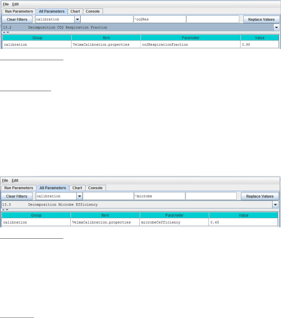
79
13.2 – Decomposition CO2 Respiration Fraction
Select “13.2 Decomposition CO2 Respiration Fraction” from the All Parameters drop-down
menu to specify a parameter value controlling CO2 production during decomposition:
Parameter Definitions
co2RespriationFraction The fraction of humus decomposition (in Carbon) lost to the
atmosphere as CO2.
Calibration Notes
You will need to iteratively calibrate “co2RespriationFraction” in order to obtain a good fit
between simulated and observed stream DOC concentrations, since DOC produced during
decomposition = 1 - co2RespriationFraction. This is most easily accomplished using VELMA’s
runtime visualization option for “Calibration Annual Nutrients”. After annual results are in the
ballpark, switch to “Calibration Daily Nutrients”.
13.3 – Decomposition Microbe Efficiency
Select “13.3 Decomposition Microbe Efficiency” from the All Parameters drop-down menu to
specify the microbial efficiency for carbon assimilation during decomposition:
Parameter Definitions
microbeCefficiency The carbon assimilation efficiency (0 – 1) of microbes. This is
a globally-applicable term of the Potter equation.
As an example, an assimilation efficiency = 0.45 means that for every gram of carbon
decomposed, 0.45 g is assimilated into the humus carbon pool (microbes are not explicitly
modeled), and the remaining 0.55 g is respired as CO2. However, a small fraction (1 –
co2RespriationFraction) of this 0.55 g goes to the DOC pool.
Consult the references below for insight into typical values for microbeCefficiency.
References:
Potter, C. S., Randerson, J. T., Field, C. B., Matson, P. A., Vitousek, P. M., Mooney, H. A., &
Klooster, S. A. (1993). Terrestrial ecosystem production: a process model based on global
satellite and surface data. Global Biogeochemical Cycles, 7(4), 811-841.
Herron, P. M., Stark, J. M., Holt, C., Hooker, T., & Cardon, Z. G. (2009). Microbial growth
efficiencies across a soil moisture gradient assessed using 13C-acetic acid vapor and 15N-
ammonia gas. Soil Biology and Biochemistry, 41(6), 1262-1269.
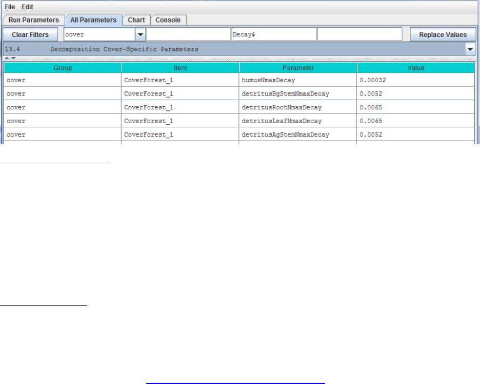
80
13.4 – Decomposition Cover-Specific Parameters
Select “13.4 Decomposition Cover-Specific Parameters” from the All Parameters drop-down
menu to specify the microbial efficiency for carbon assimilation during decomposition. These
parameters must be specified for each cover type.
Parameter Definitions
humusNmaxDecay The maximum rate of decay (0 – 1) for the humus N pool.
detritusBgStemNmaxDecay The maximum rate of decay (0 – 1) for the belowground stem
(BgStem) N pool.
detritusRootNmaxDecay The maximum rate of decay (0 – 1) for the root N pool.
detritusLeafNmaxDecay The maximum rate of decay (0 – 1) for the leaf N pool.
detritusAgStemNmaxDecay The maximum rate of decay (0 – 1) for the aboveground stem
(AgStem) N pool.
Calibration Notes
You will need to iteratively calibrate these decay constants, for each cover type, in order to
obtain a good fit between simulated and observed detritus pool data. It is almost always best to
calibrate for steady state (equilibrium) conditions, e.g., for mature cover types.
14.0 Nitrogen-Fixation (link to All Parameters TOC)
Nitrogen fixation is a process in which nitrogen (N2) in the atmosphere is converted
into ammonium (NH4). In biological systems, N fixation can be carried out by free-living
(asymbiotic) microorganisms, or by plant species that have a symbiotic relationship with N-
fixing bacteria (Frankia and Rhizobia). In symbiotic N fixation, plants provide carbohydrates as
an energy source to bacteria that in turn supply NH4 to the host plant.
Rates of symbiotic N fixation for soybeans, red alder and other species can sometimes exceed
100 kg ha-1 yr-1, an amount similar to agricultural fertilizer applications. Rates for asymbiotic N
fixers tend to be much lower – for example, <1 kg ha-1 yr-1in some PNW coniferous forests.
However, it is important to capture even small N additions, which are important for maintaining
and even increasing ecosystem N stocks over successional time scales.
We added a nitrogen fixation subroutine to VELMA v2.0 that addresses symbiotic and
asymbiotic fixation for any cover type (agricultural, grassland, forest, etc.)
The conceptual diagram below shows VELMA’s modeled pools and fluxes. Note that parameter
names in this diagram do not strictly follow those used in VELMA, but nonetheless convey the
overall structure of the N fixation subroutine.
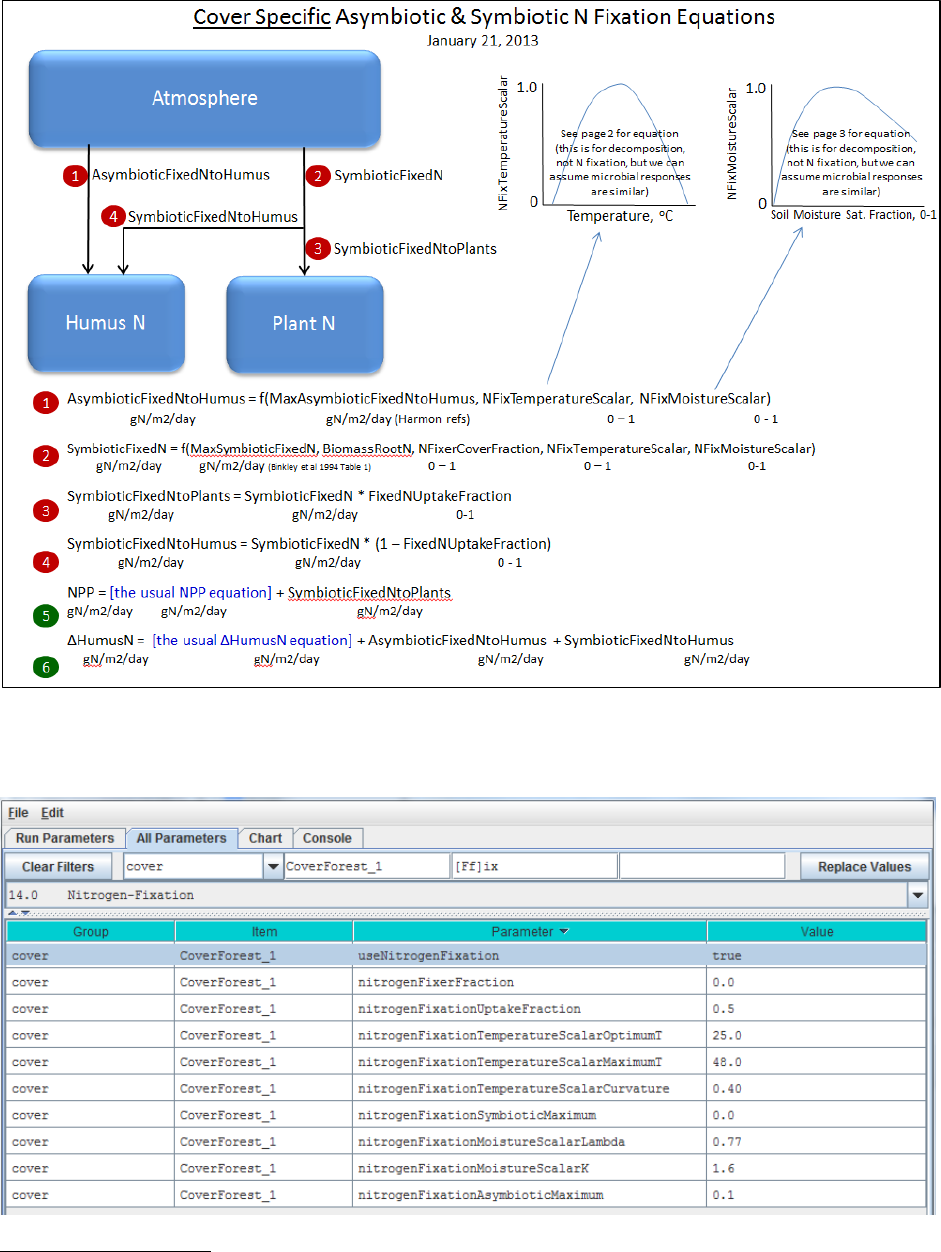
81
Select “14.0 Nitrogen-Fixation” from the All Parameters drop-down menu to specify parameter
values for asymbiotic and symbiotic N fixation.
Parameter Definitions
useNitrogenFixation When using NitrogenFixation = false (default), no
nitrogen fixation is computed for this cells of this
cover. When useNitrogenFixation = true, nitrogen

82
fixation is computed using this cover's other nitrogen
fixation parameters.
nitrogenFixerFraction The fraction of a cell's plant matter (in the range [0.0
1.0]) that performs Nitrogen fixation.
nitrogenFixationUptakeFraction The fraction (in the range [0.0 1.0]) of the symbiotic
fixed Nitrogen that is available for plant NPP. Plant
symbiotic fixed nitrogen is: Total symbiotic fixed
Nitrogen * nitrogenFixationUptakeFraction The
remainder of the total is allocated as Humus
symbiotic fixed nitrogen.
nitrogenFixationTemperatureScalarOptimumT Optimum temperature (in degrees C) parameter
of GEM temperature scalar function for Nitrogen
fixation.
nitrogenFixationTemperatureScalarMaximumT Maximum temperature (in degrees C) parameter
of GEM temperature scalar function for Nitrogen
fixation.
nitrogenFixationTemperatureScalarCurvature Curvature parameter ("qx") of GEM temperature
scalar function for Nitrogen fixation
nitrogenFixationSymbioticMaximum The maximum amount of Nitrogen converted from
the atmosphere by symbiotic processes in
gNfixed/gFixerFineRootBiomassN per m2 per day.
nitrogenFixationMoistureScalarLambda The Lambda value of the Weibull equation used to
compute a water scalar for Nitrogen fixation.
nitrogenFixationMoistureScalarK K value of the Weibull equation used to compute a
water scalar for Nitrogen fixation.
nitrogenFixationAsymbioticMaximum The maximum amount of Nitrogen converted from
the atmosphere by asymbiotic processes in
gN/m2/day.
Calibration Notes
For initial calibration of the N fixation subroutine’s temperature and moisture functions, we
recommend starting with the values shown in the screenshot above. The cover-specific
parameters will require iterative calibration against published data.
14.1 – Nitrogen-Fixation On/Off ?
See section 14.0, above, to specify whether to turn the N fixation subroutine on (true) or off
(false). We’ve placed the on/off parameter there.
15.0 Nitrification (link to All Parameters TOC)
Nitrification is the microbially-mediated conversion of ammonium (NH4+) to nitrate (NO3-). As
the diagram below indicates, nitrification (red box) is an important step in the soil nitrogen cycle
(partially shown here).
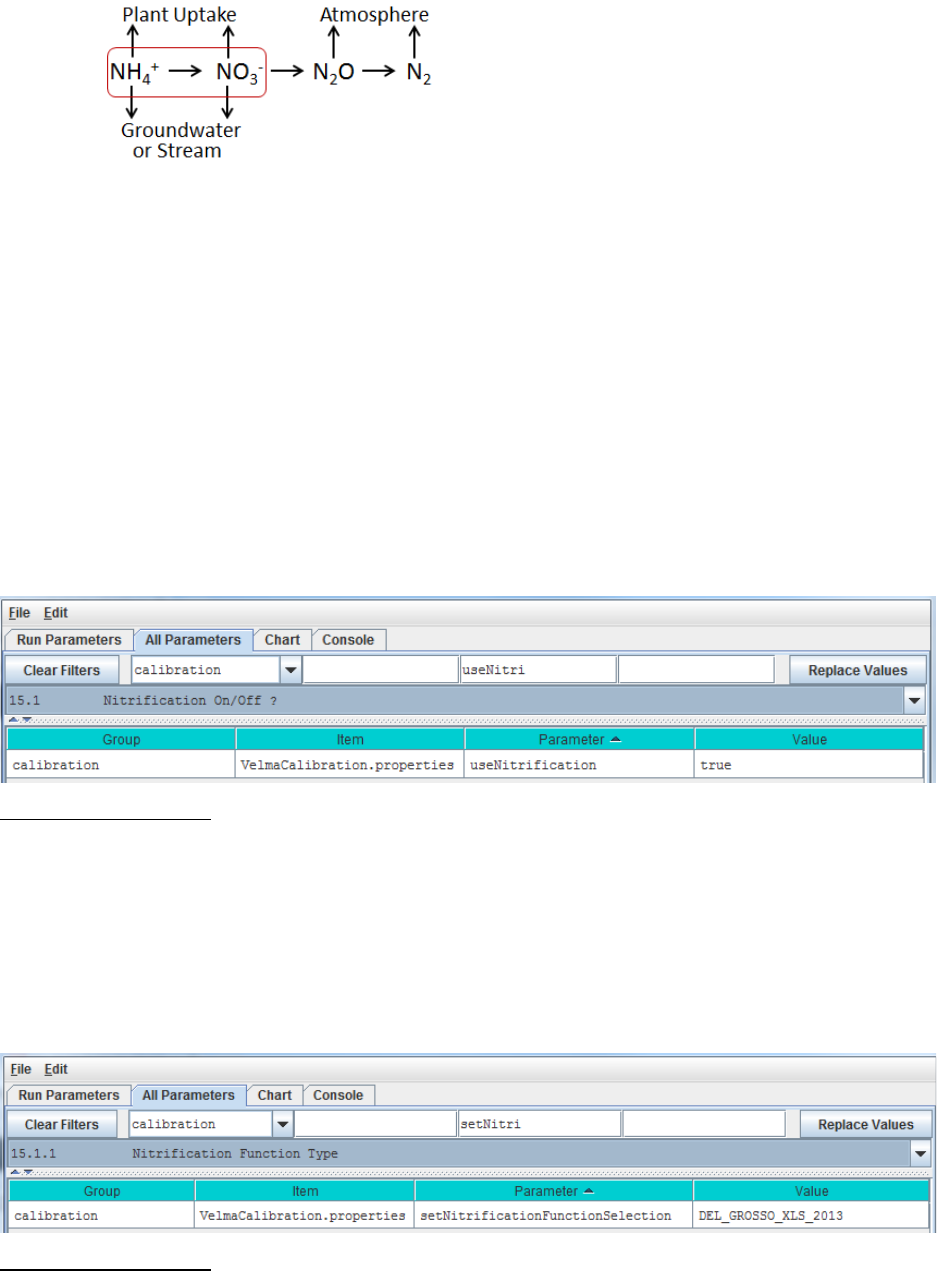
83
Compared to the positively charged NH4+ ion, the negatively charged NO3- ion is highly mobile
in soil (also negatively charged) and more readily leached to groundwater and streams.
Nitrification also affects rates of nitrogen uptake by plant species that differ in their affinities for
NH4+ and NO3- (McKane et al. 2002). Nitrification is also a preliminary step for the process of
denitrification, in which NO3- is microbially transformed to nitrous oxide (N2O), a potent
greenhouse gas, and nitrogen gas.
The default (recommended) version of the nitrification subroutine in VELMA v2.0 is based on
Parton et al. 2001, with recent modifications made by Dr. Stephen Del Grosso
(steve.delgrosso@ars.usda.gov) and coworkers. Dr. Del Grosso’s modifications are described in
his NGAS spreadsheet model.
15.1 – Nitrification On/Off
Select “15.1 Nitrification On/Off ?” from the All Parameters drop-down menu to specify whether
to turn the Nitrification subroutine on (true) or off (false).
Parameter Definitions
useNitrogenFixation When set false daily nitrification amounts are ignored and
the PSM model behaves as if the nitrification amount is
zero When set true (default) nitrification occurs normally
15.1.1 – Nitrification Function Type
Select “15.1.1 Nitrification Function Type” from the All Parameters drop-down menu to specify
the
Parameter Definitions
setNitrogenFunctionSelection Specify "PARTON_1996" "PARTON_2001" or
"DEL_GROSSO_XLS_2013" as the value of the
setNitrificationFunctionSelection property. Warning: be

84
sure to use UPPERCASE text! The simulator engine will
compute nitrifcation amounts using the specified function.
PARTON_1996 = Function based upon equation given in
Figure 2 (d) in [Parton et al. 1996] from Global
Biochemical Cycles v.10. PARTON_2001 = Function
based upon equation (2) in [Parton et al. 2001] from Journal
of Geophysical Research v.106.
DEL_GROSSO_XLS_2013 = (Default /
RECOMMENDED) function implementing the Excel
2013 spreadsheet model provided by Dr. Stephen Del
Grosso.
15.1.2 – Nitrification Soil-Specific Parameters
Select “15.1.2 Nitrification Function Type” from the All Parameters drop-down menu to specify
nitrification subroutine parameters. The parameters shown below must be specified for each soil
type in your watershed (just one soil type shown in the screenshot below).
Parameter Definitions
nitrificationK1 Fraction of net Nitrogen mineralized that is nitrified
per day range in [0.0 1.0]. [Parton et al. 2001].
nitrificationKmax Maximum fraction of NH4 nitrified per day in units
of gN/m2/day range in [0.0 1.0]. [Parton et al.
2001]
nitrificationToN2o N2O flux associated with nitrification in units of
gN/m2/day
nitrificationWfpsCoeff0 Soil-specific coefficient for Water Filled Pore Space
(WFPS) effect on nitrification equation.
nitrificationWfpsCoeff1 Soil-specific coefficient for Water Filled Pore Space
(WFPS) effect on nitrification equation.
nitrificationWfpsCoeff2 Soil-specific coefficient for Water Filled Pore Space
(WFPS) effect on nitrification equation.
nitrificationWfpsCoeff3 Soil-specific coefficient for Water Filled Pore Space
(WFPS) effect on nitrification equation.
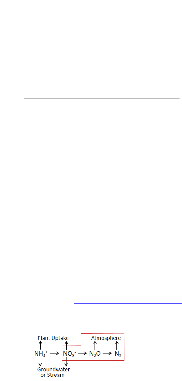
85
pH This soil's pH value.
Calibration Notes
The nitrification model has been extensively applied to agricultural systems by the NGAS model
developers (Parton et al. 2001; Del Grosso et al. 2001 and 2006). We recommend starting with
the default parameter values provided by Stephen Del Grosso in his NGAS spreadsheet model.
Default Parameter Values:
nitrificationK1 = 0.20 (Parton et al. 2001; Del Grosso NGAS spreadsheet model)
nitrificationKmax = 0.1 (Parton et al. 2001; Del Grosso NGAS spreadsheet model)
nitrificationToN2o = 0.02 (Parton et al. 2001; Del Grosso NGAS spreadsheet model = 0.012)
. Soil Texture .
Nitrification Parameter Coarse Fine Volcanic ash
nitrificationWfpsCoeff0 0.5 0.65 0.75
nitrificationWfpsCoeff1 0 0 0
nitrificationWfpsCoeff2 1.5 1.2 1.2
nitrificationWfpsCoeff3 4.5 2.5 2.5
References for Sections 15.0 – 15.1.2
Del Grosso, S. J., Parton, W. J., Mosier, A. R., Ojima, D. S., Kulmala, A. E., & Phongpan, S.
(2000). General model for N2O and N2 gas emissions from soils due to dentrification. Global
Biogeochemical Cycles, 14(4), 1045-1060.
Del Grosso, S. J., Parton, W. J., Mosier, A. R., Walsh, M. K., Ojima, D. S., & Thornton, P. E.
(2006). DAYCENT national-scale simulations of nitrous oxide emissions from cropped soils in
the United States. Journal of environmental quality, 35(4), 1451-1460.
McKane, R. B., Johnson, L. C., Shaver, G. R., Nadelhoffer, K. J., Rastetter, E. B., Fry, B., ... &
Murray, G. (2002). Resource-based niches provide a basis for plant species diversity and
dominance in arctic tundra. Nature, 415(6867), 68-71.
Parton, W. J., Holland, E. A., Del Grosso, S. J., Hartman, M. D., Martin, R. E., Mosier, A. R., ...
& Schimel, D. S. (2001). Generalized model for NO x and N2O emissions from soils. Journal of
Geophysical Research: Atmospheres (1984–2012), 106(D15), 17403-17419.
16.0 Denitrification (link to All Parameters TOC)
Denitrification is the microbially-mediated conversion of nitrate (NO3-) to nitrous oxide (N2O)
and nitrogen gas (N2). This process is represented in the red-outlined area in the diagram below.
Nitrate that is not denitrified or taken up by plants can be readily transported to ground and
surface waters (the high mobility of NO3- in soil is because both are negatively charged). Thus,
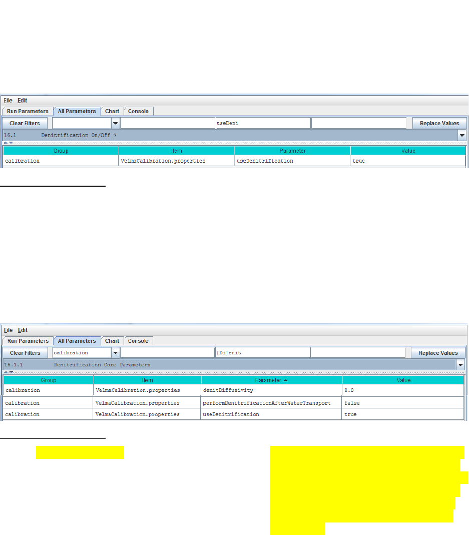
86
denitrification can be important for protecting water quality. On the other hand, if denitrification
does not go to completion (stops at N2O instead of N2) it can increase atmospheric inputs of
N2O, a potent greenhouse gas.
The denitrification subroutine in VELMA v1.0 and v2.0 is based on Del Grosso et al. 2001.
However, VELMA v2.0 includes recent updates to equations and correction to parameter values
described in Dr. Stephen Del Grosso’s (steve.delgrosso@ars.usda.gov) NGAS spreadsheet
model.
16.1 – Denitrification On/Off?
Select “16.1 Denitrification On/Off ?” from the All Parameters drop-down menu to specify
whether to turn the denitrification subroutine on (true) or off (false).
Parameter Definitions
setNitrogenFunctionSelection When set “false” daily denitrification amounts are
ignored and VELMA’s biogeochemistry submodel
behaves as if the denitrification amount is zero. When
set “true” (default) denitrification occurs normally.
16.1.1 – Denitrification Core Parameters
Select “16.1.1 Denitrification Core Parameters” from the All Parameters drop-down menu to
specify denitrification subroutine parameter values. These global parameters are applicable to all
soil types.
Parameter Definitions
denitDiffusivity This is the value of the "a" parameter in Del
Grosso et al. (2000) fig.7(a). It controls the
shape of the logistic function that defines the
response of “relative denitrification” (0.0 –
1.0) to water filled pore space (WFPS %).
See calibration notes at the end of section
16.0, below.
performDenitrificationAfterWaterTransport When set “true” daily denitrification
amounts are calculated AFTER vertical and
lateral transportation of chemicals by water
occurs. When set “false” (default) daily
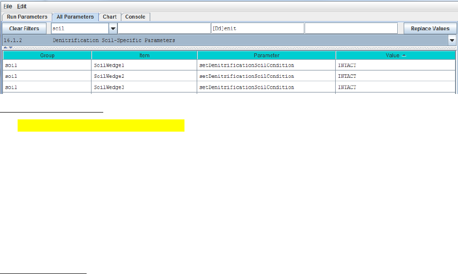
87
denitrification occurs BEFORE water
transport.
useDenitrification When set “false” daily denitrification
amounts are ignored and the PSM model
behaves as if the denitrification amount is
zero. When set “true” (default)
denitrification occurs normally
16.1.2 – Denitrification Soil-Specific Parameters
Select “16.1.2 Denitrification Soil-Specific Parameters” from the All Parameters drop-down
menu to specify the following set of denitrification parameters for each soil type in your
watershed. There is just one parameter per soil type (3 soil types are shown in the screenshot
below).
Parameter Definitions
setDenitrificationSoilCondition Defines soil condition with respect to denitrification
calculations. Value must be one of the following: "INTACT"
(the default value) or "REPACKED_COARSE" or
"REPACKED_MEDIUM" or "REPACKED_FINE" The
value is case-sensitive and must appear exactly as given here
(but with the surrounding double-quotes). In practice, Del
Grosso’s NGAS spreadsheet uses “INTACT” = undisturbed
soils, and "REPACKED_MEDIUM” and
"REPACKED_FINE" = medium or fine textured soil
samples, respectively, that have been repacked in the lab
after field collection.
Calibration Notes:
The denitrification subroutine has been extensively applied to agricultural systems by the NGAS
model developers (Parton et al. 2001; Del Grosso et al. 2000 and 2006). The parameter values
used in the model seem to be fairly robust across the wide range of conditions reported by the
authors. When calibrating the denitrification subroutine for a new site, we recommend that you
initially focus on just two parameters (assuming all the true/false options are set up correctly).
These are the yellow-highlighted parameters above: denitDiffusivity and
setDenitrificationSoilCondition.
The denitDiffusivity parameter controls the shape of the logistic function that defines the
response of “relative denitrification” (0.0 – 1.0) to water filled pore space (WFPS %). Figure 7
in Del Grosso et al. (2000) illustrates this:
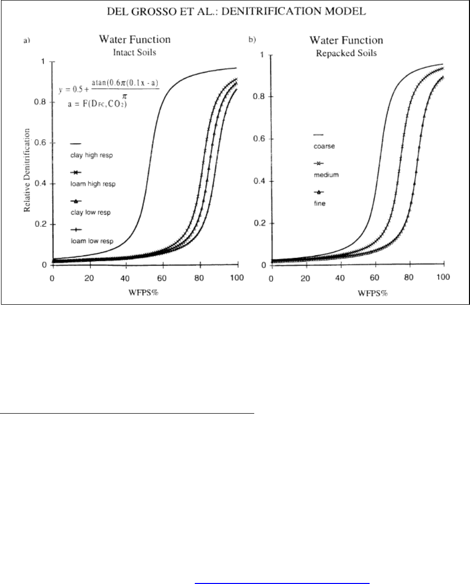
88
Thus, you will need to adjust the denitDiffusivity parameter (“a” in Figure 7) to obtain a
response for the soil texture that is most appropriate for your watershed. You will also need to
specify “INTACT” for undisturbed soils. “REPACKED_MEDIUM” or “REPACKED_FINE”
refers to soil columns that have been reconstructed in the laboratory (Del Grosso et al. 2000).
You will need to decide if the REPACKED choices are appropriate for compacted field soils,
e.g., under high tillage practices.
References for section 16.0 (all subsections sections)
Del Grosso, S. J., Parton, W. J., Mosier, A. R., Ojima, D. S., Kulmala, A. E., & Phongpan, S.
(2000). General model for N2O and N2 gas emissions from soils due to dentrification. Global
Biogeochemical Cycles, 14(4), 1045-1060.
Del Grosso, S. J., Parton, W. J., Mosier, A. R., Walsh, M. K., Ojima, D. S., & Thornton, P. E.
(2006). DAYCENT national-scale simulations of nitrous oxide emissions from cropped soils in
the United States. Journal of environmental quality, 35(4), 1451-1460.
Parton, W. J., Holland, E. A., Del Grosso, S. J., Hartman, M. D., Martin, R. E., Mosier, A. R., ...
& Schimel, D. S. (2001). Generalized model for NO x and N2O emissions from soils. Journal of
Geophysical Research: Atmospheres (1984–2012), 106(D15), 17403-17419.
17.0 – Simulation Run Schedule (link to All Parameters TOC)
To let VELMA know when to start and stop a simulation, you specify need to specify values for
the following parameters:
forcing_start First year of driver (forcing) data available for the
simulation model run
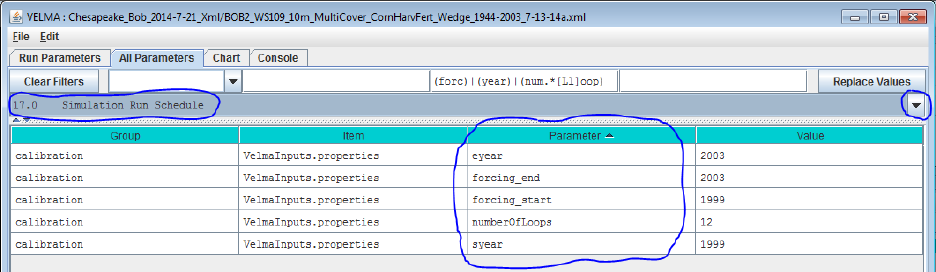
89
forcing_end Last year of driver (forcing) data available for the
simulation model run
syear Starting year of simulation model run
eyear Ending year of simulation model run
numberOfLoops The number of times (loops) to repeat a simulation (syear
to eyear will repeat for the specified number of loops)
The Forcing Start and End Years Specify When a Simulation CAN Run
The VELMA Simulator expects every driver and observed data file specified in the simulation
configuration to have 1 line of data for each day between the first day of the year specified for
the forcing_start parameter and the last day of the year specified for the forcing_end
parameter.
For example, if forcing_start = 2000 and forcing_end = 2001, each driver or observed data file
must have 366 + 365 lines of data (one for each of the 731 days of years 2000 through 2001).
The value specified by forcing_start must be less than or equal to the value of forcing_end.
The Simulation Start and End Years Specify When a Simulation WILL Run
The years that the VELMA Simulator actually runs a simulation for are specified by the syear
(start year) and eyear (end year) simulation configuration parameters. It is an error for syear’s
value to be greater than eyear’s, and for either value to lie outside the bounds of the years
specified by forcing_start and forcing_end, however syear and eyear may specify a sub-range
within that range.
For example, if [forcing_start, forcing_end] = [1995, 2010], [syear, eyear] may be [1997,
2010], or even a single year, like [1998, 1998].
The Loops Parameter Specifies How Many Times the Simulation Repeats a Run
The numberOfLoops parameter defaults to “1”, which tells the VELMA Simulator to run the
specified simulation from start year to end year once, and then stop. Setting the numberOfLoops
parameter to n, (with > 1) tells the VELMA simulator to run the simulation from start year to end
year n times in a row, but to only initialize the simulation before the first start-to-end run. In this
way, the numberOfLoops parameter provides a (simplistic) spin-up mechanism. The second start-
to-end run after the first will begin with the simulation’s data state where it was at the end of the
first start-to-end run, and so on.
Use the All Parameters Outline Selector to Focus on the Simulation Run Schedule Parameters
You can filter the All Parameters tab’s parameters table to focus on the simulation run schedule
by selecting item “17.0 Simulation Run Schedule” in the outline dropdown selector:
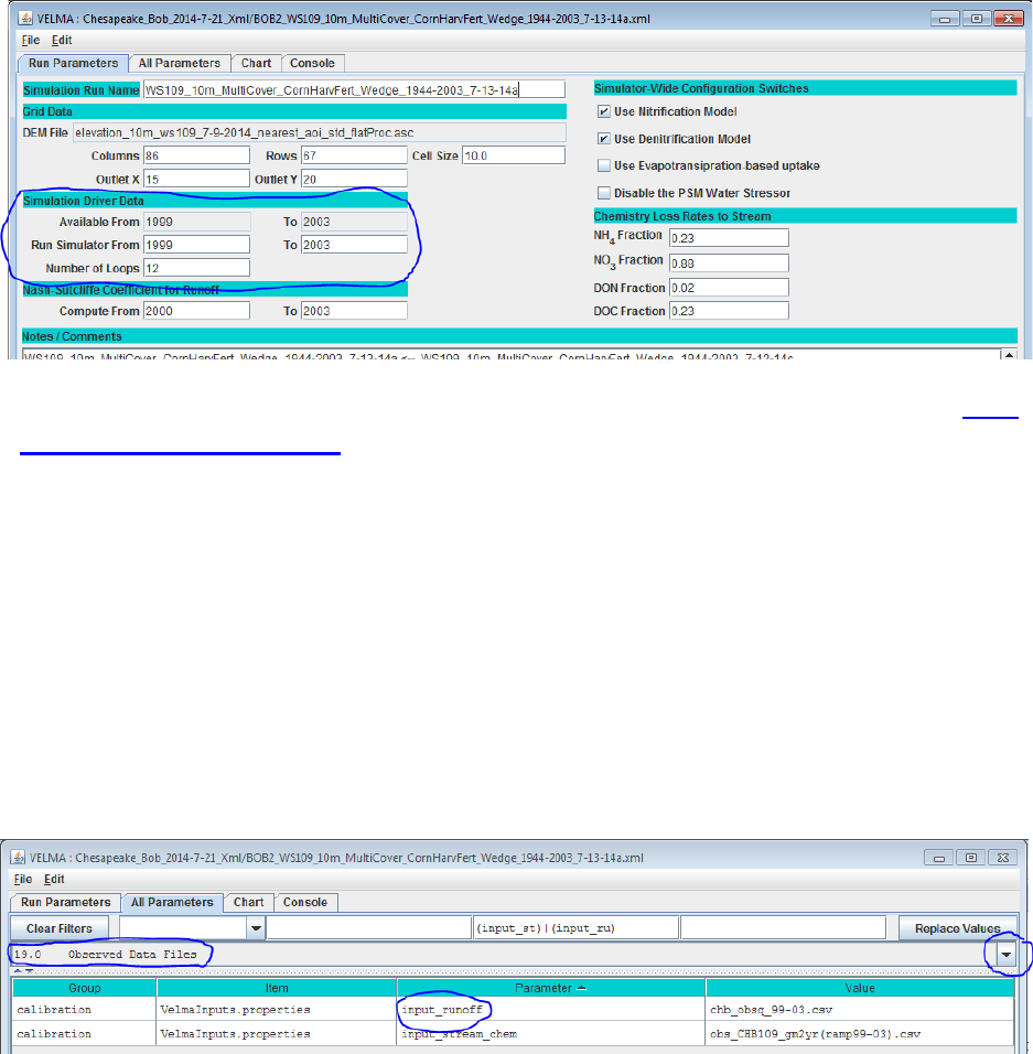
90
You Can Also Review and Set Some of these Values in the Run Parameters Tab
Compare circled fields in the Run Parameters tab below with the parameters circled in the All
Parameters table above. Setting the “Run Simulator From” and “To” fields in the Run
Parameters tab sets the values of the syear and eyear parameters. Setting the Run Parameters
“Number of Loops” value sets the value of the numberOfLoops parameter. Note however, that
you can only set the forcing_start and forcing_end values in the All Parameters table. These
values are read-only fields in the Run Parameters tab. The screenshot above happens to specify
12 loops – i.e. run the simulation [1999, 2003] x12 – that’s a significant spin up. Generally
speaking, find out how long one simulation loop takes to run before embarking on that many
multiple loops.
18.0 – Years to Compute Nash-Sutcliffe for Runoff (link
to All Parameters TOC)
The VELMA Simulator Calculates a Nash-Sutcliffe Value for Runoff
Whenever possible, the VELMA simulator automatically computes a Nash-Sutcliffe Coefficient
for observed vs. simulated annual runoff values. In order to calculate the runoff Nash-Sutcliffe,
the simulator must know which span of years to include in the calculation, and have observed
runoff data for those years available.
To ensure that the VELMA simulator is able to compute a meaningful Nash-Sutcliffe value for
your simulation run, provide values for the following configuration parameters.
Set the Observed Runoff Source File
Click the All Parameters tab’s configuration outline dropdown selector and select item
“19.0 Observed Data Files”. The All Parameters table should then look like this:
Set the input_runoff parameter to the name of a .csv file containing valid observed runoff data.
A valid file has a single column of floating-point data, one day’s observed runoff value per row.
There must be exactly as many rows in the file as there are days in the simulation configuration’s
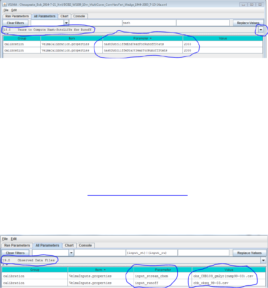
91
forcing_start to forcing_end parameter’s span of years. (E.g. if forcing_start = 2000 and
forcing_end = 2001, then there must be 366 + 365 or 731 rows of data in the file.)
The specified file’s location is assumed to be the directory specified by the
inputDataLocationRootName + inputDatalocationDirName.
Set the Years to Simulation the Nash-Sutcliffe
Click the All Parameters outline dropdown selector again, and this time select item “18.0 Years
to Compute Nash-Sutcliffe for Runoff”. The All Parameters table should then look like this:
The nashSutcliffeStartYearForRunoffStats and nashSutcliffeEndYearForRunoffStats
specify the first and last years of the simulation run that are used to compute the Nash-Sutcliffe
coefficient. Obviously, these start and end year values must be within the range of the
simulation run’s start and end years as a whole. For example, if your simulation runs from 1995
to 2005, you cannot specify years 1980 to 2009 as the span for computing the Nash-Sutcliffe.
The VELMA Simulator Writes the Nash-Sutcliffe Coefficient for Runoff to an Output File
The VELMA simulator writes the Nash-Sutcliffe coefficient for runoff to a file named
“NashSutcliffeCoefficients.txt”. This is a simple text file, created in the directory specified by
the simulation configuration’s intializeOutputDataLocationRoot parameter.
The file contains a single line, reporting the Nash-Sutcliffe result like this:
Nash-Sutcliffe Coefficient=0.8045351825866978 Loop=1 Years=[1969 to 2008]
The Computed Nash-Sutcliffe Value is Only as Accurate as the Observed Data
The auto-computation of the Nash-Sutcliffe coefficient for runoff is convenient, but it is only as
accurate as the observed data and year’s span allow it to be.
19.0 – Observed Data Files (link to All Parameters TOC)
If you want VELMA to graphically display observed stream chemistry and runoff data along
with simulated values during a simulation (section 25.0), and calculate the Nash-Sutcliffe
efficiency coefficient (section 18.0), you will need to prepare input files and specify their names
in the All Parameters outline drop-down menu for section “19.0 Observed Data Files”:
For the input_runoff parameter, specify the name of a file (.csv format) containing daily
observed streamflow (runoff) values in mm/day. The data must be formatted as one value per
line in the file, and the file must have as many lines as there are days between the simulator
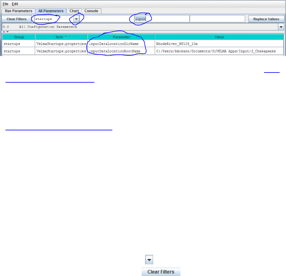
92
configuration’s specified forcing_start and forcing_end parameter values (see “All Parameters
17.0 – Simulation Run Schedule”)
For the input_chem parameter, specify the name of a file (.csv format) containing observed daily
stream chemistry values for DON, NH4, DOC and NO3, in that order! Units are g N m-2 day-1,
or g C m-2 day-1.
Both input files must be placed in the simulation configuration’s input file directory location
(inputDataLocationDirName) and name (inputDataLocationRootName). These input data
parameters can be found by selecting “Startups” under the drop-down Filter menu tab (type
“input” in the filter for the “Parameter” column if you wish to focus the selection on just these
two parameters:
20.0 – Simulation-End Data Capture for Spin-up Initialization Use (link
to All Parameters TOC)
Skip to section 21.0 where the procedure for section 20.0 is included as part of the “Simulation-
Start Initialization from Spin-up Data” procedure.
21.0 – Simulation-Start Initialization from Spin-up Data
(link to All Parameters TOC)
This section outlines a technique for using the ending state of a VELMA simulator run’s spatial
data pool values as the initial starting state for the spatial data pools of a second simulation run.
(1) Create a common simulation configuration base .xml document
The base .xml simulation configuration is your overall simulation configuration, with DEM, soil,
cover, etc. parameters set as you wish them to be for site and conditions you are simulating.
(2) Make two copies of the base simulation configuration .xml document
One of the two copies will be modified to be the spin up configuration. The other will be the
actual, final configuration.
(3) Modify the Spin up configuration to save spatial data state at the end of its simulation run
1. Load the Spin up configuration into JVelma.
2. Click to the “All Parameters” tab and select “All startups” from the drop-down list of
filters. That is, use the drop-down button located above the “Group” column, not the
“Value” column. You may need to click button first to get rid of any
filtering text already present).
3. In the All Parameter “ID Key” column, locate the setEndStateSpatialDataLocationName
parameter, then click-click into its “Value” field and type in the name of a directory
93
where the simulation can store spatial data map (“.asc”) files.
Note that:
A. The directory name may be either a fully-qualified path, or a relative path.
If it’s a relative path, JVelma assumes its root is the output directory specified by the
simulation configuration’s
/calibration/VelmaInputs.properties/initializeOutputDataLocationRoot parameter.
B. Use “/” path separators in the directory name.
C. The directory does not need to exist beforehand; JVelma will try to create it when it’s
needed during the simulation run.
4. Click to the “Run Parameters” tab and set the “Run Simulator From” and “To” values to
the years you want the Spin up to run. (You may also wish to set the Nash-Sutcliffe
coefficient “Compute From” and “To” values at this point.)
Save the Spin up configuration .xml file.
(4) Modify the Actual configuration to initialize its spatial data state at simulation start.
1. Load the Actual configuration into JVelma.
2. Click the “All Parameters” tab and select “All Startups” from the drop-down list of filters
(you may first need to click the “Clear Filters” button).
3. In the All Parameters “ID Key” column, locate the
setStartStateSpatialDataLocationFileName parameter, then click-click into its “Value”
field and type in the name of a directory where the simulation can look for spatial data
map (“.asc”) files.
Note that:
A. Presumably, the directory path will be to the directory specified as the
setEndStateSpatialDataLocationFileName value in the Spin up configuration file.
B. The directory name may be either a fully-qualified path, or a relative path.
If it’s a relative path, JVelma assumes its root is the output directory specified by the
simulation configuration’s inputDataLocationRootName/inputDataLocationDirName
parameters.
C. Use “/” path separators in the directory name.
D. The directory MUST exist at the time that the Actual simulation starts running.
4. Click to the “Run Parameters” tab and set the “Run Simulator From” and “To” values to
the years you want the Spin up to run. (You may also wish to set the Nash-Sutcliffe
coefficient “Compute From” and “To” values at this point.)
Save the Actual configuration .xml file.
(5) Run the Spin up simulation to completion.
Start JVelma, load the Spin up configuration .xml and Start the simulation running.
Wait until the Spin up simulation completes its run before proceeding.
(6) Run the Actual simulation to completion.
Start JVelma, load the Actual configuration .xml and Start the simulation running.
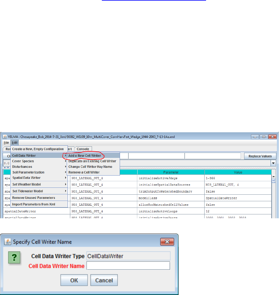
94
When the Actual configuration completes, the Actual simulation run’s results will be data based
on an initial spatial data state taken from the final spatial data state of the Spin up simulation run.
22.0 – Cell Data Writer Items (link to All Parameters TOC)
Cell Data Writers Allow You to Gather Simulation Results for a Specific Grid Location
The VELMA simulator automatically provides daily simulation results for various values (e.g.
Leaf Biomass), however these daily results are average values that are computed by summing
individual cell values and then dividing the sum by the number of cells in the simulation’s
delineated watershed.
To gather daily simulation results for a single, specific cell, you need to add a Cell Data Writer
parameterization for that cell to the simulation configuration.
Adding a Cell Data Writer to a Simulation Configuration
Cell Data Writers are optional. Simulation configurations contain zero instances of them by
default. When added, they do not change the simulation computations – they are only involved
in reporting results.
To add a Cell Data Writer to your simulation configuration:
Click the “Edit” “Cell Data Writer” “Add a New Cell Writer” menu item.
Clicking “Add a New Cell Writer” opens the Cell Writer Name dialog, which looks like this:
Enter a name for your new Cell Data Writer and click “OK”.
The name must be unique (i.e. no other Cell Data Writer already specified for this simulation
configuration can share the name you specify) and we recommend avoiding whitespace, and
punctuation characters (e.g. “(“ and “)”). An acceptable example name (assuming it’s not
already in use by another Cell Data Writer might be “Probe_Point_1” or maybe “Outlet_Cell”.
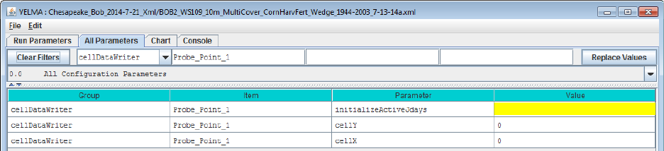
95
Configuring a Cell Data Writer’s Parameters
After you click OK in the Cell Data Writer’s naming dialog, the VELMA GUI adds the Cell
Data Writer to the simulation configuration, and sets the All Parameters tab’s filters to display
only the parameters of the newly-added Cell Data Writer.
Assuming we named our new Cell Data Writer “Probe_Point_1” and clicked OK, the VELMA
GUI would look like this afterwards:
Notice, in passing, that the configuration outline does not automatically get set by the GUI. In
the example screen capture above, it displays “0.0 All Configuration Parameters” – which is not
what is being displayed in the parameterization table. This behavior is harmless.
A Cell Data Writer has only 3 parameters, but they must all be set correctly: none are optional.
Set the initializeActiveJdays parameter to the Julian days that you want data reported for. If
you want data reported on every day of the year (this is the most common case) set the
initializeActiveJdays value to be “1-366”. (The 366 avoids missing the last day in any leap
years that occur in the simulation run.)
If you only want data reported on specific days of the year, enter the Julian Day values as a
comma-separated list (e.g. “1, 90, 180, 270” reports data on days 1, 90, 180 and 270). You may
specify an inclusive range of days by separating a start-day value from an end-day value by a
dash (e.g. (“1, 90-180, 270” reports data on days 1, days 90 through 180, and on day 270).
Set the cellX parameter’s value to the X-coordinate (i.e. column value) of the cell you want data
reported for. The valid range is from 0 (the leftmost column) to (number of columns – 1).
Set the cellY parameter’s value to the Y-coordinate (i.e. row value) of the cell you want data
reported for. The valid range is from 0 (the topmost row) to (number of rows – 1).
Cell Data Writer Output is A Comma-Separated Values File
The VELMA simulator creates 1 .csv file for each valid Cell Data Writer parameterization in the
simulation configuration .xml file.
Cell Data Writer output files are written to the Results Data Location folder. Their filenames
always begin with the prefix “Cell_” and contain the linear index, x-coordinate and y-coordinate
of the cell they contain data for (e.g. Cell_i2873_x35_y33.csv).
Each row of a Cell Data Writer output file contains results data for a specific loop, year and
Julian day during the simulation run. The file’s columns contain the specific results. The header
row of the file specifies the contents of each column. Note that some columns contain data that
never varies (e.g. the DEM_Elevation(m) column reports the cell’s elevation – which is always the
same value.)
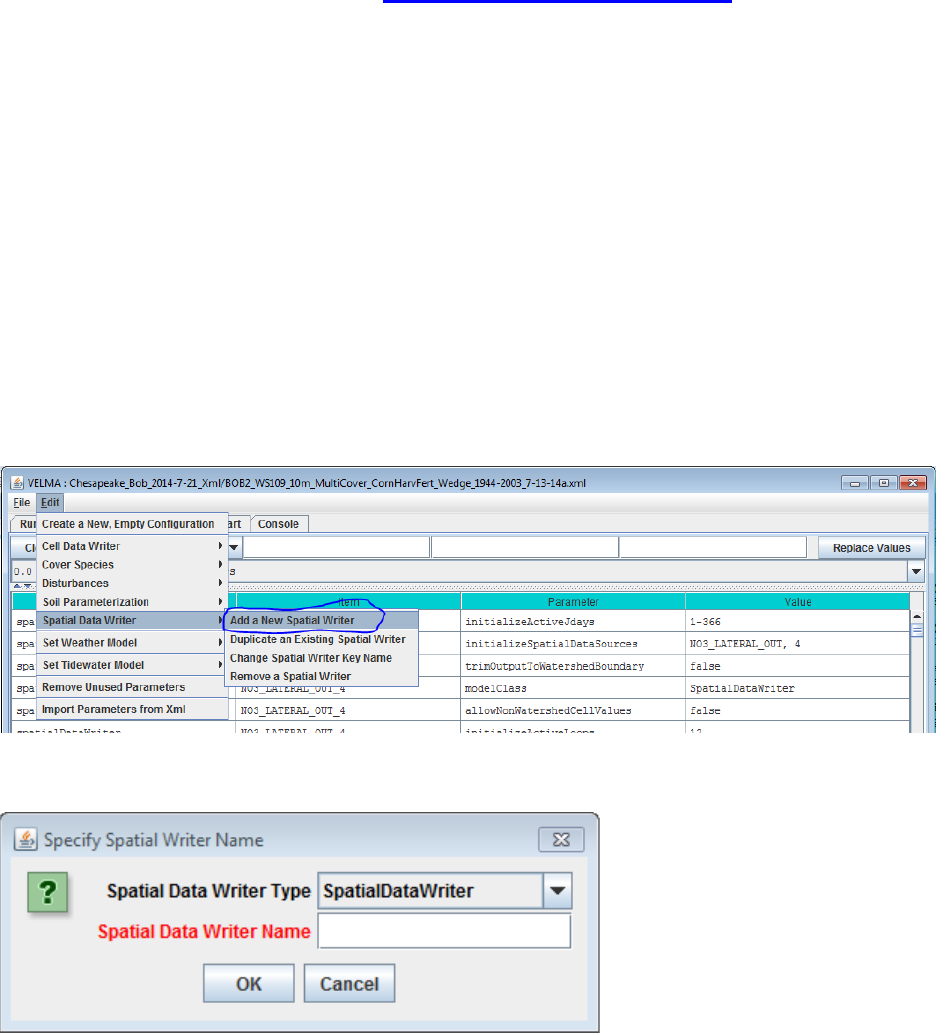
96
Cell Data Writers and Spatial Data Writers are Different, but Complementary
A Cell Data Writer reports all the results data available for a specific cell on user-specified days.
A Spatial Data Writer reports a specific result for all the cells in the simulation watershed on
user-specified days. Both are optional for simulation runs.
23.0 – Spatial Data Writer Items (link to All Parameters TOC)
Spatial Data Writers Report a Simulation Result for Every Cell in the Simulation Grid
Spatial Data Writers are how the VELMA simulation provides spatially-explicit results output.
Spatial Data Writers are layer- and result-specific. You must configure separate spatial data
writer parameterizations for each result type you will to output, and for layer of that result type.
(E.g. to get spatial data output for the Root Biomass pool layers 3 and 4, you would need to add
and configure two separate Spatial Data Writer parameterizations to your simulation
configuration.
23.1 – Spatial Data Writer Items by Model Type
Adding a Spatial Data Writer to a Simulation Configuration
Spatial Data Writers are optional. Simulation configurations contain zero instances of them by
default. When added, they do not change the simulation computations – they only report results.
To add a Spatial Data Writer to your simulation configuration:
Click the “Edit” “Spatial Data Writer” “Add a New Spatial Writer”.
Clicking “Add a New Spatial Writer” opens the Spatial Writer Type and Name dialog which
looks like this:
Leave the Spatial Data Writer Type selector set to “SpatialDataWriter”.
The Spatial Data Writer Name must be unique (i.e. no other Spatial Data Writer already
specified for this simulation configuration can share the name you specify). Avoid whitespace
and punctuation characters (e.g. “(“ and “)”). As an example, here are a couple of acceptable
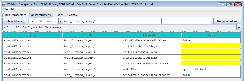
97
names (assuming they’re not already in use by another Spatial Data Writer, and the Spatial Data
Writer we’re adding will report layer 3 root biomass; “Root_Biomass_Layer_3” and “Root_L3”.
23.2 – Spatial Data Writer Items Data Sources
Configuring a Spatial Data Writer’s Parameters
After you click OK in the Spatial Data Writer’s Type and Name dialog, the VELMA GUI adds
the Spatial Data Writer to the simulation configuration, and sets the All Parameters tab’s filters
to display only the parameters of the newly-added Spatial Data Writer.
Assuming we named our new Spatial Data Writer “Root_Biomass_Layer_3” and clicked OK,
the VELMA GUI would look like this afterwards:
Notice, in passing, that the configuration outline does not automatically get set by the GUI. In
the example screen capture above, it displays “0.0 All Configuration Parameters” – which is
not what is being displayed in the parameterization table. This behavior is harmless.
A Spatial Data Writer has 7 parameters. None are optional, but one (modelClass) is set
automatically by the GUI, and two others (allowNonWatershedCellValues and
trimOutputToWatershedBoundary) default to reasonable values automatically. The remaining 4
parameters specify when this parameterization writes its specified spatial data source to file, and
what that spatial data source should be.
The Spatial Data Sources Parameter Specifies What Data Is Written
Set the initializeSpatialDataSources parameter to the name of the spatial data source you want
to report results for. The name is case-sensitive, and must exactly match a name from the Table
of Spatial Data Sources given below. Be careful to avoid leading or trailing whitespace when
you enter the spatial data sources name; leading or trailing whitespace can “break” the simulation
configuration.
If the spatial data source you choose is multi-layered (see the table), you may (in some instances,
must) explicitly specify the layer you wish to write. Specify an explicit layer by adding it,
comma-separated, after the spatial data source name. The range of valid layer numbers is [1 to
4].
For example: “BIOMASS_ROOT_N” specifies the spatial data source name for biomass root, and
“BIOMASS_ROOT_N, 2” specifies biomass root data, layer 2 (enter these, and all parameterization
values, without the surrounding quotation (“) marks).
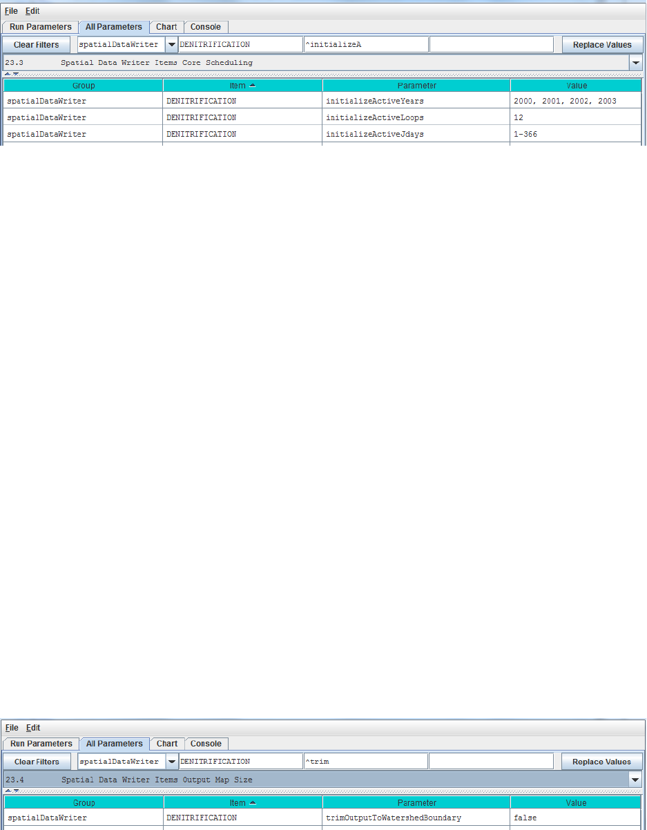
98
23.3 – Spatial Data Writer Items Core Scheduling
The Three “InitializeActive…” Parameters Specify When Data Is Written
Select “23.3 Spatial Data Writer Items Core Scheduling” from the All Parameters drop-down
outline selector menu:
Set the initializeActiveLoops, initializeActiveYears and initializeActiveJdays parameter
values to the loop numbers, years and Julian day values that you want the Spatial Data Writer to
write results for.
Any specified Loop numbers, years or Julian days that are “beyond bounds” are ignored. I.e. if
the simulation configuration specifies 3 loops, and the Spatial Data Writer
initializeActiveLoops value is set to 4, no data will ever be written. It is an error to specify
negative numbers for Loop, Year or Jday parameters.
[TIP: Setting an initializeActiveLoops value greater than the number of loops the simulation
configuration specifies run is an unintuitive yet handy way to temporarily “shut off” a spatial
data writer’s output without removing it from the simulation configuration.]
You may specify more than one value by separating values with commas, and you may specify
an inclusive range of values by separating the start and end values by dashes.
(E.g. specifying “1, 3-7, 12” for initializeActiveLoops would allow the spatial data writer to
write data in loops 1, loops 3 through 7, and loop 12 – assuming the simulation configuration’s
numberOfLoops parameter is set to 12 or more.)
You May Emphasize the Watershed Cells, or Not
When the allowNonWatershedCellValues parameter is set false, its spatial data writer writes any
cell value outside the watershed as NO_DATA (the value “-9999.0”). The default value is
false, which makes it easy to discern the watershed’s delineation in the results file. If you want
the results file to include every cell value, regardless of whether a given cell is in or out of the
watershed delineation, set this parameter to true.
23.4 – Spatial Data Writer Items Output Map Size
You May Reduce the Dimensions of the Results Grid File
Select “23.4 Spatial Data Writer Items Output Map Size” from the All Parameters drop-down
outline selector menu:
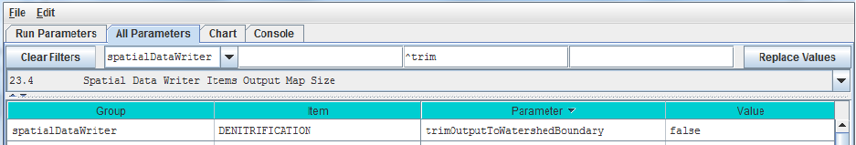
99
When trimOutputToWatershedBoundary is set false, the spatial data writer writes a results file
with the same grid dimensions at the simulation configuration’s DEM file. This (default value)
make it easy to overly Spatial Data Writer output results on top of the DEM, cover Id map, or
soil Id map files. When set to true, the spatial data writer writes a results file that contains only
the cells within the bounding rectangle of the delineated watershed. Depending upon the size of
the watershed relative to the overall DEM, this may result in Spatial Data Writer files that are
smaller, and easier to review “by hand”.
[TIP: Spatial Data Writer output results files are not really meant for “manual” review (e.g. via
Notepad or a similar simple text editor). The choice of the Grid ASCII format was for ease of
use with GIS systems, and so that they could be readily “fed back” into the VELMA Simulator
as subsequent initialization input. However, there’s nothing wrong with opening a results file in
a text editor or spreadsheet for a quick sanity check.]
To reduce the Dimensions of the Results Grid File, click the All Parameters tab’s configuration
outline dropdown selector and select “23.4 Spatial Data Writer Items Output Map Size”.
Spatial Data Writer Output is a Grid ASCII File
The VELMA simulator creates 1 .asc file each time a given Spatial Data Writer is triggered
(based on its active Loops, Years and Jdays parameter settings).
Spatial Data Writer output files are written to the Results Data Location folder. Their filenames
always begin with the prefix “Spatial_” and include the name of the spatial data source and layer
number of the data they contain. The dimensions of the Grid ASCII file match those of the
simulation configuration’s DEM .asc file, unless the trimOutputToWatershedBoundary parameter
was set “true”; in that case, the dimensions of the Spatial Data Writer output file are those of the
bounding box of the simulation run’s delineated watershed.
Each data value in the output .asc file contains the value for the specified data source for a
particular cell, on the particular loop, year and Julian day during the simulation run that the
output file was written.
Spatial Data Writers and Spatial Data Writers are Different, but Complementary
A Spatial Data Writer reports a specific result for all the cells in the simulation watershed on
user-specified days. A Spatial Data Writer reports all the results data available for a specific cell
on user-specified days. Both are optional for simulation runs.
Table of Spatial Data Sources
This table lists the available spatial data source name and their layer requirements.
SpatialDataSource Keyword means:
The spatial data source keyword names that are valid values for the
initializeSpatialDataSources parameter value of a Spatial Data Writer’s parameterization.
“Type” means:
100
• Accessor = Spatial Data that is not directly stored in a spatial data pool object.
• Direct = Spatial Data that is directly stored in a spatial data pool object.
• Buffered = Spatial Data directly stored in a spatial data pool object, but only when a
Spatial Data Writer requires it.
(In practice, you can ignore what type a spatial data source is when you are configuring a Spatial
Data Writer.)
“Can Sum Column?” means:
• N/A = Not applicable
• No = The data cannot be summed: if MultiLayer is “YES” for this type of data, then a
layer must be explicitly provided in the initializeSpatialDataSources parameter value.
• Optional = If MultiLayer is “YES” for this type of data and no explicit layer number is
indicated in the initializeSpatialDataSources parameter value, the value reported will be
the sum of all layer values at a given cell’s location.
• Always = The spatial data type is MultiLayer, but only summed data is available; no
explicit layer value is allowed in the initializeSpatialDataSources parameter value.
Type SpatialDataSource Keyword MultiLayer? Can Sum
Column?
Accessor AirTemperature N/A
Accessor CellWriter N/A
Accessor CoverAge N/A
Accessor CoverId N/A
Accessor DenitrificationLayer YES No
Accessor FlowAccumulation No
Accessor No3DenitrificationFactorLayer YES No
Accessor QetLayer YES No
Accessor Rain N/A
Accessor Snow N/A
Accessor SoilId N/A
Accessor SurfaceElevation N/A
Accessor TotalBiomassCarbon Always
Accessor TotalBiomassNitrogen Always
Accessor TotalDetritusCarbon Always
Accessor TotalDetritusNitrogen Always
Accessor TotalHumusCarbon Always
Accessor TotalVolumetricSoilMoisture Always
101
Accessor VolumetricSoilMoistureLayer YES No
Direct ACCUMULATED_DEGREE_DAY N/A
Direct ACCUMULATED_N_IN N/A
Direct ASYMBIOTIC_NITROGEN_FIXED N/A
Direct BIOMASS_AG_STEM_N N/A
Direct BIOMASS_APEX_TOTAL_STEM_N N/A
Direct BIOMASS_BG_STEM_N N/A
Direct BIOMASS_DELTA_AG_STEM_N N/A
Direct BIOMASS_DELTA_BG_STEM_N N/A
Direct BIOMASS_DELTA_LEAF_N N/A
Direct BIOMASS_DELTA_ROOT_N YES Optional
Direct BIOMASS_HARVESTED_TO_OFFSITE_C
N/A
Direct BIOMASS_LEAF_N N/A
Direct BIOMASS_ROOT_N YES Optional
Direct CO2 YES Optional
Direct DENITRIFICATION YES Optional
Direct DENITRIFICATION_CO2_SCALAR YES Optional
Direct DENITRIFICATION_NO3_SCALAR YES Optional
Direct DENITRIFICATION_WATER_SCALAR YES Optional
Direct DETRITUS_AG_STEM_N N/A
Direct DETRITUS_BG_STEM_N YES Optional
Direct DETRITUS_BURNED_C N/A
Direct DETRITUS_LEAF_N N/A
Direct DETRITUS_ROOT_N YES Optional
Direct DOC YES Optional
Direct DON YES Optional
Direct GROUND_SURFACE_TEMPERATURE N/A
Direct GROUND_TEMPERATURE_LAYERS YES Optional
Direct HUMUS YES Optional
Direct LATERAL_INFLOW YES Optional
Direct LATERAL_OUTFLOW YES Optional
Direct NH4 YES Optional
Direct NITRIFICATION YES Optional
102
Direct NO3 YES Optional
Direct NPP_C N/A
Direct NPP_N N/A
Direct STANDING_WATER N/A
Direct SURFACE_LATERAL_OUTFLOW N/A
Direct SYMBIOTIC_NITROGEN_FIXED_HUMUS
N/A
Direct SYMBIOTIC_NITROGEN_FIXED_PLANT
N/A
Direct UPTAKE_N YES Optional
Direct WATER_STORED YES Optional
Buffered DOC_LATERAL_IN YES Optional
Buffered DOC_LATERAL_OUT YES Optional
Buffered DOC_LOSS YES Optional
Buffered DON_LATERAL_IN YES Optional
Buffered DON_LATERAL_OUT YES Optional
Buffered DON_LOSS YES Optional
Buffered FERTILIZATION_HUMUS_N_ADDED N/A
Buffered FERTILIZATION_NH4_ADDED N/A
Buffered FERTILIZATION_NO3_ADDED N/A
Buffered NH4_LATERAL_IN YES Optional
Buffered NH4_LATERAL_OUT YES Optional
Buffered NH4_LOSS YES Optional
Buffered NO3_LATERAL_IN YES Optional
Buffered NO3_LATERAL_OUT YES Optional
Buffered NO3_LOSS YES Optional
24.0 – Disturbance Items (link to All Parameters TOC)
Understanding how disturbances such as harvest, fire and fertilization affect ecosystem services
has been a major motivation in the development of VELMA. For example, how do disturbances
such as forest harvest or the application of agronomic fertilizers affect hydrological and
biogeochemical processes controlling water quality and quantity, carbon sequestration,
production of greenhouse gases, etc.? Abdelnour et al. (2011, 2013) have already demonstrated
the use of VELMA v1.0 to simulate the effects of forest clearcutting on ecohydrological
processes that regulate a variety of ecosystem services.
103
With the addition of a tissue-specific plant biomass (LSR) simulator and an enhanced GUI,
VELMA v2.0 significantly expands the detail, flexibility, and ease of use for simulating
disturbance effects. Currently available disturbance models include:
− BurnDisturbanceModel effects of fire
− GrazeDisturbanceModel effects of grazing
− FertilizeLsrDisturbanceModel effects of fertilizer applications
− HarvestLsrDisturbanceModel effects of biomass harvest
Each of these disturbance models specifies where and when a disturbance event will occur. The
Burn, Graze and Harvest models have options for specifying how much of each plant tissue and
detritus pool (leaves, stems, roots) will be removed and where it goes (offsite and/or to a
specified onsite C and N pools). The Fertilize model has options for applying nitrogen as
ammonium, nitrate, urea and/or manure.
Requirements for implementing a disturbance model include (1) a grid ASCII map of your
watershed and associated parameter specifications that determine where and when a disturbance
will occur, and (2) parameter specifications that determine which plant biomass and detritus
pools will be affected, and the fraction of each pool burned, grazed or harvested and its
destination. Portions of harvested aboveground stem biomass can be exported offsite or
transferred to the aboveground stem detritus pool.
Sections 24.1 – 24.3 describe how to select a disturbance model type and specify parameter
values to simulate where, when and how disturbances occur. You can set up as many
disturbance types and events as you may require.
However, we first want to step through an example on the next four pages that illustrate how
VELMA’s new disturbance models work. We’ve chosen the Harvest disturbance model for this
example because it illustrates key concepts shared by most of the other disturbance models,
particularly with regard to how disturbances can be keyed to the LSR (Leaves-Stems-Root) plant
biomass model. We recommend that you look over the details of this example before proceeding
to sections 24.1 – 24.3.
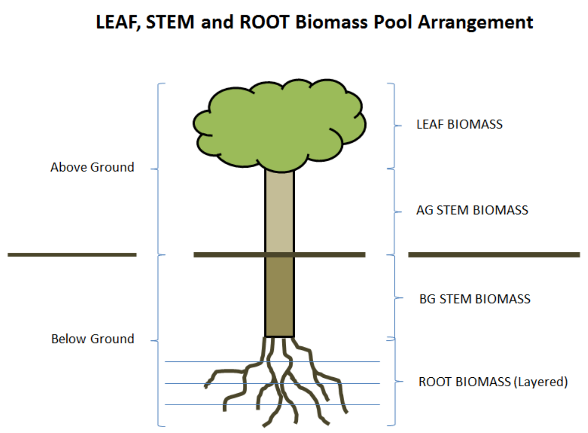
104
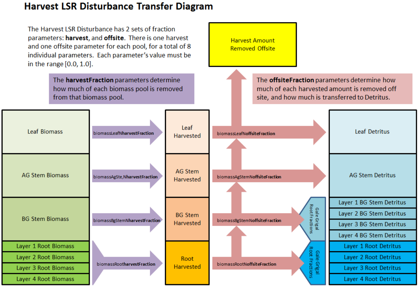
105
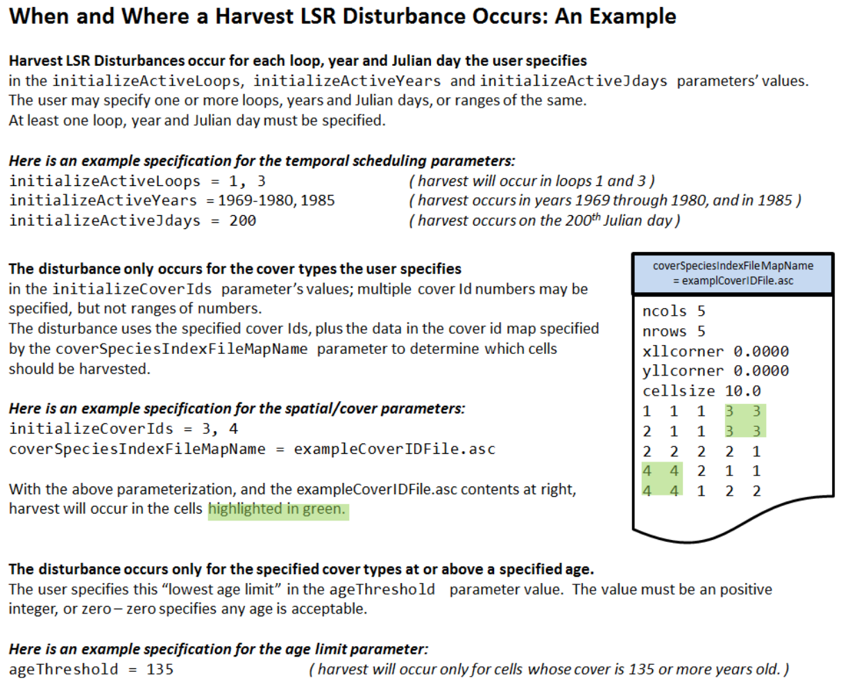
106
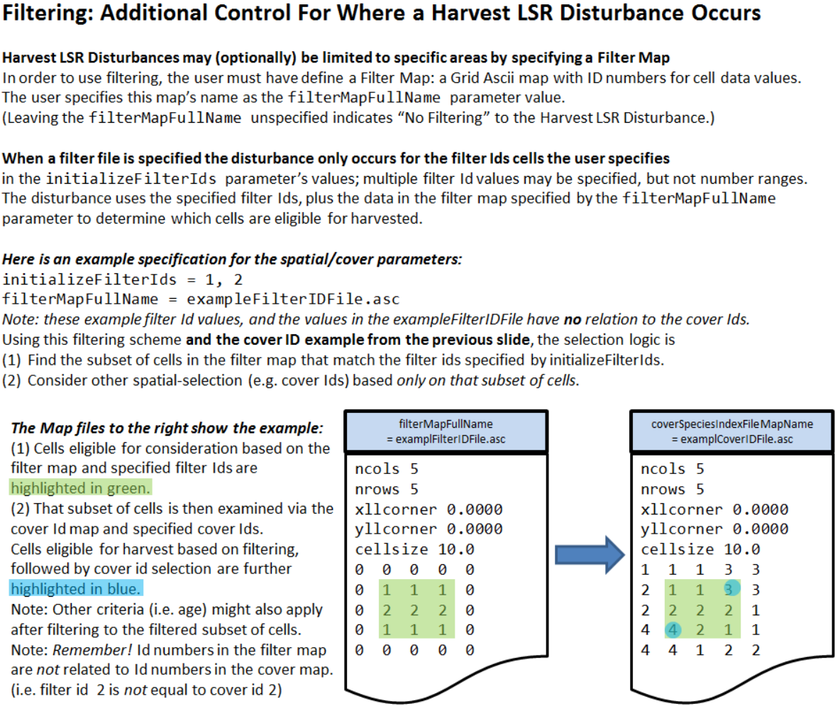
107
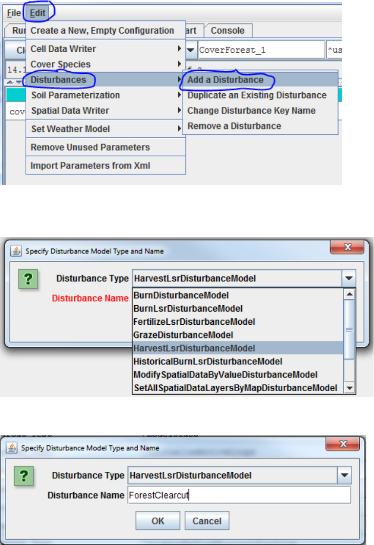
108
24.1 – Disturbance Items by Model Type
To begin, you need to select the disturbance model you want by clicking
Edit Disturbances Add a Disturbance:
You will see the following drop-down menu for selecting a Disturbance Model. To further
demonstrate the harvest disturbance example illustrated under section 24.0, we select the
HarvestLsrDisturbanceModel:
Now choose a name for your HarvestLsrDisturbanceModel and type it the “Disturbance Name”
dialog box, for example, “ForestClearcut”:
After selecting the HarvestLsrDisturbanceModel and giving it a disturbance name, go to the All
Parameters drop-down menu and select “24.1 Disturbance Items by Model Type”. You should
see the following:
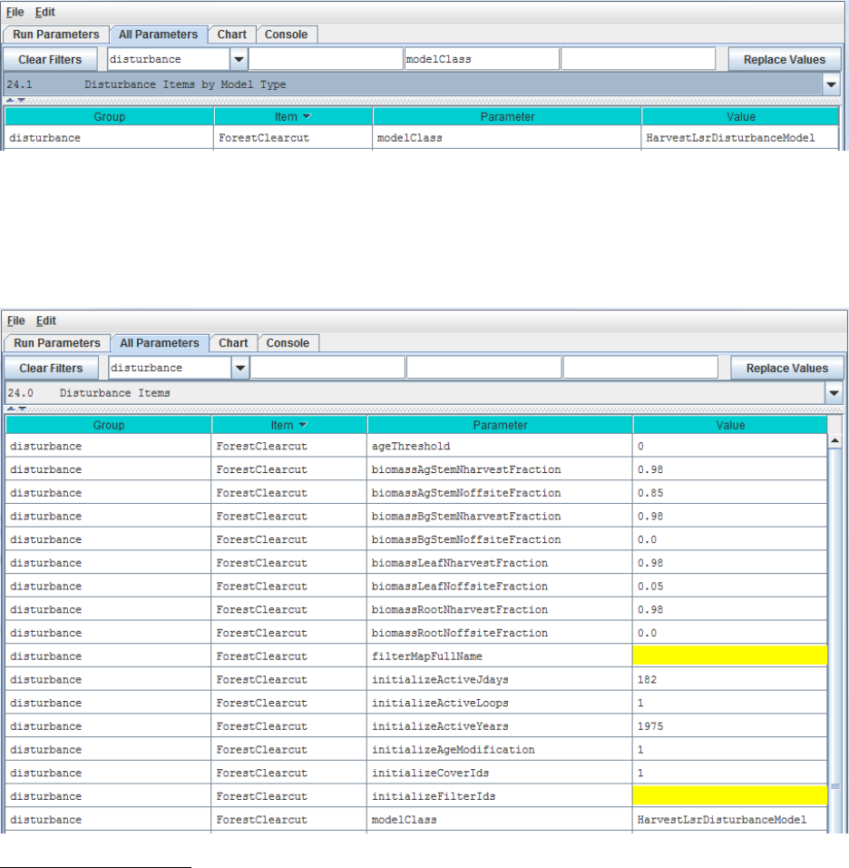
109
Select “24.0 – Disturbance Items” from the All Parameters drop-down menu to see a list of all
parameters associated with the HarvestLsrDisturbanceModel. In the screenshot below, we have
specified parameter values for the HarvestLsrDisturbanceModel disturbance we named
“ForestClearcut”:
Parameter Definitions
ageThreshold Applicable cover must be greater or equal to the
specified ageThreshold (in integer years) to be
harvested. Defaults to 0 -- i.e., any otherwise-
applicable cell is harvested regardless of age.
biomassAgStemNharvestFraction The fraction [0.0 1.0] of available above-ground
stem biomass harvested i.e. converted from biomass
above-ground stem to above-ground stem detritus
and/or removed from the simulation.
110
biomassAgStemNoffsiteFraction The fraction [0.0 1.0] of harvested above-ground
stem biomass removed offsite, i.e., removed from the
cell and the simulation.
biomassBgStemNharvestFraction The fraction [0.0 1.0] of available below-ground
biomass harvested i.e. converted from biomass
below-ground to below-ground detritus and/or
removed from the simulation.
biomassBgStemNoffsiteFraction The fraction [0.0 1.0] of harvested below-ground
stem biomass removed offsite. i.e. removed from the
cell and the simulation.
biomassLeafNharvestFraction The fraction [0.0 1.0] of available leaf biomass
harvested i.e. converted from biomass leaf to leaf
detritus and/or removed from the simulation.
biomassLeafNoffsiteFraction The fraction [0.0 1.0] of harvested leaf biomass
removed offsite. i.e. removed from the cell and the
simulation.
biomassRootNharvestFraction The fraction [0.0 1.0] of available root biomass
harvested i.e. converted from biomass root to root
detritus and/or removed from the simulation.
biomassRootNoffsiteFraction The fraction [0.0 1.0] of harvested root biomass
removed offsite. i.e. removed from the cell and the
simulation.
filterMapFullName The fully-qualified (path/name.ext) name of a Grid
ASCII (.asc) file containing (integer) filter Ids. When
left unspecified (default) indicates that filtering will
be turned off. Note: if the value for this parameter is
not a fully-qualified name the simulator engine will
prefix the specified input data location root and name
to this parameter's value to create a default fully-
qualified name.
initializeActiveJdays The comma-separated list of Julian days on which the
disturbance occurs. Entries in the list may be either
single Julian days or start-end (dash-separated)
ranges. A valid Julian day is any positive whole
number between 1 and 366 (however day 366 is
ignored in non-leap years). For example this text
triggers output on days 1 365 and between 30 and 90
inclusive: 1 30-90 365
initializeActiveLoops The comma-separated list of loop index numbers
(range [1 nth-Loop]) in which the disturbance
occurs. Entries in the list may be either single loop
numbers or start-end (dash-separated) ranges. A valid
loop index number is any positive whole number
between 1 and the number of loops specified for the
simulation run. For example in a simulation run for
10 loops this text triggers output in loops 1 3
through 5 and 10 inclusive: 1 3-5 10
initializeActiveYears The comma-separated list of Years in which the
disturbance occurs. Entries in the list may be either
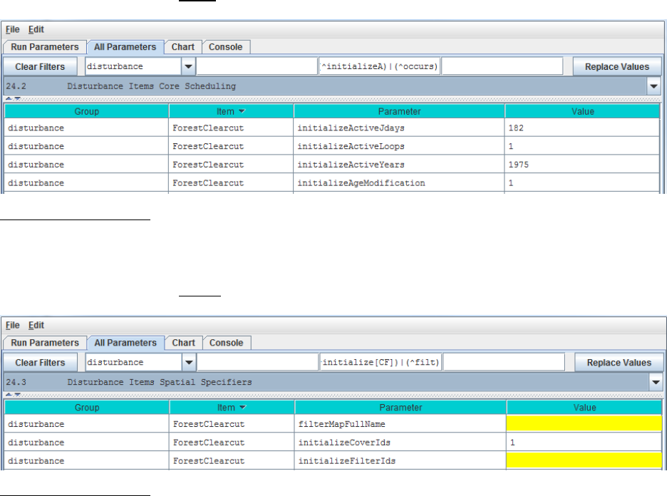
111
single years or start-end (dash-separated) ranges. A
valid year is any positive whole number (but the user
is expected to choose years within the simulation
run!). For example in a simulation run between 1995
and 2010, this text triggers output in 2000 through
2005 inclusive: 2000-2005
initializeAgeModification (Optional) Specifies the number of years to subtract
or add to the age of the cover in affected cells when
the disturbance occurs. To add n years to a cell's
cover age prefix a plus (+) sign to the number n. To
subtract n years to a cell's cover age prefix a minus (-
) sign to the number n. To set the cell's cover age to a
specific number of years specify a number n
without any sign prefix. Subtraction halts at zero (e.g.
a cover age of 7 given -10 as the modifier will result
in 0 not -3 as the modified age).
initializeCoverIds The Cover Species Id numbers that are affected by
this disturbance model. Specify a comma-separated
sequence of Cover Species uniqueId numbers.
modelClass The disturbance model's actual Java class name
Select “24.2 – Disturbance Items Core Scheduling” to focus the All Parameters table on the
parameters for specifying when disturbance events occur:
Parameter Definitions: these parameters are defined under the All Parameters screenshot for
Select “24.0 – Disturbance Items”, above.
Select “24.3 -- Disturbance Items Spatial Specifiers” to focus the All Parameters table on the
parameters for specifying where disturbance events occur:
Parameter Definitions: these parameters are defined under the All Parameters screenshot for
Select “24.0 – Disturbance Items”, above.

112
Calibration Notes
Make sure that the disturbance models you have set up are working correctly. Are disturbance
events occurring when and where you want them to, are the correct amounts of biomass being
harvested/burned/grazed, and are the correct amounts and forms of fertilizer being applied. For a
first check, click VELMA’s GUI “Chart” tab at any time during a simulation, then click the
drop-down menu button located near the lower left corner of the screen, then select an
appropriate spatial data display option (see section “25.0 – Runtime Chart Display Scale” for
details”).
For example, by selecting the “Harvest Spatial Data” menu item you can see daily and year-to-
date summaries of harvest events and their effects on various biomass tools. The two figures
below show year-end summaries of harvest events for consecutive years, 2000 and 2001. In
2000 there were no harvests (top figure: top row, middle frame). In 2001 there were several
fairly large harvest events (bottom figure: top row, middle frame). A comparison of the other
frames in top and bottom figures reveals changes in plant biomass, detritus, soil organic matter,
and cover age following harvest events.
An examination of VELMA’s daily and annual output files (csv format) provides a more
quantitative check of disturbance events.
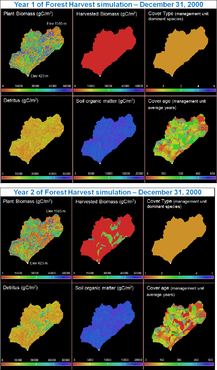
113
Screenshot of runtime “Harvest Spatial Data” display.
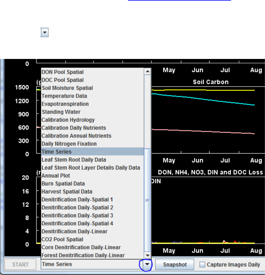
114
25.0 – Runtime Chart Display Scale (link to All Parameters TOC)
VELMA has powerful visualization capabilities built into it, hence the model’s name –
Visualizing Ecosystem Land Management Assessments. To see a list of visualization options,
select the VELMA GUI “Chart” tab at any time during a simulation, then click the drop-down
menu button ( ) located near the lower left corner of the screen, and select a display option.
Each option dynamically displays daily changes in one or more output variables. The screenshot
below shows the lower half of possible visualization options:
For example, the “Soil Moisture Spatial” visualization displays runtime daily changes in spatial
patterns of soil moisture (% saturation) for four soil layers for a 20-ha watershed on the day
currently being simulated. A screenshot for a particular day is shown below. The lower third of
display is a running graphical summary of daily changes in soil moisture per soil layer from
January 1 up to the date currently simulated. A new view is generated at the beginning of each
calendar year). A variety of hardwired display formats are used for different output variables.

115
You can save daily screenshots as .png files by clicking the “Snapshot” button (located near the
middle of the menu bar at the bottom of the screenshot, above). You can also save a series of
daily images by clicking the “Capture Images Daily” checkbox. After a simulation is completed,
third-party software can be used to stitch together a time series of saved .png screenshots to
make a time-lapse movie. However, note that saving daily .png images for long simulations can
fill large amounts of disk space.
You can use the VELMA GUI’s All Parameters tab to review and change the settings for display
parameters controlling minimum (min) and maximum (max) values for the y-axis and range
color bar. To locate all display parameters, select the “25.0 Runtime Chart Display Scale” item
from the All Parameters drop-down menu button:
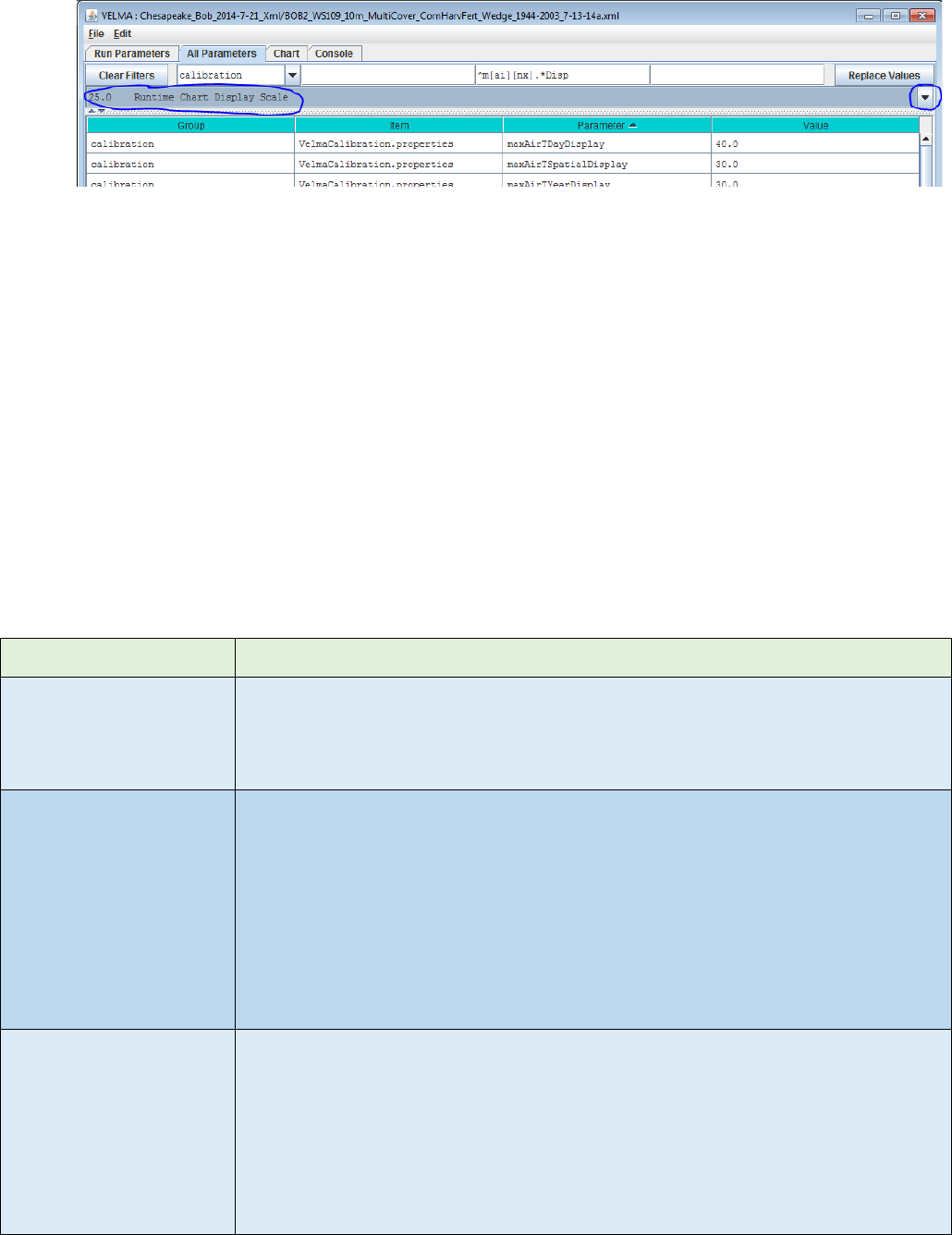
116
Different runtime display charts use different subsets of the display parameters. Unfortunately,
nothing listed under “All Parameters 25.0 Runtime Chart Display Scale” indicates which display
parameters belong to a particular runtime display chart. Therefore, we have constructed the table
below so that users can associate runtime display chart names with the display parameters used
by that chart.
For example, if you want to adjust VELMA’s “Annual Plot” display for soil humus, you would
find “Annual Plot” under the “Display Selector Name” column in the table below, copy
“maxHumusDayDisplay” and paste it in the “Parameter” search window in the VELMA GUI’s All
Parameters view. Hit your keyboard’s “Enter” key and you should see “maxHumusDayDisplay”
under “Parameter column. Specify the value you want. Repeat for the process for the
“minHumusDayDisplay” parameter. [Note: you cannot change the display parameterizations
during a simulation run. Currently, the VELMA GUI does not allow runtime display scales to
change dynamically during simulation runs. Prior to starting a simulation, you must set the
display parameters for any chart you will use during a simulation.]
Display Selector Name MIN Display Setting MAX Display Setting
<cover> + Denitrification
Daily-Linear
( always zero )
maxDenitrificationDaySpatialDis
play
( always zero ) maxNo3DenitDaySpatialDisplay
( always zero ) maxCo2DenitDaySpatialDisplay
Annual Plot
( always zero ) maxDonLossYearFinalDisplay
( always zero ) maxDocLossYearFinalDisplay
( always zero ) maxNppYearSumDisplay
minBiomassYearFinalDisplay maxBiomassYearFinalDisplay
minHumusDayDisplay maxHumusDayDisplay
minLitterDayDisplay maxLitterDayDisplay
minNepYearSumDisplay maxNepYearSumDisplay
Burn Spatial Data
minBiomassAgStemDayDisplay maxBiomassAgStemDayDisplay
minBiomassLeafDayDisplay maxBiomassLeafDayDisplay
minDetritusAgStemDayDisplay maxDetritusAgStemDayDisplay
minDetritusLeafDayDisplay maxDetritusLeafDayDisplay
minHumusDayDisplay maxHumusDayDisplay
minLitterDayDisplay maxLitterDayDisplay

117
Calibration Annual
Nutrients
( always zero ) maxNh4LossYearSumDisplay
( always zero ) maxNo3LossYearSumDisplay
( always zero ) maxDonLossYearSumDisplay
minDocLossYearSumDisplay maxDocLossYearSumDisplay
Calibration Daily Nutrients
( always zero ) maxNh4LossDayDisplay
( always zero ) maxNo3LossDayDisplay
( always zero ) maxDonLossDayDisplay
( always zero ) maxDocLossDayDisplay
Calibration Hydrology
( always zero ) maxRainDayDisplay
( always zero ) maxRunoffDayDisplay
( always zero ) maxSubRunoffDayDisplay
( always zero ) maxEtDayDisplay
minHydroYearSumDisplay maxHydroYearSumDisplay
CO2 Pool Spatial ( always zero ) maxCo2DaySpatialDisplay
Daily Nitrogen Fixation
( always zero ) maxNinDayDisplay
( always zero ) maxPlantUptakeSpatialDisplay
( always zero ) maxSymbioticNfixedDayDisplay
( always zero ) maxAsymbioticNfixedDayDisplay
( always zero ) maxDonLossDayDisplay
( always zero ) maxTotalNLossDayDisplay
( always zero )
maxNitrificationDaySpatialDispl
ay
( always zero )
maxDenitrificationDaySpatialDis
play
Default Layer 1 - 4
( always zero ) maxDonLossDayDisplay
( always zero ) maxDocLossDayDisplay
( always zero ) maxRainDayDisplay
( always zero ) maxRunoffDayDisplay
Denitrification Daily-Spatial ( always zero )
maxDenitrificationDaySpatialDis
play
Denitrification Daily-Spatial
1 - 4
( always zero )
maxDenitrificationDaySpatialDis
play
( always zero ) maxNo3DenitDaySpatialDisplay
( always zero ) maxCo2DaySpatialDisplay
DOC Pool Spatial ( always zero ) maxDocSpatialDisplay
DON Pool Spatial ( always zero ) maxDonSpatialDisplay
Evapotranspiration ( always zero ) maxEtDayDisplay
Harvest Spatial Data minBiomassDayDisplay maxBiomassDayDisplay
minHumusDayDisplay maxHumusDayDisplay

118
minLitterDayDisplay maxLitterDayDisplay
Leaf Stem Root Daily Data
minBiomassAgStemDayDisplay maxBiomassAgStemDayDisplay
minBiomassBgStemDayDisplay maxBiomassBgStemDayDisplay
minBiomassLeafDayDisplay maxBiomassLeafDayDisplay
minBiomassRootDayDisplay maxBiomassRootDayDisplay
minDetritusAgStemDayDisplay maxDetritusAgStemDayDisplay
minDetritusBgStemDayDisplay maxDetritusBgStemDayDisplay
minDetritusLeafDayDisplay maxDetritusLeafDayDisplay
minDetritusRootDayDisplay maxDetritusRootDayDisplay
Leaf Stem Root Layer
Details Daily Data
minBiomassRootLayersDayDisplay maxBiomassRootLayersDayDisplay
minDetritusBgStemLayersDayDisplay
maxDetritusBgStemLayersDayDispl
ay
minDetritusRootLayersDayDisplay maxDetritusRootLayersDayDisplay
minHumusLayersDayDisplay maxHumusLayersDayDisplay
LSR Summary Spatial
( always zero ) maxNppDayDisplay
minBiomassDayDisplay maxBiomassDayDisplay
minHumusDayDisplay maxHumusDayDisplay
minLitterDayDisplay maxLitterDayDisplay
NH4 Pool Spatial ( always zero ) maxNh4SpatialDisplay
Nitrification Daily-Spatial ( always zero )
maxNitrificationDaySpatialDispl
ay
Nitrogen Fixation Daily-
Spatial
( always zero ) maxSymbioticNfixedDayDisplay
( always zero ) maxAsymbioticNfixedDayDisplay
NO3 Pool Spatial ( always zero ) maxNo3SpatialDisplay
Plant Uptake Spatial minPlantUptakeSpatialDisplay maxPlantUptakeSpatialDisplay
Productivity Spatial
( always zero ) maxNppDayDisplay
( always zero ) maxNh4SpatialDisplay
( always zero ) maxNo3SpatialDisplay
minBiomassDayDisplay maxBiomassDayDisplay
Snow Dynamics Spatial
( always zero ) maxRainSpatialDisplay
( always zero ) maxSnowSpatialDisplay
( always zero ) maxSnowDepthSpatialDisplay
( always zero ) maxSnowMeltSpatialDisplay
minAirTSpatialDisplay maxAirTSpatialDisplay
Standing Water
( always zero ) maxRainDayDisplay
( always zero ) maxRunoffDayDisplay
( always zero ) maxStandingWaterDayDisplay
Temperature Data minAirTDayDisplay maxAirTDayDisplay

119
Time Series
( always zero ) maxDonLossDayDisplay
( always zero ) maxDocLossDayDisplay
( always zero ) maxRainDayDisplay
( always zero ) maxRunoffDayDisplay
minAirTDayDisplay maxAirTDayDisplay
minBiomassDayDisplay maxBiomassDayDisplay
minHumusDayDisplay maxHumusDayDisplay
minLitterDayDisplay maxLitterDayDisplay
VSA Spatial and Hydro
Linear
( always zero ) maxRainDayDisplay
( always zero ) maxRunoffDayDisplay
Weather Summary Spatial
( always zero ) maxRainDayDisplay
( always zero ) maxRainSpatialDisplay
( always zero ) maxSnowSpatialDisplay
( always zero ) maxSnowMeltSpatialDisplay
minAirTDayDisplay maxAirTDayDisplay
minAirTSpatialDisplay maxAirTSpatialDisplay

120
APPENDICES
VELMA Version 2.0

121
Appendix 1:
Overview of VELMA’s Leaf-Stem-Root (LSR)
Plant Biomass Submodel
(Link to All Parameters Table of Contents)
In VELMA version 1.0, plant biomass in each cell was simulated in aggregate. That is, leaves, stems
and roots were lumped together in a single biomass pool (Abdelnour et al. 2011). This lumped approach
greatly simplified the structure and application of the model. Although version 1.0 successfully
simulates important aspects of catchment hydrology and biogeochemistry (e.g., Abdelnour et al. 2011,
2013), it does not simulate effects associated with phenological changes and disturbances and that
disproportionately affect specific plant tissues, for example, leaf growth and senescence, defoliation
events, selective removal of high or low C/N tissues via harvest, grazing, fire, etc.
To address such effects, version 2.0 simulates four plant biomass pools: leaves, aboveground stems,
belowground stems, and fine roots. Main features of this leaf-stem-root (LSR) submodel include:
• Live plant biomass pools for four tissue types (also see Figure 1 and explanation preceding
“All Parameters Section 5.0” of the User Manual)
o Leaves (annual or perennial grasses, deciduous or coniferous trees, etc.)
o Aboveground stems (trees, grasses, etc.)
o belowground stems (<2 mm diameter, not involved in water and nutrient uptake)
o fine roots (<2 mm diameter, involved in water and nutrient uptake)
• Dead (detritus) plant biomass pools for each of the four plant tissue types
• A user-specified C/N ratio for each plant tissue type. In version 2.0, a tissue’s C/N ratio is
applied to both the live and dead biomass pools. Simulation of separate live and dead C/N
ratios will be addressed in future versions
• A new plant tissue mortality submodel simulates the loss of live biomass to detritus (see
Appendix 1, Figures A1.1 – A1.4)
• A new decomposition model based on Potter et al. (1993) simulates the decomposition of
detritus to CO2 and humus (Appendix 1, Figures A1.5 – A1.8)
• A specified fraction of total plant nitrogen uptake is allocated to each plant tissue type, such
that the fractions for all tissues = 1.0 (see Appendix 1, Figures A1.1 – A1.4)
Figures A1.1 – A1.11, below, graphically summarize the LSR submodel structure and model equations.
These figures portray the pools (boxes) and fluxes (arrows) of nitrogen and/or carbon from live to dead
biomass and from dead biomass to the humus pool and atmosphere. Pools and fluxes involving
VELMA’s four soil layers are also shown. In each successive figure, a red encircling line delineates a
subset of the LSR system for which text is provided to describe associated model parameters and
equations that govern simulated C and N pools and fluxes. Note that parameter names in the VELMA
version 2.0 program Java code and GUI do not necessarily conform to Figures A1.1 – A1.11 parameter
names, which were modified using more rigorous naming rules during the VELMA programming
process.
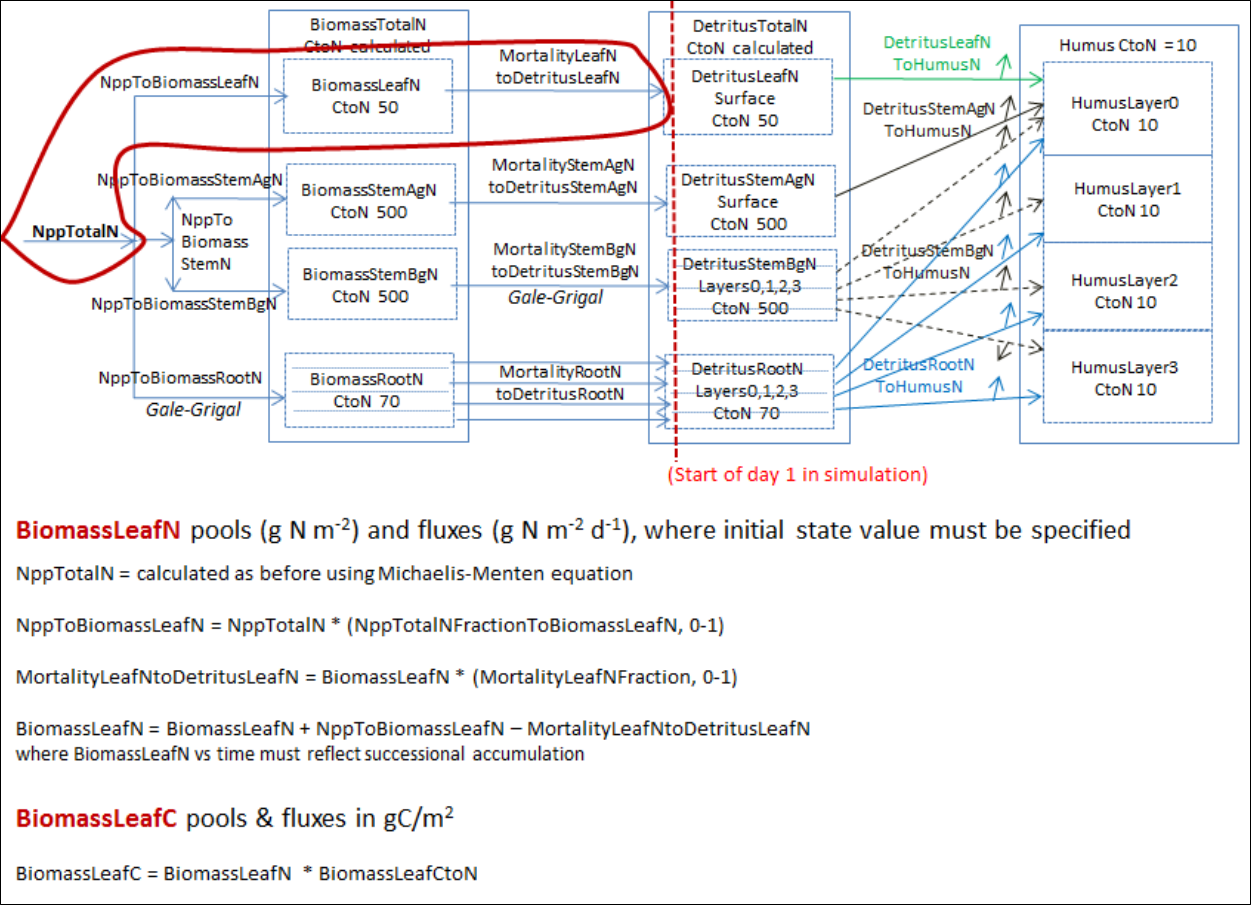
122
Figure A1.1
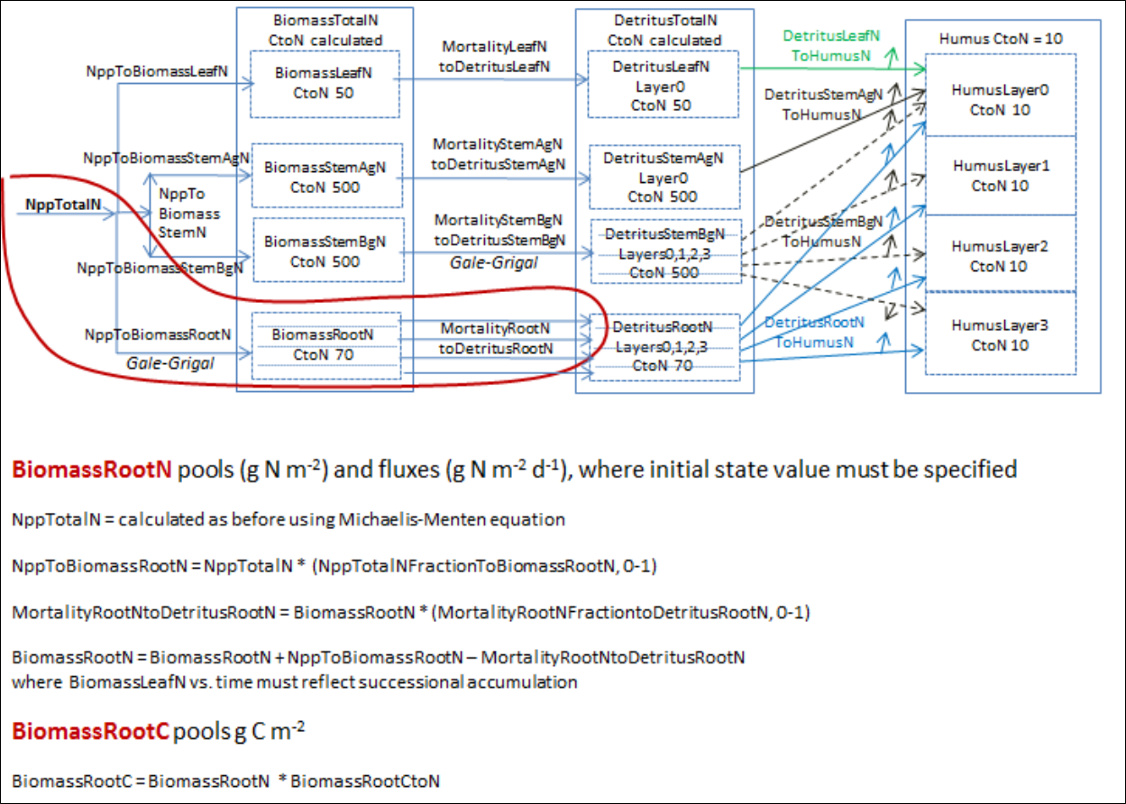
123
Figure A1.2
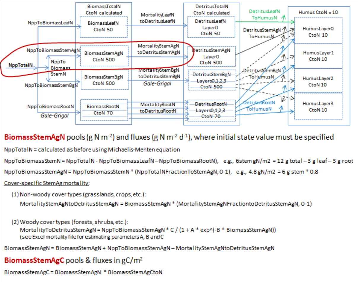
124
Figure A1.3
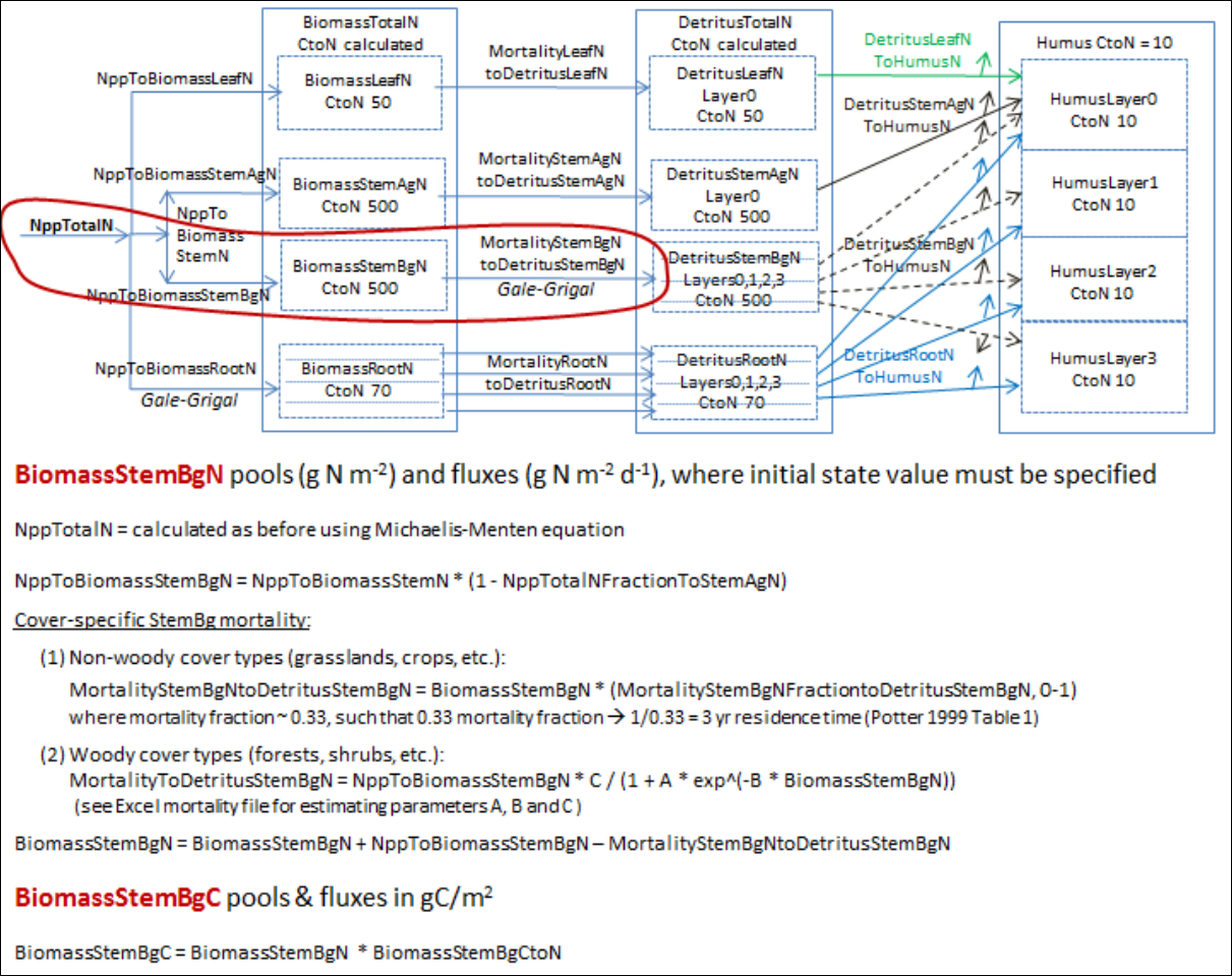
125
Figure A1.4

126
Figure A1.5
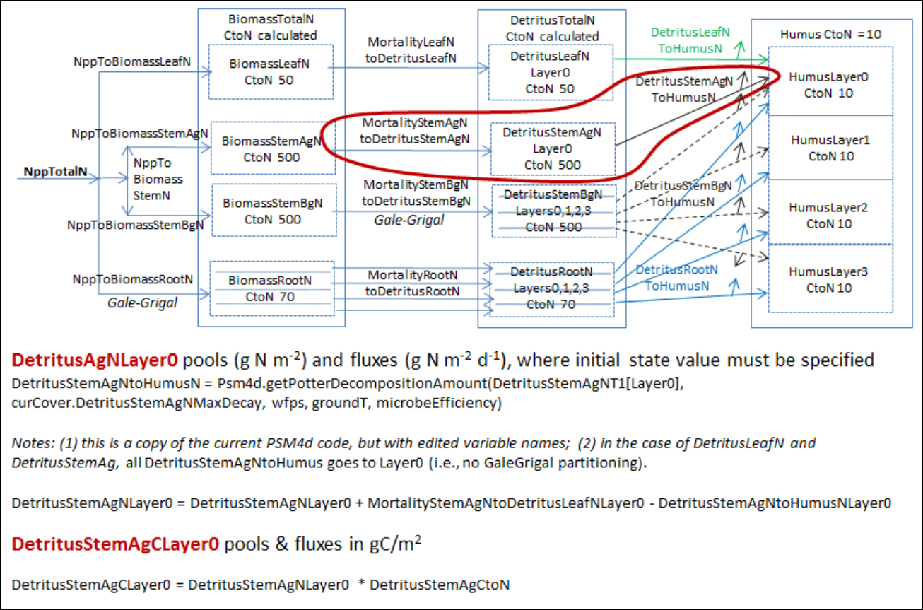
127
Figure A1.6
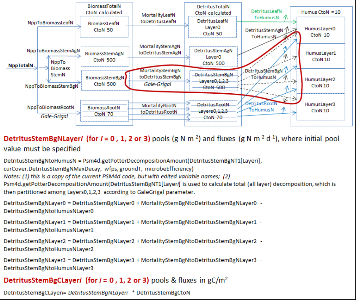
128
Figure A1.7
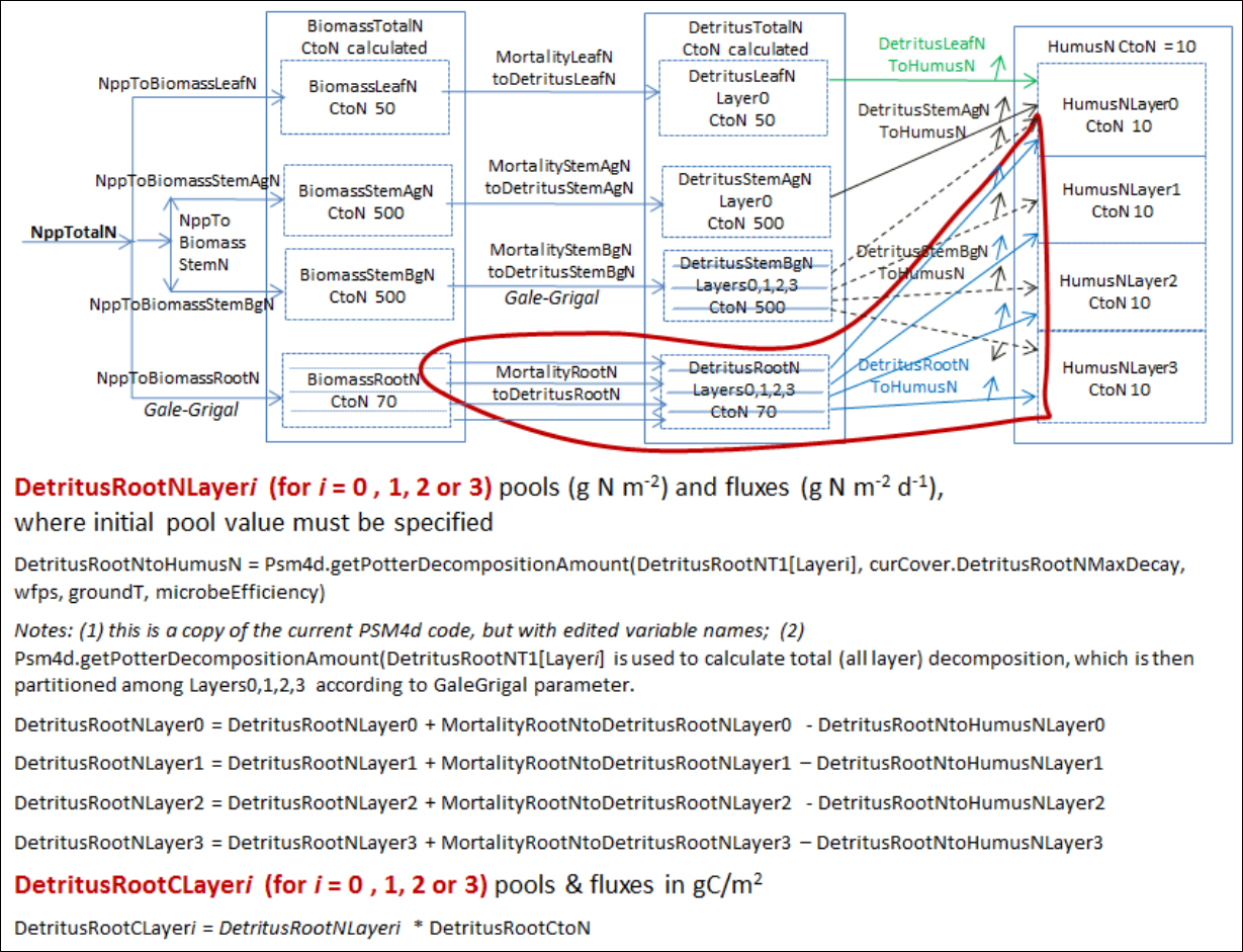
129
Figure A1.8
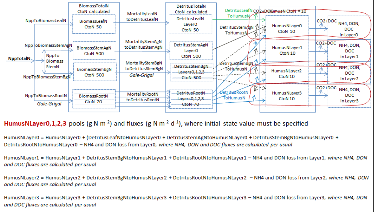
130
Figure A1.9
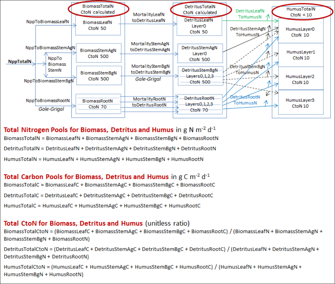
131
Figure A1.10

132
Figure A1.11

133
Appendix 2:
Initializing a Spatial Data Pool Using an
ASCII Grid
(Link to All Parameters Table of Contents)
VELMA Simulator spatial data pools may be initialized by specifying “Set Spatial Data By Map” disturbances as
part of a simulator run’s simulation configuration. Each spatial data pool (and each layer of that pool for multi-
layer pools) that is initialized must have a separate disturbance specified for it, and its own Grid ASCII (.asc) map
file available for the disturbance to use as a data source3.
Assuming an otherwise already configured simulation configuration is loaded into JVelma, here is how to
initialize a spatial data pool (using the leaf biomass pool as our example) by adding a Set Spatial By Map
disturbance event to the configuration:
Note
It’s assumed that before configuring the simulation, you’ve already created a Grid ASCII map file (.asc) for the
disturbance to use. How you create the map is up to you, but it must in standard Grid ASCII format, and have
the same dimensions as the Grid ASCII map of DEM data that the simulation will use.
For this example, each cell value in the Grid ASCII map file is assumed to be an amount of leaf biomass (in grams
per square meter).
Add the New Disturbance Parameters to the Simulation Configuration
1. In JVelma, with the simulation configuration loaded, Click/open the “Edit” menu and Click/Select
“Disturbances “ -> “Add a Disturbance”.
2. In the Disturbance Model Selector dialog, use the drop-down selector to find the
“SetSpatialDataByMapDisturbanceModel” and Click/Set it as the Disturbance Type.
3. In the text box next to the “DisturbanceName” prompt, type in a name for this particular disturbance.
The name should be unique (the dialog will warn you if you enter a name already in use) and it is better
to avoid whitespace and non-alphanumeric characters.
For this is example, the name will be “Init_Leaf_Biomass”.
4. Click the “OK” button. The dialog closes, the parameters for a new Set Spatial Data By Map disturbance
are added to the simulation configuration, and the view should shift to these new parameters in
JVelma’s “All Parameters” tab window.
Configure the New Disturbance Parameters
The parameters for the Set Spatial Data By Map disturbance tell the disturbance When it should occur, What its
data source is, and Which Spatial Data Pool to apply that data source to.
3 Two or more Set Spatial Data By Map disturbances may be set to use the same Grid ASCII map file as their input data
source, but it’s more likely that a given spatial data pool to have its own unique input data source.

134
The initializeActiveLoops, initializeActiveYears” and initializeActiveJdays parameters,
plus the occursAtStepStart parameter specify when this disturbance should occur. To initialize the leaf
biomass pool before any simulation steps occur, set them as follows:
Parameter Name
Set Value As …
Comment
initializeActiveLoops 1 Occurs during the first loop
initializeActiveYears 2000 Assumes 2000 is the simulation’s start year
initializeActiveJdays 1 Occurs during the first Julian day
occursAtStepStart true Disturbance will occur before any simulation
work is performed on the day when it occurs
Set the spatialDataFileFullName parameter to the fully-qualified path and name of the Grid ASCII file that
you plan to use as the input data source for biomass leaf values.
For this example, suppose that file is named “LeafBiomassData.asc” and resides in directory “C:\My Data\”. The
spatialDataFileName value should then be set to: “C:/My Data/LeafBiomassData.asc” (without the double-
quotes).
Note
Instead of Windows backslash “\” path separators, use forward slash “/” characters as path separators.
Also, be very careful with whitespace; if there is any, it must exactly match whatever whitespace is present in
the actual path and filename.
Set the spatialDataName parameter to the Spatial Data Pool that will receive data from the file.
For our example of leaf biomass, the pool name is “BIOMASS_LEAF_N” (without the double-quotes).
Note
A table containing the names of the Velma Simulator’s spatial data pools is available at the end of this
document.
Set the spatialDataLayer parameter to the (one-based) layer index number of the spatial data pool layer
that will receive data from the file.
For single-layer spatial data pools this value MUST be set to “1” see the table of spatial data at the end of this
document for a summary of how many layers each pool has.
In summary, here is the full parameterization for our example Set (Leaf Biomass) Spatial Data Pool By Map
disturbance:

135
ID Key
Value
/disturbance/Init_Leaf_Biomass/initializeActiveJdays 1
/disturbance/Init_Leaf_Biomass/initializeActiveLoops 1
/disturbance/Init_Leaf_Biomass/initializeActiveYears 2000
/disturbance/Init_Leaf_Biomass/modelClass SetSpatialDataByMapDisturbanceModel
/disturbance/Init_Leaf_Biomass/occursAtStepStart true
/disturbance/Init_Leaf_Biomass/spatialDataFileFullName C:/My Data/LeafBiomassData.asc
/disturbance/Init_Leaf_Biomass/spatialDataLayer 1
/disturbance/Init_Leaf_Biomass/spatialDataName BIOMASS_LEAF_N
Configured as specified by the parameters above, this SetSpatialDataByMapDisturbanceModel
disturbance occurs once during the simulation; in the first loop, on the first day of 2000 (assumed to be the first
year of simulation for our example) and before any simulation work is done on that day.
When the disturbance occurs, it will open the Grid ASCII spatial data file
“C:/My Data/LeafBiomassdata.asc”, and set each cell of the BIOMASS_LEAF_N spatial data pool in layer 1 to the
value for that cell read from the .asc spatial data file.
That’s all there is to it!
Although SetSpatialDataByMapDisturbanceModel disturbances may be used for other purposes, by
varying when they occur, this example shows the commonest use-case; initializing specific non-uniform values
into a spatial data pool at the start of a simulation.

136
Appendix 3:
Creating Initial ASCII Grid Chemistry Spatial
Data Pools
(Link to All Parameters Table of Contents)
Initial chemistry or nutrient pools are created through a series of transformations of above ground
Biomass to each of the respective spatial data pools. These transformations are defined by relationship
ratios (fractions) each pool has to “real” or estimated measurements of Biomass (g/m²) for the study
area.
37 VELMA Simulator spatial data pools will be created from this one raster grid Biomass layer. See
Table 1 for the complete list of initial layers that will be created. Each spatial data pool layer will have
its own corresponding Grid ASCII (.asc) map file upon completion of the Python script. These Grid
ASCII (.asc) map files will be used as inputs to VELMA for initializing the map disturbance events.
Figure 1 describes the internal processing flow, inputs, and outputs of the script. Figure 2 describes the
calculations and quality control of the internal Python processing.
Software Requirements
• ArcGIS 10.0 or higher with “Spatial Analyst” license
• NumPy package installed, for the Python version used by ArcGIS 10.X
• IDLE – Python’s Integrated Development Environment installed
File Requirements for Data Processing
• Raster above ground biomass of the study area
o Unit type – Carbon grams / m²
o “.tif” extension
o Raster has been clipped and snapped to same dimensions as the Grid ASCII map of DEM
data that the simulation will use.
• Summary Biomass to ratio pools file
o “.csv” comma delaminate format
o No headers
o Biomass values (stand age / mass) is in the first column
o Pool ratios values in subsequent columns (quantity 37)
o Column arrangement /order is known for the ratios
Setting up Python Script for Data Processing
The script is set up in two general sections, “User defined inputs” and “Processing functions”. “User
defined inputs” is where inputs, outputs, and column order will be defined or edited. Changes to the
“Processing functions” section of the Python code should be avoided.
Note
While editing “User defined inputs”
• All file and folder paths need to be enclosed in double quotes: "C:/Temp/Biomass/"
137
• All paths in Python use a “/” instead of the DOS “\”
• Folder defined paths need to end in “/” "C:/Temp/Biomass/"
• File defined paths need to end with correct extension "C:/Temp/Biomass/C_g_leaf.tif"
• Ensure that all final output working directories are the same
Note
Biomass to ratio pools file
• Column arrangement must be maintained as noted above
Editing the Python Script
1. Right click the “lookup_ratio_calculate_biomass_func.py” script and click “Edit With IDLE”
2. Editing within the “User defined inputs” section
3. Edit all path variables for:
o “biomassLayer” – Biomass file
o “inputPath” – Main output directory
o “massRatio” – “.csv” Summary Biomass to ratio pools file
o Ouput rasters files, for each of the velma attributes - “.tif” extension
o Column number of pool ratio to biomass – Order specific
o Carbon to nitrogen ratios
o Raster attributes
xllcorner
yllcorner
cellsize
nodata
4. Pres Ctrl+S to save the file
5. Press F5 to run!
Note
Processing time is very dependent on processing power and the size of your study area. For example
the Blue River, in Oregon, had a study grid of ~350,000 cells and took 7-12hours to complete all 37
pools. The Python shell will print updates of pool processing steps, and say “All Done!” when it’s done.

138
Table 1. Initial spatial pools derived from ratios to above
ground biomass (C g/m^2)
Spatial Data Pool Name
Layers
Unit Type
BIOMASS_AG_STEM_N
1
N g/m^2
BIOMASS_BG_STEM_N
1
N g/m^2
BIOMASS_LEAF_N
1
N g/m^2
BIOMASS_ROOT_N
4
N g/m^2
DETRITUS_AG_STEM_N
1
N g/m^2
DETRITUS_BG_STEM_N
4
N g/m^2
DETRITUS_LEAF_N
1
N g/m^2
DETRITUS_ROOT_N
4
N g/m^2
DOC
4
C g/m^2
DON
4
N g/m^2
HUMUS
4
N g/m^2
NH4
4
N g/m^2
NO3
4
N g/m^2

139
Figure 1. Process flow diagram of ratio (fractions) processing of “observed” above ground biomass (g /
m²) to the final nitrogen (g / m²) spatial data pools for VELMA’s initialization of disturbance events.
Biomass (1)
Biomass
Ratios (37)
Live Mass
Carbon (7)
Humus
Carbon (4)
Detritus
Carbon (10)
Organic
Chem (16)
Live Mass
Nitrogen (7)
Humus
Nitrogen (4)
Detritus
Nitrogen
GIS
Raster
CSV
Live Mass
Nitrogen (7)
Humus
Nitrogen (4)
Detritus
Nitrogen
Organic
Chem (16)
VELMA
ASCII
Legend:
Conversion
g Mass -> C g / m²
Python
Conversion
C g / m² -> N g / m²
Conversion
Raster -> ASCII Grid
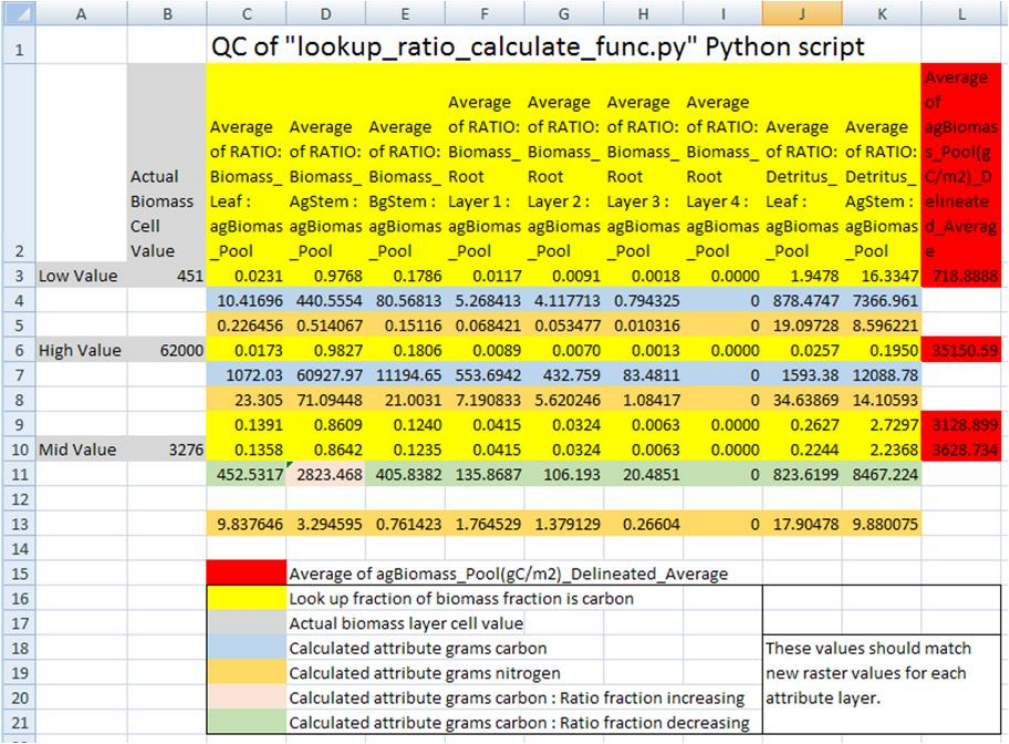
140
Figure 2. Quality control check of Python script’s dynamic conversions of “observed” above ground
biomass (g / m²) to the final nitrogen (g / m²) spatial data pools. Conversion of biomass (g / m²) to the
final nitrogen (g / m²) were made through an intermediate step of converting mass to carbon (g / m²),
and then using different C to N ratios for each pool to calculate the final nitrogen pools. Fractions
(ratios) of spatial pools change both in the positive and negative direction as a forest ages or increases in
total biomass. Ratio pools can increases or decreases between stand age increments, and the
calculations of these intermediate biomass observational values must reflect this dynamic nature of
changing ratios between time steps. Intermediate values of biomass, those that land in between time
step years, were therefore linearly interpolated between the time point bounds. Spatial map ASCII grid
values for each of the 37 pools should then backward match ratio conversions and final C to N
calculations to the original “observed” above ground biomass. (Only a partial list of pools is displayed
here).
Example: A mid biomass cell value at B10 = 3276 (g / m²) and is part way between stand age values at
L9 and L10. It’s above ground stem carbon mass fraction increases from 0.8609 (D9) to 0.8642 (D10).
So its fraction stem mass (column D) should increase as its percentage difference moves from L9
towards LD10. Conversely, for all the other pool attributes, its percentage difference would increase as
its fraction moves the opposite direction from rows 10 to rows 9.
141
Appendix 4:
Overview of VELMA Simulator Output
(Link to All Parameters Table of Contents)
Where are VELMA Simulator Results Located?
The results of a VELMA Simulator run are a collection of data files that the simulator writes to a specific
directory location. That directory is specified in the simulator configuration by 2 related parameters:
/calibration/VelmaInputs.properties/initializeOutputDataLocationRoot
and
/calibration/VelmaInputs.properties/run_index
The initializeOutputDataLocationRoot’s value should be a fully qualified path, and the run_index should
be the name of a directory under that path.
For example, given the following configuration:
ID Key Value
/calibration/VelmaInputs.properties/initializeOutputDataLocationRoot C:/MyVELMA_OutputData
/calibration/VelmaInputs.properties/run_index LittleMtn_ClearCut
All results for the simulation run are written to the directory:
C:/MyVELMA_OutputData/LittleMtn_ClearCut
If the directory name specified as the value for run_index does not exist as a subdirectory of the directory path
specified for initializeOutputDataLocationRoot, the VELMA simulator will create it as a subdirectory before
writing any results.
If the run_index directory name already exists as a subdirectory of the initializeOutputDataLocationRoot
directory path, the VELMA simulator does not overwrite existing contents. Instead, it creates a new
subdirectory named <run_index>_<n>, where <run_index> is the value of the run_index parameter, and <n>
is a unique sequence number. This allows you to run the same simulation several times, without losing the
results for any of the individual simulation runs.
If you ran the simulation run with the example parameters above 3 times in a row, without removing any results
directories, you would end up with 3 complete sets of results data in the 3 following directories:
C:/MyVELMA_OutputData/LittleMtn_ClearCut
C:/MyVELMA_OutputData/LittleMtn_ClearCut_0
C:/MyVELMA_OutputData/LittleMtn_ClearCut_1

142
What Results are Available after a VELMA Simulation is Run?
The VELMA simulator writes several different types of results data, in several different file formats:
Image Data
For each year of the simulations runs via the JVelma GUI, the GUI creates a PNG image that shows the current
graph/chart state on the last day of the year. These files appear in the run_index directory with the following
naming format:
out_<run_index>_<loopNumber>_<YYYY>.png
Where <run_index> is the value of the run_index parameter, <loop_number> is the simulation loop number
and <YYYY> is the year for the particular image.
For example here is the 2nd loop, year 1979 PNG file for a simulation run of the example configuration used
earlier in this document:
out_LittleMtn_ClearCut_1_1978.png
The actual chart or graph type in the image is whatever the user had selected in the JVelma GUI when the
simulator completed the particular year.
Table Data
Table data are files of comma-separated values (.csv) data. They are the primary results output of a VELMA
simulator run. The VELMA simulator produces several .csv files; some document what the configuration of the
simulation run was, while others report the actual simulation results.
File name
Contents Type
Description
DemState.csv
Simulation Configuration
Information about the DEM and watershed
delineation.
CoverState.csv
Simulation Configuration
Information about the specified cover types.
SoilState.csv
Simulation Configuration
Information about the specified soil
parameterizations.
SimulationConfiguration.csv
Simulation Configuration
The full set of parameters used to configure
the simulation.
DailyResults.csv
Simulation Results
The primary, per-day results output for the
simulation run.
Combined_DailyResults.csv
Simulation Results
A convenience file: contains the combined
contents of the DemState, SoilState,
CoverState and DailyResults .csv files.
Calibration_DailyResults.csv
Simulation Results
Additional, per-day results data that does
not appear in the DailyResults .csv file.
AnnualResults.csv
Simulation Results
Derived from the contents of DailyResults;
per year min, max, sum and range values for
each column of DailyResults file.
Text Data
Text data files contain simple text summaries of either results data or simulator configuration information for a
particular simulation run.
143
Of these, the most important is the NashSutcliffeCoefficients.txt, which contains a Nash-Sutcliffe
coefficient value computed for the simulated runoff values. Note that this file only contains useful data if the
VELMA simulator was provided with observed runoff data as part of its simulation configuration.

144
Appendix 5:
Generating daily temperature and
precipitation grids for running VELMA
(Link to All Parameters Table of Contents)
Introduction
The VELMA model runs at a daily time step on a spatial grid covering the study area of interest. The
grid is scalable but is often desired to be at a fairly fine scale of resolution, e.g., 30-m cells. The model
requires daily values of precipitation and mean temperature for each cell. Historic daily temperature and
precipitation records can be obtained from weather stations in the National Weather Service or other
networks. A simplistic approach would be to assign temperature and precipitation values to each cell
equal to those at the nearest weather station (Thiessen polygons). However, this would lead to a very
“blocky” spatial data set with sharp discontinuities along lines equidistant from two weather stations.
Smoother surfaces could be obtained by using algorithms such as inverse distance weighting to calculate
values for each cell depending on their distance from multiple weather stations. Both of these
approaches ignore spatial variation in weather variables that are related to physiographic characteristics
other than distance from a data source. Elevation is often a strong driver of both temperature gradients
due to adiabatic cooling and precipitation gradients due to orographic effects produced as the rising air
cools, lowering its moisture-holding capacity and causing precipitation of the excess.
The PRISM model was developed to spatially interpolate climate data from observational
networks in a way that accounts for elevation and other physiographic variables of importance.
Originally developed for precipitation (Daly et al. 1994), it has since been expanded to include
temperature as well (Daly et al. 2008). The model has become the most widely used source of spatial
climate data sets in the U.S. and has been extensively used worldwide (Daly and Bryant 2013).
Daily time series of PRISM interpolated temperature and precipitation data are supposed to be
available for grids in the conterminous U.S. at a 4-km resolution (PRISM Climate Group 2013; data set
AN81d), but as of 3/6/14 this FTP link through the PRISM Climate Group web site
(http://prism.oregonstate.edu/) was not functional. Even if available, a 4-km grid scale is very coarse
compared to the finer scale resolution (e.g., 30-m) often desired for VELMA runs. Daily PRISM time
series at higher resolution more suitable for supporting VELMA runs would need to be purchased,
which would add significant cost to the application of VELMA to a study area. Depending on the
number of cells in the study area, reading in daily grids of weather data would also significantly slow
down the processing time for VELMA runs as well as greatly increasing the memory requirements.
This manual describes an alternative approach for providing VELMA with daily temperature and
precipitation data for each cell in a study grid. The desire is to capture the essence of PRISM’s
consideration of physiographic factors, but without (a) the expense of purchasing custom PRISM high-
resolution daily time series products, or (b) the processing time and memory requirements that use of
these products would entail. The method involves developing statistical regression relationships
between weather variables from PRISM monthly 30-year normal maps and physiographic factors
(elevation, etc.). Those relationships are then applied on a cell-by-cell basis, adjusting for the departure
of daily weather values from monthly normals at a reference weather station in the study area. The steps
involved in developing and applying these regressions are described below, using a VELMA application

145
at the H.J. Andrews Experimental Forest in Oregon (hereafter referred to a HJA) as a specific example.
Comments are also given about how this may vary for other application study sites.
Procedure
1. Choose candidate variables and assemble data
PRISM assumes that elevation is the most important factor in the distribution of temperature and
precipitation, but it also includes effects of a variety of other physiographic variables; these include
topographic facet, proximity to coastlines, cold air drainage, and measures of topographic complexity
(Daly and Bryant 2013). The first step in the regression approach is to choose proxy variables, for
which data are available on a cell-by-cell basis, that are relevant to these physiographic relationships in
PRISM. For the HJA we chose elevation, flow accumulation, and heat load index. Flow accumulation
(also known as contributing area) is the area of cells that are upslope of the target cell, into which water
would flow. This is commonly used to model hydrologic routing, but is also relevant to cold air
drainage modeled in PRISM. Heat load index is a variable that quantifies the heat load from annual
incident solar radiation as a function of slope and aspect (McCune and Keon 2002), which relates to the
topographic facets in PRISM. In other study areas, other appropriate variables might include distance
from coastline if there is a significant coastal to inland gradient, or latitude if there is a sizable north to
south gradient, for example.
Once these physiographic variables have been selected, a data set must be assembled that
includes values for each of the cells in the study area. In the HJA study, a 30-m grid was used. A 30-m
Digital Elevation Model (DEM) provided the data necessary for elevation and calculation of flow
accumulation and heat index in a Geographic Information System (GIS) for each 30-m grid cell. In
addition to physiographic data, PRISM monthly “normals” for temperature and precipitation must be
assembled for each cell. On the PRISM web site (http://prism.oregonstate.edu) data sets are freely
available for the conterminous United States that include 30-year monthly temperature and precipitation
normals for 1981-2010 at resolutions of 800 m and 4 km (PRISM Climate Group 2013). As an
alternative, for the HJA study we used 50-m resolution PRISM data sets from the HJA web site
(http://andrewsforest.oregonstate.edu/) that included monthly normals for total precipitation (mm) and
daily mean temperature (C; average of daily minimum and daily maximum). The PRISM temperature
data were based on 30 years of weather station observation (1971-2000), but 50-m PRISM precipitation
data were only available at the time for 1981-1989. The monthly normals were rescaled to the 30-m
grid, and this data set was merged with the 30-m physiographic data set. In summary, for each of
73,331 30-m cells the HJA data set included:
Jan – Dec monthly normal precipitation (mm/month)
Jan – Dec monthly normal mean temperature (C; average of daily min and max)
elevation (m)
flow accumulation (unitless)
heat load index (unitless)
Example maps of these HJA data are shown in Fig. 1.
2. Exploratory data analysis
Once the data set has been read in, the distributions of values for the variables should be
examined. This serves two purposes. First, it allows checking to see if all values are in an appropriate
range and that there have not been any gross data transcription errors. Second, it allows consideration of
whether transformations of the original variables might be another choice. In the case of the HJA data,

146
for example, the flow accumulation variable was found to be very highly right skewed. A log10
transformation was used to create an alternative variable for testing in the regression model fitting.
Correlation coefficients can be calculated between the weather variables (temperature and
precipitation) and the physiographic variables. As expected, and as assumed by PRISM, in the HJA data
set this analysis revealed that the strongest correlation was with elevation. Plots of temperature and
precipitation versus elevation should be made for each month to see the form of this relationship. For
HJA precipitation, this revealed fairly linear patterns for some months (Fig. 2a), but concave-upwards
patterns for other months (Fig. 2b) indicating a possible quadratic relationship with elevation.
Consequently, an elevation2 variable was created for testing alternative regression models. For HJA
temperature, there was a linear increase with elevation up to a point, and then a linear decrease with
elevation (Fig. 3). This indicated that a spline regression model be used, fitting a piecewise linear model
with an inflection point.
3. Regression and model selection
Once the physiographic variables have been selected (step 1), additional polynomial terms have
been created if indicated (step 2), and alternative transformations have been created if indicated (step 2),
then alternative regression models can be fit for each month and the most appropriate model form
chosen. Akaike’s information criterion (AIC; Akaike 1974) is a widely used statistic to choose among
competing regression models. It represents a compromise between goodness of fit (which increases
with more parameters) and parsimony (which decreases with more parameters). In practice, ΔAIC
values are computed as the model AIC value minus the minimum AIC value for all models tested.
While it is possible that different models might have the lowest AIC value for different months, models
with ΔAIC < 2 are considered roughly equivalent. For consistency, it is desirable to choose a single
model form that applies for all months and has ΔAIC < 2.
For HJA precipitation, the dependent variable was the mean precipitation for each month, and
the independent variables were elevation (elev), elevation2 (elevsq), heat load index (hli), and log10 of
flow accumulation (logfacc). Alternative regression models were fit that included elev and various
subsets of the other variables. The full model with all the variables was selected as the best model; it
had ΔAIC = 0 for 8 of the 12 months and <2 for the other 4 months (Fig. 4). The regression parameters
are shown in Table 1. The regression residuals fell inside an envelope of +20% (or better) of the
monthly estimates over all months (Fig. 5). Sample SAS code for generating and comparing the
regression models is given in Appendix 5.1, below.
For HJA temperature, the dependent variable was the mean temperature for each month, and the
independent variables were elevation (elev), heat load index (hli), and either flow accumulation (facc) or
log10 of flow accumulation (logfacc). Alternative regression models were fit that included elev and
various subsets of the other variables. To do the spline fit, a non-linear regression procedure was used
(PROC NLIN in SAS) that seeks an iterative solution to the regression parameters for each of the two
linear pieces, as well as the inflection point where they meet. The full model with elev, hli, and facc was
selected as the best model; it had ΔAIC = 0 for 9 of the 12 months, <2 for 2 months, and 2.6 for the
remaining month (Fig. 6). Models incorporating logfacc rather than facc failed to converge for several
of the months, so facc was used instead. The regression parameters are shown in Table 2. The
regression residuals roughly fell inside an envelope of +1 °C over all months (Fig. 7). Sample SAS code
for generating and comparing the regression models is given in Appendix 5.2, below.
4. Implementation to get daily temperature and precipitation
The regression models give estimates of the long-term normal monthly mean temperature and
precipitation totals at each cell, based on its elevation, heat load index, and flow accumulation values.
(The monthly precipitation totals must be divided by the number of days in the month to translate this to
a daily basis.) However, many VELMA applications seek to do simulations based on historic daily
147
weather time series, or even on future scenarios of daily weather time series (adding projected
temperature and precipitation changes to historic weather time series, for example).
One mechanism to translate the regression temperature and precipitation monthly estimates into
daily time series for each cell is to adjust the values using daily deviations from the monthly normals for
a reference weather station in the study area. Essentially, this assumes that the daily deviations from
climate normals are the same across the entire study area. For the HJA study, the PRIMET weather
station was used as the reference (Fig. 8). (For future development, methods to use several reference
weather stations might be explored, e.g., using inverse distance weighting to determine the deviations to
apply to each cell in the study area.) Using the HJA example, the steps for this procedure were as
follows:
• Compute expected daily PRIMET temperature (T) and precipitation (P) using the regression
equations for that month, and the elev, hli, and facc values for the PRIMET location. (Divide the
monthly P total estimates by the number of days in the month to get the daily estimate; this is not
necessary for temperature.)
• Using the observed daily PRIMET T and P values, compute T and P deviations (observed –
expected).
• Compute expected T and P values for all other cells using their elev, hli, and facc values.
• Add the PRIMET T and P deviations to the expected values for all cells.
• Using P as an example:
Subscript 0 denotes PRIMET, x denotes other location, m denotes month, ndaysm denotes
number of days in month m, exp denotes expected value from regression
P0 = observed P at PRIMET for a day in month m
P0,exp = (am + bm*elev0 + cm*elevsq0 + dm*hli0 + em*logfacc0) / ndaysm
Δ = P0 – P0,exp
Px’ = Px,exp + Δ
= (am + bm*elevx + cm*elevsqx + dm*hlix + em*logfaccx) / ndaysm + Δ
A test was done to make sure the adjustment was working correctly in the VELMA code by
focusing on the 30-m cell in which PRIMET was located. For each day in 2007, the expected daily
precipitation and temperature were calculated from the regression equations and then adjusted following
the procedure above. As expected, the adjusted simulated results for PRIMET were identical to the
observed precipitation and temperature data, indicating that the code correctly implemented these
procedures (Fig. 9).
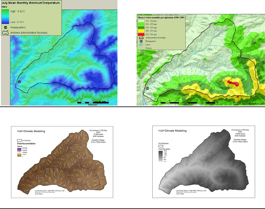
148
Fig. 1 – Example maps of H.J. Andrew Experimental Forest PRISM climate and physiographic
variables.
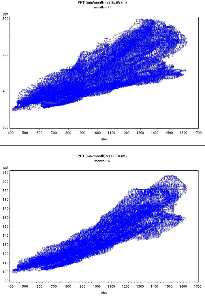
149
Fig. 2 – Plots of monthly mean precipitation (mm) versus elevation for H.J. Andrews Experimental
Forest. (a) November data, showing more or less linear increase. (b) May data, showing a quadratic
increase.
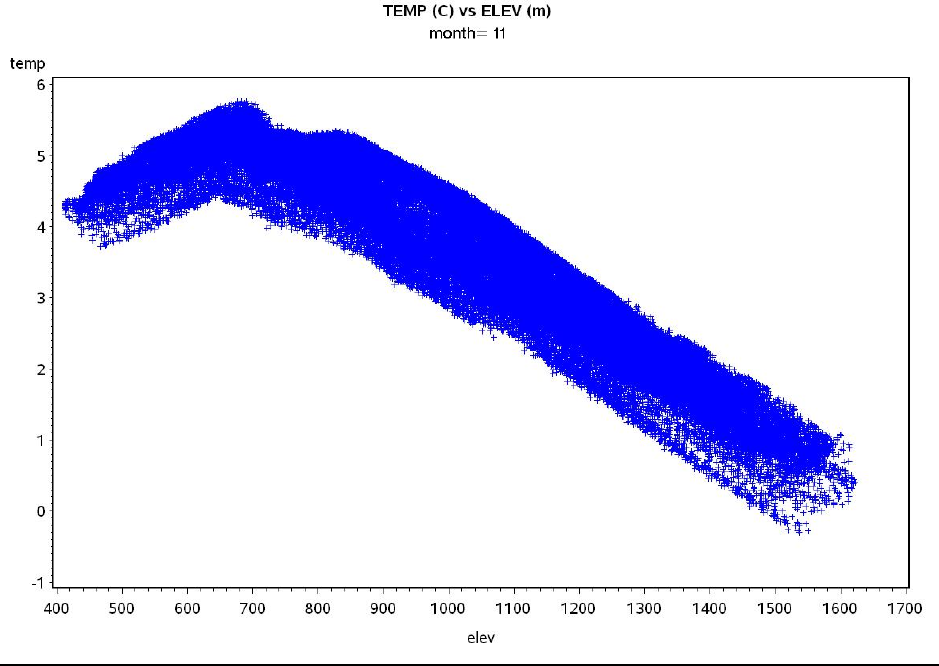
150
Fig. 3 - Plots of monthly mean temperature (C) for November versus elevation for H.J. Andrews
Experimental Forest. Note the piecewise linear relationship, with an inflection point at around 700 m
elevation.
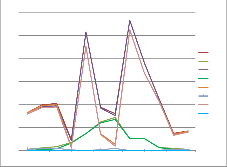
151
Fig. 4 – Plot of ΔAIC over all months for alternative precipitation regression models at H.J. Andrews
Experimental Forest. E = elevation, E2 = elevation2, H = heat load index, F = log10 of flow
accumulation.
0
1000
2000
3000
4000
5000
6000
12345678910 11 12
ΔAIC
Month
E
EE2
EH
EE2H
EF
EE2F
EHF
EE2HF
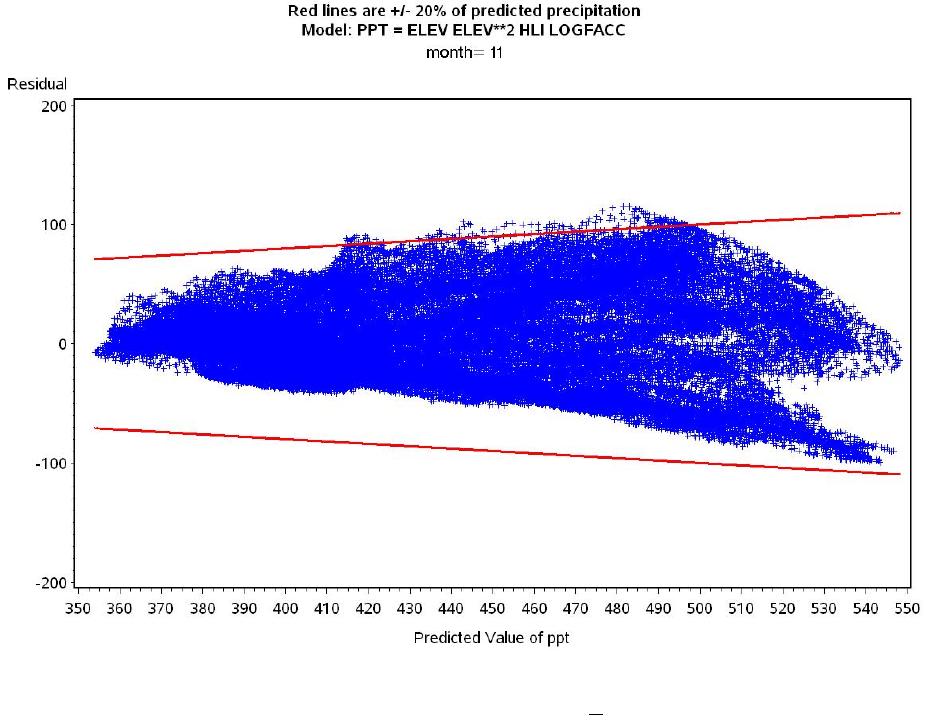
152
Fig. 5 – Graph of November precipitation regression residuals versus predicted precipitation at H.J.
Andrews Experimental Forest. Red bounding lines represent +20% of the monthly precipitation
estimate.
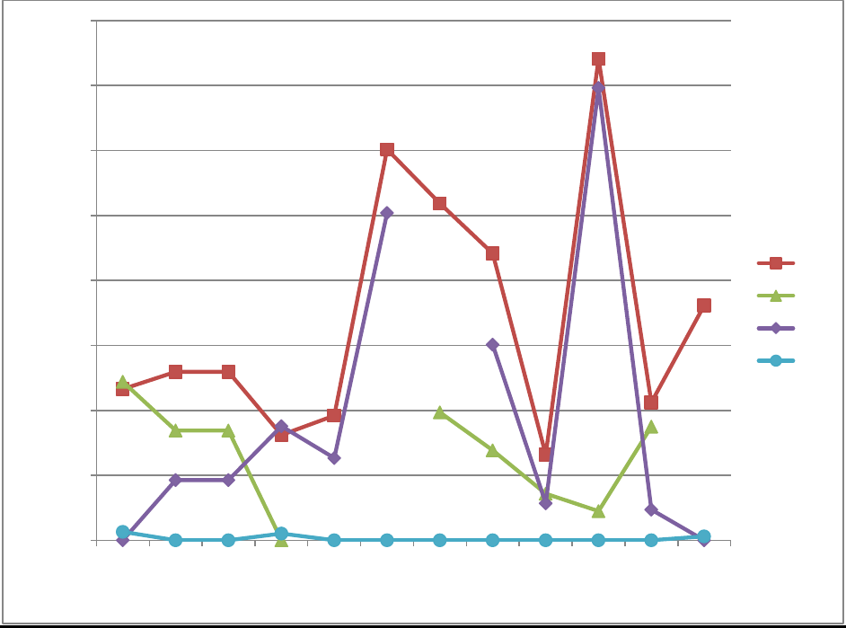
153
Fig. 6 – Plot of ΔAIC over all months for alternative temperature regression models at H.J. Andrews
Experimental Forest. E = elevation, H = heat load index, F = flow accumulation.
0
20
40
60
80
100
120
140
160
12345678910 11 12
ΔAIC
Month
E
EH
EF
EHF
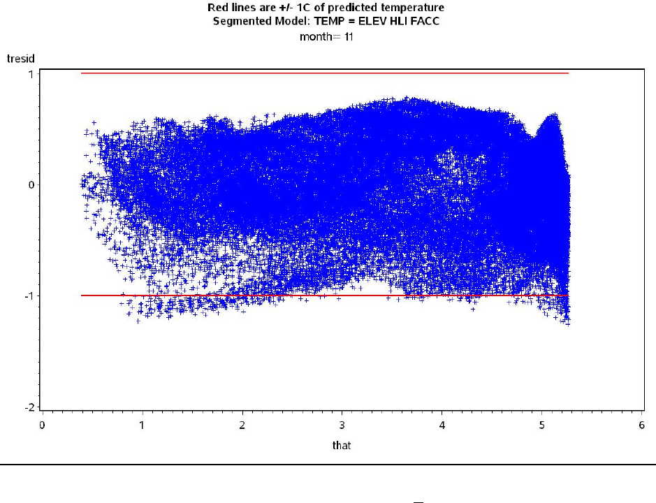
154
Fig. 7 – Graph of November mean temperature regression residuals versus predicted precipitation at H.J.
Andrews Experimental Forest. Red bounding lines represent +1 °C.

155
Fig. 8 – Map of weather station locations at the H.J. Andrews Experimental Forest.
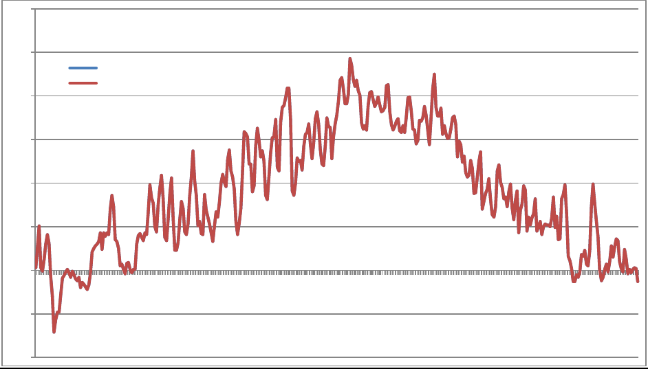
156
Fig. 9 – Comparison of observed H.J. Andrews Experimental Forest PRIMET weather station daily
mean temperature for 2007 and VELMA simulated data for the same location. The VELMA simulated
data used the temperature regression equation to estimate monthly normal temperature for the cell
containing PRIMET, and then made adjustments based on the observed PRIMET daily mean
temperature. This is a check to make sure that the implementation of the temperature regression and
adjustment is working correctly, as indicated by the coincidence of the blue and red lines (red is on top).
-10
-5
0
5
10
15
20
25
30
1
12
23
34
45
56
67
78
89
100
111
122
133
144
155
166
177
188
199
210
221
232
243
254
265
276
287
298
309
320
331
342
353
364
Degrees C
Julian Day
PRIMET AirT Observed Vs Simulated Comparison : 2007
PRIMET AIRPRI01
PRIMET Simulated

157
Month
a
b
c
d
e
1
259.751
0.011833
5.24E-05
-3.94717
-0.09685
2
241.5404
0.006131
6.1E-05
-5.15183
0.892817
3
210.8037
0.037236
4.62E-05
-4.20577
0.951439
4
96.40946
0.080534
7.44E-06
-1.44569
1.250961
5
88.34944
0.014202
3.06E-05
-0.20094
1.259266
6
53.51838
0.048195
9.53E-06
0.873204
1.297879
7
13.08702
0.023576
2.49E-06
0.686924
0.685529
8
21.89397
7.78E-05
6.23E-06
-0.00893
0.199088
9
70.03036
0.007598
2.39E-05
-0.00868
0.959202
10
124.4332
-0.00302
3.59E-05
-1.16562
0.890761
11
316.075
0.072349
4.32E-05
-4.40543
1.247633
12
290.7049
0.034712
4.62E-05
-4.46288
0.495517
Table 1. Monthly mean precipitation regression model coefficients based on PRISM data for 30-m
cells in the H. J. Andrews Experimental Forest. The models are of the form:
P = a + b*elev + c*elevsq + d*hli + e*logfacc
P in mm/month, elev in m, elevsq in m2, hli is unitless, logfacc is unitless

158
Month
b
c
d
e
g
h
i
j
x
1
0.007047
0.018444
2.75E-06
-1.12696
-0.00434
0.012177
-1.6E-05
6.606466
679.15
2
0.006148
0.065628
2.76E-06
1.024448
-0.00545
0.037565
-1.5E-05
8.958362
684.28
3
0.001492
0.041412
1.47E-06
5.402304
-0.00656
0.039723
-5.7E-06
11.03547
699.67
4
-0.00239
0.053357
2.53E-07
10.24696
-0.00697
0.043574
6.13E-06
13.99039
818.03
5
0.004219
0.059169
1.86E-06
8.916032
-0.00707
0.056038
-1.2E-05
16.80074
698.66
6
-0.00222
0.046785
-1.3E-06
16.98087
-0.00684
0.078366
1.33E-05
20.81386
827.75
7
-0.00123
0.004955
-2.5E-06
19.38073
-0.00633
0.073345
-1.9E-06
23.54351
814.57
8
-0.00023
0.00407
-2.6E-06
18.81907
-0.00585
0.007047
9.03E-06
23.53079
836.26
9
0.001476
-0.0342
-2.3E-06
14.80655
-0.00612
0.047614
7.6E-06
20.83291
791.89
10
-0.00023
0.018716
-1.2E-06
11.70249
-0.00641
0.112236
-8.6E-06
16.77907
819.27
11
0.002002
0.014029
-2.6E-07
3.771477
-0.00556
0.027117
-1.4E-05
9.412401
745.95
12
0.00697
0.047469
2.59E-06
-1.28579
-0.00399
0.007256
-1.7E-05
6.096779
674.34
Table 2. Monthly mean temperature regression model coefficients based on PRISM data for 30-m cells
in the H. J. Andrews Experimental Forest. The models are of the form:
For elev < x: T = b*elev + c*hli + d*facc + e
For elev > x: T = g*elev + h*hli + i*facc + j
T is in °C, elev in m, hli is unitless, facc is unitless

159
References
Akaike H (1974) A new look at the statistical model identification. IEEE Transactions on Automatic
Control 19:716-723
Daly C, Bryant K (2013) The PRISM Climate and Weather System - An Introduction. In. PRISM Climate
Group, Oregon State University, Corvallis, Oregon,
http://prism.oregonstate.edu/documents/PRISM_history_jun2013.pdf
Daly C, Halbleib M, Smith JI et al. (2008) Physiographically sensitive mapping of climatological
temperature and precipitation across the conterminous United States. International Journal of
Climatology 28:2031-2064
Daly C, Neilson RP, Phillips DL (1994) A statistical-topographic model for mapping climatological
precipitation over mountainous terrain. Journal of Applied Meteorology 33:140-158
McCune B, Keon D (2002) Equations for potential annual direct incident radiation and heat load.
Journal of Vegetation Science 13:603-606
PRISM Climate Group (2013) Descriptions of PRISM Spatial Climate Datasets for the Conterminous
United States. In. PRISM Climate Group, Oregon State University, Corvallis, Oregon,
http://prism.oregonstate.edu/documents/PRISM_history_jun2013.pdf

160
Appendix 5.1 – Sample SAS code for generating and comparing monthly total precipitation regression
models at H.J. Andrews Experimental Forest.
proc reg data=hja.hja outest=parmout;
by month;
model ppt = elev elevsq hli logfacc / selection=cp aic;
output out=pptout p=phat r=presid;
Notes:
• The input data are read in from the file ‘hja’ in the SAS library (folder) ‘hja’.
• Separate models are fit for each month.
• With the ‘selection’ option, models are fit using all the various sets of independent variables listed.
• By using the ‘aic’ option, Akaike Information Criterion (AIC) values are given in the output for each
model. This allows calculation of ΔAIC compared to the model with the lowest AIC value (Fig. 4).
• The parameter estimates for each model are written to the file ‘parmout’ (Table 1).
• Predicted estimates (‘phat’) and residuals (‘presid’) are written to the file ‘pptout’ for plotting
residuals vs. predicted values (Fig. 5).

161
Appendix 5.2 – Sample SAS code for generating and comparing monthly temperature regression models
at H.J. Andrews Experimental Forest.
* TEMP MODEL WITH ELEV, HLI, FACC. BEST MODEL - MIN AIC FOR MOST MONTHS,
MINIMAL DELTA AIC FOR OTHER MONTHS;
* Segmented model, linear with elev above and below a join point x;
proc nlin data=hja.hja outest=parmout;
by month;
parms b=0.01 c=0 d=0 e=0 g=-0.005 h=0 i=0 j=10;
file print;
x = ((h-c)*hli + (i-d)*facc + (j-e))/(b-g);
if elev < x then do;
model temp = b*elev + c*hli + d*facc + e;
der.b = elev;
der.c = hli;
der.d = facc;
der.e = 1;
der.g = 0;
der.h = 0;
der.i = 0;
der.j = 0;
end;
else do;
model temp = g*elev + h*hli + i*facc + j;
der.b = 0;
der.c = 0;
der.d = 0;
der.e = 0;
der.g = elev;
der.h = hli;
der.i = facc;
der.j = 1;
end;
if _obs_=1 then do; * PRINT X ESTIMATE TO TRACK CONVERGENCE;
put x =;
end;
output out=tempout predicted=that residual=tresid;
Notes:
• The input data are read in from the file ‘hja’ in the SAS library (folder) ‘hja’.
• Separate models are fit for each month.
• This is a spline model, fitting linear models above and below an inflection point at elevation x,
which is also estimated. This requires use of an iterative non-linear procedure (PROC NLIN).
Unlike PROC REG in Appendix 5.1, this does not have the capability to fit multiple alternative
models at once and report the AIC values for each. Instead, each alternative model must be
specified. The above code specifies the full model with elev, hli, and facc. AIC values are not
automatically printed and must be calculated from the sum of squares error (SSE), number of
parameters (p; 4 in this case), and number of sample points (n; 73,331 in this case), according to the
formula: AIC = n * ln(SSE / n) + 2*p. ΔAIC values are then calculated by subtracting the AIC for
the model with the lowest AIC value (Fig. 6).
• The ‘parms’ statement specifies starting values for the parameters to begin the iterative search for
best fit.
162
• x represents the elevation at which the two piecewise linear models meet. To make the overall
model continuous requires that the estimated temperature must be the same for both piecewise linear
models at that point. The expression for x is derived by setting the two models equal to each other
and solving for elev at which they are equal:
b*elev + c*hli + d*facc + e = g*elev + h*hli + i*facc + j
b*elev - g*elev = h*hli - c*hli + i*facc - d*facc + j – e
x = elev = ((h – c)*hli + (I - d)*facc + (j – e))/(b – g)
• The ‘der’ statements specify the first derivatives of each of the linear models with respect to each of
the parameters.
• The parameter estimates for each model are written to the file ‘parmout’ (Table 2).
• Predicted estimates (‘that’) and residuals (‘tresid’) are written to the file ‘tempout’ for plotting
residuals vs. predicted values (Fig. 7).
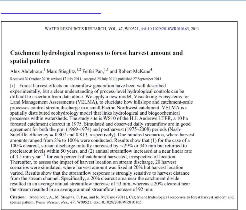
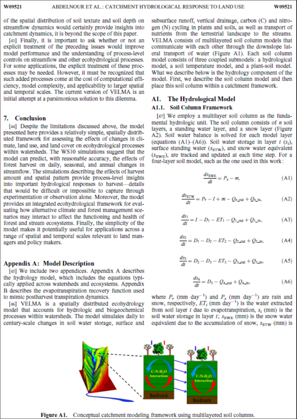
164
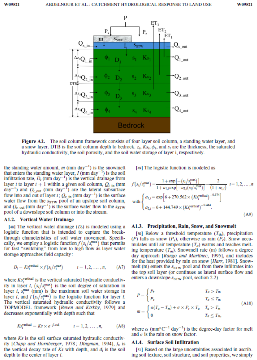
165
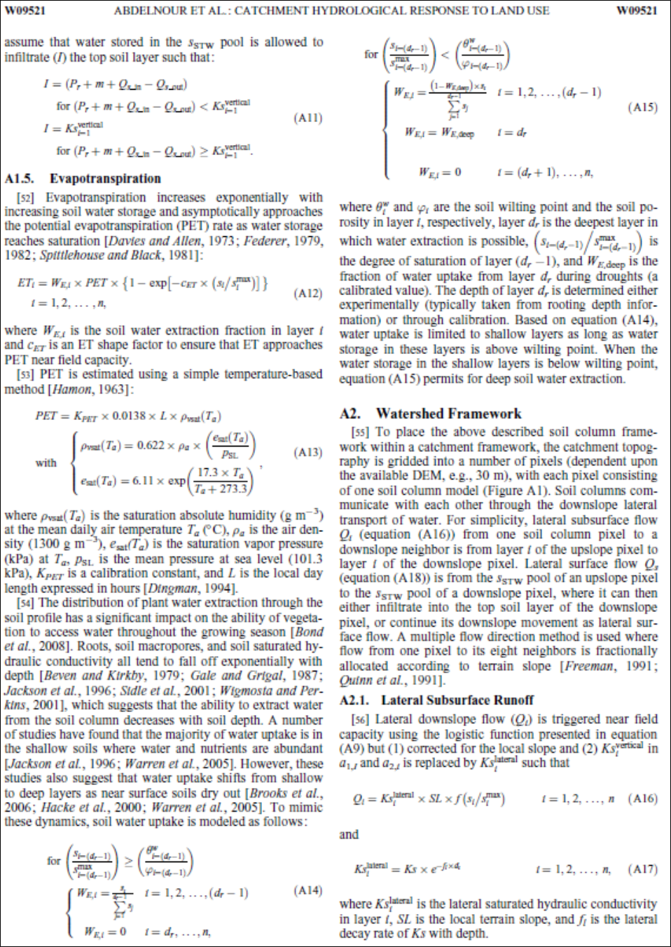
166
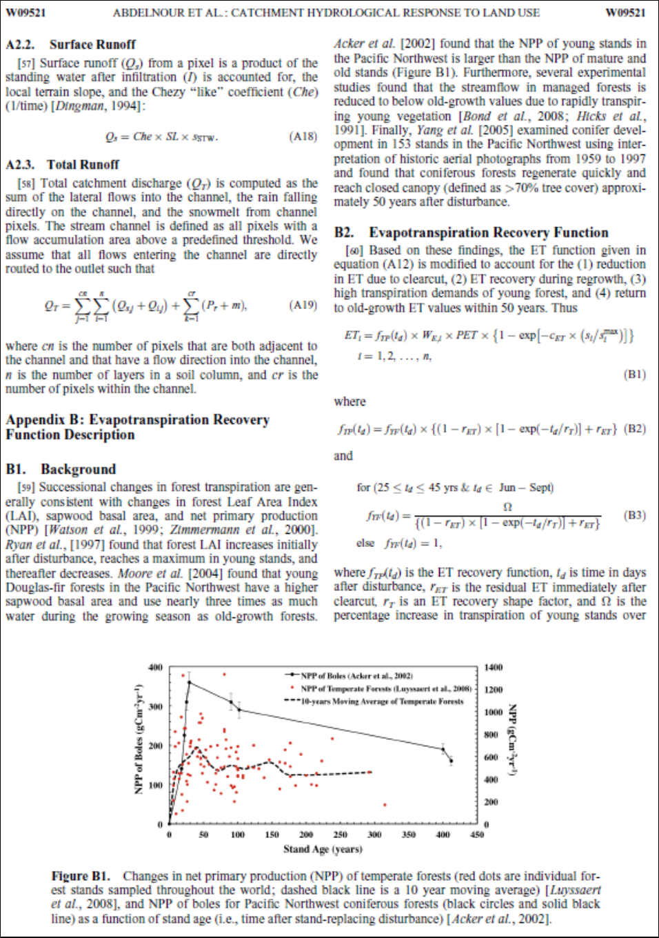
167
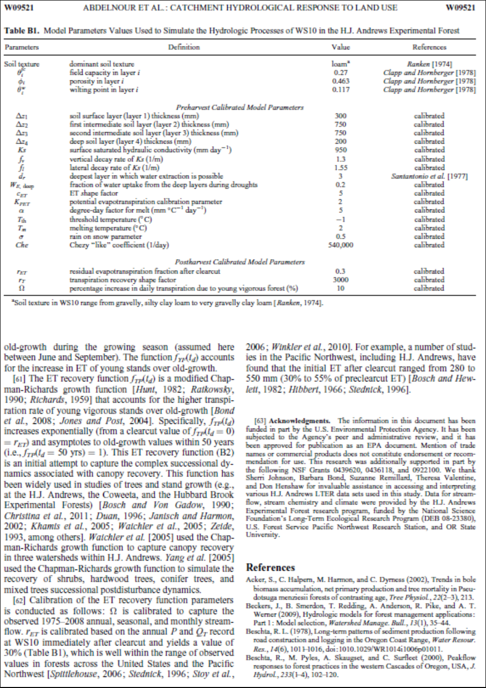
168
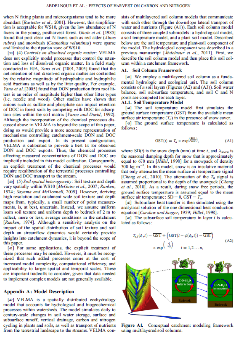
170
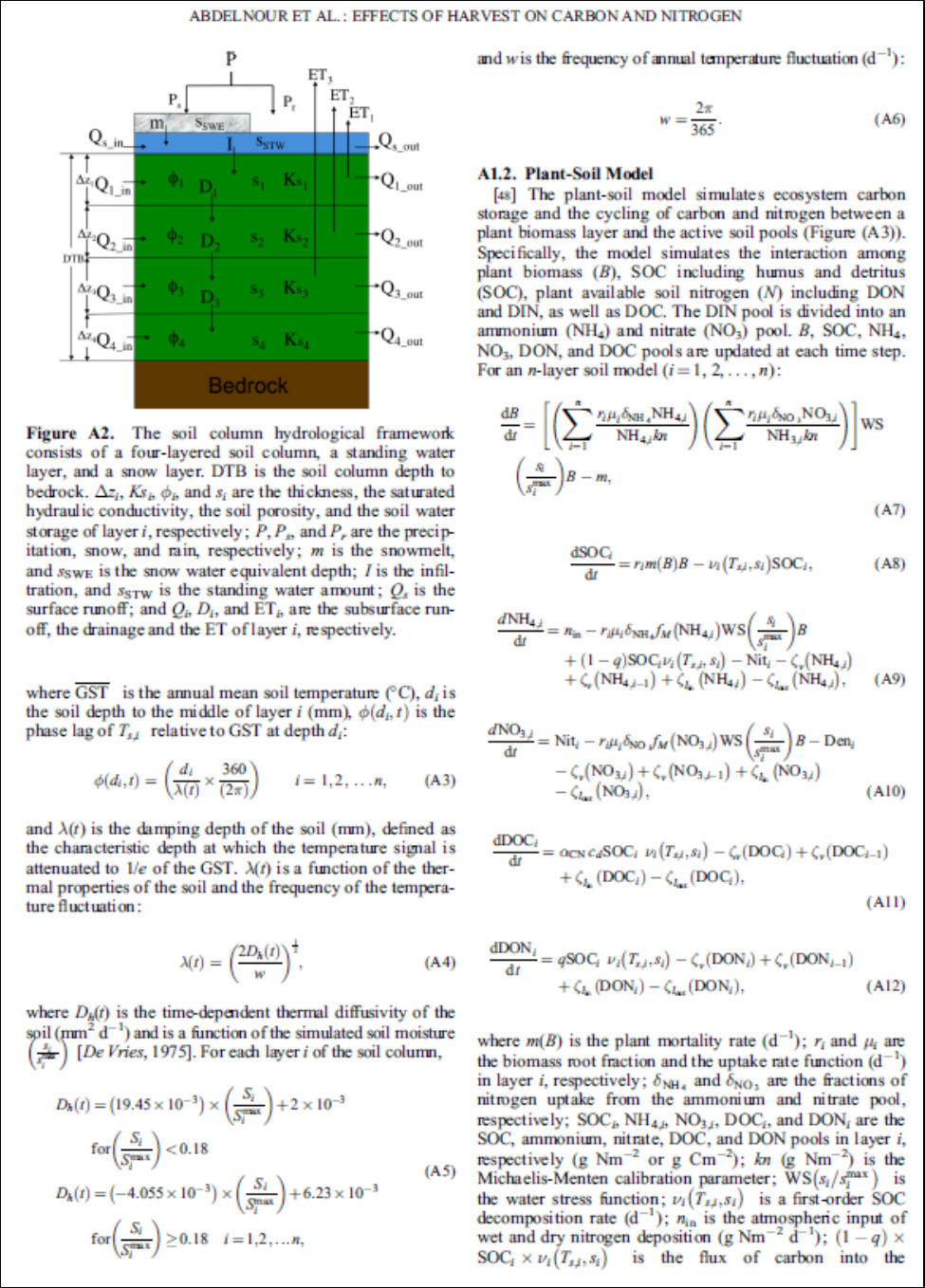
171

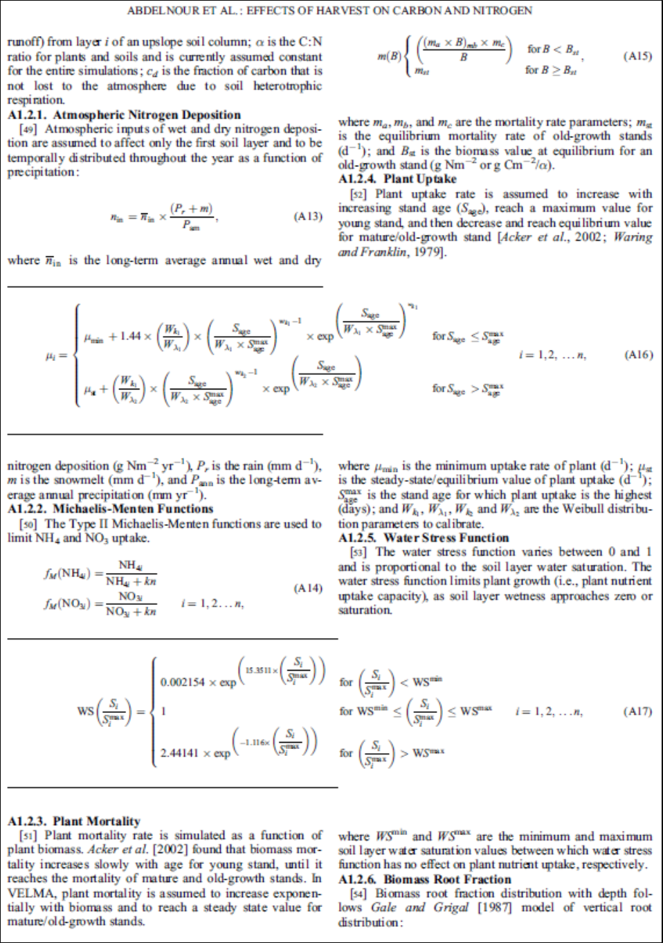
173
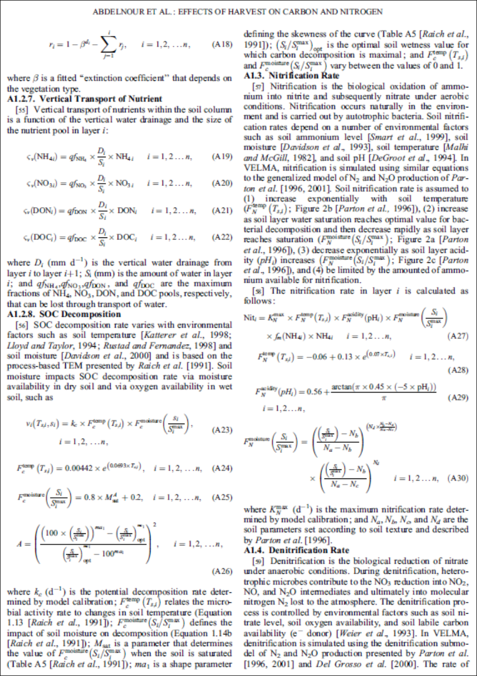
174
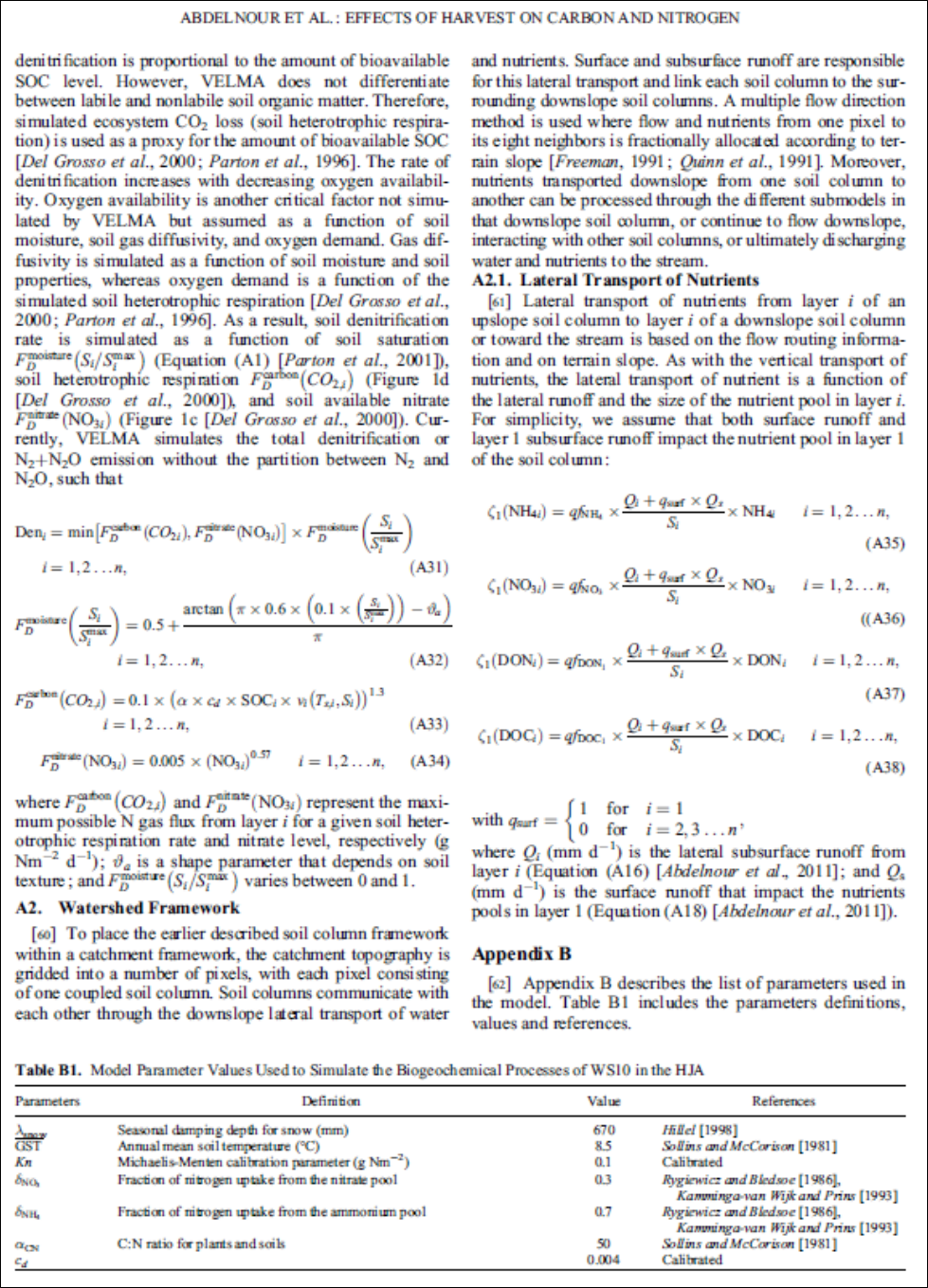
175
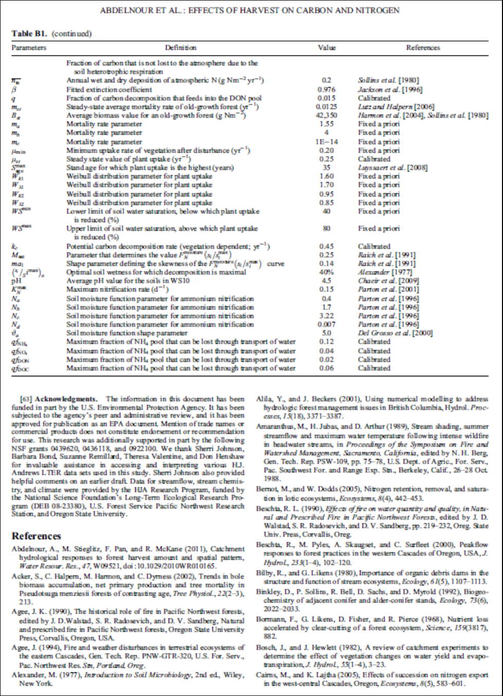
176

177
Appendix 7:
Creating Flat-Processed DEM Data For
The VELMA Simulator and Determining
Outlet and Watershed Delineation
The VELMA Simulator requires a Digital Elevation Map (DEM) for any simulation it runs.
This DEM contains elevation data for the area simulated.
The area specified must contain no "sinks" or "flat spots".
When VELMA simulates surface waterflow it must be able to flow "off" the map area in some
way. Water is not allowed to pool anywhere within the simulation area.
In order to ensure this "no flat spots rule", DEM data used by the VELMA Simulator is first
"flat-processed" to remove any sinks or flat spots.
Use JPDEM to prepare DEM data for use by the VELMA Simulator.
NOTE
You must have Java 1.7 installed on your computer to run JPDEM.
I. Creating a Flat-Processed DEM
Start JPDEM
Open a Windows Command Line and enter the command:
C:\> java -Xmx1024m -jar C:\full\path\to\JPDEM.jar
The "-Xmx1024m" tells the Java Runtime Environment (JRE) to let JPDEM have 1024
megabytes (1 gigabyte) of working memory.
If your machine doesn't have that much memory, substitute a smaller value (e.g. "512" instead of
"1024"). Alternately, if the .asc file of DEM data you intend to load is very large (and your
machine has the memory) you may substitute a larger value (e.g. "2048" instead of "1024").
If the full path to the JPDEM.jar file contains whitespace characters, place double-quotes around
the path.
Example:
"C:\full\path\with white space\to\JPDEM.jar"
Loading DEM Data Into JPDEM
Load a "raw" DEM file into JPDEM (the file must be in standard ESRI Grid .asc format).
Click the "File" menu, then select and click "Load DEM File".
The "Select DEM File to Load" dialog window opens.
178
Browse to the location of your DEM file, and click the name of the DEM file.
The DEM file's name appears in the "File Name:" text box.
Click "Load File" to load that file's data into JPDEM.
The file is loaded, and an image of the file appears in JPDEM's map display.
If the file is too small (has few rows and columns), click the Image Scale up-arrow button to
"zoom in".
Flat Processing DEM Data In JPDEM
Click the "Tools" menu, then select and click "Flat-Process DEM Data (Standard)".
JPDEM will process the DEM, adjusting elevation data to remove flat spots or sinks within the
DEM data's area.
If the processing takes more than a second or two, the display will periodically update, showing
remaining flat spots in blue.
When the flat-processing algorithm finishes, the display shifts to a grey-scale representation,
with darker-colored pixels representing cells with higher flow-accumulation values.
Note:
There are several menu options for Flat-Processing DEM data.
The "(Standard)" menu item uses an algorithm that produces good results, but generally takes
more time to produce them. We do not, at this time, recommend using the other two flat-
processing algorithms. They are still being developed.
Saving Flat-Processed DEM Data From JPDEM To a File
After JPDEM finishes flat-processes DEM data, click the "File" menu, then click the "Save DEM
As ..." submenu, and finally select and click the "Ascii Grid" menu item.
The "Save DEM Grid to File" dialog window opens.
Browse to the location you wish to save the data in, then type a name for the file in the "File
Name:" text box.
Finally, click the "Save File" button to save the DEM data to the specified file name and
location.
Note
Flat-processed DEM data may be loaded into JDPEM just like "raw" DEM data.
Flat-processed DEM date does not need to be flat-processed again after it is loaded into JPDEM.
However, to view the flow-accumulation grey-scale visualization of that flat-processed data, you
must determine the flow data information for the flat-processed DEM values.
II. Watershed Delineation
Determining Flow Data For a Flat-Processed DEM
Load a flat-processed DEM .asc file into JPDEM, in the same way you would load a "raw" DEM
file.
After loading the DEM data, click the "Tools" menu, then select and click the "Determine DEM
Flow Data (Standard)" menu item.
JPDEM will then compute flow data (flow direction and accumulation values) for each cell in
the DEM area.
179
Once the flow data is computed, JPDEM will shift the display to the flow-accumulation grey-
scale visualization.
Note
Loading a "raw" DEM file and then immediately trying to determine DEM flow data should not
crash JPDEM, but it won't result in any meaningful information either.
Note
The difference in results between the "(Standard)" and "(Alternate)" flow data algorithms should
be zero or very small.
You may use either algorithm. The Alternate algorithm is somewhat faster, but often not much
faster than the Standard algorithm.
Determining Watershed Delineation
Flat-processed, flow-accumulated DEM data in JDEM may be used to determine the delineation
relative to a specified outlet cell (i.e. the set of cells that flow "to" a specified "outlet" cell).
In order to compute the delineation for an outlet cell, you must first specify the coordinates of the
outlet cell.
You can do this either by entering the zero-based x (column) and y (row) coordinates of the
outlet cell in the "Outlet X=" and "Y =" number boxes, above JPDEM's map display, or by using
the mouse.
To select an outlet cell using the mouse, do the following:
Move the mouse pointer over the cell you wish to select.
Press down on either the right or left mouse button.
A context menu should pop-up, containing information about the cell you are pointing at.
Holding the mouse button down, drag the mouse pointer onto the menu item containing cell info
(the info should highlight), then release the mouse button.
The menu goes away, and the x and y coordinates for the cell you selected appear in the "Outlet
X = " and "Y = " number boxes above the map display.
Note:
"Zoom in" on the map display by clicking the up-arrow button of the "Image Scale" to make
selecting a specific cell easier. For example, at "Image Scale 3", for example, every cell is
displayed by 3x3 pixels.
However, on very large maps zooming too far in can crash the display, because it may run out of
memory.
Once the coordinates of an outlet cell are specified, click the "Tools" menu, then select and click
the "Delineate DEM Data (Experimental)" menu item.
JPDEM will then compute the delineation (i.e. the area of cells) for the currently specified
"Outlet X =" and "Y =" values.
The resulting area is displayed in a logarithmic-coloring blue-red scale, superimposed over the
grey-scale of the flow-accumulation display.
If the delineation looks incorrect, change the outlet cell coordinates and re-run the delineation.
When the delineation looks correct, record the "Outlet X =" and "Y =" values for future reference
and use with JVELMA. (JPDEM does not "record" outlet values anywhere.)
Note
There are currently four different JPDEM delineation algorithm implementations to choose
from.
We believe they all produce the same results (except possibly for cells on the edge of the DEM
180
area -- which is an acceptable difference). However, they vary greatly in how long they take to
run. Use the "(Experimental)" algorithm for delineation: it runs significantly faster than any of
the other delineation implementations. In particular, do not use the "(PDEM-2)" algorithm,
which can take a very long time to run, even for small maps.
