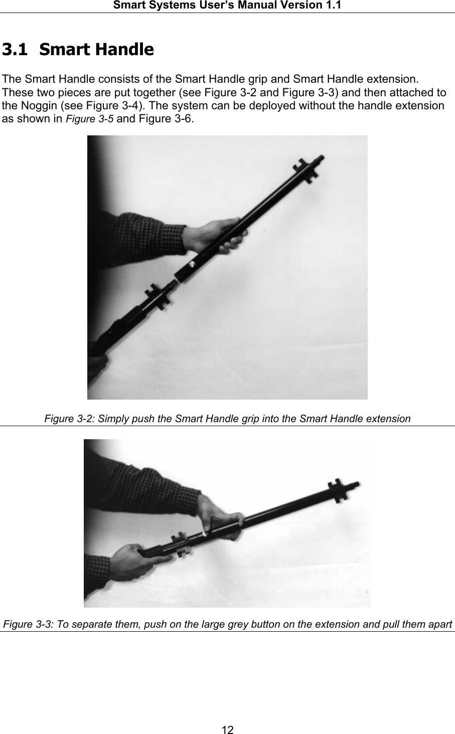
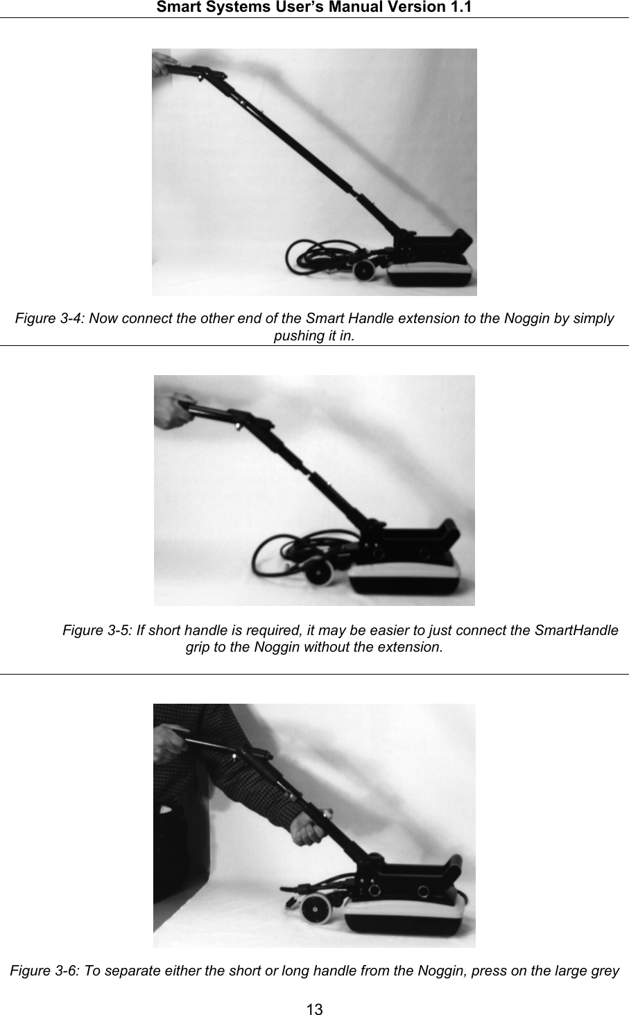
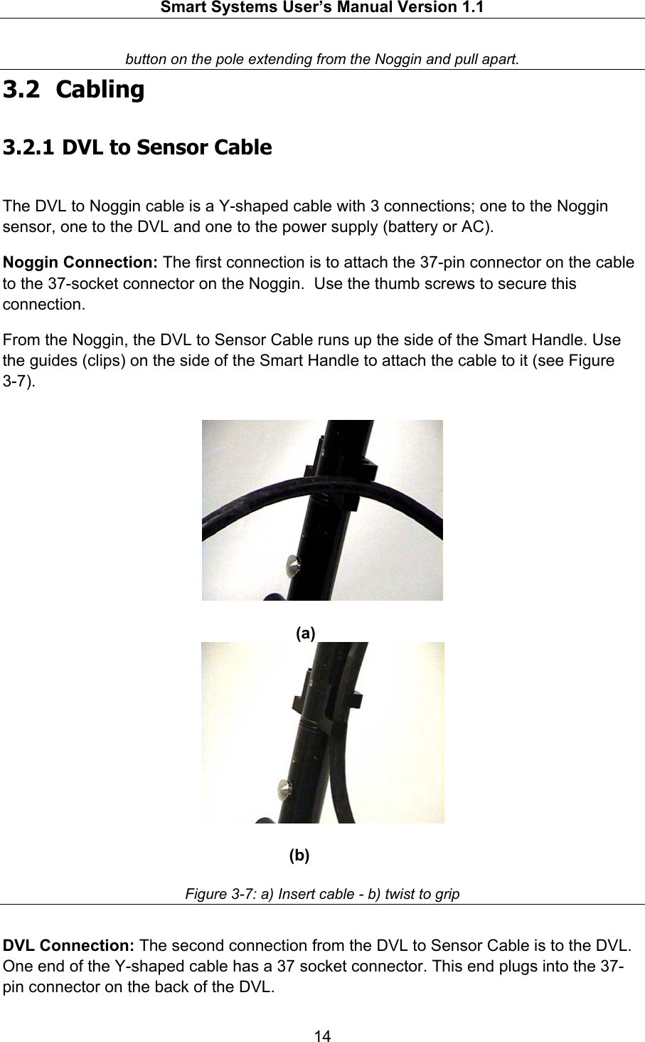
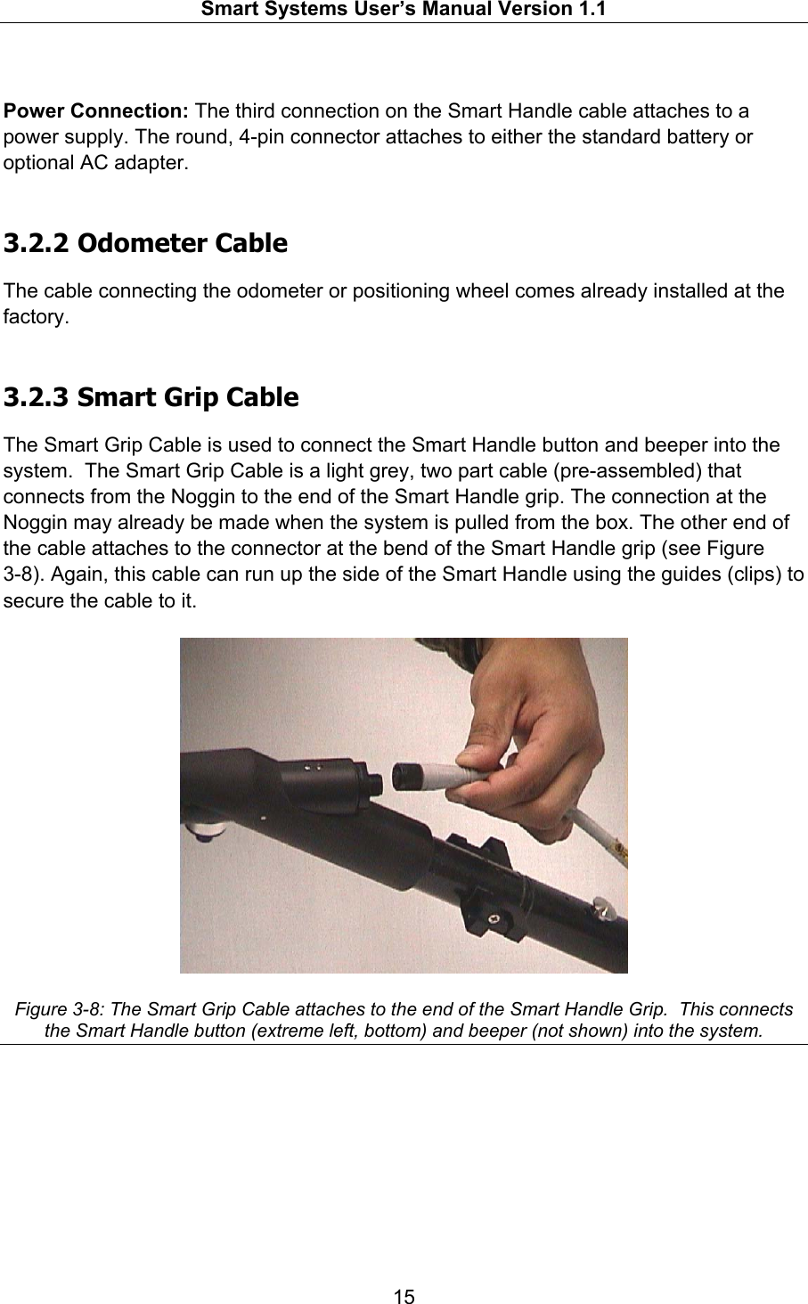
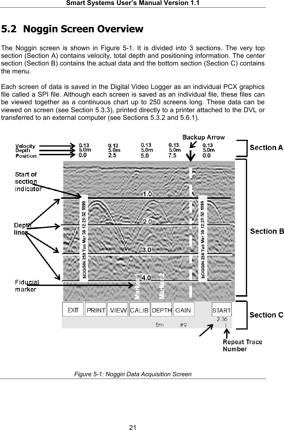
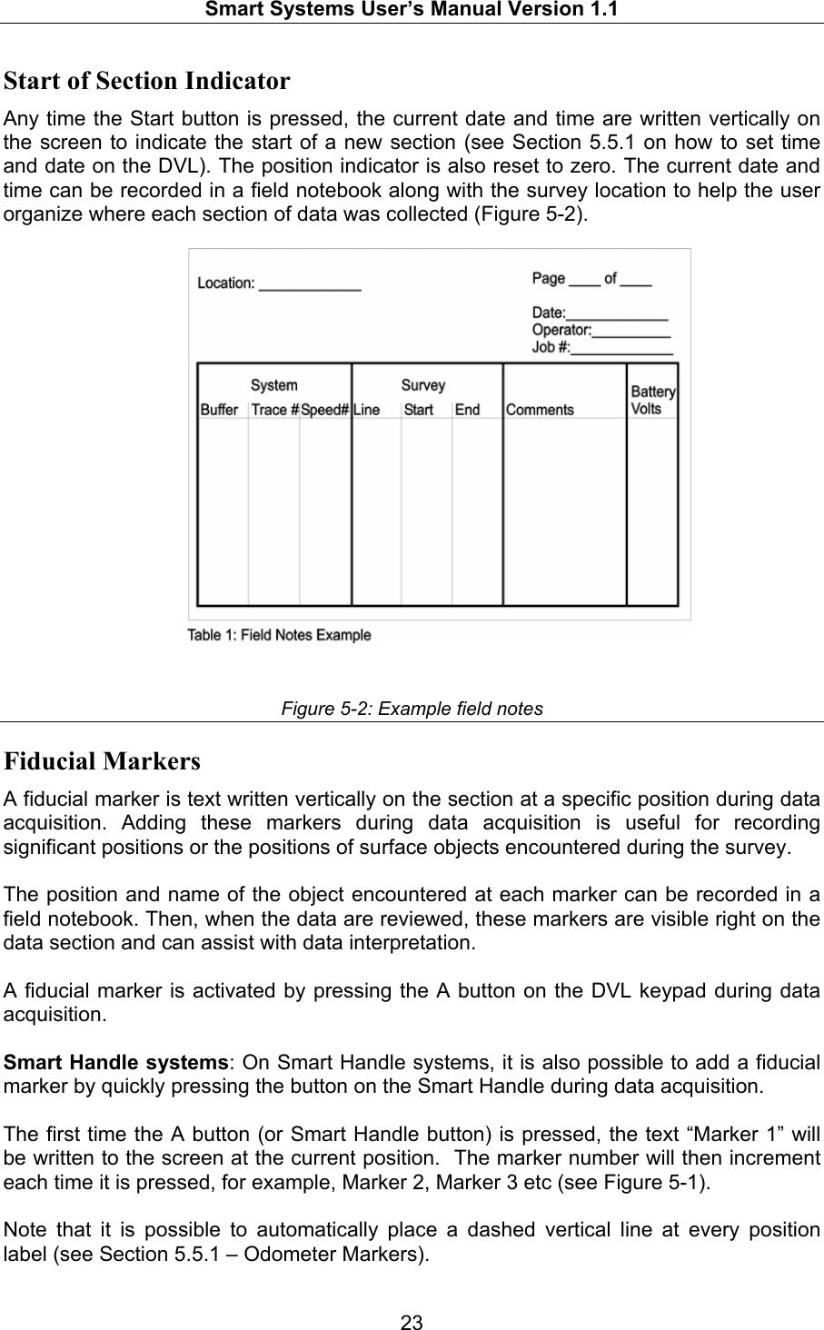
Sensors and Software NOGGIN1000 User Manual SmartSystemsV11
Sensors & Software Inc. SmartSystemsV11
UserManual.wiki
>
Sensors and Software
>
NOGGIN1000 User Manual
Revised Users Manual
Navigation menu
Upload a User Manual
Namespaces
Wiki Guide
HTML
PDF
Info
Views
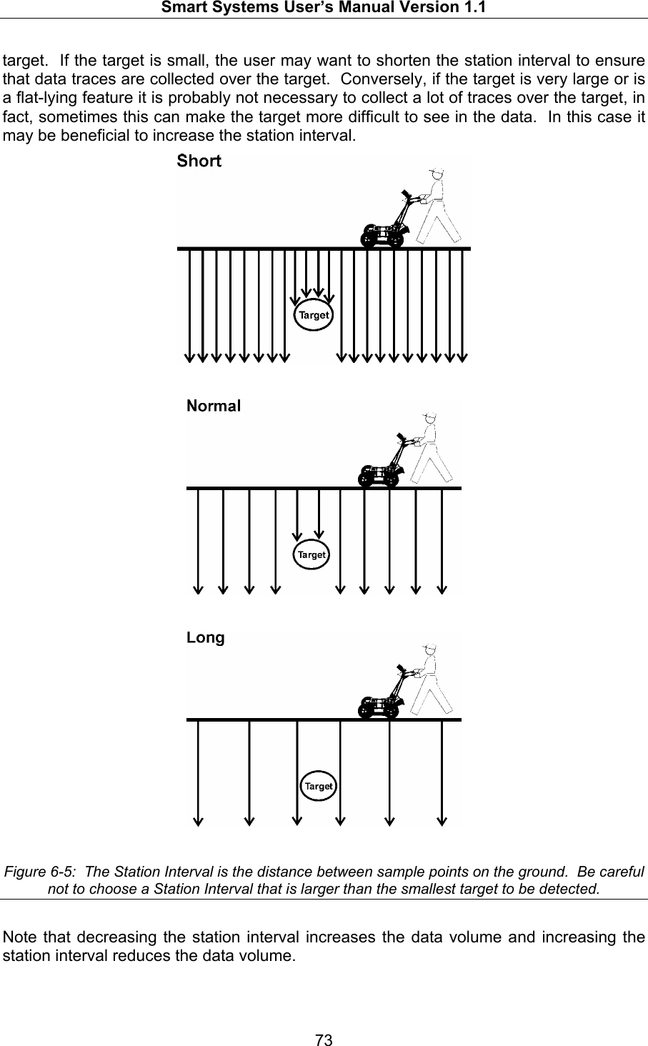
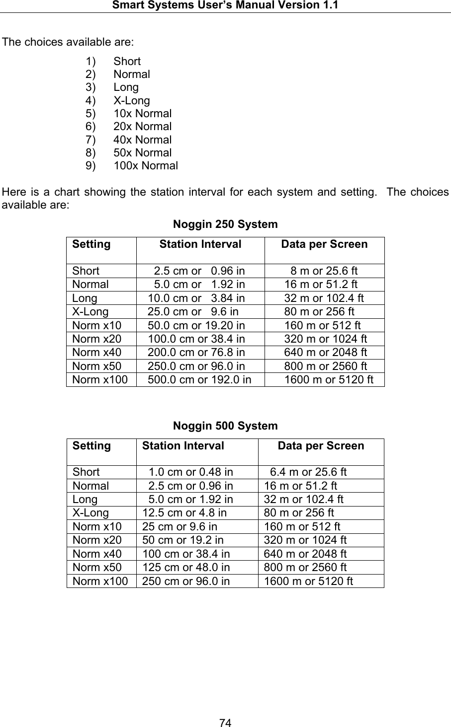
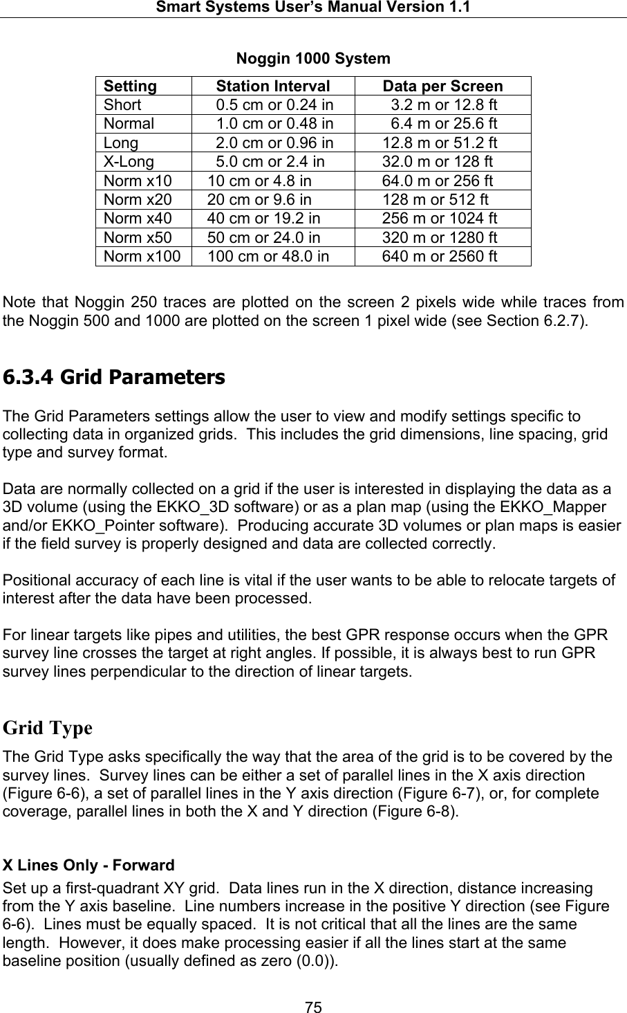
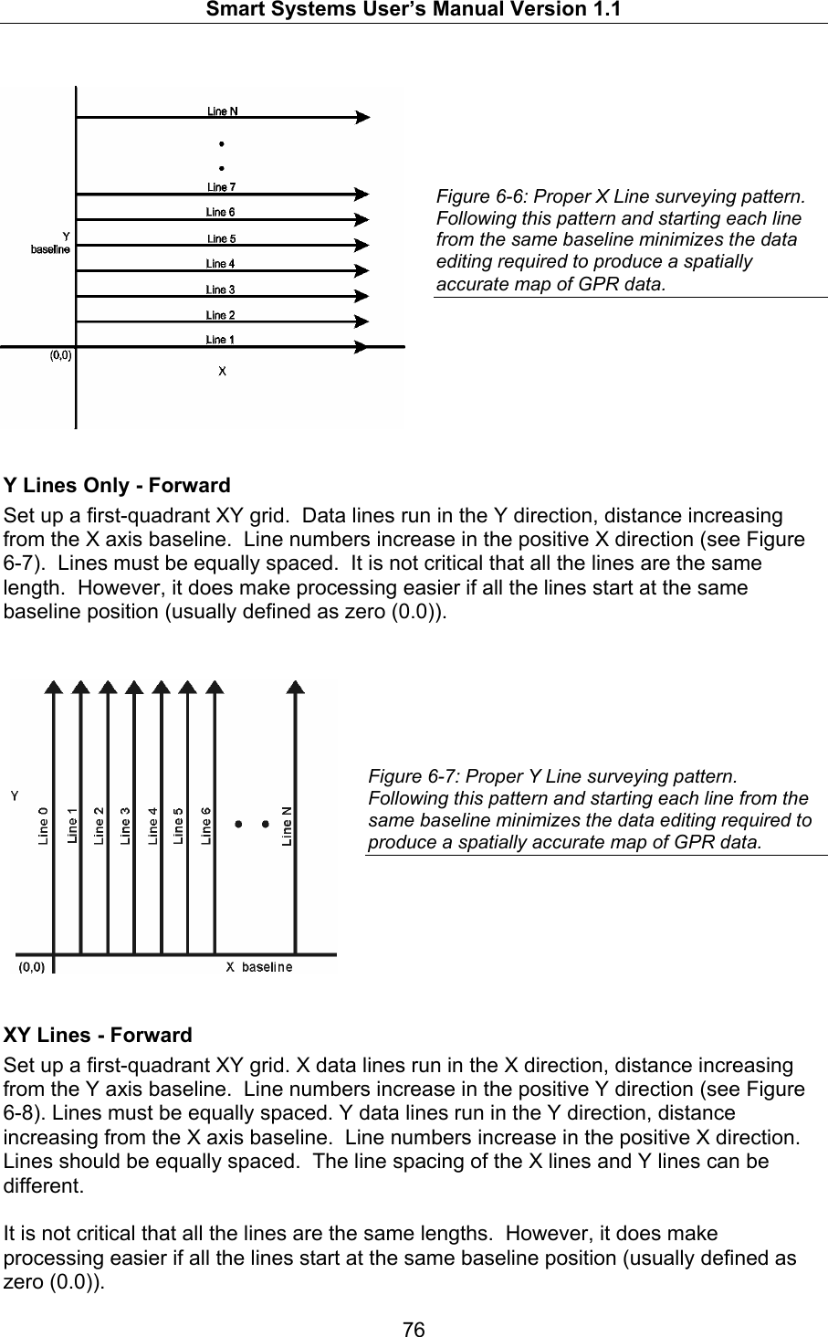
User Manual
Discussion / Help
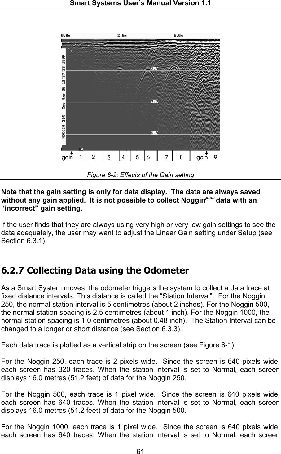
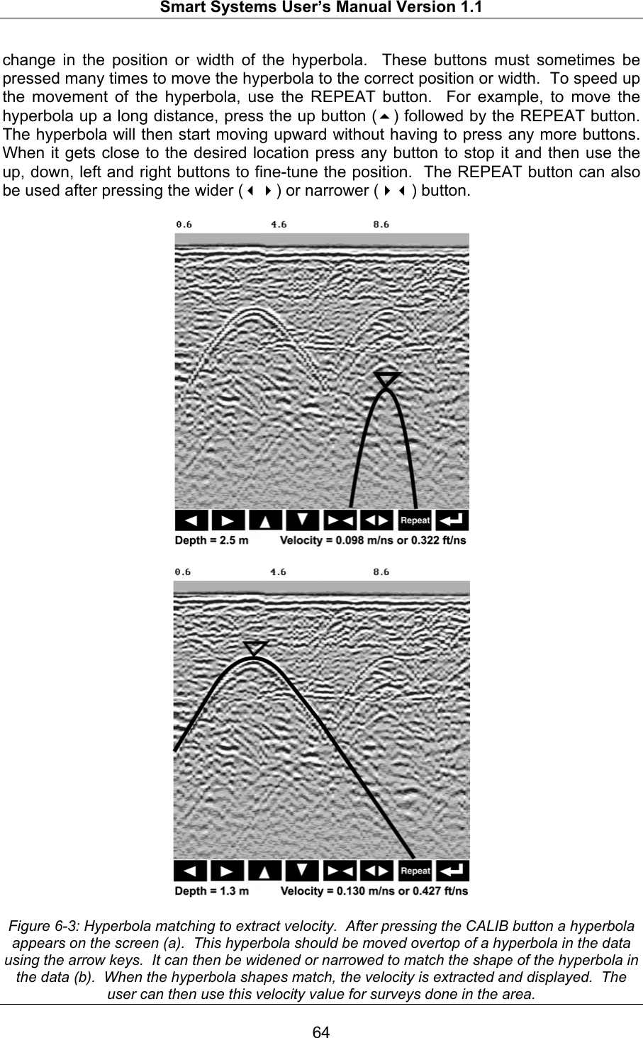
Navigation
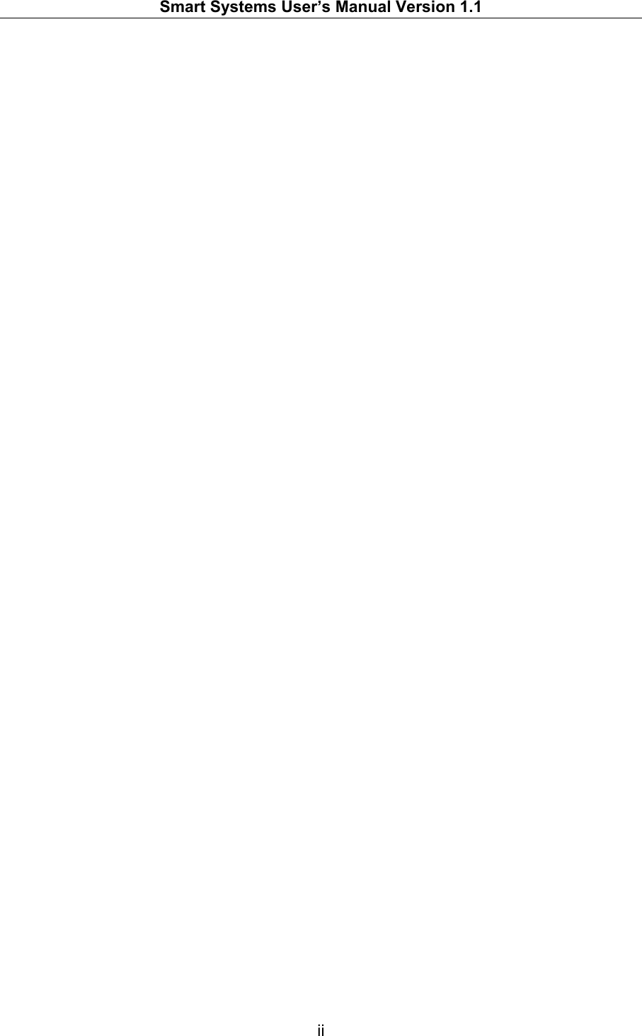
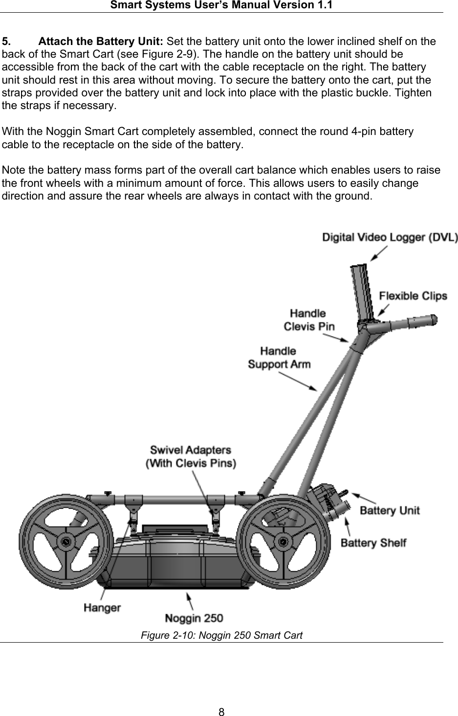
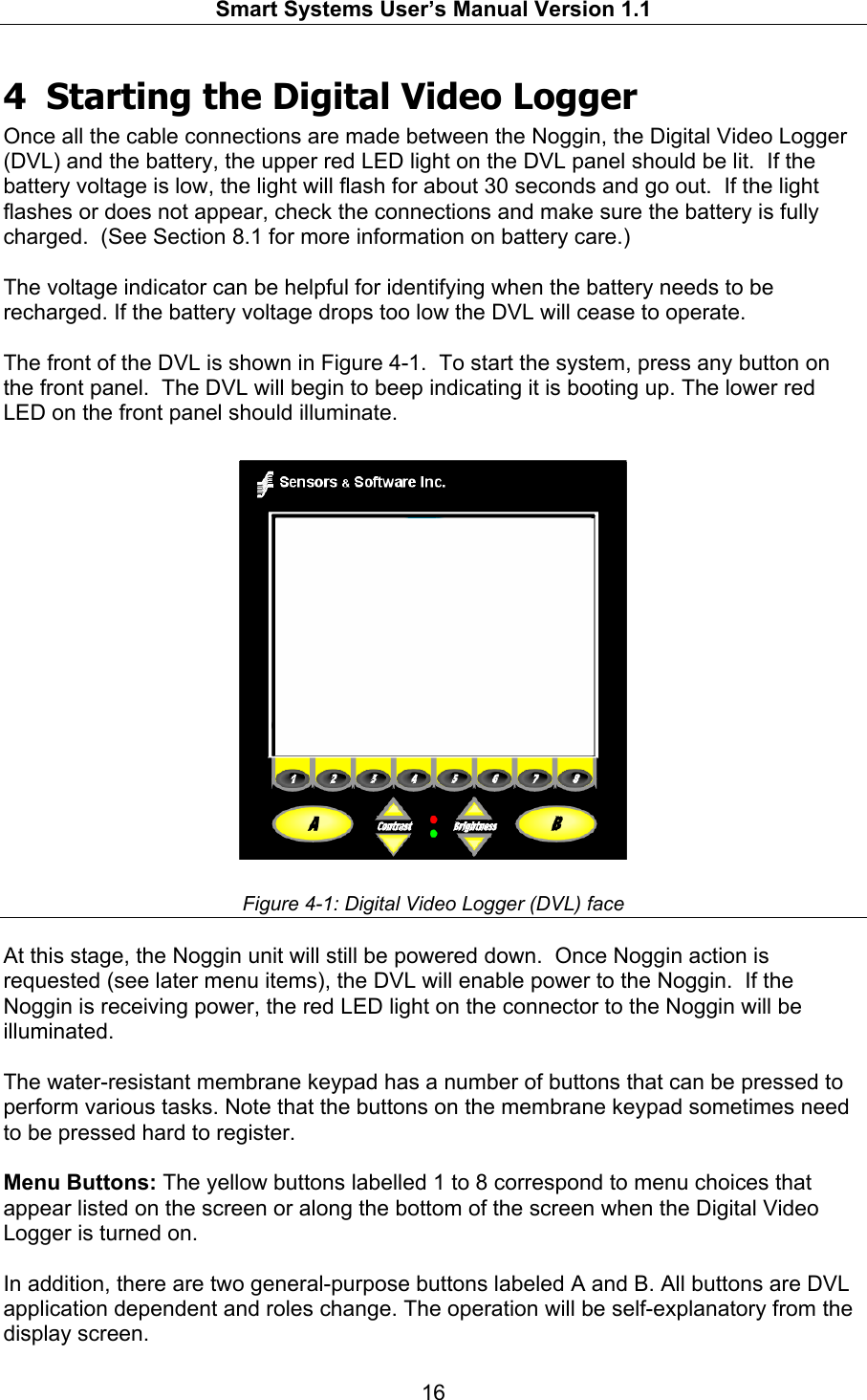
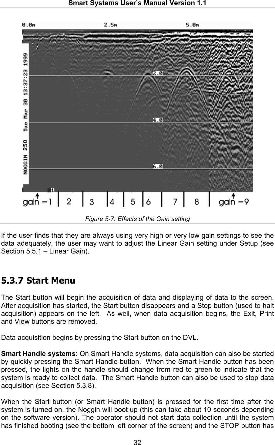
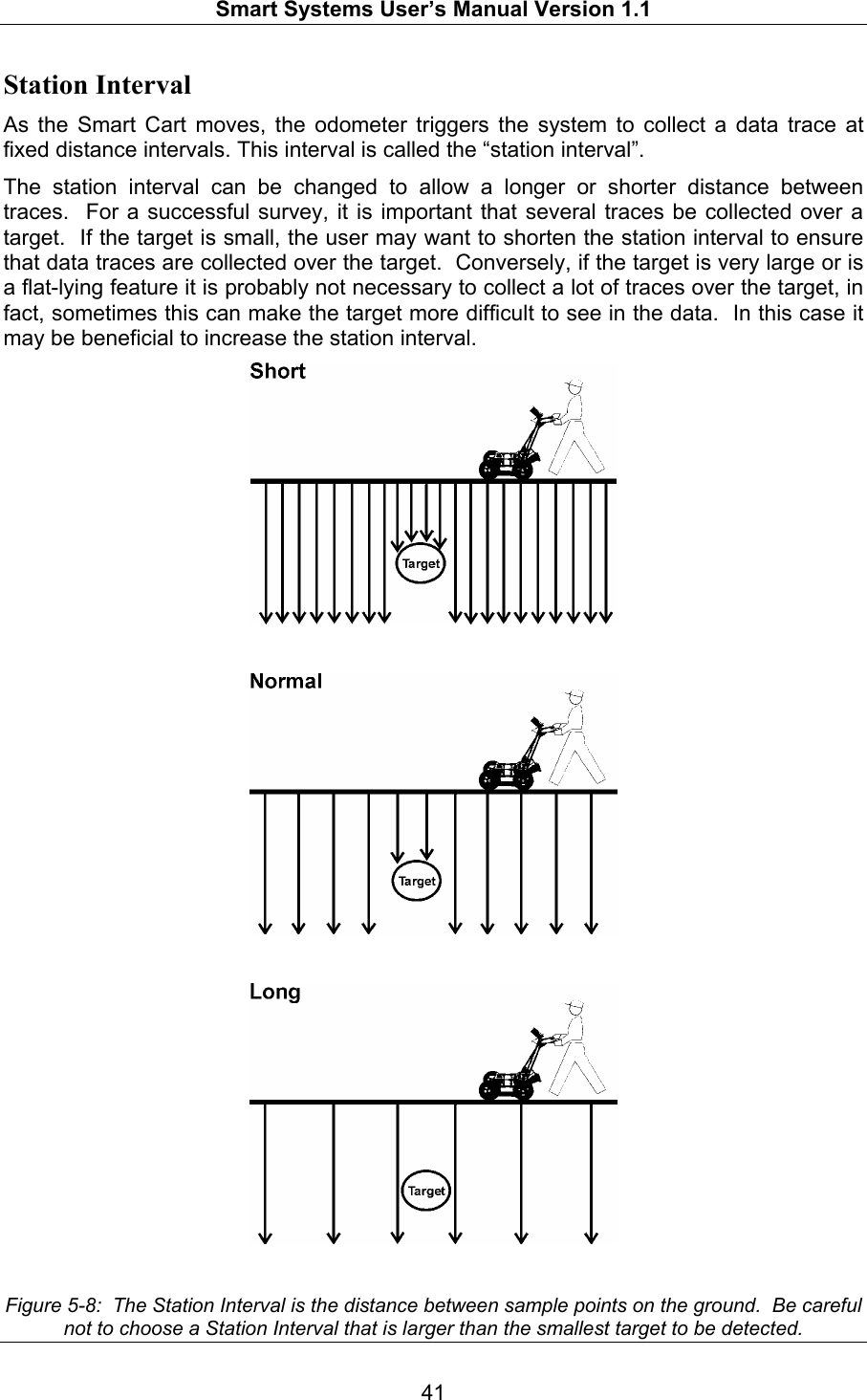

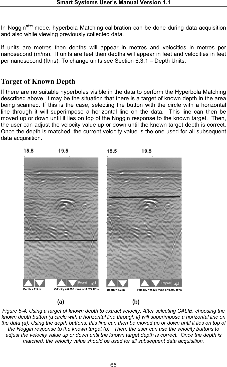
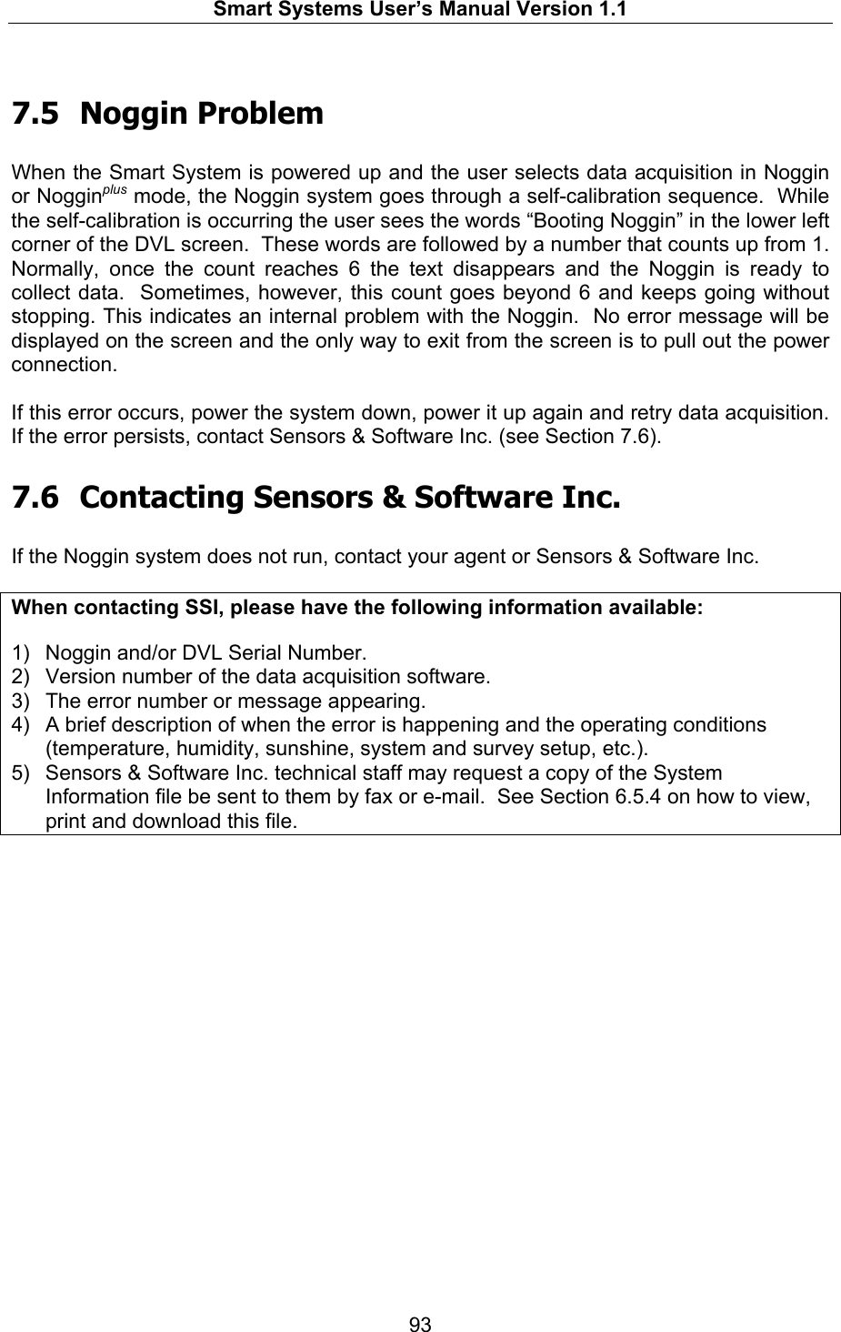
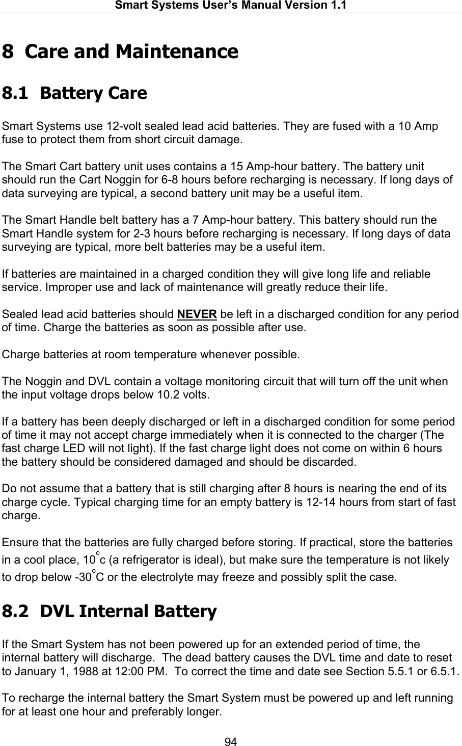
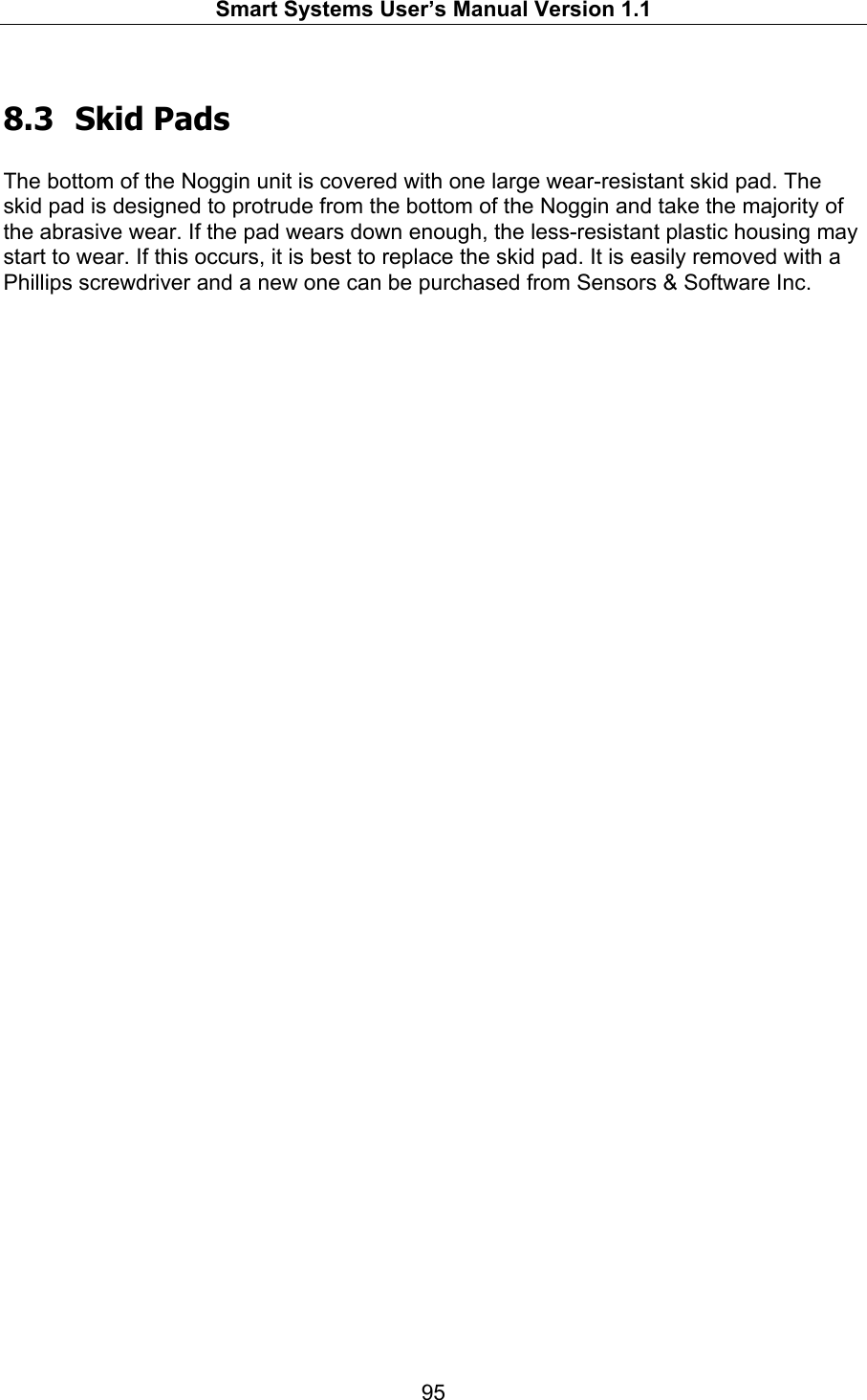
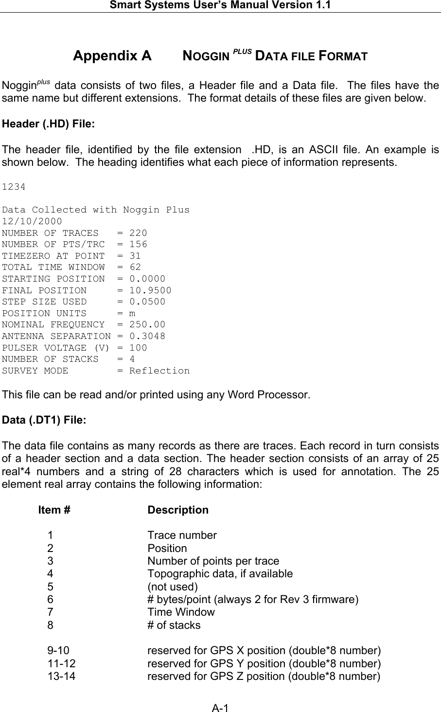
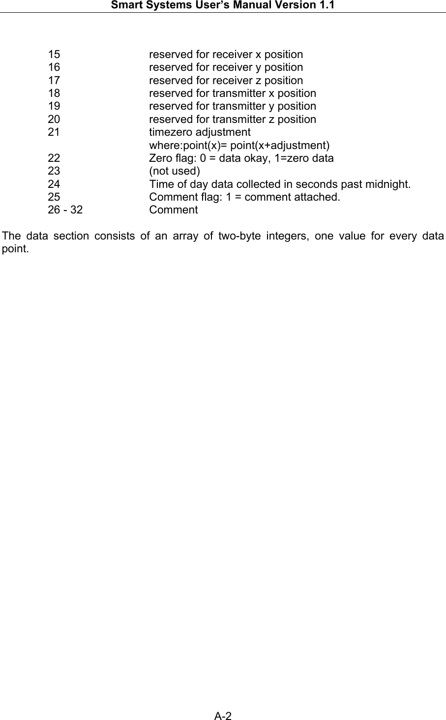
![Smart Systems User’s Manual Version 1.1 C-4 GROUND PENETRATING RADAR COORDINATION NOTICE NAME: ADDRESS: CONTACT INFORMATION [contact name and phone number]: AREA OF OPERATION [counties, states or larger areas]: FCC ID: [e.g. QJQ-NOGGIN250 for Noggin 250 system)] EQUIPMENT NOMENCLATURE: [ e.g. Noggin 250] Send the information to: Frequency Coordination Branch., OET Federal Communications Commission 445 12th Street, SW Washington, D.C. 20554 ATTN: UWB Coordination Fax: 202-418-1944 INFORMATION PROVIDED IS DEEMED CONFIDENTIAL](https://usermanual.wiki/Sensors-and-Software/NOGGIN1000/User-Guide-282339-Page-116.png)