Sensors and Software NOGGIN250 User Manual SmartSystemsV11
Sensors & Software Inc. SmartSystemsV11
Revised Manual with Warning on Page C2

Users Manual Version 1.1

Smart Systems User’s Manual Version 1.1
ii

Smart Systems User’s Manual Version 1.1
iii
Information on pulseEKKO, Noggin and Conquest Products Regarding
Electromagnetic Emissions
Emissions
All governments have regulations on the level of electromagnetic emissions that an
electronic apparatus can emit. The objective is to assure that one apparatus or device
does not interfere with any other apparatus or device in such a way as to make the other
apparatus non-functional.
Sensors & Software Inc. have extensively tested their pulseEKKO, Noggin and
Conquest subsurface imaging products using independent testing houses and comply
with the regulations of the USA, Canada, European Community and other major
jurisdictions on the matter of emissions.
Not all electronic devices have been designed for interference immunity. When placed
in close proximity to another device interference may occur. There has never been a
report of interference from GPR products to date. If you observe unusual behavior on
nearby devices while you are operating a pulseEKKO, Noggin or Conquest product,
immediately turn off the product. You can test the cause and affect between the product
and the device if the disturbance starts and stops when the product is powered up and
shut off. If interference is confirmed, stop using the product.
Immunity
Immunity regulations place the onus on instrument/apparatus/device manufacturers to
assure that extraneous interference will not unduly cause an
instrument/apparatus/device to stop functioning or to function in a faulty manner.
Based on independent testing house measurements, Sensors & Software Inc. systems
comply with such regulations in Canada, USA, European Community and most other
jurisdictions. One must remember that Sensors & Software Inc.’s products are designed
specifically to sense electromagnetic fields. External sources of electromagnetic fields
such as TV stations, radio stations and cell phones, can cause detectable signals that
may degrade the quality of the data that the products record and display.
Such interference is unavoidable but sensible survey practice and operation by an
experienced practitioner can minimize such problems. In some geographic areas
emissions from external sources may be so large as to preclude useful measurements.
Such conditions are readily recognized and accepted by the professional geophysical
community as a fundamental limitation of geophysical survey practice.
Health
The interaction of electromagnetic fields with humans is an evolving field of
epidemiology although one which creates sensational press headlines. Humans are
immersed daily in a sea of electromagnetic fields which cover a wide range of
frequencies. Systematic correlation between EM fields and human illness have only
been reported at very high powers (millions of times greater than any Sensors &
Software Inc. product) for military radar systems operating in the 5000 to 20,000 MHz
range where physical burning/heating (basically like a microwave oven) have been
reported.

Smart Systems User’s Manual Version 1.1
iv
Sensors & Software Inc. monitors the research in this area. To date, the power levels of
Sensors & Software Inc.’s products are so small as to be inconsequential compared to
other common sources. If you are happy that a cell phone is not hazardous, then
Sensors & Software Inc.’s product, being of much lower power, need be of little concern.
Also see Appendix B - Health & Safety Certification.
Safety
Concerns are expressed from time to time on the hazard of subsurface imaging products
being used near blasting caps and unexploded ordnance (UXO). Experience with
blasting caps indicates that the power of Sensors & Software Inc.’s products are not
sufficient to trigger blasting caps. Based on a conservative independent testing house
analysis, we recommend keeping the subsurface imaging transmitters at least 5 feet
(2m) from blasting cap leads as a precaution.
The UXO issue is more complex and standards on fuses do not exist for obvious
reasons. To date, no problems have been reported with any geophysical instrument
used for UXO. Since Proximity and vibration are also critical for UXO, the best advice is
to be cautious and understand the risks.

Smart Systems User’s Manual Version 1.1
v
Copyright and Warranty Information
Software Licence & Limited Warranty
Important: Please read this document carefully before removing the SOFTWARE PRODUCT diskettes
from their protective cover or assembling the HARDWARE PRODUCT. By removing the
diskettes or assembling the hardware, you are agreeing to become bound by the terms of
this agreement. If you do not agree to the terms of this agreement, promptly contact
Sensors & Software, Inc. at the address indicated at the end of this document.
Definition
The word PRODUCT as used herein defines any complete Sensors & Software, Inc. ground penetrating radar
system comprised of the HARDWARE PRODUCT and SOFTWARE PRODUCT.
SOFTWARE PRODUCT
Licence Agreement
In order to preserve and protect its rights under the applicable laws, Sensors & Software, Inc. (hereafter SSI)
does not sell any rights to its software products. Rather, SSI grants the right to use its software, diskettes
and documentation (hereafter collectively called SOFTWARE PRODUCT) by means of a SOFTWARE PRODUCT
LICENCE. You acknowledge and agree that SSI retains worldwide title and rights to all its software and that
the PRODUCT contains proprietary materials protected under copyright, trademark and trade secret laws.
Grant of
SOFTWARE PRODUCT
Licence
In consideration of payment of the license fee which is part of the price you pay for this product and your
agreement to abide by the terms and conditions of this License Agreement, SSI grants to you, the Licensee,
a non-exclusive right to use the SOFTWARE PRODUCT under the following conditions:
You may:
• use the
SOFTWARE PRODUCT on a single workstation owned, leased or otherwise controlled by you
• copy the SOFTWARE PRODUCT for backup purposes in support of your use of the product on a single
workstation
You may not:
• copy, distribute or sell copies of the SOFTWARE PRODUCT or accompanying written materials, including
modified or merged SOFTWARE PRODUCT to others
• sell, license, sublicense, assign or otherwise transfer this license to anyone without the prior written
consent of SSI
• modify, adapt, translate, decompile, disassemble or create derivative works based on the SOFTWARE
PRODUCT
Termination
This license is effective until terminated. You may terminate the license at any time by returning the PRODUCT
and all copies to SSI. The license will automatically terminate without notice by SSI if you fail to comply with
any terms or conditions of this agreement. Upon termination, you agree to return the SOFTWARE PRODUCT and
all copies to SSI.
Update Policy
SSI may create, from time to time, updated versions of its PRODUCT. At its option, SSI will make such
updates available to licensees who have paid the update fee.

Smart Systems User’s Manual Version 1.1
vi
Product Limited Warranty
SSI warrants the HARDWARE PRODUCT to be free from defect in material and workmanship under normal use
for a period of ninety (90) days from the date of shipment. Any computer systems purchased with the
product are subject to the manufacturer's warranty and not the responsibility of SSI.
SSI warrants the diskettes on which the SOFTWARE PRODUCT is furnished to be free from defects in material
and workmanship under normal use for a period of ninety (90) days from the date of purchase as evidenced
by a copy of your invoice.
Except as specified above, the PRODUCT is provided "as is" without warranty of any kind, either expressed or
implied, including, but not limited to, the use or result of use of the product in terms of correctness, accuracy,
reliability, currentness or otherwise. The entire risk as to the results and performance of the PRODUCT is
assumed by you. If the PRODUCT is defective or used improperly, you, and not SSI or its dealers, distributors,
agents, or employees, assume the entire cost of all necessary servicing, repair or correction.
Limitation of Liability
SSI's entire liability and your exclusive remedy shall be, at SSI's opinion, either
• the replacement of any diskette or hardware components which do not meet SSI's Limited Warranty and
which are returned to SSI postage prepaid with a copy of the receipt, or
• if SSI is unable to deliver a replacement diskette which is free of defects in material or workmanship,
Licensee may terminate this agreement and have the license fee refunded by returning all copies of the
SOFTWARE PRODUCT postage prepaid with a copy of the receipt.
If failure of the diskette or hardware component resulted from accident, abuse or misapplication, SSI shall
have no responsibility to replace the diskette, refund the license fee, or replace the hardware component.
NOTE: DO NOT TAMPER WITH UNIT. No user serviceable parts in unit. If tampering is evident,
warranty is void and null.
No oral or written information or advice given by SSI, its dealers, distributors, agents or employees shall
create a warranty or in any way increase the scope of this warranty and you may not rely on any such
information or advice.
Neither SSI or anyone else who has been involved in the creation, production or delivery of the PRODUCT
shall be liable for any direct, indirect, special, exemplary, incidental or consequential damages, claims or
actions including lost information, lost profits, or other damages arising out of the use or inability to use this
PRODUCT even if SSI has been advised of the possibility of such damages.
This warranty gives you specific rights. You may have other rights which vary from province to province,
territory to territory and certain limitations contained in this limited warranty may not apply to you.
General
pulseEKKO®, Noggin®, SpiView®, and SnowScan®, are registered trademarks of SSI. No right, license, or
interest to such trademarks is granted hereunder with the purchase of the PRODUCT or the SOFTWARE
PRODUCT license.
Governing Law
In the event of any conflict between any provision in this license agreement and limited warranty and any
applicable provincial legislation, the applicable provincial legislation takes precedence over the contravening
provision. This agreement shall be governed and construed in accordance with the laws of the Province of
Ontario, Canada.

Smart Systems User’s Manual Version 1.1
vii
Serviceability
Should any term of this agreement be declared void or not enforceable by any court of competent
jurisdiction, the remaining terms shall remain in full effect.
Waiver
Failure of either party to enforce any of its rights in this agreement or take action against any other party in
the event of a breach of this agreement shall not be considered a waiver of the right to subsequent
enforcement of its rights or actions in the event of subsequent breaches by the other party.
Acknowledgement
You acknowledge that you have read this agreement, understand it and agree to be bound by its terms and
conditions. You further agree that this agreement is the complete and exclusive statement of agreement
between the parties and supersedes all proposals or prior agreements oral or written between the parties
relating to the subject matter of this agreement.
Should you have any questions concerning this agreement, please contact in writing:
Sensors & Software Inc.
1091 Brevik Place
Mississauga, Ontario
Canada L4W 3R7
Tel:(905) 624-8909
Fax:(905) 624-9365
E-mail: radar@sensoft.ca
Noggin Smart Cart, Noggin, CartView and SpiView are trademarks of Sensors &
Software, Inc..

Smart Systems User’s Manual Version 1.1
viii

Smart Systems User’s Manual Version 1.1
ix
TABLE OF CONTENTS
1 GENERAL OVERVIEW .................................................................................1
2 ASSEMBLING THE SMART CART...............................................................2
2.1 Configuring the Smart Cart to Carry a Different Noggin System............................................ 10
3 ASSEMBLING THE SMART HANDLE SYSTEM ........................................11
3.1 Smart Handle................................................................................................................................. 12
3.2 Cabling ........................................................................................................................................... 14
3.2.1 DVL to Sensor Cable .................................................................................................................. 14
3.2.2 Odometer Cable .......................................................................................................................... 15
3.2.3 Smart Grip Cable ........................................................................................................................ 15
4 STARTING THE DIGITAL VIDEO LOGGER ...............................................16
4.1 Running a DVL Detached from a Smart System........................................................................ 18
5 NOGGIN.......................................................................................................19
5.1 Overview of Noggin Menu Options.............................................................................................. 19
5.1.1 Run.............................................................................................................................................. 19
5.1.2 Demo........................................................................................................................................... 19
5.1.3 Noggin Setup .............................................................................................................................. 19
5.1.4 Transfer All Buffers.................................................................................................................... 19
5.1.5 Delete All Buffers ....................................................................................................................... 20
5.1.6 Upgrades ..................................................................................................................................... 20
5.1.7 Return.......................................................................................................................................... 20
5.2 Noggin Screen Overview............................................................................................................... 21
5.2.1 Section A - Data Parameters ....................................................................................................... 22
5.2.2 Section B - Data Display............................................................................................................. 22
Depth Lines.......................................................................................................................................... 22
Battery Voltage Indicator..................................................................................................................... 22
Start of Section Indicator ..................................................................................................................... 23
Fiducial Markers.................................................................................................................................. 23
5.2.3 Section C - Menu ........................................................................................................................ 24
5.3 Noggin Menu Options ................................................................................................................... 24
5.3.1 Exit.............................................................................................................................................. 24
5.3.2 Print Menu .................................................................................................................................. 24
Printing Data to an attached Printer..................................................................................................... 24
Transferring Data to an External PC.................................................................................................... 26
5.3.3 View Menu.................................................................................................................................. 27
5.3.4 Calib. (Calibration) Menu ........................................................................................................... 27
Hyperbola Matching ............................................................................................................................ 27
Target of Known Depth ....................................................................................................................... 29
Selecting a Media ................................................................................................................................ 30

Smart Systems User’s Manual Version 1.1
x
Input a Velocity Value......................................................................................................................... 30
5.3.5 Depth Menu ................................................................................................................................ 31
5.3.6 Gain Menu .................................................................................................................................. 31
5.3.7 Start Menu................................................................................................................................... 32
5.3.8 Stop Menu................................................................................................................................... 33
5.4 Noggin Data Acquisition ............................................................................................................... 34
5.4.1 Collecting Data using the Odometer ........................................................................................... 34
Reducing Data Quality by Moving too Fast ........................................................................................35
Backing up the System to Pinpoint Target Positions........................................................................... 35
5.4.2 Collecting Data using Continuous Operation (No Odometer) .................................................... 36
5.4.3 Saving Data................................................................................................................................. 36
5.4.4 Deleting Data .............................................................................................................................. 36
5.4.5 Special Keys................................................................................................................................ 37
5.4.6 Error Messages............................................................................................................................ 37
5.5 Noggin Setup.................................................................................................................................. 38
5.5.1 Editing DVL Settings.................................................................................................................. 38
Default Settings ................................................................................................................................... 38
Time and Date ..................................................................................................................................... 38
Save Data Mode................................................................................................................................... 38
Units Used ........................................................................................................................................... 38
Odometer Markers............................................................................................................................... 39
Odometer Calibration .......................................................................................................................... 39
Cart Direction ...................................................................................................................................... 40
Odometer Active.................................................................................................................................. 40
Label Size ............................................................................................................................................ 40
Noggin System .................................................................................................................................... 40
Station Interval .................................................................................................................................... 41
Station Interval ................................................................................................................................ 42
Linear Gain .......................................................................................................................................... 43
Arrow Reference.................................................................................................................................. 44
Window Zooming................................................................................................................................ 44
GPS Setup Menu ................................................................................................................................. 45
Mode ............................................................................................................................................... 46
Baud Rate ........................................................................................................................................ 47
Stop Bits .......................................................................................................................................... 47
Data Bits.......................................................................................................................................... 47
Parity ............................................................................................................................................... 47
End String........................................................................................................................................ 48
System Test #1 ................................................................................................................................ 48
System Test #2 ................................................................................................................................ 49
Transfer Rate ....................................................................................................................................... 49
Reset Counter ...................................................................................................................................... 49
5.6 Noggin Buffer File Management.................................................................................................. 50
5.6.1 Transferring all Buffer Files to an External Computer using the WinPXFER Program ............. 50
Connecting the Digital Video Logger to an External Computer.......................................................... 50
Installing and Running the WinPXFER Program ................................................................................ 51
Transferring Buffer Files ..................................................................................................................... 52
Parallel Port not bi-directional Error.................................................................................................... 52
Viewing SPI Files in SpiView on the External PC.............................................................................. 53
5.6.2 Deleting all Buffer Files on the DVL.......................................................................................... 53
5.7 Upgrades ........................................................................................................................................ 53

Smart Systems User’s Manual Version 1.1
xi
5.8 Advanced Topics ........................................................................................................................... 54
5.8.1 How Depth is Determined........................................................................................................... 54
6 NOGGINPLUS ................................................................................................55
6.1 Overview of Nogginplus Menu Options ......................................................................................... 55
6.1.1 Line ............................................................................................................................................. 55
6.1.2 Grid ............................................................................................................................................. 55
6.1.3 Setup ........................................................................................................................................... 56
6.1.4 File Management ........................................................................................................................ 56
6.1.5 Run without Saving Data ............................................................................................................ 56
6.1.6 Utilities........................................................................................................................................ 56
6.1.7 Return.......................................................................................................................................... 56
6.2 Nogginplus Data Acquisition........................................................................................................... 57
6.2.1 Replaying or Overwriting Data...................................................................................................58
6.2.2 Screen Overview......................................................................................................................... 58
6.2.3 Section A – Position Information................................................................................................59
6.2.4 Section B - Data Display............................................................................................................. 59
Depth Lines.......................................................................................................................................... 59
Fiducial Markers.................................................................................................................................. 59
6.2.5 Section C - Menu ........................................................................................................................ 60
6.2.6 Gain............................................................................................................................................. 60
6.2.7 Collecting Data using the Odometer ........................................................................................... 61
Reducing Data Quality by Moving too Fast ........................................................................................62
Backing up the Cart to Pinpoint Target Positions................................................................................62
6.2.8 Calib. (Calibration) Menu ........................................................................................................... 63
Hyperbola Matching ............................................................................................................................ 63
Target of Known Depth ....................................................................................................................... 65
6.2.9 Error Messages............................................................................................................................ 66
6.3 Nogginplus Setup ............................................................................................................................. 67
6.3.1 System Parameters ...................................................................................................................... 67
Depth ................................................................................................................................................... 67
Velocity ............................................................................................................................................... 68
Depth Units.......................................................................................................................................... 68
Noggin System .................................................................................................................................... 69
Stacks................................................................................................................................................... 69
Linear Time Gain................................................................................................................................. 69
Position Units ...................................................................................................................................... 70
6.3.2 Cart Parameters........................................................................................................................... 70
Cart Direction ...................................................................................................................................... 70
Odometer Active.................................................................................................................................. 70
Auto Start............................................................................................................................................. 70
Arrow Offset........................................................................................................................................ 70
Trip Menu ............................................................................................................................................ 71
Transfer Rate ....................................................................................................................................... 71
Odometer Number ............................................................................................................................... 71
6.3.3 Line Parameters .......................................................................................................................... 72
Start Position........................................................................................................................................ 72
Line Direction...................................................................................................................................... 72
Station Interval .................................................................................................................................... 72
Station Interval ................................................................................................................................ 74
6.3.4 Grid Parameters .......................................................................................................................... 75
Grid Type............................................................................................................................................. 75

Smart Systems User’s Manual Version 1.1
xii
X Lines Only - Forward .................................................................................................................. 75
Y Lines Only - Forward .................................................................................................................. 76
XY Lines - Forward ........................................................................................................................ 76
Survey Format ..................................................................................................................................... 77
X Lines Only – Forward and Reverse ............................................................................................. 77
Y Lines Only – Forward and Reverse ............................................................................................. 78
XY Lines – Forward and Reverse ................................................................................................... 78
Grid Dimensions.................................................................................................................................. 79
Line Spacing ........................................................................................................................................ 79
6.3.5 GPS Parameters .......................................................................................................................... 80
Mode.................................................................................................................................................... 81
Baud Rate ............................................................................................................................................ 83
Stop Bits .............................................................................................................................................. 83
Data Bits .............................................................................................................................................. 83
Parity.................................................................................................................................................... 83
End String............................................................................................................................................ 83
System Test #1 ................................................................................................................................ 84
System Test #2 ................................................................................................................................ 84
6.3.6 Set Defaults................................................................................................................................. 84
6.4 Nogginplus File Management ......................................................................................................... 85
6.4.1 Transferring all Data Files to an External Computer using the WinPXFER Program................ 85
Connecting the Digital Video Logger to an External Computer.......................................................... 85
Installing the WinPXFER Program ..................................................................................................... 85
Exporting Data to an External Computer............................................................................................. 86
Parallel Port not bi-directional Error.................................................................................................... 87
Viewing Data Files on the External Computer .................................................................................... 88
6.4.2 Deleting Data on the DVL .......................................................................................................... 88
6.5 Nogginplus Utilities.......................................................................................................................... 89
6.5.1 Time and Date............................................................................................................................. 89
6.5.2 Odometer Calibration.................................................................................................................. 89
6.5.3 Upgrade....................................................................................................................................... 90
6.5.4 System Information..................................................................................................................... 90
7 TROUBLESHOOTING.................................................................................91
7.1 Power Supply ................................................................................................................................. 91
7.2 System Communications............................................................................................................... 91
7.3 System Overheating ...................................................................................................................... 92
7.4 DVL Problem................................................................................................................................. 92
7.5 Noggin Problem ............................................................................................................................. 93
7.6 Contacting Sensors & Software Inc............................................................................................. 93
8 CARE AND MAINTENANCE .......................................................................94
8.1 Battery Care................................................................................................................................... 94
8.2 DVL Internal Battery.................................................................................................................... 94

Smart Systems User’s Manual Version 1.1
xiii
8.3 Skid Pads........................................................................................................................................ 95
APPENDIX A NOGGINPLUS DATA FILE FORMAT........................................ A-1
APPENDIX B HEALTH AND SAFETY CERTIFICATION ............................. B-1
APPENDIX C FCC REGULATIONS .............................................................. C-1
APPENDIX D OPERATION OF SHUT OFF SWITCH ................................... D-1
References

Smart Systems User’s Manual Version 1.1
xiv
Smart Systems User’s Manual Version 1.1
1
1 General Overview
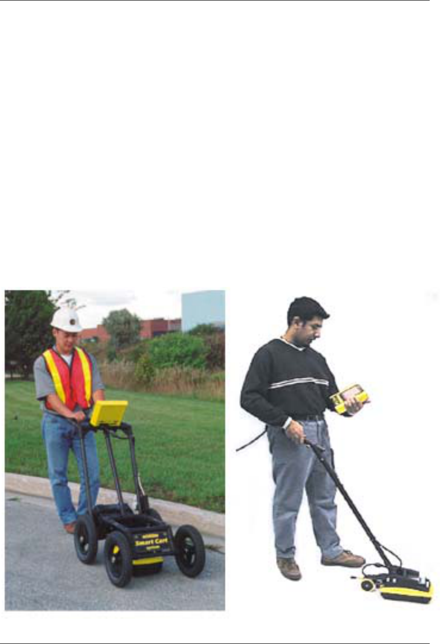
Noggin Smart Systems are integrated ground penetrating radar (GPR) data acquisition
platforms. Once the unit has been assembled and powered up you can be carrying out a
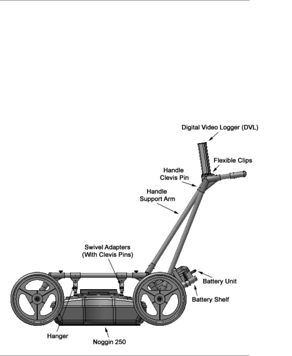
GPR survey in less than a minute. There are two different configurations available, the
Smart Cart system and the Smart Handle system (see Figure 1-1).
The Smart Cart system consists of the cart structure, a Noggin, an odometer wheel, a
digital video logger (DVL), and a battery. Section 2 describes how to assemble a Smart
Cart system.
The Smart Handle system consists of the Smart Handle, a Noggin, an odometer wheel,
a digital video logger (DVL), and a battery. Section 3 describes how to assemble a
Smart Handle system.
Each Smart System’s DVL comes with all the necessary software installed. This includes
software to acquire data as well as software to replay data files. Data management
software allows the data to be transferred to an external computer for further processing
and/or plotting.
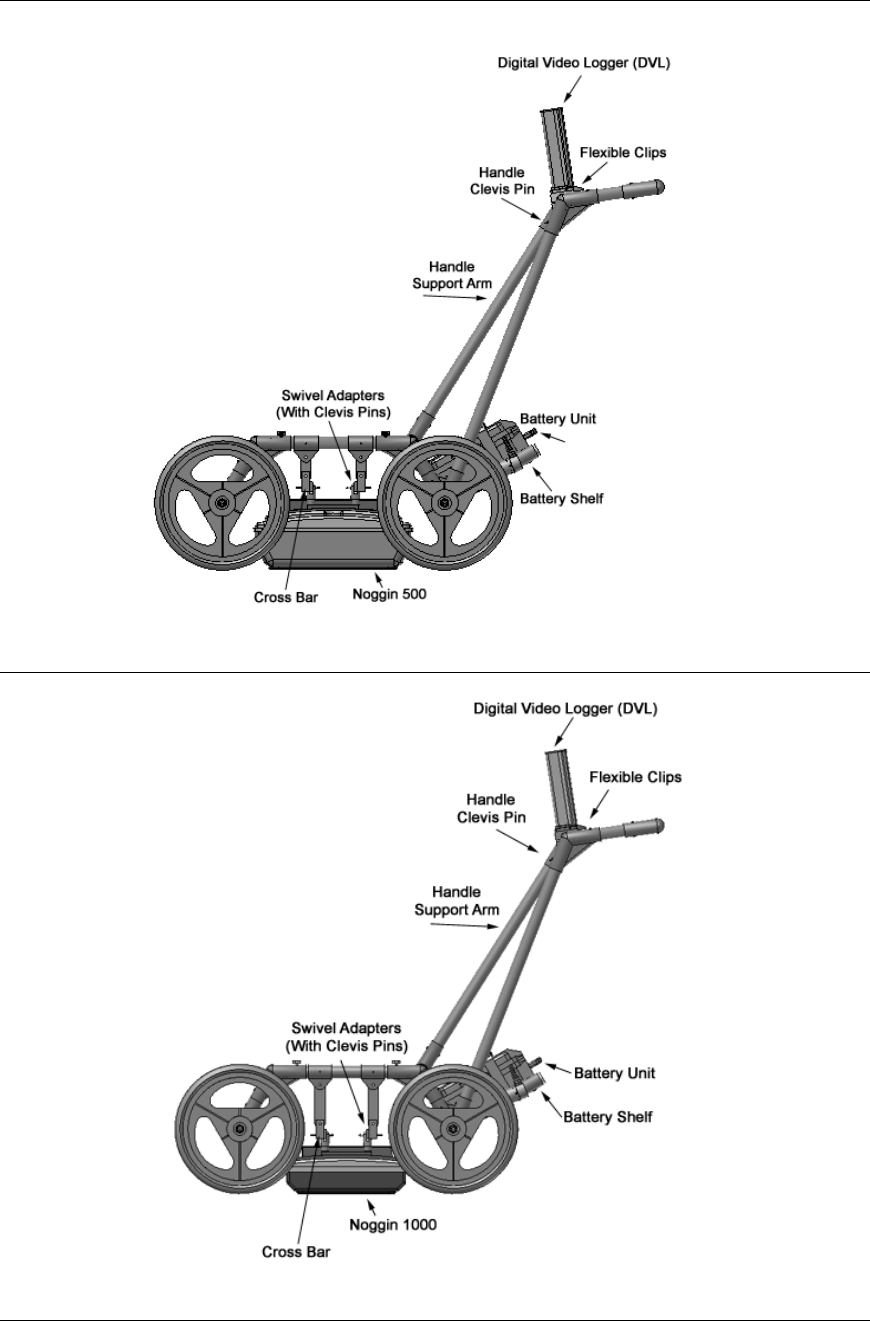
Figure 1-1: Noggin Smart Cart system (left) and Noggin Smart Handle System (right).
Smart Systems User’s Manual Version 1.1
2
2 Assembling the Smart Cart
The Noggin Smart Cart can be configured for Noggin 250, Noggin 500 or Noggin 1000
operation. For the Noggin 250 Smart Cart, refer to Figure 2-10. For the Noggin 500
Smart Cart, refer to Figure 2-11 and for the Noggin 1000 Smart Cart, refer to Figure
2-12.
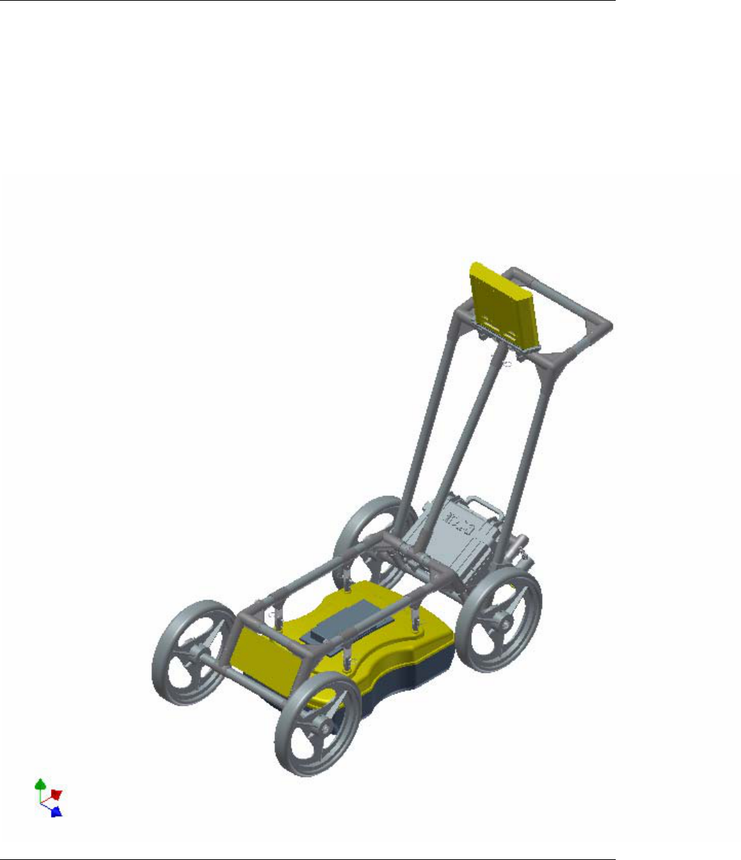
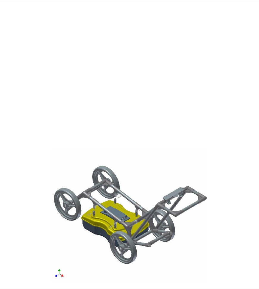
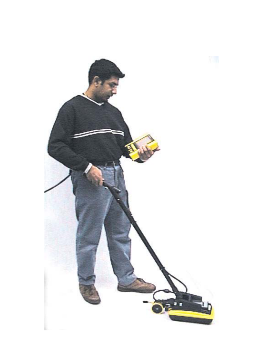
Figure 2-1: Fully assembled Smart Cart
Smart Systems User’s Manual Version 1.1
3
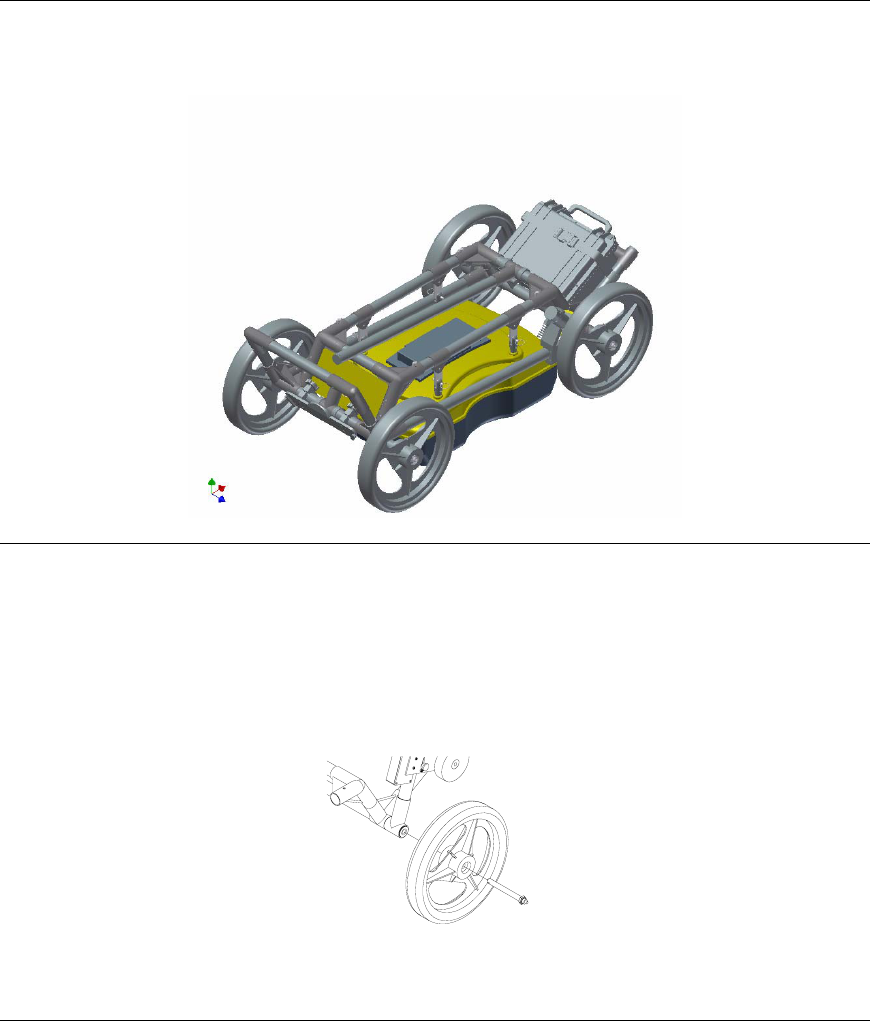
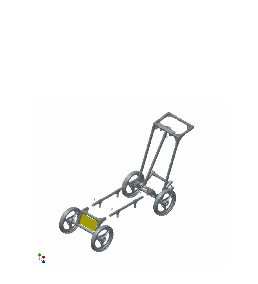
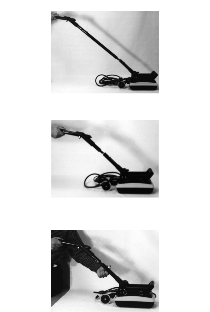
The Noggin Smart Cart comes fully assembled but in collapsed position (Figure 2-2).
The steps necessary to have a fully functioning system are:
Figure 2-2: Smart Cart in collapsed position.
1. Attach wheels (if necessary): The Smart Cart may have been shipped without
the wheels attached or they may have been removed for storage. If this is the case, find
the axle for each wheel, press the button on the end of the axle, and insert the axle
through the wheel and into the cart frame. This is shown in Figure 2-3.
Figure 2-3: Attaching the wheel.
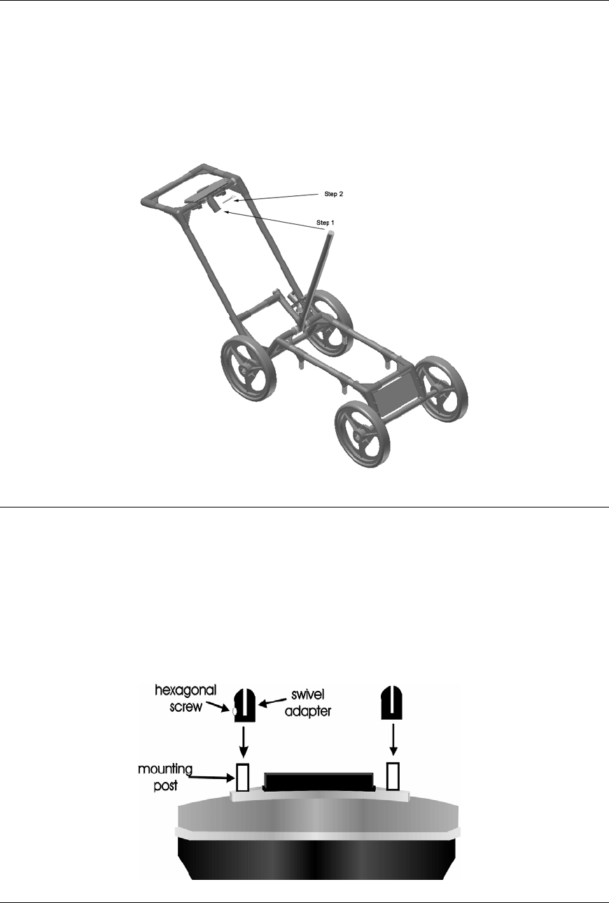
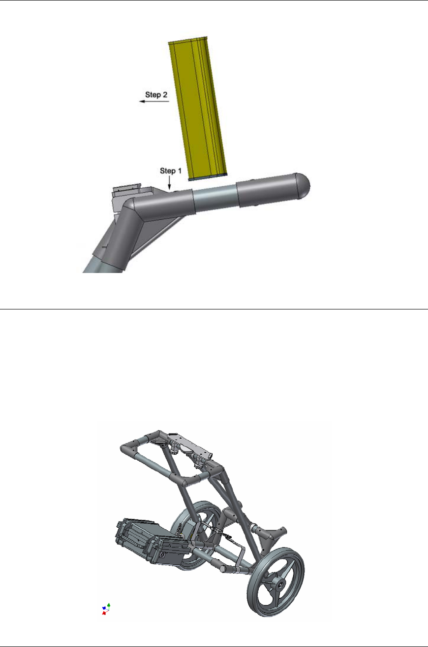
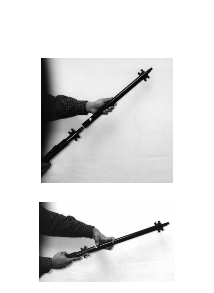
2. Unfold the Handle: Refer to Figure 2-4. Pull the ring to remove the handle
Clevis pin from the handle support arm. Raise the handle support arm and then the
handle and place the open end of the T-shaped tube on the handle onto the end of the
support arm (Step 1). Then lock the handle into position by lining up the hole in the
support arm with the hole in the T-shaped tube and inserting the handle Clevis pin (Step
2). (When folding the Smart Cart back up always ensure the handle folds down before
the handle support arm.)
With the system unfolded, make sure the small odometer wheel makes good contact
with the side of the cart wheel. If this contact is too loose, the odometer wheel may slip,
resulting in erroneous position measurements. If the odometer wheel seems loose, use
Smart Systems User’s Manual Version 1.1
4
a ¼ inch Allen (hexagonal) wrench to loosen the screws on the side of the odometer
(see Figure 2-10 or Figure 2-11) and pivot the entire odometer unit until the small
odometer wheel makes good contact with the side of the cart wheel. Then tighten the
screws to lock the odometer wheel in this position. After this has been done, it will be
necessary to re-calibrate the odometer (see Section 6.5.2).
Figure 2-4: Smart Cart set up.
3. Attach the Noggin: Before the Noggin unit can be attached to the Smart Cart,
the 4 swivel adapters (with attached Clevis pins) must be attached to the mounting posts
on the Noggin (see Figure 2-5). Set the swivel adapter down on the post. It may be
necessary to loosen the Allen (hexagonal) screw before the swivel adapter will slide
down into the proper position. This can be done using the 1/8” Allen (hexagonal) wrench
provided. Now, tighten each screw and then loosen ¼ turn so that the swivel adapters
are firmly attached to the post but can still rotate. DO NOT OVER-TIGHTEN!
Figure 2-5: Attaching the swivel adapters to the Noggin 250.
Smart Systems User’s Manual Version 1.1
5
Once all 4 swivel adapters are attached, the Noggin can then be attached to the Smart
Cart.
The Noggin is usually attached to the cart with the long axis of the Noggin unit parallel to
the wheels on the cart (see Figure 2-10 ,Figure 2-11 and Figure 2-12). For this
orientation, make sure the 37 socket female electrical receptacle on the Noggin faces
the back of the cart so that the cable on the cart will reach the receptacle.
It is also possible (but not usual) to attach the Noggin to the cart with the long axis of the
Noggin perpendicular (at right angles) to the wheels on the cart. For this orientation,
make sure the 37 socket female electrical receptacle on the Noggin is on the same side
of the cart as the odometer so that the cable on the cart will reach the receptacle.
Noggin 250: Remove the Clevis pins from the swivel adapters. Now, on the bottom of
the cart, locate the 4 oval, moveable hangers suspended from the frame of the cart (see
Figure 2-6). Notice that each hanger has a hole in it. To attach the Noggin 250 to the
cart, place each hanger into the slot on the top of the swivel adapters, line up the holes
and insert the Clevis pin.
Figure 2-6: Attaching the Noggin 250 to the cart.
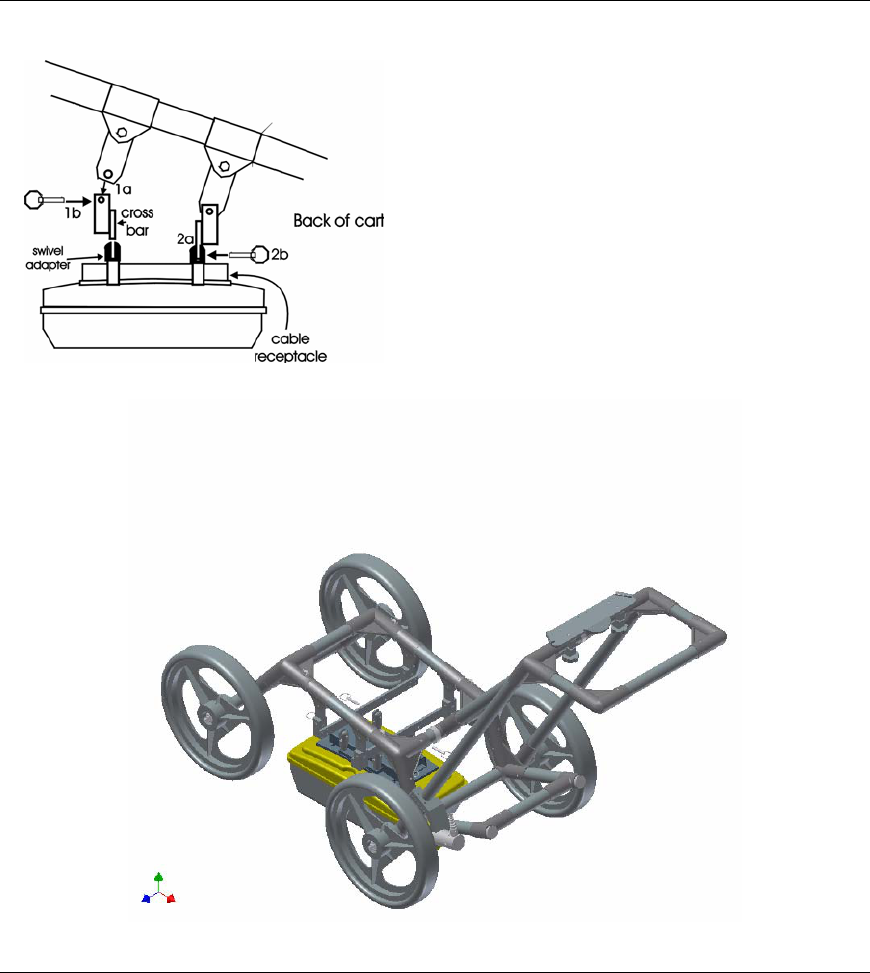
Noggin 500 and Noggin 1000: Remove the Clevis pins from the swivel adapters. Now,
on the bottom of the cart, locate the two, flat, moveable crossbars suspended from the
frame of the cart. If the crossbars are attached, go to step B.
Step A: If the crossbars are detached from the cart, they will need to be attached before
attaching the Noggin to the cart (see Figure 2-7 top). To attach the cross bars, use the 4
oval, moveable hangers suspended from the frame of the cart. Insert the hanger into the
slot on the crossbar, line up the holes and insert the Clevis pin.
Step B: Notice that each crossbar has 2 holes, one on each side. To attach the Noggin
500 to the cart, place the crossbars into the slots on the top of the swivel adapters, line
up the holes and insert the Clevis pins.
Smart Systems User’s Manual Version 1.1
6
Attach Cross bars to the cart (if
necessary).
a) Line up holes.
b) Insert Clevis pin.
Attach Noggin to cross bar.
a) Insert cross bar into swivel
adapter.
b) Insert Clevis pin.
Figure 2-7: Attaching the Noggin 500 and Noggin 1000 to the cart.
Connect the cable with the 37-pin male D connector to the Noggin and secure this
attachment by tightening the hand screws.
4. Attach the Digital Video Logger (DVL): The bottom of the Digital Video Logger
is designed to slide onto the support shelf attached to the Smart Cart (Figure 2-8). Line
up the bottom of the Digital Video Logger with the shelf and slide it back onto the shelf.
Push the Digital Video Logger back far enough so that the flexible clip on the front of the
shelf catches and holds the Digital Video Logger firmly in place. Wiggle the DVL to make
sure it is firmly snapped in before letting go of the unit. (To remove the Digital Video
Logger from the Smart Cart, this clip must be flexed downward as the DVL is slid
forward off of the shelf.
Smart Systems User’s Manual Version 1.1
7
Figure 2-8: Attaching the digital video logger (DVL). Step 1: Depress flexible clip. Step 2: Slide
DVL onto shelf.
Once the Digital Video Logger is in place, attach the cable with the 37-socket female D-
connector to the 37-pin receptacle on the back of the Digital Video Logger. This
attachment can be secured by tightening the hand screws.
The Digital Video Logger can be pivoted to adjust the view angle. If it is difficult to pivot
the Digital Video Logger, slightly loosen the hand screws on the bottom of the support
shelf.
Figure 2-9: The Noggin Smart Cart battery.
Smart Systems User’s Manual Version 1.1
8
5. Attach the Battery Unit: Set the battery unit onto the lower inclined shelf on the
back of the Smart Cart (see Figure 2-9). The handle on the battery unit should be
accessible from the back of the cart with the cable receptacle on the right. The battery
unit should rest in this area without moving. To secure the battery onto the cart, put the
straps provided over the battery unit and lock into place with the plastic buckle. Tighten
the straps if necessary.
With the Noggin Smart Cart completely assembled, connect the round 4-pin battery
cable to the receptacle on the side of the battery.
Note the battery mass forms part of the overall cart balance which enables users to raise
the front wheels with a minimum amount of force. This allows users to easily change
direction and assure the rear wheels are always in contact with the ground.
Figure 2-10: Noggin 250 Smart Cart
Smart Systems User’s Manual Version 1.1
9
Figure 2-11: Noggin 500 Smart Cart
Figure 2-12: Noggin 1000 Smart Cart
Smart Systems User’s Manual Version 1.1
10
2.1 Configuring the Smart Cart to Carry a Different
Noggin System
The Noggin Smart Cart can be configured to carry a Noggin 250, Noggin 500 or a
Noggin 1000 system. This can be done by replacing the two support arms on the cart
(see Figure 2-13) with the support arms for another system. Each arm is attached to the
cart by two hand screws. For each arm, remove the screws, detach the arm from the
cart and replace it with the new arm.
Figure 2-13: Changing the Smart Cart’s support arms to carry a different Noggin system.
Smart Systems User’s Manual Version 1.1
11
3 Assembling the Smart Handle System
Figure 3-1: Smart Handle System with a Noggin 1000
Smart Systems User’s Manual Version 1.1
12
3.1 Smart Handle
The Smart Handle consists of the Smart Handle grip and Smart Handle extension.
These two pieces are put together (see Figure 3-2 and Figure 3-3) and then attached to
the Noggin (see Figure 3-4). The system can be deployed without the handle extension
as shown in Figure 3-5 and Figure 3-6.
Figure 3-2: Simply push the Smart Handle grip into the Smart Handle extension
Figure 3-3: To separate them, push on the large grey button on the extension and pull them apart
Smart Systems User’s Manual Version 1.1
13
Figure 3-4: Now connect the other end of the Smart Handle extension to the Noggin by simply
pushing it in.
Figure 3-5: If short handle is required, it may be easier to just connect the SmartHandle
grip to the Noggin without the extension.
Figure 3-6: To separate either the short or long handle from the Noggin, press on the large grey
Smart Systems User’s Manual Version 1.1
14
button on the pole extending from the Noggin and pull apart.
3.2 Cabling
3.2.1 DVL to Sensor Cable
The DVL to Noggin cable is a Y-shaped cable with 3 connections; one to the Noggin
sensor, one to the DVL and one to the power supply (battery or AC).
Noggin Connection: The first connection is to attach the 37-pin connector on the cable
to the 37-socket connector on the Noggin. Use the thumb screws to secure this
connection.
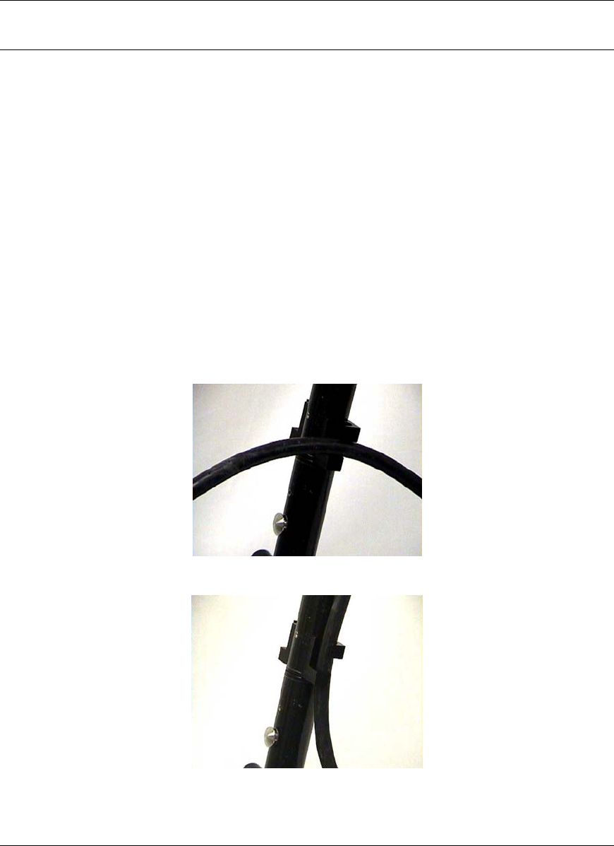
From the Noggin, the DVL to Sensor Cable runs up the side of the Smart Handle. Use
the guides (clips) on the side of the Smart Handle to attach the cable to it (see Figure
3-7).
(a)
(b)
Figure 3-7: a) Insert cable - b) twist to grip
DVL Connection: The second connection from the DVL to Sensor Cable is to the DVL.
One end of the Y-shaped cable has a 37 socket connector. This end plugs into the 37-
pin connector on the back of the DVL.
Smart Systems User’s Manual Version 1.1
15
Power Connection: The third connection on the Smart Handle cable attaches to a
power supply. The round, 4-pin connector attaches to either the standard battery or
optional AC adapter.
3.2.2 Odometer Cable
The cable connecting the odometer or positioning wheel comes already installed at the
factory.
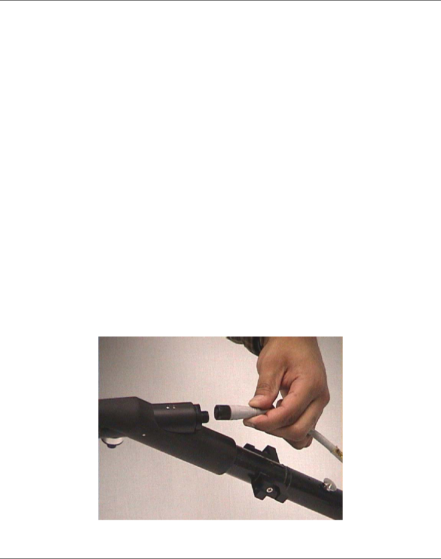
3.2.3 Smart Grip Cable
The Smart Grip Cable is used to connect the Smart Handle button and beeper into the
system. The Smart Grip Cable is a light grey, two part cable (pre-assembled) that
connects from the Noggin to the end of the Smart Handle grip. The connection at the
Noggin may already be made when the system is pulled from the box. The other end of
the cable attaches to the connector at the bend of the Smart Handle grip (see Figure
3-8). Again, this cable can run up the side of the Smart Handle using the guides (clips) to
secure the cable to it.
Figure 3-8: The Smart Grip Cable attaches to the end of the Smart Handle Grip. This connects
the Smart Handle button (extreme left, bottom) and beeper (not shown) into the system.
Smart Systems User’s Manual Version 1.1
16
4 Starting the Digital Video Logger
Once all the cable connections are made between the Noggin, the Digital Video Logger
(DVL) and the battery, the upper red LED light on the DVL panel should be lit. If the
battery voltage is low, the light will flash for about 30 seconds and go out. If the light
flashes or does not appear, check the connections and make sure the battery is fully
charged. (See Section 8.1 for more information on battery care.)
The voltage indicator can be helpful for identifying when the battery needs to be
recharged. If the battery voltage drops too low the DVL will cease to operate.
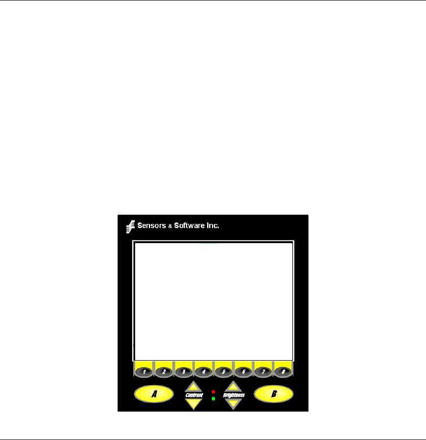
The front of the DVL is shown in Figure 4-1. To start the system, press any button on
the front panel. The DVL will begin to beep indicating it is booting up. The lower red
LED on the front panel should illuminate.
Figure 4-1: Digital Video Logger (DVL) face
At this stage, the Noggin unit will still be powered down. Once Noggin action is
requested (see later menu items), the DVL will enable power to the Noggin. If the
Noggin is receiving power, the red LED light on the connector to the Noggin will be
illuminated.
The water-resistant membrane keypad has a number of buttons that can be pressed to
perform various tasks. Note that the buttons on the membrane keypad sometimes need
to be pressed hard to register.
Menu Buttons: The yellow buttons labelled 1 to 8 correspond to menu choices that
appear listed on the screen or along the bottom of the screen when the Digital Video
Logger is turned on.
In addition, there are two general-purpose buttons labeled A and B. All buttons are DVL
application dependent and roles change. The operation will be self-explanatory from the
display screen.

Smart Systems User’s Manual Version 1.1
17
Screen: The DVL screen is a grayscale LCD selected for its wide temperature range
and visibility in sunlight. Visibility can be a major problem with viewing GPR data
displays outdoors and considerable effort has been expended on getting a readily visible
outdoor display.
Brightness: The yellow Brightness control arrows are used to increase and decrease
the screen brightness. For example, increasing the Brightness setting may improve the
visibility of the screen when outside on a sunny day. Note, however, that increasing the
screen brightness also increases battery consumption so don’t use a bright screen
unless necessary.
Contrast: The yellow Contrast control arrows are used to increase and decrease the
screen contrast. For example, increasing the Contrast setting may improve the visibility
of weaker features on the screen. Adjusting the contrast has little effect on battery
consumption.
Temperature sensors within the DVL automatically compensate the screen setting so
that manual adjustments of Brightness and Contrast should seldom be needed after
initial setup.
Once the Digital Video Logger powers up, the Main Menu is displayed with 3 choices:
A – NOGGIN
B – NOGGIN PLUS
5 – POWER OFF
12.1 V 38°C Rev 3.00
100°F
• Pressing the A button starts the software for standard Noggin systems. Details about
the Noggin system software can be found in Section 5.
• Pressing the B button starts the software for Nogginplus systems. Details about the
Nogginplus system software can be found in Section 6.
• Pressing the 5 button will turn the DVL off.
• Note that Nogginplus systems will operate with both the Noggin and Nogginplus
software while standard Noggin systems will only operate with the Noggin
software.
This screen also displays the following information:
• Battery Voltage: The system will shut down when the battery voltage reaches 10.2
Volts (see Section 8.1 for more details on the battery).
• Temperature: The internal temperature of the DVL is displayed on this screen in
Celsius and Fahrenheit.
• Software Version: The version of the software loaded on the DVL.
Smart Systems User’s Manual Version 1.1
18
When the Smart Cart is not being used, do not leave the
battery plugged in. The system draws about 0.1 amps even
when it is powered off and this will gradually drain the
battery.
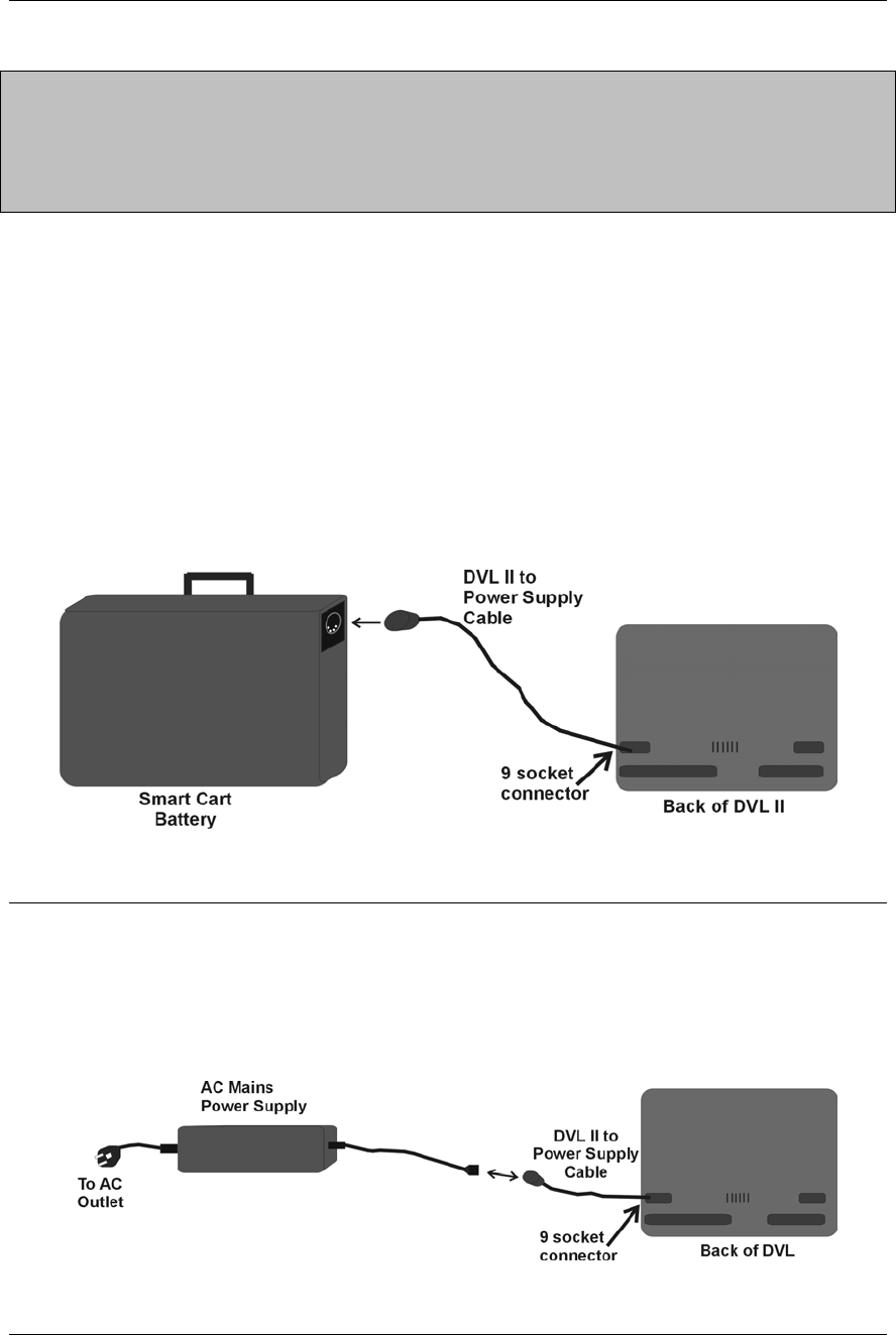
4.1 Running a DVL Detached from a Smart System
When collecting data with a Smart System, the DVL is powered by the system battery. It
is possible to detach the DVL from the Smart Cart (see Figure 2-8) or the Smart Handle
system and use it away from the system to review, print or download data. There are 2
ways to power the DVL away from the Smart System and both involve using optional
accessories.
The optional DVL II to Power Supply Cable allows the user to power the DVL away from
the cart using the system battery. As shown in Figure 4-2, the cable connects the
battery to the 9-socket connector on the back of the DVL.
Figure 4-2: The optional DVL II to Power Supply cable can be used to power the Digital Video
Logger (DVL) from the system battery.
To avoid having to use the system battery to power the DVL, an optional AC power
supply is available. This, when combined with the DVL II to Power Supply Cable, allows
the user to power the DVL away from the cart using AC power. As shown in Figure 4-3,
the AC power supply connects to the DVL II to Power Supply Cable which connects to
the 9 socket connector on the back of the DVL.
Figure 4-3: The optional DVL II to Power Supply cable can be combined with an optional AC
power supply to power the Digital Video Logger (DVL) without the system battery.

Smart Systems User’s Manual Version 1.1
19
5 Noggin
5.1 Overview of Noggin Menu Options
The Noggin main menu has the following choices:
A – RUN
B – DEMO
1 – NOGGIN SETUP
2 – TRANSFER ALL BUFFERS
3 – DELETE ALL BUFFERS
4 – UPGRADES
7 – RETURN
12.1 V Rev 6.00
5.1.1 Run
Pressing the A button starts the Noggin data acquisition program (see Section 5.4).
5.1.2 Demo
Pressing the B button starts the Noggin Demonstration program. This program simulates
data acquisition (without actually moving the cart) by displaying a default data set. This
data set cycles continuously until the user exits from the demo program. This allows the
user to see and experiment with the different menu items and different settings to see
the effect they have on the data presentation.
It is useful to run the demonstration program while reviewing the Noggin Screen
Overview described in Section 5.2 and Noggin Menu Options described in Section 5.3.
5.1.3 Noggin Setup
There are many background setup parameters related to the Noggin Smart Cart
operation that can be edited. This menu allows the user to display and change various
settings for different aspects of the Smart Cart system. The user can also reset all the
parameters to the factory default settings. See Section 5.5 – Default Settings.
5.1.4 Transfer All Buffers
Pressing the number 2 on the main menu transfers ALL the data buffers (up to 250
screens) from the DVL to an external PC. See Section 5.6.1.

Smart Systems User’s Manual Version 1.1
20
5.1.5 Delete All Buffers
Pressing the number 3 on the main menu allows the user to delete ALL the data buffers
currently saved on the DVL. See Section 5.6.2
5.1.6 Upgrades
Pressing the number 4 on the main menu puts the DVL into listen mode to allow a
software upgrade to be transferred from an external PC to the DVL. Avoid pressing this
button until the instructions in a software upgrade tell you to. Once pressed, the DVL
must be powered down exit from this menu item. See Section 5.7.
5.1.7 Return
This button will return the user to main menu. See Section 4.
Smart Systems User’s Manual Version 1.1
21
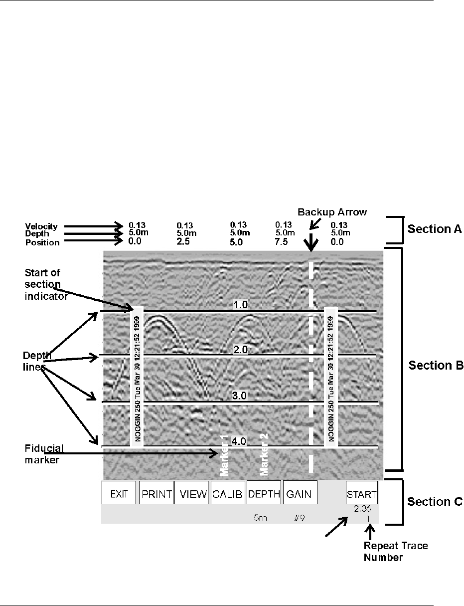
5.2 Noggin Screen Overview
The Noggin screen is shown in Figure 5-1. It is divided into 3 sections. The very top
section (Section A) contains velocity, total depth and positioning information. The center
section (Section B) contains the actual data and the bottom section (Section C) contains
the menu.
Each screen of data is saved in the Digital Video Logger as an individual PCX graphics
file called a SPI file. Although each screen is saved as an individual file, these files can
be viewed together as a continuous chart up to 250 screens long. These data can be
viewed on screen (see Section 5.3.3), printed directly to a printer attached to the DVL or
transferred to an external computer (see Sections 5.3.2 and 5.6.1).
Figure 5-1: Noggin Data Acquisition Screen

Smart Systems User’s Manual Version 1.1
22
5.2.1 Section A - Data Parameters
Section A displays three items:
1) The total depth to the bottom of the data image in Section B,
2) The velocity used to calculate the total depth and the depth lines (see
Depth Lines in Section 5.2.2) and
3) The position indicator in meters or feet (depending on the odometer units
set, see Section 5.5.1 – Units).
Rather than displaying total depth and depth lines the user can select to display the total
time window in nanoseconds (see Section 5.5.1 - Units).
Note that it is possible to change the position label size (see Section 5.5.1 – Label Size).
5.2.2 Section B - Data Display
This section contains the actual data collected or replayed. The section also contains the
depth indicator lines, battery voltage indicator (which is visible each time you start), start
of section indicators, and any fiducial markers the user enters. See the sections below
for more details.
Depth Lines
Depth lines are horizontal labelled lines indicating the estimated depth. They are very
useful for getting depth estimates to features of interest in the data.
The positions of the Depth Lines are controlled by the current velocity value as well as
the depth selected. See Section 5.3.5 on selecting different depths and Section 5.8.1 for
more details on how depths are determined.
To display the correct depth, it is the responsibility of the user to calibrate the
system to the correct velocity of the material (see Section 5.3.4 on how to
calibrate the system).
Note that it is possible to change the depth units and the depth label size (see Section
5.5.1).
Battery Voltage Indicator
When the Start button is pressed, the current battery voltage will be displayed on the
extreme left side of the screen.
The voltage indicator can be helpful for identifying when the battery needs to be
recharged. If the battery voltage drops below 10.5 volts the DVL will cease to operate
and this monitoring capacity will not be available.
Smart Systems User’s Manual Version 1.1
23
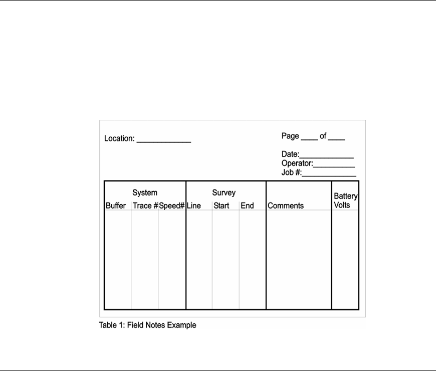
Start of Section Indicator
Any time the Start button is pressed, the current date and time are written vertically on
the screen to indicate the start of a new section (see Section 5.5.1 on how to set time
and date on the DVL). The position indicator is also reset to zero. The current date and
time can be recorded in a field notebook along with the survey location to help the user
organize where each section of data was collected (Figure 5-2).
Figure 5-2: Example field notes
Fiducial Markers
A fiducial marker is text written vertically on the section at a specific position during data
acquisition. Adding these markers during data acquisition is useful for recording
significant positions or the positions of surface objects encountered during the survey.
The position and name of the object encountered at each marker can be recorded in a
field notebook. Then, when the data are reviewed, these markers are visible right on the
data section and can assist with data interpretation.
A fiducial marker is activated by pressing the A button on the DVL keypad during data
acquisition.
Smart Handle systems: On Smart Handle systems, it is also possible to add a fiducial
marker by quickly pressing the button on the Smart Handle during data acquisition.
The first time the A button (or Smart Handle button) is pressed, the text “Marker 1” will
be written to the screen at the current position. The marker number will then increment
each time it is pressed, for example, Marker 2, Marker 3 etc (see Figure 5-1).
Note that it is possible to automatically place a dashed vertical line at every position
label (see Section 5.5.1 – Odometer Markers).

Smart Systems User’s Manual Version 1.1
24
5.2.3 Section C - Menu
The bottom section contains the user menu selection and current program settings. This
menu is described in more detail in Section 5.3.
During data acquisition it also displays the current odometer position and the Repeat
Trace Number that indicates if the system is moving too quickly and reducing data
quality (see Section 5.4.1).
5.3 Noggin Menu Options
The default menu selection is divided up into 7 sections: Exit, Print, View, Calib., Depth,
Gain and Start. Each of these options is addressed below.
Execution of a menu item is done by pressing the key immediately below the menu item.
Pressing the key will change the setting for that menu item. For example, pressing the
key below the Depth menu item will start to cycle through the different depth settings
available.
5.3.1 Exit
This button will terminate the Noggin program and return the user to Noggin main menu.
The user can then run the Noggin again, run the demo program, change DVL settings,
download data to an external PC, delete data or return to the main menu (see Section
3).
Note that when the Start button is pressed and data acquisition begins (see Section
5.3.7), the Exit button turns into a Stop button (see Section 5.3.8). Data acquisition must
be stopped by pressing the Stop button before it is possible to exit from this menu.
5.3.2 Print Menu
This menu item allows the user to:
1) Print data images directly to an attached printer or,
2) Transfer one or more screens (or buffers) of data to an external computer
(PC) as a single PCX graphics file. This type of transfer is appropriate
when the user wants to transfer the data to an external computer for use
with third-party graphics software packages like Microsoft Paint and
Word.
Printing Data to an attached Printer
The Noggin data images can be printed directly to a few select, but common, printers.
The supported printers are HP LaserJet printers, most Epson printers and the Seiko
DPU5400 thermal printer. As well, any printer that can emulate these printers can be
used (see your printer’s User’s Guide for emulation modes available). For example,
Smart Systems User’s Manual Version 1.1
25
Canon BubbleJet printers can usually be configured to emulate an Epson and most HP
printers will work using the Laser driver.
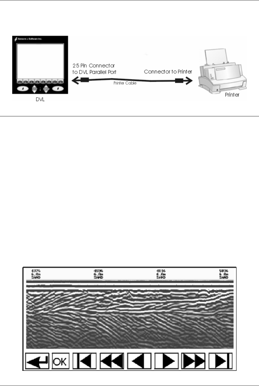
Figure 5-3: Attaching a printer to the DVL using a standard printer cable.
On the back of the DVL there is a standard 25 socket parallel port. A printer can be
attached to the parallel port on the DVL with a standard printer cable, just as you would
attach a printer to any computer (Figure 5-3).
Always power down the DVL before attaching a printer. This will prevent damage
to the parallel port.
On the Digital Video Logger, after the Print option is selected, the user must define the
section to be printed. The left edge of the page must be established first. This is done by
lining up the left edge of the Digital Video Logger screen with the edge of the plot
desired. Use the arrow buttons on the screen to move the section back and forth (Figure
4.1). A single arrow moves the image 8 pixels either right (), or left (). A double
arrow will move the image 640 pixels or 1 full page to the right () or left (). A single
arrow with a vertical line will move the section either to the start (❙), or end (❙) of the
section. If the start or end of section button is pressed, the image will page through one
screen at a time. Data scrolling can be stopped by pressing any button. Once the left
edge is in place, pressing the OK button will lock the left edge of the plot.
Figure 5-4: Noggin Print Screen

Smart Systems User’s Manual Version 1.1
26
The right edge of the plot must now be defined the same as the left, however now using
the right edge of the Digital Video Logger screen. Note that the right edge cannot exceed
the left edge.
Next, select the type of printer attached (LASER for HP LaserJets and many other HP
printers, EPSON for Epson or Canon BubbleJet printers or SEIKO for the Seiko
DPU5400 Thermal printer). Text will appear on the bottom of the DVL screen indicating
the image is printing on the printer.
If an error occurs during the printing operation, press the A button to Abort. Try to
resolve the problem and try again. It may be necessary to turn the DVL off and power it
back on and try printing again.
When the print is complete the user is returned to the Noggin screen.
Transferring Data to an External PC
There are two ways of transferring data to an external computer. The first is to transfer
one or more screens (or buffers) of data as a single PCX graphics file. This method is
described in this section. The second way of transferring data files to an external
computer is to copy all the individual SPI (PCX) files from the DVL (see Section 5.6.1).
This method is useful when the user wants to view the data on an external computer
using the SpiView software. SpiView is available from Sensors & Software Inc.
The data transfer function can only be used after the parallel XFER cable has been
connected from the DVL to the external computer and after the WinPXFER
program has been installed on the external computer and run. Section 5.6.1
describes how to attach the parallel XFER cable and also how to install and run
the WinPXFER program.
Once WinPXFER has been run on the external computer, it is ready to receive data
image files from the Digital Video Logger.
On the Digital Video Logger, after the Print option is selected, the user must define the
section to be printed. The left edge of the page must be established first. This is done by
lining up the left edge of the Digital Video Logger screen with the edge of the plot
desired. Use the arrow buttons on the screen to move the section back and forth (Figure
4.1). A single arrow moves the image 8 pixels either right (), or left (). A double
arrow will move the image 640 pixels or 1 full page to the right () or left (). A single
arrow with a vertical line will move the section either to the start (❙), or end (❙) of the
section. If the start or end of section button is pressed, the image will page through one
screen at a time. Data scrolling can be stopped by pressing any button. Once the left
edge is in place, pressing the OK button will lock the left edge of the plot.
The right edge of the plot must now be defined the same as the left, however now using
the right edge of the Digital Video Logger screen. Note that the right edge cannot exceed
the left edge.
Next, select a name for the image file from the options CART-1 to CART-4. As long as
the WinPXFER program is running on the external PC, the file will be transferred to the
current directory indicated by WinPXFER. When the data image file transfer is complete,

Smart Systems User’s Manual Version 1.1
27
the user will find a data image (CART-n.PCX) file on the external computer in the current
directory.
When the data transfer is complete, on the external computer, exit from the WinPXFER
program. Press any button on the DVL to return to the Noggin screen.
5.3.3 View Menu
The View function allows the user to scroll back through previously recorded data in the
same manner as the Print function (see Section 5.3.2).
5.3.4 Calib. (Calibration) Menu
Noggin systems can be used to scan into many different materials including soil, rock,
concrete, snow, ice and wood. The radio wave emitted by a Noggin system will travel at
different velocities depending on the material being scanned. The depth values on the
Depth menu (see Section 5.3.5) and on Depth Lines (see Section 5.2.2) are only
accurate if the system has been properly calibrated to determine the velocity of the
material being scanned. See Section 5.8.1 for more details about how depth is
calculated.
The Calibration function allows the user to input the velocity of the material being
scanned. Velocity can be determined in one of four different ways depending on the
situation:
1) Hyperbola matching
2) Target of known depth
3) Select a media
4) Input a velocity value
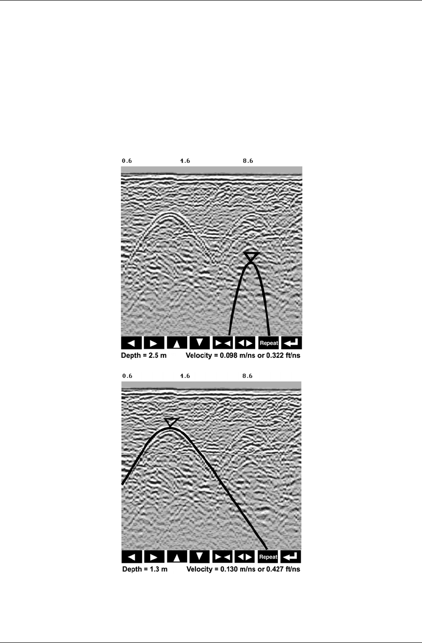
Hyperbola Matching
This is the most accurate way of determining the velocity of the material being scanned
because it extracts the speed using data collected in the area. This method may not
work in all situations because it depends on having a good quality hyperbola (or inverted
U) in the data. A hyperbola is the characteristic Noggin response from a small point
target like a pipe, rock or even a tree root. If the hyperbola has long tails on it, we can
match the shape of the hyperbola and determine the velocity of the material in the area.
With the hyperbola visible on the DVL screen, select the hyperbola (∩) button. This will
superimpose a hyperbola on the data. This hyperbola can be moved up (), down (),
left () and right () using the appropriate arrow buttons. The goal is move the
hyperbola until it lies on top of the hyperbola in the data (see Figure 5-5). Then, the user
can adjust the width of the hyperbola to make it wider () or narrower () until the
shape of the hyperbola matches the shape of the hyperbola in the data. After matching
the hyperbola, the velocity value is extracted and used for all subsequent data
acquisition.
Smart Systems User’s Manual Version 1.1
28
Pressing the up, down left, right, wider and narrow buttons once makes a very small
change in the position or width of the hyperbola. These buttons must sometimes be
pressed many times to move the hyperbola to the correct position or width. To speed up
the movement of the hyperbola, use the REPEAT button. For example, to move the
hyperbola up a long distance, press the up button () followed by the REPEAT button.
The hyperbola will then start moving upward without having to press any more buttons.
When it gets close to the desired location press any button to stop it and then use the
up, down, left and right buttons to fine-tune the position. The REPEAT button can also
be used after pressing the wider () or narrower () button.
Figure 5-5: Hyperbola matching to extract velocity. After pressing the CALIB button a hyperbola
appears on the screen (a). This hyperbola should be moved overtop of a hyperbola in the data
using the arrow keys. It can then be widened or narrowed to match the shape of the hyperbola in
the data (b). When the hyperbola shapes match, the velocity is extracted and used to make
depth estimates more accurate in subsequent data.
Smart Systems User’s Manual Version 1.1
29
Hyperbola Matching calibration can only be done during data acquisition. It cannot be
done when viewing previously collected data. Further, the Hyperbola Matching
calibration is only available after at least half a screen of data with the same depth
setting have been collected. If less than half a screen of data are collected and the
CALIB button is selected, only calibrations selecting a material or inputting a
velocity are available (see below).
Depths will appear in metres or feet depending on which units are selected. Velocities
appear in both metres per nanosecond (m/ns) and feet per nanosecond (ft/ns). To
change units see Section 5.5.1 - Units.
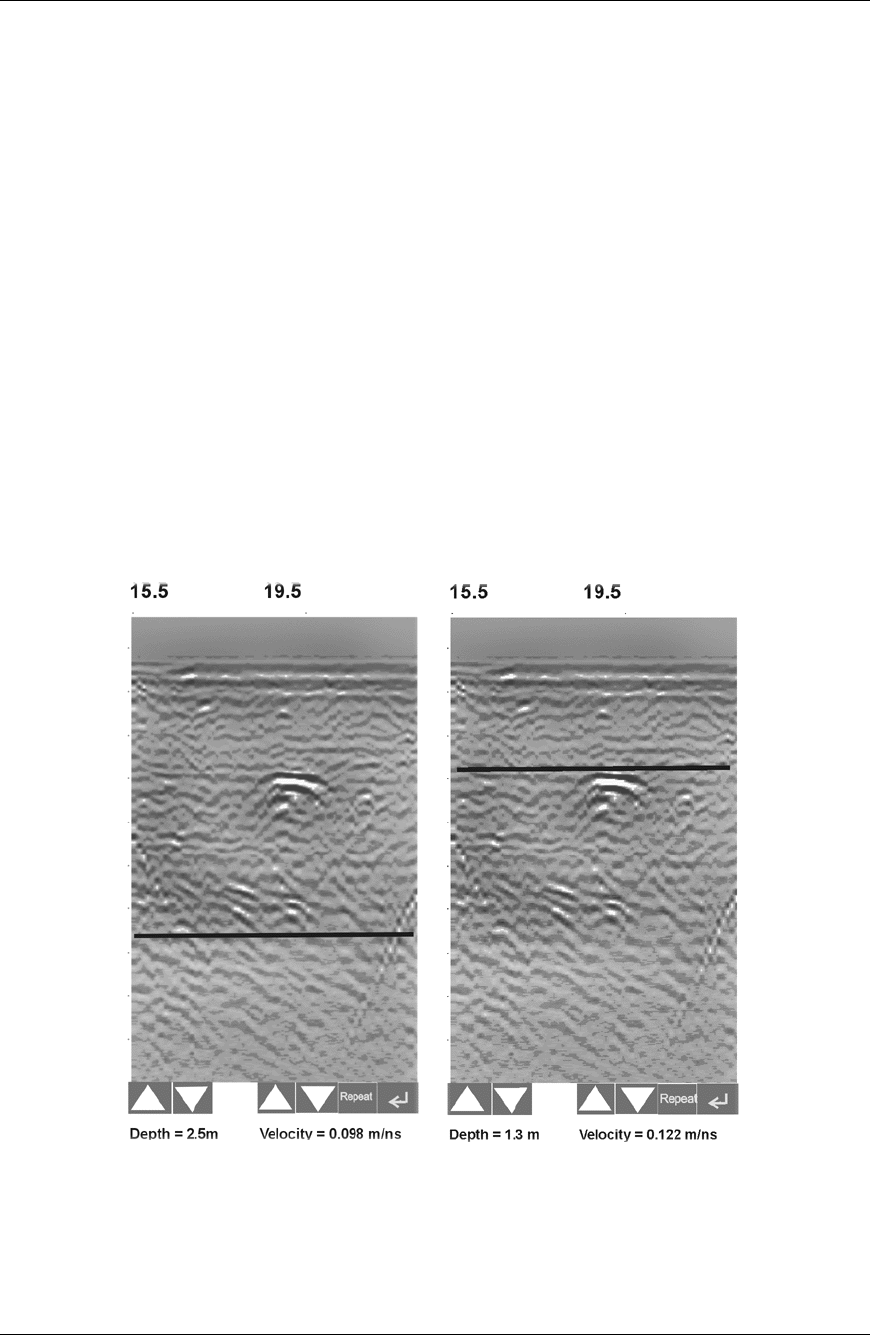
Target of Known Depth
If there are no suitable hyperbolas visible in the data to perform the Hyperbola Matching
described above, it may be the situation that there is a target of known depth in the area
being scanned. If this is the case, selecting the button with the circle with a horizontal
line through it will superimpose a horizontal line on the data. This line can then be
moved up or down until it lies on top of the Noggin response to the known target. Then,
the user can adjust the velocity value up or down until the known target depth is correct.
Once the depth is matched, the current velocity value is the one used for all subsequent
data acquisition.
(a) (b)
Figure 5-6: Using a target of known depth to extract velocity. After selecting CALIB, choosing the
known depth button (a circle with a horizontal line through it) will superimpose a horizontal line on
the data (a). Using the depth buttons, this line can then be moved up or down until it lies on top of
the Noggin response to the known target (b). Then, the user can adjust the velocity value up or
down until the known target depth is correct. Once the depth is matched, the extracted velocity
value is automatically used for all subsequent data acquisition.

Smart Systems User’s Manual Version 1.1
30
If units are metres then depths will appear in metres. If units are feet then depths will
appear in feet. Velocities appear in both metres per nanosecond (m/ns) and feet per
nanosecond (ft/ns). To change units see Section 5.5.1 - Units.
Selecting a Media
If a good hyperbola or a target of known depth is not available, the user will have to
estimate the velocity by selecting the predominant material in the area. This can be
done by selecting the MEDIA button and selecting one of the 8 choices. The velocity
associated with each of these choices is given in the following chart:
Material Velocity (m/ns) (ft/ns)
Very Dry Soil 0.170 0.558
Dry Soil 0.130 0.427
Dry Rock 0.120 0.394
Soil 0.100 0.328
Rock 0.100 0.328
Wet Soil 0.080 0.262
Wet Rock 0.080 0.262
Very Wet Soil 0.065 0.213
Input a Velocity Value
It is also possible to input a velocity value directly. When the Velocity button is selected
the user sees the current velocity and can use the up and down arrows to increase or
decrease that value. A table of typical radar velocities in various materials is given
below. If in doubt, use a value of 0.10 m/ns. This is a good average velocity that will
provide a good estimate of depth in most situations.
Material Velocity (m/ns) (ft/ns)
Air 0.300 1.000
Ice 0.170 0.558
Dry Soil 0.130 0.427
Dry Rock 0.120 0.394
Soil 0.100 0.328
Wet Rock 0.100 0.328
Concrete 0.100 0.328
Pavement 0.100 0.328
Wet Soil 0.065 0.213
Water 0.033 0.108
Velocities appear in both metres per nanosecond (m/ns) and feet per nanosecond
(ft/ns). To change units see Section 5.5.1 - Units.

Smart Systems User’s Manual Version 1.1
31
5.3.5 Depth Menu
This button cycles through 5 different depth ranges. The velocity of the material
determined under Calibration (Section 5.3.4) affects the total apparent depth scanned.
See Section 5.8.1 for more details about how depth is calculated.
The Depth units can be changed to metres, feet or time in nanoseconds. For details,
see Section 5.5.1 – Units. As well, all the Depth values can also be doubled or halved
by changing the Window Zoom option (see Section 5.5.1).
It is important to remember that the properties of the material control the actual
depth being scanned. Just because the Depth setting is set to a certain value, it
does not necessarily mean that the Noggin is able to penetrate to that depth and
collect data. For example, if the Depth setting is 5 meters but the material
penetration is only 3 meters the last 2 meters of the image will not contain
subsurface information. Some materials will absorb the Noggin signal and limit
penetration to less than the selected depth.
If the depth setting is deeper than the Noggin signals penetrate, the data in the lower
part of the section will look blank or speckled rather than signal with continuity.
5.3.6 Gain Menu
The signals that the Noggin system collects from the ground can be very weak,
especially from deeper objects. To see these weak signals it is necessary to amplify or
apply “gain” to them.
The Gain setting controls how much the signal is amplified. It varies from 1 to 9 with 1
the lowest and 9 the highest. In general, if the target is relatively shallow (1-2 meters) a
low gain value can be used. If the target is deeper or if the screen seems to be blank or
speckled in the lower part of the data section, increase the gain setting. Remember,
however, that if the Noggin signal is not penetrating to the maximum depth setting, even
the maximum gain setting will not show any data.
Figure 5-7 shows the effect of the gain setting. The data on the left has a gain of 1
incrementing to the right up to a gain of 9.
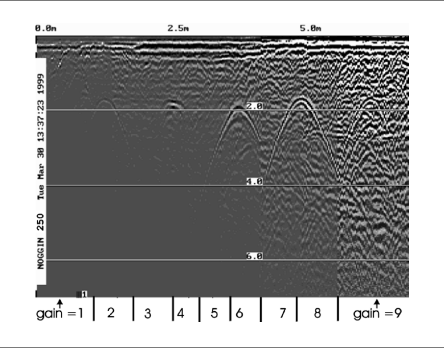
Smart Systems User’s Manual Version 1.1
32
Figure 5-7: Effects of the Gain setting
If the user finds that they are always using very high or very low gain settings to see the
data adequately, the user may want to adjust the Linear Gain setting under Setup (see
Section 5.5.1 – Linear Gain).
5.3.7 Start Menu
The Start button will begin the acquisition of data and displaying of data to the screen.
After acquisition has started, the Start button disappears and a Stop button (used to halt
acquisition) appears on the left. As well, when data acquisition begins, the Exit, Print
and View buttons are removed.
Data acquisition begins by pressing the Start button on the DVL.
Smart Handle systems: On Smart Handle systems, data acquisition can also be started
by quickly pressing the Smart Handle button. When the Smart Handle button has been
pressed, the lights on the handle should change from red to green to indicate that the
system is ready to collect data. The Smart Handle button can also be used to stop data
acquisition (see Section 5.3.8).
When the Start button (or Smart Handle button) is pressed for the first time after the
system is turned on, the Noggin will boot up (this can take about 10 seconds depending
on the software version). The operator should not start data collection until the system
has finished booting (see the bottom left corner of the screen) and the STOP button has

Smart Systems User’s Manual Version 1.1
33
appeared on the left. The current battery voltage will then be displayed on the left side
of the screen. This battery voltage appears only briefly before starting data collection.
Anytime the Start button (or Smart Handle button) is pressed, the current date and time
are written vertically on the screen to indicate the start of a new section (see Section
5.5.1 – Time and Date to set time and date). The position indicator is also reset to
zero. The current date and time can be recorded in a field notebook along with the
survey location to help the user organize where each section of data was collected.
5.3.8 Stop Menu
After the Start button is pressed, it disappears from the menu and the Exit button turns
into a Stop button. Data acquisition can be stopped by pressing the Stop button.
Smart Handle systems: On Smart Handle systems, data acquisition can also be
stopped by pressing the Smart Handle button and holding it pressed for about 1 second
before releasing it. When the Smart Handle button has been pressed like this, the lights
on the handle should change from green to red to indicate that the system has stopped
collecting data.
Using the Smart Handle button, it is possible to start a new line, collect the line,
stop the line and start a new line without having to touch the DVL menu buttons.

Smart Systems User’s Manual Version 1.1
34
5.4 Noggin Data Acquisition
Data acquisition is done simply by pushing the Smart Cart or Smart Handle system
along the survey line. This is usually done with the odometer active, however, it is
possible to turn off the odometer and run the Smart System in continuous operation (see
Section 5.5.1 – Odometer Active).
During data acquisition, the settings for Depth (Section 5.3.5) and Gain (Section 5.3.6)
can be changed by pressing the corresponding button until the desired setting appears.
This can be done while the instrument is collecting data; there is no need to stop first.
5.4.1 Collecting Data using the Odometer
As the Smart System moves, the odometer triggers the system to collect a data trace at
fixed distance intervals. This interval is called the “station interval”. For the Noggin 250,
the normal station interval is 5 centimeters (about 2 inches). For the Noggin 500, the
normal station interval is 2.5 centimeters (about 1 inch). For the Noggin 1000, the normal
station interval is 1.0 centimeter (about 0.48 inch). The station interval can be changed
in the Setup (see Section 5.5.1 – Station Interval).
Each data trace is plotted as a vertical strip on the screen (see Figure 5-1).
For the Noggin 250, each trace is 2 pixels wide. Since the screen is 640 pixels wide,
each screen has 320 traces. When the station interval is set to Normal, each screen
displays 16.0 metres (51.2 feet) of data for the Noggin 250.
For the Noggin 500, each trace is 1 pixel wide. Since the screen is 640 pixels wide,
each screen has 640 traces. When the station interval is set to Normal, each screen
displays 16.0 metres (51.2 feet) of data for the Noggin 500.
For the Noggin 1000, each trace is 1 pixel wide. Since the screen is 640 pixels wide,
each screen has 640 traces. When the station interval is set to Normal, each screen
displays 6.4 metres (25.6 feet) of data for the Noggin 1000.
The maximum number of screens (or buffers) that can be saved on the Digital Video
Logger is 250. This gives a total survey distance of 4000 metres (2.4 miles) for both the
Noggin 250 and Noggin 500. For the Noggin 1000, the total survey distance in 250
screens is 1600 metres (1.2 miles). For more details on total distances and Station
Intervals see Section 5.5.1 – Station Interval.
The odometer units that appear across the top of the screen can be set to either metres
or feet (see Section 5.5.1 – Units).
Smart Systems can normally collect data at a very fast walking pace. However, if the
system is moved too quickly, data quality is reduced (see below).
During data acquisition, the current odometer position value (in the current units, either
metres or feet) is written to the lower right corner of the screen.

Smart Systems User’s Manual Version 1.1
35
Note that Smart systems can be configured to collect data either by pushing the system
(forward) or pulling the system (reverse). See Section 5.5.1 – Cart Direction about
changing the system direction.
The odometer should be periodically re-calibrated to ensure accuracy. The procedure for
re-calibrating the odometer is described in Section 5.5.1 – Odometer Calibration.
Reducing Data Quality by Moving too Fast
On the lower right corner of the data acquisition screen, under the current odometer
position value (see Figure 5-1) is a single digit number that usually displays one (1).
This value is the Repeat Trace number.
If the Smart System is being used with the odometer and is moved too quickly for the
Noggin to keep up, traces are skipped and the quality of the survey is reduced. The
skipped traces do not actually create gaps in the data but rather, the last trace that was
collected properly is repeated. The Repeat Trace number displays the number of traces
that are being plotted to the screen. If this number exceeds 1 or if the user notices the
data looking smeared or “blocky”, this is probably due to moving the Smart System too
quickly. To eliminate this, either reduce the cart speed or, if possible, reduce the Depth
setting (see Section 5.3.5).
Note that skipping traces is not usually a problem because in order for the system to do
this it has to be moving at a running pace. It is more likely to happen if the depth setting
is very deep (> 10 metres).
Backing up the System to Pinpoint Target Positions
The odometer also allows the user to stop the Smart System in the middle of a survey
line and back up. When this is done, an arrow and vertical line appear on the data image
and move back along the image as the system moves backwards (see Figure 5-1). This
makes it possible to correlate a target in the data image to an exact location on the
ground. Once the arrow lines up with the target, mark the ground at the centre point of
the Noggin.
When the Smart System is moved forward again to continue with the survey, it does not
start collecting data again until you reach the position where you stopped at. This feature
is useful for producing a continuous data image even if the system is backed up during
the survey line.
Note that it is not possible to back up and have the arrow indicator move more
than one screen.
Sometimes it may be desirable to back up to a point and then continue collecting data
starting at that point. To do this, reset the odometer by pressing Stop and then Start
again. When the Smart System is moved forward, it will collect data immediately.
The physical position corresponding to the Back-up arrow can be changed from the
centre of the Noggin to any other position. See Section 5.5.1 – Arrow Reference on
changing the Arrow Reference value.

Smart Systems User’s Manual Version 1.1
36
5.4.2 Collecting Data using Continuous Operation (No
Odometer)
It is also possible to turn off the odometer input and have the Noggin system run in
continuous mode (see Section 5.5.1 – Odometer Active). This means that the system
collects data even if it is not moving. This option may be the only way of collecting data
when using an odometer wheel is not practical.
When the odometer is turned off, it is up to the user to keep track of positioning by some
other method, for example, a measuring tape, using fiducial markers (see Section 5.2.2)
or GPS (see Section 5.5.1 – GPS Setup Menu).
In this mode, data collection is dependent on two factors, 1) the speed that the Noggin
system is collecting data and 2) the speed the Noggin system is moving.
When the odometer has been turned off, the user can control the speed the Noggin
collects data by increasing or decreasing the number of stacks (for more details on
Stacking, see Section 6.3.1 - Stacks). Increasing the number of Stacks has the effect of
slowing down the data collection speed Noggin system. Decreasing the number of
Stacks has the effect of speeding up the data collection speed Noggin system.
The speed the Noggin moves determines the distance between sample points on the
ground (station interval). This type of data collection requires experimenting with the
number of stacks (see above) and practicing to find a satisfactory speed for the Noggin.
Moving too quickly may result in under-sampling the data making it more difficult to
interpret. Moving too slowly may result in over-sampling the data. This stretches the
data image making it more difficult to interpret. As well, maintaining a uniform walking
speed is important for minimizing image distortion.
Each data trace is plotted as a vertical strip on the screen. Since the station interval is
not fixed, each screen of data can represent any ground distance.
5.4.3 Saving Data
The user has two options for saving data (see Section 5.5.1 – Save Data Mode):
1) Do not save data, or
2) Save up to 250 screens (or buffers) of data and then prompt user to delete data.
When data are saved on the DVL, it acts like a continuous roll chart up to 250 screens
long. If there are data that need to be permanently saved, make sure they are
transferred to an external computer (see Sections 5.3.2 and 5.6.1) before they are
overwritten.
5.4.4 Deleting Data
The easiest way to delete all the data currently on the DVL is to go to the main menu
and press 3 (see Section 5.6.2).

Smart Systems User’s Manual Version 1.1
37
The user is prompted to delete data when the maximum number of screens (250) has
been reached. When this occurs, the user MUST delete 10%, 25%, 50%, 75% or 100%
of the screens. Note that when less than 100% of the screens are being deleted, the
oldest screens are deleted first.
It is also possible to delete all or some of the current screens of data before 250 have
been collected. To do this, stop the system, press the B button and then follow the
directions to delete 10%, 25%, 50%, 75% or 100% of the screens. Note that when less
than 100% of the screens are being deleted, the oldest screens are deleted first.
5.4.5 Special Keys
A Button = Fiducial Marker
Smart Handle button = Fiducial Marker
During data acquisition, the user can press the A button or, on a the Smart Handle
system, the Smart Handle button to put a fiducial marker on the data (see Section 5.2.2
– Fiducial Markers).
B Button = Background Subtraction Filter:
BEWARE THAT THE BACKGROUND SUBTRACTION PROCESS REMOVES DATA. IT
SHOULD ONLY BE TURNED ON WHEN THIS TYPE OF FILTERING IS NECESSARY.
The background subtraction process has the effect of removing flat-lying events in the
data and enhancing dipping events (like the response from pipes and other point
targets). It can also assist in seeing very shallow targets (< 0.5 meters) that may be
masked by the strong signals at the start of the trace.
Pressing the B button during data acquisition turns on (or off) the Background
Subtraction filter. When it is turned on, the text B-SUB ON is displayed in the lower right
corner of the screen. Stopping data acquisition turns the Background Subtraction filter
off.
5.4.6 Error Messages
If an error occurs, an error message will appear in the bottom left section of the Noggin
screen. EXIT the program and turn off the Digital Video Logger.
Make sure the cables are not damaged and that all cable connections are tightly
secured. Sometimes vibrations cause the cable connections to loosen just a bit and
break contact and this can cause errors. Disconnecting cables and reconnecting them
may provide a better contact and solve the problem. Also check and make sure the
battery is adequately charged. Turn the Digital Video Logger back on and try running the
system again.
For more information on Troubleshooting the system, see Section 7.

Smart Systems User’s Manual Version 1.1
38
5.5 Noggin Setup
5.5.1 Editing DVL Settings
Pressing the number 1 on the main menu selects the SETUP item. SETUP lists the
settings that can be edited in the Noggin software. Pressing the 1 button (labelled NEXT)
moves forward through the list and pressing the 2 button (labelled PREV) moves
backward through the list. To select a setting to edit, press the 3 button (labelled SET).
Then use the numbered buttons to select the new setting or press the A button to exit
without changing the setting. When all the desired changes have been made, press the
8 button (labelled SAVE) to save the new settings and return to the main menu. To
discard the edits and return to the previous settings, press the 7 button (labelled QUIT).
Default Settings
It is possible to change all the settings back to the default settings by pressing the 6
button (labelled RESET).
The SETUP options are outlined below.
Time and Date
The date and time are written to the data image every time data are collected. The DVL
date and time setting can be changed by moving to one or more of the appropriate fields
and editing the current setting. The LEFT and RIGHT arrows are used to move between
fields. To change any of the numbers or months, use the UP and DOWN arrows to
increase or decrease the value. When the desired date and time are set, press ENTER
to save the changes.
Save Data Mode
This setting controls how data are saved on the DVL. The available options are:
1) No saving of data buffer: If data are not saved, then only data currently on the screen
can be seen. As data scrolls off the screen it is gone and cannot be recovered or
viewed. In this case the View button will not appear.
2) Prompt at end of buffer (default): If this setting is selected, after the maximum 250
number of buffers has been reached, the program prompts the user to delete 10%,
25%, 50%, 75% or 100% of the data buffers. The oldest buffers are deleted first.
Units Used
This is the setting for the position and depth units. The available options are:
1) metres (default)
2) feet
3) metres and time
4) feet and time
Options 3 and 4 mean that position will be displayed in metres or feet and depth will

Smart Systems User’s Manual Version 1.1
39
displayed in time (nanoseconds). If time is selected the “depth” lines (Section 5.2.2) are
actually time lines.
Odometer Markers
This setting determines whether a vertical dashed line is put on the data image each
time a position label is written to the screen. The available options are:
1) Place a fid at each label
2) No fids at position labels (default)
Odometer Calibration
The odometer should be calibrated periodically to ensure accuracy.
Noggin Smart Systems can take input from several different odometers.
It is very important that the user selects and calibrates the odometer appropriate
for their Smart System.
When Odometer Calibration is selected from the Setup menu, the user is prompted to
select the odometer that is being used with the Smart System.
If a Smart Cart System is being used, select one of the two Smart Cart odometers
(usually #1).
If a Smart Handle system is being used, select one of the two Smart Handle odometers
(usually #1).
If the system is being towed behind a vehicle and using the transmission odometer to
trigger the system, select one of the two Vehicle odometers (usually #1).
The odometers labelled Other are to be used in future configurations.
Once an odometer is selected, the user is prompted to either 1) manually enter the
odometer calibration factor or 2) to actually calibrate the odometer over a known
distance. To achieve the highest accuracy, it is recommended that the user choose
option number 2 - Odometer Calibration.
When Odometer Calibration is selected, the user is prompted to select the length of the
line to calibrate on. There are 8 different choices in metres and 8 choices in feet. To
toggle the units between metres and feet, press the B button. Pressing the A button on
this screen gives the additional option to select a user defined value. The user-defined
value can range from 0.01 to 5000 metres or 0.01 to 26400 feet.
When the calibration distance has been selected follow the directions on the screen:
1) Set cart at zero and press A
2) Move the cart the selected distance and press B
3) Press A to exit.

Smart Systems User’s Manual Version 1.1
40
Odometer calibration values for the Smart Cart odometer should be around 4000.
Odometer calibration values for the Smart Handle odometer should be around 1500.
Odometer calibration values for the Vehicle odometer vary but may be around 50.
Cart Direction
This setting determines whether data are collected as the Smart System is pushed
forward or pulled in reverse. The back up arrow (see Section 5.4.1) will work in the
direction opposite to this setting. The available options are:
1) Forward (push the cart) (default)
2) Reverse (pull the cart)
Odometer Active
This setting determines whether the odometer is used to collect data. If no, then the
system runs continuously (see Section 5.4.2).
1) Yes (use the odometer) (default)
2) No (operate continuously)
If the user selects to turn the odometer off, another menu screen appears and the user is
then prompted to select the number of stacks for the system to run at. Increasing the
number of stacks has the effect of slowing down the data acquisition speed. Decreasing
the number of stacks has the effect of speeding up the data acquisition speed.
The number of stacks should be set to a value that, when combined with speed the
Noggin is moving at, provides an appropriate station interval. This may take a little
experimenting to determine the optimal values for stacks and Noggin speed.
Label Size
This setting determines the size of the position labels across the top of the data image
and the depth labels beside the horizontal depth lines. The sizes available are:
1) Small
2) Medium (default)
3) Large
4) Extra Large
Noggin System
Noggin Smart Carts can be used with the Noggin 250, 500 and 1000 systems. Noggin
Smart Handle systems can be used with the Noggin 500 and 1000 systems. The
Noggin System should be set to the type of Noggin currently in use on the Smart
System. The systems available are:
1) Noggin 250 System
2) Noggin 500 System
3) Noggin 1000 System
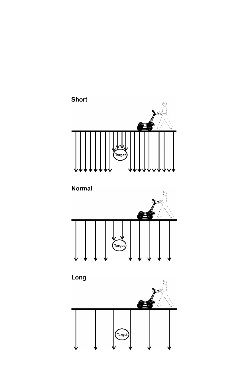
Smart Systems User’s Manual Version 1.1
41
Station Interval
As the Smart Cart moves, the odometer triggers the system to collect a data trace at
fixed distance intervals. This interval is called the “station interval”.
The station interval can be changed to allow a longer or shorter distance between
traces. For a successful survey, it is important that several traces be collected over a
target. If the target is small, the user may want to shorten the station interval to ensure
that data traces are collected over the target. Conversely, if the target is very large or is
a flat-lying feature it is probably not necessary to collect a lot of traces over the target, in
fact, sometimes this can make the target more difficult to see in the data. In this case it
may be beneficial to increase the station interval.
Figure 5-8: The Station Interval is the distance between sample points on the ground. Be careful
not to choose a Station Interval that is larger than the smallest target to be detected.
Smart Systems User’s Manual Version 1.1
42
Note that decreasing the station interval increases the data volume and increasing the
station interval reduces the data volume.
The choices available are:
1) Short
2) Normal
3) Long
4) X-Long
5) Normal x 10
6) Normal x 20
7) Normal x 40
8) Normal x 50
9) Normal x 100
Each choice listed will be followed by an actual value in metres or inches depending on
which units are selected and which Noggin system is being used. Here is a chart
showing the station interval for each system and setting. The choices available are:
Noggin 250 System
Setting
Station Interval Data per Screen Total Data for 250
Screens
Short 2.5 cm or 0.96 in 8 m or 25.6 ft 2 km or 1.2 miles
Normal 5.0 cm or 1.92 in 16 m or 51.2 ft 4 km or 2.4 miles
Long 10.0 cm or 3.84 in 32 m or 102.4 ft 8 km or 4.8 miles
X-Long 25.0 cm or 9.6 in 80 m or 256 ft 20 km or 12.1 miles
Norm x10 50.0 cm or 19.20 in 160 m or 512 ft 40 km or 24.2 miles
Norm x20 100.0 cm or 38.4 in 320 m or 1024 ft 80 km or 48.5 miles
Norm x40 200.0 cm or 76.8 in 640 m or 2048 ft 160 km or 97.0 miles
Norm x50 250.0 cm or 96.0 in 800 m or 2560 ft 200 km or 121.2 miles
Norm x100 500.0 cm or 192.0 in 1600 m or 5120 ft 400 km or 242.4 miles
Noggin 500 System
Setting
Station Interval Data per Screen Total Data for 250
Screens
Short 1.0 cm or 0.48 in 6.4 m or 25.6 ft 1.6 km or 1.2 mile
Normal 2.5 cm or 0.96 in 16 m or 51.2 ft 4 km or 2.4 miles
Long 5.0 cm or 1.92 in 32 m or 102.4 ft 8 km or 4.8 miles
X-Long 12.5 cm or 4.8 in 80 m or 256 ft 20 km or 12.1 miles
Norm x10 25 cm or 9.6 in 160 m or 512 ft 40 km or 24.2 miles
Norm x20 50 cm or 19.2 in 320 m or 1024 ft 80 km or 48.5 miles
Norm x40 100 cm or 38.4 in 640 m or 2048 ft 160 km or 97.0 miles
Norm x50 125 cm or 48.0 in 800 m or 2560 ft 200 km or 121.2 miles
Norm x100 250 cm or 96.0 in 1600 m or 5120 ft 400 km or 242.4 miles

Smart Systems User’s Manual Version 1.1
43
Noggin 1000 System
Setting Station Interval Data per Screen Total Data for 250
Screens
Short 0.5 cm or 0.24 in 3.2 m or 12.8 ft 0.8 km or 0.61 mile
Normal 1.0 cm or 0.48 in 6.4 m or 25.6 ft 1.6 km or 1.2 mile
Long 2.0 cm or 0.96 in 12.8 m or 51.2 ft 3.2 km or 2.4 miles
X-Long 5.0 cm or 2.4 in 32.0 m or 128 ft 8.0 km or 6.1 miles
Norm x10 10 cm or 4.8 in 64.0 m or 256 ft 16.0 km or 12.1 miles
Norm x20 20 cm or 9.6 in 128 m or 512 ft 32.0 km or 24.2 miles
Norm x40 40 cm or 19.2 in 256 m or 1024 ft 64.0 km or 48.5 miles
Norm x50 50 cm or 24.0 in 320 m or 1280 ft 80.0 km or 60.6 miles
Norm x100 100 cm or 48.0 in 640 m or 2560 ft 160 km or 121.2 miles
Note that Noggin 250 traces are plotted on the screen 2 pixels wide while traces from
the Noggin 500 and 1000 are plotted on the screen 1 pixel wide (see Section 5.4.1).
Linear Gain
As described in Section 5.3.6, the weak signals must be amplified or “gained” to see
them on the display. The Gain button described in Section 5.3.6 can be set to a value
from 1 to 9 depending on the amount of gain required (1 is lowest gain, 9 is highest
gain).
There is also a second level of gain available to the user and that is the Linear Gain
setting. The default Linear Gain setting of 2.5 is usually adequate for most ground
conditions, however, if the user finds that they are surveying in areas where high Gain
button settings are always required to see data, it may be advantageous to increase the
Linear Gain setting. Conversely, if the user finds that low Gain button values work to
see the data, it may be useful to decrease the Linear Gain setting.
The choices available for Linear Gain are:
1) 0.0
2) 0.5
3) 1.0
4) 1.5
5) 2.0
6) 2.5 (default)
7) 3.0
8) 5.0

Smart Systems User’s Manual Version 1.1
44
Arrow Reference
Section 5.4.1 describes the Back-up Arrow that appears when a Smart System is
backed up. The Back-up Arrow allows the user to pinpoint the exact ground position
corresponding to a target response on the data image. The Arrow Reference value is
used to change the physical position that corresponds to the Back-up Arrow. If the
Arrow Reference value is set to the default value of zero (0.0) metres, the Back-up arrow
position corresponds with the center point of the Noggin.
However, the Arrow Reference value can be changed so that the Back-up Arrow
corresponds to a position at any offset from the center of the Noggin. For example,
setting the Arrow Reference value to +0.25 meters moves the Back-up Arrow to line up
with a position 25 centimeters in front of the Noggin centre point (on the Noggin 500
Smart Cart this roughly corresponds to the front axle). Setting the Arrow Reference
value to -0.25 meters moves the Back-up Arrow to line up with a position 25 centimeters
in behind the Noggin centre point (on the Noggin 500 Smart Cart this roughly
corresponds to the back axle). In this way, the Arrow Reference value can be changed
to correspond with any position desired by the user.
One reason the user may want to change the Arrow Reference value is so that the
Noggin does not cover the actual target location. This makes it easier to spray paint a
mark or put a flag on the ground where the target occurs.
To change the Arrow Reference value, use the Increase and Decrease buttons. The
Increase button will increment the value by 0.025 meters or 2.5 centimeters. The
Decrease button will decrement the value by 0.025 meters or 2.5 centimeters. Positive
values correspond to positions in front of the Noggin and negative values are positions
behind the Smart Cart. Note that the Arrow Reference value is always expressed in
metres regardless of the settings of the other units. When the Arrow Reference value
has been set, press 4 to save it.
1) Increase
2) Decrease
3) Set to Zero
4) Save and Return
Window Zooming
Window Zooming allows the user to double or half all the default depth settings. For
example, if the Window Zooming is set to the default of 100%, the user may find the five
Depth settings to be 2.5, 5.0, 7.5, 10.0 and 15.0 metres. If the Window Zooming option is
changed to 50% then the Depth settings are reduced to one half, specifically 1.25, 2.5,
3.75, 5.0, and 7.5 metres. Similarly, if The Window Zoom option is set to 200% then the
Depth settings are doubled, specifically 5.0, 10.0, 15.0, 20.0 and 30.0 metres. This
option allows the user to make larger or smaller depth ranges than the default.
The choices available are:
1) 50%
2) 100% (default)
3) 200%

Smart Systems User’s Manual Version 1.1
45
GPS Setup Menu
The Global Positioning System (GPS) uses special satellites around the Earth to
determine the position of a GPS receiver located at any position on the surface of the
Earth. GPS receivers can be purchased from a number of manufacturers.
The DVL has a serial port on the back for attaching a GPS receiver. This port will
accommodate any GPS receiver that has a standard serial port output.
This feature allows GPS information to be logged while collecting Noggin data. The GPS
information may be useful for determining where a specific target of interest is located in
GPS co-ordinates.
The DVL can be set up to read and log GPS information collected during data
acquisition with the Noggin system. GPS information can be logged in two different
ways: 1) to display GPS information on the data image every certain number of data
traces collected by the Noggin system, or 2) to display GPS information on the data
image every time the user presses the A button during data acquisition.
In order for the DVL to read the GPS data string, the GPS settings for the specific GPS
receiver being used must be input into this menu. There are 4 important items that must
be specified correctly for the DVL to display the GPS strings. These items are Baud
Rate, Stop Bits, Data Bits and Parity. These are discussed in more detail below. The
default values listed below are the values that are typically used. Read the GPS
Receiver User’s Guide or experiment with the settings to find the correct ones.
Once these 4 items are set correctly you should be able to run System Test #1 and have
GPS information written to the screen.
When the logging of GPS information is enabled, during data acquisition a message will
appear in the bottom left-hand corner of the DVL screen indicating whether GPS data is
successfully being received (see Section 6.2.4).
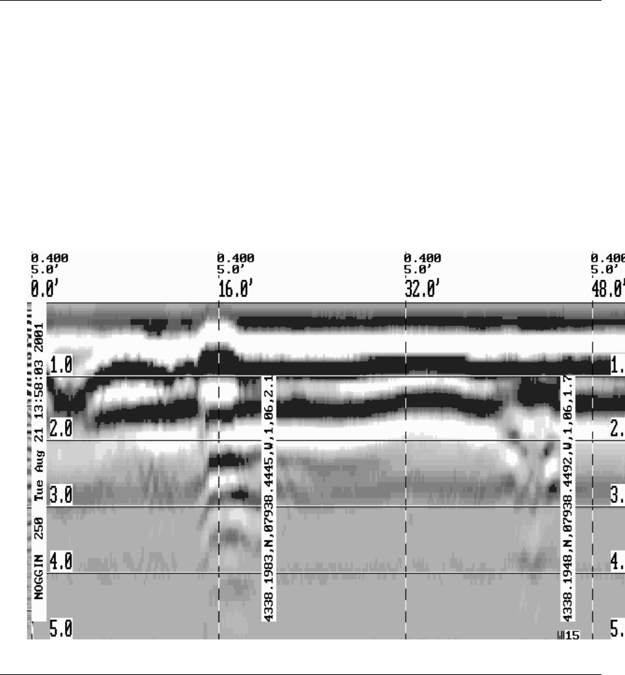
Smart Systems User’s Manual Version 1.1
46
Mode
There are three GPS modes available:
1) Off mode means that a GPS receiver is not connected to the DVL so no GPS
information is being logged. This should be the setting if you do not have a GPS
receiver.
2) Display every X traces mode means that every time the Noggin collects a user-
defined number of traces trace of GPR data, a data string of GPS information will be
written to the data image.
For example, the data may look like this:
Figure 5-9: Noggin Data with GPS information written to the screen every 150 traces
When this option is selected, the user is prompted to enter the number of traces to
collect before the GPS information is written to the data image.
With a Noggin 250 system, there are 320 traces per screen so using a value of 160
traces would ensure that there are 2 GPS positions on each screen.
With a Noggin 500 and Noggin 1000 system, there are 640 traces per screen so
using a value of 320 traces would ensure that there are 2 GPS positions on each
screen.
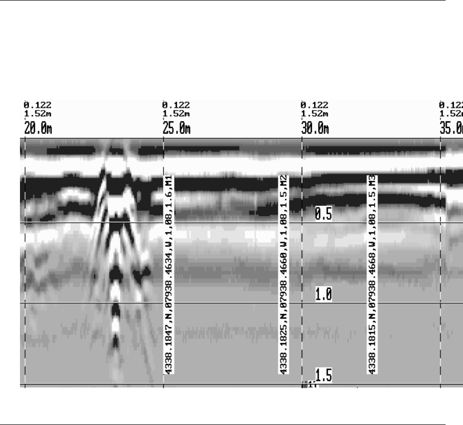
Smart Systems User’s Manual Version 1.1
47
3) Tagging with the A Button mode means that whenever the A button is pressed
during data acquisition, a data string of GPS information will be written onto the data
image.
For example, the data may look like this:
Figure 5-10: Noggin Data with GPS information written to the screen when the A button is
pressed.
Baud Rate
The baud rate is the speed that data is sent from the GPS receiver to the serial port of
the DVL. The available options are: 2400, 4800, 9600 (default) or 19200.
Stop Bits
The available settings for Stop Bits are: 1 (default) or 2.
Data Bits
The available settings for Data Bits are: 7 or 8 (default).
Parity
The available settings for Parity are: none (default), odd or even.

Smart Systems User’s Manual Version 1.1
48
End String
The GPS receiver can be set up to send one or more types of data strings. These
strings are called NMEA-0183 strings and each contains positional or other information
in specific formats. Each type of string is specified by a 5-character prefix. There are
numerous NMEA strings but examples of three different NMEA strings (GPGGA,
GPVTG and GPGSA) are shown below.
$GPGGA,134713.00,4338.221086,N,07938.421365,W,2,06,2.1,152.51,M,-35.09,M,5.0,0118*79
$GPVTG,34.0,T,,,001.4,N,002.5,K,D*70
$GPGSA,A,3,30,26,10,13,24,06,,,,,,,4.2,2.1,3.6*36
$GPGGA,134713.00,4338.221086,N,07938.421365,W,2,06,2.1,152.51,M,-35.09,M,5.0,0118*79
$GPVTG,34.0,T,,,001.4,N,002.5,K,D*70
$GPGSA,A,3,30,26,10,13,24,06,,,,,,,4.2,2.1,3.6*36
$GPGGA,134713.00,4338.221086,N,07938.421365,W,2,06,2.1,152.51,M,-35.09,M,5.0,0118*79
$GPVTG,34.0,T,,,001.4,N,002.5,K,D*70
$GPGSA,A,3,30,26,10,13,24,06,,,,,,,4.2,2.1,3.6*36
$GPGGA,134713.00,4338.221086,N,07938.421365,W,2,06,2.1,152.51,M,-35.09,M,5.0,0118*79
$GPVTG,34.0,T,,,001.4,N,002.5,K,D*70
$GPGSA,A,3,30,26,10,13,24,06,,,,,,,4.2,2.1,3.6*36
Before using the GPS with the Noggin, the DVL software needs to know the prefix of the
LAST string being sent in each group. In the example above, three strings are being
sent each time (GPGGA, GPVTG and GPGSA). Since GPGSA is the last one being
sent in each group, the End String needs to be specified as GPGSA.
To see what the End String is for your particular GPS, run System Test #1 and note the
first 5 characters on the last line after each series of strings is written to the screen.
These are the 5 characters that need to be filled in under End String.
The End String option allows the user to fill in the 5 character GPS prefix. Use the Left
and Right buttons to move left or right to different characters in the string. The currently
selected character will have an “^” under it. To change the letter of the current
character, use the Next button to change it to the next letter in the alphabet and the
Previous button to change it to the previous letter in the alphabet. Using these keys all 5
characters can be filled in with the necessary GPS End String.
See the GPS Receiver User’s Guide for details on how to set up the receiver to output
specific NMEA strings or groups of NMEA strings.
System Test #1
After all the settings above have been input and the GPS receiver is attached to the
serial port on the DVL, the user can test that the DVL is receiving the GPS output by
using the Test option.
If the NMEA strings are successfully being read by the DVL they will appear on the DVL
screen. This is a good time to note the prefix of the last NMEA string in the list and input
it in the End String setting above.
If the NMEA strings do not appear, check that the port settings are correct. It is also
possible that a crossover cable is required between the output cable of the GPS receiver
and the serial port on the DVL.

Smart Systems User’s Manual Version 1.1
49
System Test #2
Once the GPS system is running successfully, System Test #2 can be used to
graphically display the GPS data. This screen displays the GPS Time, Latitude,
Longitude and Altitude as well as other values indicating the accuracy of the GPS
reading. The GPS position is also displayed in a square that can be Zoomed from 2
metres square to 16384 metres square.
Transfer Rate
Transfer Rate is a variable from 1 to 8 that corresponds to the speed of the data transfer
from the Noggin to the DVL. A value of 8 provides the fastest transfer speed while a
value of 1 is the slowest.
For standard Smart Systems like the Smart Cart system and Smart Handle system
the Transfer Rate value must be set to 8.
The Transfer Rate value will only be decreased for systems with data cables longer than
standard lengths. Please contact Sensors & Software before changing the Transfer
Rate on your system.
Reset Counter
The Noggin software records the total distance the cart has travelled. This value is
displayed in Setup but cannot be changed.
The Noggin software also records a distance that can be reset by the user. To reset the
distance counter, move to the Reset Counter option and press the SET button.
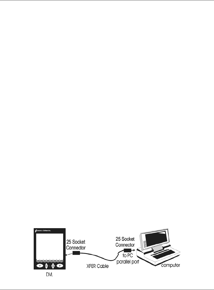
Smart Systems User’s Manual Version 1.1
50
5.6 Noggin Buffer File Management
Files collected with the Noggin system can be transferred to an external computer
(Section 5.6.1) or deleted from the DVL (Section 5.6.2).
5.6.1 Transferring all Buffer Files to an External Computer
using the WinPXFER Program
Pressing the number 2 on the main Noggin menu transfers ALL the data buffers (up to
250 screens) from the DVL to an external computer. This type of transfer allows the user
to view the data on the external computer using the SpiView software. SpiView is
available from Sensors & Software Inc.
There are two ways of transferring data to an external PC. This section describes
transferring all data files to an external computer. The other method is to transfer one or
more screens of data as a single PCX graphics file (see Section 5.3.2, Transferring Data
to an External PC). This other type of transfer is appropriate when the user wants to
transfer a small amount of data to an external computer for use with third-party graphics
software packages like Microsoft Paint and Word.
To transfer all the data buffers from the DVL to an external computer, the computer must
be connected to the DVL using the special parallel XFER cable that is supplied with the
system (Section 5.6.1). Note that this is a special cable and standard 25 pin to 25 pin or
Laplink cables will not work. As well, the computer must have the WinPXFER program
running on it (Section 5.6.1).
Connecting the Digital Video Logger to an External Computer
The Smart Cart comes with a separate cable called the parallel XFER cable. This cable
is designed to connect the DVL to an external computer.
Figure 5-11: Parallel XFER cable connections
The 2 connections that must be made before attempting to transfer data are:
1) Attach the 25 socket parallel connector to the 25 socket parallel port on back of
the Digital Video Logger, and
2) Attach the 25 socket parallel connector the parallel port of the external computer.
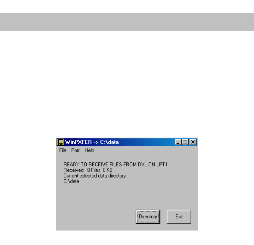
Smart Systems User’s Manual Version 1.1
51
WARNING: To avoid damaging any of the components, turn off the DVL
and computer before making any of these connections.
Installing and Running the WinPXFER Program
The Smart system comes with a CD-ROM containing the WinPXFER program.
To install the WinPXFER program, follow the directions in the “Getting Started”
document that accompanies the CD. Basically, running the SETUP.EXE program from
the WinPXFER folder on the CD will install WinPXFER on the computer.
Once the WinPXFER program has been installed on the computer and the user is ready
to transfer data to the computer, the WinPXFER program needs to be run. This can be
done using the WinPXFER shortcut on the Desktop, double-clicking the WinPXFER.EXE
program in Windows Explorer or pressing Start – Programs – Sensors & Software GPR
and finally WinPXFER.
Figure 5-12: WinPXFER main screen
When the WinPXFER program has been run, it will display a screen as shown in Figure
5-12:
This means that it is ready to receive data transferred from the DVL to the LPT port
number 1.
This command assumes that the data buffers are being transferred across Parallel Port
1 (LPT1). If using Parallel Port 2 (LPT2) or higher (LPT3, LPT4 etc.), specify the parallel
port number under the Port menu item from WinPXFER.
The name of the folder (or directory) that the Noggin data will be transferred into is listed
under the “Current selected data directory”. In the example in Figure 5-12, the data will
be transferred to the c:\data directory. The data directory can be changed by pressing
the Directory button and choosing another directory.

Smart Systems User’s Manual Version 1.1
52
Transferring Buffer Files
Once the parallel XFER cable is connected (Section 5.6.1) and the WinPXFER software
is installed and running (Section 5.6.1), it is now possible to transfer all data buffer files
to the external computer.
On the DVL, from the main menu, select number 2 – TRANSFER ALL BUFFERS.
The data will be transferred from the DVL to the computer and saved in the current
working directory. The progress of the data transfer will be displayed on the DVL screen
and the external computer.
When the data transfer is complete, on the external computer, exit from the WinPXFER
program. Press any button on the DVL to return to the main menu.
Parallel Port not bi-directional Error
Sometimes, when attempting to transfer data to the PC, the error message “LPT1 is not
bi-directional” may appear on the DVL screen. When transferring data from the DVL unit
to a PC, the printer port is used. The WinPXFER program utilizes the functions of a bi-
directional printer port for high-speed data transfer. A bi-directional port allows data to
be sent in both directions over the data lines. Most modern ports are bi-directional;
however, they may not be configured as such and may be configured as ‘output only’.
There are a number of ways the port can be reconfigured depending on the type and
manufacturer of your computer. Most computers configure the port using a BIOS setup
program. Again, different manufactures have different ways to start this program. Some
use the Delete key on boot up, some use the F1 or F2 key on boot up, some have a
special key sequence and others use a program run through DOS or Windows. Often
there is a line of text written to the screen during the boot-up sequence that indicates
which key must be pressed to run Setup. This key MUST be pressed BEFORE
Windows starts. If you miss pressing it, go into Windows, shut down, restart the
computer and try again. Consult your owners’ manual for details.
After the BIOS Setup program starts, the Parallel or Printer port configuration that needs
to be changed is normally under the ‘Peripheral’ or “Advanced” setting heading. If you
can’t find it under these headings, look under the various headings for some setting like
“Parallel Mode” or “Parallel Configuration”. Take note of what the current setting is. The
typical settings are Normal, ECP, EPP and bi-directional. It may require some
experimentation to find the correct setting that works with the WinPXFER program.
First, try changing the setting to bi-directional. Save the settings and exit the Setup
program (usually there is a special key like F10 to do this). Then allow the computer to
continue to boot up. Then, try transferring data again, as described above. If the “LPT1
is not bi-directional” error occurs again, reboot the PC, run the BIOS Setup program,
change the Parallel port setting to EPP, save the settings and try again. The settings
don’t appear standard so no one particular setting will solve the error on all computers.
Keep trying the different parallel port settings until one of them eliminates the error and
allows data transfer.

Smart Systems User’s Manual Version 1.1
53
Viewing SPI Files in SpiView on the External PC
If the buffer data transferred to the external computer are to be viewed using the
SpiView software, all of the data buffer files (SPIxx.PCX) must be copied to the
\SPIVIEW\BUFFERS directory. Any buffer data files in this directory should be moved or
deleted before the new buffer data files are copied. Alternatively, the buffer location can
be changed using the SPI_LOAD.INI file (see the SpiView Manual for details). SpiView
is available from Sensors & Software Inc.
5.6.2 Deleting all Buffer Files on the DVL
Pressing the number 3 on the main menu allows the user to delete ALL the data buffers
(up to 250 screens) currently saved on the DVL.
Before the buffers are deleted, the user is asked, “Do you want to delete all the buffers?”
To answer YES to this question press the A button. To answer NO to the question press
the B button and the buffers are not deleted.
5.7 Upgrades
Pressing the number 4 on the main menu puts the DVL into listen mode to allow a
software upgrade to be transferred from an external PC to the DVL. Avoid pressing this
button until the instructions in a software upgrade tell you to. Once pressed, the DVL
must be powered down exit from this menu item.
Smart Systems User’s Manual Version 1.1
54
5.8 Advanced Topics
5.8.1 How Depth is Determined
Ground penetrating radar systems record the time for a radio wave to travel to a target
and back. The depth to that target is calculated based on the velocity at which the wave
travels to the target and back. It is calculated as:
D = V x T/2
Where D is Depth (m)
V is Velocity (m/ns)
T is Two-way travel time (ns)
The wave velocity depends on the properties of the material. The Noggin software
allows the user to input different velocities, which changes the total depth range
displayed on the screen. The velocities of common materials are:
Material Velocity (m/ns) (ft/ns)
Air 0.3 1
Ice 0.17 0.57
Dry Soil 0.15 0.5
Dry Rock 0.12 0.4
Soil 0.1 0.33
Wet Rock 0.1 0.33
Concrete 0.1 0.33
Pavement 0.1 0.33
Wet Soil 0.065 0.22
Water 0.033 0.11

Smart Systems User’s Manual Version 1.1
55
6 Noggin
plus
6.1 Overview of Noggin
plus
Menu Options
The Nogginplus main menu has the following choices:
A – LINE
B – GRID
1 – NOGGIN PLUS SETUP
2 – FILE MANAGEMENT
3 – RUN WITHOUT SAVING DATA
4 – UTILITIES
7 – RETURN
12.1 V Rev 3.00
6.1.1 Line
Survey lines collected with the Nogginplus are saved as digital data files that can be
viewed on the DVL or exported to an external computer for processing and plotting.
Sensors & Software programs like Win_EKKO, EKKO_Mapper, EKKO_3D and
EKKO_Pointer are available to process and display the data.
Pressing the A button from the main Nogginplus menu takes the user to Line data
collection. This menu allows the user to select a project number and line number to
save each data file to.
Data files from the same area can be organized and saved under a project number
selected by the user. As each individual line is collected, it is given a line number.
These line numbers are usually in sequential order but this is up to the user.
6.1.2 Grid
Survey lines collected with the Nogginplus are saved as digital data files that can be
viewed on the DVL or exported to an external computer for processing and plotting.
Pressing the B button from the main Nogginplus menu takes the user to Grid data
collection.
Grid collection involves collecting data in an organized pattern over an area. This type
of data acquisition allows the GPR data to be displayed as 3D volumes with the
EKKO_3D software or presented as plan maps with the EKKO_Mapper or
EKKO_Pointer software.
The Grid menu allows the user to select a grid number and line number to save each
data file to.

Smart Systems User’s Manual Version 1.1
56
Before the data acquisition on a grid begins, the user must define the size of the area to
be surveyed, the direction of the survey lines and line spacing. The details of the grid
survey are specified in the Grid Setup menu option (see Section 6.3.4).
6.1.3 Setup
There are many background setup parameters related to the Noggin Smart Systems
operation for line and grid surveys that can be edited. This menu allows the user to
display and change various settings for different aspects of the Smart system (see
Section 6.3). The user can also reset all the parameters to the factory default settings.
6.1.4 File Management
The file management option allows Line and Grid data to be downloaded from the DVL
to an external computer via the parallel XFER cable (see Section 6.4.1). This option can
also be used to delete data from the DVL.
6.1.5 Run without Saving Data
This option allows the user to go straight into data acquisition. This feature is to allow a
“quick look” at the data in the area. The data collected when in this mode are NOT saved
and cannot be reviewed later or exported. Data that scrolls off the edge of the screen is
gone and cannot be reviewed.
If a GPS receiver is attached to the DVL, GPS information can be logged to a file even
when the Nogginplus data are not being saved (see Section 6.3.5).
6.1.6 Utilities
This menu has utility programs to change the Date and Time on the DVL (see Section
6.5.1) calibrate the odometer (see Section 6.5.2) and use an external PC to transfer
upgraded software to the DVL (see Section 6.5.3).
6.1.7 Return
This button will return the user to main menu. See Section 3.

Smart Systems User’s Manual Version 1.1
57
6.2 Noggin
plus
Data Acquisition
Selecting the Line, Grid or Run without Saving Data options from the main Nogginplus
menu will start data acquisition. The Run without Saving Option goes straight to data
acquisition while the Line and Grid options require the user to select a project number,
file number and press Run before data acquisition begins.
If the Auto Start option is set to ON (see Section 6.3.2 – Auto Start for details) the
system will automatically boot up and be ready for data acquisition. If Auto Start is set to
OFF the user must press the Start button to boot up the system.
After acquisition has started, the Start button disappears and a Stop button (used to halt
acquisition) appears on the right. A Gain button is also visible as well as the current
depth setting and equivalent Time Window length in nanoseconds (see Figure 6-1).
Data acquisition begins by pressing the Start button on the DVL.
Starting Smart Handle systems: On Smart Handle systems, data acquisition can also
be started by quickly pressing the Smart Handle button. When the Smart Handle button
has been pressed, the lights on the handle should change from red to green to indicate
that the system is ready to collect data. The Smart Handle button can also be used to
stop data acquisition by pressing and holding the button for 1 second before releasing it.
(see Stopping Smart Handle systems below).
When the Start button is pressed for the first time after the unit is turned on, the Noggin
will boot up (this can take up to 30 seconds depending on the software version of the
Noggin). During this time the system is self-calibrating and measuring such factors as
temperature and battery voltage.
Once this boot up has been completed, data acquisition can begin. For subsequent
lines there is only a short delay before data acquisition can begin.
Data acquisition is done by pushing the Smart System along the survey line. During
data acquisition, the Gain button is dynamic and the screen display of the signal
sensitivity can be changed on the go (see Section 6.2.6).
When the survey line is completed press the Stop button to stop data acquisition. At this
point no more data can be collected without starting a new line.
Stopping Smart Handle systems: On Smart Handle systems, data acquisition can also
be stopped by pressing the Smart Handle button and holding it pressed for about 1
second before releasing it. When the Smart Handle button has been pressed like this,
the lights on the handle should change from green to red to indicate that the system has
stopped collecting data.
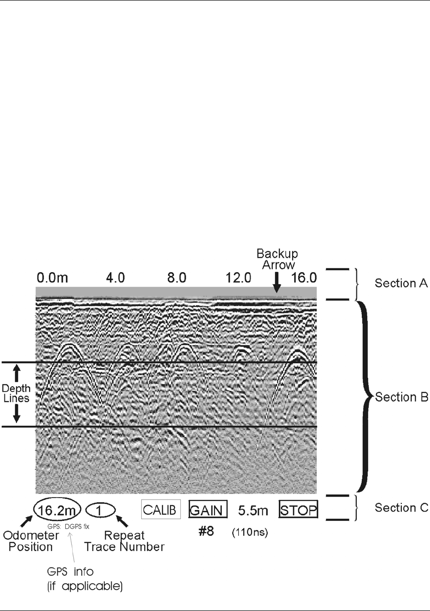
Smart Systems User’s Manual Version 1.1
58
6.2.1 Replaying or Overwriting Data
Immediately after a data file has been collected and the Stop button (or Smart Handle
button) pressed, the data file can be replayed by pressing the left and right arrow buttons
to the scroll the data to the left and right. As well, during data replay, the data can be
enlarged or “zoomed” by pressing the Zoom button and changing the zoom factor. For
example, zooming 2 times on data with a depth setting of 5.0 metres will show the first
2.5 metres of data on the screen.
Any data file that has been collected can be replayed at any time by selecting the file
number and selecting Run. The user then has the option to View, Overwrite or Delete
the data file.
6.2.2 Screen Overview
The data acquisition screen is shown in Figure 6-1. It is divided into 3 sections.
Figure 6-1: Nogginplus Data Acquisition Screen
The Noggin screen is shown in Figure 6-1. It is divided into 3 sections. The very top
section (Section A) positioning information. The center section (Section B) contains the
actual data and the bottom section (Section C) contains the menu.

Smart Systems User’s Manual Version 1.1
59
6.2.3 Section A – Position Information
The very top section (Section A) contains horizontal spatial positioning information in
feet or metres depending on the position units setting (see Section 6.3.1).
6.2.4 Section B - Data Display
This section contains the actual data collected or replayed. The section also contains the
depth indicator lines and any fiducial markers the user enters. See the sections below for
more details.
If a GPS receiver is attached to the DVL, a file containing GPS information can be saved
(see Section 6.3.5).
Depth Lines
Depth lines are horizontal lines indicating the estimated depth. They are very useful for
getting depth estimates to features of interest in the data.
The Depth Lines are controlled by the current velocity value as well as the depth
selected. See Section 6.3.1 on changing the depth setting and for more details on how
depths are determined.
To display the correct depth, it is the responsibility of the user to calibrate the
system to the correct velocity of the material (see Section 6.2.8 on how to
calibrate the system). Once a velocity value has been determined see Section
6.3.1 on how to change the velocity setting.
Note that it is possible to change the depth units between metres and feet (see Section
6.3.1).
Fiducial Markers
A fiducial marker is a dotted vertical line placed on the data section at a specific position
during data acquisition. Adding these markers during data acquisition is useful for
recording significant positions or the positions of surface objects encountered during the
survey.
A fiducial marker is activated by pressing the A button on the keypad during data
acquisition. As well, when using the backup arrow (Section 6.2.7) fiducial markers can
be added at the current arrow location by pressing the A button.
Smart Handle systems: On Smart Handle systems, it is also possible to add a fiducial
marker by quickly pressing the button on the Smart Handle during data acquisition.
The position and name of the object encountered at each marker can be recorded in a
field notebook. The fiducial marker is written to the trace header of the next trace to be
collected. Fiducial markers are numbered sequentially (F1, F2 etc.). When the data are
transferred to a PC and reviewed, these markers can assist with data interpretation.

Smart Systems User’s Manual Version 1.1
60
If a GPS receiver is attached to the DVL, a file containing GPS information can be
saved. In Fuducial Tagging mode, whenever a fiducial marker is added to the data, a
line of GPS information will be added to the GPS file (see Section 6.3.5)
6.2.5 Section C - Menu
The bottom section (Section C) contains the user menu selection and current program
settings. This includes:
1) The total depth (and time window) to the bottom of the data image in
Section B (see Section 6.3.1),
2) The Gain button and current Gain setting (see Section 6.2.6),
3) GPS information (if GPS receiver attached, see below and Section 6.3.5),
4) The current odometer position,
5) The Repeat Trace Number which indicates when the system is being
moved too fast (see Section 6.2.7) and
6) The Calib button for calibrating the velocity setting (see Section 6.2.8).
If a GPS receiver is attached to the DVL (see Section 6.3.5) a message will appear in
the bottom left corner of the menu indicating whether the GPS data is successfully being
logged. The possible messages are:
1) GPS: DGPS fix means differential GPS data are currently being logged.
2) GPS: GPS fix means standard GPS data are currently being logged.
3) GPS: fix not valid means GPS data are NOT currently being logged.
This is usually because GPS satellites are not available.
4) GPS: No Input means the GPS receiver is not operating properly. Check
the settings and test the system (see Section 6.3.5).
5) GPS: No GGA means the GPS receiver is not outputting a GGA NMEA
string that the DVL requires (see Section 6.3.5).
6.2.6 Gain
During data acquisition, the Gain setting can be changed by pressing the Gain button
until the desired setting appears. This can be done while the instrument is collecting
data; there is no need to stop first.
The signals that the Noggin system collects from the ground can be very weak,
especially from deeper objects. To see these weak signals it is necessary to amplify or
apply “gain” to them.
The Gain setting controls how much the signal is amplified. It varies from 1 to 9 with 1
the lowest and 9 the highest. In general, if the target is relatively shallow (1-2 metres) a
low gain value can be used. If the target is deeper or if the screen seems to be blank or
speckled in the lower part of the data section, increase the gain setting. Remember,
however, that if the Noggin signal is not penetrating to the maximum depth setting, even
the maximum gain setting will not show any data.
Figure 6-2 shows the effect of the gain setting. The data on the left has a gain of 1
incrementing to the right up to a gain of 9.
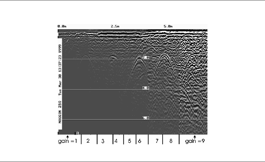
Smart Systems User’s Manual Version 1.1
61
Figure 6-2: Effects of the Gain setting
Note that the gain setting is only for data display. The data are always saved
without any gain applied. It is not possible to collect Nogginplus data with an
“incorrect” gain setting.
If the user finds that they are always using very high or very low gain settings to see the
data adequately, the user may want to adjust the Linear Gain setting under Setup (see
Section 6.3.1).
6.2.7 Collecting Data using the Odometer
As a Smart System moves, the odometer triggers the system to collect a data trace at
fixed distance intervals. This distance is called the “Station Interval”. For the Noggin
250, the normal station interval is 5 centimetres (about 2 inches). For the Noggin 500,
the normal station spacing is 2.5 centimetres (about 1 inch). For the Noggin 1000, the
normal station spacing is 1.0 centimetres (about 0.48 inch). The Station Interval can be
changed to a longer or short distance (see Section 6.3.3).
Each data trace is plotted as a vertical strip on the screen (see Figure 6-1).
For the Noggin 250, each trace is 2 pixels wide. Since the screen is 640 pixels wide,
each screen has 320 traces. When the station interval is set to Normal, each screen
displays 16.0 metres (51.2 feet) of data for the Noggin 250.
For the Noggin 500, each trace is 1 pixel wide. Since the screen is 640 pixels wide,
each screen has 640 traces. When the station interval is set to Normal, each screen
displays 16.0 metres (51.2 feet) of data for the Noggin 500.
For the Noggin 1000, each trace is 1 pixel wide. Since the screen is 640 pixels wide,
each screen has 640 traces. When the station interval is set to Normal, each screen

Smart Systems User’s Manual Version 1.1
62
displays 6.4 metres (25.6 feet) of data for the Noggin 1000.
The odometer units that appear across the top of the screen can be set to either metres
or feet (see Section 6.3.1).
During data acquisition, the current odometer position value (in the current units, either
metres or feet) is written to the lower left corner of the screen (see Figure 6-1).
Note that Smart Systems can be configured to collect data either by pushing or pulling
the Noggin. See Section 6.3.2 about changing the direction of data acquisition.
The odometer should be periodically re-calibrated to ensure accuracy. The procedure for
re-calibrating the odometer is described in Section 6.5.2.
Reducing Data Quality by Moving too Fast
On the lower part of the data acquisition screen, beside the current odometer position
value is a single digit number that usually displays one (1). This value is the Repeat
Trace number.
If the Smart System is being used with the odometer and is moved too quickly for the
Noggin system to keep up, traces are skipped and the quality of the survey is reduced.
The skipped traces do not actually create gaps in the data but rather, the last trace that
was collected properly is repeated. The Repeat Trace number displays the number of
traces that are being plotted to the screen. If this number exceeds 1 or if the user notices
the data looking smeared or “blocky”, this is probably due to moving the cart too quickly.
To eliminate this either slow down the system speed, decrease the number of Stacks or
reduce the Depth setting (see Section 6.3.1).
If the cart is being moved too fast, after the data survey line is complete, the DVL will
indicate the total number of traces that were “skipped”. The user then has the option to
Autofix the data. The Autofix process replaces any repeated traces in the data with
interpolated traces. While this process does not solve the problem of skipping traces, it
will make the data traces look less “blocky”.
If the number of traces skipped is a significant percentage of the total number of traces
collected, i.e. 10% or more, the operator should slow down, decrease the number of
Stacks or reduce the Depth setting (see Section 6.3.1).
Backing up the Cart to Pinpoint Target Positions
The odometer also allows the user to stop the Smart System in the middle of a survey
line and back up. When this is done, an arrow and vertical line appear on the data image
and move back along the image as the system moves backwards (see Figure 6-1). This
makes it possible to correlate a target in the data image to an exact location on the
ground. Once the arrow lines up with the target, mark the ground at the centre point of
the Noggin.
When the system is moved forward again to continue with the survey, the Smart system
does not start collecting data again until you reach the position where you stopped at.

Smart Systems User’s Manual Version 1.1
63
This feature is useful for producing a continuous data image even if the system is
backed up during the survey line.
Note that it is not possible to back up and have the arrow indicator move more than one
screen.
The physical position corresponding to the Back-up arrow is the centre of the Noggin.
This position can be changed from the centre of the Noggin to any other position. See
Section 6.3.2 on changing the Arrow Offset value.
6.2.8 Calib. (Calibration) Menu
Noggin systems can be used to scan into many different materials including soil, rock,
concrete, snow, ice and wood. The radio wave emitted by a Noggin system will travel at
different velocities depending on the material being scanned. The depth value (see
Section 6.3.1) and on Depth Lines (see Section 6.2.4) are only accurate if the system
has been properly calibrated to determine the velocity of the material being scanned.
See Section 6.3.1 - Depth for more details about how depth is calculated.
The Calibration function is a tool for determining the velocity of the material being
scanned. A velocity value can be input directly (see Section 6.3.1 - Velocity) or
determined in one of two different ways depending on the situation:
1) Hyperbola matching
2) Target of known depth
Note that unlike the Calibration with Noggin systems (see Section 5.3.4), the
Nogginplus Calibration does NOT automatically update the velocity value in the
software. In the Nogginplus calibration, once a velocity is determined, the user
must enter it into the System Parameters (see Section 6.3.1 - Velocity).
Hyperbola Matching
This is the most accurate way of determining the velocity of the material being scanned
because it extracts the speed using data collected in the area. This method may not
work in all situations because it depends on having a good quality hyperbola (or inverted
U) in the data. A hyperbola is the characteristic Noggin response from a small point
target like a pipe, rock or even a tree root. If the hyperbola has long tails on it, we can
match the shape of the hyperbola and determine the velocity of the material in the area.
With the hyperbola visible on the DVL screen, select the hyperbola (∩) button. This will
superimpose a hyperbola on the data. This hyperbola can be moved up (), down (),
left () and right () using the appropriate arrow buttons. The goal is move the
hyperbola until it lies on top of the hyperbola in the data (see Figure 6-3). Then, the user
can adjust the width of the hyperbola to make it wider () or narrower () until the
shape of the hyperbola matches the shape of the hyperbola in the data. After matching
the hyperbola, the velocity value is displayed and now can be entered under the System
Parameters (see Section 6.3.1 –Velocity).
Pressing the up, down left, right, wider and narrow buttons once makes a very small
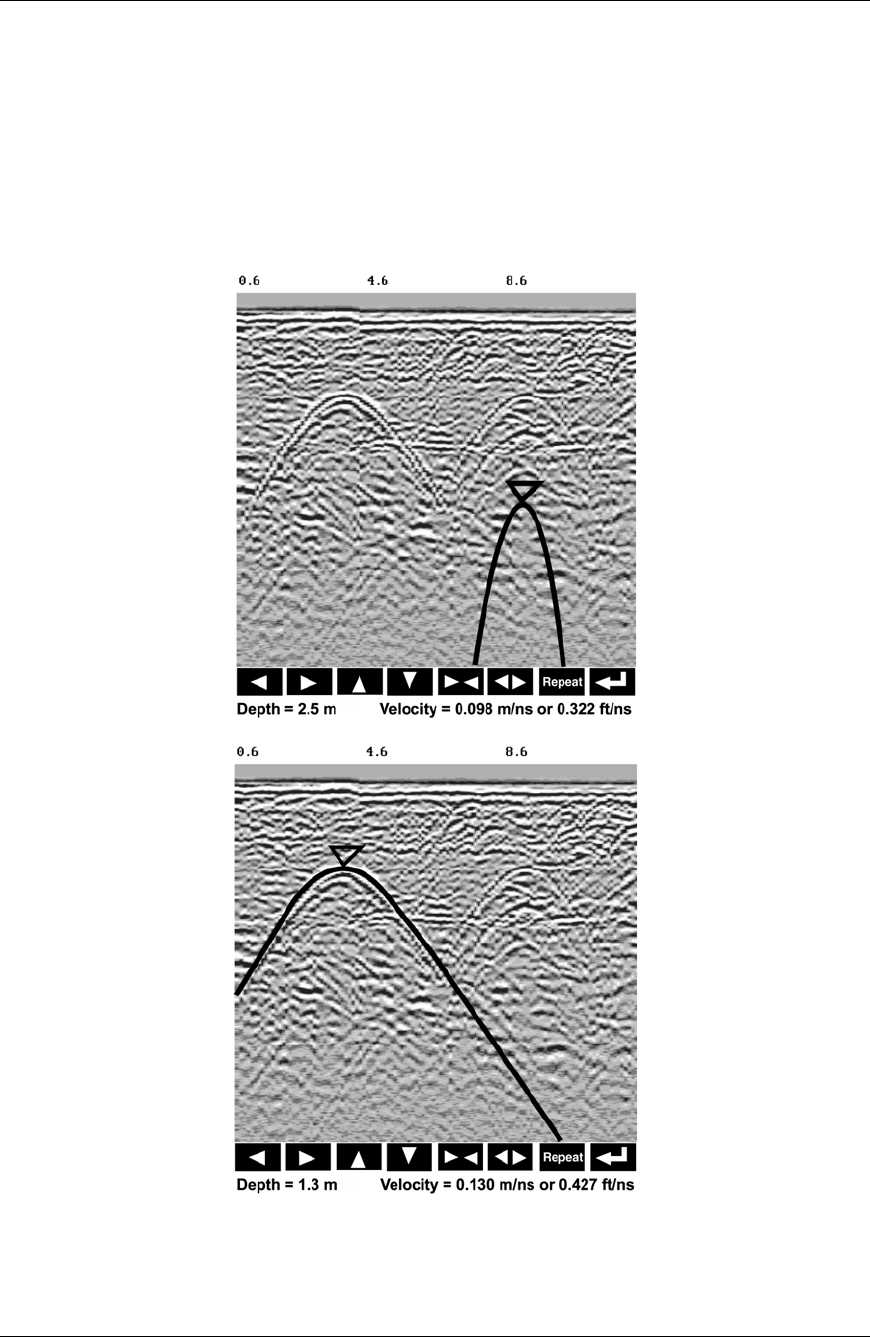
Smart Systems User’s Manual Version 1.1
64
change in the position or width of the hyperbola. These buttons must sometimes be
pressed many times to move the hyperbola to the correct position or width. To speed up
the movement of the hyperbola, use the REPEAT button. For example, to move the
hyperbola up a long distance, press the up button () followed by the REPEAT button.
The hyperbola will then start moving upward without having to press any more buttons.
When it gets close to the desired location press any button to stop it and then use the
up, down, left and right buttons to fine-tune the position. The REPEAT button can also
be used after pressing the wider () or narrower () button.
Figure 6-3: Hyperbola matching to extract velocity. After pressing the CALIB button a hyperbola
appears on the screen (a). This hyperbola should be moved overtop of a hyperbola in the data
using the arrow keys. It can then be widened or narrowed to match the shape of the hyperbola in
the data (b). When the hyperbola shapes match, the velocity is extracted and displayed. The
user can then use this velocity value for surveys done in the area.
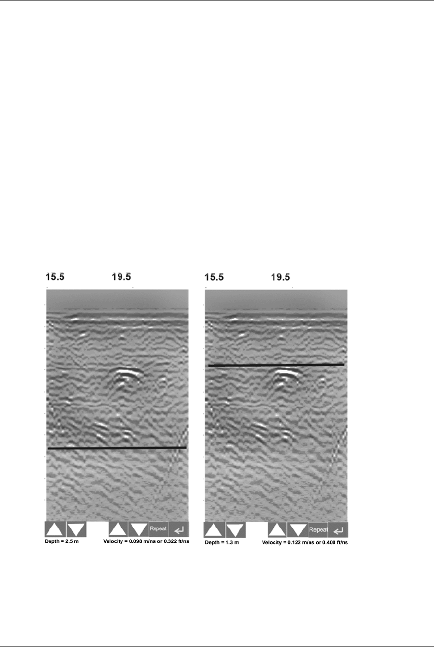
Smart Systems User’s Manual Version 1.1
65
In Nogginplus mode, hyperbola Matching calibration can be done during data acquisition
and also while viewing previously collected data.
If units are metres then depths will appear in metres and velocities in metres per
nanosecond (m/ns). If units are feet then depths will appear in feet and velocities in feet
per nanosecond (ft/ns). To change units see Section 6.3.1 – Depth Units.
Target of Known Depth
If there are no suitable hyperbolas visible in the data to perform the Hyperbola Matching
described above, it may be the situation that there is a target of known depth in the area
being scanned. If this is the case, selecting the button with the circle with a horizontal
line through it will superimpose a horizontal line on the data. This line can then be
moved up or down until it lies on top of the Noggin response to the known target. Then,
the user can adjust the velocity value up or down until the known target depth is correct.
Once the depth is matched, the current velocity value is the one used for all subsequent
data acquisition.
(a) (b)
Figure 6-4: Using a target of known depth to extract velocity. After selecting CALIB, choosing the
known depth button (a circle with a horizontal line through it) will superimpose a horizontal line on
the data (a). Using the depth buttons, this line can then be moved up or down until it lies on top of
the Noggin response to the known target (b). Then, the user can use the velocity buttons to
adjust the velocity value up or down until the known target depth is correct. Once the depth is
matched, the velocity value should be used for all subsequent data acquisition.

Smart Systems User’s Manual Version 1.1
66
If units are metres then depths will appear in metres and velocities in metres per
nanosecond (m/ns). If units are feet then depths will appear in feet and velocities in feet
per nanosecond (ft/ns). To change units see Section 6.3.1 – Depth Units.
6.2.9 Error Messages
If an error occurs during data acquisition, an error message will appear in the bottom left
section of the data acquisition screen. Note the message number, exit the program and
turn off the Digital Video Logger.
Make sure the cables are not damaged and that all cable connections are tightly
secured. Sometimes vibrations cause the cable connections to loosen just a bit and
break contact and this can cause errors. Disconnecting cables and reconnecting them
may provide a better contact and solve the problem. Also check and make sure the
battery is adequately charged. Turn the Digital Video Logger back on and try running the
system again.
For more information on Troubleshooting the system, see Section 7.

Smart Systems User’s Manual Version 1.1
67
6.3 Noggin
plus
Setup
Pressing the number 1 on the main menu selects the Setup item. Setup lists the various
parameters that can be edited. These parameters are organized under the following
headings:
1 - System Parameters
2 - Cart Parameters
3 - Line Parameters
4 - Grid Parameters
5 – GPS Parameters
6 – Set Defaults
To select a setting to edit, press the corresponding number button. Then use the
numbered buttons to select the new setting. It is also possible to change all the settings
back to the factory default settings by pressing the 6 button (labelled Set Defaults).
The SETUP options are outlined below.
6.3.1 System Parameters
The System Parameters settings allow the user to view and modify settings specific to
the data collection of the Noggin system. This includes the type of Noggin system, the
desired depth of investigation, the velocity of the material being surveyed, the units of
depth and position, the number of stacks and the amount of linear gain.
Depth
The depth setting is how deep the radar will try to probe in to the subsurface. It is
important to realize that the depth setting is an estimated value that is dependent on the
velocity of the material being probed.
Ground penetrating radar systems record the time for a radio wave to travel to a target
and back. They do not measure the depth to that target directly. The depth to a target is
calculated based on the velocity at which the wave travels to the target and back. It is
calculated as:
D = V x T/2
Where D is Depth (m)
V is Velocity (m/ns)
T is Two-way travel time (ns)
The Depth units can be changed to metres, feet or time in nanoseconds. For details,
see Depth Units below in this section.
Smart Systems User’s Manual Version 1.1
68
It is important to remember that just because the Depth setting is set to a certain
value, it does not necessarily mean that the Noggin is able to penetrate to that
depth and collect data. For example, if the Depth setting is 5 metres but the
material penetration is only 3 metres the last 2 metres of the image will not
contain subsurface information. Some materials will absorb the Noggin signal and
limit penetration to less than the selected depth.
If the depth setting is deeper than the Noggin signals penetrate, the data in the lower
part of the data screen will look blank or speckled rather than signal with continuity.
Velocity
The wave velocity depends on the properties of the material. The Nogginplus software
allows the user to input a velocity, which changes the total time window collected by the
system.
See Section 6.2.8 for a discussion about determining velocity.
A table of typical radar velocities in various materials is given below. If in doubt, use a
value of 0.10 m/ns. This is a good average velocity that will provide a good estimate of
depth in most situations.
Material Velocity (m/ns) (ft/ns)
Air 0.300 1.000
Ice 0.170 0.558
Dry Soil 0.130 0.427
Dry Rock 0.120 0.394
Soil 0.100 0.328
Wet Rock 0.100 0.328
Concrete 0.100 0.328
Pavement 0.100 0.328
Wet Soil 0.065 0.213
Water 0.033 0.108
If units are metres then velocities will appear in metres per nanosecond (m/ns). If units
are feet then velocities will appear in feet per nanosecond (ft/ns). To change units see
Section 6.3.1 – Depth Units.
The Noggin will accept units in metres/nanosecond or feet/nanosecond depending on
the Depth Units setting.
Depth Units
This is the setting for the units of the horizontal depth lines that appear on the screen.
The available settings are metres, feet or nanoseconds (ns). If nanoseconds are
selected the “depth” lines (see Section 6.2.2) are actually time lines.
1. metres
2. feet
3. nanoseconds

Smart Systems User’s Manual Version 1.1
69
Noggin System
The Noggin System should be set to the type of Noggin currently in use on the Smart
System. The Noggins available are:
1. Noggin 250
2. Noggin 500
3. Noggin 1000
Stacks
Some materials tend to absorb radar signals and limit penetration. These materials are
said to be lossy. When collecting data in lossy areas or areas with a lot of radio
frequency noise, one way of increasing data quality is to collect more than one trace at
each survey position, average them and save the averaged trace. This is known as
“stacking”. Data quality improves because the noise, which is usually random (like white
noise on a TV screen with no station in the area), tends to zero when averaged.
Consequently, the usable signal is easier to see. This is known as increasing the “signal-
to-noise ratio”.
The amount of Stacking can vary from 1 to 2048 by factors of 2.
While stacking improves data quality, it also forces the user to slow down survey
production. The more stacks the longer it takes to collect data at each survey position.
Therefore, it is important to find the lowest number of stacks that still reveal the target
adequately. For most surveys, stacking 4 times is suitable.
See the warning in Section 6.2.7 about losing data if the Smart System is moving too
quickly for the Noggin system to keep up.
Linear Time Gain
As described in Section 6.2.6, the weak signals must be amplified or “gained” to see
them on the display. The Gain button described in Section 6.2.6 can be set to a value
from 1 to 9 depending on the amount of gain required (1 is lowest gain, 9 is highest
gain).
There is also a second level of gain available to the user and that is the Linear Gain
setting. The default Linear Gain setting of 2.0 is usually adequate for most ground
conditions, however, if advanced users find that they are surveying in areas where high
Gain button settings are always required to see data, it may be advantageous to
increase the Linear Gain setting. Conversely, if the user finds that low Gain button
values work to see the data, it may be useful to decrease the Linear Gain setting.
For the experienced user, the setting indicates the gain increases per nanosecond.
The Linear Gain setting can vary from 0.0 to 5.0 in steps of 0.5.

Smart Systems User’s Manual Version 1.1
70
Position Units
This is the setting for the position units used by the odometer. The available options are:
1. metres (default)
2. feet
6.3.2 Cart Parameters
The Cart Parameters settings allow the user to view and modify settings specific to the
Smart Cart or Smart Handle system. This includes the direction the Noggin will move to
collect data, whether or not the odometer is active and whether Auto Start is on or off.
Cart Direction
This setting determines whether data are collected as the Noggin is pushed forward or
pulled in reverse. The back up arrow (see Section 6.2.7) will work in the direction
opposite to this setting. The available options are:
1. Push (default)
2. Pull
Odometer Active
This setting determines whether the odometer is used to collect data. If no, then the
system runs continuously.
1. Yes (use the odometer) (default)
2. No (operate continuously)
Auto Start
If the Auto Start option is set to ON (the default), after the user presses Run to collect a
data line, the system will automatically boot up and be ready for data acquisition, rather
than having the Start button appear. This prevents the user from having to press the
Start button at the start of every new line. This setting is especially useful when
collecting numerous lines as occurs when collecting grid data. If Auto Start is set
to OFF the user must press the Start button to begin data acquisition for each line.
Arrow Offset
Section 6.2.7 describes the Back-up Arrow that appears when the Smart System is
backed up. The Back-up Arrow allows the user to pinpoint the exact ground position
corresponding to a target response on the data image. The Arrow Offset value is used
to change the physical position that corresponds to the Back-up Arrow. If the Arrow
Reference value is set to the default value of zero (0.0) metres, the Back-up arrow

Smart Systems User’s Manual Version 1.1
71
position corresponds with the centre point of the Noggin.
However, the Arrow Offset value can be changed so that the Back-up Arrow
corresponds to a position at any offset from the centre of the Noggin. For example,
setting the Arrow Offset value to +0.25 metres moves the Back-up Arrow to line up with
a position 25 centimetres in front of the Noggin centre point (on the Noggin 500 Smart
Cart this roughly corresponds to the front axle). Setting the Arrow Reference value to -
0.25 metres moves the Back-up Arrow to line up with a position 25 centimetres in behind
the Noggin centre point (on the Noggin 500 Smart Cart this roughly corresponds to the
back axle). In this way, the Arrow Offset value can be changed to correspond with any
position desired by the user.
One reason the user may want to change the Arrow Offset value is to ensure that the
Noggin does not cover the actual target location. This makes it easier to spray paint a
mark or put a flag on the ground where the target occurs.
Positive values correspond to positions in front of the Noggin and negative values are
positions behind the Noggin. Note that the Arrow Offset value is always expressed in
metres regardless of the settings of the other units.
Trip Menu
The software records the total distance the cart has travelled. This value is displayed in
Setup but cannot be changed.
The software also records a distance that can be reset by the user. To reset the
distance counter, move to the Reset Counter option and press the Zero button.
Transfer Rate
Transfer Rate is a variable from 1 to 8 that corresponds to the speed of the data transfer
from the Noggin to the DVL. A value of 8 provides the fastest transfer speed while a
value of 1 is the slowest.
For standard Smart Systems like the Smart Cart system and Smart Handle system
the Transfer Rate value must be set to 8.
The Transfer Rate value will only be decreased for systems with data cables longer than
standard lengths. Please contact Sensors & Software before changing the Transfer
Rate on your system.
Odometer Number
Noggin Smart Systems can take input from several different odometers.
It is very important that the user selects and calibrates the odometer appropriate
for their Smart System.
When Odometer Number is selected, the user is prompted to select the odometer that is
being used with the Smart System.

Smart Systems User’s Manual Version 1.1
72
If a Smart Cart System is being used, select one of the two Smart Cart odometers
(usually #1).
If a Smart Handle system is being used, select one of the two Smart Handle odometers
(usually #1).
If the system is being towed behind a vehicle and using the transmission odometer to
trigger the system, select one of the two Vehicle odometers (usually #1).
The odometers labelled Other are to be used in future configurations.
The number after the odometer is the current Odometer Calibration value for that
odometer. To calibrate the odometer, see Section 6.5.2.
6.3.3 Line Parameters
The Line Parameters settings allow the user to view and modify settings specific to
collecting data as individual lines, namely, the starting position of the line and line
direction.
Start Position
The Start Position is the position value at the very beginning of a line. This will usually
be set to zero (0.0). However, if the user wants a data file to start at a position other
than zero, this value can be edited.
Line Direction
The Line Direction setting specifies which direction that line will be collected, either
Forward or Reverse. Data are usually collected in a forward direction.
If data are collected in the Forward direction the position stepsize is positive, that is, the
position value of each data collection point increments positively. For example, for a
Noggin 250 system, if the Start Position is 10.0 and the Line Direction is Forward, the
positions on the line will increment 10.00, 10.05, 10.10, 10.15 ….
If data are collected in the Reverse direction the position stepsize is negative, that is, the
position value of each data collection point increments negatively. For example, for a
Noggin 250 system, if the Start Position is 10.0 and the Line Direction is Reverse, the
positions on the line will decrement 10.00, 9.95, 9.90, 9.85 ….
Station Interval
As Smart Systems moves, the odometer triggers the system to collect a data trace at
fixed distance intervals. This interval is called the “station interval”.
The station interval can be changed to allow a longer or shorter distance between
traces. For a successful survey, it is important that several traces be collected over a
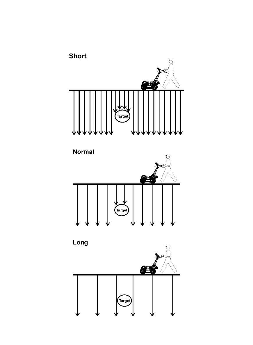
Smart Systems User’s Manual Version 1.1
73
target. If the target is small, the user may want to shorten the station interval to ensure
that data traces are collected over the target. Conversely, if the target is very large or is
a flat-lying feature it is probably not necessary to collect a lot of traces over the target, in
fact, sometimes this can make the target more difficult to see in the data. In this case it
may be beneficial to increase the station interval.
Figure 6-5: The Station Interval is the distance between sample points on the ground. Be careful
not to choose a Station Interval that is larger than the smallest target to be detected.
Note that decreasing the station interval increases the data volume and increasing the
station interval reduces the data volume.
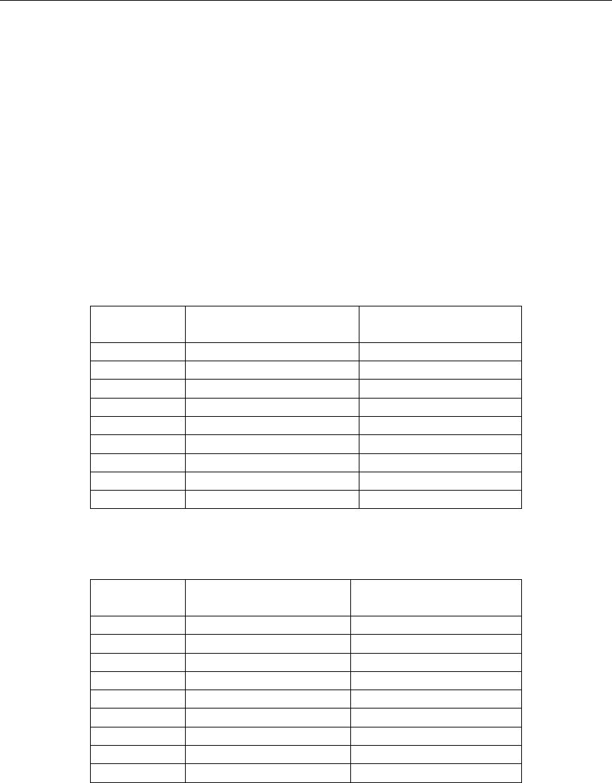
Smart Systems User’s Manual Version 1.1
74
The choices available are:
1) Short
2) Normal
3) Long
4) X-Long
5) 10x Normal
6) 20x Normal
7) 40x Normal
8) 50x Normal
9) 100x Normal
Here is a chart showing the station interval for each system and setting. The choices
available are:
Noggin 250 System
Setting
Station Interval Data per Screen
Short 2.5 cm or 0.96 in 8 m or 25.6 ft
Normal 5.0 cm or 1.92 in 16 m or 51.2 ft
Long 10.0 cm or 3.84 in 32 m or 102.4 ft
X-Long 25.0 cm or 9.6 in 80 m or 256 ft
Norm x10 50.0 cm or 19.20 in 160 m or 512 ft
Norm x20 100.0 cm or 38.4 in 320 m or 1024 ft
Norm x40 200.0 cm or 76.8 in 640 m or 2048 ft
Norm x50 250.0 cm or 96.0 in 800 m or 2560 ft
Norm x100 500.0 cm or 192.0 in 1600 m or 5120 ft
Noggin 500 System
Setting
Station Interval Data per Screen
Short 1.0 cm or 0.48 in 6.4 m or 25.6 ft
Normal 2.5 cm or 0.96 in 16 m or 51.2 ft
Long 5.0 cm or 1.92 in 32 m or 102.4 ft
X-Long 12.5 cm or 4.8 in 80 m or 256 ft
Norm x10 25 cm or 9.6 in 160 m or 512 ft
Norm x20 50 cm or 19.2 in 320 m or 1024 ft
Norm x40 100 cm or 38.4 in 640 m or 2048 ft
Norm x50 125 cm or 48.0 in 800 m or 2560 ft
Norm x100 250 cm or 96.0 in 1600 m or 5120 ft
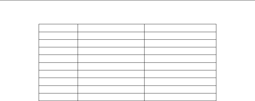
Smart Systems User’s Manual Version 1.1
75
Noggin 1000 System
Setting Station Interval Data per Screen
Short 0.5 cm or 0.24 in 3.2 m or 12.8 ft
Normal 1.0 cm or 0.48 in 6.4 m or 25.6 ft
Long 2.0 cm or 0.96 in 12.8 m or 51.2 ft
X-Long 5.0 cm or 2.4 in 32.0 m or 128 ft
Norm x10 10 cm or 4.8 in 64.0 m or 256 ft
Norm x20 20 cm or 9.6 in 128 m or 512 ft
Norm x40 40 cm or 19.2 in 256 m or 1024 ft
Norm x50 50 cm or 24.0 in 320 m or 1280 ft
Norm x100 100 cm or 48.0 in 640 m or 2560 ft
Note that Noggin 250 traces are plotted on the screen 2 pixels wide while traces from
the Noggin 500 and 1000 are plotted on the screen 1 pixel wide (see Section 6.2.7).
6.3.4 Grid Parameters
The Grid Parameters settings allow the user to view and modify settings specific to
collecting data in organized grids. This includes the grid dimensions, line spacing, grid
type and survey format.
Data are normally collected on a grid if the user is interested in displaying the data as a
3D volume (using the EKKO_3D software) or as a plan map (using the EKKO_Mapper
and/or EKKO_Pointer software). Producing accurate 3D volumes or plan maps is easier
if the field survey is properly designed and data are collected correctly.
Positional accuracy of each line is vital if the user wants to be able to relocate targets of
interest after the data have been processed.
For linear targets like pipes and utilities, the best GPR response occurs when the GPR
survey line crosses the target at right angles. If possible, it is always best to run GPR
survey lines perpendicular to the direction of linear targets.
Grid Type
The Grid Type asks specifically the way that the area of the grid is to be covered by the
survey lines. Survey lines can be either a set of parallel lines in the X axis direction
(Figure 6-6), a set of parallel lines in the Y axis direction (Figure 6-7), or, for complete
coverage, parallel lines in both the X and Y direction (Figure 6-8).
X Lines Only - Forward
Set up a first-quadrant XY grid. Data lines run in the X direction, distance increasing
from the Y axis baseline. Line numbers increase in the positive Y direction (see Figure
6-6). Lines must be equally spaced. It is not critical that all the lines are the same
length. However, it does make processing easier if all the lines start at the same
baseline position (usually defined as zero (0.0)).
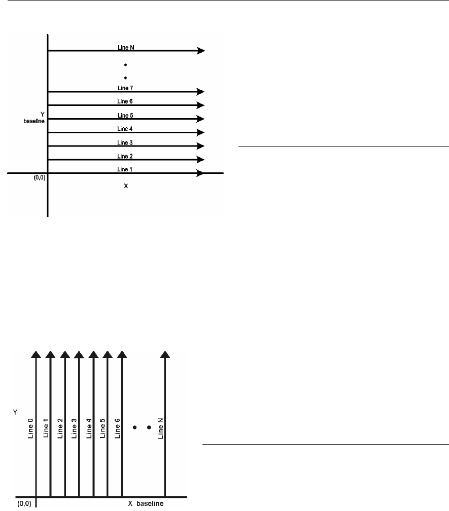
Smart Systems User’s Manual Version 1.1
76
Figure 6-6: Proper X Line surveying pattern.
Following this pattern and starting each line
from the same baseline minimizes the data
editing required to produce a spatially
accurate map of GPR data.
Y Lines Only - Forward
Set up a first-quadrant XY grid. Data lines run in the Y direction, distance increasing
from the X axis baseline. Line numbers increase in the positive X direction (see Figure
6-7). Lines must be equally spaced. It is not critical that all the lines are the same
length. However, it does make processing easier if all the lines start at the same
baseline position (usually defined as zero (0.0)).
Figure 6-7: Proper Y Line surveying pattern.
Following this pattern and starting each line from the
same baseline minimizes the data editing required to
produce a spatially accurate map of GPR data.
XY Lines - Forward
Set up a first-quadrant XY grid. X data lines run in the X direction, distance increasing
from the Y axis baseline. Line numbers increase in the positive Y direction (see Figure
6-8). Lines must be equally spaced. Y data lines run in the Y direction, distance
increasing from the X axis baseline. Line numbers increase in the positive X direction.
Lines should be equally spaced. The line spacing of the X lines and Y lines can be
different.
It is not critical that all the lines are the same lengths. However, it does make
processing easier if all the lines start at the same baseline position (usually defined as
zero (0.0)).
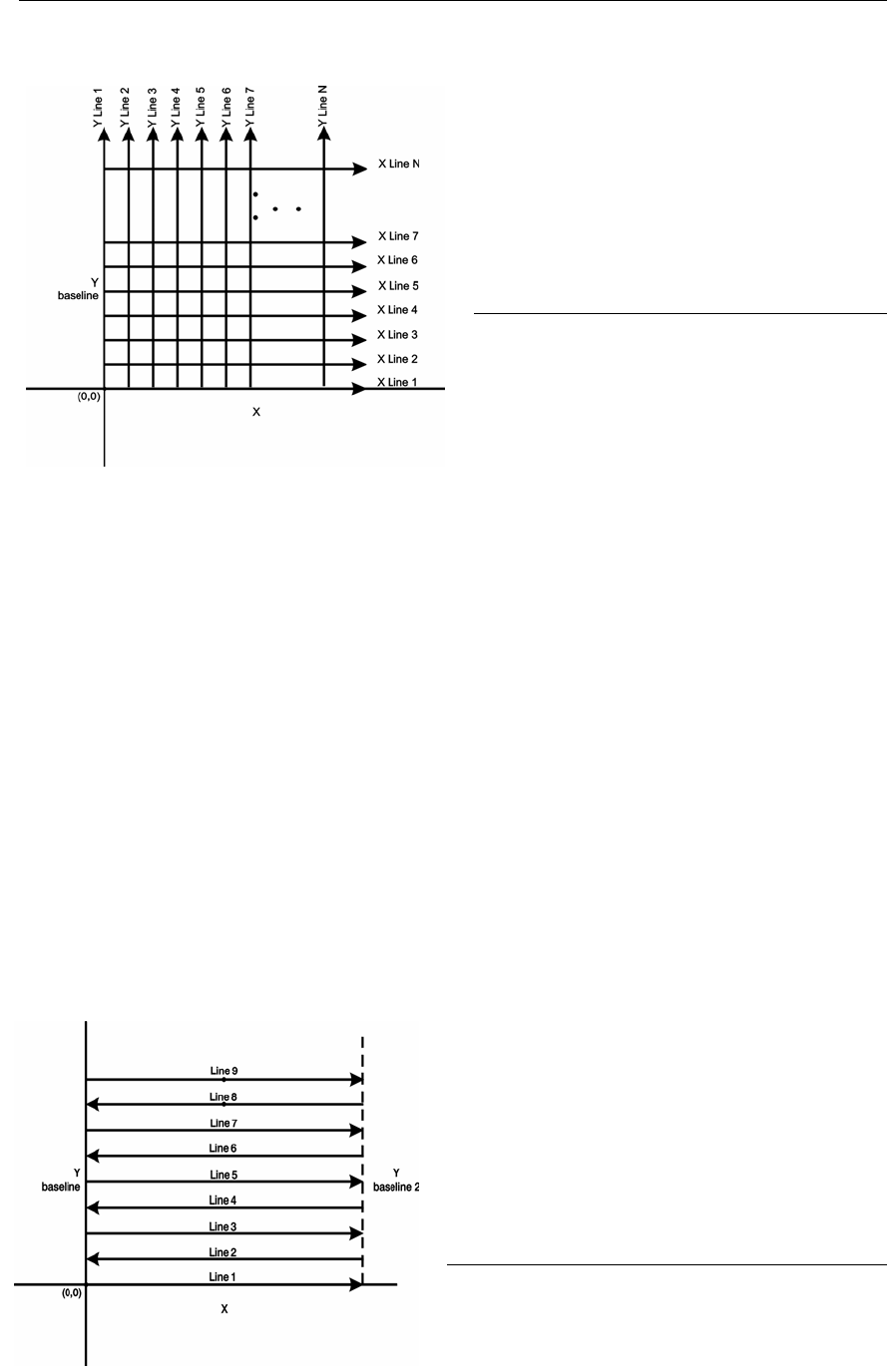
Smart Systems User’s Manual Version 1.1
77
Figure 6-8: Proper XY grid surveying pattern.
Following this pattern and starting each line
from the same baseline minimizes the data
editing required to produce a spatially
accurate map of GPR data
Survey Format
The Survey Format specifies how the lines will be collected. The lines shown in Figure
6-6, Figure 6-7, and Figure 6-8 are all collected in the Forward direction only. This
means that each line starts at the X or Y baseline.
When the length of the survey lines are more than about 20 metres, data acquisition
speed may be increased by collecting every second line in the reverse direction (Figure
6-9, Figure 6-10, and Figure 6-11). This is called a Forward and Reverse survey format.
Using forward and reverse format can speed acquisition but can lead to mapping
artifacts called “herringbone” if there are positional errors. It is important that the
odometer is calibrated (Section 6.5.2) and that the Grid Dimensions are correct (Section
6.3.4 – Grid Dimensions).
X Lines Only – Forward and Reverse
Using the Forward and Reverse survey format, X line data are collected in the pattern
shown in Figure 6-9.
Figure 6-9: For collecting GPR data consisting of
long data lines it makes more sense to follow a
forward and reverse surveying pattern. For the
final data to be spatially correct with a minimum
of editing, data collected in this pattern should be
on lines that extend completely from one
baseline to the other.
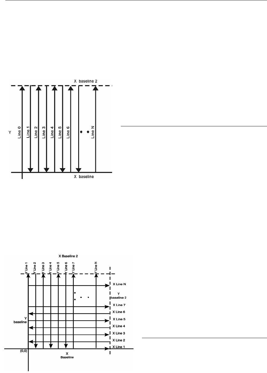
Smart Systems User’s Manual Version 1.1
78
Y Lines Only – Forward and Reverse
Using the Forward and Reverse survey format, Y line data are collected in the pattern
shown in Figure 6-10.
When data are collected like this, it is important that lines start and end on established
baselines, otherwise, when lines are reversed to the correct orientation for the display,
they may be offset from one another.
Figure 6-10: For collecting GPR data consisting of
long data lines it makes more sense to follow a
forward and reverse surveying pattern. For the final
data to be spatially correct with a minimum of editing,
data collected in this pattern should be on lines that
extend completely from one baseline to the other.
XY Lines – Forward and Reverse
Using the Forward and Reverse survey format, XY line data are collected in the pattern
shown in Figure 6-11.
When data are collected like this, it is important that lines start and end on established
baselines, otherwise, when lines are reversed to the correct orientation for the display,
they may be offset from one another.
Figure 6-11: For collecting GPR data on a grid
consisting of long data lines, it makes more
sense to follow a forward and reverse
surveying pattern. For the final data to be
spatially correct with a minimum of editing,
data collected in this pattern should be on
lines that extend completely from one
baseline to the other.

Smart Systems User’s Manual Version 1.1
79
Grid Dimensions
For grid data acquisition, the grid size needs to be specified. The user needs to input
the length of the X dimension and the length of the Y dimension. The dimensions
entered are assumed to be in the same units as the Position Units (see Section 6.3.1),
i.e. metres or feet.
On this screen the user needs to highlight the dimension to be changed. The user can
toggle between the X and Y fields by pressing the X/Y button.
The dimension value is incremented or decremented by pressing the +Line or –Line
buttons. The dimension value will change by a value equal to the current Line Spacing
in that dimension.
For example, if the Line Spacing (see below) in the X direction is 0.5 metres, the grid
dimension in the X direction will increment or decrement in 0.5 metre intervals.
Note that the maximum number of lines that can be collected in each direction is
100. Therefore, the X and Y grid dimensions cannot be set to a value that will
result in more than 100 lines being collected.
For example, if the Line Spacing between Y lines (defined as lines parallel to the Y axis)
is set to 0.25 metres, the maximum X dimension is (100-1) X 0.25 = 24.75 metres. (One
is subtracted because the first line is at position 0.0 metres.)
To increase the X dimension value, the Y line spacing must be increased. Using the
example above, if the Y Line Spacing is increased to 0.30 metres then the maximum X
dimension is (100-1) X 0.30 = 29.70 metres.
If the Grid Type is set to X Lines only or Y Lines only (see Section 6.3.4), the length of
those lines are not restricted by the Line Spacing parameter of the opposite dimension.
That is why if an X Lines only grid is selected, the X dimension can be input as a value
rather than an increment of the Y Line Spacing. Similarly, if a Y Lines only grid is
selected, the Y dimension can be input as a value rather than an increment of the X Line
Spacing.
Line Spacing
For grid data acquisition, the distance between survey lines needs to be specified.
If the grid type is X Lines only (see Section 6.3.4) then the spacing between the X lines
needs to be input.
If the grid type is Y Lines only (see Section 6.3.4) then the spacing between the Y lines
needs to be input.
If the grid type is XY Lines (see Section 6.3.4) then the spacing between the X lines and
Y lines need to be input. The line spacing can be different. The user can toggle between
the X line spacing and Y line spacing fields by pressing the X/Y button.

Smart Systems User’s Manual Version 1.1
80
Note that the maximum number of lines that can be collected in each direction is
100.
The calculation for determining an appropriate line spacing is complex. One has to
consider system frequency, target size and practical considerations. In general, the
Noggin 250 should have a line spacing of 0.5 metres or less, the Noggin 500 should
have a line spacing of 0.25 metres or less and the Noggin 1000 should have a line
spacing of 0.10 metres or less.
However, line spacing should really be determined by target size. In most cases the
system must pass over a target to detect it. Therefore, the line spacing needs to be on
the order of the size of the target or smaller, if practical. This can be adjusted to a larger
spacing for larger targets or targets with a linear extent. As well, these rules may have
to be bent for practical purposes like survey production rates. The fact is that a tighter
line spacing takes longer to collect and this may not be economically possible in all
circumstances.
6.3.5 GPS Parameters
The Global Positioning System (GPS) uses special satellites around the Earth to
determine the position of a GPS receiver located at any position on the surface of the
Earth. GPS receivers can be purchased from a number of manufacturers.
The DVL has a serial port on the back for attaching a GPS receiver. This port will
accommodate any GPS receiver that has a standard serial port output.
This feature allows GPS information to be logged while collecting Nogginplus data. The
GPS information may be useful for mapping where GPR surveys have been performed
(see Reading per Trace mode below) or determining where a specific target of interest is
located in GPS co-ordinates (see Fiducial Tagging mode below).
The DVL can be set up to read and log GPS information collected during data
acquisition with the Nogginplus system. GPS information can be logged in two different
ways: 1) for every trace collected by the Nogginplus system, or 2) every time the user
adds a fiducial to the data by pressing the A button (see Section 6.2.4 – Fiducial
Markers).
This feature provides a means of logging GPS information to an independent file. Note
that the GPS information is NOT automatically integrated with the Nogginplus data.
After data acquisition is complete, the data can be downloaded to a PC and the
Win_EKKO_Pro software can be used to integrate the GPS data with the Nogginplus
data.
In order for the DVL to read the GPS data string, the GPS settings for the specific GPS
receiver being used must be input into this menu. There are 4 important items that must
be specified correctly for the DVL to display the GPS strings. These items are Baud
Rate, Stop Bits, Data Bits and Parity. These are discussed in more detail below. The
default values listed below are the values that are typically used. Read the GPS
Receiver User’s Guide or experiment with the settings to find the correct ones.

Smart Systems User’s Manual Version 1.1
81
Once these 4 items are set correctly you should be able to run System Test #1 and have
GPS information written to the screen.
When the logging of GPS information is enabled, during data acquisition a message will
appear in the bottom left-hand corner of the DVL screen indicating whether GPS data is
successfully being received (see Section 6.2.4).
Mode
There are three GPS modes available:
1) Off mode means that a GPS receiver is not connected to the DVL so no GPS
information is being logged. This should be the setting if you do not have a GPS
receiver.
2) Reading every x traces mode means that every time the Nogginplus collects a
user-defined number of traces of GPR data, a data string of GPS information will
be added to a file. This file has the same name as the data file i.e. LINE6, but with
a GPS extension. This file can be accessed after transferring the GPR data files to
an external PC (see Section 6.4.1).
For example, if the number of traces is set to 1, the LINE6.GPS may look like this:
Trace #1
$GPGGA,134713.00,4338.221086,N,07938.421365,W,2,06,2.1,152.51,M,-35.09,M,5.0,0118*79
$GPVTG,34.0,T,,,001.4,N,002.5,K,D*70
$GPGSA,A,3,30,26,10,13,24,06,,,,,,,4.2,2.1,3.6*36
Trace #2
$GPGGA,134713.00,4338.221086,N,07938.421365,W,2,06,2.1,152.51,M,-35.09,M,5.0,0118*79
$GPVTG,34.0,T,,,001.4,N,002.5,K,D*70
$GPGSA,A,3,30,26,10,13,24,06,,,,,,,4.2,2.1,3.6*36
Trace #3
$GPGGA,134713.00,4338.221086,N,07938.421365,W,2,06,2.1,152.51,M,-35.09,M,5.0,0118*79
$GPVTG,34.0,T,,,001.4,N,002.5,K,D*70
$GPGSA,A,3,30,26,10,13,24,06,,,,,,,4.2,2.1,3.6*36
Trace #4
$GPGGA,134713.00,4338.221086,N,07938.421365,W,2,06,2.1,152.51,M,-35.09,M,5.0,0118*79
$GPVTG,34.0,T,,,001.4,N,002.5,K,D*70
$GPGSA,A,3,30,26,10,13,24,06,,,,,,,4.2,2.1,3.6*36
Note that when the Reading per Trace option is on, it is still possible to add fiducial
markers to the GPS file. These will appear as F1, F2 etc. between the trace
numbers. For example, a portion of LINE6.GPS may look like this:
Trace #85
$GPGGA,134850.00,4338.204868,N,07938.429003,W,2,06,2.1,152.60,M,-35.09,M,4.2,0118*74
$GPVTG,152.6,T,,,002.3,N,004.3,K,D*43
$GPGSA,A,3,30,26,10,13,24,06,,,,,,,4.2,2.1,3.7*37
F1
$GPGGA,134850.00,4338.204868,N,07938.429003,W,2,06,2.1,152.60,M,-35.09,M,4.2,0118*74
$GPVTG,152.6,T,,,002.3,N,004.3,K,D*43
$GPGSA,A,3,30,26,10,13,24,06,,,,,,,4.2,2.1,3.7*37
Trace #86
$GPGGA,134851.00,4338.204362,N,07938.428362,W,2,06,2.1,152.40,M,-35.09,M,5.2,0118*72
$GPVTG,136.9,T,,,002.8,N,005.2,K,D*45
$GPGSA,A,3,30,26,10,13,24,06,,,,,,,4.2,2.1,3.7*37
3) Fuducial Tagging mode means that whenever a fiducial marker (F1, F2 etc.) is
added to the data (see Section 6.2.4), a data string of GPS information will be added
to a file. This file has the same name as the data file i.e. LINE6, but with a GPS
extension. This file can be accessed after transferring the GPR data files to an

Smart Systems User’s Manual Version 1.1
82
external PC (see Section 6.4.1).
For example, LINE6.GPS may look like this:
F1
$GPGGA,134218.00,4338.190204,N,07938.438411,W,2,05,2.6,154.60,M,-35.09,M,4.0,0118*7B
$GPVTG,356.8,T,,,000.2,N,000.4,K,D*4B
$GPGSA,A,3,30,10,13,24,06,,,,,,,,4.3,2.6,3.4*36
F2
$GPGGA,134219.00,4338.190294,N,07938.438409,W,2,05,2.6,154.45,M,-35.09,M,5.0,0118*7C
$GPVTG,1.3,T,,,000.4,N,000.7,K,D*44
$GPGSA,A,3,30,10,13,24,06,,,,,,,,4.3,2.6,3.4*36
F3
$GPGGA,134221.00,4338.190261,N,07938.438285,W,2,05,2.6,154.05,M,-35.09,M,5.2,0118*79
$GPVTG,10.0,T,,,000.2,N,000.4,K,D*72
$GPGSA,A,3,30,10,13,24,06,,,,,,,,4.3,2.6,3.4*36
F4
$GPGGA,134222.00,4338.190397,N,07938.438255,W,2,05,2.6,153.95,M,-35.09,M,5.0,0118*73
$GPVTG,9.8,T,,,000.3,N,000.5,K,D*42
$GPGSA,A,3,30,10,13,24,06,,,,,,,,4.3,2.6,3.4*36
If the GPS mode is set to Reading per Trace or Fiducial Tagging AND the Nogginplus
is Run Without Saving Data (see Section 6.1.5), it is still possible to log GPS data
strings. Every time a fiducial marker is added to the data (see Section 6.2.4), a data
string of GPS information is added to a file. This file is called TAGGED.GPS and can
be exported and/or deleted using the Nogginplus File Management (see Section 6.4).
An example of a TAGGED.GPS file is shown below.
New File 09-18-2000 13:53:38
F1
$GPGGA,134227.00,4338.190520,N,07938.438280,W,2,05,2.6,153.98,M,-35.09,M,4.6,0118*7E
$GPVTG,347.7,T,,,000.3,N,000.5,K,D*44
$GPGSA,A,3,30,10,13,24,06,,,,,,,,4.3,2.6,3.4*36
F2
$GPGGA,134228.00,4338.190238,N,07938.438286,W,2,05,2.6,153.87,M,-35.09,M,4.4,0118*75
$GPVTG,5.4,T,,,000.2,N,000.4,K,D*42
$GPGSA,A,3,30,10,13,24,06,,,,,,,,4.3,2.6,3.4*36
F3
$GPGGA,134229.00,4338.190277,N,07938.438273,W,2,05,2.6,153.76,M,-35.09,M,5.4,0118*7A
$GPVTG,23.4,T,,,000.1,N,000.2,K,D*73
$GPGSA,A,3,30,10,13,24,06,,,,,,,,4.3,2.6,3.4*36
F4
$GPGGA,134231.00,4338.190127,N,07938.438362,W,2,05,2.6,154.59,M,-35.09,M,5.0,0118*7A
$GPVTG,20.2,T,,,000.2,N,000.3,K,D*74
$GPGSA,A,3,30,10,13,24,06,,,,,,,,4.3,2.6,3.4*36
********************************************************************************
New File 09-18-2000 13:55:36
F1
$GPGGA,134259.00,4338.192453,N,07938.449096,W,2,06,2.4,153.14,M,-35.09,M,5.4,0118*75
$GPVTG,310.9,T,,,000.5,N,001.0,K,D*4A
$GPGSA,A,3,04,30,10,13,24,06,,,,,,,3.2,2.4,2.1*32
F2
$GPGGA,134301.00,4338.192559,N,07938.449176,W,2,06,2.4,153.17,M,-35.09,M,5.0,0118*7A
$GPVTG,314.4,T,,,000.6,N,001.1,K,D*41
$GPGSA,A,3,04,30,10,13,24,06,,,,,,,3.2,2.4,2.1*32
F3
4) GPR data out port mode means that the GPR data stream will be output to the
serial port of the DVL. This is for users who wish to read the GPR data into their own
PC or other device. Contact Sensors & Software Inc. for more details if you want to
use this option.
Note that this option slows down data acquisition speeds.

Smart Systems User’s Manual Version 1.1
83
Baud Rate
The baud rate is the speed that data is sent from the GPS receiver to the serial port of
the DVL. The available options are: 2400, 4800, 9600 (default) or 19200.
Stop Bits
The available settings for Stop Bits are: 1 (default) or 2.
Data Bits
The available settings for Data Bits are: 7 or 8 (default).
Parity
The available settings for Parity are: none (default), odd or even.
End String
The GPS receiver can be set up to send one or more types of data strings. These
strings are called NMEA-0183 strings and each contains positional or other information
in specific formats. Each type of string is specified by a 5-character prefix. There are
numerous NMEA strings but examples of three different NMEA strings (GPGGA,
GPVTG and GPGSA) are shown below.
$GPGGA,134713.00,4338.221086,N,07938.421365,W,2,06,2.1,152.51,M,-35.09,M,5.0,0118*79
$GPVTG,34.0,T,,,001.4,N,002.5,K,D*70
$GPGSA,A,3,30,26,10,13,24,06,,,,,,,4.2,2.1,3.6*36
$GPGGA,134713.00,4338.221086,N,07938.421365,W,2,06,2.1,152.51,M,-35.09,M,5.0,0118*79
$GPVTG,34.0,T,,,001.4,N,002.5,K,D*70
$GPGSA,A,3,30,26,10,13,24,06,,,,,,,4.2,2.1,3.6*36
$GPGGA,134713.00,4338.221086,N,07938.421365,W,2,06,2.1,152.51,M,-35.09,M,5.0,0118*79
$GPVTG,34.0,T,,,001.4,N,002.5,K,D*70
$GPGSA,A,3,30,26,10,13,24,06,,,,,,,4.2,2.1,3.6*36
$GPGGA,134713.00,4338.221086,N,07938.421365,W,2,06,2.1,152.51,M,-35.09,M,5.0,0118*79
$GPVTG,34.0,T,,,001.4,N,002.5,K,D*70
$GPGSA,A,3,30,26,10,13,24,06,,,,,,,4.2,2.1,3.6*36
Before using the GPS with the Nogginplus, the DVL software needs to know the prefix of
the LAST string being sent in each group. In the example above, three strings are being
sent each time (GPGGA, GPVTG and GPGSA). Since GPGSA is the last one being
sent in each group, the End String needs to be specified as GPGSA.
To see what the End String is for your particular GPS, run System Test #1 and note the
first 5 characters on the last line after each series of strings is written to the screen.
These are the 5 characters that need to be filled in under End String.
The End String option allows the user to fill in the 5 character GPS prefix. Use the Left
and Right buttons to move left or right to different characters in the string. The currently
selected character will have an “^” under it. To change the letter of the current
character, use the Next button to change it to the next letter in the alphabet and the
Previous button to change it to the previous letter in the alphabet. Using these keys all 5

Smart Systems User’s Manual Version 1.1
84
characters can be filled in with the necessary GPS End String.
See the GPS Receiver User’s Guide for details on how to set up the receiver to output
specific NMEA strings or groups of NMEA strings.
System Test #1
After all the settings above have been input and the GPS receiver is attached to the
serial port on the DVL, the user can test that the DVL is receiving the GPS output by
using the Test option.
If the NMEA strings are successfully being read by the DVL they will appear on the DVL
screen. This is a good time to note the prefix of the last NMEA string in the list and input
it in the End String setting above.
If the NMEA strings do not appear, check that the port settings are correct. It is also
possible that a crossover cable is required between the output cable of the GPS receiver
and the serial port on the DVL.
System Test #2
Once the GPS system is running successfully, System Test #2 can be used to
graphically display the GPS data. This screen displays the GPS Time, Latitude,
Longitude and Altitude as well as other values indicating the accuracy of the GPS
reading. The GPS position is also displayed in a square that can be Zoomed from 2
metres square to 16384 metres square.
6.3.6 Set Defaults
To reset all the parameter settings back to the factory default settings press the 6 button
(labelled Set Defaults).
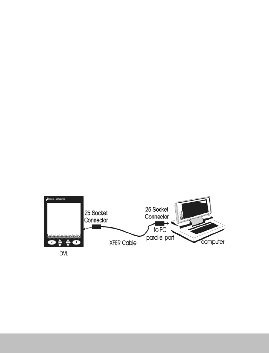
Smart Systems User’s Manual Version 1.1
85
6.4 Noggin
plus
File Management
The File Management option is available by pressing 2 from the main Nogginplus menu.
This option allows the user to export Nogginplus data or the TAGGED.GPS file (see
Section 6.3.5) to an external computer using the parallel XFER cable. It is also here that
the user can delete data from the DVL.
Before data export can take place, the DVL must be connected to the external computer
using the parallel XFER cable that is supplied with the system. As well, the WinPXFER
program must be installed and running on the external computer.
6.4.1 Transferring all Data Files to an External Computer
using the WinPXFER Program
Connecting the Digital Video Logger to an External Computer
Smart Systems come with a separate cable called the parallel XFER cable. This cable is
designed to connect the DVL to an external computer. Note that this is a special cable
and standard 25 pin to 25 pin or Laplink cables will not work.
Figure 6-12: Parallel XFER cable connections
The 2 connections that must be made before attempting to transfer data are:
3) Attach the 25 socket parallel connector to the 25 socket parallel port on back of
the Digital Video Logger, and
4) Attach the 25 socket parallel connector the parallel port of the external computer.
WARNING: To avoid damaging any of the components, turn off the DVL
and computer before making any of these connections.
Installing the WinPXFER Program
The Smart system comes with a CD-ROM containing the WinPXFER program.
To install the WinPXFER program, follow the directions in the “Getting Started”
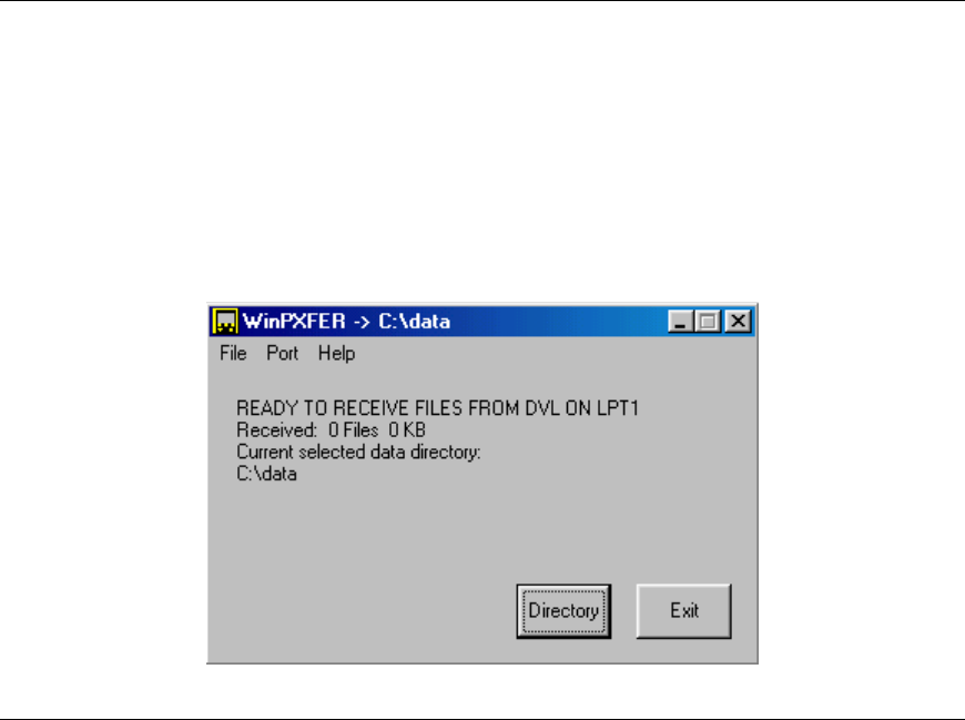
Smart Systems User’s Manual Version 1.1
86
document that accompanies the CD. Basically, running the SETUP.EXE program from
the WinPXFER folder on the CD will install WinPXFER on the computer.
Once the WinPXFER program has been installed on the computer and the user is ready
to transfer data to the computer, the WinPXFER program needs to be run. This can be
done using the WinPXFER shortcut on the Desktop, double-clicking the WinPXFER.EXE
program in Windows Explorer or pressing Start – Programs – Sensors & Software GPR
and finally WinPXFER.
Figure 6-13: WinPXFER main screen
When the WinPXFER program has been run, it will display a screen as shown in Figure
6-13:
This means that it is ready to receive data transferred from the DVL to the LPT port
number 1.
This command assumes that the data buffers are being transferred across Parallel Port
1 (LPT1). If using Parallel Port 2 (LPT2) or higher (LPT3, LPT4 etc.), specify the parallel
port number under the Port menu item from WinPXFER.
The name of the folder (or directory) that the Noggin data will be transferred into is listed
under the “Current selected data directory”. In the example in Figure 6-13, the data will
be transferred to the c:\data directory. The data directory can be changed by pressing
the Directory button and choosing another directory.
Exporting Data to an External Computer
Once the parallel XFER cable is connected (see above) and the WinPXFER software is
installed and running (see above), it is now possible to export data to the external
computer.
All the data in one or more Line or Grid Projects or the TAGGED.GPS file (see Section
6.3.5) can be transferred to an external computer. From the main File Management
menu, the user selects whether to export Line data, Grid data or the TAGGED.GPS file.
If Line or Grid data is selected, the next screen lists the current projects.

Smart Systems User’s Manual Version 1.1
87
One project can be highlighted and selected for export. Use the up and down arrows to
highlight the project and then press the XFER button to transfer to the PC.
It is also possible to use the TAG button to select several projects and export them all at
once. Use the up and down arrows to highlight the projects, the TAG button to tag each
project and then press the XFER button to transfer all the projects to the PC.
The data will be transferred from the DVL to the computer and saved in a sub-folder
from the current data directory indicated on the WinPXFER program, for example,
\DATA\PROJECT2. The progress of the data transfer will be displayed on the DVL
screen and the external computer.
When the data transfer is complete, exit from the WinPXFER program. Press any button
on the DVL to return to the main menu.
Parallel Port not bi-directional Error
Sometimes, when attempting to transfer data to the PC, the error message “LPT1 is not
bi-directional” may appear on the DVL screen. When transferring data from the DVL unit
to a PC, the printer port is used. The WinPXFER program utilizes the functions of a bi-
directional printer port for high-speed data transfer. A bi-directional port allows data to
be sent in both directions over the data lines. Most modern ports are bi-directional;
however, they may not be configured as such and may be configured as ‘output only’.
There are a number of ways the port can be reconfigured depending on the type and
manufacturer of your computer. Most computers configure the port using a BIOS setup
program. Again, different manufactures have different ways to start this program. Some
use the Delete key on boot up, some use the F1 or F2 key on boot up, some have a
special key sequence and others use a program run through DOS or Windows. Often
there is a line of text written to the screen during the boot-up sequence that indicates
which key must be pressed to run Setup. This key MUST be pressed BEFORE
Windows starts. If you miss pressing it, go into Windows, shut down, restart the
computer and try again. Consult your owners’ manual for details.
After the BIOS Setup program starts, the Parallel or Printer port configuration that needs
to be changed is normally under the ‘Peripheral’ or “Advanced” setting heading. If you
can’t find it under these headings, look under the various headings for some setting like
“Parallel Mode” or “Parallel Configuration”. Take note of what the current setting is. The
typical settings are Normal, ECP, EPP and bi-directional. It may require some
experimentation to find the correct setting that works with the WinPXFER program.
First, try changing the setting to bi-directional. Save the settings and exit the Setup
program (usually there is a special key like F10 to do this). Then allow the computer to
continue to boot up. Then, try transferring data again, as described above. If the “LPT1
is not bi-directional” error occurs again, reboot the PC, run the BIOS Setup program,
change the Parallel port setting to EPP, save the settings and try again. The settings
don’t appear standard so no one particular setting will solve the error on all computers.
Keep trying the different parallel port settings until one of them eliminates the error and
allows data transfer.

Smart Systems User’s Manual Version 1.1
88
Viewing Data Files on the External Computer
After transferring data files to the external computer the Nogginplus data files can be
viewed, processed and plotted using the Win_EKKO, EKKO_3D, EKKO_Mapper or
EKKO_Pointer software.
Appendix A contains details about the file format of Nogginplus data.
6.4.2 Deleting Data on the DVL
After data has been successfully transferred to an external computer or if the data is
longer required, the whole Line or Grid project can be deleted from the DVL. From the
File Management main menu, select Delete Line Project or Delete Grid Project. The
next screen lists all the current projects.
To delete a project, use the up and down arrows to highlight it and then press the DEL
button.
It is also possible to use the TAG button to select several projects and delete them all at
once. Use the up and down arrows to highlight the projects, the TAG button to tag each
project and then press the DEL button to delete the data from the DVL.
Before the project is deleted, the user is asked to confirm the deletion by pressing Yes or
No. If the answer to the question is No, the project is not deleted.
This menu also allows the user to delete the TAGGED.GPS file.

Smart Systems User’s Manual Version 1.1
89
6.5 Noggin
plus
Utilities
Pressing the number 4 on the main menu selects Utilities. This menu has utility
programs to change the date and time on the DVL and also calibrate the odometer.
6.5.1 Time and Date
The date and time are saved with the data files. The DVL date and time setting can be
changed by moving to one or more of the appropriate fields and editing the current
setting. The LEFT and RIGHT arrows are used to move between fields. To change any
of the numbers or months, use the UP and DOWN arrows to increase or decrease the
value. When the desired date and time are set, press ENTER to save the changes.
6.5.2 Odometer Calibration
The odometer should be calibrated periodically to ensure accuracy.
Noggin Smart Systems can take input from several different odometers.
It is very important that the user selects and calibrates the odometer appropriate
for their Smart System.
When Odometer Calibration is selected, the user is prompted to select the odometer that
is being used with the Smart System.
If a Smart Cart System is being used, select one of the two Smart Cart odometers
(usually #1).
If a Smart Handle system is being used, select one of the two Smart Handle odometers
(usually #1).
If the system is being towed behind a vehicle and using the transmission odometer to
trigger the system, select one of the two Vehicle odometers (usually #1).
The odometers labelled Other are to be used in future configurations.
Once an odometer is selected, the user is prompted to either 1) manually enter the
odometer calibration factor or 2) to actually calibrate the odometer over a known
distance. To achieve the highest accuracy, it is recommended that the user choose
option number 2 - Odometer Calibration.
When Odometer Calibration is selected, the user is prompted to select the length of the
line to calibrate on. There are 8 different choices in metres and 8 choices in feet. To
toggle the units between metres and feet, press the B button. Pressing the A button on
this screen gives the additional option to select a user-defined value. The user-defined
value can range from 0.01 to 5000 metres or 0.01 to 26400 feet.

Smart Systems User’s Manual Version 1.1
90
When the calibration distance has been selected follow the directions on the screen:
4) Set cart at zero and press A
5) Move the cart the selected distance and press B
6) Press A to exit.
Odometer calibration values for the Smart Cart odometer should be around 4000.
Odometer calibration values for the Smart Handle odometer should be around 1500.
Odometer calibration values for the Vehicle odometer vary but may be around 50.
6.5.3 Upgrade
This option is used to upgrade the software on the DVL. DO NOT press this button until
told to do so in the instructions accompanying the software upgrade.
6.5.4 System Information
This option can be used to list system information that may be useful to troubleshoot a
problem with the Noggin. The information is intended for the use of Sensors & Software
staff to assist in solving a problem with the Noggin system.
System information can be listed to the screen, printed directly to an attached printer or
transferred to a PC.
To print the information to a printer, attach the printer to the parallel port of the DVL and
then press the B button.
To transfer the information file to a PC, attach the parallel XFER cable from the parallel
port of the PC to the parallel port of the DVL. Then run the WinPXFER program on the
PC (see Section 6.4.1) and press the 1 button.
Sensors & Software technical staff may request that this information be sent to them. A
printed copy of the information can be faxed to Sensors & Software Inc. If the data is
transferred to a PC, the data file can be e-mailed to Sensors & Software Inc.

Smart Systems User’s Manual Version 1.1
91
7 Troubleshooting
Noggin Smart Systems are designed to minimize user problems; however, all electronic
devices are subject to possible failure. The following are troubleshooting hints in the
likelihood of occurrence if your Smart System fails to operate.
7.1 Power Supply
The most common problem that can occur while trying to run a system is insufficient
power. The battery may be dead or have a low voltage. If the system is being run from
AC, there may be a problem with the AC power supply or adapter.
If there is enough power to run the DVL, the upper red LED on the front of the DVL will
light up when the battery is plugged into the system. If this light is on and the DVL boots
up, runs and displays the main menu, next check that the red light on the connector to
the Noggin is on. If this light is off then there is a problem with the connection from the
DVL to the Noggin. Check the connection and this part of the cable.
If the DVL is running but the Noggin system will not run, go to the main menu and check
that battery voltage in the lower left corner (see Section 4) is above 10.5 volts. If not, the
battery needs to be recharged or replaced for the Noggin to run (see below).
If the battery voltage is less than about 10.5 volts, the DVL may not turn on and the
upper red LED will flash or not illuminate.
Check the battery voltage with a voltmeter. Try to do this while the system is still
attached to the Smart System to get a true measure of the voltage while under load (it
will be necessary to open the Smart Cart battery case and connect the voltmeter to the
positive and negative battery terminals). If the battery has a low voltage or seems dead,
try the system with another battery (if available), or give the battery a good 12-14 hour
charge and try running the system again.
If the battery does not charge up to 12 Volts or more, it should be replaced.
Smart System batteries are fused to protect the system. For the Smart Cart system,
open the battery case and check that the 10 Amp fuse is OK. If necessary, replace it
with one of the spare fuses available inside the battery case. The smaller belt batteries
available for the Smart Handle systems are also fused. Remove the battery from
padded casing and check the 5 Amp fuse. Replace the fuse if necessary.
7.2 System Communications
If the system power supply is OK but the Noggin does not respond there may be a
communication failure between the DVL and the Noggin. This type of failure is often
indicated by a 10000 series error number like 10012.

Smart Systems User’s Manual Version 1.1
92
If an error occurs, an error message will appear in the bottom left section of the Noggin
screen. EXIT the program and turn off the Digital Video Logger. Disconnect the power
source to completely shut down the system.
Make sure the cables are not damaged and that all cable connections are tightly
secured. Sometimes vibrations cause the cable connections to loosen just a bit and
break contact and this can cause errors. Disconnecting cables and reconnecting them
may provide a better contact and solve the problem. Turn the Digital Video Logger back
on and try running the system again.
If the power supply and cable are OK, the problem is likely a failure of the DVL. The
DVL has no user-serviceable parts so it will have to be returned to Sensors & Software
Inc for inspection and possible repair (see Section 7.6).
7.3 System Overheating
The Noggin systems are designed to operate to an internal temperature of 70 C or 158
F. In situations of high ambient temperatures or long exposure to direct sun, this
maximum internal temperature may be exceeded and cause the system to fail. While
the temperature displayed on the DVL in the lower left corner of the main menu indicates
the internal temperature of the DVL and not the Noggin, this temperature should give an
idea of whether the Noggin is overheating.
If you suspect that the Noggin system is overheating, shut it off and give it a chance to
cool down in a shady location before trying to run it again. Placing a wet cloth on top of
the Noggin may help in cooling it down.
If the situation is such that the high temperatures or direct sun cannot be avoided, it may
be a good idea to put some sort of shade over the Noggin.
Contact Sensors & Software Inc. if the problem persists as there may be defective
electronic components that need to be replaced (see Section 7.6).
7.4 DVL Problem
While the DVL has been ruggedized as much as possible, it should be handled in much
the same way a notebook computer is. If the DVL does not power up and boot up, there
may be a problem with the CPU or the storage media. If this occurs, contact Sensors &
Software Inc. (see Section 7.6).

Smart Systems User’s Manual Version 1.1
93
7.5 Noggin Problem
When the Smart System is powered up and the user selects data acquisition in Noggin
or Nogginplus mode, the Noggin system goes through a self-calibration sequence. While
the self-calibration is occurring the user sees the words “Booting Noggin” in the lower left
corner of the DVL screen. These words are followed by a number that counts up from 1.
Normally, once the count reaches 6 the text disappears and the Noggin is ready to
collect data. Sometimes, however, this count goes beyond 6 and keeps going without
stopping. This indicates an internal problem with the Noggin. No error message will be
displayed on the screen and the only way to exit from the screen is to pull out the power
connection.
If this error occurs, power the system down, power it up again and retry data acquisition.
If the error persists, contact Sensors & Software Inc. (see Section 7.6).
7.6 Contacting Sensors & Software Inc.
If the Noggin system does not run, contact your agent or Sensors & Software Inc.
When contacting SSI, please have the following information available:
1) Noggin and/or DVL Serial Number.
2) Version number of the data acquisition software.
3) The error number or message appearing.
4) A brief description of when the error is happening and the operating conditions
(temperature, humidity, sunshine, system and survey setup, etc.).
5) Sensors & Software Inc. technical staff may request a copy of the System
Information file be sent to them by fax or e-mail. See Section 6.5.4 on how to view,
print and download this file.

Smart Systems User’s Manual Version 1.1
94
8 Care and Maintenance
8.1 Battery Care
Smart Systems use 12-volt sealed lead acid batteries. They are fused with a 10 Amp
fuse to protect them from short circuit damage.
The Smart Cart battery unit uses contains a 15 Amp-hour battery. The battery unit
should run the Cart Noggin for 6-8 hours before recharging is necessary. If long days of
data surveying are typical, a second battery unit may be a useful item.
The Smart Handle belt battery has a 7 Amp-hour battery. This battery should run the
Smart Handle system for 2-3 hours before recharging is necessary. If long days of data
surveying are typical, more belt batteries may be a useful item.
If batteries are maintained in a charged condition they will give long life and reliable
service. Improper use and lack of maintenance will greatly reduce their life.
Sealed lead acid batteries should NEVER be left in a discharged condition for any period
of time. Charge the batteries as soon as possible after use.
Charge batteries at room temperature whenever possible.
The Noggin and DVL contain a voltage monitoring circuit that will turn off the unit when
the input voltage drops below 10.2 volts.
If a battery has been deeply discharged or left in a discharged condition for some period
of time it may not accept charge immediately when it is connected to the charger (The
fast charge LED will not light). If the fast charge light does not come on within 6 hours
the battery should be considered damaged and should be discarded.
Do not assume that a battery that is still charging after 8 hours is nearing the end of its
charge cycle. Typical charging time for an empty battery is 12-14 hours from start of fast
charge.
Ensure that the batteries are fully charged before storing. If practical, store the batteries
in a cool place, 10oc (a refrigerator is ideal), but make sure the temperature is not likely
to drop below -30oC or the electrolyte may freeze and possibly split the case.
8.2 DVL Internal Battery
If the Smart System has not been powered up for an extended period of time, the
internal battery will discharge. The dead battery causes the DVL time and date to reset
to January 1, 1988 at 12:00 PM. To correct the time and date see Section 5.5.1 or 6.5.1.
To recharge the internal battery the Smart System must be powered up and left running
for at least one hour and preferably longer.

Smart Systems User’s Manual Version 1.1
95
8.3 Skid Pads
The bottom of the Noggin unit is covered with one large wear-resistant skid pad. The
skid pad is designed to protrude from the bottom of the Noggin and take the majority of
the abrasive wear. If the pad wears down enough, the less-resistant plastic housing may
start to wear. If this occurs, it is best to replace the skid pad. It is easily removed with a
Phillips screwdriver and a new one can be purchased from Sensors & Software Inc.

Smart Systems User’s Manual Version 1.1
A-1
Appendix A NOGGIN PLUS DATA FILE FORMAT
Nogginplus data consists of two files, a Header file and a Data file. The files have the
same name but different extensions. The format details of these files are given below.
Header (.HD) File:
The header file, identified by the file extension .HD, is an ASCII file. An example is
shown below. The heading identifies what each piece of information represents.
1234
Data Collected with Noggin Plus
12/10/2000
NUMBER OF TRACES = 220
NUMBER OF PTS/TRC = 156
TIMEZERO AT POINT = 31
TOTAL TIME WINDOW = 62
STARTING POSITION = 0.0000
FINAL POSITION = 10.9500
STEP SIZE USED = 0.0500
POSITION UNITS = m
NOMINAL FREQUENCY = 250.00
ANTENNA SEPARATION = 0.3048
PULSER VOLTAGE (V) = 100
NUMBER OF STACKS = 4
SURVEY MODE = Reflection
This file can be read and/or printed using any Word Processor.
Data (.DT1) File:
The data file contains as many records as there are traces. Each record in turn consists
of a header section and a data section. The header section consists of an array of 25
real*4 numbers and a string of 28 characters which is used for annotation. The 25
element real array contains the following information:
Item # Description
1 Trace number
2 Position
3 Number of points per trace
4 Topographic data, if available
5 (not used)
6 # bytes/point (always 2 for Rev 3 firmware)
7 Time Window
8 # of stacks
9-10 reserved for GPS X position (double*8 number)
11-12 reserved for GPS Y position (double*8 number)
13-14 reserved for GPS Z position (double*8 number)

Smart Systems User’s Manual Version 1.1
A-2
15 reserved for receiver x position
16 reserved for receiver y position
17 reserved for receiver z position
18 reserved for transmitter x position
19 reserved for transmitter y position
20 reserved for transmitter z position
21 timezero adjustment
where:point(x)= point(x+adjustment)
22 Zero flag: 0 = data okay, 1=zero data
23 (not used)
24 Time of day data collected in seconds past midnight.
25 Comment flag: 1 = comment attached.
26 - 32 Comment
The data section consists of an array of two-byte integers, one value for every data
point.
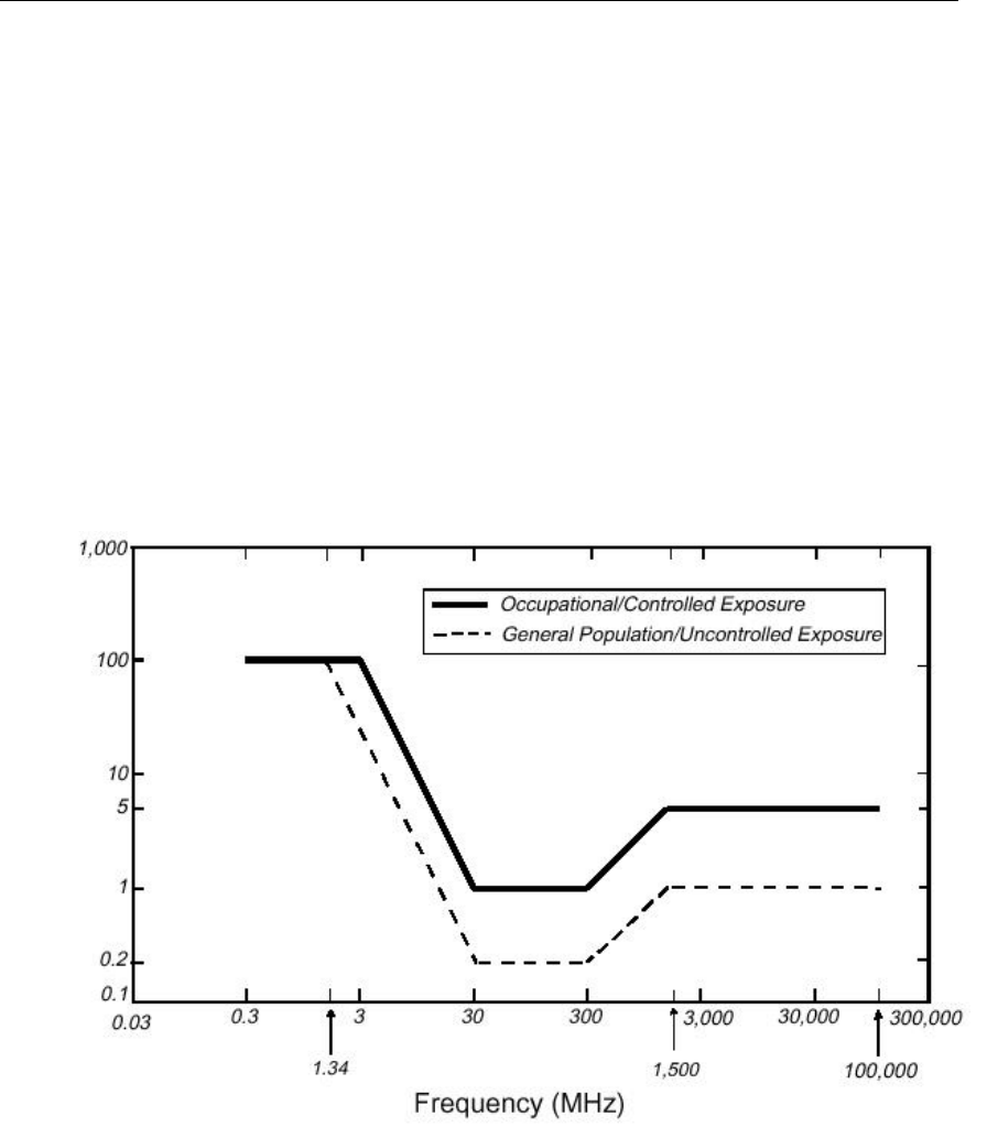
Smart Systems User’s Manual Version 1.1
B-1
Appendix B HEALTH AND SAFETY CERTIFICATION
Radio frequency electromagnetic fields can pose a health hazard when the fields are
intense. Detailed discussions on the subject are contained in the references and the
web sites listed below.
The USA Federal Communication Commission (FCC) and Occupational Safety
and Health Administration (OSHA) both specify acceptable levels for
electromagnetic fields. Similar power levels are mandated by corresponding
agencies in other countries. Maximum permissible exposures and time duration
specified by the FCC and OSHA vary with excitation frequency. The lowest
threshold plane wave equivalent power cited is 0.2 mW/cm2 for general
population over the 30 to 300 MHz frequency band. All other applications and
frequencies have higher tolerances as shown in graphically in Figure 1.
Figure 1: FCC limits for maximum permissible exposure (MPE) plane-wave equivalent power density mW/cm2.
All Sensors & Software Inc. pulseEKKO, Noggin and Conquest products are
normally operated at least 1 m from the user and as such are classified as
“mobile” devices according to the FCC. Typical power density levels at a
distance of 1 m or greater from any Sensors & Software Inc. product are less
than 10-3 mW/cm2 which are 200 to 10,000 times lower than mandated limits. As
such, Sensors & Software Inc. products pose no health and safety risk when
operated in the normal manner of intended use.

Smart Systems User’s Manual Version 1.1
C-1
Appendix C FCC REGULATIONS
This device complies with Part 15 of the FCC Rules. Operation is subject to the
following two conditions:
(1) this device may not cause harmful interference and
(2) this device must accept any interference received, including
interference that may cause undesired operation.
FCC Class A Digital Device or Peripheral – User Information
This equipment has been tested and found to comply with the limits for a Class A digital
device, pursuant to Part 15 of the FCC Rules. These limits are designed to provide
reasonable protection against harmful interference when the equipment is operated in a
commercial environment. This equipment generates, uses and can radiate radio
frequency energy and, if not installed and used in accordance with the instruction
manual, may cause harmful interference to radio communications. Operation of this
equipment in a residential area is likely to cause harmful interference in which case the
user will be required to correct the interference at his own expense.
WARNING
Changes or Modifications not expressly approved by Sensors & Software Inc. could void
the user’s authority to operate the equipment.
Certification of this equipment has been carried out using approved cables and
peripheral devices. The use of non-approved or modified cables and peripheral devices
constitutes a Change or Modification outlined in the warning above.

Smart Systems User’s Manual Version 1.1
C-2
Operating Restrictions
Operation of this device is restricted to law enforcement, fire and rescue officials,
scientific research institutes, commercial mining companies, and construction
companies. Operation by any other party is a violation of 47 U.S.C. §301 and could
subject the operator to serious legal penalties.
FCC Interpretation of this label issued July 12, 2002
The regulations contain restrictions on the parties that are eligible to operate imaging
systems. 1
Under the new regulations, GPRs and wall imaging systems may be used
only by law enforcement, fire and emergency rescue organizations, by scientific
research institutes, by commercial mining companies, and by construction companies.
Since the adoption of the Order, we have received several inquiries from the operators
of GPRs and wall imaging systems noting that these devices often are not operated by
the users listed in the regulations but are operated under contract by personnel
specifically trained in the operation of these devices. We do not believe that the recent
adoption of the UWB rules should disrupt the critical safety services that can be
performed effectively only through the use of GPRs and wall imaging systems. We
viewed these operating restrictions in the broadest of terms. For example, we believe
that the limitation on the use of GPRs and wall imaging systems by construction
companies encompasses the inspection of buildings, roadways, bridges and runways
even if the inspection finds no damage to the structure and construction does not
actually result from the inspection; the intended purpose of the operation of the UWB
device is to determine if construction is required. We also believe that the GPRs and
wall imaging systems may be operated for one of the purposes described in the
regulations but need not be operated directly by one of the described parties. For
example, a GPR may be operated by a private company investigating forensic evidence
for a local police department.
FCC Permitted Mode of Usage
The GPR antenna must be kept on the surface to be in compliance with FCC
regulations. Use of the antenna is not permitted if it is lifted off the surface. Use as a
wall imaging device is prohibited.
1 See 47 C.F.R. §§ 15.509(b), 15.511(b), and 15.513(b).

Smart Systems User’s Manual Version 1.1
C-3
GPR Use Coordination
FCC regulation 15.525(c) requires users of GPR equipment to coordinate the use of
their GPR equipment as decribed below:
(a) UWB imaging systems require coordination through the FCC before the
equipment may be used. The operator shall comply with any constraints on equipment
usage resulting from this coordination.
(b) The users of UWB imaging devices shall supply detailed operational areas to
the FCC Office of Engineering and Technology who shall coordinate this information with
the Federal Government through the National Telecommunications and Information
Administration. The information provided by the UWB operator shall include the name,
address and other pertinent contact information of the user, the desired geographical
area of operation, and the FCC ID number and other nomenclature of the UWB device.
This material shall be submitted to the following address:
Frequency Coordination Branch., OET
Federal Communications Commission
445 12th Street, SW
Washington, D.C. 20554
ATTN: UWB Coordination
The form given on the following page is a suggested format for performing the
coordination.

Smart Systems User’s Manual Version 1.1
C-4
GROUND PENETRATING RADAR COORDINATION NOTICE
NAME:
ADDRESS:
CONTACT INFORMATION [contact name and phone number]:
AREA OF OPERATION [counties, states or larger areas]:
FCC ID: [e.g. QJQ-NOGGIN250 for Noggin 250 system)]
EQUIPMENT NOMENCLATURE: [ e.g. Noggin 250]
Send the information to:
Frequency Coordination Branch., OET
Federal Communications Commission
445 12th Street, SW
Washington, D.C. 20554
ATTN: UWB Coordination
Fax: 202-418-1944
INFORMATION PROVIDED IS DEEMED CONFIDENTIAL

Smart Systems User’s Manual Version 1.1
C-5
FCC Shut Off Switch
FCC regulation 15.509(c) requires that a GPR system incorporate a manually operated
switch that causes the transmitter to cease operation within 10 seconds of being
released by the operator.
Sensors & Software GPR systems will only operate when triggered by the operator. If
the system is not triggered by the operator it will cease transmitting within 10 seconds of
releasing the trigger.

Smart Systems User’s Manual Version 1.1
D-1
Appendix D OPERATION OF SHUT OFF SWITCH
Sensors & Software Inc.’s GPR systems transmitters will not operate in the free run
mode for more than 10 seconds without the shut off switch installed and depressed
by the user.
Installation
To install the switch, plug the 25 pin male connector into the printer port of the DVL-II
or the controlling PC. Software will automatically detect the switch.
Operation
To operate the switch, hold the button in the closed position. Releasing the button
for more than 10 seconds will cause the unit to stop functioning.

Smart Systems User’s Manual Version 1.1
References
1. Questions and answers about biological effects and potential hazards of
radio-frequency electromagnetic field
USA Federal Communications Commission, Office of Engineering &
Technology
OET Bulletin 56
(Contains many references and web sites)
2. Evaluation Compliance with FCC Guidelines for Human Exposure to
Radio Frequency Electromagnetic Fields.
USA Federal Communications Commission, Office of Engineering &
Technology
OET Bulletin 56
(Contains many references and web sites)
3. USA Occupational Safety and Health Administration regulations
paragraph 1910.67 and 1910.263.
Web Sites
www.fcc.gov/Bureau/EngineeringTechnlogy/Documents/bulletin
www.osha-slc.gov/SLTC (see radio frequency)