TEXAS INSTRUMENTS Calculator Manual L0806875
User Manual: TEXAS TEXAS INSTRUMENTS Calculator Manual TEXAS INSTRUMENTS Calculator Owner's Manual, TEXAS INSTRUMENTS Calculator installation guides
Open the PDF directly: View PDF ![]() .
.
Page Count: 446 [warning: Documents this large are best viewed by clicking the View PDF Link!]
TEXAS
|NSTIRUMENTS
TI-83
GRAPHINGCALCULATOR
GUIDEBOOK
TI-GRAPH LINK, Calculator-Based Laboratory, CBL, CBL 2, Calculator-Based Ranger, CBR,
Constant Memory, Automatic Power Down, APD, and EOS are trademarks of Texas
Instruments Incorporated.
IBM is a registered trademark of International Business Machines Corporation.
Macintosh is a registered trademark of Apple Computer, Inc.
Windows is a registered trademark of Microsoft Corporation.
© 1996, 2000, 200I Texas Instruments Incorporated.
Important
US FCC
Information
Concerning
Radio Frequency
Interference
Texas Instrtu-nents makes no warranty, either expressed or
ilnplied, including but not lilnited to any implied warranties of
inerchantability and fitness for a particular purpose, regarding any
progralns or book rnateriais and rnakes such inateriais availaMe
solely on an "as-is" basis.
In no event shall Texas Instrmnents be liable to anyone for special,
collateral, ineidentai, or eonsequentiai damages in connection with
or arising out of the purchase or use of these inateriais, and the
sole and exclusive liability of Texas Instruments, regardless of the
form of action, shall not exceed the purchase price of this
equipment. Moreover, Texas Instruments shall not be liable for any
claim of any kind whatsoever against the use of these materials by
any other party.
This equiplnent has been tested and found to cornply with the
limits for a Class B digital device, pumuant to Pm't 15 of the F(C
rules. These limits are designed to provide reasonable protection
against harmflfl interference in a residential installation. This
equiprnent generates, uses, and can radiate radio frequency enet}4y
and, if not installed and used in accordance with the instructions,
inay cause hannflll inte_ferenee with radio colnmunications.
However, there is no guarantee that inte_ferenee will not occur in
a particular instailation.
If this equiplnent does cause harrnful interference to radio or
telexdsion reception, which can be determined by turning the
equipment off and on, you can try to correct the inte_ference by
one or inore of the following measures:
• Reorient or relocate the receiving antenna.
• Increase the separation between the equiplnent and receiver.
• Connect the equipment into an outlet on a circuit different
fl_m that to which the receiver is connected.
• Consult the dealer or an experienced radio/television
technician for help.
Caution: Any changes or modifications to this equiprnent not
expressly approved by Texas Instrulnents may void your authority
to operate the equiplnent.
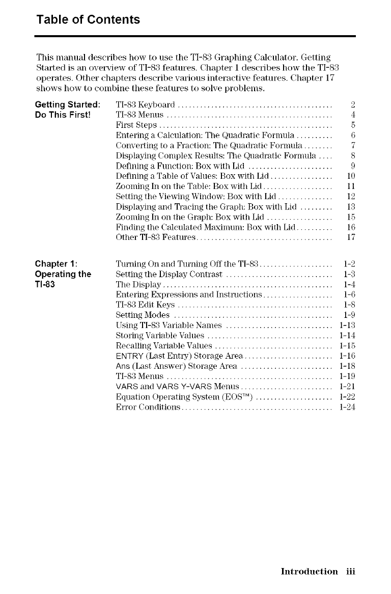
Table of Contents
This nlanual describes how to use the TI-83 Graphing Calculator, Getting
Started is an overview of TI-83 features. Chapter 1 describes how the TI-83
operates. Other chapters describe various interactive features. Chapter 17
shows how to combine these features to solve problems,
Getting Started: TI-83 Keyboard ..........................................
Do This First! TI-83 Menus .............................................
First Steps ...............................................
Entering a Calculation: The Quadratic Formula ..........
Converting to a Fraction: The Quadratic Formula ........
I)isplaJ_ng ('omplex Results: The Quadratic Formula ....
Defining a Function: Box with Lid .......................
Defining a Table of Values: Box with Lid ...............
Zooming In on the Table: Box with Lid .................
Setting tile Viewing Window-: Box with Lid .............
I)isplaJ_ng and Tracing the Graph: Box with Lid .......
Zooming In on tile Graph: Box with Lid ................
Finding the Calculated Maximum: Box with Lid ........
Other TI-83 Features .....................................
2
4
F)
6
7
8
9
10
11
12
13
15
16
17
Chapter 1 :
Operating the
TI-83
Turning On and Turning Off the TI-83 .................... 1-2
Setting the Display Contrast ............................. 1-3
The Display .............................................. 1-4
Entering Expressions and Instructions ................... 1-6
TI-83 Edit Keys .......................................... 1-8
Setting Modes ........................................... 1-9
Using TI-83 Variable Names ............................. 1-13
Storing Variable Values .................................. 1-14
Recalling Variable Values ................................ 1-15
ENTRY (Last Entry) Storage A_'ea ........................ 1-16
Ans (Last Pmswer) Storage Pa'ea ......................... 1-18
TI-83 Menus ............................................. 1-19
VARS and VARS Y-VARS Menus ......................... 1-21
Equation Operating System (EOS TM) ..................... 1-22
Error Conditions ......................................... 1-24
Introduction iii
Chapter 2:
Math, Angle, and
Test Operations
Getting Started: Coin Flip ................................ 2-2
Keyboard Math Operations .............................. 2-3
MATH Operations ........................................ 2-5
Using tile Equation Solver ............................... 2-8
MATH NUM (Numbe 0 Operations ........................ 2-13
Entering and Using Complex Nmnbers ................... 2-16
MATH CPX (Complex) OperatMns ....................... 2-18
MATH PRB (Probability) Operations ..................... 2-20
ANGLE Operations ....................................... 2-23
TEST (Relational) Operations ............................ 2-25
TEST LOGIC (Boolean) Operations ...................... 2-26
Chapter 3:
Function
Graphing
Getting Started: Graphing a Circle ....................... 3-2
Defining Graphs ......................................... 3-3
Setting the Graph Modes ................................. 3-4
Defining Funetions ...................................... 3-5
Seleeting and Deseleeting Punetions ..................... 3-7
Setting Graph Styles for Flmetions ....................... 3-9
Setting the Viewing Window \Tariahles ................... 3-11
Setting the Graph Format ................................ 3-13
Displaying Graphs ....................................... 3-15
Exploring Graphs with the Free-Moving Cursor .......... 3-17
Exploring Graphs with TRACE ........................... 3-18
Exploring Graphs with the ZOOM Instructions ........... 3-20
Using ZOOM MEMORY .................................. 3-23
Using the CALC (Calculate) Operations .................. 3-25
Chapter 4:
Parametric
Graphing
Getting Started: Path of a Ball ........................... 4-2
Defining and Displaying Parametric Graphs .............. 4-4
Exploring Parametrie Graphs ............................ 4-7
Chapter 5: Getting Started: Polar Rose .............................. 5-2
Polar Graphing Defining and Displaying Polar Graphs ................... 5-3
ExNodng Polar Graphs .................................. 5-6
iv Introduction
Chapter 6:
Sequence
Graphing
Getting Started: Forest and Trees ........................ (;-2
Defining and Displaying Sequence Graphs ............... 6-3
Selecting Axes Combinations ............................ 6-8
Exploring Sequence Graphs .............................. (;-9
Graphing Web Plots ...................................... 6-11
Using Web Plots to Illustrate Convergence ............... 6-12
Graphing Phase Plots .................................... 6-13
Comparing TI-83 and TI-82 Sequence Variables .......... 6-15
Keystroke Differences Between TI-83 and TI-82 ......... 6-16
Chapter 7:
Tables
Getting Started: Roots of a Function ..................... 7-2
Setting Up the Table ..................................... 7-3
Defining the Dependent Variables ........................ 7-4
I)isplaying the Table ..................................... 7-5
Chapter 8:
DRAW
Operations
Getting Started: Drawing a Tangent Line ................. 8-2
Using the DRAW Menu ................................... 8-3
Clearing Drawings ....................................... 8-4
Drawing Line Segments .................................. 8-5
Drawing Horizontal and Vertical Lines ................... 8-6
Drawing Tangent Lines .................................. 8-8
Drawing Functions and Inverses ......................... 8-9
Shading Areas on a Graph ............................... 8-10
Drawing Circles .......................................... 8-11
Placing Text on a Graph ................................. 8-12
UsHlg Pen to Draw on a Graph ........................... 8-13
Drawing PoHlts on a Graph .............................. 8-14
Drawing Pixels .......................................... 8-16
StorH N Graph Pictures (Pic) ............................. 8-17
Recalling Graph Pictures (Pic) ........................... 8-18
StorHlg Graph Databases (GDB) ......................... 8-19
Recalling Graph Dadabases (GDB) ....................... 8-20
Chapter 9:
Split Screen
Getting Started: Exploring the Unit Circle ................ 9-2
Using Split Screen ....................................... 9-3
Horiz (Horizontal) Split Screen ........................... 9-4
G-T (Graph-Table) Split Screen .......................... 9-5
TI-83 Pixels in Horiz aim G-T Modes ..................... 9-6
Introduction v
Chapter 10:
Matrices Getting Started: Systems of Linear Equations ............ 10-2
Defining a Matrix ........................................ 10-3
Viewing and Editing Matrix Elements .................... 10-4
Using Matrices with Expressions ........................ 10-7
I)isplaying and Copying Matrices ........................ 10-8
Using Math Functions with Matrices ..................... 10-9
Using the MATRX MATH Operations ..................... 10-12
Chapter 11:
Lists Getting Started: Generating a Sequence .................. 11-2
Naming Lists ............................................. 11-3
Storing and Displaying Lists ............................. 11-4
Entering List Names ..................................... 11-6
Attaching Formulas to List Names ....................... 11-7
Using Lists in Expressions ............................... 11-9
LIST OPS Menu .......................................... 11-10
LIST MATH Menu ........................................ 11-17
Chapter 12:
Statistics Getting Started: Pendulum Lengihs and Periods ......... 12-2
Setting up Statistical Palalyses ........................... 12-10
Using the Stat List Editor ................................ 12-11
Attaching Formulas to List Names ....................... 12-14
I)etaehi_lg Fornmlas from List Names .................... 12-16
Switching Stat List Editor Contexts ...................... 12-17
Stat List Editor Contexts ................................. 12-18
STAT EDIT Menu ........................................ 12-20
Regression Model Features .............................. 12-22
STAT CALC Menu ........................................ 12-24
Statistical Variables ...................................... 12-29
Statistical Analysis in a Program ......................... 12-30
Statistical Plotting ....................................... 12-31
Statistical Plotting in a Program ......................... 12-37
Chapter 13:
Inferential
Statistics and
Distributions
Getting Started: Mean Height of a Population ............ 13-2
hfferential Star Editors ................................... 13-6
8TAT TESTS Menu ...................................... 13-9
Inferential Statistics Input Descriptions .................. 13-26
Test and Interval Output Variables ....................... 13-28
Distribution Functions ................................... 13-29
Distribution Shading ..................................... 13-35
vi Introduction
Chapter 14:
Financial
Functions
Getting Started: Finzmeing a Car. ........................ 14-2
Getting Started: (;omputing Compound Interest .......... 14-3
Using tile TVM Solver .................................... 14-4
Using tile Financial Functions ........................... 14-5
Calculating Time Value of Money (TVM) ................. 14-6
Calculating (;ash Flows .................................. 14-8
Calculating Amortization ................................ 14-9
Calculating Interest Conversion .......................... 14-12
Finding I)ays between [)ates_)ef'nm N Payment Method ..... l '4-13
Using tile TVM Variables ................................. 14-14
Chapter 15:
CATALOG,
Strings,
Hyperbolic
Functions
Browsing tile TI-83 CATALOG ........................... 17)-2
Entering and Using Strings ............................... 15-g
Storing Strings to String Variables ....................... 1:)-4
String Functions and Instructions in the CATALOG ...... 1.5-6
Hyperbolic Functions in the CATALOG .................. 15-10
Chapter 16:
Programming
Getting Started: Volume of a Cylinder .................... 16-2
Creating and Deleting Progrmns ......................... 16-4
Entering Command Lines and Executing Programs ...... 16-5
Editing Programs ........................................ 16-6
Copying and Renmning Programs ........................ 16-7
PRGM CTL (Control) Instructions ....................... 16-8
PRGM I/O (Input/Output) Instructions ................... 16-16
('ailing Other Programs as Subroutines .................. 16-22
Chapter 17:
Applications
Comparing Test Results Using Box Plots ................ 17-2
Graphing Pieeewise Punetions ........................... 17-4
Graphing Inequalities .................................... 17-5
Solving a System of Nonlinear Equations ................ 17-6
Using a Program to ( reate the Sierpinski Triangle ....... 17-7
Graphing Cobweb Attractors ............................ 17-8
Using a Program to Guess the Coefficients ............... 17-9
Graphing the Unit Circle and Trigonometric (;m_es ...... 17-10
Finding the Area between Curves ........................ 17-11
Using Parametric Equations: Ferris Wheel Problem ...... 17-12
Demonstrating the Fundamental Theorem of Calculus... 17-14
Computing Areas of Regular N-Sided Polygons .......... 17-16
Computing and Graphing Mortgage Payments ........... 17-18
Introduction vii
Chapter 18:
Memory
Management
{'heeLing Awailable MemolTy"............................. 18-2
Deleting Items from MemoKy" ............................ 18-3
Clearing Entries and List Elements ...................... 18-4
Resetting the TI-8:3 ...................................... 18-5
Chapter 19:
Communication
Link
Getting Started: Sending Variables ....................... 19-2
TI-83 LINK ............................................... 19-3
Selecting Items to Send .................................. 19-4
Receiving Items .......................................... 19-5
Transmitting Items ....................................... 19-6
Transmitting Lists to a TI-82 ............................. 19-8
Transmitting from a TI-82 to a TI-83 ..................... 19-9
Backing Up MemoKy" ..................................... 1%10
Appendix A:
Tables and
Reference
Information
TabD of Functions and Instructions ..................... A-2
Menu Map ............................................... A-39
Vm'iables ................................................ A-49
Statistical Formulas ..................................... A-50
Financial Fommlas ...................................... A-.M
Appendix B:
General
Information
BatteKy" Information ...................................... B-2
In Case of Difficulty ..................................... B-4
En'or Conditions ......................................... B-5
Accuracy hfformation .................................... B-10
Support and Service Infommtion ......................... B-12
Win'rarity Information .................................... B-13
Index
viii Introduction
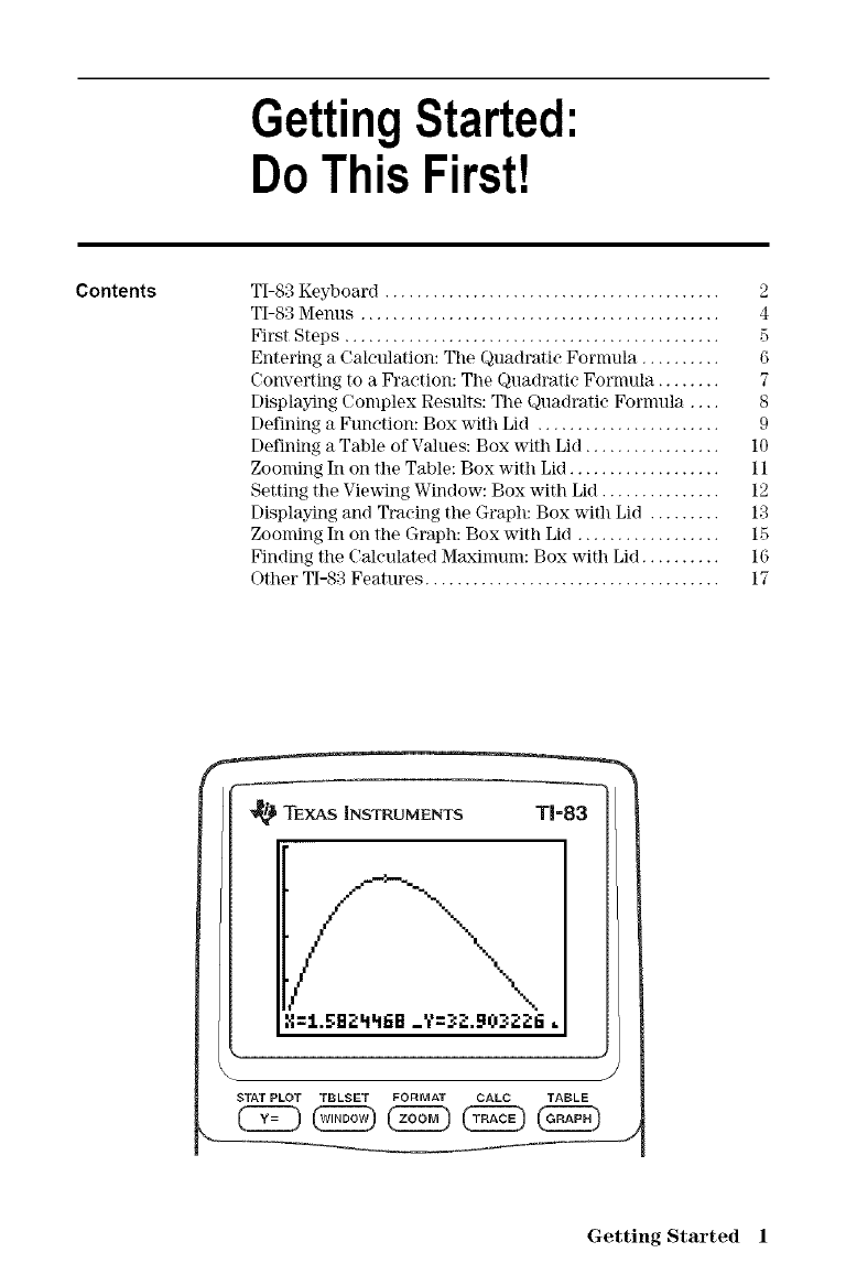
GettingStarted:
Do ThisFirst!
Contents TI-83 Keyboard ..........................................
TI-S3 Menus .............................................
First Steps ...............................................
Entering a Calculation: The Quadratie Fonuula ..........
('onverting to a Fraction: The Quadratie Formula ........
Displaying Complex Results: The Quadratic Formula ....
Defining a Function: Box with Lid .......................
Defining a Table of Values: Box with Lid ...............
Zooming In on the Table: Box with Lid .................
Setting tile Viewing Window-: Box with Lid .............
Displaying and Traeing the Graph: Box with Lid .......
Zooming In on tile Graph: Box with Lid ................
Finding the ('aleulated Maximum: Box with Lid ........
Other TI-83 Features .....................................
2
4
5
6
7
8
9
10
11
12
13
15
16
17
TEXAS INSTRUMENTS T1=83
/ \ \.
X=:I..5:B;!:=I_fiB _Y=_;i:.90_;i:_lfi =
J
STATPLOT TBLSET FORMAT CALC TABLE
Getting Started 1
TI-83 Keyboard
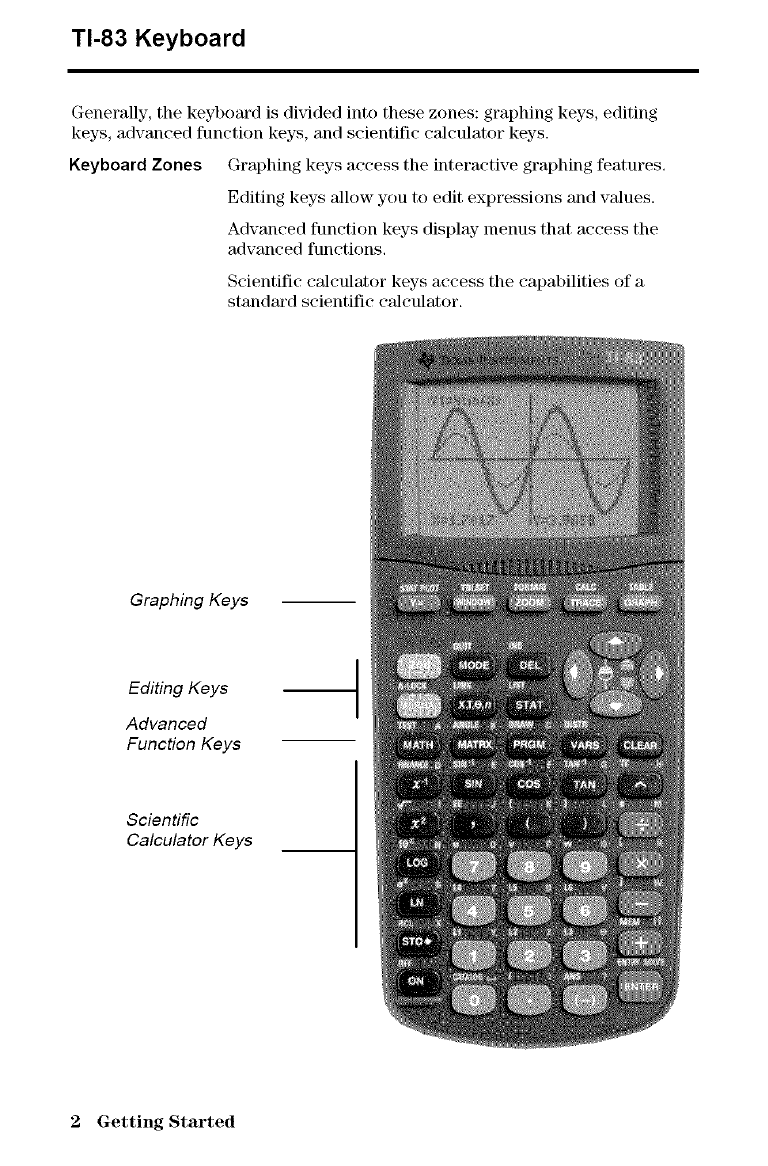
Generally, the keybom'd is dwided into these zones: graphing keys, editing
keys, advanced function keys, and scientific calculator keys.
Keyboard Zones Graphing keys access the interactive graphing features.
Editing keys allow you to edit expressions and values.
Advanced function keys display menus that access the
advanced functions.
Scientific calculator keys access the capabilities of a
standard scientific calculator.
Graphing Keys
Editing Keys
Advanced
FuncffonKeys
Scientific
Calculator Keys
2Getting Started
Using the
Color-Coded
Keyboard
Using the K_
and @ Keys
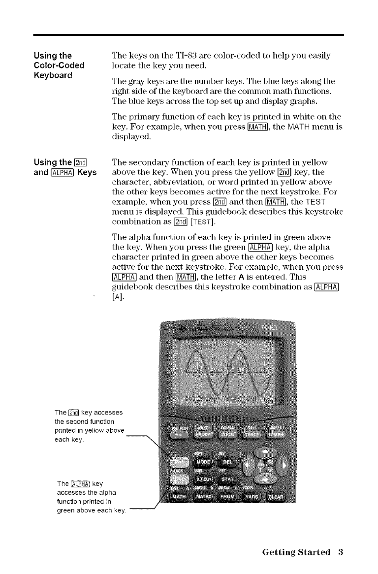
The keys on the TI-83 are color-coded to help you easily
locate the key you need.
The gray keys are the number keys. The blue keys along the
right side of the keyboard are the conunon math functions.
The blue keys across the top set up and display graphs.
The primaKF function of each key is printed in white on the
key. For example, when you press FMA_], the MATH menu is
displayed.
The secondary function of each key- is pnnted in yellow
above the key-. When you press the yellow [_ key, the
character, abbreviation, or word printed in yellow above
the other keys becomes active for the next keystroke. For
example, when you press [_ and then [M#Y_, the TEST
menu is displayed. This guidebook describes this keystroke
combination as [_ [TEST],
The alpha function of each key is printed in green above
the key. When you press the green @ key, the alpha
character printed in green above the other keys becomes
active for the next keystroke. For example, when you press
@ and then [MATH],the letter Ais entered. This
guidebook describes this keystroke combination as @
[A].
The_key accesses
the second function
printed in yeltow above
each key --'_
The@key
accessesthe alpha
function printedin
green above each key
Getting Started 3
TI-83 Menus
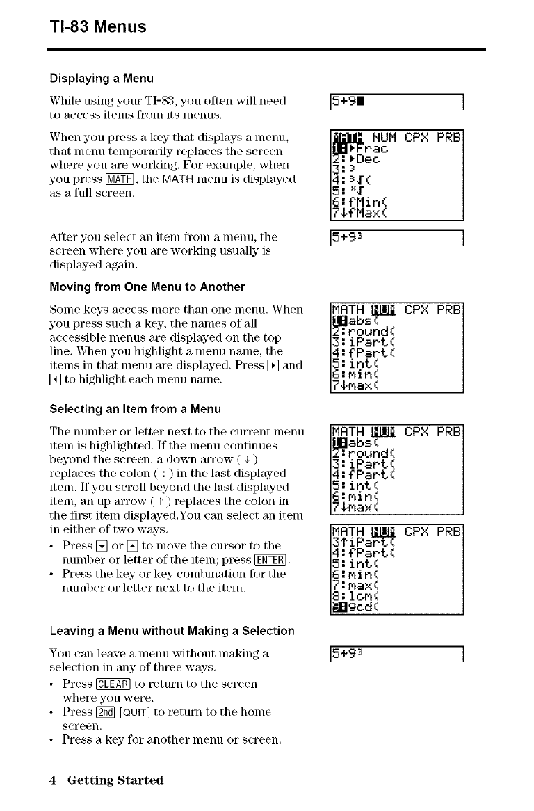
Displaying a Menu
While using your TI-83, you often will need
to access items from its menus,
When you press a key- that displays a menu,
that menu temporarily replaces the screen
where you are working. For example, when
you press _, the MATH menu is displayed
as a full screen.
After you select an item fronl a menu, the
screen where you m'e working usually is
displayed again.
Moving from One Menu to Another
Solne keys access nlore than one lnenu. When
you press such a key, the names of all
accessible menus are displayed on the top
line. When you highlight a menu name, the
items in that menu are displayed. Press [] and
[] to highlight each menu nalne.
Selecting an Item from aMenu
The number or letter next to the current menu
item is highlighted. If the menu continues
beyond the screen, a down arrow ( _ )
replaces the colon ( : ) in the last displayed
item. If you scroll beyond the last displayed
item, an up arrow ( t ) replaces the colon in
the first item displayed.You can select all item
in either of two ways.
• Press [] or [] to lnove the cursor to the
number or letter of the item; press [g_.
• Press the key or key combination fia" the
number or letter next to the item.
Leaving a Menu without Making a Selection
You can leave a lnenu without lnaking a
selection in ally of three ways.
• Press @ to return to the screen
where you were.
• Press [2_] [QUIT] to t_tum to the home
screen.
• Press a key for another lnenu or screen.
[5+9| [
_ NUM CPX PRB
Pao
:*Dec
4:_(
5:_
6:¢Min(
74€Max(
5+9_
_sl_[ CPX PRB[
round(
5:int(
6:Min(
74.max(
round(
3:iPart(
4:?Part(
5:int(
5:Min(
74Max(
MRTH _ CPX PRB
3tiPar.t(
4:?Part(
5:int(
6:Min(
7:max(
8:fOR(
i_lEIgcd(
15+9_ I
4 Getting Started
First Steps
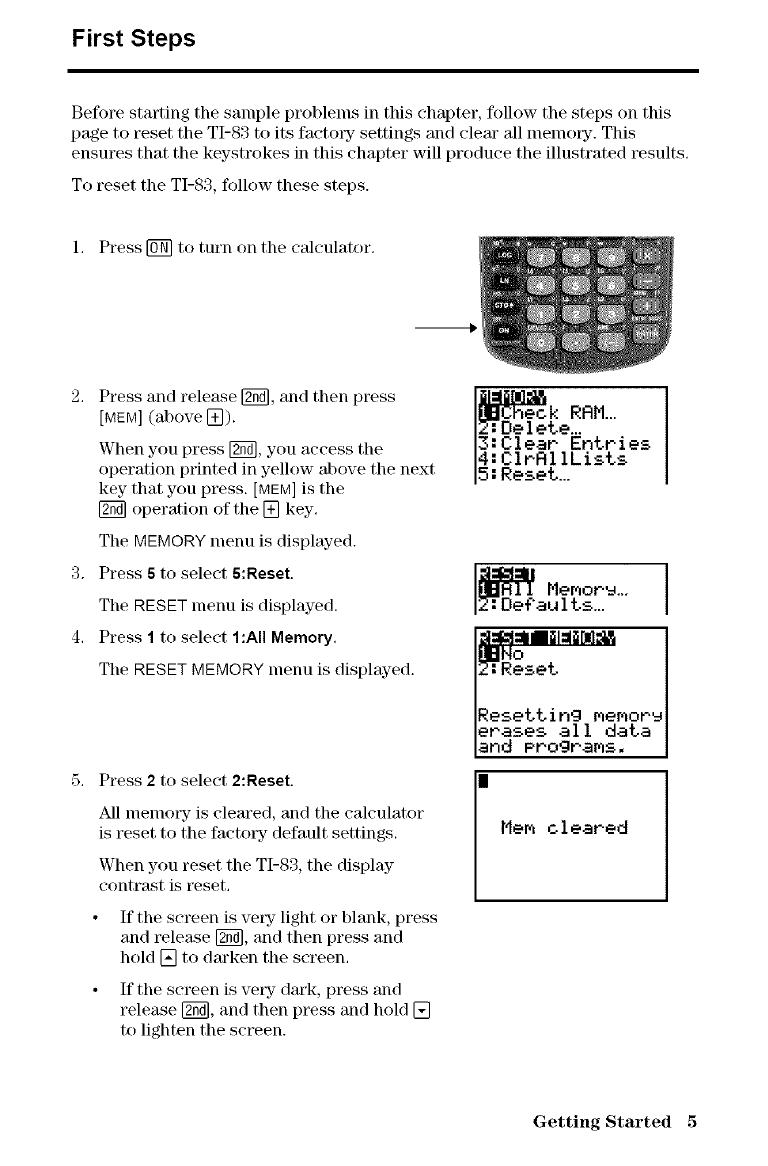
Before starting the sample pr()blems in this chapter, follow the steps on this
page to reset the TI-83 to its factotT settings and cleat" all nlenlot_y-. This
ensures that the keystrokes in this chapter will produce the illustrated results.
To reset the TI-83, follow these steps.
1, Press FOR]to turn on the calculator.
2, Press and release [_, and then press
[MEM] (above []).
When you press [2_], you access the
operation printed in yellow above the next
key that you press. [MEM]is the
operation of the [] key.
The MEMORY menu is displayed.
3. Press 5to select 5:Reset.
The RESET menu is displayed.
4, Press 1to select 1:All Memory,
The RESET MEMORY menu is displayed.
5, Press 2to select 2:Reset.
M1 nlenlot_y- is cleared, and the calculator
is reset to the factor T default settings.
When you reset the TI-83, the display
contrast is reset.
If the screen is vetT light or blank, press
and t_lease D_], and then press and
hold [] to darken the screen.
If the screen is very dark, press and
release [2_, and then press and hold []
to lighten the screen.
RRM...
3:Clear Entries
4:ClrRllLists
5:Reset...
_MeMoru..,
a. DeCaults...
Resettin9 memoru
erases all data
and PrograMs.
|MeM oleared
Getting Started 5
Entering a Calculation: The Quadratic Formula
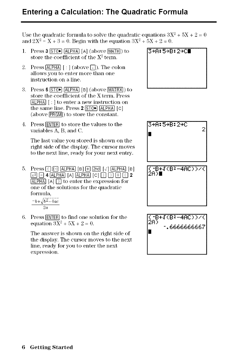
Use the quadratic fornmla to solve the quadratic equations 3X 2 + 5X + 2 = 0
and 2X 2 - X + 3 = 0, Begin with the equation 3X 2 + 5X + 2 = 0,
1, Press 3 _ @ [n] (above 1_]) to 3÷R: 5÷B: 2÷C|
store the coefficient of the X 2 tenn.
2, Press @ [ : ] (above [_). The colon
allows you to enter more than one
instruction on a line,
3, Press 6 _ @ [B] (above _) to
store the coefficient of the X term. Press
@ [ : ] to enter a new instruction on
the same line. Press 2_ @ [c]
(above _) to store the constant.
4, Press [NY_ to store the values to the
variables A, B, and C.
The last wdue you stored is shown on the
right side of the display. The cursor moves
to the next line, ready for your next entt3z,
Press[] [] @ [B] [] _ [<] @ [B]
D [] 4_ [A]_ [c] []17113[] 2
@ [A] [] to enter the expression for
one of the solutions for the quadratic
formula,
-b+2a
÷R: 5÷B: 2÷C 2
Press _ to find one solution for the
equation 3X 2 + 5X + 2 = 0.
The answer is shown on the right side of
the display. The cursor nloves to the next
line, ready for you to enter the next
expression.
6 Getting Started
Converting to a Fraction: The Quadratic Formula
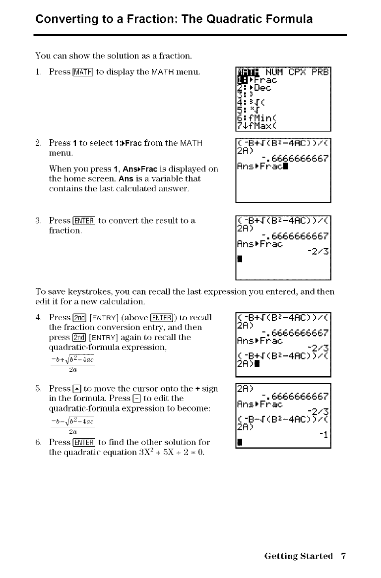
You can show the solution as a fl'action.
1. Press [_ to display the MATH lnenu.
Press 1 to select 1:)Frac froln the MATH
lnenu,
When you press 1, AnsJ,Frac is displayed on
the home screen. Arts is a variable that
contains the last calculated answer.
NUN CPX PRB
Pao
eo
3:_
4:_#(
5: *#
6:¢Min(
7¢€Ma× (
(-B+#(BZ-4RC))/(
2R) %6666666667
Rns*Fr, ac|
Press 1_ to convert the result to a
fl'action.
(-B+4-(BZ-4RC) )/(
2R)
To save keystrokes, you can recall the last expression you entered, and then
edit it for a new calculation.
Press [2_ [ENTRY](above [gNT_) to recall
the fraction conversion entry, and then
press Fffffd][ENTRY]again to recall the
quadratic-fornmla expression,
2a
5, Press [] to nlove the cursor onto the + sign
in the fornmla, Press [] to edit the
quadratic-fornmla expression to become:
2a
6, Press 1_ to find the other solution for
the quadratic equation 3X 2 + 5X + 2 = 0.
I-B+E(BZ-4RC))/(
R) -.6666666667
Rns*Fpac -2/3
(-B+E(BZ-4RC))/(
2R)|
2R) -.6666666667
Rns_Frac -2/31
(-B-.r(BZ-4RC))/(
_R) -1
Getting Started 7
Displaying Complex Results: The Quadratic Formula
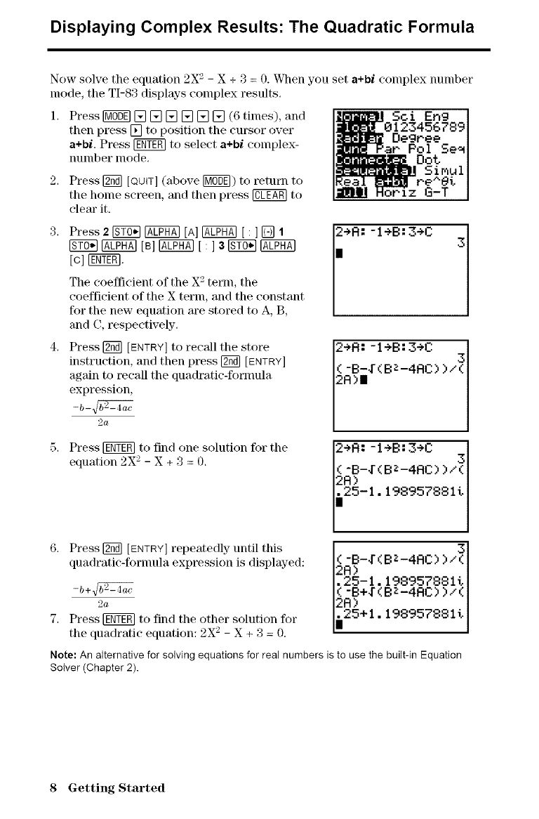
Now solve the equation 2X 2 - X + 3 = 0. When you set a+bi complex number
mode, the TI-83 displays complex results.
Press 1_ [] [] [] [] [] [] (6 times), and
then press [] to position the cursor over
a+bi. Press @ to select a+bi coinplex-
number mode.
2, Press [_ [QU*T] (above _E]) to return to
the home screen, and then press @ to
cleat" it.
zG-T
Press 2_ @ [A] @ [: ] [] 1
[c] F_q.
The coefficient of the X 2 term, the
coefficient of the X term, and the constant
for the new equation are stored to A, B,
and C, respectively.
eR:-leB:3aC 3
Press [_ [ENTRY] to recM1 the store
instruction, and then press [_ [ENTRY]
again to recall the quadratic-fornmla
expression,
2o
2+R: -1+B:3+C 3
Press @ to find one solution for the
equation 2X 2 - X + 3 = 0.
12+R:-I+B:3+C
i25-I. 198957881t
Press [2_ [ENTRY]repeatedly until this
quadratic-fornmla expression is displayed:
2a
Press @ to find the other solution for
the quadratic equation: 2X 2 - X + 3 = 0.
(-B-g(BZ-4RC))/_
2R)
.25-1.198957881t
(-B+E(BZ-4RC))/(
2R)
i25+1.198957881t
Note: An alternative for solving equations for real numbers is to use the built-in Equation
Solver (Chapter 2).
8 Getting Started
Defining a Function: Box with Lid
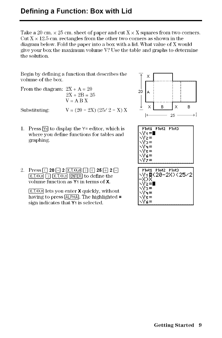
Take a 20 enl. x 25 enl. sheet of paper and cut X × X squm'es fronl two comers,
Cut X × 12,5 cm. rectangles from the other two corners as shown in the
diagram below, Fold the paper into a box with a lid. What value of X would
give your box the nlaxinmln volume V? [ _se the table and graphs to determine
the solution,
Begin by defining a function that describes the
volunle of the box.
From the diagram: 2X + A = 20
2X + 2B = 25
V=ABX
Substituting: V = (21) - 2X) (25/2 - X) X
1. Press [] to display the Y= editor, which is
where you define functions for tables and
graphing.
Press[] 20[] 2 _ [] [] 25[] 2[]
[] _ [_ to define the
volume function as Y1 in terms of X.
lets you enter Xquickly, without
having to press @. The highlighted =
sign indicates that Y1 is selected.
_ x B
PloL:L Plot;' PICL3
","?t =I
\y._=
xY_=
"_y_=
,..y_=
,,y_=
xY?=
\'14tB<20-2X) <25/2
-X)X
_Yz=l
,..y_=
xYfi=
Getting Started 9
Defining a Table of Values: Box with Lid
The table feature of the TI-83 displays numeric inforlnation about a function.
You can use a table of values fl'om the function defined on page 9 to estimate
an answer to the problem,
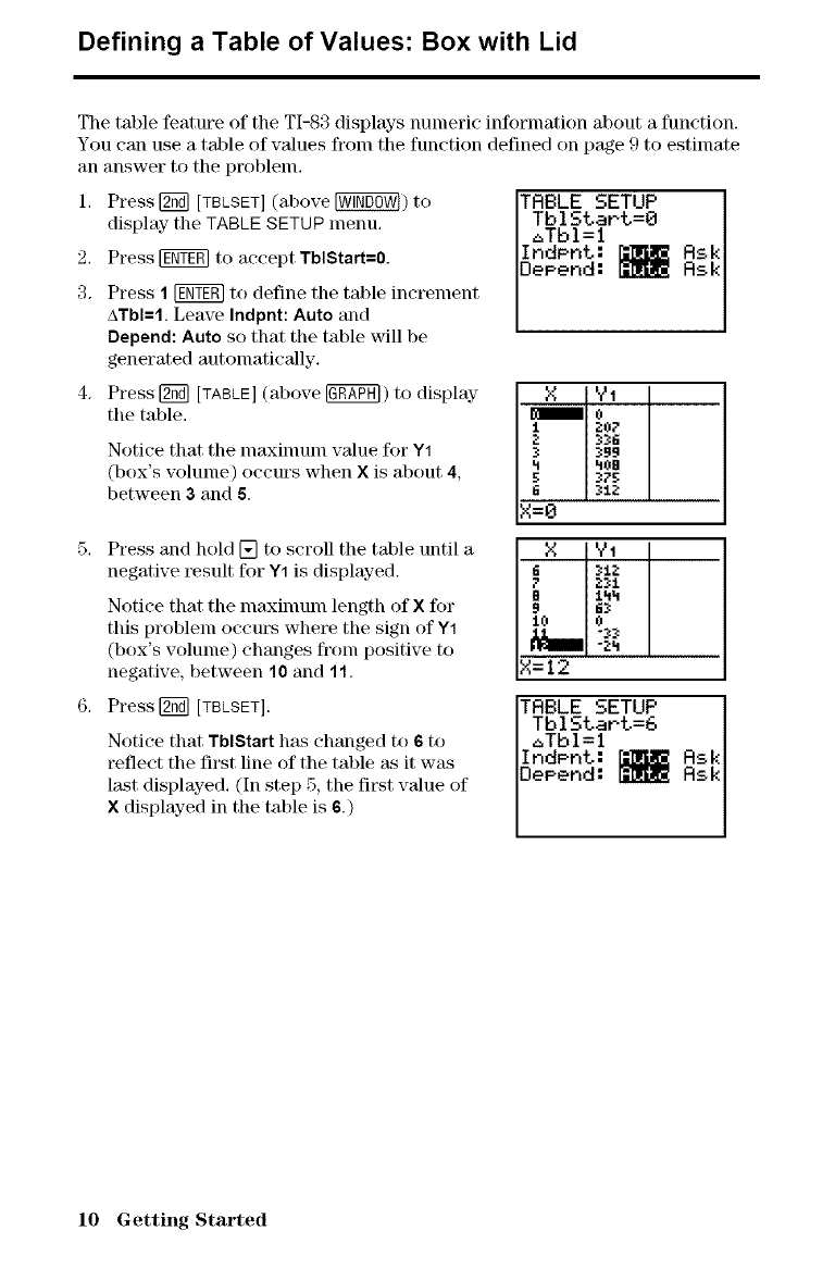
1, Press [2_ [TBLSET] (a|)ove _) to
display the TABLE SETUP menu,
2, Press [gNT_ to accept TblStart=0.
3. Press 1[ggY_ to define the table increment
ATbI=I. Leave Indpnt: Auto and
Depend: Auto so that the table will be
generated automatically,
4. Press [2_ [TABLE](above _) to display
the table,
Notice that the nlaxilnuln value for Y1
(box's volunm) occurs when Xis about 4,
between 3and 5.
TABLESETUP
Tb IStart=O
aTbl=l
Indent:
Depend:
X 91
Io
1 207
Z3_6
_99
hOB
63t_
X=O
X V1
E_t2
F231
B lhh
10 0
X=12
5, Press and hold [] to scroll the table until a
negative result for Y1 is displayed.
Notice that the nmxinmm length of X for
this problem occurs where the sign of Y1
(box's volume) changes from positive to
negative, between 10 and 11,
6, Press[2_ [TBLSET].
Notice that TblStart h_s changed to 6 to
reflect the first line of the table as it was
last displayed, (In step 5, the first value of
X displayed in the table is 6.) TRBLE SETUP Rsk
TblStart=6
_Tbl=l
IndPn÷: P._ _.
Depend:
10 Getting Started
Zooming In on the Table: Box with Lid
You can adjust the way a table is displayed to get lnore inforlnation about a
defined function. With smaller values for aTbl, you can zoom in on the table.
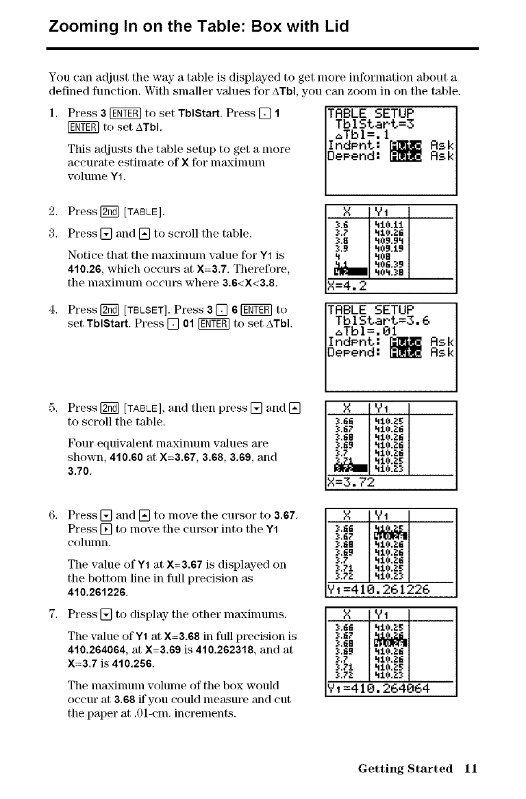
Press 3_to set TblStart. Press [] 1
[gNT_ to set ATbl.
This adjusts the table setup to get a nlore
accurate estimate of Xfor lnaxilnuln
volunle Y1. TABLESETUP
TblStart=3
_Tbl=. 1
IndPnt: r=Rg_t_
Depend: r=_r;J_
2, Press[2_ [TABLE], X91
_.6 4±0.11
3. Press [] and [] to scroll the table. :<;' _.0.z6
KB hOg,gtl
2,.9 h09.19
Notice that tile nlaxinluln value for Y1 is _ 't0a
410.26, which occurs at X=3.7. Therefore, u06.x9
h0h.3B
the nlaxinmln occurs where 3.6<X<3.8, X=4.2
Press [2_ [TBLSET]. Press 3[] 6 _ to
set TblStart. Press [] 01 [gNT_ to set ATbl.
Press [2_ [TABLE], and then press [] and []
to scroll the table.
Four equivalent nlaxinluln values are
shown, 410.60 at X=3.67, 3.68, 3.69, and
3.70.
TRBLE SETUP
TblStart=3.6
_Tbl=.Ol
IndPnt: _ Rsk
Depend: _ Rsk
gYI
K67 hi0&6
3,68 h10,?.6
K69 h10.;':6
3.? h:t0._:6
h:t0.23
X=3, 72
X Y_
-_:.6B hlO.Z6
3.69 h10,_':6
3.? hlO,Z6
3.71 h10.25
_.72 h10.2_
V, =410, 261226
X V_
3.66 h10.2_
3.6}'
K6B
K69 h10,?.6
3.7 h10,;':6
3.71 h10._:5
2;.72 ht0.23
V, =410, 264064
Press [] and [] to inove the cursor to 3.67.
Press [] to lnove the cursor into tile Y1
colulnn,
Tile value of Y1 at X=3.67 is displayed on
the bottoln line in full precision as
410.261226.
Press [] to display tile other nlaxinlunls.
The value of Y1 at X=3.68 in full precision is
410.264064, at X=3.69 is 410.262318, and at
X=3.7 is 410.266.
The lnaxilnuln volulne of the box would
occur at 3.68 if you could lneasure and cut
the paper at .01-eln. increments.
Getting Started 11
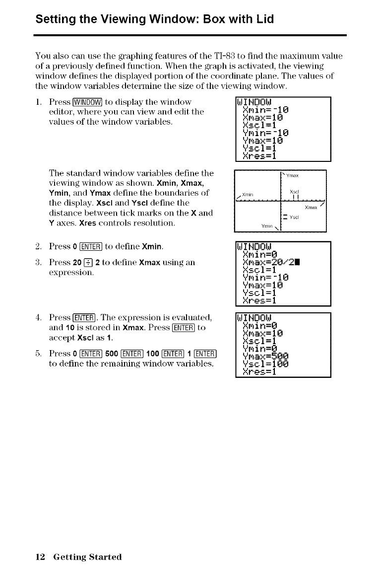
Setting the Viewing Window: Box with Lid
You also can use the graphing features of the TI-83 to find the nlaxinlunl value
of a previously defined function. When the graph is activated, the viewing
window defines the displayed portion of the coordinate plane. The values of
the window variables determine tile size of tile xqewing window.
Press _ to display tile window
editor, where you can view and edit the
values of the window variables.
WINDOW
XMin=-lO
XMax=lO
XscI=I
VMin=-lO
VMax=lO
Vscl=l
Xres=l
:_Ymax
Xscl
j Xmm
Xma× /
iZ Ysd
Ymin \
WINDOW
Xmin=O
XMax=20/2I
Xscl=l
VMin=-lO
YMax=IO
Yscl=l
Xres=l
WINDOW
XMin=O
Xmax=lO
XS61=I
VMin=O
VMax=500
Yscl=100
Xres=l
The standard window variables define the
viewing window _ shown. Xmin, Xmax,
Ymin, and Ymax define the boundm'ies of
the display. Xscl and Yscl define the
distance between tick nmrks on the Xand
Y taxes. Xres controls resolution.
2. Press 0_ to define Xmin.
3. Press 20 [] 2 to define Xmax using an
expression.
4. Press [g_gO. The expression is evaluated,
and 10 is stored in Xmax. Press [gffT_] to
accept Xscl as 1.
5. Press 0[ggggm500 [ggggm100 [g_gN 1[ggggm
to define the remaining window variables.
12 Getting Started
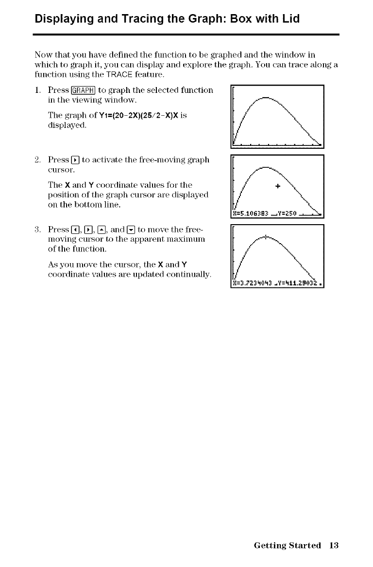
Displaying and Tracing the Graph: Box with Lid
Now that you have defined the function to be graphed and the window in
which to graph it, you can display- and explore the graph. You call trace along a
function using the TRACE feature.
1. Press _ to graph the selectedfunctionillthe viewing window. I_i/f .-_.-_-, Nj
The graph of Y1--(20 - 2X)(25/2 -X)X is
displayed.
Press [] to activate the free-moving graph
cursor,
The Xand Ycoordinate values for the
position of the graph cursor are displayed
on the bottom line.
3. Press _], [], [], and [] to move the free-
moving cm\sor to the apparent nlaxinmln
of the function.
As you move the cursor, the Xand Y
coordinate values are updated continually.
Getting Started 13
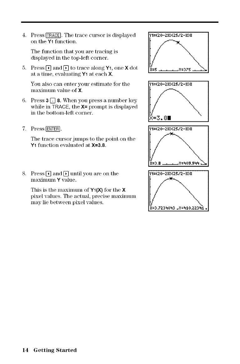
4. Press _. The trace cursor is displayed
on the Y1 function.
The function that you are tracing is
displayed in the top-left corner.
Press [] and [] to trace along Y1, one X dot
at a time, evaluating Y1 at each X.
You also can enter your estimate for the
nlaxinmln value of ×.
6. Press a [] 8. When you press a number key
while in TRACE, the X= prompt is displayed
in the bottom-left corner.
7. Press [gNT_.
The trace cursor jumps to tile point on the
Y1 function evaluated at X=a.8.
Press [] and [] until you are on the
nlaxinlunl Y wdue.
This is the nlaxinlunl of YI(X) for the X
pixel values. The actual, precise nl_kxinlunl
may lie between pixel values.
?t: G:'_)-::"}D_.::'_/::"-}{)}:
t/ ',..
[?t:{20-2g:l{2gc'2:-{,l)g
'¢l=€.RO-l_g)(2g/l_-l{)g
?t:G_O-_:8)(2:gd_-R):_
14 Getting Started
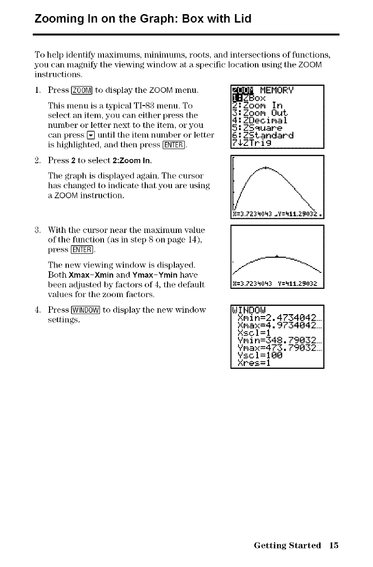
Zooming In on the Graph: Box with Lid
To help identify nlaxinlulns, nlininlulns, roots, and intersections of functions,
you can magnify the viewing window at a specific location using tile ZOOM
instructions.
1. Press _ to display- the ZOOM lnenu.
This menu is a typical TI-83 menu. To
select an item, you can either press the
number or letter next to the item, or you
can press [] until the item number or letter
is highlighted, and then press [_.
2. Press 2to select 2:Zoom In.
The graph is displayed again. The cursor
has changed to indicate that you m'e using
a ZOOM instruction.
With the cm_sor near the nlaxinlunl vMue
of the function (as in step 8 on page 14),
press [_.
The new viewing window is displayed.
Both Xmax-Xmin and Ymax-Ymin have
been adjusted by factors of 4, the default
values for the zoom factors.
MEMORY
In
3:Zoom Out
4:ZOeoiMal
5:ZS_uare
6:ZStandard
?4ZTPig
X=.3.7;_.3LI0_.Y=_:tl.=90.3;: .
Press _ to display the new window
settings.
WINDOW
Xmin=2.4734042_.
XMax=4.9734042...
Xsol=l
YMin=348.79032...
YMaX=473.79032...
Yscl=100
Xres=l
Getting Started 15
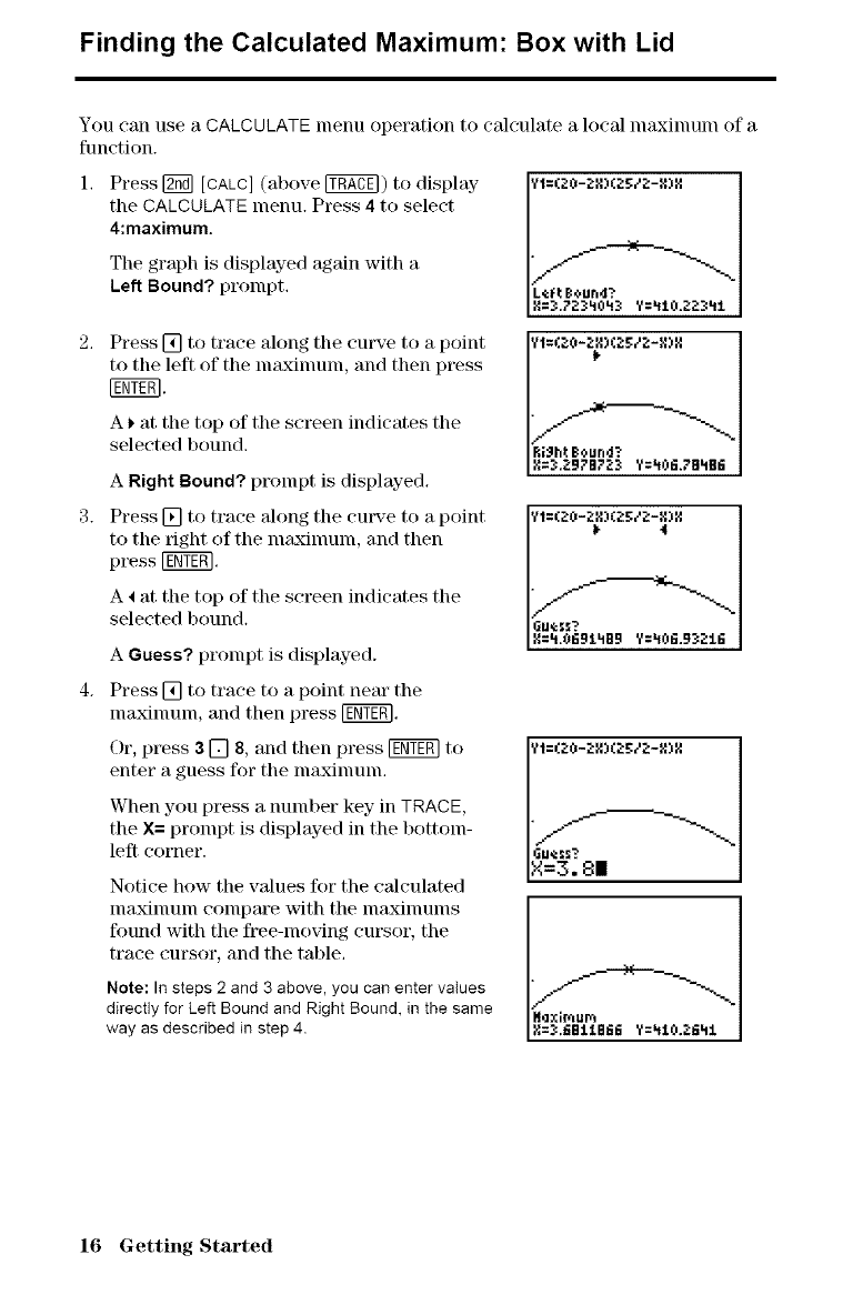
Finding the Calculated Maximum: Box with Lid
You can use aCALCULATE menu operation to calculate alocal maxinmm of a
function.
Press [2_ [CALC] (above _) to display
the CALCULATE menu. Press 4 to select
4:maximum.
The graph is displayed again with a
Left Bound? prompt,
Press [] to trace along the curve to a point
to tile left of the nlaxinluln, and then press
[N!N.
A _ at the top of the screen indicates the
selected bound.
ARight Bound? prompt is displayed.
3. Press [] to trace along the curve to a point
to the right of the nlaxinluln, and then
press [g_gm.
A _ at the top of the screen indicates the
selected bound.
AGuess? prompt is displayed.
Gu¢_=?
X=_.O69i_g9 Y=_06.9_216
4. Press [] to trace to a point neat" the
inaxiinuin, and then press [ggT_q.
Or, press 3[] 8, and then press [ggT_q to
enter a guess for the nmxinmm.
When you press a number key in TRACE,
the X= prompt is displayed in the bottom-
left corner.
Notice how the values for the calculated
nlaxinlunl compare with the nlaxinlunls
found with the free-moving cursor, the
trace cursor, and the table.
Note: In steps2 and 3 above,youcan entervalues
directlyfor Left BoundandRight Bound,in thesame
way as describedin step 4.
16 Getting Started
Other TI-83 Features
Getting Started has introduced you to basic TI-83 operation. This guidebook
describes in detail the features you used in Getting Started. It also covers the
other features and capabilities of the TI-83.
Graphing You can store, graph, and analyze up to 10 functions
(Chapter 3), up to six parametric functions (Chapter 4), up
to six polar functions (Chapter 5), and up to three
sequences (Chapter 6). You can use DRAW operations to
annotate graphs (Chapter 8).
Sequences You can generate sequences and graph thenl over time. Or,
you can graph them as web plots or as phase plots
(Chapter 6).
Tables You can create function evaluation tables to analyze nlany
functions sinmltaneously (Chapter 7).
Split Screen You can split the screen horizontally to display- both a
graph and a related editor (such msthe Y= editor), the
table, the stat list editor, or the home screen, Ms(), you can
split the screen verticMly to display a graph and its table
sinmltaneously (Chapter 9),
Matrices You can enter and save up to 10 matrices and perform
standard matrix operations on them (Chapter 10).
Lists You can enter and save as nlany lists as lllelllOl_y-allows for
use in statistical analyses. You can attach fornmlas to lists
for automatic computation. You can use lists to evaluate
expressions at nmltiple values sinmltaneously and to graph
a family of curves (Chapter 11).
Statistics You can perform one- and two-variable, list-based
statistical analyses, including logistic and sine regression
analysis. You can plot the data as a histogram, xyLine,
scatter plot, modified or regulm" box-and-whisker plot, or
normal probability plot. You can define and store up to
three stat plot definitions (Chapter 12).
Getting Started 17
Inferential
Statistics You can perform 16 hypothesis tests and confidence
inte_'als and 15 distribution functions. You can display
hypothesis test results graphically or numerically
(Chapter 13).
Financial
Functions You can use tilne-value-of-lnoney (TVM) functions to
analyze financial instruments such as annuities, loans,
mortgages, leases, and sa_lngs. You can analyze the value
of money over equal time periods using cash flow
functions. You can amortize loans with the amortization
functions (Chapter 14).
CATALOG The CATALOG is a convenient, alphal_etieal list of all
functions and instructions on the TI-83. You can paste any
function or instruction from the CATALOG to the current
cursor location (Chapter 15).
Programming You can enter and store programs that include extensive
control and input!output instructions (Chapter 16).
Communication
Link The TI-83 has a port to connect and conlnlunieate with
another TI-83, a TI-82, the Calculator-Based Laborato_sJ u
(CBL 2TM, CBL TM) System, a Calculator-Based Ranger TM
(CBWM), or a personal computer. The unit-to-unit link
cable is included with the TI-83 (Chapter 19).
18 Getting Started
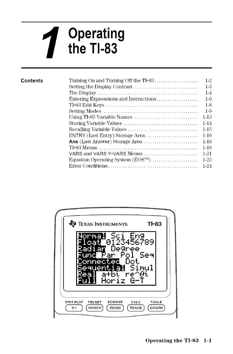
1Operating
the TI-83
Contents Turning On and Turning Off tile TI-83 .................... 1-2
Setting the Display Contrast ............................. 1-3
Tile Display" .............................................. 1-4
Entering Expressions and Instructions ................... 1-6
TI-83 Edit Keys .......................................... 1-8
Setting Modes ........................................... 1-9
Using TI-83 Variable Names ............................. 1-13
Storing Variable Values .................................. 1-14
Recalling Variable Values ................................ 1-15
ENTRY (Last Entry) Storage Area ........................ 1-16
Ans (Last Answer) Storage Area ......................... 1-18
TI-8:_ Menus ............................................. 1-19
VARS and VARS Y-VARS Menus ......................... 1-21
Equation Operating System (EOS TM) ..................... 1-22
En'or Conditions ......................................... 1-24
TEXAS INSTRUMENTS TI-83
Sol Eng
123456789
Degree
Pol Se_
Dot
Si_ul
Horiz G-T
J
STAT PLOT TBLSET FORMAT CALC TABLE
Operating tile TI-83 1-1
Turning On and Turning Off the TI-83
Turning On the
Calculator
Turning Off the
Calculator
Batteries
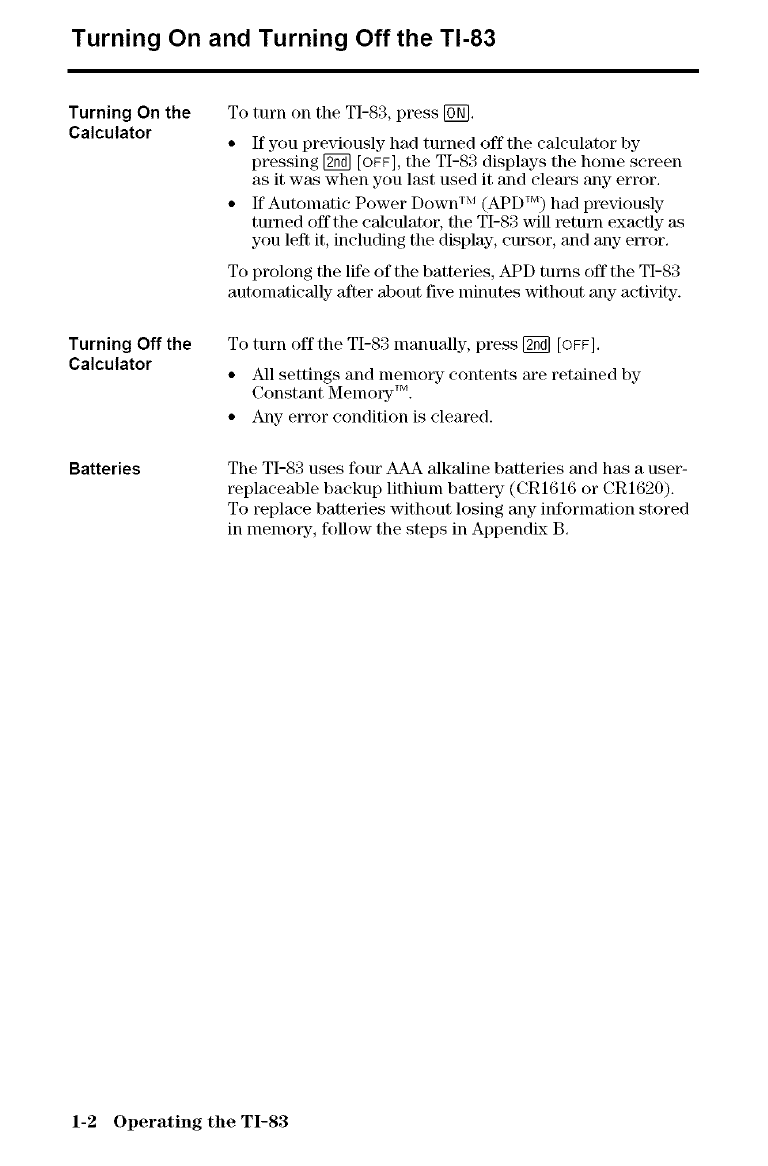
To turn on the TI-83, press ION].
• If you previously had turned off the calculator by
pressing K_] [OFF], the TI-83 displays the home screen
as it was when you last used it and clears any error.
• If Automatic Power Down m (APD TM) hal p_eviously
turned off the calculator, the TI-83 will return exactly as
you left it, including the display, cursor, and any em)r.
To prolong the life of the batteries, APD turns off the TI-83
automatically after about five minutes without any actixqty.
To turn offthe TI-83 manually, press [_ [OFF].
• All settings and memory contents are retained by
Constant Memo_y TM.
• Any er_)r condition is cleared.
The TI-83 uses four AAA alkaline batteries and has a user-
replaceable backup lithium batte_Ty- (CR1616 or CR1620).
To replace batteries without losing any information stored
in memory, follow the steps in Appendix B.
1-2 Operating the TI-83
Setting the Display Contrast
Adjusting the
Display Contrast
When to Replace
Batteries
You can adjust the display contrast to suit your viewing
angle and lighting conditions. As you change the contrast
setting, a number from 0 (lightest) to 9 (darkest) in the
top-right corner indicates the current level. You may not be
able to see the number if contrast is too light or too dark.
Note: The T1-83 has 40 contrast settings, so each number 0through 9
represents four settings.
The TI-83 retains tile contrast setting in nlenlol_y- when it is
turned off.
To adjust the contrast, follow these steps.
1. Press and release the D_] key.
2. Press and hold [] or [], which are below and above the
contra_t sjnnbol (yellow, half-shaded circle).
• [] lightens the screen.
• [] darkens the screen.
Note: If you adjust the contrast setting to 0, the display may become
completely blank. To restore the screen, press and release _, and
then press and hold [] until the display reappears.
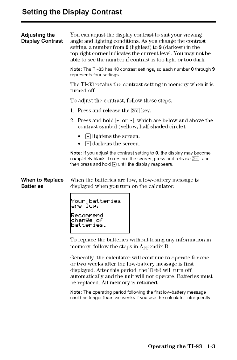
When the batteries are low, a low-battelT message is
displayed when you turn on the calculator.
Your battePies
ape lou.
Recommend
change of
batteries,
To replace the batteries without losing any- information in
memory, follow tile steps in Appendix B.
Generally-, the calculator will continue to operate for one
or two weeks after the low-batte<F message is fil_t
displayed. After this period, the TI-83 will turn off
automatically and the unit will not operate. Batteries nmst
be replaced. All nmmow is retained.
Note: The operating period following the first low-battery message
could be longer than two weeks if you use the calculator infrequently.
Operating the TI-83 1-3
The Display
Types of
Displays
Home Screen
Displaying
Entries and
Answers
Returning to the
Home Screen
Busy Indicator
The TI-83 displays both text and graphs. Chapter 3
describes graphs. Chapter 9 describes how the TI-83 can
display- a horizontally or vertically split screen to show
graphs and text simultaneously.
The home screen is the prima_T screen of the TI-83. On
this screen, enter instructions to execute and expressions
to evaluate. The answers are displayed on the same screen.
When text is displayed, the TI-83 screen can display a
nlaxinmm of eight lines with a nmxinmm of 16 characters
per line. If all lines of the display are full, text scrolls off
the top of the display. If an expression on the home screen,
the Y= editor (Chapter 3), or the program editor
(Chapter 16) is longer than one line, it wraps to the
beginning of the next line. In numeric editors such as the
window screen (Chapter 3), a long expression scrolls to
the right and left.
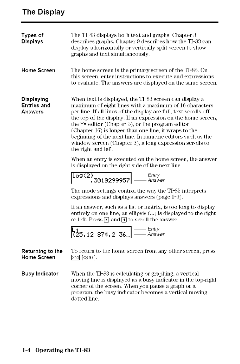
VC]mn an enhT is executed on the home screen, the answer
is displayed on the right side of the next line.
io9(2) Entry
• 3010299957 Answer
The mode settings control the way the TI-83 interprets
expressions and displays answers (page 1-9).
If an answer, such as a list or matrix, is too long to display
entirely on one line, an ellipsis (...) is displayed to the right
or left. Press [] and [] to scroll the answer.
ILl Entry
1{25.12 874.2 36_ Answer
To return to the honle screen fronl any- other screen, press
[_ [QUIT].
When the TI-83 is calculating or graphing, a vertical
moving line is displayed as a busy indicator in the top-right
corner of the screen. When you pause a graph or a
program, the busy indicator becomes a vertical moving
dotted line.
1-4 Operating the TI-83
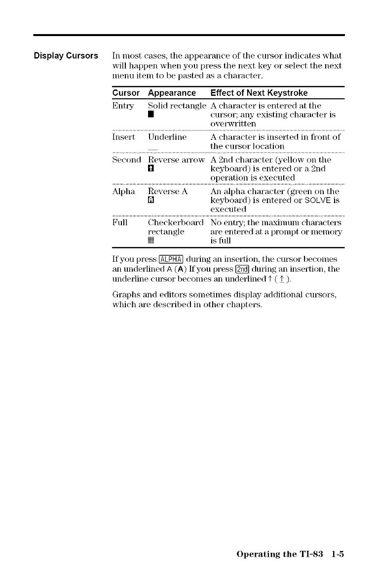
Display Cursors In most cases, the appearance of the cursor indicates what
will happen when you press the next key- or select the next
menu item to be pasted as a character.
Cursor Appearance Effect of Next Keystroke
EntKF Solid rectangle A character is entered at the
• cursor; any existing character is
ove_wvritten
Insert Underline A character is inserted in front of
Second Reverse a_TOW A 2nd character (yellow on the
[] keyboard) is entered or a 2nd
operation is executed
Alpha Reverse A An alpha character (green on the
[] keyboard) is entered or SOLVE is
executed
Full Checkerboard No ently; the lnaxilnuln ehara('te_
rectangle are entered at a prompt or lnelnory
iiiiiii is full
If you press @ during an insertion, the cursor becomes
an underlined A (A) ff you p_ss [_ during an insertion, the
underline cursor becomes an underlined I' (I').
Graphs and editors sometimes display additional cursors,
which are described in other chapters.
Operating the TI-83 1-5
Entering Expressions and Instructions
What Is an
Expression?
Entering an
Expression
Multiple Entries
on a Line
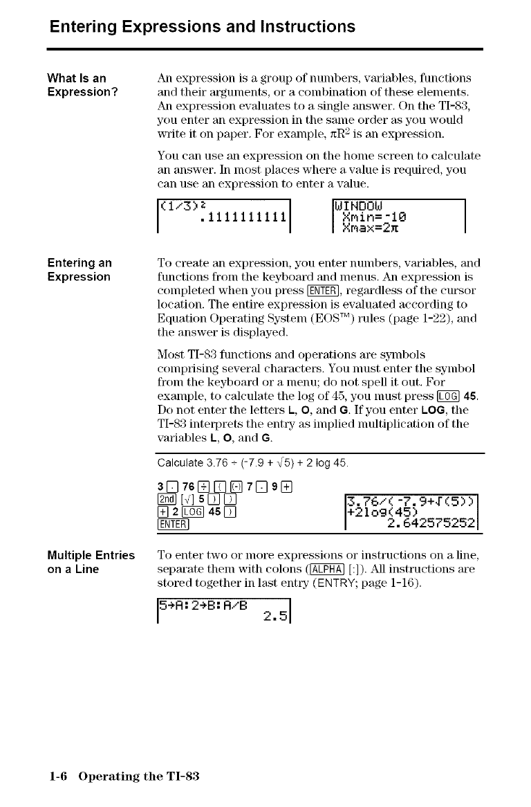
An expression is a group of numbers, variables, functions
and their arguments, or a combination of these elements.
An expression evaluates to a single answer. On the TI-83,
you enter an expression in the same order _.s you would
write it on paper. For exalnple, xR 2 is an expression.
You can use an expression on tile home screen to calculate
an answer. In most places where a value is required, you
can use an expression to enter a value.
(i/3) z I WINDOW [
• 111111111 Xmin=-10
Xmax=2x I
To create an expression, you enter numbers, variables, and
functions from the keyboard and menus. AI_ expression is
coinpleted when you press [gNY_, regardless of the cursor
location. The entire expression is evaluated according to
Equation Operating System (EOS TM) rules (page 1-22), and
the answer is displayed.
Most TI-83 functions and operations are s3qnbols
comprising several characters. You nmst enter the symbol
from the keyboard or a menu; do not spell it out. For
example, to calculate the log of 45, you nmst press [UfN 45.
Do not enter the letters t., O, and 6. If you enter LOG, the
TI-83 inteqorets the enttT as implied nmltiplication of the
variables L, O, and G
Calculate 3.76 + (-7.9 + _5) + 2 Iog 45.
a[E]r6@DDrDg@
[d 5DD
@21 q 45D 2. 642575252
To enter two or more expressions or instructions on a line,
separate them with colons (@ [:]). All instructions are
stored together in last enttT (ENTRY; page 1-16).
15+R:2+B:R/B 2.51
1-6 Operating the TI-83
Entering a
Number in
Scientific
Notation
Functions
Instructions
Interrupting a
Calculation
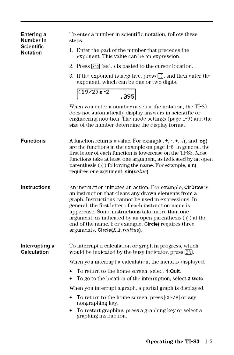
To enter a number in scientific notation, ff)llow these
steps.
1. Enter the part of the number that precedes the
exponent. This value can be an expression.
2. Press [_ [EE]. Eis pasted to the cursor location.
3. If the exponent is negative, press D, and then enter the
exponent, which can be one or two digits.
l(19/2) £-2 .0951
When you enter a number in scientific notation, the TI-83
does not automatically display answers in scientific or
engineering notation. The mode settings (page 1-9) and the
size of the number determine the display- format.
A function returns a value. For example, +, -, +, _(, and log(
are tlle functions in the example on page 1-6. In general, the
first letter of each function is lowercase on the TI-83. Most
functions take at least one a_gument, as indicated by _m open
parenthesis ( ( ) following the name. For exalnple, sin(
_qui_s one argument, sin(value).
An instruction initiates an action. For example, ClrDraw is
an instruction that clears any- drawn elements from a
graph. Instructions cannot be used in expressions. In
general, the first letter of each instruction name is
uppercase. Some instructions take more than one
argument, as indicated by an ()pen parenthesis ( ( ) at the
end of the name. For example, Circle( requires three
arguments, Circle(X,Y, radius).
To intetTupt a eMeulation or graph in progress, which
would be indicated by the busy indicator, press [_].
When you interrupt a calculation, the menu is displayed.
• To return to the home screen, select 1:Quit.
• To go to the location of the interruption, select 2:Goto,
When you interrupt a graph, a partial graph is displayed.
• To return to the home screen, press @ or any
nongraphing key.
• To restart graphing, press a graphing key or select a
graphing instruction.
Operating the TI-83 1-7
TI-83 Edit Keys
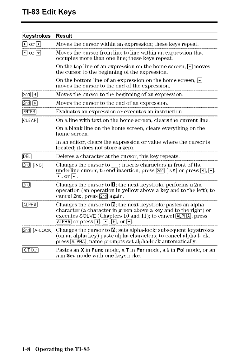
Keystrokes
[] or []
[] or []
Result
Moves the cursor within an expression; these keys repeat.
Moves the cursor from line to line within an expression that
occupies more than one line; these key-s repeat.
On the top line of an expression on the honle screen, [] nloves
the cursor to the beginning of the expression.
On the bottom line of an expression on the home screen, []
nloves the cursor to the end of the expression.
Moves the cursor to the beginning of an expression.
Moves the cursor to the end of an expression.
Evaluates an expression or executes an instruction.
On a line with text on the home screen, clears the current line.
On a blank line on the honle screen, clears everything on the
home screen.
In an editor, clears the expression or value where the cursor is
located; it does not store a zero.
Deletes a character at the cursor; this key repeats.
[_ tINS] Changes the cursor to __ ; inserts chm'acters in front of the
underline cursor; to end insertion, press [2_] [,NS] or press [], [],
[], or [].
[_ Changes the cursor to n; the next keystroke performs a 2nd
operation (an operation in yellow above a key- and to the left); to
cancel 2nd, press [2_] again.
@ Changes the cursor to i51;the next keystroke pastes an alpha
character (a character in green above a key and to the right) or
executes SOLVE (Chapters 10 and 11); to cancel @, press
@ or press _, [], [], or [].
[_ [A-LOCK] Changes the cursor to r/l;sets alpha-lock; subsequent keystrokes
(on an alpha key) paste alpha characters; to cancel alpha-lock,
press @; name prompts set alpha-lock automatically.
Pastes an X in Func Inode, a Tin Par Inode, a O in Pol Inode, or an
nin Seq mode with one keystroke.
1-8 Operating the TI-83
Setting Modes
Checking Mode
Settings
Changing Mode
Settings
Setting aMode
from a Program
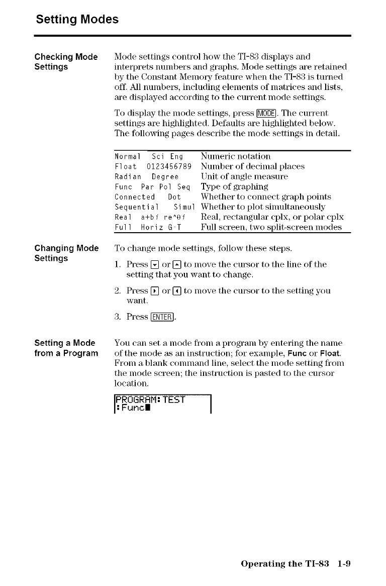
Mode settings control how the TI-83 displays and
interprets numbers and graphs. Mode settings are retained
by the Constant Meln(aTy- feature when the TI-83 is turned
off. All numbet_, including elements of matrices and lists,
are displayed according to the current mode settings.
To display- the mode settings, press [Mff_]. The current
settings are highlighted. Defaults are highlighted below.
The following pages describe the mode settings in detail.
Normal Sci Eng Numeric notation
Float 0123456789 Nulnber of deeilnal places
Radian Degree Unit of angle men,sure
Func Par Pol Seq Type of graphing
Connected Dot Whether to connect graph points
Sequential Simul Whether to plot sinmltaneously
Real a+b ire^0 iReal, rectangular cplx, or polar eplx
Ful 1 H0ri z G T Full screen, two split-screen modes
To change nlode settings, follow these steps.
1. Press [] or [] to lnove the cm\sor to the line of the
setting that you want to change.
2. Press [] or [] to nlove the cursor to the setting you
want.
3. Press [ggY_,
You call set a mode fronl a program by entering the name
of the mode as all instruction; for example, Func or Float.
Fronl a blank eonlnland line, select the nlode setting fronl
the mode screen; the instruction is pasted to the cursor
location.
PROGRRM: TEST
:FuncI I
Operating the TI-83 1-9
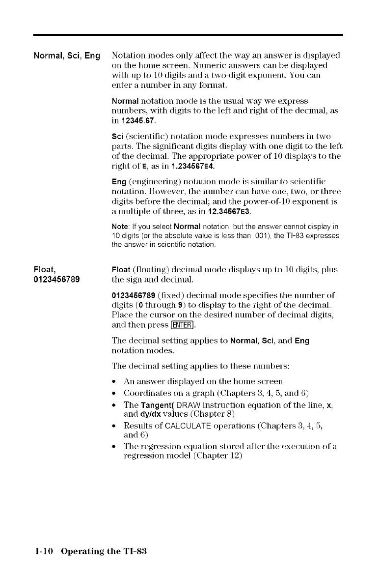
Normal, Sci, Eng
Float,
0123456789
Notation modes only 'affect the way an answer is displayed
on the home screen. Numeric answers can be displayed
with up to 10 digits and a two-digit exponent. You can
enter a number in any- format.
Normal notation mode is the usual way we express
numbers, with digits to the left and right of the decimal, as
in 12345.67.
Sci (scientific) notation mode expresses number,s in two
pm'ts. The significant digits display- with one digit to the left
of the decimal. The app_)priate power of 10 displays to the
right of E, t_sin 1.234567E4.
Eng (engineering) notation mode is similm" to scientific
notation. However, the number can have one, two, or three
digits before the decimal; and the power-of-10 exponent is
a nmltiple of three, as in 12.34567E3.
Note: Ifyou select Normal notation, but the answer cannot display in
10 digits (or the absolute value is tess than .00I ), the TF83 expresses
the answer in scientific notation.
Float (floating) decimal mode displays up to 10 digits, plus
the sign and decimal.
0123456789 (fixed) decimal mode specifies the number of
digits (0 through 9) to display to the right of the decimal.
Place the cursor on the desired number of decimal digits,
and then press [ENYE_.
The decimal setting applies to Normal, Sci, and Eng
notation modes.
The decimM setting applies to these numbers:
• An answer displayed on the home screen
• Coordinates on a graph (Chapters 3, 4, 5, and 6)
• The Tangent( DRAW instruction equation of the line, x,
and dy/dx values (Chapter 8)
• Results of CALCULATE operations (Chapters 3, 4, 5,
and 6)
• The regression equation stored after the execution of a
regression lnodel (Chapter 12)
1-10 Operating the TI-83
Radian, Degree
Func, Par, Pol,
Seq
Connected, Dot
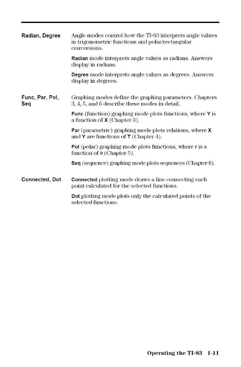
Angle modes control how the TI-83 inteq)rets angle values
in trigonometric functions and polar/rectangular
conversions.
Radian mode intelprets angle values as radians. Answers
display- in radians.
Degree mode interprets angle vMues as degrees. Answers
display- in degrees.
Graphing modes define the graphing paralneters. Chapters
3, 4, 5, and 6 describe these nlodes in detail.
Func (function) graphing mode plots functions, where Yis
a function of X (Chapter 3).
Par (parametric) graphing mode plots relations, where X
and Yare functions of T (Chapter 4).
Pol (polar) graphing mode plots functions, where r is a
function of 0 (Chapter 5).
Seq (sequence) graphing mode plots sequences (Chapter 6).
Connected plotting mode draws a line connecting each
point eMeulated for the selected functions.
Dot plotting mode plots only the e;flculated points of the
selected functions.
Operating the TI-83 1-11
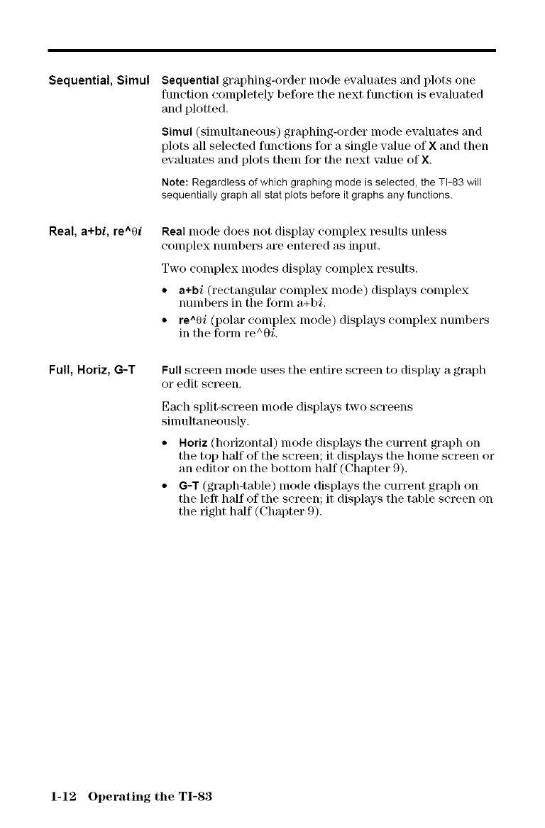
Sequential, Simul Sequential graphing-order mode evaluates and plots one
function completely before the next function is evaluated
and plotted.
Simul (sinmltaneous) graphing-order mode evaluates and
plots all selected functions for a single wdue of X and then
evMuates and plots them for the next value of X.
Note: Regardless of which graphing mode is selected, the TI-83 wil!
sequentially graph all stat plots before it graphs any functions.
Real, a+bi, re^Of Real mode does not display complex results unless
complex numbers are entered as input.
Two complex modes display- complex results.
• a+bi (rectangulm" complex mode) displays complex
numbers in the form a+bi.
• re^0i (polar complex mode) displays complex numbers
in the fornl re^Oi.
Full, Horiz, G-T Full screen mode uses the entire screen to display- a graph
or edit screen.
Each split-screen nlode displays two screens
sinmltaneously.
•Horiz (horizontal) mode displays the current graph on
the top half of the screen; it displays the home screen or
an editor on the bottom h'alf (Chapter 9),
•G-T (graph-table) mode displays the current graph on
the left half of the screen; it displays the table screen on
the right half (Chapter 9).
1-12 Operating the TI-83
Using TI-83 Variable Names
Variables and
Defined Items
Notes about
Variables
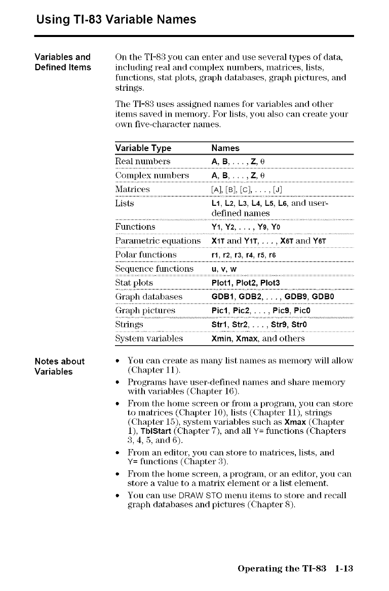
On the TI-83 you can enter and use several types of data,
including real and complex numbe_\s, matrices, lists,
functions, stat plots, graph databases, graph pictures, and
strings.
The TI-83 uses ansigned names for variables and other
items saved in nlenlol_yL For lists, you 'also can create your
own five-character names.
Variable Type Names
Real numbers A, B,..., Z, 0
Complex numbers A, B,..., Z, 0
Matrices [A], [B], [C], . . . , [J]
Lists Cl, L2, L3, L4, LS, L6, and user-
defined haines
Functions Y1, Y2,..., Yg, Yo
Parametric equations XIT and YIT, ... , X6T and Y6T
Polar functions rl, r2, r3, r4, r5, r6
Sequence functions u, v, w
Stat plots Plot1, Plot2, Plot3
Graph databases GDB1, GDB2,..., GDB9, GDB0
Graph pictures Picl, Pic2,..., Pic9, Pic0
Strings Strl, Str2,..., Str9, Str0
System variables Xmin, Xmax, and others
• You can create as many list names as nlenlo_y- will Mlow
(Chapter 11).
•Progranls have user-defined nanles and share nlenlory
with variables (Chapter 16).
• FI_)lll the honle screen or fronl a progranl, you can store
to matrices (Chapter 10), lists (Chapter 11), strings
(Chapter 15), system variables such me Xmax (Chapter
1), TblStatt (Chapter 7), and all Y= functions (Chapters
3, 4, 5, and 6),
• FI_Olll an editor, you can store to matrices, lists, and
Y= functions (Chapter 3).
• FI_Olll the honle sereen_ a progranl, or all editor, you can
store a value to a lnatrix element or a list element.
• You can use DRAW STO menu items to store and reeM1
graph datab_kses and pictures (Chapter 8).
Operating the TI-83 1-13
Storing Variable Values
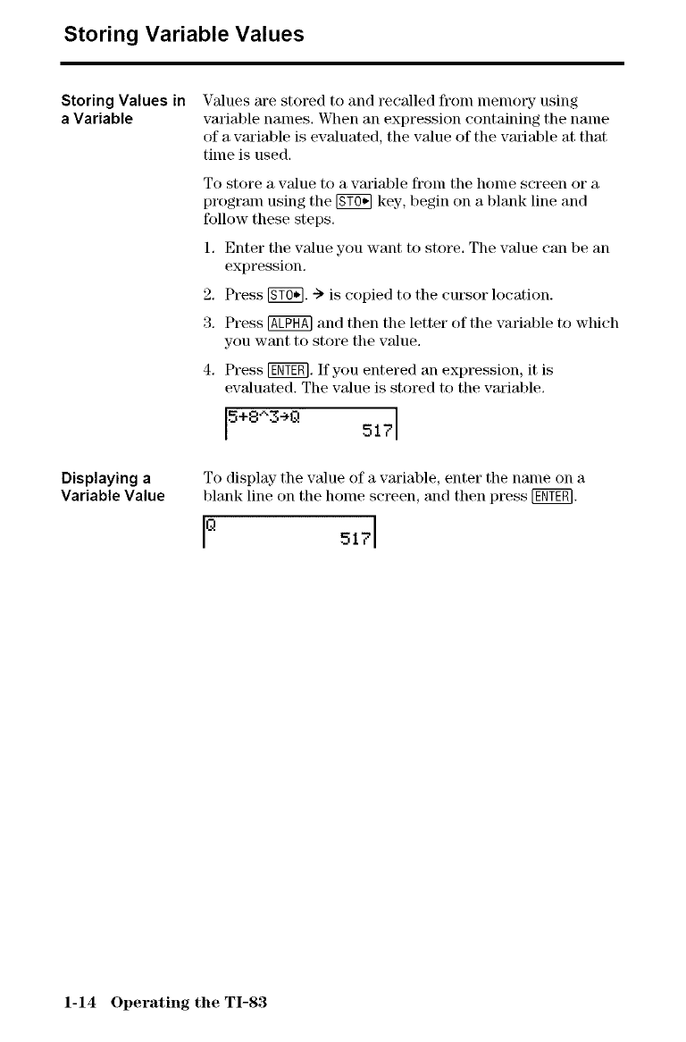
Storing Values in
aVariable
Displaying a
Variable Value
Values are stored to and recalled fronl nlenlol_- using
variable names. When an expression containing the name
of a variable is evMuated, the vMue of the variable at that
time is used.
To store a value to a vm'iable fronl the home screen or a
program using the _ key, begin on a blank line and
follow these steps.
1. Enter the value you want to store. The value can be an
expression.
2. Press _. -> is copied to the cursor location.
3. Press @ and then the letter of the variable to which
you want to store the value.
4. Press [gg_O. If you entered an expression, it is
evaluated. The value is stored to the variable.
[5+8_'3÷Q 517[
To display- the value of a vm'iable, enter the name on a
blank line on the home screen, and then press IgOr.
I° 5171
1-14 Operating the TI-83
Recalling Variable Values
Using Recall
(RCL)
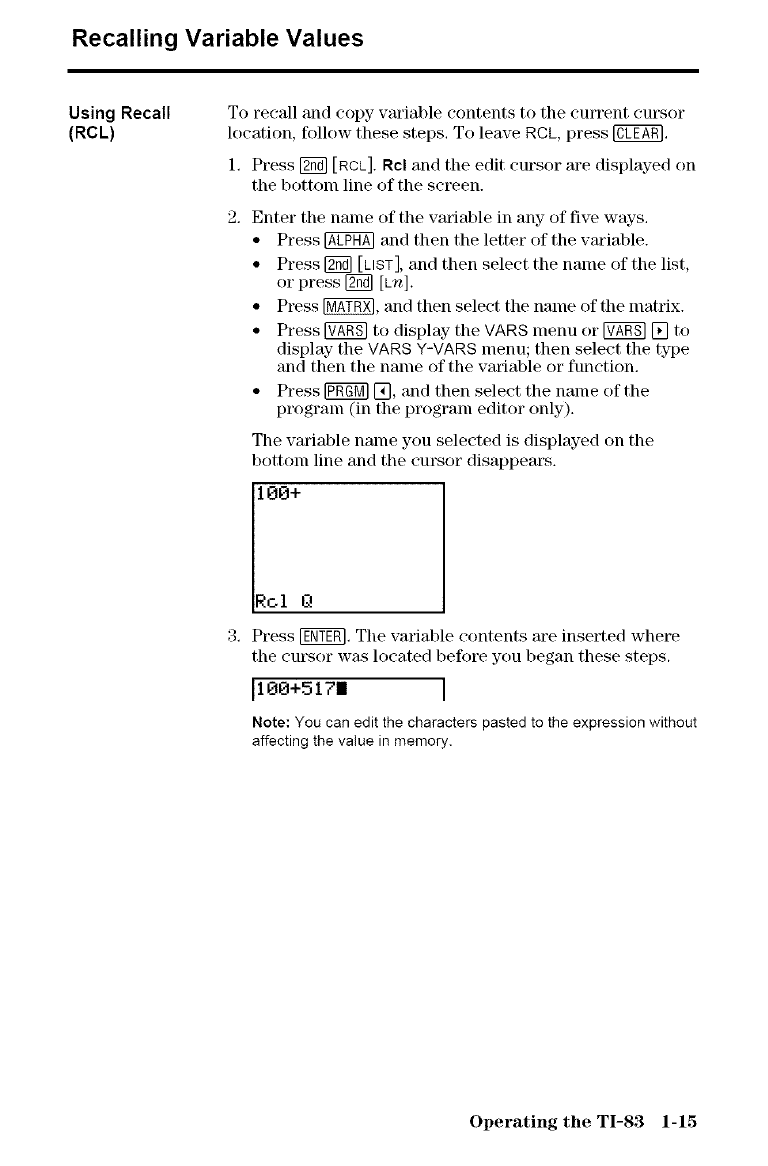
To recall and copy variable contents to the current cursor
location, follow these steps. To leave RCk, press @.
1. Press [2_] ERCL]. Rcl and the edit cursor are displayed on
the bottom line of the screen.
Enter the name of the variable in any of five ways.
• Press @ and then the letter of the variable.
• Press [g_ [LIST], and then select the name of the list,
or press [g_ [Ln].
• Press _, and then select the name of the matrix.
• Press [V_g] to display the VARS menu or _ [] to
display the VARS Y-VARS menu; then select the type
and then the name of the variable or function.
• Press NRgM] [_, and then select the name of the
program (in the program editor only).
The variable name you selected is displayed on the
bottom line and the cursor disappeat\s.
100+
Rol 0
Press IENTEEI.The variable contents are inserted where
the cursor w_s located befot_ you began these steps.
1100+517I I
Note: You can edit the characters pasted to the expression without
affecting the value in memory.
Operating the TI-83 1-15
ENTRY (Last Entry) Storage Area
Using ENTRY
(Last Entry)
Accessing a
Previous Entry
When you press [g_ on the holne screen to evaluate an
expression or execute an instruction, the expression or
instruction is placed in a storage area called ENTRY (last
ent_T). When you tu_ off the TI-83, ENTRY is retained in
lllelllOl_y',
To recall ENTRY, press 12_ [ENTRY].The last entry is
pasted to the cur_nt cursor location, where you can edit
and execute it. On the home screen or in an editor, the
current line is clea_d and the last entry is pasted to the
line.
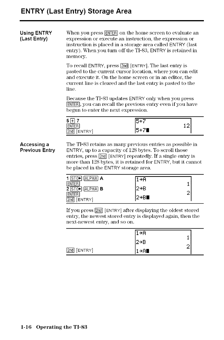
Because the TI-83 updates ENTRY only when you press
[g_, you can recall the previous entry even if you have
begun to enter the next expression.
5[] 75+7 12
F_a] [ENTRY] 5 +711
The TI-83 retains as many previous entries as possible in
ENTRY, up to a capacity of 128 bytes. To scroll those
entries, press [_ [ENTRY] repeatedly. If a single ent_T is
more than 128 bytes, it is retained for ENTRY, but it cannot
be placed in the ENTRY storage area.
I_A 1÷1::1 12
I_ 2+B
2_B
[_ 2+BI
[ENTRY]
If you press [2@] [ENTRY] after displaying the oldest stored
enttT, the newest stored entry is displayed again, then the
next-newest entry, and so on,
[ENTRY]
2eB
1+RII
1-16 Operating the TI-83
Reexecuting the
Previous Entry
Multiple Entry
Values on a Line
After you have pasted the last entt'y to the home screen
and edited it (if you chose to edit it), you can execute the
entry-. To execute the last ent_T, press [_T_].
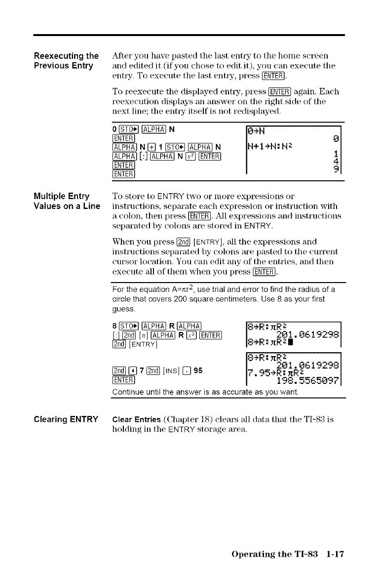
To reexecute the displayed entry, press _ again. Each
reexecution displays an answer on the right side of the
next line; the entry- itself is not redisplayed.
F_°_ @ NO+N 0
@N[]I_@N N+I÷N:NZ
To store to ENTRY two or more expressions or
instructions, separate each expression or instruction with
a colon, then press [_T_. All expressions and instructions
separated by colons are stored in ENTRY.
When you press K_ [ENTRY], all the expressions and
instructions separated by colons are p_sted to the current
cursor locatkm. You can edit any of the entries, and then
execute all of them when you press [_R].
For the equation A=_r 2, use trial and error to find the radius of a
circle that covers 200 square centimeters. Use 8 as your first
guess.
[:][_ [_-]@ R[_7 [_E_
F_ [E.TR¥]
[] 7[_ [INS] [] 95
F_t_q
8÷R:_RZ I
201.0619298
8÷R:=RZI
8+R:_Rz
201.0619298
7.95+R:_Rz
198.5565097
Continue until the answer is as accurate as you want.
Clearing ENTRY Clear Entries (Chapter 18) cleats all data that the TI-83 is
holding in the ENTRY storage area.
Operating the TI-83 1-17
Ans (Last Answer) Storage Area
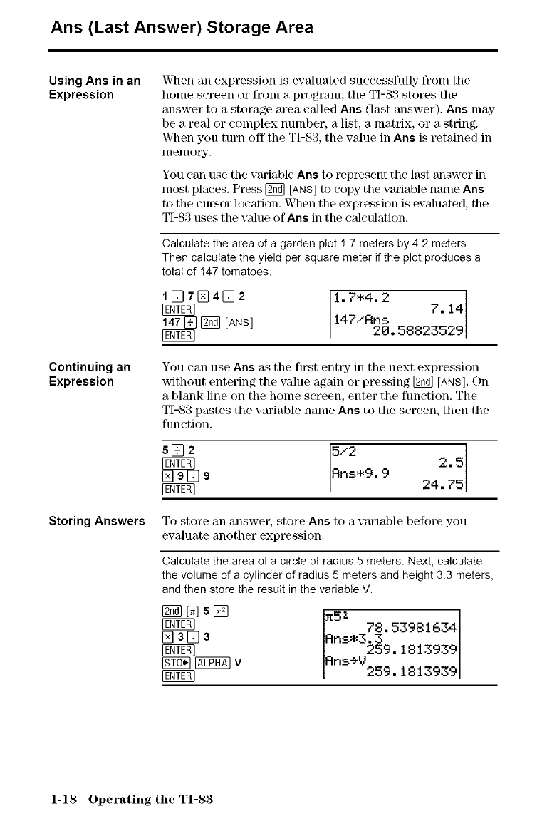
Using Ans in an
Expression
Continuing an
Expression
Storing Answers
When an expression is evaluated successfully- fronl the
home screen (Jr from a program, the TI-83 stores the
answer to a storage at_a called Ans (last answer). Ans nlay
be a real or complex number, a list, a lnatrix, or a string.
When you turn off the TI-83, the value in Ans is t_tained in
nlenlol_y.
You can use the variable Ans to represent the last answer in
most places. Press [2_] tANS] to copy the vm'iable name Ans
to the cm'sor location. When the expression is evaluated, the
TI-83 uses the value of Ans in the calculation.
Calculate the area of a garden plot 1.7 meters by 4.2 meters.
Then calculate the yield per square meter if the plot produces a
total of 147 tomatoes.
1[]TN4C32
147 [] _ [ANS]
1.7.4.2 714[
147/Rn_ 5882s5291
You can use Ans as the first enhTy in the next expression
without entering the value again or pressing [_ tANS].On
a blank line on the home screen, enter the function. The
TI-83 pastes the vm'iable name Ans to the screen, then the
function.
s[]2 5/2 2.5
_gDg[N_ffl Rns*9.9 24.75
To store an answer, store Ans to a variable before you
evMuate another expression.
Calculate the area of a circle of radius 5 meters. Next, calculate
the volume of a cylinder of radius 5 meters and height 3.3 meters,
and then store the result in the variable V.
I_ [_]s []
N3D3
__v
xSZ
78.53981634
Rns*3.o I
Rns+U 259.1813939
259.1813939
1-18 Operating the TI-83
TI-83 Menus
Using a TI-83
Menu
Scrolling a Menu
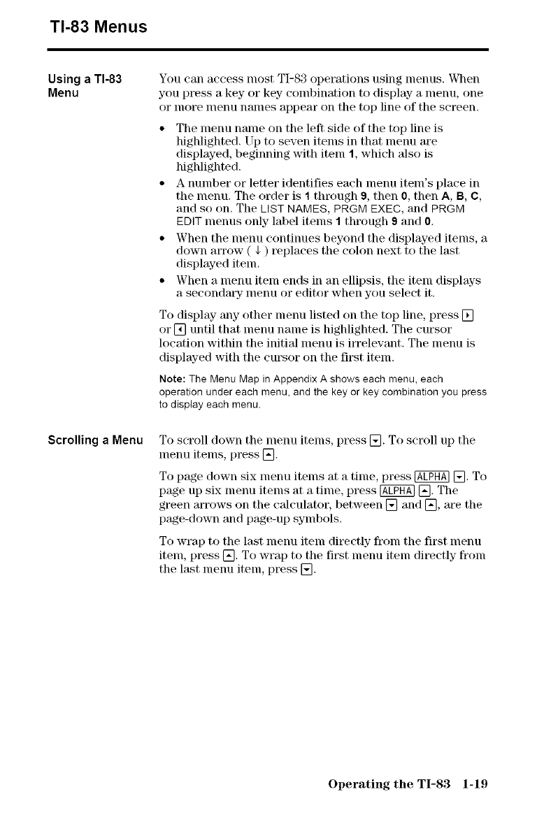
You can access lnost TI-83 operations using lnenus. When
you press a key or key- combination to display a menu, one
or more menu names appear on the top line of the screen.
• The menu name on the left side of the top line is
highlighted. Up to seven items in that menu are
displayed, beginning with item 1, which 'also is
highlighted.
• A number or letter identifies each menu item's place in
the menu. The order is 1 through 9, then 0, then A, B, C,
and so on. The LISTNAMES, PRGM EXEC, and PRGM
EDIT menus only label items 1 through 9 and 0.
• When the menu continues beyond the displayed items, a
down arrow ( $ ) replaces the colon next to the last
displayed item.
• When a menu item ends in an ellipsis, the item displays
a secondat7 menu or editor when you select it.
To display any other menu listed on the top line, press []
or [] until that menu name is highlighted. The cursor
location within the initial menu is irrelewmt. The menu is
displayed with the cursor on the first item.
Note: The Menu Map in Appendix A shows each menu, each
operation under each menu, and the key or key combination you press
to display each menu.
To scroll down the menu items, press []. To scroll up the
menu items, press [].
To page down six menu items at a time, press @ []. To
page up six menu items at a time, press @ []. The
green arrows on the calculator, between [] and [], are the
page-down and page-up symbols.
To wrap to the last menu item directly fronl the first menu
item, press []. To wrap to the first menu item directly fi'om
the last menu item, press [].
Operating the TI-83 1-19

Selecting an Item
from a Menu
Leaving a Menu
without Making a
Selection
You can select an item from a menu in either of two ways,
• Press the number or letter of the item you want to
select. The cursor can be anywvhere on the menu, and
the item you select need not be displayed on the screen,
• Press [] or [] to move the cursor to the item you want,
and then press [E6T_.
After you select an item from a menu, the TI-83 typically
displays the previous screen,
Note: On the LIST NAMES, PRGM EXEC, and PRGM EDIT
menus, only items 1 through 9 and 0 are labeled in such a way that
you can select them by pressing the appropriate number key. To move
the cursor to the first item beginning with any alpha character or 6,
press the key combination for that alpha character or e. If no items
begin with that character, then the cursor moves beyond it to the next
item.
Calculate :_27.
You can leave a menu without making a selection in any- of
four ways.
• Press [_] [QUIT] to return to the home screen.
• Press @ to return to the prexdous screen.
• Press a key or key- combination for a different menu,
such as [M_ or [_ [LIST].
• Press a key or key combination for a different screen,
such as [] or _ [TABLE],
1-20 Operating the TI-83
VARS and VARS Y-VARS Menus
VARS Menu
Selecting a
Variable from the
VARS Menu or
VARS Y-VARS
Menu
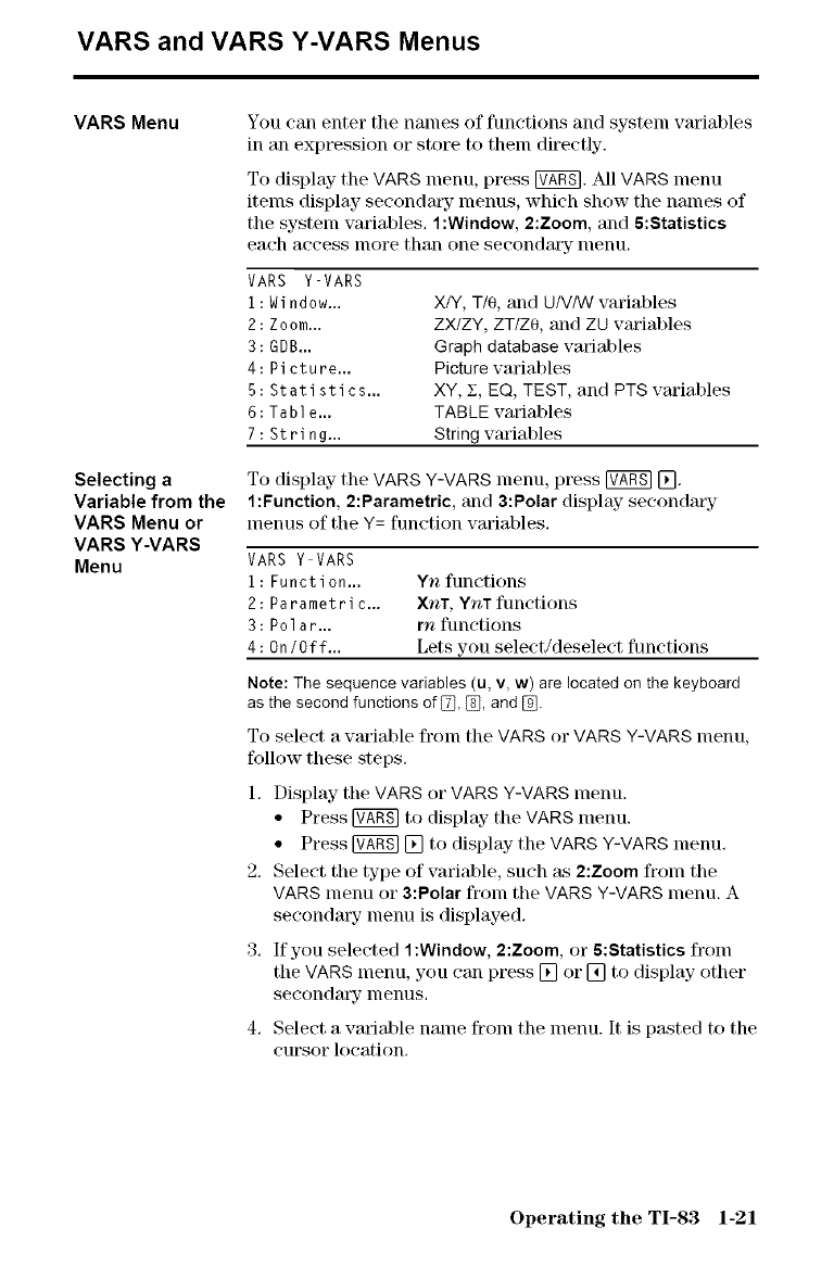
You can enter the haines of functions and systeln varial>les
in an expression or store to them directly.
To display the VARS inenu, press _. All VARS inenu
items display secondm:y- menus, which show the names of
the system variables. 1:Window, 2:Zoom, and 5:Statistics
each access lnore than one secondaYy lnenu,
VARS Y VARS
i: Window...
2 : Zoom.,.
3: GDB...
4:Picture.,.
5:Statistics.,.
6: Table...
7: String..,
X/Y, T/O, and U/VNV variables
ZX/ZY, ZT/ZO, and ZU wuiables
Graph database vmiables
Picture variables
XY, Z, EQ, TEST, and PTS vmiables
TABLE vmiables
String variables
To display the VARS Y-VARS menu, press _ [].
1:Function, 2:Parametric, and 3:Polar display seconda[3_
menus of the Y= function vmiables.
VARS Y VARS
i: Function...
2: Parametric...
3:Polar...
4:On/Off...
Yn functions
X_?,T,Y'rtT functions
rn functions
Lets you select/deselect functions
Note: The sequence variables (u, v, w) are located on the keyboard
as the second functions olin, 1%1,and El.
To select a variable fronl the VARS or VARS Y-VARS menu,
follow these steps.
1. Display the VARS or VARS Y-VARS menu.
• Press [_ to display the VARS menu.
• Press _ [] to display the VARS Y-VARS lnenu.
2. Select the type of variable, such as 2:Zoom from the
VARS menu or 3:Polar froln the VARS Y-VARS menu. A
secondm:y- menu is displayed.
3. If you selected 1:Window, 2:Zoom, or 5:Statistics from
the VARS menu, you can press [] or [] to display ()the["
secondal_y- lnenus,
4. Select a variable name from the menu. It is pasted to the
CUrSOr location.
Operating the TI-83 1-21
Equation Operating System (EOS TM)
Order of
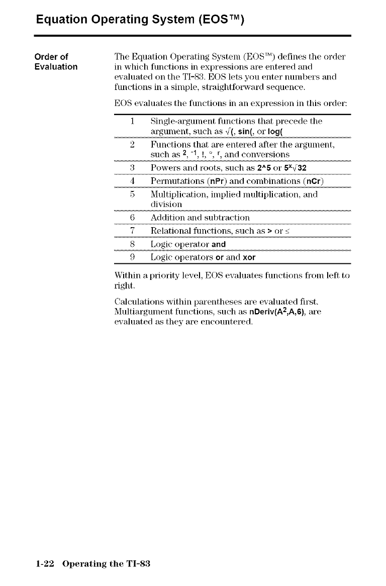
Evaluation The Equation Operating System (EOS TM) defines the order
in which functions in expressions are entered and
evaluated on the TI-83. EOS lets you enter numbers and
functions in a simple, straightfot_vard sequence.
EOS evaluates the functions in an expression in this order:
1 Single-argument functions that precede the
argument, such as ¢(, sin(, or log(
2 Functions that are entered after the argument,
such _ks2, -1, 1, o, r, and conversions
3 Powers and roots, such as 2^5 or 5x¢32
4 Pernmtations (nPr) and combinations (nOr)
5 Multiplication, implied nmltiplication, and
division
6 Addition and subtraction
7 Relational functions, such _ > or <
8 Logic operator and
9 Logic operators or and xor
Within a priority level, EOS evaluates functions fronl left to
right.
Calculations within parentheses are ewduated first.
Multiargument functions, such as nDeriv(A2,A,6), are
evaluated as they are encountered.
1-22 Operating the TI-83
Implied
Multiplication
Parentheses
Negation
The TI-83 recognizes implied nmltiplication, so you need
not press [] to express nmltiplication in all cases. For
example, the TI-83 intel_rets 2_, 4sin(46), 5(1+2), and (2"5)7
as implied nmltiplication.
Note: TI-83 implied multiplication rules differ from those of the TI-82.
For example, the TI-83 evaluates 1/2X as (1/2)*X, while the TI-82
evaluates 1/2X as 1/(2"X) (Chapter 2).
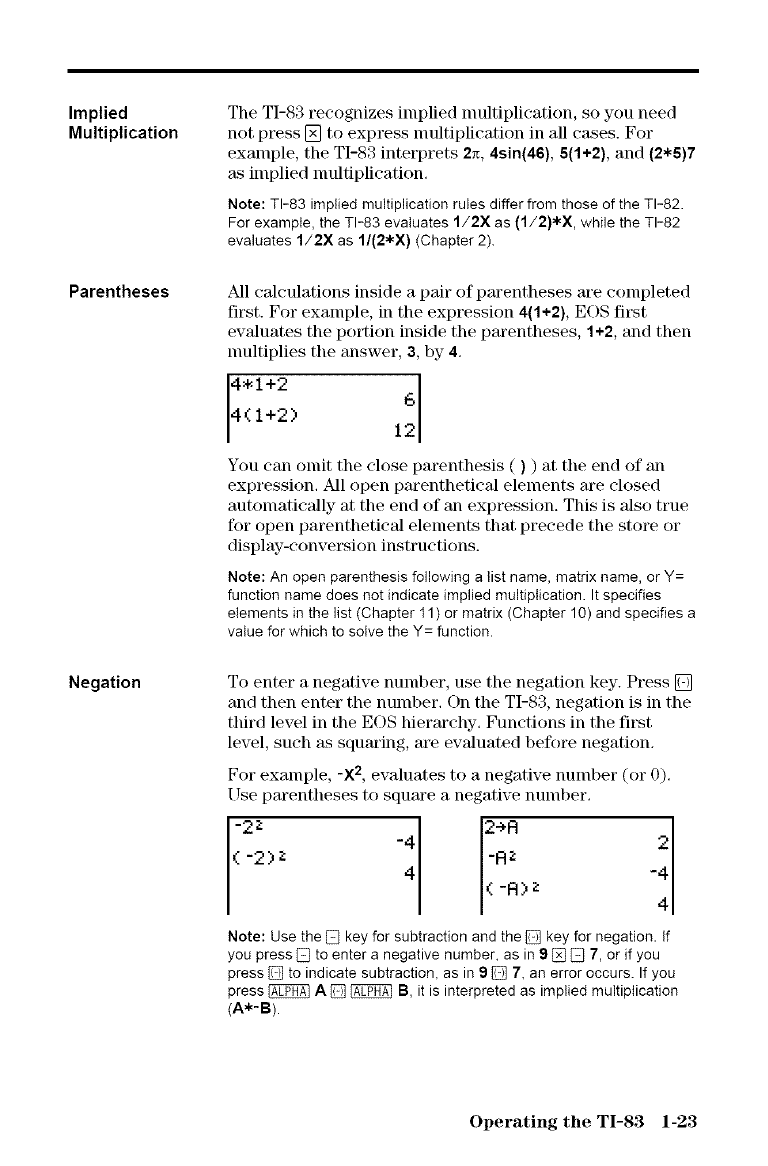
All calculations inside a pair of pm'entheses are completed
first. For example, in the expression 4(1+2), EOS first
evaluates the portion inside the pm'entheses, 1+2, and then
nmltiplies the answer, 3, by 4.
4.1+2 I_
4(1+2)
You can omit tile ('lose parenthesis ( )) at tile end of an
expression. All ()pen parenthetical elements are closed
automatic_dly at the end of an expression. This is Mso true
for open parenthetical elements that precede the store or
display-conversion instructions.
Note: An open parenthesis following a list name, matrix name, or Y=
function name does not indicate implied multiplication. It specifies
elements in the list (Chapter I1) or matrix (Chapter 10) and specifies a
value for which to solve the Y= function.
To enter a negative number, use the negation key. Press []
and then enter the number. On the TI-83, negation is in the
third level in the EOS hierm'chy. Functions in the fil\st
level, such as squaring, ale ewduated before negation.
For example, -X 2, evaluates to a negative number (or 0).
[ _se parentheses to square a negative number.
-2z _ 12->R
(-2) z _ -AZ 42
( -A )z-4
Note:Use the[] key forsubtractionand the[] keyfornegation.If
you press [] to enter a negative number, as in 9[] [] 7, or if you
press [] to indicate subtraction, as in !) [] 7, an error occurs. If you
press @ A [] @ B, it is interpreted as implied multiplication
(A*-B).
Operating the TI-83 1-23
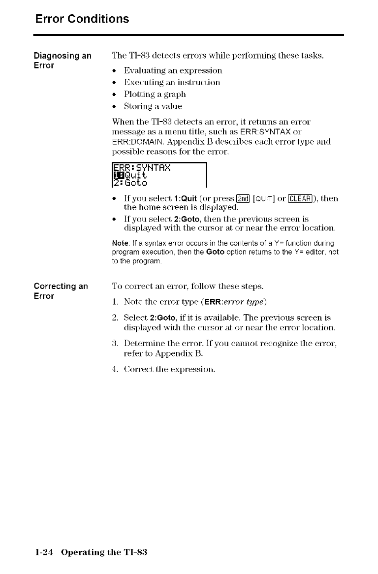
Error Conditions
Diagnosing an
Error
Correcting an
Error
The TI-83 detects errot\s while performing these tasks.
• Ewduating an expression
• Executing an instruction
• Plotting a graph
• Storing a value
VClmnthe TI-83 detects an error, it returns an etTor
message as a menu title, such _ts ERR:SYNTAX or
ERR:DOMAIN. Appendix B describes each error type and
possible reasons for tile etTor.
ERR: S_,"NTRX I
_a[IQuit I
2: Goto
• If you select 1:OuR (or press [_ [QUIT]or @), then
tile home screen is displayed.
• If you select 2:Goto, then the prexqous screen is
displayed with the cut\sot at or neat" the error location.
Note: If a syntaxerroroccurs in thecontentsof a Y= functionduring
program execution, thenthe Goto option returnsto the Y=editor, not
to theprogram.
To eotTect an error, follow these steps.
1. Note the error type (ERR:e_9"or type).
2. Select 2:Goto, if it is available. The previous screen is
displayed with the cursor at or neat" the error location.
3. Determine the error. If you cannot recognize the error,
refer to Appendix B.
4. Correct the expression.
1-24 Operating the TI-83
Math,Angle,andTest
Operations
Contents Getting Started: Coin Flip ................................ 2-2
Keyboard Math Operations .............................. 2-3
MATH Operations ........................................ 2-5
Using the Equation Solver ............................... 2-8
MATH NUM (Number) Operations ........................ 2-13
Entering and Using Complex Nmnbers ................... 2-16
MATH CPX (Complex) Operations ....................... 2-18
MATH PRB (Probability) Operations ..................... 2-20
ANGLE Operations ....................................... 2-23
TEST (Relational) Operations ............................ 2-24
TEST LOGIC (Boolean) Operations ...................... 2-26
'_ TEXAS iNSTRUMENTS T1=83
Q^3+PZ-125=O
-Q=4.6415888336...
P=5
bound={-50,50}
-le_t-rt=O
J
STAT PLOT TBLSET FORMAT CALC TABLE
Math, Angle, and Test Operations 2-1
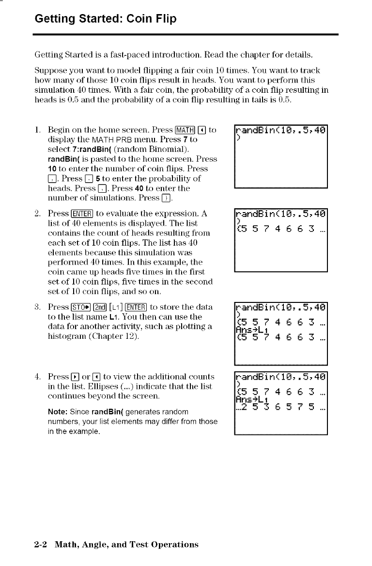
Getting Started: Coin Flip
Getting Started is a fast-paced introduction. Read the chapter for details.
Suppose you want to model flipping a fair coin 10 times. You want to track
how many of those 10 coin flips result in heads. You want to perform this
sinmlation 40 times. With a fair coin, the probability of a coin flip resulting in
heads is 0.5 and the probability of a coin flip resulting in tails is I).5.
1. Begin on tile home screen. Press [_ [] to
display the MATH PRB menu. Press 7 to
select 7:randBin( (random Binomial).
randBin( is pasted to the home screen. Press
10 to enter the number of coin flips. Press
[]. Press [] 5to enter the probability of
heads. Press []. Press 40 to enter the
number of sinmlations. Press D-
2. Press _ to evaluate the expression. A
list of 40 elements is displayed. The list
contains the count of heads resulting from
each set of 10 coin flips. The list has 40
elements because this sinmlation was
performed 40 times. In this example, the
coin came up heads five times in the first
set of 10 coin flips, five times in the second
set of 10 coin flips, and so on.
3. Press [_ [_ [L1][gNTgmto store the data
to the list name L1.You then can use the
data for another activity, such as plotting a
histogram (Chapter 12).
4. Press [] or [] to view the additional counts
in the list. Ellipses (...) indicate that the list
continues beyond the screen.
Note: Since randBin( generates random
numbers, your list elements may differ from those
in the example.
_andBin(10,.5,40
_andBin( 10,. 5,40
{5574663_.
Rgs_L_ 4 6 6 3 ...
andBin( 10,. 5, 40
5 5 7 4 6 6 3 ,..
..£._._L_6 5 7 5 ...
2-2 Math, Angle, and Test Operations
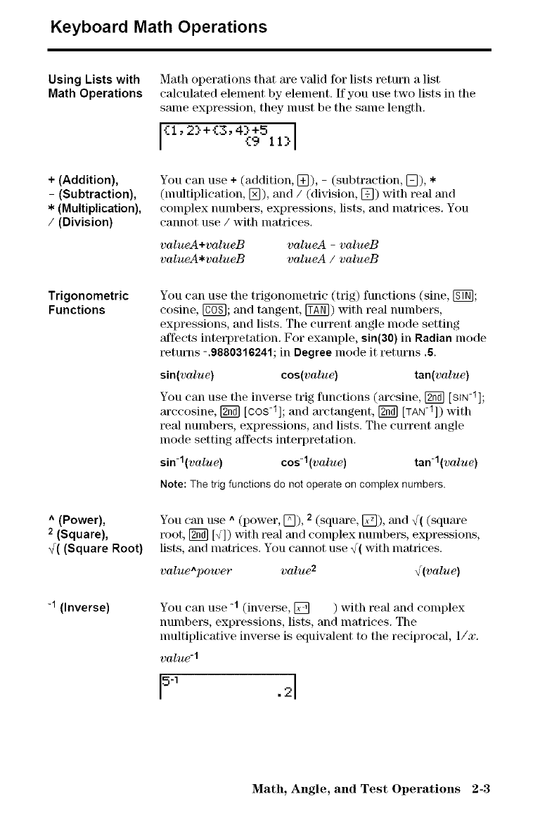
Keyboard Math Operations
Using Lists with
Math Operations
+ (Addition),
-(Subtraction),
* (Multiplication),
/(Division)
Math operations that are valid ff)rlists return a list
calculated element by element. If you use two lists in the
same expression, they nmst be the same length.
{1,2}+{3, 4}+5
{9 113
You can use +(addition, E]), - (subtraction, E]), *
(nmltiplieation, [_), and /(division, []) with real and
complex numbers, expressions, lists, and lnatrices. You
cannot use /with matrices.
valueA+valueB
valueA*valueB
valueA -valueB
valueA / valueB
Trigonometric
Functions
^(Power),
2(Square),
,[( (Square Root)
-1 (inverse)
You can use the trigonometric (trig) functions (sine, [gN];
cosine, [Ugg]; and tangent, _) with real number\%
expressions, and lists. The current angle mode setting
'affects interpretation. For example, sin(a0) in Radian mode
tetut]ls -.9880316241; in Degree mode it returns .5.
sin(value) cos(value) tan(value)
You can use the inverse trig functions (aresine, [g_] [StN-1];
arccosine, [g_] [c05-t]; and arctangent, [g_] [TAN-t])with
real nmnbers, expressions, and lists. The current angle
mode setting affects interpretation.
sin -1(value) cos -1(value) tan -1(value)
Note: The trig functions do not operate on complex numbers.
You can use ^ (power, [_), 2 (square, [77]),and _/( (square
root, [g_] [4]) with teal and complex numbers, expressions,
lists, and nmtrices. You cannot use _( with matrices.
value^power value 2 _[(value)
You can use -1 (inverse, [] ) with real and complex
numbers, expressions, lists, and matrices. The
nmltiplieative inverse is equivalent to the reciprocal, l/x.
value-1
15' .21
Math, Angle, and Test Operations 2-3
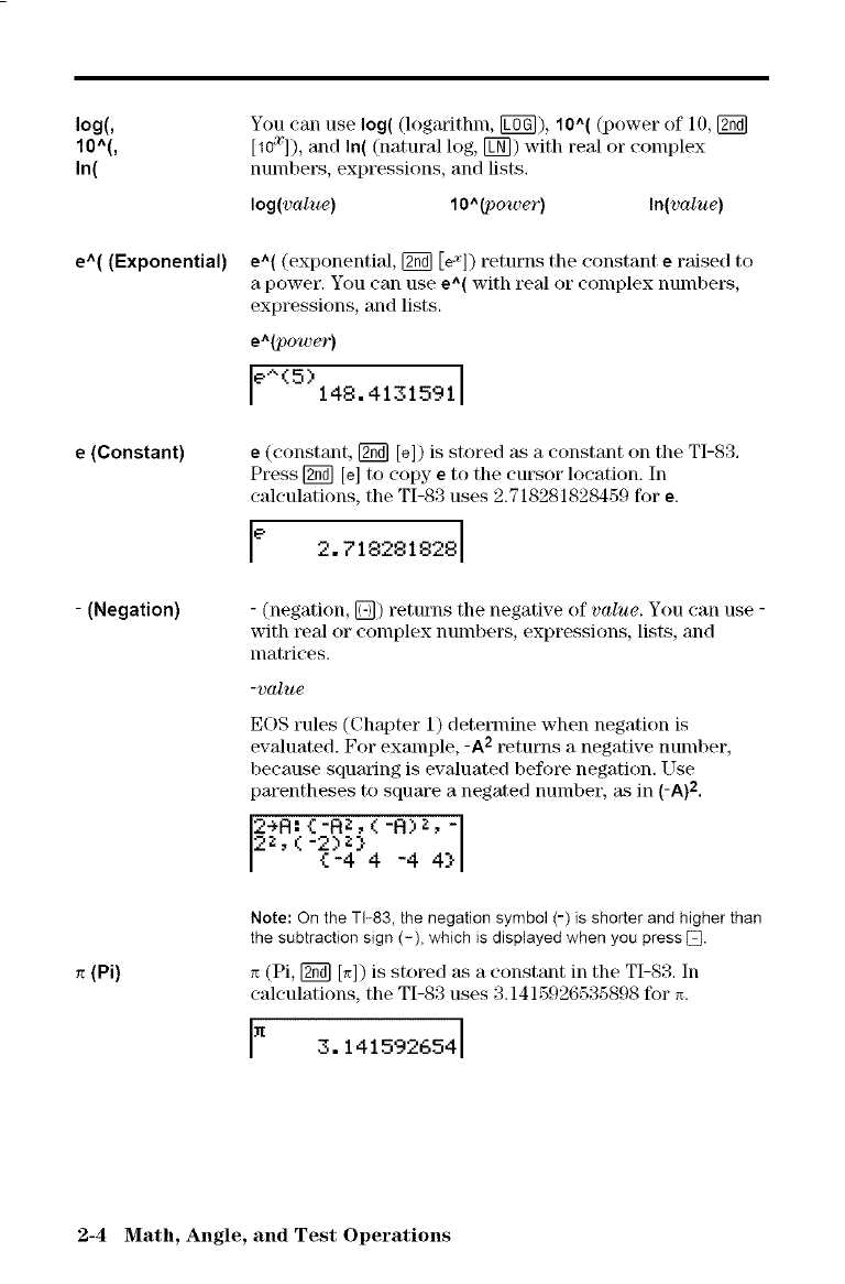
log(,
10^(,
In(
e^( (Exponential)
e(Constant)
-(Negation)
(Pi)
You can use log( (logarithln, FO_), 10^( (power of 10, [_
[10x]), and In( (natural log, @) with real or eolnplex
nulnbers, expressions, and lists,
log(value) lO^{power) In(value)
e^( (exponential, [2_ [ex]) returns the constant eraised to
a power. You can use e^( with real or complex numbers,
expressions, and lists.
eA(t)owe_ ,')
le^(5)148.41315911
e(constant, [g_] [el) is stored as a constant on the TI-83.
Press Kfid][el to copy eto the cursor location. In
calculations, the TI-83 uses 2.718281828459 for e.
e2.718281828
- (negation, D) returns the negative of value. You can use -
with real or complex numbers, expressions, lists, and
matrices.
-value
EOS rules (Chapter 1) determine when negation is
evaluated. For example, -A2t_turns a negative nulnber,
because squaring is evaluated before negation. Use
parentheses to square a negated number, as in (-A)2,
2+R: {-RZ, ( -R>a, -
2z, ( -2)z}
{-4 4 -4 4}
Note: On the TI-83, the negation symbol (-) is shorter and higher than
the subtraction sign (-), which is displayed when you press D.
(Pi, [g_ [_]) is stored as a constant in the TI-83, In
calculations, the TI-83 uses 3.1415926535898 for _.
Ix 3.1415926541
2-4 Math, Angle, and Test Operations
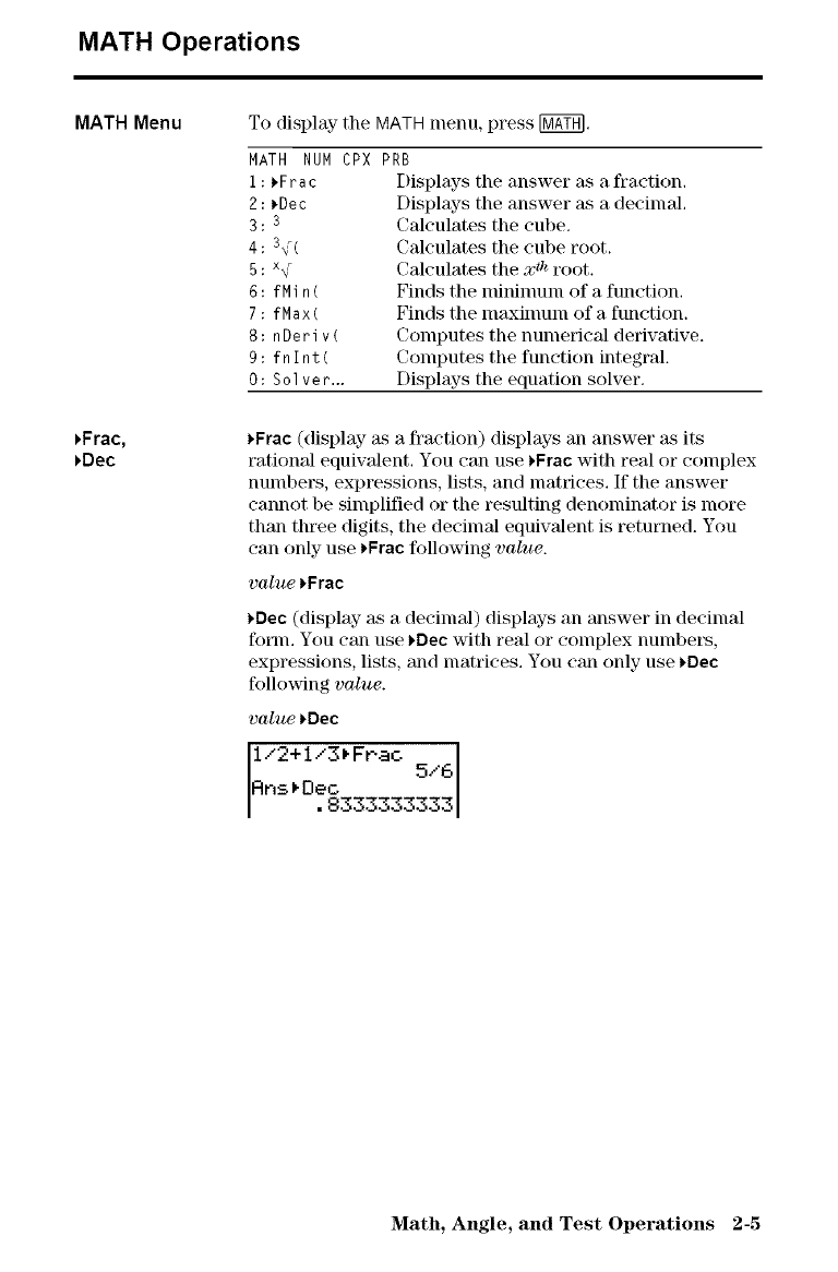
MATH Operations
MATH Menu
_Frac,
_Dec
To display the MATH menu, press [MKTgl.
MATH NUMCPX PRB
1: _Fra c Displays the answer as a fraction.
2:_Dec
3:3
4:3_(
5: x#
6: fMin(
7: fMax(
8:nDeriv(
9: fnlnt(
O: Solver.,.
Displays the answer as a decimal.
Calculates the cube.
Calculates the cube root.
Calculates the x t;_root.
Finds the nlininmln of a function.
Finds the nlaxinlunl of a function.
(3olnputes the numerical derivative.
(Tonlputes tile function integral.
Displays the equation solver.
_Frac (display at a fraction) displays an answer _L_its
rational equivalent. You can use _Frac with real or complex
numbers, expressions, lists, and matrices. If the answer
cannot be simplified or the resulting denominator is more
than three digits, the decimal equivalent is returned. You
can only use _Frac following value.
value _Frac
_Dec (display as a decimal) displays an answer in decimal
form. You can use *Dec with real or complex numbet_,
expressions, lists, and matrices. You can only use _Dec
following value.
value _Dec
I/2+I/3_Frac o/61
Ans_Deo
.8333333333
Math, Angle, and Test Operations 2-5
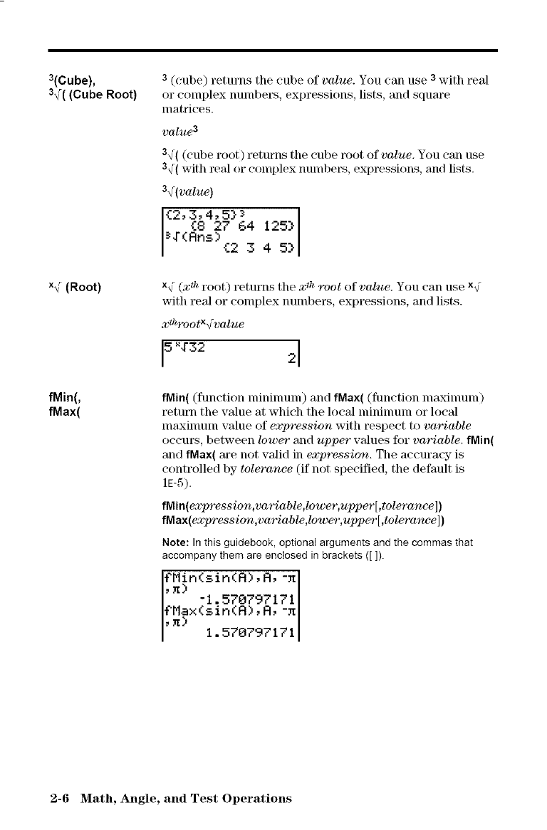
3(Cube),
3_r( (Cube Root)
x_ (Root)
fMin(,
fMax(
3(cube) returns the cube of value. You can use 3with real
or complex numbers, expressions, lists, and square
nmtrices.
value 3
3_( (cube root) returns the cube root of value. You can use
3_( with real or complex numbers, expressions, and lists.
3_(value)
{2,3,4,5}3{8 27 64 125}
_J'(Rns){2 3 4 5}
x_ (xth root) returns the x th root of value. You can use x_
with real or complex numbers, expressions, and lists.
xthrootX-_ value
5 N'32 2
fMin( (function nlininlunl) and fMax( (function nlaxinlunl)
retun_ the value at which the local ndninmm or local
nmxinmnl value of expression with respect to variable
occurs, between/ower and upper values for variable, fMin(
and fMax( are not valid in expression. The accuracy" is
controlled by tolerance (if not specified, the default is
iE-5),
fMin(expression,variable,lower,upper[,toleranoe])
fMax(expression,variable,lower, upper[,toleranoe])
Note: In this guidebook, optional arguments and the commas that
accompany them are enclosed in brackets ([ ]).
f'Min(_in(R), R, -_
-I. 570797171
r_x(sir,(A), R,-:_
• 1.570797171
2-6 Math, Angle, and Test Operations
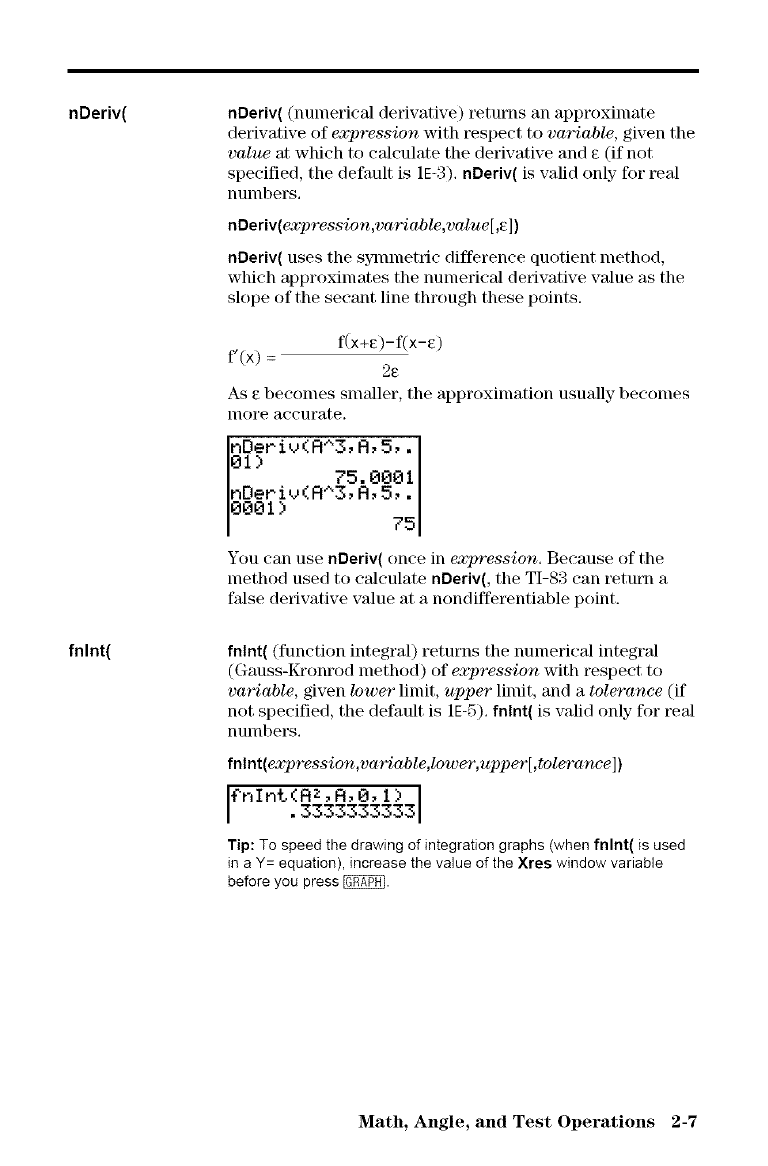
nDeriv(
fnlnt(
nDeriv( (numerical derivative) returns an approximate
derivative of expression with respect to variable, given the
value at which to calculate the derivative and e (if not
specified, the default is 1E-3). nDeriv( is valid only for real
numbers,
nDeriv(expression,variable,value[,a])
nDeriv( uses the s:nnmetrie difference quotient method,
which approximates the numerical derivative value as the
slope of the secant line through these points.
f(x+e)-f(x-e)
f'(x) =2e
As e becomes smaller, the approxinmtion usually- becomes
nlore accurate.
nDer iv(RA3, R, 5,.
01 ) 75,0001
nDeriv(R^3o R, 5,.
0001 ) 75
You can use nOeriv( once in expression. Because of the
method used to calculate nDeriv(, the TI-83 can return a
false derivative value at a nondifferentiable point.
fnlnt( (function integral) returns the numerical integral
(Gauss-Kronrod method) of expression with respect to
variable, given/ower limit, upper limit, and a tolerance (if
not specified, the default is 1E-5). fnlnt( is valid only- for real
nunlbers.
fnlnt(expression,variable,lower, upper[,tolerance])
?nlnt(A_,R,O&l)
•3333330333
Tip: To speed the drawing of integration graphs (when fnlnt( is used
in a Y= equation), increase the value of the Xres window variable
before you press _.
Math, Angle, and Test Operations 2-7
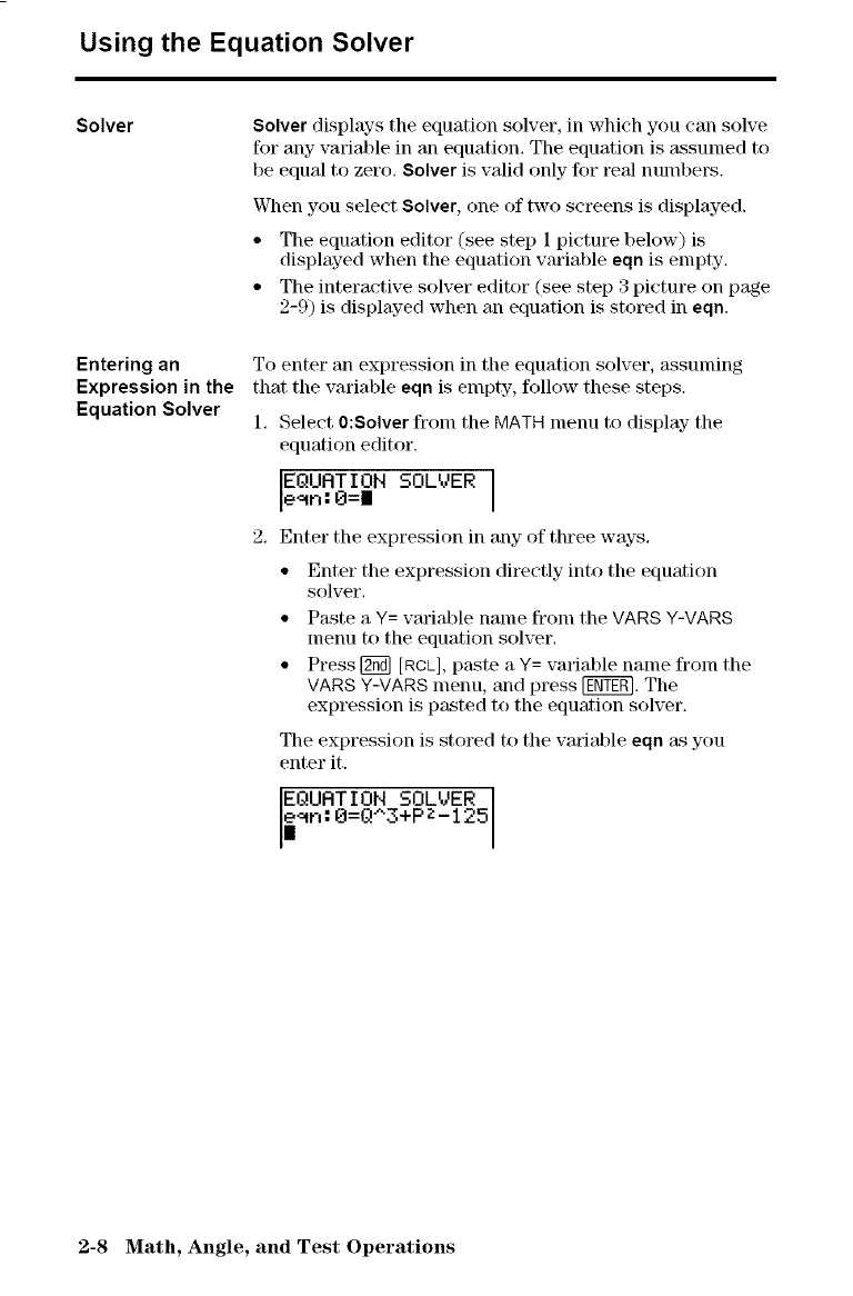
Using the Equation Solver
Solver
Entering an
Expression in the
Equation Solver
Solver displays the equation solver, in which you can solve
for any variable in an equation, The equation is assunled to
be equal to zero. Solver is valid only for real numbers.
Vcl_en you select Solver, one of two screens is displayed.
• The equation editor (see step 1 picture below) is
displayed when the equation wu'iable eqn is empty,
• The interactive solver editor (see step 3 picture on page
2-9) is displayed when an equation is stored in eqn.
To enter an expression in the equation solver, assunling
that the variable eqn is empty, follow these steps.
1, Select 0:Solver from the MATH menu to display- the
equation editor.
EQUATION SOLVER
e_n: 0=|
2, Enter the expression in any of three ways,
• Enter the expression directly into the equation
solver,
• Paste a Y= vmiable name from the VANS Y-VANS
lnenu to the equation solver,
• Press [_ [act_], p_kste a Y= variable name from the
VANS Y-VANS lnenu, and press [_, The
expression is pasted to the equation solver.
The expression is stored to the variable eqn as you
enter it.
EQURTION SOLVER
e_n: O=Q"3+P z-125
|
2-8 Math, Angle, and Test Operations
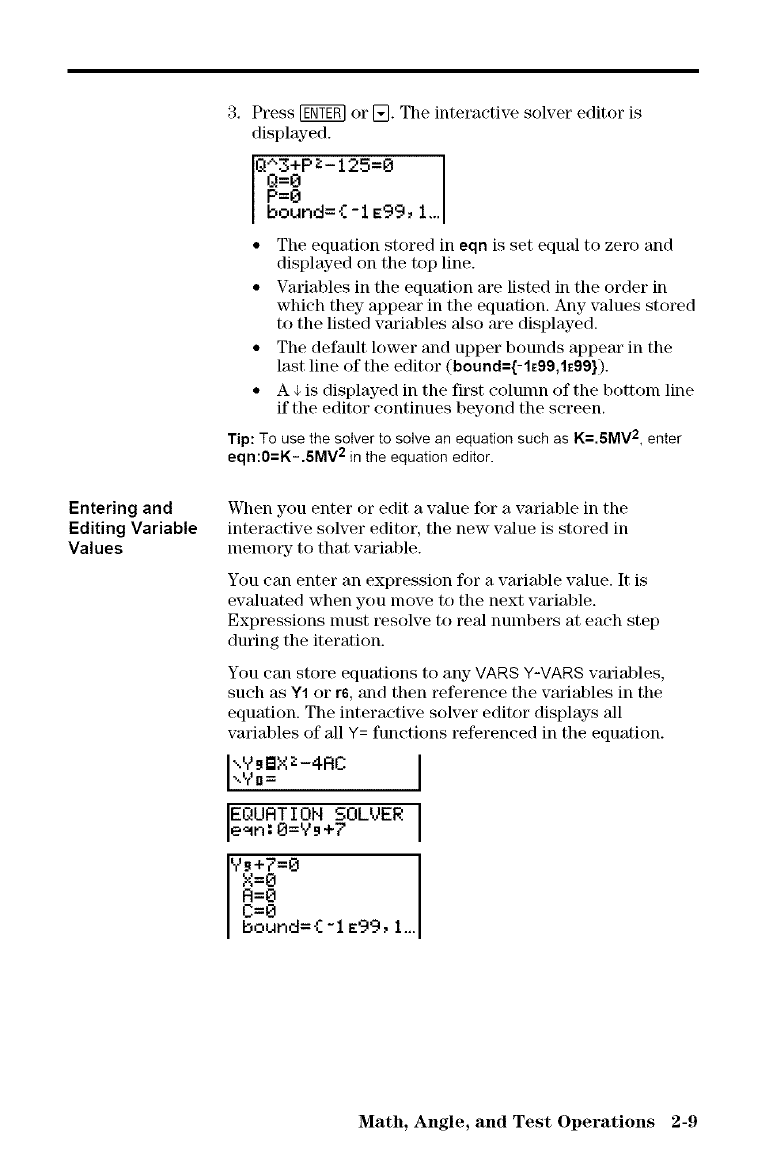
Entering and
Editing Variable
Values
3, Press _ or [_. The interactive solver editor is
displayed.
1%35 -1 5=8
P=8 1...
bound={ -1 E99,
• The equation stored in eqn is set equal to zero and
displayed on the top line.
• Variables in the equation are listed in tile order in
which they appear in the equation. Any values stored
to the listed variables also are displayed.
• The default lower and upper bounds appeal" in the
last line of the editor (bound={-1E99,1E99}).
• A 4 is displayed in the first colunul of the bottonl line
if tile editor continues beyond the screen.
Tip: To usethe solverto solve an equationsuchas K=.SMV2, enter
eqn:0=K-.SMV 2 inthe equationeditor.
When you enter or edit a value for a variable in the
interactive solver editor, the new value is stored in
nlenlol_y- to that varialfle.
You can enter an expression for a variable value. It is
ewduated when you move to the next varialfle.
Expressions nmst resolve to real numbers at each step
during the iteration.
You can store equations to any VAR8 Y-VARS variables,
such as Y1 or r6, and then reference the w_riables in tile
equation. The interactive solver editor displays all
varialfles of all Y= functions referenced in the equation.
EQURTION SSL_)ER Ie_n: 8=V., +7
Y_+7=Obound=C=BR=SX=8{ -i E99, I.,.
Math, Angle, and Test Operations 2-9
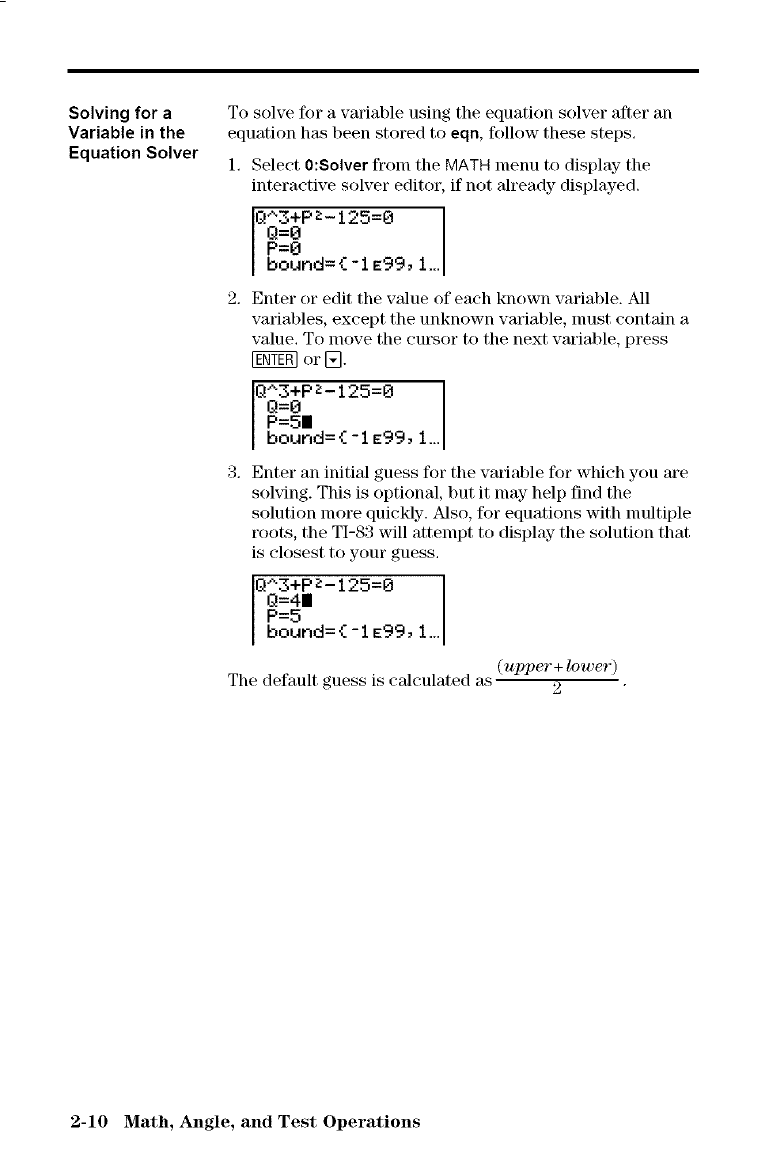
Solving for a
Variable in the
Equation Solver
To solve for a variable using the equation solver after an
equation has been stored to eqn, follow these steps.
1. Select 0:Solver from the MATH menu to display the
interactive solver editor, if not already displayed.
I% ;P -125=°P=oL.
bound={-1E99,
2. Enter Ol" edit tile value of each known variable. All
variables, except the unknown variable, nmst contain a
value. To move the cm\sor to the next wuiable, press
INto or _.
QQ3;PZ-125=0p=5I 1...
bound={ -1 E99,
3. Enter an initial guess for tile variable for which you are
solving. This is optional, but it may help find the
solution more quickly-. Also, for equations with nmltiple
roots, the TI-83 will attempt to display the solution that
is closest to your guess,
IQ"3+Pp=sQ=4Iz- 125=0 1...
bound={ -I E99,
The default guess is calculated as (upper+ lower)
2
2-10 Math, Angle, and Test Operations
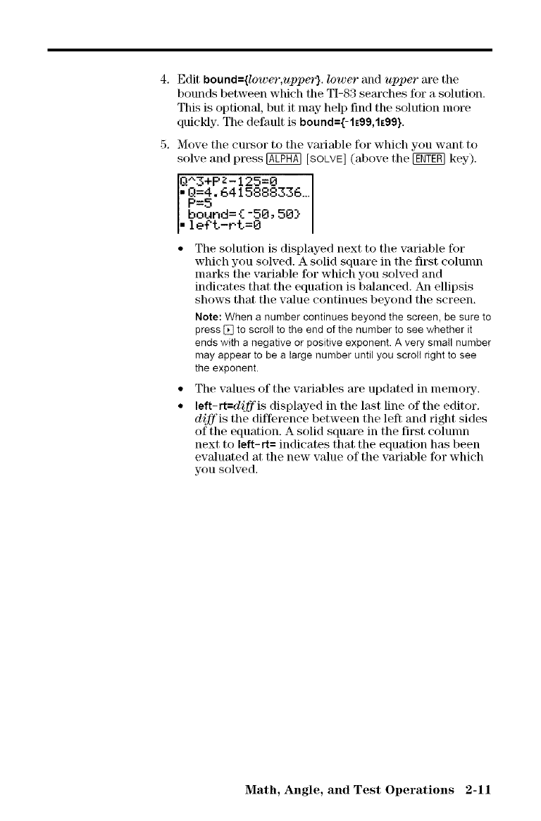
4. Editbound={lower,upper},lower and upper are the
bounds between which the TI-83 searches for a solution.
This is optional, but it may help find the solution more
quickly. The default is bound={- 1E99,1E99}.
5. Move the cursor to the variable for which you want to
solve and press @ [SOLVE](above the [gNTgNkey-).
Q_'3+PZ-125=0
I,Q=4.6415888336...
P=5
bound={-50,50}
leCt-rt=O
The solution is displayed next to tile variable for
which you solved. A solid square in the fil_t colunm
marks the variable for which you solved and
indicates that the equation is balanced. An ellipsis
shows that tile value continues beyond the screen.
Note: When a number continues beyond the screen, be sure to
press [] to scroll to the end of the number to see whether it
ends with a negative or positive exponent. A very small number
may appear to be a large number until you scroll right to see
the exponent.
The values of the variables are updated in nlenlot'y.
left-rt=diffis displayed in the last line of the editor.
diffis tile difference between the left and right sides
of the equation. A solid square in the first colunm
next to left-rt= indicates that the equation has been
evaluated at the new value of tile variable for which
you solved.
Math_ Angle_ and Test Operations 2-11
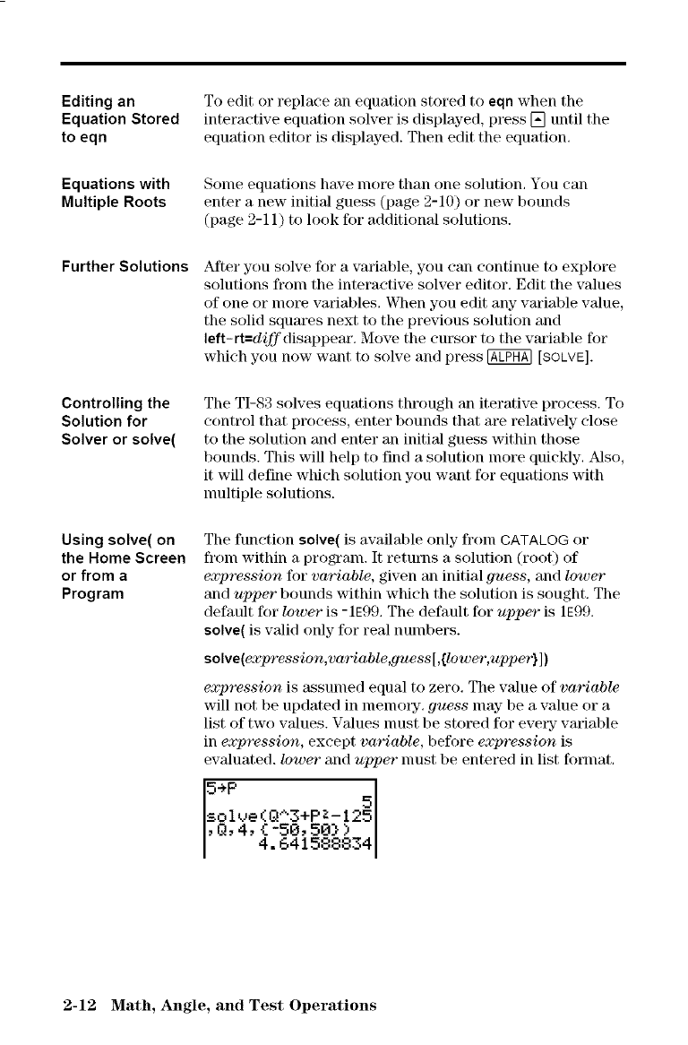
Editing an
Equation Stored
to eqn
Equations with
Multiple Roots
Further Solutions
Controlling the
Solution for
Solver or solve(
Using solve( on
the Home Screen
or from a
Program
To edit or replace an equation stored to eqn when the
interactive equation solver is displayed, press [] until the
equation editor is displayed. Then edit the equation.
Sonle equations have nlore than one solution. You can
enter a new initial guess (page 2-10) or new bounds
(page 2-11) to look for additional solutions.
After you solve for a varialfle, you can continue to explore
solutions from the interactive solver editor. Edit the values
of one or more varialfles. When you edit any variable value,
the solid squares next to the previous solution and
left-rt=diff disappear. Move the cursor to the varialfle for
which you now want to solve and press @ [SOLVE].
The TI-83 solves equations through an iterative process. To
control that process, enter bounds that are relatively close
to the solution and enter an initial guess within those
bounds. This will help to find a solution more quickly. Also,
it will define which solution you want for equations with
nmltiple solutions.
The function solve( is available only fronl CATALOG or
from within a program. It returns a solution (root) of
expression for variable, given an initial guess, and lower
and upper bounds within which the solution is sought. The
default for lower" is -1E99. The default for upper is 1E99.
solve( is vMid only for real numbers.
soNe(expression,variable,guess[ ,{lower, upper'} ])
expression is assumed equal to zero. The value of variable
will not be updated in nlenlory, guess nlay be a value or a
list of two values. Values must be sto[_d for eve_Ty"variable
in expression, except variable, before expression is
evaluated./ower and upper nmst be entered in list format.
4. 641588834
2-12 Math, Angle, and Test Operations
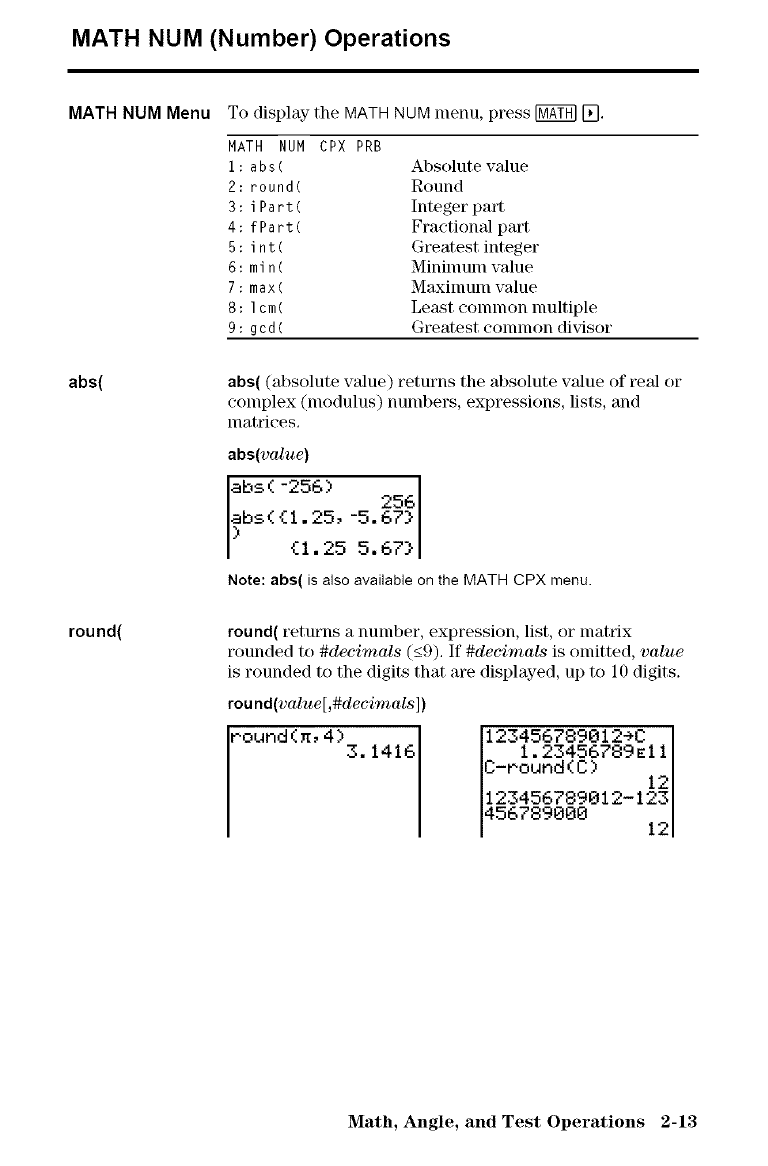
MATH NUM (Number) Operations
MATH NUM Menu
abs(
round(
To display the MATH NUM menu, press _ [Z],
MATH NUM CPX PRB
i : ab s ( Al_solute value
2: round( Round
3 : i Part ( Integer part
4 : f Pa r t ( Fractional part
5 : i nt( Greatest integer
6 : mi n (Mininmln value
7 : max ( Maxinlunl value
8 : ] cm( Legist eonlnlon nmltiple
9 :gcd ( Greatest eonnnon divisor
abs( (absolute value) returns the absolute value of real or
complex (modulus) numbers, expressions, lists, and
matrices.
abs(value)
abs ( -256 ) 2561,
abs( {I.25, -5.67}
I {1.25 5.67}
Note: abs( is also available on the MATH CPX menu.
round( returns a nunlber, expression, list, or nlatrix
rounded to #decimals (_<9). If #decimals is omitted, value
is rounded to the digits that are displayed, up to 10 digits.
round(value [,#decimals ])
round (x, 4) 3. 1416
123456789012÷C I
1.23456789E111
C-round(C) !21
123456789012-Iz3
456789000 12
Math, Angle, and Test Operations 2-13
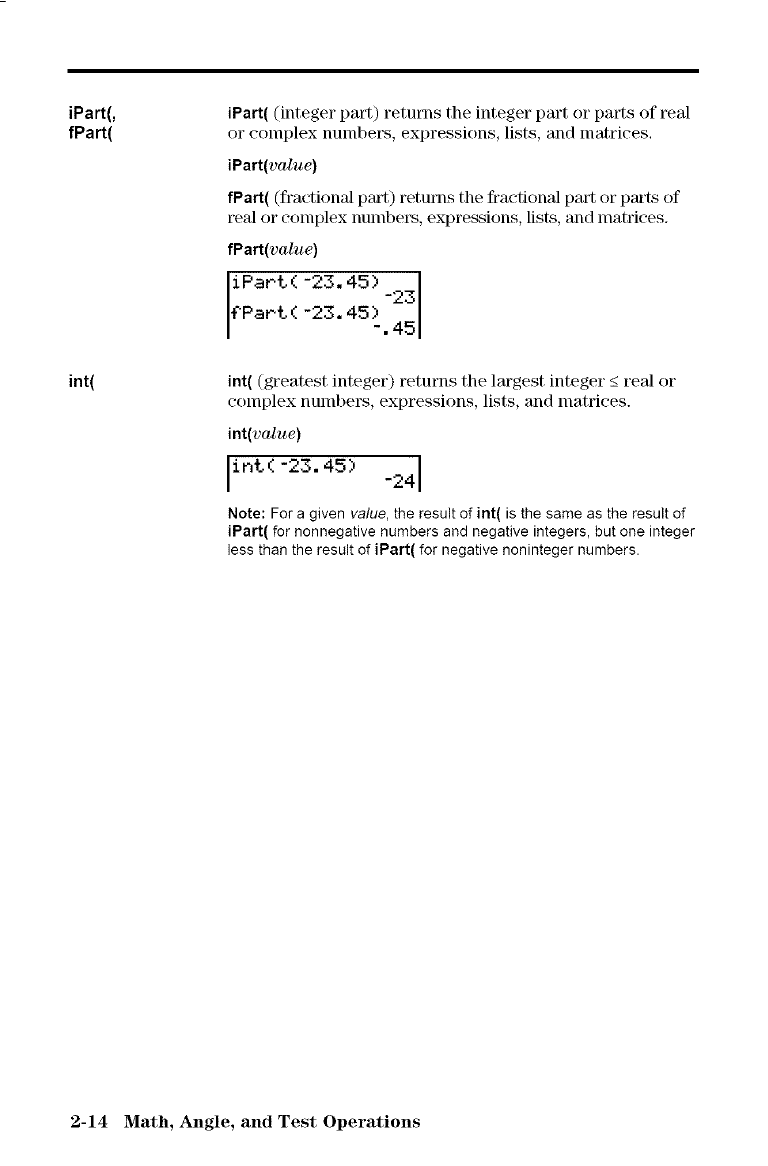
iPart(,
fPart(
int(
iPart( (integer part) returns the integer part or parts of ++al
or complex numbers, expressions, lists, and matrices.
iPart(value)
fPart( (fra('tional paxt) returns the fractional part or p_u'ts of
real or complex numbe_, expressions, lists, and lnatrices.
fPart(value)
iPart (-23.45) -23
f Part ( -23.45)._ 45
int( (greatest integer) returns the largest integer _<real or
complex numbers, expressions, lists, and nmtrices.
int(value)
lint(-23.45) _241
Note:Fora givenvalue,theresultofint(isthesame as theresultof
iPart( for nonnegative numbers and negative integers, but one integer
less than the result of iPart( for negative noninteger numbers.
2-14 Math, Angle, and Test Operations
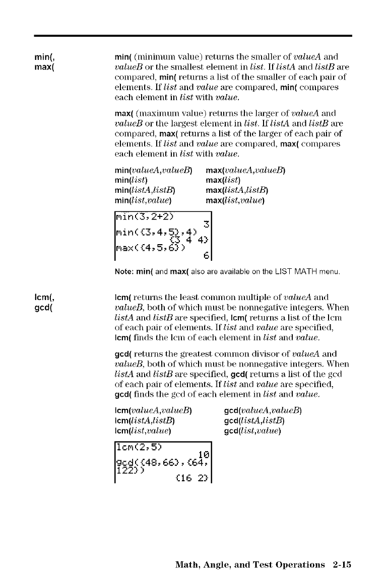
min(,
max(
Icm(,
gcd(
min( (ndnimum value) returns the smaller of valueA and
valueB or the smallest element in list, If listA and listB are
compared, min( returns a list of the smaller of each pair of
elements, If list and value are compared, min( compares
each element in list with value,
max( (n]axin]on] value) returns the larger of valueA and
valueB or the largest element in list. If listA and listB are
con]pared, max( retm'ns a list of the larger of each pair of
elements. If list and value are compared, max( compares
each element in list with value,
min(valueA,valueB) max(valueA,valueB)
min(list) max(list)
min(listA,listB) max(listA,listB)
min(list,value) max(list,value)
r,,in(3,2+2)= 3[
r,,in( {3, 4, _,}, 4) I
{3 4 4}
r,Jax( {4, 5, 6}) 6
Note: rain( and max( also are available on the LIST MATH menu.
Icm( t_tums the least eonlnlon nmltiple of valueA and
valueB, both of which must be nonnegative integers, When
listA and listB are specified, Icm( retm'ns a list of the lcm
of each pair of elements. If list and value are specified,
Icm( finds the leln of each element in list and value,
gcd( returns the greatest conlnlon divisor of valueA and
valueB, both of which must be nonnegative integers, When
listA and listB are specified, gcd( t'etun_s a list of the ged
of each pair of elements. If list and value are specified,
gcd( finds the ged of each element in list and value,
Icm(valueA,valueB) gcd(valueA,valueB)
Icm(listA,listB) gcd(listA,listB)
Icm(list,value) gcd(list,value)
10M(2,5) 10
god( {48, 66}, {64,
122} ){16 2}
Math, Angle, and Test Operations 2-15
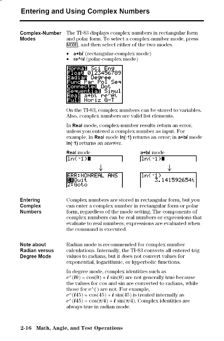
Entering and Using Complex Numbers
Complex-Number
Modes The TI-83 displays complex numbers in rectangular form
and polar forln. To select a complex-nulnber lnode, press
[MffffE],and then select either of the two modes.
•a+bi (rectangular-complex lnode)
•re^0/(polar-colnplex mode)
Sci Eng
Entering
Complex
Numbers
Note about
Radian versus
Degree Mode
Dot
Horiz G-T
On the TI-83, complex numbet\s can be stored to variables.
Also, complex numbers are valid list elements.
In Real mode, COlnplex-nulnber results return an error,
unless you entered a complex number as input. For
example, in Real mode In(-1) returns an error; in a+bi nlode
In(-1) returns an answer.
Real mode
lin<-i;,m l
4,
ERR-'NONRERL RNS i
ilBQuit i
2: Goto
a+bi lnode
Iln( -l>m I
Complex numbers are stored in rectangular form, but you
can enter a complex number in rectangulm' form or polar
form, regm'dless of the mode setting. The components of
complex numbers can be real numbers or expressions that
evMuate to reM numbers; expressions m'e evMuated when
the connnand is executed.
Radian mode is reconnnended for conlplex number
calculations. Internally-, the TI-83 converts all entered trig
values to radians, but it does not convert values for
exponential, logarithmic, or hyperbolic functions.
In degree mode, complex identities such as
e^ (i0) = cos(0) + isin(0) are not generally true because
the values for cos and sin are converted to radians, while
those for e ^ () are not. For example,
e^(i45) = cos(45) + isin(45) is treated internally as
e^ (i45) = cos(_/4) + isin(x/4). Complex identities are
always tree in radian mode.
2-16 Math, Angle, and Test Operations
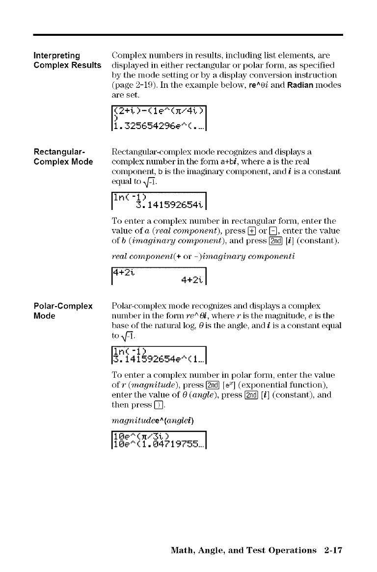
Interpreting
Complex Results
Rectangular-
Complex Mode
Polar-Complex
Mode
Complex numbers in results, including list elements, are
displayed in either rectangular or polar form, as specified
by the mode setting or by a display conversion instruction
(page 2-19). In the example below, re^0/and Radian modes
are set.
_2+t)-(le'-(x/4t)
1.325654296e^( ....
Rectangular-complex mode recognizes and displays a
complex number in the fore1 a+bi, where a is the ten
component, b is the imagimuy component, and iis a constant
equM to @'1.
-1)
lln< 3.141592654tI
To enter a complex nulnber in rectangular form, enter the
value of a(real component), press [] or [], enter the value
of b(imaginary component), and press [_ [i] (constant).
real component(÷ or -)imaginary cornponenti
14+2t 4+2t I
Polar-complex mode recognizes and displays a complex
number in the form re ^ 0/, where ris the nmgnitude, eis the
b_e of the natm'al log, 0is the angle, and iis a constant equM
in(-I)
3.141592654e^ ( I...
To enter a complex number in polar ff)nn, enter the value
of r (magnitude), press [_ [ex] (exponential function),
enter the value of 0(angle), press [_ [i] (constant), and
then press D.
ma_dtudeea(anglei)
10e._(n/3t)
10e"(I.04719755...
Math, Angle, and Test Operations 2-17
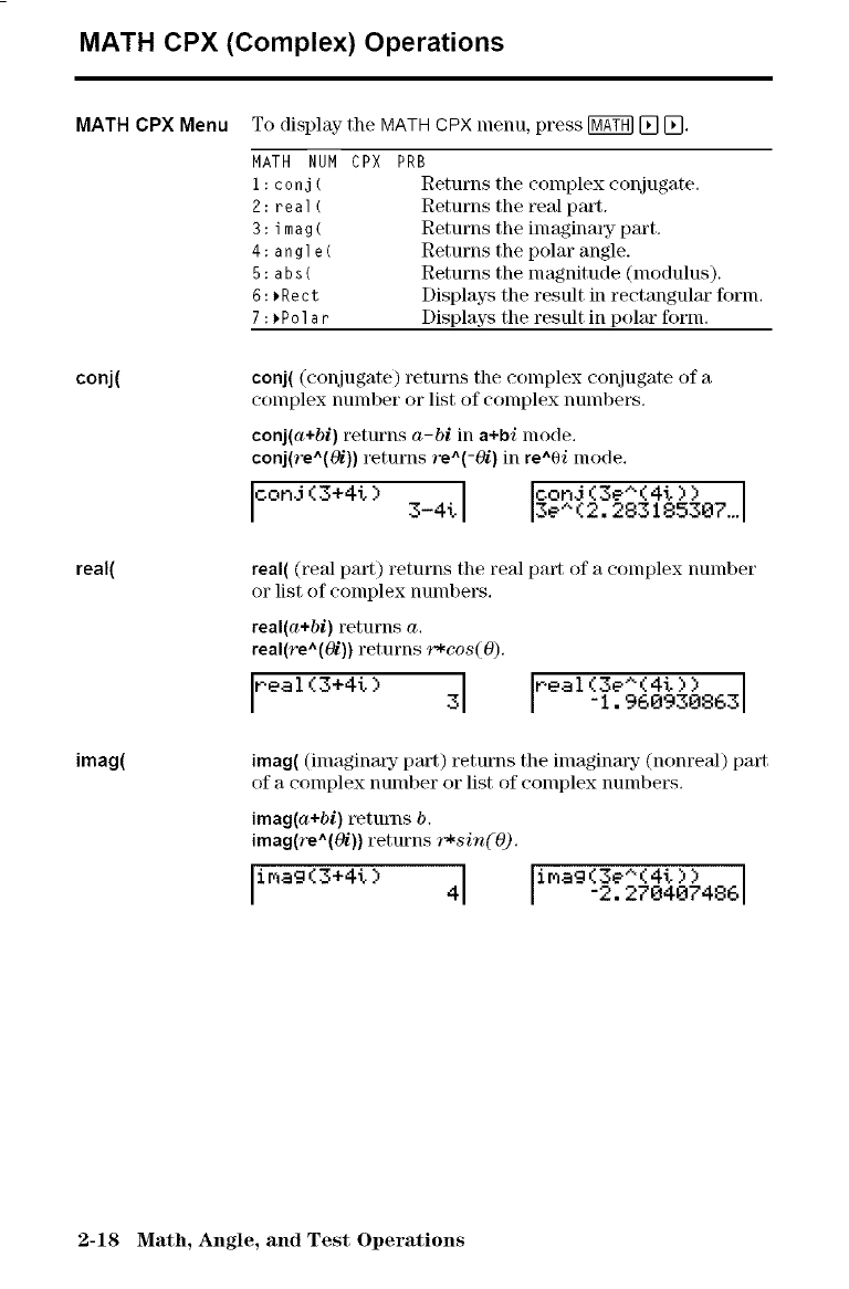
MATH CPX (Complex) Operations
MATH CPX Menu
conj(
real(
imag(
To display the MATH CPX menu, press [_ [] [],
MATH NUM
1:conj(
2:real(
3:imag(
4:angle(
5:abs(
6:_Rect
7:_Polar
CPX PRB
Returns the complex conjugate,
Returns the real part.
Returns the imaginary part,
Returns the polar angle.
Returns the magnitude (modulus),
Displays the result in rectangular form,
Displays the result in polar form,
conj((conjugate) returns the complex conjugate of a
complex number or list of complex numbers,
conj(a+bi) returns a-bi in a+bi nlode,
conj(re^(0i)) returns re^C0/) in re^ei mode,
toni (3+4t) 3-4t1 c°nJ (3e^(4t >>
3e"(2. 28318530?._
real( (real part) returns the real part of a complex number
or list of complex nmnbers,
real(a+bi) returns a,
real(f'e^(0i)) returns _"*cos(O).
r.eal(3+4t) 3[ real (3e_'(4t > >
-I.968938863
imag( (imaginary part) returns the imagining- (nonreal) part
of a complex number or list of complex numbers.
imag(a+bi) t_tunls b.
imag(re^(Oi)) returns _'_sin(O),
Iimag(3+4t ) 41 imag(3e^(4t >>-2.270407486
2-18 Math, Angle, and Test Operations
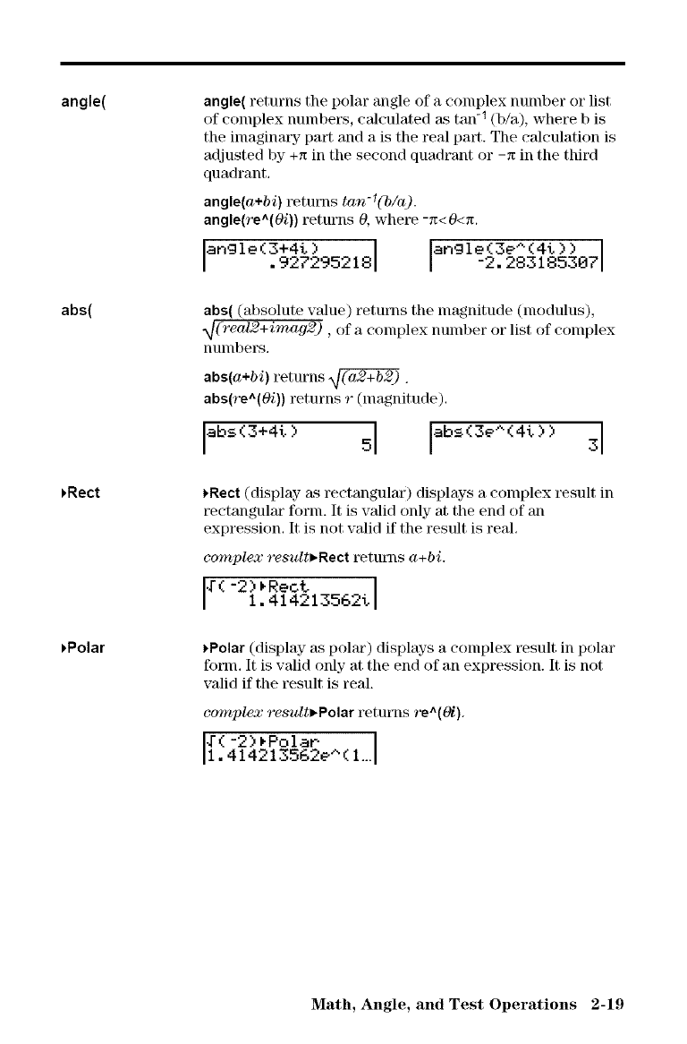
angle(
abs(
_Rect
)Polar
angle( returns the polar angle of a complex number or list
of complex numbers, calculated as tan -1 (b/a), where b is
the imaginatT part and a is the real part. The calculation is
adjusted by +x in the second quadrant or -x in the third
quadrant.
angle(a+bi) returns tan-l(b/a).
angle(re^(Oi)) returns 0, where -x<O<x.
an91 e (3+4t ) an91 e (38^ (4i.) )
•927295218 -2. 283185387
abs( (absolute value) returns the lnagnitude (lnodulus),
_(real2+imag2) , of a complex nulnber or list of eonlplex
nulnl)ers,
abs(a+bi) returns _ .
abs(re^(Oi)) returns r(nmgnitude),
labs(3+4t ) 51 [abs(3e^(4t )) 31
)Rect (display as reetanguhu') displays a complex t_sult in
rectangular form. It is valid only at the end of an
expression, It is not valid if the result is real,
complex result_Rect returns a+bi.
_Rec.t
1#(-2_.414213562t1
)Polar (display as polar) displays a coInplex result in polar
form, It is valid only at the end of an expression. It is not
valid if the result is real.
^
corr_plexresult_Polarreturnsre (_).
#(-2)_PolaP
1.4142135628^(I...
Math, Angle, and Test Operations 2-19
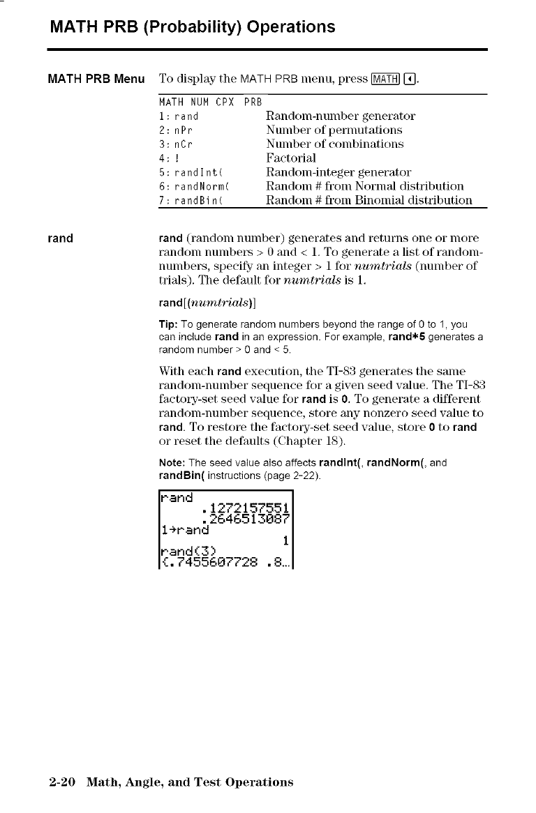
MATH PRB (Probability) Operations
MATH PRB Menu To display the MATH PRB menu, press _ E},
MATH NUMCPX PRB
i: rand
2: nPr
3:nCr
4:!
5: randlnt(
6: randNorm(
7: randBin(
Randonl-nunlber generator
Number of pernmtations
Number of combinations
Factorial
Random-integer generator
Random # from Normal distribution
Random # from Binomial distribution
rand rand (random number) generates and returns one or more
random numbers > 0 and < 1. To generate a list of random-
numbers, specify- an integer > 1 for numt'rials (number of
trials). The default for numt'rials is 1.
rand [(num trials)]
Tip: To generate random numbers beyond the range of Oto I, you
can include rand in an expression. For example, rand*5 generates a
random number > 0 and < 5.
With each rand execution, the TI-83 generates the salne
randonl-number sequence for a given seed value. The TI-83
factoFf-set seed value for rand is 0. To generate a different
randonl-number sequence, store any nonzero seed value to
rand. To restore the factoFy--set seed vMue, store 0 to rand
or reset the defaults (Chapter 18).
Note: The seedvaluealso affectsrandlnt(, randNorm(, and
randBin( instructions(page2-22).
r'and
•1272157551
1÷rand 2646513087
rand(3)
{. 7455607728
2-20 Math, Angle, and Test Operations
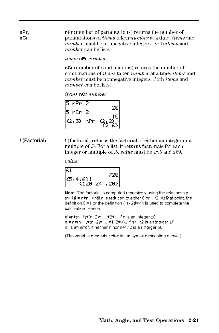
nPr,
nCr
!(Factorial)
nPr (number of permutations) returns the number of
pernmtations of items taken number at a time. items and
number must be nonnegative integers, Both items and
number can be lists.
items nPr number
nCr (number of combinations) returns the number of
combinations of items taken number at a time. items and
number nmst be nonnegative integers. Both items and
number can be lists.
itemsnCrnumb_"
5 nPe 2 (2_2_i;
5 nCe 2
{2,3> nPP _ 6}
! (factorial) returns the factorial of either an integer or a
nmltiple of .5. For a list, it returns factorials for each
integer or nmltiple of .5. value nmst be _>-.5 and _<69.
value!
£120 24 720}
Note: The factorial is computed recursiveiy using the relationship
(n+t)! = n.n!, until n is reduced to either 0 or -1/2. At that point, the
definition 0!=I or the definition (-1/2)!=_- is used to complete the
calculation. Hence:
n!=n*(n-I )*(n-2)* ... *2* I, if n is an integer >0
n!= n*(n-1 )*(n-2)* ....1/2.-_;, if n+1/2 is an integer >O
n! is an error, if neither n nor n+I/2 is an integer >0.
(The variable n equals value in the syntax description above.)
Math, Angle, and Test Operations 2-21
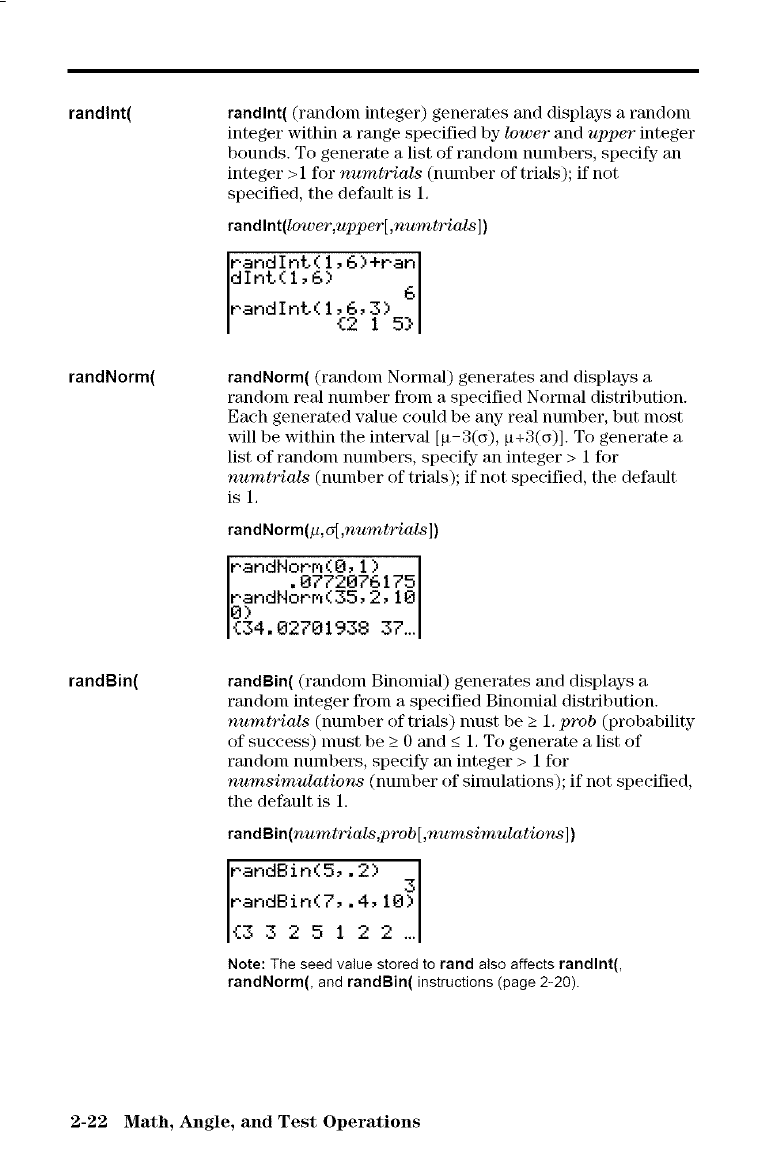
randlnt(
randNorm(
randBin(
randlnt( (random integer) generates and displays a random
integer within a range specified by lower and upper integer
bounds. To generate a list of random numbers, specify an
integer > 1 for numt,Fials (number of trials); if not
specified, the default is 1.
randlnt(lower,upper[,numtrials])
rand Int ( 1,6)+ra G
dlnt(1,6)
randInt( 1,{26, 3)i5}
randNorm( (random Normal) generates and displays a
random real number fi'onl a specified Normal distribution.
Each generated value could be any real number, but most
will be within the intercal [p-3(_), p+3(o)]. To generate a
list of random numbers, specify- an integer > 1 for
numtrials (number of trials); if not specified, the default
is 1.
randNorm(p,ol,numtrials])
randNorm(O, 1)
.0_7207G175
_ndNo:r,(35,2,10
_34.02r01938 37_.
randBin( (randon] Binomial) generates and displays a
random integer from a specified Binomial distribution.
numtrials (nmnber of trials) lnust be _>1, prob (probability
of success) must be _>0 and _<1. To generate a list of
randonl nunlbers, specify an integer > 1 for
numsimulations (nmnber of sinmlations); if not specified,
the default is 1.
randBin(numtrials,prob[,numsimulations])
randBirKS,,2) 3
randBin(7,. 4, 10)
{332512 2 ...
Note: The seed value stored to rand also affects randlnt(,
randNorm(, and randBin( instructions (page 2-20).
2-22 Math, Angle, and Test Operations
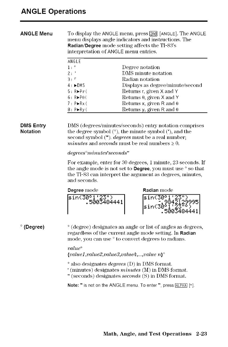
ANGLE Operations
ANGLE Menu
DMS Entry
Notation
°(Degree)
To display the ANGLE menu, press [_ [ANGLE]. The ANGLE
menu displays angle indicatot\_ and instruetions. The
Radian/Degree mode setting affects the TI-S3's
interpretation of ANGLE menu entries.
ANGLE
1: °
2:'
3: r
4: ,DMS
5: R,Pr(
6: R_PO(
7: P_Rx(
8: PmRy(
Degree notation
DMS minute notation
Radian notation
Displays as degree/lninute/seeond
Returns r, given X and Y
Returns 0, given X and Y
Returns x, given R and 0
Returns y, given R and 0
DMS (degrees/minutes/seconds) entlT notation comprises
the degree sjonbol (°), the minute sjonbol ('), and the
second symbol ("). degrees nmst be a real number;
minutes and seconds nlust be real numbers _>0.
degrees°minutes'seconds ''
For exalnple, enter for 30 degrees, 1 minute, 23 seconds. If
the angle nlode is not set to Degree, you nmst use ° so that
the TI-83 call interpret the atgulnent as degrees, minutes,
and seconds.
Degree mode
sin(30° 1'23") I
.5003484441
Radian mode
sin(30° 1'23") I
-. 98421299951
sin(30 °l 23 o)
•5003484441
°(degree) designates an angle or list of angles as degrees,
regardless of the current angle mode setting. In Radian
nlode, you Call use ° to convert degrees to radians.
value °
{value1 ,value2,value3,value_ ,...,value n} °
° also designates degrees (D) in DMS format.
' (minutes) designates minutes (M) in DMS format.
"(seconds) designates seconds (S) in DMS format..
Note: " is not on the ANGLE menu. To enter ", press @ [-].
Math, Angle, and Test Operations 2-23
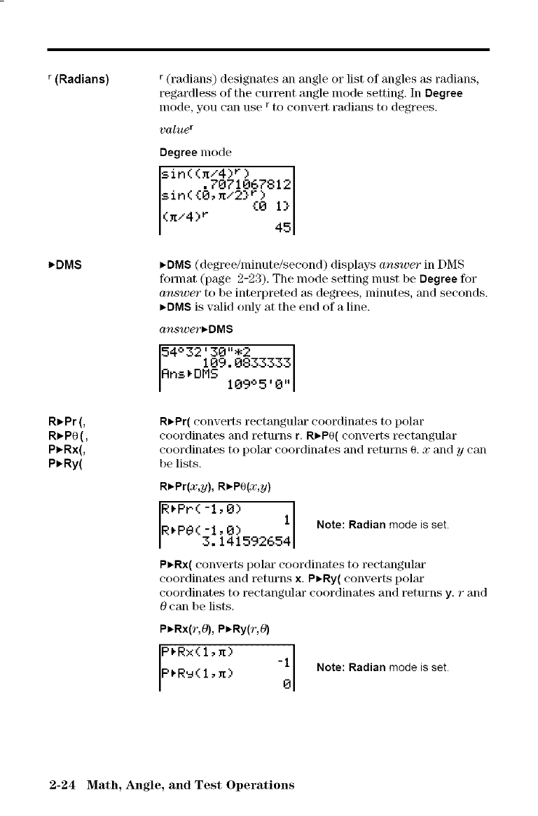
r(Radians)
_DMS
R_Pr (,
R_,Pe (,
P_-Rx(,
P*Ry(
r (radians) designates an angle or list of angles as radians,
regardless of the cmTent angle mode setting. In Degree
mode, you can use r to convert radians to degrees.
value r
Degree mode
sin (<_/4.') r )
•7071067812
sin( {0, ,/2} _) 1}%w.J
(x/4> r 45
_DMS (degree/minute/second) displays answer in DMS
format (page 2-23). The nlode setting lnust be Degree for
answer to be interpreted as degrees, minutes, and seconds.
_DMS is valid only at the end of a line.
answe_'_DMS
54°32'30"*2 I
109.08333331
Rns*DMS 10905 0
RI_Pr(converts rectangular coordinates to polar
coordinates and returns r, R_PO( converts rectangular
coordinates to polar coordinates and returns O.xand ycan
be lists.
R*Pr(x,y), R*PO(x,y)
R*Pr(-1,O) I
,05 !I Note: Radian mode is set
e,eo( } 14i5926541
PI_Rx( converts polar coordinates to rectangular
coordinates and returns x. PI*Ry( converts polar
coordinates to reetangulm" coordinates and returns y. rand
0can be lists.
P*Rx(r,_,P*Ry(v,_
P*Rx(I,x)
P*R_(I,x) -10 Note: Radian mode is set.
2-24 Math, Angle, and Test Operations
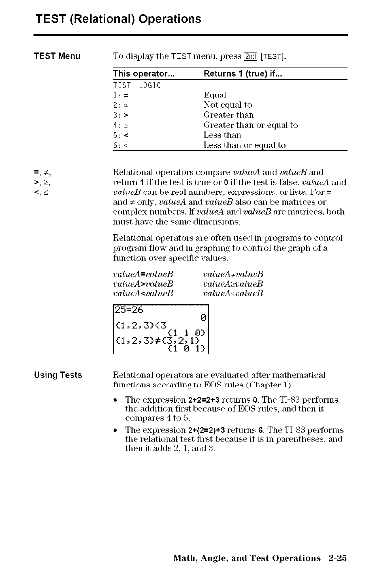
TEST (Relational) Operations
TEST Menu
>_ ->,
<,_<
Using Tests
To display the TEST menu, press [_ [TEST].
This operator... Returns 1 (true) if,..
TEST LOGIC
1 : =Equal
2 : _ Not equal to
3 : > Greater than
4 : > Greater than or equal to
5:<Less than
6 : < Less than or equal to
Relational operators compare valueA and valueB and
return 1 if the test is true or 0 if the test is false, valueA and
valueB can be real numbet_, expressions, or lists. For =
and _ only, valueA and valueB also can be matrices or
complex numbers. If valueA and valueB are matrices, both
nmst have the same dimensions.
Relational operators are often used in programs to eont_x)l
program flow and in graphing to control the graph of a
function over specific values.
valueA =valueB valueA _valueB
valueA >value B valueA >valueB
valueA <valueB valueA <valueB
25=26 el
{i'2'3}<3{i 1 0}
Relational operatot_ are evMuated after lnathelnatieal
functions according to EOS rules (Chapter 1).
• The expression 2+2=2+3 returns 0. The TI-83 performs
the addition first because of EOS rules, and then it
compares 4 to 5.
• The expression 2+(2=2)+3 returns 6. The TI-83 performs
the relational test first because it is in parentheses, and
then it adds 2, 1, and 3.
Math, Angle, and Test Operations 2-25
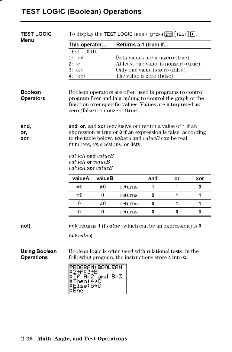
TEST LOGIC (Boolean) Operations
TEST LOGIC
Menu
Boolean
Operators
and,
or_
xor
not(
Using Boolean
Operations
To display the TEST LOGIC menu, press [_ [TEST] [_.
This operator... Returns a 1 (true} if...
TEST LOGIC
1 : an d Both values are nonzero (true).
2: 0cAt least one value is nonzero (tree),
3 : x0c Only one value is zero (false),
4 : n0t ( The value is zero (false).
Boolean operators are often used in programs to control
program flow and in graphing to control the graph of the
function over specific values. Values are interpreted _ts
zero (false) or nonzero (ttlle).
and, or, and xor (exclusive or) return a value of 1 if an
expression is true or 0if an expression is false, according
to the table below, valueA and valueB can be real
numbers, expressions, or lists.
valueA and valueB
valueA or valueB
valueA xor valueB
valueA valueB and or xor
€0 €0 returns 1 1 0
€0 0 returns 0 1 1
0€0 returns 0 1 1
0 0 returns 0 0 0
not( returns 1if value (which can be an expression) is O,
not(value)
Boolean logic is often used with relational tests. In the
following program, the instructions store 4 into C,
PROGRAM::2+R: 3+BBOOLEAN I
:If" R=2 and B=3
:Then: 4eC
:Else: 5eC
:End
2-26 Math_ Angle_ and Test Operations
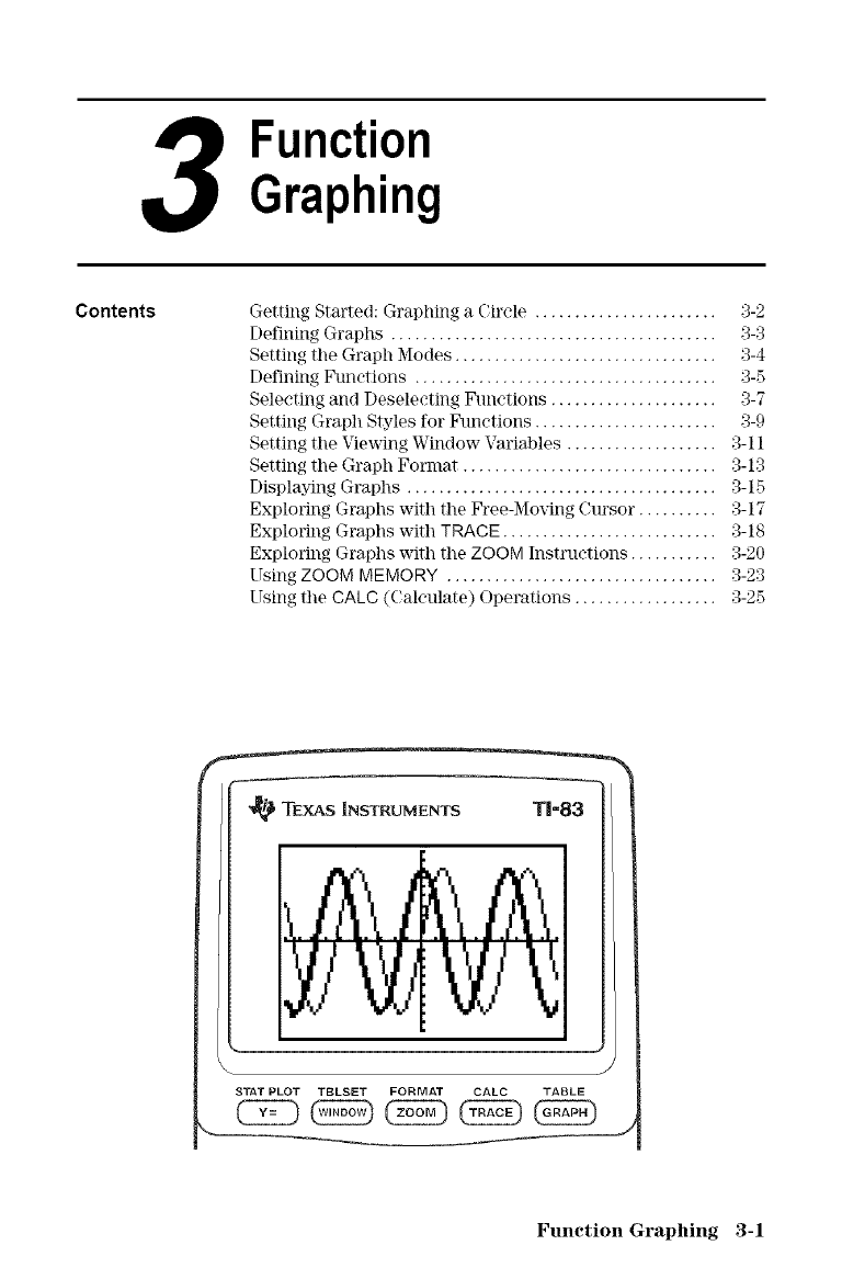
Contents Getting Started: Graphing a Circle ....................... 3-2
Defining Graphs ......................................... 3-3
Setting tile Graph Modes ................................. 3-4
Defining Funetions ...................................... 3-5
Selecting and Deseleeting Ftmetions ..................... 3-7
Setting Graph Styles for Ptmetions ....................... 3-9
Setting the Viewing Window \Tariables ................... 3-11
Setting the Graph Format ................................ 3-13
DisNaying Graphs ....................................... 3-15
Exploring Graphs with the Free-Mo_ng Cursor .......... 3-17
Exploring Graphs with TRACK ........................... 3-18
Exploring Graphs with the ZOOM Instructions ........... _-20
Using ZOOM MEMORY .................................. G-23
Using the CALC (Calculate) Operations .................. 3-25
_ TEXAS INSTRUMENTS T|=83
J
STAT PLOT TIBLSET FORMAT CALC TABLE
Fllnction Graphing 3-1
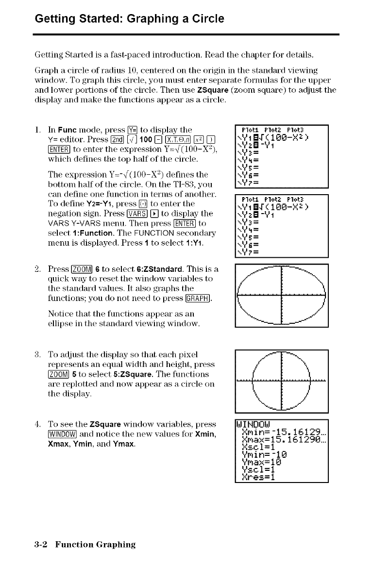
Getting Started: Graphing a Circle
Getting Started is a fast-paced introduction. Read the chapter for details.
Graph a circle of radius 10, centered on the origin in the standard viewing
window. To graph this circle, you nmst enter separate formul_ts for the upper
and lower portions of the circle. Then use ZSquare (zoom square) to adjust the
display- and make tile functions appear as a circle.
In Func mode, press [] to display tile
Y= editor. Press _ [_] 100 [] _ [] []
to enter the expression Y=f(100-X2),
which defines the top half of the circle.
The expression Y=-f(100-X 2) defines the
bottom half of the circle. On the TI-83, you
can define one function in terms of another.
To define Y2=-Y1, press [] to enter the
negation sign. Press FqAgg][] to display- the
VARS Y-VARS menu. Then press _ to
select 1:Function. The FUNCTION seeondatT
menu is displayed. Press 1to select 1:Y1.
Press _ 6 to select 6:ZStandard. This is a
quick way- to reset the window wu'iables to
the standard values. It also graphs the
functions; you do not need to press [ggAPH].
Notice that the functions appear as an
ellipse in the standard xqewing window.
To adjust the display- so that each pixel
represents an equal width and height, press
6 to select 8:ZSquare. The functions
are replotted and now appear as a circle on
the display.
To see the ZSquare window variables, press
and notice the new values for Xmin,
Xmax, Ymin, and Ymax.
_INOOW
Xmin=-15.16129...
Xmax=15.161290...
XsGI=I
Vnin=-lO
9max=lO
Vscl=l
Xres=l
3-2 Function Graphing
Defining Graphs
TI-83--Graphing
Mode Similarities
Defining aGraph
Displaying and
Exploring a
Graph
Saving a Graph
for Later Use
Chapter 3 specifically describes function graphing, but the
steps shown here are similar for each TI-83 graphing
mode. Chapters 4, 5, and 6 describe aspects that are unique
to paralnetric graphing, polar graphing, and sequence
graphing.
To define a graph in any graphing mode, follow these
steps. Some steps are not always necessmT.
1. Press [ff0_] and set the appropriate graph mode
(page 3-4).
2. Press [] and enter, edit, or select one or more functions
in the Y= editor (page 3-5 and 3-7).
3. Deselect stat plots, ifnecessmT (page 3-7).
4. Set the graph style ff)r each function (page 3-9).
5. Press _ and define the viewing window variables
(page 3-11).
6. Press _ [FORMAT] and select the graph format settings
(page 3-13).
After you have defined a graph, press [ffg_] to display- it.
Explore the behavior of the function or functions using the
TI-83 tools described in this chapter.
You can store the elements that define the current graph to
any- of 10 graph database variables (GDB1 through GDBg,
and GDB0; Chapter 8). To recreate the current graph later,
simply recall the graph database to which you stored the
original graph.
These types of information m'e stored in a GDB
• Y= functions
• Graph style settings
• Window settings
• Format settings
You can store a picture of the current graph display to any
of 10 graph picture variables (Picl through Picg, and Pie0;
Chapter 8). Then you can superimpose one or more stored
pictures onto the current graph.
Function Graphing 3-3
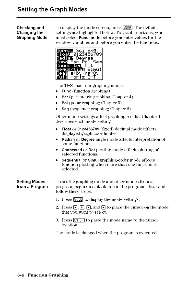
Setting the Graph Modes
Checking and
Changing the
Graphing Mode
To display- the mode screen, press [_. The default
settings are highlighted below. To graph functions, you
nmst select Func mode before you enter values for the
window vm'iables and before you enter the functions.
Sci Eng
Setting Modes
from a Program
Dot
Horiz G-T
The TI-83 has four graphing modes.
•Func (function graphing)
•Par (parametric graphing; Chapter 4)
•Pol (polar graphing; Chapter 5)
•Seq (sequence graphing; Chapter 6)
Other mode settings affect graphing results. Chapter 1
describes each mode setting.
•Float or 0123456789 (fixed) decinlal nlode affects
displayed graph coordinates.
•Radian or Degree angle mode affects interpretation of
some functions.
•Connected or Dot plotting mode 'affects plotting of
selected functions.
•Sequential or Simul graphing-order mode affects
function plotting when nlore than one function is
selected.
To set the graphing mode and other nlodes fronl a
program, begin on a blank line in the program editor and
follow these steps.
1. Press [MO_] to display- the lnode settings.
2. Press [], [], [_, and [] to place the cursor on the mode
that you want to select.
3. Press _ to paste the Inode name to the cursor
location.
The nlode is changed when the program is executed.
3-4 Function Graphing
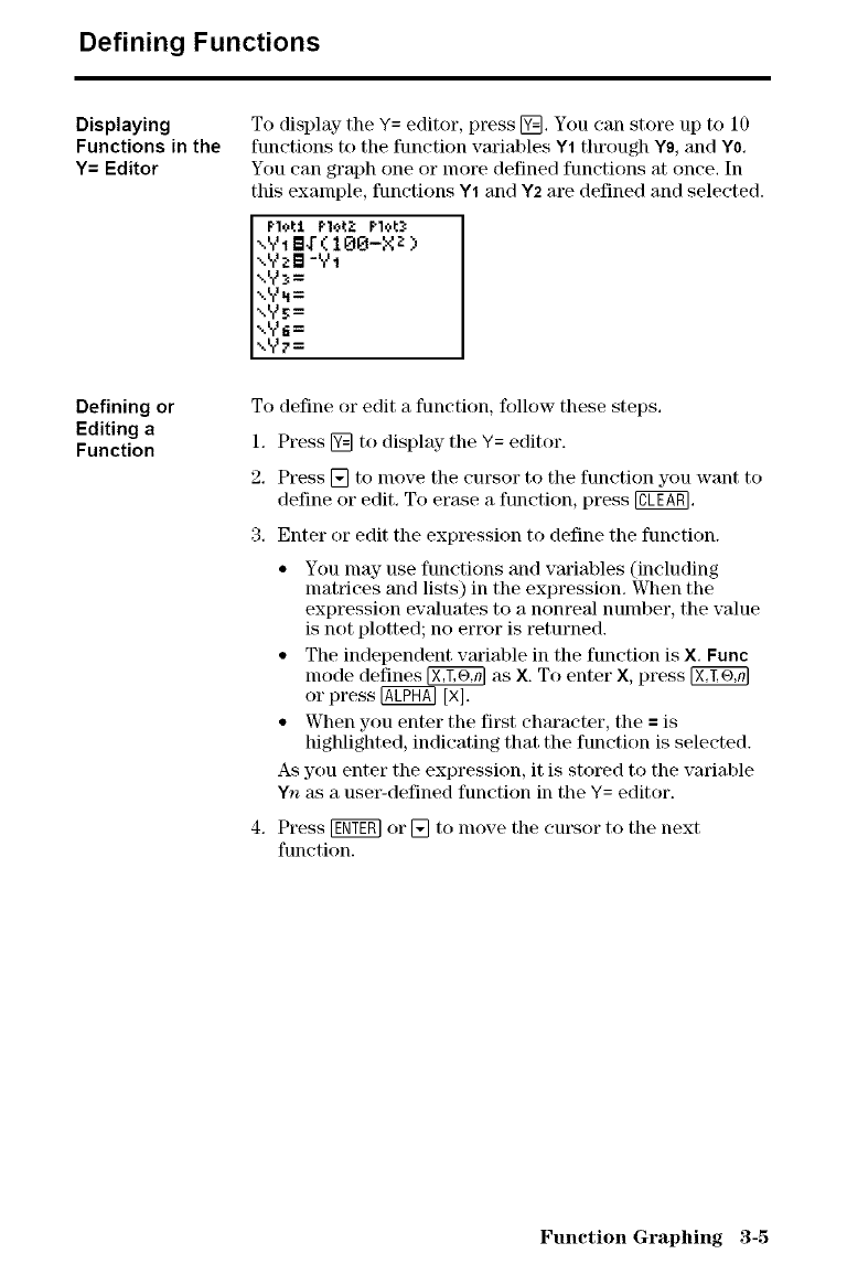
Defining Functions
Displaying
Functions in the
Y= Editor
Defining or
Editing a
Function
To display the Y= editor, press @. You can store up to 10
functions to tile function variables Y1 through Y9, and YO.
You can graph one or more defined functions at once. In
this example, functions Y1 and Y2 are defined and selected.
PI,'.,LI PloLg Pl,:,t_:
-,y1B4"(100-ga:)
.,YaB -YI
\Y_=
..Y_=
,,y_=
,,y_=
-,y_=
To define or edit a function, follow these steps.
1. Press [] to display the Y= editor.
2, Press [] to nlove the cursor to the function you want to
define or edit, To erase a function, press @,
3. Enter or edit the expression to define the function.
• You lnay use functions and variables (including
matrices and lists) in the expression. When the
expression ewduates to a nonreal number, the value
is not plotted; no error is returned.
• The independent variable in the function is X. Func
lnode defines _ as X. To enter X, press
or press @ [x].
• When you enter the first character, the = is
highlighted, indicating that the function is selected.
As you enter the expression, it is stored to the variable
Yn as a use>defined function in the Y= editor.
4. Press [gNY_or [] to l:love the cursor to the next
function.
Function Graphing 3-5
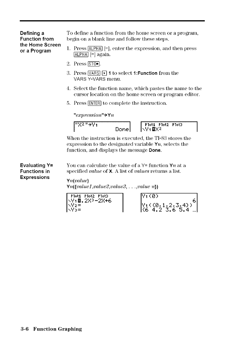
Defining a
Function from
the Home Screen
or aProgram
Evaluating Y=
Functions in
Expressions
To define a function fronl the home screen or a prograln,
begin on a blank line and follow these steps.
1. Press @ [,], enter the expression, and then press
@ [-1 again.
2. Press _.
3. Press _ [] 1to select 1:Function fl'om the
VARS Y-VARS menu,
4. Select the function name, which p_stes the name to the
cursor location on the home screen or program editor.
5. Press _ to complete the instruction.
"expression " _ Yn
I"X z''÷Vt Donel "J',JtI_IX2PI':'tt P10t;: Plot, I
When the instruction is executed, the TI-83 stores the
expression to the designated variable Yn, selects the
function, and displays the message Done.
You can calculate the value of a Y= function Yn at a
specified value of X. A list of values returns a list.
Yn(value)
Yn({valuel ,value2,value3, . ..,value n})
Pl*tl Pl*{2 P10t) IY1 (0) 6
\V1 B. 2Xs-2X+6
,,..z= I '_1 ({0, 1,2,3,4} )
xV_-= ._6 4.2 3.6 5.4 ...
3-6 Function Graphing
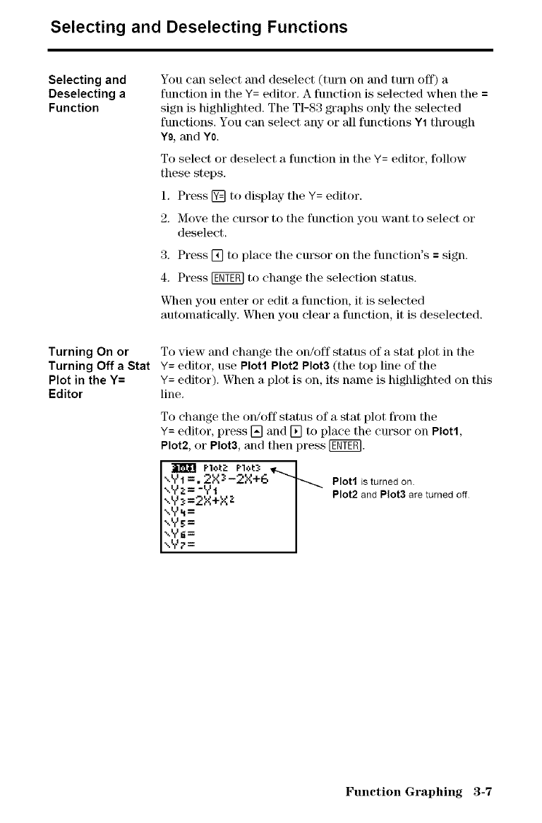
Selecting and Deselecting Functions
Selecting and
Deselecting a
Function
Turning On or
Turning Off a Stat
Plot in the Y=
Editor
You can select and deselect (turn on and turn off) a
functkm in the Y= editor. A function is selected when the =
sign is highlighted. The TI-83 graphs only the selected
functions. You can select any or all functions Y1 through
Yg, and Y0.
To select or deselect a function in the Y= editor, follow
these steps.
1. Press [] to display the Y= editor.
2. Move the cursor to the function you want to select or
deselect.
3, Press [] to place the cursor on the functkm's =sign.
4. Press [gg_g] to change the selection status.
When you enter or edit a function, it is selected
automatically. When you clem' a function, it is deselected.
To view and change the OlVOff status of a stat plot in the
Y= editor, use Plot1 Plot2 Plot3 (the top line of the
Y= editor). When a plot is on, its name is highlighted on this
line.
To change the OlgOff status of a stat plot fronl the
Y= editor, press [] and [] to place the cursor on Plot1,
Plot2, or Plot& and then press [g_N.
_lotz Plet_ _ J
",YI =. 2X3-2X+6 -'1---,_ Plott isturnedon.
\Vz= -Yt I
,_.y_=2X+XZ j Plot2 and Plot3 are turned off
\Y_= J
",us =
",'¢_= /
-W= I
Function Graphing 3-7
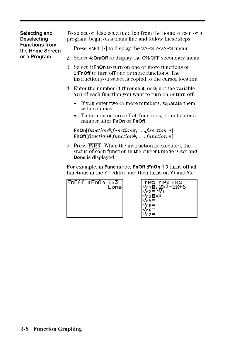
Selecting and
Deselecting
Functions from
the Home Screen
or a Program
To select or deselect a function fronl the home screen or a
program, begin on a blank line and follow these steps.
1. Press _ [] to display- the VANS Y-VANS menu.
2. Select 4:On/Off to display the ON/OFF secondary menu.
3. Select l:FnOn to turn on one or more functions or
2:FnOff to turn off one or more functions. The
instruction you select is copied to the cursor location.
4. Enter the number (1 through 9, or 0; not the variable
Yn) of each function you want to turn on or turn off.
• If you enter two or more numbers, separate them
with eonunas.
• To turn on or turn off all functions, do not enter a
number after FnOn or FnOff,
FnOn[function#function#,.,, function n]
FnOff[function# function# .... function n]
5, Press [ggTig], When the instruction is executed, the
status of each function in the eutTent mode is set and
Done is displayed.
For example, in Func mode, FnOff :FnOn 1,3 turns off all
functions in the Y= editor, and then turns on Y1 and Y3.
FnOff :FnOn Dlo3e I Pl<,tl Plo_Z Plot._
",Y1B. 2X_-2X+6
_,Y;_= -Y1
",YsBXZ
xy_=
xY_=
\Y_=
,,y_=
3-8 Function Graphing
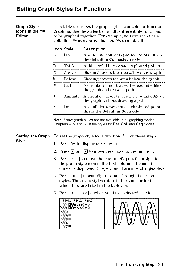
Setting Graph Styles for Functions
Graph Style
Icons in the Y=
Editor
Setting the Graph
Style
This table describes the graph styles available for function
graphing. Use the styles to visually differentiate functions
to be graphed together, For example, you can set Y1 as a
solid line, Y2 as a dotted line, and Y3 as a thick line,
Icon Style Description
".. Line A solid line connects plotted points; this is
the default in Connected mode
"i Thick A thick solid line connects plotted points
'_.i Above Shading covers the area a*bove the graph
ik Below Shading covet\_ the area below the graph
'1! Path A circular cursor traces the leading edge of
the graph and draws a path
(! Aidmate A circular cursor traces the leading edge of
the graph without drawing a path
". Dot A snlall dot represents each plotted point;
this is the default in Dot mode
Note: Some graph styles are not available in all graphing modes.
Chapters 4, 5, and 6 list the styles for Par, Pol, and Seq modes.
To set the graph style for a function, follow these steps.
1. Press [] to display the Y= editor.
2. Press [] and [] to nlove the cut\sor to the function.
3. Press [] [] to move the cm'sor left, past the = sign, to
the graph style icon in the first colunm. The insert
cm'sor is displayed. (Steps 2 and 3 are interchangeable.)
4. Press _ repeatedly to rotate through the graph
styles. The seven styles rotate in the same order in
which they are listed in the table above.
5. Press [], [], or [] when you have selected a style.
PlotJ. F'1ot;_P1ot:_
",Y1B8sin(X)
_YzB8cos(X)
\Y_=
xY_=
\Y_=
xy_=
xy_=
Function Graphing 3-9
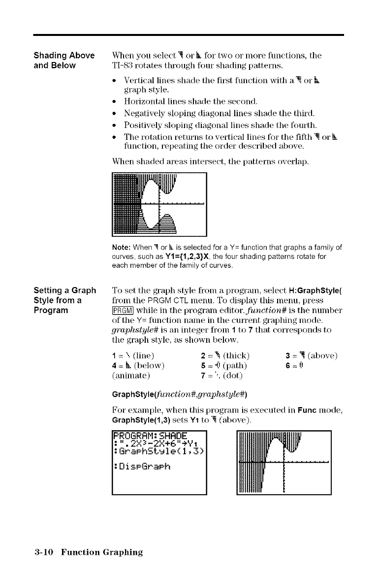
Shading Above
and Below
When you select _mor 1;.for two or more functions, the
TI-83 rotates through four shading patterns.
• Vertical lines shade the first function with a '_.1or b.
graph style.
• Horizontal lines shade the second.
• Negatively sloping diagonal lines shade the third.
• Positively sloping diagonal lines shade the fom'th.
• The rotation returns to vertical lines for the fifth '_.ior i;.
function, repeating the order described above.
VClmn shaded are_Ls intersect, the patterns overlap.
Setting a Graph
Style from a
Program
Note: When _1or h_,is selected for a Y= function that graphs a family of
curves, such as Yl={1,2,3}X, the four shading patterns rotate for
each member of the family of curves.
To set the graph style fl'onl a program, select H:GraphStyle(
from the PRGM CTL menu. To display this menu, press
[V_ while in the program editor.function# is the nmnber
of the Y= function name in the current graphing mode.
graphstyle# is an integer from 1 to 7 that corresponds to
the graph style, as shown below.
1 = ". (line) 2 = '_i(thick) 3 = ,m(above)
4 = 1'.-.(below) 8= ':) (path) 6= (!
(animate) 7= ". (dot)
GraphStyle(fanction#,graphstyle#)
For example, when this program is executed in Func mode,
GraphStyle(1,3) sets Y1 to '_](above),
:OisPGr'aPh
3-10 Function Graphing
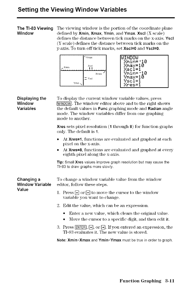
Setting the Viewing Window Variables
The TI-83 Viewing
Window The viewing window is the portion of the coordinate plane
defined by Xmin, Xmax, Ymin, and Ymax. Xscl (X scale)
defines the distance between tick marks on the x-axis. Yscl
(Y scale) defines the distance between tick marks on the
y-axis. To turn off tick marks, set Xscl=0 and Yscl=0.
_Ymax
Xsc_
Xmax /
_--Yscl
Ymir_ N
WINDOW
Xmin=-lO
XMax=lO
Xscl=l
Ymin=-lO
Ymax=lO
Yscl=l
XPes=l
Displaying the
Window
Variables
Changing a
Window Variable
Value
To display the current window variable values, press
_. The window editor above and to the right shows
the default values in Func graphing mode and Radian angle
nlode. The window variables differ fronl one graphing
mode to another.
Xres sets pixel resolution (1 through 8) for function graphs
only. The default is 1.
• At Xres=l, functions are evaluated and graphed at each
pixel on the x-axis.
• At Xres=8, functions are evaluated and graphed at every
eighth pixel along the x-axis.
Tip: SmalIXres valuesimprovegraph resolutionbut maycausethe
TI-83 to drawgraphs more slowly.
To change a window variable value fronl the window
editor, follow these steps.
1. Press [] or [] to move the cut\sor to the window
variable you want to change.
2. Edit the value, which can be an expression.
• Enter a new wdue, which clears the original value.
• Move the cursor to a specific digit, and then edit it.
3. Press [g_gff], [], or []. If you entered an expression, the
TI-83 ewduates it. The new value is stored.
Note: Xmin<Xmax andYmin<Ymax must be true in orderto graph.
Function Graphing 3-11
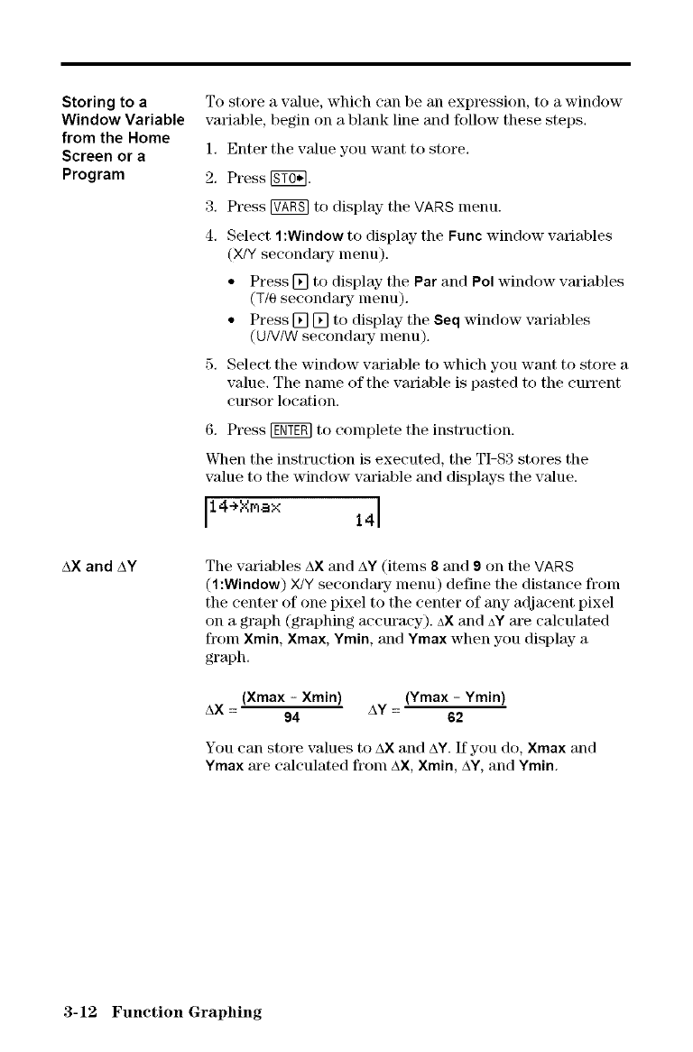
Storing to a
Window Variable
from the Home
Screen or a
Program
AX and AY
To store a value, which can be an expression, to a window
variable, begin on a blank line and follow these steps,
1, Enter the value you want to store,
2, Press _.
3, Press _ to display- the VARS menu.
4, Select 1 :Window to display the Func window variables
(X/Y secondmT menu).
• Press [] to display the Par and Pol window variables
(T/0 secondm_y- menu).
• Press [] [] to display the Seq window variables
(UN/W secondary menu).
5, Select the window variable to which you want to store a
value, The name of the variable is pasted to the current
CUrSOr location.
6, Press _ to complete the instruction.
When the instruction is executed, the TI-83 stores the
value to the window variable and displays the vMue.
J14+Xv,ax 14J
The variables AX and AY (items 8 and 9 on the VARS
(1:Window) X/Y seeondmT menu) define the distance from
the center of one pixel to the center of any adjacent pixel
on a graph (graphing accuracy), a× and AY are calculated
from Xmin, Xma×, Ymin, and Yma× when you display- a
graph.
(Xmax - Xmin) (Ymax - Ymin)
AX = AY -
94 62
You can store values to AX and AY. If you do, Xmax and
Ymax m'e cMculated from AX, Xmin, AY,and Ymin.
3-12 Function Graphing
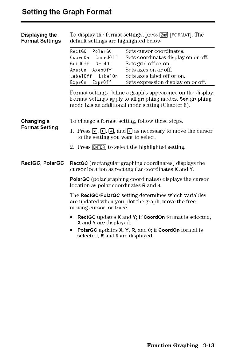
Setting the Graph Format
Displaying the
Format Settings
Changing a
Format Setting
RectGC, PolarGC
To display- the format settings, pl_ss [2_ [FORMAT]. The
default settings are highlighted below.
RectGC PolarGC
CoordOn CoordOff
GridOff GridOn
AxesOn AxesOff
LabelOff LabelOn
ExprOn ExprOff
Sets cursor coordinates.
Sets coordinates display on or off.
Sets grid off or on.
Sets axes on or off.
Sets axes label oft"or on.
Sets expression display on or off.
Format. settings define a graph's appearance on the display.
Format settings apply to all graphing modes. Seq graphing
mode has an additional mode setting (Chapter 6).
To change a fornlat setting, follow these steps.
1. Press [_, [}_],[], and [] as necessary- to lnove the cursor
to the setting you want to select.
2. Press [ggYgg]to select the highlighted setting.
RectGC (rectangular graphing coordinates) displays the
cursor location _LSrectangular coordinates Xand Y.
PolarGC (polar graphing coordinates) displays tile cursor
location as polar coordinates R and 0.
The RectGC/PolarGC setting determines which wuiables
are updated when you plot tile graph, move the free-
nloving cursor, or trace.
• RectGC updates X and Y; if CoordOn format is selected,
Xand Y are displayed.
•PolarGC updates X, Y, R, and 0; if CoordOn format is
selected, R and 0 are displayed.
Function Graphing 3-13
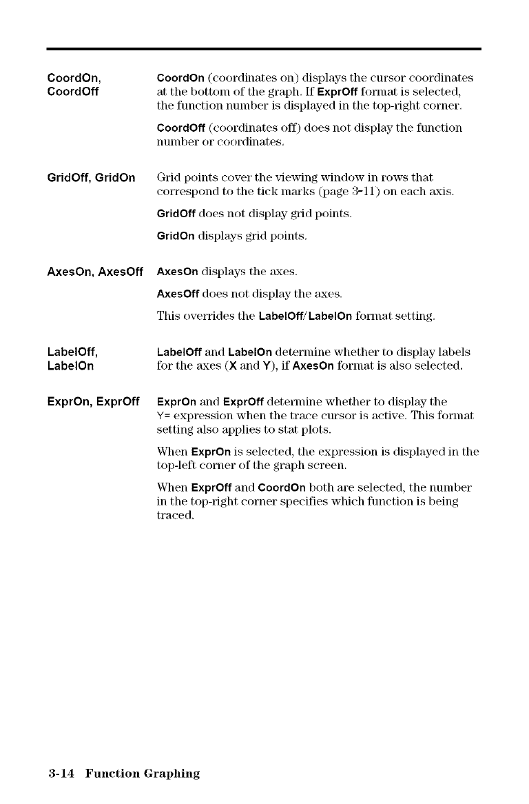
CoordOn,
CoordOff
GridOff, GridOn
AxesOn, AxesOff
LabelOff,
LabelOn
ExprOn, ExprOff
CoordOn (coordinates on) displays the cursor coordinates
at the bottom of the graph, If ExprOff format is selected,
the function number is displayed in the top-right corner,
CoordOff (coordinates off) does not display- the function
number or coordinates,
Grid points cover the viewing window in rows that
correspond to the tick marks (page 3-11) on each axis.
GridOff does not display grid points.
GridOn displays grid points.
AxesOn displays the axes.
AxesOff does not display- the axes.
This overrides the LabelOff/LabelOn format setting.
LabelOff and LabelOn determine whether to display labels
for the axes (X and Y), if AxesOn format is also selected.
ExprOn and ExprOff determine whether to display- the
Y= expression when the trace cursor is active. This format
setting also applies to stat plots.
When ExprOn is selected, the expression is displayed in the
top-left comer of the graph screen.
When ExprOff and CoordOn both are selected, the number
in the top-right corner specifies which function is being
traced.
3-14 Function Graphing
Displaying Graphs
Displaying a New
Graph
Pausing or
Stopping aGraph
Smart Graph
To display the graph of the selected function or functions,
press _. TRACE, ZOOM instructions, and CALC
operations display- the graph automatically. As the TI-83
plots the graph, the busy indicator is on. As the graph is
plotted, X and Y m'e updated.
V_l_ile plotting a graph, you can pause or stop graphing.
• Press [ggT_ to pause; then press [ggT_ to resume.
• Press [ON]to stop; then press _ to redraw.
Snlart Graph is a TI-83 feature that redisplays the last
graph ilnlnediately when you press _, but only if all
graphing factors that would cause replotting have
remained the same since the graph was last displayed.
If you performed any of these actions since the graph was
last displayed, the TI-83 will replot the graph based on new
values when you press _.
• Changed a mode setting that affects graphs
• Changed a function in the current picture
• Selected or deselected a function or stat plot
• Changed the value of a variable in a selected function
• Changed a window variable or graph fornlat setting
• Cleared drawings by selecting ¢lrDraw
• Changed a stat plot definition
Function Graphing 3-15
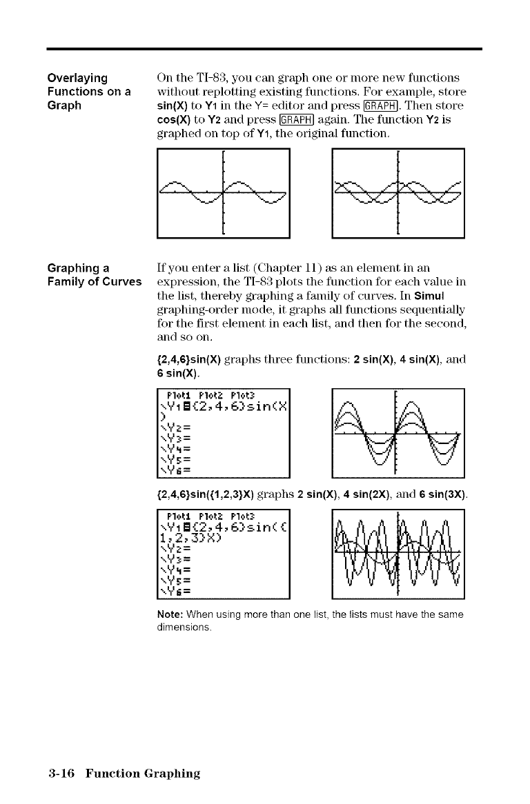
Overlaying
Functions on a
Graph
On the TI-83, you can graph one or more new functions
without replotting existing functions, For example, store
sin(X) to Y1 in the Y= editor and press [_7. Then store
cos(X) to Y2 and press _ again. The function Y2 is
graphed on top of Y1, the original function,
Graphing a
Family of Curves
If you enter a list (Chapter 11) as an element in an
expression, the TI-83 plots the function for each value in
the list, thereby graphing a family of curves. In Simul
graphing-order mode, it graphs 'all functions sequentiMly
for the fit.st element in each list, and then for the second,
and so on.
{2,4,6}sin(X) graphs three functions: 2sin(X), 4 sin(X), and
6sin(X).
Plot1 PIo_Z Plot_
_.YtB£2, 4, 6}sin(X
xy?=
\y_,=
-.y_=
",y_=
-.y_=
{2,4,6}sin({1,2,3}X) graphs 2sin(X), 4sin(2X), and 6 sin(3X).
PI_L1 PlOL_: Plot. _ '_
".YIB(2, 4, 6}sin(
1,2,3}X)
\Yz =
\Y_=
\Y_=
-.y_=
..y_=
Note: When using more than one list, the lists must have the same
dimensions.
3-16 Function Graphing
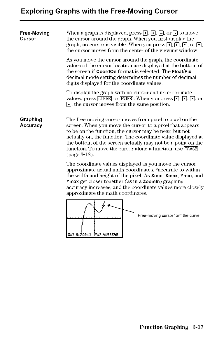
Exploring Graphs with the Free-Moving Cursor
Free-Moving
Cursor
Graphing
Accuracy
When a graph is displayed, press [], [], [], or [] to nlove
tile cursor around the graph. When you first display- the
graph, no cursor is visible. When you press [], [], [], or [],
the cursor moves from the center of the viewing window.
As you move the cursor around the graph, the coordinate
values of the cursor location m'e displayed at the bottom of
the screen if ¢oordOn format is selected. The Float/Fix
decimal mode setting determines tile number of decimal
digits displayed for the coordinate wdues.
To display the graph with no cursor and no coordinate
values, press @ or [gg_g]. When you press [], [], [], or
[], the cursor moves froln the same position.
The flee-moving cursor nloves fronl pixel to pixel on the
screen. When you move the cursor to a pixel that appears
to be on the function, the cursor nlay be neat', but not
actuMly on, the function. The coordinate value displayed at
the bottom of the screen actuMly lnay not be a point on the
function. To lnove the cursor along a function, use
(page 3-18).
The coordinate values displayed as you move the cursor
approximate actuM math coordinates, *accurate to within
the width and height of the pixel. As Xmin, Xmax, Ymin, and
Ymax get closer together (as in a Zoomln) graphing
accuracy ineretkqes, and the coordinate values nlore closely
approxinlate the lnath coordinates.
Free-moving cursor 'on" the curve
Function Graphing 3-17
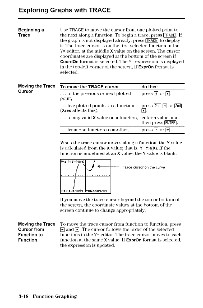
Exploring Graphs with TRACE
Beginning a
Trace
Moving the Trace
Cursor
Moving the Trace
Cursor from
Function to
Function
Use TRACE to move the cursor from one plotted point to
the next along a function• To begin a trace, press _. If
the graph is not displayed already, press _ to display
it. The trace cursor is on the first selected function in the
Y= editor, at the middle × value on the screen• The cursor
coordinates are displayed at the bottom of the screen if
CoordOn format is selected. The Y= expression is displayed
in the top-left corner of the screen, if ExprOn format is
selected.
To move the TRACE cursor,., do this:
•, , to the previous or next plotted press [] or [].
point,
•.. five plotted points on a function press [g_ [] or K_
(Xres affects this), [].
•.. to any valid Xvalue on a function, enter a value, and
then press [KNT_.
•fronl one function to another, press [] or [].
When the trace cursor nloves along a function, the Ywdue
is calculated from the X value; that is, Y=Yn(X). If the
function is undefined at an X value, the Y value is blank.
'_1='_-_i_*_ J_
..... i ............
/
g:?,:LB:LLIBgR f:IL:L:LBLIT09
-- -- Trace cursor on the curve
If you nlove the trace cursor beyond the top or bottonl of
the screen, the coordinate values at the bottom of the
screen continue to change appropriately.
To nlove the trace cursor fronl function to function, press
[] and []. The cursor follows the order of the selected
functions in the Y= editor• The trace cursor moves to each
function at the same × value• If ExprOn format is selected,
the expression is updated.
3-18 Function Graphing
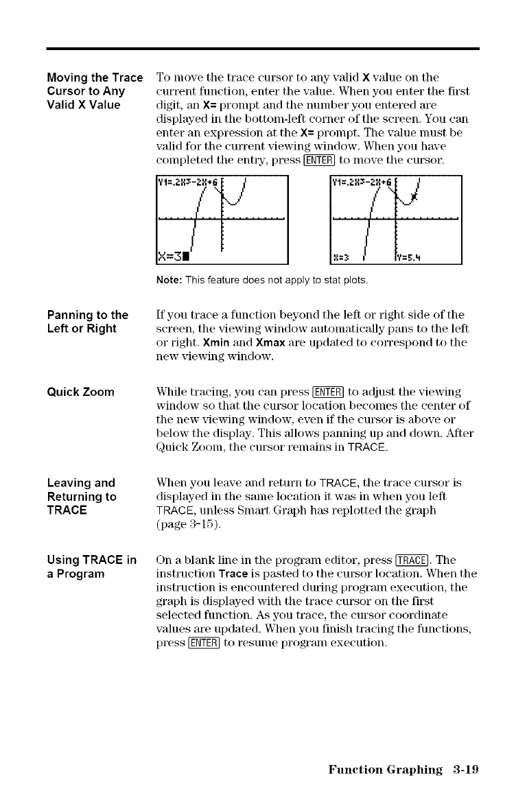
Moving the Trace
Cursor to Any
Valid X Value
Panning to the
Left or Right
Quick Zoom
Leaving and
Returning to
TRACE
Using TRACE in
a Program
To move the trace cursor to any valid X value on the
current function, enter the value. When you enter the first
digit, an X= prompt and the number you entered are
displayed in the bottom-left corner of the screen. You can
enter an expression at the X= prompt. The value nmst be
valid for the current viewing window. When you have
coinpleted the enttT, press _ to inove the cursor.
Zt L;t L......
Note: This feature does not apply to stat plots.
If you trace a function beyond the left or right side of the
screen, the viewing window automatically pans to the left
or right. Xmin and Xmax are updated to correspond to the
new viewing window.
While tracing, you can press _ to adjust the viewing
window so that the cursor location beconles the center of
the new xqewing window, even if the cursor is above or
below the display. This allows panning up and down. After
Quick Zoom, the cursor remains in TRACE.
When you leave and return to TRACE, the trace cursor is
displayed in the same location it was in when you left
TRACE, unless Smart Graph has replotted the graph
(page 3-15).
On a blank line in the prograln editor, press _. The
instruction Trace is pasted to the cursor location. When the
instruction is encountered during program execution, the
graph is displayed with the trace cursor on the first
selected function. As you trace, the cursor coordinate
values are updated. When you finish tracing the functions,
press _ to resume program execution.
Function Graphing 3-19
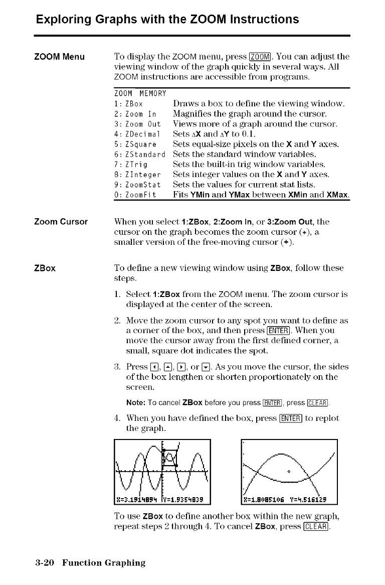
Exploring Graphs with the ZOOM Instructions
ZOOM Menu To display the ZOOM menu, press _, You can adjust the
viewing window of the graph quickly- in several ways. All
ZOOM instructions axe accessible fronl programs.
ZOOM MEMORY
i: ZBox
2: Zoom In
3: Zoom Out
4: ZDecimal
5: ZSquare
6: ZStandard
7: ZTrig
8: Zlnteger
9: ZoomStat
0: ZoomFit
Draws a box to define the viewing window.
Magnifies the graph around the cursor.
Views more of a graph atxmnd the cursor.
Sets aX and aY to O. 1.
Sets equal-size pixels on the Xand Y m,ces.
Sets the standard window variables.
Sets the built-in trig window variables.
Sets integer values on the Xand Y m,ces.
Sets the values for current stat lists.
Fits YMin and YMax between XMin and XMax.
Zoom Cursor
ZBox
When you select 1 :ZBox, 2:Zoom In, or 3:Zoom Out, the
cursor on the graph becomes the zoom cursor (+), a
smaller version of the free-mo_dng cursor (+).
To define a new viewing window using ZBox, follow these
steps,
1, Select l:ZBox from the ZOOM menu. The zoom cursor is
displayed at the center of the screen.
2. Move the zoonl cursor to any spot you want to define as
a cornet" of the box, and then press [N_N. When you
lnove the cm_or away- from the first defined corner, a
smM1, square dot indicates the spot.
3. Press [_, E], [_, or [_. As you lnove the cursor, the sides
of the box lengthen or shorten proportionately on the
screen.
Note: To cancel ZBox before you press _, press @.
4. When you have defined the box, press [_ to replot
the graph.
V]\,, ,,/'
X:3,:L9J.tlBBq t:! .B2:.t:LIB3B
To use ZBox to define another box within the new graph,
repeat steps 2 through 4. To cancel ZBox, press @.
3-20 Function Graphing
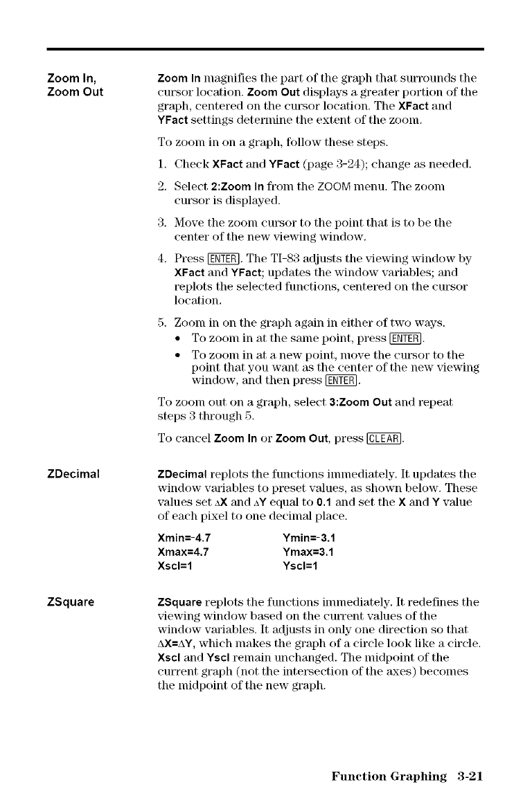
Zoom In,
Zoom Out
ZDecimal
ZSquare
Zoom In magnifies the part of the graph that surrounds the
cursor location. Zoom Out displays a greater portion of the
graph, centered on the cut\sor location. The XFact and
YFact settings determine the extent of the zoom.
To zoom in on a graph, follow these steps.
1, Check XFact and YFact (page 3-24); change as needed.
2, Select 2:Zoom In from the ZOOM menu. The zoom
cursor is displayed.
3, Move the zoom cut, or to the point that is to be the
center of the new viewing window,
4, Press [gNYE_, The TI-83 adjusts the viewing window by
XFact and YFact; updates the window variables; and
replots the selected functions, centered on the cursor
location,
5. Zoonl in on the graph again in either of two ways.
• To zoom in at the same point, press [_T_].
• To zoom in at a new point, move the cm\sor to the
point that you want as the center of the new viewing
window, and then press [_T_].
To zoom out on a graph, select 3:Zoom Out and repeat
steps 3 through 5.
To cancel Zoom In or Zoom Out, press @.
ZDecimal replots the functions inunediately. It updates the
window variables to preset values, tks shown below. These
values set AX and AYequal to 0.1 and set the X and Y value
of each pixel to one decimal place.
Xmin=-4.7 Ymin=-3.1
Xmax=4.7 Ymax=3,1
Xscl=l Yscl=l
ZSquare replots the functions immediately. It redefines the
xqewing window based on the cun'ent values of the
window variables. It adjusts in only one direction so that
AX=AY,which makes the graph of a circle look like a circle.
Xscl and Yscl remain unchanged. The midpoint of the
current graph (not the intersection of the axes) becomes
the midpoint of the new graph.
Function Graphing 3-21
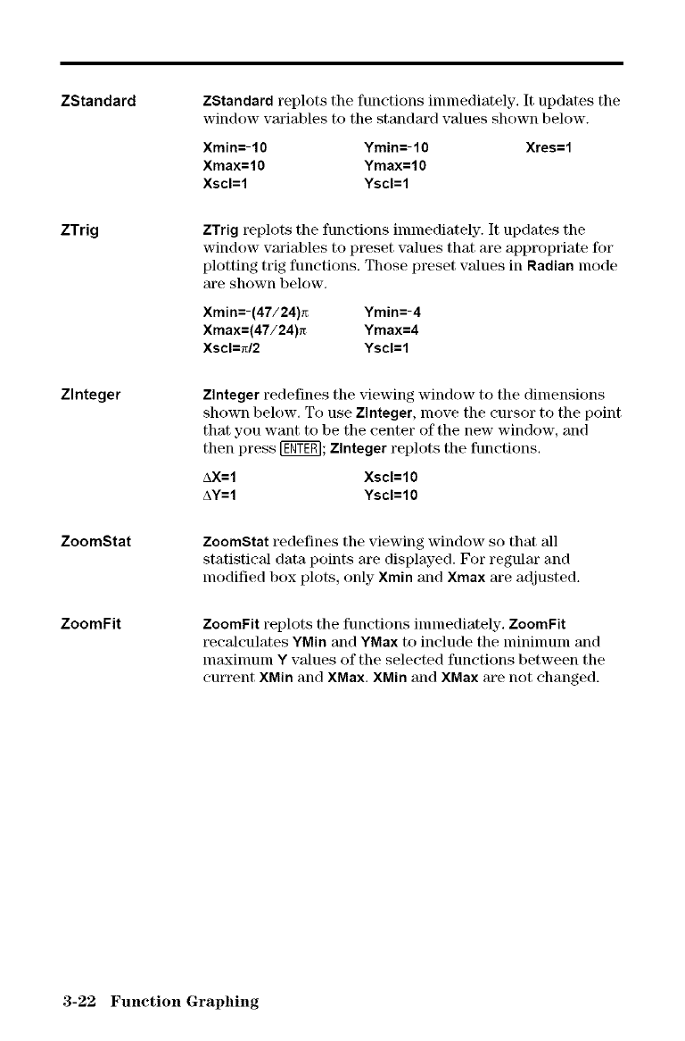
ZStandard
ZTrig
Zlnteger
ZoornStat
ZoomFit
ZStandard replots the functions immediately, It updates the
window vm'iables to the standm'd values shown below.
Xmin=-lO Ymin=-lO Xres=l
Xmax=lO Ymax=lO
Xscl=l Yscl=l
ZTrig replots the functions immediately. It updates the
window vm'iables to preset values that are appropriate ffw
plotting trig functions. Those preset values in Radian mode
m'e shown below,
Xmin=-(47/24)_ Ymin=-4
Xmax=(47/24)_ Ymax=4
Xscl=_/2 Yscl=l
Zlnteger redefines the viewing window to the dimensions
shown below, To use Zlnteger, move the cursor to the point
that you want to be the center of the new window, and
then press [_T_]; Zlnteger replots the functions,
AX=I Xscl=lO
AY=I YscI=IO
ZoomStat redefines the viewing window so that all
statistical data points m'e displayed. For regular and
modified box plots, only Xmin and Xmax m'e adjusted.
ZoomFit replots the functions immediately, ZoomFit
recalculates YMin and YMax to include the nlininmm and
nlmNinlunl Yvalues of the selected functions between the
current XMin and XMax. XMin and XMax are not changed.
3-22 Function Graphing
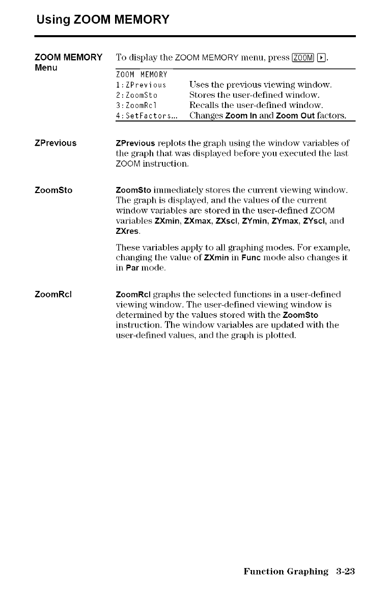
Using ZOOM MEMORY
ZOOM MEMORY
Menu
ZPrevious
ZoomSto
ZoomRcl
To display the ZOOM MEMORY menu, p_ss _ [_.
ZOOM MEMORY
1:ZPrevious
2:ZoomSto
3:ZoomRcl
4:SetFactors...
[_ses the pre_ious _iewing window,
Stores the user-defined window,
Recalls the user-defined window.
Changes Zoom In and Zoom Out factors.
ZPrevious replots the graph using the window variables of
the graph that was displayed before you executed the last
ZOOM instruction.
ZoomSto inunediately stores the cmTent viewing window.
The graph is displayed, and the values of the current
window variables are stored in the user-defined ZOOM
variables ZXmin, ZXmax, ZXscl, ZYmin, ZYmax, ZYscl, and
ZXres.
These variables apply to all graphing modes. For example,
changing the value of ZXmin in Func nlode also changes it
in Par mode,
ZoomRcl graphs the selected functions in a user-defined
viewing window. The user-defined viewing window is
determined by the values stored with the ZoomSto
instruction. The window variables are updated with the
user-defined values, and the graph is plotted.
Function Graphing 3-23
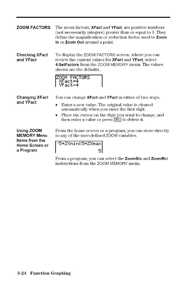
ZOOM FACTORS
Checking XFact
and YFact
Changing XFact
and YFact
Using ZOOM
MEMORY Menu
Items from the
Home Screen or
a Program
The zoonl factors, XFact and YFact, are positive numbers
(not necessarily intege_\_) greater than or equal to 1, They
define the magnification or reduction factor used to Zoom
In or Zoom Out around a point,
To display the ZOOM FACTORS screen, where you can
t_iew the current values for XFact and YFact, select
4:SetFactors from the ZOOM MEMORY menu. The values
shown m'e the defaults.
ZOOM FRCTORS I
XFacL=4
VFact=4
You can change XFact and YFact in either of two ways.
• Enter a new value. The original value is cleared
automatically when you enter the first digit.
• Place the cursor on the digit you want to change, and
then enter a value or press [bE[] to delete it,
From the home screen or a program, you can store directly
to any of the user-defined ZOOM vm'iables.
1-5÷ZXr_in:5÷ZXr_,a5
From a program, you can select the ZoomSto and ZoomRcl
instructions fronl the ZOOM MEMORY menu.
3-24 Function Graphing
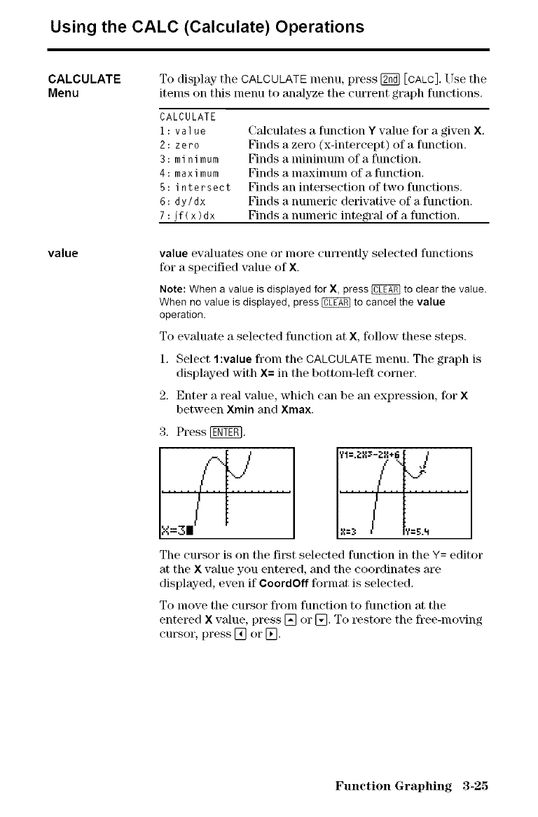
Using the CALC (Calculate) Operations
CALCULATE
Menu
value
To display the CALCULATE nlenu, press I_ [CALC], Use the
items on this menu to analyze tile current graph functions,
CALCULATE
i: value
2: zero
3: minimum
4: maximum
5:intersect
6:dy/dx
7:ff(x)dx
Calculates a function Yvalue for a given X,
Finds a zero (x-intercept) of a function.
Finds a nlininmln of a function,
Finds a nlaxinmln of a function.
Finds an intersection of two functions,
Finds a numeric derivative of a function.
Finds a numeric integral of a function,
value evaluates one or more currently selected functions
for a specified value of X.
Note: Whena valueis displayedfor X, press[_ to clear thevalue.
Whenno valueisdisplayed, press @ to cancelthevalue
operation.
To evaluate a selected function at X, ff)llow these steps.
1, Select 1:value froln the CALCULATE menu, The graph is
displayed with X= in tile bottom-left corner.
2, Enter a real value, which can be an expression, for X
between Xmin and Xmax.
3. Press IE_]. "7i7.J
The cursor is on the first selected function in the Y= editor
at the X value you entered, and the coordinates are
displayed, even if ¢oordOff fornlat is selected.
To nlove the cm'sor fl'om function to function at the
entered Xvalue, press [] or [], To t_store the free-re(Mug
cursor, press [] or [].
Function Graphing 3-25
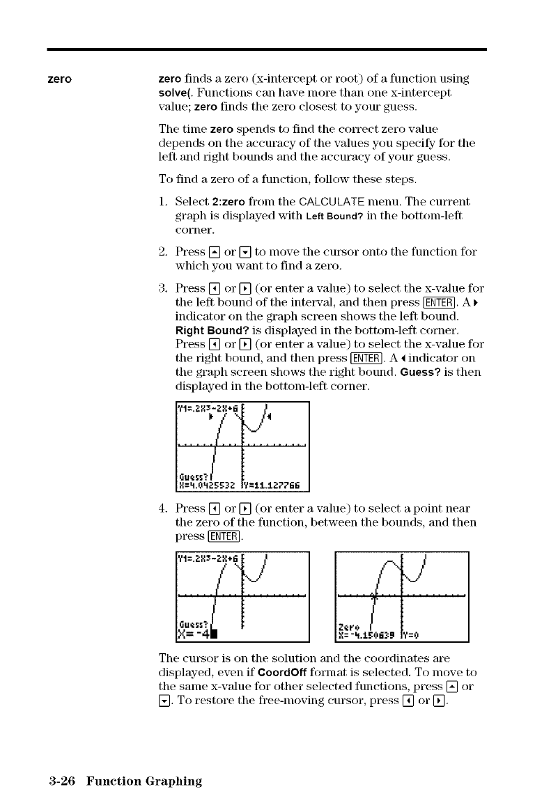
zero zero finds a zero (x-intercept or root) of a function using
solve(. Functions can have more than one x-intercept
value; zero finds the zero closest to your guess.
The time zero spends to find the eotTect zero value
depends on the accuracy of the values you specify for the
left and right bounds and the accuracy of your guess.
To find a zero of a function, follow these steps.
1. Select 2:zero froln the CALCULATE menu. The current
graph is displayed with Left Bound? in the bottom-left
corner.
2_
3.
Press [] or [] to move the cm\sor onto the function %r
which you want to find a zero.
Press [] or [] (or enter a value) to select the x-value for
the left bound of the interval, and then press I_T_. A
indicator on the graph screen shows the left bound.
Right Bound? is displayed in the bottom-left corner.
Press [] or [] (or enter a value) to select the x-value for
the right bound, and then press IT_. A _ indicator on
the graph screen shows the right bound. Guess? is then
displayed in the bottom-left corner.
Press [] or [] (or enter a value) to select a point near
the zero of the function, between the bounds, and then
press [_T_].
ZCYO
The cursor is on the solution and the coordinates are
displayed, even if ¢oordOff format is selected. To move to
the same x-value for other selected functions, press [] or
[]. To restore the free-moving cursor, press [] or [].
3-26 Function Graphing
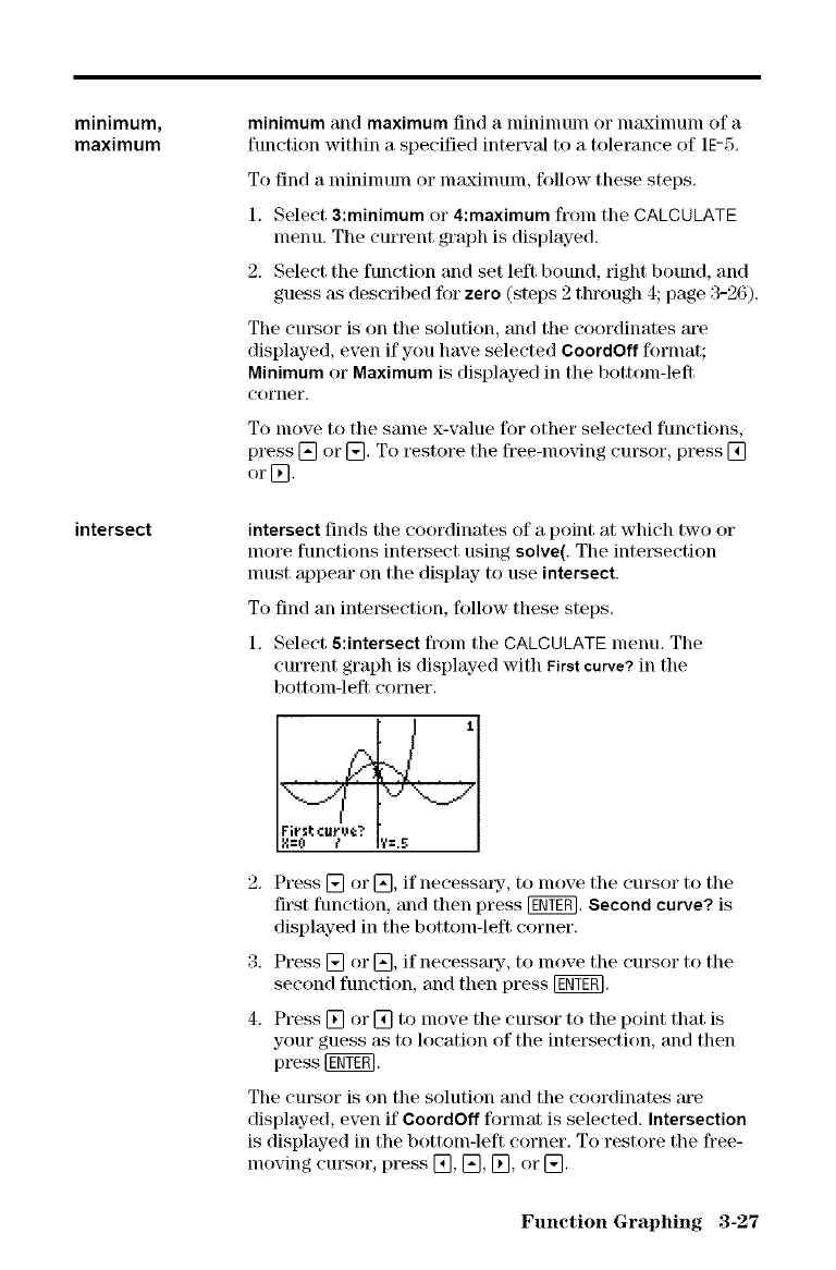
minimum,
maximum minimum and maximum find a ndninmln or nl3xinlunl of a
function within a specified inteP_+al to a tolerance of 1E-5.
To find a nlininlunl Or nlaxinlunl, follow these steps.
1. Select 3:minimum or 4:maximum fronl the CALCULATE
nlenu. The current graph is displayed.
2. Select the function and set left bound, right bound, and
guess _ts described for zero (steps 2 through 4; page 3-26).
The cursor is on the solution, and the coordinates ate
displayed, even if you have selected CoordOff format;
Minimum or Maximum is displayed in the bottom-left
c()rner.
To nlove to the salne x-value for other selected functions,
press [] or []. To restore the free-moving cursor, press []
or [].
intersect intersect finds the coordinates of a point at which two or
nlore functions intersect using solve(. The intersection
nmst appear on the display to use intersect.
To find an intersection, follow these steps.
1. Select 5:intersect fi'om the CALCULATE menu. The
current graph is displayed with First curve? in the
bottom-left corner.
c >.J *
Fit_t cul_ve?
ll=0 € Y=.5
2. Press [] or [], if necessatT, to nlove the cursor to the
first function, and then press [gg7_. Second curve? is
displayed in the bottom-left corner.
3. Press [] or [], if necessatT, to nlove the cursor to the
second function, and then press [gg7_.
4. Press [] or [] to nlove the cursor to the point that is
your guess as to location of the intersection, and then
press [gfff_.
The cursor is on the solution and the coordinates are
displayed, even if CoordOff format is selected. Intersection
is displayed in the bottom-left corner. To restore the free-
moving cursor, press [], [], [], or [].
Function Graphing 3-27
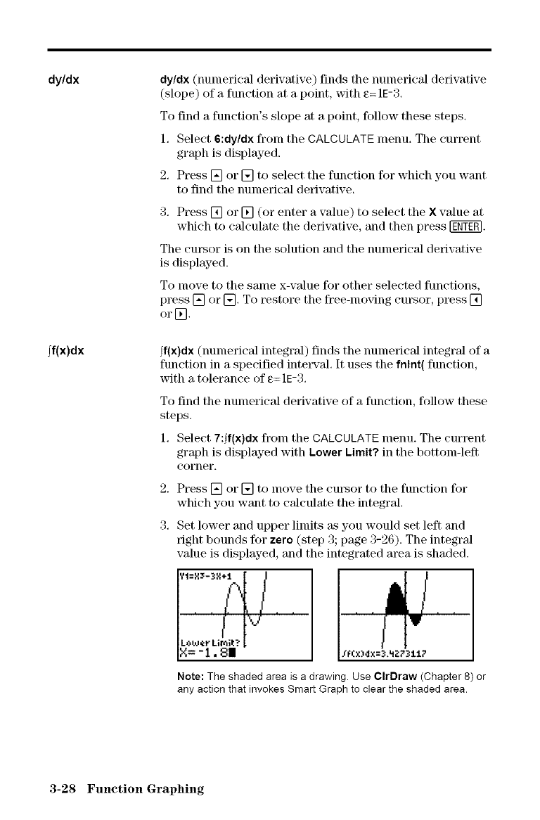
dy/dx
ff(x)dx
dy/dx (numerical derivative) finds the numerical derivative
(slope) of a function at a point, with e= 1E-3,
To find a function's slope at a point, follow these steps,
1, Select 6:dy/dx from the CALCULATE menu. The current
graph is displayed.
2, Press [] or [] to select the function for which you want
to find the numerical derivative.
3, Press [] or [] (or enter a value) to select the X value at
which to calculate the deriwttive, and then press [_TE_.
The cursor is on the solution and the numerical derivative
is displayed.
To move to the same x-value for other selected functions,
press [] or [], To _store the free-moving cursor, press []
or [].
j'f(x)dx(numerical integral) finds the numerical integral of a
function in a specified inte[w'al, It uses the fntnt( function,
with a tolerance of e= 1E-3.
To find the numerical derivative of a function, follow these
steps.
1, Select 7:jf(x)dx from the CALCULATE menu. The current
graph is displayed with Lower LimR? in the bottom-left
corner.
2,
3,
Press [] or [] to move the cm\sor to the function for
which you want to calculate the integral.
Set lower and upper limits as you would set left and
right bounds for zero (step 3; page 3-26). The integral
value is displayed, and the integrated area is shaded.
;'t=X_-3_÷:1. [ J
,,f'I-J,
LeLOeV Limit? I,
_= -1•_II Sf(x)4x=_._Z?_li7
Note: The shaded area is a drawing. Use ClrDraw (Chapter 8) or
any action that invokes Smart Graph to clear the shaded area.
3-28 Function Graphing
4Parametric
Graphing
Contents Getting Started: Path of a Ball ........................... 4-2
Defining and Displaying Parametrie Graphs .............. 4-4
Exploring Parametric Graphs ............................ 4-7
_TEXAS INSTRUMENTS TF83
/
J
STAT PLOT TBLSET FORMAT CALC TABLE
Parametric Graphing 4-1
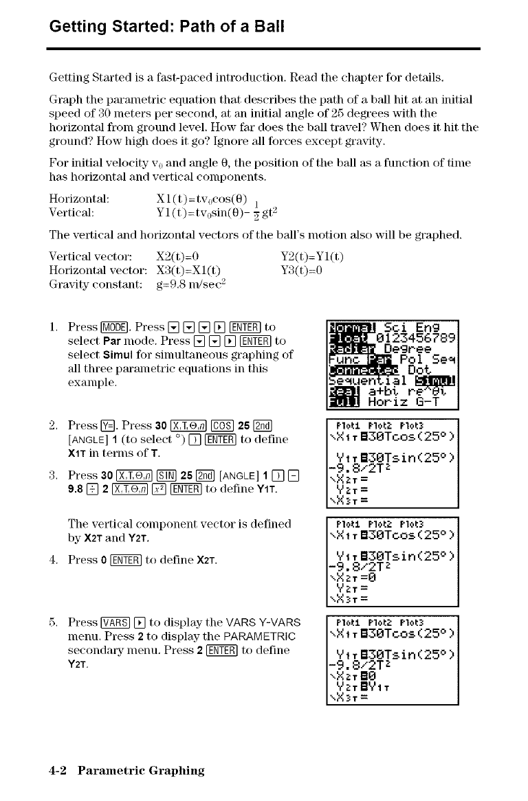
Getting Started: Path of a Ball
Getting Started is a fast-paced introduction. Read the chapter for details.
Graph the parametric equation that describes the path of a ball hit at an initial
speed of 30 meters per second, at an initial angle of 25 degrees with the
horizontal from ground level. How fat" does the ball travel? When does it hit the
ground? How high does it go? Ignore all forces except gravity.
For initial velocity v0 and angle 0, the position of the ball as a function of time
has horizontal and vertical components.
Horizontal: X1 (t)=tv0cos(0) 1 ,
Vertical: Y1 (t)=tv0sin(0)- g gt 2
The vertical and horizontal vectors of the bali's motion also will be graphed.
Vertical vector: X2(t)=0 Y2(t)=Yl(t)
Horizontal vector: X3(t)=Xl(t) Y3(t)=0
Gravity constant: g=9,8 m/see 2
Press [_3_. Press [] [] [] [] [_ to
select Par mode. Press [] [] [] [_ to
select 8imul R)r sinmltaneous graphing of
all three parametric equations in this
example.
Press @. Press 30 _ [_ 26 [_
[ANGLE] I (to select °) [] [_ to define
XITin terms of T.
Press 30 _ _ 28 [_ [ANGLE]1 [] []
9.8 [] 2 _ [] _ to define YIT.
The vertical component vector is defined
by X2Tand Y2T.
4. Press 0[ggY_ to define X2T.
Press [_ [] to display the VARS Y-VARS
menu, Press 2to display the PARAMETRIC
secondmT nlenu, Press 2 [gN?_7to define
Y2T,
4-2 Parametric Graphing
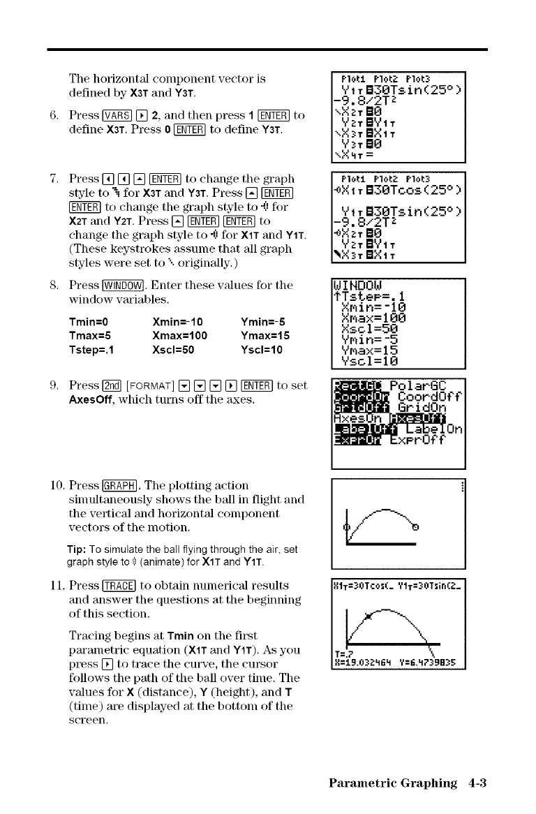
The horizontal component vector is
defined by X3Tand Y3T,
Press [gAg_ [] 2, and then press 1[gNTgglto
define X3T.Press 0 [gNT_ to define Y3T.
Press [] [] [] _ to change the graph
style to 5 for X3Tand Y3T. Press [] [gNY_
[gNT_ to change the graph style to .41!for
X2Tand Y2T. Press [] [gNY_ [gNT_ to
change the graph style to "0for XlT and Y1T.
(These keystrokes _tssume that all graph
styles were set to "..originally.)
Press _. Enter these values for the
window variables.
Tmin=0 Xmin=-10 Ymin=-5
Tmax=5 Xmax=100 Ymax=15
Tstep=,l Xscl=50 Yscl=10
Press [g_ [FORMAT] [] [] [] [] F_ to set
AxesOff, which turns off the axes.
PI,:,I:t PI,:,L> PlOI:3
91T B30Tsin (25 ° )
-9.8/2TZ
xXzT Be
VaT B'¢1T
",X_T BX1T
V St 1_10
\X_T =
Plo_t PloLZ Plot3
_XITB30Tcos(25 ° )
YITB30Tsin(25 ° )
-9.8/2TZ
_XZT B0
YZT BYI T
_T _1 T
WINDOW
STsteP=,l
XMin=-lO
gMax=100
Xscl=50
Vmin=-5
Vmax=15
Vsol=lO
PolarGC
CoordO££
GridOn
xPrO_£
10. Press _. The plotting action
sinmltaneously shows the ball in flight and
the vertical and horizontal component
vectors of the motion.
Tip: To simulate the ball flying through the air, set
graph style to _)(animate) for XIT and YIT.
11. Press _ to obtain numerical results
and answer the questions at the beginning
of this section.
Tracing begins at Tmin on the first
pm'ametric equation (X1Tand Y1T), As you
press [] to trace the curve, the cursor
follows the path of the ball over time. The
values for X (distance), Y (height), and T
(time) are displayed at the bottom of the
screen.
/---_,.
glT=3OTcg¢_;(_ Y1T=30TSin(_:_
Parametric Graphing 4-3
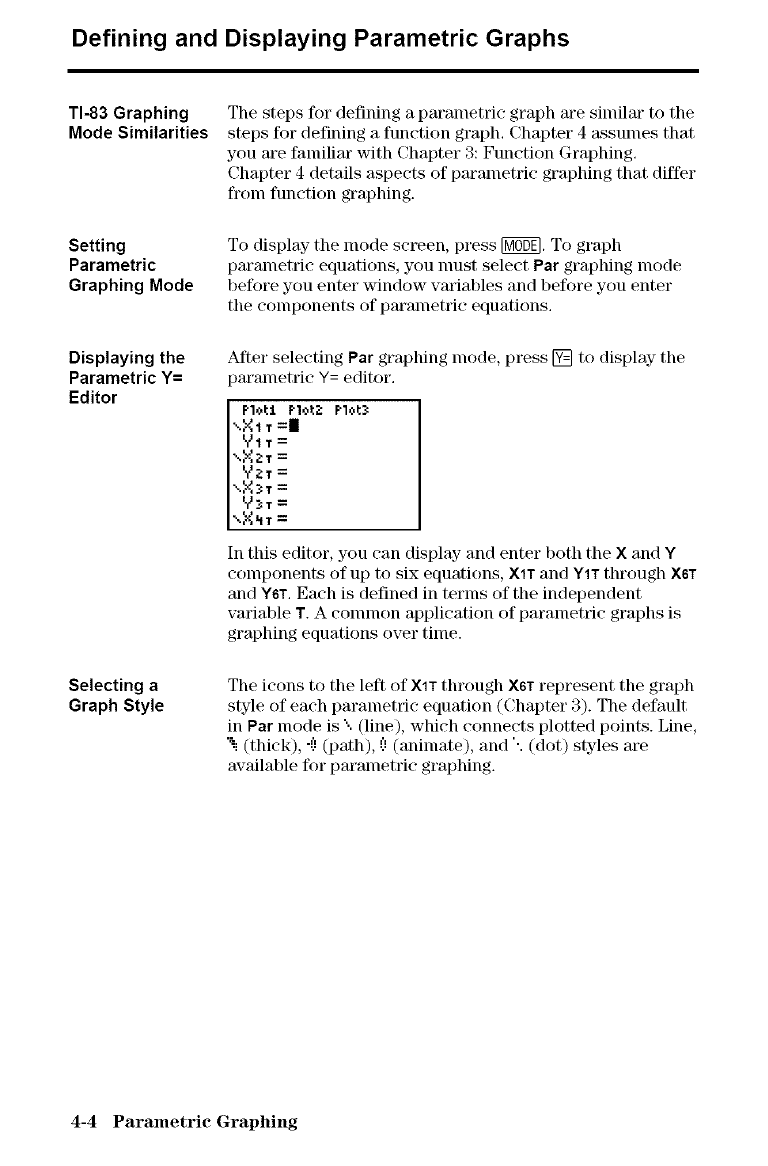
Defining and Displaying Parametric Graphs
TI-83 Graphing
Mode Similarities
Setting
Parametric
Graphing Mode
Displaying the
Parametric Y=
Editor
Selecting a
Graph Style
The steps for defining a parametric graph are similar to the
steps for defining a function graph. Chapter 4 assumes that
you are familiar with Chapter 3: Function Graphing.
Chapter 4 details aspects of parametric graphing that differ
from function graphing.
To display- the mode screen, press NgffE].To graph
parametric equations, you nmst select Par graphing mode
before you enter window wu'iables and before you enter
tile components of parametric equations.
After selecting Par graphing mode, press [] to display the
_arametric Y= editor.
P10L1 Plo_:2 Plot3
_.X1T=11
YtT----
,,X;_T=
'y';_V=
\X_T=
y__T=
In this editor, you can display and enter both the Xand Y
conlponents of up to six equations, X1T and Y1T through X6T
and YST. Each is defined in terms of the independent
variable T. A common application of parametric graphs is
graphing equations over time.
The icons to the left of XIT through X6Trepresent the graph
style of each parametric equation (Chapter 3). The default
in Par mode is "..(line), which connects plotted points. Line,
'_i (thick),-(! (path), (!(animate), and ". (dot) styles are
available for parametric graphing.
4-4 Parametric Graphing
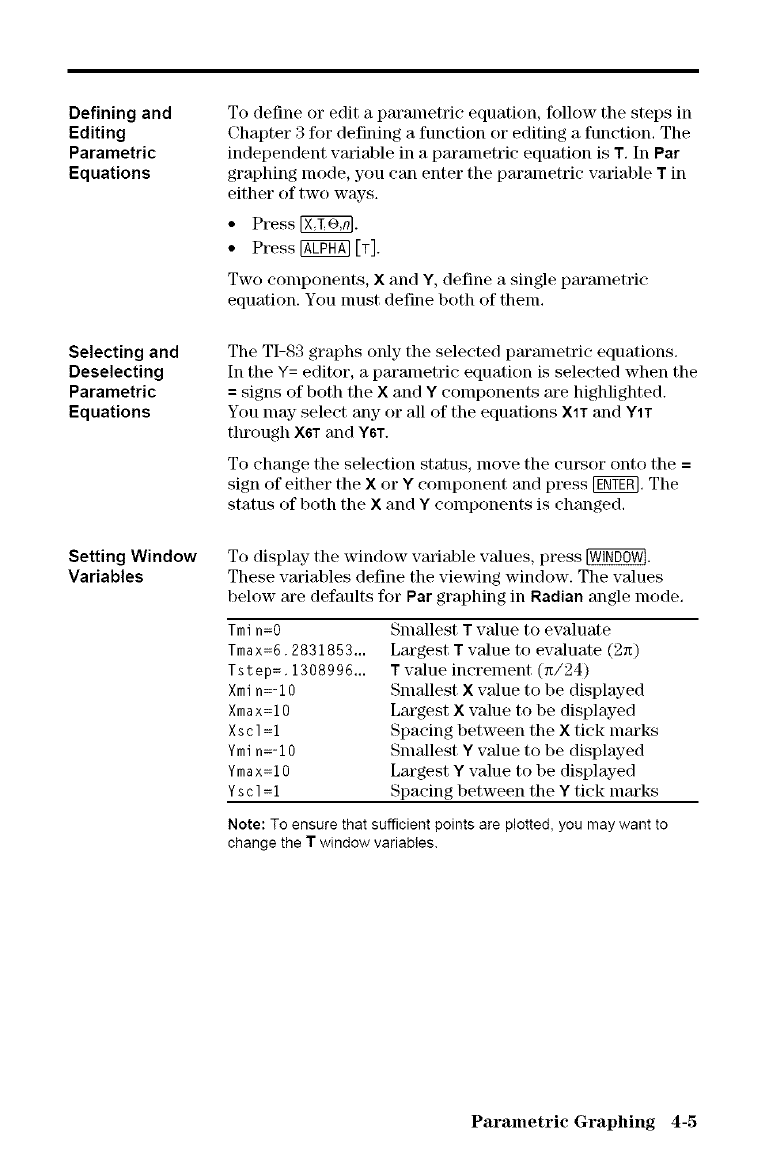
Defining and
Editing
Parametric
Equations
Selecting and
Deselecting
Parametric
Equations
Setting Window
Variables
To define or edit a parametric equation, follow the steps in
Chapter 3 for defining a function or editing a function. The
independent variable in a paralnetrie equation is T. In Par
graphing mode, you can enter the paralnetric variable Tin
either of two ways.
• Press _.
• Press@ [T].
Two components, Xand Y, define a single parametric
equation. You nmst define both of them.
The TI-83 graphs only the selected parametric equations.
In the Y= editor, a parametric equation is selected when the
= signs of both the Xand Y components are highlighted.
You may select any or all of the equations XIT and YIT
through X6T and Y6T.
To change the selection status, move the cursor onto the =
sign of either the Xor Y colnponent and press [gNYE_. The
status of both the Xand Y components is changed.
To display" the window variable values, press _.
These vmiables define the viewing window. The values
below are defaults for Par graphing in Radian angle mode.
Tmin=O
Tmax=6.2831853,..
Tstep=.1308996...
Xmin=-10
Xmax=10
Xscl=1
Ymin=-10
Ymax=10
Yscl=1
Smallest Tv'Mue to evaluate
Largest Tvalue to evaluate (2x)
T value increment (x/24)
SmMlest X vMue to be displayed
Largest X value to be displayed
Spacing between the X tick nlarks
SmMlest Y vMue to be displayed
Largest Y value to be displayed
Spacing between the Y tick marks
Note: To ensure that sufficient points are plotted, you may want to
change the T window variables.
Parametric Graphing 4-5
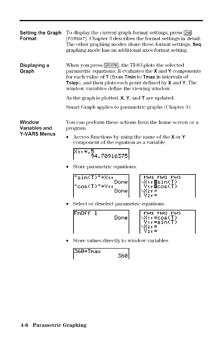
Setting the Graph
Format
Displaying a
Graph
To display- the current graph format settings, press [_
[FORMAT], Chapter 3 describes the format settings in detail,
The other graphing modes share these format settings; $eq
graphing mode has an additional axes format setting,
When you press _, the TI-83 plots the selected
parametric equations, It evaluates the Xand Ycomponents
for each value ofT (fronl Tmin to Tmax in intel_'als of
Tstep), and then plots each point defined by X and Y. The
window vm'iables define the viewing window.
As the graph is plotted, X, Y, and T m'e updated.
Snlart Graph applies to parametric graphs (Chapter 3).
Window
Variables and
Y-VARS Menus
You can perform these actions fronl the home screen or a
program.
• Access functions by using the name of the X or Y
component of the equation as a vm'iable.
*.5 -,
NiT 94. r0916375
• Store parametric equations.
"cos(T) "÷Yi"sin(T) "÷Xl TD°neTDone \XzT="XlTBsin(T)yzT=Vin°tITBcos(T)nOtznots I
• Select or deselect parametric equations,
FR0t'f" 1 Done Pl0tl ,otz ,,t, I
",XlT =cos(T)
YiT=sin(T) I
xXzT=
YZT=
• Store values directly to window variables.
360÷Tnax 360
4-6 Parametric Graphing
Exploring Parametric Graphs
Free-Moving
Cursor
TRACE
The free-lnoving cursor in Par graphing works the salne as
in Func graphing.
In RectGC format, nloving the cursor updates the values of
Xand Y; if CoordOn format is selected, Xand Y are
displayed.
In PolarGC format, X, Y, R, and 0 are updated; if CoordOn
format is selected, R and 0 m'e displayed.
To activate TRACE, press _. When TRACE is active,
you can nlove the trace cursor along the graph of the
equation one Tstep at a time. When you begin a trace, the
trace cursor is on the first selected function at Train. If
ExprOn is selected, then the function is displayed.
In RectGC format, TRACE updates and displays the vMues
of X, Y, and T if CoordOn format is on.
In PolarGC format, X, Y, R, 0 and Tare updated; if CoordOn
format is selected, R, 0, and T are displayed. The X and Y
(or Rand 0) values are calculated from T.
To nlove five plotted points at a time on a function, press
[] or [2ffd][_. If you nlove the cursor beyond the top or
bottom of the screen, the coordinate values at the bottom
of the screen continue to change appropriately.
Quick Zoom is available in Par graphing; panning is not
(Chapter 3).
Parametric Graphing 4-7
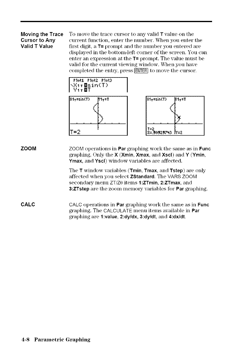
Moving the Trace
Cursor to Any
Valid TValue
To move the trace cursor to any valid T value on the
current function, enter the number, When you enter the
first digit, a T= prompt and the number you entered are
displayed in the bottom-left corner of the screen. You can
enter an expression at the T= prompt, The wdue nmst be
valid for the current _ewing window, When you have
colnpleted the ent_% press [K_Y_ to lnove the cursor.
PIoI:I PloL2 Plot_
_.X1 T_sir,(T)
YtT_T
XIT=_;ifl(T) _,Ii T=T
}
T=2
XIT=S;n(T) _IT=T
(
T=;_
ZOOM ZOOM operations in Par graphing work the same as in Func
graphing. Only the X (Xmin, Xmax, and Xscl) and Y (Ymin,
Ymax, and Yscl) window vm'iables are affected.
The T window vm'iables (Train, Tmax, and Tstep) are only-
'affected when you select ZStandard. The MARS ZOOM
seeondm_y- menu ZT/Z0 items 1 :ZTmin, 2:ZTmax, and
3:XTstep are the zoom memory variables for Par graphing.
CALC CALC operations in Par graphing work the same as in Func
graphing. The CALCULATE menu items available in Par
graphing are 1:value, 2:dy/dx, 3:dy/dt, and 4:dx/dt.
4-8 Parametric Graphing
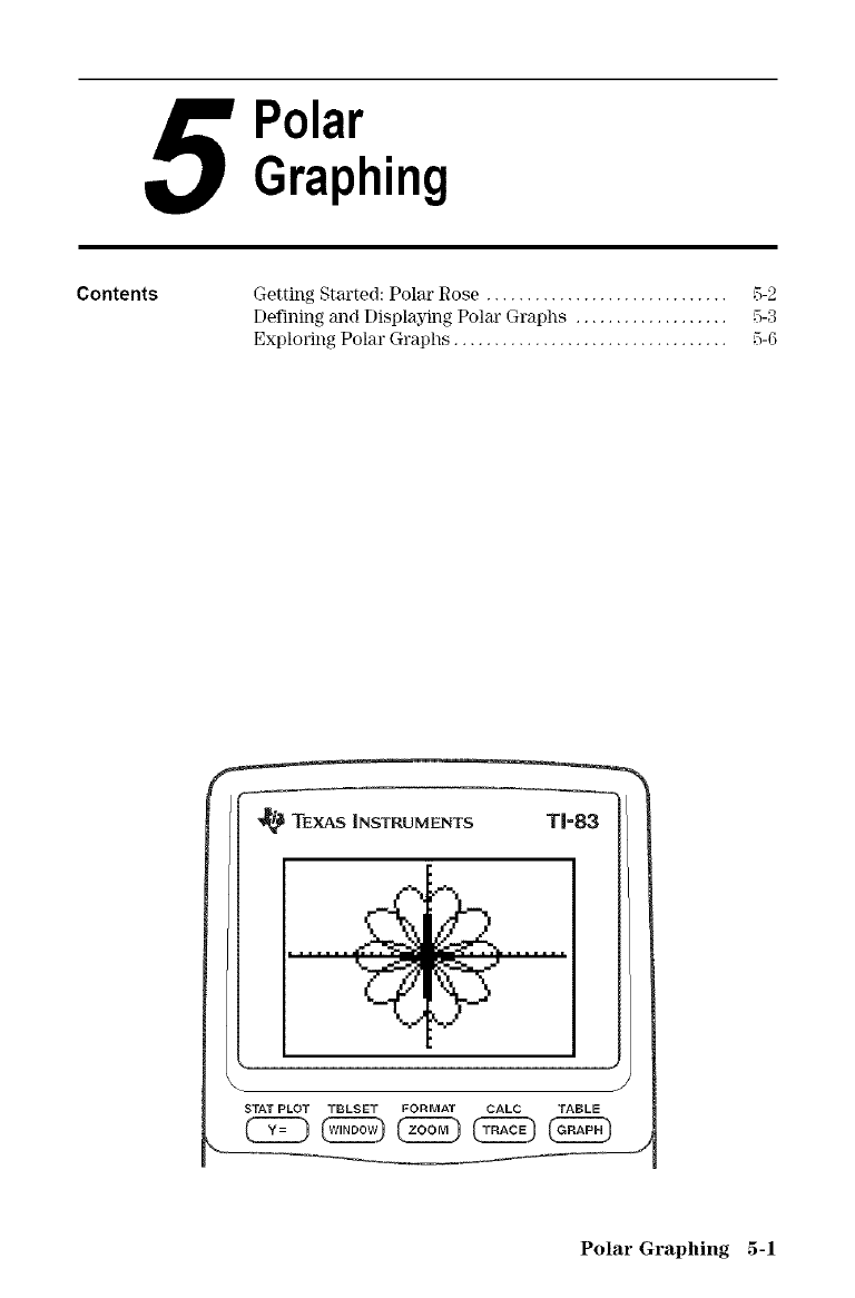
Polar
Graphing
Contents Getting Started: Polar Rose .............................. 5-2
Defining and Displaying Polar Graphs ................... 5-3
Exploring Polar Graphs .................................. 5-6
TEXAS INSTRUMENTS T1=83
J
STAT PLOT TBLSET FORMAT CALC TABLE
Polar Graphing 5-1
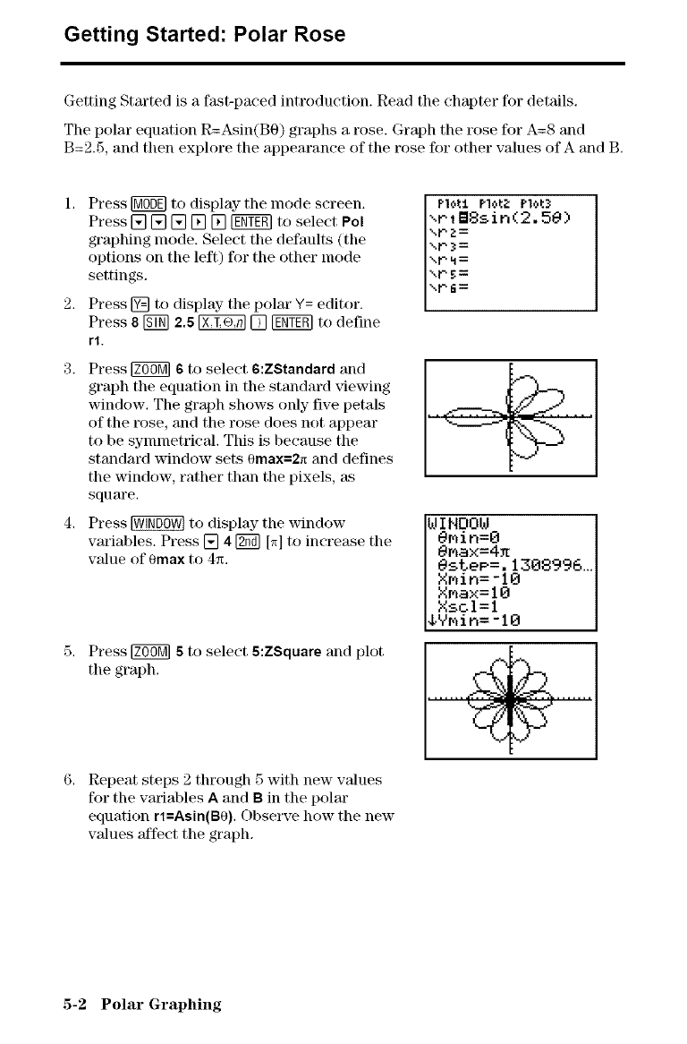
Getting Started: Polar Rose
Getting Started is a fast-paced introduction. Read the chapter for details.
The polar equation R=Asin(B0) graphs a rose. Graph the rose for A=8 and
B=2.5, and then explore the appearance of the rose for other values of A and B.
Press _ to display the mode screen.
Press [] [] [] [] [] [gfff_] to select Pol
graphing mode. Select the defaults (the
options on tile left) for the other nlode
settings.
Press [] to display- the polar Y= editor.
Press 8NTN2.6 _ [] [g_gO to define
rl.
3. Press _ 6 to select 6:ZStandard and
graph the equation in the standard viewing
window. The graph shows only five petals
of the rose, and the rose does not appear
to be synunetrical. This is because the
standard window sets 0max=2= and defines
the window, rather than the pixels, as
square.
4. Press _ to display the window
variables. Press [] 4[gfi_ [_] to increase the
value of 0max to 4x.
5, Press _ 5to select 5:ZSquare and plot
the graph.
Repeat steps 2 through 5 with new values
for the variables Aand Bin the polar
equation rl=Asin(B0). Observe how the new
values 'affect the graph.
Plot:t Plot2 Plot3
_rl B8sin(2.50)
\r_:=
i_.r_ =
%rfi=
WINDOW
Omin=O
OMaX=4X
Ostee=,1308996...
XMin=-lO
Xmax=lO
XSCI=I
_VMin=-lO
5-2 Polar Graphing
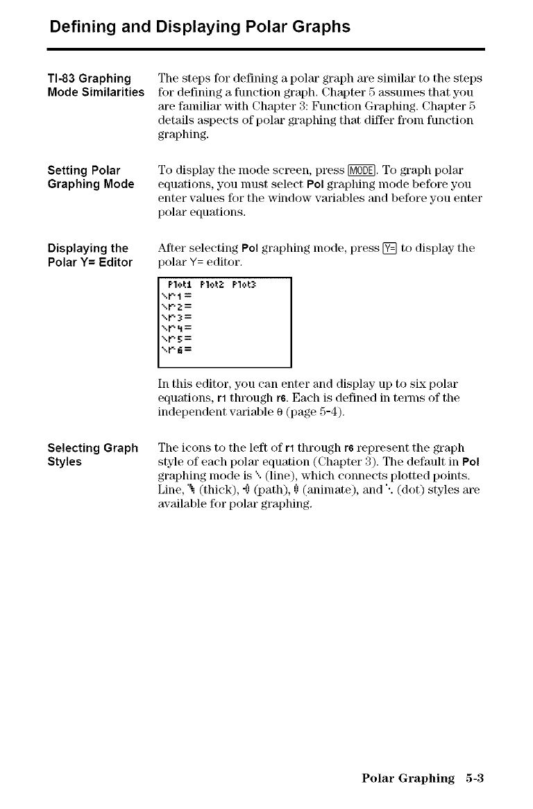
Defining and Displaying Polar Graphs
TI-83 Graphing
Mode Similarities
Setting Polar
Graphing Mode
Displaying the
Polar Y= Editor
Selecting Graph
Styles
The steps for defining a polar graph are similar to the steps
for defining a function graph. Chapter 5 assumes that you
are familiar with Chapter 3: Function Graphing. Chapter 5
details aspects of polar graphing that differ from function
graphing.
To display- the mode screen, press [M6_]. To graph polar
equations, you nmst select Pol graphing mode before you
enter values for the window variables and before you enter
polar equations.
After selecting Pol graphing mode, press [] to display- the
_olar Y= editor.
PI,:,I:I PloL2 Plot3
\rl=
\i-- 2----
M-_3:=
\1,-,tl =
\1.'. _ =
\p6=
In this editor, you can enter and display up to six polar
equations, rl through r6. Each is defined in terms of the
independent variable 0 (page 5-4).
The icons to the left of rl through r6 represent the graph
style of each polar equation (Chapter 3). The default in Pol
graphing mode is "..(line), which connects plotted points.
Line, "i (thick), -(! (path), (! (animate), and ". (dot) styles are
available for polar graphing.
Polar Graphing 5-3
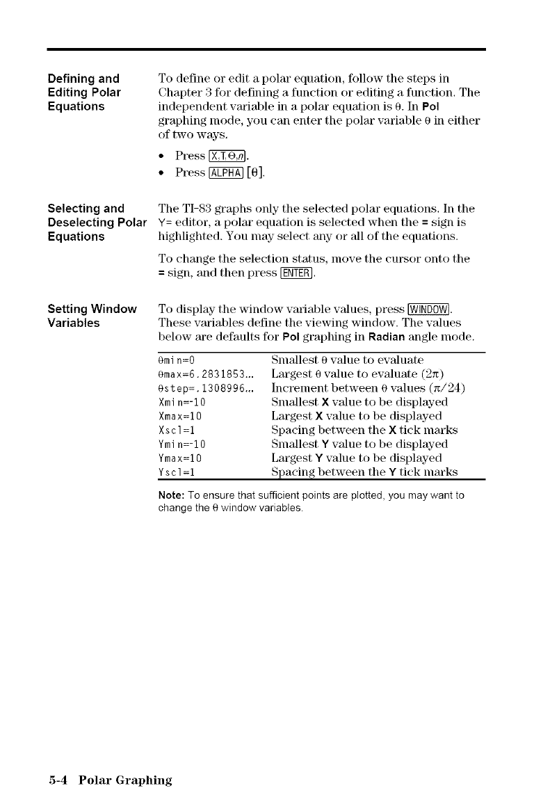
Defining and
Editing Polar
Equations
Selecting and
Deselecting Polar
Equations
Setting Window
Variables
To define or edit a polar equation, follow the steps in
Chapter 3 for defining a function or editing a function. The
independent vm'iable in a polar equation is 0. In Pol
graphing mode, you can enter the polar variable 0 in either
of two ways.
• Press _.
• Press@ [0].
The TI-83 graphs only the selected polar equations. In the
Y= editor, a polar equation is selected when the =sign is
highlighted. You nlay select any- or M1of the equations.
To change the selection status, nlove the cursor onto the
= sign, and then press [_.
To display- the window variable values, press _.
These variables define the viewing window. The values
below are defaults for Pol graphing in Radian angle mode.
Omin=O
Omax=6.2831853,..
Ostep=.1308996...
Xmin=-10
Xmax=10
Xscl=1
Ymin=-10
Ymax=10
Yscl=1
SmMlest 0 value to evMuate
Largest 0 vMue to evaluate (2=)
Increment between @values (=/24)
SmMlest X vMue to be displayed
Largest X value to be displayed
Spacing between the X tick marks
SmMlest Y value to be displayed
Largest Y value to be displayed
Spacing between the Y tick marks
Note: To ensure that sufficient points are plotted, you may want to
change the 0 window variables.
5-4 Polar Graphing
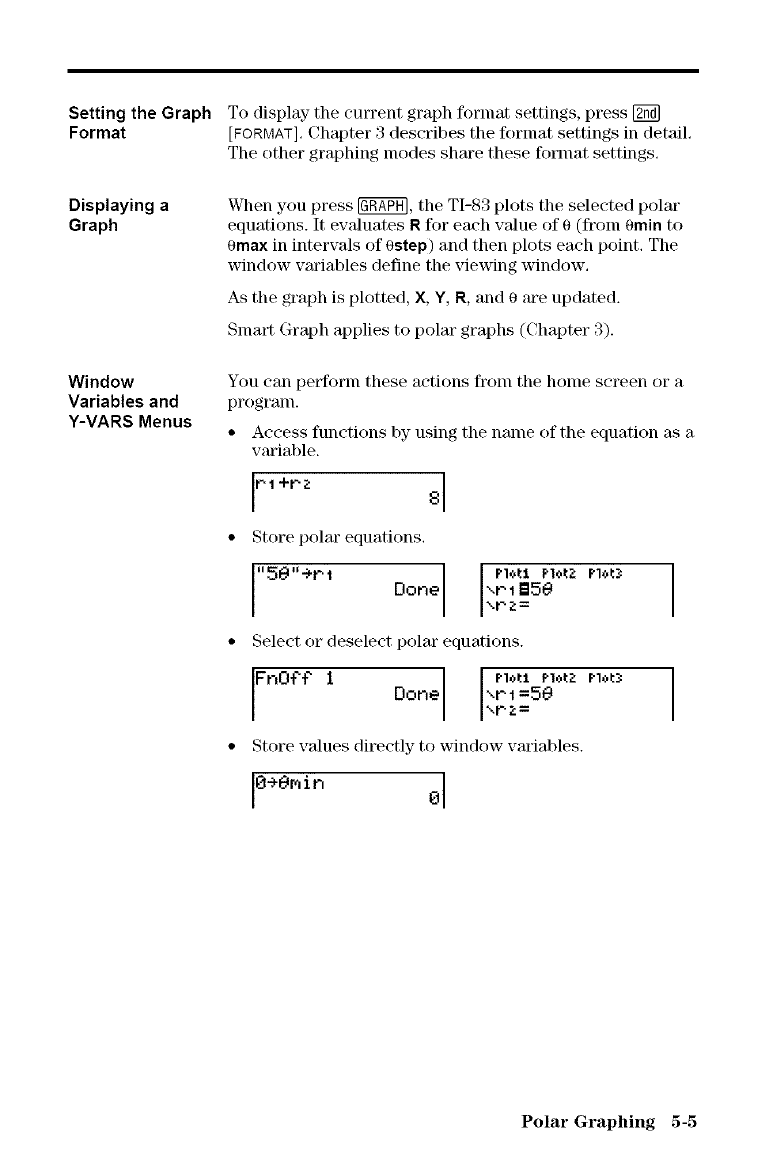
Setting the Graph
Format
Displaying a
Graph
Window
Variables and
Y-VARS Menus
To display the current graph format settings, press [2_]
[FORMAT].Chapter 3 describes the forlnat settings in detail.
The other graphing lnodes share these format settings.
When you press _, the TI-83 plots the selected polar
equations. It evMuates R for each value of 0 (from 0min to
0max in intervals of 0step) and then plots each point. The
window variables define the viewing window.
As the graph is plotted, X, Y, R, and 0 are updated.
Slnart Graph applies to polm" graphs (Chapter 3).
You can perfornl these actions fronl the honle screen or a
program.
• Access functions by using the name of the equation as a
wuiable
rl +r.z 8
• Store polar equations,
"51_1"÷1"i Done \r?:=\rll_5OPl°tlP10t_: Plot3 I
• Select or deselect polar equations.
FnOff 1 Done Plott PIotZ Plot_ I
xr I=50 I
• Store values directly to window variables.
IO+Orqih OI
Polar Graphing 5-5
Exploring Polar Graphs
Free-Moving
Cursor
TRACE
Moving the Trace
Cursor to Any
Valid e Value
ZOOM
CALC
The ffee-mo_ing cursor in Pol graphing works the same as
in Func graphing. In RectGC fonnat, moving tile cursor
updates the values of Xand Y; if CoordOn format is
selected, Xand Y are displayed. In PolarGC format, X, Y, R,
and 0 are updated; if CoordOn format is selected, Rand 0
m'e displayed.
To activate TRACE, press _. When TRACE is active,
you can nlove the trace cursor along the graph of the
equation one 0step at a time. When you begin a trace, tile
trace cursor is on the first selected function at 0min. If
ExprOn fornlat is selected, then the equation is displayed.
In RectGC format, TRACE updates the values of X, Y, and 0;
if CoordOn format is selected, X, Y, and 0 are displayed. In
PolarGC format, TRACE updates X, Y, R, and 0; if CoordOn
format is selected, Rand 0 m'e displayed.
To nlove five plotted points at a time on a function, press
Kffa][] or Kffa][Z]. If you move tile trace cursor beyond tile
top or bottonl of the selden, the coordinate values at the
bottonl of the screen continue to change appropriately.
Quick Zoom is available in Pol graphing mode; panning is
not (Chapter 3).
To nlove the trace cursor to any valid 0 value on the
current function, enter the number. When you enter the
first digit, a 0= prompt and the number you entered are
displayed in tile bottom-left corner of tile screen. You can
enter an expression at the 0= prompt. The value must be
valid for the current viewing window. When you complete
tile enhT, press _ to nlove the cursor.
ZOOM operations in Pol graphing work the same as in Func
graphing. Only the X(Xmin, Xmax, and Xscl) and Y (Ymin,
Ymax, and Yscl) window variables are affected.
The 0 window variables (0rain, 0max, and Ostep) are not
'affected, except when you select ZStandard. The VARS
ZOOM seeondmTy- menu ZT/ZO items 4:Z0min, 5:Z0max, and
6:Z0step m'e zoom nlemoKy-varialfles ff_r Pol graphing.
CALC operations in Pol graphing work the sanle as in Func
graphing. The CALCULATE nlenu items available in Pol
graphing are 1:value, 2:dy/dx, and 3:dr/d0.
5-6 Polar Graphing
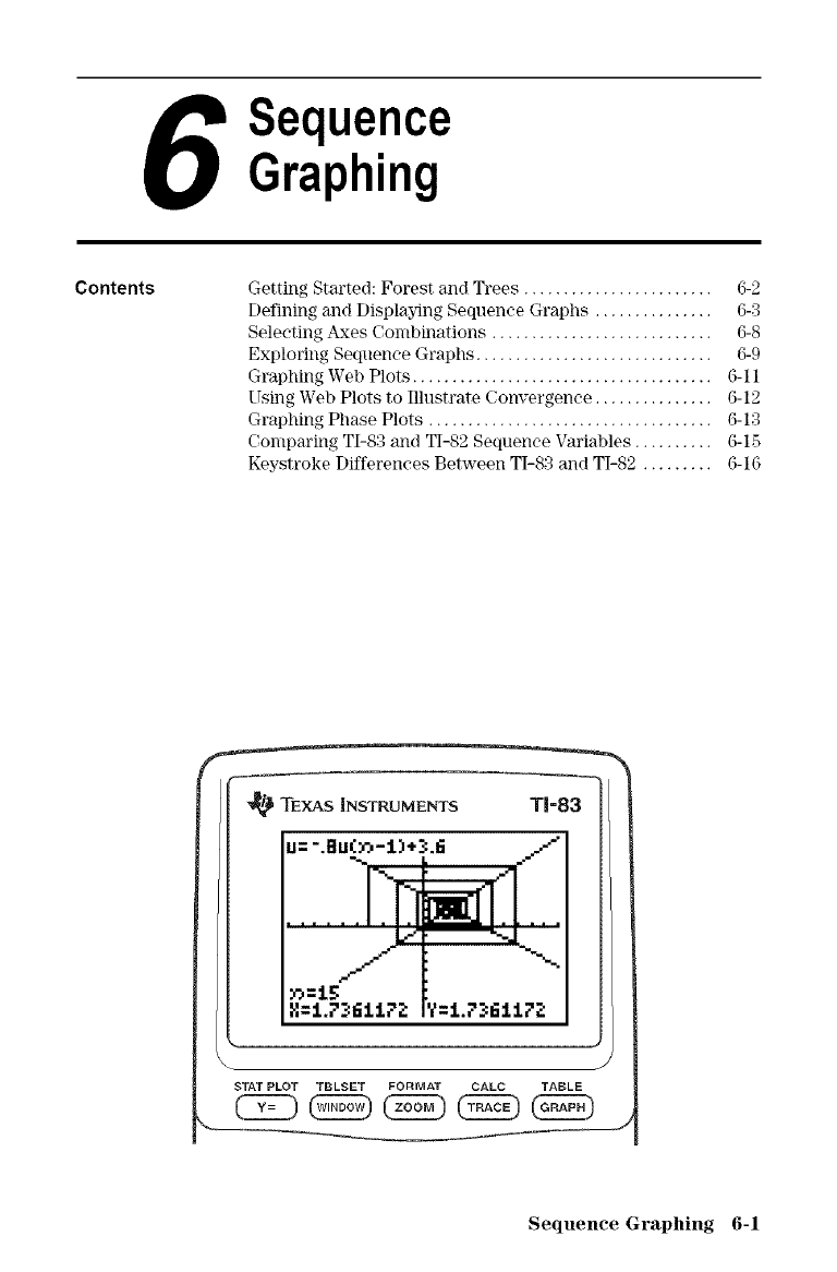
Sequence
Graphing
Contents Getting Started: Forest and Trees ........................ 6-2
Defining and Displaying Sequence Graphs ............... 6-3
Selecting Axes ('ombinations ............................ 6-8
Exploring Sequence Graphs .............................. 6-9
Graphing Web Plots ...................................... 6-11
Using Web Plots to Illustrate Convergence ............... 6-12
Graphing Phase Plots .................................... 6-13
Comparing TI-83 and TI-82 Sequence Variables .......... 6-1.5
Keystroke Differences Between TI-83 and TI-82 ......... 6-16
'_ TEXAS iNSTRUMENTS T1=83
u= -.Bu(7_-:1.)+3.6
-,_ I=
-% l
........ ....
>'_=:L5 I' "_ "%_
X=l.F_61172 i'=1._ _:61172
J
STATPLOT TBLSET FORMAT CALC TABLE
Sequence Graphing 6-1
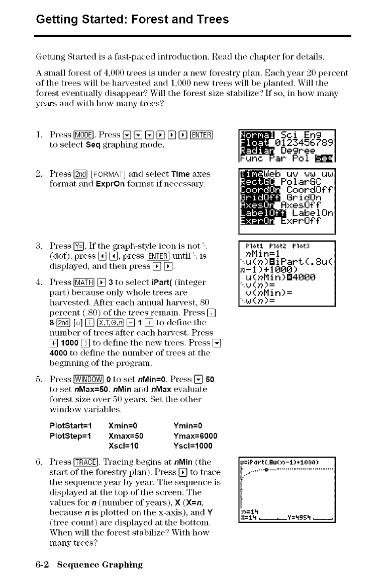
Getting Started: Forest and Trees
Getting Started is a fast-paced introduction. Read the chapter for details.
A small forest of 4,0!)0 trees is under a new forestw plan. Each year 20 percent
of the trees will be hmwested and 1,000 new trees will be planted. Will the
forest eventually- disappear? Will the forest size stabilize? If so, in how many
yeat\_ and with how many trees?
Press IM65E].Press [] [] [] [] [] [] IgffTgR]
to select Seq graphing mode.
Press [_ [FORMAT] and select Timeaxes
format and ExprOnformat if neeessatT.
Soi Eng
0123456789
Degree
ar Pol
UM MW UW
PolaPGC
CoopdO_
GridOn
RxesO_
LabelOn
3. Press @. If the graph-style icon is not ".
(dot), press [] [], press [g_-gRquntil ". is
displayed, and then press [] [].
4. Press [_ [] ato select iPart( (integer
pro't) because only whole trees are
harvested. After each annual hatw'est, 80
percent (.80) of the trees remain. Press []
8[_ [u] [] _ [] 1 [] to define the
number of trees after each harvest. Press
[] 1000 [] to define the new trees. Press []
4000 to define the number of trees at the
beginning of the program.
5. Press [_ 0 to set nNin=0. Press [] 60
to set nNax=fi0, nNin and nMax evaluate
forest size over 50 years. Set the other
window variables.
PlotStart=l Xmin=0 Ymin=0
PlotStep=l Xmax=50 Ymax=6000
Xscl=10 Yscl=1000
Press _. Tracing begins at nMin (the
start of the foresttT plan). Press [] to trace
the sequence year by year. The sequence is
displayed at the top of the screen. The
values for n(number of years), X (X=n,
because nis plotted on the x-axis), and Y
(tree count) are displayed at the bottom.
When will the forest stabilize? With how
many trees?
PI_I PI_tZ Plot3
_Min=l
'..u(_bBiPart(.Bu(
_-I)+1000)
u(_Min)B4000
".v(_)=
v(_Min)=
".u(_)=
lu=iPart(.Bu(_-l)+lOO0) I
6-2 Sequence Graphing
Defining and Displaying Sequence Graphs
TI-83 Graphing
Mode Similarities
Setting Sequence
Graphing Mode
The steps for defining a sequence graph are similar to the
steps for defining a function graph. Chapter 6 assumes that
you are familiar with Chapter 3: Function Graphing.
Chapter 6 details aspects of sequence graphing that differ
froln function graphing.
To display- the mode screen, press [M6D_.To graph
sequence functions, you nmst select 8eq graphing mode
before you enter window wu'iables and before you enter
sequence functions.
Sequence graphs automatically plot in Simul mode,
regardless of the current plotting-order mode setting.
TI-83 Sequence
Functions u, v,
and w
The TI-83 has three sequence functions that you can enter
from the keyboard: u, v, and w. They are above the [7], [],
and [] keys.
You call define sequence functions in terms off
• The independent variable n
• The previous term in the sequence function, such as
u(n-1)
• The term that precedes tile previous term in tile
sequence function, such as u(n-2)
• The previous term or the term that precedes the
previous term in another sequence function, such as
u(n-1) or u(n-2) t_ferenced in the sequence v(n).
Note: Statements in this chapter about u(n) are also true for v(n) and
w(n); statements about u(n-1) are also true for v(n-1) and w(n-1);
statements about u(n-2) are also true for v(n-2) and w(n-2).
Sequence Graphing 6-3
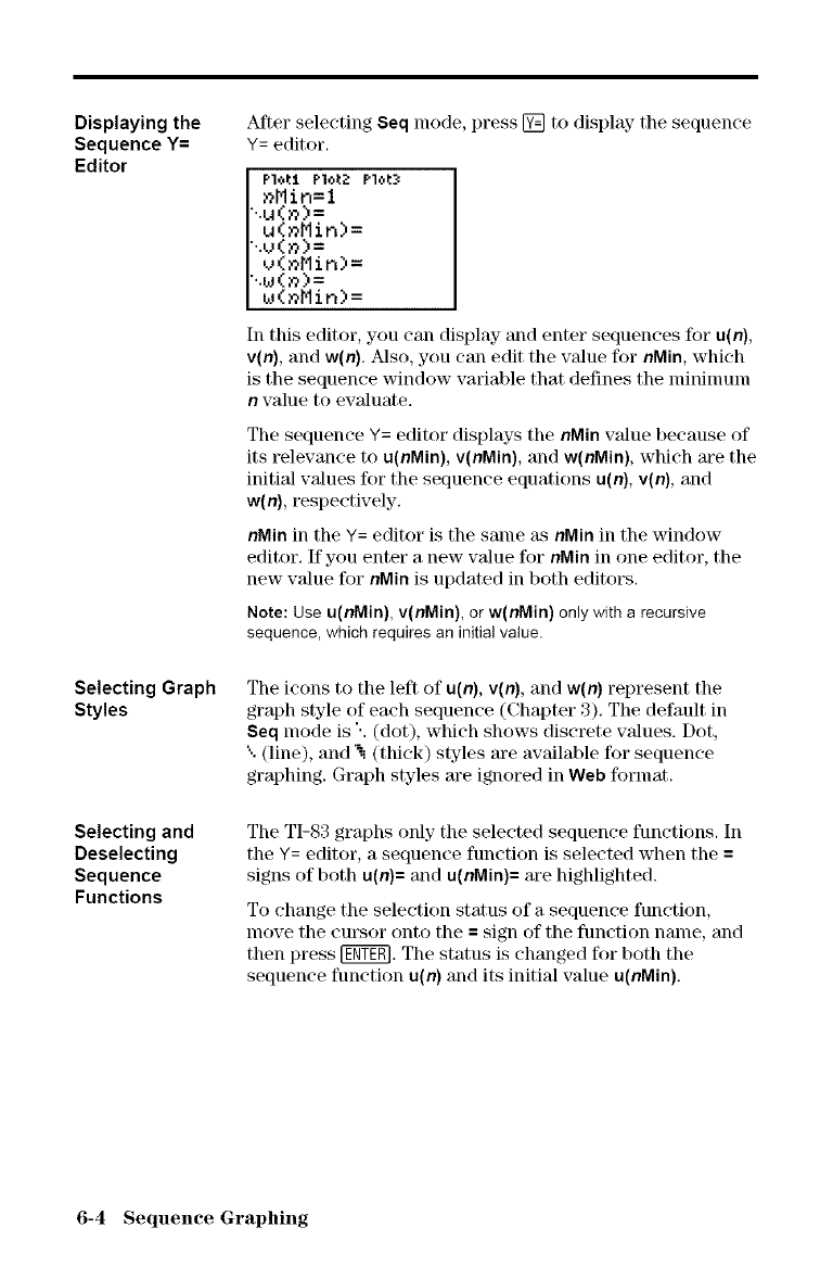
Displaying the
Sequence Y=
Editor
Selecting Graph
Styles
Selecting and
Deselecting
Sequence
Functions
After selecting Seq mode, press [] to display- the sequence
Y= editor.
nMin=l
",.u(n)=
u(nMin)=
"..v(n)=
v(nMin)=
"..u(n)=
u(nMin)=
In this editor, you can display and enter sequences for u(n),
v(n), and w(n), Also, you can edit the value for nMin, which
is the sequence window variable that defines the nlininluln
nvalue to evaluate.
The sequence Y= editor displays the nMin value because of
its relevance to u(nMin), v(nMin), and w(nMin), which are the
initial values for the sequence equations u(n), v(n), and
w(n), respectively.
nMin in the Y= editor is the same as nMin in the window
editor. If you enter a new value for nMin in one editor, the
new value for nMin is updated in both editors.
Note: Useu(nMin), v(nMin), or w(nMin) only with a recursive
sequence,whichrequires an initialvalue.
The icons to the left of u(n), v(n), and w(n) represent the
graph style of each sequence (Chapter 3). The default in
$eq mode is ". (dot), which shows discrete values. Dot,
"..(line), and "i (thick) styles m'e available for sequence
graphing. Graph styles m'e ignored in Web format.
The TI-83 graphs only the selected sequence functions. In
the Y= editor, a sequence function is selected when the =
signs of both u(n)= and u(nMin)= are highlighted.
To change the selection status of a sequence function,
move the cut\sor onto the = sign of the function name, and
then press [g_. The status is changed for both the
sequence function u{n) and its initial value u(nMin).
6-4 Sequence Graphing
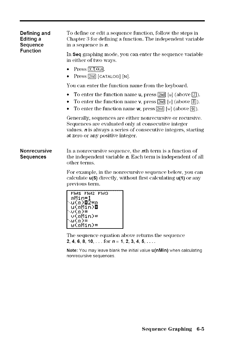
Defining and
Editing a
Sequence
Function
Nonrecursive
Sequences
To define or edit a sequence function, follow the steps in
Chapter 3 for defining a function. The independent vmiable
in a sequence is n.
In Seq graphing mode, you can enter the sequence vmiable
in either of two ways.
• Press _.
• Press [g67][CATALOG][N].
You can enter the function name from the keyboard.
• To enter the function name u, press [gh_][u] (above [_).
• To enter the function name v, press [g6_ [v] (above [_).
• To enter the function name w, press [g67][w] (above [_).
Generally, sequences are either nonrecursive or recursive.
Sequences are evaluated only at consecutive integer
values, nis always a series of consecutive integers, starting
at zero or any positive integer.
In a nonrecursive sequence, the nth term is a function of
the independent variable n. Each term is independent of all
other terms.
For example, in the nonrecursive sequence below, you can
calculate u(6) directly, without fit\_t calculating u(1) or any
%exdous terlll,
PloL1 PloL2 Plot3
_Hin=l
,.u(_)B2*n
u(_Min)B
"..v(_)=
v(_Min)=
"'.u(_)=
u(_Min)=
The sequence equation above returns the sequence
2, 4, 6, 8,10, . . . for n=1,2,3,4,5,....
Note: You may leave blank the initial value u(nMin) when calculating
nonrecursive sequences.
Sequence Graphing 6-5
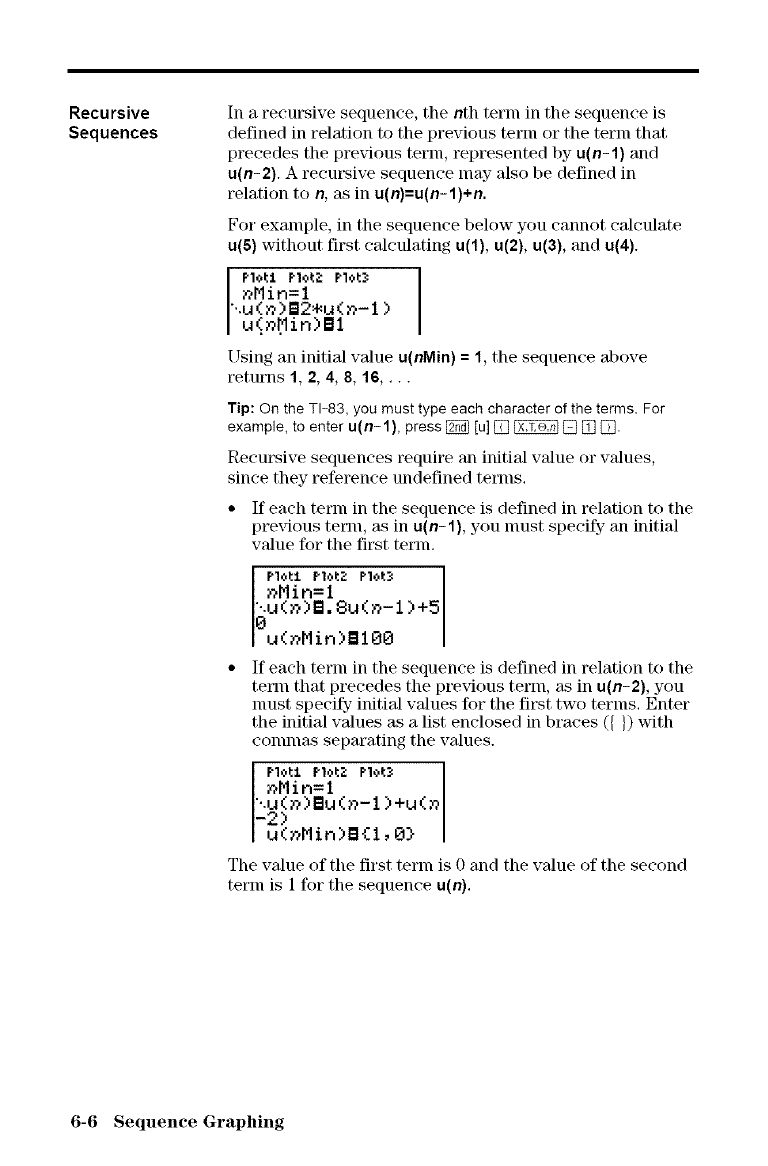
Recurslve
Sequences
In a reem\Mve sequence, the nth term in the sequence is
defined in relation to the previous term or the term that
precedes the previous term, represented by u(n-1) and
u(n-2). A reem\Mve sequence may also be defined in
relation to n, as in u(n)=u(n- 1)+n.
For example, in the sequence below you cannot calculate
u(5) without first calculating u(1), u(2), u(3), and u(4).
plo1:1 PloL2 pl,:a:_: I
_Min=l I
"..u(_)B2*u(n-1 )
u(.n[_in)B1
Using an initial value u(nMin) = 1, the sequence above
returns 1, 2, 4, 8, 16,...
Tip: On the TI-83, you must type each character of the terms. For
example, to enter u(n-1), press _ [u] [] _ [] [] lB.
Recursive sequences require an initial value or values,
since they reference undefined terms.
• If each term in the sequence is defined in relation to the
pre_dous term, as in u(n-1), you nmst specify an initial
value for the first tenn.
PloLi plol:._ Plot3
nMin=l
..u (n) B. 8u (n- 1 )+5
0
u(nMin)B100
If each term in the sequence is defined in relation to the
term that precedes the previous term, as in u(n-2), you
nmst specify- initial values for the first two terms. Enter
the initial values as a list enclosed in braees ({ }) with
commas separating the values.
Plot't PloI:2 Plot3
nMin=l
I..u(n)Bu(n-1 )+u(n
-2) }[ u(r_Min)B{l,O
The value of the first term is 0 and the value of the second
term is 1 for the sequence u(n).
6-6 Sequence Graphing
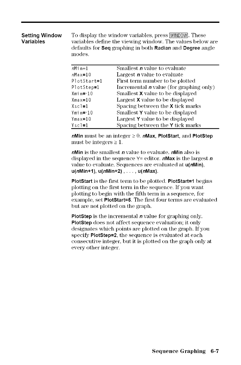
Setting Window
Variables To display- the window variables, press _, These
variables define the viewing window. The values below are
defaults for Seq graphing in both Radian and Degree angle
nlodes,
nMin=1
nMax:10
PlotStart:1
PlotStepffil
Xmin:-10
Xmax=lO
Xscl=l
Ymin=-lO
Ymax=lO
Yscl=l
Smallest nvalue to ev'gduate
Largest nvalue to evaluate
First term number to be plotted
Incremental nvalue (for graphing only)
Smallest X value to be displayed
Largest X value to be displayed
Spacing between the X tick marks
Smallest Y value to be displayed
Largest Y value to be displayed
Spacing between the Y tick marks
nMin must be an integer k O, nMax, PlotStart, and PlotStep
nmst be integers _>1,
nMin is the smallest nwdue to evaluate, nMin also is
displayed in the sequence Y= editor, nMax is the largest n
value to evaluate. Sequences are evaluated at u(nMin),
u(nMin+l), u(nMin+2), ... ,u(nMax).
PlotStart is the first term to be plotted. PlotStart=l begins
plotting on tile first term in tile sequence. If you want
ph)tting to begin with the fifth term in a sequence, for
exalnple, set PlotStart=& The first four terms are evaluated
but are not plotted on the graph.
PlotStep is the incremental nwdue for graphing only.
PlotStep does not 'affect sequence evaluation; it only
designates which points are plotted on the graph. If you
specify PlotStep=2, the sequence is ewduated at each
consecutive integer, but it is plotted on the graph only at
evew other integer.
Sequence Graphing 6-7
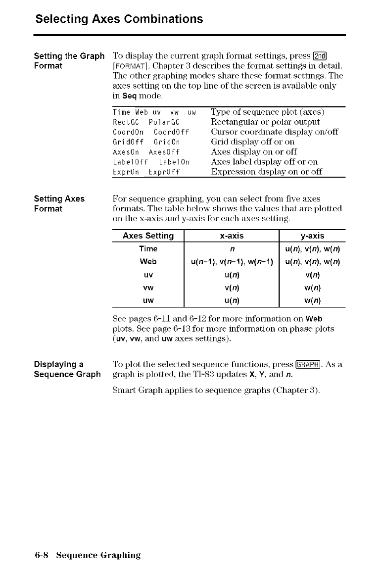
Selecting Axes Combinations
Setting the Graph
Format
Setting Axes
Format
Displaying a
Sequence Graph
To display- the current graph format settings, press [_
[FORMAT], Chapter 3 describes the format settings in detail,
The other graphing modes share these format settings, The
m,ces setting on the top line of the screen is available only
in Seq mode,
Time Web uv vw uw
RectGC PolarGC
CoordOn CoordOff
GridOff GridOn
AxesOn AxesOff
LabelOff LabelOn
ExprOn ExprOff
Type of sequence plot (m,ces)
Rectangular or polar output
Cursor coordinate display mdoff
Grid display off or on
Axes display on or off
Axes label display- off or on
Expression display on or off
For sequence graphing, you can select fronl five axes
formats. The table below shows the values that are plotted
on the x-axis and y-m'ds for each axes setting.
Axes Setting
Time
Web
uv
vw
uw
x-axis
n
u(n-1), v(n-1),w(n-1)
u(n)
v(n)
u(n)
y-axis
u(n), v(n),w(n)
u(n), v(n),w(n)
v(n)
w(n)
w(n)
See pages 6-11 and 6-12 for nlore information on Web
plots. See page 6-13 for more information on phase plots
(uv, vw, and uw m,ces settings).
To plot the selected sequence functions, press _. As a
graph is plotted, the TI-83 updates X, Y, and n.
Snlart Graph applies to sequence graphs (Chapter 3).
6-8 Sequence Graphing
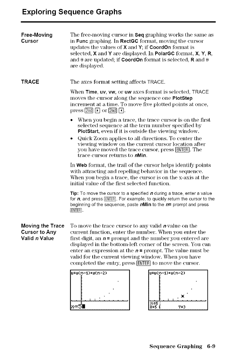
Exploring Sequence Graphs
Free-Moving
Cursor
TRACE
Moving the Trace
Cursor to Any
Valid nValue
The free-moving cursor in Seq graphing works the same as
in Func graphing. In RectGC fonnat, nloving tile cursor
updates the values of Xand Y; if CoordOn format is
selected, Xand Yare displayed. In PolarGC fornlat, X, Y, R,
and 0 are updated; if CoordOn format is selected, R and 0
m'e displayed.
The axes fornlat setting affects TRACE.
When Time, uv, vw, or uw axes format is selected, TRACE
moves the cursor along the sequence one PlotStep
increment at a time. To nlove five plotted points at once,
press [_ [] or [_ [].
• When you begin a trace, the trace cursor is on the first
selected sequence at the term number specified by
PlotStart, even if it is outside the viewing window.
• Quick Zoom applies to all directions. To center the
viewing window on the current cursor location after
you have moved the trace cursor, press [_. The
trace cursor t_tun_s to nMin.
In Web format, the trail of the cursor helps identify points
with attracting and repelling behavior in the sequence.
When you begin a trace, the cursor is on the x-axis at the
initial wdue of the first selected function.
Tip: To move the cursor to a specified nduring a trace, enter a value
for n, and press _. For example, to quickly return the cursor to the
beginning of the sequence, paste nMin to the n= prompt and press
To nlove the trace cursor to any valid nvMue on the
current function, enter the number. When you enter the
first digit, an n= prompt and the number you entered are
displayed in the bottom-left corner of the screen. You can
enter an expression at the n= prompt. The value nmst be
valid for the current viewing window. When you have
completed the entKy-,press [gfff_ to move the cursor.
U=U(:O-1)+U(:O-Z)
I . , .:": "
;o=_: " "
}1=5"I_ ?=3
Sequence Graphing 6-9
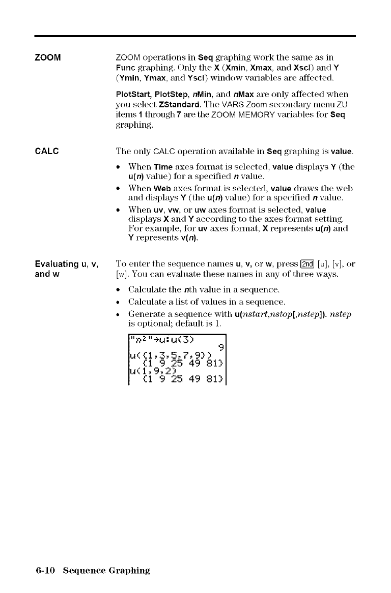
ZOOM
CALC
Evaluating u, v,
and w
ZOOM operations in Seq graphing work the same as in
Func graphing, Only the X (Xmin, Xmax, and Xscl) and Y
(Ymin, Ymax, and Yscl) window variables are affected.
PlotStart, PlotStep, nMin, and nMax are only affected when
you select ZStandard. The VARS Zoom secondary lnenu ZU
items 1through 7are the ZOOM MEMORY variables for Seq
graphing.
The only CALC operation available in Seq graphing is value.
• When Time axes format is selected, value displays Y (the
u(n) value) for a specified nvalue.
• When Web axes format is selected, value draws the web
and displays Y (the u(n) value) for a specified nvalue,
• When uv, vw, or uw axes format is selected, value
displays X and Y according to the axes format setting.
For example, for uv axes format, X represents u(n) and
Y represents v(n),
To enter the sequence names u, v, or w, press [2_] [u], [v], or
[w], You can evaluate these names in any- of three ways,
• Calculate the nth value in a sequence.
• Calculate a list of values in a sequence.
• Generate a sequence with u(nstart,nstop[,nstep]), nstep
is optional; default is 1.
"nz"+u:u(3) 9
u({1,3,5,7,9})
{i 925 49 81}
u(1,9,2)
{1 9 25 49 81}
6-10 Sequence Graphing
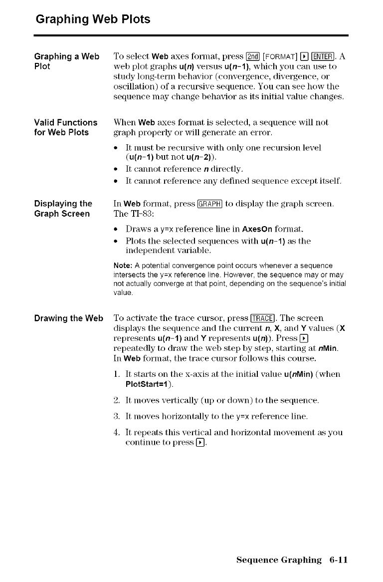
Graphing Web Plots
Graphing a Web
Plot
Valid Functions
for Web Plots
Displaying the
Graph Screen
Drawing the Web
To select Web axes format, press [_ [FORMAT] [] [E_], A
web plot graphs u(n) versus u(n-1), which you can use to
study long-term behavior (convergence, divergence, or
oscillation) of a reeursive sequence. You can see how the
sequence lnay change behavior as its initial value changes.
V_l_en Web axes format is selected, a sequence will not
graph properly or will generate an error.
• It must be recursive with only one recursion level
(u(n-1) but not u(n-2)).
• It cannot reference ndirectly.
• It cannot reference any defined sequence except itself.
In Web format, press _ to display the graph screen.
The TI-83:
• Draws a y=x reference line in AxesOn format.
• Plots the selected sequences with u(n-1) as the
independent variable.
Note: A potential convergence point occurs whenever a sequence
intersects the y=x reference line. However, the sequence may or may
not actually converge at that point, depending on the sequence's initial
value.
To activate the trace cursor, press _. The screen
displays the sequence and the emTent n, X, and Y values (X
represents u(n-1) and Y represents u(n)). Press []
repeatedly to draw the web step by step, starting at nMin.
In Web format, the trace cursor follows this course.
1. It starts on the x-axis at the initial value u(nMin) (when
PlotStart=l).
2. It lnoves vertically (up or down) to the sequence.
3. It lnoves horizontally to the y=x reference line.
4. It repeats this vertical and horizontal movenlent as you
continue to press [].
Sequence Graphing 6-11
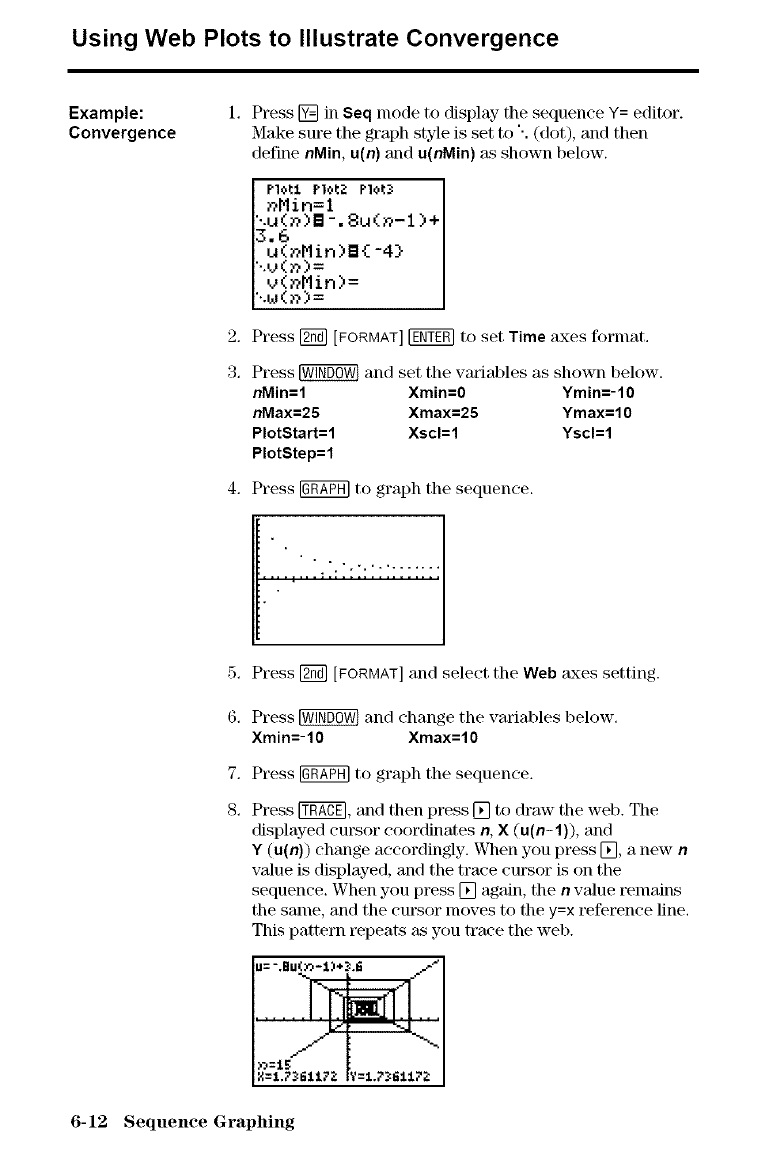
Using Web Plots to Illustrate Convergence
Example:
Convergence
2.
3.
Press [] in Seq mode to display the sequence Y= editor.
Make sure the graph style is set to ". (dot), and then
define nMin, u(n) and u(nMin) as shown below.
_Min=lPl_lPloL_ PloL_ )+
u(_Min)B{-4}
"-.v(n)=
v(nMin)=
".uO?)=
Press [_ [FORMAT] _ to set Time axes ff)rmat,
Press [_ and set the variables as shown below.
nMin=l Xmin=0 Ymin=-10
nMax=25 Xmax=25 Ymax=l 0
PlotStart=l Xscl=l Yscl=l
PlotStep=l
4. Press [g_ to graph the sequence.
5, Press [_ [FORMAT]and select the Web axes setting.
6. Press [_ and change the variables below.
Xmin=-10 Xmax=10
7.
8.
Press [g_ to graph the sequence.
Press _, and then press [] to draw the web. The
displayed cursor coordinates n, X (u(n-1)), and
Y(u(n)) change accordingly. When you press [], a new n
value is displayed, and the trace cursor is on the
sequence. When you press [] again, the nvalue remains
the same, and the cursor moves to the y=x reference line.
This pattern repeats as you tra_'e the web.
u=-.au(._._-:t:,*_:.e t.-*
N'--_.?_:EII?2 I?=1,?_:El172
6-12 Sequence Graphing
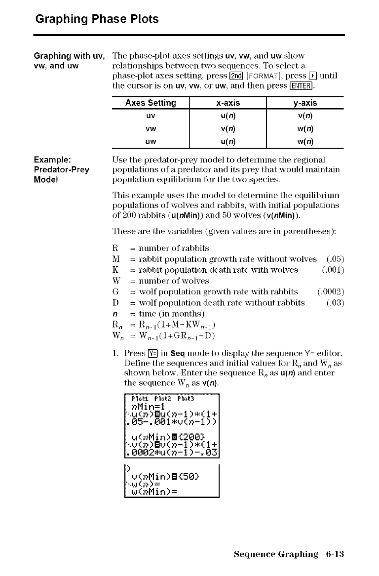
Graphing Phase Plots
Graphing with uv,
vw, and uw
Example:
Predator-Prey
Model
The phase-plot m,ces settings uv, vw, and uw show
relationships between two sequences. To select a
phase-plot axes setting, press [_ [FORMAT],press [] until
the cursor is on uv, vw, or uw, and then press [_.
Axes Setting x-axis y-axis
uv u(n) v(n)
vw v(n) w(n)
uw u(n) w(n)
Use the predator-prey model to determine the regionM
populations of a predator and its pt_y that would maintain
population equilibrium for the two species.
This example uses the model to determine the equilibrium
populations of wolves and rabbits, with initial populations
of 200 rabbits (u(nMin)) and 50 wolves (v(nMin)).
These are the wu'iables (given values are in pm'entheses):
R = number of rabbits
M = rabbit population growth rate without wolves (.05)
K = rabbit population death rate with wolves (.001)
W = number of wolves
G = wolf population growth rate with rabbits (.0002)
D = wolf population death rate without rabbits (.03)
n= time (in months)
Rn= Rn_I(I+M-KWn_I)
W, = W,_I(I+GRn_I-D )
1, Press [] in Seq mode to display the sequence Y= editor.
Define the sequences and initial wdues for Rnand Wnas
shown below. Enter the sequence Rnas u(n) and enter
the sequence Wnas v(n).
Plot:l. Plot::" F'lot2, l
nMir,=l I
".l.l(_) BM(_- 1 )*( 1+1
•05-. 00 l*v(n-1 ) )l
-.u(n) By (_- 1)*( 1+
•0002.u (n-1)-. 03
)v(nMin)B{50}
".t0(n)=
u_(r_Min)=
Sequence Graphing 6-13
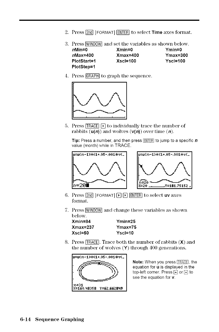
2, Press _ [FORMAT] _ to select Time axes format,
3, Press _ and set the variables as shown below.
nMin=O Xmin=O Ymin=O
nMax=400 Xmax=400 Ymax=300
PlotStart=l Xscl=100 Yscl=100
PlotStep=l
4, Press [ghT_] to graph the sequence,
5, Press _ [] to individually trace the number of
rabbits (u(n)) and wolves (v(n)) over time (n),
6,
7.
Tip: Press a number, and then press _ to jump to a specific n
Press [g_] [FORMAT] [] [] _ to select uv axes
format,
Press _ and change these variables as shown
below.
Xmin=84 Ymin=25
Xmax=237 Ymax=75
Xscl=50 Yscl=lO
Press _. Trace both the number of rabbits (X) and
the number of wolves (Y) through 400 generations,
I g=160.LIB_.=:B y=6;',66;'BLI9
Note: When you press [_, the
equation for uis displayed in the
top-left corner. Press [] or [] to
see the equation for v.
6-14 Sequence Graphing
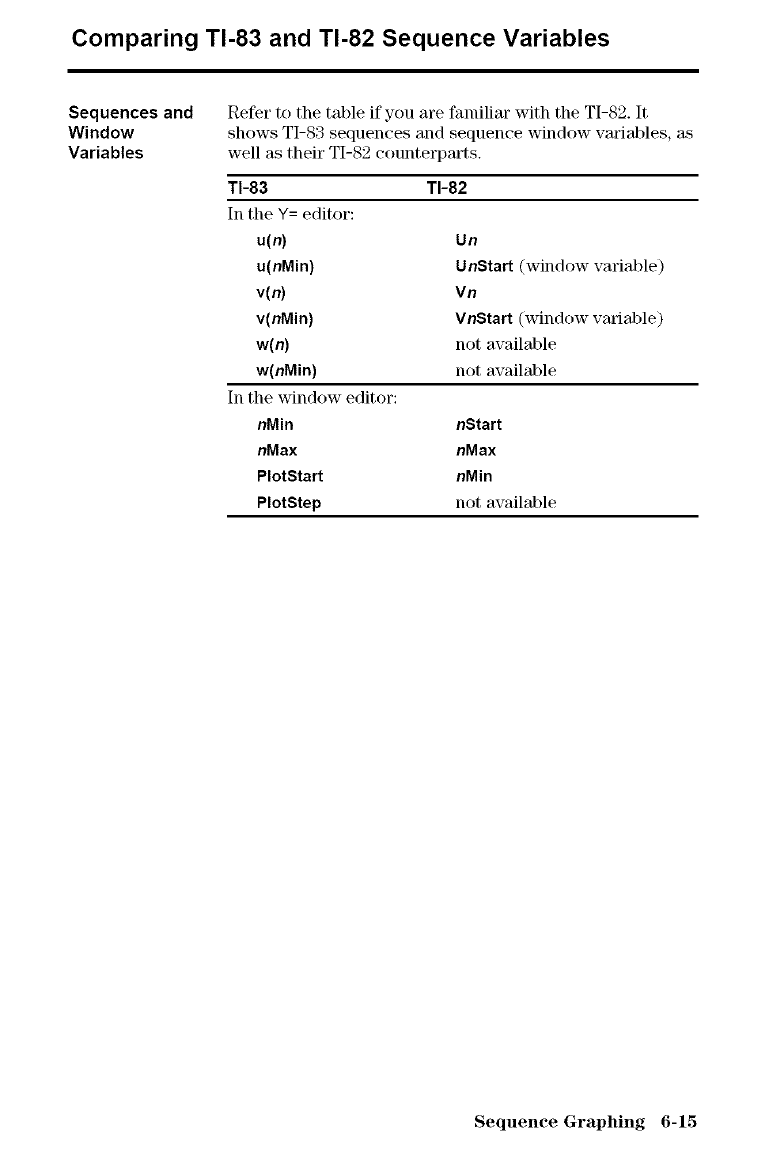
Comparing TI-83 and TI-82 Sequence Variables
Sequences and
Window
Variables
Refer to the table if you are familim" with the TI-82. It
shows TI-83 sequences and sequence window vm'iables, as
well as their TI-82 counterparts.
TI-83
In the Y= editor:
u(n)
u(nMin)
v(n)
v(nMin)
w(n)
w(nMin)
In the window editor:
nMin
nMax
PlotStart
PlotStep
TI-82
Un
UnStart (window variable)
Vn
VnStart (window vm'iable)
not available
not available
nStart
nMax
nMin
not available
Sequence Graphing 6-15
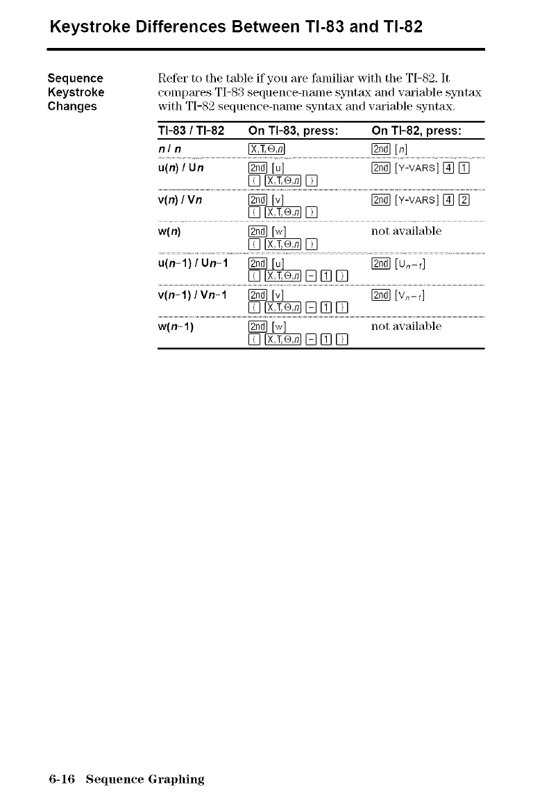
Keystroke Differences Between TI-83 and TI-82
Sequence
Keystroke
Changes
Re%r to the table if you are familiar with the TI-82. It
conlpares TI-83 sequence-name sy_tax and variable sy_tax
with TI-82 sequence-name syntax and variable syntax.
TI183 /TI-82 On TI183, press: On TI-82, press:
n/n_ _ [,]
u(n) /Un _ [u] _ [Y-VARS] [] []
D_D
v(n)/vn _ [i r_ [¥-VARS][] []
D_D
w(n) _ [w] not available
D_D
u(n-1)lUn-1 _ [u] _ [Un-l]
D_DmD
v(n-1)/vn-1 I_ [v] I_ [vn-_]
I]]_E]mD
w(n-1) _ [w] not available
[]_•mD
6-16 Sequence Graphing
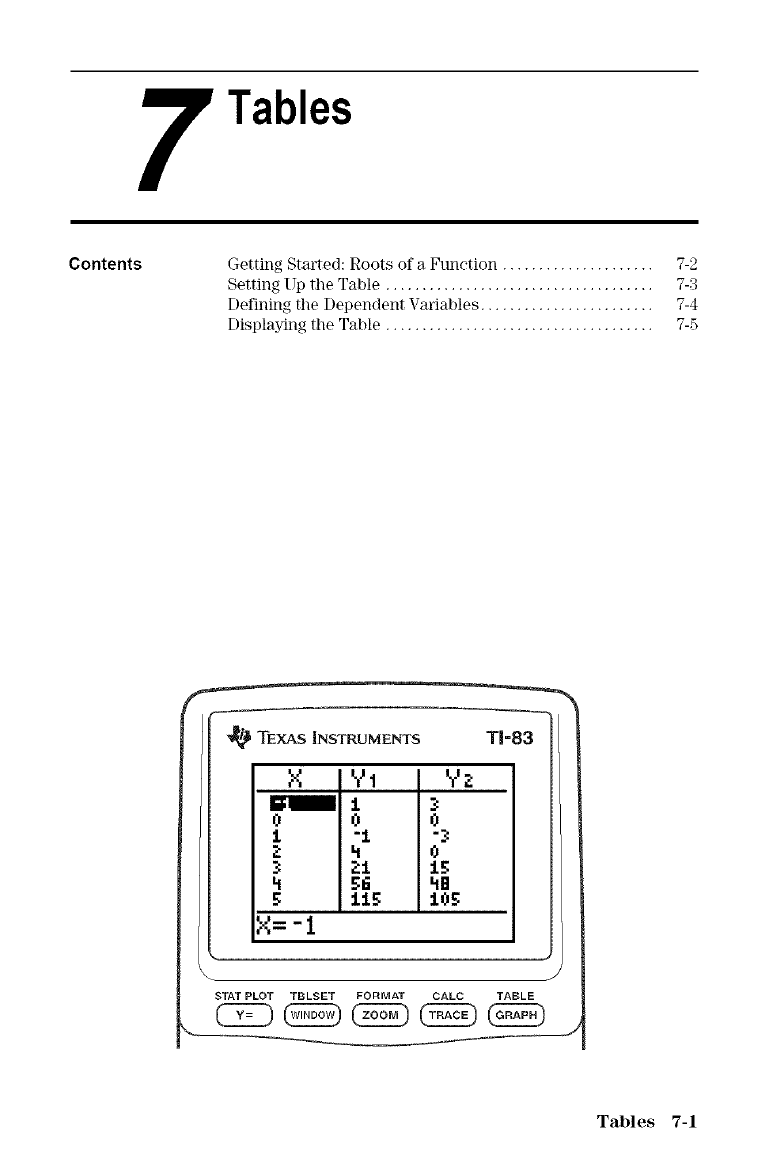
Tables
Contents Getting Started: Roots of a Function ..................... 7-2
Setting Up the Table ..................................... 7-3
Defining the Dependent Variables ........................ 7-4
Displaying the Table ..................................... 7-5
'_ TEXAS iNSTRUMENTS T1=83
XY_ Y2
0 0 0
1"1 "_
2 h 0
21 15
h_hE
511_ 10_
X= -1
J
STAT PLOT TBLSET FORMAT CALC TABLE
Tables 7-1
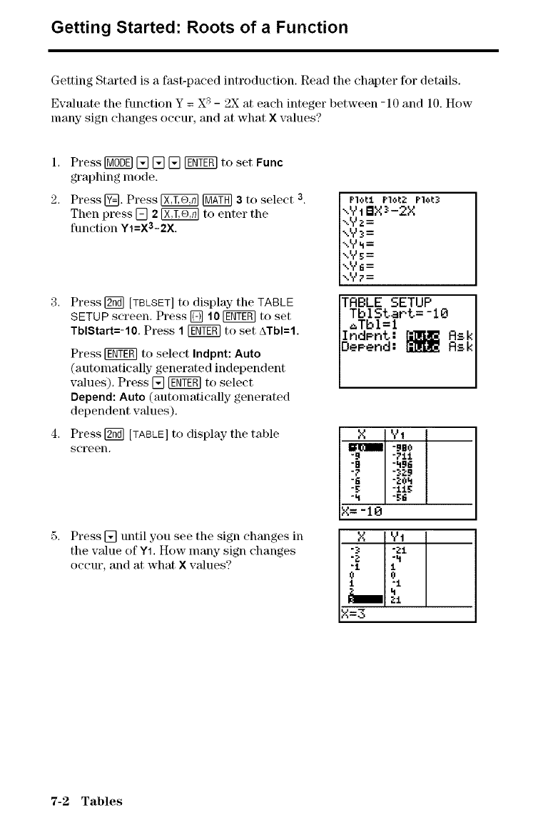
Getting Started: Roots of a Function
Getting Started is a fast-paced introduction. Read the chapter for details.
Evaluate the function Y = X :_- 2X at each integer between -10 and 10. How
many sign changes occur, and at what Xvalues?
1.
2.
Press _ [] [] [] FENY_to set Func
graphing mode.
Press @. Press _ _ 3to select 3
Then press [] 2_ to enter the
function Y1=X3-2X.
Press [_ [TBLSET] to display- the TABLE
SETUP screen. Press [] 10 _to set
TblStart=-10, Press 1_to set ATbI=I.
Press _ to select Indpnt: Auto
(automatically generated independent
values). Press [] [gNT_ to select
Depend: Auto (automatically generated
dependent values).
Press [_ [TABLE]to display the table
screen.
Press [] until you see the sign changes in
the value of Y1. How many sign changes
occur, and at what X values?
Plol:l P1*{_ Pl_l:_
-.Y1BX x-2X
,,yz=
b.Y_=
•,.y _=
\Yg=
".YG=
\YT=
TABLE SETUP
TbIStart= -10
_Tbl=l
Indent: _ Ask
Depend: _ Ask
XY_
"9 "7tl
"B "h96
"? "329
"6 "_.Oh
"_: "Jig
"h "gtl
X= -10
X YI
"2 "h
"1 1
0 0
1 "t
h
X=3
7-2 Tables
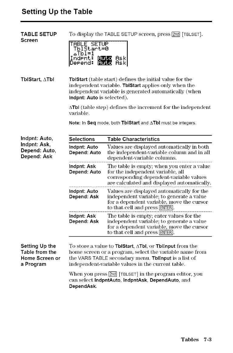
Setting Up the Table
TABLE SETUP
Screen
TblStart, ATbl
Indpnt: Auto,
Indpnt: Ask,
Depend: Auto,
Depend: Ask
Setting Up the
Table from the
Home Screen or
aProgram
TodisplaytheTABLESETUPscreen, press[_[TBLSET].
TRBLE SETUP Rsk
TblStart=O
_Tbl=l
IndPnt:
Depend: i Rsk
TblStart (table start) defines the initial value for the
independent variable. TblStart applies only when the
independent variable is generated automatically (when
Indpnt: Auto is selected).
ATbl (table step) defines the increment for the independent
variable.
Note: In Seq mode, both TblStart and ATbl must be integers.
Selections Table Characteristics
Indpnt: Auto Values are displayed automatically in both
Depend: Auto the independent-variable colunm and in all
dependent-variable colunms.
Indpnt: Ask The table is empty; when you enter a value
Depend: Auto for the independent variable, all
corresponding dependent-variable values
are cah:ulated and displayed automatically.
Indpnt: Auto Values are displayed autonmtically for the
Depend: Ask independent variable; to generate a value
for a dependent variable, move the cursor
to that cell and press [E_.
Indpnt: Ask The table is empty; enter values for the
Depend: Ask independent variable; to generate a value
for a dependent variable, move the cm:sor
to that cell and press [EN_,
To store a value to TblStart, ATbl, or TblInput from the
home screen or a program, select the variable name from
the VARB TABLE seconda[w menu. TblInput is a list of
independent-variable values in the cmTent table.
When you press [2_ [TBLSET] in the program editor, you
can select IndpntAuto, IndpntAsk, DependAuto, and
DependAsk.
Tables 7-3
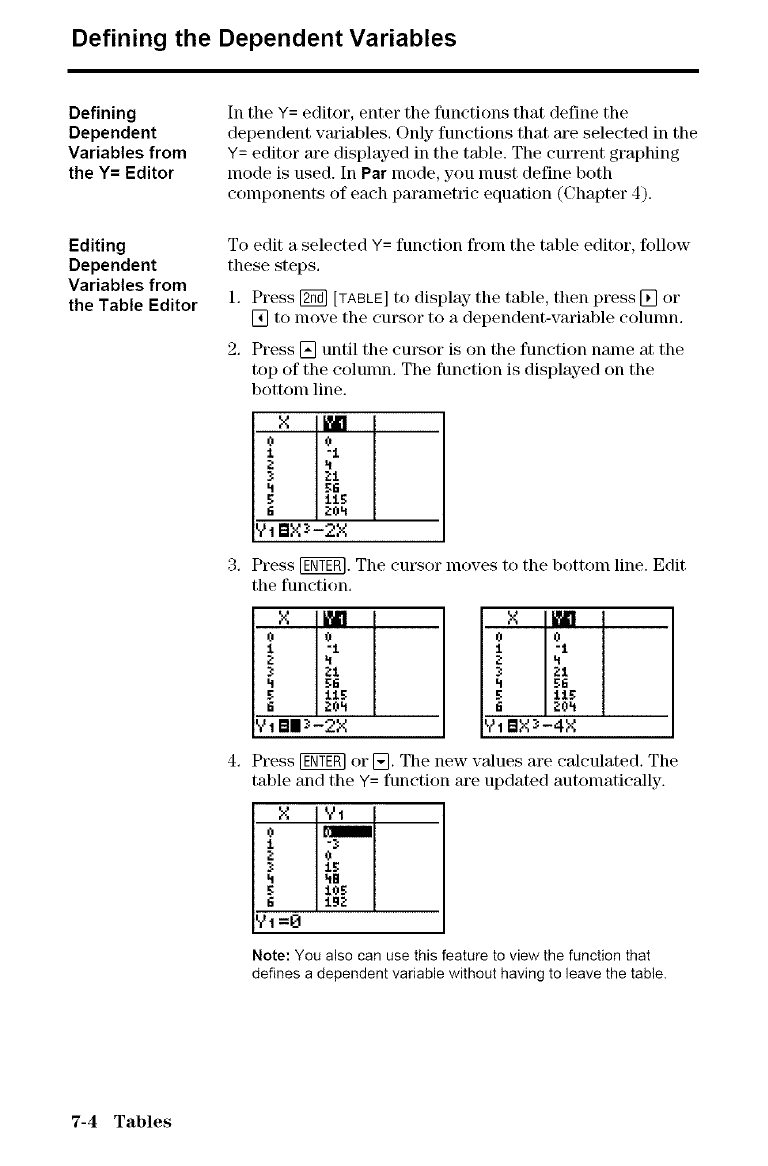
Defining the Dependent Variables
Defining
Dependent
Variables from
the Y= Editor
Editing
Dependent
Variables from
the Table Editor
In the Y= editor, enter the functions that define the
dependent vmiables. Only functions that are selected in the
Y= editor are displayed in the table. The current graphing
mode is used. In Par mode, you nmst define both
components of each parametric equation (Chapter 4).
To edit a selected Y= function fronl the table editor, follow
these steps.
1. Press [_ [TABLE]to display" the table, then press [] or
[] to move the cursor to a dependent-variable column.
2. Press [] until the cursor is on the function name at the
top of the colunm. The function is displayed on the
bottonl line.
5G
20't
Vt BX_-2X
3, Press [ggT_. The cursor moves to the bottonl line. Edit
the function.
X ml
o o
I"t
.-, it
2t
LI _6
_; I15
I_ 20_
71BII_-2X
X m
o o
t "1
620_
V1BX:-4X
Press [ggT_ or []. The new values are calculated. The
table and the Y= function are updated automatically.
X Y1
"3
Yt =O
Note: You also can use this feature to view the function that
defines a dependent variable without having to leave the table.
7-4 Tables
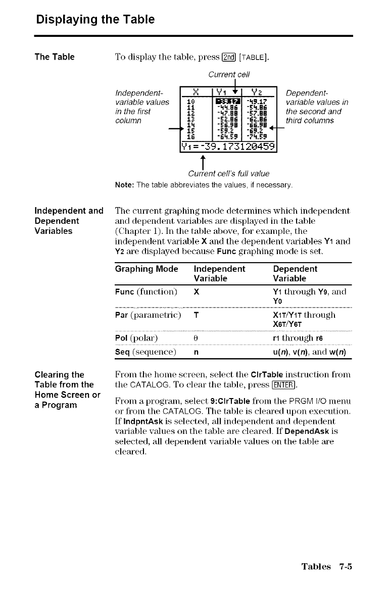
Displaying the Table
The Table To display- the table, press [_q [TABLE].
Current cell
Independent- X _ 1 4, Y z Dependent-
variable values to _ -_9.iz variable values in
11 "hh.86 "_:h.86
in the first lZ -h?.eB -_:Z.BE the second and
column 13 -_Z.I_6 -6Z.eE third columns
1h "_'.gB "G6.98 _. --
1 1_ "_ 9"_ "E.q.Z --
16 "6h._:B "?h,59
Y1 = -39, 173120459
T
Current cell's full value
Note: The table abbreviates the values, if necessary.
Independent and
Dependent
Variables
Clearing the
Table from the
Home Screen or
a Program
The current graphing lnode determines which independent
and dependent varial)les are displayed in the table
(Chapter 1). In the tal)le above, for example, the
independent variable X and the dependent wuiables Y1 and
Y2 are displayed because Func graphing mode is set.
Graphing Mode Independent Dependent
Variable Variable
Func (function) X Y1 through Yg, and
Y0
Par (parametric) TX1T/Y1T through
X6T/Y6T
Pol (polar) 0 rl through r6
Seq (sequence) n u(n), v(n), and w(n)
From the home screen, select the CIrTable instruction fronl
the CATALOG. To clear the table, press [ggY_.
From a program, select 9:CIrTable from the PRGM I/0 menu
or from the CATALOG. The talfle is cleared upon execution.
If IndpntAsk is selected, 'all independent and dependent
varialfle values on the table are cleared. If DependAsk is
selected, all dependent variable values on the talfle are
cleared.
Tables 7-5
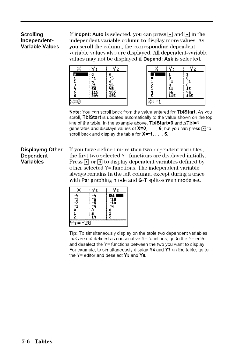
Scrolling
Independent-
Variable Values
If Indpnt: Auto is selected, you can press [] and [] in the
independent-variable colunm to display more wdues. As
you scroll the colunm, the corresponding dependent-
variable values also are displayed. All dependent-variable
values may not be displayed if Depend: Ask is selected.
X YI Yz
1"t "_
z 4 ¢
4 _6 4B
5 115 105
6 204 192
X=O
X YI Yz
1"t I"_
4 io
.3 21 1_:
18.r.
X= -1
Note: You can scroll back from the value entered for TblStart. As you
scroll, TblStart is updated automatically to the value shown on the top
line of the table. In the example above, TblStart=0 and ATbI=I
generates and displays values of X=0,..., 6; but you can press [] to
scroll back and display the table for X=-I,..., 5.
Displaying Other
Dependent
Variables
If you have defined more than two dependent variables,
the first two selected Y= functions are displayed initially-.
Press [] or [] to display dependent variables defined by
other selected Y= functions. The independent wuiable
always remains in the left colunm, except during a trace
with Par graphing nlode and G-T split-screen nlode set.
XYz Y_
"_ "6 ":LB
"2 "6 "10
"1 "4 "LI
O_O
1G 2
Z:L=I ;L
Y_= -28
Tip: To simultaneously display on the table two dependent variables
that are not defined as consecutive Y= functions, go to the Y= editor
and deselect the Y= functions between the two you want to display.
For example, to simultaneously display Y4 and Y7 on the table, go to
the Y= editor and deselect Y5 and Y6.
7-6 Tables
8Dnrs Wuctions
Contents Getting Started: Drawing a Tangent Line ................. 8-2
Using the DRAW Menu ................................... 8-3
Clearh]g Dra,_lngs ....................................... 8-4
Drawing Line Segments .................................. 8-5
Drawing Horizontal and Vertical Lines ................... 8-(;
Drawing Tangent Lines .................................. 8-8
Drawing Functions and hwerses ......................... 8-9
Shading Areas on a Graph ............................... 8-10
Drawing ('ircles .......................................... 8-11
Plaeing Text on a Graph ................................. 8-12
Using Pen m Draw on a Graph ........................... 8-1:3
Drawing Points on a Graph .............................. 8-14
Drawing Pixels .......................................... 8-16
Storing Graph Pictures (Pies) ............................ 8-17
Recalling Graph Pictures (Pics) .......................... 8-18
Storing Graph Databases (GDBs) ........................ 8-19
Recalling Graph Databases (GDBs) ...................... 8-20
4_ TEXAS INSTnUMENTS T1=83
STAT PLOT TBLSET FORMAT CALC T._,B LE
DRAW Instructions 8-1
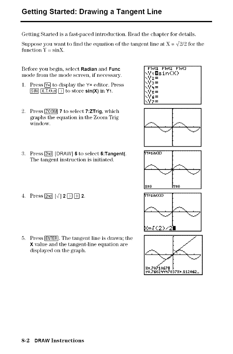
Getting Started: Drawing a Tangent Line
Getting Started is a fast-paced introduction. Read the chapter for details.
Suppose you want to find the equation of the tangent line at X = _2 for the
function Y= sinX.
Before you begin, select Radian and Func
mode from the mode screen, if necessaw.
1. Press [] to display- the Y= editor. Press
[g_ _ [] to store sin(X) in Y1.
2. Press _ 7to select 7:ZTrig, which
graphs the equation in the ZOOlll Trig
window.
P1,'.,tl Plot_ Pl(,t3
".Y1Bsin(X)
%yz=
",Yx=
-.y_=
-,y_=
,,y_=
xY_'=
/-7--,. /-7_
"..>" ".L/
Press [g_ [DRAW] 6 to select 6:Tangent(.
The tangent instruction is initiated.
4. Press_ [4] 2[] [] 2.
Press [ggg_. The tangent line is drawn; the
Xvalue and the tangent-line equation are
displayed on the graph.
tl==in(:4)
/-7_. /-7\
".,_i_1 -,,_i___
1{=0 ?=0
tl=sih((X)
_.--.. /2"-..
-,_i_1 ",2/
4=,r(2)/211
_[//
8-2 DRAW Instructions
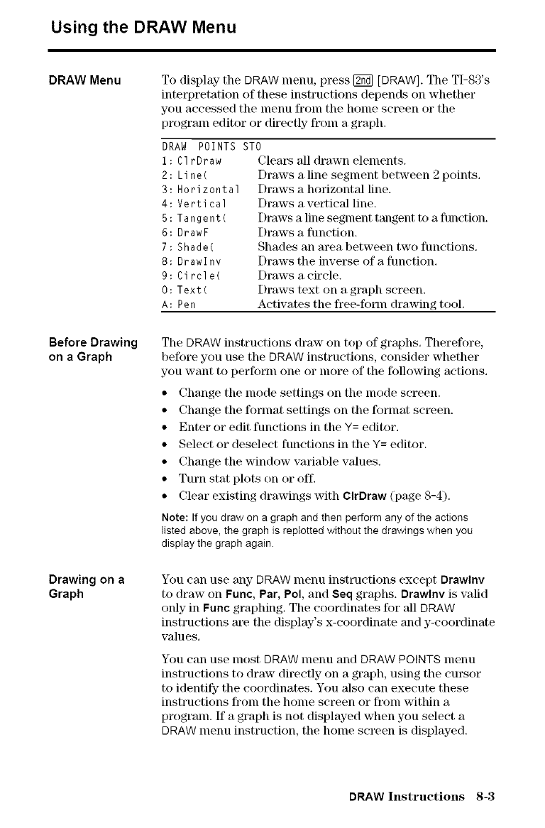
Using the DRAW Menu
DRAW Menu
Before Drawing
on a Graph
Drawing on a
Graph
To display the DRAW menu, press [_ [DRAW]. The TI-S3's
interpretation of these instructions depends on whether
you accessed the menu fronl the honle screen or the
program editor or directly- from a graph.
DRAW POINTS STO
1 : C1rDraw Clears all drawn elements.
2: Line(
3: Horizontal
4: Vertical
5: Tangent(
6: DrawF
7: Shade(
8: Drawlnv
9: Circle(
O: Text(
A: Pen
Draws a line segment between 2 points,
Draws a horizontal line.
Draws a vertical line.
Draws a line segment tangent to a function.
Draws a function.
Shades an area between two functions.
Draws the inverse of a function.
Draws a circle.
Draws text on a graph screen.
Activates the free-form drawing tool.
The DRAW instructions draw on top of graphs. Therefore,
before you use the DRAW instructions, consider whether
you want to perform one or more of the following actions,
• Change the mode settings on the mode screen,
• Change the fornlat settings on the format screen.
• Enter or edit functions in the Y= editor,
• Select or deselect functions in the Y= editor.
• Change the window variable values.
• Turn stat plots on or off.
• Clear existing drawings with ClrDraw (page 8-4).
Note: If you draw on a graph and then pedorm any of the actions
listed above, the graph is reptotted without the drawings when you
display the graph again.
You can use any DRAW menu instructions except Drawlnv
to draw on Func, Par, Pol, and Seq graphs. Drawlnv is valid
only in Func graphing. The coordinates for all DRAW
instructions ate the display's x-coordinate and y-coordinate
values.
You can use most DRAW menu and DRAW POINTS menu
instructions to draw directly on a graph, using the cursor
to identify the coordinates. You also can execute these
instructions from the home screen or from within a
progranl. If a graph is not displayed when you select a
DRAW menu instruction, the home screen is displayed.
DRAW Instructions 8-3
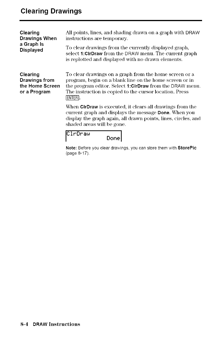
Clearing Drawings
Clearing
Drawings When
a Graph Is
Displayed
Clearing
Drawings from
the Home Screen
or aProgram
All points, lines, and shading drawn on a graph with DRAW
instructkms are temporm'y.
To elem' drawings from the currently displayed graph,
select 1 :ClrDraw from the DRAW menu, The current graph
is replotted and displayed with no drawn elements,
To clem' drawings on a graph fronl the holne screen or a
program, begin on a blank line on the home screen or in
the program editor. Select 1:CIrDraw from the DRAW menu.
The instruction is copied to the cursor location. Press
When CIrDraw is executed, it clears 'all drawings from the
current graph and displays the message Done. When you
display the graph again, all drawn points, lines, circles, and
shaded areas will be gone.
ClrOraw Done
Note:Beforeyoucleardrawings,youcanstore them withStorePic
(page 8-17).
8-4 DRAW Instructions
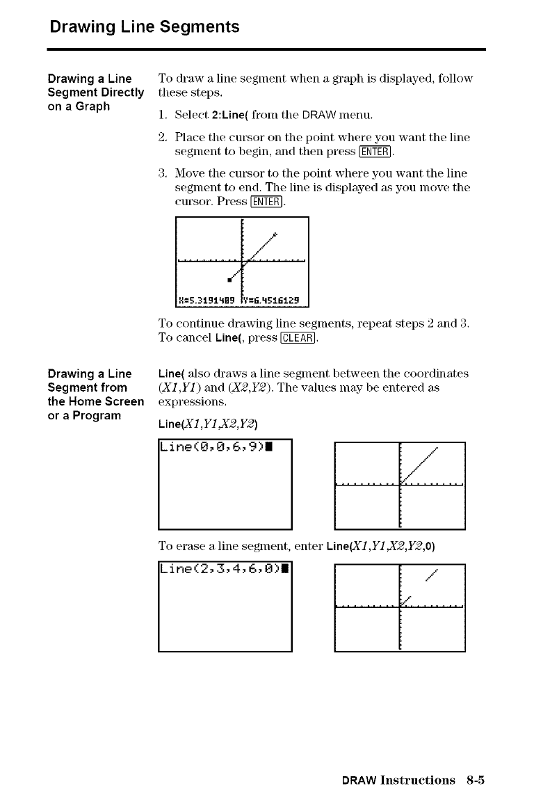
Drawing Line Segments
Drawing a Line
Segment Directly
on a Graph
Drawing a Line
Segment from
the Home Screen
or a Program
To draw a line segment when a graph is displayed, follow
these steps.
1. Select 2:Line( from the DRAW menu.
2. Place the cursor on the point where you want the line
segment to begin, and then press [_E_.
3. Move the cursor to the point where you want the line
segment to end. The line is displayed _s you move the
cursor. Press [ggY_.
R=5,3191_Bgl/I=_.qSi_t_9
To continue drawing line segments, repeat steps 2 and 3.
To cancel Line(, press @.
Line( also draws a line segment between the coordinates
(X1 ,Y1) and (X2,Y2). The values nlay be entered ZLS
expressions.
Line(X1,Y1,X2,Y2)
Line (0, 0, 6, 9)11
To erase a line segment, enter Line(X1,Y1,X2,Y2,0)
Line(2, 3, 4, 6, 0)11 /,
DRAW Instructions 8-5
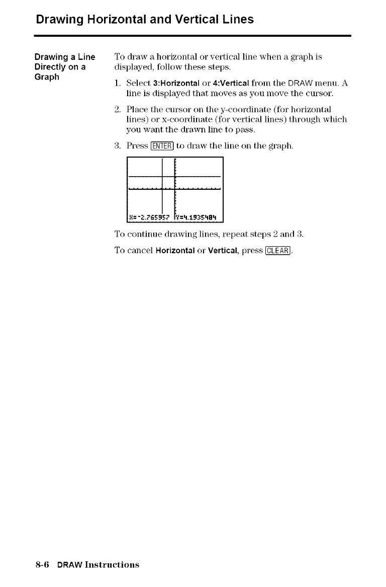
Drawing Horizontal and Vertical Lines
Drawing a Line
Directly on a
Graph
To draw a horizontal or vertical line when a graph is
displayed, follow these steps.
1, Select 3:Horizontal or 4:Vertical from the DRAW menu. A
line is displayed that nloves as you nlove the cursor.
2. Place the cm'sor on the y-coordinate (for horizontal
lines) or x-coordinate (for vertical lines) through which
you want the drawn line to pass.
3. Press [_ to draw the line on the graph.
To continue drawing lines, repeat steps 2 and 3.
To cancel Horizontal or Vertical, press @,
8-6 DRAW Instructions
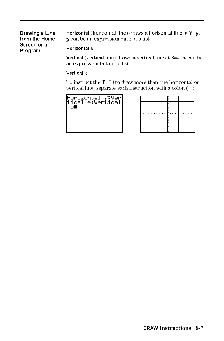
Drawing a Line
from the Home
Screen or a
Program
Horizontal (horizontal line) draws a horizontal line at Y=y.
y can be an expression but not a list.
Horizontal y
Vertical (vertical line) draws a vertical line at X=x, x can be
an expression but not a list,
Vertical _"
To instruct tile TI-83 to draw more than one horizontal or
vertical line, separate each instruction with a colon ( : ).
Ho_-izor,÷_al 7: Vet
t_al 4: Vertical ......................
DRAW Instructions 8-7
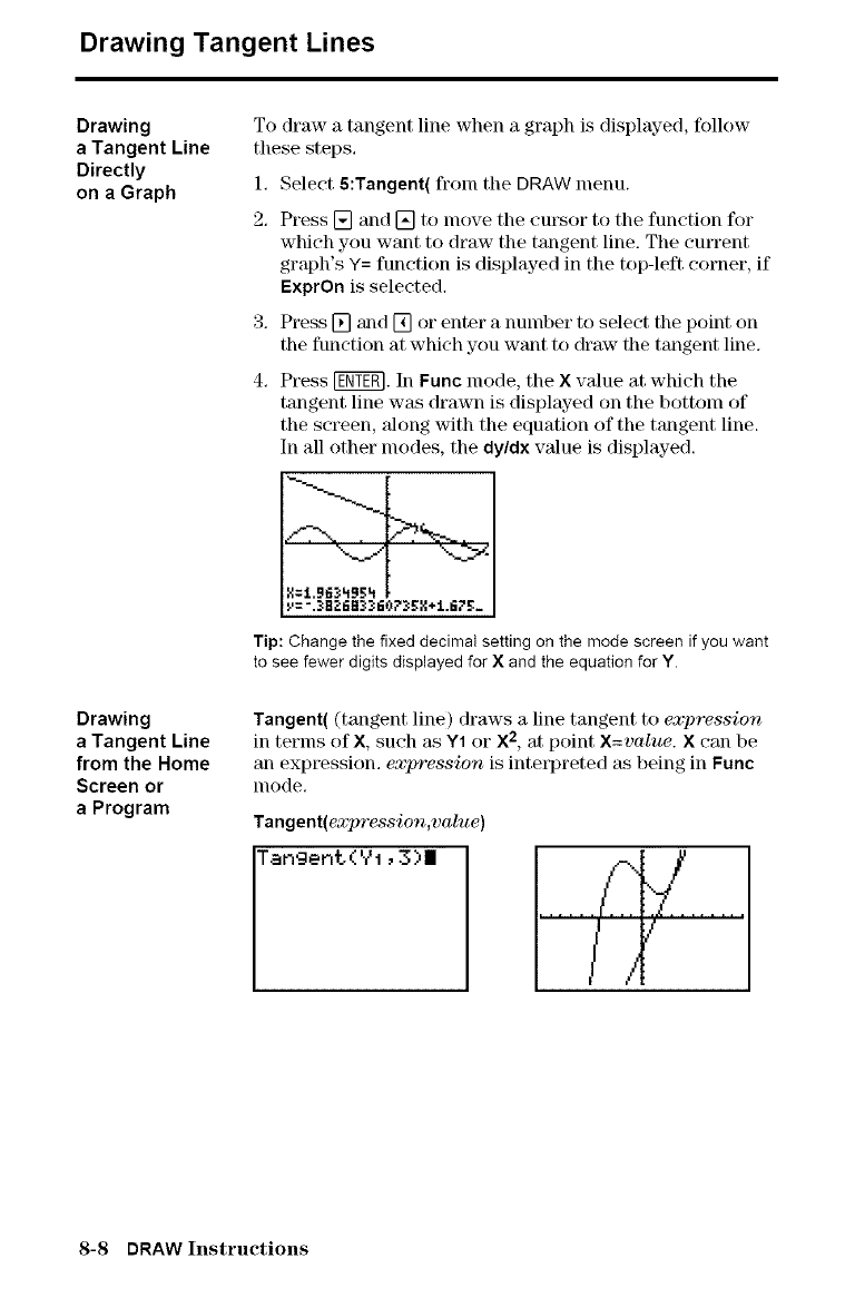
Drawing Tangent Lines
Drawing
aTangent Line
Directly
on a Graph
Drawing
aTangent Line
from the Home
Screen or
a Program
To draw a tangent line when a graph is displayed, follow
these steps,
1, Select 5:Tangent( fron] the DRAW nlenu.
2. Press [] and [] to move the cm_or to the function for
which you want to draw the tangent line. The cmTent
graph's Y= function is displayed in the top-left corner, if
ExprOn is selected.
3. Press [] a_d [] or enter a number to select the point on
the function at which you want to draw the tangent line.
4. Press [E_. In ffunc mode, the X value at which the
tangent line wa_ drawn is displayed on the bottom of
the screen, along with the equation of the tangent line.
In all other nlodes, the dy/dx value is displayed.
X=i,gt;_:
Tip: Change the fixed decimal setting on the mode screen if you want
to see fewer digits displayed for X and the equation for Y.
Tangent( (tangent line) draws a line tangent to expression
in terms of X, such as Y1 or X2, at point X=value. Xcan be
an expression, expression is interpreted as being in Func
nlode,
Tangent(expression,value)
Tangent ('gi, 3)|
8-8 DRAW Instructions
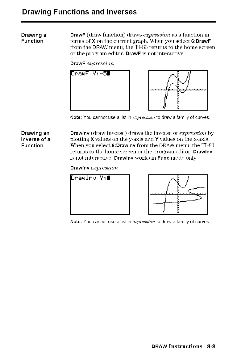
Drawing Functions and Inverses
Drawing a
Function DrawF (draw function) draws expression at a function in
terms of Xon the current graph, When you select 6:DrawF
froln the DRAW menu, the TI-83 returns to the home screen
or the program editor, DrawF is not interactive,
DrawF expression
[Ir.at0F t?1-5 II ...... ./_-.._ .(_. .....
Note: You cannot use a list in exp'_vssion to draw a family of curves.
Drawing an
Inverse of a
Function
Drawlnv (draw inverse) draws the inverse of expression by
plotting Xvalues on the y-axis and Yvalues on the x-axis.
V_lmn you select 8:Drawlnv from the DRAW menu, the TI-83
returns to the home screen or the program editor. Drawlnv
is not interactive. Drawlnv works in Func mode only.
Drawlnv expression
Drato Inv '.?ill . .@__SI.
Note: You cannot use a list ine_pression to draw a familyof curves.
DRAW Instructions 8-9
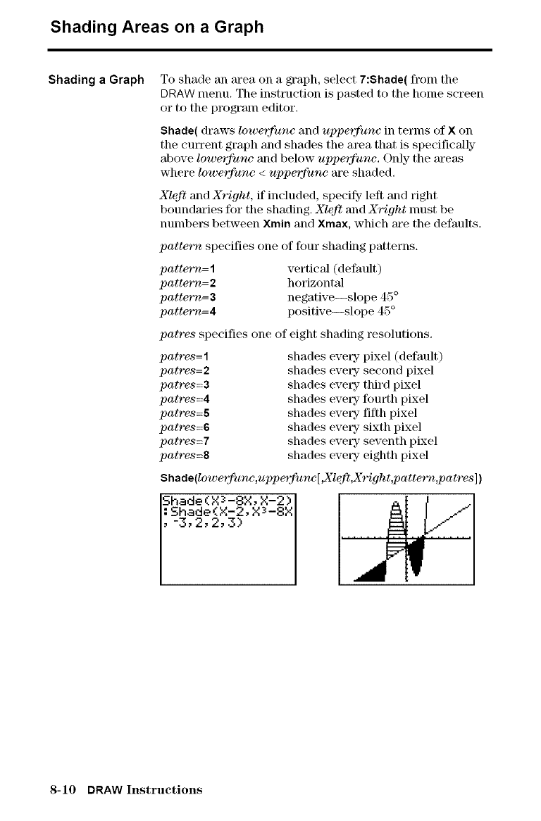
Shading Areas on aGraph
Shading a Graph To shade an area on a graph, select 7:Shade( fronl the
DRAW menu. The instruction is pasted to the home screen
or to the program editor.
Shade( draws loweffune and uppeffunc in terms of X on
the current graph and shades the area that is specifically
above lowerfane and below uppe_2fune. Only the areas
where lowerfane <uppeffunc are shaded.
Xleft and Xright, if included, specify- left and right
boundaries for the shading. Xleft and Xright nmst be
numbers between Xmin and Xmax, which axe the defaults.
patte_ specifies one of four shading patterns.
pattern= 1vertical (default)
pattern= 2horizontal
pattern= 3negative--slope 45°
pattern=4 positive--slope 45°
patres specifies one of eight shading resolutions.
patres= 1shades every pixel (default)
patres=2 shades evetF- second pixel
patres=3 shades every third pixel
patres=4 shades eve_- fourth pixel
patres=5 shades every fifth pixel
patres=6 shades eve_Ty-sixth pixel
patres=7 shades evetsz seventh pixel
patres=8 shades every eighth pixel
Shade(lowerfanc,uppe_:func[._left._right,patte_,patres])
Shade(X_-8X, X-2), ....... ____...;.:(
8-10 DRAW Instructions
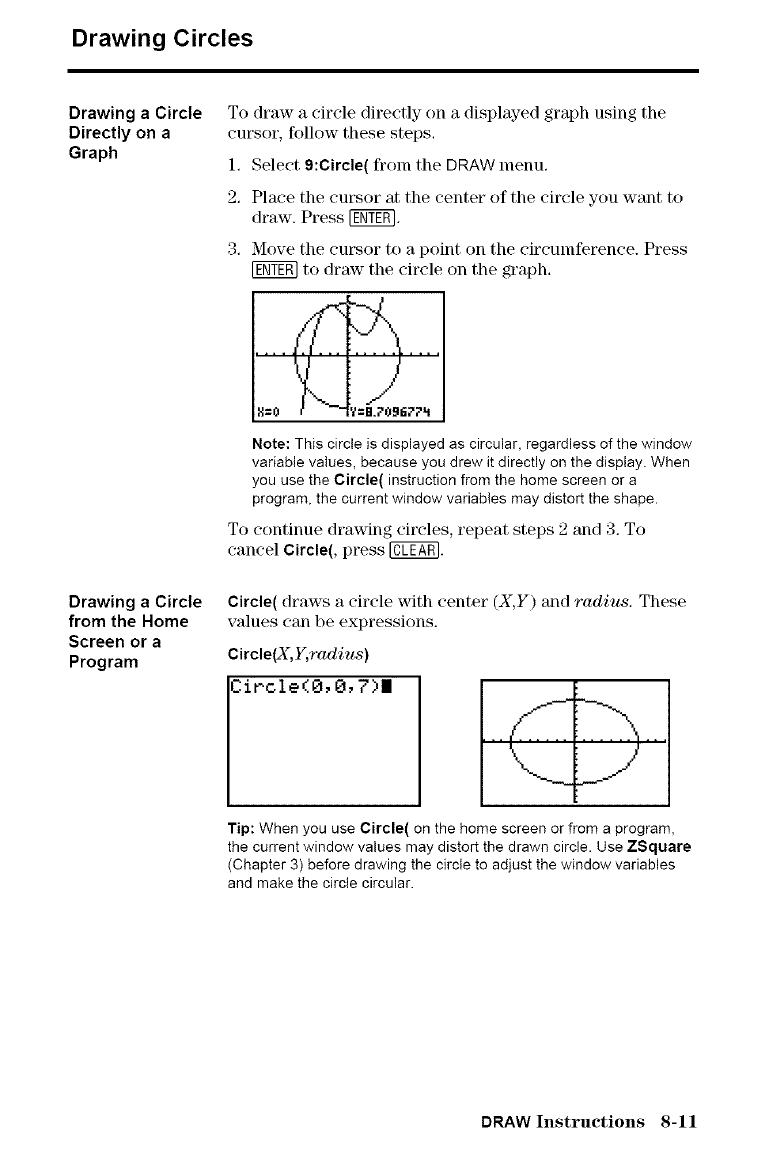
Drawing Circles
Drawing a Circle
Directly on a
Graph
Drawing a Circle
from the Home
Screen or a
Program
To draw a circle directly on a displayed graph using the
cursor, follow these steps,
1, Select 9:Circle( fronl the DRAW menu.
2, Place the cursor at the center of the circle you want to
draw. Press [NTEN.
3. Move the cursor to a point on the circumference. Press
[ggTE_ to draw the circle on the graph.
Note: This circle is displayed as circular, regardless of the window
variable values, because you drew it directly on the dispiay. When
you use the Circle( instruction from the home screen or a
program, the current window variables may distort the shape.
To continue drawing circles, repeat steps 2 and 3, To
cancel Circle(, press @.
Circle( draws a circle with center (X,Y) and radius. These
values can be expressions.
Circle(X,Y, radius)
Ciwcle(O, 0, 7)1
Tip: When you use Circle( on the home screen or from a program,
the current window values may distort the drawn circle. Use ZSquare
(Chapter 3) before drawing the circle to adjust the window variables
and make the circle circular.
DRAW Instructions 8-11
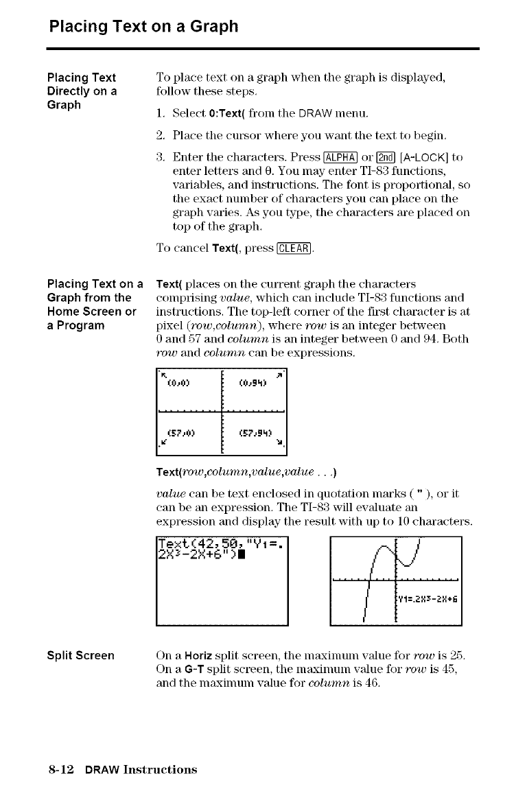
Placing Text on a Graph
Placing Text
Directly on a
Graph
Placing Text on a
Graph from the
Home Screen or
aProgram
Split Screen
To place text on a graph when the graph is displayed,
follow these steps,
1, Select 0:Text( from the DRAW menu.
2, Place the cursor where you want the text to begin.
3, Enter the characters. Press @ or [_ [A-LOCK] to
enter lettet\s and 0. You nlay enter TI-83 functions,
variables, and instructions. The font is proportional, so
the exact number of characters you can place on the
graph varies. As you type, the characters are placed on
top of the graph.
To cancel Text(, press @,
Text( places on the current graph the chara('ters
comprising value, which can include TI-83 functions and
instructions. The top-left corner of the first character is at
pixel (row,column), where row is an integer between
0 and 57 and column is an integer between 0 and 94. Both
row and colnft_firt can be expressions.
Text(row,column,value,value.. ,)
value can be text enclosed in quotation marks ( " ), or it
can be an expression. The TI-83 will evaluate an
expression and display the result with up to 10 characters.
Text(42,50,"Vt=.
2XX-2X+6 )|
..... ......
I ?'I=._:X_-_:X+G
On a Horiz split screen, the nlaxinlunl value for row is 25,
On a G-T split screen, the nlaxinlunl value for ro_t_)is 45,
and the nlaxinlunl value for column is 46,
8-12 DRAW Instructions
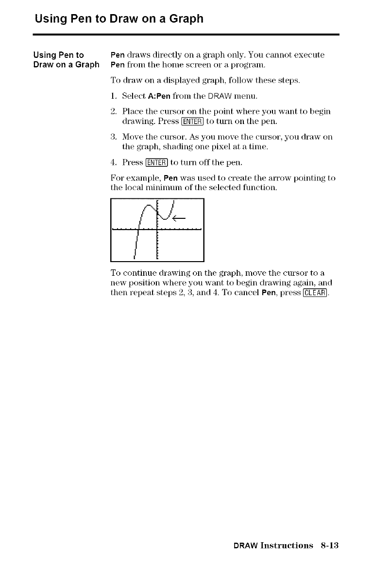
Using Pen to Draw on a Graph
Using Pen to
Draw on a Graph
Pen draws directly on a graph only, You cannot execute
Pen from the home screen or a progranL
To draw on a displayed graph, follow these steps.
1. Select A:Pen from the DRAW menu,
2. Place the cursor on the point where you want to begin
drawing. Press [_ to turn on the pen,
3. Move the cursor. As you move the cursor, you draw on
the graph, shading one pixel at a time,
4. Press [_ to turn off the pen,
For example, Pen was used to create the arrow pointing to
the local minimunl of the selected function.
..... E.,dL
I
To continue drawing on the graph, nlove the cursor to a
new position where you want to begin drawing again, and
then repeat steps 2, 3, and 4. To cancel Pen, press @.
DRAW Instructions 8-13
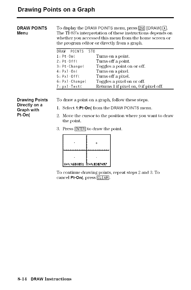
Drawing Points on a Graph
DRAW POINTS
Menu
Drawing Points
Directly on a
Graph with
Pt-On(
To display- the DRAW POINTS menu, press [_a] [DRAW] [_.
The TI-83's interpretation of these instructions depends on
whether you accessed this nlenu froth the home screen or
the program editor or directly froth a graph.
DRAW POINTS ST0
i : Pt On( Turns on apoint.
2: Pt Off(
3: Pt Change(
4: Pxl On(
5: Pxl Off(
6: Pxl Change(
7: pxl Test(
Turns off a point.
Toggles a point on or off.
Turns on a pixeL
Turns off a pixel.
Toggles a pixel on or off,
Returns 1 if pixel on, 0 if pixel off,
To draw a point on a graph, follow these steps.
1, Select 1:Pt-On( from the DRAW POINTS menu,
2. Move the cursor to the position where you want to draw
the point.
3. Press [ggY_ to draw the )oint.
o
R:Ll,_6e0mgl y:LI.BM]?O.:I?
To continue drawing points, repeat steps 2 and 3. To
cancel Pt-On(, press @.
8-14 DRAW Instructions
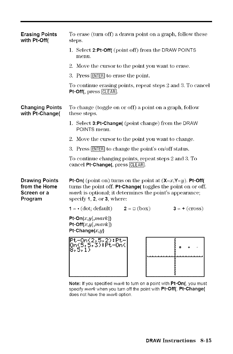
Erasing Points
with Pt-Off(
Changing Points
with Pt-Change(
Drawing Points
from the Home
Screen or a
Program
To erase (turn off) a drawn point on a graph, follow these
steps,
1. Select 2:Pt-Off( (point off) from the DRAW POINTS
nlenu,
2. Move the cursor to the point you want to erase.
3. Press _ to ertkse the point.
To continue ertLsing points, repeat steps 2 and 3. To cancel
Pt-Off(, press @.
To change (toggle on or off) a point on a graph, %llow
these steps.
1. Select 3:Pt-Change( (point change) from the DRAW
POINTS menu.
2. Move the cursor to the point you want to change.
3. Press I_ to change the point's on/off status.
To continue changing points, t_peat steps 2 and 3. To
cancel Pt-Change(, press @.
Pt-On( (point on) turns on the point at (X=x,Y=y). Pt-Off(
tutlls the point off. Pt-Change( toggles the point on or off.
mark is optional; it determines the point's appearance;
specify 1, 2, or 3, where:
1=•(dot; default) 2= [] (box) 3=+(cross)
Pt-On(x,y[,mark])
Pt-Off(x,y[ ,mark ])
Pt-Change(x,y)
Pt.-0n ( 2, 5, 2> :Pt,-
..
Note: If you specified mark to turn on a point with Pt-On(, you must
specify mark when you turn off the point with Pt-Off(. Pt-Change(
does not have the mark option.
DRAW Instructions 8-15
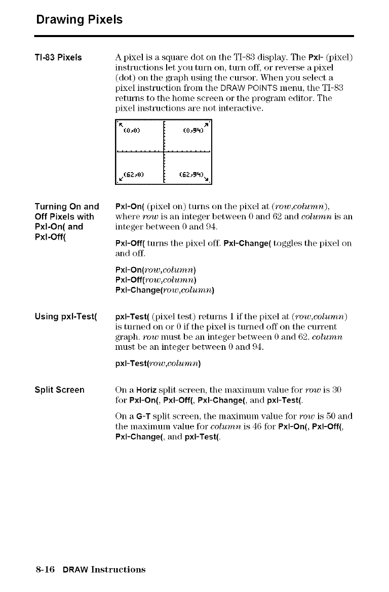
Drawing Pixels
TI-83 Pixels A pixel is a square dot on the TI-83 display. The Pxl- (pixel)
instructions let you turn on, turn off, or reverse a pixel
(dot) on the graph using the cursor. When you select a
pixel instruction from the DRAW POINTS menu, the TI-83
retm'ns to the home screen or the program editor. The
_ixel instl_ctions are not interactive.
p; jq
Turning On and
Off Pixels with
Pxl-On( and
Pxl-Off(
Using pxI-Test(
Split Screen
PxI-On( (pixel on) turns on the pixel at (row,column),
where row is an integer between 0 and 62 and column is an
integer between 0 and 94.
PxI-Off( turns the pixel off. Pxl-Change( toggles the pixel on
and off.
Pxl-On(row,column)
Pxl-Off(row,column)
Pxl-Change(_'ow,column)
pxI-Test( (pixel test) returns 1 if the pixel at (row,column)
is turned on or 0 if the pixel is tunled off on the curl_nt
graph, row nmst be an integer between 0 and 62. column
nmst be an integer between 0 and 94.
pxI-Test(row,colu'rnn)
On a Horiz split screen, the maxinmm value for row is 30
for PxI-On(, PxI-Off(, Pxl-Change(, and pxI-Test(.
On a G-T split screen, the nlaxinlunl value for row is 50 and
tile nlaxinlunl value for column is 46 for PxI-On(, PxI-Off(,
Pxl-Change(, and pxI-Test(.
8-16 DRAW Instructions
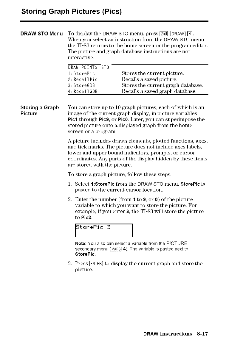
Storing Graph Pictures (Pics)
DRAW STO Menu
Storing aGraph
Picture
To display the DRAW STO menu, press [g_ [DRAW] [_,
When you select an instruction fronl the DRAW STO menu,
the TI-83 returns to the home screen or the program editor.
The picture and graph database instructions are not
interactive.
DRAW POINTS STO
1:StorePic
2:RecallPic
3:StoreGDB
4:RecalIGDB
Stores the current picture.
Recalls a saved picture.
Stores the current graph datal)ase.
Recalls a saved graph database.
You can store up to 10 graph pictures, each of which is an
image of the cmTent graph display-, in picture wuialfles
Pie1 through Picg, or PicO.Later, you can superimpose the
stored picture onto a displayed graph from the home
screen or a program.
A picture includes drawn elements, plotted functions, axes,
and tick marks. The picture does not include axes labels,
lower and upper bound indicators, prompts, or cursor
coordinates. Any parts of the display- hidden by these items
m'e stored with the picture.
To store a graph picture, follow these steps.
1. Select 1:StorePic fronl the DRAW STO menu. StorePic is
DL_ted to the current cursor location.
2. Enter the number (from 1 to 9, or 0) of the picture
variable to which you want to store the picture. For
example, if you enter 3, the TI-83 will store the picture
to Pic3.
5tor.ePio 3
Note: You alsocan selecta variablefromthe PICTURE
secondarymenu(_ 4). The variableispastednextto
8torePic.
3. Press [ggTE_ to display- the current graph and store the
picture.
DRAW Instructions 8-17
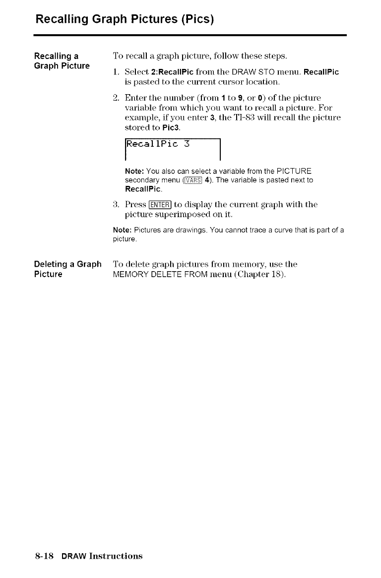
Recalling Graph Pictures (Pics)
Recalling aTo
Graph Picture 1.
Deleting a Graph
Picture
recall a graph picture, follow these steps,
Select 2:RecallPic ffonl the DRAW STO menu, RecallPic
is pasted to the current cursor location,
Enter the number (from 1to 9, or 0) of the picture
varial)le from which you want to recall a picture. For
example, if you enter 3, the TI-83 will recall the picture
stored to Pic3.
Reoal IPio 3
Note: You also can select a variable from the PICTURE
secondary menu (_ 4). The variable is pasted next to
RecallPic.
3, Press I_ to display- the current graph with the
picture superimposed on it,
Note: Pictures are drawings. You cannot trace a curve that is part of a
picture.
To delete graph pictures from memo[3z, use the
MEMORY DELETE FROM menu (Chapter 18).
8-18 DRAW Instructions
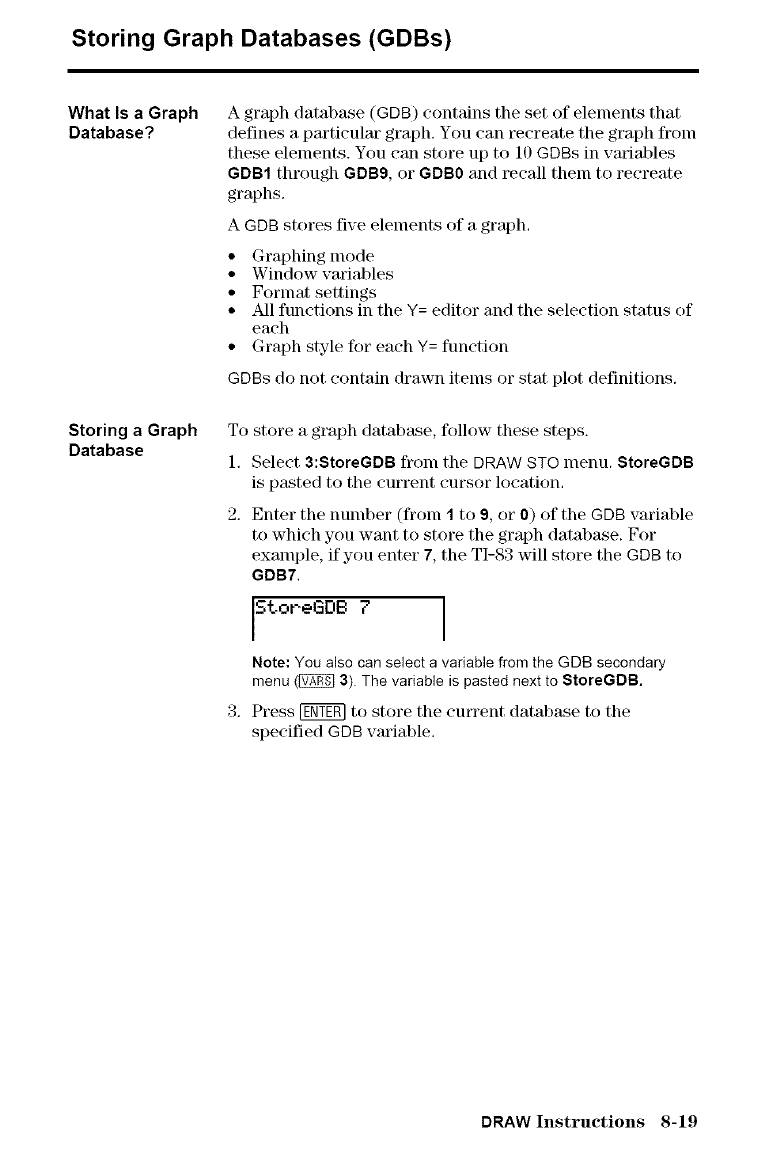
Storing Graph Databases (GDBs)
What Is a Graph
Database.'?
Storing a Graph
Database
A graph database (GDB) contains the set of elements that
defines a pm'ticular graph. You can recreate the graph froln
these elements. You can store up to 10 GDBs in variables
GDB1 through GDB9, or GDB0 and recall them to recreate
graphs.
A GDB stores five elements of a graph.
• Graphing mode
• Window variables
• Format settings
• All functions in the Y= editor and the selection status of
each
• Graph style for each Y= function
GDBs do not contain drawn items or stat plot definitions.
To store a graph database, follow these steps.
1, Select 3:StoreGDB from the DRAW STO menu. StoreGDB
is pasted to the current cursor location,
2. Enter the number (from 1to 9, or 0) of the GDB variable
to which you want to store the graph database. For
example, if you enter 7, the TI-83 will store the GDB to
GDB7,
StoreGDB 7
Note: You also can select a variable from the GDB secondary
menu ([_ 3). The variable is pasted next to $toreGDB.
3, Press 1_ to store the current database to the
specified GDB variable.
DRAW Instructions 8-19
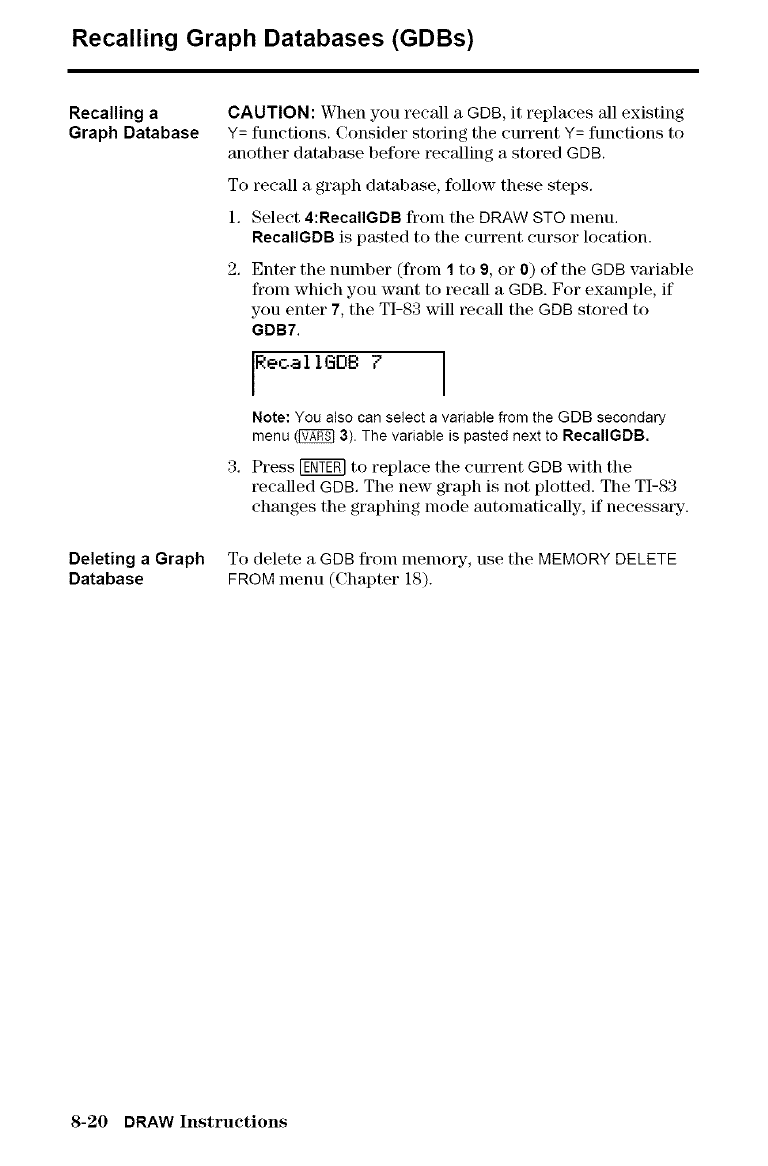
Recalling Graph Databases (GDBs)
Recalling a
Graph Database
Deleting a Graph
Database
CAUTION: When you recall a GDB, it replaces all existing
Y= functions. Consider storing the cutTent Y= functions to
another database before recalling a stored GDB.
To recall a graph database, follow these steps.
1. Select 4:RecalIGDB from the DRAW STO menu.
RecalIGDB is pasted to the current cursor location.
2. Enter the number (from 1to 9, or 0) of the GDB variable
from which you want to recall a GDB. For example, if
you enter 7, the TI-83 will recall the GDB stored to
GDB7,
Reoal IGDB 7
Note: You alsocan selecta variablefromthe GDB secondary
menu(_ 3). The variableis pastednextto RecalIGDB.
3, Press [_ to replace the current GDB with the
recalled GDB. The new graph is not plotted. The TI-83
changes the graphing mode automatically, if necessat T.
To delete a GDB fronl nlemo_T, use the MEMORY DELETE
FROM menu (Chapter 18).
8-20 DRAW Instructions
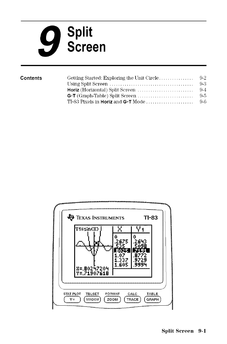
SplitScreen
Contents Getting Started: Exploring tile Unit Circle ................ 9-2
Using Split Screen ....................................... 9-3
Horiz (Horizontal) Split Screen .......................... 9-4
G-T (Graph-Table) Split Screen .......................... 9-5
TI-83 Pixels in Horiz and G-T Mode ...................... 9-6
'_ TEXAS INSTRUMENTS T1=83
','t==in_)JoX IoY 1
_'.', l _, .._,75 1.2,_3
1.07 1.1177_:
2.337 .97:_9
X=.BO:_h7:_O h 1.605 .ggg4
?=.7190761B
J
STATPLOT TBLSET FORMAT CALC TABLE
Split Screen 9-1
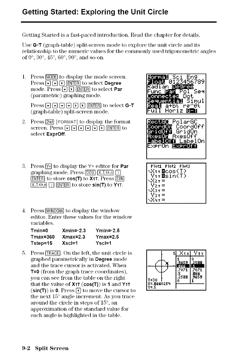
Getting Started: Exploring the Unit Circle
Getting Started is a fast-paced introduction. Read the chapter for details.
Use G-T (graph-table) split-screen mode to explore the unit circle and its
relationship to the numeric values for tile connnonly used trigonometric angles
of 0°, 30 °, 45°, 60 °, 90 °, and so on.
Press [g6m to display the mode screen.
Press [] [] [] [g_ to select Degree
mode. Press [] [] [g_ to select Par
(parametric) graphing mode.
Press [] [] [] [] [] [] [g_ to select G-T
(graph-table) split-screen mode.
Press [_ [FORMAT]to display" the format
screen. Press [] [] [] [] [] [] [g_ to
select ExprOff.
Press [] to display" the Y= editor for Par
graphing mode. Press [g6_ _ []
[ggg_] to store cos(T) to XIT, Press [gF_
[] _ to store sin(T) to YIT.
Press _ to display the window
editor. Enter these values for the window
variables.
Train=0 Xmin=-2.3 Ymin=-2.5
Tmax=360 Xmax=2.3 Ymax=2.fi
Tstep=l 5 Xscl=l Yscl=l
Press _. On the left, the unit circle is
graphed parametrically in Degree mode
and the trace cursor is activated. When
T=0 (from the graph trace coordinates),
you can see from the table on the right
that the value of XlT (cos(T)) is 1and YIT
(sin(T)) is 0. Press [] to move the cursor to
the next 15°angle increment. As you trace
around the circle in steps of 15°, an
approximation of the standard value for
each angle is highlighted in the table.
li X1, V1T
i 0
.g .Bfl6
.zsne ._ss_
T=_O 0 1
g:.BSfi02B_
9-2 Split Screen
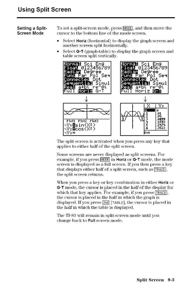
Using Split Screen
Setting a Split-
Screen Mode To set a split-screen lnode, press [MO0_,and then nlove the
cursor to tile bottol:l line of the l:lode screen.
• Select Horiz (horizontal) to display- the graph screen and
another screen split horizontally.
• Select G-T (graph-table) to display the graph screen and
table screen split vertically.
Sci Eng Sci Eng
Dot
The split screen is activated when you press any key that
applies to either half of the split screen.
Sonle screens m'e never displayed +is split screens. For
example, if you press _ in Roriz or G-T inode, the inode
screen is displayed as a full screen. If you then press a key
that displays either half of a split screen, such as _,
the split screen returns.
VC]mnyou press a key or key combination in either Horiz or
6-7 mode, the cursor is placed in the half of the display- for
which that key applies. For example, if you press _,
the cursor is placed in the half in which the graph is
displayed. If you press [g_ [TABLE],the cursor is placed in
the half in which the table is displayed.
The TI-83 will remain in split-screen lnode until you
change back to Full screen mode.
Split Screen 9-3
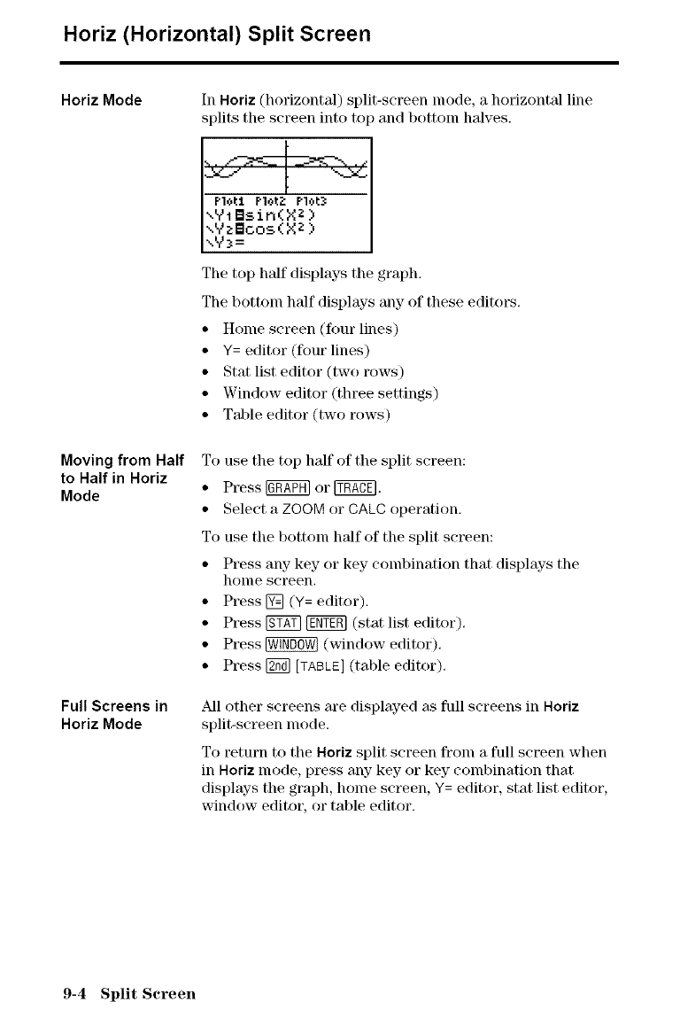
Horiz (Horizontal) Split Screen
Horiz Mode
Moving from Half
to Half in Horiz
Mode
Full Screens in
Horiz Mode
In Horiz (horizontal) split-screen lnode, a horizontal line
splits tile screen into tc ) and bottom halves.
\ViBsin(X z)
,.YzBcos(XZ )
\Y._=
The top half displays the graph.
The bottom half displays any of these editors.
• Home screen (four lines)
• Y= editor (four lines)
• Stat list editor (two rows)
• Window editor (three settings)
• Table editor (two rows)
To use the top half of tile split screen:
• Press [g_ or _.
• Select a ZOOM or CALC operation.
To use tile bottonl half of tile split screen:
• Press any key or key combination that displays the
home screen.
• Press [] (Y= editor).
• Press [gT_ [g_ (stat list editor).
• Press _ (window editor).
• Press [2_ [TABLE](table editor).
All other screens are displayed as full screens in Horiz
split-screen mode.
To return to the Horiz split screen from a full screen when
in Horiz mode, press any- key or key combination that
displays the graph, home screen, Y= editor, stat list editor,
window editor, or table editor.
9-4 Split Screen
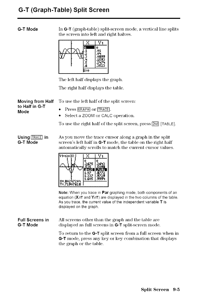
G-T (Graph-Table) Split Screen
G-T Mode
Moving from Half
to Half in G-T
Mode
Using _in
G-T Mode
Full Screens in
G-T Mode
In G-T (graph-table) split-screen mode, a vertical line splits
tile screen into left and right halves.
X Y1
Io
,2: X=Bgq.
The left half displays the graph.
The right half displays the table.
To use the left half of the split screen:
• Press [g_ or _.
• Select a ZOOM or CALC operation.
To use tile right half of the split screen, press [:_ [TABLE].
As you lnove tile trace cursor along a graph in the split
screen's left half in G-T mode, the table on the right half
autolnatically scrolls to match tile current cursor values.
x_ X Vi
1.07 .B77_
1._7_7 ,97:'9
t,l_0g .999h
g=.B0ZtlTZ0h
Y=,7190761B
Note: When you trace in Par graphing mode, both components of an
equation (XnT and YnT) are displayed in the two columns of the table.
As you trace, the current value of the independent variable Tis
displayed on the graph.
All screens other than the graph and the table are
displayed as full screens in G-T split-screen mode.
To return to the G-T split screen from a full screen when in
G-T mode, press any key or key combination that displays
the graph or the table.
Split Screen 9-5
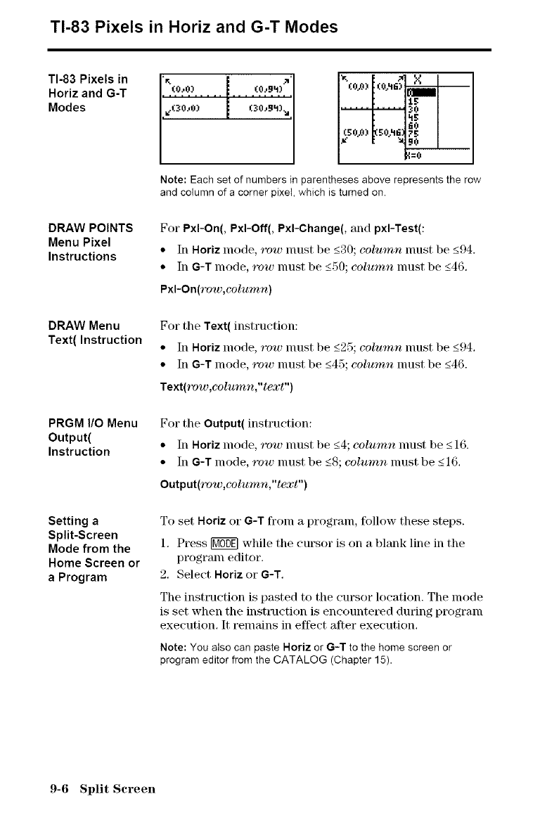
TI-83 Pixels in Horiz and G-T Modes
TI-SaPixelsin "i
Horiz and G-T (o,0.', l .(°._.h.)?l
Modes €,30,0) 1 o0,9_)_,
"*. _ X
lg
30
_g
60
I=o
Note: Each set of numbers in parentheses above represents the row
and column of a corner pixeI, which is turned on.
DRAW POINTS
Menu Pixel
Instructions
For PxI-On(, PxI-Off(, Pxl-Change(, and pxI-Test(:
• In Horiz mode, row nmst be _<30; column nmst be _<94.
• In G-T mode, row nmst be _<50; column nmst be _<46.
Pxl-On(row,column)
DRAW Menu
Text( Instruction
For the Text( instruction:
• In Horiz mode, row nmst be _<25; column must be _<94.
• In G-T mode, row nmst be _<45; column nmst be _<46.
Text(row,column,"text")
PRGM I/O Menu
Output(
Instruction
For the Output( instruction:
• In Horiz mode, row nmst be _<4; column nmst be _<16.
• In G-T mode, row nmst be _<8; column nmst be _<16.
Output(row,column, "text")
Setting a
Split-Screen
Mode from the
Home Screen or
a Program
To set Horiz or G-T from a program, follow these steps.
1. Press [M0_] while the cursor is on a blank line in the
program editor.
2, Select Horiz or G-T,
The instruction is pasted to the cursor location. The mode
is set when the instruction is eneountered during program
execution. It remains in effect after execution.
Note: You also can paste Horiz or G-T to the home screen or
program editor from the CATALOG (Chapter 15).
9-6 Split Screen
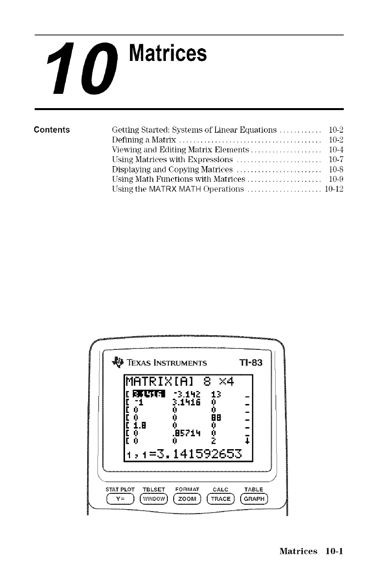
10 Matrices
Contents Getting Started: Systems of Linear Equations ............ 10-2
Defining a Matrix ........................................ 10-2
Viewing and Editing Matrix Elements .................... 10-4
Using Matrices with Expressions ........................ 10-7
Displaying and Copying Matrices ........................ 10-8
Using Math Functions with Matrices ..................... 10-9
Using the MATRX MATH Operations ..................... 10-12
'_ TEXAS iNSTRUMENTS T1=83
MRTRIX[R] 8 x4
r_-_.:l.h_: 1:_
E"1 _:.1h11_ 0
ro 0 0
r 0 0 BB
E1.B 0 0
r 0 .8571h 0
[0 0 2
i, i=3.141592653
J
STATPLOT TBLSET FORMAT CALC TABLE
Matrices 10-1
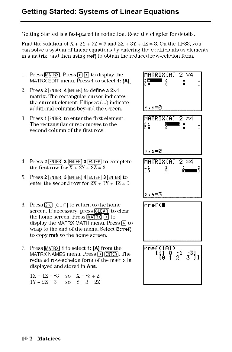
Getting Started: Systems of Linear Equations
Getting Started is a fast-paced introduction. Read the chapter for details.
Find the solution of X + 2Y + 3Z = 3 and 2X + 3Y + 4Z = 3. On the TI-83, you
can solve a system of linear equations by entering the coefficients as elements
in a matrix, and then using rref( to obtain the reduced row-echelon form.
1. Press [_. Press [] [] to display- the
MATRX EDIT menu. Press 1to select 1: [A],
2. Press 2[_ 4[_ to define a 2x4
matrix. The rectangular cursor indicates
the current element. Ellipses (...) indicate
additional eolunms beyond the screen.
3. Press 1[_ to enter the first element.
The rectangular cursor nloves to the
second colunm of the first row.
4.
5.
Press 2[g_ 3[g_ 3[g_ to complete
the first mw for X + 2Y + 3Z = 3.
Press 2[_ 3[_ 4 [_ 3[_ to
enter the second row for 2X + 3Y+ 4Z = 3,
Press [_ [QUIT] to return to the home
screen. If necessary, press @ to clear
the home screen. Press _ [] to
display the MATRX MATH menu. Press [] to
wrap to the end of the menu. Select B:rref(
to copy rref( to the home screen.
Press [_ 1to select 1: [A] from the
MATRX NAMES menu. Press [] FENTERI.The
reduced row-echelon form of the matrix is
displayed and stored in Ans.
iX- 1Z=-3 so X=-3+Z
1Y+2Z=3 so Y=3-2Z
MATRIX[R] 2x4
[0 0
1_1=0
MATRIX[R] 2 x4
[0 0 0
I_Z=0
IMRTRIX[A] 2 x4
rre?(|
rref'([Al )-31
[[1 18 213 ]l
10-2 Matrices
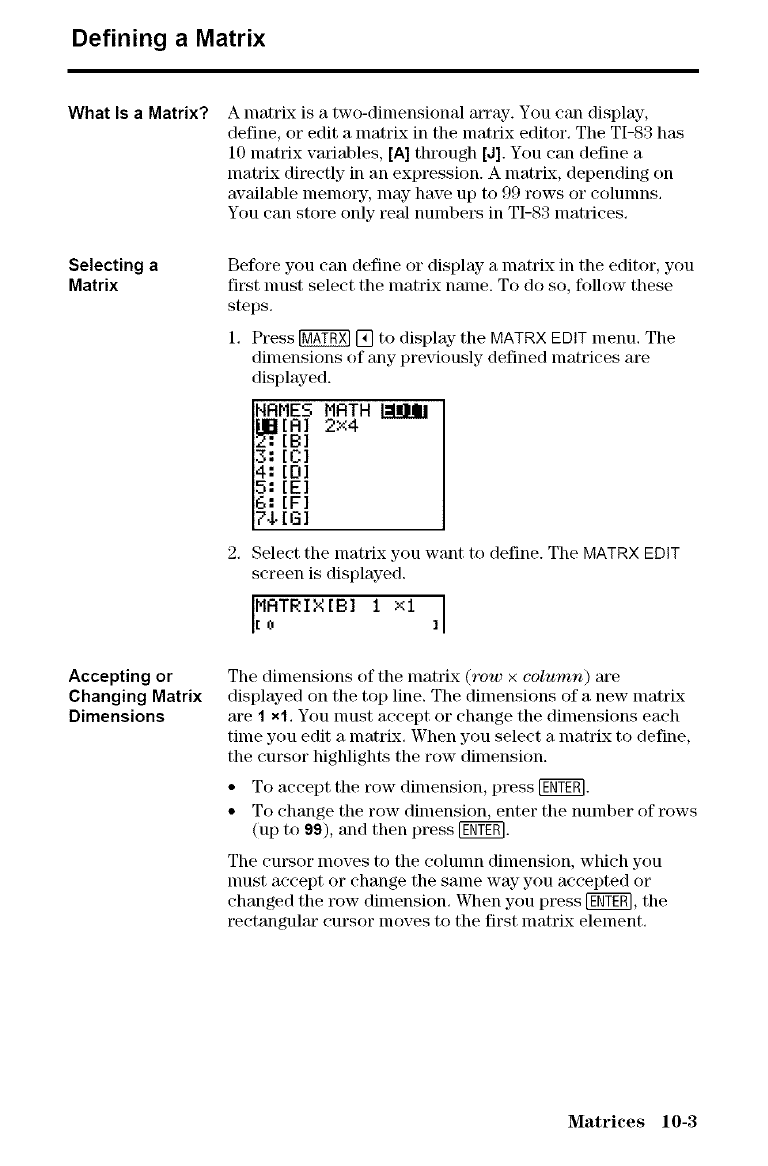
Defining a Matrix
What Is a Matrix? A matrix is a two-dimensional alTay. You can display',
define, or edit a matrix in the matrix editor. Tile TI-83 h_s
10 matrix variables, [A] through [J]. You can define a
matrix directly in an expression. A matrix, depending on
available nlelnolT, may have up to 99 rows or colunms.
You can store only real numbers in TI-83 matrices.
Selecting a
Matrix
Accepting or
Changing Matrix
Dimensions
Before you can define or display a matrix in the editor, you
first nmst select the matrix name. To do so, follow these
steps.
1. Press _ [] to display the MATRX EDIT menu. The
dimensions of any previously defined lnatrices are
displayed.
MATH
[el
[D]
[El
[F]
[G]
2, Select the matrix you want to define. The MATRX EDIT
screen is displayed.
MATRIX[B] I xl
ro I
The dimensions of the matrix (row xcolumn) are
displayed on the top line. The dimensions of a new matrix
are 1 xl, You nmst accept or change the dimensions each
time you edit a matrix, When you select a matrix to define,
the cursor highlighLs the row dimension.
• To accept the row dimension, press [_.
• To change the row dimension, enter the number of rows
(up to 99), and then press [_.
The cursor moves to the eolunm dimension, which you
must accept or change the same way you accepted or
changed the row dimension. When you press [_, the
rectangular cursor moves to the first matrix element.
Matrices 10-3
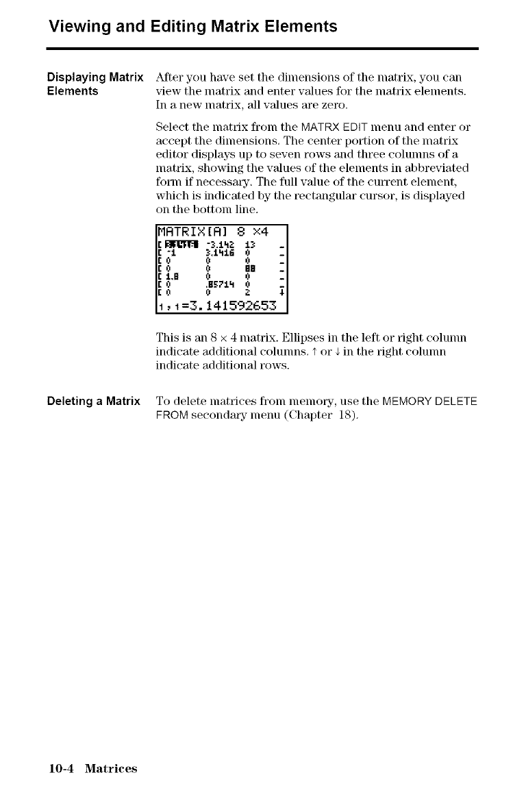
Viewing and Editing Matrix Elements
Displaying Matrix
Elements After you have set the dimensions of the matrix, you can
view the matrix and enter values for the matrix elements.
In a new matrix, 'all values are zero.
Select the matrix from the MATRXEDIT menu and enter or
accept the dimensions. The center portion of the matrix
editor displays up to seven rows and three eolunms of a
matrix, showing the values of the elements in abbreviated
form if necessary. The full vMue of the current element,
which is indicated by the t_ctangular cursor, is displayed
on the bottonl line.
MRTRIX[R] 8 x4 i
"t _:.tht6 0
0
i,i=3. 141592653
This is an 8 x 4 matrix. Ellipses in the left or right colunm
indicate additional columns, i' or _ in the right column
indicate additional rows.
Deleting a Matrix To delete matrices fronl nlenlory, use the MEMORY DELETE
FROM seconding- menu ((;hapter 18).
10-4 Matrices
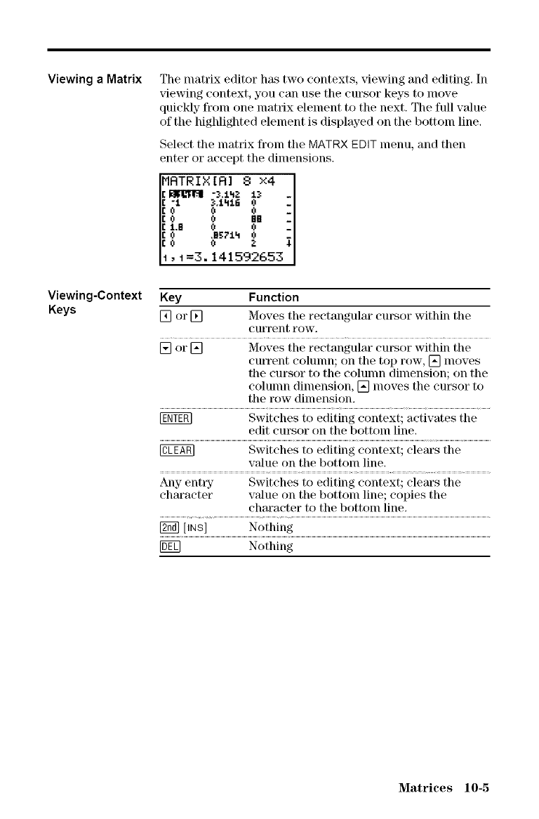
Viewing a Matrix
Viewing-Context
Keys
The matrix editor has two contexts, viewing and editing, In
viewing context, you can use the cursor keys to move
quickly from one matrix element to the next. The full value
of the highlighted element is displayed on the bottom line,
Select the inatrix fl'oin the MATRX EDIT menu, and then
enter or accept the dimensions.
MRTRIX[R] 8 x4 1
":1, }.:DI:I.I_ 0
2
I,I=3. 141592653
Key Function
[] or [] Moves the rectangular cursor within the
current row.
[] or [] Moves the rectangular cursor within the
current coluinn; on the top row, [] moves
the cursor to the colunm dimension; on the
coluinn dimension, [] moves the cursor to
the row dimension.
[gNT_ Switches to editing context; activates the
edit cursor on the bottom line.
@ Switches to editing context; clears the
value on the bottoin line.
Any entry Switches to editing context; clears the
character value on the bottoln line; copies the
character to the bottom line.
[_ [INS] Nothing
[ggn Nothing
Matrices 10-5
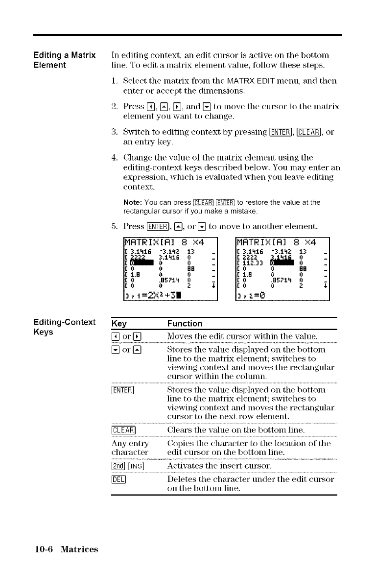
Editing aMatrix
Element
Editing-Context
Keys
In editing context, an edit cursor is active on the bottom
line. To edit a lnatrix element value, follow these steps.
1. Select the matrix from the MATRX EDiT menu, and then
enter or accept the dimensions.
2. Press [], [], [], and [] to nlove the cursor to the lnatrix
element you want to change.
3. Switch to editing context by pressing [ggT_, @, or
an entw key-.
4. Change the value of the tnatrix element using the
editing-context keys described below. You nlay enter an
expression, which is evaluated when you leave editing
context.
Note: You can press @ _ to restore the value at the
rectangular cursor if you make a mistake.
5. Press IgOr, [], or [] to Inove to another element.
MRTRIX[RI 8 ×4
r :Ll_ntG ":kl_ 13
[ 0 0 BII
[:t.B 0 0
[0.BgT:th 0
[0 0
3, i=2Xz+3|
MRTRIX[R] 8 x4 i
3.1_I_ ").1ill 1_
Key Function
[] or [] Moves the edit cursor within the value,
[] or [] Stores the value displayed on the bottom
line to the nlatrix element; switches to
xqewing context and nloves the rectangular
cut.or within the colunm.
[g_Tgm Stores the value displayed on the bottom
line to the nlatrix element; switches to
viewing context and moves the rectangular
cm'sor to the next row element.
@ Clears the value on the bottom line.
Any entry- Copies the character to the location of the
character edit cursor on the bottom line.
[_ [INS] Activates the insert cursor.
[DE[] Deletes the character under the edit cursor
on the bottonl line.
10-6 Matrices
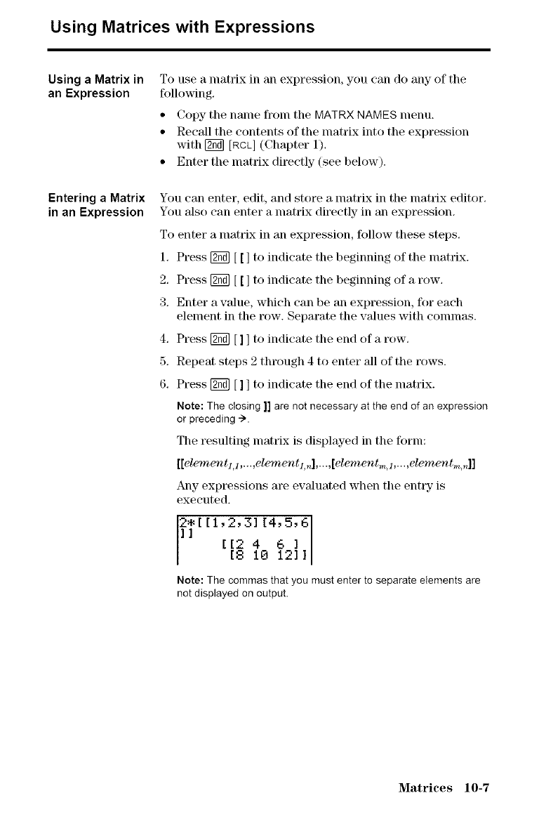
Using Matrices with Expressions
Using a Matrix in
an Expression
Entering a Matrix
in an Expression
To use a matrix in an expression, you can do any of the
following.
• Copy the name from the MATRX NAMES menu.
• Recall the contents of the lnatrix into the expression
with [_ [RCL] (Chapter 1).
• Enter the matrix directly (see below).
You can enter, edit, and store a matrix in the nlatlJx editor.
You also can enter a nlatrix directly in an expression.
To enter a nlatrix in an expression, follow these steps.
1. Press [2_] [ [ ] to indicate the beginning of the nlatrix.
2. Press [2_] [ [ ] to indicate the beginning of a row.
3. Enter a value, which can be an expression, for each
element in the row. Sepm'ate the values with conlnlas.
4. Press [2_] [] ] to indicate the end of a row.
5. Repeat steps 2 through 4 to enter all of the rows.
6. Press [2_] [] ] to indicate the end of the nlatrix.
Note: The closing ]] are not necessary at the end of an expression
or preceding -'>.
The resulting matrix is displayed in the form:
[[elementl,l,._,elementl,_l,...,[element.,,_,l,...,element,,_,_]]
Any expressions are evaluated when the enttsz is
executed.
2.[11[1,2,31[[_418"1014'5'161211
Note: The commas that you must enter to separate elements are
not displayed on output.
Matrices 10-7
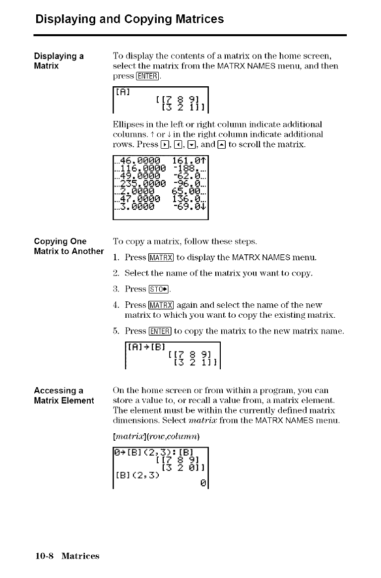
Displaying and Copying Matrices
Displaying a
Matrix
Copying One
Matrix to Another
Accessing a
Matrix Element
To display- the contents of a matrix on the home screen,
select the nmtrix from tile MATRX NAMES menu, and then
press [_.
lEA, El; 711
Ellipses in the left or fight eolunm indicate additional
colunms. I' or 4 in the right colunm indicate additional
rows. Press [_, [], [], and [] to scroll the lnatrix.
46.0000 I
...116. 0000
...49. 0000 --62. (_iiiI
-96.8...I
%88oo
65.00...I
i::47'. 0000 -69.04,
...3, 0000 136,0...
To copy a matrix, follow these steps.
1. Press [_ to display the MATRXNAMES menu.
2. Select the name of the lnatrix you want to copy.
3. Press _.
4. Press _ again and select the name of the new
nmtrix to which you want to copy the existing matrix.
5. Press [_ to copy the lnatrix to the new lnatrix nalne.
On the home screen or fronl within a program, you can
store a vMue to, or recM1 a value from, a matrix element.
The element nmst be within the currently defined matrix
dimensions. Select matrix from the MATRX NAMES menu.
[matrixl(row,column)
0-:* [BI (2, 3)-" [BI
[[7 891
[B1(2,3)[3 20110
10-8 Matrices
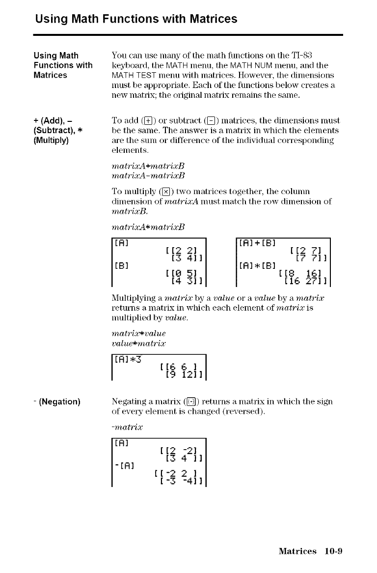
Using Math Functions with Matrices
Using Math
Functions with
Matrices
+ (Add), -
(Subtract), *
(Multiply)
-(Negation)
You can use many of the math functions on the TI-83
keybom'd, tile MATH menu, tile MATH HUM menu, and tile
MATH TEST menu with matrices. However, the dimensions
nmst be appropriate. Each of the functions below creates a
new matrix; the original matrL, c remains the same.
To add ([_) or subtract ([_) matrices, the dimensions must
be the same, The answer is a matrix in which the elements
are the sum or difference of the individual corresponding
elements.
matrixA +matrixB
matrixA -mat)_ixB
To nmltiply ([_) two matrices together, the colunm
dimension of matrixA nlust match the row dimension of
matrixB.
matrixA *mat_qxB
Multiplying a matrix by a value or a value by a matrix
returns a matrix in which each element of matrix is
nmltiplied by value,
matrix*value
value*matrix
Negating a matrix (D) returns a matrix in which the sign
of evetN element is changed (reversed),
-matrix
[RI [[212; 41-211]
-ira -41
Matrices 10-9
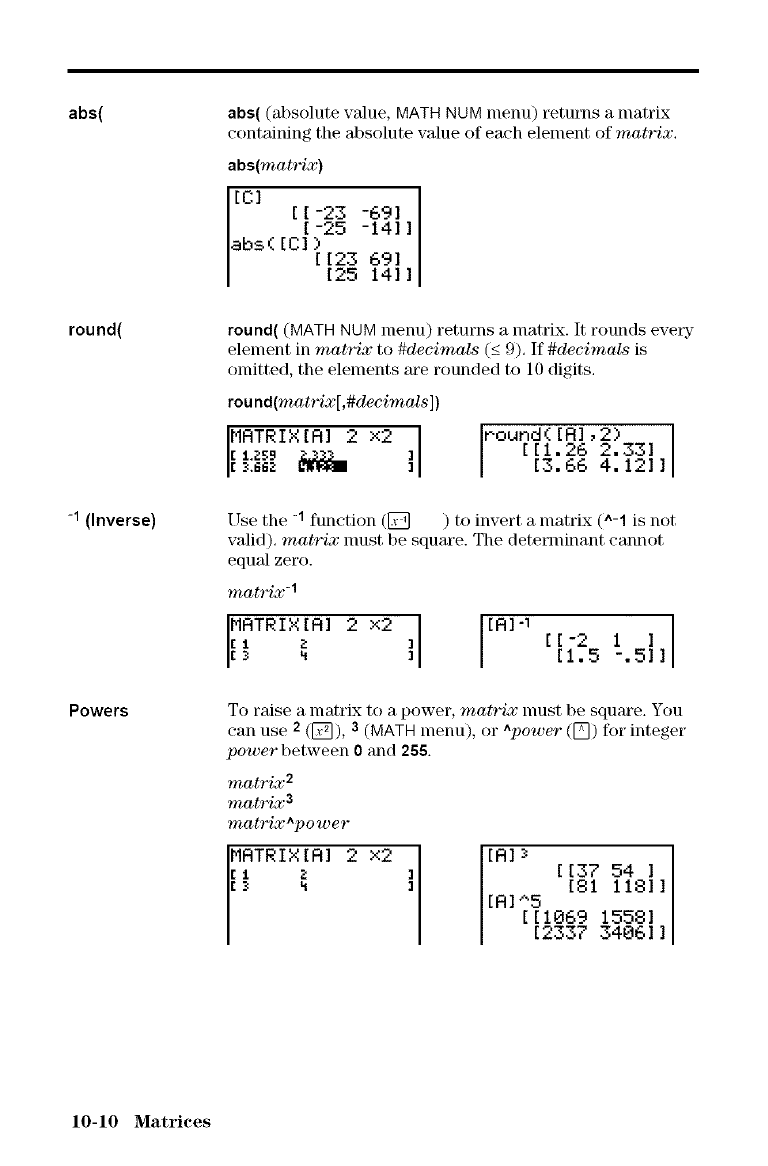
abs(
round(
-I (Inverse)
Powers
abs( (absolute value, MATH NUM menu) returns a matrix
containing the absolute value of each element of matrix.
abs(mat_qx)
[°] 14,69'
abs([Cl_[2512369]14]
round( (MATH NUM menu) returns a matrix. It rounds every
element in matrix to #decimals (<_9), If #decimals is
olnitted, the elements are rounded to 10 digits,
rou nd(mat)qx[ ,#decimals ])
MAT IX[m2 ×2 1
[3,662 I,'15_ Pound([A],2) ]
[[1.26 2.331
[3.66 4.121
[Jse the -1 function ([_ ) to invert a matrix ("-1 is not
valid), matrix nmst be square. The determinant cannot
equal zero.
matrix-1
MRTRIX[R] 2 x2 ] l[m-, ]
El z[[-2 1 ]E_ _ [1.5 -.51
To raise a lnatrix to a power, matrix lnust be square. You
can use 2 (_), 3 (MATH menu), or ^power (D) for integer
power between 0 and 2S&
matrix 2
matrix 3
matrix^power
MRTRIX[R]__ 2 x2 ] [R]_ i
[[37 54 ]
[81 1181
[R]_,5
[[1069 15581
[2337 34061
10-10 Matrices
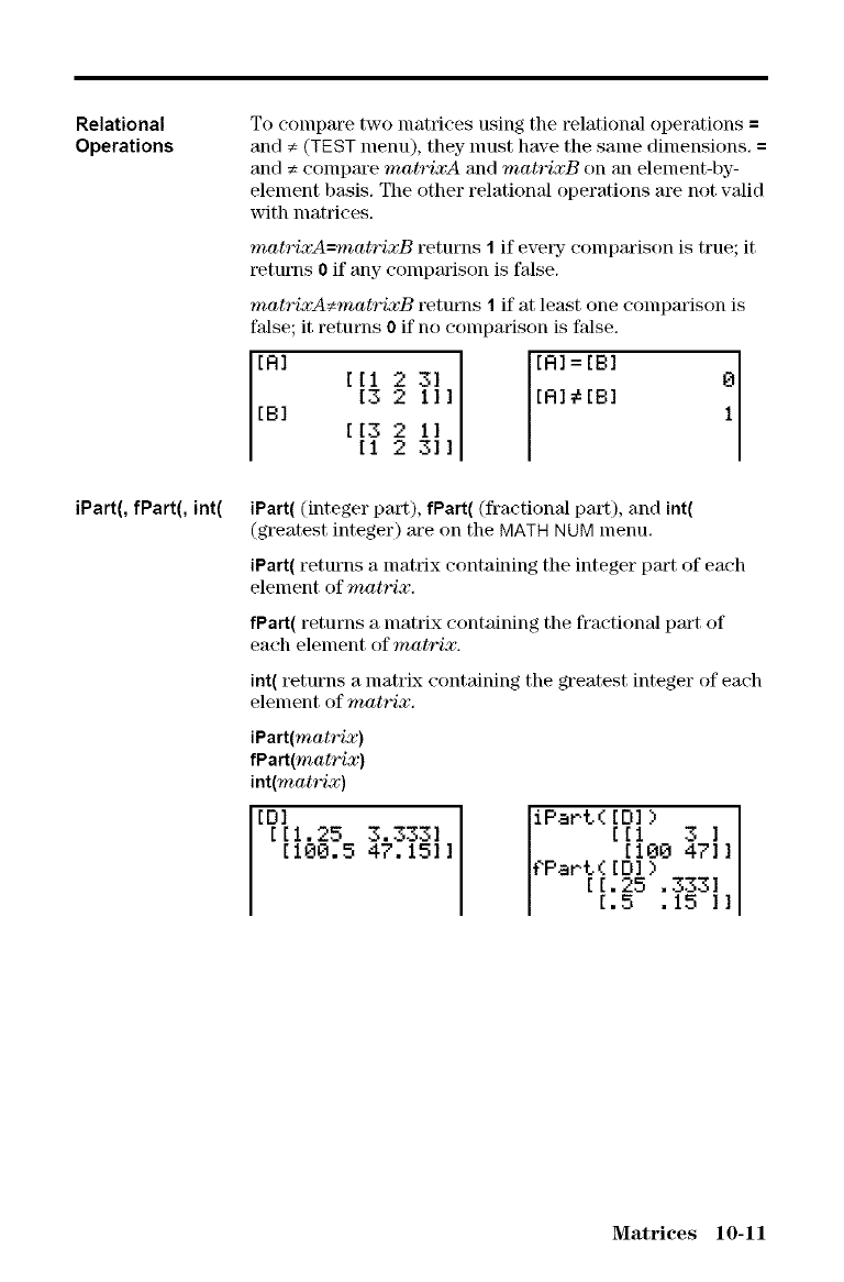
Relational
Operations
iPart(, fPart(, int(
To compare two matrices using the relational operations =
and _ (TEST menu), they must have the sanle dimensions, =
and _ compare mat_ixA and mat_ixB on an element-by-
element basis. The other relational operations are not valid
with matrices.
matri._'A=matrixB returns 1if eveFy" comparison is true; it
t_tums 0 if any comparison is false.
matrixA_matrixB t_tums 1if at least one comparison is
false; it returns 0 if no comparison is false,
[R]=[B]
[RI#[B]
iPart( (integer part), fPart( (fractional part), and int(
(greatest integer) are on the MATH NUM menu,
iPart( returns a matrix containing the integer part of each
element of matrix,
fPart( returns a matrix containing the fractional part of
each element of matrix.
int( returns a matrix containing the greatest integer of each
element of matrix,
iPart(matrix)
fPart(matrix)
int(matrix)
100.5 47. 151
iPaPt([D1) i
[[1 31
[100 471
¢PaPt([D])
[[.25 .3331
[.5 .15 ]
Matrices 10-11
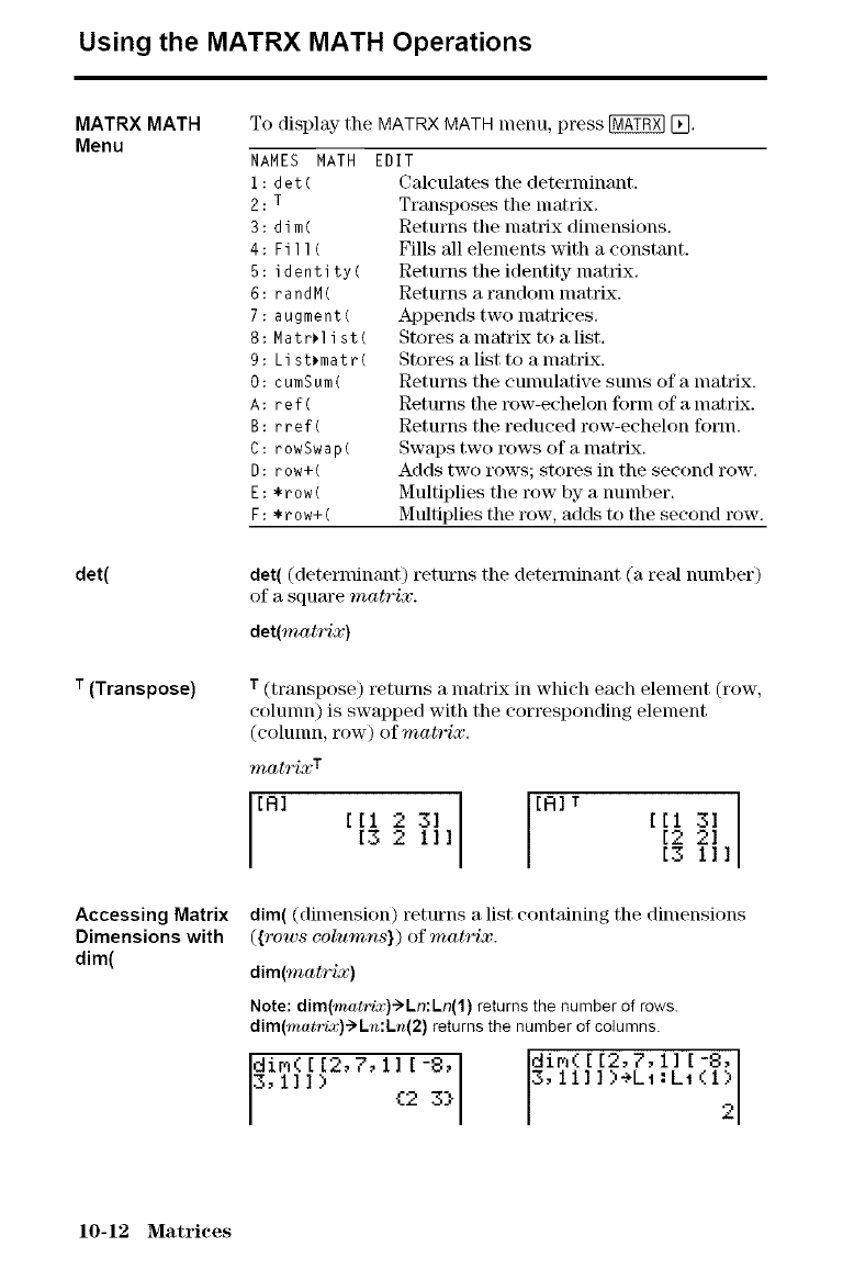
Using the MATRX MATH Operations
MATRX MATH
Menu
det(
T(Transpose)
Accessing Matrix
Dimensions with
dim(
To display the MATRX MATH menu, press _ [_,
NAMES MATH
i: det(
2: T
3: dim(
4: Fill(
5:identity(
6: randM(
7:augment(
8: Matr*list(
9: List*matr(
O: cumSum(
A: ref(
B: rref(
C: rowSwap(
D: row+(
E: *row(
F: *row+(
EDIT
Calculates the determinant.
Transposes the matrix,
Returns the matrix dimensions.
Fills all elements with a constant.
Returns the identity matrix.
Returns a random matrix.
Appends two matrices.
Stores a matrix to a list.
Stores a list to a matrix.
Returns the eunmlative sums of a matrix.
Returns the row-echelon form of a matrix.
Returns the reduced row-echelon form.
Swaps two rows of a matrix.
Adds two rows; stores in the second row.
Multiplies the row by a number.
Multiplies the row, adds to the second row.
det((determinant) returns the determinant (a real number)
of a squm'e matrix.
det(matrix)
T(transpose) returns a matrix in which each element (row,
colunm) is swapped with the corresponding element
(colunm, row) of matrix.
matrix T
[R]
[[1 2 311
[32 11
[R]T
[3 11
dim((dimension) returns a list containing the dimensions
({rows columns} ) of mat_qz.
dim(matrix)
Note: dim(mat'rix)->Ln:Ln(1) returns the number of rows.
dim(mat'rix)->Ln:Ln(2) returns the number of columns.
dim( [_2,7,11[ -8, dim([l>+Li:L1
3,111 {2 3} 3,111
10-12 Matrices
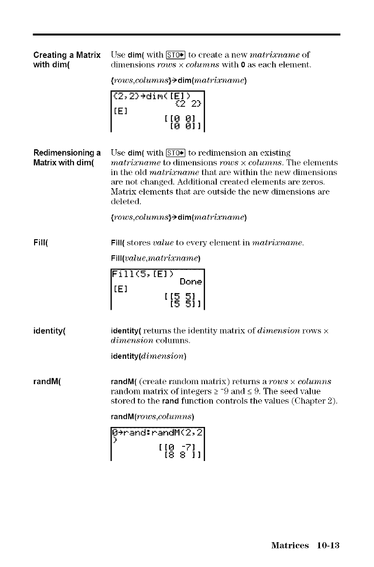
Creating a Matrix
with dim(
Redimensioning a
Matrix with dim(
Fill(
identity(
randM(
Use dim( with _ to create a new matrixname of
dimensions rows x columns with 0_Lseach element.
{rows,columns}_dim(mat_xname)
{2,2}+di_([E]) I
I
[0 01
[E] [ [0 011
Use dim( with _ to redimension an existing
matrixname to dimensions rows xcolumns, The elements
in the old matrixname that m_ within the new dimensions
are not changed. Additional created elements are zeros.
Matrix elements that m'e outside the new dimensions are
deleted.
{rows,columns}-> dim(matrixname)
Fill(storesv_uetoeve_ elementin mat_xname.
Fill(v_ue,mat_xname)
FilI(5,[E]) Done
[El [[5 5]
[5 51]
identity( returns the identity matrix of dimension rows x
dimension colunms.
identity(dimension)
randM( (create random matrix) returns a rows xcolumns
random matrix of integers _>-9 and _<9, The seed value
stored to the rand function controls the values (Chapter 2),
randM(rows,eolumns)
I÷r-and: PahdM(2,2 I
[[0 -71
[88 1]
Matrices 10-13
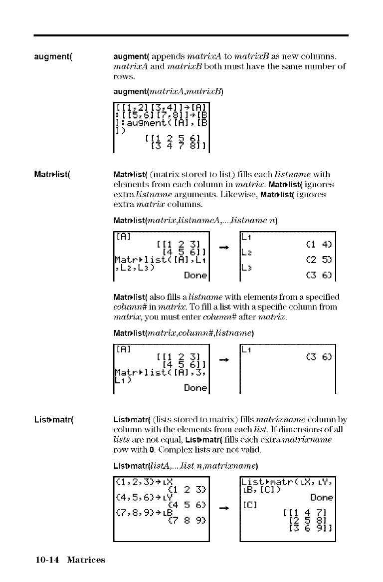
augment(
Mats,list(
augment( appends matrixA to matrixB as new colunms.
matrixA and mahqxB both nlust have tile sanle number of
[_)WS.
augment(mat) qxA,matrixB)
[1,21 [3,41 ]+JR] ]
[ [5,61 [7,811+[BI
_a,.,gr,,ent([Rl,[B[
[[1 256]
[3 47811
MatrHist( (lnatrix stored to list) fills each listname with
elements from each colunm in mahqx. MatrHist( ignores
extra listname arguments. Likewise, MatrHist( ignores
extra matrix colunms.
MatrHist(matrix,listnomeA,._,listname n)
[[R] [[1 2 31It( i_ {I ii
MatP_lis[4 5 611 "* Lz
,Li,LI) [Rl,LiDone {3{25}
MatrHist( also fills alistname with elements fronl a specified
column# in matrix. To fill a list vdth a specific colunm from
matrix, you lnust enter column# _ffter matrix.
Mat_list(matrix,column#,listnome)
[R] It1 2 31 ILt {3 6}
[a 56111 "*
Matr_list(
Lt )JR] ,3,
Done
Listymatr( List)matr( (lists stored to matrL, c) fills matrixna,me colunm by
colunm with the elements fronl each list. If dimensions (ffMI
lists are not equal, Cist_matr(fills each extra matrixna,r_w
row with O.Conlplex lists are not valid.
List_matr(listA,._,list n,mah_xname)
List.*matP( IX, L_", I
{1'2'3}+L_I 2 3} LB,[CI) O°nel'
{4'5'6]'+L_4 5 _ ... [C] [[1 _ _ll]l
10-14 Matrices
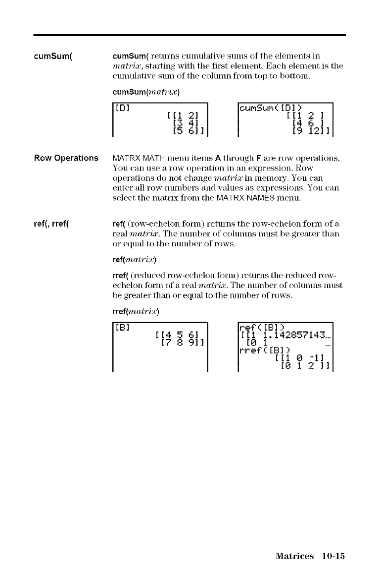
cumSum(
Row Operations
ref(, rref(
cumSum( returns cumulative sums of the elements in
mat_'ix, starting with tlle first element. Each element is the
cumulative sum of the colunm from top to bottom.
cumSum(mat,_ix)
[0] [[1151361412]] °ur_Su'_([Dl_[9[46212]]]]
MATRX MATH menu items A th['ough F m'e row operations.
You can use a row operation in an expression, Row
operations do not change matrix in nlenloi_yL You can
enter all row numbers and values as expressions. You can
select the matrix fronl the MATRX NAMES menu,
ref( 0"ow-echelon fornl) returns the row-echelon if)rill of a
real mat'_i:c. The number of columns must be greater than
or equal to the number of _'ows.
ref(mat,_ix)
rref( (reduced row-echelon ff)rm) ret, umls the reduced row-
echelon form of a _al matrix', The number of colunms must
be greater than or equal to the number of rows,
rref(mat,_ix)
[B] [ [4 5 6] ]
[7 89]
re?([B])
[[1 1.142857143_3
[0 1 ...
rre?([B])
[[1 0 -1]
[0 1 2 ]]
Matrices 10-15
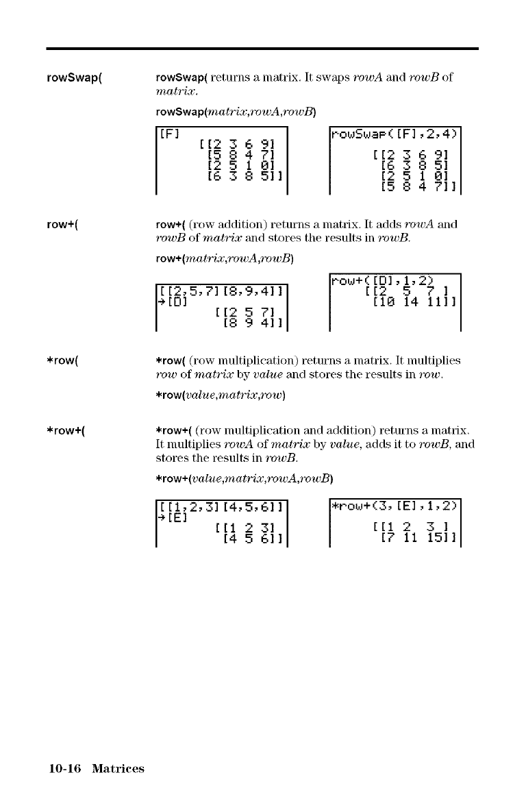
rowSwap(
row+(
* row(
* row+(
rowSwap( returns a matrix, It swaps rowA and rowB of
matrix,
rowSwap(matrix, rowA,rowB)
[F] [[2 _ 46 791]
[2 5 1 O]
[6 3 8 51
PowSwaP ( [F] ,2,4>[I
row+( (row addition) returns a lnatnx. It adds rowA and
rowB of matrix and stores the results in rowB.
row+(mat_x,rowA,rowB)
[[2,5,7118,9,411
+[O] [[2 5 71
[8 9 41 row+{[D],l,2)[1012514711111
*row( (row nmltiplieation) returns a matrix. It nmltiplies
row of matrix by value and stores the results in row.
*row(value,matrix,row)
*row+( (row nmltiplication and addition) returns a nlatdx,
It nmltiplies rowA of matrix by value, adds it to rowB, and
stores the results in rowB.
*row+(value,matrix,rowA,rowB)
*Pow+(3, [E], 1,2) I
[[1 21 3511
10-16 Matrices
11 Lists
Contents Getting Started: Generating a Sequence .................. I I-2
Naming Lists ............................................. 11-3
Storing and Displaying Lists ............................. 11-4
Entering List Names ..................................... 11-6
Attaching Fornmlas to List Names ....................... 11-7
Using Lists in Expressions ............................... 11-9
LIST ©PS Menu .......................................... 11-10
LIST MATH Menu ........................................ 11-17
'_ TEXAS iNSTRUMENTS T1=83
cunSu_,( {1,2, 3, 4,
5} ){1 6 18 15}
J
STATPLOT TBLSET FORMAT CALC TABLE
Lists 11-1
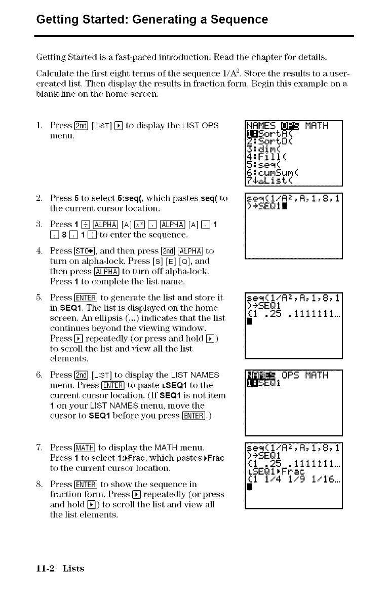
Getting Started: Generating a Sequence
Getting Started is a fast-paced introduction. Read the chapter for details.
Calculate the first eight terms of the sequence i/k-'. Store the results to a use>
created list. Then display the results in fraction form. Begin this example on a
blank line on the home screen.
1, Press [gfi_ [LIST] [] to display the LIST OPS
nlenu,
2. Press 6to select 6:seq(, which pastes seq( to
the current cursor location.
3. Press l[] @ [A][] [] @ [A][] l
[] 8[] 1[] to enter the sequence.
4. Press F_, and then press [_ @ to
turn on alpha-lock. Press [s] [E] [Q], and
then press @ to turn off alpha-lock.
Press 1to complete the list name.
5. Press F_ to generate the list and store it
in SEQ1. The list is displayed on the home
screen. An ellipsis (...) indicates that the list
continues beyond the viewing window.
Press [] repeatedly- (or press and hold [_)
to scroll the list and view all the list
elements.
Press [gfi_ [LIST] to display the LIST NAMES
menu. Press FENTEmto p_Bte LSEQ1to the
current cursor location. (If SEQ1 is not item
1 on your LIST NAMES menu, move the
cursor to SEQ1 before you press F_.)
7. Press [_ to display the MATH menu.
Press 1to select 1:*Frac, which pastes *Frac
to the current cursor location.
8. Press F_ to show the sequence in
fraction form. Press [] repeatedly (or press
and hold [_) to scroll the list and view all
the list elements.
MRTH
3:dim(
4:Fill(
5:se_(
8:cumSu_(
7$_List(
se_(I/RZ,R,1,8,1
i;S_ .1111111...
_IOPS MRTH
Ise_(i/Ri,R,1,8,1
)+SEQI
{i .25 .1111111._
LSEQI*Frac
_I 1/4 1,'9 Ix16_.
11-2 Lists
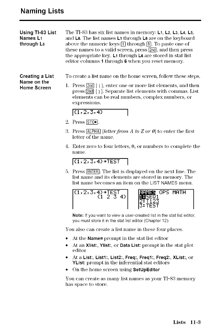
Naming Lists
Using TI-83 List
Names L1
through L6
Creating a List
Name on the
Home Screen
The TI-83 has six list names in nlenlol_-: L1, L2, L3, L4, L5,
and L6. The list names L1 through L6 are on the keyboard
above the numeric keys [] through [_. To paste one of
these names to a valid screen, press E_], and then press
the appropriate key. L1 through L6 are stored in stat list
editor colunms 1through 6when you reset nlenlory,
To create a list name on the home screen, follow these steps.
1. Press [_] [ { ], enter one or more list elements, and then
press [_ [ }]. Separate list elements with conunas. List
elements can be real nulnbe_\s, complex numbers, or
expressions.
I<1'2'3'4> I
2. Press _.
3. Press @ [letter from A to Z or 0] to enter the first
letter of the name.
4. Enter zero to four letters, 0, or numbers to complete the
nanle.
[<10203,4}+TEST I
5, Press [E_, The list is displayed on the next line. The
list name and its elements are stored in memory. The
list name becomes an item on the LIST NAMES menu.
_:I,2,3,4]'+TEST{I2 3 4} 21TEI2_""_OPS MRTH I
Note: if you want to view a user-created list in the stat list editor,
you must store it in the stat list editor (Chapter 12).
You also call create a list nalne ill these four places,
• At the blame= prompt in the stat list editor
• At an Xlist:, Ylist:, or Data List: Dxnnpt in the stat plot
editor
• At a List:, List1:, List2:, Freq:, Freql:, Freq2:, XList:, or
YList: prompt in the inferential stat editors
• On the home screen using SetUpEditor
You can create as many list names as your TI-83 memo[3z
has space to store.
Lists 11-3
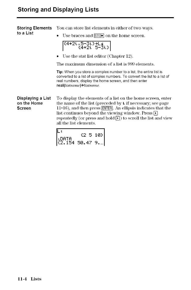
Storing and Displaying Lists
Storing Elements
to a List
Displaying a List
on the Home
Screen
You can store list elements in either of two ways.
• Use braces and _ on the home screen.
{4+2t, 5-3t } _k G
{4+2t _,-3t }
• Use the stat list editor (Chapter 12).
The maxinmm dimension of a list is 999 elements.
Tip: When you store a complex number to a list, the entire list is
converted to a list of complex numbers. To convert the list to a list of
real numbers, display the home screen, and then enter
real(listname)->listname.
To display" the elements of a list on the home selden, enter
the name of the list (preceded by L if neeessa_77; see page
11-16), and then press FEET'. An ellipsis indicates that the
list continues beyond the viewing window. Press []
repeatedly (or press and hold []) to scroll the list and view
all the list elements.
_IDRTR {2 5 _0}
{2. 154 50,47 ....
11-4 Lists
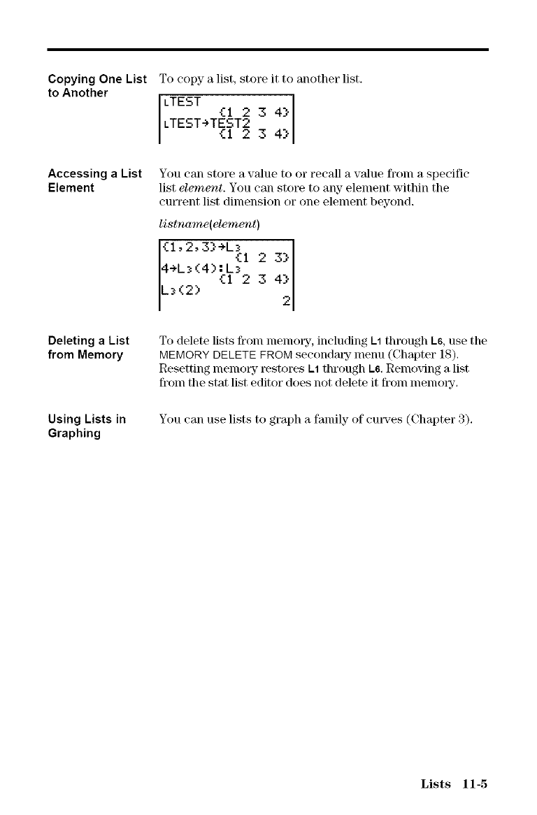
Copying One List
to Another
Accessing aList
Element
Deleting a List
from Memory
To copy a list, store it to another list.
LTEST {123:}}
LTEST÷TEST2
{123
You can store a value to or recall a value fronl a specific
list element. You can store to any element within the
current list dimension or one element beyond.
listname(element)
{1'2'3}÷L_I 23}
4÷L_(4){L_234
L:_(z.) }2
To delete lists fronl nlenlol_, including L1through L6,use the
MEMORY DELETE FROM secondatF- menu (Chapter 18).
Resetting nlenlory restores L1through L6. Removing a list
from the stat list editor does not delete it from nlenlol_L
Using Lists in
Graphing
You can use lists to graph a family of creates (Chapter 3).
Lists 11-5
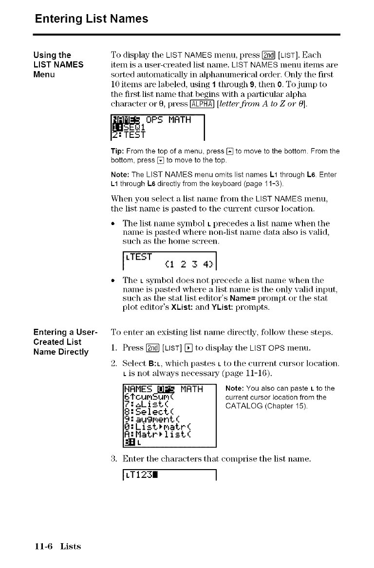
Entering List Names
Using the
LIST NAMES
Menu
Entering a User-
Created List
Name Directly
To display- the LIST NAMES menu, press [_ [LIST]. Each
item is a user-created list name. LIST NAMES menu items m'e
sorted automatically in alphanumerieal order. Only the first
10 items are labeled, using 1 through 9, then 0. To jump to
the first list name that begins with a particulm" alpha
character or 0, press @ [letter from A to Z or 0].
_ IOF'S MRTH
TI
Tip: From the top of a menu, press [] to move to the bottom. From the
bottom, press [] to move to the top.
Note: The LIST NAMES menu omits list names I_1through 1.6. Enter
L1through L6 directly from the keyboard (page 11-3).
When you select a list name from the LIST NAMES menu,
the list name is pasted to the cmTent cursor location.
• The list name symbol, precedes a list nmne when the
name is pasted where non-list name data also is valid,
such as the home screen.
LTEST (I 2 34}
• The Lsymbol does not precede a list name when the
name is pasted where a list name is the only valid input,
such as the stat list editor's Name-- p_x)mpt or the stat
plot editor's XList: and YList: prompts.
To enter an existing list nmne directly-, follow these steps.
1. Press [_ [LIST] [] to display" the LIST OPS menu.
Select B:L, which pastes Lto the current cursor location.
L is not always necessary (page 11-16).
NRMES [_]_R MRTH Note: You also can paste L to the
61"CMFISL, Ir'l (current cursor location from the
7: _List( CATALOG (Chapter I5).
8: Selec.t(
9: augrqent(
81List*F, ate(
R: Mate* 1ist(
=11,
3. Enter the characters that conlprise the list name.
ILT123I I
11-6 Lists
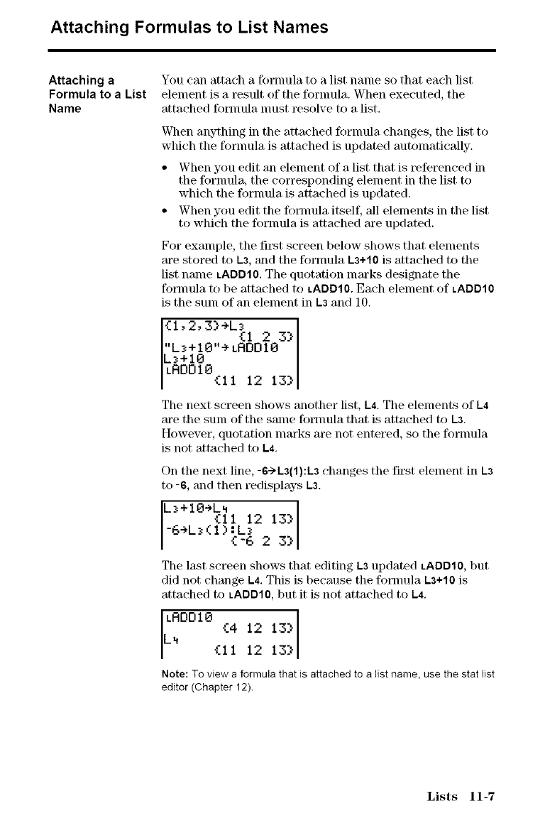
Attaching Formulas to List Names
Attaching a
Formula to a List
Name
You call attach a formula to a list name so that each list
element is a result of the fornmla. When executed, the
attached formula nmst resolve to a list.
V_llen anything in the attached formula changes, the list to
which the fornmla is attached is updated automatically.
• When you edit an element of a list that is referenced in
the fornmla, the corresponding element in the list to
which the fornmla is attached is updated.
• When you edit the fonnula itself, all elements in the list
to which the fornmla is attached are updated.
For example, the fit\st screen below shows that elements
are stored to L3, and the fornmla L3+10 is attached to the
list name LADD10, The quotation lnarks designate the
formula to be attached to LADD10. Each element of LADD10
is the sum of an element in L3 and 10.
{I°2'3}÷L_I 2 3}[
"L_+IO"+ LADD10
La+IB I
LRDD10
{11 12 13}
The next screen shows another list, L4.The elements of L4
are the sum of the same formula that is attached to L3.
However, quotation marks are not entered, so the fornmla
is not attached to L4,
On the next line, -6->L3(1):L3 changes the first element in L3
to -6, and then redisplays L3.
W+IO+L4 I
{II 12 13}I
-6÷Li(1):Li
{-6 2 3}
Tile last screen shows that editing L3updated LADD10, but
did not change L4. This is because the formula L3+10 is
attached to LADDIO,but it is not attached to L4.
LRDDIO {4 12 13}
L4 {Ii 12 13}
Note: To view a formula that is attached to a list name, use the stat list
editor (Chapter12).
Lists 11-7
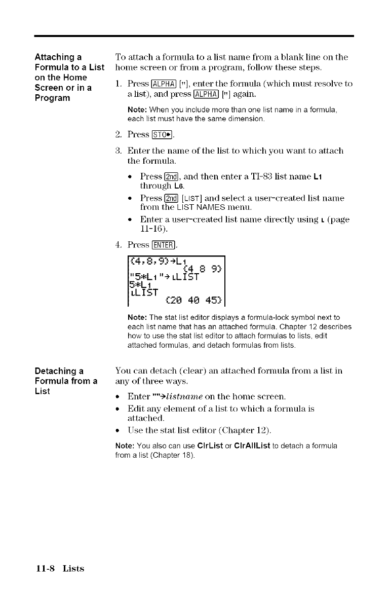
Attaching a
Formula to a List
on the Home
Screen or in a
Program
Detaching a
Formula from a
List
To attach a ff)rnmla to a list name from a blank line on the
home screen or from a program, follow these steps.
1. Press @ [.], enter the formula (which must resolve to
a list), and press @ [-] again.
Note: When you include more than one list name in a formula,
each list must have the same dimension.
2,
3.
Press _.
Enter the name of the list to which you want to attach
the fornmla.
• Press [_, and then enter a TI-83 list name kl
through ks.
• Press [_ [LIST] and select a usm_created list name
from the LIST NAMES menu.
• Enter a use_created list name directly- using t (page
11-16).
Press ITNt_RI.
{4, 8, 9}÷L_4 8 9}
"5*LI '% tLIST
5.LI
LLIST {28 40 45}
Note: The stat list editor displays a formula-lock symbol next to
each list name that has an attached formula. Chapter 12 describes
how to use the stat list editor to attach formulas to lists, edit
attached formulas, and detach formulas from lists.
You can detach (cleat') an attached fornmla fron] a list in
any- of tht_e ways.
• Enter ""Olistname on the home screen.
• Edit any element of a list to which a fornmla is
attached.
• Use the stat list editor (Chapter 12).
Note: You also can use ClrList or ClrAIIList to detach a formula
from a list (Chapter 18).
11-8 Lists
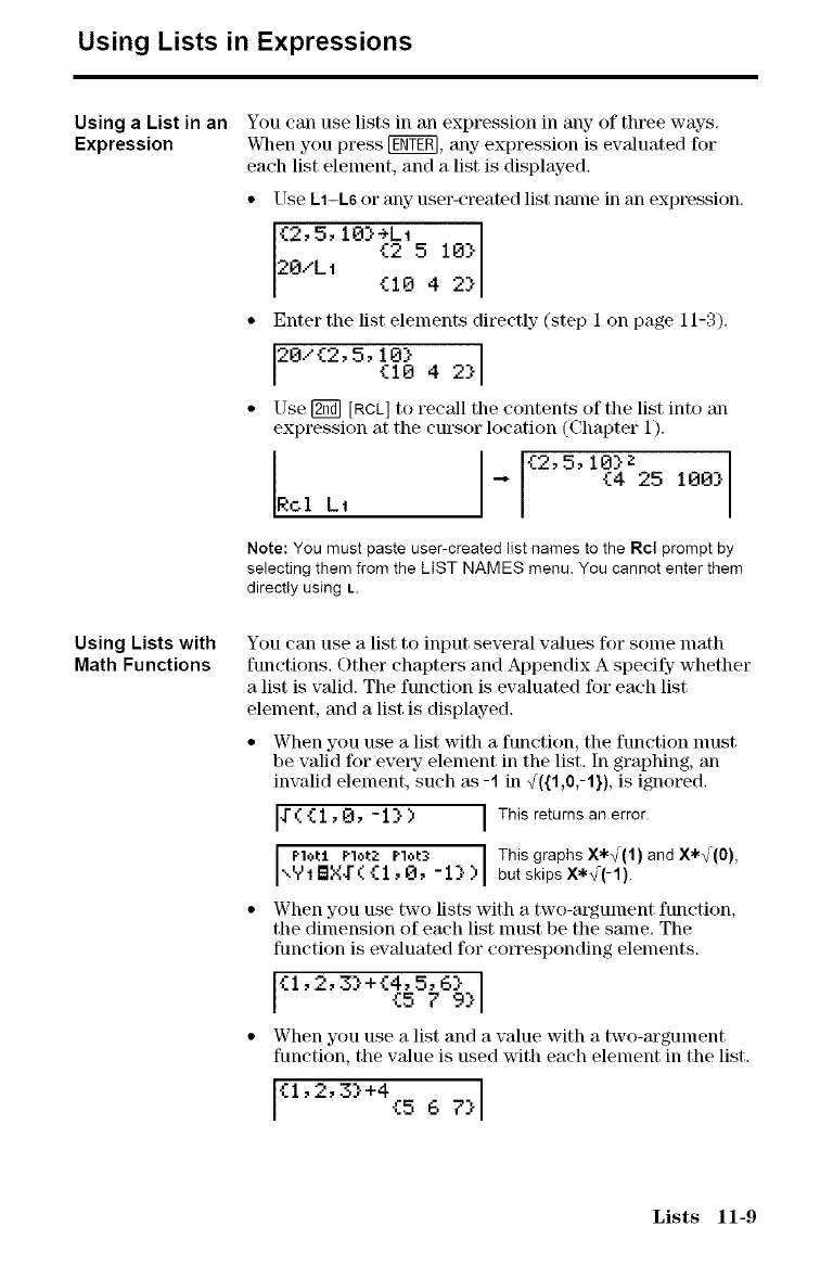
Using Lists in Expressions
Using a List in an
Expression
You can use lists in an expression in any- of three ways.
When you press [NY_, any expression is evaluated for
each list element, and a list is displayed.
• Use L1-Ls or any user-created list name in an expression.
5 16}
20/L1 {10 4 2}
• Enter the list elements directly (step 1 on page 11-3).
20/{2, 5, 10}{10 4 2}
• Use [_ [RCL] to recall the contents of the list into an
expression at the cursor location (Chapter 1).
Rcl Lt "* {2,5,10}I{425 i00}
Note: You must paste user-created list names to the Rcl prompt by
selecting them from the LIST NAMES menu. You cannot enter them
directly using L.
Using Lists with
Math Functions You can use a list to input several values ff)r some math
functions. Other chapters and Appendix A specify whether
a list is valid. The function is evaluated for each list
element, and a list is displayed.
When you use a list with a function, the function lnust
be valid for every element in the list, In graphing, an
invalid element, such as -1 in _({1,0,-1}), is ignored,
14"({1,O,-1}) I This returns an error.
F'loti Plot_: F'lot3 ) This graphsX*_(1) and X*_(O),
\VIBx,r( {1, O, -I} but skips X*_(-1).
When you use two lists with a two-argulnent function,
the dimension of each list must be the same, The
function is evaluated for corresponding elements.
{i, 2, 3}+{4, 5, 6}
{5 79}
When you use a list and a value with a two-argument
function, the value is used with each element in the list.
{1'2'3}+4{5 67}
Lists 11-9
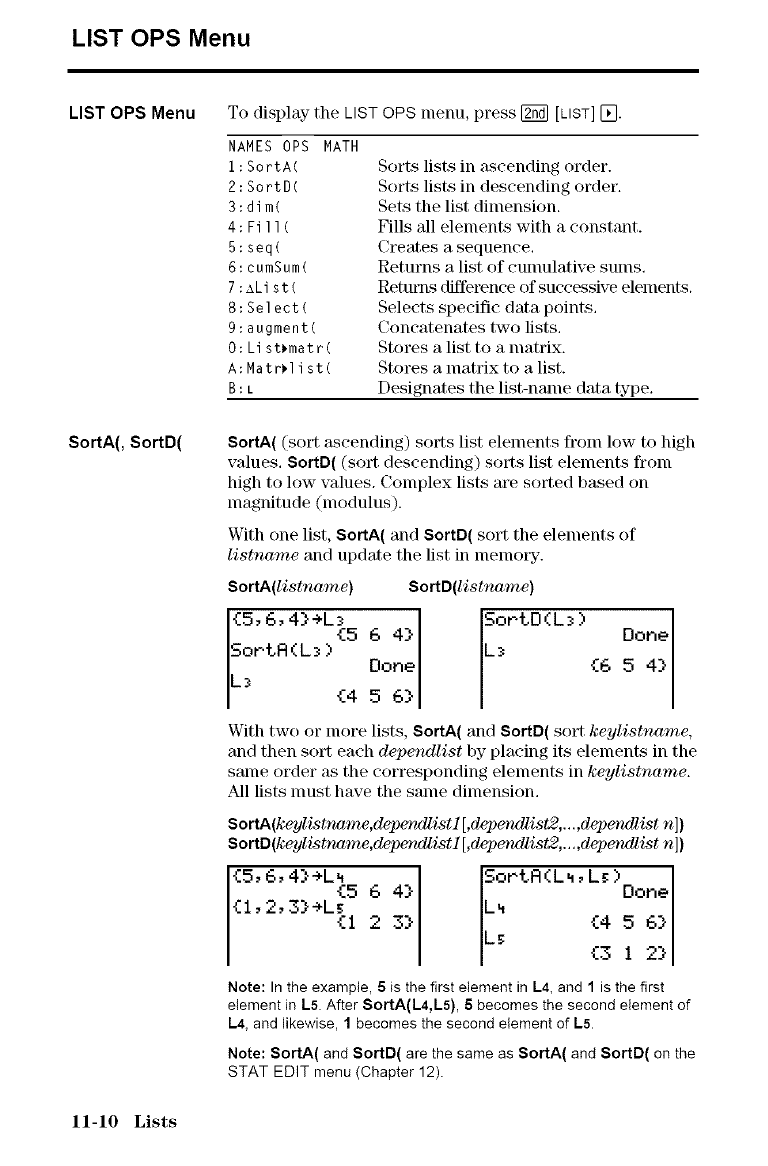
LIST OPS Menu
LIST OPS Menu
SortA(, SortD(
To display the LIST OPS menu, press [_ [LIST] [_.
NAMES OPS MATH
1:SortA(
2:SortD(
3:dim(
4:Fill(
5:seq(
6:cumSum(
7:aList(
8:Select(
9:augment(
O:List_matr(
A:Matr_list(
B:L
Sorts lists in _Lscending order.
Sorts lists in descending order.
Sets the list dimension,
Fills 'all elements with a constant.
Creates a sequence,
Returns a list of cunmlative sums,
Returns difference of successive elements,
Selects specific data points,
Concatenates two lists,
Stores a list to a nlatrix.
Stores a lnatrix to a list.
Designates the list-name data type,
SortA( (sort ascending) sorts list elements fron] low to high
values, SortD( (sort descending) sorts list elements from
high to low values. Complex lists are sorted based on
magnitude (modulus).
With one list, SortA( and SortD( sort the elements of
listnome and update the list in nlenloi_.
SortA(listname) SortD(listname)
Sor.tR(L_ ) Done {6
L_ {4 5 6}
With two or more lists, SortA( and SortD( sort keylistname,
and then sort each dependlist by placing its elements in the
same order as the corresponding elements in keylistname.
All lists nmst have the same dimension,
SortA(k¢ylistname,deperwllistl[,depe_wllist2,...,depe_wllist n])
SortD(k¢ylistname,deperwllistl[,depe_wllist2,...,depe_wllist n])
{5'6'4}÷L_5 64} S°rtR(k_'L_>Done
{1,2,3},L_I 2 _ {4 5 6}
3} {3 1 2}
Note: In the example, 5is the first element in L4, and 1 is the first
element in L5. After SortA(L4,Ls), 5becomes the second element of
L4, and likewise, 1becomes the second element of L5.
Note: SortA( and SortD( are the same as $ortA( and SortD( on the
STAT EDIT menu (Chapter 12).
11-10 Lists
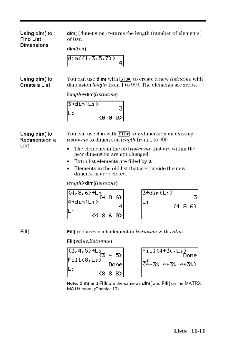
Using dim( to
Find List
Dimensions
Using dim( to
Create a List
Using dim( to
Redimension a
List
Fill(
dim((dimension) returns the length (number of elements)
of list.
dim(list)
diM({1,3,5,7}) 4
You can use dim( with _ to create a new listname with
dimension length from 1 to 999. The elements are zeros.
length_ dim(listname)
3÷diFKLz ) 0_
Lz {0 0
You can use dim with [gg_] to redimension an existing
listnome to dimension length from 1 to 999.
• The elements in the old listname that are within the
new dimension are not changed.
• Extra list elements are filled by 0.
• Elements in the old list that are outside the new
dimension are deleted.
length_ dim(listname)
{4'8'6}÷L_4 8 6
4÷dim(L1 )
LI {4 8 6 0} 3÷diM(L1 ) 6_
L1 {4 8
Fill( replaces each element in listnome with value.
Fill(value,listname)
{3'4'5}÷L_3 4 5}
FilI(8,L_) Done
L_ {8 8 8}
Fill(4+3t,Li_one
Li
{4+or 4+3t 4+3t}
Note: dim( and Fill( are the same as dim( and Fill( on the MATRX
MATH menu (Chapter 10).
Lists 11-11
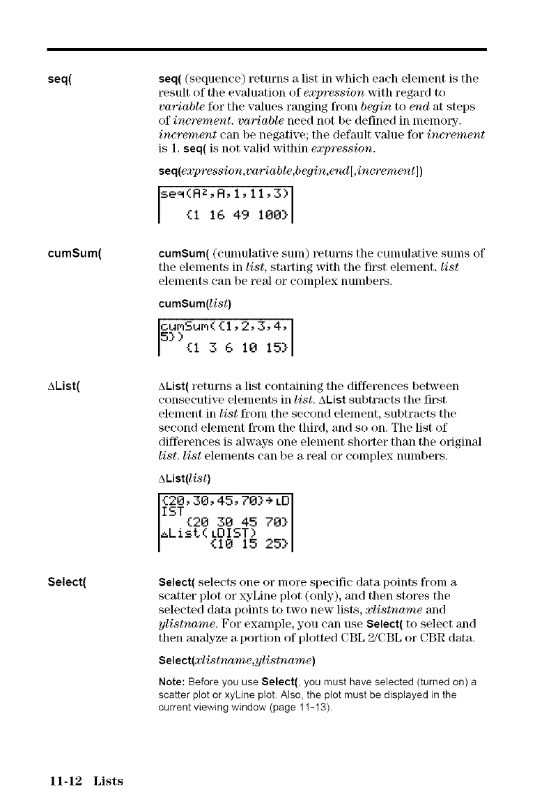
seq(
cumSum(
AList(
Select(
seq((sequence) returns a list in which each element is the
result of the evaluation of expression with regard to
variable for the values ranging from begin to end at steps
of increment, variable need not be defined in memory.
increment can be negative; the default value for increment
is 1. seq( is not valid within expression.
seq(expression,variable,begin,e_l[,increment])
se_(AZ, R, 1,11,3)
{I 16 49 100}
cumSum( (cunmlative sunl) returns the cunmlative sunls of
the elements in list, starting with the first element, list
elements can be real or complex numbers.
cumSum(list)
c.umSum( {i,2, 3,4,
5}){I 3 610 15}
aList( returns a list containing the differences between
consecutive elements in list. AList subtracts the first
element in list from the second element, subtracts the
second element from the third, and so on. The list of
differences is always one element shorter than the original
list. list elements can be a real or complex numbers.
AList(list)
{20,30, 45., 70}÷ LD
IST I
{20 30 45 70}
aList(LDIST)
{10 15 25}
Select( selects one or more specific data points fronl a
scatter plot or xyLine plot (only), and then stores the
selected data points to two new lists, xlistname and
ylistname. For example, you can use Select( to select and
then analyze a portion of plotted CBL 2/CBL or CBR data.
Select(xlistname,ylistname)
Note: Before you use Select(, you must have selected (turned on) a
scatter plot or xyLine plot. Also, the plot must be displayed in the
current viewing window (page 11-13).
11-12 Lists
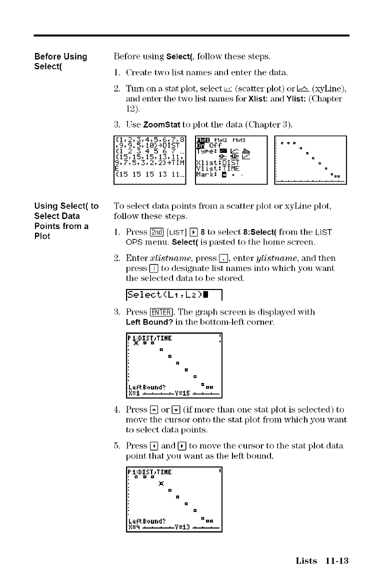
Before Using
Select(
Using Select( to
Select Data
Points from a
Plot
Before using Select(, follow these steps.
1. Create two list names and enter the data.
2. Turn on a stat plot, select Le: (scatter plot) or [_- (xyLine),
and enter the two list names for Xlist: and Ylist: (Chapter
12).
3. Use ZoomStat to plot the data (Chapter 3).
{1,2, 3, 4, 5,6,7,8]
,9,9.5,10}+DIST I _DOnO_z _1*t_
el. . °o
I{i 2 3 45 6 7...I TgPe: I If"_ ".
1{15, 15, 15, 13, ll,I _ i_ _ .
IEg,?,5,3,2,2)÷TIM I Xlist.:oIsm °
YlisL:TIME °
I{15 15 15 13 11...I Mark: [] ֥ %.
t J
To select data points fronl a scatter plot or xyLine plot,
follow these steps.
1. Press [2_] [LIST][] 8 to select 8:Select( from the LIST
OPS menu. Select( is pasted to the home screen.
2. Enter xlistname, press [], enter ylistname, and then
press [] to designate list names into which you want
the selected data to be stored.
ISeleot(L1,Cz)l I
3. Press [g_-gm. The graph screen is displayed with
Left Bound? in the bottom-left corner.
au iI
LeFtBound? 000
Press [] or [] (if more than one stat plot is selected) to
move the cursor onto the stat plot from which you want
to select data points.
Press [] and [] to move the cursor to the stat plot data
)oint that you want as the left bound.
keFt BOLIhd? _ua
Lists 11-13
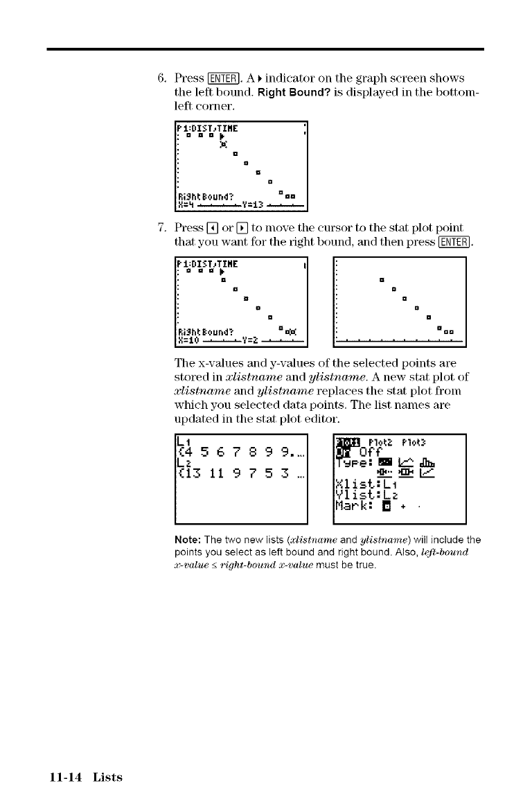
6. Press [NER]. A _indicator on the graph screen shows
the left bound. Right Bound? is displayed in the bottonl-
left corner.
Pi:BIST.,TIH{
oa a _
u
U
a
U
RiZlht _OUnd? uua
Press [] or [] to nlove tile cursor to the stat plot point
that you want for the ri ht bound, and then press [ENY_.
PI:DIST_TIHE
:a aa_
iamu a o
Ri_htBound? " u u"_ u " [] u
The x-values and y-values of the selected points are
stored in xlistname and ylistname. A new stat plot of
._:listname and ylistname replaces the stat plot from
which you selected data points. The list names are
updated in the stat plot editor.
119 7 s 3
]91ist:Lz
Mark: [] ÷ .
Note: The two new lists (xlistnanw and ylistname) willinclude the
points you select as left bound and right bound. Also, left-bonnd
x-volne < "l_ight-bound x-value must be true.
11-14 Lists
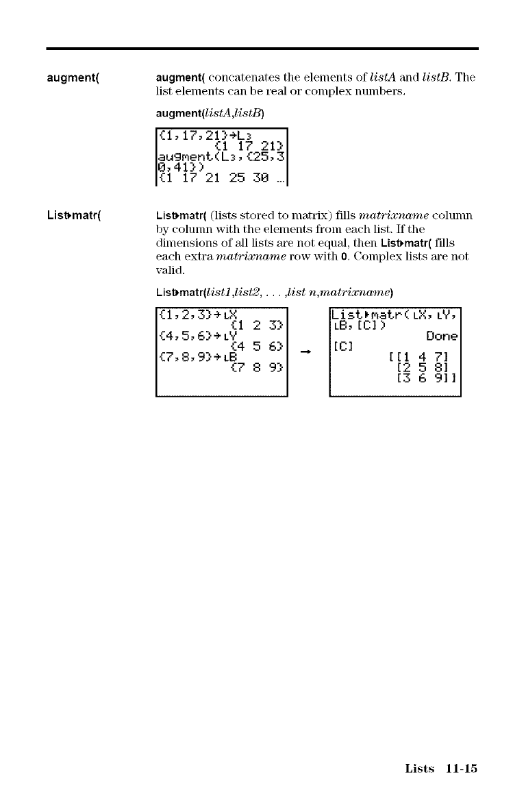
augment(
List_matr(
augment(concatenates the elements of listA and listB. The
list elements can be real or complex numbers.
augment(listA,listB)
{1,17,21}+L_
{1 1721}
augment.(L_o{a5,3
8,41}) -,
{1 17 21 25 o0 ...
List*matr( (lists stored to matrix) fills matrixname colunm
by colunm with the elements from each list. If the
dimensions of all lists are not equal, then List_matr{ fills
each extra matrixname row with O. Complex lists are not
valid.
List*matr(listl,list2, ...,list n,mat_xname)
3} List*matt( LX, L'_J, I
{l'2'3}+LX1 2 LB, 1C1) Oone[
Lists 11-15
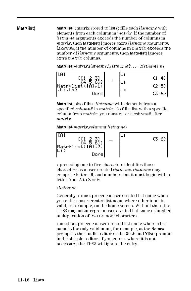
MatrHist( MatrHist( (matrix stored to lists) fills each listname with
elements from each colunm in mahqx. If the number of
listname argulnents exceeds the number of colunms in
matrix, then MatrHist( ignores extra listr_ame arguments.
Likewise, if the number of colunms in matrix exceeds the
number of listr_ame arguments, then MatrHist( ignores
extra matrix colunms.
Mat_list(mat_x,listnamel,listname2 .... ,listnamen)
[4 5 6111 -- Lz
Matr_li_t( {2 5}
,Lz,L_) [RI,L1
Done {3
Math.list(also fills a listname with elements fronl a
specified column# in matrix. To fill a list with a specific
colunm from matrix, you nmst enter a column# after
matrix.
Mat_list(matrix,column#,listnome)
IN] [[1 2 31 [ L1 {3 6}
5 6111 --
Matt*list(
LI) [R1,3,
Done
t preceding one to five characters identifies those
characters _ts a use>created listname, listname may
comprise letter\% 0, and numbers, but it nmst begin with a
letter fi'onl A to Z or 0.
Llistname
Generally, L must precede a user-created list name when
you enter a use>created list name where other input is
valid, for example, on the home screen. Without the t, the
TI-83 may misinterpret a use>created list name as implied
nmltiplication of two or more characters.
t need not precede a use>created list name where a list
name is the only valid input, for example, at the Name=
prompt in the stat list editor or the Xlist: and Ylist: prompts
in the stat plot editor. If you enter • where it is not
necessary, the TI-83 will ignore the enttT.
11-16 Lists
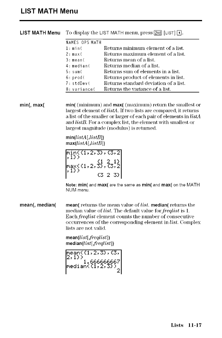
LIST MATH Menu
LIST MATH Menu To display the LIST MATH menu, press [_ [LIST] E],
NAMES OPS MATH
i: min(
2: max(
3: mean(
4: median(
5: sum(
6: prod(
7:stdDev(
8: variance(
Returns nnninmm element of a list.
Returns nl_ximum element of a list.
Returns mean of a list,
Returns median of a list,
Returns sum of elements in a list.
Returns product of elements in list,
Returns standard deviation of a list,
Returns the variance of a list,
min(, max(
mean(, median(
min((nlininlunl) and max((nlaxinlunl) retul]l the smallest or
largest element of listA. If two lists are compared, it returns
a list of the snmller or larger of each pair of elements in listA
and listB. For a complex list, the element with snmllest or
largest magnitude (modulus) is returned.
min(listA [,listB ])
max(listA[,listB])
mir,({lo2,3},{3,21
,i}> {I 2 I}II
max({l,2,3},
,i}> {3 2{3'23}
Note: min( and max( are the same as min( and max( on the MATH
NUM menu.
mean( returns the mean value of list. median( returns the
median value of list. The default value forfreqlist is 1.
Eachfreqlist element counts the number of consecutive
occurrences of the corresponding element in list. Complex
lists are not valid.
mean(list[ #¢reqlist])
median(list[ dreqlist ])
mean( {1,2,3}, {3,
2, I} >I. 666666667
_'_edian ({i, 2, 3} )2
Lists 11-17
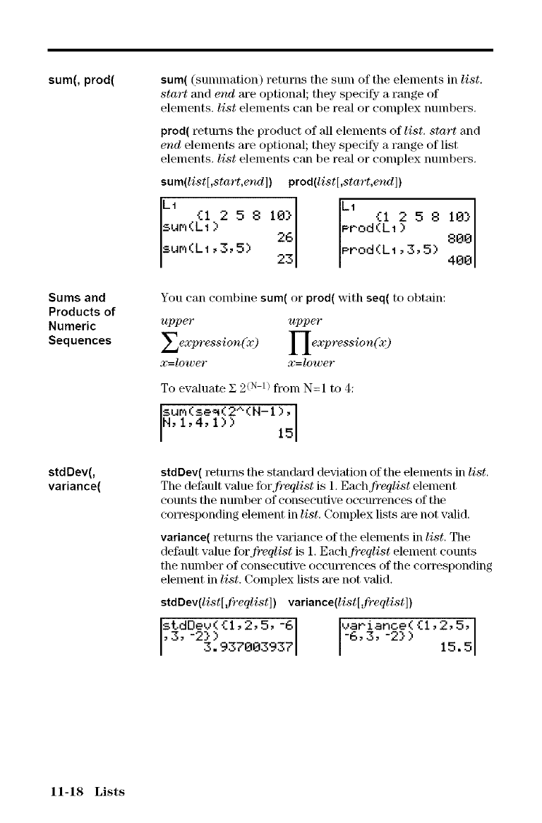
sum(, prod(
Sums and
Products of
Numeric
Sequences
stdDev(,
variance(
sum((sununation) returns the sunl of the elements in list,
start and end are optional; they specify a range of
elements, list elements can be real or complex numbers.
prod( _tma_s the product of all elements of list. start and
end elements are optional; they specify- a range of list
elements, list elements can be real or complex nmnbers.
sum(list[,start,ef_l]) prod(list[,start,ef_l])
L_ {I 2 5 8 10} k_ {I 2 5 8 10}
sur_(L_ ) 26 Prod(L1 )
su_KLI,3,5) 23 Prod(Li,3,5) 400800
You can colnbine sum( or prod( with seq( to obtain:
upper
expression(x)
x=lower
upper
x=lower
To evaluate Z 2 (N 1)fl'Oln N=I to 4:
sur_(se_ (2" (N- I ),
N, 1,4, I)) 15
stdDev( retrains the standard deviation of the element._ in list.
The default value forfreqlist is 1, Eachfreqlist element
counts the number of consecutive occurrences of the
con'esponding element in list. Complex lists m'e not valid.
variance( returns the variance of the elements in list, The
default value forfreqlist is 1, Eachfreqlist element counts
the number of consecutive occmTences of the corresponding
element in list. Complex list.s are not valid.
stdDev(list[freqlist]) vadance(list[freqlist])
stdOev( {i, 2, 5, -6 variance( {i,
,3, -2}) -6,3, -2}) 2,5,
3.937003937 15.5
11-18 Lists
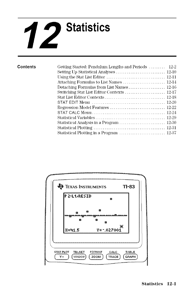
2Statistics
Contents Getting Started: Pendulum Lengihs and Periods ......... 12-2
Setting Up Statistical Analyses ........................... 12-10
Using the Stat List Editor ................................ 12-11
Attaching Fornmlas to List Names ....................... 12-14
Detaching Formulas from List Names .................... 12-1(;
Switching Stat List Editor Contexts ...................... 12-17
Stat List Editor Contexts ................................. 12-18
STAT EDITMenu ........................................ 12-20
Regression Model Features .............................. 12-22
STAT CALC Menu ........................................ 12-24
Statistical Variables ...................................... 12-2(.)
Statistical Analysis in a Program ......................... 12-30
Statistical Plotting ....................................... 12-31
Statistical Plotting in a Program ......................... 12-37
TEXAS INSTRUMENTS TI-83
p Z:LI_RE:VIn D
0
M M
0 0 0
g=Nl.g Y='.OZ7001
J
STAT PLOT TBLSET FORMAT CALC TABLE
Statistics 12-1
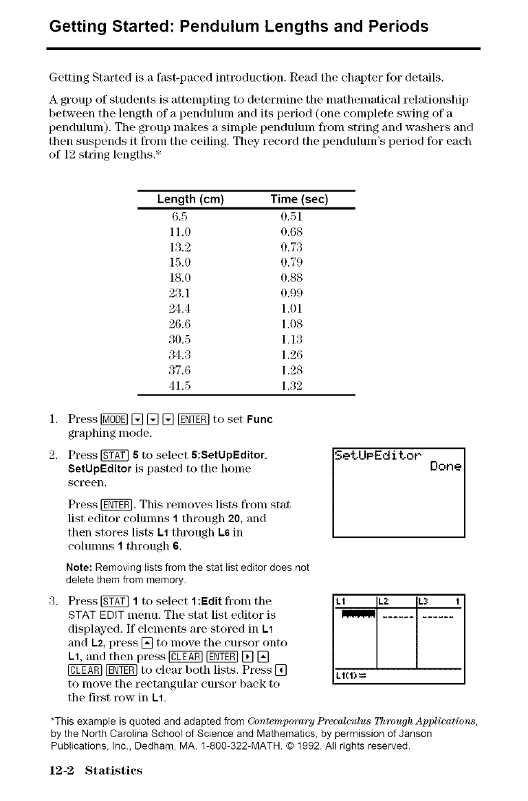
Getting Started: Pendulum Lengths and Periods
Getting Started is a fast-paced introduction. Read the chapter for details.
A group of students is attempting to determine the lnathelnatical relationship
between the length of a pendulum and its period (one complete swing of a
pendulum). The group makes a simple pendulum froln string and washers and
then suspends it from tile ceiling. They record the pendulum's period for each
of 12 string lengths.*
Length (cm) Time (sec)
6.5 0.51
11.0 0.68
13.2 0.73
15.0 0.79
18.0 0.88
23.1 0.99
24.4 1.01
26.6 1.08
30.5 1.13
34.3 1.26
37.6 1.28
41.5 1.32
1. Press [_DE] [] [] [] [g_gg] to set Func
graphing mode.
2. Press [g_g] 5 to select 5:SetUpEditor.
SetUpEditor is pasted to the honm
screen.
Press [gfff_. This relnoves lists fronl stat
list editor colunms 1through 20, and
then stores lists L1through L6 in
eolunms 1through 6.
Note: Removinglistsfromthe stat list editordoesnot
deletethem frommemory.
3. Press [gf_] 1to select 1:Edit fronl the
STAT EDIT menu. The stat list editor is
displayed. If elements are stored in 1-1
and I_2,press [] to move the cursor onto
1_1,and then press @ [gNT_ [] []
@ [gg7_ to clear both lists. Press []
to move the rectangular cut\sor back to
the first row in 1_1.
SetUeEditof Done[
L1(1)=
*This example is quoted and adapted from Contempo'_mT P'recal(vdns Th'mugh Applications,
by the North Carolina School of Science and Mathematics, by permission of Janson
Publications, Inc., Dedham, MA. 1-800-322-MATH. © 1992. Aft rights reserved.
12-2 Statistics
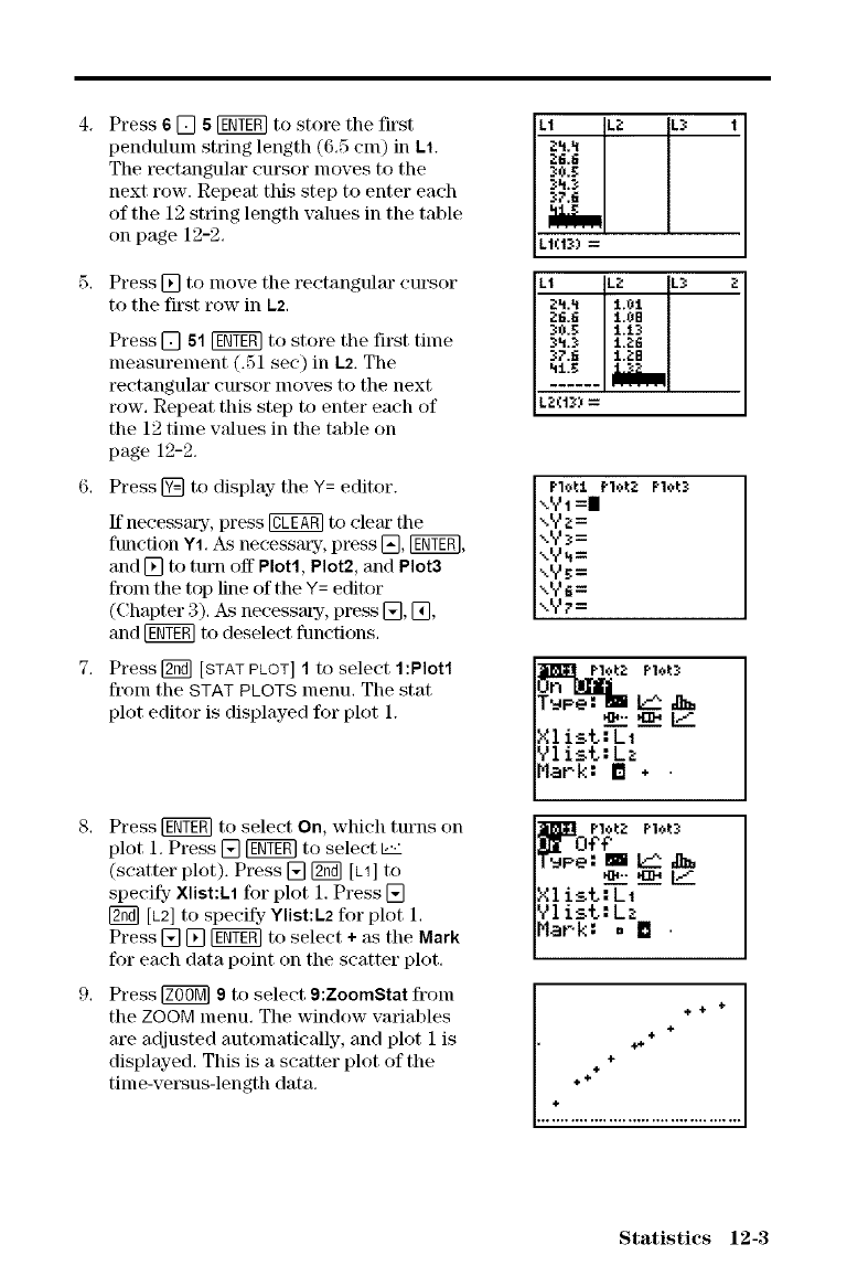
4. Press6[] 6_ to store the first
pendulum string length (6.5 cm) in 1.1.
The _ctangular cursor nloves to the
next row. Repeat this step to enter each
of the 12 string length values in the table
on page 12-2.
Press [] to inove the rectangular cursor
to the first row in 1.2.
Press [] 61 _ to store the first time
measurement (.51 sec) in 1.2. The
rectangulm" cursor moves to the next
row, Repeat this step to enter each of
the 12 time wdues in the table on
page 12-2.
6. Press [] to display- the Y= editor.
If necessm'y, press @ to clem" the
fm_ction Y1. As necessmy, press [], [E_,
and [] to turn off Plot1, Plot2, and Plot3
from the top line of the Y= editor
(Chapter 3). As necessmy, press [], [_,
and [_ to deselect functions.
Press [_ [STAT PLOT] 1to select 1:Plot1
fi'om the STAT PLOTS menu. The stat
plot editor is displayed for plot 1.
Press _ to select On, which turns on
plot 1. Press [] _ to select ,,'."
(scatter plot). Press [] _ [L1] to
specify- ×list:1.1 for plot 1. Press []
[L2] to specify- Ylist:1.2 for plot 1.
Press [] [] _ to select + _ksthe Mark
for each data point on the scatter plot.
Press _ 9 to select 9:ZoomStat fronl
the ZOOM menu. The window variables
are adjusted automatically, and plot 1 is
displayed. This is a scatter plot of the
time-versus-length data.
LI .Z L_: 1
26,6
37.ti
L1(1_) =
Lt .Z L_: Z
26.6 t.0B
3LI.:_ t.Ztl
3?.tl J..ZB
Plot1 PloLZ Plot:_
\V1 =11
".Yz=
_.y_=
xy_=
"_y_=
xY_;=
\Y?=
_peO Plo_2 P1o_:_
+-,._
liar-k: .[] •
÷ + ÷
÷
÷
++
+
+÷+
+
Statistics 12-3
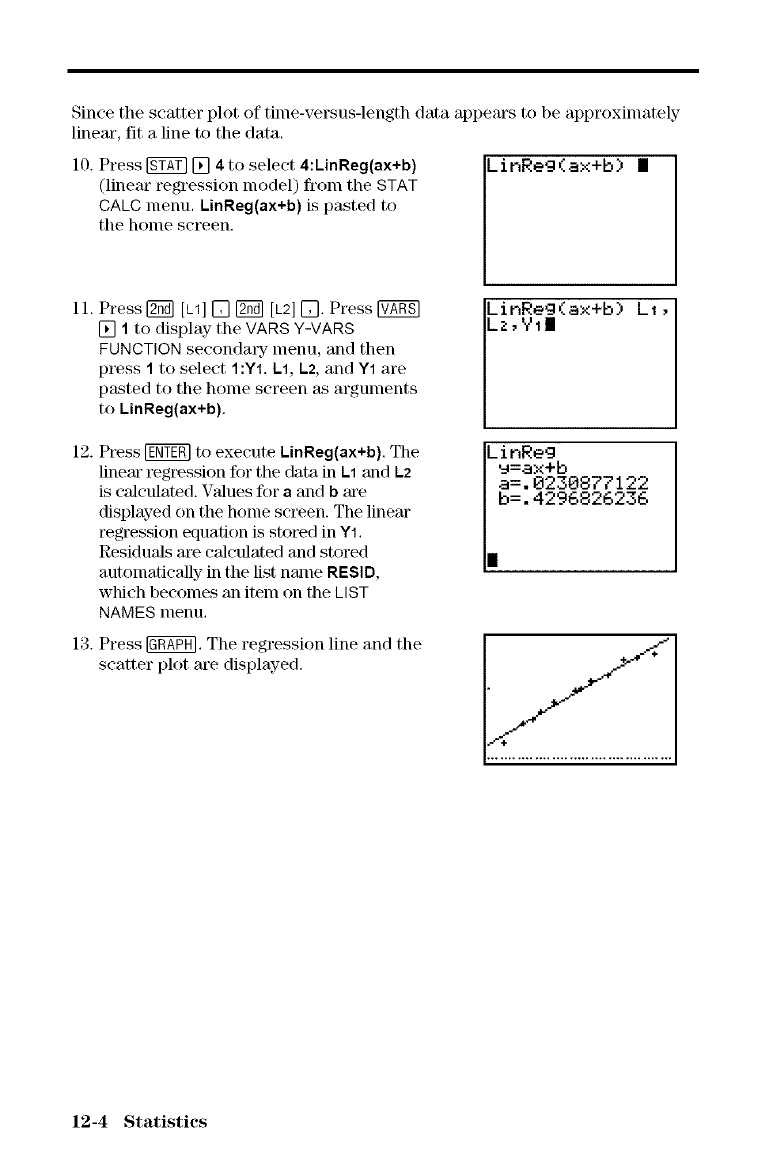
Sincethescatterplotoftime-versus-lengthdataappearstobeapproxhnately
linear, fit a line to the data.
10. Press _ [] 4 to select 4:LinReg(ax+b) LinReg(ax+b) |
(linear regression nlodel) fronl the STAT
CALC menu, kinReg(ax+b) is pasted to
tile home screen.
11. Press [_ [L1] [] _ [L2] [_. Press
[] 1to display the VARS Y-VARS
FUNCTION secondmT menu, and then
D_ss 1to select 1:Y1. Lt L2, and Y1 are
pasted to the home screen as arguments
to LinReg(ax+b).
12. Press [_ to execute LinReg(ax+b). The
lineal" regression for the data in L1 and L2
is calculated. Values for a and b are
displayed on the home screen. The linear
regression equation is stored in Y1,
Residuals are calculated and stored
automatically in the list name RESID,
which becomes an item on the LIST
NAMES menu,
13. Press _. The regression line and the
scatter plot are displayed.
LinReg
9=_x+b
a=.0230877122
b=.4296826236
12-4 Statistics
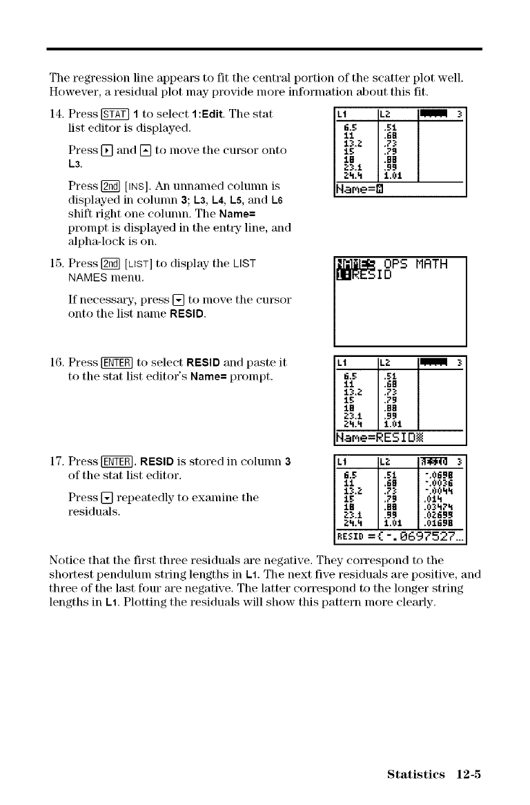
Theregressionlineappearstofitthecentralportionofthescatterplotwell.
However,aresidualplotmayprovidemoreinformationaboutthisfit.
14.Press[g_g] 1to select 1:Edit. The stat
list editor is displayed.
Press [] and [] to lnove the cursor onto
L3.
Press [_ [INS]. An unnamed colunm is
displayed in colunm 3; 1.3, k4, L5, and 1_6
shift right one colunm. The Name=
prompt is displayed in the entry line, and
alpha-lock is on.
15. Press [2_ [LIST] to display the LIST
NAMES menu.
If necessatT, press [] to inove the cursor
onto the list name RESID.
16. Press _ to select RESID and paste it
to the stat list editor's Name= pt_mlpt.
E2; 2;1
11 ._8
1_; ,79
18 ,8B
;:3.1 .99
2h.h 1,01
NaMe=_
Lt .2 _
&5 ,B1
11 ,l_B
13.2 .73
1_: .79
1B .EB
.2_:.1 .99
2h.h 1.01
I_.B ,51 ".06911
11 .6B ".0036
13.2 ,73 ".OOhh
1_: .79 .01h
1E .BE .03h?h
?._:.1 .99 .0Z699
2h._ 1.=31 .0lEgit
eCSZD=£-. 0697527...
17. Press IgOr. RESID is stored in colunm 3
of the stat list editor.
Press [] repeatedly to examine the
residuals.
Notice that the first three residuals are negative. They cotTespond to the
shortest pendulum string lengths in L1. The next five residuals are positive, and
three of the last four are negative. The latter correspond to the longer string
lengths in L1. Plotting the residuals will show this pattern more clearly.
Statistics 12-5
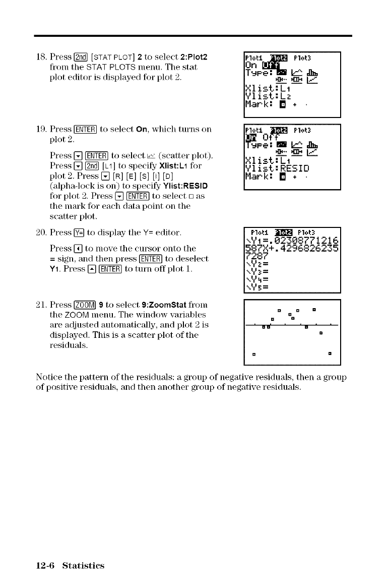
18. Press [2_] [STAT PLOT] 2to select 2:Plot2
from the STAT PLOTS menu. The stat
plot editor is displayed for plot 2.
19. Press [_T@] to select On, which turns on
plot 2.
Press [] FEffEENto select _ (scatter plot).
Press [] [2_] [L1] to specify Xlist:L1 ff)r
plot 2. Press [] [R] [E] [S] [I] [D]
(alpha-lock is on) to specify Ylist:RESID
for plot 2. Press [] FEflT_]to select [] as
the mark for each data point on the
scatter plot.
20. Press [] to display the Y= editor.
Press [] to nlove the cursor onto the
= sign, and then press [g_ to deselect
Y1. Press [] [g_ to turn offplot 1.
21. Press _ 9to select 9:ZoomStat fl'oln
the ZOOM menu. The window variables
are adjusted automatically, and plot 2 is
displayed. This is a scatter plot of the
residuals.
Pl*t:[O_ P10t?
_uPe: m k:2 dt_
Xlist:L1
YI ist: RESIO
Mark: [] * .
PI*L1 _Pl*t_
xY1 =. 02308771216
587X+. 4296826135
7287
xYz=
xY?=
xY_=
\Y_=
D
Eli=
Notice the pattern of the residuals: a group of negative residuals, then a group
of positive residuals, and then another group of negative residuals.
12-6 Statistics
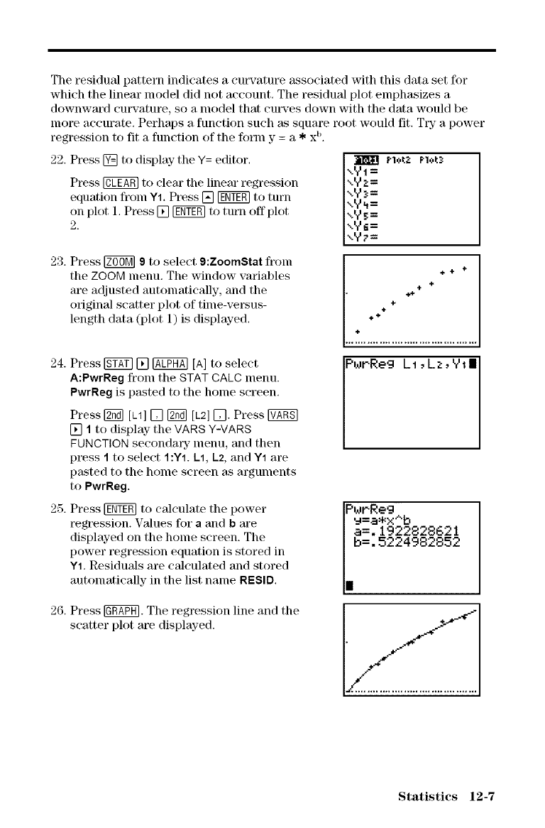
Theresidualpatternindicatesacm5Tatureassociatedwiththisdatasetfor
whichthelinearmodeldidnotaccount.Theresidualplotemphasizesa
downwardcurvature,soamodelthatcm_'esdownwiththedatawouldbe
moreaccurate.Perhapsafunctionsuchassquarerootwouldfit.TFFapower
regression to fit a function of the form y = a * xt'.
22. Press [] to display the Y=editor,
Press @ to clear tile linear regression
equation from Y1,Press [] [ggY_ to turn
on plot 1,Press [] [g_gO to turn off plot
2.
23. Press _ 9to select 9:ZoomStat froin
the ZOOM menu. The window variables
are adjusted automatically, and the
original scatter plot of time-versus-
length data (plot 1) is displayed.
",Yz=
,.Y_=
_.y_=
-,y_=
_.y_=
\y;_=
÷ + ÷
+
_+
÷
÷÷÷
÷
PuPReg L1,Lz,Yi|
24. Press Fgg_ [] @ [A] to select
A:PwrReg from the STAT CALC menu.
PwrReg is pasted to the home screen.
Press [g_ [L1][] [g_ [L2][]. Press
[] 1to display the VARS Y-VAR$
FUNCTION secondmT menu, and then
press 1to select 1:Y1.1.1, 1_2,and Y1 are
pasted to the home screen as arguments
to PwrReg.
25. Press [g_gm to calculate the power
regression. Values for a and b are
displayed on the home screen. The
power regression equation is stored in
Y1. Residuals are calculated and stored
automatically in the list name RESID,
PwrReg
_=a*x^b
a=.1922828621
b=.5224982852
26. Press _. The regression line and the
scatter plot are displayed.
Statistics 12-7
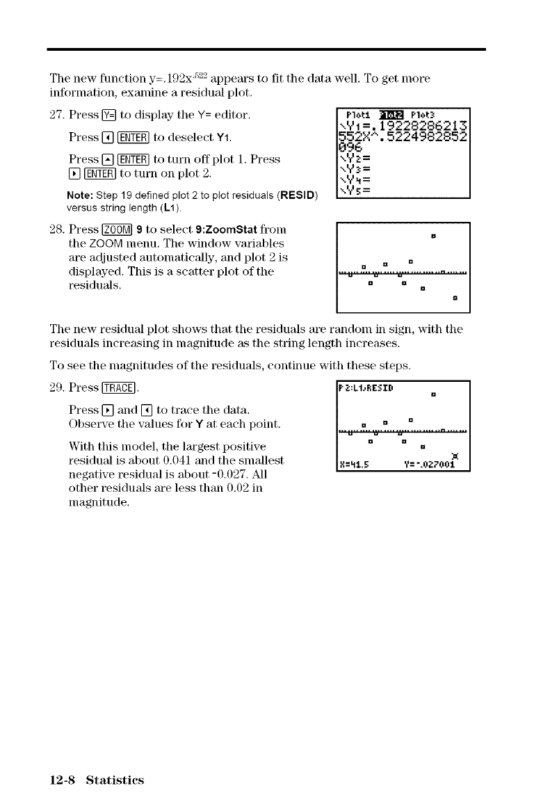
The new function y=.192x _"- appears t( fit the data well. To get nlore
information, examine a residual plot.
27. Press [] to display the Y= editor.
Press [] _ to deselect Y1.
Press [] [NY_ to turn offplot 1. Press
[] [ggY_ to turn on plot 2.
Note: Step 19 defined plot 2 to plot residuals (RESID)
versus string length (11).
Pl*tl _Pl*t3
".,Y 1----.19228286213
552X% 5224982852
\y_=
\Y_=
28. Press _ 9 to select 9:ZoomStat froln
the ZOOM menu. The window variables
are adjusted automaticMly, and plot 2 is
displayed. This is a scatter plot of the
residuMs.
[]
Da
El
The new residual plot shows that the residuals are random in sign, with the
residuals increasing in magnitude as the string length increases.
To see the magnitudes of the residuals, continue with these steps.
29. Press _.
Press [] and [] to trace the data.
Observe the values for Y at each point.
With this model, the largest positive
residual is about 0.041 and the smallest
negative residual is about -0.027. All
other residuals are less than 0.02 in
magnitude.
P;':LI_F;E$'r B []
II/:_1.5 Y:'.OZ?OOJ.
12-8 Statistics
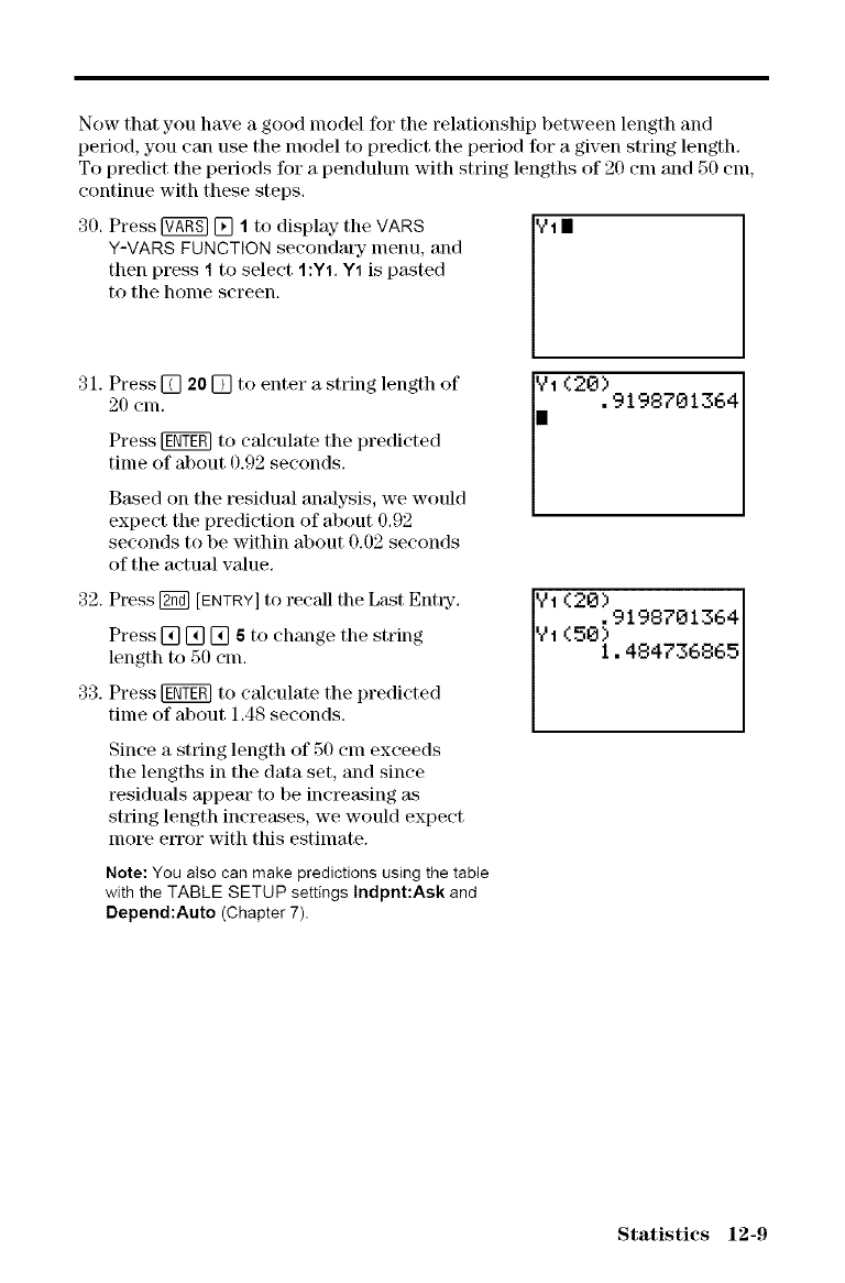
Nowthatyouhaveagoodmodelfortherelationshipbetweenlengthand
period,youcanusethemodeltopredicttheperiodforagivenstringlength.
Toprediettheperiodsforapendulumwithstringlengthsof20cmand50cm,
continuewiththesesteps.
30.Press[_ [] 1todisplay-theVARS
Y-VARSFUNCTIONseconda[wmenu,and
thenpress1toselect1:Y1.Y1ispasted
tothehomescreen.
31.Press[] 20 [] to enter a string length of
20 enl,
Press _ to calculate the predicted
time of about 0.92 seconds.
Based on the residual anMysis, we would
expect the prediction of about 0.92
seconds to be within about 0.02 seconds
of the actual value.
_1 II
32. Press _ [ENTRY] to recall the Last EnbTy'.
Press [] [] [] 6to change the string
length to 51) enL
33. Press _ to calculate the predicted
time of about 1.48 seconds.
Since a string length of 50 cnl exceeds
the lengths in the data set, and since
residuals appear to be increasing _
string length increases, we would expect
more etTor with this estimate.
_11(50)(28!9198781364
I. 484736865
Note: You also can make predictions using the table
with the TABLE SETUP settings Indpnt:Ask and
Depend:Auto (Chapter 7).
Statistics 12-9
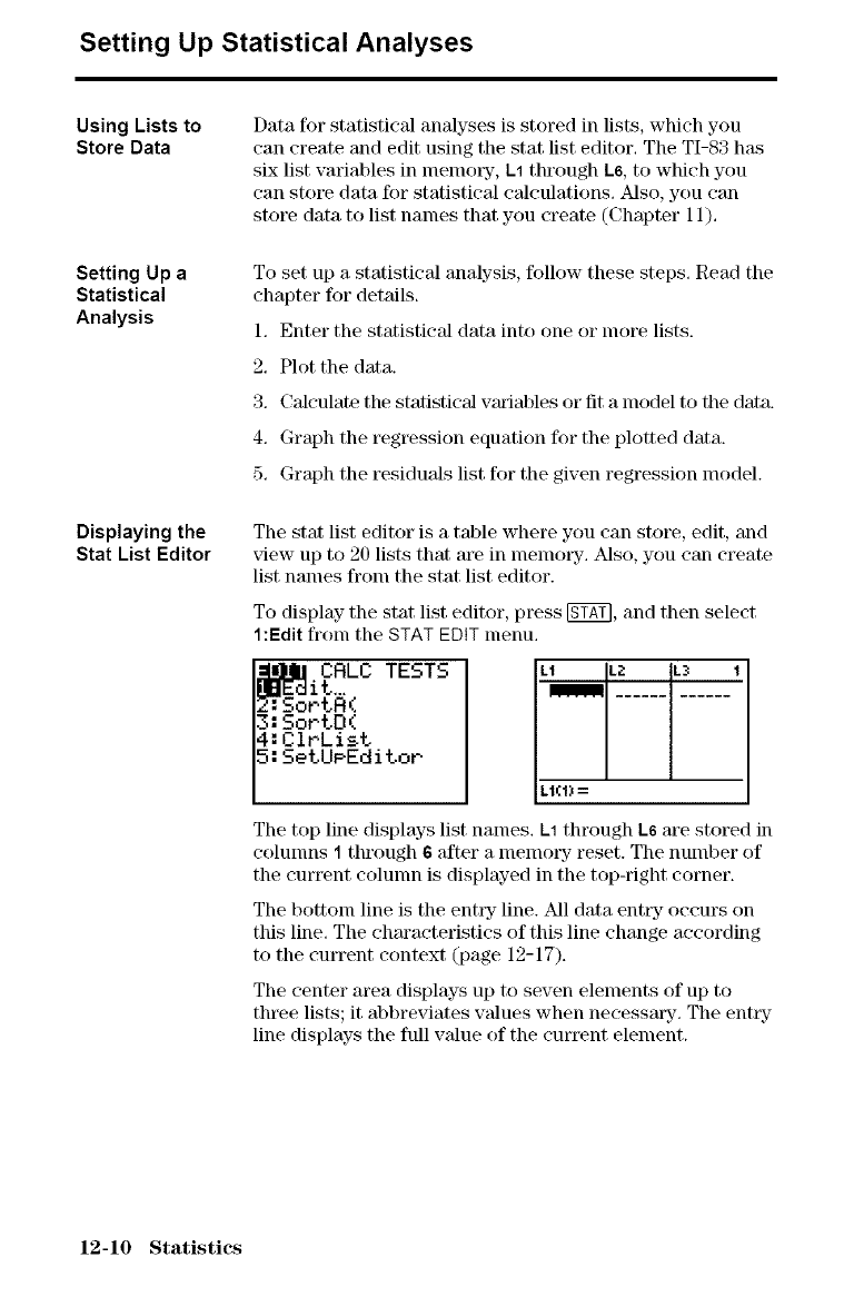
Setting Up Statistical Analyses
Using Lists to
Store Data
Setting Up a
Statistical
Analysis
Displaying the
Stat List Editor
Data for statistieM analyses is stored in lists, which you
can create and edit using the stat list editor. The TI-83 h_ks
six list vadal_les in lnelnory, L1 through L6, to which you
can store data ff_r statistical calculations. Also, you call
store data to list names that you create (Chapter 11).
To set up a statistical analysis, follow these steps. Read the
chapter for details.
1. Enter the statistical data into one or more lists.
2. Plot the data.
3. Calculate the statistical vm'iables or fit a model to the data
4. Graph the regression equation for the plotted data.
5. Graph the residuals list ff)r the given regression model.
The stat list editor is a table where you can store, edit, and
xqew up to 20 lists that are in nlenlol_yL Also, you Call create
list nalnes fronl the stat list editor.
To display- the stat list editor, press [g_T], and then select
1:Edit fronl the STAT EDIT menu,
CRLC TESTS
SortO(
ClrList
SetUeEditor
L1 L_: ._ 1
mmm
LI(I)=
The top line displays list names. L1 through L6 are stored in
colunms 1through 6 after a lnelnolT reset. The number of
the current colunm is displayed in the top-right corner.
The bottom line is the entry line. All data entry occurs on
this line. The characteristics of this line change according
to the current context (page 12-17).
The center area displays up to seven elements of up to
tht_e lists; it abbreviates wdues when neeessalT. The enttT
line displays the full value of the curt_nt element.
12-10 Statistics
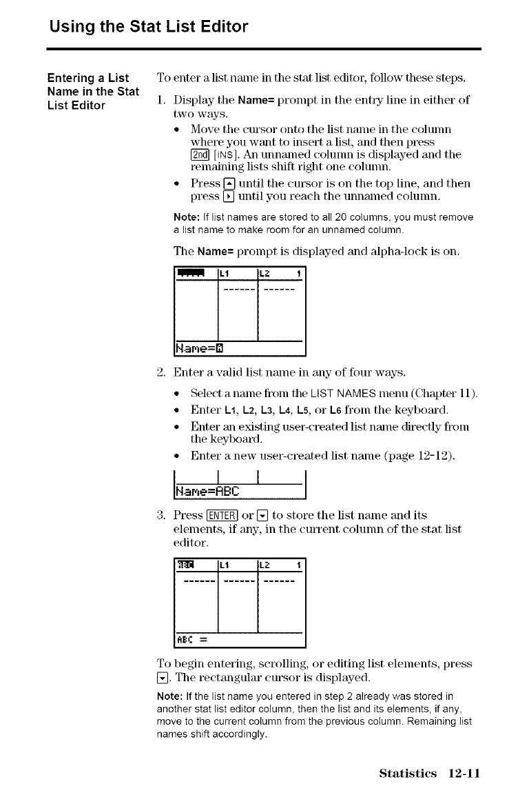
Using the Stat List Editor
Entering a List
Name in the Stat
List Editor
To enter a list name in tile stat list editor, follow these steps.
1. Display the Name= prompt in the entt T line in either of
two ways.
• Move the cursor onto the list name in the colunm
whet_ you want to insert a list, and then press
[_ [iNS]. Nil unnamed colunm is displayed and the
remaining lists shift right one colunm.
• Press [] until the cut\sor is on the top line, and then
press [] until you reach the unnamed colunm.
Note: If list namesare storedto all20 columns,you mustremove
a listnameto makeroomfor an unnamedcolumn.
The Name= prompt is displayed and alpha-lock is on.
LI L:;" 1
qame=_
2. Enter a valid list name in any of four ways.
• Select a name fl'onl file LIST NAMES menu (Chapter 11).
• Enter Cl, C2, Ca, L4, ks, or C6fronl the keyboard.
• Enter an existing user-created list name directly from
the key! Joard.
• Enter a new user-created list name (page 12-12).
I I I
I,Iamo=RBC I
3. Press [ggtgN or [] to store the list name and its
elements, if any-, in the cutTent colunm of the stat list
editor.
Lt k:;" t
To begin entering, scrolling, or editing list elements, press
[]. The rectangular cursor is displayed.
Note: If the list name you entered in step 2 already was stored in
another stat list editor column, then the list and its elements, if any,
move to the current column from the previous column. Remaining list
names shift accordingly.
Statistics 12-11
Creating a Name
in the Stat List
Editor
Removing a List
from the Stat List
Editor
Removing All
Lists and
Restoring L1
through L6
Clearing All
Elements from a
List
To create a name in the stat list editor, ff)llow these steps,
1,
2,
3,
Follow step 1 on page 12-11 to display- the Name=
prompt.
Press [letter from A to Z or 0] to enter the first letter of
the name. The first character cannot be a number.
Enter zero to four letters, O, or numbers to conlplete the
new user-created list name. List names can be one to
five characters long.
Press [g_ or [] to store the list name in the current
colunm of the stat list editor. The list name becomes an
item on the [_[ST NAMES menu (Chapter 11).
To remove a list from the stat list editor, move the cursor
onto the list name and then press [DTn. The list is not deleted
from memory; it is only removed from the stat list editor.
Note: To delete a list name from memory, use the MEMORY
DELETE:List selection screen (Chapter 18).
You can remove all user-created lists from the stat list
editor and restore list names L1 through L6 to colunms 1
through 6 in either of two ways.
• Use SetUpEdRor with no arguments (page 12-21).
• Reset all memotT (Chapter 18).
You can clear all elements from a list in any- of five ways.
• Use ClrList to clear specified lists (page 12-20).
• In the stat list editor, press [] to move the cursor onto a
list name, and then press @ [ggg_.
• In the stat list editor, move the cursor onto each
element, and then press [g_ one by one.
• On the home screen or in the program editor, enter
O->dim(listname) to set the dimension of listname to 0
(Chapter 11).
• Use ClrAIILists to cleat' all lists in memory (Chapter 18).
12-12 Statistics
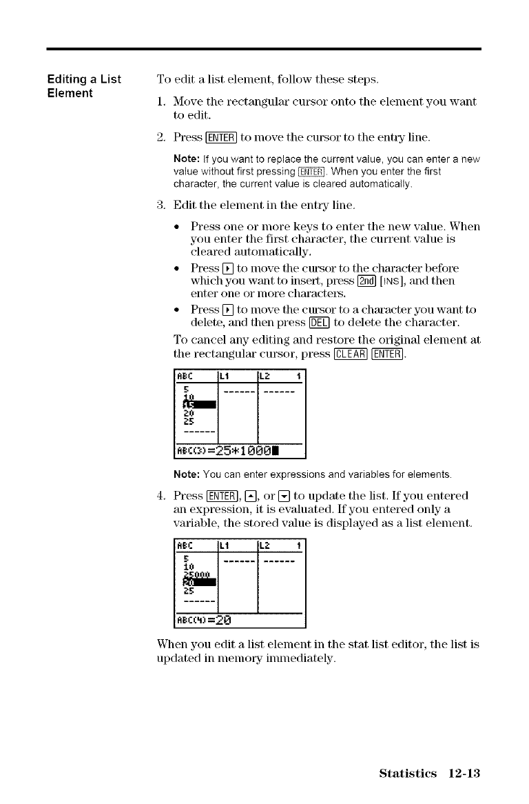
Editing aList
Element To edit a list element, follow these steps.
1. Move the rectangular cursor onto the element you want
to edit.
2. Press [_ to move the cursor to the entry line.
Note: If you want to replace the current value, you can enter a new
value without first pressing _. When you enter the first
character, the current value is cleared automatically.
3, Edit tile element in tile entity- line,
• Press one or lnore keys to enter the new value. When
you enter the ill,st character, the current value is
cleared automatically.
• Press [] to move the cta'sor to the character before
which you want to insert, D_ess [_ [_NS], and then
enter one or more charactegs,
• Press [] to move the cta'sor to a chm'acter you want to
delete, and then press [ff_] to delete the character.
To cancel any editing and restore the original element at
the rectangular cursor, press @ [_.
ABe Lt L2 t
_co)=25-1000|
Note: You can enter expressions and variables for elements.
4. Press [gNYE_, [], or [] to update the list. If you entered
all expression, it is evaluated. If you entered only a
variable, the stored value is displayed as a list element.
ttl_C L1 L_: 1
:LO
_C(_)=20
When you edit a list element ill the stat list editor, the list is
updated in nlenloFy inunediately.
Statistics 12-13
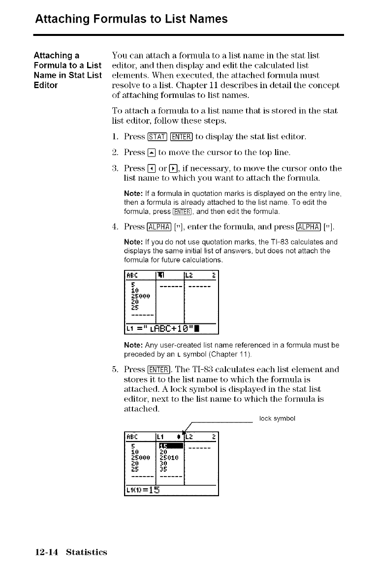
Attaching Formulas to List Names
Attaching a
Formula to a List
Name in Stat List
Editor
You can attach a fornmla to a list name in the stat list
editor, and then display- and edit the calculated list
elements. VCl_enexecuted, the attached fommla nmst
resolve to a list. Chapter 11 describes in detail the concept
of attaching fornmlas to list names.
To attach a fonnula to a list name that is stored in the stat
list editor, follow these steps.
1. Press [Kf_T]_ to display the stat list editor.
2. Press [] to move the cursor to the top line.
3. Press [] or [_, if necessm% to move the cm_sor onto the
list name to which you want to attach the fornmla.
Note: If a formula in quotation marks is displayed on the entry line,
then a formula is already attached to the list name. To edit the
formula,press_, andthen edit theformula.
4. Press @ [,,], enter the fornmla, and press @ [,,].
Note: If youdo notuse quotationmarks,the T1-83calculatesand
displays thesame initiallist of answers,butdoes notattach the
formula forfuture calculations.
I i:i_¢ "II] L;_ ;;
tO ....
L20__ul_5__.LFIEIC+IO"11
Note: Any user-created list name referenced in a formula must be
preceded by an L symbol (Chapter 11 ).
5. Press IENTERI.The TI-S3 calculates each list element and
stores it to the list name to which the fornmla is
attached. A lock symbol is displayed in the stat list
editor, next to the list name to which the fornmla is
attached.
lock symboI
/
I=I_C Lt $j L> _:
tO _:0
;;_:O00 _O::!.0
u_1_=15
12-14 Statistics
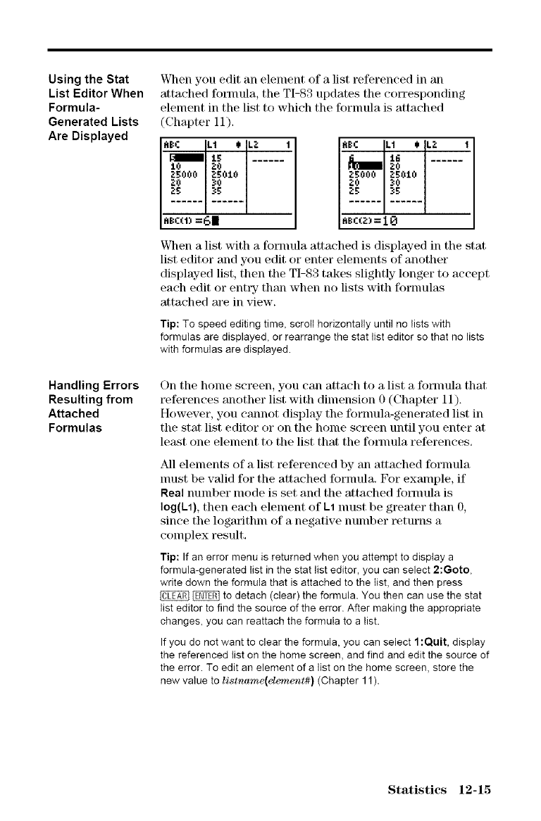
Using the Stat
List Editor When
Formula-
Generated Lists
Are Displayed
Handling Errors
Resulting from
Attached
Formulas
When you edit an element of a list referenced in an
attached fommla, the TI-83 updates the co_Tesponding
element in the list to which the fornmla is attached
(Chapter 11).
ABC LI $._: 1
t5
I(, _:0
2_:000 _:_:0i0
Z$ ._0
ItI_C LI $ .2 1
>0
2_:000 ;:_:0i0
_c_z_=1e
When a list with a formula attached is displayed in the stat
list editor and you edit or enter elements of another
displayed list, then the TI-83 takes slightly- longer to accept
each edit or ent_3; than when no lists with formulas
attached are in view.
Tip: To speed editing time, scroll horizontally until no lists with
formulas are displayed, or rearrange the stat list editor so that no lists
with formulas are displayed.
On the home screen, you can attach to a list a formula that
t_ferences another list with dimension 0 (Chapter 11).
However, you cannot display the fornmla-generated list in
the star list editor or on the home screen until you enter at
least one element to the list that the formula references.
All elements of a list t_ferenced by an attached fornmla
nmst be valid for the attached fornmla, For example, if
Real number mode is set and the attached formula is
log(l_1), then each element of 1.1 nmst be greater than O,
since the logarithm of a negative number returns a
complex result,
Tip: If an error menu is returned when you attempt to display a
formula-generated list in the stat list editor, you can select 2:Goto,
write down the formula that is attached to the list, and then press
_ to detach (clear) the formula. You then can use the stat
list editor to find the source of the error. After making the appropriate
changes, you can reattach the formula to a list.
If you do not want to clear the formula, you can select 1:Quit, display
the referenced list on the home screen, and find and edit the source of
the error. To edit an element of a list on the home screen, store the
new value to list'name(element#) (Chapter 11).
Statistics 12-15
Detaching Formulas from List Names
Detaching a
Formula from a
List Name
You can detach (clear) a formula fronl a list name in any of
four ways,
• In the stat list editor, nlove the cursor onto the name of
the list to which a fornmla is attached. Press [gflT_
@ [Ni_. All list elements remain, but the fommla
is detached and the lock symbol disappeat\s.
• In the stat list editor, nlove the cursor onto an element
of the list to which a fornmla is attached. Press [gflT_,
edit the element, and then press [ggT_. The element
changes, the fornmla is detached, and the lock symbol
disappears. All other list elements remain.
• Use CIrList (page 12-20). All elements of one or more
specified lists are cleared, each formula is detached, and
each lock symbol disappears. All list names remain.
• Use ClrAIILists (Chapter 18). All elements of 'all lists in
nlenlory are cleared, M1fornml_ts m'e detached from 'all
list names, and all lock symbols disappear. All list
nanles renlain.
Editing an
Element of a
Formula-
Generated List
As described above, one way to detach a fornmla fronl a
list name is to edit an element of the list to which the
formula is attached. The TI-83 protects against
inadvertently detaching the fornmla from the list name by
editing an element of the fornmla-generated list.
Because of the protection feature, you lnust press [gflT_
before you can edit an element of a formula-generated list.
The protection feature does not allow you to delete an
element of a list to which a formula is attached. To delete
an element of a list to which a formula is attached, you
nmst first detach the fornmla in any- of the ways described
above.
12-16 Statistics
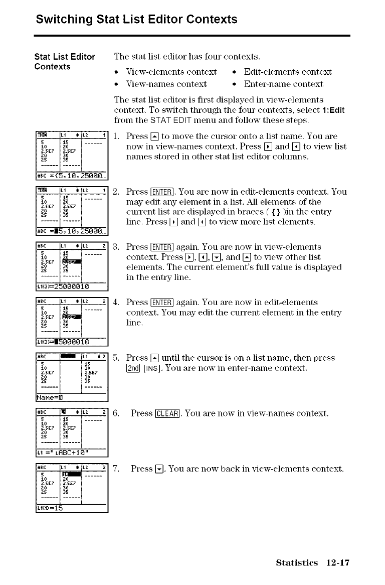
Switching Stat List Editor Contexts
Stat List Editor
Contexts
Lt _L_ 1
20
Z,SE7 2,55?
2_ 30
Z5 35
_c ={5, 10,25000...
LI $L2 i
5 i _5 ......
I_5._ii_5,
_5 i 35
Asc :|5_10,25000...
_5C LI $L&
2_5E?
_ i 3_
_5 i 35
LIc3)=25000010
AI_5 LI $ L2
5 i _,5 ......
2_5E7
25 i 35
LI(3)=|5000010
5 _5
:i._ 20
2,557 2.557
20 3_
25 35
fist _'1 _ L2 2
5 i 15 ......
2.5E7 _.5£?
_ i 30
25 i 35
Li =" LR_C+10"
_5C LI $ L2 2.
5 im ......
:L_ i 20
2.5E7 i 2,557
2_ i 30
25 i 35
LI(I)=15
The stat list editor has four contexts,
• View-elements context • Edit-elements context
• View-nanles context • Enter-name context
The star list editor is first displayed in view-elements
context. To switch through the four contexts, select 1:Edit
from the STAT EDIT menu and follow these steps,
1, Press [] to move the cursor onto a list name. You are
now in view-names context, Press [] and [] to xqew list
names stored in other stat list editor columns,
2.
3.
4.
Press [_, You are now in edit-elements context, You
may edit any element in a list, All elements of the
cmTent list are displayed in braces ( { } )in the enhzy-
line, Press [] and [] to view more list elements.
Press [gNY_ again. You are now in view-elements
context. Press [], [_, [], and [] to view other list
elements. The current element's full value is displayed
in the entt3z line.
Press fNY_ again. You are now in edit-elements
context. You may edit the current element in the entl3z
line,
5, Press [] until the cursor is on a list name, then press
[_ [INs]. You are now in enter-name context,
6, Press @, You are now in view-naines context.
7, Press [], You are now back in _dew-elements context.
Statistics 12-17
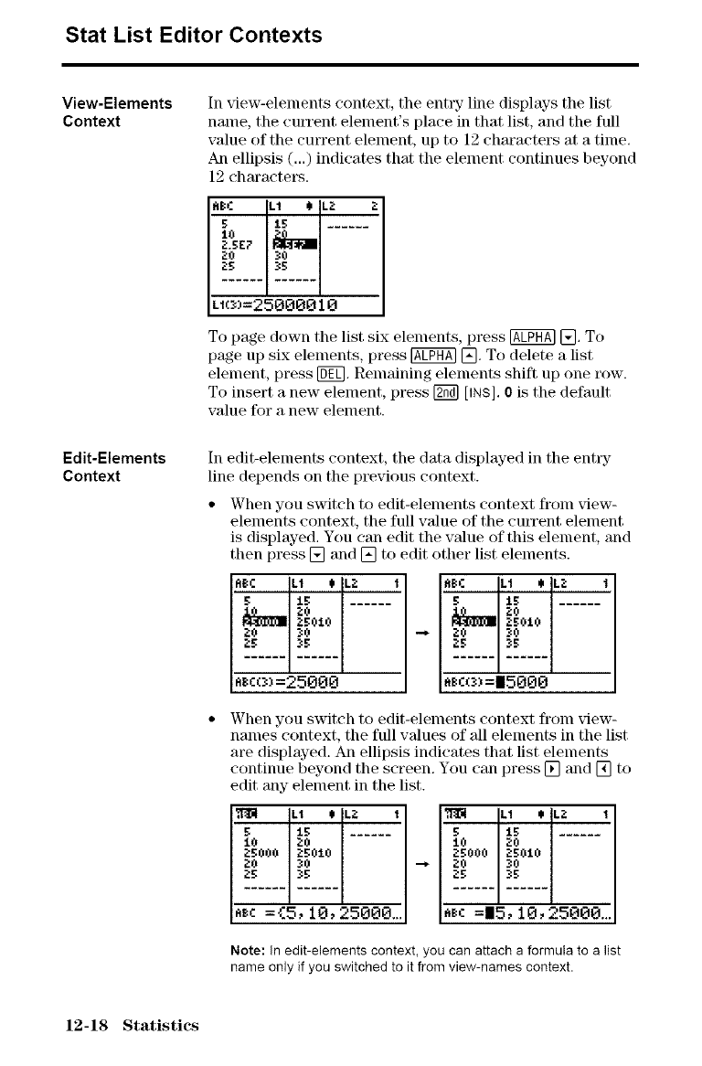
Stat List Editor Contexts
View-Elements
Context In view-elements context, the enttT line displays the list
name, the cmTent element's place in that list, and the full
value of the current element, up to 12 chm'acters at a time.
An ellipsis (...) indicates that the element continues beyond
12 characte_\s.
hBC Lt $._ 2
5t5
2._:E7
;'0 _0
tu_)=25000010
To page down the list six elements, press @ []. To
page up six elements, press @ []. To delete a list
element, press [DT0.Remaining elements shift up one row.
To insert a new element, press [g_ [INS]. 0 is the default
value for a new element.
Edit-Elements
Context In edit-elements context, the data displayed in the enttT
line depends on the previous context.
When you switch to edit-elements context from xqew-
elements context, the full value of the cmTent element
is displayed. You can edit the value of this element, and
then press [] and [] to edit other list elements.
R_(: LI $L_:
_0 _0
_g 3E:
_co)=25000
ABe LI $
2g010
2g 25
A_co_=|5000
When you switch to edit-elements context fronl view-
names context, the full vMues of 'allelements in the list
are displayed. An ellipsis indicates that list elements
continue beyond the screen. You can press [] and [] to
edit any element in the list.
L1 $k:;" 1
g1_; -,
t0 Z0
_000 Zg0t0
IA_c:£5, 10, 25000._ _c =I5, 10, 25000...
L1 $.2 1
I0 ZO
Z_:000 7_010
Note: In edit-elements context, you can attach a formula to a list
name only if you switched to it from view-names context.
12-18 Statistics
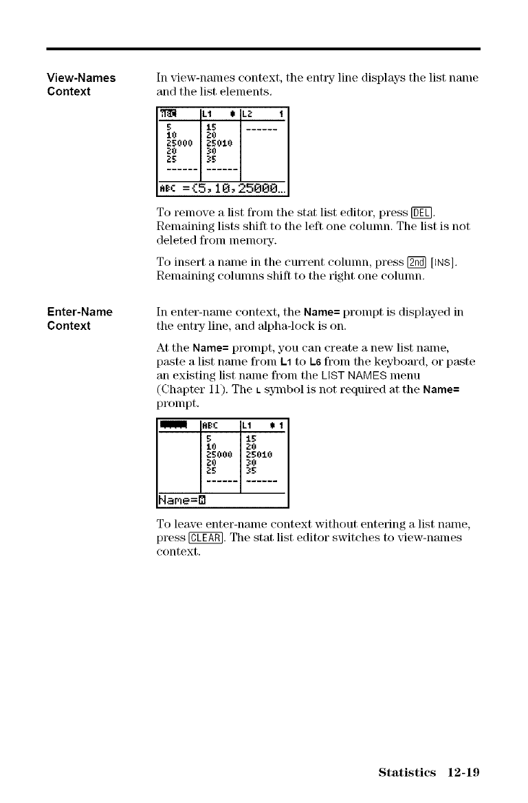
View-Names
Context
Enter-Name
Context
In view-names context, the entry line displays the list name
and the list elements,
LI € .2 I
515
10 _O
25 _O
25 _5
,Pc =15,10,25000_.
To remove a list from the stat list editor, press [3_],
Remaining lists shift to the left one colunm. The list is not
deleted from memow.
To insert a name in the eutTent colunm, press [_ [_NS],
Remaining eolunms shift to the right one colunm,
In enter-name context, the Name= prompt is displayed in
the entw line, and alpha-lock is on.
At the Name= prompt, you can create a new list name,
Dkste a list nalne fronl L1 to L6 fronl tile keyboard, or paste
an existing list nalne froln the LIST NAMES menu
(Chapter 11). The • s3qnbol is not required at the Name=
prompt.
_BC .1 ') i
r. 1_r
10 _0
_OOO -_SOiO
_O 30
Name=_
To leave enter-name context without entering a list name,
press @. The stat list editor switches to xqew-names
context.
Statistics 12-19
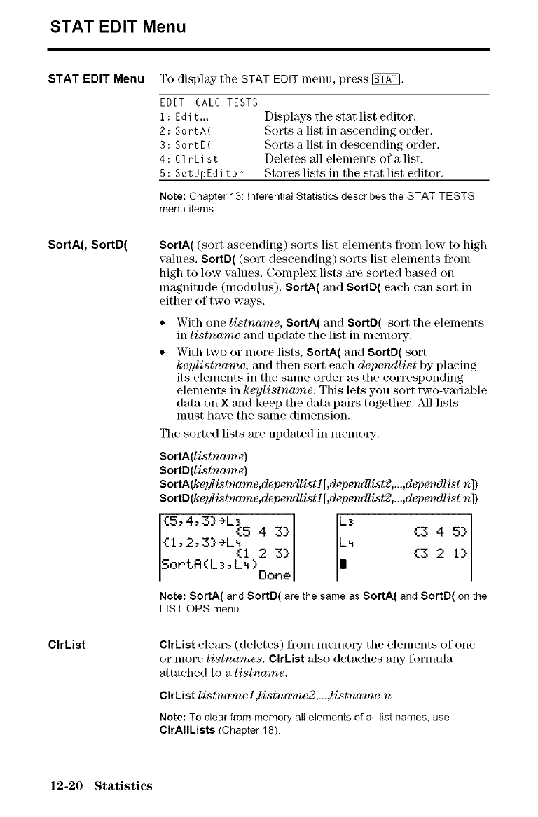
STAT EDIT Menu
STAT EDIT Menu
SortA(, SortD(
CIrList
To display the STAT EDIT menu, press [_,
EDIT CALC TESTS
i: Edit..,
2: SortA(
3: SortD(
4: ClrList
5: SetUpEditor
Displays the stat list editor.
Sorts a list in ascending order.
Sorts a list in descending order.
Deletes all elements of a list.
Stores lists in the stat list editor.
Note: Chapter 13: Inferential Statistics describes the STAT TESTS
menu items.
SortA( (sort ascending) sorts list elements fl'om low to high
values, SortD( (sort descending) sorts list elements fl'om
high to low values, Complex lists are sorted based on
magnitude (modulus). SortA( and SortD( each can sort in
either of two ways.
With one listname, SortA( and SortD( sort the elements
in listname and update the list in memory.
With two or more lists, SortA( and SortD( sort
keylistname, and then sort each dependlist by placing
its elements in the same order as the corresponding
elements in keylistname, This lets you sort two-variable
data on X and keep the data pairs together, All lists
nmst have the same dimension.
The sorted lists are updated in nlen]ot_yL
SortA(listname)
SortD(listname)
SortA(k¢ylistname,depe_MJistl[,depezwllist2,...,depezMlist n])
SortD(k_ylistname,depe_Mlistl[,depe_wllist2,...,depe_Mlist n])
{5, 4,33 +L _ IL_ I}
{5 4 3}I {3 4 5}
{1,2,3}+L4 I _
,- {i 2 3} {3 2
_ortR (L_, L4 >Done
Note: SortA( and SortD( are the same as SortA( and SortD( on the
LIST OPS menu.
ClrList clears (deletes) from memotT the elements of one
or more listnames. Clrkist also detaches any fornmla
attached to a listname.
ClrList listname l ,listname2,...,listname n
Note: To clear from memory al! elements of all list names, use
OIrAIILists (Chapter 18).
12-20 Statistics
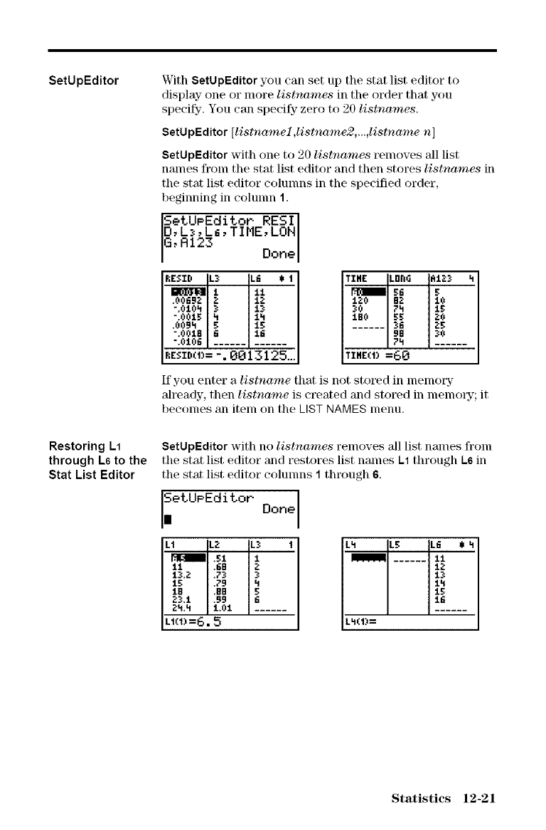
SetUpEditor With SetUpEditor you can set up the stat list editor to
display- one or more listnames in the order that you
specify-. You can specify zero to 20 listnames.
SetUpEditor [listnamel,listname2,...,listname n]
SetUpEditor with one to 20 listnames removes all list
names fron] the stat list editor and then stores listnames in
the stat list editor colunms in the specified order,
beginningincoluinnl.
SetUPEditor RESI
D,L_,L_,TIME,LOH
G,RI23 Done
_E_ID L_ ._ _t
.00692 2 12
".001_ h t_
.OOBh _ I_
",OOIB 6 16
",0106
RESZD<V=-. 0013125_.
TIME Lgn6 _123 h
s6 Is
120 B2 It0
30 ?h I1_
...... _6 I_
98 130
TIHE(!) =_
If you enter a listname that is not stored in lnelnory
already, then listname is created and stored in memory; it
becoines an item on the LIST NAMES menu,
Restoring L1
through L6 to the
Stat List Editor
SetUpEditor with no listnames removes all list names fronl
the stat list editor and restores list names kl through ks in
the stat list editor columns 1through 6.
SetUPEditor Done
|
Lt L2 ._ t
._1 1
11 ,6B _"
13.2 ,7_
1_; ,79 h
1B .BB 5
2_.1 ,99 6
:*h,h 1,01
L1(I:_=6,5
Lh L5 [L6 $ h
1LI
[i6
Lh(1)=
Statistics 12-21
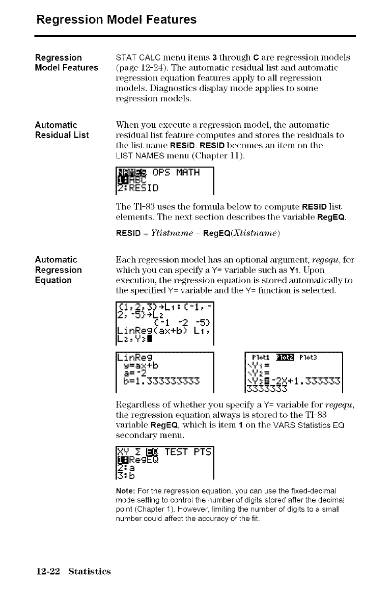
Regression Model Features
Regression
Model Features
Automatic
Residual List
Automatic
Regression
Equation
STAT CALC menu items 3through Care regression models
(page 12-24). The automatic residual list and automatic
_gression equation features apply to all regression
models, Diagnostics display mode applies to some
regression models.
Vclmn you execute a regression model, the automatic
residual list feature computes and stores the residuals to
the list name RESID. RESID becomes an item on the
LIST NAMES menu (Chapter 11).
OPS MRTH
The TI-83 uses the fommla below to compute RESID list
elements. The next section describes the variable RegEQ.
RESID =Ylistname -RegEQ(Xlistname)
Each regression nlodel has an optional argulnent, regequ, for
which you can specify- a Y= variable such as Y1. Upon
execution, the regression equation is stored automatically to
the specified Y= variable and the Y= function is selected.
2, -5_÷t_l -2
LinReg(ax+b)
Lz,Y_I
Lir_Re9 I nou _ no_
[ ,,,1=
b=I.333333333 B-2X+l. 333333
13333333 I
Regardless of whether you specify- a Y= variable for regequ,
the regression equation always is stored to the TI-83
variable RegEQ, which is item 1on the VARS Statistics EQ
secondmT menu.
XY E L_ TEST PTS
3-'b
Note: For the regression equation, you can use the fixed-decimal
mode setting to control the number of digits stored after the decimal
point (Chapter I ). However, limiting the number of digits to a small
number could affect the accuracy of the fit.
12-22 Statistics
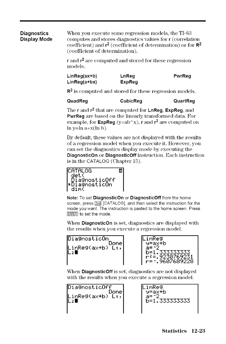
Diagnostics
Display Mode
When you execute sonle t_gression nlodels, the TI-83
computes and stores diagnostics values for r (correlation
coefficient) and r2(coefficient of determination) or for N2
(coefficient of determination).
r and r2 are computed and stored for these regression
models.
LinReg(ax+b) LnReg PwrReg
LinReg(a+bx) ExpReg
R2 is computed and stored for these t_gression models.
QuadReg CubicReg QuartReg
The r and r2that are computed for LnReg, ExpReg, and
PwrReg are based on the linearly transformed data. For
example, for ExpReg (y=ab^x), r and r2 are computed on
In y=ln a+x(ln b).
By- default, these values are not displayed with the results
of a regression model when you execute it. However, you
can set the diagnostics display mode by executing the
DiagnosticOn or DiagnosticOff instruction. Each instruction
is in the CATALOG (Chapter 15).
CATALOG
det(
DiagnostioO_
vDiagnostioOn
diM(
Note: To set DiagnosticOn or DiagnosticOff from the home
screen, press _ [CATALOG], and then select the instruction for the
mode you want. The instruction is pasted to the home screen. Press
to set the mode.
When DiagnosticOn is set, di_nostics m'e displayed with
the results when you execute a regression model.
OiagnostioOnoone LinReg
_=_x+b
L_Reg(a×+b) L,, a=-2
b=1.333333333
ni=.9230769231
n=-.9607689228
When DiagnosticOff is set, di_nostics are not displayed
with the results when you execute a regression model.
Diagno_tioO¢_one LinReg
_=ax+b
L_Reg(ax+b) LI, a=-2
b=1.333333333
Statistics 12-23
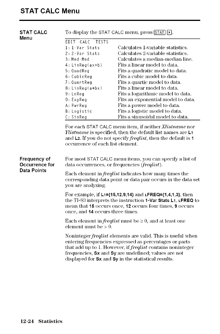
STAT CALC Menu
STAT CALC
Menu
Frequency of
Occurrence for
Data Points
To display the STAT CALC menu, press [KY_] [_.
EDIT CALC TESTS
1:1 Var Stats
2:2 Var Stats
3:Med Med
4: LinReg(ax+b)
5:QuadReg
6: CubicReg
7: QuartReg
8: LinReg(a+bx)
9: LnReg
O: ExpReg
A: PwrReg
B: Logistic
C: SinReg
Calculates 1-vmiable statistics,
Calculates 2-vmiable statistics.
Calculates a lnedian-lnedian line,
Fits a linear model to data.
Fits a quadratic model to data,
Fits a cubic model to data.
Fits a quartic model to data,
Fits a linear model to data.
Fits a logarithmic model to data,
Fits an exponential model to data,
Fits a power model to data,
Fits a logistic model to data,
Fits a sinusoidal model to data,
For each STAT CALC menu item, if neither Xlistname nor
Ylistname is specified, then the default list names m'e kl
and k2. If you do not specifyfreqlist, then the default is 1
occurrence of each list element.
For most STAT CALC nlenu itenls, you can specify a list of
data occurrences, or frequencies (freqlist).
Each element infreqlist indicates how many times the
corresponding data point or data pair occurs in the data set
you are analyzing.
For example, if 1_1={15,12,9,14} and LFRlaQ={1,4,1,3}, then
the TI-83 interprets the instruction 1-Vat Stats 1.1, LFREO to
mean that 16 occurs once, 12 occurs four times, 9occurs
once, and 14 occurs three times.
Each element infreqlist nmst be _>0, and at least one
element nmst be > 0.
Nonintegerfreqlist elements m'e valid. This is useful when
entering frequencies expressed as percentages or parts
that add up to 1. However, iffreqlist contains noninteger
frequencies, Sx and Sy are undefined; wdues m'e not
displayed for Sx and $y in the statistical results,
12-24 Statistics
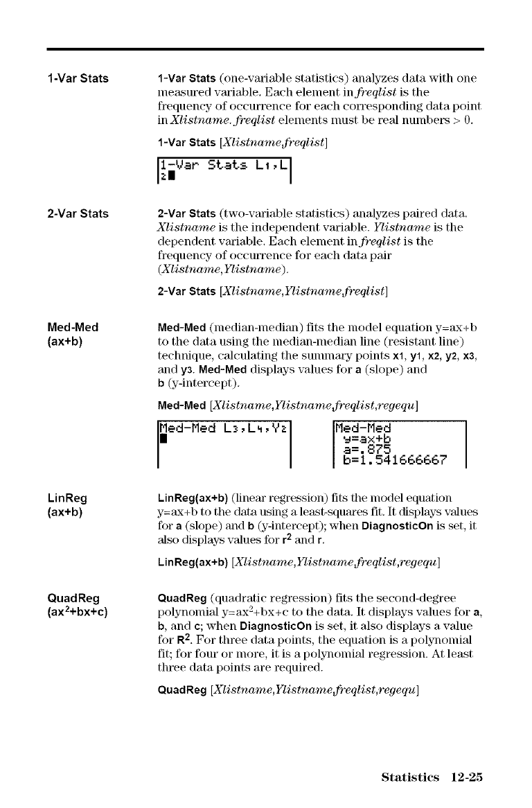
1-Var Stats
2-Var Stats
Med-Med
(ax+b)
LinReg
(ax+b)
QuadReg
(axZ+bx+c)
1-Var Stats (one-variable statistics) analyzes data with one
measm'ed variable. Each element infreqlist is the
frequency of occurrence for each corresponding data point
in Xlistname. freqlist elements nmst be real numbers > 0.
1-Var Stats [Xlistnamefreqlist]
_iVaP Stats LI,L
2-Var Stats (two-variable statistics) analyzes paired data.
Xlistname is the independent variable. Ylistname is the
dependent variable. Each element infreqlist is the
frequency of occutTence for each data pair
(Xlistname, Ylistname),
2-Var Stats [Xlistname,_Tistnome_freqlist]
Med-Med (nmdian-n]edian) fits the model equation y=ax+b
to the data using the median-nmdim_ line (resistmlt line)
technique, calculating the sunul]aYy points xl, yl, x2, y2, x3,
and y3. Med-Med displays values for a (slope) and
b (y-intercept).
Med-Med[Xlis_ame,_is_ame_v_ist,regequ]
_ed-Med L_,L_,Yz Med-Med
_=ax+b
a=.875
b=1.541666667 I
LinReg(ax+b) (linear regression) fits the model equation
y=ax+b to the data using a least-squares fit. It displays values
for a(slope) and b(y-intercept); when DiagnosticOn is set, it
also displays values for r2and r,
LinReg(ax+b) [Xlistname,Ylistname_freqlist,regequ]
QuadReg (quadratic regression) fits the second-degree
polynomial y=ax2+bx+c to the data. It displays values for a,
b, and c; when DiagnosticOn is set, it also displays a value
for R2. For three data points, the equation is a polynomial
fit; for four or more, it is a polynomial regression. At least
three data points are required.
QuadReg [Xlistname,Ylistname_freqlist,regequ]
Statistics 12-25
CubicReg
(ax3+bx2+cx+d)
CubicReg (cubic regression) fits the third-degree
polynomial y=ax:_+bx2+ex+d to the data. It displays wdues
for a, b, c, and d; when DiagnosticOn is set, it also displays
a wdue for R2. For four points, the equation is a polynomial
fit; for five or more, it is a polynomial regression. At least
four points are requil_d.
CubicReg [Xlistname,_istnamedCreqlist,regequ ]
Qua_Reg
(ax4+bx3+cx2+
dx+e)
LinReg
(a+bx)
LnReg
(a+b In(x))
ExpReg
(abx)
QuartReg (quartic regression) fits tile fourth-degree
polynomial y=ax4+bx:%cx2+dx+e to the data. It displays
values for a, b, c, d, and e; when DiagnosticOn is set, it also
displays a wdue for R2. For five points, the equation is a
polynomial fit; for six or more, it is a polynomial
regression. At least five points are required.
OuartReg [Xlistname,YlistnamedCreqlist,regequ]
LinReg(a+bx) (linear regression) ills the model equation
y=a+bx to the data using a least-squalls fit. It displays values
for a (y-intercept) and b(slope); when DiagnosticOn is set, it
also displays values for r2and r.
LinReg(a+bx) [Xlistname,_istnamedCreqlist,regequ ]
LnReg (logarithmic regression) fits the model equation
y=a+b ln(x) to the data using a least-squares fit and
transformed values ln(x) and y. It displays values for aand
b; when DiagnosticOn is set, it also displays values for r2
and r.
LnReg [Xlistname,YlistnamedCreqlist,regequ]
ExpReg (exponential regression) fits the model equation
y=ab _ to the data using a least-squares fit and transformed
values x and ln(y). It displays values for aand b; when
DiagnosticOn is set, it also displays values for r2 and r.
ExpReg [Xlistname,YlistnamedCreqlist,regequ]
12-26 Statistics
PwrReg
(axb)
Logistic
c/(l+a*e -bx)
SinReg
a sin(bx+c)+d
PwrReg (power l_gression) fits the model equation y=ax bto
the data using a least-squares fit and transformed values
ln(x) and ln(y). It displays wdues for a and b; when
DiagnosticOn is set, it 'also displays values for r2 and r.
PwrReg [Xlistname,Ylistname_freqlist,regequ]
Logistic fits the model equation y=c/(l+a*e -bx) to tile data
using an iterative least-squares fit. It displays values for a, b,
and c.
Logistic [Xlistname,Ylistname_reqlist,regequ]
SinReg (sinusoidal regression) fits the model equation
y=a sin(bx+e)+d to the data using an iterative least-squares
fit. It displays values for a, b, c, and d. At least fore" data
points m'e required. At least two data points per cycle m'e
required in order to avoid aliased frequency estimates.
SinReg [iterations,Xlistname,I_istname,period,regequ]
iterations is the nlaxinlonl number of times the algorithm
will iterate to find a solution. The value for iterations can
be an integer _>1 and _<16; if not specified, the default is 3.
The algorithm nlay find a solution before iterations is
l_a('hed. Typically, lm'ger values for iterations result in
longer execution times and better accuracy for SinReg, and
vice versa.
Aperiod guess is optional. If you do not specify-period, the
difference between time values in Xlistname must be equal
and the time values nmst be ordered in ascending
sequential order. If you specify-period, the algorithm nlay
find a solution nlore quickly, or it nlay find a solution when
it would not have found one if you had omitted a value for
period. If you specify period, the differences between time
values in Xlistname can be unequal.
Note: The output of SinReg is always in radians, regardless of the
Radian/Degree mode setting.
ASinReg example is shown on tile next page.
Statistics 12-27
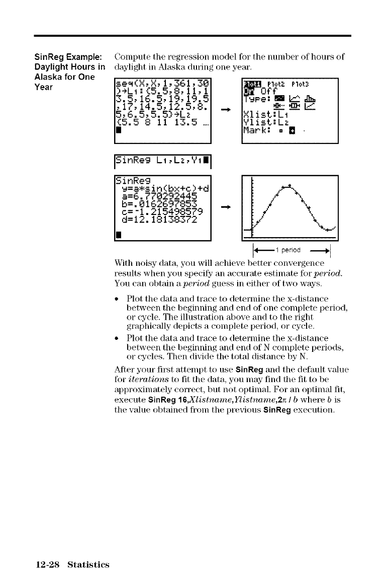
SinReg Example:
Daylight Hours in
Alaska for One
Year
Compute the regression model for the number of hours of
daylight in Alaska durin
se_(X, X, 1,361,30
)+LI : {5.5,8, ii, 1
3.5, 16.5, 19, 19.5
,17, 14.5, 12.5,8.
5_6.5,5.5}+Lz
{5.5 8 Ii 13.5
one year.
[liar Notz _lotx
orr
IT_Pe:_I.._ _
-_ li<,listiE1-
6Jlist:Lz
Mark: ° [] .
SinReg LI,Li,VI1
SinReg
_=a*sin(bx+c)+d
a=6.770292445
b=.8162697853
o=-1.215498579
d=12.18138372
With noisy data, you will achieve better convergence
results when you specify- an accurate estimate for period.
You can obtain aperiod guess in either of two ways.
• Plot the data and trace to determine the x-distance
between the beginning and end of one complete period,
or cycle. The illustration above and to the right
graphically depicts a complete period, or cycle.
• Plot the data and trace to determine the x-distance
between the beginning and end of N complete periods,
or cycles. Then divide the total distance by N.
M'ter your fit_t attempt to use SinReg and the default value
for iterations to fit the data, you may find the fit to be
approximately correct, but not optimal. For an optimal fit,
execute SinReg 16,Xlistname,I_istfzame,2_ I b where bis
the value obtained froln the prexqous SinReg execution.
12-28 Statistics
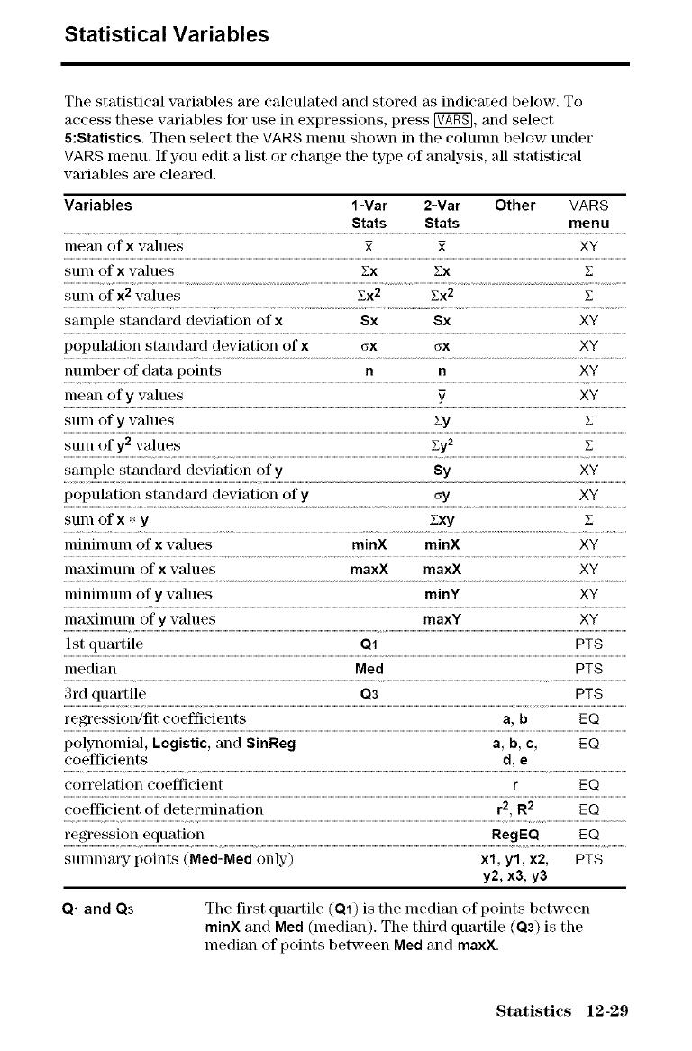
Statistical Variables
The statistical variables are calculated and stored as indicated below, To
access these variables ff)r use in expressions, press _, and select
5:Statistics. Then select the VARS menu shown in the colunm below under
VARS menu. If you edit a list or change the type of analysis, all statistical
vm'iables m'e clem'ed.
Variables 1-Var 2-Var Other VARS
Stats Stats menu
mean of xvalues _ _ XY
SUnl of xvalues Ex Ex E
sunl of X2values Yx2Yx2E
sample standard deviation of xSx Sx XY
population standard deviation of x _x Gx XY
nulnber of data points n n XY
mean of yvalues _ XY
sunl of yvalues 2y 1;
sunl of y2 values 'Fy2 y
sample standard dexqation of y Sy XY
population standard deviation of y_y XY
sunl of X * y Zxy Z
lninimuln of xvalues minX minX XY
lnaxilnuln of xvalues maxX max)( XY
lninimuln of yvalues minY XY
lnaxilnum of yvalues maxY XY
1st quartile Q1 PTS
median Med PTS
3rd quartile Q3 PTS
regression/fit coefficients a, bEQ
polynomial, Logistic, and SinReg a, b, c, EQ
coefficients d, e
correlation coefficient rEQ
coefficient of determination r2, R2 EQ
regression equation RegEQ EQ
sulnl:laI T points (Med-Med only) xl, yl, x2, PTS
y2, x3, y3
Q1 and Q3 The first quartile (Q1) is the median of points between
minX and Meal (median). The third quartile (Q3) is the
median of points between Med and maxX.
Statistics 12-29
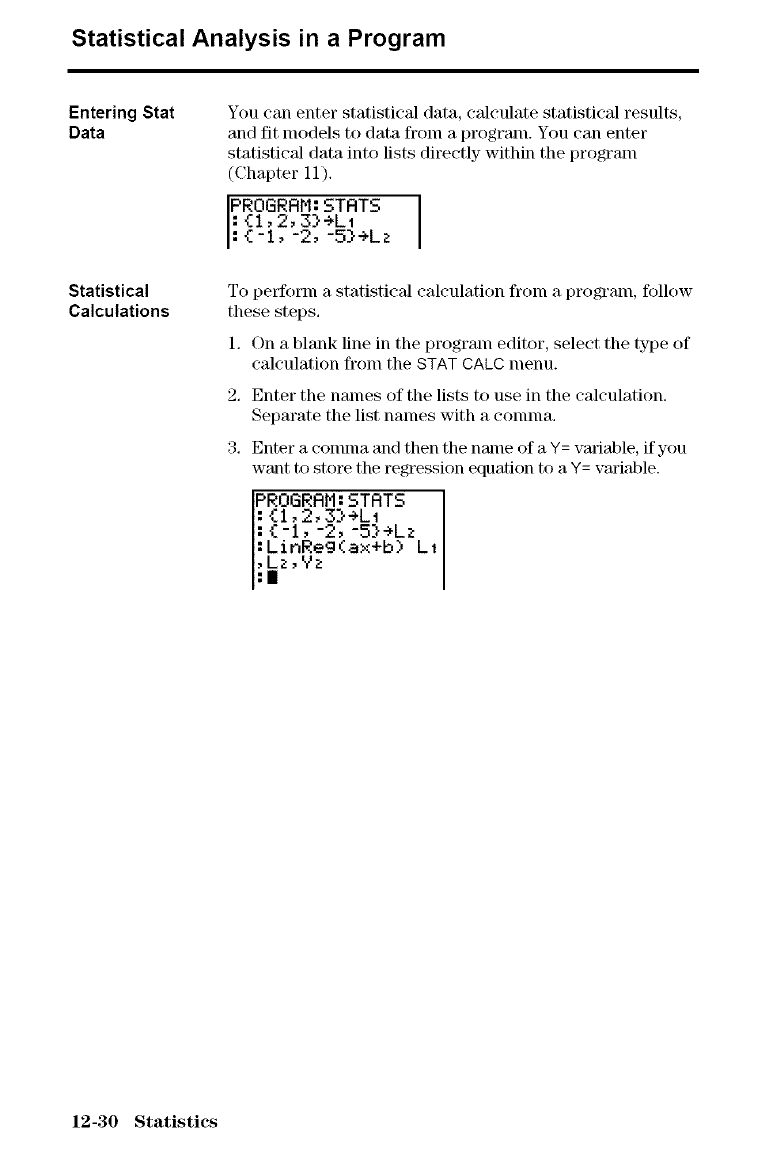
Statistical Analysis in a Program
Entering Stat
Data
Statistical
Calculations
You can enter statisticM data, calculate statistical results,
and fit models to data from a program. You can enter
statistical data into lists directly within the program
(Chapter 11),
PROGRRM: STRTS ]
: {1,2,3}÷LI
: {-I, -2, -5}÷Lz
To perform a statistical calculatkm from a program, follow
these steps,
1, On a blank line in the progrmn editor, select the type of
calculation from the $TAT CALC menu.
2, Enter the names of the lists to use in the calculation.
Separate the list names with a conlnla,
3, Enter a conulla and then the name of a Y= variable, if you
want to store the regression equation to a Y= variable.
PROGRRM:STRT5
:{1,2,3}÷LI
:{-I,-2,-5}÷L1
:LinReg(ax+b) LI
12-30 Statistics
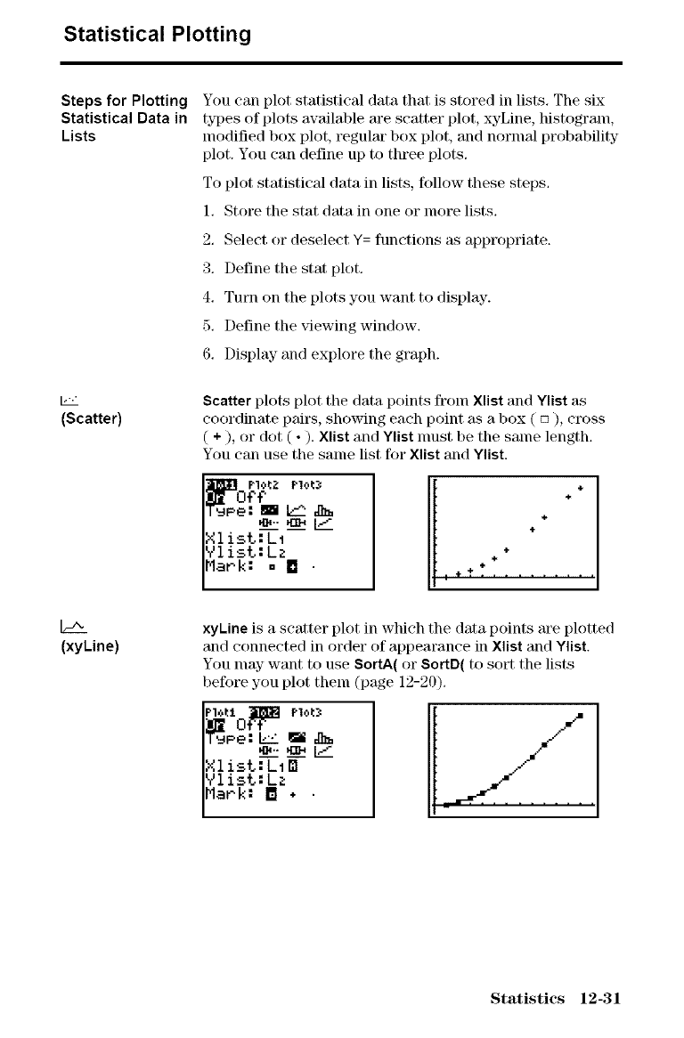
Statistical Plotting
Steps for Plotting
Statistical Data in
Lists
(Scatter)
(xyLine)
You call plot statistical data that is stored in lists. The six
types of plots available m'e scatter plot, xyLine, histogram,
modified box plot, regulm" box plot, and normal probability
plot. You can define up to three plots.
To plot statistical data in lists, follow these steps.
1, Store the stat data in one or more lists.
2, Select or deselect ¥= functions as appropriate.
3, Define the stat plot.
4. Turn on the plots you want to display.
5, Define the v_ewing window.
6, Display and explore the graph.
Scatter plots plot the data points fronl Xlist and Ylist as
coordinate pairs, showing each point as a box ( o ), cross
(+), or dot ( • ). Xlist and Ylist nmst be the sanle length.
You can use the same list for Xlist and Ylist,
"t]';i'Off
T'_Pe:_m_,._ k____
Xlist.;_t--
Vli__L:Lz
Mark: [] []
÷
÷
÷
÷
+÷
:+_ .........
xyLine is a scatter plot in which the data points are plotted
and connected in order of appearance in Xlist and Ylist.
You nlay want to use SortA( or SortD( to sort the lists
beffwe you plot them (page 12-20).
_Pe: -L_ _ J_
Y,IisL:LI_
Vlist:Lz
Mark: [] *.
Statistics 12-31
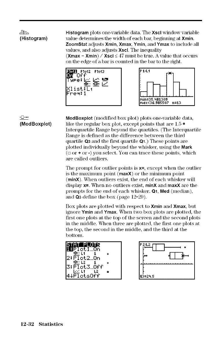
(Histogram)
(ModBoxplot)
Histogram plots one-variable data. The Xscl window variable
value determines the width of each bar, beginning at Xmin.
ZoomStat adjusts Xmin, Xmax, Ymin, and Ymax to include all
values, and 'also adjusts Xscl. The inequality
(Xmax - Xmin) /Xscl _<47 must be true. A value that occurs
on the edge of a bar is counted in the bar to the right.
m 0f'€
Xlist,;"Ct
Fr.e_: I
i ;
Ip_in=_B.4Bt30B
ModBoxplot (modified box plot) plots one-variable data,
like the regular box plot, except points that are 1.5 *
Interquartile Range beyond the quartiles. (The Interquartile
Range is defined _s the difference between the third
quartile Q3 and the first quartile Q1.) These points are
plotted individually beyond the whisker, using the Mark
(5 or + or ,) you select. You can trace these points, which
are called outliers.
The prompt ff)r outlier points is x=, except when the outlier
is the maximunl point (maxX) or the minimunl point
(minX). When outliers exist, the end of each whisker will
display x=. When no outliers exist, minX and maxX are the
prompts for the end of each whisker. O1, Med (median),
and Q3 define the box (page 12-29).
Box plots are plotted with respect to Xmin and Xmax, but
ignore Ymin and Ymax. When two box plots are plotted, the
first one plots at the top of the screen and the second plots
in the middle. When three a_ plotted, the first one plots at
the top, the second in the middle, and the third at the
bottonL
Lt 1 +
2:Plot2...On
,'D,-L2 1 +
3: P 1 ot3...O_f
L1 LZ
4.&P lotsO_
12-32 Statistics
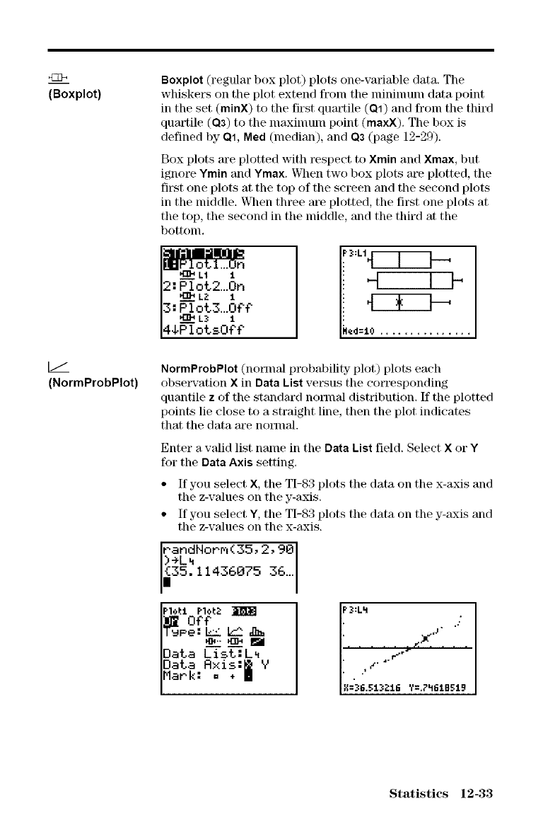
(Boxplot)
(NormProbPIot)
Boxplot (regular box plot) plots one-variable data. The
whiskers on the plot extend fronl tile nlininlunl data point
in the set (minX) to the first quartile (Q1) and from the third
quartile (Q3) to the nlaxinmln point (maxX). The box is
defined by Q1, Med (median), and Q3 (page 12-29).
Box plots are plotted with respect to Xmin and Xmax, but
ignore Ymin and Ymax. When two box plots are plotted, the
first one plots at the top of the screen and the second plots
in the middle. When three ale plotted, the first one plots at
tile top, tile second in tile middle, and the third at the
bottonl.
L,t li q le
2: Plot2...0n
3:Plot3...Of'f"
44,P 1otsOtPt" ,a ....
NormProbPIot (normal probability plot) plots each
observation X in Data List vel\sus the corresponding
quantile zof the standard nonnM distribution, If the plotted
points lie close to a straight line, then the plot indicates
that the data are normal.
Enter a valid list nalne in the Data List field. Select Xor Y
for the Data Axis setting.
• If you select X, tile TI-83 plots tile data on tile x-axis and
the z-values on the y-axis.
• If you select Y, the TI-83 plots the data on the y-axis and
the z-values on the x-axis.
[PandHorp_(35, 2,90
)÷L_ 7 36
Plot1 p1OI:;_
m 0f'f"
T_Pe: -L_ b-_ 31_
_.- a]b I
Data Crst.--: L _
Data Axis:@ Y
Mar'k: =*II
P3:Lh
N=')E.E:1321E ?=.?hEIBB19
Statistics 12-33
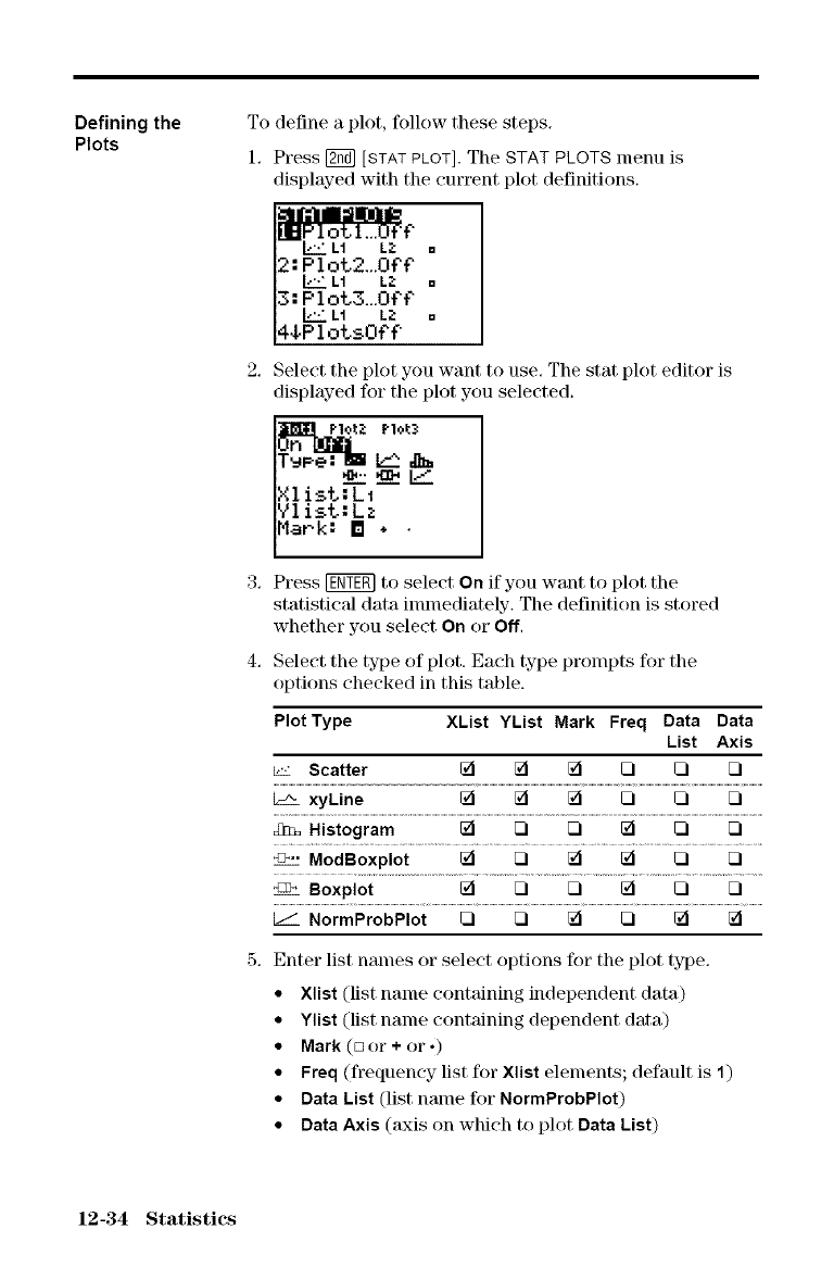
Defining the
Plots To define a plot, follow these steps.
1, Press [_ [STAT PLOT]. The STAT PLOTS menu is
displayed with the current plot definitions,
2, Select the plot you want to use, The stat plot editor is
displayed for the plot you selected,
3, Press _ to select On if you want to plot the
statistical data imnlediately. The definition is stored
whether you select On or Off,
4, Select the type of plot. Each type prompts for the
options checked in this table.
Plot Type XList YList Mark Freq Data Data
List Axis
_L_ Scatter _ _i _ rl [] []
xyLine _ 121 _ [] [] []
Zn_ Histogram _ [] [] _ [] []
o,. ModBoxplot _ [] _ _ [] []
_:_> Boxplot _ [] [] _ [] []
[__ NormProbPIot [] [] _ [] _ lTI
Enter list names or select options for the plot type,
• Xlist (list name containing independent data)
• Ylist (list name containing dependent data)
•Mark (aor +or.)
• Freq (frequency list for Xlist elements; default is 1")
•Data List (list nanle for NormProbPIot)
•Data Axis (axis on which to plot Data List)
12-34 Statistics
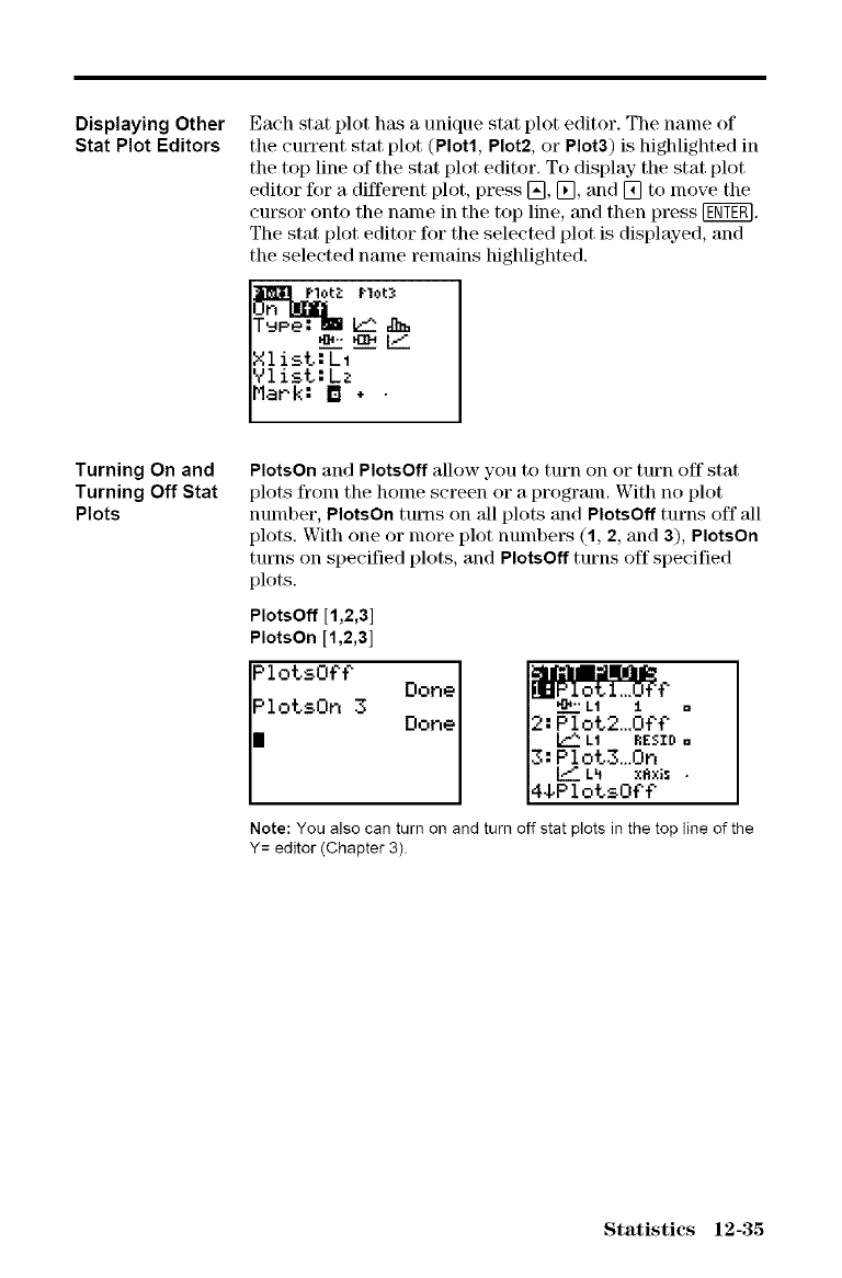
Displaying Other
Stat Plot Editors Each stat plot has a unique stat plot editor. The name of
the current stat plot (Plot1, Plot2, or Plot3) is highlighted in
the top line of the stat plot editor. To display the stat plot
editor for a different plot, press [], [], and [] to lnove the
cursor onto the name in the top line, and then press [_.
The stat plot editor for the selected plot is displayed, and
the selected name remains highlighted.
_" _ L_
Xlist:L1
Vlist:Lz
Mark: [] *
Turning On and
Turning Off Stat
Plots
PlotsOn and PlotsOff allow you to turn on or turn off stat
plots from the home screen or a program. With no plot
number, PlotsOn turns on M1plots and PlotsOff turns off 'all
plots. With one or more plot numbers (1, 2, and 3), PlotsOn
turns on specified plots, and PlotsOff turns off specified
plots.
PlotsOff [1,2,3]
PlotsOn [1,2,3]
PlotsOf'f"
Note: You also can turn on and turn off stat plots in the top line of the
Y= editor (Chapter 3).
Statistics 12-35
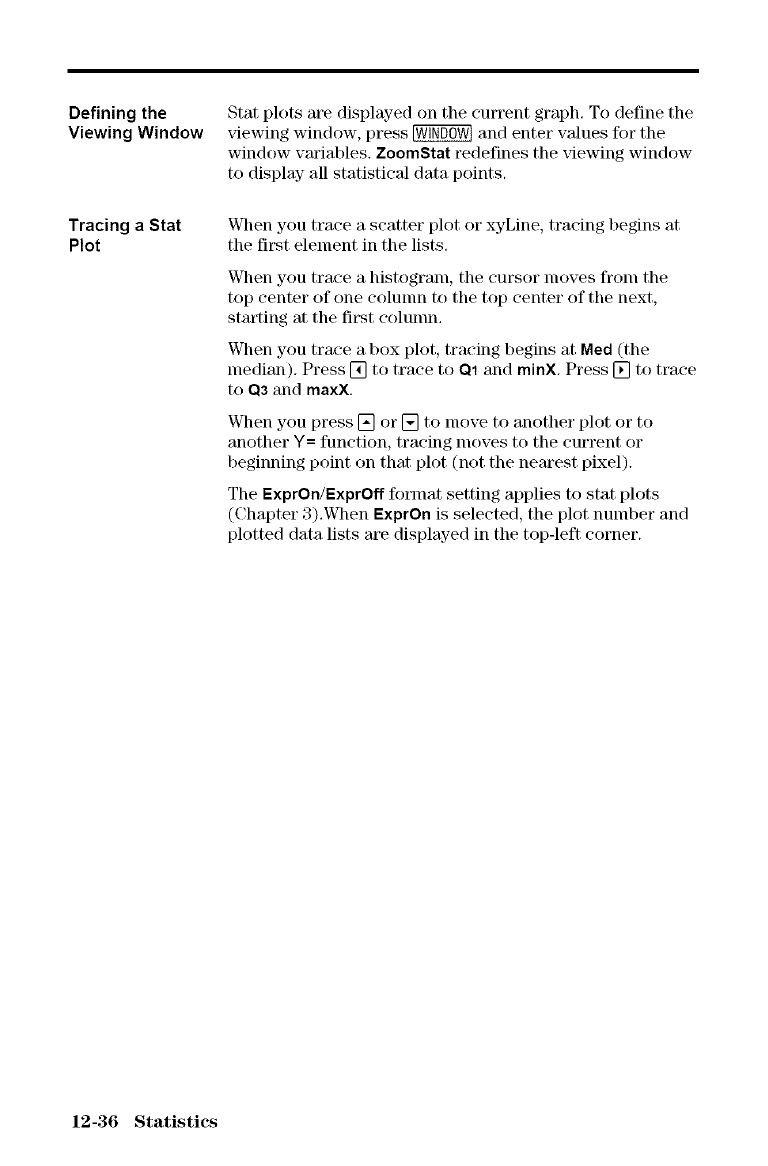
Defining the
Viewing Window
Tracing a Stat
Plot
Stat plots are displayed on the current graph. To define the
xqewing window, press _ and enter values for the
window variables. ZoomStat redefines the xqewing window
to display all statistical data points.
When you trace a scatter plot or xyLine, tracing begins at
the first element in the lists.
VClmnyou trace a histogram, the cursor nloves fronl the
top center of one colunm to tile top center of tile next,
starting at the first colunm.
When you trace a box plot, tracing begins at Med (the
median). Press [] to trace to Ol and minX. Press [] to trace
to O3 and maxX.
When you press [] or [] to move to another plot or to
another Y= function, tracing moves to the current or
beginning point on that plot (not the nearest pixel).
The ExprOn/ExprOff format setting applies to stat plots
(Chapter 3).When ExprOn is selected, the plot number and
plotted data lists are displayed in the top-left corner.
12-36 Statistics
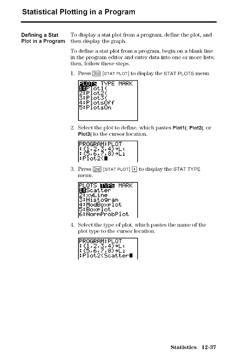
Statistical Plotting in a Program
Defining a Stat
Plot in aProgram
To display a stat plot fronl a program, define the plot, and
then display the graph.
To define a star plot from a program, begin on a blank line
in the program editor and enter data into one or more lists;
then, follow these steps.
1. Press [g_ [STATPLOT]to displw tile STAT PLOTS menu.
T"tPE MARK
i3:Plot3(
i4.PlotsOgg
5:Plot.sOn
Select the plot to define, which pastes Plot1(, Plot2(, or
Plot3( to the cursor location.
PROGRAM:PLOT
:{I,2,3,4}+LI
:{5,6,7,8}+Lz
:Plot2(I
Press[_[STATPLOT][_todisplaytheSTATTYPE
nlenu,
PLOTS _ MARK
._Soatter
z: x_Line
5:Bo>,'gIot
S:HorMProbPlot
Select the type of plot, which pastes the name of the
plot type to the cm'sor location.
PROGRAM:PLOT
:{1,2,3,4}+LI
:{5,6,7,8}+Lz
:Plot2(SoatterI
Statistics 12-37
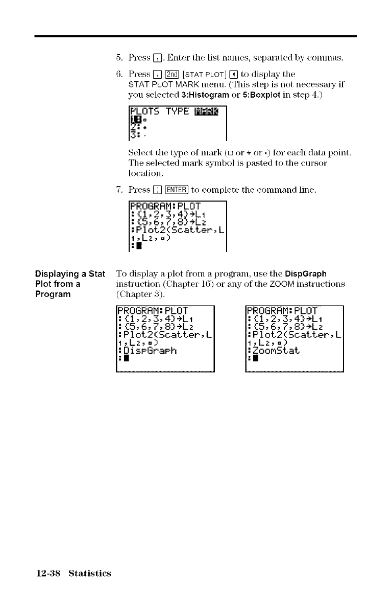
Displaying a Stat
Plot from a
Program
5_
6,
Press []. Enter the list names, separated by eonunas.
Press [] [_ [STAT PLOT] [] to display the
STAT PLOT MARK menu. (This step is not necessaqy- if
you selected 3:Histogram or 6:Boxplot in step 4.)
Select the type of nlark (D or + or °) for each data point.
The selected mm'k symbol is pasted to the cursor
location.
Press [] _ to complete the command line,
PROGRAM: PLOT L
: {I02,3,4}÷LI
: {5, 6, 7,8}÷Lz
:Plot2(Soattet-,
To display- a plot from a program, use the DispGraph
instruction (Chapter 16) or any of the ZOOM instructions
(Chapter 3),
PROGRR_I: PLOT
: {1,2,3,4}÷LI
:,.5,6, _, 8}+Lz
: Plot2(ScatteP, L
I,Lz,=)
::DisParaF-h
PROGRRM:PLOT
:{1,2,3,4}÷Lt
:_506,7,8}÷Lz
:Plot2(ScatteP,L
I,Lz,.)
::_°°MStat
12-38 Statistics
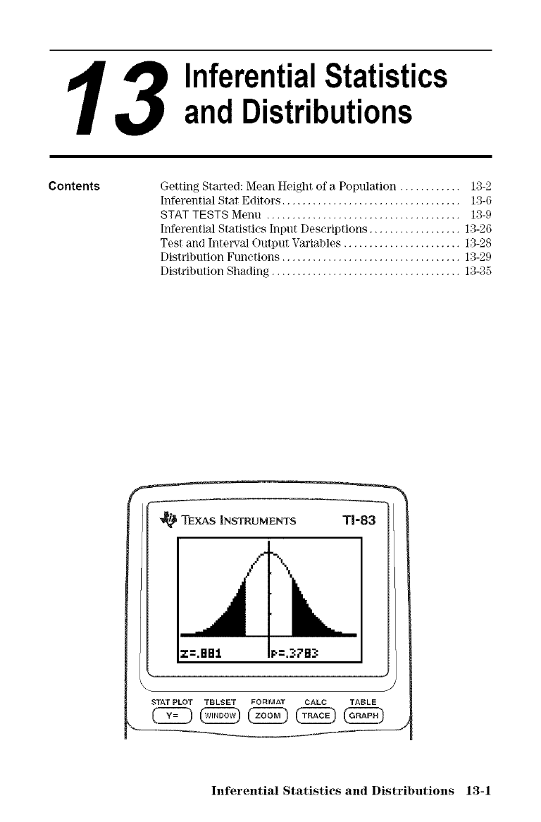
3InferentialStatisticsand Distributions
Contents Getting Started: Mean Height of a Population ............ 13-2
Inferential Star Editors ................................... 13-6
STAT TESTS Menu ...................................... 13-9
Inferential Statistics Input I)eseriptions .................. 13-26
Test and Interval Output Variables ....................... 13-28
Distribution Functions ................................... 13-29
Distribution Shading ..................................... 13-35
'_ TEXAS iNSTRUMENTS T1=83
z=.ee:l. I_=._?e:_
J
STATPLOT TBLSET FORMAT CALC TABLE
Inferential Statistics and Distributions 13-1
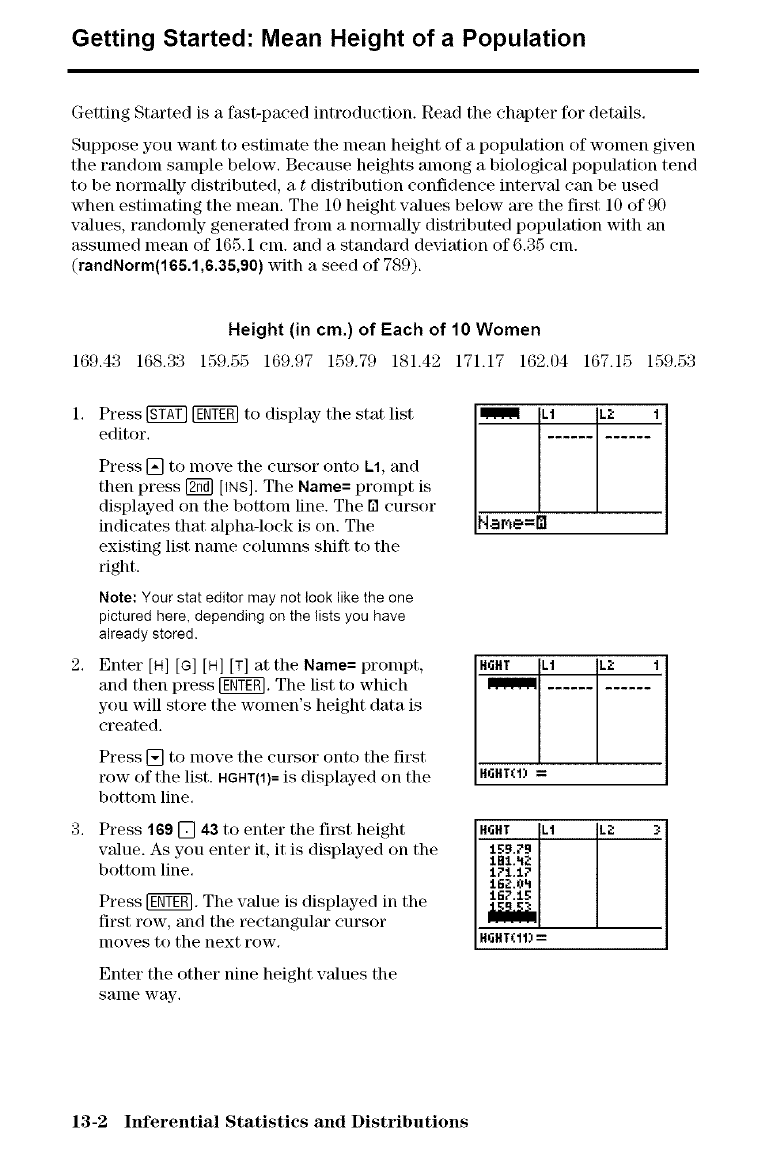
Getting Started: Mean Height of a Population
Getting Started is a fast-paced introduction. Read the chapter for details.
Suppose you want to estimate the mean height of a population of women given
tile random sample below. Because heights among a biological population tend
to be normally distributed, a tdistribution confidence interval can be used
when estimating the mean. The l0 height wdues below are the first l0 of 90
wdues, randonfly generated from a normally distributed population with an
assumed mean of 165.1 cm. and a standard dexqation of 6.35 cm.
(randNorm(165.1,6.36,90) with a seed of 789).
Height (in cm.) of Each of 10 Women
169.43 168.33 159.55 169.97 159.79 181.42 171.17 162.64 167.15 159.53
Press [gTKg][gNT_ to display the stat list
editor.
Press [] to nlove the cursor onto L1, and
then press [_] [,NS]. The Name= prompt is
displayed on the bottom line. The [] cursor
indicates that alpha-lock is on. The
existing list name eolunms shift to the
right.
Note: Your stat editor may not look like the one
pictured here, depending on the lists you have
already stored.
Enter [H] [G] [H] [T] at the Name= prompt,
and then press [gNT_. The list to which
you will store the women's height data is
created.
Press [] to move the cursor onto the first
row of the list. HGHT(1)=is displayed on the
bottom line.
Press 169 [] 43 to enter the first height
value. As you enter it, it is displayed on the
bottom line.
Press [gNT_. The value is displayed in the
first row, and the rectangular cursor
nloves to the next row.
Enter the other nine height values the
sanle way,
1.I L_ I
HaMe==
HGHT .1 L;' 1
mmm
H6HT(1) =
HGHT .1 L_ 3
1_9.7B
171.17
16Y.tg
H6HT(11)=
13-2 hfferential Statistics and Distributions
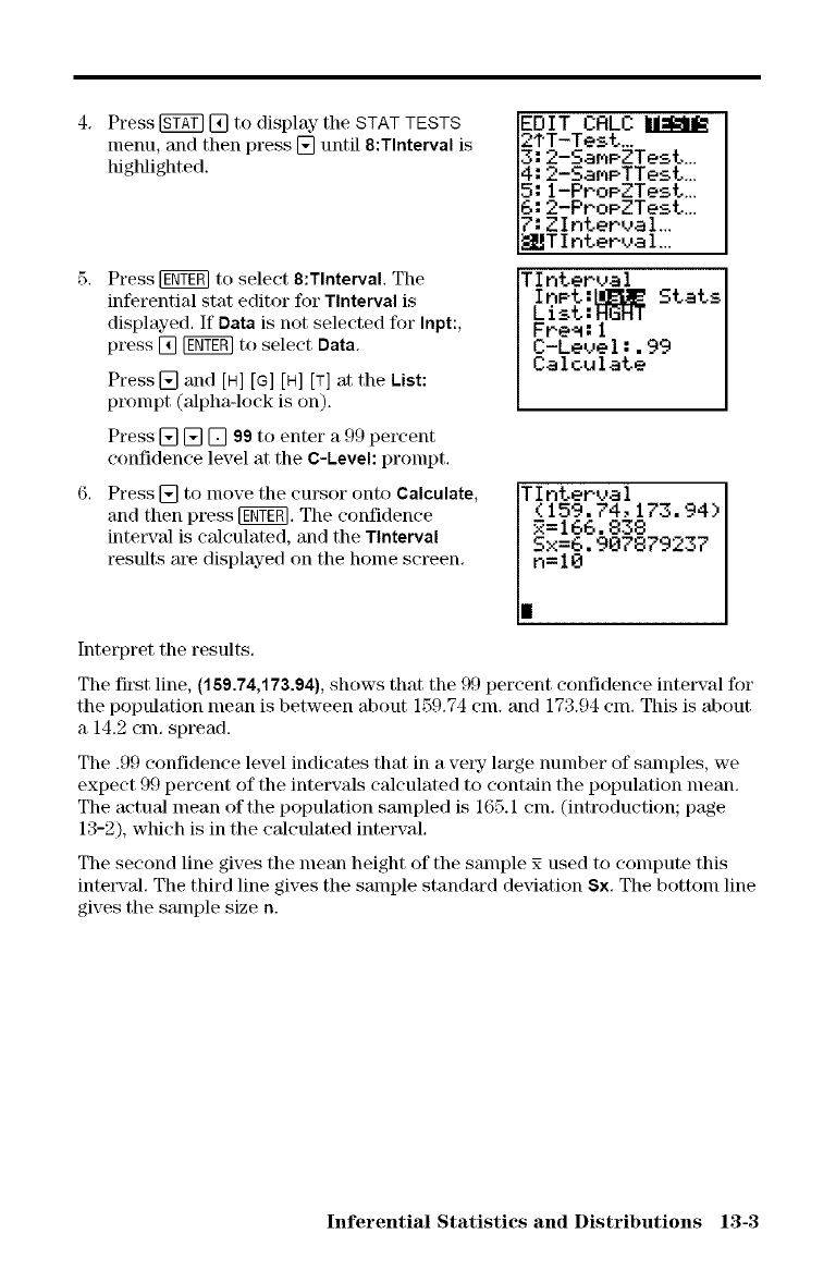
4. Press [gY_ [] to display the STAT TESTS
menu, and then press [] until 8:Tlnterval is
highlighted.
5. Press _ to select 8:Tlnterval. The
inferential stat editor for Tlnterval is
displayed. If Data is not selected for Inpt:,
press [] [ggY_ to select Data.
Press [] and [H] [G] [a] [T] at the List:
prompt (alpha-lock is on).
Press [] [] [] g@to enter a 99 percent
confidence level at the C-Level: prompt.
6. Press [] to move the cursor onto Calculate,
and then press IgOr. The confidence
intet¢TM is calculated, and the Tlnterval
results are displayed on the home screen.
Interpret the results.
EDIT CRLCIII_
2ST-Test,,
3:2-SamPZTest
4:2-Sar4eTTest_
7:ZIntervM,.,"-
[_tlTInterval...
TlntervM
InPt:_ Stats
List:HGHT
Fre_:1
C-Level:.99
Calculate
Tlnterval
(159.74,173.94)
R=166.838
Sx=6.907879237
n=lO
The first line, (159.74,173.94), shows that the 99 percent confidence inte_xal for
the population mean is between about 159.74 cm. and 173.94 cm. This is about
a 14.2 cm. spread.
The .99 confidence level indicates that in a vet3z lm'ge number of samples, we
expect 99 percent of the intervals calculated to contain the population mean.
The actual mean of the population sampled is 165.1 cm. (introduction; page
13-2), which is in the calculated interval.
The second line gives the mean height of the sample N used to compute this
intet_'al. The third line gives the sample standard deviation Sx. The bottom line
gives the sample size n.
Inferential Statistics and Distributions 13-3
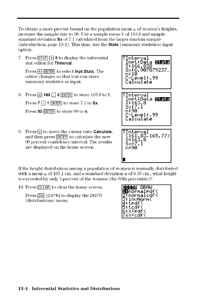
To obtain a more precise bound on the population mean _tof women's heights,
increase the sample size to 96. Use a sample mean ._ of 163.8 and sample
standard deviation Sx of 7.1 calculated from the larger random sample
(introduction; page 13-2). This time, use the Stats (sunullal_y statistics) input
option.
Press [g_g] [] 8to display" the inferential
star editor for Tlnterval.
Press [] [g_N to select Inpt:Stats. The
editor changes so that you can enter
sunullal_ statistics as input.
TInterual
InPt:Data I¢_
5:166.838
Sx:G.90787923Z_
n:10
C-Leuel:.99
Calculate
TInterual
InPt:Data _
R:IG3.8
Sx:7.1
n:90
C-Leuel:.99
Calculate
8. Press [] 163 [] 8 [N?_ to store 163.8 to _.
Press 7[] 1[ggY_ to store 7.1 to Sx.
Press 90 [NTgN to store 96 to n.
Press [] to move the cursor onto Calculate,
and then press [g_N to calculate the new
99 percent confidence interval. The results
are displayed on the home screen.
TInterual
(161.83,165.77)
R=163.8
Sx=7.1
n=90
If the height distribution among a population of women is normally distributed
with a nlean [J of 165.1 cm. and a standard deviation _ of 6.35 cm., what height
is exceeded by only 5 percent of the women (the 95th percentile)?
10. Press @ to clear the home screen.
Press [2_] [DISTR] to display the DISTR
(distributions) menu.
DRAW
normalcd?(
3:invNorm(
4:tPd?(
5:tod¢(
6:XZpd?(
74XZod¢(
13-4 hfferential Statistics and Distributions
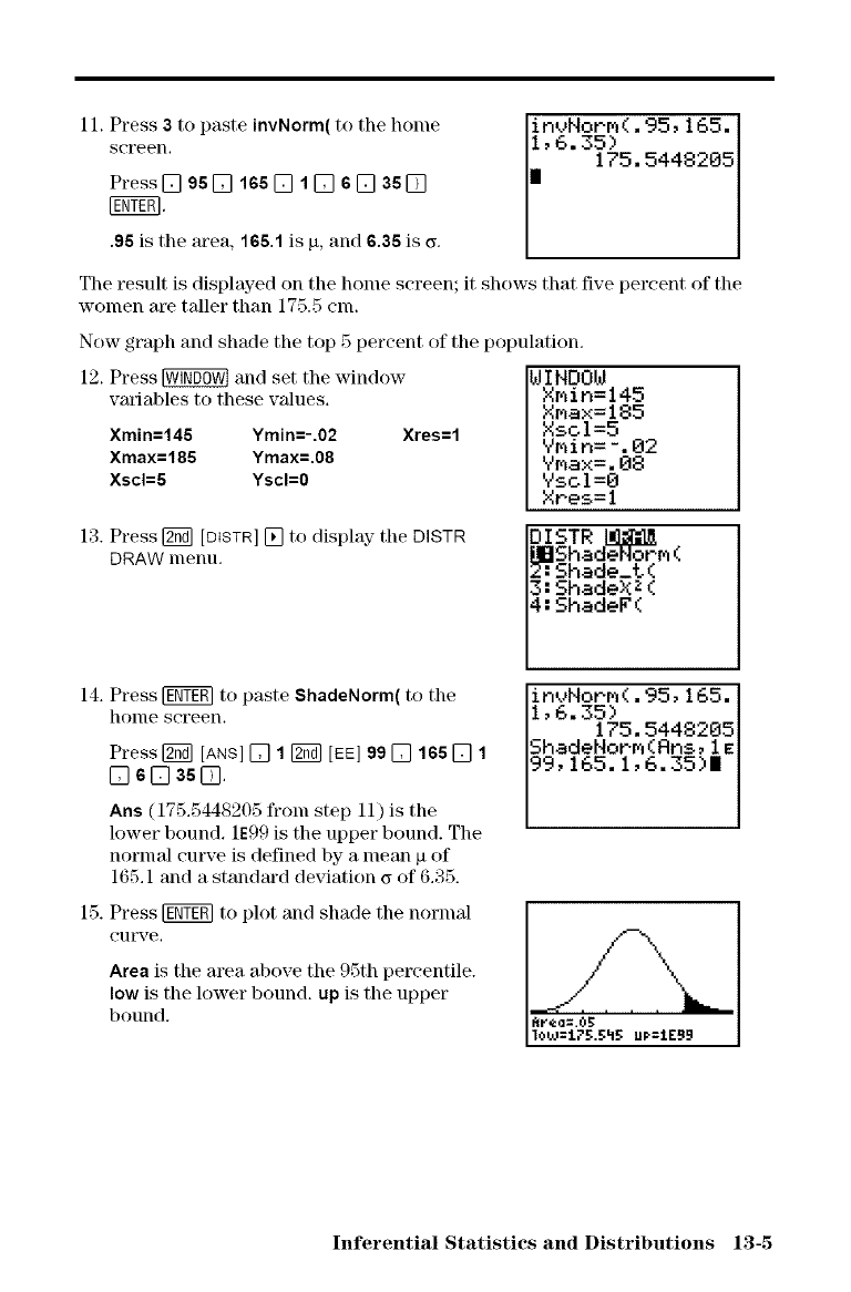
11.Press3to paste invNorm( to the home invHorr_(. 95,165.
screen. 1_6.35)
Press_ 95_ lS5_ 1_ 6_ 35_ I175.5448285
.95 is the area, 1G5.1 is p, and 6.35 is o.
The result is displayed on the home screen; it shows that five percent of the
women are taller than 175.5 cm.
Now graph and shade the top 5 percent of the population.
Xres=l
12. Press [_ and set the window
variables to these values.
Xmin=145 Ymin=-.02
Xmax=185 Ymax=.08
Xscl=5 Yscl=0
gINDOg
XMin=145
Xmax=185
Xsol=5
YMin=-.82
YMax=.88
Yscl=O
XPes=1
13. Press [_ [DISTR] [] to display the DISTR
DRAW menu. STR Llli'_l_
ShadeNoPm (
3: ShadeX z (
4: ShadeF (
invHor.M(. 95,165.
1,6.35)
175. 5448285
ShadeNoPFKRns, 1E
99, 165. 1,6.35)I
firca=.OB
low='l 7_:._:LI_: up,=:LEBB
14. Press _ to paste ShadeNorm( to the
home screen.
Press [_ [ANS] [] 1 _ [EEl 99_ 165[_ 1
D6[]asD.
Ans (175.5448205 from step 11) is the
lower bound. 1E99 is the upper bound. The
normal curve is defined by a mean p of
165.1 and a standm'd deviation o of 6.35.
15. Press [gfff_ to plot and shade the normal
eui%re.
Area is the area above the 95th percentile.
low is the lower bound, up is the upper
bound.
Inferential Statistics and Distributions 13-5
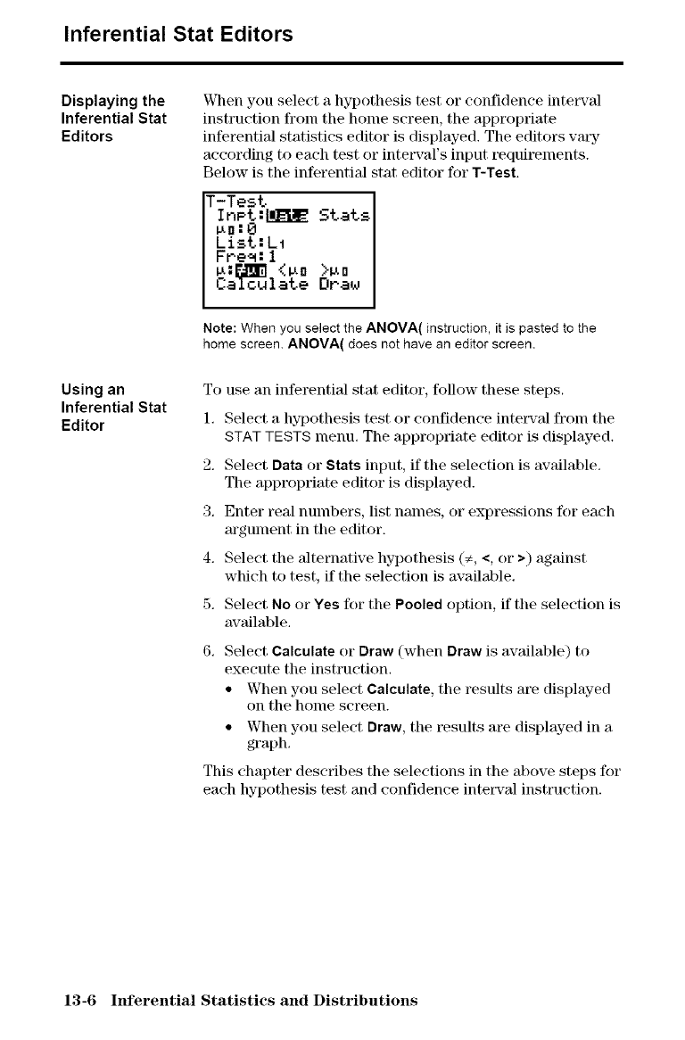
Inferential Stat Editors
Displaying the
Inferential Stat
Editors
When you select a hypothesis test or confidence intetsTal
instruction from the home screen, the appropriate
inferential statistics editor is displayed. The editors yaw
according to each test or interval's input requirements.
Below is the inferential stat editor for T-Test.
T-Test
InPt:_ Stats
List:L1
Fne_:l
_:_ <_ >_n
Calculate Orau
Using an
Inferential Stat
Editor
Note: When you select the ANOVA( instruction, it is pasted to the
home screen. ANOVA( does not have an editor screen.
To use an inferential stat editor, follow these steps.
1. Select a hypothesis test (Jr confidence intet_'al from the
STAT TESTS menu. The appropriate editor is displayed.
2. Select Data or Stats input, if the selection is available.
The appropriate editor is displayed.
3. Enter real numbers, list names, (Jr expressions for each
argument in the editor.
4. Select the alternative hypothesis (€, <, or >) against
which to test, if the selection is available.
5. Select No or Yes for the Pooled option, if the selection is
available.
6. Select Calculate (Jr Draw (when Draw is available) to
execute the instruction.
• When you select Calculate, the results are displayed
on the honle screen.
• When you select Draw, the t_sults are displayed in a
graph.
This chapter describes the selections in the above steps for
each hypothesis test and confidence intetwal instruction.
13-6 hfferential Statistics and Distributions
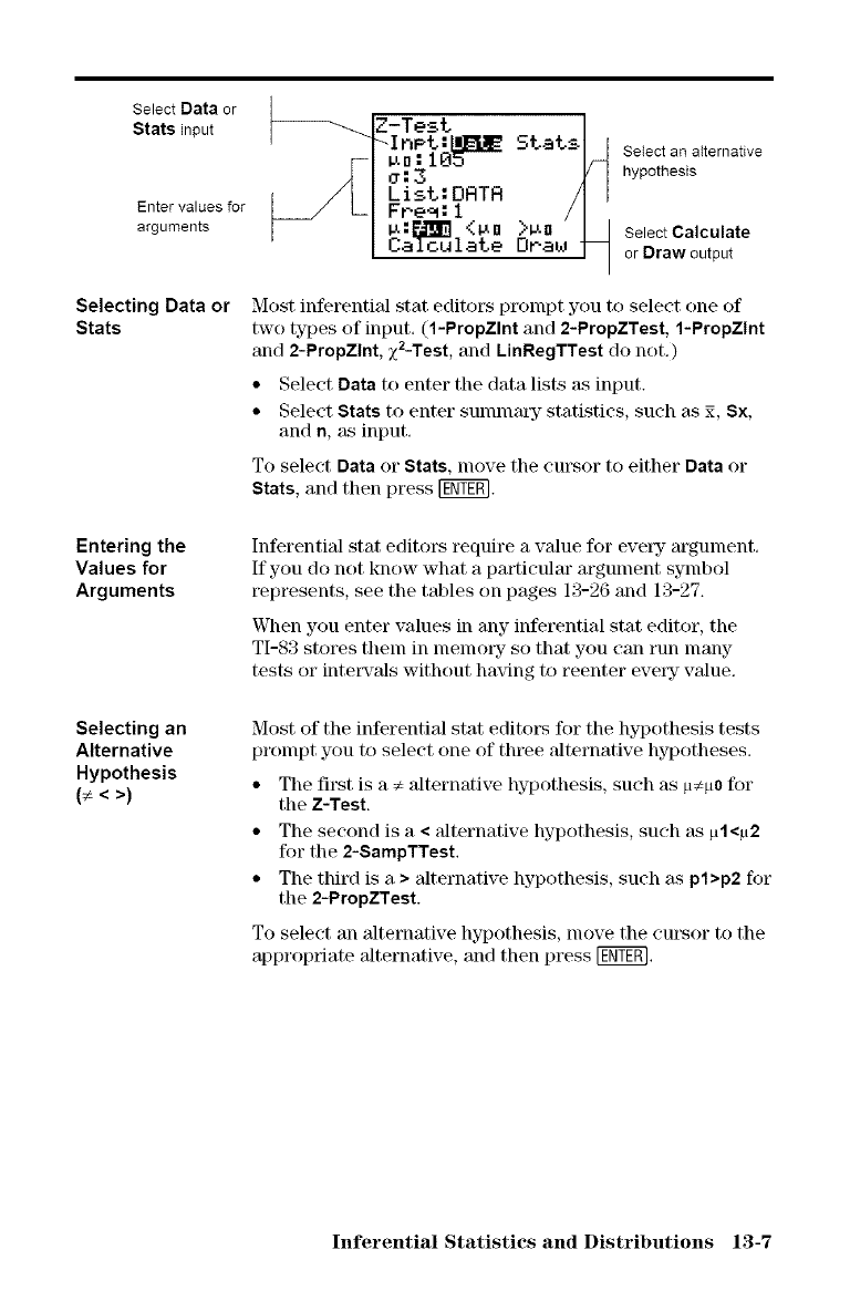
Select Data or
Stats input
Enter values for
arguments
Selecting Data or
Stats
Entering the
Values for
Arguments
Selecting an
Alternative
Hypothesis
(_ < >)
Stats
Calculate Omau
Sete_ an alternative
hypothesis
Select Calculate
or Draw output
Most inferential stat editors prompt you to select one of
two types of input. (1-PropZlnt and 2-PropZTest, 1-PropZlnt
and 2-PropZlnt, x2-Test, and LinRegTTest do not,)
• Select Data to enter the data lists _s input.
• Select Stats to enter sunmm_ statistics, such as 2, Sx,
and n, as input.
To select Data or Stats, move the cursor to either Data or
Stats, and then press [ggY_.
Inferential stat editors require a value for ever7 argument.
If you do not know what a pm'ticulm" argument symbol
represents, see the tables on pages 13-26 and 13-27.
When you enter values in any inferential stat editor, the
TI-83 stores them in nlenlory so that you can run many
tests or intetnT'als without having to reenter evet3z vMue.
Most of the inferential stat editors for the hypothesis tests
prompt you to select one of three alternative hypotheses.
• The first is a _ Mternative hypothesis, such as p¢p0 for
the Z-Test.
• The second is a <alternative hypothesis, such as pl<_t2
for tile 2-SampTTest.
• The third is a >alternative hypothesis, such as pl>p2 for
the 2-PropZTest.
To select an alternative hypothesis, nlove the cursor to the
appropriate alternative, and then press [ggY_.
Inferential Statistics and Distributions 13-7
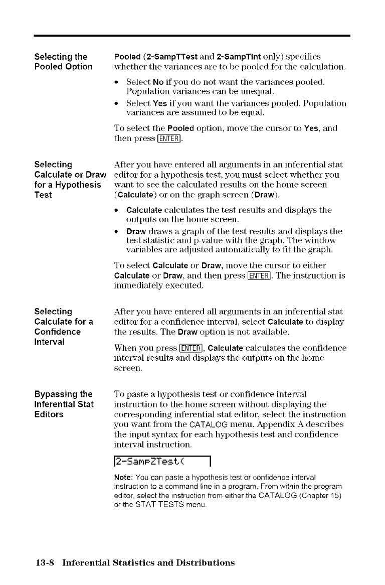
Selecting the
Pooled Option
Selecting
Calculate or Draw
for a Hypothesis
Test
Selecting
Calculate for a
Confidence
Interval
Bypassing the
Inferential Stat
Editors
Pooled (2-SampTTest and 2-SampTInt only) specifies
whether the vmiances m'e to be pooled for the calculation,
• Select No if you do not want the vmiances pooled.
Population vm'iances can be unequal.
• Select Yes if you want the wu'iances pooled. Population
wu'iances m'e assumed to be equal.
To select the Pooled option, move the cursor to Yes, and
then press [_T_].
Alter you have entered all arguments in an inferential star
editor for a hypothesis test, you nmst select whether you
want to see the calculated results on the home screen
(Calculate) or on the graph screen (Draw).
• Calculate c_dculates the test results and displays the
outputs on the home screen.
• Draw draws a graph of the test results and displays the
test statistic and p-value with the graph. The window
variables m'e adjusted automatically to fit the graph.
To select Calculate or Draw, nlove the cursor to either
Calculate or Draw, and then press IgOr. The instruction is
inunediately executed.
Alter you have entered all arguments in an inferential star
editor for a confidence inte_'al, select Calculate to display
the results. The Draw option is not available.
When you press [g_EN, Calculate calculates the confidence
inte_w'M results and displays the outputs on the home
screen.
To paste a 1wpothesis test or confidence inte_-'al
instruction to the home screen without displaying the
corresponding inferential stat editor, select the instruction
you want from the CATALOG menu. Appendix A describes
the input syntm, c for each hypothesis test and confidence
inte_nTal instruction.
12-Sar,_PZTest(I
Note:You can pastea hypothesistestorconfidenceinterval
instruction to a command line in a program. From within the program
editor, select the instruction from either the CATALOG (Chapter I5)
or the STAT TESTS menu.
13-8 hfferential Statistics and Distributions
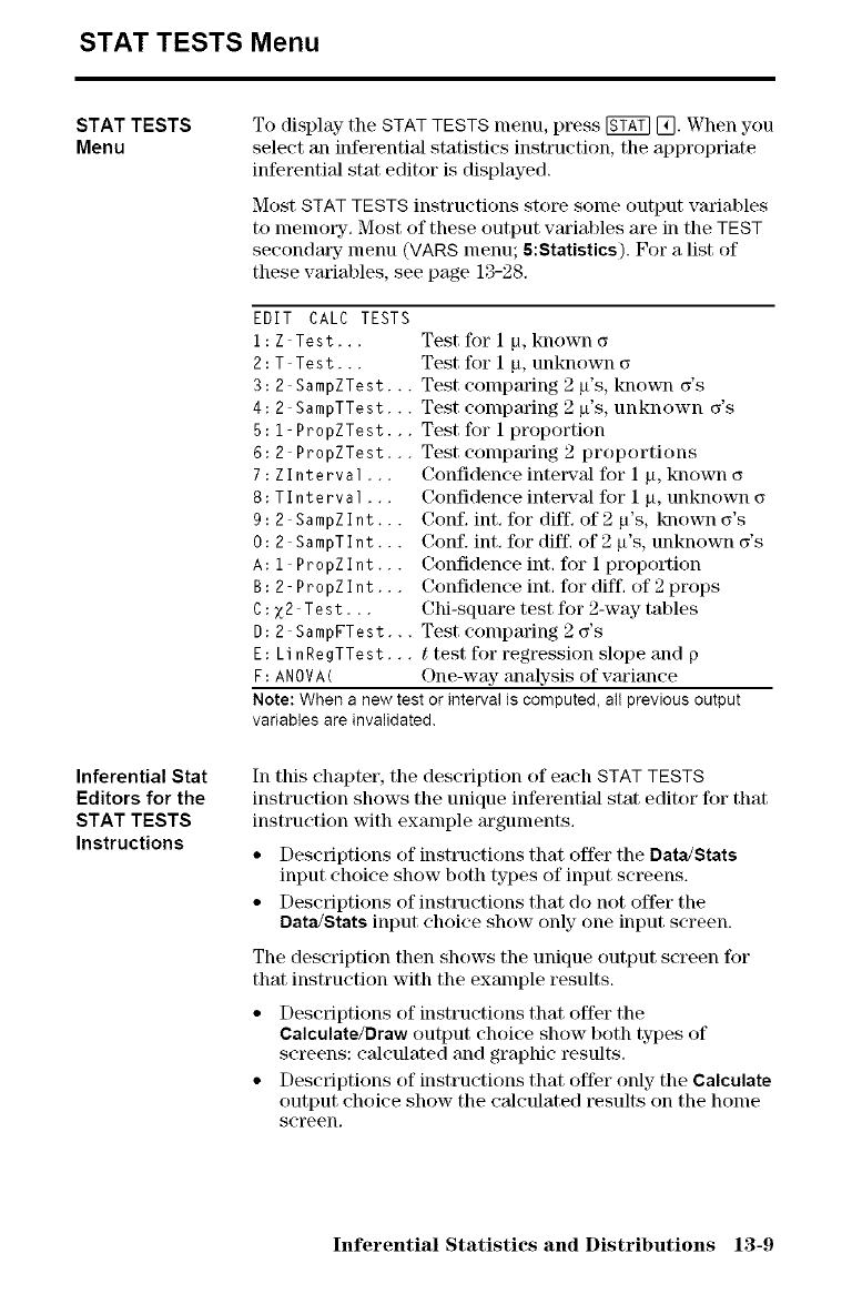
STAT TESTS Menu
STAT TESTS
Menu
Inferential Stat
Editors for the
STAT TESTS
Instructions
To display the STAT TESTS menu, press [gT_] [_. When you
select an inferential statistics instruction, the appropriate
inferential stat editor is displayed.
Most STAT TESTS instructions store some output varial_les
to memory. Most of these output variables are in the TEST
secondmT menu (VARS menu; 5:Statistics). For a list of
these varial)les, see page 13-28.
EDIT CALC TESTS
1:Z Test,..
2:T Test,.,
3:2 SampZTest...
4:2 SampTTest,..
5:1 PropZTest...
6:2 PropZTest,..
7:Zlnterval,.,
8:Tlnterval,.,
9:2 SampZlnt.,.
0:2 SampTlnt.,.
A:I PropZlnt.,.
B:2 PropZlnt.,.
C:X2 Test,,.
D:2 SampFTest...
E: LinRegTTest,..
F: ANOVA(
Test for 1 p, known
Test for i p, unknown
Test compming 2 #'s, known _'s
Test compming 2 #'s, unknown _'s
Test for 1 proportion
Test compming 2proportions
Confidence intmwal for 1 #, known
Confidence intmwal for 1 #, unknown
Conf. int. for diff. of 2 p's, known o's
Conf. int. for diff. of 2 #'s, unknown o's
Confidence int. for 1 proportion
Confidence int. for diff. of 2 props
Chi-squm'e test for 2-way tables
Test compming 2 o's
ttest for regression slope and p
One-way analysis of variance
Note: When a new test or interval is computed, all previous output
variables are invalidated.
In this chapter, the description of each STAT TESTS
instruction shows the unique inferential stat editor for that
instruction with example arguments.
• Descriptions of instructions that offer the Data/Stats
input choice show both types of input screens.
• Descriptions of instructions that do not ofl_r the
Data/Stats input choice show only one input screen.
The description then shows the unique output screen for
that instruction with the example results.
• Descriptions of instructions that offer the
Calculate/Draw output choice show both types of
screens: calculated and graphic results.
• Descriptions of instructions that offer only the Calculate
output choice show the calculated results on the home
screen.
Inferential Statistics and Distributions 13-9
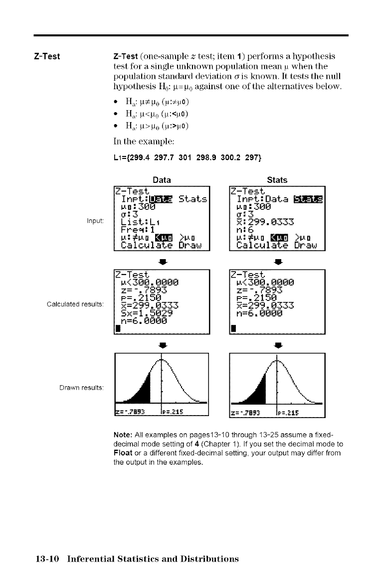
Z-Test
Input:
Calculated results:
Z-Test (one-sample ztest; item 1) performs a hypothesis
test for a single unknown population mean _ when the
population standard deviation cris known. It tests the null
hypothesis H0: g= P0 against one of the alternatives below.
• H_,:_!¢P0 (vt:_to)
• H_,:_<_00a:<_to)
• H_,:_>_0 (_t:>_to)
In tile example:
L1={299,4 297.7 301 298.9 300.2 297}
Data
Z-Test
Inet:_ Stats
0.:3
List:L1
Fre_:l
_:#_ _ >_o
Calculate Draw
Z-Test
v.<300. 0000
z= -. 7893
P=. 2150
_=299. 0333
mx= 1. 5029
ir,=6. 0000
.@
:=-.7B9_ _=._I_
Stats
Z-Test
InPt:Oata
v.n : 300
0:3
_: 299. 0333
n:6
v.:#v.n_ >_n
Calculate Draw
Z-Test
u<300.0000
z=-.7893
e=.2150
R=299.0333
I n=6.0000
.@
Drawn results:
Note: All examples on pages13-10 through t3-25 assume a fixed-
decimal mode setting of 4 (Chapter 1). If you set the decimal mode to
Float or a different fixed-decimal setting, your output may differ from
the output in the examples.
13-10 Inferential Statistics and Distributions
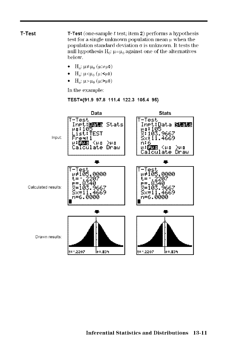
T-Test
Input:
Calculated results:
T-Test (one-sample ttest; item 2) performs a hypothesis
test for a single unknown population mean p when the
population standard deviation _ is unknown. It tests the
null hypothesis H0:P=P0 against one of the alternatives
below.
•H_,:PCPo (p:¢po)
• H_,:P<Po (p:<po)
• H_,:P>Po (,u:>_.to)
In the example:
TEST={91.9 97.8 111.4 122.3 105.4 95}
Data
T-Test
InPt:_ Stats
_n:105
List:TEST
FPe_:l
_:_ <_n >_n
Calculate DPau
T-Test
,,lo5.00oo
t=-.,_20_
P=. 8340
2= 100 •9667
Sx= 1 I. 4669
in=6. 0000
t= -,i:_:07 _=,g3h
Stats
T-Test
InPt:Oata
p0:105
7,:103. 9667
Sx: 11.4669
n:6
Calculate OPau
T-Test
_#105.0000
t=-.2207
P=.8340
R=103.9667
Sx=II.4669
in=6.0000
Drawn results:
Inferential Statistics and Distributions 13-11
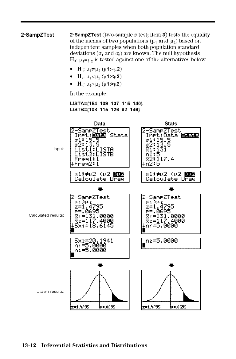
2-SampZTest
Input:
Calculated results:
Drawn resutts:
2-SampZTest (two-sample ztest; item 3) tests the equality
of the means of two populations (Pl and #2) based on
independent samples when both population standard
deviations (_1 and a_,) are known. The null hypothesis
H0:#1=p2 is tested against one of the alternatives below.
• H_,: _[l<_t2 (pl:<p2)
• H_,: #1>P2 (pl:>p2)
In the example:
LISTA={154 109 137 116 140}
LISTB={108 115 126 92 146}
Data
2-SamPZTest
InPt =I_ Stats
¢I: 15.5
¢2:13.5
ListI:LISTR
List2:LISTB
FPe_l:l
_Fre_2:l
_I:#_2 <_2 _
Calculate Drau
2-SaMmZTest
P:. 695
_1=131.0000
2z=I17.4000
1_Sx,=18.6145
S×z=20.1941
ni=5.0000
inz=5.0000
//
z=l.h795 _=.Ofigg
Stats
2-SaMPZTest
InPt:Data
¢I: 15.5
¢2:13.5
RI: 131
hi:5
R2:117.4
_n2:5
=-LI:#p.2 <p.2 I_
Calculate Dr-a,,J
2-SaMPZTest
z= I. 4795
P=. 0695
RI=131. 0000
Rz=117.4000
l.n i =5. 0000
I
i
r,z=5.0000
i
13-12 Inferential Statistics and Distributions
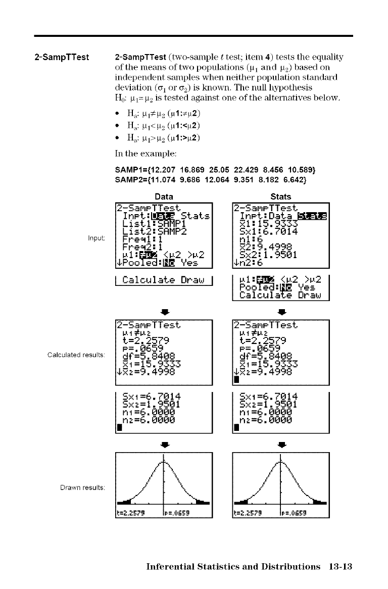
2-SampTTest
Input:
Calculated results:
2-SampTTest (two-sample ttest; item 4) tests the equality
of the lneans of two populations (_l 1 and g2) based on
independent samples when neither population standard
deviation ((_1or (_2)is known, The null hypothesis
n0:_11=_12 is tested against one of the alternatives below.
• H_,:_11<_l2(_1:<_2)
• H_,:_11>_12(_1:>_2)
In the example:
8AMPl={12.207 16.869 25,05 22,429 8,456 10,589}
SAMP2={11.074 9.686 12.064 9.351 8.182 6.642}
Data
2-SamPTTest
InPt:liI_11_Stats
ListI:SRMPI
List2:SRMP2
Fre_l:l
Fre_2:l
SPooled:l_ 9es
I Calc.ulate Draw I
Stats
2-SaMPTTesL
Inet: Data !i_rul_lEl
1 : 15. 9333
SxI :6. 7014
nl:6
_2:9.4998
Sx2: I. 9501
i.n2:6
_LI:_ <_2 >_2
PooI_:[_ Yes
Calculate Draw
2-SamPTTest
t=2.2579
P=.0659
d_=5.8408
RI=15.9333
$_z=9.4998
m =6. 00e
I r,z=6. 0000
2-SamPTTest
t=2.2579
P=.0659
d€=5.8408
RI=15.9333
_2z=9.4998
I SXI=6"7014
Sxz=1.9501
ni=6.0000
nz=6.0000
Drawn resutts:
Inferential Statistics and Distributions 13-13
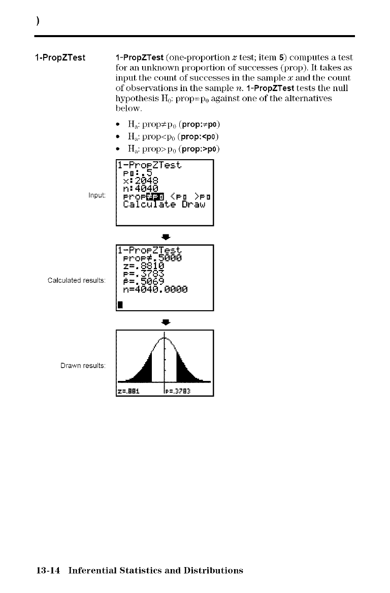
1-PropZTest
Input:
Calculated results:
1-PropZTest (one-proportion ztest; item B) computes a test
for an unknown proportion of successes (prop). It takes as
input the count of successes in the sample xand the count
of observations in the sample n. 1-PropZTest tests the null
hypothesis H0:prop=p0 against one of the alternatives
below.
• H_,:prop€p0 (prop:¢p0)
• H_,:prop<p0 (prop:<po)
• H_,:prop>p0 (prop:>po)
1-ProPZTest I
pill .5 I
x: 2848 I
n: 4848 I
eroI=Ei1"_,'1<ell >Pal
Caloulate Draw
l-ProeZTest
ProP#. 5000
z=. 8810
P=. o783
_=. 5069
in=4e4e. 0088
Drawn results:
13-14 Inferential Statistics and Distributions
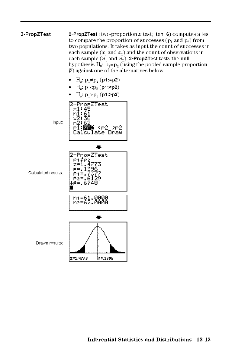
2-PropZTest
Input:
2-PropZTest (two-proportion ztest; item 6) computes a test
to compare the proportion of successes (Pl and P2) fronl
two populations. It takes _ksinput the count of successes in
each sample (x 1and x2) and the count of observations in
each sample (nl and n2). 2-PropZTest tests the null
hypothesis H0:pl=p2 (using the pooled sample proportion
_) against one of the alternatives below.
• H_,:pl;eP2 (pl:_p2)
• H_,:pl<P2 (pl:<p2)
• H_,:pl>P2 (pl:>p2)
2-PPoeZTest
xi:45
hi:61
x2:38
n2:62
el:I <e2 >e2
Calculate Draw
Calculated results:
B-
2-ProeZTest
e1#ez
z=1.4773
P=.1396
@i=.7377
@z=.6129
4#=.6748
|
nI=61.0000
nl=62.0000
-I
Drawn results:
Inferential Statistics and Distributions 13-15
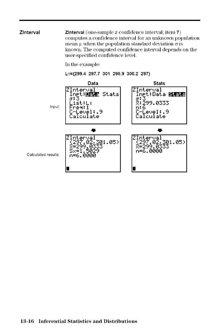
Zlnterval
Input:
Zlnterval (one-sample zconfidence intetsTal; item 7)
computes a confidence interval for an unknown population
mean p when the population standard deflation cris
known. The computed confidence intet_-'al depends on the
user-specified confidence level,
In the example:
L1={299.4 297.7 301 298.9 300.2 297}
Data
ZInterval
In_t:l_ellI_Stats
List:L1
Fre_:l
C-Level:.9
Calculate
Stats
ZInterval
Inet:Data
_:3
R: 299. 0333
n:6
C-Legel :. 9
Calculate
Calculated results:
-B-
ZInterval
(297.02,301.85)
R=299.0333
Sx=1.5029
|n=6.0000
Zlnterval
(297.02,301.05)
I
13-16 Inferential Statistics and Distributions
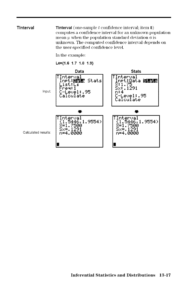
Tlnterval
Input:
Tlnterval (one-sample tconfidence inte_nTal; item 8)
computes a confidence interval for an unknown population
mean p when the population standard deviation _ is
unknown. The computed confidence inte_wTal depends on
the user-specified confidence level.
In the example:
L6={1.6 1.7 1.8 1.9}
Data
Tlnterval
InPt:llL_u1_Stats
List:L_
Fre_:l
C-Level:.95
Calculate
Stats
TInterva I
InF.t:Data
_: 1.75
Sx:. 1291
n:4
C-Level: .95
Caloulate
Calculated results:
-B-
TInterval
(1.5446,1.9554)
R=1.7500
Sx=.1291
|n=4.0000
TInterval
(1.5446, i.9554)
R=1.7500
Sx=.1291
|n=4.0000
Inferential Statistics and Distributions 13-17
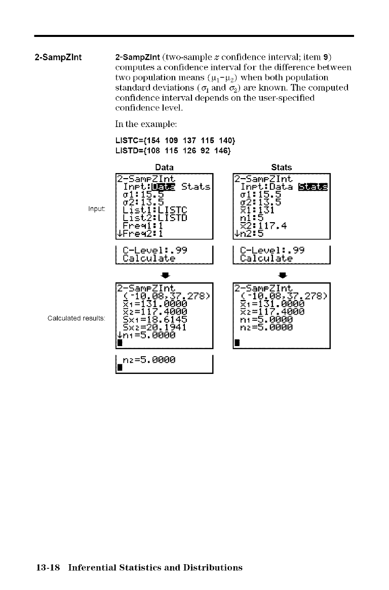
2-SampZlnt
Input:
Calculated results:
2-SampZInt (two-sample z confidence inte_wTal;item 9)
c()mputes a confidence inte[wTal for the difference between
two population means ({11-_12) when both population
standard deviations (or1and a_) are known. The computed
confidence inte_'al depends on the user-specified
confidence level.
In the example:
LISTC={154 109 137 116 140}
LISTD={108 115 126 92 146}
Data
2-SamPZlnt
InPt:[._Z Stats
_i:15.5
_2:13.5
ListI:LISTC
List2:LISTD
Fre_l:l
SFre_2:l
C-Level:.99
Calculate
2-SamPZInt
(-10.08,37.278)
21=131.0000
2z=117.4000
Sxi=18.6145
Sxz=20.1941
$ni=5.0000
|
n2=5.0000
|
Stats
2-SamPZ Int
InPt:Data
_I: 15.5
¢2:13.5
21:131
ni:5
22:117.4
_n2:5
C-Level:.99
Calculate
2-SamPZlnt
(-10.08,37.278)
21=131.0000
2_=117.4000
m=5.0000
inz=5.0000
13-18 Inferential Statistics and Distributions
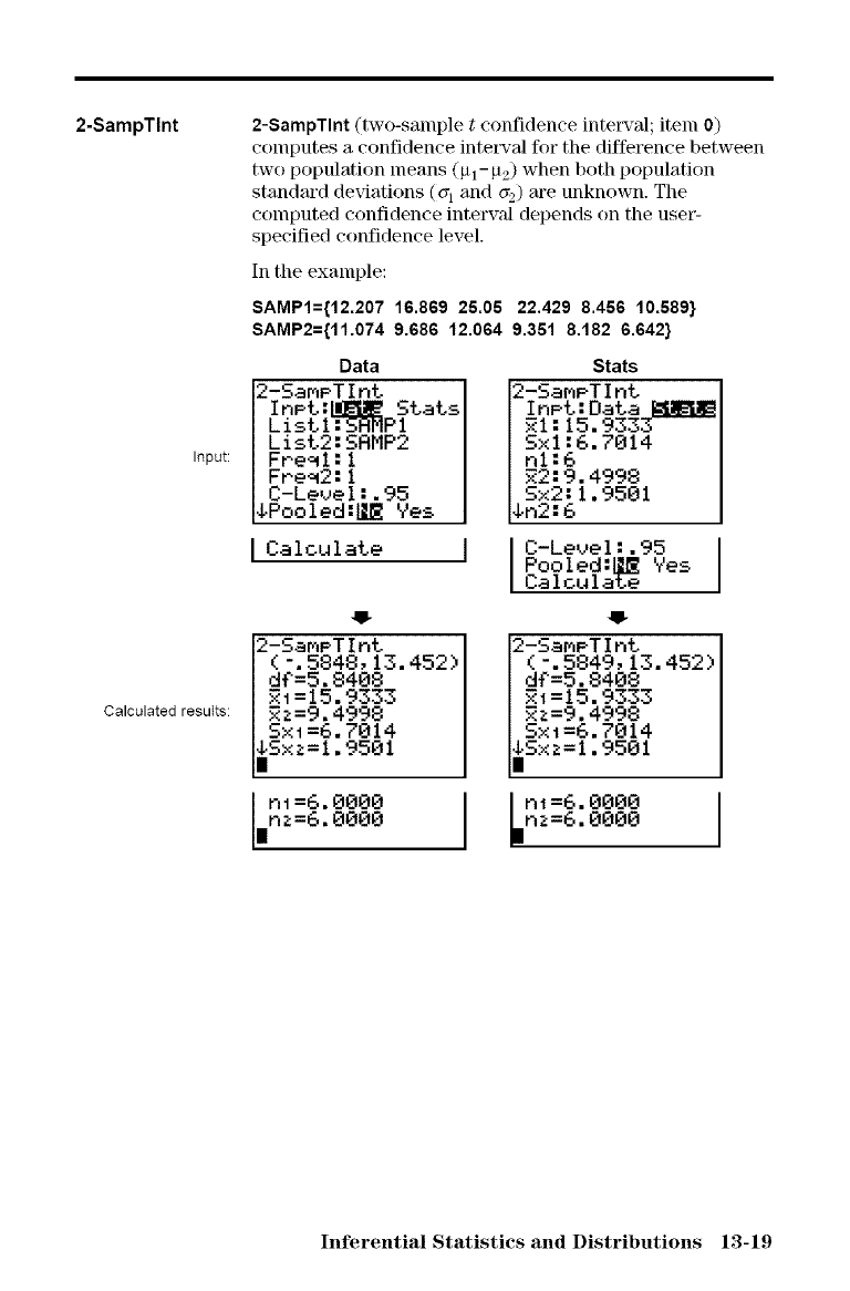
2-SampTInt
Input:
Calculated results:
2-SampTInt (two-sample tconfidence inte[wTal; item O)
c()mputes a confidence inte[wTal for the difference between
two population means (Pl-P2) when both population
standard deviations (a 1 and _) are unknown. The
computed confidence interval depends on the user-
specified confidence level.
In the example:
SAMP1={12.207 16.869 25.05 22,429 8.456 10.589}
SAMP2={11.074 9.686 12.064 9.351 8,182 6.642}
Data
2-SamPTlnt
InPt:_ Stats
ListI:SRMPI
List2:SRMP2
Fne_l:1
Fne_2:l
C-Level:.95
$Pooled:l:_ Yes
Calculate
2-SamPTlnt
(%5848,13.452)
d¢=5.8408
Ri=15.9333
Rz=9.4998
SxI=6.7014
$Sxz=1.9501
|
ni=6.8000
nz=6.0000
|
Stats
2-SaP/PT I r=t
Sxl :6. 7014
nl:6
R2:9.4998
Sx2:1.9581
_n2:6
C-Level :. 95
Pooled:l:_ Yes
Calculate
2-SamPT Int
( -.5849, 13. 452)
df=5.8408
_i =15. 9333
R1=9.4998
SxI=6. 7014
_Sx1=1.9501
|
i
ni=6.0000
nz=6.0000
Inferential Statistics and Distributions 13-19
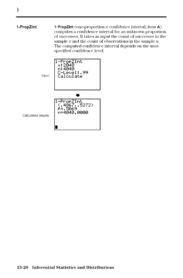
1-PropZlnt 1-PropZInt (one-proportion zconfidence inte_'al; item A)
computes a confidence interval for an unknown proportion
of successes. It takes as input the count of successes in the
sample xand the count of obse_'ations in the sample n.
The computed confidence intetnTal depends on the user-
specified confidence level.
1-PPoeZlnt
x: 2848
n: 4848
C-Leve I :.99
input: Caicuiate
Calculated results:
-B-
l-ProeZlnt
(.4867,.5272)
A=.5069
|n=4040.0000
13-20 Inferential Statistics and Distributions
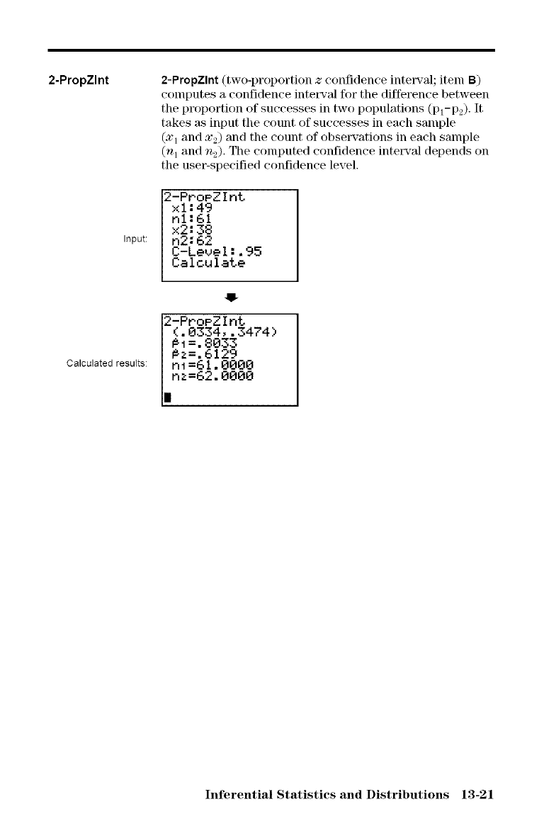
2-PropZlnt 2-PropZInt (two-proportion zconfidence inte_'al; item B)
computes a confidence intet_'al for the difference between
the proportion of successes in two populations (Pl-P2)- It
takes a_ninput the count of successes in each sample
(Xl and x2) and the count of observations in eaeh sample
(n 1 and n2), The computed confidence intetnTal depends on
the user-specified confidence level.
2-Pt-oPZ Int
xi:49
nl:61
x2:38
Input: n2: 62
C-Leve I :.95
Calculate
Calculated results:
-I
2-PPoeZInt
(.0334,.3474)
#I=.8033
#z=.6129
ni=61.0000
|nz=62.0000
Inferential Statistics and Distributions 13-21
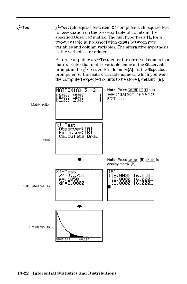
z2-Test
Matrix editor:
Input:
z2-Test (chi-squm'e test; item C) computes a chi-squm'e test
for association on the two-way table of counts in the
specified Observed lnatrix. The null hypothesis H 0 for a
two-way table is: no association exists between row
variables and colunm variables. The Mternative hypothesis
is: the vm'iables are related.
Before computing a zZ-Test, enter the obsetnTed counts in a
matrix. Enter that matrix variable name at the Observed:
prompt in the z2-Test editor; default=[A]. At the Expected:
prompt, enter the matrix variable name to which you want
the computed expected counts to be stored; default=[B].
MATRIX[R] 3 x2 ]
[5.0000 19.000
[ i0. o000t,.000
J.3.000
Xi-Test
Observed:[R]
Exeected:[B]
Calculate Draw
XZ-Test
XZ=3.3750
P=.1850
d€=2.0000
Note: Press _ [] [] 1to
select 1:[A] from the MATRX
EDIT menu.
Calculated results:
Note: Press_ [B]_ to
display matrix [B].
[B]
[[8.0000 16.000.
[ :8888
16.000...i
Drawn results:
13-22 Inferential Statistics and Distributions
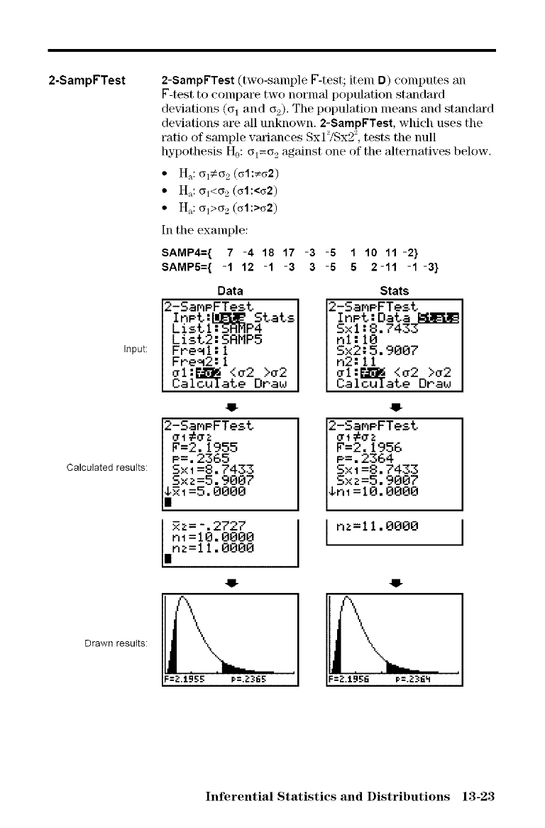
2-SampVTest
Input:
Calculated results:
2-SampFTest (two-sample V-test; item D) computes an
V-test to compare two normal population standard
deviations ((31 and (32). The population means and standard
deflations are all unknown. 2-$ampFTest, which uses the
ratio of sample variances Sxl_/Sx2 _, tests the null
hypothesis H0:(31=(32 against one of the alternatives below.
• H_,: (315(32 (G1:_(52)
•H_,:(31<(32 ((51 :<(52)
•H_,:(31>(32 ((51 :>(52)
In the example:
SAMP4={ 7-4 18 17 -3 -5 1 10 11-2}
SAMPS={ -1 12 -1 -3 3-5 5 2-11 -1-3}
Data
2-SamPFTest
InPt:_ SLats
ListI:SRMP4
List2:SRMP5
FPe_l:l
FPe_2:l
_i:_ <z2 >z2
Caloulate OPaw
Stats
2-Sar/PFTest
InPt: Data_
Sx i :8. 7433
hi: 10
Sx2: 5. 9007
n2: II
zl:_ <_2 >z2
Calculate Dra_,J
2-SameFTest
zl#zz
F=2. 1956
P=. 2364
S× _=8. 7433
Sxz=5. 9007
_nl =10. 0000
nz=l I.0000
2-SaMPFTest
zl #zz
F=2. 1955
P=. 2365
Sxl =8. 7433
Sx z=5. 9007
_i =5. 0000
2z=-.2727
n_=lO. 0000
in _= 1 I. 0000
Drawn results:
Inferential Statistics and Distributions 13-23
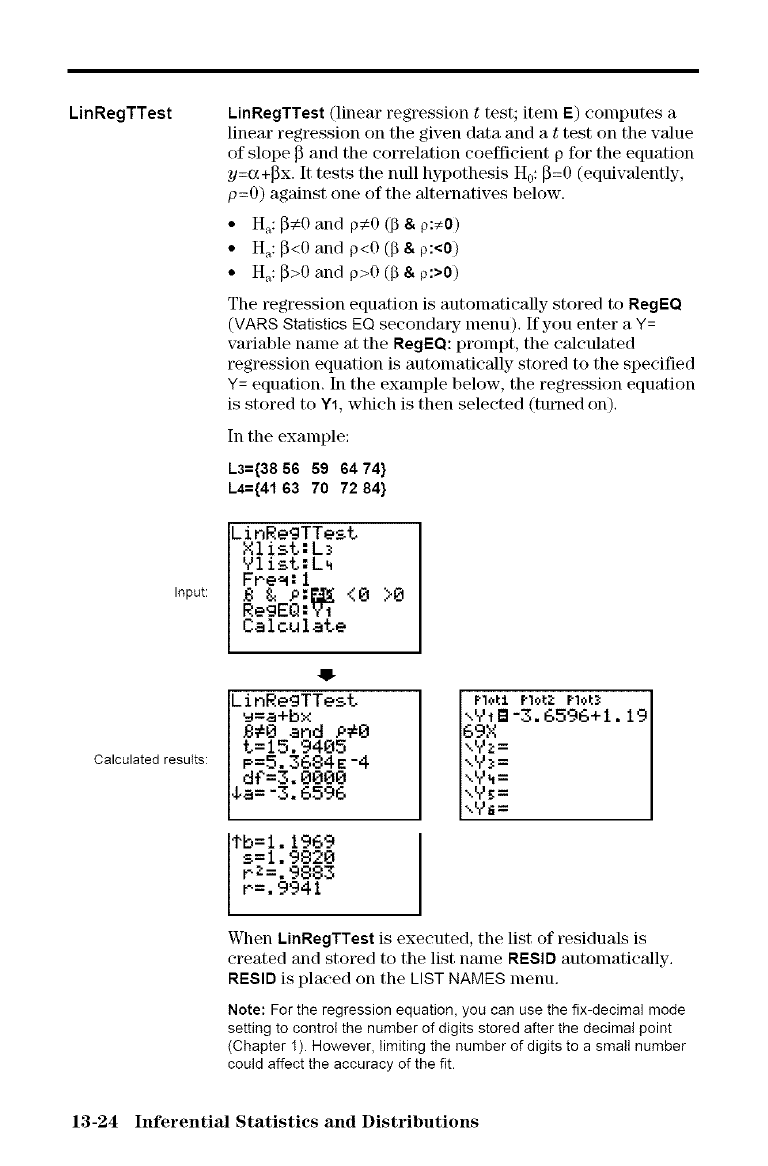
LinRegTTest
Input:
LinRegTTest (linear regressk)n ttest; item E) computes a
linear regression on the given data and a ttest on the value
of slope _ and the correlation coefficient p for the equation
y=(x +_x. It tests the null hypothesis H0:_=0 (equivalently,
p=O) against one of the alternatives below.
• Hr,: _€0 and pC0 ([3 & p:_0)
• H_,: _<0 and p<0 (9 & p:<0)
• H_,: _>0 and p>0 (9 & P:>0)
The regression equation is automatically stored to RegEQ
(MARS Statistics EQ secondary menu). If you enter a Y=
variable name at the RegEO: prompt, the eMeulated
regression equation is automatically stored to the specified
Y= equation. In the example below, the regression equation
is stored to Y1, which is then selected (turned on).
In the example:
L3={38 56 59 64 74}
L4={41 63 70 72 84}
LinRegTTest
Xlist:L_
91ist:L4
Fre_:l
B & P:_ <0 >0
RegEQ:_
Calculate
Calculated results:
lJ-
LinRegTTest
_=a+bx
B_O and p_O
t=15.9405
P=5.3684E-4
d€=3.8888
4a=-3.6596
$b=i.1969
s_1.9820
P_=.9883
P=,9941
PloLt PloI:Z PloL3 19
",371B-3. 6596+i.
69X
xYz=
xY4=
xVs=
xY_=
When LinRegTTest is executed, the list of residuals is
created and stored to the list name RESID automatically.
RESID is placed on the LIST NAMES menu.
Note: For the regression equation, you can use the fix-decimal mode
setting to control the number of digits stored after the decimal point
(Chapter I). However, limiting the number of digits to a small number
could affect the accuracy of the fit.
13-24 Inferential Statistics and Distributions
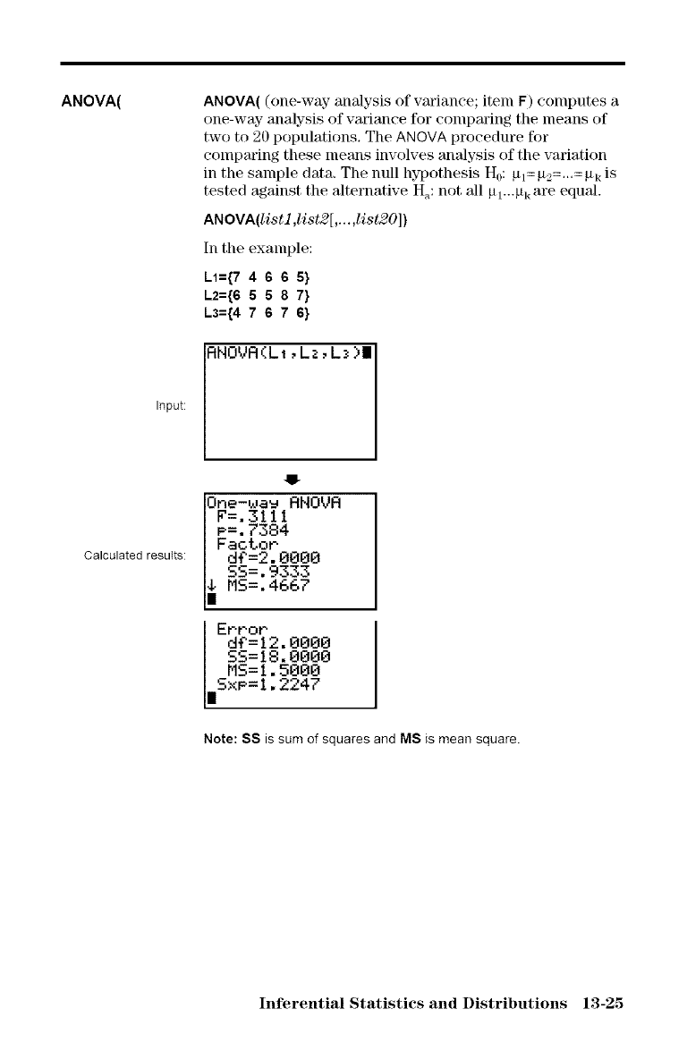
ANOVA(
Input:
ANOVA( (one-way analysis of variance; item F) computes a
one-way analysis of variance for COlnparing the means of
two to 20 populations. The ANOVA procedure for
COlnparing these means involves analysis of the variation
in the sample data. The null hypothesis H0:#1=#2 ..... #k is
tested against the alternative H_,: not all p 1---#l_are equal.
ANOVA(listl,list2[,...,list20])
In the example:
L1={7 4665}
L2={6 5 5 8 7}
L3={4 7 6 7 6}
RNOVR(LI,Lz,L_)I
Calculated results:
ll-
One-_au RNOVR
F=.olll
P=.7384
Factor
d_=2.0000
SS=.9333
_MS=.4667
Error
d_=12.0000
SS=18.0000
MS=1.5000
I_xP=1.2247
Note: SS is sum of squares and MS is mean square.
Inferential Statistics and Distributions 13-25
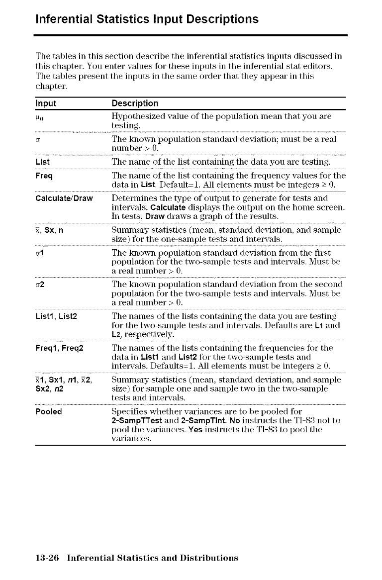
Inferential Statistics Input Descriptions
The tables in this section describe the inferential statistics inputs discussed in
this chapter. You enter values for these inputs in the inferentiM stat editors.
The tables present the inputs in the same order that they appear in this
chapter.
Input Description
_0 Hypothesized value of the population mean that you are
testing.
G The known population standard deviation; must be a real
number > 0.
List The name of the list containing the data you are testing.
Freq The name of the list containing the frequency values for the
data in List. Default=l. All elements must be integers ->0.
Calculate/Draw Determines the type of output to generate for tests and
intervals. Calculate displays the output on the home screen.
In tests, Draw draws a graph of the results.
_, Sx, n Sumlnary statistics (mean, standard deviation, and sample
size) for the one-sample tests and intervals.
_1 The known population standard deviation fronl the first
population for the two-sample tests and intervals. Must be
a real number > 0.
_2 The known population standard deviation fronl the second
population for the two-sample tests and intervals. Must be
a real number > 0.
List1, List2 The names of the lists containing the data you are testing
for the two-salnple tests and intervals. Defaults are L1 and
L2,respectively.
Freql, Freq2 The names of the lists containing the frequencies for the
data in List1 and List2 for the two-salnple tests and
intervals. Defaufis=l. All elements must be integers _>0.
_1, Sxl, nl, _2, Sununary statistics (mean, standard deviation, and sample
Sx2, n2 size) for sample one and sample two in the two-salnple
tests and intervals.
Pooled Specifies whether variances are to be pooled for
2-SampTTest and 2-SampTInt. No instructs the TI-83 not to
pool the variances. Yes instructs the TI-83 to pool the
variances.
13-26 Inferential Statistics and Distributions
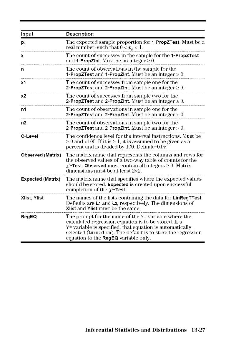
Input Description
P0 The expected sample proportion for 1-PropZTest. Must be a
real nmnber, such that 0 < I90< 1.
x The count of successes in the sample for the 1-PropZTest
and 1-PropZlnt. Must be an integer _>0.
n Tile count of observations in the sample for the
1-PropZTest and 1-PropZlnt. Must be an integer > O.
xl The count of successes fronl sample one for the
2-PropZTest and 2-PropZlnt. Must be an integer _>0.
x2 The count of successes froln sample two for the
2-PropZTest and 2-PropZlnt. Must be an integer _>0.
nl The count of observations in sample one for the
2-PropZTest and 2-PropZlnt. Must be an integer > 0.
n2 The count of observations in sample two for the
2-PropZTest and 2-PropZlnt. Must be an integer > 0.
C-Level The confidence level for the inteP_-al instructions. Must be
>_0 and <100. If it is _>1, it is assumed to be given as a
percent and is divided by 100. Default=0.95.
Observed (Matrix) The matrix name that represents the colunms and rows for
the obseP_'ed values of a two-way table of counts for the
z2-Test. Observed nmst contain 'allintegers _>0. Matrix
dimensions nmst be at least 2x 2.
Expected (Matrix) The matrix name that specifies where the expected values
should be stored. Expected is created upon successful
completion of the z_Test.
Xlist, Ylist The names of the lists containing the data for LinRegTTest.
Defaults are L1 and L2, respectively. The dimensions of
Xlist and Ylist nmst be the same.
RegE(:l The prolnpt for the name of the Y= variable where the
cMculated regression equation is to be stored. If a
Y= variable is specified, that equation is automatically
selected (turned on). The default is to store the regression
equation to the RegEQ variable only.
Inferential Statistics and Distributions 13-27
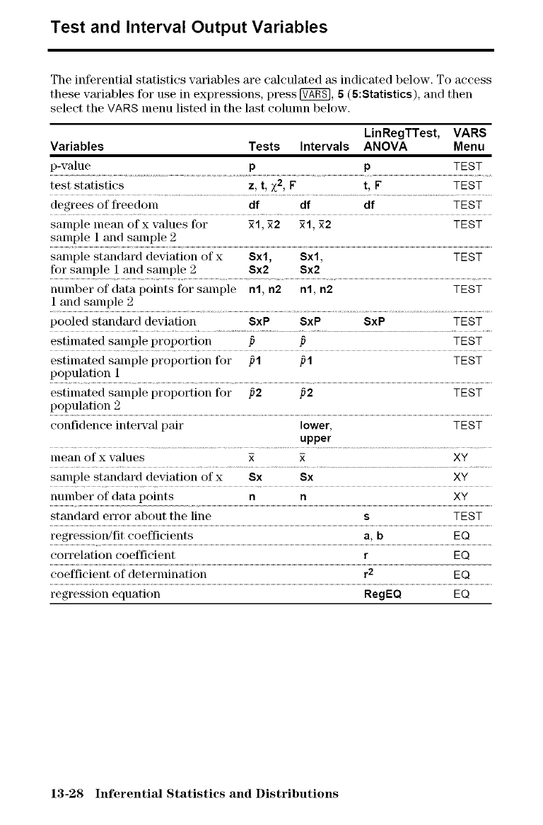
Test and Interval Output Variables
The inferential statistics variables are calculated as indicated below. To access
these variables for use in expressions, press [_, 5(5:Statistics), and then
select the VARS menu listed in the last column below.
LinRegTTest, VARS
Variables Tests Intervals ANOVA Menu
p-value p p TEST
test statistics z, t, Z2_ F t, F TEST
degrees of freedom df df df TEST
sample mean of x values for 21,22 21, 22 TEST
sample 1 and sample 2
sample standard deviation of x Sxl, Sxl, TEST
for sample 1 and sample 2 Sx2 Sx2
nulnber of data points for sample nl, n2 nl, n2 TEST
1 and sample 2
pooled standm'd deviation SxP SxP SxP TEST
estimated sample proportion /3 /3 TEST
estimated sample proportion for /31 /31 TEST
population 1
estimated sample proportion for /32 /32 TEST
population 2
confidence interval pair lower, TEST
upper
mean of x values 2 _ XY
sample standm'd deviation of x Sx Sx XY
nulnber of data points n n XY
standard error about the line s TEST
regression/fit coefficients a, bEQ
correlation coefficient rEQ
coefficient of determination r2 EQ
regression equation RegEQ EQ
13-28 Inferential Statistics and Distributions
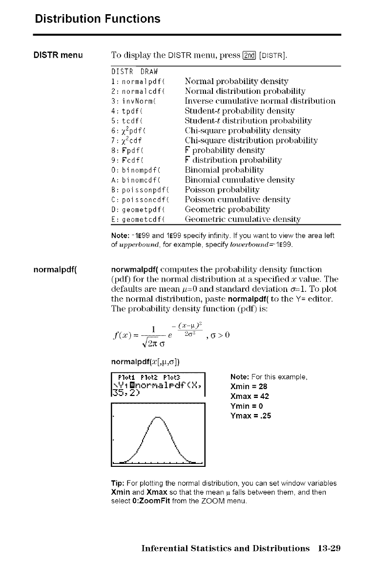
Distribution Functions
DISTR menu
normalpdf(
To display the DISTR menu, press [_ [DiSTR],
DISTR DRAW
i: normalpdf(
2: normalcdf(
3:invNorm(
4:tpdf(
5:tcdf(
6: z2pdf(
7: x2cdf
8: Fpdf(
9: Fcdf(
O: binompdf(
A: binomcdf(
B: poissonpdf(
C: poissoncdf(
D: geometpdf(
E: geometcdf(
Normal probability density-
Normal distribution probability
Inverse cunmlative normal distribution
Student-t probability density
Student-t distribution probability
Chi-square probability density-
Chi-square distribution probability
F probability density-
F distribution probability
Binomial probability
Binomial cunmlative density-
Poisson probability
Poisson cunmlative density
Geometric probability
Geometric cunmlative density-
Note: -1E99 and IE99 specify infinity. If you want to view the area left
of upp¢rbound, for example, specify lowerbound_1E99.
norwmalpdf( computes the probability density function
(pdf) for the normal distribution at a specified xvalue, The
defaults are mean p=O and standard deviation cr=l. To plot
the normal distribution, p_k_te normalpdf( to the Y= editor.
The probability density function (pdf) is:
1 - (x-")=
f(x)=_e 2_ ,_>0
4"z_c_
normalpdf(x[,p,o])
Pl,:,tl P10L2 Plot3
",V1 Bnor.r_alPdf" (X,
35,2>
Note: For this example,
Xmin = 28
Xmax = 42
Ymin = 0
Ymax = .25
Tip: For plotting the normal distribution, you can set window variables
Xmin and Xmax so that the mean p falls between them, and then
select 0:ZoomFit from the ZOOM menu.
Inferential Statistics and Distributions 13-29
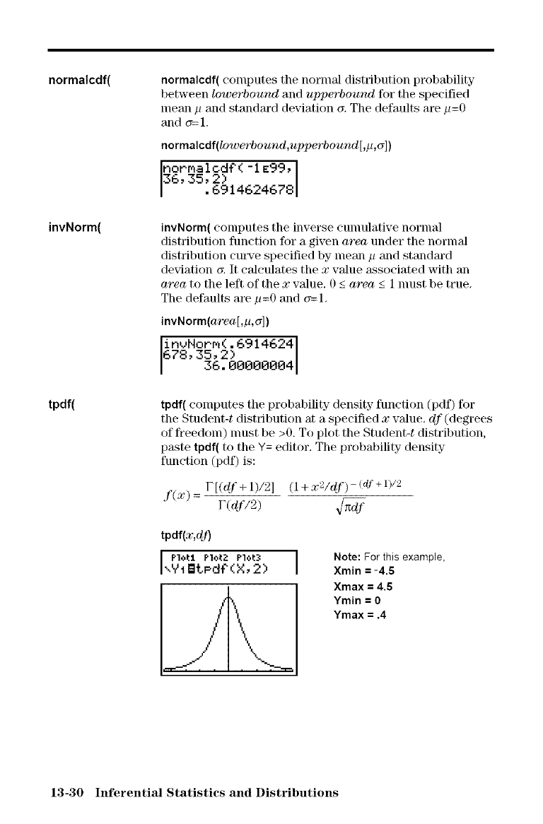
normalcdf(
invNorm(
tpdf(
normalcdf( computes the normal distribution probability
between lowerbound and upperbound for the specified
nlean u and standard deviation or.The defaults are u=0
and 6= 1.
normalcdf(_werbound,upperbound[,p,_])
noPmalod_(-iE99,
36,35,2)
.6914624678
invNorm( computes the inverse cumulative normal
distribution function for a given area under the normal
distribution cut_'e specified by mean pand standard
de_iation cr. It calculates the xvalue associated with an
area to the left of the xvalue. 0 _<area _<1 must be true.
The defaults are p=0 and or=1.
invNorm(area[,p,_])
invNorr_(. 6914624
678,35, 2)
36. ee0000e4
tpdf( computes the probability density- function (pdf) %r
the Student-t distribution at a specified xvalue, df (degrees
of freedom) must be >0. To plot the Student-t distribution,
paste tpdf( to the Y= editor, The probability density-
function (pdf) is:
F [(df + 1)/2] (1 + x2/df) - (if + 1)/2
f(x) =F(df /2) x/_f
tpdf(x, dJ)
Pl_{:[ P1¢_: Plo{. _
",YI BtPd{'(X, 2) INote: For this example,
Xmin =-4.5
Xmax =4.5
Ymin = 0
Ymax = .4
13-30 Inferential Statistics and Distributions
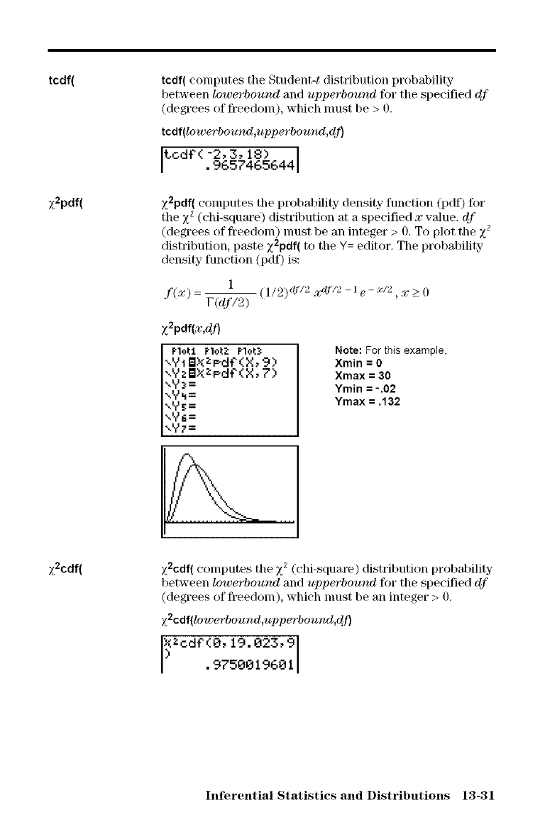
tcdf(
x2pdf(
tcdf( computes the Student-t distribution probability
between lowo'bound and uppe_"bound for the specified df
(degrees of freedom), which nmst be > O.
tcdf(lowerbound,uppe'rbou.rwl,d]_
tc.d_" ( -2, 3, 18)
•9657465644
z2pdf( computes the probability density function (pdf) ff)r
the X2 (chi-square) distribution at a specified xvalue, df
(degrees of freedoln) nmst be an integer > 0, To plot the X2
distribution, paste x2pdf( to the Y= editor, The probability
density function (pdf) is:
1
f(x) = (1/2)df/2 x/f/:) -1e-x/:), x _>0
r(df /2)
:2pdf(x,dj)
P1,;,tl PloLZ Plot_
\YI B:KZPdf'(X, 9)
",VZ I_I;_Z Pdla (X _F)
xYs=
\Y_=
\Y_=
xY_=
\Y_=
Note: For this example,
Xmin = 0
Xmax = 30
Ymin = -.02
Ymax = .132
x2cdf( x2cdf( computes the Z z (chi-square) distribution probability
between lowerbound and upperbound for the specified df
(degrees of freedom), which nmst be an integer > O.
z2cdf(lowe'rbound,upperbound,dj)
_Zc.d_(O, 19. 023,9
.9750019601
Inferential Statistics and Distributions 13-31
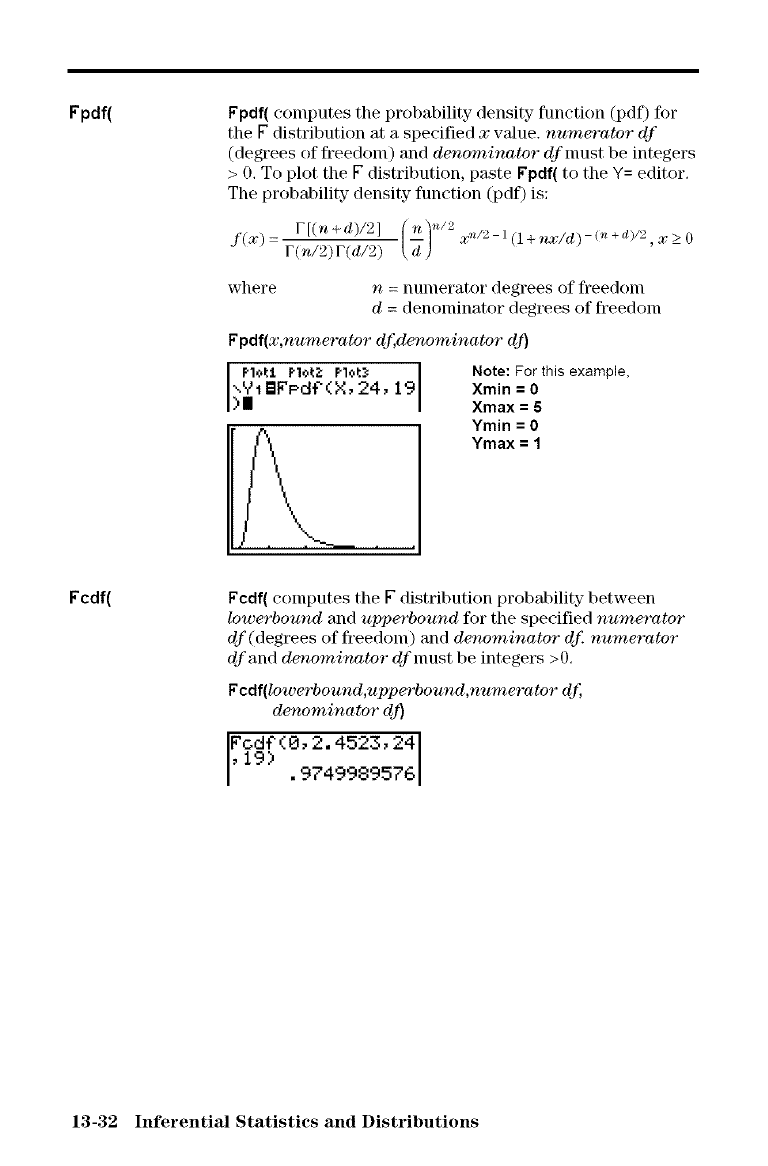
Fpdf( Fpdf( computes the probability density- function (pdf) for
the F distribution at a specified xvalue, numerator df
(degrees of freedonl) and denominator dfnmst be integers
> O. To plot the F distribution, paste Fpdf( to the Y= editor.
The probability density function (pdf) is:
F[(n+d)/2] (d)n/2xn/2 l(l+,_a_./d)(n+d)/2,X> 0
f(X) = F(n/2)F(d/2)
where n= numerator degrees of freedom
d= denominator degrees of fi'eedom
F pdf(x,numero tor dr, denominator dJ_
Plot:l, plot:i: Plo_,3 Note: For this example,
_._1BFPdf (X, 24, 19 Xmin = 0
Xmax = 5
Ymin = 0
Ymax = 1
Fcdf( Fcdf( computes the F distribution probability between
lowerbound and uppe'rbound for the specified nume_-ator
df (degrees of freedon0 and denominator dr. numerator
dfand denominator df nmst be integers >0.
Fcdf(lowerbound,upperbound,numerator dr,
denominator dJ)
Fodf'(O, 2. 4523,24
,19) -,
• 9_ 49989576
13-32 Inferential Statistics and Distributions
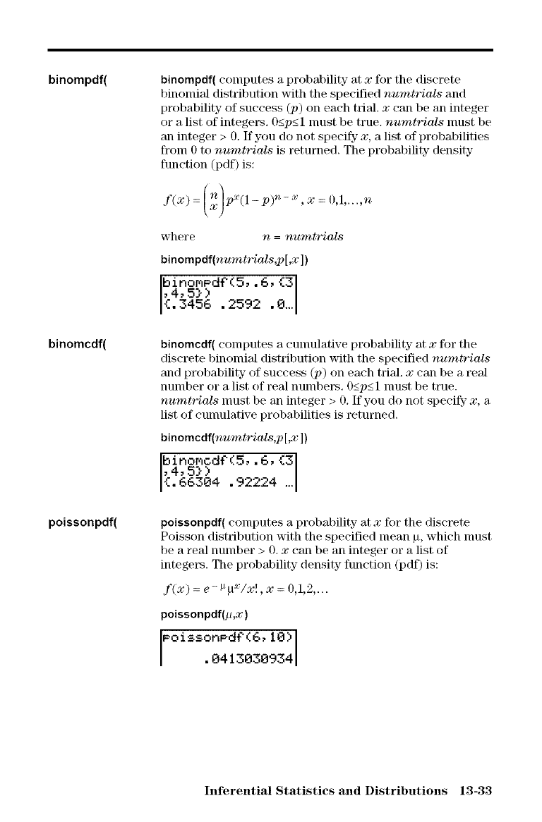
binompdf(
binomcdf(
poissonpdf(
binompdf( computes a probability at xffw the discrete
binomial distribution with the specified numtrials and
probability of success (1)) on each trial, x can be an integer
or a list of integers. O_<p_<lnmst be true. numtrials nmst be
an integer > O. If you do not specify x, a list of probabilities
from 0 to numtrials is returned. The probability density
function (pdf) is:
X ( _7/, x n-x X
f( )=/xiP (l-p) , =O,1,...,n
where n=numtrials
binompdf(numtrials,p[,x ])
binomPd¢(5,. 6, {3
,4,5})
{. 3456 .2592 .0...
binomcdf( computes a cunmlative probability at xff)r the
discrete binomial distribution with the specified numtrials
and probability of success (p) on each trial, x can be a real
nmnber or a list of real nmnbers. O_<p_<1 nmst be true.
numtrials nmst be an integer > O. If you do not specify- x, a
list of cunmlative probabilities is returned.
binomcdf(numtrials,p[,x ])
binomcd¢(5,. 6, {3
,4,5})
{,66304 .92224 ...
poissonpdf( computes a probability at xff)r the discrete
Poisson distribution with the specified mean {l, which nmst
be a real nmnber > O. x can be an integer or a list of
integers. The probability density function (pdf) is:
f(x) =e- _ ,uX/x!, x= 0,1,2,...
poissonpdf(p,x)
PoissonPd¢(6,10)
.0413030934
Inferential Statistics and Distributions 13-33
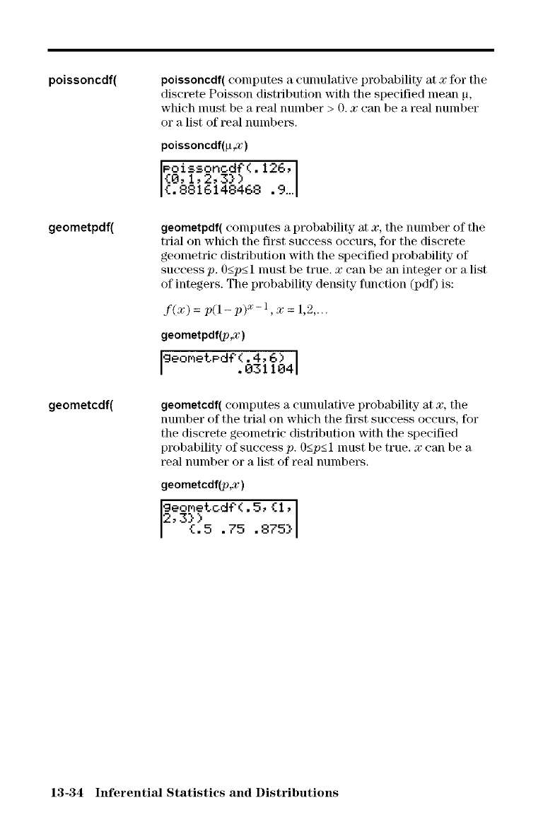
poissoncdf(
geometpdf(
geometcdf(
poissoncdf( computes a eunmlative probability at xfor the
discrete Poisson distribution with the specified mean _l,
which nmst be a real number > O. xcan be a real number
or a list of real numbers.
poissoncdf(p,x)
eoissonod¢(.126,
{0,1,2,3})
{.8816148468 .9...
geometpdf( computes a probability at x, the number of tlle
trial on which the first success occurs, for the discrete
geometric distribution with the specified probability of
success p. 0_<p_<l nmst be true. xcan be an integer or a list
of integers. The probability density function (pdf) is:
f(x) =p(1 -p)X - 1, x= 1,2,...
geometpdf_,x)
geo_eted?(.4,6)
.031104
geometcdf( computes a cunmlative probability at x, the
number of the trial on which the first success occurs, for
the discrete geometric distribution with the specified
probability of success p. O_<p_<1 must be true. xcan be a
real number or a list of real numbers.
geometcdf_,x)
geo_etod¢(.5,{l,
2,3J)
{.5 .75 .875}
13-34 Inferential Statistics and Distributions
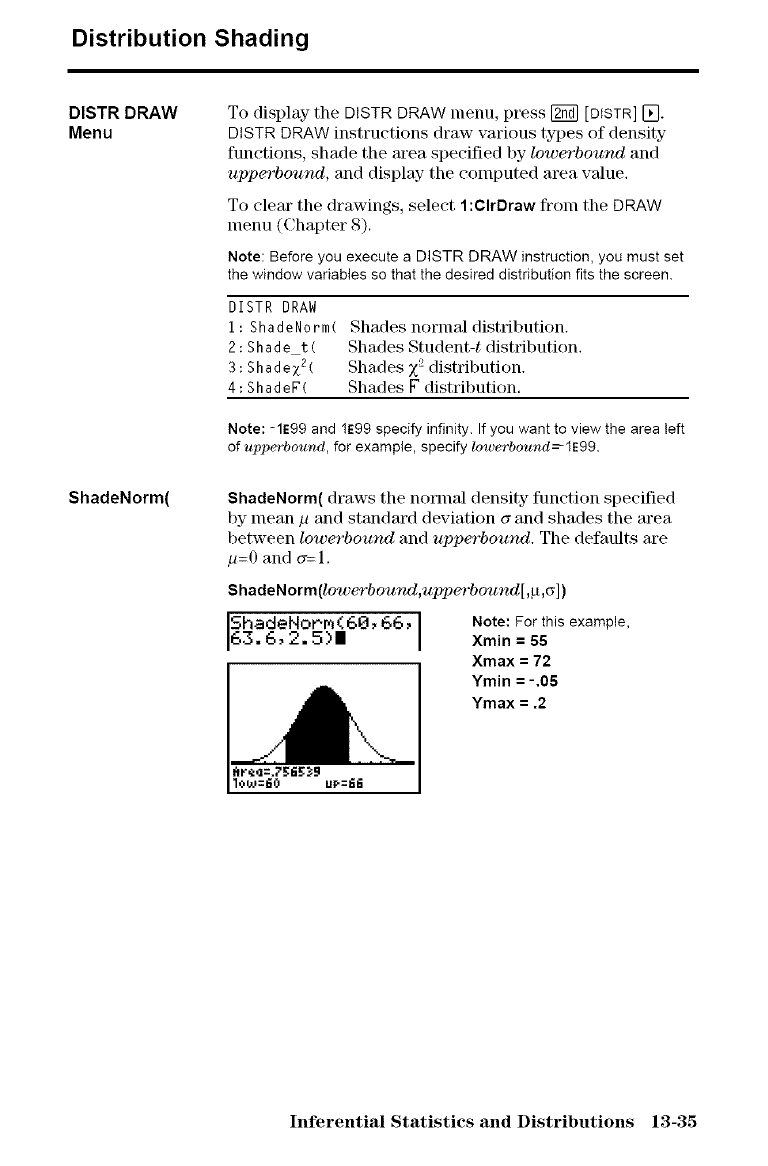
Distribution Shading
DISTR DRAW
Menu
ShadeNorm(
To display the DISTR DRAW menu, p_ss _ [DISTR] [].
DISTR DRAW instructions draw vmious types of density
functions, shade the area specified by lower'bound and
uppc'rbound, and display- the computed area vMue.
To clem" the drawings, select l:CIrDraw from the DRAW
menu (Chapter 8).
Note: Before you execute a DISTR DRAW instruction, you must set
the window variables so that the desired distribution fits the screen.
DISTR DRAW
i: ShadeNorm(
2:Shade t(
3:Shadez2(
4:ShadeF(
Shades normal distribution.
Shades Student-t distribution,
Shades )_ distribution.
Shades Fdistribution,
Note: -1E99 and IE99 specify infinity. If you want to view the area left
of upperbowad, for example, specify lowe'rbownd_1E99.
ShadeNorm( draws the normal density function specified
by mean uand standard deviation aand shades the m'ea
between lowc'rbound and upperbound. The defaults are
u=0 and a= 1.
ShadeNorm(lowerboural,uppc'rbound[,g,c_])
Note: For this example,
Xmin = 55
Xmax = 72
Ymin =-,05
Ymax = ,2
Inferential Statistics and Distributions 13-35
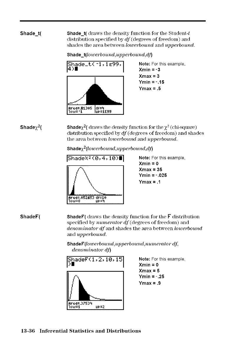
Shade_t(
Shadex2(
ShadeF(
Shade_t( draws the density function for the Student-t
distribution specified by df (degrees of freedom) and
shades the area between lowe_rbound and upperbound.
Shade_t(lowerbound,upperbound,dJ_
4)IShade-t(-l'IE99' Note: For this example,
Xmin =-3
Xmax = 3
Ymin = -,lS
Ymax = .S
Shadex2( draws the density function for the Z2(chi-square)
distribution specified by df (degrees of freedom) and shades
the area between lowerbou_l and uppe_rbound.
Shadex2(lowerbound,uppe_'bound,dj)
IShadeXZ (0, 4, 10)I I Note: For this example.
Xmin = 0
Xmax = 35
Ymin = -.025
Ymax = .1
ShadeF( draws the density function for the F distribution
specified by numerator df (degrees of freedom) and
denominator dfand shades the area between lowed'bound
and upperbour_l.
ShadeF (lowe'rbound,upperbound,numerator dr,
denominator d_
ShadeF()i 1,2, 10, 15 Note: For this example,
Xmin = 0
Xmax = S
Ymin = -.25
Ymax = .9
13-36 Inferential Statistics and Distributions
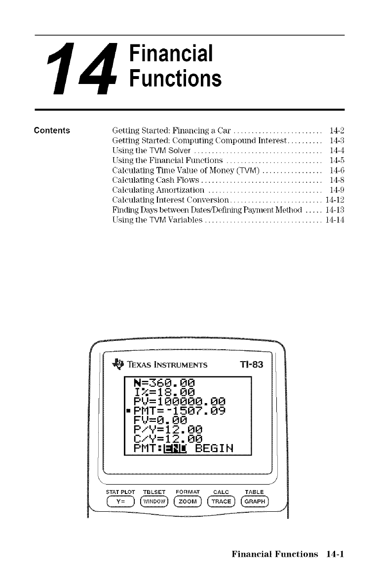
14 Financial
Functions
Contents Getting Started: Einaneing a Car. ........................ I4-2
Getting Started: Computing Compound Interest .......... 14-3
Using the TVM Solver .................................... 14-4
Using the Financial Functions ........................... 14-5
Calculating Time Value of Money (TVM) ................. 14-6
Calculating Cash Flows .................................. 14-8
Calculating Amortization ................................ 14-9
Calculating Interest Conversion .......................... I4-I2
Finding Days between Date_)efil_N Paynlent Method ..... 14-13
Using tile TVM Variables ................................. 14-14
TEXAS INSTRUMENTS T1=83
N=360.00
I_=IB.00
PV=100000.00
-PMT=-I507.09
FV=0.00
P/V=12.00
C/Y=12.00
PMT:L_ BEGIN
STAT PLOT TBLSET FORMAT CALC TABLE
Financial Functions 14-1
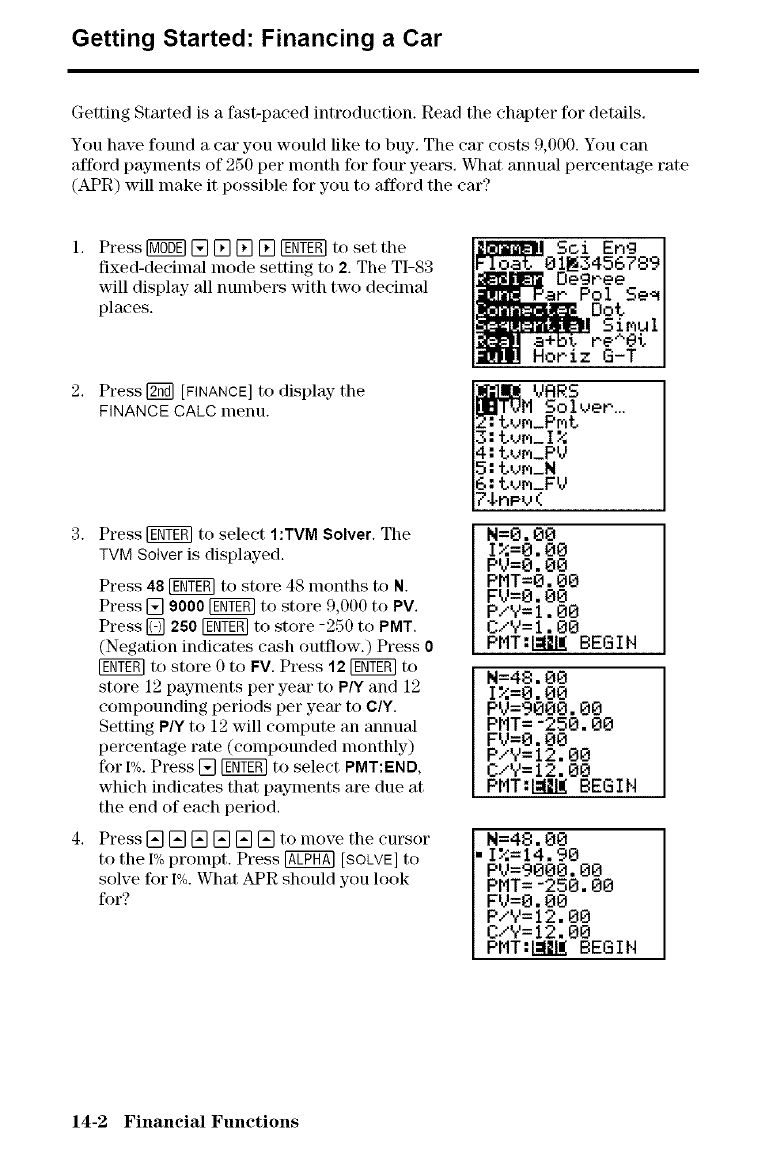
Getting Started: Financing a Car
Getting Started is a ftkst-paced introduction. Read the chapter for details.
You have found a cat" you would like to buy-. The car costs 9,1)00. You can
afford payments of 250 per month for four years. What annual percentage rate
(APR) will make it possible for you to afford the car?
Press[_[][][][][_to setthe
fixed-deeimalmode seging to 2. The TI-83
will display all numbers with two decimal
places.
2. Press [_ [FINANCE]to display" the
FINANCE CALC menu.
3. Press [_ to select I:TVM Solver. The
TVM Solver is displayed.
Press 48 [_ to store 48 months to N.
Press [] 9000 [gNT_ to store 9,000 to PV.
Press [] 2S0 [gNT_ to store -250 to PMT.
(Negation indicates cash outflow.) Press 0
[ggg_ to store 0 to FV. Press 12 F_tggl to
store 12 payments per year to P/Y and 12
compounding periods per year to O/Y.
Setting PlY to 12 will compute an annual
percentage rate (compounded monthly)
for I%.Press [] [gNT_ to select PMT:END,
which indicates that payments are due at
the end of each period.
4. Press [] [] [] [] [] [] to move the cursor
to the I%prompt. Press @ [SOLVE] to
solve for I%.What APR should you look
for?
Sci Ehg
_I_3456789
Degree
Pol Se_
Dog
Horiz G-T
VRRS
Solver...
gum_I%
gvm_PV
tvm_N
tvm_FV
,nev(
N=0.00
I%=0.00
PV=0.00
PMT=0.00
FV=0.00
P/Y=l.O0
C/V=l.00
PMT:L_ BEGIN
N=48.00
I%=0.00
PV=9000.00
PMT=-250.00
FV=0.00
P/Y=12.00
C/Y=12.00
PMT:[__[LL_BEGIN
N=48.00
"1%=14.90
PV=9000.00
PMT=-250.00
FV=0.00
P/Y=12.00
C/Y=12.00
PMT:L:[II_BEGIN
14-2 Financial Functions
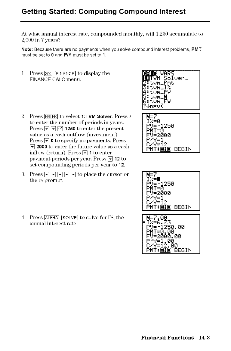
Getting Started: Computing Compound Interest
At what annual interest rate, compounded monthly, will 1,250 accumulate to
2,000 in 7 years?
Note: Because there are no payments when you solve compound interest problems, PMT
must be set to 0 and PlY must be set to 1.
Press [_ [FINANCE] to display- the
FINANCE CALC menu.
Press [_ to select I:TVM Solver. Press 7
to enter the number of periods in years,
Press [] [] [] 12S0 to enter the present
value as a cash outflow (investment).
Press [] 0 to specify- no payments. Press
[] 2000 to enter the future value as a cash
inflow (return), Press [] 1to enter
payment periods per year, Press [] 12 to
set compounding periods per yea[" to 12.
Press [] [] [] [] [] to place the cursor on
the 1%prompt.
Press @ [SOLVE] to solve for I%, the
annual interest ['ate.
Z.._tvVRR5
M Solver
_,_PMt
3: tw,_l%
4: tvM_PV
5: tur,,_N
6: tvr.__FV
74nPv(
N=7
1%=0
PV=-1250
PMT=O
FV=2000
P/9=I
C/Y=12
PMT:L_IiE BEGIN
N=7
1%=|
PV=-1250
PMT=O
FV=2000
P/Y=1
C/Y=I2
PMT:I=_I_ BEGIN
.N=7.O0
1%=6.73
PV=-1250.00
PMT=0.00
FV=2000.00
P/Y=l.00
C/Y=12.00
PMT:_ BEGIN
Financial Functions 14-3
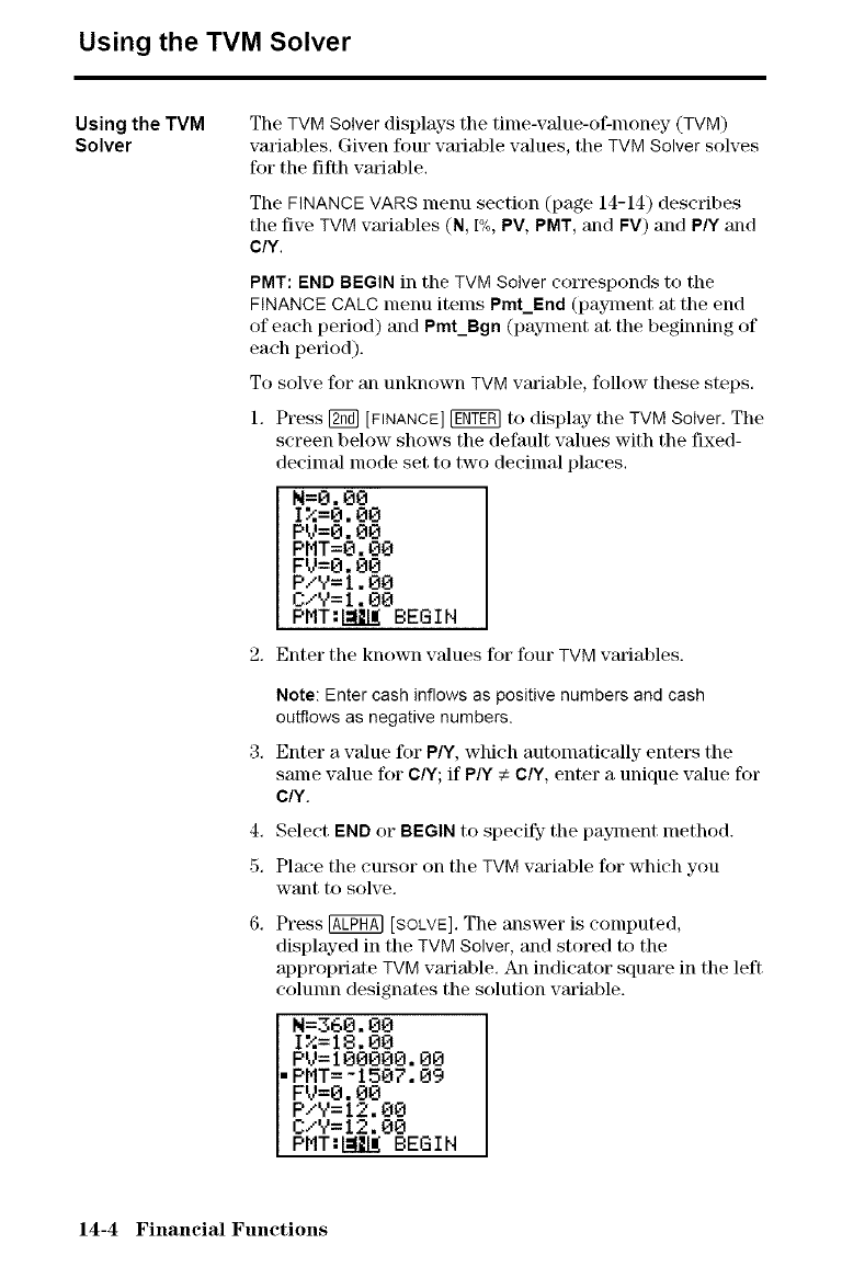
Using the TVM Solver
Using the TVM
Solver The TVM Solver displays the time-value-of-money (TVM)
variables. Given four variable wdues, tile TVM Solver solves
for the fifth variable.
The FINANCE VARS menu section (page 14-14) describes
the five TVM variables (N, I%, PV, PMT, and FV) and PlY and
C/Y,
PMT: END BEGIN in the TVM Solver corresponds to the
FINANCE CALC menu items Pmt_End (pa3qnent at the end
of each period) and Pmt_Bgn (payment at the beginning of
each period).
To solve for an unknown TVMvm'iable, follow these steps.
1, Press [2ffa][FINANCE] _ to display the TVM Solver. The
screen below shows the default values with the fixed-
decimal mode set to two decimal places,
N=0.00
Ia=0.00
PV=0.00
PMT=O,00
FV=0.00
P/V=I.00
C/V=I.O0
PMT:[__II_BEGIN
2. Enter the known vMues for four TVM variables.
Note: Enter cash inflows as positive numbers and cash
outflows as negative numbers.
Enter a value for P/Y, which automatically enters the
same wdue for C/Y; if PW €CIY, enter a unique value for
C/Y.
4. Select END or BEGIN to specify- the pa3qnent method.
5. Place the cursor on the TVM vm'iable for which you
want to solve.
Press @ [SOLVE].The answer is computed,
displayed in tile TVM Solver, and stored to the
appropriate TVM variable, An indicator square in the left
colunm designates the solution variable.
N=360.00
I%=1B.00
PV=100000.00
PMT=-I507.09
FV=0.00
P/Y=I2.00
CXY=12.00
PMT:I:IIIIBEGIN
14-4 Financial Functions
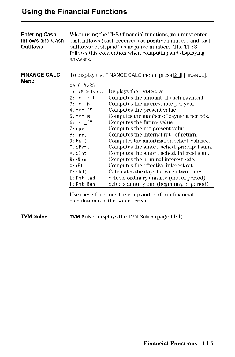
Using the Financial Functions
Entering Cash
Inflows and Cash
Outflows
FINANCE CALC
Menu
TVM Solver
When using the TI-83 financial functions, you lnust enter
cash inflows (cash received) as positive numbers and cash
outflows (cash paid) as negative numbel\_. The TI-S3
follows this convention when computing and displaying
answers.
To display the FINANCE CALC menu, press [_ [FINANCE].
CALC VARS
i : TVM Sol ver.,.
2 : tvm Pmt
3: tvm I%
4:tvm PV
5:tvm N
6:tvm FV
7:npv(
8:irr(
9: bal(
O:EPrn(
A:EInt(
B:_Nom(
C:_Eff(
D:dbd(
E: Pmt End
F: Pmt Bgn
Displays tile TVM Solver.
Conlputes the amount of each payment.
Conlputes the interest rate per year,
Computes the present value.
Colnputes the nulnber of paylnent periods,
Computes the future value,
Computes the net present value,
Computes the internal rate of l_tum.
Computes the amortization sched, balance,
Computes the amort, sched, principal sum,
Computes the amort, sched, interest sum.
Computes the nominal interest rate,
Computes the effective interest rate.
Calculates the days between two dates,
Selects ordinary annuity (end of period).
Selects annuity- due (beginning of period),
[ _se these functions to set up and perform financial
calculations on the home screen,
TVM Solver displays tile TVM Solver (page 14-4).
Financial Functions 14-5
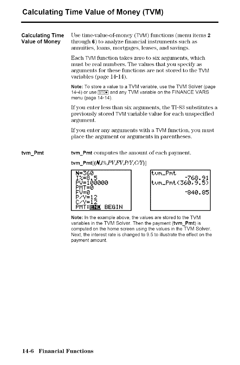
Calculating Time Value of Money (TVM)
Calculating Time
Value of Money
tvm_Pmt
I_se tilne-value-of-lnoney (TVM) functions (menu items 2
through 6) to analyze financial instruments such as
annuities, loans, mortgages, leases, and sa_ings.
Each TVM function takes zero to six arguments, which
must be real numbers. The wdues that you specify as
arguments for these functions m'e not stored to the TVM
variables (page 14-14).
Note: To store a value to a TVM variable, use the TVM Solver (page
14-4) or use _ and any TVM variable on the FINANCE VARS
menu (page 14-14).
If you enter less than six arguments, the TI-83 substitutes a
previously stored TVM vm'iable value for each unspecified
argument.
If you enter any argunlents with a TVM function, you nlust
place the argmnent or arguments in parentheses,
tvm_Pmt computes the amount of each payment.
tvm_Pmt [(N,I %,PV,FV, P_, C/Y) ]
N=360
I%=8.5
Pg=IO0000
PMT=O
FV=O
P/?=I2
C/V=12
PMT:I_I[ BEGIN
tvm_Pmt -768 91 I
tvm_Pr_t (360, 9: 5) I
-840.85
Note: In the example above, the values are stored to the TVM
variables in the TVM Solver. Then the payment (tyro_Pint) is
computed on the home screen using the values in the TVM Solver.
Next, the interest rate is changed to 9.5 to illustrate the effect on the
payment amount.
14-6 Financial Functions
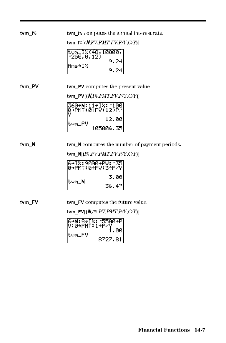
tvm_]%
tvm_PV
tvm_N
tvm_FV
tvm_I% computes the annual inte[_st rate.
tvm_1%[(N,PV,PMT, FV, P/Y, C/Y) ]
tvm_l%(48, 10000, I
-250,0, 12) 9 24
Rns÷l% 9124
tvm_PV computes the present vMue.
tvm_PV[(_I%,PMT, FV, P/Y,C/Y)]
360÷N:II÷I%:-100
÷PMT:O÷FV:12÷P/
tvm_PV 12.00
I 1o5oo6.351
tvm_N computes the number of paylnent periods.
tvm_N[(I%_V_MT, FV, P/Y,C/Y)]
6÷I%:9000÷PV:-351
O÷PMT:O+FV:3÷P/V l
tvm_N 3.00
36.47
tvm_FVcomputesthe _turevMue.
tvm_FV[(_I%,PV, PMT_X,C/Y)]
6÷N:8÷I%:-5500÷P
V:0÷PMT:l÷P/_.00
tvm_FV 8727.81
Financial Functions 14-7
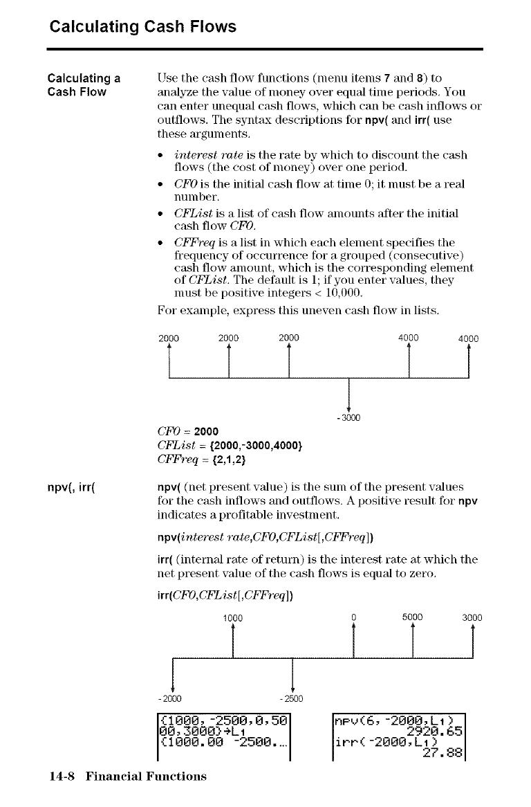
Calculating Cash Flows
Calculating a
Cash Flow Use the cash flow functions (menu items 7 and 8) to
analyze the value of money over equal time periods. You
can enter unequal cash flows, which can be cash inflows or
outflows. The syntax descriptions for npv( and irr( use
these arguments.
•interest rate is the rate by which to discount the cash
flows (the cost of money) over one period.
• CFO is the initial cash flow at time 0; it nmst be a real
nunlber.
• CFList is a list of cash flow alnounts after the initial
c_sh flow CFO.
• CFFreq is a list in which each element specifies the
frequency of occurrence for a grouped (consecutive)
cash flow amount, which is the corresponding element
of CFList. The default is 1; if you enter values, they
nmst be positive integers < 10,000.
For example, express this uneven cash flow in lists.
2000 2000 2000 4000 4000
; I T I I
CFO = 2000
CFList = {2000,-3000,4000}
CFFreq = {2,1,2}
1
- 3000
npv(, irr( npv( (net present value) is the sunl of the present values
for the cash inflows and outflows. A positive result for npv
indicates a profitable investment.
npv(interest rate,CFO,CFList[,CFFreq])
irr( (internal rate of return) is the interest rate at which the
net present value of the cash flows is equal to zero,
irr(CFO,CFList[,CFFreq])
1000 0 5000 3000
1 1
2000 -2500
{1000,-2500,0,501
00,3000_+L1 I
<1000.00 -2500....
nPv(6,-2000,Lt)
2920.65
irP(-2000,L1) 27.88
14-8 Financial Functions
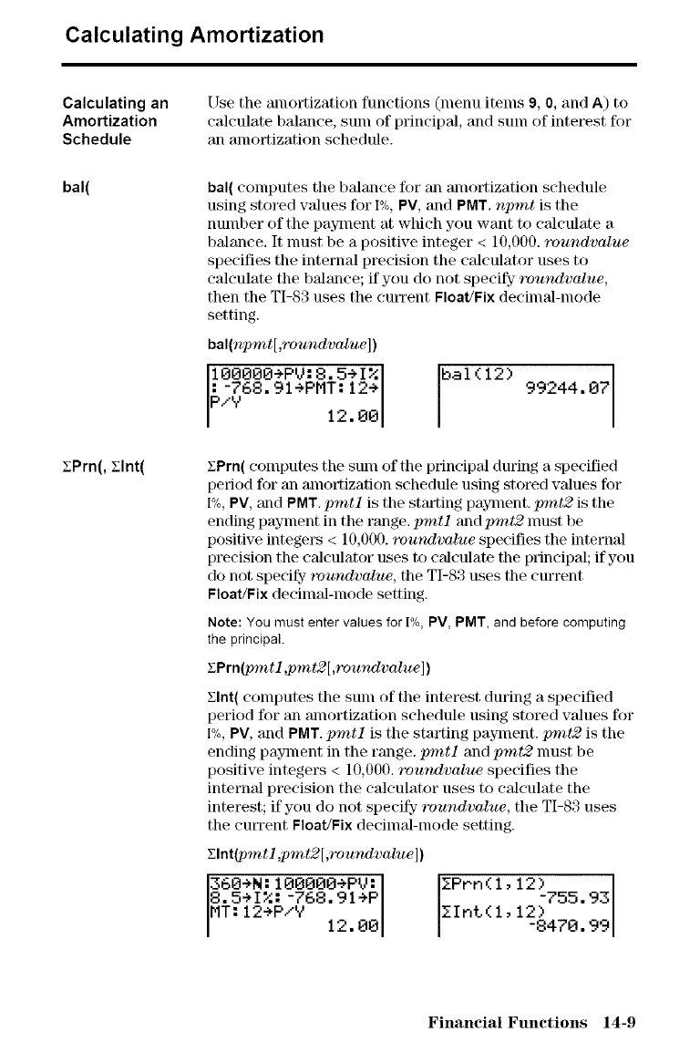
Calculating Amortization
Calculating an
Amortization
Schedule
bal(
EPrn(, Elnt(
Use the amortization functions (menu items 9, 0, and A) to
calculate balance, sum of principal, and sum of interest for
an amortization schedule.
bal( computes tile balance ff)r an amortization schedule
using stored wdues ff)r I%, PV, and PMT. npmt is the
number of the payment at which you want to calculate a
balance. It nmst be a positive integer < 10,000. roundvalue
specifies the internal precision the calculator uses to
calculate the balance; if you do not specify roundvalue,
then the TI-83 uses the cmTent Float/Fix decimal-mode
setting.
bal(npmt[,roundvalue])
IO0000÷PV: 8.5÷I% bal (12) 99244.07
I_.O0
EPrn( computes the sunl of the principal during a specified
period for an amortization schedule using stored values for
I%, PV, and PMT. pmtl is the starting paylnent, pmt2 is the
ending payment in the range, pmtl and pmt2 nmst be
positive integers < 10,000. roufwlvalue specifies the internal
precision the calculator uses to calculate the principal; if you
do not specify- _vu.rwlvalue, the TI-83 uses the current
Float/Fix deeinml-mode setting.
Note: You must enter values for 1%, PV, PMT, and before computing
the principal.
EPrn(pmtl,pmt2[,rou_wlvalue])
Elnt( computes the stun of the interest during a specified
period for an amortization schedule using stored values for
I%, PV, and PMT. pmtl is the starting paylnent, pmt2 is the
ending payment in the range, pmtl and pmt2 nmst be
positive integers < 10,000. roundvalue specifies the
internal precision the calculator uses to calculate the
interest; if you do not specify- roundvalue, the TI-83 uses
the emTent Float/Fix deeinml-mode setting.
Elnt(pmt l,pmt2[ ,roundvalue ])
360÷N: 100000÷PV: I EF'Po (I, 12)755._
8.5÷1%: -768.91÷P 93
MT:I2÷P/V 12.00 EInt(l,12)_8470.99
Financial Functions 14-9
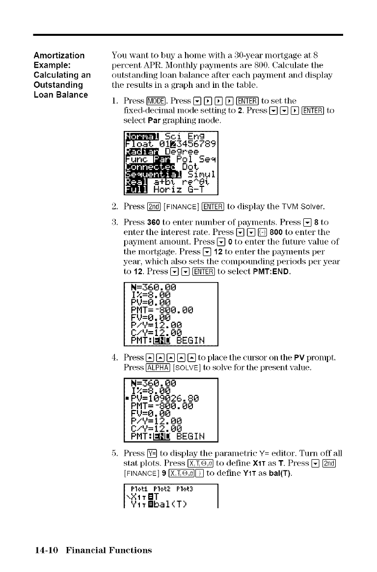
Amortization
Example:
Calculating an
Outstanding
Loan Balance
You want to buy a home with a 30-year mortgage at S
percent APR. Monthly payments are 800, Calculate the
outstanding loan balance after each payment and display-
the results in a graph and in the table,
1, Press [_]. Press [] [] [] [] _ to set the
fixed-decimal mode setting to 2, Press [] [] [] _ to
select Par graphing mode,
Sci Eng I
II_34567891
Degree I
_Pol Se_
Dot I
SiMi I
hi, I e^8'
Horiz G-T
2, Press [_ [FINANCE] _ to display the TVM Solver.
3. Press 360 to enter number of payments. Press [] 8 to
enter the interest rate. Press [] [] [] 800 to enter the
paynmnt amount. Press [] 0 to enter the future value of
tile mortgage. Press [] 12 to enter the payments per
year, which also sets the compounding periods per year
to 12. Press [] [] _ to select PMT:END,
N=360.00
I%=8.00
PV=0.00
PMT=-800.00
FV=0.00
P/Y=12.00
C/Y=12.00
PMT:[_:IIL_BEGIN
4. Press [] [] [] [] [] to place the cul_or on tile PV prompt.
Press @ [SOLVE] to solve for the present value.
N=360.00
I%=8.00
PV=109026.80
PMT=-800.00
FV=0.00
PIV=I2.00
C/Y=12.00
PMT:I:I_I_BEGIN
5, Press [] to display tile parametric Y= editor. Turn off all
stat plots. Press _ to define X1T as T. Press [] [g_
[FINANCE] 9 _[_ to define Y1T as bal(T).
pI,:,I:I pl,:,l:._ plol:_
\X1 "r_T
YIT_baI(T)
14-10 Financial Functions
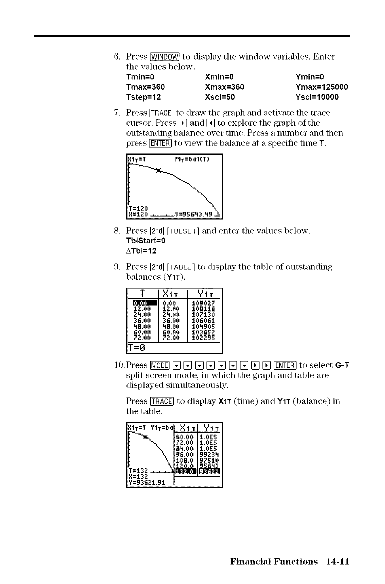
6. Press _ to display- the window variables. Enter
tile values below.
Tmin=0 Xmin=0 Ymin=0
Tmax=360 Xmax=360 Ymax=125000
Tstep=12 Xscl=50 Yscl=10000
7, Press _ to draw the graph and activate the trace
cursor. Press [] and [] to explore the graph of the
outstanding bahmce over time. Press a number and then
press [gNY_ to xqew the balance at a specific time T.
1T=T Y1T=b_I(T)
S, Press [g_ [TBLSET] and enter the vMues below.
TblStart=0
ATbI=12
9, Press [g_ [TABLE] to display the table of outstanding
balances (Y1T).
tZ.00 ,"4t-,a" YtT
Tim O,00 10907::7
IaL0O 10Bl11_
31L00 lO60E:I,
tlIEII00 rIB.00 1Oh9O_:
E0.O0 I;0,00 1031_g2
?_2{_00 72.00 10_:29g
T-
10.Press [g0_ [] [] [] [] [] [] [] [] [] [V_Y_ to select G-T
split-screen mode, in which the graph and table are
displayed sinmltaneously.
Press _ to display- XIT (time) and YIT (balance) in
the table.
_0.00 1.0Eg
72,00 1,0E5
.._.Eh.00 t.OEg
96.00 99_h
t0B,0 97510
T=132 _
X=132
?=93621.91
Financial Functions 14-11
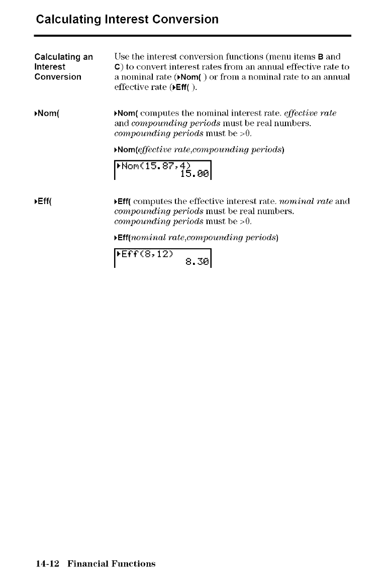
Calculating Interest Conversion
Calculating an
Interest
Conversion
,Nom(
,Eft(
Use the interest conversion functions Onenu items Band
C) to convert interest rates from an annual effective rate to
a nominal rate (_Nom() or from a nominal rate to an annual
effective rate (_Eff().
_Nom( computes the nominal interest rate. effective rate
and compounding periods nmst be real numbers.
compounding periods nmst be >0.
_Nom(effective rate,compounding periods)
_Nor_( 15.87, 4)15.00
)Elf( computes the effective interest rate. nominal rate and
compounding periods must be real nulnbers.
compounding periods must be >0.
_Eff(nominal rate,compounding periods)
_E€€(8,12) 8.30
14-12 Financial Functions
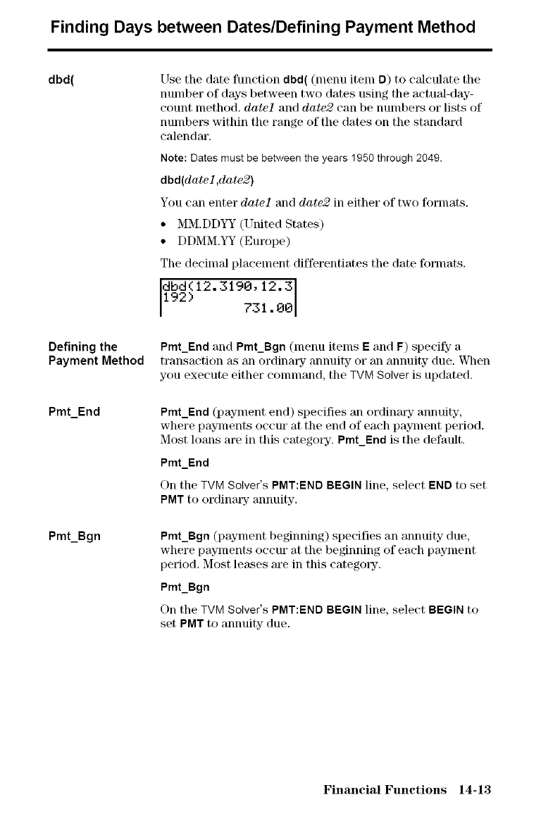
Finding Days between Dates/Defining Payment Method
dbd(
Defining the
Payment Method
Pint_End
Pmt_Bgn
Use the date function dbd( (menu item D) to calculate the
number of days between two dates using the actual-day-
count method, datel and date2 can be numbers or lists of
numbers within the range of the dates on the standard
calendar.
Note: Dates must be between the years I950 through 2049.
dbd(date l,date2)
You can enter datel and date2 in either of two formats.
• MM.DDYY (United States)
• DDMM.YY (Europe)
The decimal placement differentiates the date formats,
dbd( 12. 3190, 12.3
192) 731.00
Pmt_End and Pmt_Bgn (menu items Eand F) specify- a
transaction _k_an ordinmy7 annuity or an annuity due. VC]mn
you execute either conunand, the TVM Solver is updated.
Pmt_End (payment end) specifies an ordinmTy- annuity-,
where payments occur at the end of eaeh payment period.
Most loans are in this catego[% Pint_End is the default.
Pmt_End
On the TVM Solver's PMT:END BEGIN line, select END to set
PMT to ordinmTy- annuity.
Pmt_Bgn (payment beginning) specifies an annuity due,
where payments occur at the beginning of each payment
period. Most leases are in this catego_7.
Pmt_Bgn
On the TVM Solver's PMT:END BEGIN line, select BEGIN to
set PMT to annuity due.
Financial Functions 14-13
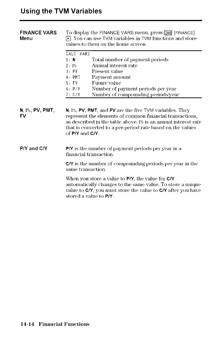
Using the TVM Variables
FINANCE VARS
Menu
N, [%, PV, PMT,
FV
PlY and C/Y
To display the FINANCE VARS menu, press _ [FINANCE]
[_. You can use TVM variables in TVM functions and store
values to them on the home screen,
CALC VARS
1: N
2:1%
3: PV
4: PMT
5: FV
6: P/Y
7: C/Y
Total number of payment periods
Annual interest rate
Present value
Payment amount
Future value
Number of payment periods per year
Number of compounding periods/year
N, I%, PV, PMT,and FV are the five TVM wu'iables. They
t_present the elements of eonunon financial transactions,
as described in the table above. I%is an annual interest rate
that is converted to a per-period rate based on the values
of P/Y and C/Y.
PW is the number of payment periods per year in a
financial transaction.
C/Yis the number of compounding periods per year in the
salne transaction.
When you store a value to P/Y, the value for C/Y
automatically changes to the same value. To store a unique
value to g/Y, you nmst store the value to C/Y after you have
stored a value to PlY.
14-14 Financial Functions
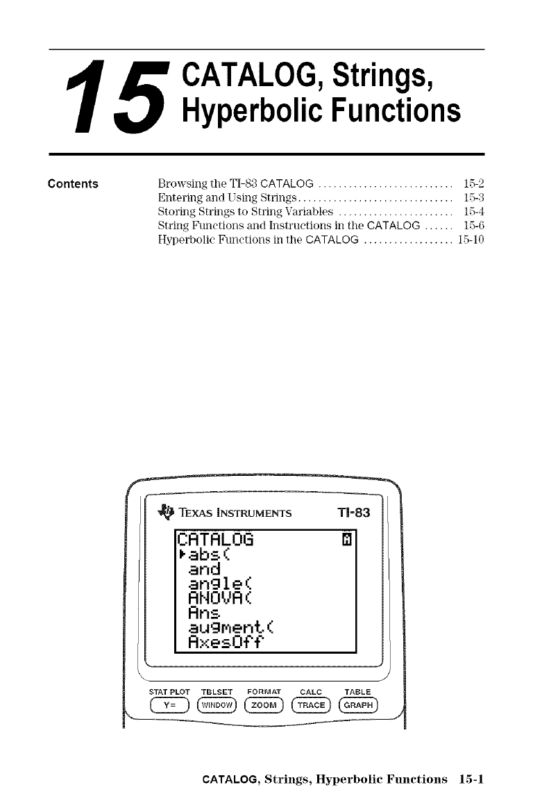
5CATALOG,Strings,
HyperbolicFunctions
Contents Browsing tile TI-83 CATALOG ........................... 15-2
Entering and Using Strings ............................... 15-3
Storing Strings to String Variables ....................... 15-4
String Functions and Instructions in the CATALOG ...... 15-6
Hyperbolic Functions in tile CATALOG .................. 15-10
TEXAS INSTRUMENTS T1=83
mCATALOG
_abs(
and
angle(
QNOUA(
Ans
augnenL(
AxesO_¢
J
STAT PLOT TBLSET FORMAT BALe TABLE
CATALOG, Strings, Hyperbolic Functions 15-1
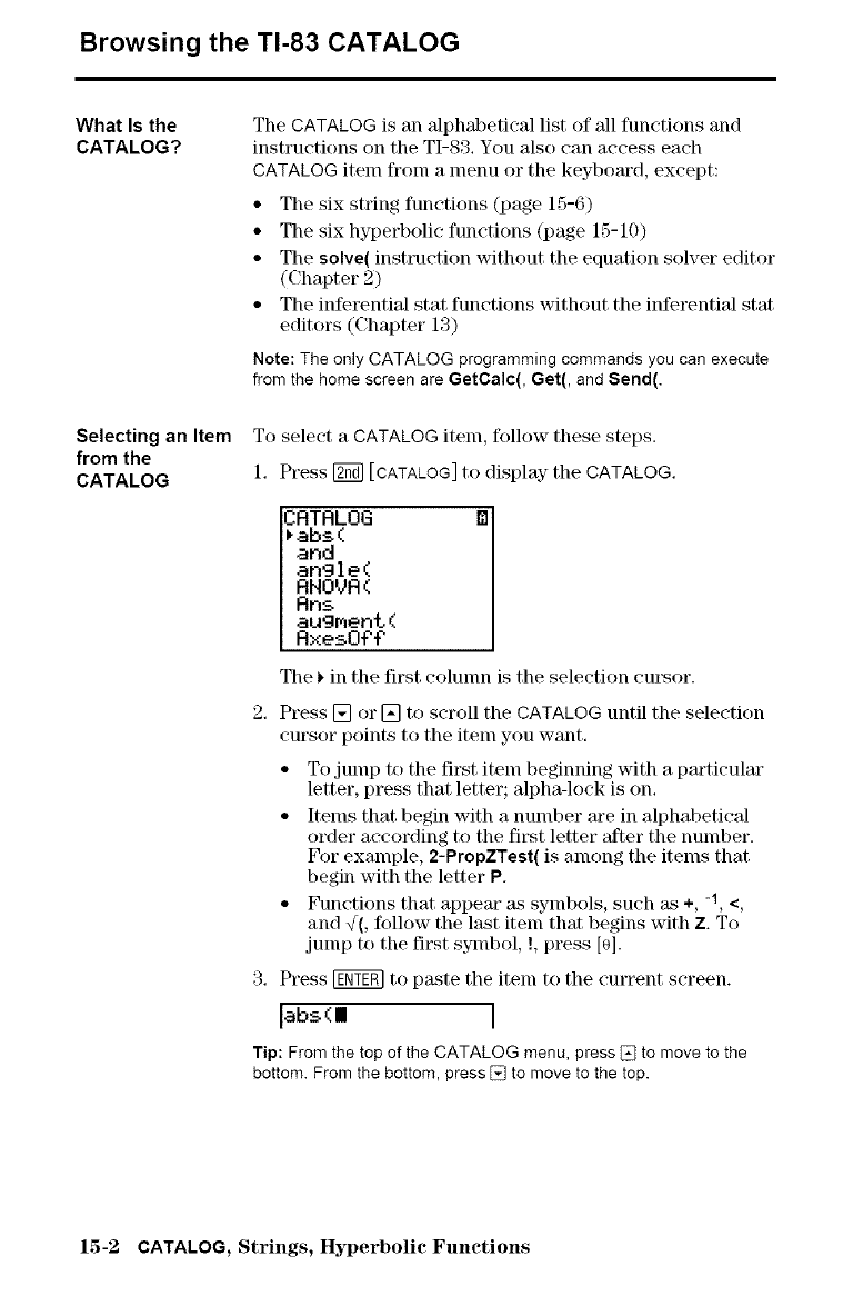
Browsing the TI-83 CATALOG
What Is the
CATALOG?
Selecting an Item
from the
CATALOG
The CATALOG is an alphabetical list of all functions and
instructions on the TI-83. You also can access each
CATALOG item fronl a menu or the keyboard, except:
• The six string functions (page 15-6)
• The six hyperbolic functions (page 15-10)
• The solve( instruction without the equation solver editor
(Chapter 2)
• The inferential stat functions without the inferential stat
editors (Chapter 13)
Note:The only CATALOG programming commandsyoucan execute
from thehomescreenare GetCalc(, Get(, and Send(.
To select a CATALOG item, follow these steps.
1. Press F_a][CATALOG] to display the CATALOG.
iCRTRLOG
i*abs(
and
angle(
RNOVR(
Rn_
augment(
Axes0€€
The _ in the first colunm is the selection cursor.
2. Press [] or [] to scroll the CATALOG until the selection
cursor points to the item you want.
• To jump to the first item beginning with a particular
letter, press that letter; alpha-lock is on.
• Items that begin with a number are in alphabetical
order according to the first letter 'after the number.
For example, 2-PropZTest( is among the itenls that
begin with the letter P.
• Functions that appear as symbols, such as +, -1, <,
and g(, follow the last item that begins with Z. To
jump to the first s3qnbol, !, press [@
3. Press [ggY_ to paste the item to the current screen.
Iabs(1 I
Tip: From the top of the CATALOG menu, press [] to move to the
bottom. From the bottom, press [] to move to the top.
15-2 CATALOG, Strings, Hyperbolic Functions
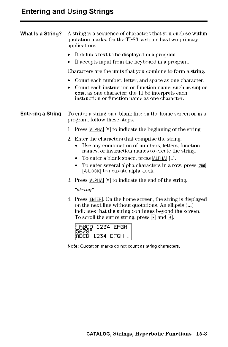
Entering and Using Strings
What Is a String?
Entering a String
A string is a sequence of characters that you enclose within
quotation marks, On the TI-83, a string has two primaFy"
applications.
• It defines text to be displayed in a p_x)gram.
• It accepts input from the keyboard in a program,
Characters are the units that you combine to form a string.
• Count each number, letter, and space as one character,
• Count each instruction or function name, such as sin( or
cos(, as one character; the TI-83 interprets each
instruction or function name as one character.
To enter astring on ablank line on the home screen or in a
program, follow these steps.
1, Press @ [,] to indicate the beginning of the string.
2, Enter the characters that comprise the string.
• Use any combination of numbers, letters, function
names, or instruction names to create the string.
• To enter ablank space, press @ [_],
• To enter several alpha characters in a row, press [_
[A-LOCK] to activate alpha-lock.
3, Press @ [-] to indicate the end of the string.
"string"
4. Press [ENY_. On the home screen, the string is displayed
on the next line without quotations. An ellipsis (...)
indicates that the string continues beyond the screen,
To scroll the entire string, press [] and EO-
"RBC,D, 1234 EFGH
5678
RBCD 1234 EFGH ...
Note: Quotation marks do not count as string characters.
CATALOG, Strings, Hyperbolic Functions 15-3
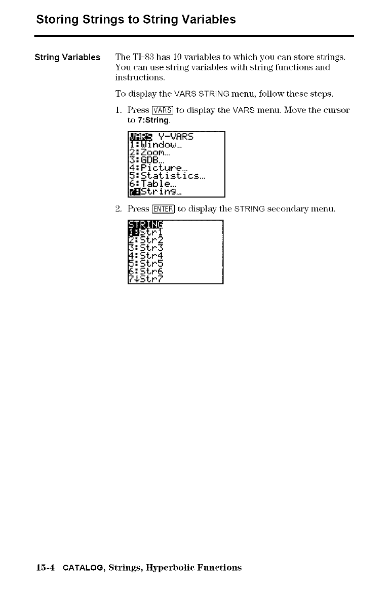
Storing Strings to String Variables
String Variables The TI-83 has 10 variables to which you can store strings.
You can use string variables with string functions and
instructions.
To display the VARS STRING menu, follow these steps.
1, Press _ to display- the VARS menu, Move the cursor
to 7:String.
_ Y-VRRS
ndo_z..
2: Zoom.
3: GDB...
4: Picture...
5: Statistics_.
6: Table...
WString...
2, Press_ to displaytheSTRING secondarymenu,
5:Str3
Str4
Str5
Str6
,Str7
15-4 CATALOG, Strings, Hyperbolic Functions
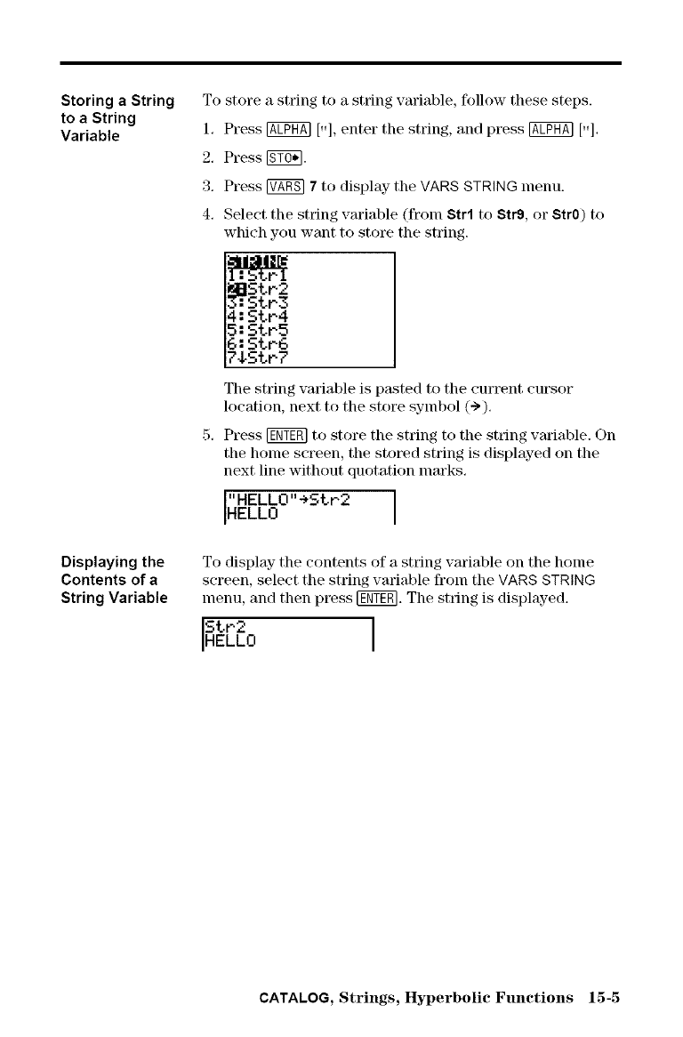
Storing a String
to a String
Variable
Displaying the
Contents of a
String Variable
To
1.
2.
3.
4.
store a string to a string variable, follow these steps.
Press @ [,], enter the string, and press @ [-].
Press _.
Press _ 7 to display the VARS STRING menu.
Select the string variable (from $trl to $tr9, or $tr0) to
which you want to store the string.
4:Str.4
5:StP5
6:_tr6
74Str-7
The string variable is D_sted to the current cursor
location, next to the store symbol (-)).
Press _ to store the string to the string variable. On
the home screen, the stored string is displayed on the
next line without quotation marks.
"HELL0"eStP2
HELLO
To display the contents of a string variable on the home
screen, select the string variable from the VARS STRING
menu, and then press [gNT_. The string is displayed.
St.r2
HELLO I
CATALOG, Strings, Hyperbolic Functions 15-5
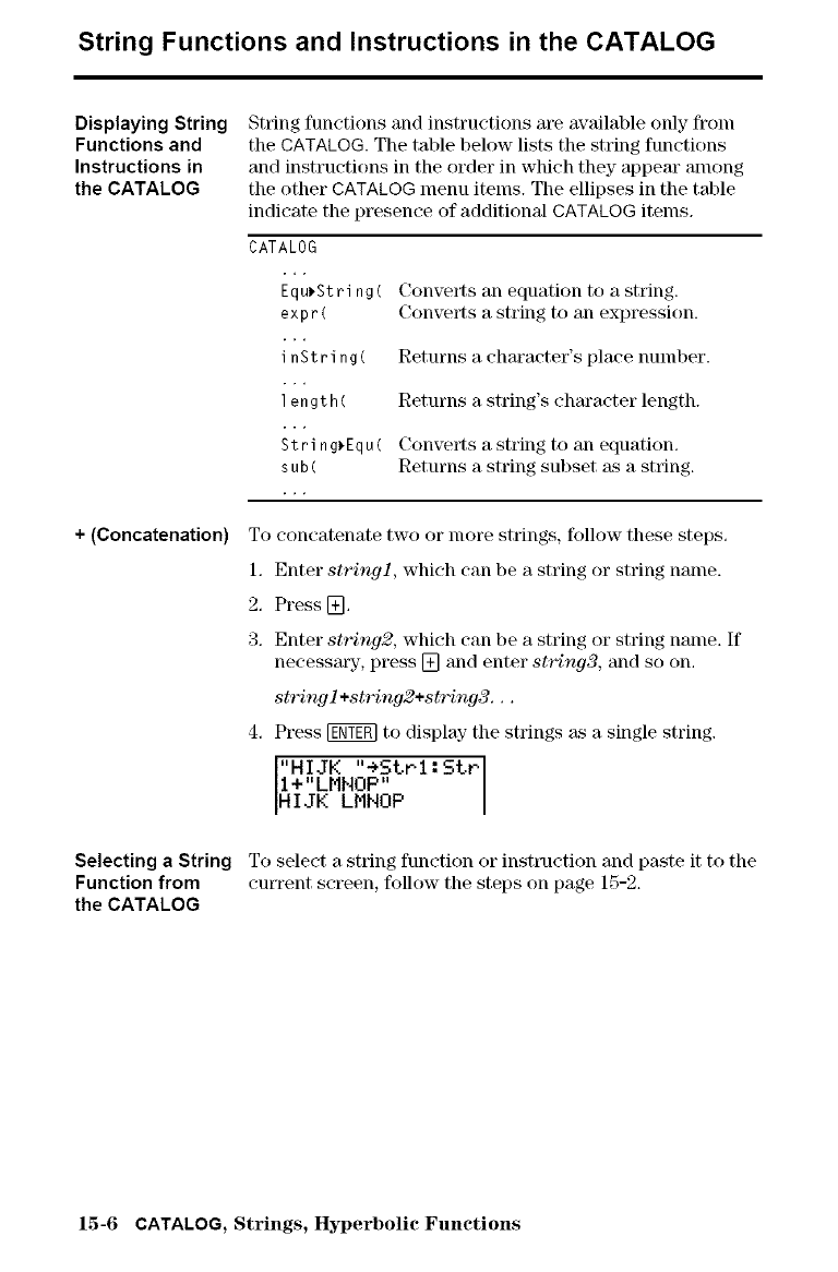
String Functions and Instructions in the CATALOG
Displaying String
Functions and
Instructions in
the CATALOG
+ (Concatenation)
Selecting a String
Function from
the CATALOG
String functions and instructions m'e available only fronl
the CATALOG. The table below lists the string functions
and instructions in the order in which they appem" among
the other CATALOG menu items. The ellipses in the table
indicate the presence of additional CATALOG items.
CATALOG
Equ)String(
expr(
inString(
length(
String)Equ(
sub(
Converts an equation to a string,
Converts a string to an expression.
Returns a chm'acter's place number.
Returns a string's chm'acter length.
Converts a string to an equation,
Returns a string subset as a string,
To concatenate two or more strings, follow these steps,
1, Enter stringl, which can be a string or string name.
2, Press [],
3, Enter string2, which can be a string or string name, If
necessmT, press [] and enter string3, and so on,
stringl +string2+string3, , ,
4, Press [_ to display- the strings as a single string.
"HIJK "+StPl :5tr
1+"LMHOP"
HIJK LMNOP
To select a string function or instruction and paste it to the
current screen, follow the steps on page 15-2.
15-6 CATALOG, Strings, Hyperbolic Functions
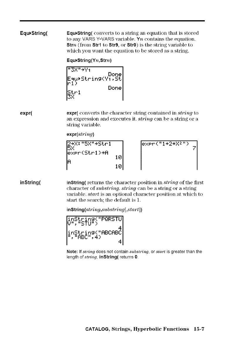
Equ*String(
expr(
inString(
Equ*String( converts to a string an equation that is stored
to any- VARS ¥-VARS variable. Yn contains the equation.
Strn (from Strl to Strg, or Str0) is the string variable to
which you want the equation to be stored as a string.
Equ*Stdng(Yn,Strn)
"3X"÷Y1 Done
E_u*String(gt, St
rl) Done
expr( converts the chm'acter string contained in string to
an expression and executes it. string can be a string or a
stringvariable.
expr(string)
l_X:"5X"+Strl 10 exPr(
x_r(Strl)÷R I0
,,l+2+XZ,,)
7
inString( returns the chm'acter position in string of the first
character of substring, string can be a string or a string
variable, start is an optional character position at which to
start the search; the default is 1.
inString(string,subst,ring[ ,start])
inStr ing ( "PQRSTU
V", "STU" ) 4
inStr ing ( "RBCRBC
,RBC ,4) 4
Note: If st:_ing does not contain snbst:Hng, or start is greater than the
lengthof string, inString( returns O.
CATALOG, Strings, Hyperbolic Functions 15-7
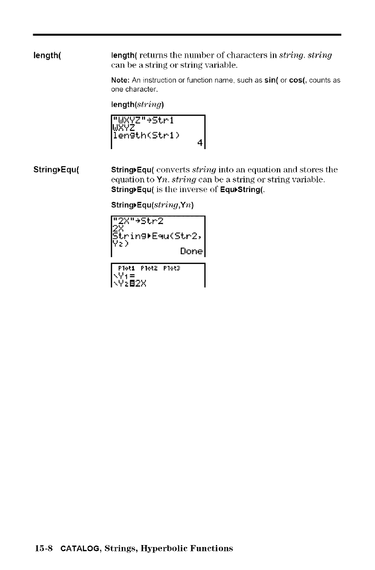
length(
String*Equ(
length( returns the number of chara('ters in st'ring, string
can be a string or string variable.
Note: An instruction or function name, such as sin( or cos(, counts as
one character.
length(string)
WXYz"WXYZ"eStrl 4
length(Strl)
String*Equ( converts st'ring into an equation and stores tlle
equation to Yn. st'ring can be a string or string vmiable,
String*Equ( is tlle inverse of Equ*String(.
String*Equ(st'ring,Yn)
String*E_u(Str2, I
'.?z) Done
Plot1 Plot;" Plot3 I
,,yl= I
",YzB2X
15-8 CATALOG, Strings, Hyperbolic Functions
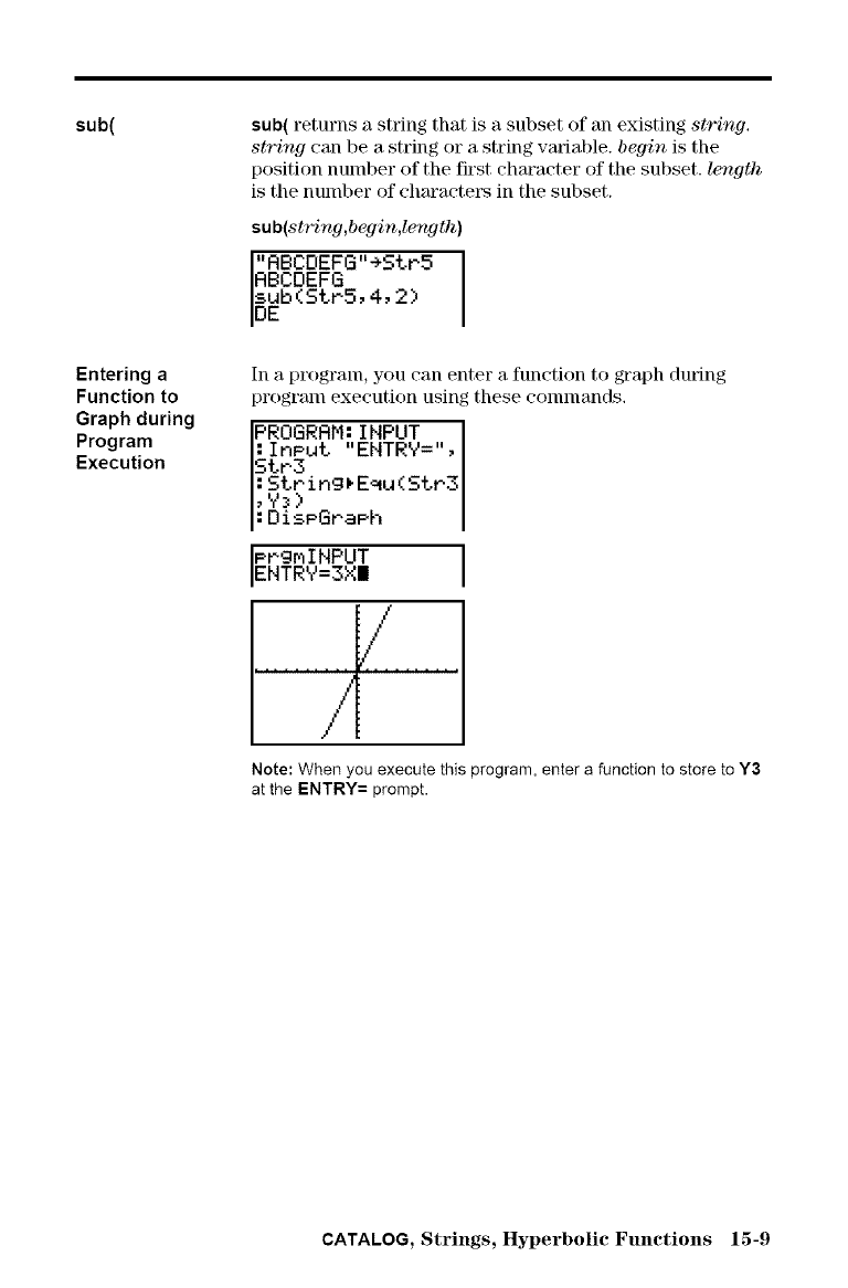
sub(
Entering a
Function to
Graph during
Program
Execution
sub( returns a string that is a subset of an existing st'ring.
string can be a string or a string variable, begin is the
position number of the first character of the subset, length
is the number of characters in the subset.
sub(st_ng,b_in,length)
ABCDEFG"RBCDEFG"÷SLP5I
sub(StP5,4,2)
DE
Inapmgram, youcanentera Nnctiontographdunng
programexecutionusin theseconunands.
PROGRRM:INPUT
:InPut "ENTRY ='' ,
StP3
:String*E_u(Str3
,Y_)
:DisPGraPh
PPYmINPUT
ENTRY=3XI
/
/
/
Note: When you execute this program, enter a function to store to Y3
at the ENTRY= prompt.
CATALOG, Strings, Hyperbolic Functions 15-9
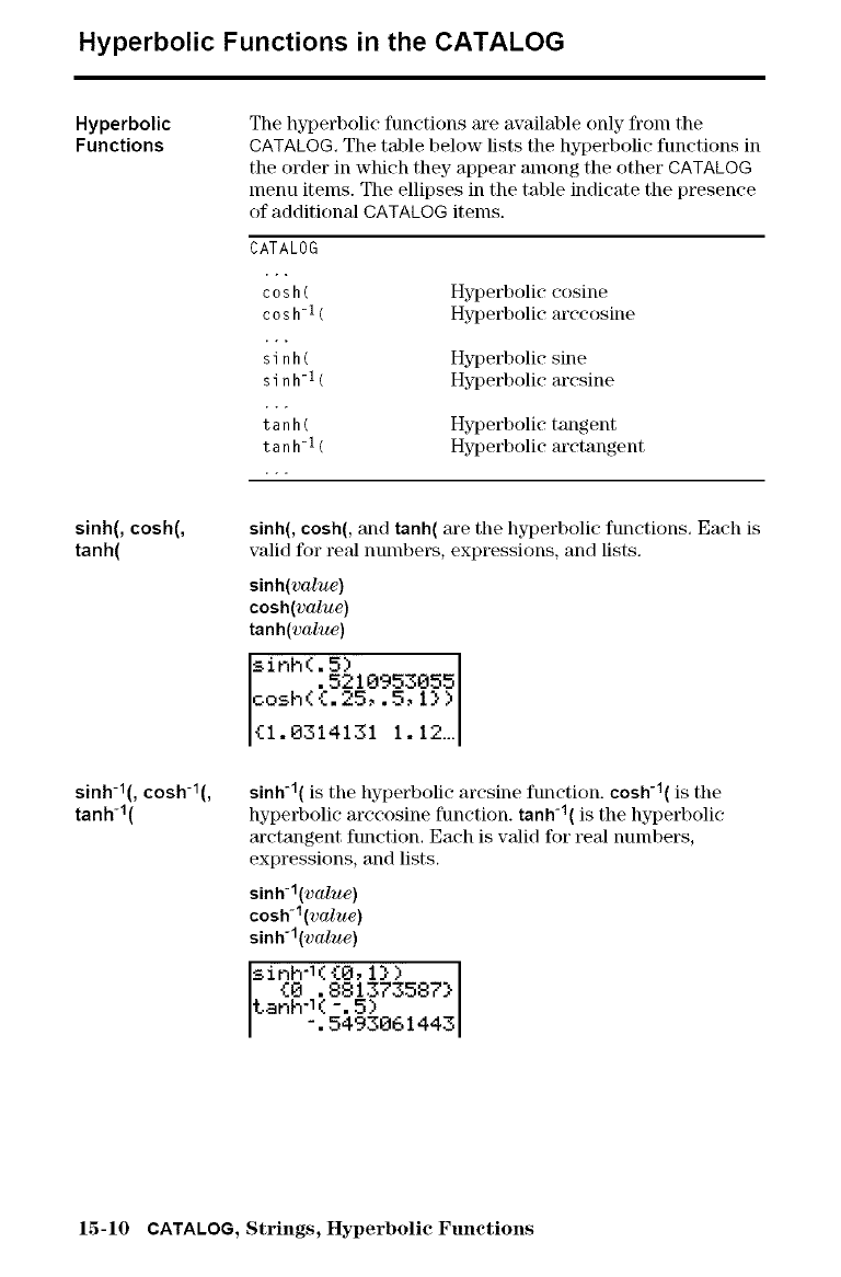
Hyperbolic Functions in the CATALOG
Hyperbolic
Functions The hyperbolic functions are available only from the
CATALOG, The table below lists the hyperbolic functions in
the order in which they appear among the other CATALOG
menu items. The ellipses in the table indicate the presence
of additional CATALOG items.
CATALOG
c0 s h ( Hyperbolic cosine
c0 s h-1 ( Hyperbolic arccosine
s i nh ( Hyperbolic sine
si nh-1 ( Hyperbolic arcsine
t a nh ( Hyperbolic tangent
t a nh- 1( Hyperbolic arctangent
sinh(, cosh(,
tanh(
sinhd(, cosh-l(,
tanh-l(
sinh(, cosh(, and tanh( are the hyperbolic functions. Each is
valid for real numbers, expressions, and lists.
sinh(value)
cosh(value)
tanh(value)
sinh(.5)
.5210953055
cosh( {.25,. 5, I} )
{1.8314131 1.12
sinh-l( is the hyperbolic arcsine function, cosh-l( is the
hyperbolic arccosine function, tanh-l( is the hyperbolic
m'ctangent function. Each is valid for real nulnbers,
expressions, and lists.
sinh- l(value)
cosh- 1(value)
sinh -1(value)
sinh-1({O,l}) I
{0 .881373587}I
tanh-1(-.5)
-.5493061443
15-10 CATALOG, Strings, Hyperbolic Functions
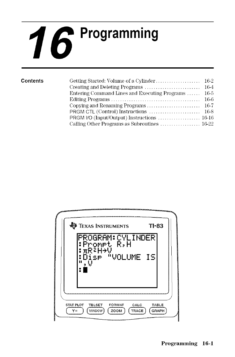
6Programming
Contents Getting Started: Volume of a Cylinder .................... 16-2
Creating and Deleting Programs ......................... 16-4
Entering Colnmand Lines and Executing Programs ...... 16-5
Editing Programs ........................................ 16-6
Copying and Renaming Programs ........................ 16-7
PRGM CTL (Control) Instructions ....................... 16-8
PRGM I/O (Input/Output) Instructions ................... 16-16
('ailing Other Programs as Subroutines .................. 16-22
'_ TEXAS INSTRUMENTS T1=83
PROGRRM: CYL INDER
:PromPt R, H
:_R zH÷V
:Oise "VOLUME IS
.,.j
:I
J
STATPLOT TBLSET FORMAT CALC TABLE
Programming 16-1
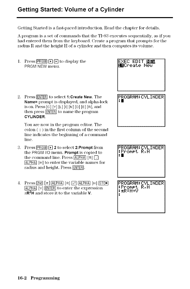
Getting Started: Volume of a Cylinder
Getting Started is a fast-paced introduction. Read the chapter for details.
A program is a set of connnands that the TI-83 executes sequentially, as if you
had entered them fl'om the keyboard. Create a program that prompts for the
radius R and the height H of a cylinder and then computes its volume.
Press [E_ [] [] to display the
PRGM NEW menu.
Press [_ to select 1:Create New. The
Name= prompt is displayed, and alpha-lock
is on. Press [c] [Y][L][I] [N][D] [E] [R], and
then press [g_-gm to name the prograin
CYLINDER.
You are now in the program editor. The
colon ( : ) in the first colunm of the second
line indicates the beginning of a command
line.
Press [E_ [] 2to select 2:Prompt from
the PRGM I/O menu. Prompt is copied to
the command line. Press @ [R] []
@ [H]to enter the variable names for
radius and height. Press [_.
Press [g_ Ix] @ [R] [] @ [H][g?_
@ [v] [_ to enter the expression
_R2H and store it to the variable V.
EXEC EDIT [{L_
BBCreate Flew
PIROGRRM:CYLINDER
PROGRRM: CYL INDER
16-2 Programming
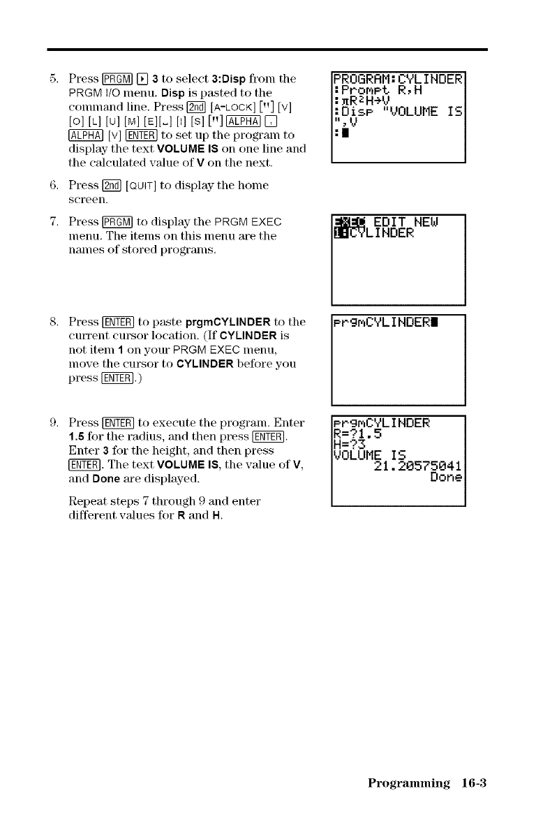
6.
7.
Press J_ [] 3to select 3:Disp fronl the
PRGM I/O menu. Disp is p_ksted to the
conunand line. Press J_ [A-LOCK]["] [V]
[O] [L] [U] [M] [E][_] [I] [S] ["]@1_
@ [V]_ to set up the program to
display" the text VOLUMEIS on one line and
the calculated value of Von the next.
Press J_ [QUIT]to display tile home
screen.
Press [gff_ to display- the PRGM EXEC
menu. The items on this menu are the
names of stored programs.
Press [g_ to paste prgmCYLINBER to the
cmTent cursor location. (If CYLINDER is
not item 1 on your PRGM EXEC menu,
move the cursor to CYLINDERbefore you
press [ggT_. )
PROGRAM:CYLINBER
l:ProMPt R,H I
:=RZH+V
_DisP "VOLUME IS
:i v
_EOIT NEW
LINOER
Prg_CYLINOER|
Press [ggT_ to execute the prograln. Enter
1.8 if)r the radius, and then press [g_.
Enter a for the height, and then press
[g_. The text VOLUME iS, the value of V,
and Done are displayed.
Repeat steps 7 through 9 and enter
different values for R and H.
PPgMCYLINDER
R=?1.5
H=?3
VOLUME IS I
21.20575041
Bone
Programming 16-3
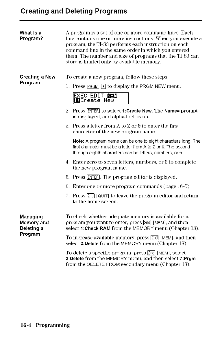
Creating and Deleting Programs
What Is a
Program.'?
Creating a New
Program
Managing
Memory and
Deleting a
Program
A prograln is a set of one or more connnand lines. Each
line contains one or more instructions. When you execute a
prograln, the TI-83 perk)tins each instruction on each
connnand line in the salne order in which you entered
them. The number and size of programs that the TI-83 can
store is limited only by available lnelnolT.
To create a new program, k)llow these steps.
1. Press _ [] to display tile PRGM NEW menu.
EXEC EDIT IIL=I_
HBCreate New
2. Press _ to select 1:Create New. The Name= proInpt
is displayed, and alpha-lock is on.
3. Press a letter fi'oln A to Z or 0 to enter tile first
character of tile new program nalne.
Note: A programname can beone to eight characterslong. The
first character must bea letter fromA to Z or e. The second
through eighth characters canbe letters,numbers, or e.
4. Enter zero to seven letters, numbers, or 0 to conlplete
the new prograln nalne.
5, Press ITNYERI,Tile prograin editor is displayed.
6. Enter one or more prograln commands (page 16-5).
7. Press [_ [QUIT]to leave the progranl editor and return
to the holne screen.
To check whether adequate nlenlol_y- is available for a
prograln you want to enter, press [_ [MEM], and then
select 1:Check RAM froln the MEMORY menu (Chapter 18).
To increase available nlenlolTy- ,press [_ [MEM], and then
select 2:Delete froln the MEMORY menu (Chapter 18).
To delete a specific prograln, press [_ [MEM], select
2:Delete froln the MEMORY menu, and then select 7:Prgm
froln the DELETE FROM seeondalT menu (Chapter 18).
16-4 Progranuning
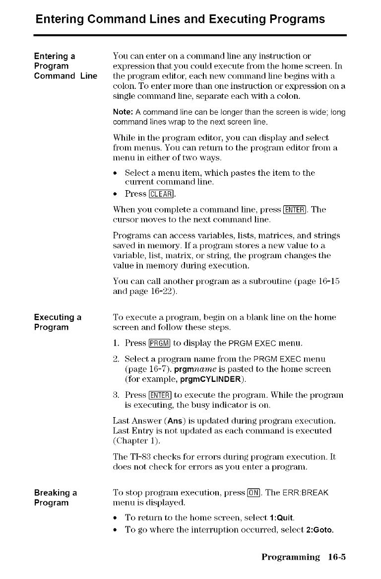
Entering Command Lines and Executing Programs
Entering a
Program
Command Line
Executing a
Program
Breaking a
Program
You emn enter on a eonulland lille any instruction or
expression that you could execute from the home screen. In
the program editor, each new eonunand line begins with a
colon. To enter more than one instruction or expression on a
single eonunand line, separate each with a colon.
Note: A command line can be longer than the screen is wide; Iong
command lines wrap to the next screen line.
While ill the program editor, you call display and select
fronl menus. You can return to the prograln editor fronl a
menu in either of two ways.
• Select a menu item, which pastes the item to the
cmTent conunand line.
• Press @.
When you complete a eolnmand line, press [NY_. The
CUrSOr nloves to tile next eonulland lille,
Progralns can access variables, lists, lnatrices, and strings
saved in nlenlol_yL If a prograln stores a new wdue to a
variable, list, lnatrix, or string, the prograln changes the
value in nlenlory during execution.
You e an call another prograln as a subroutine (page 16-15
and page 16-22).
To execute a program, begin on a blank line on the home
screen and follow these steps.
1. Press [_ to display- the PRGM EXEC menu.
2. Select a pmgraln nalne froln the PRGM EXEC lnenu
(page 16-7). prgmname is pasted to the home screen
(for example, prgmCYUNDER).
3. Press [_ to execute the program. While the program
is executing, the busy indicator is on.
L_Bt Answer (Ans) is updated during prograln execution.
Last EntlT is not updated as each eonulland is executed
(Chapter 1).
The TI-83 checks for errors during prograln execution. It
does not check for errors msyou enter a progranL
To stop prograln execution, press [_. The ERR:BREAK
nlenu is displayed.
• To return to the honle screen, select 1:Quit.
• To go where the interruption occurred, select 2:Goto.
Programming 16-5
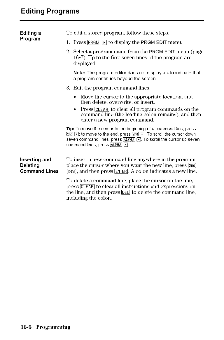
Editing Programs
Editing a
Program
Inserting and
Deleting
Command Lines
To edit a stored program, ff)llow these steps.
1. Press [V_ [] to display- the PRGM EDIT menu.
2. Select a program name froln the PRGM EDIT menu (page
16-7), Up to the first seven lines of the program are
displayed.
Note: The program editor does not display a ¢ to indicate that
a program continues beyond the screen.
3, Edit the program conlnland lines.
• Move tile cursor to the appropriate location, and
then delete, ove_wvrite, or insert.
• Press @ to clear all program eominands on the
eomnmnd line (the lending colon remains), and then
enter a new progrmn eonmmnd.
Tip: To move the cursor to the beginning of a command line, press
[_; to move to the end, press _ lB. To scroll the cursor down
seven command lines, press @ [_. To scroll the cursor up seven
command lines, press @ [_.
To insert a new eonnnand line anywhere in the progranl,
place the cursor where you want the new line, press [_
[tNs], and then press [_T_. A colon indicates a new line.
To delete a conlnland line, place the cursor on the line,
press @ to clear all instructions and expressions on
the line, and then press [ff_ to delete the eonlnland line,
including the colon.
16-6 Programming
Copying and Renaming Programs
Copying and
Renaming a
Program
Scrolling the
PRGM EXEC and
PRGM EDIT
Menus
To copy all conunand lines fronl one progranl into a new
program, follow steps 1 through 5 for Creating a New
Program (page 16-4), and then follow these steps.
1. Press [_ [RCL]. Rcl is displayed on the bottom line of
the prograln editor in the new program (Chapter 1).
2. Press _ [] to display- the PRGM EXEC menu.
3. Select a nalne fronl the menu. prgmname is pasted to
tile bottom line of the program editor.
4. Press [ENt_. All colnnland lines fl'om the selected
program are copied into the new program.
Copying programs h_s at least two convenient
applications.
• You can create a template for groups of instl_ctions
that you use Kequently.
• You can rename a program by copying its contents into
a new program.
Note: You also can copy all the command linesfrom one existing
program to another existing program using RCU
The TI-S3 sorts PRGM EXEC and PRGM EDIT menu items
automatically into alphanumerical order. Each menu only
labels the first 10 itenls using 1 through 9, then 0.
To jump to the first prograln name that begins with a
particular alpha character or O, press @ [letter from A
to Z or 0].
Tip: From the top of either the PRGM EXEC or PRGM EDIT menu,
press [] to move to the bottom. From the bottom, press [] to move to
the top. To scroll the cursor down the menu seven items, press @
[]. To scroll the cursor up the menu seven items, press @ [].
Programming 16-7
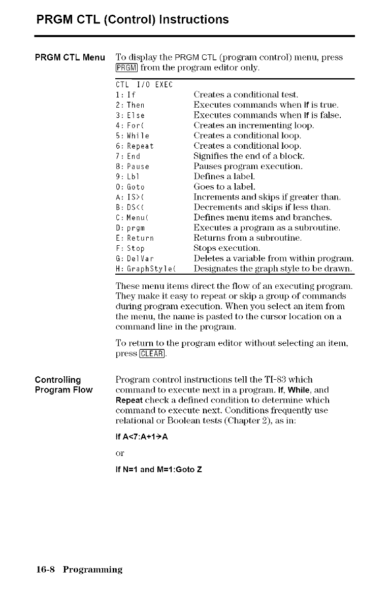
PRGM CTL (Control) Instructions
PRGM CTL Menu
Controlling
Program Flow
To display the PRGM CTL (program control) menu, press
[_ from the prograln editor only.
CTL I/0 EXEC
i: If
2: Then
3: Else
4: For(
5: While
6: Repeat
7: End
8: Pause
9: Lbl
O: Geto
A: IS>(
B: DS<(
C: Menu(
D: prgm
E: Return
F: Stop
G: DelVar
H: GraphStyle(
Creates a conditional test.
Executes conlnlands when If is true,
Executes eonnnands when If is false,
Creates an incrementing loop.
Creates a conditional loop.
Creates a conditional loop.
Signifies the end of a block.
Pauses program execution,
Defnes a label.
Goes to a label.
Increments and skips if greater than.
Decrements and skips if less than.
Defines menu items and branches.
Executes a program as a subroutine.
Returns from a subroutine.
Stops execution.
Deletes a wuiable from within program.
Designates the graph style to be drawn.
These menu items direct the flow of an executing program.
They make it eaksy to repeat or skip a group of commands
during program execution. When you select an item from
the menu, the name is pasted to the cursor location on a
conlnland line in the program.
To return to the program editor without selecting an item,
press @.
Program control instructions tell the TI-83 which
command to execute next in a program, If, While, and
Repeat check a defined condition to determine which
command to execute next, Conditions frequently use
relational or Boolean tests (Chapter 2), as in:
IfA<7:A+I->A
OF
If N=I and M:l:Goto Z
16-8 Programming
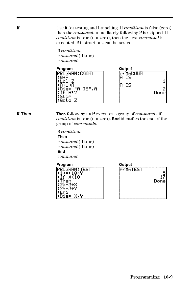
If-Then
[ _se If for testing and branching. If condition is false (zero),
then the command inunediately following If is skipped. If
condition is true (nonzero), then the next command is
executed. If instructions can be nested.
:If condition
:command (if true)
:command
Program
PROGRAM: COUNT
:O÷R _
:Lbl
:A+l÷A._ T_-,,
:OisP M i_ _,,,
: If' R_2
I: Stop
1:Goto Z
output
PrgmCOUNT
IR IS
R IS
Then following an If executes a group of commands if
condition is true (nonzero). End identifies the end of the
group of commands.
:If condition
:Then
:command (if true)
:command (if true)
:End
:co_and
Program
PROGRRM:TEST
:I÷X:IO÷Y
:I_ X<IO
:Then
:2X+3÷X
:2Y-3÷Y
l:End
I:OisP X,Y
output
PPgmTEST O0_!
Programming 16-9
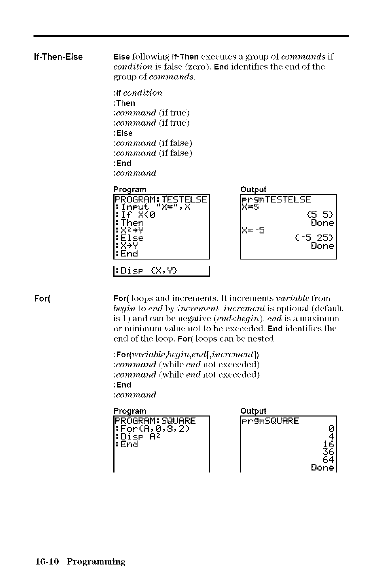
If-Then-Else Else following If-Then executes a group of commands if
condition is false (zero). End identifies the end of the
group of commands.
:If condition
:Then
:command (if true)
:command (if true)
:Else
:command (if false)
:command (if false)
:End
:command
Pro_lram
PROGRRM" TESTELSE
:InPut "X=",X
: Ii_X<B
:Then
:Xz÷y
:Else
: X÷Y
:End
:OisP {X,Y}
output
_:_TESTELSE
{5 5}
X=-5 Done
{-5 25}
Done
For( For( loops and inc[_ments. It increments variable fron]
begin to e_d by increme_t, increment is optional (default
is 1) and can be negative (end<begin). end is a nlmKinlunl
or lnininmnl value not to be exceeded. End identifies the
end of the loop. For( loops can be nested.
:For(variable,begin,end[,increme_t])
:command (while end not exceeded)
:command (while e_d not exceeded)
:End
:command
Pro_lram
PROGRRM: SQURRE
:For(R, 0, 8, 2)
::EDi,Ip RZ
output
PPgf_SQURRE Oon40e643616
16-10 Programming
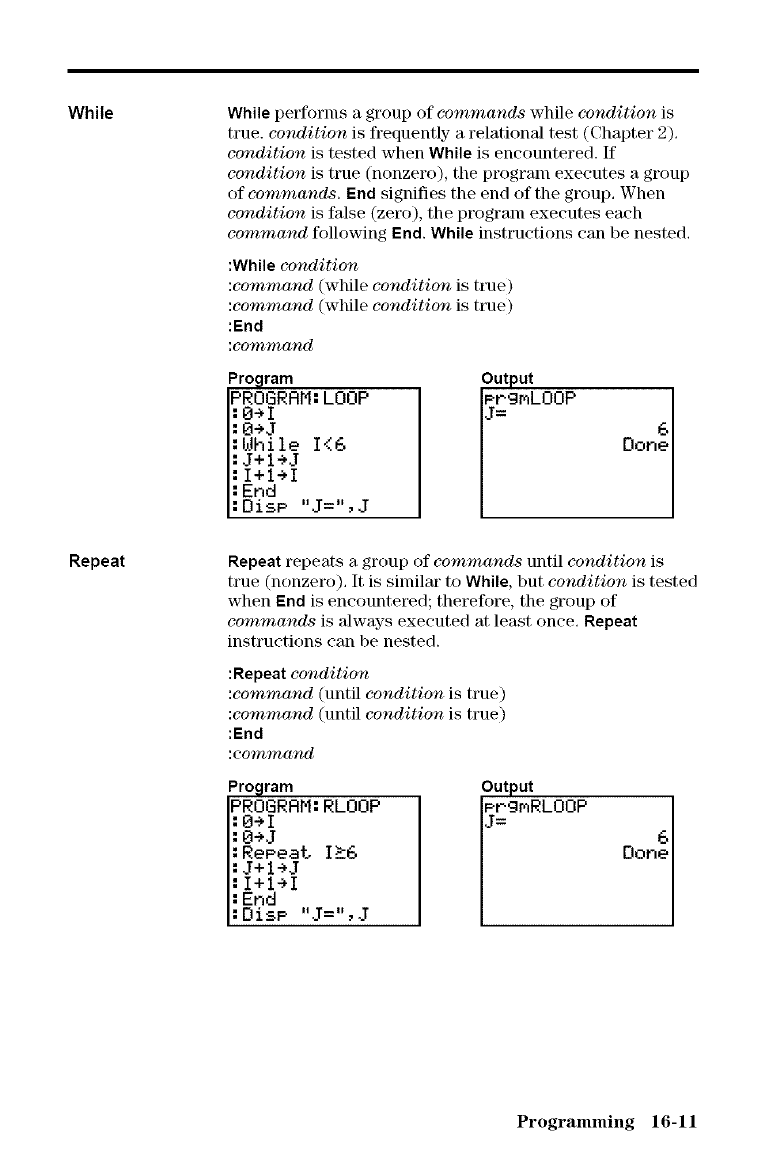
While
Repeat
While performs a group of commands while condition is
true. condition is frequently a relational test (Chapter 2).
condition is tested when While is encountered. If
condition is true (nonzero), the program executes a group
of commands, End signifies the end of the group, When
condition is false (zero), the p_)gram executes each
command following End. While instructions can be nested.
:While condition
:command (while condition is true)
:command (while condition is true)
:End
:command
Program
PROGRAM: LOOP
:O÷l
:While _,.,_
:J+l÷J
: I+l÷I
:End
I:DisP J= ,J
Output
,_9mLOOP Done6
Repeat repeats a group of commands until condition is
true (nonzero). It is similar to While, but condition is tested
when End is encountered; therefore, the group of
commands is always executed at least once. Repeat
instructions can be nested.
:Repeat condition
:command (until condition is true)
:command (until condition is true)
:End
:command
Program
PROGRRM: RLOOP
I:0÷I
:O÷J >
:Repeat I_6
:J+l÷J
: I+l÷I
:End
FDisP .J= ,J
Output
,_r-cJrqRLOOP Done6
Programming 16-11
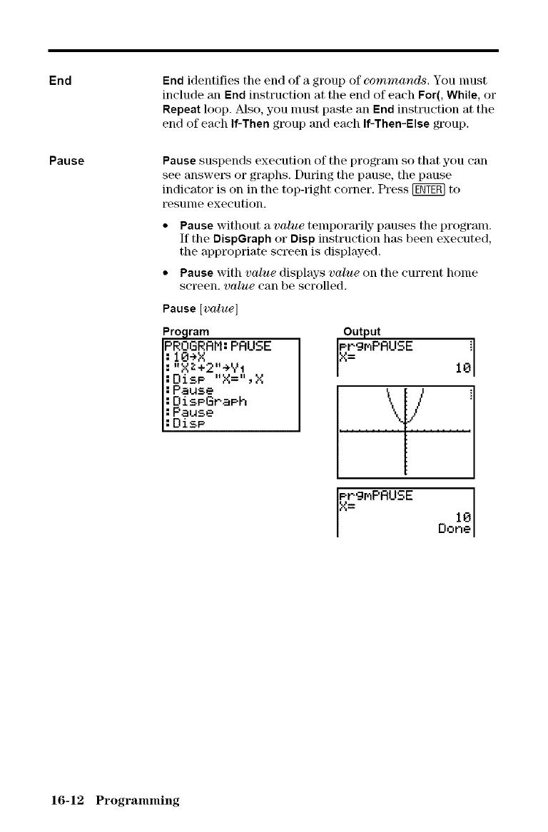
End
Pause
End identifies the end of a group of commands. You nmst
include an End instruction at the end of each For(, While, or
Repeat k)op. Also, you nmst paste an End instruction at the
end of each If-Then group and each If-Then-Else group.
Pause suspends execution of the program so that you can
see answers or graphs, During the pause, the pause
indicator is on in the top-right corner. Press _ to
resume execution.
Pause without a value temporarily pauses the pr()gram.
If the DispGraph or Disp instruction has been executed,
the appropriate screen is displayed.
Pause with value displays value on the current home
screen, value can be scrolled.
Pause [value]
Program
PROGRRM: PRUSE
: 10+X
:"XZ+2"÷y1
:DisP "X=", X
:Pause
:DisPGraF-h
I: Pause
l:OisP
output
PPgF_PRUSE
X= 10
16-12 Programming
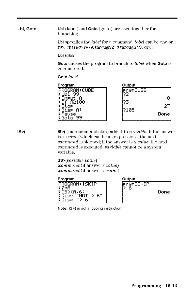
Lbl, Goto
IS>(
Lbl (label) and Goto (go to) are used together for
branching.
Lbl specifies the label for a conlnland, label can be one or
two characters (A through Z, 0 through 99, or 0).
Lbl label
Goto causes the program to branch to label when Goto is
encountered.
Goto label
Pro_lram
PROGRRM: CUBE
:Lbl 99
: Input R
: If' R._100
:Stop
:Dise R-_
I:Pause
I:Goto 99
output
IPegmCUBE?31105 Done278
IS>( (inc_ment and skip) adds 1 to variable. If the answer
]s > value (which can be an expression), the next
command is skipped; if the answer is _<value, the next
command is executed, variable cannot be a system
variable,
:lS>(variable,value)
:command (if answer _<value)
:command (if answer > value)
Program Output
IPROGRRM:::::DispDi-_pT÷RIs>(R;'6)NOT>ISKIP6> 6 " I_r_mISKIP Done
Note: IS>( is not a looping instruction.
Programming 16-13
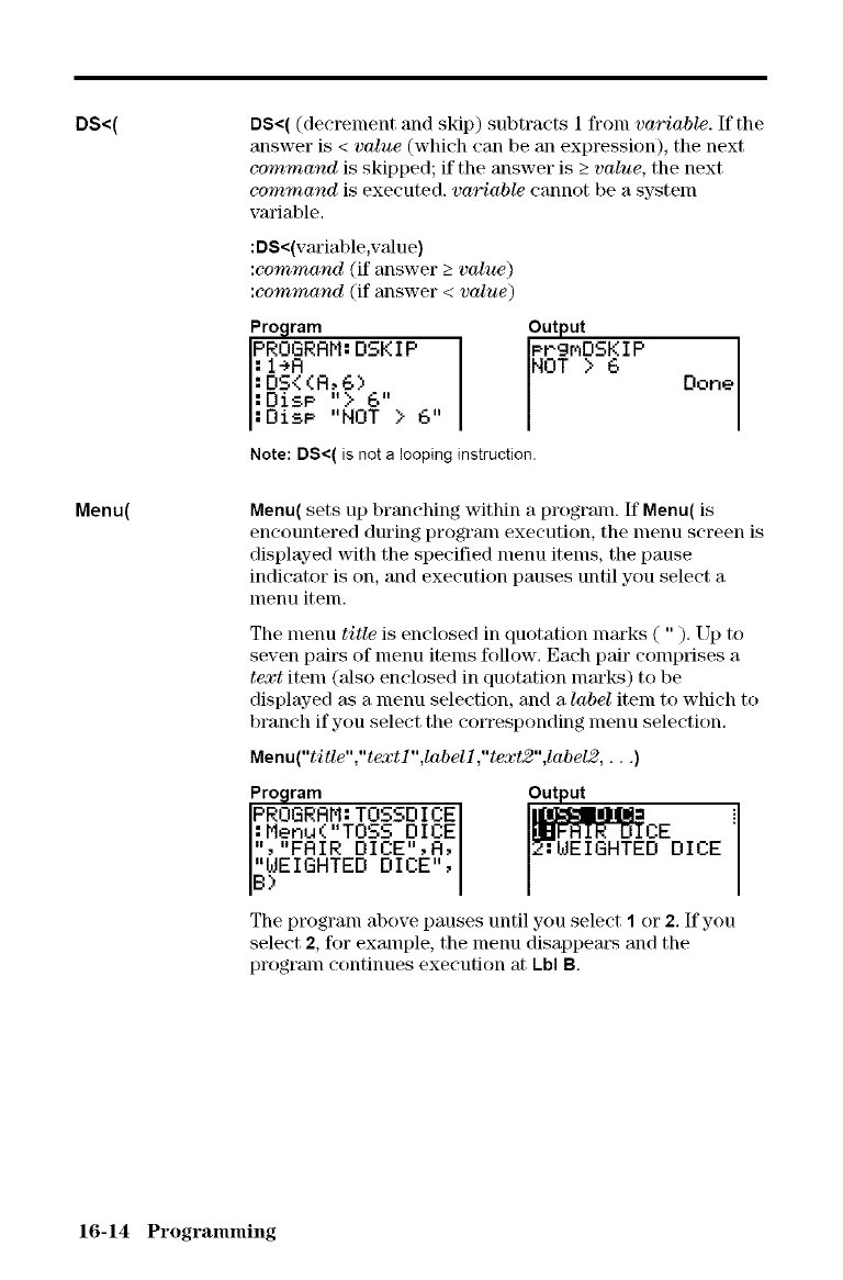
DS<(
Menu(
DS<( (decrement and skip) subtracts 1 fronl variable. If the
answer is < value (which can be an expression), the next
command is skipped; if the answer is _>value, the next
command is executed, variable cannot be a system
variable,
:DS<(variable,wdue)
:command (if answer _>value)
:command (if answer < value)
Pro_lram
PROGRRM::I+R DSKIP I
:DS\ (A, 6>
:DisP "> 6"
:DisP 'NOT > 6
Note: DS<( is not a looping instruction.
Menu( sets up branching within a program. If Menu( is
encountered during prograln execution, the menu screen is
displayed with the specified menu items, the pause
indicator is on, and execution pauses until you select a
menu item.
The lnenu title is enclosed in quotation lnarks ( " ). Up to
seven pairs of menu items follow. Each pair conlprises a
text item (also enclosed in quotation marks) to be
displayed as a menu selection, and a label item to which to
branch if you select the corresponding menu selection.
Menu("title","te:ct l",label l ,"te:ct2",label2 .... )
Program
PROGRR_,!: TOSSDICE i
:Menu( TOSS DICE
","FRIR OICE",R, DICE
;WEIGHTED DICE ,
The progranl above pauses until you select 1or 2. If you
select 2, for example, the menu disappears and the
program continues execution at Lbl B.
16-14 Programming
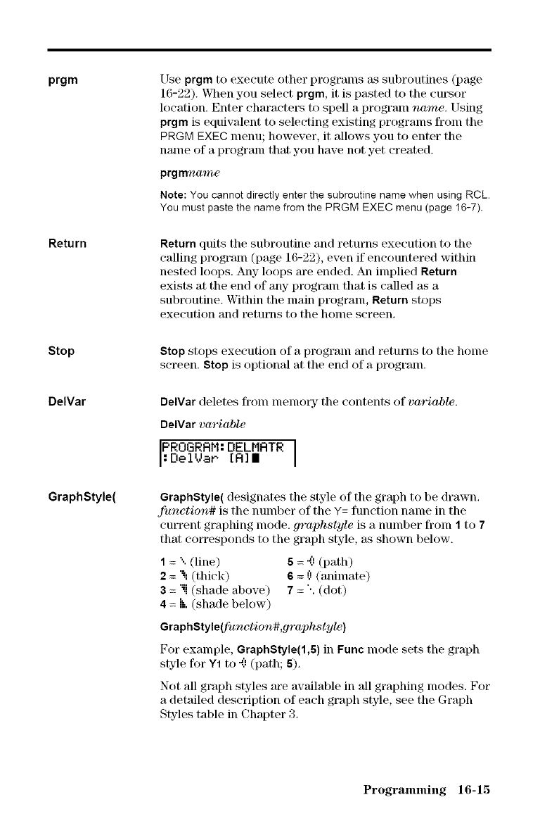
prgm [ _se prgm to execute other programs as subroutines (page
16-22). When you select prgm, it is pasted to the cut, or
location. Enter characters to spell a program name. Using
prgm is equivalent to selecting existing programs fronl the
PRGM EXEC menu; however, it allows you to enter the
name of a program that you have not yet created.
prgmname
Note: You cannot directly enter the subroutine name when using RCL.
You must paste the name from the PRGM EXEC menu (page I6-7).
Return Return quits the subroutine and returns execution to the
calling program (page 16-22), even if encountered within
nested loops. Any loops are ended. An implied Return
exists at the end of any- program that is called as a
subroutine. Within the main program, Return stops
execution and retut_ls to the honle screen.
Stop Stop stops execution of a program and returns to the home
screen. Stop is optional at the end of a program.
DelVar
GraphStyle(
DelVar deletes fronl nlenlory the contents of variable.
DelVar variable
PROGRRH: DELMRTR I
: DelUar. [R]I
GraphStyle( designates the style of the graph to be drawn.
fanction# is the number of the Y= function name in the
current graphing mode. graphstyle is a number from 1to 7
that corresponds to the graph style, as shown below.
1 = ". (line) 5 = '_.)(path)
2 = "i (thick) 6 = .'.'.'(animate)
3=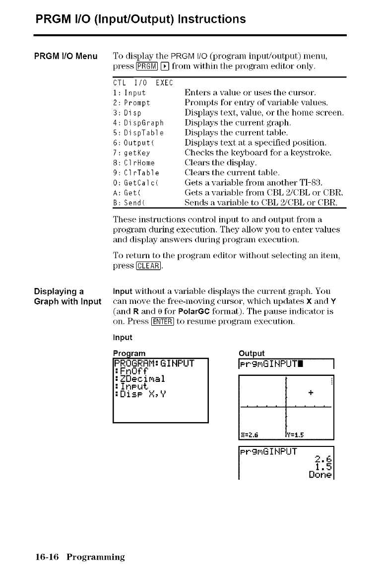
PRGM I/0 (Input/Output) Instructions
PRGM I/0 Menu
Displaying a
Graph with Input
To display the PRGM I/0 (progranl input/output) menu,
press _ [] fronl within tile prograln editor only.
CTL I10 EXEC
i: Input
2: Prompt
3: Disp
4: DispGraph
5: DispTable
6:Output(
7: getKey
8:C1 rHome
9: ClrTable
O: GetCalc(
A: Get(
B: Send(
Enters a value or uses the cursor.
Prompts for enhT of variable values.
Displays text, value, or the home screen.
Displays the current graph.
Displays the current table.
Displays text at a specified position.
Cheeks the keyboard for a keystroke.
Clears the display.
Clears the current table.
Gets a wtriable froln another TI-83.
Gets a varialfle from CBL 2/CBL or CBR.
Sends a variable to CBL 2JCBL or CBR.
These instructions control input to and output fronl a
program during execution. They allow you to enter values
and display- answers during program execution.
To return to the program editor without selecting an item,
press @.
Input without a variable displays the current graph. You
can move the free-moving cursor, which updates X and Y
(and R and 0 for PolarGC format). The pause indicator is
on. Press [gNYgmto resulne prograln execution.
Input
Program
PROGRRM: GIHPUT
:FnOff
:ZOeoimal
I:Input
: Dise X, V
Output
Pr, gmG IHPUTI
[.
I1=_:,6 ?=:!..5
PrgmG IHPUT 2.6
1.5
Done
16-16 Programming
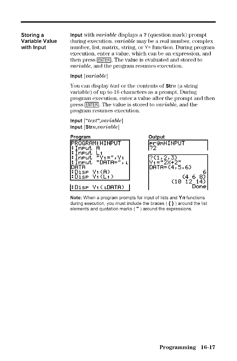
Storing a
Variable Value
with Input
Input with variable displays a ? (question nlark) prompt
dm'ing execution, variable may be a real number, complex
number, list, matrix, string, or Y= function. Dm'ing program
execution, enter a wdue, which can be an expression, and
then press [_T_]. The value is evaluated and stored to
variable, and the program resumes execution.
Input [variable]
You can display- text or the contents of Strn (a string
variable) of up to 16 ehm'acters as a prompt. During
program execution, enter a value after the prompt and then
press [_T_]. The value is stored to variable, and the
progranl resunlos execution.
Input ["text",variable]
Input [Strn,variable]
Program
PROGRRM: HINPUT
-'InPut "YI=",YI
-'InPut "DRTR=",
DRTR
:OisP VI(R)
:OisP YI(LI)
-"Oi_P '_t (LORTR)
output
Pr.gFiH INPUT
?2
?{1,2,3}
Vt ="2X+2"
DRTR={4, 5, 6} 6
{4 6 8}
{10 12 14}
Oone
Note: When a program prompts for input of lists and Yn functions
during execution, you must include the braces ( { } ) around the list
elements and quotation marks ( ") around the expressions.
Programming 16-17
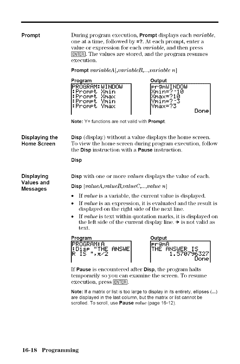
Prompt
Displaying the
Home Screen
During program execution, Prompt displays each variable,
one at a time, followed by =?. At each prompt, enter a
value or expression for each variable, and then pl_ss
[ggT_. The values are stored, and the prograln resulnes
execution.
Prompt variableA [,variableB,...,variable n]
Program
PROGRAM:WINDOW
:PronPt XMin
:Pror_Pt XMax
:ProMPt Ymin
:PromPt YMax
output
PrgMWINOOW Done
XMin=?-le
X_ax=?lO
_Min=?-3
V_ax=?3
Note: Y= functions are not valid with Prompt.
Disp (display) without a value displays the home screen.
To _ew the home screen during program execution, follow
the Disp instruction with a Pause instruction.
Disp
Displaying
Values and
Messages
Disp with one or more values displays the value of each.
Disp [valueA,valueB,valueC,...,value n]
• If value is a variable, the current value is displayed.
• If value is an expression, it is evaluated and the result is
displayed on tile right side of the next line.
• If value is text within quotation marks, it is displayed on
the left side of the current display- line. -) is not valid as
text.
Program
PROGRRM:R RNSWE
:OisP "THE
R IS ,x/2
Output
PPgNA
THE ANSWER IS
1.578796327
Done
If Pause is encountered after Disp, the program halts
temporarily so you can examine the screen, To resume
execution, press [_T_].
Note: If a matrix or list is too large to display in its entirety, ellipses (...)
are displayed in the last column, but the matrix or list cannot be
scrolled. To scroll, use Pause w/ue (page I6-I2).
16-18 Programming
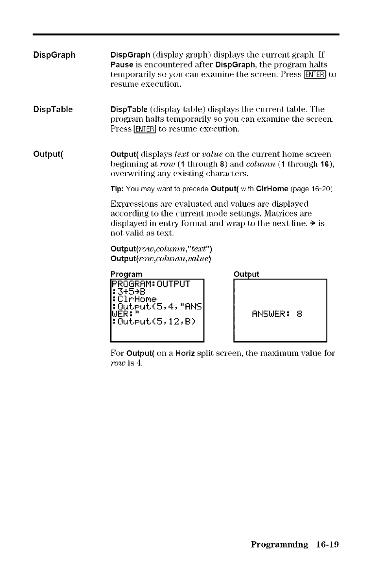
DispGraph
DispTable
Output(
DispGraph (display- graph) displays the current graph. If
Pause is encountered after DispGraph, the program halts
temporarily so you can examine the screen. Press _ to
resume execution,
DispTable (display table) displays tile current table, The
program halts temporarily so you can examine the screen.
Press _ to resume execution,
Output( displays text or value on the current home screen
beginning at row (1 through 8) and column (1 through 16),
ove_vriting any existing characters.
Tip: You maywantto precede Output( with ClrHome (page 16-20).
Expressions are evaluated and values are displayed
according to the current mode settings. Matrices are
displayed in entw format and wrap to the next line. ->is
not valid as text.
Output(fvw,column,"text")
Output(row,column,v_ue)
Program • I
PROGRRM.OJTPUT
:3+5+B
:CIrHoMe
:OutPut(5,4,"RHS
WER:"
:Out.eut.(5,12,B)
For Output( on a Horiz split screen, the nlaxinlunl value for
row is 4.
Programming 16-19
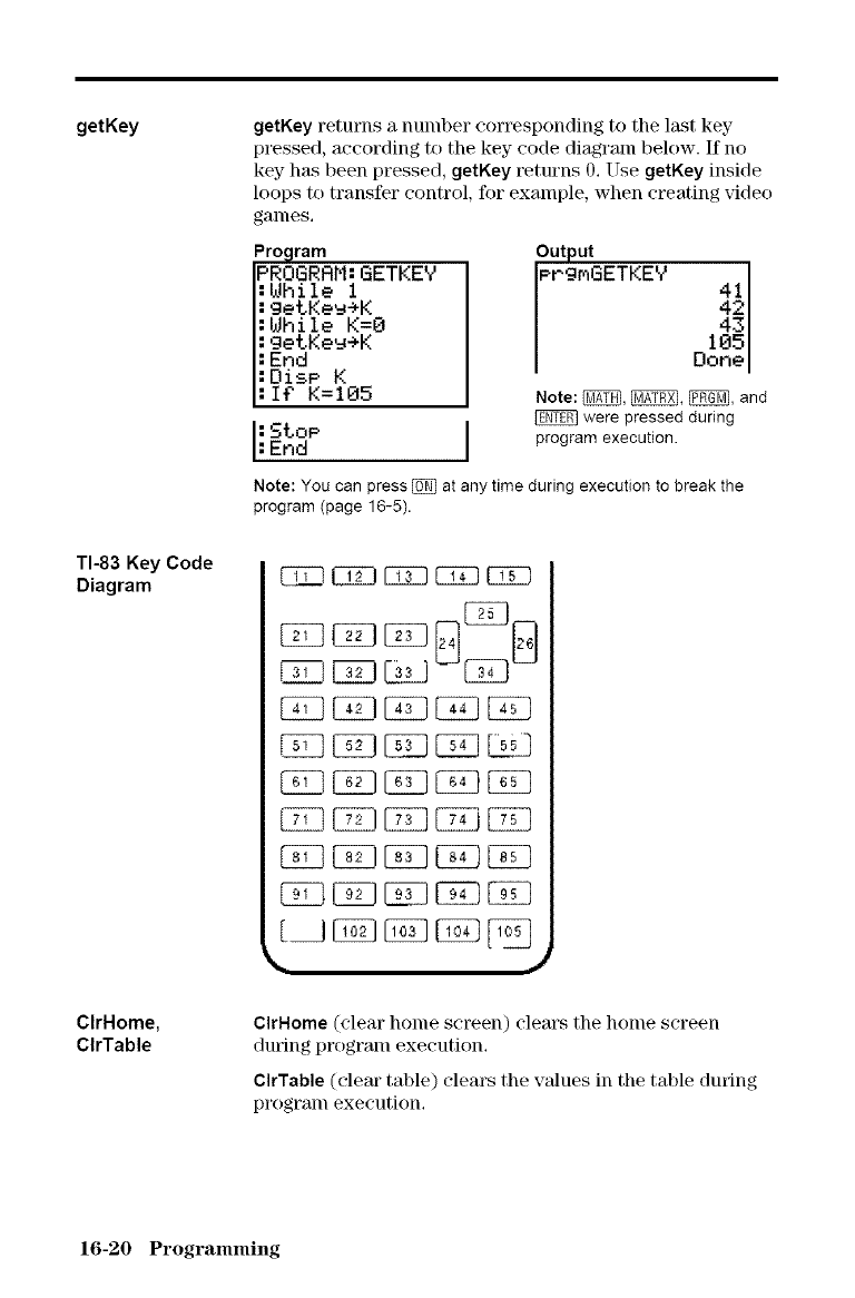
getKey getKey returns a number corresponding to the last key
pressed, according to the key code diagraln below. If no
key- has been pressed, getKey t_turns O. Use getKey inside
loops to transfer control, for example, when creating video
gaines.
Program
PROGRRM:GETKEV
:While 1
:getKeu+K
:While K=O
:getKe_eK
:End
:OisP K
:I¢ K=105
:Stop
:End
Output
PPg_GETKEV 1
Done
Note: _, [_, [_, and
were pressed during
program execution.
Note: You can press [_ at any time during execution to break the
program (page 16-5).
TI-83 Key Code
Diagram C15D12_22!IZD C_ Ei_
IZ] --E521-
ClrHome,
CIrTable ClrHome (clear home screen) clears the home screen
during program execution.
ClrTable (clear table) clears the values in the table during
program execution.
16-20 Programming
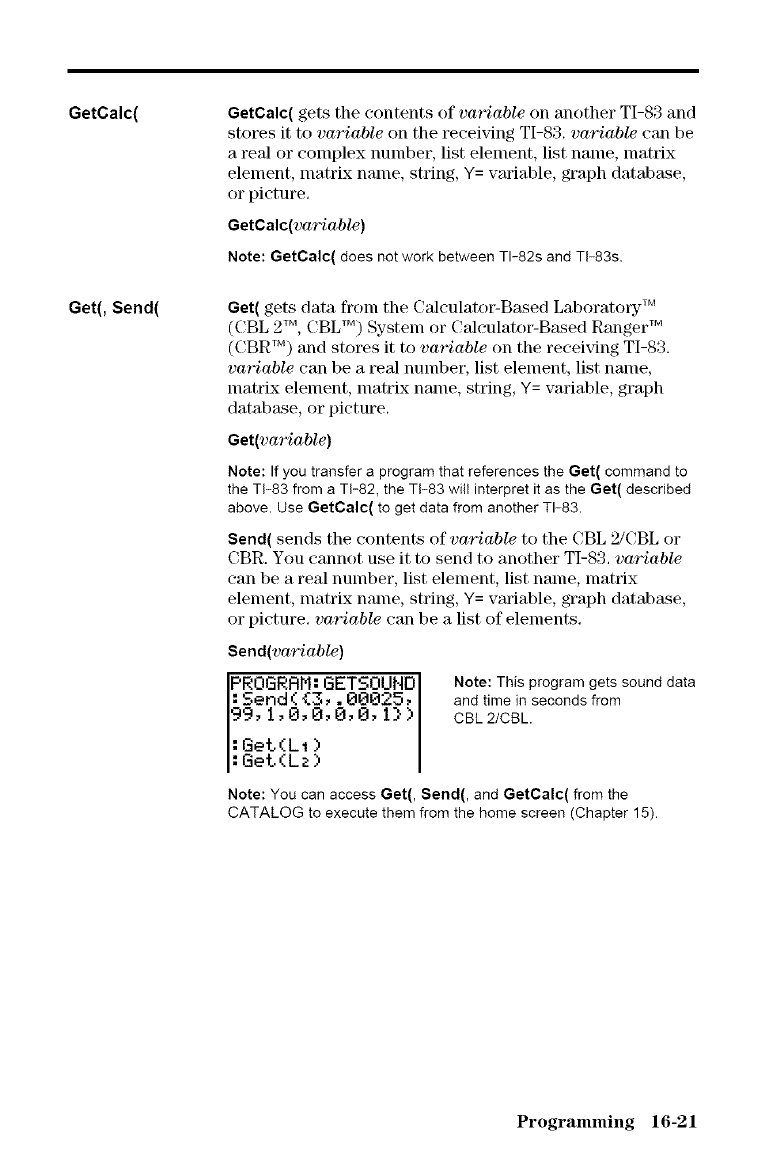
GetCalc(
Get(, Send(
GetCalc( gets the contents of variable on another TI-83 and
stores it to variable on the receiving TI-83. variable can be
a real or complex number, list element, list name, matrix
element, matrix name, string, Y= variable, graph database,
or picture.
GetCalc(variable)
Note: GetCalc( does not work between TI-82s and TF83s.
Get( gets data fronl the Calculator-Based Laboratory TM
(CBL 2 TM, CBL TM) System or Calculator-Based Ranger TM
(CBR TM) and stores it to variable on the receiving TI-83.
variable can be a real number, list element, list name,
nmtrix element, nmtrix name, string, Y= variable, graph
database, or picture.
Get(variable)
Note: If you transfer a program that references the Get( command to
the TF83 from a TI-82, the TF83 will interpret it as the Get( described
above. Use GetCalc( to get data from another TI-83.
Send( sends the contents of variable to the CBL 2/CBL or
CBR. You cannot use it to send to another TI-83. variable
can be a real nmnber, list element, list name, matrix
element, matrix name, string, Y= variable, graph database,
or picture, variable can be a list of elements.
Send(variable)
PROGRRM:GETSOUND
:Send({3,.000_5,
99,1,0,0,0,0,1})
:Get(L1)
:Get(Lz)
Note: This program gets sound data
and time in seconds from
CBL 2/CBL.
Note: You can access Get(, Send(, and GetCalc( from the
CATALOG to execute them from the home screen (Chapter 15).
Programming 16-21
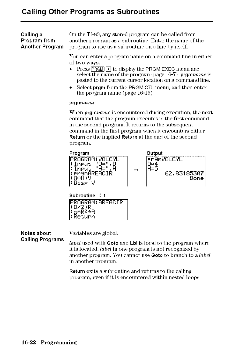
Calling Other Programs as Subroutines
Calling a
Program from
Another Program
Notes about
Calling Programs
On the TI-83, any stored program can be called fronl
another program as a subroutine, Enter the name of the
program to use as a subroutine on a line by itself,
You can enter a program name on a conunand line in either
of two ways,
• Press NggM][] to display the PRGM EXEC menu and
select the name of the program (page 16-7). prgmname is
pasted to the cm_'ent cm_sor location on a conullalld line.
• Select prgm from the PRGM CTL menu, and then enter
the program name (page 16-15),
prgmnome
When prgmname is encountered during execution, the next
command that the program executes is the first command
in the second program. It returns to the subsequent
conunand in the first program when it encounters either
Return or the implied Return at the end of the second
program.
Pro_lram
PROGRAM: VOLCYL
:Input "D=",D
:InPut. "H=",H
:PPgrIRRERCIR
:RmH÷V
:DisP V
Output
H=5 62. 83185307
Done
Subroutine I t
PROGRRM:RRERCIR:Return:n.RZ÷A:D/2÷RI
Variables are global.
label used with Goto and kbl is local to the program where
it is located, label in one program is not recognized by
another program. You cannot use 6oto to branch to a label
in another program.
Return exits a subroutine and returns to the calling
program, even if it is encountered within nested loops.
16-22 Programming
7Applications
Contents Comparing Test Results Using Box Plots ................ 17-2
Graphing Pieeewise Functions ........................... 17-4
Graphing Inequalities .................................... 17-5
Sohdng a System of Nonlinear Equations ................ 17-6
Using a Program to Create the Sierpinski Triangle ....... 17-7
Graphing Cobweb Attractors ............................ 17-8
Using a Program to Guess the Coefficients ............... 17-9
Graphing the Unit Circle and Trigonometric (;ma_es ...... 17-10
Finding the Area between Curves ........................ 17-11
Using Parametric Equations: Ferris Wheel Problem ...... 17-12
Demonstrating the Fundamental Theorem of ('aleulus... 17-14
('omputing Areas of Regular N-Sided Polygons .......... 17-16
Computing and Graphing Mortgage Payments ........... 17-18
TEXAS INSTRUMENTS TI-83
J
STATPLOT TBLSET FORMAT CALC TABLE
Applications 17-1
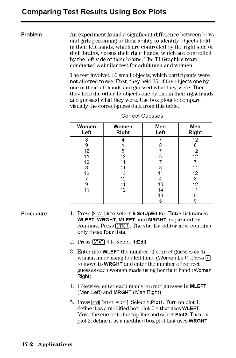
Comparing Test Results Using Box Plots
Problem
Procedure
An experiment found a significant difference between boys
and gifts pertaining to their ability to identify objects held
in their left hands, which are controlled by the right side of
their brains, versus their right hands, which are controlled
by the left side of their brains, The TI Graphics team
conducted a similm" test for adult men and women.
The test involved 30 slnall objects, which pm'ticipants were
not allowed to see. First, they held 15 of the objects one by
one in their left hands and guessed what they were. Then
they held the other 15 objects one by one in their right hands
and guessed what they were. Use box plots to compare
_isually the eotTect-guess data from this table.
Correct Guesses
Women
Le_
8
9
12
11
10
8
12
7
9
11
Women
Right
4
1
8
12
11
!1
13
!2
!1
12
Men
Left
7
8
7
5
7
8
11
4
!0
14
13
5
Men
Right
12
6
12
12
7
11
12
8
12
11
9
9
1, Press _ 5to select 5:SetUpEditor, Enter list names
WLEFT, WRGHT, MLEFT, and MRGHT, separated by
conlnlas, Press [_. The stat list editor now contains
only these four lists.
2. Press [_Y] 1 to select 1:Edit.
3. ]_nter into WLEFT the number of correct guesses each
woman made using her left hand (Women Left). Press []
to move to WRGHT and enter the number of correct
guesses each woman made using her right hand (Women
Right).
4. Likewise, enter each lnan's correct guesses in MLEFT
(Men Left) and MRGHT (Men Right).
5. Press [_ [STAT PLOT], Select 1:Plot1. Turn on plot 1;
define it as a modified box plot 4>- that uses WLEFT.
Move the eta'sot to the top line and select Plot2. Turn on
plot 2; define it as a modified box plot that uses WRGHT,
17-2 Applications
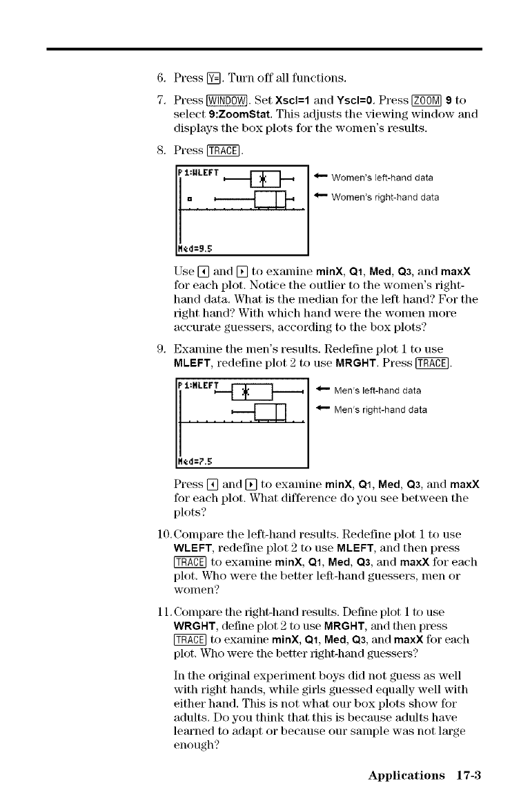
6.Press@.Turnoffallfunctions,
7.Press_. SetXscl=landYscl=0.Press_ 9to
select9:ZoomStat.Thisadjuststheviewingwindowand
displaystheboxplotsforthewomen'sresults.
8. Press_.
kd=9.5
Use [] and [] to exalnine minX, Ol, Med, O3, and maxX
for each plot. Notice the outlier to the women's right-
hand data. What is the median ff)r the left hand? For the
right hand? With which hand were the women more
accurate guessers, according to the box plots?
9. Examine the men's results. Redefine plot 1 to use
MLEFT, redefine plot 2 to use MRGHT. Press _.
_" Men's right-hand data
d=7.5 ""
Press [] and [] to examine minX, Q1, Med, Q3, and maxX
for each plot. What difference do you see between the
plots?
10.Compare the left-hand results. Redefine plot 1 to use
WLEFT, redefine plot 2 to use MLEFT, and then press
to examine minX, Q1, Med, Q3, and maxX for each
plot. Who were the better left-hand guesse_\% men or
women?
11. Company the right-hand results. Define plot 1 t_) use
WRGHT, define plot 2 to use MRGHT, zu_d then press
to examine minX, OI, Med, O3, and maxX for each
plot. Who were the better right-herod guesse_?
In the original experiment boys did not guess as well
with right hands, while girls guessed equally well with
either hand. This is not what our box plots show for
adults. Do you think that this is because adults have
learned to adapt or because our sample was not large
enough?
Applications 17-3
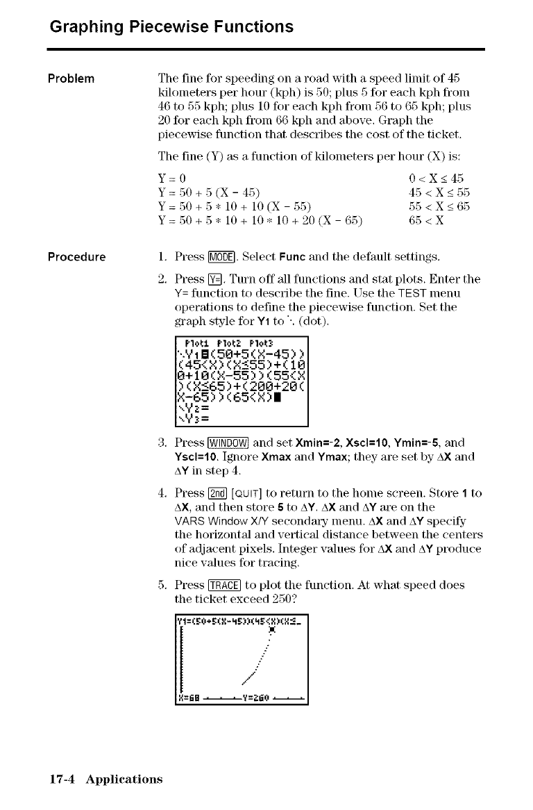
Graphing Piecewise Functions
Problem
Procedure
The fine for speeding on a road with a speed limit of 45
kilometers per hour (kph) is 50; plus 5 for each kph from
46 to 55 kph; plus 10 for each kph froln 56 to 65 kph; plus
20 for each kph from 66 kph and above. Graph the
piecewise function that describes the cost of the ticket.
The fine (Y) as a function of kilometers per horn" (X) is:
Y=0 0<X_<45
Y= 50 + 5 (X- 45) 45 < X_< 55
Y= 50 + 5 *10 +10 (X - 55) 55<X_<65
Y= 50 + 5. 10 + 10. 10 + 20 (X- 65) 65 < X
1,
2.
Press Noel. Select Func and the default settings.
Press @. Tm'n off all functions and stat plots. Enter the
Y= function to describe the fine. Use the TEST menu
operations to define the pieeewise function. Set the
graph style for Y1 to ". (dot).
PloLt F'lol:2 PI<,I:_:
'..Y1 B(50+5(X-45) )
(45<X) (X_<55)+(10
0+10(X-55) ) (5.J< X
)(X_<65)+(200+20(
X-65) ) (65< X)I
,,yz=
,,V_=
Press _ and set Xmin=-2, Xscl=10, Ymin=-5, and
Yscl=10. Ignore Xmax and Ymax; they are set by AX and
AY in step 4.
Press [_ [QUIT] to return to the holne screen. Store 1to
AX, and then store 5to AY, AX and AY m'e on the
VARS Window X/Y secondary menu. AX and AY specify
the horizontal and vertical distance between the centers
of adjacent pixels, Integer values for AX and AY produce
nice values for tracing,
Press _ to plot the function. At what speed does
the ticket exceed 250?
17-4 Applications
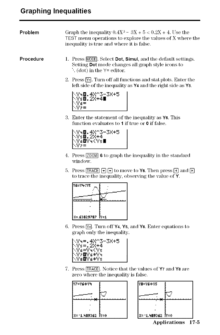
Graphing Inequalities
Problem
Procedure
Graph the inequality 0.4X;_ - 3X + 5 < 0.2X + 4. Use the
TEST menu operations to explore the values of X where the
inequMity is true and where it is false,
4.
5,
Press [M0_]. Select Dot, Simul, and the default settings.
Setting Dot mode changes 'all graph style icons to
'. (dot) in the Y= editor.
Press @. Turn off all functions and stat plots. Enter the
left side of the inequality as Y4and the right side as Y5.
'..9 _B. 4X^3-3X+5
I"-Y _B. 2X+411
...Yti=
[..Y?=
Enter the statement of the inequality as Y6. This
function evaluates to 1if true or 0 if false.
'..Y_B. 4X"3-3X+5
'..Y_B; 2X+4
'-.Y_B_<Y_II
.5??=
Press _ 6 to graph the inequality in the standard
window.
Press _ [] [] to move to Y6, Then press [] and []
to trace the inequality, observing the value of Y,
--' ;' = [
11=.ti_8;;9;_87 I?=i.
Press @. Turn off Y4,Y5,and Y6.Enter equations to
graph only the inequality.
'..'.?_=, 4X"3-3X+5
".Y_=. _.X+4
'..9_=_,_<9_
..YnBYt*9_
Press _. Notice that the values of Y7 and Y8 are
zero where the inequality- is false.
ll:':t._Bg._6;_ !Y:0
?ll=¥fi_?_;
:I=':L4Bg._fi,_ t=0
Applications 17-5
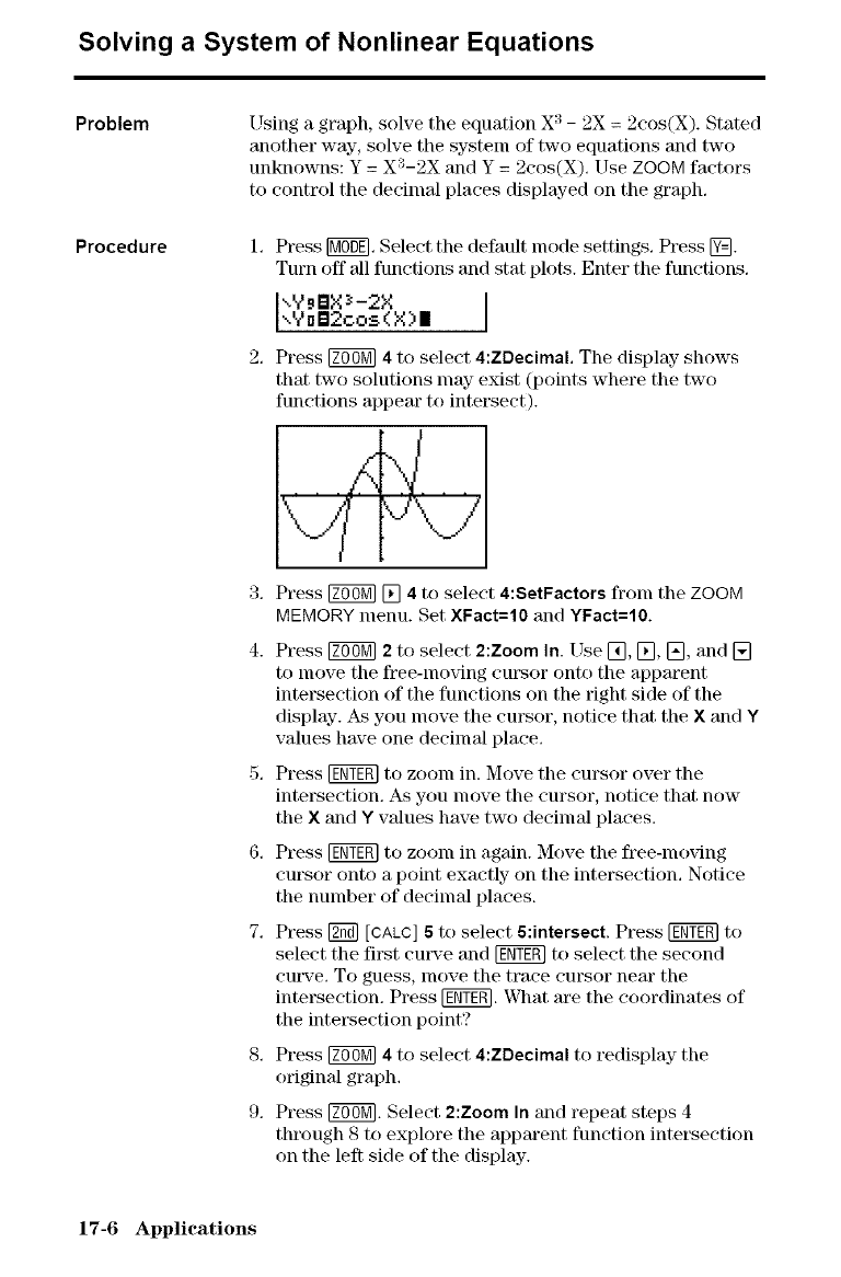
Solving a System of Nonlinear Equations
Problem
Procedure
Using a graph, solve the equation X :_- 2X = 2cos(X). Stated
another way-, solve the system of two equations and two
unknowns: Y = X:_-2X and Y = 2cos(X), Use ZOOM factors
to control the decimal places displayed on the graph.
3,
4.
Press [_, Select the default lnode settings. Press @.
Turn off 'all functions and stat plots. Enter the functions.
\V_BX_-2X
",'toB2cos (X) I
Press _ 4 to select 4:ZDecimal, The display shows
that two solutions may exist (points where the two
functions appear to intersect).
r
Press _ [] 4 to select 4:SetFactors fi'om the ZOOM
MEMORY menu. Set XFact=lO and YFact=lO.
Press _ 2 to select 2:Zoom In. Use [_, [], [], and []
to move the free-moving cm_or onto the apparent
intersection of the functions on the right side of the
display. As you move the cursor, notice that the X and Y
values have one decimal place.
5, Press [_ to ZOOln in. Move the cursor over the
intersection, As you move the cursor, notice that now
the X and Y values have two decimal places.
6, Press [_ to zoom in again. Move the free-lnoving
cursor onto a point exactly- on the intersection, Notice
the number of decimal places.
7. Press K_ [CALC] 6 to select 6:intersect. Press _ to
select the first cmwe and [_ to select the second
cm_'e. To guess, move the trace cursor near the
intersection, Press [_. What are the coordinates of
the intersection point?
8, Press _ 4 to select 4:ZDecimal to redisplay the
original graph,
9. Press _. Select 2:Zoom In and repeat steps 4
through 8 to explore the apparent function intersection
on the left side of the display.
17-6 Applications
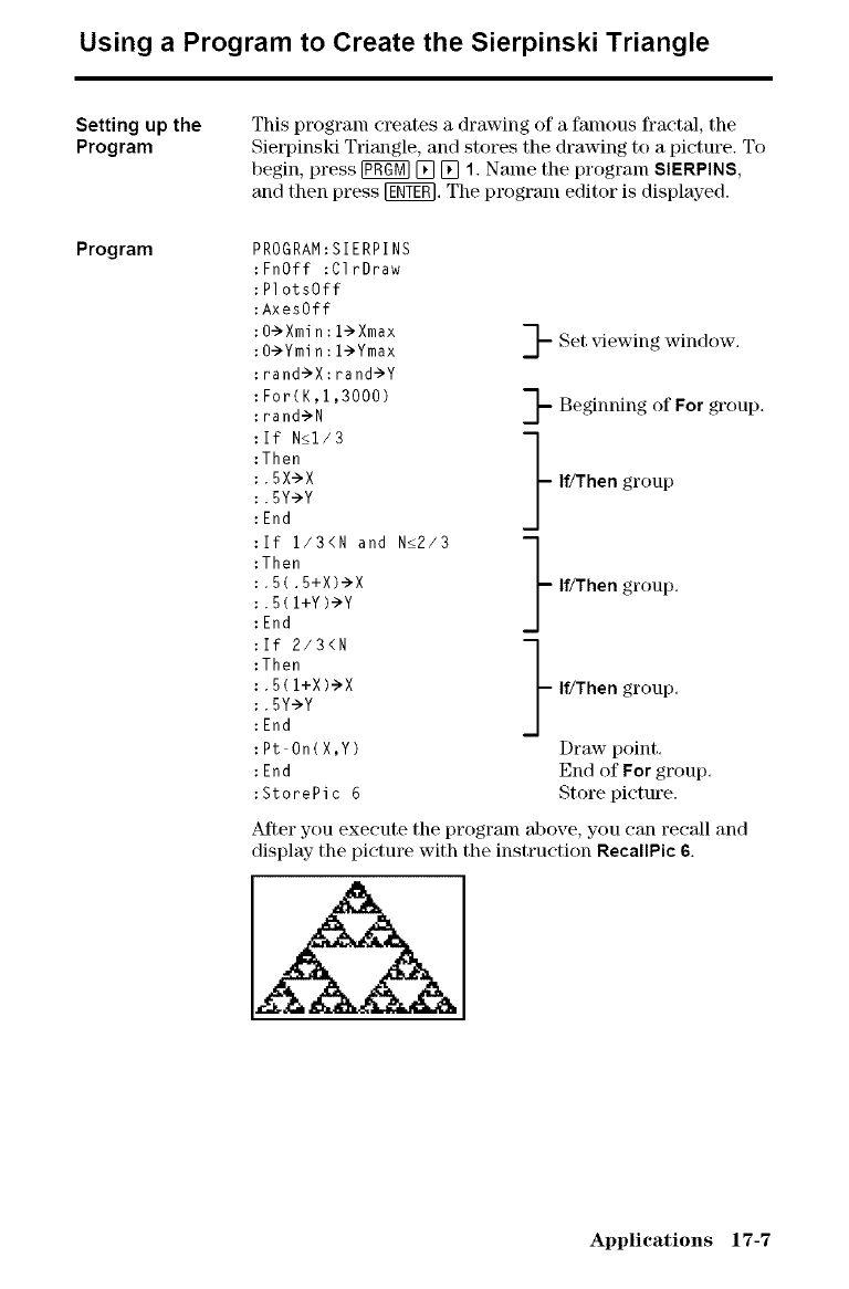
Using a Program to Create the Sierpinski Triangle
Setting up the
Program
This program creates a drawing of a falnous ffactal, the
Sietpinski Triangle, and stores the drawing to a picture. To
begin, press #ggM] [] [] 1. Name the prograln SlERPINS,
and then press [gg7_l. The program editor is displayed.
Program PROGRAM:SIERPI NS
:FnOff :ClrDraw
:Pl otsOff
:AxesOff
::0->Ymi0->Xminn::l->Ymaxl->Xmax } Set _qewing window.
:rand->X: rand->Y
: Fo r ( K, 1,3 00 0 ) -1-- Beginning of Fo rgroup.
:rand->N
:If N<1/3 }
:Then
:. 5X->X If/Then group
:.SY->Y
:End
:If I/3<N and N<2/3 7
:Then
:. 5(, 5+X)->X If/Then group.
:. 5( I+Y)->Y
:End
:If 2/3<N }
:Then
:. 5 ( l+X )->X If/Then group,
:.5Y->Y
:End
: Pt On( X, Y ) Draw point.
: End End of For group.
:StorePi c 6 Store picture.
After you execute the prograln above, you can recall and
display the picture with the instruction RecallPic 6.
Applications 17-7
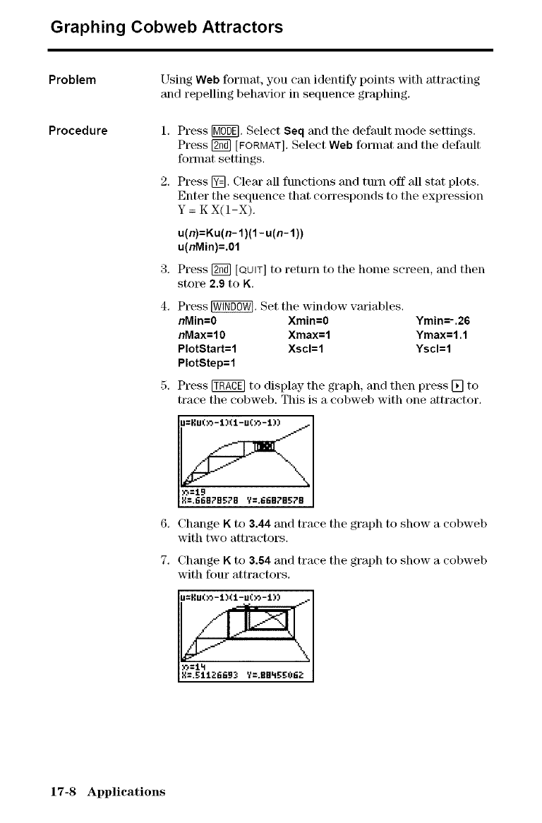
Graphing Cobweb Attractors
Problem
Procedure
Using Web format, you can identify points with attracting
and repelling behavior in sequence graphing,
3,
4,
6,
7,
Press [MO0_. Select Seq and the default nlode settings.
Press _ [FORMAT]. Select Web format and tile default
fonnat settings,
Press @, Clear all functions and tul_ off all stat plots.
Enter the sequence that corresponds to the expression
Y = K X(1-X),
u(n)=Ku(n- 1)(1 - u(n- 1))
u(nMin)=.01
Press [g_ [QUIT] to return to tim holne screen, and then
store 2.9 to K.
Press _, Set the window variables,
nMin=0 Xmin=0 Ymin=-.26
nMax=lO Xmax=l Ymax=l.1
PlotStart=l Xscl=l Yscl=l
PlotStep=l
Press _ to display- the graph, and then press [] to
trace the cobweb. This is a cobweb with one attractor,
lu=Hu,:_-:i.XI-u(_-I)) ..- I
Change K to 3.44 and trace the graph to show a cobweb
with two attractors.
Change Kto 3.54 and trace the graph to show a cobweb
with four attractors,
U=I_u{_-lXl-uCo-1))
17-8 Applications
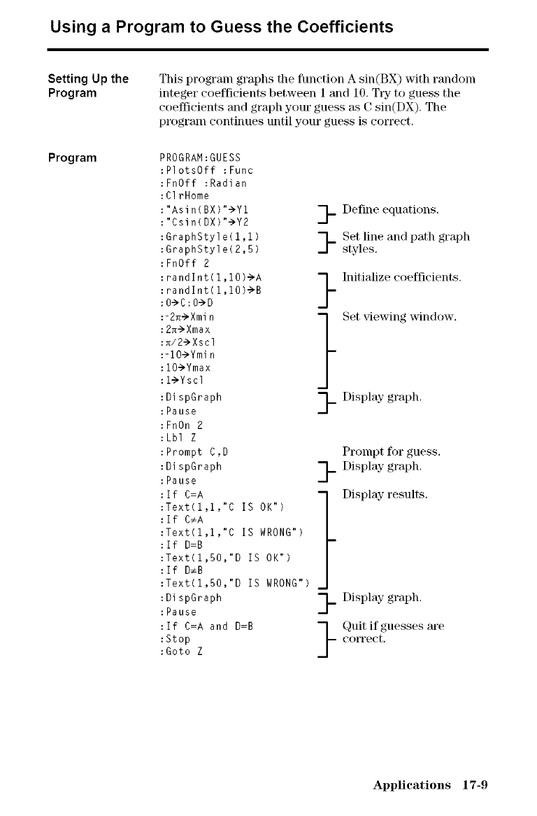
Using a Program to Guess the Coefficients
Setting Up the
Program
This program graphs the function A sin(BX) with random
integer coefficients between 1 and 10. Try to guess the
coefficients and graph your guess at C sin(DX). The
program continues until your guess is correct.
Program PROGRAM:GUESS
:PlotsOff :Func
:FnOff :Radian
:ClrHome
:"Asin(BX)"_Yl
:"Csin(DX)"_Y2
:GraphStyle(l,l)
:GraphStyle(2,5)
:FnOff 2
:randlnt(l,lO)_A
:randlnt(l,lO)_B
:O_C:O_D
:-2_Xmin
:2_Xmax
:_/2_Xscl
:-lO_Ymin
:lO_Ymax
:l_Yscl
:DispGraph
:Pause
:FnOn 2
:Lbl Z
:Prompt C,D
:DispGraph
:Pause
:If C=A
:Text(l,l,"C IS OK")
:If C_A
:Text(l,l,"C IS WRONG")
:If D=B
:Text(l,50,"D IS OK")
:If D_B
:Text(l,50,"D IS WRONG")
:DispGraph
:Pause
:If C=A and D=B
:Stop
:Goto Z
Define equations,
Set line and path graph
styles.
- Initialize coefficients.
I
Set viewing window.
I
=Display graph,
I
Prompt for guess,
- Display graph,
Display results,
- Display graph.
Quit if guesses are
-- correct,
Applications 17-9
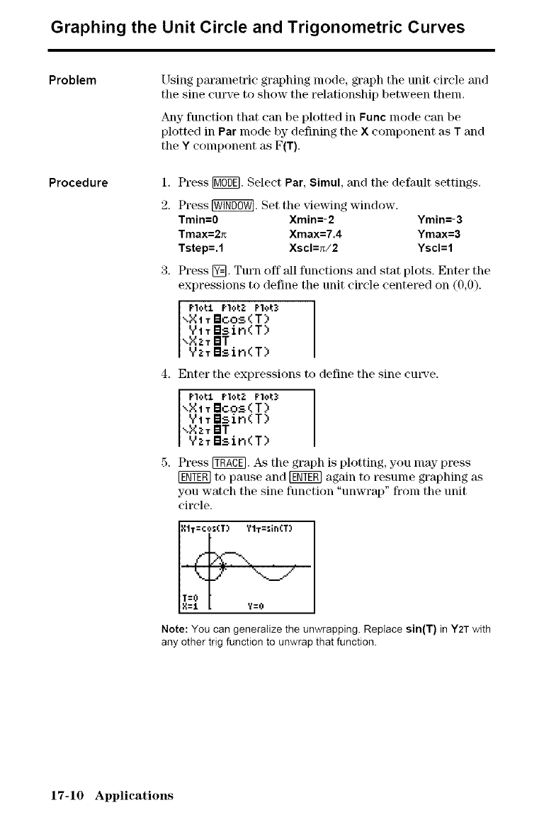
Graphing the Unit Circle and Trigonometric Curves
Problem
Procedure
[ _sing parametric graphing mode, graph the unit circle and
tile sine curve to show the relationship between them.
Any function that can be plotted in Func mode can be
plotted in Par mode by defining the X component as T and
the Y component as F(T).
1. Press [MffffE].Select Par, Simul, and the default settings.
2. Press _. Set the viewing window.
Tmin=0 Xmin=-2 Ymin=-3
Tmax=2_ Xmax=7.4 Ymax=3
Tstep=.1 Xscl=_/2 Yscl=l
3, Press @, Turn off all functions and stat plots. Enter the
expressions to define the unit circle centered on (0,0).
Not:J, PI0L2 P10t)
",XIT_cos (T)
Y1T lisin(T)
\XzT fiT
YzT lisin(T)
4. Enter the expressions to define the sine curve.
PlotJ. Plot_ PloI:3
",X1T lic.os(T)
YIT lisin(T)
"..XzTliT
Y.-Tlisin(T)
5. Press _. As the graph is plotting, you may press
[ggT_ to pause and [ggT_ again to resulne graphing as
you watch the sine function "unwrap" from the unit
circle.
:{IT=C.,:,;(T) Y1T=_irff.T)
2/
== =
Note: You can generalize the unwrapping. Replace sin(T) in Y2Twith
anyother trigfunction to unwrapthatfunction.
17-10 Applications
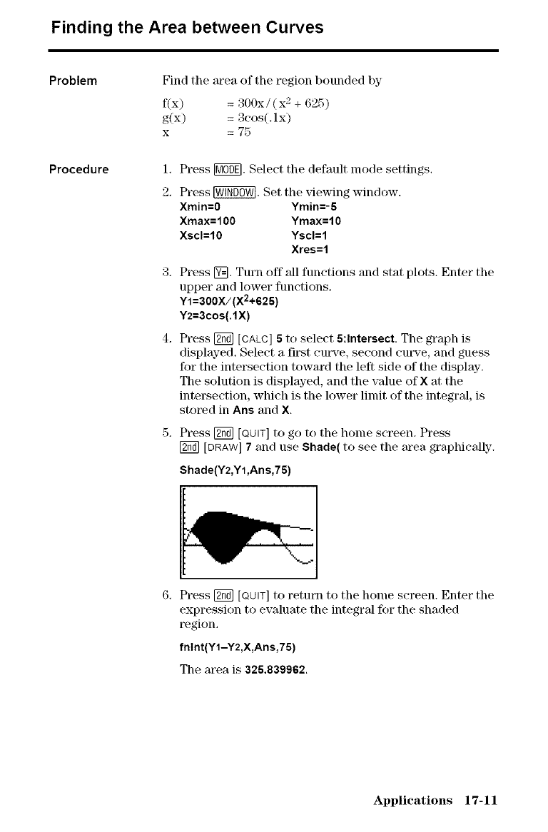
Finding the Area between Curves
Problem
Procedure
Find the area of the region bounded by
fix) = 300x/(x 2 + 625)
g(x) = 3cos(. ix)
x = 75
1.
2.
Press [MffffE].Select the default lnode settings.
Press _. Set the viewing window.
Xmin=0 Ymin=-5
Xmax=100 Ymax=10
Xscl=10 Yscl=l
Xres=l
3. Press @. Turn off all functions and stat plots. Enter the
upper and lower functions.
Y1=a00x/(x2+625)
Y2=3COS(.1X)
4. Press [g_] [CALC]5to select 5:Intersect. The graph is
displayed. Select a first cutwe, second cut,'e, and guess
for the intersection toward the left side of the display.
The solution is displayed, and the value of X at the
intersection, which is the lower limit of the integral, is
stored in Ans and X.
Press _ [QUIT] to go to the home screen. Press
[_ [DRAW]7and use Shade( to see the area graphically.
Shade(Y2,Y1,Ans,75)
6, Press [2_] [QUIT] to return to tile honle screen. Enter tile
expression to evaluate the integral for the shaded
region,
fnlnt(Y1-Y2,X,Ans,75)
The area is 325.839962.
Applications 17-11
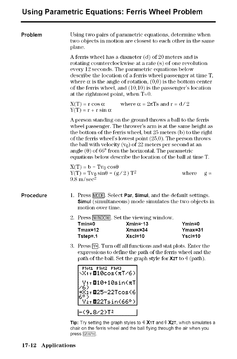
Using Parametric Equations: Ferris Wheel Problem
Problem
Procedure
[ _sing two pai_\q of parametric equations, determine when
two objects in motion are closest to each other in the Salne
plane.
A ferris wheel has a diameter (d) of 20 meters and is
rotating counterclockwise at a rate (s) of one revolution
ever T 12 seconds. The paralnetric equations below
describe the location of a fen'is wheel passenger at time T,
where (x is the angle of rotation, (0,0) is the bottom center
of the fen'is wheel, and (10,10) is the passenger's location
at the rightmost point, when T=0.
X(T) = r cos (x where (x = 2xTs and r = d/2
Y(T) = r + r sin (x
A person standing on the ground throws a ball to the ferds
wheel passenger. The thrower's ann is at the sanle height as
the bottoln of the ferds wheel, but 25 meters (b) to the right
of the fen'is wheel's lowest point (25,0). The person throws
the ball with velocity (v0) of 22 meters pet" second at an
angle (0) of 66 ° froln the horizontal. The parametric
equations below describe the location of the ball at tinle T.
X(T) = b - Tv0 cos0
Y(T) = Tv0 sin0 - (g/2) T _ where g =
9,_ nl/see 2
1, Press [MO0_. Select Par, Simul, and the default settings.
Simul (sinmltaneous) mode sinmlates the two objects in
nlotion over tinle.
Press _. Set the viewing window.
Tmin=0 Xmin=-13 Ymin=0
Tmax=12 Xmax=34 Ymax=31
Tstep=.l Xscl=lO Yscl=lO
Press @. Turn off all functions and stat plots. Enter tile
expressions to define tile path of the ferris wheel and tile
)ath of the ball. Set tile graph style for X2T to 4j (path).
i PloL:L Plot_: Plot_:
",X1T B1Ocos(xT/6)
YITBlO+lOsin(_T
t6)
*)XzT B25-22Toos(6
5 ° )
ViT B22Tsin(66 ° )
-(9.8/2)TZ
Tip: Try setting the graph styles to ",.'_XlT and 0X2T, which simulates a
chair on the ferris wheel and the bal! flying through the air when you
press _.
17-12 Applications
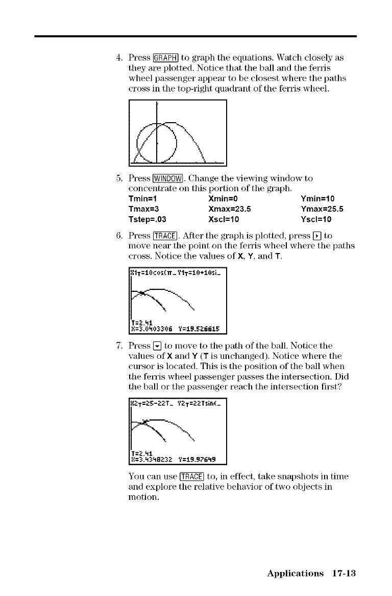
4. Press [_ to graph the equations. Watch closely as
they are plotted. Notice that the ball and the ferris
wheel passenger appear to be closest where the paths
cross in the top-right quadrant of the ferris wheel,
5, Press [_. Change the _iewing window to
concentrate on this portion of the graph.
Tmin=l Xmin=0 Ymin=10
Tmax=3 Xmax=23.5 Ymax=25.5
Tstep=.03 Xscl=10 Yscl=10
6. Press _. After the graph is plotted, press [] to
nlove neat" tile point on the ferris wheel where the paths
cross, Notice the values of X, Y, and T,
IIT=t0_.O_;(1T_ YtT=IO÷10;;_
7, Press [] to nlove to the path of the ball. Notice the
values of X and Y (T is unchanged). Notice where the
cursor is located. This is the position of the ball when
the fetTis wheel passenger passes the inter\section. Did
the ball or the passenger reach the intersection first?
You can use _ to, in effect, take snapshots in tilne
and explore the relative behavior of two objects in
motion,
Applications 17-13
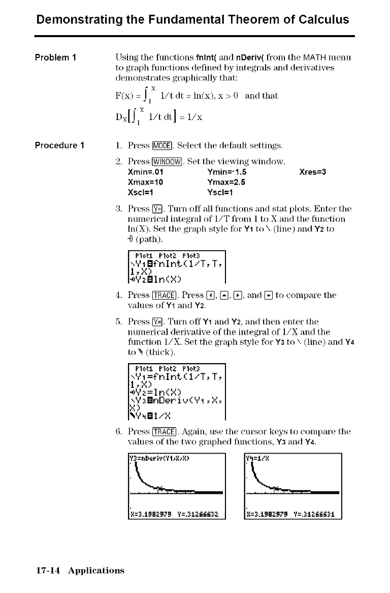
Demonstrating the Fundamental Theorem of Calculus
Problem 1
Procedure 1
Using the functions fnlnt( and nDeriv( fronl the MATH menu
to graph functions defined by integrals and derivatives
demonstrates graphically that:
fx
F(x)= 1 1/tdt=ln(x),x>0 and that
Ifx 1
Dx 1 1/t dt = 1/x
1.
2.
4.
5.
Press 1_. Select tile default settings.
Press _. Set the viewing window.
Xmin=.01 Ymin=-l.5
Xmax=10 Ymax=2.5
Xscl=l Yscl=l
Xres=3
Press @, Turn off 'allfunctions and stat plots. Enter tile
numerical integral of 1/T from 1 to X and the function
ln(X). Set the graph style for Y1 to "..(line) and Y2 to
.4:,(path).
Plot:l. Pl¢,t2 P1ot_
",Yt Bi'n InL( l/T, T,
1,X)
_¢2Bln(g)
Press _. Press [], [], [], and [] to eolnpare the
values of Y1 and Y2,
Press @. Turn off Y1 and Y2, and then enter the
numerical derivative of the integral of 1/X and the
function 1/X. Set the graph style for Y3 to ', (line) and Y4
to _. (thick),
Ploti p1,,:,l:2 Plot_:
:,Y:,_oior_1_T,T,
_Y2'=In(g)
_BnOeri_,(Y1 ,X,
_,YuBI/X
Press _. Again, use the cursor keys to compare the
values of the two graphed functions, Y3 and Y4.
17-14 Applications
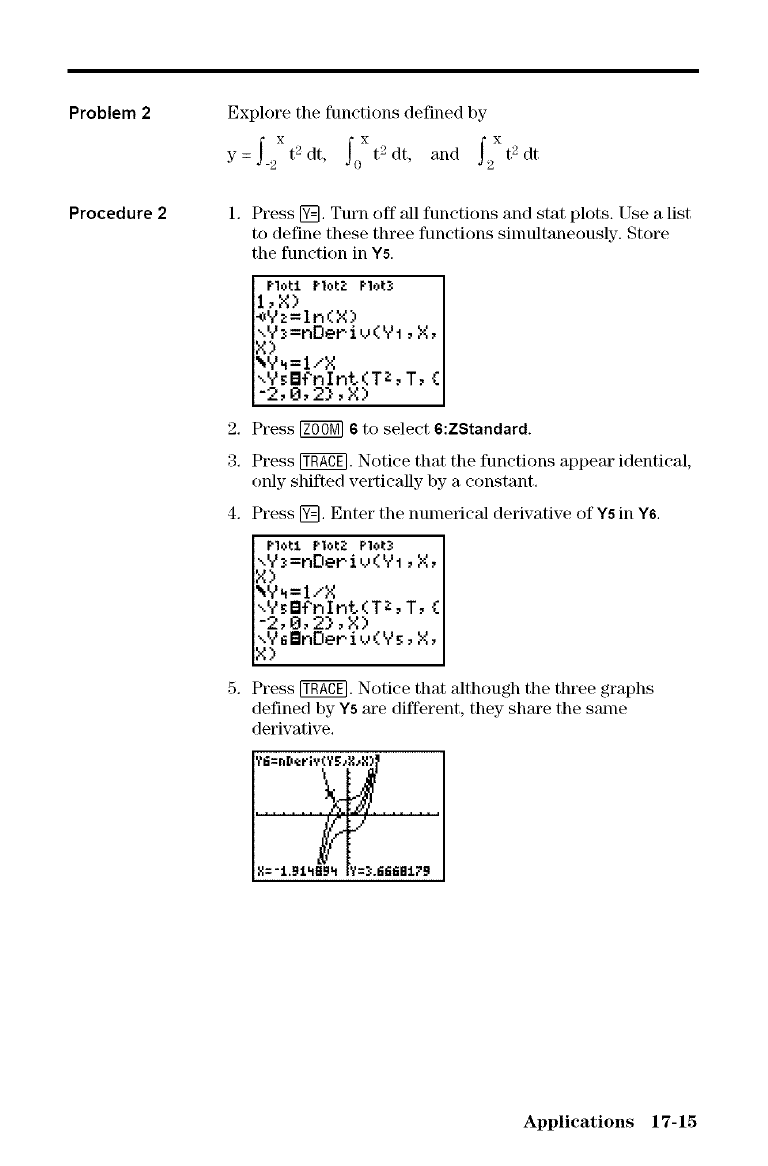
Problem 2
Procedure 2
Explore the functions defined by
X X X
Y:f-2 t2dt' f0 t2dt' and f2 t2dt
2,
3,
Press @, Turn off all functions and stat plots. Use a list
to define these three functions sinmltaneously. Store
the function in Ys.
_'_=nDerib=(Yt"°Yz=lr_(x)l'x)Pl°t:LPlol:Z F'loL_. _ _
'_Y_=I/X T, (
,,Y_B?nlnL(T z ,
i-::,o,2>,x)
Press _ $ to select $:ZStandard.
Press _. Notice that the functions appear identical,
only shifted vertically by a constant.
Press @, Enter the numerical derivative of Y5 in Y6,
\Y_=nDeriv(Y1, X,
X)
"*Y_=I/X
"..Y_B_nIn÷.(TZ, T, (
-2,0,2>,X)
\YeBnOer iv(Y_, X,
x)
Press _. Notice that although the three graphs
defined by Y5 are different, they share tile same
derivative,
N="t.9£_Bi!_?i¢).6_,fiBt?9
Applications 17-15
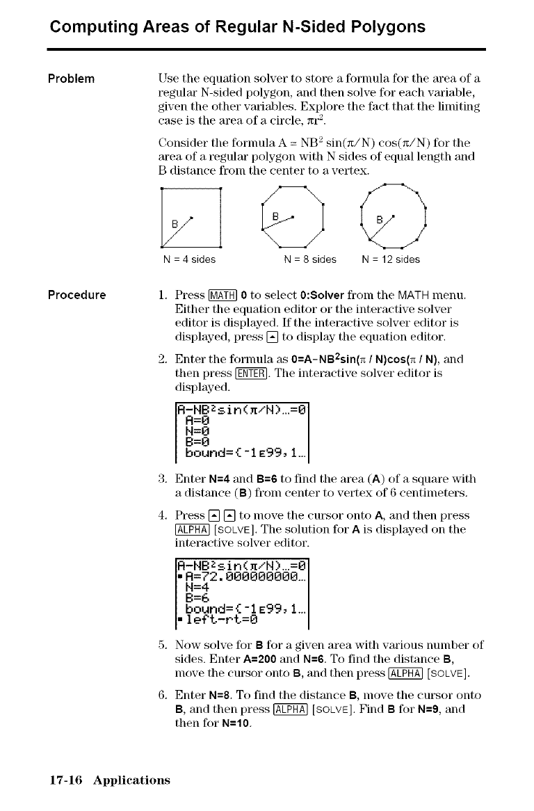
Computing Areas of Regular N-Sided Polygons
Problem Use the equation solver to store a fornmla ff)r the m'ea of a
regulm" N-sided polygon, and then solve for each vm'iable,
given the other variables. Explore the fact that the limiting
case is the area of a circle, _r 2.
Consider the fonnula A = NB 2 sin(_/N) cos(_/N) for the
m'ea of a regulm' polygon with N sides of equal length and
B distance from the center to a vertex.
N = 4 sides N = 8 sides N = 12 sides
Procedure 1, Press [_ 0to select 0:Solver froln the MATH menu,
Either the equation editor or the interactive solver
editor is displayed. If the interactive solver editor is
displayed, press [] to display the equation editor,
2, Enter the fonnula as 0=A-NB2sin(_ /N)cos(_ /N), and
then press [_. The interactive solver editor is
displayed.
R_NBZsin(_/N).,,=O
bound={ -1 E99, 1...
3, Enter N=4 and B=6 to find the area (A) of a square with
a distance (B) from center to vertex of 6 centimeters,
4, Press [] [] to nlove the cursor onto A, and then press
@ [SOLVE], The solution for Ais displayed on the
interactive solver editor.
:l-NBZsin(_/N)...=el
: 2.00o000000I
B=6
bound={ -1 E99, 1...
le_t-rt=e
5. Now solve for Bfor a given area with vm'ious number of
sides. Enter A=200 and N=6. To find the distance B,
lnove the cursor onto B, and then press @ [SOLVE].
6, Enter N=8, To find the distance B, nlove the cursor onto
B, and then press @ [SOLVE]. Find Bfor N=9, and
then for N=10.
17-16 Applications
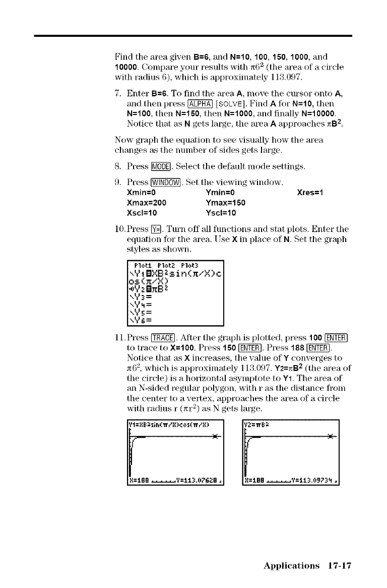
FindtheareagivenB=6, and N=10, 100, 150, 1000, and
10000. Compare your results with =62 (the area of a circle
with radius 6), which is approximately 113.097.
7. Enter B=6. To find the area A, move the cursor onto A,
and then press @ [SOLVE]. Find Afor N=10, then
N=100, then N=160, then N=1000, and finally N=10000.
Notice that as N gets large, the area A approaches _B 2.
Now graph the equation to see visually how the area
changes as the number of sides gets lm'ge.
8, Press NgffE].Select the default lnode settings,
9. Press _. Set the viewing window.
Xmin=O Ymin=O
Xmax=200 Ymax=150
Xscl=lO YscI=IO
Xres=l
10.Press @. Turn off all functions and stat plots. Enter the
equation for the m'ea. I Jse X in place of NSet the graph
styles as shown.
Plot]. F'10t2 F'10t._
xViBXBZsin<_/X)c
os(_/X)
-W._BnB z
,.'-,as=
xY.1=
,,V_:=
,&'6=
11.Press _. After the graph is plotted, press I O0[gNgggl
to trace to X=100. Press 150 [ggTgm.Press 188 [ggTg_.
Notice that _LsX increases, the value of Yconverges to
=62, which is approximately 113.097. Y2=_B2 (the area of
the circle) is a horizontal asymptote to Y1. The area of
an N-sided regular polygon, with r as the distance fl'om
the center to a vertex, approaches the area of a circle
with radius r (_r 2) as N gets large.
;' 1:1-,'B;a_;ir=r..'n"r'N),2.o_;( Tr_'g:E '¢_::Tr£:::
8:tBB _Y=lt3.0762B, 8:tEE _Y:ti3.0973_ •
Applications 17-17
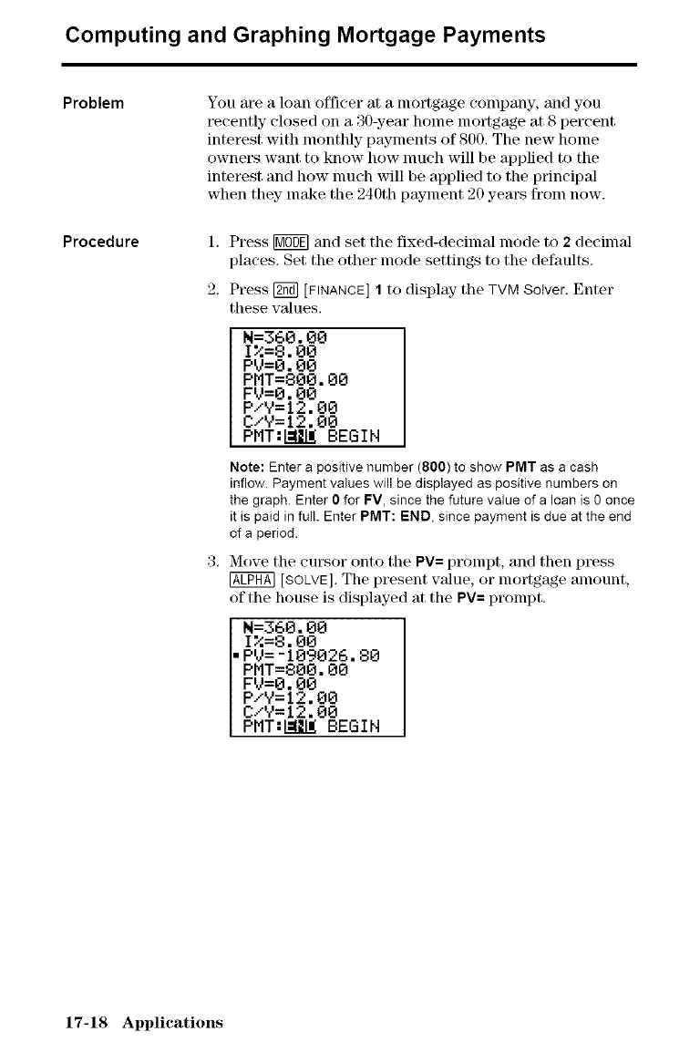
Computing and Graphing Mortgage Payments
Problem
Procedure
You at_ a loan officer at a mortgage conlpany, and you
recently closed on a 30-yem' holne lnortgage at 8 percent
interest with monthly payments of 800, The new home
owners want to know how nmch will be applied to the
interest and how nmch will be applied to the principal
when they make the 240th payment 20 years from now.
1, Press [_ and set the fixed-decimal lnode to 2decimal
places. Set the other mode settings to the defaults.
2. Press [_ [FINANCE] 1to display" the TVM Solver. Enter
these values.
N=360.00
I_=8.00
PV=0.00
PMT=800.00
FV=0.00
P/V=I2.00
C/V=12,00
PMT:[_=[II_BEGIN
Note: Enter a positive number (800) to show PMT as a cash
inflow. Payment values will be displayed as positive numbers on
the graph. Enter 0 for FV, since the future value of a loan is 0 once
it is paid in ful!. Enter PMT: END, since payment is due at the end
of a period.
3, Move the cursor onto the PV= prompt, and then press
@ [80LYE], The present value, or lnortgage amount,
of the house is displayed at the PV= prompt,
N=360.00
I%=8.00
PV=-IO9026,B0
PMT=B00.00
FV=0.00
P/V=12.00
C/Y=12.00
PMT:LqIL_ BEGIN
17-18 Applications
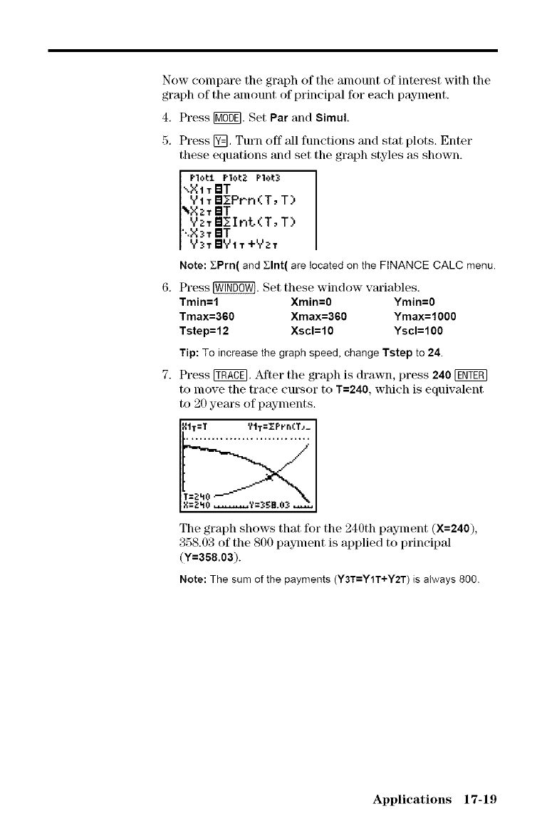
Nowcomparethegraphoftheamountofinterestwiththe
graphoftheamountofprincipalforeachpayment.
4, Press[NffffE].Set Par and Simul.
5, Press @, Turn off all functions and stat plots. Enter
these equations and set the graph styles as shown.
Plot1 Plol:_ Plot_:
",XIT BT
Vi TBFPr'n(T, T)
_XzT BT
'Y'zT B_- Int.< T, T)
".X_T BT
V:_T BVIT +VZT
Note: ZPrn( and ZInt( are located on the FINANCE CALC menu,
6, Press _. Set these window variables.
Tmin=l Xmin:0 Ymin=0
Tmax=360 Xmax=360 Ymax=1000
Tstep=12 Xscl=10 Yscl=100
Tip: To increase the graph speed, change Tstep to 24.
7. Press _. After the graph is drawn, press 240
to move the trace cursor to T=240, which is equivalent
to 20 years of payments.
IIT=T ?tT='_F'r_rKT__
The graph shows that ff)r the 240th payment (X=240),
358.03 of the 800 pay3nent is applied to principal
(Y:368.03).
Note: The sum of the payments (Y3T=Y1T+Y2T) is always 800.
Applications 17-19
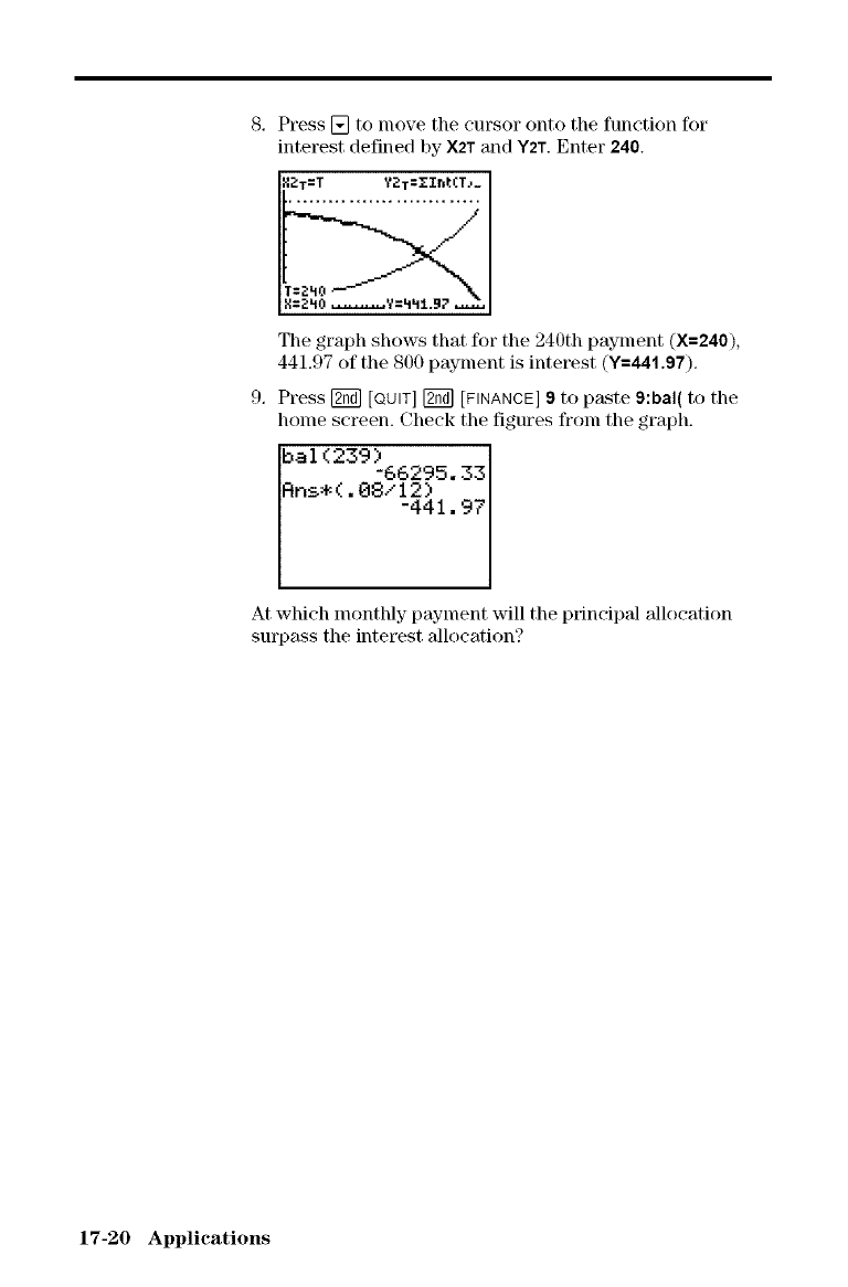
8. Press[] tomovethecursorontothefunctionfor
interestdefinedbyX2TandY2T.Enter240.
The graph shows that for the 240th payment (X=240),
441.97 of the 800 payment is interest (Y=441 .gT).
9. Press _ [QUIT] [_ [FINANCE] 9to paste 9:bal( to the
home screen. Check the figures from the graph.
_ai(239) -66295.33
_nsm(.08/12)
-441,97
At which monthly payment will the principal allocation
surp_kss the interest allocation?
17-20 Applications
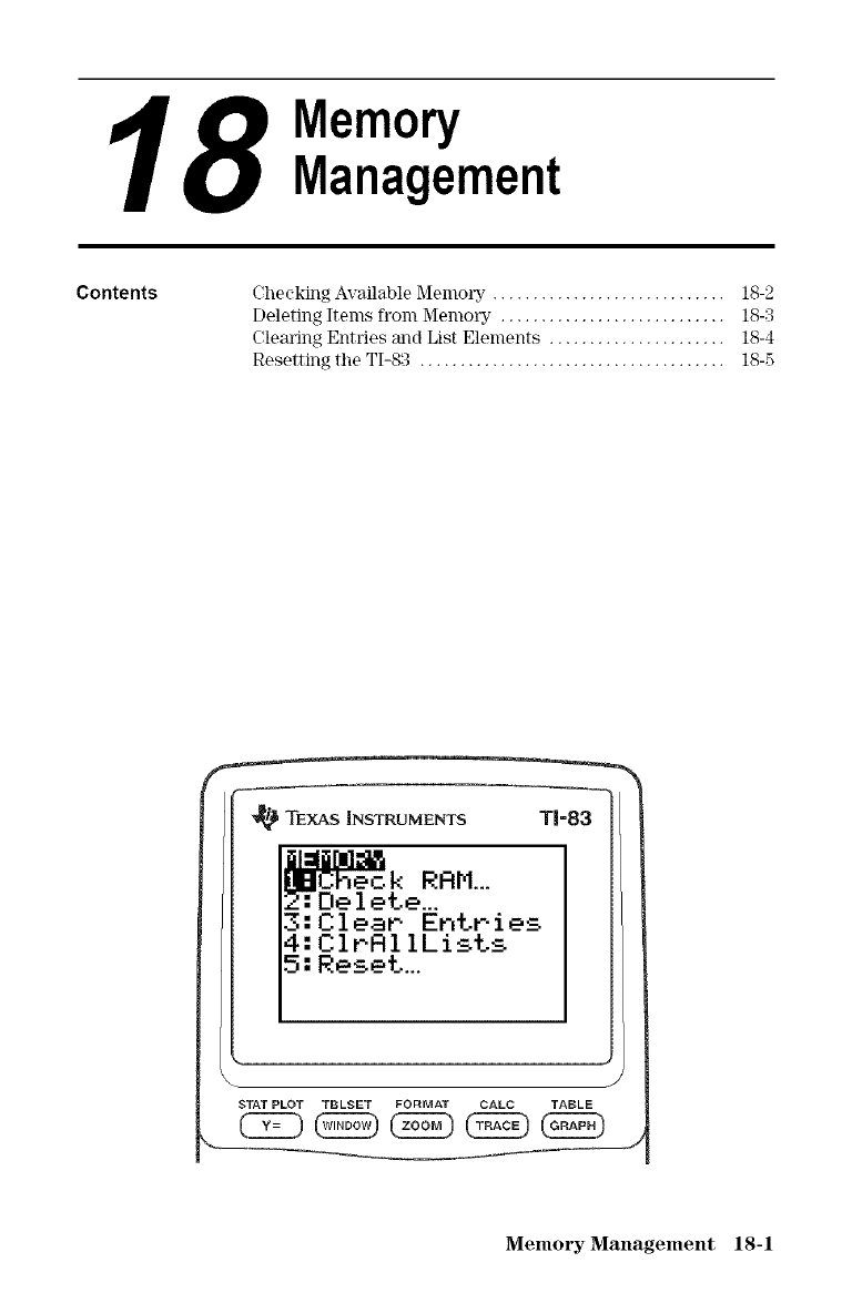
18Menrn2gq/ement
Contents Checking A_ailable MemolTy ............................. I8-2
Deleting Items from MemmTy ............................ I8-3
Clearing Entries and List Elements ...................... 18-4
Resetting the TI-83 ...................................... 18-5
TEXAS INSTRUMENTS TF83
RRM_
Delete...
3:Clear Entries
4: CIRRI ILists
5: Reset...
J
STAT PLOT TBLSET FORMAT CALC TABLE
Memory Management 18-1
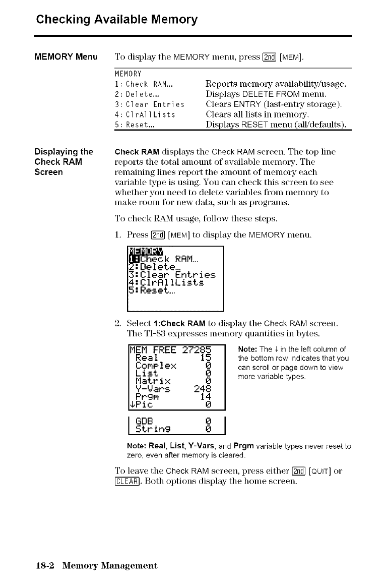
Checking Available Memory
MEMORY Menu To display the MEMORY menu, press [_ [MEM].
MEMORY
i: Check RAM...
2: Delete...
3: Clear Entries
4: ClrAllLists
5: Reset..,
Reports memory availability/usage,
Displays DELETE FROM menu,
Clem's ENTRY (l_kst-entry storage).
Clears all lists in memo_T.
Displays RESET menu (all/defaults).
Displaying the
Check RAM
Screen
Check RAM displays the Check RAM screen. The top line
t_ports the total amount of available nlenlol_y-. The
remaining lines report the amount of lnelnot7 each
variable type is using. You can check this screen to see
whether you need to delete variables from memo_T to
nmke room for new data, such as programs.
To check RAM usage, follow these steps.
1. Press [2_] [MEM] to display the MEMORY menu.
RRM...
_:Clear Entries
_:ClrRllLists
5:Reset...
2. Select I :Check RAM to display the Check RAM screen.
The TI-S3 expresses memory quantities in bytes.
MEM FREE 27285
Real 15
ComPlex 8
List 8
Matrix 8
Y-Vats 248
Prgm 14
4Pio 8
GOB 0
String 0
Note: The J_in the left column of
the bottom row indicates that you
can scroll or page down to view
more variable types.
Note: Real, List, Y-Vars, and Prgm variable types never reset to
zero, even after memory is cleared.
To leave the Check RAM screen, press either [_ [QUIT] or
@. Both options display- the home screen.
18-2 Memmw Management
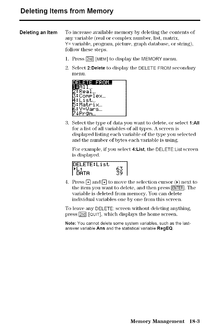
Deleting Items from Memory
Deleting an Item To increase available nlenlol_ by deleting the contents of
any- variable (real or colnplex nulnber, list, matrix,
Y= variable, prograln, picture, graph database, or string),
follow these steps.
1. Press [2_] [MEN]to display the MEMORY lnenu.
2. Select 2:Delete to display- the DELETE FROM secondalTy-
nleno.
3. Select the type of data you want to delete, or select 1:All
for a list of all variables of 'all types. A screen is
displayed listing each variable of the type you selected
and the number of bytes each variable is using.
For exalnple, if you select 4:List, the DELETE:List screen
is displayed.
DELETE: Li_t
_LI 63
DATA 39
4. Press [] and [] to nlove tile selection cursor (_) next to
the item you want to delete, and then press _. The
variable is deleted fronl nlenlot_y-. You Call delete
individual vm'iables one by one froln this screen.
To leave ally DELETE: screen without deleting anything,
press [_ [QUIT],which displays the home screen.
Note: You cannot delete some system variables, such as the last-
answer variable Ans and the statistical variable RegEQ
Memory Management 18-3
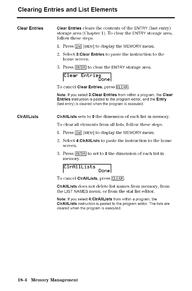
Clearing Entries and List Elements
Clear Entries
CIrAIILists
Clear Entries clears the contents of the ENTRY (last entry)
storage area (Chapter 1). To cleat" the ENTRY storage area,
follow these steps.
1, Press [_ [MEM] to display the MEMORY menu.
2, Select 3:Clear Entries to paste the instruction to the
home screen.
3. Press [_ to clear the ENTRY storage area.
IcleaP Entt'ie_one I
To cancel Clear Entries, press @,
Note: If you select 3:Clear Entries from within a program, the Clear
Entries instruction is pasted to the program editor, and the Entry
(last entry) is cteared when the program is executed.
CIrAIILists sets to 0tile dimension of each list in lllelllOl_yL
To clear all elements from all lists, follow these steps,
1, Press [_ [MEM] to display the MEMORY menu,
2, Select 4:ClrAIIkists to paste the instruction to the home
screen.
3. Press _ to set to 0the dimension of each list in
nlenlory.
IC1rA11Lists lionel
To cancel CIrAIILists, press @.
CIrAIILists does not delete list nanles fronl nlenlol_y-, fronl
the LiST NAMES menu, or froln the stat list editor.
Note: If you select 4:CIrAIIkists from within a program, the
CIrAIILists instruction is pasted to the program editor. The lists are
cleared when the program is executed.
18-4 MemolT Management
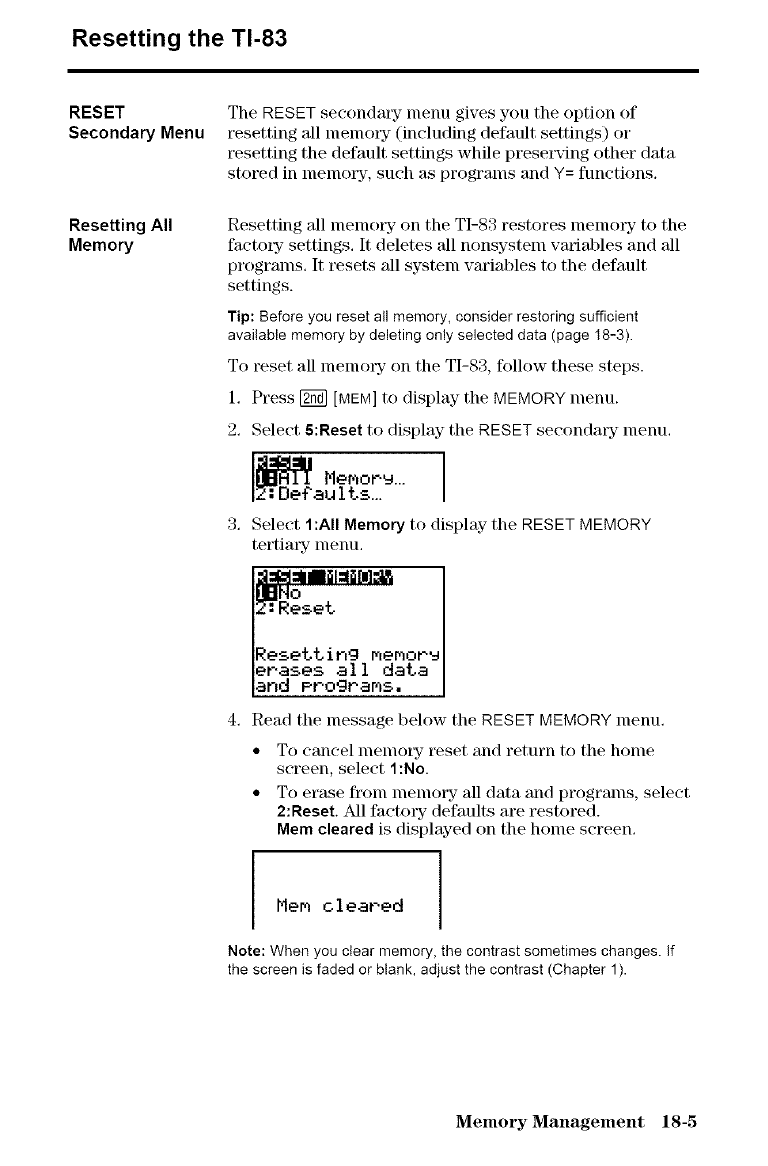
Resetting the TI-83
RESET
Secondary Menu
Resetting All
Memory
The RESET seconda[7 lnenu gives you the option of
resetting all memory (including default settings) or
_setting the default settings while prese_Mng other data
stored in lnelno_T, such as programs and Y= functions.
Resetting all nlenloFy Oil the TI-83 restores nlenlory to the
factor7 settings, It deletes all nonsystem variables and all
programs. It resets all system variables to the default
settings.
Tip: Before you reset all memory, consider restoring sufficient
available memory by deleting only selected data (page I8-3).
To reset all nlenlory on the TI-83, follow these steps.
1. Press [2_] [MEM] to display the MEMORY menu.
2. Select 5:Reset to display the RESET secondary menu.
.._. Mer_or-u...
2:: Defau lts...
3, Select 1:All Memory to display the RESET MEMORY
tertimT nlenu.
Resetting memoru
erases all data
and Programs,
4. Read the message below tile RESET MEMORY menu.
• To cancel memoL_- reset and retm'n to tile home
screen, select 1:No.
• To erase fronl lnelnol T all data and progralns, select
2:Reset. All factory defaults are restored.
Mere cleared is displayed on the home screen.
IMem cleared
Note:When you clearmemory, thecontrastsometimeschanges.If
thescreenisfadedorblank,adjustthecontrast(ChapterI).
Memory Management 18-5
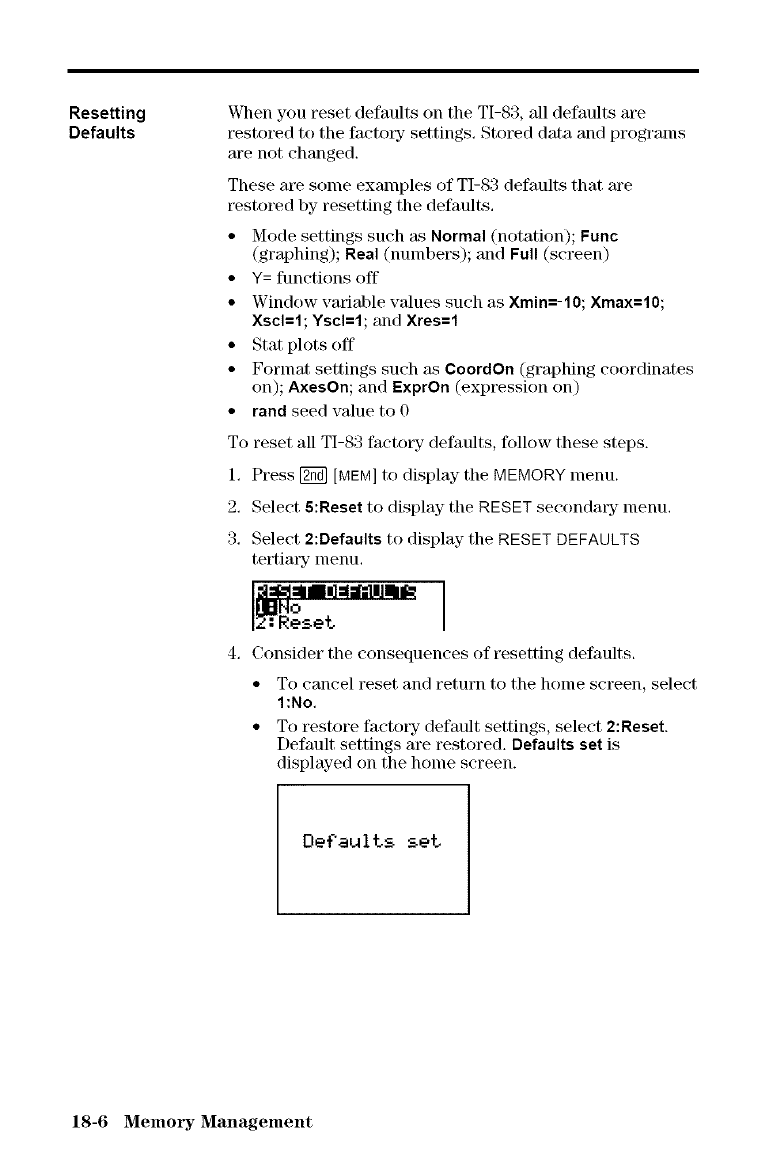
Resetting
Defaults When you reset defaults on the TI-83, all defaults are
restored to the factory settings. Stored data and programs
are not changed.
These are some examples of TI-83 defaults that are
restored by resetting the defaults.
• Mode settings such as Normal (notation); Func
(graphing); Real (numbers); and Full (screen)
• Y= functions off
• Window variable values such as Xmin=-lO; Xmax=lO;
Xscl=l; YscI=I; and Xres=l
• Stat plots off
• Format settings such as eoordOn (graphing coordinates
on); AxesOn; and ExprOn (expression on)
• rand seed value to 0
To reset all TI-83 factory defaults, follow these steps.
1. Press [g_] [MEM] to display the MEMORY menu.
2. Select 5:Reset to display the RESET secondary menu.
3. Select 2:Defaults to display the RESET DEFAULTS
tertimT menu.
4. Consider the consequences of resetting defaults.
• To cancel reset and return to the home screen, select
1:No.
• To restore factory default settings, select 2:Reset.
Default settings are restored. Defaults set is
displayed on the home screen.
Defaults set
18-6 Memmw Management
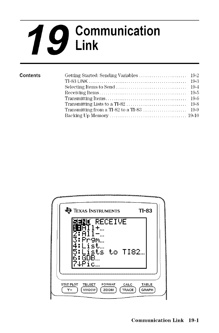
19 ci° municati°n
Contents Getting Started: Sending Variables ....................... 19-2
TI-83 kINK ............................................... 19-3
Selecting Items to Send .................................. 19-4
Receiving Items .......................................... 19-5
Transmitting Items ....................................... 19-6
Transmitting Lists to a TI-82 ............................. 19-8
Transmitting from a TI-82 to a TI-8:I ..................... 19-9
Backing Up MemmTy"..................................... 19-10
TEXAS INSTRUMENTS 1"1=83
RECEIVE
to TI82...
J
STAT PLOT TBLSET FORMAT CALC T._,B LE
Communication Link 19-1
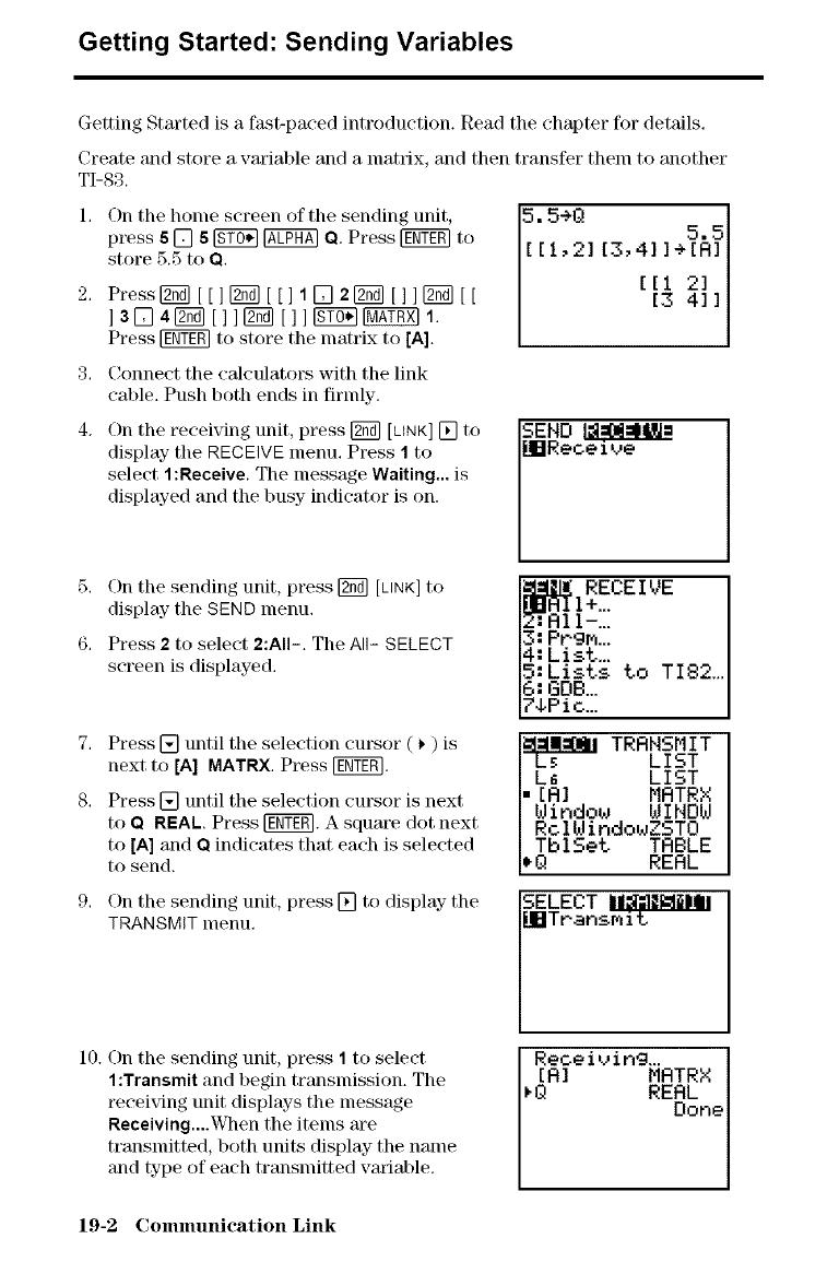
Getting Started: Sending Variables
Getting Started is a fast-paced introduction. Read the chapter for details.
Create and store a wu'iable and a matrix, and then transfer then] to another
TI-83.
On the home screen of the sending unit,
press 5[] 5Fgg6gl@ O. Press [gfff_ to
store 5.5 to Q.
Press[_[[][_[[l 1[]2[_[11[_[[
] 3 _ 412_ [1 ] [2_ [1 ] _ [NN_ 1.
Press [_ to store the lnatrix to [A].
3. Connect the calculators with the link
cable. Push both ends in firmly.
4. On the receiving unit, press [_ [LINK] [] tO
display tile RECEIVE menu. Press 1to
select 1:Receive. The message Waiting... is
displayed and the busy indicator is on.
SEHD [_
IERec.e ive
5, On the sending unit, press [2_] [LINK] to
display the SENDmenu.
6, Press 2to select 2:All-. The All- SELECT
screen is displayed.
Z,_AI RECEIVE
3:Prgm...
4:List...
5:List.s to TI82...
6:GOB...
7gPic...
TRRNSMIT
k_ LIST
.L_ LIST
[R] MRTRX
Window WINOW
RclWindouZSTO
TblSet TABLE
_Q RERL
7,
8.
Press [] until the selection cursor ( _) is
next to [A] MATRX.Press [ggTEg].
Press [] until the selection cursor is next
to QREAL. Press [_. A square dot next
to [A] and Oindicates that each is selected
to send.
9. On the sending unit, press [] to display the
TRANSMIT menu.
10. On the sending unit, press 1to select
1:Transmit and begin transmission. The
receiving unit displays the message
Receiving....When the items are
transmitted, both units display the name
and type of each transmitted variable.
SELECT IdII._IIIiIIi
[llTransr_it
Receiving,..
[ R]MRTRX
'Q REDRLne
19-2 Conununication Link
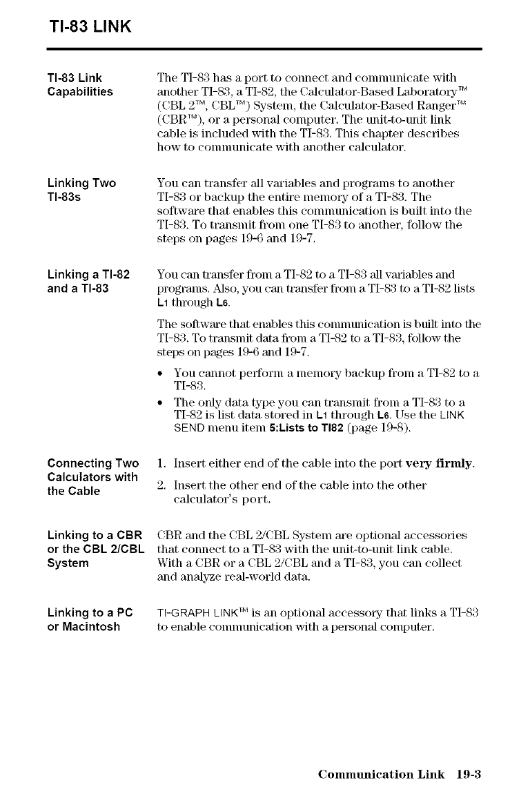
TI-83 LINK
TI-83 Link
Capabilities
Linking Two
TI-83s
Linking a TI-82
and a TI-83
Connecting Two
Calculators with
the Cable
Linking to a CBR
or the CBL 2/CBL
System
Linking to a PC
or Macintosh
The TI-83 has a port to connect and conlnlunicate with
another TI-83, a TI-82, the Calculator-Based Lal)oratory TM
(CBL 2 TM, CBL TM) System, the Calculator-Ba_ed Ranger TM
(CBWM), or a personal conlputer. The unit4o-unit link
cable is included with the TI-83. This chapter describes
how to comnmnicate with another calculator.
You can transfer all variables and programs to another
TI-83 or backup the entire nlenlol'y of a TI-83. The
softwm'e that enables this communication is built into the
TI-83. To transmit from one TI-83 to another, follow the
steps on pages 19-6 and 19-7.
You can transfer fronl a TI-82 to a TI-83 all variables and
programs. Also, you cal_ tral_sfer from a TI-83 to a TI-82 lisL_
L1 through L6.
The softwaxe that enables this conunm_ication is built int_) the
TI-83. To tral_nlit data from a TI-82 t_) a TI-83, follow the
steps on pages 19-6 at_d 19-7.
• You cannot perform a memory backup from a TI-82 to a
TI-83,
• The only data type you can transmit from a TI-83 to a
TI-82 is list data stored in L1 through L6, Use the kINK
SEND menu item 5:Lists to TI82 (page 19-8).
1. Insert either end of the cable into the port very firmly.
2. Insert the other end of the cal>le into the other
calculator's port.
CBR and the CBL 2/CBL System are optional accessories
that connect to a TI-83 with the unit-to-unit link cal fie,
With a CBR or a CBL 2/CBL and a TI-83, you can collect
and analyze real-world data.
TI-GRAPH LINK TM is an optional accessory- that links a TI-S3
to enable conmmnication with a personal conlputer.
Communication Link 19-3
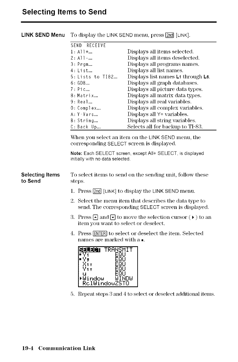
Selecting Items to Send
LINK SEND Menu
Selecting Items
to Send
To display the LINK SEND menu, press [_ [LINK].
SEND RECEIVE
i:A11 +.., Displays
2:A11 -.., Displays
3 : P rgm... Displays
4: Li st... Displays
5: Lists to T182... Displays
6 : GDB... Displays
7 : Pi c... Displays
8 : Matrix... Displays
9 : Real ... Displays
0 : Compl ex.., Displays
A: Y Vars... Displays
B: String.,.
C: Back Up.,,
M1 items selected.
'all items deseleeted.
all progranls names.
'all list names,
list names L1 through Ls.
'all graph databases.
M1 picture data types,
'all matrix data types.
M1 real vmiables,
'all complex variables.
M1 Y= variables.
Displays all string variables.
Selects all for backup to TI-83.
When you select an item on the LINKSEND menu, the
corresponding SELECT screen is displayed.
Note: Each SELECT screen, except All+ SELECT, is displayed
initially with no data selected.
To select items to send on the sending unit, follow these
steps.
1. Press [2_] [LINK]to display" the LINKSEND menu.
2. Select the menu item that describes the data type to
send. The corresponding SELECT screen is displayed.
3. Press [] and [] to nlove the selection cursor (_) to an
item you want to select or deselect.
4. Press _ to select or deselect the iteln. Selected
nalnes are nlarked with a ..
_ TRRNSMIT
EQU
• Y_ EQU
Xl T EQU
Vi T EQU
u EQU
FWindow WINDW
RclWindowZSTO
5, Repeat steps 3 and 4 to select or deselect additional items.
19-4 Conununication Link
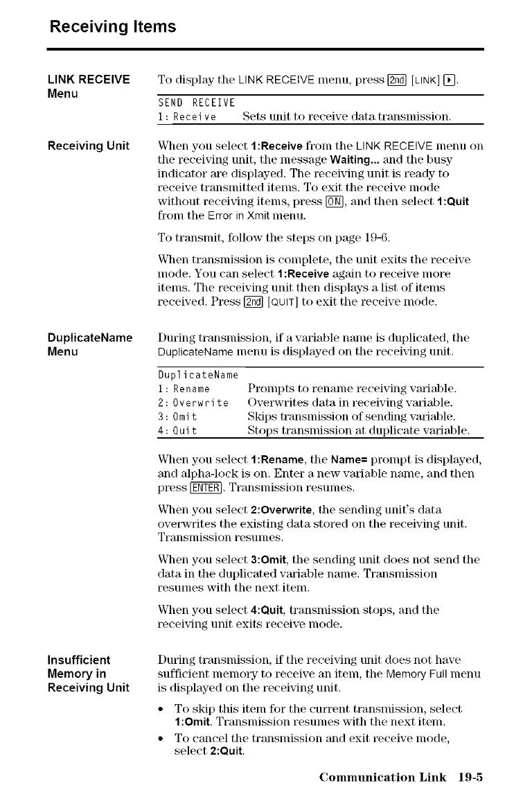
Receiving Items
LINK RECEIVE
Menu
Receiving Unit
DuplicateName
Menu
Insufficient
Memory in
Receiving Unit
To display the LINK RECEIVE menu, press _ [LINK] C_.
SEND RECEIVE
1 : Re ee i v e Sets unit to receive data transmission.
VClmnyou select 1:Receivefrom the LINK RECEIVE menu on
the receiving unit, the message Waiting... and the busy
indicator are displayed. The receiving unit is ready to
t_eeive transmitted items. To exit the receive mode
without receiving items, press [0N],and then select 1:Quit
from the Error in Xmit menu.
To transmit, follow the steps on page 19-6.
When transmission is complete, the unit exits the receive
mode. You can select 1:Receive again to receive mot_
items. The receiving unit then displays a list of items
received. Press [_ [QUIT] to exit the receive mode.
During transmission, if a variable name is duplicated, the
Dup[icateName menu is displayed on the receixqng unit.
Dupl i cateName
i : Rename
2: Overwrite
3: Omit
4: Quit
Prompts to rename receiving variable.
Ove_wvrites data in receiving variable.
Skips transmission of sending variable.
Stops transmission at duplicate variable.
When you select 1:Rename,the Name=prompt is displayed,
and alpha-lock is on. Enter a new variable name, and then
press [_. Transinission resuines.
When you select 2:Overwrite, the sending unit's data
ovet_vrites the existing data stored on the receiving unit.
Transmission resumes.
When you select 3:Omit, the sending unit does not send the
data in the duplicated variable name. Transmission
resumes with the next item.
When you select 4:Quit, transmission stops, and the
receiving unit exits receive mode.
During transmission, if the receiving unit does not have
sufficient lnelnol T to receive an item, the Memory Full lnenu
is displayed on the receiving unit.
• To skip this item for the current transmission, select
1:Omit. Transmission resumes with the next item.
• To cancel the transmission and exit receive mode,
select 2:Quit.
Communication Link 19-5
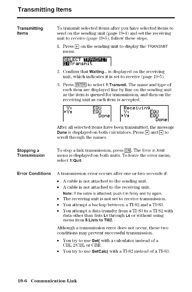
Transmitting Items
Transmitting
Items
Stopping a
Transmission
Error Conditions
To transmit selected items after you have selected items to
send on the sending unit (page 19-4) and set the receiving
unit to receive (page 19-5), follow these steps.
1. Press [] on tile sending unit to display- the TRANSMIT
nlenu,
I T%Ts I
2. Confirm that Waiting,.. is displayed on the receiving
unit, which indicates it is set to receive (page 19-5).
3. Press [g_-gm to select 1:Transmit. The name and type of
each item are displayed line by line on the sending unit
as the item is queued for transmission, and then on tile
receiving unit as each item is accepted.
*'799t EQoUoneEQUI*V_VIRotei_,,ing...EQ_oneEQUI
After all selected items have been transmitted, the lnessage
Done is displayed on both calculators. Press [] and [] to
scroll through the names.
To stop a link transmission, press []_]. The Error in Xmit
menu is displayed on both units. To leave the error menu,
select 1:Quit.
A transnlission error occurs after one or two seconds if:
• A cable is not attached to the sending unit.
• A cable is not attached to the receiving unit.
Note: If the cane is attached, push it in firmly and try again.
• The receiving unit is not set to receive transmission.
•You attempt a backup between a TI-82 and a TI-Sa.
•You attempt a data transfer from a TI-83 to a TI-82 with
data other than lists L1 through L6 or without using
menu item 5:Lists to TI82.
Although a transmission error does not occur, these two
conditions nlay prevent successful transmission.
• You ttT to use Get( with a calculator instead of a
CBL 2/CBL or CBR.
• You tit to use GetCalc( with a TI-82 instead of a TI-83,
19-6 Conununication Link
Transmitting
Items to an
Additional TI-83
After sending or receiving data, you can repeat the same
transmission to additional TI-83 units--from either the
sending unit or the receiving unit--without having to
reselect data to send. The current items remain selected.
Note: You cannot repeat transmission if you selected All+ or All-.
To transmit to an additional TI-83, follow these steps.
1, Set the TI-83 to receive (page 19-5),
2, Do not select or deselect any new items to send. If you
select or deselect an item, all selections or deselections
from the previous transmission are cleared.
3, Disconnect the link cable from one TI-S3 and connect it
to the additional TI-83,
4. Set the additional TI-83 to receive (page 19-5),
5, Press [7_ [LINK] on the sending TI-83 to display the
LINK SEND menu.
6, Select the menu item that you used for the l_kst
transmission. The data from your last transmission is
still selected.
7, Press [] to display the LINK TRANSMIT menu,
8, Confirm that the receiving unit is set to receive
(page 19-5).
9, Press [EfiY_ to select 1:Transmit and begin translnitting.
Communication Link 19-7
Transmitting Lists to a TI-82
Transmitting
Lists to a TI-82 The only data type you can transmit fronl a TI-83 to a TI-82
is list data stored in L1 through L6.
To transmit to a TI-82 the list data that is stored to TI-83
lists L1, L2, L3, L4, LS, or L6, follow these steps.
1, Set the TI-82 to receive (page 19-5).
2, Press [_ [LINK] 5on the sending TI-83 to select
5:Lists to TI82. The SELECT screen is displayed.
3, Select each list to transmit.
4. Press [] to display the LINK TRANSMIT menu,
5, Confirm that the receiving unit is set to receive
(page 19-5).
6, Press [_ to select 1:Transmit and begin transmitting.
Note: If dimension > 99 for a T1-83 list that is selected to send, the
receiving TI-82 will truncate the list at the ninety-ninth element during
transmission.
19-8 Coinnmnication Link
Transmitting from a TI-82 to a TI-83
Resolved
Differences
between the TI-82
and TI-83
Unresolved
Differences
between the TI-82
and TI-83
GenerMly, you can transmit items to a TI-83 fronl a TI-82,
but differences between tile two products may affect some
transmitted data, This table shows differences for which
the software built into the TI-83 automatically adjusts
when a TI-83 receives TI-82 data,
TI-82 TI-83
nMin PlotStart
nStart nMin
Un u
Vn v
UnStart u(nMin)
VnStart v(nMin)
TblMin TblStart
For example, if you transmit from a TI-82 to a TI-83 a
program that contains nStart on a command line and then
display" the p_ogram on the receiving TI-83, you will see
that nMin has automatically replaced nStart on the
conlnland line,
The s(dtware built into the TI-S3 cannot resolve some
differences between the TI-82 and TI-83, which are
described below. You nmst edit the data on the TI-83 after
you transmit to account for these differences, or the TI-83
will misinterpret the data.
The TI-83 reinterprets TI-82 prefix functions to include
()pen parentheses, which may add extraneous parentheses
to transmitted expressions.
For example, if you transmit sin X+5 from a TI-82 to a
TI-83, the TI-83 reinteq_rets it as sin(×÷5. Without a closing
parenthesis after ×, the TI-83 interprets this as sin(×÷5), not
the stun of 5and sin(X).
If a TI-82 instruction that the TI-83 cannot translate is
transmitted, the ERR:INVALID menu is displayed when the
TI-83 attempts to execute the instruction. For example, on
the TI-82, the chm'acter group Un-1 is pasted to the cursor
location when you press _ [un- 1]. The TI-83 cannot
directly translate Un-1 to the TI-83 syntax u(n-1), so the
ERR:INVALID menu is displayed.
Note: T1-83 implied multiplication rules differ from those of the T1-82.
For example, the TI-83 evaluates 1/2X as (1/2)*X, while the TI-82
evaluates 1/2X as 1/(2"X) (Chapter 2).
Communication Link 19-9
Backing Up Memory
Memory Backup
Receiving Unit
To copy the exact contents of lnelnol_y- in the sending TI-83
to the lnelnory of the receiving TI-83, put the other unit in
t_ceive mode. Then, on the receiving unit, select C:Back Up
fronl the LINK SEND menu.
Warning: C:Back Up ove_wvrites the lnelnol_y- in the
receiving unit; all information in the lnelnory of the
receiving unit is lost.
Note: If you do not want to do a backup, select 2:Quit to return to
the LINK SEND menu.
•Select 1:Transmit to begin transmission.
BItTt-ansr_ i t
2: Quit
As a safety check to prevent accidental loss of nlenlory,
the message WARNING - Backup is displayed when the
t_cei_lng unit receives notice of a backup.
• To continue with the backup process, select 1:Continue.
The backup transmission begins.
• To prevent the backup, select 2:Quit.
Note:If a transmissionerroris returnedduring a backup, the receiving
unitisreset.
Memory Backup When the backup is complete, both the sending calculator
Complete and receiving calculator display a confirlnation screen.
IMEMOR'? BACKUDPonel
19-10 (domnmnication Link
ATablesand Reference
Information
Contents Table of Functions and Instructions ..................... A-2
TI-83 Menu Map ......................................... A-39
Variables ................................................ A-49
Statistics Formulas ...................................... A-50
Financial Formulas ...................................... A-54
Tables and Reference Information A-1
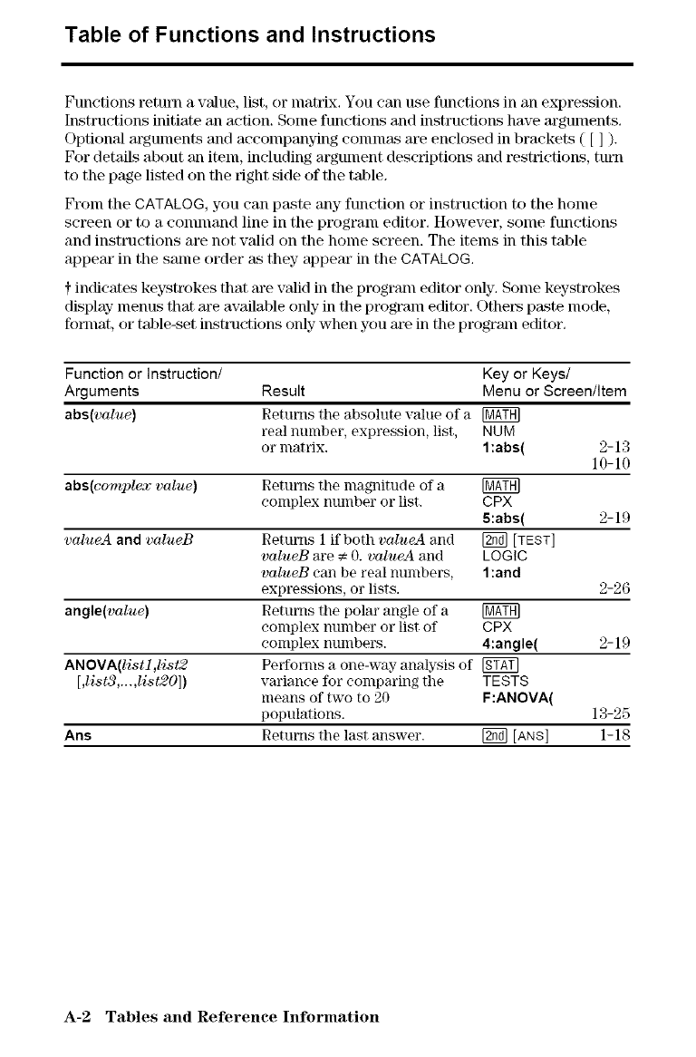
Table of Functions and Instructions
Functions return a value, list, or matrix. You can use functions in an expression.
Instructions initiate an action. Some functions and instructions have arguments.
Optional arguments and accompanying conunas are enclosed in brackets ( [ ] ).
For details about an item, including argument descriptions and restrictions, turn
to the page listed on the right side of the table.
From the CATALOG, you can paste any function or instruction to the home
screen or to a conunand line in the program editor. However, some functions
and instructions are not wflid on the home screen. The items in this table
appear in the same order as they- appear in the CATALOG.
f indicates keystrokes that are valid in the program editor only. Some keystrokes
display menus that are available only in the program editor. Others paste mode,
fommt, or table-set instructions only- when you are in the program editor.
Function or Instruction/ Key or Keys/
Arguments Result Menu or Screen/Item
abs(value) Returns the absolute value of a [_
real number, expression, list, NUM
or matrix. 1:abs( 2-13
10-10
abs(complex 'value) Returns the nmgnitude of a
complex nmnber or list. CPX
5:abs( 2-19
valueA and valueB Returns 1 if both valueA and [_ [TEST]
valueB are € 0. valueA and LOGIC
valueB ean be real numbers, 1:and
expressions, or lists. 2-26
angle{value) Returns the polar angle of a [_
complex number or list of CPX
complex numbers. 4:angle( 2-19
ANOVA(listl,list2 Performs a one-way analysis of [gg_]
[,list3,...,list20]) variance for comparing the TESTS
means of two to 20 F:ANOVA(
populations. 13-25
Ans Returns the last answer. [_ [ANS] 1-18
A-2 Tables and Reference Information
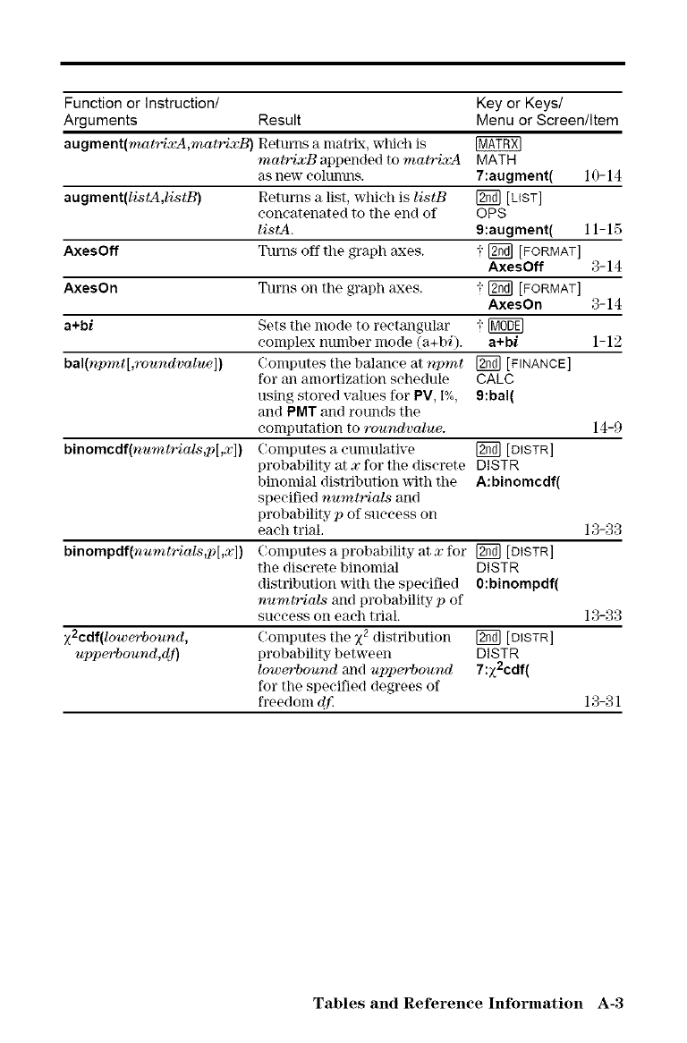
Function or Instruction/ Key or Keys/
Arguments Result Menu or Screen/Item
augment(matrixA,matrixB) Retm'ns a mahlx, width is
matrixB appended to matrixA MATH
as new colunms. 7:augment( 10-14
augment(listA,listB) Returns a list, which is listB _ [LIST]
concatenated to tile end of OPS
listA. 9:augment( 11-15
AxesOff Turns off the graph axes. ; [2_ [FORMAT]
AxesOff 3-14
AxesOn Turns on tile graph axes. ; [2_ [FORMAT]
AxesOn 3-14
a+bl Sets tile mode to reetangular i I_
complex number mode (a+bi). a+bi 1-12
bal(npmt[,roundvalue]) Computes the balance at npmt [_ [FINANCE]
for an amortization schedule CALC
using stored values for PV, I%, 9:bal(
and PMT and rounds the
computation to roundvalue. 14-9
binomcdf(numtrials,p[,x]) Computes a cumulative [_ [D}STR]
probability at xfor the discrete DISTR
binomial distribution ,slth tile A:binomcdf(
specified numtrials and
probabilityp of success on
each trial. 13-33
binompdf(numtriols,p[,x]) Computes a probability at xfor [_ [DtSTR]
tile discrete binomial DISTR
distribution _ith tile specified 0:binompdf(
nuratrials and probabilityp of
success on each trial. 13-33
x2cdf(low6_pbound, Computes tile g2distribution _ [DISTR]
upperbound,dy') probability between DISTR
lower'bound and upped)ound 7:x2cdf(
for the specified degrees of
freedom dJ2 13-31
Tables and Reference Information A-3
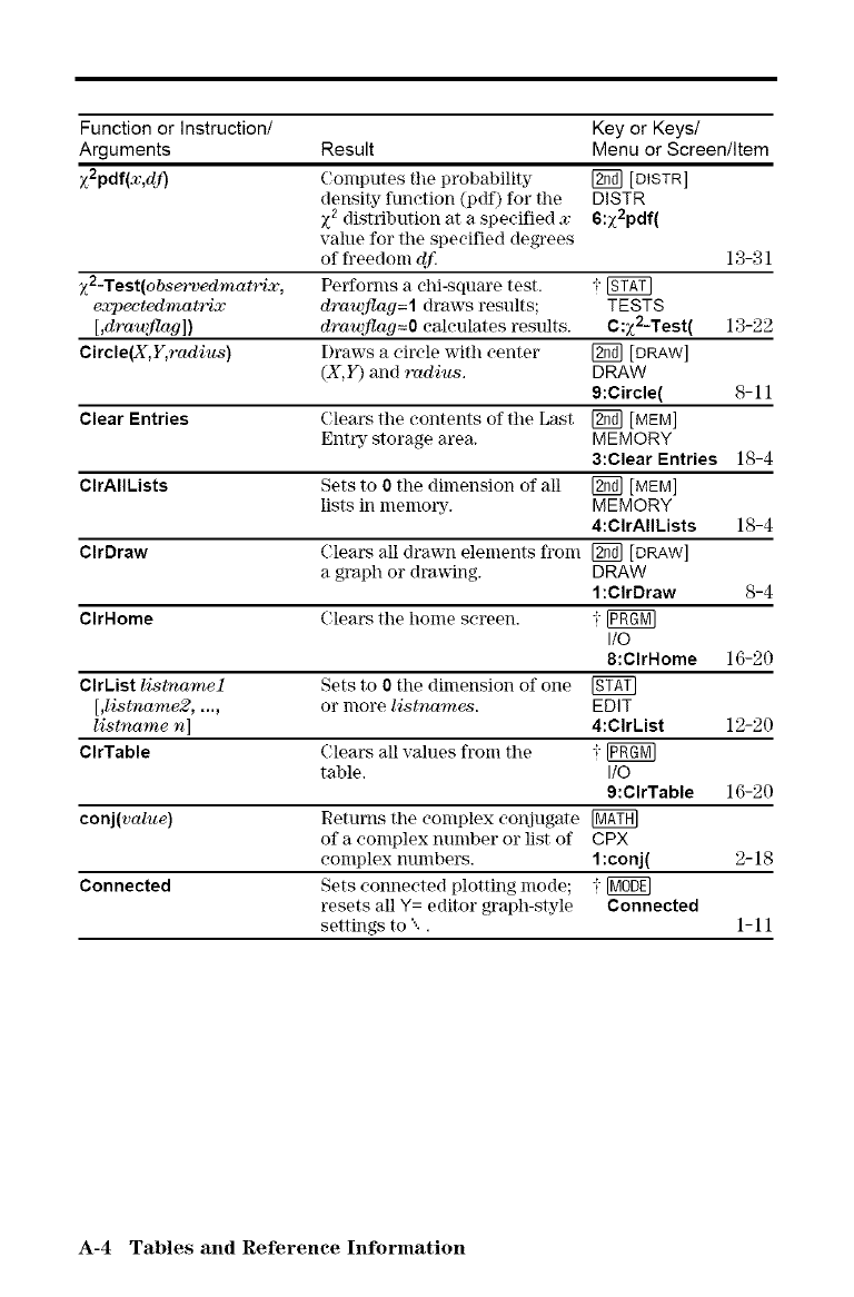
Function or Instruction/ Key or Keys/
Arguments Result Menu or Screen/Item
z2pdf(x,dj ") Computes the probabi]ity [_ [DISTR]
density function (pdf) for tile DISTR
X2 distribution at a specified x6:z2pdf(
value for the specified degrees
of freedom df 13-31
z2-Test(observedmatrix, Performs a ehi-square test. i [_
expeetedmatrix drmqflag=l draws results; TESTS
[,drawflag]) drmqflag=O calculates results. C:x2-Test( 13-22
Circle(X,Y, radius) Draws a circle with center [_ [DRAW]
(X,Y) and radius. DRAW
9:Circle( 8-11
Clear Entries Clears the contents of the Last [_dl [MEM]
EntKy storage area. MEMORY
3:Clear Entries 18-4
ClrAIILists Sets to 0the dimension of all [_ [MEM]
lists in memoKy'. MEMORY
4:ClrAIIkists 18-4
ClrDraw Clears all drawn elements from [_ [DRAW]
a graph or dra_lng. DRAW
1:ClrDraw 8-4
ClrHome Clears the home screen, i [0ggM]
IIO
8:Clrl-tome 16-20
Clrkist listnamel Sets to 0the dimension of one [gg_]
[,listuame2, ..., or more listnames. EDIT
listname n] 4:ClrList 12-20
ClrTable Clears all values from the i [gggM]
table. I/O
9:ClrTable 16-20
conj(value) Returns tile complex conjugate [_TH]
of a complex number or list of CPX
complex numbers. 1:conj( 2-18
Connected Sets connected plotting mode; i
resets all Y= editor graph-style Connected
settings to "... 1-11
A-4 Tables and Reference Information
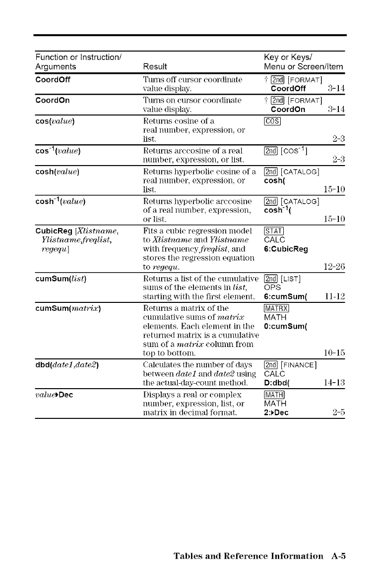
Function or Instruction/ Key or Keys/
Arguments Result Menu or Screen/Item
CoordOff TLims oft" cursor coordinate i- _ [FORMAT]
value display. CoordOff 3-14
CoordOn Turns on cursor coordinate 1 [2_ [FORMAT]
value display. CoordOn 3-14
cos(value) Returns cosine of a [g6N]
real nunlber, expression, or
list. 2-3
cos-l(volue) Returns arccosine of areal Kffd] [cos -1]
number, expression, or list. 2-3
cosh(value) Returns hyperbolic cosine of a Kffd] [CATALOG]
real number, expression, or cosh(
list. 15-10
cosh-l(value) Returns hyperbolic arccosine Kffd] [CATALOG]
of a real number, expression, cosh-l(
or list. 15-10
CubicReg [Xlistname, Fits a cubic regression model NTAf]
Ylistname_fr_qlist, to Xlistname and Ylistname CALC
regequ] with frequencyfrvqlist, and 6:CubicReg
stores tile regression equation
to vegequ. 12-26
cumSum(list) Returns a list of the cumulative [_ [LIST]
stuns of tile elements in list, OPS
starting _lth the first element. 6:cumSum( 11-12
cumSum(matrix) Returns a matrix of tile
cunmlative sums of matrix MATH
elements. Each element inthe 0:cumSum(
returned nmtrlx is a cunmlative
SUnl of a matrix cohlnln fi'om
to[) to bottom. 10-15
dbd(datel,date2) Calculates the number of days Kffa] [F,NANCE]
between date1 ram date2 using CALC
the actual-day-count method. D:dbd( 14-13
value_Dec Displays a real or complex
number, expression, list, or MATH
matrix in decimal format. 2:_Dec 2-5
Tables and Reference Information A-5
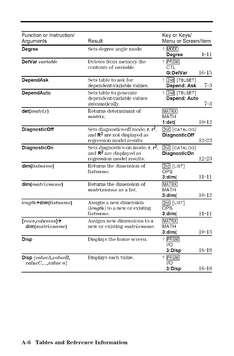
Function or Instruction/ Key or Keys/
Arguments Result Menu or Screen/Item
Degree Sets degree angle mode. i
Degree 1-11
DelVar variable Deletes from nlemolTy" the i
contents of .variable. CTL
G:DelVar 16-15
DependAsk Sets table to ask for -1-[_ [TBLSET]
dependent-variable values. Depend: Ask 7-3
DependAuto Sets table to generate -;- [_ [TBLSET]
dependentwariable values Depend: Auto
automatically. 7-3
det(matrix) Returns determinant of
matrix. MATH
l:det( 10-12
DiagnosticOff Sets dia_lostlcs-offmode; r, r2, _ [CATALOG]
and R2 are not displayed as DiagnosticOff
regression model results. 12-23
DiagnosticOn Sets diagnostics-on mode; r, r2, [_ [CATALOG]
and R2 m'e displayed as DiagnosticOn
regression model results. 12-23
dim(listname) Returns tile dilnenslon of [_ [LIST]
listname. OPS
3:dim( 11-11
dim(matri:vname) Returns tile dimension of
matri:_'name as a list. MATH
3:dim( 10-12
length->dim(listname) Assigns anew dimension _[LIST]
(length) to a new or existing OPS
listname. 3:dim( 11-11
{rows,columns}-> Assigns new dimensions to a
dim(matri:vname) new or existing matri:vname. MATH
3:dim( 10-13
Disp Displays the home screen. i IIO
3:Disp 16-18
Disp [valueA,valueB, Displays each value, i
valueC,...,value n] I/O
3:Disp 16-18
A-6 Tables and Reference Information
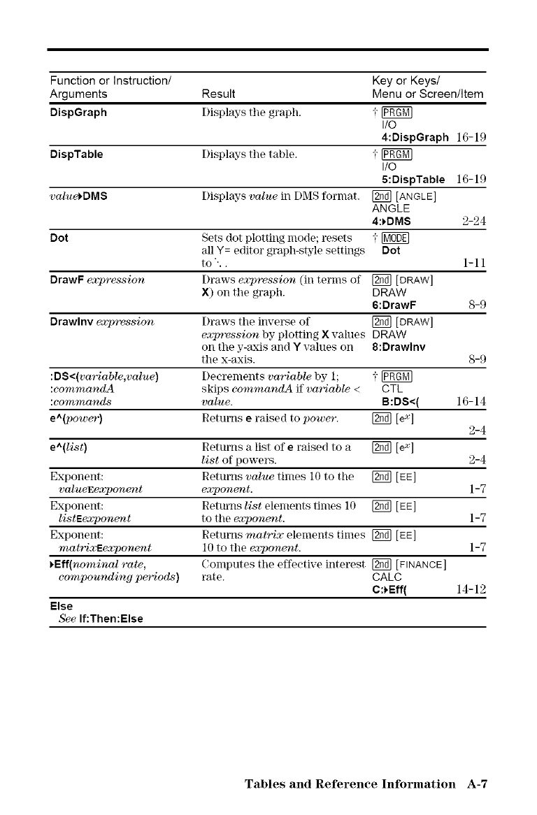
Function or Instruction/ Key or Keys/
Arguments Result Menu or Screen/Item
DispGraph Displays tile graph. ; I_
I/O
4:DispGraph 16-19
DispTable Displays tile table. -;-IIO
5:DispTable 16-19
value_DMS Displays value il1 [)MS fornlat. [_ [ANGLE]
ANGLE
4:_DMS 2-24
Dot Sets (lot plotting mode; resets i [_
all.Y= editor graph-style settings Dot
to ... 1-11
DrawF expression Draws expression (in terms of [_ [DRAW]
X) on the graph. DRAW
6:OrawF 8-9
Drawlnv expression Draws the immerse of [_ [DRAW]
expression by plotting X values DRAW
on the y-axis and Y values on 8:Drawlnv
the x-axis. 8-9
:DS<(variable,value) Decrements variable by 1; i
:commandA skips cornmandA if variable < CTL
:commands value. B:DS<( 16-14
e^(power) Returns e raised to power. _ [ex] 2-4
e^(list) Returns a list of e raised to a _ [ex]
list of powers. 2-4
Exponent: Returns value times 10 to the [_ [EE]
valueEexponez_t exponez_t. 1-7
Exponent: Retm'ns list elements times 10 [_ tEE]
listEe_onent to the exponent. 1-7
Exponent: Returns matrix elements times [_ tEE]
rnatrixEexponecnt 10 to the exponea_t. 1-7
_Eff(nominal rate, Computes the effective interest [_ [FINANCE]
compounding periods) rate. CALC
C:_Eff( 14-12
Else
See If:Then:Else
Tables and Reference Information A-7
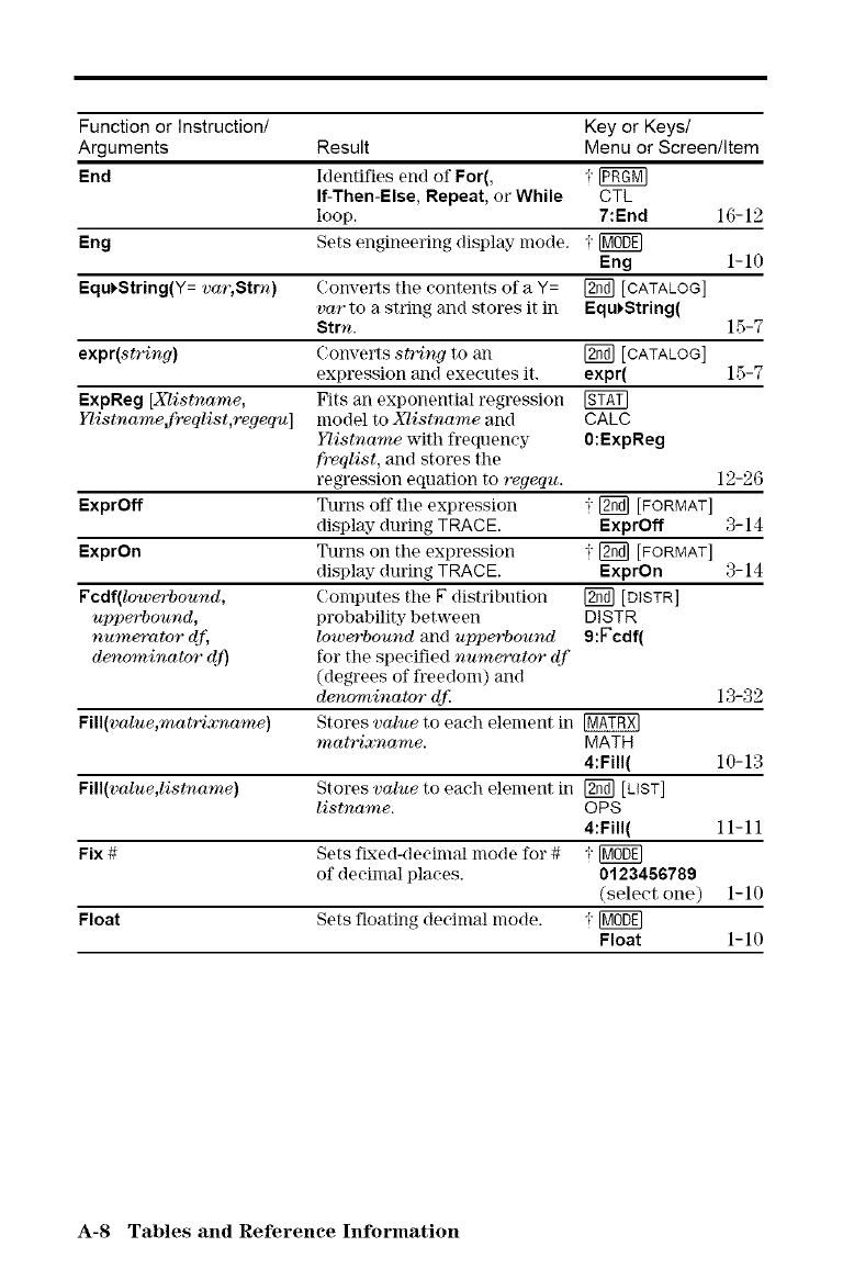
Function or Instruction/ Key or Keys/
Arguments Result Menu or Screen/Item
End Identifies end of For(, -;-
If-Then-Else, Repeat, or While CTL
loop. 7:End 16-12
Eng Sets engineering display mode. i
Eng 1-10
Equ)String(Y= va_;Stru) Converts tile contents of a Y= [_ [CATALOG]
vat to a string and stores it in Equ)String(
Stru. 15-7
expr(string) Com_erts SD'_ng to all [_ [CATALOG]
expression and executes it. expr( 15-7
ExpReg [Xlistname, Fits an exponential regression
}qistuame,flreqlist,regequ] model to Xlistuame and CALC
lqistuame with frequency 0:ExpReg
freqlist, and stores the
regression equation to regequ. 12-26
ExprOff Turns off the expression -;- [_ [FORMAT]
display during TRACE. ExprOff 3-14
ExprOn Turns on the expression -;- [_ [FORMAT]
display during TRACE. ExprOn 3-14
Fcdf(lowerbound, Computes the F distribution _M] [DISTR]
upperbound, probability between DISTR
numerator df, lowerbound and upperbound 9:Fcdf(
denominator dr) for the specified numerator df
(degrees of freedom) and
denominator djr 13-32
Fill(value,raatri:_name) Stores value to each element in
mat.ri:vname. MATH
4:Fill( 10-13
Fill(volue,listuame) Stores value to each element in _ [LIST]
listuame. OPS
4:Fill( 11-11
Fix # Sets fixed-decimal mode for # i
of decimal places. 0123456789
(select one) 1-10
Float Sets floating decimal mode. i Float 1-10
A-8 Tables and Reference Information
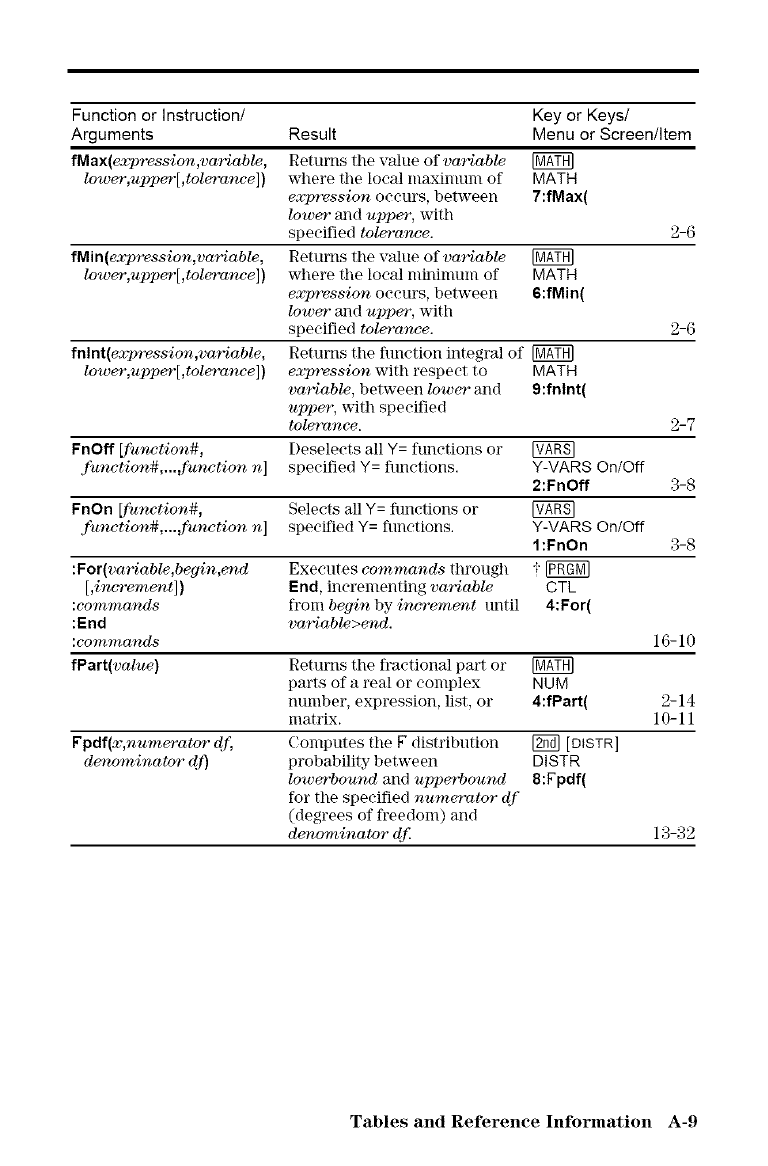
Function or Instruction/ Key or Keys/
Arguments Result Menu or Screen/Item
fMax(expression,variable, Retm'ns the value of variable
lower',upper'[,tolerance]) where the local maximum of MATH
expression occm's, between 7:fMax(
lower" and upper', with
specified toleronee. 2-6
fMin(expression,variable, Returns tile value of variable
lower',upper'[,toleranee]) where the local mininmn] of MATH
expression occm's, between 6:fMin(
lower" trod upper', with
specified toleronee. 2-6
fnlnt(expression,variable, Returns the function integral of [_
lower',upper'[,tolerance Dexpression with respect to MATH
variable, between/ower, and 9:fntnt(
upper', with specified
toleronce. 2-7
FnOff [function#, Deselects all Y= functions or
function#,...,function n] specified Y= functions. Y-VANS On/Off
2:FnOff 3-8
FnOn [function#, Selects all Y= fimctions or
.function#,..._function n] specified Y= functions. Y-VANS On/Off
1:FnOn 3-8
:For(variable,begin,er_d Executes commands through i [gggM]
[,incremer_t]) End, incrementing variable CTL
:commands fi'om begin by increment until 4:For(
:End variable>end.
:commands 16-10
fPart(value) Returns the fractional part or [_
pm'ts of a real or complex NUM
number, expression, list, or 4:fPart( 2-14
matrix. 10-11
Fpdf(x,numerotardf, Computes tile g distribution [_ [DtSTR]
denominator dy) probability between DISTR
lower'bound and upperbound 8:Fpdf(
for tile specified numerator df
(degrees of freedom) and
dermminator df 13-32
Tables and Reference Information A-9
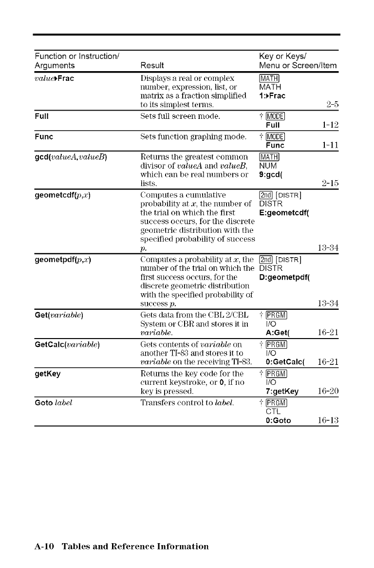
Function or Instruction/ Key or Keys/
Arguments Result Menu or Screen/Item
value_Frac Displays a real o1"eon]plex [_
nmnber, expression, list, or MATH
matrix as a fraction simplified 1 :_Frac
to its simplest terms. 2-5
Full Sets full screen mode. i [_
Full 1-12
Func Sets function graphing mode. i Func 1-11
gcd(valueA, valueB) Returns the greatest common [_
divisor of volueA and valueB, NUM
which can be realnmnbers or 9:gcd(
lists. 2-15
geometcdf_,x) (;omputes a emnulative [_ [DISTR]
probability at x, the number of DISTR
the trial on which the first E:geometcdf(
suceess oeeurs, for tile diserete
geometric distribution with tile
specified probability of success
p. 13-34
geometpdf(p,x) Computes a probability at x, the [_ [DISTR]
number of the trial on which the DISTR
first success occurs, for the D:geometpdf(
discrete geometric distribution
wlth the specified probability of
success p. 13-34
Get(variable) Gets data from the CBL 2/CBL -;-
System or CBR and stores it in I/O
variable. A:Get( 16-21
GetCalc(variable) Gets contents of variable on i
another TI-83 and stores it to I/O
variable on the receix_ N TI-83. 0:GetCalc( 16-21
getKey Returns tile key code for the i [0_
current keystroke, or 0, if no IIO
key is pressed. 7:getKey 16-20
Goto label Transfers control to label. iCTL
O:Goto 16-13
A-IO Tables and Reference Information
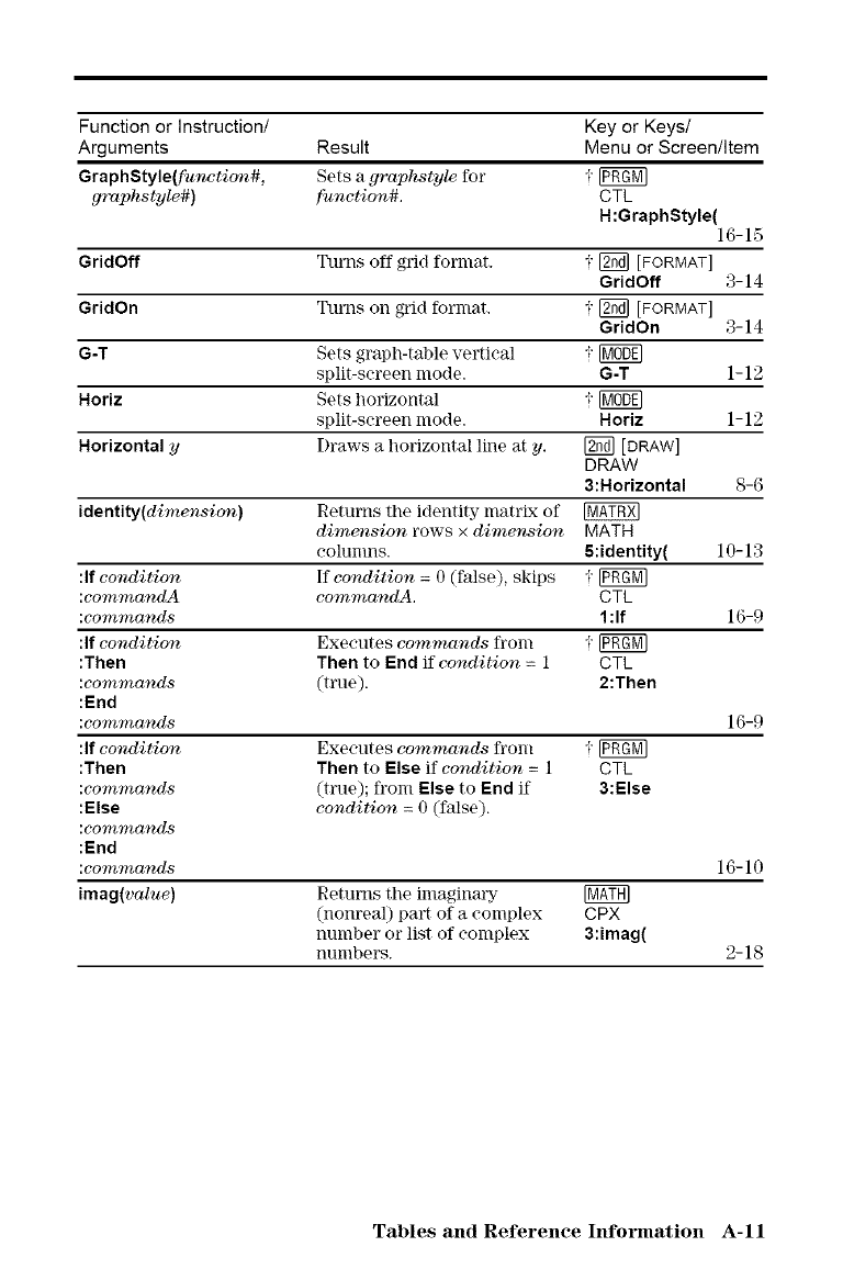
Function or Instruction/ Key or Keys/
Arguments Result Menu or Screen/Item
GraphStyle(function#, Sets a grophstyle for -;-
grophstyle#) function#. CTL
H:GraphStyle( 16-15
GridOff Turns off grid format, i- _ [FORMAT]
6ridOff 3-14
GridOn Turns on grid format. -;- _ [FORMAT]
GridOn 3-14
G-T Sets graph-table vertical i
split-screen mode. G-T 1-12
Horiz Sets horizontal i I_bg]
split-sereen mode. Horiz 1-12
Horizontal yDraws a horizontal line at y. [_ [DRAW]
DRAW
3:Horizontal 8-6
identity(dimension) Returns the identity matrix of
dimension rows x dimension MATH
eolumns. S:identity( 10-13
:If condition If condition = O (false), skips i [g_
:commandA commandA. CTL
:commands 1:If 16-9
:If condition Executes commands from i [0ggM]
:Then Then to End if condition = 1 CTL
:commands (true). 2:Then
:End
:commands 16-9
:If condition Executes commands from i [0ggM]
:Then Then to Else if condition = 1 CTL
:commands (true); from Else to End if 3:Else
:Else condition =O(false).
:commands
:End
:commands 16-10
imag(value) Returns the imaginmTy
(nonreal) part of a complex CPX
number or list of complex 3:imag(
numbers. 2-18
Tables and Reference hfformation A-11
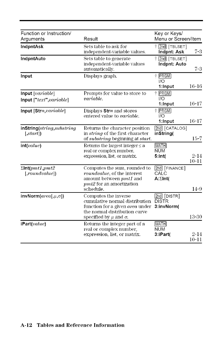
Function or Instruction/ Key or Keys/
Arguments Result Menu or Screen/Item
IndpntAsk Sets table to ask for -;-[_ [TBLSET]
independent-variable values. Indpnt: Ask 7-3
IndpntAuto Sets table to generate -1-[2_ [TBLSET]
independent-variable values Indpnt: Auto
automatically. 7-3
Input Displays graph. -1-
IIO
1:Input 16-16
Input [.variable] Prompts for value to store to i
Input ["text",variable] variable. I/0
1:Input 16-17
Input [Strn,variable] Displays Strn and stores -;-
entered value to variable. I/O
1:Input 16-17
inString(s#qng,subs#qng Returns tile (-haraeter position [_ [CATALOG]
[,start]) in string of tile first eharaeter inString(
of substring beginning at start. 15-7
int(value) Returns the lm'gest integer _<a [_TH]
real or complex ntmlber, NUM
expression, list, or matrkx. 5:int( 2-14
10-11
Elnt(pmtl,pmt2 Conlputes tile sum, rounded to [_ [FINANCE]
[,roundvalue]) roundvalue, of the interest CALC
amount between pmtl and A:Zlnt(
pint2 for an amortization
schedule. 14-9
invNorm(area[,p,_;]) Computes tile inverse _ [DtSTR]
emnulative normal distribution DISTR
funetion for a given area under 3:invNorm(
the normal distribution curve
specified by/_ and a. 13-30
iPart(value) Returns tile integer part of a
real or eomplex number, NUM
expression, list, or matrix. 3:iPart( 2-14
10-11
A-12 Tables and Reference Inforination
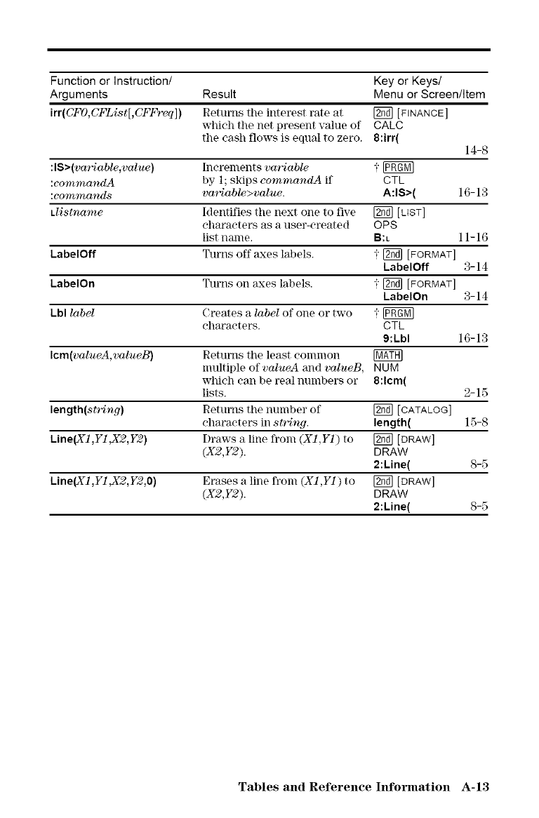
Function or Instruction/ Key or Keys/
Arguments Result Menu or Screen/Item
irr(OFO,OFList[,OFF_q]) Returns the interest rate at [_ [FINANCE]
which the net present vahle of CALC
file cash flows is equal to zero. 8:irr( 14-8
:lS>(variable,value) Increments variable i
:commandA by 1; skips commandA if CTL
:commands variable>volue. A:IS>( 16-13
Llistname Identifies the next one to five [_ [UST]
characters as a user-created OPS
list name. B:L 11-16
LabelOff Turns off axes labels. -1-[_ [FORMAT]
LabelOff 3-14
LabelOn Turns ol1 axes labels, i- [_ [FORMAT]
LabelOn 3-14
Lbl label Creates a label of one or two i
characters. CTL
9:Lbl 16-13
Icm(valueA,valueB) Returns the least conunon [_
inultiple of volueA and valueB, NUM
which can be real nulnbers or 8:lcm(
lists. 2-15
length(string) Returns the number of [_ [CATALOG]
chm'aeters in st_ng, length( 15-8
Line(X1,Y1Jd2,Y2) [)raws a line from (X1,Y1) to [_ [DRAW]
(X2,Y2). DRAW
2:Line( S-5
Line(X1,Y1,X2,Y2,0) Erases a line from (X1,Y1) to [_ [DRAW]
(X2,Y2). DRAW
2:Line( 8-5
Tables and Reference Information A-13
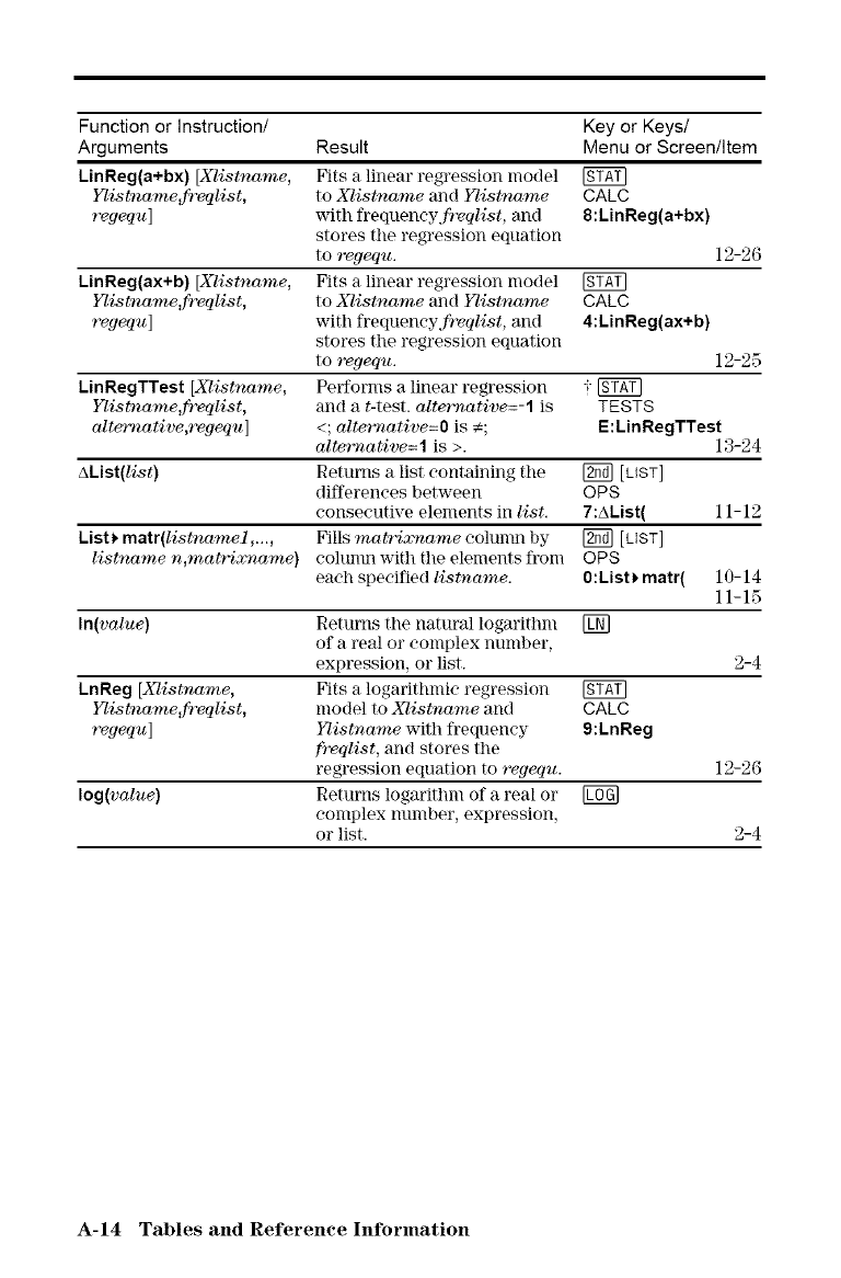
Function or Instruction/ Key or Keys/
Arguments Result Menu or Screen/Item
LinReg(a+bx) [Xlistname, Fits a linear regression inodel
Iqistname,freqlist, to Xlistname and Iqistname CALC
regequ] with frequencyfrvqlist, and 8:LinReg(a+bx)
stores the regression equation
to regequ. 12-26
kinReg(ax+b) [Xlistname, Fits a linear regression model [g_g]
Iqistname_freqlist, to Xlistname and Iqistname CALC
regequ] with frequency.fr_qlist, and 4:kinReg(ax+b)
stores the regression equation
to regequ. 12-25
LinRegTTest [Xlistname, Performs a linear regression i [g_g]
Iqistname,freqlist, and a t-test, alternative=-1 is TESTS
olternative,regequ] <; alternative=O is €; E:LinRegTTest
alternative=l is >. 13-24
AList(list) Returns a list containing the _[LIST]
differences between OPS
consecutive elements in list. 7:AList( 11-12
List_ matr(listnamel,..., Fills matrixname colunm by [_ [LIST]
listname n,matri:_'name) cohmm with the elements from OPS
each specified listuame. 0:List _matr( 10-14
11-15
In(value) Returns the natural logarithm @
of a real or complex number,
expression, or list. 2-4
knReg [Xlistname, Fits a logarithmic regression [g_T]
Ylistname,fr_qlist, model to Xlistuame and CALC
regequ] }qistuame with frequency 9:LnReg
freqlist, and stores the
regression equation to regequ. 12-26
log(value) Returns logarithm of a real or [[OG]
complex nilnlber, expression,
or list. 2-4
A-14 Tables and Reference Information
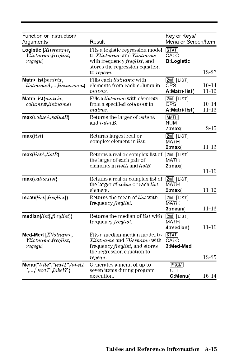
Function or Instruction/ Key or Keys/
Arguments Result Menu or Screen/Item
Logistic [Xlistname, Fits a logistie regression mode] [gTAT]
YTist.name,fr_ql.ist, to Xlistname and YTistname CALC
regequ] with frequeneyfr_qlist, and B:kogistic
stores the regression equation
to regequ. 12-27
Matr_ list(matrix, Fills each listname with [_ [LIST]
listnameA,...,listname n) elements from eaeh column in OPS 10-14
matrix. A:MatO list( 11-16
MatrMist(mat.rix, Fills a listuame _lth elements [_ [LIST]
column#,listname) from a specified eoluran# in OPS 10-14
matrix. A:MatO list( 11-16
rnax(valueA,valueB) Returns the larger of valueA
and valueB. NUM
7:rnax( 2-15
max(list) Returns largest real or [2_] [LIST]
complex element in list. MATH
2:max( 11-16
rnax(listA,listB) Retm'ns a real or eomplex list of [2_] [LIST]
the larger of each pair of MATH
elements in listA and listB. 2:max( 11-16
max(value, list) Retm'ns a real or complex list of [_ [LIST]
the larger of value or each list MATH
element. 2:max( 11-16
rnean(list[,frvqlist]) Returns the mean of list with [_ [LIST]
frequeney frvqlist. MATH
3:mean( 11-16
median(list[,fr_qlist]) Returns the median of list with [_ [LIST]
frequeney frvqlist. MATH
4:median( 11-16
Med-Med [Xlistname, Fits a median-median model to
Ylistname_fr_qlist, Xlistname and Ia'ist'name _lth CALC
regequ] frequeneyfrvqlist, and stores 3:Ned-Ned
the regression equation to
regequ. 12-25
Menu("title","textl"',labell Generates a menu of up to i [_
[,...,"textT',labelT]) seven items during program CTL
exeeution. C:Menu( 16-14
Tables and Reference hfformation A-15
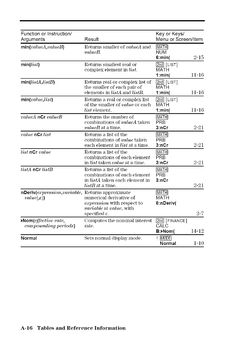
Function or Instruction/ Key or Keys/
Arguments Result Menu or Screen/Item
min(valueA,valueB) Returns smaller of valueA and
valueB. NUM
6:min( 2-15
min(list) Returns smallest real or _ [LIST]
complex element in list. MATH
l:min( 11-16
min(listA,listB) Returns real or complex list of [_ [LIST]
tile smaller of each pair of MATH
elements in listA and listB. 1:min( 11-16
min(value,list) Returns a real or complex list _ [LIST]
of the smaller of value or each MATH
list element. 1 :min( 11-16
valueA nCr valueB Returns the number of [_
combinations of valueA taken PRB
valueB at a time. 3:nOr 2-21
value nCr list Returns a list of the
combinations of value taken PRB
each element in list at a time. 3:nCr 2-21
list nCr value Returns a list of the
combinations of each element PRB
in list taken value at a time. 3:nCr 2-21
listA nCr listB Returns a list of the [_TH]
combinations of each element PRB
in listA taken each element in 3:nOr
listB at a time. 2-21
nDeriv(expression,variable, Returns approximate [_
value[,e]) numerical derivative of MATH
expression with respect to 8:nDeriv(
variable at value, with
specified e. 2-7
*Nom(ef_t_ct'ive rate, Computes the nominal interest [2_] [FINANCE]
compounding pe/riods) rate. CALC
B:*Nom( 14-12
Normal Sets normal display mode. i Normal 1-1O
A-16 Tables and Reference Information
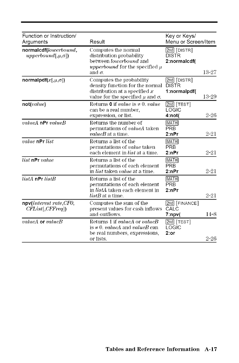
Function or Instruction/ Key or Keys/
Arguments Result Menu or Screen/Item
normalcdf(low_rbound, (;omputes tile normal [_ [DISTR]
upperbound [,_,(_])distribution probability D IST R
between low_rbound and 2:normalcdf(
upperbound for the specified p
and _. 13-27
normalpdf(x[,p,(_]) (;omputes tile probability [_ [DtSTR]
density function for the nornlal DISTR
distribution at a specified x1 :normalpdf(
value for tile specified/_ and c_. 13-29
not(value) Returns 0if value is :/: 0. value [_ [TEST]
can be a real number, LOG IC
expression, or list. 4:not( 2-26
valueA nPr valueB Returns tile number of [_TH]
permutations of volueA taken PRB
valueB at a time. 2:nPr 2-21
value nPr list Returns a list of tile [_TH]
permutations of value taken PRB
each element in list at a time. 2:nPr 2-21
list nPr value Returns a list of tile [_TH]
permutations of each element PRB
in list taken value at a time. 2:nPr 2-21
listA nPr listB Returns a list of tile [_TH]
permutations of each element PRB
in listA taken each element in 2:nPr
listB at a time. 2-21
npv(interest rate,CFO, Computes the sum of the [2_] [FINANCE]
CFList[,CFFreq]) present values for cash inflows CALC
and outflows. 7:npv( 14-8
valueA or volueB Returns 1 if valueA or volueB [2_] [TEST]
is € 0. volueA and valueB can LOGIC
be realnumbers, expressions, 2:or
or lists. 2-26
Tables and Reference hfformation A-17
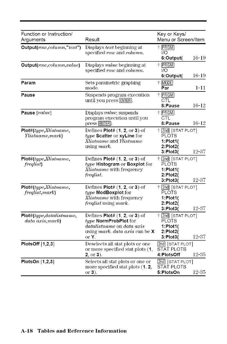
Function or Instruction/ Key or Keys/
Arguments Result Menu or Screen/Item
Output(vow,coluran,"text") Displays text beginning at i [P_M]
specified row and column. I/O
6:Output( 16-19
Output(row,column,value) Displays value begiJming at i [gggN]
specified row and column. I/O
6:Output( 16-19
Param Sets parametric graphing i
mode. Par 1-11
Pause Suspends program execution i [gggN]
until you press _. CTL
8:Pause 16-12
Pause ['value] Displays value; suspends i
program execution until you CTL
press [_. 8:Pause 16-12
Plot#(type,Xlistuame, Defines Plot# (1, 2, or 3) of 1 [2_] [STAT PLOT]
YTistname,mark} type Scatter 05"xyLine for PLOTS
Xlistuame and Iqistuame 1:Plot1(
using mark. 2:Plot2(
3:Plot3( 12-37
Plot#(type,Xlistuame, Defines Plot# (1, 2, 05"3) of ; [2_] [STAT PLOT]
,frvqlist) type Histogram 05"Boxplot for PLOTS
Xlistuame _lth frequency 1:Plot1(
fr_qlist. 2:Plot2(
3:Plot3( 12-37
Plot#(type,_istuame, Defines Plot# (1, 2, or 3) of -;-[_ [STAT PLOT]
.fr_qlist,mark) type ModBoxplot for PLOTS
Xlistname _lth frequency 1:Plot1(
frvqlist using mark. 2:Plot2(
3:Plot3( 12-37
Plot#(type,datalistname, Defines Plot# (1, 2, 05"3) of -;-[_ [STAT PLOT]
data axis,mark) type NormProbPIot for PLOTS
datalistuame on data axis 1:Plot1(
using mark. data axis can be X 2:Plot2(
or Y. 3:Plot3( 12-37
PlotsOff [1,2,3] Deseleets all star plots or one _ [STAT PLOT]
or more specified stat [)lots (1, STAT PLOTS
2, 05"3). 4:PlotsOff 12-35
PlotsOn [1,2,3] Selects all stat plots o1" one or [_ [STAT PLOT]
more specified stat plots (1, 2, STAT PLOTS
or 3). 5:PlotsOn 12-35
A-18 Tables and Reference Information
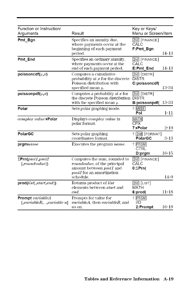
Function or Instruction/ Key or Keys/
Arguments Result Menu or Screen/Item
Pmt_Bgn Specifies an mmuity due, F2Ta] [FINANCE]
where payments occur at the CALC
beginning of each payment F:Pmt_Bgn
period. 14-13
Pmt_End Specifies an ordinary annuity, F2na][FINANCE]
where payments occur at the CALC
end of each payment period. E:Pmt_End 14-13
poissoncdf(,u,x) (;omputes a cumulative [_ [DtSTR]
probability at xfor the discrete DISTR
Poisson distribution with C:poissoncdf(
specified mean ,u. 13-34
poissonpdf(_,x) Computes a probabilii7 at xfor F2na][DtSTR]
the discrete Poisson distribution DISTR
with the specified nlean _. B:poissonpdf( 13-33
Polar Sets polar graphing mode. iPol 1-11
eomplex 'value i.Polar Displays eomplex 'value in
polar format. CPX
7:_Polar 2-19
PolarGC Sets polar graphing ; r2_ [FORMAT]
coordinates fornmt. PolarGC 3-13
prgmname Executes the program name. iCTRL
D:prgm 16-15
EPrn(pmtl,pmt2 Computes the sum, rounded to [_ [FINANCE]
[,roundvolue]) roundvalue, of the prineipal CALC
amount between pmtl and 0:EPrn(
pint2 for an amortization
schedule. 14-9
prod(list[,sta,r¢,e/nd]) Returns product of list [_ [LIST]
elements between start and MATH
end. 6:prod( 11-18
Prompt variableA Prompts for value for i [0ggM]
[,variableB,...,vaviable n] variableA, then variableB, and I/O
so on. 2:Prompt 16-18
Tables and Reference hfformation A-19
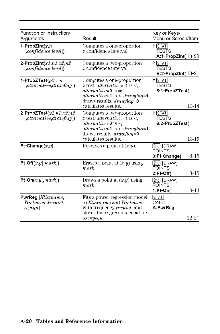
Function or Instruction/ Key or Keys/
Arguments Result Menu or Screen/Item
1-PropZlnt(x,n Computes a one-proportion i
[,confidence level]) z eonfidence interval. TESTS
A:l-PropZlnt( 13-20
2-PropZlnt(xl,nl ,x2,n2 Computes a two-proportion i
[,confidence level]) z eonfidence interval. TESTS
B:2-PropZlnt( 13-21
1-PropZTest(pO,x,n Computes a one-proportion i
[,alternative,drawflag]) ztest. olternative=-I is <; TESTS
alternative=O is _; 5:1-PropZTest(
alternative=l is >. d'rmqflog=l
draws results; drawflog=O
calculates results. 13-14
2-PropZTest(xl ,nl ,x2,n2 Computes a two-proportion i [g_g]
[,alternative,drawflog]) ztest. olternative=-I is <; TESTS
alternative=O is €; 6:2-PropZTest(
alternative=l is >. drmqflog=l
draws results; drawflog=O
calculates results. 13-15
Pt-Change(x,y) Reverses a point at (x,y). [_ [DRAW]
POINTS
3:Pt-Change( 8-15
Pt-Off(x,y[,mark]) Erases a point at (x,y) using [_ [DRAW]
mark. POINTS
2:Pt-Off( 8-15
Pt-On(x,y[,mark]) Draws a point at (x,y) using [_ [DRAW]
mark. POINTS
l:Pt-On( 8-14
PwrReg [Xlistname, Fits a power regression model [g_
Ylistname,freqlist, to Xlistname and Ylistname CALC
regequ] with frequencyfr_qlist, and A:PwrReg
stores the regression equation
to regequ. 12-27
A-20 Tables and Reference Information
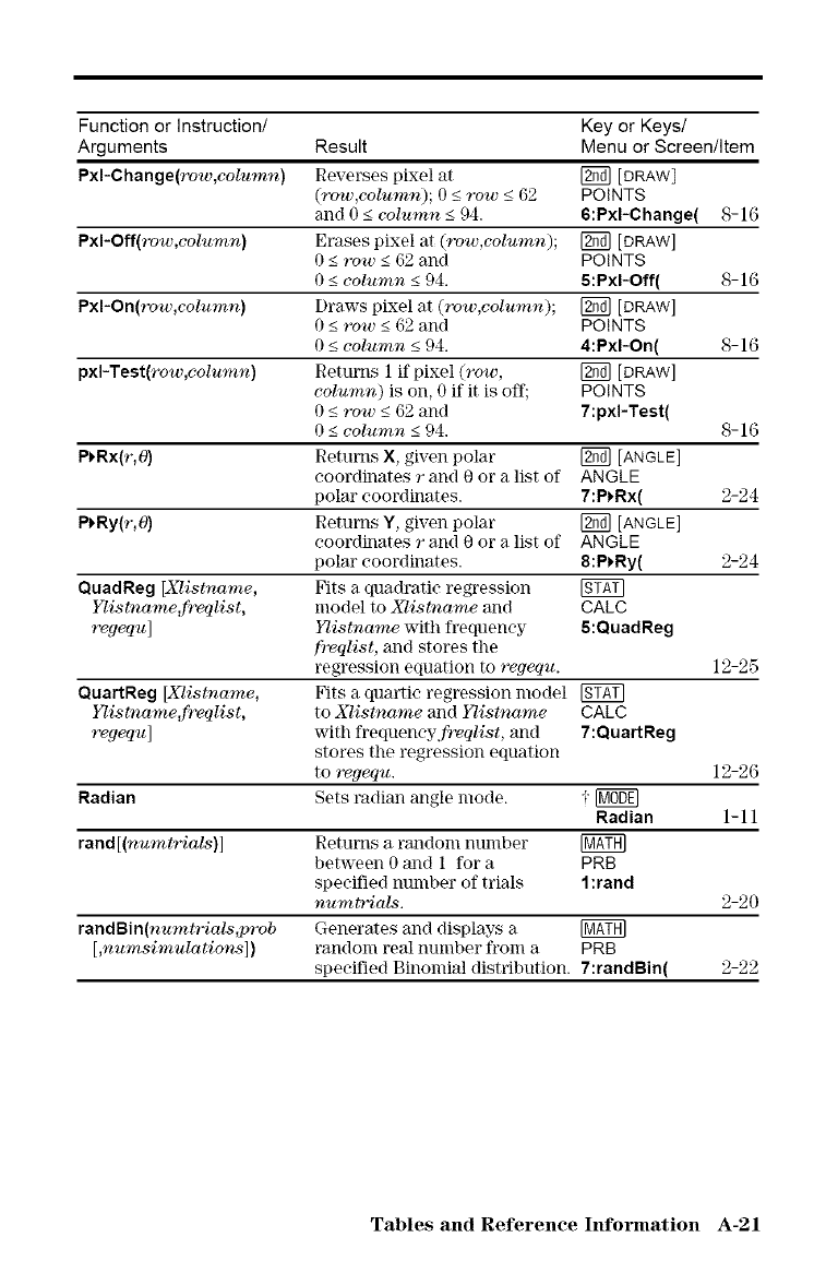
Function or Instruction/ Key or Keys/
Arguments Result Menu or Screen/Item
Pxl-Change(row,column) Reverses pixel at [_ [DRAW]
(_w,column); 0 <_row <_62 POINTS
and 0 _<column <_94. 6:Pxl-Change( S-16
Pxl-Off(row,column) Erases pixel at (_vw,eolumn); [_ [DRAW]
0 <-row <_62 and POINTS
0 <_column <_94. 5:PxI-Off( 8-16
Pxl-On(row,column) Draws pixel at (row,column); [_ [DRAW]
0 <-row <-62 and POINTS
0 <_column <_94. 4:PxI-On( 8-16
pxI-Test(row,column) Returns 1 if pixel (row, [_ [DRAW]
column) is on, 0 if it is oft'; POINTS
0 <_row <_62 and 7:pxI-Test(
0 <_column <_94. 8-16
P)Rx(r,0) Returns X, given polar [_ [ANGLE]
coordinates rand O or a list of ANGLE
polar coordinates. 7:P_.Rx( 2-24
P)Ry(r,O) Returns Y, given polar [_ [ANGLE]
eoordflmtes rand O or a list of ANGLE
polar coordinates. 8:P_.Ry( 2-24
QuadReg [Xlistname, Fits a quadratic regression [g_
Ylistname,fr_qlist, model to Xlistname and CALC
regequ] Iqist,name with frequency 5:OuadReg
frvqlist, and stores the
regression equation to regequ. 12-25
OuartReg [Xlistname, Fits a quartie regression model [gTfT]
Iqistname,frvqlist, to Xlistname and Iqistname CALC
regequ] with frequeneyfrvqlist, and 7:QuartReg
stores the regression equation
to regequ. 12-26
Radian Sets radian angle mode. i 1_
Radian 1-11
rand [(numtrials)] Returns a ral]dom nt:[mber [_
between 0 and 1 for a PRB
speeified number of trials 1 :rand
numtrials. 2-20
randBin(numtrials,prob Generates and displays a
[,numsimulations]) random real number from a PRB
specified Binonfial distribution. 7:randBin( 2-22
Tables and Reference hfformation A-21
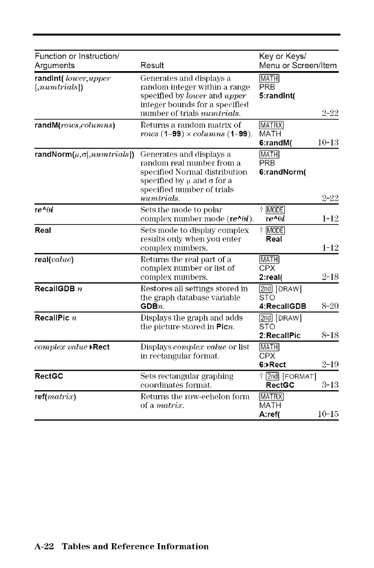
Function or Instruction/ Key or Keys/
Arguments Result Menu or Screen/Item
randlnt( lower, upper Generates all(] displays a [_tH]
[,numtrials]) randoln integer withil] a range PRB
specified by lower and upper S:randlnt(
integer bounds for a specified
number of trials numtrials. 2-22
randM(rows,columns) Returns a random matrix of [_
rows (1-99) x columns (1-99). MATH
6:randM( 10-13
randNorm(p,c_[,numtrials]) Generates and displays a
random real number from a PRB
specified Normal distribution 6:randNorm(
specified by p and _ for a
specified number of trials
numtriols. 2-22
re^Oi Sets tile mode to polar i
complex number mode (re^Oi). re^Oi 1-12
Real Sets inode to display complex i [M0_]
results only when you enter Real
complex numbers. 1-12
real(value) Returns the real part of a [_
complex number or list of CPX
complex numbers. 2:real( 2-18
RecaIIGDB nRestores all settings stored in [_ [DRAW]
tile graph database variable STO
GDBn. 4:RecallGDB 8-20
RecallPic nDisplays tile graph 31l(1 adds [_ [DRAW]
tile picture stored in Picn. STO
2:RecallPic S-1S
complex 'value _Rect Displays complex 'value or list
in rectangular format. CPX
6:_Rect 2-19
RectGC Sets rectangular graphing 1 _ [FORMAT]
coordinates format. RectGC 3-13
ref(matrix) Returns tile row-echelon forln
of a matrix. MATH
A:ref( 10-15
A-22 Tables and Reference Inforination
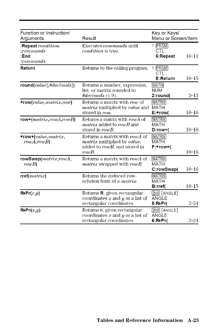
Function or Instruction/ Key or Keys/
Arguments Result Menu or Screen/Item
:Repeat condition Executes eommands until i [_
:commands condition is true. CTL
:End 6:Repeat 16-11
:commands
Return Returns to tile calling program. i [0ggM]
CTL
E:Return 16-15
round(value[,#deeimals]) Returns a number, expression, [_
list, or matrix rounded to NUM
#decimols (<_9). 2:round( 2-13
*row(value,matrix,row) Returns a matrix _lth row of
matrix nmltiplied by volue and MATH
stored in row. E:*row{ 10-16
row+(matrix,rowA,rowB) Returns a matrix _lth rowA of
matrix added to rowB and MATH
stored in rowB. D: row+( 10-16
*row+(value,matrix, Returns a matrix _lth rowA of
rowA,rowB) matrix nmltiplied by volue, MATH
added to rowB, and stored in F:*row+(
rowB. 1O- 16
rowSwap(matrix,rowA, Returns a matrix _lth rowA of
rowB) matrix swapped _lth rowB. MATH
C:rowSwap( 10-16
rref(matrix) Returns the reduced row-
echelon form of a matrix. MATH
B:rref( 10-15
R_Pr(x,y) Returns R, given reetanguhu" [2_ [ANGLE]
coordinates xand yor a list of ANGLE
rectangular coordinates. 5:R_Pr( 2-24
R_PO(x,y) Returns 0, given rectangular [_ [ANGLE]
coordinates xand yor a list of ANGLE
rectangular coordinates. 6:R_PO( 2-24
Tables and Reference hfformation A-23
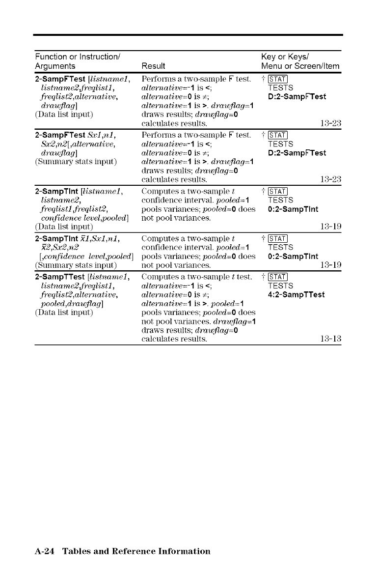
Function or Instruction/ Key or Keys/
Arguments Result Menu or Screen/Item
2-SampFTest [listnameZ, Performs a two-san]pie Ftest. i
listname2_fr_qlistl, alternative=-1 is <; TESTS
fr_qlist2,alternative, alternative=O is _; D:2-SampFTest
drowflag] alternative= l is >. drawflag= l
(Data list input) draws results; drawflag=O
calculates results. 13-23
2-8ampFTest Sxl,nl, Performs a two-sample F test. i
Sx2,n2[,alternative, alternative=-1 is <; TESTS
drowflag] alternative=O is _; D:2-SampFTest
(Summary stats input) alternative=l is >. drawflag=l
draws results; drawflog=O
calculates results. 13-23
2-SampTInt [listnamel, Computes a two-sample ti
listname2, confidence intm_'al, pooled=l TESTS
frvqlistl _frvqlist2, pools variances; pooled=O does 0:2-SampTInt
canfidezwe level,pooled] not pool variances.
(Data list input) 13-19
2-SampTInt 21,Sx1,n1, Computes a two-sample ti
22,Sx2,n2 confidence intm_,al, pooled=l TESTS
[,confidence level,pooled] pools variances; pooled=O does 0:2-SampTInt
(Sununary stats input) not pool variances. 13-19
2-SampTTest [listnamel,
listname2_frvqlistl ,
frvqlist2,alternative,
pooled,draw flag]
(Data list input)
Computes a two-sample ttest. i
alternative=-1 is <; TESTS
alternative=O is _; 4:2-SampTTest
alternative= l is >. pooled= l
pools variances; pooled=O does
not pool vm'iances, drawflog=l
draws results; drawflog=O
calculates results. 13-13
A-24 Tables and Reference Information
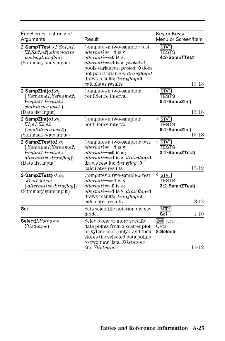
Function or Instruction/
Arguments
2-Sam pTTest 5l,Sxl,nl,
22 ,Sx2 ,n2[ ,olternative
pooled,draw.flag]
(Smmnary stats input)
2-SampZInt(_l,a,
[,listnamel ,listname2
frvqlistl _frvqlist2,
canfidence level])
(Data list input)
2-SampZlnt(_l,_,
_1,nl ,_2,n2
[,confidence level])
(Smmnary stats input)
2-SampZTest(_l,_
[,listnamel ,listname2
.frvqlistl ,frvqlist2,
alternative,drowflag])
(Data list input)
2-SampZTest(61 ,_,
_1 ,nl ,_2,n2
[,alternative,drawflog])
(Summary stats input)
Key or Keys/
Result Menu or Screen/Item
_r_tq
TESTS
4:2-SampTTest
TESTS
9:2-SampZlnt(
Computes a two-sample ttest.
alternative=-1 is <;
alternative=O is _;
alternative= l is >. pooled= l
pools variances; pooled=O does
not pool variances, drawflog=l
draws results; drawflog=O
calculates results.
Computes a two-sample z
confidence intm_al.
Computes a two-sample z
confidence intm_al.
13-13
13-18
TESTS
9:2-SampZlnt( 13-18
TESTS
3:2-SampZTest(
Computes a two-sample ztest.
alternative=-1 is <;
alternative=O is _ ;
alternative=l is >. drawflag=l
draws results; drawflag=O
calculates results. 13-12
Computes a two-sample ztest. i [gt_]
alternative=-1 is <; TESTS
alternative=O is ;_; 3:2-SampZTest(
alternative= l is >. draw.flag= l
draws results; drawflog=O
calculates results. 13-12
Sci Sets scientific notation display i [MODEl
mode. Sci 1-10
Select(Xlistname, Seleets one o1" more speeific _ [LIST]
Iqistname) data points from a scatter plot OPS
or xyLine plot (only), and then 8:Select(
stores the selected data points
to two new lists, Xlistname
and Ylistname. 11-12
Tables and Reference hfformation A-25
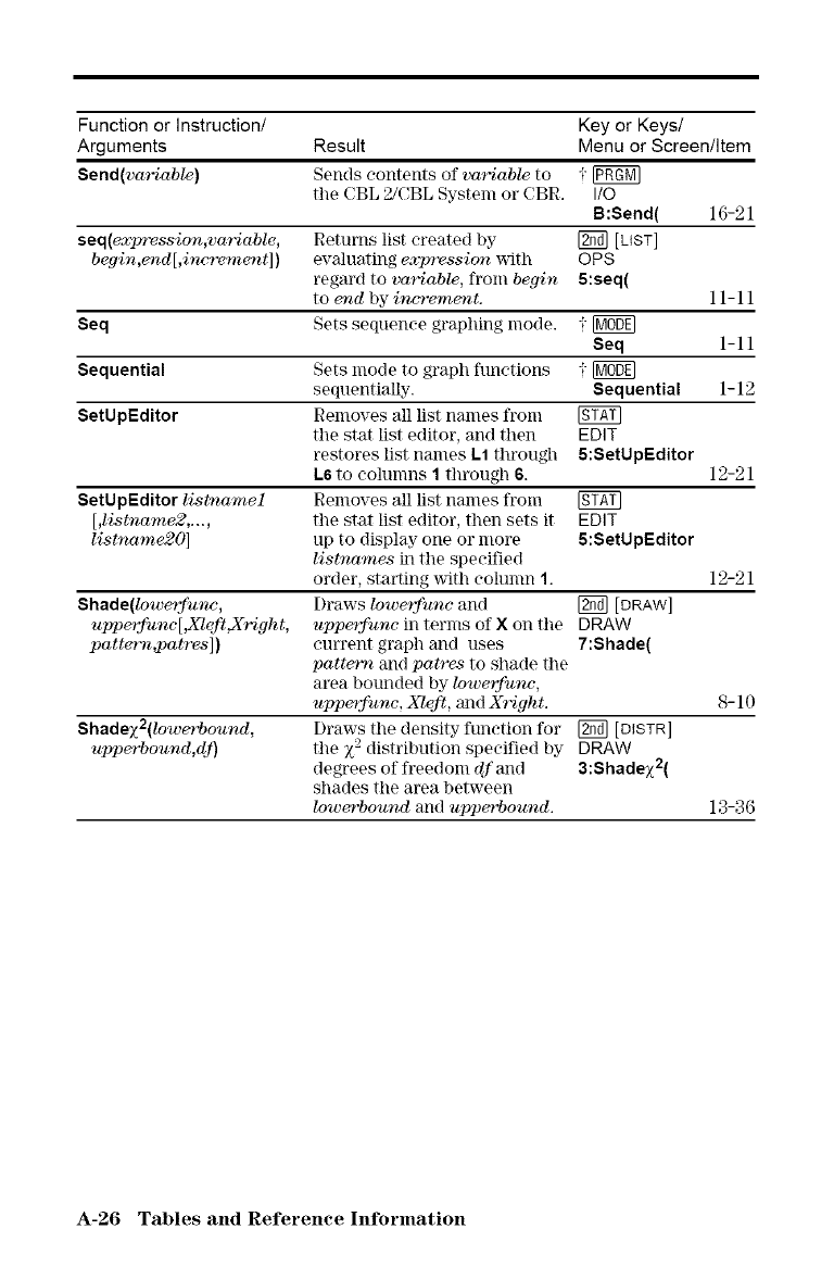
Function or Instruction/ Key or Keys/
Arguments Result Menu or Screen/Item
Send(variable} Sends contents of variable to -;-
the CBL 2/CBL System or CBR. I/O
B:Send( 16-21
seq(expression,variable, Returns list ereated by _ [LIST]
begin,end[,increment]) evaluating expression _lth OPS
regard to 'variable, from begin 5:seq(
to end by incremez_t. 11-11
Seq Sets sequence graphing mode. i
Seq 1-11
Sequential Sets mode to graph ftmetions i
sequentially. Sequential 1-12
SetUpEditor Removes all list names from
the stat list editor, all(] then EDIT
restores list names L1 through 5:SetUpEditor
L6 to eolumns 1 through 6. 12-21
SetUpEditor listnamel Removes all list names from
[,listname2,..., the stat list editor, then sets it EDIT
listname20] up to display one or more 5:SetUpEditor
listnames in the specified
order, starting _lth eohmm 1. 12-21
Shade(lowe:rfune, Draws lowerfune and [_ [DRAW]
upperfunc[,Xleft_rqght, upperfune in terms of Xon the DRAW
pattern,patres]) current graph and uses 7:Shade(
pattern and pat'r_s to shade the
area bounded by lowerfunc,
upperfunc, Xleft, and X'rqght. 8-10
Shadez2(lowerbound, Draws the density function for [_ [DISTR]
upperbound,dy') the Z2 distribution specified by DRAW
degrees of freedom dfand 3:Shade)_2(
shades tile area between
lowerbound and upper_ound. 13-36
A-26 Tables and Reference Information
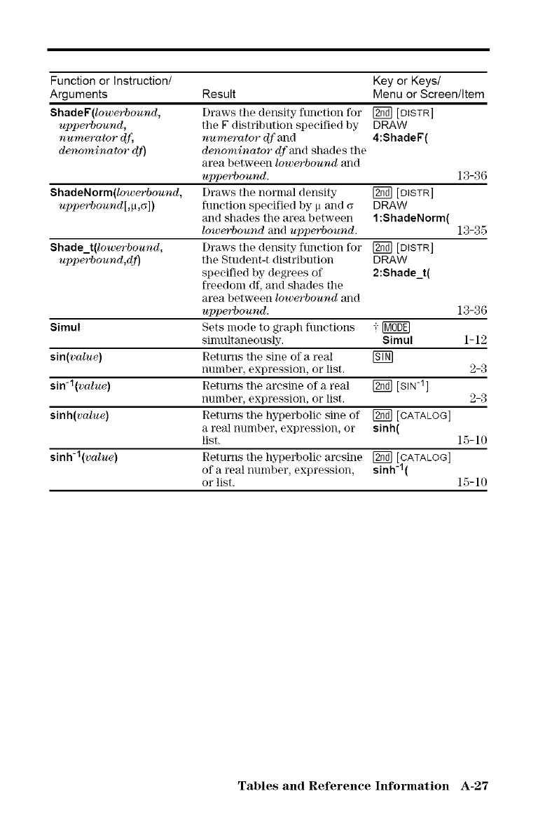
Function or Instruction/ Key or Keys/
Arguments Result Menu or Screen/Item
ShadeF(lowerbound, Draws the density function for _ [DISTR]
upperbound, the F distribution specified by DRAW
numerator df, numerator (lf and 4:ShadeF(
denominator d,f) denorainator df and shades the
area between lower'bound and
upperSound. 13-36
$hadeNorm(lower'bound, Draws the normal density _ [DISTR]
upper'bound[,p,G]) function specified by p and (_ DRAW
and shades the area between 1:ShadeNorm(
lower'bound and upper'bound. 13-35
Shade_t(lower'bound, Draws the density function for [_ [DISTR]
upperbound,dJ') the Student-t distribution DRAW
specified by degrees of 2:Shade_t(
freedom df, and shades the
area between lower'bound and
upperSound. 13-36
Simul Sets mode to graph functions i [_Dg]
simultaneously. Simul 1-12
sin(volue) Returns tile sine of a real Ig]N]
number, expression, or list. 2-3
sin-l(volue) Returns tile m-csine of a real [_ [SIN-1]
number, expression, or list. 2-3
sinh(volue) Returns tile hypet%olic sine of _ [CATALOG]
areal number, expression, or sinh(
list. 15-10
sinh-l(value) Returns the hyperbolic arcsine _ [CATALOG]
of a real number, expression, sinh -1(
or list. 15-10
Tables and Reference hfformation A-27
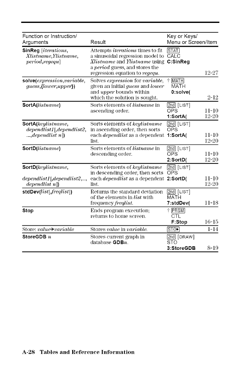
Function or Instruction/ Key or Keys/
Arguments Result Menu or Screen/Item
SinReg [iterations, Attempts iterations times to fit
Xlistname,I_istname, a sJnusoJdal regression model to CALC
period,regequ] Xlistname and Iqistname using C:SinReg
aperiod guess, and stores the
regression equation to regequ. 12-27
solve(expression,variable, Solves expression for variable, i
guess,{lower',upper_) given an initial guess and lower" MATH
and upper" bounds within 0:solve(
which the solution is sought. 2-12
SortA(listuame) Sorts elements of listname in _ [LIST]
ascending order. OPS 11-10
1:SortA( 12-20
SortA(keylistuame, Sorts elements of keylistuame [2_] [LIST]
dependlistl [,dependlist2, in ascending order, then sorts OPS
...,dependlist n]) each dependlist as a dependent l:Sorth( 11-10
list. 12-20
SortD(listuame) Sorts elements of listname in [_ [LIST]
descending order. OPS 11-10
2:SortD( 12-20
SortD(keylistuarae, Sorts elements of keylistuarae [_ [LIST]
in descending order, then sorts OPS
de_er_dlistl [,deper_dlist2,..., each dependlist as a dependent 2:SortD( 11-10
dependlist n]) list. 12-20
stdDev(list[,frvqlist]) Returns the standard deviation [_ [LIST]
of the elements in list with MATH
frequencyfrvqlist. 7:stdDev( ll-lS
Stop Ends program execution; i [gggM]
returns to home screen. CTL
F:Stop 16-15
Store: value_variable Stores value in variable. _ 1-14
StoreGDB nStores current graph in [_ [DRAW]
datahase GDBn. STO
3:StoreGDB 8-19
A-28 Tables and Reference Information
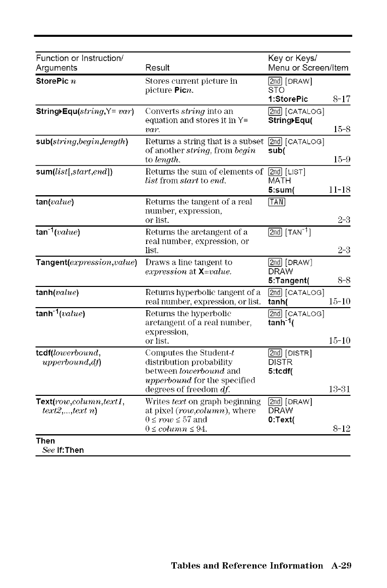
Function or Instruction/ Key or Keys/
Arguments Result Menu or Screen/Item
StorePic nStores eun'ent pleture in [_ [DRAW]
picture Picn. STO
l:StorePic 8-17
String_*Equ(string,Y= vat') Converts stt'ing iJlto an _ [CATALOG[
equation and stores it in Y: String_Equ(
vat_ 15-8
sub(string,begin,h_.ngth) Returns a string that is a subset [gffd][CATALOG]
of another string, from begin sub(
to length. 15-9
sum(list[,stat't,end]) Returns the sum of elements of [gffd][LIST]
list from start to end. MATH
5:sum( 11-18
tan(value) Returns the ttmgent of a real
nunlber, expression,
or list. 2-3
tan-l(value) Returns the aretangent of a [gffd][TAN-1]
real nunlber, expression, or
list. 2-3
Tangent(ea_ression,value) Draws a line tangent to [gffd][DRAW]
expression at X=value. D RAW
5:Tangent( 8-8
tanh(value) Returns hyperbolic tangent of a [_ [CATALOG]
real number, expression, or list. tanh( 15-10
tanh-l(value) Returns the hyperbolic _ [CATALOG]
aretangent of a real number, tanh-l(
expression,
or list. 15-10
tcdf(lowerbound, Computes the Student-t [2_ [DISTR]
upp_rbound,dJ_ distribution probability DISTR
between lower_ound and 5:tcdf(
upperSound for the specified
degrees of freedom 4/: 13-31
Text(row,column,textl, Writes text on graph beginning [_ [DRAW]
text2,...,text n) at pixel (row,column), where DRAW
0 <_row <_57 and 0:Text(
0 <_column <_94. 8-12
Then
See If:Then
Tables and Reference hfformation A-29
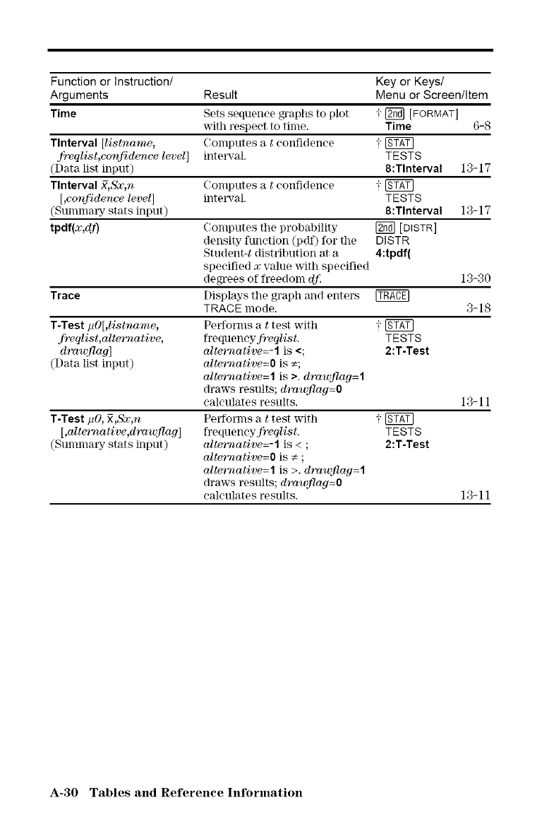
Function or Instruction/ Key or Keys/
Arguments Result Menu or Screen/Item
Time Sets sequenee graphs to plot -;-[_ [FORMAT]
with respect to time. Time 6-8
Tlnterval [listname, Computes a tconfidence i
.fr_qlist,eonfidence level] inte_ral. TESTS
(Data list input) 8:Tlnterval 13-17
Tlnterval ;7,Sx,n Computes a tconfidence i
[,confidence level] inte_ral. TESTS
(Summary stats input) 8:Tlnterval 13-17
tpdf(x,df) Computes the probability" [_ [DISTR]
density" function (pdf) for the DISTR
Student-t distribution at a 4:tpdf(
specified xvalue _ith specified
degrees of freedom ddq 13-30
Trace Displays the graph and enters
TRACE mode. 3-18
Performs a ttest with i
frequeneyfrvqlist. TESTS
alternative=-1 is <; 2:T-Test
alternative=O is €;
alternative= lis >. drawflag= l
draws results; drawfiag=O
calculates results. 13-11
Performs a ttest with i
frequeneyfrvqlist. TESTS
alternative=-1 is < ; 2:T-Test
alternative=O is €: ;
alternative=l is >. drawflag=l
draws results; drawf!og=O
ealeulates results. 13-11
T-Test pO[,listname,
frvqlist,alternative,
d'r'o_ag]
(Data list input)
T-Test pO, _,Sx,n
[,olternative,drawflag]
(Summary stats input)
A-30 Tables and Reference Information
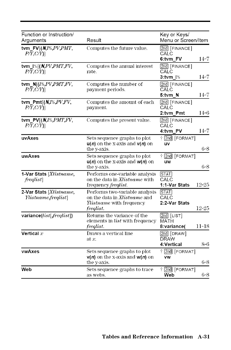
Function or Instruction/ Key or Keys/
Arguments Result Menu or Screen/Item
tvm_FV[(N,I%,PV,PMT, Conlptltes tile ftlture va]ue. [_ [FINANCE]
P/Y,C/Y) ] CALC
6:tvm_FV 14-7
tvm_I%[(N, PV,PMT,FV, (;omputes tile annual interest [_ [FINANCE]
PlY, C/Y)] rate. CALC
3:tvm_I% 14-7
tvm_N[(I%,PV, PMT,FV, (;omputes tile number of _ [FINANCE]
P/Y,C/Y)] payment periods. CALC
5:tvm_N 14-7
tvm_Pmt[(N,I%,PV,FV, (;omputes the amount of eaeh [_ [FINANCE]
P/If, C/Y)] payment. CALC
2:tvm_Pmt 14-6
tvm_PV[(N,I%,PMT,FV, (;omputes tile present value. [_ [FINANCE]
P/Y,C/Y) ] CALC
4:tvm_PV 14-7
uvAxes Sets sequence graphs to [)lot ; [2_] [FORMAT]
u(n)on the x-axis and v(n)on uv
the y-axis. 6-8
uwAxes Sets sequence graphs to [)lot ; [2_] [FORMAT]
u(n) on the x-axis and w(n) on uw
the y-axis. 6-8
1-Mar Stats [Xlistname, Performs one-variable analysis [gT_]
.frwqlist] on tile data in XTistname _ith CALC
frequeneyfrvqlist, l:l-Var Stats 12-25
2-Mar Stats [Xlistname, Performs two-variable analysis [gT_]
Ylistnarae,fr_qlist] on the data in Xlistnarae and CALC
Iaistname with frequeney 2:2-Mar Stats
fr_qlist. 12-25
variance(list[,fr_qlist]) Returns the variance of the [g_] [LIST]
elements in list wlth frequeney MATH
frvqlist. 8:variance( 11-18
Vertical xDraws a vertical line [_ [DRAW]
at x. DRAW
4:Vertical S-6
vwAxes Sets sequenee graphs to [)lot i- [2_] [FORMAT]
v(n) on the x-axis and w(n) on vw
the y-axis. 6-8
Web Sets sequence graphs to trace ; [2_] [FORMAT]
as webs. Web 6-8
Tables and Reference hfformation A-31
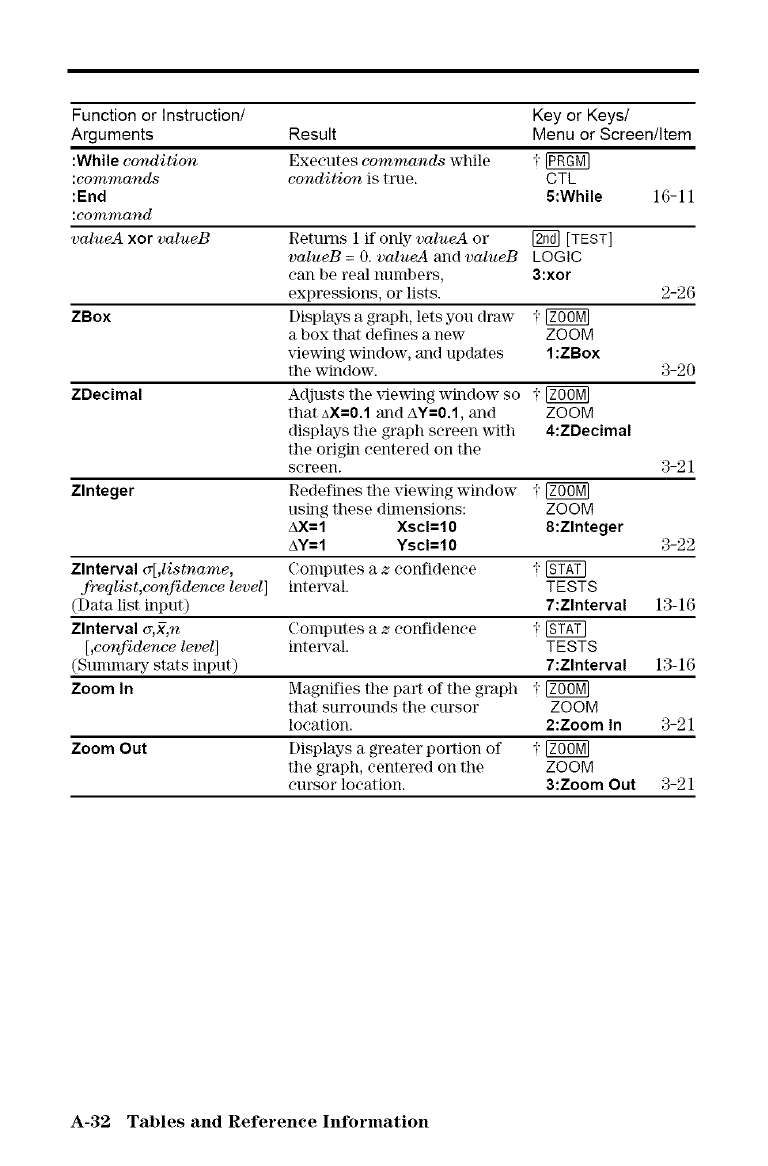
Function or Instruction/ Key or Keys/
Arguments Result Menu or Screen/Item
:While condition Executes commands while i
:commands condition is true. CTL
:End 5:While 16-11
:command
valueA xor valueB Returns 1 if only valueA or _ [TEST]
valueB = O. valueA and valueB LOGIC
can be real numbers, 3:xor
expressions, or lists. 2-26
ZBox Displays a graph, lets you draw -;-
a box that defines a new- ZOOM
_ewing window, and updates 1:ZBox
the window. 3-20
ZDecimal Adjusts tile _dewing window so i
that aX=0.1 and AY=0.1, and ZOOM
displays tile graph screen with 4:ZDecimal
tile origin centered on the
screen. 3-21
Zlnteger Redefines tile viewing window i
using these dimensions: ZOOM
AX=I XscI=10 8:Zlnteger
AY=I YscI=I 03-22
Zlnterval c_[,listname, Computes a zconfidenee i
.fr_qlist,confidence level] intel_al. TESTS
(Data list input) 7:Zlnterval 13-16
Zlnterval c_,;7,n Computes a zconfidenee i [_
[,confidence level] intel_al. TESTS
(Summary stats input) 7:Zlnterval 13-16
Zoom In Magnifies tile part of the graph i
that surrounds the eursor ZOOM
location. 2:Zoom In 3-21
Zoom Out Displays a greater portion of i
the graph, centered on the ZOOM
cursor location. 3:Zoom Out 3-21
A-32 Tables and Reference Inforination
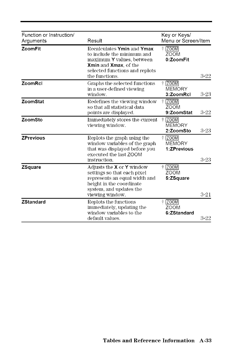
Function or Instruction/ Key or Keys/
Arguments Result Menu or Screen/Item
ZoomFit Recalculates Ymin and Ymax i
to hmlude tile nlininluni and ZOOM
nlaxinmm Yvalues, between O:ZoomFit
Xmin and Xmax, of the
selected functions and replots
tile functions. 3-22
ZoomRcl Graphs tile selected functions i
in a user-defined _dewing MEMORY
window. 3:ZoomRcl 3-23
ZoomStat Redefines tile viewing window i
so that all statistical data ZOOM
points are displayed. 9:ZoomStat 3-22
ZoomSto Immediately stores tile current i
viewing window. MEMORY
2:ZoomSto 3-23
ZPrevious Replots tile graph using the i
window variables of the graph MEMORY
that was displayed before you 1:ZPrevious
executed the last ZOOM
instruction. 3-23
ZSquare Adjusts tile X or Ywindow i
settings so that each pixel ZOOM
represents m] equal width and 5:ZSquare
height in the coordinate
system, and updates the
viewing window. 3-21
ZStandard Replots the functions i
immediately, updating the ZOOM
window variables to the 6:ZStandard
default values. 3-22
Tables and Reference Information A-33
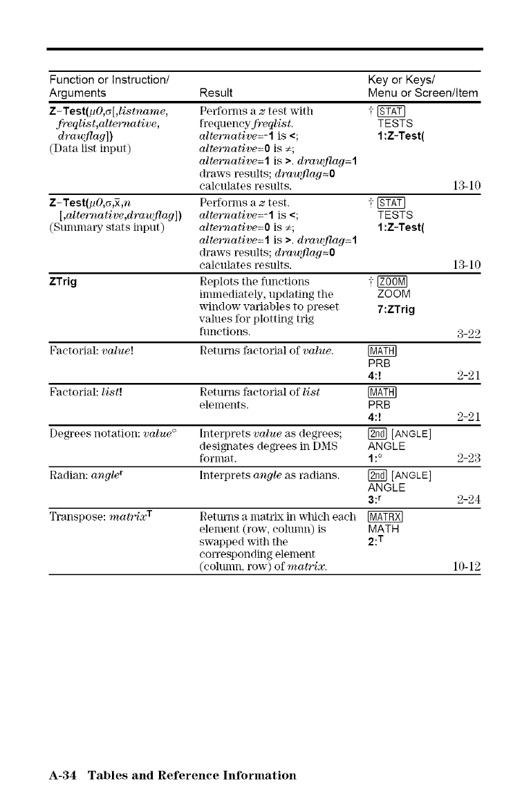
Functionor Instruction/
Arguments
Z-Test(pO,_[,listname, Performs a ztest with i [_
f_qlist,elternative, frequencyfreqlist. TESTS
drawflag]) alterr_ative=-I is <; 1:Z-Test(
(Data list input) alterr_ative=O is €;
alterr_ative= l is >. drawflag= l
draws results; drawflag=O
calculates results. 13-10
Z-Test(pO,_,_,n Performs a ztest. i
[,olterr_ative,drawflag]) alterr_ative=-I is <; TESTS
(Smmnary stats input) alterr_ative=O is €; 1:Z-Test(
alterr_ative=l is >. draw.flag=l
draws results; drawflog=O
calculates results. 13-10
ZTrig Replots the functions i
immediately, updating the ZOOM
window variables to preset 7:ZTrig
values for plotting trig
functions. 3-22
Factorial: value! Returns faetodal of value. PRB
4:! 2-21
Factorial: list! Returns factorial of list
elements. PRB
4:! 2-21
Degrees notation: value ° Interprets value as degrees; [_ [ANGLE]
designates degrees in [)MS ANGLE
fornlat. 1:° g-23
Radian: angle r Interprets angle as radim]s. [_ [ANGLE]
ANGLE
3: r g-24
Transpose: matrix T Retrains a matrix in wltich each
element (row, column) is MATH
swapped with tile 2: T
corresponding element
(cohmm, row) of matrix. 10-12
Key or Keys/
Result Menu or Screen/Item
A-34 Tables and Reference Information
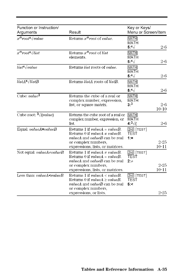
Function or Instruction/ Key or Keys/
Arguments Result Menu or Screen/Item
xt_ZrootX_value Retm'ns x_root of value. MATH
5:x_ 2-6
xtlZrootX_list Returns xthroot of list
elements. MATH
5:x-_ 2-6
listX_value Returns list roots of value. MATH
5:x-_ 2-6
listAX_listB Returns listA roots of listB. MATH
5:x-_ 2-6
Cube: value 3 Returns the cube of a real or [_TH]
complex nmnber, expression, MATH
list, or square matrix. 3:3 2-6
10-10
Cube root: 3_(value) Remms tile cube root of a real or
complex nmnber, expression, or MATH
list. 4:3_( 2-6
Equal: valueA=valueB Returns l lfvalueA = valueB. [_ [TEST]
Returns 0 if valueA _valueB. TEST
valueA and valueB can be real 1 :=
or complex numbers, 2-25
expressions, lists, or matriees. 1O- 11
Not equal: valueAcvalueB Returns 1 if valueA _valueB. [_ [TEST]
Returns 0 if valueA =volueB. TEST
valueA and volueB can be real 2:€
or complex nmnbers, 2-25
expressions, lists, or matrices. 10-11
Less than: valueA<valueB Returns 1 if volueA <volueB. [2T3] [TEST]
Returns 0 if volueA >_valueB. TEST
valueA and volueB can be real S:<
o1"eomplex nunlbers,
expressions, or lists. 2-25
Tables and Reference hfformation A-35
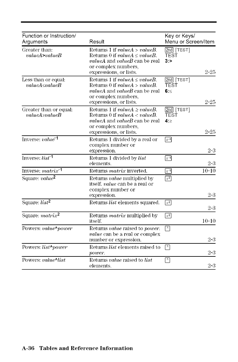
Function or Instruction/ Key or Keys/
Arguments Result Menu or Screen/Item
Greater than: Returns 1 if valueA > valueB. [_ [TEST]
valueA>valueB Returns 0 if valueA <_valueB. TEST
valueA and valueB can be real 3:>
O1" eonlplex llUIslbers_
expressions, or lists. 2-25
Less than or equal: Returns 1 if valueA <_valueB. _ [TEST]
volueA<_volueB Returns 0 if valueA >volueB. TEST
valueA and volueB can be real 6:_<
O1"eoIslplex nunlbers,
expressions, or lists. 2-25
Greater than or equal: Returns 1 if volueA 2 valueB. _ [TEST]
valueA>valueB Retunls 0 if volueA <valueB. TEST
valueA and volueB can be real 4:>
O1"eonlplex nunlbers,
expressions, or lists. 2-25
Inverse: value -1 Returns 1 dix_ded by a real or []
eonsplex nunsber or
expression. 2-3
Inverse: list -1 Returns 1 divided by list []
elements. 2-3
Inverse: matrix -1 Returns matrix inverted. [] 10-10
Squm'e: value 2 Returns value multiplied by []
itsel£ value can be a real or
eonlplex nunlber or
expression. 2-3
Square: list 2 Returns list elements squared. [] 2-3
Square: mat'ri:_ _ Returns matrix multiplied by []
itsel£ 10-10
Powers: value^power Returns value raised to power. []
value can be a real 05"eoinplex
number or expression. 2-3
Powers: list^power Returns list elements raised to []
power'. 2-3
Powers: value^list Returns value raised to list []
elements. 2-3
A-36 Tables and Reference Information
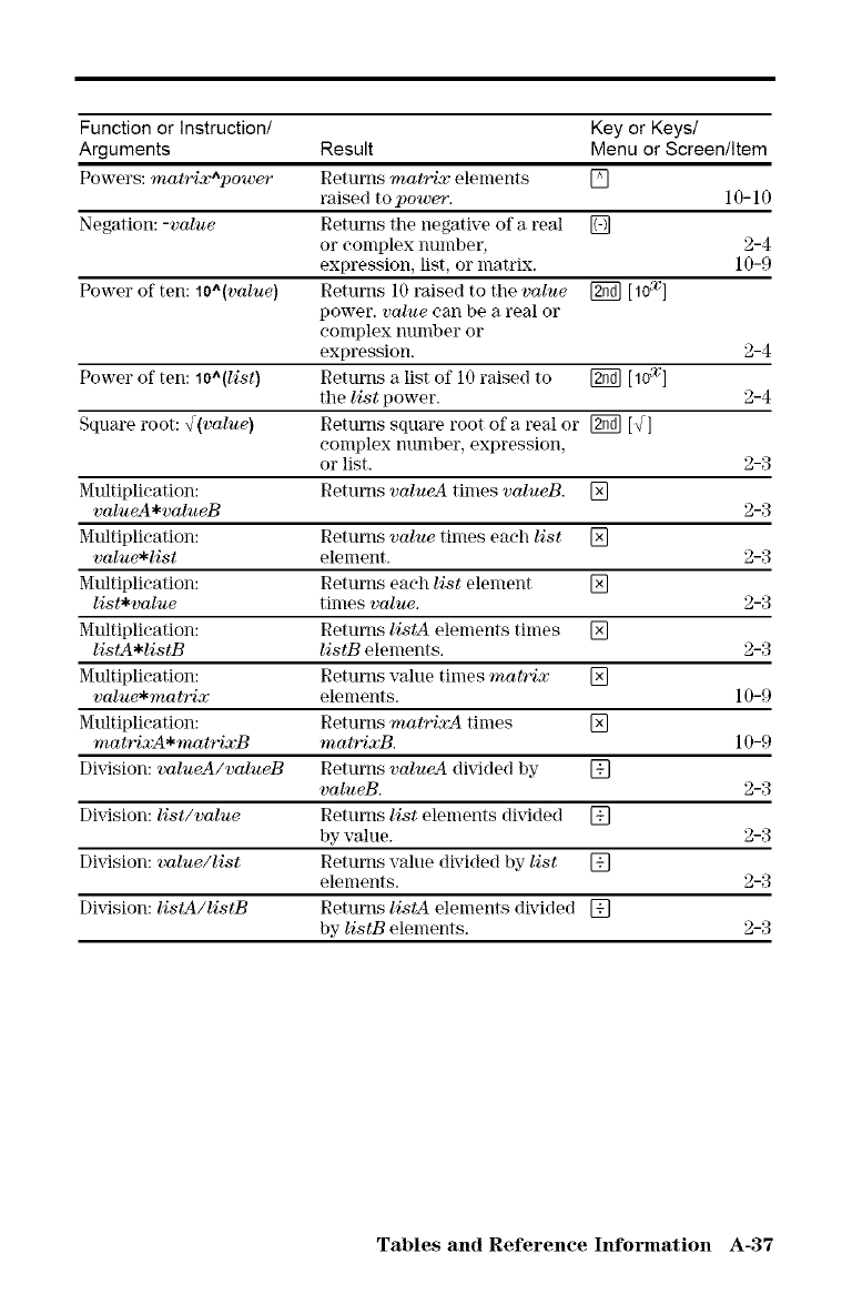
Function or Instruction/ Key or Keys/
Arguments Result Menu or Screen/Item
Powers: mat'rix^pow_" Returns matrix elements []
raised to power. 1O- 10
Negation: -volue Returns the negative of a real []
o1"complex number, 2-4
expression, list, o1"matrix. 10-9
Power of ten: lo^(volue) Returns 10 raised to tile value _ [10x]
power, volue can be a real or
conlplex ntlnlber or
expression. 2-4
Power of ten: lo^(list) Returns a list of 10 raised to _ [10x]
the list power. 2-4
Square root: ,[(value) Returns square root of a real or _ [_]
complex number, expression,
or list. 2-3
Multiplication: Returns volueA times volueB. []
volueA*valueB 2-3
Multiplication: Returns volue times each list []
volue*list element. 2-3
Multiplication: Returns each list element []
list*value times volue. 2-3
Multiplication: Returns listA elements times []
listA*listB listB elements. 2-3
Multiplieation: Returns value times matrix []
value*matrix elements. 10-9
Multiplication: Returns matrixA times []
matrixA*matrixB matrixB. 10-9
Division: valueA/valueB Returns valueA dMded by []
valueB. 2-3
Division: list/value Returns list elements dMded []
by value. 2-3
Division: value/list Returns value dMded by list []
elements. 2-3
Division: listA/listB Returns listA elements dMded []
by listB elements. 2-3
Tables and Reference hfformation A-37
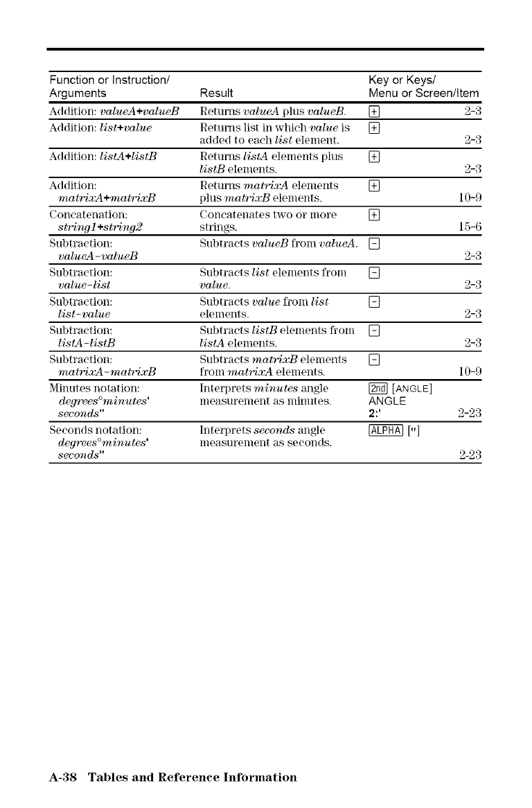
Function or Instruction/ Key or Keys/
Arguments Result Menu or Screen/Item
Addition: valueA+valueB Returns valueA plus valueB. [] 2-3
Addition: list+value Returns list in which value is []
added to each list element. 2-3
Addition: listA+listB Returns listA elements plus []
listB elements. 2-3
Addition: Returns matrixA elements []
matrixA+matrixB plus matrixB elements. 10-9
Concatenation: Concatenates two or more []
string l +string2 strings. 15-6
Subtraction: Subtracts valueB from val'ueA. []
valueA -valueB 2-3
Subtraction: Subtracts list elements from []
value-list value. 2-3
Subtraction: Subtracts value from list []
list- value elements. 2-3
Subtraction: Subtracts listB elements from []
listA-listB listA elements. 2-3
Subtraction: Subtracts matrixB elements []
matrixA-matrixB from matrixA elements. 10-9
Minutes notation: Interprets minutes angle [_ [ANGLE]
degrees°minutes ' nleasurement as minutes. ANGLE
seeonds" 2:' 2-23
Seconds notation: Interprets seconds angle @ [.]
degrees°minutes ' nleasurenlent as seconds.
seeonds" 2-23
A-38 Tables and Reference Information
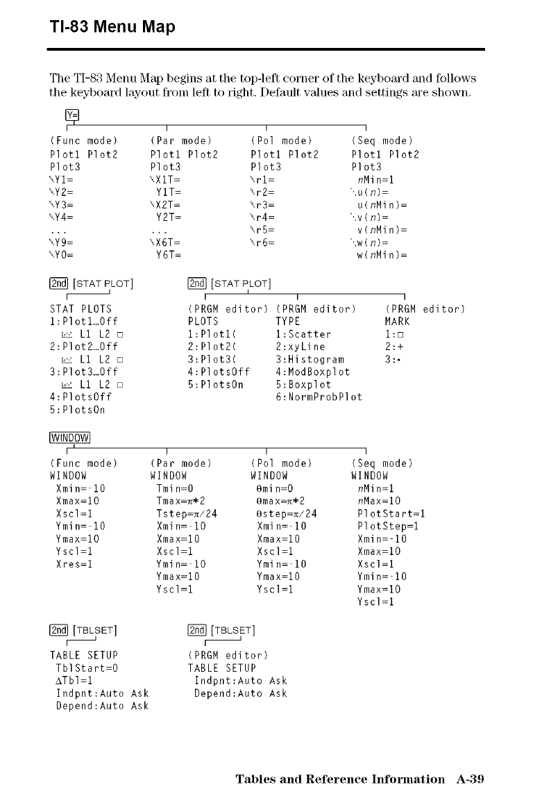
TI-83 Menu Map
The TI-83 Menu Map begins at the top-left corner of the keyboard and follows
tile keyboard layout from left to right. Default values and settings are shown,
IIII
(Func mode) (Par mode) (Pol mode) (Seq mode)
Plotl Plot2 Plotl Plot2 Plotl Plot2 Plotl Plot2
Plot3 Plot3 Plot3 Plot3
",,YI= ",XIT= ",rl= nMin=l
",,Y2= YIT= ",r2= ",u(n)=
",Y3= ",X2T= ",r3= u(nMin)=
",,Y4= Y2T= ",r4= ",v(n)=
...... ",rS= v(nMin)=
",,Y9= ",X6T= ",r6= ",w(n)=
",,YO= Y6T= w(nMin)=
[STATPLOT] [_][STATPLOT]
__1 I
I I I
STAT PLOTS (PRGM editor) (PRGM editor)
l:Plotl...Off PLOTS TYPE
_:L LI L2 m l:Plotl( l:Scatter
2:Plot2...Off 2:Plot2( 2:xyLine
_:L LI L2 _ 3:Plot3( 3:Histogram
3:Plot3...Off 4:PlotsOff 4:ModBoxplot
_:L LI L2 m 5:PlotsOn 5:Boxplot
4:PlotsOff 6:NormProbPlot
5:PlotsOn
I
(PRGM editor)
MARK
Z:D
2:+
3:,
III
(Func mode) (Par mode) (Pol mode)
WINDOW WINDOW WINDOW
Xmin= i0 Tmin=O Omin=O
Xmax=lO Tmax=_2 Omax=_2
Xscl=1 Tstep=_/24 Ostep=_/24
Ymin= 10 Xmin= 10 Xmin= 10
Ymax=10 Xmax=iO Xmax=iO
Yscl=1 Xscl=1 Xscl=1
Xres=1 Ymin= 10 Ymin= 10
Ymax=iO Ymax=iO
Yscl=1 Yscl=1
I
(Seq mode)
WINDOW
nMin=1
nMax=10
PlotStart=1
PlotStep=1
Xmin= i0
Xmax=lO
Xscl=l
Ymin= i0
Ymax=lO
Yscl=l
[TBLSET] _ [TBLSET]
iI FI
TABLE SETUP (PRGM editor)
TblStart=O TABLE SETUP
ATbI=I Indpnt:Auto Ask
Indpnt:Auto Ask Depend:Auto Ask
Depend:Auto Ask
Tables and Reference Information A-39
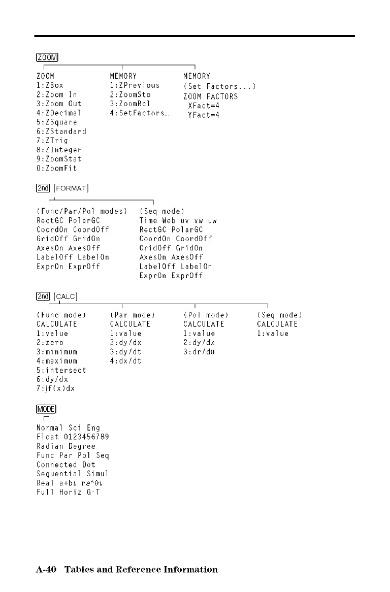
i I
ZOOM
1:ZBox
2:Zoom In
3:Zoom Out
4:ZDecimal
5:ZSquare
6:ZStandard
7:ZTrig
8:Zlnteger
9:ZoomStat
O:ZoomFit
I I
MEMORY MEMORY
1:ZPrevious (Set Factors,.,)
2:ZoomSto ZOOM FACTORS
3:ZoomRcl XFact=4
4:SetFactors_ YFact=4
[FORMAT]
I
I
(Func/Par/Po] modes)
RectGC PolarGC
CoordOn CoordOff
GridOff GridOn
AxesOn AxesOff
LabelOff LabelOn
ExprOn ExprOff
I
(Seq mode)
Time Web uv vw uw
RectGC PolarGC
CoordOn CoordOff
GridOff GridOn
AxesOn AxesOff
LabelOff LabelOn
ExprOn ExprOff
[CALC]
I
(Func mode)
CALCULATE
1:value
2:zero
3:minimum
4:maximum
5:intersect
6:dy/dx
7:if(x)dx
I
(Par mode)
CALCULATE
1:value
2:dy/dx
3:dy/dt
4:dx/dt
I
(Pol mode)
CALCULATE
1:value
2:dy/dx
3:dr/dO
H
Normal Sci Eng
Float 0123456789
Radian Degree
Func Par Pol Seq
Connected Dot
Sequential Simul
Real a+bt re^Bt
Full Horiz G T
I
(Seq mode)
CALCULATE
1:value
A-40 Tables and Reference Information
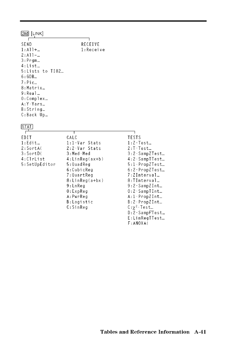
I
SEND
1:A11+...
2:All-...
3:Prgm...
4:List._
5:Lists to T182...
6:GDL
7:Pic._
8:Matrix...
9:Real._
O:Complex._
A:Y Vars...
B:String._
C:Back Up...
I
RECEIVE
1:Receive
i I
EDIT
1:Edit._
2:SortA(
3:SortD(
4:ClrList
5:SetUpEditor
I
CALC
1:1Var Stats
2:2 Var Stats
3:Med Med
4:LinReg(ax+b)
5:QuadReg
6:CubicReg
7:QuartReg
8:LinReg(a+bx)
9:LnReg
O:ExpReg
A:PwrReg
B:Logistic
C:SinReg
I
TESTS
I:Z Test...
2:T Test...
3:2 SampZTest...
4:2 SampTTest...
5:1 PropZTest...
6:2 PropZTest...
7:Zlnterval...
8:Tlnterval...
9:2 SampZlnt._
0:2 SampTlnt._
A:I PropZlnt._
B:2 PropZlnt._
C:Z 2 Test...
D:2 SampFTest._
E:LinRegTTest...
F:ANOVA(
Tables and Reference Information A-41
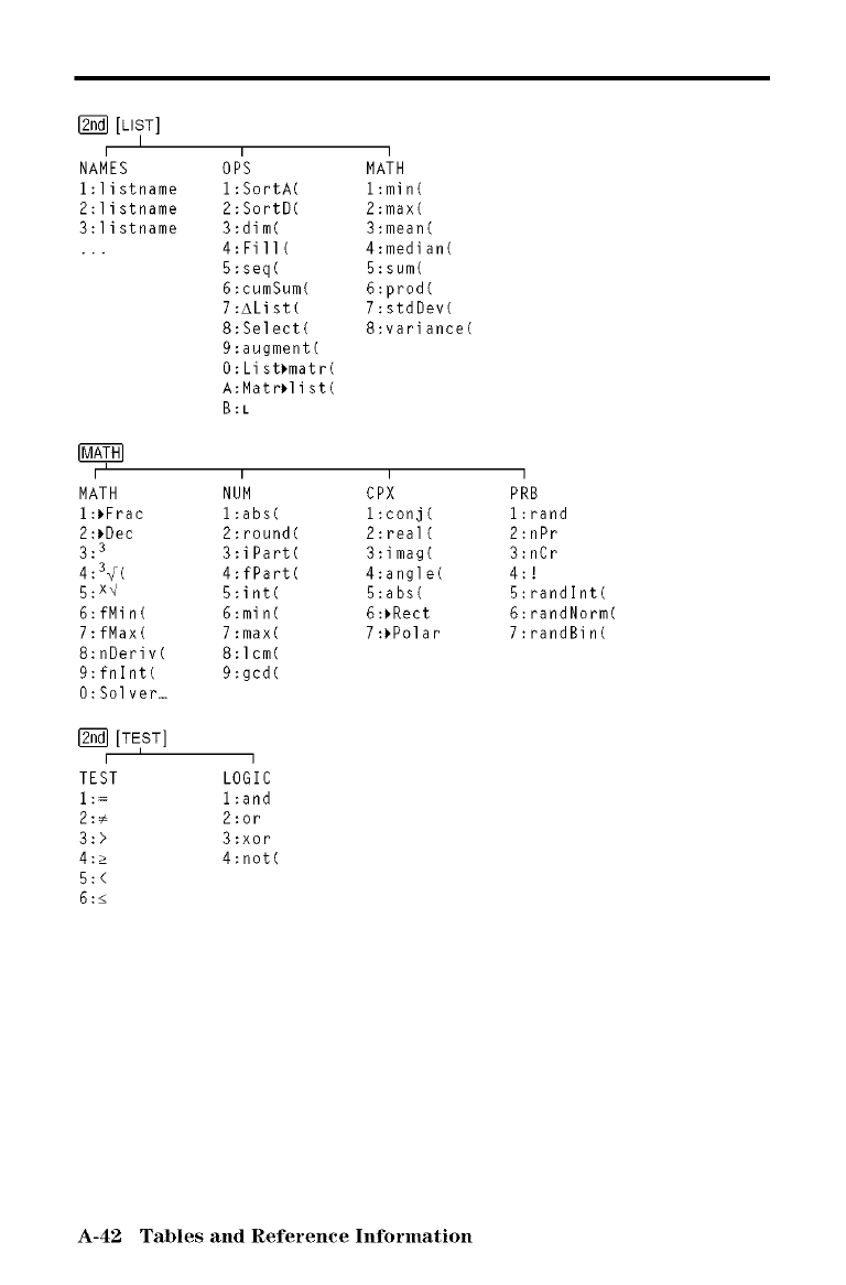
[LIST]
I
I
NAMES
l:listname
2:listname
3:listname
1 1
OPS MATH
l:SortA( 1:min(
2:SortD( 2:max(
3:dim( 3:mean(
4:Fill( 4:median(
5:seq( 5:sum(
6:cumSum( 6:prod(
7:AList( 7:stdDev(
8:Select( 8:variance(
9:augment(
O:List_matr(
A:Matr_list(
B:L
I I 1 1
MATH NUM CPX
l:_Frac l:abs( 1:conj(
2:_Dec 2:round( 2:real(
3:3 3:iPart( 3:imag(
4:3_r( 4:fPart( 4:angle(
5: x_ 5:int( 5:abs(
6:fMin( 6:min( 6:_Rect
7:fMax( 7:max( 7:_Polar
8:nDeriv( 8:Icm(
9:fnlnt( 9:gcd(
O:Solver._
[2nd][TEST]
I I
TEST LOGIC
i:= l:and
2:_ 2:or
3:> 3:xor
4:> 4:not(
5:<
6:<
1
PRB
1:rand
2:nPr
3:nCr
4:!
5:randlnt(
6:randNorm(
7:randBin(
A-42 Tables and Reference Information
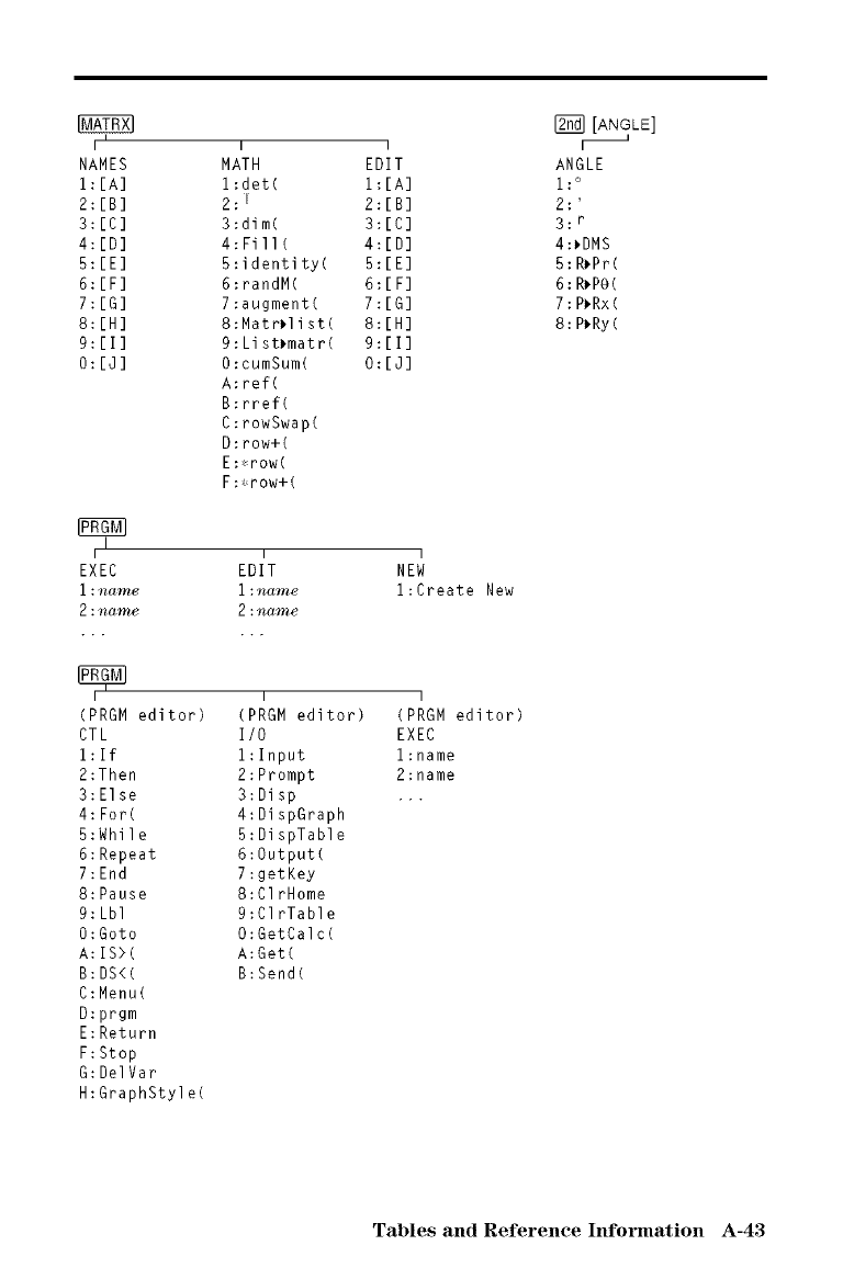
I I I
NAMES MATH
I:[A] 1:det(
2:[B] 2: I
3:[C] 3:dim(
4:[D] 4:Fill(
5:[E] 5:identity(
6:[F] 6:randM(
7:[G] 7:augment(
8:[H] 8:Matr_list(
9:[I] 9:List_matr(
O:[J] O:cumSum(
A:ref(
B:rref(
C:rewSwap(
D:row+(
E:*row(
F:*row+(
I
I I
EXEC EDIT
l:nan_ l:name
2:na_ 2:na_e
I
(PRGM editor)
CTL
1:If
2:Then
3:Else
4:For(
5:While
6:Repeat
7:End
8:Pause
9:Lbl
O:Goto
A:IS>(
B:DS<(
C:Menu(
D:prgm
I
(PRGM editor)
I/0
1:Input
2:Prompt
3:Disp
4:DispGraph
5:DispTable
6:Output(
7:getKey
8:ClrHeme
9:ClrTable
O:GetCalc(
A:Get(
B:Send(
E:Return
F:Stop
G:DelVar
H:GraphStyle(
I
EDIT
I:[A]
2:[B]
3:[C]
4:[D]
5:[E]
6:[F]
7:[G]
8:[H]
9:[I]
O:[J]
I
NEW
1:Create New
I
(PRGM editor)
EXEC
m:name
2:name
r_q [AN_LE]
F--
ANGLE
1: °
2:'
3: r
4:_DMS
5:R_Pr(
6:R_PO(
7:P_Rx(
8:P_Ry(
Tables and Reference Information A-43

I
DRAW
l:C]rDraw
2:Line(
3:Horizontal
4:Vertical
5:Tangent(
6:DrawF
7:Shade(
8:Drawlnv
9:Circle(
O:Text(
A:Pen
I
POINTS
1:Pt On(
2:Pt Off(
3:Pt Change(
4:Pxl On(
5:Pxl Off(
6:Pxl Change(
7:pxl Test(
I
STO
1:StorePic
2:RecallPic
3:StoreGDB
4:RecalIGDB
1
VARS
1:Window._
2:Zoom._
3:GDB...
4:Picture._
5:Statistics...
6:Table...
7:String._
I
Y VARS
1:Function._
2:Parametric...
3:Polar._
4:On/Off...
VARS
i I
(Window...)
X/Y
l:Xmin
2:Xmax
3:Xscl
4:Ymin
5:Ymax
6:Yscl
7:Xres
8:AX
9:AY
0:XFact
A:YFact
I I
(Window...) (Window...)
T/e U/V/W
1:Tmin 1:u(nMin)
2:Tmax 2:v(nMin)
3:Tstep 3:w(nMin)
4:emin 4:nMin
5:6max 5:nMax
6:6step 6:PlotStart
7:PlotStep
A-44 Tables and Reference Information
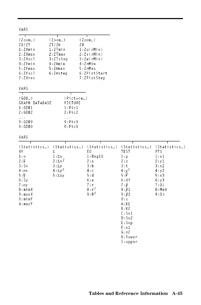
VARS
I I I
(Zoom...) (Zoom...) (Zoom...)
ZX/ZY ZT/Ze ZU
l:ZXmin l:ZTmin l:Zu(nMin)
2:ZXmax 2:ZTmax 2:Zv(nMin)
3:ZXscl 3:ZTstep 3:Zw(nMin)
4:ZYmin 4:ZOmin 4:ZnMin
5:ZYmax 5:Z@max 5:ZnMax
6:ZYscl 6:Z@step 6:ZPlotStart
7:ZXres 7:ZPlotStep
VARS
I
(GDB...)
GRAPH DATABASE
I:GDB1
2:GDB2
9:GDB9
O:GDBO
VARS
I
(Statistics...)
XY
l:n
2:_
3:Sx
4:_x
6:Sy
7:_y
8:minX
9:maxX
O:minY
A:maxY
I
(Picture...)
PICTURE
1:Picl
2:Pic2
9:Pic9
O:PicO
I
(Statistics...)
Z
I:Zx
2:Zx 2
3:Zy
4:Zy 2
5:Zxy
I I I
(Statistics...) (Statistics...) (Statistics...)
EQ TEST PTS
I:RegEQ 1:p i:xl
2:a 2:z 2:yi
3:b 3:t 3:x2
4:c 4:Z 2 4:y2
5:d 5:F 5:x3
6:e 6:df 6:y3
7:r 7:# 7:Q1
8:r 2 8:#1 8:Med
9:R 2 9:#2 9:Q3
O:s
A:_I
B:_2
C:Sxl
D:Sx2
E:Sxp
F:nl
G:n2
H:lower
I:upper
Tables and Reference Information A-45
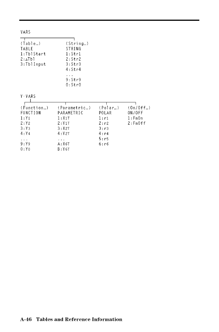
VARS
I I
(Table...) (String...)
TABLE STRING
1:TblStart 1:Strl
2:ATbl 2:Str2
3:TbIInput 3:Str3
4:Str4
9:Str9
O:StrO
Y VARS
I
III
(Function...) (Parametric...) (Polar...)
FUNCTION PARAMETRIC POLAR
I:YI I:XIT i:ri
2:Y2 2:YIT 2:r2
3:Y3 3:X2T 3:r3
4:Y4 4:Y2T 4:r4
5:r5
O:Yo B:Y6T
I
(On/Off._)
ON/OFF
1:FnOn
2:FnOff
A-46 Tables and Reference Information
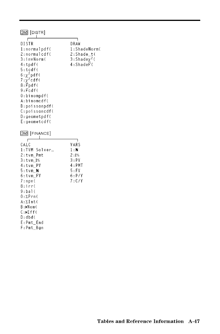
[_ [DISTR]
I
I
DISTR
1:normalpdf(
2:normalcdf(
3:invNorm(
4:tpdf(
5:tcdf(
6:z2pdf(
7:z2cdf(
8:Fpdf(
9:Fcdf(
O:binompdf(
A:binomcdf(
B:poissonpdf(
C:poissoncdf(
D:geometpdf(
E:geometcdf(
I_ [FINANCE]
I
I
CALC
I:TVM Solver...
2:tvm Pmt
3:tvm I%
4:tvm PV
5:tvm N
6:tvm FV
7:npv(
8:irr(
9:hal(
O:XPrn(
A:glnt(
B:_Nom(
C:_Eff(
D:dbd(
E:Pmt End
F:Pmt Bgn
I
DRAW
1:ShadeNorm(
2:Shade t(
3:Shadez2(
4:ShadeF(
I
VARS
I:N
2:1%
3:PV
4:PMT
5:FV
6:P/Y
7:C/Y
Tables and Reference Information A-47
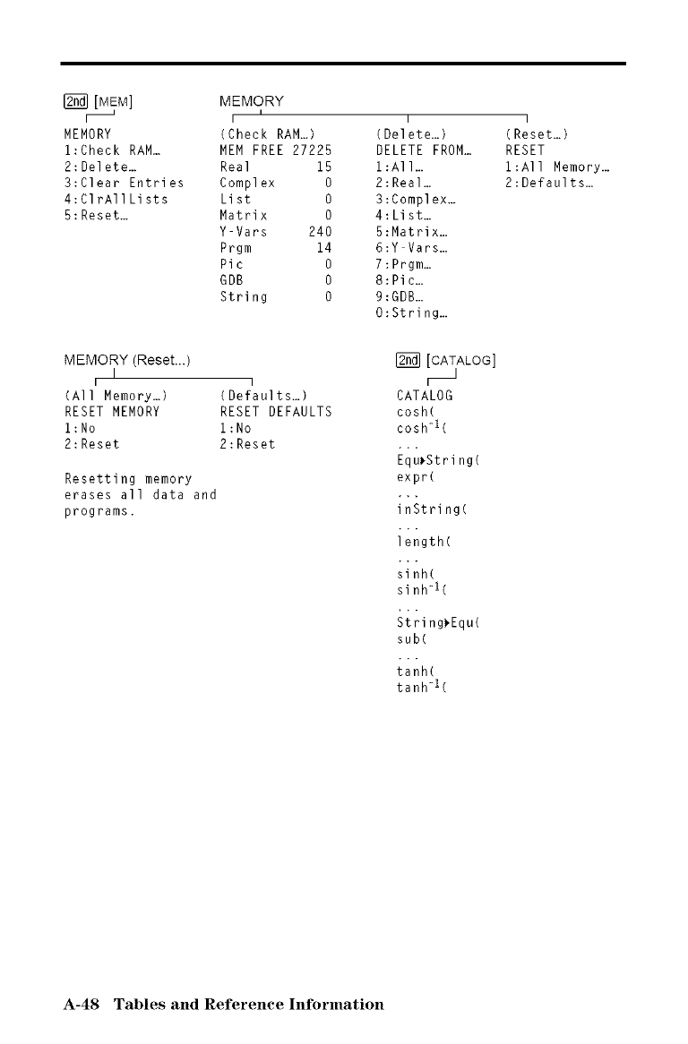
[MEM]
i--J
MEMORY
l:Check RAM_
2:Delete._
3:Clear Entries
4:ClrAllLists
5:Reset...
MEMORY
I
I I
(Check RAM...) (Delete...)
MEM FREE 27225 DELETE FROM...
Real 15 1:All...
Complex 0 2:Real._
List 0 3:Complex._
Matrix 0 4:List...
Y Vars 240 5:Matrix...
Prgm 14 6:Y Vars...
Pic 0 7:Prgm...
GDB 0 8:Pic...
String 0 9:GDB...
O:String...
MEMORY (Reset...)
I
I I
(All Memory...) (Defaults...)
RESET MEMORY RESET DEFAULTS
1:No 1:No
2:Reset 2:Reset
Resetting memory
erases all data and
programs•
12_]_ALOG]
CATALOG
cosh(
cosh-l(
Equ_String(
expr(
inString(
length(
sinh(
sinh-1(
String_Equ(
sub(
tanh(
tanh-1(
I
(Reset...)
RESET
1:All Memory...
2:Defaults._
A-48 Tables and Reference Information
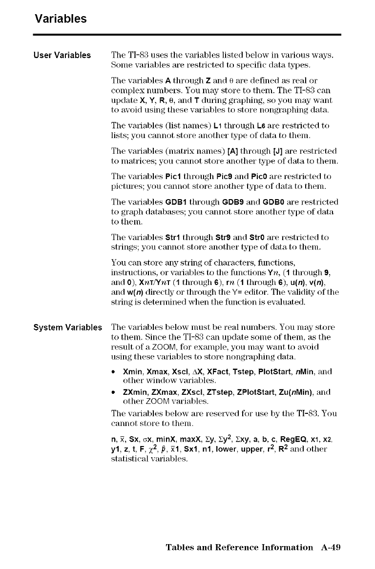
Variables
User Variables
System Variables
The TI-83 uses the variables listed below in various ways,
Some variables are restricted to specific data types.
The variables A through Z and 0 are defined as real or
complex numbers. You may store to them. The TI-83 can
update X, Y, R, 0, and T dm'ing graphing, so you may want
to avoid using these varial)les to store nongraphing data.
The variables (list nalnes) L1 through LS are restricted to
lists; you cannot store another type of data to them.
The wu'iables (matrix names) [A] through [J] are restricted
to matrices; you cannot store another type of data to them,
The vm'iables Pie1 through Pie9 and Pic0 are restricted to
pictures; you cannot store another type of data to them.
The variables GDB1 through GDB9 and GDB0 are restricted
to graph databases; you cannot store another type of data
to them,
The variables Strl through Str9 and StrO m'e restricted to
strings; you cannot store another type of data to them.
You can store any string of characters, functions,
instructions, or vm'iables to the functions Yn, (1 through 9,
and 0), XnT/YnT (1 through 6), rn (1 through 6), u(n), v(n),
and w(n) directly or through the Y= editor. The validity of the
string is determined when the function is evaluated.
The variables below nmst be real numbers. You may store
to them. Since the TI-83 can update some of them, as the
result of a ZOOM, for example, you nlay want to avoid
using these variables to store nongraphing data.
• Xmin, Xmax, Xsel, AX, XFact, Tstep, PlotStart, nMin, and
()tiler window variables,
•ZXmin, ZXmax, ZXscl, ZTstep, ZPIotStart, Zu(nMin), and
other ZOOM variables.
The variables below are resetwed for use by the TI-83. You
cannot store to them.
n, _, Sx, _x, minX, maxX, Ey, Ey2, Exy, a, b, e, RegEQ, xl, x2,
yl, z, t, F, Z2, p, xl, Sxl, nl, lower, upper, r2, R2 aft(] other
statistical variables,
Tables and Reference hfformation A-49
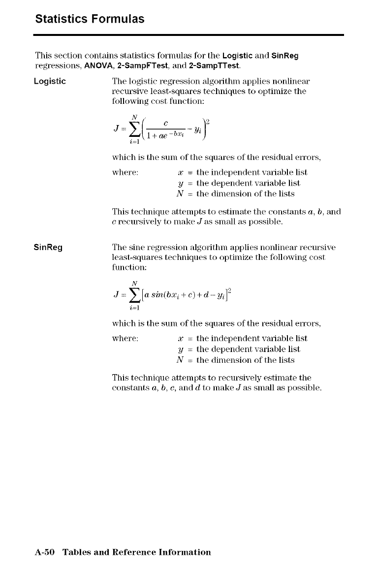
Statistics Formulas
This section contains statistics fornmlas for the Logistic and SinReg
regressions, ANOVA, 2-SampFTest, and 2-SampTTest.
Logistic The logistic regression algorithm applies nonlinear
t_cursive least-squares techniques to optimize the
following cost function:
N
j c
:z(-i÷o>,4
which is the sunl of the squares of the residual errors,
where: x= the independent variable list
y= the dependent variable list
N= the dimension of the lists
This technique attempts to estimate the constants a, b, and
et_cursively to make Jas small as possible.
SinReg The sine regression algorithm applies nonlinear recut_ive
least-squares techniques to optimize the following cost
function:
N
J= E[a siyt(bxi + e)+ d- yi]2
i=1
which is the sunl of the squares of the residual errors,
where: x= the independent variable list
y= the dependent variable list
N= the dimension of the lists
This technique attempts to recursively estimate the
c()nstants a, b, c, and dto make Jas small as possible.
A-50 Tables and Reference Inforination
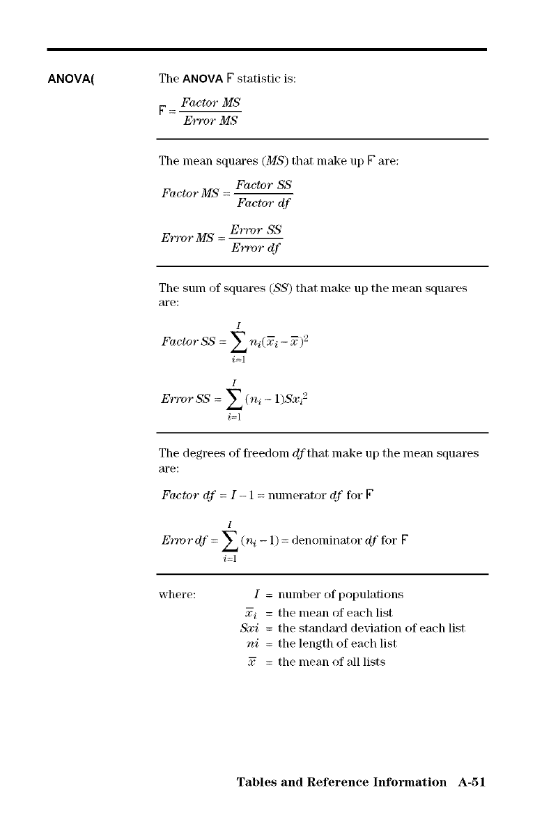
ANOVA( The ANOVA Fstatisticis:
Factor MS'
FError MS
The mean squares (MS) that make up F are:
Factor SS
Factor MS' Factor df
Error SS
Error MS' =Error df
The sum of squares (SS) that make up the mean squares
are:
I
Factor SS = E ni(xi -2) 2
i=1
I
Error SS = E (ni - 1)Sxi 2
i=l
The degrees of freedoln dfthat make up the mean squares
are:
Factor df =I- 1 = numerator df for V
I
Ermrdf = E (hi - 1) = denolninator df if)r F
i=l
where: I= number of populations
_:i = the mean of each list
Sxi = the standard deviation of each list
ni = the length of each list
_: = the mean of all lists
Tables and Reference Information A-51
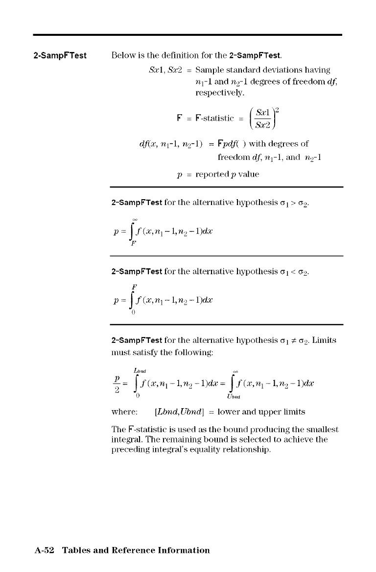
2-SampFTest Below is the definition for the 2-SampFTest.
Sxl, Sx2 = Sample standard deviations having
nl-1 and n2-1 degrees of freedom df,
respectively.
F = F-statistic [ Sx2 )
dr(x, nl-1 ,n2-1 ) = Fpdf( ) with degrees of
fl'eedom df, hi-1 , and n2-1
p= reportedp wdue
2-SampFTest for the alternative hypothesis (s 1 > (s2.
p= i f(x, nl - 1,n 2 - 1)dx
2-SampFTest for the alternative hypothesis (_1< (_2-
F
p= ff(x,n 1-1,n 2-1)dx
0
2-SampFTest for the alternative hypothesis (_1 :_ (_2.Limits
nmst satisfy the following:
Lb nd
/92=f f(x'nl- l'n2-1)dx= ff(x,n 1-1,n 2-1)dx
0U_,_
where: [Lbnd, Ubnd] = lower and upper limits
The F-statistic is used as the bound producing the smallest
integral. The reinaining bound is selected to achieve the
preceding integral's equality relationship.
A-52 Tables and Reference Information
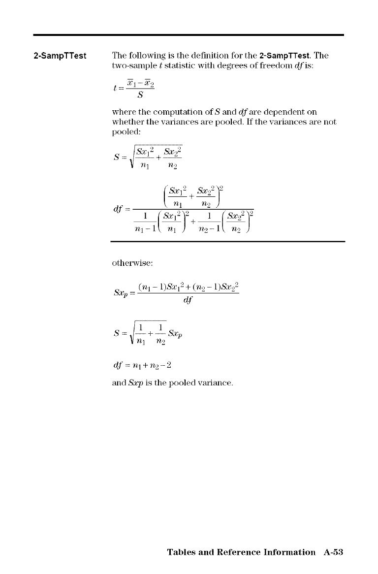
2-SampTTest The following is the definition for the 2-SampTTest, The
two-sample tstatistic with degrees of freedom dfis:
t= Xl--X2
s
where tile computation of Sand df are dependent on
whether the variances are pooled. If the variances are not
pooled:
S = ]_/$2b'12qSX22
Vnl n2
d f-
S:t;12 + ,gXd2 )2
l l (s.s/,,
nl-lk nl } nz-lk nz )
otherwise:
(n I -1)SXl 2 +(n 2 -1)SX2 2
_:t;p = df
S= J1 +1Sxp
V)'_I n2
df =nl+n2-2
and Sxp is the pooled variance.
Tables and Reference Information A-53
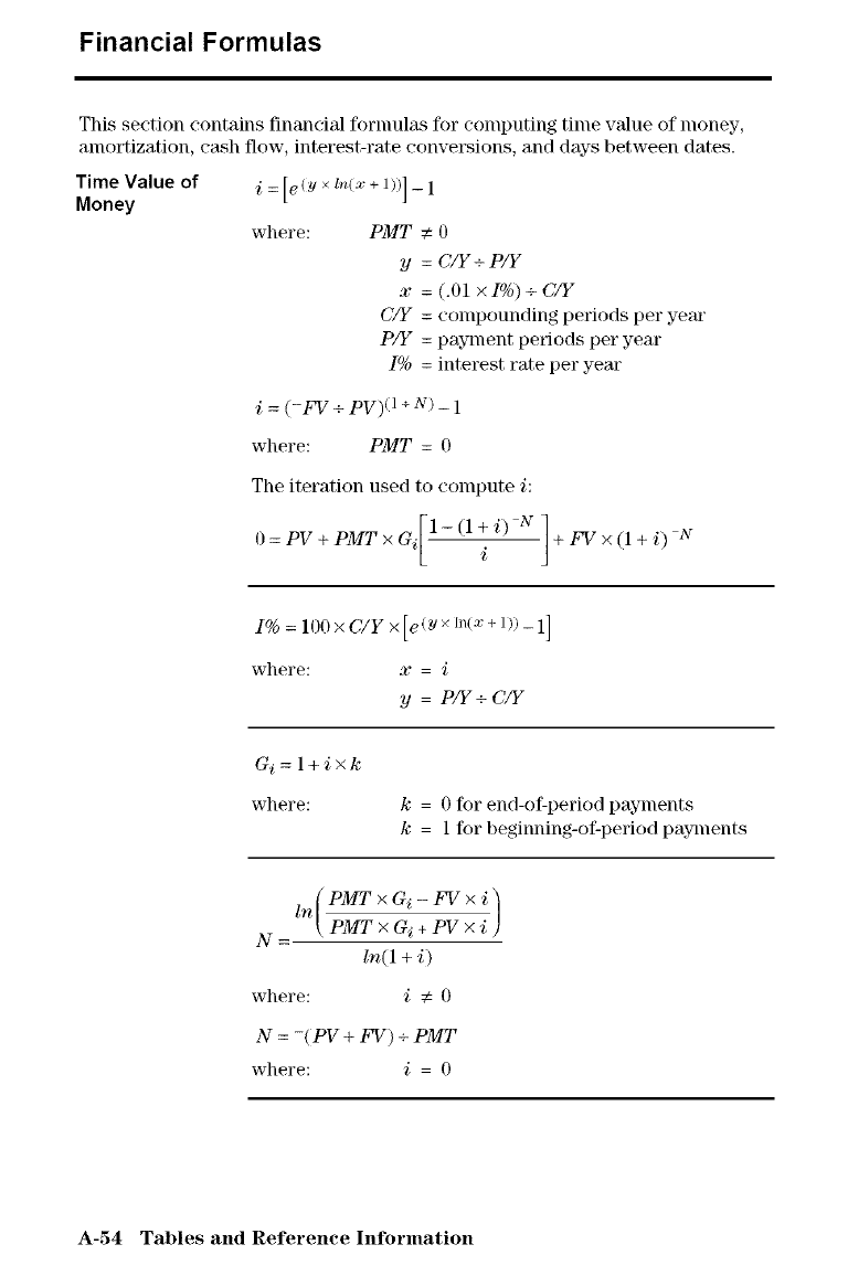
Financial Formulas
This section contains financial fommlan for computing time value of money,
amortization, cash flow, interest-rate conve_\sions, and days between dates.
Time Value of i=[e(y×ln(x+l))]_l
Money
where: PMT € 0
y=C/Y +P/Y
x= (.01 ×1%) + C/Y
C/Y = compounding periods per year
P/Y = payment periods per year
I% = interest rate per yem"
i= (-FV + PV)( 1+ N) _1
where: PMT = 0
The iteration used to compute i:
[1-(1+i) NI+FV×(I+i) N
0 = PV +PMT xG i
1% = 100 × C/Y × [e(Y × ln(x + 1)) _ 1]
where: x=i
y=P/Y+C/Y
G i = l+i×k
where: k= 0 for end-of-period payments
k= 1 for beginning-of-period payments
N- [PMTxGi+PVxi)
ln(1 +i)
where: i€ 0
N= -(PV + FV) +PMT
where: i = 0
A-54 Tables and Reference Information
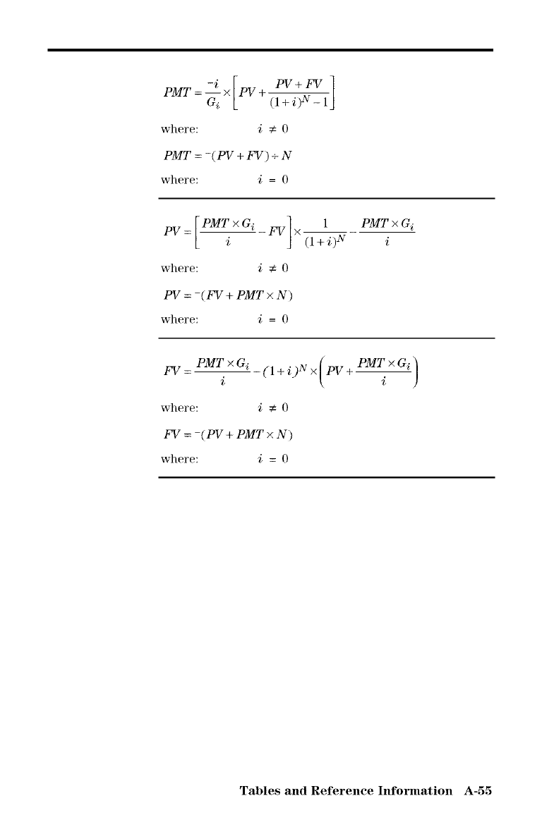
PMT=-ix[PV_ PV+FV ]
Gi [ (I+i)N- lJ
where: i€ 0
PMT = -(PV + FV) +N
where: i= 0
J(l+i)
where: i€ 0
PV = -(FV + PMT ×N)
where: i= 0
PMT xGi
i
FV PMT xGi (
i (l+i)N× PV-_
where: i€ 0
FV = -(PV + PMT xN)
where: i= 0
PMT×Gi.)
Tables and Reference Information A-55
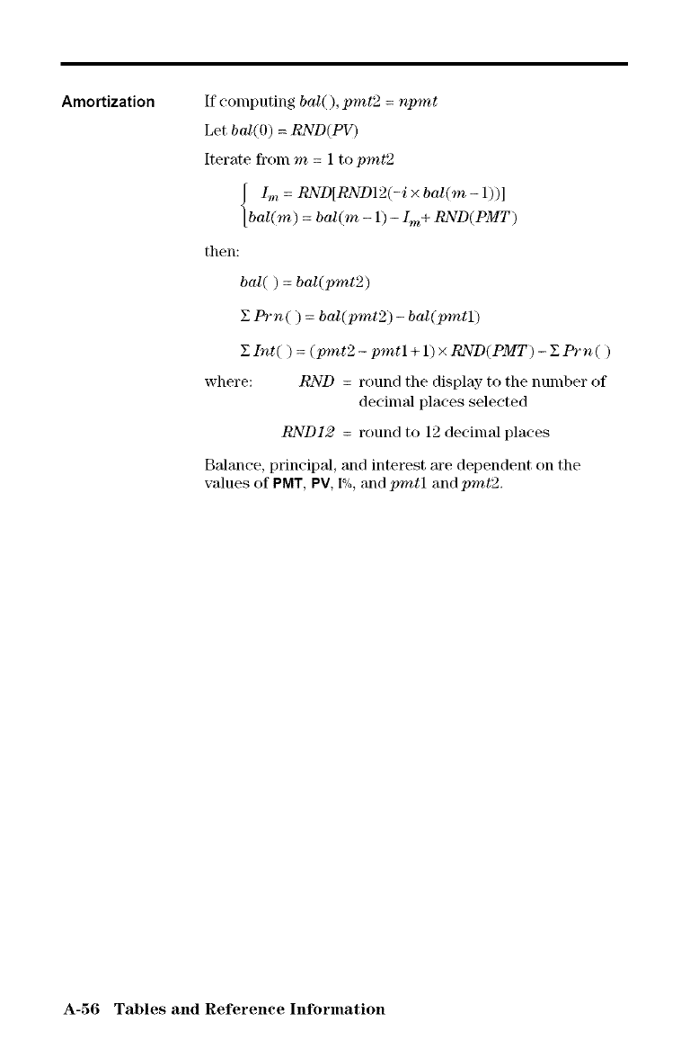
Amortization If computing bal(), pint2 =npmt
Let hal(O) =RND(PV)
Iterate fronl m= 1 to pint2
Lm =RND[RND12(-i xbal(m - 1))]
hal(m) =bal(m - 1) -[m+ RND(PMT)
then:
hal() =hal(pint2)
EPrn( ) = bal(pmt2) -bal(pmtl)
ZInt( ) = (pint2 - pmtl + 1) x RND(PMT) - Z Prn( )
where: RND = round the display- to the number of
decimal places selected
RND12 = round to 12 decimal places
Balance, principal, and interest are dependent on the
values of PMT, PV, I°/o,and pmtl and pint2.
A-56 Tables and Reference Information
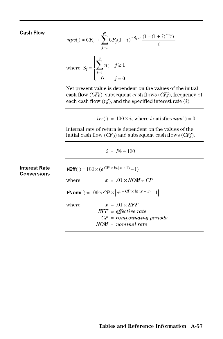
Cash Flow N
npv() = CF0 + _CFj(1 +/) & _(1 - (1 _/) rq)
j=l
where:Sj= ni J >-1
j= 0
Net present value is dependent on the values of the initial
cash flow (CFII), subsequent cash flows (CFj), frequency of
each cash flow (nj), and the specified interest rate (i),
irr() = 100 × i, where isatisfies npv() = 0
Internal rate of return is dependent on the values of the
initial c_h flow (CFo) and subsequent cash flow. (CFj),
i=I% + 100
Interest Rate
Conversions VEff( ) = 100 × (e cT × Zn(x+ 1)_1)
where: x= ,01 x NOM+ CP
_Nom( ) = 100 × CP × [ei + cP × z,.(x+ 1)_ 1]
where: x=,01 ×EFT"
EFF =effective rate
CP =compounding periods
NOM =nominal rote
Tables and Reference Information A-57
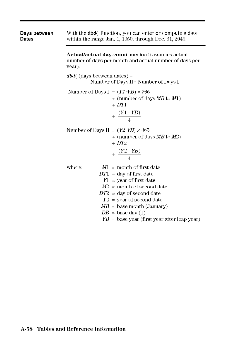
Daysbetween Withthedbd(function,youcanenterorcomputeadate
Dates within the range Jan. 1, 1950, through Dec. 31, 2049.
Actual/actual day-count method (assunles actual
number of days per month and actual number of day-s per
year):
dbd( (days between dates) =
Number of Days II - Number of Days I
Number of Days I = (Y1-YB) × 365
+ (number of days MB to M1)
+DT1
(Y1 - YB)
+4
Number of Day-s II = (Y2-YB) x 365
+ (number of days MB to 11//2)
+DT2
(Y2 - YB)
+4
where: M1 = month of first date
DT1 = day of first date
Y1 = year of first date
M2 = month of second date
DT2 = day of second date
Y2 = year of second date
MB = base month (January)
DB = base day (1)
YB = base year (first year _ter leap year)
A-58 Tables and Reference Information
BGeneralInformation
Contents Batte_" Infommtion ...................................... B-2
In Case of Difficulty ..................................... B-4
Error Conditions ......................................... B-5
Accuracy Infomlation .................................... B-10
Support and Sep_iee Information ......................... B-12
Warranty Infornlation .................................... B-13
General Information B-1
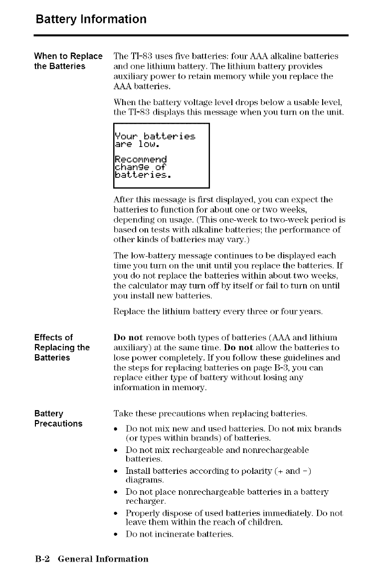
Battery Information
When to Replace
the Batteries
Effects of
Replacing the
Batteries
Battery
Precautions
The TI-83 uses five batteries: four AAA alkaline batteries
and one lithium battery-. The lithium battery pro_qdes
auxilimTF power to retain menlot T while you replace the
AAA batteries.
When the battery voltage level drops below a usable level,
the TI-83 displays this message when you turn on the unit.
_Jour batteries
are low.
Reco_r_end
change o?
batteries.
Alter this message is first displayed, you can expect the
batteries to function for about one or two weeks,
depending on usage. (This one-week to two-week period is
based on tests with alkaline batteries; the performance of
other kinds of batteries may vm3z.)
The low-battery message continues to be displayed each
time you turn on the unit until you replace the batteries. If
you do not replace the batteries within about two weeks,
the calculator may turn off by itself or fail to turn on until
you install new batteries.
Replace the lithimn batte_y- eve_3z three or four years.
Do not remove both types of batteries (AAA and lithium
auxiliat_F) at the same time. Do not allow the batteries to
lose power completely. If you follow these guidelines and
the steps for replacing batteries on page B-3, you can
replace either type of batter T without losing any
information in memo_7.
Take these precautions when replacing batteries.
• Do not mix new and used batteries. Do not mix brands
(or types within brands) of batteries.
• Do not mix rechm'geable and nonrechargeable
batteries.
• Install batteries according to polarity (+ and -)
diagrams.
• Do not place nonreehargeable batteries in a battery
recharger.
• Properly dispose of used batteries immediately. Do not
leave them within the reach of children.
• Do not incinerate batteries.
B-2 General hfformation
Replacing the
Batteries
To replace the batteries, follow these steps.
1. Turn offthe calculator. Replacethe slide cover over the
keybom'd to avoid inadvertently turning on the
calculator. Turn the back of the calculator toward you.
Hold the cMeulator upright. Place your thumb on the
oval indentation on the battetsz cover. Push down and
toward you to slide the cover al_out IAinch (6 nlnl). Lift
off the cover to expose the batte_3z eolnpartment.
Note: To avoid loss of infornmtion stored in
memory, you nmst turn off the calculator. Do not
remove the AAA batteries and the lithium battery
simultaneously.
3. Replace all four AAA alkaline batteries at the same
time. Or, replace the lithium batte_Ty-.
• To replace the AAA alkaline batteries, remove all
four discharged AAA batteries and install new ones
according to the polm'ity (+ and -) diagrams in the
batte_3z compartment.
• To remove the lithimn batte_Ty-,place your index
finger on the battet3z. Insert the tip of a ball-point pen
(or similar instrument) under the battery at the small
opening provided in the batte_sz compartment.
Carefully P_TY"the battetsz upward, holding it with
your thumb and finger. (There is a spring that pushes
against the underside of the battet3z.)
• Install the new batte_sz, + side up, by inserting the
batte_3z and gently- snapping it in with your finger.
Use a CR1616 or CR1620 (or equivalent) lithium
batte_y-.
4. Replace the batte_y- compartment cover. Turn the
calculator on and adjust the display contrast, if
necessmTy- (step 1; page B-4).
General Information B-3
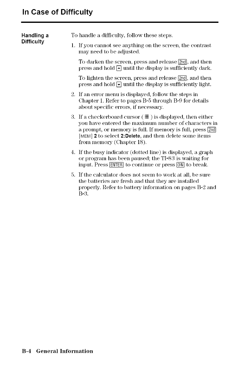
In Case of Difficulty
Handling a
Difficulty
To handle a difficulty, follow these steps.
1. If you cannot see anything on the screen, the contrast
nlay need to be adjusted.
To darken the screen, press and release [2_, and then
press and hold [] until the display- is sufficiently dark.
To lighten the screen, press and release [_], and then
press and hold [] until the display is sufficiently light.
2. If an error menu is displayed, follow the steps in
Chapter 1. Refer to pages B-5 through B-9 for details
about specific errors, if necessatT.
3. If a checkerboard cursor ( N ) is displayed, then either
you have entered the nlaxinlunl number of characters in
a prompt, or nlenlory is full. If nlenlory is full, press [_
[MEM]2 to select 2:Delete, and then delete some items
fronl nlenlory (Chapter 18).
4, If the busy indicator (dotted line) is displayed, a graph
or program has been paused; the TI-83 is waiting for
input, Press [gNT_ to continue or press [_] to break,
5, If the calculator does not seem to work at all, be sure
the batteries are flesh and that they are installed
properly. Refer to battew information on pages B-2 and
B-3.
B-4 General Information
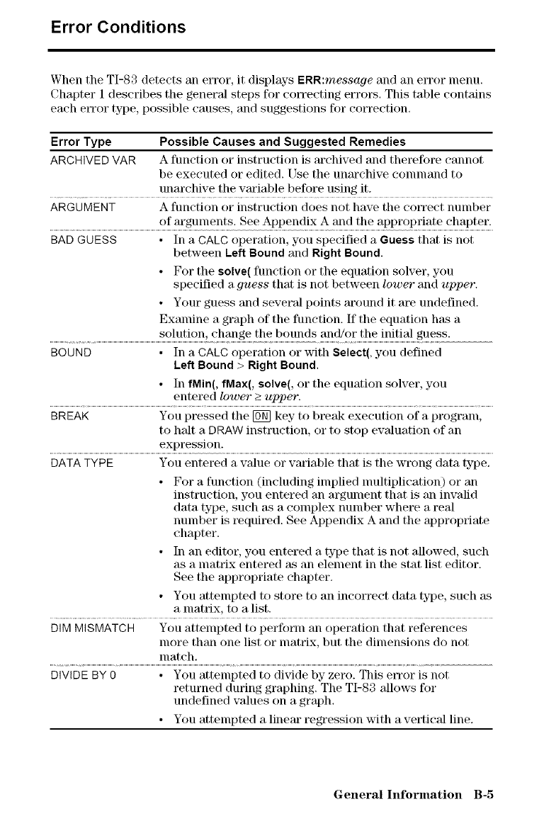
Error Conditions
When the TI-83 detects an error, it displays ERR:message and an error menu.
Chapter 1 describes the general steps for eotTeeting errors, This table contains
each etTor type, possible causes, and suggestions for correction,
Error Type Possible Causes and Suggested Remedies
ARCHIVED VAR A function or instruction is archived and therefore cannot
be executed or edited. [_se the unto'chive command to
mmrehive the variable before using it.
ARGUMENT A function or instruction does not have the co_Tect number
of arguments. See Appendix A and the appropriate chapter.
BADGUESS • In a CALC operation, you specified a Guess that is not
between Left Bound and Right Bound.
• For the solve( function or the equation solver, you
specified a guess that is not between lower and upper.
• Your guess and severM points around it are undefined.
Exa]nine a graph of the function. If the equation has a
solution, change the bounds and/or the initial guess.
BOUND • In a CALC operation or with Select(, you defined
Left Bound >Right Bound,
• In fMin(, fMax(, solve(, or the equation solver, you
entered lower >_upper.
BREAK You pressed the [ON]key to break execution of a prograln,
to halt a DRAW instruction, or to stop evaluation of an
expression.
DATATYPE You entered a value or variable that is the wrong data type.
• For a function (including implied lnultiplication) or an
instruction, you entered an argument that is an invalid
data type, such _ts a complex number where a real
number is required. See Appendix A and the appropriate
chapter.
• In an editor, you entered a type that is not allowed, such
as a matrix entered as an element in the stat list editor.
See the appropriate chapter.
•You attelnpted to store to an incorrect data type, such as
a nmtrix, to a list.
DIMMISMATCH You attempted to perform an operation that references
more than one list or lnatrix, but the dimensions do not
lnateh.
DIVIDE BY0 • You attempted to dixqde by zero. This error is not
returned during graphing. The TI-83 allows for
undefined values on a graph.
•You attelnpted a linear regression with a vertical line.
General Infornmtion B-5
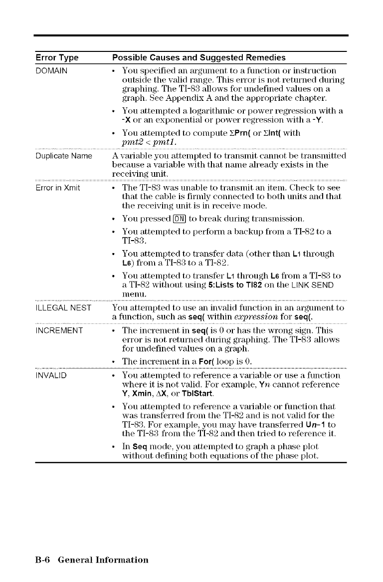
Error Type Possible Causes and Suggested Remedies
DOMAIN • You specified an argument to a function or instruction
outside the wdid range, This elTor is not returned during
graphing. The TI-83 allows for undefined values on a
graph, See Appendix A and tile appropriate chapter.
• You attempted a logarithmic or power regression with a
-X or an exponential or power regression with a -Y.
• You attempted to compute XPrn( or Xlnt( with
pint2 <pint1.
Duplicate Name A variable you attempted to transmit cannot be translnitted
because a variable with that name already exists in the
receiving unit.
Error in Xmit • The TI-83 was unable to transmit an item. Check to see
that the cable is firnfly connected to both units and that
the receiving unit is in receive mode.
• You pressed [_ to break during transmission.
• You attempted to perform a backup from a TI-82 to a
TI-83.
• You attempted to transfer data (()tiler than kl through
1.6) from a TI-83 to a TI-82.
• You attempted to transfer kl through L6 from a TI-83 to
a TI-82 without using 5:Lists to TI82 on the LINK SEND
nlenu,
ILLEGAL NEST You attempted to use an invalid function in an argument to
a function, such as seq( within e_ression for seq(.
INCREMENT • The increment in seq( is 0 or has the wrong sign. This
error is not returned during graphing. The TI-83 allows
for undefined values on a graph,
• The increment in a For( loop is 0,
INVALID • You attempted to refel_nce a variable or use a function
where it is not valid. For example, Yn cannot reference
Y, Xmin, AX, or TblStart,
• You attempted to reference a variable or function that
was transferred from the TI-82 and is not valid for the
TI-S3. For example, you may have transfen'ed Un-1 to
the TI-83 from the TI-82 and then tried to reference it.
•In Seq mode, you attempted to graph a phase plot
without defining both equations of the phase plot.
B-6 General hfformation
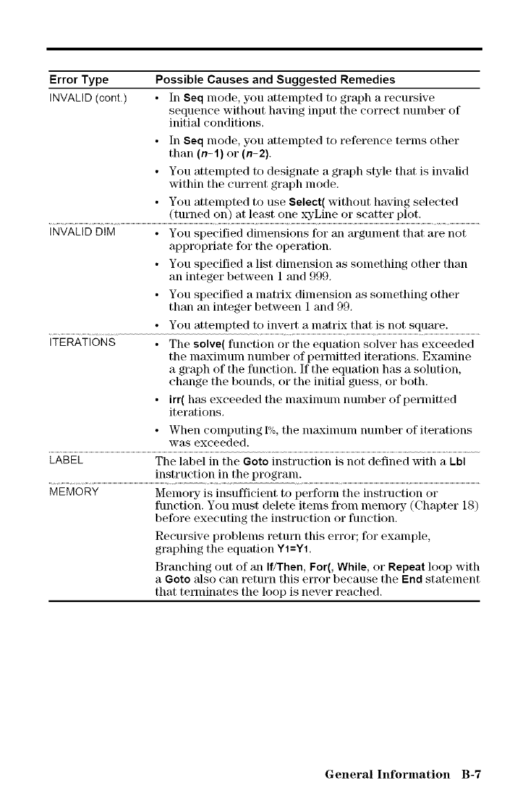
Error Type
INVALID (cont.)
Possible Causes and Suggested Remedies
• In Seq nlode, you attempted to graph a recursive
sequence without having input the correct number of
initial conditions.
• In Seq mode, you attempted to reference terms other
than (n-l) or (n-2).
You attelnpted to designate a graph style that is invalid
within the eutTent graph mode.
You attempted to use Select{ without having selected
(turned on) at least one xyLine or scatter plot.
INVALIDDIM You specified dimensions for an argument that are not
appropriate for the operation.
You specified a list dimension as something other than
an integer between 1 and 999.
You specified a matrix dimension as something other
than an integer between 1 and 99.
You attempted to invert a matrix that is not square.
ITERATIONS • The solve( function or the equation solver has exceeded
the nmximum number of permitted iterations. Examine
a graph of the function. If the equation has a solution,
change the bounds, or the initial guess, or both.
•irr( has exceeded the nmxinmm number of permitted
iterations.
• When computing 1%,the nl_Lxinlunl number of iterations
was exceeded.
LABEL The label in the Goto instruction is not defined with a Lbl
instruction in the program.
MEMORY Memory is insufficient to perform the instruction or
function. You nmst delete items from memory (Chapter 18)
before executing the instruction or function.
Reeursive problems return this error; for example,
graphing the equation YI=Y1.
Branching out of an If/Then, For(, While, or Repeat loop with
aGoto also can return this error because the End statelnent
that terminates the loop is never reached.
General Information B-7
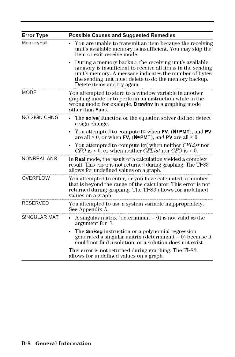
Error Type
MemoryFull
Possible Causes and Suggested Remedies
• You are unable to transmit an item because tile receiving
unit's available lnelnol_y- is insufficient. You lnay skip the
iteln or exit receive triode,
• During a lnelnol_y- backup, the receiving unit's available
nlenlory is insufficient to receive all itelns in the sending
unit's lnelnot_yL A lnessage indicates the number of bytes
the sending unit nmst delete to do the lnetnol_- backup.
Delete items and try again.
MODE You attempted to store to a window variable in another
graphing mode or to perform an instruction while in the
wrong nlode; for exaInple, Drawlnv in a graphing nlode
other than Func.
..............................The saiv;{ function _;i the equation ......
a sign change.
• You atteinpted to compute I%when FV, (N*PMT), and PV
are all _>O, or when FV, (N*PMT), and PV are all _<O.
• You attempted to eonlpute irr( when neither CFList nor
CFO is > O, or when neither CFList nor CFO is < O.
NONREAL ANS In Real mode, the result of a calculation yielded a complex
result. This error is not returned during graphing. The TI-83
allows fox"undefined values oil a graph.
OVERFLOW You attempted to enter, or you have calculated, a number
that is beyond the range of the calculator. This error is not
returned during graphing. Tile TI-83 allows for undefined
wdues on a graph.
RESERVED You attempted to use a wsteln variable inappropriately.
See Appendix A.
SINGULAR MAT • A singular matrix (determinant = 0) is not valid as the
argument for %
• The 8inReg instruction or a polynomial regression
generated a singular matrix (determinant = 0) because it
could not find a solution, or a solution does not exist.
This error is not returned during graphing. Tile TI-83
allows for undefined values on a graph.
B-8 General hfformation
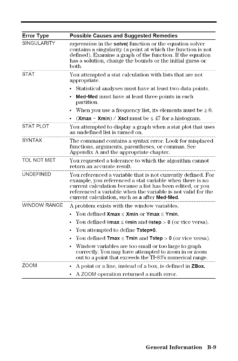
Error Type Possible Causes and Suggested Remedies
SINGULARITY expression ill the solve( function or the equation solver
contains a singularity (a point at which the function is not
defined). Examine a graph of the function. If the equation
h_s a solution, change the bounds or the initial guess or
both.
STAT You attempted a stat calculation with lists that are not
appropriate.
• Statistical analyses must have at least two data points.
• Ned-Ned must have at least three points in each
partition.
• When you use a frequency list, its elements must be _>0.
•(Xmax - Xmin) /Xscl nmst be <_47 for a histogram.
STAT Pt_OT Y0u atte;_pted to display a graph when a stat plot that uses
an undefined list is turned on.
SYNTAX The connnand contains a syntax error. Look for lnisplaced
functions, arguments, parentheses, or colnnlas. See
Appendix A and the appropriate chapter,
TOL NOT MET You requested a tolerance to which the algorithln cannot
retum an accurate result.
UNDEFINED You referenced a variable that is not currently defined. For
example, you referenced a stat variable when there is no
current calculation because a list has been edited, or you
referenced a variable when the variable is not valid for the
current calculation, such as a 'after Med-Med.
WINDOW RANGE A probleln exists with the window variables.
•You defined Xmax _<Xmin or Ymax _<Ymin.
•You defined 0max _<0min and 0step > 0(or xqce versa).
• You attempted to define Tstep=0.
• You defined Tmax _<Train and Tstep > 0 (or vice versa).
• Window variables are too SLUM1or too large to graph
correctly. You may have attempted to zoom in or zoom
out to a point that exceeds tile TI-83's nulnerical range.
ZOOM • A point or a line, instead of a box, is defined in ZBox.
• A ZOOM operation returned a math error.
General Information B-9
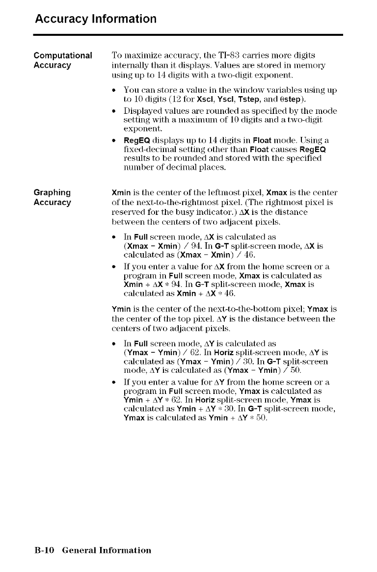
Accuracy Information
Computational
Accuracy
Graphing
Accuracy
To maximize accuracy-, the TI-83 carries more digits
internally than it displays. Values m_ stored in nlemo_-
using up to 14 digits with a two-digit exponent.
• You can store a value in the window vm'iables using up
to 10 digits (12 for Xscl, Yscl, Tstep, and 0step).
• Displayed values are rounded as specified by the mode
setting with a nlaxinmln of 10 digits and a two-digit
exponent.
• ReflEO displays up to 14 digits in Float mode. [ Mng a
fixed-decilnal setting other than Float causes ReflEO
results to be rounded and stored with the specified
number of decimal places.
Xmin is the center of the leffmost pixel, Xmax is the center
of the next-to-the-rightmost pixel. (The rightmost pixel is
reserved for the busy indicator,) AX is the distance
between the centers of two adjacent pixels.
• In Full screen mode, AX is calculated zks
(Xmax - Xmin) /94. In G-T split-screen mode, AX is
calculated as (Xmax - Xmin) /46.
• If you enter a value ff)r AX from the home screen or a
program in Full screen mode, Xmax is calculated as
Xmin + AX * 94. In G-T split-screen mode, Xmax is
calculated as Xmin + AX * 46,
Ymin is the center of the next-to-the-bottom pixel; Ymax is
the center of the top pixel. AY is the distance between the
centers of two adjacent pixels.
• In Full screen mode, AY is calculated as
(Ymax -Ymin) /62. In Horiz split-screen nlode, AYis
cMculated as (Ymax - Ymin) /30. In G-T split-screen
mode, AY is c'Mculated as (Ymax - Ymin) /50.
• If you enter a vMue for AYfronl the home screen or a
program in Full screen mode, Ymax is calculated as
Ymin + AY * 62. In Horiz split-screen nlode, Ymax is
eMculated as Ymin + AY * 30. In G-T split-screen nlode,
Ymax is calculated _ksYmin + AY* 50,
B-IO General Information
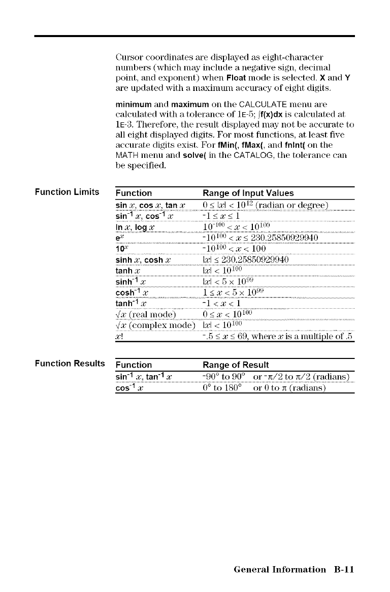
Cursorcoordinatesaredisplayedaseight-character
numbers(whichmayincludeanegativesign,decimal
point,andexponent)whenFloatmodeisselected.XandY
areupdatedwithanlaxinmlnaccuracyofeightdigits.
minimum and maximum on the CALCULATE menu are
calculated with a tolerance of 1E-5; _f(x)dx is calculated at
1E-3. Therefore, the result displayed nlay not be accurate to
'all eight displayed digits. For most functions, at least five
accurate digits exist. For fMin(, fMax(, and fntnt( on the
MATH menu and solve( in the CATALOG, the tolerance can
be specified.
Function Limits
Function Results
Function Range of Input Values
sn cos. " ....................0 .......
sin-12a',COS-1 X...........-1 < x<_1 ...............................
ex-10100< x-<230.25850929940
1_ -10 i00 < x< 100
sinh x, cosh wIxl _<230.25850929940
tanh xIxl < 10 i°°
sinh :_ xIxl < 5 x 10⁹!_..............................
cosh-1 .%, <l_<x 5x 1()9!_
tanh :_ x...........................................................-1 <x< .........................1
_x (real lnode) 0 < x < 10100
_X (complex mode) Ixl < 10 t°°
x! -.5 -<x-< 69, where xis a multiple of .5
Function Range of Result
1 1 o o )
tan- x-90 to 90 or-_/2 t0_/2 (radians)
cos-1x0° to 180° or 0 to x (radians)
General Information B-11
Support and Service Information
Product Support
Customers in the U.S., Canada, Puerto Rico, and the Virgin Islands
For general questions, contact Texas Instrunmnts Customer Support:
phone: 1-800-TI-CARES (1-800-842-2737)
e-mail: ti-cares@ti.com
For technical questions, call the Progrannning Assistance Group of Custonler
Support:
phone: 1-972-917-8324
Customers outside the U.S., Canada, Puerto Rico, and the Virgin Islands
Contact TI by e-mail or visit the TI calculator home page on the World Wide Web.
e-mail: ti-cares@ti.com
Internet: education.ti.com
Product Service
Customers in the U.S. and Canada Only
Always contact Texas Instrmnents Customer Support before returning a product
for service.
Customers outside the U.S. and Canada
Refer to the leaflet enclosed with this product or contact your local Texas
Instruments retaileddistributor.
Other TI Products and Services
Visit the TI calculator honle page on the World Wide Web.
education.ti.com
Refer to the leaflet enclosed with this product or contact your local Texas
Instruments retailer/distributor.
B-12 General Information
Warranty Information
Customersinthe U,S.andCanadaOnly
One-Year Limited Warranty for Electronic Product
This Texas Instruments ("TI") electronic product warranty extends only to the original
purchaser and user of the product.
Warranty Duration. This TI electronic product is warranted to the original purchaser
for a period of one (1) year fl'om the original purchase date.
Warranty (;overage. This TI electronic product is warranted against defective
rnaterials and construction. THIS WARRANTY IS VOID IF THE PRODUCT HAS BEEN
DAMAGED BY ACCIDENT OR UNREASONABLE USE, NEGLECT, IMPROPER
SERVICE, OR OTHER CAUSES NOT ARISING OUT OF DEFECTS IN MATERIALS
OR CONSTRUCTION.
Warranty Disclaimers. ANY IMPLIED WARRANTIES ARISING OUT OF THIS SALE,
INCLUDING BUT NOT LIMITED TO THE IMPLIED WARRANTIES OF
MERCHANTABILITY AND FITNESS FOR A PARTICULAR PURPOSE, ARE LIMITED
IN DURATION TO THE ABOVE ONE-YEAR PERIOD. TEXAS INSTRUMENTS SHALL
NOT BE LIABLE FOR LOSS OF USE OF THE PRODUCT OR OTHER INCIDENTAL
OR CONSEQUENTIAL COSTS, EXPENSES, OR DAMAGES INCURRED BY THE
CONSUMER OR ANY OTHER USER.
Sortie states/provinces do not allow the exclusion or limitation of implied warranties or
consequential damages, so the above limitations or exclusions may not apply to you.
Legal Remedies. This warranty gives you specific legal rights, mid you may also have
other rights that vat_ fl'om state to state or province to province.
Warranty Performance. [)tiring the above one (1) year warranty period, your defective
product will be either repaired or replaced with a reconditioned model of an equivalent
quality (at TI's option) when the product is returned, postage prepaid, to Texas
Instruments Service Facility. The warranty of the repaired or replacement unit will
continue for the warranty of the original unit or six (6) months, whichever is longer.
Other than the postage requirement, no charge will be made for such repair and/or
replacernent. TI strongly recommends that you insure the product for value prior to
rnailing.
Software. Software is licensed, not sold. TI and its licensom do not warrant that the
software will be free fl_m errom or rneet your specific requirements. All software is
provided "AS IS."
Copyright. The software and any docurnentation supplied with this product are
protected by copyright.
General Information B-13

Australia &New Zealand Customers only
One-Year Limited Warranty for Commercial Electronic Product
This Texas Instruments electronic product wmTanty extends only to the
original purchaser and user of the product.
Warranty Duration. This Tex_Ls Instruments electronic product is warranted
to the original purchaser for a period of one (1) year from the original
purchase date.
Warranty Coverage. This Texas Instruments electronic product is warranted
against defective materials and construction. This warranty is void if the
product luks been damaged by accident or unreasonable use, neglect, improper
set_ice, or other causes not arising out of defects in materials or construction.
Warranty Disclaimers. Any implied warranties arising out of this sale,
including but not limited to tile implied warranties of merchantability
and fitness for a particular purpose, are limited in duration to tile
above one-year period. Texas Instruments shall not be liable for loss
of use of the product or other incidental or consequential costs,
expenses, or danlages incm'red by the consuiner or any other user.
Sonic jurisdictions do not allow the exclusion or limitation of implied
warranties or consequential damages, so the al)ove limitations or exclusions
nlay not apply to you.
Legal Remedies. This warranty gives you specific legal rights, and you nlay
also have other rights that vm_- from jurisdiction to jm'isdiction.
Warranty Performance. Dm'ing the above one (1) year warranty period,
your defective product will be either repaired or replaced with a new or
reconditioned model of an equivalent quality (at TI's option) when the product
is returned to the original point of purchase. The repaired or replacement unit
will continue for the warranty of the original unit or six (6) months, whichever
is longer. Other than your cost to return the product, no charge will be made
for such repair and/or replacement. TI strongly recommends that you insm'e
the product for value if you mail it.
Software. Software is licensed, not sold. TI and its licensors do not warrant
that the software will be free from errors or meet your specific requirements.
All software is provided "AS IS."
Copyright. The software and any documentation supplied with this product
are protected by copyright.
All CustomersOutsidethe U.8. andCanada
For information about the length and terms of the warranty, refer to your package
and/or to the warranty statement enclosed with this product, or contact your local Texas
Instruments retailer/distributor.
B-14 General Information
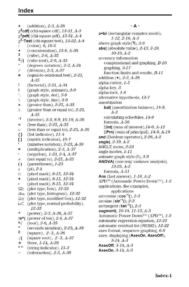
Index
+(addition), 2-3, A-38
z2cdf( (chi-square cdf), 13-31, A-3
x2pdf( @hi-square pdf), 13-31, A-4
x2-Test (ehi-square test), 13-22, A-4
: (colon), 6, 16-5
+ (concatenation), 15-6, A-38
3 (cube), 2-6, A-35
3_( (cube root), 2-6, A-35
° (degrees notation), 2-3, A-34
/(division), 2-3, A-37
=(equal-to relational test), 2-25,
A-35
! (factorial), 2-21, A-34
0(graph style, animate), 3-9
'. (graph style, (lot), 3-9
".. (graph style, line), 3-9
> (greater than), 2-25, A-35
> (greater than or equal to), 2-25,
A-35
• . o
-1 (mx.erse), 2-3, 8-9, 10-10, A-36
< (less than), 2-25, A-35
< (less than or equal to), 2-25, A-36
{ } (list indicator), 11-4
[] (matrix indicator), 10-7
(minutes notation), 2-23, A-38
* (multiplication), 2-3, A-37
(negation), 1-23, 2-4, A-37
(not equal to), 2-25, A-35
() (parentheses), 1-23
(pi), 2-4
[] (pixel mark), 8-15, 12-34
+ (pixel mark), 8-15, 12-34
(pixel mark), 8-15, 12-34
_::> (plot type, box), 12-33
2m= (plot type, histogram), 12-32
_:>'_" (plot type, modified box), 12-32
__ (plot type, normal probability),
12-33
^ (power), ~-3, A-36, A-37
10"( (power often), 2-#,A-37
×/ (root), 2-6, A-35
(seconds notation), 2-23, A-38
2(square), 2-3, A-36
_( (square root), 2-3, A-37
--> Store, 1-1]-_, A-28
.... (string indicator), 15-3
(subtraction), 2-3, A-38
-A-
a+bl (rectangular complex mode),
1-12, 2-16, A-3
above graph style(N), 3-9
abs( (absolute value), 2-13, 2-19,
10-10,A-2
accuracy information
computational and graphing, B-10
graphing, 3-17
function limits and results, B-11
addition (+), 2-3, A-38
alpha cursor, 1-5
alpha key, 3
alpha-lock, 1-8
alternative hypothesis, 13-7
amortization
hal( (amortization balanee), 14-9,
A-3
calculating schedules, 1]-t-9
fornmla, A-56
Elnt( (sum of interest),14-9, A-12
EPrn( (sum of principal), lJ.t-9, A-19
and (Boolean operator), 2-26, A-2
angle(, 2-19, A-2
ANGLE menu, 2-23
angle modes, 1-11
animate graph style (_), 3-9
ANOVA( (one-way variance analysis),
13-25, A-2
fornmla, A-51
Ans (last answer), 1-18, A-2
APD TM (Automatic Power Down__), 1-2
applications. ,fee examples,
applications
areeosine (cos < 0, 2-3
aresine (sin<0, 2-3
aretangent (tan "10, 2-3
augment(, 10-1J-t, 11-15,A-3
Automatic Power Down _xt(AP[Y_), 1-2
automatic regression equation, 12-22
automatic residual list (RESID), 12-22
axes fommt, sequence graphing, 6-8
axes, displaying (AxesOn, AxesOff),
3-14, A-3
AxesOff, 3-14t, A-3
AxesOn, 3-14t, A-3
Index-1
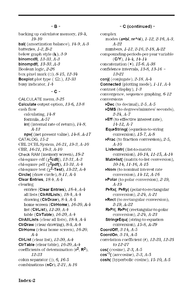
-B-
backing up calculator memmTy, 19-4,
19-10
bal( (amortization balance), 14-9, A-3
batteries, 1-2, B-2
below- graph style (6), 3-9
binomcdf(, 13-33, A-3
binompdf(, 13-33, A-3
Boolean logie, 2-26
box pixel mark ([]), 8-15, 12-34
Boxplot plot type (_), 12-33
busy indicator, 1-4
-C-
CALCULATE metal, 3-25
Calculate output option, 13-6, 13-8
cash flow"
calculating, 14-8
fornmla, A-57
irr( (internal rate of return), 14-8,
A-13
npv( (net present value), 14-8, A-17
CATALOG, 15-2
CBL 2/CBL System, 16-21, 19-3, A-IO
CBR, 16-21, 19-3, A-IO
Check RAM (memol_y screen), 18-2
old-square cdf 0_2cdf0,13-31, A-3
old-square pdf (z2pdf(), 13-31, A-4
eld-squm'e test (z2-Test), 13-22, A-4
Circle( (draw" circle), & l 1, A-4
Clear Entries, 1&4 ,A-4
clearing
entries (Clear Entries), 18-4, A-4
all lists (ClrAIIkists), 1&4, A-4
draw3ng (ClrDraw), 8-4, A-4
home screen (ClrHome), 16-20, A-4
list (Clrkist), 12-20, A-4
table (ClrTable), 16-20, A-4
ClrAIIkists (dear all lists), 1&4, A-4
ClrDraw (clear drawing), &4, A-4
ClrHome (clear home screen), 16-20,
A-4
Clrkist (elear list), 12-20, A-4
ClrTable (elear table), 16-20, A-4
coefficients of determination (r 2, R2),
12-23
colon separator (:), 6, 16-5
combinations (nCr), 2-21, A-16
- C (continued) -
complex
modes (a+bl, re^01), 1-12, 2-16, A-3,
A-22
numbers, 1-12, 2-16, 2-18, A-22
compounding-periods-per-year variable
(c/Y), 14-4, 14-14
coneatenation (+), 15-6, A-38
confidenee intervals, 13-8, 13-16 -
13-21
conj((conjugate), 2-18, A-4
Connected (plotting mode), 1-11, A-4
contrast (display), 1-3
convergence, sequence graphing, 6-12
conversions
)Dec (to deeimal), 2-5, A-5
_DMS (to degree_minute_ seeonds),
2-24, A-7
_Eff (to effeetwe interest rate),
14-12, A-7
Equ_String( (equation-to-string
conversion), 15-7, A-8
_Frac (to fraction conversion), 2-5,
A-IO
kist_matr( (list-to-matrix
conversion), 10-14, 11-15, A-14
MatrHist((matrix-to-list conversion),
10-14, 11-16, A-15
)Nora (to nominal interest rate
conversion), 14-12, A-16
)Polar (to polar eonversion), 2-19,
A-19
PH_x(, P)Ry( (polar-to-reetangular
conversion), 2-24, A-21
_Rect (to rectangular conversion),
2-19, A-22
R_Pr(, R_Pe( (reetangular-to-polm"
conversion), 2-24, A-23
String)Equ( (string-to-equation
conversion), 15-8, A-29
CoordOff, 3-14, A-5
CoordOn, 3-14, A-5
correlation eoefficient (r), 12-23, 12-25
to 12-27
cos((cosine), 2-3, A-5
cos'l((areeosine), 2-3, A-5
cosh( (hyperbolic cosine), 15-10, A-5
Index-2
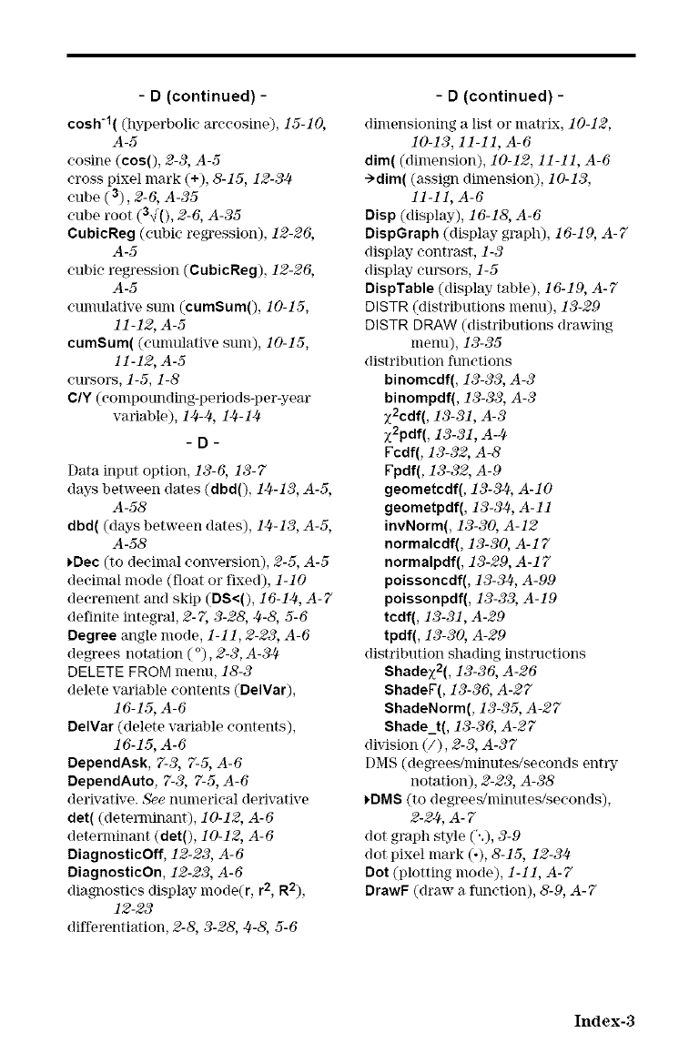
- D (continued)-
cosh'l( (hyperbolic arceosine), 15-10,
A-5
cosine (cos(), 2-3, A-5
cross pixel mark (+), 8-15, 12-34
cube (3), 2-6, A-35
cube root (3_(), 2-6, A-35
CubicReg (cubic regression), 12-26,
A-5
cubic regression (CubicReg), 12-26,
A-5
eunmlative sum (cumSumO, 10-15,
11-12, A-5
cumSum( (cumulative sum), 10-15,
11-12, A-5
cursors, 1-5, 1-8
C/Y (compounding-periods-per-year
variable), 124-Y4,124-124
- D-
Data input option, 13-6, 13-7
days between dates (dbd0, 14-13, A-5,
A-58
dbd( (days between dates), 14-13, A-5,
A-58
_Dec (to decimal conversion), 2-5, A-5
decimal mode (float or fixed), 1-10
decrement and skip (DS<(), 16-14, A-7
definite integral, 2-7, 3-28, 4-8, 5-6
Degree angle mode, 1-11, 2-23, A-6
degrees notation (°), 2-3, A-3J4
DELETE FROM menu, 18-3
delete vm'iable contents (DelVar),
16-15, A-6
DeWar (delete vm'iable contents),
16-15, A-6
DependAsk, 7-3, 7-5, A-6
DependAuto, 7-3, 7-5, A-6
derivative. See numerical derivative
det((determinant), 10-12, A-6
determinant (det0, 10-12, A-6
DiagnostieOff, 12-23, A-6
DiagnostieOn, 12-23, A-6
diagnostics display mode(r, r2, R2),
12-23
differentiation, 2-8, 3-28, 4-8, 5-6
-D (continued) -
dimensioning a list or matrix, 10-12,
10-13, 11-11, A-6
dim((dimension), 10-12, 11-11, A-6
->dim( (assign dimension), 10-13,
11-11, A-6
Disp (display), 16-18, A-6
DispGraph (display graph), 16-19, A-7
display contrast, 1-3
display cursors, 1-5
DispTable (display table), 16-19, A- 7
DISTR (distributions memO, 13-29
DISTR DRAW (distributions drawing
menu), 13-35
distribution functions
binomedf(, 13-33, A-3
binompdf(, 13-33, A-3
z2cdf(, 13-31, A-3
z2pdf(, 13-31, A-4
Fcdf(, 13-32, A-8
Fpdf(, 13-32, A- 9
geometcdf(, 13-34, A- I O
geometpdf(, 13-34, A-11
invNorm(, 13-30, A-12
normalcdf(, 13-30, A-1 7
normalpdf(, 13-29, A-17
poissoncdf(, 13-324, A-99
poissonpdf(, 13-33, A-19
tcdf(, 13-31, A-29
tpdf(, 13-30, A-29
distribution shadh]g instructions
Shadex2(, 13-36, A-26
ShadeF(, 13-36, A-27
ShadeNorm(, 13-35, A-27
Shade_t(, 13-36, A-27
dhqsion (/), 2-3, A-37
[)MS (degrees/minutes/seconds entity"
notation), 2-23, A-38
_DMS (to degreegminutes/seconds),
2-224, A- 7
dot graph style ('..), 3-9
dot pixel Inark (.), 8-15, 12-324
Dot (plotting mode), 1-11, A-7
DrawF (draw- a function), &9, A-7
Index-3
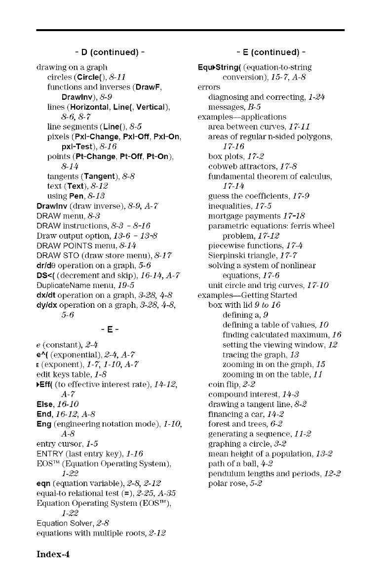
- D (continued)-
drawing on agraph
circles (Circle(), 8-11
flmetions and inverses (DrawF,
Drawlnv), 8-9
lines (Horizontal, Line(, Vertical),
8-6, 8-7
line segments (Line(), 8-5
pixels (PxI-Change, Pxl-Off, Pxl-On,
pxI-Test), 8-16
points (Pt-Change, Pt-Off, Pt-On),
8-14
tangents (Tangent), 8-8
text (Text), 8-12
using Pen, 8-13
Drawlnv (draw" inverse), 8-9, A-7
DRAW menu, 8-3
DRAW instructions, 8-3 -8-16
[)raw- output option, 13-6 -13--8
DRAW POINTS menu, 8-14
DRAW STO (draw" store menu), 8-17
dr/d0 operation on a graph, 5-6
DS<( (decrement and skip), 16-14, A-7
DuplicateName menu, 19-5
dx/dt operation on a graph, 3-28, 4-8
dy/dx operation on a graph, 3-28, 4-8,
5-6
-E-
e(constant), 2-4
e^((exponential), 2-4, A- 7
E (exponent), 1-7, 1-10, A-7
edit keys table, 1-8
t.Eff( (to effective interest rate), 14-12,
A-7
Else, 16-10
End, 16-12, A-8
Eng (engineering notation mode), 1-10,
A-8
entry cm'sor, 1-5
ENTRY (last entry key), 1-16
EOS TM (Equation Operating System),
1-22
eqn (equation variable), 2-8, 2-12
equal-to relational test (=), 2-25, A-35
Equation Operating System (EOSTM),
1-22
Equation Solver, 2-8
equations with nmltiple roots, 2-12
-E(continued) -
Equi_String( (equation-to-string
conversion), 15-7, A-8
errors
diagnosing and correcting, 1-24
messages, B-5
example _-applieations
m'ea between cm_es, 17-11
m'eas of regular n-sided polygons,
17-16
box plots, 17-2
cobweb attractors, 17-8
fundamental theorem of calculus,
17-14
guess the coefficients, 17-9
inequalities, 17-5
mortgage payments 17-18
parametric equations: ferris wheel
problem, 1 7-12
pieeewise functions, 1 7-4
Sierpinski triangle, 1 7- 7
solving a system of nonlinear
equations, 17-6
unit circle and trig curves, 17-10
examples_--Getting Started
box w_th lid 9 to 16
defining a, 9
defining a table of values, 10
finding calculated maxinmm, 16
setting the viewlng window, 12
tracing the graph, 13
zooming in on the graph, 15
zooming in on the table, 11
coin flip, 2-2
compound interest, 14-3
drawing a tangent line, 8-2
financing a era', 14-2
forest and trees, 6-2
generating a sequence, 11-2
graphing a circle, 3-2
mean height of a population, 13-2
path of a ball, J-t-2
pendulum lengths and periods, 12-2
polar rose, 5-2
Index-4
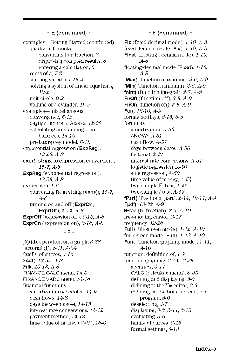
-E (continued) -
exalnp]es_--Getting Started (continued)
quadratic formula
converting to a fraction, g
displaying eomplex results, 8
entering a calculation, 6
roots of a, 7-2
sendHlg variables, 19-2
solving a system of linear equations,
10-2
unit circle, 9-2
volume of a cylinder, 16-2
examples_-nliseellaneous
convergence, 6-12
daylight hours in Alaska, 12-28
calculating outstanding loan
balances, lJ-t-l O
predator-prey model, 6-13
exponential regression (ExpReg),
12-26, A-8
expr( (string-to-expression conversion),
15-7, A-8
ExpReg (exponential regression),
12-26, A-8
expression, 1-6
converting front string (expr(), 15- 7,
A-8
turning on and off (lllxprOn,
lllxprOff), 3-1].t ,A-8
lllxprOff (expression off), 3-1].t, A-8
lllxprOn (expression on), 3-1].t, A-8
- F-
ff(x)dx operation on a graph, 3-28
factorial (!), 2-21, A-3]._
fandly of eut_es, 3-16
Fcdf(, 13-32, A-8
Fill(, 10-13, A-8
FINANCE CALC menu, 14-5
FINANCE VARS menu, 1]-t-1]-t
financial functions
amortization schedules, 10.-9
cash flows, 14-8
days between dates, 14-13
interest rate conversions, 14-12
payment method, 14-13
time value of money (TVM), 14-6
- F (continued) -
Fix (fJxed-deeimal mode), 1-10, A-8
fixed-deeimal mode (Fix), 1-10, A-8
Float (floating-decimal mode), 1-10,
A-8
floating-decimal mode (Float), 1-10,
A-8
fMax( (function maximum), 2-6, A-9
fMin( (function ndnimum), 2-6, A-9
fnlnt( (function integral), 2-7, A-9
FnOff (function off), 3-8, A-9
FnOn (function on), 3-8, A-9
For(, 16-10, k-9
format settings, 3-13, 6-8
formulas
amortization, A-56
ANOVA, A-51
cash flow, A-57
days between dates, A-58
factorial, 2-21
interest rate conversions, A-57
logistic regression, A-50
sine regression, A-50
time value of money, A-5].t
two-sample T-Test, A-52
two-sample ttest, A-53
fPart( (fractional part), 2-1& 10-11, A-9
Fpdf(, 13-32, A-9
)Frac (to fraction), 2-5, A-IO
free-moving cursor, 3-17
frequency, 12-2].t
Full (full-screen mode), 1-12, A-IO
full-screen mode (Full), 1-12, A-IO
Func (function graphing mode), 1-11,
A-IO
function, definition of, 1-7
function graphing, 3-1 to 3-28
accuracy, 3-17
CALC (calculate menu), 3-25
defining and displaying, 3-3
defining in the Y= editor, 3-5
defining on the home screen, in a
program, 3-6
deselecting, 3- 7
displaying, 3-3, 3-11, 3-15
evaluating, 3- 6
family of cmxres, 3-16
format settings, 3-13
Index-5
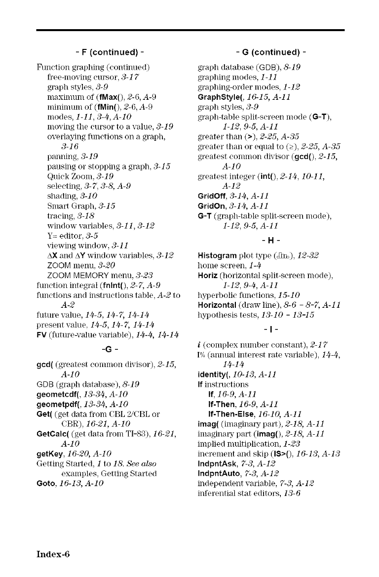
-F (continued) -
Ftmction graphing (continued)
free-moving cursor, 3-17
graph styles, 3-9
maximunl of (fMax0, 2-6, A-9
minimmn of (fMin0, 2-6, A-9
modes, 1-11, 3-4,A-10
moving the cursor to a value, 3-19
overlaying functions on a graph,
3-16
panning, 3-19
pausing or stopping a graph, 3-15
Quick Zoom, 3-19
selecting, 3-7, 3-8, A- 9
shading, 3-10
Snmrt Graph, 3-15
tracing, 3-18
window variables, 3-11, 3-12
Y= editor, 3-5
_ewing window, 3-11
AX and AY window variables, 3-12
ZOOM menu, 3-20
ZOOM MEMORY menu, 3-23
function integral (fnlnt0, 2-7, A-9
functions and instructions table, A-2 to
A-2
future vahle, 14-5, 14-7, l J-t-lJ-t
present value, 14-5, 14-7, 1J-t-l}-t
FV (future-value vm'iable), 1J4-J4, 1J4-1J4
-G -
gcd( (greatest common divisor), 2-15,
A-IO
GDB (graph database), 8-19
geometcdf(, 13-34, A- I O
geometpdf(, 13-34, A- I O
Get( (get data from CBL 2/CBL or
CBR), 16-21, A-IO
GetCalc( (get data from TI-83), 16-21,
A-IO
getKey, 16-20, A-IO
Getting Started, 1to 18. See also
examples, Getting Started
Goto, 16-13, A-IO
-G (continued) -
graph database (GDB), 8-19
graphing modes, 1-11
graphing-order modes, 1-12
GraphStyle(, 16-15, A-11
graph styles, 3-9
graph-table split-screen mode (G-T),
1-12, 9-5, A-11
greater than (>), 2-25, A-35
greater than or equal to (>), 2-25, A-35
greatest common divisor (gcd0, 2-15,
A-IO
greatest integer (intO, 2-14, 10-11,
A-12
GridOff, 3-14, A-11
GridOn, 3-14, A-11
G-T (graph-table split-screen mode),
1-12, 9-5, A-11
- H -
Histogram plot type (2m_), 12-32
home screen, l-J4
Horiz (horizontal split-screen mode),
1-12, 9-4, A-11
hyperbolic functions, 15-10
Horizontal (draw- line), &6 - 8-7, A-11
hypothesis tests, 13-10 -13"-15
i(complex number constant), 2-17
1%(annual interest rate variable), 14-4,
14-14
identity(, 10-13, A-11
if instructions
If, 16-9, A-11
If-Then, 16-9, A-11
If-Then-Else, 16-10, A-11
imag( (imaginmTy" pm't ), 2-18, A-11
imaginary part (imagO, 2-18, A-11
implied nmltiplieation, 1-23
increment and skip (IS>(), 16-13, A-13
IndpntAsk, 7-3, A-12
IndpntAuto, 7-3, A-12
independent variable, 7-3, A-12
inferential stat editors, 13-6
Index-6
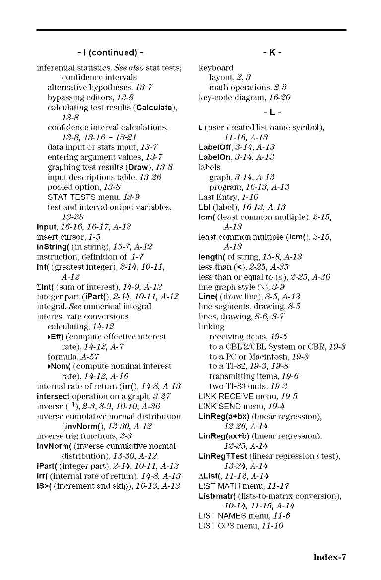
-I (continued) -
inferential statistics. See also stat tests;
confidence intervals
alternative hypotheses, 13- 7
bypassing editors, 13-8
calculating test results (Calculate),
13-8
confidence interval calculations,
13-8, 13-16 -13-21
data input or stats input, 13-7
entering argument values, 13- 7
graphing test results (Draw), 13-8
input descriptions table, 13-26
pooled option, 13-8
STAT TESTS menu, 13-9
test and interval output variables,
13-28
Input, 16-16, 16-17, A-12
insert cursor, 1-5
inString( (in string), 15-7, A-12
instruction, definition of, 1-7
int( (greatest integer), 2-1#, 10-11,
A-12
Elnt( (sum of interest), 1#-9, A-12
integer part (iPart0, 2-1#, 10-11, A-12
integral. See nmnerical integral
interest rate conversions
eMeulating, 14-12
_Eff( (compute effective interest
rate), 14-12, A-7
formula, A-57
_Nom( (compute nondnal interest
rate), 1#-12, A-16
internal rate of return (irr(), 1#-8, A-13
intersect operation on a graph, 3-27
inverse (-1), 2-3, 8-9, 10-10, A-36
inverse eunmlative normal distribution
(invNorm0, 13-30, A-12
inverse trig functions, 2-3
invNorm( (inverse eunmlative normal
distribution), 13-30, A-12
iPart( (integer part), 2-14, 10-11, A-12
irr( (internal rate of return), 14-8, A-13
I$>( (increment and skip), 16-13, A-13
-K-
keyboard
layout, 2, 3
ninth operations, 2-3
key-code diagrmn, 16-20
- L-
L(user-created list nmne symbol),
11-16, A-13
LabelOff, 3-14, A-13
LabelOn, 3-14, A-13
labels
graph, 3-14, A-13
program, 16-13, A-13
Last Entry, 1-16
Lbl (label), 16-13, A-13
Icm( (least common multiple), 2-15,
A-13
least common nmltiple (Icm(), 2-15,
A-13
length( of string, 15-8, A-13
less than (<), 2-25, A-35
less than or equal to (<), 2-25, A-36
line graph style C'), 3-9
Line( (draw line), 8-5, A-13
line segments, drawing, &5
lines, drawing, 8-6, &7
linking
receMng items, 19-5
to a CBL 2/CBL System or CBR, 19-3
to a PC or Macintosh, 19-3
to a TI-82, 19-3, 19-8
transndtting items, 19- 6
two TI-83 units, 19-3
LINK RECEIVE menu, 19-5
LINK SEND menu, 19-4
kinReg(a+bx) (linear regression),
12-26, A-14
LinReg(ax+b) (linear regression),
12-25, A-14
LinRegTTest (linear regression ttest),
13-2#, A-14
AList(, 11-12, A-14
LIST MATH menu, 11-17
List_matr( (lists-to-matrix conversion),
10-14, 11-15, A-14
LIST NAMES menu, 11-6
LIST OPS menu, 11-10
Index-7
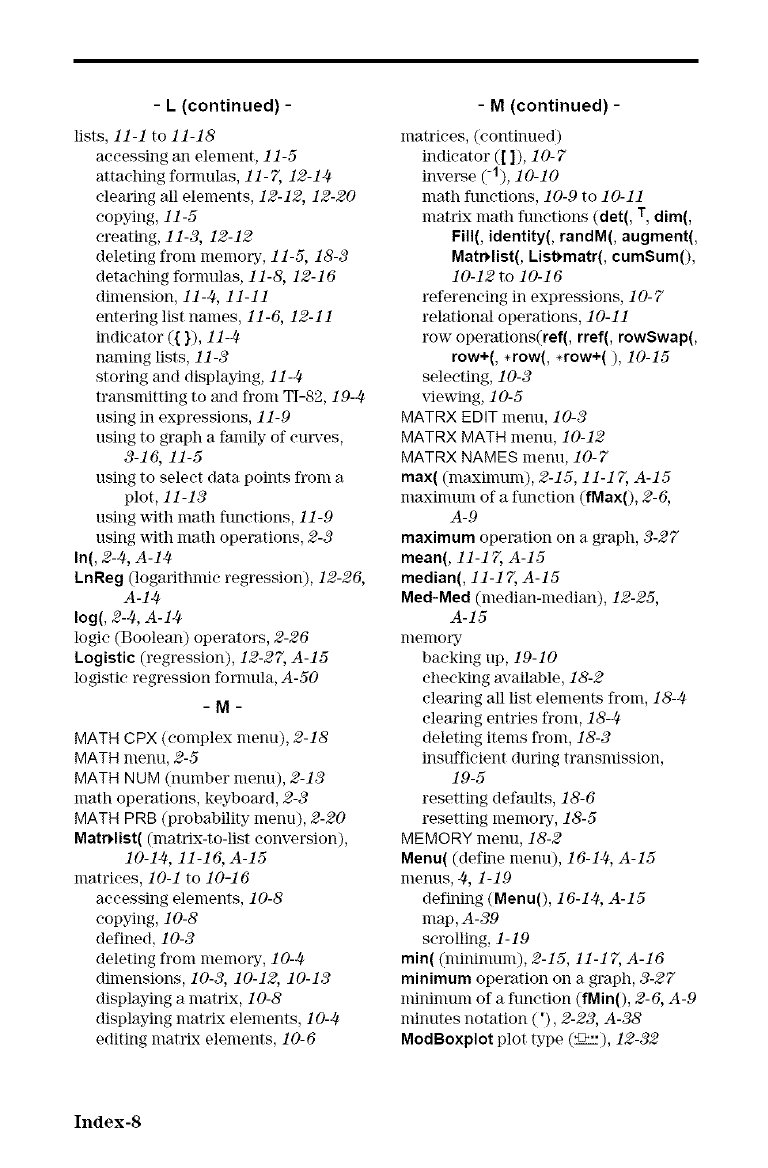
-L(continued) -
lists, 11-1 to 11-18
aeeessing an element, 11-5
attaehing fornmlas, 11-7, 12-14
clearing all elements, 12-12, 12-20
eopying, 11-5
creating, 11-3, 12-12
deleting from memory, 11-5, 18-3
detaching fommlas, 11-8, 12-16
dimension, 11-4, 11-11
entering list names, 11-6, 12-11
indicator ({ }), 11-4.
naming lists, 11-3
storing and displaJAng, 11-4.
transmitting to and from TI-82, 19-4
using in expressions, 11-9
using to graph a family of curves,
3-16, 11-5
using to select data points from a
plot, 11-13
using ,_th math functions, 11-9
using _th ninth operations, 2-3
In(, 2-4, A-14
LnReg (logarithmic regression), 12-26,
A-14
log(, 2-4, A-14
logic (Boolean) operators, 2-26
Logistic (regression), 12-27, A-15
logistic regression fornmla, A-50
- M -
MATH CPX (eomplex menu), 2-18
MATH menu, 2-5
MATH NUM (number menu), 2-13
math operations, keyboard, 2-3
MATH PRB (probability menu), 2-20
MatrHist( (nmtrix-to-list conversion),
10-14, 11-16, A-15
matrices, 10-1 to 10-16
accessing elements, 10-8
copying, 10-8
defined, 10-3
deleting from memory, 10-4
dimensions, 10-3, 10-12, 10-13
displaying a nmtrix, 10-8
displaying matrix elements, 10-4
editing matrix elements, 10-6
-M (continued) -
matriees, (eontinued)
indicator ([ ]), 10-7
inverse (-1), 10-10
math functions, 10-9 to 10-11
matrix math functions (det(, T, dim(,
Fill(, identity(, randM(, augment(,
MatrHist(, List_matr(, cumSumO,
10-12 to 10-16
reDreneing in expressions, 10- 7
relational operations, 10-11
row operations(ref(, rref(, rowSwap(,
row+(, *row(, *row+(), 10-15
selecting, 10-3
xqewing, 10-5
MATRX EDIT menu, 10-3
MATRX MATH menu, 10-12
MATRX NAMES menu, 10-7
max((maximum), 2-15, 11-17, A-15
maximum of a funetion (fMax0, 2-6,
A-9
maximum operation on a graph, 3-27
mean(, 11-17, A-15
median(, 11-17, A-15
Meal-Meal (median-median), 12-25,
A-15
inenlolTy"
backing up, 19-10
checking available, 18-2
clearing all list elements from, 18-4
elem'tng entries from, 18-4
deleting items from, 18-3
insufficient during transmission,
19-5
resetting defaults, 18-6
resetting memory, 18-5
MEMORY menu, 18-2
Menu( (define menu), 16-14, A-15
menus, 4, 1-19
defining (Menu(), 16-14, A-15
nmp, A-39
scrolling, 1-19
min( (minhmm0, 2-15, 11-17, A-16
minimum operation on a graph, 3-27
minimum of a function (fMin0, 2-6, A-9
minutes notation ('), 2-23, A-38
ModBoxplot plot type (4>.), 12-32
Index-8
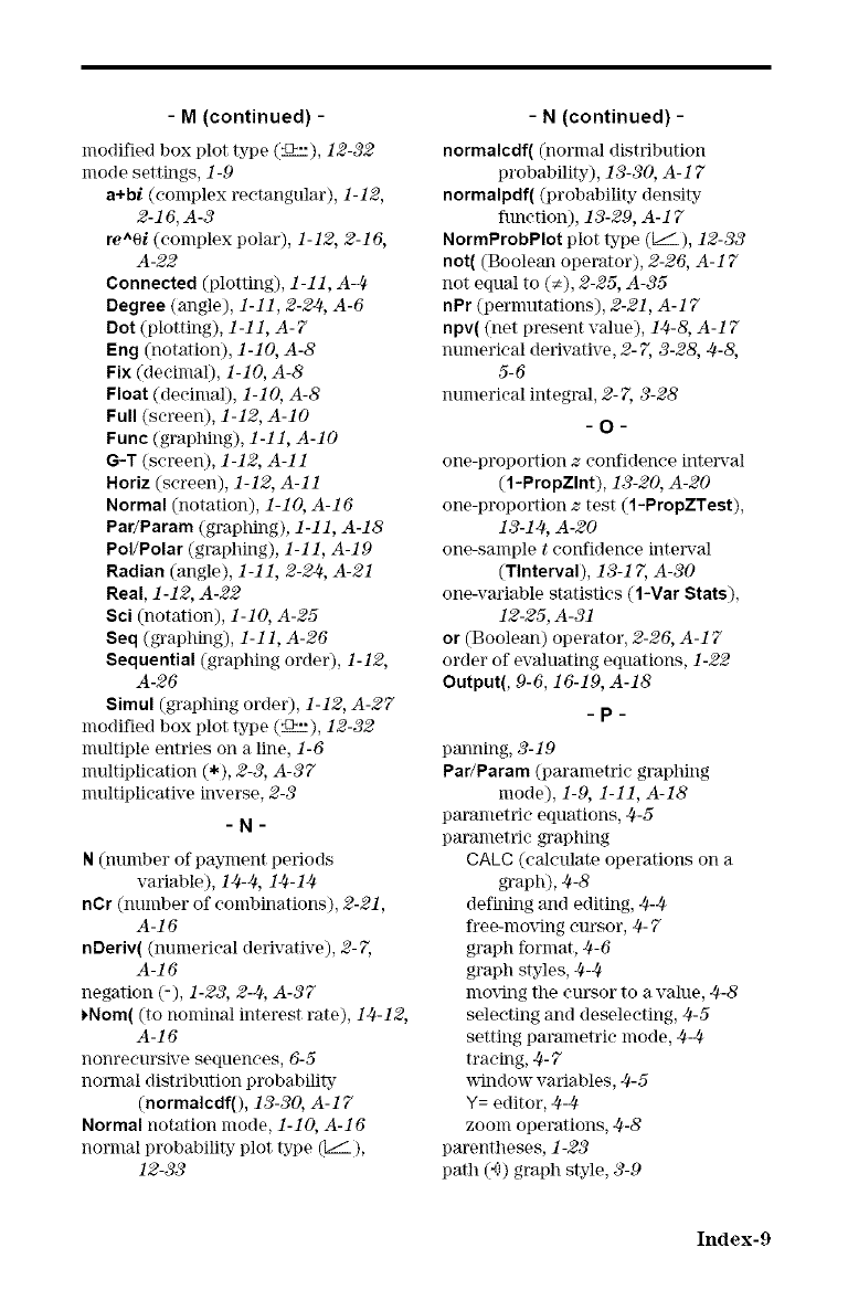
-M (continued) -
modified box [)lot type (o..), 12-32
mode settings, 1-9
a+bl (complex rectangular), 1-12,
2-16, A-3
re^Of (complex polar), 1-12, 2-16,
A-22
Connected (ploning), 1-11, A-4
Degree (angle), 1-11, 2-24, A-6
Dot (plotting), 1-11, A-7
Eng (notation), 1-10, A-8
Fix (decimal), 1-10, A-8
Float (decimal), 1-10, A-8
Full (screen), 1-12, A-IO
Func (graphing), 1-11, A-IO
G-T (screen), 1-12, A-11
Horiz (screen), 1-12, A-11
Normal (notation), 1-10, A-16
Par/Param (graphing), 1-11, A-18
Pol/Polar (graphing), 1-11, A-19
Radian (angle), 1-11, 2-24, A-21
Real, 1-12, A-22
Sci (notation), 1-10, A-25
Seq (graphing), 1-11, A-26
Sequential (graphing order), 1-12,
A-26
Simul (graphing order), 1-12, A-27
modified box [)lot type (o..), 12-32
multiple entries on a line, 1-6
multiplication (*), 2-3, A-37
multiplieative inverse, 2-3
-N-
N(number of payment periods
variable), 14-4, 14-14
nCr (number of combinations), 2-21,
A-16
nDeriv( (numerical derivative), 2-7,
A-16
negation (-), 1-23, 2-4, A-37
_Nom( (to nominal interest rate), 14-12,
A-16
nonrecursive sequences, 6-5
normal distribution probability
(normalcdf(), 13-30, A-17
Normal notation mode, 1-10, A-16
normal probability plot type (__),
12-33
-N (continued) -
normalcdf( (normal distribution
probability), 13-30, A-17
normalpdf( (probability density
function), 13-29, A-17
NormProbPIot plot type ([__), 12-33
not( (Boolean operator), 2-26, A-17
not equal to (_), 2-25, A-35
nPr (pernmtations), 2-21, A-17
npv( (net present value), 14-8, A-17
numerical derivative, 2- 7, 3-28, 4-8,
5-6
numerical integral, 2- 7, 3-28
- O-
one-proportion zconfidence inte_ral
(1-PropZInt), 13-20, A-20
one-proportion ztest (1-PropZTest),
13-14, A-20
one-sample tconfidence inte_al
(Tlnterval), 13-17, A-30
one-variable statistics (1-Var Stats),
12-25, A-31
or (Boolean) operator, 2-26, A-17
order of evaluating equations, 1-22
Output(, 9-6, 16-19, A-18
panning, 3-19
Par/Param (pm'ametrie graphing
mode), 1-9, 1-11, A-18
parametric equations, 4-5
parametric graphing
CA/C (calculate operations on a
graph), 4-8
defi_ling and editing, 4-4
free-moving cursor, 4- 7
graph format, 4-6
graph styles, 4-4
moving the cursor to a value, 4-8
selecting and deseleeting, 4-5
setting parametric mode, 4-4
tracing, 4- 7
window variables, 4-5
Y= editor, 4-4
zoom operations, 4-8
parentheses, 1-23
path (_.))graph style, 3-9
Index-9
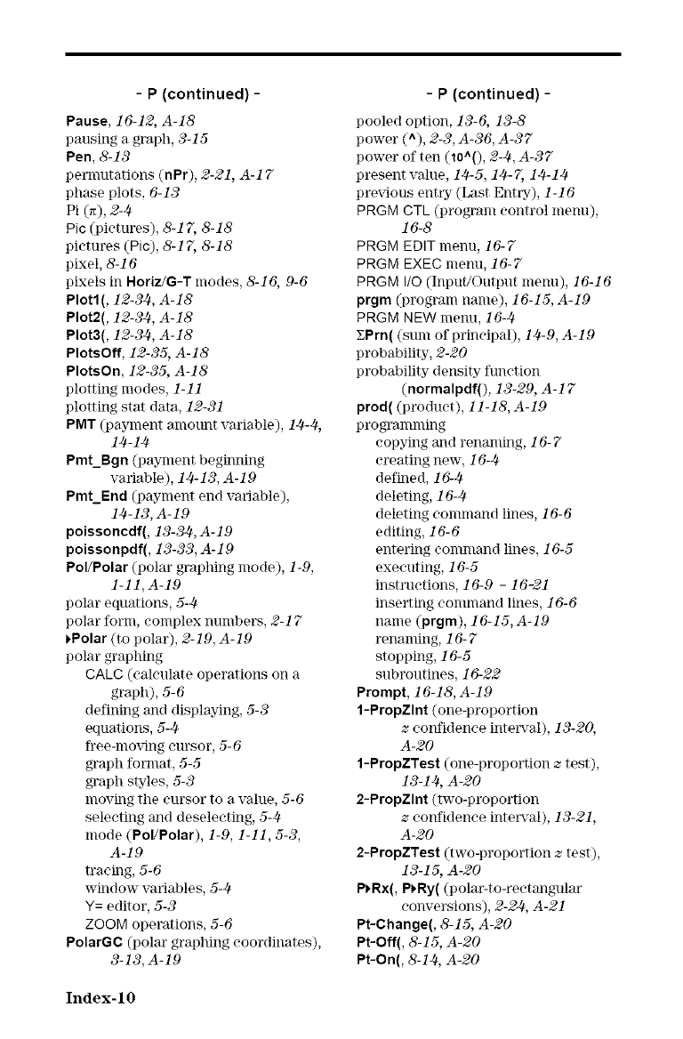
-P (continued) -
Pause, 16-12, A-18
pausing a graph, 3-15
Pen, 8-13
pernmtations (nPr), 2-21, A-17
phase plots, 6-13
Pi (_), 2-4
Pic (pictures), 8-17, 8-18
pictures (Pic), 8-17, 8-18
pixel, 8-16
pixels in Horiz/G-T modes, 8-16, 9-6
Plot4 (, 12-34, A-18
Plot2(, 12-34, A-18
Plot3(, 12-34, A-18
PlotsOff, 12-35, A-18
PlotsOn, 12-35, A-18
plotting modes, 1-11
plotting stat data, 12-31
PMT (payment amount variable), 14-4,
14-14
Pmt_Bgn (payment beghming
variable), 14-13, A-19
Pmt_End (payment end variable),
14-13,A-19
poissoncdf(, 13-324, A-19
poissonpdf(, 13-33, A-19
Pol/Polar (polar graphing mode), 1-9,
1-11,A-19
polar equations, 5-4
polar form, complex numbers, 2-17
*Polar (to polar), 2-19, A-19
polar graphing
CALC (calculate operations on a
graph), 5-6
defining and displaying, 5-3
equations, 5-4
free-moxqngcursor, 5-6
graph format, 5-5
graph styles, 5-3
moving the cursor to a value, 5-6
selecting and deselecting, 5-4,
mode (Pol/Polar), 1-9, 1-11, 5-3,
A-19
tracing, 5-6
window variables, 5-]-_
Y= editor, 5-3
ZOOM operations, 5-6
PolarG¢ (polm" graphing coordinates),
3-13, A-19
-P (continued) -
pooled option, 13-6, 13-8
power (^), 2-3, A-36, A-37
power of ten (10^0, 2-& A-37
present vahle, 1].t-5, 1].b7, 14-1].t
prexqous entlT (Last Entry), 1-16
PRGM CTL (program control menu),
16-8
PRGM EDIT menu, 16-7
PRGM EXEC menu, 16-7
P RGM I/O (Input/Output menu), 16-16
prgm (program name), 16-15, A-19
PRGM NEW menu, 16-0.
ZPrn( (sum of principal), 12.t-9, A-19
probability, 2-20
probability density" function
(normalpdfO, 13-29, A-17
prod((product), 11-18, A-19
programming
copying and renaming, 16-7
creating new-, 16J._
defined, 16J.t
deleting, 16J-_
deleting command lines, 16-6
editing, 16-6
entering command lines, 16-5
executing, 16-5
instructions, 16-9 -16-21
inserting command lines, 16-6
name (prgm), 16-15, A-19
renaming, 16- 7
stopping, 16-5
subroutines, 16-22
Prompt, 16-18, A-19
1-PropZlnt (one-proportion
zconfidence interval), 13-20,
A-20
1-PropZTest (one-proportion ztest),
13-1].t, A-20
2-PropZlnt (two-proportion
zconfidence interval), 13-21,
A-20
2-PropZTest (two-proportion ztest),
13-15, A-20
P)'Rx(, P)'Ry( (polar-to-rectangular
conversions), 2-24, A-21
Pt-Change(, 8-15, A-20
Pt-Off(, 8-15, A-20
Pt-On(, 8-10, A-20
Index-lO
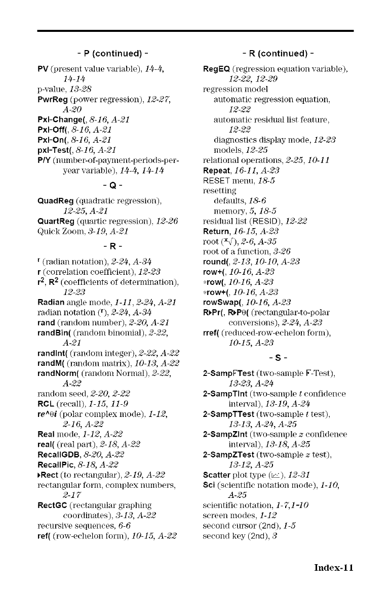
-P (continued) -
PV (present value variable), lJ4-J4,
114-114
p-value, 13-28
PwrReg (power regression), 12-27,
A-20
Pxl-Change(, 8-16, A- 21
PxI-Off(, 8-16, A-21
PxI-On(, 8-16, A-21
pxI-Test(, 8-16, A-21
PlY (nunlber-of-payment-periods-per-
year variable), lJ4-J4, lJ4-1J4
QuadReg (quadratic regression),
12-25, A-21
QuartReg (quartic regression), 12-26
Quick Zoom, 3-19, A-21
-R-
r (radian notation), 2-2/4, A-3J4
r (correlation coefficient), 12-23
r2, R2 (coefficients of determination),
12-23
Radian angle mode, 1-11, 2-2J4, A-21
radian notation (r), 2-24, A-34
rand (random number), 2-20, A-21
randBin( @andom binomial), 2-22,
A-21
randlnt( (random integer), 2-22, A-22
randM( (random matrix), 10-13, A-22
randNorm( (random Normal), 2-22,
A-22
random seed, 2-20, 2-22
RCL (recall), 1-15, 11-9
re^Oi (polm" complex mode), 1-12,
2-16, A-22
Real mode, 1-12, A-22
real( (real part), 2-18, A-22
RecalIGDB, 8-20, A-22
RecallPic, 8-18, A-22
_Rect (to rectangulm'), 2-19, A-22
rectangular form, complex numbers,
2-17
RectGC (rectangular graphing
coordinates), 3-13, A-22
recursive sequences, 6-6
ref( (row-echelon form), 10-15, A-22
-R (continued) -
RegEQ (regression equation vm'iable),
12-22, 12-29
regression model
automatic regression equation,
12-22
automatic residual list feature,
12-22
diagnostics display mode, 12-23
models, 12-25
relational operations, 2-25, 10-11
Repeat, 16-11, A-23
RESET menu, 18-5
resetting
defaults, 18-6
memmTy', 5, 18-5
resklual list (RESID), 12-22
Return, 16-15, A-23
root (x?), 2-6, A-35
root of a function, 3-26
round(, 2-13, 10-10, A-23
row+(, 10-16, A-23
*row(, 10-16, A-23
*row+(, 10-16, A-23
rowSwap(, 10-16, A-23
RH=r(, I_P0( (reetangular-to-polm"
conversions), 2-2J4, A-23
rref( (reduced-row-echelon form),
10-15, A-23
-S -
2-SampFTest (two-sample g-Test),
13-23, A-2J4
2-SampTInt (two-sample tconfidence
illtel_ral), 13-19, A-24
2-SampTTest (two-sample ttest),
13-13, A-2J4, A-25
2-SampZlnt (two-sample zconfidence
inte_5,al), 13-18, A-25
2-SampZTest (two-sample ztest),
13-12, A-25
Scatter plot type (L_), 12-31
Sci (scientific notation mode), 1-10,
A-25
scientific notation, 1-7,1-10
screen modes, 1-12
second cursor (2nd), 1-5
second key (2nd), 3
Index- 11
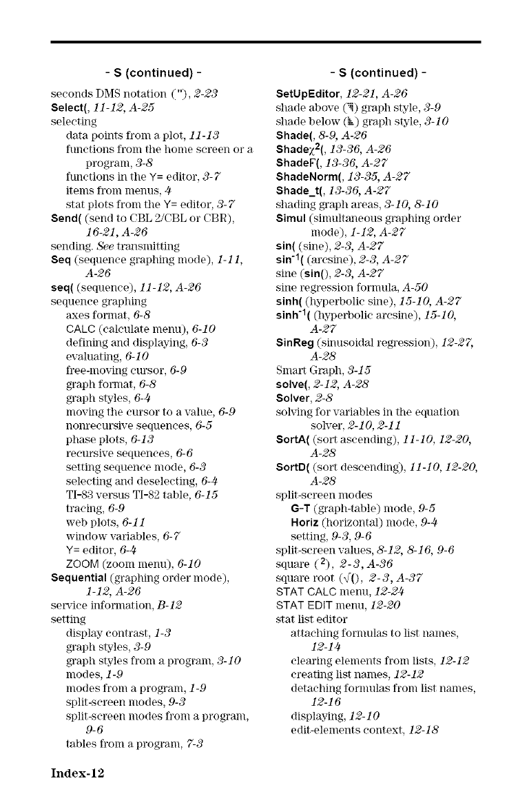
-S (continued) -
seconds DMS notation ('), 2-23
Select(, 11-12, A-25
selecting
data points from a plot, 11-13
functions from the home screen or a
program, 3-8
functions in tile Y= editor, 3-7
items from nlenus, J4
stat plots from tile Y= editor, 3-7
Send( (send to (BL 2/('BL or CBR),
16-21, A-26
sending. See trtmsmitting
Seq (sequence graphing mode), 1-11,
A-26
seq((sequence), 11-12, A-26
sequence graphing
axes fommt, 6-8
CALC (calculate memO, 6-10
defining and displaying, 6-3
evaluati]lg, 6-10
free-mo_ng cursor, 6-9
graph fommt, 6-8
graph styles, 6-J4
moving the cursor to a value, 6-9
nonreeursive sequences, 6-5
phase plots, 6-13
recursive sequences, 6-6
setting sequence mode, 6-3
selecting and deseleeting, 6-4
TI-83 versus TI-82 table, 6-15
tracing, 6-9
web plots, 6-11
window variables, 6- 7
Y= editor, 6-J4
ZOOM (zoom menu), 6-10
Sequential (graphing order mode),
1-12, A-26
service infornmtion, B-12
setting
display contrast, 1-3
graph styles, 3-9
graph styles from a program, 3-10
modes, 1-9
modes from a program, 1-9
split-screen modes, 9-3
split-screen modes from a program,
9-6
tables from a program, 7-3
-S(continued) -
SetUpEditor, 12-21, A-26
shade above (7) graph style, 3-9
shade below- (6) graph style, 3-10
Shade(, 8-9, A-26
Shadexi(, 13-36, A-26
ShadeF(, 13-36, A-27
ShadeNorm(, 13-35, A-27
Shade_t(, 13-36, A-27
shading graph areas, 3-10, 8-10
Simul (simultaneous graphing order
mode), 1-12, A-27
sin((sine), 2-3, A-27
sin'1((m-csine), 2-3, A-27
sine (sin(), 2-3, A-27
sine regression formula, A-50
sinh( (hyperbolic sine), 15-10, A-27
sinh'l( (hyperbolic m'csine), 15-10,
A-27
SinReg (sinusoMal regression), 12-27,
A-28
Smart Graph, 3-15
solve(, 2-12, A-28
Solver, 2-8
solving for variables in tile equation
solver, 2-10, 2-11
SortA( (sort ascending), 11-10, 12-20,
A-28
SortD( (sort descending), 11-10, 12-20,
A-28
split-screen modes
G-T (graph-table) mode, 9-5
Horiz (horizontal) mode, 9-#
setting, 9-3, 9-6
split-screen values, 8-12, 8-16, 9-6
square (2), 2-3, A-36
square root (_(), 2-3, A-37
STAT CALC menu, 12-2J-t
STAT KDIT menu, 12-20
stat list editor
attaching formulas to list names,
12-1J.t
clearing elements from lists, 12-12
creating list names, 12-12
detaching fornmlas from list names,
12-16
displaying, 12-10
edit-elements context, 12-18
Index-12
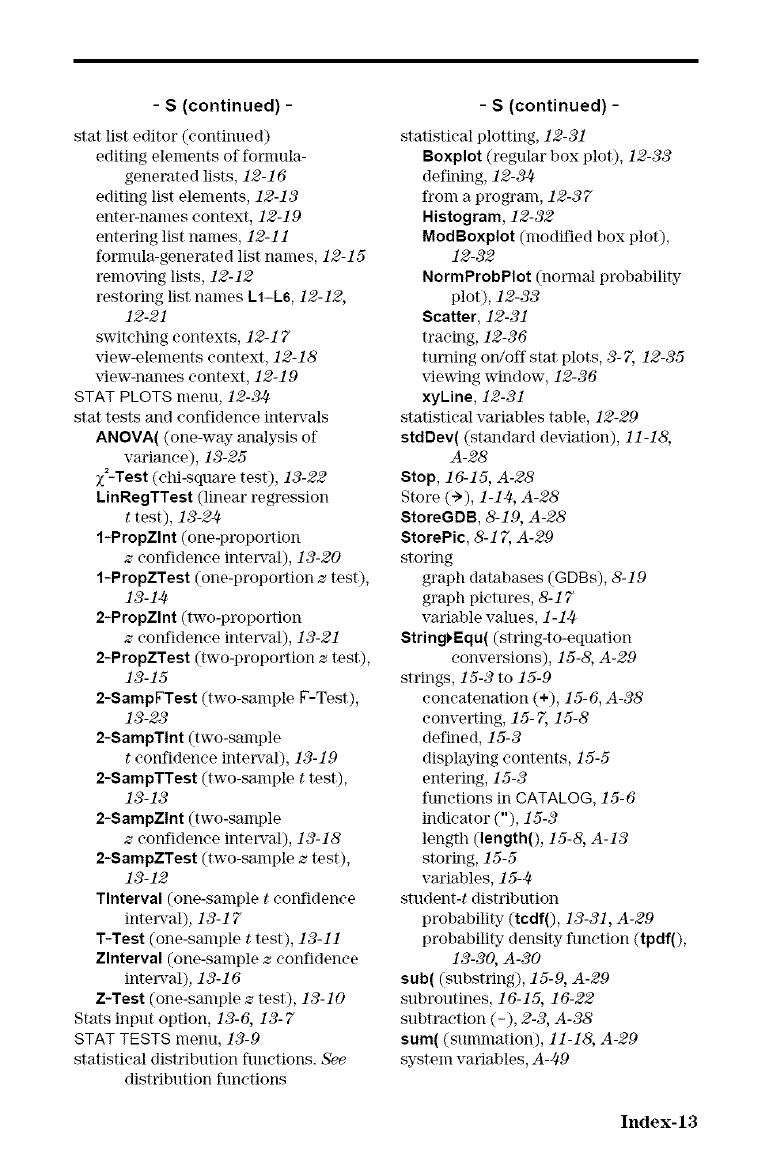
-S (continued) -
star list editor (eonthmed)
editing elements of fornmla-
generated lists, 12-16
editing list elements, 12-13
enter-names context, 12-19
entering list names, 12-11
formula-generated list names, 12-15
remoxqng lists, 12-12
restoring list names L1-L& 12-12,
12-21
switching eontexts, 12-17
x_ew-elements eontext, 12-18
x_ew-names eontext, 12-19
STAT PLOTS metal, 12-34
stat tests and confidence intel_rals
ANOVA( (one-way analysis of
variance), 13-25
x2-Test (ehi-squm'e test), 13-22
LinRegTTest (linear regression
ttest), 13-24
1-PropZlnt (one-proportion
zconfidence interval), 13-20
1-PropZTest (one-proportion ztest),
13-14
2-PropZlnt (two-proportion
zeonfidence interval), 13-21
2-PropZTest (two-proportion ztest),
13-15
2-SampFTest (two-sample F-Test),
13-23
2-SampTInt (two-sample
teonfidenee interval), 13-19
2-SampTTest (two-sample ttest),
13-13
2-SampZlnt (two-sample
zeonfidenee interval), 13-18
2-SampZTest (two-sample ztest),
13-12
Tlnterval (one-sample teonfidenee
inte_x_al), 13-17
T-Test (one-sample ttest), 13-11
Zlnterval (one-sample zeonfidenee
inte_x_al), 13-16
Z-Test (one-sample ztest), 13-10
Stats input option, 13-6, 13-7
STAT TESTS menu, 13-9
statistieal distribution functions. See
distribution functions
-S (continued) -
statistieal plotting, 12-31
Boxplot (regular box plot), 12-33
defining, 12-34
from a program, 12-37
Histogram, 12-32
ModBoxplot (modified box plot),
12-32
NormProbPIot (normal probability
plot), 12-33
Scatter, 12-31
tracing, 12-36
turning on/off stat plots, 3-7, 12-35
x_e,slng window, 12-36
xyLine, 12-31
statistieal vm'iables table, 12-29
stdDev( (standard dexdation), 11-18,
A-28
Stop, 16-15, A-28
Store (-)), 1-14, A-28
StoreGDB, 8-19, A-28
StorePic, 8-17, A-29
storing
graph databases (GDBs), 8-19
graph pictures, 8-17
vmiable values, 1-14
String_Equ( (string-to-equation
conversions), 15-8, A-29
strings, 15-3 to 15-9
concatenation (÷), 15-6, A-38
converting, 15-7, 15-8
defined, 15-3
displaying contents, 15-5
entering, 15-3
functions in CATALOG, 15-6
indicator ("), 15-3
length (length(), 15-8, A-13
storing, 15-5
vmiables, 15-4
student-t distribution
probability (tcdf0, 13-31, A-29
probability density function (tpdf0,
13-30, A-30
sub((substring), 15-9, A-29
subroutines, 16-15, 16-22
subtraction (-), 2-3, A-38
sum((sumnmtion), 11-18, A-29
system variables, A-49
Index-13
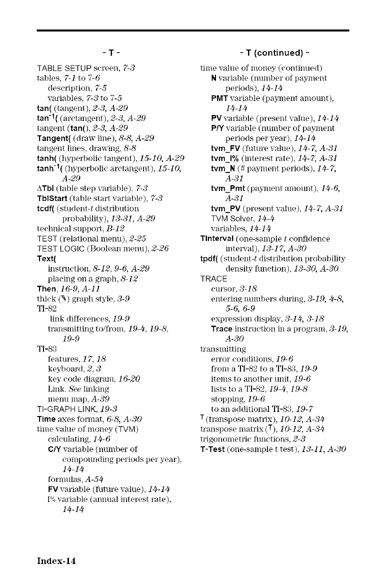
-T-
TABLE SETUP screen, 7-3
tables, 7-1 to 7-6
description, 7-5
variables, 7-3 to 7-5
tan((tangent), 2-3, A-29
tan'l((aretangent), 2-3, A-29
tangent (tan(), 2-3, A-29
Tangent( (draw line), 8-8, A-29
tangent lines, drawi_lg, 8-8
tan h( (hyperbolic tangent), 15-10, A-29
tanh'l( (hyperbolic aretangent), 15-10,
A-29
ATbl (table step variable), 7-3
TblStart (table start variable), 7-3
tcdf( (student-t distribution
probability), 13-31, A-29
teelmieal support, B-12
TEST (relational menu), 2-25
TEST LOGIC (Boolean menu), 2-26
Text(
instruction, 8-12, 9-6, A-29
placing on a graph, 8-12
Then, 16-9, A-11
thick (_.) graph style, 3-9
TI-82
link differences, 19-9
transmitting to/from, 19-2-t, 19-8,
19-9
TI-83
features, 17, 18
keyboard, 2, 3
key code diagram, 16-20
Link. See linking
menu map, A-39
TI-GRAPH LINK, 19-3
Time axes format, 6-8, A-30
time value of money (TVM)
calculating, 12-t-6
C/Y vm'iable (nmnber of
compounding periods per year),
12`1-12`1
formulas, A-54
FV vm'iable (furore value), 12`1-12`1
I% variable (annual interest rate),
12.t-12.t
-T(continued) -
time value of money (eontinued)
Nvm'iable (number of payment
periods), 14-12-t
PMT vm'iable (payment amount),
14-14
PV variable (present value), 12`1-12`1
PlY vm'iable (number of payment
periods per yem'), 12`1-12-1
tvm_FV (future value), 12-1-7,A-31
tyro_l% (interest rate), 14-7, A-31
tvm_N (# payment periods), 12-1-7,
A-31
tvm_Pmt (payment amount), 14-6,
A-31
tvm_PV (present Vahle), 12`1-7, A-31
TVM Solver, 12-1-2-1
vm'iables, 12-1-14
Tlnterval (one-sample teonfidenee
interval), 13-17, A-30
tpdf( (student-t distribution probability
density funetion), 13-30, A-30
TRACE
eursor, 3-18
entering numbers during, 3-19, 4-8,
5-6, 6-9
expression display, 3-12`1,3-18
Trace instruction in a program, 3-19,
A-30
transmitting
error conditions, 19-6
from a TI-82 to a TI-83, 19-9
items to another unit, 19-6
lists to a TI-82, 19-2-1,19-8
stopping, 19- 6
to an additional TI-83, 19-7
T(transpose matrix), 10-12, A-34
transpose matrix (T), 10-12, A-34
trigonometric functions, 2-3
T-Test (one-sample t test), 13-11, A-30
Index-14
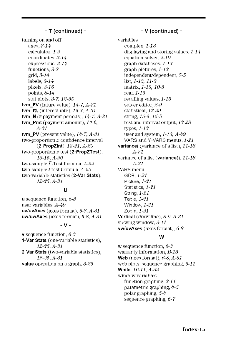
- T (continued) -
turlling Ol1and off
axes, 3-1J4
calculator, 1-2
coordinates, 3-14
expressions, 3-1J4
functions, 3- 7
grid, 3-1J4
labels, 3-1J4
pixels, 8-16
points, 8-1J4
stat plots, 3-7, 12-35
tvm_FV (future vane), lj4 -7, A-31
tyro_l% (interest rate), 114-7, A-31
tvm_N (# payment periods), 114-7, A-31
tvm_Pmt (payment amount), 114-6,
A-31
tvm_PV (present value), 114-7, A-31
two-proportion zconfidence inte_a_al
(2-PropZlnt), 13-21, A-20
two-proportion ztest (2-PropZTest),
13-15, A-20
two-sample F-Test formula, A-52
two-sample ttest formula, A-53
two-vm'iable statistics (2-Var Stats),
12-25, A-31
-U-
u sequence function, 6-3
user variables, A-49
uv/uvAxes (axes format), 6-8, A-31
uw/uwAxes (axes format), 6-8, A-31
-V-
vsequence function, 6-3
1-Var Stats (one-variable statistics),
12-25, A-31
2-Var Stats (two-variable statistics),
12-25, A-31
value operation on a graph, 3-25
-V (continued) -
vmialAes
complex, 1-13
displaying and storing values, 1-11t
equation solver, 2-10
graph databases, 1-13
graph pictures, 1-13
independent/dependent, 7-5
list, 1-13, 11-3
matrix, 1-13, 10-3
real, 1-13
recalling values, 1-15
solver editor, 2-9
statistical, 12-29
string, 15-].L15-5
test aim inte_xral output, 13-28
types, 1-13
user and system, 1-13, A J-t9
VARS and Y-VARS menus, 1-21
variance( (variance of a list), 11-18,
A-31
vm'ianee of a list (variance(), 11-18,
A-31
VARS menu
GDB, 1-21
Picture, 1-21
Statistics, 1-21
String, 1-21
Table, 1-21
Window, 1-21
Zoom, 1-21
Vertical (draw line), &6, A-31
_dewing window, 3-11
vw/uvAxes (axes format), 6-8
W
wsequence function, 6-3
warranty inforlnation, B-13
Web (axes format), 6-8, A-31
web plots, sequence graphing, 6-11
While, 16-11,A-32
window variables
function graphing, 3-11
parametric graphing, ]4-5
polar graphNg, 5-]4
sequence graphing, 6- 7
Index-15
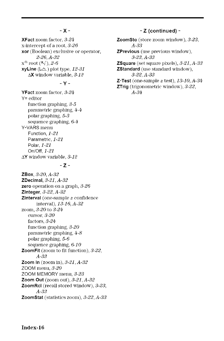
-X-
XFact zoom factor, 3-2J4
x-intercept of a root, 3-26
xor (Boolean) exclusive or operator,
2-26, A-32
xmroot (_), 2-6
xyLine ([__) plot type, 12-31
AX window variable, 3-12
-y-
YFact zoom factor, 3-2J4
Y= editor
function graphing, 3-5
parametric graphing, J4-J4
polar graphing, 5-3
sequence graphing, 624
Y-VARS menu
Function, 1-21
Parametric, 1-21
Polar, 1-21
On/Off, 1-21
AY window variable, 3-12
-Z-
ZBox, 3-20, A-32
ZDecimal, 3-21, A-32
zero operation on a graph, 3-26
Zlnteger, 3-22, A-32
Zlnterval (one-sample zconfidence
intm_al), 13-16, A-32
zoom, 3-20 to 3-214
cursor, 3-20
factors, 3-2J4
function graphing, 3-20
parametric graphing, J4-8
polar graphing, 5-6
sequence graphing, 6-10
ZoomFit (zoom to fit function), 3-22,
A-33
Zoom In (zoom in), 3-21, A-32
ZOOM menu, 3-20
ZOOM MEMORY menu, 3-23
Zoom Out (zoom out), 3-21, A-32
ZoomRcl (recall stored window), 3-23,
A-33
ZoomStat (statistics zoom), 3-22, A-33
- Z (continued) -
ZoomSto (store zoom _lndow), 3-23,
A-33
ZPrevious (use previous window),
3-23, A-33
ZSquare (set square pixels), 3-21, A-33
ZStandard (use standard window),
3-22, A-33
Z-Test (one-sample ztest), 13-10, A-3]-_
ZTrig (trigonometric window), 3-22,
A-3J4
Index-16
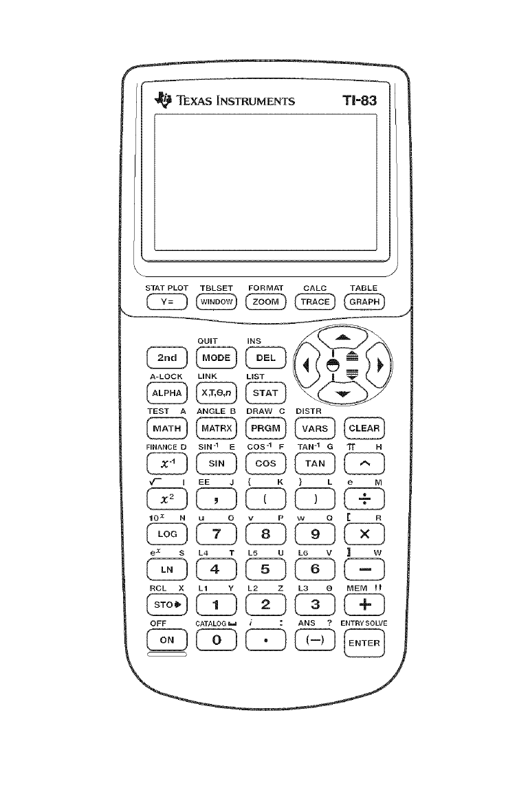
_TEXAS INSTRUMENTS T1=83
STAT PLOT TBLSET FORMAT
J
CALC TABLE
QUiT INS
A-LOCK LiNK LiST
TEST A ANGLE E{ DRAW C
FINANCE D SIN -1 E COS -1 F
I EE J { K
exSL4 TL5 U
RCL X L1 Y L2 Z
DISTR
TAN -1 G 1T N
} L eIvI
L6 V _ W
L3 ® ME[V] f_
OFF CATALOG _ i :ANS ?ENTRY SOLVE