Maxon Cinema 4D 9.5 Dynamics C4D Us
Cinema 4D - 9.0 - Dynamics C4D_dynamics_9.0_us User Guide for Maxon Cinema 4D Software, Free Instruction Manual
User Manual: maxon Cinema 4D - 9.5 - Dynamics Free User Guide for Maxon Cinema 4D Software, Manual
Open the PDF directly: View PDF ![]() .
.
Page Count: 262 [warning: Documents this large are best viewed by clicking the View PDF Link!]

Dynamics
Dynamics
Programming Team Christian Losch, Philip Losch, Richard Kurz, Tilo Kühn, Thomas Kunert,
David O’Reilly, Cathleen Poppe.
Plugin Programming Sven Behne, Wilfried Behne, Michael Breitzke, Kiril Dinev, Per-Anders Edwards,
David Farmer, Jamie Halmick, Richard Hintzenstern, Jan Eric Hoffmann,
Eduardo Olivares, Nina Ivanova, Markus Jakubietz, Eric Sommerlade,
Hendrik Steffen, Jens Uhlig, Michael Welter, Thomas Zeier.
Product Manager Marco Tillmann.
QA Manager Björn Marl.
Writers Paul Babb, Rick Barrett, Oliver Becker, Jens Bosse, Chris Broeske, Chris Debski,
Glenn Frey, Michael Giebel, Jason Goldsmith, Jörn Gollob, Sven Hauth,
Josiah Hultgren, Arndt von Königsmarck, David Link, Arno Löwecke, Aaron Matthew,
Josh Miller, Matthew ‘Mash’ O’Neill, Janine Pauke, Marcus Spranger, Luke Stacy,
Perry Stacy, Marco Tillmann, Jeff Walker, Scot Wardlaw.
SDK Docs & Support David O’Reilly, Mikael Sterner.
Layout Oliver Becker, Harald Egel, Michael Giebel, David Link, Luke Stacy, Jeff Walker.
Translation Oliver Becker, Michael Giebel, Arno Löwecke, Björn Marl, Josh Miller, Janine Pauke,
Luke Stacy, Marco Tillmann, Scot Wardlaw.
Copyright © 1989-2004 by MAXON Computer GmbH. All rights reserved.
English translation Copyright © 2004 by MAXON Computer Ltd. All rights reserved.
This manual and the accompanying software are copyright protected. No part of this document may be
translated, reproduced, stored in a retrieval system or transmitted in any form or by any means, electronic or
mechanical, for any purpose, without the express written permission of MAXON Computer.
Although every precaution has been taken in the preparation of the program and this manual, MAXON Computer
assumes no responsibility for errors or omissions. Neither is any liability assumed for damages resulting from
the use of the program or from the information contained in this manual.
This manual, as well as the software described in it, is furnished under license and may be used or copied
only in accordance with the terms of such license. The content of this manual is furnished for informational
use only, is subject to change without notice, and should not be construed as a commitment by MAXON
Computer. MAXON Computer assumes no responsibility or liability for any errors or inaccuracies that may
appear in this book.
MAXON Computer, the MAXON logo, CINEMA 4D, Hyper NURBS, and C.O.F.F.E.E. are trademarks of MAXON
Computer GmbH or MAXON Computer Inc. Acrobat, the Acrobat logo, PostScript, Acrobat Reader, Photoshop
and Illustrator are trademarks of Adobe Systems Incorporated registered in the U.S. and other countries. Apple,
AppleScript, AppleTalk, ColorSync, Mac OS, QuickTime, Macintosh and TrueType are trademarks of Apple
Computer, Inc. registered in the U.S. and other countries. QuickTime and the QuickTime logo are trademarks
used under license. Microsoft, Windows, and Windows NT are either registered trademarks or trademarks
of Microsoft Corporation in the U.S. and/or other countries. UNIX is a registered trademark only licensed
to X/Open Company Ltd. All other brand and product names mentioned in this manual are trademarks or
registered trademarks of their respective companies, and are hereby acknowledged.
MAXON Computer End User License Agreement
NOTICE TO USER
WITH THE INSTALLATION OF DYNAMICS (THE “SOFTWARE”) A CONTRACT IS CONCLUDED BETWEEN YOU
(“YOU” OR THE “USER”) AND MAXON COMPUTER GMBH ( THE “LICENSOR”), A COMPANY UNDER GERMAN
LAW WITH RESIDENCE IN FRIEDRICHSDORF, GERMANY.
WHEREAS BY USING AND/OR INSTALLING THE SOFTWARE YOU ACCEPT ALL THE TERMS AND CONDITIONS
OF THIS AGREEMENT. IN THE CASE OF NON-ACCEPTANCE OF THIS LICENSE YOU ARE NOT PERMITTED TO
INSTALL THE SOFTWARE.
IF YOU DO NOT ACCEPT THIS LICENSE PLEASE SEND THE SOFTWARE TOGETHER WITH ACCOMPANYING
DOCUMENTATION TO MAXON COMPUTER OR TO THE SUPPLIER WHERE YOU BOUGHT THE SOFTWARE.
1. General
Under this contract the Licensor grants to you, the User, a non-exclusive license to use the Software and its
associated documentation. The Software itself, as well as the copy of the Software or any other copy you
are authorized to make under this license, remain the property of the Licensor.
2. Use of the Software
You are authorized to copy the Software as far as the copy is necessary to use the Software. Necessary
copies are the installation of the program from the original disk to the mass storage medium of your
hardware as well as the loading of the program into RAM.
(2) Furthermore the User is entitled to make a backup copy. However only one backup copy may be made
and kept in store. This backup copy must be identied as a backup copy of the licensed Software.
(3) Further copies are not permitted; this also includes the making of a hard copy of the program code on a
printer as well as copies, in any form, of the documentation.
3. Multiple use and network operation
(1) You may use the Software on any single hardware platform, Macintosh or Windows, and must decide
on the platform (Macintosh or Windows operating system) at the time of installation of the Software. If
you change the hardware you are obliged to delete the Software from the mass storage medium of the
hardware used up to then. A simultaneous installation or use on more than one hardware system is not
permitted.
(2) The use of the licensed Software for network operation or other client server systems is prohibited if this
opens the possibility of simultaneous multiple use of the Software. In the case that you intend to use the
Software within a network or other client server system you should ensure that multiple use is not possible
by employing the necessary access security. Otherwise you will be required to pay to the Licensor a special
network license fee, the amount of which is determined by the number of Users admitted to the network.
(3) The license fee for network operation of the Software will be communicated to you by the Licensor
immediately after you have indicated the number of admitted users in writing. The correct address of the
Licensor is given in the manual and also at the end of this contract. The network use may start only after
the relevant license fee is completely paid.
4. Transfer
(1) You may not rent, lease, sublicense or lend the Software or documentation. You may, however, transfer
all your rights to use the Software to another person or legal entity provided that you transfer this
agreement, the Software, including all copies, updates or prior versions as well as all documentation to
such person or entity and that you retain no copies, including copies stored on a computer and that the
other person agrees that the terms of this agreement remain valid and that his acceptance is communicated
to the Licensor.
(2) You are obliged to carefully store the terms of the agreement. Prior to the transfer of the Software you
should inform the new user of these terms. In the case that the new user does not have the terms at hand
at the time of the transfer of the Software, he is obliged to request a second copy from the Licensor, the
cost of which is born by the new licensee.
(3) After transfer of this license to another user you no longer have a license to use the Software.
5. Updates
If the Software is an update to a previous version of the Software, you must possess a valid licence to such
previous version in order to use the update. You may continue to use the previous version of the Software
only to help the transition to and the installation of the update. After 90 days from the receipt of the
update your licence for the previous version of the Software expires and you are no longer permitted to use
the previous version of the Software, except as necessary to install the update.
6. Recompilation and changes of the Software
(1) The recompilation of the provided program code into other code forms as well as all other types
of reverse engineering of the different phases of Software production including any alterations of the
Software are strictly not allowed.
(2) The removal of the security against copy or similar safety system is only permitted if a faultless
performance of the Software is impaired or hindered by such security. The burden of proof for the fact that
the performance of the program is impaired or hindered by the security device rests with the User.
(3) Copyright notices, serial numbers or other identications of the Software may not be removed or
changed. The Software is owned by the Licensor and its structure, organization and code are the valuable
trade secrets of the Licensor. It is also protected by United States Copyright and International Treaty
provisions. Except as stated above, this agreement does not grant you any intellectual property rights on
the Software.
7. Limited warranty
(1) The parties to this agreement hereby agree that at present it is not possible to develop and produce
software in such a way that it is t for any conditions of use without problems. The Licensor warrants that
the Software will perform substantially in accordance with the documentation. The Licensor does not
warrant that the Software and the documentation comply with certain requirements and purposes of the
User or works together with other software used by the licensee. You are obliged to check the Software
and the documentation carefully immediately upon receipt and inform the Licensor in writing of apparent
defects 14 days after receipt. Latent defects have to be communicated in the same manner immediately
after their discovery. Otherwise the Software and documentation are considered to be faultless. The
defects, in particular the symptoms that occurred, are to be described in detail in as much as you are able
to do so. The warranty is granted for a period of 6 months from delivery of the Software (for the date of
which the date of the purchase according to the invoice is decisive). The Licensor is free to cure the defects
by free repair or provision of a faultless update.
(2) The Licensor and its suppliers do not and cannot warrant the performance and the results you may
obtain by using the Software or documentation. The foregoing states the sole and exclusive remedies for
the Licensor’s or its suppliers’ breach of warranty, except for the foregoing limited warranty. The Licensor
and its suppliers make no warranties, express or implied, as to noninfringement of third party rights,
merchantability, or tness for any particular purpose. In no event will the Licensor or its suppliers be liable
for any consequential, incidental or special damages, including any lost prots or lost savings, even if a
representative of the Licensor has been advised of the possibility of such damages or for any claim by any
third party.
(3) Some states or jurisdictions do not allow the exclusion or limitation of incidental, consequential or
special damages, or the exclusion of implied warranties or limitations on how long an implied warranty
may last, so the above limitations may not apply to you. In this case a special limited warranty is attached
as exhibit to this agreement, which becomes part of this agreement. To the extent permissible, any implied
warranties are limited to 6 months. This warranty gives you specic legal rights. You may have other rights
which vary from state to state or jurisdiction to jurisdiction. In the case that no special warranty is attached
to your contract please contact the Licensor for further warranty information.
The user is obliged to immediately inform the transport agent in writing of any eventual damages in transit
and has to provide the licensor with a copy of said correspondence, since all transportation is insured by
the licensor if shipment was procured by him.
8. Damage in transit
You are obliged to immediately inform the transport agent in writing of any eventual damages in transit
and you should provide the Licensor with a copy of said correspondence, since all transportation is insured
by the Licensor if shipment was procured by him.
9. Secrecy
You are obliged to take careful measures to protect the Software and its documentation, in particular the
serial number, from access by third parties. You are not permitted to duplicate or pass on the Software or
documentation. These obligations apply equally to your employees or other persons engaged by you to
operate the programs. You must pass on these obligations to such persons. You are liable for damages in all
instances where these obligations have not been met. These obligations apply equally to your employees or
other persons he entrusts to use the Software. The User will pass on these obligations to such persons. You
are liable to pay the Licensor all damages arising from failure to abide by these terms.
10. Information
In case of transfer of the Software you are obliged to inform the Licensor of the name and full address of
the transferee in writing. The address of the Licensor is stated in the manual and at the end of this contract.
11. Data Protection
For the purpose of customer registration and control of proper use of the programs the Licensor will store
personal data of the Users in accordance with the German law on Data Protection (Bundesdatenschutzg
esetz). This data may only be used for the above-mentioned purposes and will not be accessible to third
parties. Upon request of the User the Licensor will at any time inform the User of the data stored with
regard to him.
12. Other
(1) This contract includes all rights and obligations of the parties. There are no other agreements. Any
changes or alterations of this agreement have to be performed in writing with reference to this agreement
and have to be signed by both contracting parties. This also applies to the agreement on abolition of the
written form.
(2) This agreement is governed by German law. Place of jurisdiction is the competent court in Frankfurt
am Main. This agreement will not be governed by the United Nations Convention on Contracts for the
International Sale of Goods, the application of which is expressly excluded.
(3) If any part of this agreement is found void and unenforceable, it will not affect the validity of the
balance of the agreement which shall remain valid and enforceable according to its terms.
13. Termination
This agreement shall automatically terminate upon failure by you to comply with its terms despite being
given an additional period to do so. In case of termination due to the aforementioned reason, you are
obliged to return the program and all documentation to the Licensor. Furthermore, upon request of
Licensor you must submit written declaration that you are not in possession of any copy of the Software on
data storage devices or on the computer itself.
14. Information and Notices
Should you have any questions concerning this agreement or if you desire to contact MAXON Computer for
any reason and for all notications to be performed under this agreement, please write to:
MAXON Computer GmbH
Max-Planck-Str. 20
D-61381, Friedrichsdorf
Germany
or for North and South America to:
MAXON Computer, Inc.
2640 Lavery Court Suite A
Newbury Park, CA 91320
USA
or for the United Kingdom and Republic of Ireland to:
MAXON Computer Ltd
The Old School, Greeneld
Bedford MK45 5DE
United Kingdom
We will also be pleased to provide you with the address of your nearest supplier.
Contents
Introduction ..........................................................................................................1
Registration ........................................................................................................................................... 1
Installation............................................................................................................................................. 1
Training.................................................................................................................................................. 1
Web Resources ...................................................................................................................................... 2
Technical Support .................................................................................................................................. 2
Dynamics Tutorials................................................................................................5
Overview................................................................................................................................................ 5
Basic Recipe ......................................................................................................................................... 27
Move and Stop .................................................................................................................................... 35
Motion with Drag ................................................................................................................................ 47
Gravity Collisions ................................................................................................................................. 59
Rigid Body Springs 1............................................................................................................................ 69
Rigid Body Springs 2............................................................................................................................ 77
Gravity Collisions with Constraints...................................................................................................... 89
Collision Detection .............................................................................................................................. 99
Gravity Collisions with Soft Bodies .................................................................................................... 109
Gravity Collisions with Plastic Soft Bodies..........................................................................................117
Soft Bodies with Wind ....................................................................................................................... 129
Self Collision ...................................................................................................................................... 139
Dynamics Reference.......................................................................................... 151
Force Fields .........................................................................................................................................151
Gravity .......................................................................................................................................... 153
Wind ............................................................................................................................................. 162
Drag .............................................................................................................................................. 165
Solver Object ..................................................................................................................................... 169
Oversampling ............................................................................................................................... 170
Subsampling ................................................................................................................................. 171
Rigid Bodies ....................................................................................................................................... 175
Rigid Body Dynamic Tag ............................................................................................................... 175
Rigid Body Spring Tag................................................................................................................... 188
RBS Draw Tool.......................................................................................................................... 191
RBS Selection Tool ................................................................................................................... 193
Springs Menu........................................................................................................................... 204
Initialize Object............................................................................................................................. 205
Initialize All Objects ...................................................................................................................... 205
Soft Bodies ........................................................................................................................................ 207
Creating a Soft Body..................................................................................................................... 208
Add Soft Springs Dialog ............................................................................................................... 208
Delete Soft Springs ........................................................................................................................211
Soft Body Dialog............................................................................................................................211
Set Soft Mass ................................................................................................................................ 227
Initialize Soft Rest Length ............................................................................................................. 227
Constraints ........................................................................................................................................ 229
Constraint Tag .............................................................................................................................. 229
Soft Constraints ............................................................................................................................ 235
Keyframe Animation.......................................................................................................................... 237
Parameter Animation for Gravity, Wind and Drag........................................................................ 238
Baking a Dynamics Animation...................................................................................................... 239
Bake Solver .............................................................................................................................. 239
Bake All Solvers........................................................................................................................ 239
Clear Solver.............................................................................................................................. 239
Clear All Solvers ....................................................................................................................... 239
Tips and Tricks .............................................................................................................................. 240
Frequently Asked Questions .............................................................................................................. 241
Index..................................................................................................................249

DYNAMICS INTRODUCTION 1
Thank you for purchasing Dynamics, the ultimate CINEMA 4D module for creating the
realistic motion of interacting objects. With Dynamics you will be able to simulate
real-world motion, apply real-world forces like wind and gravity, apply friction, detect
collisons and much more. You will also be able to combine dynamics with traditional
keyframe animation.
This manual is divided into a tutorial section and a reference section. Dynamics is
by denition a fairly complex subject, it is literally chaos, so in order to get a feel for
Dynamics we recommend you work through the tutorials in the order they appear
in this manual and, if something isn’t clear, look it up in the reference for a full
description.
Dynamics is a powerful beast and it will require some taming; but, once controlled,
it will save you much time and enrich your animations with a realism that is almost
impossible to achieve using keyframes.
Registration
Registering your Dynamics module is extremely important. The serial number included
with your Dynamics package is temporary and it will expire three months after the
module’s installation. To receive your nal serial number, you must register. So please
ll in and return the registration form at the earliest opportunity.
Registering your Dynamics module will also entitle you to free technical support via
telephone, fax and email. And by checking the appropriate box on the registration
form, MAXON will keep you informed of the latest product information and
updates.
Please note that you can also register online at www.maxon.net, MAXON’s
homepage.
Installation
To install Dynamics, run the installation program and follow the on-screen installation
instructions.
The installation program will create a Dynamics folder in your CINEMA 4D folder. The
installation program will place all the CINEMA 4D Dynamics les into this Dynamics
folder.
Training
Training is available for Dynamics and other MAXON products. For details, please
contact MAXON or your local MAXON distributor.
Introduction
With Dynamics you will soon
be creating stunningly realistic
animation that would be almost
impossible to achieve using the
traditional keyframe approach.

2 INTRODUCTION DYNAMICS
Web Resources
Thousands of powerful resources are available on the web, including online tutorials,
discussion lists, textures, models, galleries and information on 3D books. You will nd
links to a rich selection of these sites at www.maxon.net, MAXON’s homepage.
One website that you may wish to bookmark is www.plugincafe.com, the home
of CINEMA 4D plugins. Here you will nd dozens of useful plugins, both free and
commercial. For plug-in developers, there are resources, including the SDK, tutorials
and a free support forum.
Lastly there is the MAXON website itself, www.maxon.net. In addition to the links
mentioned above, it is from here that you can register your MAXON product, download
updates, send MAXON a suggestion, check out the gallery, learn from online tutorials
and much more.
Technical Support
Your local MAXON distributor will be delighted to assist you with your technical
queries for Dynamics. You are also welcome to contact MAXON directly.
Please note that you will be entitled to free technical support provided you have
registered your Dynamics module (see Registration, above).

Dynamics Tutorials
DYNAMICS

DYNAMICS
Overview
Creating physically realistic
animation by keyframing can
be time-consuming. By letting
Dynamics take control of the
motion of objects and the
interactions between them, much
of that tedious work can be
removed.
Dynamics enables a wide range of dynamics to be simulated. This chapter will outline
the dynamics that are available, which include:
• Rigid and soft bodies
• Gravity, drag and wind
• Springs
• Collisions
• Constraints
The use of dynamics will be outlined, giving some ideas of how each area can be
used to create various types of simulation.
Simulating real world dynamics can be computationally expensive and has some
limitations which must be overcome by art rather than science. The advantages of
using simulation over traditional keyframing for motion and object interaction means
that once you have a simulation environment created you can move and alter objects
without needing to keyframe the whole sequence again.
Although the advantages are powerful, to prevent wasted time during the development
of an animation that uses Dynamics you must be aware of the limitations.
OVERVIEW 5

6 OVERVIEW DYNAMICS
DYNAMICS OVERVIEW 7
Limitations
Calculations on current computer systems are subject to inaccuracies and numerical
size limits, and although Dynamics does a great job of overcoming these problems,
you may nd that you occasionally need to alter values and options to assist it.
Using extreme scales is not
recommended as this would give
Dynamics some phenomenal
numbers to calculate.
Real world physical values range from the incredibly small to the extremely large.
Trying to represent this vast range of values within a computer would require a very
powerful system and would make simulation unusable for serious animation work.
The solution adopted in Dynamics is to use no physically meaningful values, even
though the dynamics of Dynamics does give truly realistic appearing dynamics.
This means that you enter values according to your scene and how you want the
dynamics to appear. This also gives you the artistic freedom to create scenes that do
not strictly adhere to real world dynamics.
The standard sizes and values used in CINEMA 4D work best with Dynamics values
close to 1. Making your scene smaller in scale will tend to mean making the Dynamics
values lower, and scaling up your scene will tend to mean having larger Dynamics
values. The actual values themselves depend on the interactions you want to achieve;
the tutorials in this manual will help to give you a good starting point for some
common values and how to adjust them to give the dynamics you want.
6 OVERVIEW DYNAMICS
DYNAMICS OVERVIEW 7
Rigid Bodies
The dynamics of rigid bodies is the simplest to understand and is a good starting
point to begin understanding Dynamics.
Each object we want to be
affected by Dynamics must have
either a Soft or Rigid Body tag.
Rigid bodies are objects which do not change their geometries during the dynamics
simulation. They have properties similar to real world solid objects and will appear
to interact and move just as real solid objects would.
Each rigid body has a velocity and mass; these are used by Dynamics to determine
how the rigid body object interacts and moves.
Objects we want to calculate
must be children of a Solver
object.
To begin a simulation you need a Solver object. This object literally solves the
mathematics needed to give physically realistic motion. By placing your objects (with
the relevant tags) inside the solver, you enable them to interact with the dynamics
objects and to be controlled by the simulation.
8 OVERVIEW DYNAMICS
DYNAMICS OVERVIEW 9
The simplest starting point is to make an object move. This requires the object to
have a rigid body dynamic tag, a mass and a velocity. The solver will then calculate
the object’s new position on each frame, which will be a straight line in the direction
given by the velocity. The velocity values entered for the rigid body (Start tab in the
Attribute manager) tell Dynamics how many units the object should move along
each axis in one second.
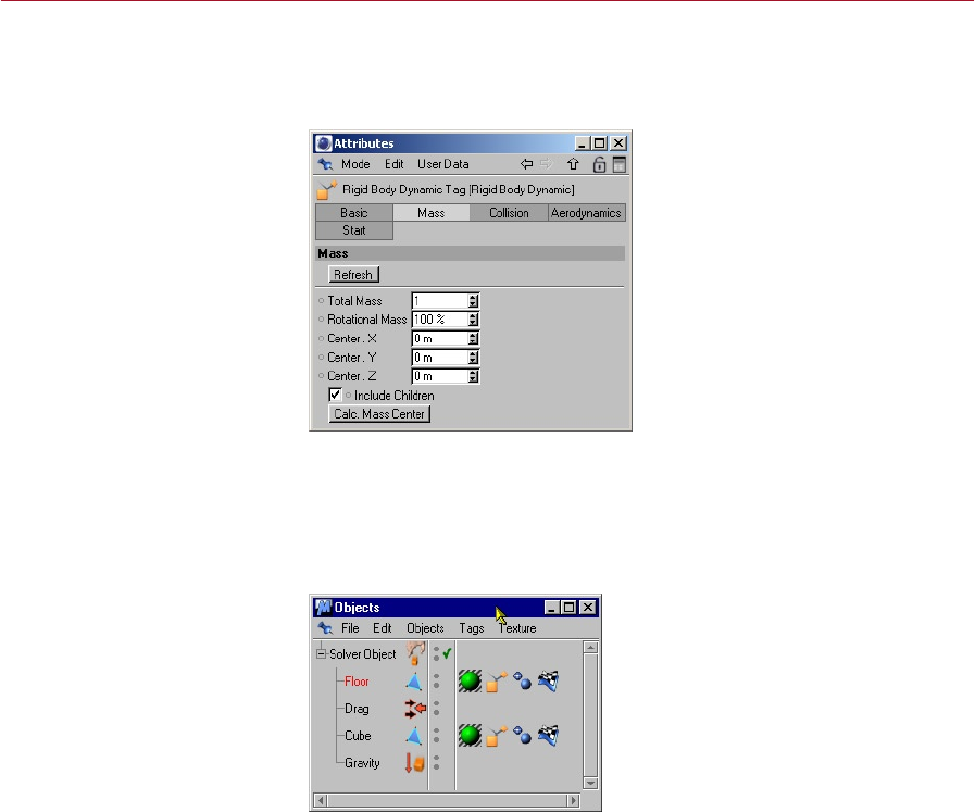
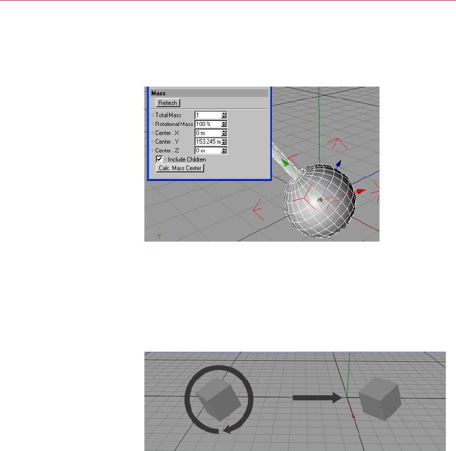
The centre of mass does not
have to be at the origin, we can
specify an offset.
In a similar way to moving an object in a straight line, you can also rotate a rigid
body around its centre of mass. You can place this special point anywhere you like;
physically it would depend on the density and shape of an object, but here we have
no need for these so Dynamics enables you to set it manually, or have it placed at the
centre of the geometry. This special point is where Dynamics will check all rigid body
positions and perform all interactions — this is an important point to remember.
For rotation, the values given in the Start tab for the angular velocity tell Dynamics
how many degrees per second the object should rotate about each axis.
If there are no friction collisions
or wind then rotation and
movement are able to remain
totally independent of each
other.

8 OVERVIEW DYNAMICS
DYNAMICS OVERVIEW 9
Now that we have objects moving and rotating we need to know how to change their
paths and make them interact with other objects, otherwise they’ll continue for as
long as the simulation runs, or until their energy runs out, moving and rotating in
exactly the same way. This energy loss is part of the dynamics calculations, you can
turn it off if you wish to create the outer space feel, but overall a small energy loss
will work to control your scene and will only slow your objects slightly.
In the real world, to change an object’s motion you need to apply a force to it — hitting
it in a collision, blowing it with wind, letting gravity do its thing. The same applies in
Dynamics, which offers many different ways to apply forces to objects. This tutorial
manual will guide you through those forces.
10 OVERVIEW DYNAMICS
DYNAMICS OVERVIEW 11
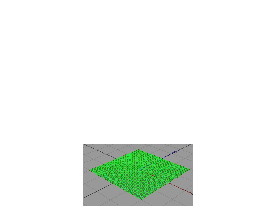
Soft Bodies
A soft body can be thought of as a mesh of small masses, each mass located at the
points on your object. These masses can interact with the dynamics just as the centre
of mass of the rigid bodies does.
Soft Bodies are one of the most
powerful features of Dynamics.
The masses associated with each point of a soft body are called soft masses and can
be given a custom mass, just as rigid bodies can, enabling you to effectively change
the surface density of the object.
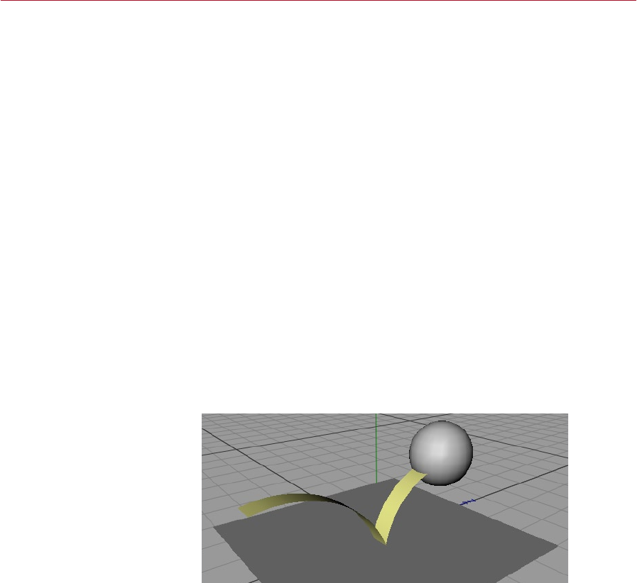
As with rigid bodies, you can set them to have a zero mass, which prevents the
dynamics from moving that mass. This is useful as a simple form of constraint for
soft bodies; by setting certain soft masses to zero you can give the impression of an
object being attached to something else in your scene.
We can assign weightlessness
to certain points, effectively
holding up an object in a certain
place.
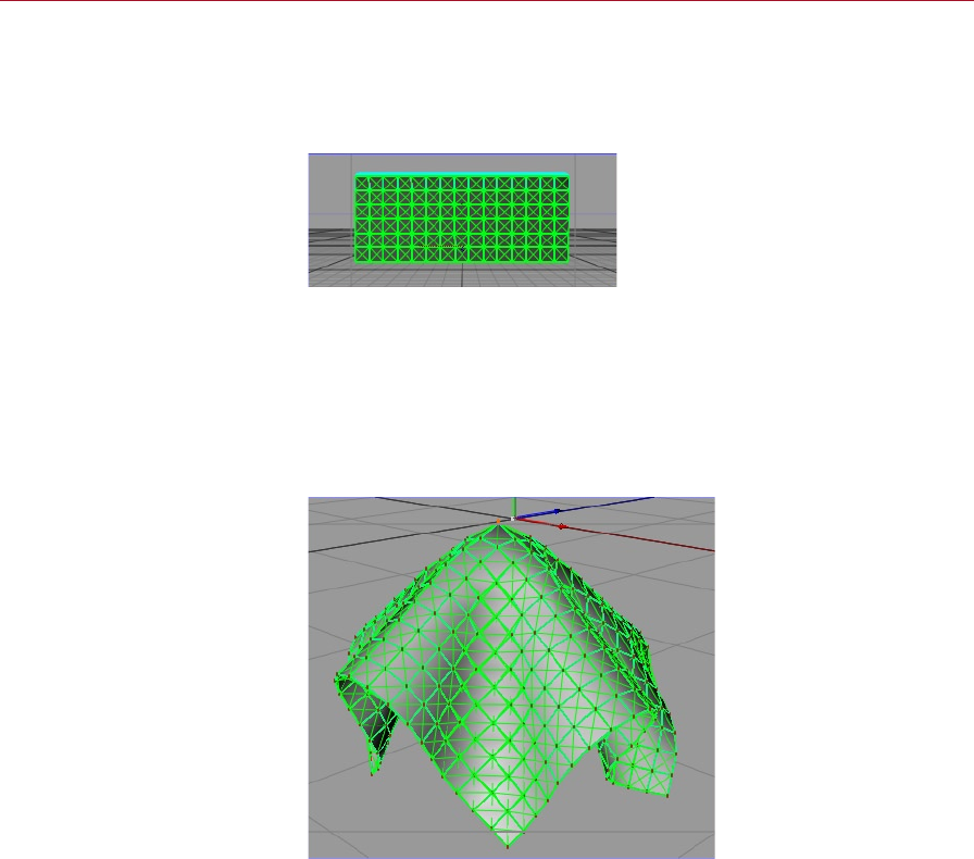
Attaching springs between the soft masses will give the object a surface structure that
can control how the polygons can compress and stretch. The forces within Dynamics
can affect the soft mass motion, which is then controlled by the springs on the object
to give the impression of a soft structure or a material.
10 OVERVIEW DYNAMICS
DYNAMICS OVERVIEW 11
Creating the illusion of materials is a difcult job for keyframing. CINEMA 4D Dynamics
provides you with the ability to use the power of dynamics to create the animation
needed to give materials movement in a physically realistic manner. Soft body objects
have their points linked by layers of springs, each type of layer (custom, structural,
shear and exion) can have its own options for the springs. These springs give the
object a structure that enable it to squash and fold, unlike a rigid body which retains
the same geometry throughout the dynamics simulation.
Dynamics has the ability to layer different types of springs that join different points
on your surface. This layering of springs is important in creating realistic appearing
materials. Items such as cloth tend to be very rigid if you try to stretch them, yet fold
easily if you try to squash them.
This type of structure can be created by using structural springs to give the whole
object a stiff yet exible structure, and then by adding exion springs you give the
object the ability to fold gently rather than creasing along the lines of the polygon
structure.
By adjusting the stiffness and damping of these springs you can form many different
types of materials. You can also change the type of behavior of the springs so that
you can permanently deform the shape as the springs are stretched or compressed;
this type of behavior is known as ‘plastic’.
Virtual springs are created
between certain points, these
are what will give the soft
material its motion.
Creating complex materials can be achieved by limiting the points to which certain
springs are attached and by adjusting the soft masses of the points. Creating different
types of materials is a case of trying different spring congurations and values, with
a little logic applied to how they should behave.
You can control the motion of the soft bodies by using a target, and this is a way of
making soft bodies follow another object. You can also control how well the target
object is followed, which enables you, for example, to add clothing and have it move
with your character.

12 OVERVIEW DYNAMICS
DYNAMICS OVERVIEW 13
Damping of the springs should be used in a similar way to that in which drag is used
to help Dynamics. If you use a large stiffness or low mass you may nd that the points
begin to vibrate wildly and may even explode the object. By adding damping and
drag you can help Dynamics to control these increasing velocities and give a more
controlled simulation.

12 OVERVIEW DYNAMICS
DYNAMICS OVERVIEW 13
Forces
To help animate real world motion, Dynamics has force objects which can cause
an object’s motion to change in a realistic way. These are Gravity, Drag, Wind and
Springs. There are also collisions for realistic impacts between objects, and frictional
forces between objects.
There are a variety of ways in
which we can move and deform
objects — wind, gravity, drag
and springs are the most basic.
When using forces within Dynamics you may experience motion that becomes
unrealistic and unpredictable, or perhaps objects which suddenly vanish from view.
This is the behavior that occurs when the values within the solver become too large
or too small and therefore become subject to the limitations of computation outlined
above. There are a number of ways to help Dynamics overcome these limitations.
You can rst try adjusting the values for your objects, making sure they’re as close
to 1 as possible while still giving the motion and interactions you need for your
animation.
Another solution is to change the way in which the solver calculates the motion. In
the real world, objects move in a continuous way, they don’t jump from one position
to another on a per frame basis. The Solver object can oversample between each
frame to increase the accuracy of the motion and to help reduce sudden changes
and inaccuracies.
Changing the integration method (how the motion is calculated) can also help prevent
sudden unrealistic changes.
Motion in the real world is also subject to many forms of energy dissipation where
the energy transfers to many other forms; for example when a falling object collides
with another some of its energy will dissipate to sound and heat.
Energy dissipation is also needed for realistic simulation. By using a Drag object in
your solver you can gently apply a frictional type of force to your objects (similar to
air resistance), giving more realistic motion and rescuing the solver from continually
increasing velocities.
14 OVERVIEW DYNAMICS
DYNAMICS OVERVIEW 15
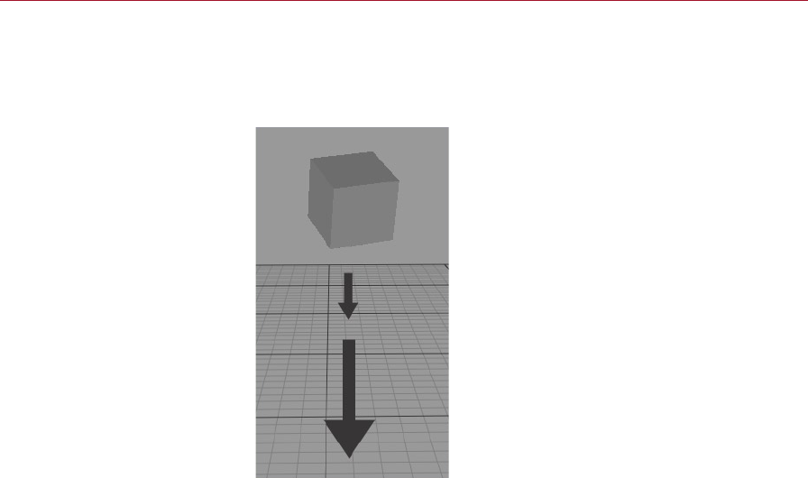
Gravity
Ask most people what gravity does and they will probably say that it causes things to
fall. This is a simplied view, but often in an animation all you want is for an object
to fall in one direction, normally down.
Gravity can act in a single
direction, such as the downward
pull of the Earth.
With Dynamics this type of force can be added to a simulation using an axial gravity
eld in the direction you wish objects to fall. By adjusting the strength and scales
that you use for your objects, you can have objects falling in a way that is familiar
and realistic.
Having very large scale objects will require a large gravity strength to give realistic
motion, which will require more accurate, and hence slower, simulation. Keeping
object scales towards the default CINEMA 4D sizes will enable you to use lower values
for gravity (and all other forces) which in turn will enable you to use less accurate and
faster simulation. This is a balance that you will need to nd for individual scenes.
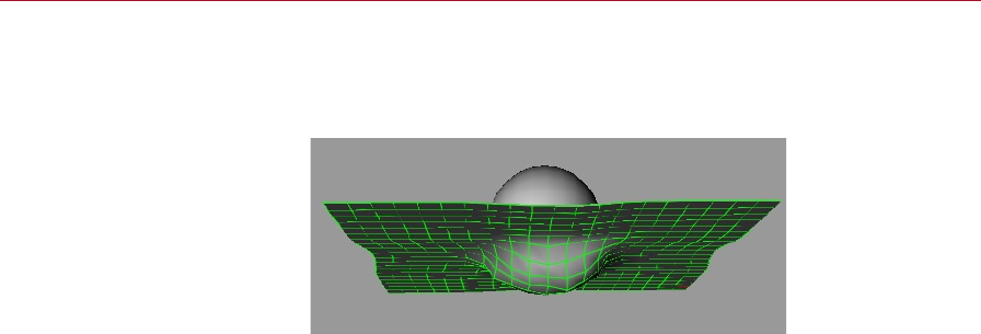
More accurately, gravity is an attractive force between any two objects with mass.
In Dynamics this type of gravity is given the name Newton, after the man who
discovered it and invented these simplied laws. This type of gravity can be used to
give objects interactions, to either repel them from each other, or to attract. By using
anti-gravity (making the strength negative, that is) you can simulate a simple type
of collision — if two objects get close enough they can be repelled, which appears
visually to be a collision.
14 OVERVIEW DYNAMICS
DYNAMICS OVERVIEW 15
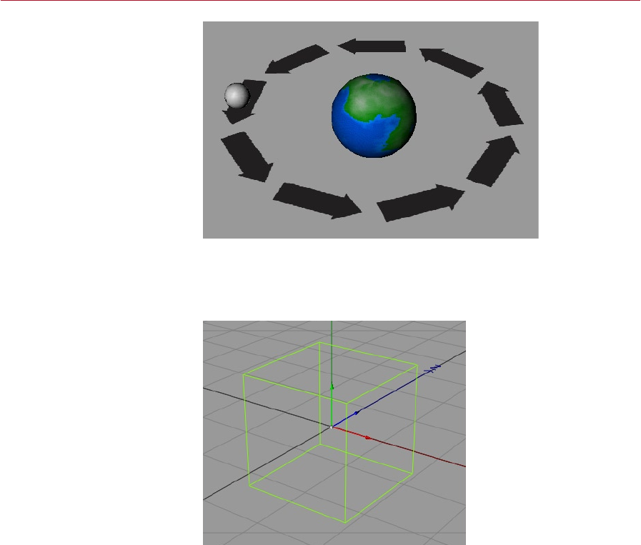
Newtonian gravity is available
for larger scale scenes, such as
planets orbiting.
The distance over which gravity can act can be set, along with where and how strong
the repulsion is for the distance the objects are apart. These types of settings are crucial
for making gravity collisions work, otherwise you may nd that collisions become
either squishy or so strong that objects y out of view at extraordinary speeds.
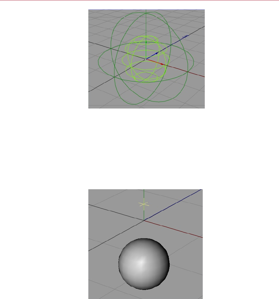
All forces can be restricted
to a size and shape, anything
outside of this shape will not be
affected.
Further types of collisions are possible using gravity by careful positioning of volumes
of gravity. The shape of the gravity eld can be changed, enabling you to have a
gravity eld around an object, or only in a part of your scene. By making gravity
objects children of your real objects you can have them move and rotate as your
objects do.
16 OVERVIEW DYNAMICS
DYNAMICS OVERVIEW 17
The forces may be set to
deteriorate over distance, this
behavior is called falloff.
The type of falloff can make a big difference to your collisions. For some collisions
having no falloff can mean you need a higher accuracy to simulate the physics. If you
have a lower accuracy, then should an object get too far into a gravity eld before the
calculations are affected by it, the object can be given too much of a push and will
gain more energy than before it collided; if this continues, eventually your simulation
will have objects moving so fast that they vanish from sight.
A way to control this is to use only a thin shell of gravity around objects, and this is
set with the falloff. By using the inverse square falloff you can soften collisions and
help prevent sudden explosions of energy. The inverse square falloff gives the objects
a push away as they get close, and then only as they get very close do they collide.
The centre of mass is used to
determine if an object is inside
another’s eld of inuence.

16 OVERVIEW DYNAMICS
DYNAMICS OVERVIEW 17
A good point to remember is that all of this takes place at the centre of mass. You
need to have the gravity eld size large enough so that the distance between objects’
centres of mass doesn’t enable the geometry to penetrate too far into each other. It
is also useful to remember that you can move the centre of mass of objects; in some
cases you can move this to enable easier control over the collisions, or to prevent
some objects from interacting with the gravity.
18 OVERVIEW DYNAMICS
DYNAMICS OVERVIEW 19
Drag
In the real world objects tend to interact in such a way that energy is transferred
away from their motion. Unless you are in outer space, any movement is resisted by
the air and surfaces around you.
Drag is able to simulate air
resistance, water, slime or even
very dense substances such as
mud.
To create this type of slowed motion you can add a Drag object. By using drag you can
create an environment around objects that is similar to air. By using a low strength
drag you can help the solver by continually lowering the speeds of the objects, helping
to prevent them from gaining more energy than they started with. This is a useful
point to remember: energy always appears to be lost — if you drop a ball on to the
oor, it will never bounce higher than the point from which you dropped it, and
eventually it will stop bouncing altogether.
You can also use the energy loss option in the Solver object. This is an important value
to get to know; by using this you can control the object’s movement and reduce any
errors that can occur. By balancing the integration method and the oversampling
used in the solver with the energy loss you can usually lower the oversampling,
greatly speeding up the calculations. In many scenes it may be possible to replace
drag with the energy loss, but remember that the energy loss will apply to all objects
in the solver.
If we nd that our simulation
is not running smoothly, drag
can often be used to calm
everything down.

18 OVERVIEW DYNAMICS
DYNAMICS OVERVIEW 19
Drag objects have other uses, apart from giving an environment of air or uid type
resistance. By using volumes of drag you can carefully position them around your
scene to help change the motion of objects.
By using anti-drag (negative drag strength) you can increase the velocity or rotation
or your objects. If you want to do this, remember that the object must already have
some values; try starting the object off with a very small velocity and very small
angular velocity. However, keep in mind that drag cannot change the direction of
the motion, only speed it up or slow it down.
Drag is useful to prevent or stop jitter or motion. If you use a gravity collision (see
above), objects may jitter if they continually collide. An example would be a ball
falling on to a oor — careful positioning of a Drag object in a cube shape can stop
the object from moving and colliding, giving the impression of it coming to rest on
the oor.
Drag may also be used to prevent objects from penetrating gravity elds too much
during collisions. The discrete nature of the motion means that an object could enter
a gravity eld too far. The rst repulsion would move the object to the edge of the
gravity, but still within it, so then on the next frame it gets repulsed again, giving
the object far too much energy, which can lead to the scene exploding from view. If
you position a drag within your gravity, then any objects entering too far will also
be affected by the drag and the effects of the gravity are greatly reduced, helping
to stop sudden explosions of speed during collisions.
20 OVERVIEW DYNAMICS
DYNAMICS OVERVIEW 21
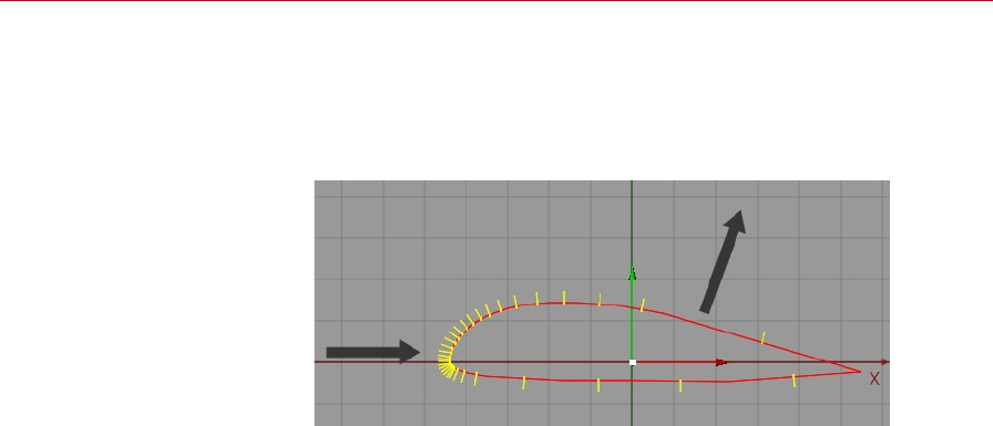
Wind
So far in this outline of dynamics, the forces have all been straightforward, acting
only on the centre of mass of each object or the point masses of the soft bodies. The
Wind object is slightly more complex in that the actual polygons and their associated
normals are used to nd the overall force.
Wind offers many real-world
options such as lift and drag,
as well as the more basic ones
such as impact.
This force can be used to give the impression of wind acting on an object to blow
or lift it. As with gravity, the wind force can alter the path of an object, and as with
the other forces, the centre of mass (or the origin for a soft body) must be within
the bounds of any shape used for the wind. By varying the strength of the wind and
its direction (by using keyframes and adjusting the parameters) you can add effects
such as turbulence and gentle breezes.
Most of the time real world wind will uctuate rather than give a constant force, so
you may nd a small amount of keyframing of the wind useful to give that extra
realistic touch.
20 OVERVIEW DYNAMICS
DYNAMICS OVERVIEW 21
Collisions
The most noticeable change in an object’s motion tends to be during collisions with
other objects. Dynamics offers full collision detection so that you can have your scene
fully interacting in a realistic way.
Although collision detection may be desirable, using it is even more computationally
expensive than the motion calculations. Imagine you had a scene lled with many
objects, and each object has many polygons. Taking a simplied example of collision
detection where any polygon can collide with any other polygon, each must be
checked and the appropriate motion calculated. Naturally, the collision detection in
Dynamics is not this simple and performs many complex tests to help speed up the
detection, but still the checks and calculations are numerous and lengthy, making
collision detection a slow process, so it needs to be used cautiously.
A reasonable solution is to use full collision detection only when absolutely necessary,
and to use the simplest geometry as possible (your real object can be a child of the
simplied geometry).
Or use one of the simpler collision detection types available. If the collisions are not
fully visible or can be carefully controlled, then you can use the forces as another
collision detection technique that gives a much faster solution. Our ‘Gravity Collisions’
tutorial illustrates this technique using gravity.
In the real world all solid objects will collide if they try to move into the same places.
Collisions give rise to complex motion where an object might rotate, slow down,
speed up, change its path.
Collision detection is another of
Dynamics’ powerful features.
When objects come into contact they also experience frictional forces as the surfaces
push and grind against each other. Dynamics has an advanced collision detection
system that can aid in simulating this friction.
22 OVERVIEW DYNAMICS
DYNAMICS OVERVIEW 23
Soft bodies will also interact with collisions, and also may have collision detection with
themselves to prevent the geometry from penetrating itself, which cannot happen
in the real world. As with rigid bodies, the collisions are time consuming, and if an
alternative method can be used then it may be advisable to do so.
It is possible to create collisions
between soft bodies and rigid
bodies.
Although using realistic collisions can be essential for close-up shots during
an animation, they do have some drawbacks that should be considered during
planning.
Limitations
The main limitation of the full collision detection is the sheer amount of computing
needed to check and calculate the complex motion. This processing can be reduced
by using simple geometry which has only the main surface features and then using
the real object as a child.
To enable faster collision detection, Dynamics provides some simple geometry types
for the collision tests. If you can make your geometry even simpler than these built
in ones, then you may nd using the parent (simple) and child (real) method faster
than using the built-in simple geometries.
When the collisions are controlled or not a main part of your scene, you may be able
to use the simpler force collisions that were outlined above in Gravity and Drag. These
have the great advantage of speed, but also require a little more time to correctly set
up the objects, plus they may need more adjustments should you later alter the scene.
The advantage real collisions have is that they will always interact in a realistic way.
22 OVERVIEW DYNAMICS
DYNAMICS OVERVIEW 23
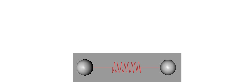
Springs
By adding a spring between two objects you can give them a simple form of constraint.
This join can be made to act as a usual spring would, so that if you compress it the
spring resists and gives a force pushing the spring back to its original length (the
‘rest’ length), and if you try and stretch the spring it will pull back with a force again
to its rest length. By increasing the stiffness you can create a simple link that can
hold two objects together.
Many objects are not linked by
solid geometry such as hinges
or joints. In these cases, use
springs.
As with the soft body springs you can use the plastic property of springs so that if
they become stretched or compressed by a certain amount they will permanently
deform. You also have the option to break the joint if the stretching or compression
becomes too great.
Springs also have the ability to rotate an object; this ‘angular’ type of spring behaves
as a coiled spring would in an old-fashioned wind-up clock.

24 OVERVIEW DYNAMICS
Constraints
The forces we have so far seen in Dynamics make up much of our real world
experiences. There is one more macroscopic force that we all experience from time
to time; this is known as electromagnetism.
Electromagnetism shows up all over our lives, from magnets on fridge doors to the
electricity that powers your computer. This force is also what binds and holds all
objects together and forms the very links and bonds that make our world. When
two objects collide, it is this electromagnetic force that stops them from penetrating
each other.
Although Dynamics does not have this electromagnetic force, it does enable you to
simulate these types of collisions.
In the real world we create joints and pins to stop objects moving, or to control how
they are allowed to move, by causing collisions. Achieving this with the collision
detection in Dynamics is possible, but will be very complex and can be very slow
in calculating all the complex collisions that may have to happen in order to stop
a simple interaction. To enable a fast and efcient solution to this, Dynamics has a
Constraint tag that can restrain the motion of objects, thus providing the links that
occur naturally between objects.
This ability enables you to limit the movement that the dynamics can exert on the
objects under simulation. Constraints can be used to link objects together, x an
object to a point or to an axis so that it can slide along the axis, or to x movement
so that objects can not be slowed down or speeded up by the forces in the scene
— just as an engine would push an object along at a constant speed even though air
resistance and friction try and stop it.
Basic Recipe
DYNAMICS BASIC RECIPE 27
DYNAMICS BASIC RECIPE 27
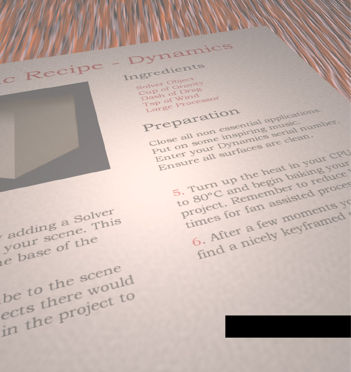
Basic Recipe
In this tutorial we’ll take some
simple basic rst steps that ensure
a working Dynamics simulation.
We’ll also highlight some things
you should watch out for.
To begin any dynamics within CINEMA 4D we need to add some additional objects
and tags into our scene. The Solver object is where all the magic happens, and this is
the main control over how the dynamics engine works, how accurate and thus how
fast the dynamics can be calculated.
We’ll learn how to create a solid (rigid) object and give it a mass to which a velocity
can be applied. We’ll learn how to set an object in motion, how to add gravity so that
the moving object also falls, and how to add some drag or ‘air resistance’ to further
enhance the realism of the movement.
Lastly we will learn a simple way to stop a moving object when it ‘hits’ a solid,
unmovable object like a oor.
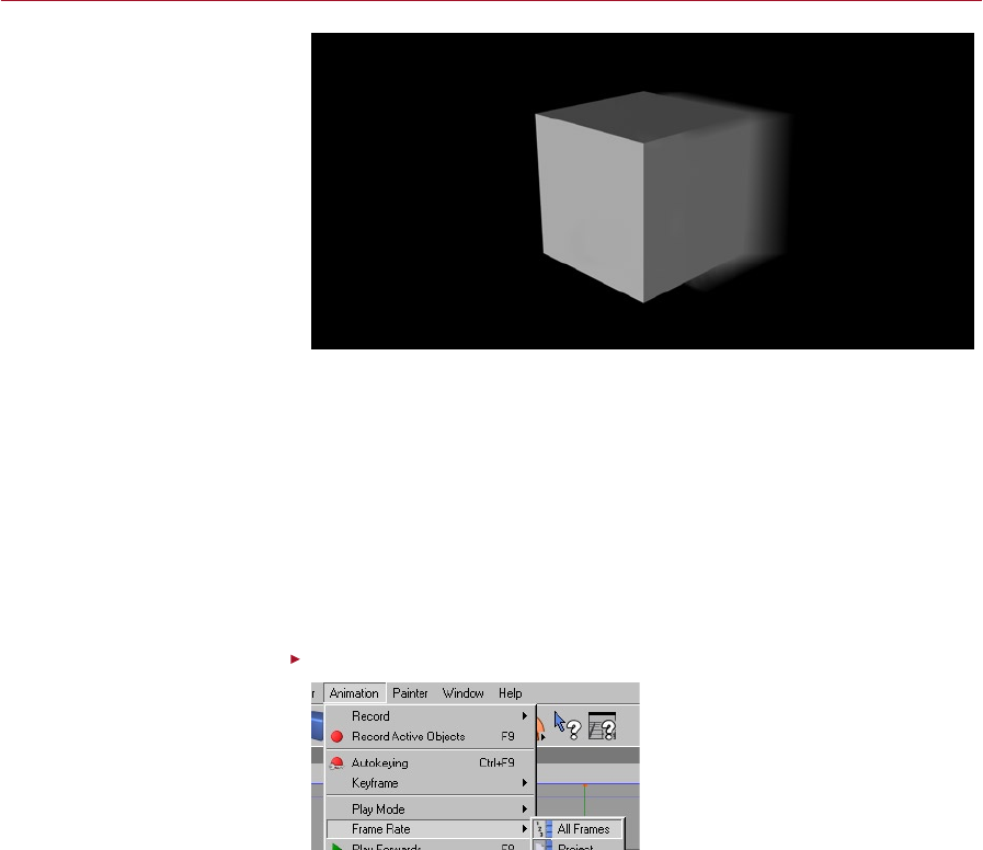
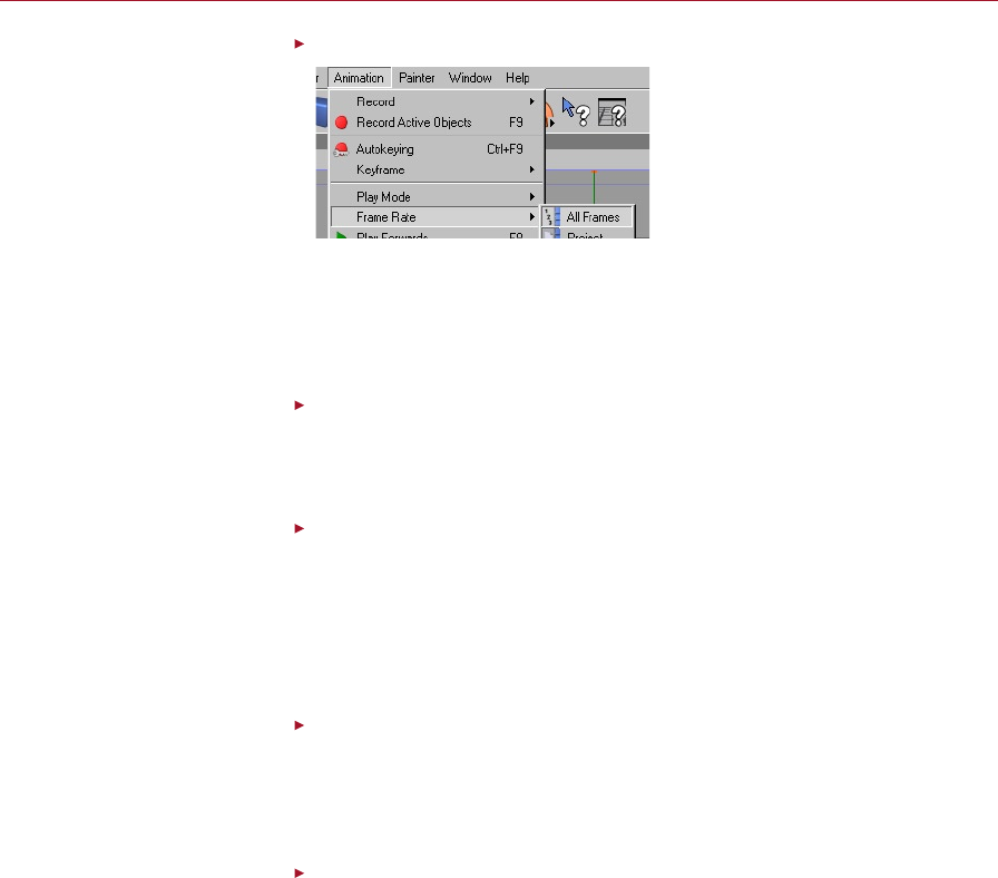
Ensure that Animation > Frame Rate > All Frames is enabled.
We must display all frames to
ensure that we do not miss any
unusual movements.
When using dynamics we need to be able to see every frame; this enables us to
check that every frame is how we want it to look, plus it prevents the dynamics from
calculating many frames at once, which can be slow on some complex scenes.
28 BASIC RECIPE DYNAMICS
DYNAMICS BASIC RECIPE 29
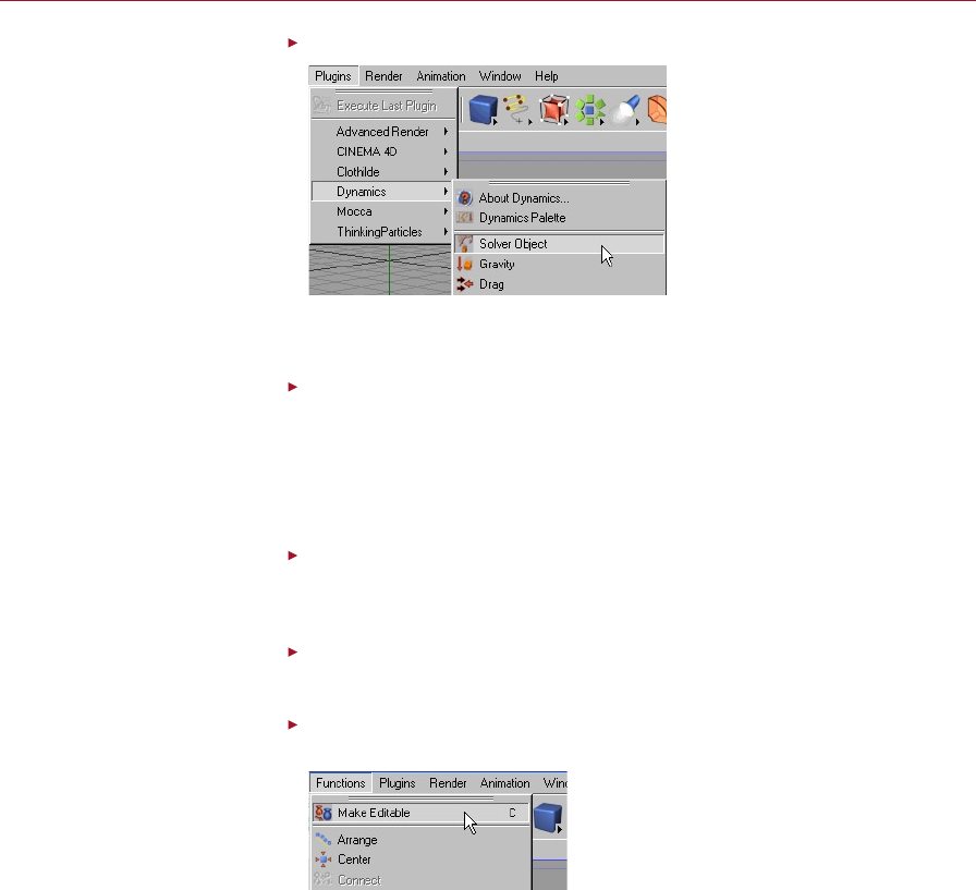
Select Plugins > Dynamics > Solver Object.
We need at least one Solver
object in our project to turn on
Dynamics.
A Solver object will appear in the Object manager; this object is where we will add
the objects that we want to interact through dynamics.
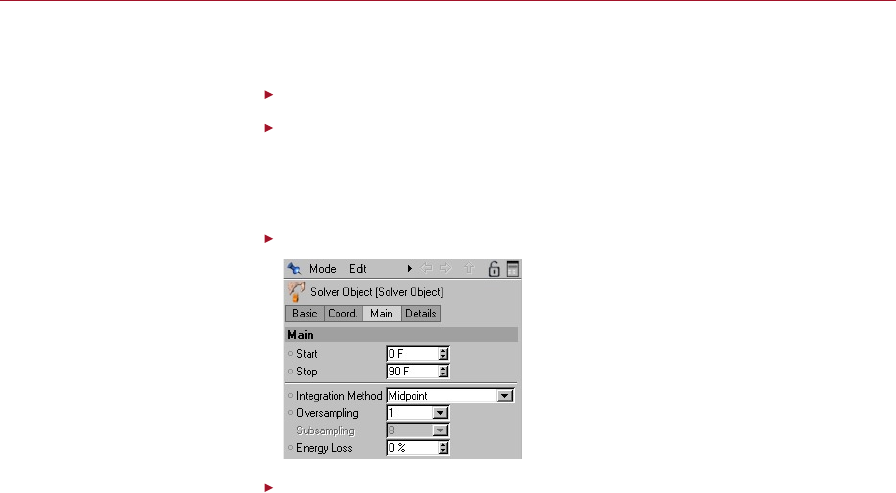
Click on the Solver object’s icon, set the Integration Method to Midpoint and
the Oversampling to 4.
By using a Midpoint method, the dynamics system can be calculated very quickly.
Although it is not the most accurate method, it will make almost no difference to this
scene. To make it slightly more accurate, an Oversampling setting of 4 will calculate
four imaginary frames between each real frame.
Set the Energy Loss to 0.
Using the default Energy Loss of 5% can often be benecial, however in this case it
would cause out objects to slow down far too quickly.
Select Objects > Primitive > Cube.
We’ll begin by making a simple cube move using dynamics.
Ensure you have the Cube object selected, then select Functions > Make Editable
and drag the Cube object into the Solver object.
Only polygon objects can make
use of Rigid Body Dynamic tags.
To perform dynamics on an object we must have it within the solver and it must be
a polygon object (Make Editable ensures this).
28 BASIC RECIPE DYNAMICS
DYNAMICS BASIC RECIPE 29
Command-click on a Mac if you
have only one mouse button.
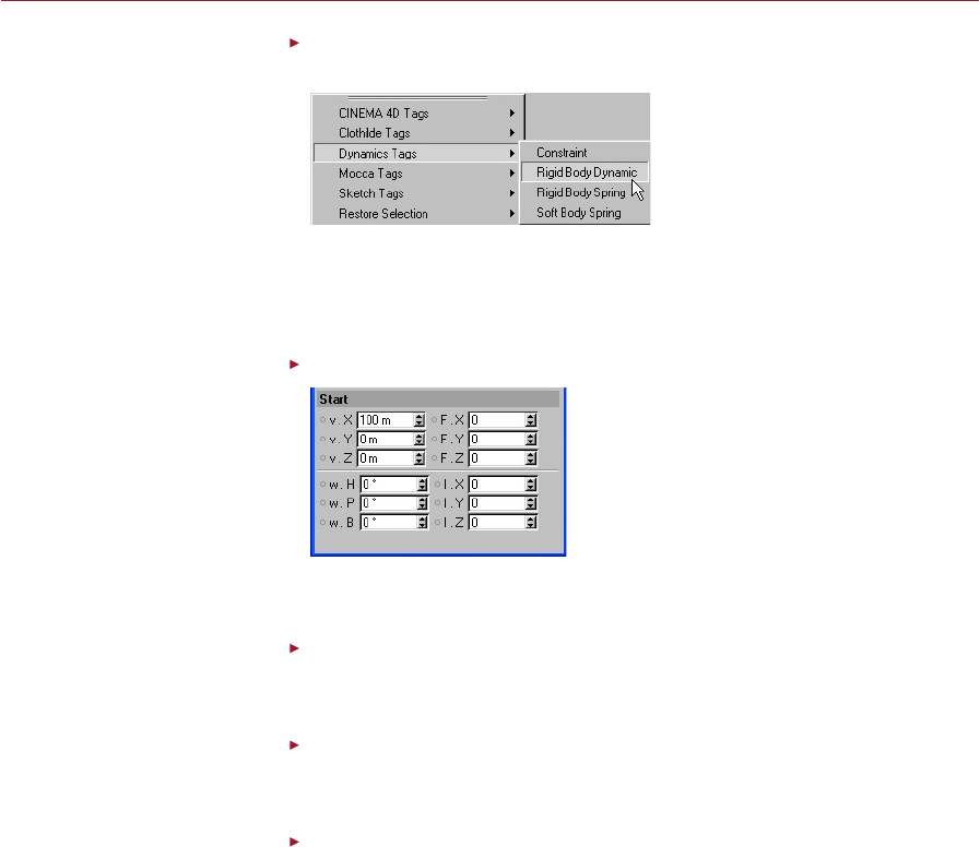
Making sure you have the Cube object selected, right-click and select Dynamics
Tags > Rigid Body Dynamic.
By default, the Rigid Body
Dynamic tag will give our cube
a mass.
This will add a new tag to the Cube object, and the tag’s settings will appear in the
Attribute manager. For us to move the cube, we want it to become a solid object
and to have a mass so that we can tell the dynamics what velocity the cube should
start moving with.
Click on the Start tab and set the v.X value to 100.
Objects can be given an initial
speed and rotation from the
Start tab.
By setting the v.X parameter we tell the dynamics to move the cube along the positive
x-axis by 100 units per second. Close the window when you’re nished.
Click Play and then click stop when you are nished.
We now need to view the dynamics animation to check all is working as we intended.
As you can see, the Cube object moves slowly down the x-axis.
Select Plugins > Dynamics > Gravity and drag the new Gravity object into the
Solver object.
This adds some world gravity to make the object fall as it moves.
Click Play and then click Stop when you are nished.
The cube now falls as it moves along the x-axis.
30 BASIC RECIPE DYNAMICS
DYNAMICS BASIC RECIPE 31
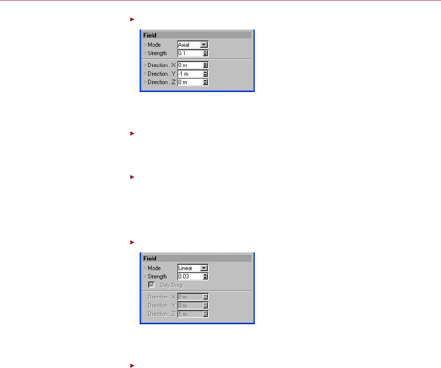
Click the Gravity object’s icon and set its Strength to 0.1.
The default gravity strength of 1
may be too much for our scene
so we have reduced its strength.
This will slow down the fall of the cube due to gravity so that we can see the curve
of the object’s movement as it falls and moves along the x-axis.
Click Play and then click Stop when you are nished.
As you can see, the cube falls once more, but this time it takes longer to fall because
we lowered the gravity strength.
Select Plugins > Dynamics > Drag and drag the Drag object into the Solver
object. Change the name of the Drag object to Air.
We’ve just added some air resistance to the scene, this makes it a little more realistic.
An alternative would have been to leave a small amount of Energy Loss in the Solver
settings.
Click on the Air object’s icon and set its Strength to 0.03.
Air resistance will be
encountered in almost all
everyday locations; this, too, can
be simulated.
We want to slow the object very slightly as it moves, so setting low drag strength
will slowly resist the object’s movement.
Click Play and then click Stop when you are nished.
The cube now begins moving and then gradually stops moving along the x-axis and
just falls. Gravity is accelerating the cube downwards on every frame so the drag
makes little difference, but the velocity at the start has no force keeping it moving
and so slowly the drag stops this motion.
30 BASIC RECIPE DYNAMICS
DYNAMICS BASIC RECIPE 31
Select Plugins > Dynamics > Drag but this time do not drag the Drag object
into the solver. Change the name of the Drag object to Floor.
We’re now going to add a soft oor for the cube to fall on to. This is a way to stop
the object from falling further, and a soft oor will have little or no bounce, so we
can use a drag object to stop the cube moving as if it had hit the oor.
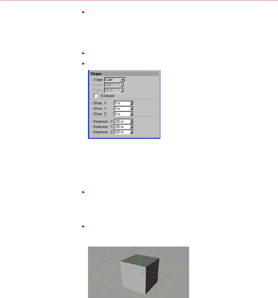
Click the Floor object’s icon and set its Strength to 10.
Click the Shape tab and select the Cube Shape.
Collisions do not have to be
between solid objects. There
is no reason not to use a very
strong gravity or drag eld to
halt something.
We want to create a local volume of drag that can act as a oor. It is important to
remember that as with other force objects in Dynamics, only the centre of mass is used
for the interaction; this means that we must ensure that any real geometry placed
in the scene will react before the geometry intersects. So with our cube, if we had a
real oor object we would need to place it far enough into the drag cube so that the
cube’s bottom surface stops before the cube goes through the oor.
Click Play. When the cube is in the position where the oor drag should stop it,
click Stop.
We need to nd out where the cube will be when it should hit the oor. This will
make placing the Floor object much easier.
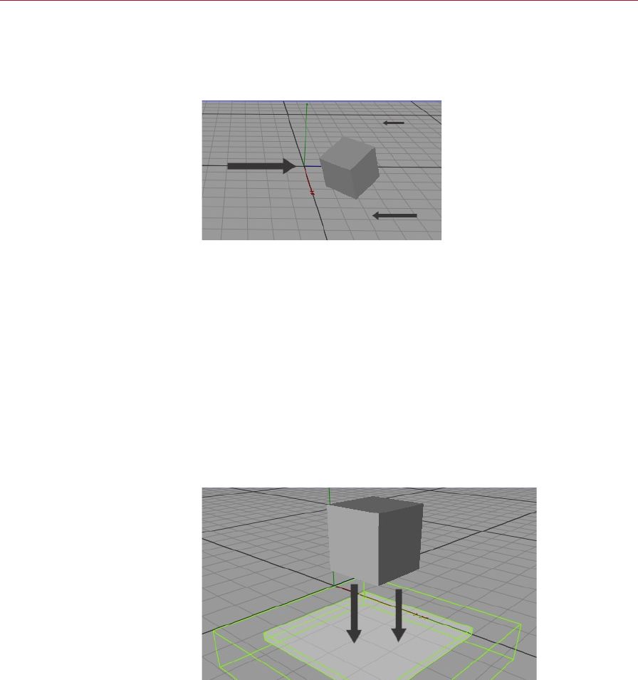
Move the Floor object so that its centre is in the same position as the cube’s
centre. Scale the Floor object along the y-axis (by changing the Dimension.Y in
the Attribute manager) to make a oor.
Position and scale the drag eld
to create a oor-like object.
32 BASIC RECIPE DYNAMICS
This will be where the cube comes to a stop as it hits the oor. By increasing the
strength of the drag we can stop movement almost immediately.
Drag the Floor object into the solver.
Click Go to Start of Animation and then click Play; click Stop when you are
nished.
As you can see, the cube falls as before, and then stops as the centre of mass comes
into the oor drag.
Click the Solver object’s icon and set the Oversampling to 1.
Although lower solver settings
equate to fewer calculations,
they can be inaccurate and lead
to problems.
Click Play and then click Stop when you are nished.
This time you can see the cube shoots away from or through the drag. The reason
why is that we made the dynamics less accurate. The large value set for the drag
strength causes the solver to explode and the motion of the cube to be calculated
incorrectly. This is an important point to remember. If you nd your motion is going
wrong, check your solver settings; you may nd increasing the accuracy or method
helps, or you may have to reduce the values used in your objects.
Summary
We have seen how to add the Solver object that controls the dynamics simulation, how
to add in your objects and then how to make them interact with dynamics objects
within the simulator and to be controlled by the dynamics itself.
With the simple example of a falling cube we’ve also seen how to use drag to perform
a simple collision with a soft oor and to give the impression of a cube landing.
We have also seen how we can adjust the Solver object to correct for any unpredictable
motion and how this can relate to the values used in the dynamics objects.
Once we understand these basic principles we will be able to begin experimenting
with Dynamics and create our own dynamic animations from scratch.
Move and Stop

DYNAMICS MOVE & STOP 35

DYNAMICS MOVE & STOP 35
Move and Stop
In this tutorial we will learn how
to set an object in motion, alter
its trajectory and then stop it at a
predetermined point. Quiet please,
game on...
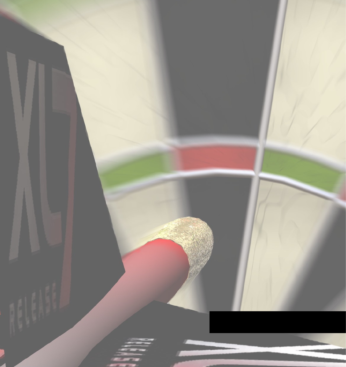
This tutorial demonstrates how to create a simple dynamics simulation of a dart in
ight that strikes a dart board. The simulation makes use of rigid body dynamics,
illustrating the initial setting up of a rigid body, plus it uses force elds to simulate
a collision between dart and board.
Though Dynamics features collision detection, it’s not always prudent to use it. In
this case using force elds also offers us more control.
Select File > Open. Navigate to the Move And Stop tutorial folder on your
Documentation CD and open the le named ‘mas.c4d’.
Open the le to begin the
tutorial.
The Tutorials folder is in the
Dynamics module folder. Each
tutorial has its own folder within
the main Tutorials folder.
This is the initial, non-animated darts scene. We are going to create a dynamics
simulation to score a treble 20 with our dart.
36 MOVE & STOP DYNAMICS
DYNAMICS MOVE & STOP 37
Ensure that Animation > Frame Rate > All Frames is enabled.
When working with Dynamics,
always enable the All Frames
option to ensure a smooth
workow.
When using dynamics we need to be able to see every frame; this enables us to
check that every frame is how we want it to look, plus it prevents the dynamics
from calculating many frames at once, which can be slow on some complex scenes.
When working with dynamics we should make it a habit to ensure that All Frames
is enabled.
Select Plugins > Dynamics > Solver Object.
All dynamics animations need to be set up using special objects that control how the
dynamics system will run. The most important object is the dynamics solver, which
actually does all the calculation.
Click the Solver object’s icon and set the Integration Method to Adaptive and
the Stop frame to 19.
The dart will y for only a very short period of time, and at a very high velocity.
Choosing the Adaptive method enables us to sub-sample the frames further when
necessary. We have chosen to stop the simulation at frame 19 because by then the
dart will have come to a full stop. If the solver continued to calculate the frames it
would slow things down unnecessarily.
Set Oversampling to 16, Subsampling to 128.
Each frame will be divided into a further 16 virtual frames. During each of these
frames, Dynamics will check to see if the dart has reached the board. When the dart
nears the board, sub-sampling will begin and each of the 16 virtual frames will be
divided again into another 128 frames.
Set the Energy Loss to 0.
There is no need for the system to articially lose energy. All of the motion energy
will be dissipated by the drag elds (which have yet to be added).
36 MOVE & STOP DYNAMICS
DYNAMICS MOVE & STOP 37
Select Objects > Primitive > Polygon.
If you unfold the Dart hierarchy you can see it is made from lots of separate objects.
However we really only need to apply the dynamics properties to one object. We
could connect the Dart hierarchy to form a single object but then it would lose its
texturing. A better option is to add a special helper object set so it doesn’t render
in the nal animation and use this as a container for the Dart object. That’s what
we are doing here.
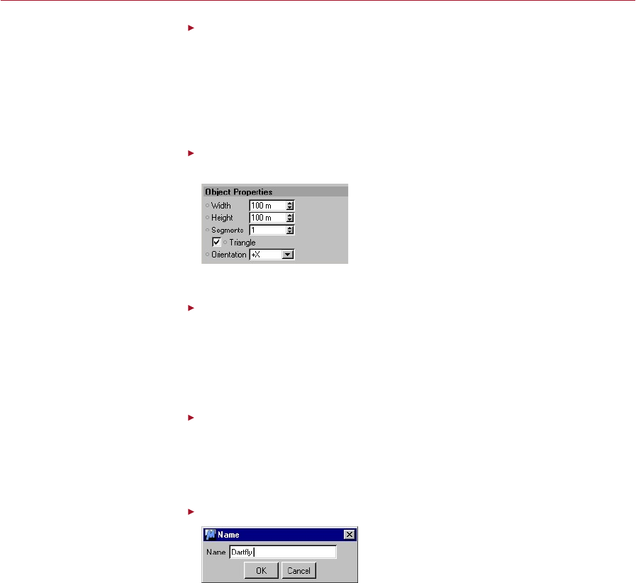
Click on the polygon’s icon, set the Orientation to +X and enable the Triangle
option.
All rigid Dynamics objects
must be polygons; use a simple
invisible one and attach the real
objects to it.
This creates a triangle polygon which we can animate as if it were the dart object.
Press the ‘c’ key.
This will turn the primitive into an editable polygon object, as required by Dynamics.
(The ‘c’ key is the keyboard short-cut for the Functions > Make Editable command.)
The exact shape and size of this object is actually irrelevant, though if the rendered
object is very complex, to speed display we can preview the simulation using this
container only.
In the Object manager, drag the Dart object into the Polygon object.
When we animate the Polygon object, the dart will move too, just like any other
hierarchy in CINEMA 4D. Remember that dynamics only works with polygon objects,
which is why we used a Polygon object for the container and converted it. Empty
polygons, splines or nulls will not work.
Double-click on the Polygon object’s name and rename it Darty.
Naming objects as we go along
is always a good idea.
Because both the Dart and the Darty objects are at the origin we don’t need to
adjust their relative positions.
38 MOVE & STOP DYNAMICS
DYNAMICS MOVE & STOP 39
Drag the Darty object into the solver.
If you play the animation now nothing will happen because we have not added any
forces or dynamic properties to the system — the solver has nothing to solve, so this
is the next step.
Select Plugins > Dynamics > Gravity.
Gravity is required to make the dart y in a slight arc rather than perfectly straight.
Select Plugins > Dynamics > Drag.
It’s a good idea to always add a Drag object to our simulations to provide a kind
of all-round damping for the solver, and to prevent the system from spontaneously
gaining energy. Our Drag object is going to slow down the dart while it is in ight,
simulating air resistance.
Drag the Gravity and Drag objects into the solver.
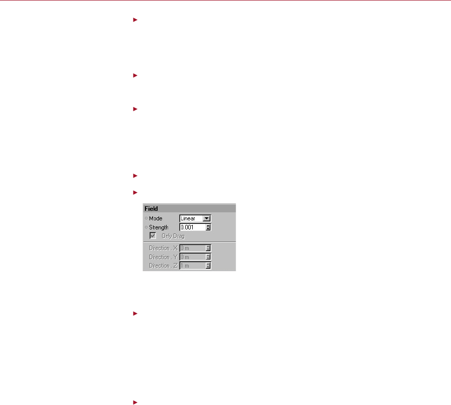
Click the Drag icon and on the Field tab set the Strength to 0.001.
Depending on the scale of our
scenes, the default drag strength
may be more akin to water.
The default value is too high and is more like water than air. By reducing the Strength
we are thinning the drag.
In the Object manager, select the DartFly object, then select File > Dynamics
Tags > Rigid Body Dynamic.
We need to assign a special Rigid Body Dynamic tag to the Darty object. This
provides the object with various dynamic properties that we can change to create
our customised simulation. This, together with the gravity and drag force elds,
denes the dynamics system and provides the solver with enough information to
create a simulation.
Click Play and click Stop when you are nished.
Now if you play the animation the dart will begin to drop. Remember it’s the
polygonless Darty object that is being animated by the dynamics, the real Dart
object is merely going along for the ride.
38 MOVE & STOP DYNAMICS
DYNAMICS MOVE & STOP 39
Click on the Darty object’s Rigid Body Dynamic tag.
In order to propel the dart into the dartboard we must give it some energy. We can
do that by adjusting the Rigid Body parameters.
In the Attribute manager, click the Start tab.
This is where we dene the initial trajectory of the rigid body object.
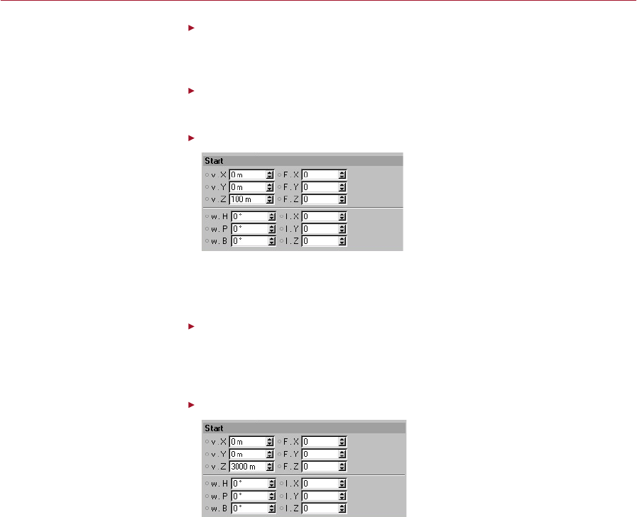
Set the v.Z value to 100.
We need to give our dart a little
push to set it moving.
The rst section at the top left, the ‘v.’ values, tells Dynamics how fast the object is
moving initially in each direction. Note that these values are only for the start of the
simulation, it’s like giving our object an initial push to get it going.
Click Play and click Stop when you are nished.
Playing the animation, we can see that the dart moves forward slightly as it falls
under the pull of gravity. It seems that a value of 100 is not nearly enough to get it
to the dart board.
In the Rigid Body Dynamic tag’s settings, set v.Z to 3000.
At a speed of 3,000 the dart ies
quickly.
A value of 3000 should provide just the right amount of oomph, and at around frame
16 the dart should intersect the board.
40 MOVE & STOP DYNAMICS
DYNAMICS MOVE & STOP 41
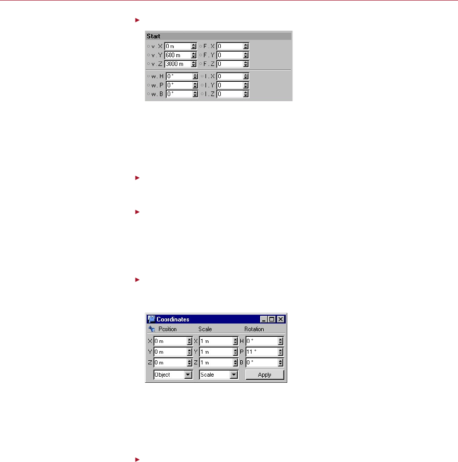
Set v.Y to 600.
A bit of upwards thrust will
create an arced ight.
If we were throwing a dart at a dartboard we would instinctively make some
compensations for the effect of gravity and project the dart in an upwards arc
rather than desperately trying to throw it in a straight line at our target. In order
to improve our score, we need to adjust the ight of the dart by giving it a little
upwards (Y) energy.
Click Play, click Stop and rewind when you are nished.
The dart now ies in an arc and intersects the board at the treble 20 mark.
Disable the Solver object by clicking on its green tick icon in the Object
manager.
If you try to rotate the Darty object while the solver is still enabled, you will nd
it is totally unresponsive and it will not remember any settings you change. Before
changing any dynamics objects you must rst disable the solver.
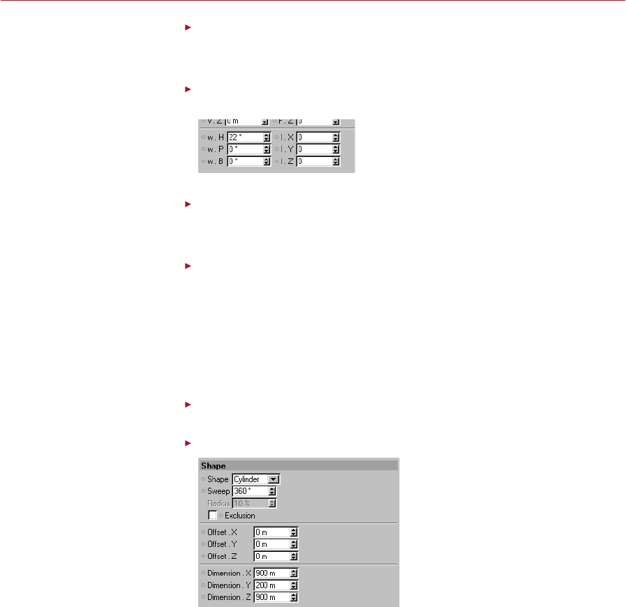
Select the Darty object in the Object manager, then, using the Coordinate
manager (or the Coordinates tab in the Attribute manager), rotate the Darty
object’s pitch to 11 degrees.
We have the arced motion of the
dart, now we need it to point in
the direction it is moving.
The ight of the dart still isn’t right. Really the dart should follow the arc rather than
remain pointing in the same direction. We can adjust its initial orientation then add
a small amount of angular movement in the Rigid Body dialog to make the dart
rotate in its ight. The setting we have just made is the angle at which the dart will
be thrown.
Select Plugins > Dynamics > Initialize Object.
We must store this new position before re-enabling the solver, otherwise it will revert
to its original position.
40 MOVE & STOP DYNAMICS
DYNAMICS MOVE & STOP 41
Enable the solver by clicking on its red X icon in the Object manager.
For dynamics to have any effect on the scene, the solver must be enabled, otherwise
nothing will move or rotate when we play the animation.
Click on the Darty object’s Rigid Body Dynamic tag. Click the Start tab and set
the w.H value to 22.
Some tweaking of the
parameters is needed.
Click Play and click Stop when you are nished.
Now when the simulation plays the dart will rotate in ight so that it intersects the
dartboard at a nearly perpendicular angle.
Select Plugins > Dynamics > Drag and drag this new Drag object into the solver.
Rename it BoardDrag (by double clicking on its name).
All well and good so far but the dart is passing right through the board and the
wall. We need to stop the dart so it sticks in the dartboard by just the right amount.
Dynamics enables us do this using forces. There are two good reasons for using forces,
rstly it is much more efcient than using collision detection, and secondly the dart
needs to partially penetrate the board rather than bounce off it; forces gives us the
control to be able to achieve this.
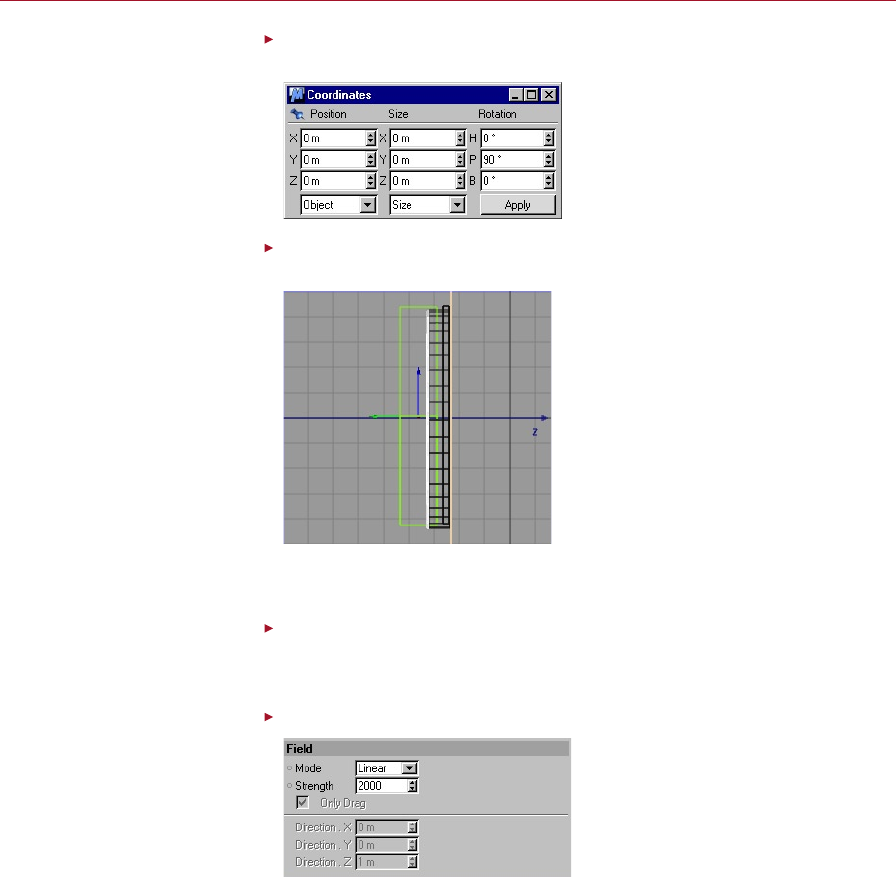
Click on the Board object icon then click the Shape tab and set Shape to
Cylinder.
Set Dimension.X to 900, Dimension.Y to 200 and Dimension.Z to 900.
The drag eld needs to be
roughly the same shape as the
dartboard geometry.
We can make the drag eld affect a specic region of space by giving it a limited area
of inuence. We have made it a cylinder as this is the shape of the dartboard.
42 MOVE & STOP DYNAMICS
DYNAMICS MOVE & STOP 43
Ensure the Board object is selected in the Object manager, then, using the
Coordinate manager, rotate the Board object 90 degrees in pitch.
The drag eld also needs to face
in the same direction as the
dartboard geometry.
Use the mouse in the viewports to move the Board object along its local Y axis
until it is over the dartboard.
The drag eld needs to be in the
same position as the dartboard
geometry.
These last four actions above will position and scale the drag eld over the real
dartboard so that the darts appear to stop when they hit the board.
Click Play and click Stop when you are nished.
If you play the simulation now you’ll see that the dart is stopped by the dartboard
but pokes through it!
Click on the Board object icon and on the Field tab set the Strength to 2000.
The dart hits the board at a
relatively high velocity, so the
drag needs to be very strong to
catch it.
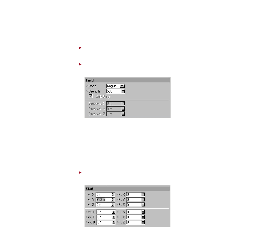
42 MOVE & STOP DYNAMICS
DYNAMICS MOVE & STOP 43
This will now cause the dart to actually stop when it encounters the dartboard rather
than just slow down slightly. If the dart goes too far into the dartboard, move the
Board object until the only the tip of the dart is stuck in the board. However, the
angular momentum of the dart is causing it to rotate in the board even though it
has stopped its ight.
In the Object manager, Ctrl-drag the BoardDrag object to duplicate it and then
rename it BoardRot (by double clicking on its name).
Click on the BoardRot object icon and on the Field tab set the Mode to Angular
and the Strength to 500.
A separate drag object is
required to stop the dart
rotating.
We can stop the dart from rotating by using another drag eld set to Angular mode.
This will halt all unwanted rotations as the dart hits the board.
If you’ve used different values to the ones given in this tutorial you may nd that
the dart ies straight through the board! To solve this, increase the Oversampling
and Subsampling values for the Solver object. This will increate the accuracy of the
dynamics simulation.
Click on the Dart object’s Rigid Body Dynamic tag. Click the Start tab and set
v.Y to 610.
One nal adjustment is needed
to get a respectable score ;-)
We can ne-tune the height at which the dart hits the board by adjusting the v.Y
value. Time to practice our aim!

44 MOVE & STOP DYNAMICS
Summary
You should now understand how we can use a drag eld to simulate the thickness of
any object or substance, from owing air and water right up to a wooden surface or
sheet of steel. The strength of the drag all depends on how tightly packed the atoms
are. To control the degree of penetration of the dart, simply move the BoardDrag drag
eld towards or away from the dartboard. To control how fast the dart decelerates
within the eld, scale it in Y and adjust the Strength.
You should also realise how much control we will be able to give our simulation;
just because the dart stops when it hits the board does not mean that it has to stop
rotating. It’s up to us!
If you're not sure how else you can use the objects we've just been using, take a look
at the Newton's Cradle tutorial (Gravity Collisions with Constraints) where you will
nd more uses for both gravity elds and drag elds.

Motion with Drag
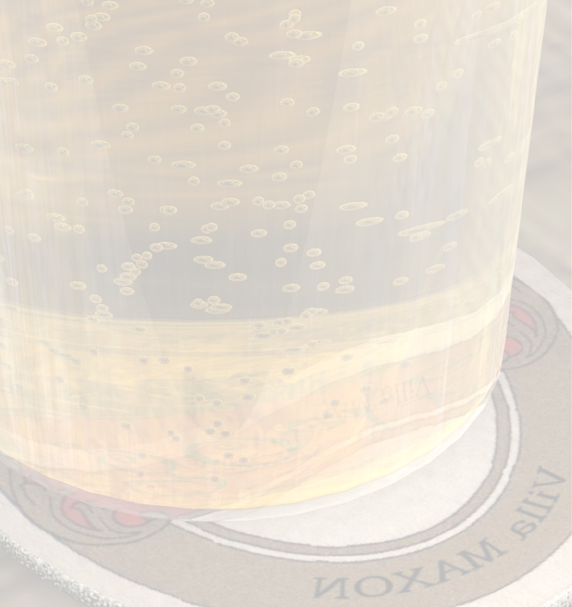
DYNAMICS MOTION WITH DRAG 47

DYNAMICS MOTION WITH DRAG 47
Motion
with Drag
Creating a falling object that has
its motion controlled by using
drag objects to give the illusion of
the object passing into a uid.
Altering the motion of our objects is essential to making a realistic looking animation.
The Drag and Axial Gravity objects will be covered in this tutorial, illustrating how to
use drag to speed up and slow down a moving and rotating object.
We will start by making a coin fall, followed by adjusting the fall to give the impression
that the coin is falling into a liquid. This requires us to slow down the fall due to the
viscosity of the liquid, then to cause the coin to tumble slightly before it nally comes
to rest at the bottom of the glass.
Select File > Open. Navigate to the Motion With Drag tutorial folder on your
documentation CD and open the le named ‘mwd.c4d’.
Open the le to begin the
tutorial.
The Tutorials folder is in the
Dynamics module folder. Each
tutorial has its own folder within
the main Tutorials folder.
The scene objects are now available in the Object manager. We now want to take our
coin and drop it into the pint of beer. The two important objects in this scene are the
Pint object and the Coin object.
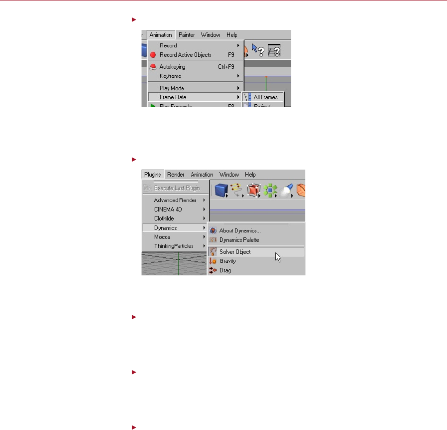
48 MOTION WITH DRAG DYNAMICS
DYNAMICS MOTION WITH DRAG 49
Ensure that Animation > Frame Rate > All Frames is enabled.
Display every frame to guarantee
accurate calculations.
When using dynamics we need to be able to see every frame; this enables us to
check that every frame is how we want it to look, plus it prevents the dynamics from
calculating many frames at once, which can be slow on some complex scenes.
Select Plugins > Dynamics > Solver Object.
Solver objects are needed for all
Dynamics simulations.
A Solver object will appear in the Object manager; this object is where we will add
the objects that we want to interact through dynamics.
In the Object manager, ensure you have the Solver object selected, then in the
Attribute manager, click on the Main tab and set the Stop frame to 1000.
We want the animation to last for the length of our timeline, so we set the stopping
frame for the dynamics to the end frame on our timeline.
Leave the Integration Method set to Adaptive. Set the Oversampling to 4 and
the Subsampling to 8.
We are using the adaptive method because it produces very accurate results, which
is always a good thing when we are working with complex scenes.
Set the Energy Loss to 0.
There is no need for the system to articially lose energy. All of the motion energy
will be dissipated by the drag elds (which have yet to be added).
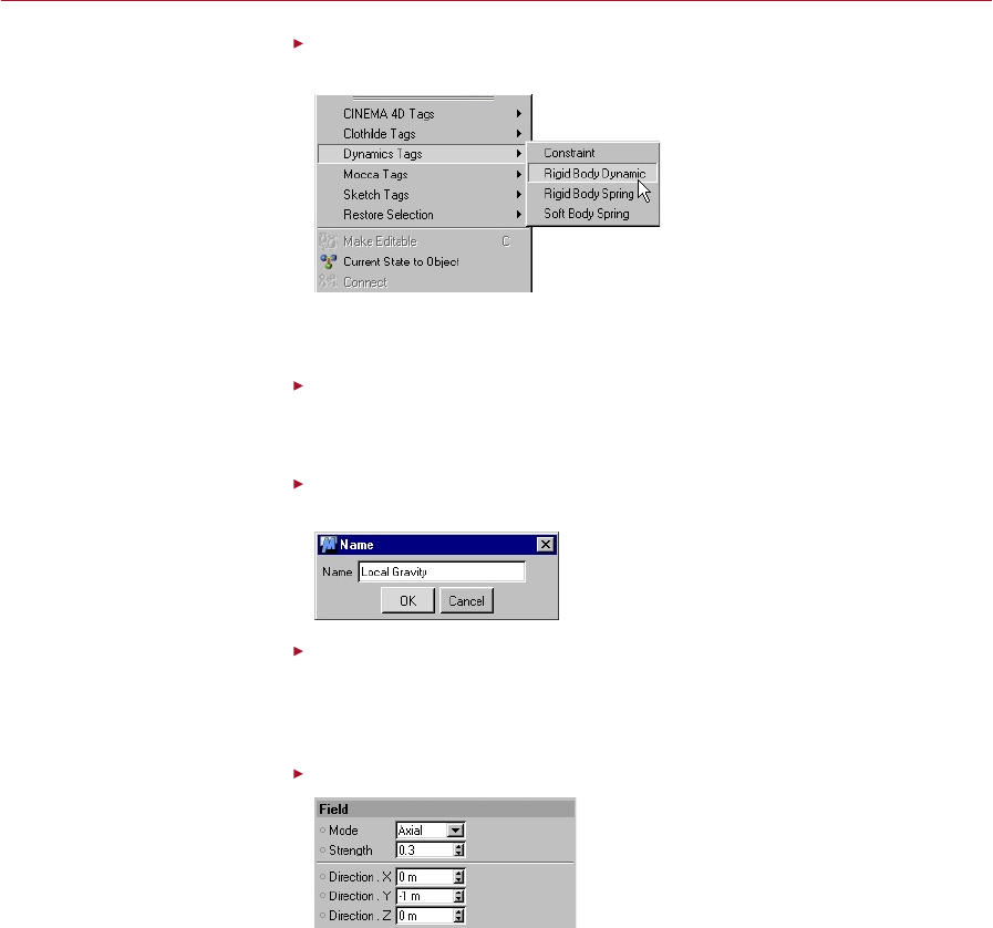
48 MOTION WITH DRAG DYNAMICS
DYNAMICS MOTION WITH DRAG 49
Command-click on a Mac if you
have only one mouse button.
In the Object manager, ensure you have the Coin object selected, then right-click
and select Dynamics Tags > Rigid Body Dynamic.
To enable the coin to
interact with other Dynamics
objects we are giving it a
Rigid Body Dynamic tag.
We need to make the coin a solid object so that we can use a Gravity object to make
it fall into the beer; we will be using the Pint object as our beer in this scene.
Drag the Coin object into the solver.
To enable the dynamics to take control of the coin falling we need it to be a child of
the Solver object.
Select Plugins > Dynamics > Gravity. Double-click on the Gravity name in the
Object manager and set the name to Local Gravity.
If we rename our objects as
we create them, we will save
ourselves hassle when our
projects become larger.
Drag the Local Gravity object into the solver.
We need a Gravity object to give the coin the movement that will make it appear to
fall; this will apply a force on to the centre of mass of the coin (set in the Rigid Body
Dynamic tag).
In the Attribute manager, click on the Field tab and set the Strength to 0.3.
In the Gravity dialog we can
specify both how strong the pull
is, and in which direction.
We need the coin to accelerate only for a xed amount, the remaining motion will
be controlled by drag.

50 MOTION WITH DRAG DYNAMICS
DYNAMICS MOTION WITH DRAG 51
Click on the Shape tab and set the Shape to Cube.
Gravity doesn’t have to be
everywhere, it can be restricted
to a shape, in our case a cube.
Here we need a only simple cube shape for the gravity so that we can control exactly
where the coin is accelerated.
Select the Local Gravity object and move it up the Y axis so that the bottom of
the gravity cube is just about at the top of the beer glass.
Our cube of gravity needs to be
positioned.
While the coin is in the air above the beer glass we want it to accelerate. Although
normally we would also have air resistance, in this case we can ignore it because the
coin falls only a short distance before it enters the uid.
Click Play and then Click stop when you are nished.
You can see that the coin begins to fall gently until it leaves the gravity cube, at which
point in time it then moves at the same speed downwards. This gives us our starting
point for the coin dropping into the beer.
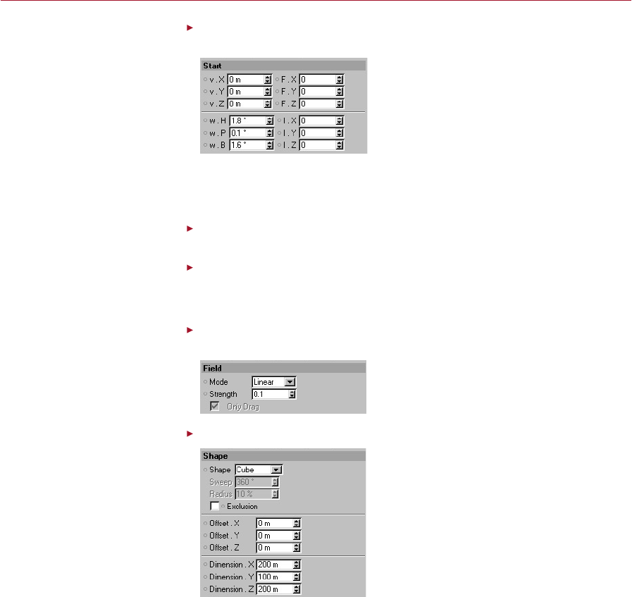
50 MOTION WITH DRAG DYNAMICS
DYNAMICS MOTION WITH DRAG 51
Click the Rigid Body Dynamic tag for the coin object, then click the Start tab.
Set w.H to 1.8, w.P to 0.1 and w.B to 1.6.
All Dynamics objects can be
given an initial motion; set it up
on the Start tab.
To use drag we need to have some velocity or angular velocity. Drag can only slow
down or speed up our motion. We want to be able to spin the coin, so we need to give
it a very small rotation so that it appears not to rotate until the time we want it to.
Select Plugins > Dynamics > Drag. Double-click on the Drag name in the Object
manager and set the name to Enter Beer.
Drag the Enter Beer object into the solver.
We need to slow down the coin as it strikes the surface of the beer; this can be
achieved with drag.
Click on the Enter Beer object’s icon. In the Attribute manager, click on the Field
tab and set the Strength to 0.1.
Reduce the strength of the drag
so that the liquid becomes easier
to pass through.
Click on the Shape tab and set Shape to Cube and Dimension.Y to 100.
The beer is present only inside
the glass, so its area of inuence
needs to be restricted.
We only need to slow down the motion slightly at the very top of the beer, this needs
to last only a short time so we use a attened cube along the Y.
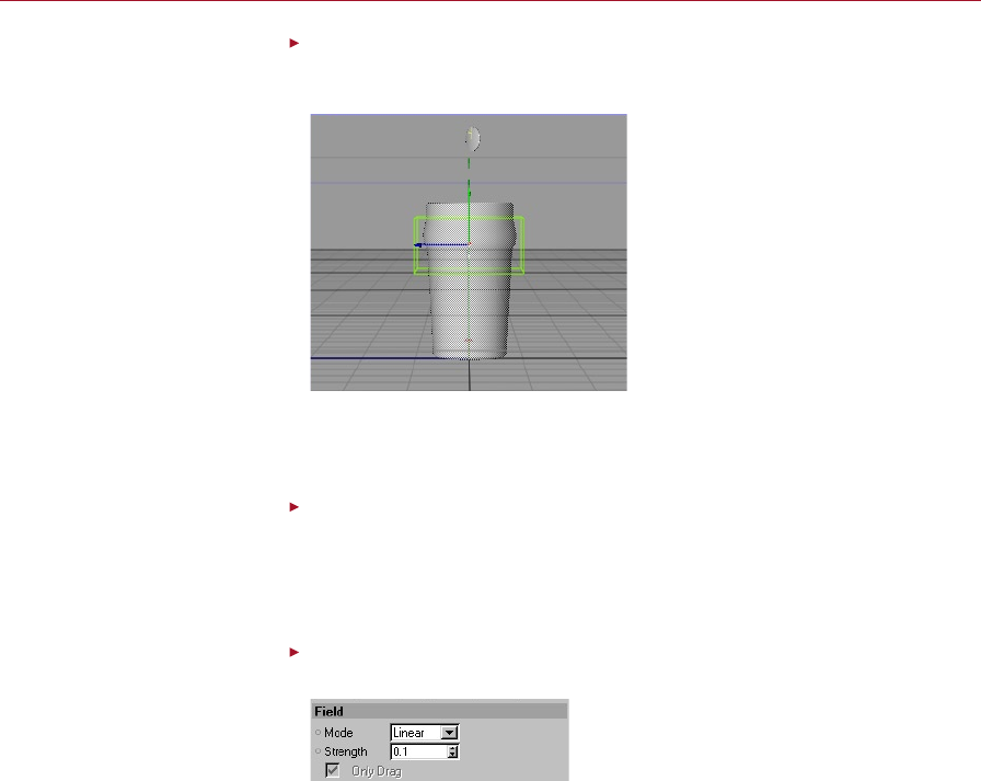
52 MOTION WITH DRAG DYNAMICS
DYNAMICS MOTION WITH DRAG 53
In the Object manager, ensure you have the Enter Beer object selected and move
the cube up the Y axis so that the top of the drag cube is just below the surface
of the beer.
Now that the drag has been
restricted to a certain area, it
needs to be positioned inside
the beer.
This small volume of drag will give us the slowing down we need to make it appear that
the coin is entering a uid. For this tutorial we’ll simplify the motion and exaggerate
the movement slightly to make it easier to follow.
Select Plugins > Dynamics > Drag. Double-click on the Drag name in the Object
manager and set the name to In Beer, then drag In Beer into the solver.
We need to gently slow down the coin as it passes through the uid. In air the falling
object would reach a maximum velocity known as the terminal velocity, but due to
the short distance the coin is falling we will not need to concern ourselves with it.
Click on the In Beer object’s icon. In the Attribute manager, click the Field tab
and set the Strength to 0.1.
Just like the other two drag
objects, this one will need to be
cut down in size.
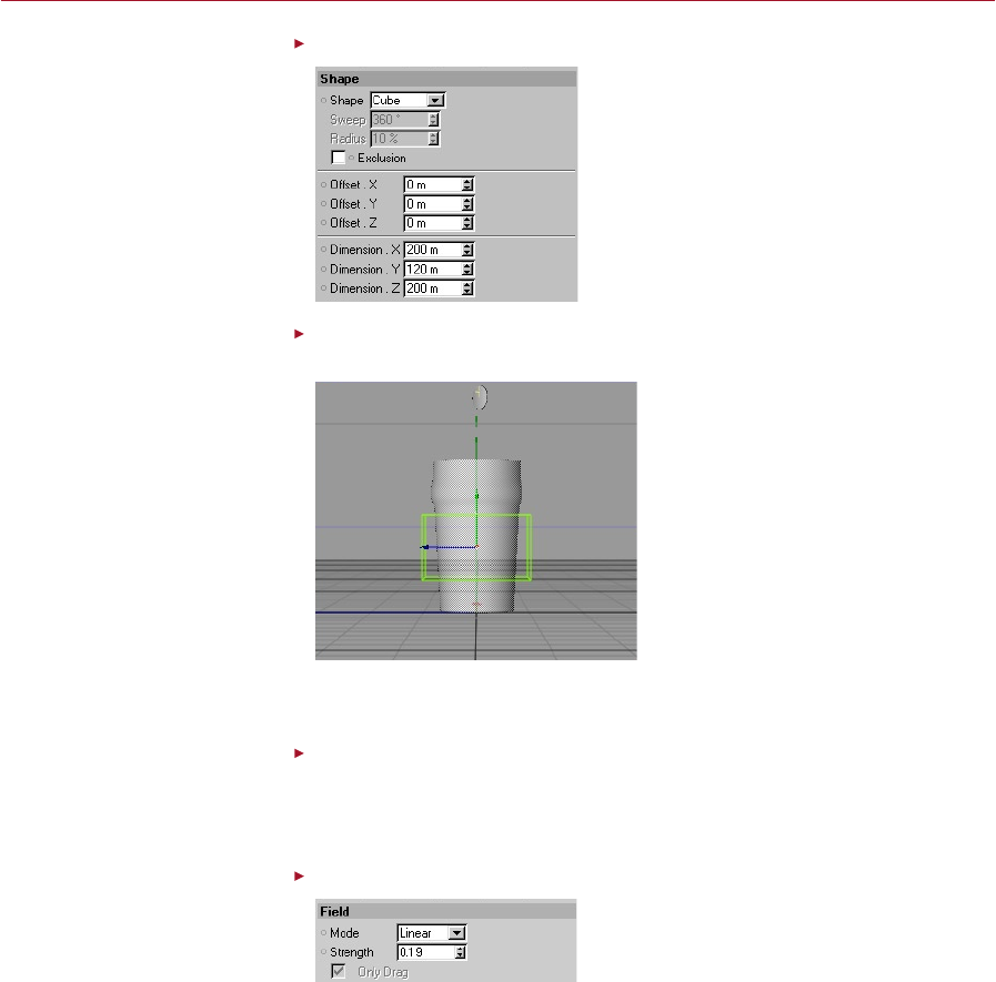
52 MOTION WITH DRAG DYNAMICS
DYNAMICS MOTION WITH DRAG 53
Click the Shape tab and set Shape to Cube and Dimension.Y to 120.
Changing the drag object’s
shape means that it is no longer
present everywhere, in our case
only inside the green cube.
Move the In Beer drag cube so that its top is just below the bottom of the Enter
Beer drag cube.
Position the In Beer drag object
as illustrated here.
We wish to slow down the coin for only the main body of the beer, beyond this we
need to stop it to prevent the coin leaving the glass.
Select Plugins > Dynamics > Drag. Double-click on the Drag name in the Object
manager and set the name to End Beer, then drag End Beer into the solver.
To give the impression of the coin coming to rest at the bottom of the glass we need
a drag object that can stop the motion.
Click the Field tab for the End Beer object and set the Strength to 0.19.
Reducing the strength of the
drag will change it from a thick
goo into a smooth pint of beer.
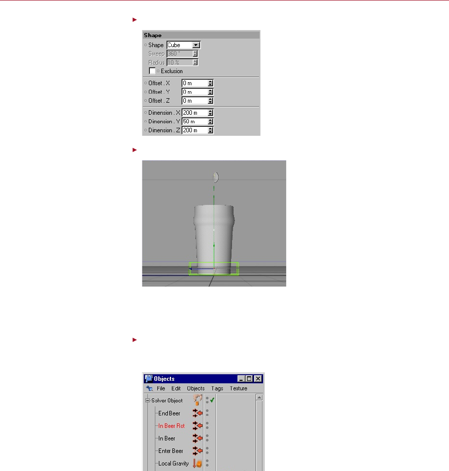
54 MOTION WITH DRAG DYNAMICS
DYNAMICS MOTION WITH DRAG 55
Click the Shape tab and set the Shape to Cube and Dimension.Y to 50.
Fake the displacement of the
beer by telling the drag to cover
only the bottom of the glass.
Move the End Beer drag cube so that its bottom is at the bottom of the glass.
Position the drag eld so that
it is overlapping the bottom of
the glass.
This will stop the object moving. Play it to see how it looks … but the fall is not yet
complete. We now want the coin resting approximately at at the bottom of the
glass.
Making sure you have your Object manager open and the In Beer object selected,
select Edit > Copy in the Object manager, followed by Edit > Paste. Double-click
this new In Beer object’s name and set the name to In Beer Rot.
A duplicate of this drag is
needed to alter the rate at which
it rotates. This is known as an
‘angular’ drag.
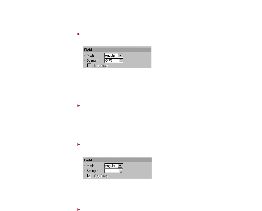
54 MOTION WITH DRAG DYNAMICS
DYNAMICS MOTION WITH DRAG 55
We want to use the same position and shape for our next drag object as we did for
the main body drag, so it is easier to simply copy and paste this object and then
modify it.
Click the Field tab for the In Beer Rot object and set the Mode to Angular and
the Strength to -0.75. Drag the In Beer Rot object into the solver.
The drag type needs switching
from Linear to Angular.
To make the coin spin around and land at the bottom of the glass we need to increase
any rotation it has already. This can be used to give the illusion that an object that
appears to be not rotating has its motion changed, but we are in fact simply speeding
it up enough so that the coin orients to a at position as it leaves the angular drag.
Making sure you have your Object manager open and the End Beer object
selected, select Edit > Copy, followed by Edit > Paste, then double-click this
new End Beer object’s name and change it to End Beer Rot.
Again we want to use the same position and shape for our new drag object as we
did for the end drag.
Ensure you have the End Beer Rot object selected. Click the Field tab and set Mode
to Angular and Strength to 1. Drag the End Beer Rot object into the solver.
The duplicate drag needs to
be set to Angular to stop the
coin rotating when it comes to
a stop.
To stop the coin spinning and to make it land at the bottom of the glass we need to
stop any rotation as well as any linear motion. The two End Beer drags will stop all
motion of the coin.
Click Play and then click Stop when you are nished.
The coin should fall into the beer, be slowed as it enters, followed by a gentle fall
through the beer with a slow rotation, nally rotating at the bottom to land and sit
at the bottom of the glass.

56 MOTION WITH DRAG DYNAMICS
Summary
You may nd that your motion isn’t exactly the same as the one shown in the diagrams
or in the nished animation in the Motion With Drag tutorial folder (‘mwdnal.c4d’).
This will apply to all dynamics, the exact motion depends on the positions and values
we set, and as such we need to become accustomed to adjusting scenes and values
to give us the motion we require.
You can adjust the values slightly to slow or speed up the fall and rotation; the
nal resting orientation of the coin slightly depends on the positions of the drag
objects.
Although this scene isn’t fully realistic — the surface of the beer remains still even
though a coin struck it — we will return to it in later tutorial to add a liquid-like
surface using soft bodies.
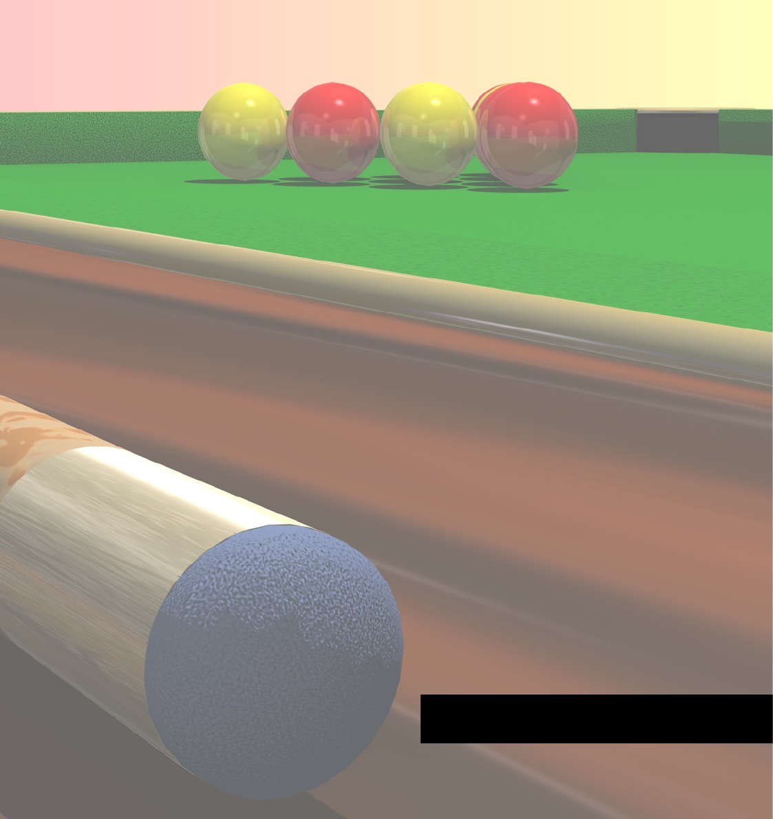
Gravity Collisions
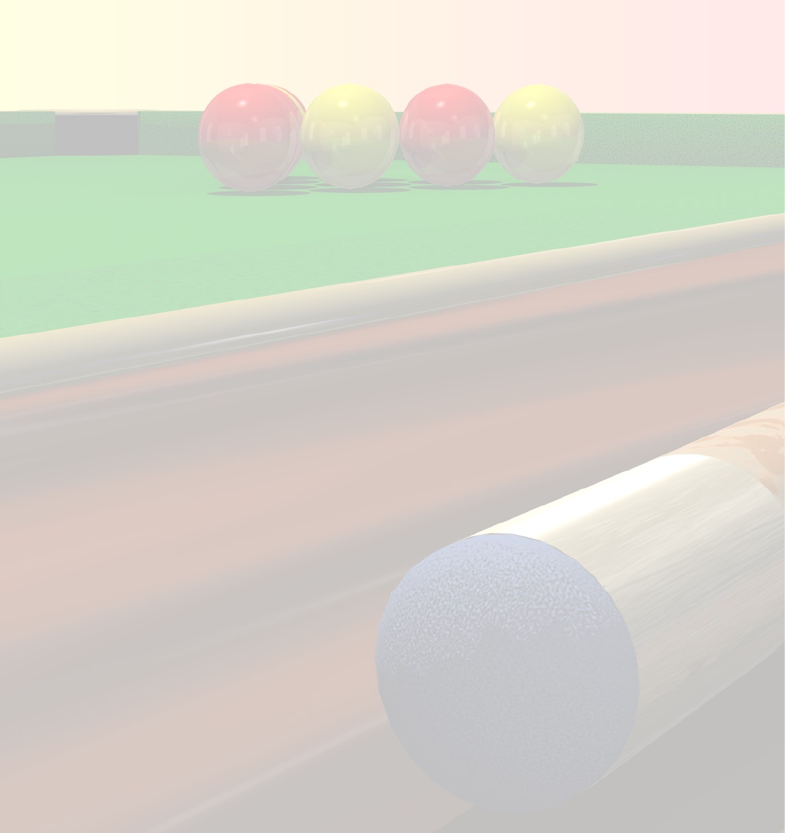
DYNAMICS GRAVITY COLLISIONS 59
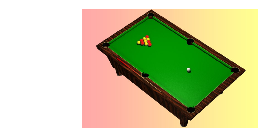
DYNAMICS GRAVITY COLLISIONS 59
Gravity
Collisions
Using full collision detection
is not always essential to a
working dynamics animation. To
save processing time, carefully
constructed scenes can use gravity
to create a simplied repulsion
instead.
Full-blooded collision detection takes a lot of processing. The more objects there are
in our scene, the more motion has to be checked and re-computed for every frame,
keeping in mind that if one object hits another and causes it to move, then not only
does the new movement have to be calculated but new checks have to be made to
see if the object which has been shunted is now going to interact with anything else.
And so on until every object in the scene has reacted, or not, to the initial collision.
With complex scenes, all you can do is throw gigahertz at the problem.
Or is it? Does every collision have to be an accurate simulation of real-world dynamics?
If we can fudge it so that it looks real enough and save ourselves days of computation,
isn’t that worth it?
Of course it is. In this tutorial we will be looking at one way in which collisions can
be simulated cheaply. While we may need to spend a little extra time setting up
the scene, with clever use of gravity we can make objects ‘bounce’ off each other
realistically and it will cost us a lot less processing time.
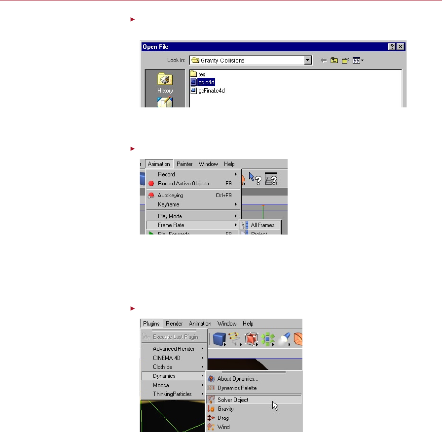
60 GRAVITY COLLISIONS DYNAMICS
DYNAMICS GRAVITY COLLISIONS 61
Select File > Open. Navigate to the Gravity Collisions tutorial folder on your
Documentation CD and open the le named ‘gc.c4d’.
Open the gc.c4d le for a ready-
made pool table.
The Tutorials folder is in the
Dynamics module folder. Each
tutorial has its own folder within
the main Tutorials folder.
The scene objects are now available in the Object manager. We now want to make
the balls interact with the cue and table, and of course each other.
Ensure that Animation > Frame Rate > All Frames is enabled.
When working with Dynamics
we should always ensure that
CINEMA 4D is set to display
every frame.
When using dynamics we need to be able to see every frame; this enables us to
check that every frame is how we want it to look, plus it prevents the dynamics
from calculating many frames at once, which can be slow on some complex scenes.
When working with dynamics we should make it a habit to ensure that All Frames
is enabled.
Select Plugins > Dynamics > Solver Object.
Without the Solver object
models cannot be moved by
Dynamics.
A Solver object will appear in the Object manager; this object is where we will add
the objects that we want to interact through dynamics and is necessary for any
dynamics system to work.
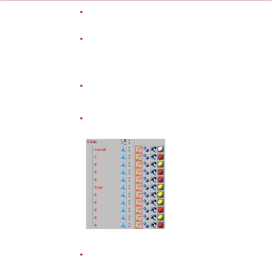
60 GRAVITY COLLISIONS DYNAMICS
DYNAMICS GRAVITY COLLISIONS 61
Click the Main tab and set the Stop frame to 300.
We want the animation to last the length of our timeline, so we set the stopping
frame for the dynamics to the end frame on our timeline.
Leave the Integration Method to Adaptive. Set the Oversampling to 8 and the
Subsampling to 8.
When the balls initially collide there will be many collisions to calculate as they ricochet
off one another. If Midpoint calculations were used then there is a chance that one
of the balls may intersect another. By using Adaptive we can specify a subsampling
which will be used to further divide the frames when it becomes necessary.
Set the Energy Loss to 3.
After we strike the balls they will eventually come to a stop due to the friction of
both the air and the table surface. Energy Loss will simulate this by gradually slowing
down all of the balls.
Command-click on a Mac if you
have only one mouse button.
In the Object manager, open the Balls group. Select all child objects of ‘Balls’.
Right-click on one of the selected balls then select Dynamics Tags > Rigid Body
Dynamic.
Adding Rigid Body Dynamic
tags is needed to assign each
ball a mass. Without mass, no
calculations can be made.
For our collisions we will need each ball to be a solid object with a mass; this enables
us to make use of the dynamics force objects.
Select Plugins > Dynamics > Gravity and drag the Gravity object and the Balls
group into the solver. Double-click on the Gravity object’s name, rename it
Collisions, then click OK.
For our collisions we’ll use a Gravity object to enable our balls to interact.
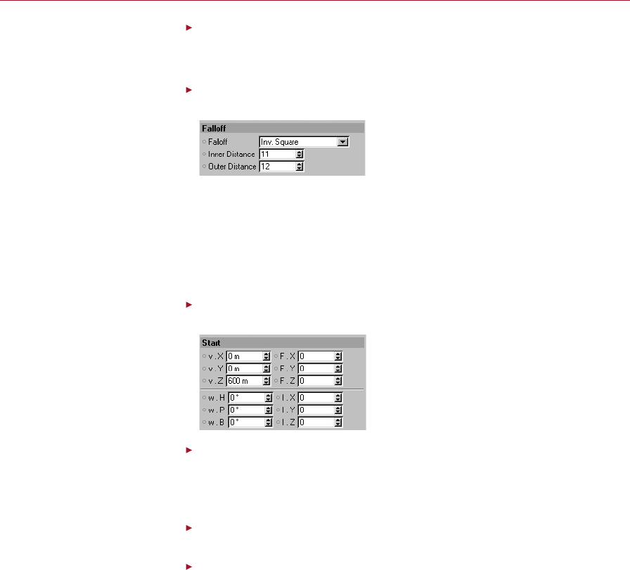
62 GRAVITY COLLISIONS DYNAMICS
DYNAMICS GRAVITY COLLISIONS 63
Click the Field tab and set the Strength to -4000000 and the Mode to Newton.
Setting a massive negative strength for gravity will make it appear as though nothing
can enter the gravity eld; anything that comes near will bounce away immediately.
Click on the Falloff tab, set the Falloff to Inv. Square, the Inner Distance to 11
and the Outer Distance to 12.
Gravity collisions are almost
always faster to calculate, and
in this case will give convincing
enough results.
For our collisions we want each ball to be repelled if any other ball comes within
range, so that they appear to collide. To reduce any unpredictable collisions we use
a thin falloff shell to soften the impact slightly as the balls start to collide.
The Inner Distance and Outer Distance values are set so that, as the centres of mass
of both balls come within the diameter of the balls with which they collide, it appears
that the outer geometry has collided.
Click on the Cue Ball object’s Rigid Body Dynamic tag. Click the Start tab and
set v.Z to 600.
We’ll start off simply by making
the cue ball move by itself.
Click Play and then click Stop when you are nished.
We can now check to see if our balls interact in a manner we are happy with. The cue
ball should move up the pool table and strike the rst red ball, which will strike into
the pack of balls and scatter them gently at the top of the table.
Select Plugins > Dynamics > Gravity and drag the Gravity object into the
solver.
Double-click on the Gravity object’s name and rename it Top-Left Border.
To make the balls interact with the table we need to give the illusion of the cushions
situated around the edges of the table. For this purpose we can use further Gravity
elds to repel the balls as they come within range of the table edges.
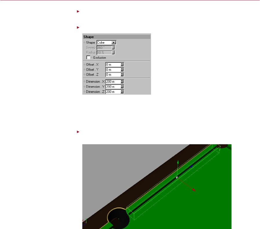
62 GRAVITY COLLISIONS DYNAMICS
DYNAMICS GRAVITY COLLISIONS 63
Click the Field tab for Top-Left Border, set the Strength to -100, Direction.X to
-1 and the other Direction values to zero.
Click the Shape tab and set the Shape to Cube.
Using a cube of gravity we can
fake a collision with the cushion
by suddenly repelling the ball.
By using an axial cube of gravity we can place a border around the table which
will stop the balls from leaving the connes of the table. We need the direction of
the axial gravity to always point inwards towards the table, which is why we set
Direction.X to -1.
Scale (Use Object Tool) and position the cube of gravity into a thin cuboid shape
along the top-left cushion between the middle and top pockets.
Position the cube of gravity so
that it is more or less in the same
position as the cushion.
By placing this cube as a border we can make the cushions appear to interact with balls
that come within the cube of gravity. The balls will interact only once a ball’s centre of
mass enters the cube of gravity, so we must ensure we position the cube far enough
inside the table so that the geometry of the ball and cushion don’t penetrate.
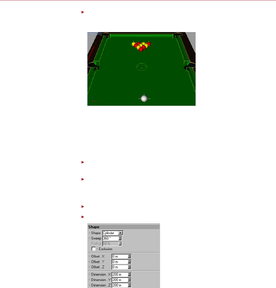
64 GRAVITY COLLISIONS DYNAMICS
DYNAMICS GRAVITY COLLISIONS 65
Copy and paste the Top-Left Border Gravity object to create the borders around
the table for each piece of cushion between the pockets — six in total. As you
paste them, rename each copy accordingly.
Create ve more cushions by
duplicating the original one.
How you rotate these will affect
the sign (+ or -) of the axial
gravity (see main text).
We will need to rotate the gravity by 90 degrees in the relevant directions to create
the top and bottom cushions. Ensure that the red axis of each gravity object points
inwards towards the table (this will save us from having to change the direction of
the axial gravity on the Field tab).
By placing the gravity objects around the table we have a fully interacting table so
that the balls will bounce off the cushions and off each other.
Select Plugins > Dynamics > Gravity and drag the Gravity object into the
solver.
Double-click on the Gravity object’s name and rename it Top-Left Pocket.
To make the balls fall into the pockets we need to add additional gravity objects,
otherwise the balls will leave the table through gaps in the border gravity objects.
On the Field tab for the Top-Left Pocket Gravity object, set Strength to 20.
Click the Shape tab and set the Shape to Cylinder.
We’re aiming to pot at least one
ball, so gravity is needed over
each hole.
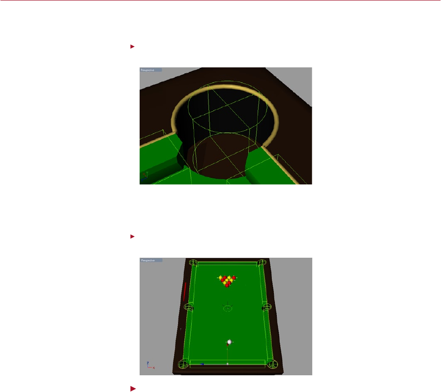
64 GRAVITY COLLISIONS DYNAMICS
DYNAMICS GRAVITY COLLISIONS 65
The Gravity object needs to be shaped so that as the ball enters the pocket it will be
forced downwards, giving the impression of it falling.
Scale and position the pocket’s gravity cylinder so that it is slightly smaller than
the diameter of the top-left pocket.
The cylinder of gravity needs
to be scaled and positioned
accordingly.
We need to place the gravity so that as a ball’s edge begins to leave the surface of
the table, it will begin to fall; this will help to stop the edge of the ball falling through
the table.
Copy and paste the top-left pocket’s gravity object to create the gravity for the
other pockets.
Just as we did with the cushions,
replicate ve more gravity elds
and place them inside each hole.
Click Play and then click Stop when you are nished.
The Cue Ball should move up the table and collide as before, but this time the balls
should also bounce around the inside of the table.

66 GRAVITY COLLISIONS DYNAMICS
Summary
Try changing the cue ball’s v.X value on the Start tab in the Rigid Body dialog and
see if you can pot a ball. This illustrates the exibility of Dynamics, once the scene is
created we can continue to adjust the object interactions without needing to adjust
the whole animation, the dynamics will handle it for us. We can take this one step
further, we can introduce keyframing into the dynamics. There are a number of ways
to use keyframes; we can use them on objects with a zero mass, or on the children
of dynamics objects.
One thing you should always bear in mind when creating a simulation is how much
the viewer will see. In this tutorial you may have noticed that none of the balls actually
roll. Of course it is possible to make this happen using real collisions and friction, but
if the end viewer cannot tell, then there is no reason not to use a quicker method,
such as these gravity force elds.
In the nished scene in the Gravity Collisions tutorial folder (‘gcnal.c4d’) we have
included a simple cue object; you can try use keyframing to move the cue and make
it strike the cue ball, rather than moving the cue ball itself.
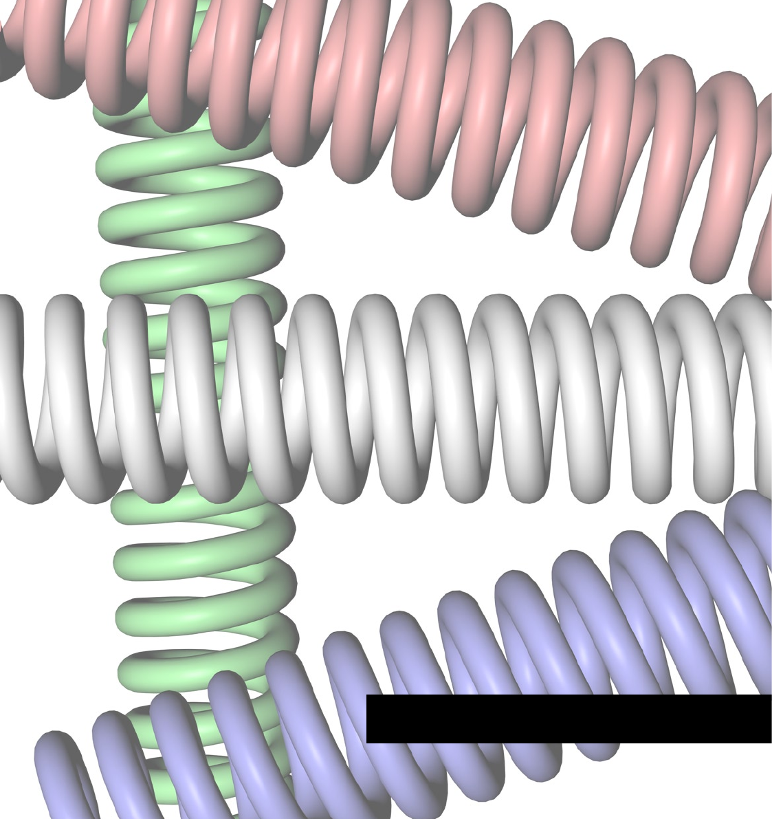
Rigid Body Springs 1
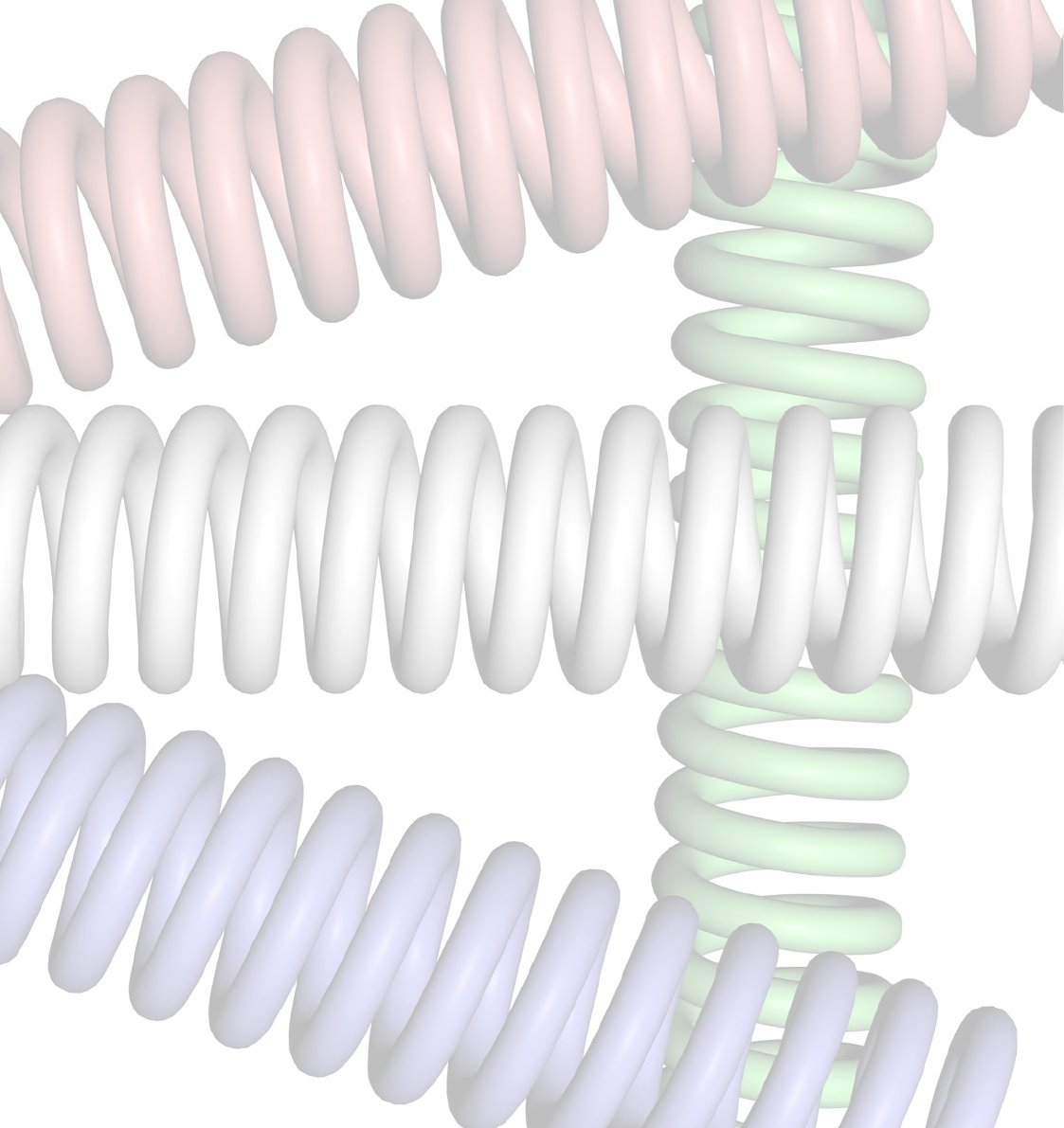
DYNAMICS RIGID BODY SPRINGS 69
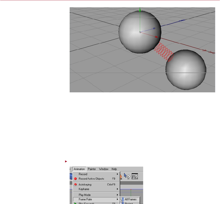
DYNAMICS RIGID BODY SPRINGS 69
Rigid Body
Springs 1
Springs are an important feature
of Dynamics and have more uses
than you might imagine. In this
tutorial we will illustrate how
springs are applied.
Rigid body springs are an invisible link between two or more objects that can either pull
or push each other. We can compress a spring, to simulate the suspension of a vehicle
for example, or stretch one, perhaps to create a catapult. Springs are represented in
the CINEMA 4D viewports by a coiled line which looks (we hope) like a spring. Just
like real springs, we can ruin them by overstretching; if this happens then they will
lose much of their elastic properties and become more like a plastic material.
It is even possible to break springs by pulling on them too hard!
By increasing the stiffness of springs we can create a simple link that can hold two
objects together. Springs also have the ability to rotate an object; think of a at,
tightly coiled spring in anything clockwork.
Ensure that Animation > Frame Rate > All Frames is enabled.
If a scene is too complex to
handle in realtime, frames
may be dropped. Avoid this by
forcing the display of all frames.
When using dynamics we need to be able to see every frame; this enables us to
check that every frame is how we want it to look, plus it prevents the dynamics
from calculating many frames at once, which can be slow on some complex scenes.
When working with dynamics we should make it a habit to ensure that All Frames
is enabled.
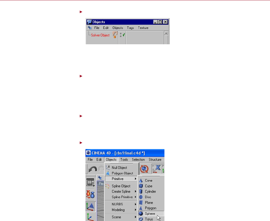
70 RIGID BODY SPRINGS DYNAMICS
DYNAMICS RIGID BODY SPRINGS 71
Select Plugins > Dynamics > Solver Object.
Solver objects are used to
specify which objects are
calculated; we are allowed to
have more than one.
A Solver object will appear in the Object manager; this object is where we will add
the objects that we want to interact through dynamics and is necessary for any
dynamics system to work.
On the Solver object’s Main tab set the Integration Method to Midpoint and
decrease the Oversampling to 2.
Midpoint calculations are the quickest available. As no accuracy is needed in this
scene it can quite safely be used. Reducing the Oversampling will give us a further
boost of speed.
Leave the Energy Loss set to 1.
To bring the simulation to an eventual stop it needs to lose energy at some point. By
giving it an overall energy loss, it cannot keep going forever.
Select Objects > Primitive > Sphere, twice.
We will use simple spheres for
our springs example as they
are very quick to draw in the
viewport.
This adds two spheres into the scene. We will link these two objects with a spring as
soon as we have prepared them.
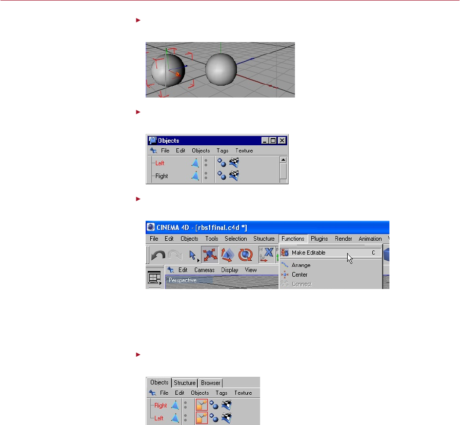
70 RIGID BODY SPRINGS DYNAMICS
DYNAMICS RIGID BODY SPRINGS 71
Move one of the spheres to the left so that it is separated from the other, as
illustrated in the picture below.
Move the spheres apart so that
the spring, when we add it, can
pull them together.
In the Object manager, double-click on the name of each of the spheres in turn
and name them Left and Right accordingly.
To help differentiate between
the two spheres we are giving
them logical labels.
In the Object manager, select both spheres (Shift-click to multi-select) and select
Functions > Make Editable.
Dynamics cannot work on
primitive objects, so convert
them to polygons to continue.
Remember that all objects you want to be affected by dynamics must be polygon
objects. This function will convert the parametric sphere (indicated by a dark blue
sphere icon next to its name) into a polygon object (indicated by a light blue triangle
icon by its name) as is required by Dynamics.
In the Object manager, select the two spheres and select File > Dynamics Tags
> Rigid Body Dynamic.
Dynamics needs to know
the mass of an object in
order to calculate its motion.
A Rigid Body Dynamic tag
enables us to add this mass.
This gives our spheres a Rigid Body tag each so that Dynamics knows that it should
be calculating its position and rotation. A new icon will appear to the right of each
sphere’s name, this is the Rigid Body Dynamic tag. You will also see tags’ settings
appear in the Attribute manager.
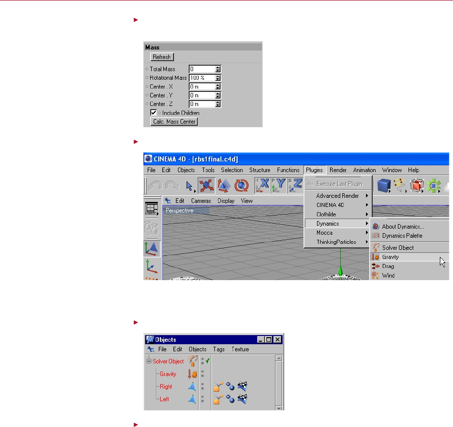
72 RIGID BODY SPRINGS DYNAMICS
DYNAMICS RIGID BODY SPRINGS 73
Click on the Right sphere’s Rigid Body Dynamic tag, click the Mass tab and set
the Total Mass to 0.
Set the mass to 0 to stop an
object from falling under the
inuence of gravity.
Select Plugins > Dynamics > Gravity.
To make our spheres move, we
need to add a force, in this case
gravity.
One of the last things that needs doing before we add our springs is to add some
gravity in order to make our spheres move.
In the Object manager, drag both spheres and the gravity into the solver.
We are dropping the gravity
and spheres into the solver so
that dynamics can be applied
to them.
Click Play and click Stop when you are nished.
You should see the left-hand sphere drop to the ground and the right-hand one
remain stationary. This is because the right-hand one has no mass, so therefore
cannot fall.
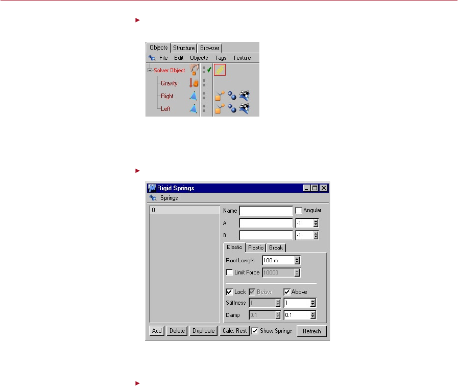
72 RIGID BODY SPRINGS DYNAMICS
DYNAMICS RIGID BODY SPRINGS 73
In the Object manager, select the Solver object then select File > Dynamics Tags
> Rigid Body Spring.
Springs can range from rigid
suspension springs to loose
rubber bands.
Now its time to give our spheres a more interesting motion by adding a spring between
them. Rigid springs are created within a Rigid Body Spring tag. When adding a new
Rigid Body Spring tag you will automatically be shown the Rigid Springs dialog.
In the Rigid Springs dialog, click the Add button.
Add a single spring between the
two spheres.
This begins the process of adding a spring between the two objects. Some boxes will
become active at the top of the dialog.
Set the name to Spring 1.
It is a good idea to get into the habit of naming your springs just as you would name
objects in a project.
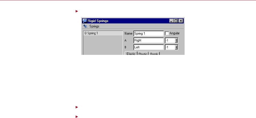
74 RIGID BODY SPRINGS DYNAMICS
Set A to Right and set B to Left.
We set A and B to specify which
objects we wish to join with this
spring.
The A and B boxes are the names of the two objects you wish to join. We entered in
the names Left and Right because this is what we named them earlier.
On the right-hand side of A and B you will see another two input boxes, both reading
-1. The number in these boxes decides which point number the springs will attach
to. The number -1 is a special number which tells Dynamics to connect the spring to
the object’s origin.
Click Refresh and close the Rigid Springs dialog.
Click Play and click Stop when you are nished.
You will now see the two spheres interacting, thanks to the spring.
Summary
Now we know how to apply a simple spring. We have not yet looked into changing the
stiffness or damping of the spring, both of these areas will be covered and explained
next in Rigid Body Springs 2. We recommend you head straight on into this second
springs tutorial where you will be able to start having some fun with them on our
bouncy character.
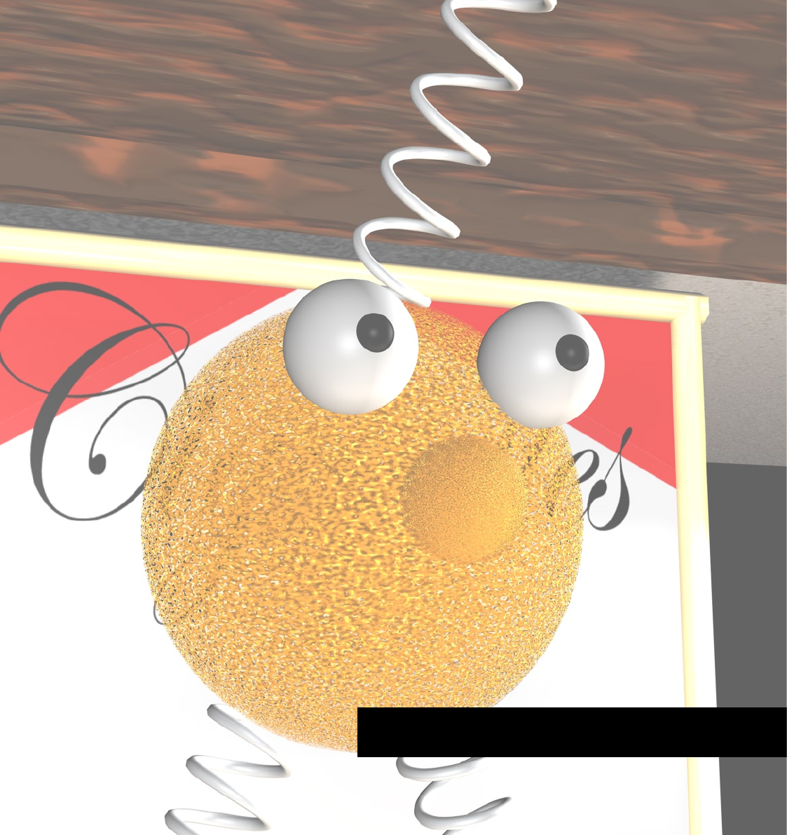
Rigid Body Springs 2
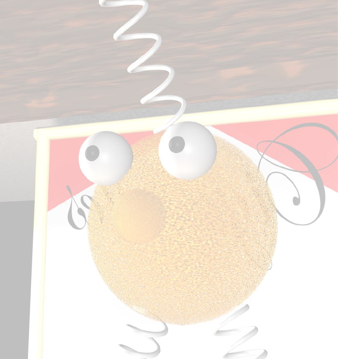
DYNAMICS RIGID BODY SPRINGS 77
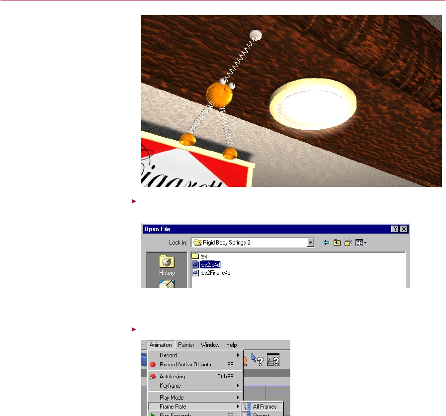
DYNAMICS RIGID BODY SPRINGS 77
Rigid Body
Springs 2
In this tutorial we will be applying
what we learned in Rigid Body
Springs 1 to a real scene. The end
result will be a bouncy advertising
mascot which illustrates the
sudden release of stored energy.
Select File > Open. Navigate to the Rigid Body Springs 2 tutorial folder on your
Documentation CD and open the le named ‘rbs2.c4d’.
Open the bar scene from
the Tutorials folder, this has
everything we need to get
started.
The Tutorials folder is in the
Dynamics module folder. Each
tutorial has its own folder within
the main Tutorials folder.
You will see four objects in the Object manager: Top, Body, Rfoot and Lfoot (Body is
actually a group of objects, but it will be treated as one).
Ensure that Animation > Frame Rate > All Frames is enabled.
Depending on your computer,
it may not be able to maintain
a steady 25 fps. All Frames will
avoid the danger of any frames
being skipped.
When using dynamics we need to be able to see every frame; this enables us to
check that every frame is how we want it to look, plus it prevents the dynamics
from calculating many frames at once, which can be slow on some complex scenes.
When working with dynamics we should make it a habit to ensure that All Frames
is enabled.
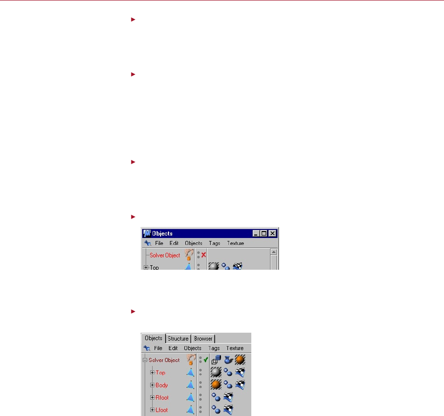
78 RIGID BODY SPRINGS DYNAMICS
DYNAMICS RIGID BODY SPRINGS 79
Select Plugins > Dynamics > Solver Object.
A Solver object will appear in the Object manager; this object is where we will add
the objects that we want to interact through dynamics and is necessary for any
dynamics system to work.
On the Main tab set the Stop frame to 1000, the Integration Method to Midpoint
and the Oversampling to 2.
In this tutorial we are making a springy pub mascot bounce around randomly. This
means that there is almost no need for accuracy because it can’t really go wrong.
Setting the calculations to Midpoint and the Oversampling to 2 means the least
processing power is required. Increasing the stop frame to 1000 ensures the simulation
does not stop prematurely.
Set the Energy Loss to 1.
Rather than add a Drag object to the scene for air resistance, we will instead set a
global energy loss. This means that the whole simulation is constantly losing energy,
which will cause the springy character to eventually come to a rest.
Click on the green tick next to the Solver object to disable it.
We can tell a Solver object not to
affect a scene by disabling it in
the Object manager.
It is a good idea to turn off the Solver object so that it does not have an effect on
the scene until we are ready for it to.
In the Object manager, drag the four objects (Top, Body, Lfoot, Rfoot) into the
Solver object.
These objects will make up
the head, feet and link of our
springy character.
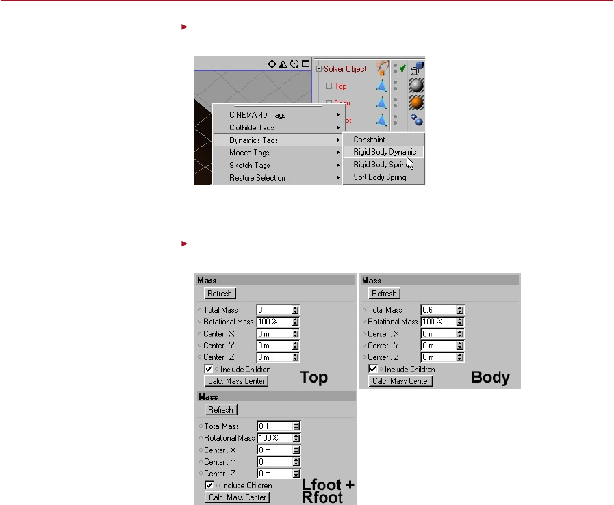
78 RIGID BODY SPRINGS DYNAMICS
DYNAMICS RIGID BODY SPRINGS 79
In the Object manager, select the four objects (Top, Body, Lfoot, Rfoot) and then
select File > Dynamics Tags > Rigid Body Dynamic.
All Dynamics objects must have
either a Rigid or Soft Body tag.
This adds a Rigid Body Dynamic tag to each of the four objects and will allow Dynamics
to inuence them.
Click on each Rigid Body Dynamic tag one after the other and on the Mass tab,
set the Total Mass as follows: Top = 0, Body = 0.6, Lfoot and Rfoot = 0.1.
DIfferent masses for different
objects.
We can nail an object in place by
giving it a mass of 0.
Only keyframes can move such
objects.
A mass of 0 guarantees that the Top object will not fall down when we later add
gravity to the scene. As the feet are the smallest objects, they will also be the lightest,
hence the low mass of 0.1.
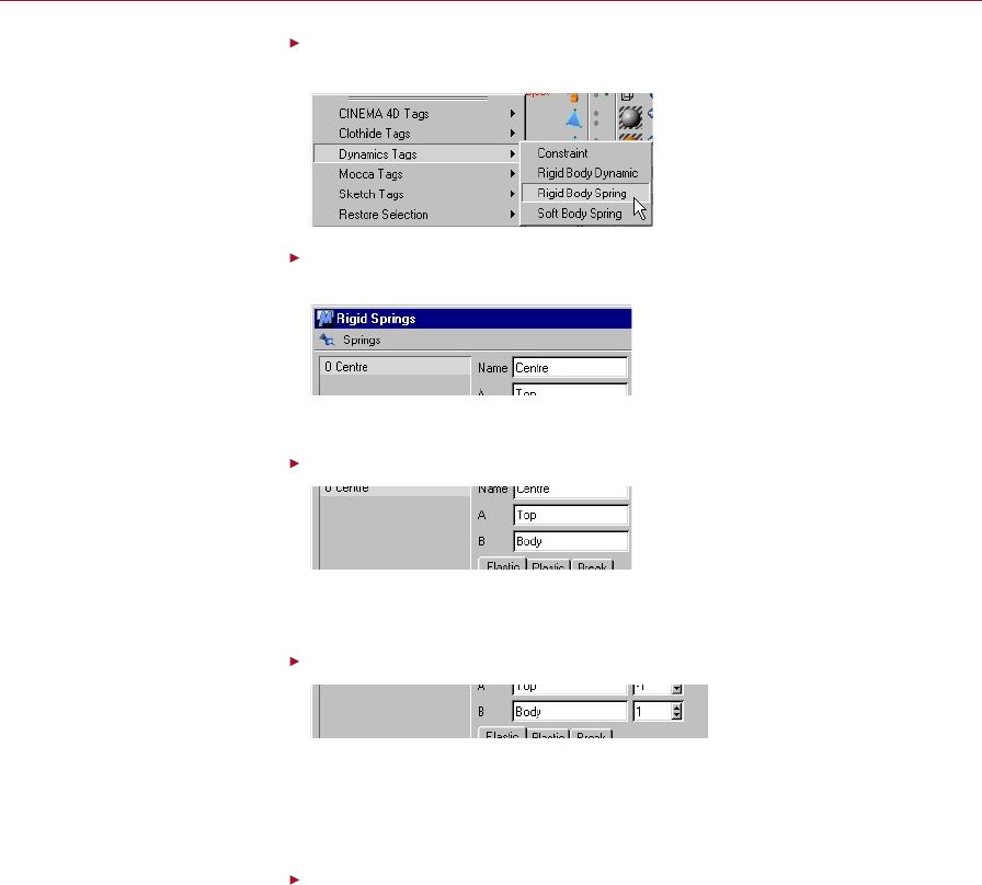
80 RIGID BODY SPRINGS DYNAMICS
DYNAMICS RIGID BODY SPRINGS 81
Command-click on a Mac if you
have only one mouse button.
In the Object manager, right-click on the Solver object and select Dynamics
Tags > Rigid Body Spring.
The Rigid Body Spring tag must
be assigned to the Solver object.
In the Rigid Springs dialog, click the Add button to create a spring and set its
Name to be Centre.
We can create as many springs
between whichever objects we
like.
This will help later on if we need to know which spring is which.
Set A to Top and B to Body. Note that these names are case-sensitive!
Just like the objects in the Object
manager, we should name our
springs to help us remember
what they are for.
The A and B values in this dialog determine which two objects will be linked; as this
is the main centre spring we need to connect it between the Top and Body objects.
Set the box to the right of B to 1.
Each spring must be linked to
another object; here we are
linking the two spheres.
To the right of the A and B values are two further values which determine where the
springs attach to the objects named in A and B. The rst one can be left at -1 so that
it connects to Top’s origin. The second one is set to 1 so that it connects to the top
of the Body object.
Set Rest Length to 200.
The distance between the Top and Body objects is far greater than the default Rest
Length of 100 units. So this value is increased to reduce the tension placed on the
spring.
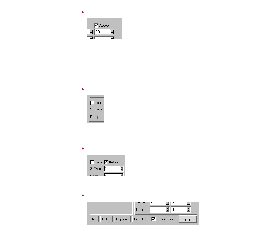
80 RIGID BODY SPRINGS DYNAMICS
DYNAMICS RIGID BODY SPRINGS 81
Set the Above Stiffness value to 0.3.
We can reduce the strength of
the springs to make them very
loose.
At the bottom of the Rigid Springs dialog are the Above and Below values. Above
settings are applied when the spring is stretched past its rest length; Below settings
come into effect when you compress the spring below its rest length.
By reducing the spring stiffness we are making the spring elasticity weaker so that
it does not ping back as quickly.
Disable the Lock option.
If the spring settings are locked
then we will be restricted to
using the same settings for
when the spring is compressed
and stretched.
The Below section is currently greyed out because the Lock option is enabled. When the
Lock option is enabled you will be able to enter values only into the Above section.
Ensure that the Below Stiffness value is set to the default setting of 1.
We may select different
behaviours for when the
spring is either stretched or
compressed.
This will ensure that the spring cannot squash down very much.
Set the Damp value to 0 for both Above and Below.
We don’t want the spring’s
motion to die out; we can keep
them moving by eliminating the
Damp settings.
Damp is short for damping. We set it to zero so that the spring does not lose any
energy by bouncing back and forth.
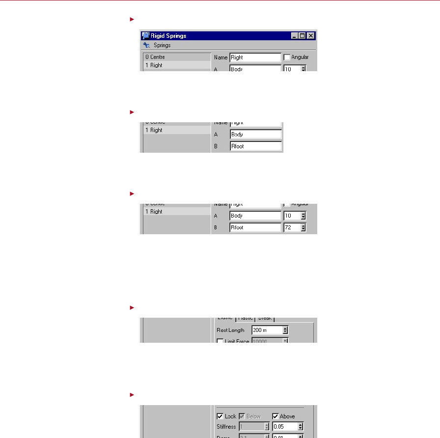
82 RIGID BODY SPRINGS DYNAMICS
DYNAMICS RIGID BODY SPRINGS 83
Click the Add button to create a new spring and set its Name to Right.
The springs for the feet need
different settings from the main
one connecting the body.
We are now adding a new spring for the body and right foot. This spring should be
named Right as it will connect the right foot to the body.
Set A to Body and B to Rfoot.
This time a new spring will be
connected between the main
body and the right foot.
Just as we did before, we have to tell Dynamics which two objects it should connect
with this new spring.
Set the box to the right of A to 10 and the box to the right of B to 72.
We have already found the
correct points to connect for a
realistic motion.
To keep the character’s feet separate we need to attach them to the opposite sides
of the body so that they do not end up dangling down in the same location. In this
case, point number 10 of the Body object is on the bottom right-hand side and point
72 of the Rfoot object is at the very top. (If you select any point of an object, you can
see what number it is in the Structure manager.)
Set the Rest Length to 200.
This spring is almost identical to
the main spring, using the same
rest length settings.
The distance between the right foot and the body is almost the same as the distance
between the body and the top, this means we can use the same rest length for the
spring.
Set the Above Stiffness all the way down to 0.05.
Reduce the default stiffness
until it represents a very loose
and slack spring.
The feet are also very small and light; if we used the default spring stiffness then the
feet would not bounce very much at all. We need to make the spring very loose.
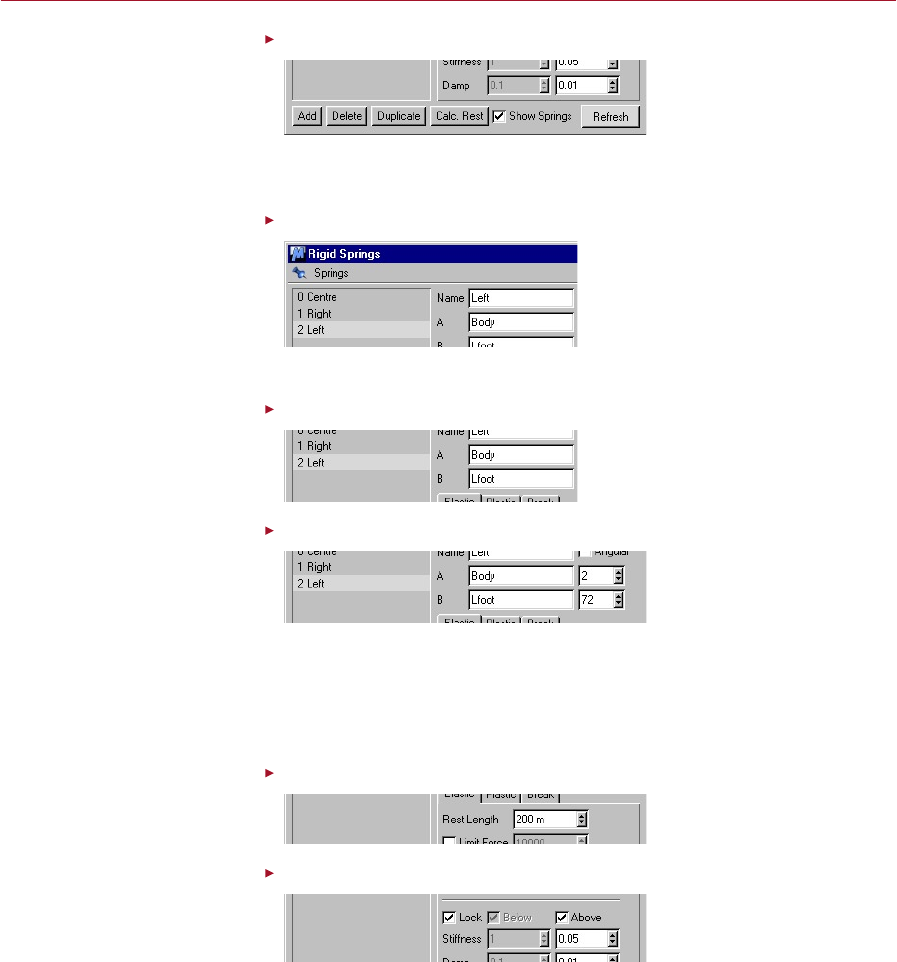
82 RIGID BODY SPRINGS DYNAMICS
DYNAMICS RIGID BODY SPRINGS 83
Set the Above Damp to 0.01.
Because the feet are very light
and loose, we need to make
them lose some energy.
The damping on these springs will also need to be reduced so that they bounce for
a longer period of time.
Click the Add button to create a new spring and set its Name to be Left.
Individual springs are needed for
each foot to act independently.
We are now adding a new spring for the body and left foot.
Set A to Body and B to Lfoot.
A rigid spring will be created
between whichever two objects
are in the A and B boxes.
Set the box to the right of A to 2 and the box to the right of B to 72.
The smaller boxes to the right of
A and B decide which points of
the object will be joined.
To keep the character’s feet separate we need to attach them to the opposite sides
of the body so that they do not end up dangling down in the same location. In this
case, point number 2 of the Body object is on the bottom left-hand side and point
72 of the Lfoot object is at the very top. (If you select any point of an object, you can
see what number it is in the Structure manager.)
Set the Rest Length to 200.
The rest length is the length
that the spring will always try to
become.
Set the Above Stiffness all the way down to 0.05.
Just like the right spring, the
left spring needs to have the
stiffness reduced quite a lot.
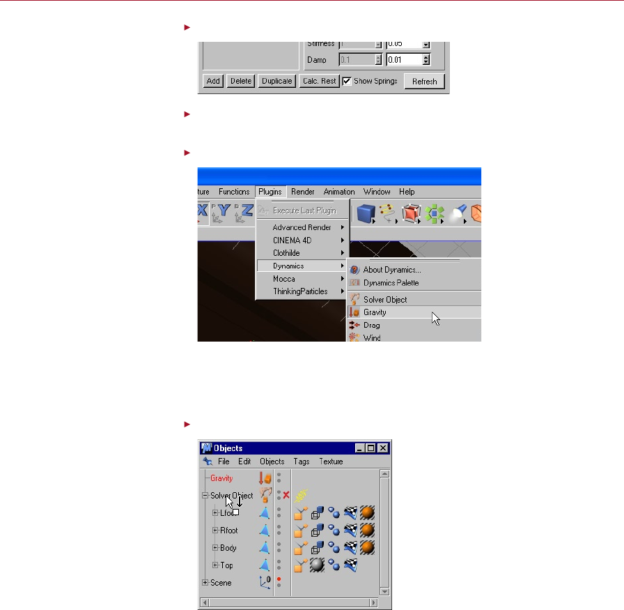
84 RIGID BODY SPRINGS DYNAMICS
DYNAMICS RIGID BODY SPRINGS 85
Set the Above Damp to 0.01.
Damping can be used to calm
down the motions of springs,
simulating natural energy loss.
After you have entered the settings for all three springs, click on Refresh to save
the settings. Close the Rigid Springs dialog as it is no longer needed.
Select Plugins > Dynamics > Gravity.
Without gravity our scene would
look highly unrealistic.
A Gravity object is essential to this scene in order to pull the objects downwards;
otherwise they would not bounce very convincingly. The default settings simulate
earth’s gravity so we do not need to open the dialog.
Drag the gravity into the solver.
All forces we want to use in our
simulation must be children of a
Solver object.
Without Gravity in a simulation there is a high chance that it will appear to be in outer
space, gravity is needed to pull the springs back down.
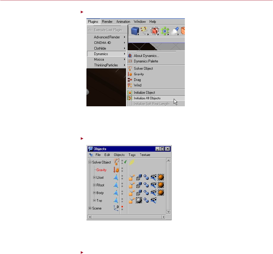
84 RIGID BODY SPRINGS DYNAMICS
DYNAMICS RIGID BODY SPRINGS 85
Select Plugins > Dynamics > Initialize All Objects.
We should always initialise a
scene before enabling a Solver
object.
Now that we have everything in place we need to initialise all the objects. This
will cause the Solver object to take note of all positions and use them for the start
positions of the simulation.
Enable the Solver object by clicking on its red cross.
Springs enabled, Dynamics
requires an active Solver object
to calculate the simulation.
The Solver now has all the new coordinates for the objects so it is safe to re-enable
it. The simulation will only take place if the Solver object is switched on by displaying
a green tick next to its name.
Click Play to see the bouncy character spring to life.
You might notice that at times the feet pass through each other. If you turn to the
tutorial on Gravity Collisions you can learn how to prevent this from happening. (The
nished animation in the tutorials folder, ‘rbs2nal.c4d’, uses this technique.)

86 RIGID BODY SPRINGS DYNAMICS
Summary
While following this tutorial you may have noticed the Plastic and Break tabs inside
the Rigid Springs dialog. We did not cover these here as they were not needed to
create the movements we were after. You can of course try enabling the Plastic and
Break sections if you wish. These will ruin the springs if you stretch them too much
and if pulled on too hard, actually snapping the spring so it no longer has any effect
on the dynamics.
When we get to the soft body tutorials we will see that they have very similar spring
dialogs. This is because each point on a soft body is actually connected with a spring
in order to give it a uid motion and to allow it to stretch.
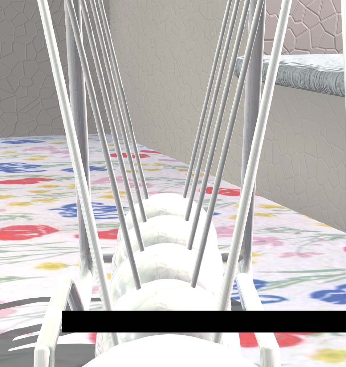
Gravity Collisions with Constraints
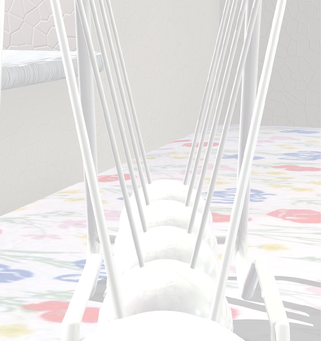
DYNAMICS GRAVITY COLLISIONS WITH CONSTRAINTS 89
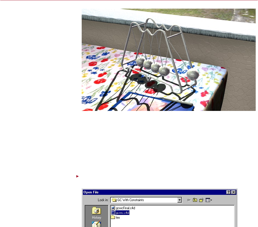
DYNAMICS GRAVITY COLLISIONS WITH CONSTRAINTS 89
Gravity
Collisions with
Constraints
In many circumstances we may
need to limit the motion of
objects because they are attached
to other objects; for this we use
constraints.
During dynamics simulations all objects are treated as individuals and the hierarchy
of objects is ignored if they have a rigid or soft body tag. This raises the question of
how we link objects together and still enable them to interact through the dynamics
engine.
We could link two objects using a spring, and in some cases this is a valid choice, but
it is also subject to the limits of the solver on the values for the forces. Using a spring
which has a very high stiffness can lead to overowing values which can eventually
break the dynamics. Using constraints doesn’t suffer this problem.
Select File > Open. Navigate to the GC With Constraints tutorial folder on your
Documentation CD and open the le named ‘gcwc.c4d’.
Open the le to begin the
tutorial.
The Tutorials folder is in the
Dynamics module folder. Each
tutorial has its own folder within
the main Tutorials folder.
The new scene is now available in the view, this is a Newton’s cradle. The idea behind
this executive toy is that in a perfect Newton’s cradle the momentum is transferred
between the two end balls without the middle balls seeming to move. In our animation
we shall aim for a similar appearance by using simplied gravity collisions. We will keep
it deliberately simple so that we can see the collisions and constraints in action.
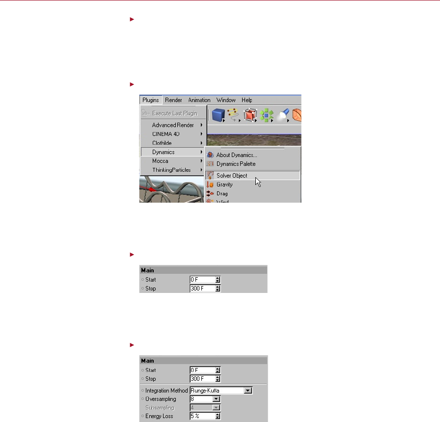
90 GRAVITY COLLISIONS WITH CONSTRAINTS DYNAMICS
DYNAMICS GRAVITY COLLISIONS WITH CONSTRAINTS 91
Ensure that Animation > Frame Rate > All Frames is enabled.
We need to be able to see every frame; this enables us to check that every frame is
how we want it to look, plus it prevents the dynamics from calculating many frames
at once, which can be slow on some complex scenes. When working with dynamics
we should make it a habit to ensure that All Frames in enabled.
Select Plugins > Dynamics > Solver Object.
Solver objects determine the
accuracy of the simulation.
A Solver object will appear in the Object manager; this object is where we will add
the objects that we want to interact through dynamics and is necessary for any
dynamics system to work.
On the Solver’s Main tab set the Stop frame to 300.
By default, the simulation stops
too early for us. Extend it by
adjusting the Stop frame.
We want the animation to last the length of our project as dened in the project
settings, so we set the stopping frame for the dynamics to the end frame on our
timeline.
Set the Integration Method to Runge-Kutta, and the Oversampling to 8.
When no soft bodies or real
collisions are used, we can often
use lower settings in the solver.
When the initial ball collides, the other balls will also collide in very quick succession.
If we used a lower integration type of oversampling the collisions can become softer
and may end up speeding up the movement rather than just passing it along.
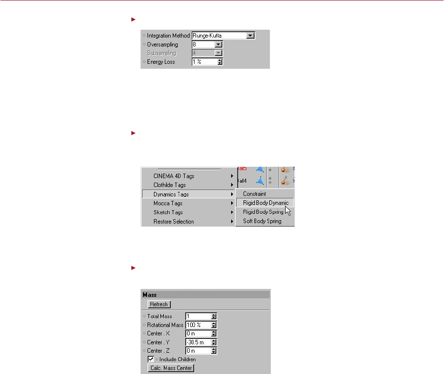
90 GRAVITY COLLISIONS WITH CONSTRAINTS DYNAMICS
DYNAMICS GRAVITY COLLISIONS WITH CONSTRAINTS 91
Set the Energy Loss to 1%.
We can make the Newton’s
cradle lose energy over time
by specifying an Energy Loss
amount.
To help control the momentum transfer during the dynamics and to aid in slowing
the balls’ collisions as would really happen we need a little energy loss. By using this
option it is also possible to use a slightly lower oversampling as it aids in preventing
the increasing velocities that can lead to the dynamics breaking.
Command-click on a Mac if you
have only one mouse button.
In the Object manager, open the Cradle group and select the ve balls (from
Ball5 to Ball1). Right-click on one of the balls and select Dynamics Tags > Rigid
Body Dynamic.
Rigid Body Dynamic tags enable
Dynamics to take control of the
objects’ motion.
Each of our balls will need to be a solid object so that we may use the gravity collision
method discussed in a previous tutorial.
Ensure that all ve Rigid Body Dynamic tags are selected. On the Mass tab, set
the Center.Y to -30.5.
The centre of mass needs to be
moved downwards to the middle
of the ball.
The ball object actually includes the wires from which it will swing. We have positioned
the origin for these objects at the top point about which they will swing, this is used
later by the constraints. To position the centre of mass at the correct point, which
is at the centre of each ball, we need to adjust it using the custom offset from the
origin of object.
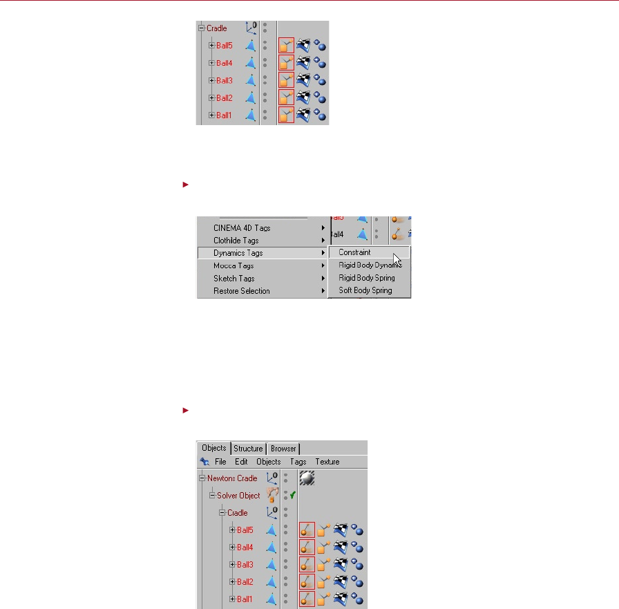
92 GRAVITY COLLISIONS WITH CONSTRAINTS DYNAMICS
DYNAMICS GRAVITY COLLISIONS WITH CONSTRAINTS 93
Identical tags for the ve balls.
As each ball is identical, there is no reason not to give them all the same centre of
mass.
Command-click on a Mac if you
have only one mouse button.
Ensure that all ve balls are selected. Right-click on one of the balls then select
Dynamics Tags > Constraint.
The constraint tag will restrict
the movement of an object
around its origin.
To pin our cradle balls to the surrounding frame we will need to constrain them to
a point. We prevent them from moving by xing each x, y and z coordinate of the
object’s origin to a point about which we want it to swing.
We need each ball to be constrained so that when they collide they are forced to
swing about the xed point of their origin.
Ensure that all ve Constraint tags are selected. In the Attribute manager, click
the Use Current button.
Constraint positions are
calculated relative to the parent.
A 0,0,0 offset places them in the
same location.
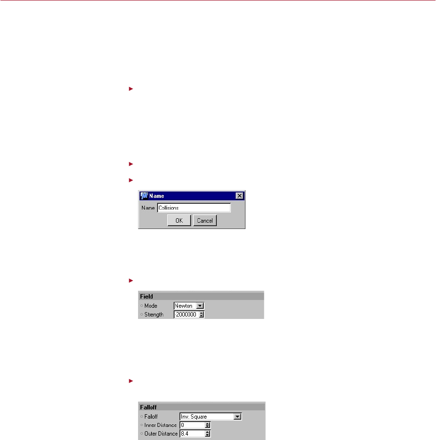
92 GRAVITY COLLISIONS WITH CONSTRAINTS DYNAMICS
DYNAMICS GRAVITY COLLISIONS WITH CONSTRAINTS 93
To constrain an object we need to give the dynamics a coordinate that is relative
to its parent to which each coordinate can be xed. This is an important point to
remember, the actual point is always relative to the parent, and this will be where
the object’s origin will become xed. We must also remember to correct the centre
of mass from the origin should we move the origin away from where the centre of
mass should be.
Drag the Cradle group into the Solver object.
Now that we have prepared each of our balls, we can place them into the solver. When
this happens the dynamics will initialise each object automatically and x its initial
position. If you later wish to move any of the objects you must turn off the solver and
then move the object, followed by the Initialize All Objects or Initialize Object option
in the Plugins > Dynamics menu, then turn the solver on again.
Select Plugins > Dynamics > Gravity and drag the Gravity object into the solver.
Double-click on the Gravity object’s name, rename it Collisions, click OK.
We are renaming the Gravity
object to reect its purpose.
For our balls to collide we’ll use a Gravity object to speed up the processing needed
for the animation. For collisions that don’t appear directly in front of the camera and
don’t need much detail, using Gravity can make a big saving in processing time.
On the Field tab, set the Strength to -2000000 and the Mode to Newton.
Huge numbers will give the
effect of a collision.
Setting a very large negative strength for the gravity will make it appear as though
nothing can enter the gravity eld; anything that comes near it will bounce away
immediately. The disadvantage of using this technique is that when the values for the
Gravity are so high we must be careful to prevent the scene from exploding.
Click on the Falloff tab, set the Falloff to Inv. Square, the Inner Distance to 8
and the Outer Distance to 8.4.
Lower solver settings can be
used if we make use of a falloff
value; this gives the objects a
chance to be repelled.
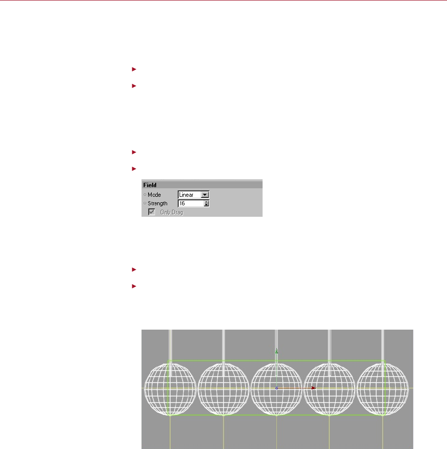
94 GRAVITY COLLISIONS WITH CONSTRAINTS DYNAMICS
DYNAMICS GRAVITY COLLISIONS WITH CONSTRAINTS 95
To compensate for the extremely large gravity strength we will use a falloff that
will create a very thin shell of gravity around the surface of each ball. This will make
the collision very strong only over a very small region, helping to make the collision
appear more realistic.
Select Plugins > Dynamics > Gravity and drag the Gravity object into the solver.
On the Field tab, set the Strength to 6.
The balls will appear to swing more freely if there is a force to pull them back down
again. As the gravity tries to pull, the constraint will hold the origin of the object at
its xed position. The only motion we didn’t constrain was the angle, allowing the
ball to pivot and swing freely.
Select Plugins > Dynamics > Drag and drag the Drag object into the solver.
On the Drag’s Field tab, set the Strength to 16.
Small areas of drag can be used
to calm down the simulation.
To help control our extremely large gravity we are going to stop any jitter and
exploding motion by forcing the balls in the centre to remain virtually still. This will
make our cradle appear more like a real perfect one.
Click on the Shape tab and set the Shape to Cube.
In the viewport, position the Drag object (the green outlined cube) at the centre
ball, then scale and rotate the cube so that the drag is completely around the
three middle balls and the edges are just covering the centres of mass of the
two outer balls.
Place the drag eld into the
position where we want to slow
down movement.
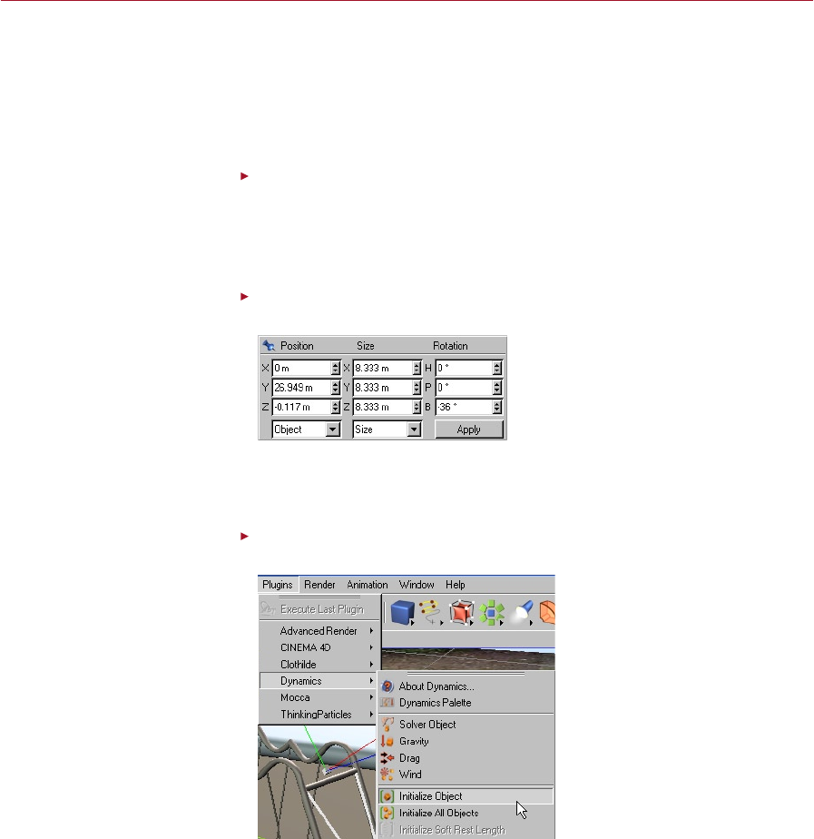
94 GRAVITY COLLISIONS WITH CONSTRAINTS DYNAMICS
DYNAMICS GRAVITY COLLISIONS WITH CONSTRAINTS 95
To aid the motion of our outer balls we set the drag so that, if they should move
too far towards the inner balls, they will be slowed greatly, allowing the inner balls’
gravity to force them back outwards. This will give a slight bump as the outer balls
crash down, making it appear more realistic.
If you’re feeling brave, try changing the size of the Drag object and see how this
affects the movement of the balls.
Check the time slider to ensure that the current frame is 0, then click on the
small green tick next to the Solver.
Before adjusting the position or rotation for objects you need to disable the solver,
otherwise it has control over the objects and will prevent you from interacting with
them in the viewport.
In the Object manager, select the Ball1 object then in the Coordinate manager
set the B rotation to -36 and click Apply.
Pull back the rst ball into
position, ready to be released.
This pulls back the ball ready to drop it. Once we have a simple cradle working we
can try changing the angle; we may nd that at large angles we need to increase the
strength of the gravity or the drag.
Ensure that the Ball1 object is selected in the Object manager, then select
Plugins > Dynamics > Initialize Object.
After moving an object in a
solver we must initialise either
the scene or the object to retain
the current positions.

96 GRAVITY COLLISIONS WITH CONSTRAINTS DYNAMICS
Click the red cross next to the solver to turn it back on.
Having moved our object to a new position we need to tell the dynamics that this
is our starting position.
Click Play and then click Stop when you are nished.
The initial ball that we rotated swings and collides with the second ball. Each ball
collides until the nal ball is forced to swing again around is pivot. By adjusting the
strength of the gravity we can speed up the swing of the outer balls.
Summary
By constraining motion we can link objects together, or make them appear to be
connected, such as the balls and frame of the cradle. The use of gravity for the collisions
gives us a virtually realistic appearing animation at much lower processing power.
Unlike the pool table example, here the balls would not rotate and so this could be
used under closer inspection.
The main problems with gravity collisions are a tendency to suddenly gain speed
during the interaction; we have shown how to cope with this by careful positioning
of drag to remove this additional motion.
Taking this scene a step further, we could introduce more balls, or make two balls
swing to start with. Although making alterations such as these will require some
modications to the scene, the time saved in processing the animation over real
collisions can be a worthwhile investment.
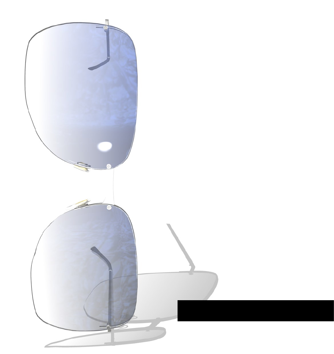
Collision Detection
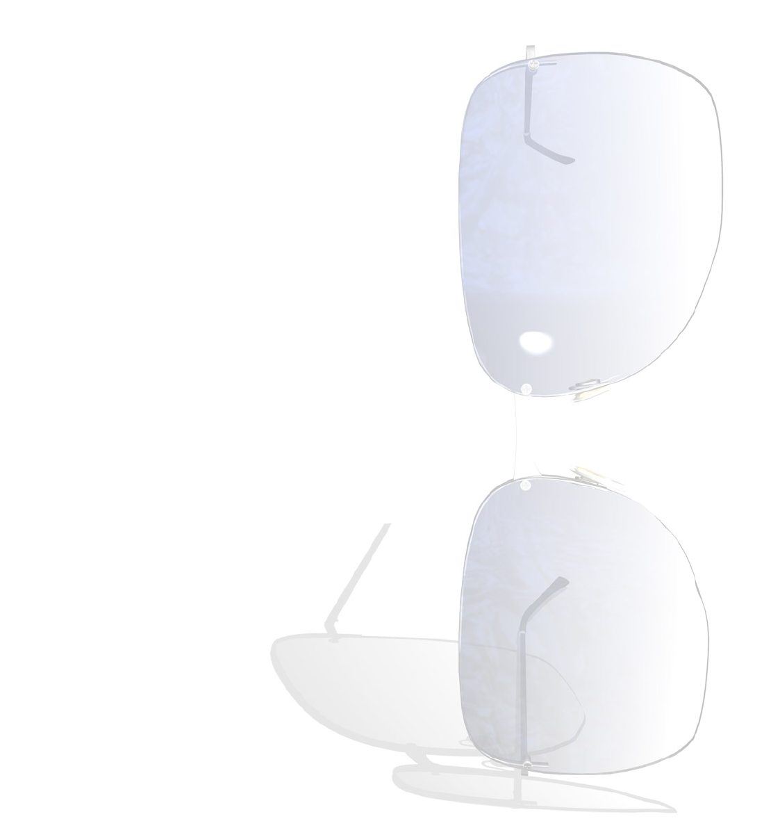
DYNAMICS COLLISION DETECTION 99
DYNAMICS COLLISION DETECTION 99
Collision
Detection
While gravity based collisions
can be useful, when objects
need realism in their interactions,
nothing beats the full and proper
detection of collisions.
When using collisions in our animation we can break up the detail into various levels.
The less detail we need then the more we can use simple gravity repulsion to create
the illusion of collision.
The next level up from faked collisions is to use very simple proxy objects with full
collision detection. By using these we can vary the detail needed in our collisions
from very simple geometry to a polygon reduced duplicate of our real geometry. If
we have a close up and need perfect behaviour, we can use a more detailed proxy,
or our original object itself.
The advantage of simplied collisions through gravity or proxy objects is to give a
speed boost to the simulation. Full collision detection with all our real objects will
depend fully on their complexity, and in some cases may not even work due to the
objects being over complex for the collision detection system to handle; the only
solution in such a situation is to nd a proxy object that closely matches the original,
but that is also simple enough to use.
We’re going to take an intricately modelled pair of sunglasses and drop them on to
a table top; we’ll use a simple proxy object to help us.
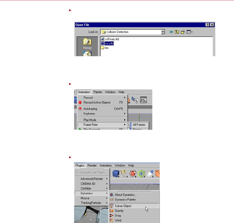
100 COLLISION DETECTION DYNAMICS
DYNAMICS COLLISION DETECTION 101
Select File > Open. Navigate to the Collision Detection tutorial folder on your
Documentation CD and open the le named ‘cd.c4d’.
Open the cd.c4d le to be
presented with a pair of glasses
which we can drop.
The Tutorials folder is in the
Dynamics module folder. Each
tutorial has its own folder within
the main Tutorials folder.
The scene objects are now available in the Object manager. We have already made
a simple proxy object for you, a cube, which has been hidden in the render and
viewport.
Ensure that Animation > Frame Rate > All Frames is enabled.
Display every single frame to
make sure Dynamics does not
miss out any frames needed for
the calculation.
When using the dynamics we need to be able to see every frame, this enables us to
check that every frame is how we want it to look, plus prevents the dynamics from
calculating many frames at once, which can be slow on some complex scenes.
Select Plugins > Dynamics > Solver Object.
Solver objects are required for
Dynamics to know which objects
it should be working on.
A Solver object will appear in the Object manager. This is where we will add the objects
that we want to interact through dynamics to give us our collision.
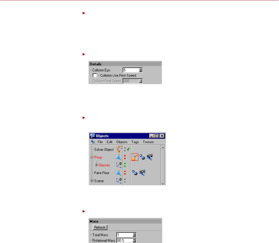
100 COLLISION DETECTION DYNAMICS
DYNAMICS COLLISION DETECTION 101
On the Solver object’s Main tab, set the Integration Method to Midpoint and
Oversampling to 8.
Generally collisions on their own will work with a less accurate integration method
and lower oversampling, the type of dynamics that need high oversampling and
accuracy are soft bodies.
Click the Details tab and set the Collision Eps to 5.
We need to alter some of the
solver settings, such as the Eps,
in order to suit the simulation.
The Eps setting (Epsilon) determines how close an object can get to another before
it collides. By reducing this setting we can give the effect of the object deforming
slightly by allowing colliding objects to penetrate each other slightly.
Command-click on a Mac if you
have only one mouse button.
Drag the Glasses object into the Proxy object then, making sure you have the Proxy
object selected, right-click and select Dynamics Tags > Rigid Body Dynamic.
Use proxy objects as stand-ins
if the geometry of the actual
objects is too complex.
We want the proxy object to be our rigid body; the glasses will follow the motion of
this proxy by sitting in the proxy object’s local coordinates.
On the Mass tab set the Rotational Mass to 80%.
To make our glasses appear
lighter we will reduce the
rotational mass; they can now
rotate more upon landing.
Our sunglasses are made from a light material and should rotate easily. They also
have a heavy front so we want them to drop on the table and rock slightly, plus
rotate a little from the collision. Often collisions need their rotational mass changing,
real objects rotate differently depending on the density of the materials from which
they are made.
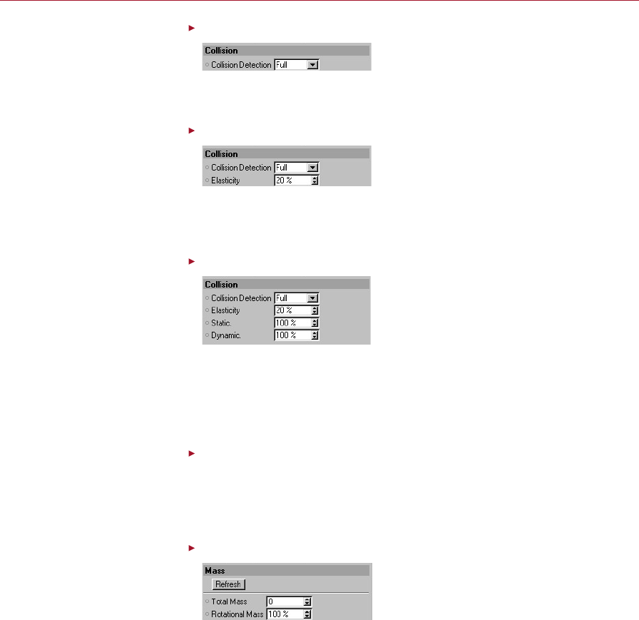
102 COLLISION DETECTION DYNAMICS
DYNAMICS COLLISION DETECTION 103
Click the Collision tab and set Collision Detection to Full.
Full detection is required for the
glasses to land convincingly.
Our proxy object is already simple, so we don’t want any of the simplied collision
detection methods, we need the full detection on our own simple geometry.
Set the Elasticity to 20%.
We need the glasses to bounce
slightly, reducing the elasticity
to 20% should be ne.
As our sunglasses fall on to the table, they will not bounce very much. The structure
of the sunglasses is exible and the energy will be mostly lost from the collision.
Reduced Elasticity will prevent the sunglasses from bouncing.
Set the Static and Dynamic coefcients to 100%.
Without friction coefcients the
glasses will continue to slide
after they have hit the ground.
When our sunglasses are on the surface of the table we don’t want them moving
around; friction will keep them still and stop them sliding or rotating. Friction is
controlled by the static and dynamic coefcient values. Here we are using the
dynamic coefcient to slow down the sunglasses while they are moving and the
static coefcient to keep them in place once they have come to a stop.
Command-click on a Mac if you
have only one mouse button.
In the Object manager, select the Fake Floor object, right-click and select
Dynamics Tags > Rigid Body Dynamic.
We want our sunglasses to appear to land on a solid surface. In a similar way to that
in which we used a proxy object for the sunglasses, we are going to use a single plane
as a proxy object for the collision.
On the Mass tab, set the Total Mass to 0.
To create a rigid and unmovable
oor in our scene, we set its
mass to 0.
We don’t want our plane to move when the sunglasses land, or for the gravity object
to move our Fake Floor object; setting its mass to zero will prevent dynamics from
having any effect on it.
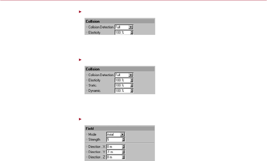
102 COLLISION DETECTION DYNAMICS
DYNAMICS COLLISION DETECTION 103
Click on the Collision tab and set Collision Detection to Full.
Full collision detection will
improve the accuracy of the
simulation.
As with our proxy object, we have already simplied the geometry so we can use
full collision detection.
Set the Static and Dynamic coefcients to 100%.
The oor also needs the friction
coefcients enabled for it to grip
the glasses when they land.
We want our oor to keep grip of the sunglasses, to stop them sliding around, so we
use the static and dynamic coefcients to add friction.
Select Plugins > Dynamics > Gravity and on the Field tab set the Strength to 5.
The downward pull of gravity
will be a common requirement
in many simulations.
We want our sunglasses to fall quickly on to the oor; to make it appear realistic it
should take much less than a second for them to fall that distance. When creating
scenes such as this, it is worth checking that we have got roughly the right timing
for falls and collision; if things fall or move too slowly or too quickly, the animation
won’t look quite right. Set up a simple real life situation or, if you’re really brave, try
calculating the times with mathematics.
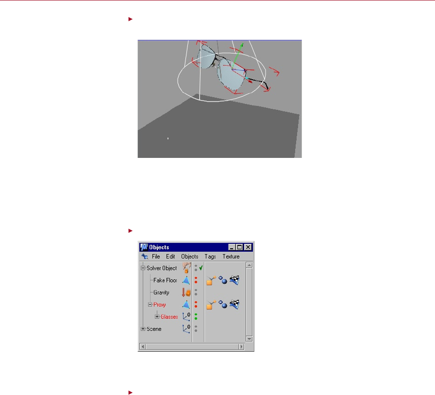
104 COLLISION DETECTION DYNAMICS
DYNAMICS COLLISION DETECTION 105
In the viewport, move and rotate the proxy object so that it is above the oor
at a slight angle.
Reposition the glasses above
the ground so that they have a
distance to fall.
Now we have our scene ready, we want to drop the sunglasses. Moving them up and
rotating them slightly will give a more interesting bounce. The proxy object has been
designed to show overall collision of the glasses, so rotating the sunglasses so that
they land lens-rst will not give a realistic looking collision; for this we would have
to add a curve to the front of the proxy.
Drop the Proxy object, Fake Floor and Gravity into the Solver object.
Place the three objects into the
solver so that Dynamics can
apply physical movements to
them.
Now we have prepared each object, we need to put them into the solver so that
Dynamics can take over and make our animation come to life.
Click Play and then click Stop when you are nished.
The falling sunglasses show a simple way of using proxy objects. We have ignored some
areas in this, such as the arms of the glasses, but for medium detail collisions that are
not in the full view of the camera, or in a distant part of your scene, such simplication
helps to greatly speed up the process of building the scene, plus animating it.

104 COLLISION DETECTION DYNAMICS
DYNAMICS COLLISION DETECTION 105
You may have noticed that the sunglasses are still moving around long after the
collision. These small movements are to be expected when we are working with
dynamics simulations. One way to halt the sunglasses would be to turn off the
dynamics simulation at just the right moment using the solver’s Stop parameter on
the Main tab.
Summary
As we have seen, we do not need to use the full geometry of the original object for
collision detection. Our model geometry will often be far too complex to be used like
this and will take a long time to render. By using proxy objects we can create much
simpler stand-in objects to which we can apply collision detection.
Depending on your computer system, during this tutorial you may have noticed that
the playback speed in the viewport was not very smooth. If so, you may wish to make
use of the Render > Make Preview command which will enable you to create a much
smoother playback of the simulation.
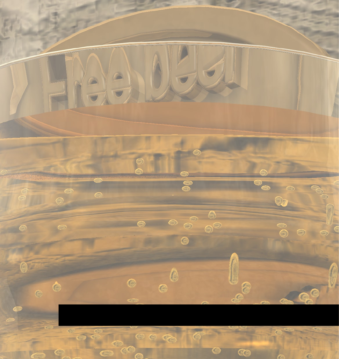
Gravity Collisions with Soft Bodies
DYNAMICS GRAVITY COLLISIONS WITH SOFT BODIES 109
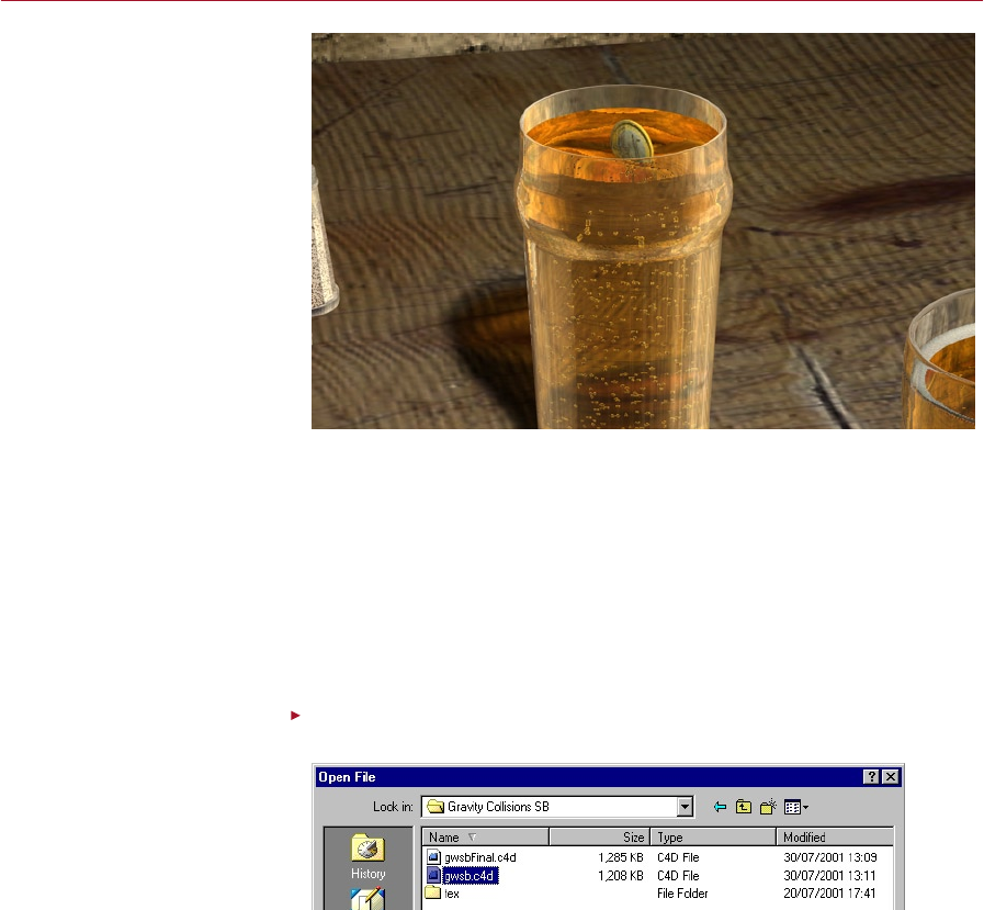
DYNAMICS GRAVITY COLLISIONS WITH SOFT BODIES 109
Gravity
Collisions with
Soft Bodies
We can interact with soft body
masses by using gravity in a
similar way to that in which we
created simple collisions with rigid
bodies.
It is possible to use soft bodies to simulate a rippling surface in order to create the
illusion of water. A liquid surface has a tension that makes it act in a similar way to
the soft bodies in Dynamics. By using gravity to affect the soft body it is possible
to disturb a surface in such a way that it gives the impression of objects interacting
with the water.
In this tutorial we are going to extend the Motion With Drag tutorial by causing the
surface of the beer to ripple when the coin drops into it.
We will see that by adding some soft body springs to the Beer object we can use
gravity and drag to simulate a pretty realistic liquid, rippling surface.
Select File > Open. Navigate to the ‘GC With Soft Bodies’ tutorial folder on your
Documentation CD and open the le named ‘gwsb.c4d’.
Open the le to begin the
tutorial.
The Tutorials folder is in the
Dynamics module folder. Each
tutorial has its own folder within
the main Tutorials folder.
The scene objects are now available in the Object manager. As in the Motion With
Drag tutorial, we want to take this one step further and make the coin actually move
the surface of the beer.
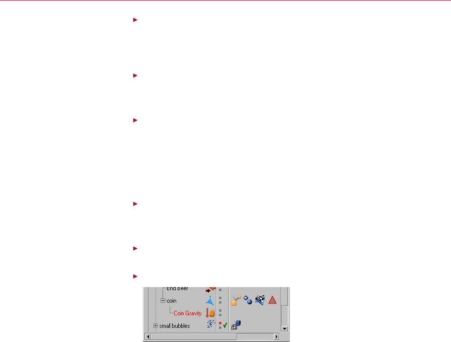
110 GRAVITY COLLISIONS WITH SOFT BODIES DYNAMICS
DYNAMICS GRAVITY COLLISIONS WITH SOFT BODIES 111
Ensure that Animation > Frame Rate > All Frames is enabled.
When using dynamics we need to be able to see every frame; this enables us to
check that every frame is how we want it to look, plus it prevents the dynamics from
calculating many frames at once, which can be slow on some complex scenes.
Disable the Beer Solver object by clicking on its green tick.
To allow us to start moving objects within the solver we need to disable it. While a
solver is enabled it will override anything we try to do, such as moving objects.
Click on the Solver object’s icon and on the Main tab set the Integration Method
to Adaptive, Oversampling to 16 and Subsampling to 16.
By using Adaptive we can specify a subsampling value which will be used to further
divide the frames when it becomes necessary.
Although there is a Soft Body integration method, we won’t use it here because it is
geared towards simulating cloth-like motion.
Leave the Energy Loss set to 0.
There is no need for us to remove energy from the system because we already have
several drag objects set up from the Motion With Drag tutorial.
Select Plugins > Dynamics > Gravity. In the Object manager, double-click on
the name of the Gravity object, change its name to Coin Gravity and click OK.
Drag the Coin Gravity object into the Coin object to make it a child of Coin.
By making the gravity eld a
child of the coin, it will move
wherever the coin goes.
To enable the coin to interact with the beer we will use a Gravity object to pull at the
surface of the beer as the coin falls into it.
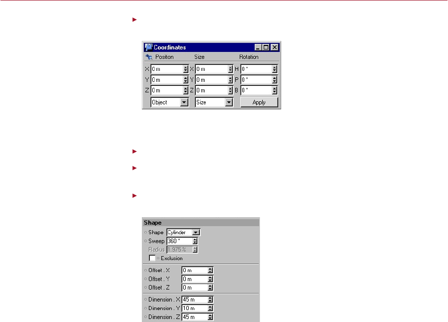
110 GRAVITY COLLISIONS WITH SOFT BODIES DYNAMICS
DYNAMICS GRAVITY COLLISIONS WITH SOFT BODIES 111
Ensure you have the Coin Gravity object selected, then in the Coordinate manager
set the X, Y and Z positions and the H, P and B angles to 0 and click Apply.
Setting all of the values to zero
will cause the object to take up
the same position as its parent,
in this case the coin.
So that we can make a gravity eld around the coin, we are changing the origin of
the Coin Gravity to be the same as that of the Coin.
In the Object manager, click on the Coin Gravity icon.
On the Field tab, set Strength to 30, Direction.Z to -1 and the other Direction
values to 0.
Click the Shape tab and set the Shape to Cylinder, Dimension.X and Z to 45, and
Dimension.Y to 10.
Similar or identically shaped
force elds can be used in place
of full collision detection.
We’ll use a shape and size for the gravity that is approximately that of the coin; this
will help to pull the surface of the beer in a similar way to that which the coin would
as it collides with the beer.
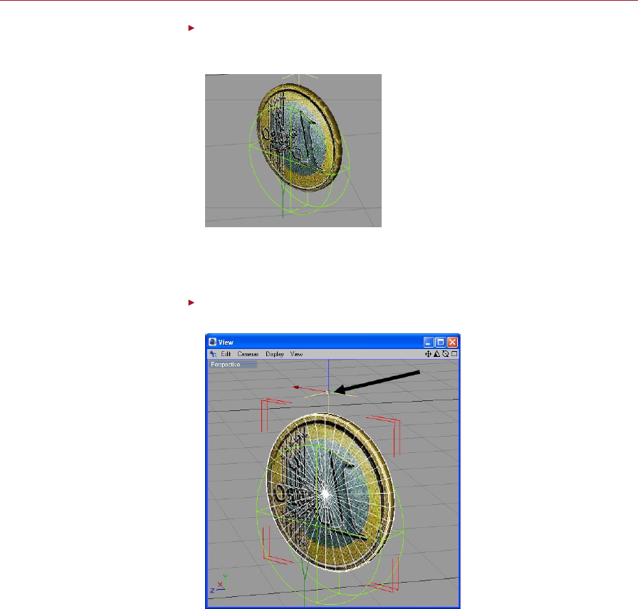
112 GRAVITY COLLISIONS WITH SOFT BODIES DYNAMICS
DYNAMICS GRAVITY COLLISIONS WITH SOFT BODIES 113
Ensure you have Coin Gravity selected and, in the viewport, move the object
down the world Y axis so that the bottom of the gravity cylinder is slightly below
the coin.
The surface of the liquid needs
a fraction of a second to
accelerate, moving the gravity
will give it the time it needs.
The gravity collision will be soft, that is it will not start moving immediately, so we
want the surface to start moving just as the geometry of the coin reaches it. By
positioning the gravity far enough below the coin we should achieve this.
Ensure you have the Coin object selected, then select the Object Axis Tool and
make sure the origin is outside of the Coin Gravity and just above the coin.
Force elds affect an object
only if its axis is within the
eld. We can move the origin
away to deliberately exclude its
inuence.
In this case, we do not want the coin itself to interact with its own gravity. By moving
the coin’s origin it will still interact with the local gravity but will be outside the
inuence of the Coin Gravity object.
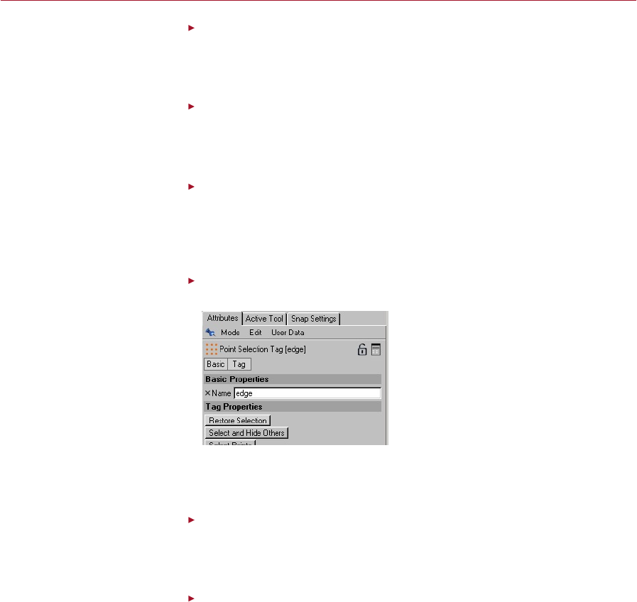
112 GRAVITY COLLISIONS WITH SOFT BODIES DYNAMICS
DYNAMICS GRAVITY COLLISIONS WITH SOFT BODIES 113
Select Plugins > Dynamics > Initialize All Objects.
The scene (or individual objects) must be initialised before re-enabling the Solver
object. If we enabled the solver without doing this then all the movements we made
would be lost.
Enable the Solver object by clicking on its red cross.
With the Solver object turned off, Dynamics will not calculate anything inside it. We
have to enable the solver before we proceed otherwise no springs will be shown, nor
will they affect the project as they should.
Command-click on a Mac if you
have only one mouse button.
In the Object manager, right-click on the Beer Geometry object and select
Dynamics Tags > Soft Body Spring and close the dialog (we’ll add the springs
later).
To create our beer surface we need to add a soft body tag so that we can add the
springs for the geometry.
Click on the Edge point selection tag for the Beer Geometry object. In the
Attribute manager click Restore Selection, then select the Points tool.
To stop the surface from ying
away we can effectively nail
down the edge of the beer.
You should be able to see that the points around the surface of the beer are selected;
we need these points so that we can dene the edge of our surface. (If you can’t see
the points it probably means that you haven’t selected the Points tool.)
Select Plugins > Dynamics > Set Soft Mass, set the Mass to 0 and click OK.
To stop the edge of our surface moving we need to ensure that its points have a mass
of zero; this stops the dynamics from controlling the motion and can be used as a
boundary to prevent movement.
Double-click on the Surface point selection tag for the Beer Geometry object.
You can now see that the whole surface is selected; these are the points to which
we want to add springs.

114 GRAVITY COLLISIONS WITH SOFT BODIES DYNAMICS
Select Plugins > Dynamics > Add Soft Springs and click OK.
For the surface use the default settings and structural springs; these springs link all
points along the polygons of the surface and will hold the points together.
Click Play and then click Stop when you are nished.
The coin should fall into the beer; the surface should be pulled down and then should
gently spring back up and ripple. Although this is not a true uid, it can be adequately
used to give a uid-like behaviour.
Summary
We have learned from this tutorial that soft bodies can be used for more than just
cloth — any exible surface or object can be created and interacted with. The motion
of these types of objects is usually difcult to create by keyframing, and by using
dynamics we can drastically shorten the time spent getting the motion to appear
correct.
We have seen how to use gravity shapes to affect only certain areas of our scene, and
how to move the object axis to prevent interactions with gravity objects that use a
child to make them follow the rigid bodies movement.
We have also seen how to set the soft masses using the point selection tools, and
how to add springs to only selected points.
By using these techniques we can create many complex types of materials from simple
actions and leave the hard work to Dynamics.
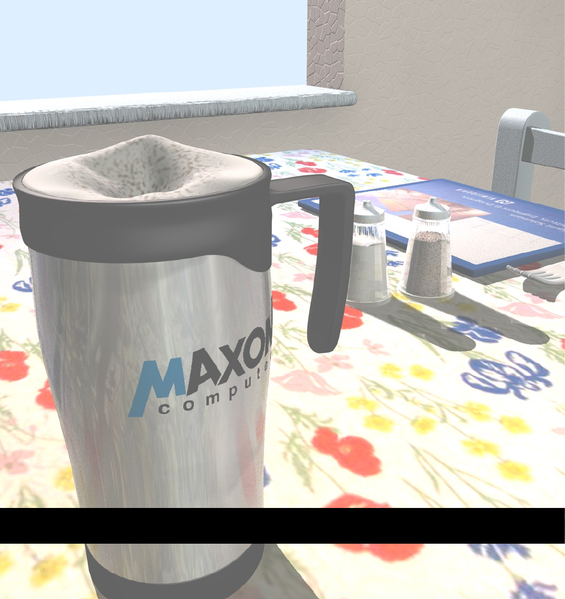
Gravity Collisions with Plastic Soft Bodies
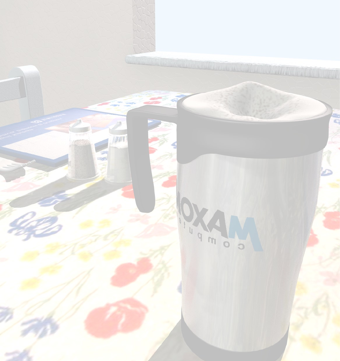
DYNAMICS GRAVITY COLLISIONS WITH PLASTIC SOFT BODIES 117
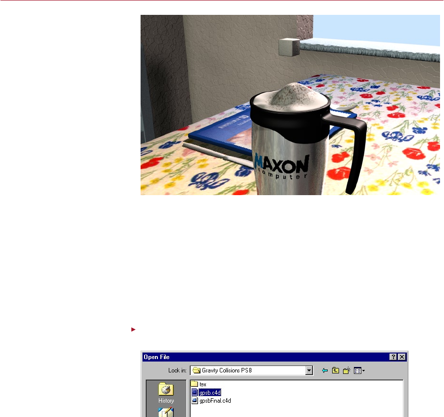
DYNAMICS GRAVITY COLLISIONS WITH PLASTIC SOFT BODIES 117
Gravity
Collisions
with Plastic
Soft Bodies
Sometimes we may want the
surface of a soft body to retain
a shape once deformed. We
can achieve this with the plastic
springs option.
We can use the plastic nature of soft body springs to create the impression of a soft
body that will remain deformed. In the real world a spring that is stretched too far
will start to behave more like plastic, remaining deformed at its stretched length. Soft
body springs can be made to exhibit this behaviour, so that once they are stretched
they will remain deformed, while still giving some resistance to the motion via the
stiffness of the springs.
By using gravity we can pull on the soft masses to deform the soft body while using
the plastic option to retain the deformation of the geometry. We are going to use
this technique to create a sugar cube dropping into some thick creamy froth that will
deform as the cube enters, but will not return to its original shape.
Select File > Open. Navigate to the ‘Gravity Collisions PSB’ tutorial folder on
your Documentation CD and open the le named ‘gpsb.c4d’.
Open the gpsb.c4d le from the
tutorials folder, this will be our
starting scene.
The Tutorials folder is in the
Dynamics module folder. Each
tutorial in this manual has its
own folder within the main
Tutorials folder.
The scene objects are now available in the Object manager. The main objects we are
interested in are the Sugar Cube and the Froth.
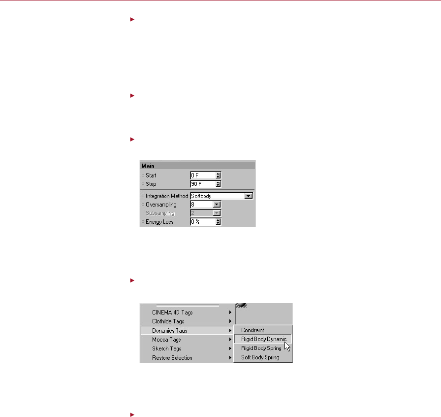
118 GRAVITY COLLISIONS WITH PLASTIC SOFT BODIES DYNAMICS
DYNAMICS GRAVITY COLLISIONS WITH PLASTIC SOFT BODIES 119
Ensure that Animation > Frame Rate > All Frames is enabled.
When using dynamics we need to be able to see every frame; this enables us to
check that every frame is how we want it to look, plus it prevents the dynamics
from calculating many frames at once, which can be slow on some complex scenes.
When working with dynamics we should make it a habit to ensure that All Frames
is enabled.
Select Plugins > Dynamics > Solver Object.
A Solver object will appear in the Object manager; this object is where we will add
the objects that we want to interact through dynamics.
On the Main tab, set the Integration Method to Softbody, Oversampling to 8
and Energy Loss to 0.
Use the Softbody
integration method.
The Softbody integration method is ideal here because it provides for extremely fast
soft body calculations. An Oversampling value of 8 is as low as we can go before the
simulation becomes unstable.
Command-click on a Mac if you
have only one mouse button.
In the Object manager, right-click on the Sugar Cube objec t, select
Dynamics Tags > Rigid Body Dynamic.
The sugar cube will be the
only rigid body object in this
simulation.
We need to make the Sugar Cube a solid object (i.e. a rigid body) so that we can use
a Gravity object to make it fall into the mug. Later we will also need to adjust the
centre of mass for the Sugar Cube by adjusting its origin.
Drag the Sugar Cube object into the solver.
To enable the dynamics to take control of the sugar cube falling we need it to be a
child of the Solver object; this is where the dynamics are calculated and all objects
within it that have a dynamics tag can interact with the dynamics.
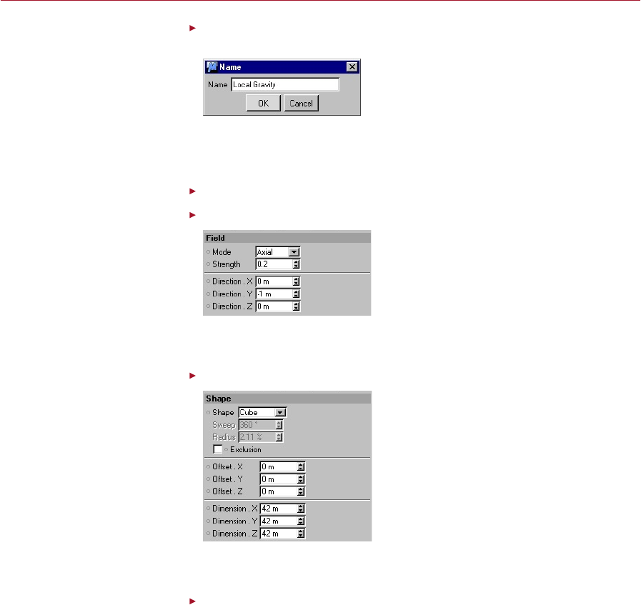
118 GRAVITY COLLISIONS WITH PLASTIC SOFT BODIES DYNAMICS
DYNAMICS GRAVITY COLLISIONS WITH PLASTIC SOFT BODIES 119
Select Plugins > Dynamics > Gravity, then double-click on the Gravity name in
the Object manager and name it Local Gravity.
We may need more than one
Gravity object, it is a good
idea to name them while we
remember what they do.
To give the sugar cube the movement that will make it appear to fall, we need a
Gravity object; this will apply a force at the sugar cube’s centre of mass causing it to
accelerate in the direction of the axial gravity eld.
Drag Local Gravity into the Solver object.
On the Local Gravity’s Field tab, set the Strength to 0.2.
Default values will rarely be
adequate for our simulations; be
prepared to adjust them.
We need the sugar cube to accelerate for just a short distance; the remaining motion
will be hidden within the mug.
Click the Shape tab, set Shape to Cube and Dimension.X, Y and Z to 42.
Forces do not have to be
everywhere. Here we are
restricting the gravitational
inuence to a particular shape.
We need only a simple cube shape for the gravity so that we can control exactly where
the sugar cube is accelerated.
In the Object manager, select the Local Gravity object and select Functions >
Transfer. Drag Mug Objects from the Object manager into the Transfer To box
in the Attribute manager. Disable the Enable Scale option and click Apply.
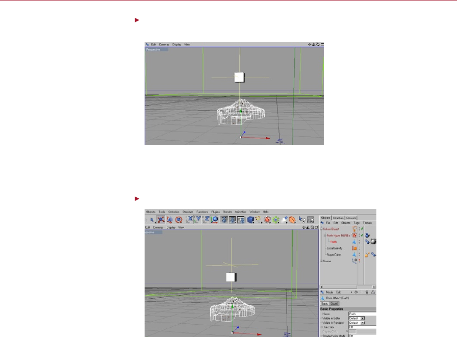
120 GRAVITY COLLISIONS WITH PLASTIC SOFT BODIES DYNAMICS
DYNAMICS GRAVITY COLLISIONS WITH PLASTIC SOFT BODIES 121
In the viewport, move the gravity cube up the Y axis so that the bottom of the
gravity cube is just above the top of the froth in the mug.
The gravity eld will cause the
sugar cube to fall, but not the
froth.
While the sugar cube is in the air above the mug, we want it to accelerate. Although
normally we would also have air resistance, in this case we can ignore it because the
cube falls for only a short time before entering the mug.
Click Play and then click Stop when you are nished.
Feel free to play the simulation
at any point during the tutorial.
It will help us to understand the
effect of each setting.
The sugar cube begins to fall gently until it leaves the gravity cube, at which point it
then moves at the same speed downwards and through the bottom of the mug. This
gives us our starting point for the sugar cube dropping into the mug.
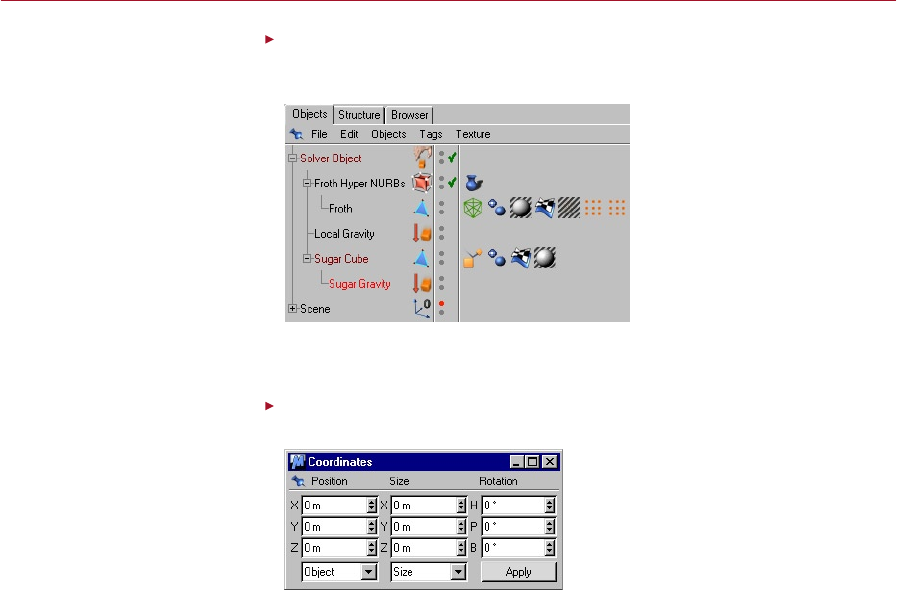
120 GRAVITY COLLISIONS WITH PLASTIC SOFT BODIES DYNAMICS
DYNAMICS GRAVITY COLLISIONS WITH PLASTIC SOFT BODIES 121
Select Plugins > Dynamics > Gravity, double-click on the name of the Gravity
object change it to Sugar Gravity and click OK. Drag the Sugar Gravity object
into the Sugar Cube object.
It’s a good idea to invent a
naming convention; this will
help us when we return to
projects.
To enable the sugar cube to interact with the froth we’ll use a Gravity object; this will
pull at the surface of the froth as the sugar falls into the mug.
Ensure that the Sugar Gravity object is selected, then in the Coordinate manager
set the X, Y and Z positions and the H, P, and B angles to 0 and click Apply.
Replicating geometry using
force elds can save much time
compared with enabling full
collision detection.
We want the origin of the Sugar Gravity object to be the same as that of the Sugar
Cube object so that we can make a gravity eld around it.
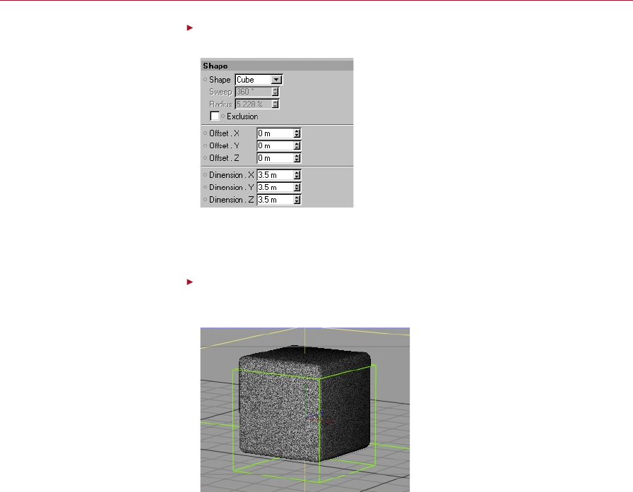
122 GRAVITY COLLISIONS WITH PLASTIC SOFT BODIES DYNAMICS
DYNAMICS GRAVITY COLLISIONS WITH PLASTIC SOFT BODIES 123
On the Sugar Gravity’s Shape tab, set Shape to Cube and Dimension.X, Y and Z
to 3.5. On the Field tab, set Strength to 20.
This gravity eld will represent
the sugar cube, it should be
scaled to similar proportions.
We’ll use a shape and size that is approximately that of the sugar cube; this will help
to pull the surface in a similar way to that in which the sugar cube would as it collides
with the froth and pushes it downwards.
Ensure that the Sugar Gravity object is selected and, in the viewport, move the
object down the Y axis so that the bottom of the gravity cube is slightly below
the sugar.
Reposition the cube of gravity so
that it can inuence the shape
of the froth just before the cube
impacts.
We want the surface of the froth to start moving noticeably just as the geometry of
the sugar cube reaches it. By positioning the Sugar Gravity far enough below the sugar
we can achieve this. You may nd that you need to go back and move the gravity up
or down slightly to achieve the movement you want.
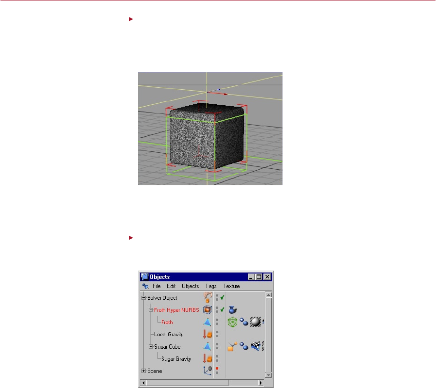
122 GRAVITY COLLISIONS WITH PLASTIC SOFT BODIES DYNAMICS
DYNAMICS GRAVITY COLLISIONS WITH PLASTIC SOFT BODIES 123
Check if the origin of the Sugar Cube is just above the Sugar Cube. If it isn’t,
turn off the Solver object (click its green check mark), then select the Object
Axis tool and move the origin along the Y axis to just above the Sugar Cube.
Select Plugins > Dynamics > Initialize All Objects. Turn the Solver object back
on (click its red cross).
Dynamics uses the origin of
objects to determine if objects
are inside a eld’s area of
inuence.
Here we do not want the sugar itself to interact with its own gravity, so by moving
its origin it will still interact with the local gravity but is outside the inuence of the
sugar gravity.
Command-click on a Mac if you
have only one mouse button.
In the Object manager, right-click on the Froth object and select Dynamics Tags
> Soft Body Spring and close the dialog. Drag the Froth Hyper NURBS object
into the solver.
The froth is the only other
geometry to be changed
by Dynamics, via the
Soft Body Spring tag.
To create our frothy surface we need to add a soft body tag so that we can create
the springs for the geometry.
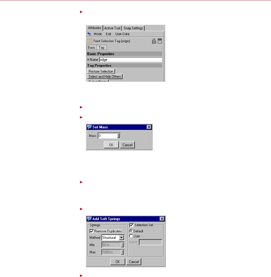
124 GRAVITY COLLISIONS WITH PLASTIC SOFT BODIES DYNAMICS
DYNAMICS GRAVITY COLLISIONS WITH PLASTIC SOFT BODIES 125
Click on the Froth object, click on its Edge point selection tag and in the Attribute
manager click Restore Selection.
Use as few springs as possible
to keep the simulation running
smoothly. Here we need to
apply them only to the top on
the froth.
You should be able to see that the points around the surface of the froth are selected;
we need these points so that we can dene the edge of our surface.
Select the Points tool.
Select Plugins > Dynamics > Set Soft Mass, set Mass to 0 and click OK.
To hold the rest of the froth in
place, simply set the mass of
these points to zero. A mass
of zero stops an object from
moving.
To stop the edge of our surface moving we need to make the points have a zero mass,
this stops the dynamics from controlling the motion and can be used as a boundary
to prevent movement.
Double-click on the Surface point selection.
You can now see the whole surface is selected, these are the points to which we
want to add springs.
Select Plugins > Dynamics > Add Soft Springs and click OK.
Add soft springs to the object.
Double-click on the Soft Body Springs tag, set Damping to 1, click the Plastic
tab and enable the Above option. Set Start At to 104%, Stiffness and Damping
to 100%, Drag to 2%, then click Refresh and close the dialog.
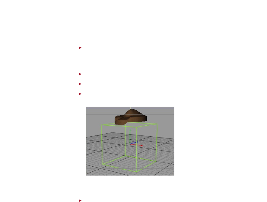
124 GRAVITY COLLISIONS WITH PLASTIC SOFT BODIES DYNAMICS
DYNAMICS GRAVITY COLLISIONS WITH PLASTIC SOFT BODIES 125
We want our froth-like surface to stretch easily, but then remain stretched without
oscillating much. The Start Above option sets the soft body springs to start using the
plastic behaviour once they have stretched above 104% of their rest lengths (their
original lengths). We add a small amount of drag to the soft masses to help to slow
any movement when the springs become plastic.
Select Plugins > Dynamics > Drag, then drag the Drag object into the solver.
Lastly, we need to stop the sugar cube from falling through the mug. By using a drag
cube inside the mug we can stop the sugar moving.
On the Field tab set Strength to 20.
Click the Shape tab and set Shape to Cube and Dimension.X, Y and Z to 20.
In the viewport, move the Drag object so that it sits below the froth as shown
in the diagram below.
Once an object is out of view, it
is not important to spend time
working on it. Just use a drag
eld to stop it.
This drag cube will stop the sugar cube once it has nished interacting with the
frothy surface.
Click Play and then click Stop when you are nished.
The sugar cube drops into the mug, pushing the frothy surface down. The froth
remains deformed and the sugar cube stays in the mug.
Summary
When using soft bodies we may nd that we need to increase the accuracy of our
solver. Soft body springs perform many calculations — the more springs we have,
the more likely we are to start having inaccuracies in the solver calculations due to
the complex motion that can occur.
We can help to control this using the damping and drag values, but sometimes the
only solution is to increase the oversampling and subsampling to prevent unwanted
uctuations in springs.

126 GRAVITY COLLISIONS WITH PLASTIC SOFT BODIES DYNAMICS
In this tutorial we have seen how to add soft body springs to selected points on a
complex geometry. By carefully adjusting the spring values we can create many types
of surface interactions. As with the liquid surface tutorial, we can see that the soft
bodies in Dynamics can be used for more than just cloth.
The plastic nature shown in this tutorial lends itself to creating stiff, structured
materials that keep their deformation. The nature of the plastic behaviour also
increases the need to have a more accurate solver. The motion of these types of
springs can be complicated because, as some of the springs start to turn plastic, the
forces between the soft masses may start to become large, causing the dynamics
to suffer.
Increasing the accuracy will help stop this, as illustrated in this tutorial. To
see the behaviour that can result from badly tuned values, try decreasing the
oversampling.

Soft Bodies with Wind

DYNAMICS SOFT BODIES WITH WIND 129
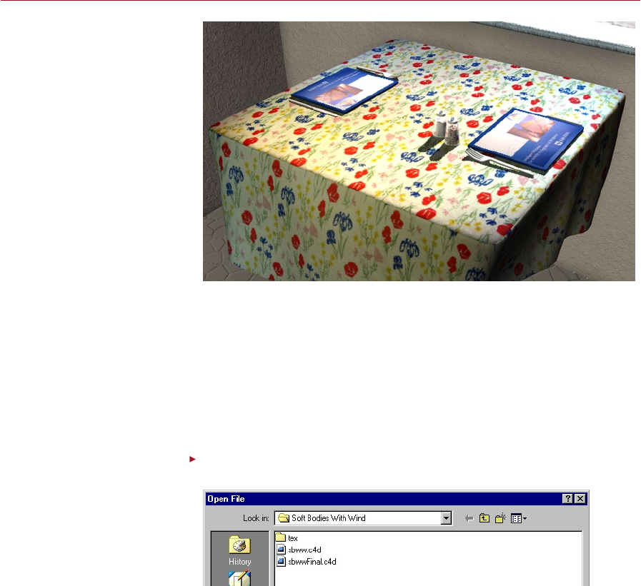
DYNAMICS SOFT BODIES WITH WIND 129
Soft Bodies
with Wind
One thing that we’re positive
you’ll want to use soft bodies
for is cloth. In this tutorial we
will apply some new dynamics
techniques in order to gently
rufe a tablecloth.
There are two ways that polygon objects can act within Dynamics. They can retain
their shapes perfectly and never deform — these are known as rigid bodies. The
other kind of dynamics object is a soft body; these can ripple like water, deform like
foam, stretch like rubber or ow like silk. Soft bodies can be virtually any material
we can imagine.
In this tutorial we will use a simplistic model of a tablecloth in order to introduce the
concepts of soft bodies and soft springs and how these react to a couple of external
forces, wind and gravity. To this purpose we will suspend exact realism so that the
basic principles are clear to us.
Select File > Open. Navigate to the Soft Bodies With Wind tutorial folder on
your Documentation CD and open the le named ‘sbww.c4d’.
Find the ‘sbww.c4d’ project and load
it; here you will nd a tablecloth we
have prepared ready for animation.
The Tutorials folder is in the
Dynamics module folder. Each
tutorial in this manual has its own
folder within the main Tutorials
folder.
This will open our tablecloth project with all modelling and lighting set up and ready
for us to begin adding a dynamics simulation. We can see three objects in the Object
manager. The Scene object is the rest of the scene and is hidden to make working
on the scene quicker: the objects in here will appear when we render. Also visible
is a HyperNURBS object which contains a Cloth object. The actual geometry on the
tablecloth is quite simple, the HyperNURBS object is there to smooth it all out.
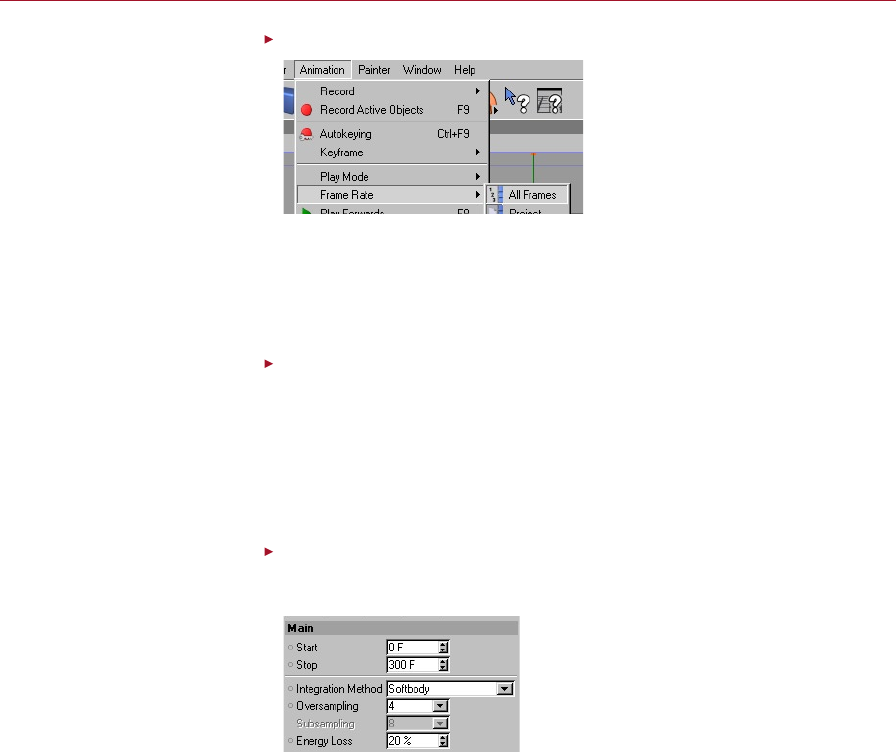
130 SOFT BODIES WITH WIND DYNAMICS
DYNAMICS SOFT BODIES WITH WIND 131
Ensure that Animation > Frame Rate > All Frames is enabled.
We must make sure that we
view each and every frame of the
simulation rather than every 10 or so.
When using dynamics we need to be able to see every frame; this enables us to
check that every frame is how we want it to look, plus it prevents the dynamics
from calculating many frames at once, which can be slow on some complex scenes.
When working with dynamics we should make it a habit to ensure that All Frames
is enabled.
Select Plugins > Dynamics > Solver Object.
All dynamics animations need to be set up using special objects that control how the
dynamics system will run. The most important object is the dynamics solver, which
actually does all the calculation — it literally solves the maths.
We can add as many Solver objects to a scene as we wish, each containing discrete
dynamics systems, therefore each system can be optimised to suit the particular
types of systems they contain.
On the Solver object’s Main tab, set the Stop frame to 300, the Integration
Method to Softbody and leave the Oversampling set to 4. Set the Energy Loss
to 20%.
Soft body simulation is quite
complex so we are speeding things
up using the optimized Softbody
integration method.
The Energy Loss has been set to 20%, this stops the apping of the cloth from
building up.
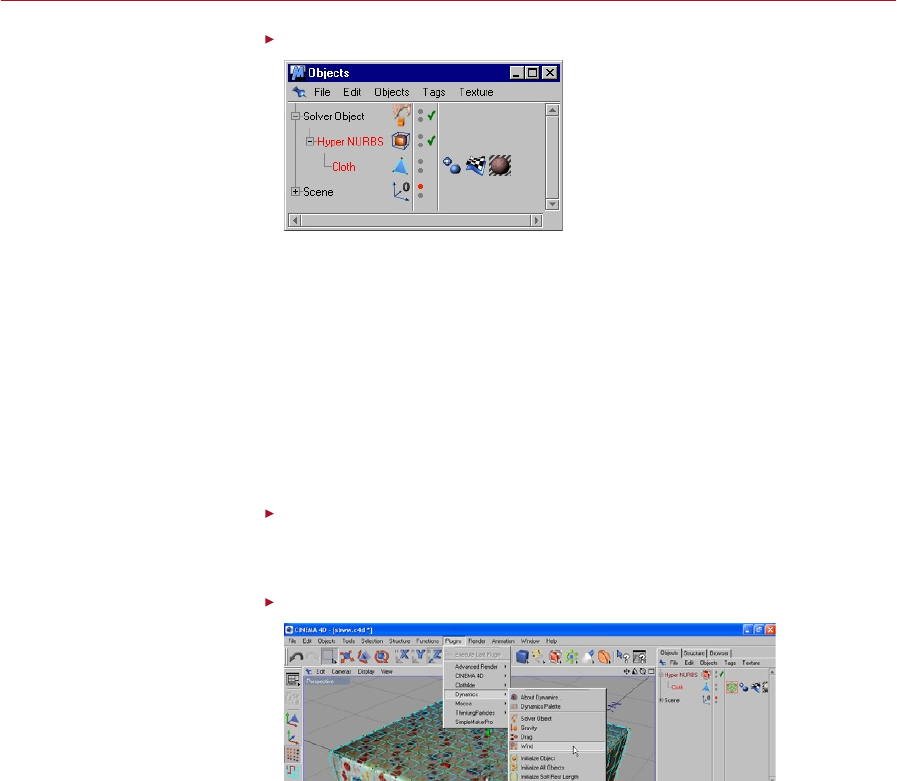
130 SOFT BODIES WITH WIND DYNAMICS
DYNAMICS SOFT BODIES WITH WIND 131
Drag the Hyper NURBS object into the solver.
All objects to be taken into account
during the calculations must be
inside the solver.
To speed up workow, only objects which are children of a Solver object will be taken
into consideration when calculating the next frame of the simulation.
You may be wondering why we shouldn’t just throw everything into a single Solver
object. Imagine you have two totally separate dynamics simulations in a scene, let’s say
a game of pool and some clothing on a character. If they were both in the same Solver
object then everything would play back at a much slower rate as the dynamics would
be constantly checking to see if any of the pool balls had collided with the cloth.
If they are in unique Solver objects then Dynamics knows not to bother checking
— each Solver object is its own mini simulation and does not care about anything
else that might be going on.
Select Plugins > Dynamics > Gravity.
As this simulation is taking place on Earth we will need some downwards gravity to
keep the cloth draped naturally over the table.
Select Plugins > Dynamics > Wind.
We need to add wind, without it our
tablecloth has no reason to move.
Without any external forces being applied to the tablecloth, nothing would move. It
is already modelled in a naturally draped state, so gravity alone will not cause it to
move. The wind is our external force.
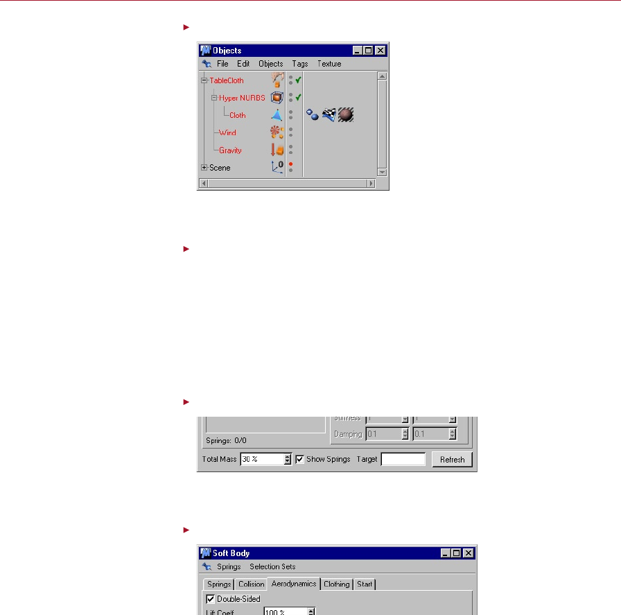
132 SOFT BODIES WITH WIND DYNAMICS
DYNAMICS SOFT BODIES WITH WIND 133
Drag both forces into the solver.
Just like the tablecloth geometry, the
forces need to be inside a solver for
them to know which objects to affect.
Just like the geometry, the two forces need to be within the solver for them to affect
anything.
In the Object manager, select the Cloth object and select File > Dynamics Tags
> Soft Body Spring.
So what do springs have to do with soft bodies? Dynamics works by connecting
together as many points as you like with many small springs. When you pull on one,
the energy is transferred throughout the object. If these springs are very tight and
stiff then it will act like a thick and strong material, such as a potato sack or heavy
denim. Having very stretchy but inexible springs will give a oppy rubber sort of
effect. More owing materials, such as silk or water, can be simulated by making the
springs tight but very exible.
In the Soft Body dialog, set the Total Mass to 30%.
When certain points have no masses,
none of the forces will inuence
them. Later we will use this feature
to keep the top of the tablecloth still.
The default total mass of 100% is too much; this would give the impression that the
tablecloth is very heavy or that there is a very strong gravitational inuence.
Click the Aerodynamics tab and enable the Double-Sided option.
Double-sided polygons enable us
to save processing power by using
objects which are just a single
polygon thick.
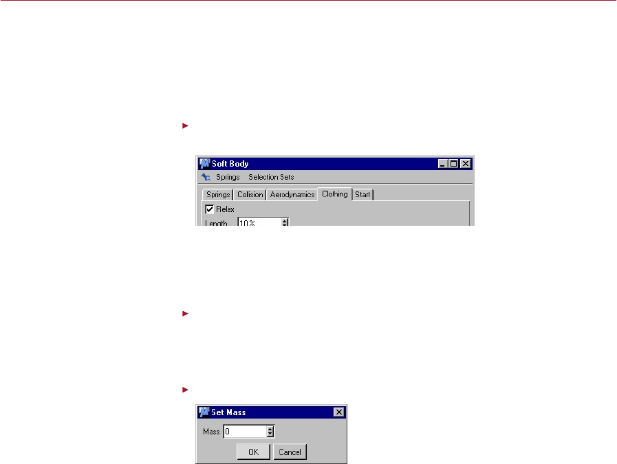
132 SOFT BODIES WITH WIND DYNAMICS
DYNAMICS SOFT BODIES WITH WIND 133
Which way something should move when calculating lift (aerodynamics, in other
words) depends on the direction of the object’s surface normals. If our tablecloth
were perfect then it would actually have some thickness to it and we wouldn’t need
to bother with this step. But as it is actually just a polygon with no thickness, if wind
hits the back of it then it will have no effect on it whatsoever. We can tell Dynamics
to make our polygons double-sided so that the wind can blow both sides.
Click the Clothing tab, enable the Relax option, click Refresh, then close the Soft
Body dialog.
Compared with other woven
materials, our tablecloth is quite
inexible. Here we are spreading the
movement energy around the cloth
by enabling the Relax option.
The Clothing tab is there to help improve the motions of clothing. The Relax option
will help to disperse the energy around the entire object. Length decides how far
from the source of movement the energy will be transferred, Depth determines how
much of this energy is distributed.
Select the Cloth object and double-click on the Cloth’s rst (left-most) Point
Selection tag.
We have already set up two point selections for the Cloth object. The rst of these
is the top of the tablecloth.
Select Plugins > Dynamics > Set Soft Mass, and set the Mass to 0.
Zero mass objects can be keyframed
or, in our case, not moved at all.
We have now set the mass of all top points to zero; this means that they will not
be blown by the wind, nor will they fall under the inuence of gravity. Here we are
basically cheating. Because the top of our tablecloth won’t move, it will look as if there
is a solid table underneath — as viewers will never actually see under the tablecloth,
they will never know the difference.
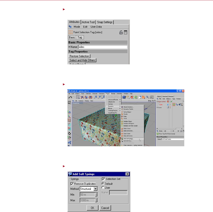
134 SOFT BODIES WITH WIND DYNAMICS
DYNAMICS SOFT BODIES WITH WIND 135
In the Object manager, double-click on the Cloth’s right-most Point Selection
tag, then in the Attribute manager click the Restore Selection button.
The second point selection is a
collection of all the points we want
to move.
The second point selection covers all of the points around the side of the tablecloth,
the ones which we want to ap in the wind.
Select Plugins > Dynamics > Add Soft Springs.
Even with a Soft Body Spring tag our
tablecloth has no springs yet. This
function will add some.
This opens the Add Soft Springs dialog. From here we can choose how different layers
of springs can be added to the tablecloth.
Set Method to Structural and click OK.
Structural springs are the only
springs which can be safely used on
their own.
There are several different types of springs we could add. We need to add only structural
springs as there will be virtually no diagonal movement in our tablecloth.
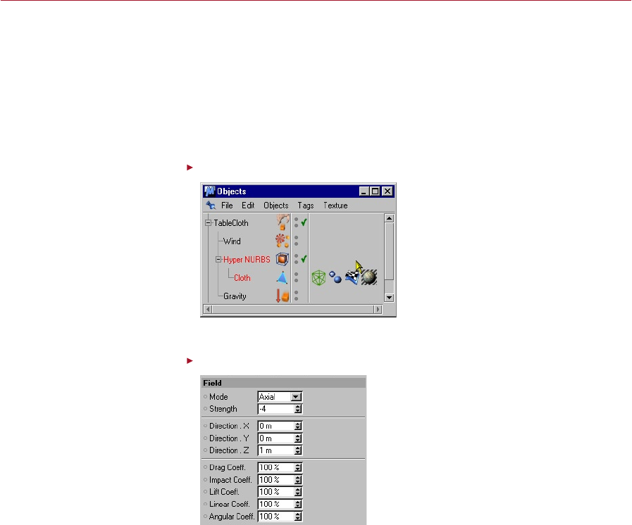
134 SOFT BODIES WITH WIND DYNAMICS
DYNAMICS SOFT BODIES WITH WIND 135
Structural springs cover our objects in a grid, ensuring that every point is connected to
at least one other. The downside of using structural springs on their own is that they
can fold like a trellis and make an object look as if it is elongated, even though none
of the springs have stretched. This will not affect our tablecloth because the geometry
has been constructed in such a way that no diagonal movement happens.
We can now see the springs we’ve created displayed in the viewport as red or green
lines. Springs selected in the Soft Body Spring tag are displayed green, unselected
springs are displayed red.
Click on the Wind icon to display its settings in the Attribute manager.
In the Object manager the Wind
object is represented by a multiple
bladed fan.
We will now add some external force to our scene in the form of a gust of wind.
On the Field tab set the Strength to -4.
Using a negative strength for wind
will have the effect of blowing in the
opposite direction to which the fan
is pointing.
Even though we have reduced the mass of the tablecloth, it is still fairly heavy, meaning
the wind will have to be stronger than the defaults in order to lift the material. The
minus sign is there to blow the wind in the opposite direction, towards us that is.
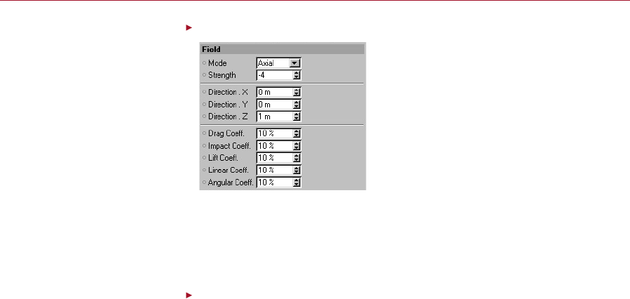
136 SOFT BODIES WITH WIND DYNAMICS
Set all of the aerodynamic coefcients (Lift, Impact and Drag) to 10%.
The default settings have the ying
abilities of a brick. To give our
tablecloth some lift we alter the
settings in this dialog.
To keep our dynamics simulation as fast as possible we have avoided the use of collision
detection for the soft bodies. This would require some humongous calculations and
they should be avoided where possible. For this reason we want to make sure that the
tablecloth doesn’t get blown so hard that it passes up through itself, and reducing
the three coefcients will achieve this.
Click Play to see the simulation play.
We will see that the top of the tablecloth remains stationary while the sides blow,
inate and ripple realistically towards the camera.
Summary
We’ve learned in this tutorial that it is not required to add soft springs to each and every
part of our object, and sometimes it is not essential to apply dynamics to every part
of an object. Even though in the real world all parts of a tablecloth will ap around,
we can save ourselves time by using springs only where they will be noticed.
This is just one application for soft body springs, you will nd more tutorials in this
manual covering different aspects and uses of them.
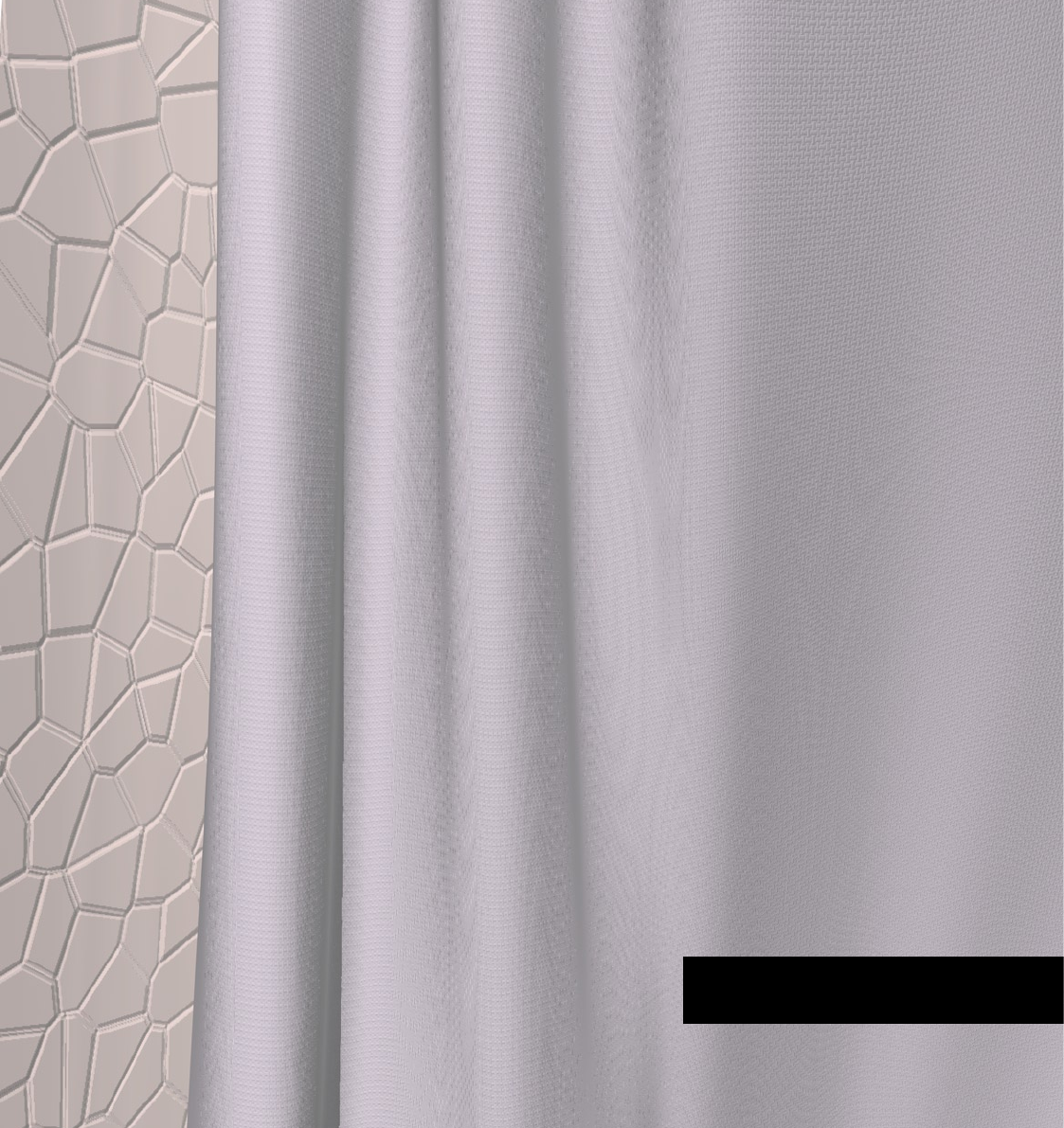
Self Collision

DYNAMICS SELF COLLISION 139
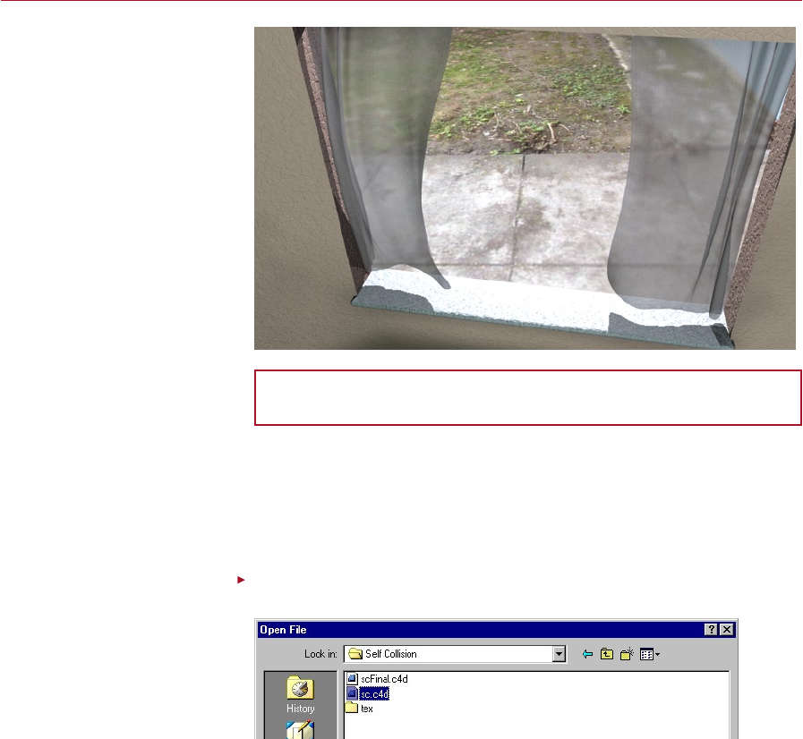
DYNAMICS SELF COLLISION 139
Self Collision
Unless we specically tell them
not to, soft bodies have a habit
of intersecting themselves as they
deform. Here we will utilise soft
body springs and full collision
detection to make some curtains
ap in the wind.
This tutorial builds on the Soft Bodies With Wind tutorial. If you haven’t completed
that previous tutorial then we recommend you do so before starting this one.
In this Self Collision tutorial we will learn about applying soft body springs only where
needed and also how to make them collide with self collisions to create a convincing
pair of curtains blowing in the wind. By adding soft body collisions we will be able to
use a strong wind which will cause the curtains to collide with themselves. Without
the self collisions they would simply pass through themselves in an unconvincing way.
Also featured here is one use of keyframes in a dynamics simulation.
Select File > Open. Navigate to the Self Collision tutorial folder on your
Documentation CD and open the le named ‘sc.c4d’.
Load the ready modelled scene;
here we will nd the pair of
curtains to be simulated.
The Tutorials folder is in the
Dynamics module folder. Each
tutorial in this manual has its
own folder within the main
Tutorials folder.
Here we will nd a scene with two identical curtains already folded and draped in
a realistic pose. We could quite easily get them into this position by starting with
at planes and allowing them to sag naturally, but loading this scene will save us a
bit of time.
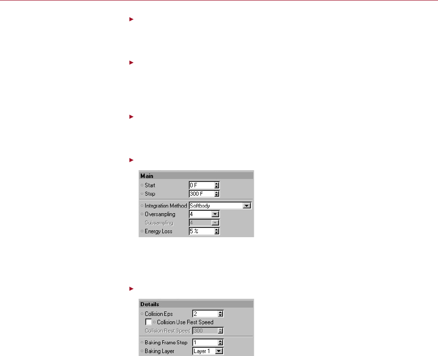
140 SELF COLLISION DYNAMICS
DYNAMICS SELF COLLISION 141
Ensure that Animation > Frame Rate > All Frames is enabled.
Remember, when working with dynamics we should make it a habit to ensure that
All Frames is enabled.
Select Plugins > Dynamics > Solver Object.
We hope you will have completed one of the easier tutorials before diving into the
deep end here, so you will know by now that a Solver Object is required before any
dynamics simulation can take place.
On the Solver object’s Main tab, set the Stop frame to 300.
Our project lasts for 300 frames. If the Stop frame were left at its default then the
simulation would end before the animation had nished.
Set the Integration method to Softbody and the Oversampling to 4.
The default solver settings are
too inaccurate for soft body
springs.
For this scene in particular it is especially important to use the Softbody integration
method. This method is much faster to calculate for this type of simulation than the
other methods, especially so later on when we come to turn on collision detection.
On the Details tab set the Collision Eps to 2.
Low Eps values generally work
best when using the Softbody
integration method.
When using the Softbody integration method it’s usually best to set the Eps to a low
value — high values can lead to an unstable simulation!
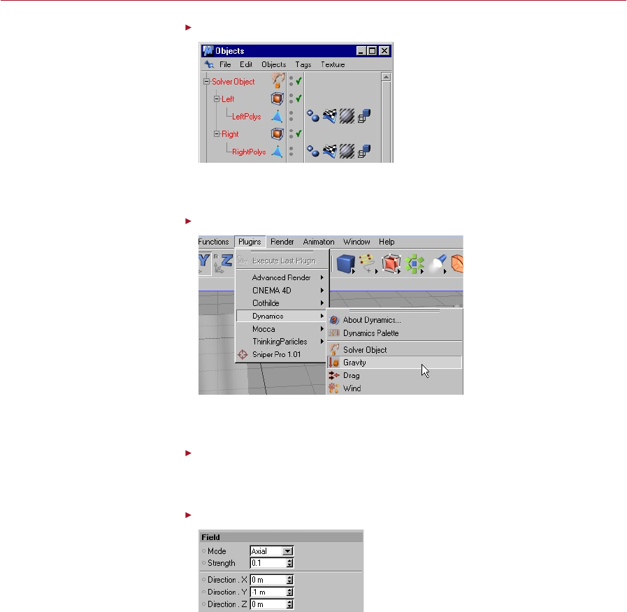
140 SELF COLLISION DYNAMICS
DYNAMICS SELF COLLISION 141
In the Object manager, drag the Left and Right objects into the solver.
The Left and Right objects are
our two curtains, they must be
children of the Solver object.
Only the children of a Solver object will be affected by dynamics, any objects outside
of this will be completely ignored, even if they are inside a different Solver object.
Select Plugins > Dynamics > Gravity.
With no gravity the
curtains would oat
upwards when blown.
Without gravity, our curtains would have no reason to fall back after being blown.
Adding a Gravity object will cause them to drape naturally.
Click on the Gravity icon.
By clicking on an object’s icon we will be presented with any options available for
that object.
On the Field tab set the Strength to 0.1.
Depending on the scale of our
scene, we may need to increase
or decrease the gravity strength.
Here we need to decrease it.
To stop the curtains from falling too quickly we are reducing the strength of the
gravity. Another way to do this would be to increase the level of drag, however this
would also slow the upward movements when blown by the wind.
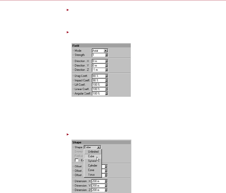
142 SELF COLLISION DYNAMICS
DYNAMICS SELF COLLISION 143
Select Plugins > Dynamics > Wind.
Seeing as this tutorial is about curtains blowing in the wind, the Wind object will
play a vital role here.
On the Field tab set Direction.Z to -1 and the Lift, Impact and Drag coefcients
to 80, 90 and 100 respectively.
We can choose to blow the
curtains inwards along -Z or
outwards along +Z.
Setting the direction to -1 on Z and reducing the strength will cause a soft breeze to
blow the curtains into the café. These numbers are not essential values, feel free to
alter them for a lighter breeze or turn them up to create a gale. When experimenting,
try to use reasonable values — setting a wind strength of 1,000, for example, could
cause problems.
Click on the Shape tab and set the Shape to Cube.
Restrict the area of inuence
for the wind by giving it a
specic shape rather than being
everywhere.
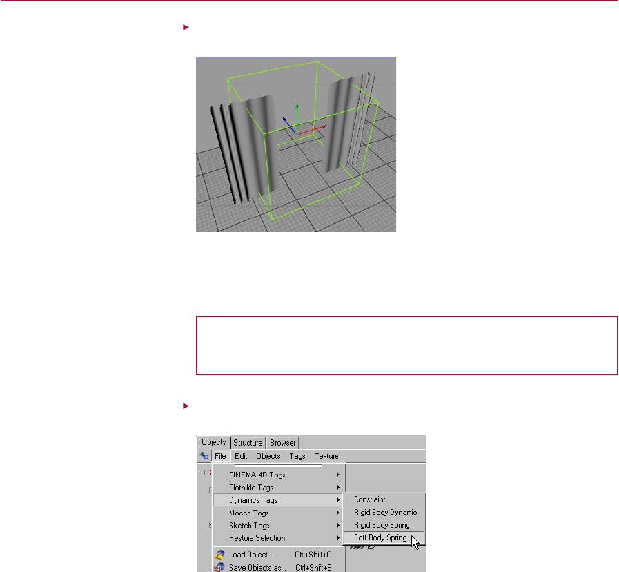
142 SELF COLLISION DYNAMICS
DYNAMICS SELF COLLISION 143
Using the Object tool, scale and move the green cube of wind so that it covers
the inside half of both curtains.
Reposition the wind so that only
certain parts of the curtains are
blown; this will make the motion
more interesting.
If we look at the curtain model we will see that the edge near the wall is all crumpled
up, as if it has been pulled open, and that the inside edge is quite spread out. The
waves on the outside of the curtains will make that part of them more rigid and less
likely to move.
We are now going to add soft springs to the left-hand curtain. When we have
nished this we will need to return to this point of the tutorial and repeat the
process to add springs to the right-hand curtain.
In the Object manager, select the object named LeftPolys then select File >
Dynamics Tags > Soft Body Spring.
A Soft Body Spring tag holds a
list of all soft springs applied to
a particular object.
Until we add a Soft Body Spring (SBS) tag the object will remain rigid and stationary
as it has no reason to move. The SBS tag will enable the object to ex and bend under
the inuence of the dynamics objects.
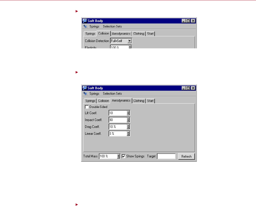
144 SELF COLLISION DYNAMICS
DYNAMICS SELF COLLISION 145
Click on the Collision tab and set the Collision Detection to Full+Self.
Self collision detection can be
used to prevent an object from
intersecting itself as it deforms.
By enabling self collisions, the curtains will not be able to pass through themselves
if the wind should blow them into such a position.
Click on the Aerodynamics tab and set the coefcients: Lift to 10, Impact to 80,
Drag to 10 and Linear to 0.
As the curtain changes shape, so
will its aerodynamic properties;
we can set these up here.
A small amount of lift is used because these are net curtains and some of the wind
will actually pass through the ne mesh, destroying most of the lift properties it
would have had. Impact is essential for the curtains to move when the wind blows
— this should be used for anything we want to be blown about such as sails, clothing
or curtains.
Enable the Double-Sided option.
Our curtains are only one polygon thick, but they need to be blown both into the
room and back out again. Enabling the Double-Sided option means that the wind
ignores the surface normals during the lift coefcient calculations.
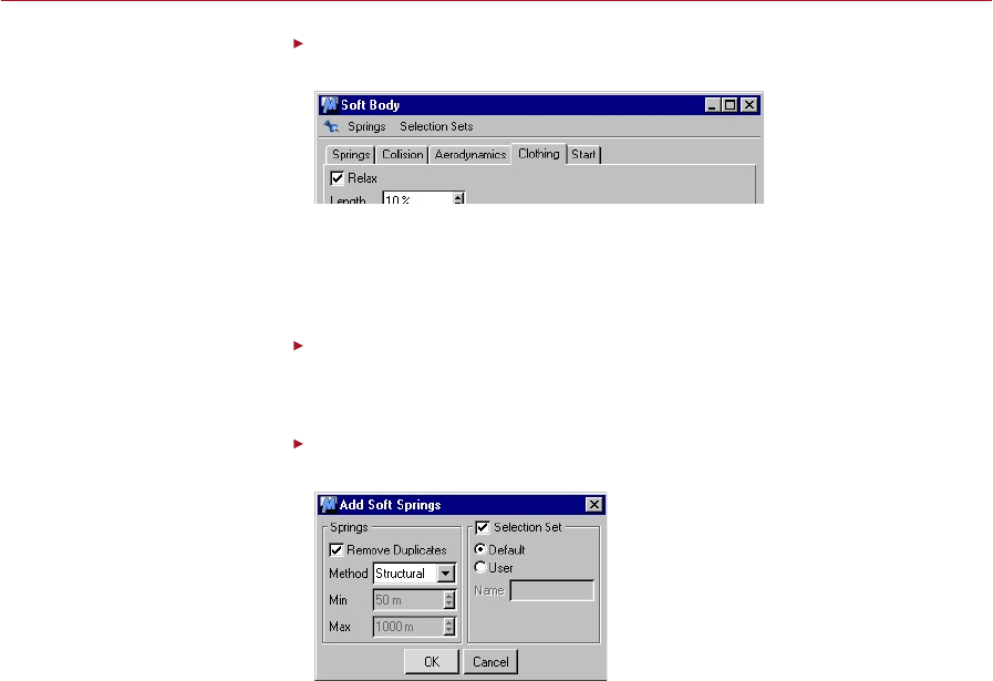
144 SELF COLLISION DYNAMICS
DYNAMICS SELF COLLISION 145
Click the Clothing tab and enable the Relax option. Click on Refresh and close
the dialog.
The Relax option is very
useful for creating owing
cloth effects.
Although curtains are exible, they stretch very little. For example, if we prodded
one with a nger the entire curtain would shift to compensate rather than form a
small peak where our nger is, which would happen only if the curtains were dense
and heavy.
Select Plugins > Dynamics > Add Soft Springs.
Even though the object has a Soft Body Spring Tag, it doesn’t actually have any springs
yet. There are various different types of spring which can be added.
Set the Method to Structural then click OK. Again select Plugins > Dynamics >
Add Soft Springs and this time set the Method to Flexion and click OK.
Uniform structural springs are
suitable for the curtains.
These structural springs will run throughout the curtain in a grid, linking each point
to at least two others. This will allow the curtain to bend and ex very sharply, but
will maintain the same basic proportions.
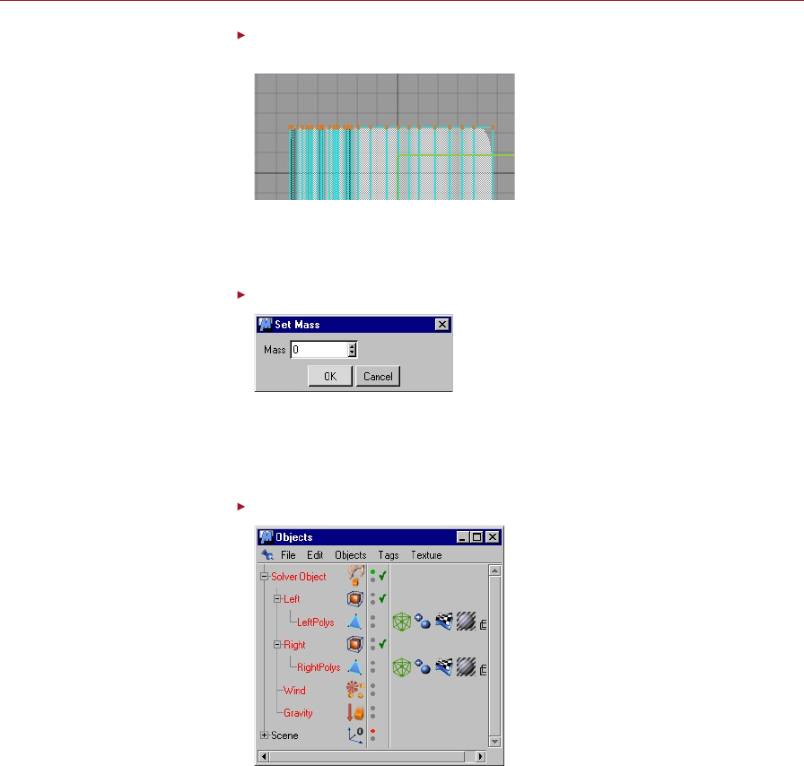
146 SELF COLLISION DYNAMICS
DYNAMICS SELF COLLISION 147
Enter point selection mode and select the top row of points on the LeftPolys
object.
Using whichever selection tool
we prefer, we select the points
we do not wish to fall due to
gravity.
Currently the curtain will fall under the inuence of gravity, to prevent this we need
to select certain points which we do not want to move. As this is a curtain it should
be held at the top.
Select Plugins > Dynamics > Set Soft Mass, set the Mass to 0 and click OK.
Setting the mass of any object
to zero tells Dynamics that
keyframes should be used
to animate it instead of the
calculated simulation.
Objects or parts of objects with no mass cannot be moved by Dynamics. These objects
will remain stationary unless they are moved by traditional keyframes. As the row of
points at the top can no longer move, the springs will hold the object together and
give a realistic motion when blown.
Drag the Gravity and Wind objects into the solver.
As with all Dynamics force elds,
to enable them we must make
them children of a Solver object.
For the wind and gravity to be taken into account when running the simulation, they
must be children of the Solver Object.

146 SELF COLLISION DYNAMICS
DYNAMICS SELF COLLISION 147
Press the Play button to see the simulation begin.
When we are satised we will need to return to an ealier point in this tutorial (see
the red box from a few pages back) and repeat the process to add springs to the
right-hand curtain. Then we can set a path and save format from the Render Settings
and then render out the nished animation.
Summary
Here we have made the curtains realistically blow in the wind and, depending on the
exact settings, slide against themselves. We should by now realise that collisions do
not always have to be large and pronounced. Often it is better that the simulation is
so well crafted that the viewer does not notice it happening.
If you nd the playback rate in the viewport is too slow to see the motion of the
curtains, you may want to temporarily disable collision detection to reduce the burden
on the processor. If possible you should also enable OpenGL (General Settings) as
this will reduce the amount of CPU time needed even further.

Dynamics Reference
DYNAMICS FORCE FIELDS 151
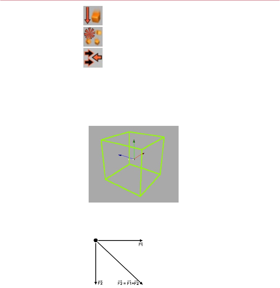
DYNAMICS FORCE FIELDS 151
If dynamics motion is to look real, it will need to take into account forces like
gravity, drag and wind. It is precisely these forces that you can simulate using
elds. Your dynamics animation will usually include at least one eld. A eld
exerts a force on objects that are inside the eld. In the case of a free-moving
object, this force will cause the object to accelerate or decelerate depending
on the direction of the eld and the direction of the object.
Fields in Dynamics are easy to use, but a few basic concepts — described in
the following — will help to explain when and how you should use elds.
For illustration purposes, a eld will be represented in this manual as a number of
lines of force that point in the direction of the force. Note that the lines of force will
not be shown in the CINEMA 4D viewport.
A eld can have one of a variety of shapes, such as cubic or spherical. The shape denes
the volume inside which the eld will exert a force on objects, i.e. the shape marks the
boundaries of the eld. It is also possible to give a eld an unlimited shape, in which
case the eld will exert its force throughout 3D space without boundaries.
A force eld in the viewport. The
boundaries of a eld are shown
as a green outline.
A moving object is usually subjected to not just one but a number of forces at any
given time. Hence Dynamics enables you to place as many force elds as you need
over the same volume of 3D space. The forces exerted on an object by overlapping
elds will be added together under the laws of physics to ensure correct motion.
Two forces, F1 and F2, are acting
on a point (top left). These two
forces will be added under the
laws of physics to produce the
correct resultant force, F3.
Force Fields
Motion is affected not by one
force but by a variety of forces
such as gravity, wind and drag.
Using elds, you can simulate
these forces of nature to increase
the realism of your dynamics
animation.
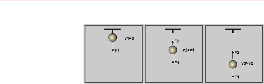
152 FORCE FIELDS DYNAMICS
DYNAMICS FORCE FIELDS 153
The diagram below demonstrates how a variety of forces can affect even a simple
motion.
Even a simple motion like a
sphere falling under gravity is
subjected to numerous forces
over the course of its motion.
Fields enable you to simulate all
of these forces.
In the left-hand picture the sphere is initially being held in place by a peg. F1 is the
force due to gravity. Not shown is the holding force that prevents the sphere from
moving. This holding force is equal and opposite to F1, hence the forces are cancelling
each other out and there is no resultant motion.
In the middle picture the peg has been removed and with it the holding force. As a
result, the sphere is accelerating towards the oor due to gravity. Now that the sphere
is moving, a new force, drag (F2), is being applied. Drag always exerts its force in the
opposite direction to the object’s motion, hence F2 acts in the opposite direction to
F1. Drag is not a constant force but instead increases with increasing fall velocity. At
this stage, F2 is less than F1, causing the sphere to accelerate.
In the right-hand picture the drag force is now equal and opposite to the gravity force.
The forces are cancelling each other out, so the object is no longer accelerating but
instead falling with constant velocity (v3).
The falling sphere example demonstrates that a motion is not always as straightforward
as it may rst appear. But by using elds, you can simulate these forces and let
Dynamics handle the interaction and computation. All this and more can be simulated
with the three types of eld available: gravity, wind and drag.
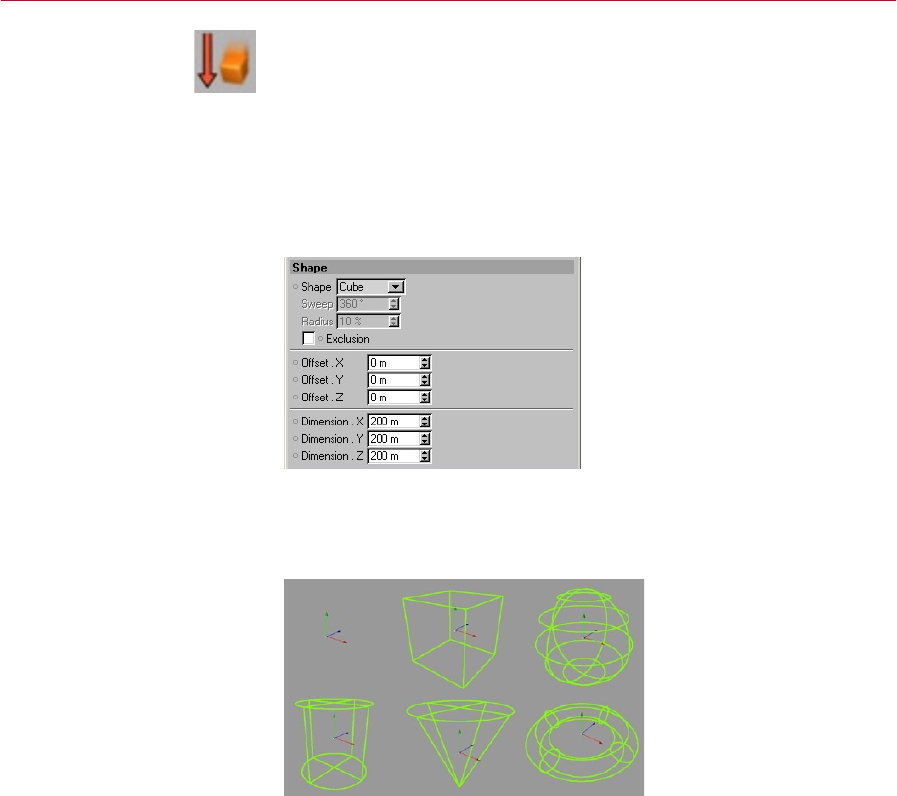
152 FORCE FIELDS DYNAMICS
DYNAMICS FORCE FIELDS 153
Gravity
Gravity is the most commonly used force. With it you can simulate most types of
motion including collision. The force exerted on an object by gravity depends on the
object’s mass. To switch off gravity for any given object in the dynamics system, set
the Mass of the object to 0. This will also switch off wind and drag for the object.
Gravity elds are also useful for simulating collision. Although Dynamics includes a
collision detection engine, collision via gravity elds can be many times faster.
Shape Tab
The Shape tab enables you to
modify the volume inside which
the eld will exert a force on
objects.
Shape
Here, set the general shape of the eld. Choose from Unlimited (exerts force
throughout 3D space), Cube, Sphere, Cylinder, Cone and Torus.
A eld can take one of the
following shapes (left to right,
top to bottom): unlimited, cube,
sphere, cylinder, cone, torus.
The eld will usually exert a force on any object that are inside the shape (provided
that Exclusion is disabled — see Exclusion, below).
The Torus shape is particularly useful for generating circular motion. This can be
achieved by using a Radial eld with Exclusion enabled. In additional, the object should
be given a starting velocity (v0) that is tangential to the torus pipe cross section, as
indicated in the diagram below.
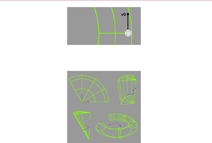
154 FORCE FIELDS DYNAMICS
DYNAMICS FORCE FIELDS 155
The torus shape is ideal for
creating circular motion.
Sweep
For the shapes that demonstrate rotational symmetry (Sphere, Cylinder and Torus),
you can additionally restrict the eld to just a section of the shape.
Some example sweeps:
120° sphere, 90° cylinder,
90° cone, 270° torus.
The default Sweep value is 360°, which corresponds to the entire shape. To restrict
the eld to just a section of the shape, enter a value less than 360°. For example, to
dene a hemispherical eld, set Shape to Sphere and Sweep to 180°.
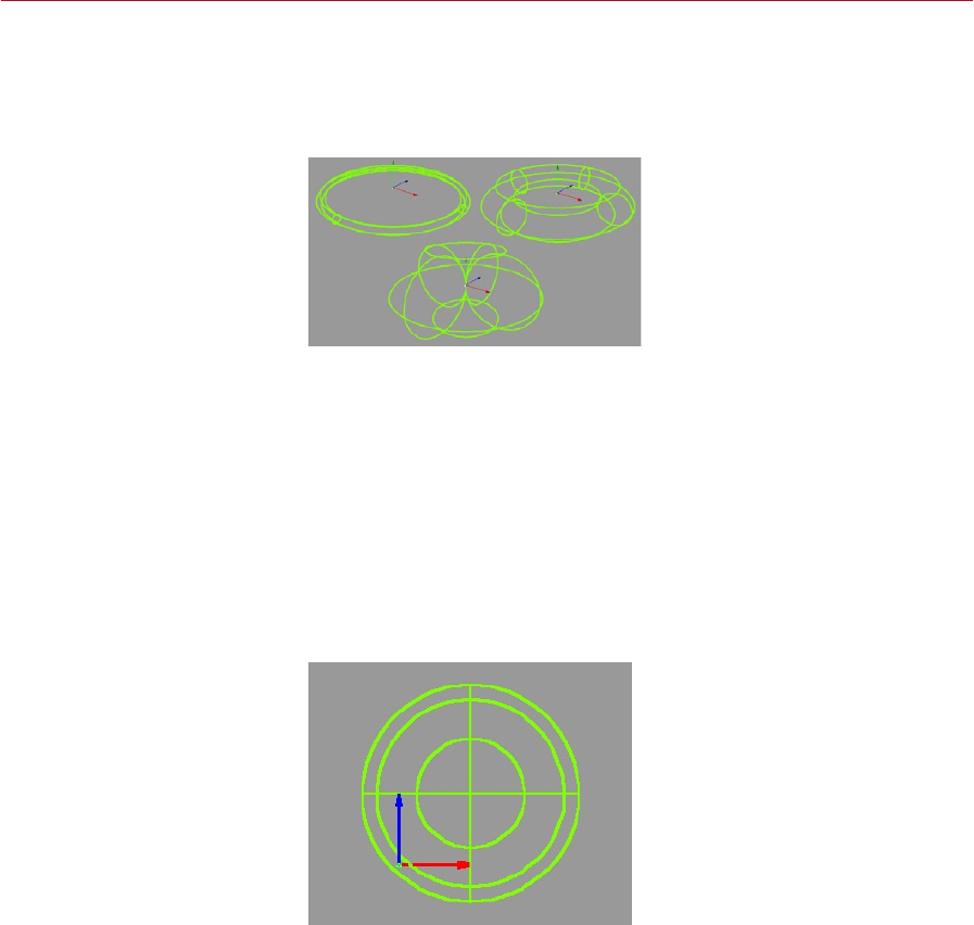
154 FORCE FIELDS DYNAMICS
DYNAMICS FORCE FIELDS 155
Radius
You can enter a value only if Shape is set to Torus.
The Radius denes the radius of the torus tube as a percentage of the entire torus
radius. You can enter a value from 0% to 100%.
A torus shape with radius set to
10%, 40% and 100%.
Exclusion
This option is enabled by default. When it is enabled, the eld will exert its force
outside the shape as opposed to inside. One possible usage is to allow the eld to
‘capture’ objects — when an object leaves the shape, a force can be exerted that will
pull the object back towards the shape.
Offset
This enables you to offset the shape of the eld away from the origin. This is useful
with the Radial eld only, where the origin denes the source of attraction or repulsion.
By using the Offset values with the Radial eld, you can effectively move the source
of attraction or repulsion away from the centre of the shape.
Here the Offset parameters
have been used to move a radial
eld’s spherical shape away
from the origin. Provided that
Strength is set to a positive
value and Exclusion is disabled,
objects inside the shape will
now be attracted towards the
bottom left rather than towards
the centre of the eld. This is
because the origin denes the
centre of attraction or repulsion.
A falloff (Falloff tab) will always refer to the eld’s origin, not to the centre of the
shape. This is explored in the diagram below.
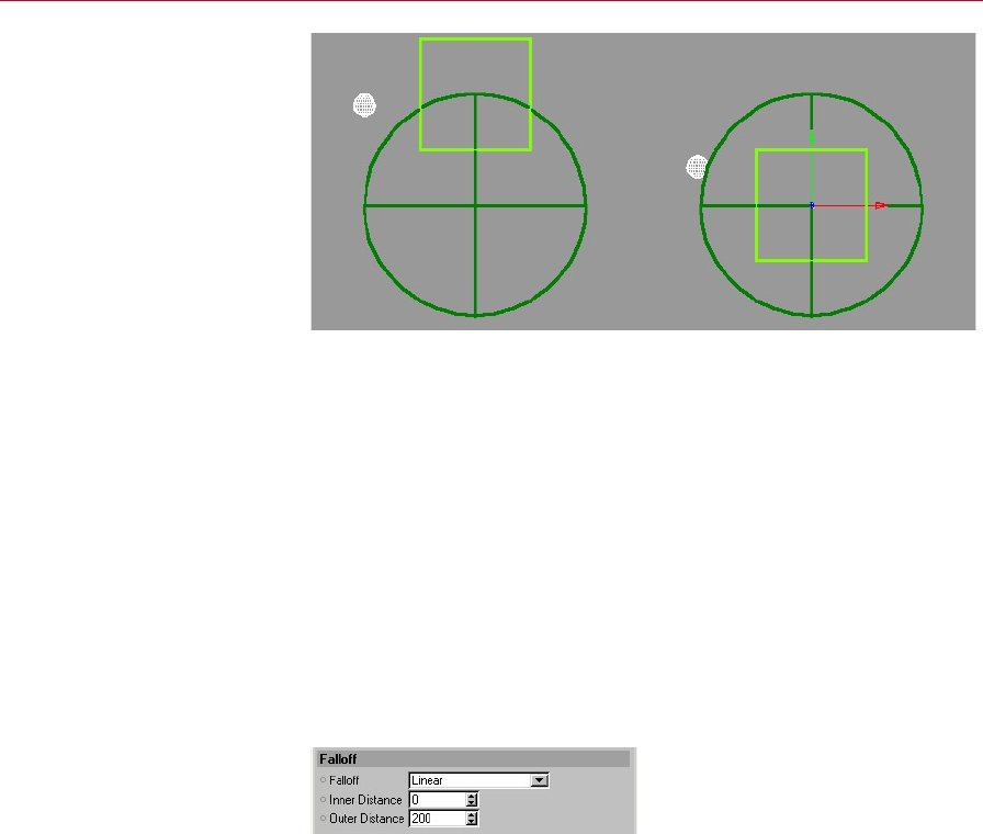
156 FORCE FIELDS DYNAMICS
DYNAMICS FORCE FIELDS 157
Two small white spheres,
both moving to the right,
are about to enter a
Radial eld whose Shape
is set to Cube. Of the two
spheres, the one on the
left will experience less
force. Due to the offset
shape, the left-hand
sphere will pass through
the edge of the falloff
(dark sphere) only.
In the diagram above are two Radial elds with Shape set to Cube. The shape of the
left Radial eld has been offset above the origin. Note how the left eld’s falloff
(dark sphere) is not offset but instead remains centred on the origin. Apart from the
shape offset, the two Radial elds are identical.
When the two spheres (travelling from left to right) enter their elds, the left sphere
will experience much less force than the right sphere. Although the left sphere will
pass through the centre of the shape, it will pass through the edge of the falloff and
experience only a fraction of the full force. The right sphere will experience more force
than the left sphere because it will pass through a eld region with less falloff.
Dimension
Here you can set the dimensions of the eld numerically. Alternatively, use the Scale
tool to resize interactively in the viewport.
Falloff Tab
A falloff enables a smoother
interaction with objects because
the force will increase gradually
rather than abruptly as the
objects move into the eld.
The parameters on this tab enable you to dene a falloff for the eld so that the
strength of the force will increase gradually towards the centre of the eld as opposed
to uniform force strength throughout the eld.
A falloff enables a smoother interaction with objects because the force will increase
gradually rather than abruptly as the objects move into the eld.
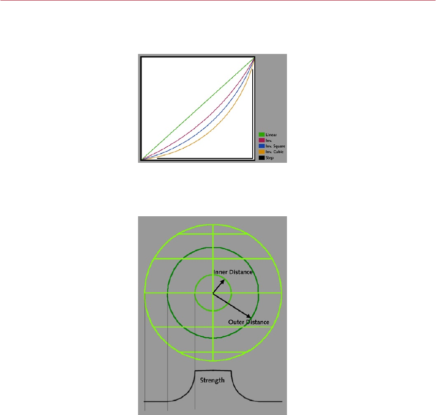
156 FORCE FIELDS DYNAMICS
DYNAMICS FORCE FIELDS 157
Falloff
Choose the type of falloff: None (the default), Linear, Inv. (Inverse), Inv. Square, Inv.
Cubic or Step.
Falloff types. With Step there
will be an abrupt transition from
no force to maximum force.
Inner Distance, Outer Distance
The Inner Distance and Outer Distance values determine the start and end distances
respectively from the origin over which there will be a falloff of the force.
The Inner Distance and Outer
Distance dene the volume in
which the falloff of force will
happen.
The example above shows a spherical eld with an Inner Distance and Outer Distance
dened. Within the Inner Distance, the full strength of the force will be exerted.
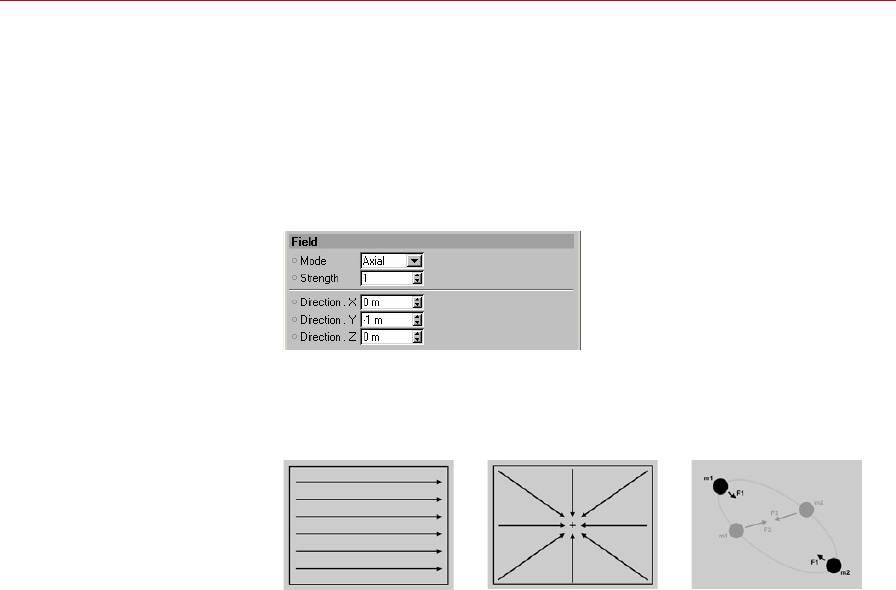
158 FORCE FIELDS DYNAMICS
DYNAMICS FORCE FIELDS 159
When an object is between the Inner Distance and Outer Distance, the strength of
the force exerted on the object will falloff according to the function dened under
Falloff. When an object is outside the Outer Distance, the eld will exert no force
on the object.
You can dene the Outer Distance to be larger than the eld itself. However, an object
will experience a force only when it is inside the eld’s shape.
Field Tab
Using the Field tab you can
dene the type, strength and
direction of the gravity eld.
Mode
Use Field to set the type of gravity eld required. Three types are available: Axial,
Radial and Newton.
Axial Radial Newton
Axial
The lines of force in the Axial eld run parallel to each other. Hence an object that is inside
the Axial eld will be accelerated in one direction only, as specied under Direction.
Radial
The Radial gravity eld will attract objects towards its centre if a positive Strength
value is used. With a negative Strength value, the eld will repel objects away from
its centre.
The Radial eld can also be used to create circular motion. The object will need a
starting velocity (v0) and it should be placed at the top of the eld with its movement
at a right angle to the line of force.

158 FORCE FIELDS DYNAMICS
DYNAMICS FORCE FIELDS 159
With a suitable starting velocity
and direction, an object in a
Radial eld will travel in a circle.
You will need to experiment in order to nd a suitable value for v0. If the object is
plunging towards the centre of the eld, you will need to increase v0. If the object
is escaping the eld, you will need to decrease v0.
The Radial eld also offers you an alternative to CINEMA 4D’s native explosions
system. To explode in all directions, placing some fragments inside the eld and set
Strength to a negative value.
Newton
The Newton eld is not a single eld. Rather, a Radial eld will be placed inside each
rigid body and soft body in the solver object. Hence all the bodies will exert a force on
each other. If the Strength value is positive, the bodies will exert a force of attraction.
With a negative Strength value, the bodies will repel each other.
One of the most important factors is the Mass of each body. The greater the body’s
mass, the greater its force of attraction or repulsion.
The distance between the bodies is also a key factor. The force of attraction or repulsion
will weaken with increasing distance.
The formula for the force is:
F = m1 * m2 / (r*r)
i.e. the force is proportional to the mass of the bodies and inversely proportional to
the square of the distance between the bodies. If you were to double a mass, the
force would be doubled. If you were to halve a mass, the force would be halved.
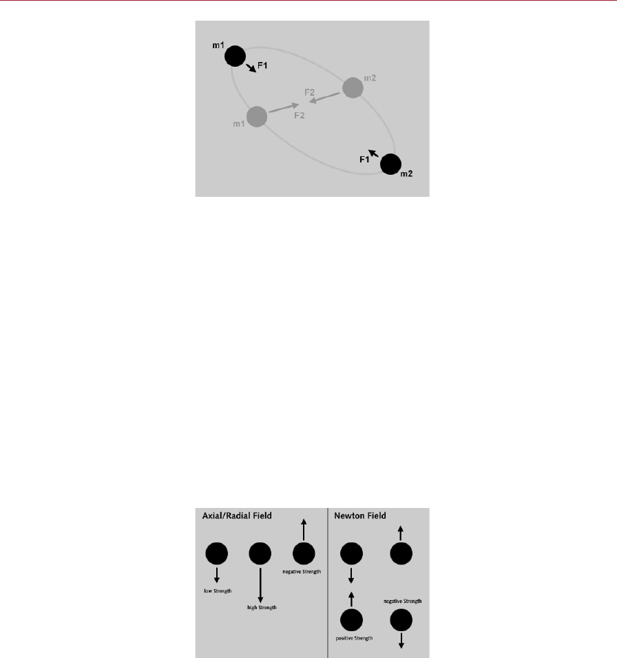
160 FORCE FIELDS DYNAMICS
DYNAMICS FORCE FIELDS 161
The Newton eld can be used to
create elliptical paths, making it
suitable for planetary orbits.
Shown above are two rigid bodies that have been placed in a Newton eld. If the
motion is drag-free — like motion in outer space — the bodies will travel along an
elliptical path. This is because the force of attraction will increase as the bodies near
each other. It is this principle of attraction that explains why the planets in our solar
system orbit the sun. The sun itself remains largely unaffected by the pull of the
planets due to its enormous mass. So to simulate planetary orbits, you should use
the Newton eld.
The Newton eld has many other uses besides planetary orbits. In particular, it can
simulate collision detection such as pool balls bouncing off each other. Although
you could alternatively use the collision detection engine, collision via gravity elds
is much faster to process.
To simulate collision detection using a Newton eld, enable the Exclusion option
(Shape tab) and set Falloff to Step (Falloff tab).
Strength
Strength denes the size of the force exerted by the eld. You can enter a positive
value or a negative value. In the case of a Newton eld, a positive value will cause
attraction whereas a negative value will cause repulsion.
The effect of a varying Strength
value on the Axial, Radial and
Newton elds.

160 FORCE FIELDS DYNAMICS
DYNAMICS FORCE FIELDS 161
Direction
You can set the direction parameters for the Axial eld only. To dene the direction
of the lines of force in the Axial eld, enter a vector (X,Y,Z) under Direction. This
setting refers to the object’s coordinate system. Note that because the direction is
dened as a vector, the values 100,10,0 dene the same direction as 10,1,0. A value of
0 signies no force in the corresponding direction. You can enter negative numbers
also for negative axis values.
Example
If you set X to 1 and Y to 1, the resultant direction of the force will be at the 45° angle
between the X and Y axes. To easily dene the angle of force, set one of the X,Y,Z
parameters to 1 and leave the other two parameters at their default value of 0. Then
use the Rotate tool to point the eld in the desired direction.
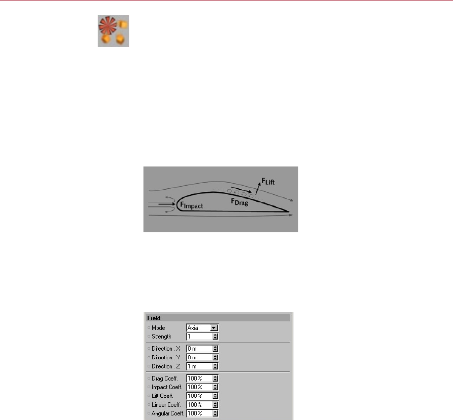
162 FORCE FIELDS DYNAMICS
DYNAMICS FORCE FIELDS 163
Wind
The wind force takes into account the shape of the object and the surface area that
is facing the wind.
In contrast to gravity, wind takes an object’s shape into account. Depending on the
direction of the wind and the object, various forces will be exerted that will change
continually as the object rotates.
Simulating these phenomena with true accuracy would involved extremely complex
equations, where even a simple motion could take hours to compute.
Dynamics simplies the aerodynamics calculation to produce realistic results in a
fraction of the normal processing time. This simplication involves breaking down
the forces that act on the object into three main types: lift, impact and drag.
With Dynamics, wind is
simulated using three key
forces: lift, impact and drag.
The diagram shows these forces
acting on a wing prole.
Shape Tab, Falloff Tab
The parameters on the Shape tab and Falloff tab work in the same way as the
parameters of the same name described in the Gravity section above.
Field Tab
Using this tab you can specify
the nature of the wind using
a simplied parameter set.
This simplication allows
fast computation while still
achieving realistic results.
Field
You can use the Field parameter to select the type of the wind eld. Two types are
available: Axial and Radial. The Axial and Radial elds function in the same way as
their counterparts described in the Gravity section above.
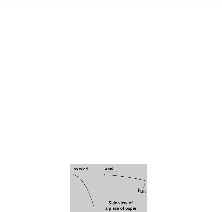
162 FORCE FIELDS DYNAMICS
DYNAMICS FORCE FIELDS 163
Strength
Here, set the strength of the wind.
Direction
This has the same effect as described in the Gravity section above.
Drag Coeff.
When air streams over a body, small eddies will beat against the body’s surfaces,
causing deceleration. The Drag Coeff. parameter denes the strength of this effect.
This decelerating effect is usually minor but occasionally it can have a telling inuence
on the object’s motion.
Impact Coeff.
The Impact Coeff. value determines the strength of the air force that will be exerted
on body surfaces that face the wind. The strength of the impact force is proportional
to the surface area facing the wind and the relative velocity of the body compared
to the wind.
Lift Coeff.
This setting denes the strength of lift.
When an airstream passes over a surface, the air pressure will drop. The faster this
airstream, the lower the pressure. A wing must be shaped so that the airstream will
pass over one wing surface more quickly than over the other wing surface. This will
create a pressure gradient, causing the wing to experience a lifting force.
If you were to hold out a piece of paper and blow along its edge, the airstream would
create lift on the paper, causing the paper to follow the direction of the airstream.
A real-world example of lift.
Blow across a hanging piece of
paper and the airstream will
create a lift force that will raise
the paper into line with the
airstream.
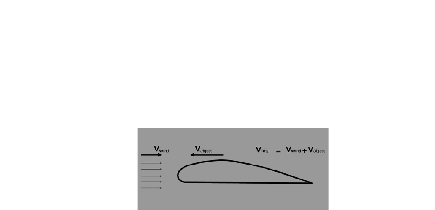
164 FORCE FIELDS DYNAMICS
DYNAMICS FORCE FIELDS 165
Note that occasionally paradoxical situations may arise, such as motion that heads
into the wind. In such cases you should reduce the Lift Coeff. in one of two places,
either in the Wind settings or the Rigid Body Dynamic settings. The latter is usually
preferable since it enables you to adjust the lift for a deviant object without affecting
the ight of other objects.
Linear Coeff., Angular Coeff.
These two settings relate to linear velocity and angular velocity, which both play a
part in an object’s motion in the wind eld. However, it is not just the wind’s velocity
that needs to be taken into account, but the object’s velocity also.
The velocity will affect an
object’s behavior in wind. The
effective velocity that will be
considered is the sum of the
wind’s velocity and the object’s
velocity.
Although Linear Coeff. and Angular Coeff. are set to 100% by default, you will need
to set values for the Linear and Angular parameters in the Rigid Body Dynamic Tag
if you want the velocity to be taken into account. This is because Linear and Angular
in the Rigid Body Dynamic Tag are set to 0 (i.e. disabled) by default. In general, leave
the parameters in the Wind settings set to 100%, but set their counterparts in the
Rigid Body Dynamic Tag to values between 1% and 10% for a realistic result.
Example 1
An aeroplane is taking off at 100 km/h, heading into a wind of 50 km/h. The relative
wind velocity that affects the wing’s surface is 150 km/h.
Example 2
A plane is taking of at 100 km/h with a following wind of 50 km/h. Hence the relative
wind velocity is just 50 km/h. This highlights the reason why aeroplanes will take off
from various runways according to the direction of the wind.
Linear Coeff. denes the strength of this effect for linear motion, whereas Angular
Coeff. denes the strength of the effect for angular motion. To switch off the linear
of angular effect, set the corresponding parameter to 0.
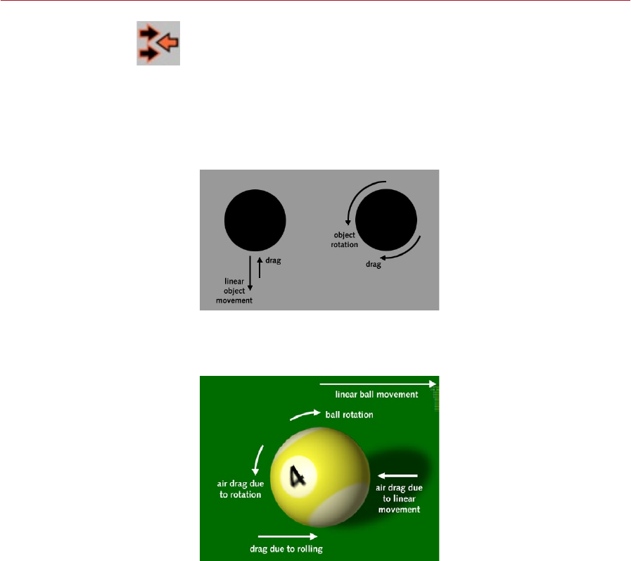
164 FORCE FIELDS DYNAMICS
DYNAMICS FORCE FIELDS 165
Drag
The drag eld affects moving objects only and it will always exert its force in the
opposite direction to the object’s motion. Almost all motion is subject to drag of
one type or another, so for realistic dynamics animation, you will usually need to use
the drag eld. Without drag, a body would continue its motion unhindered. A body
such as a parachute would never slow down.
One characteristic of drag is that it always exerts its force in the option direction to
the body’s motion. This trait is illustrated below.
Drag is always applied in the
opposite direction to the body’s
motion.
Typically, a variety of drag forces will act on an object, as shown in the next diagram.
Note that you will not have to concern yourself with all these drag forces when you
dene the drag eld.
Often a variety of drag forces
will act on the same object. Here,
three types of drag can be seen
affecting the motion of the ball.
Shape Tab, Falloff Tab
The parameters on the Shape tab and Falloff tab work in the same way as the
parameters of the same name described in the Gravity section above.

166 FORCE FIELDS DYNAMICS
DYNAMICS FORCE FIELDS 167
Field Tab
The Field tab contains
parameters for dening the
drag’s type, direction and
strength.
On the Field tab you can dene the type of drag (angular, linear or axial) as well as
its direction and strength.
Mode
Select the type of motion which the drag should affect: Linear, Angular or Axial.
Linear
The drag will affect linear motion, i.e. motion which changes the location of the body.
Linear drag will be applied regardless of the direction in which the object is moving.
Angular
This type of drag will decelerate rotating bodies.
Axial
The Axial mode breaks the following law of physics:
Drag will always be applied in the opposite direction to the body’s motion.
The Axial mode breaks the law by allowing you to specify the direction of the drag
(under Direction). Although it dees real world physics, the Axial mode helps you to
take short cuts as demonstrated in the example below.
Suppose you want to simulate a soft ball being thrown at a wall. To accomplish this,
you could use a drag eld to bring the ball to an abrupt halt in the wall region, plus
a gravity eld to accelerate the ball towards the ground after it has hit the wall.
Although a Linear drag eld would be able to halt the ball as it nears the wall, the
eld would in addition prevent the ball from accelerating towards the oor under
gravity. The ball would remain stuck to the wall.
The solution is to use the Axial eld, which will exert drag in a dened direction only.
By setting the direction of the Axial eld force to the opposite direction of the balls
initial motion, the drag will stop the ball as it nears the wall yet it will not oppose
the downwards motion. The ball will be allowed to fall to the oor.
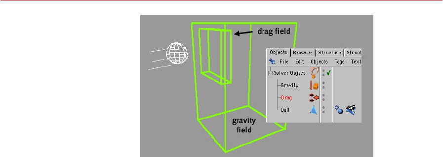
166 FORCE FIELDS DYNAMICS
DYNAMICS FORCE FIELDS 167
An Axial drag eld will oppose
an object’s motion in a dened
direction only. Here the
drag eld will stop the ball’s
horizontal motion, yet it will
not oppose the vertical motion
when the ball meets the gravity
eld and falls.
Strength
Use this to set the Strength of the drag force. Enter a high value if the objects should
come to an abrupt halt.
Only Drag
This option is available with the Axial mode only. When the option is enabled (as it
is by default), the drag will cause deceleration only. If instead the option is disabled,
objects will be accelerated by the drag if their motion is pointing in the same direction
as the drag force.
Direction
This has the same effect as described in the Gravity section above.
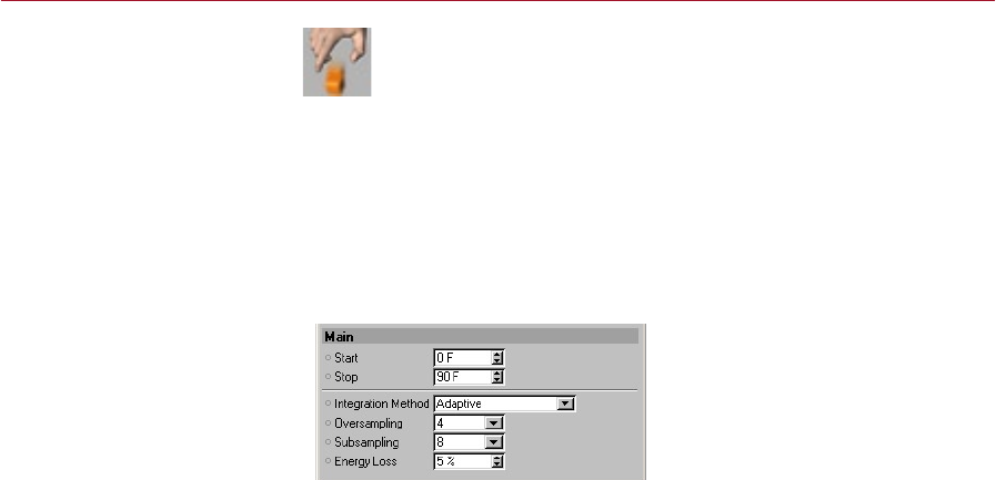
DYNAMICS SOLVER OBJECT 169
The solver acts as a container for the objects in your dynamics system.
Bodies or force elds that are not children of a solver will be ignored by the
dynamics engine. But the solver is more than just a container. It has its own
settings in the Attribute manager where you can adjust the overall behavior of the
dynamics animation such as the accuracy of the motion. A solver is a micro-universe
in the sense that it is self-contained. Its children will interact with each other while
ignoring objects that are not contained within the solver. The solver’s objects will
also ignore the children of other solvers, enabling you to use several solvers in the
same scene that will run independently of one another.
Main Tab
Without a Solver object, there
can be no dynamics.
Start, Stop
These two parameters dene when the dynamics animation will begin and when it
will stop. The Start and Stop parameters are independent of the project’s animation
length. If you set Stop to a time point beyond the project length, you will need to
increase the Maximum value in the Project Settings dialog.
Integration Method
Dynamics must solve a number of complex differential equations in order to calculate
the motion of bodies in the dynamics system. The scientic term for this entire
calculation is ‘integration’. Various integration methods can be used to solve these
equations. The Integration Method parameter denes which particular method the
solver will use.
Euler
The least accurate but fastest to calculate method. It is about half as accurate but
twice as fast at Midpoint. Use this method for simple collision animations where
no soft body objects are involved.
Midpoint
Fast to compute, but not very accurate.
To move a rigid body, rst
switch off the solver by clicking
its green tick in the Object
manager. Then move the body as
required. Once you are ready to
switch on the solver, do not click
the solver’s red cross (Object
manager). This would reset
the body to its position before
the solver was switched off.
Instead, set the new position as
the starting state by selecting
the Initialize Object function or
the Initialize All Objects function
from the Plugins > Dynamics
menu.
Solver Object
The objects in your dynamics
system must be children of a
solver object. The solver acts as
a container and also species the
general behavior of the dynamics
system such as the accuracy of
the animation.
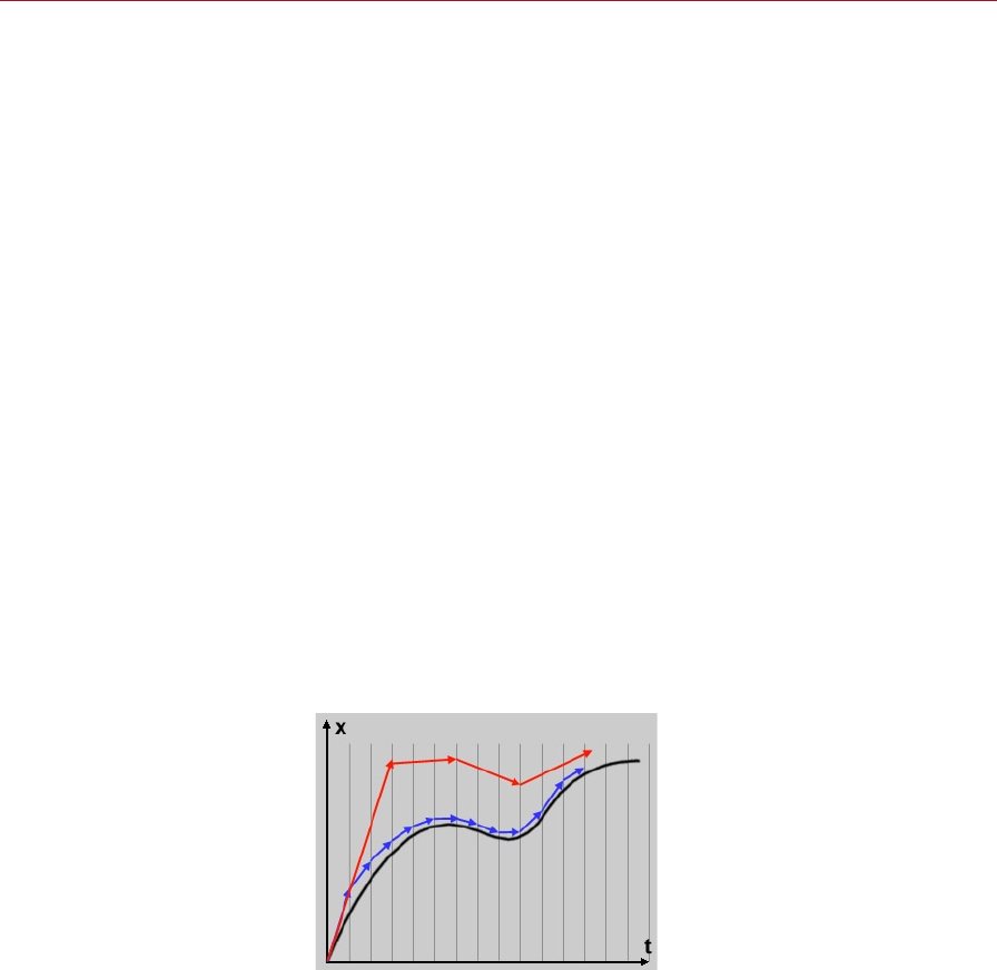
170 SOLVER OBJECT DYNAMICS
DYNAMICS SOLVER OBJECT 171
Runge-Kutta
Generally 10 times more accurate than Midpoint, but four times slower.
Adaptive
The most accurate method; slowest method to process.
Softbody
Use this method if soft bodies are involved. Usually you can set Oversampling to a
low value when using this method, such as 2 or 4. The method computes quickly,
especially with soft body collisions, and can be as much as 100 times faster than
the other methods. (Although some of the other methods are generally fast to
compute, they would be slowed down by requiring a much higher Oversampling
value than is needed with the Softbody method.)
No matter which method you choose, the motion will be approximated to some
degree. Your aim when setting the Integration Method and its associated parameters
is to nd a suitable balance between accuracy and processing time.
Oversampling
For the Midpoint and Runge-Kutta integration methods, the Oversampling value
denes the number of times the motion will be integrated per frame. Hence to increase
the accuracy of the motion, select a higher Oversampling value. Note that a higher
value will increase the processing time.
For the Adaptive integration method, the Oversampling value denes the minimum
number of integrations per frame. The actual number will depend on the Subsampling
value.
The bottom curve represents
the perfect motion. The two
other curves use the same
integration method, but the
middle curve uses a higher
Oversampling value, lending it
greater accuracy.
Current dynamics engines
are unable to solve each and
every possible combination
of bodies and force elds.
Among other things, this
may be due to rounding
errors or unsolvable
equations. In such a case,
try adjusting the position
of the individual objects,
springs and forces. Also, try
adjusting the parameters of
the springs and force elds.
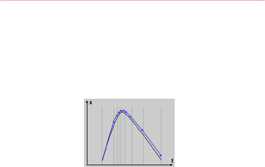
170 SOLVER OBJECT DYNAMICS
DYNAMICS SOLVER OBJECT 171
Subsampling
You can dene Subsampling for Adaptive integration only. Subsampling works
together with Oversampling to dene the number of integrations per frame for
Adaptive integration. Oversampling denes the minimum number of integrations
per frame. The Oversampling value multiplied by the Subsampling value denes the
maximum number of integrations per frame.
For example, with Oversampling set to 4 and Subsampling set to 8, there will be a
minimum of four integrations per frame and a maximum of 32 integrations per frame.
With Oversampling set to 2 and Subsampling set to 4, there will be anywhere from
2 to 8 integrations per frame.
Subsampling concentrates on critical areas of the motion, as illustrated below. The
actual number of integrations will vary from frame to frame.
With subsampling enabled,
integration is concentrated in
key areas of the animation. In
the diagram, to start with only
oversampling is applied; then,
as a critical point in the motion
is reached (the peak in the
diagram), which might be for
example a change in direction,
more and more subsampling
is applied, up to the maximum
selected. Eventually the motion
becomes less critical and we go
back to oversampling.
It is thanks to Subsampling that Adaptive is the most accurate integration method.
With subsampling, integration will be concentrated in the most critical areas.
Energy Loss
This parameter is necessary since dynamics engines tend to add energy into the
system when the Integration Method is not accurate enough; adding a small energy
loss will help to compensate for this slight inaccuracy.
This is similar to real life motion which continually loses energy due to various drag
forces. However, if you should notice that, for example, spring oscillations are damped
too quickly, reduce the Energy Loss value or the drag or damping within the force
object.
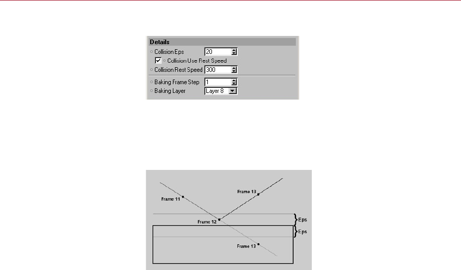
172 SOLVER OBJECT DYNAMICS
DYNAMICS SOLVER OBJECT 173
Details Tab
Here you’ll nd settings that
relate to collision detection
and baking.
Collision Eps (Epsilon)
This parameter is used for collision detection only. It denes a distance in units above
and below the surface in which collision can take place, helping to avoid penetration.
As soon as an object enters this region, the object will rebound.
Here, the dots represent the
nearest point of an object as the
object rebounds off a cuboid.
The rebound will take place as
soon as the point enters the Eps
region.
The Eps parameter is more important that it rst appears. It is especially critical
when fast-moving objects are colliding with each other. In such cases, the objects
will penetrate each other if the Eps value is set too low.
Set the Eps value too high, on the other hand, and objects will rebound before they
should. For example, two pool balls may rebound while they are still 10 cm apart
if the Eps value is too high. Here, a popular technique can help you to obtain more
reliable collisions. It works by making use of a proxy object, using a similar technique
to the proxy collision object described in the chapter on rigid bodies. This time, the
proxy object should be scaled down so that it is smaller than the real object. This will
enable you to use a higher, more reliable, Eps value.
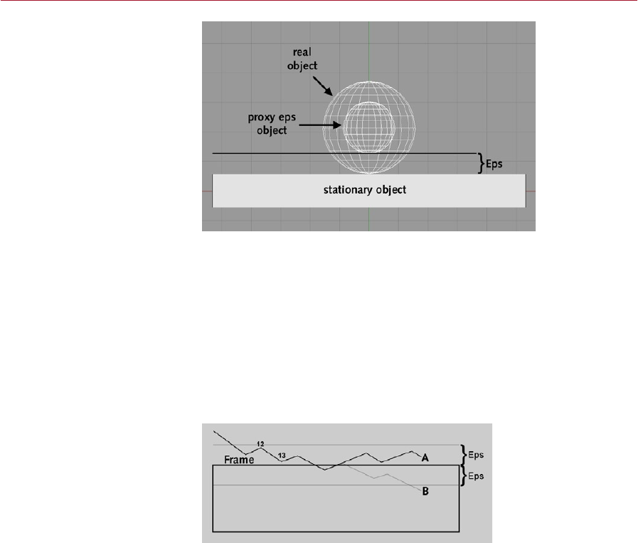
172 SOLVER OBJECT DYNAMICS
DYNAMICS SOLVER OBJECT 173
Using a smaller object as a
proxy, you can use a higher,
more reliable Eps value. The real
sphere in the diagram is in the
process of rebounding, but it is
actually the smaller proxy that
has triggered the rebound by
entering the Eps region. Without
a proxy eps object, a much lower
- and therefore less reliable - Eps
value would be needed.
Collision Use Rest Speed, Collision Rest Speed
When you slide an object over a surface using Dynamics, under some circumstances,
the object may start to ‘sink’ through the surface.
The Collision Rest Speed parameter is designed to prevent this sinking from happening.
When the Use option is enabled, it will give the sliding object a little push away from
the surface (in the direction of the surface’s normal, that is).
To prevent this little push from being added to rebounding objects that are not sliding,
the push will be exerted only if the object’s velocity in the direction of the surface is
below a certain velocity — this threshold velocity is the Collision Rest Speed.
A . Collision Use Rest Speed
enabled. B. Collision Use Rest
Speed disabled. The Rest Speed
parameter helps to prevent
sliding objects from penetrating
the surface they are sliding over.
Particularly with complicated spring-mass systems or soft bodies, an inappropriate
integration method can create unexpected behavior. This unusual behavior is possible
in all existing dynamics engines.
Also possible are instable states with which no realistic motion can be achieved
regardless of the integration settings. Such states can be tackled only by using a new
spring arrangement or by adjusting the masses, spring forces and damping.
For an object to rest on a
surface, the distance between
the object and surface must be
less than the Eps distance and
the object’s velocity must be less
than the Collision Rest Speed.
Static drag will then take hold.

174 SOLVER OBJECT DYNAMICS
Baking Frame Step
Here you determine how many keyframes will be created when you bake the motion
in the Timeline. The most accurate setting here is 1, which will cause a keyframe to
be created for each frame. If you intend to edit the animation, you should choose the
highest value possible that does not lead to errors with the motion.
Baking Layer
CINEMA 4D’s timeline has eight layers. For this parameter, select the layer in which
the baked track will be placed when you bake the motion in the Timeline. For details
on the Timeline’s layers, please consult your CINEMA 4D Reference Manual.
If strange results occur such as
an increased height of swing,
this is likely to be because extra
energy is entering the system.
Typically, this is caused by an
integration method that is too
inaccurate or parameters that
are set too low. In this case it
is always an idea to try adding
some extra energy loss, or
increasing the solver accuracy.
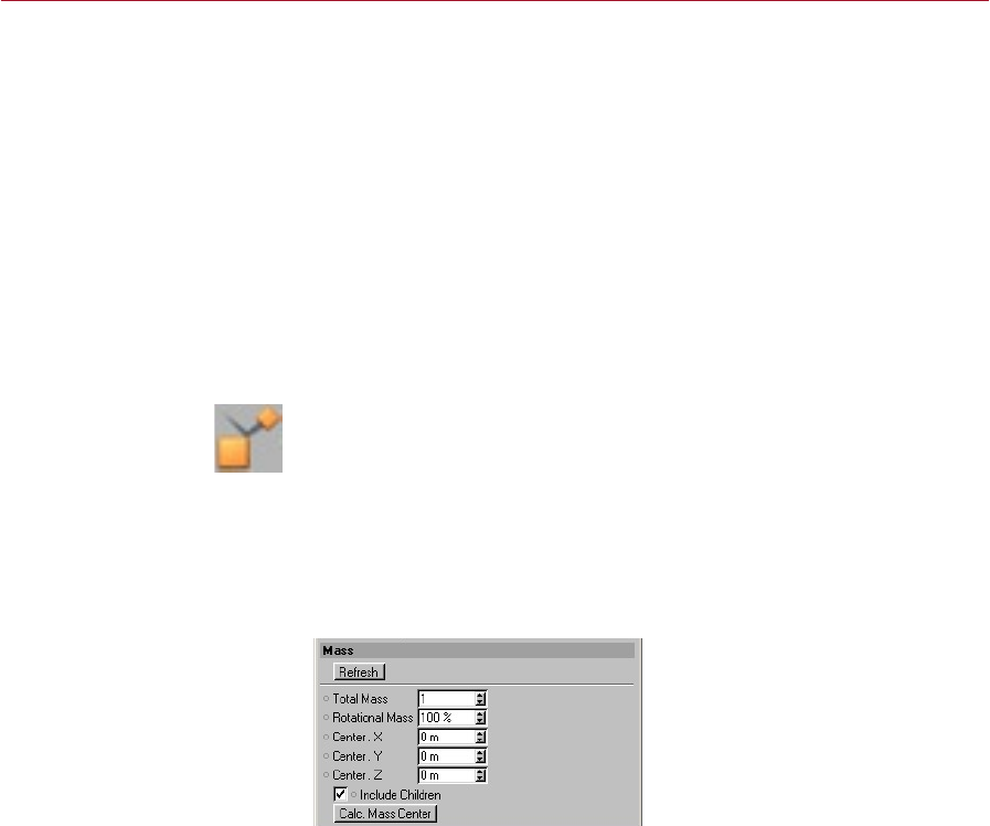
DYNAMICS RIGID BODIES 175
A rigid body is a polygon object in the dynamics system whose shape stays the same
all the time. It can be given a mass, a starting velocity and aerodynamic properties.
In addition, rigid bodies are able to collide with one another. Rigid bodies consist
of a single centre of mass that enables them to be rotated around this point during
the dynamics animation. In contrast, a soft body is built from many masses each
located at the points of the soft body object and so have no initial values for rotation
and hence cannot rotate when animated other then through their interactions with
other objects.
When deciding whether an object should be a rigid body or a soft body, consider
whether the object’s shape will change during the animation. If the object’s shape
will stay the same throughout the animation, the object should be a rigid body;
otherwise, the object should be a soft body. If you can use a rigid body instead it
will greatly speed up your animation. Only use a soft body if really needed, such as
for cloth blown by wind.
Rigid Body Dynamic Tag
To dene a polygon object as a rigid body, you must give the object a Rigid Body
Dynamic tag. To do this, rst select the object by clicking its name in the Object
manager. Next, in the Object manager, select File > Dynamics Tags > Rigid Body
Dynamic. The Rigid Body Dynamic settings will appear in the Attribute manager.
These parameters are described below, tab by tab.
Mass Tab
Double-click the Rigid Body
Dynamic tag to display its
settings in the Attribute
manager.
Total Mass
Here, set the mass of the rigid body. The Total Mass will always play a role when the
body interacts with other rigid bodies. This applies to collision detection, gravity
elds, wind, drag and rigid bodies attached via springs.
The higher the Total Mass value, the greater the force that the body will exert on the
interacting objects.
Rigid Bodies
Objects that are moving in the
dynamics system should be
dened as rigid bodies if they
don’t change their shape, such as
pool or snooker balls bouncing
off each other and the cushions.
In this chapter, you’ll learn how to
create and use rigid bodies.
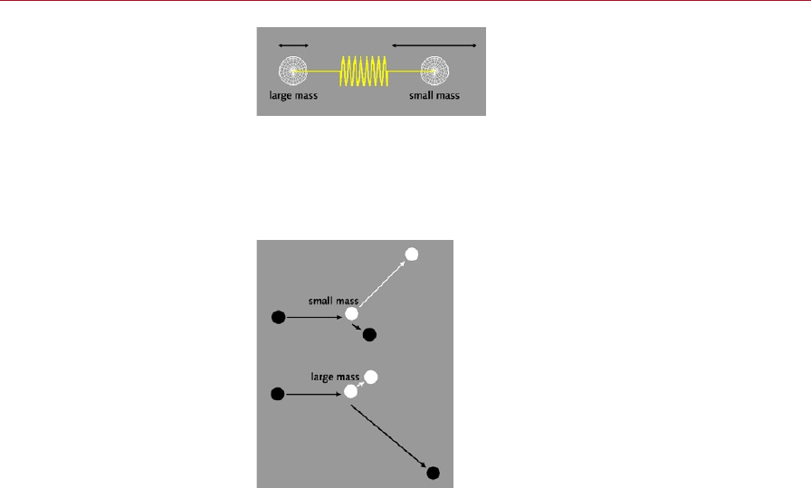
176 RIGID BODIES DYNAMICS
DYNAMICS RIGID BODIES 177
The spring pulls both spheres
with the same force giving a
higher acceleration to the right
sphere, making it oscillate more.
In the diagram above, two spherical rigid bodies are attached via a spring. Note how
the smaller mass is oscillating over a greater distance. This is because the left sphere
has a large mass, which in turn needs a higher force to give it the same acceleration.
The spring pulls both spheres with the same force giving a higher acceleration to the
right sphere, making it oscillate more.
Two cases of a black sphere
shooting into a white sphere
that is initially at rest.
Above you can see two cases of a black sphere shooting into a white sphere that is
initially at rest. In the rst case, the white sphere has a smaller mass than the incoming
black sphere and hence it is moving rapidly after the collision. In the second case,
however, the white sphere has a larger mass and so the black sphere makes little
impact on the sphere during the collision making it move slowly after the collision.
To summarize these two diagrams:
Forces being equal, a small mass will be accelerated more and tend to move faster
than a larger mass.
The greater the mass, the greater the force required to achieve the same
acceleration.
When two objects of different mass collide, the smaller mass will be affected most.
If, on the other hand, you set the Total Mass to 0, the following will apply:
The dynamics engine will exert no force on the rigid body.
You will be able to animate the rigid body using keyframes in the Timeline, even if
the rigid body is attached to another rigid body via a spring.
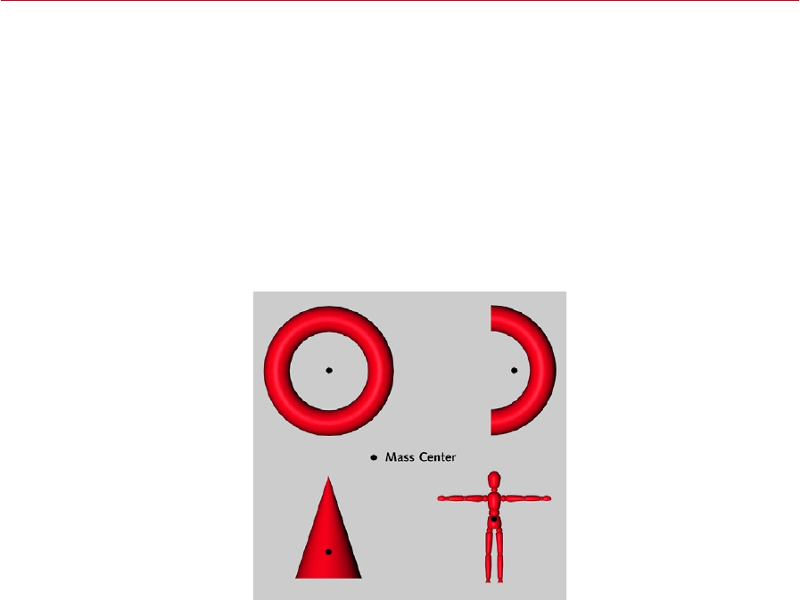
176 RIGID BODIES DYNAMICS
DYNAMICS RIGID BODIES 177
Rotational Mass
This parameter enables you to ne-tune the rotational behavior of the rigid body.
The value is specied as a percentage of the Total Mass value. The higher this Total
Mass value then the greater the force that will be required to change the rotation
of the rigid body.
Center
These three input boxes dene the X,Y,Z position of the mass centre in relation to the
origin. It is an offset. To move the centre of mass, enter the desired offset.
Each rigid body has a mass centre. By default, the mass centre will be in the same
position as the rigid body’s origin. The Center parameters enable you to change the
position of the centre of mass, which is displayed in the viewport as a yellow cross.
The mass centres of various
objects.
If a force is exerted on the centre of mass, the rigid body will experience linear
acceleration only in the direction of the force. If the force is instead exerted on a
point away from the centre of mass, such as may happen during a collision, the rigid
body will experience angular as well as linear acceleration, which will cause it to
rotate as well as move.
The centre of mass is also used to determine whether the rigid body is inside a eld.
The force will be exerted only if the centre of mass is inside the eld.
Lastly, a rigid body attached to an angular spring or used with a constraint will rotate
about its centre of mass.
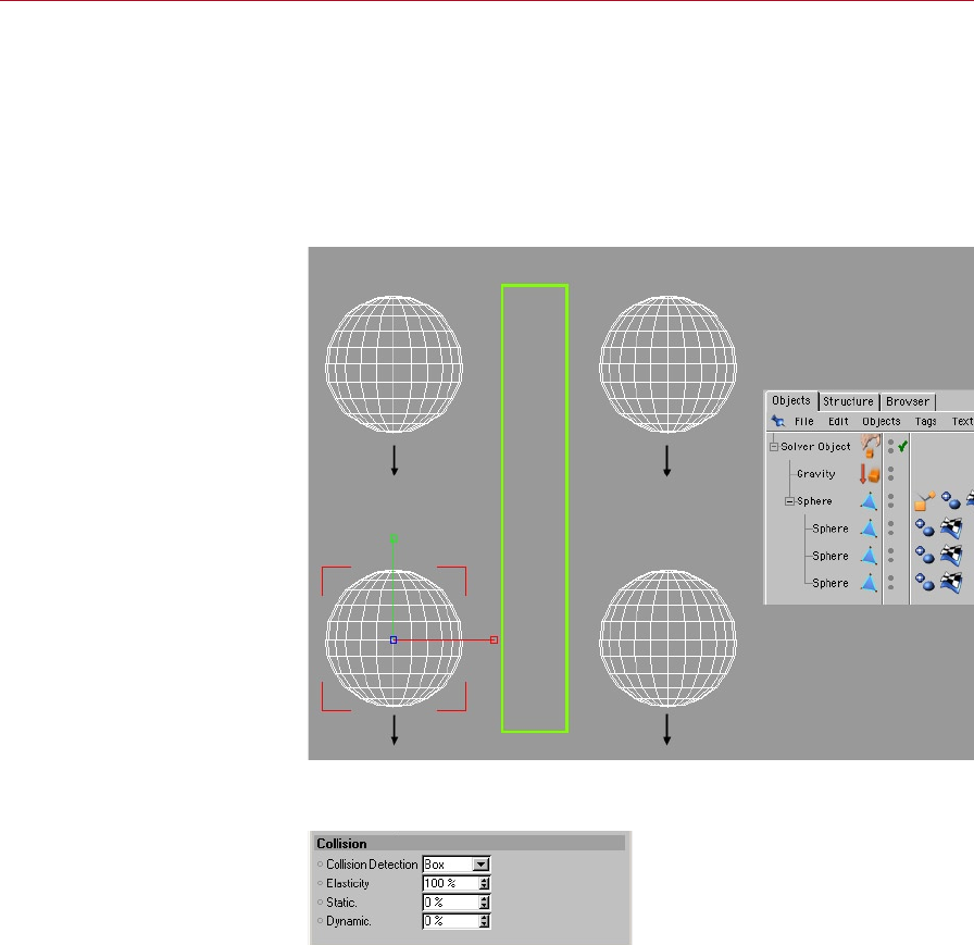
178 RIGID BODIES DYNAMICS
DYNAMICS RIGID BODIES 179
Calc. Mass Center
If you click this button, the centre of mass will be calculated based on the points of
the rigid body.
Include Children
If the rigid body has children, you will usually want the children to move along with
the rigid body without having to create a Rigid Body Dynamic tag for each child. If
you enable this option, the Mass Center will be calculated for the entire hierarchy.
A sphere with three other
spheres as children. With the
Include Children option enabled,
the entire hierarchy will fall
downwards when the parent
sphere enters the gravity eld.
Collision Tab
Collision detection is one of the
major features of Dynamics.
However, many types of
collisions can be simulated using
force elds instead, which can
be much faster to compute!
Collision detection — one of the main features of Dynamics — prevents colliding
bodies from penetrating each other. Instead the bodies will be made to bounce off
each other or slide along each other, just as if they were real solid objects.
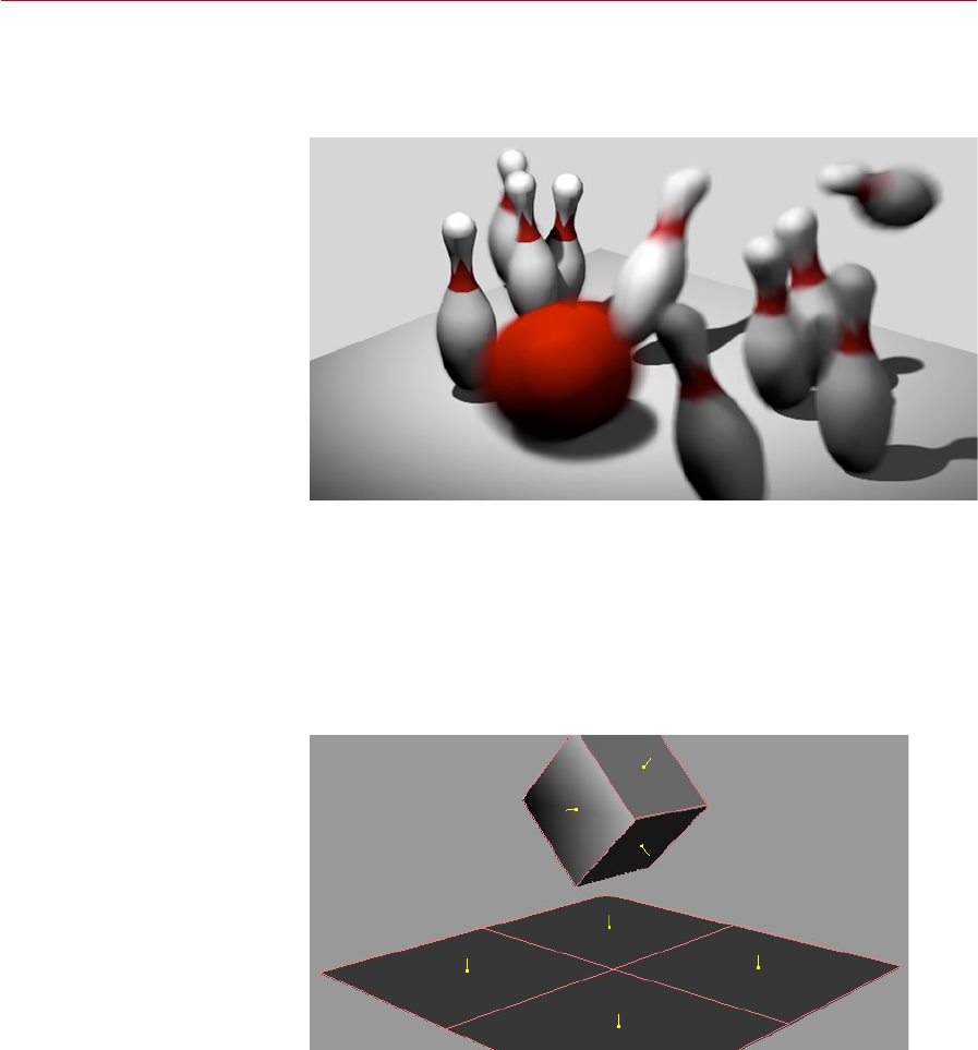
178 RIGID BODIES DYNAMICS
DYNAMICS RIGID BODIES 179
Using the parameters on this tab you can enable or disable collision detection for
the rigid body as well as adjust its collision properties such as the elasticity of the
collision, that is how much energy is lost during the collision, a perfectly elastic (100%)
collision will lose no energy.
Simulating a strike using
keyframes would be a tiresome
exercise. With collision detection,
Dynamics will calculate these
complex collisions for you.
When animating using collision detection it is vital that none of your objects with
collision detection enabled are penetrating each other at the start of the animation,
or collision detection will fail. The Console will aid you here by displaying an error
message if bodies are inside each other. To open the Console, select Window >
Console from the main menu.
Also, check that the surface normals of the colliding objects are facing each other.
If they are not, collision detection will be unable to nd a suitable solution and will
also fail.
The surface normals of colliding
objects must be facing each
other for collision detection
to function correctly. Here,
the surface normals of two
bodies are facing each other as
required.
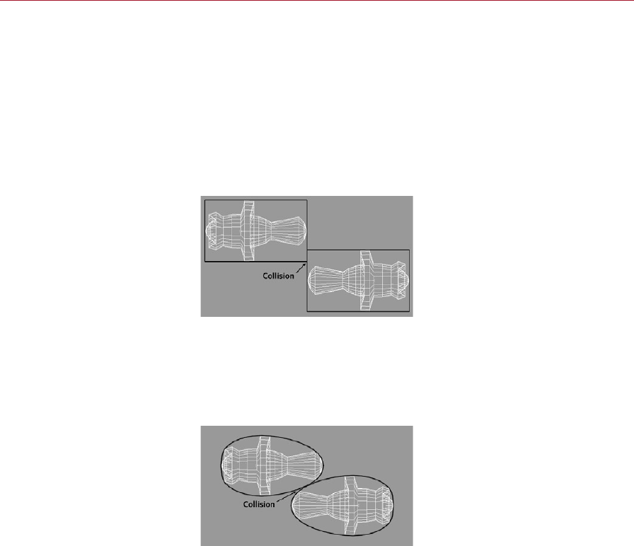
180 RIGID BODIES DYNAMICS
DYNAMICS RIGID BODIES 181
Collision Detection
Here you can select from three types of collision detection or switch off collision
detection.
None
Switches off collision detection. This is the default setting.
Box
Encloses the object in a box. Collision will take place when this box hits other objects.
This is the fastest type of collision to calculate.
With Box collision detection, a
box is placed around the object.
Collision will take place when
this box collides with another
rigid body.
Ellipsoid
This is a more accurate type of detection than Box for many spherical type shapes,
but it takes longer to calculate. You will nd a proxy object in the shape of your
surface with as fewer polygons as possible will be the best overall solution to good
and fast collision detection.
Two objects with Collision
Detection set to Ellipsoid, a
more accurate type of detection
than Box.
Full
With Full, each polygon will be checked for collision. Full is by far the most accurate
type of collision detection but it also takes much longer to process than Box and
Ellipsoid.
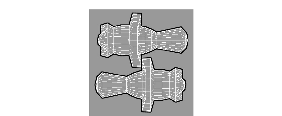
180 RIGID BODIES DYNAMICS
DYNAMICS RIGID BODIES 181
Full collision detection means
collision detection at the
polygon level.
You can, however, greatly reduce the processing time by using a proxy collision object.
These can then use the Full collision to give accurate collisions while maintaining some
speed due to the simple nature of the proxy objects polygon geometry.
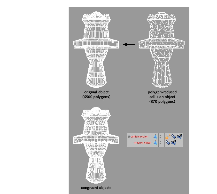
182 RIGID BODIES DYNAMICS
DYNAMICS RIGID BODIES 183
Using a proxy collision object
can save an enormous amount
of processing time while keeping
the detection accurate.
To create a proxy collision object:
Create the object that will act as the proxy collision object by copying the source
object. Use the PolyReduction tool to reduce the proxy. The proxy in the diagram has
been reduced from 6500 polygons to 370 polygons.
Ensure that the source object and proxy object are more or less the same shape.
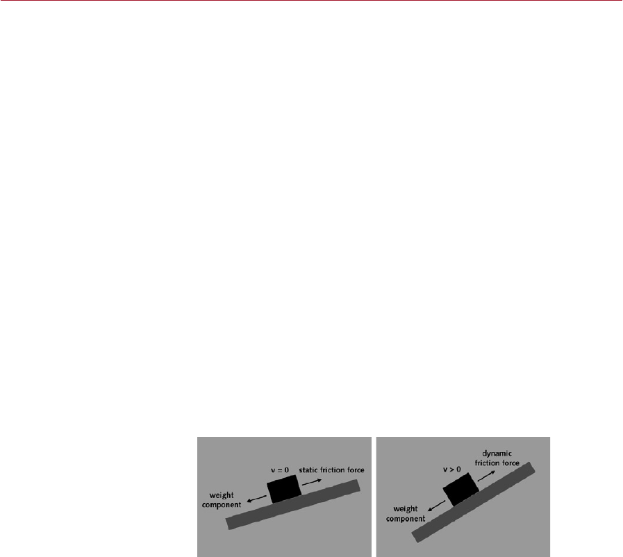
182 RIGID BODIES DYNAMICS
DYNAMICS RIGID BODIES 183
Make the source object a child of the proxy object.
Set up collision detection using the proxy object instead of the source object.
The collision detection will now be processed in a fraction of the usual time. In the
case of the diagram example, 370 polygons will now be checked instead of 6500.
Elasticity
This value denes the percentage of energy that the rigid body will retain following
a collision. An Elasticity setting of 0% would cause the rigid body to halt suddenly
during the collision while a value of 100% would see the rigid body rebound without
loss of speed.
For example, in the case of a pool table, the pool balls should have an elasticity closer to
100% than to 0% since pool balls keep most of their velocity following a collision.
Static, Dynamic
When two bodies are in contact, a type of friction will exist between the bodies. If the
bodies are at rest relative to each other, the friction will be static and will resist any
motion between the two bodies, this is the friction we mostly notice during everyday
life. If the bodies are moving relative to one another, the friction will be dynamic and
try and slow the bodies by transferring the movement to heat.
Both types of friction can be simulated with Dynamics.
Static friction is always greater than dynamic friction. For example, when trying to
push a car that has broken down it is harder to get the car moving than it is to keep
it moving.
On the left, the block’s weight
component down the incline is
not great enough to overcome
‘static’ friction, so the block does
not slide.
On the right, the incline has
been increased and the block
is now sliding. Static friction
having been overcome, the
block is now being resisted
instead by the lesser force of
‘dynamic’ friction.

184 RIGID BODIES DYNAMICS
DYNAMICS RIGID BODIES 185
Aerodynamics Tab
Note that the Wind eld
contains similar parameters
(with the exception of Double-
Sided). The parameters in the
Wind eld set the general
aerodynamics behavior while
the parameters here are used to
ne-tune the aerodynamics for
the rigid body.
You can use this tab’s parameters to modify the aerodynamic behavior of the rigid
body. The parameters here will be multiplied with those in the Wind eld. For example,
if you have set Impact to 50% in the Rigid Body Dynamic tag’s settings and 80% in
the Wind eld, the resulting value for the rigid body will be 40%.
Suppose you have 20 rigid bodies inside a Wind eld. The wind settings are working
well for 19 of the rigid bodies but the other rigid body is not moving as it should. If
you try to correct the ight of this one rigid body by adjusting the parameters in the
Wind eld, you might nd that doing this would ruin the ight of the other 19 rigid
bodies. A better solution is to modify the parameters on the Aerodynamics tab of
the rogue rigid body.
Double-Sided
If this option is disabled — the default setting — the wind will affect only those
polygons whose surface normals are facing the wind. If you enable the option, the
wind will exert its force on all polygons regardless of the direction in which their
surface normals are pointing. Only enable the Double-Sided option if your object has
no thickness and Lift is set to 0%.
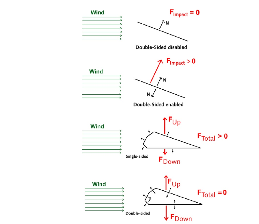
184 RIGID BODIES DYNAMICS
DYNAMICS RIGID BODIES 185
Double-Sided disabled. Since the
normal is facing away from the
wind, the wind is unable to exert
a force on the surface.
Double-Sided enabled. This
guarantees that a normal will
face the wind and hence the
wind is now able to exert a force
on the surface.
Double-Sided disabled. The wing
is experiencing a lifting force.
Double-Sided enabled, causing
equal and opposite forces for
each surface and hence no
resultant force. For this reason,
Double-Sided should be disabled
for closed polygons.
Lift
This setting denes the strength of lift. When an airstream passes over a surface,
the air pressure will drop. The faster this airstream, the lower the pressure. When
designing a wing, the wing must be shaped so that the air stream will pass over one
wing surface more quickly than over the other wing surface. This will create a pressure
gradient, causing the wing to experience a lifting force.

186 RIGID BODIES DYNAMICS
DYNAMICS RIGID BODIES 187
If you were to hold out a piece of paper and blow along its top edge, the airstream
would create lift — as the air passes over the paper, it lifts up the sheet until the
pressure is equal on both sides of the paper.
A practical example of lift.
Blow across a hanging piece of
paper and the airstream will
create a lifting force that will
move the paper into line with
the airstream.
Occasionally, paradoxical situations may arise such as motion that heads into the
wind. In such cases you should reduce the lift in one of two places. You can reduce
the parameter either in the Wind eld (Lift Coeff.) or the Rigid Body Dynamic dialog
(Lift). The latter is usually preferable since it enables you to adjust the lift for a
uncooperative object without affecting the ight of the other objects.
Impact
The Impact value determines the strength of the air force that will be exerted on
body surfaces that face the wind. The strength of the impact force is proportional
to the surface area facing the wind and the relative velocity of the body compared
to the wind.
Drag
When air streams over a body, small eddies will beat against the body’s surfaces,
causing deceleration. The Drag parameter denes the strength of this effect. This
decelerating effect is usually minor but occasionally it can have a telling inuence
on the object’s motion.
Linear, Angular
These settings work with the Linear Coeff. and Angular Coeff. settings for the Wind eld.
For details on these settings, look up “Linear Coeff., Angular Coeff.” in the index.

186 RIGID BODIES DYNAMICS
DYNAMICS RIGID BODIES 187
Start Tab
The values entered into the
Start tab will give an object an
initial state for the dynamics to
work on.
The Start tab enables you to dene the state of the rigid body at the start of the
dynamics animation, such as the rigid body’s starting velocity.
The ‘v’ settings dene the starting velocity of the rigid body. The ‘w’ settings set the
angular velocity (rotation). ‘F’ denes a force that is exerted during the rst frame
of the dynamics animation. The values you enter for ‘I’ will dene the torque applied
during the rst frame of the dynamics animation.
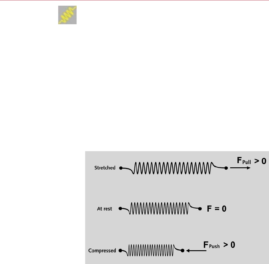
188 RIGID BODIES DYNAMICS
DYNAMICS RIGID BODIES 189
Rigid Body Spring Tag
Springs enable you to attach polygon objects to one another. Springs can be attached
to any object point and you can attach more than one spring to the same object.
To create rigid body springs, you rst need to assign a Rigid Body Spring tag to the Solver
object. To do this, select the Solver object by clicking its name in the Object manager.
Next, select File > Dynamics Tags > Rigid Body Spring from the Object manager’s menu.
This will assign the tag to the solver and at the same time the Rigid Springs dialog will
open. Using this dialog, you can create all the required springs and for each spring you
can dene its characteristics such as its rest length and its damping.
Imagine yourself pulling a spring then letting go. Once you let go, the spring will
return to its original length then compress, extend back out again, compress once
more and continue to oscillate in this way until it eventually comes to rest at its
normal length. While the spring is oscillating, it is undergoing elastic deformation,
meaning that the spring will eventually return to its original shape once all force has
been removed.
Underlying elastic deformation is one important law of physics. Provided a spring is
within its elastic deformation range, the length of the spring’s extension is directly
proportional to the force exerted on the spring. So if a force of 10 Newtons stretches
a spring by 5 cm, a force of 20 Newtons will stretch the spring by 10 cm.
Provided a spring is within its
elastic deformation range, the
length of the spring’s extension
is directly proportional to the
force exerted on the spring.
To access the Rigid Springs dialog at
any time, double-click the tag’s icon
in the Object manager.
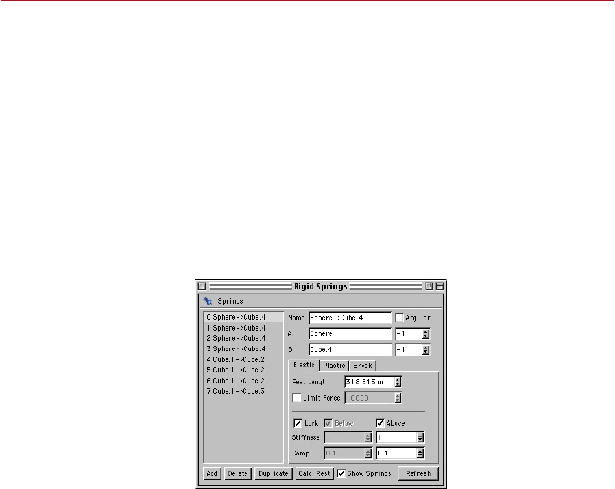
188 RIGID BODIES DYNAMICS
DYNAMICS RIGID BODIES 189
Now suppose you pull the spring a second time, only this time you pull much harder.
So much harder, in fact, that the spring is permanently distorted. When you let go,
the spring will not return to its original length. The spring has undergone plastic
deformation, which occurs once the spring has been stretched beyond a point known
as the spring’s elastic limit.
Now you pull the spring once more, only this time with all your might. So you give
a Herculean tug and ... the spring snaps of course.
All of this behavior — snapping, plastic deformation and elastic deformation — can
be simulated using the springs in Dynamics. Note that springs are displayed yellow
in the viewport when not selected.
There are two ways to create springs and attach them to rigid bodies. Either the
springs can be created using the Rigid Springs dialog or the springs can be drawn in
the viewport using the RBS Draw Tool.
Using the Rigid Springs Dialog
Create, edit and attach springs
in the Rigid Springs dialog.
Using the Rigid Springs dialog, you can create, edit and attach springs as well as adjust
all of the properties of the springs including elastic and plastic behavior.
You can select and edit multiple springs. To add a spring to the selection, Ctrl-click
the spring’s name or number in the spring list. To remove a spring from the selection,
Ctrl-click once more.

190 RIGID BODIES DYNAMICS
DYNAMICS RIGID BODIES 191
If the settings of the selected springs differ — e.g. if one spring has a Rest Length of
50 and another a Rest Length of 30 — the parameter boxes that hold the differing
values will be highlighted with a bright color. You will still be able to enter new values
using these highlighted parameters. The highlighting is simply to make you aware
that the corresponding values currently differ for the selected springs.
When you change a setting, the new setting will be applied to all of the selected
springs, regardless of whether the parameter was highlighted or not. If you need to
specify an individual parameter for a spring, you must select that spring only and
edit it separately.
Name
You can optionally type in a name for the spring.
Add, A, B
To nd out the point’s number, ensure
the rigid body is selected in the Object
manager (click on its name). Select
the Points tool, then select the point
in question. Now, open the Structure
manager (main menu: Window >
Structure Manager). Ensure the Points
mode is active (Structure manager:
Mode > Points). The point’s number will
be highlighted under the Point column.
The Add button creates a spring. The spring will appear in the spring list, which is
the large region in the left half of the dialog.
Having created a spring using Add, you need to dene which rigid bodies the spring
should be attached to. To do this, enter the names of the rigid bodies under A and B.
You must type in the names exactly as they appear in the Object manager. To the right
of A and B input boxes are two further input boxes. Use these to dene two points of
the rigid bodies to which the spring should be attached. The default value of -1 will
attach the spring to the mass centre. To change this, enter the point’s number.
Angular
Enable this option if you want to dene the spring as an angular spring. In this case
you should enter the name of the rigid body under A.
Delete
Deletes the spring that is currently selected in the spring list.
Duplicate
Duplicates the spring that is currently selected in the spring list.
Calc. Rest
Sets the Rest Length value to the spring’s current length. This is useful after you have
attached the spring to two rigid bodies since it will set the Rest Length accordingly.
Show Springs
Controls whether springs are displayed in the viewport.
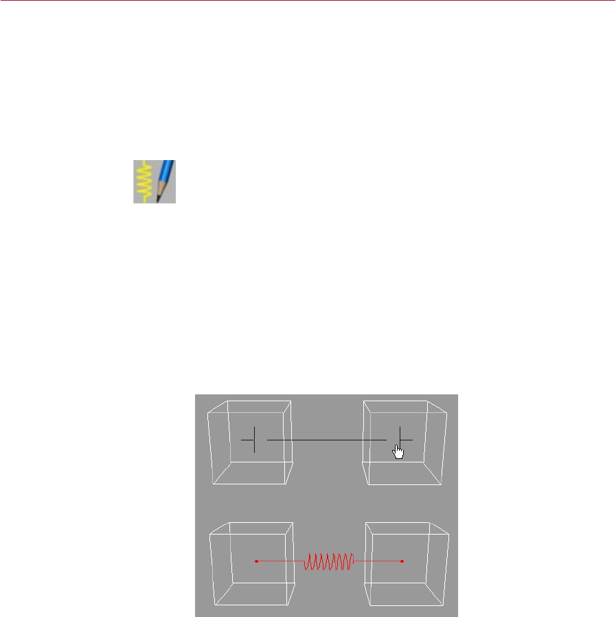
190 RIGID BODIES DYNAMICS
DYNAMICS RIGID BODIES 191
Refresh
Forces a refresh of the viewport, causing the springs to be redrawn. For example, if
you have just attached a spring between two points, clicking Refresh will make the
spring appear in the viewport. The viewport will refresh the springs automatically
when you select another spring or when you move the camera.
Using the RBS Draw Tool
Although you can create and attach springs using the Rigid Springs dialog, the RBS
Draw Tool is preferred in most cases because it enables you to draw the springs
interactively in the viewport.
Springs that you create using the RBS Draw Tool will still appear in the Rigid Springs
dialog. Hence you will be able to edit the spring parameters such as elastic and plastic
behavior later using the dialog.
Before you create the springs, rst ensure that you have assigned a Rigid Body Spring
tag to the Solver object (File > Dynamics Tags > Rigid Body Spring Tag in the Object
manager menu). Ensure also that the rigid bodies are children of this Solver object. Next,
select the RBS Draw Tool (Plugins > Dynamics > RBS Draw Tool in the main menu).
To draw the spring, drag from the rst rigid body to the second rigid body. As you
drag, a cross will appear where you rst started dragging and a second cross will
appear once the mouse pointer is in a suitable position over the second rigid body.
When you release the mouse button, the spring will be created and placed between
the two crosses.
Using the RBS Draw Tool, you
can create and attach springs
interactively in the viewport.
Two crosses will appear while
you draw to indicate the
attachment points.

192 RIGID BODIES DYNAMICS
DYNAMICS RIGID BODIES 193
Attribute manager settings
While the RBS Draw Tool is
selected, a number of options
will be available in the Attribute
manager.
While the RBS Draw Tool is selected, a number of options will be available in the
Attribute manager, including the ability to snap to points.
Auto Correct Equal Names
This option is enabled by default. If you draw a spring between two rigid bodies with
the option enabled, the names of the rigid bodies will be changed automatically to
ensure they are unique within the scope of the solver. For example, assuming there are
three rigid bodies in the solver all named Cube, when you draw a spring between two
of the bodies, they will be renamed Cube.1 and Cube.2. This automatic renaming is
advisable so that, when you later use the Rigid Springs dialog, it will be clear to which
objects each spring is attached.
Multiple Spring Check
When enabled, this option will prevent you from creating a spring where a spring
already exists between the two points.
Add RDB Tag Automatically, Rigid Body Mass
If this option is enabled when you draw a spring, Rigid Body Dynamic tags will be
assigned to the two objects that the spring is being attached to. The mass dened
under Rigid Body Mass will be assigned to the tags. The tags will not be created if
the objects already have Rigid Body Dynamic tags assigned.
Snap to Points
Enable this option if you want the cursor to snap to object points while you are
drawing the spring. If the option is disabled, the spring will snap to the mass centre
of the objects instead.
Calculate Rest Length
If Calculate Rest Length is enabled while you are drawing a spring, the Rest Length
of the spring will be set to the distance between its two attachment points. In other
words, the spring will be at rest between the two points, hence the spring will exert
no force.
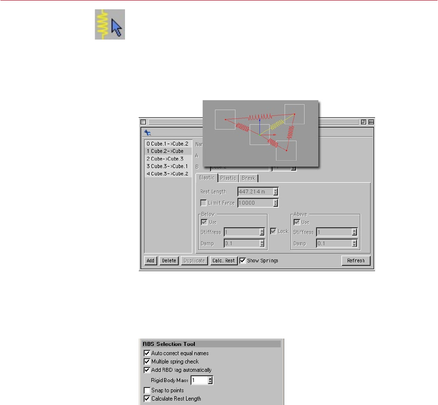
192 RIGID BODIES DYNAMICS
DYNAMICS RIGID BODIES 193
Using the Rigid Body Selection Tool
This tool is used for selecting springs in the viewport. To add a spring to the selection,
Shift-click the spring with the tool selected. To remove a spring from the selection,
Ctrl-click the spring. Selected springs are displayed red in the viewport. Selection
in the viewport is linked to selection in the spring list in the Rigid Springs dialog;
in other words, selecting springs in the viewport automatically selects them in the
spring list also and vice versa.
Spring selection: selection in the
viewport is linked to selection in
the Rigid Body Spring dialog.
You can also select springs
without using the Rigid Body
Selection tool. Simply click the
spring in the viewport to select
it. To add the spring to the
selection, Shift-click the spring.
To remove a spring from the
selection, Ctrl-click the spring.
In addition to allowing you to select springs, the Rigid Body Selection tool also lets
you re-attach springs in different positions. To do this, click-drag the end of the spring
that you want to re-attach from the old position to the new position.
Attribute manager settings
While the RBS Selection
Tool is selected, a number
of options will be available
in the Attribute manager.
While the RBS Selection Tool is selected, a number of options will be available in the
Attribute manager, including the ability to snap to points.

194 RIGID BODIES DYNAMICS
DYNAMICS RIGID BODIES 195
Auto Correct Equal Names
This option is enabled by default. If you draw a spring between two rigid bodies with
the option enabled, the names of the rigid bodies will be changed automatically to
ensure they are unique within the scope of the solver. For example, assuming there
are three rigid bodies in the solver all named Cube, when you draw a spring between
two of the bodies, they will be renamed Cube.1 and Cube.2. This automatic renaming
is advisable so that, when you later use the Rigid Springs dialog, it will be clear to
which objects each spring is attached.
Multiple Spring Check
When enabled, this option will prevent you from creating a spring where a spring
already exists between the two points.
Add RDB Tag Automatically, Rigid Body Mass
If this option is enabled when you draw a spring, Rigid Body Dynamic tags will be
assigned to the two objects that the spring is being attached to. The mass dened
under Rigid Body Mass will be assigned to the tags. The tags will not be created if
the objects already have Rigid Body Dynamic tags assigned.
Snap to Points
Enable this option if you want the cursor to snap to object points while you are
drawing the spring. If the option is disabled, the spring will snap to the mass centre
of the objects instead.
Calculate Rest Length
If Calculate Rest Length is enabled while you are drawing a spring, the Rest Length
of the spring will be set to the distance between its two attachment points. In other
words, the spring will be at rest between the two points, hence the spring will exert
no force.
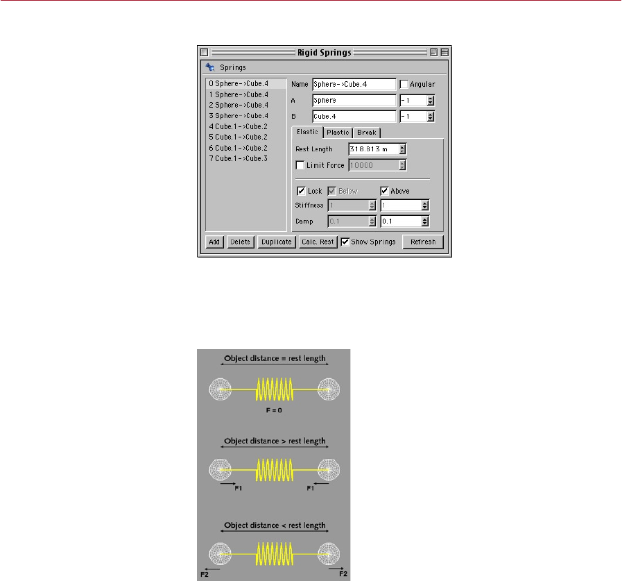
194 RIGID BODIES DYNAMICS
DYNAMICS RIGID BODIES 195
Elastic Tab
The options on this tab enable
you to dene the elastic
properties of the rigid body
spring.
Rest Length
The Rest Length denes the normal length of the spring, that is the length at which
the spring will exert no force. In the diagram below, the top spring is at its rest length
and hence it is exerting no force on the objects.
The Rest Length is decisive in
determining whether the spring
will push, pull or exert no force
on its attached objects.

196 RIGID BODIES DYNAMICS
DYNAMICS RIGID BODIES 197
If you were to attach two objects using a spring whose Rest Length value is less than
the distance between the two objects, the spring will be stretched because of this
and it will exert a force on the two bodies that will attempt to pull them towards the
rest length. Conversely, if the Rest Length value is greater than the distance between
the two attached objects, the spring will be compressed because of this and will
exert a force on the two objects that attempts to push them away from one another
and towards the rest length.
Limit Force
In some cases, the force exerted by a spring can become too great for the solver
object to process. Hence under Limit Force you can specify the maximum force that
the spring will be allowed to exert.
Lock
If enabled, this option will lock the Below values to be the same as the Above values.
Below
This option and the Stiffness and Damp parameters below it dene the spring’s
behavior when the spring is below its rest length (i.e. compressed). By default, these
settings are ghosted by the Lock option, which locks the Below parameters to the
same settings as the Above parameters. To be able to dene separate values for
compression, disable the Lock option.
Above
This value refers to the spring when it is above its rest length (stretched, that is). If
Above is enabled, the Stiffness and Damp values will be applied while the spring is
stretched. With the option disabled, the spring will be limp when stretched and it
will thus exert no force.
Stiffness
These two input boxes dene the stiffness of the spring for the Below and Above
options. The higher the value, the greater the force that will be exerted by the spring
when it is stretched or compressed. A stiff spring will be much harder to compress
or stretch than a weak spring.
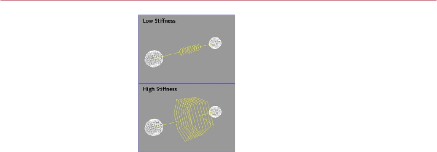
196 RIGID BODIES DYNAMICS
DYNAMICS RIGID BODIES 197
A spring’s Stiffness affects its
diameter in the viewport.
The Stiffness value of the spring is indicated in the viewport. The stiffer the spring,
the greater its diameter. The Stiffness also affects the spring’s rate of oscillation, with
a stiff spring tending to oscillate faster than a weak spring because of the greater
force that it exerts on the objects it is attached to. The time taken for an oscillation
in such a spring-mass system will also depend on the mass of the attached objects.
Damp
Like Stiffness, there are two input boxes. The left-hand input box denes the damping
for the Below option; the right-hand input box denes damping for the Above option.
All real springs will experience damping while oscillating due to resistance within their
material. Without damping, a spring would oscillate endlessly. For realistic damping,
set a value from 0.1 to 0.5.
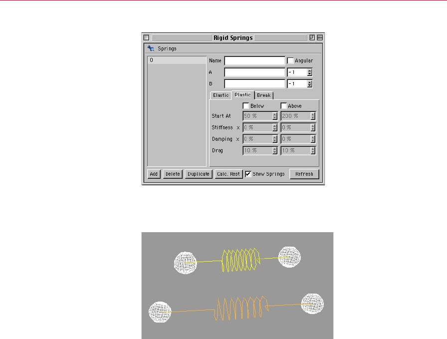
198 RIGID BODIES DYNAMICS
DYNAMICS RIGID BODIES 199
Plastic Tab
The options on the Plastic tab
enable you to dene at what
point a rigid body spring will
remain deformed.
When you stretch a spring past its elastic limit, the spring will become permanently
distorted — termed plastic deformation. On this tab, you can set the parameters that
will simulate plastic deformation for your virtual spring.
Above: A spring in the elastic state.
Below: The same spring, this
time in the plastic state. Springs
in the plastic state are shaded
orange in the viewport.
Using Below and Above, you can dene the plastic properties of the spring when
stretched and compressed. Keep in mind that a spring’s stiffness and damping will
change greatly between elastic deformation and plastic deformation.
Below
Enable this option if you want to dene the plastic properties of the spring (Start At,
Stiffness X, Damping X, Drag) when it is below its rest length (compressed, that is).
Above
When Above is enabled, you will be able to dene the plastic properties of the spring
(Start At, Stiffness X, Damping X, Drag) when it is above its rest length (stretched,
that is).

198 RIGID BODIES DYNAMICS
DYNAMICS RIGID BODIES 199
Start At
This denes the length at which plastic deformation will begin, specied as a
percentage of the Rest Length (Elastic tab). For example, if you enter a value of
200% and Rest Length = 10 m, plastic deformation will start when the spring is
20 m long.
Stiffness X
Use Stiffness X to set the stiffness of the spring for plastic deformation. The value
must be dened as a percentage of Stiffness (Elastic tab). For example, if you enter
a Stiffness X value of 10% and Stiffness = 5, the stiffness of the spring during its
elastic state will be 0.5.
Damping X
Damping X controls the strength of damping for the plastic state, dened as a
percentage of Damp (Elastic tab). For example, with Damping X set to 50% and Damp
set to 0.1, the damping during the plastic state will be 0.05.
Drag
This setting will ensure that the attached objects are damped while the spring is
undergoing plastic deformation. This can be thought of as a drag eld that affects
the two attached objects only.
Break Tab
The options on the Break tab
dene at what point a rigid
body spring will lose all of its
properties — literally break.
Like a real spring, Dynamics springs can be made to snap if you stretch them too
far. Before a real spring snaps, it will rst undergo elastic deformation followed by
plastic deformation.
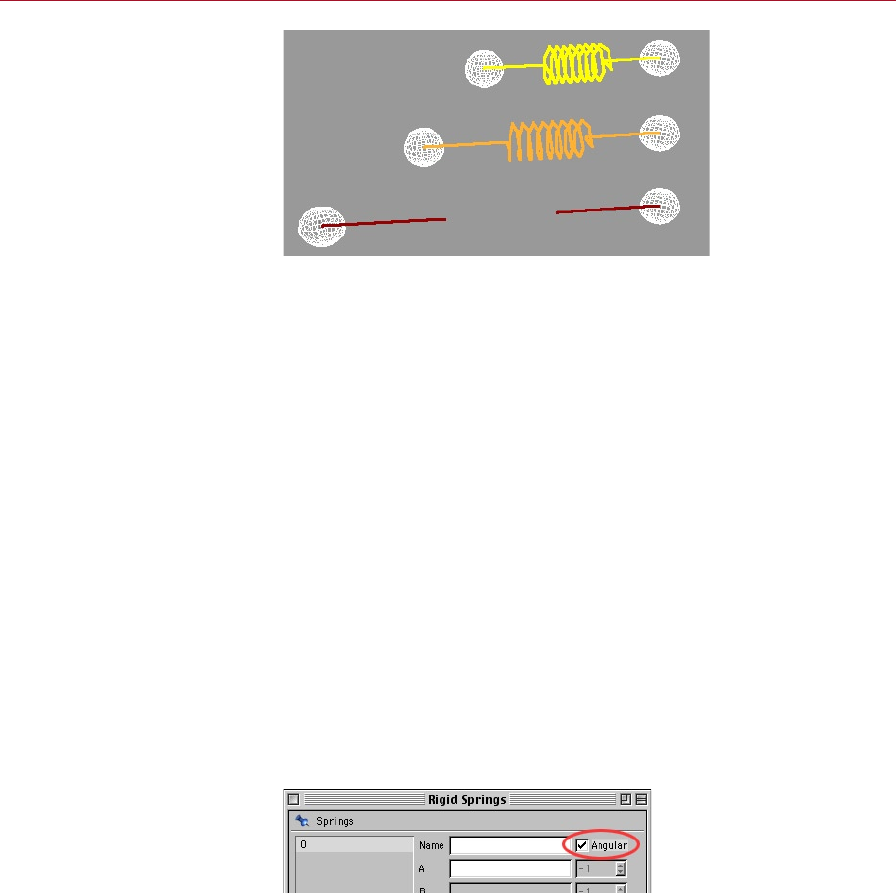
200 RIGID BODIES DYNAMICS
DYNAMICS RIGID BODIES 201
The sequence of events leading
to snapping: elastic deformation
(top), plastic deformation
(middle), snapping (below). A
broken spring is shaded red in
the viewport.
Once the spring has been broken, just as in real life it won’t be able to exert a force
on the attached objects any more.
For snapping to be possible, the
spring must have its plastic state
dened — that is, Below and/or
Above must be enabled on the
Plastic tab. However, you can, if
you wish, still have the spring
snap without it rst having to
undergo plastic deformation:
set the Start At parameters on
the Plastic tab and the Break tab
to the same value.
Below
Enable this option to allow the spring to break when compressed. Dene the breaking
point using the Start At parameter.
Above
Enable this option if the spring should break when stretched. Dene the breaking
point using the Start At parameter.
Start At
These two input boxes set the breaking point for the Below option (left-hand input
box) and the Above option (right-hand input box). Into the input boxes, enter the
breaking point as a percentage of the Rest Length (Elastic tab). For example, if Start
At is set to 300% and Rest Length is set to 200 m, the spring will snap once it reaches
600 meters in length.
Angular Springs
Angular springs — such as those used in old wristwatches — are springs that create
torque. Angular springs create rotational motion about the centre of mass. To dene
the spring to be angular, enable the Angular option.
Enable the Angular option to
dene the spring as angular
such as the type found in an old
wristwatch.
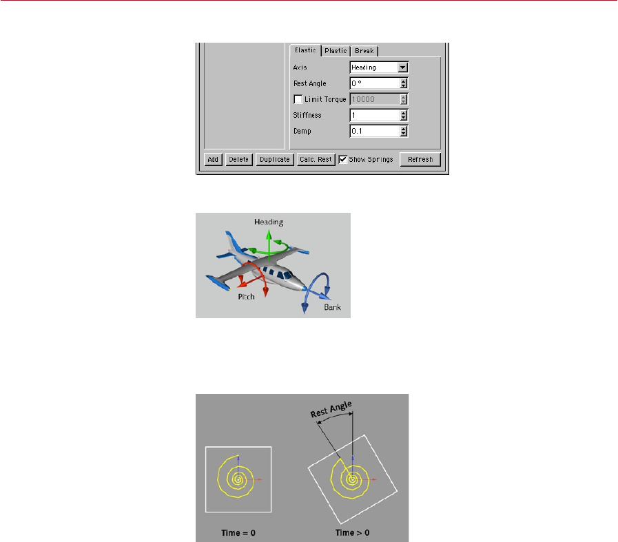
200 RIGID BODIES DYNAMICS
DYNAMICS RIGID BODIES 201
Elastic Tab
The options on this tab enable
you to dene the elastic
properties of an angular spring.
Axis
The Heading, Pitch and Bank
angles for an aeroplane.
Choose the axis of rotation: Heading, Pitch or Bank. For details on the HPB system,
please refer to your CINEMA 4D manual.
Rest Angle
The Rest Angle is the angle at
which the spring will exert no
force.
The Rest Angle is the angle at which the spring will exert no force. If you set the Rest
Angle to a value greater or less than 0, when you start the dynamics animation, the
spring and its object will rotate towards and then oscillate about the Rest Angle.
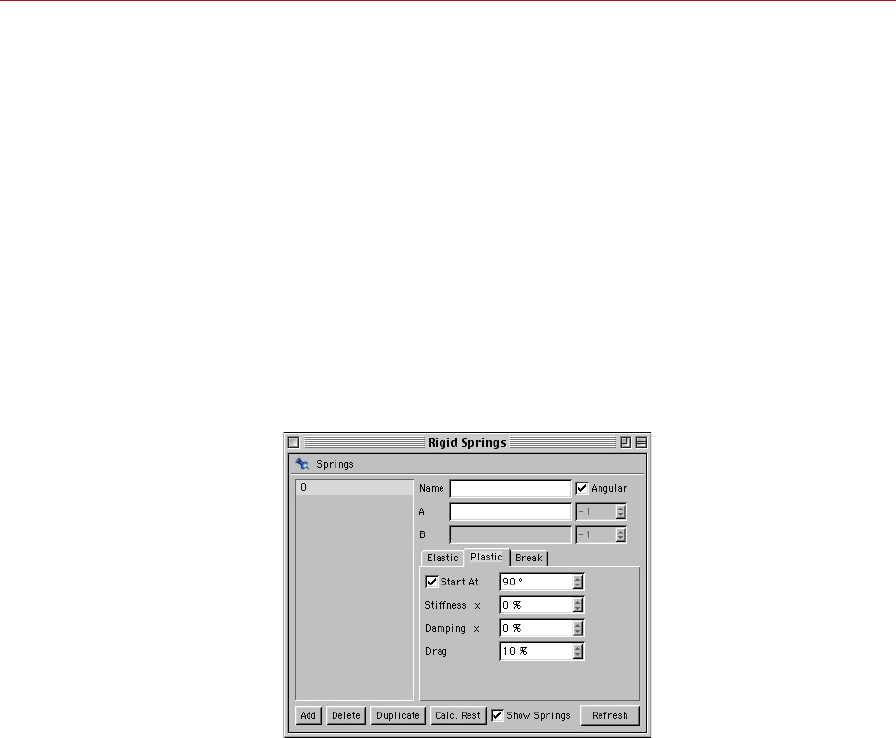
202 RIGID BODIES DYNAMICS
DYNAMICS RIGID BODIES 203
Limit Torque
Sometimes a spring can become so stretched that the massive force it exerts can no
longer be processed by the solver object. To prevent this from happening, enable the
Limit Torque option. Enter the maximum torque for the spring into the input box.
Stiffness
This value denes the stiffness of the spring; the spring constant, that is. A stiff spring
will exert more force than a weak spring, all other factors being equal. The greater
the Stiffness value, the more force the spring will exert at a given angle.
Damp
A real spring will always be subject to damping due to frictional forces in its material.
Without damping, an angular spring would never come to rest. Another good reason
for damping your Dynamics springs is that otherwise the springs will tend to gain
energy and rotate through a greater angle than they should.
Plastic Tab
The options on the Plastic tab
enable you to dene at what
point an angular spring will
remain deformed.
Angular springs share many of the characteristics of normal springs. As with a normal
spring, you can dene plastic behavior for the angular spring. The spring will become
permanently distorted once it has undergone plastic deformation. Keep in mind
that the stiffness and damping of a spring will vary greatly between its elastic state
and plastic state. A spring is shaded orange in the viewport when it is in the plastic
region.
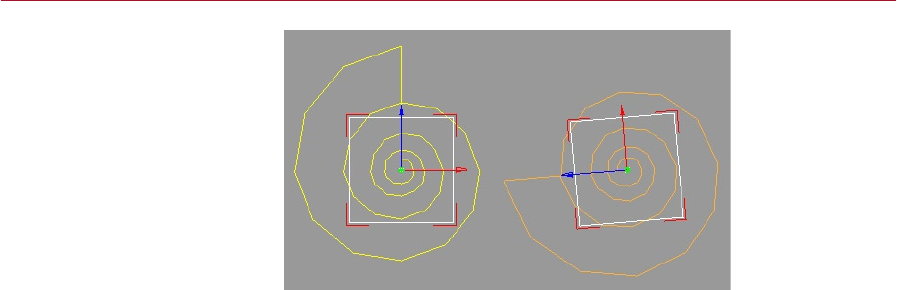
202 RIGID BODIES DYNAMICS
DYNAMICS RIGID BODIES 203
A spring in the plastic state is
shaded orange in the viewport.
Start At
The parameter denes the angle at which plastic deformation will begin. To switch
off plastic deformation, uncheck the box.
Stiffness X
This denes the stiffness of the spring during the plastic state, specied as a
percentage of Stiffness (Elastic tab). For example, if you set Stiffness X to 20% and
Stiffness = 1, the stiffness during the plastic state will be 0.2.
Damping X
Damping X controls the strength of damping during the plastic state, as a percentage
of Damp (Elastic tab). For example, with Damping X set to 50% and Damp set to 0.1,
the damping in the plastic region will be 0.05.
Drag
This setting will ensure that the attached objects are damped also while the spring
is undergoing plastic deformation. This can be thought of as a drag eld that affects
the two attached objects only.
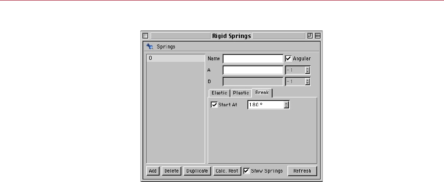
204 RIGID BODIES DYNAMICS
DYNAMICS RIGID BODIES 205
Break Tab
The options on the Break
tab dene at what point an
angular spring will lose all of its
properties — literally break.
Start At
Start Above denes the angle at which the spring will break. Once the spring has been
broken, it will no longer be able to exert a force on the attached object.
Springs Menu
Add Spring
Adds an undened spring.
Delete Spring
Deletes all selected springs.
Duplicate Spring
Duplicates the selected spring. You can attach any number of springs between two
rigid bodies. However, only one of the springs will be visible in the viewport. Works
only when one spring is selected.
Calculate Rest Length
Sets the Rest Length of all selected springs to their current lengths.
Close
Closes the dialog.

204 RIGID BODIES DYNAMICS
DYNAMICS RIGID BODIES 205
Initialization
Initialization is used to set the starting state of the dynamics objects. Two commands
are available for this: Initialize Object and Initialize All Objects.
Initialize Object
This command — accessed from main menu (Plugins > Dynamics) sets the starting
position of the selected object to its current position.
Suppose you have switched off the Solver object momentarily so that you can move
a rigid body. Having moved the rigid body, you then switch on the solver having
forgotten to use the Initialize Object command rst. The body will revert to its
previous position.
Initialize All Objects
The same applies to this function as described above for Initialize Object, with the
exception that here the starting positions of all rigid bodies and soft bodies will be
set to their current positions.
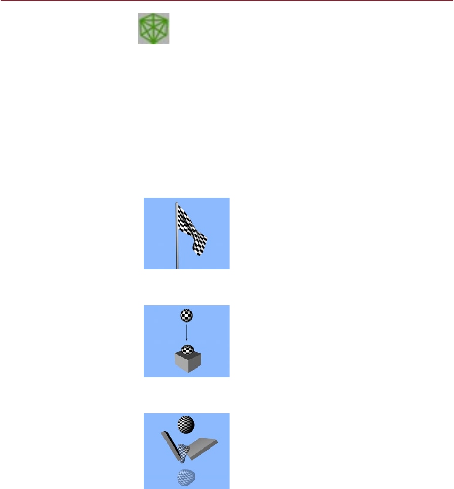
DYNAMICS SOFT BODIES 207
To know how and when you should use a soft body, it is important to be
aware of the main differences between rigid bodies and soft bodies. A
rigid body is a solid, polygonal object whose shape does not alter over
time. Rigid bodies are able to collide with each other and they can be attached to
one another using springs. Unlike soft bodies, rigid bodies can be given a starting
angular velocity.
A soft body is a collection of points that are linked together with springs. The shape
of a soft body can change over time but, unlike a rigid body, a soft body cannot
be given a starting angular velocity. This is because a soft body is built from many
masses — a mass for each point of the soft body object. These masses have no initial
values for rotation and hence cannot rotate when animated other than through their
interactions with other objects.
Soft bodies are ideal for simulating of turbulent surfaces such as a ag in the wind
or the clothes on a moving character. Because points in the soft body are linked via
springs, a force that is exerted on one point will spread out dynamically.
Soft bodies are ideal for
simulating cloth such as ags.
Soft bodies can also simulate objects that deform during a collision such as a rubber
ball bouncing on a hard surface.
Here, a soft body has been used
for the rubber ball, enabling the
ball to squash realistically when
hitting the block.
Soft bodies have another interesting property: they can squeeze through tight gaps
provided they use a low Stiffness setting!
A soft body squeezing through
a tight gap thanks to its low
Stiffness setting.
Soft Bodies
Soft bodies are used for
simulating objects that change
shape over time such as a moving
character’s clothing or a bouncing
rubber ball that squashes as it hits
a hard surface.
When using soft bodies, set
the solver object’s Integration
Method to Softbody.
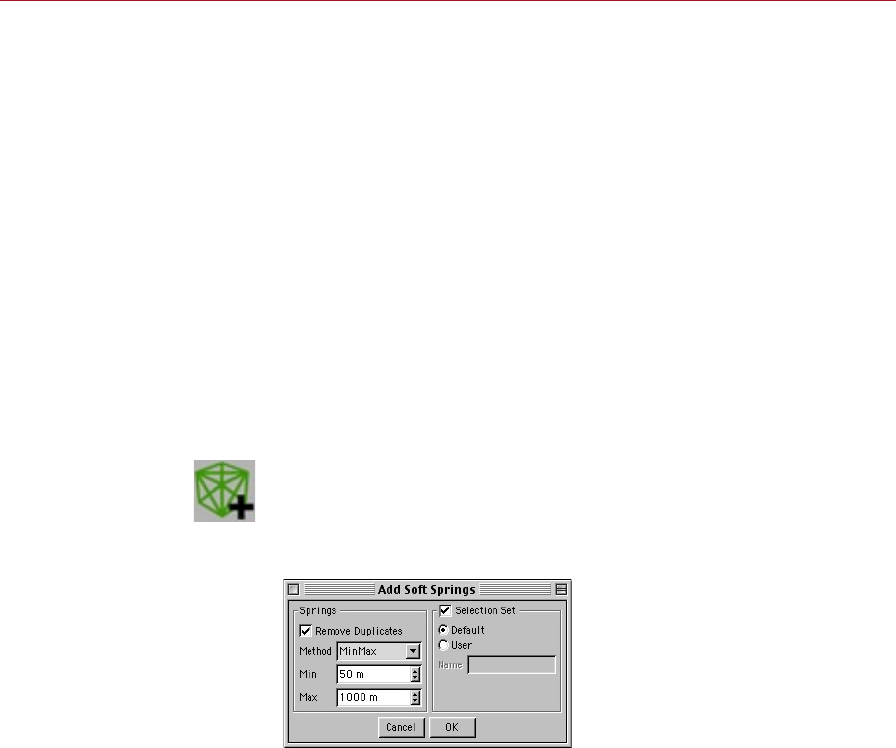
208 SOFT BODIES DYNAMICS
DYNAMICS SOFT BODIES 209
Creating a Soft Body
To create a soft body, start with a spline object or polygon object of the desired shape
and proceed as follows (note that collision detection requires geometry and hence
collision detection is not possible when using splines):
Create a solver object by selecting Plugins > Dynamics > Solver Object from the main
menu. Make the polygon or spline object a child of the solver object.
Assign a Soft Body Spring tag to the would-be soft body by selecting File > Dynamics
Tags > Soft Body Spring (Object manager menu). The Soft Body dialog will open.
Now the soft body has been created, but as of yet it has no springs. To add the springs,
select Plugins > Dynamics > Add Soft Springs from the main menu. In the dialog
that opens, set Method to the desired spring type and click OK to add the springs.
The soft body is now be ready to be used.
If points are selected when you add the springs, the springs will be added to the
selected points only; otherwise, if no points are selected, the springs will be added
to all points.
The Add Soft Springs Dialog
This dialog enables you to add springs to the soft body. There are two places where
you can access the dialog. Either select Plugins > Dynamics > Add Soft Springs from
the main menu or select Springs > Add Soft Springs from the Soft Body dialog. You
will be able to access and edit the springs later using the Soft Body dialog.
When you create a soft body,
initially it has no springs. Using
this dialog, you can add the
required springs.
If points are selected when you
add the springs, the springs
will attach selected points only;
otherwise, a layer of springs will
be added that covers the entire
soft body.
The springs will be attached to points in the soft body using one of several attachment
methods. For example, with the Structural method, each point will be connected to
its neighboring points, providing a supportive structure to the body.
Remove Duplicates
When enabled, this option will delete duplicate springs. A duplicate spring is a spring
that attaches the same two points as another spring.
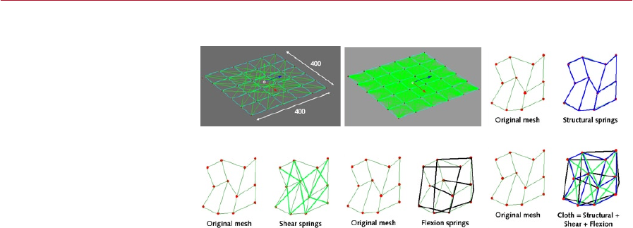
208 SOFT BODIES DYNAMICS
DYNAMICS SOFT BODIES 209
Method
The MinMax diagram shows a
plane that is 400 units by 400
units in size. Min has been set
to 380, Max has been set to
400. Subsequently each point
is connected to points that are
from 380 to 400 units away.
MinMax All Structural
Shear Flexion Cloth
This denes how the springs should be attached to the soft body’s points.
MinMax
Connects each point to all other points within the distance range specied under
Min and Max. For example, if you set Min to 40 m and Max to 60 m, each point will
be connected to points that are from 40 m to 60 m away.
All
Connects each point to all other points. Use All with caution, it will create an enormous
number of springs if the soft body has a large number of points.
Structural
Connects each point to its neighboring points (the points it shares polygon edges
with). This attachment method will help the soft body to maintain its shape, hence
most soft bodies should have a layer of Structural springs.
Shear
Connects the points in a way that will stabilize four-sided polygons. Without this
stabilization, the four-sided polygons could collapse.
Flexion
Connects each point to the neighbor of its neighbor. Flexion springs are ideal for
giving the soft body a degree of stiffness.
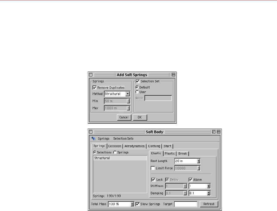
210 SOFT BODIES DYNAMICS
DYNAMICS SOFT BODIES 211
Cloth
Connects the points using a combination of Structural, Shear and Flexion springs. Use
Cloth if the soft body should simulate clothes, a ag or another type of cloth.
Selection Set
If Selection Set is enabled, the springs will be added as a selection. After the springs
have been added, the selection will then appear in the list area of the Soft Body
dialog, under Selections. See the following two diagrams.
Selection Set enabled. The
selection, named Structural,
will later appear in the list area
of the Soft Body dialog, under
Selections.
The Structural selection in the
list area of the Soft Body dialog.
Default
When Default is enabled, the spring selection will be named after the Method setting.
For example, if Method is set to Structural, the name will be Structural.
User
Enable this option if you want to enter a name for the selection under Name.
Name
This input box will become enabled when the User option is enabled. Enter your own
name for the selection here.
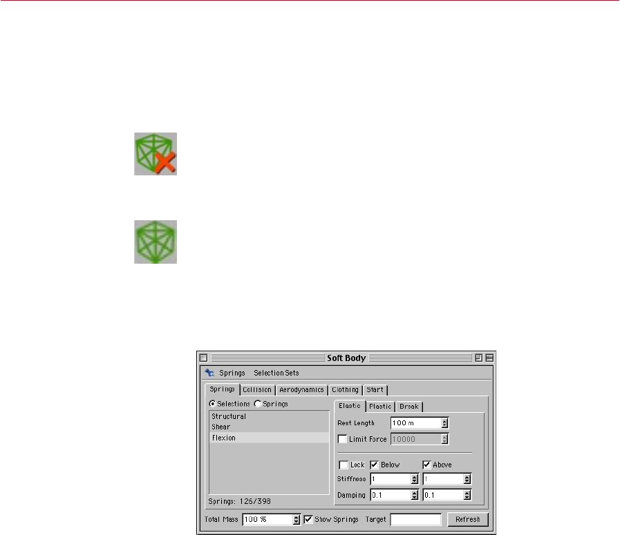
210 SOFT BODIES DYNAMICS
DYNAMICS SOFT BODIES 211
Advice on Adding Springs
Due to the complexity and number of springs in a typical soft body, fail-safe advice
is difcult to offer. In general, to simulate a very light material such as a silk cloth
uttering in the wind, use just two layers: Structural and Shear. For other types of
cloth, Cloth springs are usually a good choice. Even a rubber ball that distorts when
it bounces can be simulated with Cloth springs.
Delete Soft Springs
This function deletes all selected springs and all selected spring selections. You can
access the function from two different places: either from the Plugins > Dynamics
sub-menu (main menu), or from the Springs menu in the Soft Body dialog.
Soft Body Dialog
This dialog is the management centre for soft body springs. Here you have access the
springs and spring selections and here you can modify their parameters. In addition,
you can also set parameters that relate to the soft body as a whole such as its starting
velocity and aerodynamics properties.
Springs Tab
By creating different layers
of springs with their own
properties you can simulate
most types of materials.
The Springs tab gives you access to the list area where you can select individual
springs or selections. It also allows you to access the tabs that dene the elastic and
plastic deformation properties of the selected springs. You also have access to the
Break tab, should you wish for the springs to be able to snap.
The large area in the left half of the Soft Body dialog is the list area. This is where
spring selections or individual springs will be shown depending on whether the
Selections option or the Springs option respectively is enabled.
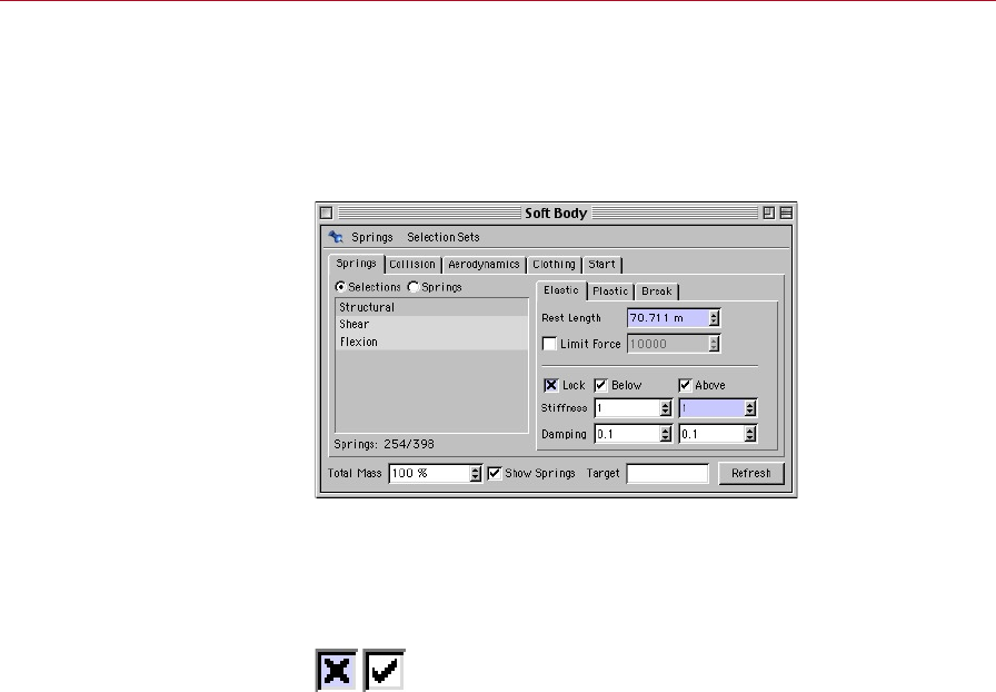
212 SOFT BODIES DYNAMICS
DYNAMICS SOFT BODIES 213
You can select more than one spring or spring selection at a time (Shift-click in the
list to add to the selection; Ctrl-click to subtract from the selection).
When you edit the parameters in the dialog with several springs selected, the new
settings will be applied to all of the selection. When several springs are selected,
parameters that have different values for the selected springs will be highlighted in
light blue.
When several springs are
selected, parameters whose
values differ within the selection
will be highlighted in light blue.
A highlighted cross in an
option means that the option
has different settings for the
selected springs. If you click the
option the cross will change into
a check and the option will be
enabled for all selected springs.
If you change the setting of a highlighted parameter, the new value will be assigned
to all selected springs and the highlighting removed.
Likewise, if you enter a value into a parameter that is not highlighted, the new value
will be assigned to all selected items.
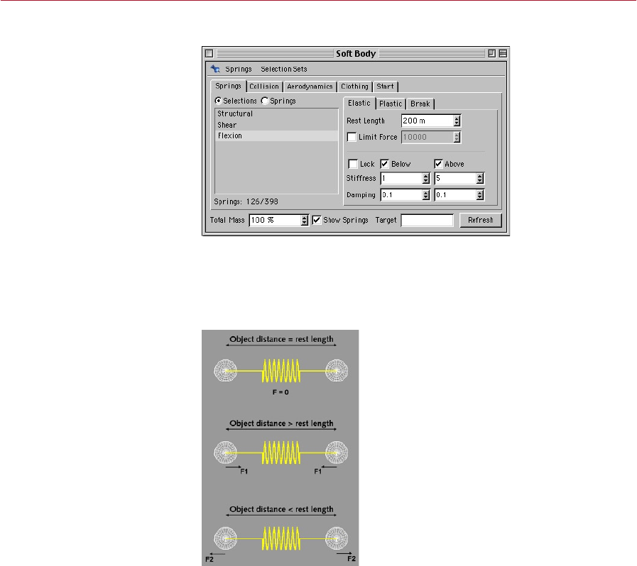
212 SOFT BODIES DYNAMICS
DYNAMICS SOFT BODIES 213
Elastic Tab
On this tab, dene the elastic
deformation behavior of
the selected springs such as
strength of damping.
Rest Length
The Rest Length denes the normal length of the spring; that is, the length at which
the spring will exert no force. In the diagram below, the top spring is at its rest length
and hence it is exerting no force on the objects.
The Rest Length is decisive in
determining whether the spring
will push, pull or exert no force
on its attached objects.
If you attach two objects using a spring whose Rest Length value is less than the
distance between the two objects, the spring will be stretched because of this and
will exert a force on the two bodies that attempts to pull them towards the rest
length. Conversely, if the Rest Length value is greater than the distance between the
two attached objects, the spring will be compressed because of this and will exert
a force on the two objects that attempts to push them away from one another and
towards the rest length.
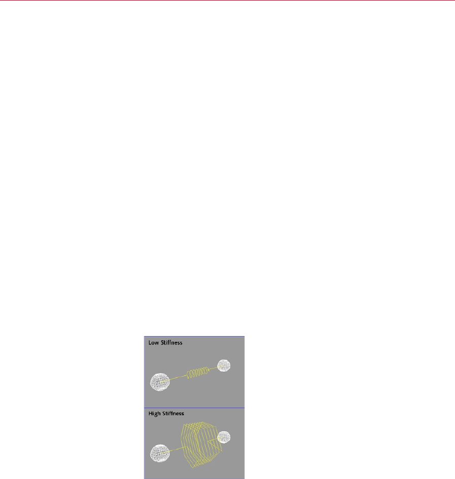
214 SOFT BODIES DYNAMICS
DYNAMICS SOFT BODIES 215
Limit Force
In some cases, the force exerted by a spring can become too great for the solver
object to process. Hence under Limit Force you can specify the maximum force that
the spring will be allowed to exert.
Lock
When enabled, this option will lock the Below values to be the same as the Above
values.
Below
This option and the Stiffness and Damping parameters below it dene the spring’s
behavior when the spring is below its rest length (i.e. compressed). By default, these
settings are ghosted by the Lock option, which locks the Below parameters to the
same settings as the Above parameters. To be able to dene separate values for
compression, disable the Lock option.
Above
This value refers to the spring when it is above its rest length (stretched, that is). If
Above is enabled, the Stiffness and Damping values will be applied while the spring
is stretched. With the option disabled, the spring will be limp when stretched and
it will thus exert no force.
Stiffness
These two input boxes dene the stiffness of the spring for the Below and Above
options. The higher the value, the greater the force that will be exerted by the spring
when it is stretched or compressed. Also, like a real spring, a stiff spring will be much
harder to compress or stretch than a weak spring.
A spring’s Stiffness affects its
diameter in the viewport.
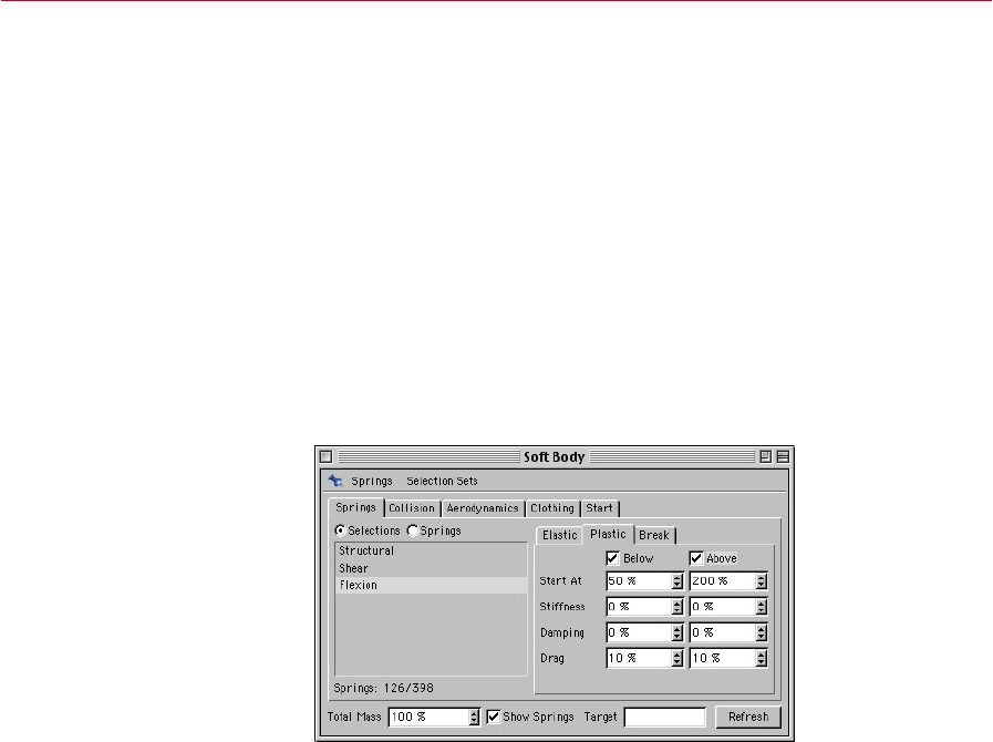
214 SOFT BODIES DYNAMICS
DYNAMICS SOFT BODIES 215
The Stiffness value of the spring is indicated in the viewport: the stiffer the spring is,
the greater its diameter will be.
The Stiffness also affects the spring’s rate of oscillation, with a stiff spring tending
to oscillate faster than a weak spring because of the greater force that it exerts on
the objects it is attached to.
Damping
Like Stiffness, there are two input boxes. The left-hand input box denes the
damping for the Below option; the right-hand input box denes damping for the
Above option.
All real springs will experience damping while oscillating due to resistance within their
material. Without damping, a spring would oscillate endlessly. For realistic damping,
enter a value from 0.1 to 0.5.
Plastic Tab
Using these parameters, you can
dene how the selected springs
will behave when undergoing
plastic (that is, permanent)
deformation. For example,
you can dene how much
the spring must be stretched
or compressed before it will
undergo plastic deformation.
When you stretch a spring past its elastic limit, the spring will become permanently
distorted — termed plastic deformation. On this tab, you can set the parameters that
will simulate plastic deformation for your virtual spring.

216 SOFT BODIES DYNAMICS
DYNAMICS SOFT BODIES 217
Above: A spring in the elastic
state. Below: The same spring,
this time in the plastic state.
Springs in the plastic state are
shaded orange in the viewport.
Using Below and Above, you can dene the plastic properties of the spring when
compressed and when stretched. Keep in mind that a spring’s stiffness and damping
will change greatly between elastic deformation and plastic deformation.
Below
Enable this option if you want to dene the plastic properties of the spring (Start At,
Stiffness, Damping, Drag) when it is below its rest length (compressed, that is).
Above
When Above is enabled, you can dene the plastic properties of the spring (Start At,
Stiffness, Damping, Drag) when it is above its rest length (stretched, that is).
Start At
This denes the length at which plastic deformation will begin, specied as a
percentage of the Rest Length (Elastic tab). For example, if you enter a value of
200% and Rest Length = 10 m, plastic deformation will start when the spring is
20 m long.
Stiffness
Use Stiffness to set the stiffness of the spring for plastic deformation. The value
must be dened as a percentage of Stiffness (Elastic tab). For example, if you enter
a Stiffness value of 10% (Plastic tab) and Stiffness = 5 (Elastic tab), the stiffness of
the spring during its elastic state will be 0.5.
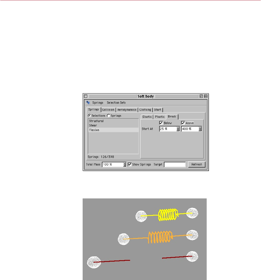
216 SOFT BODIES DYNAMICS
DYNAMICS SOFT BODIES 217
Damping
Damping controls the strength of damping for the plastic state, dened as a
percentage of Damping (Elastic tab). For example, with Damping here set to 50%
and Damping on the Elastic tab set to 0.1, the damping during the plastic state will
be 0.05.
Drag
This setting will ensure that the attached objects are damped while the spring is
undergoing plastic deformation. This can be thought of as a drag eld that affects
the two attached objects only.
Break Tab
The break tab is used to specify
if - and if so, at what length - the
selected springs will break.
Like a real spring, Dynamics springs can be made to snap if you stretch them too
far. Before a real spring snaps, it will rst undergo elastic deformation followed by
plastic deformation.
The sequence of events leading
to snapping: elastic deformation
(top), plastic deformation
(middle), snapping (bottom). A
broken spring is shaded red in
the viewport.
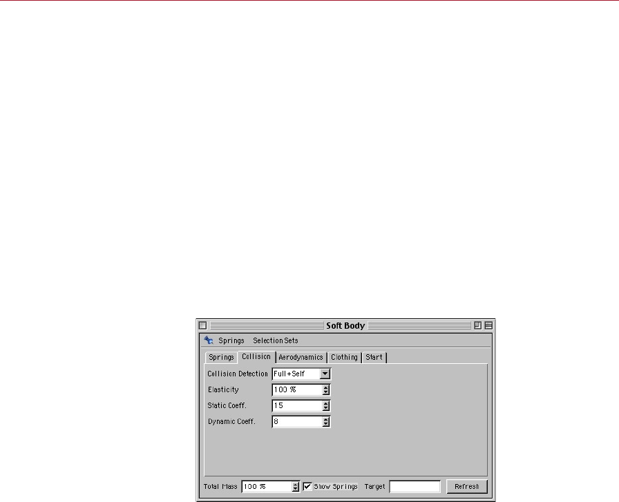
218 SOFT BODIES DYNAMICS
DYNAMICS SOFT BODIES 219
Once the spring has been broken, it will no longer be able to exert force on the
attached objects.
For snapping to be possible, the
spring must have its plastic state
dened — that is, Below and/or
Above must be enabled on the
Plastic tab. However, you can, if
you wish, still have the spring
snap without it rst having to
undergo plastic deformation:
set the Start At parameters on
the Plastic tab and the Break tab
to the same value.
Below
Enable this option to allow the spring to break when compressed. Dene the breaking
point using Start At.
Above
Enable this option if the spring should break when stretched. Dene the point at
which the spring should break under Start At.
Start At
These two input boxes set the breaking point for the Below option (left-hand input
box) and the Above option (right-hand input box). Into the input boxes, enter the
breaking point as a percentage of the Rest Length (Elastic tab). For example, if Start
At is set to 300% and Rest Length = 200 m, the spring will snap when it is 600 m
long.
Collision Tab
Collisions of soft bodies
is slower than rigid body
collisions; using as few springs
as possible will enable you to
reduce the pressure on your
solver, helping to speed up
the overall processing of the
dynamics.
Collision detection is not just for rigid bodies. With this tab, you can switch on collision
detection for the soft body. Unfortunately there are no tricks for soft body collisions
that will help you to save processing time. Here, a proxy collision object is of no use.
Collision detection with soft bodies is always a processor-intensive affair.
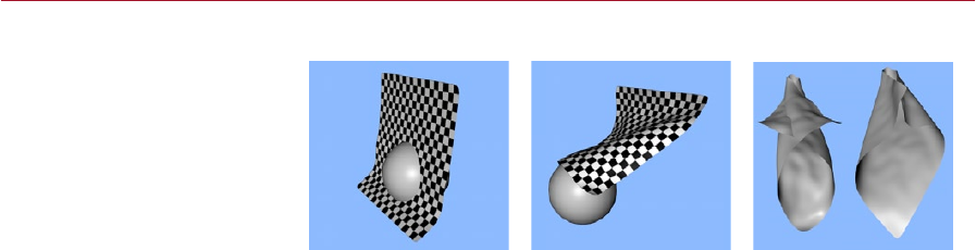
218 SOFT BODIES DYNAMICS
DYNAMICS SOFT BODIES 219
Collision Detection
None Full Full (left), Full+Self (right)
This denes the collision mode: None, Full or Full+Self.
None
Switches off collision detection.
Full
Checks each point for collision with other bodies but does not check for self collision.
This is suitable for draping cloth over an object.
Full+Self
Checks each point for collision with other bodies and also checks for self collision.
Use this setting if the soft body would otherwise intersect itself. One example is a
ag in a strong wind.
Elasticity
This value denes the percentage of energy that the soft body will retain following
a collision. An Elasticity setting of 0% would cause the soft body to halt suddenly
during the collision while a value of 100% would see the soft body rebound.
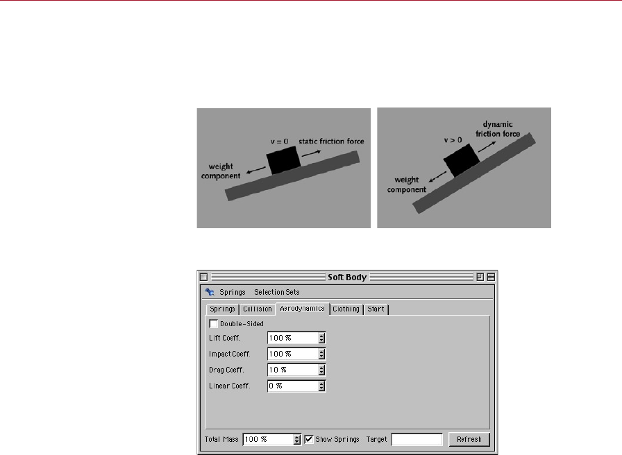
220 SOFT BODIES DYNAMICS
DYNAMICS SOFT BODIES 221
Static Coeff. Dynamic Coeff.
When two bodies are in contact, friction will exist between the bodies. This will be
static friction if the bodies are at rest, or dynamic friction is one body is sliding over
the other. Static friction should always greater than dynamic friction: more energy
is required to get a body moving than is required to keep it moving.
Left: The block’s weight
component down the incline is
not great enough to overcome
static friction. Hence the block
is not sliding. Right: The incline
of the ramp has been increased
and the block is now sliding
down the ramp. Static friction
having been overcome, the
block is now being resisted
instead by the lesser force of
dynamic friction.
Aerodynamics Tab
Material soft bodies generally
consist of a deformed plane;
using the Double-Sided option
will give a more realistic
movement with the wind.
The parameters on the soft body’s Aerodynamics tab relate to those dened in the
wind force eld’s dialog. For example, if Frontal Coeff. is set to 120% in the Wind
dialog and 50% here in the Soft Body Spring tag, the effective Frontal Coeff. will
be 60%.
Double-Sided
When this option is disabled — the default setting — the wind will affect only those
polygons whose surface normals are facing the wind. If you enable the option, the
wind will exert its force on all polygons regardless of the direction in which their
surface normals are pointing. Only enable the Double-Sided option if your object has
no thickness and Lift Coeff. is set to 0.
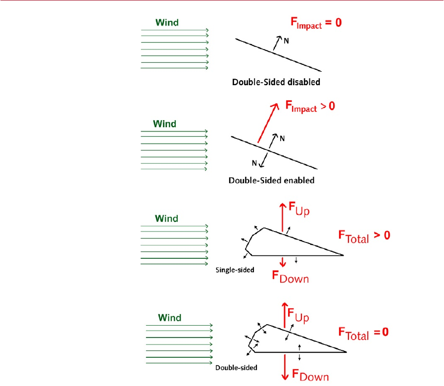
220 SOFT BODIES DYNAMICS
DYNAMICS SOFT BODIES 221
Double-Sided disabled. Since the
normal is facing away from the
wind, the wind is unable to exert
a force on the surface.
Double-Sided enabled. This
guarantees that a normal will
face the wind and hence the
wind is now able to exert a force
on the surface.
Double-Sided disabled. The wing
is experiencing a lifting force.
Double-Sided enabled, causing
equal and opposite forces
for each surface and hence
no resultant force. For closed
polygons, Double-Sided should
be disabled.
Lift Coeff.
This setting denes the strength of lift. When an airstream passes over a surface,
the air pressure will drop. The faster this airstream, the lower the pressure. When
designing a wing, the wing must be shaped so that the airstream will pass over one
wing surface more quickly than over the other wing surface. This will create a pressure
gradient, causing the wing to experience a lifting force.
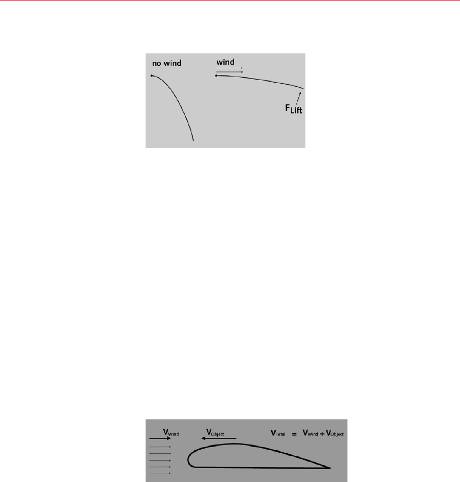
222 SOFT BODIES DYNAMICS
DYNAMICS SOFT BODIES 223
If you were to hold out a piece of paper and blow along its top edge, the airstream
would create lift — as the airstream passes over the paper, it is lifted up so that it is
at in the airstream with equal air pressure above and below.
A practical example of lift.
Blow across a hanging piece of
paper and the airstream will
create a lift force that will move
the paper into line with the
airstream.
Occasionally, paradoxical situations may arise such as motion that heads into the
wind. In such a case you should reduce the Lift Coeff. in one of two places. You can
reduce the parameter either in the Wind eld or the Soft Body tag. The latter is usually
preferable since it enables you to adjust the lift for a uncooperative object without
affecting the ight of the other objects.
Impact Coeff.
The Impact Coeff. value determines the strength of the air force that will be exerted
on body surfaces that face the wind. The strength of the impact force is proportional
to the surface area facing the wind and the relative velocity of the body compared
to the wind.
Drag Coeff.
When air streams over a body, small eddies will beat against the body’s surfaces,
causing deceleration. The Drag Coeff. parameter denes the strength of this effect.
This decelerating effect is usually minor but occasionally it can have a telling inuence
on the object’s motion.
Linear Coeff.
This setting relates to linear velocity, which plays a part in an object’s motion in the
wind force eld. However, it is not just the wind’s velocity that needs to be taken
into account, but the object’s velocity also.
The velocity will affect an
object’s behavior in wind. The
effective velocity that will be
considered is the sum of the
wind’s velocity and the object’s
velocity.
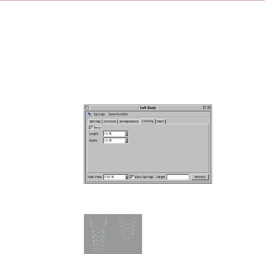
222 SOFT BODIES DYNAMICS
DYNAMICS SOFT BODIES 223
Example 1
An aeroplane is taking off at 100 km/h and heading into a wind of 50 km/h. The
relative wind velocity that is affecting the wing’s surface is 150 km/h.
Example 2
A plane is taking of at 100 km/h with a following wind of 50 km/h. Hence the relative
wind velocity is just 50 km/h. This highlights the reason why aeroplanes will take off
from various runways according to the direction of the wind.
Linear Coeff. denes the strength of this effect for linear motion. For a realistic effect,
leave Linear Coeff. in the Wind dialog set to 100% but set Linear Coeff. here in the
Soft Body dialog to a value from 1% to 10%.
Clothing Tab
Using this tab, you can make the
springs relax for a much better
simulation of cloth.
In the diagram, two cloths are
hanging from their top corner
points in a gravity force eld.
The Relax option has been
disabled for the cloth on the
left. The whole mass of the
soft body is hanging from four
springs that are being stretched
accordingly. As a result, the left
cloth is behaving more like soft
rubber than cloth. With the cloth
on the right, the Relax option
has been enabled, allowing a
more natural simulation of cloth.
Relax
Enable this option if the soft body should be cloth-like. This works by relaxing the
springs, as shown in the diagram below.
Length
Denes the length at which the springs will begin to relax. For example, if Length is
set to 10%, springs that are 10% longer than their Rest Length will be relaxed.
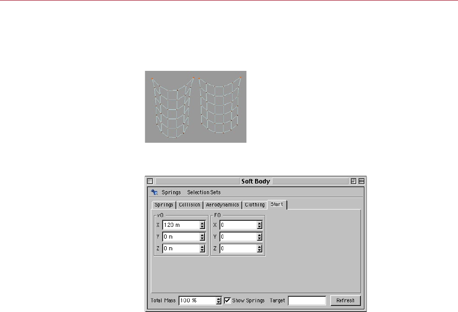
224 SOFT BODIES DYNAMICS
DYNAMICS SOFT BODIES 225
In the diagram, two soft bodies
are hanging from their top
corner points in a gravity eld.
The soft body on the right is
using a high Depth value and so
the force is being shared fairly
evenly by its springs. Contrast
this to the uneven stretching in
the left soft body, which is using
a low Depth value.
Depth
The higher this value, the more even the relaxation of the springs inside the soft body.
Forces exerted on the most strained springs will be spread among the surrounding
springs. A higher value means a wider distribution of the exerted forces.
Start Tab
This tab enables you to dene
a starting velocity for the soft
body.
v0
Denes the starting velocity (X, Y, Z) of the soft body.
F0
Denes a starting force (X, Y, Z) that will be exerted during the rst frame of the
animation only.
Total Mass
Initially, each point in a soft body will have a mass of 1. Using this parameter, you
can change the total mass of the points.
Suppose you want to create a ag in the wind, but rather than apping as intended,
the ag is hanging limply. Although you could correct this by adjusting the parameters
in the Wind dialog, it is easier to reduce the Total Mass of the ag’s points.
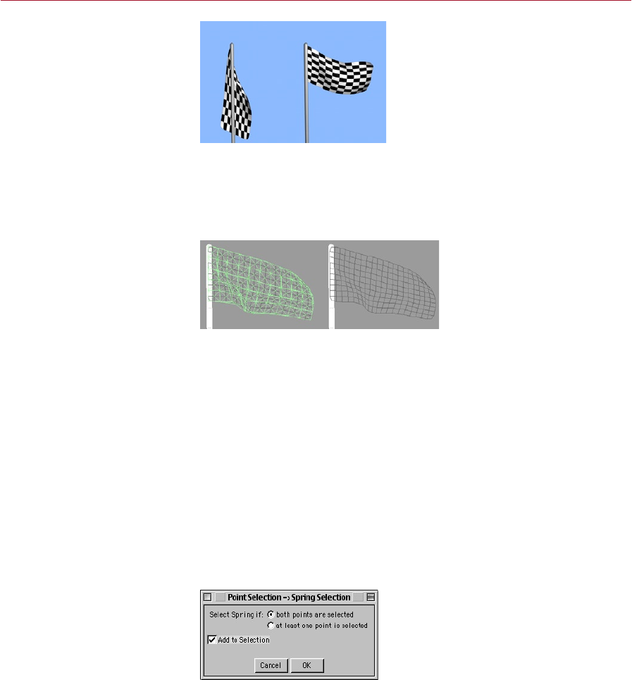
224 SOFT BODIES DYNAMICS
DYNAMICS SOFT BODIES 225
Two ags in the same wind force
eld. Left: high Total Mass value;
right: low Total Mass value.
A higher mass is synonymous with a higher inertia. A soft body with a large inertia will be
stiffer and more sluggish. For example, a silk cloth should have a lower Total Mass than
a sail (unless you prefer to adjust the motion using the aerodynamics parameters).
Show Springs
Show Springs enabled (left ag)
and disabled (right ag).
Controls whether springs are displayed in the viewport.
Springs Menu
Add Soft Springs
Opens the Add Soft Springs dialog, described earlier in this chapter.
Delete Soft Springs
Deletes all selected springs and all selected spring selections. You can access the
function from two different places: from here or from the Plugins > Dynamics menu
of the main menu.
Point Selection -> Spring Selection
Converts an existing point selection into a spring selection. After selecting the
command, the following dialog will open:
Using this dialog, you can select
springs from an existing point
selection.
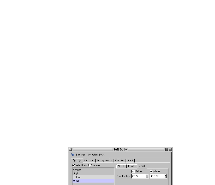
226 SOFT BODIES DYNAMICS
DYNAMICS SOFT BODIES 227
The rst option, Select Spring If Both Points Are Selected, will select springs that have
both attachment points selected.
Select Spring If At Least One Point Is Selected will select springs that have one or
both points selected.
Enable Add To Selection if you want to add the springs to the current selection.
Select All
Selects all the springs in the list area.
Deselect All
Deselects all springs.
Invert Selection
Inverts the selection. Selected springs will become deselected and deselected springs
will become selected.
Close
Closes the Soft Body dialog.
Selection Sets Menu
Save Spring Selection
Saves an existing spring selection under a name of your choosing. This is the name
that will be shown in the list area.
Here, the user has clicked the
spring selection called Below.
Note how Other is highlighted
in blue. This indicates that one
or more springs in the Below
selection are also present in the
Above selection.
Rename
Renames a spring selection.
Delete
Deletes a spring selection.
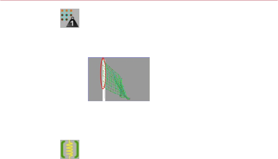
226 SOFT BODIES DYNAMICS
DYNAMICS SOFT BODIES 227
Set Soft Mass
You can reach this important function plugin from the Plugins > Dynamics menu of
the main menu. Set Soft Mass allows you to dene the mass of individual soft body
points. In particular, this is useful for xing some of the points in place — set the mass
of the points you want to x to 0. As previously mentioned in this manual, points and
bodies that have a mass of 0 will not be animated by the dynamics engine.
A soft body ag in a wind force
eld. The six left-most points of
the ag have been given a mass
of 0. As a result, these six points
are being ignored by the wind
whereas the rest of the soft
body points are apping.
Set Soft Mass is also useful for varying the mass for specic points. This can help you
to tweak the animation behavior for important parts of the soft body. Note that you
can animate soft body points of zero mass using keyframes; the keyframed points
will pull the other points along.
Initialize Soft Rest Length
Sets the Rest Length of each spring in the soft body to its current length. The command
is accessed from the Plugins > Dynamics menu of the main menu.
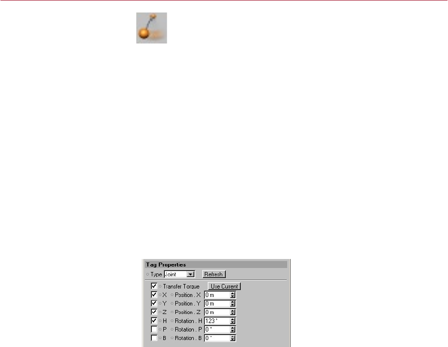
DYNAMICS CONSTRAINTS 229
Constraints are used to restrict the motion of objects. Using constraints
you can x the position of a rigid body to a particular axis or combination
of axes. For example, you can constrain a rigid body to move along the Z
axis only. You can also x the rotation of the rigid body to a particular angle and
you can link rigid bodies together. Many real objects are constrained in one way
or another. A pendulum rotates about its pivot point only. A link in a chain has its
movement restricted by the other links. The sails of a windmill turn in the wind while
the building itself remains stationary. All of this motion and more can be achieved
with the help of constraints.
The Constraint Tag
Using this tag you can dene how the rigid body should be constrained. Note that
you should place the rigid body in a position within the constraints, otherwise the
rigid body may take several animation frames to reach the required position. The
settings displayed in the Attribute manager for the Constraint tag will vary depending
on which type of constraint you’ve specied using the Type parameter. You can set
Type to Joint, Velocity or Motor.
Joint
Point to Point
If Type is set to Joint, the
rigid body will be xed to the
position dened by X, Y and Z.
This type of constraint will x the rigid body to the position dened under X, Y and
Z. Note that this position must be stated using the coordinate system of the parent
object. For example, if X, Y and Z are set to 0,0,0, the rigid body will be placed at
position 0,0,0 of the parent’s coordinate system.
Constraints
If you need to restrict the motion
of a rigid body in some way, for
example if the rigid body should
always remain on the Y = 0 plane,
then you need to use constraints.
You can use multiple
Constraint tags per rigid
body. For example, to dene
a Motor constraint and a
Velocity constraint for the
same rigid body, use two
Constraint tags — one for
the Motor constraint and
the other for the Velocity
constraint.
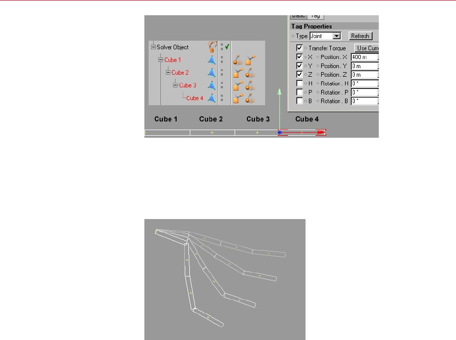
230 CONSTRAINTS DYNAMICS
DYNAMICS CONSTRAINTS 231
Objects in a hierarchy can be
linked to each other using
Constraint tags.
Shown in the diagram above are four cubes. Cube 4 is a child of Cube 3, which in
turn is a child of Cube 2, which in turn is a child of Cube 1. The origin of each cube
has been placed at the cube’s left edge — don’t let the yellow cross confuse you;
it represents the mass centre. Cube 2, Cube 3 and Cube 4 have each been assigned
a Constraint tag with Type set to Point and X set to 400. These tags will keep each
cube 400 units apart along the parent’s X-axis.
Four cubes in a gravity eld.
The cubes are being kept a
xed distance apart by their
Constraint tags.
In the diagram above, the four cubes have been placed in a gravity eld. Due to the
Constraint tags, the cubes remain linked while the chain is swinging down under
the force of gravity.
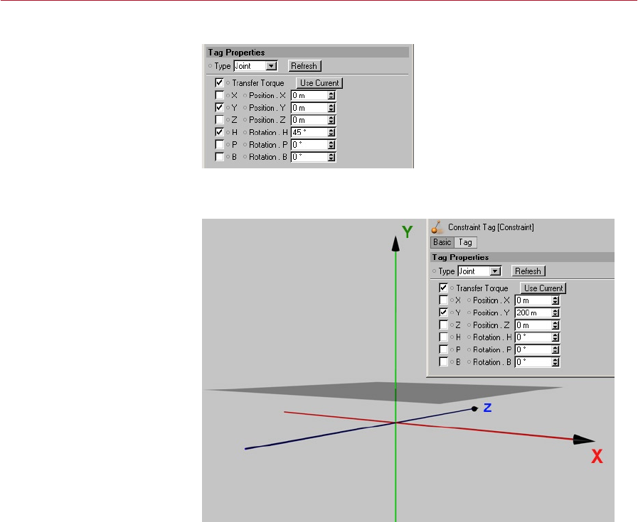
230 CONSTRAINTS DYNAMICS
DYNAMICS CONSTRAINTS 231
Point to Plane
Y set to 0. Therefore the object
will remain on the Y = 0 plane.
This will constrain the rigid body to a plane. For example, to allow the rigid body to
move along the Y = 0 plane only, set Y to 0.
Y has been set to 200. As a result,
the rigid body will be allowed
to move along the Y=200 plane
only, which is indicated by the
dark square.
With Y set to 200, movement will be allowed along the Y= 200 plane only.
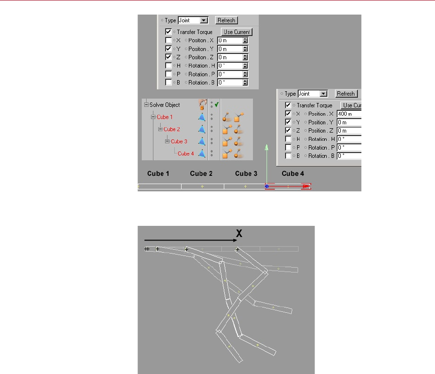
232 CONSTRAINTS DYNAMICS
DYNAMICS CONSTRAINTS 233
In the Constraint dialog for
Cube 1, X has been disabled.
This will allow Cube 1 to move
freely along the X-axis.
For the top cube in the above diagram, X has been disabled while Y and Z have both
been set to 0. Therefore the top cube is able to move freely along the X-axis only.
The chain of cubes has been
placed in a gravity eld. The top
cube is able to move freely along
the X-axis.
Use Current
If you click this button, the X,Y,Z and H,P,B input boxes will be set to the rigid body’s
current position and direction.
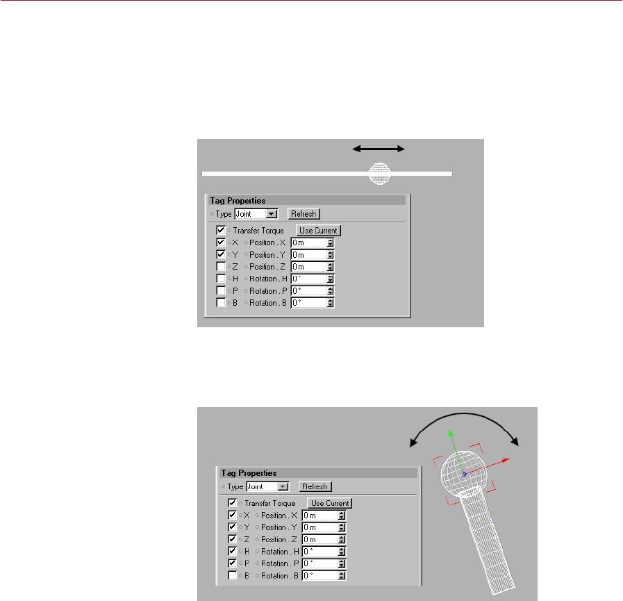
232 CONSTRAINTS DYNAMICS
DYNAMICS CONSTRAINTS 233
Angle Constraints H,P and B
When enabled, these options will align the rigid body to the angle specied in the
adjacent input boxes. The angle must be specied using the parent’s coordinate
system. You can recreate many of the joints found in nature and robotics by combining
position constraints with angle constraints.
Prismatic
This sphere has a prismatic joint,
meaning that it can be moved
along one axis only — in this
case, the Z-axis.
A prismatic joint is a joint that can be moved along a single axis only. Commonly
used for robotic joints.
Ball and Socket
The ball and socket joint allows
rotation in many directions.
The position should be xed by
entering values for X, Y and Z.
This exible ball and socket joint allows movement in many directions. Examples of
ball and socket joints include the shoulder and hip joints of the human body.
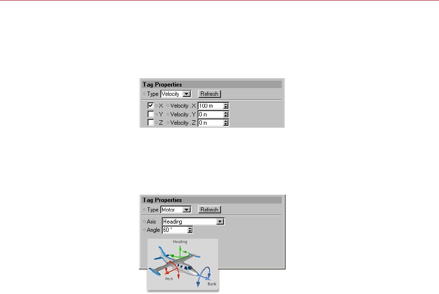
234 CONSTRAINTS DYNAMICS
DYNAMICS CONSTRAINTS 235
Transfer Torque
This should always be enabled to allow the transfer of torque between linked
objects.
Velocity
You can constrain the velocity of
the rigid body by setting Type to
Velocity.
This type is used to constrain the rigid body’s velocity. For example, if you set Velocity.Z
to 100, the rigid body will have a constant velocity of 100 units in the Z direction
regardless of any forces that the solver may exert.
Motor
With Type set to Motor, you can
constrain the rigid body to a
constant angular velocity.
If you set Type to Motor, the rigid body will rotate at a constant angular velocity as
dened under Angle. Set the rotation axis under Axis.
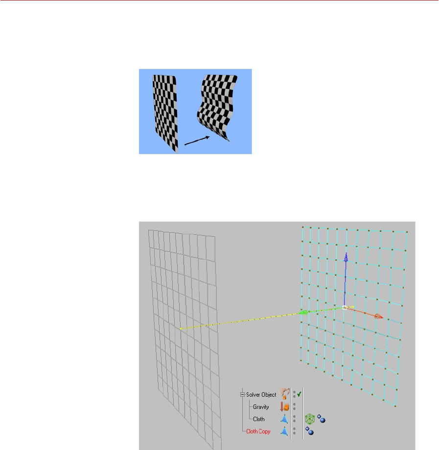
234 CONSTRAINTS DYNAMICS
DYNAMICS CONSTRAINTS 235
Soft Constraints
Although Constraint tags work for rigid bodies only, the following workaround will
enable you to constrain the motion of soft bodies. Suppose you have placed a cloth
in a gravity eld. The cloth should adopt the shape indicated below (right cloth).
Left: the starting shape of the
cloth. Right: the shape the cloth
should adopt.
To make the cloth adopt the required shape:
Create a non-dynamic copy of the soft body, in other words a copy without dynamics
tags.
Animate the copy using keyframes.
Here, the position of the copy
has been animated.
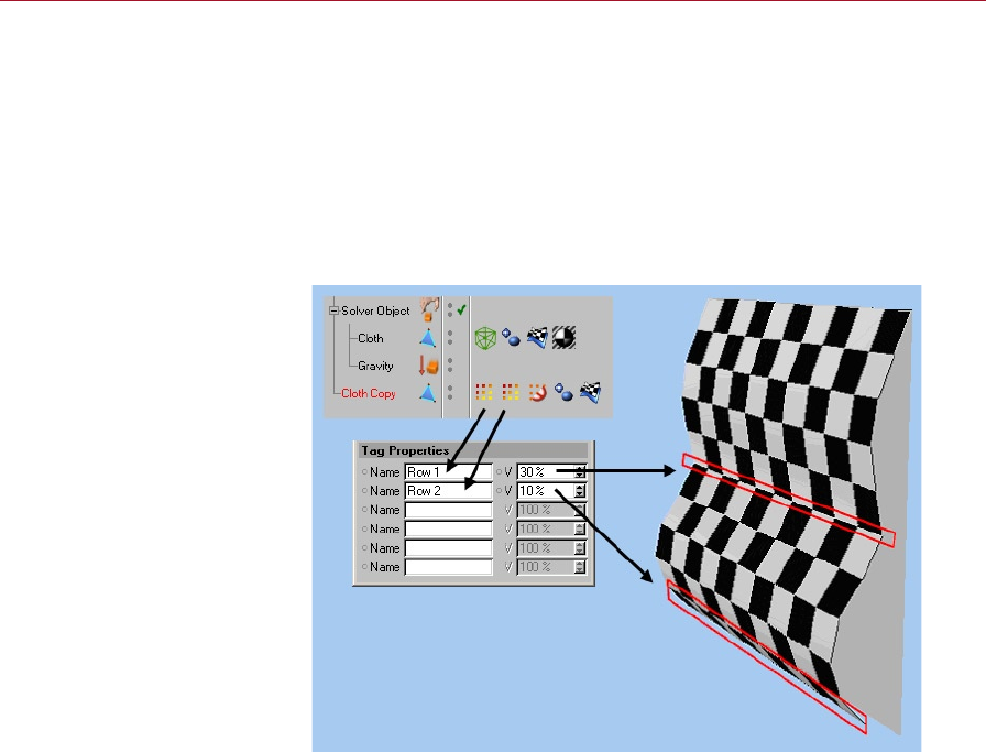
236 CONSTRAINTS DYNAMICS
In the Soft Body dialog of the soft body, under Target, type in the name of the copy.
All soft body points of zero mass will now follow the copy.
The next stage is to assign a vertex map and Restriction tag to the copy. So select
the relevant points and weight them appropriately using the Set Vertex Weight
command (select Selection > Set Vertex Weight from the main menu). Next, give a
name to the vertex map.
If you now create a Restriction tag by selecting File > CINEMA 4D Tags > Restriction
from the Object manager, you will be able to adjust the strength of up to six vertex
maps. The strength controls how closely the soft body points will follow the copy.
The chequered cloth is the soft
body, the grey rectangle just to
its right is the copy. Two vertex
maps have been created: Row 1
(Strength = 30%) and Row 2
(Strength = 10%). The two point
rows are following the copy with
varying strength.
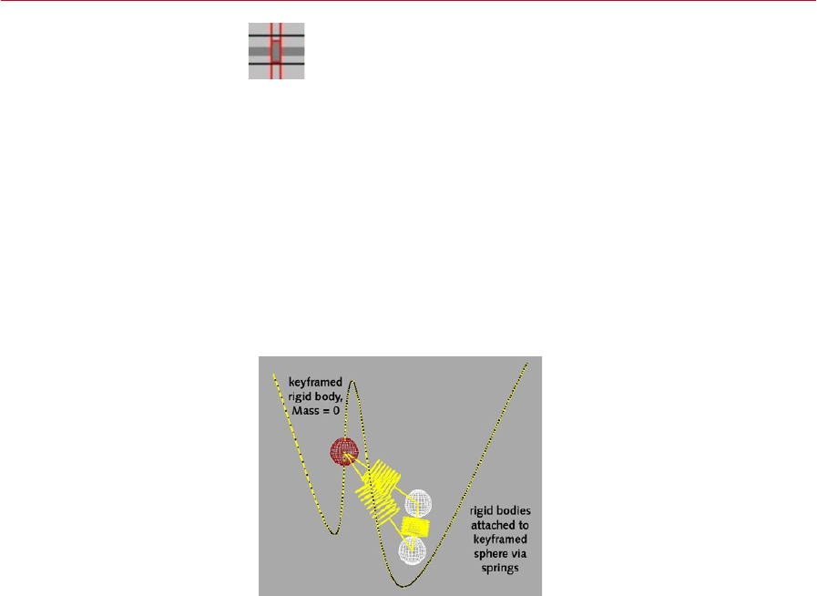
DYNAMICS KEYFRAME ANIMATION 237
Throughout all of dynamics the control of the motion is taken out of your
hands once you click Play. In many animations you need to have exact
control over positions and movements of objects. This precise control and
timing can only be achieved with some keyframing. This poses the questions of
how keyframing can be used alongside or even within the dynamics itself and what
conicts this may give rise to.
Suppose you have animated a sphere with keyframes so that the sphere moves
upwards. You have then added a Rigid Body Dynamic Tag which, with the help of
a gravity eld, wants to pull the sphere downwards. Both are not possible, so who
wins, keyframes or dynamics?
There is a solution. The trick is to set the Mass values of the rigid body or soft body
points to zero. The dynamics engine will not exert forces on any objects of mass
zero. A second property of these zero-mass objects is that you can animate them
with keyframes. Thirdly, you can attach springs to zero-mass objects; this makes it
possible to link keyframes and dynamics.
Dynamics will not exert forces on
any objects that have zero mass,
leaving you free to animate them
with keyframes.
In the diagram above, the dark sphere is a zero-mass rigid body that is moving along
the animation path (keyframe animation). The other two spheres are linked to the
rst sphere via springs. During the animation, the keyframed sphere will drag the
rigid bodies with it.
Rigid bodies that have keyframes will still be able to collide with other rigid bodies
and soft bodies. Collision detection must be enabled for all the objects involved.
Using the same technique — setting the Mass values to zero — you can animate the
points of the soft body with Point-Level Animation.
Keyframe
Animation
With dynamics there are several
ways to animate objects in
CINEMA 4D. This means that
conict situations can arise.
Solutions are a few clicks away!
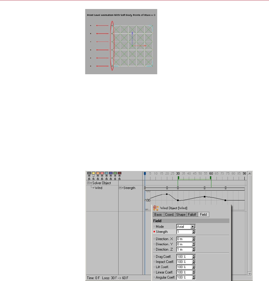
238 KEYFRAME ANIMATION DYNAMICS
DYNAMICS KEYFRAME ANIMATION 239
Soft bodies with zero masses
may be animated with point-
level animation.
The rest of the soft body will follow the animated points. This method enables you
to move soft bodies without having to use force elds.
Parameter Animation for Gravity, Wind and Drag
The following areas of dynamics can be animated:
• Gravity • Wind • Friction • Constraint tag • Solver object
• Rigid Body Dynamic tag
For realistic wind, vary the Strength and Direction parameters.
Proceed with caution when animating Solver objects or Rigid Body Dynamic tags
— unexpected effects are possible! Although parameters such as Integration Method
can be animated, there isn’t much point in animating these parameters anyhow.
Using parameter tracks you can
animate dynamics force elds.
238 KEYFRAME ANIMATION DYNAMICS
DYNAMICS KEYFRAME ANIMATION 239
Baking a Dynamics Animation
Dynamics allows you to bake all dynamics motion in the Timeline. This has several
advantages:
After baking, you can edit the animation using the Timeline.
The animation will run much faster in the viewport once baked.
Baking will ensure that the animation runs exactly the same on another computer
(without baking, the animation may run differently on another computer due to
differing processor accuracy).
After baking you can render over a network using the NET Render module.
After baking you can export the animated objects to other programs via a le
format such as FBX.
Baking will take approximately as long as the time it would take the dynamics
animation to play in the viewport so, in some cases, baking may take a considerable
time. You can abort the baking process at any time by pressing the Esc key.
Once baking has completed, the Solver object will be switched off automatically and
you will be able to play back the animation. The moment you switch on the solver,
the dynamics engine will take over.
Any existing tracks in the Timeline will be overwritten during baking, assuming the
same timeline layer is being used. Rigid bodies will be baked using Position, Scale and
Rotation sequences only, while soft bodies will have a PLA sequence assigned.
Bake Solver
Bakes the selected object’s Solver, including all rigid bodies and soft bodies.
Bake All Solvers
This function will bake all Solver objects in the scene, including their rigid bodies
and soft bodies.
Clear Solver
If you have previously baked a solver, the Timeline will contain the corresponding
animation tracks. With this command you can delete all tracks for the current Solver
object.
Clear All Solvers
This command will delete all animation tracks for all Solver objects in the scene.
Because of the differences
in the way decimal numbers
are calculated on different
platforms, moving a
dynamics animation across
platforms may require
the values to be tweaked
on the new platform.
The only way to avoid
this problem is to ‘bake’
individual solver objects or
the entire scene so that the
animation is turned into a
set of keyframes rather than
movement that has to be
calculated.

240 KEYFRAME ANIMATION DYNAMICS
Tips and Tricks
Get into the habit of setting the viewport frame rate to All Frames. To do this, click
this icon in the Time palette.
A menu will appear. On this menu, enable the All Frames option if it isn’t already
enabled. This will ensure that each frame in the dynamics animation will be played
in the viewport, thus guarding against dropped frames.

DYNAMICS FREQUENTLY ASKED QUESTIONS 241
Why isn’t the movement in the viewport smooth?
The viewport playback speed is entirely dependant upon your CPU speed and the
complexity of the simulation.
If you are simulating orbiting planets, say, you should be able to sustain a reasonable
25 or 30 fps on almost any computer. However, if you have designed a detailed scene
with many physical objects and full collision detection, expect the frame rate to slow
down. Also, don’t expect speedy results if you have loaded an existing scene and
simply added some dynamics; it is far more efcient to design a dynamics simulation
from scratch.
Here are some tips:
Try to limit the number of polygons in the scene as much as possible.
Use a strong negative gravity field instead of collision detection where
possible.
For soft bodies, rather than using an object with a high polygon count, try using
one with a low polygon count and dropping it inside a Hyper NURBS object; this
way Dynamics has to run its calculations only on the low polygon object.
Enable OpenGL; this will free up your processor to calculate the physics while the
display of your simulation is handled by the graphics card.
How can I make a sail that will move a yacht when the wind blows it?
To create a yacht’s sail you will need to use soft bodies.
First of all create your sail and mast, then add the soft body and rigid body tags to
these. The easiest way to attach the sail to the mast is by using rigid springs; if you
make these very short and very stiff they will act like a short piece of rope connecting
the sail and the mast together. We recommend that you use the RBS Draw Tool to
connect the springs between the edges of the sail and the mast.
Depending on the type of sail you want to create, you may only want to pin the sail
at three or four points or you may want to have regular ties all along the mast to
keep the sail attached rmly. Using many springs to connect the sail will give pleasing
taught ripples through it as the wind blows.
Why do the objects penetrate each other when colliding?
No object in the world is perfectly rigid. By allowing objects to penetrate each other
slightly you will give the impression that they are actually deforming under the collision,
which can give a natural look. However, this is not what you want if you are using
very thin, or transparent, objects.
Frequently
Asked
Questions
No matter how many time you
read the manuals (you have,
haven’t you?), there will always
be questions that pop into
your head. In this section we
try to anticipate some of these
— FAQs can be a valuable
resource to supplement your
understanding.

242 FREQUENTLY ASKED QUESTIONS DYNAMICS
DYNAMICS FREQUENTLY ASKED QUESTIONS 243
To achieve more rigid collisions you may wish to increase the Oversampling value in
the Solver object. This will cause more frames to be calculated between each real
frame, increasing the chances of a ‘correct’ collision. Alternatively, increase the Eps
value; this will enlarge the object’s collision boundaries so Dynamics will think that
the objects have collided slightly earlier.
Why do the objects levitate?
If gravity is present in your scene and you have the camera positioned exactly side-on
to an object on a perfectly at surface, you may see that it is actually hovering very
slightly above the surface.
This is due to the Collision Eps value of the Solver (in the Details tab), which determines
how close objects must be before they are considered to be touching. Reduce this
value to allow the objects to get closer together.
How can I make a brick wall and then knock it down?
One of the difculties in setting up a brick wall is getting the bricks to keep still
before they are knocked down.
You could arrange the bricks so that they have a small gap between them, this gap
being the same size as the Collision Eps value in the Solver. Alternatively, you could
drop the bricks onto each other and initialize the scene once they are at rest. This
will then start the simulation with the bricks in this state.
How you knock down the wall is entirely up to you!
Why does the scene explode and/or objects disappear?
If you nd objects suddenly disappearing into the distance or soft bodies violently
rippling then it is likely that your Solver Object’s integration method is set too low.
The level you need for the Integration Method largely depends on the relative speeds
of the objects controlled by the Solver. For example, a dart hitting a dartboard hits
it at a relatively high speed; this means that you need a very accurate solver to make
sure it stops when it reaches the board.

242 FREQUENTLY ASKED QUESTIONS DYNAMICS
DYNAMICS FREQUENTLY ASKED QUESTIONS 243
I have no idea what values to use for the friction coefcients.
Here is a useful list of friction presets that is not intended to be physically accurate
but should achieve the effect you want:
Dynamic coefcient Static coefcient
Shoe on carpet 70% 95%
Shoe on ice 20% 20%
Shoe in grass 50% 65%
Tire on dry Tarmac 95% 98%
Tire on wet Tarmac 75% 97%
Tire in ice Tarmac 30% 80%
Puck on air hockey table 5% 5%
Brick on concrete 80% 90%
Soap on enamel 10% 50%
Football on grass 55% 65%
You can use static coefcient values over 100% to simulate a very coarse, or ribbed
surface, such as polystyrene or a stony surface.
Why do I get different results for the same scene on the Mac and the PC?
This is an inherent problem of using cross platform software. Macs and PCs both
use very different processors and the FPU (Floating Point Unit) varies between them.
This can often give slightly different answers to the same calculation because of the
differing rounding algorithms and precision used.
So, if a pinball hits a ipper and bounces off, the Mac may calculate the ball has left
the ipper at one angle and the PC may come up with a different value. This may be
a fraction of a degree. However, by the time the ball reaches the top of the table, it
could mean the ball hitting a completely different part of the table. As the simulation
continues, the ball ends up taking a vastly different route. For this reason you may wish
to bake your simulation or use a network that has only one type of processor in it.
Why does the cloth look like rubber?
The most likely cause of this is that the springs are too stiff and have a low density mesh.
The default cloth springs use all three types of spring: structural, exion and shear.
The exion springs can stop the material from creasing like cloth usually does.
If you have a cloth with few subdivisions the exion springs will spread themselves
quite widely and, because they only link to every other point, they cannot then fold.
To get around this you can either remove the exion springs altogether or use a ner
mesh for the cloth.

244 FREQUENTLY ASKED QUESTIONS DYNAMICS
DYNAMICS FREQUENTLY ASKED QUESTIONS 245
Why does the cloth fall apart when I use only shear or exion springs?
If you take a closer look at these two types of springs you’ll notice that they are all
criss-crossed. Both types of spring actually consist of two layers of springs that are
in no way connected. This means that if you grab the cloth by setting a single point
to have a mass of 0, then only one layer of springs will be held whilst the other layer
is allowed to fall. So the answer here is to add some structural springs.
How can I connect a rigid body to a soft body?
Currently the only way to x a rigid to soft body is by using a Rigid Spring tag.
Why do I have to initialize the scene?
Dynamics simulates movement starting from an initial set of values; subsequently
everything happens automatically. The scene needs to be initialized because Dynamics
modies the position, rotation and shape of objects independently of CINEMA 4D‘s
object system.
Suppose you’ve played a simulation through a few frames. What will happen now if
you pause the playback and move an object? Should the object start its animation from
that position the next time you play the scene? You can see that it is important that
Dynamics’ position and rotation data is held separately from CINEMA 4D’s data.
Scene and object initialization is done automatically where possible (such as when
you drag an object into the Solver). You should only need to initialize the scene when
you manually change the starting positions.
Why can’t I blow part of a rigid object to spin it?
All forces such as wind, gravity or drag will only affect an object whose centre of
mass is inside the eld and these forces will affect the entire object. This means you
can’t blow, say, half a page of paper to make it spin; the paper will move linearly in
this case. In certain cases it may be possible to use a drag eld.
My simulation is nice, but takes too long to calculate. How can I speed it up?
This is usually a scale problem.
Suppose you’ve created a scene of a ball falling on a plane. It would appear to behave
completely differently if you used a 100 m wide ball than if you used a 1 cm wide
bouncy ball (parallax). The easiest way to adapt this behavior is to increase the gravity
strength. Increased gravity will cause objects to fall more quickly and this is often
enough to make the simulation run as you expected.

244 FREQUENTLY ASKED QUESTIONS DYNAMICS
DYNAMICS FREQUENTLY ASKED QUESTIONS 245
The objects don’t react when they collide with each other. What’s going on?
This is likely to happen if you have scaled an object using the Object tool; Dynamics
does not work correctly with objects that have had their system scaled. You will need
to select the object and choose Functions > Reset System to return the object to the
correct scale. You may then use the Model tool to scale the object as you need it.
Why do highly damped rigid springs explode?
Spring damping uses a similar algorithm to the drag object and you will notice that
too much drag will cause objects to gain energy in an uncontrollable way. This sounds
counter-intuitive but is due to the fact that if you try to remove too much energy
from a system in a short space of time some of the objects will try to continue at high
velocity, destabilizing the system. This also affects soft body springs.
I have an object at an angle. Why don’t the start values make it move in the
direction it is pointing?
All Dynamics objects work using the world coordinate system, not the object’s local
coordinates. The only exception to this is constraints, which use the coordinate system
of the parent object.
Why does the console say ‘Maximum number of contact points reached!’?
This message is telling you that Dynamics has exceeded the maximum number of
points that it can simultaneously calculate for collision detection.
This will often not inuence the scene in any noticeable way. If you see this message
and notice an object has not collided when it should, try reducing the collision type
from Full, or try using a proxy object.
Why are the objects jittering and sliding when they should have come to rest?
This is most likely caused by having inappropriate Solver settings. It is generally
recommended that you use the Midpoint integration method for simulation with
collision detection. Enabling Energy Loss and Collision Use Rest Speed will also help.
When a soft body collides with a rigid body, the rigid body pokes through the
cloth. How can I stop this?
This is due to the different ways in which collisions are calculated between soft and
rigid bodies. Soft bodies do not have collision detection along their edges, only their
points may collide.
Increasing the Collision Eps setting on the Solver’s Details tab will give the colliding
objects a ‘thicker collision skin’ and will therefore help solve this problem.

246 FREQUENTLY ASKED QUESTIONS DYNAMICS
Why has the object stopped moving?
It has hit something.
Gravity has stopped it.
The Solver has some Energy Loss.
It has entered a strong Drag eld.
The scene is processor intensive and has caused the frame rate to drop
dramatically.
Your Solver is still set to work for the default 75 frames.
How can I create falling leaves?
It depends on how much detail you want them to have.
In reality leaves are soft bodies but they are usually so light that they will not deform
when they are blown about and hit other objects. This means you can often get away
with using a rigid body for the leaf in Dynamics.
If your leaves are just one polygon thick make sure you have Double-Sided enabled
(Rigid Body tag, Aerodynamics tab) so that they can be blown no matter which way
they face.
How can I create hair?
You can make soft and exible hair by creating a long ribbon shape and turning it
into a soft body. Then use an alpha map on the object to give the impression that it
has many hairs. Self collision detection can be used to prevent the hair from passing
through the body and itself.
Why do I have to use polygon or spline objects in Dynamics?
All objects must be in a polygon form for Dynamics to work; this is because parametric
objects contain no real geometry for the Dynamics engine to work with.
A spline object may be used as a soft body because it is only the points that matter
when soft body calculations are made by Dynamics.

Index
DYNAMICS INDEX 249

DYNAMICS INDEX 249
A
Above
parameter (rb spring in break state) 200
parameter (rb spring in elastic state) 196
parameter (rb spring in plastic state) 198
parameter (sb spring in break state) 218
parameter (sb spring in elastic state) 214
parameter (sb spring in plastic state) 216
Acceleration
and mass 176
Accuracy
of collision 172
of motion 170
Adaptive
integration method 170
Add
rigid body spring 204
soft body spring 208, 225
soft body springs, advice 211
spring 190
Advice
on soft body springs 210
Aerodynamics
angular coefcient 186
drag coefcient 186, 222
impact coefcient 186, 222
lift 163
lift coefcient 184, 221
linear coefcient 186, 222
of rigid bodies 183
of soft bodies 220
Air pressure 184, 221
All frames 240
Angular
springs 200
type of spring 190
Angular coefcient
aerodynamic 186
Angular spring
damping parameter (in plastic state) 203
drag parameter (in plastic state) 203
maximum torque 202
rest angle 201
start at parameter (break tab) 204
start at parameter (in plastic state) 203
stiffness 202
stiffness parameter (in plastic state) 203
Angular springs
break 204
break tab 204
elasticity 201–204
elastic tab 201–204
plasticity 202–204
plastic tab 202–204
Angular velocity
constraining 234
initial, of rigid body 187
Animating
drag 238
gravity 238
wind 238
Animation
baking 239
delete baked tracks 239
keyframe 237
shape of object during 175
speed 175
stopping and starting 169
Auto correct names
while drawing springs 192, 194
Axial
gravity eld 158
B
Bake scene 239
Bake solver 239
Baking
a dynamics animation 239
into a particular layer 174
number of keyframes 174
Baking Frame Step 174
Baking Layer 174
Balance
forces 152
Ball and socket
joint 233
Below
parameter (rb spring in break state) 200
parameter (rb spring in elastic state) 196
parameter (rb spring in plastic state) 198
parameter (sb spring in break state) 218
parameter (sb spring in elastic state) 215
parameter (sb spring in plastic state) 216
Body
joints 233
Box
type of collision detection (rigid bodies)
180
Break
an angular spring 204
Breaking
of springs 199, 217
point of a spring 200, 218
C
Centre of mass
of rigid body 177
Checking
multiple springs while drawing 192, 194
Children
of rigid body 178
CINEMA 4D NET 239
Circular motion
under gravity 158
Clear scene 239
Clear solver 239
Cloth
constraining 235
Clothing tab
of soft body 223
Coefcient
drag 163
impact 163
Coefcients
of friction 220
Collision
accuracy 172
energy after 183, 219
simulating 160
simulating with drag 166
with gravity 153
Collisions
of rigid bodies 178
of soft bodies 218–227
Collision detection
box (rigid bodies) 180
Collision Eps parameter 172
disable 178
ellipsoid (rigid bodies) 180
enable 178
full+self (soft bodies) 219
full (rigid bodies) 180
full (soft bodies) 219
switching off 180, 219
type, for rigid bodies 179
type, for soft bodies 218
using a proxy object 180
Collision Rest Speed 173
Compressing
a spring 196, 198, 214, 216
a spring, then breaking 200, 218
Conict
between keyframing and dynamics 237
Console
using to check penetrating objects 179
Constrain
angular velocity 234
Constraint
joint type 229
motor type 234
tag 229
velocity type 234
Constraints 229
DYNAMICS INDEX 251
of soft bodies 235
with cloth 235
Correcting
names while drawing springs 192, 194
Current position
xing of rigid body 232
D
Damping
energy within Dynamics 171
of rb spring in elastic state 197
of rb spring in plastic state 199
of sb spring in elastic state 215
of sb spring in plastic state 216
parameter (angular spring in plastic
state) 203
plastic, for an angular spring, when it
will start 203
Deformation
plastic, for an angular spring, when it
will start 203
where it will start for an rb spring 199
where it will start for an sb spring 216
Delete
baked animation tracks 239
rb spring 204
sb spring 225
sb spring selection 226
soft body spring 211
spring 190
Details tab
solver object 172
Dialog
rigid body springs 189
soft body springs 211
Direction
drag eld option 167
of gravity eld 160
wind eld option 163
Disable
collision detection 178, 180, 219
Display
soft body springs 225
springs 190
Distance
affecting gravity 159
Double-sided
wind affecting 184, 220
Drag 151, 165
and rb spring in plastic state 199
and sb spring in plastic state 217
animating 238
direction 167
mode 166
of object attached to an angular spring
in plastic 203
parameter (angular spring in plastic
state) 203
strength 167
strength of 186, 222
using to simulate collision 166
Drag coefcient 186, 222
wind eld option 163
Drawing
rb springs interactively 191
Dropped frames
guarding against 240
Duplicate
rb spring 204
remove from soft body springs 208
spring 190
Dynamic
friction 183, 220
Dynamics
and keyframing 237
E
Editing
multiple rb springs 189
Elasticity
of angular springs 201–204
of rb springs 195
of rigid body 183
of sb springs 213
of soft body 219
Ellipsoid
type of collision detection (rigid bodies)
180
Enable
collision detection 178
Energy
retained after collision 183, 219
Energy loss 171
Eps
parameter 172
Euler
integration method 169
Exclusion
gravity eld option 155
F
Falloff
gravity eld option 156
Field
wind eld option 162
Fixing
of cloth 235
of sb springs 227
rigid bodies 229
soft bodies 235
Force
affecting motion 151
drag 151, 165
gravity 151, 152
initial, of rigid body 187
initial, of soft body 224
lines of 151
wind 151, 158
Forces
in balance 152
Force eld 151
Frames
guarding against dropped 240
Friction
coefcients 183, 220
of rigid body 183
of soft body 219
Full
type of collision detection (rigid bodies)
180
type of collision detection (soft bodies)
219
G
Gravity 151, 152
and collisions 153
animating 238
axial 158
direction 160
falloff 156
Newton 159
radial 158
size of eld 156
strength 160
I
Impact coefcient 186, 222
wind eld option 163
Initialize
all objects 205
object 205
rest length of sb springs 227
rigid body object 205
Initial state
of soft body 224
Integration
oversampling 170
subsampling 171
Integration method
adaptive 170

DYNAMICS INDEX 251
Euler 169
midpoint 169
of Dynamics 169
Runge-Kutta 170
Softbody 170
Interactive
drawing of rb springs 191
Introduction
to rigid body springs 188
J
Joint
ball and socket 233
body 233
prismatic 233
robotic 233
transferring torque 234
type of constraint 229
K
Keyframes
baking 174
Keyframe animation 237
L
Lift 184
on a wing 163
wind eld option 163
Lift coefcient 221
Limit force
of rb spring 196
of sb spring 213
Linear Coeff., Angular Coeff. 164
Linear coefcient
aerodynamic 186, 222
Linear velocity
initial, of rigid body 187
initial, of soft body 224
Lines of force 151
Lock
below/above values of rb spring 196
below/ above values of sb spring 214
Loss
of energy within system 171
M
Managing
soft body springs 211
Mass
affecting gravity 159
and acceleration 176
centre of 177
of rigid body 175
of sb springs 227
rotational 176
setting to zero 237
Maximum force
exerted by rb spring 196
exerted by sb spring 214
Menu
rigid body springs 204
soft body springs 225
Method
of attaching soft body springs 208
Midpoint
integration method 169
Mode
drag eld option 166
of drag 166
Motion
accuracy 170
adjusting using integration method 169
affected by force 151
baking 239
circular, under gravity 158
planetary 160
Motor
type of constraint 234
Multiple
check while drawing rb springs 192, 194
rb springs 189
Multiple use iii
N
Name
rigid body spring 190
soft body spring set 210
NET 239
Network operation iii
Newton
gravity eld 159
O
Object
collision detection 172
controlling sinking 173
Initialize 205
proxy 180
rest speed 173
rigid body 175
rigid body, initialize 205
soft body 207
soft body, creating 208
solver 169
solver, attaching rb springs to 188
solver, bake 239
solver, clear 239
transferring torque between linked
objects 234
Objects
checking penetration of 179
Offset
gravity eld option 155, 156
Oversampling
and integration 170
Overview
of rb springs 188
P
Parameter
tracks in the timeline 238
Penetrating
objects, checking 179
Penetration
controlling during collision 172
Planetary motion 160
Plastic
angular spring damping, when it will
start 203
angular spring deformation, when it will
start 203
state of angular spring, drag of attached
object 203
stiffness for an angular spring, when it
will start 203
Plasticity
of angular springs 202–204
of rb springs 198
of sb springs 215
Point selection
to sb spring selection 225
Point to plane
xing of rigid body 231
Point to point
xing of rigid body 229
Polygon object
converting to a rigid body 175
Pressure
air 184, 221
Prismatic
joint 233
Proxy
collision object 180
R
Radial gravity eld 158

252 INDEX DYNAMICS
DYNAMICS INDEX 253
Radius
gravity eld option 154
RBS draw tool 191
RBS selection tool 193
RDB tag
add automatically while drawing rb
springs 194
add automatically while drawing springs
192
Relax
soft body springs 223
Remove
duplicate soft body springs 208
soft body spring 211
Rename
sb spring selection 226
Restriction tag 236
Rest angle
of angular spring 201
Rest length
calculate while drawing rb springs 192,
194
of rb spring 195
of rb spring, calculate 204
of sb spring 213
of sb springs, initialize 227
Rigid bodies
vs soft bodies 175, 207
Rigid body
aerodynamics 183
bake 239
children 178
collisions 178
constraining 229
elasticity 183
xing point to plane 231
xing point to point 229
xing using current position 232
friction 183
mass 175
Rigid body angular springs 200
damping parameter in plastic state 203
drag parameter in plastic state 203
start above parameter (break tab) 204
start above parameter in plastic state
203
stiffness parameter in plastic state 203
Rigid body dynamics 175
initialization 205
Rigid body dynamic tag 175
Rigid body springs
‘start at’ parameter in plastic state 199
above parameter in break state 200
above parameter in elastic state 196
above parameter in plastic state 198
add 204–205
adding 190
angular 200
angular type 190
below parameter in break state 200
below parameter in elastic state 196
below parameter in plastic state 198
break 199
breaking point 200
calculate rest length 204–205
damping in elastic state 197
damping in plastic state 199
delete 204–205
deleting 190
dialog 189
displaying 190
drag in plastic state 199
drawing interactively 191
duplicate 204–205
duplicating 190
elasticity 195
limiting angular torque 202
lock above and below values 196
maximum force exerted by 196
naming 190
plastic 198
refresh display of 190
rest angle of angular 201
rest length 195
selecting 193
springs menu 204
stiffness in elastic state 196
stiffness in plastic state 199
stiffness of angular spring 202
Rigid body spring tag 187
Robotic
joint 233
Rotation
constraining 229
initial, of rigid body 187
Rotational mass 176
Runge-Kutte
integration method 170
S
Save
sb spring selection 226
Scene
bake 239
clear animation tracks 239
Initialize 205
Secrecy v
Selecting
multiple rb springs 189
rb springs 193
Selection
adding soft body springs as 210
of points to sb springs 225
of sb springs 226
of sb springs, delete 226
of sb springs, rename 226
of sb springs, save 226
Selection set
and adding soft body springs 210
Self
collision (soft bodies) 219
Setting up 169
Shape
of gravity eld 161
Show
rigid body springs 190
soft body springs 225–227
Simulate
collisions 160
Sinking
controlling 173
Size
gravity eld option 156
Snap
while drawing rb springs 192, 194
Snapping
of rb springs 199
of sb springs 217
Softbody
integration method 170
Soft bodies
vs rigid bodies 175, 207
Soft body
aerodynamics 220
bake 239
clothing tab 223
collisions 218
constraining 235
elasticity 219
friction 220
initial state 224
start tab 224
Soft body dynamics 207
Soft body object
creating 207
Soft body spring
add 208
delete 211
Soft body springs
‘all’ method 209
‘cloth’ method 210
‘exion’ method 209
‘minmax’ method 209
‘shear’ method 209
‘start at’ parameter in plastic state 216
‘structural’ method 209

252 INDEX DYNAMICS
DYNAMICS INDEX 253
above parameter in break state 218
above parameter in elastic state 214
above parameter in plastic state 216
add 225–227
advice on adding 211
below parameter in break state 218
below parameter in elastic state 214
below parameter in plastic state 216
break 217
breaking point 218
damping in elastic state 215
damping in plastic state 217
default name of selection set 210
delete 225–227
dialog 211
drag in plastic state 217
elasticity 213
initialize rest length 227
lock above and below values 214
maximum force exerted by 214
methods of attaching 209
name of selection set 210
plastic 215
relaxing 223
rest length 213
selection 226
set soft mass 227
show 225–227
springs menu 225–227
springs tab 211
stiffness in elastic state 214
stiffness in plastic state 216
Soft mass
of sb springs 227
Solver
bake 239
clear 239
Solver object 169
attaching rb springs to 188
details tab 172
frame step 174
integration type 169
rest speed 173
Speed
constraining 234
of animation 175
Spring, rigid body
‘start at’ parameter in plastic state 199
above parameter in break state 200
above parameter in elastic state 196
above parameter in plastic state 198
add 190
angular type 190
below parameter in break state 200
below parameter in elastic state 196
below parameter in plastic state 198
breaking point 200
damping in elastic state 197
damping in plastic state 199
delete 190
drag in plastic state 199
duplicate 190
example 176
how it breaks when compressed 200
how it breaks when stretched 200
how it reacts when compressed 196,
198
how it reacts when stretched 196, 198
lock above and below values 196
maximum force exerted by 196
name 190
refresh 190
rest length 195
show 190
stiffness in elastic state 196
stiffness in plastic state 199
where plastic deformation will begin
199
Spring, soft body
‘start at’ parameter in plastic state 216
above parameter in break state 218
above parameter in elastic state 214
above parameter in plastic state 216
below parameter in break state 218
below parameter in elastic state 214
below parameter in plastic state 216
breaking point 218
damping in elastic state 215
damping in plastic state 217
drag in plastic state 217
how it breaks when compressed 218
how it breaks when stretched 218
how it reacts when compressed 214,
216
how it reacts when stretched 214, 216
lock above and below values 214
maximum force exerted by 214
rest length 213
stiffness in elastic state 214
stiffness in plastic state 216
where plastic deformation will begin
216
Springs
add 204–205, 225–227
calculate rest length 204–205
delete 204–205, 225–227
duplicate 204–205
methods of attaching to soft bodies 209
rigid body, menu 204
soft body, menu 225–227
Springs, rigid body
add 204–205
add RBD tag automatically while draw-
ing 192, 194
and rigid body 177
angular 200
auto correct names while drawing 192,
194
break tab 199
calculate rest length 204–205
calculate rest length while drawing 192,
194
delete 204–205
drawing interactively 191
duplicate 204–205
editing multiple 189
elastic tab 195
introduction 188
multiple 189
multiple check 192, 194
plastic tab 198
rigid body 187
rigid body dialog 189
selecting 193
selecting multiple 189
snapping while drawing 192, 194
springs menu 204
Springs, soft body
add 225–227
break tab 217
delete 225–227
initialize rest length 227
plastic tab 214–215
selection 226
set soft mass 226–227
show 225–227
soft body dialog 211
springs menu 225–227
springs tab 211
Start
animation 169
Start above
parameter (angular spring, break tab)
204
parameter (angular spring in plastic
state) 203
Start At
parameter (sb spring in plastic state)
216
Start at
parameter (rb spring in plastic state)
199
Start tab
of soft body 224
Static
friction 183, 220
Stiffness
of angular spring 202

254 INDEX DYNAMICS
of rb spring in elastic state 196
of rb spring in plastic state 199
of sb spring in elastic state 214
of sb spring in plastic state 216
parameter (angular spring in plastic
state) 203
plastic, for an angular spring, when it
will start 203
Stop
animation 169
Strength
drag eld option 167
of force on an aerodynamic object 186,
222
of gravity eld 160
Stretching
an rb spring 196, 198
an rb spring, then breaking 200
an sb spring 214, 216
an sb spring, then breaking 218
Subsampling
and integration 171
Sweep gravity eld option 153
T
Tag
constraint 229
restriction 236
rigid body dynamic 175
rigid body spring 187
Timeline
baking 174
Torque
initial, of rigid body 187
of angular spring 202
transferring between linked objects 234
Transfer iv
torque between linked objects 234
Type
of collision detection, for rigid bodies
179
of collision detection, for soft bodies
219
U
User
naming soft body spring set 210
V
Velocity,
angular 186
initial, of rigid body 187
initial, of soft body 224
linear 186, 222
type of constraint 234
W
Wind 151, 158–161
and aerodynamics 183, 220
animating 238
direction 163
on both sides of an object 220
Wing 185, 221
using with wind 163
Z
Zero
mass 237
