Casio Graphing Calculator Calculators And Translators Classpad330Plus Users Manual ClassPad 330 PLUS_Software_Eng

CLASSPAD330PLUS to the manual df552c66-4575-4408-aa4e-07dc73f78b54

CP330PLUSver310_Soft CP330PLUSver310_Soft_EN ClassPad 330 PLUS | Calculators | Manuals | CASIO

2015-01-21

: Casio Casio-Casio-Graphing-Calculator-Calculators-And-Translators-Classpad330Plus-Users-Manual-242732 casio-casio-graphing-calculator-calculators-and-translators-classpad330plus-users-manual-242732 casio pdf

Open the PDF directly: View PDF .
Page Count: 921 [warning: Documents this large are best viewed by clicking the View PDF Link!]

Contents
About This User’s Guide
Chapter 1 Getting Acquainted
Chapter 2 Using the Main Application
Chapter 3 Using the Graph & Table Application
Chapter 4 Using the Conics Application
Chapter 5 Using the 3D Graph Application
Chapter 6 Using the Sequence Application
Chapter 7 Using the Statistics Application
Chapter 8 Using the Geometry Application
Chapter 9 Using the Numeric Solver Application
- 9-1 Numeric Solver Application Overview
- 9-2 Using Numeric Solver
Chapter 10 Using the eActivity Application
Chapter 11 Using the Presentation Application
Chapter 12 Using the Program Application
Chapter 13 Using the Spreadsheet Application
Chapter 14 Using the Differential Equation Graph Application
Chapter 15 Using the Financial Application
Chapter 16 Configuring System Settings
Appendix

ClassPad 330 PLUS

ClassPad OS Version 3.10

Software

User’s Guide

CASIO Education website URL

http://edu.casio.com

ClassPad website URL

http://edu.casio.com/products/classpad/

Access the URL below and register as a user.

http://edu.casio.com/dl/

20110901

Contents

About This User’s Guide

ClassPad Keypad and Icon Panel .....................................................................0-1-1

On-screen Keys, Menus, and Other Controllers ................................................0-1-2

Page Contents ....................................................................................................0-1-3

Chapter 1 Getting Acquainted

1-1 General Guide ....................................................................................... 1-1-1

General Guide ....................................................................................................1-1-2

Using the Stylus .................................................................................................1-1-4

1-2 Turning Power On and Off ................................................................... 1-2-1

Turning Power On .............................................................................................1-2-1

Turning Power Off .............................................................................................1-2-1

Resume Function ..............................................................................................1-2-1

1-3 Using the Icon Panel ............................................................................. 1-3-1

1-4 Built-in Applications ............................................................................ 1-4-1

Starting a Built-in Application ..............................................................................1-4-2

Application Menu Operations .............................................................................1-4-2

1-5 Built-in Application Basic Operations ................................................. 1-5-1

Application Window ...........................................................................................1-5-1

Using a Dual Window Display ............................................................................1-5-1

Using the Menu Bar ............................................................................................1-5-3

Using the O Menu ..........................................................................................1-5-4

Using Check Boxes ............................................................................................1-5-6

Using Option Buttons ..........................................................................................1-5-7

Using the Toolbar ...............................................................................................1-5-8

Interpreting Status Bar Information ....................................................................1-5-9

Pausing and Terminating an Operation .............................................................1-5-9

1-6 Input ....................................................................................................... 1-6-1

Using the Soft Keyboard ....................................................................................1-6-1

Input Basics .......................................................................................................1-6-3

Advanced Soft Keyboard Operations ................................................................1-6-8

1-7 Variables and Folders .......................................................................... 1-7-1

Folder Types .......................................................................................................1-7-1

Variable Types ...................................................................................................1-7-2

Creating a Folder ...............................................................................................1-7-4

Creating and Using Variables .............................................................................1-7-5

Assigning Values and Other Data to a System Variable ..................................1-7-10

Locking a Variable or Folder .............................................................................1-7-10

Rules Governing Variable Access ....................................................................1-7-11

Contents

20110401

1-8 Using the Variable Manager ................................................................. 1-8-1

Variable Manager Overview ...............................................................................1-8-1

Starting Up the Variable Manager ......................................................................1-8-1

Variable Manager Views .....................................................................................1-8-2

Exiting the Variable Manager ............................................................................1-8-2

Variable Manager Folder Operations .................................................................1-8-3

Variable Operations ............................................................................................1-8-7

1-9 Configuring Application Format Settings ........................................... 1-9-1

Specifying a Variable ..........................................................................................1-9-2

Initializing All Application Format Settings ..........................................................1-9-3

Application Format Settings ................................................................................1-9-4

Chapter 2 Using the Main Application

2-1 Main Application Overview .................................................................. 2-1-1

Starting Up the Main Application ........................................................................2-1-1

Main Application Window ...................................................................................2-1-1

Main Application Menus and Buttons .................................................................2-1-3

Using Main Application Modes ...........................................................................2-1-4

Accessing ClassPad Application Windows from the Main Application ...............2-1-5

Accessing the Main Application Window from Another ClassPad

Application ..........................................................................................................2-1-6

2-2 Basic Calculations ................................................................................ 2-2-1

Arithmetic Calculations and Parentheses Calculations ......................................2-2-1

Using the e Key ..............................................................................................2-2-2

Omitting the Multiplication Sign ..........................................................................2-2-2

Using the Answer Variable (ans) ........................................................................2-2-2

Assigning a Value to a Variable ..........................................................................2-2-4

Calculation Error .................................................................................................2-2-4

Calculation Priority Sequence ............................................................................2-2-5

Calculation Modes ..............................................................................................2-2-6

2-3 Using the Calculation History .............................................................. 2-3-1

Viewing Calculation History Contents .................................................................2-3-1

Re-calculating an Expression .............................................................................2-3-2

Deleting Part of the Calculation History Contents ..............................................2-3-4

Clearing All Calculation History Contents ...........................................................2-3-4

2-4 Function Calculations........................................................................... 2-4-1

2-5 List Calculations ................................................................................... 2-5-1

Inputting List Data ...............................................................................................2-5-1

Using a List in a Calculation ...............................................................................2-5-3

Using a List to Assign Different Values to Multiple Variables .............................2-5-4

2-6 Matrix and Vector Calculations ............................................................ 2-6-1

Inputting Matrix Data ..........................................................................................2-6-1

Performing Matrix Calculations ...........................................................................2-6-4

Using a Matrix to Assign Different Values to Multiple Variables .........................2-6-6

Contents

20110401

Contents

2-7 Specifying a Number Base ................................................................... 2-7-1

Number Base Precautions ..................................................................................2-7-1

Binary, Octal, Decimal, and Hexadecimal Calculation Ranges ..........................2-7-1

Selecting a Number Base ...................................................................................2-7-3

Arithmetic Operations .........................................................................................2-7-4

Bitwise Operations ..............................................................................................2-7-5

Using the baseConvert Function (Number System Transform) ..........................2-7-5

2-8 Using the Action Menu ......................................................................... 2-8-1

Abbreviations and Punctuation Used in This Section .........................................2-8-1

Example Screenshots .........................................................................................2-8-2

Displaying the Action Menu ................................................................................2-8-3

Using the Transformation Submenu ...................................................................2-8-3

Using the Advanced Submenu ...........................................................................2-8-8

Using the Calculation Submenu .......................................................................2-8-12

Using the Complex Submenu ...........................................................................2-8-19

Using the List-Create Submenu .......................................................................2-8-21

Using the List-Calculation Submenu ................................................................2-8-24

Using the Matrix-Create Submenu ...................................................................2-8-31

Using the Matrix-Calculation Submenu ............................................................2-8-33

Using the Vector Submenu ...............................................................................2-8-38

Using the Equation/Inequality Submenu .........................................................2-8-42

Using the Assistant Submenu ..........................................................................2-8-47

Using the Distribution and Inv. Distribution Submenus ....................................2-8-48

Using the Financial Submenu ...........................................................................2-8-57

Using the Command Submenu ........................................................................2-8-64

2-9 Using the Interactive Menu ................................................................. 2-9-1

Interactive Menu and Action Menu .....................................................................2-9-1

Interactive Menu Example ..................................................................................2-9-1

Using the “apply” Command ...............................................................................2-9-4

2-10 Using the Main Application in Combination with Other

Applications ........................................................................................ 2-10-1

Opening Another Application’s Window ...........................................................2-10-1

Closing Another Application’s Window .............................................................2-10-2

Using the Graph Window $ and 3D Graph Window % ..............................2-10-2

Using a Graph Editor Window (Graph & Table: !, Conics: *,

3D Graph: @, Numeric Solver: 1) ...............................................................2-10-4

Using the Stat Editor Window ( ...................................................................2-10-5

Using the Geometry Window 3 ....................................................................2-10-9

Using the Sequence Editor Window & ........................................................2-10-11

2-11 Using Verify ......................................................................................... 2-11-1

Starting Up Verify .............................................................................................2-11-1

Verify Menus and Buttons ................................................................................2-11-2

Using Verify ......................................................................................................2-11-3

2-12 Using Probability ................................................................................ 2-12-1

Starting Up Probability ......................................................................................2-12-2

Probability Menus and Buttons .........................................................................2-12-2

Using Probability ...............................................................................................2-12-4

2-13 Running a Program in the Main Application .................................... 2-13-1

20110401

Chapter 3 Using the Graph & Table Application

3-1 Graph & Table Application Overview ................................................... 3-1-1

Starting Up the Graph & Table Application .........................................................3-1-1

Graph & Table Application Window ....................................................................3-1-1

Graph & Table Application Menus and Buttons ..................................................3-1-2

Graph & Table Application Status Bar ................................................................3-1-7

Graph & Table Application Basic Operations .....................................................3-1-7

3-2 Using the Graph Window ...................................................................... 3-2-1

Configuring View Window Parameters for the Graph Window ...........................3-2-1

Viewing Graph Window Coordinates ..................................................................3-2-5

Scrolling the Graph Window ...............................................................................3-2-6

Panning the Graph Window ................................................................................3-2-6

Zooming the Graph Window ...............................................................................3-2-7

Other Graph Window Operations .....................................................................3-2-10

3-3 Storing Functions ................................................................................. 3-3-1

Using Graph Editor Sheets .................................................................................3-3-1

Specifying the Function Type .............................................................................3-3-2

Storing a Function ..............................................................................................3-3-3

Using Built-in Functions ......................................................................................3-3-5

Saving the Message Box Expression to the Graph Editor Window ....................3-3-5

Editing Stored Functions ....................................................................................3-3-6

Deleting All Graph Editor Expressions ...............................................................3-3-7

Graphing a Stored Function ...............................................................................3-3-7

Saving Graph Editor Data to Graph Memory ....................................................3-3-14

3-4 Using Table & Graph ............................................................................. 3-4-1

Generating a Number Table ...............................................................................3-4-1

Editing Number Table Values .............................................................................3-4-4

Deleting, Inserting, and Adding Number Table Lines .........................................3-4-5

Regenerating a Number Table ...........................................................................3-4-6

Generating a Number Table and Using It to Draw a Graph ...............................3-4-7

Saving a Number Table to a List ........................................................................3-4-8

Generating a Summary Table ............................................................................3-4-9

Making the Graph Editor Window the Active Window ......................................3-4-15

3-5 Modifying a Graph................................................................................. 3-5-1

Modifying a Single Graph by Changing the Value of a Coefficient

(Direct Modify) ....................................................................................................3-5-1

Simultaneously Modifying Multiple Graphs by Changing Common Variables

(Dynamic Modify) ................................................................................................3-5-4

3-6 Using the Sketch Menu ......................................................................... 3-6-1

Sketch Menu Overview .......................................................................................3-6-1

Using Sketch Menu Commands .........................................................................3-6-1

3-7 Using Trace ............................................................................................ 3-7-1

Using Trace to Read Graph Coordinates ...........................................................3-7-1

Linking Trace to a Number Table .......................................................................3-7-3

Generating Number Table Values from a Graph ................................................3-7-4

3-8 Analyzing a Function Used to Draw a Graph ..................................... 3-8-1

G-Solve Menu Overview .....................................................................................3-8-1

Using G-Solve Menu Commands .......................................................................3-8-2

Contents

20110401

Chapter 4 Using the Conics Application

4-1 Conics Application Overview ............................................................... 4-1-1

Starting Up the Conics Application .....................................................................4-1-1

Conics Application Window ................................................................................4-1-1

Conics Application Menus and Buttons ..............................................................4-1-2

Conics Application Status Bar ............................................................................4-1-4

4-2 Inputting Equations ............................................................................. 4-2-1

Using a Conics Form to Input an Equation .........................................................4-2-1

Inputting an Equation Manually ..........................................................................4-2-3

Transforming a Manually Input Equation to a Conics Form ...............................4-2-3

4-3 Drawing a Conics Graph ...................................................................... 4-3-1

Drawing a Parabola ............................................................................................4-3-1

Drawing a Circle .................................................................................................4-3-4

Drawing an Ellipse ..............................................................................................4-3-5

Drawing a Hyperbola ..........................................................................................4-3-6

Drawing a General Conics ..................................................................................4-3-8

4-4 Using Trace to Read Graph Coordinates ............................................ 4-4-1

Using Trace ........................................................................................................4-4-1

4-5 Using G-Solve to Analyze a Conics Graph ......................................... 4-5-1

Displaying the G-Solve Menu .............................................................................4-5-1

Using G-Solve Menu Commands .......................................................................4-5-2

Chapter 5 Using the 3D Graph Application

5-1 3D Graph Application Overview .......................................................... 5-1-1

Starting Up the 3D Graph Application ................................................................5-1-1

3D Graph Application Window ............................................................................5-1-1

3D Graph Application Menus and Buttons .........................................................5-1-2

3D Graph Application Status Bar ........................................................................5-1-4

5-2 Inputting an Expression ....................................................................... 5-2-1

Using 3D Graph Editor Sheets ...........................................................................5-2-1

Storing a Function ..............................................................................................5-2-2

5-3 Drawing a 3D Graph .............................................................................. 5-3-1

Configuring 3D Graph View Window Parameters ..............................................5-3-1

3D Graph Example .............................................................................................5-3-3

5-4 Manipulating a Graph on the 3D Graph Window ................................ 5-4-1

Enlarging and Reducing the Size of a Graph .....................................................5-4-1

Switching the Eye Position .................................................................................5-4-1

Rotating the Graph Manually ..............................................................................5-4-2

Rotating a Graph Automatically ..........................................................................5-4-3

Initializing the Graph Window .............................................................................5-4-3

5-5 Other 3D Graph Application Functions ............................................... 5-5-1

Using Trace to Read Graph Coordinates ...........................................................5-5-1

Inserting Text into a 3D Graph Window ..............................................................5-5-1

Calculating a z-value for Particular x- and y-values, or s- and t-values ..............5-5-2

Using Drag and Drop to Down a 3D Graph ........................................................5-5-3

Contents

20110401

Chapter 6 Using the Sequence Application

6-1 Sequence Application Overview .......................................................... 6-1-1

Starting up the Sequence Application ................................................................6-1-1

Sequence Application Window ...........................................................................6-1-1

Sequence Application Menus and Buttons .........................................................6-1-2

Sequence Application Status Bar .......................................................................6-1-6

6-2 Inputting an Expression in the Sequence Application ...................... 6-2-1

Inputting Data on the Sequence Editor Window .................................................6-2-1

Inputting Data on the Sequence RUN Window ..................................................6-2-1

6-3 Recursive and Explicit Form of a Sequence ...................................... 6-3-1

Generating a Number Table ...............................................................................6-3-1

Graphing a Recursion .........................................................................................6-3-3

Determining the General Term of a Recursion Expression ................................6-3-5

Calculating the Sum of a Sequence ...................................................................6-3-6

6-4 Using LinkTrace .................................................................................... 6-4-1

6-5 Drawing a Cobweb Diagram ................................................................. 6-5-1

Chapter 7 Using the Statistics Application

7-1 Statistics Application Overview ........................................................... 7-1-1

Starting Up the Statistics Application ..................................................................7-1-2

Stat Editor Window Menus and Buttons .............................................................7-1-3

Stat Editor Window Status Bar ...........................................................................7-1-4

7-2 Using Stat Editor ................................................................................... 7-2-1

Basic List Operations ..........................................................................................7-2-1

Inputting Data into a List .....................................................................................7-2-4

Editing List Contents ...........................................................................................7-2-7

Sorting List Data .................................................................................................7-2-8

Controlling the Number of Displayed List Columns ............................................7-2-9

Clearing All Stat Editor Data ...............................................................................7-2-9

7-3 Before Trying to Draw a Statistical Graph ........................................... 7-3-1

Using the SetGraph Menu ..................................................................................7-3-1

Configuring StatGraph Setups ............................................................................7-3-2

7-4 Graphing Single-Variable Statistical Data ........................................... 7-4-1

Normal Probability Plot (NPPlot) ........................................................................7-4-1

Histogram Bar Graph (Histogram) ......................................................................7-4-2

Med-Box Plot (MedBox) .....................................................................................7-4-2

Normal Distribution Curve (NDist) ......................................................................7-4-3

Broken Line Graph (Broken) ...............................................................................7-4-4

7-5 Graphing Paired-Variable Statistical Data........................................... 7-5-1

Drawing a Scatter Plot and xy Line Graph .........................................................7-5-1

Drawing a Regression Graph (Curve Fitting) .....................................................7-5-2

Graphing Previously Calculated Regression Results .........................................7-5-4

Drawing a Linear Regression Graph ..................................................................7-5-5

Drawing a Med-Med Graph ................................................................................7-5-6

Drawing Quadratic, Cubic, and Quartic Regression Graphs ..............................7-5-7

Drawing a Logarithmic Regression Graph ..........................................................7-5-9

Drawing an Exponential Regression Graph (

y = a·eb

x) ...................................7-5-10

Drawing an Exponential Regression Graph (

y = a·bx)......................................7-5-11

Contents

20110401

Drawing a Power Regression Graph (

y = a·xb) ................................................7-5-12

Drawing a Sinusoidal Regression Graph (

y = a·sin(b·x + c) + d) .....................7-5-13

Drawing a Logistic Regression Graph (

y = c

1 +

e–b·x

) ........................................7-5-14

Overlaying a Function Graph on a Statistical Graph ........................................7-5-15

7-6 Using the Statistical Graph Window Toolbar ...................................... 7-6-1

7-7 Performing Statistical Calculations ..................................................... 7-7-1

Viewing Single-variable Statistical Calculation Results ......................................7-7-1

Viewing Paired-variable Statistical Calculation Results ......................................7-7-4

Viewing Regression Calculation Results ............................................................7-7-5

Residual Calculation ...........................................................................................7-7-5

Copying a Regression Formula to the Graph & Table Application .....................7-7-6

7-8 Test, Confidence Interval, and Distribution Calculations .................. 7-8-1

Statistics Application Calculations ......................................................................7-8-1

Program Application Calculations .......................................................................7-8-1

7-9 Tests ....................................................................................................... 7-9-1

Test Command List ............................................................................................7-9-2

7-10 Confidence Intervals ........................................................................... 7-10-1

Confidence Interval Command List ..................................................................7-10-2

7-11 Distributions ........................................................................................ 7-11-1

Distribution Command List ...............................................................................7-11-3

7-12 Statistical System Variables ............................................................... 7-12-1

Chapter 8 Using the Geometry Application

8-1 Geometry Application Overview .......................................................... 8-1-1

Starting Up the Geometry Application ................................................................8-1-3

Geometry Application Menus and Buttons .........................................................8-1-3

8-2 Drawing Figures .................................................................................... 8-2-1

Using the Draw Menu .........................................................................................8-2-1

Inserting Text Strings into the Screen ..............................................................8-2-18

Attaching an Angle Measurement to a Figure ..................................................8-2-19

Displaying the Measurements of a Figure ........................................................8-2-22

Displaying the Result of a Calculation that Uses On-screen Measurement

Values ...............................................................................................................8-2-25

Using the Special Shape Submenu ..................................................................8-2-27

Using the Construct Submenu ..........................................................................8-2-30

Transformation Using a Matrix or Vector (General Transform) ........................8-2-37

8-3 Editing Figures ...................................................................................... 8-3-1

Selecting and Deselecting Figures .....................................................................8-3-1

Moving and Copying Figures ..............................................................................8-3-3

Pinning an Annotation on the Geometry Window ...............................................8-3-4

Specifying the Number Format of a Measurement .............................................8-3-5

Using the Measurement Box ..............................................................................8-3-6

Contents

20110401

8-4 Controlling Geometry Window Appearance ....................................... 8-4-1

Configuring View Window Settings .....................................................................8-4-1

Selecting the Axis Setting ...................................................................................8-4-2

Toggling Integer Grid Display On and Off ..........................................................8-4-3

Zooming ..............................................................................................................8-4-3

Using Pan to Shift the Display Image .................................................................8-4-6

8-5 Working with Animations ..................................................................... 8-5-1

Using Animation Commands ..............................................................................8-5-1

8-6 Using the Geometry Application with Other Applications ................ 8-6-1

Drag and Drop ....................................................................................................8-6-1

Copy and Paste ..................................................................................................8-6-5

Dynamically Linked Data ....................................................................................8-6-5

8-7 Managing Geometry Application Files ................................................ 8-7-1

File Operations ...................................................................................................8-7-1

Folder Operations ...............................................................................................8-7-4

Chapter 9 Using the Numeric Solver Application

9-1 Numeric Solver Application Overview ................................................ 9-1-1

Starting Up the Numeric Solver Application .......................................................9-1-1

Numeric Solver Application Window ...................................................................9-1-1

Numeric Solver Menus and Buttons ...................................................................9-1-1

9-2 Using Numeric Solver ........................................................................... 9-2-1

Chapter 10 Using the eActivity Application

10-1 eActivity Application Overview .......................................................... 10-1-1

Starting Up the eActivity Application .................................................................10-1-1

eActivity Application Window ...........................................................................10-1-1

eActivity Application Menus and Buttons ..........................................................10-1-2

eActivity Application Status Bar ........................................................................10-1-4

eActivity Key Operations ..................................................................................10-1-4

10-2 Creating an eActivity .......................................................................... 10-2-1

Basic Steps for Creating an eActivity ...............................................................10-2-1

Managing eActivity Files ...................................................................................10-2-3

10-3 Inserting Data into an eActivity ......................................................... 10-3-1

Inserting a Text Row .........................................................................................10-3-1

Inserting a Calculation Row ..............................................................................10-3-3

Inserting an Application Data Strip ...................................................................10-3-5

Strip Help Text ................................................................................................10-3-14

Moving Information Between eActivity and Applications ................................10-3-15

Inserting a Geometry Link Row ......................................................................10-3-17

10-4 Working with eActivity Files ............................................................... 10-4-1

Opening an Existing eActivity ...........................................................................10-4-1

Browsing the Contents of an eActivity ..............................................................10-4-2

Editing the Contents of an eActivity ..................................................................10-4-2

Expanding an Application Data Strip ................................................................10-4-2

Modifying the Data in an Application Data Strip ...............................................10-4-3

Saving an Edited eActivity ................................................................................10-4-3

Contents

20110401

10-5 Transferring eActivity Files ................................................................ 10-5-1

Transferring eActivity Files between Two ClassPad Units ...............................10-5-1

Transferring eActivity Files between a ClassPad Unit and a Computer ...........10-5-2

Chapter 11 Using the Presentation Application

11-1 Presentation Application Overview ................................................... 11-1-1

Starting Up the Presentation Application ..........................................................11-1-2

Presentation Application Window .....................................................................11-1-2

Presentation Application Menus and Buttons ...................................................11-1-3

Screen Capture Precautions ............................................................................11-1-4

11-2 Building a Presentation ...................................................................... 11-2-1

Adding a Blank Page to a Presentation ............................................................11-2-2

11-3 Managing Presentation Files ............................................................. 11-3-1

11-4 Playing a Presentation ........................................................................ 11-4-1

Using Auto Play ................................................................................................11-4-1

Using Manual Play ............................................................................................11-4-2

Using Repeat Play ............................................................................................11-4-3

11-5 Editing Presentation Pages ................................................................ 11-5-1

About the Editing Tool Palette ..........................................................................11-5-1

Entering the Editing Mode ................................................................................11-5-1

Editing Operations ............................................................................................11-5-3

Using the Eraser ...............................................................................................11-5-7

11-6 Configuring Presentation Preferences ............................................. 11-6-1

11-7 Presentation File Transfer .................................................................. 11-7-1

Chapter 12 Using the Program Application

12-1 Program Application Overview .......................................................... 12-1-1

Starting Up the Program Application ................................................................12-1-1

Program Loader Window ..................................................................................12-1-1

Program Editor Window ....................................................................................12-1-3

12-2 Creating a New Program .................................................................... 12-2-1

General Programming Steps ............................................................................12-2-1

Creating and Saving a Program .......................................................................12-2-1

Running a Program ..........................................................................................12-2-5

Pausing Program Execution .............................................................................12-2-6

Terminating Program Execution .......................................................................12-2-6

Configuring Parameter Variables and Inputting Their Values ..........................12-2-7

Using Subroutines ............................................................................................12-2-8

12-3 Debugging a Program ......................................................................... 12-3-1

Debugging After an Error Message Appears ....................................................12-3-1

Debugging a Program Following Unexpected Results .....................................12-3-1

Modifying an Existing Program to Create a New One ......................................12-3-2

Searching for Data Inside a Program ...............................................................12-3-5

12-4 Managing Files .................................................................................... 12-4-1

Renaming a File ...............................................................................................12-4-1

Deleting a Program ...........................................................................................12-4-1

Changing the File Type ....................................................................................12-4-2

Contents

20110401

12-5 User-defined Functions ...................................................................... 12-5-1

Creating a New User-defined Function ............................................................12-5-1

Executing a User-defined Function ..................................................................12-5-3

Editing a User-defined Function .......................................................................12-5-4

Deleting a User-defined Function .....................................................................12-5-4

12-6 Program Command Reference .......................................................... 12-6-1

Using This Reference .......................................................................................12-6-1

Program Application Commands ......................................................................12-6-2

Application Command List ..............................................................................12-6-15

12-7 Including ClassPad Functions in Programs ..................................... 12-7-1

Including Graphing Functions in a Program ....................................................12-7-1

Using Conics Functions in a Program ..............................................................12-7-1

Including 3D Graphing Functions in a Program ................................................12-7-2

Including Table & Graph Functions in a Program .............................................12-7-2

Including Recursion Table and Recursion Graph Functions in a Program .......12-7-3

Including List Sort Functions in a Program .......................................................12-7-3

Including Statistical Graphing and Calculation Functions in a Program ...........12-7-4

Chapter 13 Using the Spreadsheet Application

13-1 Spreadsheet Application Overview ................................................... 13-1-1

Starting Up the Spreadsheet Application ..........................................................13-1-1

Spreadsheet Window .......................................................................................13-1-1

13-2 Spreadsheet Application Menus and Buttons .................................. 13-2-1

13-3 Basic Spreadsheet Window Operations ........................................... 13-3-1

About the Cell Cursor .......................................................................................13-3-1

Controlling Cell Cursor Movement ....................................................................13-3-1

Navigating Around the Spreadsheet Window ...................................................13-3-2

Hiding or Displaying the Scrollbars ...................................................................13-3-4

Selecting Cells ..................................................................................................13-3-5

Using the Cell Viewer Window .........................................................................13-3-6

13-4 Editing Cell Contents .......................................................................... 13-4-1

Edit Mode Screen .............................................................................................13-4-1

Entering the Edit Mode .....................................................................................13-4-2

Basic Data Input Steps .....................................................................................13-4-3

Inputting a Formula ...........................................................................................13-4-4

Inputting a Cell Reference ................................................................................13-4-6

Inputting a Constant .........................................................................................13-4-8

Using the Fill Sequence Command ..................................................................13-4-9

Cut and Copy ..................................................................................................13-4-11

Paste ..............................................................................................................13-4-11

Specifying Text or Calculation as the Data Type for a Particular Cell ............13-4-13

Using Drag and Drop to Copy Cell Data within a Spreadsheet ......................13-4-14

Using Drag and Drop to Obtain Spreadsheet Graph Data .............................13-4-16

Recalculating Spreadsheet Expressions ........................................................13-4-17

Importing and Exporting Variable Values .......................................................13-4-21

Searching for Data in a Spreadsheet .............................................................13-4-26

Sorting Spreadsheet Data ..............................................................................13-4-29

Contents

20110401

13-5 Using the Spreadsheet Application with the eActivity

Application........................................................................................... 13-5-1

Drag and Drop ..................................................................................................13-5-1

13-6 Statistical Calculations ....................................................................... 13-6-1

13-7 Cell and List Calculations .................................................................. 13-7-1

Spreadsheet [List-Calculation] Submenu Basics ..............................................13-7-1

Cell Calculation and List Calculation Functions ................................................13-7-4

13-8 Formatting Cells and Data .................................................................. 13-8-1

Standard (Fractional) and Decimal (Approximate) Modes ...............................13-8-1

Plain Text and Bold Text ..................................................................................13-8-1

Text and Calculation Data Types .....................................................................13-8-1

Text Alignment ..................................................................................................13-8-2

Number Format ................................................................................................13-8-2

Changing the Width of a Column ......................................................................13-8-3

13-9 Graphing .............................................................................................. 13-9-1

Graph Menu ......................................................................................................13-9-1

Graph Window Menus and Toolbar ................................................................13-9-11

Basic Graphing Steps .....................................................................................13-9-13

Regression Graph Operations (Curve Fitting) ................................................13-9-15

Other Graph Window Operations ...................................................................13-9-16

Chapter 14 Using the Differential Equation Graph Application

14-1 Differential Equation Graph Application Overview .......................... 14-1-1

Differential Equation Graph Application Features ............................................14-1-1

Starting Up the Differential Equation Graph Application ...................................14-1-2

Differential Equation Graph Application Window ..............................................14-1-2

Differential Equation Editor Window Menus and Buttons .................................14-1-4

Differential Equation Graph Window Menus and Buttons ................................14-1-6

Differential Equation Graph Application Status Bar ..........................................14-1-8

14-2 Graphing a First Order Differential Equation.................................... 14-2-1

Inputting a First Order Differential Equation and Drawing a Slope Field ..........14-2-1

Inputting Initial Conditions and Graphing the Solution Curves of a

First Order Differential Equation .......................................................................14-2-3

Configuring Solution Curve Graph Settings ......................................................14-2-4

14-3 Graphing a Second Order Differential Equation .............................. 14-3-1

Drawing the Phase Plane of a Second Order Differential Equation .................14-3-1

Inputting Initial Conditions and Graphing the Solution Curve of a

Second Order Differential Equation ..................................................................14-3-2

14-4 Graphing an Nth-order Differential Equation ................................... 14-4-1

Inputting an Nth-order Differential Equation and Initial Conditions, and then

Graphing the Solutions .....................................................................................14-4-1

14-5 Drawing f(x) Type Function Graphs and Parametric Function

Graphs.................................................................................................. 14-5-1

Drawing an f

(x) Type Function Graph ..............................................................14-5-1

Drawing a Parametric Function Graph .............................................................14-5-2

Contents

20110401

14-6 Configuring Differential Equation Graph View Window

Parameters ........................................................................................... 14-6-1

Configuring Differential Equation Graph View Window Settings ......................14-6-1

Differential Equation Graph View Window Parameters ....................................14-6-2

14-7 Differential Equation Graph Window Operations ............................. 14-7-1

Graph Zooming and Scrolling ...........................................................................14-7-1

Configuring and Modifying Initial Conditions ....................................................14-7-1

Using Trace to Read Graph Coordinates .........................................................14-7-5

Graphing an Expression or Value by Dropping it into the Differential

Equation Graph Window ...................................................................................14-7-6

Chapter 15 Using the Financial Application

15-1 Financial Application Overview ......................................................... 15-1-1

Starting Up the Financial Application ................................................................15-1-1

Financial Application Menus and Buttons .........................................................15-1-2

Configuring Default Financial Application Settings ...........................................15-1-4

Financial Application Pages .............................................................................15-1-5

Financial Calculation Screen Basics ................................................................15-1-6

Variables ...........................................................................................................15-1-7

15-2 Simple Interest .................................................................................... 15-2-1

Simple Interest Fields .......................................................................................15-2-1

Financial Application Default Setup for Examples ............................................15-2-1

Calculation Formulas ........................................................................................15-2-2

15-3 Compound Interest ............................................................................. 15-3-1

Compound Interest Fields ................................................................................15-3-1

Financial Application Default Setup for Examples ............................................15-3-1

Calculation Formulas ........................................................................................15-3-3

15-4 Cash Flow ............................................................................................ 15-4-1

Cash Flow Fields ..............................................................................................15-4-1

Inputting Cash Flow Values ..............................................................................15-4-1

Calculation Formulas ........................................................................................15-4-4

15-5 Amortization ........................................................................................ 15-5-1

Amortization Fields ...........................................................................................15-5-1

Financial Application Default Setup for Examples ............................................15-5-1

Calculation Formulas ........................................................................................15-5-4

15-6 Interest Conversion............................................................................. 15-6-1

Interest Conversion Fields ................................................................................15-6-1

Calculation Formulas ........................................................................................15-6-2

15-7 Cost/Sell/Margin .................................................................................. 15-7-1

Cost/Sell/Margin Fields ....................................................................................15-7-1

Calculation Formulas ........................................................................................15-7-1

15-8 Day Count ............................................................................................ 15-8-1

Day Count Fields ..............................................................................................15-8-1

Financial Application Default Setup for Examples ............................................15-8-1

15-9 Depreciation ........................................................................................ 15-9-1

Depreciation Fields ...........................................................................................15-9-1

Calculation Formulas ........................................................................................15-9-3

Contents

20110401

Contents

15-10 Bond Calculation............................................................................... 15-10-1

Bond Calculation Fields ..................................................................................15-10-1

Financial Application Default Setup for Examples ..........................................15-10-1

Calculation Formulas ......................................................................................15-10-4

15-11 Break-Even Point .............................................................................. 15-11-1

Break-Even Point Fields .................................................................................15-11-1

Financial Application Default Setup for Examples ..........................................15-11-1

Calculation Formulas ......................................................................................15-11-3

15-12 Margin of Safety ................................................................................ 15-12-1

Margin of Safety Fields ...................................................................................15-12-1

Calculation Formulas ......................................................................................15-12-1

15-13 Operating Leverage .......................................................................... 15-13-1

Operating Leverage Fields .............................................................................15-13-1

Calculation Formulas ......................................................................................15-13-1

15-14 Financial Leverage ............................................................................ 15-14-1

Financial Leverage Fields ...............................................................................15-14-1

Calculation Formulas ......................................................................................15-14-1

15-15 Combined Leverage .......................................................................... 15-15-1

Combined Leverage Fields .............................................................................15-15-1

Calculation Formulas ......................................................................................15-15-1

15-16 Quantity Conversion ......................................................................... 15-16-1

Quantity Conversion Fields ............................................................................15-16-1

Calculation Formulas ......................................................................................15-16-2

15-17 Performing Financial Calculations Using Commands ................... 15-17-1

Financial Application Setup Commands .........................................................15-17-1

Financial Calculation Commands ...................................................................15-17-1

Chapter 16 Configuring System Settings

16-1 System Setting Overview ................................................................... 16-1-1

Starting Up the System Application ..................................................................16-1-1

System Application Window .............................................................................16-1-1

System Application Menus and Buttons ...........................................................16-1-2

16-2 Managing Memory Usage ................................................................... 16-2-1

Memory Usage Sheets .....................................................................................16-2-1

Deleting Memory Usage Data ..........................................................................16-2-3

16-3 Using the Reset Dialog Box ............................................................... 16-3-1

16-4 Initializing Your ClassPad ................................................................... 16-4-1

16-5 Specifying the Display Language ...................................................... 16-5-1

16-6 Specifying the Font Set ...................................................................... 16-6-1

16-7 Specifying the Alphabetic Keyboard Arrangement ......................... 16-7-1

16-8 Viewing Version Information .............................................................. 16-8-1

16-9 Registering a User Name on a ClassPad .......................................... 16-9-1

16-10 Specifying the Complex Number Imaginary Unit ........................... 16-10-1

16-11 Assigning Shift Mode Key Operations to Hard Keys ..................... 16-11-1

20110401

Contents

Appendix

1 Character Code Table ............................................................................α-1-1

2 System Variable Table ...........................................................................α-2-1

3 Command and Function Index .............................................................α-3-1

4 Graph Types and Executable Functions .............................................α-4-1

5 Error Message Table .............................................................................α-5-1

20060301

About This User’s Guide

This section explains the symbols that are used in this user’s guide to represent keys, stylus

operations, display elements, and other items you encounter while operating your ClassPad.

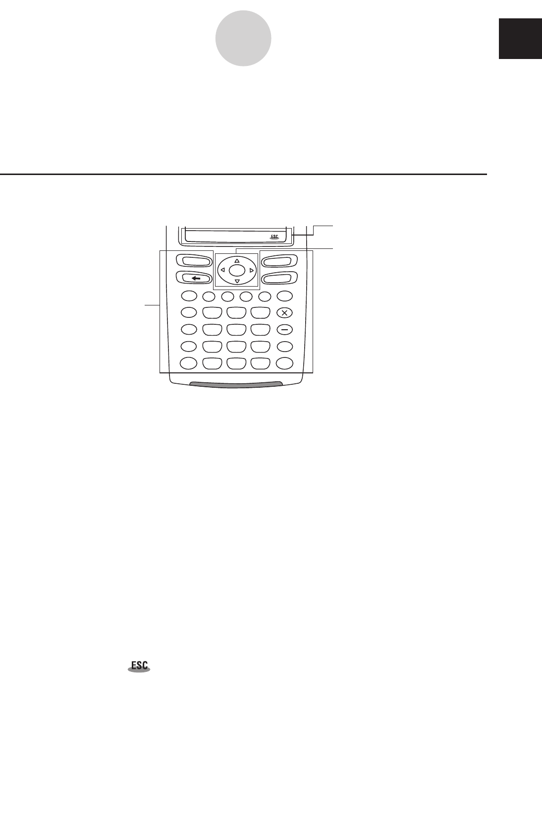
ClassPad Keypad and Icon Panel

1 Keypad

2 Icon panel

3 Cursor key

1 Keypad

ClassPad keypad keys are represented by illustrations that look like the keys you need to

press.

Example 1: Key within text

Press the k to show the soft keyboard.

Example 2: A series of key operations

c2+3-4+10E

When you see something like the above, simply press the keys in the indicated sequence,

from left to right.

2 Icon panel

An operation that requires tapping an icon on the icon panel is indicated by an illustration of

the icon.

Example 1: Tap m to display the application menu.

Example 2: Tap to cancel an ongoing operation.

3 Cursor key

Operation of the cursor key is represented by arrow buttons that indicate which part of the

cursor key you need to press: f, c, d, e.

Example 1: Use d or e to move the cursor around the display.

Example 2: dddd

The above example means that you should press d four times.

smMrSh

(

)

(–)

y÷

EXE

Keyboard

ON/OFF

Clear

EXP

0-1-1

About This User’s Guide 0

20110401

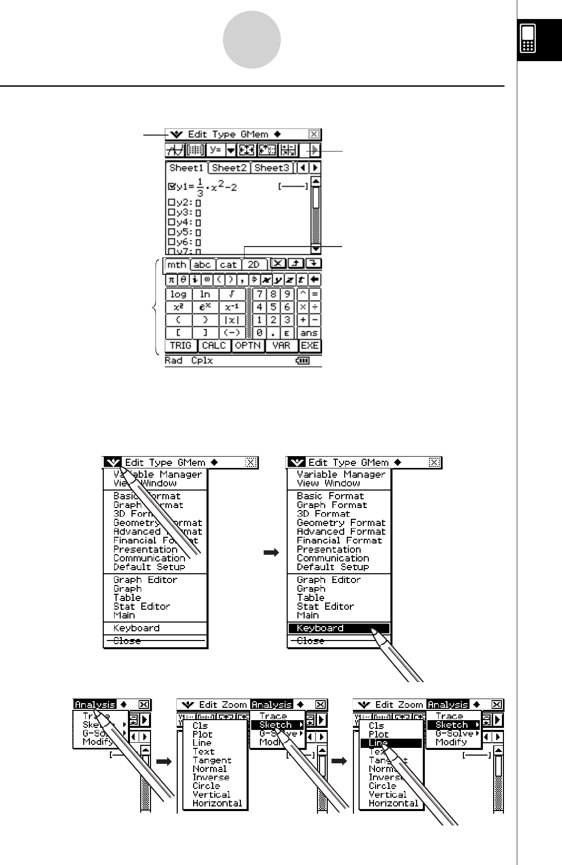
On-screen Keys, Menus, and Other Controllers

4 Menu bar

Menu names and commands are indicated in text by enclosing them inside of brackets.

The following examples show typical menu operations.

Example 1: Tap the O menu and then tap [Keyboard].

5 Toolbar

6 Soft keyboard

Tabs

Example 2: Tap [Analysis], [Sketch], and then [Line].

0-1-2

About This User’s Guide

20060301

5 Toolbar

Toolbar button operations are indicated by illustrations that look like the button you need to

tap.

Example 1: Tap $ to graph the functions.

Example 2: Tap ( to open the Stat Editor window.

6 Soft keyboard

Key operations on the soft keyboards that appear when you press the k key are

indicated by illustrations that look like the keyboard keys.

You can change from one keyboard type to another by tapping one of the tabs along the top

of the soft keyboard.

Example 1: baa/gw

Example 2: ) Ngce*fw

Important!

• If a procedure in this User’s Guide requires use of a soft keyboard, press the k key to

display the soft keyboard. The k key operation is not included as one of the procedure

steps. For more details about how to input data on the ClassPad, see “1-6 Input”.

Page Contents

Three-part page numbers are centered at the top of each

page. The page number “1-4-2”, for example, indicates

Chapter 1, Section 4, page 2.

0-1-3

About This User’s Guide

Note

Display examples shown in this User’s Guide are intended for illustrative purposes only.

The text, values, menus and buttons shown in the screen shots, and other details shown

in this User’s Guide may be slightly different from what actually appears on your ClassPad

screen.

20060301

Getting Acquainted

1-1 General Guide

1-2 Turning Power On and Off

1-3 Using the Icon Panel

1-4 Built-in Applications

1-5 Built-in Application Basic Operations

1-6 Input

1-7 Variables and Folders

1-8 Using the Variable Manager

1-9 Configuring Application Format Settings

Chapter

20110901

1-1 General Guide

Front

1-1-1

General Guide

Side

Back

(

)

(–)

쎹

−

EXE

Keyboard

ON/OFF

Clear

smMrSh

.EXP

20060301

General Guide

The numbers next to each of the items below correspond to the numbers in the illustration on

page 1-1-1.

Front

1 Touch screen

The touch screen shows calculation formulas, calculation results, graphs and other

information. The stylus that comes with the ClassPad can be used to input data and perform

other operations by tapping directly on the touch screen.

2 Stylus

This stylus is specially designed for performing touch screen operations. The stylus slips

into a holder on the right side of the ClassPad for storage when it is not in use. For more

information, see “Using the Stylus” on page 1-1-4.

3 Icon panel

Tapping an icon executes the function assigned to it. See “1-3 Using the Icon Panel” for

details.

4 o key

Press this key to toggle ClassPad power on and off. See “1-2 Turning Power On and Off” for

details.

5 c key

• Pressing this key while inputting data clears all of the data you have input up to that point.

For details, see “Input Basics” on page 1-6-3.

• Pressing the c key while a calculation operation is in progress interrupts the

calculation. For details, see “Pausing and Terminating an Operation” on page 1-5-9.

6 Cursor key (fcde)

Use the cursor key to move the text cursor, selection highlighting, and other selection tools

around the display.

7 k key

Press this key to toggle display of the soft keyboard on and off. For details, see “Using the

Soft Keyboard” on page 1-6-1.

8 K key

• Pressing this key while inputting numeric, expression, or text data deletes one character to

the left of the current cursor position. For details, see “Input Basics” on page 1-6-3.

• Pressing the K key while a calculation operation is in progress pauses the calculation.

For details, see “Pausing and Terminating an Operation” on page 1-5-9.

1-1-2

General Guide

20110901

9 Keypad

Use these keys to input the values and operators marked on them. See “1-6 Input” for

details.

0 E key

Press this key to execute a calculation operation or enter a return.

Side

! 3-pin data communication port

Connect the data communication cable here to communicate with another ClassPad unit or

a CASIO Data Analyzer. See “Chapter 2 – Performing Data Communication” in the separate

Hardware User’s Guide for details.

@ 4-pin mini USB port

Connect the data communication cable here to exchange data with a computer. You can

connect to a CASIO projector and project ClassPad screen contents. See “Chapter 2 –

Performing Data Communication” in the separate Hardware User’s Guide for details.

Back

# Battery compartment

Holds the four AAA-size batteries, or four nickel-metal hydride batteries that power the

ClassPad. For details, see “Power Supply” in the separate Hardware User’s Guide.

$ RESTART button

Press this button to reset the ClassPad. For details, see “Performing the RAM Reset

Operation” in the separate Hardware User’s Guide.

1-1-3

General Guide

20110901

Important!

• Be sure that you do not misplace or lose the stylus. Keep the stylus in the holder on the

right side of the ClassPad whenever you are not using it.

• Do not allow the tip of the stylus to become damaged. Using a stylus with a damaged tip to

perform touch screen operations can damage the touch screen.

• Use only the stylus that comes with your ClassPad or some other similar instrument to

perform touch screen operations. Never use a pen, pencil or other writing instrument, which

can damage the touch screen.

Tap

Drag

• This is equivalent to clicking with a mouse.

• To perform a tap operation, tap lightly with the

stylus on the ClassPad’s touch screen.

• Tapping is used to display a menu, execute an

on-screen button operation, make a window

active, etc.

• This is equivalent to dragging with a mouse.

• To perform a drag operation, hold the tip of the

stylus on the touch screen as you move the

stylus to another location.

• Dragging is used to change the setting of a

slider or some other on-screen controller, to

move a formula, etc.

Using the Stylus

Most value and formula input, command executions, and other operations can be performed

using the stylus.

k Things you can do with the stylus

1-1-4

General Guide

20110901

1-2 Turning Power On and Off

Turning Power On

You can turn on the ClassPad either by pressing the o key or by tapping the touch

screen with the stylus.

• Turning on the ClassPad displays the window that was on the display when you last turned

it off. See “Resume Function” below.

• Note that you need to perform a few initial setup operations when you turn on the ClassPad

the first time after purchasing it. For details, see “Getting Ready” in the separate Hardware

User’s Guide.

Turning Power Off

To turn off the ClassPad, hold down the o key for about two seconds, or until the ending

screen appears. For details about the ending screen, see “Specifying the Ending Screen

Image” in the separate Hardware User’s Guide.

Important!

The ClassPad also has an Auto Power Off feature. This feature automatically turns the

ClassPad off when it is idle for a specified amount of time. For details, see “Auto Power Off”

in the separate Hardware User’s Guide.

Resume Function

Any time the ClassPad powers down (because you turn off power or because of Auto Power

Off), the Resume function automatically backs up its current operational status and any data

in RAM. If you turn ClassPad power back on, the Resume function restores the backed up

operational status and RAM data.

1-2-1

Turning Power On and Off

20110401

1-3 Using the Icon Panel

The icon panel of seven permanent icons is located below the touch screen.

Tapping an icon executes the function assigned to it.

The table below explains what you can do with the icon panel icons.

Function

When you want to do this: Tap this icon:

Display the

O menu to configure settings, switch to the application

menu, etc.

See “Using the O Menu” on page 1-5-4.

Display the application menu

See “1-4 Built-in Applications” for details.

Start the Main application

See “Chapter 2 – Using the Main Application” for details.

Resize the currently active window (when there are two windows

displayed) so it fills the entire display, or return to the dual window

display again

See “Using a Dual Window Display” on page 1-5-1.

Swap the upper window and lower window (when there are two

windows displayed)

See “Using a Dual Window Display” on page 1-5-1.

Capture the currently displayed screen for transfer to a computer or for

use with the ClassPad’s presentation application

See “Chapter 11 – Using the Presentation Application” and

“Chapter 2 – Performing Data Communication” in the separate

Hardware User’s Guide.

Perform the same operation as a computer’s ESC key

The actual operation performed when this icon is tapped depends on

the application you are currently using.

Tip

Tapping the s icon while the application menu is on the screen will display a menu that you can

use to perform the following operations.

• Move an icon (page 1-4-3)

• Swap two icons (page 1-4-4)

• Adjust touch panel alignment (page 1-4-4)

1-3-1

Using the Icon Panel

20060301

To perform this type of operation: Select this icon: See Chapter:

•

Access the eActivity function

• General calculations, including function calculations

• Matrix calculations

• Computer Algebra System

• Create a list

• Perform statistical calculations

• Draw a statistical graph

• Input data into a spreadsheet

• Manipulate spreadsheet data

• Graph spreadsheet data

• Register a function and create a table of solutions by

substituting different values for the function’s variables

• Draw a graph

• Perform sequence calculations

• Solve recursion expressions

• Draw the graph of a conics section

• Graph the 3D function z = f(x,y)

• Draw geometric figures

• Build animated figures

• Obtain the value of any variable in an equation,

without transforming or simplifying the equation

• Draw vector fields and solution curves to explore

differential equations

• Perform simple interest, compound interest,

and other financial calculations

• Create and run a presentation using ClassPad

application window

• Register a file name in the programming area

• Input a program or run a program

1-4 Built-in Applications

Tapping m on the icon panel displays the application menu.

The table below shows the icon menu names of the built-in applications, and explains what

you can do with each application.

1-4-1

Built-in Applications

20110901

Starting a Built-in Application

Perform the steps below to start a built-in application.

u ClassPad Operation

(1) On the icon panel, tap m to display the application menu.

(2) If you cannot see the icon of the application you want on the menu, tap the scroll

buttons or drag the scroll bar to bring other icons into view.

(3) Tap an icon to start its application.

Tip

• You can also start the Main application by tapping M on the icon panel. See “1-3 Using the Icon

Panel” for details.

Application Menu Operations

The following describes the various types of operations you can perform while the

application menu is on the display.

• Starting an application

See “Starting a Built-in Application” above.

Application Menu

1-4-2

Built-in Applications

Scroll down button

Scrollbar

Scroll up button

To perform this type of operation: Select this icon:

See Chapter:

See Chapter 2 in the separate

Hardware User’s Guide.

See the separate E-Con

User’s Guide.

• Clear the memory

• Adjust contrast

• Configure other system settings

• Exchange data with another ClassPad,

a computer, or another device

• Control the optionally available EA-200

Data Analyzer.

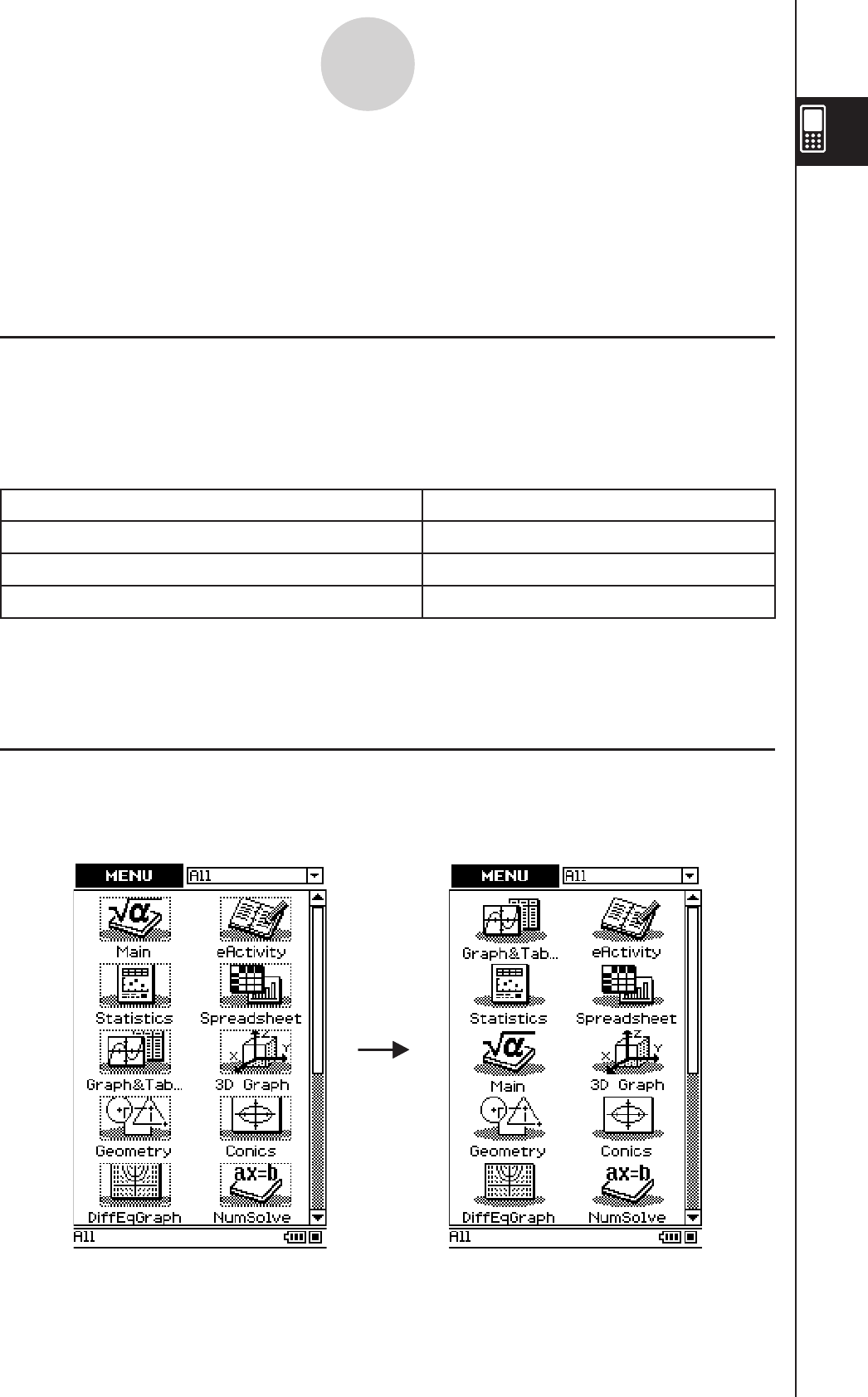
20110401

• Displaying applications according to group (Additional Applications, All Applications)

See “Using Application Groups” below.

• Moving or swapping icons

See “Moving an Icon” below, and “Swapping Two Icons” on page 1-4-4.

• Deleting an application

See “Deleting an Application” on page α-2-1 in the separate Hardware User’s Guide.

k Using Application Groups

You can use application groups to specify the type of applications that appear on the

application menu.

To select an application group, tap the box in the upper right of the application menu, and

then select the group you want from the list that appears.

To display these icons: Select this application group:

Add-in applications only Additional

All applications All

Add-in applications above built-in applications Add-ins First

Tip

• Nothing appears on the application menu if you select the “Additional” group while there are no

add-in applications installed on the ClassPad.

k Moving an Icon

You can use the procedure below to move an icon to a different location on the application

menu.

1-4-3

Built-in Applications

20060301

u ClassPad Operation

(1) On the icon panel, tap m to display the application menu.

(2) Tap at the top left of the application menu.

• This opens a menu of setting options.

(3) Tap [Move Icon].

(4) Tap the icon you want to move (J in this example).

• This selects the icon.

(5) Tap the icon that you want the first icon to follow (C in this example).

• This moves the icon.

k Swapping Two Icons

Perform the following steps to swap two icons on the application menu.

u ClassPad Operation

(1) On the icon panel, tap m to display the application menu.

(2) Tap at the top left of the application menu.

• This opens a menu of setting options.

(3) Tap [Swap Icon].

(4) Tap one of the icons.

• This selects the icon.

(5) Tap the other icon (the one you want to swap with).

• This swaps the icons.

k Adjusting Touch Panel Alignment

Perform the following steps to align the touch panel.

u ClassPad Operation

(1) On the icon panel, tap m to display the application menu.

(2) Tap at the top left of the application menu.

• This opens a menu of setting options.

(3) Tap [Touch Panel Alignment].

• This displays the Touch Panel Alignment screen.

(4) Use the stylus to tap the center of each of the four crosses as they appear on the

screen.

• Tapping the center of the fourth cross completes touch panel alignment and returns

you to the application menu.

• When aligning your ClassPad try to tap the exact center of each cross.

1-4-4

Built-in Applications

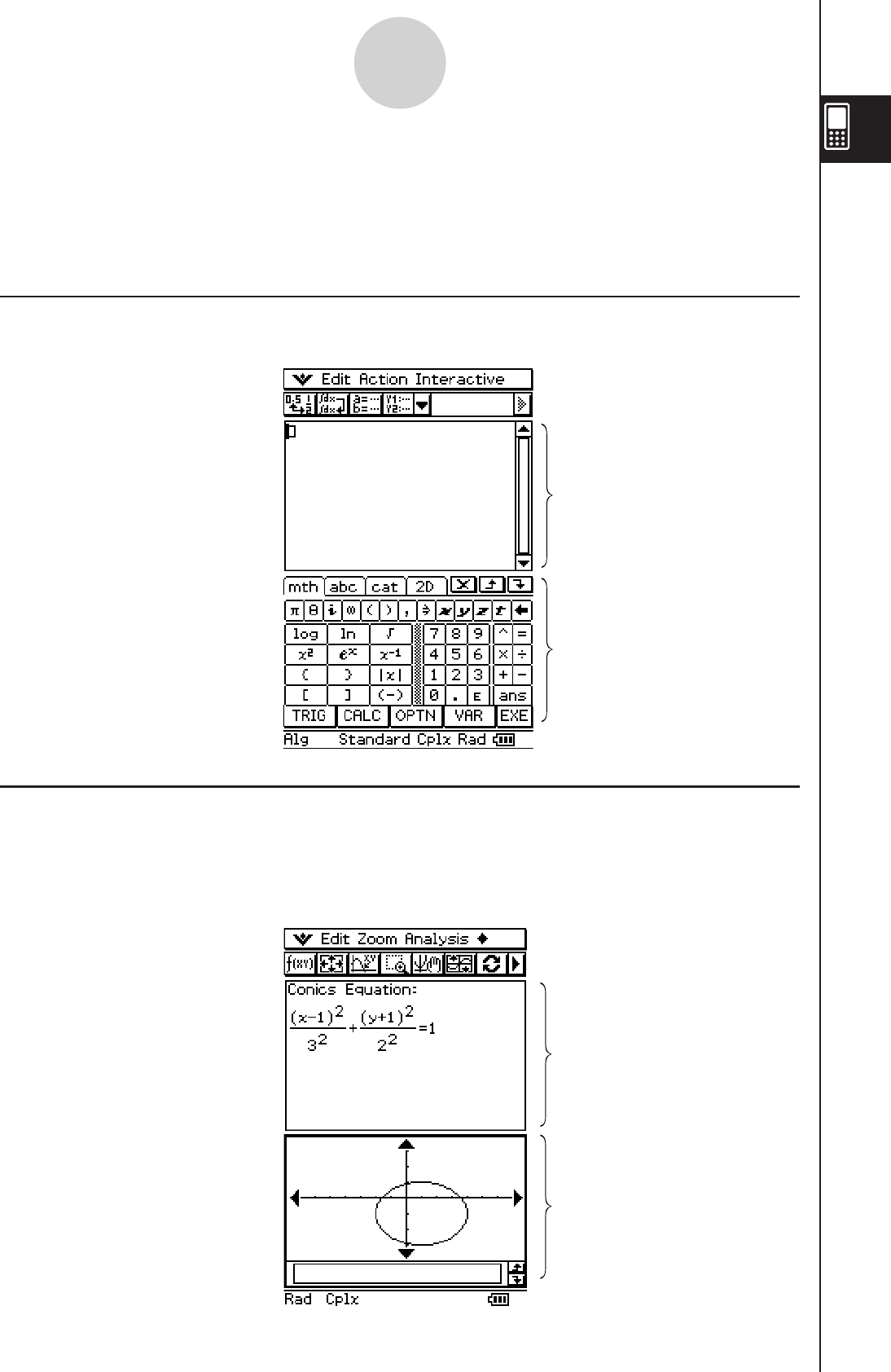
20060301

1-5 Built-in Application Basic Operations

This section explains basic information and operations that are common to all of the built-in

applications.

Application Window

The following shows the basic configuration of a built-in application window.

Using a Dual Window Display

Many applications split the display between an upper window and a lower window, each

of which shows different information. The sample screenshot below is from the Conics

application, which uses the upper window for input of expressions, and the lower window for

graphing.

1-5-1

Built-in Application Basic Operations

Application window

}

Menu bar

}

Toolbar

}

Status bar

Soft keyboard (page 1-6-1)

Upper window

Lower window

20060301

When using two windows, the currently selected window (the one where you can perform

operations) is called the “active window”. The menu bar, toolbar, and status bar contents are

all applicable to the active window. The active window is indicated by a thick boundary around

it.

u To switch the active window

While a dual window is on the display, tap anywhere inside the window that does not have a

thick boundary around it to make it the active window.

• Note that you cannot switch the active window while an operation is being performed in the

current active window.

u To resize the active window so it fills the display

While a dual window is on the display, tap r. This causes the active window to fill the

display. To return to the dual window display, tap r again.

u To swap the upper and lower windows

While a dual window is on the display, tap S. This causes the upper window to become the

lower window, and vice versa. Swapping windows does not have any affect on their active

status. If the upper window is active when you tap S for example, the window will remain

active after it becomes the lower window.

Tip

• When you tap r button while a dual window is on the display, the currently active window will

fill the display, but the other (inactive) window does not close. It remains open, hidden behind the

active window. This means you can tap S to bring the hidden window forward and make it the

active window, and send the current active window to the background.

u To close the active windows

While a dual window is on the display, tap at to top right corner of the window to close the

active window, which causes the other (inactive) window to fill the display.

Tip

• When the close ( ) button is dimmed, it means that the active window cannot be closed for some

reason.

1-5-2

Built-in Application Basic Operations

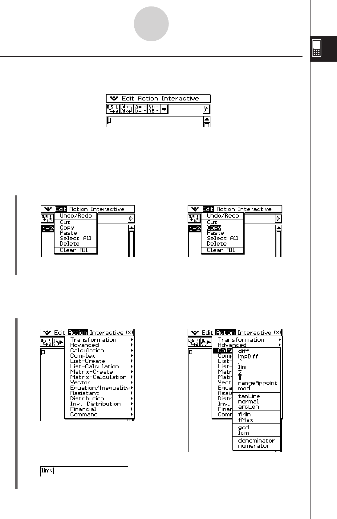
20101001

(3) Tap [lim].

• This inputs “lim(”.

Example 1: Choosing the [Edit] menu’s [Copy] item

u ClassPad Operation

(1) Tap [Edit]. (2) Tap [Copy].

Example 2: Choosing [lim], which is on the [Calculation] submenu of the [Action] menu.

u ClassPad Operation

(1) Tap [Action]. (2) Tap [Calculation].

1-5-3

Built-in Application Basic Operations

• This displays the contents of the • This performs a copy operation.

[Edit] menu.

Using the Menu Bar

The menu bar appears along the top of the window of each application. It shows the menus

that you can access for the currently active window.

Tapping the menu bar menu displays its commands, options, and settings from which you

can choose the one you want. Some menu items have a single selection as shown in

Example 1, below, while other menu items display a submenu of selections from which you

can choose as shown in Example 2.

}

Menu bar

• This displays the contents of the

[Action] menu.

• This displays the contents of the

[Calculation] submenu.

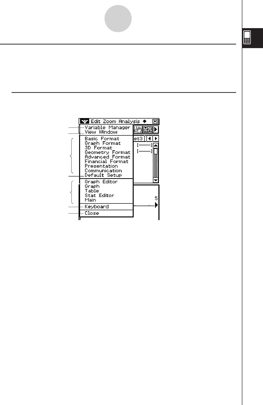
20060301

Using the O Menu

The O menu appears at the top left of the window of each application, except for the

System application.

You can access the O menu by tapping s on the icon panel, or by tapping the menu

bar’s O menu.

k O Menu Items

The following describes all of the items that appear on the O menu.

1 Tapping [Variable Manager] starts up the Variable Manager. See “1-8 Using the Variable

Manager” for details.

2 Tapping [View Window] displays a dialog box for configuring the display range and other

graph settings. For details, see the explanations for the various applications with graphing

capabilities (Graph & Table, Conics, 3D Graph, Statistics, etc.)

3 Tapping a menu selection displays a dialog box for configuring the corresponding setup

settings. See “1-9 Configuring Application Format Settings” for details.

4 Tapping [Default Setup] returns all settings to their initial defaults (except for the current

folder setting). See “1-9 Configuring Application Format Settings” for details.

5 This area shows a list of all of the windows that can be accessed from the current

application (Graph & Table application in this example). Tapping a menu selection displays

the corresponding window and makes it active. For details, see “Using the O Menu to

Access Windows” on page 1-5-5.

6 Tap [Keyboard] to toggle display of the soft keyboard on and off.

7 Tapping [Close] closes the currently active window, except in the following cases.

• When only one window is on the display

• When the currently active window cannot be closed by the application being used

You cannot, for example, close the Graph Editor window from the Graph & Table

application.

1-5-4

Built-in Application Basic Operations

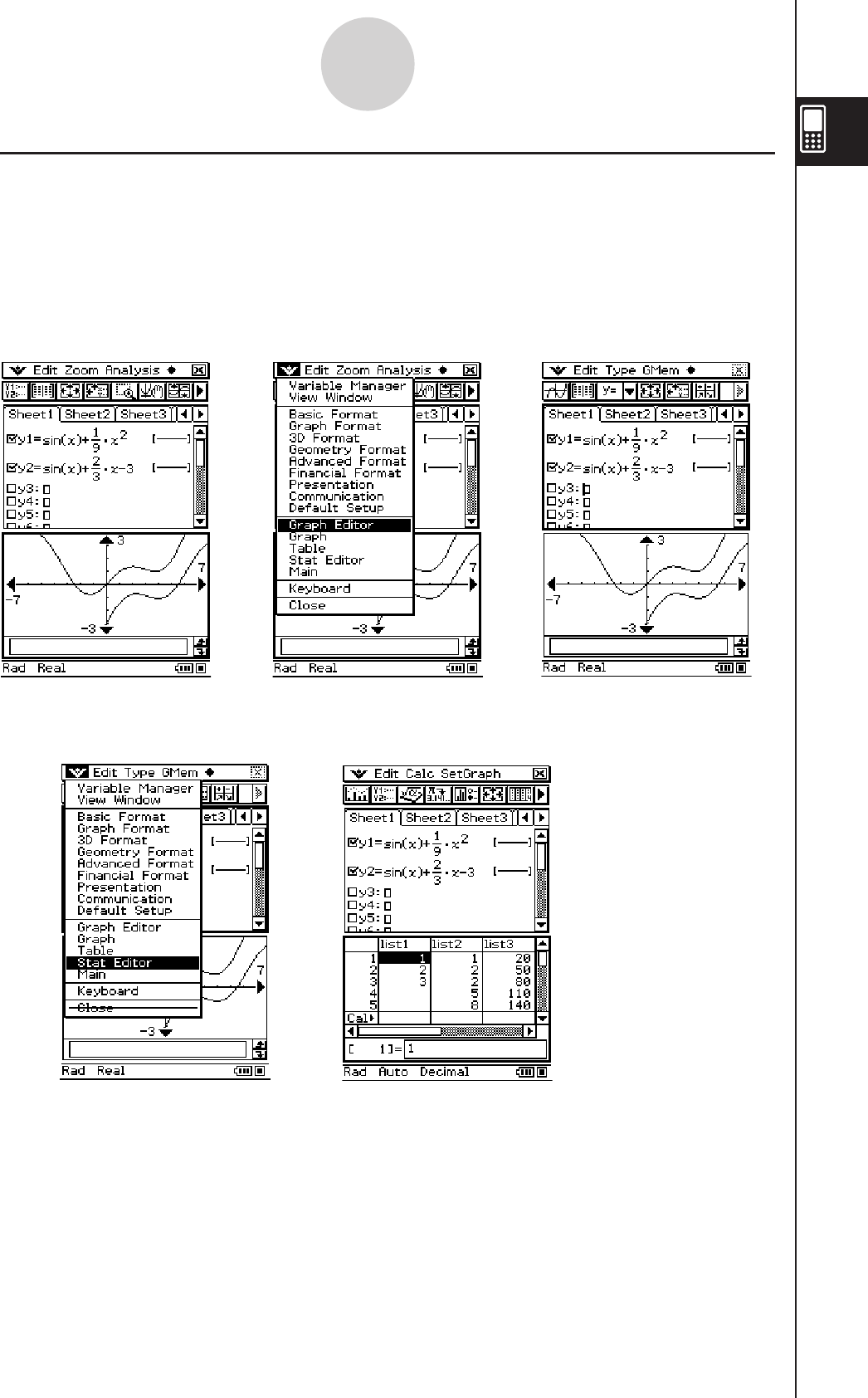
20060301

k Using the O Menu to Access Windows

Most ClassPad applications support simultaneous display of two windows. When two

windows are on the display, the one with a thick selection boundary around it is the active

window. The displayed menu and toolbar are the ones for the currently active window.

You can use the O menu to change the active window and to display the window you want.

u Window Selection Example (Graph & Table)

(1) Graph window is active.

(2) Tap O and then

[Graph Editor].

(3) Graph Editor window

becomes active.

1-5-5

Built-in Application Basic Operations

(4) Tap O and then

[Stat Editor].

(5) Stat Editor window

appears and becomes

active.

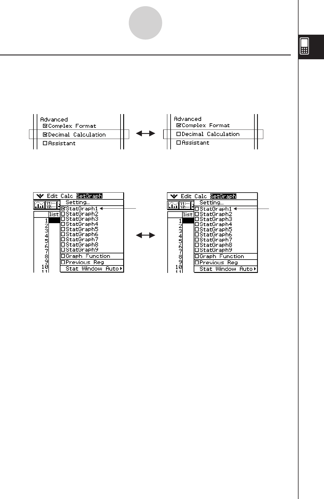
20060301

1-5-6

Built-in Application Basic Operations

Using Check Boxes

A check box shows the current status of a dialog box option that can be turned on or off. An

option is turned on (selected) when its check box has a check mark inside it. An option is

turned off when a check box is cleared.

Tapping a check box toggles the option on (checked) and off (cleared).

Check boxes also appear on menus. Menu check boxes operate the same way as dialog box

check boxes.

Option turned offOption turned on

Option turned on Option turned off

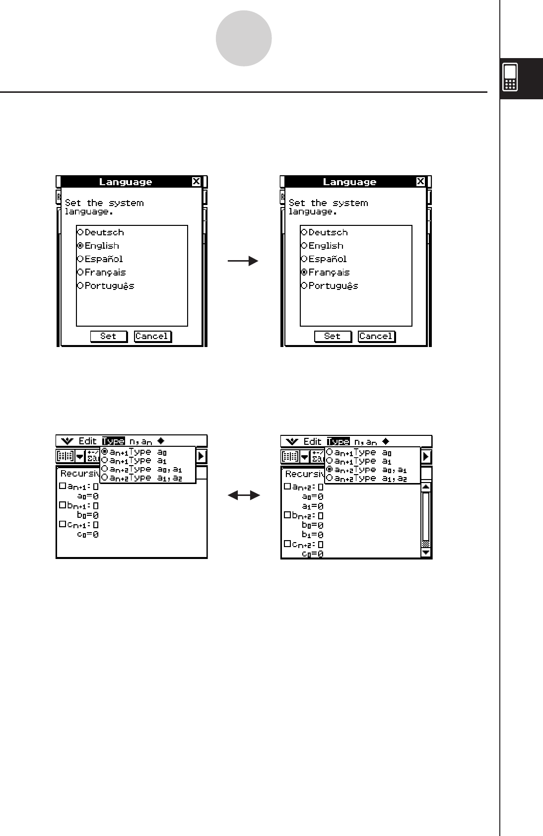
20060301

1-5-7

Built-in Application Basic Operations

Using Option Buttons

Option buttons are used on dialog boxes that present you with a list of options from which

you can select only one. A black option button indicates the currently selected option, while

the buttons of the options that are not selected are white.

Option buttons also appear on menus. Menu option buttons operate the same way as dialog

box option buttons.

Tap “Français”. This selects “Français” and

deselects “English”.

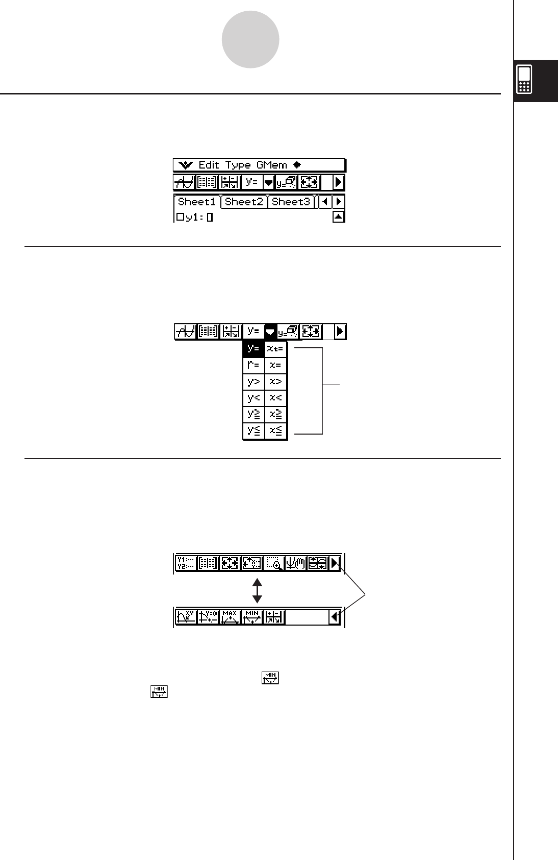
20060301

Using the Toolbar

The toolbar is located directly underneath the menu bar of an application window. It contains

the buttons for the currently active window.

k Toggling between Multiple Toolbars

With some applications, not all of the buttons can fit on a single toolbar. When this happens,

the buttons that cannot fit are placed onto a second toolbar. When there are two toolbars,

each of them has an arrow button on the far right. Toolbar 1 has a u button while toolbar 2

has a t button. Tapping an arrow button toggles between the two toolbars.

1-5-8

Built-in Application Basic Operations

}

Toolbar

List of options

Tap here to toggle

k Toolbar Buttons

Normally, you tap a button to execute the command assigned to it. Some buttons, however,

have a down arrow v next to them. Tapping the arrow displays a list of options from which

you can select.

Tip

• The explanations in this manual make no distinction between toolbar 1 and toolbar 2.

Even if a button is located on toolbar 2 (like the button in the above example) you will be

instructed simply to “tap ”.

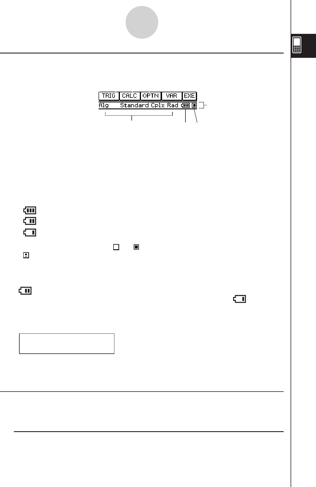
20110401

Interpreting Status Bar Information

The status bar appears along the bottom of the window of each application.

1 Information about current application

Tip

• You can change the configuration of a setting indicated in the status bar by tapping it. Tapping

“Cplx” (indicating complex number calculations) while the Main application is running will toggle

the setting to “Real” (indicating real number calculations). Tapping again will toggle back to “Cplx”.

For information about application-specific information that appears in the status bar, see the

sections in this manual that describes each application.

2 Battery level indicator

....................... full

....................... medium

....................... low

3 This indicator flashes between and while an operation is being performed.

appears here to indicate when an operation is paused.

Important!

• Be sure to replace batteries as soon as possible whenever the battery level indicator shows

(medium).

• Replace batteries immediately whenever the battery level indicator shows (low). At this

level, you will not be able to perform data communication or other functions.

• The following message indicates that batteries are about to die. Replace batteries

immediately whenever this message appears.

Batteries are extremely low!

Replace batteries immediately!

• See the separate Hardware User’s Guide for details about replacing batteries.

Pausing and Terminating an Operation

Many of the built-in applications provide operations to pause and terminate (break)

expression processing, graphing, and other operations.

k Pausing an Operation

Pressing the K key while an expression processing, graphing, or other operation is being

performed pauses the operation. Pressing K again resumes the operation.

1-5-9

Built-in Application Basic Operations

Status bar

123

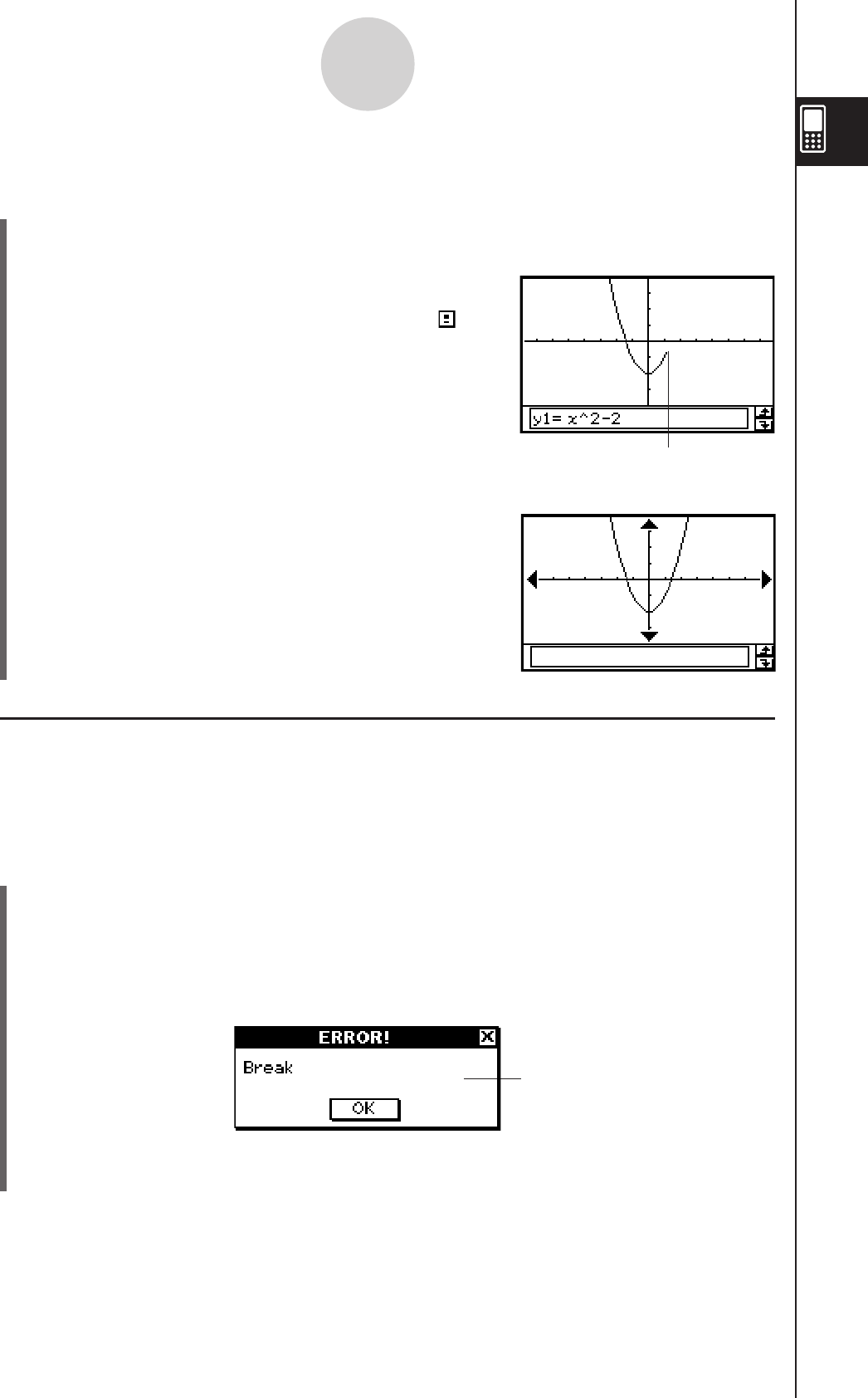
20060301

Break dialog box

1-5-10

Built-in Application Basic Operations

Example: To pause a graphing operation and then resume it

uClassPad Operation

(1) Use the Graph & Table application to draw a graph.

• For details about graphing, see “Chapter 3 – Using the Graph & Table Application”.

(2) While the graph is being drawn, press the K key.

• This pauses the draw operation and displays on

the right side of the status bar.

(3) To resume the operation, press the K key again.

• This resumes the draw operation, which continues

until the graph is complete.

k Terminating an Operation (Break)

Pressing the c key while an expression processing, graphing, or other operation is being

performed terminates the operation.

Example: To terminate a graphing operation

u ClassPad Operation

(1) Use the Graph & Table application to draw a graph.

• For details about graphing, see “Chapter 3 – Using the Graph & Table Application”.

(2) While the graph is being drawn, press the c key.

• This terminates the draw operation and displays the Break dialog box, indicating the

Break state.

Draw is paused at the point

where K is pressed.

(3) To exit the Break state, tap the [OK] button.

• This returns the ClassPad to its status before you started the graphing operation.

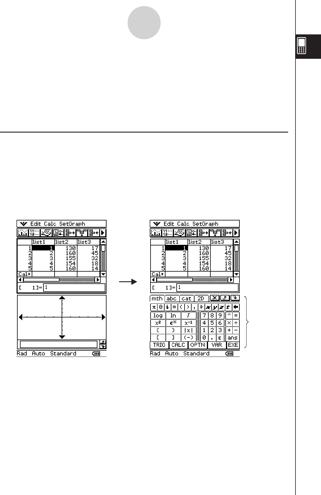
20060301

1-6 Input

You can input data on the ClassPad using its keypad or by using the on-screen soft

keyboard.

Virtually all data input required by your ClassPad can be performed using the soft keyboard.

The keypad keys are used for input of frequently used data like numbers, arithmetic

operators, etc.

Using the Soft Keyboard

The soft keyboard is displayed in the lower part of the touch screen. A variety of different

special-purpose soft keyboard styles help to take much of the work out of data input.

u To display the soft keyboard

When the soft keyboard is not on the touch screen, press the k key, or tap the O

menu and then tap [Keyboard]. This causes the soft keyboard to appear.

1-6-1

Input

• Pressing the k key again hides the soft keyboard.

• The icon panel’s r icon is disabled while the soft keyboard is on the display.

For details about r, see “Using a Dual Window Display” on page 1-5-1.

The soft

keyboard

appears.

Press k.

20090601

k Soft Keyboard Styles

There are four different soft keyboard styles as described below.

• Math (mth) Keyboard

Pressing

k will display the keyboard that you last

displayed while working in that application. If you quit the

application and go into another application, then the 9

(default) soft keyboard appears.

You can use the math (mth) keyboard to input values,

variables, and expressions. Tap each lower button to see

additional characters, for example tap -. For more

information, see “Using the Math (mth) Keyboard” on page

1-6-8.

• Alphabet (abc) Keyboard

Use this keyboard to input alphabetic characters, Greek

characters, and other characters, as well as logical symbols

and other numeric symbols. Tap one of the buttons along

the bottom of the keyboard to see additional characters, for

example, tap n. For more information, see “Using the

Alphabet (abc) Keyboard” on page 1-6-10.

• Catalog (cat) Keyboard

This keyboard provides a scrollable list that can be used

to input built-in functions, built-in commands, system

variables, and user-defined functions. Tap a command to

select it and then tap it again to insert it. Selecting an item

from the Form list changes the available commands. For

more information, see “Using the Catalog (cat) Keyboard”

on page 1-6-13.

• 2D Keyboard

This keyboard displays various templates for natural input

of fractions, exponential values, matrices, differential and

integral calculus expressions, etc. Note that natural input

is available in most ClassPad applications. Natural input

cannot be used in the geometry measurement box or when

entering data into a list. For more information, see “Using

the 2D Keyboard” on page 1-6-15.

Tip

• 2D math symbols are easy to use. Just tap the image of the symbol you would like to use and it

will appear in your application.

• 2D math symbols can be used in most applications.

1-6-2

Input

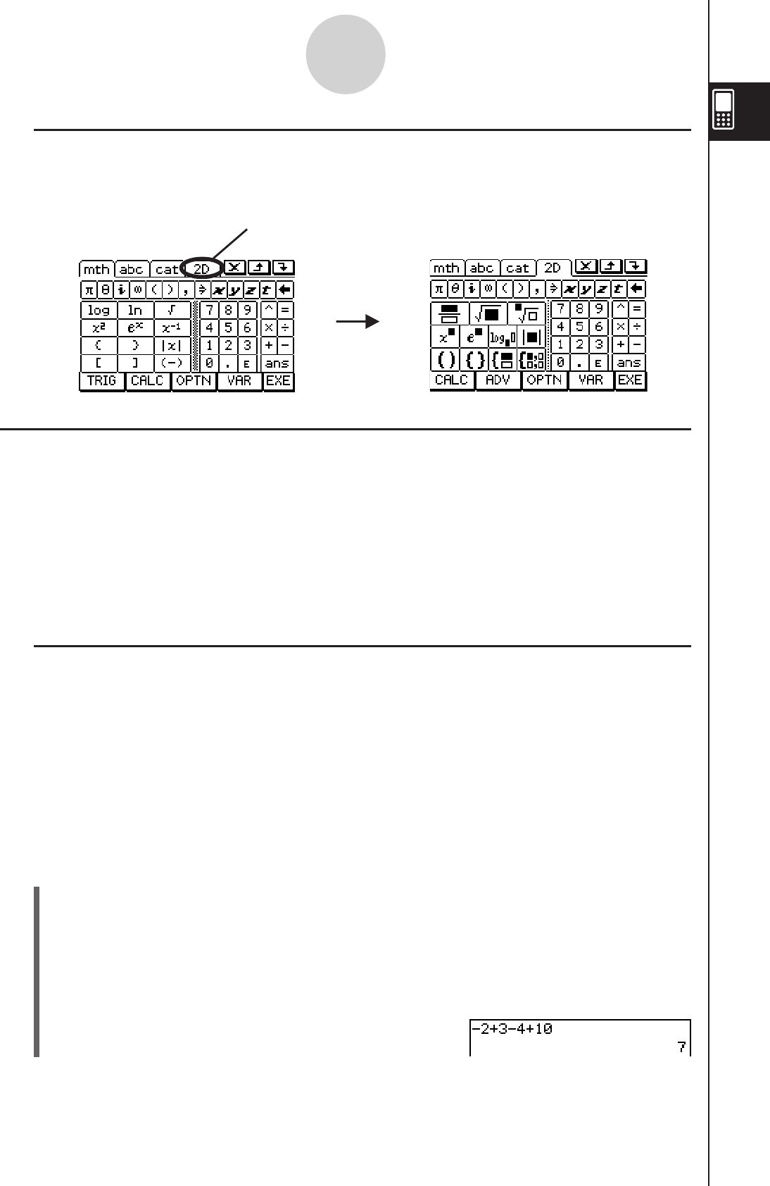
20090601

k Selecting a Soft Keyboard Style

Tap one of the tabs along the top of the soft keyboard (9, 0, (, or )) to select

the keyboard style you want.

1-6-3

Input

To display the 2D

keyboard

Tap here.

Input Basics

This section includes a number of examples that illustrate how to perform basic input

procedures. All of the procedures assume the following.

• The Main application is running.

For details, see “Starting a Built-in Application” on page 1-4-2.

• The soft keyboard is displayed.

For details, see “Using the Soft Keyboard” on page 1-6-1.

k Inputting a Calculation Expression

You can input a calculation expression just as it is written, and press the E key to execute

it. The ClassPad automatically determines the priority sequence of addition, subtraction,

multiplication, division, and parenthetical expressions.

• Before starting any calculation, be sure to clear the ClassPad by pressing c.

See Chapter 2 for more information about inputting expressions.

• Use the z or - key to input the minus sign before a negative value.

Example 1: To simplify –2 + 3 – 4 + 10

u ClassPad Operation

Using the keypad keys

cz2+3-4+10E

Using the soft keyboard

Tap the keys of the math (mth) keyboard or the 2D keyboard to input the calculation

expression.

c9-c+d-e+baw

When the soft keyboard is not on the touch screen, press the k key, or tap the O

menu and then tap [Keyboard]. This causes the soft keyboard to appear on the display.

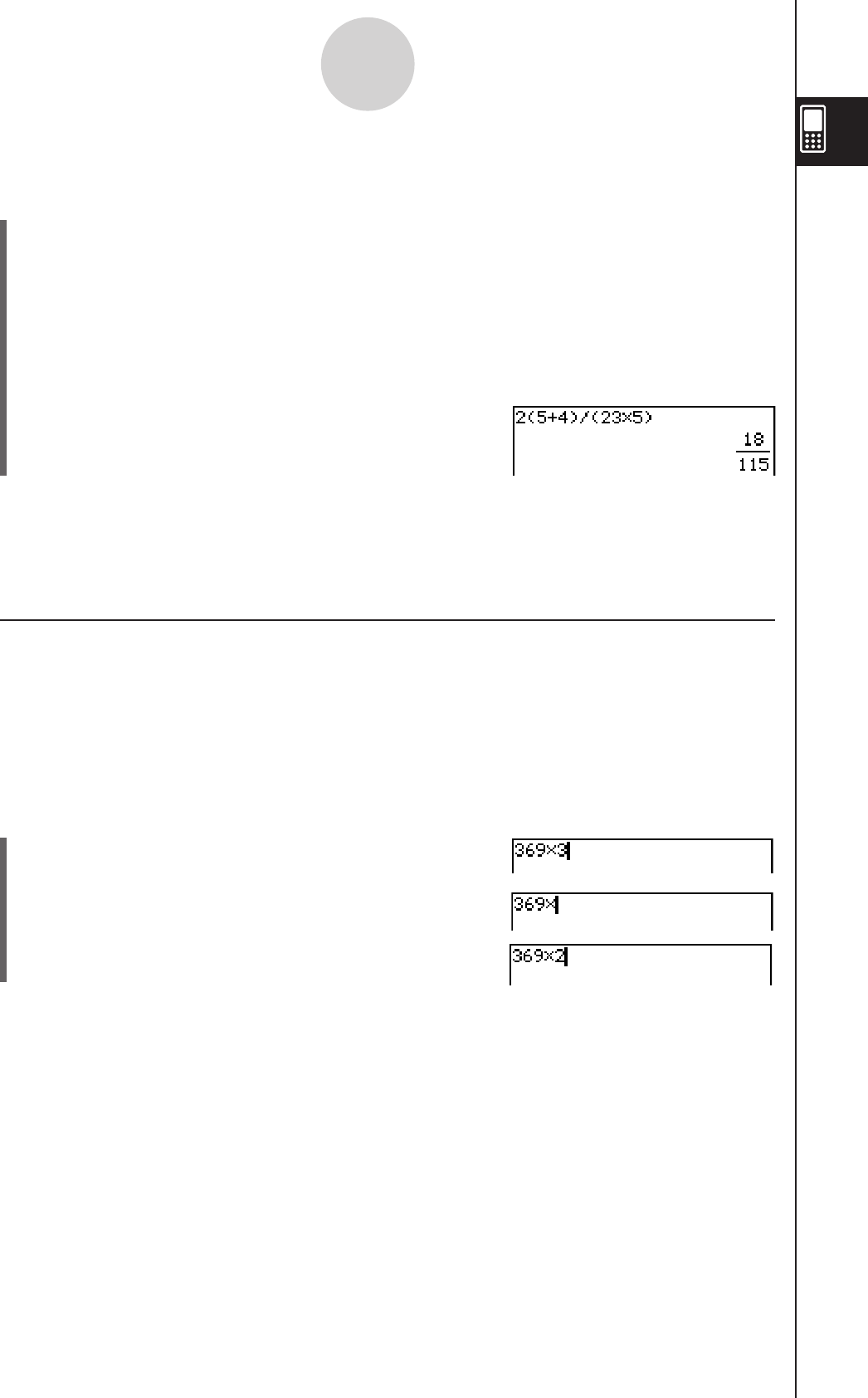
20060301

1-6-4

Input

Example 2: To simplify 2 (5 + 4) ÷ (23 × 5)

u ClassPad Operation

Using the keypad keys

c2(5+4)/(23*5)E

Using the soft keyboard

Tap the keys of the math (mth) keyboard or the 2D keyboard to input the calculation

expression.

c9 (or )) c(f+e)/(cd*f)w

Tip

• As shown in Example 1 and Example 2, you can input simple arithmetic calculations using either

the keypad keys or the soft keyboard. Input using the soft keyboard is required to input higher

level calculation expressions, functions, variables, etc.

k Editing Input

The following are the different techniques you can use to edit your input.

u To change something right after you input it

When the cursor is located at the end of your input, press K to delete the character or

operator you want to edit.

Example: To change the expression 369 × 3 to 369 × 2

(1)

c369*3

(2) K

(3)

Tip

• Or, drag your stylus across 3 to select it and input 2.

20060301

u To delete an unneeded key operation

Use d and e to move the cursor to the location immediately to the right of the key

operation you want to delete, and then press K. Each press of K deletes one

command to the left of the cursor.

Example: To change the expression 369 × × 2 to 369 × 2

(1)

c369**2

(2)

Tip

• You can move the cursor without using the cursor key by tapping at the destination with the

stylus. This causes the cursor to jump to the location where you tap.

u To correct a calculation expression

Use d and e to move the cursor to the location immediately to the right of the location

you want to correct, and then press K.

Example: To correct cos(60) so it becomes sin(60)

(1) Use the mathematics (mth) keyboard to input “cos(60)”.

c9Tcga)

(2) Move the cursor to the location immediately to the right of “cos(”.

ddd

(3) Delete “cos(”.

KKKK

(4) Input “sin(”.

(5) Tap

I to return to the initial math (mth) key set. See “Using the Math (mth)

Keyboard” on page 1-6-8 for details.

Tip

• Or, drag your stylus across “cos(” to select it and input “sin(”.

After you make all of the changes you want, press E to calculate the result. To continue

inputting the calculation, press e to move the cursor to the end of the calculation, and input

what you want.

1-6-5

Input

Tapping the T key causes it to

change to I and displays a key set

for inputting trigonometric functions.

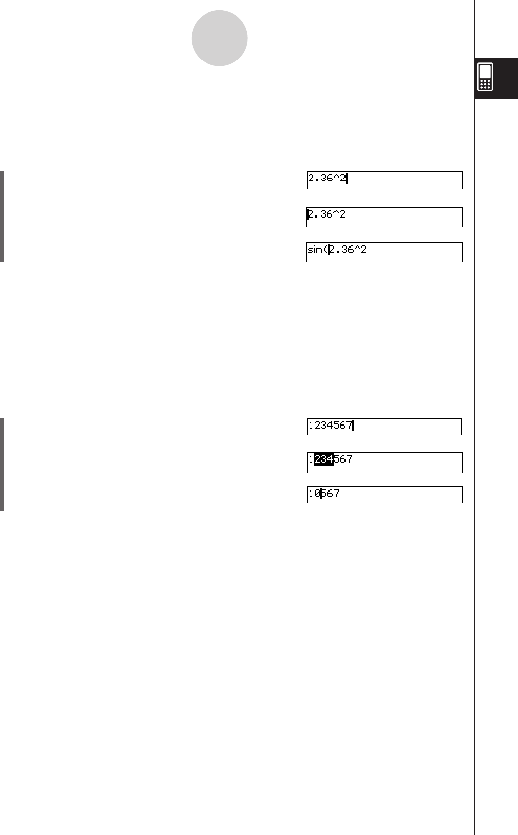
20060301

u To insert new input into the middle of an existing calculation expression

Use d or e to move the cursor to the location where you want to insert new input, and

then input what you want.

Example: To change 2.362 to sin(2.362)

(1)

c9c.dgx

(2)

dddddd

(3)

Tip

• You can move the cursor without using the cursor key by tapping at the destination with the

stylus. This causes the cursor to jump to the location where you tap.

u To replace a range of input with new input

After you drag the stylus across the range of input that you want to replace, enter the new

input.

Example: To replace the “234” of “1234567” with “0”.

(1) Input “1234567”.

c1234567

(2) Drag the stylus across “234” to select it.

(3) Input “0”.

Tip

• You can perform d and K key operations by pressing the corresponding keypad key or soft

key.

1-6-6

Input

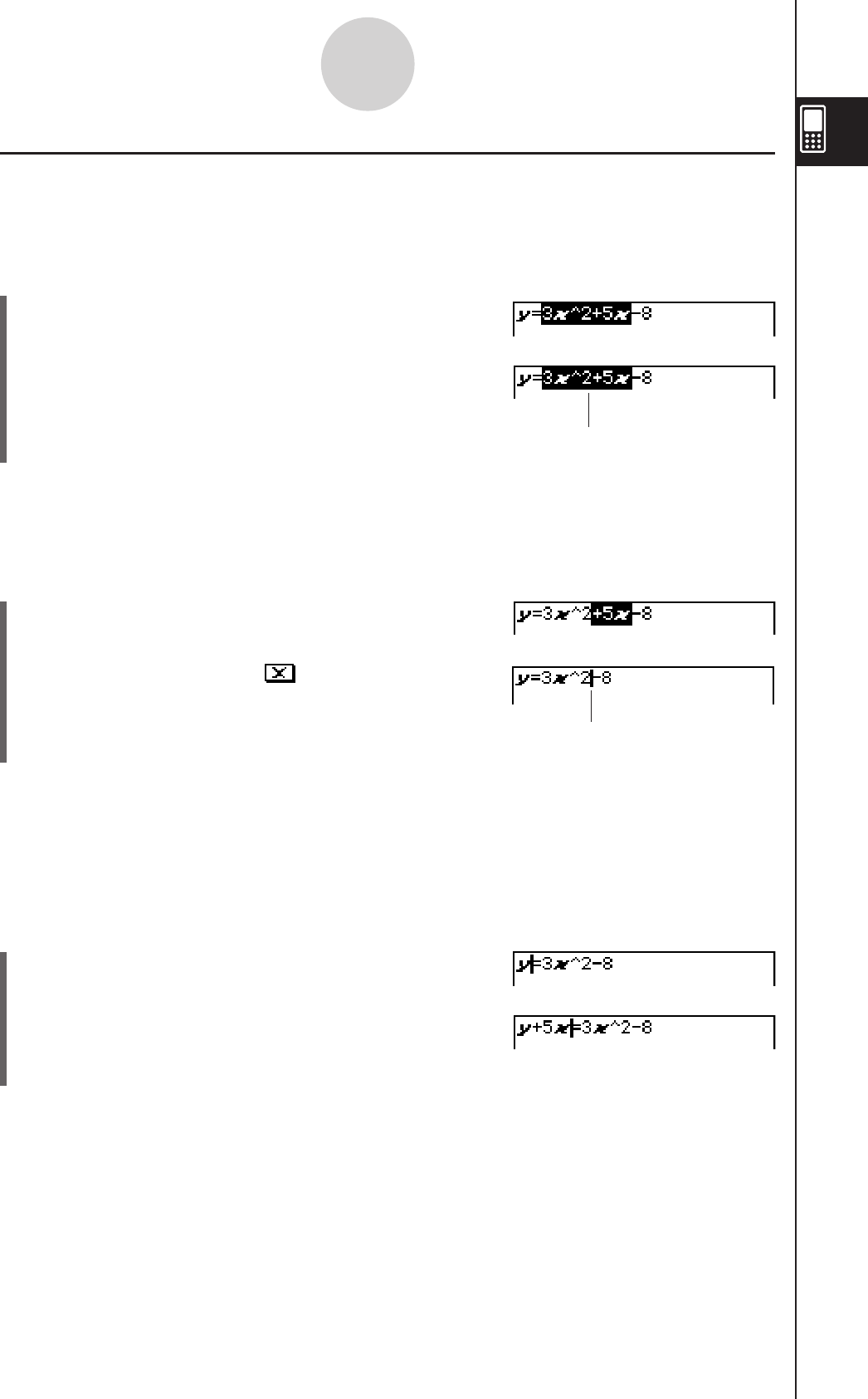
20060301

k Using the Clipboard for Copy and Paste

You can copy (or cut) a function, command, or other input to the ClassPad’s clipboard, and

then paste the clipboard contents at another location.

u To copy characters

(1) Drag the stylus across the characters you

want to copy to select them.

(2) On the soft keyboard, tap G.

• This puts a copy of the selected characters onto

the clipboard.

1-6-7

Input

The selected characters are not

changed when you copy them.

Tip

• You can also copy characters by tapping the [Edit] menu and then tap [Copy].

u To cut characters

(1) Drag the stylus across the characters you want to

cut to select them.

(2) On the soft keyboard, tap .

• This moves the selected characters onto

the clipboard.

Tip

• Performing a copy or cut operation causes the clipboard contents to be replaced by the newly

copied or cut characters.

• You can also cut characters by tapping the [Edit] menu and then tap [Cut].

u To paste the clipboard contents

(1) Move the cursor to the location where you want to

paste the clipboard contents.

(2) On the soft keyboard, tap H.

• This pastes the clipboard contents at the current

cursor location.

Tip

• The clipboard contents remain on the clipboard after you paste them. This means you can paste

the current contents as many times as you like.

• You can also paste the clipboard contents by tapping the [Edit] menu and then tap [Paste].

Cutting causes the original

characters to be deleted.

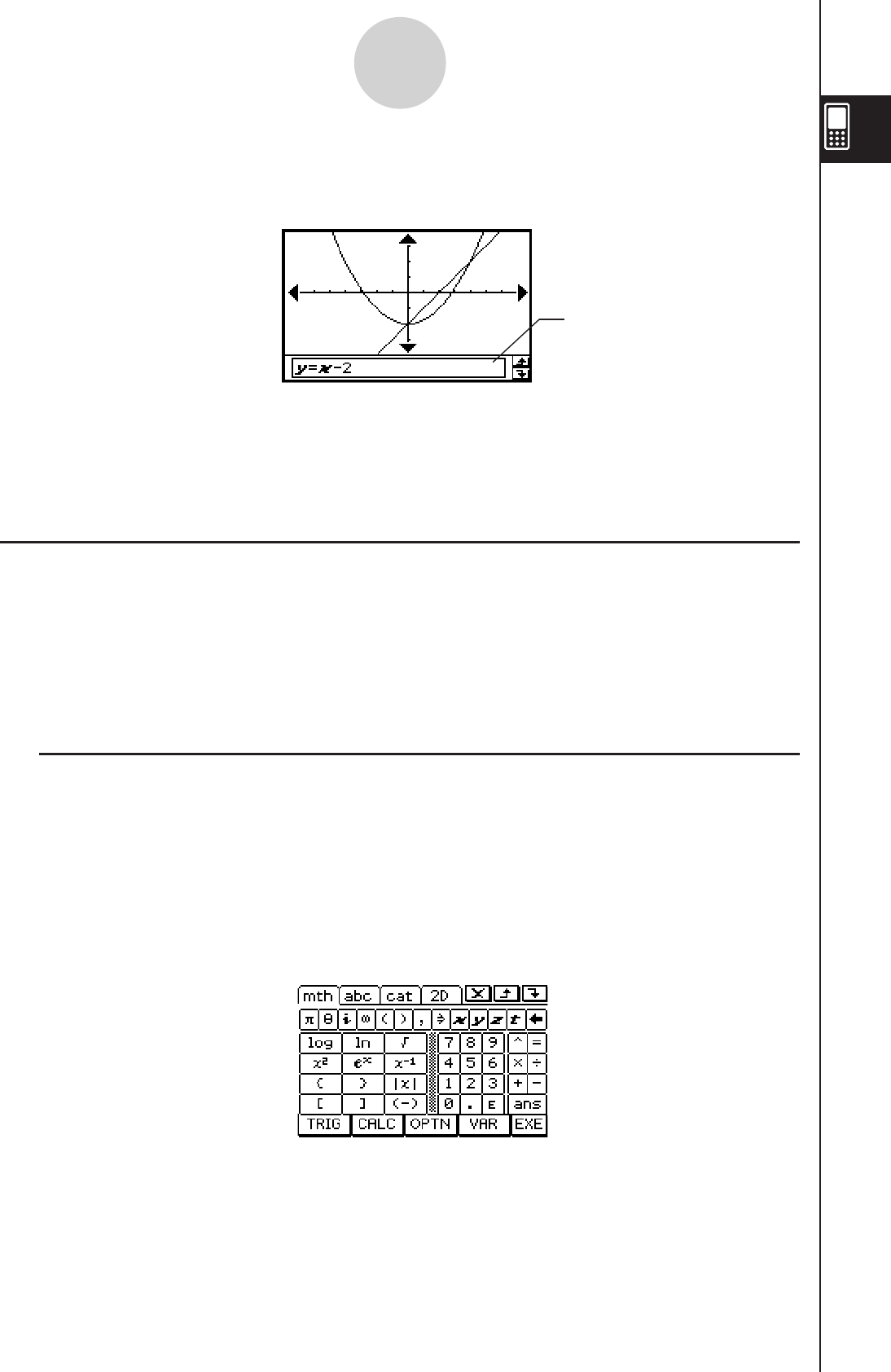
20060301

1-6-8

Input

uCopying and pasting in the message box

The “message box” is a 1-line input and display area under the Graph window (see Chapter 3).

You can use the two buttons to the right of the message box to copy the message box

contents (G button), or to paste the clipboard contents to the message box (H button).

Copy and paste are performed the same way as the copy and paste operations using the

soft keyboard.

Advanced Soft Keyboard Operations

As explained in “Using the Soft Keyboard” on page 1-6-1, there are four soft keyboard types:

the math (mth) keyboard, the alphabet (abc) keyboard, the catalog (cat) keyboard, and the

2D math (2D) keyboard. This section provides more detailed information about soft keyboard

operations and the various key sets available with each soft keyboard.

• All of the explanations in this section start from the initial key set of each keyboard.

k Using the Math (mth) Keyboard

The math (mth) keyboard is for inputting calculation expressions and numeric expressions. In

addition to the initial math (mth) key set, you can also select from among four other key sets

named T (trigonometry), - (calculus), K (option), and V (variable).

u Initial math (mth) keyboard key set

If you stay in the same application, the keyboard that you used last will appear when you

press the k key.

Message box

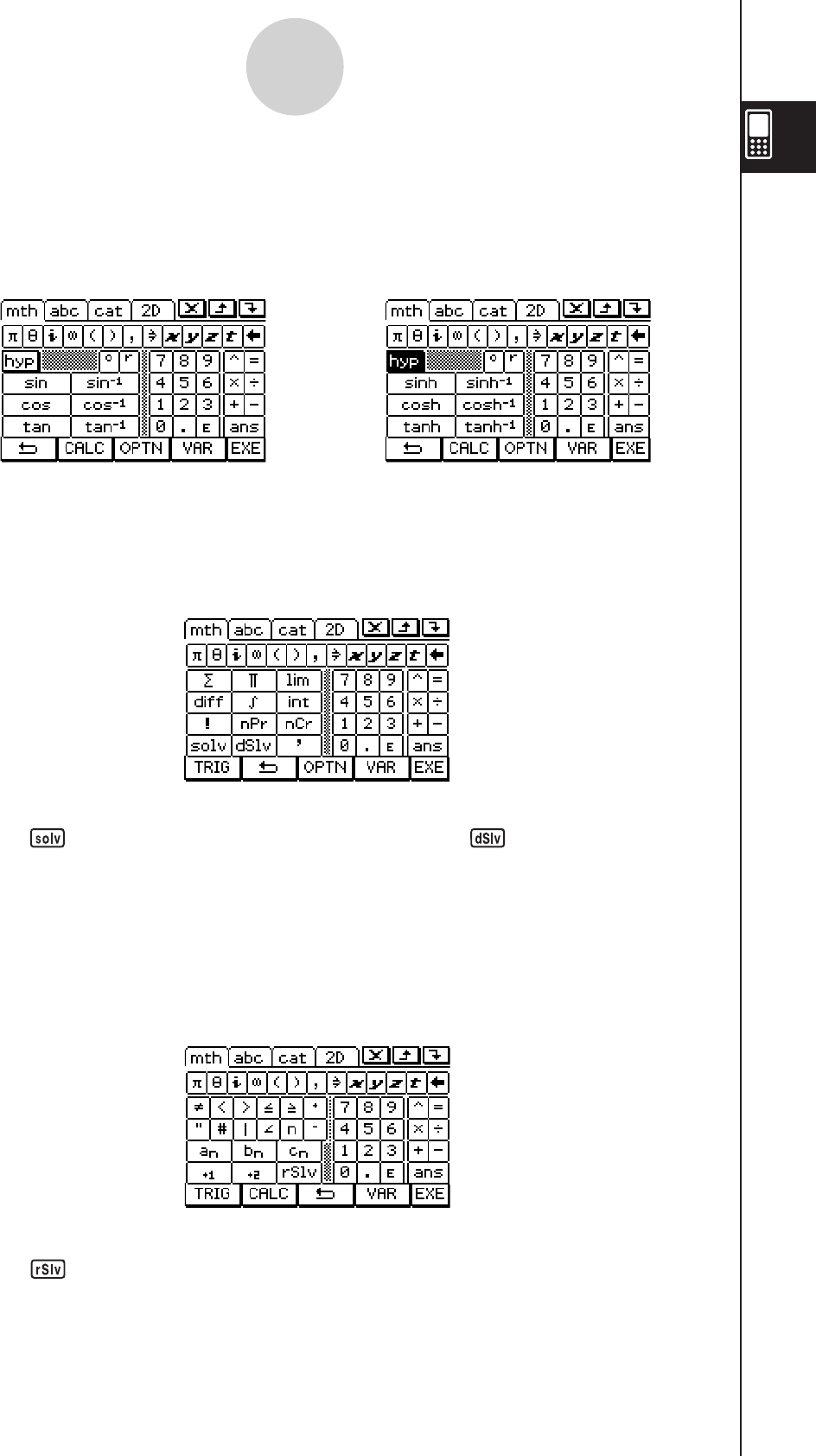
20060301

1-6-9

Input

u T key set

Tapping the T key displays keys for inputting trigonometric functions, and changes the

T softkey to I. You can tap this key to toggle between T and the default 9

keyboard. Tapping the = (hyperbolic) key switches to a key set for inputting hyperbolic

functions. Tap the = key again to return to the regular T key set.

← = →

Tip

• Tapping the key inputs the “solve” function, while tapping the key inputs the “dSolve”

function. See pages 2-8-43 and 2-8-44 for information about these functions.

• For information about each of functions or symbols, see “2-4 Function Calculations”.

u K key set

Tapping the K key displays keys for inputting “<”, “≠”, and other special operators, and

changes the K softkey to I. You can tap this key to toggle between K and the default

9 keyboard.

u - key set

Tapping the - key displays keys for inputting differential and integral calculus expressions,

permutations, etc., and changes the - softkey to I. You can tap this key to toggle

between - and the default 9 keyboard.

Tip

• Tapping the key inputs the “rSolve” function. See page 6-3-5 for information about this

function.

• For information about each of the functions and symbols, see “2-4 Function Calculations”.

20110401

1-6-10

Input

Tip

• As its name suggests, a single-character variable is a variable name that consists of a single

character like “a” or “x”. Each character you input on the V keyboard is treated as a single-

character variable. To input multiple-character variable names like “ab” or multiple-character

strings, you must use the alphabet (abc) keyboard. For more information, see “Using Single-

character Variables” on page 1-6-12.

• For information about the D key that appears in the lower right of all of the math (mth) keyboard

key sets, see “Using the Answer Variable (ans)” on page 2-2-2.

k Using the Alphabet (abc) Keyboard

In addition of the initial alphabet (abc) key set, you can also select from among three

other key sets, within alphabet (abc), named M (character symbols), n (mathematics

symbols), and S (extra symbols).

u Initial alphabet (abc) keyboard key set

This keyboard is for inputting lower-case alphabetic characters. Tap L to shift the keyboard

or E to caps lock the keyboard when you want to input upper-case characters.

• Note that the initial alphabet (abc) keyboard uses the qwerty key arrangement, which is

similar to a computer keyboard. You can also change to an azerty or qwertz arrangement.

See “16-7 Specifying the Alphabetic Keyboard Arrangement”.

u V key set

Tapping the V key displays keys for inputting single-character variables, and changes

the V softkey to I. You can tap this key to toggle between V and the default 9

keyboard. Tapping the E key switches to a key set for inputting upper-case single-

character variables.

← E →

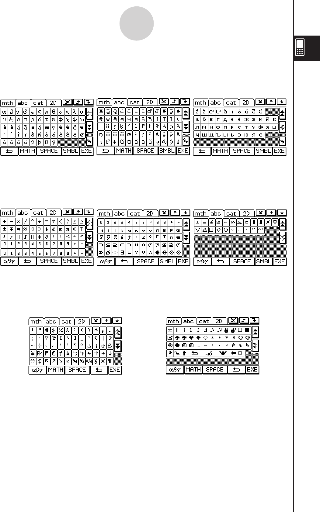
20060301

• Tap I to return to the initial alphabet (abc) key set.

u S key set

Use this key set to input punctuation and symbols. Tap the J and K buttons to scroll to

additional keys.

1-6-11

Input

• Tap I to return to the initial alphabet (abc) key set.

u n key set

This key set contains some of the mathematical expression symbols that are also available

on the math (mth) keyboard. Tap the J and K buttons to scroll to additional keys.

u M key set

Use the M key set to input Greek characters, Cyrillic characters, and accented characters.

Tap the J and K buttons to scroll to additional keys. Tapping E caps locks the keyboard

for input of upper-case characters.

• Tap I to return to the initial alphabet (abc) key set.

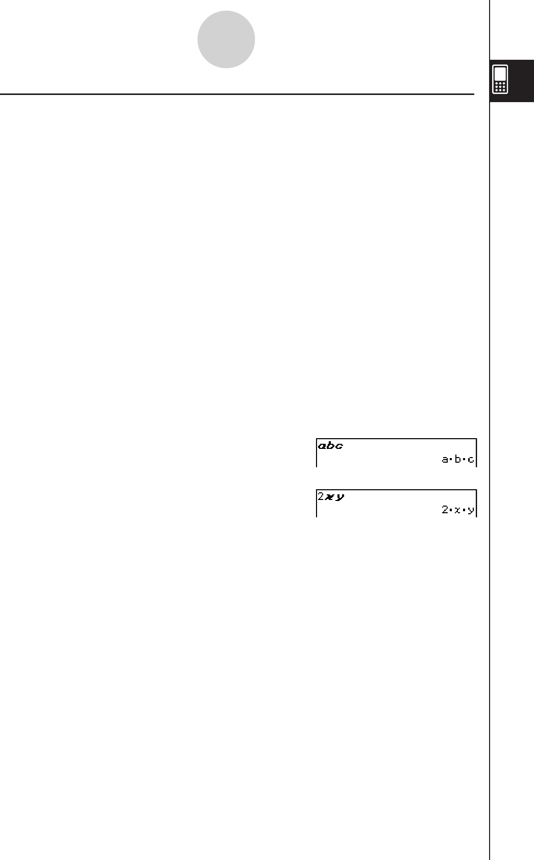
20060301

1-6-12

Input

k Using Single-character Variables

As its name suggests, a single-character variable is a variable name that consists of a single

character like “a” or “x”. Input of single-character variable names is subject to different rules

than input of a series of multiple characters (like “abc”).

u To input a single-character variable name

Any character you input using any one of the following techniques is always treated as a

single-character variable.

• Tapping any key in the math (mth) keyboard’s V key set (page 1-6-10)

• Tapping any key in the 2D keyboard’s V key set (page 1-6-17)

• Tapping the X, Y, Z or [ key to the left of the 9 key of the math (mth) keyboard or

2D keyboard

• Pressing the x, y, or Z keypad key

If you use the above key operations to input a series of characters, each one is treated as a

single-character variable. Inputting A, B, C, for example, is treated as the mathematical

expression a × b × c, and not as the characters “abc”.

Tip

• The single-character variables described above make it possible for you to perform calculations

as they appear in your textbook.

Example 1: 9VABCw

Example 2: 2xyE

Tip

• When you input a single-character variable, its name appears on the display as an italicized bold

character. This is simply to let you know that the letter is a single-character variable name.

20110401

u To input a series of multiple characters

A series of multiple characters (like “list1”) can be used for variable names, program

commands, comment text, etc. Always use the alphabet (abc) keyboard when you want to

input a series of characters.

Example: 0abcw

You can also use the alphabet (abc) keyboard to input single-character variable names.

To do so, simply input a single character, or follow a single character with a mathematical

operator.

Example: 0a*b+cw

Tip

• A single-character variable you input using the alphabet (abc) keyboard is identical to a single-

character variable you input using the math (mth) keyboard.

k Using the Catalog (cat) Keyboard

The “Form” menu of the catalog keyboard lets you select one of the following five categories:

[Func] (built-in functions on pages 2-4-2 and 2-8-1), [Cmd] (built-in commands and operators

on pages 1-7-4 and 12-6-1), [Sys] (system variables on page α-2-1), [User] (user-defined

functions on page 12-5-1), and [All] (all commands, functions, etc.). After selecting a

category, you can choose the item you want from the alphabetized list that appears on the

catalog (cat) keyboard.

Tip

• Note that user-defined variables and user-defined programs cannot be input using the catalog (cat)

keyboard. Use the Variable Manager (page 1-8-1) instead.

• A user-defined function must be stored in the “library” folder to appear in the catalog (cat)

keyboard list when the [User] category is selected.

1-6-13

Input

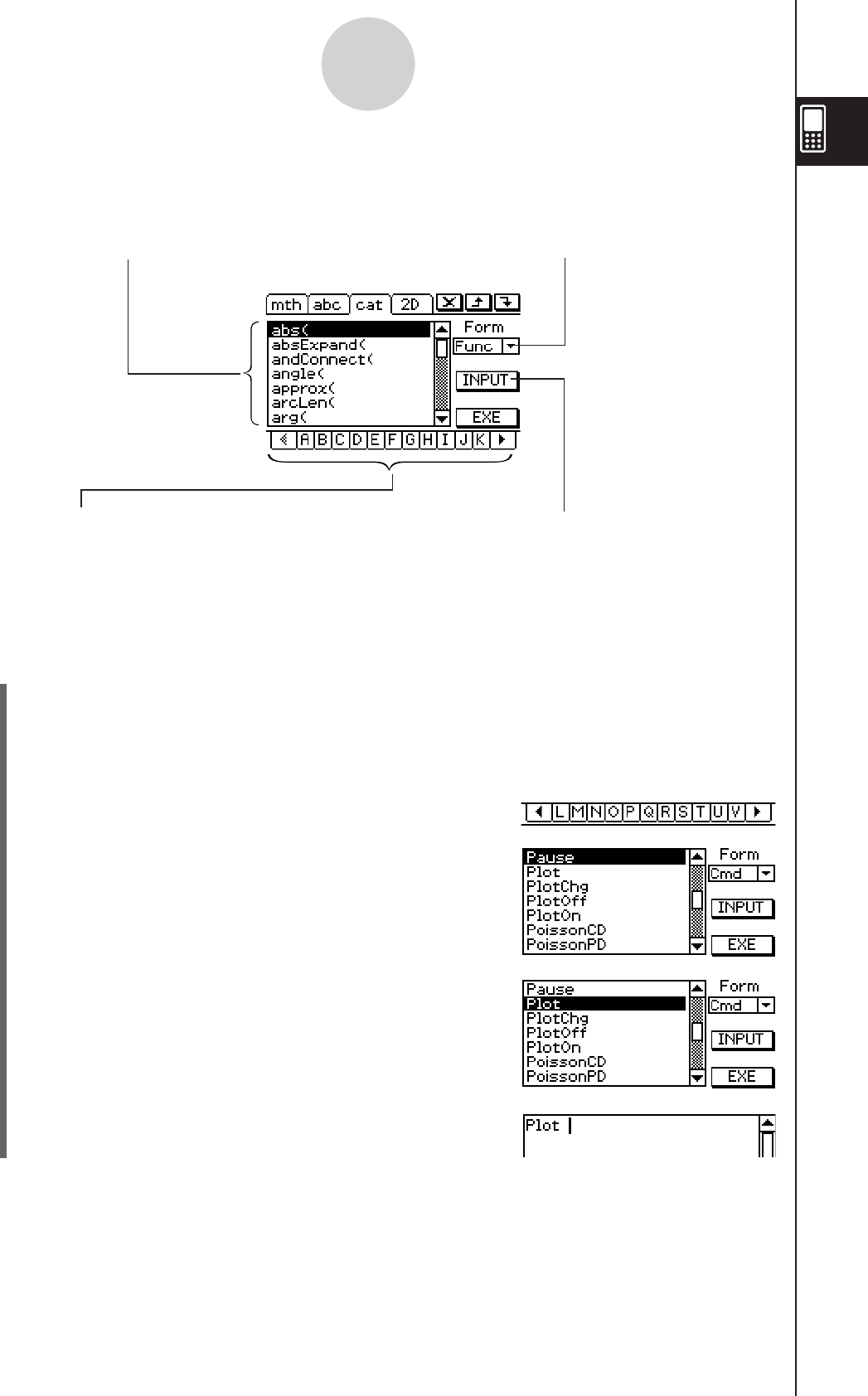
20060301

u Catalog (cat) keyboard configuration

1-6-14

Input

This is an alphabetized list of commands,

functions, and other items available in the

category currently selected with “Form”.

Tap the down button and then select the

category you want ([Func], [Cmd], [Sys],

[User], or [All]) from the list that appears.

Tapping a letter button displays the

commands, functions, or other items that

begin with that letter.

Tap this key to input the item that is

currently selected in the alphabetized list.

u To use the catalog (cat) keyboard

Example: To input the built-in “Plot” command

(1) Tap

( to display the catalog (cat) keyboard.

(2) Tap the “Form” down arrow button v and then select [Cmd] from the list of categories

that appears.

(3) Tap the

u button in the lower right corner until the P key is visible.

(4) Tap

(5) In the alphabetized list, tap “Plot”.

(6) Tap [INPUT] to input the command.

Tip

• Instead of tapping [INPUT] in step (6), you could also tap the command you selected in step (5) a

second time to input the command.

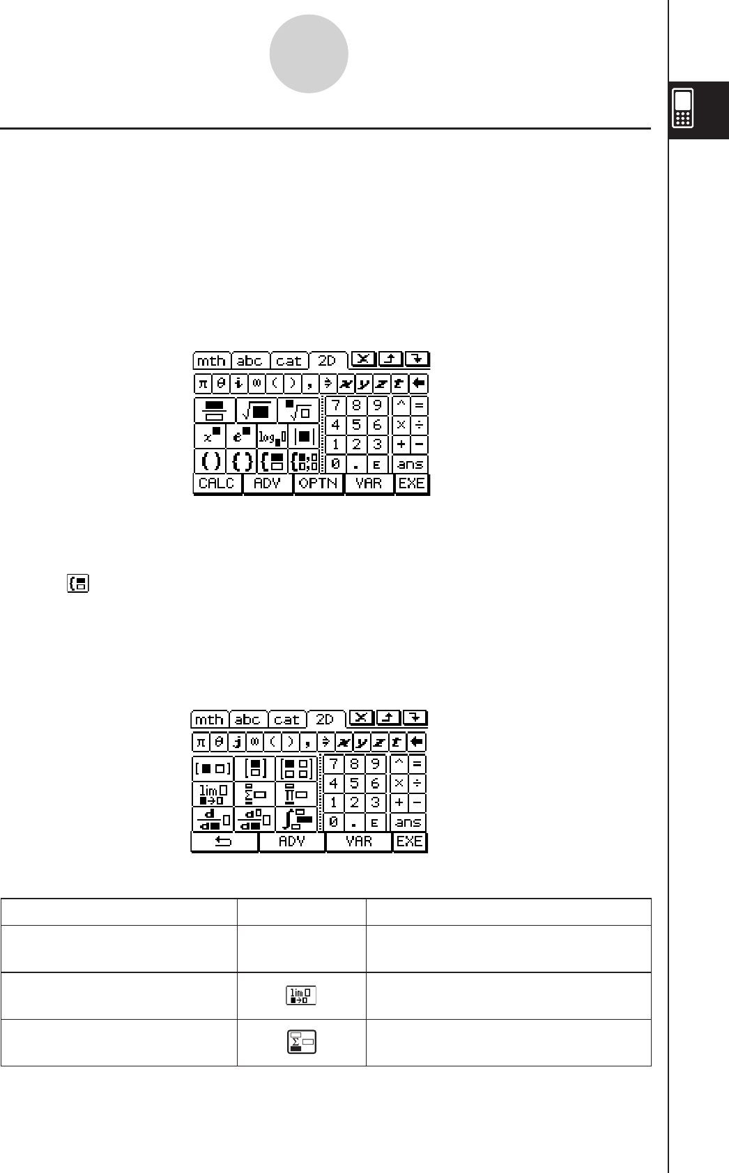
20090601

1-6-15

Input

k Using the 2D Keyboard

The 2D keyboard provides you with a number of templates that let you input fractions,

exponential values, nth roots, matrices, differentials, integrals, and other complex

expressions as they appear in your textbook.

It also includes a V key set that you can use to input single-character variables like the

ones you can input with the math (mth) keyboard.

u Initial 2D keyboard key set

This key set lets you input fractions, exponential values, nth roots, etc. as they appear in your

textbook.

Tip

• For information about each function or symbol, see “2-4 Function Calculations”.

• Use the

1 key to input the piecewise function template. See page 2-4-12 for more information.

• Use the key to input the simultaneous equations template. See page 2-8-43 for more

information.

u - key set

Tapping the - key displays a keyboard like the one shown below, which has a I key in

place of the - key. Tapping I returns to the initial 2D keyboard.

The following are the mathematical expressions you can input with this 2D keyboard.

To input this: Use these keys: For more information, see:

Matrix templates 6, 7, 8“Matrix and Vector Calculations” on

page 2-6-1.

Limit template “lim” under “Using the Calculation

Submenu” on page 2-8-15.

Sum template “Σ” under “Using the Calculation

Submenu” on page 2-8-15.

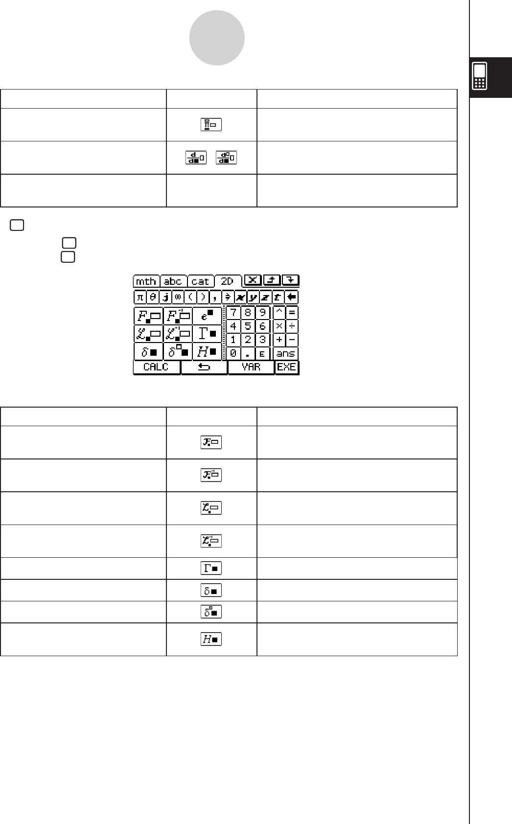
20090601

To input this: Use these keys: For more information, see:

Sum of product template “Π” under “Using the Calculation

Submenu” on page 2-8-15.

Differential coefficient template , “diff” under “Using the Calculation

Submenu” on page 2-8-13.

Integration template P“∫” under “Using the Calculation

Submenu” on page 2-8-14.

u ADV key set

Tapping the ADV key displays a keyboard like the one shown below, which has a I key in

place of the ADV key. Tapping I returns to the initial 2D keyboard.

The following are the mathematical expressions you can input with this 2D keyboard.

To input this: Use these keys: For more information, see:

Fourier transform template “fourier” under “Using the Advanced

Submenu” on page 2-8-9.

Inverse Fourier transform

template

“invFourier” under “Using the

Advanced Submenu” on page 2-8-9.

Laplace transform template “laplace” under “Using the Advanced

Submenu” on page 2-8-8.

Inverse Laplace transform

template

“invLaplace” under “Using the

Advanced Submenu” on page 2-8-8.

Gamma function “Gamma Function” on page 2-4-18.

Delta function “Dirac Delta Function” on page 2-4-16.

nth-delta function “nth Delta Function” on page 2-4-16.

Heaviside function “Heaviside Unit Step Function” on

page 2-4-17.

1-6-16

Input

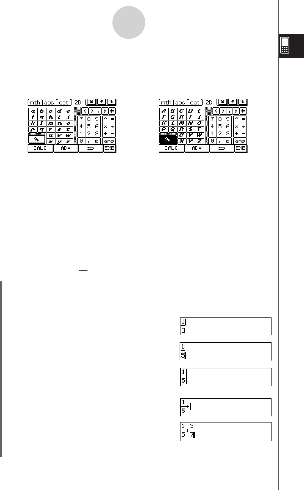
20060301

u V key set

Tapping the V key displays keys for inputting single-character variables, and changes the

V softkey to I. You can tap this key to toggle between V and the initial 2D keyboard.

Tapping the E key switches to a key set for inputting upper-case single-character

variables.

Tip

• As its name suggests, a single-character variable is a variable name that consists of a single

character like “a” or “x”. Each character you input on the V keyboard is treated as a single-

character variable. You cannot use the V keyboard to input multiple-character variable names

like “ab” or multiple-character strings. You must use the alphabet (abc) keyboard when you want

to input a multiple-character string. For more information, see “Using Single-character Variables”

on page 1-6-12.

• For information about the D key that appears in the lower right of all of the 2D keyboard key

sets, see “Using the Answer Variable (ans)” on page 2-2-2.

• Note that natural input is available in most applications of the ClassPad. Natural input cannot be

used in the geometry measurement box or when entering data into a list.

u To use the 2D keyboard for natural input

Example 1: To input +

(1) On the application menu, tap J to start the Main application.

(2) Press the

c key.

(3) Press the

k key, and then tap ) to display the 2D keyboard.

(4) Tap

N and then tap b to input the numerator.

(5) Tap the input box of the denominator to move the

cursor there, or press c and then tap f.

(6) Press

e to move the cursor to the right side of 1/5.

• Instead of using

e to move the cursor, you could

also tap with the stylus at the cursor destination.

(7) Tap

(8) Tap

N, and then repeat steps (4) through (6) to

input 3/7.

(9) After everything is the way you want, press E.

← E →

1-6-17

Input

20060301

1-6-18

Input

Tip

• If you want your ClassPad to evaluate a calculation expression and display a result in the eActivity

application, you must input the calculation in a calculation row. See “Inserting a Calculation Row”

on page 10-3-3.

Example 2: To input

(1) Tap

) to display the 2D keyboard and then tap -.

(2) Tap .

(3) In the input box below Σ, input “k=1”.

Vkeb

(4) Tap with the stylus to move the cursor to the other

input locations and input the required information.

In the input box above Σ, tap L.

(5) Input the part of the expression that comes to the right of Σ.

kIJ c

(6) After everything is the way you want, press E.

Example 3: To input

(1) Tap

) to display the 2D keyboard and then tap -.

(2) Tap

(3) Input the part of the expression that comes to the right of ∫.

(b-XJ ce)

QXeeX

• Or you can use 2D math symbols to enter the

expression.

Initially, the cursor

appears here.

k = 1

∫

(1– x2) ex dx

Initially, the cursor appears in the

input box to the right of ∫.

20060301

1-6-19

Input

(4) Tap with the stylus to move the cursor to the other input locations to enter the

limits of integration.

In the input box above ∫, tap b.

In the input box below ∫, tap a.

(5) After everything is the way you want, press E.

20060301

1-7-1

Variables and Folders

1-7 Variables and Folders

Your ClassPad lets you register text strings as variables. You can then use a variable to

store a value, expression, string, list, matrix, etc. A variable can be recalled by a calculation

to access its contents.

Variables are stored in folders. In addition to the default folders that are provided

automatically, you can also create your own user folders. You can create user folders as

required to group variables by type or any other criteria.

Folder Types

Your ClassPad stores variables in one of four types of folders described below.

Tip

• You cannot put a folder inside of another folder.

• You can view the contents of a folder using the Variable Manager (page 1-8-1). Note, however,

that you cannot open the “system” folder for viewing.

• The “system” folder contents are listed within the ( page of the keyboard when “Sys” is

selected for “Form”.

Folder Type Description

“system” Folder

“library” Folder

“main” Folder

User Folder

This is one of the ClassPad’s reserved folders, which is provided by

default. It is used for storage of system variables, which are pre-

defined variables used by ClassPad applications and other system

operations.

Some examples of system variables are “list1” through “list6”, View

Window parameters “xmin” and “xmax”, etc. A system variable can be

accessed by any application simply by specifying the applicable

variable name.

Also a ClassPad reserved folder, the “library” folder can be used for

storing user-created variables. Variables stored in the “library” folder

can be accessed without specifying a path, regardless of the current

folder setting (see next page).

The “main” folder is also a ClassPad reserved folder, and acts as the

default current folder. While the “main” folder is the current folder, all

variables created by ClassPad application operations are stored here

when you do not specify a path for variable storage.

This is a folder created and named by you. You can make a user

folder the current folder, move variables to a user folder, etc. You can

also delete and rename a user folder as required. You can have up to

87 user folders in ClassPad memory at one time.

20110401

k Current Folder

The current folder is the folder where the variables created by applications (excluding

eActivity) are stored and from which such variables can be accessed. The initial default

current folder is the “main” folder.

You can also select a user folder you created as the current folder. For more information

about how to do this, see “Specifying the Current Folder” on page 1-8-3.

Variable Types

ClassPad variables can be broadly grouped into three types: general variables, system

variables, and local variables.

1-7-2

Variables and Folders

Variable Type Description

General Variables

System Variables

Local Variables

A general variable is one you create using any name you want.

Unless you specify otherwise when you are creating it, a general

variable is stored in the current folder. You can use the same name

for multiple variables, as long as each of them is stored in a different

folder. General variables can be deleted, renamed, etc.

System variables are pre-defined reserved variables used by

ClassPad applications and other system operations. They are stored

in the “system” folder. System variables can be accessed without

specifying the folder name, and can even be accessed from another

folder. Since system variable names are reserved words, they cannot

be renamed. Whether you are allowed to delete or change the

contents of a system variable depends on each variable.

• For the names of and detailed information about system variables,

see the “System Variable Table” on page α-2-1.

A local variable is a variable that is temporarily created by a defining

function, program, or other operation for a particular purpose. A local

variable is deleted automatically when execution of the program or

user-defined function that created it is complete. You can create a

local variable by including the “Local” command in a program. Any

variable specified as the argument of a program or a user-defined

function is automatically treated as a local variable.

20110901

k Variable Data Types

ClassPad variables support a number of data types. The type of data assigned to a variable

is indicated by a data type name. Data type names are shown on the Variable Manager

variable list, and on the Select Data dialog box that appears when you are specifying a

variable in any ClassPad application. The following table lists all of the variable data type

names and explains the meaning of each.

1-7-3

Variables and Folders

* Protected variable types

Some data types are protected. A variable whose data type is protected cannot be

overwritten with another variable, which protects variable contents from being inadvertently

altered. Data types whose names are marked with an asterisk in the above table are

protected.

Tip

• Note that whether or not a data type is protected is determined by the system. You cannot

change the protection status of a data type.

• Even when a variable is a protected data type, you can rename, delete, or move it. To disable

these operations, you need to lock the variable. For more information, see “Locking a Variable or

Folder” on page 1-7-10.

• The elements of the LIST data type can contain EXPR or STR type data only. The elements of

the MAT data type can contain EXPR type data only.

Data Type Name Data Type

Real number, complex number or expression data

String data

List data created using the Statistics application, Main application, etc.

Matrix data created using the Main application, etc.

General program

User-defined function

Text data

Geometry application data

General-purpose data

Data other than that described above

Image data

• ClassPad image data includes graph image data saved using the

Store function, image data captured using the Presentation

application, and picture data transferred from the computer.

Graph memory data saved using the Graph & Table application

• For more information, see “Saving Graph Editor Data to Graph

Memory” on page 3-3-14.

Edit prohibited program

EXPR

STR

LIST

MAT

PRGM*

EXE*

FUNC*

GEO*

MEM*

OTHR

PICT*

GMEM*

TEXT*

20060301

Creating a Folder

You can have up to 87 user folders in memory at the same time. This section explains how

to create a user folder and explains the rules that cover folder names.

You can create a folder using either the Variable Manager or the “NewFolder” command.

k Creating a folder using the Variable Manager

On the Variable Manager window, tap [Edit] and then [Create Folder]. For more information,

see “1-8 Using the Variable Manager”.

k Creating a folder using the “NewFolder” command

In the Main application or in a program, execute the “NewFolder” command.

Example: To create a new folder named “Test”

u ClassPad Operation

(1) Tap

m to display the application menu, and then tap J to start the Main

application.

(2) Display the catalog (cat) keyboard, and then input the “NewFolder” command.

a. In the [Form] menu, select [Cmd].

b. Tap

u and the [N] to display the first command that starts with the letter “N”.

c. In the command list, tap “NewFolder” to select it.

d. Tap [INPUT].

1-7-4

Variables and Folders

(3) Following the “NewFolder” command you just input, enter “Test”.

e s t

“NewFolder”

command

20060301

(4) Tap

w to execute the command.

• The message “done” appears on the display to let you know that command execution

is complete.

1-7-5

Variables and Folders

Tip

• You can use the Variable Manager to view the contents of a folder you create. For more

information, see “1-8 Using the Variable Manager”.

• For information about commands you can use to perform folder operations, see “12-6 Program

Command Reference”.

k Folder Name Rules

The following are the rules that apply to folder names.

• Folder names can be up to 8 bytes long.

• The following characters are allowed in a folder name.

Upper-case and lower-case unaccented characters (character codes 65 to 90, 97 to 122)

Upper-case and lower-case accented characters (character codes 257 to 416, 513 to 672)

Subscript characters (character codes 480 to 491, 496 to 512, 737 to 746, 752 to 766)

Numbers (character codes 48 to 57)

Underscore (character code 95)

• Folder names are case-sensitive.

For example, each of the following is treated as a different folder name: abc, Abc, aBc,

ABC.

• A reserved word (system variable names, built-in function names, command names, etc.)

cannot be used as a folder name.

• A number, subscript characters or the underscore (_) cannot be used as the first character

of a folder name.

Creating and Using Variables

This section explains how to create a new variable (general variable), and provides a simple

sample calculation that illustrates how to use a variable.

k Variable Name Rules

The rules for naming variables are identical to those that cover folder names. For more

information, see “Folder Name Rules” above.

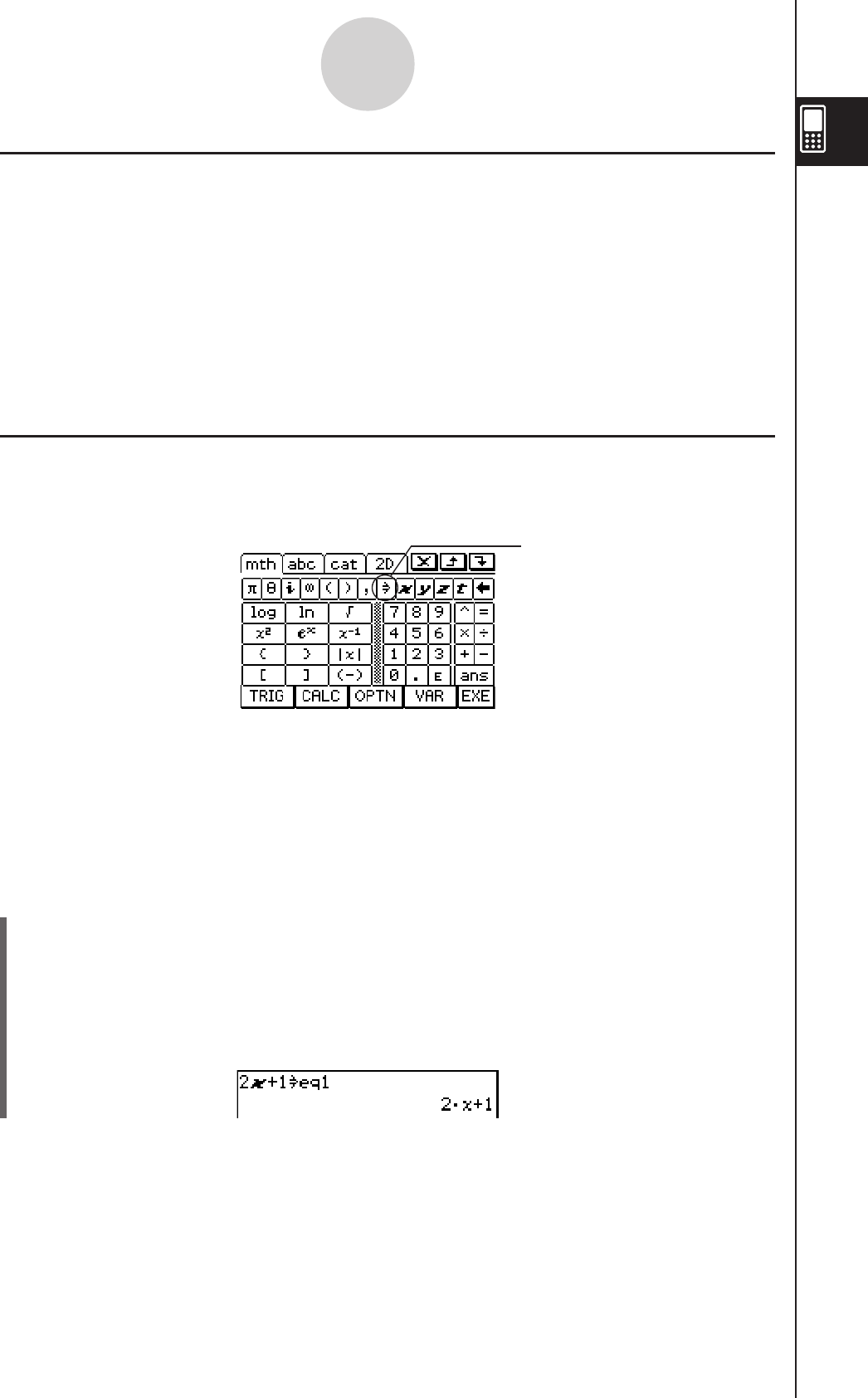
20060301

k Single-character Variable Precautions

Your ClassPad supports the use of single-character variables, which are variables whose

names consist of a single character like “a” or “x”. Some ClassPad keys (x, y, Z

keypad keys, math (mth) soft keyboard X, Y, Z, [ keys, V key set keys, etc.) are

dedicated single-character variable name input keys. You cannot use such a key to input a

variable name that has more than one character.

For example, pressing the keypad keys x and y in succession is interpreted by the

ClassPad as the multiplication expression “x × y”, and not as the characters “xy”. In order to

input a variable name made up of two or more characters, use the alphabet (abc) keyboard.

For more information, see “Using Single-character Variables” on page 1-6-12.

k Creating a New Variable

The most common way to create a new variable is assigning a value or expression to the

applicable variable name. Use the variable assignment key (W) to assign data to a variable.

1-7-6

Variables and Folders

The following is an example of assignment to a variable while “main” is specified as the

current folder.

Example: To create a new variable named “eq1” and assign the expression 2x + 1 to it

The following assumes that there are no variables named “eq1” or “x” currently in

the “main” folder.

u ClassPad Operation

(1) On the application menu, tap J to start the Main application.

(2) Press

k to display the soft keyboard, and then perform the following key operation.

9cX+bW

0eqbw

• This creates a variable named “eq1” in the current folder (the “main” folder in this

example), and assigns the expression 2x + 1 to it.

Assign key

This key is included on the math

(mth) and 2D soft keyboards.

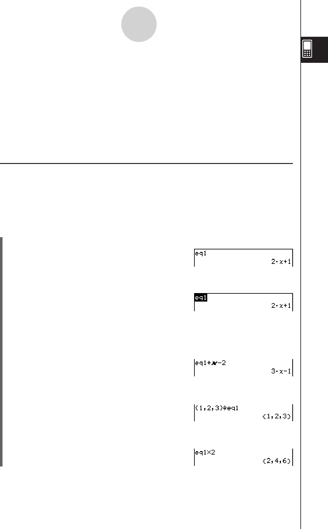
20060301

1-7-7

Variables and Folders

Tip

• As shown in the above example, assigning something to a variable with a name that does not

yet exist in the current folder causes a new variable with that name to be created. If a variable

with the specified name already exists in the current folder, the contents of the existing variable

are replaced with the newly assigned data, unless the existing variable is protected. For more

information about protected variables, see “Protected variable types” on page 1-7-3.

• To store the newly created variable in a folder other than the current folder, specify the variable

name as follows: <folder name>\<variable name>.

• You can use the Variable Manager to view the contents of a variable you create. For more

information, see “1-8 Using the Variable Manager”.

k Variable Usage Example

The following example uses the variable we created in the example under “Creating a New

Variable” on page 1-7-6.

Example: To copy the variable “eq1” and then paste it into the following two equations:

eq1 + x – 2 and eq1 × 2

u ClassPad Operation

(1) First, check the current contents of variable “eq1”.

0eqbw

(2) Copy the variable by dragging the stylus across “eq1” and then tapping G, or tap [Edit]

[Copy].

• Copy and paste comes in handy when you need to input the same variable into

multiple expressions. You can also drag “eq1” to another line.

(3) Perform the key operation below to input and execute the first expression:

eq1 + x – 2.

H (or [Edit] [Paste]) 9+X-cw

(4) Perform the key operation below to replace the current contents of “eq1” with the list

{1, 2, 3}.

9{b,c,d}W

(5) Perform the key operation below to input and execute the second expression:

eq1 × 2

H9*cw

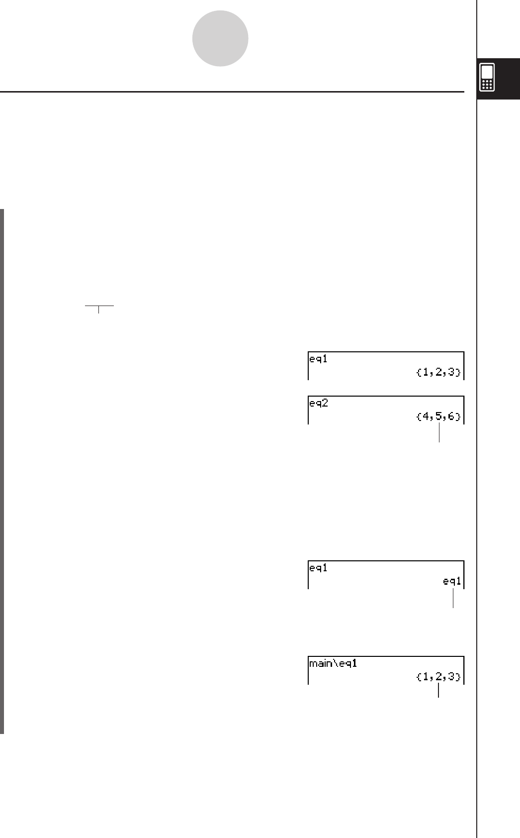
20060301

1-7-8

Variables and Folders

k “library” Folder Variables

Variables in the “library” folder can be accessed without specifying a path name, regardless

of the current folder.

Example: To create and access two variables, one located in the “library” folder and one

located in another folder

u ClassPad Operation

(1) With “main” specified as the current folder (the default), perform the following operation

to create a variable named “eq1” and assign the indicated list data to it.

{1, 2, 3} S eq1w

(2) Keeping “main” specified as the current folder, perform the following operation to create

a variable named “eq2” in the “library” folder, and assign the indicated list data to it.

{4, 5, 6} S library \ eq2 w

Specifies the “library” folder.

(3) Check the contents of the two variables.

eq1 w

(4) Change the current folder specification to “Test”.

• Use the Basic Format dialog box (page 1-9-4) or the Variable Manager (page 1-8-1)

to change the current folder specification.

(5) Perform the following operations to view the contents of variables “eq1” and “eq2”.

eq1 w

eq2 w

Since variable “eq2” is stored in the

“library” folder, you do not need to

indicate a path to access it.

Since this key operation does not access the

“main” folder, the variable name (“eq1”) is

displayed without showing the variable contents.

main\eq1 w

Specifying the path to the “main” folder

where “eq1” is located displays the

contents of the variable.

20060301

1-7-9

Variables and Folders

eq2 w

Tip

• Specifying a variable name that exists in both the current folder and the “library” folder causes

the variable in the current folder to be accessed. For details about the variable access priority

sequence and how to access variables in particular folders, see “Rules Governing Variable

Access” on page 1-7-11.

• You can use the Variable Manager (page 1-8-1) to move existing variables from the “main” folder

or a user folder to the “library” folder, or from the “library” folder to other folders.

k Using Stat Editor to Create a LIST Variable

Stat Editor makes creation of LIST variables (variables that contain list data) quick and easy.

This capability really comes in handy when you need to perform a calculation (statistical

calculations, etc.) that involves a large number of LIST variables.

Stat Editor appears as the initial screen when you start up the Statistics application. You can

also access the Stat Editor window from the Main, Graph & Table, and eActivity applications.

Since variable “eq2” is stored in the

“library” folder, you do not need to

indicate a path to access it.

Input a variable name like “list_t” into the title cell at the top of the list on the Stat Editor

window (1), and then input values into the list (2). This creates a LIST variable with the

name list_t that is assigned the contents of the list of data (2). The above example creates a

LIST variable named “list_t” and assigns it the list data “{12, 24, 36}”.

Tip

• For details about using Stat Editor, see “7-2 Using Stat Editor”.

20110401

1-7-10

Variables and Folders

Assigning Values and Other Data to a System Variable

As its name suggests, a system variable is a variable that is created and used by the system

(page 1-7-5). Some system variables allow you to assign values and other data to them,

while some system variables do not. For more information about which variables allow you to

control their contents, see the “System Variable Table” on page α-2-1.

Locking a Variable or Folder

Locking a variable or folder protects against inadvertently deleting it or changing its contents.

You can unlock a locked variable or folder to re-enable deletion and data assignment.

• Locking a variable disables the following operations on it: delete, overwrite, rename, and

move (to another folder).

• Locking a folder makes it impossible to delete or rename the folder.

Tip

• In terms of ClassPad variables, “lock” is completely different from “protect”. For more information

about “protect”, see “Variable Data Types” on page 1-7-3.

You can lock and unlock a variable or folder using either the Variable Manager or commands.

u To lock or unlock a variable or folder using the Variable Manager

In the Variable Manager, select the folder or variable you want to lock or unlock and then

tap [Edit] - [Lock] or [Edit] - [Unlock]. For more information, see “1-8 Using the Variable

Manager”.

u To lock or unlock a variable or folder using commands

In the Main application or in a program, execute one of the commands described below.

Lock a variable Lock <variable name>

Unlock a variable Unlock <variable name>

Lock a folder LockFolder <folder name>

Unlock a folder UnlockFolder <folder name>

Use this command syntax:

To do this:

For information about commands, see “12-6 Program Command Reference”.

20060301

1-7-11

Variables and Folders

Rules Governing Variable Access

Normally, you access a variable by specifying its variable name. The rules in this section

apply when you need to reference a variable that is not located in the current folder or to

access a variable that has the same name as one or more variables located in other folders.

k Variable Search Priority Sequence

Specifying a variable name to access a variable, searches variables in the following

sequence.

(1) Local Variables

(2) Current Folder Variables

(3) “library” Folder Variables

• Multiple variables with the same name can exist simultaneously as a local variable, as

a variable in the current folder, and as a variable in the “library” folder. In this case, the

ClassPad searches folders according to the sequence shown above and accesses the first

instance of the variable that it finds. If you want to access such a variable when it occurs

lower in the above priority sequence, you need to specify the folder name along with the

variable name as shown in “Specifying a Variable in a Particular Folder” below.

• If a variable you specify cannot be found, it is treated as an “undefined variable”.

• Note that the “system” folder is not included in the above variable search. When accessing

a variable in the system folder, you need to specify the variable name only, without

specifying the folder name.

Tip

• Local variables exist only as long as the program or user-defined function for which it was created

in being executed.

• When a variable search is required during a subroutine called by a program or user-defined

function, the local variable search range includes only the local variables of the subroutine

currently being executed.

• For information about programs and user-defined functions, see Chapter 12.

• Only local variables and current folder variables are searched in the case of an operation that

stores variable data or a command that performs an operation on a variable (like “DelVar”).

Normally, “library” folder variables are not searched. If you want to include “library” folders in the

search, you need to specify the “library” folder as the variable location as explained below.

k Specifying a Variable in a Particular Folder

You can access a variable located inside the “main” folder, “library” folder, or a particular

user folder by specifying the folder name along with the variable name. Use the following

syntax when specifying a folder name:

Example: To specify variable “abc” located in the “main” folder

main\abc

20060301

1-8-1

Using the Variable Manager

1-8 Using the Variable Manager

The Variable Manager is a tool for managing user variables, programs, user functions, and

other types of data. Though this section uses only the term “variables”, the explanations

provided here also refer to the other types of data that can be managed by the Variable

Manager.

Variable Manager Overview

This section explains how to start up and exit the Variable Manager. It also provides

information about the configuration of the Variable Manager.

With the Variable Manager you can:

• Create, delete, rename, lock, and unlock folders for storing variables, and configure current

folder settings.

• Delete, copy, rename, move, lock, unlock, search for variables, and view the contents of

variables.

Starting Up the Variable Manager

To start up the Variable Manager, tap O, and then tap [Variable Manager].

• Starting up the Variable Manager initially displays the folder list, which is described on the

next page.

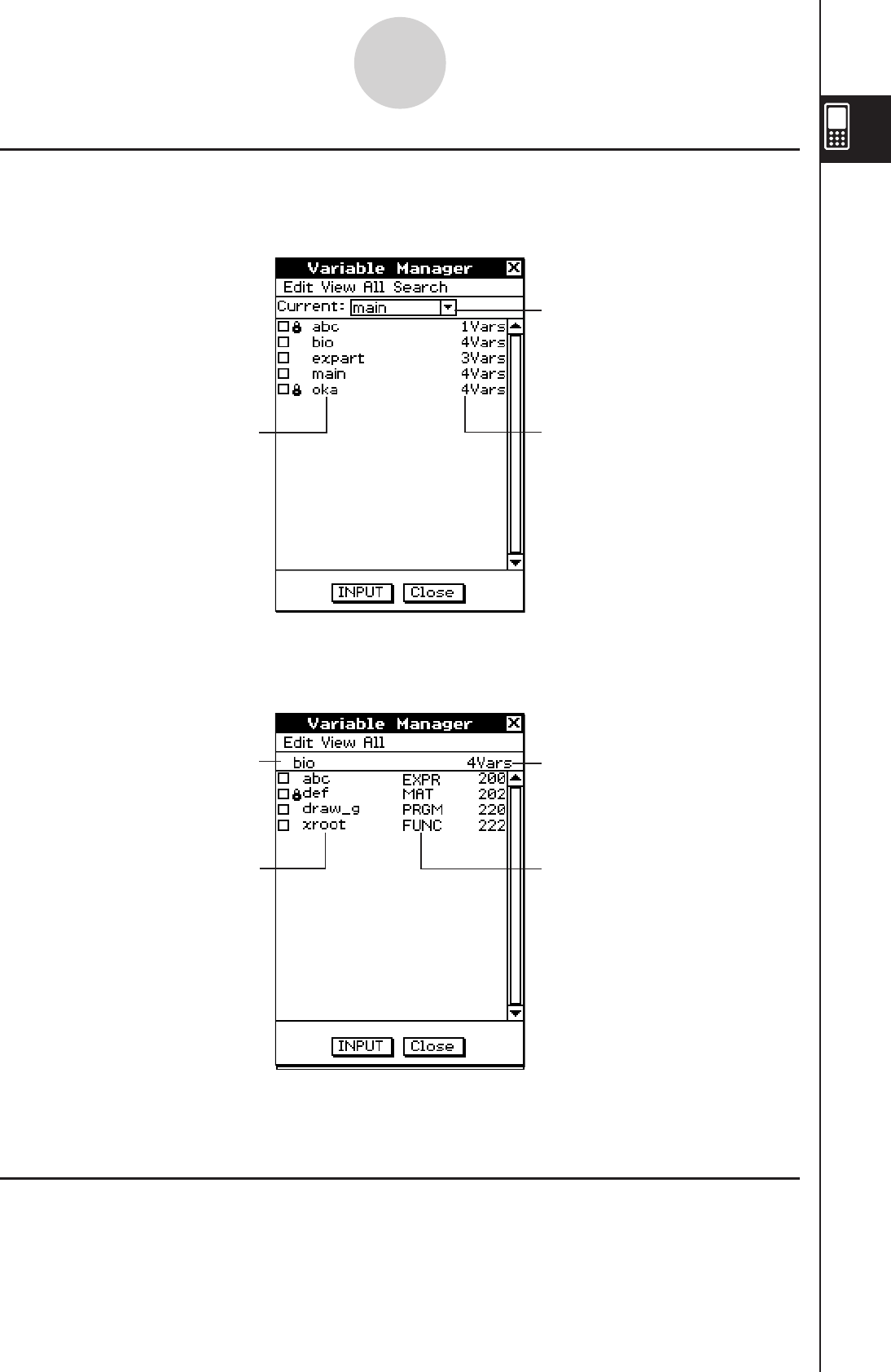
20060301

• Tapping a folder name on the folder list selects it. Tapping the folder name again displays

the folder’s contents; a variable list.

Current folder

Folder names Number of variables contained

in the folder

Folder List

Number of variables contained

in the folder

Variable names Variable data types (page 1-7-3)

and sizes (bytes)

Variable List

Folder name

• To close the variable list and return to the folder list, tap [Close].

Exiting the Variable Manager

To exit the Variable Manager, tap the [Close] button.

1-8-2

Using the Variable Manager

Variable Manager Views

The Variable Manager uses two views, a folder list and a variable list.

• The folder list always appears first whenever you start up the Variable Manager.

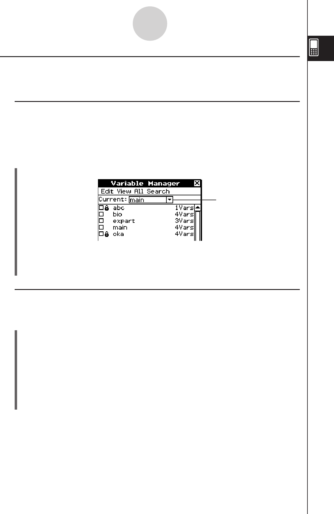
20060301

Variable Manager Folder Operations

This section describes the various folder operations you can perform using the Variable

Manager.

k Specifying the Current Folder

The “current folder” is the folder where the variables created by applications (excluding

eActivity) are stored and from which such variables can be accessed. The initial default

current folder is the “main” folder.

You can also select a folder you created yourself as the current folder.

uClassPad Operation

(1) Start up the Variable Manager and display the folder list.

(2) Tap the [Current] down arrow button. On the list that appears, select the folder that

you want to specify as the current folder.

(3) Tap [Close] to close the folder list.

k Creating a New Folder

You can use the following procedure to create up to 87 folders, as you need them.

uClassPad Operation

(1) Start up the Variable Manager, which causes the folder list to appear.

(2) On the folder list, tap [Edit] and then [Create Folder].

• This displays a dialog box for inputting a folder name.

(3) Enter the folder name, and then tap [OK].

• This creates the new folder and returns to the folder list.

• Normally, a folder name can contain up to eight bytes. If your folder name includes 2-byte

characters, you may not be able to input eight characters for the folder name. For details

about folder names, see page 1-7-5.

Current folder

1-8-3

Using the Variable Manager

• An error message appears and your folder is not created if there is already a folder with the same

name you input. Tap [OK] to close the error message dialog box, and then specify a different

name for the folder you are creating.

Tip

20060301

k Selecting and Deselecting Folders

The folder operations you perform are performed on the currently selected folders. The

folders that are currently selected on the folder list are those whose check boxes are selected

(checked). You can use the following operations to select and deselect folders as required.

To do this: Do this:

Select a single folder Select the check box next to the folder name.

Deselect a single folder Clear the check box next to the folder name.

Select all the folders in the list Tap [All] and then [Select All].

Deselect all the folders in the list Tap [All] and then [Deselect All].

1-8-4

Using the Variable Manager

• If no check box is currently selected on the folder list, any folder operation that is performed

affects the folder whose name is currently highlighted on the list. If any folder check box is

currently selected, only that folder is affected by a folder operation, and the folder whose name is

highlighted on the list is not affected.

• Selecting the check box of a folder causes the check boxes of all of the variables inside of it also

to become selected.

• When renaming a folder, only the folder whose name is highlighted on the folder list is renamed.

Other folders whose check boxes are selected are not affected.

k Deleting a Folder

Warning!

Before deleting a folder, make sure you no longer need any of the variables contained

inside it. It is probably a good idea to first delete the variables you don’t need and move the

variables you do need to another folder, and then delete the empty folder.

uClassPad Operation

(1) Start up the Variable Manager and display the folder list.

(2) Open the folder you want to delete and check its contents.

• Make sure you no longer need any of the variables in the folder. If any of the

variables are locked, unlock them.

• After checking the contents of the folder, close it to return to the folder list.

(3) Select the check box next to the folder you want to delete.

• You can select and delete multiple folders, if you want.

(4) On the folder list, tap [Edit] and then [Delete].

(5) In response to the confirmation dialog box that appears, tap [OK] to delete the folder

or [Cancel] to exit the dialog box without deleting the folder.

Tip

20060301

1-8-5

Using the Variable Manager

• You cannot delete the “library” folder or the “main” folder.

• If no check box is currently selected on the folder list, the folder whose name is currently

highlighted on the list is deleted when you tap [Edit] and then [Delete].

• An error message appears and the folder is not deleted if any one of the following conditions

exists.

• The folder is locked.

• Any variable inside the folder is locked.

• There are still variables inside the folder.

k Renaming a Folder

You can use the following procedure to change the name of an existing folder.

uClassPad Operation

(1) Start up the Variable Manager and display the folder list.

(2) Tap the name of the folder you want to rename so it is highlighted.

(3) Tap [Edit] and then [Rename].

• This displays a dialog box for inputting a new folder name.

(4) Input the new folder name.

(5) When the name is the way you want, tap [OK] to save it, or tap [Cancel] to cancel the

rename procedure.

• When renaming a folder, only the folder whose name is highlighted on the folder list is renamed.

Other folders whose check boxes are selected are not affected.

• A folder that is locked cannot be renamed.

k Locking and Unlocking a Folder

A folder cannot be deleted or renamed while it is locked. Lock any folder that you want to

protect against accidental deletion.

u To lock a folder

(1) Start up the Variable Manager and display the folder list.

(2) Select the check box next to the folder you want to lock.

• If you want to lock multiple folders, select all of their check boxes.

(3) Tap [Edit] and then [Lock].

• This locks the currently selected folder, and adds a b icon to the left of its name to

indicate that it is locked.

u To unlock a folder

(1) Start up the Variable Manager and display the folder list.

(2) Select the check box next to the folder you want to unlock.

(3) Tap [Edit] and then [Unlock].

Tip

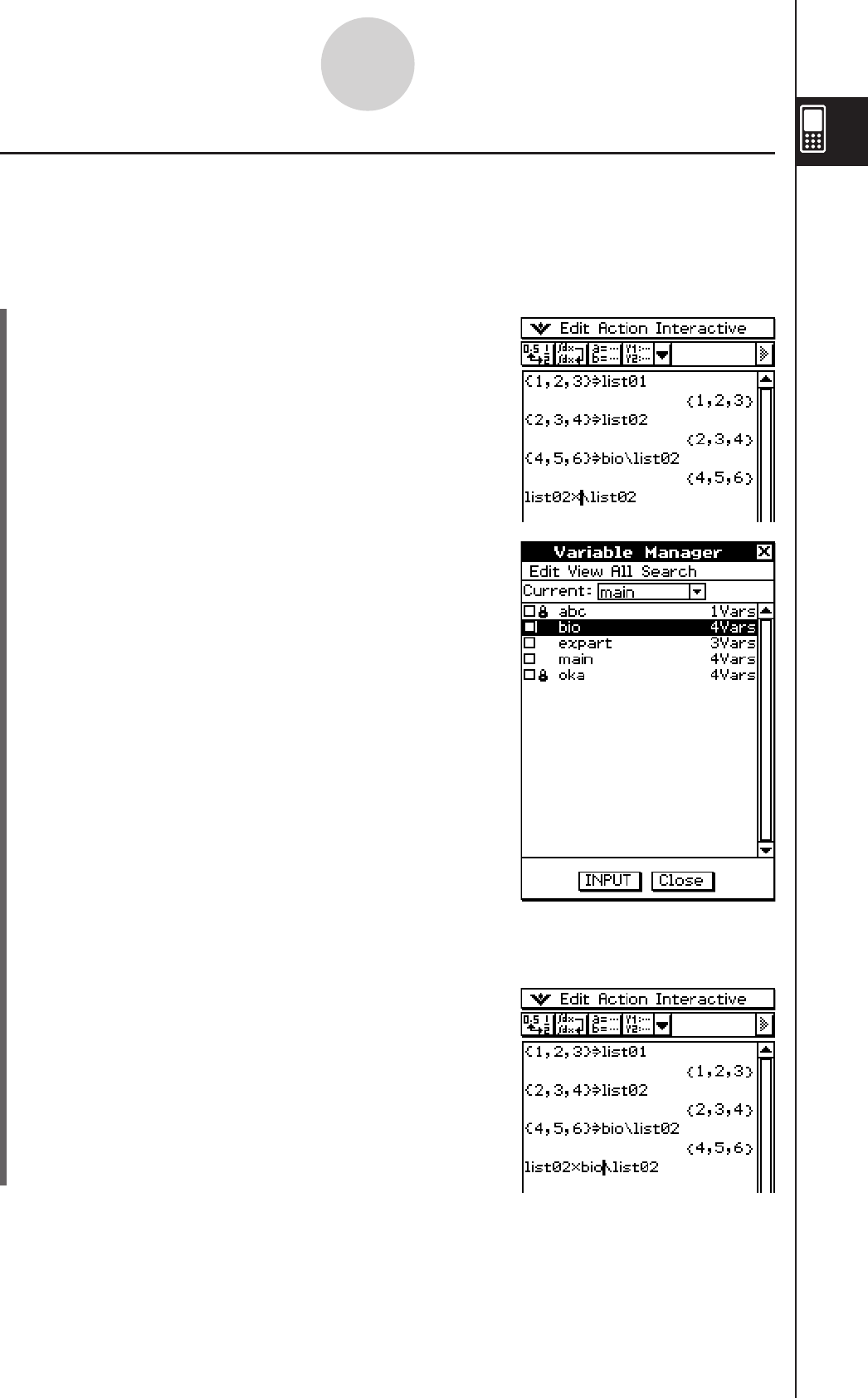
20060301

k Inputting a Folder Name into an Application

Perform the procedure below when you want to input the name of a folder displayed on

the Variable Manager window into the application from which you started up the Variable

Manager.

uClassPad Operation

(1) In the Main application, Graph & Table application,

or some other application, move the cursor to the

location where you want to input the folder name.

1-8-6

Using the Variable Manager

(2) Start up the Variable Manager to display the list of

folders.

(3) Tap the folder whose name you want to input, so the name is highlighted.

(4) Tap [INPUT].

• This exits the Variable Manager and inputs the

name of the folder you selected in step (3) into the

application at the current cursor position.

20060301

Variable Operations

This section explains the various operations you can perform on the Variable Manager

variables.

k Opening a Folder

Perform the steps below to open a folder and display the variables contained inside it.

u ClassPad Operation

(1) Start up the Variable Manager and display the folder list.

(2) Tap the name of the folder you want to open so it is highlighted, and then tap it again.

• This opens the folder and displays a variable list showing its contents.

(3) To return to the folder list, tap [Close].

k Opening the “library” Folder

Note that the procedure you need to use to open the “library” folder is different from the

procedure for opening other folders.

u ClassPad Operation

(1) Start up the Variable Manager and display the folder list.

(2) Tap [View] and then [“library” Folder].

• This opens the “library” folder and displays a variable list showing its contents.

(3) To return to the folder list, tap [Close].

Tip

• You can also open the “library” folder (by tapping [View] and then [“library” Folder]) while the

variable list is on the display.

k Displaying a List of a Particular Type of Variable

You can use the variable list to produce a list of a particular type of variable only.

u ClassPad Operation

(1) In the Variable Manager, open any folder to display a variable list of its contents.

(2) Tap [View] and then [Variable Type].

• This displays the Variable Type dialog box for

specifying the variable data type.

1-8-7

Using the Variable Manager

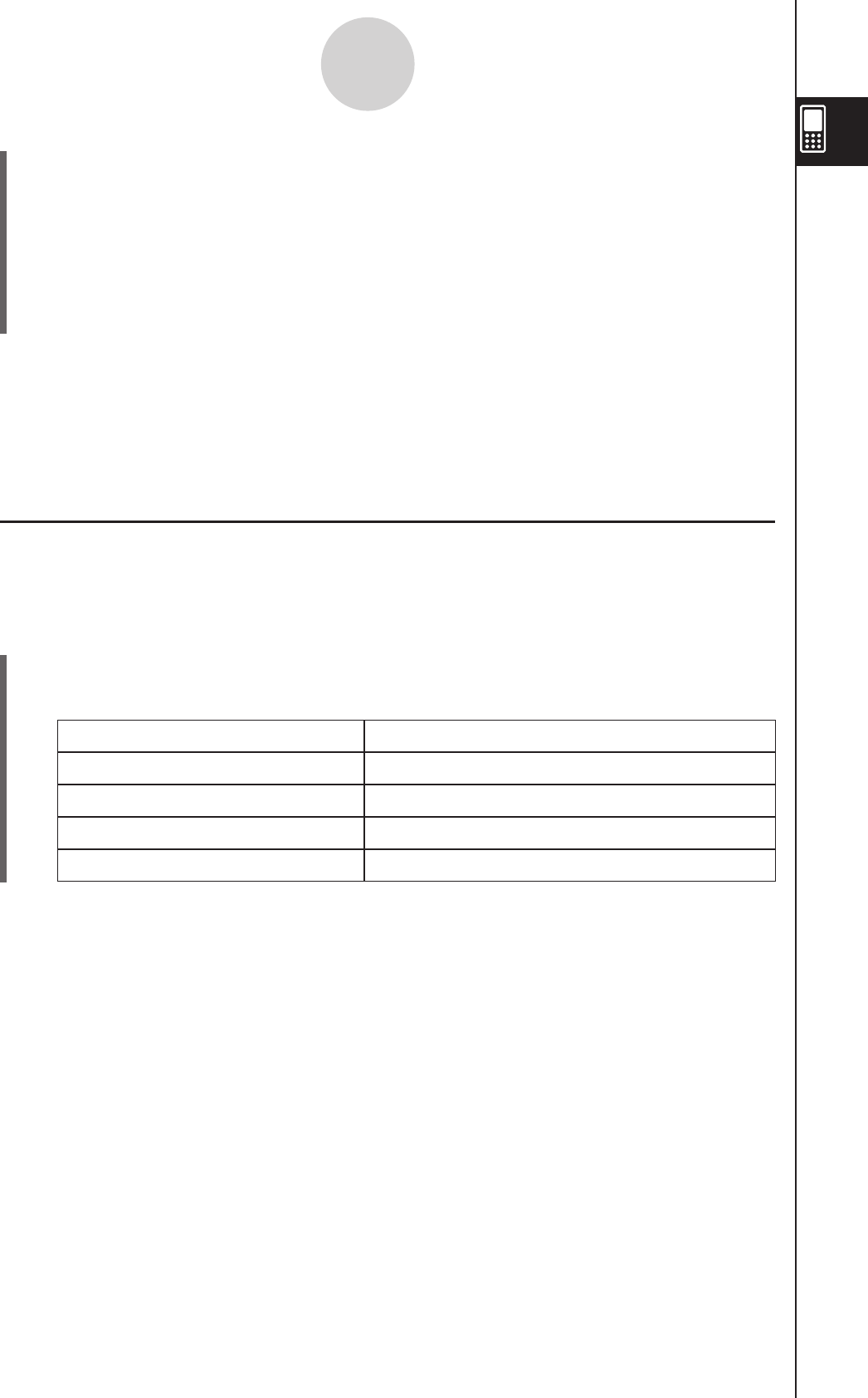
20060301

1-8-8

Using the Variable Manager

(3) On the dialog box, tap the down arrow button and then select the data type from the

list that appears.

• To display variables for all data types, select [All].

• For details about data type names and variables, see “Variable Data Types” on page

1-7-3.

(4) After selecting the data type you want, tap [OK] to apply it or [Cancel] to exit the

selection dialog box without changing the current setting.

Tip

• Returning to the folder list or exiting the Variable Manager causes the data type to change to the

initial default setting, which is [All].

• Performing this operation clears the check boxes for all of the variables inside the applicable

folder.

k Selecting a Variable

Before you can copy, delete, or perform any other operation on a variable, you must first

select it.

u To select or deselect a variable

(1) In the Variable Manager, open any folder to display a variable list of its contents.

(2) Perform one of the operations described below to select or deselect a variable.

To do this: Do this:

Select a single variable Select the check box next to the variable name.

Deselect a single variable Clear the check box next to the variable name.

Select all the variables in the list Tap [All] and then [Select All].

Deselect all the variables in the list Tap [All] and then [Deselect All].

Tip

• If no check box is currently selected on the variable list, any variable operation that is performed

affects the variable whose name is currently highlighted on the list. If any variable check box is

currently selected, only that variable is affected by a variable operation, and the variable whose

name is highlighted on the list is not affected.

• The selected/deselected status of a variable is retained, even when you return from the variable

list to the folder list. Exiting the Variable Manager or changing the data type selection, however,

causes all variables to be deselected.

• When renaming a variable, only the variable whose name is highlighted on the variable list is

renamed. If other variables are selected (checked), they will not be affected.

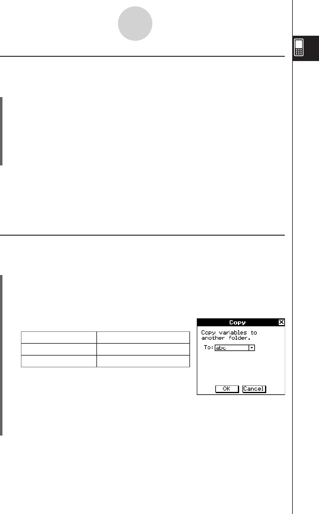
20060301

1-8-9

Using the Variable Manager

k Deleting a Variable

Perform the following steps when you want to delete a variable.

u ClassPad Operation

(1) Open the folder that contains the variable you want to delete and display the variable

list.

(2) Select the check box next to the variable you want to delete.

• To delete multiple variables, select all of their check boxes.

(3) Tap [Edit] and then [Delete].

(4) In response to the confirmation dialog box that appears, tap [OK] to delete the

selected variable or [Cancel] to cancel the delete operation.

Tip

• If no check box is selected on the variable list, the variable whose name is currently highlighted

on the list is deleted when you tap [Edit] and then [Delete].

• If the currently selected variable is locked, an error message appears and the variable is not

deleted.

k Copying and Moving a Variable

You can use the procedure below to copy or move a variable to another folder.

u ClassPad Operation

(1) Open the folder that contains the variable you want to copy or move, and display the

variable list.

(2) Select the check box next to the variable you want to copy or move.

• To copy or move multiple variables, select all of their check boxes.

(3) Perform the copy operation or the move operation.

To do this: Perform this operation:

Copy the variable Tap [Edit] and then [Copy].

Move the variable Tap [Edit] and then [Move].

• This causes a dialog box for selecting the destination

folder to appear.

(4) On the dialog box, tap the down arrow button and then select the destination folder

from the list that appears.

(5) When the destination folder you want is selected, tap [OK] to perform the copy or

move operation, or tap [Cancel] to cancel the procedure.

20060301

Tip

• If no check box is currently selected on the variable list, the variable whose name is currently

highlighted on the list is copied or moved.

• If a variable with the same name already exists in the destination folder, the variable in the

destination folder is replaced with the one that you are copying or moving.

• An error message appears and the variable is not copied or moved if a variable with the same

name already exists in the destination folder and that variable is locked or protected.

• A variable that is locked cannot be moved.

k Renaming a Variable

Perform the following steps when you want to rename a variable.

u ClassPad Operation

(1) Open the folder that contains the variable you want to rename and display the variable

list.

(2) Tap the name of the variable you want to rename so it is highlighted.

(3) Tap [Edit] and then [Rename].

• This displays a dialog box for inputting a new variable name.

(4) Input the new variable name.

(5) When the name is the way you want, tap [OK] to save it, or tap [Cancel] to cancel the

rename procedure.

Tip

• When renaming a variable, only the variable whose name is highlighted on the variable list is

renamed. Other variables whose check boxes are selected are not affected.

• A variable that is locked cannot be renamed.

k Locking and Unlocking a Variable

A locked variable cannot be deleted, moved, or renamed. A locked variable also cannot be

overwritten by a variable with the same name being moved or copied into its folder. Lock any

variable that you want to protect against accidental deletion.

u To lock a variable

(1) Open the folder that contains the variable you want to lock and display the variable

list.

(2) Select the check box next to the variable you want to lock.

• If you want to lock multiple variables, select all of their check boxes.

(3) Tap [Edit] and then [Lock].

• This locks the currently selected variable, and adds a b icon to the left of its name to

indicate that it is locked.

1-8-10

Using the Variable Manager

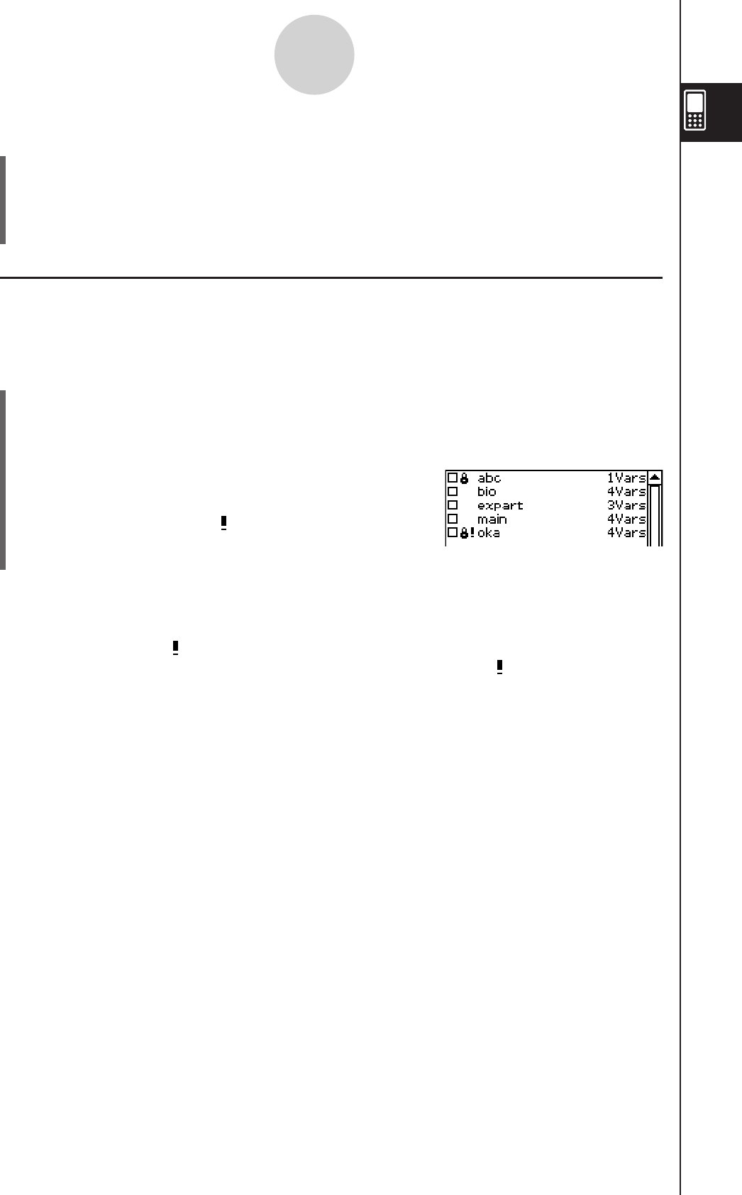
20060301

1-8-11

Using the Variable Manager

u To unlock a variable

(1) Open the folder that contains the variable you want to unlock and display the variable

list.

(2) Select the check box next to the variable you want to unlock.

(3) Tap [Edit] and then [Unlock].

k Searching for a Variable

You can use the following procedure to search the “main” folder or a user defined folder for a

particular variable name. Note that you cannot search the “library” folder.

uClassPad Operation

(1) Start up the Variable Manager and display the folder list.

(2) On the folder list, tap [Search] and then [Search].

• This displays a dialog box for inputting a search string.

(3) Enter the variable name you want to find and then tap

[OK].

• An exclamation point ( ) appears in front of all

folders containing a variable name that matches

the name in your search.

Tip

• The message “Not Found” appears on the display if a match cannot be found.

• The exclamation point ( ) remains on the folder list until you exit the Variable Manager or

perform another search operation. Also note that the exclamation point ( ) remains in front of the

folder name, even if you delete or rename the found variable.

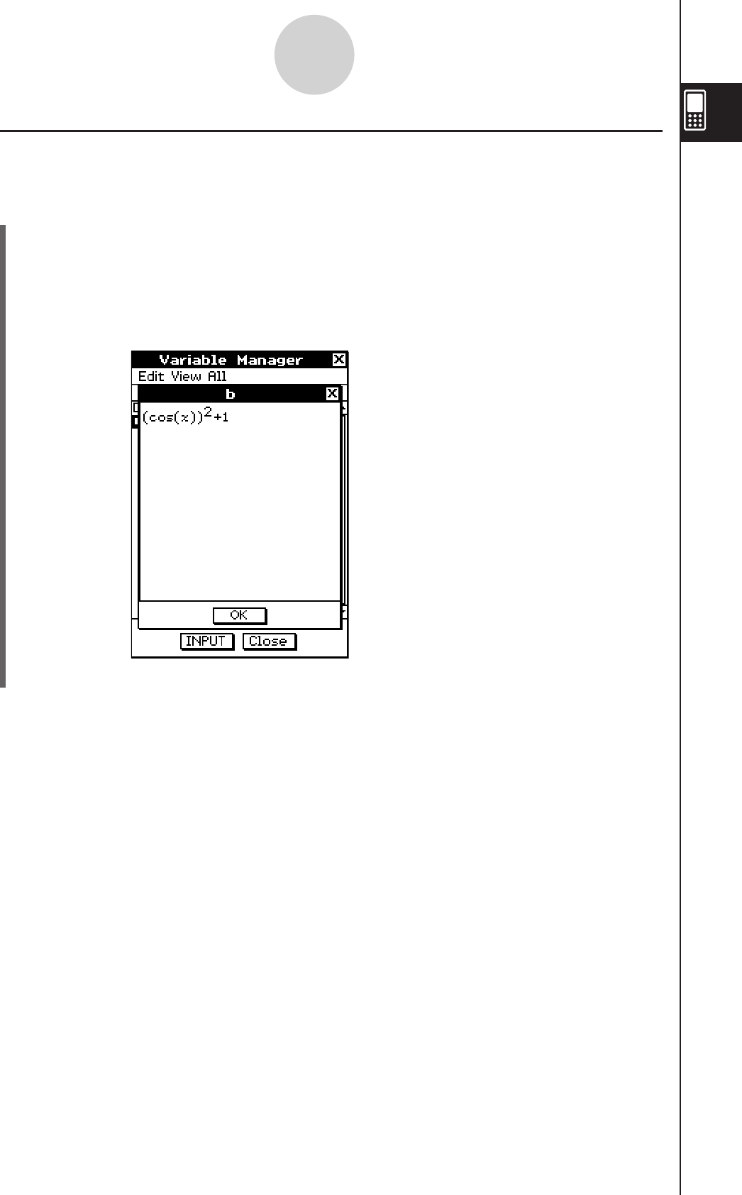
20060301

1-8-12

Using the Variable Manager

Example of EXPR variable contents

k Viewing the Contents of a Variable

You can use the Variable Manager to view the contents of a particular variable.

uClassPad Operation

(1) Open the folder that contains the variable whose contents you want to view and

display on the variable list.

(2) Tap the name of the variable whose contents you want to view so it is highlighted, and

then tap it again.

• This displays a dialog box that shows the contents of the variable.

(3) To close the dialog box, tap [OK].

Tip

• You can use this procedure to display the contents of the following variable types only: EXPR,

STR, LIST, MAT, FUNC, PRGM, TEXT, PICT.

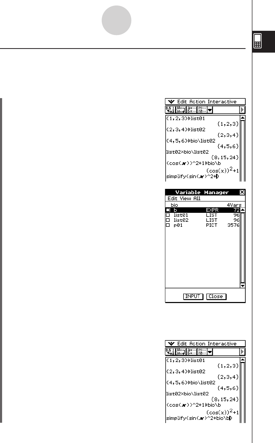
20060301

1-8-13

Using the Variable Manager

k Inputting a Variable Name into an Application

Perform the procedure below when you want to input the name of a variable from the

Variable Manager window into the application from which you started up the Variable

Manager.

uClassPad Operation

(1) In the Main application, Graph & Table application, or

some other application, move the cursor to the location

where you want to input the variable name.

(2) Start up the Variable Manager to display the folder list.

(3) Find the name of the folder that contains the variable whose name you want to input,

and tap it twice.

(4) Tap the variable whose name you want to input, so its name is highlighted.

(5) Tap [INPUT].

• This exits the Variable Manager and inputs the

name of the variable you selected in step (4) into the

application at the current cursor position.

• In this example, the variable is located in a folder

(bio) that is not the current folder, so the folder name

needs to be specified (bio\ list02). If the variable

is located in the current folder, you do not need to

specify the folder name (list02).

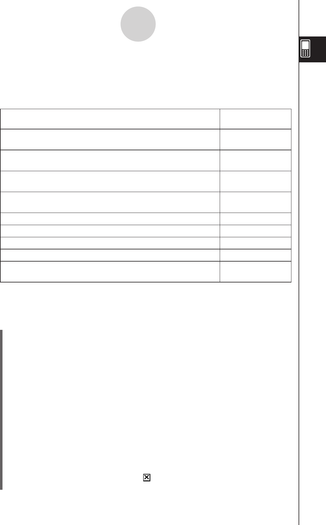
20060301

1-9 Configuring Application Format Settings

The O menu includes format settings for configuring the number of calculation result

display digits and the angle unit, as well as application-specific commands. The following

describes each of the settings and commands that are available on the O menu.

To do this: Select this O

menu command:

Specify folder for variables, and to configure number format, angle,

and other basic settings for all built-in applications Basic Format

Configure Graph window and graph drawing settings for Graph &

Table, Conics, and other graphing applications Graph Format

Configure 3D Graph window and graph drawing settings for the 3D

Graph application 3D Format

Configure number format and angle settings for Geometry

application Geometry Format

Configure Fourier transform and FFT settings Advanced Format

Configure Financial application settings Financial Format

Configure Presentation application settings Presentation

Configure Communication application settings Communication

Return all [Setup] menu settings to their initial default values (except

for the current folder setting specified on Basic Format dialog box) Default Setup

Tip

• For more details about the structure and content of the O menu, see “Using the O Menu” on

page 1-5-4.

u ClassPad Operation

(1) Open any application (except the System application).

(2) Tap

(3) Tap the menu command you want: Basic Format, Graph Format, 3D Format, Geometry

Format, Advanced Format, Financial Format, Presentation, or Communication.

• To configure Graph Format settings, for example, tap O and then [Graph Format].

This displays the Graph Format dialog box.

• Some setup dialog boxes contain multiple tabbed sheets like the Graph Format

dialog box. Tap the tab for the sheet that contains the settings you want to configure.

(4) Use the dialog box to configure the settings you want.

• For details about the settings you can configure on each of the dialog boxes, see

“Application Format Settings” on page 1-9-4.

• Some settings require specification of a variable. For more information, see

“Specifying a Variable” on the next page.

(5) To close a dialog box and apply its settings, tap [Set]. To close a dialog box without

applying its settings, tap [Cancel] or the button in the upper right corner of the dialog

box.

1-9-1

Configuring Application Format Settings

20060301

Specifying a Variable

Certain settings require that you specify variables. If you specify a user-stored variable when

configuring the setting of such an item, you must specify the folder where the variable is

stored and the variable name.

Example: To use [Table Variable] on the [Special] tab of the Graph Format dialog box for

configuring a user variable

uClassPad Operation

(1) Tap

O, or tap s on the icon panel, and then tap [Graph Format].

• This displays the Graph Format dialog box.

(2) Tap the [Special] tab.

(3) Tap the [Table Variable] down arrow button.

• This displays a list of variables.

(4) On the list, tap “Select List Name…”.

• This displays the Select Data dialog box for selecting a variable.

1-9-2

Configuring Application Format Settings

Variable type

Select the folder where

the variable is stored.

Specify the variable name.

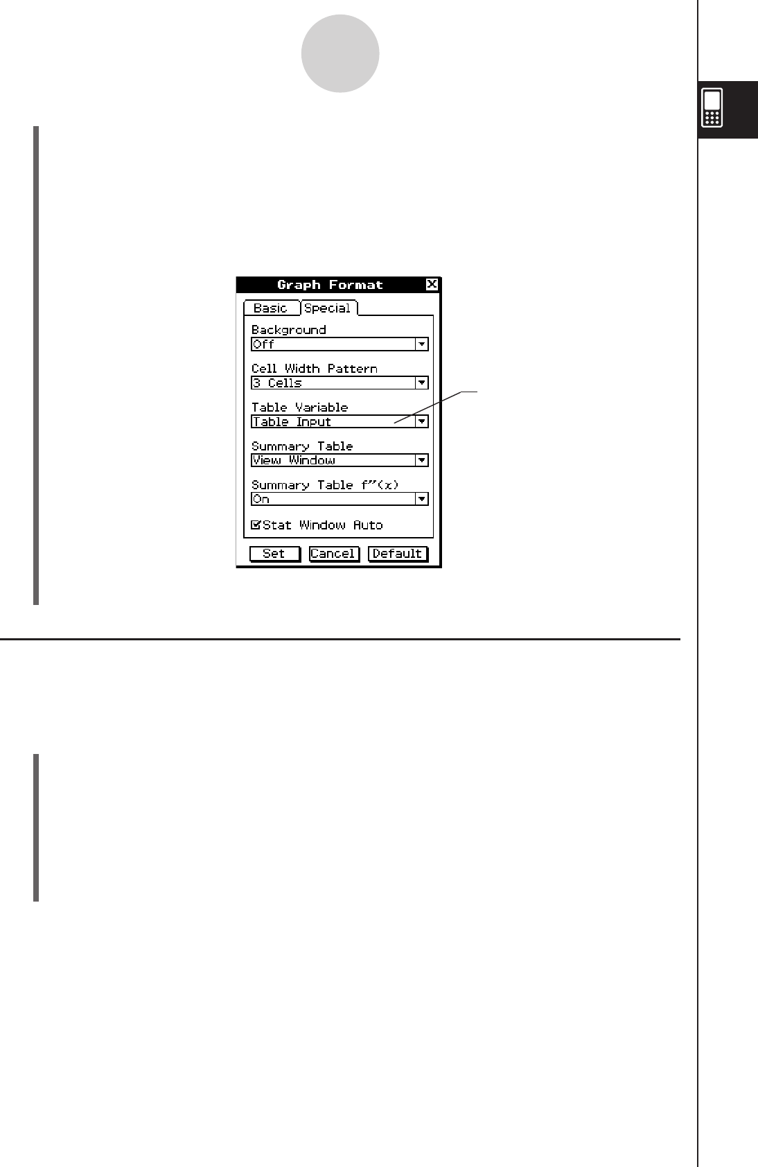
20060301

(7) Tap [Set] to save your settings.

Initializing All Application Format Settings

Perform the following procedure when you want to return all application format settings to

their initial defaults.

uClassPad Operation

(1) Tap

O, or tap s on the icon panel, and then tap [Default Setup].

(2) In response to the “Reset Setup Data?” message that appears, tap [OK] to initialize all

settings or [Cancel] to cancel the reset operation.

• If you tap [OK], the settings are initialized and then a dialog box appears on the

display.

• For details about the initial default setting for each item, see “Application Format

Settings” on page 1-9-4.

This line shows the <folder

name>\<variable name>

specified in step (5) (“main\ab”

in this case).

This box indicates that “main\ab”

is selected for Table Variable.

1-9-3

Configuring Application Format Settings

(5) Use the Select Data dialog box to specify the folder where the variable is saved, and

then specify the variable name.

• The sample dialog box in step (4) shows selection of the list variable named “ab”,

which is located in the folder named “main”.

(6) Tap [OK].

• This closes the Select Data dialog box.

• Initializing the application format settings does not affect the current folder setting on the Basic

Format dialog box. For details about the current folder, see “Specifying the Current Folder” on

page 1-8-3.

Tip

20101001

1-9-4

Configuring Application Format Settings

Application Format Settings

This section provides details about all of the settings you can configure using the application

format settings.

The following two points apply to all of the dialog boxes.

• Some settings involve turning options on or off. Selecting a check box next to an option (so

it has a check mark) turns it on, while clearing the check box turns it off.

• Other settings consist of a text box with a down arrow button on the right. Tap the down

arrow button to display a list of available settings, and then tap the setting you want.

Important!

• Settings that are marked with an asterisk (*) in the following tables are the initial defaults.

k Basic Format Dialog Box

Use the Basic Format dialog box to configure basic settings for calculations, cells, and other

parameters.

u Current Folder

To specify this folder as the current folder: Select this setting:

main main*

A user-defined folder Any other setting

• [Current Folder] settings can also be configured using the Variable Manager. For more

information, see “Specifying the Current Folder” on page 1-8-3.

20101001

1-9-5

Configuring Application Format Settings

u Number Format

To specify this type of numeric value display format: Select this setting:

Auto exponential display for values less than 10–2 and from 1010

or greater (when you are in the Decimal mode) Normal 1*

Auto exponential display for values less than 10–9 and from 1010

or greater (when you are in the Decimal mode) Normal 2

Fixed number of decimal places Fix 0 – 9

Fixed number of significant digits Sci 0 – 9

u Angle

To specify this angle unit: Select this setting:

Radians Radian*

Degrees Degree

Grad Grad

u Advanced

To do this: Do this:

Perform complex number calculations

(Complex mode)

Select the [Complex Format] check

box.

Perform real number calculations (Real mode) Clear the [Complex Format] check box.*

Display results as a decimal (Decimal mode)*1 Select the [Decimal Calculation]

check box.

Leave calculation results as expressions

(Standard mode)*1

Clear the [Decimal Calculation]

check box.*

Turn off auto simplification of expressions

(Assistant mode)*2 Select the [Assistant] check box.

Turn on auto simplification of expressions

(Algebra mode)*2 Clear the [Assistant] check box.*

Specify descending order (e.g. x2 + x + 1) for

the calculation result expression

Select the [Descending Order]

check box.*

Specify ascending order (e.g. 1 + x + x2) for

the calculation result expression Clear the [Descending Order] check box.

Specify that variables in Complex Mode

calculation should be treated as real numbers

• With this setting, re(a+bi)=a and im(a+bi)=b.

Select the [Variable is Real] check box.

Specify that variables in Complex Mode

calculation should be treated as complex

numbers

Clear the [Variable is Real] check box.*

Divide total population on its center point

between upper and lower groups, with the

median of the lower group Q1 and the median

of the upper group Q3

Select the [Q1, Q3 on Data] check box.

Make the value of element whose cumulative

frequency ratio is greater than 1/4 and nearest

to 1/4 Q1 and the value of element whose

cumulative frequency ratio is greater than 3/4

and nearest to 3/4 Q3

Clear the [Q1, Q3 on Data] check box.*

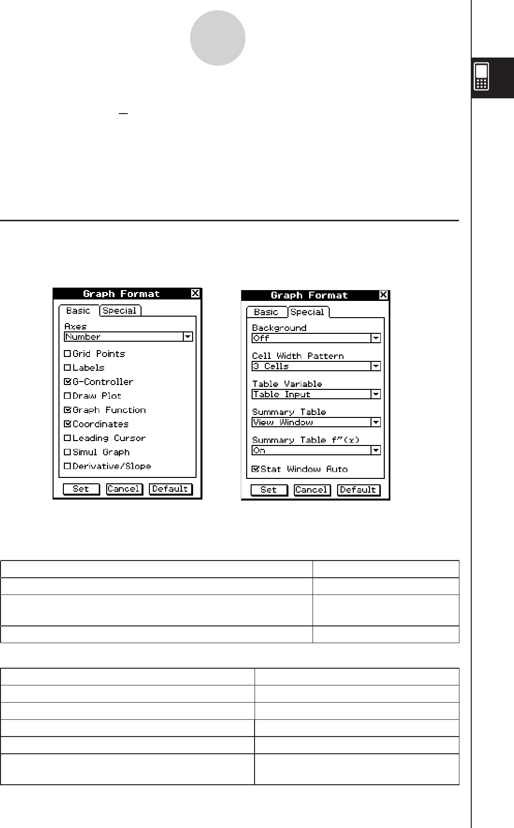
20101001

k Graph Format Dialog Box

Use the Graph Format dialog box to configure settings for the Graph window and for drawing

graphs.

1-9-6

Configuring Application Format Settings

Basic Tab

u Axes

To do this: Select this setting:

Turn on display of Graph window axes On*

Turn on display of Graph window axes along with maximum

and minimum value of each axis Number

Turn off display of Graph window axes Off

u Other settings

To do this: Do this:

Turn on display of Graph window grid Select the [Grid Points] check box.

Turn off display of Graph window grid Clear the [Grid Points] check box.*

Turn on display of Graph window axis labels Select the [Labels] check box.

Turn off display of Graph window axis labels Clear the [Labels] check box.*

Turn on display of graph controller arrows during

graphing Select the [G-Controller] check box.

*1 Executing 1

÷ 2 in the Decimal mode produces a result of 0.5, while the Standard mode

produces a result of 1

2 .

*2 Executing

x2 + 2x + 3x + 6 E in the Assistant mode produces a result of x2 + 2

•

x + 3

•

x + 6,

while the Algebra mode produces a result of x2 + 5

•

x + 6.

Important!

The Assistant mode is available in the Main application and eActivity application only.

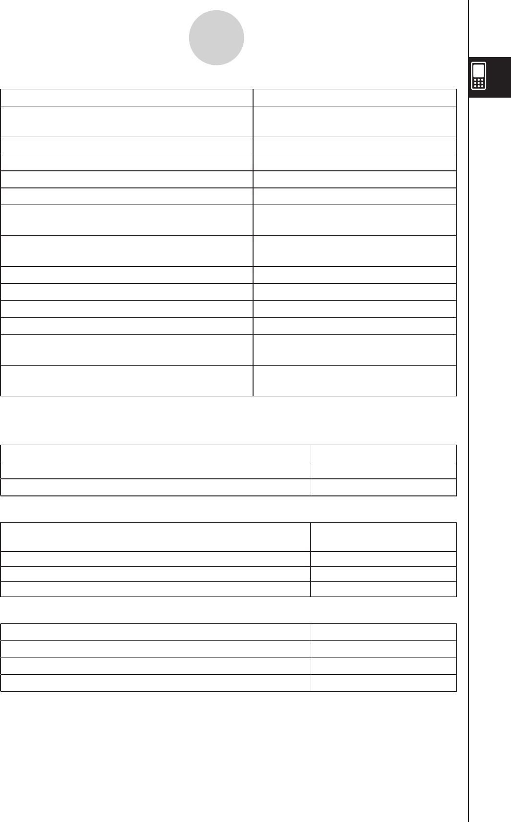
20101001

To do this: Do this:

Turn off display of graph controller arrows during

graphing Clear the [G-Controller] check box.*

Draw graphs with plotted points Select the [Draw Plot] check box.

Draw graphs with solid lines Clear the [Draw Plot] check box.*

Turn on display of function name and function Select the [Graph Function] check box.*

Turn off display of function name and function Clear the [Graph Function] check box.

Turn on display of Graph window pointer

coordinates Select the [Coordinates] check box.*

Turn off display of Graph window pointer

coordinates Clear the [Coordinates] check box.

Turn on display of leading cursor during graphing Select the [Leading Cursor] check box.

Turn off display of leading cursor during graphing Clear the [Leading Cursor] check box.*

Draw multiple graphs simultaneously Select the [Simul Graph] check box.

Draw multiple graphs one-by-one Clear the [Simul Graph] check box.*

Turn on display of coordinates of Graph window

pointer and its derivative on number table display Select the [Derivative/Slope] check box.

Turn off display of coordinates of Graph window

pointer and its derivative on number table display Clear the [Derivative/Slope] check box.*

Special Tab

u Background

To do this: Select this setting:

Turn off Graph window background display Off*

Select an image to be used as Graph window background <pict name>

u Cell Width Pattern

To specify this row width for stat editor and data table

displays: Select this setting:

2 cells 2 Cells

3 cells 3 Cells*

4 cells 4 Cells

u Table Variable

To specify this source for table data: Select this setting:

Table input Table input*

List data list1 through list6

Select list data to be used as source for table data <list name>

1-9-7

Configuring Application Format Settings

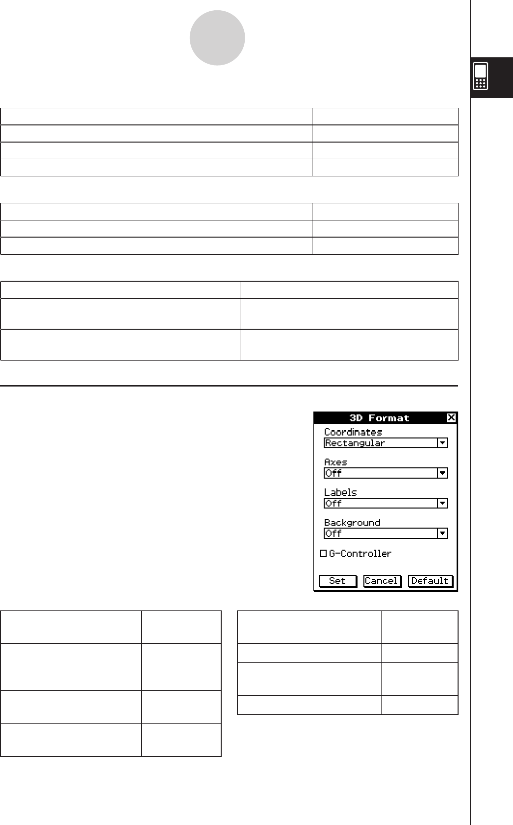
20101001

1-9-8

Configuring Application Format Settings

u Coordinates

To do this: Select this

setting:

Display coordinate values

using rectangular

coordinates

Rectangular*

Display coordinate values

using polar coordinates Polar

Turn off display of

coordinates Off

u Axes

To do this: Select this

setting:

Display axes normally On

Display box type

coordinate axes Box

Turn off display of axes Off*

u Summary Table

To specify this source for summary table data: Select this setting:

View Window View Window*

List data list1 through list6

Select list data to be used as source for summary table data <list name>

u Summary Table f ’’(x)

To do this: Select this setting:

Turn on display of second derivative for summary tables On*

Turn off display of second derivative for summary tables Off

u Stat Window Auto

To do this: Do this:

Configure Statistics application View Window

settings automatically Select the [Stat Window Auto] check box.*

Configure Statistics application View Window

settings manually Clear the [Stat Window Auto] check box.

k 3D Format Dialog Box

Use the 3D Format dialog box to configure settings for

the 3D Graph window and for drawing 3D graphs.

For full details about the 3D Graph application,

see Chapter 5.

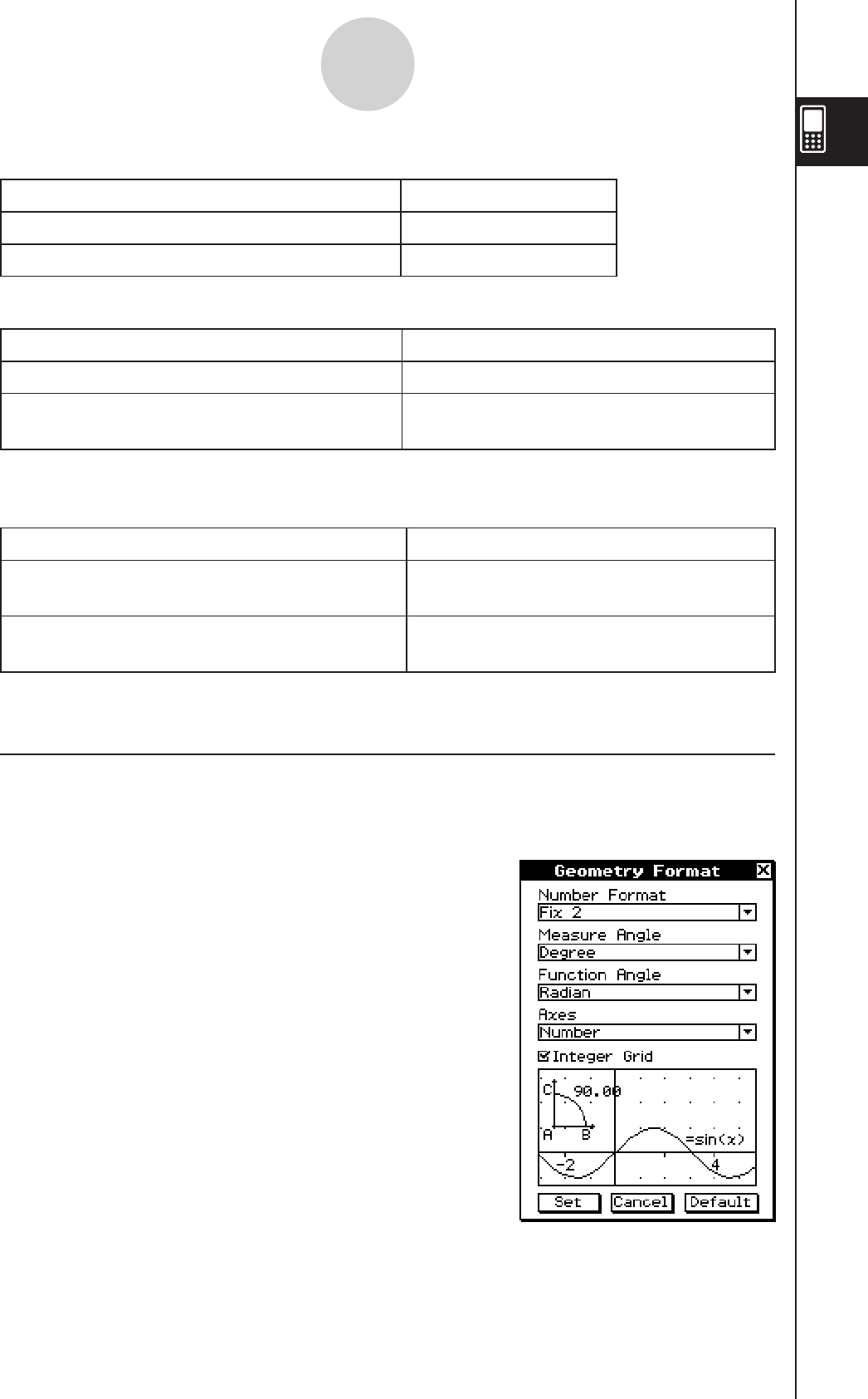
20101001

1-9-9

Configuring Application Format Settings

• The above is the same as the [G-Controller] setting on the Graph Format dialog box.

u G-Controller

To do this: Do this:

Turn on display of graph controller arrows

during graphing Select the [G-Controller] check box.

Turn off display of graph controller arrows

during graphing Clear the [G-Controller] check box.*

k Geometry Format Dialog Box

Use the Geometry Format dialog box to configure settings for the Geometry application.

Tip

• The information that appears in the preview area at

the bottom of the dialog box shows a preview of the

Geometry application window, based on the settings

configured in upper half of the dialog box.

• The above is the same as the [Background] setting on the Graph Format dialog box.

u Background

To do this: Select this setting:

Turn off Graph window background display Off*

Select an image to be used as the Graph

window background <pict name>

u Labels

To do this: Select this setting:

Turn on display of Graph window axis labels On

Turn off display of Graph window axis labels Off*

20101001

1-9-10

Configuring Application Format Settings

u Function Angle

To specify the angle unit for graphing: Select this setting:

Radian Radian*

Degree Degree

Grad Grad

u Axes

To set the initial Graph window axes condition when

opening the Geometry application: Select this setting:

Turn on display of Graph window axes On

Turn on display of Graph window axes along with maximum

and minimum value of each axis Number

Turn off display of Graph window axes Off*

u Integer Grid

To set the initial condition of integer grid when

opening the Geometry application: Do this:

Turn on display of integer grid Select the [Integer Grid] check box.

Turn off display of integer grid Clear the [Integer Grid] check box.*

u Measure Angle

To specify the angle unit for the measurement box: Select this setting:

Radian Radian

Degree Degree*

Grad Grad

u Number Format

To specify this type of numeric value display format on

the Geometry window: Select this setting:

Auto exponential display for values less than 10–2 and from

1010 or greater (when you are in the Decimal mode) Normal 1

Auto exponential display for values less than 10–9 and from

1010 or greater (when you are in the Decimal mode) Normal 2

Fixed number of decimal places Fix 0 – 9

Fixed number of significant digits Sci 0 – 9

• The initial default [Number Format] setting is Fix 2.

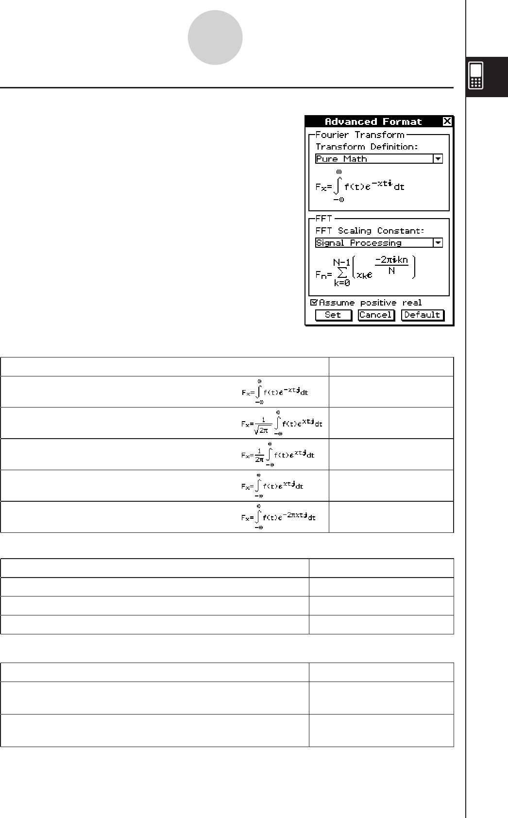
20101001

1-9-11

Configuring Application Format Settings

k Advanced Format Dialog Box

Use the Advanced Format dialog box to configure

settings for Fourier transform and FFT settings.

u FFT

To do this: Select this setting:

Specify Pure Math for FFT scaling constant Pure Math

Specify Signal Processing for FFT scaling constant Signal Processing*

Specify Data Analysis for FFT scaling constant Data Analysis

u Assume positive real

To do this: Do this:

Assume variables for Fourier calculation are positive reals Select the [Assume positive

real] check box.*

Allow complex numbers as variables for Fourier calculation Clear the [Assume positive

real] check box.

u Fourier Transform

To do this: Select this setting:

Specify following formula for Fourier transform: Pure Math*

Specify following formula for Fourier transform: Modern Physics

Specify following formula for Fourier transform: Classical Physics

Specify following formula for Fourier transform: Probability

Specify following formula for Fourier transform: Signal Processing

20110401

1-9-12

Configuring Application Format Settings

k Financial Format Dialog Box

Use the Financial Format dialog box to configure

settings for the Financial application.

Basic Tab

u Days in Year

To do this: Select this setting:

Specify a 360-day year 360 days

Specify a 365-day year 365 days*

u Payment Date

To do this: Select this setting:

Specify beginning of period for the payment date Beginning of period

Specify end of period for the payment date End of period*

u Date Format

To do this: Select this setting:

Specify day/month/year as the date format DD/MM/YYYY

Specify month/day/year as the date format MM/DD/YYYY*

Specify year/month/day as the date format YYYY/MM/DD

u Automatically copy common fields to new calculation

To do this: Do this:

When changing to another calculation type,

automatically copy the contents of all fields in

the current calculation whose names match the

names of fields in the new calculation

Select the [Automatically copy common

fields to new calculation] check box.

When changing to another calculation type,

clear all fields

Clear the [Automatically copy common

fields to new calculation] check box.*

20060301

1-9-13

Configuring Application Format Settings

Special Tab

u Odd Period

To do this: Select this setting:

Specify compound interest for odd (partial) months Compound (CI)

Specify simple interest for odd (partial) months Simple (SI)

Specify no separation of full and odd (partial) months Off*

u Compounding Frequency

To do this: Select this setting:

Specify once a year compounding Annual*

Specify twice a year compounding Semi-annual

u Bond Interval

To do this: Select this setting:

Use a number of payments as term for bond calculations Term*

Use a date as term for bond calculations Date

u Profit Amount/Ratio

To do this: Select this setting:

Use amount (PRF) for break-even point calculations Amount (PRF)*

Use profit ratio (r%) for break-even point calculations Ratio (r%)

u Break-Even Value

To do this: Select this setting:

Use quantity for break-even point calculations Quantity*

Use sales amount for break-even point calculations Sales

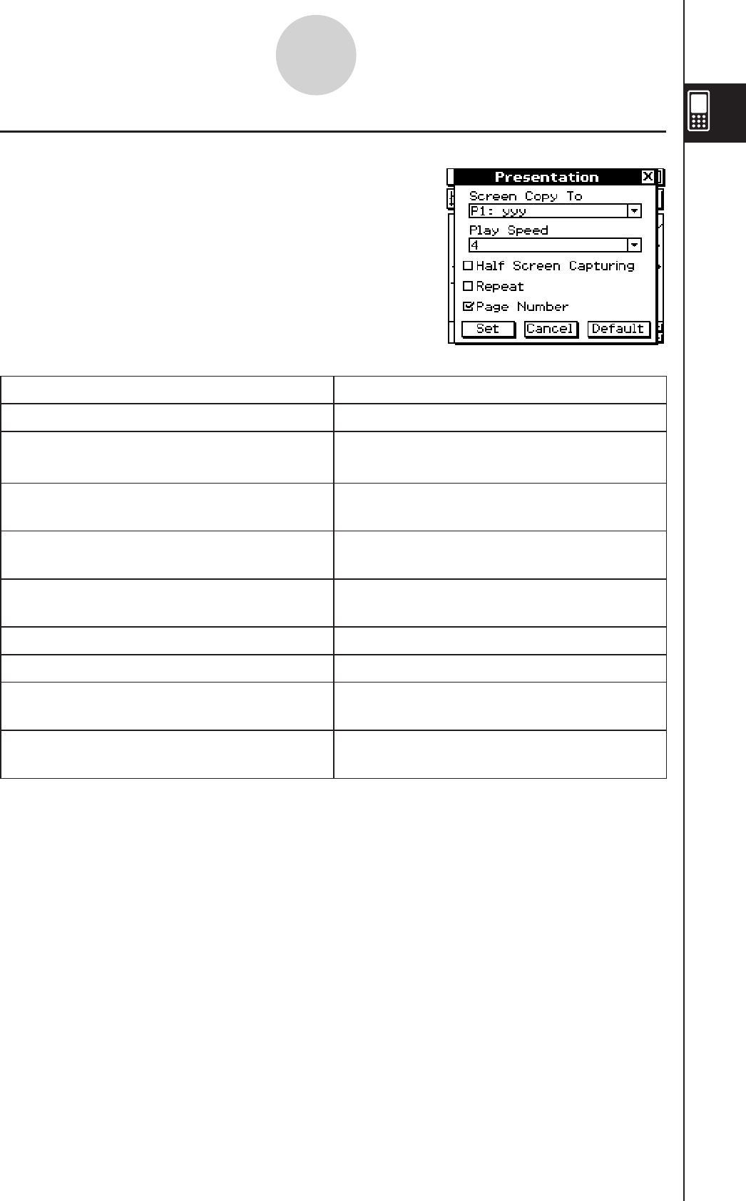
20060301

1-9-14

Configuring Application Format Settings

k Presentation Dialog Box

Use the Presentation dialog box to configure settings

for the Presentation application. For full details about the

Presentation application, see Chapter 11.

To do this: Do this:

Send hard copy data to an external device Select “Outer Device” for [Screen Copy To].*

Save hard copy data internally as

Presentation data

Select “P1:<File name>**” through

“P20:<File name>**” for [Screen Copy To].

Specify the page change speed for Auto

Play

Specify a [Play Speed] value from 1 (fastest)

to 10 (slowest).

Capture the upper half of the window when

h is tapped

Select the [Half Screen Capturing] check

box.

Capture the entire window when h is

tapped

Clear the [Half Screen Capturing] check

box.*

Turn on repeat playback of files Select the [Repeat] check box.

Turn off repeat playback of files Clear the [Repeat] check box.*

Turn on page number display during

playback and editing Select the [Page Number] check box.*

Turn off page number display during

playback and editing Clear the [Page Number] check box.

• The initial default [Play Speed] setting is 4.

** <File name> will show the name of the presentation file.

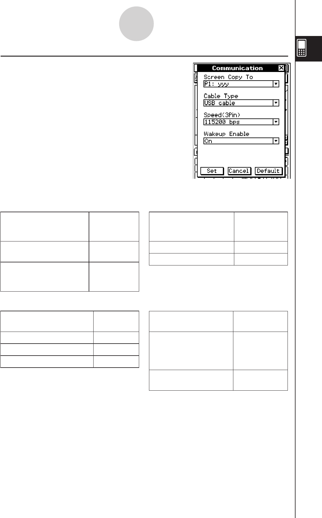
20110401

1-9-15

Configuring Application Format Settings

k Communication Dialog Box

Use the Communication dialog box to configure

communication settings. For full details about the

Communication application, see Chapter 2 in the separate

Hardware User’s Guide.

u Speed (3Pin)

To specify this data rate

for 3-pin communication:

Select this

setting:

9,600 bps 9600 bps

38,400 bps 38400 bps

115,200 bps 115200 bps*

u Screen Copy To

To do this with hard

copy data generated by

tapping h:

Select this

setting:

Send hard copy data to an

external device

Outer

Device*

Save hard copy data

internally as Presentation

data

P1 - P20

u Cable Type

To use this type of

cable for data

communication:

Select this

setting:

3-pin cable 3pin cable

USB cable USB cable*

u Wakeup Enable

To do this: Select this

setting:

Turn on the wakeup

function (page 2-3-2 in

the separate Hardware

User’s Guide)

On*

Turn off the wakeup

function Off

20060301

Using the Main

Application

The Main application is a general-purpose numerical and mathematical

calculation application that you can use to study mathematics and

solve mathematical problems. You can use the Main application to

perform general operations from basic arithmetic calculations, to

calculations that involve lists, matrices, etc.

The Main application also provides you with an [Action] menu and

[Interactive] menu from which you can select approximately 120

different commands for working with mathematical expressions.

2-1 Main Application Overview

2-2 Basic Calculations

2-3 Using the Calculation History

2-4 Function Calculations

2-5 List Calculations

2-6 Matrix and Vector Calculations

2-7 Specifying a Number Base

2-8 Using the Action Menu

2-9 Using the Interactive Menu

2-10 Using the Main Application in Combination with

Other Applications

2-11 Using Verify

2-12 Using Probability

2-13 Running a Program in the Main Application

Chapter

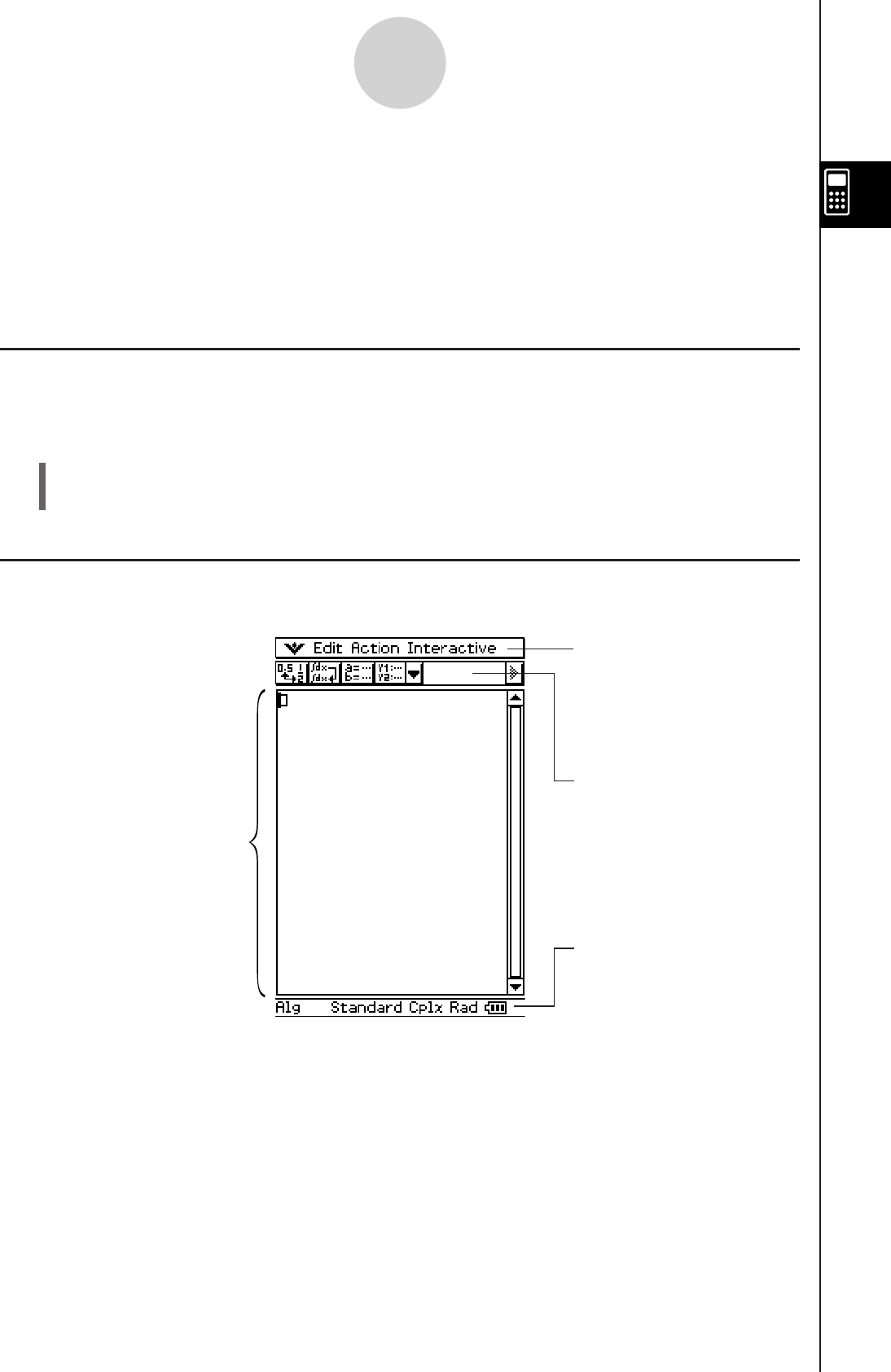
20060301

2-1-1

Main Application Overview

2-1 Main Application Overview

This section provides information about the following.

• Main application windows

• Modes that determine how calculations and their results are displayed

• Menus and their commands

Starting Up the Main Application

Use the following procedure to start up the Main application.

u ClassPad Operation

On the application menu, tap J.

This starts the Main application and displays the work area.

Main Application Window

Starting up the Main application displays a large white work area.

Work area

Use this area for inputting

operations and commands.

ClassPad also uses this

area to output calculation

results.

Menu bar

The [Action] menu and

[Interactive] menu are for

executing mathematical

expressions.

Toolbar

Status bar

This area shows the current

mode settings for the Main

application.

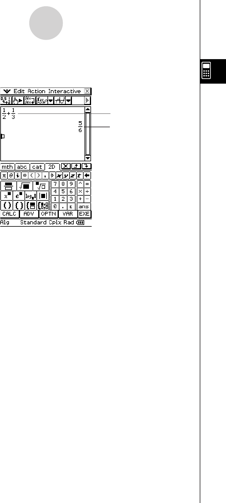
20090601

• Basic Main application operations consist of inputting a calculation expression into the work

area and pressing E. This performs the calculation and then displays its result on the right

side of the work area.

Calculation

result

Input

expression

• Calculation results are displayed in natural format, with mathematical expressions

appearing just as they do in your textbook. You can also input expressions in natural format

using the ) soft keyboard.

• The Main application also has a calculation history feature, which saves up to 30 calculation

expressions you input and their calculated results. As long you do not clear the record, this

information is available for later recall. This way you can recall a past calculation, make

changes to it, and recalculate.

2-1-2

Main Application Overview

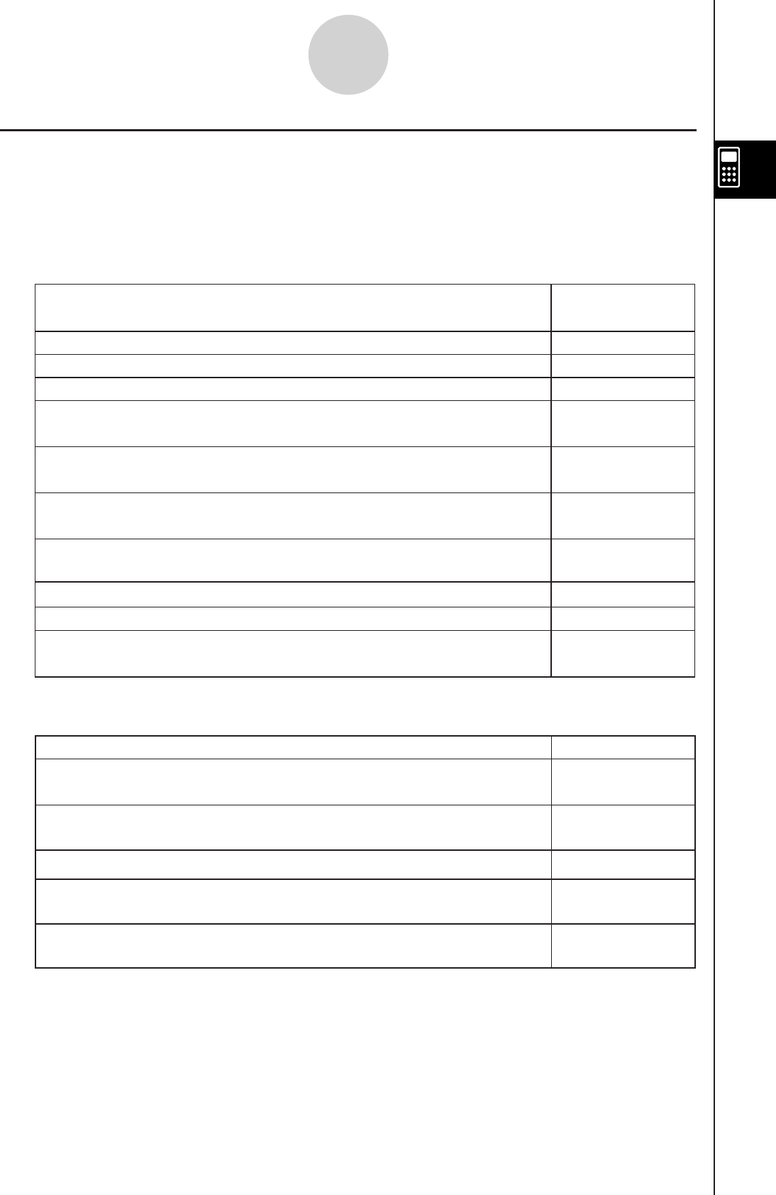
20060301

To do this: Select this

menu item:

Undo the last operation or redo an operation that was just undone Edit - Undo/Redo

Cut the selected character string and place it onto the clipboard Edit - Cut

Copy the selected character string and place it onto the clipboard Edit - Copy

Paste the contents of the clipboard at the current cursor position in

the work area Edit - Paste

Select the entire row (input expression or value, or result) where the

cursor is located in the work area Edit - Select All

Delete the input expression and its result where the cursor is located

in the work area Edit - Delete

Clear all work area contents (calculation history) Edit - Clear All

Clear variables that contain numbers, list and matrices Edit - Clear All

Variables

Insert a command into the work area (page 2-8-1) Action

Execute an Interactive command for the expression selected in the

work area (page 2-9-1) Interactive

Main Application Menus and Buttons

This section explains the operations you can perform using the menus and buttons of the

Main application.

• For information about the O menu, see “Using the O Menu” on page 1-5-4.

Menu Commands

2-1-3

Main Application Overview

* Normally, inputting and executing an expression like ∫ (x × sin(x), x) integrates x × sin(x)

and displays the result sin(x) – x × cos(x). Tapping 0 displays ∫ (x × sin(x), x) as-is, in a

natural math format without performing any calculation.

Button Functions

To do this: Tap this button:

Toggle calculation result display between the Standard mode and

Decimal mode

Output an input expression as-is*

Recalculate the equation just for the current line where the cursor is

currently located

Switch between binary, octal, decimal or hexadecimal number bases

during normal calculation (page 2-7-3)

Access ClassPad application windows from the Main application

(page 2-1-5)

20060301

Using Main Application Modes

The Main application has a number of different modes that control how calculation results are

displayed, as well as other factors. The current mode is indicated in the status bar.

k Status Bar Mode Indicators

2-1-4

Main Application Overview

• You can tap a mode name in the status bar to change it, or use the O menu’s [Basic

Format] command to change the setting of each mode. For details about these settings,

see “1-9 Configuring Application Format Settings”.

• For details about the calculations and result displays produced in each of the above modes,

see “Calculation Modes” on page 2-2-6.

1234

Status Bar

Location Indicator Description Setting Status

Assist Assistant mode: Does not automatically

simplify expressions. Assistant

Decimal

Calculation

Complex

Format

Angle

Alg Algebra mode: Automatically simplifies

expressions. Off*

Decimal Decimal mode: Converts result to a

decimal (approximate value). On

Standard

Standard mode: Displays result in exact

form (fractional format). If a result cannot

be displayed in exact form, however, it will

be displayed as a decimal approximation.

Off*

Cplx Complex mode: For complex number

calculations. On

Real Real mode: For real number calculations. Off*

Rad Radian mode: Angles displayed in radians. Radian*

Deg Degree mode: Angles displayed in

degrees. Degree

Gra Grad mode: Angles displayed in grads. Grad

Settings that are marked with an asterisk (*) in the following tables are initial defaults.

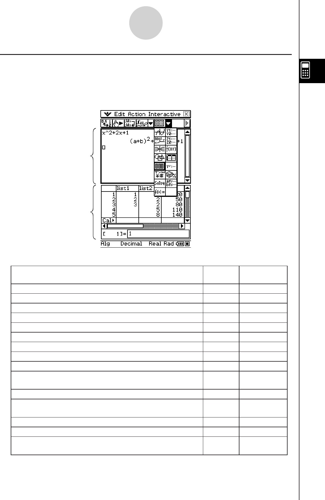
20060301

Accessing ClassPad Application Windows from the Main Application

Tapping the down arrow button on the toolbar displays a palette of 15 icons that you can

use to access certain windows of other ClassPad applications. Tapping the ( button, for

example, splits the display into two windows, with the Stat Editor window of the Statistics

application in the lower window.

2-1-5

Main Application Overview

The following table displays the application you can access with each of the buttons.

Main application

work area

Stat Editor window • For details about swapping the

positions of the two windows,

activating a window, closing a

window, etc, see “Using a Dual

Window Display” on page 1-5-1.

To display this window: Tap this

button: See Chapter:

Graph & Table application Graph window

Graph & Table application Graph Editor window

3D Graph application 3D Graph window

3D Graph application 3D Graph Editor window

Conics application Conics Graph window

Conics application Conics Editor window

Geometry application Geometry window

Spreadsheet application window

Statistics application Stat Editor window

(

Numeric Solver application Numeric Solver window

Sequence application Sequence Editor window

Verify window

Differential Equation application Differential Equation Editor

window 14

Financial application window

Probability window

See “2-12 Using

Probability”.

See “2-11 Using

Verify”.

20060301

• You can perform drag and drop operations with expressions between the Main application

work area and the currently displayed window. For example, you could drag an expression

from the Main application work area to the Graph window, and graph the expression. For

details, see “2-10 Using the Main Application in Combination with Other Applications”.

• For details about how to use each type of window, see the chapter for the appropriate

application.

Accessing the Main Application Window from Another ClassPad

Application

Some ClassPad applications allow you to access the Main application window by tapping

O and then [Main]. In the Statistics application and some other applications, you can also

access the Main application window by tapping the ~ button.

The following are examples of what you can do after opening the Main application window

within another application.

• Using the Main application window as a calculator to perform a simple calculation

• Using drag and drop to copy expressions and values between windows

Example: To drag an expression from the Graph Editor window to the Main application work

area

2-1-6

Main Application Overview

For full details about individual operations, see the chapters that cover each application.

Tip

• You cannot access the Main application window from the Geometry, Presentation, Spreadsheet,

Financial, Communication, or System application.

• You can access the Geometry application from the Main application.

20060301

2-2-1

Basic Calculations

2-2 Basic Calculations

This section explains how to perform basic mathematical operations in the Main application.

Arithmetic Calculations and Parentheses Calculations

• You can perform arithmetic calculations by inputting expressions as they are written. All of

the example calculations shown below are performed using the 9 soft keyboard, unless

noted otherwise.

• To input a negative value, tap - or - before entering the value.

• The order of operations is followed when a calculation consists of mixed arithmetic

operations (multiplication and division are given priority over addition and subtraction).

• The example calculations are all performed using the Decimal mode. Using the Standard

mode causes results to be displayed as fractions. For details about the Decimal mode and

Standard mode, see “Status Bar Mode Indicators” on page 2-1-4.

Calculation Key Operation

23 + 4.5 – 53 = –25.5 cd+e.f-fdw

56 × (–12) ÷ (–2.5) = 268.8 fg*(-bc)/(-c.f)w

(2 + 3) × 102 = 500 (c+d)Ecw

1 + 2 – 3 × 4 ÷ 5 + 6 = 6.6 b+c-d*e/f+gw

100 – (2 + 3) × 4 = 80 baa-(c+d)*ew

2 + 3 × (4 + 5) = 29 c+d*(e+f)w

(7 – 2) × (8 + 5) = 65 (h-c)*(i+f)w

g/(e*f)w or

) Ngce*fw

(1 + 2i) + (2 + 3i) = 3 + 5i (b+ci)+(c+di)w

(2 + i) × (2 – i ) = 5 (c+i)*(c-i)w

Tip

• For details about the calculations and result displays produced in each mode, see “Calculation

Modes” on page 2-2-6.

• To toggle a result between decimal and fractional format, tap u before pressing E.

6 = 0.3

4 × 5

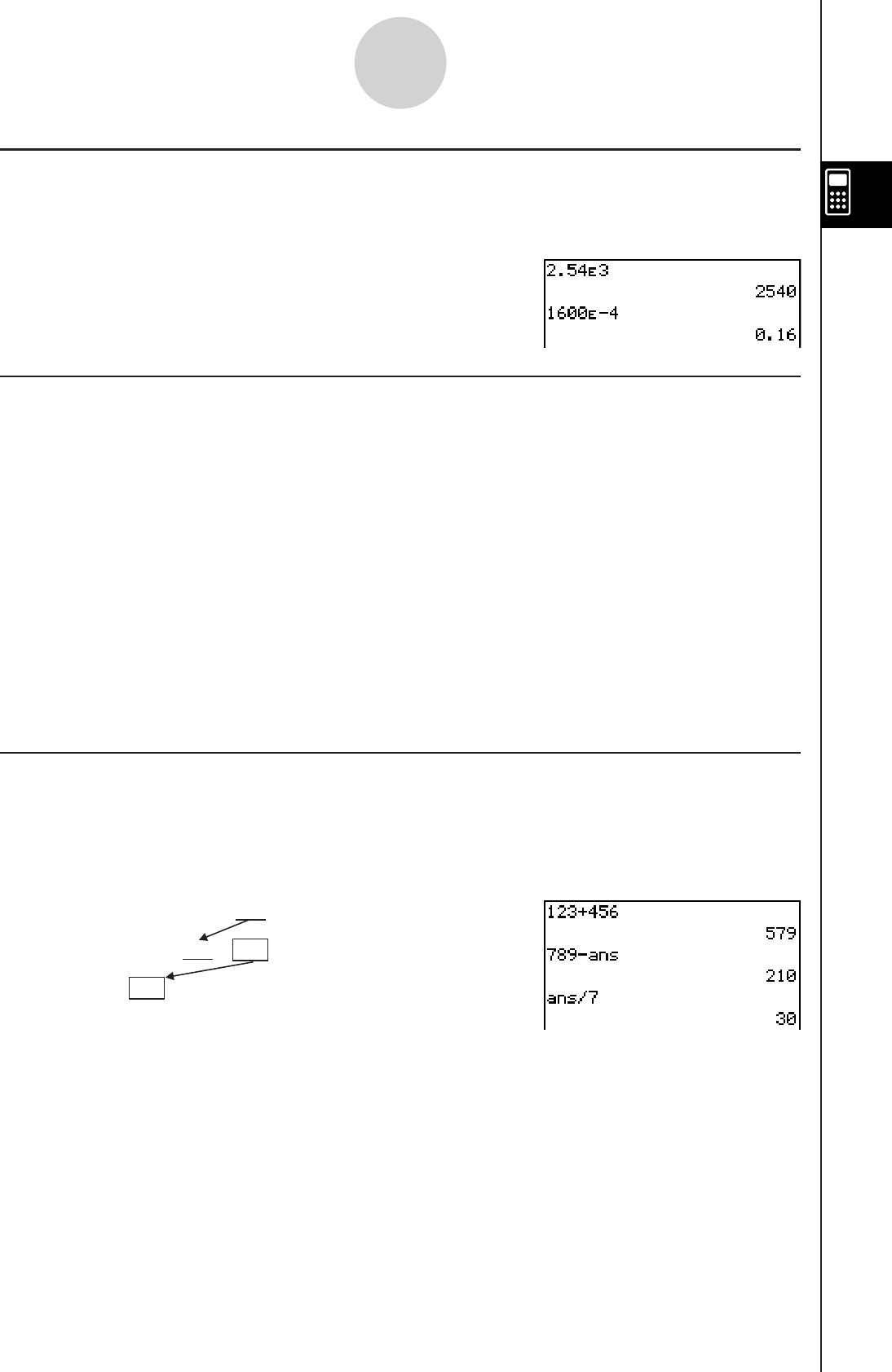
20060301

2-2-2

Basic Calculations

Using the e Key

Use the e key to input exponential values. You can also input exponential values using the

E key on the 9 and ) keyboards.

Examples: 2.54 × 103 = 2540

c.feedw

1600

× 10–4 = 0.16

bgaaE-ew

Omitting the Multiplication Sign

You can omit the multiplication sign in any of the following cases.

• In front of a function

Examples: 2sin (30), 10log (1.2)

• In front of a constant or variable

Examples: aπ, 2ab, 3ans

• In front of an open parenthesis

Examples: 3(5 + 6), (a + 1)(b – 1)

Note that you must use a multiplication sign when the expression directly in front of the

open parenthesis is a literal variable. Example: ab (3 + b) must be written ab × (3 + b).

Otherwise, your input is considered to be in function notation (

f (x)).

• In front of the e key or E key (See “Using the e Key” above.)

• In front of a matrix or list

Examples: a {1, 2, 3}, 3 [[1, 2] [3, 4]]

Using the Answer Variable (ans)

Any time you execute a calculation in the Main application work area, the last result is

assigned automatically to a variable named “ans” (answer). You can even recall current “ans”

variable contents and input them into another calculation by tapping the D key as shown

below.

Example: 123 + 456 = 579 bcd+efgw

789 – 579 = 210 hij-Dw

210

÷ 7 = 30 /hw*

* Starting a calculation expression with +, −, ×, ÷, or ^ operator will cause the “ans”

variable to be inserted automatically to the left of the operator, even if you do not tap

the

D key. For more information, see “Performing Continuous Calculations” on

page 2-2-3.

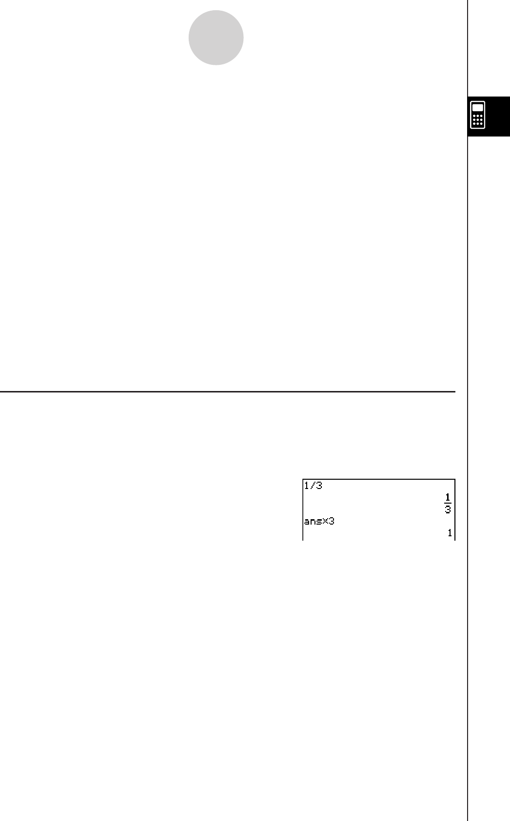
20060301

2-2-3

Basic Calculations

Tip

• The “ans” variable is a system variable. For details about system variables, see “1-7 Variables

and Folders”.

• Since “ans” is a variable name, you can specify the “ans” variable by inputting [a][n][s] on the

0 (alphabet) keyboard, or by tapping the D key on the 9 or the ) keyboard.

• The “ans” variable stores the result of your last or most recent calculation.

• The work area maintains a calculation history of the calculations you perform (page 2-3-1). Any

instance of the “ans” variable in the calculation history contains the result of the calculation

immediately prior to that instance. You can use “ans” as many times as you want in calculations,

as long as you remember that the value or expression assigned to each “ans” variable in the

calculation history is determined by the calculation immediately preceding it.

• Using the “ans” variable in a calculation results in an error if the previous calculation produced an

error display or after a program produces the “done” message on the display.

• The format of the calculation result value assigned to the “ans” variable depends on the Basic

Format dialog box [Number Format] setting (page 1-9-5). The following illustrates the format used

when “Fix2” is selected for the [Number Format] setting.

approx (1/3)

w 0.33

ans

× 3 w 0.99

See “Standard Mode and Decimal Mode” on page 2-2-6.

k Performing Continuous Calculations

Answer memory also lets you use the result of one calculation as one of the arguments in

the next calculation.

Example: 1 ÷ 3 =

1 ÷ 3 × 3 =

cb/dw

(Continuing)*dw

Continuous calculations can be used with +, –, ×, ÷, and ^.

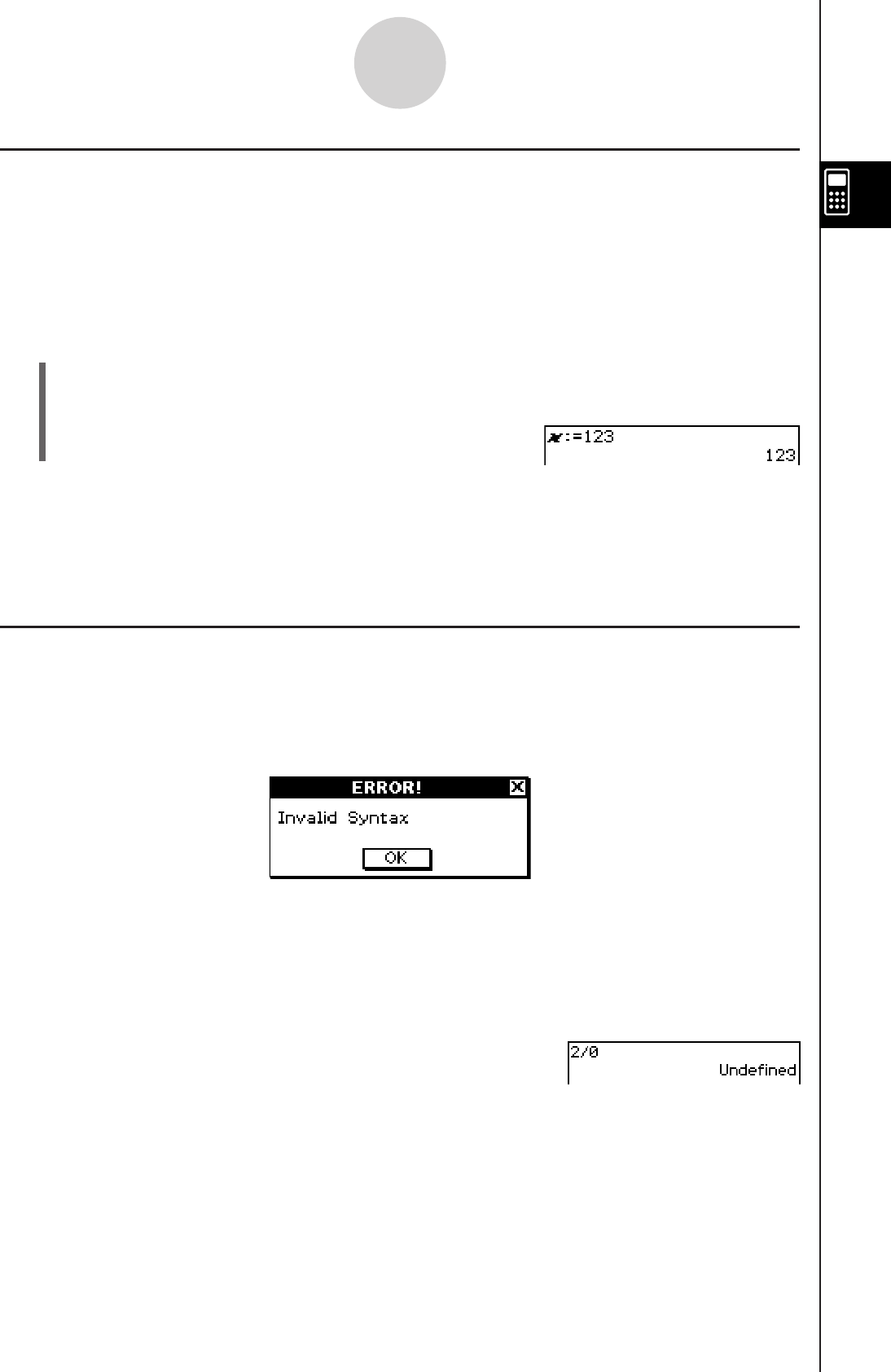
20110401

Calculation Error

An error message dialog box, like the one shown below, appears when there is a problem

with the syntax of an input expression or value, when the number of decimal places of a

calculation result in the Standard mode (page 2-2-6) exceeds a specified range, etc. Tap [OK]

to close the dialog box and return to the calculation.

Tip

• The text of the error message dialog box depends on the type of error that occurred. For details,

see the “Error Message Table” on page -5-1.

• If you perform a calculation that is mathematically undefined (such as division by zero), the

message “Undefined” appears in place of the calculation result, without display of an error

message.

2-2-4

Basic Calculations

Assigning a Value to a Variable

Besides using the variable assignment key (W, page 1-7-6), you can also use the syntax

shown below in the Main application and eActivity application to assign a value to a variable.

Syntax: Variable: = value

Example: Assign 123 to variable x

uClassPad Operation

(1) Perform the key operation below in the Main application work area.

9X0L:9=bcd

(2)

Important!

“:=” can be used only in Main and eActivity. It can NOT be used in a program. In the Program

application, you must use W to store a value to a variable.

20060301

Calculation Priority Sequence

Your ClassPad automatically performs calculations in the following sequence.

1 Commands with parentheses (sin(, diff(, etc.)

2 Factorials (x!), degree specifications (o, r ), percents (%)

3 Powers

4 π, memory, and variable multiplication operations that omit the multiplication sign (2π, 5A,

etc.)

Command with parentheses multiplication operations that omit the multiplication sign (2 3,

etc.)

× , ÷

5 +, –, (–)

6 Relational operators (=, ≠, <, >, <, >)

7 and

8 or, xor

9 with ( | )

Example: 2 + 3 × (log (sin(2π2)) + 6.8) = 22.07101691 (In Algebra mode, Decimal mode,

Radian mode.)

Tip

• Expressions in parentheses are given priority.

• In cases where a series of calculations in the same expression includes more than one of the

operators 4 through 9 that are the same priority sequence level, the same level operations are

performed from left to right. A series of power calculations 3 (example: 5^2^3) is performed from

right to left (5^(2^3)).

2-2-5

Basic Calculations

20060301

Calculation Modes

The Main application has a number of different modes, as described under “Using Main

Application Modes” on page 2-1-4. The display format of calculation results depends on the

currently selected Main application mode. This section tells you which mode you need to

use for each type of calculation, and explains the differences between the calculation results

produced by each mode.

• All of the following calculation examples are shown using the Algebra mode only.

k Standard Mode and Decimal Mode

The Standard mode displays calculation results in mathematical expression format whenever

possible, while the decimal mode converts calculation results to a decimal form. When the

Decimal mode is selected, you can control the use of exponential notation with the [Number

Format] setting on the Basic Format dialog box (page 1-9-5).

u Examples of Decimal mode and Standard mode result displays

Expression

Decimal Mode Result Standard Mode Result

50 ÷ 4 = 12.5 12.5 25

100 ÷ 6 = 16.6666666... 16.66666667 50

2 + 2 = 3.414213562... 3.414213562 2 +

3.52 ÷ 3 + 2.5 = 6.583333333... 6.583333333 79

π = 3.1415926535... 3.141592654 π

sin (2.1π) × 5 = 1.5450849718... 1.545084972 5

( 5 − 1 )

• The Decimal mode results in the above table show what would appear on the display when

“Normal 1” is selected for the [Number Format] setting on the Basic Format dialog box.

2-2-6

Basic Calculations

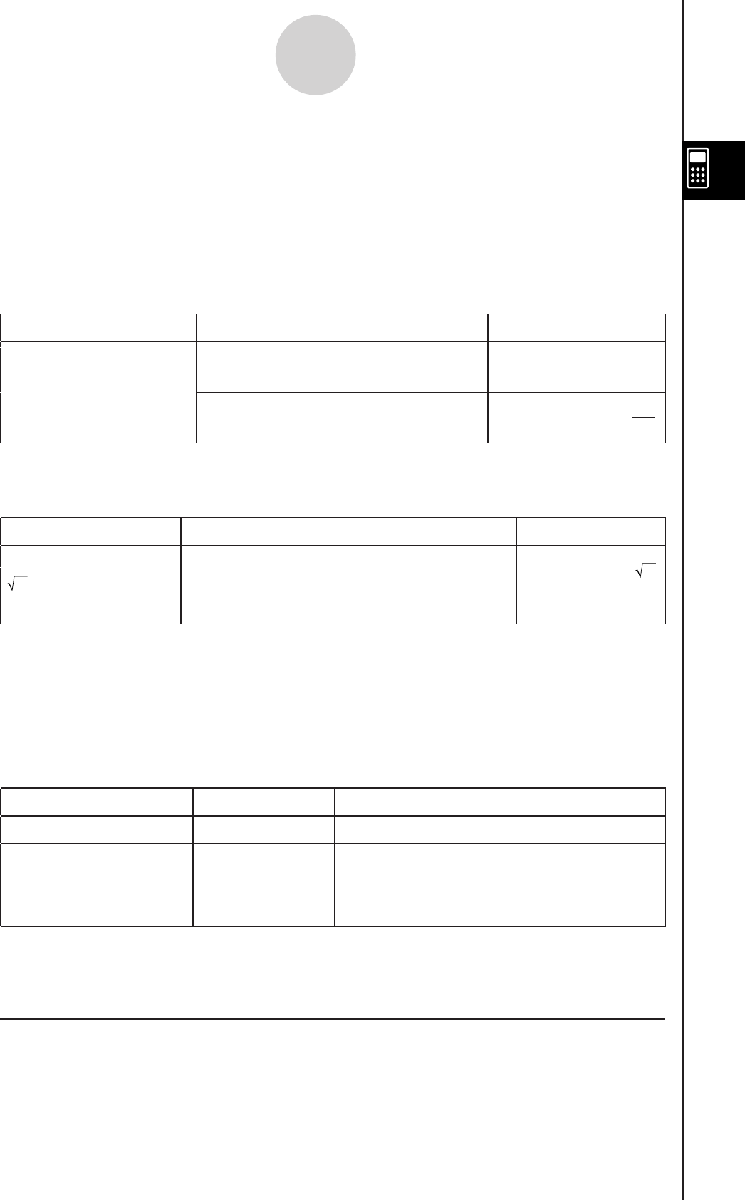
20090601

u Using the u Button to Toggle between the Standard Mode and Decimal

Mode

You can tap u to toggle a displayed value between Standard mode and Decimal mode

format.

Note that tapping u toggles the format of a displayed value. It does not change the current

Standard mode/Decimal mode setting.

Example 1: Tapping u while the ClassPad is configured for Standard mode (Normal 1)

display

Expression ClassPad Operation Displayed Result

100 ÷ 6 = 16.6666666...

baa/gu

(Switches to Decimal mode format.) 16.66666667

u (Switches back to Standard mode

format.)

Example 2: Tapping u while the ClassPad is configured for Decimal mode (Normal 1)

display

Expression ClassPad Operation Displayed Result

2 + 2 = 3.414213562...

9c)+cu

(Switches to Standard mode format.) 2 + 2

u (Switches back to Decimal mode format.) 3.414213562

u Number of Decimal Places, Number of Significant Digits, Normal Display

Settings

The [Number Format] settings on the Basic Format dialog box (page 1-9-4) specify the

number of decimal places, the number of significant digits, and the normal display setting

for Main application Decimal mode calculation results. The following shows how calculation

results appear under each setting.

Expression Normal 1 Normal 2 Fix 3 Sci 3

50 ÷ 4 = 12.5 12.5 12.5 12.500 1.25E + 1

100 ÷ 6 = 16.6666666... 16.66666667 16.66666667 16.667 1.67E + 1

1 ÷ 600 = 0.00166666... 1.666666667E –3 0.00166666666 0.002 1.67E – 3

1011 ÷ 4 = 2.5E + 10 2.5E + 10 2.5E + 10 2.5E + 10 2.50E + 10

• The allowable range for the number of decimal places is Fix 0 to Fix 9, and the range for

the number of significant digits is Sci 0 to Sci 9. For details about the [Number Format]

settings, see “Basic Format Dialog Box” on page 1-9-4.

k Complex Mode and Real Mode

The Complex mode is for complex number calculations, while the Real mode is limited to

calculations within the range of real numbers. Performing a calculation in the Real mode

that produces a result that is outside the range of real numbers causes an error (Non-Real in

Calc).

2-2-7

Basic Calculations

20110401

u Examples of Complex mode and Real mode calculation results

Expression Complex Mode Real Mode

solve (x3 – x2 + x – 1 = 0, x){

x = –i, x = i, x = 1} {x = 1}

i + 2i 3·iERROR: Non-Real in Calc

(1 + '

i)(⬔(2,45°)) ⬔(4,105) ERROR: Non-Real in Calc

Tip

• You can select “ i ” or “ j ” for the imaginary unit. See “Specifying the Complex Number Imaginary

Unit” on page 16-10-1.

• If the expression includes ⬔(r,), calculation results should be ⬔(r,) form.

k Radian Mode, Degree Mode and Grad Mode

You can specify radians, degrees or grads as the angle unit for display of trigonometric

calculation results.

u Examples of Radian mode, Degree mode and Grad mode calculation results

Expression Radian Mode Degree Mode Grad Mode

sin (π/4) 2

2sin sin

sin (45) sin (45) 2

2sin (45)

sin (50) sin (50) sin (50) 2

Important!

Regardless of the currently selected angle unit setting, a calculation that includes an

imaginary number power exponent (such as: eπi) is performed using radians as the angle unit

(eπi = −1).

k Assistant Mode and Algebra Mode

The Algebra mode automatically simplifies mathematical expressions produced by

calculations. No simplification is performed in the Assistant mode. In the Assistant mode,

you can view intermediate results as well, which allows you to see the steps that lead to a

particular result as shown in the “expand” example below.

u Examples of Assistant mode and Algebra mode calculation results

Expression Assistant Mode Algebra Mode

x2 + 2x + 3x + 6 x2 + 2

x + 3

x + 6 x2 + 5

x + 6

expand ((x+1)2)x2 + 2

1 + 12x2 + 2

x + 1

x + 1 (When 1 is assigned to x)x + 1 2

Important!

The Assistant mode is available in the Main application and eActivity application only.

2-2-8

Basic Calculations

( )

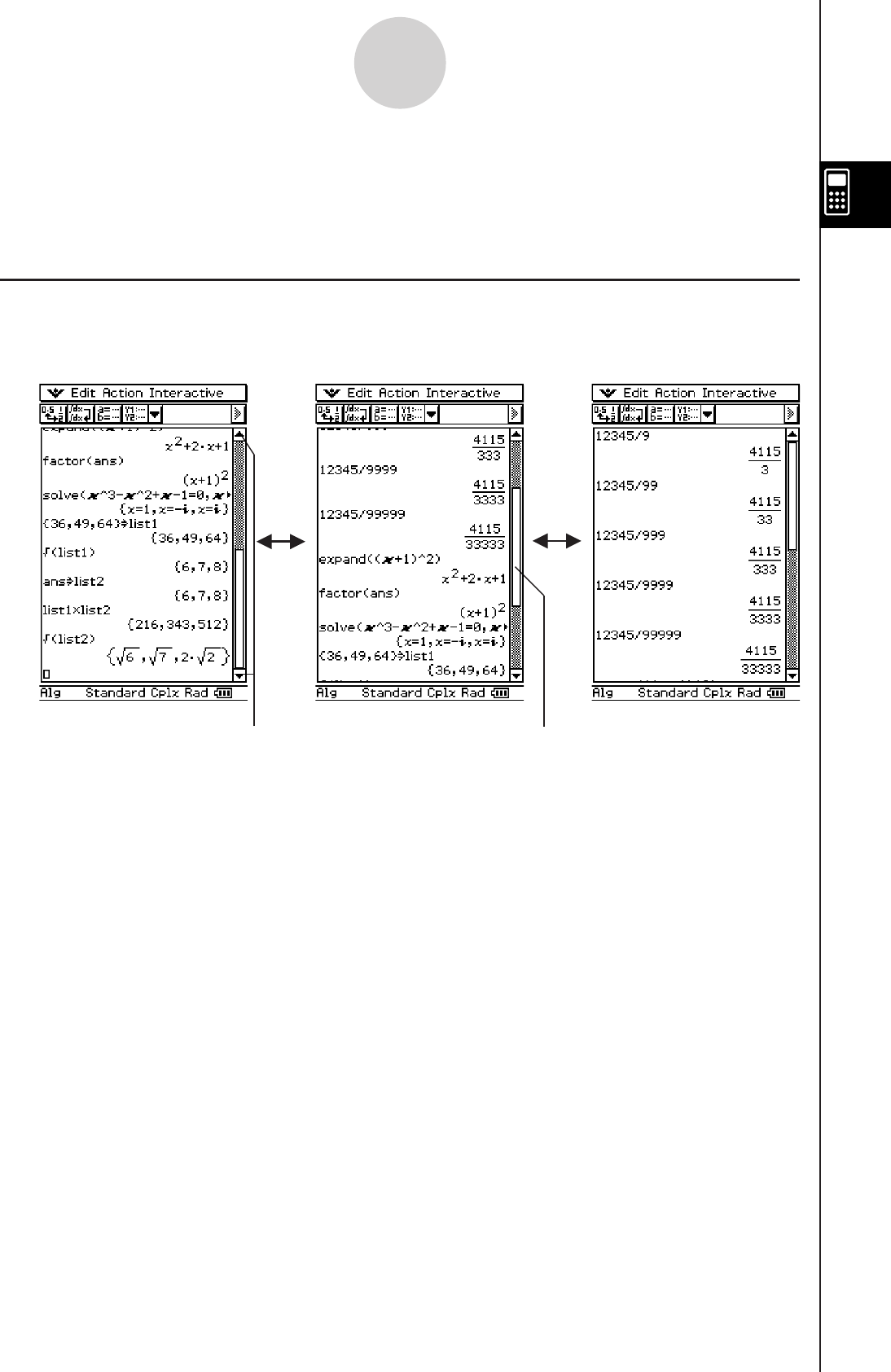
20060301

2-3 Using the Calculation History

The Main application work area calculation history can contain up to 30 expression/result

pairs. You can look up a previous calculation, edit, and then re-calculate it, if you want.

Viewing Calculation History Contents

Use the scroll bar or scroll buttons to scroll the work area window up and down. This brings

current calculation history contents into view.

2-3-1

Using the Calculation History

You can use the cursor keys to move to an input expression/calculation result within the

calculation history window.

Tip

• After the number of expression/result pairs reaches 30, performing a new calculation causes the

oldest calculation currently in the calculation history memory to be deleted.

Scroll button Scroll bar

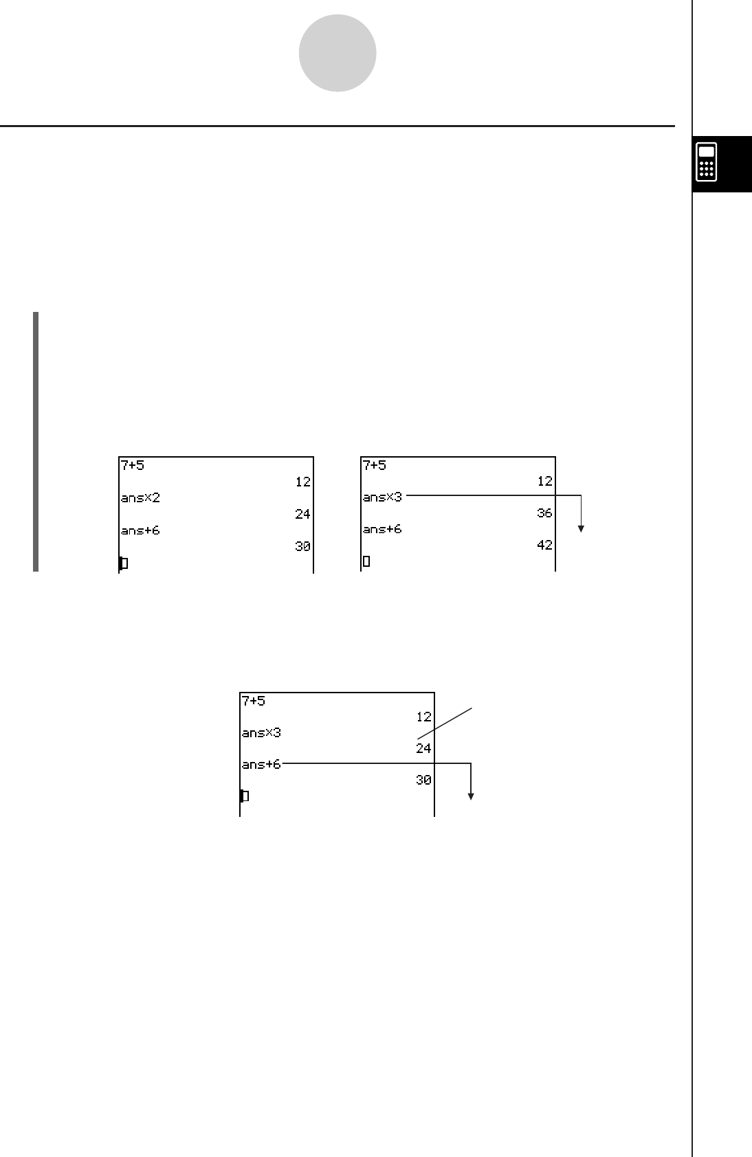
20060301

Re-calculating an Expression

You can edit a calculation expression in the calculation history and then re-calculate the

resulting expression. Tapping w re-calculates the expression where the cursor is currently

located, and also re-calculates all of the expressions below the current cursor location.

Example 1: To change the expression “ans × 2” to “ans × 3” in the example below, and then

re-calculate

uClassPad Operation

(1) Tap to the right of the expression “ans × 2” to locate the cursor there.

(2) Delete “2” and input “3”.

(3) Tap

• This re-calculates the expression where the cursor is located, and all the expressions

underneath it.

Important!

Remember that re-calculation is performed starting from the current cursor location. If, after

performing the first two steps of the above procedure, you move the cursor to the end of

“ans + 6” in line 3 of the calculation history and then tap w, only line 3 is re-calculated.

2-3-2

Using the Calculation History

Re-calculated

If you edit multiple expressions in the calculation history, always make sure that the cursor is

located in the uppermost line that you edited before you tap w.

Re-calculated

Not re-calculated

(because it is above the

cursor location)

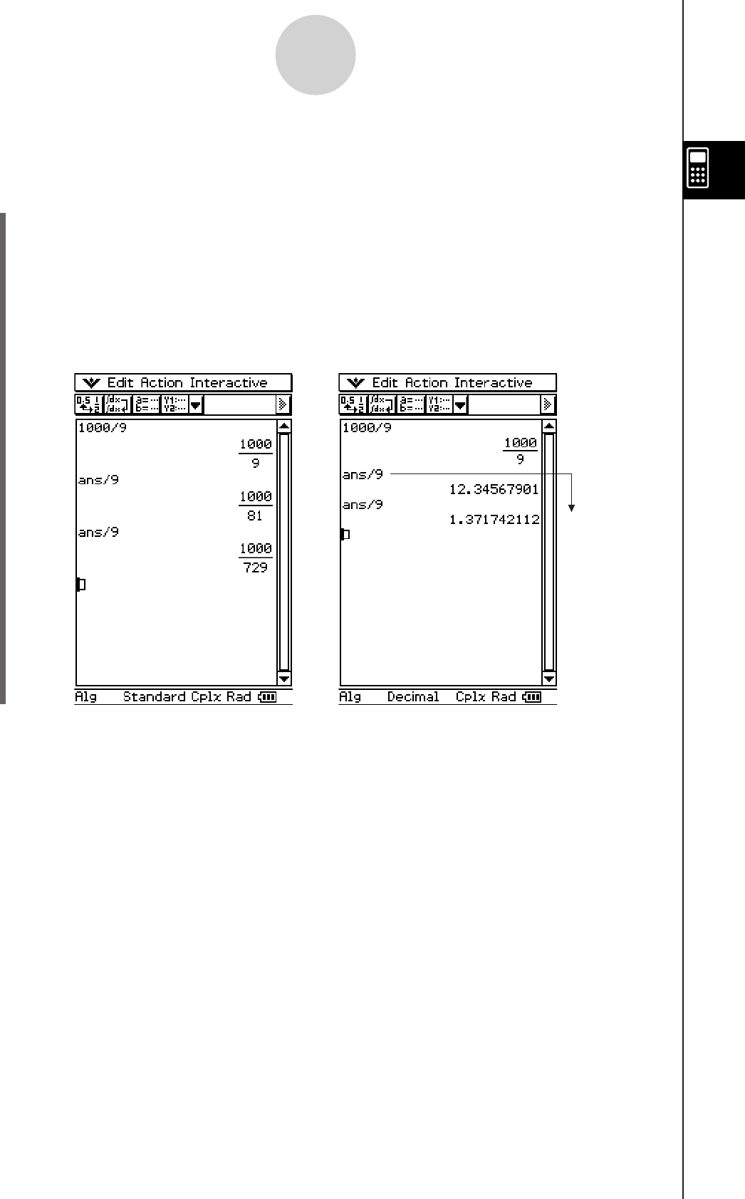
20060301

Example 2: To change from the Standard mode to the Decimal mode (page 2-2-6), and then

re-calculate

uClassPad Operation

(1) Move the cursor to the location from which you want to re-calculate.

• In this example, we will tap the end of line 2 to locate the cursor there.

(2) Tap “Standard” on the status bar to toggle it to “Decimal”.

(3) Tap

• This recalculates all of the expressions starting from the cursor position, and displays

the results using Decimal mode format.

2-3-3

Using the Calculation History

Tip

• You can also change to Decimal mode by tapping s on the icon panel and then tapping [Basic

Format]. Select the “Decimal Calculation” check box and then tap [Set].

• To re-calculate only a single specific line, tap D. Tapping D re-calculates the calculation

where the cursor is currently located only. It does not affect anything in calculation history that

comes before or after the line.

• To re-calculate all of the expressions in the calculation history, locate the cursor in the top line,

and then tap w.

Re-calculated

20060301

Deleting Part of the Calculation History Contents

You can use the following procedure to delete an individual two-line expression/result unit

from the calculation history.

uClassPad Operation

(1) Move the cursor to the expression line or result line of the two-line unit you want to

delete.

(2) Tap [Edit] and then [Delete].

• This deletes the expression and result of the two-line unit you selected.

Important!

Even if the result of the deleted two-line unit has an effect on subsequent calculations, the

affected calculations are not updated automatically following the deletion. When you want to

update everything in the calculation history following the deleted unit, move the cursor to a

line that is above the one you deleted and then tap w. For details about re-calculation, see

page 2-3-2.

Clearing All Calculation History Contents

Perform the following procedure when you want to clear the entire calculation history

currently in the Main application work area.

uClassPad Operation

(1) Tap [Edit] and then [Clear All].

(2) In response to the confirmation message that appears, tap [OK] to clear calculation

history contents, or [Cancel] to cancel.

2-3-4

Using the Calculation History

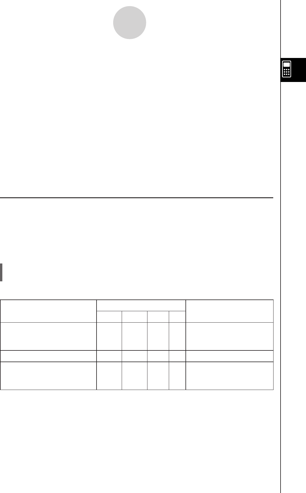
20060301

2-4-1

Function Calculations

2-4 Function Calculations

This section explains how to perform function calculations in the Main application work area.

• Most of the operators and functions described in this section are input from the 9 (math)

and ( (catalog) keyboard. The actual keyboard you should use to perform the sample

operations presented here is the one indicated by a  mark or by button names* (“TRIG”,

“MATH”, “Cmd”, etc.) in one of the columns titled “Use this keyboard”.

* For more information about these buttons, see “Advanced Soft Keyboard Operations” (page

1-6-8).

• You do not need to input the closing parenthesis that comes immediately before an E

key operation. All of the calculation examples in this section omit the closing parentheses

before E.

The following example calculations are all performed using the Decimal mode. Using the

Standard mode causes results to be displayed as fractions. For details about the Decimal

mode and Standard mode, see “Status Bar Mode Indicators” on page 2-1-4.

k Angle Conversion (°, r)

The first two examples below use “Degree” (indicated by “Deg” in the status bar) as the

angle unit setting. The final example uses “Radian” (indicated by “Rad” in the status bar) as

the angle unit setting. Note that using the wrong angle unit setting will make it impossible to

produce correct calculation results.

u To change the angle unit setting

(1) On the

O menu, tap [Basic Format].

(2) Tap the [Angle] down arrow button, and then select [Radian], [Degree] or [Grad].

For more information about this operation, see “1-9 Configuring Application Format Settings”.

Problem Use this keyboard: Operation

mth abc cat 2D

Convert 4.25 radians to

degrees.

= 243.5070629

TRIG MATH Cmd 4.25 Rw

47.3

+ 82.5rad = 4774.20181

° TRIG MATH Cmd 47.3 + 82.5 Rw

How many radians is

243.5070629°?

= 4.249999999

TRIG MATH Cmd Change the [Angle] setting

to “Radian”, and then input

243.5070629 *w.

Tip

• You can also change the angle unit setting by tapping the current setting (Rad, Deg, or Gra) on

the status bar. Each tap will cycle through the available settings.

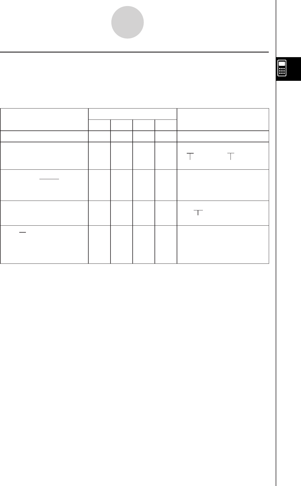
20060301

k Trigonometric Functions (sin, cos, tan) and Inverse Trigonometric

Functions (sin–1, cos–1, tan–1)

The first four examples below use “Degree” (indicated by “Deg” in the status bar) as the

angle unit setting. The final example uses “Radian” (indicated by “Rad”). For details about

these settings, see “1-9 Configuring Application Format Settings”.

Problem Use this keyboard: Operation

mth abc cat 2D

sin63° = 0.8910065242 TRIG Func s 63 w

sin45° × cos65°

= 0.5976724775

TRIG Func 2*s 45 )*c 65 w

Can be omitted.

cosec30° = 1

sin30° = 2 TRIG

Func 1/s30w or

) N 1 c

9 s 30 w

sin–10.5 =30°

(Determine x for sinx = 0.5.)

TRIG Func S 0.5 w

“.5” can also be used.

TRIG Func Change the [Angle] setting to

“Radian”.

c7 /3 w or

c)N 7c 3 w

Tip

• The angle unit setting you specify remains in effect until you change it.

• To move between entry boxes in a 2D math symbol you can use the cursor keys or tap inside a

box.

2-4-2

Function Calculations

cos(( π

3) rad) = 0.5

20060301

k Logarithmic Functions (log, ln) and Exponential Functions (e, ^, k )

Problem Use this keyboard: Operation

mth abc cat 2D

log1.23 (log101.23) =

0.08990511144

Func l 1.23 w or

)V 10 e 1.23 w

ln90 (loge90) = 4.49980967 Func I 90 w or

)V0ne

e 90 w

log39 = 2 Func l 3 , 9 w or

)V 3 e 9 w

101.23 = 16.98243652 MATH Cmd 10 { 1.23 w

e4.5 = 90.0171313 MATH Func e 4.5 w or

)Q 4.5 w

(–3)4 = (–3) × (–3) × (–3) ×

(–3) = 81

MATH Cmd (- 3 ){ 4 w

–34 = – (3 × 3 × 3 × 3) = –81 MATH Cmd - 3 { 4 w

7 123 (= 123 )

= 1.988647795

MATH Cmd 123 {( 1 / 7 w or

)% 7 e 123 w

2 + 3 × 3 64 – 4 = 10 MATH Cmd 2 + 3 * 64 {( 1 /

3 )- 4 w or ) 2 +

3 *% 3 e 64 e- 4 w

Can be omitted.

Tip

• ^ and

  have a higher calculation priority sequence than × and ÷.

2-4-3

Function Calculations

—

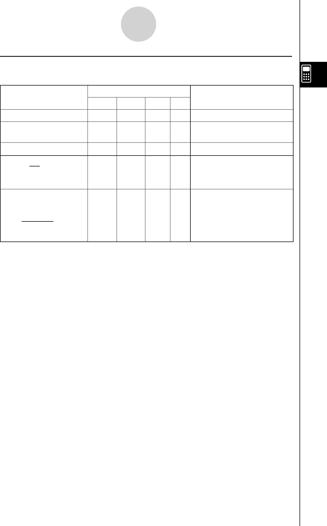
20060301

k Hyperbolic Functions (sinh, cosh, tanh) and Inverse Hyperbolic Functions

(sinh–1, cosh–1, tanh–1)

Problem Use this keyboard: Operation

mth abc cat 2D

sinh3.6 = 18.28545536 TRIG Func =1 3.6 w

cosh1.5 – sinh1.5

= 0.2231301601

TRIG Func =2 1.5 )-11.5

e–1.5 = 0.2231301601* MATH Func e - 1.5 w

cosh–1 ( 20

15 )

= 0.7953654612

TRIG Func =@ 20 / 15 w or

=@)N 20 c

15 w

Solve for x given

tanh(4x) = 0.88.

= 0.3439419141

TRIG Func =# 0.88 )/ 4 w or

)N9=#

0.88 )c 4 w

* This problem checks whether coshx  sinhx = ex. Solving the problem above this one

(cosh1.5 – sinh1.5) and comparing it with this problem’s solution shows that they are equal.

2-4-4

Function Calculations

x = tanh–10.88

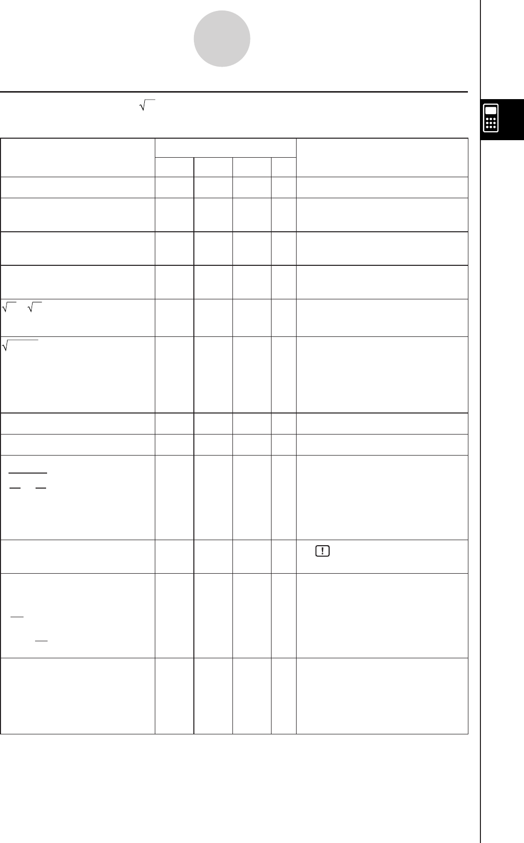
20110401

k Other Functions (%, , x2, x–1, x!, abs, ⬔, signum, int, frac, intg, fRound,

sRound)

Problem Use this keyboard: Operation

mth abc cat 2D

What is 12% of 1500? 180 SMBL Cmd 1500 * 12 &w

What percent of 880 is 660?

75%

SMBL Cmd 660 / 880 &w

What value is 15% greater

than 2500? 2875

SMBL Cmd 2500 *( 1 + 15 &

What value is 25% less than

3500? 2625

SMBL Cmd 3500 *( 1 - 25 &

2 + 5 = 3.65028154 Func 9 2 )+ 9 5 w or

)5 2 e+5 5 w

(3 + i) = 1.755317302

+ 0.2848487846i

Func Change to the Complex mode

(“Cplx” indicated on the status

bar).

9 3 +0w or

)5 3 +0w

(–3)2 = (–3) × (–3) = 9 Cmd (- 3 )xw

–32 = –(3 × 3) = –9 Cmd - 3 xw

–

1 = 12 Cmd ( 3 X- 4 X)Xw

)N 1 cN 1 c

3 e-N

1 c 4 w

8! (= 1 × 2 × 3 × … × 8)

= 40320

CALC SMBL Cmd 8 w

What is the absolute value

of the common logarithm of

⎜log ( 3

4)⎟ = 0.1249387366

Func $l 3 / 4 w or

)4 V 10 eN

3 c 4 w

8⬔40° × 5⬔35°

⬔(8,40) × ⬔(5,35)

OPTN

Change to the Degree mode

(“Deg” indicated on the status

bar).

~ 8 , 40 )*~ 5 ,

35 )w

2-4-5

Function Calculations

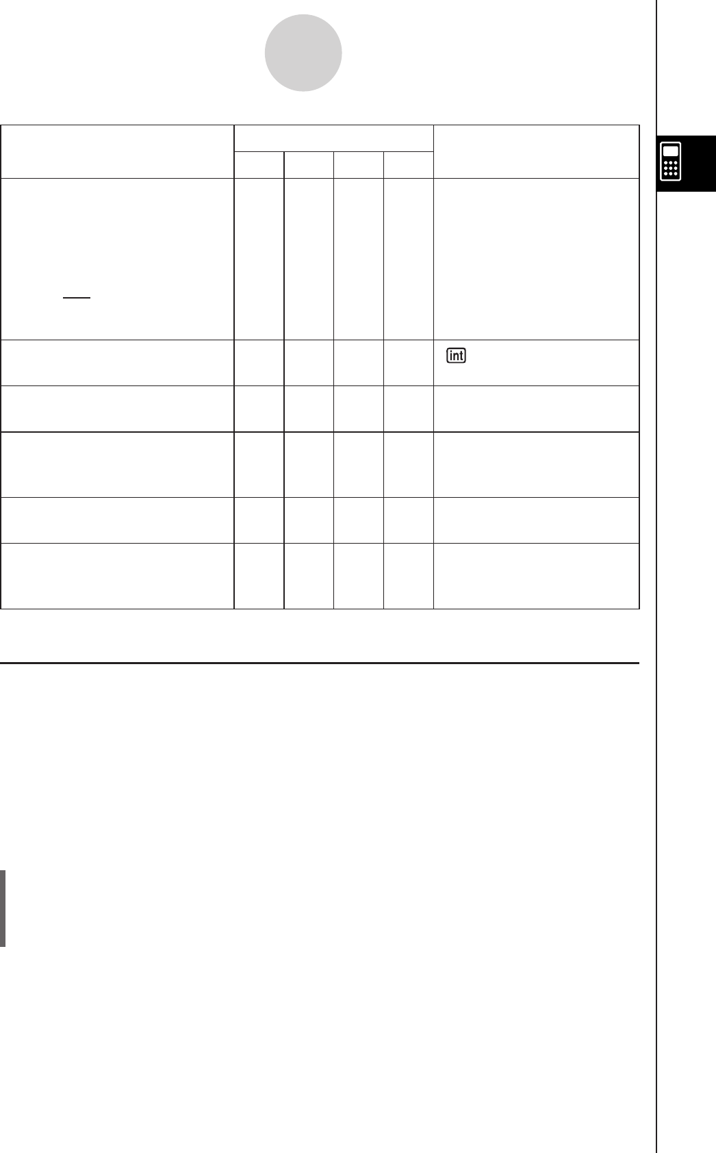
20090601

Problem Use this keyboard: Operation

mth abc cat 2D

What is the sign of

–3.4567? –1

(signum returns –1 for a

negative value, 1 for a

positive value, “Undefined” for

0, and A

⎜A⎟ for an

imaginary number.)

Func [signum] - 3.4567 w

What is the integer part of

–3.4567? –3

CALC Func - 3.4567 w

What is the decimal part of

–3.4567? –0.4567

Func [frac] - 3.4567 w

What is the greatest integer

less than or equal to

–3.4567? –4

Func [intg] - 3.4567 w

What is –3.4567 rounded to

two decimal places? –3.46

Func [fRound] - 3.4567 , 2

What is –34567 rounded to

four significant digits?

–34570

Func [sRound] - 34567 , 4

* To round to 10 digits, specify “0” for the second argument.

k Random Number Generator (rand, randList, randNorm, randBin, RandSeed)

• The ClassPad random number generator can generate truly random numbers (non-

sequential random numbers) and random numbers that follow a particular pattern (sequential

random numbers). Using the “randList” function, you can generate a list whose elements

contain random numbers. There are nine different patterns for generation of sequential

random numbers. Use the “RandSeed” command to switch between non-sequential and

sequential random number generation, and to select the sequential random number

generation pattern.

u ClassPad Operation

(1) Use the “RandSeed” command to configure random number generation settings, if

required.

(2) Use the “rand”, “randList”, “randNorm”, or “randBin” function to generate the random

numbers.

2-4-6

Function Calculations

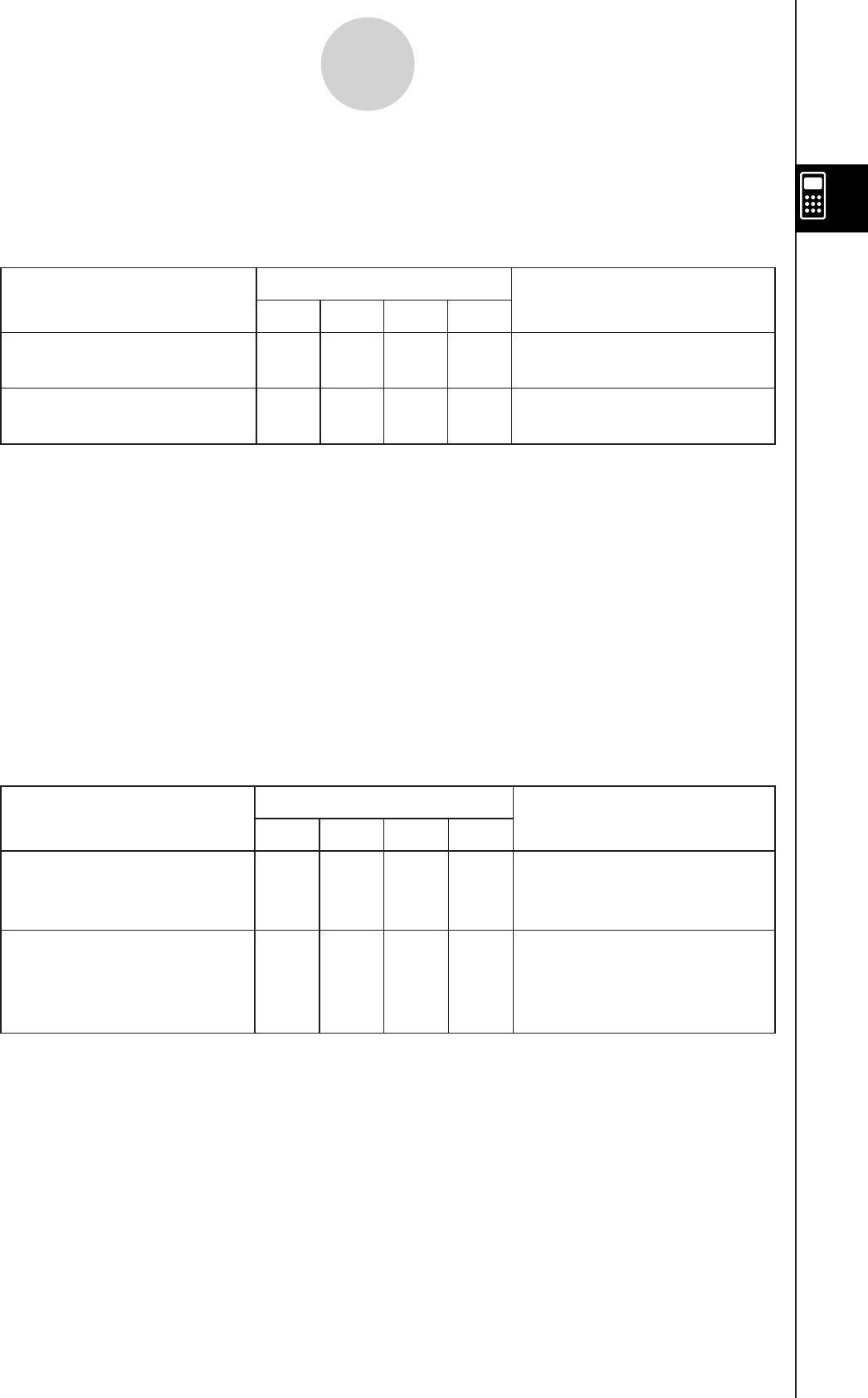
20090601

u “rand” Function

• The “rand” function generates random numbers. If you do not specify an argument, “rand”

generates 10-digit decimal values 0 or greater and less than 1.

Specifying two integer values for the argument generates random numbers between them.

Problem Use this keyboard: Operation

mth abc cat 2D

Generate random numbers

between 0 and 1.

Func [rand] w

Generate random integers

between 1 and 6.

Func [rand] 1 , 6 w

u “randList” Function

Syntax: randList(n [, a, b])

Function:

• Omitting arguments “a” and “b” returns a list of n elements that contain decimal random

values.

• Specifying arguments “a” and “b” returns a list of n elements that contain integer random

values in the range of “a” through “b”.

Description:

• “n” must be a positive integer.

• The random numbers of each element are generated in accordance with “RandSeed”

specifications, as with the “rand” function.

Problem Use this keyboard: Operation

mth abc cat 2D

Generate a list of three

elements that contain

decimal random values.

Func [randList] 3 w

Generate a list of five

elements that contain

random values in the range

of 1 through 6.

Func [randList] 5, 1, 6 w

u “randNorm” Function

The “randNorm” function generates a 10-digit normal random number based on a specified

mean  and standard deviation  values.

Syntax: randNorm(,  [, n])

Function:

• Omitting a value for “n” (or specifying 1 for “n”) returns the generated random number as-is.

• Specifying a value for “n” returns the specified number of random values in list format.

2-4-7

Function Calculations

20090601

2-4-8

Function Calculations

Description:

• “n” must be a positive integer, and “

” must be greater than 0.

Problem Use this keyboard: Operation

mth abc cat 2D

Randomly produce a body

length value obtained in

accordance with the normal

distribution of a group of

infants less than one year

old with a mean body length

of 68cm and standard

deviation of 8.

Func [randNorm] 8 , 68 w

Randomly produce the body

lengths of five infants in the

above example, and display

them in a list.

Func [randNorm] 8 , 68 , 5

u “randBin” Function

The “randBin” function generates binomial random numbers based on values specified for

the number of trials n and probability P.

Syntax: randBin(n, P [, m])

Function:

• Omitting a value for “m” (or specifying 1 for “m”) returns the generated random number as-

is.

• Specifying a value for “m” returns the specified number of random values in list format.

Description:

• “n” and “m” must be positive integers.

Problem Use this keyboard: Operation

mth abc cat 2D

Randomly produce the

number of heads that can be

expected in accordance with

binomial distribution for five

coin tosses where the

probability of heads is 0.5.

Func [randBin] 5 , 0.5 w

Perform the same coin toss

sequence described above

three times and display the

results in a list.

Func [randBin] 5 , 0.5 , 3 w

20090601

u “RandSeed” Command

• You can specify an integer from 0 to 9 for the argument of this command. 0 specifies non-

sequential random number generation. An integer from 1 to 9 uses the specified value as

a seed for specification of sequential random numbers. The initial default argument for this

command is 0.

• The numbers generated by the ClassPad immediately after you specify sequential random

number generation always follow the same random pattern.

Problem Use this keyboard: Operation

mth abc cat 2D

Generate sequential random

numbers using 3 as the

seed value.

Cmd [RandSeed] 3 w

Generate the first value.

Generate the second value.

Generate the third value.

Func [rand]

[rand] w

Tip

• Random values generated by these commands are pseudo random values.

• The arguments a and b of “rand(a,b)” and “randList(n,a,b)” must be integers, subject to the

following conditions.

a < b

⎟ a

⎟ , ⎟ b

⎟ < 1E10

b – a < 1E10

k Integer Functions

These functions take integers only as their arguments and return integers.

u “iGcd” Function

Syntax: iGcd(Exp-1, Exp-2[, Exp-3…Exp-10)]

(Exp-1 through Exp-10 all are integers.)

iGcd(List-1, List-2[, List-3…List-10)]

(All elements of List-1 through List-10 are integers.)

Function:

• The first syntax above returns the greatest common divisor for two to ten integers.

• The second syntax returns, in list format, the greatest common divisor (GCD) for each of

the elements in two to ten lists. When the arguments are {a,b}, {c,d}, for example, a list will

be returned showing the GCD for a and c, and for b and d.

Description:

• All of the lists must have the same number of elements.

• When using the “iGcd(List-1, List-2[, List-3…List-10)]” syntax, one (and only one)

expression (Exp) can be include as an argument in place of a list.

2-4-9

Function Calculations

20090601

Problem Use this keyboard: Operation

mth abc cat 2D

Determine the greatest

common divisors of {4, 3},

{12, 6}, and {36, 9}.

Func [iGcd] { 4 , 3 },{

12 , 6 },{ 36 , 9

})w

u “iLcm” Function

Syntax: iLcm(Exp-1, Exp-2[, Exp-3…Exp-10)]

(Exp-1 through Exp-10 all are integers.)

iLcm(List-1, List-2[, List-3…List-10)]

(All elements of List-1 through List-10 are integers.)

Function:

• The first syntax above returns the least common multiple for two to ten integers.

• The second syntax returns, in list format, the least common multiple (LCM) for each of the

elements in two to ten lists. When the arguments are {a,b}, {c,d}, for example, a list will be

returned showing the LCM for a and c, and for b and d.

Description:

• All of the lists must have the same number of elements.

• When using the “iLcm(List-1, List-2[, List-3…List-10)]” syntax, one (and only one)

expression (Exp) can be include as an argument in place of a list.

Problem Use this keyboard: Operation

mth abc cat 2D

Determine the least common

multiples of {4, 3}, {12, 6},

and {36, 9}.

Func [iLcm] { 4 , 3 },{

12 , 6 },{ 36 , 9

})w

u “iMod” Function

Syntax: iMod(Exp-1/List-1, Exp-2/List-2[)]

Function:

• This function divides one or more integers by one or more other integers and returns the

remainder(s).

Description:

• Exp-1 and Exp-2, and all of the elements of List-1 and List-2 must be integers.

• You can use Exp for one argument and List for the other argument (Exp, List or List, Exp) if

you want.

• If both arguments are lists, both lists must have the same number of elements.

2-4-10

Function Calculations

20090601

Problem Use this keyboard: Operation

mth abc cat 2D

Divide 21 by 6 and 7, and

determine the remainder

of both operations.

(iMod(21, {6, 7})

Func [iMod] 21 ,{ 6 , 7

})w

k Permutation (nPr) and Combination (nCr)

u Total Number of Permutations

u Total Number of Combinations

Problem Use this keyboard: Operation

mth abc cat 2D

How many different

permutations are possible

when you have 10 different

objects and arrange them

four at a time?

10P4 = 5040

CALC Func } 10 , 4 w

How many different

combinations are possible

when you have 10 different

objects and remove four at

a time?

10C4 = 210

CALC Func { 10 , 4 w

nPr = –––––

(

n – r)!

nPr = –––––

(

n – r)!

nCr = –––––––

r! (n – r)!

nCr = –––––––

r! (n – r)!

2-4-11

Function Calculations

20090601

2-4-12

Function Calculations

k Condition Judgment (judge, piecewise)

u“judge” Function

The “judge” function returns TRUE when an expression is true, and FALSE when it is false.

Problem Use this keyboard: Operation

mth abc cat 2D

Is the following expression

true or false?

1 = 1 TRUE

Func [judge] 1 = 1 w

Is the following expression

true or false?

1 < 0 FALSE

Func [judge] 1 0 w

u “piecewise” Function

The “piecewise” function returns one value when an expression is true, and another value

when the expression is false.

The syntax of the “piecewise” function is shown below.

piecewise(<condition expression>, <return value when true>, <return value when false or

indeterminate> [ ) ]

piecewise(<condition expression>, <return value when true>, <return value when false>,

<return value when indeterminate> [ ) ]

Use the 2D keyboard (1) to input “piecewise” function according to the syntax shown

below.

Problem Use this keyboard: Operation

mth abc cat 2D

For the expression 0 > x

(x = variable), return 1 when

x is 0 or less, and 2 when x

is greater than 0 or

undefined.

Func [piecewise] 0 5 X, 1 ,

2 w

1 1 c 2 ef 0 5 X

For the expression 1 > x

(x = variable), return 1 when

x is 1 or less, and 2 when x

is greater than 1.

1 1 c 2 ef 1 5 X

c 1 Xw

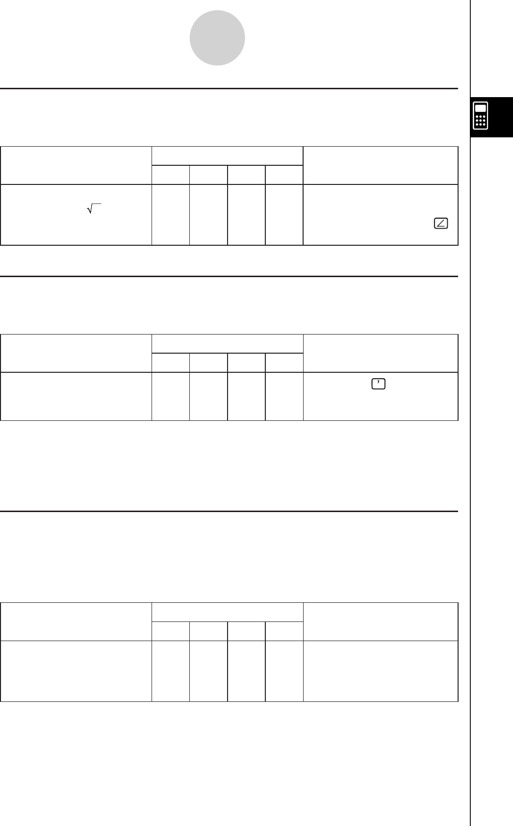
20090601

k Angle Symbol (∠)

Use this symbol to specify the coordinate format required by an angle in a vector.

You can use this symbol for a vector only.

Problem Use this keyboard: Operation

mth abc cat 2D

Convert the polar

coordinates r = 2 ,

= π /4 to rectangular

coordinates. [1, 1]

OPTN Func Change the [Angle] setting to

“Radian”.

[toRect] [9 2 ),

7/ 4 )]w

k Derivative Symbol (’)

A single derivative symbol indicates the first derivative of an equation in the format:

<variable name>’.

Problem Use this keyboard: Operation

mth abc cat 2D

Solve the differential

equation y’ = x.

{y = 0.5 · x2 + const (1)}

CALC SMBL Cmd [dSolve] Y=X,X

,Yw

Important!

The “dSolve” function can solve differential equations up to three degrees, so a maximum of

three derivative symbols (y’’’) can be used. Executing a “dSolve” calculation that has more

than three derivative symbols will result in an Invalid Syntax error.

k Primality Test (isPrime)

The “isPrime” function determines whether the number provided as the argument is prime

(returns TRUE) or not (returns FALSE). The syntax of the “isPrime” function is shown below.

isPrime(Exp/List[ ) ]

• Exp or all of the elements of List must be integers.

Problem Use this keyboard: Operation

mth abc cat 2D

Determine whether the

numbers 51 and 17 are

prime.

(isPrime({51, 17})

Func [isPrime] { 51 , 17

})w

2-4-13

Function Calculations

20090601

2-4-14

Function Calculations

k Equal Symbols and Unequal Symbols (=, ≠, <, >, , >)

You can use these symbols to perform a number of different basic calculations.

Problem Use this keyboard: Operation

mth abc cat 2D

To add 3 to both sides of

x = 3. x + 3 = 6

MATH Cmd (X= 3 )+ 3 w

Subtract 2 from both sides

of y < 5. y – 2 < 3

OPTN MATH Cmd (Y

5 )- 2 w

Tip

• In the “Syntax” explanations of each command under “2-8 Using the Action Menu”, the following

operators are indicated as “Eq/Ineq”: =, ≠, <, >, <, >. Whether or not the “Eq/Ineq” operators

include the “≠” operator is specified for each command by a separate note.

• An expression that contains multiple equation or inequality operators cannot be input as a single

expression. For output expressions, an expression can be output with multiple operators only in

the case of inequality operators that are facing in the same direction (example: –1< x <1).

Example: solve(x2 – 1

< 0, x) w {–1 < x < 1}

k “with” Operator ( | )

The “with” (I) operator temporarily assigns a value to a variable. You can use the “with”

operator in the following cases.

• To assign the value specified on the right side of | to the variable on the left side of |

• To limit or restrict the range of a variable on the left side of | in accordance with conditions

provided on the right side of |

The following is the syntax for the “with” (I) operator.

Exp/Eq/Ineq/List/Mat|Eq/Ineq/List/(and operator)

You can put plural conditions in a list or connected with the “and” operator on the right side.

“

≠” can be used on the left side or the right side of |.

Problem Use this keyboard: Operation

mth abc cat 2D

Evaluate x2 + x + 1 when

x = 3. 13

OPTN SMBL Cmd X{ 2 +X+ 1 UX

= 3 w

For x2 – 1 = 0, determine

the value of x when x > 0.

{

x = 1}

OPTN SMBL Cmd [solve] X{ 2 - 1 = 0

,X)UX

0 w

Determine the value of

abs (x) when x >0. x

OPTN SMBL Cmd $X)UX

0 w

20090601

2-4-15

Function Calculations

k Solutions Supported by ClassPad (TRUE, FALSE, Undefined, No Solution, ∞,

const, constn)

Solution Description Example

TRUE Output when a solution is true. judge (1 = 1) w

FALSE Output when a solution is false. judge (1 < 0) w

Undefined Output when a solution is undefined. 1/0 w

No Solution Output when there is no solution. solve (abs (x) = –1, x) w

∞Infinity lim (1/x2, x, 0) w

const Constant displayed as const(1) when any

value that is a constant is included in the

solution. In the case of multiple constants,

they are indicated as const(1), const(2),

and so on.

dSolve (y = x, x, y) w

{y = 0.5·x2 + const (1)}

constn Constant displayed as constn(1) when the

solution includes any integer value that is

a constant. In the case of multiple

constants, they are indicated as constn(1),

constn(2), and so on.

Change the [Angle] setting to

“Degree”.

solve (sin (x) = 0, x) w

{x = 180·constn (1)}

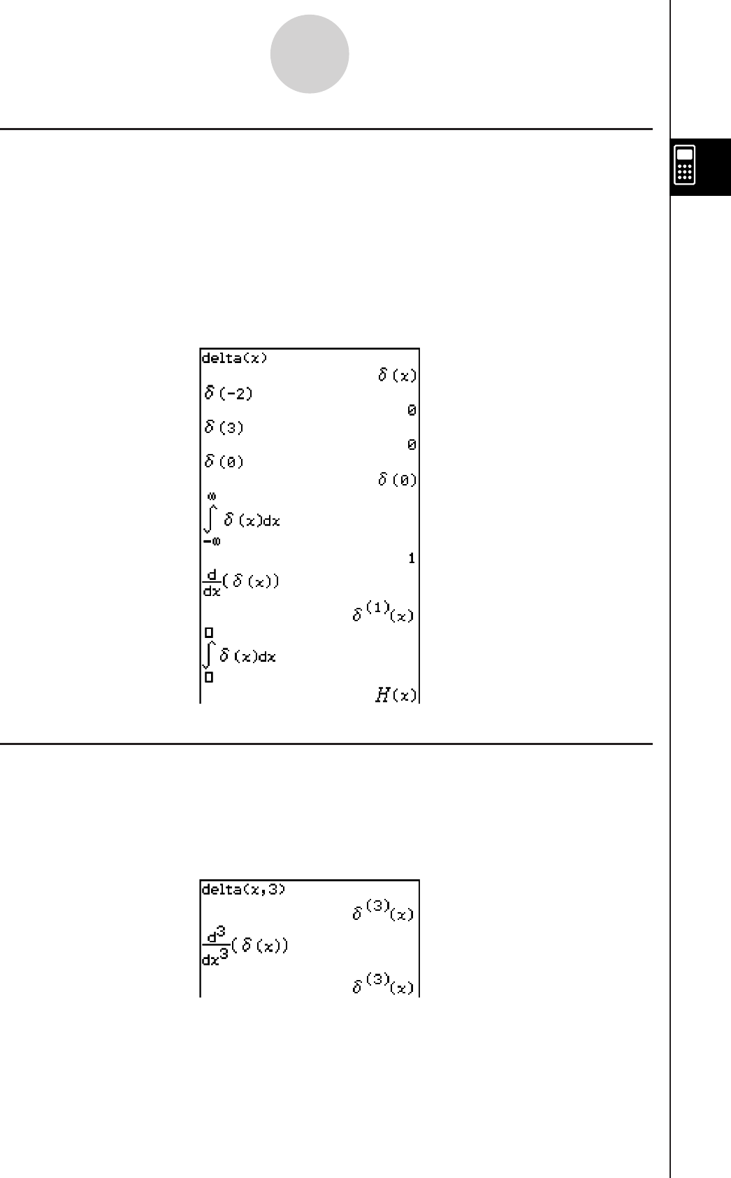
20090601

k Dirac Delta Function

“delta” is the Dirac Delta function. The delta function evaluates numerically as shown below.

x ≠ 0

δ(x) =

{

δ(x), x = 0

Non-numeric expressions passed to the delta function are left unevaluated. The integral of a

linear delta function is a Heaviside function.

Syntax: delta(x)

x : variable or number

Examples:

k nth Delta Function

The nth-delta function is the nth differential of the delta function.

Syntax: delta(x, n)

x : variable or number

n : number of differentials

Examples:

2-4-16

Function Calculations

20090601

k Heaviside Unit Step Function

“heaviside” is the command for the Heaviside function, which evaluates only to numeric

expressions as shown below.

x < 0

H(x) = , x = 0

x > 0

Any non-numeric expression passed to the Heaviside function will not be evaluated, and any

numeric expression containing complex numbers will return undefined. The derivative of the

Heaviside function is the Delta function.

Syntax: heaviside(x)

x : variable or number

Examples:

2-4-17

Function Calculations

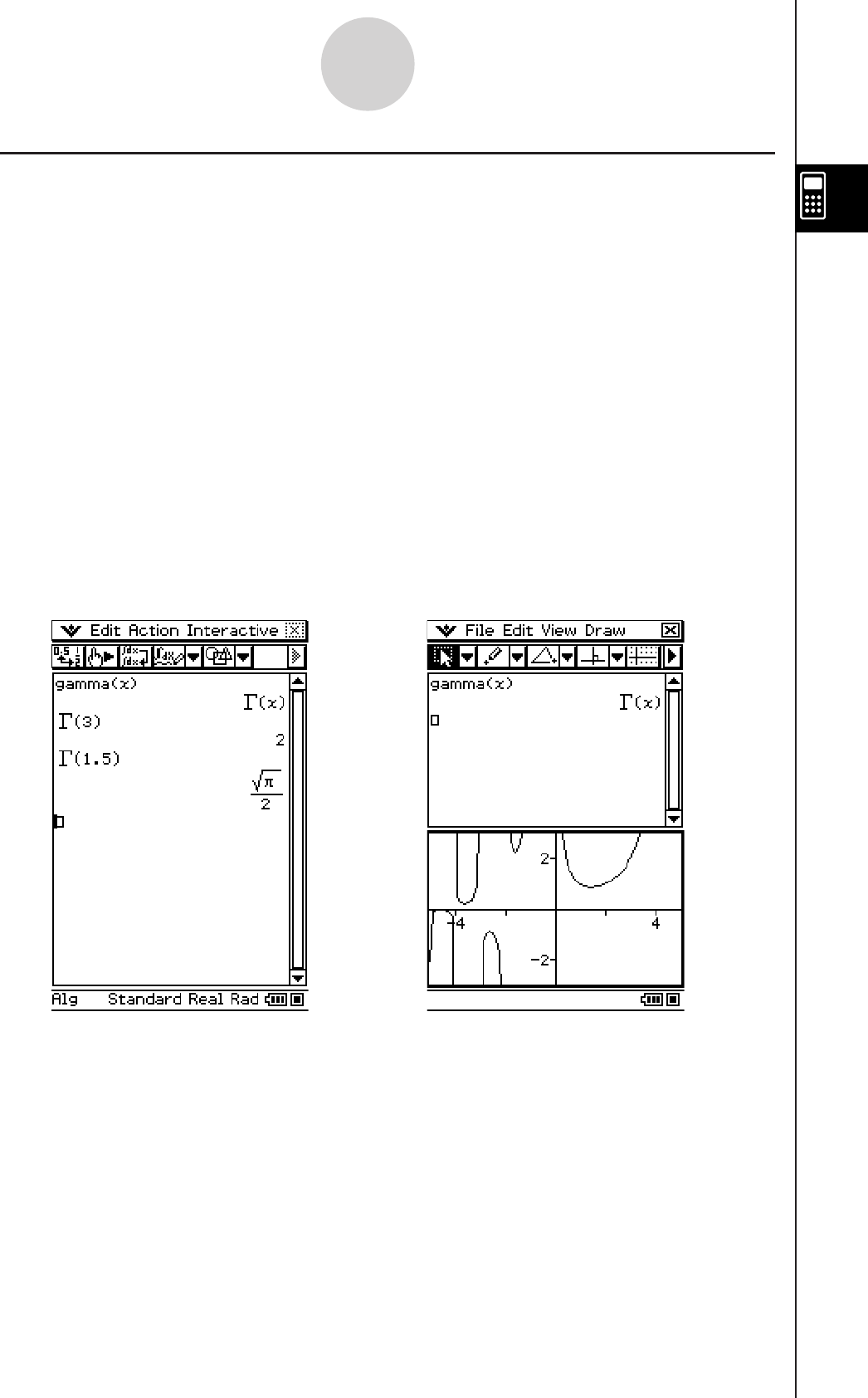
20110901

k Gamma Function

The Gamma function is called “gamma” on the ClassPad.

∫

+∞

tx–1e–t dtΓ(x) =

For an integer n the gamma is evaluated as shown below.

(n – 1) !, n > 0

Γ(n) =

{

undefined, n < 0

The gamma is defined for all real numbers excluding zero and negative integers. It is also

defined for all complex numbers where either the real or imaginary part of the complex

number is not an integer.

Gamma of a symbolic expression returns unevaluated.

Syntax: gamma(x)

x : variable or number

Examples:

2-4-18

Function Calculations

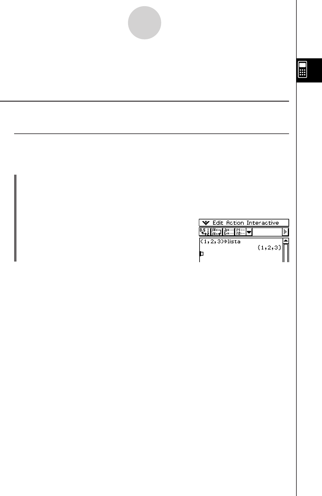
20060301

2-5-1

List Calculations

2-5 List Calculations

This section explains how to input data using the Main application or Stat Editor, and how to

perform basic list calculations.

Inputting List Data

You can input list data from the work area or on the Stat Editor window.

k Inputting List Data from the Work Area

Example: To input the list {1, 2, 3} and assign it to LIST variable “lista”.

u ClassPad Operation

(1) Tap

m to display the application menu, and then tap J to start the Main application.

(2) Press

k to display the soft keyboard.

(3) Next, perform the following key operation.

9{b,c,d}W

0listaw

Tip

• For information about assigning data to a variable, see “Creating and Using Variables” on page

1-7-5.

• You can also create a list using commands in the [List-Create] group on the [Action] menu. For

information about using these commands, see “2-8 Using the Action Menu”.

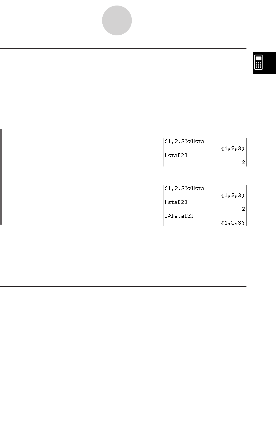
20060301

k LIST Variable Element Operations

You can recall the value of any element of a LIST variable. When the values {1, 2, 3} are

assigned to “lista”, for example, you can recall the second value in the “lista”, when you need

it.

You can also assign a value to any element in a list. When the values {1, 2, 3} are assigned

to “lista”, for example, you can replace the second value with “5” to end up with {1, 5, 3}.

After performing the procedure under “Inputting List Data from the Work Area”, perform the

following operation.

u ClassPad Operation

(1) Recall the value of the second element of LIST variable “lista”.

0lista9[c]w

2-5-2

List Calculations

(2) Assign “5” to the second element of LIST variable “lista”.

fW0lista9[c]w

Tip

• You can also perform the above operations on the “ans” variable (page 2-2-2) when it contains

LIST data.

Example: {1, 2, 3, 4} w {1, 2, 3, 4}

D[c]w 2

k Inputting List Data Using the Stat Editor Window

Tapping ( displays the Stat Editor window, which you can then use to input list data. List

data input this way is assigned to a LIST variable, so you can access it by specifying the

applicable variable name.

For more information about using the Stat Editor window to create a list, see “7-2 Using Stat

Editor”.

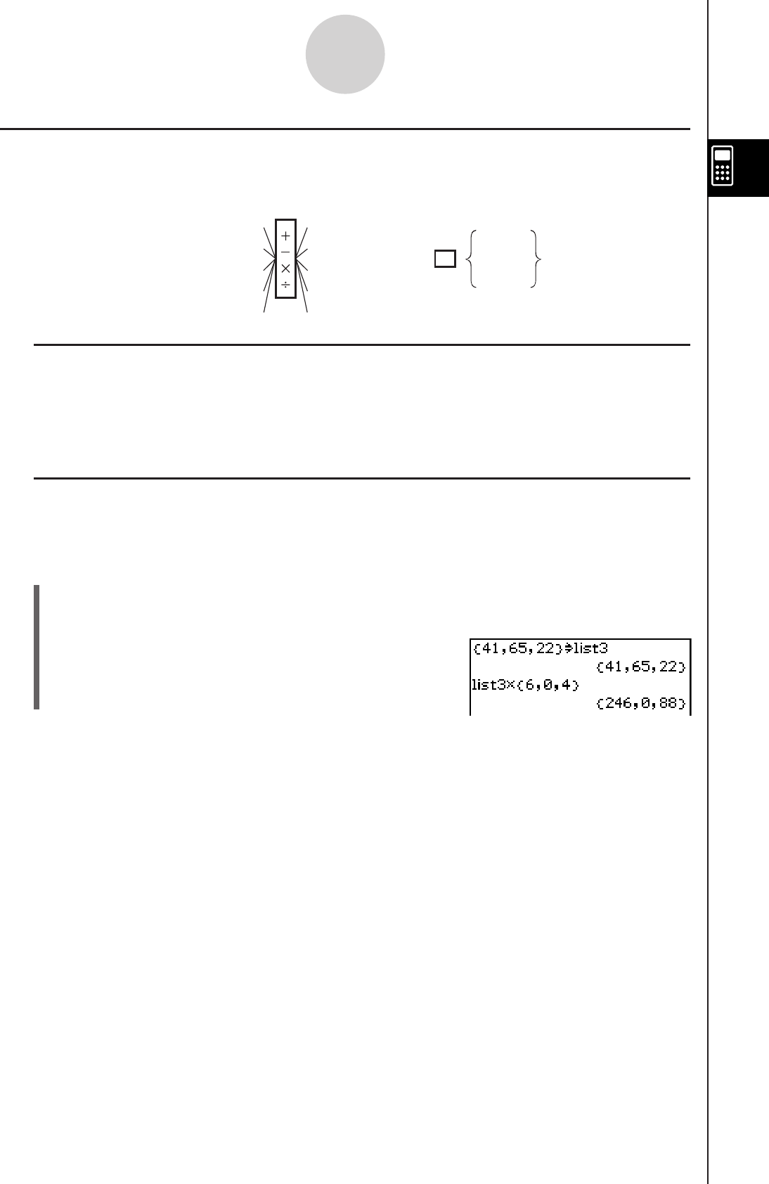
20060301

Using a List in a Calculation

You can perform arithmetic operations between two lists, between a list and a numeric value,

or between a list and an expression, equation, or inequality.

2-5-3

List Calculations

k List Calculation Errors

• When you perform an arithmetic operation between two lists, both of the lists need to have

the same number of cells. An error will occur if they do not.

• An error will also occur whenever an operation between any two cells of the two lists results

in an error.

k List Calculation Example

Example: Perform the operation list3 × {6, 0, 4} when list3 contains {41, 65, 22}

u ClassPad Operation

(1) Perform the key operation below in the Main application work area.

0listd9*{g,a,e}

(2)

List

Numeric Value

Expression

Equation

Inequality

List

Numeric Value

Expression

Equation

Inequality

=List

Tip

• List operations (extraction of list maximum and minimum, calculation of list total, etc.) can

also be performed using the commands in the [List-Calculation] group of the [Action] menu.

For more information, see “2-8 Using the Action Menu”.

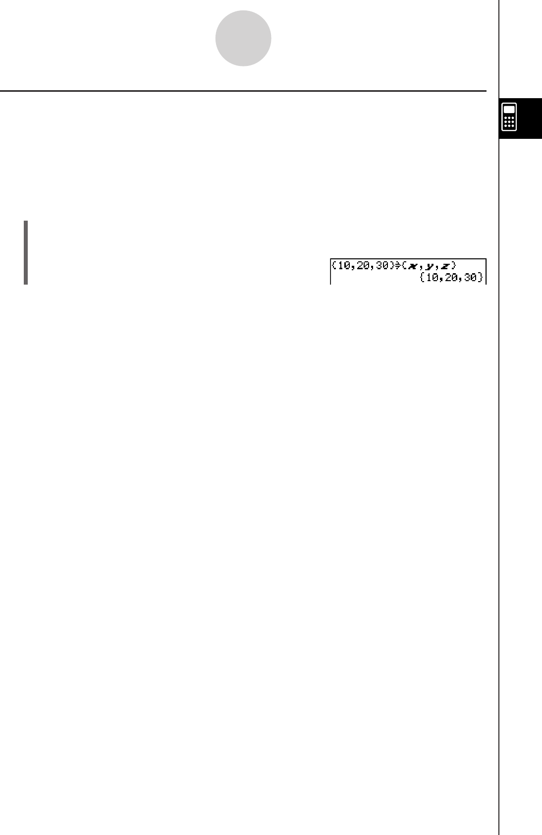
20060301

2-5-4

List Calculations

Using a List to Assign Different Values to Multiple Variables

Use the procedure in this section when you want to use a list to assign various different

values to multiple variables.

Sintaxis: List with Numbers S List with Variables

Example: Assign the values 10, 20, and 30, to variables x, y, and z respectively

u ClassPad Operation

(1) Perform the key operation below in the Main application work area.

9{ba,ca,da}W{X,Y,Z}

(2)

Tip

• You can perform this operation using a matrix that has a single row and multiple columns, or

multiple rows and a single column. For details see “Using a Matrix to Assign Different Values to

Multiple Variables” on page 2-6-6.

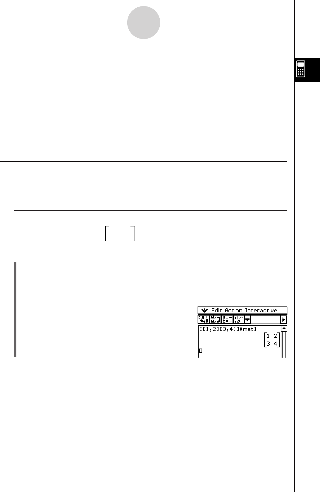
20060301

2-6 Matrix and Vector Calculations

This section explains how to create matrices in the Main application, and how to perform

basic matrix calculations.

Tip

• Since a vector can be viewed as 1-row by n-column matrix or n-row by 1-column matrix, this

section does not include explanations specifically about vectors. For more information about

vector-specific calculations, see the explanations about the applicable [Action] menu items in

“2-8 Using the Action Menu”.

Inputting Matrix Data

You can use the 9 (math) keyboard to input matrix values in a single line in the work

area, or the ) keyboard to input matrix values using an actual on-screen matrix.

k Inputting Matrix Values with the 9 Keyboard

Example: To input the matrix 1 2 and assign it to the variable “mat1”

3 4

u ClassPad Operation

(1) On the application menu, tap J to start the Main application.

(2) Press

k to display the soft keyboard.

(3) Next, perform the following key operation.

9[[b,c][d,e]]W

0matbw

2-6-1

Matrix and Vector Calculations

Tip

• For information about assigning data to a variable, see “Creating and Using Variables” on page

1-7-5.

20060301

k Matrix Variable Element Operations

You can recall the value of any element of a MATRIX variable. When the data 1 2

3 4

is assigned to matrix “mat1”, for example, you can recall the element located at row 2,

column 1.

You can also assign a value to any element in a matrix. For example, you could assign the

value “5” to the element at row 1 column 2 in “mat1”, which produces the matrix 1 5

3 4 .

After performing the procedure under “Inputting Matrix Values with the 9 Keyboard”,

perform the following operation.

u ClassPad Operation

(1) Recall the value in row 2, column 1 of MATRIX variable “mat1”.

0matb9[c,b]w

↑

Row Column

2-6-2

Matrix and Vector Calculations

(2) Assign “5” to the element at row 1, column 2 of MATRIX variable “mat1”.

fW0matb9[b,c]w

Tip

• You can also perform the above operations on the “ans” variable (page 2-2-2) when it contains

MATRIX data.

Example: [[b,c][d,e]]w 1 2

3 4

D[c,b]w 3

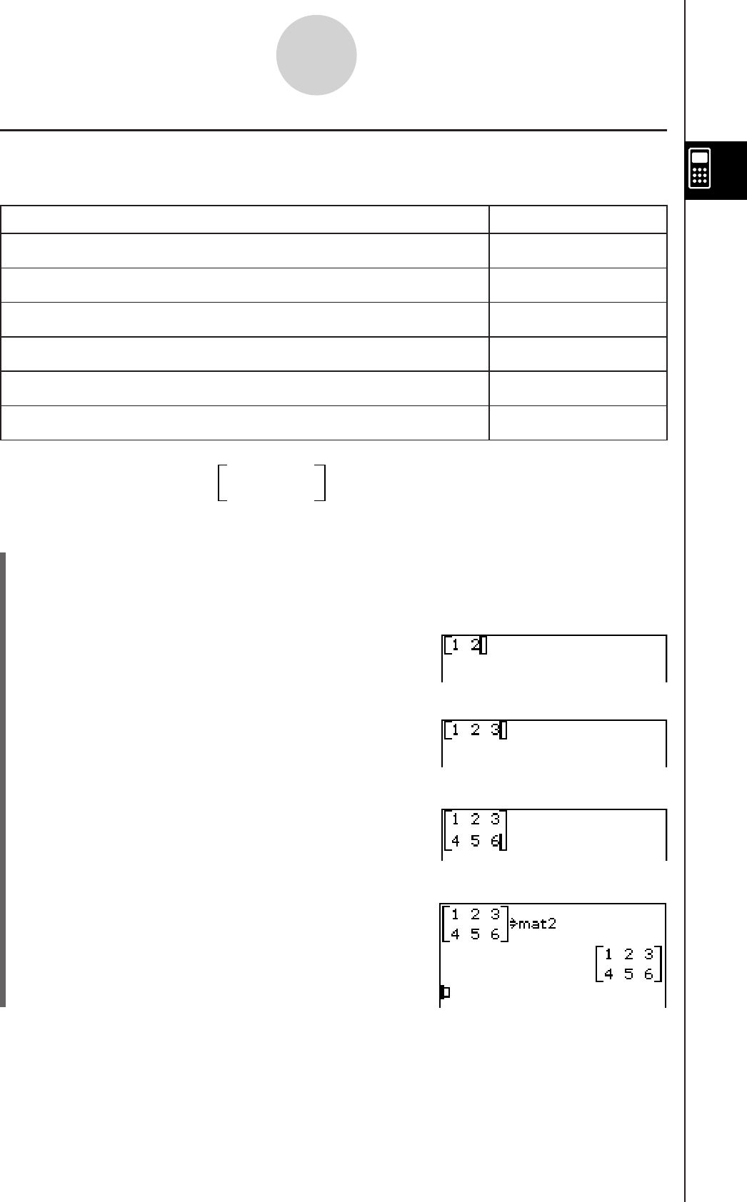
20060301

k Inputting Matrix Values with the ) Keyboard

The 6, 7, and 8 keys of the ) keyboard make matrix value input quick and easy.

To do this: Tap this 2D key:

Create a new 1-row × 2-column matrix 6

Create a new 2-row × 1-column matrix 7

Create a new 2-row × 2-column matrix 8

Add a column to the currently displayed matrix 6

Add a row to the currently displayed matrix 7

Add both a row and column to the currently displayed matrix 8

Example: To input the matrix 1 2 3

4 5 6 and assign it to the variable “mat2”

u ClassPad Operation

(1) Tap

)- to display the - keyset of the ) keyboard, and then perform the

key operation below in the Main application work area.

(Creates a 1-row × 2-column matrix.)

bec

2-6-3

Matrix and Vector Calculations

6 (Adds one column to the matrix.)

7 (Adds one row to the matrix.)

eefeg

(2) Perform the key operation below to assign the matrix to the variable named “mat2”.

0matcw

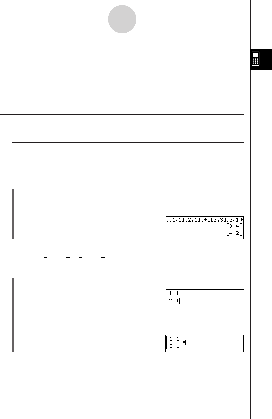
20060301

Tip

• In step (1) of the above procedure, we added rows and columns as they became necessary.

Another way to accomplish the same result would be to add rows and columns to create a blank

matrix of the required dimensions, and then start data input. You could create a 2-row × 3-column

matrix by tapping 6, 6, 7, or 6, 8. In either case, you could also tap the buttons in

reverse of the sequence shown here.

• You can also create matrices using the commands of the [Matrix-Create] group on the [Action]

menu. For information about using these commands, see “2-8 Using the Action Menu”.

Performing Matrix Calculations

This section provides examples of how to perform the most basic types of matrix calculations.

k Matrix Addition, Subtraction, Multiplication, and Division

Example 1: 1 1

2 1 + 2 3

2 1

u ClassPad Operation

(1) Perform the key operation below in the Main application work area.

[[b,b][c,b]]+

[[c,d][c,b]]

(2) Tap

2-6-4

Matrix and Vector Calculations

Example 2: 1 1

2 1

× 2 3

2 1

u ClassPad Operation

(1) Tap

), -, 8, and then input the values for the first matrix.

(2) Tap the area to the right of the input matrix or press the cursor e key to move the

cursor to the right of the input matrix. Next, tap *.

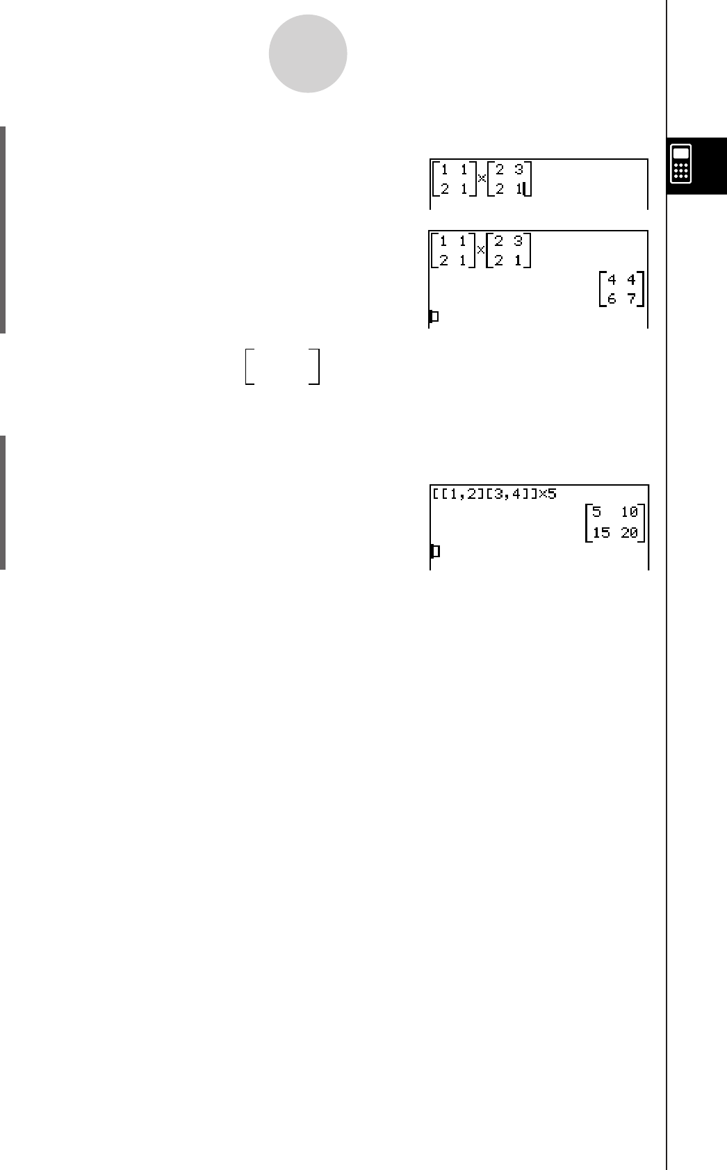
20060301

(3) Tap

8, and then input the values for the second matrix.

2-6-5

Matrix and Vector Calculations

Example 3: To multiply the matrix 1 2

3 4 by 5

u ClassPad Operation

(1) Perform the key operation below in the Main application work area.

9[[b,c][d,e]]*f

(2) Tap

(4) Tap

Tip

• Note that when adding or subtracting two matrices, they both must have the same number

of rows and the same number of columns (the same dimensions). An error occurs (Invalid

Dimension Error) when the two matrices have different dimensions.

• When multiplying two matrices, the number of columns in the matrix to the left of the multiplication

sign (×) must be the same as the number of rows in the matrix to the right of the multiplication

sign. An error occurs (Invalid Dimension Error) when you attempt to multiply two matrices that do

not satisfy the above conditions.

• Multiplication is assumed if you do not include any operator between two matrices.

[[1, 2] [3, 4]] [[2, 2] [2, 2]] for example, is treated as [[1, 2] [3, 4]] × [[2, 2] [2, 2]].

20060301

2-6-6

Matrix and Vector Calculations

k Raising a Matrix to a Specific Power

Example: To raise 1 2

3 4 to the power of 3

Use the procedures described under “Matrix Addition, Subtraction, Multiplication,

and Division” on page 2-6-4 to input the calculation.

The following are the screens that would be produced by each input method.

Tip

• You can perform matrix calculations using the commands of the [Matrix-Calculation] group on the

[Action] menu. For information about using these commands, see “2-8 Using the Action Menu”.

• You can raise only a square matrix to a specific power. An error occurs when you try to raise a

non-square matrix to a specific power.

Using a Matrix to Assign Different Values to Multiple Variables

Use the procedure in this section when you want to use a matrix to assign various different

values to multiple variables.

Syntax: Matrix with Numbers → Matrix with Variables

(The matrix can be one line with multiple columns, or multiple lines with one

column.)

Example: Assign the values 10, 20, and 30, to variables x, y, and z respectively

u ClassPad Operation

(1) Perform the key operation below in the Main application work area.

)s7bacca7daeW

7XcY7Z

(2)

Tip

• You can also perform this operation using a list. For details see “Using a List to Assign Different

Values to Multiple Variables” on page 2-5-4.

Input using the 9 keyboard Input using the ) keyboard

20101001

2-7 Specifying a Number Base

While using the Main application, you can specify a default number base (binary, octal,

decimal, hexadecimal) or you can specify a number base for a particular integer value.

You can also convert between number bases and perform bitwise operations using logical

operators (not, and, or, xor). Note that while a default number base is specified, you can

input integers only.

Number Base Precautions

Note the following limitations, which all apply while a default number base (binary, octal,

decimal, hexadecimal) is specified in the Main application.

• You cannot use scientific functions, or [Action] or [Interactive] menu commands.

• Except for Ans (Answer Memory variable), you cannot use variables.

• You can input integers only. An error (Invalid syntax ERROR) will occur if you try to input a

non-integer value (like 1.5 or 2).

• If a calculation produces a non-integer result (with a decimal part), the calculator will cut off

the decimal part automatically. For example, the calculation 5 ÷ 2 while decimal is selected

as the number base is 2.

• An error message is displayed if you try to enter a value that is invalid for the speicfied

number base. The following shows the numerals that can be used in each number system.

Binary: 0, 1

Octal: 0, 1, 2, 3, 4, 5, 6, 7

Decimal: 0, 1, 2, 3, 4, 5, 6, 7, 8, 9

Hexadecimal: 0, 1, 2, 3, 4, 5, 6, 7, 8, 9, A, B, C, D, E, F

Binary, Octal, Decimal, and Hexadecimal Calculation Ranges

• The following are the display capacities for each of the number bases.

Number Base

Display Capacity

Binary 32 digits

Octal 11 digits

Decimal 10 digits

Hexadecimal 8 digits

• Negative binary, octal, and hexadecimal values are produced using the two's complement

of the original value.

2-7-1

Specifying a Number Base

20060301

• The following are the calculation ranges for each of the number bases.

Binary Values:

Positive: 0 x 01111111111111111111111111111111

Negative: 10000000000000000000000000000000

11111111111111111111111111111111

Octal Values:

Positive: 0 x 17777777777

Negative: 20000000000 x 37777777777

Decimal Values:

Positive: 0 x 2147483647

Negative: −2147483648

x −1

Hexadecimal Values:

Positive: 0 x 7FFFFFFF

Negative: 80000000 x FFFFFFFF

2-7-2

Specifying a Number Base

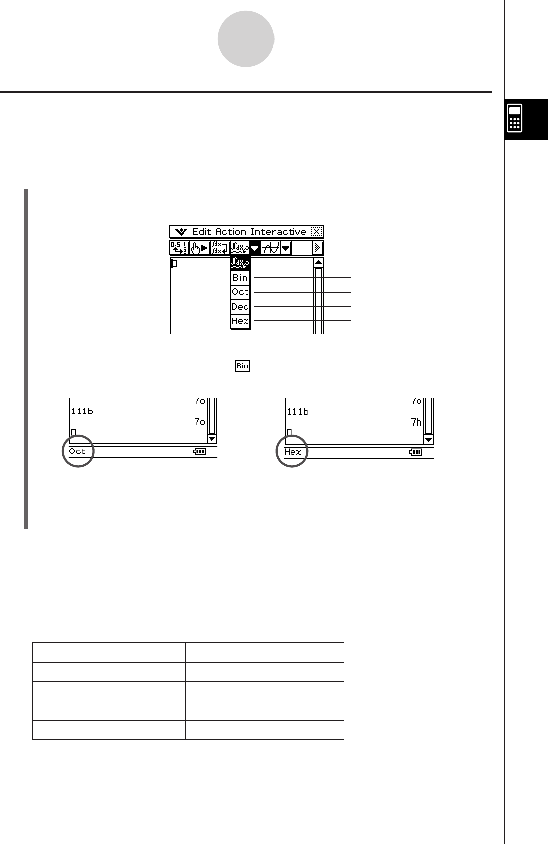
20060301

Selecting a Number Base

Specifying a default number base in the Main application will apply to the current line

(expression/result pair), and to all subsequent lines until you change the default number base

setting. Use the number toolbar’s base buttons to specify the number base.

u To select the number base for the line where the cursor is located

(1) Tap the down arrow button next to the < button.

• This displays a palette of number base buttons.

2-7-3

Specifying a Number Base

(2) Tap the button that corresponds to the number base you want to use.

• To select binary, for example, tap .

• The currently selected number base is indicated in the status bar.

Normal

Binary

Octal

Decimal

Hexadecimal

(3) Execute the calculation.

• When you press E to execute the calculation, the number base you selected in

step 2 is also applied automatically to the next line. You can continue using the same

number base in the next line or change to another number base.

Important!

• A line for which a number base is not specified is called a “normal calculation line.” To

return a line to a normal calculation line, tap < in step 2 of the above procedure.

• Calculation results produced by a line for which a number base is specified are followed by

one of the suffixes listed below, to indicate its number system.

Number System

Suffix

Binary b

Octal o

Decimal d

Hexadecimal h

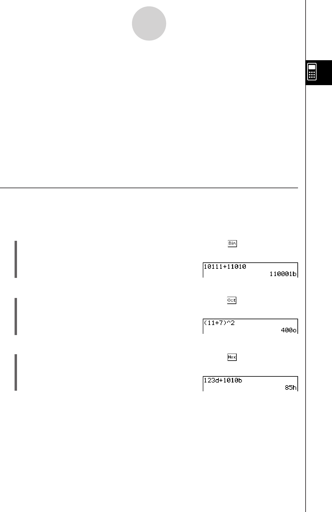
20060301

• Whenever you input a value into a line for which a number base is specified, the input value

is converted automatically to the specified number base. Performing the calculation 19+1 in

a line for which Hex (Hexadecimal) is specified as the number base, both the 19 and 1 are

interpreted as hexadecimal values, which produces the calculation result 1Ah. The “h” is

the suffix indicating hexadecimal notation.

u To specify a number base for an input value

You can input the following suffixes to specify the number base of a value as you input it: [b]

(binary), [o] (octal), [d] (decimal), and [h] (hexadecimal).

You can specify a number base for an input value only when a default number base (besides

normal) is selected

Tip

• For actual operation examples, see Example 3 under “Arithmetic Operations” below.

Arithmetic Operations

You can use the following operators when performing binary, octal, decimal and hexadecimal

values: +, −, ×, ÷, ^. You can also use parenthetical expressions.

Example 1: To calculate 101112 + 110102

(1) Tap the down arrow button next to the < button, and then tap .

(2) Perform the following key operation.

babbb+bbabaw

Example 2: To calculate (118 + 78)2

(1) Tap the down arrow button next to the < button, and then tap .

(2) Perform the following key operation.

(bb+h){cw

Example 3: Perform the calculation 12310 + 10102 so it produces a hexadecimal result

(1) Tap the down arrow button next to the < button, and then tap .

(2) Perform the following key operation using the soft keyboard.

0bcdd9+0bababw

2-7-4

Specifying a Number Base

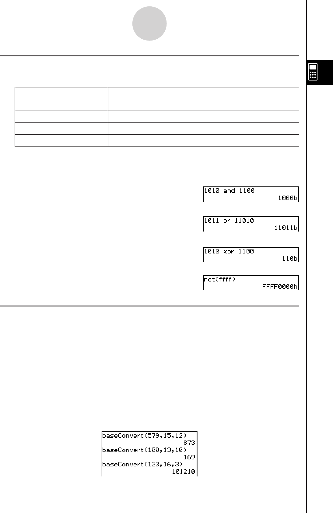
20060301

Bitwise Operations

The logical operators listed below can be used in calculations.

Operator

Description

and Returns the result of a bitwise product.

or Returns the result of a bitwise sum.

xor Returns the result of a bitwise exclusive logical sum.

not Returns the result of a complement (bitwise inversion).

Examples 1, 2, and 3 use Bin (binary) as the number system. Example 4 uses Hex

(hexadecimal).

Example 1: 10102 and 11002 = 10002

0babapandpbbaaw

Example 2: 10112 or 110102 = 110112

0babbporpbbabaw

Example 3: 10102 xor 11002 = 1102

0babapxorpbbaaw

Example 4: not (FFFF16) = FFFF000016

0not(ffffw

Using the baseConvert Function (Number System Transform)

The baseConvert function lets you convert a number in one base (number system) to its

equivalent in another base.

Important!

• The baseConvert function works for positive integers only.

• The baseConvert function cannot be used in a line for which a particular number base is

specified. It can be used in a normal calculation line only.

Syntax: baseConvert (Number, Current base, Expected base)

• Number must be a positive integer consisting of digits 0 to 9 and/or A to F.

• The current base and expected base can be any whole number from 2 to 16.

Examples:

2-7-5

Specifying a Number Base

20080201

2-8-1

Using the Action Menu

2-8 Using the Action Menu

The [Action] menu helps to make transformation and expansion functions, calculus functions,

statistical functions, and other frequently used mathematical menu operations easier to use.

Simply select the function you want, and then enter expressions or variables in accordance

with the syntax of the function.

Tip

• Unless specifically indicated otherwise, all of the explanations in this section are performed using

the following modes: Algebra mode, Standard mode, Complex mode, Radian mode, Descending

Order.

• You can use the [Interactive] menu to select most of the commands that are included on the [Action]

menu. Selecting a command on the [Action] menu will simply input the function for that command.

With the [Interactive] menu selecting a command will display a dialog box that prompts for input of

the command’s arguments (when necessary). This means that the [Interactive] menu eliminates

the need to remember details about the syntax of a function. For details about using the [Interactive]

menu, see page 2-9-1.

Abbreviations and Punctuation Used in This Section

The following are the meanings of the abbreviations and punctuation used in the syntax

descriptions in this section.

Some of the syntaxes in the following explanations indicate the following for parameters:

Exp/Eq/Ineq/List/Mat

These abbreviations mean that you can use any of the following as a parameter: expression,

equation, inequality list, or matrix.

When you see this: It means this:

Exp

Ineq

List

Mat

Expression (Value, Variable, etc.)

Equation

Inequality

List

Matrix

[ ] You can omit the item(s) inside the brackets.

{ } Select one of the items inside the braces.

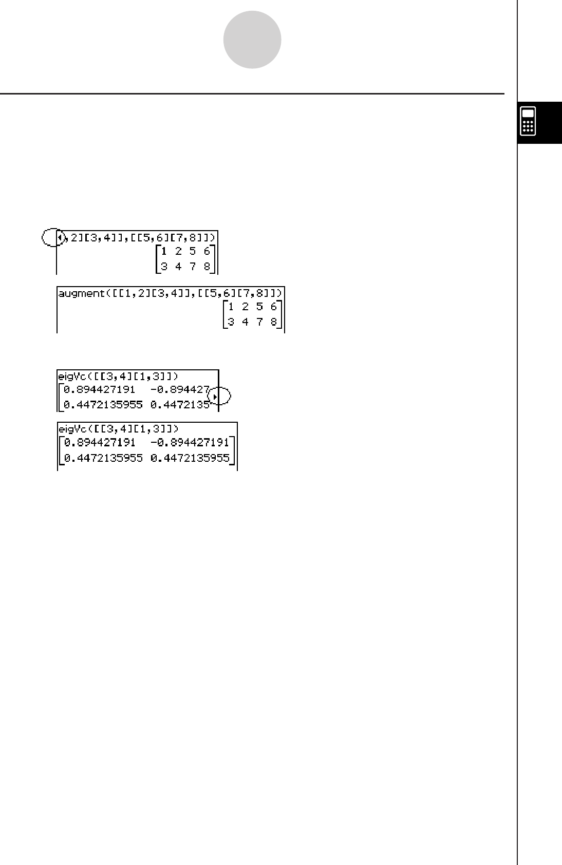
20080201

2-8-2

Using the Action Menu

Example Screenshots

The screenshots below show examples of how input and output expressions appear on the

ClassPad display.

In some cases, the input expression and output expression (result) may not fit in the display

area. If this happens, tap the left or right arrows that appear on the display to scroll the

expression screen and view the part that does not fit.

When the input expression does not fit:

When the output expression does not fit:

All of the screenshots in this section show the “complete expression” version.

Displayed expression

Complete expression

Displayed expression

Complete expression

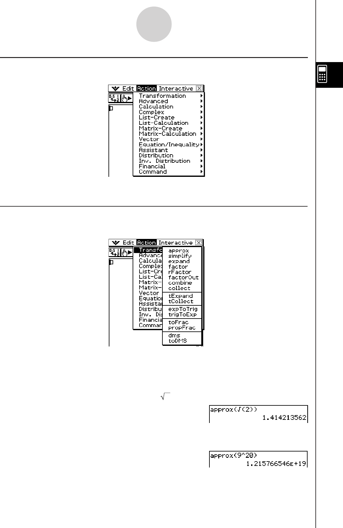
20101001

Displaying the Action Menu

Tap [Action] on the menu bar to display the submenus shown below.

2-8-3

Using the Action Menu

The following explains the functions that are available on each of these submenus.

Using the Transformation Submenu

The [Transformation] submenu contains commands for expression transformation, like

“expand” and “factor”.

u approx

Function: Transforms an expression into a numerical approximation.

Syntax: approx (Exp/Eq/Ineq/List/Mat [

)

]

• Ineq (inequality) includes the “⫽” (not equal to) relational operator.

Example: To obtain the numerical value of 2

Menu Item: [Action][Transformation][approx]

(Number Format: Normal 1)

Example: To obtain the numerical value of 920

Menu Item: [Action][Transformation][approx]

(Number Format: Normal 1)

• For information about the internal operations and the number of digits of a displayed

value, see page 2-2-7.

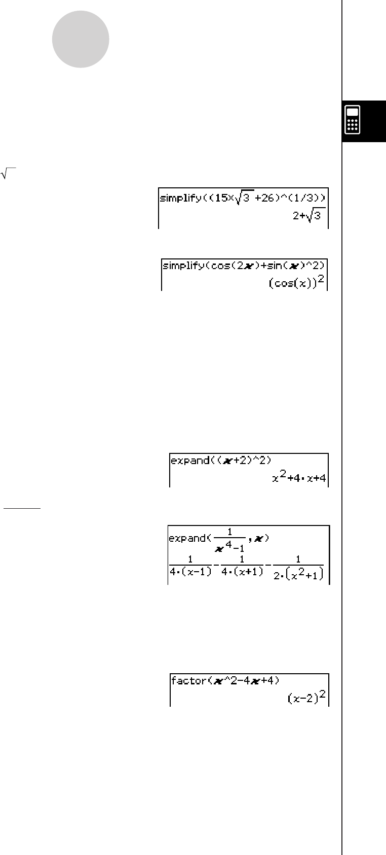
20060301

u simplify

Function: Simplifies an expression.

Syntax: simplify (Exp/Eq/Ineq/List/Mat [

)

]

• Ineq (inequality) includes the “≠” (not equal to) relational operator.

Example: To simplify (15 3

+ 26)^(1/3)

Menu Item: [Action][Transformation][simplify]

Example: To simplify cos(2x) + (sin(x))2 (in the Radian mode)

Menu Item: [Action][Transformation][simplify]

u expand

Function: Expands an expression.

Syntax: expand (Exp/Eq/Ineq/List/Mat [

)

]

expand (Exp,variable [

)

]

• Ineq (inequality) includes the “≠” (not equal to) relational operator.

• If you specify a variable, Exp is decomposed into partial fractions, with respect to the

variable.

Example: To expand (x + 2)2

Menu Item: [Action][Transformation][expand]

Example: To decompose into partial fractions, with respect to x

Menu Item: [Action][Transformation][expand]

u factor

Function: Factors an expression.

Syntax: factor (Exp/Eq/Ineq/List/Mat [

)

]

• Ineq (inequality) includes the “≠” (not equal to) relational operator.

Example: To factor x2  4x + 4

Menu Item: [Action][Transformation][factor]

(x4 – 1)

2-8-4

Using the Action Menu

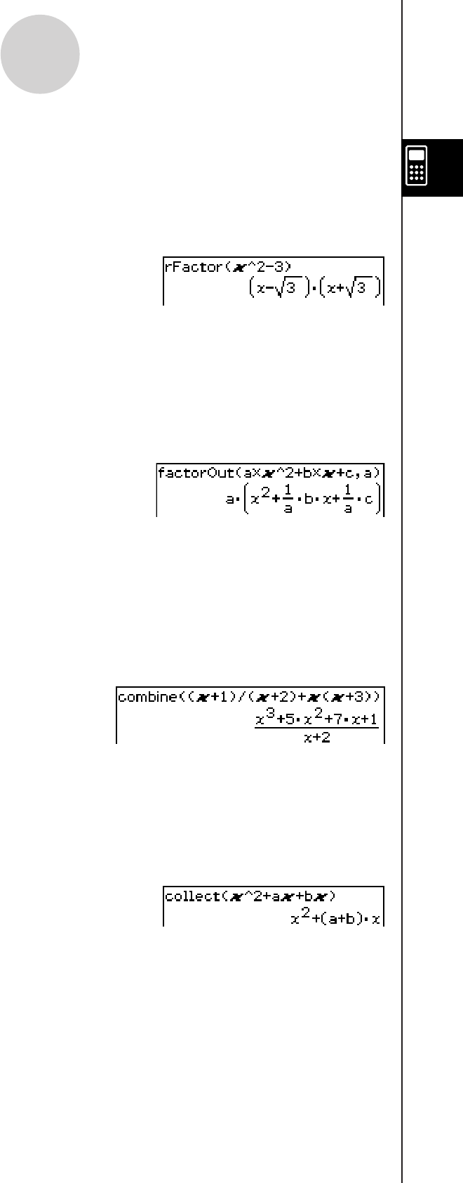
20080201

2-8-5

Using the Action Menu

u rFactor

Function: Factors an expression up to its roots, if any.

Syntax: rFactor (Exp/Eq/Ineq/List/Mat [

)

]

• Ineq (inequality) includes the “≠” (not equal to) relational operator.

Example: To factor x2  3

Menu Item: [Action][Transformation][rFactor]

u factorOut

Function: Factors out an expression with respect to a specified factor.

Syntax: factorOut (Exp/Eq/Ineq/List/Mat, Exp [

)

]

• Ineq (inequality) includes the “≠” (not equal to) relational operator.

Example: To factor “a” out ax2 + bx + c

Menu Item: [Action][Transformation][factorOut]

u combine

Function: Transforms multiple fractions into their common denominator equivalents and

reduces them, if possible.

Syntax: combine (Exp/Eq/Ineq/List/Mat [

)

]

• Ineq (inequality) includes the “≠” (not equal to) relational operator.

Example: To transform and reduce (x + 1)/(x + 2) + x(x + 3)

Menu Item: [Action][Transformation][combine]

u collect

Function: Rearranges an expression with respect to a specific variable.

Syntax: collect (Exp/Eq/Ineq/List/Mat[,Exp] [

)

]

• Ineq (inequality) includes the “≠” (not equal to) relational operator.

Example: To rearrange x2 + ax + bx with respect to x

Menu Item: [Action][Transformation][collect]

• “x” is the default when you omit “[,Exp]”.

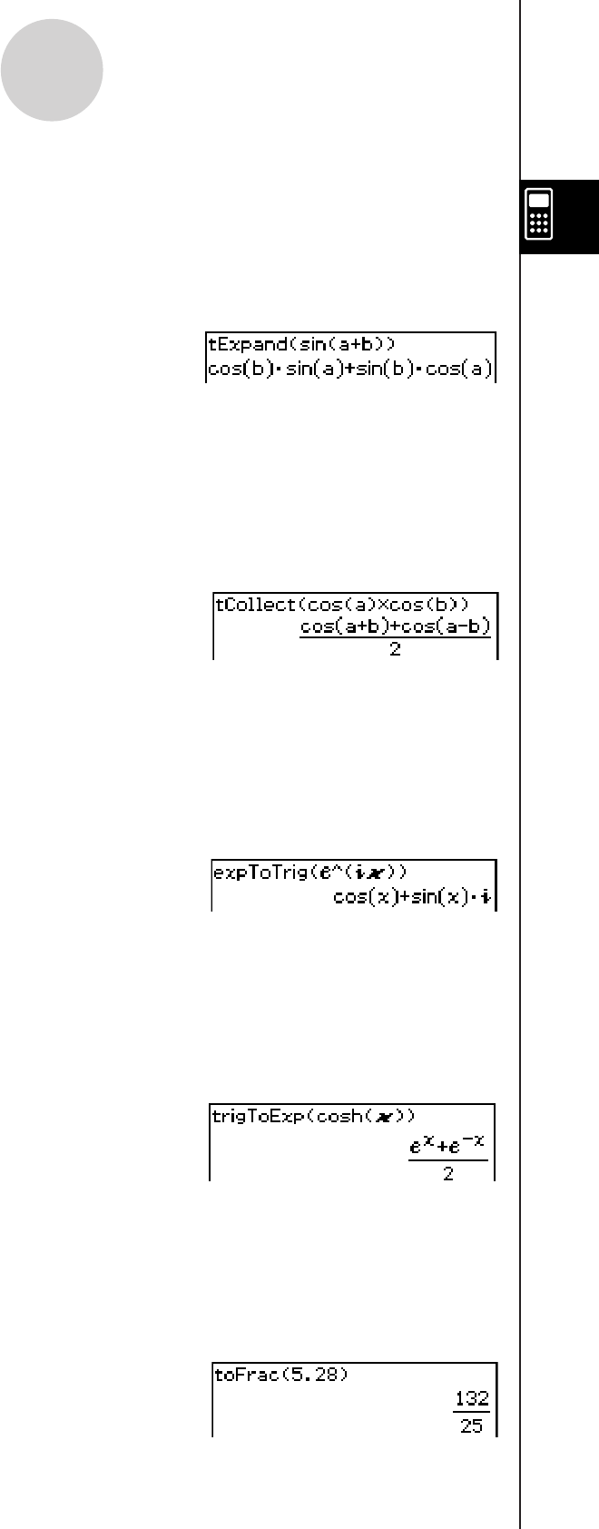
20080201

2-8-6

Using the Action Menu

u tExpand

Function: Employs the sum and difference formulas to expand a trigonometric function.

Syntax: tExpand(Exp/Eq/Ineq/List/Mat [

)

]

• Ineq (inequality) includes the “≠” (not equal to) relational operator.

Example: To expand sin (a + b)

Menu Item: [Action][Transformation][tExpand]

u tCollect

Function: Employs the product to sum formulas to transform the product of a trigonometric

function into an expression in the sum form.

Syntax: tCollect (Exp/Eq/Ineq/List/Mat [

)

]

• Ineq (inequality) includes the “≠” (not equal to) relational operator.

Example: To transform cos(a) × cos(b) into an expression in the sum form

Menu Item: [Action][Transformation][tCollect]

u expToTrig

Function: Transforms an exponent into a trigonometric or hyperbolic function.

Syntax: expToTrig (Exp/Eq/Ineq/List/Mat [

)

]

• Ineq (inequality) includes the “≠” (not equal to) relational operator.

Example: To transform eix into a trigonometric function (Radian mode)

Menu Item: [Action][Transformation][expToTrig]

u trigToExp

Function: Transforms a trigonometric or hyperbolic function into exponential form.

Syntax: trigToExp (Exp/Eq/Ineq/List/Mat [

)

]

• Ineq (inequality) includes the “≠” (not equal to) relational operator.

Example: To transform coshx into exponential form

Menu Item: [Action][Transformation][trigToExp]

u toFrac

Function: Transforms a decimal value into its equivalent fraction value.

Syntax: toFrac (Exp/Eq/Ineq/List/Mat [

)

]

• Ineq (inequality) includes the “≠” (not equal to) relational operator.

Example: To transform 5.28 into its equivalent fraction value

Menu Item: [Action][Transformation][toFrac]

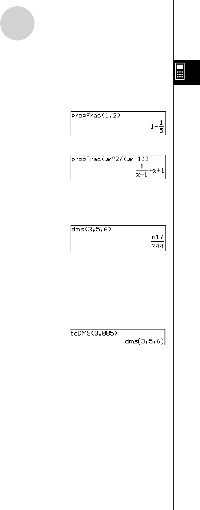
20080201

2-8-7

Using the Action Menu

u propFrac

Function: Transforms a decimal value into its equivalent proper fraction value.

Syntax: propFrac (Exp/Eq/Ineq/List/Mat [

)

]

• Ineq (inequality) includes the “≠” (not equal to) relational operator.

Example: To transform 1.2 into its equivalent proper fraction value

Menu Item: [Action][Transformation][propFrac]

Example: To divide x2 by (x – 1)

Menu Item: [Action][Transformation][propFrac]

u dms

Function: Transforms a DMS format value into its equivalent degrees-only value.

Syntax: dms (Exp/List-1 [,Exp/List-2][,Exp/List-3] [

)

]

Example: To transform (3, 5, 6) (= 3q 5’ 6”) into its equivalent degrees-only value

Menu Item: [Action][Transformation][dms]

• Zero is the default when you omit [,Exp/List-2] or [,Exp/List-3][

)

u toDMS

Function: Transforms a degrees-only value into its equivalent DMS format value.

Syntax: toDMS (Exp/List [ ) ]

Example: To transform 3.085 degrees into its equivalent DMS format value

Menu Item: [Action][Transformation][toDMS]

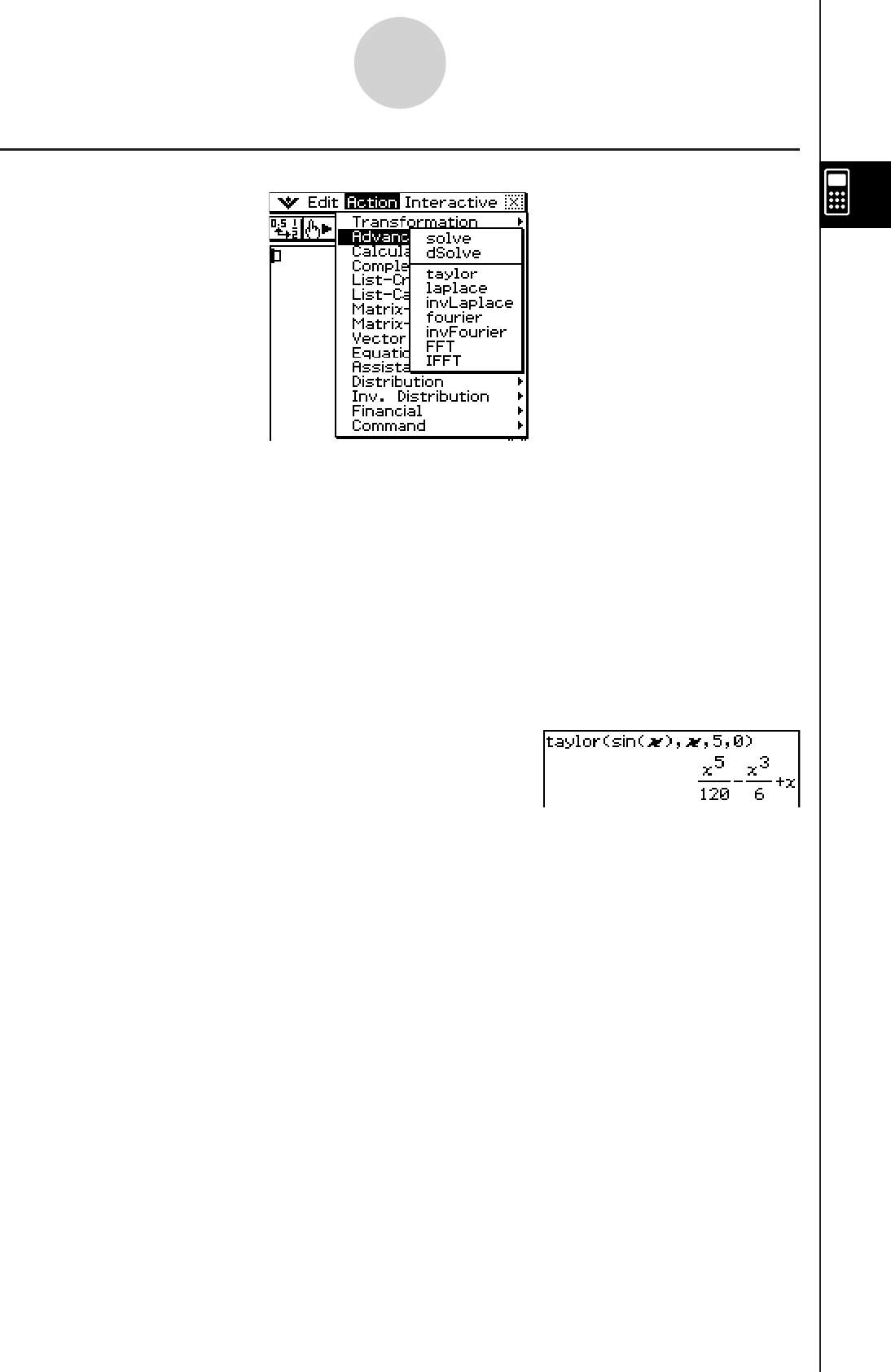
20101001

Using the Advanced Submenu

u solve

For information about solve, see page 2-8-43.

u dSolve

For information about dSolve, see page 2-8-44.

u taylor

Function: Finds a Taylor polynomial for an expression with respect to a specific variable.

Syntax: taylor (Exp/List, variable, order [,center point] [

)

]

Example: To find a 5th order Taylor polynomial for sin(x) with respect to x = 0 (in the

Radian mode)

Menu Item: [Action][Advanced][taylor]

2-8-8

Using the Action Menu

• Zero is the default when you omit “[,center point]”.

u laplace, invLaplace

“laplace” is the command for the Laplace transform, and “invLaplace” is the command for

the inverse of Laplace transform.

∫

∞

0f(t)e–stdtL[ f(t)] (s)=

Function:

The Laplace Transform is called “laplace” on the ClassPad.

The inverse of Laplace Transform is called “invLaplace” on the ClassPad.

Syntax: laplace(f(t), t, s)

f(t) -- expression

t -- variable with respect to which the expression is transformed

s -- parameter of the transform

invLaplace(L(s), s, t)

L(s) -- expression

s -- variable with respect to which the expression is transformed

t -- parameter of the transform

20080201

ClassPad supports transform of the following functions.

sin(x), cos(x), sinh(x), cosh(x), xn, x, ex, heaviside(x), delta(x), delta(x, n)

ClassPad does not support transform of the following functions.

tan(x), sin– 1(x), cos– 1(x), tan– 1(x), tanh(x), sinh– 1(x), cosh– 1(x), tanh– 1(x), log(x), ln(x), 1/x,

abs(x), gamma(x)

Laplace Transform of a Differential Equation

The laplace command can be used to solve ordinary differential equations. ClassPad does

not support System of Differential Equations for laplace.

Syntax: laplace(diff eq, x, y, t)

diff eq -- differential equation to solve

x -- independent variable in the diff eq

y -- dependent variable in the diff eq

t -- parameter of the transform

Lp means F(s)=L[f(t)] in the result of transform for a differential equation.

An example using Laplace to solve a differential equation:

u fourier, invFourier

Function: “fourier” is the command for the Fourier Transform, and “invFourier” is the

command for the inverse Fourier Transform.

Syntax: fourier(f(x),x,w,n)

invFourier(f(w),w,x,n)

f(x) -- expression

x -- variable with respect to which the expression is transformed with

w -- parameter of the transform

n -- 0 to 4, indicating Fourier parameter to use (optional)

ClassPad supports transform of the following functions.

sin(t), cos(t), log(t), ln(t), abs(t), signum(t), heaviside(t), delta(t), delta(t,n), eti

ClassPad does not support transform of the following functions.

tan(t), sin– 1(t), cos– 1(t), tan– 1(t), sinh(t), cosh(t), tanh(t), sinh– 1(t), cosh– 1(t), tanh– 1(t),

gamma(t), t , et

2-8-9

Using the Action Menu

where x(0) = 3x’ + 2x = e–t

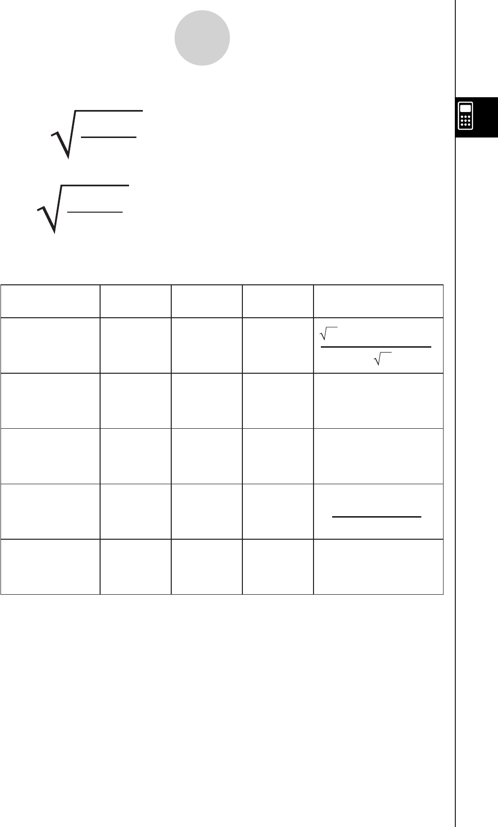
20080201

The values of a and b depend on the scientific discipline, which can be specified by the

value of n (optional fourth parameter of Fourier and invFourier) as shown below.

n (optional) ab

Definition of the Fourier

Integral

Modern Physics

001

∫

∞

–∞eω•x•i • f(x)dx

2 •

2 • π

Pure Math

11–1

Probability

211

Classical Physics

3–11

∫

∞

–∞eω•x•i • f(x)dx

2 • π

Signal Processing

4 0 –2*π

Tip

• The Advanced Format dialog box can be used to configure settings related to the Fourier

Transform, such a Fourier Transform definition, etc. For details, see “Advanced Format Dialog

Box” on page 1-9-11.

2-8-10

Using the Action Menu

The Fourier Transform pairs are defined using two arbitrary constants a, b.

∫

∞

–∞f(t)eibωt dt

F(ω) =

⏐b ⏐

(2π)1–a

∫

∞

–∞F(ω)e–ibωt dω

f(t) =

⏐b ⏐

(2π)1+a

∫

∞

–∞e–ω•x•i • f(x)dx

∫

∞

–∞eω•x•i • f(x)dx

∫

∞

–∞e–2•π•ω•x•i • f(x)d

20080201

2-8-11

Using the Action Menu

u FFT, IFFT

Function: “FFT” is the command for the fast Fourier Transform, and “IFFT” is the

command for the inverse fast Fourier Transform.

2n data values are needed to perform FFT and IFFT. On the ClassPad, FFT and IFFT are

calculated numerically.

Syntax: FFT( list ) or FFT( list, m)

IFFT( list ) or IFFT( list, m)

• Data size must be 2n for n = 1, 2, 3, ...

• The value for m is optional. It can be from 0 to 2, indicating the FFT parameter to use.

m = 0 Signal Processing

m = 1 Pure Math

m = 2 Data Analysis

The Fourier Transform is defined as the following:

Some authors (especially physicists) prefer to write the transform in terms of angular

frequency ω ≡ 2π

instead of the oscillation frequency

However, this destroys the symmetry, resulting in the transform pair shown below.

∫

∞

–∞F(k)e2πikx dk

f(x) =

∫

∞

–∞f(x)e–2πikx dx

F(k) =

∫

∞

–∞h(t)e–iωt dt

H(ω) = F [h(t)] =

∫

∞

–∞H(ω)eiωt dω

h(t) = F –1[H(ω)] = 1

2π

∫

∞

–∞f(t)e–iyt dt

g(y) = F [ f(t)] = 1

2π

∫

∞

–∞g(y)eiyt dy

f(t) = F –1[g(y)] = 1

2π

To restore the symmetry of the transforms, the convention shown below is sometimes

used.

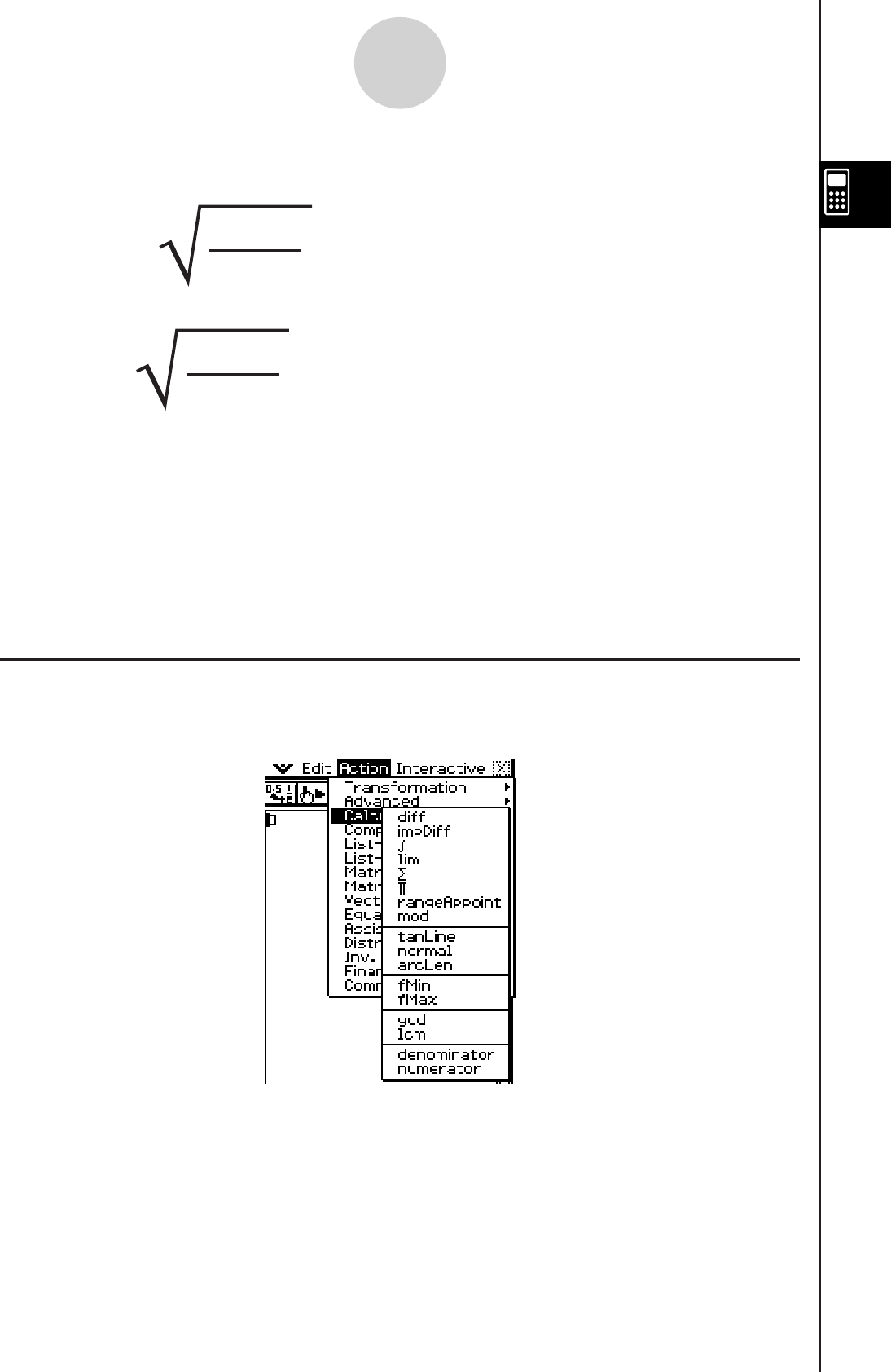
20101001

2-8-12

Using the Action Menu

Using the Calculation Submenu

The [Calculation] submenu contains calculus related commands, such as “diff” (differentiation)

and “ ” (integration).

Unfortunately, a number of conventions are in widespread use for a and b. For example,

(0, 1) is used in modern physics, (1, –1) is used in pure mathematics and systems

engineering, (1, 1) is used in probability theory for the computation of the characteristic

function, (–1, 1) is used in classical physics, and (0, –2π) is used in signal processing.

Tip

• The Advanced Format dialog box can be used to configure Fast Fourier Transform settings. For

details, see “Advanced Format Dialog Box” on page 1-9-11.

In general, the Fourier transform pair may be defined using two arbitrary constants a and

b as shown below.

∫

∞

–∞f(t)eibωt dt

F(ω) = ⏐b⏐

(2π)1–a

∫

∞

–∞F(ω)e–ibωt dω

f(t) = ⏐b⏐

(2π)1+a

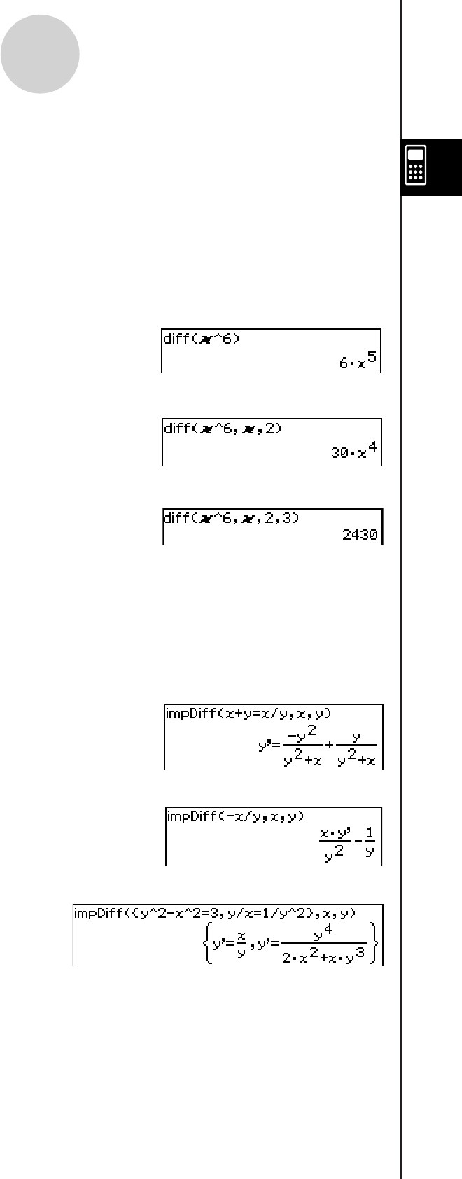
20090601

2-8-13

Using the Action Menu

u impDiff

Function: Differentiates an equation or expression in implicit form with respect to a

specific variable.

Syntax: impDiff(Eq/Exp/List, independent variable, dependent variable)

Example: To find y’ using implicit differentiation

Menu Item: [Action][Calculation][impDiff]

Example: To find

y’ for a list of equations

Menu Item: [Action][Calculation][impDiff]

Important!

The derivative symbol (’) cannot be used in the argument of “impDiff(”. Trying to use a

derivative symbol would result in a Wrong Argument Type error.

Example: To find y” given y’ = −x/y

Menu Item: [Action][Calculation][impDiff]

u diff

Function: Differentiates an expression with respect to a specific variable.

Syntax: diff(Exp/List[,variable] [ ) ]

diff(Exp/List,variable,order[,a] [ ) ]

• “a” is the point for which you want to determine the derivative.

• “order” = 1 when you use the following syntax: diff(Exp/List[,variable][ ) ]. The default

variable is “x” when “variable” is omitted.

Example: To differentiate x6 with respect to x

Menu Item: [Action][Calculation][diff]

Example: To find the second derivative of x6 with respect to x

Menu Item: [Action][Calculation][diff]

Example: To find the second derivative of x6 with respect to x at x = 3

Menu Item: [Action][Calculation][diff]

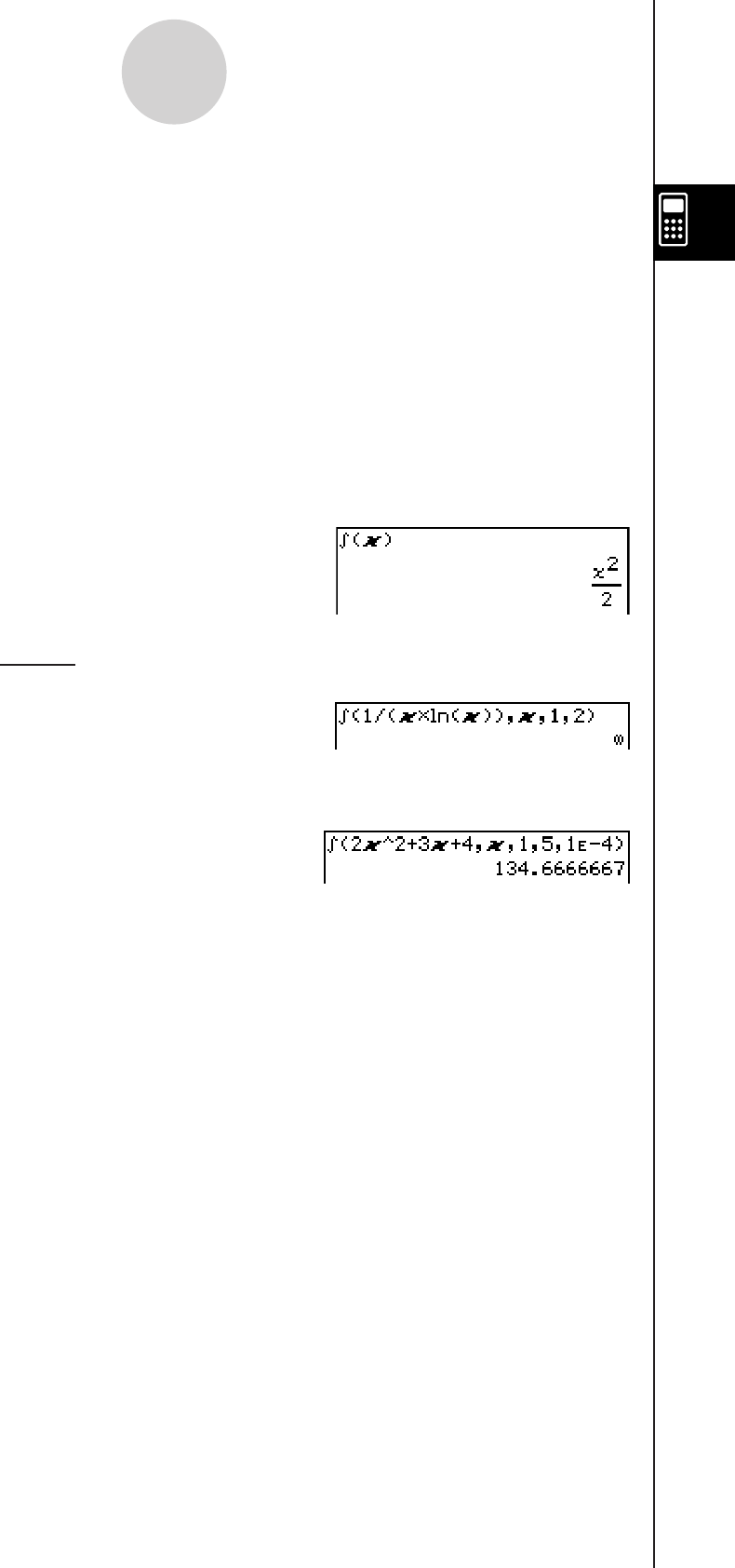
20080201

2-8-14

Using the Action Menu

u ∫

Function: Integrates an expression with respect to a specific variable.

Syntax:  (Exp/List[,variable] [ ) ]

 (Exp/List, variable, lower limit, upper limit [,tol ] [ ) ]

• “x” is the default when you omit [,variable].

• “tol ” represents the allowable error range.

• This command returns an approximate value when a range is specified for “tol”.

• This command returns the true value of a definite interval when nothing is specified

for “tol ”. If the true value cannot be obtained, however, this command returns an

approximate value along with tol =1E – 5.

Example: To integrate x with respect to x

Menu Item: [Action][Calculation][



]

Example: To integrate 2x2 + 3x + 4 with respect to x between x = 1 and x = 5, with an

allowable error range of 1E – 4

Menu Item: [Action][Calculation][



]

Example: To integrate x × ln(x) with respect to x between x = 1 and x = 2

Menu Item: [Action][Calculation][



]

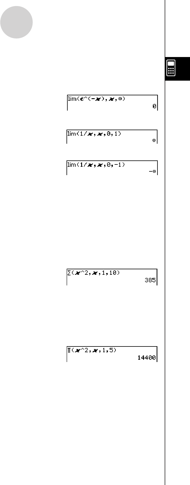
20080201

2-8-15

Using the Action Menu

u Σ

Function: Evaluates an expression at discrete variable values within a range, and then

calculates a sum.

Syntax: Σ(Exp/List, variable, lower value, upper value [

)

]

Example: To calculate the sum of x2 as the value of x changes from x = 1 through x =10.

Menu Item: [Action][Calculation][Σ]

u Π

Function: Evaluates an expression at discrete variable values within a range, and then

calculates a product.

Syntax: Π(Exp/List, variable, lower value, upper value [

)

]

Example: To calculate the product of x2 as the value of x changes from x = 1 through

x = 5

Menu Item: [Action][Calculation][Π]

u lim

Function: Determines the limit of an expression.

Syntax: lim (Exp/List, variable, point [,direction] [

)

]

Example: To determine the limit of e –x as x approaches ∞

Menu Item: [Action][Calculation][lim]

Example: To determine the limit of 1/x as x approaches 0 from the right

Menu Item: [Action][Calculation][lim]

Example: To determine the limit of 1/x as x approaches 0 from the left

Menu Item: [Action][Calculation][lim]

• This function returns the limit from the left when “direction” < 0, the limit from the right

when “direction” > 0, and the limit from both sides (left and right) when “direction” = 0 or

when the direction is omitted.

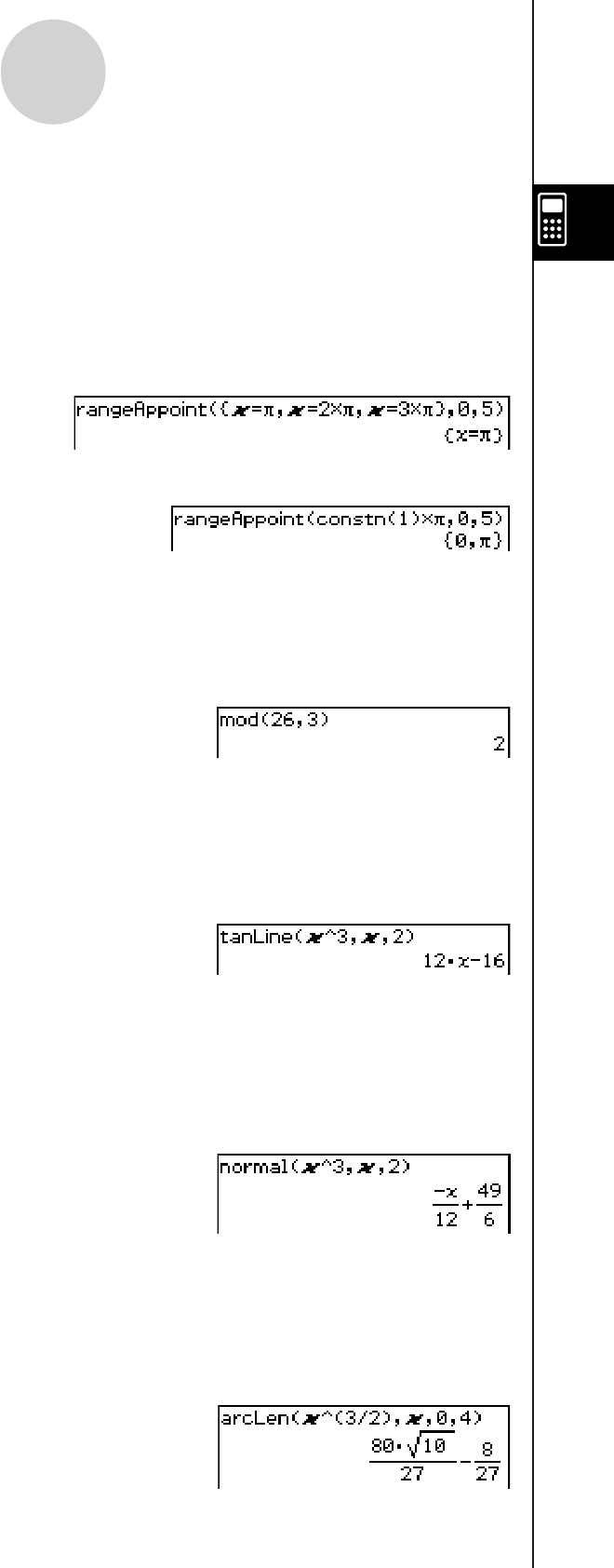
20080201

2-8-16

Using the Action Menu

u normal

Function: Returns the right side of the equation for the line normal (y = ‘expression’) to the

curve at the specified point.

Syntax: normal (Exp/List, variable, variable value at point of normal [

)

]

Example: To determine the function of the line normal to y = x3 at x = 2

Menu Item: [Action][Calculation][normal]

u arcLen

Function: Returns the arc length of an expression from a start value to an end value with

respect to a specified variable.

Syntax: arcLen (Exp/List, variable, start value, end value [

)

]

Example: To determine the arc length for y = x3

—

2 from x = 0 to x = 4

Menu Item: [Action][Calculation][arcLen]

u rangeAppoint

Function: Finds an expression or value that satisfies a condition in a specified range.

Syntax: rangeAppoint (Exp/Eq/List, start value, end value [

)

]

• When using an equation (Eq) for the first argument, input the equation using the syntax

Var = Exp. Evaluation will not be possible if any other syntax is used.

Example: To find the expression(s) in the list {x = π, x = 2π, x = 3π} that belong(s) to the

closed range 0 < x < 5

Menu Item: [Action][Calculation]

[rangeAppoint]

Example: To find the “n” that satisfies the condition 0 < n × π < 5

Menu Item: [Action][Calculation][rangeAppoint]

u mod

Function: Returns the remainder when one expression is divided by another expression.

Syntax: mod ({Exp/List} -1, {Exp/List} -2 [ ) ]

Example: To determine the remainder when 26 is divided by 3 (26mod3)

Menu Item: [Action][Calculation][mod]

u tanLine

Function: Returns the right side of the equation for the tangent line (y = ‘expression’) to

the curve at the specified point.

Syntax: tanLine (Exp/List, variable, variable value at point of tangency [

)

]

Example: To determine the function of the line tangent to y = x3 at x = 2

Menu Item: [Action][Calculation][tanLine]

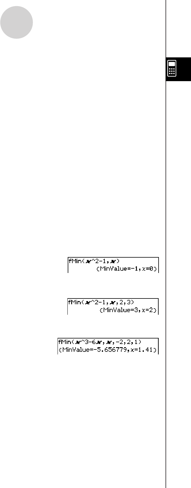
20080201

2-8-17

Using the Action Menu

Example: To find the minimum point of x2 – 1 with respect to x, when 2 < x < 3

Menu Item: [Action][Calculation][fMin]

Example: To find the minimum point of x3 – 6x with respect to x,

when –2 < x < 2 and n = 1

Menu Item: [Action][Calculation][fMin]

u fMin

Function: Returns the minimum point in a specific range of a function.

Syntax: fMin(Exp[,variable] [ ) ]

fMin(Exp,variable,start value,end value[,n] [ ) ]

• “x” is the default when you omit “[,variable]”.

• Negative infinity and positive infinity are the default when the syntax fMin (Exp [,variable]

[ ) ] is used.

• “n” is calculation precision, which you can specify as an integer in the range of 1 to 9.

Using any value outside this range causes an error.

• This command returns an approximate value when calculation precision is specified for

“n”.

• This command returns a true value when nothing is specified for “n”. If the true value

cannot be obtained, however, this command returns an approximate value along with

n = 4.

• Discontinuous points or sections that fluctuate widely can adversely affect precision or

even cause an error.

• Inputting a larger number for “n” increases the precision of the calculation, but it also

increases the amount of time required to perform the calculation.

• The value you input for the end point of the interval must be greater than the value you

input for the start point. Otherwise an error occurs.

Example: To find the minimum point of x2 – 1 with respect to x

Menu Item: [Action][Calculation][fMin]

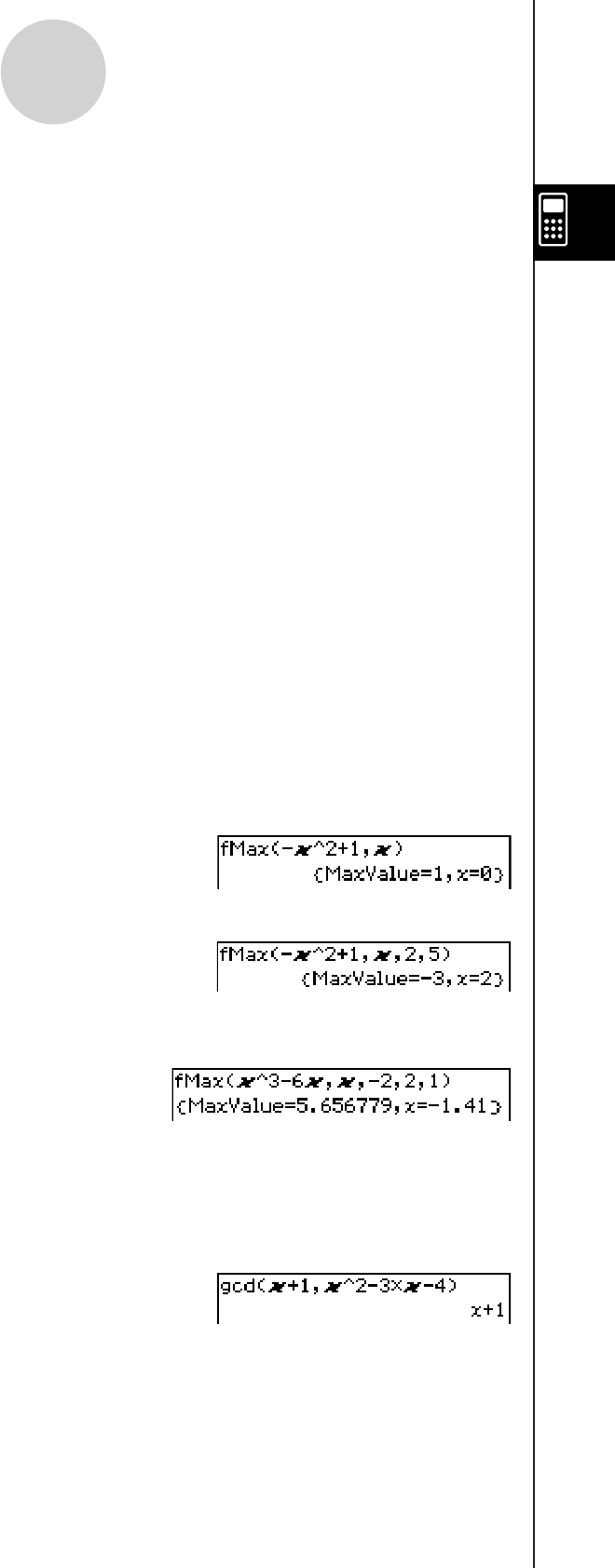
20080201

2-8-18

Using the Action Menu

u gcd

Function: Returns the greatest common denominator of two expressions.

Syntax: gcd (Exp/List-1, Exp/List-2 [

)

]

Example: To obtain the greatest common denominator of x + 1 and x2 – 3x – 4

Menu Item: [Action][Calculation][gcd]

u fMax

Function: Returns the maximum point in a specific range of a function.

Syntax: fMax(Exp[,variable] [ ) ]

fMax(Exp,variable,start value,end value[,n] [ ) ]

• “x” is the default when you omit “[,variable]”.

• Negative infinity and positive infinity are the default when the syntax fMax (Exp [,

variable] [ ) ] is used.

• “n” is calculation precision, which you can specify as an integer in the range of 1 to 9.

Using any value outside this range causes an error.

• This command returns an approximate value when calculation precision is specified for

“n”.

• This command returns a true value when nothing is specified for “n”. If the true value

cannot be obtained, however, this command returns an approximate value along with

n = 4.

• Discontinuous points or sections that fluctuate widely can adversely affect precision or

even cause an error.

• Inputting a larger number for “n” increases the precision of the calculation, but it also

increases the amount of time required to perform the calculation.

• The value you input for the end point of the interval must be greater than the value you

input for the start point. Otherwise an error occurs.

Example: To find the maximum point of –x2 + 1 with respect to x

Menu Item: [Action][Calculation][fMax]

Example: To find the maximum point of –x2 + 1, when 2 < x < 5

Menu Item: [Action][Calculation][fMax]

Example: To find the maximum point of x3 – 6x with respect to x,

when –2 < x < 2 and n = 1

Menu Item: [Action][Calculation][fMax]

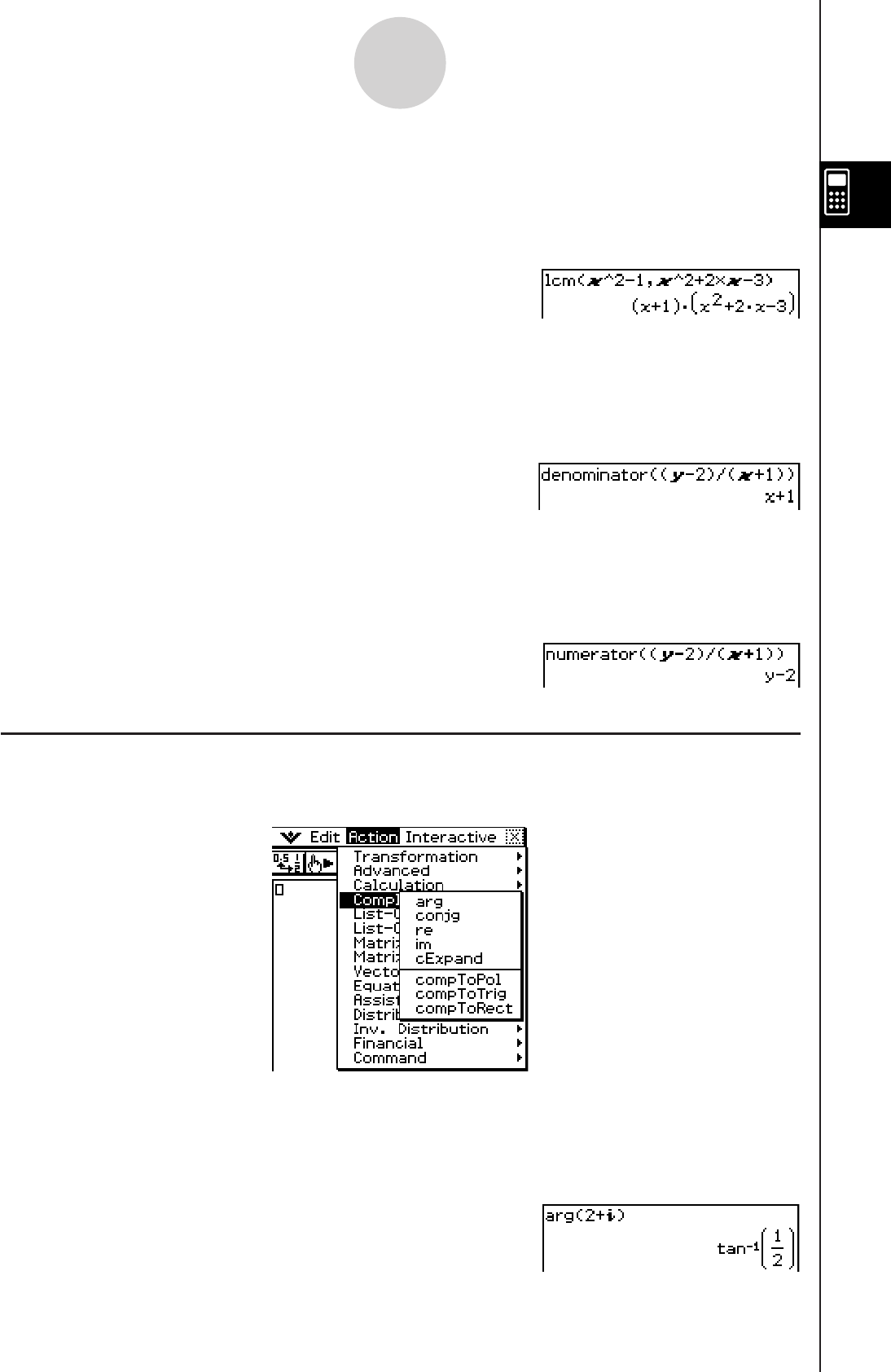
20110501

2-8-19

Using the Action Menu

u arg

Function: Returns the argument of a complex number.

Syntax: arg (Exp/Eq/List/Mat [ ) ]

Example: To obtain the argument of complex 2 + i (in the Radian mode)

Menu Item: [Action][Complex][arg]

u lcm

Function: Returns the least common multiple of two expressions.

Syntax: lcm (Exp/List-1, Exp/List-2 [

)

]

Example: To obtain the least common multiple of x2 – 1 and x2 + 2x – 3

Menu Item: [Action][Calculation][lcm]

u denominator

Function: Extracts the denominator of a fraction.

Syntax: denominator (Exp/List [

)

]

Example: To extract the denominator of the fraction (y – 2)/(x + 1)

Menu Item: [Action][Calculation][denominator]

u numerator

Function: Extracts the numerator of a fraction.

Syntax: numerator (Exp/List [ ) ]

Example: To extract the numerator of the fraction (y – 2)/(x + 1)

Menu Item: [Action][Calculation][numerator]

Using the Complex Submenu

The [Complex] submenu contains commands that relate to calculations that involve

complex numbers.

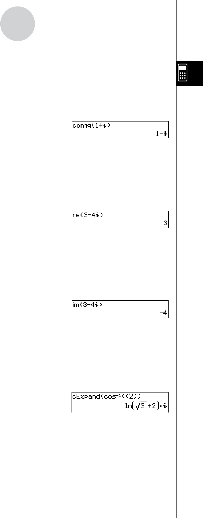
20110901

2-8-20

Using the Action Menu

u conjg

Function: Returns the conjugate complex number.

Syntax: conjg (Exp/Eq/List/Mat [ ) ]

• An inequality with the “⫽” (not equal to) relation symbol is also included (only in the Real

mode).

Example: To obtain the conjugate of complex number 1 + i

Menu Item: [Action][Complex][conjg]

u re

Function: Returns the real part of a complex number.

Syntax: re (Exp/Eq/List/Mat [ ) ]

• An inequality with the “⫽” (not equal to) relation symbol is also included (only in the Real

mode).

Example: To obtain the real part of complex number 3 – 4i

Menu Item: [Action][Complex][re]

u im

Function: Returns the imaginary part of a complex number.

Syntax: im (Exp/Eq/List/Mat [ ) ]

• An inequality with the “⫽” (not equal to) relation symbol is also included (only in the Real

mode).

Example: To obtain the imaginary part of complex number 3 – 4i

Menu Item: [Action][Complex][im]

u cExpand

Function: Expands a complex expression to rectangular form (a + bi).

Syntax: cExpand (Exp/Eq/List/Mat [ ) ]

• Ineq (inequality) includes the “⫽” (not equal to) relational operator.

• The variables are regarded as real numbers.

Example: To expand cos–1(2) (in the Radian mode)

Menu Item: [Action][Complex][cExpand]

u compToPol

Function: Transforms a complex number into its polar form.

Syntax: compToPol (Exp/Eq/List/Mat [ ) ]

• Ineq (inequality) includes the “⫽” (not equal to) relational operator.

• When the argument is Mat (Matrices), calculation can be performed using the Radian

angle unit only.

20110901

2-8-21

Using the Action Menu

Example: To transform 1 + i into its polar form

Menu Item: [Action][Complex][compToPol]

Radian mode Degree mode Grad mode

u compToTrig

Function: Transforms a complex number into its trigonometric/hyperbolic form.

Syntax: compToTrig (Exp/Eq/List/Mat [ ) ]

• Ineq (inequality) includes the “⫽” (not equal to) relational operator.

Example: To transform 1 + i into its trigonometric form (in the Radian mode)

Menu Item: [Action][Complex][compToTrig]

u compToRect

Function: Transforms a complex number into its rectangular form.

Syntax: compToRect (⬔(r,) or r

· e^(

i) form [ ) ]

Example: To transform a complex number into its rectangular form.

Menu Item: [Action][Complex][compToRect]

Using the List-Create Submenu

The [List-Create] submenu contains commands that are related to creating lists.

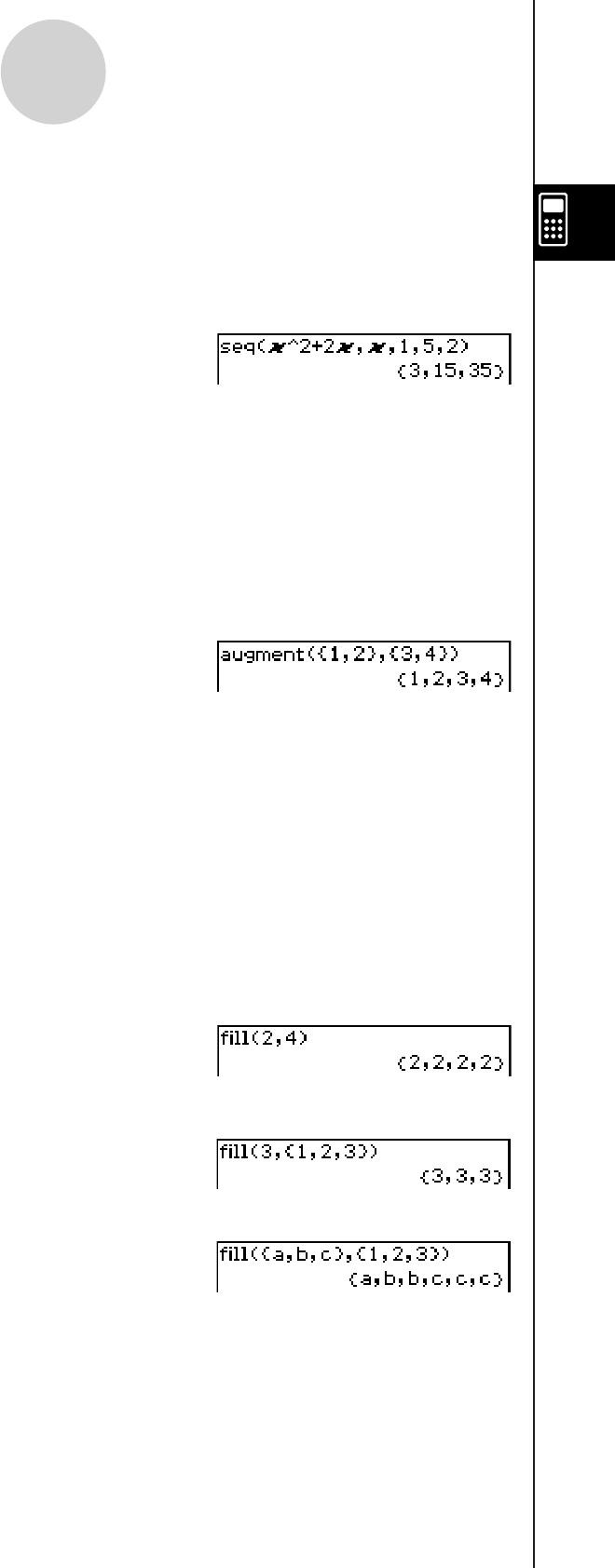
20080201

2-8-22

Using the Action Menu

u seq

Function: Generates a list in accordance with a numeric sequence expression.

Syntax: seq (Exp, variable, start value, end value [,step size] [ ) ]

Example: To generate a list in accordance with the expression x2 + 2x when the start

value is 1, the end value is 5, and the step size is 2

Menu Item: [Action][List-Create][seq]

• “1” is the default when you omit “[,step size]”.

• The step size must be a factor of the difference between the start value and the end

value.

u augment

Function: Creates a new list by appending one list to another.

Syntax: augment (List-1, List-2 [ ) ]

Example: To combine list {1, 2} and list {3, 4}

Menu Item: [Action][List-Create][augment]

u fill

Function: Replaces the elements of a list with a specified value or expression. This

command can also be used to create a new list whose elements all contain the

same value or expression, or a new list in which the frequency of each element

in the first list is determined by the corresponding element in the second list.

Syntax: fill (Exp/Eq/Ineq, number of elements [ ) ]

fill (Exp/Eq/Ineq, List [ ) ]

• Ineq (inequality) includes the “≠” (not equal to) relational operator.

Syntax: fill (List, List [ ) ]

Example: To create a list consisting of four identical elements (2)

Menu Item: [Action][List-Create][fill]

Example: To replace the elements of the list {1, 2, 3} with 3

Menu Item: [Action][List-Create][fill]

Example: To create a list in which the frequencies of a, b and c are 1, 2 and 3, respectively

Menu Item: [Action][List-Create][fill]

20080201

u subList

Function: Extracts a specific section of a list into a new list.

Syntax: subList (List [,start number] [,end number] [

)

]

Example: To extract the second through the fourth elements of the list {1, 2, 3, 4, 5}

Menu Item: [Action][List-Create][subList]

• The leftmost element is the default when you omit “[,start number]”, and the rightmost

element is the default when you omit “[,end number]”.

u shift

Function: Returns a list in which elements have been shifted to the right or left by a

specific amount.

Syntax: shift (List [,number of shifts] [

)

]

• Specifying a negative value for “[,number of shifts]” shifts to the right, while a positive

value shifts to the left.

Example: To shift the elements of the list {1, 2, 3, 4, 5, 6} to the left by three

Menu Item: [Action][List-Create][shift]

• Right shift by one (–1) is the default when you omit “[,number of shifts]”.

u rotate

Function: Returns a list in which the elements have been rotated to the right or to the left

by a specific amount.

Syntax: rotate (List [,number of rotations] [

)

]

• Specifying a negative value for “[,number of rotations]” rotates to the right, while a

positive value rotates to the left.

Example: To rotate the elements of the list {1, 2, 3, 4, 5, 6} to the left by two

Menu Item: [Action][List-Create][rotate]

• Right rotation by one (–1) is the default when you omit “[,number of rotations]”.

u sortA

Function: Sorts the elements of the list into ascending order.

Syntax: sortA (List [

)

]

Example: To sort the elements of the list {1, 5, 3} into ascending order

Menu Item: [Action][List-Create][sortA]

2-8-23

Using the Action Menu

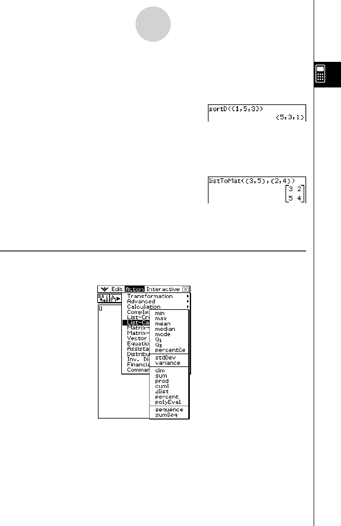
20101001

2-8-24

Using the Action Menu

u sortD

Function: Sorts the elements of the list into descending order.

Syntax: sortD (List [

)

]

Example: To sort the elements of the list {1, 5, 3} into descending order

Menu Item: [Action][List-Create][sortD]

u listToMat

Function: Transforms lists into a matrix.

Syntax: listToMat (List-1 [, List-2, ..., List-N] [

)

]

Example: To transform the lists {3, 5} and {2, 4} into a matrix

Menu Item: [Action][List-Create][listToMat]

u matToList

• For information abot matToList, see page 2-8-33.

Using the List-Calculation Submenu

The [List-Calculation] submenu contains commands related to list calculations.

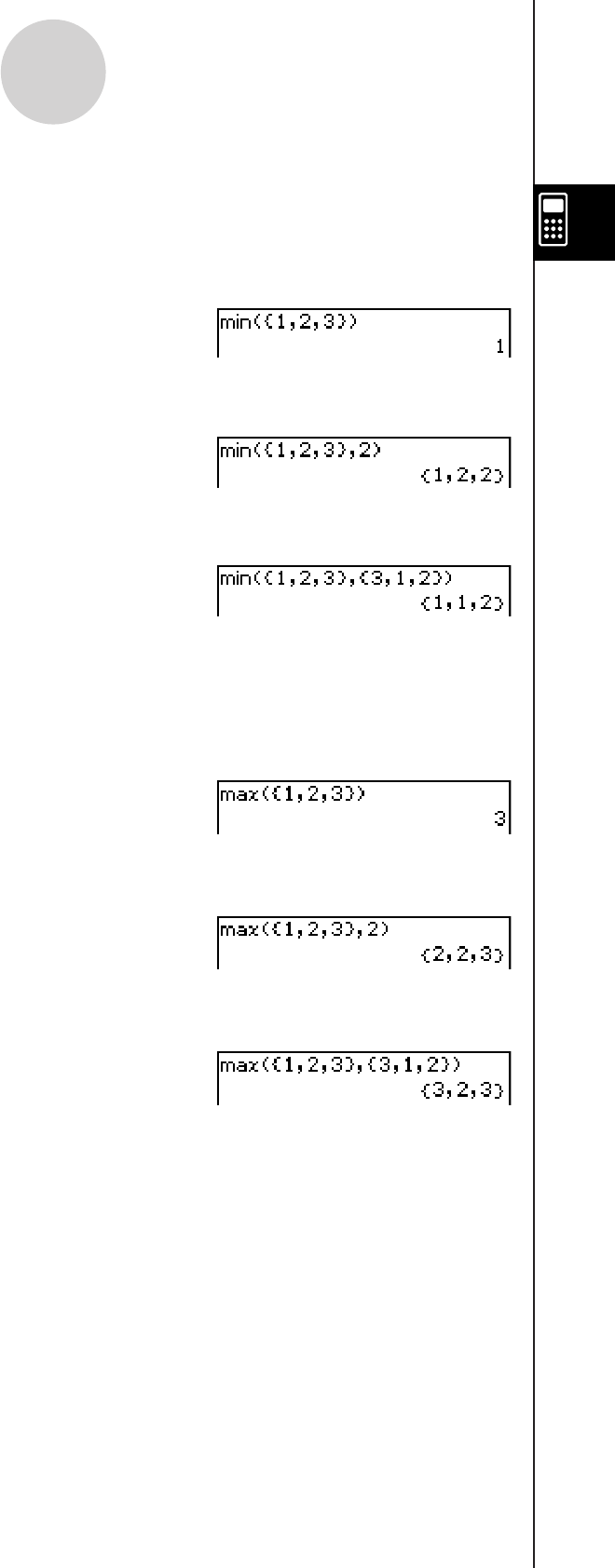
20060301

u min

Function: Returns the minimum value of an expression or the elements in a list.

Syntax: min (Exp/List-1[, Exp/List-2] [

)

]

Example: To determine the minimum values of the elements in list {1, 2, 3}

Menu Item: [Action][List-Calculation][min]

Example: To compare each element of list {1, 2, 3} with the value 2, and produce a list

whose elements contain the lesser value of each comparison

Menu Item: [Action][List-Calculation][min]

Example: To compare the elements of list {1, 2, 3} and list {3, 1, 2}, and produce a list

whose elements contain the lesser value of each comparison

Menu Item: [Action][List-Calculation][min]

2-8-25

Using the Action Menu

u max

Function: Returns the maximum value of an expression or the elements of a list.

Syntax: max (Exp/List-1[, Exp/List-2] [

)

]

Example: To determine the maximum value of the elements in list {1, 2, 3}

Menu Item: [Action][List-Calculation][max]

Example: To compare each element of list {1, 2, 3} with the value 2, and produce a list

whose elements contain the greater value of each comparison

Menu Item: [Action][List-Calculation][max]

Example: To compare the elements of list {1, 2, 3} and list {3, 1, 2}, and produce a list

whose elements contain the greater value of each comparison

Menu Item: [Action][List-Calculation][max]

20060301

Example: To determine the mean of the elements in the list {1, 2, 3}, whose respective

frequencies are {3, 2, 1}

Menu Item: [Action][List-Calculation][mean]

u median

Function: Returns the median of the elements in a list.

Syntax: median (List-1[, List-2] [

)

]

• “List-2” specifies the frequency of each element in “List-1”.

Example: To determine the median of the elements in the list {1, 2, 3}

Menu Item: [Action][List-Calculation][median]

Example: To determine the median of the elements in the list {1, 2, 3}, whose respective

frequencies are {3, 2, 1}

Menu Item: [Action][List-Calculation][median]

u mode

Function: Returns the mode of the elements in a list.

Syntax: mode (List-1[, List-2] [

)

]

• “List-2” specifies the frequency of each element in “List-1”.

Example: To determine the mode of the elements in the list {1, 1, 2, 2, 2}

Menu Item: [Action][List-Calculation][mode]

Example: To determine the mode of the elements in the list {1, 2, 3}, whose respective

frequencies are {3, 2, 1}

Menu Item: [Action][List-Calculation][mode]

• If there are multiple modes, they are returned in a list.

2-8-26

Using the Action Menu

u mean

Function: Returns the mean of the elements in a list.

Syntax: mean (List-1[, List-2] [

)

]

• “List-2” specifies the frequency of each element in “List-1”.

Example: To determine the mean of the elements in list {1, 2, 3}

Menu Item: [Action][List-Calculation][mean]

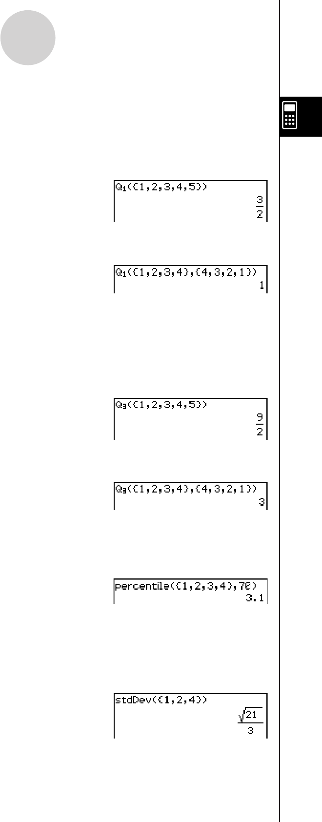
20101001

u Q1

Function: Returns the first quartile of the elements in a list.

Syntax: Q1 (List-1[, List-2] [

)

]

• “List-2” specifies the frequency of each element in “List-1”.

Example: To determine the first quartile of the elements in the list {1, 2, 3, 4, 5}

Menu Item: [Action][List-Calculation][Q1]

Example: To determine the first quartile of the elements in the list {1, 2, 3, 4}, whose

respective frequencies are {4, 3, 2, 1}

Menu Item: [Action][List-Calculation][Q1]

u Q3

Function: Returns the third quartile of the elements in a list.

Syntax: Q3 (List-1[, List-2] [

)

]

• “List-2” specifies the frequency of each element in “List-1”.

Example: To determine the third quartile of the elements in the list {1, 2, 3, 4, 5}

Menu Item: [Action][List-Calculation][Q3]

Example: To determine the third quartile of the elements in the list {1, 2, 3, 4}, whose

respective frequencies are {4, 3, 2, 1}

Menu Item: [Action][List-Calculation][Q3]

u percentile

Function: Finds the nth percentile point in a list.

Syntax: percentile ( list, number )

u stdDev

Function: Returns the sample standard deviation of the elements in a list.

Syntax: stdDev (List [

)

]

Example: To determine the sample standard deviation of the elements in the list {1, 2, 4}

Menu Item: [Action][List-Calculation][stdDev]

2-8-27

Using the Action Menu

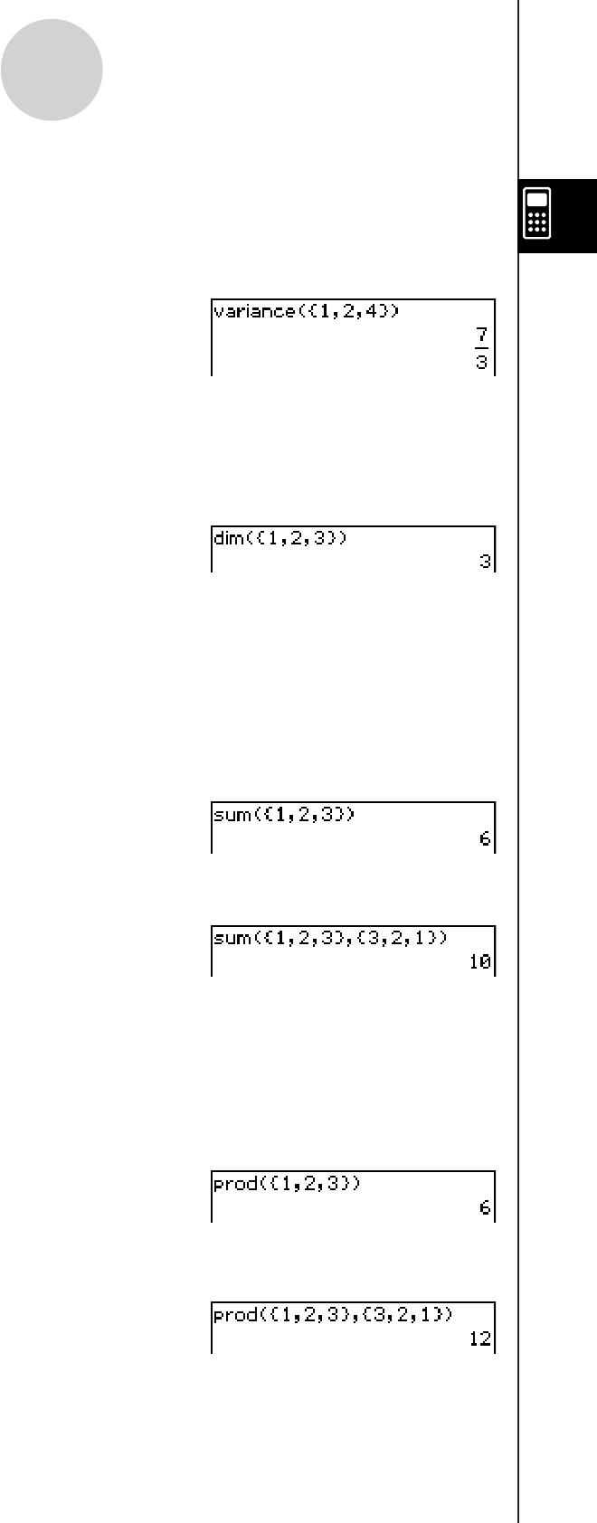
20060301

u variance

Function: Returns the sample variance of the elements in a list.

Syntax: variance (List [

)

]

Example: To determine the sample variance of the elements in the list {1, 2, 4}

Menu Item: [Action][List-Calculation][variance]

u dim

Function: Returns the dimension of a list.

Syntax: dim (List [

)

]

Example: To determine the dimension of the list {1, 2, 3}

Menu Item: [Action][List-Calculation][dim]

u sum

Function: Returns the sum of the elements in a list.

Syntax: sum (List-1[, List-2] [

)

]

• “List-2” specifies the frequency of each element in “List-1”.

Example: To determine the sum of the elements in the list {1, 2, 3}

Menu Item: [Action][List-Calculation][sum]

Example: To determine the sum of the elements in the list {1, 2, 3}, whose respective

frequencies are {3, 2, 1}

Menu Item: [Action][List-Calculation][sum]

u prod

Function: Returns the product of the elements in a list.

Syntax: prod (List-1[, List-2] [

)

]

• “List-2” specifies the frequency of each element in “List-1”.

Example: To determine the product of the elements in the list {1, 2, 3}

Menu Item: [Action][List-Calculation][prod]

Example: To determine the product of the elements in the list {1, 2, 3}, whose respective

frequencies are {3, 2, 1}

Menu Item: [Action][List-Calculation][prod]

2-8-28

Using the Action Menu

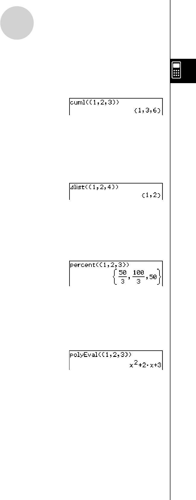
20060301

2-8-29

Using the Action Menu

u cuml

Function: Returns the cumulative sums of the elements in a list.

Syntax: cuml (List [

)

]

Example: To determine the cumulative sums of the elements in the list {1, 2, 3}

Menu Item: [Action][List-Calculation][cuml]

u Alist

Function: Returns a list whose elements are the differences between two adjacent

elements in another list.

Syntax: Alist (List [

)

]

Example: To generate a list whose elements are the differences between two adjacent

elements in the list {1, 2, 4}

Menu Item: [Action][List-Calculation][Alist]

u percent

Function: Returns the percentage of each element in a list, the sum of which is assumed

to be 100.

Syntax: percent (List [

)

]

Example: To determine the percentage of each element in the list {1, 2, 3}

Menu Item: [Action][List-Calculation][percent]

u polyEval

Function: Returns a polynomial arranged in the descending order of powers, so

coefficients correspond sequentially to each element in the input list.

Syntax: polyEval (List [,Exp/List] [

) ]

Example: To create a second degree polynomial with the coefficients {1, 2, 3}

Menu Item: [Action][List-Calculation][polyEval]

• “x” is the default when you omit “[,Exp/List]”.

20060301

2-8-30

Using the Action Menu

u sequence

Function: Returns the lowest-degree polynomial that represents the sequence expressed

by the input list. When there are two lists, this command returns a polynomial

that maps each element in the first list to its corresponding element in the

second list.

Syntax: sequence (List-1[, List-2] [,variable] [

)

]

• “x” is the default when you omit “[,variable]”.

Example: To determine a polynomial for a sequence expressed by the list {3, 5, 7, 9}

Menu Item: [Action][List-Calculation][sequence]

Example: To determine a polynomial that maps each element in the list {1, 3, 5, 7} to its

corresponding element in the list {0, –1, 2, –3}.

Menu Item: [Action][List-Calculation][sequence]

u sumSeq

Function: Finds the lowest-degree polynomial that represents the sequence expressed

by the input list and returns the sum of the polynomial. When there are two

lists, this command returns a polynomial that maps each element in the first

list to its corresponding element in the second list, and returns the sum of the

polynomial.

Syntax: sumSeq (List-1[, List-2] [,variable] [

)

]

• “x” is the default when you omit “[,variable]”.

Example: To determine the sum of a polynomial for a sequence expressed by the list

{3, 5, 7, 9}

Menu Item: [Action][List-Calculation][sumSeq]

Example: To obtain the polynomial that maps the elements in the list {9, 7, 4, 1} to

its corresponding elements in the list {0, 4, 6, 5}, and return the sum of the

polynomial.

Menu Item: [Action][List-Calculation][sumSeq]

20101001

2-8-31

Using the Action Menu

Using the Matrix-Create Submenu

The [Matrix-Create] submenu contains commands related to creation of matrices.

u trn

Function: Returns a transposed matrix.

Syntax: trn (Mat [

)

]

Example: To transpose the matrix [[1, 2] [3, 4]]

Menu Item: [Action][Matrix-Create][trn]

u augment

Function: Returns a matrix that combines two other matrices.

Syntax: augment (Mat-1, Mat-2 [

)

]

Example: To combine the two matrices [[1, 2] [3, 4]] and [[5, 6] [7, 8]]

Menu Item: [Action][Matrix-Create][augment]

u ident

Function: Creates an identity matrix.

Syntax: ident (natural number [

)

]

Example: To create a 2 × 2 identity matrix

Menu Item: [Action][Matrix-Create][ident]

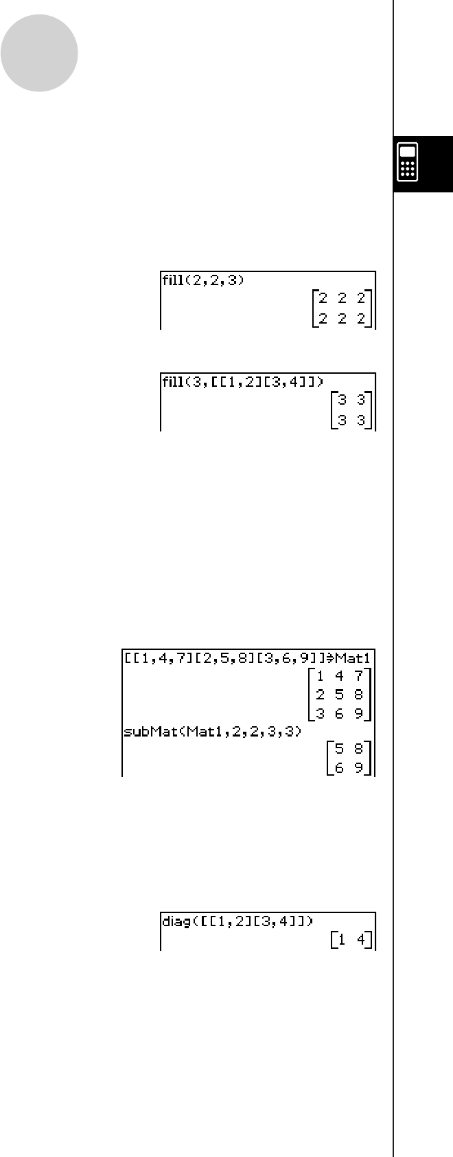
20060301

2-8-32

Using the Action Menu

u fill

Function: Creates a matrix with a specific number of rows and columns, or replaces the

elements of a matrix with a specific expression.

Syntax: fill (Exp, number of rows, number of columns [

)

]

fill (Exp, Mat [

)

]

Example: To create a 2 × 3 matrix, all whose elements are 2

Menu Item: [Action][Matrix-Create][fill]

Example: To replace all of the elements of the matrix [[1, 2] [3, 4]] with 3

Menu Item: [Action][Matrix-Create][fill]

u subMat

Function: Extracts a specific section of a matrix into a new matrix.

Syntax: subMat (Mat [,start row] [,start column] [,end row] [,end column] [

)

]

• “1” is the default when you omit “[, start row]” and “[, start column]”.

• The last row number is the default when you omit “[, end row]”.

• The last column number is the default when you omit “[, end column]”.

Example: To extract the section from row 2, column 2, to row 3, column 3 from the matrix

[[1, 4, 7] [2, 5, 8] [3, 6, 9]]

Menu Item: [Action][Matrix-Create][subMat]

u diag

Function: Returns a one-row matrix containing the elements from the main diagonal of a

square matrix.

Syntax: diag (Mat[

)

]

Example: To extract the diagonal elements of the matrix [[1, 2] [3, 4]]

Menu Item: [Action][Matrix-Create][diag]

u listToMat

• For information about listToMat, see page 2-8-24.

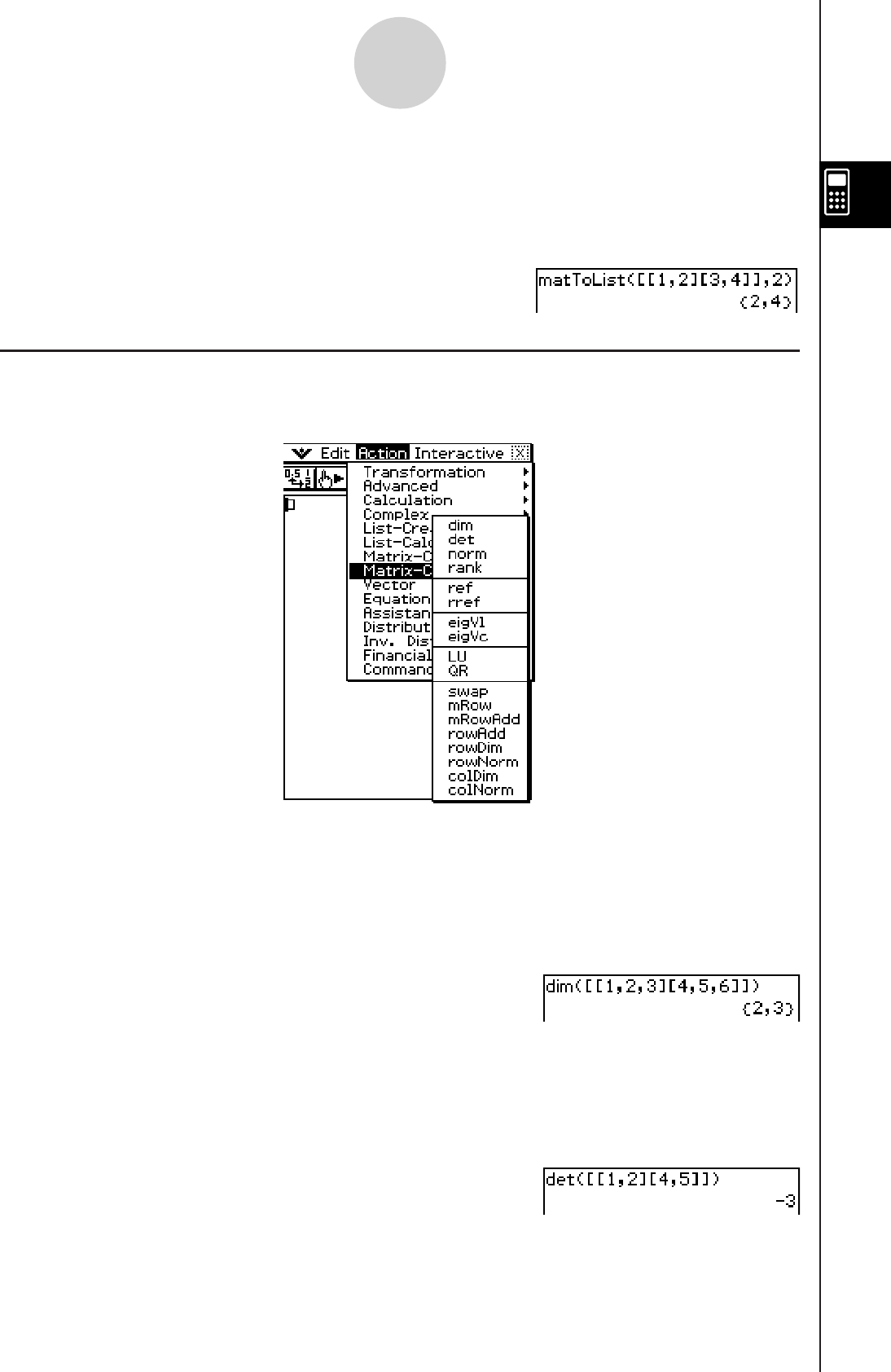
20101001

u matToList

Function: Transforms a specific column of a matrix into a list.

Syntax: matToList (Mat, column number [

)

]

Example: To transform column 2 of the matrix [[1, 2] [3, 4]] into a list

Menu Item: [Action][Matrix-Create][matToList]

Using the Matrix-Calculation Submenu

The [Matrix-Calculation] submenu contains commands that are related to matrix calculations.

2-8-33

Using the Action Menu

u dim

Function: Returns the dimensions of a matrix as a two-element list {number of rows,

number of columns}.

Syntax: dim (Mat [

)

]

Example: To determine the dimensions of the matrix [[1, 2, 3] [4, 5, 6]]

Menu Item: [Action][Matrix-Calculation][dim]

u det

Function: Returns the determinant of a square matrix.

Syntax: det (Mat [

)

]

Example: To obtain the determinant of the matrix [[1, 2] [4, 5]]

Menu Item: [Action][Matrix-Calculation][det]

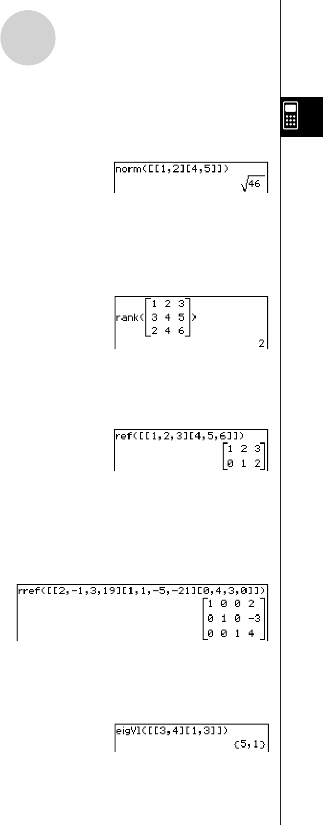
20060301

u norm

Function: Returns the Frobenius norm of the matrix.

Syntax: norm (Mat [

)

]

Example: To determine the norm of the matrix [[1, 2] [4, 5]]

Menu Item: [Action][Matrix-Calculation][norm]

u rank

Function: Finds the rank of matrix.

The rank function computes the rank of a matrix by performing Gaussian

elimination on the rows of the given matrix. The rank of matrix A is the

number of non-zero rows in the resulting matrix.

Syntax: rank (Matrix)

u ref

Function: Returns the row echelon form of a matrix.

Syntax: ref (Mat [

)

]

Example: To obtain the row echelon form of the matrix [[1, 2, 3] [4, 5, 6]]

Menu Item: [Action][Matrix-Calculation][ref]

u rref

Function: Returns the reduced row echelon form of a matrix.

Syntax: rref (Mat [

)

]

Example: To obtain the reduced row echelon form of the matrix [[2, –1, 3, 19] [1, 1, –5, –21]

[0, 4, 3, 0]]

Menu Item: [Action]

[Matrix-Calculation][rref]

u eigVl

Function: Returns a list that contains the eigenvalue(s) of a square matrix.

Syntax: eigVl (Mat [

)

]

Example: To obtain the eigenvalue(s) of the matrix [[3, 4] [1, 3]]

Menu Item: [Action][Matrix-Calculation][eigVl]

2-8-34

Using the Action Menu

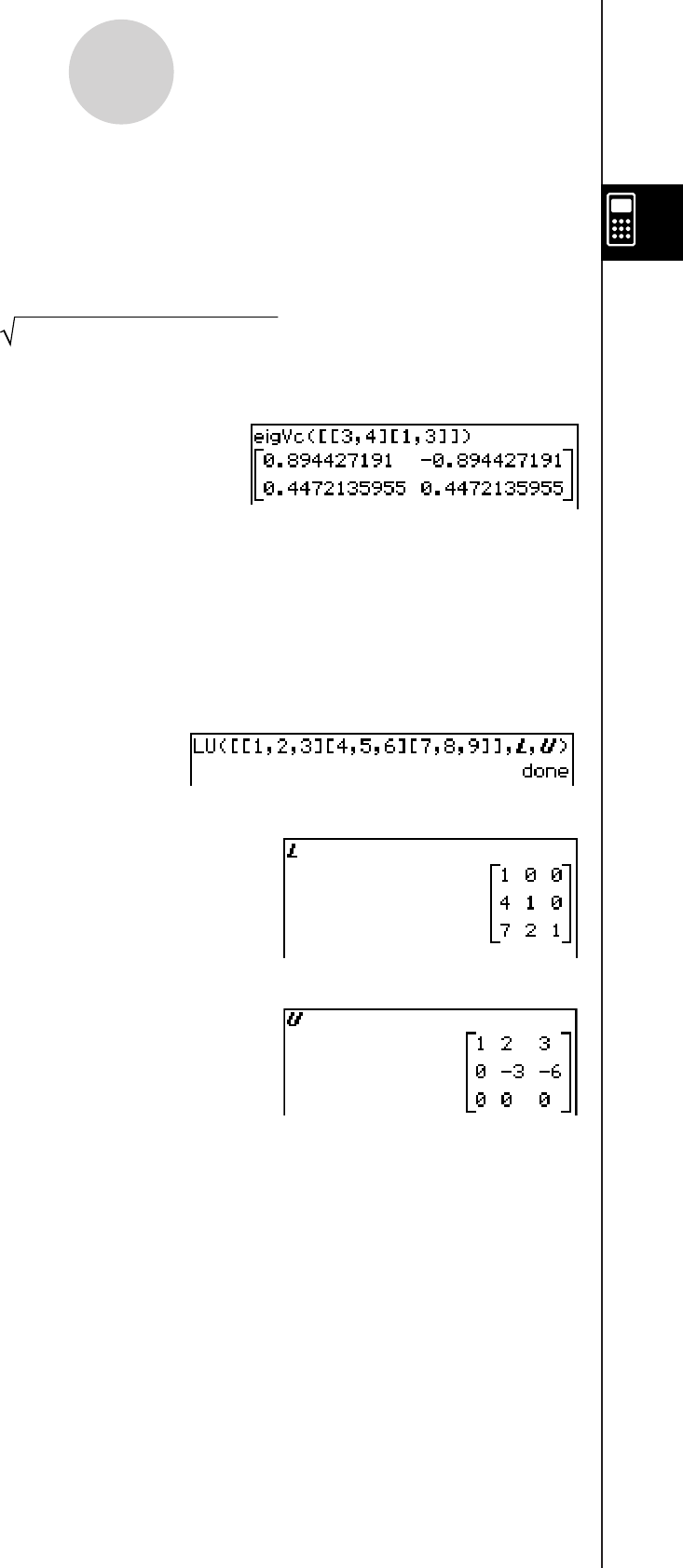
20060301

2-8-35

Using the Action Menu

u eigVc

Function: Returns a matrix in which each column represents an eigenvector of a square

matrix.

• Since an eigenvector usually cannot be determined uniquely, it is standardized as

follows to its norm, which is 1:

When V = [x1, x2, ..., xn], (⎥ x1⎥2 + ⎥ x2⎥2 + .... + ⎥ xn⎥2) = 1.

Syntax: eigVc (Mat [

)

]

Example: To obtain the eigenvector(s) of the matrix [[3, 4] [1, 3]]

Menu Item: [Action][Matrix-Calculation][eigVc]

u LU

Function: Returns the LU decomposition of a square matrix.

Syntax: LU (Mat, lVariableMem, uVariableMem [

)

]

Example: To obtain the LU decomposition of the matrix [[1, 2, 3] [4, 5, 6] [7, 8, 9]]

• The lower matrix is assigned to the first variable L, while the upper matrix is assigned to

the second variable U.

Menu Item: [Action][Matrix-Calculation][LU]

To display the lower matrix

Menu Item: [VAR][CAP][L][EXE]

To display the upper matrix

Menu Item: [VAR][CAP][U][EXE]

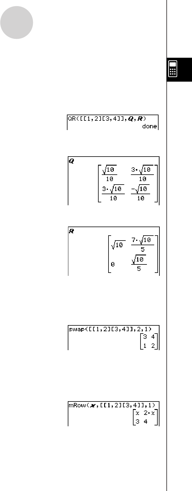
20060301

2-8-36

Using the Action Menu

u QR

Function: Returns the QR decomposition of a square matrix.

Syntax: QR (Mat, qVariableMem, rVariableMem [

)

]

Example: To obtain the QR decomposition of the matrix [[1, 2] [3, 4]]

• The unitary matrix is assigned to variable Q, while the upper triangular matrix is

assigned to variable R.

Menu Item: [Action][Matrix-Calculation][QR]

To display the unitary matrix

Menu Item: [VAR][CAP][Q][EXE]

To display the upper triangular matrix

Menu Item: [VAR][CAP][R][EXE]

u swap

Function: Swaps two rows of a matrix.

Syntax: swap (Mat, row number-1, row number-2 [

)

]

Example: To swap row 1 with row 2 of the matrix [[1, 2] [3, 4]]

Menu Item: [Action][Matrix-Calculation][swap]

u mRow

Function: Multiplies the elements of a specific row in a matrix by a specific expression.

Syntax: mRow (Exp, Mat, row number [

)

]

Example: To multiply row 1 of the matrix [[1, 2] [3, 4]] by x

Menu Item: [Action][Matrix-Calculation][mRow]

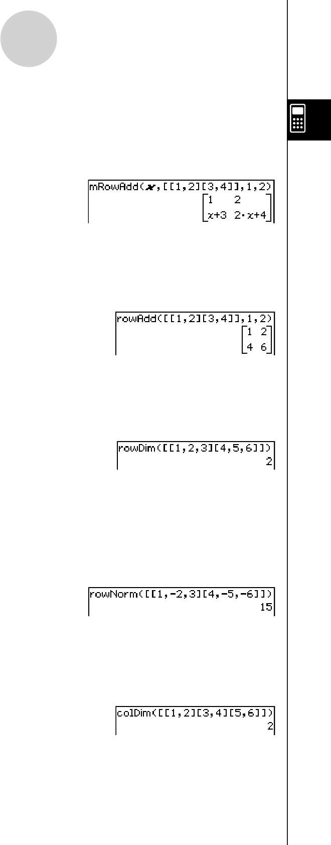
20060301

u mRowAdd

Function: Multiplies the elements of a specific row in a matrix by a specific expression,

and then adds the result to another row.

Syntax: mRowAdd (Exp, Mat, row number-1, row number-2 [

)

]

Example: To multiply row 1 of the matrix [[1, 2] [3, 4]] by x, and then add the result to row 2

Menu Item: [Action][Matrix-Calculation][mRowAdd]

u rowAdd

Function: Adds a specific matrix row to another row.

Syntax: rowAdd (Mat, row number-1, row number-2 [

)

]

Example: To add row 1 of the matrix [[1, 2] [3, 4]] to row 2

Menu Item: [Action][Matrix-Calculation][rowAdd]

u rowDim

Function: Returns the number in rows in a matrix.

Syntax: rowDim (Mat [

)

]

Example: To obtain the number of rows in the matrix [[1, 2, 3] [4, 5, 6]]

Menu Item: [Action][Matrix-Calculation][rowDim]

u rowNorm

Function: Calculates the sums of the absolute values of the elements of each row of a

matrix, and returns the maximum value of the sums.

Syntax: rowNorm (Mat [

)

]

Example: To calculate the sums of the absolute values of the elements in each row of the

matrix [[1, –2, 3] [4, –5, –6]], and obtain the maximum value of the sums

Menu Item: [Action][Matrix-Calculation][rowNorm]

u colDim

Function: Returns the number of columns in a matrix.

Syntax: colDim (Mat [

)

]

Example: To obtain the number of columns in the matrix [[1, 2] [3, 4] [5, 6]]

Menu Item: [Action][Matrix-Calculation][colDim]

2-8-37

Using the Action Menu

20101001

2-8-38

Using the Action Menu

u colNorm

Function: Calculates the sums of the absolute values of the elements of each column of a

matrix, and returns the maximum value of the sums.

Syntax: colNorm (Mat [

)

]

Example: To calculate the sums of the absolute values of the elements in each column of

the matrix [[1, –2, 3][4, –5, –6][–7, 8, 9]], and obtain the maximum value of the

sums

Menu Item: [Action][Matrix-Calculation]

[colNorm]

Using the Vector Submenu

The [Vector] submenu contains commands that are related to vector calculations.

• A vector is handled as a 1 × N matrix or N × 1 matrix.

• A vector in the form of 1 × N can be entered as [……] or [[……]].

Example: [1, 2], [[1, 2]]

• Vectors are considered to be in rectangular form unless ∠() is used to indicate an angle

measure.

20060301

u augment

Function: Returns an augmented vector [Mat-1 Mat-2].

Syntax: augment (Mat-1, Mat-2 [

)

]

Example: To augment vectors [1, 2] and [3, 4]

Menu Item: [Action][Vector][augment]

u fill

Function: Creates a vector that contains a specific number of elements, or replaces the

elements of a vector with a specific expression.

Syntax: fill (Exp, Mat [

)

]

fill (Exp, 1, number of columns [

)

]

Example: To replace the elements of the vector [1, 2] with x

Menu Item: [Action][Vector][fill]

Example: To create a 1 × 3 (1 row, 3 columns) vector, all of whose elements are “3”

Menu Item: [Action][Vector][fill]

u dim

Function: Returns the dimension of a vector.

Syntax: dim (Mat [

)

]

Example: To determine the dimension of the vector [1, 2, 3]

Menu Item: [Action][Vector][dim]

• The vector [1, 2, 3] is handled as a 1 × 3 matrix.

u unitV

Function: Normalizes a vector.

Syntax: unitV (Mat [

)

]

• This command can be used with a 1 × N or N × 1 matrix only.

Example: To normalize the vector [1, 3, 5]

Menu Item: [Action][Vector][unitV]

2-8-39

Using the Action Menu

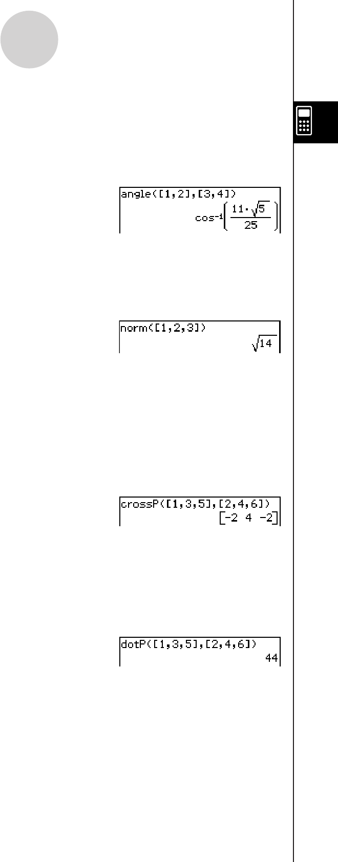
20060301

u angle

Function: Returns the angle formed by two vectors.

Syntax: angle (Mat-1, Mat-2 [

)

]

• This command can be used with a 1 × N or N × 1 matrix only.

Example: To determine the angle formed by vectors [1, 2] and [3, 4] (in the Radian mode)

Menu Item: [Action][Vector][angle]

u norm

Function: Returns the norm of a vector.

Syntax: norm (Mat [

)

]

Example: To obtain the norm of the vector [1, 2, 3]

Menu Item: [Action][Vector][norm]

u crossP

Function: Returns the cross product of two vectors.

Syntax: crossP (Mat-1, Mat-2 [

)

]

• This command can be used with a 1 × N or N × 1 matrix only (N = 2, 3).

• A two-element matrix [a, b] or [[a], [b]] is automatically converted into a three-element

matrix [a, b, 0] or [[a], [b], [0]].

Example: To obtain the cross product of the two vectors [1, 3, 5] and [2, 4, 6]

Menu Item: [Action][Vector][crossP]

u dotP

Function: Returns the dot product of two vectors.

Syntax: dotP (Mat-1, Mat-2 [

)

]

• This command can be used with a 1 × N or N × 1 matrix only.

Example: To obtain the dot product of the two vectors [1, 3, 5] and [2, 4, 6]

Menu Item: [Action][Vector][dotP]

2-8-40

Using the Action Menu

20060301

u toRect

Function: Returns an equivalent rectangular form [x y] or [x y z].

Syntax: toRect (Mat [,natural number] [

)

]

• This command can be used with a 1 × N or N × 1 matrix only (N = 2, 3).

• This command returns “x” when “natural number” is 1, “y” when “natural number” is 2,

and “z” when “natural number” is 3.

• This command returns a rectangular form when you omit “natural number”.

Example: To transform the polar form [ 2 , ∠(π/4)] into an equivalent rectangular form

(in the Radian mode)

Menu Item: [Action][Vector][toRect]

u toPol

Function: Returns an equivalent polar form [r∠].

Syntax: toPol (Mat [,natural number] [

)

]

• This command can be used with a 1 × 2 or 2 × 1 matrix only.

• This command returns “r” when “natural number” is 1, and “

” when “natural number” is 2.

• This command returns a polar form when you omit “natural number”.

Example: To transform the rectangular form [1, 2] into its equivalent polar form

Menu Item: [Action][Vector][toPol]

u toSph

Function: Returns an equivalent spherical form [

∠ ∠

Syntax: toSph (Mat [,natural number] [

)

]

• This command can be used with a 1 × 3 or 3 × 1 matrix only.

• This command returns “

” when “natural number” is 1, “

” when “natural number” is 2,

and “

” when “natural number” is 3.

• This command returns a spherical form when you omit “natural number”.

Example: To transform the rectangular form [1, 1, 1] into its equivalent spherical form

(in the Radian mode)

Menu Item: [Action][Vector][toSph]

2-8-41

Using the Action Menu

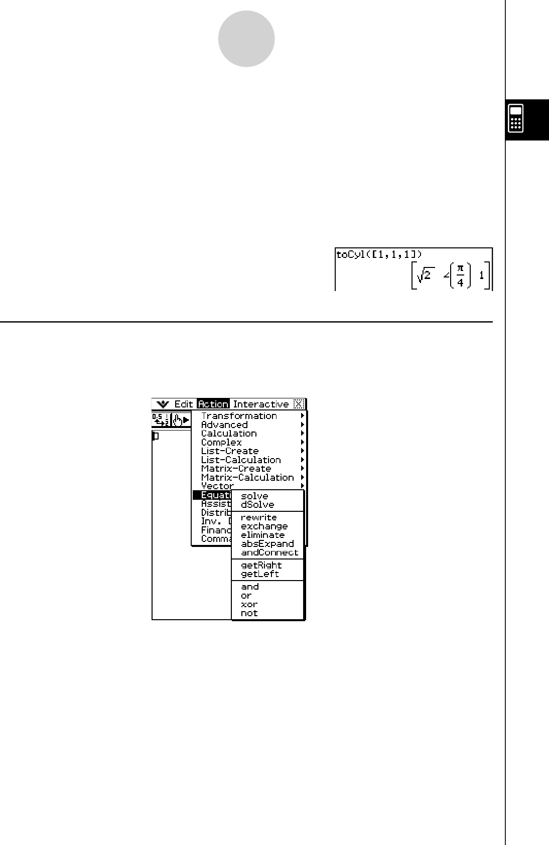
20101001

u toCyl

Function: Returns an equivalent cylindrical form [r∠

z].

Syntax: toCyl (Mat [,natural number] [

)

]

• This command can be used with a 1 × 3 or 3 × 1 matrix only.

• This command returns “r” when “natural number” is 1, “

” when “natural number” is 2,

and “z” when “natural number” is 3.

• This command returns a cylindrical form when you omit “natural number”.

Example: To transform the rectangular form [1, 1, 1] into an equivalent cylindrical form

(in the Radian mode)

Menu Item: [Action][Vector][toCyl]

Using the Equation/Inequality Submenu

The [Equation/Inequality] submenu contains commands that are related to equations and

inequalities.

2-8-42

Using the Action Menu

20090601

2-8-43

Using the Action Menu

u solve

Function: Returns the solution of an equation or inequality.

Syntax: solve(Exp/Eq/Ineq [,variable] [

)

]

• For this syntax, “Ineq” also includes the ⫽ operator.

• “x” is the default when you omit “[,variable]”.

solve(Exp/Eq,variable[, value, lower limit, upper limit] [

)

]

• This syntax does not support “Ineq”, but the ⫽ operator is supported.

• “value” is an initially estimated value.

• This command is valid only for equations and ⫽ expressions when “value”

and the items following it are included. In that case, this command returns

an approximate value.

• A true value is returned when you omit “value” and the items following it.

When, however, a true value cannot be obtained, an approximate value is

returned for equations only based on the assumption that value = 0, lower

limit = –∞, and upper limit = ∞.

solve({Exp-1/Eq-1, ..., Exp-N/Eq-N}, {variable-1, ..., variable-N} [

)

]

• When “Exp” is the first argument, the equation Exp = 0 is presumed.

Example: To solve ax + b = 0 for x

Menu Item: [Action][Equation/Inequality][solve]

Example: To solve simultaneous linear equations 3x + 4y = 5, 2x – 3y = –8

Menu Item: [Action][Equation/Inequality][solve]

You also could input the simultaneous equations shown in this example using the 2D

keyboard key. The following shows the required input syntax.

Exp-1/Eq-1

Exp-N/Eq-N variable-1, ..., variable-N

• The following shows the required key operation to input this example using the key.

d≈+eY=fcc≈-dY=-i

e≈,Yw

• To input simultaneous equations with three or more unknowns, press the key when

the cursor is in the Exp-N/Eq-N input field. Each press of will add one more line for

input of an equation.

20090601

2-8-44

Using the Action Menu

Note

For the solution, the solve function returns an expression or value for the expression

(Exp/Eq) input as its argument. The message “More solutions may exist” will appear on

the display when a value is returned as the solution, because there may be multiple

solutions.

The solve function can return a maximum of 10 solutions in the case of values.

Example: To solve cos (x) = 0.5 for x (initial value: 0)

Menu Item: [Action][Equation/Inequality][solve]

(Angle unit setting: Deg)

u dSolve

Function: Solves first, second or third order ordinary differential equations, or a system of

first order differential equations.

Syntax: dSolve(Eq, independent variable, dependent variable [, initial condition-1, initial

condition-2][, initial condition-3, initial condition-4][, initial condition-5, initial

condition-6] [

)

]

dSolve({Eq-1, Eq-2}, independent variable, {dependent variable-1, dependent

variable-2} [, initial condition-1, initial condition-2, initial condition-3, initial

condition-4] [

)

]

• If you omit the initial conditions, the solution will include arbitrary constants.

• Input all initial conditions equations using the syntax Var = Exp. Any initial condition that

uses any other syntax will be ignored.

Example: To solve a differential equation y’ = x, where y = 1 when x = 0.

Menu Item: [Action][Equation/Inequality][dSolve]

Example: To solve the system of first order differential equations y’ = y + z, z’ = y – z,

where “x” is the independent variable, “y” and “z” are the dependent variables,

and the initial conditions are y = 3 when x = 0, and z = 2 – 3 when x = 0

Menu Item: [Action][Equation/Inequality][dSolve]

u rewrite

Function: Moves the right side elements of an equation or inequality to the left side.

Syntax: rewrite(Eq/Ineq/List [

)

]

• Ineq (inequality) includes the “≠” (not equal to) relational operator.

Example: To move the right side elements of x + 3 = 5x – x2 to the left side

Menu Item: [Action][Equation/Inequality][rewrite]

20090601

2-8-45

Using the Action Menu

u exchange

Function: Swaps the right-side and left-side elements of an equation or inequality.

Syntax: exchange(Eq/Ineq/List [

)

]

• Ineq (inequality) includes the “≠” (not equal to) relational operator.

Example: To swap the left-side and right-side elements of 3 > 5x – 2y

Menu Item: [Action][Equation/Inequality][exchange]

u eliminate

Function: Solves one equation with respect to a variable, and then replaces the same

variable in another expression with the obtained result.

Syntax: eliminate(Eq/Ineq/List-1, variable, Eq-2 [

)

]

• Ineq (inequality) includes the “≠” (not equal to) relational operator.

Example: To transform y = 2x + 3 to x =, and substitute the result into 2x + 3y = 5

Menu Item: [Action][Equation/Inequality][eliminate]

u absExpand

Function: Divides an absolute value expression into formulas without absolute value.

Syntax: absExpand(Eq/Ineq [

)

]

• Ineq (inequality) includes the “≠” (not equal to) relational operator.

Example: To remove the absolute value from ⎜2x – 3 ⎜ = 9

Menu Item: [Action][Equation/Inequality][absExpand]

u andConnect

Function: Combines two equations or inequalities into a single expression.

Syntax: andConnect(Eq/Ineq-1, Eq/Ineq-2 [

)

]

• Ineq (inequality) includes the “≠” (not equal to) relational operator.

Example: To rewrite x > –1 and x < 3 into a single inequality

Menu Item: [Action][Equation/Inequality][andConnect]

u getRight

Function: Extracts the right-side elements of an equation or inequality.

Syntax: getRight(Eq/Ineq/List [

)

]

• Ineq (inequality) includes the “≠” (not equal to) relational operator.

Example: To extract the right side elements of y = 2x2 + 3x + 5

Menu Item: [Action][Equation/Inequality][getRight]

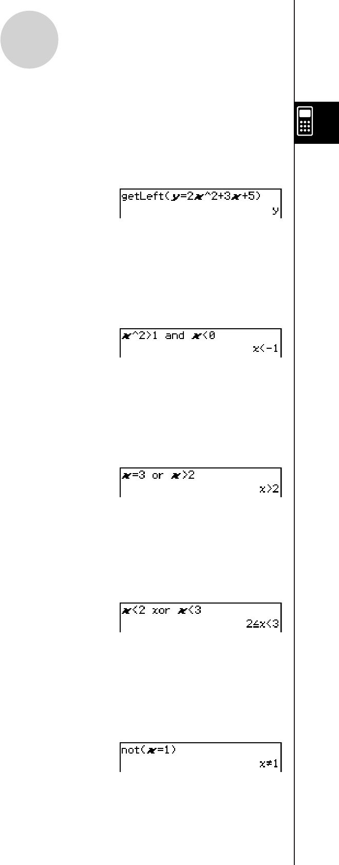
20090601

2-8-46

Using the Action Menu

u getLeft

Function: Extracts the left-side elements of an equation or inequality.

Syntax: getLeft(Eq/Ineq/List [

)

]

• Ineq (inequality) includes the “≠” (not equal to) relational operator.

Example: To extract the left side elements of y = 2x2 + 3x + 5

Menu Item: [Action][Equation/Inequality][getLeft]

u and

Function: Returns the result of the logical AND of two expressions.

Syntax: Exp/Eq/Ineq/List-1 and Exp/Eq/Ineq/List-2

• Ineq (inequality) includes the “≠” (not equal to) relational operator.

Example: To obtain the result of the logical AND of x2 > 1 and x < 0

Menu Item: [Action][Equation/Inequality][and]

u or

Function: Returns the result of the logical OR of two expressions.

Syntax: Exp/Eq/Ineq/List-1 or Exp/Eq/Ineq/List-2

• Ineq (inequality) includes the “≠” (not equal to) relational operator.

Example: To obtain the result of the logical OR of x = 3 or x > 2

Menu Item: [Action][Equation/Inequality][or]

u xor

Function: Returns the logical exclusive OR of two expressions.

Syntax: Exp/Eq/Ineq/List-1 xor Exp/Eq/Ineq/List-2

• Ineq (inequality) includes the “≠” (not equal to) relational operator.

Example: To obtain the logical exclusive OR of x < 2 xor x < 3

Menu Item: [Action][Equation/Inequality][xor]

u not

Function: Returns the logical NOT of an expression.

Syntax: not(Exp/Eq/Ineq/List [

)

]

• Ineq (inequality) includes the “≠” (not equal to) relational operator.

Example: To obtain the logical NOT of x = 1

Menu Item: [Action][Equation/Inequality][not]

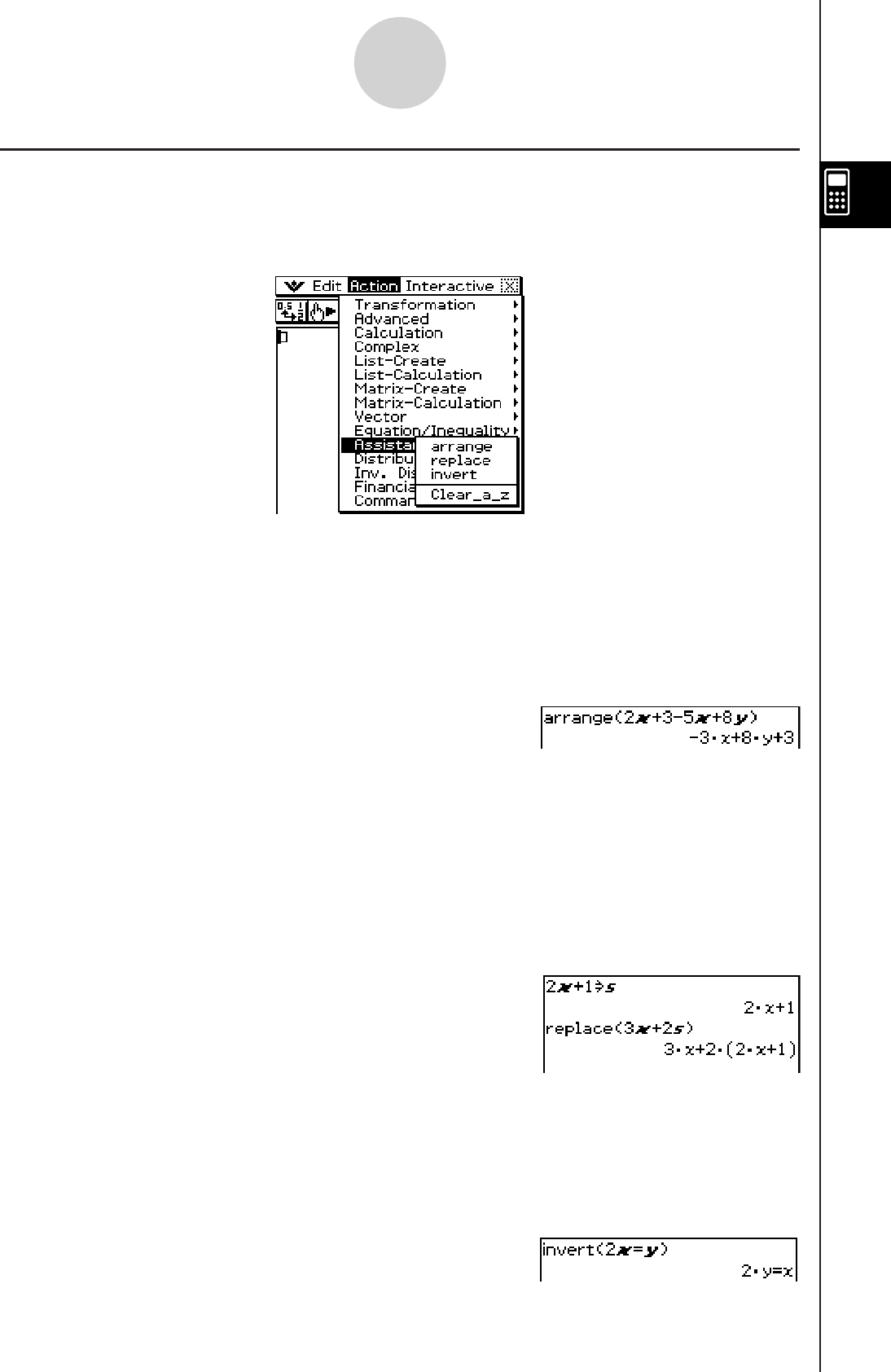
20101001

2-8-47

Using the Action Menu

Using the Assistant Submenu

The [Assistant] submenu contains two commands related to the Assistant mode.

• Note that the following commands are valid in the Assistant mode only. For more

information on the Assistant mode see “Assistant Mode and Algebra Mode” on page 2-2-8.

u arrange

Function: Collects like terms and arranges them in descending order, starting with the

term that contains the smallest coefficient.

Syntax: arrange (Exp/Eq/Ineq/List/Mat [

)

]

• Ineq (inequality) includes the “⫽” (not equal to) relational operator.

Example: To arrange 2x + 3 – 5x + 8y in the sequence of its variables

Menu Item: [Action][Assistant][arrange]

u replace

Function: Replaces the variable in an expression, equation or inequality with the value

assigned to a variable using the “store” command.

Syntax: replace (Exp/Eq/Ineq/List/Mat [

)

]

• Ineq (inequality) includes the “⫽” (not equal to) relational operator.

Example: To replace s in the expression 3x + 2s, when the expression 2x + 1

is assigned to s

Menu Item: [Action][Assistant][replace]

u invert

Function: Inverts two variables in an expression.

Syntax: invert (Exp/Eq/Ineq/List [,variable-1, variable-2] [

)

]

• Ineq (inequality) includes the “⫽” (not equal to) relational operator.

Example: To invert x and y in the expression 2x = y

Menu Item: [Action][Transformation][invert]

• x and y are inverted when variables are not specified.

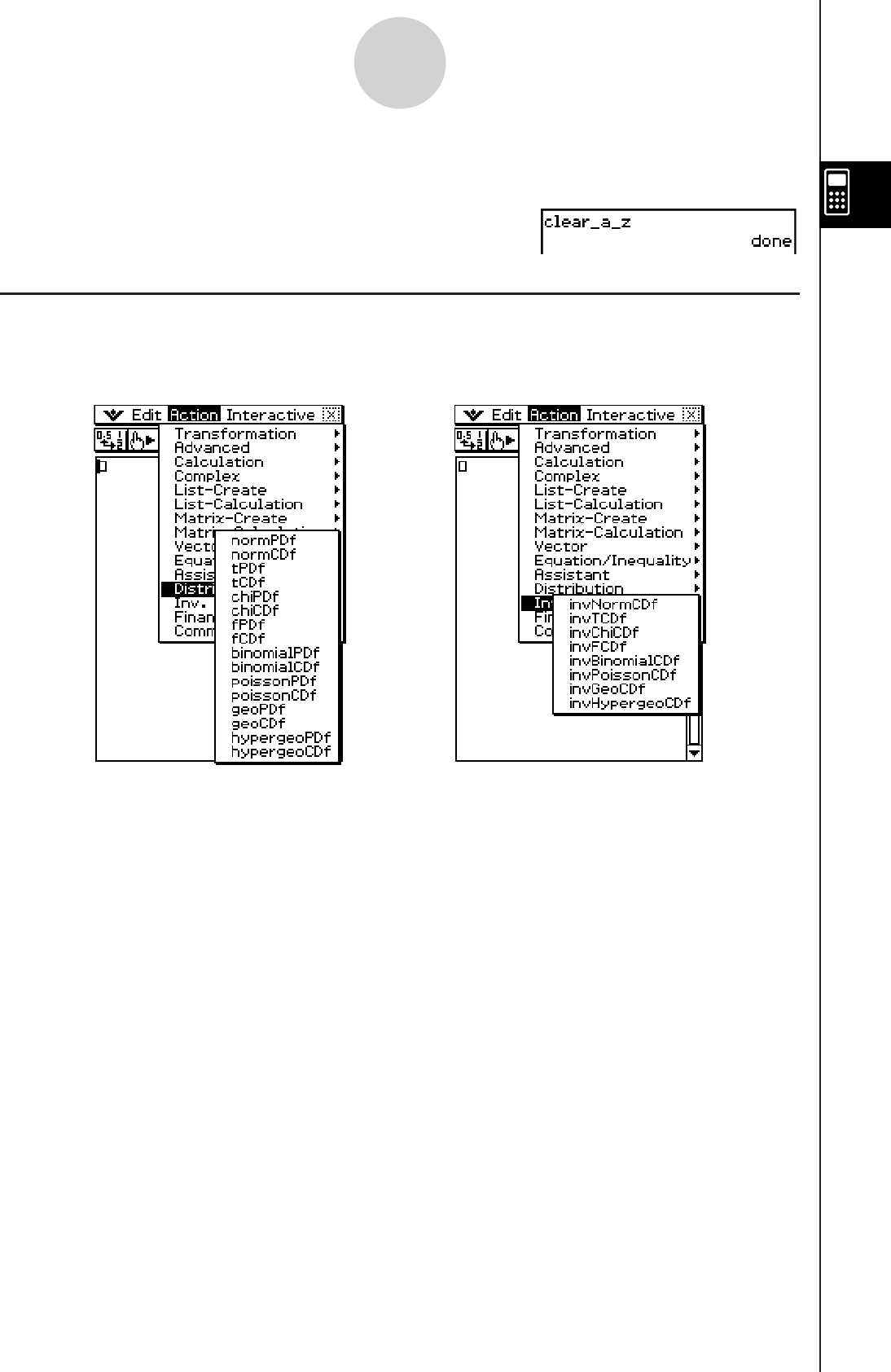
20101001

2-8-48

Using the Action Menu

u Clear_a_z

Function: Clears all single-character variable names (a-z and A-Z) in the current folder.

Using the Distribution and Inv. Distribution Submenus

The [Distribution] and [Inv. Distribution] submenus include functions related to each type of

statistical calculation distribution probability.

Note

The functions on the [Distribution] and [Inv. Distribution] submenus perform the same calculations

as the Distribution commands that are available in the Statistics application and the Main, eActivity,

and Program applications. For information about the numeric expressions used in calculations,

the meanings of the variables used in the syntaxes of the functions presented in this section, and

the system variables that store the values obtained as calculation results, see the “Distribution

Command List” on pages 7-11-3 to 7-11-26.

Also see the “Distribution Command List” for information about how to use Distribution commands

in the Statistics application and the required syntax when using Distribution commands within other

applications.

Specifying Arguments within the Distribution Function

You can specify either values or list data for any of the arguments within the Distribution

function. The normPDf function (page 2-8-49) syntax (normPDf(x, , )) that returns normal

probability density can be used to perform the calculations shown below. The “Number

Format” setting is “Fix 2” for all calculation results.

normPDf(1, 1, 0) = 0.24

normPDf({1, 2}, 1, 0) = {0.24, 0.05}

normPDf(1, {1, 2}, 0) = {0.24, 0.18}

20090601

normPDf({1, 2},{1, 2}, 0) = {0.24, 0.12}

normPDf({1, 2},{1, 2},{1, 0}) = {0.40, 0.12}

The following explains how to specify list data in arguments and how calculation results are

output.

(a) Specifying list data for a single argument

• Basically, you can specify any list you like, but the each of the elements in the list must

be in accordance with the conditions required by the argument of the function being

used.

• Calculation is performed on each element within the list and results are output as

shown below.

normPDf(x, {1, 2}, )

= {<normPDf(x, 1, ) calculation result>, <normPDf(x, 2, ) calculation result>}

(b) Specifying list data for multiple arguments

• In this case, all of the lists must have the same number of elements. Otherwise an

Invalid Dimension error will occur.

• Calculation is performed on each element within the list and results are output as

shown below.

normPDf({x1, x2}, {1, 2}, )

= {<normPDf(x1, 1, ) calculation results>, <normPDf(x2, 2, ) calculation results>}

Assignment of List Data Calculation Results to Variables

Using the list data in the argument of the Distribution function causes calculation results to

be output as list data, which is assigned as-is to the “ans” variable.

In addition to the “ans” variable, calculations that use the Distribution function causes

calculation results also to be assigned to certain system variables. For example, the normal

probability density variable returned by normPDf is assigned to system variable prob. Only

the last element of the list data will be assigned to a system variable as a calculation result.

For information about which calculation result is assigned to which variable, see the

“Calculation Result Output” item for each command in “7-11 Distributions” (pages 7-11-3 to

7-11-25).

u normPDf

Function: Returns the normal probability density for a specified value.

Syntax: normPDf(x[,

)]

• When

and

are skipped,

= 1 and

= 0 are used.

Example: To determine the normal probability density when x = 37.5,

= 2,

= 35

Menu Item: [Action][Distribution][normPDf]

For more information, see “Normal Probability Density” on page 7-11-3.

2-8-49

Using the Action Menu

20090601

u normCDf

Function: Returns the cumulative probability of a normal distribution between a lower

bound and an upper bound.

Syntax: normCDf(lower value, upper value[,

)]

• When

and

are skipped,

= 1 and

= 0 are used.

Example: To determine the normal probability density when lower bound value = −∞,

upper bound value = 36,

= 2,

= 35

Menu Item: [Action][Distribution][normCDf]

For more information, see “Normal Cumulative Distribution” on page 7-11-4.

u invNormCDf

Function: Returns the boundary value(s) of a normal cumulative distribution probability

for specified values.

Syntax: invNormCDf([tail setting, ]area value[,

)]

• When

and

are skipped,

= 1 and

= 0 are used.

• “tail setting” displays the probability value tail specification, and Left, Right, or Center

can be specified. Enter the following values or letters to specify:

Left: −1, “L”, or “l”

Center: 0, “C”, or “c”

Right: 1, “R”, or “r”

When input is skipped, “Left” is used.

• When one argument is omitted (resulting in three arguments), Tail=Left.

• When two arguments are omitted (resulting in two arguments), Tail=Left,

=0.

• When three arguments are omitted (resulting in one argument), Tail=Left,

=1,

=0.

• When “tail setting” is Center, the lower bound value is returned.

Example: To determine the upper bound value when tail setting = Left, area value = 0.7,

= 2,

= 35

Menu Item: [Action][Inv. Distribution][invNormCDf]

For more information, see “Inverse Normal Cumulative Distribution” on page 7-11-5.

u tPDf

Function: Returns the Student-t probability density for a specified value.

Syntax: tPDf(x, df [ ) ]

Example: To determine the Student-t probability density when x = 2, df = 5

Menu Item: [Action][Distribution][tPDf]

For more information, see “Student-t Probability Density” on page 7-11-6.

2-8-50

Using the Action Menu

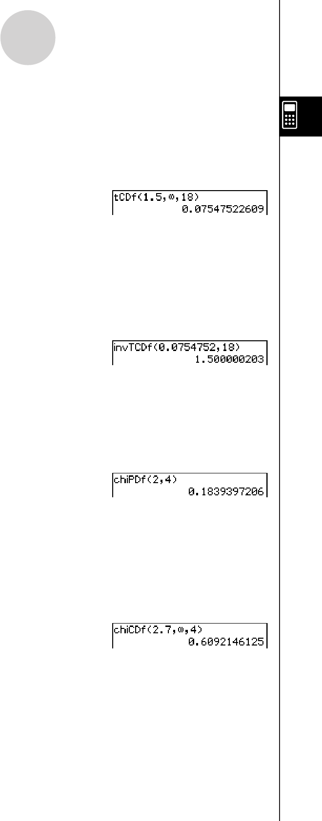
20090601

u tCDf

Function: Returns the cumulative probability of a Student-t distribution between a lower

bound and an upper bound.

Syntax: tCDf(lower value, upper value, df [ ) ]

Example: To determine the Student-t distribution probability when lower value = 1.5,

upper value = ∞, df = 18

Menu Item: [Action][Distribution][tCDf]

For more information, see “Student-t Cumulative Distribution” on page 7-11-7.

u invTCDf

Function: Returns the lower bound value of a Student-t cumulative distribution probability

for specified values.

Syntax: invTCDf(prob, df [ ) ]

Example: To determine the lower bound value when prob = 0.0754752, df = 18

Menu Item: [Action][Inv. Distribution][invTCDf]

For more information, see “Inverse Student-t Cumulative Distribution” on page 7-11-8.

u chiPDf

Function: Returns the χ2 probability density for specified values.

Syntax: chiPDf(x, df [ ) ]

Example: To determine the χ2 probability density when x = 2, df = 4

Menu Item: [Action][Distribution][chiPDf]

For more information, see “2 Probability Density” on page 7-11-9.

u chiCDf

Function: Returns the cumulative probability of a χ2 distribution between a lower bound

and an upper bound.

Syntax: chiCDf(lower value, upper value, df [ ) ]

Example: To determine the χ2 probability when lower value = 2.7, upper value = ∞, df =4

Menu Item: [Action][Distribution][chiCDf]

For more information, see “χ2 Cumulative Distribution” on page 7-11-10.

u invChiCDf

Function: Returns the lower bound value of a χ2 cumulative distribution probability for

specified values.

Syntax: invChiCDf(prob, df [ ) ]

Example: To determine the lower bound value when prob = 0.6092146, df = 4

2-8-51

Using the Action Menu

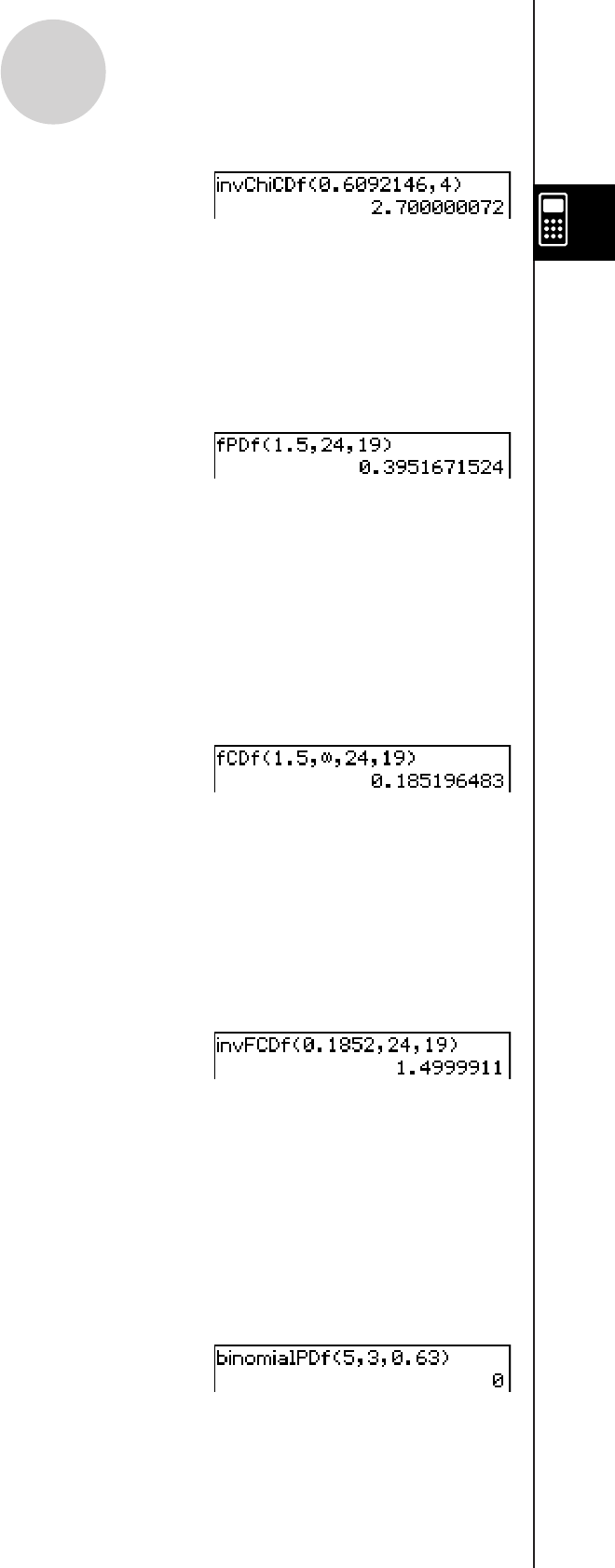
20090601

2-8-52

Using the Action Menu

Menu Item: [Action][Inv. Distribution][invChiCDf]

For more information, see “Inverse χ2 Cumulative Distribution” on page 7-11-10.

u fPDf

Function: Returns the F probability density for a specified value.

Syntax: fPDf(x, n:df, d:df [ ) ]

Example: To determine the F probability density when x = 1.5, n:df = 24, d:df = 19

Menu Item: [Action][Distribution][fPDf]

For more information, see “F Probability Density” on page 7-11-11.

u fCDf

Function: Returns the cumulative probability of an F distribution between a lower bound

and an upper bound.

Syntax: fCDf(lower value, upper value, n:df, d:df [ ) ]

Example: To determine the F distribution probability when lower value = 1.5, upper

value = ∞, n:df = 24, d:df = 19

Menu Item: [Action][Distribution][fCDf]

For more information, see “F Cumulative Distribution” on page 7-11-12.

u invFCDf

Function: Returns the lower bound value of an F cumulative distribution probability for

specified values.

Syntax: invFCDf(prob, n:df, d:df [ ) ]

Example: To determine the lower bound value when prob = 0.1852, n:df = 24, d:df = 19

Menu Item: [Action][Inv. Distribution][invFCDf]

For more information, see “Inverse F Cumulative Distribution” on page 7-11-13.

u binomialPDf

Function: Returns the probability in a binomial distribution that the success will occur on

a specified trial.

Syntax: binomialPDf(x, numtrial value, pos [ ) ]

Example: To determine the binomial probability when x = 5, numtrial value = 3,

pos = 0.63

Menu Item: [Action][Distribution][binomialPDf]

For more information, see “Binomial Distribution Probability” on page 7-11-14.

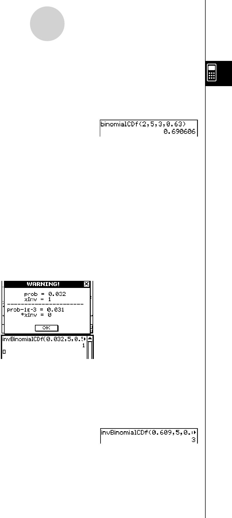
20090601

u binomialCDf

Function: Returns the cumulative probability in a binomial distribution that the success

will occur between specified lower value and upper value.

Syntax: binomialCDf(lower value, upper value, numtrial value, pos [ ) ]

Example: To determine the binomial cumulative probability when lower value = 2, upper

value = 5, numtrial value = 3, pos = 0.63

Menu Item: [Action][Distribution][binomialCDf]

For more information, see “Binomial Cumulative Distribution” on page 7-11-15.

u invBinomialCDf

Function: Returns the minimum number of trials of a binomial cumulative probability

distribution for specified values.

Syntax: invBinomialCDf(prob, numtrial value, pos [ ) ]

Important!

When executing the invBinomialCDf function the calculator uses the specified prob value

and the value that is one less the prob value minimum number of significant digits (*prob

value) to calculate minimum number of trials values. The results are assigned to the

system variables xInv (calculation result using prob) and *xInv (calculation result using

*prob). The invBinomialCDf function always returns the xInv value only. However, when

the xInv and *xInv values are different, the warning message shown below appears

showing both values.

The calculation results of invBinomialCDf are integers. Accuracy may be reduced when

the first argument has 10 or more digits. Note that even a slight difference in calculation

accuracy affects calculation results. If a warning message appears, check the displayed

values.

Example: To determine the minimum number of trials when prob = 0.609, numtrial

value = 5, pos = 0.63

Menu Item: [Action][Inv. Distribution][invBinomialCDf]

For more information, see “Inverse Binomial Cumulative Distribution” on page 7-11-16.

2-8-53

Using the Action Menu

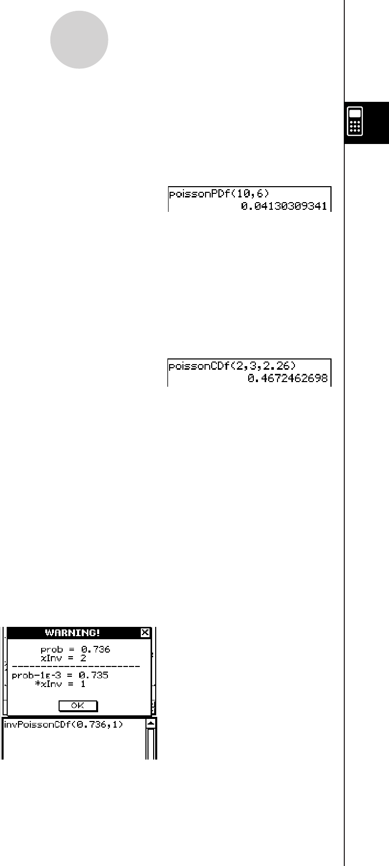
20090601

u poissonPDf

Function: Returns the probability in a Poisson distribution that the success will occur on a

specified trial.

Syntax: poissonPDf(x, ␭ [ ) ]

Example: To determine the Poisson probability when x = 10, ␭ = 6

Menu Item: [Action][Distribution][poissonPDf]

For more information, see “Poisson Distribution Probability” on page 7-11-17.

u poissonCDf

Function: Returns the cumulative probability in a Poisson distribution that the success will

occur between specified lower value and upper value.

Syntax: poissonCDf(lower value, upper value, ␭ [ ) ]

Example: To determine the Poisson cumulative probability when lower value = 2, upper

value = 3, ␭ = 2.26

Menu Item: [Action][Distribution][poissonCDf]

For more information, see “Poisson Cumulative Distribution” on page 7-11-18.

u invPoissonCDf

Function: Returns the minimum number of trials of a Poisson cumulative probability

distribution for specified values.

Syntax: invPoissonCDf(prob, ␭ [ ) ]

Important!

When executing the invPoissonCDf function the calculator uses the specified prob value

and the value that is one less the prob value minimum number of significant digits (*prob

value) to calculate minimum number of trials values. The results are assigned to the

system variables xInv (calculation result using prob) and *xInv (calculation result using

*prob). The invPoissonCDf function always returns the xInv value only. However, when

the xInv and *xInv values are different, the warning message shown below appears

showing both values.

The calculation results of invPoissonCDf are integers. Accuracy may be reduced when

the first argument has 10 or more digits. Note that even a slight difference in calculation

accuracy affects calculation results. If a warning message appears, check the displayed

values.

2-8-54

Using the Action Menu

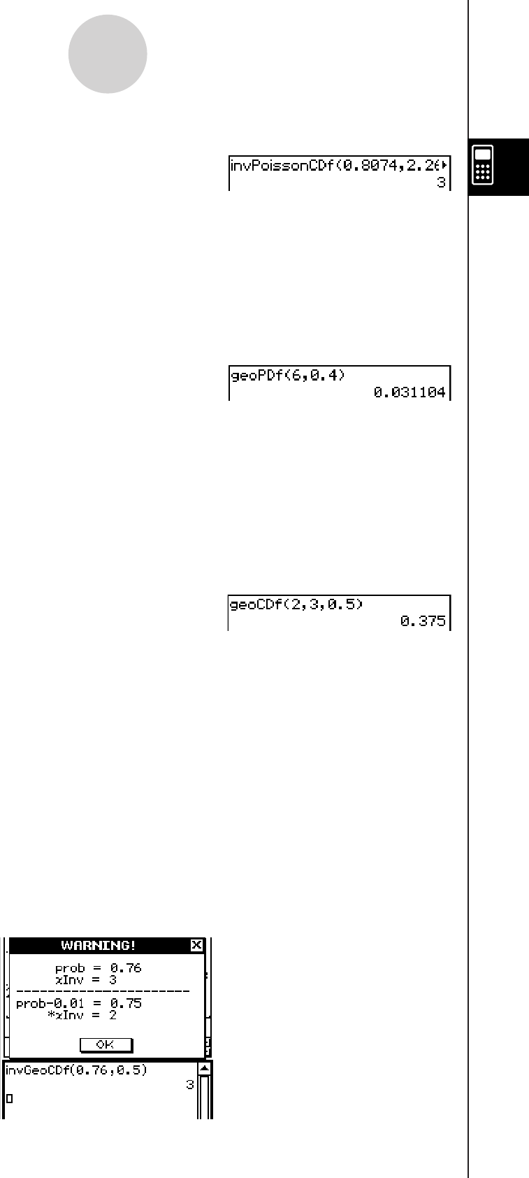
20090601

Example: To determine the minimum number of trials when prob = 0.8074, ␭ = 2.26

Menu Item: [Action][Inv. Distribution][invPoissonCDf]

For more information, see “Inverse Poisson Cumulative Distribution” on page 7-11-19.

u geoPDf

Function: Returns the probability in a geometric distribution that the success will occur on

a specified trial.

Syntax: geoPDf(x, pos [ ) ]

Example: To determine the geometric probability when x = 6, pos = 0.4

Menu Item: [Action][Distribution][geoPDf]

For more information, see “Geometric Distribution Probability” on page 7-11-20.

u geoCDf

Function: Returns the cumulative probability in a geometric distribution that the success

will occur between specified lower value and upper value.

Syntax: geoCDf(lower value, upper value, pos [ ) ]

Example: To determine the geometric probability when lower value = 2, upper value = 3,

pos = 0.5

Menu Item: [Action][Distribution][geoCDf]

For more information, see “Geometric Cumulative Distribution” on page 7-11-21.

u invGeoCDf

Function: Returns the minimum number of trials of a geometric cumulative probability

distribution for specified values.

Syntax: invGeoCDf(prob, pos [ ) ]

Important!

When executing the invGeoCDf function the calculator uses the specified prob value

and the value that is one less the prob value minimum number of significant digits (*prob

value) to calculate minimum number of trials values. The results are assigned to the

system variables xInv (calculation result using prob) and *xInv (calculation result using

*prob). The invGeoCDf function always returns the xInv value only. However, when the

xInv and *xInv values are different, the warning message shown below appears showing

both values.

2-8-55

Using the Action Menu

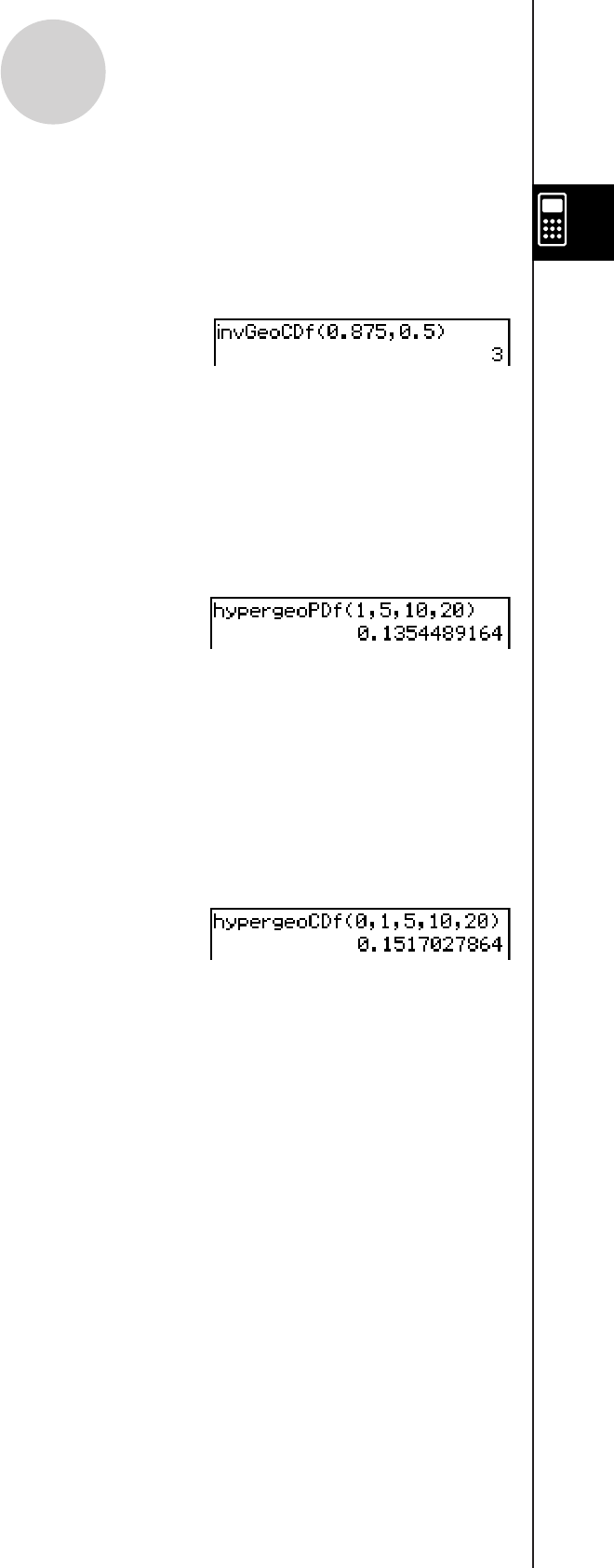
20090601

The calculation results of invGeoCDf are integers. Accuracy may be reduced when the

first argument has 10 or more digits. Note that even a slight difference in calculation

accuracy affects calculation results. If a warning message appears, check the displayed

values.

Example: To determine the minimum number of trials when prob = 0.875, pos = 0.5

Menu Item: [Action][Inv. Distribution][invGeoCDf]

For more information, see “Inverse Geometric Cumulative Distribution” on page 7-11-22.

u hypergeoPDf

Function: Returns the probability in a hypergeometric distribution that the success will

occur on a specified trial.

Syntax: hypergeoPDf(x, n, M, N [ ) ]

Example: Determine the hypergeometric probability when x = 1, n = 5, M = 10, N = 20.

Menu Item: [Action][Distribution][hypergeoPDf]

For more information, see “Hypergeometric Distribution Probability” on page 7-11-23.

u hypergeoCDf

Function: Returns the cumulative probability in a hypergeometric distribution that the

success will occur between specified lower value and upper value.

Syntax: hypergeoCDf(lower value, upper value, n, M, N [ ) ]

Example: Determine the hypergeometric cumulative distribution when lower value = 0,

upper value = 1, n = 5, M = 10, N = 20.

Menu Item: [Action][Distribution][hypergeoCDf]

For more information, see “Hypergeometric Cumulative Distribution” on page 7-11-24.

u invHypergeoCDf

Function: Returns the minimum number of trials of a hypergeometric cumulative

distribution for specified values.

Syntax: invHypergeoCDf(prob, n, M, N [ ) ]

Important!

When executing the invHypergeoCDf function the calculator uses the specified prob

value and the value that is one less the prob value minimum number of significant digits

(*prob value) to calculate minimum number of trials values. The results are assigned to

the system variables xInv (calculation result using prob) and *xInv (calculation result

using *prob). The invHypergeoCDf function always returns the xInv value only. However,

when the xInv and *xInv values are different, the warning message shown below appears

showing both values.

2-8-56

Using the Action Menu

20101001

The calculation results of invHypergeoCDf are integers. Accuracy may be reduced when

the first argument has 10 or more digits. Note that even a slight difference in calculation

accuracy affects calculation results. If a warning message appears, check the displayed

values.

Example: To determine the minimum number of trials when prob = 0.3, n = 5, M = 10, N = 20

Menu Item: [Action][Inv. Distribution][invHypergeoCDf]

For more information, see “Inverse Hypergeometric Cumulative Distribution” on page 7-11-25.

Using the Financial Submenu

The [Financial] submenu contains commands that are related to financial calculations.

2-8-57

Using the Action Menu

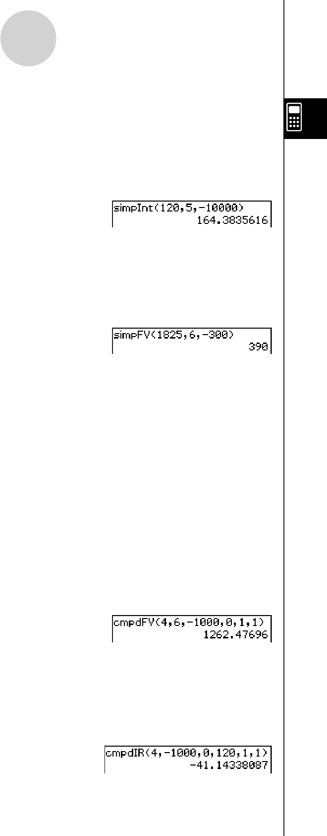
20110401

Simple Interest

For the meaning of each argument, see “Simple Interest” (page 15-2-1).

u simpInt

Function: Returns the interest based on simple interest calculation.

Syntax: simpInt (n,I%,PV)

Example: simpInt (120,5,−10000)

Menu Item: [Action][Financial][Simple Interest][simpInt]

u simpFV

Function: Returns the total of principal and interest based on simple interest

calculation.

Syntax: simpFV (n,I%,PV)

Example: simpFV (1825,6,−300)

Menu Item: [Action][Financial][Simple Interest][simpFV]

Compound Interest

• P/Y and C/Y can be omitted for all compound interest calculations. When they are omitted,

calculations are performed using P/Y=1 and C/Y=1.

• If you perform a calculation that uses a compound interest function (cmpdFV, cmpdIR,

cmpdN, cmpdPmt, cmpdPV), the argument(s) you input and the calculation results will be

saved to the applicable variables (n, I%, PV, etc.). If you perform a calculation that uses

any other type of financial calculation function, the argument and calculation results are

not assigned to variables.

• For the meaning of each argument, see “Compound Interest” (page 15-3-1).

u cmpdFV

Function: Returns the final input/output amount or total principal and interest.

Syntax: cmpdFV (n,I%,PV,PMT,P/Y,C/Y)

Example: cmpdFV (4,6,−1000,0,1,1)

Menu Item: [Action][Financial][Compound Interest][cmpdFV]

u cmpdIR

Function: Returns the annual interest.

Syntax: cmpdIR (n,PV,PMT,FV,P/Y,C/Y)

Example: cmpdIR (4,−1000,0,120,1,1)

Menu Item: [Action][Financial][Compound Interest][cmpdIR]

2-8-58

Using the Action Menu

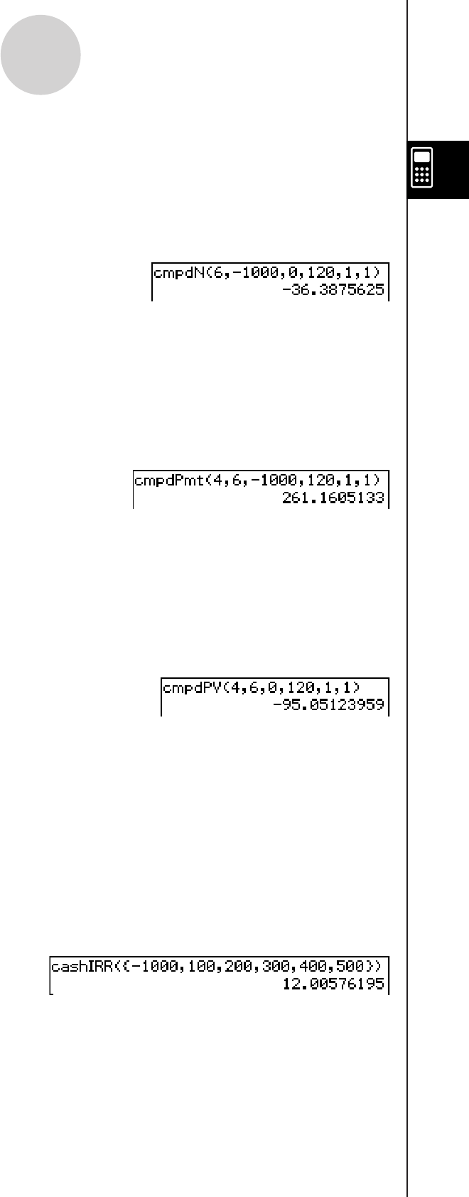
20101001

u cmpdN

Function: Returns the number of compound periods.

Syntax: cmpdN (I%,PV,PMT,FV,P/Y,C/Y)

Example: cmpdN (6,−1000,0,120,1,1)

Menu Item: [Action][Financial][Compound Interest][cmpdN]

u cmpdPmt

Function: Returns equal input/output values (payment amounts for installment

payments, deposit amounts for savings) for a fixed period.

Syntax: cmpdPmt (n,I%,PV,FV,P/Y,C/Y)

Example: cmpdPmt (4,6,−1000,120,1,1)

Menu Item: [Action][Financial][Compound Interest][cmpdPmt]

u cmpdPV

Function: Returns the present value (loan amount for installment payments, principal

for savings).

Syntax: cmpdPV (n,I%,PMT,FV,P/Y,C/Y)

Example: cmpdPV (4,6,0,120,1,1)

Menu Item: [Action][Financial][Compound Interest][cmpdPV]

Cash Flow (Investment Appraisal)

For the meaning of each argument, see “Cash Flow” (page 15-4-1).

u cashIRR

Function: Returns the internal rate of return.

Syntax: cashIRR (Cash)

Example: list1 = {−1000,100,200,300,400,500}

cashIRR (list1)

Menu Item: [Action][Financial][Cash Flow]

[cashIRR]

2-8-59

Using the Action Menu

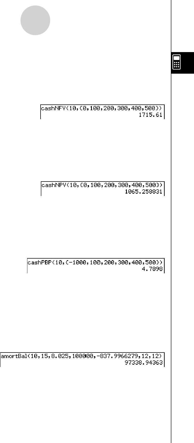
20101001

u cashNFV

Function: Returns the net future value.

Syntax: cashNFV (I%,Cash)

Example: list1 = {0,100,200,300,400,500}

cashNFV (10,list1)

Menu Item: [Action][Financial][Cash Flow][cashNFV]

u cashNPV

Function: Returns the net present value.

Syntax: cashNPV (I%,Cash)

Example: list1 = {0,100,200,300,400,500}

cashNPV (10,list1)

Menu Item: [Action][Financial][Cash Flow][cashNPV]

u cashPBP

Function: Returns the payback period.

Syntax: cashPBP (I%,Cash)

Example: list1 = {−1000,100,200,300,400,500}

cashPBP (10,list1)

Menu Item: [Action][Financial][Cash Flow][cashPBP]

Amortization

For the meaning of each argument, see “Amortization” (page 15-5-1).

u amortBal

Function: Returns the remaining principal balance following payment PM2.

Syntax: amortBal (PM1,PM2,I%,PV,PMT,P/Y,C/Y)

Example: amortBal (10,15,8.025,100000,−837.9966279,12,12)

Menu Item: [Action][Financial][Amortization][amortBal]

2-8-60

Using the Action Menu

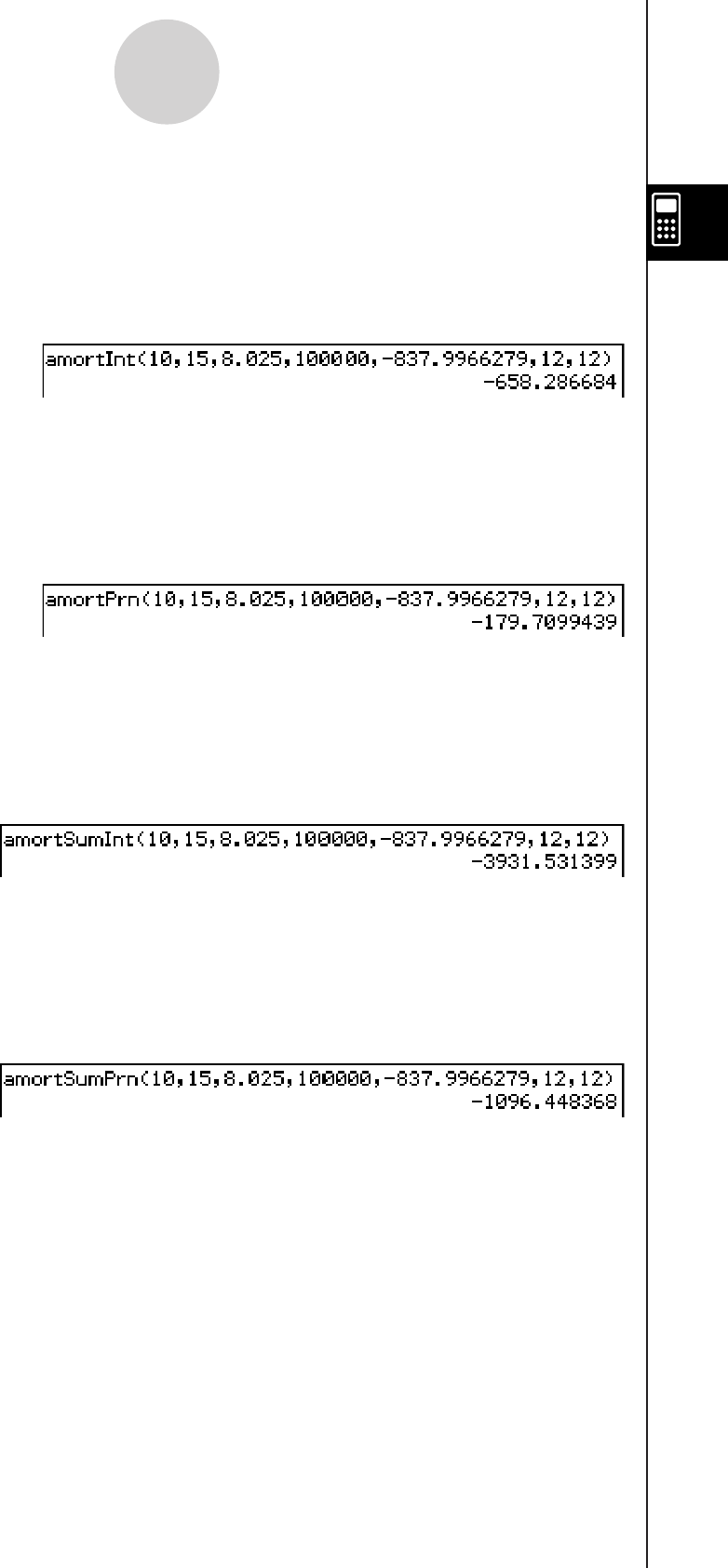
20101001

u amortInt

Function: Returns the interest paid for payment PM1.

Syntax: amortInt (PM1,PM2,I%,PV,PMT,P/Y,C/Y)

Example: amortInt (10,15,8.025,100000,−837.9966279,12,12)

Menu Item: [Action][Financial][Amortization][amortInt]

u amortPrn

Function: Returns the principal and interest paid for payment PM1.

Syntax: amortPrn (PM1,PM2,I%,PV,PMT,P/Y,C/Y)

Example: amortPrn (10,15,8.025,100000,−837.9966279,12,12)

Menu Item: [Action][Financial][Amortization][amortPrn]

u amortSumInt

Function: Returns the total principal and interest paid from payment PM1 to PM2.

Syntax: amortSumInt (PM1,PM2,I%,PV,PMT,P/Y,C/Y)

Example: amortSumInt (10,15,8.025,100000,−837.9966279,12,12)

Menu Item: [Action][Financial][Amortization][amortSumInt]

u amortSumPrn

Function: Returns the total principal paid from payment PM1 to PM2.

Syntax: amortSumPrn (PM1,PM2,I%,PV,PMT,P/Y,C/Y)

Example: amortSumPrn (10,15,8.025,100000,−837.9966279,12,12)

Menu Item: [Action][Financial][Amortization][amortSumPrn]

2-8-61

Using the Action Menu

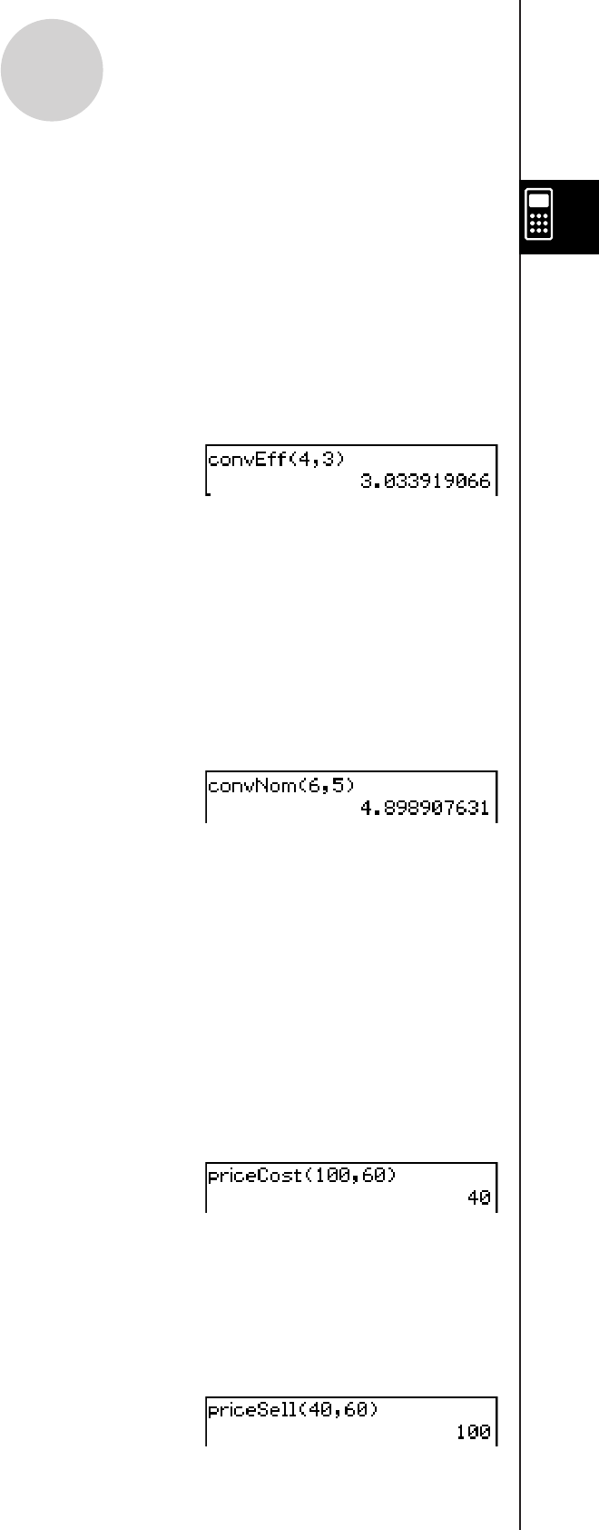
20101001

Interest Conversion

For the meaning of each argument, see “Interest Conversion” (page 15-6-1).

u convEff

Function: Returns the interest rate converted from the nominal interest rate to the

effective interest rate.

Syntax: convEff (n,I%)

Example: convEff (4,3)

Menu Item: [Action][Financial][Interest Conversion][convEff]

Note: When

I% is EFF, this command returns APR.

u convNom

Function: Returns the interest rate converted from the effective interest rate to the

nominal interest rate.

Syntax: convNom (n,I%)

Example: convNom (6,5)

Menu Item: [Action][Financial][Interest Conversion][convNom]

Note: When

I% is APR, this command returns EFF.

Cost/Sell/Margin

For the meaning of each argument, see “Cost/Sell/Margin” (page 15-7-1).

u priceCost

Function: Returns the cost based on a specified selling price and margin.

Syntax: priceCost (Sell,Margin)

Example: priceCost (100,60)

Menu Item: [Action][Financial][Cost/Sell/Margin][priceCost]

u priceSell

Function: Returns the selling price based on a specified cost and margin.

Syntax: priceSell (Cost,Margin)

Example: priceSell (40,60)

Menu Item: [Action][Financial][Cost/Sell/Margin][priceSell]

2-8-62

Using the Action Menu

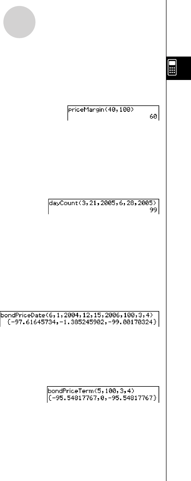
20110401

u priceMargin

Function: Returns the margin based on a specified cost and selling price.

Syntax: priceMargin (Cost,Sell)

Example: priceMargin (40,100)

Menu Item: [Action][Financial][Cost/Sell/Margin][priceMargin]

Day Count

For the meaning of each argument, see “Day Count” (page 15-8-1).

u dayCount

Function: Returns the number of days from a specified d1 to specified d2.

Syntax: dayCount (MM1,DD1,YYYY1,MM2,DD2,YYYY2)

Example: dayCount (3,21,2005,6,28,2005)

Menu Item: [Action][Financial][dayCount]

Bond Calculation

For the meaning of each argument, see “Bond Calculation” (page 15-10-1).

u bondPriceDate

Function: Returns in list form bond prices based on specified conditions.

Syntax: bondPriceDate (MM1,DD1,YYYY1,MM2,DD2,YYYY2,RDV,CPN,YLD) =

{PRC,INT,CST}

Example: bondPriceDate (6,1,2004,12,15,2006,100,3,4)

Menu Item: [Action][Financial][Bond Calculation][bondPriceDate]

u bondPriceTerm

Function: Returns in list form bond prices based on specified conditions.

Syntax: bondPriceTerm (N,RDV,CPN,YLD) = {PRC,INT,CST}

Example: bondPriceTerm (5,100,3,4)

Menu Item: [Action][Financial][Bond Calculation][bondPriceTerm]

2-8-63

Using the Action Menu

20110401

u bondYieldDate

Function: Returns the yield based on specified conditions.

Syntax: bondYieldDate (MM1,DD1,YYYY1,MM2,DD2,YYYY2,RDV,CPN,PRC)

Example: bondYieldDate (6,1,2004,12,15,2006,100,3,−97.61645734)

Menu Item: [Action][Financial][Bond Calculation][bondYieldDate]

u bondYieldTerm

Function: Returns the yield based on specified conditions.

Syntax: bondYieldTerm (N,RDV,CPN,PRC)

Example: bondYieldTerm (5,100,3,−95.54817767)

Menu Item: [Action][Financial][Bond Calculation][bondYieldTerm]

Using the Command Submenu

u Define

Function: Creates a user-defined function.

For more information, see “Define” on page 12-6-9 and “Creating a User-defined Function

Using the Define Command” on page 12-5-2.

u DispStat

Function: Displays previous statistical calculation results.

For more information, see “DispStat” on page 12-6-28 and “To explore statistical data” on

page 12-7-5.

u Clear_a_z

Function: Clears all single-character variables.

For more information, see “Clear_a_z” on page 2-8-48.

u DelVar

Function: Deletes a specified variable.

For more information, see “DelVar” on page 12-6-39.

u Clear All Variables

Function: Clear variables that contain numbers, list and matrices.

2-8-64

Using the Action Menu

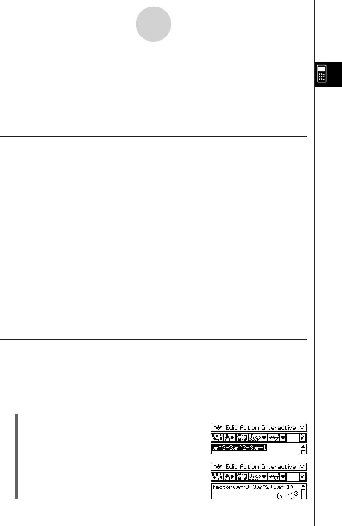
20060301

(3) Tap [Interactive], [Transformation], and then [factor].

• This factorizes the selected expression.

2-9 Using the Interactive Menu

The [Interactive] menu includes most of the commands that are on the [Action] menu.

Selecting a command on the [Action] menu will simply execute the command. With the

[Interactive] menu, on the other hand, selecting a command will display a dialog box

prompting input of the arguments required by the command’s syntax (when necessary).

The following are the differences between the [Interactive] menu and [Action] menu.

Interactive Menu and Action Menu

• With the [Action] menu, you select a command to input a function into the work area.

• With the [Interactive] menu, you drag the stylus across existing input in the work area and

then select a command. This encloses the highlighted expression with the command and

opens a dialog box if more arguments are needed.

• When you select an [Interactive] menu item without highlighting an expression first, a dialog

box will open prompting you for the necessary arguments.

• When a command requires multiple arguments, a dialog box appears prompting you for the

arguments with the [Interactive] menu.

• The [Interactive] menu has an “apply” command while the [Action] menu does not.

• The “DispStat”, “Clear_a_z,” and “DelVar” commands of the [Action] menu’s [Command]

submenu are not included on the [Interactive] menu.

Tip

• Operation of the following [Interactive] menu commands is identical to the same commands on

the [Action] menu.

[Transformation], [Advanced], [Calculation], [Complex], [List-Create], [List-Calculation], [Matrix-

Create], [Matrix-Calculation], [Vector], [Equation/Inequality], [Assistant], Define

• For information about using these commands, see “2-8 Using the Action Menu”.

Interactive Menu Example

The following example shows how to use the [Transformation]-[factor] command from both

the [Interactive] menu and the [Action] menu.

Example: To factorize the expression x3 – 3x2 + 3x – 1

u To factorize from the Interactive menu

(1) In the work area, input the expression you want to factorize (x3 – 3x2 + 3x – 1).

(2) Drag the stylus across the expression to select it.

2-9-1

Using the Interactive Menu

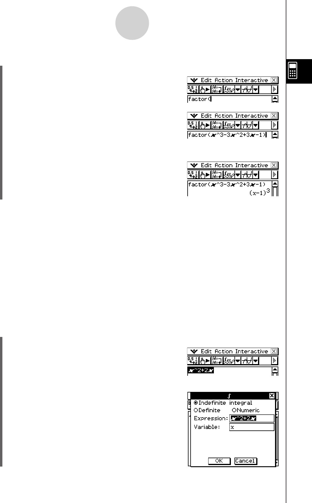
20060301

2-9-2

Using the Interactive Menu

u To factorize from the Action menu

(1) Tap [Action], [Transformation], and then [factor].

• This inputs “factor(” into the work area.

(2) Input the expression you want to factorize

(x3 – 3x2 + 3x – 1).

(3) Tap w.

• This factorizes the selected expression.

[Interactive] menu operations come in handy in the following cases.

• When you want to use a command on an expression you are calculating

• When you want to use a command that requires multiple arguments

When you use the [Interactive] menu to access a command that requires multiple arguments

or if you access a command without first highlighting an expression, the dialog box that

appears shows the number of arguments, the contents of each argument, and the input

sequence. This lets you perform your input without worrying about command syntax.

The following procedure shows an example of using the [Interactive] menu when three

arguments need to be specified.

Example: To obtain the definite integral of x2 + 2x, 1 s x s 2

uClassPad Operation

(1) In the work area, input the expression (x2 + 2x).

(2) Drag the stylus across the expression to select it.

(3) Tap [Interactive], [Calculation], and then [ ∫ ].

• This displays the ∫ dialog box.

• Though the above two procedures are quite different, they both produce the same result.

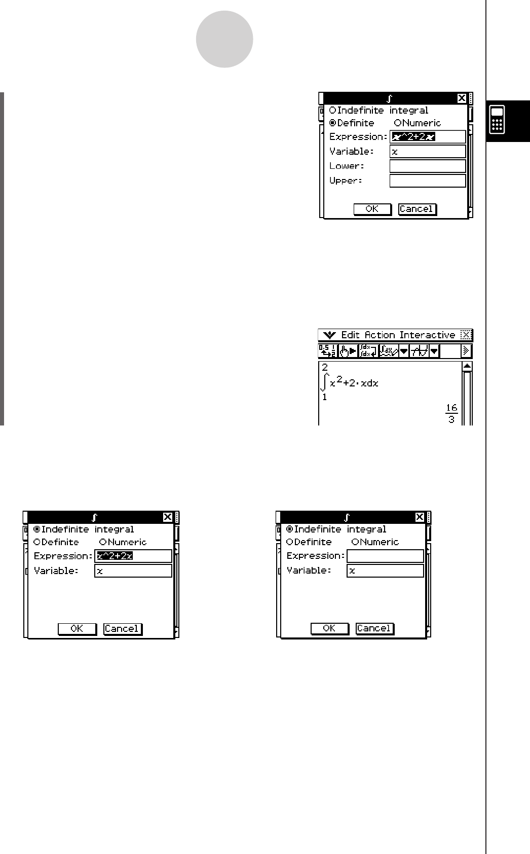
20060301

(4) On the dialog box, tap “Definite integral” to select it.

• This displays boxes for specifying the variable

and the lower limit and the upper limit.

2-9-3

Using the Interactive Menu

(5) Input the required data for each of the following three arguments.

Variable:

Lower: 1

Upper: 2

(6) Tap [OK].

• This performs the calculation and displays the

solution.

Tip

• You can execute a command on the Interactive menu without selecting an expression in the work

area. On the dialog box that appears, enter the expression you can to perform into the

“Expression” box.

Dialog box when no expression is selected. Dialog box when an expression is selected

in the work area when you tap [Interactive] -

[Calculation] - [∫].

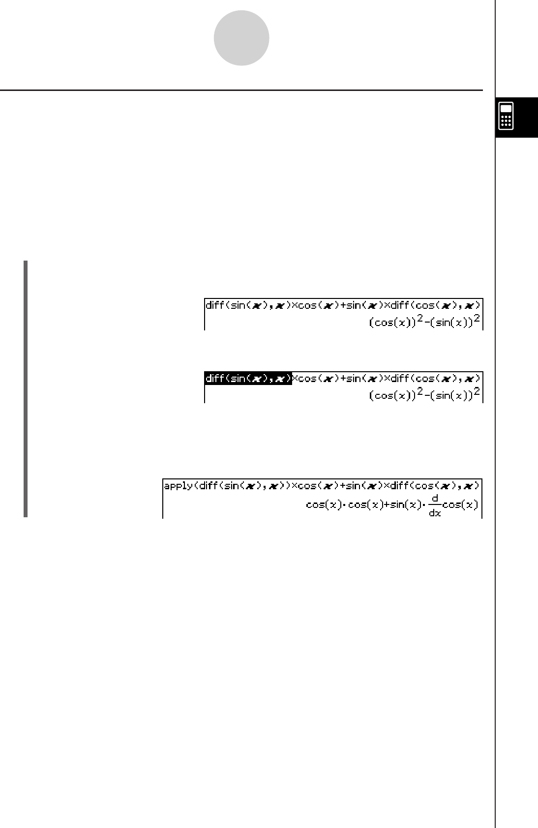
20060301

2-9-4

Using the Interactive Menu

(3) Tap [Interactive] and then [apply].

• This executes the part of the calculation you selected in step (2). The part of the

calculation that is not selected (× cos(x) + sin(x) × diff(cos(x),x)) is output to the

display as-is.

Using the “apply” Command

The “apply” command is included on the [Interactive] menu only. You can use this command

to execute only a specific part of an expression and display its result.

Example: To calculate the result of diff(sin(x),x) × cos(x) + sin(x) × diff(cos(x),x), and then

calculate only part of the expression

Note

• This procedure assumes that your ClassPad is configured with the following mode settings:

Algebra, Complex, Radian, Descending Order.

u ClassPad Operation

(1) Input the example calculation provided above and execute it.

• For details about differential calculations, see “2-8 Using the Action Menu”.

(2) Drag the stylus across “diff(sin(x),x)” to select it.

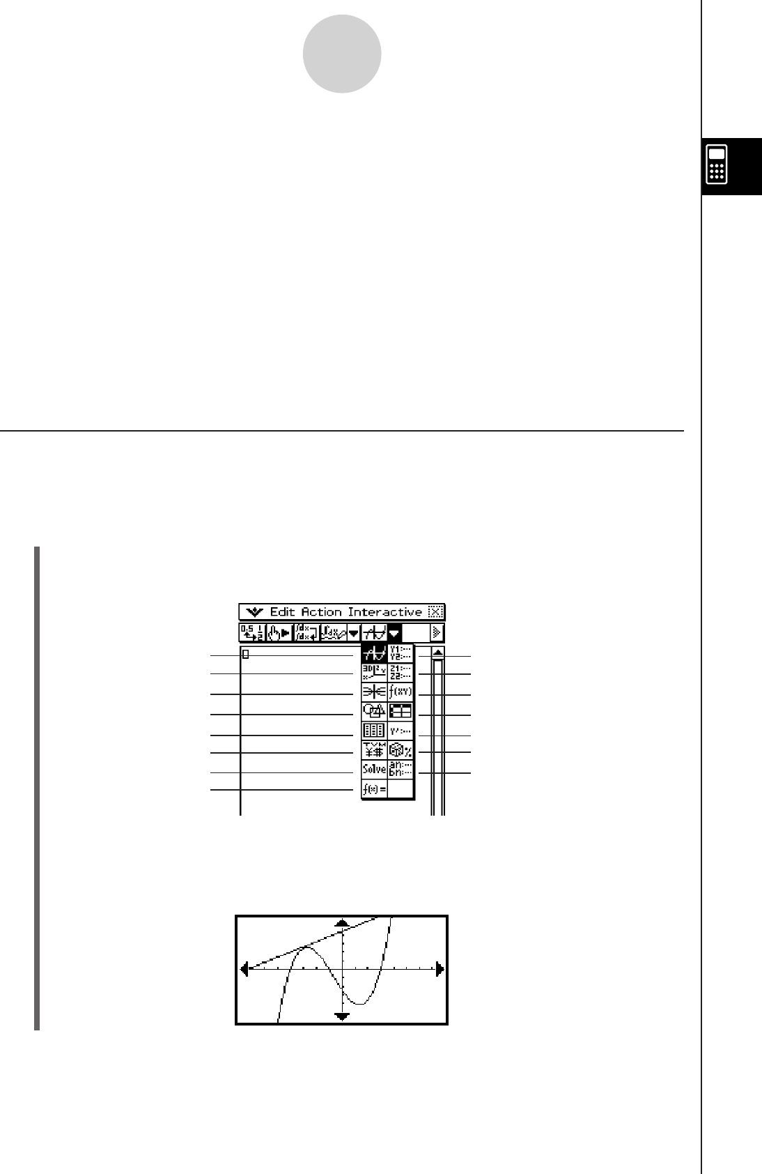
20060301

2-10-1

Using the Main Application in Combination with Other Applications

Graph

3D Graph

Conics Graph

Geometry

Stat Editor

Financial

Numeric Solver

Verify

Graph Editor

3D Graph Editor

Conics Editor

Spreadsheet

Differential Equation Editor

Probability

Sequence Editor

(2) Tap the button that corresponds to the window you want to display.

• This causes the window that corresponds to the button you tap to appear in the lower

window.

2-10 Using the Main Application in Combination

with Other Applications

You can access the windows of other ClassPad applications from the Main application and

perform copy, paste, and other operations between them.

This section explains how to access the windows of other applications from the Main

application, and provides examples of the various operations you can perform between them.

Important!

• For details about the windows produced by each ClassPad application, see the chapter that

covers the application. All of the explanations in this section assume that you are already

familiar with the operations in the other ClassPad applications.

Opening Another Application’s Window

Use the following procedure to access the window of another application from the Main

application window.

u ClassPad Operation

(1) Tap the right most toolbar down arrow button.

• This displays a palette of application icons.

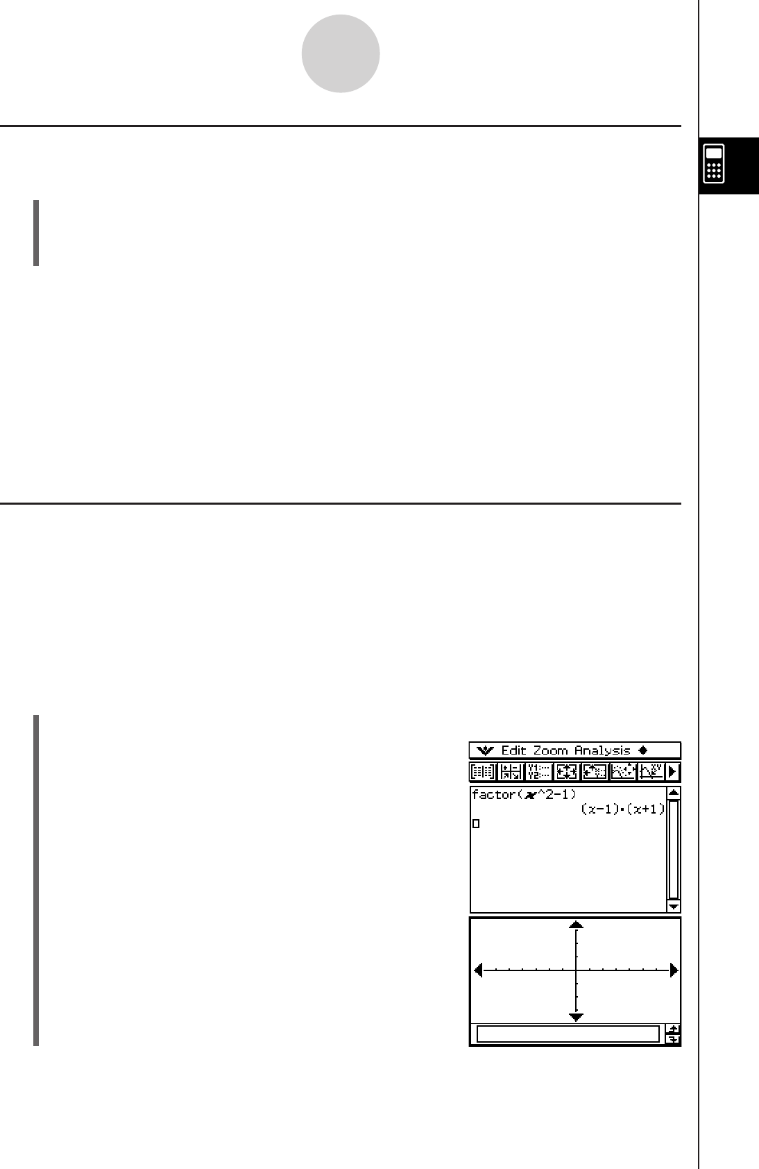
20060301

2-10-2

Using the Main Application in Combination with Other Applications

Closing Another Application’s Window

u ClassPad Operation

(1) Tap anywhere inside of the window you would like to close.

(2) Tap the S button in the upper right corner, or tap O and then [Close].

• The Main application work area expands to fill the entire display.

Tip

• Even if you used the icon panel r icon to expand the lower window to fill the entire display,

tapping O and then [Close] closes it and returns to the work area window.

• Nothing happens if you tap O and then [Close] while the work area window is active.

• For more information about enlarging one of the windows on a dual window display to fill the

entire display (r), swapping the contents of the upper window and lower window (S),

making a window active, and other window operations, see “Using a Dual Window Display” on

page 1-5-1.

Using the Graph Window $ and 3D Graph Window %

Dragging a function from the work area to the Graph window $ graphs it in the format of

y = f(x).

Dragging a function from the work area to the 3D Graph window % graphs it in the format of

z = f(x, y).

Example: To execute the expression factor(x2 – 1) in the work area, and then graph x2 – 1

u ClassPad Operation

(1) Input “factor (x2 – 1)” into the work area, and then tap w.

(2) Tap

$ to display the Graph window in the lower

window.

20060301

2-10-3

Using the Main Application in Combination with Other Applications

(3) Drag the stylus across “x^2 – 1” in the work area to

select it.

(4) Drag the selected expression to the Graph window.

• This graphs y = x2 – 1. This graph reveals that

the x-intercepts are x = ±1.

Tip

• As can be seen in the above example, a graph can be drawn when you drop an expression in the

form of f(x) into the Graph window. In the case of the 3D Graph window, the expression must be

in the form of f(x,y).

• For more information about the Graph window, see Chapter 3. For more information about the 3D

Graph window, see Chapter 5.

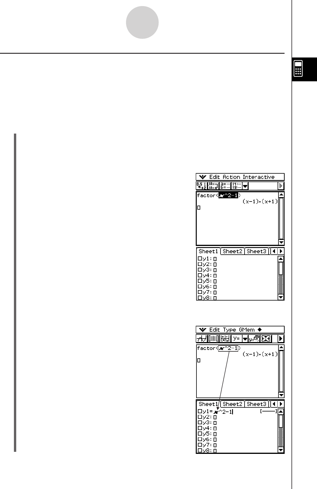
20060301

2-10-4

Using the Main Application in Combination with Other Applications

Using a Graph Editor Window (Graph & Table: !, Conics: *, 3D Graph:

@, Numeric Solver: 1)

You can copy expressions by dragging them between the work area window and the Graph

Editor, Conics Editor, 3D Graph Editor, and Numeric Solver windows.

Example: To copy an expression in the work area by dragging it to the Graph Editor window

u ClassPad Operation

(1) On the work area window, tap ! to display the Graph Editor window in the lower

window.

• If you already have some functions input in the Graph & Table application, those

functions will be displayed on the Graph Editor window.

(2) In the work area, drag the stylus across the expression

you want to copy so it is selected.

(3) Drag the selected expression to the location on the Graph Editor window where you

want to copy it.

• This makes the Graph Editor window active and

copies the expression to the location where you

dropped it.

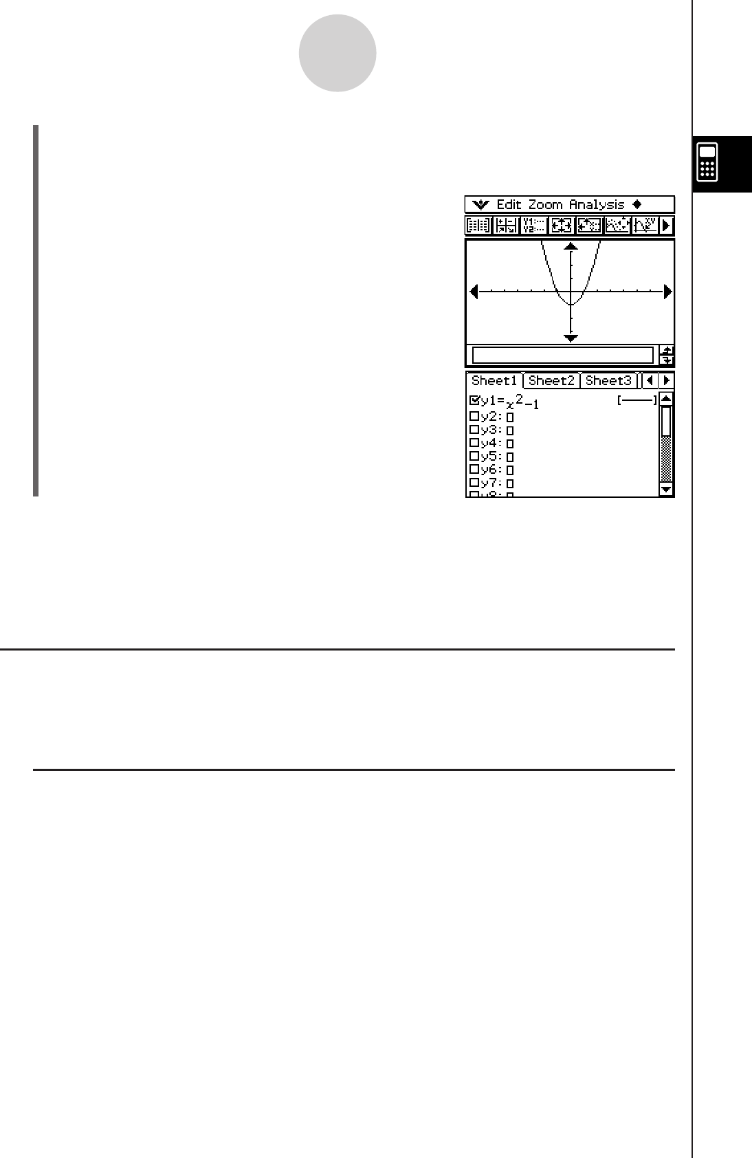
20060301

2-10-5

Using the Main Application in Combination with Other Applications

(4) Press E to register the expression.

• The copied expression is displayed in natural format, with the check box

next to it selected.

•

You could now tap $ to graph the function.

Tip

• For more information about the Graph Editor window, see Chapter 3. For more information about

the Conics Graph Editor window, see Chapter 4. For more information about the 3D Graph Editor

window, see Chapter 5. For more information about the Numeric Solver window, see Chapter 9.

Using the Stat Editor Window (

You can use the Stat Editor window to create new LIST variables and edit existing LIST

variables. You can also use the Stat Editor window to display the contents of a LIST variable

created using the work area by specifying the LIST variable’s name.

k Example List Operation

The following are the general steps for using the Stat Editor. The steps indicated in

parentheses refer to the steps under “ClassPad Operation” below.

1. Display the Stat Editor (step (1)) and input data for two LIST variables named “list1” and

“list2” (step (2)).

2. On the work area window, perform calculations that use “list1” and “list2” (steps (3) and (4)).

3. Use the work area to assign numbers to a variable and create a new LIST variable (steps (5)

and (6)).

4. Display the Stat Editor window and recall the LIST variable you created (steps (7), (8) and

(9)).

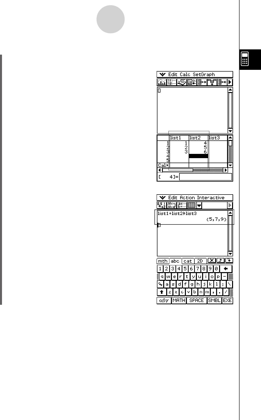
20060301

2-10-6

Using the Main Application in Combination with Other Applications

u ClassPad Operation

(1) On the work area window, tap ( to display the Stat Editor window in the lower

window.

(2) Input the following list data into the lists named “list1”

and “list2”. list1 = {1, 2, 3} list2 = {4, 5, 6}

(3) Make the work area window active, and then perform

the following calculation: list1 + list2 S list3.

• You could also input “list3:=list1+list2” to produce the

same result.

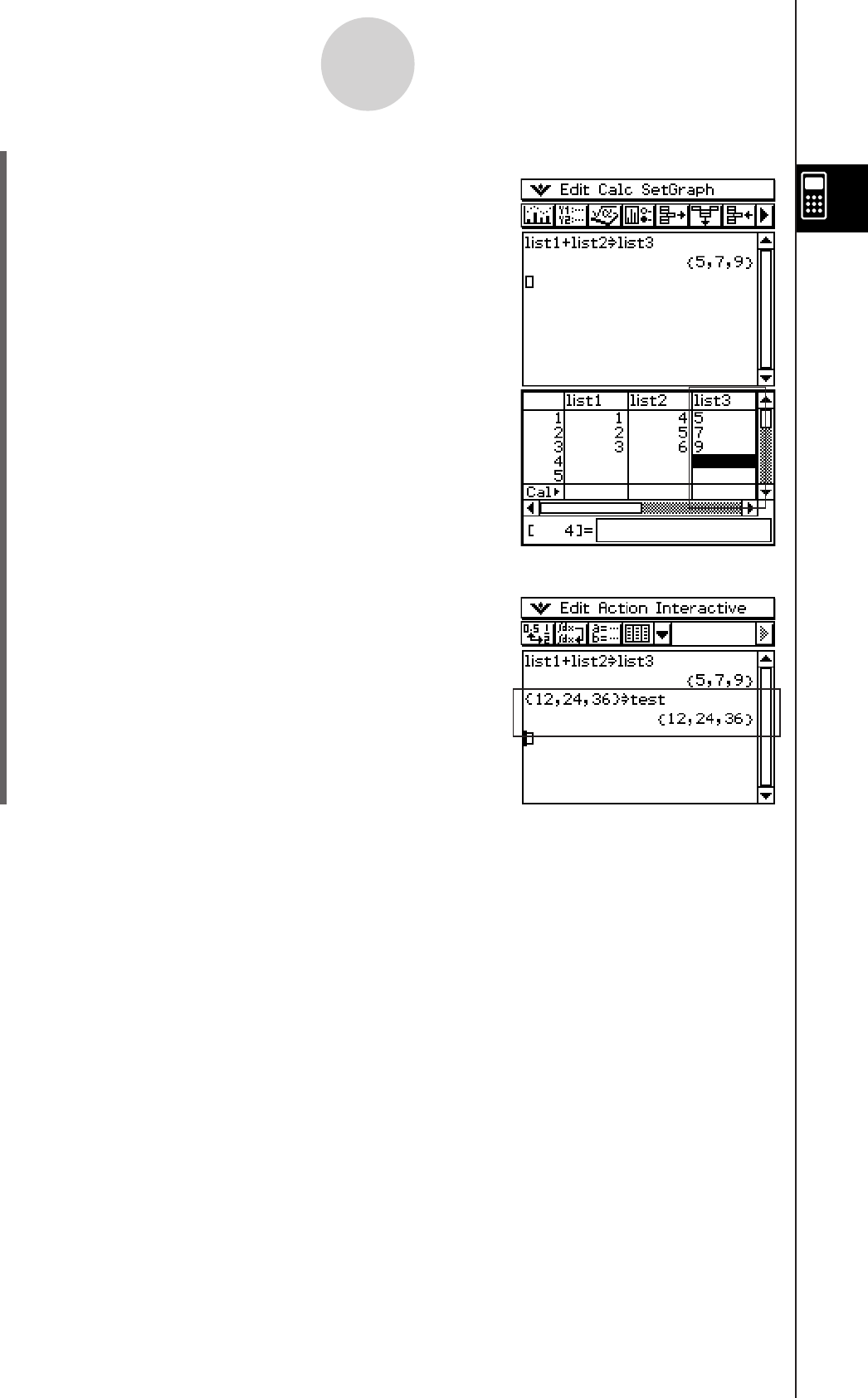
20060301

2-10-7

Using the Main Application in Combination with Other Applications

(4) Tap the Stat Editor window to make it active.

• Here you can see that list3 contains the result of

list1 + list2.

(5) Tap the work area window to make it active.

(6) Perform the operation {12, 24, 36}⇒test, which

assigns the list data {12, 24, 36} to the LIST

variable named “test”.

20090601

(7) Tap the Stat Editor window to make it active.

(8) Scroll the screen to the right until the blank list to

the right of “list6” is visible.

2-10-8

Using the Main Application in Combination with Other Applications

(9) Tap the blank cell next to “list6”, input “test”, and then tap w.

• This displays the list data {12, 24, 36}, which is assigned to the variable named

“test”.

• At this point you can perform list editing operations

like append, delete, edit, etc.

Tip

• list1 through list6 are LIST type system variables. For more information, see “1-7 Variables and

Folders”.

• For information about inputting and editing list data using the Stat Editor, see Chapter 7.

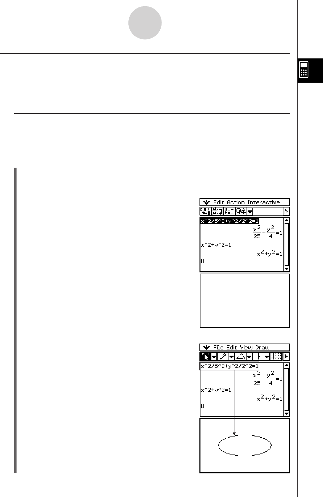
20060301

2-10-9

Using the Main Application in Combination with Other Applications

Using the Geometry Window 3

When there is a Geometry window on the display, you can drag values and expressions to

the Geometry window to draw the graph or figure of the value or expression. You can also

drag a figure from the Geometry window to the work area, which displays the corresponding

expression or value.

k Dragging an Expression from the Work Area to the Geometry Window

Example: To input the expressions x2/52 + y2/22 = 1 and x2 + y2 = 1 in the work area,

and then drag them to the Geometry window

u ClassPad Operation

(1) Input the two expressions into the work area.

(2) Tap 3 to display the Geometry window in the lower window.

•

The Geometry window that initially appears is blank.

(3) Drag the stylus across x2/52 + y2/22 = 1

in the work area to select it.

(4) Drag the selected expression to the Geometry window.

•

An ellipse appears in the Geometry window.

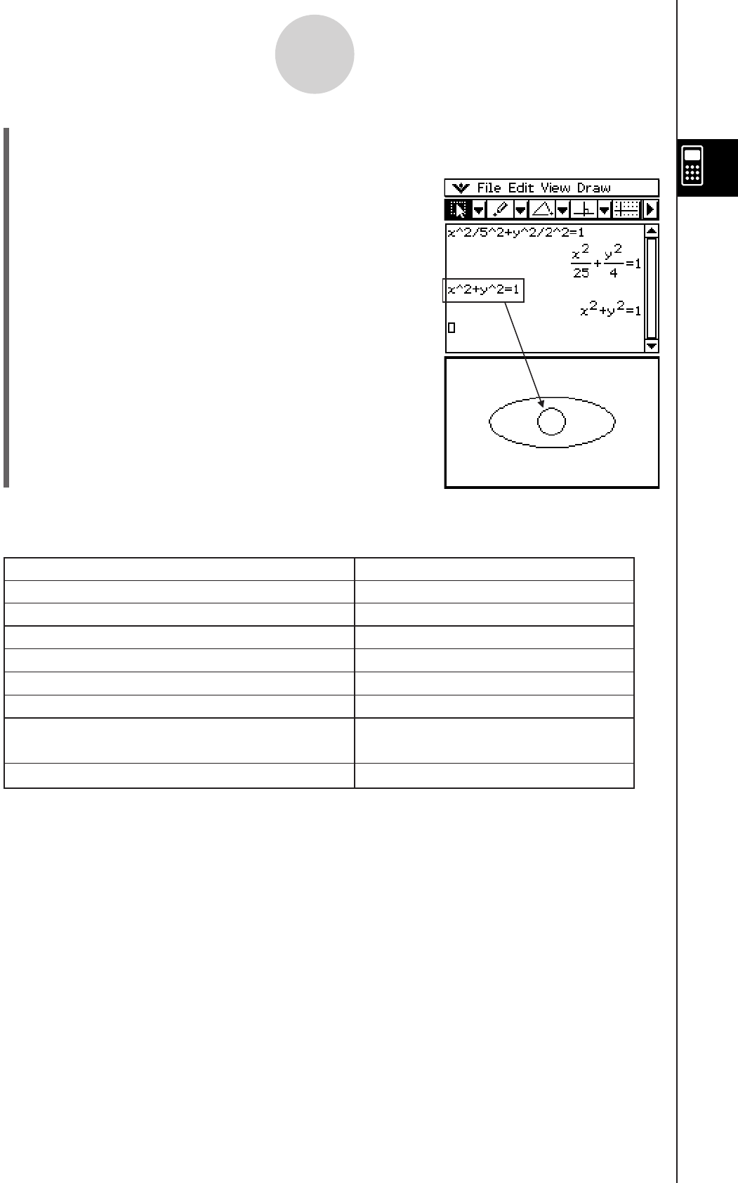
20060301

2-10-10

Using the Main Application in Combination with Other Applications

(5) Drag the stylus across x2 + y2 = 1 in the work area to select it.

(6) Drag the selected expression to the Geometry window.

•

A circle appears in the Geometry window.

Tip

• The following table shows the types of expressions you can drop into the Geometry window.

Dropping this into the Geometry window: Displays this:

Linear equation in x and y

Equation of circle in x and y

2-dimensional vector (2 rows × 1 column format)

Equation of hyperbola in x and y

Equation y = f(x)

2 × n matrix, n > 3

An infinite line

A circle

Equation of ellipse in x and yAn ellipse

A point

A hyperbola

A curve

n × 2 matrix, n > 3 An open polygon

A polygon (each column

represents a vertex of the polygon)

• When the expression is not recognized, Geometry displays it as text.

20060301

2-10-11

Using the Main Application in Combination with Other Applications

k Dragging a Figure from the Geometry Window to the Work Area

The following shows what happens when you drag a figure from the Geometry window to the

work area.

Dropping this into the work area: Displays this:

Point

Line

Circle, Arc, Ellipse, Function, or Curve

Line Pair

A point and its image under a transformation

Coordinates as a vector (2 × 1 matrix)

Equation of the line

Vector An ordered pair (head of vector

assuming the tail is at the origin)

Corresponding equation

Simultaneous equations for the pair

Matrix expression for the transformation

Polygon 2 ×

matrix

Open Polygon (Created by Animation)

× 2 matrix

A point and its image

Point Circle

Tip

• For details about Geometry window operations, see Chapter 8.

Using the Sequence Editor Window &

Displaying the Sequence Editor window from the Main application makes it possible for you

to perform the same operations you can perform in the Sequence application. You can also

use drag and drop to copy expressions between the work area and the Sequence Editor

window.

Tip

• For information about Sequence Editor operations and other Sequence application operations,

see Chapter 6.

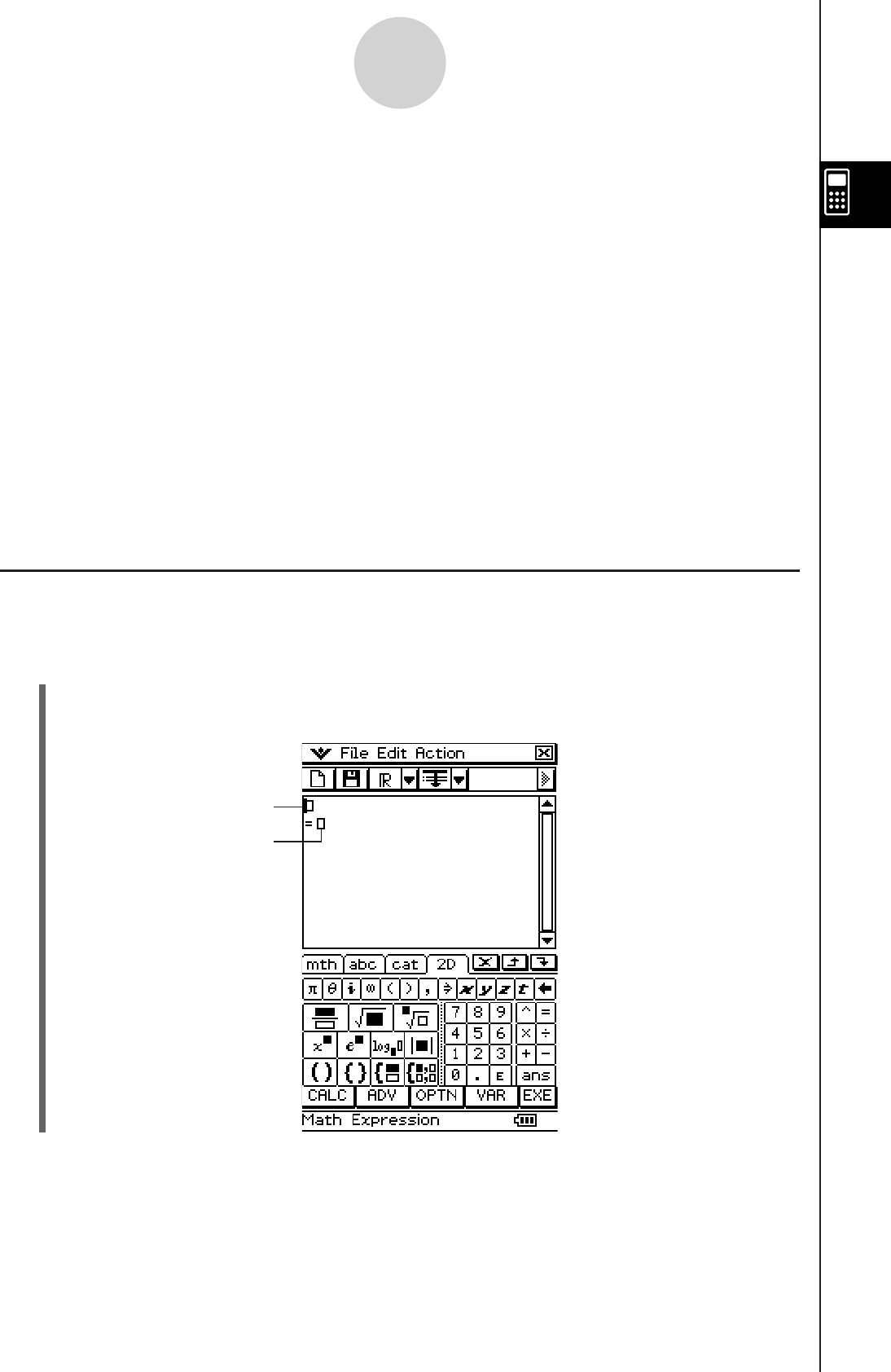
20090601

2-11-1

Using Verify

2-11 Using Verify

Verify provides you with a powerful tool to check whether your numeric or algebraic

manipulations are correct. Verify will assist you in simplifying an expression by verifying

whether or not the expression you entered is equivalent to your original expression. If it

is, you will get a pleasant response; if not, you will need to correct your mistake before

continuing.

You can access Verify within the Main application or the eActivity application. In the Main

application, you can save Verify sessions in ClassPad memory and reopen the session for

future use.

Verify sessions can also be saved within an eActivity. For more information on saving an

eActivity, see “10-2 Creating an eActivity”.

Important!

• Most Verify operations are the same in both the Main application and the eActivity

application.

Starting Up Verify

Use the following procedure to start up Verify.

u ClassPad Operation

(1) Tap the right most toolbar down arrow button.

(2) On the icon palette that appears, tap W.

Left-side expression

Right-side expression

20060301

Verify Menus and Buttons

This section provides basic information about Verify menus, commands, and buttons.

Tip

• O menu items are the same for all applications. For more information, see “Using the O

Menu” on page 1-5-4.

k File Menu

To do this: Select this File

menu item:

Discard the current window contents and create a new file New

Open an existing file Open

Save the current window contents to a file Save

k Edit Menu

To do this: Select this Edit

menu item:

Undo the last operation or redo an operation that was just undone Undo/Redo

Cut the currently selected object and place it onto the clipboard Cut

Copy the currently selected object and place it onto the clipboard Copy

Paste the current clipboard contents onto the screen Paste

Select the entire row where the cursor is located Select All

Delete the entire row where the cursor is located Delete

Clear the Verify window Clear All

k Action Menu

For information about Action menu commands, see “2-8 Using the Action Menu”.

Important!

Some Action menu commands are not useful in Verify, but for ease of use Verify’s Action

menu is identical to the Action menus in the Main application and the eActivity application.

2-11-2

Using Verify

20060301

2-11-3

Using Verify

k Verify Buttons

To do this: Tap this Verify button:

Clear the Verify window (same as the Clear All command)

Open or save a file (Main application only) R

Specify the complex number calculation range for Verify T

Specify the real number calculation range for Verify Y

Specify the positive real number calculation range for Verify U

Verify the equation starting from the first line

Verify the equation starting from the current line

Using Verify

The following examples show the basic steps for using Verify.

Important!

• In Verify, you can press E or tap with the stylus to move the cursor between lines.

• A message will appear to let you know whether or not the calculation result is valid.

Example 1: To factor 50 completely

u ClassPad Operation

(1) Tap the right most toolbar down arrow button.

(2) On the icon palette that appears, tap W.

(3) Input 50 and tap w.

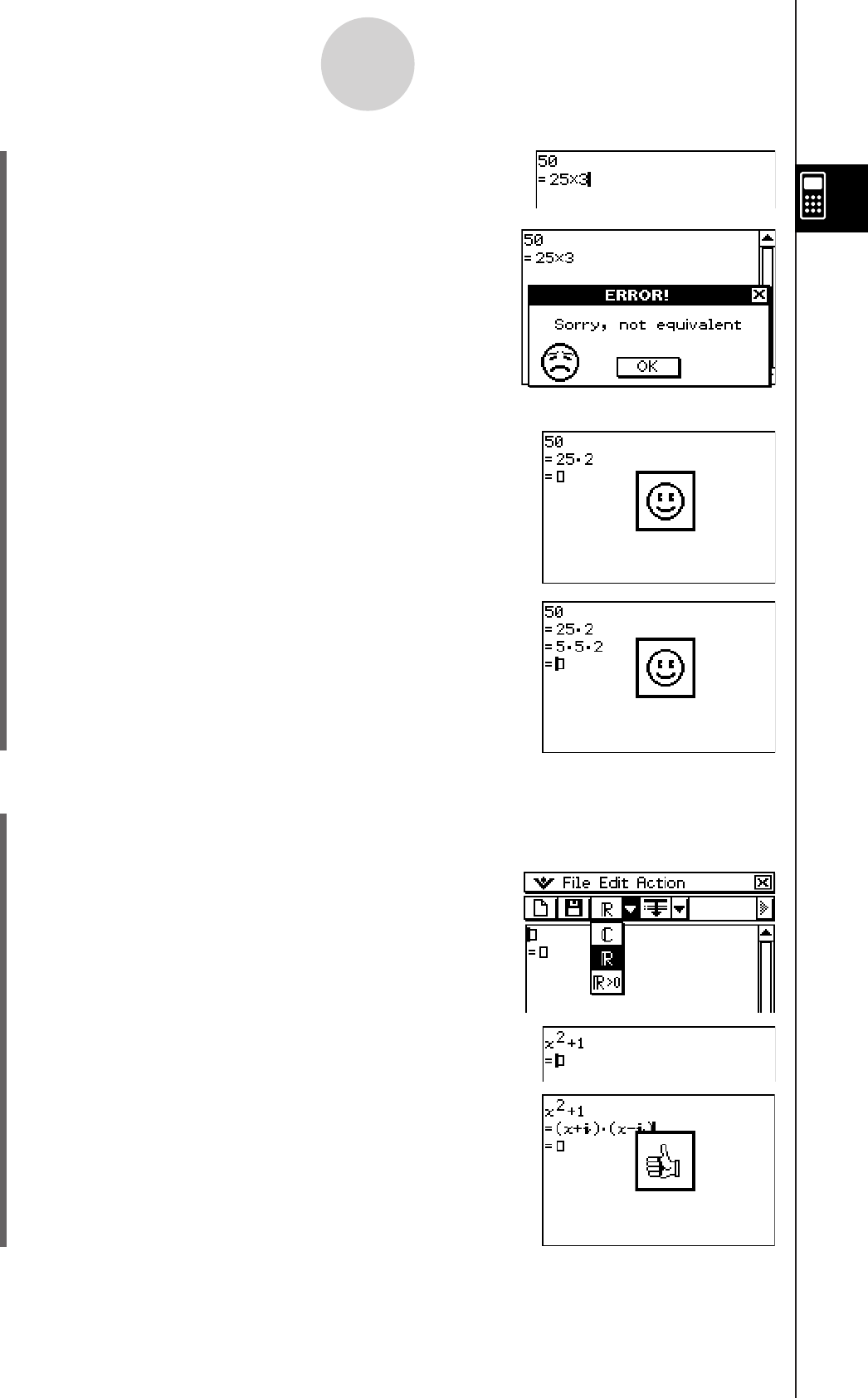
20060301

2-11-4

Using Verify

(4) Following the equal sign (=), input 25 × 3 and tap w.

(5) Tap [OK] to close the error dialog that appears.

(6) Change 25

× 3 to 25 × 2 and tap w.

(7) Following the next equal sign (=), input 5 × 5 × 2 and

tap w.

Example 2: To rewrite x2 + 1 in factored form

(1) Tap the left most toolbar icon E to begin a new Verify session.

(2) Tap [OK] to clear the window.

(3) Tap the down arrow on the toolbar and select T.

(4) Input

x^2 + 1 and press E.

(5) Input (x + i)(x – i) and press E.

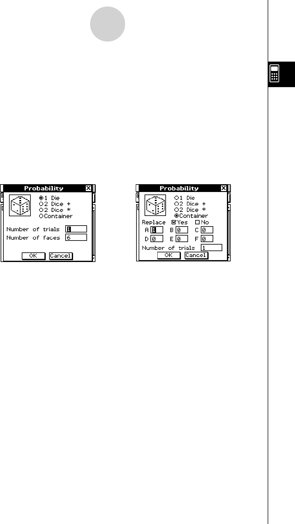
20060301

2-12 Using Probability

You can use Probability to simulate the following.

• The die faces that will appear when a single die is thrown a specified number of times (1

Die)

• The sum of the data of dice faces that will appear when a pair of dice is shown a

specified number of times (2 Dice +)

• The product of the data of dice faces that will appear when a pair of dice is shown a

specified number of times (2 Dice `

)

• When any number of balls labeled A, B, C, D, E, and F are placed into a box, data about

how many times each ball will be drawn within a specified number of draws (Container)

You can specify any integer from 1 to 20 as the number of die faces.

You can access Probability in the Main application or the eActivity application. From either

application, you can save Probability sessions in ClassPad memory and reopen the session

for future use.

Probability sessions also can be inserted into an eActivity. For more information, see “10-2

Creating an eActivity”.

Important!

Most Probability operations are the same in both the Main application and the eActivity

application.

2-12-1

Using Probability

Probability dialog box

when Container is selected

Probability dialog box

when 1 Die is selected

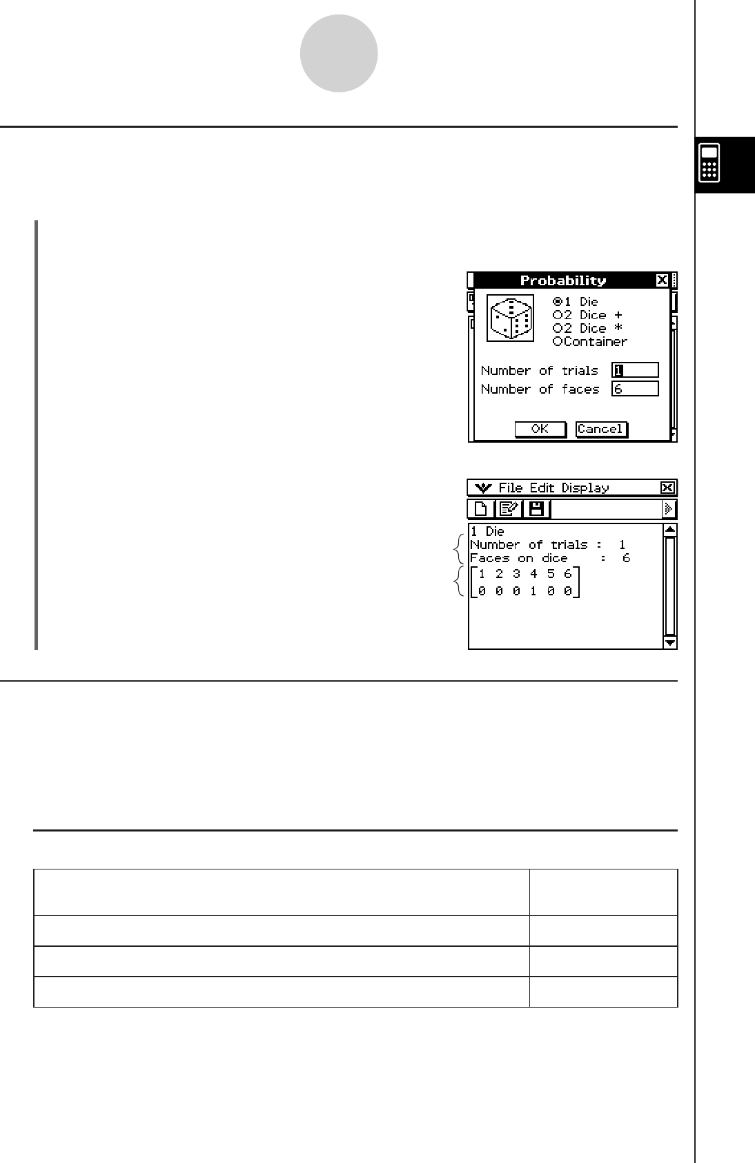
20060301

Starting Up Probability

Use the following procedure to start up Probability.

u ClassPad Operation

(1) Tap the right most toolbar down arrow button.

(2) On the icon palette that appears, tap P.

• This will display an initial Probability dialog box like

the one shown below. You can use this dialog box to

try the probability emulation.

(3) Tap [OK].

• This will execute the probability emulation using the

default setup (1 Die, Number of trials: 1, Number of

faces: 6 ).

Probability Menus and Buttons

This section provides basic information about Probability menus, commands, and buttons.

Tip

• O menu items are the same for all applications. For more information, see “Using the O

Menu” on page 1-5-4.

k File Menu

To do this: Select this File

menu item:

Discard the current window contents and create a new file New

Open an existing file Open

Save the current window contents to a file Save

2-12-2

Using Probability

Trial result

Trial information

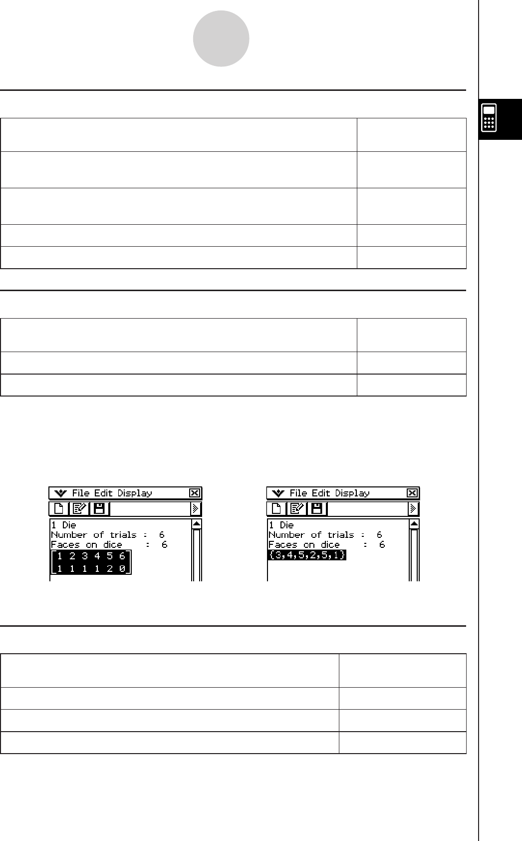
20060301

k Edit Menu

To do this: Select this Edit

menu item:

Copy the currently selected object (trial information or trial result) and

place it onto the clipboard Copy

Display the Probability dialog box and try the probability emulation (the

trial result will be added to the end of the current file) Add

Delete the currently selected trial data Delete

Clear the Probability window (and display the Probability dialog box) Clear All

k Display Menu

To do this: Select this Display

menu item:

Show the selected result distribution table format Distribution

Show the selected result as a list data format Sample Data

Tip

• Under initial default settings, trial results are shown in distribution table format. Selecting

distribution table results and selecting [Sample Data] on the [Display] menu will change them to

list data format. Conversely, selecting table results and selecting [Distribution] on the [Display]

menu will change them to distribution table format.

List Data FormatDistribution Table Format

2-12-3

Using Probability

k Probability Buttons

To do this: Select this Probability

button:

Discard the current window contents and create a new file E

Display the Probability dialog box and try the probability emulation P

Open an existing file R

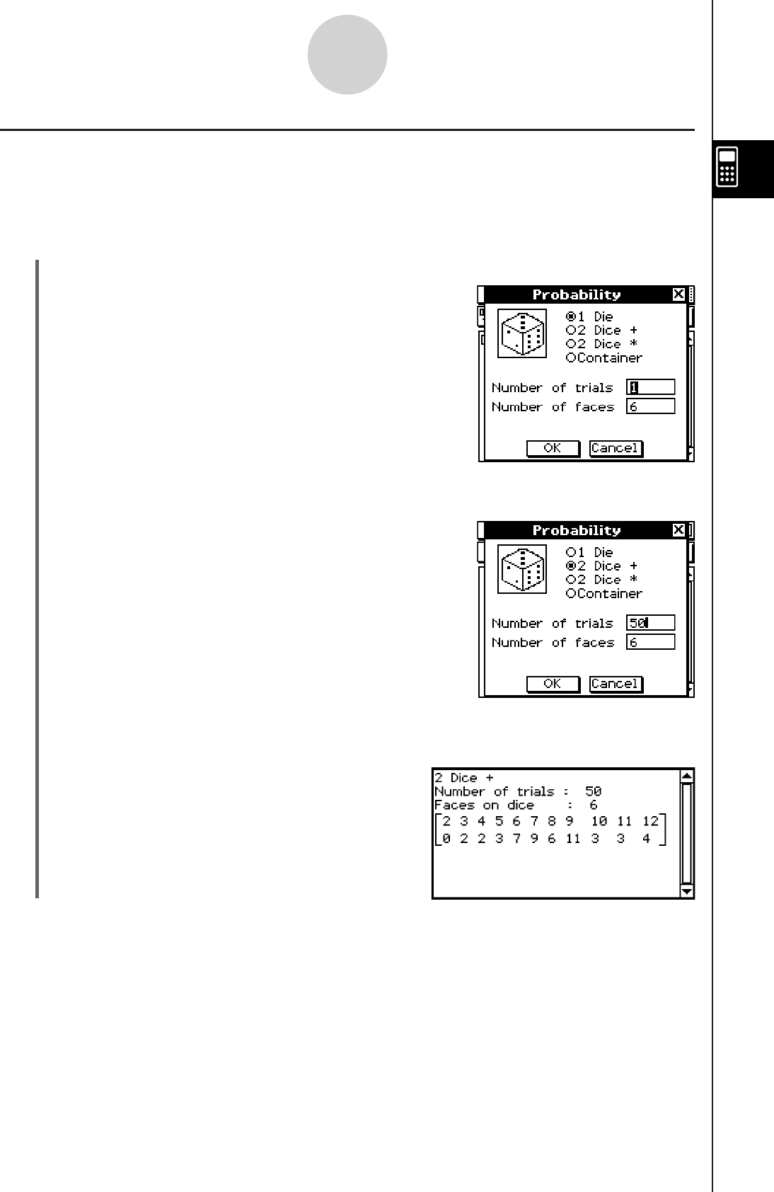
20060301

Using Probability

The following examples show the basic steps for using Probability.

Example 1: To obtain the sum data when a two six-sided die are thrown 50 times

u ClassPad Operation

(1) Tap the right most toolbar down arrow button.

(2) On the icon palette that appears, tap P.

• This displays the Probability dialog box.

(3) Tap the button next to “2 Dice +” to select it.

(4) Enter 50 into the “Number of trials” box.

• Leave the value in the “Number of faces”

box at it intial default value (6).

(5) Tap [OK].

• The result will appear in the Probability

window.

2-12-4

Using Probability

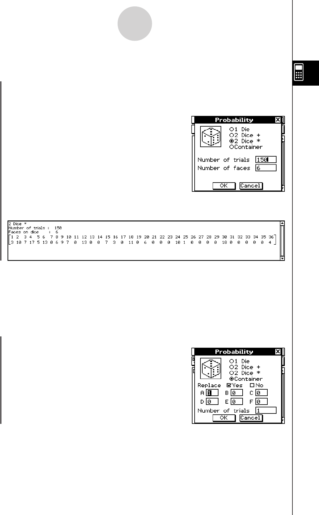
20060301

Example 2: To obtain the product data when a two six-sided die are thrown 150 times

(This example assumes you are continuing from Example 1.)

(1) Tap

P to display the Probability dialog box.

(2) Tap the button next to “2 Dice `” to select it.

(3) Enter 150 into the “Number of trials” box.

• Leave the value in the “Number of faces”

box at it initial default value (6).

(4) Tap [OK].

• The result will appear in the Probability window.

Example 3: After putting 10 A-balls, 2- B-balls, and 30 C-balls into a box, determine how

many times each type of ball will be drawn when there is a total of 50 draws.

Each time a ball is drawn, it should be replaced into the box before the next

draw.

(This example assumes you are continuing from Example 2.)

(1) Tap

P to display the Probability dialog box.

(2) Tap the button next to “Container” to select it.

2-12-5

Using Probability

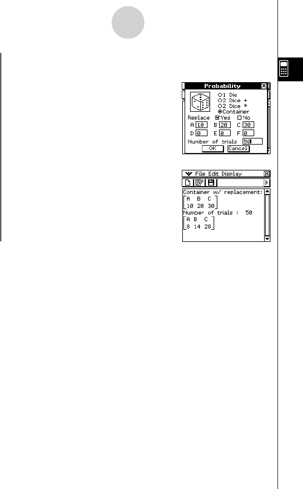
20060301

(3) Configure the following settings on the dialog box.

• Replace: Yes (Indicates the ball is replaced before the next draw. If the ball is not

replaced, select “No”.)

• A: 10, B: 20, C: 30 (Leaver other letters set to zero.)

• Number of trials: 50

(4) Tap [OK].

• The result will appear in the Probability window.

2-12-6

Using Probability

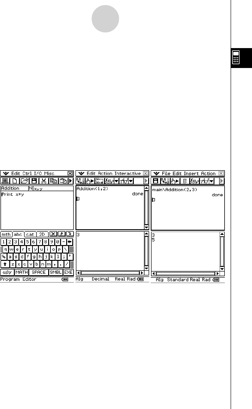
20090601

Main applicationProgramProgram eActivity application

2-13 Running a Program in the Main Application

You can run a program in the Main application or the eActivity application.

Syntax: Folder name\Program name(parameter)

• You do not need to specify the folder name if the program you want to run is in the

current folder. If you leave ClassPad configured with its initial default settings, the

current folder for both the Program application and the Main application is the “main”

folder, so you normally do not need to specify a folder name.

• Unless you change it, the current folder of the eActivity application is the “eAct” folder,

so you always need to specify the folder name. If you want to run a program that is in

the “main” folder, input “main\Program name(parameter)”.

Important!

If the program command “Pause” is used in a program, it is ignored when the program is

called from Main or eActivity.

2-13-1

Running a Program in the Main Application

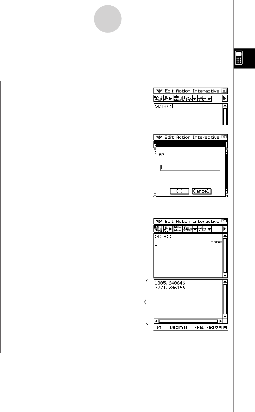
20060301

(3) Enter 20 and then tap [OK].

• This will run OCTA and display the results

in the program output window.

(4) To close the program output window, tap anywhere inside it and then tap the S button

in upper right corner.

Program output window

2-13-2

Running a Program in the Main Application

Example: To run the program named OCTA that we created and stored under “Creating

and Saving a Program” (page 12-2-1) from the Main application, and determine

the surface area and of a regular octahedron with a side length of 20 cm

u ClassPad Operation

(1) Perform the key operation below in the Main application work area.

0EOCTA9()

(2) Tap

20060301

Using the Graph & Table

Application

The Graph & Table application allows you to input and graph

rectangular coordinate equations (or inequalities), polar coordinate

equations, and parametric expressions. After you graph an expression,

you can zoom in or out, and move a pointer along the graph, displaying

its coordinates as you go. You can also perform various graph-based

analytical operations to determine the points of intersect of two graphs,

and to determine the maximum, minimum, point of inflection, and

definite integral for a particular range of a parabola or other figure. You

can even generate number tables and summary tables for functions

that you input.

3-1 Graph & Table Application Overview

3-2 Using the Graph Window

3-3 Storing Functions

3-4 Using Table & Graph

3-5 Modifying a Graph

3-6 Using the Sketch Menu

3-7 Using Trace

3-8 Analyzing a Function Used to Draw a Graph

Chapter

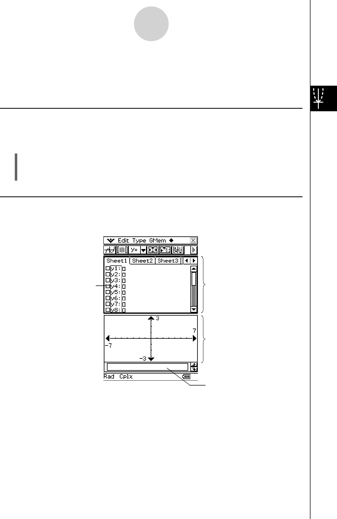
20060301

3-1 Graph & Table Application Overview

This section describes the configuration of the Graph & Table application windows and

provides basic information about its menus and commands.

Starting Up the Graph & Table Application

Use the following procedure to start up the Graph & Table application.

u ClassPad Operation

On the application menu, tap T.

This starts the Graph & Table application and displays the Graph Editor window and the

Graph window.

Graph & Table Application Window

When you start up the Graph & Table application, two windows appear on the display:

the Graph Editor window and the Graph window.

3-1-1

Graph & Table Application Overview

• A Graph Editor sheet can contain up to 20 functions. You can have up to 100 functions

stored in the Graph Editor at one time. Functions stored in the Graph Editor can be graphed

on the Graph window.

• The Graph window and Table window have a message box along the bottom that can

display expressions and values, or be used for input and editing.

Graph Editor window

Graph window

Message box

Line numbers

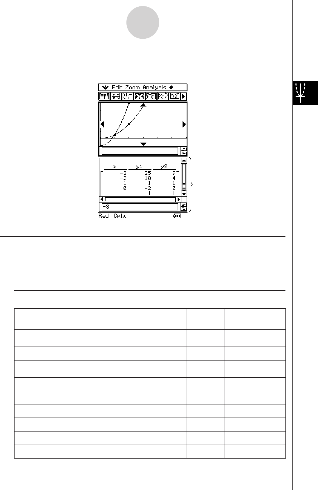
20060301

You can also use a function on the Graph Editor window to generate a number table or a

summary table. Number tables and summary tables are displayed in a Table window.

Graph & Table Application Menus and Buttons

This section explains the operations you can perform using the Graph & Table application

menus and buttons.

• For information about the O menu, see “Using the O Menu” on page 1-5-4.

k Graph Editor Window Menus and Buttons

3-1-2

Graph & Table Application Overview

Table window

To do this: Tap this

button:

Or select this

menu item:

Cut the selected character string and place it onto the

clipboard — Edit - Cut

Copy the selected character string to the clipboard — Edit - Copy

Paste the contents of the clipboard at the current cursor

position in the Graph Editor window — Edit - Paste

Select the entire expression you are editing — Edit - Select All

Clear all of the expressions from the Graph Editor window

— Edit - Clear All

Input a rectangular coordinate type function dType - y= Type

Input a polar coordinate type function fType - r= Type

Input a parametric function gType - ParamType

Input an X equality hType - x= Type

20070301

20060301

To do this: Tap this

button:

Or select this

menu item:

Input a rectangular coordinate type inequality

jType - y> Type

lType - y< Type

'Type - yt Type

XType - ys Type

Input an X inequality

kType - x> Type

;Type - x< Type

ZType - xt Type

CType - xs Type

Input two functions in a list and shade between them Type - ShadeType

Save all of the expressions on the Graph Editor window — GMem - Store

Recall batch saved data to the Graph Editor window — GMem - Recall

Display the Dynamic Graph dialog box (page 3-5-4) — a - Dynamic Graph

Display the Draw Shade dialog box (page 3-3-12) — a - Draw Shade

Use a built-in function for input — a - Built-In

Specify “AND Plot” as the inequality plot setting — a - Inequality Plot -

and

Specify “OR Plot” as the inequality plot setting — a - Inequality Plot -

Delete all of the expressions on the active sheet — a - Sheet -

Clear Sheet

Return all sheet names to their initial defaults — a - Sheet -

Default Name

Graph the selected function(s) $—

Generate a summary table for the selected function 4—

Display the View Window dialog box to configure Graph

window settings 6O - View Window

Display the Table Input dialog box for configuring settings 8—

Generate a table for the selected function #—

Display the Variable Manager (page 1-8-1) — O - Variable

Manager

3-1-3

Graph & Table Application Overview

20060301

k Graph Window Menus and Buttons

To do this: Tap this

button:

Or select this

menu item:

Cut the character string selected in the message box

and place it onto the clipboard — Edit - Cut

Copy the character string selected in the message box

to the clipboard — Edit - Copy

Paste the contents of the clipboard at the current cursor

position in the message box — Edit - Paste

Select all of the text in the message box — Edit - Select All

Clear all of the Graph window contents — Edit - Clear All

Enlarge the part of the screen bounded by a box QZoom - Box

Specify a zoom factor — Zoom - Factor

Zoom in by the zoom factor — Zoom - Zoom In

Zoom out by the zoom factor — Zoom - Zoom Out

Configure View Window y-axis parameters and redraw

the graph so it fills the graph screen along the y-axis RZoom - Auto

Return a graph to its original size — Zoom - Original

Adjust View Window x-axis values so they are identical

to the y-axis values — Zoom - Square

Round coordinate values displayed using Trace

(page 3-7-1) — Zoom - Round

Make the value of each dot equal 1, which makes all

coordinate values integers — Zoom - Integer

Return View Window parameters to their settings prior

to the last zoom operation — Zoom - Previous

Perform a quick zoom operation (page 3-2-9)

—Zoom -

Quick Initialize

— Zoom - Quick Trig

— Zoom - Quick log(x)

— Zoom - Quick e^x

— Zoom - Quick x^2

— Zoom - Quick –x^2

—Zoom -

Quick Standard

3-1-4

Graph & Table Application Overview

20060301

To do this: Tap this

button:

Or select this

menu item:

Display the coordinates at a particular point on a graph =Analysis - Trace

Insert a point, graphic, or text into an existing graph

(page 3-6-1) — Analysis - Sketch

Obtain the root (x-intercept) of a graph YAnalysis - G-Solve -

Root

Obtain the maximum value of a graph UAnalysis - G-Solve -

Max

Obtain the minimum value of a graph IAnalysis - G-Solve -

Min

Obtain the maximum value in the range displayed on the

Graph window —Analysis - G-Solve -

fMax

Obtain the minimum value in the range displayed on the

Graph window —Analysis - G-Solve -

fMin

Obtain the y-intercept of a graph — Analysis - G-Solve -

y-Intercept

Obtain the point of intersection for two graphs — Analysis - G-Solve -

Intersect

Obtain the y-coordinate for a given x-coordinate — Analysis - G-Solve -

y-Cal

Obtain the x-coordinate for a given y-coordinate — Analysis - G-Solve -

x-Cal

Obtain the definite integral for a particular range — Analysis - G-Solve -

∫dx

Obtain the point of inflection — Analysis - G-Solve -

Inflection

Obtain the distance between two points — Analysis - G-Solve -

Distance

Obtain the volume of a solid of revolution — Analysis - G-Solve -

π ∫ (f (x))2 dx

Modify a graph by changing the value of a coefficient — Analysis - Modify

Save a graph as image data (page 3-2-10) — a - Store Picture

Recall the image of a graph (page 3-2-10) — a - Recall Picture

Display the Dynamic Graph dialog box (page 3-5-4) — a - Dynamic Graph

Display the Draw Shade dialog box (page 3-3-12) — a - Draw Shade

Use a built-in function template to input a function for

graphing

• Note that built-in functions are graphed automatically

and cannot be used for input on the Graph Editor

window.

—a - Built-In

3-1-5

Graph & Table Application Overview

20060301

To do this: Tap this

button:

Or select this

menu item:

Specify “AND Plot” as the inequality plot setting — a - Inequality Plot -

and

Specify “OR Plot” as the inequality plot setting — a - Inequality Plot -

Re-draw a graph — a - ReDraw

Make the Graph Editor window active !—

Generate a number table for an existing graph #—

Display the View Window dialog box to configure Graph

window settings 6O - View Window

Display the Table Input dialog box for configuring settings 8—

Pan the Graph window T—

Display the Variable Manager (page 1-8-1) — O - Variable

Manager

Generate a summary table for an existing graph 4—

k Table Window Menus and Buttons

To do this: Tap this

button:

Or select this

menu item:

Cut the character string selected in the message box

and place it onto the clipboard — Edit - Cut

Copy the character string selected in the message box

to the clipboard — Edit - Copy

Paste the contents of the clipboard at the current cursor

position in the message box — Edit - Paste

Select all of the text in the message box — Edit - Select All

Clear all of the Table window contents — Edit - Clear All

Delete a line from a table — T-Fact - Delete

Insert a line into a table — T-Fact - Insert

Add a line after the currently selected line — T-Fact - Add

Draw a connect type graph using a generated table $Graph - G-Connect

Draw a plot type graph using a generated table !Graph - G-Plot

Save the contents of a table to a list — a - Table to List

Re-generate a table based on current table settings — a - ReTable

Delete the displayed table — a - Delete Table

Move the pointer to the location on a graph that

corresponds to the value selected in a table —a - Link

3-1-6

Graph & Table Application Overview

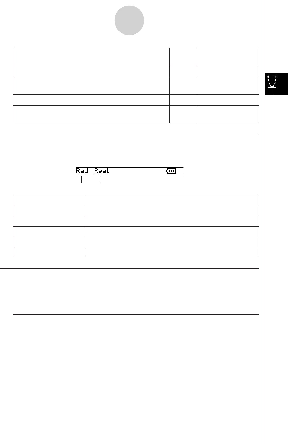
20060301

3-1-7

Graph & Table Application Overview

Graph & Table Application Status Bar

The status bar at the bottom of the Graph & Table application shows the current angle unit

setting and [Complex Format] setting (page 1-9-5).

Graph & Table Application Basic Operations

This section explains how to input a function on the Graph Editor window and then graph it

on the Graph window. These are the most basic operations you can perform with the Graph

& Table application.

k Function Storage and Graphing Example

This example shows how to input two functions on Sheet 1 of the Graph & Table application,

and then draw their graphs.

Tip

• The Graph Editor window has five sheets, named Sheet 1 through Sheet 5, for input of

expressions. For more information, see “Using Graph Editor Sheets” on page 3-3-1.

Angle unit Real mode

If you see this: It means this:

Rad The angle unit setting is radians.

Deg The angle unit setting is degrees.

Gra The angle unit setting is grads.

Cplx The Complex (complex number calculation) mode is selected.

Real The Real (real number calculation) mode is selected.

To do this: Tap this

button:

Or select this

menu item:

Make the Graph Editor window active !—

Display the View Window dialog box to configure Graph

window settings 6O - View Window

Display the Table Input dialog box for configuring settings 8—

Display the Variable Manager (page 1-8-1) — O - Variable

Manager

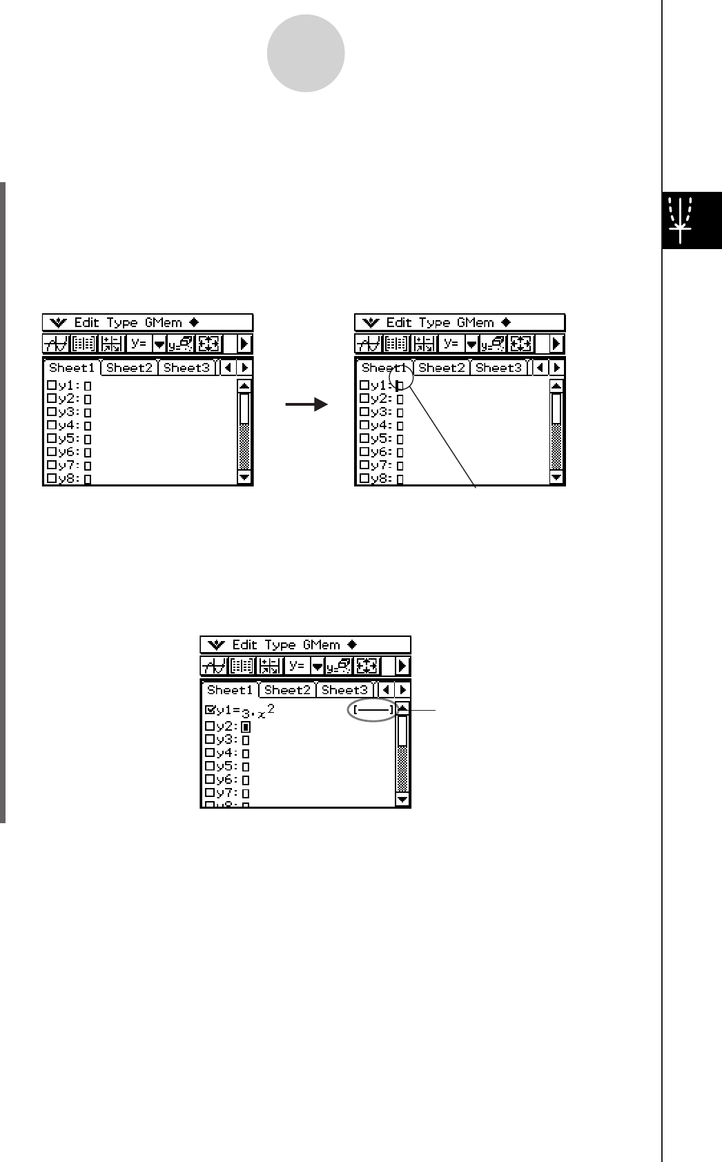
20060301

Example 1: To input the function y = 3x2 on Sheet 1 and graph it

uClassPad Operation

(1) On the application menu, tap T.

• This starts the Graph & Table application.

(2) In the Graph Editor window, tap the input box immediately to the right of line number

y1.

• This locates the cursor in the input box for line y1.

3-1-8

Graph & Table Application Overview

(3) Input the expression.

3x{2E

• Pressing E stores the expression you input and puts a check mark into the check

box to the left of line number y1. When a line number has a check mark next to it, it

means that the expression is currently selected for graphing.

When you input an expression,

the line style that will be used for

the graph will appear here. See

page 3-3-8 for information about

configuring line settings.

Hint:

Tap the line that is circled above!

Cursor

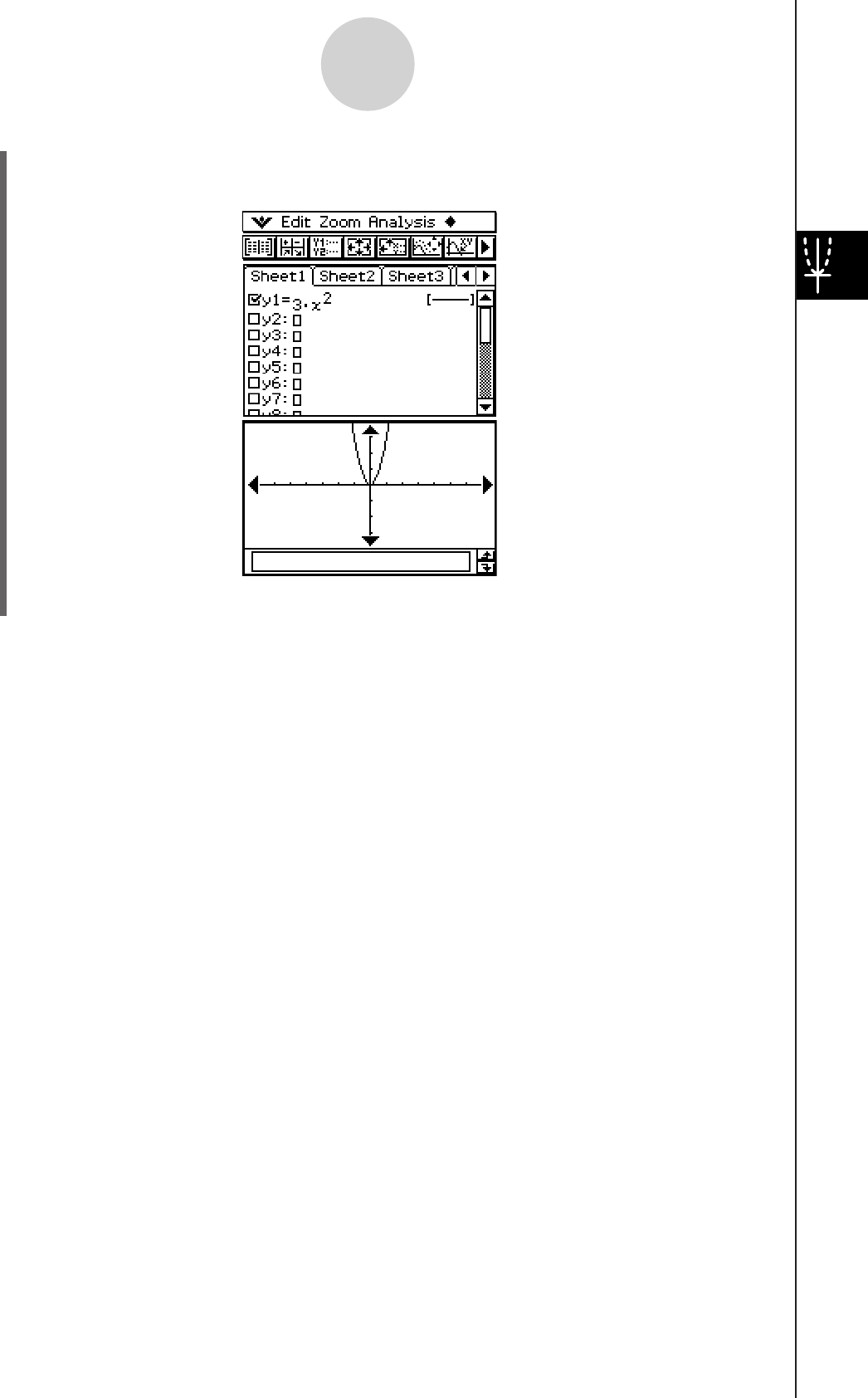
20060301

3-1-9

Graph & Table Application Overview

(4) Tap

• This graphs the expression.

The expression is displayed in the message box while the graph is being drawn.

Tip

• The Graph window message box is for both input and output. It displays information about the

function and other information. You can also use it to edit the function, which causes the graph to

change shape. Details about the information that appears in the message box and how to use the

message box are covered on page 1-6-8.

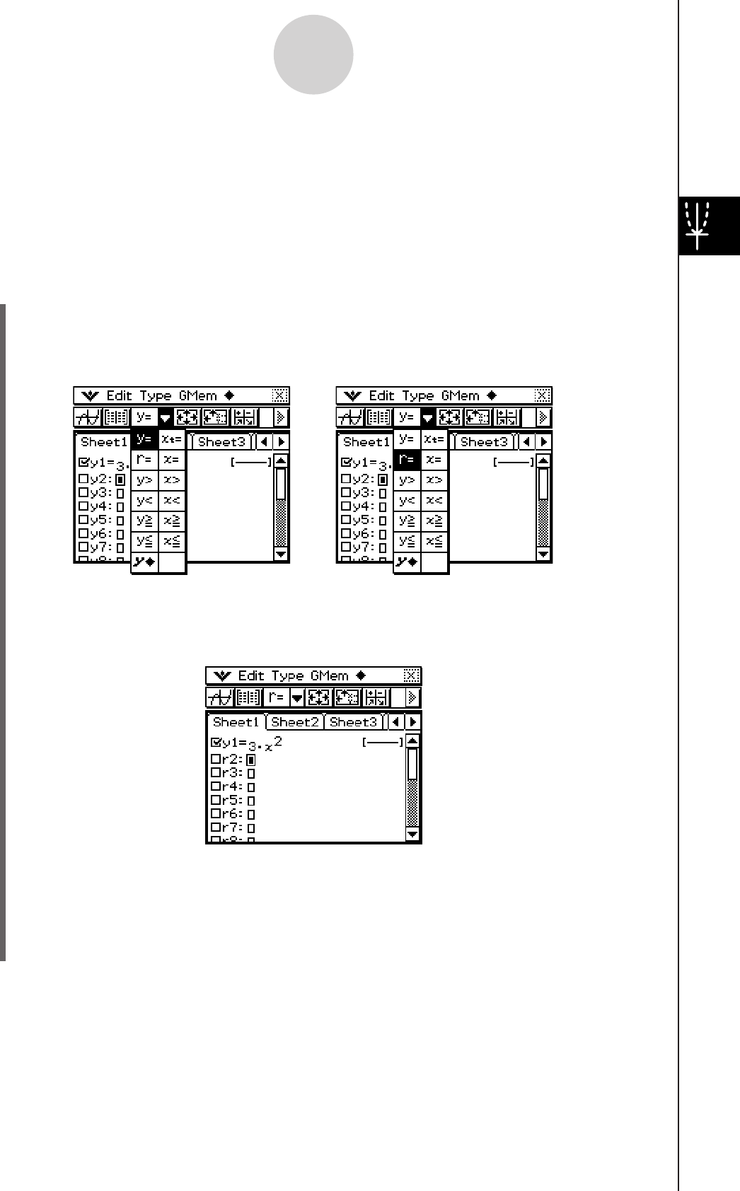
20060301

Example 2: To input the function r = 3sin2 into line 2 of Sheet 1 and graph it

In Example 1, we graphed a rectangular expression in the form of y = f(x). You can also input

polar coordinate expressions, inequalities, and other types of functions for graphing as well.

In this example, we input and graph the polar coordinate expression r = 3sin2 . Note that

the following sample procedure assumes that you have already completed the steps for

Example 1.

u ClassPad Operation

(1) Tap anywhere inside of the Graph Editor window to make it active.

(2) Tap the down arrow next to “y =”, or on the menu tap [Type]. On the list that appears,

tap “r =”.

• This causes the line numbers next to any line on the Graph Editor window that does

not contain an expression to change from “y” to “r” (r2, r3, etc.). The line numbers of

lines that already contain expressions do not change.

(3) Tap the input box to the right of line number r2 and input the expression.

k9dTsc8)w

• Tapping w stores the expression you input and puts a check mark into the check

box to the left of line number r2. When a line number has a check mark next to it, it

means that the expression is currently selected for graphing.

3-1-10

Graph & Table Application Overview

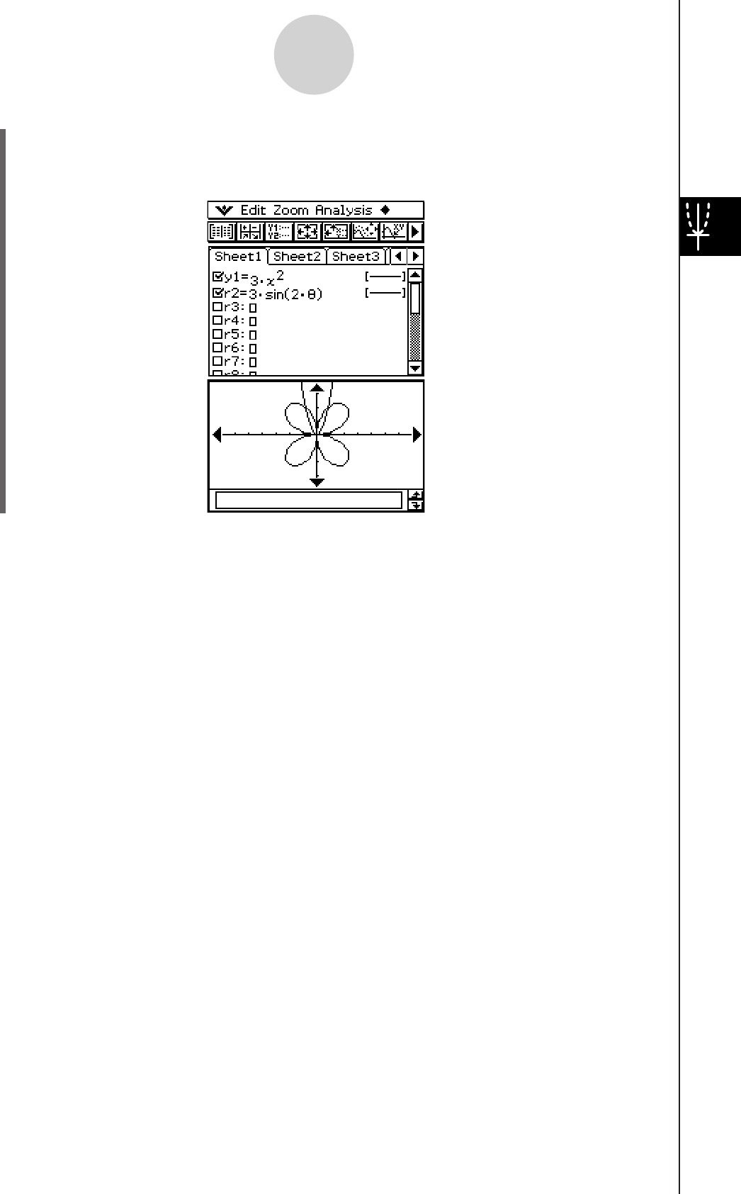
20060301

3-1-11

Graph & Table Application Overview

(4) Tap

• Since there are check marks next to both “y1” and “r2”, both expressions are

graphed.

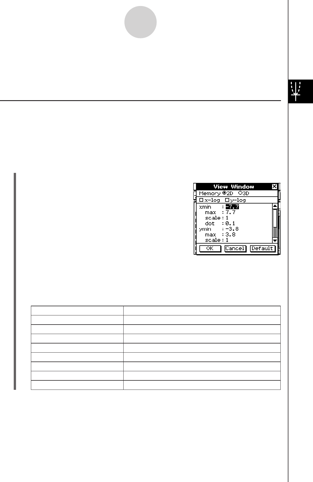
20060301

3-2-1

Using the Graph Window

3-2 Using the Graph Window

This section explains Graph window operations, including configuring display settings,

scrolling, zooming the image, and more.

Configuring View Window Parameters for the Graph Window

The View Window dialog box lets you specify the maximum and minimum values for each

axis, the space between the marks on each axis (the scale), and other graph display

parameters. Before drawing a graph, be sure to first configure View Window parameters to

ensure proper display of the graph.

u To configure View Window parameters

(1) On the application menu, tap T.

(2) Tap

6, or tap O and then [View Window].

• This displays the View Window dialog box.

(3) Tap the “2D” option button so the option is selected.

(4) Configure View Window parameters required for the type of graph you want to draw.

• Press c to move the cursor and then input an appropriate value for each parameter.

Rectangular Coordinates

Use this item: To configure this View Window parameter:

xmin

xmax

xscale

xdot

ymin

ymax

yscale

ydot

x-axis minimum value

x-axis maximum value

x-axis marker spacing

Value of each dot on the x-axis

y-axis minimum value

y-axis maximum value

y-axis marker spacing

Value of each dot on the y-axis

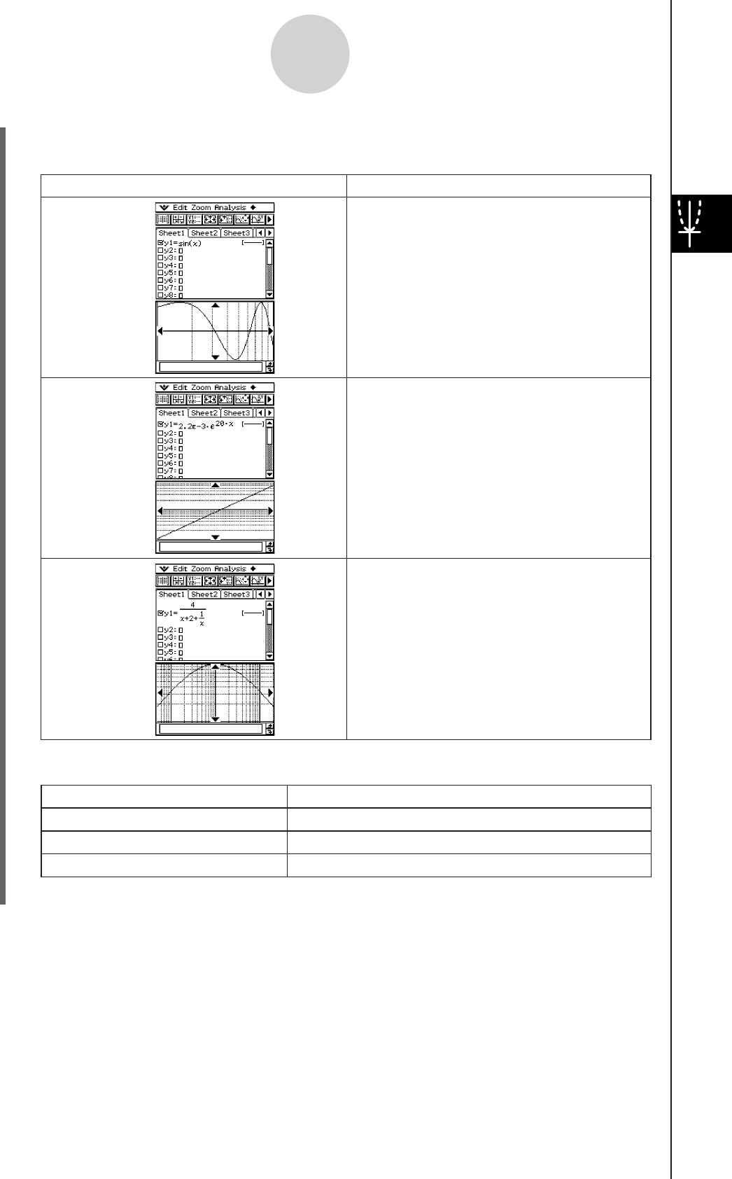
20060301

3-2-2

Using the Graph Window

Polar Coordinates and Parametric Coordinates

To select this type of graph:

-log graph

Do this:

Select the

-log check box.

• This automatically sets “xdot” and

“xscale” to “Auto”.

Select the

-log check box.

• This automatically sets “ydot” and

“yscale” to “Auto”.

Select the

-log check box and the

-log check box.

This automatically sets “xdot”, “xscale”,

“ydot”, and “yscale” to “Auto”.

Use this item:

t min

t max

t step

To configure this View Window parameter:

Minimum value of t

Maximum value of t

Step size of t

(5) After all the parameters are the way you want, tap [OK].

Tip

• When you tap [OK] after changing View Window dialog box settings while the Graph window is

active, the graph is redrawn automatically using the new View Window settings.

• If the Graph window is not active, tapping [OK] closes the View Window dialog box without

redrawing the graph. To redraw the graph in this case, tap $ on the Graph Editor window.

• You can also use the rectangular coordinate View Window dialog box to select x-log

graph, y-log graph, or xy-log graph.

20060301

u View Window parameter precautions

• An error occurs if you input 0 for tstep.

• An error also occurs if you input a value that is out of range for a parameter, if you input a

minus sign only, or if you perform any other illegal input.

• An error occurs if ymin is greater than or equal to the ymax. The same is also true for the

xmin and xmax. If the value you specify for tmin is greater than the value you specify for

tmax, the tstep setting is automatically changed to a negative value.

• When the View Window setting produces an axis that does not fit on the display, the scale

of the axis is indicated on the edge of the display closest to the origin.

• Changing the xmin (ymin) or xmax (ymax) value automatically changes the xdot (ydot)

value, while changing the xdot (ydot) value automatically changes the xmax (ymax) value.

u To initialize View Window parameters

(1) On the application menu, tap T.

(2) Tap

6. This displays the View Window dialog box.

(3) Tap [Memory] and then [Initial]. This initializes View Window parameters to the values

noted below.

xmin = –7.7 xmax = 7.7 xscale = 1 xdot = 0.1

ymin = –3.8 ymax = 3.8 yscale = 1 ydot = 0.1

min = 0 tmax = 6.28318530717 tstep = 0.05235987755

u To initialize the View Window for an angle unit

(1) On the application menu, tap T.

(2) Tap

6. This displays the View Window dialog box.

(3) Tap [Memory] and then [Trigonometric]. This initializes View Window parameters in

accordance with the angle unit, as shown below.

(Setup: Radian)

xmin = –9.4247779607 xmax = 9.42477796076

xscale = 1.57079632679 xdot = 0.12239971377

ymin = –1.6 ymax = 1.6

yscale = 0.5 ydot = 0.04210526315

min = 0 tmax = 6.28318530717

step = 0.05235987755

(Setup: Degree)

xmin = –540 xmax = 540 xscale = 90 xdot = 7.01298701298

ymin = –1.6 ymax = 1.6 yscale = 0.5 ydot = 0.04210526315

min = 0 tmax = 360 tstep = 3

3-2-3

Using the Graph Window

20060301

3-2-4

Using the Graph Window

u To standardize the View Window

(1) On the application menu, tap T.

(2) Tap

6. This displays the View Window dialog box.

(3) Tap [Memory] and then [Standard]. This applies the standard View Window parameters

shown below.

xmin = –10 xmax = 10 xscale = 1 xdot = 0.12987012987

ymin = –10 ymax = 10 yscale = 1 ydot = 0.26315789473

min = 0 tmax= 6.28318530717 tstep = 0.05235987755

u To auto configure View Window parameters

(1) On the application menu, tap T.

(2) Tap

6. This displays the View Window dialog box.

(3) Tap [Memory] and then [Auto]. This causes View Window parameters to be configured

automatically in accordance with the function on the Graph Editor window.

• When multiple expressions are selected for graphing, the one with the lowest

numbered line is used for auto setting of View Window parameters.

Tip

• Initializing or standardizing View Window parameters causes polar/parametric coordinate values

tmin, tmax, and tstep to be adjusted automatically in accordance with the currently selected

angle unit. In the Degree mode, for example, the following settings are configured:

tmin = 0, tmax = 360, tstep = 3

k Using View Window Memory

You can store your custom View Window settings for later use.

u To save the current View Window setup

(1) On the application menu, tap T.

(2) Tap

(3) On the View Window dialog box, configure the parameters you want.

(4) Tap [Memory] and then [Store]. This displays a dialog box for inputting a name for the

View Window setup.

(5) Enter the name and then tap [OK].

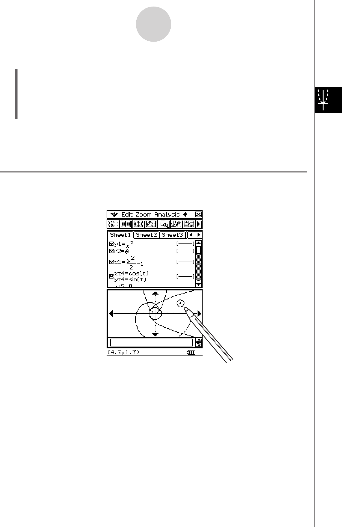
20060301

3-2-5

Using the Graph Window

u To recall a setup from View Window memory

(1) On the application menu, tap T.

(2) Tap

6. This displays the View Window dialog box.

(3) Tap [Memory] and then [Recall]. This displays a list of names of the View Window

setups you have stored in memory.

(4) Select the name of the setup you want, and then tap [OK].

Tip

• Recalling a View Window setup causes the current View Window parameters to be replaced by

the parameters of the recalled setup.

Viewing Graph Window Coordinates

Tapping and holding a point on Graph window with the stylus will display the coordinates at

that location in the status bar.

Coordinate

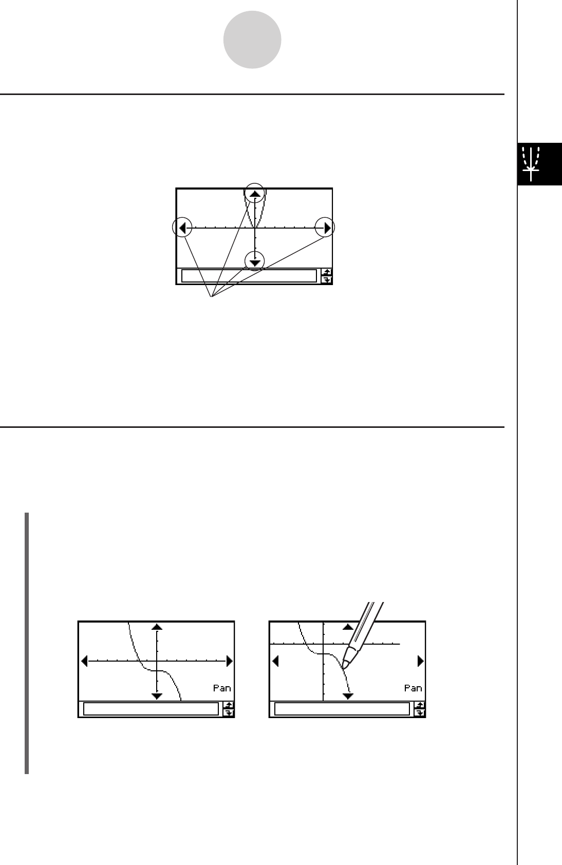
20060301

3-2-6

Using the Graph Window

Panning the Graph Window

Placing the stylus against the Graph window and dragging causes the window to scroll

automatically in the direction you drag.

u ClassPad Operation

(1) Tap the Graph window to make it active.

(2) Tap

(3) Holding the stylus anywhere against the Graph window, drag it in the direction you

want.

• This causes the Graph window to scroll automatically in accordance with the

dragging.

(4) When the Graph window shows the area you want, remove the stylus from the display.

• This causes the graph to be redrawn on the Graph window.

After T is tapped While panning

Tip

• Display of the graph controller arrows is turned off under initial default settings. Use the Graph

Format dialog box to turn them on, if you want. For more information, see “Application Format

Settings” on page 1-9-4.

• You can also use the graph controller arrows and cursor key to change the configuration of a

graph. For details, see “3-5 Modifying a Graph”.

Graph controller arrows

Scrolling the Graph Window

After drawing a graph, you can use either of the two operations to scroll it up, down, left, or

right.

• Tap the graph controller arrows at the edges of the Graph window.

• Use the cursor key.

20060301

3-2-7

Using the Graph Window

Zoom Command Description

Box

Factor

Zoom In

Zoom Out

Auto

Original

Square

Round

Integer

Quick Initialize

Quick Trig

Quick log (x)

Quick e^x

Quick x^2

Quick –x^2

Quick Standard

With “box zoom”, you draw a selection boundary around the area you

would like to enlarge. This causes the selected area to be enlarged so

it fills the entire graph display.

“Factor zoom” lets you specify a zoom factor for enlarging or reducing

a graph.

Use the [Factor] command to configure zoom factor settings, the

[Zoom In] command to zoom in, and the [Zoom Out] command to

zoom out.

“Auto zoom” automatically configures View Window y-axis values and

redraws the graph so it fills the Graph window along the y-axis.

Return a graph to its original View Window settings

Executing this command adjusts View Window x-axis values so that

they are identical to the y-axis values.

Round View Window settings (xmin, xmax, xdot) to an appropriate

number of decimal places and redraw the graph.

This command makes the value of each dot equal 1, which makes all

coordinate values integers.

Performing a zoom operation changes View Window parameter

values. Execute this command to return View Window parameters to

their settings prior to the last zoom operation.

These seven quick zoom commands cause the graph to be redrawn

using preset View Window parameter values (page 3-2-9).

Zooming the Graph Window

Your ClassPad provides you with a wide selection of zoom commands that you can use to

enlarge or reduce an entire graph or a specific area of a graph.

k Zoom Commands

The Graph window’s [Zoom] menu contains the zoom commands described in the table

below.

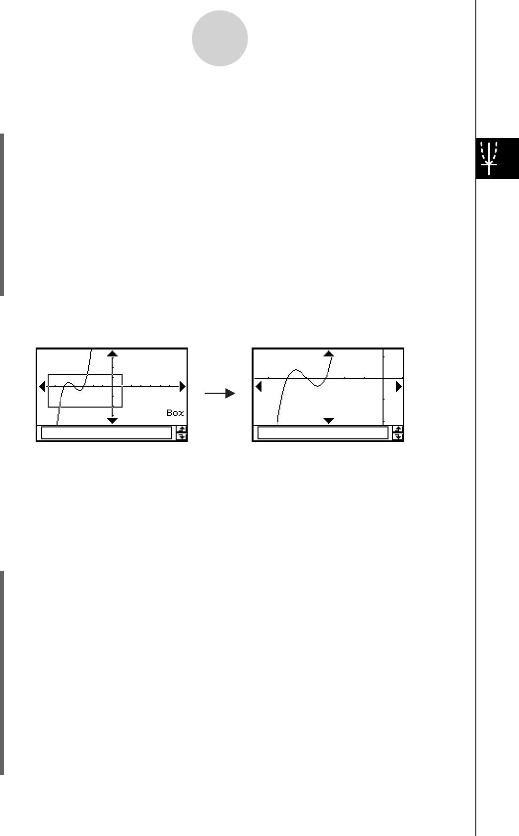
20060301

3-2-8

Using the Graph Window

u To use factor zoom

Example: To enlarge the graphs of the following two expressions, by a factor of 5 in both

directions, to determine whether they come into contact with each other

y1 = (x + 4)(x + 1)(x – 3)

y2 = 3x + 22

(1) On the application menu, tap T.

(2) On the Graph Editor window, input y1 = (x + 4)(x + 1)(x – 3) and y2 = 3x + 22.

• For details about how to input an expression, see “Function Storage and Graphing

Example” on page 3-1-7 and “3-3 Storing Functions”.

(3) Tap

6 to display the View Window, and then configure it with the following

parameters.

xmin = –8, xmax = 8, xscale = 1

ymin = –30, ymax = 30, yscale = 5

• See “To configure View Window parameters” on page 3-2-1.

(4) Tap

$ to graph the functions.

(5) Tap [Zoom] and then [Factor].

• This displays a dialog box for configuring x- and y-axis zoom factor settings.

u To use box zoom

Example: To use box zoom to enlarge part of the graph y = (x + 5)(x + 4)(x + 3)

(1) On the application menu, tap T.

(2) On the Graph Editor window, input y = (x + 5)(x + 4)(x + 3).

• For details about how to input an expression, see “Function Storage and Graphing

Example” on page 3-1-7 and “3-3 Storing Functions”.

(3) Tap

$ to graph the functions.

(4) Tap [Zoom] and then [Box], or tap Q.

(5) On the Graph window, drag the stylus to draw a selection boundary around the area

you want to enlarge.

(6) Remove the stylus from the display and the area within the selection boundary expands

to fill the entire Graph window.

Box Zoom Result

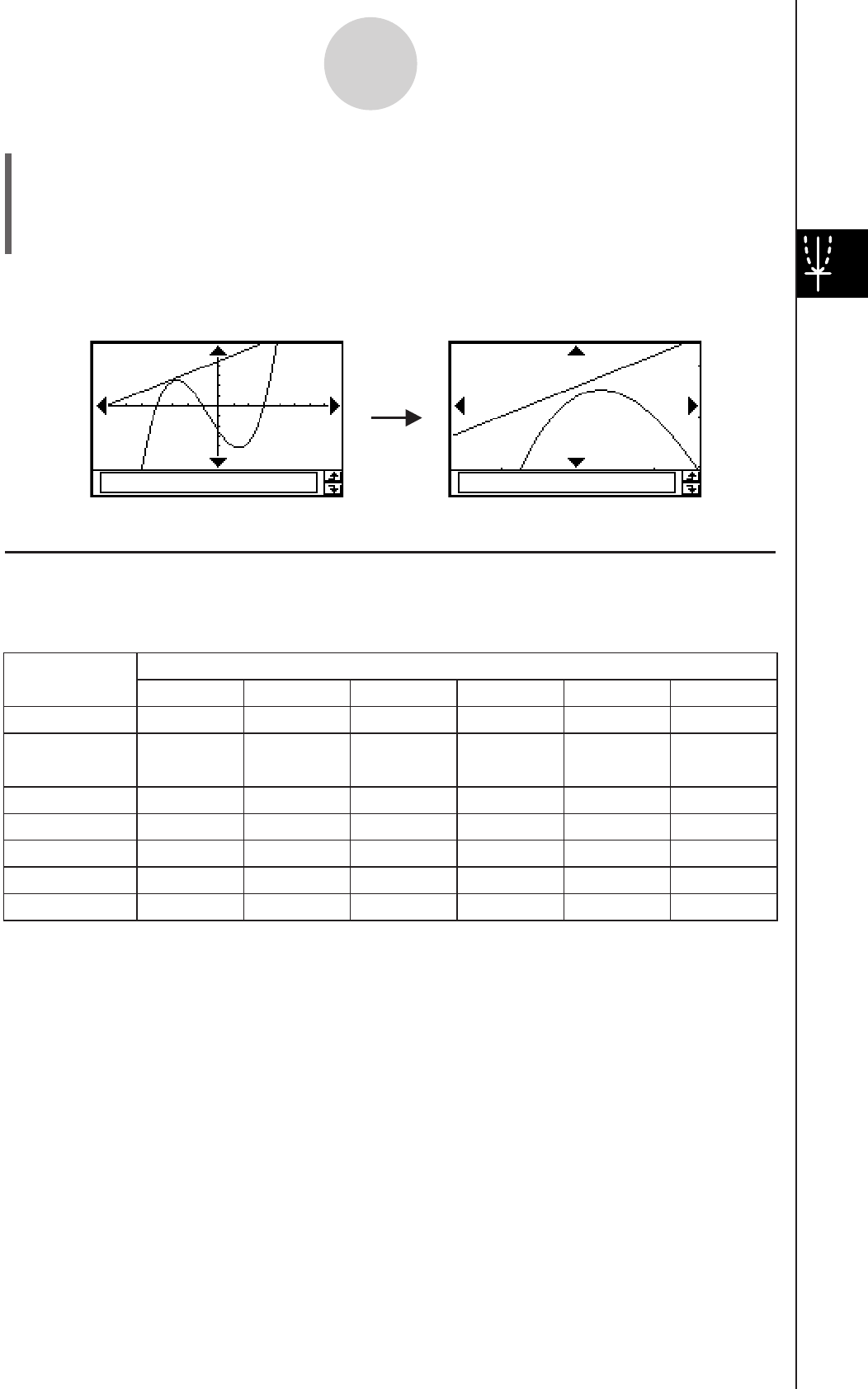
20101001

3-2-9

Using the Graph Window

(6) Input 5 for both the xFactor and yFactor, and then tap [OK].

(7) Tap

T, and then use the stylus to drag the screen image so the part you want to

zoom is in the center of the screen.

(8) Tap [Zoom] and then [Zoom In].

Factor Zoom Result

View Window Parameter Values

Command

Quick Initialize

Quick Trig

Quick log (x)

Quick e^x

Quick x^2

Quick –x^2

Quick Standard

xmin xmax xscale ymin ymax yscale

–7.7 7.7 1 –3.8 3.8 1

–12.1

(–3.85π)

12.1

(3.85π)

1.570

(π/2) –2.1 2.1 1

–2 13.4 2 –3.8 3.8 1

–2.2 2.2 1 –1.4 9 1

–7.7 7.7 2 –10 66 5

–7.7 7.7 2 –66 10 5

–10 10 1 –10 10 1

The applicable set of View Window parameter values is applied as soon as you select a

quick zoom command on the Graph window’s [Zoom] menu.

Tip

• Any View Window parameter that is not shown in the above table is unchanged when you

execute a quick zoom command.

• When the angle unit setting is degrees, Quick Trig configures the following values.

xmin = –540, xmax = 540, xscale = 90

ymin = –1.6, ymax = 1.6, yscale = 0.5

k Using Quick Zoom

The seven quick zoom commands draw a graph using preset built-in View Window

parameter values.

20060301

3-2-10

Using the Graph Window

kUsing Other Zoom Menu Commands

The [Auto], [Original], [Square], [Round], [Integer], and [Previous] zoom commands are

executed as soon as you tap one of them on the Graph window’s [Zoom] menu.

For information about what each command does, see “Zoom Commands” on page 3-2-7.

Tip

• For auto zoom, you can tap the R button instead of using the [Zoom] - [Auto] menu command.

• With Integer Zoom, tap T and then use the stylus to drag the screen image so the part you

want to zoom is in the center of the screen.

Other Graph Window Operations

This section explains how to save a screenshot of the Graph Window, how to redraw a

graph, how to make the Graph Editor Window the active window.

k Saving a Screenshot of a Graph

Use the following procedures to save a screenshot of a graph as image data for later recall.

u To save a screenshot of a graph

(1) On the application menu, tap T.

(2) Draw the graph you want to save.

(3) Tap

a and then [Store Picture]. This displays a dialog box for inputting a name for the

screenshot.

(4) Enter the name and then tap [OK].

u To recall a screenshot of a graph

(1) On the application menu, tap T.

(2) Tap the Graph window to make it active.

(3) Tap

a and then [Recall Picture]. This displays a list of names of graph images you

have stored in memory.

(4) Select the name of the image you want, and then tap [OK].

20060301

k Redrawing a Graph

Use the following procedure to redraw a graph when necessary.

u ClassPad Operation

(1) Tap the Graph window to make it active.

(2) Tap

a and then [ReDraw].

• While the Graph Editor window is active, you can redraw the graph by tapping $.

Important!

• Use the a - [ReDraw] command to redraw a graph that you drew by dragging an

expression from another window to the Graph window (see “2-10 Using the Main

Application in Combination with Other Applications”), or a graph you modified using some

Sketch menu (see “3-6 Using the Sketch Menu”). After deleting the redrawn graph, you

can redraw the graph of the expression selected on the Graph window by tapping [Analysis],

[Sketch], and then [Cls].

kMaking the Graph Editor Window the Active Window

While the Graph window is active, you can make the Graph Editor window the active window

by tapping anywhere inside of it, by tapping !, or by tapping Oand then [Graph Editor].

3-2-11

Using the Graph Window

20060301

3-3 Storing Functions

Use the Graph Editor window to store a Graph & Table application function. This section

covers Graph Editor operations, and explains how to store functions.

Using Graph Editor Sheets

The Graph Editor window has five tabbed sheets named Sheet 1 through Sheet 5, each of

which can contain up to 20 functions. You can have up to 100 functions stored in the Graph

Editor at one time.

You can graph up to 20 functions simultaneously, as long as all of the functions are on the

same sheet.

k Selecting a Sheet

Use the operations described below to change from one sheet to another.

3-3-1

Storing Functions

k Renaming a Sheet

Initially, the fives sheets are assigned default names from Sheet 1 through Sheet 5. You can

use these sheet names as they are, or you can perform the steps below to rename a sheet.

u ClassPad Operation

(1) Tap the tab of the sheet you want to rename so that sheet becomes active.

(2) Tap the tab of the active sheet again.

• This displays a dialog box for inputting a sheet

name.

(3) Enter up to 8 bytes for the sheet name, and then tap [OK].

Tap the tab of the sheet you

want to select. The currently

selected sheet is the “active”

sheet.

Tap here to scroll the tabs so

the ones that do not fit on the

current window come into view.

20060301

k Returning Sheets to Their Default Names

The procedure below returns the sheet names to their initial default names (Sheet 1 through

Sheet 5).

u ClassPad Operation

(1) Tap the Graph Editor window to make it active.

(2) Tap

a, [Sheet], and then [Default Name].

• This returns the currently active sheet to its default name.

k Initializing a Sheet

The following procedure initializes a sheet, which clears all of its functions and renames the

sheet to its default name.

u ClassPad Operation

(1) If the sheet you want to initialize is not active, tap its tab.

(2) Tap

a, [Sheet], and then [Clear Sheet].

(3) In response to the confirmation message that appears, tap [OK] to initialize the sheet or

[Cancel] to cancel the operation.

• For details about editing and deleting individual functions, see “Editing Stored Functions”

on page 3-3-6.

• You can delete all expressions on all of the sheets by tapping [Edit] and then [Clear All].

For more information, see “Deleting All Graph Editor Expressions” on page 3-3-7.

Specifying the Function Type

When storing a Graph & Table application function, the first thing you need to do is specify

the function type. The following table lists all of the function types that you can select.

3-3-2

Storing Functions

y = Rectangular coordinate expression

Polar coordinate expression

Parametric expressions

X = expression

Inequality

r =

xt/yt =

x =

y >

y <

y ≤

y ≥

x >

x <

x ≤

x ≥

Two functions in a list with shading

between them

20060301

u ClassPad Operation

(1) On the application menu, tap T.

(2) On the Graph Editor window, tap the down arrow next to “y =”, or tap [Type].

(3) On the list that appears, tap the function type you want to select.

Storing a Function

This section presents a number of examples that illustrate how to store a Graph & Table

application function.

u To store a rectangular coordinate function (Y=)

Example: To store the rectangular coordinate function y = 2x2 – 5 in line number y1

(1) On the Graph Editor window, tap [Type] and then [y=Type] to specify a rectangular

coordinate expression.

(2) Tap the box to the right of line number “y1”, and then input the expression:

2x{ 2-5.

(3) Press

E to store the expression.

u To store a polar coordinate equation (r=)

Example: To store the polar coordinate equation r = 5sin3

 in line number r2

(1) On the Graph Editor window, tap [Type] and then [r=Type] to specify a polar coordinate

expression.

(2) Tap the box to the right of line number “r2”, and then input the expression:

k9fTsd8).

(3) Tap

w to store the expression.

u To store parametric functions

Example: To store the parametric functions below in line numbers xt3/yt3

xt = 3sint

yt = 3cost

(1) On the Graph Editor window, tap [Type] and then [ParamType] to specify parametric

expressions.

(2) Tap the box to the right of line number “xt3”, and then input the x-expression:

k9dTst)w.

(3) Tap the box to the right of line number “yt3”, and then input the y-expression:

9dct)w.

3-3-3

Storing Functions

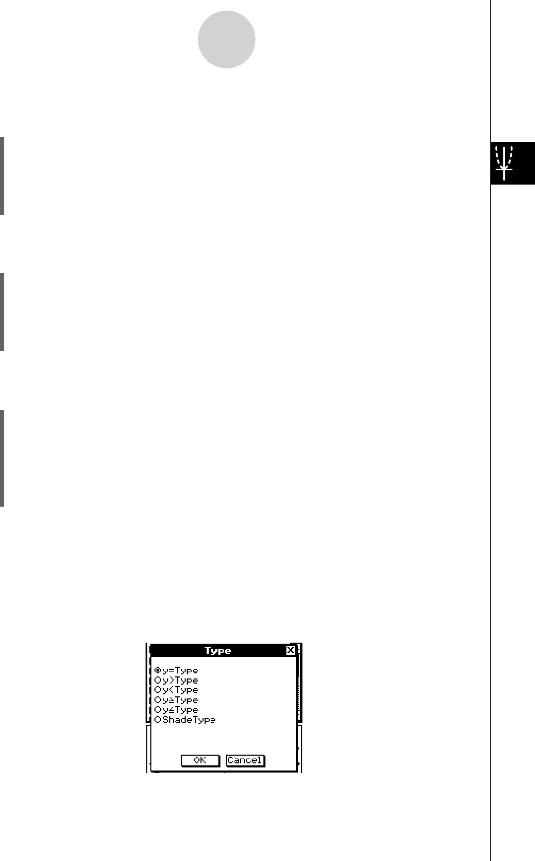
20060301

u To store an x = equation

Example: To store

x = 3y in line x4

(1) On the Graph Editor window, tap [Type] and then [x=Type] to specify an

x = equation.

(2) Tap the box to the right of line number “x4”, and then input the equation:

3y.

(3) Press

E to store the equation.

u To store an inequality

Example: To store the inequality y > x2 – 2x – 6 in line y5

(1) On the Graph Editor window, tap [Type] and then [y>Type] to specify an inequality

expression.

(2) Tap the box to the right of line number “y5”, and then input the expression:

x{2-2x-6.

(3) Press

E to store the expression.

u To store a shade type (ya)

Example: To store

f(x) = x2 – 1, g(x) = –x2 + 1, –1 < x < 1 in line y6

(1) On the Graph Editor window, tap [Type] and then [ShadeType] to specify a shade type

expression.

(2) Tap the box to the right of line number “y6”, and then input the expression:

k9{X{c-b,-X{c+b}KU-

b$X$b

(3) Press

E to store the expression.

Tip

• An error message appears if you enter an expression that does not fit the function type. Either

input the new function into a different line or delete the current function and then change the type

before re-inputting the function.

• You can change the equality/inequality sign of an x-type (x =, x>, x<, xt, xs) or y-type

(y =, y>, y<, yt, ys, ShadeType) expression after you input it. Simply tap the current equality/

inequality sign.

3-3-4

Storing Functions

On the Type dialog box that appears, select the sign you want and then tap [OK].

20060301

Using Built-in Functions

Your ClassPad is pre-programmed with the commonly used functions listed below. You can

recall a built-in function, save it to an Graph Editor sheet, assign values to its coefficients,

and graph the results.

y = a·x + b

y = a·x^2 + b·x + c

y = a·x^3 + b·x^2 + c·x + d

y = a·sin (b·x + c) + d

y = a·cos (b·x + c) + d

y = a·tan (b·x + c) + d

y = a·log (b·x + c) + d

y = a·ln (b·x + c) + d

y = a·e^(b·x + c) + d

y = a^(b·x + c) + d

y = a /(b·x + c) + d

u ClassPad Operation

(1) On the application menu, tap T.

(2) On the Graph Editor window, select the sheet and the line where you want to store the

built-in function.

(3) Tap

a and then [Built-In].

(4) On the menu that appears, tap the built-in function you want to select.

• This displays a dialog box for assigning values to the coefficients. The actual

coefficients that appear (a through d) depend on the built-in function you selected.

(5) Assign values to each coefficient.

(6) Tap [OK].

Saving the Message Box Expression to the Graph Editor Window

You can save the expression currently displayed in the Graph window message box to the

Graph Editor window. This capability comes in handy when you want to save an expression

that appears in the message box while you are using the sketch function (see “3-6 Using the

Sketch Menu”).

Note

• The following are the steps you should perform after an expression is stored in the

message box of the Graph window.

3-3-5

Storing Functions

20060301

u To save an expression from the message box to the Graph Editor window

(1) Tap the Graph window to make it active.

(2) Perform a Trace operation (see “3-7 Using Trace”) or any other operation that causes

the message box to appear.

(3) Tap inside the message box to select the entire expression or drag the stylus across

the part of the expression you want to select.

(4) Tap

(5) Tap the Graph Editor window to make it active.

(6) Select the sheet and tap the line where you want to save the expression, which moves

the cursor there.

(7) Tap [Edit] and then [Paste].

(8) Press

E to store the expression.

Tip

• You can also drag the expression from the message box to the Graph Editor window. In this

case, you must drop the expression into a line on the Graph Editor window that does not already

contain an expression.

Editing Stored Functions

u To edit a function

Example: To edit the function stored in line y2 of the Graph Editor to

(1) On the Graph Editor window, tap line y2.

(2) Tap the area immediately to the right of the numerator of so the cursor is located

there.

(3) Press

K and then 2 to edit the fraction.

(4) Press

E to store the edited version of the function.

u To delete a function

(1) On the Graph Editor window, select the sheet that contains the function you want to

delete.

(2) Tap the function you want to delete so the cursor is located anywhere inside it.

(3) Tap [Edit] and then [Select All].

(4) Press

• This deletes the selected function.

3-3-6

Storing Functions

y = x2 – — x3

—

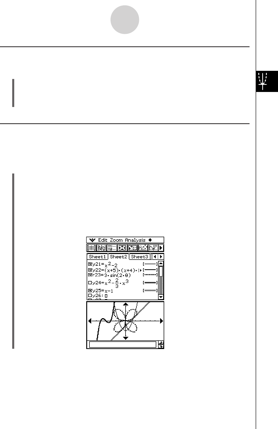
20060301

Deleting All Graph Editor Expressions

Use the following procedure to delete all of the expressions on all Graph Editor sheets, and

initialize all of the sheet names.

(1) On the Graph Editor window, tap [Edit] and then [Clear All].

(2) In response to the confirmation dialog box that appears, tap [OK] to delete all

expressions and initialize sheet names. To cancel the operation without deleting or

initializing anything, tap [Cancel].

Graphing a Stored Function

You can select multiple functions and graph them simultaneously, as long as all of the

functions are on the same sheet. You can turn graphing of each function on or off, and even

specify the line style to be used for each function.

u ClassPad Operation

(1) Tap the tab of the sheet that contains the functions you want to graph to make it active.

• If the functions you want to graph are on Sheet 2, for example, tap the [Sheet2] tab.

(2) Select the check boxes of all the functions you want to graph, and clear the check

boxes of all the functions you do not want to graph.

• See “Specifying the Function You Want to Graph” on page 3-3-8 for more information.

(3) You can tap the current line style given to specify another style, if you want.

• See “Specifying the Graph Line Style” on page 3-3-8 for more information.

(4) Tap

$ to graph.

3-3-7

Storing Functions

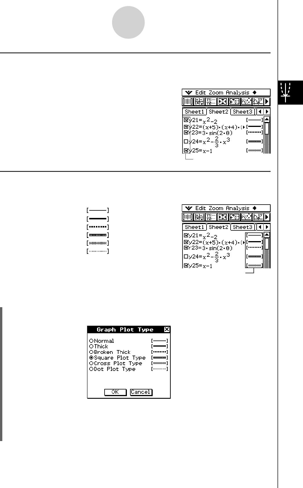
20060301

k Specifying the Function You Want to Graph

On the Graph Editor window, you can select one or more functions for graphing by selecting

their check boxes. The functions whose check boxes are cleared are not graphed.

• This check box is selected, so the function next to it will be

graphed when you tap $. If you do not want to graph this

function, tap the check box to clear it.

• Each time you tap a check box, it toggles between being

selected (checked) and cleared (unchecked).

k Specifying the Graph Line Style

You can specify one of the six line styles shown below for each function on the Graph Editor

window.

Normal ........................

Thick ...........................

Broken Thick ...............

Square Plot Type ........

Cross Plot Type ..........

Dot Plot Type ..............

The currently selected line style appears in the line style area next to each function.

u ClassPad Operation

(1) Tap the line style next to the function whose line style you want to specify. This displays

the Graph Plot Type dialog box.

3-3-8

Storing Functions

Line style area

Check box

(2) Select the line style you want, and then tap [OK].

• A preview of the line style you select appears in the line style area next to the

function.

• To graph the function using the selected line style, tap $.

Tip

• For an inequality region, the selected line style is used as the shading pattern.

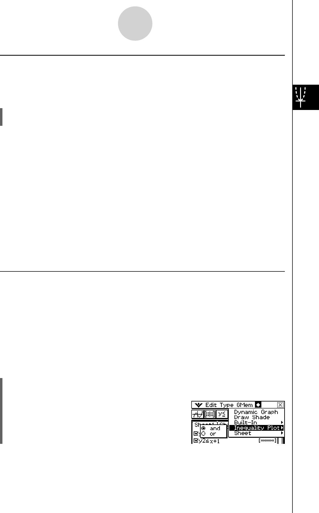
20060301

k Quick Graphing of an Expression Using Drag and Drop

You can use the following procedure to graph a single function, even when you have multiple

functions selected on the Graph Editor window.

u ClassPad Operation

(1) Tap the tab of the sheet that contains the function you want to graph to make it active.

(2) Drag the function you want to graph to the Graph window.

Tip

• The above drag and drop procedure can be used to graph a function, regardless of whether the

function’s check box is selected or cleared.

• When you quick graph a function using drag and drop, the function is always treated as a “y=”

expression, regardless of the graph type specified for the function.

• Up to 30 of the graphs you draw in the Graph window are stored in memory as you draw them.

This includes graphs drawn from Graph Editor window functions, graphs drawn using the Sketch

functions (Tangent, Normal, Inverse), and graphs drawn using the drag and drop operation

described above. Though you can draw more than 30 graphs at one time, any graphs after the

30th are not stored in memory.

• All of the Graph window graphs that are currently stored in memory are redrawn when you scroll

the Graph window or tap the [ReDraw] command on the a menu. Since only 30 graphs are

stored in memory, anything drawn after the 30th graph is not redrawn. Keep this limitation in mind

when you draw a large number of graphs at the same time.

k Overlaying Two Inequalities in an AND Plot / OR Plot

Use the following procedure to overlay two inequalities in an AND Plot or OR Plot which are

described below.

• AND Plot

With an AND Plot, only the parts of the inequalities that overlap are shaded.

• OR Plot

With an OR Plot, the inequalities are overlaid as they are.

Example: To graph the inequalities y < x2, y < x + 1

u ClassPad Operation

(1) Store

y < x2 in line y1 and y < x + 1 in line y2.

(2) On the

a menu, tap [Inequality Plot].

Select [and] or [or] on the submenu that appears.

3-3-9

Storing Functions

20060301

3-3-10

Storing Functions

(3) Tap

AND Plot OR Plot

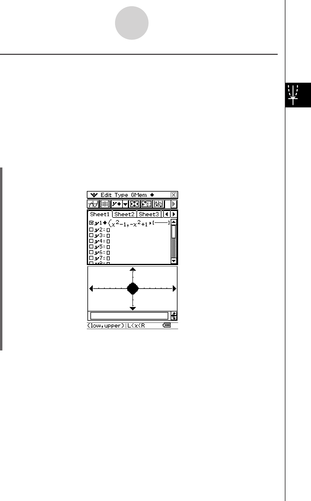
20060301

k Shading the Region Bounded by Two Expressions

You can shade the region bounded by two expressions by specifying [ShadeType] as the

function type and then inputting the expressions in the syntax shown below.

Syntax: ya {lower function f(x), upper function g(x)}

A < x < B

The value of B must be greater than A.

• A < x < B can be omitted.

• A < x < B can be replaced with x > A.

• A < x < B can be replaced with x < B.

Example: To graph f(x) = x2 – 1, g(x) = –x2 + 1, –1 < x < 1

u ClassPad Operation

(1) On the Graph Editor Window, tap [Type] and then [ShadeType].

(2) Store

ya{ x2–1, –x2+1}

–1<x<1 in line y1.

(3) Tap

• When [ShadeType] is selected as the function type, the status bar displays “{low,

upper}

L<x<R”.

3-3-11

Storing Functions

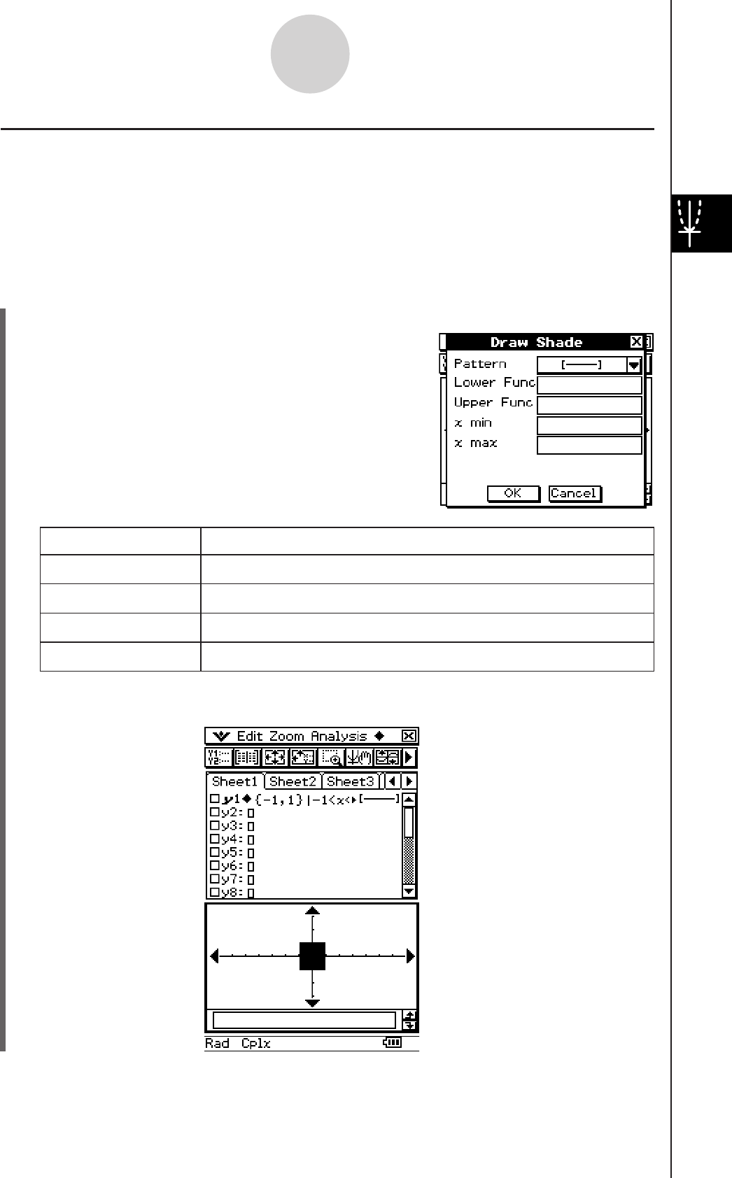
20060301

3-3-12

Storing Functions

k Using the Draw Shade Dialog Box to Shade the Region Bounded by Two

Expressions

In this case, you input the expressions on a Draw Shade dialog box instead of the Graph

Editor Window.

Example: To graph f(x) = –1, g(x) = 1, –1 < x < 1

u ClassPad Operation

(1) On the

a menu, tap [Draw Shade].

• This displays the Draw Shade dialog box.

Pattern Select the shading pattern.

Lower Func Input the lower function f(x).

Upper Func Input the upper function g(x).

x min Specify the lower limit of the shaded region.

x max Specify the upper limit of the shaded region.

(2) Input the following: Lower Func: –1, Upper Func: 1, x min: –1, x max: 1

(3) Tap [OK].

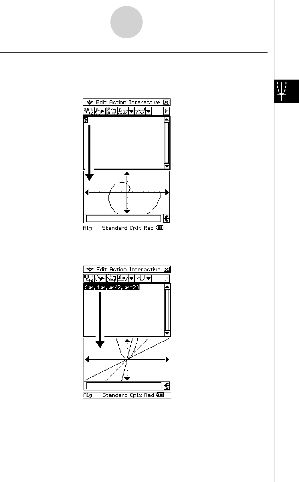
20060301

k Dropping an Expression from the Main Application Work Area into the

Graph Window

• You can graph a polar coordinate expression by dragging it from the Main Application work

area and dropping it into the Graph window.

• If there are multiple expressions in the same Main Application work area line, all of the

expressions will be graphed when you drop the line into the Graph window.

3-3-13

Storing Functions

20060301

Saving Graph Editor Data to Graph Memory

Graph memory lets you store all of the expressions and their related information to a file for

later recall.

Each graph memory file contains the following data:

• Functions on all five Graph Editor sheets (up to 100 functions)

• Whether the check box next to each function is selected (checked) or cleared (unchecked)

• The line style of each function

• The graph type of each function

• The View Window settings

• Which sheet is currently active

• Sheet names

u To save Graph Editor data to graph memory

(1) Tap the Graph Editor window to make it active.

(2) Tap [GMem] and then [Store]. This displays a dialog box for inputting a name for the

graph memory file.

(3) Enter the name and then tap [OK].

u To recall a graph memory file

(1) Tap [GMem] and then [Recall]. This displays a list of names of graph memory files you

have stored in memory.

(2) Select the name of the graph memory file you want, and then tap [OK].

3-3-14

Storing Functions

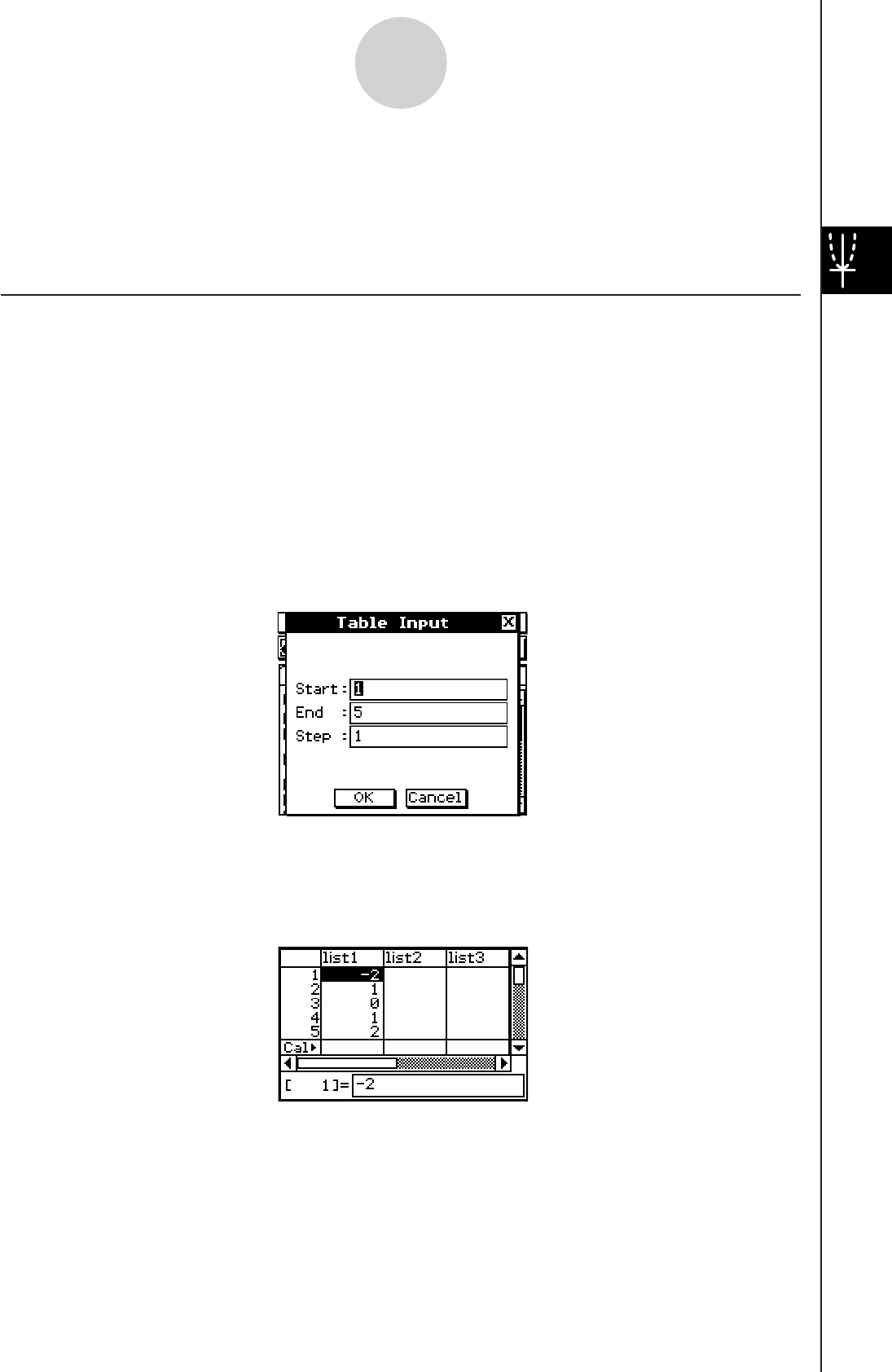
20060301

3-4-1

Using Table & Graph

For details about using the Stat Editor, see Chapter 7.

3-4 Using Table & Graph

The Graph & Table application includes a “Table window” for displaying number tables and

summary tables generated with the functions you input on the Graph Editor window.

Generating a Number Table

You can use either of the following two methods to generate a number table using a Graph

& Table application function. The method used to generate the number table depends on the

setting of the Graph Format dialog box [Table Variable] item.

• For details about Graph Format settings, see “Application Format Settings” on page 1-9-4.

u Specifying a range of values for x using the Table Input dialog box

This is the initial default number table generation method. With this method, you use the

Table Input dialog box to specify a range of values for variable x, and then generate a

number table for those values. This number table generation method is in effect whenever

“Table Input” is selected for the [Table Variable] setting.

u Assigning list values to x

With this number table generation method, you must first use the Stat Editor to create a list

and store the list data. To access the Stat Editor, tap O and then [Stat Editor].

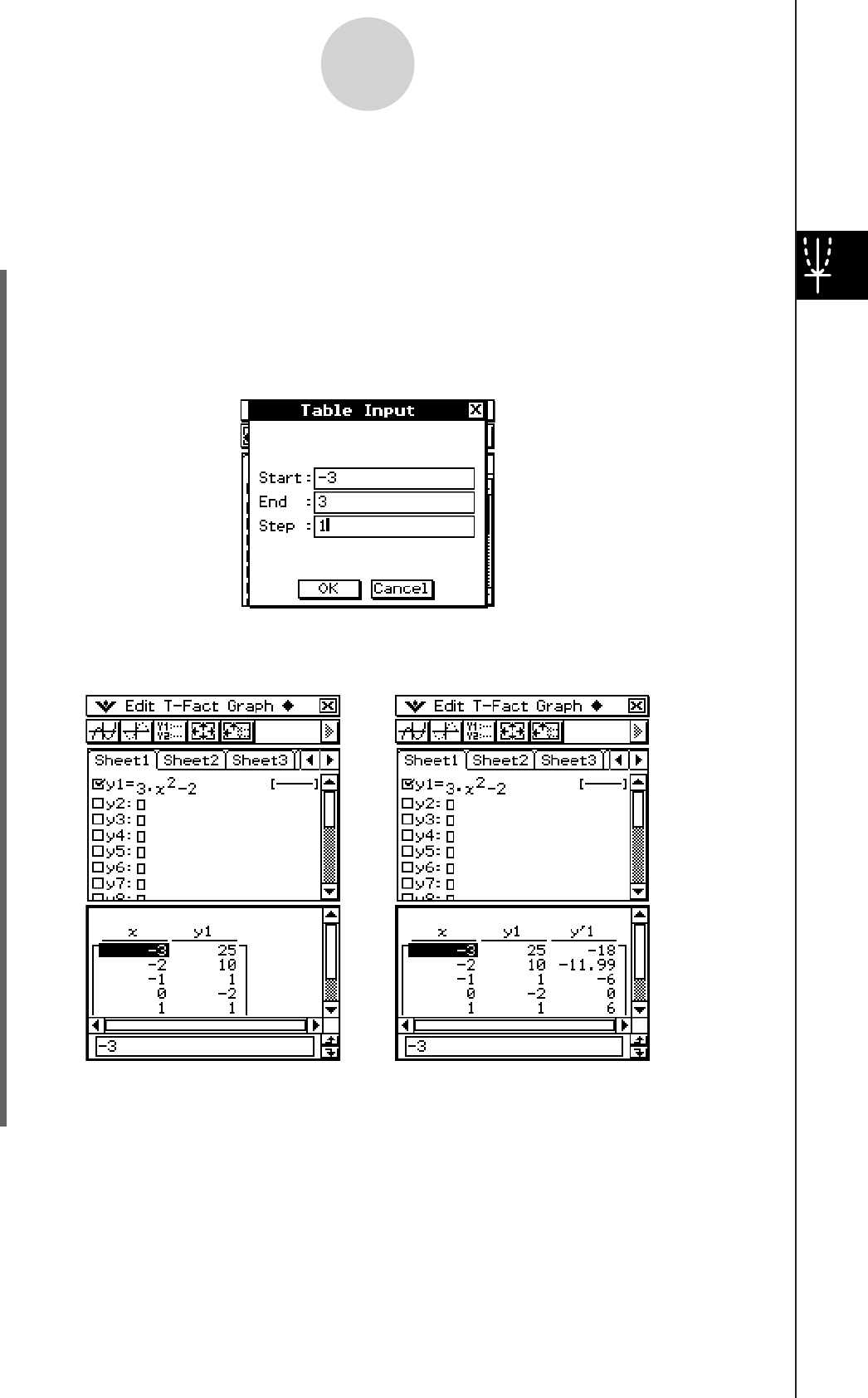
20060301

u To generate a number table by specifying a range of values for x using the

Table Input dialog box

Example: To generate a number table for the function y = 3x2 – 2 as the value of x changes

from –3 to 1 in increments of 1

(1) On the application menu, tap T.

(2) In line

y1 of the Graph Editor window, input and save y = 3x2 – 2.

(3) Tap

8. This displays the Table Input dialog box.

(4) Input the following values for the x-values of your table, and then tap [OK].

(5) Tap

• This generates the number table and displays the result on the Table window.

3-4-2

Using Table & Graph

• The derivative is also included in the number

table when the Graph Format “Derivative/

Slope” check box is selected.

Tip

• The above operation is possible only when “Table Input” (which is the initial default) is selected

for the Graph Format dialog box [Table Variable] item.

• You can specify the width of table cells using the [Cell Width Pattern] on the Graph Format dialog

box (page 1-9-6).

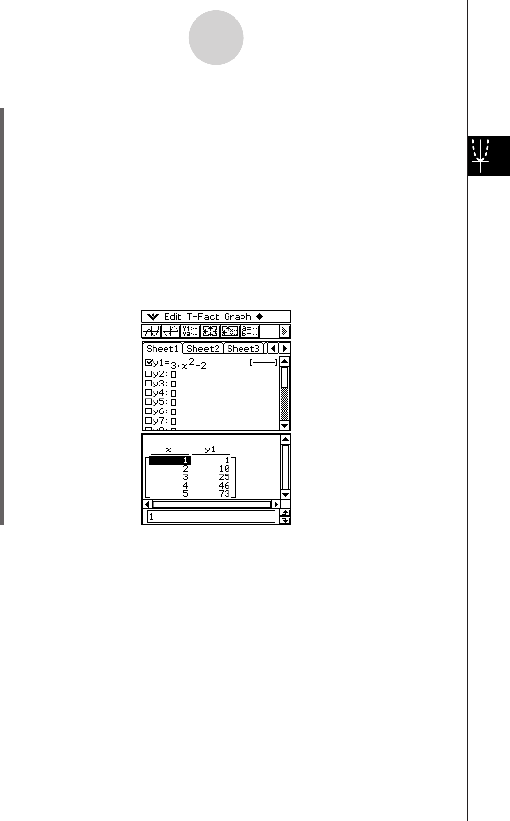
20060301

u To generate a number table by assigning list values to x

(1) Create and save the list of values to be assigned.

list1 = 1, 2, 3, 4, 5

(2) In line

y1 of the Graph & Table application Graph Editor window, input and save

y = 3x2 – 2.

(3) Specify the list that contains the values you want to assign to x (list1 in this example).

• You can configure list data settings using the Graph Format dialog box.

For details about Graph Format settings, see “Application Format Settings” on page

1-9-4.

(4) On the Graph Editor window, tap the function you want to use for number table

generation (y1 in this example).

(5) Tap

• This generates the number table and displays the result on the Table window.

3-4-3

Using Table & Graph

Tip

• The above operation is possible only when “List” (list1 through list6 or a list variable created by

you) is selected for the Graph Format dialog box [Table Variable] item. Note that “Table Input” is

the default, so you need to change the [Table Variable] setting in order to generate a table using

list values.

20060301

k Table Generation Precautions

• Table generation is performed using the currently selected function that is of the current

function type selected on the Graph Editor window toolbar.

• Though the selected current function type is “y=” in the above screenshot, there is no “y=”

type function selected on the Graph Editor window. Tapping # to generate a table when

the above condition exists causes the error message “No Item(s) Checked” to appear.

• An inequality cannot be used to generate a table.

Editing Number Table Values

Changing an x-value in the number table automatically calculates and displays the

corresponding y-value.

Example: To change the x-value in line 3 of the number table from –1 to –2.5

To generate a table, see “To generate a number table by specifying a range of

values for x using the Table Input dialog box” on page 3-4-2.

uClassPad Operation

(1) Tap the cell in line 3 of column x of the number

table to select it.

3-4-4

Using Table & Graph

(2) Perform the key operation: z2.5.

• Pressing z causes the Enter Value dialog box

to appear with a minus sign (–) in the [x-value]

input box. Continue with the rest of the key

operation to input the required value, and then

tap [OK]. This changes the value in the selected

cell to the one you input. The y-value is updated automatically in

accordance with the new x-value.

Current function type

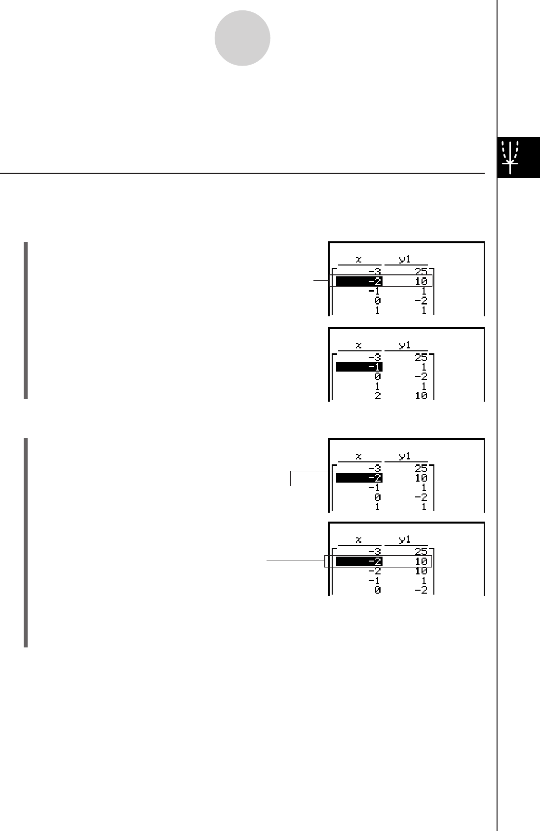
20060301

3-4-5

Using Table & Graph

Tip

• An error message appears and the number table contents are not changed if you enter an illegal

value for x (such as 6 ÷ 0).

• The data in a “Y” column (Y1, Y2, etc.) of a table cannot be modified.

Deleting, Inserting, and Adding Number Table Lines

You can use the following procedures to delete, insert, and add number table lines.

u To delete a number table line

(1) Tap the

x-value of the line you want to delete.

(2) Tap [T-Fact] and then [Delete].

This line will be deleted.

u To insert a number table line

(1) Tap the

x-value of the line below the location where

you want to insert a line.

(2) Tap [T-Fact] and then [Insert].

Inserted line

The new line contains the

same values as the one

you selected in step (1).

The line will be inserted here.

• After inserting a new line, you can edit the x-value, if you want. For more information,

see “Editing Number Table Values” on page 3-4-4.

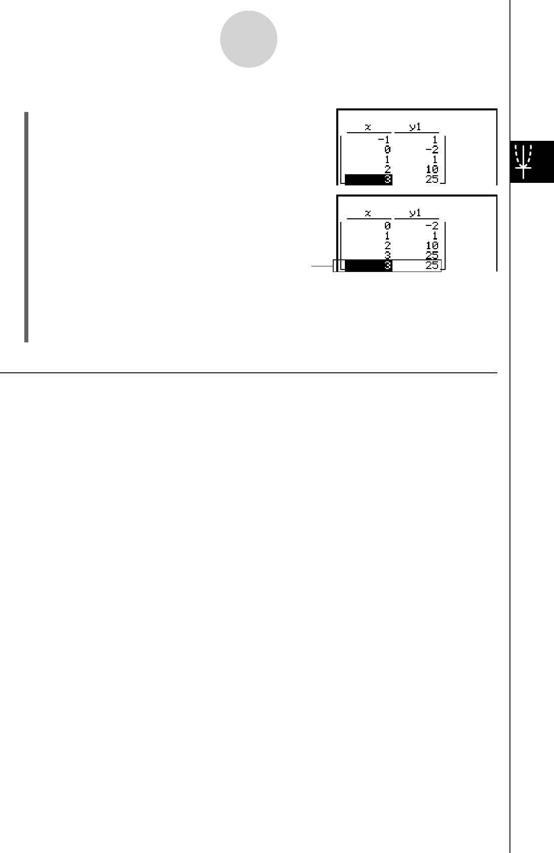
20060301

3-4-6

Using Table & Graph

u To add a number table line

(1) Tap the

x-value of the bottom line of the number table.

(2) Tap [T-Fact] and then [Add].

• After adding a new line, you can edit the x-value, if you want. For more information, see

“Editing Number Table Values” on page 3-4-4.

• You can add a line anywhere. When you add a line, it will appear after the line you

selected.

Regenerating a Number Table

After changing [Table Input] settings, you can regenerate a table based on the new settings

by tapping a and then [ReTable]. You can also use [ReTable] after editing the contents of

a table to return the table to its original (pre-edited) state.

Added line

The new line contains the

same values as the bottom

line of the number table.

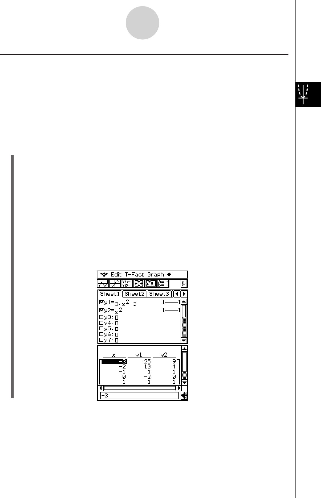
20060301

Generating a Number Table and Using It to Draw a Graph

After using a function to generate a number table, you can use the number table values to

draw a graph. You can use number table values to draw two different types of graphs: a

“connect type graph” on which points are connected by lines, or a “plot type graph” on which

points are simply plotted, without being connected.

Example: To generate number tables for the functions y = 3x2 – 2 and y = x2 as the value of

x changes from –3 to 3 in increments of 1, and then use the generated values to

draw a graph

uClassPad Operation

(1) On the application menu, tap T.

(2) On the Graph Editor window, input 3x2 – 2 in line y1, and x2 in line y2.

(3) Tap

6 to display the View Window dialog box, and then configure it with the following

parameters.

xmin = –3, xmax = 3, xscale = 1

ymin = –2, ymax = 10, yscale = 2

(4) Tap

8 to display the Table Input dialog box, and then configure it with the following

settings.

Start: –3, End: 3, Step: 1

(5) Tap

• This generates the number table and displays the result on the Table window.

3-4-7

Using Table & Graph

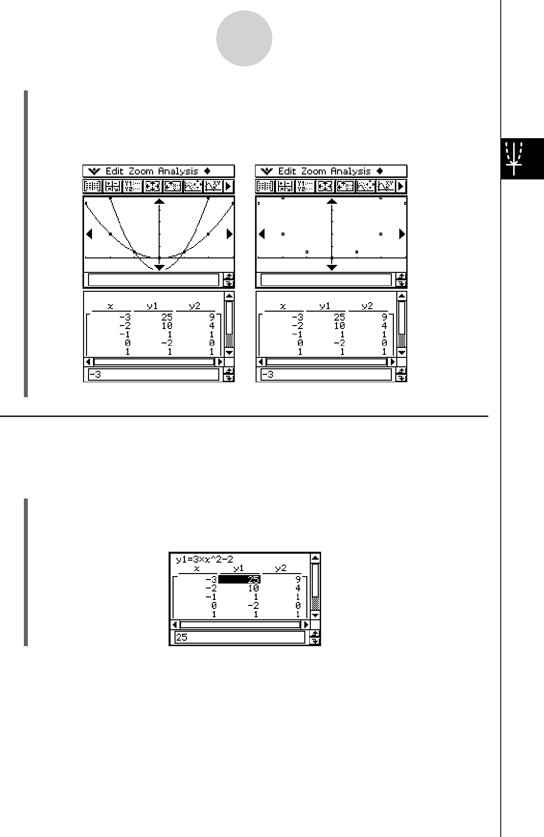
20060301

(6) Specify the graph type.

• To specify a connect type graph, tap [Graph] and then [G-Connect], or tap $. To

specify a plot type graph, tap [Graph] and then [G-Plot], or tap !.

• This draws the graph on the Graph window.

Saving a Number Table to a List

You can use the following procedure to save a particular column of a number table to a LIST

variable.

uClassPad Operation

(1) On the Table window select any cell in the column you want to save to a LIST variable.

• To save column y1 in the window shown below, for example, select any cell in column

y1.

3-4-8

Using Table & Graph

Connect Type Graph Plot Type Graph

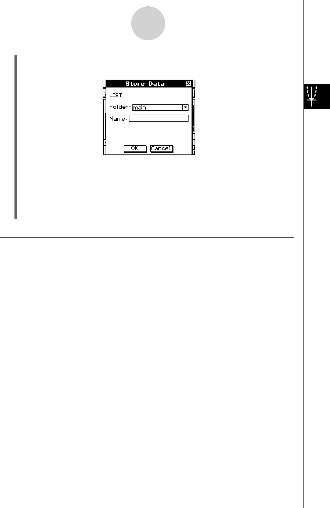
20060301

(2) Tap

a and then [Table to List].

• This displays a dialog box for specifying a variable name.

3-4-9

Using Table & Graph

(3) Enter the name you want to give to the variable, and then tap [OK].

• This assigns the list of data you selected to a variable with the name you specified.

• If the variable name you input has not been used yet for another variable, ClassPad

creates a new variable. With some data types, if the variable name you input is

already being used for an existing variable, the existing variable is replaced by the

new one. For more information, see “Variable Data Types” on page 1-7-3.

Generating a Summary Table

You can use any of the three methods described below to generate a summary table from a

function that has already been saved.

u Automatic x-value settings

This method automatically generates an ideal summary table for the function. This method

uses View Window settings when generating the table.

u Using View Window xmin and xmax values as the x-value settings

With this method, you simply provide the upper and lower x-value limits, and your ClassPad

generates the correct summary table for that range of values. This method uses View

Window settings when generating the table.

20060301

u Specifying all x-values

This method generates a reference table by looking up data stored in a list. A LIST variable is

used to specify the x-values. When using this method, it is up to you specify all of the correct

x-values required to generate the summary table. The summary table will not be generated

correctly if you provide incorrect x-values.

The following shows examples of each of the three available summary table generation

methods by generating a table for the function y = x3 – 3x.

3-4-10

Using Table & Graph

x –1 0 1

f⬘(x) + 0 – –3 – 0 +

f⬙(x) – –6 – 0 + 6 +

f (x) 2 0 –2

Tip

• You can control whether or not the summary table should include an f ⬙(x) line (quadratic

differential component) using the [Summary Table f ⬙(x)] setting on the [Special] tab of the Graph

Format dialog box (page 1-9-7). Turning on the [Summary Table f ⬙(x)] option causes both linear

differential components and quadratic differential components to be displayed in the summary

table. Turning it off shows linear differential components only.

k Generating a Summary Table Using Automatically Set x-Values

With this method, the summary table is generated using a range of values from –∞ to ∞.

u ClassPad Operation

(1) On the Graph Format dialog box, select “View Window” for the [Summary Table]

setting, and specify the value you want for [Cell Width Pattern]. This example uses a

[Cell Width Pattern] setting of “4 Cells”.

• To open the Graph Format dialog box, tap O, and then [Graph Format].

• For additional details about Graph Format settings, see “Application Format Settings”

on page 1-9-4.

(2) Input the function y = x3 – 3x on the Graph Editor window.

• Generation of summary tables is supported for “y=” type functions only.

• Clear the check boxes of all other functions on the Graph Editor window, if

necessary. Select the check box next to y = x3 – 3x and press E.

• If the check boxes of more than one “y=” type functions are selected, the one with

the lowest line number (y1, y2, y3, etc.) is used for number table generation.

(3) Tap

6 to display the View Window dialog box.

Summary Table and Graph of y = x3 – 3x

(The graph to the right is for reference only.)

–2

–1

–2 –1 12

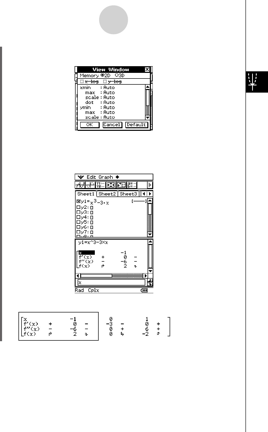
20060301

(4) Tap [Memory] and then [Auto].

• This causes all settings on the View Window dialog box to change to “Auto”.

3-4-11

Using Table & Graph

(5) Tap the [OK] button to close the View Window dialog box.

(6) Tap

u to toggle to toolbar 2 and then tap 4.

• This starts summary table generation, and displays the result on the Table window.

Note that generation of a summary table can take a bit of time.

• You can scroll the window to view all of the contents of the table.

20060301

• Tapping $ here graphs the function using the View Window settings automatically

configured for summary table generation.

3-4-12

Using Table & Graph

Important!

• A monotone increasing function or other special function may not be solvable by the

ClassPad’s internal summary table calculation. If this happens, use the procedure under

“Generating a Summary Table by Specifying All of the Values for x” (page 3-4-14) to

calculate the elements of the summary table. In addition to View Window parameters, you

can also select previously stored list data to specify the range of a summary table. On the

Graph Format dialog box (displayed using the O menu), select the [Special] tab, tap the

“Summary Table” down arrow button, and then select the name of the list you want to use

on the menu that appears.

• If you draw a graph or generate a summary table while “Auto” is specified for View Window

parameters, the ClassPad calculates appropriate parameters and configures View Window

settings accordingly.

k Generating a Summary Table Using View Window

With this method, the summary table is generated using the range you define for the View

Window “xmin” and “xmax” parameters.

uClassPad Operation

(1) On the Graph Format dialog box, select “View Window” for the [Summary Table]

setting, and specify the value you want for [Cell Width Pattern]. This example uses a [Cell

Width Pattern] setting of “4 Cells”.

• For details about Graph Format settings, see “Application Format Settings” on page

1-9-4.

(2) Input the function y = x3 – 3x on the Graph Editor window.

• Generation of summary tables is supported for “y=” type functions only.

• Clear the check boxes of all other functions on the Graph Editor window, if necessary.

Select the check box next to y = x3 – 3x and press E.

• If the check boxes of more than one “y=” type functions are selected, the one with the

lowest line number (y1, y2, y3, etc.) is used for number table generation.

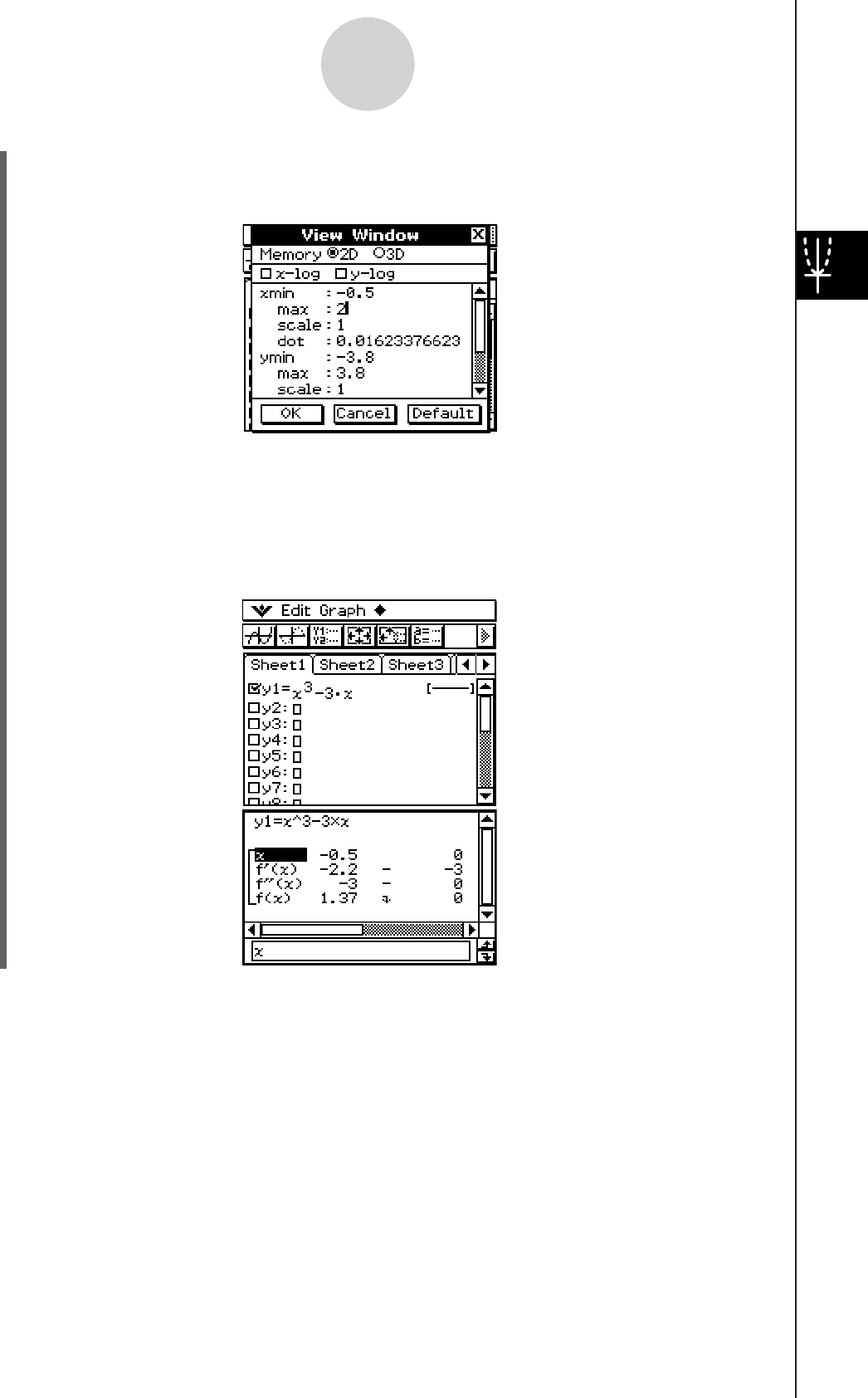
20060301

• For this example, we will specify xmin = –0.5 and xmax = 2.

(5) Tap the [OK] button to close the View Window dialog box.

(6) Tap

• This starts the summary table generation using the range you specified in step (4),

and displays the result on the Table window.

(3) Tap

6 to display the View Window dialog box.

(4) Specify the x-values for the summary table by specifying values for the [xmin] and [xmax]

settings.

3-4-13

Using Table & Graph

Important!

• A monotone increasing function or other special function may not be solvable by the

ClassPad’s internal summary table calculation. If this happens, use the procedure under

“Generating a Summary Table by Specifying All of the Values for x” (page 3-4-14) to

calculate the elements of the summary table. In addition to View Window parameters, you

can also select previously stored list data to specify the range of a summary table. On the

Graph Format dialog box (displayed using the O menu), select the [Special] tab, tap the

“Summary Table” down arrow button, and then select the name of the list you want to use

on the menu that appears.

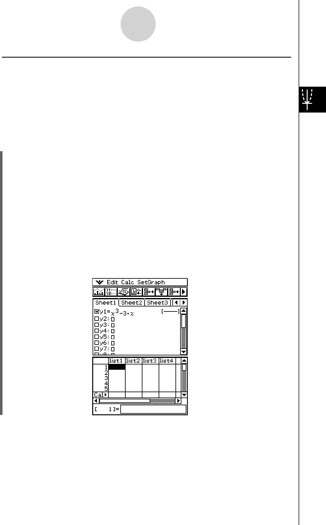
20060301

k Generating a Summary Table by Specifying All of the Values for x

In both of the previous examples, summary table generation is performed using View

Window settings to calculate values for x that satisfy the function f⬘(x) = 0. With this table

generation method, x-values are not calculated automatically.

It is up to you to use a LIST variable to specify all of the x-values that appear in the summary

table.

In the example below, x-values will be stored in a LIST variable named “list1”, which is then

used to generate a summary table.

u ClassPad Operation

(1) On the Graph Format dialog box, select “list1” for the [Summary Table] setting, and

specify the value you want for [Cell Width Pattern]. This example uses a [Cell Width

Pattern] setting of “4 Cells”.

• For details about Graph Format settings, see “Application Format Settings” on page

1-9-4.

(2) Input the function y = x3 – 3x on the Graph Editor window.

• Generation of summary tables is supported for “y=” type functions only.

• Clear the check boxes of all other functions on the Graph Editor window, if

necessary. Select the check box next to y = x3 – 3x and press E.

• If the check boxes of more than one “y=” type functions are selected, the one with the

lowest line number (y1, y2, y3, etc.) is used for number table generation.

(3) Tap

O and then [Stat Editor] to display the Stat Editor window.

3-4-14

Using Table & Graph

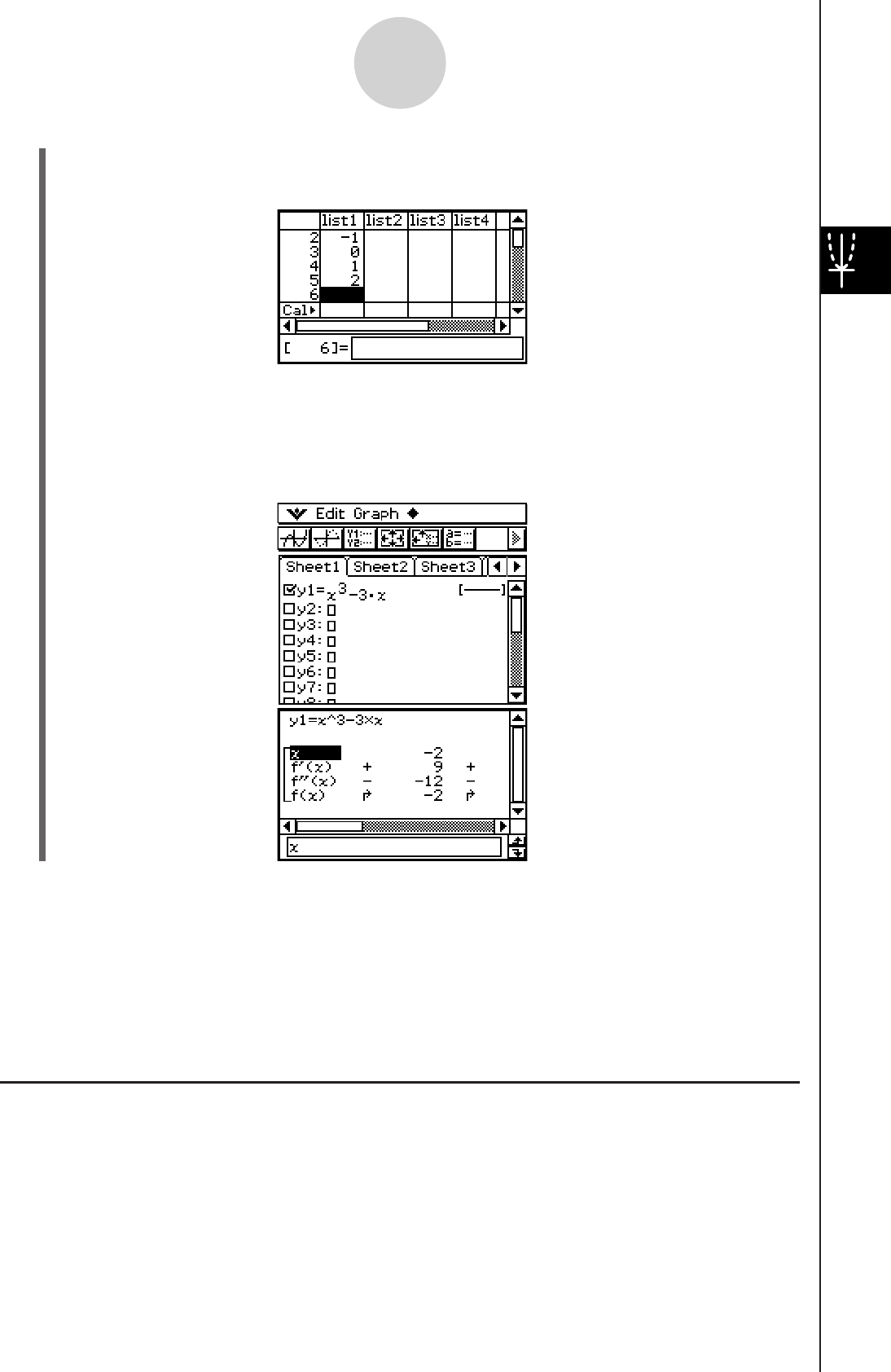
20060301

(5) Tap the Graph Editor window to make it active.

(6) Tap

• This starts summary table generation using the x-values you input in step (4), and

displays the result on the Table window.

3-4-15

Using Table & Graph

Important!

• For the above method to correctly generate a summary table, you must have legal x-values

in the list assigned to the LIST variable. Note that an error occurs if the specified LIST

variable is empty or does not exist.

• Some functions may not be solvable by the ClassPad’s internal summary table calculation.

When this happens, the “Can’t Solve!” error message appears on the display.

Making the Graph Editor Window the Active Window

While the Table window is active, you can make the Graph Editor window the active window

by tapping anywhere inside of it or by tapping !.

(4) Input the values you want to specify for x into list1.

• Here, we will input the following values: x = –2, –1, 0, 1, 2.

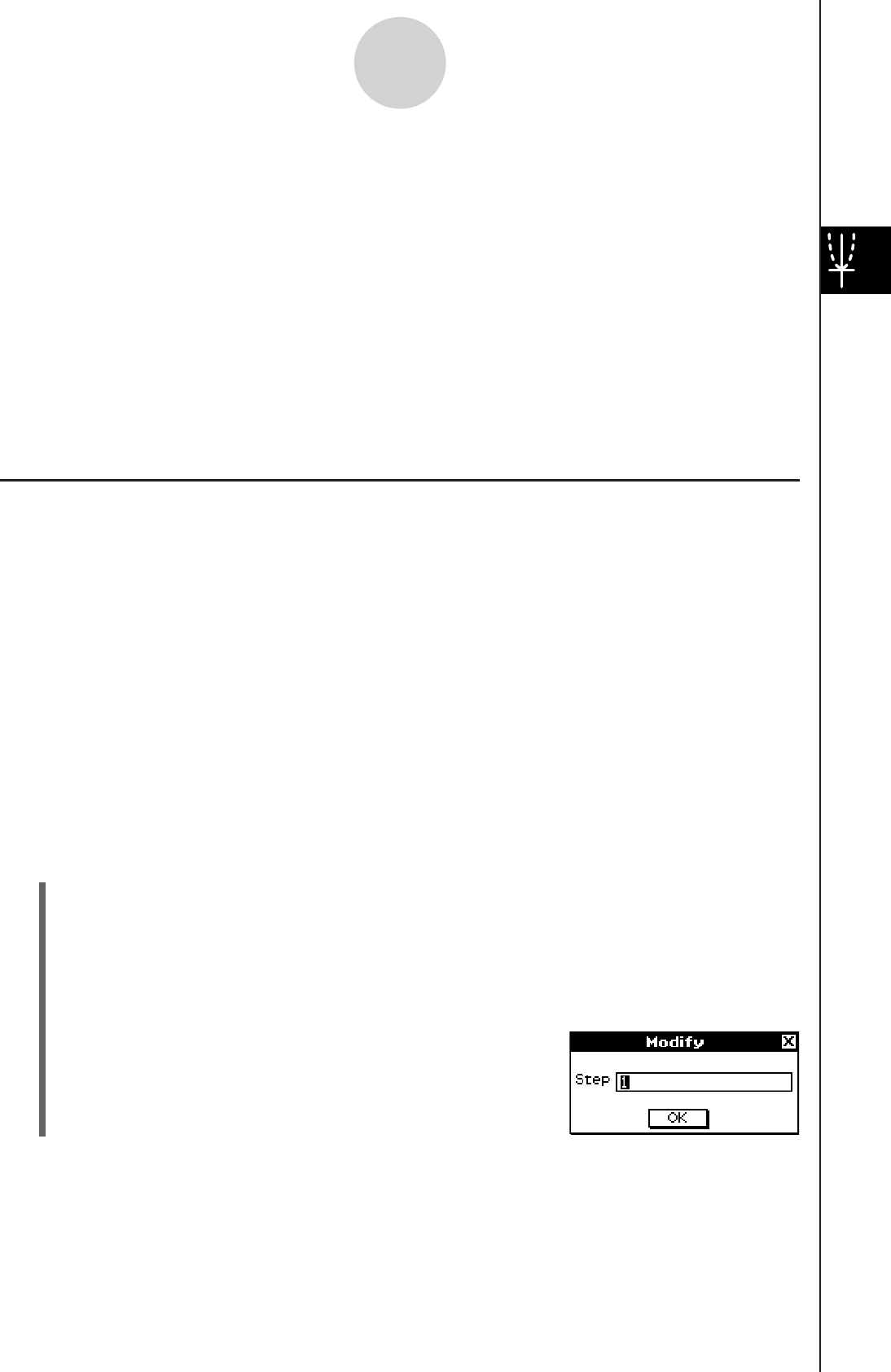
20060301

3-5 Modifying a Graph

A graph can be modified in real time as you change its coefficients and/or the variables. The

Graph & Table application provides you with two methods for modifying a graph.

Direct Modify

“Direct Modify” changes the coefficient in the equation of the original graph. This method can

be used when you are modifying a single graph.

Dynamic Modify

“Dynamic Modify” changes the values assigned to common variables of multiple functions.

Use Dynamic Modify when you want to modify multiple graphs at the same time.

Modifying a Single Graph by Changing the Value of a Coefficient (Direct

Modify)

Use the following procedure to change the values of the coefficients of a function within a

specific range to find out the effect the change has on the shape or position of the graph.

u To modify a single graph

Example: To graph the functions y = 2x2 + 3x – 1 and y = 2x + 1, and then find out how a

change in the coefficients of each function affects the shape and position of the

graphs

Note

• Before starting the following procedure, check the Graph Format dialog box to make sure

that the [G-Controller] setting is turned on. For information about the Graph Format dialog

box, see page 1-9-6.

uClassPad Operation

(1) On the application menu, tap T.

(2) Configure View Window parameters.

(3) On the Graph Editor window, input 2x2 + 3x –1 in line y1, and 2x + 1 in line y2.

(4) Tap

$ to graph the functions.

(5) Tap [Analysis] and then [Modify].

• This displays a dialog box for inputting the step.

3-5-1

Modifying a Graph

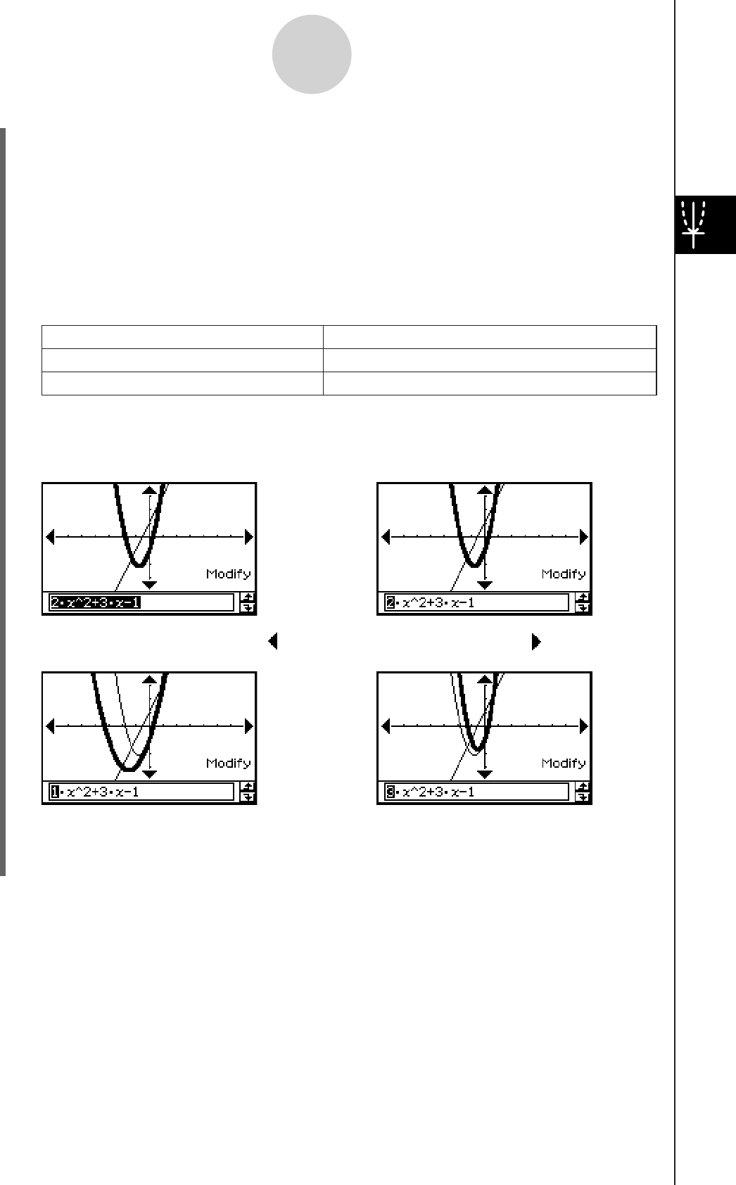
20060301

3-5-2

Modifying a Graph

To do this:

Tap the right graph controller arrow.

Tap the left graph controller arrow.

Do this:

Decrease the value of the coefficient

Increase the value of the coefficient

• You can use the Dynamic Graph dialog box on page 3-5-4 to change the increment,

if you want.

(6) Input the amount of change (step) in the coefficient value, and then tap [OK].

• This causes “Modify” to appear on the Graph window and the y1 graph (2x2 + 3x –1)

to become active, which is indicated by a thick graph line.

• The function of the currently active graph is displayed in the Graph window message

box.

(7) In the function displayed in the message box, select the coefficient you want to change.

(8) Tap the left or right graph controller button to change the value of the coefficient you

selected in step (7).

• At this point, you could select other coefficients and change their values as well, if you

want.

Important!

• If display of the graph controller arrows is turned off,select the coefficient you want to

modify, tap the Graph window with the stylus and then use the left and right cursor keys to

change the coefficient value.

• When the graph controller is off and the entire expression is selected you can use the left

and right cursor keys to change the modified graph.

• When the graph controller is on or off you can edit the expression directly and then press

E to change the modified graph.

Step (7)

Tap .Tap .

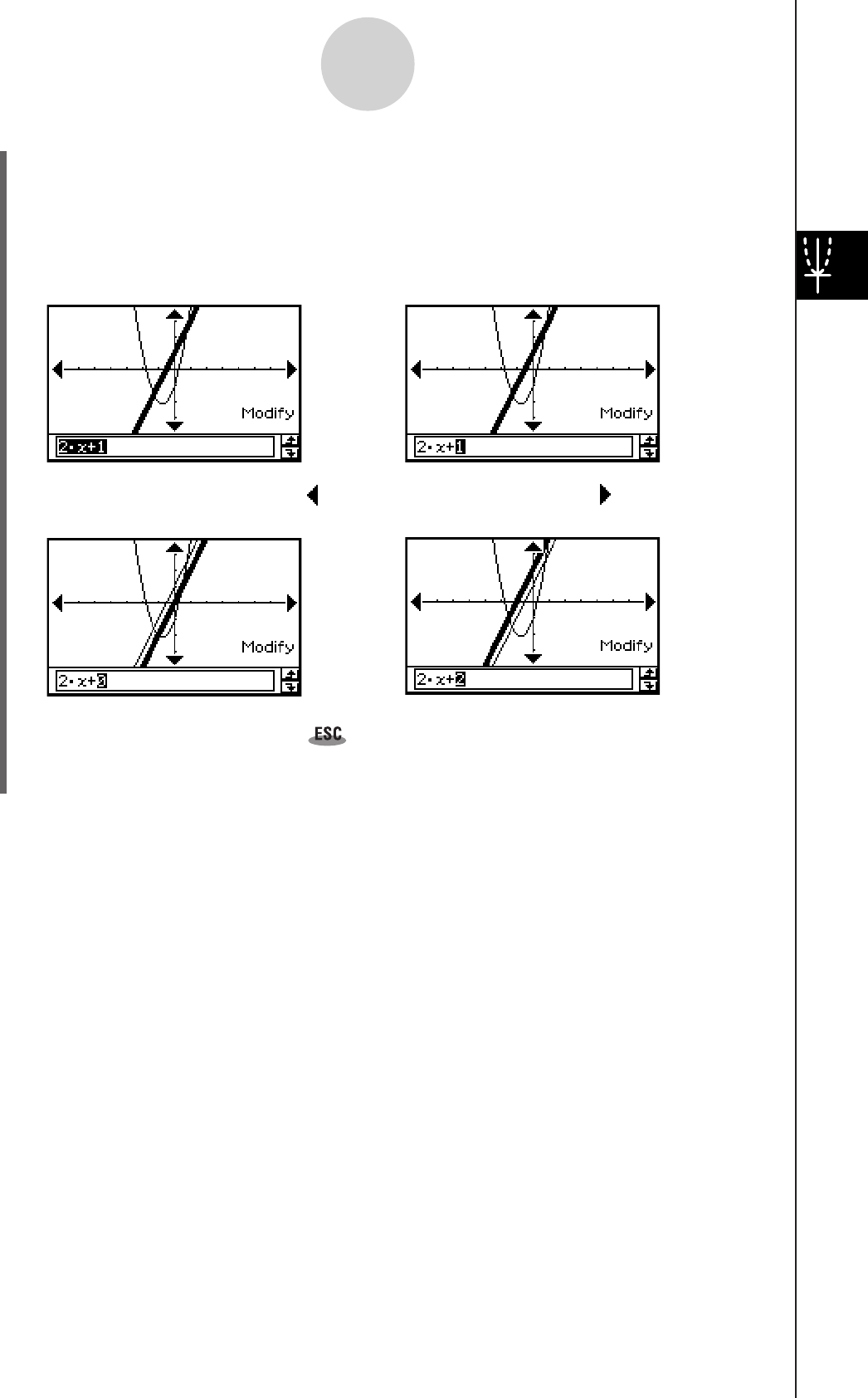
20060301

(9) To modify the y2 graph (2x + 1), tap the down graph controller arrow to make it the

graph active.

• You can use the up and down cursor keys or graph controller arrows to switch

between the two graphs, as required.

• Repeat steps (7) and (8) to modify the currently selected graph.

Tap .Tap .

3-5-3

Modifying a Graph

(10) To quit graph modification, tap on the icon panel.

• This causes “Modify” to disappear from the display, returning to the normal Graph

window.

20060301

Simultaneously Modifying Multiple Graphs by Changing Common

Variables (Dynamic Modify)

Use the procedure below to change the values of up to two common variables used in

multiple functions to simultaneously modify the graphs.

u To modify multiple graphs simultaneously

Example: To graph the functions y = ax2 – b and y = ax + b, and then find out how a change

in variable a from 1 to 4 and a change in variable b from –2 to 2 affect the shape

and position of each graph

(1) On the application menu, tap T.

(2) Tap

O and then [Main] to display the Main application window.

Tip

• For details about using the Main application, see Chapter 2.

(3) Use the Main application work area to assign values to variables “a” and “b” (a = 1 and

b = 2 in this example).

VbW aw

cW bw

(4) Tap

O and then [Close] to close the Main application window.

(5) Configure View Window parameters.

(6) On the Graph Editor window, input ax2 – b in line y1, and ax + b in line y2.

(7) Tap

$ to draw the graph.

(8) Tap

a and then [Dynamic Graph]. This displays the Dynamic Graph dialog box.

(9) Configure the following settings on the Dynamic Graph dialog box.

3-5-4

Modifying a Graph

Description

Setting

Dynamic ]':

Start: 1

End: 4

Step: 1

Dynamic `$:

Start: –2

End: 2

Step: 1

Specifies a variable whose value is changed when you press the left

or right cursor key, or tap the left or right graph controller arrow.

These items specify the upper limit (End) and lower limit (Start) of

the range of change of the Dynamic ]' value.

Use this setting to specify the increment of change in the Dynamic

]' value when you press the left or right cursor key, or tap the left

or right graph controller arrow.

Specifies another variable whose value is changed when you press

the up or down cursor key, or tap the up or down graph controller

arrow.

These items specify the upper limit (End) and lower limit (Start) of

the range of change of the Dynamic `$ value.

Use this setting to specify the increment of change in the Dynamic

`$ value when you press the up or down cursor key, or tap the up

or down graph controller arrow.

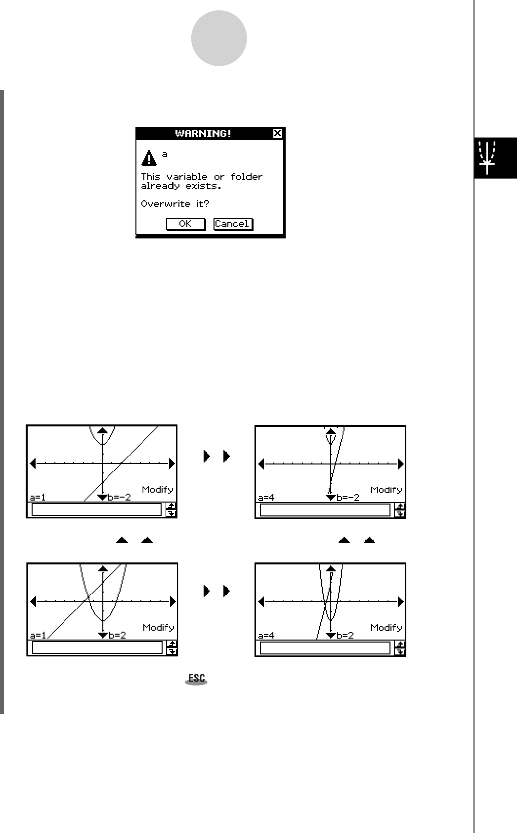
20060301

(10) Tap [OK].

• This displays a WARNING! dialog box for overwriting variable a.

3-5-5

Modifying a Graph

• This graphs the functions using the a and b variable start values you specified on the

Dynamic Graph dialog box, and displays “Modify” on the Graph window.

…

……

(13) Modify the graphs by changing the value of variable a or b.

• To change the value of variable a, press the left or right cursor key, or tap the left or

right graph controller arrow.

• To change the value of variable b, press the up or down cursor key, or tap the up or

down graph controller arrow.

(14) To quit graph modification, tap on the icon panel.

• This causes “Modify” to disappear from the display, returning to the normal Graph

window.

(11) Tap [OK].

• This displays a WARNING! dialog box for overwriting variable b.

(12) Tap [OK].

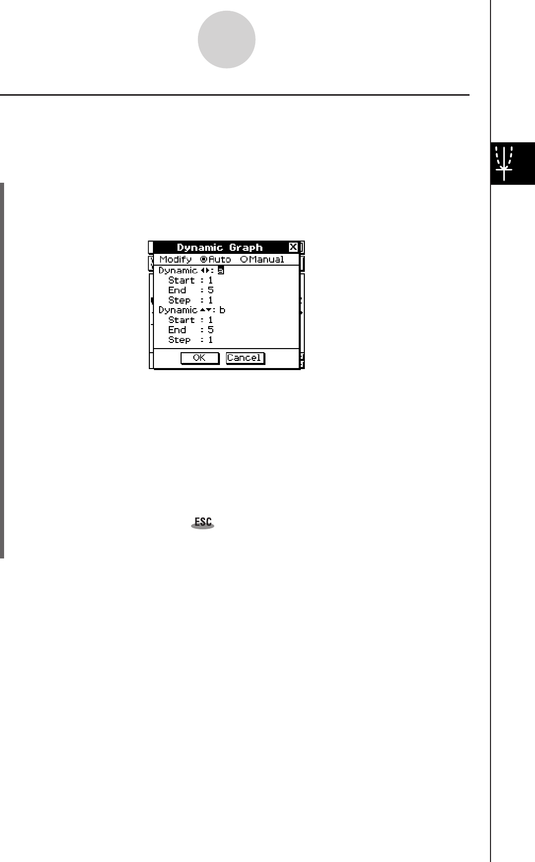
20060301

3-5-6

Modifying a Graph

with the settings you configure on the Dynamic Graph dialog box.

u ClassPad Operation

(1) Perform steps (1) through (9) under “To modify multiple graphs simultaneously” on

page 3-5-4.

(2) On the Dynamic Graph dialog box, tap the [Auto] option.

k Cycling Through Graph Changes Automatically

Use the following procedure to cycle automatically through graph changes in accordance

(3) Tap [OK].

• This graphs the functions using the a and b variable start values you specified on the

Dynamic Graph dialog box, and displays “Modify” on the Graph window.

(4) Execute an auto change operation.

• To execute three cycles of an auto change operation for variable a, tap the right

graph controller arrow.

• To execute three cycles of an auto change operation for variable b, tap the up graph

controller arrow.

(5) To quit graph modification, tap on the icon panel.

• This causes “Modify” to disappear from the display, returning to the normal Graph

window.

20060301

Clear figures and text you have added using the sketch feature

Plot a point on the Graph window

Draw a line on the Graph window

Write text on the Graph window

Draw a line that is tangent to a particular point on a graph

Draw a line that is normal to a particular point on a graph

Draw a circle

Draw a vertical line

Draw a horizontal line

Graph the inverse of a function

Cls

Plot

Line

Tex t

Tangent

Normal

Inverse

Circle

Vertical

Horizontal

Select this Sketch

menu command:

To do this:

3-6-1

Using the Sketch Menu

3-6 Using the Sketch Menu

The [Sketch] menu lets you add points, lines, figures, and text after you draw a graph. You

can also add tangent and normal lines to your graph.

Sketch Menu Overview

To access the [Sketch] menu, tap [Analysis] and then [Sketch]. The following table describes

the commands that are available on the [Sketch] menu.

Using Sketch Menu Commands

This section describes how to use each of the commands on the [Sketch] menu. Note that all

of the procedures in this section are performed in the Graph & Table application, which you

can enter by tapping the T icon on the application menu.

u To plot a point on the Graph window

(1) While the Graph window is active, tap [Analysis], [Sketch], and then [Plot].

(2) Tap the location on the Graph window where you want to plot a point.

• Instead of tapping the Graph window, you could also use the keypad to specify the

coordinates of the point. Pressing a number key displays a dialog box for inputting

coordinates. The value of the key you just pressed is input for the x-coordinate. After

inputting values for the x- and y-coordinates, tap [OK]

to plot the point at the location you specified.

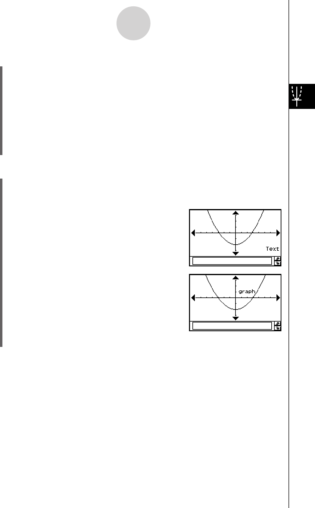
20060301

3-6-2

Using the Sketch Menu

u To draw a line on the Graph window

(1) While the Graph window is active, tap [Analysis], [Sketch], and then [Line].

(2) On the Graph window, tap the start point of the line and then tap the end point. This

causes a straight line to be drawn between the two points. The message box shows the

equation of the line.

• Instead of tapping the Graph window, you can use the keypad to specify the

coordinates of the start point and end point. Pressing a number key displays a dialog

box for inputting coordinates. The value of the key you just pressed is input for the

x-coordinate of the starting point. After inputting values for the x- and y-coordinates

of the start point (x1, y1) and the x- and y-coordinates of the end point (x2, y2), tap [OK]

to draw a straight line between the two points you specified.

u To write text on the Graph window

(1) While the Graph window is active, tap [Analysis], [Sketch], and then [Text].

• This displays a dialog box for inputting text.

(2) Enter the text you want and then tap [OK].

• This displays the word “Text” in the lower right

corner of the Graph window.

(3) Place the stylus on the screen and hold it there.

• This causes the text you input in step (2) to

appear at the location where you are pointing

with the stylus.

(4) Drag the text to the location you want, and then lift the stylus from the screen.

Tip

• The amount of text you can input is limited only by how much can fit on the Graph window.

• You can repeat the above operation and input multiple text blocks, if you want.

• You cannot edit text after inputting it into a graph. To make any changes in text, you first need to

clear the existing text (page 3-6-5) and then replace it with new text.

20060301

u To draw a line tangent to a graph

Example: To draw a line tangent to the graph y = x2 – x – 2 when x = 1

(1) In line

y1 of the Graph Editor window, input and save y = x2 – x – 2.

(2) Tap

$ to graph the function.

(3) Tap [Analysis], [Sketch], and then [Tangent].

• This displays the crosshair pointer along with its corresponding coordinate values.

(4) Press

• This displays a dialog box for inputting the point

of tangency x-value, with 1 specified as the point.

3-6-3

Using the Sketch Menu

(5) Tap [OK].

• This closes the dialog box and moves pointer to the location you specified in step (4).

(6) Press

Tip

• Instead of inputting coordinate values in steps (4) and (5), you can use the cursor key or the

graph controller arrows to move the pointer to the point of tangency on the Graph window.

u To draw a line that is normal to a graph

The procedure for drawing a line that is normal to a graph is virtually identical to the

procedure “To draw a line tangent to a graph”, above. The only difference is in step (3),

where you need to tap [Analysis], [Sketch], and then [Normal] instead of [Tangent].

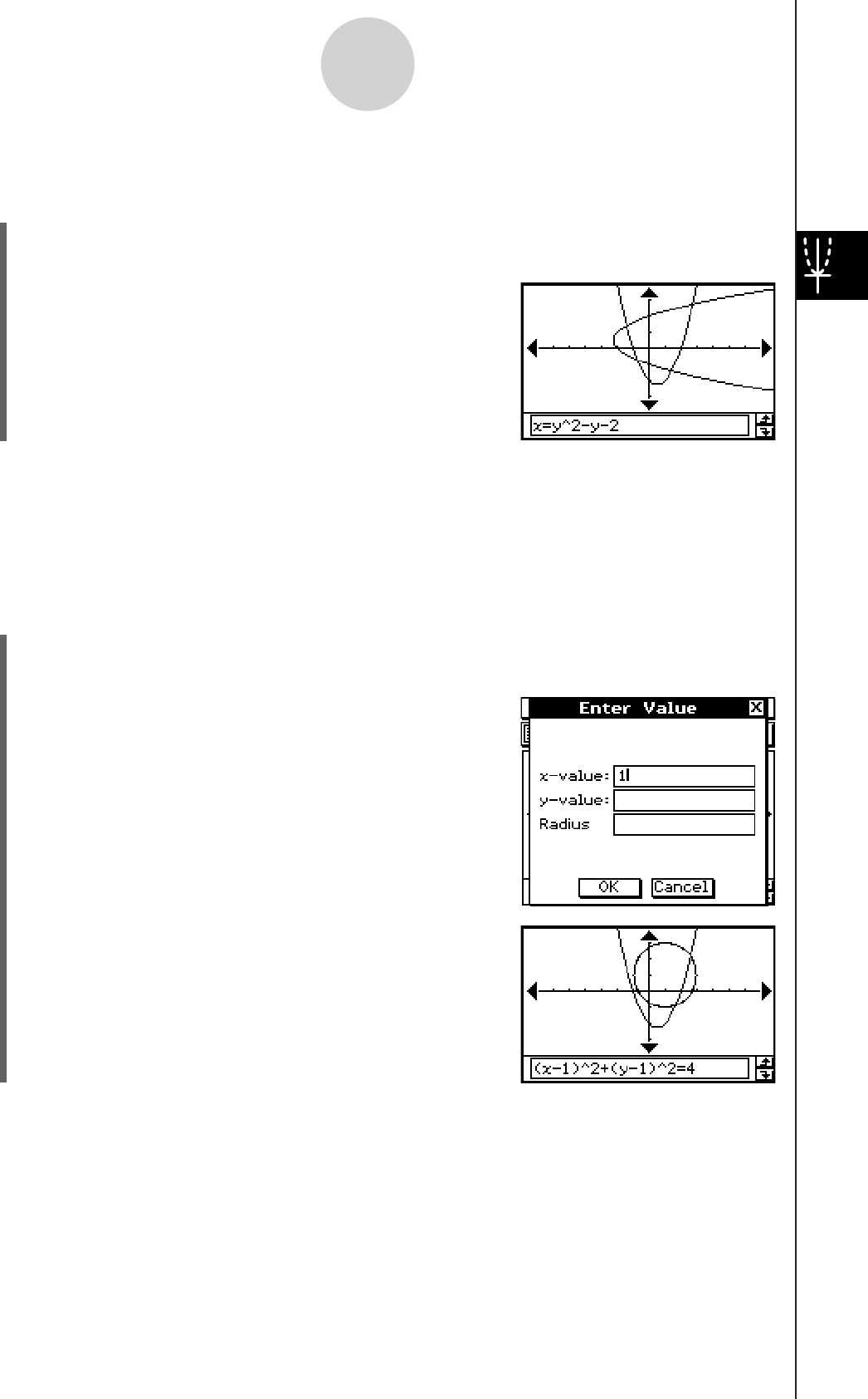
20060301

u To graph the inverse of a function

Example: To graph y = x2 – x – 2 and then overlay it with x = y2 – y – 2

(1) In line

y1 of the Graph Editor window, input and save y = x2 – x – 2.

(2) Tap

$ to graph the function.

(3) Tap [Analysis], [Sketch], and then [Inverse].

• This graphs the inverse function. The message

box briefly shows the inverse function.

3-6-4

Using the Sketch Menu

Tip

• If a function does not have an inverse, the graph produced by the [Inverse] command will be the

result of interchanging the x and y variables of the original function.

u To draw a circle

Example: To draw a circle with a center point located at (1, 1) and a radius of 2

(1) While the Graph window is active, tap [Analysis], [Sketch], and then [Circle].

• This display “Circle” on the Graph window.

(2) Press

• This displays a dialog box for specifying the

center point coordinates (x, y) and the radius r,

with 1 specified as the value of x.

(3) Enter value for x, y, and r, and then tap [OK].

• This closes the dialog box and draws the circle

according to your specifications. The message

box shows the function for the circle.

Tip

• Instead of inputting values, you can also draw a circle using stylus operations only. To do so,

perform the following operation in place of step (2) of the above operation.

(2) Tap the point where you want the center of the circle to be, and then tap a second point

anywhere on the circle’s circumference.

• You could also tap the center point, and then drag to the second point.

20060301

u To draw a vertical or horizontal line

Example: To draw a vertical line at x = 2

(1) While the Graph window is active, tap [Analysis], [Sketch], and then [Vertical].

• This displays “Vertical” on the Graph window, and the ClassPad waits for you to draw

the vertical line.

(2) Press

• This displays a dialog box for specifying the x-coordinate of the vertical line, with 2

specified as the x-coordinate.

• Instead of inputting a value here, you can use the stylus to tap the point through

which the vertical line should pass.

(3) Tap [OK].

• This closes the dialog box and draws the vertical line at x = 2.

Tip

• To draw a horizontal line, tap [Analysis], [Sketch], and then [Horizontal] in place of [Vertical] in

step (1) of the above procedure. In the case of a horizontal line, you need to specify the

y-coordinate in step (2).

u To clear figures inserted using the Sketch menu

To clear plots, lines, text, or other figures inserted using the [Sketch] menu, tap [Analysis],

[Sketch], and then [Cls].

• This redraws the graph to what is stored on the Graph Editor window.

3-6-5

Using the Sketch Menu

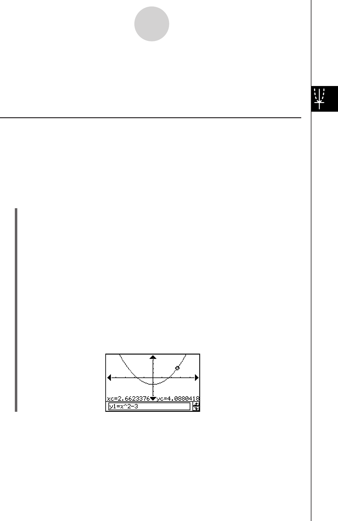
20060301

3-7 Using Trace

Trace lets you move a point along a graph and displays the coordinates for the current

pointer location. You can also link the trace operation to the number table used to draw a

graph, so the pointer jumps to the coordinates that are currently selected in the table.

Using Trace to Read Graph Coordinates

Starting the trace operation causes a crosshair pointer to appear on the graph. You can then

press the cursor key or tap the graph controller arrows to move the pointer. The coordinates

are displayed as you move the pointer.

u To perform a trace operation

Example: To graph the function y = x2 – 3 and then use the trace operation to read

coordinates on the graph

(1) Tap

6 to display the View Window dialog box, and then configure it with the following

parameters.

xmin = –5, xmax = 5, xscale = 1

ymin = –10, ymax = 10, yscale = 2

(2) On the Graph Editor window, input and store x2 – 3 into line y1, and then tap $ to

graph it.

(3) Tap [Analysis], [Trace], or tap =.

• The pointer will not be visible when it is located at a point outside the graph display

area.

• If “Error” appears in place of the xc or yc coordinate, it means that the current point is

undefined. Press the left or right cursor key to move to a point that is defined.

(4) Press the left or right cursor key, or tap the left or right graph controller arrow.

• This moves the pointer along the graph, and displays the coordinates of the current

pointer location.

3-7-1

Using Trace

20060301

• You can also move the pointer to a particular point by inputting coordinates. Pressing

a number key displays a dialog box for inputting coordinates. Input the values you

want and then tap [OK].

• When there are multiple graphs on the Graph window, you can use the up and down

cursor keys or the up and down graph controller arrows to move the pointer between

graphs.

(5) To quit the trace operation, tap on the icon panel.

Tip

• While the trace pointer is on the window, tapping the displayed coordinate values causes the

coordinate values to appear in the message box. You can then copy the coordinates to the

clipboard.

k Specifying the Format of the Coordinates Displayed by Trace

Check boxes on the Graph Format dialog box (page 1-9-6) let you specify whether you want

to display pointer coordinates only, or pointer coordinates plus the derivative. You can also

turn off the display of the coordinates, if you want.

3-7-2

Using Trace

Turn off coordinate display

Display coordinates and the

derivative

Select the [Derivative/Slope] check box under

[Graph Format].

Clear the [Coordinate] check box under [Graph Format].

• Neither coordinates nor the derivative is displayed when

the [Coordinate] check box is cleared, regardless of the

current [Derivative/Slope] setting.

Do this:

To do this:

For details about Graph Format settings, see “Application Format Settings” on page 1-9-4.

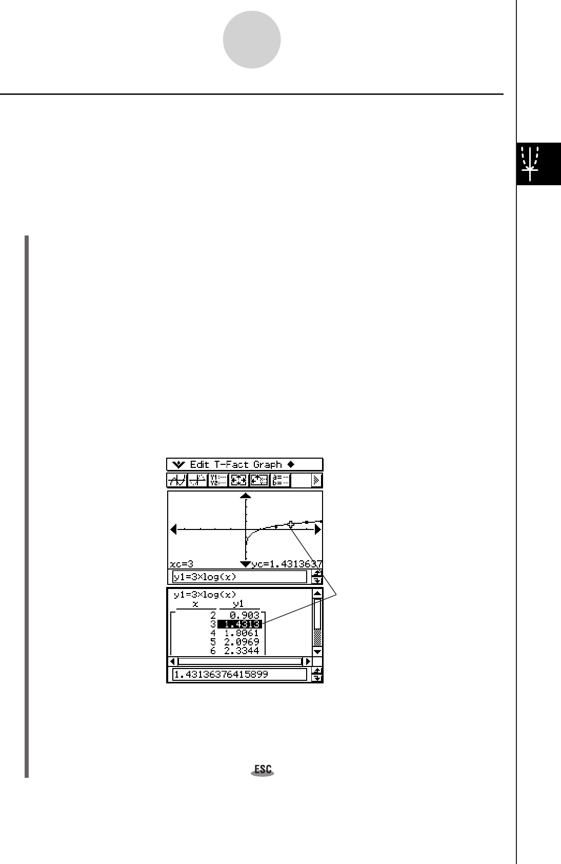
20060301

Linking Trace to a Number Table

This section explains how you can link the movement of the trace pointer to the values in the

number table used to draw the graph. This type of operation is called “linked trace”.

• For information about generating a number table and performing other table operations,

see “3-4 Using Table & Graph”.

Example: To link trace to a number table created by graphing y = 3logx

u ClassPad Operation

(1) Display the View Window dialog box, and then configure it with the following

parameters.

xmin = –5, xmax = 5, xscale = 1

ymin = –10, ymax = 10, yscale = 2

(2) Display the Table Input dialog box, and then configure it with the following settings.

Start: 2, End: 9, Step: 1

(3) On the Graph Editor window, input and store y = 3logx into line y1, and then tap #.

• This generates a number table and displays it.

(4) Tap

a and then [Link].

• This displays the Graph window and draws the graph, with the trace pointer located

on the graph line. The coordinates of the trace pointer location will also be shown.

• Tapping a cell in the y1 column causes the trace pointer to move the location of the

cell’s value.

3-7-3

Using Trace

The highlighted table value

corresponds to the current

location of the trace pointer

on the graph.

(5) You can perform the following operations while a linked trace operation is in progress.

• You can move the highlighting in the number table by pressing the up and down

cursor keys, or by tapping the cell you want to select. Doing so causes the trace

pointer to jump to the corresponding location on the graph.

(6) To quit the linked trace operation, tap on the icon panel.

20060301

Generating Number Table Values from a Graph

A “graph-to-table” feature lets you extract the coordinate values at the current pointer location

and input them into a table.

Example: Generate a table and graph for the expression y = x3 – 3x, and input the

coordinates for specific points on the graph into a table

Use the initial View Window settings (page 3-2-3).

Configure the Table Input settings shown below.

Start: 1, End: 4, Step: 1

u ClassPad Operation

(1) Input the function y = x3 – 3x on the Graph Editor window.

(2) Tap

$ to graph the function.

(3) Tap

# to generate the table.

3-7-4

Using Trace

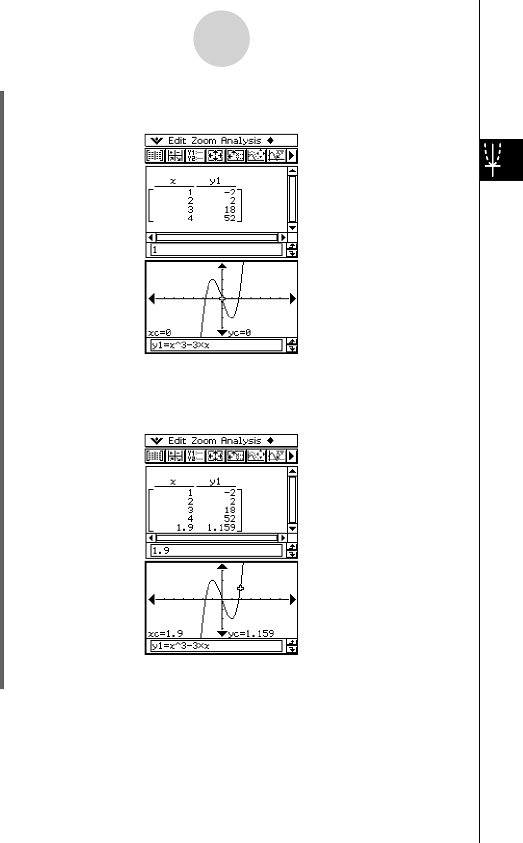
20060301

(4) Tap the Graph window to make it active. Next, tap [Analysis] and then [Trace].

• This causes a pointer to appear on the graph.

(5) Use the cursor key to move the pointer along the graph until it reaches a point whose

coordinates you want to input into the table.

(6) Press

E to input the coordinates at the current cursor position at the end of the table.

3-7-5

Using Trace

(7) Repeat steps (5) and (6) to input the rest of the coordinates you want.

20110401

3-8 Analyzing a Function Used to Draw a Graph

Your ClassPad includes a G-Solve feature that lets you perform a variety of different

analytical processes on an existing graph.

G-Solve Menu Overview

To access the [G-Solve] menu, tap [Analysis] and then [G-Solve]. The following describes

the commands that are available on the [G-Solve] menu.

3-8-1

Analyzing a Function Used to Draw a Graph

Tip

• See page

α-4-1 of the Appendix for information about graph types and executable G-Solve

functions.

Root (the

-intercept)

Maximum value

Minimum value

Root

Max

Min

Select this G-Solve menu command:

To obtain this for the graph:

Point of intersection for two graphs

-coordinate for a given

-coordinate

-coordinate for a given

-coordinate

Definite integral for a particular range

Volume of a solid of revolution

-intercept

Maximum value in the range displayed on the

Graph window

Inflection

Minimum value in the range displayed on the

Graph window

π ∫ (

(

))

Distance

∫

-Cal

-Intercept

Intersect

-Cal

Max

Min

Point of inflection

Distance between two points

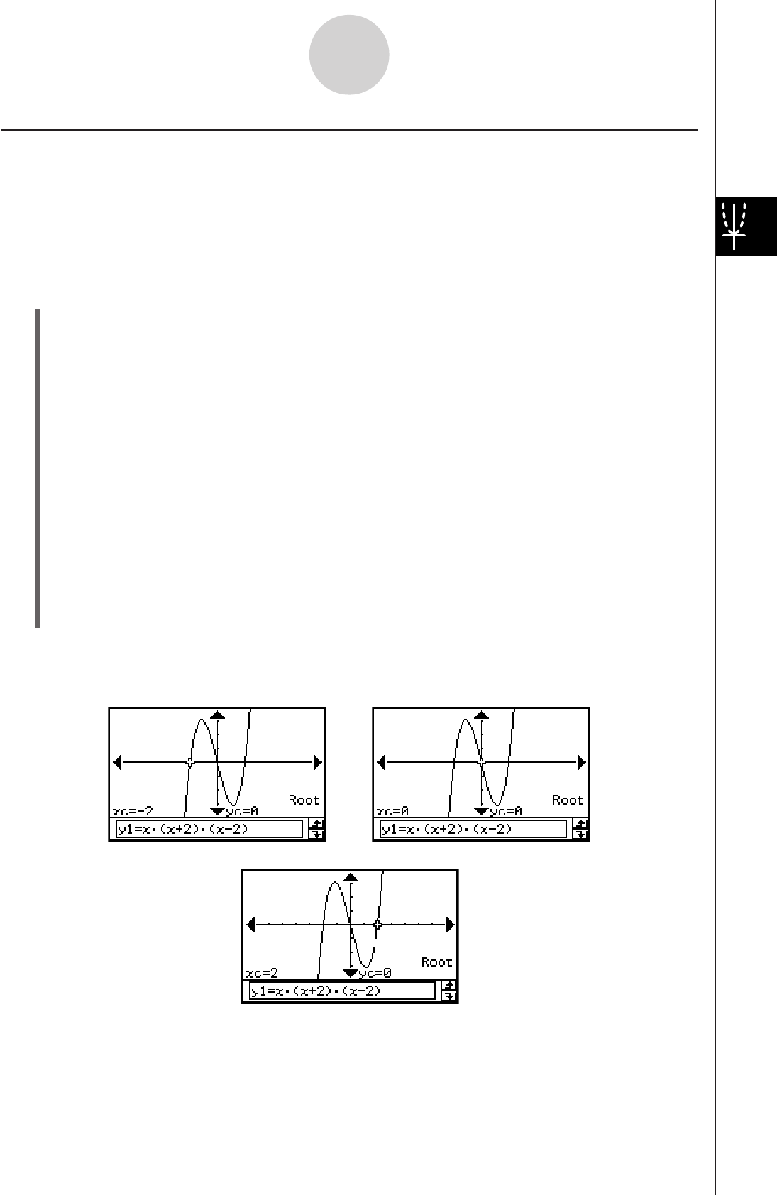
20060301

Using G-Solve Menu Commands

This section describes how to use each of the commands on the [G-Solve] menu. Note that

all of the procedures in this section are performed in the Graph & Table application, which

you can enter by tapping the T icon on the application menu.

u To obtain the root of a function

Example: To graph the function y = x(x + 2)(x – 2) and obtain its root

(1) Display the View Window dialog box, and then configure it with the following

parameters.

xmin = –7.7, xmax = 7.7, xscale = 1

ymin = –3.8, ymax = 3.8, yscale = 1

(2) On the Graph Editor window, input and store y = x(x + 2)(x – 2) into line y1, and then

tap $ to graph it.

• Make sure that only y1 is checked.

(3) Tap [Analysis], [G-Solve], and then [Root], or tap Y.

• This displays “Root” on the Graph window, and locates a pointer at the first solution of

the root (root for smallest value of x). The x- and y-coordinates at the current pointer

location are also shown on the Graph window.

(4) To obtain other roots, press the left or right cursor key, or tap the left or right graph

controller arrows.

• If there is only one solution, the pointer does not move when you press the cursor key.

Result Screenshots

3-8-2

Analyzing a Function Used to Draw a Graph

20060301

u To obtain the minimum value, maximum value, fMax, fMin, y-intercept,

and inflection of a function

Example: To graph the function y = x2(x + 2)(x – 2) and obtain its minimum value

(1) Display the View Window dialog box, and then configure it with the following

parameters.

xmin = –7.7, xmax = 7.7, xscale = 1

ymin = –3.8, ymax = 3.8, yscale = 1

(2) On the Graph Editor window, input and store y = x2 (x + 2)(x – 2) into line y1, and

then tap $ to graph it.

• Make sure that only y1 is checked.

(3) Tap [Analysis], [G-Solve], and then [Min], or tap I.

• This displays “Min” on the Graph window, and locates a pointer at the first solution of

the minimum value (minimum value of y for smallest value of x). The x- and

y-coordinates at the current pointer location are also shown on the Graph window.

(4) To obtain other minimum values, press the left or right cursor key, or tap the left or

right graph controller arrows.

• If there is only one solution, the pointer does not move when you press the cursor

key.

Result Screenshots

3-8-3

Analyzing a Function Used to Draw a Graph

Tip

• To obtain the other values, select the applicable command on the [G-Solve] menu in step (3) of

the above procedure.

Maximum value Max (or tap U)

Select this G-Solve menu command:

To obtain this value:

Minimum value in the range

displayed on the Graph window

-intercept

Inflection

Point of inflection

-intercept

fMin

Max

Maximum value in the range

displayed on the Graph window

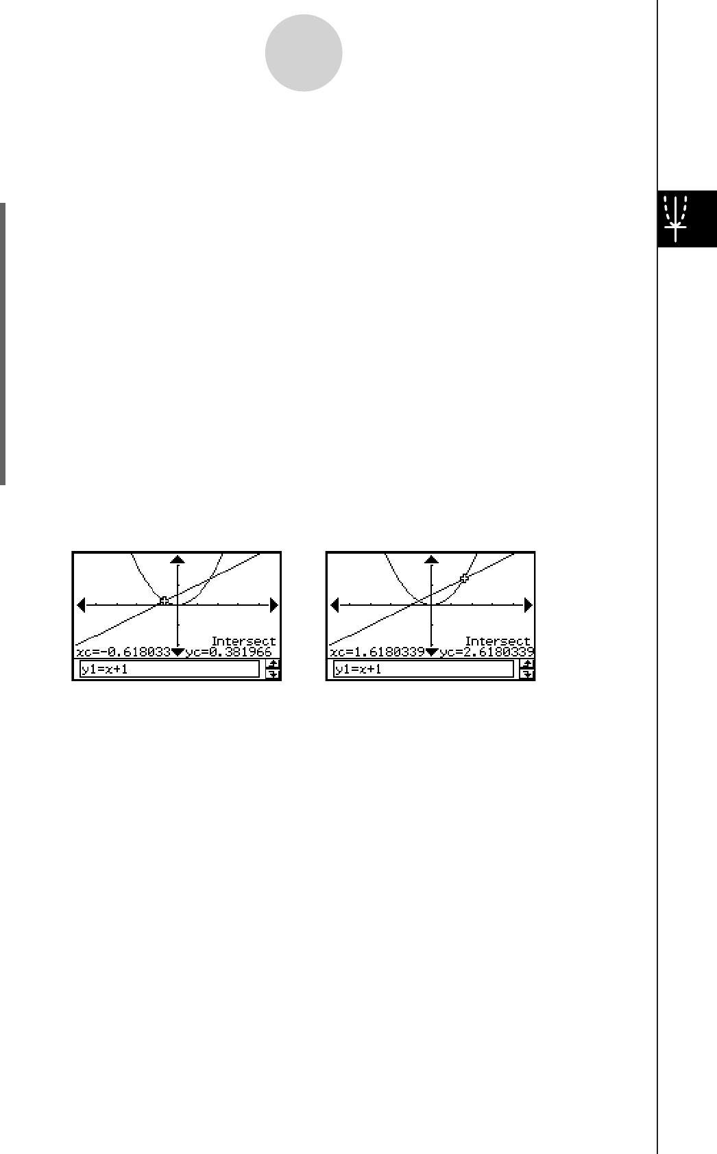
20060301

u To obtain the point of intersection for two graphs

Example: To graph the functions y = x + 1 and y = x2, and determine their point of

intersection

(1) Display the View Window dialog box, and then configure it with the following

parameters.

xmin = –5, xmax = 5, xscale = 1

ymin = –5, ymax = 5, yscale = 2

(2) On the Graph Editor window, input and store y = x + 1 into line y1 and y = x2 into y2,

and then tap $ to graph them.

• Make sure that only y1 and y2 are checked.

(3) Tap [Analysis], [G-Solve], and then [Intersect].

• This causes “Intersect” to appear on the Graph window, with a pointer located at the

point of intersection. The x- and y-coordinates at the current pointer location are also

shown on the Graph window.

(4) To obtain other points of intersection, press the left or right cursor key, or tap the left or

right graph controller arrows.

Result Screenshots

3-8-4

Analyzing a Function Used to Draw a Graph

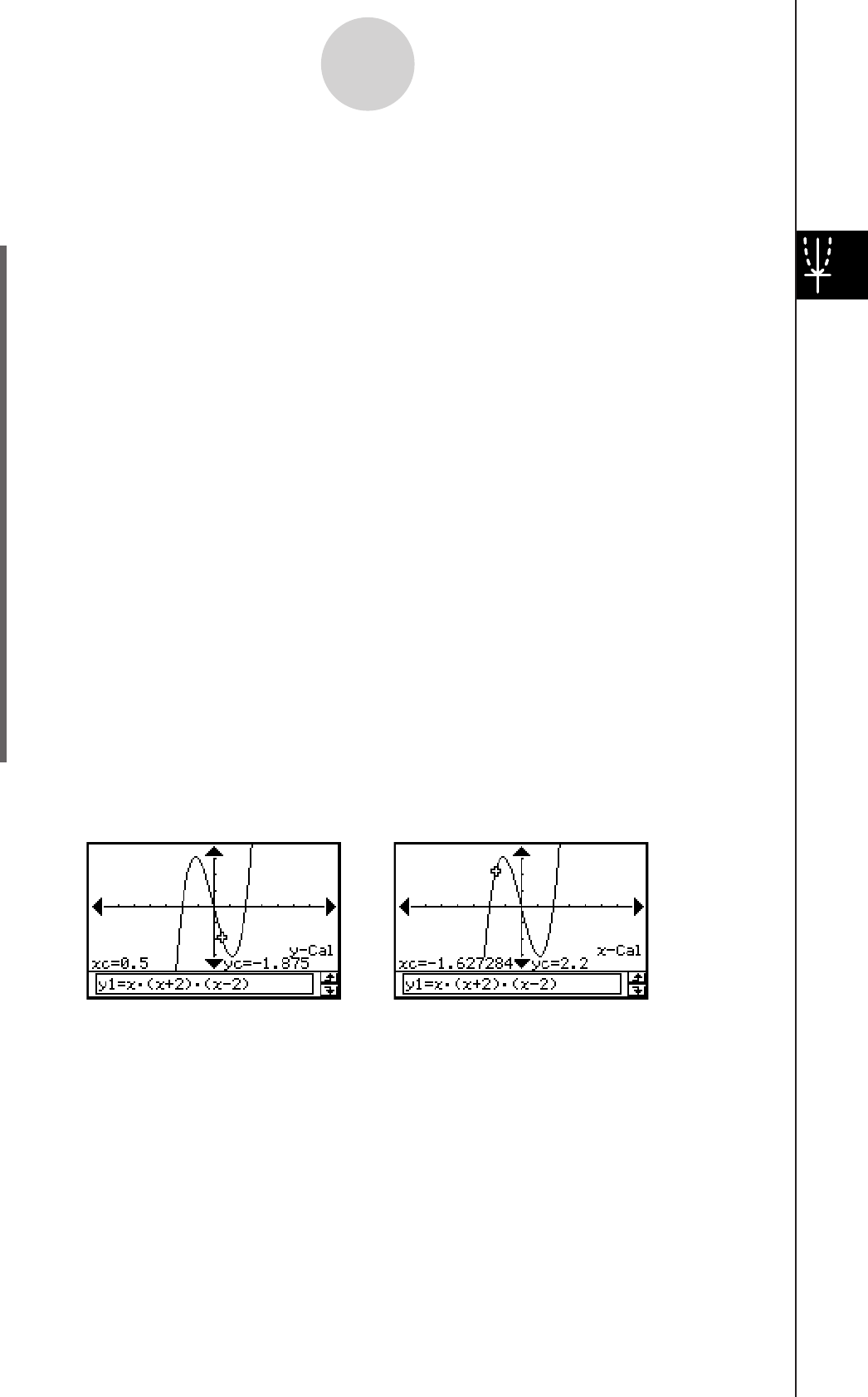
20060301

u To determine coordinates at a particular point on a graph

Example: To graph the function y = x (x + 2)(x – 2) and determine the y-coordinate when

x = 0.5, and the x-coordinate when y = 2.2

(1) Display the View Window dialog box, and then configure it with the following

parameters.

xmin = –7.7, xmax = 7.7, xscale = 1

ymin = –3.8, ymax = 3.8, yscale = 1

(2) On the Graph Editor window, input and store y = x (x + 2)(x – 2) into line y1, and then

tap $ to graph it.

• Make sure that only y1 is checked.

(3) To obtain the value of y for a particular x-value, tap [Analysis], [G-Solve], and then

[y-Cal ].

• This displays a dialog box for specifying the x-value.

(4) For this example, input 0.5 and then tap [OK].

• This moves the pointer to the location on the graph where x = 0.5, and displays the

x-coordinate and y-coordinate at that location.

(5) To obtain the value of x for a particular y-value, tap [Analysis], [G-Solve], and then

[x-Cal].

• This displays a dialog box for specifying the y-value.

(6) For this example, input 2.2 and then tap [OK].

• This moves the pointer to the location on the graph where y = 2.2, and displays the

x-coordinate and y-coordinate at that location.

Result Screenshots

3-8-5

Analyzing a Function Used to Draw a Graph

Tip

• When there are multiple results for the above procedure, press e to calculate the next value.

Pressing d returns to the previous value.

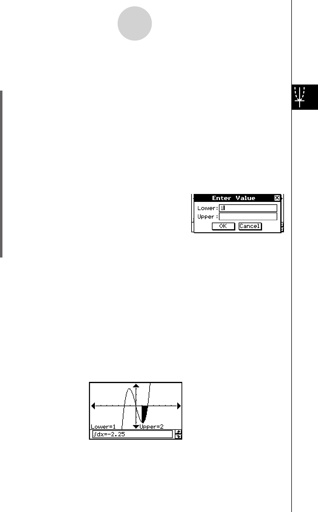
20060301

u To determine the definite integral for a particular domain

Example: To graph the function y = x(x + 2)(x – 2) and obtain its definite integral in the

domain of 1 < x < 2

(1) Display the View Window dialog box, and then configure it with the following

parameters.

xmin = –7.7, xmax = 7.7, xscale = 1

ymin = –4, ymax = 4, yscale = 1

(2) On the Graph Editor window, input and store y = x(x + 2)(x – 2) into line y1, and then

tap $ to graph it.

• Make sure that only y1 is checked.

(3) Tap [Analysis], [G-Solve], and then [

∫

dx].

• This displays “Lower” on the Graph window.

(4) Press

• This displays a dialog box for inputting an interval for

the x-values, with 1 specified for the lower limit of the

x-axis (Lower).

3-8-6

Analyzing a Function Used to Draw a Graph

(5) Tap the [Upper] input box and then input 2 for the upper limit of the x-axis.

(6) Tap [OK].

Tip

• Instead of inputting [Lower] and [Upper] values in steps (4) through (6), you can use the cursor

key or the graph controller arrows to move the pointer along the graph to specify the lower limit

and upper limit. If you do, perform the following two steps after step (3).

(4) Use the cursor key or the graph controller to move the pointer to the location of the lower limit

and then press E.

• This registers the lower limit and changes the word in the lower right corner of the Graph

window to “Upper”.

(5) Move the pointer to the location of the upper limit, and then press E.

Result Screenshot

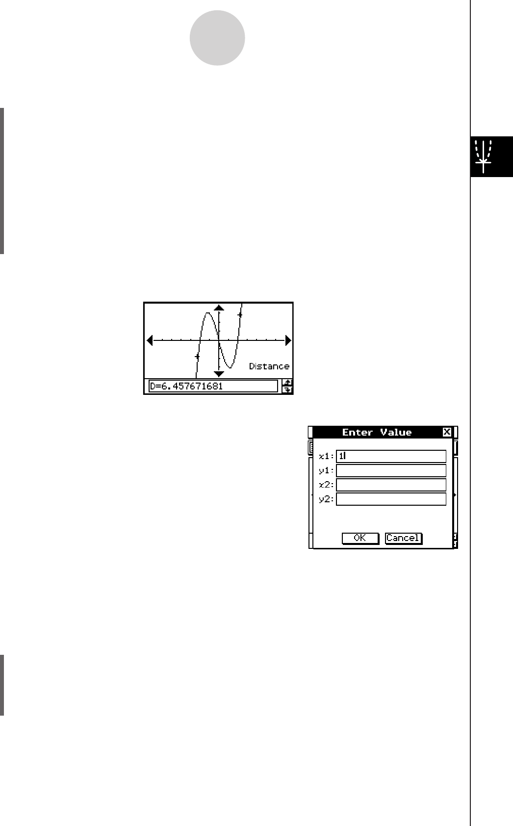
20060301

u To determine the distance between any two points

(1) Tap the Graph window to make it active.

(2) Tap [Analysis], [G-Solve], and then [Distance].

• This displays “Distance” on the Graph window, and the ClassPad waits for you to

specify the first point.

(3) Tap the first point on the Graph window.

• This causes a pointer to appear at the location where you tap.

(4) Tap the second point on the Graph window.

• This causes a pointer to appear at the second point, and the distance between the

two points to appear in the message box.

Result Screenshot

3-8-7

Analyzing a Function Used to Draw a Graph

Tip

• Instead of tapping points on the Graph window, you could also

specify points by inputting their coordinates. Without tapping

the Graph window, input a value. This causes a coordinate

specification dialog box to appear. Input the x- and

y-coordinates of the two points.

u To determine the inflection point

You can use the following procedure to determine coordinates of the inflection point for a

cubic function.

Example: To graph the function y = x3 – 1 and determine its inflection point

uClassPad Operation

(1) Display the View Window dialog box, and then configure it with the following

parameters.

xmin = –4.9, xmax = 4.9, xscale = 1

ymin = –3.3, ymax = 1.8, yscale = 1

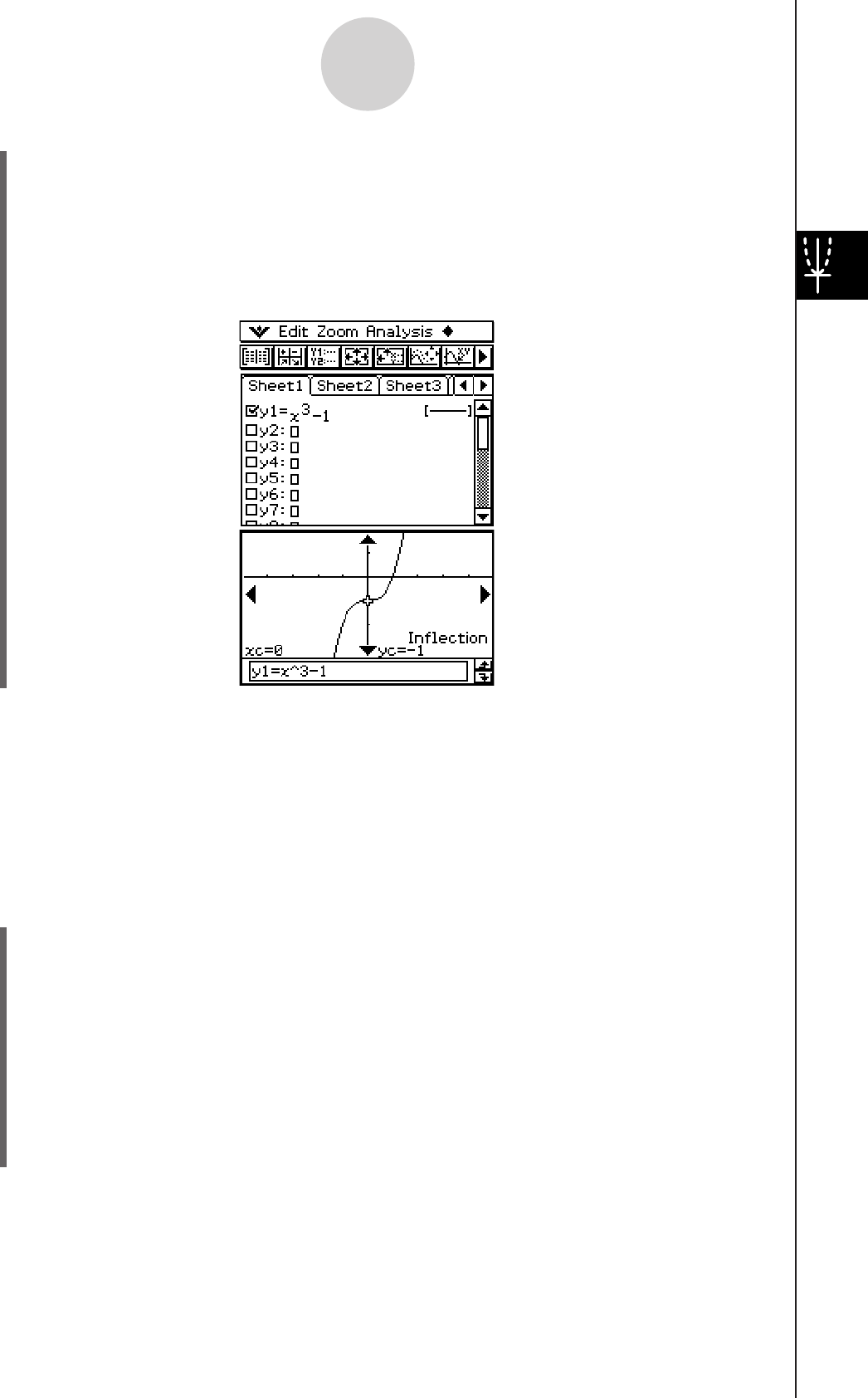
20060301

3-8-8

Analyzing a Function Used to Draw a Graph

(2) On the Graph Editor window, input and store y1 = x3 – 1 into line y1, and then tap $

to graph it.

• Make sure that only “y1” is selected (checked).

(3) Tap [Analysis], [G-Solve], and then [Inflection].

• This causes “Inflection” to appear on the Graph window, with a pointer located at the

point of inflection.

Tip

• If your function has multiple inflection points, use the cursor button or graph controller arrows to

move the pointer between them and display their coordinates.

u To obtain the volume of a solid of revolution

Example: To graph the function y = x2 – x – 2 and obtain the volume of a solid of revolution

as the line segment from x = 1 to x = 2 is rotated on the x-axis

(1) Display the View Window dialog box, and then configure it with the following parameters.

xmin = –7.7, xmax = 7.7, xscale = 1

ymin = –3.8, ymax = 3.8, yscale = 1

(2) On the Graph Editor window, input and store y = x2 – x – 2 into line y1, and then tap $

to graph it.

• Make sure that only y1 is checked.

(3) Tap [Analysis], [G-Solve], and then [ ∫

(f(x))2dx].

• This displays a crosshair pointer on the graph, and the word “Lower” in the lower right

corner of the Graph window.

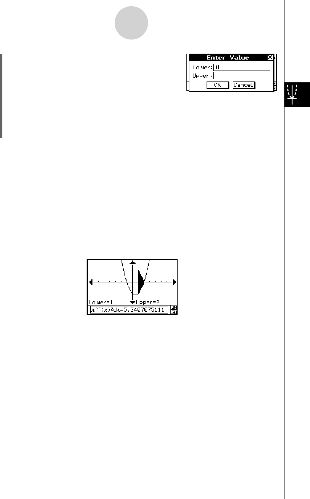
20060301

(4) Press

• This displays a dialog box for inputting an interval of

values for x, with 1 specified for the lower limit of the

x-axis (Lower).

(5) Tap the [Upper] input box and then input 2 for the upper limit of the x-axis.

(6) Tap [OK].

• This causes a silhouette of the solid of revolution to appear on the Graph window,

and its volume to appear in the message box.

Tip

• Instead of inputting [Lower] and [Upper] values in steps (4) through (6), you can use the cursor

key or the graph controller arrows to move the pointer along the graph to specify the lower limit

and upper limit. If you do, perform the following two steps after step (3).

(4) Use the cursor key or the graph controller to move the pointer to the location of the lower limit

and then press E.

• This registers the lower limit and changes the word in the lower right corner of the Graph

window to “Upper”.

(5) Move the pointer to the location of the upper limit, and then press E.

Result Screenshot

3-8-9

Analyzing a Function Used to Draw a Graph

20060301

Using the Conics

Application

The Conics application provides you with the capability to graph

circular, parabolic, elliptic, and hyperbolic functions. You can

also use the Conics application to quickly and easily determine

the proper focal point, vertex, directrix, axis of symmetry, latus

rectum, center, radius, asymptote, eccentricity, and even the

x- and y-intercepts of each type of conics.

4-1 Conics Application Overview

4-2 Inputting Equations

4-3 Drawing a Conics Graph

4-4 Using Trace to Read Graph Coordinates

4-5 Using G-Solve to Analyze a Conics Graph

Chapter

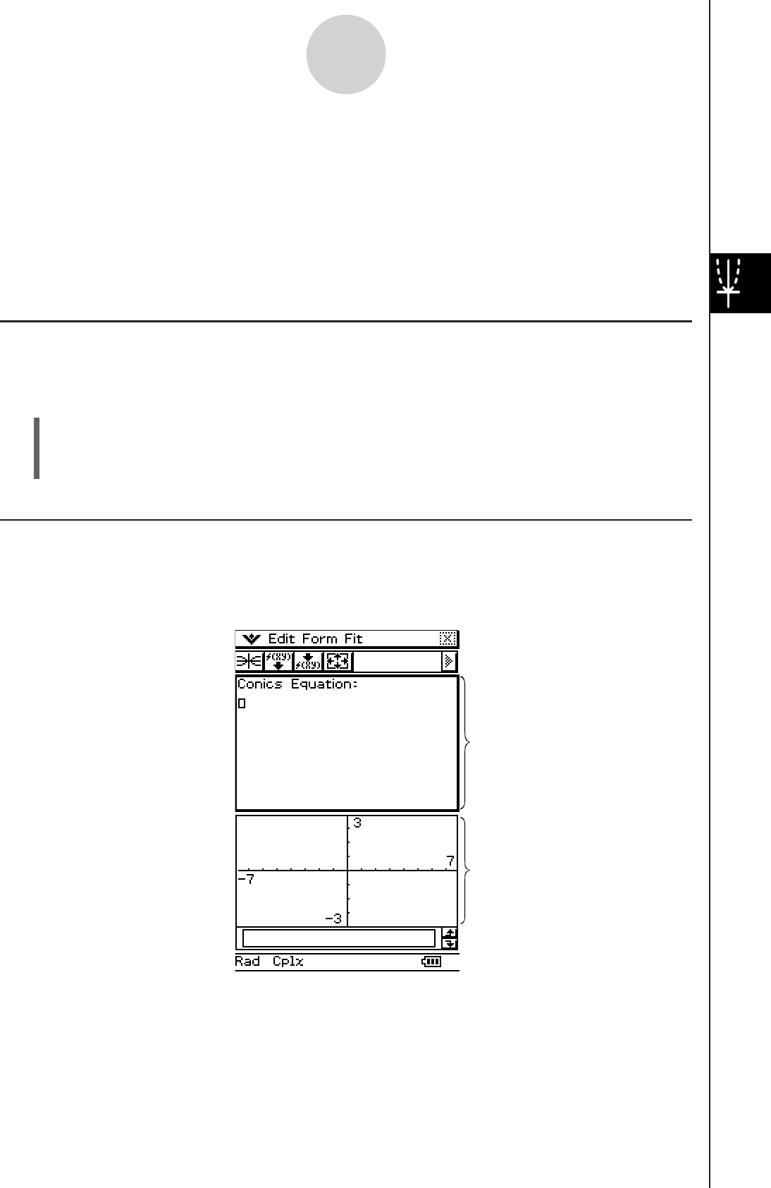
20060301

4-1 Conics Application Overview

This section describes the configuration of the Conics application windows, and provides

basic information about its menus and commands.

• The Conics application uses many of the same commands (Zoom, Trace, Sketch, etc.) as

the Graph & Table application. It is recommended that you familiarize yourself with Graph

& Table operations before trying to use the Conics application.

4-1-1

Conics Application Overview

Conics Application Window

When you start up the Conics application, two windows appear on the display: the Conics

Editor window and the Conics Graph window. A function that is input on the Conics Editor

window is graphed on the Conics Graph window.

Conics Editor window

Conics Graph window

Starting Up the Conics Application

Use the following procedure to start up the Conics application.

u ClassPad Operation

On the application menu, tap C.

This starts the Conics application and displays the Conics Editor window and the Conics

Graph window.

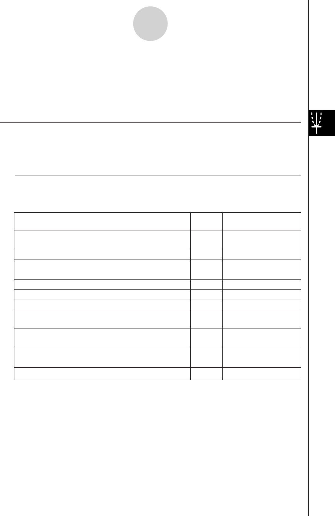
20060301

4-1-2

Conics Application Overview

Conics Application Menus and Buttons

This section explains the operations you can perform using the menus and buttons of the

Conics application window.

• For information about the O menu, see “Using the O Menu” on page 1-5-4.

k Conics Editor Window Menus and Buttons

The following describes the menu and button operations you can perform while the Conics

Editor window is active.

Copy the selected character string to the clipboard

Select all of the text on the Conics Editor window

Clear all of the text from the Conics Editor window

Insert a Conics Form on the Conics Editor window

—

Edit - Cut

Edit - Copy

Edit - Paste

Edit - Select All

Edit - Clear All

Fit - Fit into Conics

Form

O- View Window

O - Variable Manager

Form - Insert

Conics Form

Cut the selected character string and place it onto the

clipboard

Adjust the equation on the Conics Editor window so

it fits a Conics Form

^—

Draw a graph

Display the View Window dialog box (page 3-2-1) to

configure Graph window settings

—

Display the Variable Manager (page 1-8-1)

Paste the contents of the clipboard at the current

cursor position in the Conics Editor window

To do this: Tap this

button:

Or select this

menu item:

• The Conics Editor window can have one conics equation input at a time. The Conics

application includes a number of preset conics formats (page 4-2-1) that make equation

input quick and easy.

• You can tap the graph controller arrows (page 3-2-6) or use the cursor key to scroll the

Conics Graph window.

• You can use Trace (page 4-4-1) to trace a conics graph.

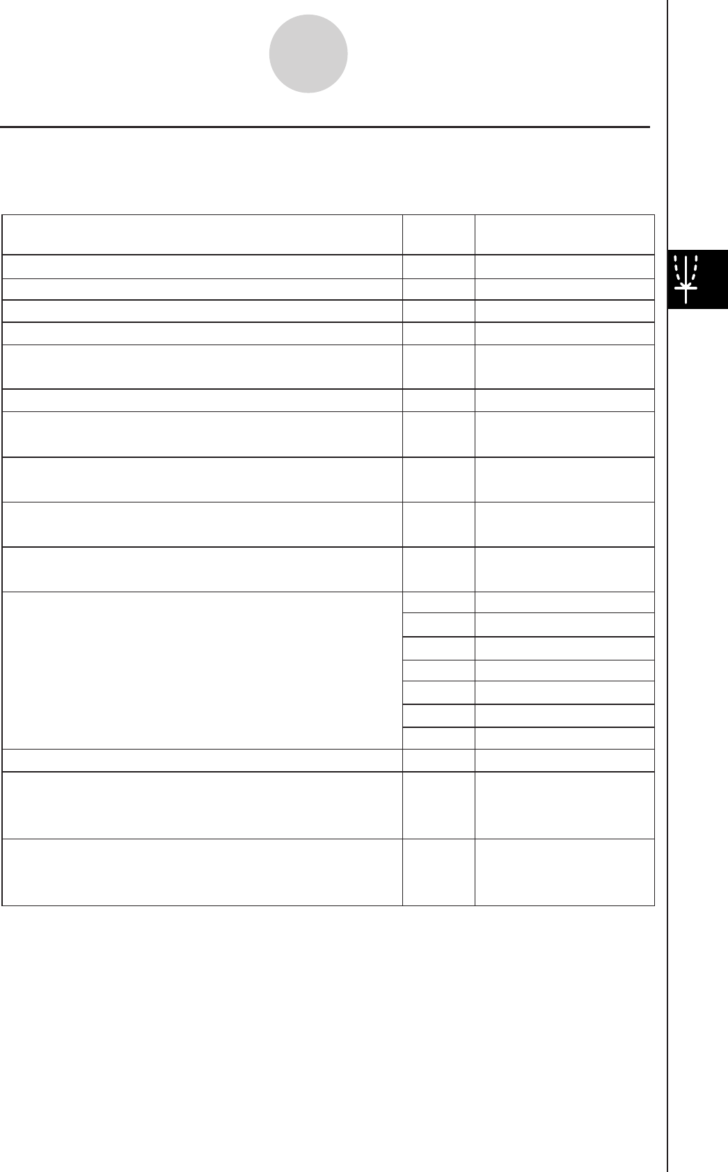
20060301

Zoom - Square

—

Zoom - Round

Zoom - Integer

—

Zoom - Previous

Zoom - Quick Initialize

—

Zoom - Quick Trig

Zoom - Quick log(x)

—

Zoom - Quick e^x

Zoom - Quick x^2

—

Zoom - Quick –x^2

—

Analysis - Trace

—Analysis - Sketch

—

Analysis

G-Solve

Insert a point, graphic, or text into an existing graph

• For details about this operation, see “3-6 Using the

Sketch Menu”.

Perform a G-Solve operation

• For details about this operation, see “4-5 Using

G-Solve to Analyze a Conics Graph”.

Display the coordinates at a particular point on a graph

Perform a quick zoom operation (page 3-2-9)

Adjust View Window x-axis values so they are identical

to the y-axis values

Round coordinate values displayed using Trace

(page 4-4-1)

Make the value of each dot equal 1, which makes all

coordinate values integers

Return View Window parameters to their settings prior

to the last zoom operation

Zoom - Quick Standard

To do this: Tap this

button:

Or select this

menu item:

Zoom - Box

—Zoom - Factor

—Zoom - Zoom In

— Zoom - Zoom Out

Zoom - Auto

Zoom - Original

—

Enlarge the part of the screen bounded by a box

Specify a zoom factor

Zoom in by the zoom factor

Zoom out by the zoom factor

Return a graph to its original size

Configure View Window y-axis parameters and redraw

the graph so it fills the Graph window along the y-axis

4-1-3

Conics Application Overview

k Conics Graph Window Menus and Buttons

The following describes the menu and button operations you can perform while the Conics

Graph window is active.

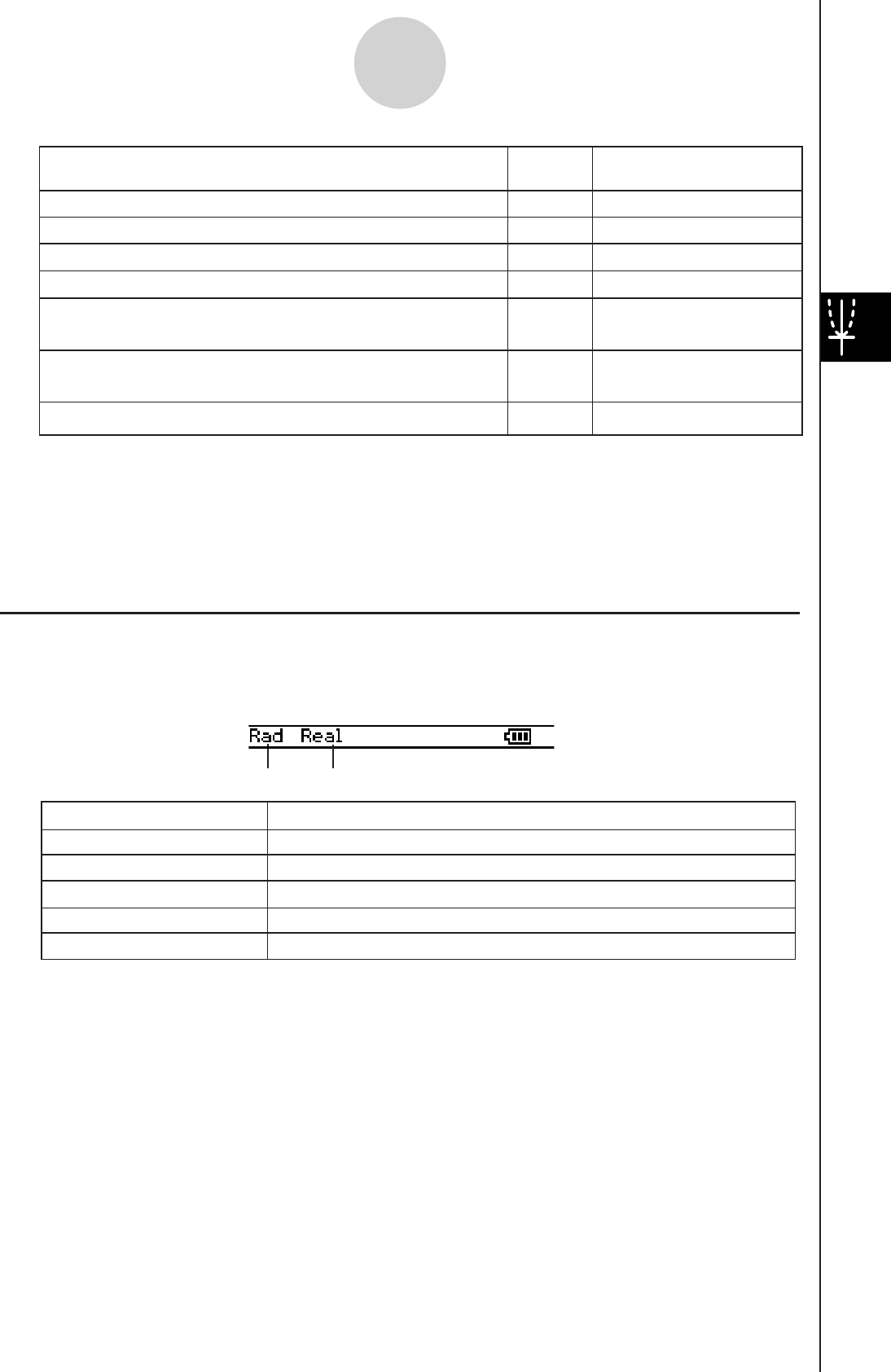
20060301

—a - Store Picture

—a - Recall Picture

a - ReDraw

O - View Window

O - Variable Manager

*O - Conics Editor

—

Display the View Window dialog box (page 3-2-1) to

configure Graph window settings

Activate the pan function for dragging the Graph

window with the stylus

Save a graph as image data (page 3-2-10)

Recall the image of a graph (page 3-2-10)

Re-draw a graph

Make the Conics Editor window active

Display the Variable Manager (page 1-8-1)

To do this: Tap this

button:

Or select this

menu item:

Tip

• The [Tangent], [Normal], and [Inverse] commands of the Graph & Table application’s Sketch

function are not included in the Conics application.

• The G-Solve feature of the Conics application performs analysis that is specially suited to conics,

and so it operates differently from the G-Solve feature of the Graph & Table application.

Conics Application Status Bar

The status bar at the bottom of the Conics application shows the current angle unit setting

and [Complex Format] setting (page 1-9-5).

Rad

Deg

Cplx

Real

The angle unit setting is radians.

The angle unit setting is degrees.

Gra The angle unit setting is grads.

The Complex (complex number calculation) mode is selected.

The Real (real number calculation) mode is selected.

If you see this: It means this:

4-1-4

Conics Application Overview

Angle unit Real mode

Tip

• Press and drag stylus to view coordinates in status bar.

20060301

4-2-1

Inputting Equations

4-2 Inputting Equations

This section explains the various ways you can input equations using the Conics Editor

window.

Using a Conics Form to Input an Equation

Preset formats can help you input conics equations quickly and easily. The following table

contains a complete list of the types of equations that you can input just by tapping [Form]

and then [Insert Conics Form].

Equations

Horizontal Parabola 1

x = A

(y – K)^2 + H

Horizontal Parabola 2

x = A

y^2 + B

y + C

Vertical Parabola 1

y = A

(x – H)^2 + K

Vertical Parabola 2

y = A

x^2 + B

x + C

Circle 1

(x – H)^2 + (y – K)^2 = R^2

Circle 2

x^2 + A

y^2 + B

x + C

y + D = 0

Ellipse

(x – H)^2 ÷ A^2 + (y – K)^2 ÷ B^2 = 1

Horizontal Hyperbola

(x – H)^2 ÷ A^2 – (y – K)^2 ÷ B^2 = 1

Vertical Hyperbola

(y – K)^2 ÷ A^2 – (x – H)^2 ÷ B^2 = 1

General Form

x^2 + B

y + C

y^2 + D

x + E

y + F = 0

Conics Forms

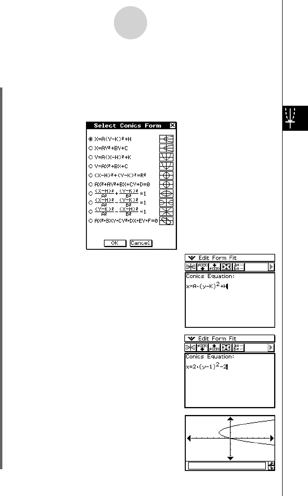
20060301

4-2-2

Inputting Equations

u To input an equation using a Conics Form

Example: To use a Conics Form to input the equation for a parabola with a horizontal axis

(principal axis parallel with x-axis)

(1) On the application menu, tap C to start the Conics application.

(2) On the Conics Editor window, tap q, or tap [Form] and then [Insert Conics Form].

• This displays the Select Conics Form dialog box.

(3) Select the Conics Form of the type of equation you

want to graph, and then tap [OK].

• Since we want to graph a parabola with a horizontal

axis in this example, select “X = A(Y – K)2 + H”. Tap

[OK] to close the Select Conics Form dialog box, and

display the selected equation in the Conics Editor

window.

(4) Modify the equation on the Conics Editor window as

required.

• Here, we will change the coefficients of the equation

as follows: A = 2, K = 1, H = –2.

(5) Tap

^ to graph the equation.

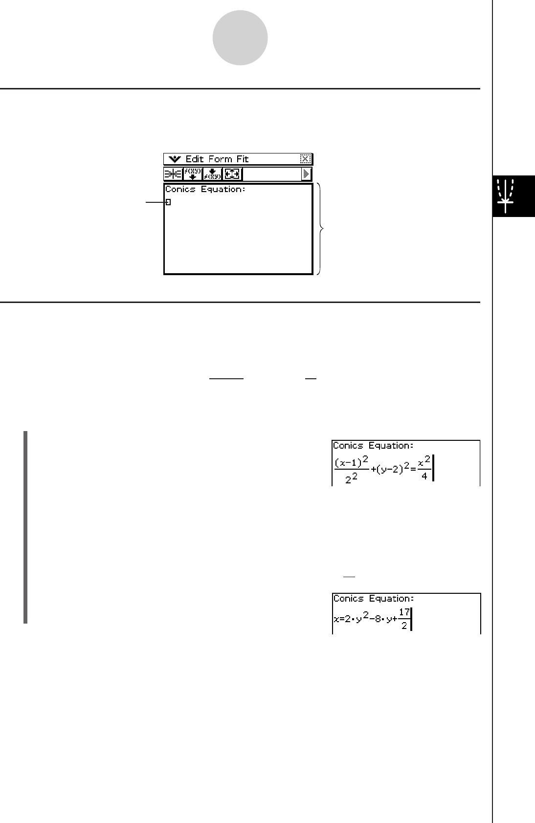
20060301

4-2-3

Inputting Equations

Inputting an Equation Manually

To input an equation manually, make the Conics Editor window active, and then use the soft

keyboard for input.

Transforming a Manually Input Equation to a Conics Form

After you manually input an equation on the Conics Editor window, you can use the

procedure below to transform it to a preset Conics Form.

Example: To transform the equation to the standard Conics Form

x = Ay2 + By + C

u ClassPad Operation

(1) On the Conics Editor window, input the above

equation.

Hint: Tap the ) tab of the soft keyboard. The 2D

fraction and 2D exponent are very helpful in entering

this equation!

Conics Editor window

(x – 1)2 + (y – 2)2 = x2

(2) After inputting the equation, tap w or tap [Fit] and then [Fit into Conics Form].

• This displays the Select Conics Form dialog box.

(3) Select “X = AY2 + BY + C” and then tap [OK].

• This transforms the equation so it becomes x = 2y2 –8

y + .

Tip

• If the equation you input cannot be transformed into the standard Conics Form you selected, the

message “Can’t Transform into This Type” appears.

• An input equation may not transform correctly if it includes a square root calculation or some

other function.

Input the equation here.

20060301

4-3-1

Drawing a Conics Graph

4-3 Drawing a Conics Graph

This section provides examples that show how to draw various types of conics graphs.

Drawing a Parabola

A parabola can be drawn with either a horizontal or vertical orientation. The parabola type is

determined by the direction of its principal axis.

k Drawing a Parabola that Opens Horizontally

A parabola with a horizontal axis is one whose principal axis is parallel to the x-axis. There

are two possible equations for a parabola with a horizontal axis:

x = A(y – K)2 + H and x = Ay2 + By + C.

Example 1: To draw the parabola x = 2(y – 1)2 – 2

u ClassPad Operation

(1) On the Conics Editor window, tap q, or tap [Form] and then [Insert Conics Form].

• This displays the Select Conics Form dialog box.

(2) Select “X = A(Y – K)2 + H” and then tap [OK].

• This closes the Select Conics Form dialog box, and displays the selected equation in

the Conics Editor window.

(3) Change the coefficients of the equation as follows: A = 2, K = 1, H = –2.

(4) Tap

^ to graph the equation.

20060301

4-3-2

Drawing a Conics Graph

Example 2: To draw the parabola x = y2 + 2y + 3

u ClassPad Operation

(1) In step (2) of the above procedure, select “X = AY2 + BY + C” on the Select Conics

Form dialog box.

(2) In step (3) of the above procedure, change the coefficients of the equation as follows:

A = 1, B = 2, C = 3.

20060301

k Drawing a Parabola that Opens Vertically

A parabola with a vertical axis is one whose principal axis is parallel to the y-axis. There are

two possible equations for a parabola with a vertical axis:

y = A(x – H)2 + K and y = Ax2 + Bx +C.

u ClassPad Operation

(1) In step (2) of the procedure under “Drawing a Parabola that Opens Horizontally”, select

“Y = A(X – H)2 + K” or “Y = AX2 + BX + C”.

(2) Specify values for the coefficients.

4-3-3

Drawing a Conics Graph

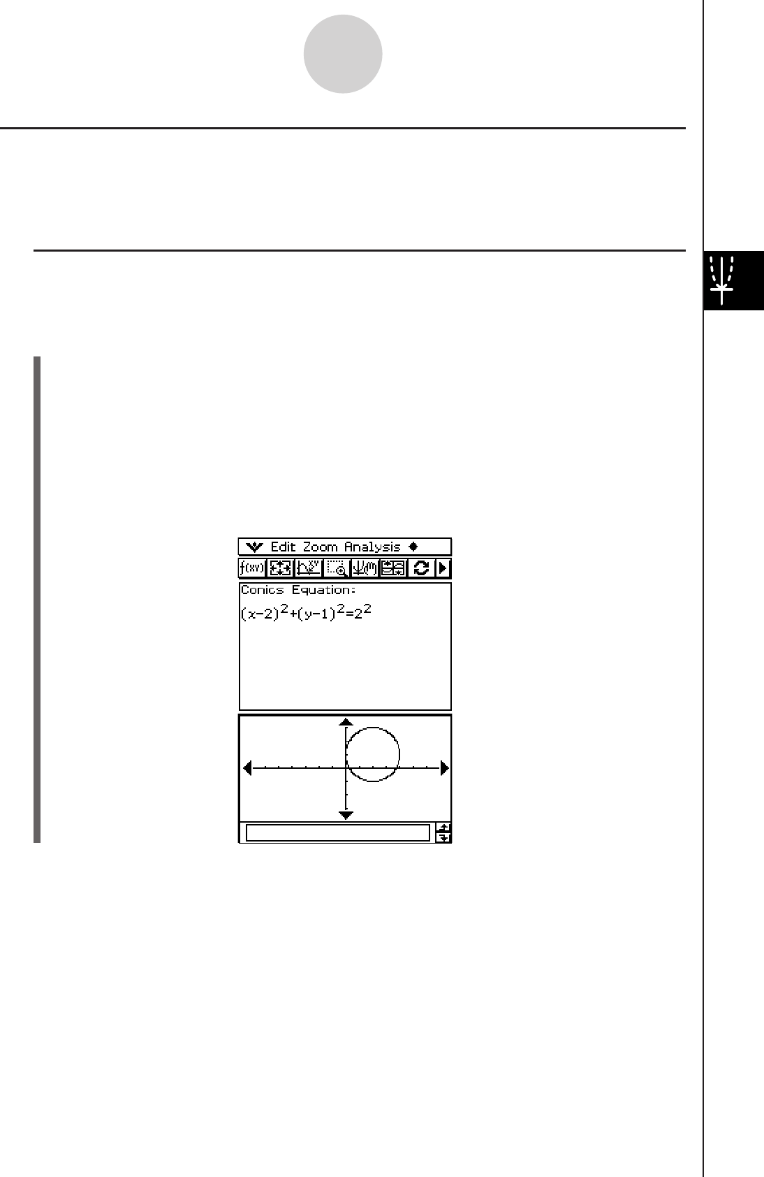
20060301

4-3-4

Drawing a Conics Graph

Drawing a Circle

There are two forms that you can use to draw a circle. One form is the standard form, which

allows you to specify the center point and radius. The other form is the general form, which

allows you to specify the coefficients of each term.

k Drawing a Circle by Specifying a Center Point and Radius

Example: To draw a circle with a center point of (2, 1) and a radius of 2

u ClassPad Operation

(1) On the Conics Editor window, tap q, or tap [Form] and then [Insert Conics Form].

• This displays the Select Conics Form dialog box.

(2) Select “(X – H)2 + (Y – K)2 = R2” and then tap [OK].

• This closes the Select Conics Form dialog box, and displays the selected equation in

the Conics Editor window.

(3) Change the coefficients of the equation as follows: H = 2, K = 1, R = 2.

(4) Tap

^ to graph the equation.

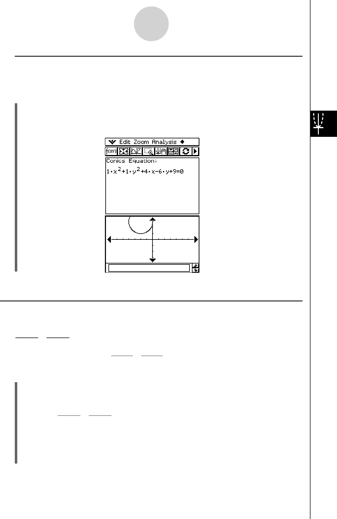
20060301

k Drawing a Circle by Specifying the Coefficients of a General Equation

Example: To draw the circle x2 + y2 + 4x – 6y + 9 = 0

u ClassPad Operation

(1) In step (2) of the procedure under “Drawing a Circle by Specifying a Center Point and

Radius”, select “AX2 + AY2 + BX + CY + D = 0”.

(2) Substitute the following values for the coefficients: A = 1, B = 4, C = –6, D = 9.

4-3-5

Drawing a Conics Graph

Drawing an Ellipse

You can draw an ellipse by specifying coefficients for the standard equation:

Example: To draw the ellipse

u ClassPad Operation

(1) On the Conics Editor window, tap q, or tap [Form] and then [Insert Conics Form].

• This displays the Select Conics Form dialog box.

(2) Select “ ” and then tap [OK].

• This closes the Select Conics Form dialog box, and displays the selected equation in

the Conics Editor window.

(3) Change the coefficients of the equation as follows: A = 2, B = 3, H = 1, K = 2.

(4) Tap

^ to graph the equation.

(x – H)2

+ (y – K)2 = 1.

2 B

(x – 1)2 + (y – 2)2 = 1

2 3

(X – H)2 + (Y – K)2 = 1

2 B

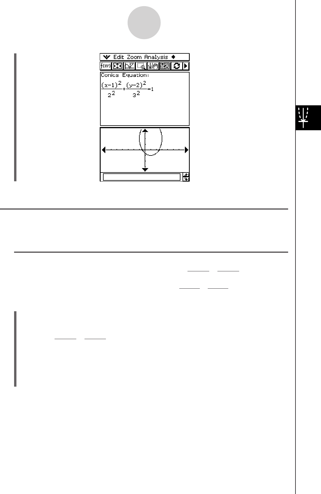
20060301

4-3-6

Drawing a Conics Graph

Drawing a Hyperbola

A hyperbola can be drawn with either a horizontal or vertical orientation. The hyperbola type

is determined by the direction of its principal axis.

k Drawing a Hyperbola that Opens Horizontally

The standard form of a hyperbola with a horizontal axis is:

Example: To draw the hyperbola with a horizontal axis

u ClassPad Operation

(1) On the Conics Editor window, tap q, or tap [Form] and then [Insert Conics Form].

• This displays the Select Conics Form dialog box.

(2) Select “ ” and then tap [OK].

• This closes the Select Conics Form dialog box, and displays the selected equation in

the Conics Editor window.

(3) Change the coefficients of the equation as follows: A = 2, B = 3, H = 1, K = 2.

(4) Tap

^ to graph the equation.

(x – H)2 – (y – K)2 = 1.

2 B

(x – 1)2 – (y – 2)2 = 1

2 3

(X – H)2 – (Y – K)2 = 1

2 B

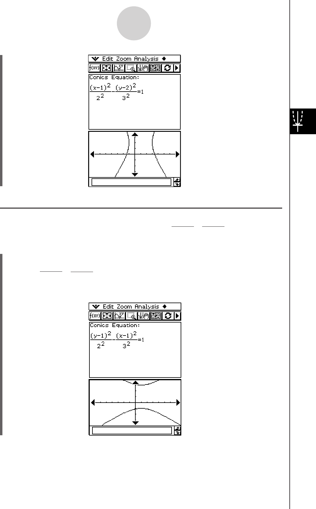
20060301

4-3-7

Drawing a Conics Graph

k Drawing a Hyperbola that Opens Vertically

The standard form of a hyperbola with a vertical axis is:

uClassPad Operation

(1) In step (2) of the procedure under “Drawing a Hyperbola that Opens Horizontally”,

select “ ”.

(2) Specify values for the coefficients.

(y – K)2 – (x – H)2 = 1.

2 B

(Y – K)2 – (X – H)2 = 1

2 B

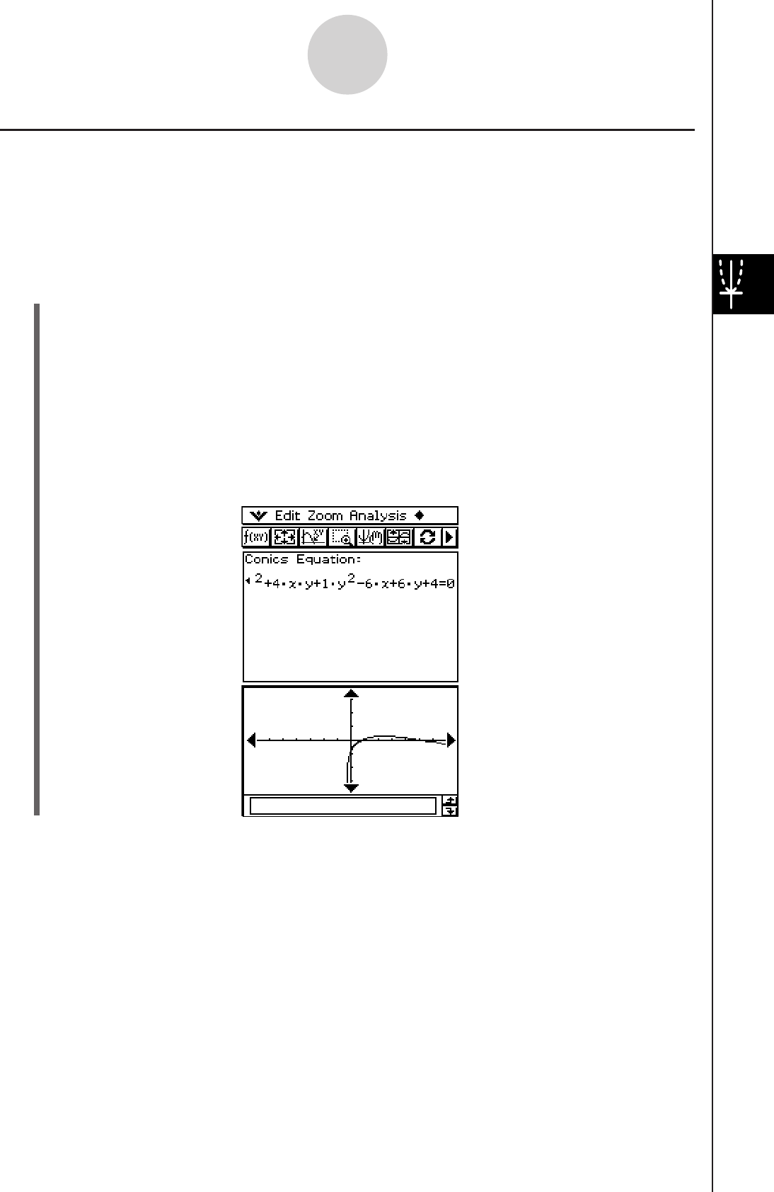
20060301

4-3-8

Drawing a Conics Graph

Drawing a General Conics

Using the conics general equation Ax2 + Bxy + Cy2 + Dx + Ey + F = 0, you can draw a

parabola or hyperbola whose principal axis is not parallel either to the x-axis or the y-axis, a

slanted ellipse, etc.

Example: To draw

x2 + 4xy + y2 – 6x + 6y + 4 = 0

u ClassPad Operation

(1) On the Conics Editor window, tap q, or tap [Form] and then [Insert Conics Form].

• This displays the Select Conics Form dialog box.

(2) Select “AX2 + BXY + CY2 + DX + EY + F = 0” and then tap [OK].

• This closes the Select Conics Form dialog box, and displays the selected equation in

the Conics Editor window.

(3) Change the coefficients of the equation as follows: A = 1, B = 4, C = 1, D = –6, E = 6,

F = 4.

(4) Tap

^ to graph the equation.

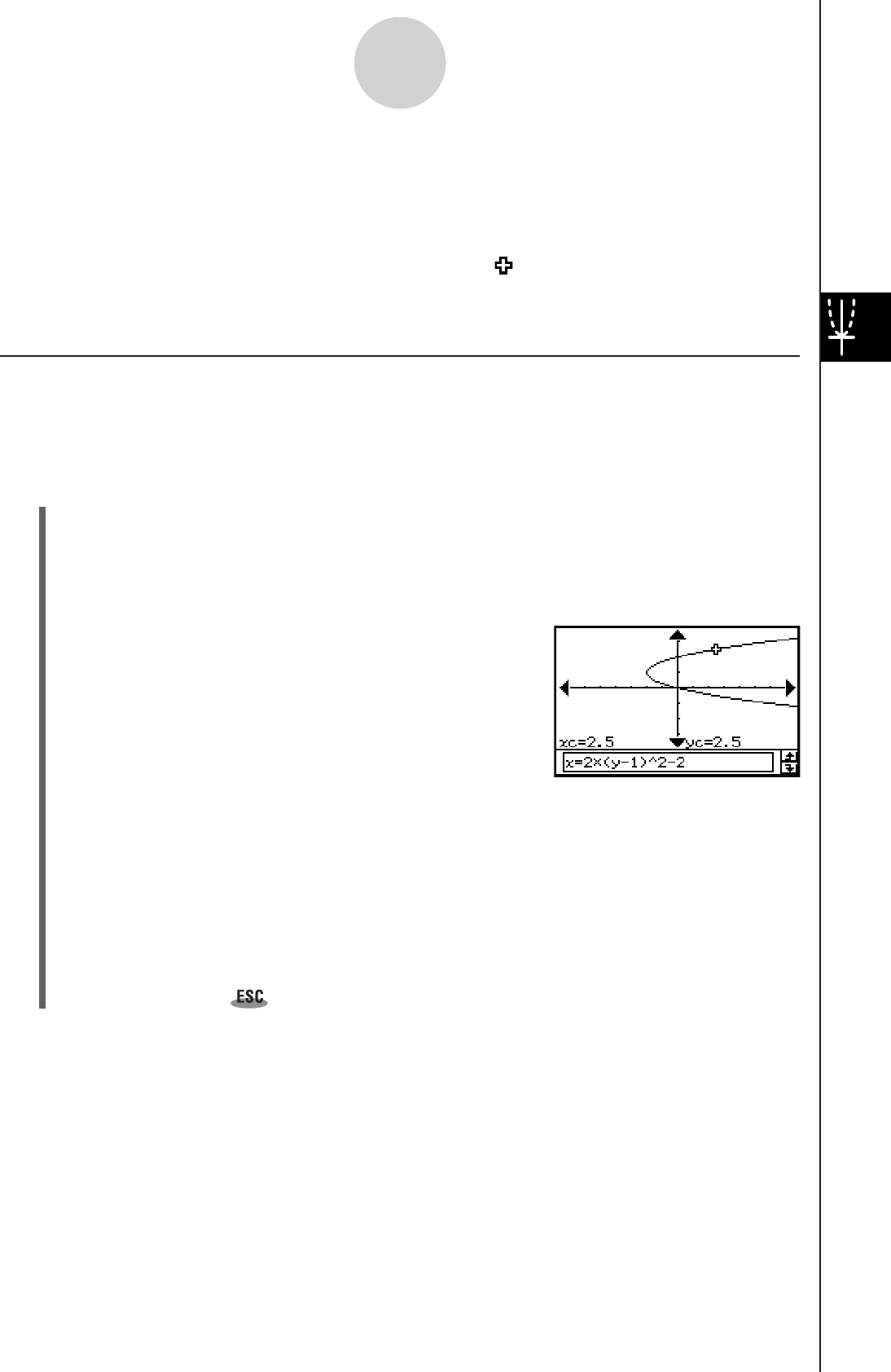
20060301

4-4-1

Using Trace to Read Graph Coordinates

4-4 Using Trace to Read Graph Coordinates

Trace allows you move a pointer along a graph line and display the coordinates at the current

pointer location.

Starting the trace operation causes a crosshair pointer ( ) to appear on the graph. You

can then press the cursor key or tap the graph controller arrows to move the pointer to the

location you want, and read the coordinates that appear on the display.

Using Trace

Example: To graph the function x = 2(y – 1)2 – 2 and then perform a trace operation to read

coordinates

u ClassPad Operation

(1) On the Conics Editor window, input the above equation and then tap ^ to graph it.

(2) Tap [Analysis] and then [Trace], or tap =.

• This causes a pointer to appear on the graph line.

(3) Press the left or right cursor key, or tap the left or right graph controller arrows.

• This moves the pointer along the graph, and displays

the coordinates of the current pointer location.

• When the location of the pointer approaches the point

of infinity on a parabolic or hyperbolic graph, “Error”

appears in place of the pointer coordinates.

• You can also move the pointer to a particular point by inputting coordinates. Inputting

a value while a trace operation is being performed displays a dialog box for inputting

a value. After you enter a value, the pointer jumps to the corresponding location when

you tap [OK].

Here, input a value for yc in the case of a parabola that opens horizontally. Input a

value for

xc in the case of a parabola that opens vertically. For any other type of

conics graph, input a value for tc in order to graph in parametric format.

(4) To exit trace, tap on the icon panel.

Tip

• While tracing, tapping the displayed coordinate values causes the coordinate values to appear in

the message box. You can then copy the coordinates to the clipboard.

20060301

4-5-1

Using G-Solve to Analyze a Conics Graph

4-5 Using G-Solve to Analyze a Conics Graph

The G-Solve menu includes commands that let you perform a variety of different analytical

processes on a graph drawn on the Conics Graph window.

Displaying the G-Solve Menu

While there is a graph on the Conics Graph window, tap [Analysis] and then [G-Solve]. You

can then use the [G-Solve] menu that appears to perform one of the operations described

below.

Tip

• Some commands are available only for certain types of graphs. Any command that is not

available for the graph currently displayed on the Conics Graph window has a line through it. A

parabola, for example, does not have a center, radius or asymptotes, so there are lines through

the [Center], [Radius], and [Asymptotes] commands of the [G-Solve] menu when there is a

parabola on the Conics Graph window.

Focus of a parabola, ellipse, or hyperbola

Vertex of a parabola, ellipse, or hyperbola

Directrix of a parabola

Axis of symmetry of a parabola

Length of the latus rectum of a parabola

Center point of a circle, ellipse, or hyperbola

Radius of a circle

x-intercept

y-intercept

x-coordinate for a given y-coordinate

Asymptotes of a hyperbola

Eccentricity of a parabola, ellipse, or hyperbola

Focus

Vertex

Directrix

Symmetry

Latus Rectum Length

Center

Radius

Asymptotes

Eccentricity

x-Intercept

y-Intercept

x-Cal

y-coordinate for a given x-coordinate y-Cal

Select this [G-Solve]

menu item:

To obtain this:

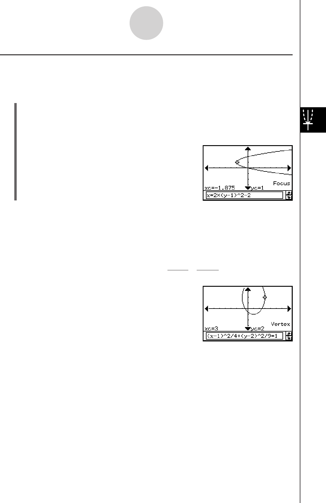
20060301

4-5-2

Using G-Solve to Analyze a Conics Graph

Using G-Solve Menu Commands

The following are some examples of how to perform the Conics application [G-Solve] menu

commands.

u To determine the focus of the parabola x = 2(y – 1)2 – 2

(1) On the Conics Editor window, input the conics equation and then tap ^ to graph it.

• Here, input the parabolic equation x = 2(y –1)2 – 2.

(2) Tap [Analysis] and then [G-Solve]. Next, on the submenu that appears, select the

command you want.

• To determine the focus for this example, select

[Focus].

Tip

• An ellipse and hyperbola has two foci. In this case, press the left and right cursor keys or tap the

left and right graph controller arrows to toggle the display between the two foci.

The following are the menu operations and sample windows for other commands.

u To determine the vertices of the ellipse

[Analysis] - [G-Solve] - [Vertex]

(x – 1)2 + ( y – 2)2 = 1

2 3

Tip

• An ellipse has four vertices and a hyperbola has two vertices. In these cases, press the left and

right cursor keys or tap the left and right graph controller arrows to toggle the display between the

vertices.

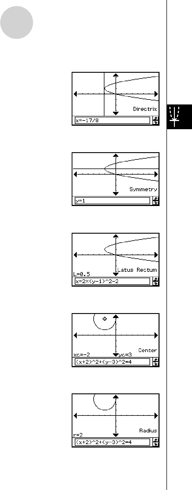
20060301

4-5-3

Using G-Solve to Analyze a Conics Graph

u To determine the directrix of the parabola x = 2( y – 1)2 – 2

[Analysis] - [G-Solve] - [Directrix]

u To determine the axis of symmetry of the parabola x = 2(y – 1)2 – 2

[Analysis] - [G-Solve] - [Symmetry]

u To determine the latus rectum of the parabola x = 2( y – 1)2 – 2

[Analysis] - [G-Solve] - [Latus Rectum Length]

u To determine the center point of the circle x2 + y2 + 4x – 6y + 9 = 0

[Analysis] - [G-Solve] - [Center]

u To determine the radius of the circle x2 + y2 + 4x – 6y + 9 = 0

[Analysis] - [G-Solve] - [Radius]

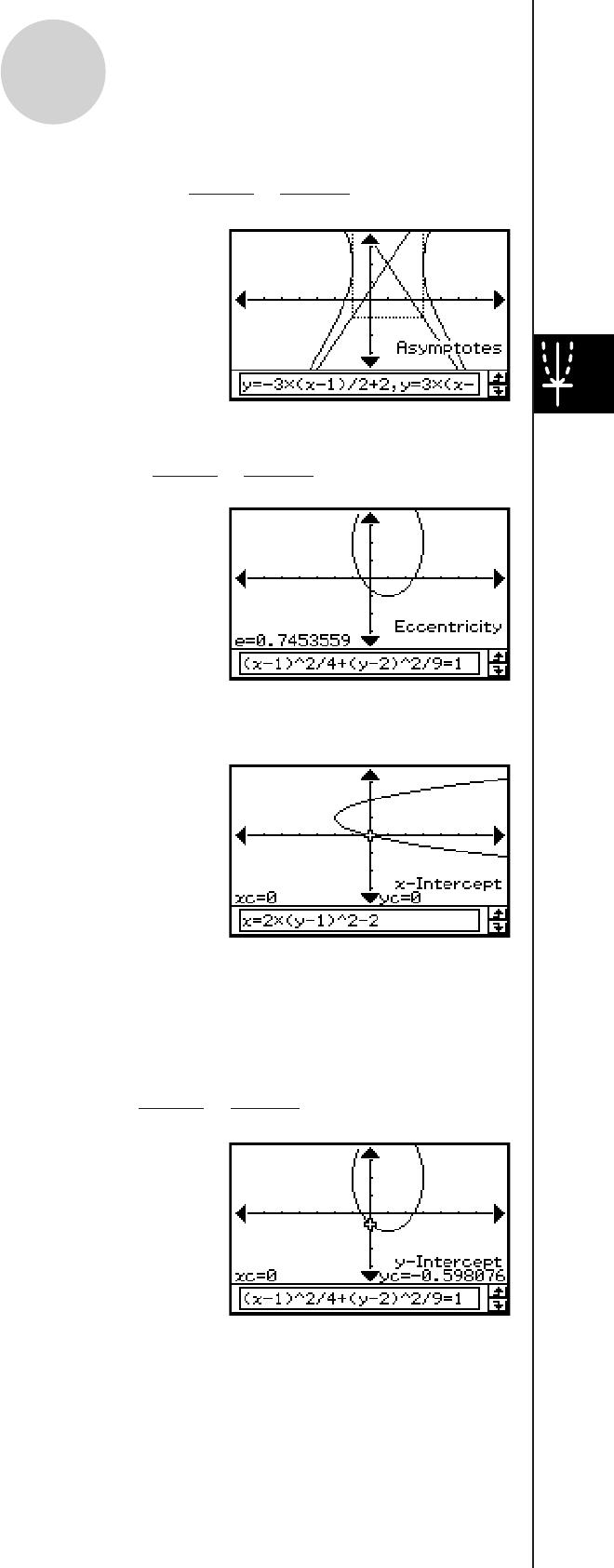
20060301

u To determine the asymptotes of the hyperbola

[Analysis] - [G-Solve] - [Asymptotes]

u To determine the eccentricity of the ellipse

[Analysis] - [G-Solve] - [Eccentricity]

u To determine the x-intercept of the parabola x = 2(y – 1)2 – 2

[Analysis] - [G-Solve] - [x-Intercept]

Tip

• When there are two x-intercepts, press the left and right cursor keys or tap the left and right graph

controller arrows to toggle the display between them.

u To determine the y-intercept of the ellipse

[Analysis] - [G-Solve] - [y-Intercept]

Tip

• When there are two y-intercepts, press the left and right cursor keys or tap the left and right graph

controller arrows to toggle the display between them.

4-5-4

Using G-Solve to Analyze a Conics Graph

(x – 1)2 – ( y – 2)2 = 1

2 3

(x – 1)2 + ( y – 2)2 = 1

2 3

(x – 1)2 + ( y – 2)2 = 1

2 3

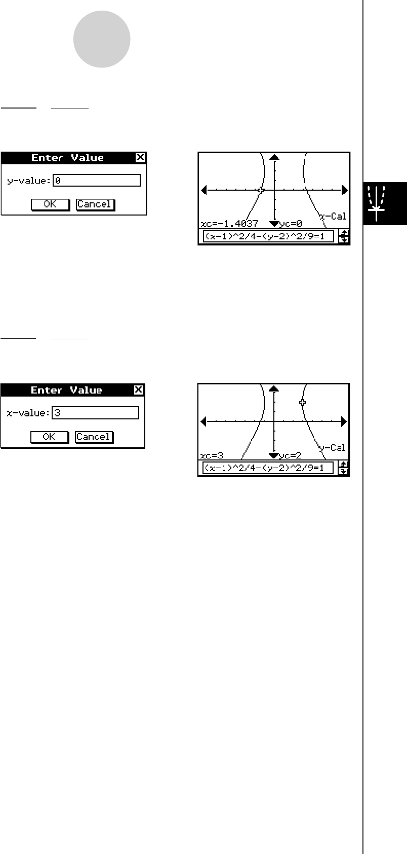
20060301

u For the hyperbola , determine the x-coordinate when the

y-coordinate is 0

[Analysis] - [G-Solve] - [x-Cal]

Tip

• When there are two x-coordinates, press the left and right cursor keys or tap the left and right

graph controller arrows to toggle the display between them.

u For the hyperbola , determine the y-coordinate when the

x-coordinate is 3

[Analysis] - [G-Solve] - [y-Cal]

Tip

• When there are two y-coordinates, press the left and right cursor keys or tap the left and right

graph controller arrows to toggle the display between them.

4-5-5

Using G-Solve to Analyze a Conics Graph

(x – 1)2 – ( y – 2)2 = 1

2 3

(x – 1)2 – ( y – 2)2 = 1

2 3

Tap [OK].

20060301

Using the 3D Graph

Application

The 3D Graph application lets you draw a 3-dimensional graph of

an equation in the form z = f (x, y) or of a parametric equation.

5-1 3D Graph Application Overview

5-2 Inputting an Expression

5-3 Drawing a 3D Graph

5-4 Manipulating a Graph on the 3D Graph Window

5-5 Other 3D Graph Application Functions

Chapter

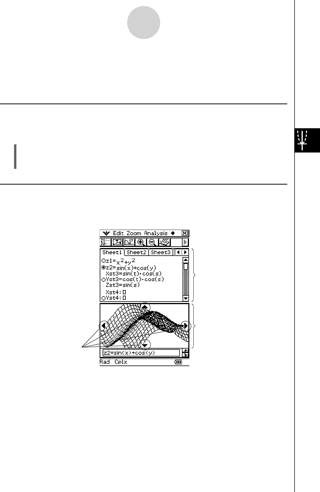
20060301

5-1 3D Graph Application Overview

This section describes the configuration of the 3D Graph application window, and provides

basic information about its menus and commands.

5-1-1

3D Graph Application Overview

3D Graph Application Window

The 3D Graph application has a 3D Graph Editor window and a 3D Graph window. Both of

these windows appear on the display when you start up the 3D Graph application. Functions

you input on the 3D Graph Editor window are graphed on the 3D Graph window.

3D Graph Editor

window

3D Graph window

Graph controller arrows

• The 3D Graph Editor has five tabbed sheets named Sheet 1 through Sheet 5. Each sheet

can contain up to 20 functions. This means you can have up to 100 functions stored in the

3D Graph Editor at one time.

• You can select any one of the expressions on the 3D Graph Editor window and graph it on

the 3D Graph window.

• You can tap the graph controller arrows on the 3D Graph window or press the cursor keys

to rotate the graph. On the 3D Graph window, you can rotate the graph image by dragging

with the stylus.

• When using Trace (page 5-5-1), tap the graph controller arrows or operate the cursor key

to move the pointer along the graph.

Starting Up the 3D Graph Application

Use the following procedure to start up the 3D Graph application.

u ClassPad Operation

On the application menu, tap D.

This starts the 3D Graph application and displays the 3D Graph Editor window and the 3D

Graph window.

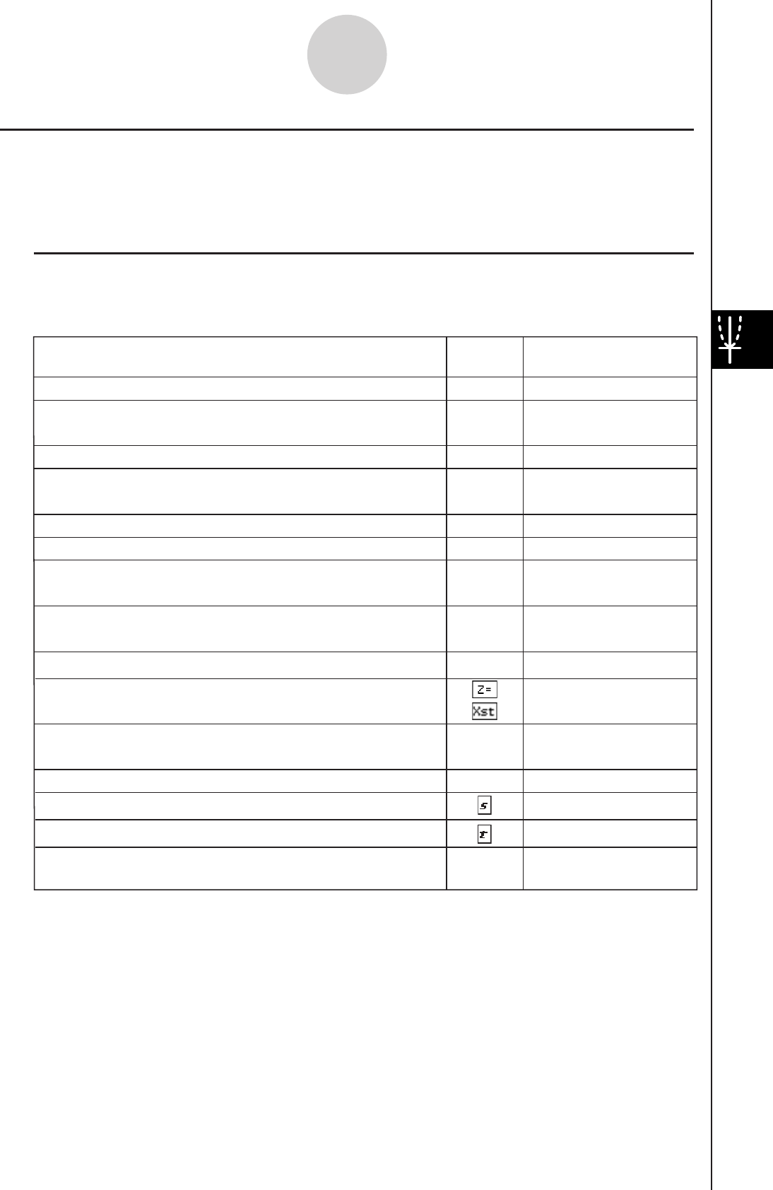
20060301

5-1-2

3D Graph Application Overview

3D Graph Application Menus and Buttons

This section explains the operations you can perform using the menus and buttons of the 3D

Graph application’s windows.

• For information about the O menu, see “Using the O Menu” on page 1-5-4.

k 3D Graph Editor Window Menus and Buttons

The following describes the menu and button operations you can perform while the 3D Graph

Editor window is active.

To do this: Tap this

button:

Or select this

menu item:

Edit - Cut

Edit - Delete

—

Edit - Copy—

Edit - Paste

—

Edit - Select All

—

—Edit - Clear All

—

Sheet - Default Name

—Sheet - Clear Sheet

O - View Window

O - Variable

Manager

%—

~—

—

Delete the current selection

Cut the selected character string and place it onto the

clipboard

Copy the selected character string to the clipboard

Paste the contents of the clipboard at the current

cursor position in the 3D Graph Editor window

Select the entire expression you are editing

Clear all the contents of the 3D Graph Editor window

Return the current sheet to its initial default name

(Sheet 1 through Sheet 5)

Return the contents and name of the currently active

sheet to their initial defaults

Toggle the equation type between

(

) and a

parametric equation

Draw a graph

Display the View Window dialog box (page 5-3-1) to

configure 3D Graph window settings

Insert variable s into a parametric equation

—

Insert variable t into a parametric equation

Display the Main application work area window

Display the Variable Manager (page 1-8-1)

20060301

5-1-3

3D Graph Application Overview

k 3D Graph Window Menus and Buttons

The following describes the menu and button operations you can perform while the 3D Graph

window is active.

To do this: Tap this

button:

Or select this

menu item:

WZoom - Zoom In

EZoom - Zoom Out

— Zoom - View-

— Zoom - View-Init

=Analysis - Trace

— Analysis - Sketch

—

a - Rotating

Enlarge the displayed graph

Reduce the size of the displayed graph

View the displayed graph from the

-axis,

-axis, or

-axis

Return the 3D Graph window to its initial default state

—a - Store Picture

Save a graph as image data (page 3-2-10)

—a - Recall Picture

Recall the image of a graph (page 3-2-10)

—a - ReDraw

O - View Window

O - Variable

Manager

Re-draw a graph

@—

Make the 3D Graph Editor window active

Display the View Window dialog box (page 5-3-1) to

configure 3D Graph window settings

~—

Display the Main application work area window

Display the Variable Manager (page 1-8-1)

Display the coordinates at a particular point on a 3D

graph

Write text on the Graph window

• See “To write text on the Graph window” on page 3-6-2,

and “To clear figures inserted using the Sketch menu” on

page 3-6-5.

— Analysis -

-Cal

Calculate a

-value for given

- and

-values, or

- and

-values, on the displayed graph

Automatically rotate a graph in the specified direction

(Left → Right, Right → Left, Top → Bottom, Bottom → Top)

for about 30 seconds

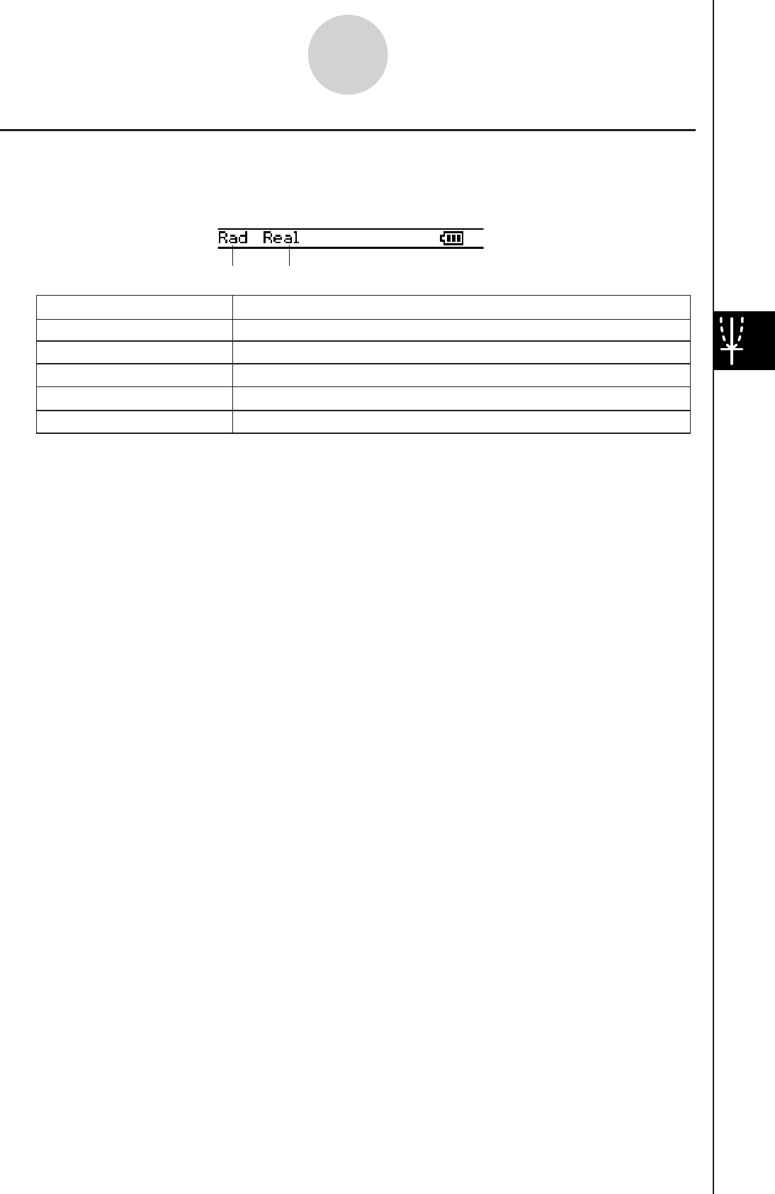
20060301

3D Graph Application Status Bar

The status bar at the bottom of the 3D Graph application shows the current angle unit setting

and [Complex Format] setting (page 1-9-5).

Rad

Deg

Gra

Real

The angle unit setting is radians.

The angle unit setting is degrees.

The angle unit setting is grads.

Cplx The Complex (complex number calculation) mode is selected.

The Real (real number calculation) mode is selected.

If you see this: It means this:

5-1-4

3D Graph Application Overview

Angle unit Real mode

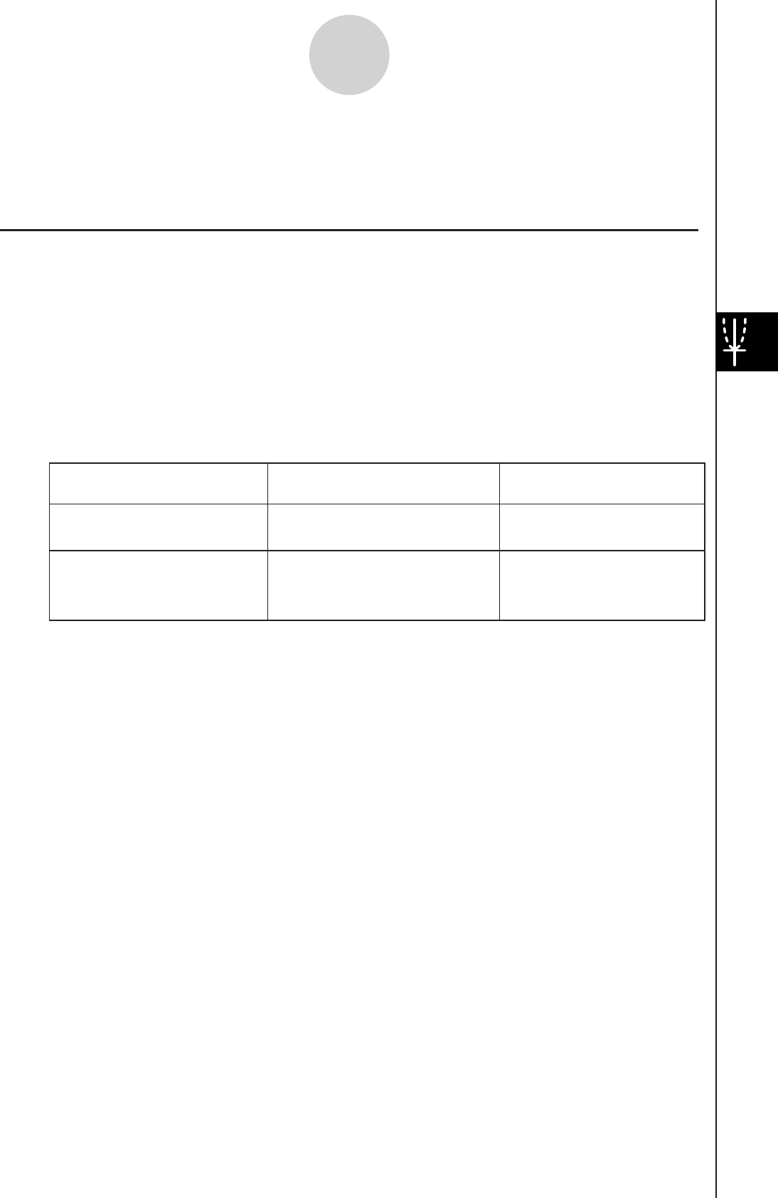
20060301

5-2-1

Inputting an Expression

5-2 Inputting an Expression

Use the 3D Graph Editor window to input 3D Graph application expressions.

Using 3D Graph Editor Sheets

The 3D Graph Editor has five tabbed sheets named Sheet 1 through Sheet 5. Each sheet

can contain up to 20 functions. This means you can have up to 100 functions stored in the

3D Graph Editor at one time. 3D Graph Editor window sheet operations are similar to the

sheet operations of the Graph & Table application. For more information, see “Using Graph

Editor Sheets” on page 3-3-1.

Tip

• The commands used to perform sheet operations in the 3D Graph application are slightly different

to those in the Graph & Table application, as described below.

To do this: Execute this command in the

Graph & Table application:

Execute this command in

the 3D Graph application:

a - Sheet - Default Name Sheet - Default Name

a - Sheet - Clear Sheet Sheet - Clear Sheet

Return the name of the active

sheet to its initial default

Return the contents and name

of the currently active sheet to

their initial defaults

• Also note that the Graph & Table application allows simultaneous graphing of multiple functions,

as long as they are on the same sheet. With the 3D Graph application, however, you can graph

only one function at a time.

20060301

5-2-2

Inputting an Expression

Storing a Function

You can input an equation of the form z = f(x, y) or a parametric equation.

Example: To store z = x2 + y2 in line z1

u ClassPad Operation

(1) On the application menu, tap D.

• This starts up the 3D Graph application and displays the initial screen of the active

3D Graph Editor window.

(2) Tap line

z1 on the 3D Graph Editor window, and input x2 + y2.

x{2+y{2

(3) Press

• This stores the expression you input and selects it,

which is indicated by the button next to it changing to

“ ”.

(4) To graph the function you just input, tap %.

• For information about graphing, see “5-3 Drawing a

3D Graph”.

Tip

• You can also use drag and drop to input an expression displayed on the Main application window

into the 3D Graph Editor window. To do this, perform the same steps as those for the Graph &

Table application. For more information, see “Quick Graphing of an Expression Using Drag and

Drop” on page 3-3-9.

z = f(x, y)Parametric Equation

20060301

5-3-1

Drawing a 3D Graph

5-3 Drawing a 3D Graph

This section explains how to draw a 3D graph, as well as how to change the angle of a graph

and how to rotate a graph.

Configuring 3D Graph View Window Parameters

Use the 3D Graph View Window to specify maximum and minimum values for the x-axis,

y-axis, z-axis, s-variable, and t-variable. You can also specify the number of lines you would

like for drawing the grid.

• For the xgrid enter the number of lines you would like drawn within the interval from xmin

to xmax. For example, if xmin = −3, xmax = 3 and xgrid= 15, 15 almost vertical lines will be

used to display your graph. The ygrid lines will be almost horizontal.

• After drawing a 3D graph, pressing the = key cycles the 3D Graph [Axes] setting (page

1-9-8) in the following sequence: “Off” → “On” → “Box” → “Off”, and so on.

Before drawing a graph, be sure to first configure View Window parameters as required to

ensure proper display of the graph.

u ClassPad Operation

(1) On the application menu, tap D.

• This starts up the 3D Graph application and displays the initial screen of the active 3D

Graph Editor window.

(2) Tap

7 to display the View Window dialog box.

(3) Tap the “3D” option button so the option is selected.

(4) Configure the View Window parameters as described below.

• Press

c to move the cursor and input an appropriate value for each parameter.

Use this

item:

Initial

default

To configure this View Window parameter:

xmin

xmax

xgrid

ymin

ymax

ygrid

zmin

Minimum x-axis value

Maximum x-axis value

Number of grid lines used for x-axis direction

Minimum y-axis value

Maximum y-axis value

Number of grid lines used for y-axis direction

Minimum z-axis value

zmax Maximum z-axis value

angle Clockwise angle of x-axis

angle Eye position relative to the plane created by

the x-axis and y-axis, and the angle of the z-axis

–3

smin

smax

tmin

Minimum s-variable value

Maximum s-variable value

Minimum t-variable value

–3.1415926535

3.14159265358

–3.1415926535

tmax Maximum t-variable value 3.14159265358

–3

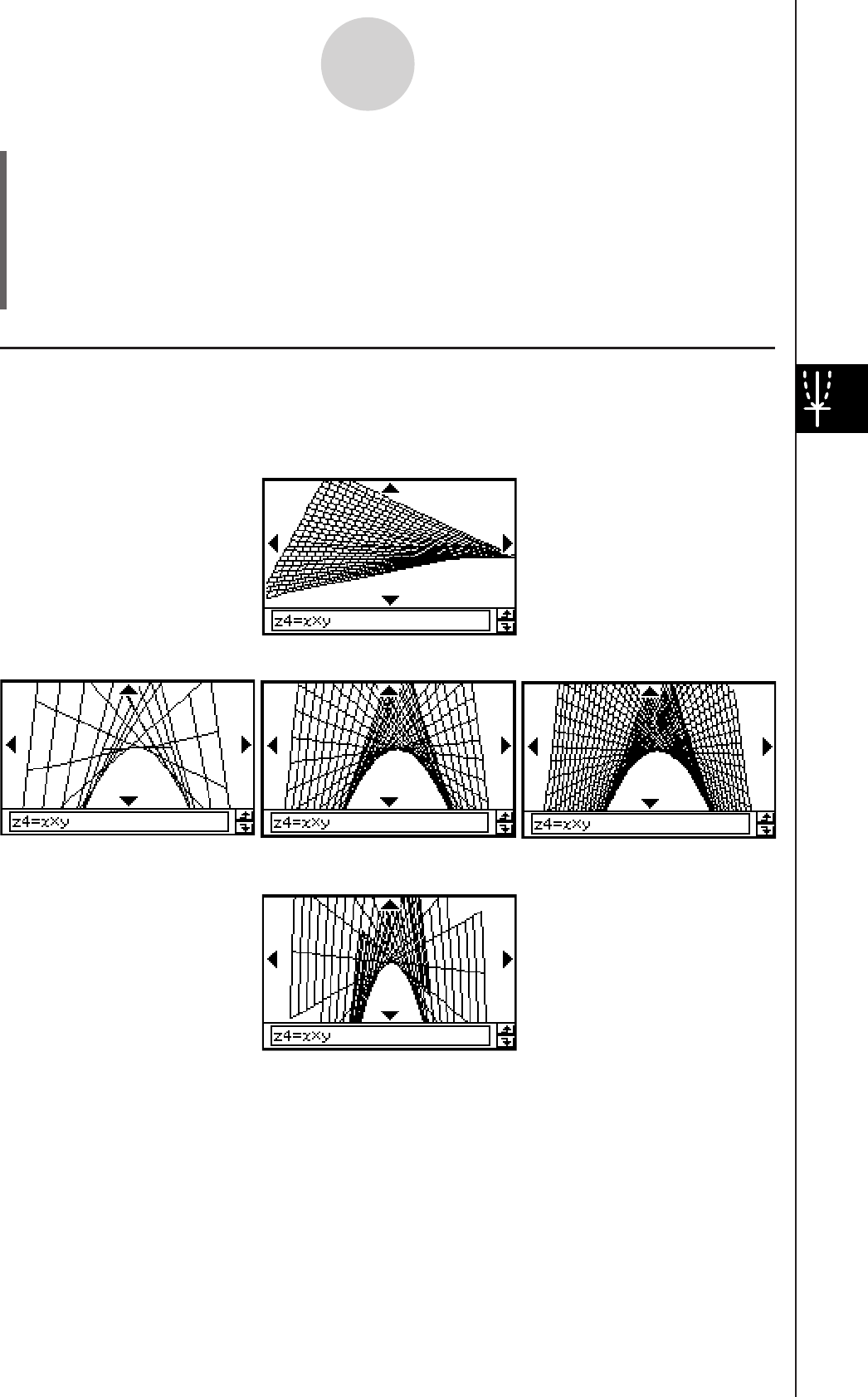
20060301

5-3-2

Drawing a 3D Graph

• The following are the allowable ranges for the indicated View Window parameters:

xgrid and ygrid: 2 to 50; angle

: –180 <

< 180; angle

: 0 to 360.

• The angle parameters,

and

, are always degrees, regardless of the current

[Angle] setting of the Basic Format dialog box (page 1-9-5).

(5) After all the parameters are the way you want, tap [OK].

• This closes the View Window dialog box.

k 3D Graphs

The following are examples of the 3D graph z = xy using a number of different 3D View

Window setups. View Window parameters that are not specified are set to the initial default

values.

Important!

• As is evident from the above sample screenshots, the greater the xgrid and ygrid

values, the more detailed the graph. Also note, however, that larger values require more

calculation, which means that the graphing operation takes more time.

• Graphing may be impossible if the xgrid and ygrid values are too small.

xmin/ymin = –1, xmax/ymax = 1

xgrid = 10, ygrid = 10 Initial defaults xgrid = 40, ygrid = 40

xmin/ymin = –5, xmax/ymax = 5

20080201

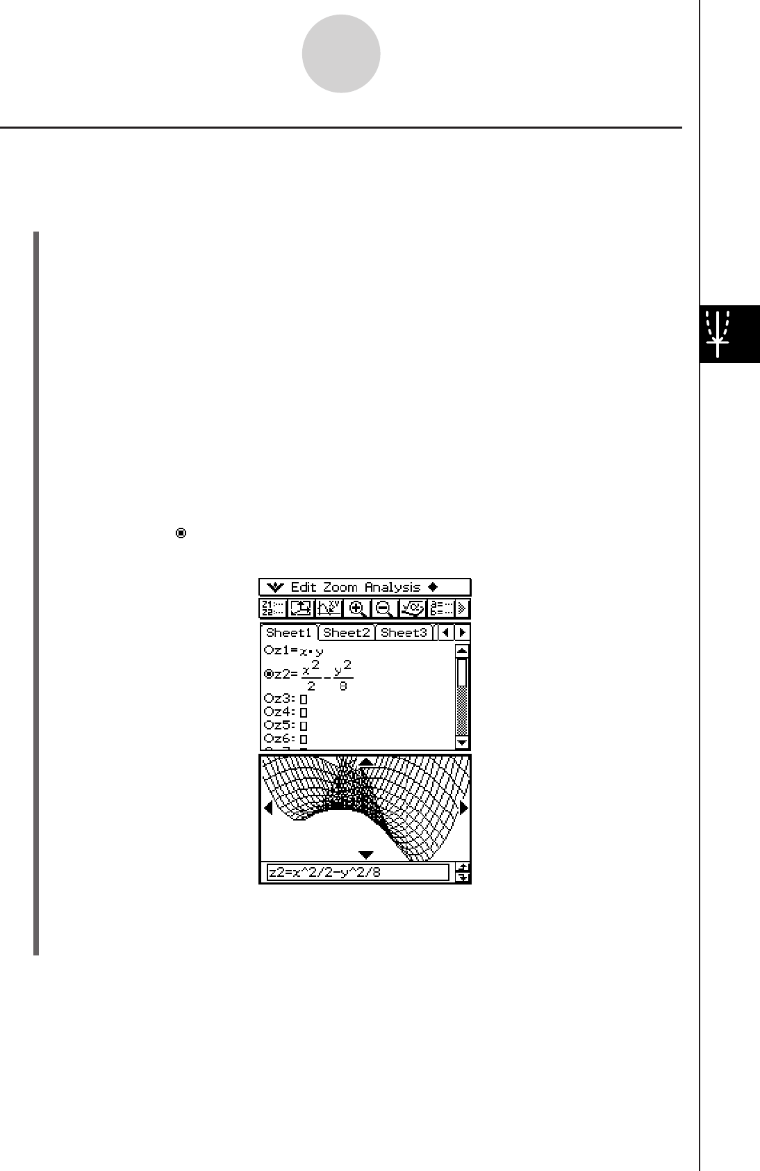
20060301

3D Graph Example

Example 1: To graph the hyperbolic paraboloid z = x2/2 – y2/8.

u ClassPad Operation

(1) In the 3D Graph application, make the 3D Graph Editor window active.

(2) Tap

7 to display the View Window dialog box, and then configure the parameters

shown below.

xmin = –3 xmax = 3 xgrid = 25

ymin = –3 ymax = 3 ygrid = 25

angle

= 45 angle

= 70

• Except for angle

, all of the above settings are initial defaults.

• After everything is the way you want, tap [OK] to close the View Window dialog box.

(3) Tap line

z2 on the 3D Graph Editor window, and then input x2/2 – y2/8.

x{2/2-y{2/8

(4) Press

• This stores the expression you input and selects it, which is indicated by the button

changing to “ ”.

(5) Tap

% to graph the expression.

5-3-3

Drawing a 3D Graph

• Here, you can use the cursor key to rotate the graph on the display. On the 3D

Graph window, you can rotate the graph image by dragging with the stylus. For more

information, see “5-4 Manipulating a Graph on the 3D Graph Window”.

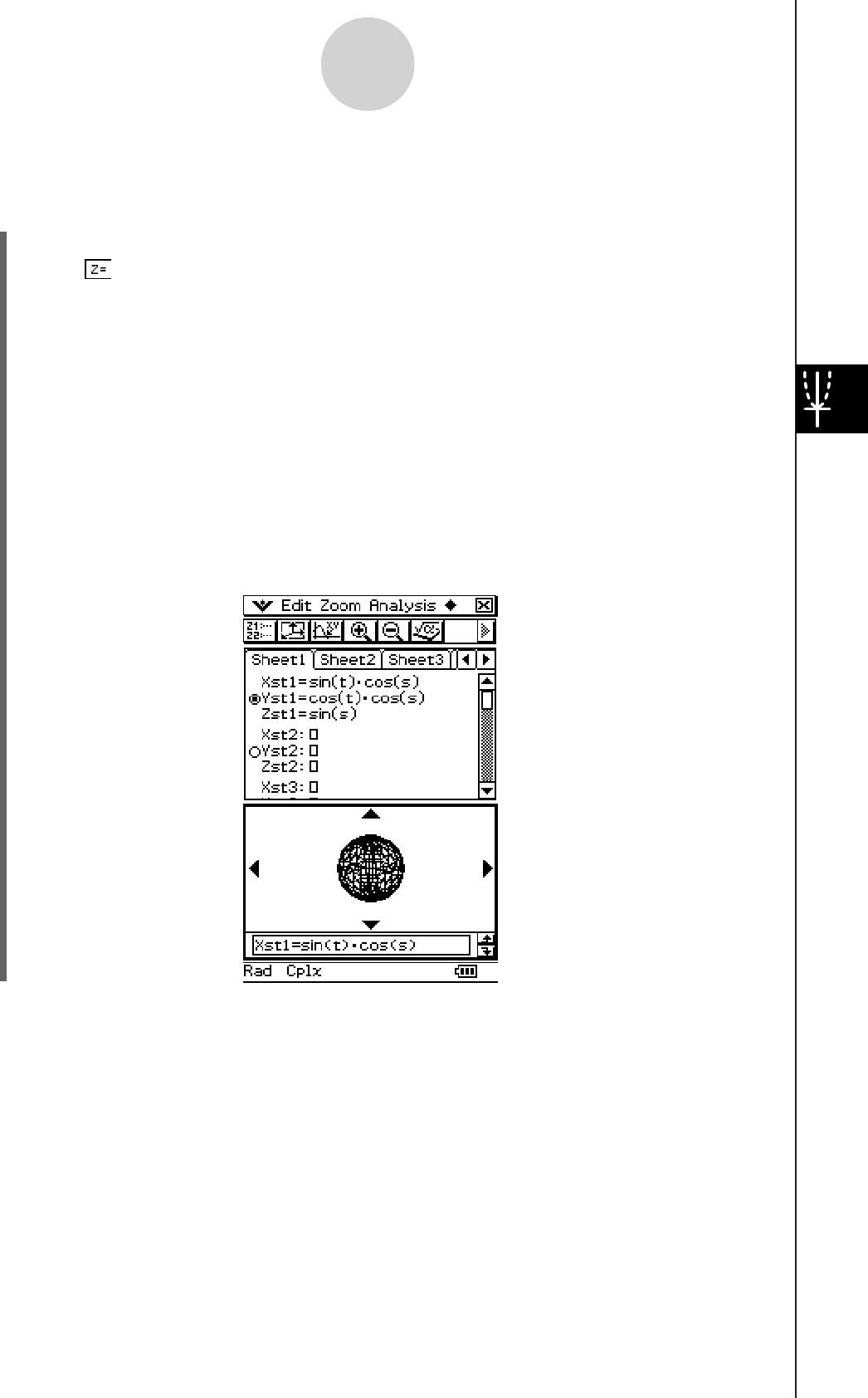
20060301

Example 2: To graph a parametric equation

u ClassPad Operation

(1) In the 3D Graph application, make the 3D Graph Editor window active.

(2) Tap to specify input of a parametric equation.

(3) Tap line Xst1, and then input sin(t) × cos(s).

k9Tst)*cs)

(4) Press

(5) In line Yst1 input cos(t) × cos(s).

ct)*cs)

(6) Press

(7) In line Zst1 input sin(s).

ss)

(8) Press

(9) Tap

% to graph the parametric equation.

5-3-4

Drawing a 3D Graph

20060301

5-3-5

Drawing a 3D Graph

k Selecting the Function to be Graphed

The 3D Graph application lets you graph only one function at a time. When you have more

than one expression input on the 3D Graph Editor window, you need to select the one you

want to graph.

Tapping the “ ” button next to a function

changes the button to “ ”, which indicates

that the function is selected. Press E to

enable graphing.

Tip

• Whenever you input a new function on the 3D Graph Editor window, the new function is selected

automatically for graphing after you press E.

k Controlling the Format of the 3D Graph

Tapping Oand [3D Format] displays the 3D Format dialog box, which you can use to

control the graph axis type, display of axis labels, and other format settings.

• For details about the settings you can configure on the 3D Format dialog box, see “3D

Format Dialog Box” on page 1-9-8.

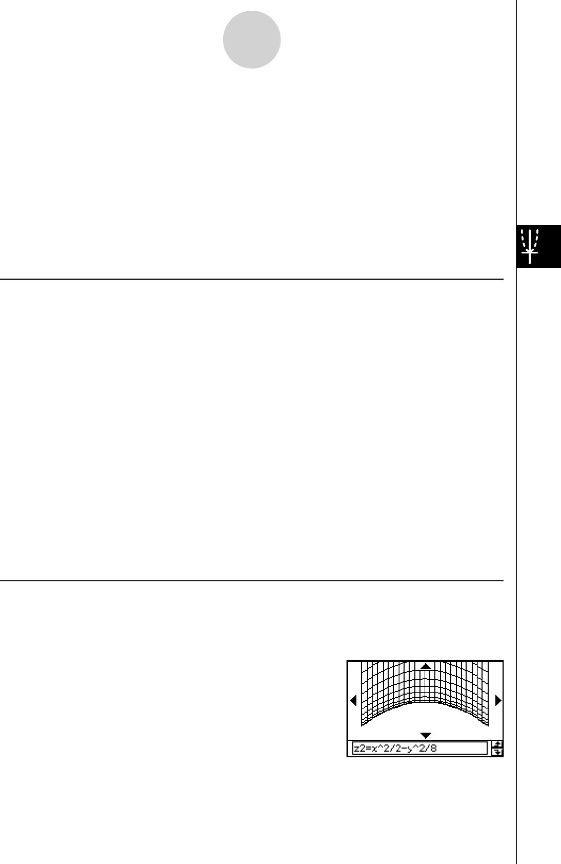
20060301

5-4-1

Manipulating a Graph on the 3D Graph Window

5-4 Manipulating a Graph on the 3D Graph

Window

This section describes how to enlarge and reduce the size of a graph, how to change the eye

position to view the graph along a particular axis, and how to perform other operations like

automatic rotation.

Important!

• All of the operations described in this section can be performed only while the 3D Graph

window is active.

Enlarging and Reducing the Size of a Graph

A displayed 3D graph can be zoomed so it is enlarged or reduced. The zoom operation is

always performed based on the center of the Graph window. You cannot select the area to

be zoomed.

u To enlarge a graph

Perform any one of the following operations:

• Tap W.

• Tap [Zoom] and then [Zoom In].

• Press the + key.

u To reduce the size of a graph

Perform any one of the following operations:

• Tap E.

• Tap [Zoom] and then [Zoom Out].

• Press the - key.

Starting from the normal size, you can enlarge a graph 14 steps or reduce its size 15 steps.

Switching the Eye Position

The following items describe how to change the eye position and view a displayed 3D graph

along a particular axis. All of the example displays below show the graph of the expression

z = x2/2 – y2/8, which we graphed under “3D Graph Example” on page 5-3-3.

• To view the graph facing the x-axis, tap [Zoom] and then

[View-x], or press the x key.

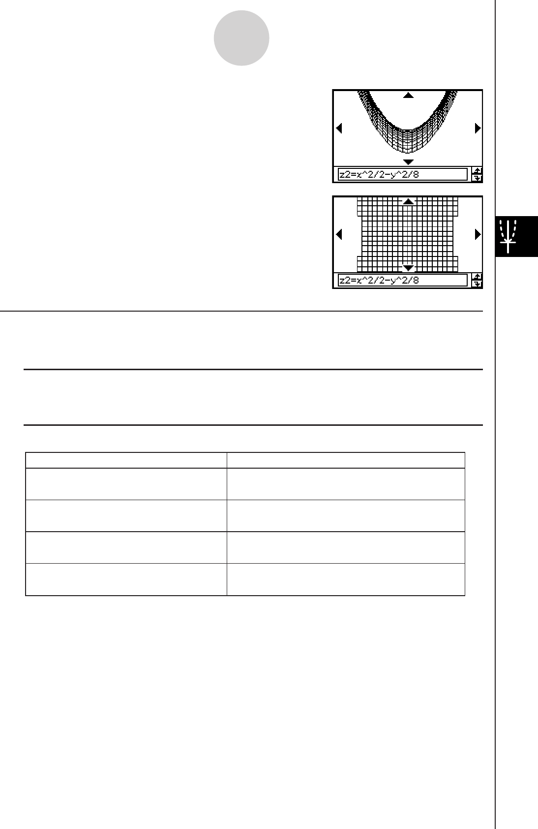
20060301

5-4-2

Manipulating a Graph on the 3D Graph Window

• To view the graph facing the y-axis, tap [Zoom] and then

[View-y], or press the y key.

• To view the graph facing the z-axis, tap [Zoom] and then

[View-z], or press the Z key.

Rotating the Graph Manually

Use the procedures described below to rotate the displayed graph manually.

k Using the Stylus to Rotate a Graph

Drag the stylus on the 3D Graph window in the direction you want to rotate the graph.

k Using the Cursor Keys and Graph Controller Arrow to Rotate a Graph

To do this:

Rotate the graph to the left

Rotate the graph to the right

Rotate the graph upwards

Rotate the graph downwards

Press the left cursor key or tap the left graph

controller arrow.

Press the right cursor key or tap the right

graph controller arrow.

Press the up cursor key or tap the up graph

controller arrow.

Press the down cursor key or tap the down

graph controller arrow.

Do this:

• Holding down a key will rotate the graph continuously.

20060301

5-4-3

Manipulating a Graph on the 3D Graph Window

Rotating a Graph Automatically

You can use the following procedure to rotate a graph automatically for about 30 seconds.

uClassPad Operation

(1) To start automatic graph rotation, tap a and then [Rotating].

(2) On the submenu that appears, select the rotation direction you want:

[Left

→ Right], [Right → Left], [Top → Bottom], or [Bottom → Top].

• Rotation continues for about 30 seconds and then stops automatically. You can also stop

automatic rotation by pressing the c key or tapping on the icon panel.

Initializing the Graph Window

To return the 3D Graph window to its initial default settings, including its View Window

settings, tap [Zoom] and then [View-Init].

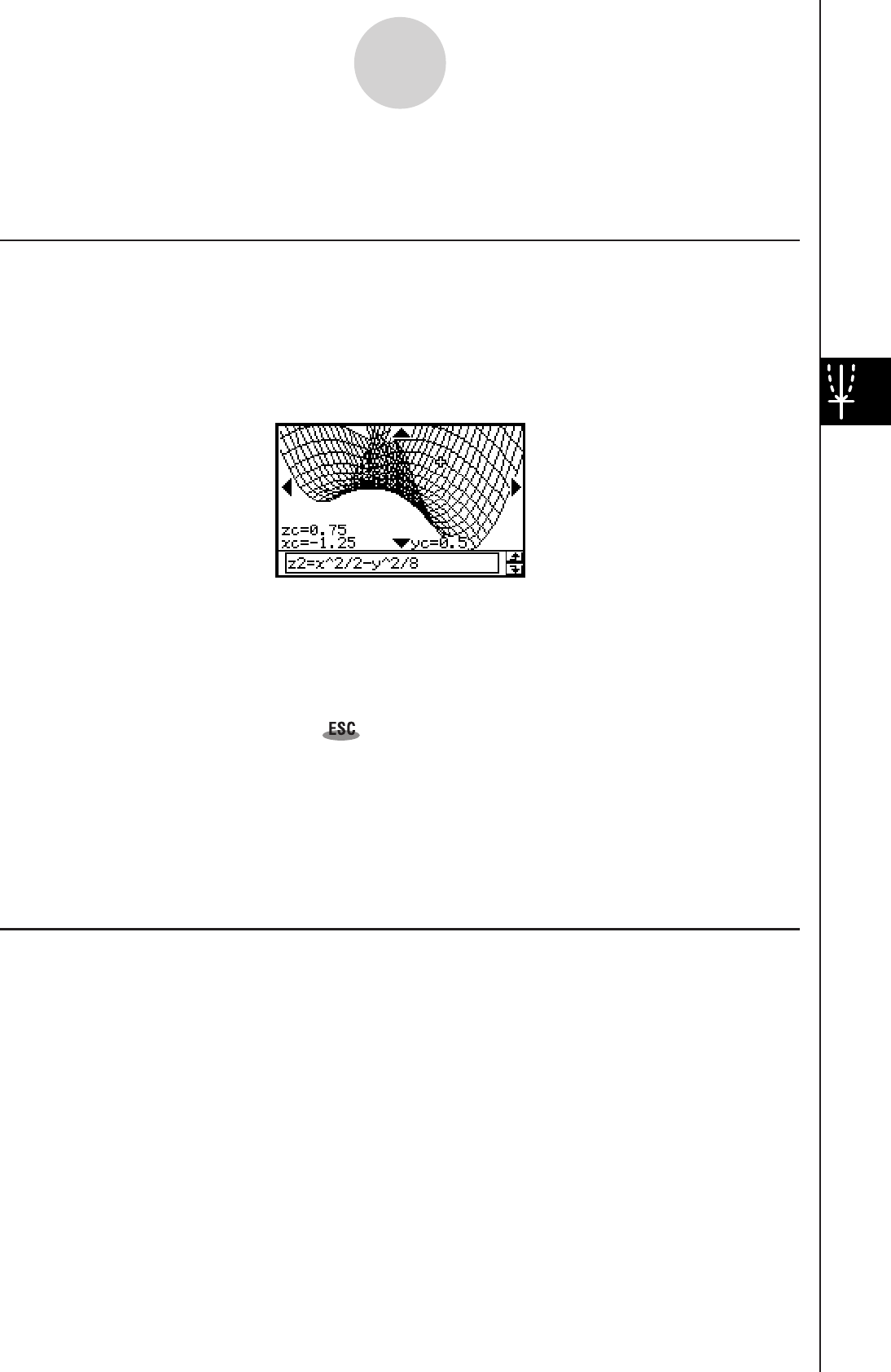
20060301

5-5-1

Other 3D Graph Application Functions

5-5 Other 3D Graph Application Functions

Using Trace to Read Graph Coordinates

Starting the trace operation causes a crosshair pointer to appear on the graph. You can then

press a cursor key or tap the graph controller arrows to move the pointer to the location you

want, and read the coordinates that appear on the display. To start the trace operation and

display the pointer, make the 3D Graph window active, and then tap =, or tap [Analysis]

and then [Trace].

• Each time you press the cursor key or tap a graph controller arrow, the pointer moves the

distance specified by the [grid] value on the 3D View Window dialog box.

• Inputting a value while a trace operation is being performed displays a dialog box for

inputting an x- and y-coordinate. Inputting values for each of the coordinates on this dialog

box causes the pointer to jump to the corresponding location when you tap [OK].

To cancel the trace operation, tap on the icon panel.

Tip

• The initial default setting for the coordinate display is rectangular coordinates (Rectangular).

Tapping Oand [3D Format] displays the 3D Format dialog box, which you can use to select

polar coordinates (Polar) or to hide coordinate values entirely.

• For details about the settings you can configure on the 3D Format dialog box, see “3D Format

Dialog Box” on page 1-9-8.

Inserting Text into a 3D Graph Window

You can insert text into a 3D Graph window and delete it as required.

For more information, see “To write text on the Graph window” on page 3-6-2, and “To clear

figures inserted using the Sketch menu” on page 3-6-5.

20060301

5-5-2

Other 3D Graph Application Functions

Calculating a z-value for Particular x- and y-values, or s- and t-values

Use the following procedure to calculate a z-value for given x- and y-values on the displayed

graph.

uClassPad Operation

(1) Draw the graph and make the 3D Graph window active.

(2) Tap [Analysis], and then [z-Cal].

• This displays a dialog box for specifying the x- and y-values.

(3) Enter values for x and y, and then tap [OK].

• This displays the x-, y-, and z-coordinate values on the 3D Graph window.

• Inputting a graph value while “z-Cal” is on the display while cause a dialog box to

appear for specifying an x- and y-value, or an s- and t-value.You can use this dialog

box to specify other x- and y-values, or s- and t-values.

• To cancel the z-Cal operation, tap on the icon panel.

The message “z-Cal” on the

3D Graph window indicates a

z-Cal operation is in progress.

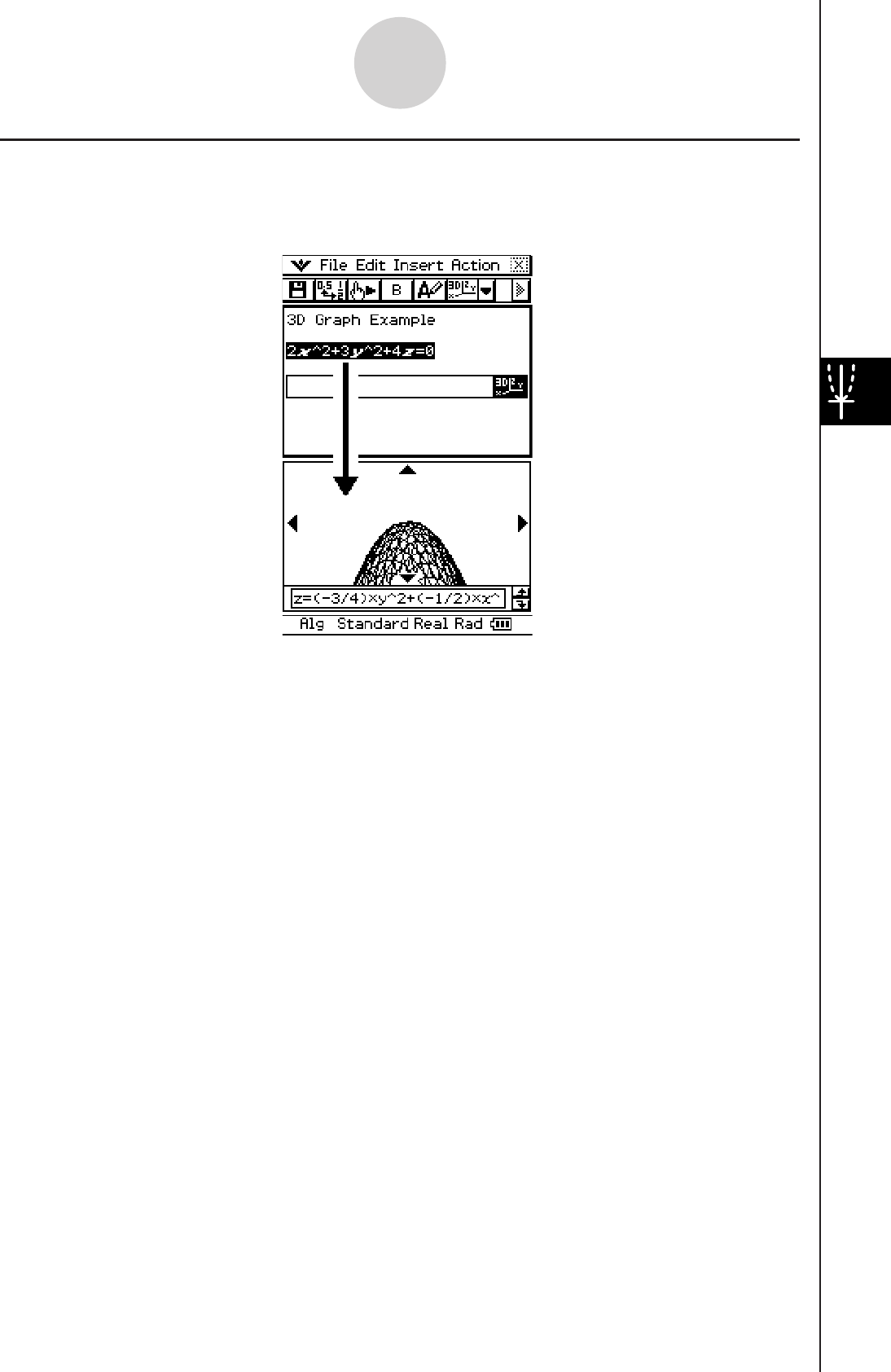
20060301

Using Drag and Drop to Draw a 3D Graph

Dropping an equation of the form z = f (x, y) into the 3D Graph window will graph the

equation.

5-5-3

Other 3D Graph Application Functions

20060301

Using the Sequence

Application

The Sequence application provides you with the tools you need

to work with explicit sequences and recursive type sequences.

6-1 Sequence Application Overview

6-2 Inputting an Expression in the Sequence

Application

6-3 Recursive and Explicit Form of a Sequence

6-4 Using LinkTrace

6-5 Drawing a Cobweb Diagram

Chapter

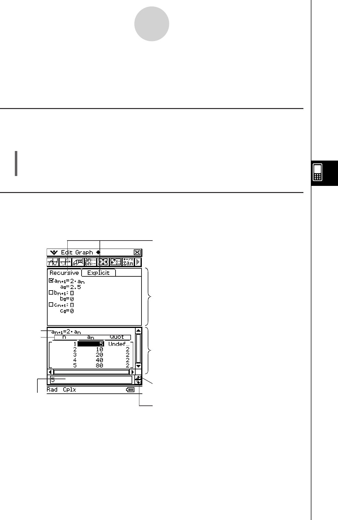
20060301

6-1-1

Sequence Application Overview

6-1 Sequence Application Overview

This section describes the configuration of the Sequence application window, and provides

basic information about its menus and commands.

Starting up the Sequence Application

Use the following procedure to start up the Sequence application.

u ClassPad Operation

On the application menu, tap H.

This starts the Sequence application and displays the Sequence Editor window and the

Table window.

Message box

Shows the value of the currently

selected table cell.

Tabs: Select either [Recursive] or [Explicit].

Sequence Editor window

Table window: For creation and display of tables.

(a) Title: Shows the equation used in the calculations.

The title is not displayed when an item in column n is

selected.

(b) Column names

Tap to copy the area selected in the message box to

the clipboard.

Tap to paste the clipboard contents at the current

cursor position in the message box.

(a)

(b)

Sequence Application Window

When you start up the Sequence application, two windows appear on the display screen:

the Sequence Editor window and Table window.

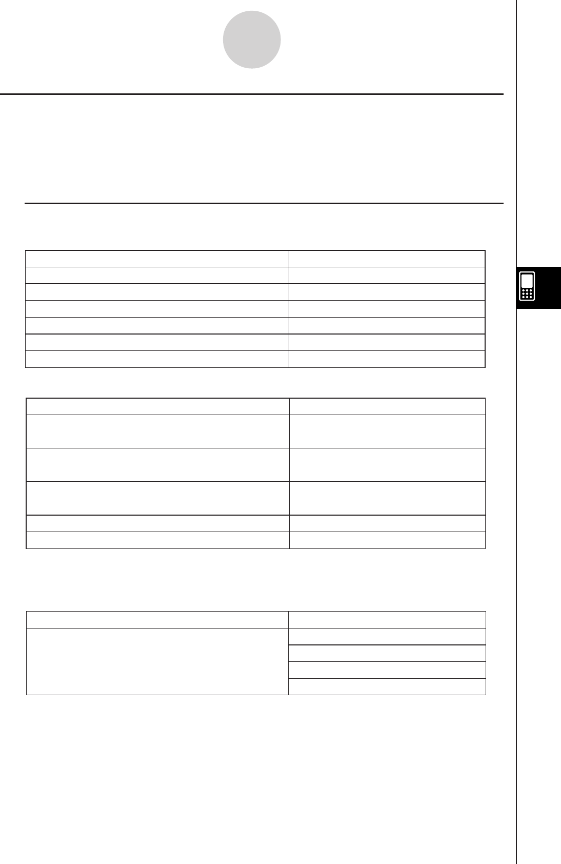
20060301

6-1-2

Sequence Application Overview

k Sequence Editor Window Menus and Buttons

O Menu

Cut the currently selected object and place it

onto the clipboard*

Copy the currently selected object and place

it onto the clipboard*

Paste the current clipboard contents onto the

screen

Select all objects on the screen*

Clear the active window

Cut

Copy

Paste

Select All

Clear All

To do this: Select this Edit menu item:

* These commands are available only for line edit operation when the Graph or Table

window is active.

Type Menu

Specify the type of expression you are inputting

when the [Recursive] tab is displayed

an+

Type a

an+

Type a

an+

Type a

, a

an+

Type a

, a

To do this: Select this Type menu item:

Edit Menu

To do this: Select this O menu item:

Display the soft keyboard Keyboard

Display the Sequence Editor window Sequence Editor

Display the Table window Ta b l e

Display the Graph window Graph

Display the Sequence RUN window Sequence RUN

Start up the Main application Main

Sequence Application Menus and Buttons

This section explains the operations you can perform using the menus and buttons of the

Sequence application’s windows.

• For information about Format related items on O menu, see “Application Format Settings”

on page 1-9-4.

20060301

Buttons

6-1-3

Sequence Application Overview

To do this: Tap this button:

Create an ordered pair table

Create an arithmetic sequence table

Create a geometric sequence table

Create a progression of difference table

Create a Fibonacci sequence table

Draw a cobweb diagram on a graph

Specify

as the recursion type

Specify

as the recursion type

Specify

as the recursion type

Specify

as the recursion type

Input term-

of a recursion expression (Appears only

when the [Explicit] tab is selected.)

Delete the recursion expression in the current active line

Display the Sequence Table Input dialog box

)

Display the Sequence RUN window

(

a Menu

Clear the contents of the currently active tab

sheet

Turn display of sequence table subtotals on and

off

After drawing a graph, turn display of generated

expressions on and off

Require pressing of E to display expression

To do this: Select this a menu item:

Clear Sheet

Set Sequence - On/ Off

Set Sequence - StepDisp

Σdisplay - On/ Off

Input a recursion expression term when

1Type is selected on the [Recursive] sheet

Input a recursion expression term when

2Type is selected on the [Recursive] sheet

Input a recursion expression term when the

[Explicit] tab is selected

n, a

, b

, or c

n, a

, b

, c

, a

1, b

1, or c

n, a

or c

To do this: Select this n, a

menu item:

n, an Menu

20060301

k Sequence Graph Window Menus and Buttons

Edit Menu

The commands on this menu are identical to those for the Sequence Editor window [Edit]

menu described on page 6-1-2.

Zoom Menu

The commands on this menu are identical to those for the Graph & Table application [Zoom]

menu described on page 3-1-4.

Analysis Menu

The [Analysis] menu includes both [Trace] and [Sketch] items. For details about [Trace] and

[Sketch], see page 3-1-5.

a Menu

The commands on this menu are identical to those for the Graph & Table application a

menu described on page 3-1-3.

6-1-4

Sequence Application Overview

Display the Sequence Editor window

Display the Sequence RUN window

Display the Sequence Table Input dialog box

Display the View Window dialog box

To do this: Tap this button:

Draw a cobweb diagram on a graph

Buttons

a Menu

Regenerate the currently displayed table

Save the contents of a table to a list

Delete the currently displayed table

Execute a table and graph link trace

ReTable

Table to List

Delete Table

Link

To do this: Select this a menu item:

k Sequence Table Window Menus and Buttons

Edit Menu

The commands on the sequence Table window [Edit] menu are identical to those for the

Sequence Editor window [Edit] menu described on page 6-1-2.

Graph Menu

Draw a connect type graph

Draw a plot type graph

G-Connect

G-Plot

To do this: Tap this button: Or select this Graph menu item:

20060301

Input a recursion system variable a

, a

, b

, c

, or c

To do this: Select one of these a0, a1 menu items:

Buttons

To do this: Tap this button:

Create a sequence table

Display the Sequence Editor window

Display the Sequence Table Input dialog box

Display the View Window dialog box

6-1-5

Sequence Application Overview

k Sequence RUN Window Menus and Buttons

Edit Menu

The commands on the Sequence RUN window [Edit] menu are identical to those for the

Sequence Editor window [Edit] menu described on page 6-1-2.

n, an Menu

Input a recursion expression term

n+1

n+2

E, or

To do this: Select one of these

menu items:

a0, a1 Menu

Calc Menu

Input the “rSolve” function rSolve

To do this: Select this Calc menu items:

To do this: Tap this button:

Display the Sequence Editor window

Create a sequence table

Display the Sequence RUN window

Display the Sequence Table Input dialog box

Display the View Window dialog box

Buttons

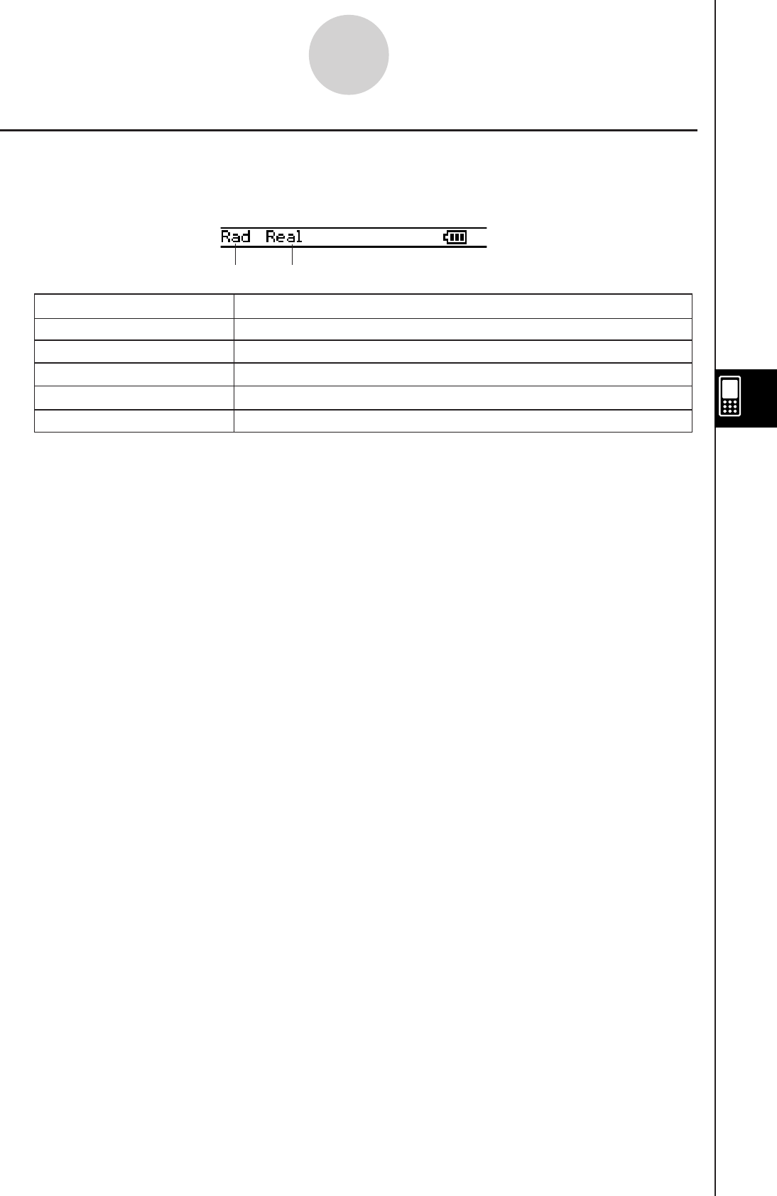
20060301

Sequence Application Status Bar

The status bar at the bottom of the Sequence application shows the current angle unit setting

and [Complex Format] setting (page 1-9-5).

6-1-6

Sequence Application Overview

Angle unit Real mode

Rad

Deg

Cplx

Real

The angle unit setting is radians.

The angle unit setting is degrees.

The Complex (complex number calculation) mode is selected.

Gra The angle unit setting is grads.

The Real (real number calculation) mode is selected.

If you see this: It means this:

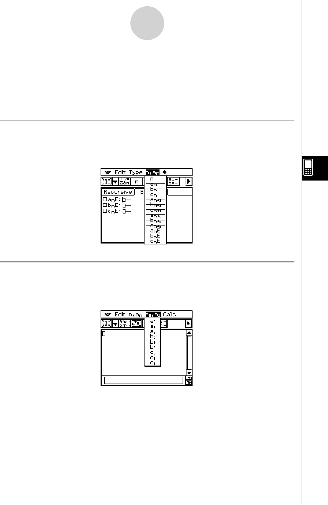
20060301

6-2 Inputting an Expression in the Sequence

Application

In the Sequence application, you input expressions using menus and buttons, without using

the soft keyboard at the bottom of the window.

Inputting Data on the Sequence Editor Window

To input an expression, tap the input location you want ((a), (b), or (c)) to locate the cursor

there. To input a recursion term, tap the [n,an] menu and then tap the term you want. If the

[Explicit] tab is displayed, you can also use the toolbar’s B to input a term-n.

Inputting Data on the Sequence RUN Window

As with the Sequence Editor window, tap ` to display the Sequence RUN window and use

the [n,an] menu to input recursion expression terms. You can also use the [a0,a1] menu to

input system variables ranging from a0 to c2.

Tip

• You can also input recursion expression terms using the 9 keyboard’s K key set.

• You can input recursion system variables (a0, anE, etc.) by tapping the ( tab on the soft

keyboard to display the catalog keyboard. Next, tap the “Form” down arrow button, and then

select [Sys].

6-2-1

Inputting an Expression in the Sequence Application

(a)

(b)

(c)

20060301

6-3 Recursive and Explicit Form of a Sequence

ClassPad supports use of three types of sequence expressions: an+1=, an+2= and anE.

Generating a Number Table

In addition to ordered pair tables, the Sequence application provides you with the means

to generate arithmetic sequence tables*1, geometric sequence tables*2, progression of

difference tables*3, and Fibonacci sequence tables*4.

*1 sequence table for determining if sequence is an arithmetic sequence

*2 sequence table for determining if sequence is a geometric sequence

*3 sequence table for determining if sequence is a progression of difference

*4 sequence table for determining if sequence is a Fibonacci sequence

Example: To create a table (Fibonacci sequence table) for the recursion

an+2 = an+1 + an, a1 = 1, a2 = 1

uClassPad Operation

(1) Start up the Sequence Editor.

• If you have another application running, tap m and then H.

• If you have the Sequence application running, tap O and then [Sequence Editor].

(2) Tap the [Recursive] tab.

(3) Specify the recursion type by tapping [Type] and then [an+2Type a1,a2].

(4) Input the recursion expression.

• Tap the input box to the right of an+2:, and then use the procedures under “6-2

Inputting an Expression in the Sequence Application” to input the following.

[

n,an] [an+1] + [n,an] [an] E

(5) Input the initial value.

1E1E

(6) Tap

• This causes the Sequence Table Input dialog box to appear.

(7) Input the

n-value range as shown below, and then tap [OK].

Start:1 End:5

6-3-1

Recursive and Explicit Form of a Sequence

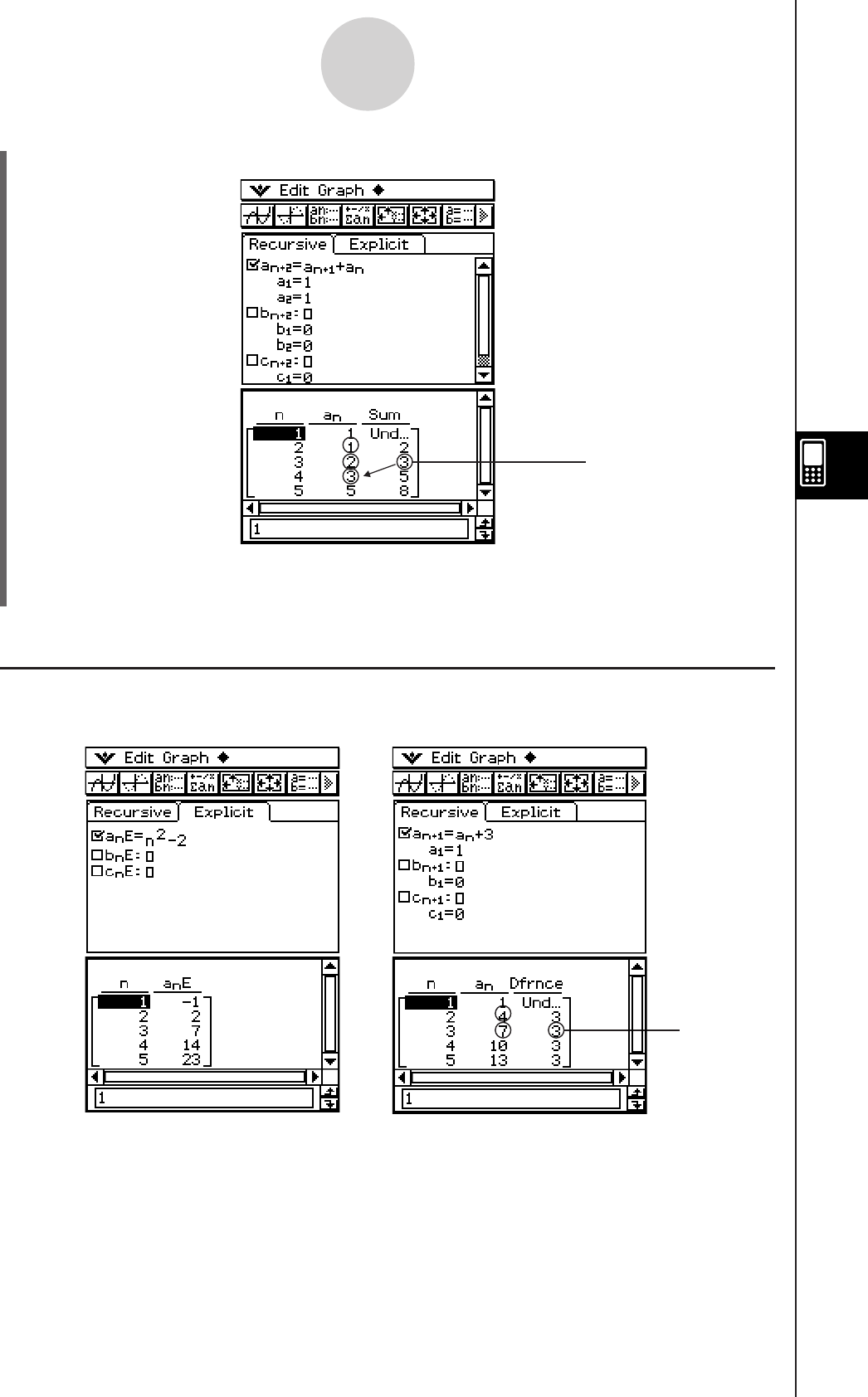
20060301

(8) Tap the down arrow button next to #, and then select ` to create the table.

k Other Table Types

The following show what the window looks like after you generate other types of tables.

6-3-2

Recursive and Explicit Form of a Sequence

Ordered Pair Table Arithmetic Sequence Table

In the above example, “4 Cells” is selected for the [Cell Width Pattern] setting of the

Graph Format dialog box (page 1-9-7).

3 = 2 + 1

3 = 7 – 4

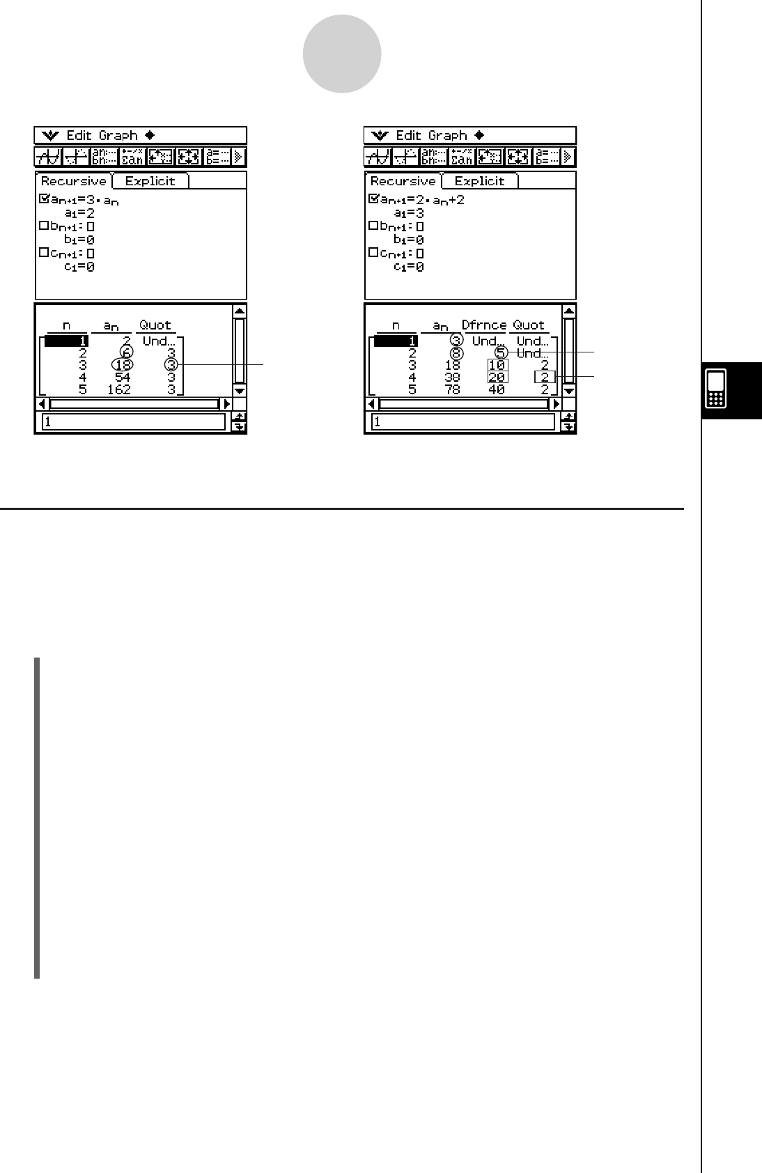
20060301

Graphing a Recursion

An expression can be graphed as a connect type graph (G-Connect) or a plot type graph

(G-Plot).

Example: To graph

an+1 = 2an+1, a1 = 1

uClassPad Operation

(1) Start up the Sequence Editor.

• If you have another application running, tap m and then H.

• If you have the Sequence application running, tap O and then [Sequence Editor].

(2) Tap the [Recursive] tab.

(3) Specify the recursion type by tapping [Type] and then [an+1Type a1].

(4) Input the recursion expression.

• Tap the input box to the right of an+1:, and then use the procedures under “6-2

Inputting an Expression in the Sequence Application” to input the following.

2 [n,an] [an]+1E

(5) Input the initial value.

(6) Tap

O and then [View Window].

• This displays a dialog box for configuring View Window settings.

6-3-3

Recursive and Explicit Form of a Sequence

Geometric Sequence Table Progression of Difference

Table

3 = 18 ÷ 6 5 = 8 – 3

2 = 20 ÷ 10

20060301

(7) Configure View Window settings as shown below.

xmin = 0 xmax = 6 xscale = 1 xdot: (Specify auto setting.)

ymin = –15 ymax = 65 yscale = 5 ydot: (Specify auto setting.)

(8) After everything is the way you want, tap [OK].

(9) Tap the down arrow button next to #, and then select + to create the table.

(10) Perform one of the following steps to draw the type of graph you want.

• To draw a connect type graph, tap $.

6-3-4

Recursive and Explicit Form of a Sequence

• To draw a plot type graph, tap !.

In the above example, “4 Cells” is selected for the [Cell Width Pattern] setting of the

Graph Format dialog box (page 1-9-7).

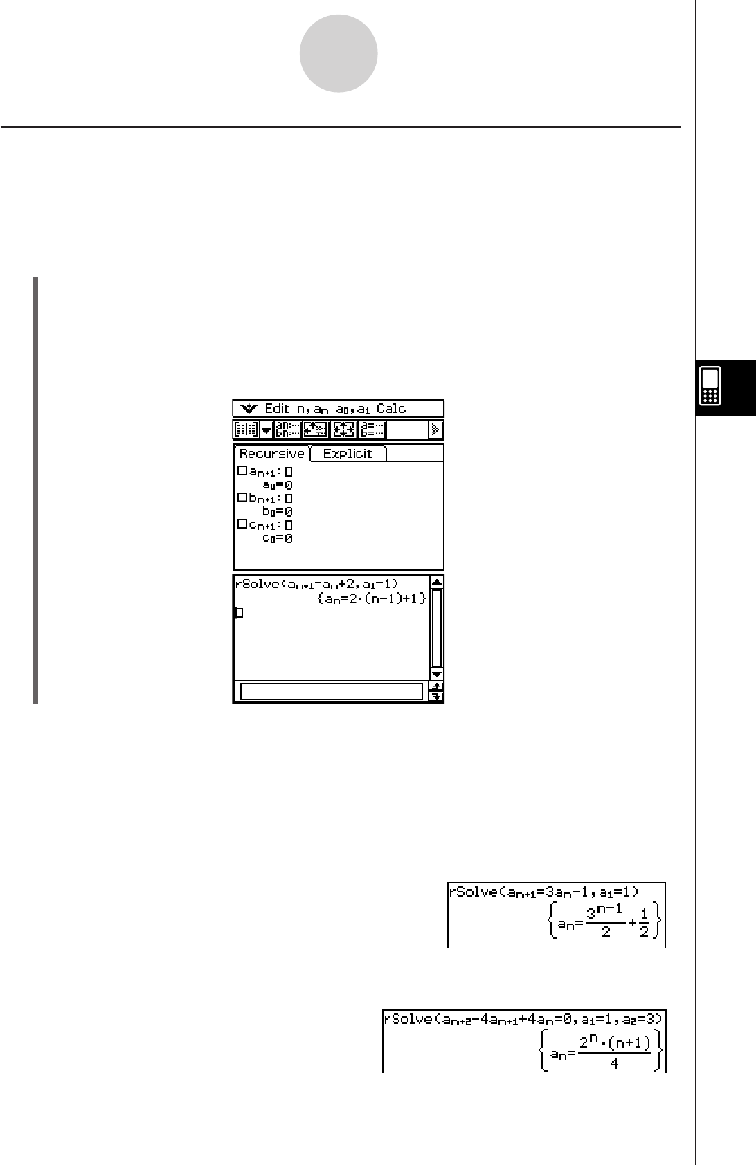
20060301

Determining the General Term of a Recursion Expression

The following procedure converts the sequence expressed by a recursion expression to the

general term format an = f (n).

Example: To determine the general term of the recursion expression an+1 = an + 2, a1 = 1

uClassPad Operation

(1) Start up the Sequence Editor.

• If you have another application running, tap m and then H.

• If you have the Sequence application running, tap O and then [Sequence Editor].

(2) Tap (or press) O, [Sequence RUN], [Calc], [rSolve], [n,an], [an+1], =, [n,an], [an], +,

2, ,, [a0,a1], [a1], =, 1, and then ).

(3) Press

6-3-5

Recursive and Explicit Form of a Sequence

u About rSolve

The rSolve function returns the explicit formula of a sequence that is defined in relation to

one or two previous terms, or a system of recursive formulas.

Syntax: rSolve (Eq, initial condition-1[, initial condition-2] [

)

]

rSolve ({Eq-1, Eq-2}, {initial condition-1, initial condition-2} [

)

] (Eq: Equation)

Example: To obtain the n-th term of a recursion formula an+1 = 3an–1 with the initial

conditions a1=1

Example: To obtain the n-th term of a recursion formula an+2 – 4an+1 + 4an = 0 with the

initial conditions a1 =1, a2 = 3

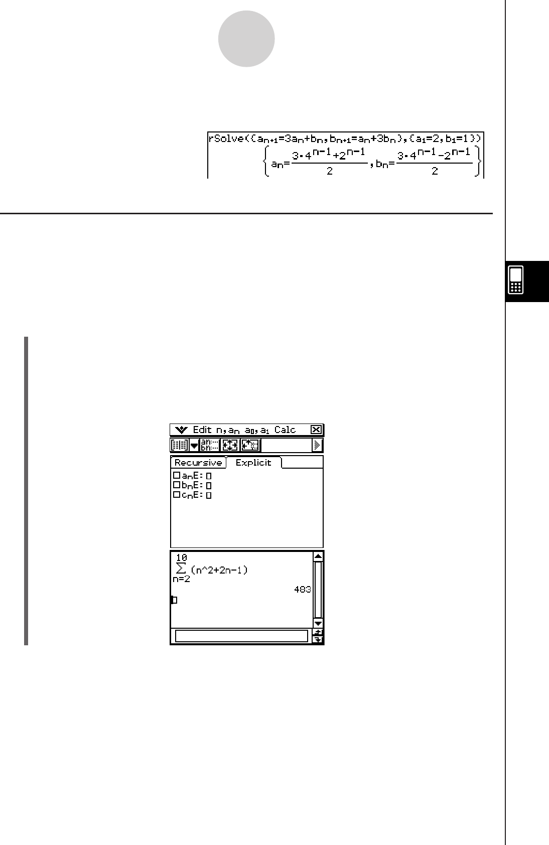
20060301

Calculating the Sum of a Sequence

Perform the following steps when you want to determine the sum of a specific range of the

sequence of a recursion expression or a general term expression.

Example: To calculate the sum of the general term expression anE = n2 + 2n – 1 in the

range of 2 < n < 10

uClassPad Operation

(1) Start up the Sequence Editor.

• If you have another application running, tap m and then H.

• If you have the Sequence application running, tap O and then [Sequence Editor].

(2) Tap (or press) O, [Sequence RUN], [Calc], [Σ], [n,an], [n], e, 2, f, 1, 0, e,

[n,an], [n], {, 2, +, 2, [n,an], [n], -, 1.

(3) Press

Tip

• For information about the syntax of the “Σ” function, see “2-8 Using the Action Menu”.

6-3-6

Recursive and Explicit Form of a Sequence

Example: To obtain the n-th terms of a system of recursion formulas an+1 = 3an + bn,

bn+1 = an + 3bn with the initial conditions a1 =2, b1 = 1

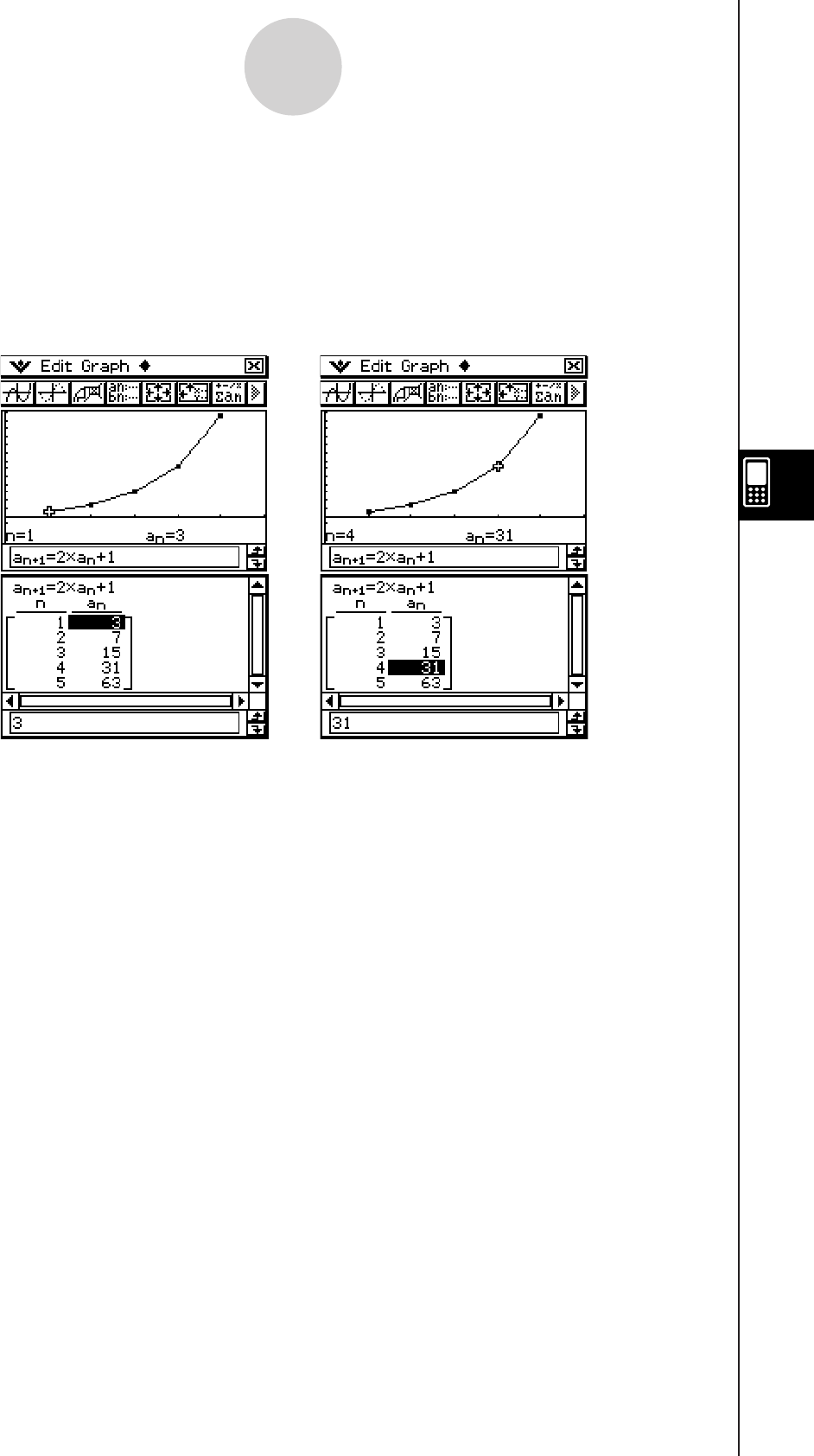
20060301

6-4 Using LinkTrace

While the Table and Graph windows are on the display, you can activate LinkTrace. To do

this, tap in the Table window to make it active. Next, tap a and then [Link]. While LinkTrace

is active, the pointer on the Graph window jumps automatically to the point indicated by the

coordinates in the currently selected table cell. Note that LinkTrace does not work when the

selected cell is in the first column (column n).

6-4-1

Using LinkTrace

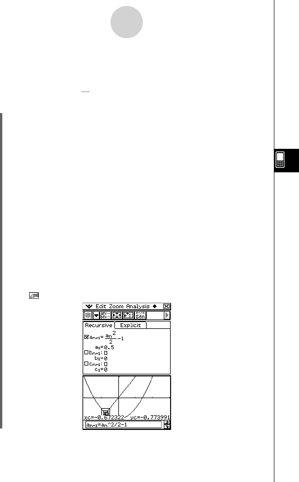
20060301

6-5 Drawing a Cobweb Diagram

You can use the procedure described here to input a sequence and draw a cobweb diagram.

Example: To graph

, a1 = 0.5

uClassPad Operation

(1) Start up the Sequence Editor.

• If you have another application running, tap m and then H.

• If you have the Sequence application running, tap O and then [Sequence Editor].

(2) Tap the [Recursive] tab.

(3) Specify the recursion type by tapping [Type] and then [an+1Type a1].

(4) Input the recursion expression.

• Tap the input box to the right of an+1:, and then use the procedures under “6-2

Inputting an Expression in the Sequence Application” to input the following.

[

n,an] [an] {2/2-1E

(5) Input the initial value.

0.5E

(6) Tap

Oand then [View Window].

• This displays a dialog box for configuring View Window settings.

(7) Configure View Window settings as shown below.

xmin = –2 xmax = 3 xscale = 1 xdot: (Specify auto setting.)

ymin = –1 ymax = 1 yscale = 1 ydot: (Specify auto setting.)

(8) After everything is the way you want, tap [OK].

(9) Tap .

(10) Press

E for each

step of the web.

Tip

• On the cobweb graph window, you can draw the cobweb diagram again by selecting Trace on the

Analysis menu.

6-5-1

Drawing a Cobweb Diagram

an+1 = an2 – 1

20060301

Using the Statistics

Application

This chapter explains how to use the Statistics application. You

can use the Statistics application to perform a variety of statistical

calculations and to graph statistical data. Numeric data stored in lists

can be used to perform Statistics application operations.

This chapter also includes information about performing statistical

tests, and calculating confidence intervals and distributions. Note

that such statistical calculations can be performed using statistical

commands to create programs using the Program application.

7-1 Statistics Application Overview

7-2 Using Stat Editor

7-3 Before Trying to Draw a Statistical Graph

7-4 Graphing Single-Variable Statistical Data

7-5 Graphing Paired-Variable Statistical Data

7-6 Using the Statistical Graph Window Toolbar

7-7 Performing Statistical Calculations

7-8 Test, Confidence Interval, and Distribution Calculations

7-9 Tests

7-10 Confidence Intervals

7-11 Distributions

7-12 Statistical System Variables

Chapter

20060301

7-1-1

Statistics Application Overview

7-1 Statistics Application Overview

This section describes the configuration of the Statistics application windows and provides

basic information about its menus and commands.

The Statistics application provides you with the tools you need to perform the operations

listed below.

You can also use the Program application (page 12-7-4) to perform statistical operations.

u List data input and sorting

u Statistical graph drawing

• Single-variable statistical graphs (Normal Probability Plot, Histogram, Med-Box plot,

Normal Distribution curve, Broken line graph)

• Paired-variable statistical graphs (Scatter diagram, xy line graph, various types of

regression graphs)

u Statistical calculation

• Single-variable statistical calculations

• Paired-variable statistical calculations

• Regression calculations

• Residual calculations

• Test, Confidence Interval and Distribution calculations

(in Statistics and Program applications)

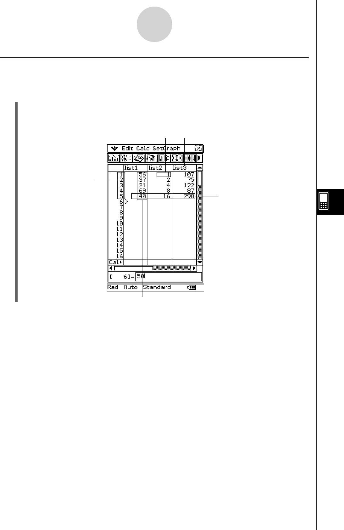
20060301

Starting Up the Statistics Application

Use the following procedure to start up the Statistics application.

u ClassPad Operation

On the application menu, tap I.

This starts the Statistics application and displays the Stat Editor window.

7-1-2

Statistics Application Overview

Line number

Cell

List name cell

(variable name)

Line

Column

20060301

Stat Editor Window Menus and Buttons

This section explains the operations you can perform using the menus and buttons of the

Statistical application’s Stat Editor window.

7-1-3

Statistics Application Overview

To do this: Tap this

button:

Or select this

menu item:

—

Open an existing list (page 7-2-3) Edit - Open List

—

Close the currently selected list (page 7-2-4) Edit - Close List

—

Jump to line 1 of the current list (page 7-2-3) Edit - Jump to Top

—

Jump to the line after the last line of the current list

(page 7-2-3) Edit - Jump to Bottom

Sort list data ascending (page 7-2-8) Edit - Sort(Ascending)

Sort list data descending (page 7-2-8) Edit - Sort(Descending)

Delete a cell (page 7-2-7) Edit - Delete - Cell

Delete all of the data in a list (page 7-2-7) Edit - Delete - Column

—

Delete a list from memory (page 7-2-7)

Edit - Delete - List Variable

Insert a cell into a list (page 7-2-7) Edit - Insert Cell

O - View Window

O - Variable Manager

Convert a mathematical expression to a value —

—

Draw a statistical graph

Display Graph Editor window

Display the Main application work area window

Display the View Window dialog box

—

Display the Variable Manager

SetGraph - Setting…

Display the Set StatGraphs dialog box

—

Display two columns in the Stat Editor window

—

Display three columns in the Stat Editor window

—

Display four columns in the Stat Editor window

Note

• See page 2-1-3 for information about [Edit] menu commands “Cut” through “Clear All”.

• The [Calc] menu contains a selection statistical analysis tools that are described in the

following sections of this chapter.

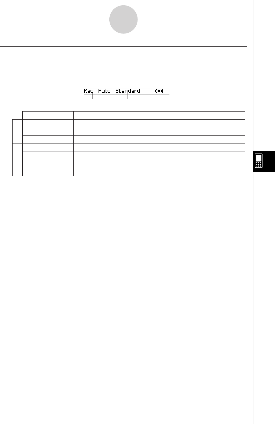
20060301

Stat Editor Window Status Bar

The status bar at the bottom of the Stat Editor window shows the current angle unit setting

(page 1-9-5), statistics View Window setting (page 7-3-2), and decimal calculation setting

(page 1-9-5).

312

7-1-4

Statistics Application Overview

Rad

Deg

Auto

<blank>

Standard

Decimal

The angle unit setting is radians.

The angle unit setting is degrees.

Statistics View Window settings are configured automatically.

Statistics View Window settings need to be configured manually.

Standard mode: Displays result in exact form (fractional format).

Decimal mode: Converts result to a decimal (approximate value).

It means this: If you see this:

Gra The angle unit setting is grads.

Tip

• The

1 and 3 settings can be changed by tapping the status bar.

• The

2 setting can be changed only on the [Special] tab of the Graph Format dialog box

under s (see page 1-9-6).

20060301

7-2-1

Using Stat Editor

7-2 Using Stat Editor

Lists play a very important role in ClassPad statistical calculations. This section provides an

overview of list operations and terminology. It also explains how to use the Stat Editor, a tool

for creating and maintaining lists.

Basic List Operations

This section provides the basics of list operations, including how to start up the Statistics

application, how to open a list, and how to close a list. It also tells you about list variables and

how to use them.

k What is a list?

A list is a type of data array that makes it possible to manipulate multiple data items as a

group. A list has one column and can contain up to 9,999 rows. You can display up to 99 lists

on the Stat Editor window.

List operations are performed using the Stat Editor window, which appears whenever you

start up the Statistics application.

Lists are treated as variables, and like variables, are stored in a folder in the memory and

can be manipulated using the Variable Manager. If a list is cleared from the display, it still

exists in memory as a variable and can be recalled when needed.

Note

• See “Inputting Data into a List” for information about data input (page 7-2-4).

k Using List Variables

The list name is located in the cell at the top of each list. List variable names can be used

inside of calculation formulas, just like any other variable name. The initial default Stat Editor

window shows six lists (columns), named list1 through list6.

20060301

k Creating a List

A list starts out with an initial default name like list1, list2, list3, etc. The Stat Editor allows you

to generate list data (list variables) quickly and easily.

Note

• The Stat Editor window has six default list variables, named “list1” through “list6”. These

lists are system variables that are defined by the system. For more information about

system variables, see “Variable Types” on page 1-7-2.

• The list name can be changed from its default name, “list1” through “list6”, to a name that

you specify.

u To create a list

(1) On the Stat Editor window, tap the list name cell at the top of the list you want to name.

This selects the list name cell.

(2) Enter up to eight bytes for the list name you want, and then press E.

• You cannot use any ClassPad reserved words as list variable names. You also

cannot specify a list name that is already used by another list.

Tip

• If you enter a list name that is already used for another list, tapping w displays the contents of

that list. The data of the existing list replaces data you have input on the Stat Editor window.

• Entering a list name without specifying a folder stores the variable name in the current folder.

To store the variable name in another folder, specify the folder name along with the list name.

To store the variable name of a list named “a” in a folder named “abc”, for example, enter the

following for the list name: abc\a. For information about creating a variable, see “Creating a New

Variable” on page 1-7-6.

k Navigating Around the Stat Editor Window

The following describes the different techniques you can use to navigate around the Stat

Editor window and select the cell you want.

u To select a cell

Use the cursor key to move the highlighting up, down, left, and right. The Stat Editor window

scrolls automatically whenever the highlighting reaches a cell at the edge of the window.

You can also select a particular cell by tapping it with the stylus.

7-2-2

Using Stat Editor

20060301

u To jump to the first or last line of a list

(1) Select any cell in the list.

(2) On the menu bar, tap [Edit].

(3) Select one of the following commands to perform the type of operation you want.

7-2-3

Using Stat Editor

Move the cursor to line 1 of the list Jump to Top

Jump to Bottom

Select this command:To do this:

Move the cursor to the line following the last line that

contains data

• If your list contains 14 entries, then the cursor will move

to the 15 entry.

• If your list contains 9999 entries (the maximum allowed),

then the cursor will move to line 9999.

k Opening a List

Lists are saved in files under their list (variable) names. This means you can close a list and

re-open it later when you need it.

There are two different methods you can use to open a list: using the [Open List] command

and inputting the name of the list in the list name cell of a column.

u To open an existing list using the “Open List” command

(1) On the Stat Editor window, select any cell in the column where you want the list you will

open to appear.

(2) On the menu bar, tap [Edit] and then [Open List].

(3) In the “list=” box that appears, enter the variable name of the list you want to open, and

then tap w.

Tip

• If you enter a variable name that does not match the names of any of the existing lists in step (3),

a new list is created using that name.

u To open an existing list by inputting its name in the list name cell

(1) On the Stat Editor window, select the list name cell of the column where you want the

list you will open to appear.

(2) Enter the variable name of the list you want to open.

(3) Tap

w to open the list.

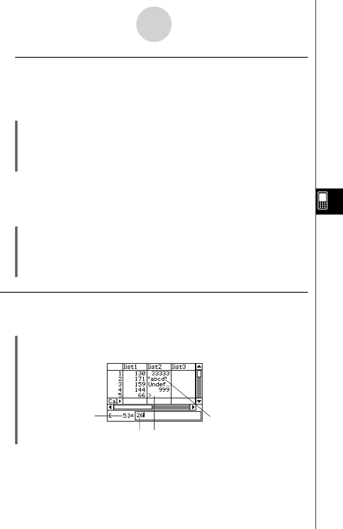
20060301

k Closing a List

Closing a list saves it under its current list (variable) name.

There are two different methods you can use to close a list: using the [Close List] command,

and clearing the list name from its list name cell.

u To close a list using the “Close List” command

(1) On the Stat Editor window, select any cell of the list you want to close.

(2) On the menu bar, tap [Edit] and then [Close List].

• The selected list disappears from the display and is replaced by all blanks.

• At this time, the “list=” box also appears. To open another list, enter its name into the

“list=” box, and then tap w.

Tip

• This above operation clears the list from the display only. The list is still stored as a list variable in

memory, and can be opened when you need it again.

u To close a list by clearing its list name

(1) On the Stat Editor window, select the list name cell of the column of the list you want to

close.

(2) Tap the “list=” box at the bottom of the Stat Editor window.

(3) Press the

c key so the list (variable) name is cleared.

(4) Tap

Inputting Data into a List

Use the procedures in this section to input data and expressions into a list.

u To input a single data item

(1) On the Stat Editor window, select the cell where you want to input the data item.

• Use the cursor key to move the highlighting, or tap the cell with the stylus.

7-2-4

Using Stat Editor

String input

Line number where

data is being input

Input data Cell where data

is being input

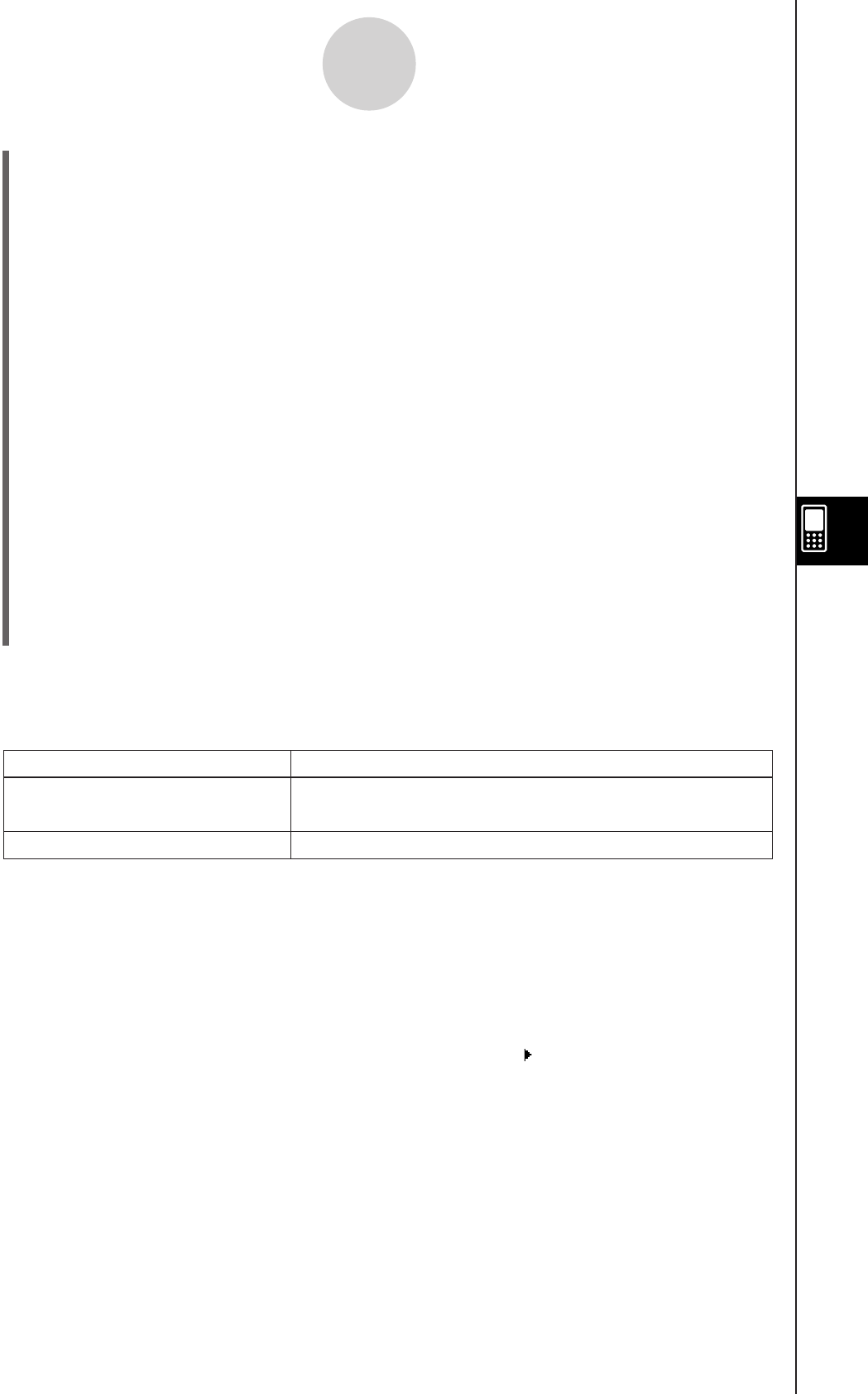
20060301

(2) Input the data you want.

To input a value

• Use the input keypad or soft keyboard that appears when you press k. You can

also access the soft keyboard by tapping O Menu.

To input a mathematical expression

• Use the soft keyboard that appears when you press k.

• When the “Decimal Calculation” check box is not selected (unchecked) on the Basic

Format dialog box (page 1-9-4), any mathematical expression you input is stored

as-is.

• When the “Decimal Calculation” check box is selected, the mathematical expression

is converted to a value before it is stored. Input of 1/2, for example, is converted to 0.5.

To input a string

• Enclose text in quotation marks to make it a string. To input quotation marks, press

k to display the soft keyboard, tap the 9 tab, and then tap K. For more

information about strings, see page 12-6-41.

(3) Press

E to store the data in the cell.

• Selecting a cell that already contains data replaces the existing data with the new

data.

Tip

• You can also input a variable name as list data. In this case, pressing E in step (3) causes

either of the following to happen.

7-2-5

Using Stat Editor

Defined variable

Undefined variable Variable name

Causes this to appear in the cell:Inputting this type of variable:

Variable contents (right aligned for value or left aligned for

expression)

• You need to assign a name to a list before you can input data. Trying to input data into an

unnamed list will cause the cursor to jump automatically to the list name cell at the top of that list.

For information on how to name lists, see “Creating a List” on page 7-2-2.

• To convert an expression in a cell to a value, select the cell and then tap 9.

• Note that statistical calculations and graphing can be performed only using a list that contains

numeric values or mathematical expressions that can be converted into numeric values. An error

occurs if you try to perform a statistical calculation or draw a graph using a list that contains a

string or a non-convertible mathematical expression.

• You cannot edit list data while the b icon is displayed in the “Cal ” line.

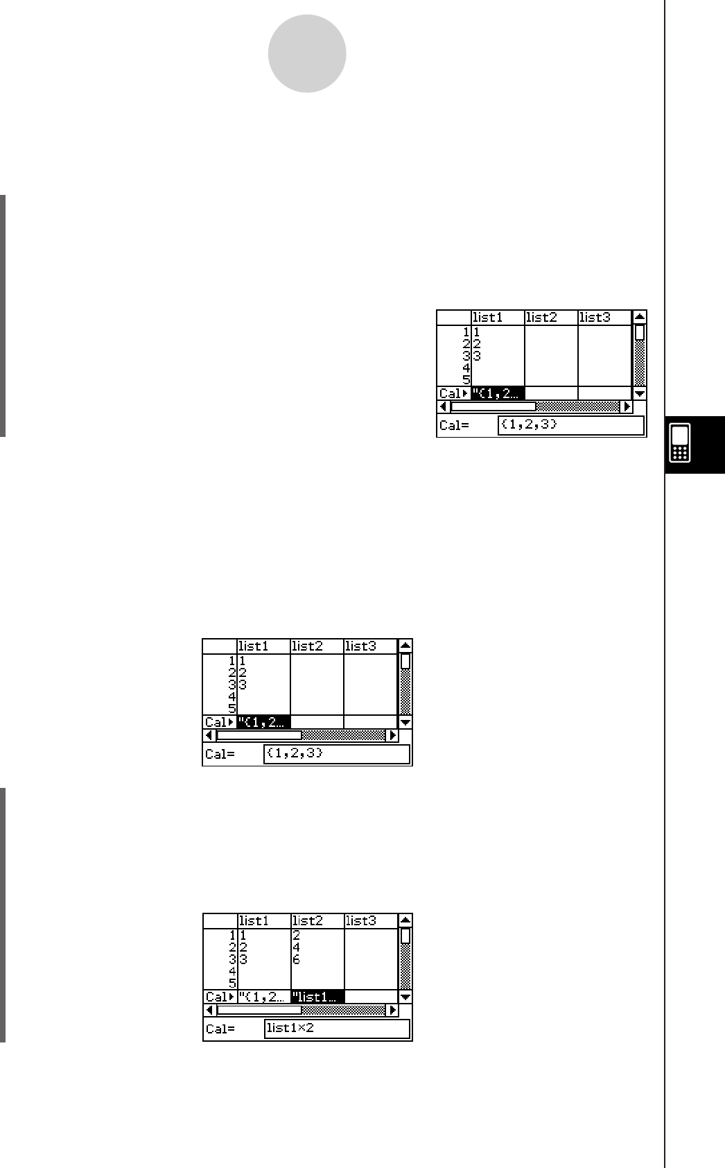
20060301

7-2-6

Using Stat Editor

u To batch input a set of data

Example: To input the values 1, 2, and 3 into list1

(1) On the Stat Editor window, select the “Cal” cell of the list where you want to input the

data (list1 in this example).

(2) Enter {1,2,3}.

• To input braces ({}), press k to display the soft keyboard, and then tap the 9

tab.

(3) Tap

Tip

• Separate values by commas. Do not input a comma following the last value.

Incorrect: {34,53,78,}

Correct: {34,53,78}

u To input calculation results into a cell

Example: To multiply the value of each cell in list1 by two and input the results in list2

(1) On the Stat Editor window, select the “Cal” cell of the list where you want to input the

calculation results (list2 in this example).

(2) In the “Cal=” box, enter the calculation formula (list1×2 in this example).

(3) Press

E to perform the calculation. The values in each cell of list1 are doubled, and

the results are input into list2.

20060301

Editing List Contents

Use the procedures in this section to delete and insert elements, to clear data, and to sort

data.

u To delete a list cell

(1) On the Stat Editor window, select the cell you want to delete.

(2) Tap [Edit].

(3) On the menu that appears, tap [Delete], and then tap [Cell] on the submenu that

appears.

• This deletes the cell and shifts all of the cells below it upwards.

Tip

• You can also delete a cell by selecting it and then pressing the c key.

• Note that deleting a cell does not affect the cells in other lists. If the position of the cell you are

deleting or the cells underneath it are aligned with certain cells of another list, deleting the cell will

cause misalignment of the cells underneath it when they shift upwards.

u To delete all of the data in a list

(1) On the Stat Editor window, select the list whose data you want to delete.

(2) Tap [Edit].

(3) On the menu that appears, tap [Delete]. On the submenu that appears, tap [Column].

(4) On the confirmation dialog box that appears, tap [OK] to delete the list data, or [Cancel]

to cancel the delete operation.

• Tapping [OK] deletes all the data from the list, and leaves the empty list in memory.

u To delete a list from memory

(1) On the Stat Editor window, select the list you want to delete.

(2) Tap [Edit].

(3) On the menu that appears, tap [Delete]. On the submenu that appears, tap [List

Variable].

(4) On the confirmation dialog box that appears, tap [OK] to delete the list, or [Cancel] to

cancel the delete operation.

• Tapping [OK] deletes the list from memory.

u To insert a cell into a list

(1) On the Stat Editor window, select the list cell where you want to insert a new cell.

(2) On the menu bar, tap [Edit] and then [Insert Cell].

• This inserts a cell at the current highlighted location, shifting all the cells below it

downwards. The new cell contains the word “Undefined”.

7-2-7

Using Stat Editor

20060301

Tip

• Note that inserting a cell does not affect the cells in other lists. If you insert a cell in a list that is

aligned with another list, the lists will become misaligned when the cells underneath are shifted

downwards.

Sorting List Data

You can use the procedures in this section to sort the data of a list in ascending or

descending order. Note that the location of the highlighting does not have any affect on

a sort operation.

u To sort a single list

(1) On the Stat Editor window, tap [Edit] and then [Sort(Ascending)] or [Sort(Descending)].

(2) In response to the “How Many Lists?” prompt that appears, select 1 and then tap [OK].

(3) In response to the “Select List Name” prompt that appears, tap the down arrow button

and then select the name (variable name) of the list you want to sort.

(4) Tap [OK] to sort the data.

u To sort multiple lists on a base list

(1) On the Stat Editor window, tap [Edit] and then [Sort(Ascending)] or [Sort(Descending)].

(2) In response to the “How Many Lists?” prompt that appears, tap the down arrow button

and then specify the number of lists you want to sort.

(3) Tap [OK].

(4) In response to the “Select Base List” prompt that appears, tap the down arrow button

and then select the name (variable name) of the list on which you want the sort to be

based.

(5) Tap [OK].

(6) In response to the “Select Second List” prompt that appears, tap the down arrow button

and then select the name (variable name) of the second list to be sorted.

(7) Tap [OK].

(8) Repeat steps (6) and (7) as many times as necessary to specify all of the lists to be

sorted.

• Tapping [OK] after selecting the final list executes the actual sort operation.

7-2-8

Using Stat Editor

20060301

Controlling the Number of Displayed List Columns

You can use the following procedures to control how many list columns appear on the

Statistics application window. You can select 2, 3, or 4 columns.

u To specify the number of columns for the list display

On the Stat Editor window, tap S (two columns), D (three columns) or F (four columns)

to specify the width. You will need to tap the arrow button on the right end of the toolbar to

see the icons.

Tip

• You can also specify the number of display cells using the [Cell Width Pattern] setting on the

[Special] tab of the Graph Format dialog box (page 1-9-6).

• When you have the Stat Editor window displayed along with a second window, you can make the

Stat Editor window active and then tap the r button on the icon panel to expand the Stat Editor

window to fill the entire display. For more information, see “Using a Dual Window Display” on

page 1-5-1.

Clearing All Stat Editor Data

Use the following procedure to initialize the Stat Editor and clear all currently displayed data.

Following this procedure, the Stat Editor shows six empty lists, named list1 through list6.

Warning!

• Performing the following procedure clears all the data from Stat Editor window list1 through

list6 and any additional lists currently in memory.

u To clear all stat editor data

(1) On the Stat Editor window, tap [Edit] and then [Clear All].

(2) On the confirmation dialog box that appears, tap [OK] to clear the all list data or [Cancel]

to cancel the clear operation.

• After you tap [OK], the Stat Editor window shows six empty lists (three lists visible on

the ClassPad display at a time), named list1 through list6.

7-2-9

Using Stat Editor

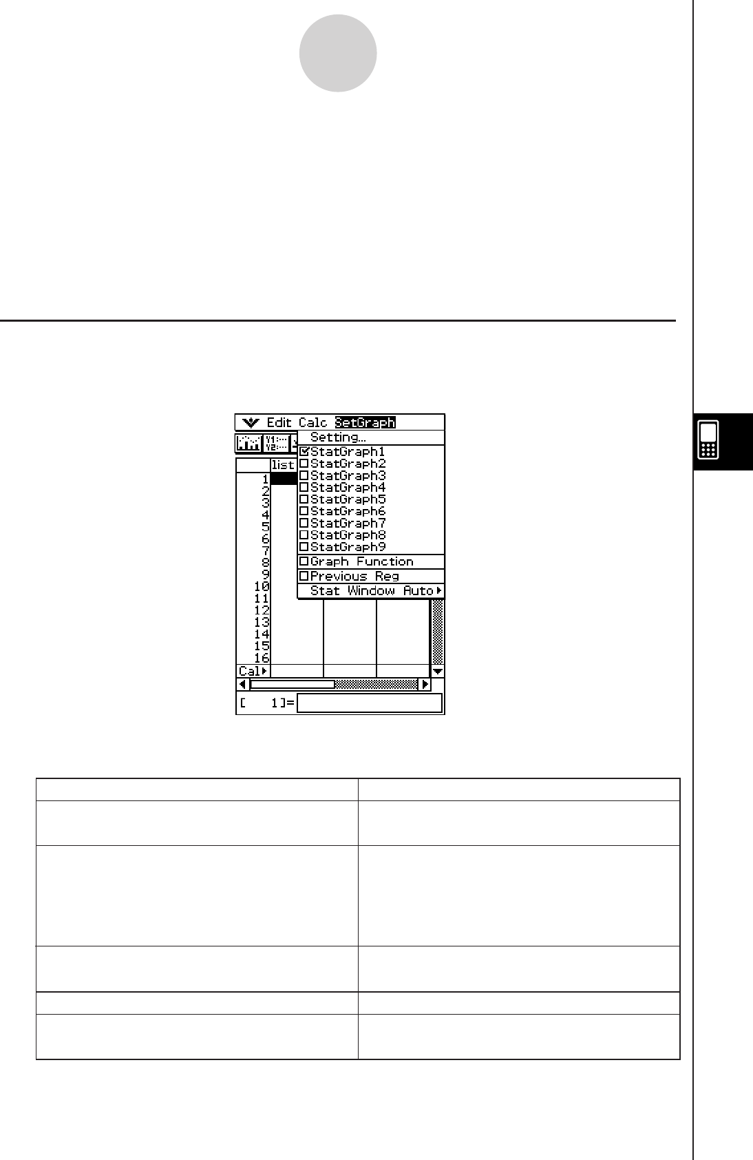
20060301

7-3 Before Trying to Draw a Statistical Graph

Before drawing a statistical graph, you need to first configure its “StatGraph setup” using the

[SetGraph] menu.

The StatGraph setup allows you to configure parameters to control the graph type, the lists

that contain a graph’s data, the type of plot markers to be used, and other settings. Up to

nine StatGraph setups, named StatGraph1, StatGraph2, and so on, can be stored in memory

for later recall.

Using the SetGraph Menu

Tapping [SetGraph] on the Stat Editor window menu bar displays a menu like the one shown

below.

7-3-1

Before Trying to Draw a Statistical Graph

The following describes what you can do with each of the [SetGraph] menu items. See the

following pages for details about performing each type of operation.

Do this:When you want to do this:

Display a dialog box for specifying the graph

type and data list for each StatGraph setup Tap [Setting…].

Select a StatGraph setup for graphing

Select the check box next to the StatGraph

setup you want to graph. This can also be

achieved by tapping [Setting...] and

scrolling through StatGraph1 through

StatGraph9.

Overlay a function graph on a statistical

graph

Select the check box next to [Graph Function].

Turn off function graph overlay

Clear the check box next to [Graph Function].

Graph the results of the last regression

calculation you performed Select the check box next to [Previous Reg].

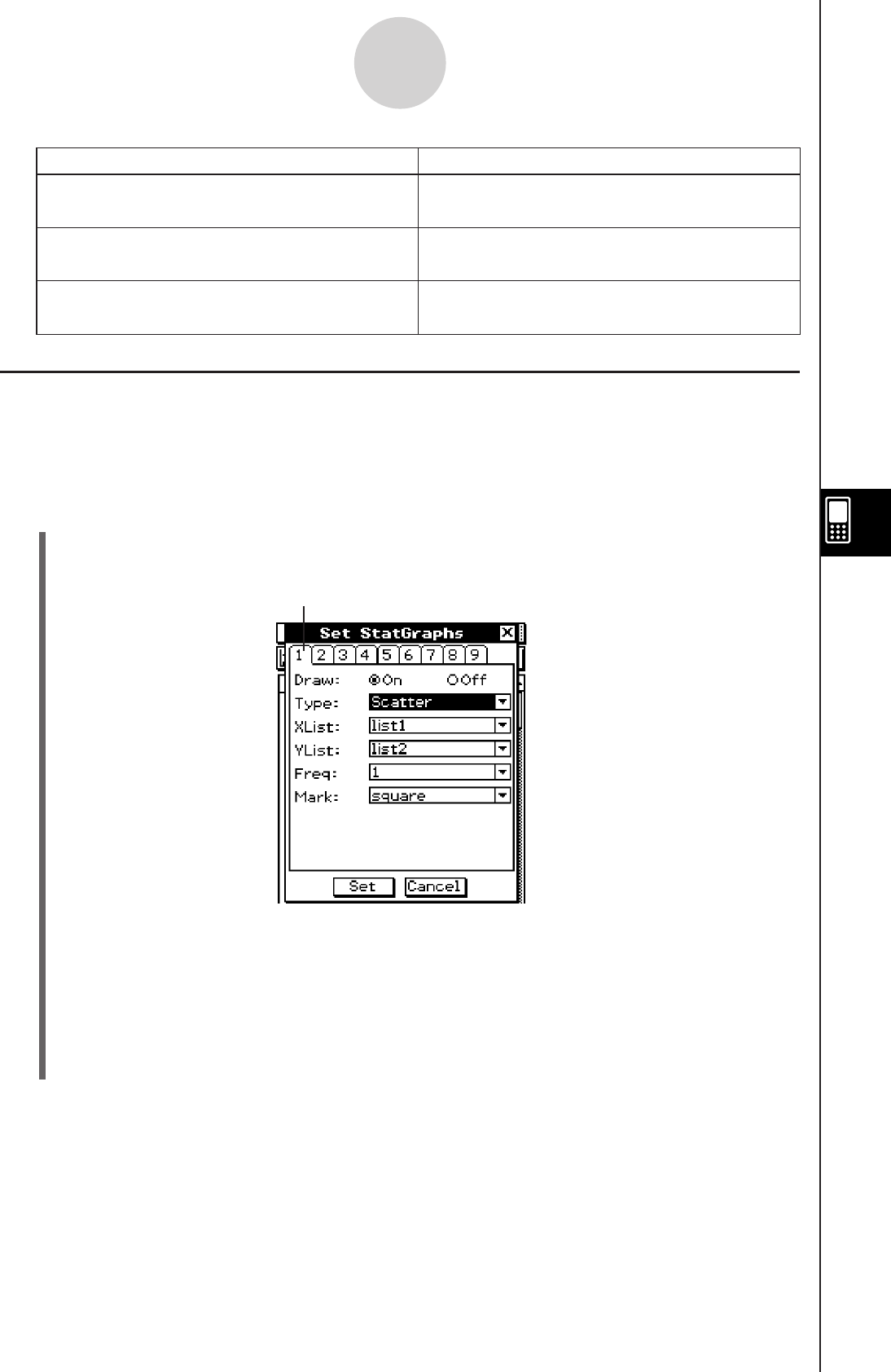
20060301

Configuring StatGraph Setups

Use the procedure below to display the Set StatGraphs dialog box and configure the nine

StatGraph setups.

u To display the Set StatGraphs dialog box

(1) On the Stat Editor window, tap [SetGraph] and then [Setting…].

• This displays the Set StatGraphs dialog box.

7-3-2

Before Trying to Draw a Statistical Graph

• There are tabs named 1 through 9, correspond to StatGraph1 through StatGraph9.

(2) Tap the tab for the StatGraph setup whose configuration you want to change.

(3) Configure the StatGraph setup settings you want as described below, and then tap [Set].

This will apply the settings for all nine StatGraphs.

• To exit the Set StatGraphs dialog box without changing any settings, tap [Cancel]

instead of [Set].

Tabs

Do this:When you want to do this:

Turn off graphing of the last regression

calculation results Clear the check box next to [Previous Reg].

Have Statistics View Window settings

configured automatically

Tap [Stat Window Auto] and then select

[On].

Configure Statistics View Window settings

manually

Tap [Stat Window Auto] and then select

[Off].

20060301

7-3-3

Before Trying to Draw a Statistical Graph

u Draw

Draw the graph using the StatGraph setup of the current tab

Not draw the graph using the StatGraph setup of the current tab

Off

Select this option:To do this:

u Type

Tap the down arrow button, and then select the graph type from the list that appears.

Scatter plot Scatter

xy line graph xyLine

Normal probability plot NPPlot

Histogram Histogram

Med-box plot MedBox

Normal distribution curve NDist

Broken line graph Broken

Linear regression graph LinearR

Med-Med graph MedMed

Quadratic regression graph QuadR

Cubic regression graph CubicR

Quartic regression graph QuartR

Logarithmic regression graph LogR

Exponential regression graph (y = a.eb.x)ExpR

Exponential regression graph (y = a.bx)abExpR

Power regression graph PowerR

Sinusoidal regression graph SinR

Logistic regression graph LogisticR

Select this option:To draw this type of graph:

u XList

Tap the down arrow button, and then select the name of the list (list1 through list6, or a list

name you assigned) that you want to use for x-axis data.

• You need to specify only an XList in the case of single-variable statistics (page 7-4-1). The

initial default [XList] setting is “list1”.

u YList

Tap the down arrow button, and then select the name of the list (list1 through list6, or a list

name you assigned) that you want to use for y-axis data.

• Specify a YList in addition to an XList in the case of paired-variable statistics (page 7-5-1).

The initial default [YList] setting is “list2”.

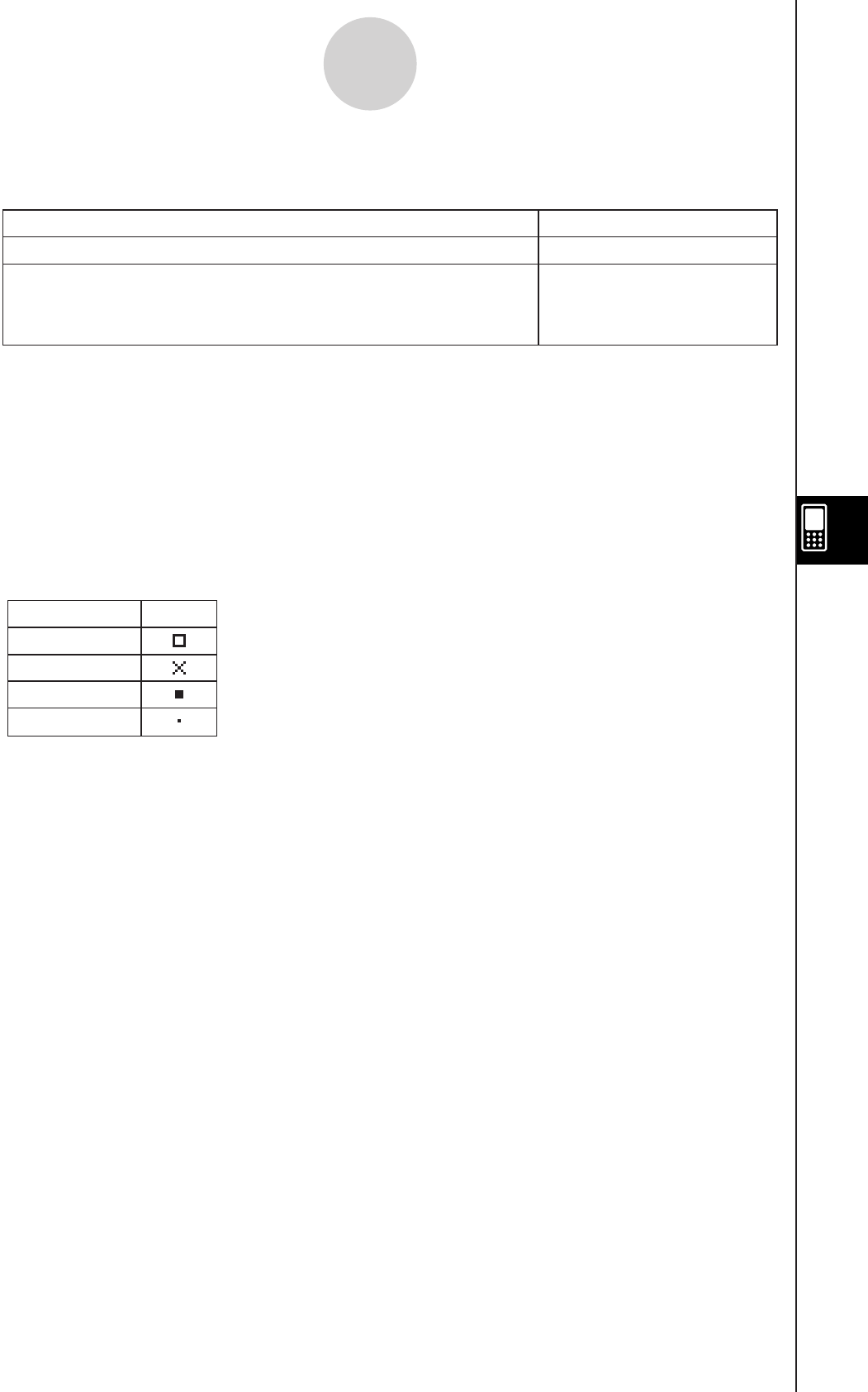
20060301

7-3-4

Before Trying to Draw a Statistical Graph

• The initial default frequency setting is 1. Specifying a list that causes each data value to be

plotted five times helps to improve the appearance of scatter plots.

• A list of frequency values can contain non-zero integers and decimal values. In the case of

a MedBox, or MedMed graph, however, a frequency list can contain positive integers only.

Non-integer values (such as those with a decimal part) cause an error during statistical

calculations.

u Mark

Tap the down arrow button, and select the shape you want to use for the plot points of a

scatter diagram (Scatter), xy line graph (xyLine), or normal probability plot (NPPlot).

Plot each data value once 1

Select this option:To do this:

Specify a list whose values indicate the frequency of each

data value

list1 — list6

(or a list name you

assigned)

u Freq

Tap the down arrow button, and then select the frequency setting from the list that appears.

square

cross

ldot

dot

MarkMark Name

Tip

• The default graph setting for all nine StatGraph setups is a scatter plot (Scatter).

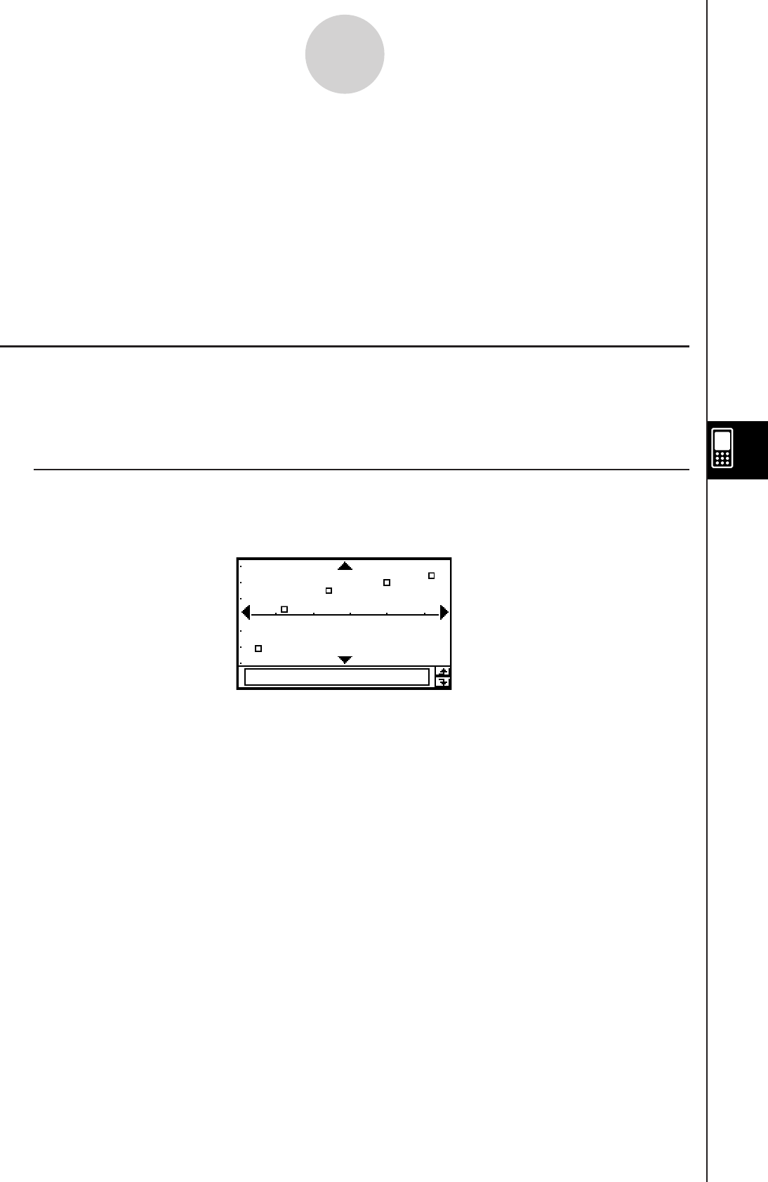
20060301

7-4 Graphing Single-Variable Statistical Data

Single-variable data is data that consists of a single value. If you are trying to obtain the

average height of the members of a single class, for example, the single variable would be

height.

Single-variable statistics include distributions and sums. You can produce any of the graphs

described below using single-variable data.

Before trying to draw any of the graphs described below, configure the graph setup using the

procedures under “Configuring StatGraph Setups” on page 7-3-2.

Normal Probability Plot (NPPlot)

The normal probability plot plots data against a theoretical normal distribution using a scatter

plot. If the scatter plot is close to a straight line, then the data is approximately normal. A

departure from the straight line indicates a departure from normality.

k Graph Parameter Settings (page 7-3-3, 7-3-4)

• [XList] specifies the list that contains the data to be plotted.

• [Mark] specifies the shape of the plot mark.

7-4-1

Graphing Single-Variable Statistical Data

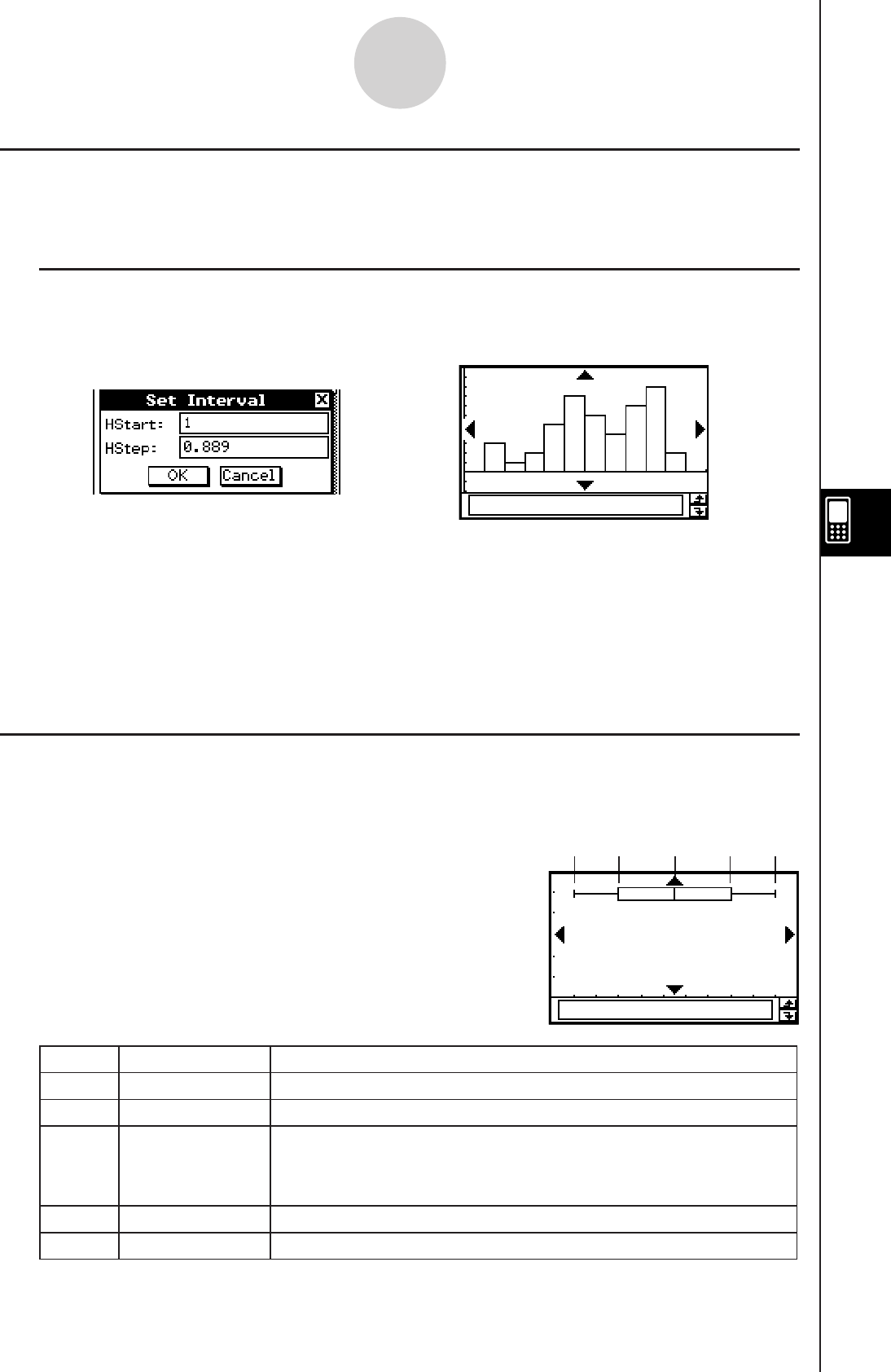
20090601

7-4-2

Graphing Single-Variable Statistical Data

Histogram Bar Graph (Histogram)

A histogram shows the frequency (frequency distribution) of each data class as a rectangular

bar. Classes are on the horizontal axis, while frequency is on the vertical axis.

k Graph Parameter Settings (page 7-3-3, 7-3-4)

• [XList] specifies the list that contains the data to be graphed.

• [Freq] specifies the frequency of the data.

A dialog box like the one shown above appears before the graph is drawn.

You can use this dialog box to change the start value (HStart) and step value

(HStep) of the histogram, if you want.

Tap [OK].

The initial HStart and HStep values on the Set Interval dialog box are set in accordance

with the Stat Window Auto setting. When On is selected for Stat Window Auto, appropriate

values for the graph data are input automatically. When Off is selected, the values that were

displayed the last time the Set Interval dialog box was displayed are input automatically.

Med-Box Plot (MedBox)

This type of graph is often called a “Box and Whisker” graph. It lets you see how a large

number of data items are grouped within specific ranges.

minX minimum

DescriptionLabel Meaning

The data’s smallest value

Q1 First Quartile The median between minX and Med

Med Median

The median of all the data values. If you have 13 values, for

example, this is the value at position seven (six values left

and right).

Q3 Third Quartile The median between maxX and Med

maxX maximum The data’s largest value

• The lines from minX to Q1, and from Q3 to maxX are called “whiskers”.

minX Q1 Med Q3 maxX minX Q1 Med Q3 maxX

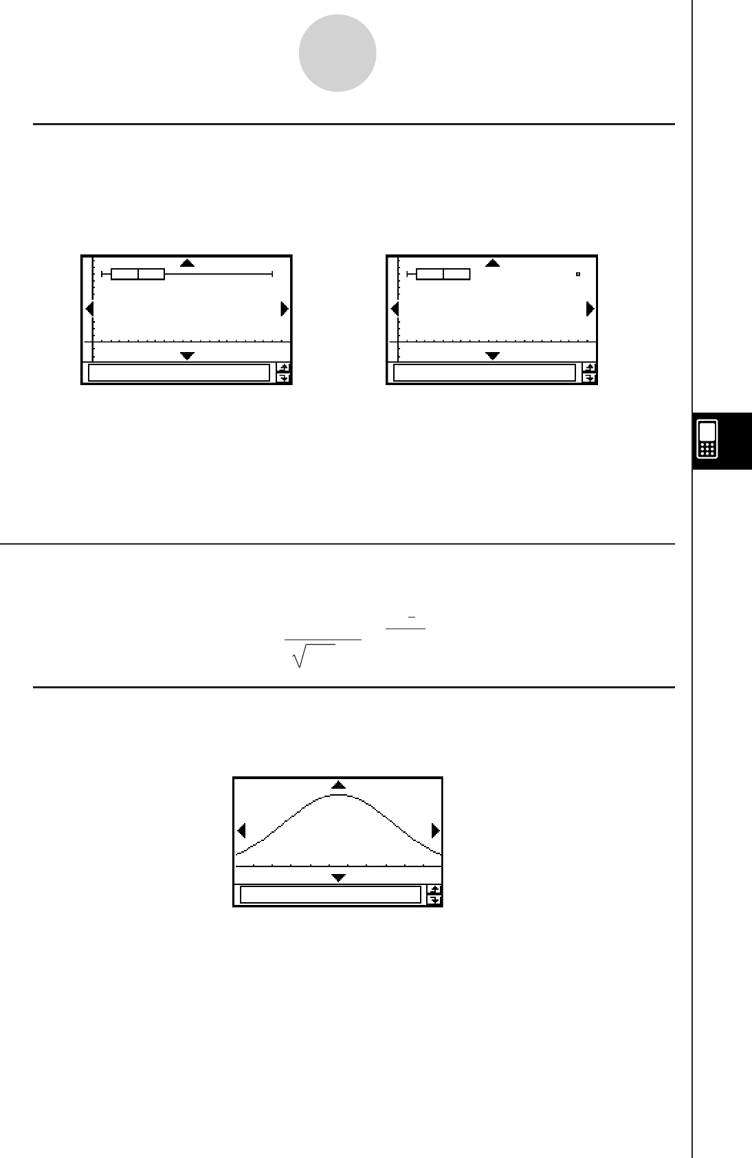
20060301

7-4-3

Graphing Single-Variable Statistical Data

k Graph Parameter Settings (page 7-3-3, 7-3-4)

• [XList] specifies the list that contains the data to be plotted.

• [Freq] specifies the frequency of the data.

• If [Show Outliers] box is checked, “outlier” square symbols are shown instead of “whisker”

lines where a data value is relatively large or small compared to the other data values.

Tip

• When specifying a list of frequency values, make sure that the list contains positive integers only.

Non-integer values (such as those with a decimal part) cause an error during statistical

calculations.

Normal Distribution Curve (NDist)

The normal distribution curve is graphed using the following normal distribution function.

y = 1

2πσ

–2σn

(x–x)

Figure. Do not show Outliers Figure. Show Outliers

k Graph Parameter Settings (page 7-3-3, 7-3-4)

• [XList] specifies the list that contains the data to be graphed.

• [Freq] specifies the frequency of the data.

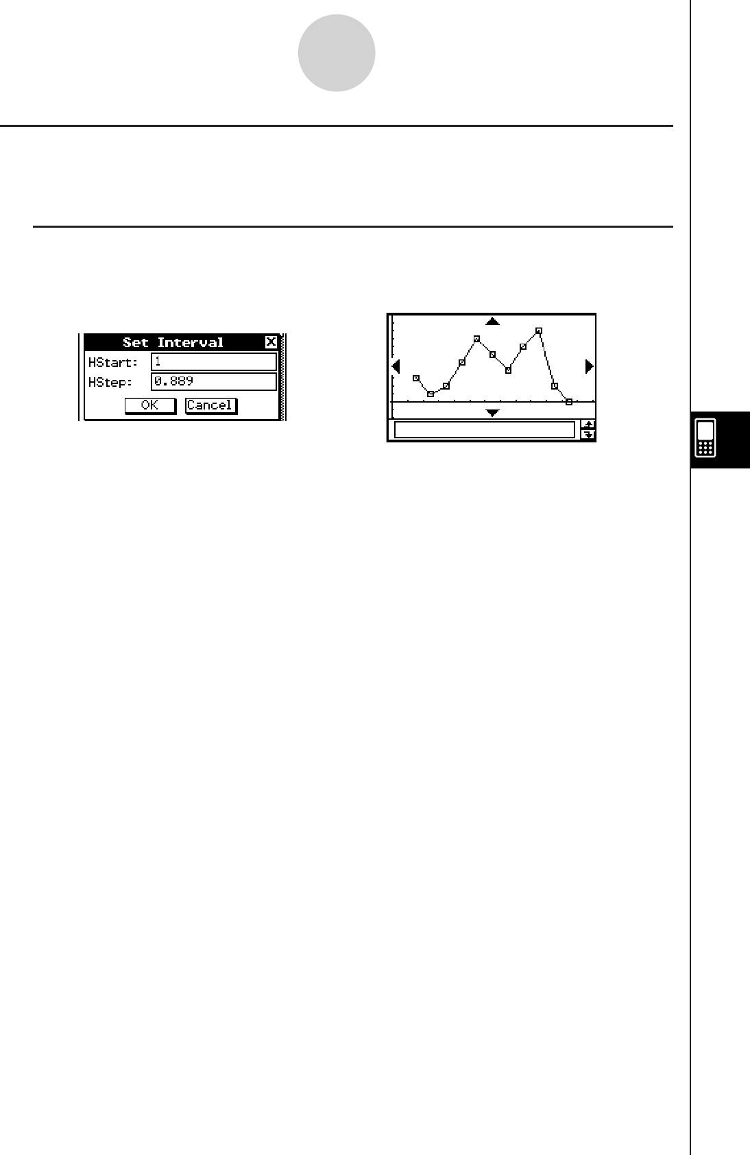
20060301

7-4-4

Graphing Single-Variable Statistical Data

A dialog box like the one shown above appears before the graph is drawn. You

can use this dialog box to change the start value (HStart) and step value (HStep)

of the histogram, if you want.

Broken Line Graph (Broken)

In the broken line graph, lines connect the pointers that fall at the center of each histogram

bar.

k Graph Parameter Settings (page 7-3-3, 7-3-4)

• [XList] specifies the list that contains the data to be graphed.

• [Freq] specifies the frequency of the data.

Tap [OK].

20060301

7-5 Graphing Paired-Variable Statistical Data

With paired-variable statistical data there are two values for each data item. An example of

paired-variable statistical data would be the change in size of an iron bar as its temperature

changes. One variable would be temperature, and the other variable is the corresponding

bar size. Your ClassPad lets you produce any of the graphs described in this section using

paired-variable data.

Before trying to draw any of the graphs described below, configure the graph setup using the

procedures under “Configuring StatGraph Setups” on page 7-3-2.

Drawing a Scatter Plot and xy Line Graph

Use the procedure below to plot a scatter diagram and then connect the dots to produce an

xy line graph.

Example: Input the paired-variable data shown below. Next, plot the data on a scatter

diagram and then connect the dots to produce an xy line graph.

list1 = 0.5, 1.2, 2.4, 4.0, 5.2

list2 = –2.1, 0.3, 1.5, 2.0, 2.4

u ClassPad Operation

(1)

m I

(2) Input the data shown above.

(3) Tap [SetGraph] and then [Setting…], or tap G.

(4) On the Set StatGraphs dialog box that appears, configure a StatGraph setup with the

scatter plot settings shown below, and then tap [Set].

Draw: On

Type: Scatter

XList: list1

YList: list2

(5) Tap

y to plot the scatter plot.

(6) Tap the List window to make it active.

(7) Tap [SetGraph] and then [Setting…], or tap G.

(8) On the Set StatGraphs dialog box that appears, configure a StatGraph setup with the

xy line graph settings shown below, and then tap [Set].

Draw: On

Type: xyLine

XList: list1

YList: list2

7-5-1

Graphing Paired-Variable Statistical Data

20101001

(9) Tap

y to draw the xy line graph.

7-5-2

Graphing Paired-Variable Statistical Data

Drawing a Regression Graph (Curve Fitting)

Use the procedures below to input paired-variable statistical data. Next perform regression

using the data and then graph the results. Note that you can draw a regression graph without

performing the regression calculation.

Example 1: Input the paired-variable data shown below and plot the data on a scatter

diagram. Next, perform logarithmic regression on the data to display the

regression parameters, and then draw the regression graph.

list1 = 0.5, 1.2, 2.4, 4.0, 5.2

list2 = –2.1, 0.3, 1.5, 2.0, 2.4

u ClassPad Operation

(1)

m I

(2) Input the data shown above.

(3) Tap [SetGraph] and then [Setting…], or tap G.

(4) On the Set StatGraphs dialog box that appears, configure a StatGraph setup with the

settings shown below, and then tap [Set].

Draw: On

Type: Scatter

XList: list1

YList: list2

(5) Tap

y to plot the scatter diagram.

Scatter diagram xy line graph

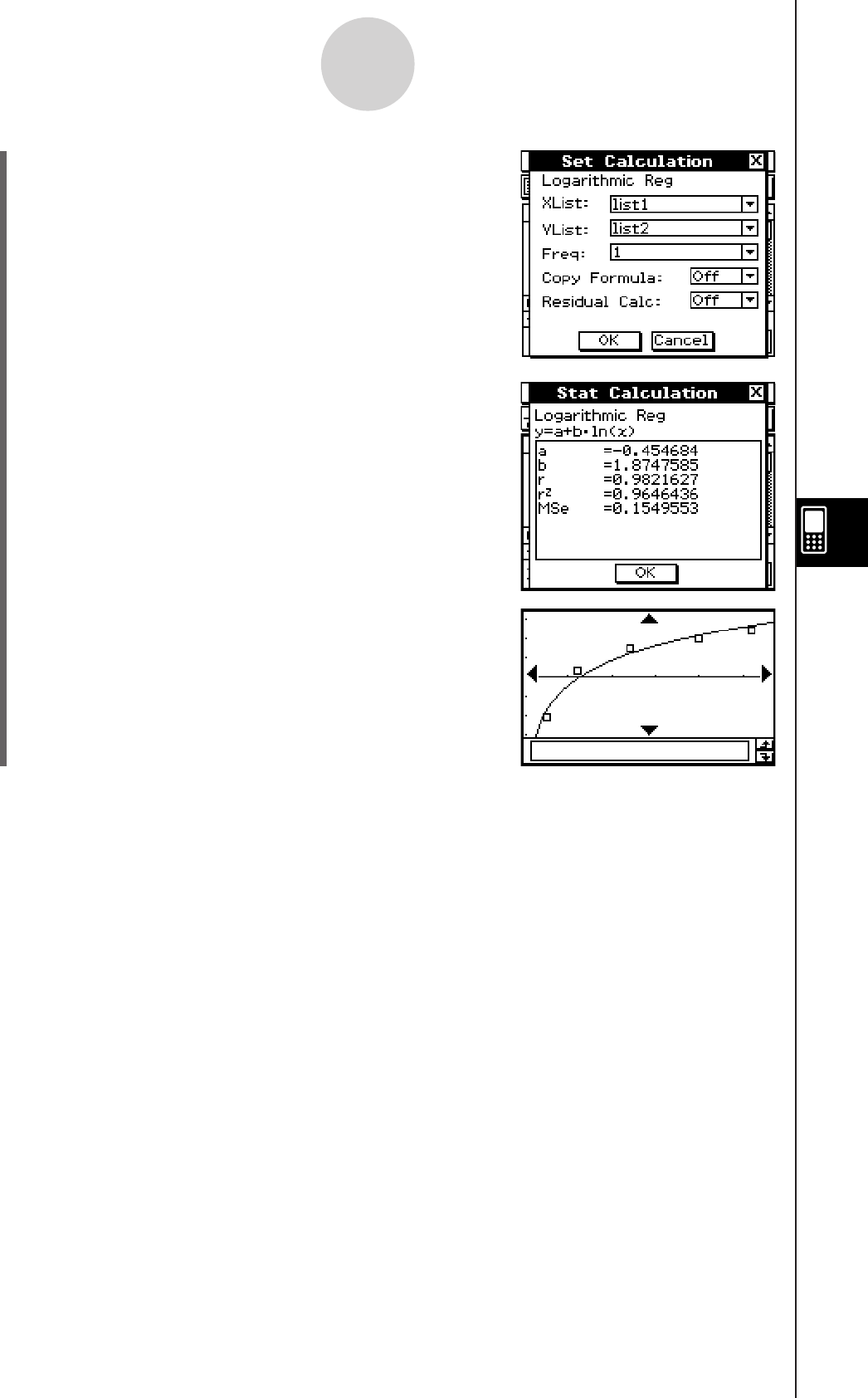
20060301

7-5-3

Graphing Paired-Variable Statistical Data

(6) Tap [Calc] [Logarithmic Reg].

(7) Tap [OK].

(8) Tap [OK]

Tip

• You can perform trace (page 3-7-1) on a regression graph. Trace scroll, however, is not

supported when a scatter diagram is displayed.

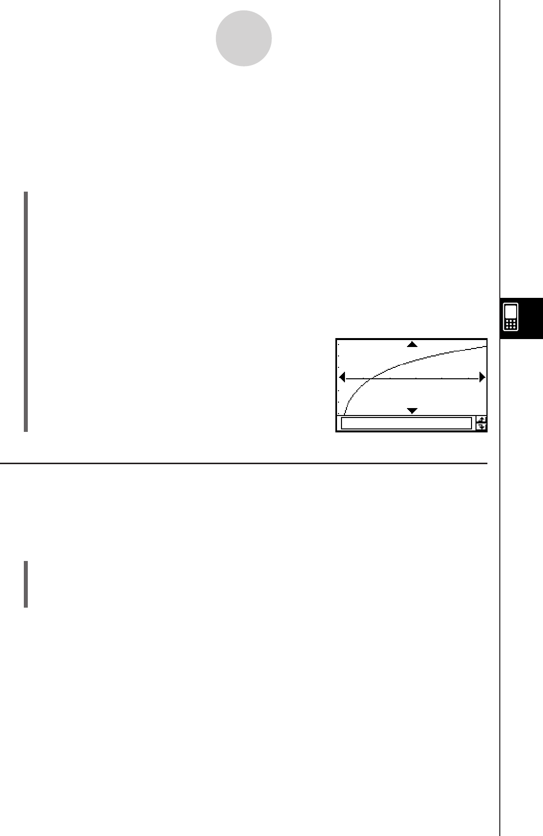
20060301

Example 2: Input the paired-variable data shown below (which is the same data as

Example 1), and then draw the regression graph without performing regression

calculation.

list1 = 0.5, 1.2, 2.4, 4.0, 5.2

list2 = –2.1, 0.3, 1.5, 2.0, 2.4

u ClassPad Operation

(1)

m I

(2) Input the data shown above.

(3) Tap [SetGraph] and then [Setting…], or tap G.

(4) On the Set StatGraphs dialog box that appears, configure a StatGraph setup with the

settings shown below, and then tap [Set].

Draw: On

Type: LogR

XList: list1

YList: list2

(5) Tap

y to graph.

7-5-4

Graphing Paired-Variable Statistical Data

Graphing Previously Calculated Regression Results

Performing the following procedure graphs the last set of regression results you calculated.

Use this procedure when you want to perform statistical calculations without graphing first,

and then graph the results.

u ClassPad Operation

(1) [SetGraph]

(2) On the menu that appears, select the [Previous Reg] check box.

(3) Tap the Graph window or y to graph the last set of regression results you calculated.

Tip

• Calculated regression results are stored in memory whenever you perform a regression

calculation from the Stat Editor menu or from the Statistical Graph [Calc] menu.

• The [Previous Reg] check box described in step (2) above is selected automatically whenever

you perform a regression calculation from the Stat Editor menu or from the Statistical Graph [Calc]

menu.

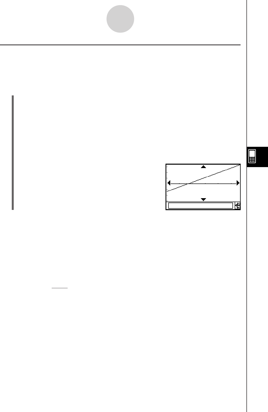
20090601

Drawing a Linear Regression Graph

Linear regression uses the method of least squares to determine the equation that best fits

your data points, and returns values for the slope and y-intercept. The graphic representation

of this relationship is a linear regression graph.

u ClassPad Operation

Start the graphing operation from the Statistics application’s Graph window or List window.

From the Graph window

Tap [Calc] [Linear Reg] [OK] [OK] ".

From the List window

Tap [SetGraph] [Setting…], or G.

On the Set StatGraphs dialog box that appears, configure a StatGraph setup with the

setting shown below, and then tap [Set].

Type: LinearR

Tap

y to draw the graph.

7-5-5

Graphing Paired-Variable Statistical Data

The following is the linear regression model formula.

y = a·x + b

: regression coefficient (slope)

b : regression constant term (y-intercept)

r : correlation coefficient

r2 : coefficient of determination

MSe : mean square error

• MSe =

n – 2 i=1

(yi – (a·xi+ b))2

20060301

Drawing a Med-Med Graph

When you suspect that the data contains extreme values, you should use the Med-Med

graph (which is based on medians) in place of the linear regression graph. Med-Med graph is

similar to the linear regression graph, but it also minimizes the effects of extreme values.

u ClassPad Operation

Start the graphing operation from the Statistics application’s Graph window or List window.

From the Graph window

Tap [Calc] [MedMed Line] [OK] [OK] ".

From the List window

Tap [SetGraph][Setting...], or G.

On the Set StatGraphs dialog box that appears, configure a StatGraph setup with the

setting shown below, and then tap [Set].

Type: MedMed

Tap

y to draw the graph.

7-5-6

Graphing Paired-Variable Statistical Data

The following is the Med-Med model formula.

y = a·x + b

a : Med-Med graph slope

b : Med-Med graph y-intercept

Tip

• When specifying a list of frequency values, make sure that the list contains positive integers

only. Non-integer values (such as those with a decimal part) cause an error during statistical

calculations.

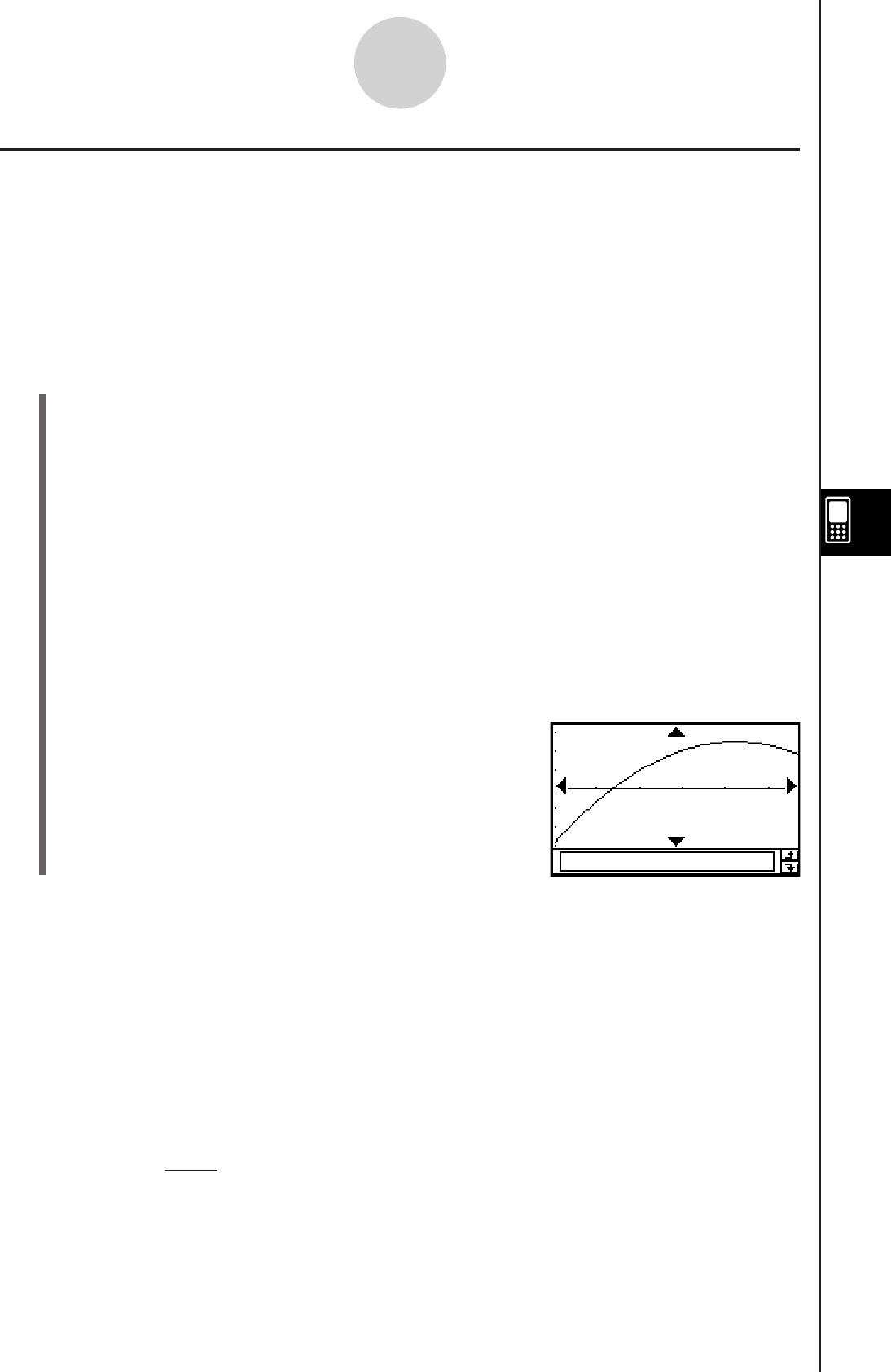
20060301

Drawing Quadratic, Cubic, and Quartic Regression Graphs

You can draw a quadratic, cubic, or quartic regression graph based on the plotted points.

These graphs use the method of least squares to draw a curve that passes the vicinity of

as many data points as possible. These graphs can be expressed as quadratic, cubic, and

quartic regression expressions.

The following procedure shows how to graph a quadratic regression only. Graphing the cubic

and quartic regressions are similar.

u ClassPad Operation (Quadratic Regression)

Start the graphing operation from the Statistics application’s Graph window or List window.

From the Graph window

Tap [Calc] [Quadratic Reg] [OK] [OK] ".

• For cubic regression tap [Cubic Reg] and for quartic regression tap [Quartic Reg]

instead of [Quadratic Reg].

From the List window

Tap [SetGraph][Setting...], or G.

On the Set StatGraphs dialog box that appears, configure a StatGraph setup with the

setting shown below, and then tap [Set].

Type: QuadR

• For cubic regression select [CubicR] and for quartic regression tap [QuartR] instead

of [QuadR].

Tap

y to draw the graph.

7-5-7

Graphing Paired-Variable Statistical Data

The following are the model formulas for each type of regression.

Quadratic Regression

Model Formula:

y = a·x2 + b·x + c

a : quadratic regression coefficient

b : linear regression coefficient

c : regression constant term (y-intercept)

r2 : coefficient of determination

MSe : mean square error

• MSe = Σ

n – 3 i=1

(yi – (a·xi + b·xi+ c))2

20060301

Cubic Regression

Model Formula:

y = a·x3 + b·x2 + c·x + d

a : cubic regression coefficient

b : quadratic regression coefficient

c : linear regression coefficient

d : regression constant term (y-intercept)

r2 : coefficient of determination

MSe : mean square error

Quartic Regression

Model Formula:

y = a·x4 + b·x3 + c·x2 + d·x + e

a : quartic regression coefficient

b : cubic regression coefficient

c : quadratic regression coefficient

d : linear regression coefficient

e : regression constant term (y-intercept)

r2 : coefficient of determination

MSe : mean square error

• MSe = Σ

n – 4

i=1

– (a·x

+ b·x

+ c·x

+d ))

• MSe =

n – 5 i=1

(yi – (a·xi4+ b·xi3 + c·xi2 + d·xi + e))2

7-5-8

Graphing Paired-Variable Statistical Data

20060301

Drawing a Logarithmic Regression Graph

Logarithmic regression expresses y as a logarithmic function of x. The normal logarithmic

regression formula is y = a + b · ln(x). If we say that X = ln(x), then this formula corresponds

to the linear regression formula y = a + b·X.

u ClassPad Operation

Start the graphing operation from the Statistics application’s Graph window or List window.

From the Graph window

Tap [Calc] [Logarithmic Reg] [OK] [OK] ".

From the List window

Tap [SetGraph][Setting...], or G.

On the Set StatGraphs dialog box that appears, configure a StatGraph setup with the

setting shown below, and then tap [Set].

Type: LogR

Tap

y to draw the graph.

7-5-9

Graphing Paired-Variable Statistical Data

The following is the logarithmic regression model formula.

y = a + b·ln(x)

a : regression constant term

b : regression coefficient

r : correlation coefficient

r2 : coefficient of determination

MSe : mean square error

• MSe = Σ

n – 2

i=1

– (a + b·ln (x

)))

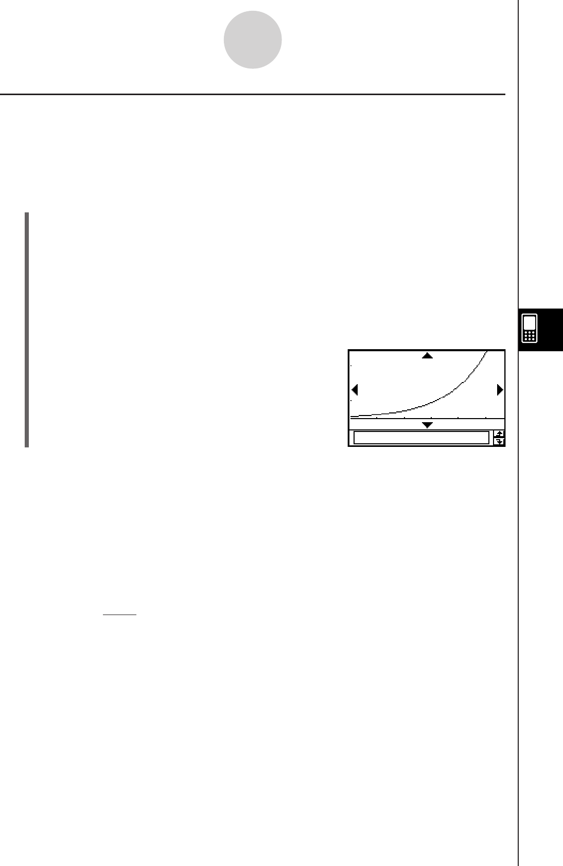
20060301

Drawing an Exponential Regression Graph ( y = a·eb·x)

Exponential regression can be used when y is proportional to the exponential function of

x. The normal exponential regression formula is y = a · eb·x. If we obtain the logarithms of

both sides, we get ln(y) = ln(a) + b·x. Next, if we say that Y = ln(y) and A = In(a), the formula

corresponds to the linear regression formula Y = A + b·x.

u ClassPad Operation

Start the graphing operation from the Statistics application’s Graph window or List window.

From the Graph window

Tap [Calc] [Exponential Reg] [OK] [OK] ".

From the List window

Tap [SetGraph][Setting...], or G.

On the Set StatGraphs dialog box that appears, configure a StatGraph setup with the

setting shown below, and then tap [Set].

Type: ExpR

Tap

y to draw the graph.

7-5-10

Graphing Paired-Variable Statistical Data

The following is the exponential regression model formula in this case.

y = a · eb·x

a : regression coefficient

b : regression constant term

r : correlation coefficient

r2 : coefficient of determination

MSe : mean square error

• MSe = Σ

n – 2

i=1

(ln (y

) – (ln (a) + b·x

))

··

20060301

Drawing an Exponential Regression Graph (

y = a·bx)

Exponential regression can be used when y is proportional to the exponential function of

x. The normal exponential regression formula in this case is y = a·bx. If we take the natural

logarithms of both sides, we get ln(y) = ln(a) + (ln(b)) · x. Next, if we say that Y = ln(y),

A = ln(a) and B = ln(b), the formula corresponds to the linear regression formula Y = A + B·x.

u ClassPad Operation

Start the graphing operation from the Statistics application’s Graph window or List window.

From the Graph window

Tap [Calc] [abExponential Reg] [OK] [OK] ".

From the List window

Tap [SetGraph][Setting...], or G.

On the Set StatGraphs dialog box that appears, configure a StatGraph setup with the

setting shown below, and then tap [Set].

Type: abExpR

Tap

y to draw the graph.

7-5-11

Graphing Paired-Variable Statistical Data

The following is the exponential regression model formula in this case.

y = a·bx

a : regression coefficient

b : regression constant term

r : correlation coefficient

r2 : coefficient of determination

MSe : mean square error

• MSe = Σ

n – 2

i=1

(ln (y

) – (ln (a) + (ln (b)) . x

))

20060301

Drawing a Power Regression Graph (

y = a·xb)

Power regression can be used when y is proportional to the power of x. The normal power

regression formula is y = a · xb. If we obtain the logarithms of both sides, we get ln(y) = ln(a)

+ b · ln(x). Next, if we say that X = ln(x), Y = ln(y), and A = ln(a), the formula corresponds to

the linear regression formula Y = A + b·X.

u ClassPad Operation

Start the graphing operation from the Statistics application’s Graph window or List window.

From the Graph window

Tap [Calc] [Power Reg] [OK] [OK] ".

From the List window

Tap [SetGraph][Setting...], or G.

On the Set StatGraphs dialog box that appears, configure a StatGraph setup with the

setting shown below, and then tap [Set].

Type: PowerR

Tap

y to draw the graph.

7-5-12

Graphing Paired-Variable Statistical Data

The following is the power regression model formula.

y = a·xb

a : regression coefficient

b : regression power

r : correlation coefficient

r2 : coefficient of determination

MSe : mean square error

• MSe = Σ

n – 2

i=1

(ln (y

) – (ln (a) + b·ln (x

)))

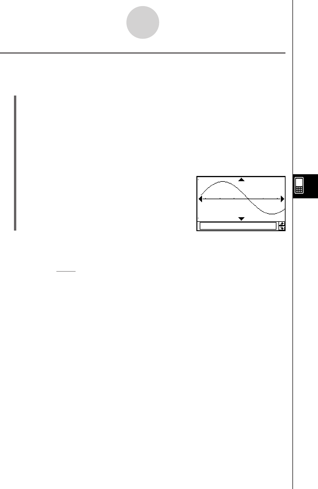
20060301

The following is the sinusoidal regression model formula.

y = a·sin(b·x + c) + d

Tip

• Make sure that “Radian” is selected for the [Angle] setting on the Basic Format dialog box (page

1-9-4) before drawing a sinusoidal regression graph. The graph cannot be drawn correctly when

the [Angle] setting is “Degree”.

• Certain types of data may cause calculation to take a long time. This is normal and does not

indicate malfunction.

Drawing a Sinusoidal Regression Graph (

y = a·sin(b·x + c) + d)

Sinusoidal regression is best for data that repeats at a regular fixed interval over time.

u ClassPad Operation

Start the graphing operation from the Statistics application’s Graph window or List window.

From the Graph window

Tap [Calc] [Sinusoidal Reg] [OK] [OK] ".

From the List window

Tap [SetGraph][Setting...], or G.

On the Set StatGraphs dialog box that appears, configure a StatGraph setup with the

setting shown below, and then tap [Set].

Type: SinR

Tap

y to draw the graph.

7-5-13

Graphing Paired-Variable Statistical Data

• MSe =

n – 2

i=1

– (a·sin (b·x

+ c) + d ))

20060301

Drawing a Logistic Regression Graph ( )

Logistic regression is best for data whose values continually increase over time, until a

saturation point is reached.

u ClassPad Operation

Start the graphing operation from the Statistics application’s Graph window or List window.

From the Graph window

Tap [Calc] [Logistic Reg] [OK] [OK] ".

From the List window

Tap [SetGraph][Setting...], or G.

On the Set StatGraphs dialog box that appears, configure a StatGraph setup with the

setting shown below, and then tap [Set].

Type: LogisticR

Tap

y to draw the graph.

7-5-14

Graphing Paired-Variable Statistical Data

The following is the logistic regression model formula.

Tip

• Certain types of data may cause calculation to take a long time. This is normal and does not

indicate malfunction.

1 +

a·e

–b

1 +

a·e

–b·x

• MSe = Σ

n – 2 1 + a·e–b·xi

i=1

yi –

20060301

Overlaying a Function Graph on a Statistical Graph

You can overlay an existing statistical graph with any type of function graph.

Example: Input the two sets of data shown below, and plot the data on a scatter plot. Next,

overlay the scatter plot with the graph of y = 2 · ln(x).

list1 = 0.5, 1.2, 2.4, 4.0, 5.2

list2 = –2.1, 0.3, 1.5, 2.0, 2.4

u ClassPad Operation

(1)

m I

(2) Input the data shown above.

(3) Tap [SetGraph][Setting...].

(4) On the Set StatGraphs dialog box that appears, configure a StatGraph setup with the

settings shown below, and then tap [Set].

Draw: On

Type: Scatter

XList: list1

YList: list2

(5) Tap

y to draw the graph.

(6) Tap the List window to make it active, and then tap !.

(7) Input the following function into line y1: 2 × ln(x).

(8) Tap

O and then [Close] to close the Graph Editor window.

(9) Tap [SetGraph] on the menu bar. On the menu that appears, select the [Graph

Function] check box.

(10) Tap

y to draw the graph.

7-5-15

Graphing Paired-Variable Statistical Data

Tip

• After drawing a function graph, you can perform trace and other functions.

20060301

7-6 Using the Statistical Graph Window Toolbar

The following describes the operations you can perform using the toolbar on the Statistical

Graph window.

7-6-1

Using the Statistical Graph Window Toolbar

Display the Stat Editor window (

Display the Graph Editor window !

Redraw the displayed graph "

Display the View Window dialog box 6

Toggle the [Stat Window Auto] setting between auto and manual s

Start a trace operation =

Start a box zoom operation Q

Enlarge the display image (zoom in) W

Reduce the display image (zoom out) E

Display the Set StatGraphs dialog box G

Display the Main application work area window ~

Pan the window T

Tap this button:To do this:

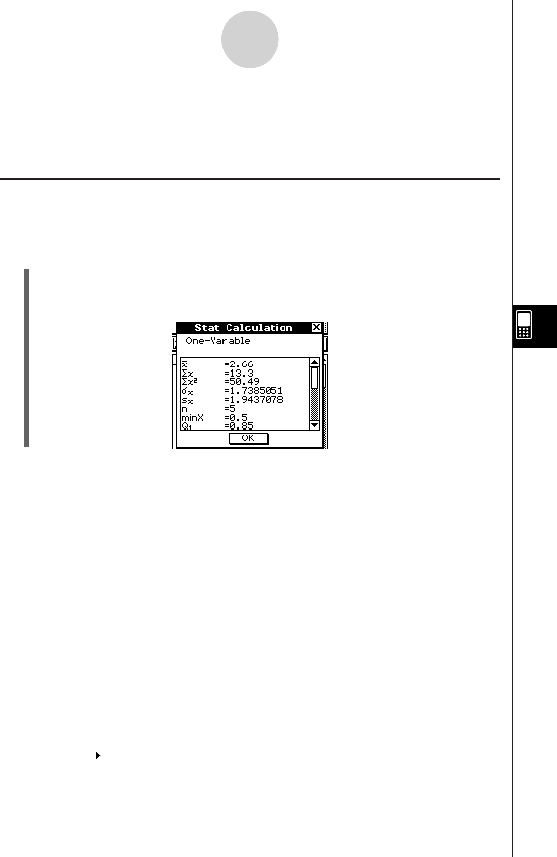
20090601

7-7 Performing Statistical Calculations

You can perform statistical calculations without drawing a graph by tapping [Calc] on the

menu bar and selecting [One-Variable] or [Two-Variable].

Viewing Single-variable Statistical Calculation Results

Besides using a graph, you can also use the following procedure to view the single-variable

statistics parameter values.

u To display single-variable calculation results

(1) On the menu bar, tap [Calc] and then [One-Variable].

(2) On the dialog box that appears, specify the [XList] name and select the [Freq] setting

(page 7-3-3, 7-3-4).

(3) Tap [OK].

7-7-1

Performing Statistical Calculations

• This displays the Stat Calculation dialog box with the single-variable statistical calculation

results described below. You can use the scrollbar to scroll the results.

o : sample mean

Σx : sum of data

Σx2 : sum of squares

σx: population standard deviation

sx : sample standard deviation

n : sample size

minX : minimum

Q1 : first quartile

Med : median

Q3 : third quartile

maxX : maximum

Mode : mode*

ModeN : number of data mode items

ModeF : data mode frequency

* If “Mode = ModeStat” is shown on the Stat Calculation dialog box, it means that

solutions are stored in the “ModeStat” system variable. To view the solutions, tap any list

name cell on the Stat Editor window, input “ModeStat”, and then tap w. This will display

the “ModeStat” system variable contents in the list.

20101001

• You can use the [Q1, Q3 on Data] setting on the Basic Format dialog box (page 1-9-4) to

select the Q1 and Q3 calculation methods. For details, see “Calculation Methods for Q1

and Q3” below.

k Calculation Methods for Q1 and Q3

Q1 and Q3 can be calculated in accordance with the [Q1, Q3 on Data] setting on the Basic

Format dialog box (page 1-9-4) as described below.

u Unchecked: (default)

With this calculation method, processing depends on whether the number of elements n in

the population is an even number or odd number.

When the number of elements

n is an even number:

Using the center point of the total population as the reference, the population elements are

divided into two groups: a lower half group and an upper half group. Q1 and Q3 then become

the values described below.

Q1 = {median of the group of 2

n items from the bottom of the population}

Q3 = {median of the group of 2

n items from the top of the population}

Center Point Center Point Center Point

When the number of elements n is an odd number:

Using the median of the total population as the reference, the population elements are

divided into two groups: a lower half group (values less than the median) and an upper half

group (values greater than the median). The median value is excluded. Q1 and Q3 then

become the values described below.

Q1 = {median of the group of 2

n – 1 items from the bottom of the population}

Q3 = {median of the group of 2

n – 1 items from the top of the population}

• When n = 1, Q1 = Q3 = population center point.

4 + 5= Median

= Q1

2 + 3= Q3

6 + 7

12345678

4 + 5= Median

= Q1

2 + 3= Q3

6 + 7

12345678

7-7-2

Performing Statistical Calculations

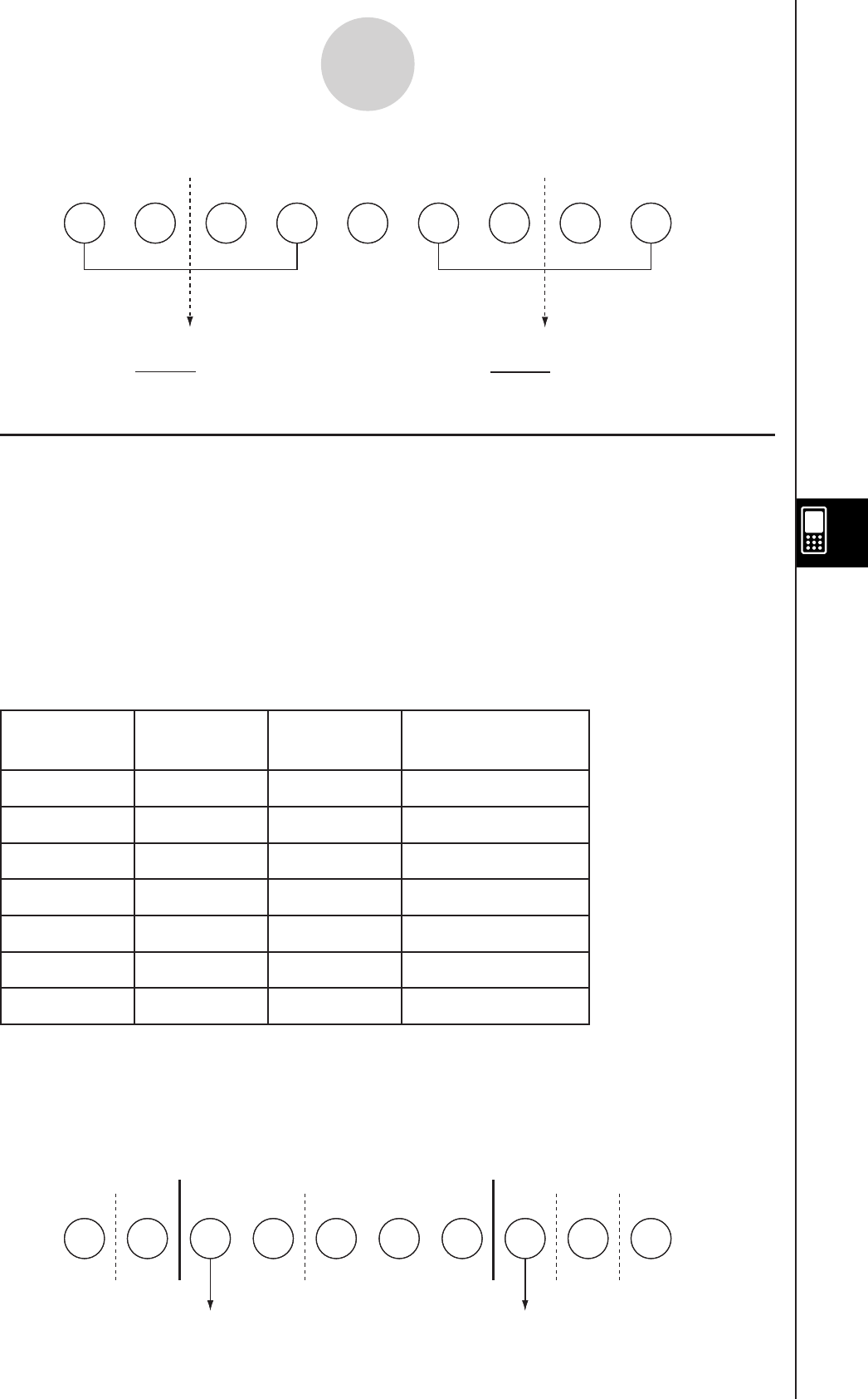
20101001

Center Point Center Point

u Checked: Q1, Q3 on Data

The Q1 and Q3 values for this calculation method are described below.

Q1 = {value of element whose cumulative frequency ratio is greater than 1/4 and nearest to

1/4}

Q3 = {value of element whose cumulative frequency ratio is greater than 3/4 and nearest to

3/4}

The following shows an actual example of the above.

(Number of Elements: 10)

Data Value Frequency Cumulative

Frequency

Cumulative

Frequency Ratio

1 1 1 1/10 = 0.1

2 1 2 2/10 = 0.2

3 2 4 4/10 = 0.4

4 3 7 7/10 = 0.7

5 1 8 8/10 = 0.8

6 1 9 9/10 = 0.9

7 1 10 10/10 = 1.0

• 3 is the value of whose cumulative frequency ratio is greater than 1/4 and nearest to 1/4,

so Q1 = 3.

• 5 is the value of whose cumulative frequency ratio is greater than 3/4 and nearest to 3/4,

so Q3 = 5.

Reference Point (0.25) Reference Point (0.75)

Median

1234567 98

= Q1

2 + 3= Q3

7 + 8

Median

1234567 98

= Q1

2 + 3= Q3

7 + 8

0.1 0.2 0.4 0.7 0.8 0.9 1.0

12 63 3 4 4 4 75

0.1 0.2 0.4 0.7 0.8 0.9 1.0

12 63 3 4 4 4 75

7-7-3

Performing Statistical Calculations

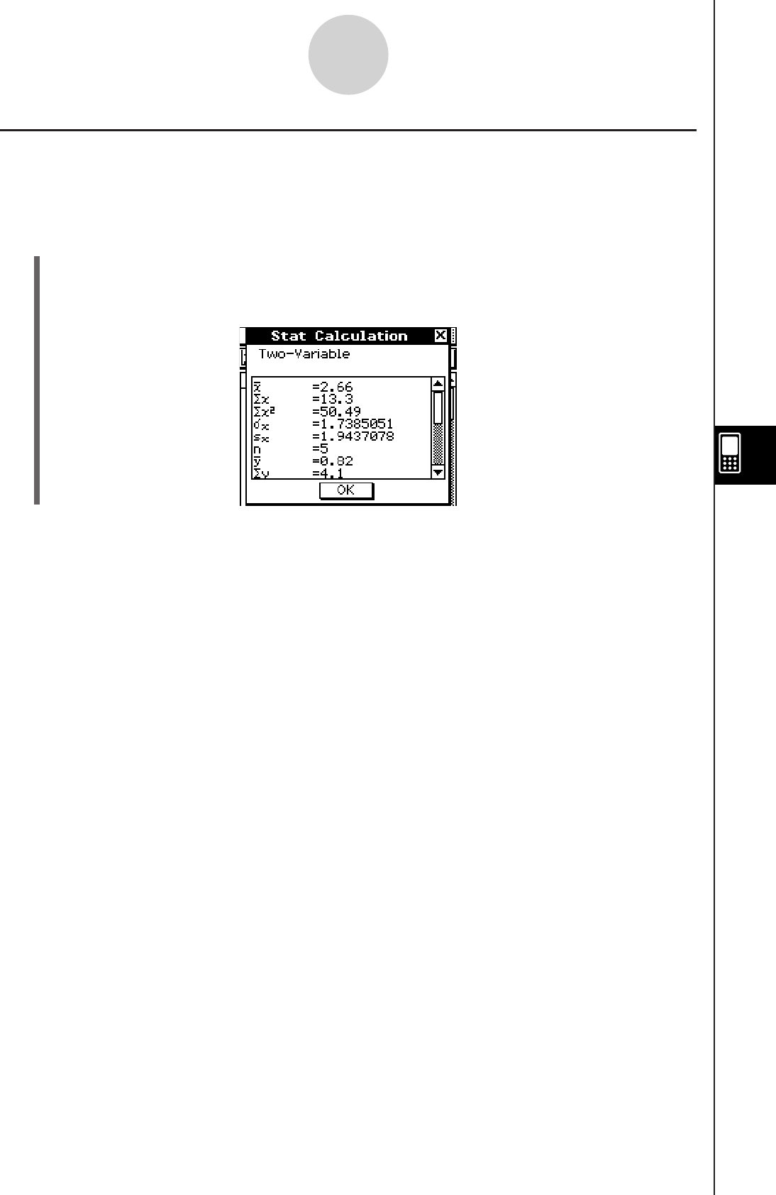
20101001

7-7-4

Performing Statistical Calculations

Viewing Paired-variable Statistical Calculation Results

Besides using a graph, you can also use the following procedure to view the paired-variable

statistics parameter values.

u To display paired-variable calculation results

(1) On the menu bar, tap [Calc] and then [Two-Variable].

(2) On the dialog box that appears, specify the [XList] name and [YList] name, and select

the [Freq] setting (page 7-3-3, 7-3-4).

(3) Tap [OK].

• This displays the Stat Calculation dialog box with the paired-variable statistical calculation

results described below. You can use the scrollbar to scroll the results.

o : sample mean of sample XList data

Σx : sum of XList data

Σx2 : sum of squares of XList data

σx : population standard deviation of XList data

sx : sample standard deviation of XList data

n : sample size

p : sample mean of sample YList data

Σy : sum of YList data

Σy2 : sum of squares of YList data

σy : population standard deviation of YList data

sy : sample standard deviation of YList data

Σxy : sum of products of XList and YList data

minX : minimum of XList data

maxX : maximum of XList data

minY : minimum of YList data

maxY : maximum of YList data

20101001

Viewing Regression Calculation Results

To view regression calculation results, tap [Calc] on the menu bar and then tap the type of

calculation results you want.

• You can also use the [DispStat] option to display the last calculated statistical results. For

details about regression calculation results, see “7-5 Graphing Paired-Variable Statistical

Data”.

Residual Calculation

Residual calculation calculates the distance (residual) between the regression model and an

actual plotted point (y-coordinates) during regression calculations.

u ClassPad Operation

(1)

m I

(2) Input the data you want into a list.

(3) Tap [Calc] and then [Linear Reg].

(4) On the dialog box that appears, tap the [Copy Residual] down arrow button, and then

select [On] or the list into which you want to copy the residual values.

• Values assigned to the “residual” system variable shows the vertical distances between

actually plotted points and the regression model.

• A positive value indicates a plot that is higher than the regression model, while a negative

value indicates a plot that is lower.

• Whenever the [Copy Residual] setting is configured as described above, the ClassPad

automatically assigns residual data to a system variable named “residual” when you

perform a regression calculation. You can use the following procedure to view the current

“residual” system variable values.

7-7-5

Performing Statistical Calculations

Linear regression Linear Reg

Med-Med MedMed Line

Quadratic regression Quadratic Reg

Cubic regression Cubic Reg

Quartic regression Quartic Reg

Logarithmic regression Logarithmic Reg

Exponential regression (

b·x)Exponential Reg

Exponential regression (

x) abExponential Reg

Power regression Power Reg

Sinusoidal regression Sinusoidal Reg

Logistic regression Logistic Reg

Tap this option:To view these calculation results:

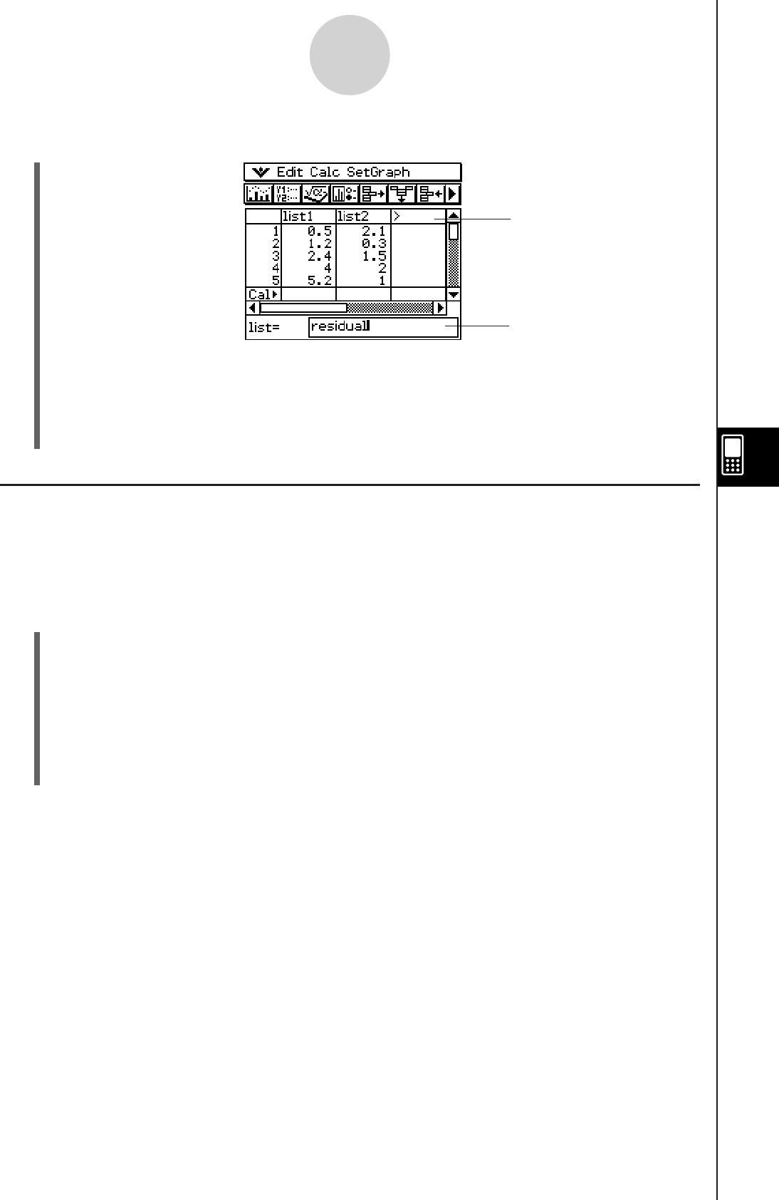
20101001

7-7-6

Performing Statistical Calculations

u To view “residual” system variable values

(1) Tap here.

(2) Tap here, and enter “residual”.

• To input lower-case alpha characters, tap the soft keyboard’s 0 tab.

(3) Tap

Copying a Regression Formula to the Graph & Table Application

You can use the following procedure to copy the calculated result of a regression formula

to the Graph & Table application. There you can use Graph functions to edit and graph the

formula, and perform other operations.

u ClassPad Operation

(1) On the List window menu bar, tap [Calc] and then [Linear Reg].

(2) On the dialog box that appears, tap the [Copy Formula] down arrow button, and then

select the Graph & Table line number (y1 through y20) to which you want to copy the

formula.

(3) Tap [OK].

• This copies the calculated regression expression to the line (y1 through y20) you

selected.

(1)

(2)

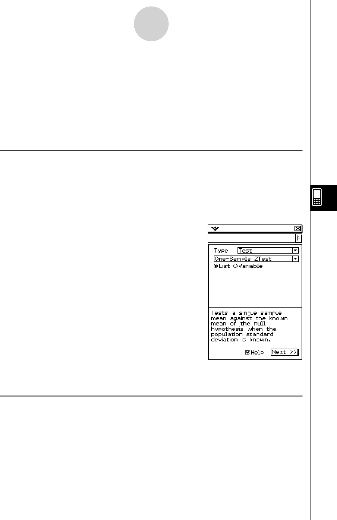
20060301

7-8-1

Test, Confidence Interval, and Distribution Calculations

7-8 Test, Confidence Interval, and Distribution

Calculations

You can use a wizard to perform test, confidence interval and distribution calculations

in the Statistics application or write a program in the Program application. In the Statistics

application, you can perform the calculations using the wizard that you launch by

tapping [Calc] on the menu bar. The following is a general overview of the steps that are

involved.

Statistics Application Calculations

1. Tap [Calc] and then tap [Test], [Interval] or [Distribution].

2. Select the calculation type and data type, then input the necessary values and conditions.

3. Execute the calculation and display its results.

4. Graph the results, if you want.

• You cannot graph interval calculations and inverse distribution calculations.

Selecting the [Help] check box of each wizard will display the

description of the commands, values and calculation results.

For more details and examples, see “7-9 Tests”, “7-10 Confidence intervals” and “7-11

Distributions”.

Program Application Calculations

1. Use statistical commands to build the necessary expressions and write them into a

program.

2. Write the “DispStat” command into the program.

• The “DispStat” is a command for displaying statistical calculation results. Statistical

calculation results cannot be displayed unless the program includes a “DispStat”

command.

3. Save the program.

4. Run the program.

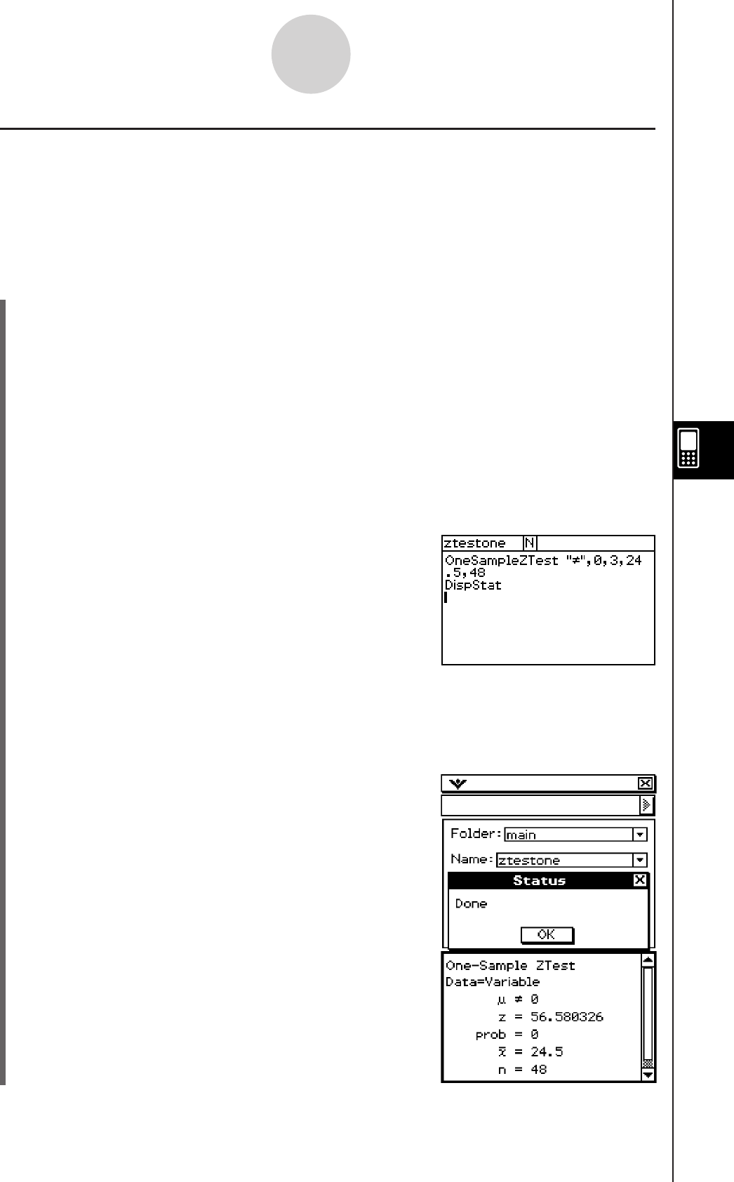
20060301

7-8-2

Test, Confidence Interval, and Distribution Calculations

k Example 1: 1-Sample ZTest

 condition : ≠

0 : 0

 : 3

o : 24.5

n : 48

u ClassPad Operation

(1)

m p

(2) Tap

(3) On the New File dialog box that appears, configure the settings as described below.

Type: Program(Normal)

Folder: Select the name of the folder where you want to save the program you are

creating.

Name: Enter a file name for the program.

Example: ztestone

(4) Tap [OK].

(5) Input commands and values for the statistical expression, and then tap w.

(6) Input the “DispStat” command, and then tap w.

(7) Tap

{ to save the program.

(8) Tap

(9) On the dialog box that appears, tap the [Name] down arrow button, and then tap the

name of the file you input in step (3).

(10) Tap

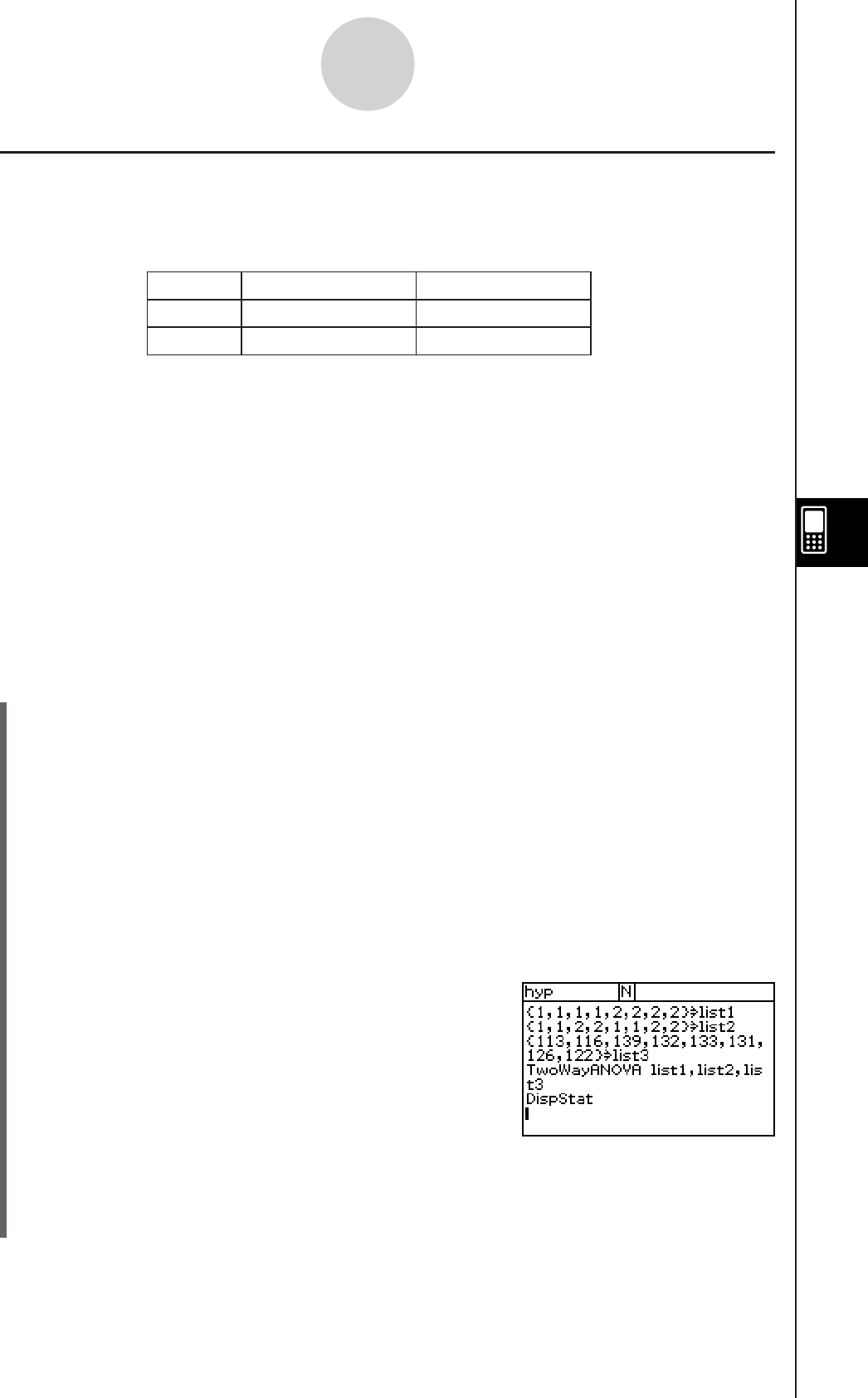
20060301

k Example 2: Two-Way ANOVA

The values in the table below are measurement results that show how the durability of

a metal product is affected by changes in heat treatment time (A) and temperature (B).

Experiments were conducted twice under each condition.

Perform analysis of variance on the null hypotheses listed below, using a 5% level of

significance.

H0 : Change in time does not affect durability.

H0 : Change in treatment temperature does not affect durability.

H0 : Changes in time and treatment temperature do not affect durability.

Use the ClassPad Two-Way ANOVA test to test the above hypotheses. Input the following

measurement data into the indicated lists. This data is from the table above.

list1 (FactorList(A)) = {1,1,1,1,2,2,2,2}

list2 (FactorList(B)) = {1,1,2,2,1,1,2,2}

list3 (DependentList) = {113,116,139,132,133,131,126,122}

u ClassPad Operation

(1) m p

(2) Tap

(3) On the New File dialog box that appears, configure the settings as described below.

Type: Program(Normal)

Folder: Select the name of the folder where you want to save the program you are

creating.

Name: Enter a file name for the program.

Example: hyp

(4) Tap [OK].

(5) Input commands and values for the statistical expression, and then tap w.

(6) Input the “DispStat” command, and then tap w.

(7) Tap

{ to save the program.

(8) Tap

(9) On the dialog box that appears, tap the [Name] down arrow button, and then tap the

name of the file you input in step (3).

Time A1 113, 116

Temperature B1

139, 132

Time A2 133, 131 126, 122

Temperature B2

7-8-3

Test, Confidence Interval, and Distribution Calculations

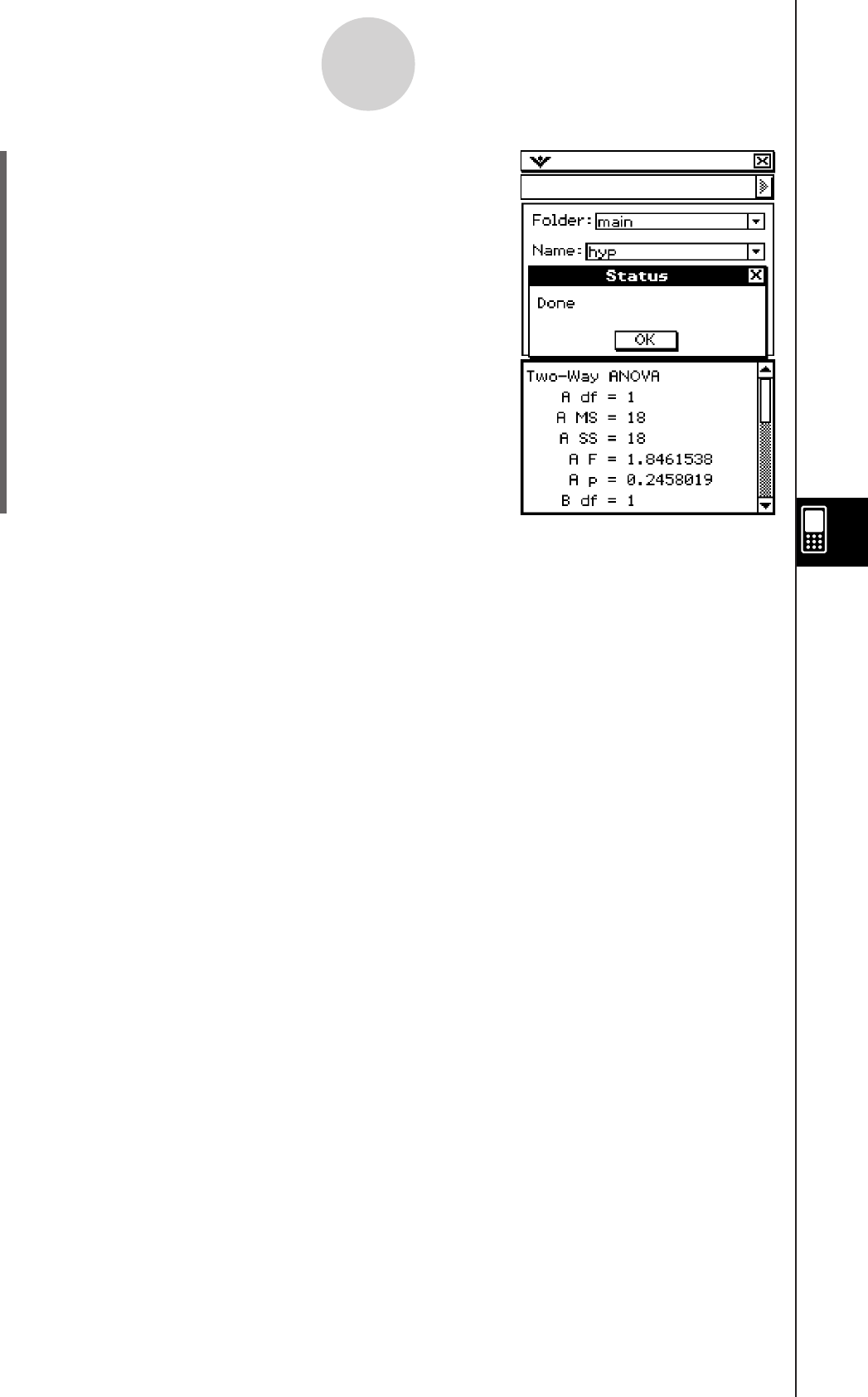
20060301

(10) Tap p.

The above results indicate that altering the time is not significant, altering the temperature is

significant, and interaction between time and temperature is highly significant.

7-8-4

Test, Confidence Interval, and Distribution Calculations

20060301

7-9-1

Te s t s

7-9 Tests

The following is a list of tests, and a description of what each one tests for.

Z Test

DescriptionTest Name

The Z Test provides a variety of different tests based on standard

deviation based tests. They make it possible to test whether or not

a sample accurately represents the population when the standard

deviation of a population (such as the entire population of a

country) is known from previous tests.

1-Sample Z Test

2-Sample Z Test

1-Prop Z Test

2-Prop Z Test

t Test Used instead of the Z Test when the population standard deviation

is unknown.

1-Sample t Test

2-Sample t Test

Linear Regression t Test

Tests a single sample mean against the known mean of the null

hypothesis when the population standard deviation is known.

The normal distribution is used for the 1-sample Z test.

Tests the difference between two means when the standard

deviations of the two populations are known.

The normal distribution is used for the 2-sample Z test.

Tests a single sample proportion against the known proportion of

the null hypothesis.

The normal distribution is used for the 1-Prop Z test.

Tests the difference between two sample proportions.

The normal distribution is used for the 2-prop Z test.

Tests a single sample mean against the known mean of the null

hypothesis when the population standard deviation is unknown.

The t distribution is used for the 1-sample t test.

Tests the difference between two means when the standard

deviations of the two populations are unknown.

The t distribution is used for the 2-sample t test.

Tests the linear relationship between the paired variables (x, y). The

method of least squares is used to determine a and b, which are the

coefficients of the regression formula y = a + bx. The p-value is the

probability of the sample regression slope (b) provided that the null

hypothesis is true,

= 0.

The t distribution is used for the linear regression t test.

χ2 Test Tests the independence of two categorical variables arranged in

matrix form. The χ2 test for independence compares the observed

matrix to the expected theoretical matrix.

The χ2 distribution is used for the χ2 test.

2-Sample F Test Tests the ratio between sample variances of two independent

random samples.

The F distribution is used for the 2-sample F test.

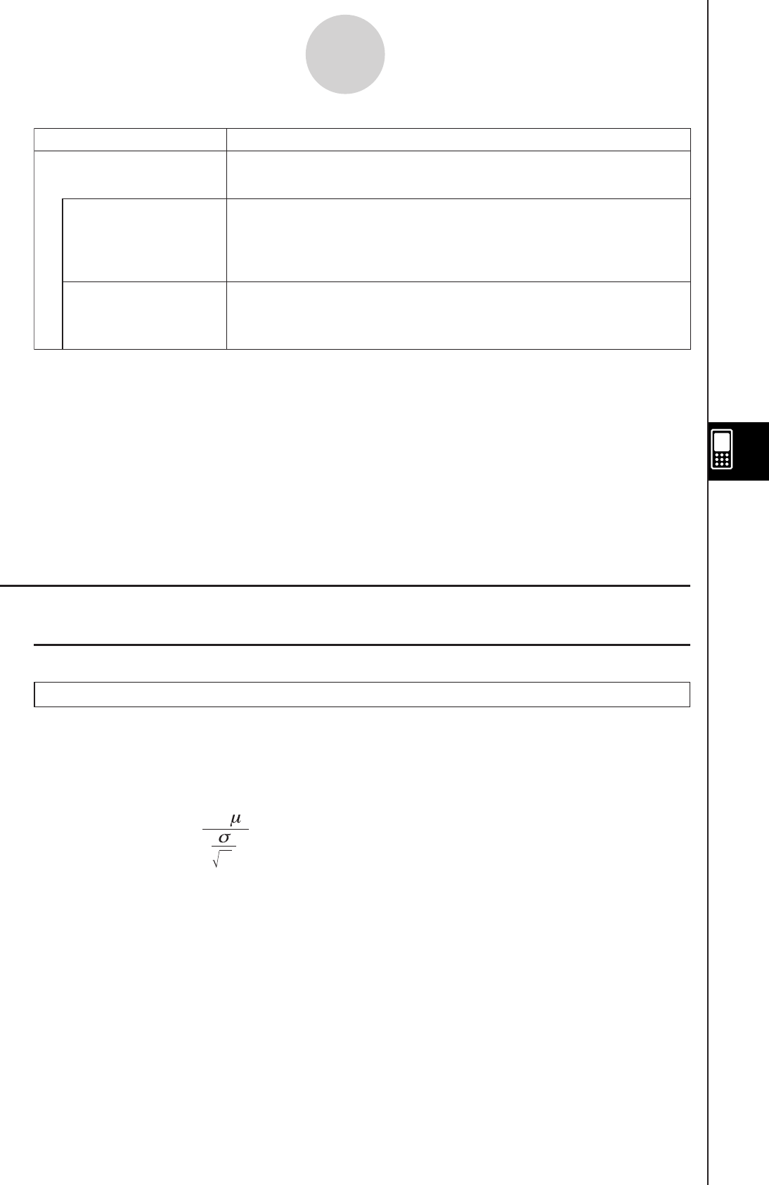
20060301

The following pages explain how to perform various statistical calculations based on the

above principles. Further details about statistical theory and terminology can be found in any

standard statistics textbook.

Tip

• Always make sure you insert one space between a command and its parameters. In the following

examples, spaces are indicated as shown below.

Command: OneSampleZTest



↑

Indicates a space.

Test Command List

k Z Test

1-Sample Z Test

Menu: [Test]-[One-Sample ZTest]

Description: Tests a hypothesis relative to a population mean when population standard

deviation is known. A 1-Sample Z Test is used for normal distribution.

Z = o

—

o : sample mean

0 : assumed population mean

 : population standard deviation

n : sample size

Definition of Terms

 condition : population mean value test conditions (“≠” specifies two-tail test,

“<”specifies lower one-tail test, “>” specifies upper one-tail test.)

0 : assumed population mean

 : population standard deviation ( > 0)

List : data list

Freq : frequency (1 or list name)

o : sample mean

n : sample size (positive integer)

7-9-2

Te s t s

ANOVA Tests the hypothesis that the population means of multiple

populations are equal.

One-Way ANOVA

Two-Way ANOVA

Tests the ratio between the variation in sample means of several

populations compared to variation among the units within the

individual samples in a single factor experiment.

The F distribution is used for the one-way ANOVA test.

Tests the ratio between the variation among the levels compared to

variation within the treatments in a two factor experiment.

The F distribution is used for the two-way ANOVA test.

DescriptionTest Name

20070301

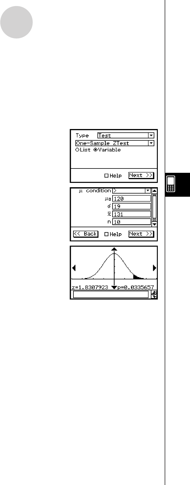
20090601

7-9-3

Te s t s

Calculation Result Output

 ≠ 0 : test condition

z : z value

p : p-value

o: sample mean

sx : sample standard deviation (Displayed only for list format.)

n: sample size

Example

Mean : 131

Sample size : 10

Population standard deviation : 19

Assumed population mean : 120

• Statistics Wizard Operation

(1) On the menu bar, tap [Calc] and then [Test].

(2) Select [One-Sample ZTest] and [Variable],

and then tap [Next >>].

(3) Select the  condition [>] and input values.

(4) Tap [Next >>].

(5) To display the graph, tap $.

u Program, eActivity or Main Application

Command: OneSampleZTest

Command Syntax

Syntax 1 (list format)

“

 condition”, 0 value,  value, List, Freq (or 1)

* “Freq” can be omitted. Doing so sets “1” for “Freq”.

Syntax 2 (parameter format)

“

 condition”, 0 value,  value, o value, n value

Input Example:

Syntax 1 (list format)

OneSampleZTest “≠”,0,1,list1,1

Syntax 2 (parameter format)

OneSampleZTest “>”,120,19,131,10

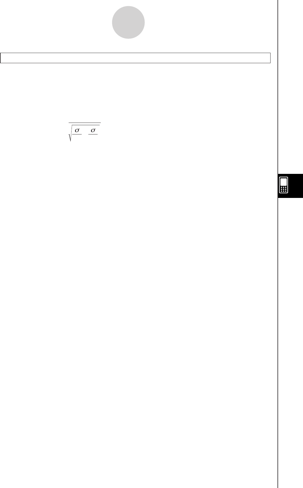
20090601

2-Sample Z Test

Menu: [Test]-[Two-Sample ZTest]

Description: Tests a hypothesis relative to the population mean of two populations when

the standard deviations of the two populations are known. A 2-Sample Z Test

is used for normal distributions.

Z = o1

—

o1 : sample mean of sample 1 data

: sample mean of sample 2 data

1 : population standard deviation of sample 1

2 : population standard deviation of sample 2

1 : size of sample 1

2 : size of sample 2

Definition of Terms

1 condition : population mean value test conditions (“≠” specifies two-tail test,

“<” specifies one-tail test where sample 1 is less than sample 2, “>”

specifies one-tail test where sample 1 is greater than sample 2).

1 : population standard deviation of sample 1 (1 > 0)

2 : population standard deviation of sample 2 (2 > 0)

List(1) : list where sample 1 data is located

List(2) : list where sample 2 data is located

Freq(1) : frequency of sample 1 (1 or list name)

Freq(2) : frequency of sample 2 (1 or list name)

o1 : sample mean of sample 1 data

n1 : size of sample 1 (positive integer)

o2 : sample mean of sample 2 data

n2 : size of sample 2 (positive integer)

Calculation Result Output

1 ≠ 2: test condition

z: z value

p: p-value

o1: sample mean of sample 1 data

o2: sample mean of sample 2 data

sx1: sample standard deviation of sample 1 (Displayed only for list format.)

sx2: sample standard deviation of sample 2 (Displayed only for list format.)

n1: size of sample 1

n2: size of sample 2

7-9-4

Te s t s

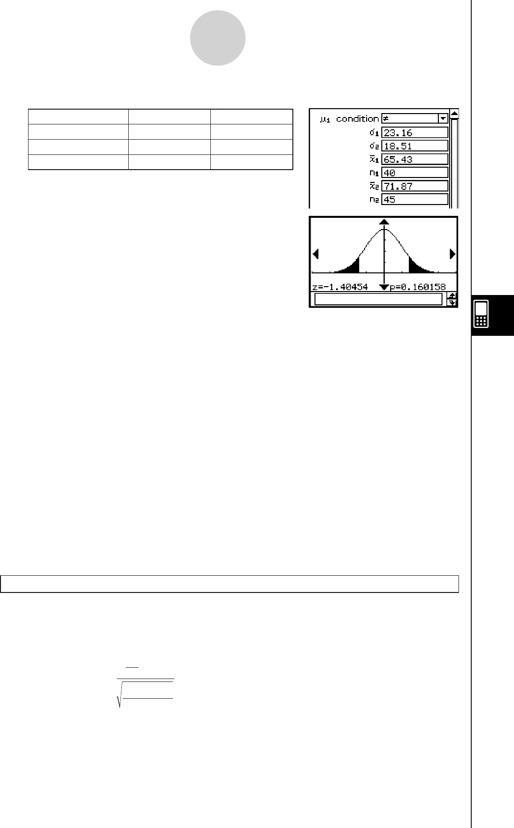
20060301

Example

Sample A Sample B

Size 40 45

Standard deviation 23.16 18.51

Mean 65.43 71.87

• Statistics Wizard Operation

(1) On the menu bar, tap [Calc] and then [Test].

(2) Select [Two-Sample ZTest] and [Variable], and

then tap [Next >>].

(3) Select the 1 condition [≠] and input values.

(4) Tap [Next >>].

(5) To display the graph, tap $.

uProgram, eActivity or Main Application

Command: TwoSampleZTest

Command Syntax

Syntax 1 (list format)

“

1 condition”, 1 value, 2 value, List(1), List(2), Freq(1) (or 1), Freq(2) (or 1)

* “Freq” can be omitted. Doing so sets “1” for “Freq”.

Syntax 2 (parameter format)

“

1 condition”, 1 value, 2 value, o1 value, n1 value, o2 value, n2 value

Input Example:

Syntax 1 (list format)

TwoSampleZTest “≠”,1,1,list1,list2,1,1

Syntax 2 (parameter format)

TwoSampleZTest “≠”,23.16,18.51,65.43,40,71.87,45

1-Prop Z Test

Menu: [Test]-[One-Prop ZTest]

Description: This command tests whether successes achieve a fixed proportion.

A 1-Prop Z Test is used for normal distribution.

Z = n

p0p0)

—

p0 p0 : expected sample proportion

n : sample size

7-9-5

Te s t s

1−

)

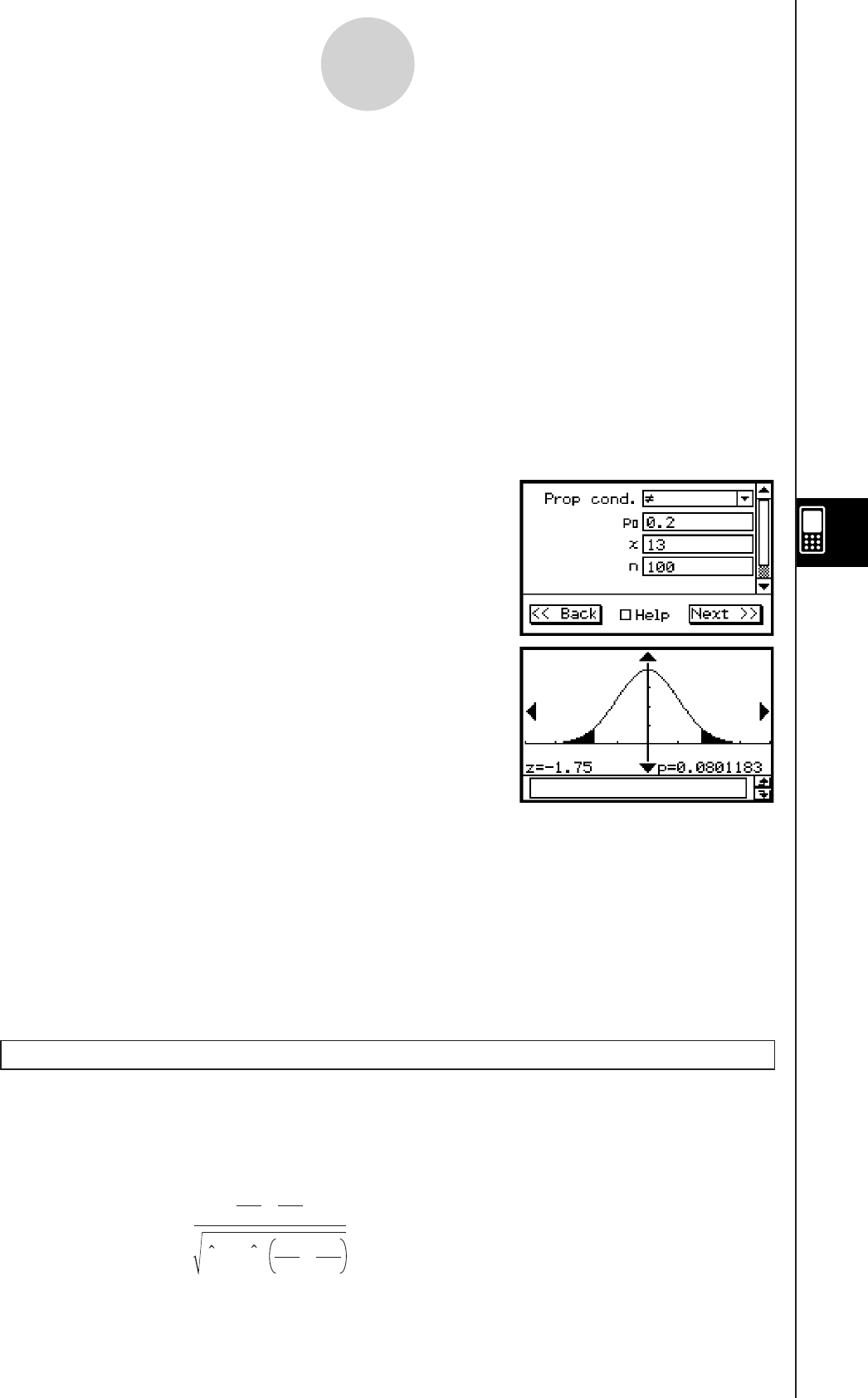
20060301

7-9-6

Te s t s

Definition of Terms

Prop condition : sample proportion test condition (“≠” specifies two-tail test, “<”

specifies lower one-tail test, “>” specifies upper one-tail test.)

p0 : expected sample proportion (0 < p0 < 1)

x : sample value (integer, x > 0)

n : sample size (positive integer)

Calculation Result Output

Prop≠0.5 : test condition

z: z value

p: p-value

ˆp

: estimated sample proportion

n: sample size

Example

Data : 13

Sample size : 100

Expected proportion : 20%

• Statistics Wizard Operation

(1) On the menu bar, tap [Calc] and then [Test].

(2) Select [One-Prop ZTest] and then tap [Next >>].

(3) Select Prop condition [≠] and input values.

(4) Tap [Next >>].

(5) To display the graph, tap $.

uProgram, eActivity or Main Application

Command: OnePropZTest

Command Syntax

“Prop condition”,

p0 value, x value, n value

Input Example:

OnePropZTest “≠”,0.2,13,100

2-Prop Z Test

Menu: [Test]-[Two-Prop ZTest]

Description: This command compares the proportion of successes for two populations.

A 2-Prop Z Test is used for normal distribution.

Z = n1

x1n2

—

p(1

—

p )n1

x1 : data value of sample 1

x2 : data value of sample 2

n1 : size of sample 1

n2 : size of sample 2

p : estimated sample proportion

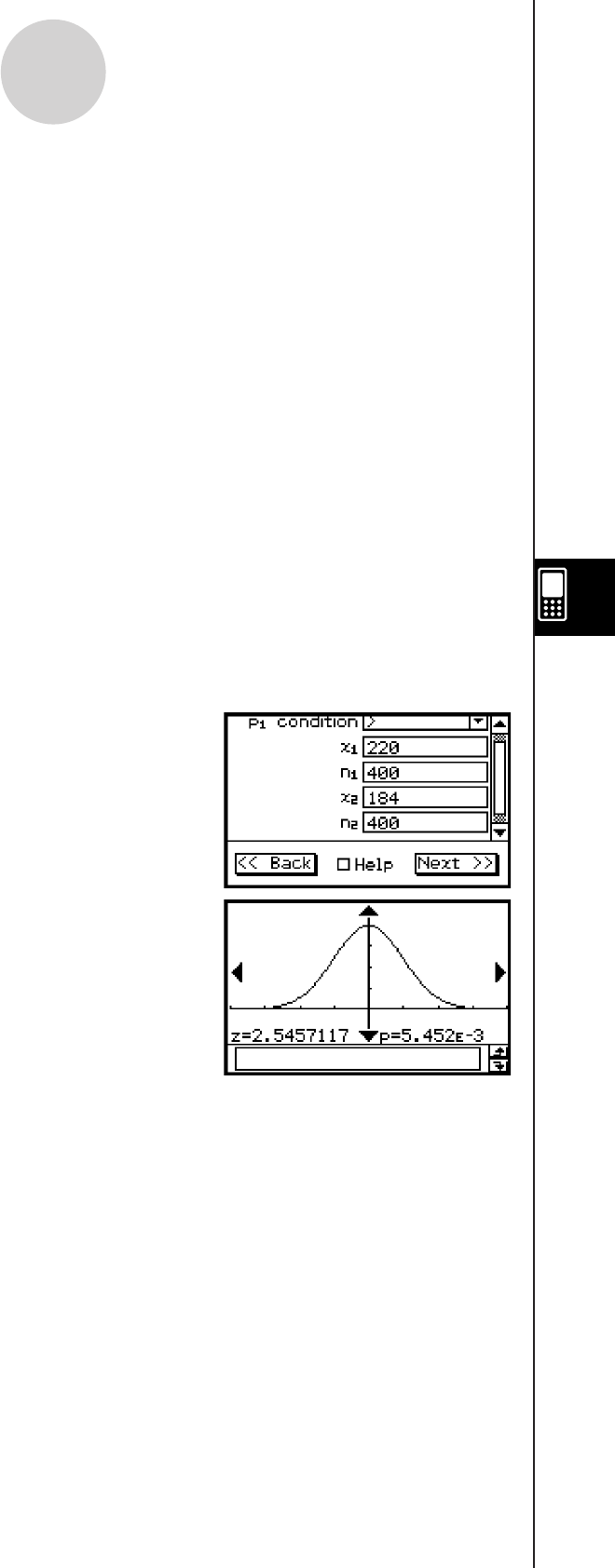
20090601

Definition of Terms

p1 condition : sample proportion test conditions (“≠” specifies two-tail test, “<”

specifies one-tail test where sample 1 is smaller than sample 2, “>”

specifies one-tail test where sample 1 is greater than sample 2.)

x1 : data value (integer, x1 > 0) of sample 1

n1 : size of sample 1 (positive integer)

x2 : data value (integer, x2 > 0) of sample 2

n2 : size of sample 2 (positive integer)

Calculation Result Output

p1>p2 : test condition

z : z value

p : p-value

ˆp 1 : estimated proportion of sample 1

ˆp 2 : estimated proportion of sample 2

ˆp : estimated sample proportion

n1 : size of sample 1

n2 : size of sample 2

Example

Data1 : 220 , sample size : 400

Data2 : 184 , sample size : 400

• Statistics Wizard Operation

(1) On the menu bar, tap [Calc] and then [Test].

(2) Select [Two-Prop ZTest] and then tap [Next >>].

(3) Select p1 condition [>] and input values.

(4) Tap [Next >>].

(5) To display the graph, tap $.

uProgram, eActivity or Main Application

Command: TwoPropZTest

Command Syntax

“

p1 condition”, x1 value, n1 value, x2 value, n2 value

Input Example:

TwoPropZTest “>”,220,400,184,400

7-9-7

Te s t s

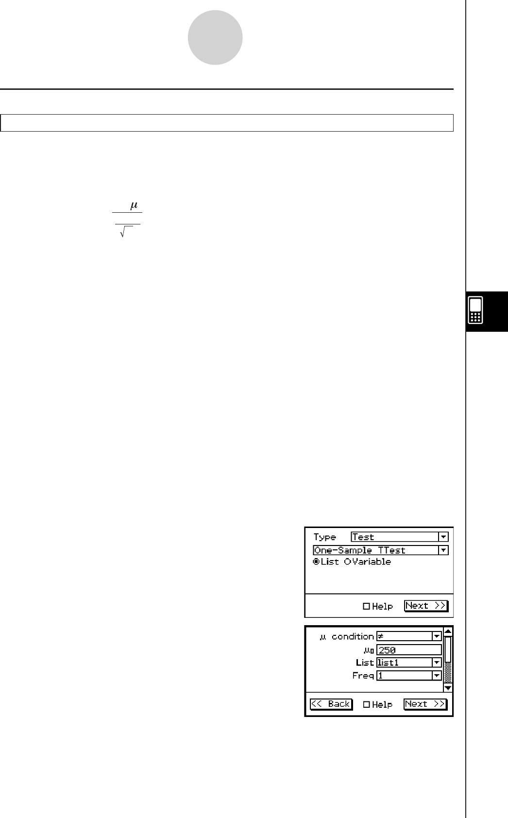
20090601

k t Test

1-Sample t Test

Menu: [Test]-[One-Sample TTest]

Description: Tests a hypothesis relative to a population mean when population standard

deviation is unknown. A 1-Sample t Test is used for t distribution.

o : sample mean

0 : assumed population mean

x : sample standard deviation

n : sample size

Definition of Terms

 condition : population mean value test conditions (“≠” specifies two-tail test, “<”

specifies lower one-tail test, “>” specifies upper one-tail test.)

0 : assumed population mean

List : data list

Freq : frequency (1 or list name)

o : sample mean

sx : sample standard deviation (sx > 0)

n : sample size (positive integer)

Calculation Result Output

 ≠ 11.3 : test condition

t : t value

p : p-value

o : sample mean

sx : sample standard deviation

n : sample size

Example 1 (calculation with list)

List : { 330, 240, 260, 390, 400, 360, 200, 180, 300 }

Assumed population mean : 250

• Statistics Wizard Operation

(1) Input the data into [list1] in the Stat Editor.

(2) On the menu bar, tap [Calc] and then [Test].

(3) Select [One-Sample TTest] and [List], and then

tap [Next >>].

(4) Select the  condition [≠] and input 0 250.

(5) Select List [list1] and Freq [1].

(6) Tap [Next >>].

t = o

—

t = o

—

7-9-8

Te s t s

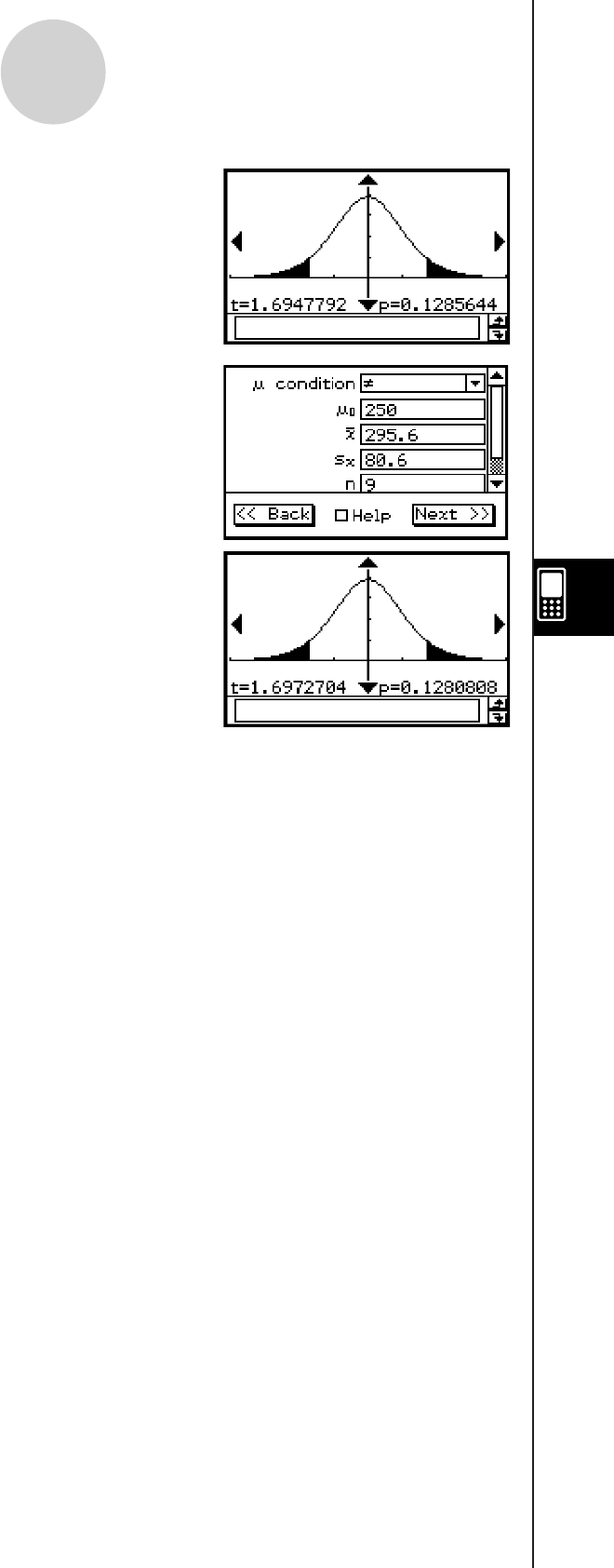
20090601

(7) To display the graph, tap $.

Example 2 (calculation with parameter)

Standard deviation : 80.6

Mean : 295.6

Sample size : 9

Assumed population mean : 250

• Statistics Wizard Operation

(1) On the menu bar, tap [Calc] and then [Test].

(2) Select [One-Sample TTest] and [Variable], and

then tap [Next >>].

(3) Select the  condition [≠] and input values.

(4) Tap [Next >>].

(5) To display the graph, tap $.

uProgram, eActivity or Main Application

Command: OneSampleTTest

Command Syntax

Syntax 1 (list format)

“

 condition”, 0 value, List, Freq (or 1)

* “Freq” can be omitted. Doing so sets “1” for “Freq”.

Syntax 2 (parameter format)

“

 condition”, 0 value, o value, sx value, n value

Input Example:

Syntax 1 (list format)

OneSampleTTest “≠”,250,list1,1

Syntax 2 (parameter format)

OneSampleTTest “≠”,250,295.6,80.6,9

7-9-9

Te s t s

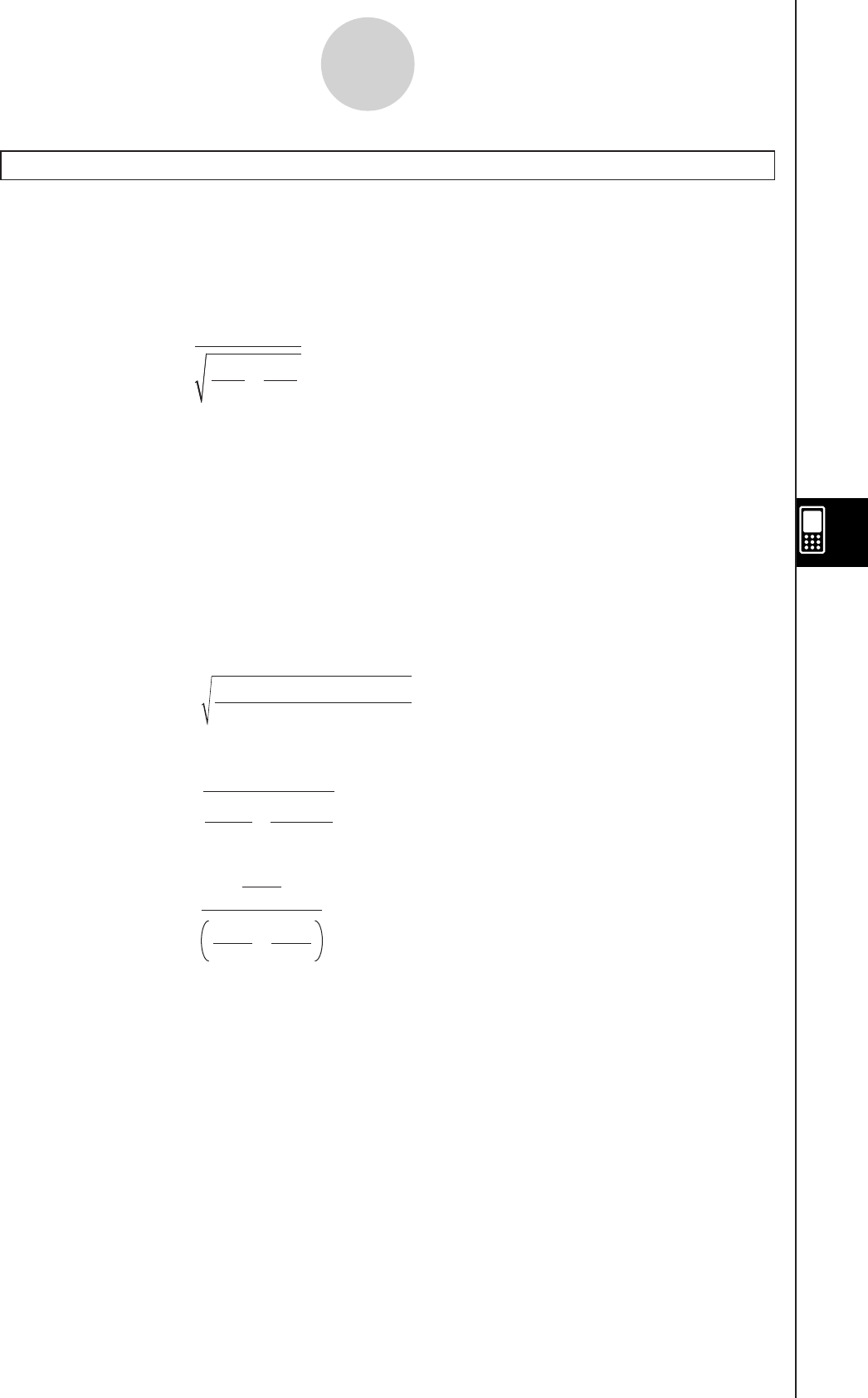
20090601

2-Sample t Test

Menu: [Test]-[Two-Sample TTest]

Description: This command compares the population means of two populations when

population standard deviation is unknown. A 2-Sample t Test is used for t

distribution.

o1 : sample mean of sample 1 data

o2 : sample mean of sample 2 data

sx1 : sample standard deviation of sample 1

sx2 : sample standard deviation of sample 2

n1 : size of sample 1

n2 : size of sample 2

This formula is applicable when the population standard deviations of the two

populations are not equal. The denominator is different when the population

standard deviations are equal.

The

t distribution degrees of freedom df and sp differ according to whether the

population standard deviations of the two populations are equal.

When the two population standard deviations are equal (pooled)

df = n1 + n2 – 2

+ n

– 2

–1)s

+(n

–1)s

When the two population standard deviations are not equal (not pooled)

df = 1

–1 +(1–C )

–1

C = n

Definition of Terms

1 condition : sample mean value test conditions (“≠” specifies two-tail test, “<”

specifies one-tail test where sample 1 is smaller than sample 2, “>”

specifies one-tail test where sample 1 is greater than sample 2.)

List(1) : list where sample 1 data is located

List(2) : list where sample 2 data is located

Freq(1) : frequency of sample 1 (1 or list name)

Freq(2) : frequency of sample 2 (1 or list name)

Pooled : On or Off

o1 : sample mean of sample 1 data

sx1 : sample standard deviation of sample 1 (sx1 > 0)

n1 : size of sample 1 (positive integer)

o2 : sample mean of sample 2 data

sx2 : sample standard deviation of sample 2 (sx2 > 0)

n2 : size of sample 2 (positive integer)

t = o1

—

sx12

sx22

t = o1

—

sx12

sx22

7-9-10

Te s t s

20090601

7-9-11

Te s t s

Calculation Result Output

1 ≠ 2 : test condition

t : t value

p : p-value

df : degrees of freedom

o1 : sample mean of sample 1 data

o2 : sample mean of sample 2 data

sx1 : sample standard deviation of sample 1

sx2 : sample standard deviation of sample 2

sp : Pooled sample standard deviation (Displayed only when pooling is

turned on.)

n1 : size of sample 1

n2 : size of sample 2

Example

list1 : {−8522, 316, −9001, 6470, 8956, 4348, 8571,

2142, −7139, 9925, 1260}

list2 : {176, 5498, 4830, 9457, 6486, 9607, −8334,

−1771, 7919, −2997}

• Statistics Wizard Operation

(1) Input the data into [list1] and [list2] in the Stat Editor.

(2) On the menu bar, tap [Calc] and then [Test].

(3) Select [Two-Sample TTest] and [List], and then tap

[Next >>].

(4) Select the 1 condition [<].

(5) Select List(1) [list1], List(2) [list2], Freq(1) [1],

Freq(2) [1] and Pooled [Off].

(6) Tap [Next >>].

(7) To display the graph, tap the $.

uProgram, eActivity or Main Application

Command: TwoSampleTTest

Command Syntax

Syntax 1 (list format)

“

1 condition”, List(1), List(2), Freq(1) (or 1), Freq(2) (or 1), Pooled condition (On

or Off)

* “Freq” can be omitted. Doing so sets “1” for “Freq”.

* “Pooled” can be omitted. Doing so sets “Off” for “Pooled”.

Syntax 2 (parameter format)

“

1 condition”, o1 value, sx1 value, n1 value, o2 value, sx2 value, n2 value, Pooled

condition (On or Off)

* “Pooled” can be omitted. Doing so sets “Off” for “Pooled”.

20090601

Input Example:

Syntax 1 (list format)

TwoSampleTTest “<”,list1,list2,1,1,Off

Syntax 2 (parameter format)

TwoSampleTTest “≠”,107.5,0.78,10,97.5,0.65,12,Off

Linear Regression t Test

Menu: [Test]-[Linear Reg TTest]

Description: This command treats two groups of data as paired variables (x, y). The

method of least squares is used to determine the most appropriate pair for the

a, b coefficients of the regression formula y = a + b.x. It also determines the

correlation coefficient and t value, and calculates the strength of the

relationship between x and y.

a : regression constant term (y-intercept)

b : regression coefficient (slope)

n : sample size (n > 3)

r : correlation coefficient

r2 : coefficient of determination

Definition of Terms

 &

condition : test conditions (“≠” specifies two-tail test, “<” specifies lower one-

tail test, “>” specifies upper one-tail test.)

XList : x-data list

YList : y-data list

Freq : frequency (1 or list name)

Calculation Result Output

 ≠ 0 &

≠ 0 : test condition

t : t value

p : p-value

df : degrees of freedom

a : regression constant term (y-intercept)

b : regression coefficient (slope)

se : standard error of estimation

r : correlation coefficient

r2 : coefficient of determination

7-9-12

Te s t s

b = Σ( x – o)( y – p)

i=1

Σ(x – o)

i=1

a = p – b.ot = r n – 2

1 – r

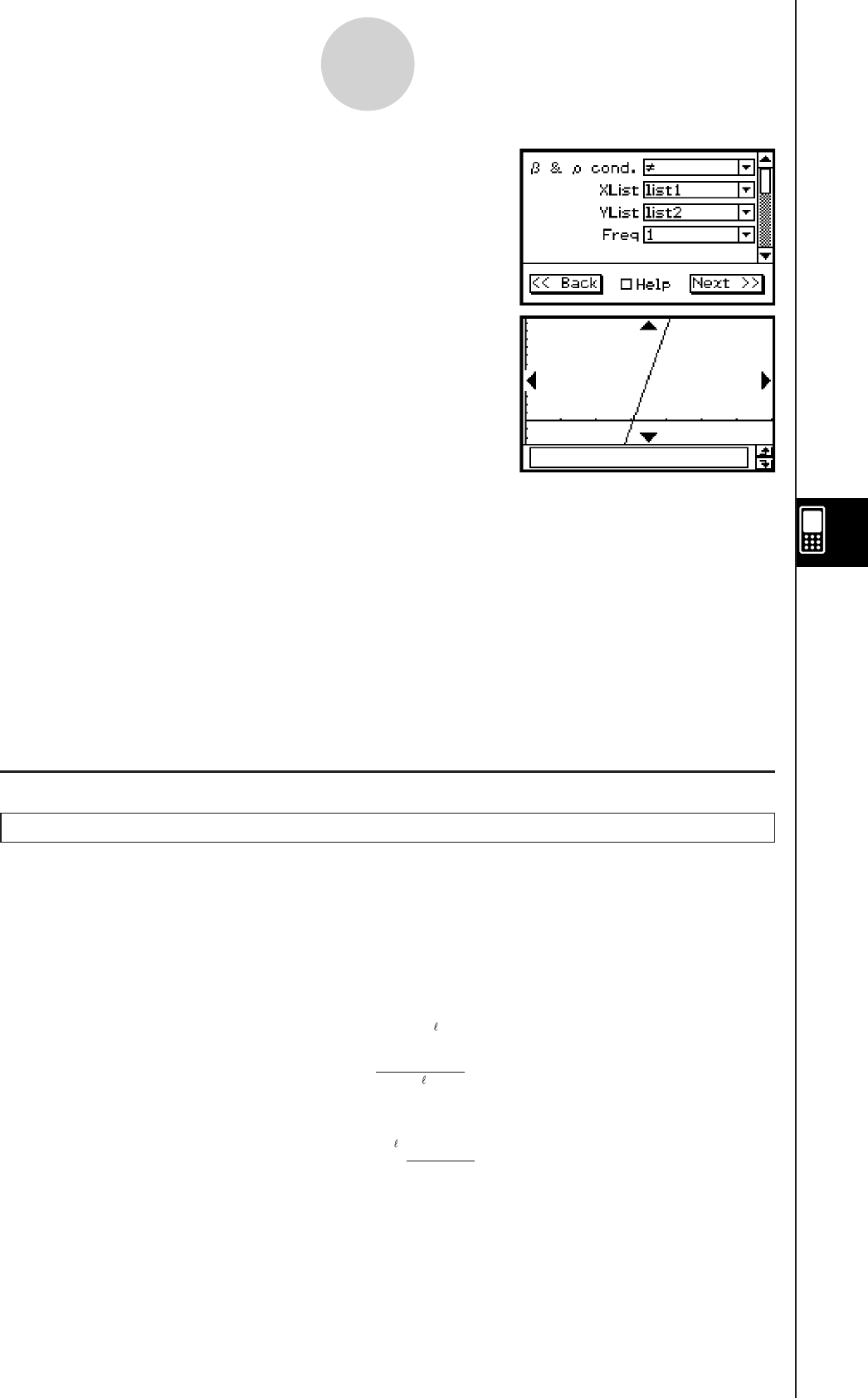
20060301

7-9-13

Te s t s

Example

list1 : { 38, 56, 59, 64, 74 }

list2 : { 41, 63, 70, 72, 84 }

• Statistics Wizard Operation

(1) Input the data into [list1] and [list2] in the Stat Editor.

(2) On the menu bar, tap [Calc] and then [Test].

(3) Select [Linear Reg TTest] and then tap [Next >>].

(4) Select the  &

condition [≠].

(5) Select XList [list1], YList [list2] and Freq [1].

(6) Tap [Next >>].

(7) To display the graph, tap $.

uProgram, eActivity or Main Application

Command: LinRegTTest

Command Syntax

“

 &

condition”, XList, YList, Freq (or 1)

* “Freq” can be omitted. Doing so sets “1” for “Freq”.

Input Example

LinRegTTest “≠”,list1,list2,1

k χ2 Test

χ2 Test

Menu: [Test]-[χ2 Test]

Description: This command tests hypotheses concerning the proportion of samples

included in each of a number of independent groups. The χ2 Test command is

used in the case of dichotomous variables, which are variables that have only

two possible values (such as “yes” or “no”).

Expected Frequencies

i=1

j=1

ΣΣ

i=1

j=1

Definition of Terms

Observed matrix: name of matrix containing observed values (positive integers in

all cells for 2 × 2 and larger matrices; positive real numbers for

one row matrices)

χ2 = ΣΣ Fij

i=1

k(xij – Fij)2

j=1

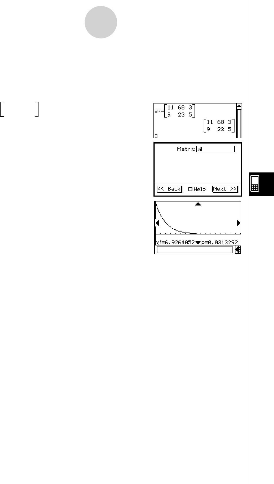
20090601

7-9-14

Tests

Calculation Result Output

χ2 : χ2 value

p : p-value

df : degrees of freedom

Example

a = 11 68 3

9 23 5

• Statistics Wizard Operation

(1)

(2) Input the matrix and assign it to variable a.

(3)

m I

(4) On the menu bar, tap [Calc] and then [Test].

(5) Select [χ2 Test] and then tap [Next >>].

(6) Input matrix a in the Matrix dialog box.

(7) Tap [Next >>].

(8) To display the graph, tap $.

uProgram, eActivity or Main Application

Command: ChiTest

Command Syntax

Observed matrix

Input Example:

ChiTest matrixa

Tip

• The minimum size of the matrix is 1 × 2. An error occurs if the matrix has only one row.

• The result of the expected frequency calculation is stored in the system variable named “Expected”.

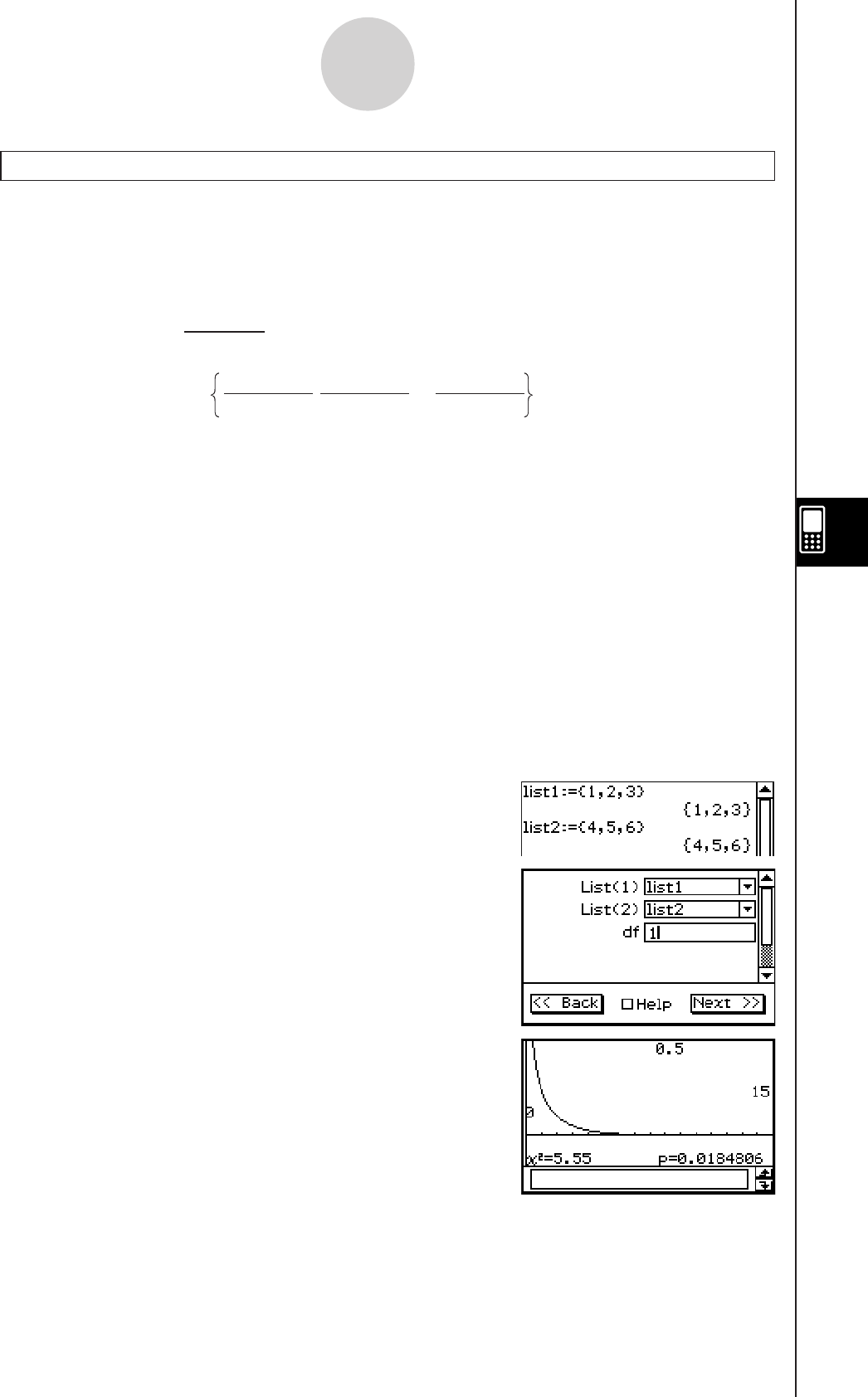
20090601

7-9-15

Tests

χ2 GOF Test

Menu: [Test]-[χ2 GOF Test]

Description: This command tests whether the frequency of sample data fits a certain

distribution. For example, it can be used to determine conformance with

normal distribution or binomial distribution.

Oi : The i-th element of the observed list

Ei : The i-th element of the expected list

Definition of Terms

Observed list : name of list containing observed counts (all cells positive integers)

Expected list : name of list that is for saving expected frequency

df : degrees of freedom

Calculation Result Output

χ2 : χ2 value

p : p-value

df : degrees of freedom

Contrib : name of list specifying the contribution of each observed count

Example

list1 = {1,2,3}, list2 = {4,5,6}, df = 1

• Statistics Wizard Operation

(1) J

(2) Input the list1 and list2.

(3) m I

(4) On the menu bar, tap [Calc] and then [Test].

(5) Select [χ2 GOF Test] and then tap [Next >>].

(6) Select List(1) [list1], List(2) [list2] and input df 1.

(7) Tap [Next >>].

(8) To display the graph, tap $.

uProgram, eActivity or Main Application

Command: ChiGOFTest

Command Syntax

Observed list, Expected list, df

Input Example:

ChiGOFTest list1, list2, 1

Tip

• The calculation results χ2, p, df, and Contrib are stored in the system variables named “χ2value”,

“prob”, “df”, and “Contrib” respectively.

χ2 = (Oi − Ei )2

Contrib = (O1 − E1 )2

(O2 − E2 )2

(Ok − Ek )2

...

χ2 = (Oi − Ei )2

Contrib = (O1 − E1 )2

(O2 − E2 )2

(Ok − Ek )2

...

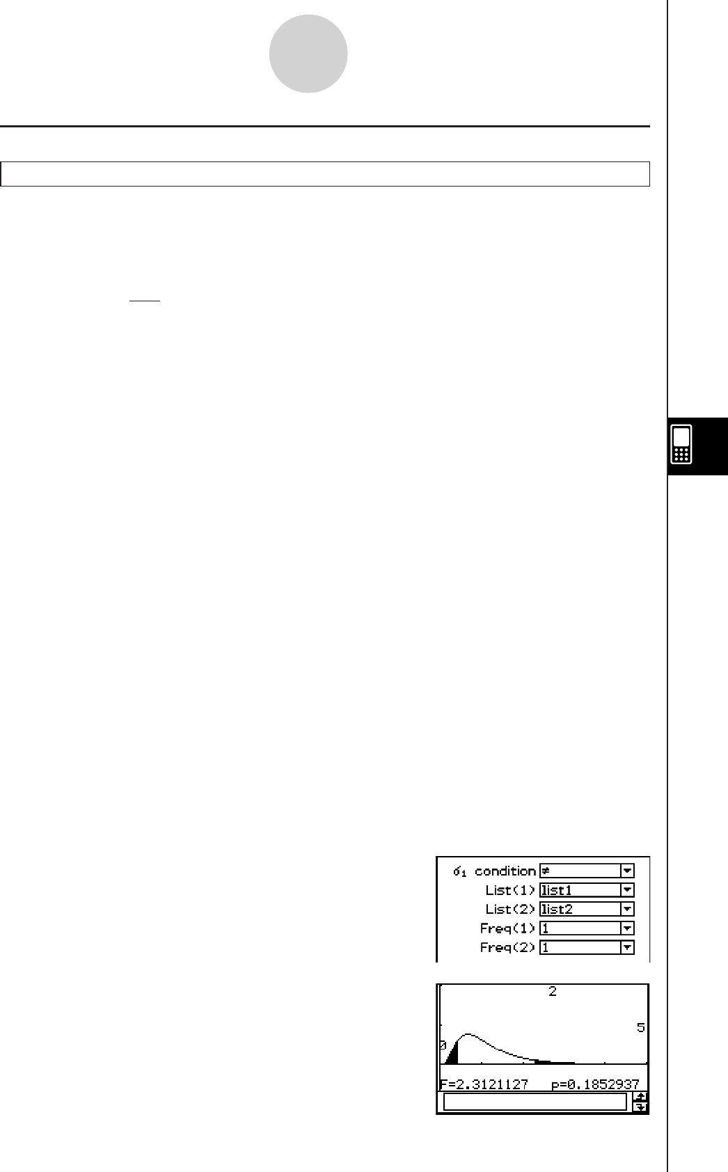
20101001

7-9-16

Tests

k 2-Sample F Test

2-Sample F Test

Menu: [Test]-[Two-Sample FTest]

Description: This command tests hypotheses concerning the ratio of the population

variance of two populations. A 2-Sample F Test uses F distribution.

Definition of Terms

1 condition: population standard deviation test conditions (“≠” specifies two-

tail test, “<” specifies one-tail test where sample 1 is smaller than

sample 2, “>” specifies one-tail test where sample 1 is greater than

sample 2.)

List(1) : list where sample 1 data is located

List(2) : list where sample 2 data is located

Freq(1) : frequency of sample 1 (1 or list name)

Freq(2) : frequency of sample 2 (1 or list name)

sx1 : sample standard deviation of sample 1 (sx1 > 0)

n1 : size of sample 1 (positive integer)

sx2 : sample standard deviation of sample 2 (sx2 > 0)

n2 : size of sample 2 (positive integer)

Calculation Result Output

1 ≠ 2 : test condition

F : F value

p : p-value

o1 : sample mean of sample 1 data (Displayed only for list format.)

o2 : sample mean of sample 2 data (Displayed only for list format.)

sx1 : sample standard deviation of sample 1

sx2 : sample standard deviation of sample 2

n1 : size of sample 1

n2 : size of sample 2

Example

list1 : { 7, −4, 18, 17, −3, −5, 1, 10, 11, −2, −3 }

list2 : { −1, 12, −1, −3, −3, 3, −5, 5, 2, −11, −1, −3 }

• Statistics Wizard Operation

(1) Input the data into [list1] and [list2] in the Stat Editor.

(2) On the menu bar, tap [Calc] and then [Test].

(3) Select [Two-Sample FTest] and [List], and then tap

[Next >>].

(4) Select the 1 condition [≠].

(5) Select List(1) [list1], List(2) [list2], Freq(1) [1] and

Freq(2) [1].

(6) Tap [Next >>].

(7) To display the graph, tap $.

F = sx12

sx22

F = sx12

sx22

20090601

7-9-17

Tests

uProgram, eActivity or Main Application

Command: TwoSampleFTest

Command Syntax

Syntax 1 (list format)

“

1 condition”, List(1), List(2), Freq(1) (or 1), Freq(2) (or 1)

* “Freq” can be omitted. Doing so sets “1” for “Freq”.

Syntax 2 (parameter format)

“

1 condition”, sx1 value, n1 value, sx2 value, n2 value

Input Example

Syntax 1 (list format)

TwoSampleFTest “≠”,list1,list2,1,1

Syntax 2 (parameter format)

TwoSampleFTest “≠”,1.94,10,2.12,15

k ANOVA

One-Way ANOVA

Menu: [Test]-[One-Way ANOVA]

Description: This command tests the hypothesis that the population means of multiple

populations are equal. It compares the mean of one or more groups based on

one independent variable or factor.

Definition of Terms

FactorList(A): list where levels of Factor A are located

DependentList: list where sample data is located

Calculation Result Output

A df : df of Factor A

A MS : MS of Factor A

A SS : SS of Factor A

A F : F value of Factor A

A p : p-value of Factor A

Errdf : df of error

ErrMS : MS of error

ErrSS : SS of error

df : degrees of freedom

SS : sum of squares

MS : mean square

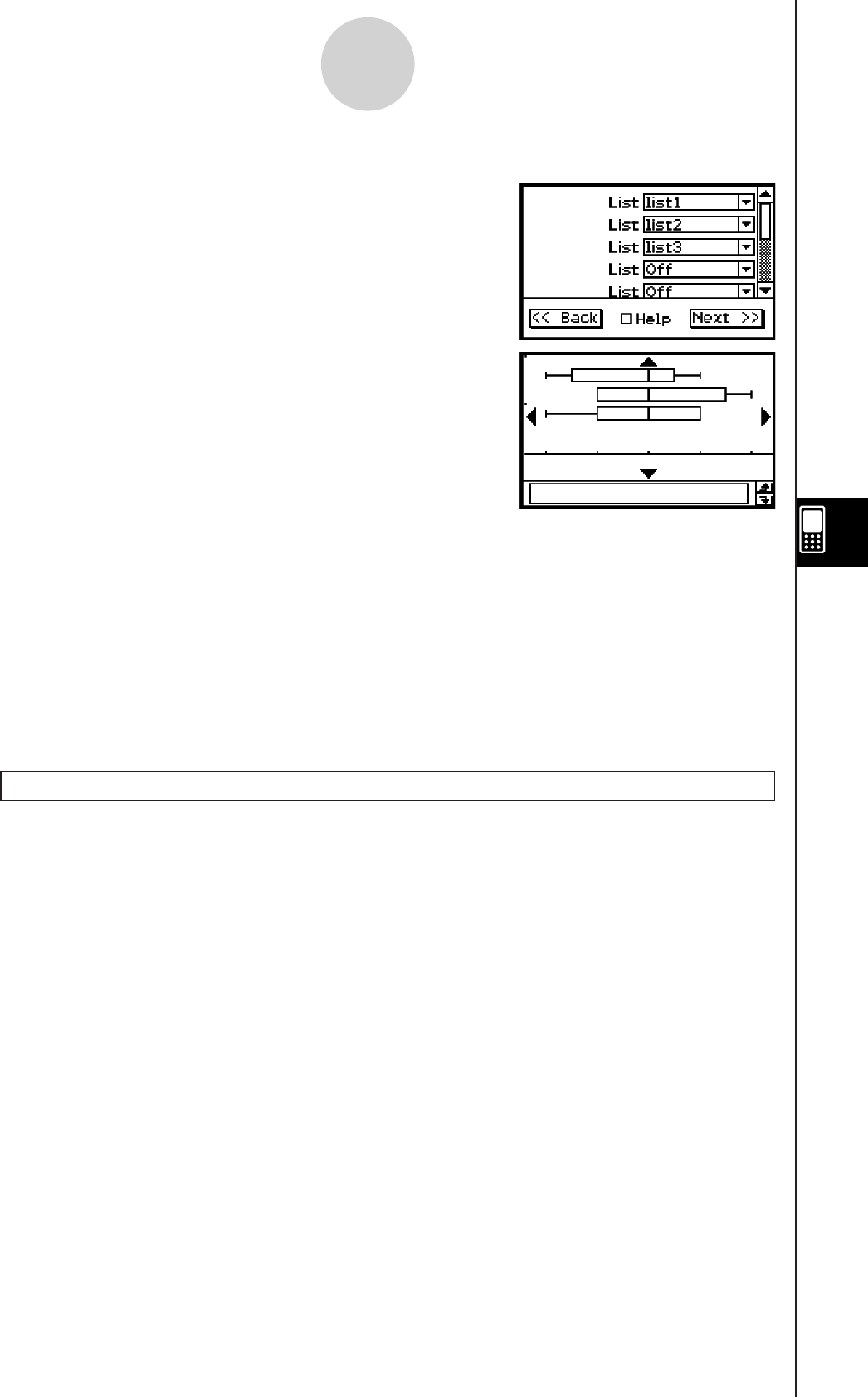
20090601

7-9-18

Te s t s

Example

list1 : { 7, 4, 6, 6, 5 }

list2 : { 6, 5, 5, 8, 7 }

list3 : { 4, 7, 6, 7, 6 }

• Statistics Wizard Operation

(1) Input the data into [list1], [list2] and [list3] in the Stat

Editor.

(2) On the menu bar, tap [Calc] and then [Test].

(3) Select [One-Way ANOVA] and then tap [Next >>].

(4) Select Lists [list1], [list2] and [list3].

(5) Tap [Next >>].

(6) To display the graph, tap $.

uProgram, eActivity or Main Application

Command: OneWayANOVA

Command Syntax

FactorList(A), DependentList

Input Example

list1:{1,1,1,1,1,2,2,2,2,2,3,3,3,3,3}

list2:{7,4,6,6,5,6,5,5,8,7,4,7,6,7,6}

OneWayANOVA list1,list2

Two-Way ANOVA

Menu: [Test]-[Two-Way ANOVA]

Description: This command tests the hypothesis that the population means of multiple

populations are equal. It examines the effect of each variable independently as

well as their interaction with each other based on a dependent variable.

Definition of Terms

FactorList(A) : list where levels of Factor A are located

FactorList(B) : list where levels of Factor B are located

DependentList : list where sample data is located

Calculation Result Output

A df : df of Factor A

A MS : MS of Factor A

A SS : SS of Factor A

A F : F value of Factor A

A p : p-value of Factor A

B df : df of Factor B

B MS : MS of Factor B

B SS : SS of Factor B

B F : F value of Factor B

B p : p-value of Factor B

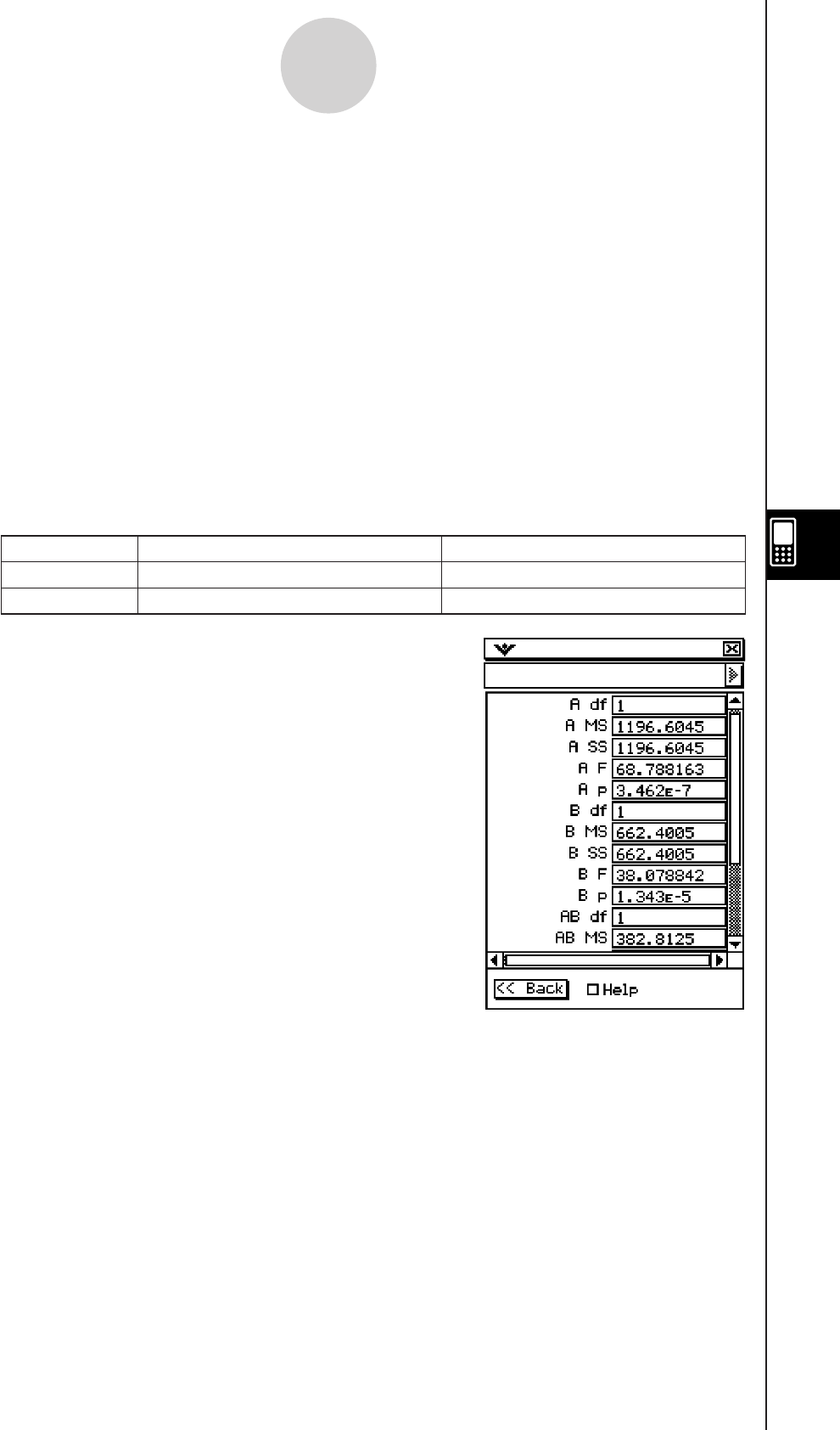
20090601

AB df : df of Factor A × Factor B

AB MS : MS of Factor A × Factor B

AB SS : SS of Factor A × Factor B

AB F : F value of Factor A × Factor B

AB p : p-value of Factor A × Factor B

Note that “AB df ”, “AB MS

”, “AB SS

”, “AB F

”, and “AB p” are not

displayed if there are no repeated data pairs.

Errdf : df of error

ErrMS : MS of error

ErrSS : SS of error

df : degrees of freedom

SS : sum of squares

MS : mean square

Example

Factor B1 Factor B2

Factor A1 14.5, 11, 10.8, 14.3, 10 (list1) 16.5, 18.4, 12.7, 14, 12.8 (list2)

Factor A2 21, 18.5, 15.2, 17.9, 21.6 (list3) 43.2, 35.2, 28.7, 41.3, 47.1 (list4)

• Statistics Wizard Operation

(1) Input the data into [list1] through [list4] in the Stat

Editor.

(2) On the menu bar, tap [Calc] and then [Test].

(3) Select [Two-Way ANOVA] and then tap [Next >>].

(4) Select Data Table type [2x2].

(5) Select Data Table lists [list1] through [list4].

(6) Tap [Next >>].

uProgram, eActivity or Main Application

Command: TwoWayANOVA

Command Syntax

FactorList(A), FactorList(B), DependentList

Input Example

list1:{1,1,1,1,1,1,1,1,1,1,2,2,2,2,2,2,2,2,2,2}

list2:{1,1,1,1,1,2,2,2,2,2,1,1,1,1,1,2,2,2,2,2}

list3:{14.5,11,10.8,14.3,10,16.5,18.4,12.7,14,12.8, 21,18.5,15.2,17.9,21.6,43.2,

35.2,28.7,41.3,47.1}

TwoWayANOVA list1,list2,list3

7-9-19

Tests

20060301

7-10-1

Confidence Intervals

7-10 Confidence Intervals

A confidence interval is a range of values that has a specified probability of containing the

parameter being estimated.

A confidence interval that is too broad makes it difficult to get an idea of where the parameter

(actual value) is located. A narrow confidence interval, on the other hand, limits the

parameter range and makes it possible to obtain highly accurate results.

The commonly used confidence levels are 68%, 95% and 99%. Raising the confidence

level broadens the confidence interval. Conversely, lowering the confidence level narrows

the confidence interval, but it also creates the risk that parameters will be missed. With a

confidence interval of 95%, for example, there is a 5% probability that a parameter will not be

within the interval.

The following is a list of confidence intervals and a description of what each obtains.

k General Confidence Interval Precautions

If you input a C-Level (confidence level) value in the range of 0 < C-Level < 1, the value you

input is used. To specify a C-Level of 95%, for example, input “0.95”.

1-Sample Z Interval

Confidence Interval Name

Calculates the confidence interval for the population mean based on

a sample mean and known population standard deviation.

Z Confidence Interval

t Confidence Interval

Description

2-Sample Z Interval

Calculates the confidence interval for the difference between

population means based on the difference between sample means

when the population standard deviations are known.

Calculates the confidence interval for the population proportion

based on a single sample proportion.

1-Prop Z Interval

2-Prop Z Interval

Calculates the confidence interval for the difference between

population proportions based on the difference between two sample

proportions.

1-Sample t Interval

Calculates the confidence interval for the population mean based on

a sample mean and a sample standard deviation when the

population standard deviation is not known.

2-Sample t Interval

Calculates the confidence interval for the difference between

population means based on the difference between sample means

and sample standard deviations when the population standard

deviations are not known.

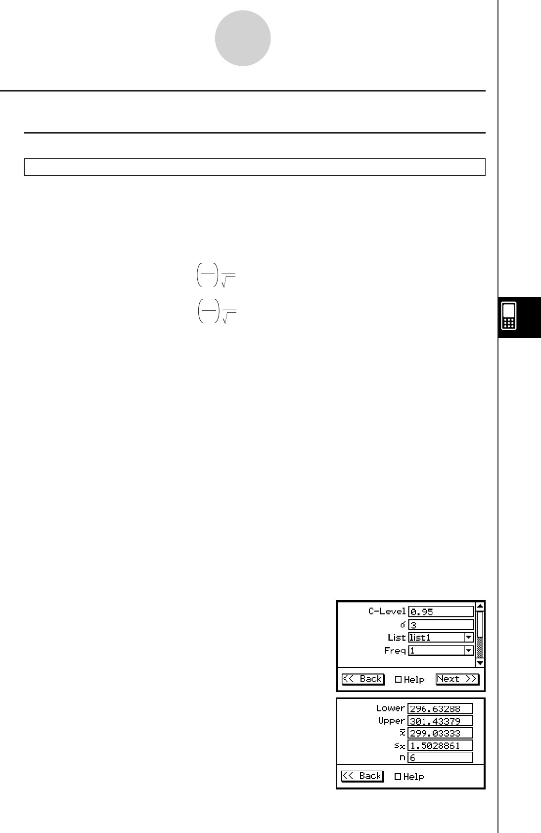
20090601

Confidence Interval Command List

k Z Confidence Interval

1-Sample Z Interval

Menu: [Interval]-[One-Sample ZInt]

Description: This command obtains the confidence interval for the population mean when

the population standard deviation is known.

The confidence interval is obtained using the following expressions.

Lower = o – Zα

Upper = o + Z α

α is the significance level, and 100 (1 – α)% is the confidence level. When the

confidence level is 95%, for example, you would input 0.95, which produces

α = 1 – 0.95 = 0.05.

Definition of Terms

C-Level : confidence level (0 < C-Level < 1)

 : population standard deviation ( > 0)

List : list where sample data is located

Freq : frequency of sample (1 or list name)

o : sample mean

n : sample size (positive integer)

Calculation Result Output

Lower : interval lower limit (left edge)

Upper : interval upper limit (right edge)

o : sample mean

sx : sample standard deviation (Displayed only for list format.)

n : sample size

Example 1 (calculation with list)

list1 : { 299.4, 297.7, 301, 298.9, 300.2, 297 }

Population standard deviation : 3

Significance level : 5% ( = confidence level : 95%)

• Statistics Wizard Operation

(1) Input the data into [list1] in the Stat Editor.

(2) On the menu bar, tap [Calc] and then [Interval].

(3) Select [One-Sample ZInt] and [List], and then tap

[Next >>].

(4) Input values.

(5) Select List [list1] and Freq [1].

(6) Tap [Next >>].

7-10-2

Confidence Intervals

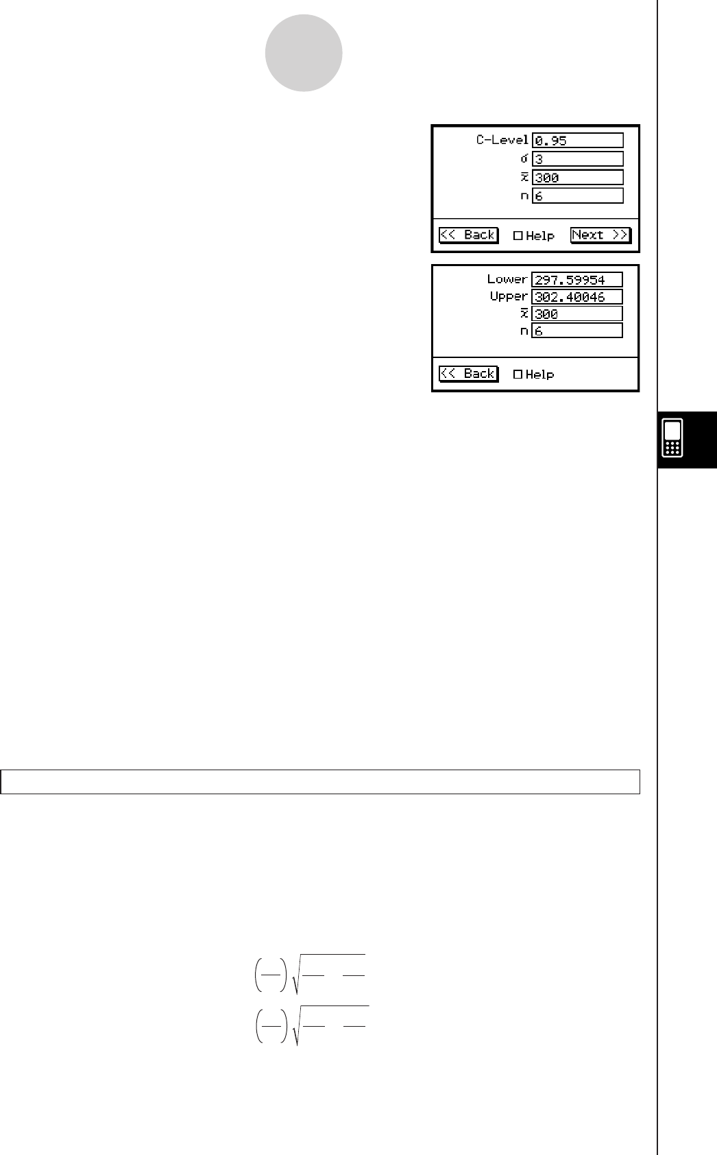
20090601

Example 2 (calculation with parameter)

Mean : 300

Sample size : 6

Population standard deviation : 3

Significance level : 5% ( = confidence level : 95%)

• Statistics Wizard Operation

(1) On the menu bar, tap [Calc] and then [Interval].

(2) Select [One-Sample ZInt] and [Variable], and then

tap [Next >>].

(3) Input values.

(4) Tap [Next >>].

uProgram, eActivity or Main Application

Command: OneSampleZInt

Command Syntax

Syntax 1 (list format)

C-Level value,

 value, List, Freq (or 1)

* “Freq” can be omitted. Doing so sets “1” for “Freq”.

Syntax 2 (parameter format)

C-Level value,

 value, o value, n value

Input Example:

Syntax 1 (list format)

OneSampleZInt 0.95,3,list1,1

Syntax 2 (parameter format)

OneSampleZInt 0.95,3,300,6

2-Sample Z Interval

Menu: [Interval]-[Two-Sample ZInt]

Description: This command obtains the confidence interval for the difference between

population means when the population standard deviations of two populations

are known.

The confidence interval is obtained using the following expressions.

The confidence level is 100 (1 – α)%.

Lower = (o1 – o2) – Zα

2n1

+n2

Upper = (o1 – o2) + Zα

2n1

+n2

o1 : sample mean of sample 1 data

o2 : sample mean of sample 2 data

1 : population standard deviation of

sample 1

2 : population standard deviation of

sample 2

1 : size of sample 1

2 : size of sample 2

7-10-3

Confidence Intervals

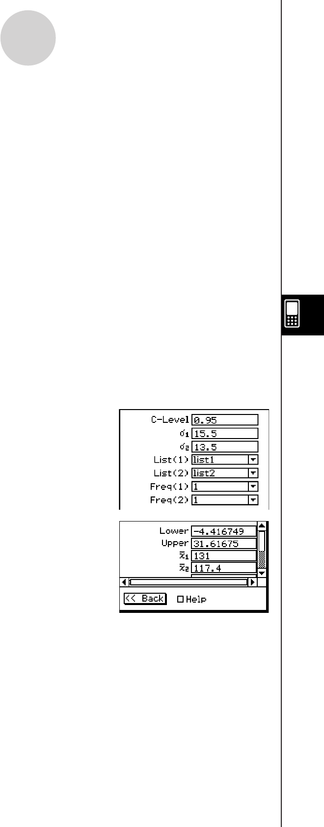
20090601

Definition of Terms

C-Level : confidence level (0 < C-Level < 1)

1 : population standard deviation of sample 1 (1 > 0)

2 : population standard deviation of sample 2 (2 > 0)

List(1) : list where sample 1 data is located

List(2) : list where sample 2 data is located

Freq(1) : frequency of sample 1 (1 or list name)

Freq(2) : frequency of sample 2 (1 or list name)

o1 : sample mean of sample 1 data

n1 : size of sample 1 (positive integer)

o2 : sample mean of sample 2 data

n2 : size of sample 2 (positive integer)

Calculation Result Output

Lower : interval lower limit (left edge)

Upper : interval upper limit (right edge)

o1 : sample mean of sample 1 data

o2 : sample mean of sample 2 data

sx1 : sample standard deviation of sample 1 (Displayed only for list format.)

sx2 : sample standard deviation of sample 2 (Displayed only for list format.)

n1 : size of sample 1

n2 : size of sample 2

Example

list1 : { 154, 109, 137, 115, 140 } , population

standard deviation : 15.5

list2 : { 108, 115, 126, 92, 146 } , population standard

deviation : 13.5

Significance level : 5% ( = confidence level : 95%)

• Statistics Wizard Operation

(1) Input the data into [list1] and [list2] in the Stat Editor.

(2) On the menu bar, tap [Calc] and then [Interval].

(3) Select [Two-Sample ZInt] and [List], and then tap

[Next >>].

(4) Input values.

(5) Select List(1) [list1], List(2) [list2], Freq(1) [1] and

Freq(2) [1].

(6) Tap [Next >>].

uProgram, eActivity or Main Application

Command: TwoSampleZInt

Command Syntax

Syntax 1 (list format)

C-Level value,

1 value, 2 value, List(1), List(2), Freq(1) (or 1), Freq(2) (or 1)

* “Freq” can be omitted. Doing so sets “1” for “Freq”.

Syntax 2 (parameter format)

C-Level value,

1 value, 2 value, o1 value, n1 value, o2 value, n2 value

7-10-4

Confidence Intervals

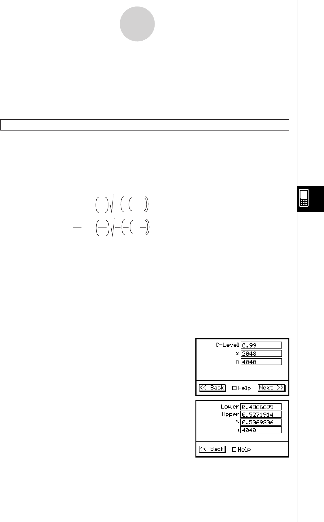
20090601

Input Example:

Syntax 1 (list format)

TwoSampleZInt 0.95,15.5,13.5,list1,list2,1,1

Syntax 2 (parameter format)

TwoSampleZInt 0.95,1,1.5,418,40,402,50

1-Prop Z Interval

Menu: [Interval]-[One-Prop ZInt]

Description: This command obtains the confidence interval of the proportion of successes

in a population.

The confidence interval is obtained using the following expressions.

The confidence level is 100 (1 – α)%.

n: sample size

x: data

Definition of Terms

C-Level: confidence level (0 < C-Level < 1)

x : data (0 or positive integer)

n : sample size (positive integer)

Calculation Result Output

Lower : interval lower limit (left edge)

Upper : interval upper limit (right edge)

ˆ p : estimated sample proportion

n : sample size

Example

Data : 2048

Sample size : 4040

Significance level : 1% ( = confidence level : 99%)

• Statistics Wizard Operation

(1) On the menu bar, tap [Calc] and then [Interval].

(2) Select [One-Prop ZInt] and then tap [Next >>].

(3) Input values.

(4) Tap [Next >>].

Lower = – Z

1–

Upper = + Z

nα

1–

Lower = – Z

1–

Upper = + Z

nα

1–

7-10-5

Confidence Intervals

20090601

7-10-6

Confidence Intervals

uProgram, eActivity or Main Application

Command: OnePropZInt

Command Syntax

C-Level value,

x value, n value

Input Example:

OnePropZInt 0.99,2048,4040

2-Prop Z Interval

Menu: [Interval]-[Two-Prop ZInt]

Description: This command obtains the confidence interval of the difference between the

proportions of successes of two populations.

The confidence interval is obtained using the following expressions.

The confidence level is 100 (1 – α)%.

Lower = – – Zα

1– n

Upper = – + Zα

1– n

1, n2 : sample size

x1, x2 : data

Definition of Terms

C-Level: confidence level (0 < C-Level < 1)

x1 : data value (integer, x1 > 0) of sample 1

n1 : size of sample 1 (positive integer)

x2 : data value (integer, x2 > 0) of sample 2

n2 : size of sample 2 (positive integer)

Calculation Result Output

Lower : interval lower limit (left edge)

Upper : interval upper limit (right edge)

ˆp 1 : estimated proportion of sample 1

ˆp 2 : estimated proportion of sample 2

n1 : size of sample 1

n2 : size of sample 2

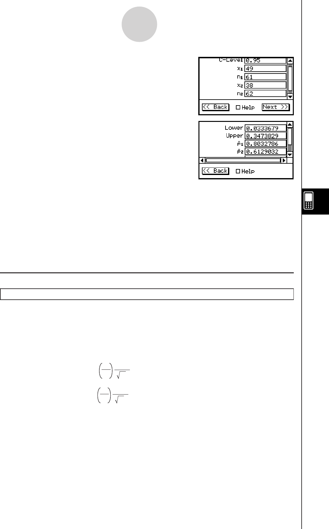
20090601

Example

Data1 : 49, sample size : 61

Data2 : 38, sample size : 62

Significance level : 5% ( = confidence level : 95%)

• Statistics Wizard Operation

(1) On the menu bar, tap [Calc] and then [Interval].

(2) Select [Two-Prop ZInt] and then tap [Next >>].

(3) Input values.

(4) Tap [Next >>].

uProgram, eActivity or Main Application

Command: TwoPropZInt

Command Syntax

C-Level value,

x1 value, n1 value, x2 value, n2 value

Input Example:

TwoPropZInt 0.95,49,61,38,62

k t Confidence Interval

1-Sample t Interval

Menu: [Interval]-[One-Sample TInt]

Description: This command obtains the confidence interval for the population mean when

the population standard deviation is unknown.

The confidence interval is obtained using the following expressions.

The confidence level is 100 (1 – α)%.

Definition of Terms

C-Level : confidence level (0 < C-Level < 1)

List : list where sample data is located

Freq : frequency of sample (1 or list name)

o : sample mean

sx : sample standard deviation (sx > 0)

n : sample size (positive integer)

Lower = o– t

n – 1

Upper = o+t

n – 1

Lower = o– t

n – 1

Upper = o+t

n – 1

7-10-7

Confidence Intervals

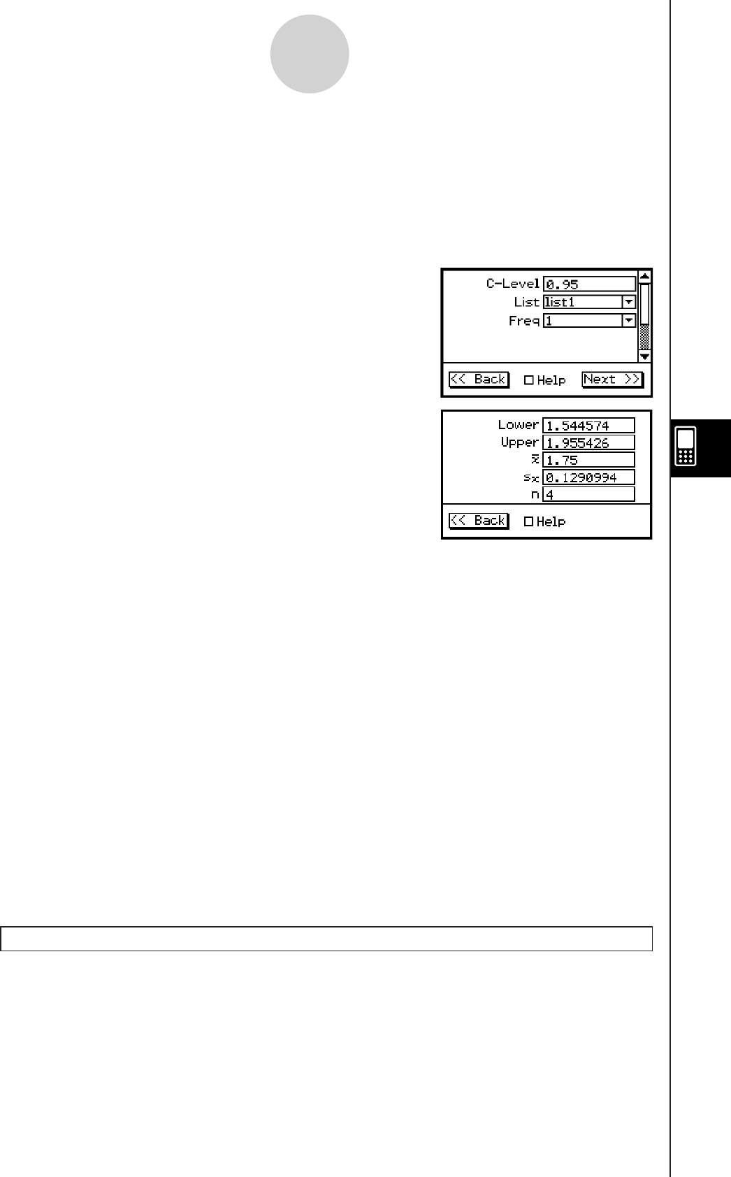
20090601

Calculation Result Output

Lower : interval lower limit (left edge)

Upper : interval upper limit (right edge)

o : sample mean

sx : sample standard deviation

n : sample size

Example

list1 : { 1.6, 1.7, 1.8, 1.9 }

Significance level : 5% ( = confidence level : 95%)

• Statistics Wizard Operation

(1) Input the data into [list1] in the Stat Editor.

(2) On the menu bar, tap [Calc] and then [Interval].

(3) Select [One-Sample TInt] and then tap [Next >>].

(4) Input value.

(5) Select List [list1] and Freq [1].

(6) Tap [Next >>].

uProgram, eActivity or Main Application

Command: OneSampleTInt

Command Syntax

Syntax 1 (list format)

C-Level value, List, Freq (or 1)

* “Freq” can be omitted. Doing so sets “1” for “Freq”.

Syntax 2 (parameter format)

C-Level value,

o value, sx value, n value

Input Example:

Syntax 1 (list format)

OneSampleTInt 0.95,list1,1

Syntax 2 (parameter format)

OneSampleTInt 0.95,66.3,8.4,12

2-Sample t Interval

Menu: [Interval]-[Two-Sample TInt]

Description: This command obtains the confidence interval for the difference between two

population means when the population standard deviations are unknown.

The confidence interval is obtained using the following expressions.

The confidence level is 100 (1 – α)%.

7-10-8

Confidence Intervals

20090601

When the two population standard deviations are equal (pooled)

When the two population standard deviations are not equal (not pooled)

Definition of Terms

C-Level : confidence level (0 < C-Level < 1)

List(1) : list where sample 1 data is located

List(2) : list where sample 2 data is located

Freq(1) : frequency of sample 1 (1 or list name)

Freq(2) : frequency of sample 2 (1 or list name)

Pooled : On or Off

o1 : sample mean of sample 1 data

sx1: sample standard deviation of sample 1 (sx1 > 0)

n1 : size of sample 1 (positive integer)

o2 : sample mean of sample 2 data

sx2 : sample standard deviation of sample 2 (sx2 > 0)

n2 : size of sample 2 (positive integer)

Calculation Result Output

Lower : interval lower limit (left edge)

Upper : interval upper limit (right edge)

df : degrees of freedom

o1 : sample mean of sample 1 data

o2 : sample mean of sample 2 data

sx1 : sample standard deviation of sample 1

sx2 : sample standard deviation of sample 2

sp : pooled sample standard deviation (Displayed only when pooling is

turned on.)

n1 : size of sample 1

n2 : size of sample 2

Lower = (o

– o

)– tα

n1+n2 –2

1+n

Upper = (o

– o

)+ tα

n1+n2 –2

1+n

Lower = (o

– o

)– tα

n1+n2 –2

1+n

Upper = (o

– o

)+ tα

n1+n2 –2

1+n

Lower = (o

– o

)– t

x12

x22

Upper = (o

– o

)+ t

x12

x22

Lower = (o

– o

)– t

x12

x22

Upper = (o

– o

)+ t

x12

x22

C =

df = 1

–1 +(1–C)

–1

C =

df = 1

–1 +(1–C)

–1

7-10-9

Confidence Intervals

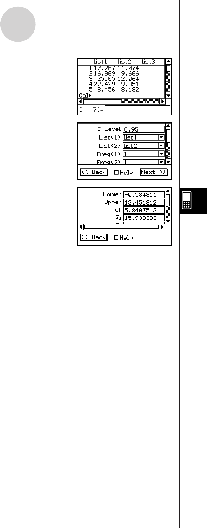
20101001

Example

list1 : { 12.207, 16.869, 25.05, 22.429, 8.456, 10.589 }

list2 : { 11.074, 9.686, 12.064, 9.351, 8.182, 6.642 }

Significance level : 5% ( = confidence level : 95%)

• Statistics Wizard Operation

(1) Input the data into [list1] and [list2] in the Stat Editor.

(2) On the menu bar, tap [Calc] and then [Interval].

(3) Select [Two-Sample TInt] and then tap [Next >>].

(4) Input value.

(5) Select List(1) [list1], List(2) [list2], Freq(1) [1],

Freq(2) [1] and Pooled [Off].

(6) Tap [Next >>].

uProgram, eActivity or Main Application

Command: TwoSampleTInt

Command Syntax

Syntax 1 (list format)

C-Level value, List(1), List(2), Freq(1) (or 1), Freq(2) (or 1), Pooled condition (On

or Off)

* “Freq” can be omitted. Doing so sets “1” for “Freq”.

* “Pooled” can be omitted. Doing so sets “Off” for “Pooled”.

Syntax 2 (parameter format)

C-Level value,

o1 value, sx1 value, n1 value, o2 value, sx2 value, n2 value, Pooled

condition (On or Off)

* “Pooled” can be omitted. Doing so sets “Off” for “Pooled”.

Input Example:

Syntax 1 (list format)

TwoSampleTInt 0.95,list1,list2,1,1,Off

Syntax 2 (parameter format)

TwoSampleTInt 0.95,80.4,2.07,30,84.2,1.96,35,On

7-10-10

Confidence Intervals

20060301

7-11-1

Distributions

7-11 Distributions

Though there are a number of different types of distributions, the one most commonly used is

the “Normal Distribution”, which is an essential type of distribution for statistical calculations.

Other types of distributions include the Poisson distribution and geometric distribution. The

type of distribution used depends on the type of data being handled.

The shape of a distribution makes it possible to determine trends in data somewhat. You can

specify a value and calculate the probability that any data value from the distribution is, for

example, less than the specified value. In other words, you can determine what percent from

the bottom that data value occurs within the distribution.

The following is a list of distributions and the description of what each one calculates.

Description

Distribution Name

Calculates the normal probability density for a specified

value.

Calculates the cumulative probability of a normal distribution

between a lower bound and an upper bound.

Calculates the boundary value(s) of a normal cumulative

probability distribution for specified values.

Calculates the Student-t probability density for a specified

value.

Calculates the cumulative probability of a Student-t

distribution between a lower bound and an upper bound.

Calculates the lower bound value of a Student-t cumulative

probability distribution for specified values.

Calculates the χ2 probability density for a specified value.

Calculates the cumulative probability of a χ2 distribution

between a lower bound and an upper bound.

Calculates the lower bound value of a χ2 cumulative

probability distribution for specified values.

Calculates the F probability density for a specified value.

Normal Distribution

t Distribution

Normal Probability Density

Student-t Probability

Density

Student-t Cumulative

Distribution

Inverse Student-t

Cumulative Distribution

Inverse χ2 Cumulative

Distribution

χ2 Cumulative Distribution

χ2 Probability Density

Normal Cumulative

Distribution

Inverse Normal Cumulative

Distribution

χ2 Distribution

F Probability Density

Calculates the cumulative probability of an F distribution

between a lower bound and an upper bound.

F Cumulative Distribution

Calculates the lower bound value of an F cumulative

probability distribution for specified values.

Inverse F Cumulative

Distribution

F Distribution

20080201

20090601

7-11-2

Distributions

Description

Distribution Name

Calculates the probability in a binomial distribution that the

success will occur on a specified trial.

Calculates the cumulative probability in a binomial distribution

that the success will occur on or before a specified trial.

Calculates the minimum number of trials of a binomial

cumulative probability distribution for specified values.

Calculates the probability in a Poisson distribution that the

success will occur on a specified trial.

Calculates the probability in a hypergeometric distribution that

the success will occur on a specified trial.

Calculates the cumulative probability in a hypergeometric

distribution that the success will occur on or before a

specified trial.

Calculates the minimum number of trials of a hypergeometric

cumulative probability distribution for specified values.

Calculates the cumulative probability in a Poisson distribution

that the success will occur on or before a specified trial.

Calculates the minimum number of trials of a Poisson

cumulative probability distribution for specified values.

Calculates the probability in a geometric distribution that the

success will occur on a specified trial.

Calculates the cumulative probability in a geometric

distribution that the success will occur on or before a

specified trial.

Calculates the minimum number of trials of a geometric

cumulative probability distribution for specified values.

Binomial Distribution

Poisson Distribution

Binomial Distribution

Probability

Poisson Distribution

Probability

Poisson Cumulative

Distribution

Inverse Poisson Cumulative

Distribution

Inverse Geometric

Cumulative Distribution

Geometric Cumulative

Distribution

Geometric Distribution

Probability

Binomial Cumulative

Distribution

Inverse Binomial

Cumulative Distribution

Geometric Distribution

Hypergeometric Distribution

Probability

Hypergeometric Cumulative

Distribution

Inverse Hypergeometric

Cumulative Distribution

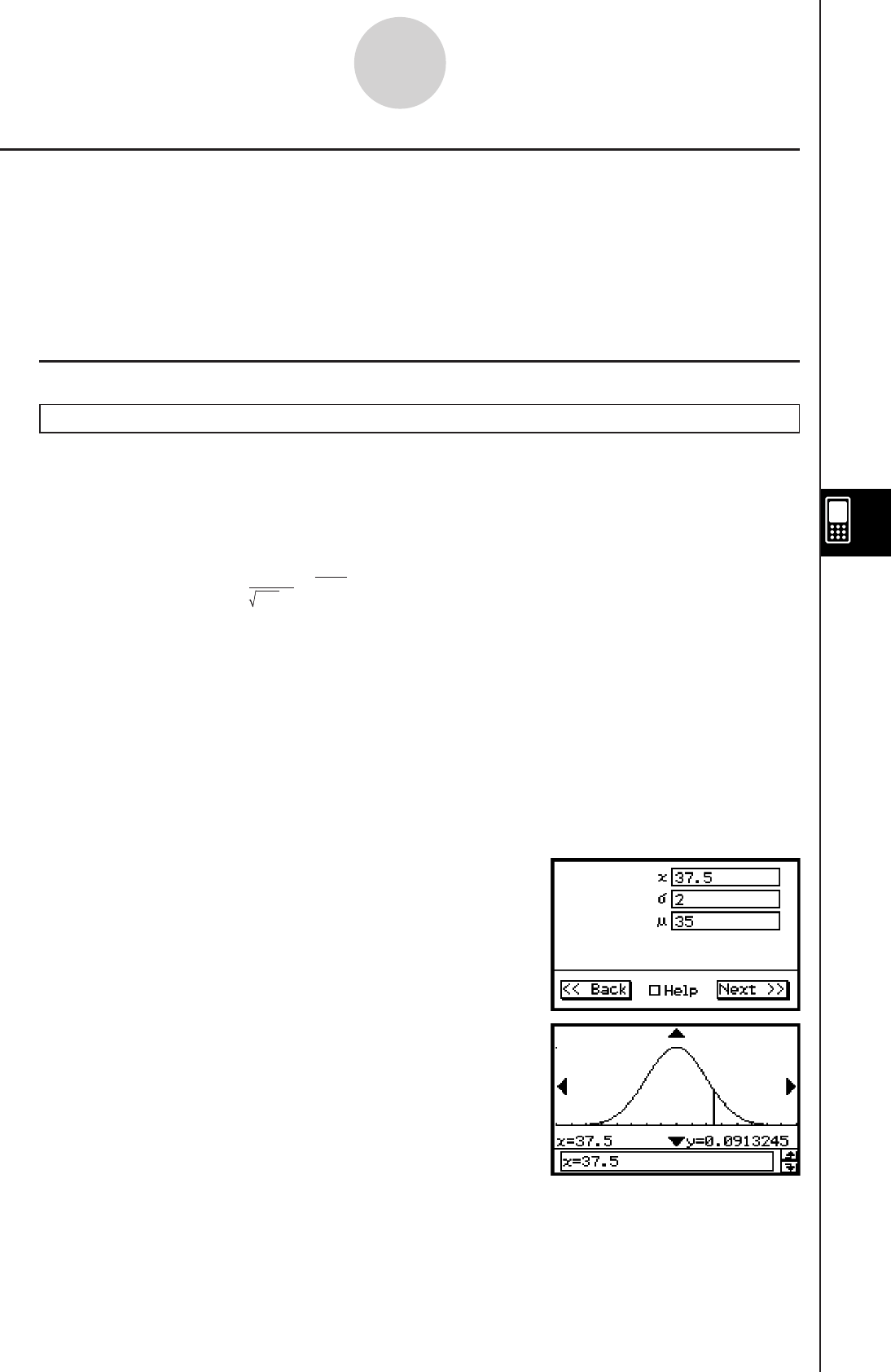
20090601

Distribution Command List

Important!

Though list data can be used within the argument of the Distribution function (page 2-8-48),

list data cannot be used in the argument of the Statistics Wizard operations described here

or in operations that use the Distribution command in the applications.

For details about using list data within the Distribution function, see “Specifying Arguments

within the Distribution Function” (page 2-8-48).

k Normal Distribution

Normal Probability Density

Menu: [Distribution]-[Normal PD]

Description: This command calculates the probability density of normal distribution from a

specified x value. Normal probability density is used for normal distribution.

( > 0)

Definition of Terms

x : data value

 : population standard deviation ( > 0)

 : population mean

Specifying  = 1 and  = 0 produces standard normal distribution.

Calculation Result Output

prob : normal probability density

Example

Data : 37.5

Population standard deviation : 2

Population mean : 35

• Statistics Wizard Operation

(1) On the menu bar, tap [Calc] and then [Distribution].

(2) Select [Normal PD] and then tap [Next >>].

(3) Input values.

(4) Tap [Next >>].

(5) To display the graph, tap $.

πσ

f (x) = 1e–2 2

(x – μ)2

πσ

f (x) = 1e–2 2

(x – μ)2

7-11-3

Distributions

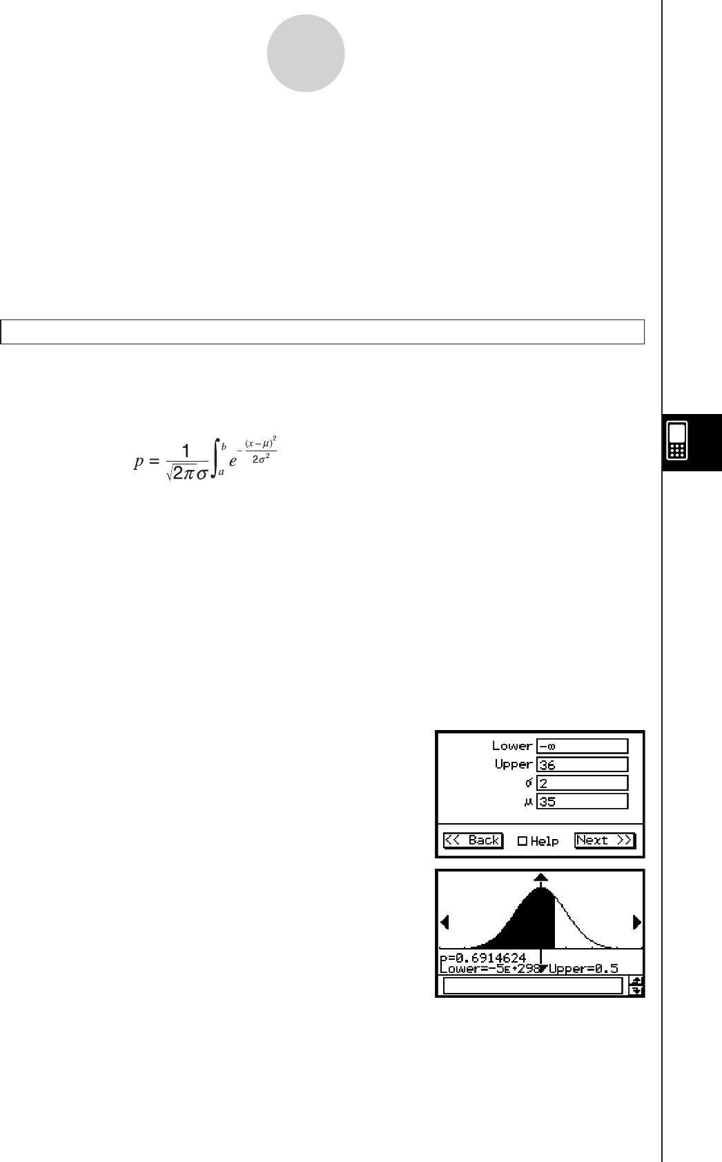
20090601

7-11-4

Distributions

uProgram, eActivity or Main Application

Command: NormPD

Command Syntax

x value,  value,  value

Input Example:

NormPD 37.5,2,35

Normal Cumulative Distribution

Menu: [Distribution]-[Normal CD]

Description: This command calculates the probability of normal distribution data falling

between a and b.

a : lower bound (Lower)

b : upper bound (Upper)

Definition of Terms

Lower : lower bound

Upper : upper bound

 : population standard deviation ( > 0)

 : population mean

Calculation Result Output

prob : normal distribution probability p

z Low : standardized lower limit z value

z Up : standardized upper limit z value

Example

Upper bound : 36 (lower bound : −∞)

Population standard deviation : 2

Population mean : 35

• Statistics Wizard Operation

(1) On the menu bar, tap [Calc] and then [Distribution].

(2) Select [Normal CD] and then tap [Next >>].

(3) Input values.

(4) Tap [Next >>].

(5) To display the graph, tap $.

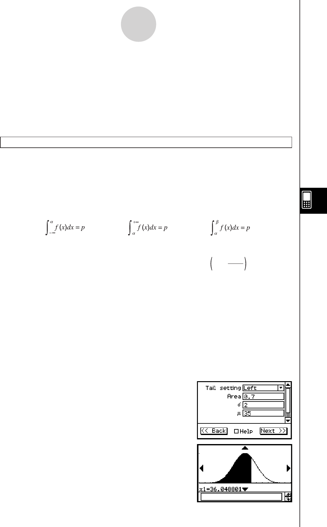
20090601

7-11-5

Distributions

uProgram, eActivity or Main Application

Command: NormCD

Command Syntax

Lower value, Upper value,  value,  value

Input Example:

NormCD −∞,36,2,35

Inverse Normal Cumulative Distribution

Menu: [Inv. Distribution]-[Inverse Normal CD]

Description: This command calculates the cumulative probability in a normal distribution

based on lower and upper bounds.

This command returns the upper and lower bound of integration values that

satisfy the equations below.

Tail:Left Tail:Right Tail:Center

Upper bound  is

returned.

Lower bound  is

returned.

Lower bound  and upper

bound  are returned.

+

 =

Definition of Terms

Tail setting: probability value tail specification (L (Left), R (Right), C (Center))

Area : probability value (0 < Area < 1)

 : population standard deviation ( > 0)

 : population mean

Calculation Result Output

inverse cumulative normal distribution

x1InvN: Upper bound when Tail:Left

Lower bound when Tail:Right or Tail:Center

x2InvN: Upper bound when Tail:Center

Example

Tail : Left

Probability : 0.7

Population standard deviation : 2

Population mean : 35

• Statistics Wizard Operation

(1) On the menu bar, tap [Calc] and then [Distribution].

(2) Select [Inverse Normal CD] and then tap [Next >>].

(3) Select Tail setting [Left] and input values.

(4) Tap [Next >>].

(5) To display the graph, tap $.

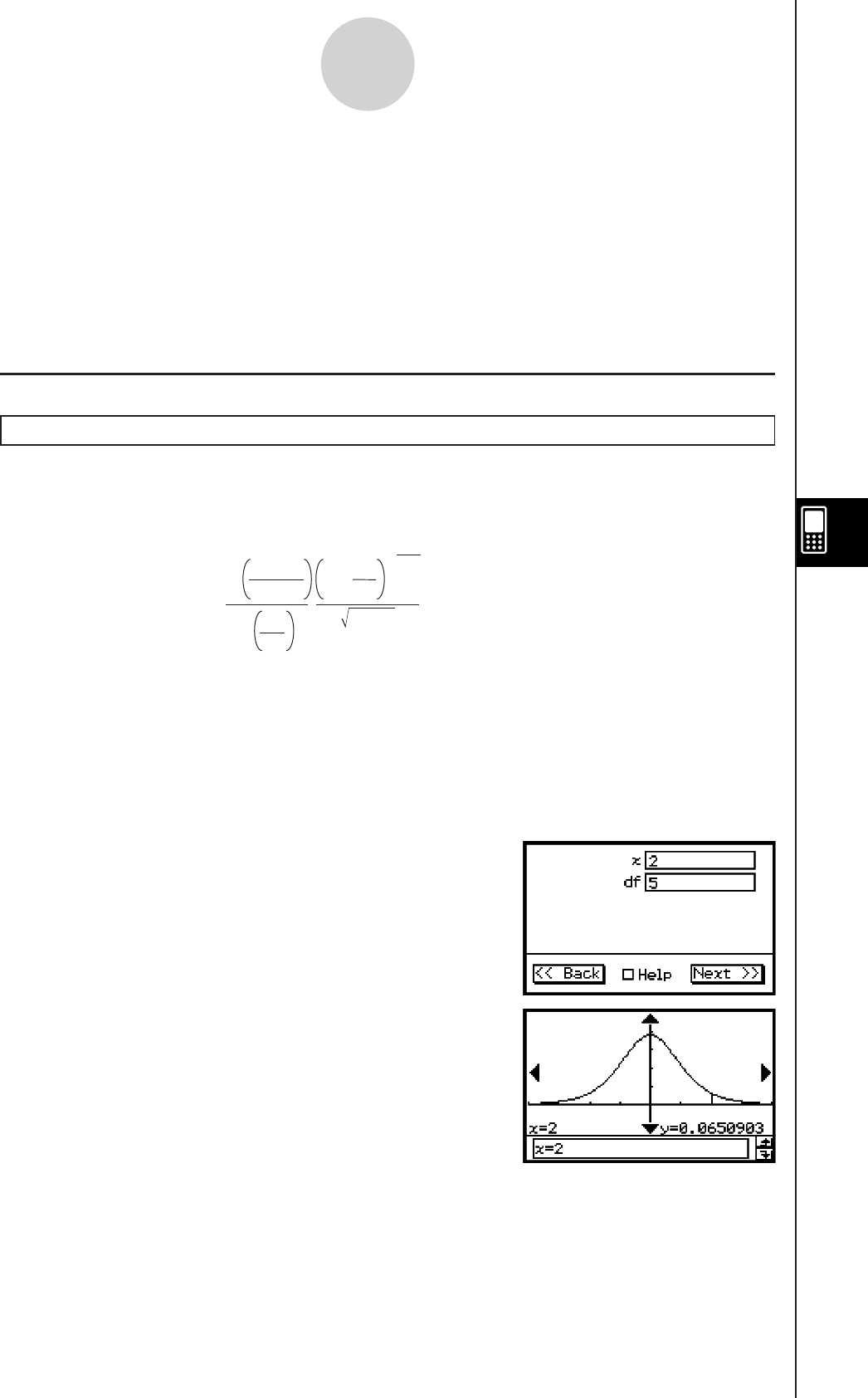
20090601

7-11-6

Distributions

uProgram, eActivity or Main Application

Command: InvNormCD or InvNorm

Command Syntax

“Tail setting”, Area value,  value,  value

Input Example:

InvNorm “L”,0.7,2,35

k t Distribution

Student-t Probability Density

Menu: [Distribution]-[Student-T PD]

Description: This command calculates t probability density from a specified x value.

(x) =

–df+1

df + 1

Definition of Terms

x : data value

df : degrees of freedom (df > 0)

Calculation Result Output

prob : Student-t probability density

Example

Data : 2

Degrees of freedom : 5

• Statistics Wizard Operation

(1) On the menu bar, tap [Calc] and then [Distribution].

(2) Select [Student-T PD] and then tap [Next >>].

(3) Input values.

(4) Tap [Next >>].

(5) To display the graph, tap $.

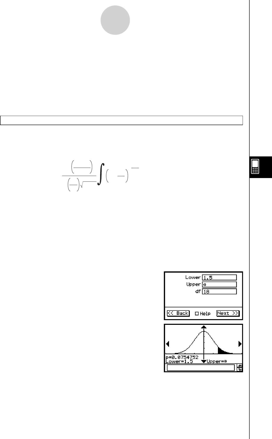
20090601

uProgram, eActivity or Main Application

Command: TPD

Command Syntax

x value, df value

Input Example:

TPD 2,5

Student-

t Cumulative Distribution

Menu: [Distribution]-[Student-T CD]

Description: This command calculates the probability of the Student-t distribution data

falling between a and b.

p =

df + 1

–df+1

1+ dx

a : lower bound (Lower)

b : upper bound (Upper)

Definition of Terms

Lower : lower bound

Upper : upper bound

df : degrees of freedom (df > 0)

Calculation Result Output

prob : Student-t distribution probability p

t Low : lower bound value you input

t Up : upper bound value you input

Example

Lower bound : 1.5 (upper bound : ∞)

Degrees of freedom : 18

• Statistics Wizard Operation

(1) On the menu bar, tap [Calc] and then [Distribution].

(2) Select [Student-T CD] and then tap [Next >>].

(3) Input values.

(4) Tap [Next >>].

(5) To display the graph, tap $.

7-11-7

Distributions

20090601

7-11-8

Distributions

uProgram, eActivity or Main Application

Command: TCD

Command Syntax

Lower value, Upper value, df value

Input Example:

TCD 1.5,∞,18

Inverse Student-t Cumulative Distribution

Menu: [Inv. Distribution]-[Inverse T CD]

Description: This command calculates the inverse of the t cumulative distribution.

This command returns the lower bound of integration value  that satisfies the

equation above.

Definition of Terms

prob : t cumulative probability (p, 0 < p < 1)

df : degrees of freedom (df > 0)

Calculation Result Output

xInv : inverse t cumulative distribution

Example

Probability : 0.0754752

Degrees of freedom : 18

• Statistics Wizard Operation

(1) On the menu bar, tap [Calc] and then [Distribution].

(2) Select [Inverse T CD] and then tap [Next >>].

(3) Input values.

(4) Tap [Next >>].

uProgram, eActivity or Main Application

Command: InvTCD

Command Syntax

prob value, df value

Input Example:

InvTCD 0.0754752,18

∞∞

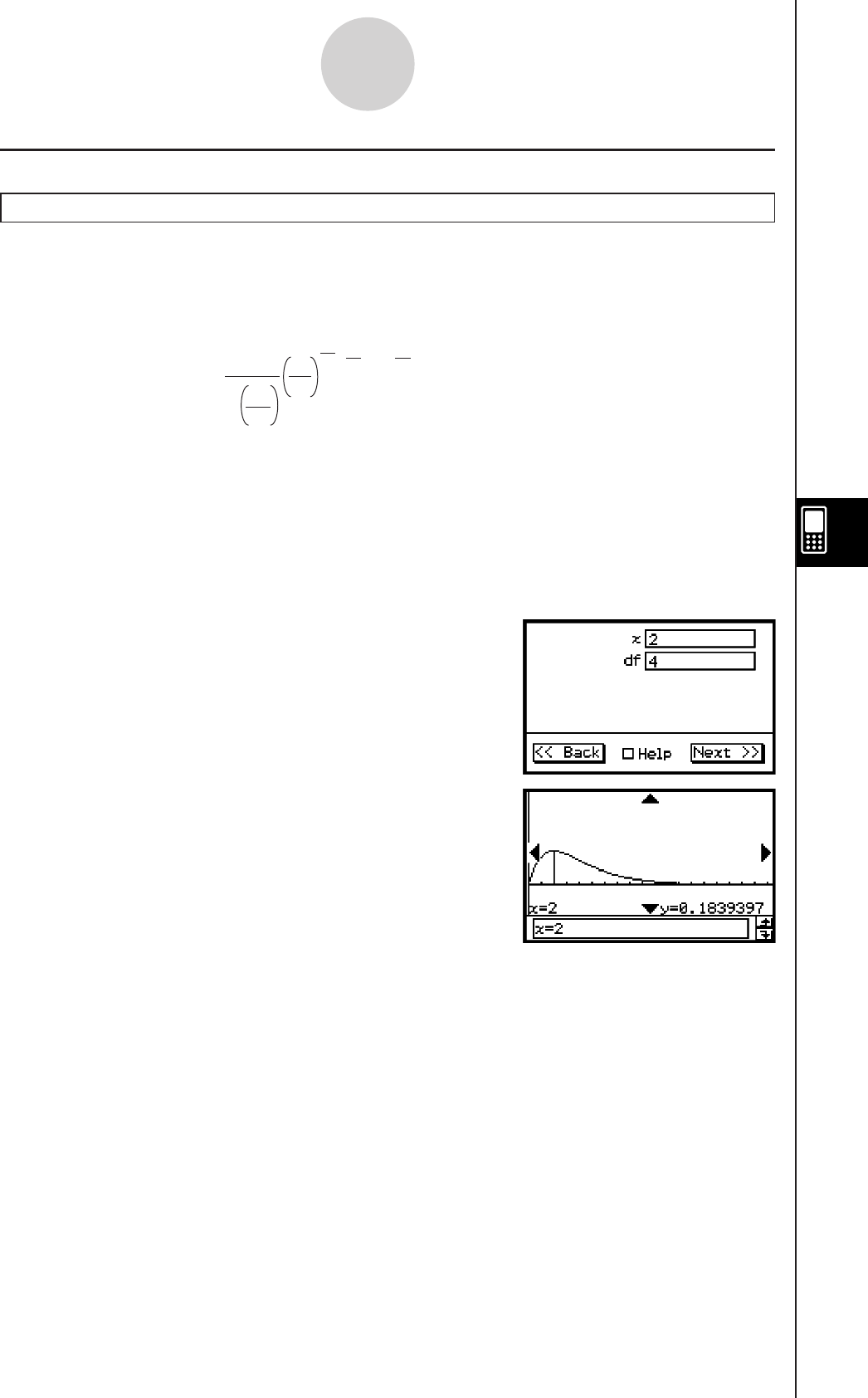
20060301

7-11-9

Distributions

k χ2 Distribution

χ2 Probability Density

Menu: [Distribution]-[χ2PD]

Description: This command calculates the probability density of χ2 distribution from a

specified x value.

f (x) =

x e

2–1 x

–

Definition of Terms

x : data value

df : degrees of freedom (positive integer)

Calculation Result Output

prob : χ2 probability density

Example

Data : 2

Degrees of freedom : 4

• Statistics Wizard Operation

(1) On the menu bar, tap [Calc] and then [Distribution].

(2) Select [χ2 PD] and then tap [Next >>].

(3) Input values.

(4) Tap [Next >>].

(5) To display the graph, tap $.

uProgram, eActivity or Main Application

Command: ChiPD

Command Syntax

x value, df value

Input Example:

ChiPD 2,4

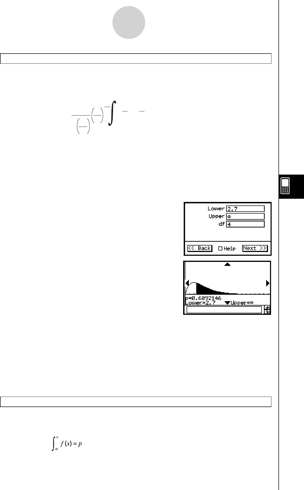
20090601

χ2 Cumulative Distribution

Menu: [Distribution]-[χ2 CD ]

Description: This command calculates the probability of χ2 distribution data falling between

a and b.

p =

x e dx

2–1 x

–

a : lower bound (Lower)

b : upper bound (Upper)

Definition of Terms

Lower : lower bound

Upper : upper bound

df : degrees of freedom (positive integer)

Calculation Result Output

prob : χ2 distribution probability p

Example

Lower bound : 2.7 (upper bound : ∞)

Degrees of freedom : 4

• Statistics Wizard Operation

(1) On the menu bar, tap [Calc] and then [Distribution].

(2) Select [χ2 CD] and then tap [Next >>].

(3) Input values.

(4) Tap [Next >>].

(5) To display the graph, tap $.

uProgram, eActivity or Main Application

Command: ChiCD

Command Syntax

Lower value, Upper value, df value

Input Example:

ChiCD 2.7,∞,4

Inverse χ2 Cumulative Distribution

Menu: [Inv. Distribution]-[Inverse χ2 CD]

Description: This command calculates the inverse of the χ2 cumulative distribution.

This command returns the lower bound of integration value  that satisfies the

equation above.

∞∞

7-11-10

Distributions

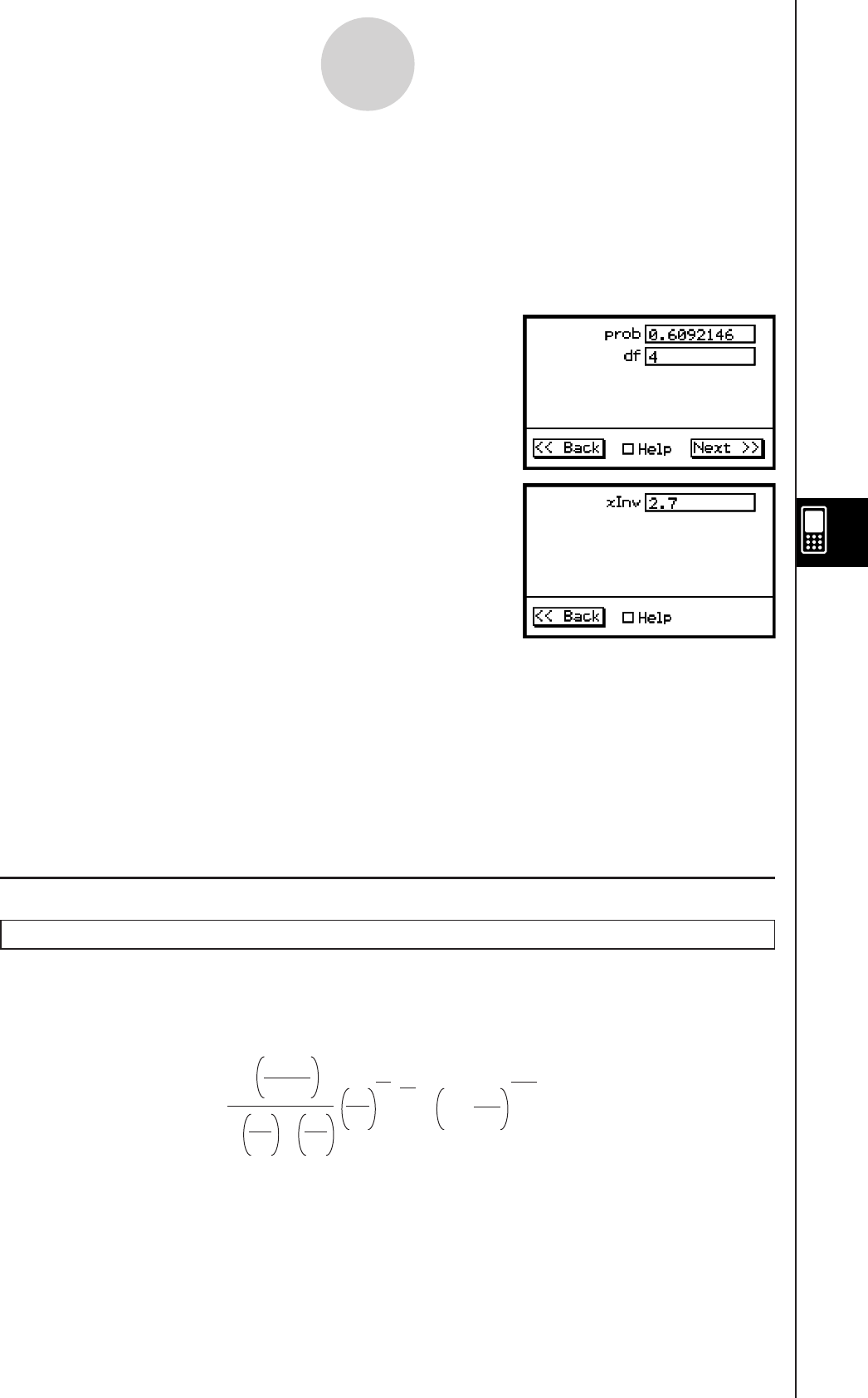
20060301

Definition of Terms

prob : χ2 cumulative probability (p, 0 < p < 1)

df : degrees of freedom (positive integer)

Calculation Result Output

xInv : inverse χ2 cumulative distribution

Example

Probability : 0.6092146

Degrees of freedom : 4

• Statistics Wizard Operation

(1) On the menu bar, tap [Calc] and then [Distribution].

(2) Select [Inverse χ2 CD] and then tap [Next >>].

(3) Input values.

(4) Tap [Next >>].

uProgram, eActivity or Main Application

Command: InvChiCD

Command Syntax

prob value, df value

Input Example:

InvChiCD 0.6092146,4

k F Distribution

F Probability Density

Menu: [Distribution]-[F PD]

Description: This command calculates the probability density of F distribution from a

specified x value.

2–1

Γ2

n + d

Γ2

1 +

n + d

f (x) =

–

Definition of Terms

x : data value

n:df : degrees of freedom of numerator (positive integer)

d:df : degrees of freedom of denominator (positive integer)

Calculation Result Output

prob : F probability density

7-11-11

Distributions

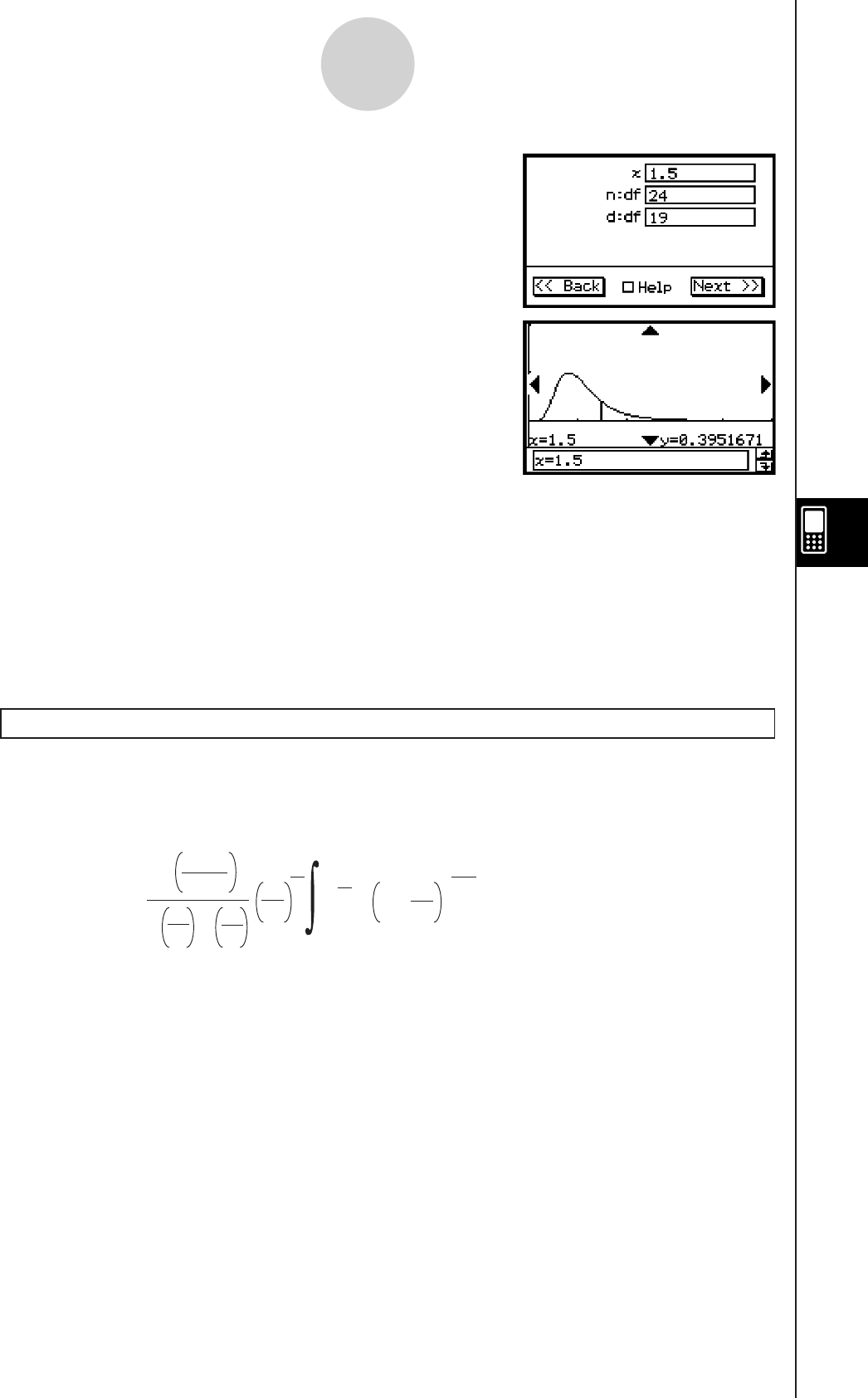
20060301

Example

Data : 1.5

Degrees of freedom of numerator : 24

Degrees of freedom of denominator : 19

• Statistics Wizard Operation

(1) On the menu bar, tap [Calc] and then [Distribution].

(2) Select [F PD] and then tap [Next >>].

(3) Input values.

(4) Tap [Next >>].

(5) To display the graph, tap $.

uProgram, eActivity or Main Application

Command: FPD

Command Syntax

x value, n:df value, d:df value

Input Example:

FPD 1.5,24,19

F Cumulative Distribution

Menu: [Distribution]-[F CD]

Description: This command calculates the probability of F distribution data falling between

a and b.

p =

2–1

Γ2

n + d

Γ2

n.x

1 +

n + d

–

: lower bound (Lower)

b : upper bound (Upper)

Definition of Terms

Lower : lower bound

Upper : upper bound

n:df : degrees of freedom of numerator (positive integer)

d:df : degrees of freedom of denominator (positive integer)

Calculation Result Output

prob : F distribution probability p

7-11-12

Distributions

20080201

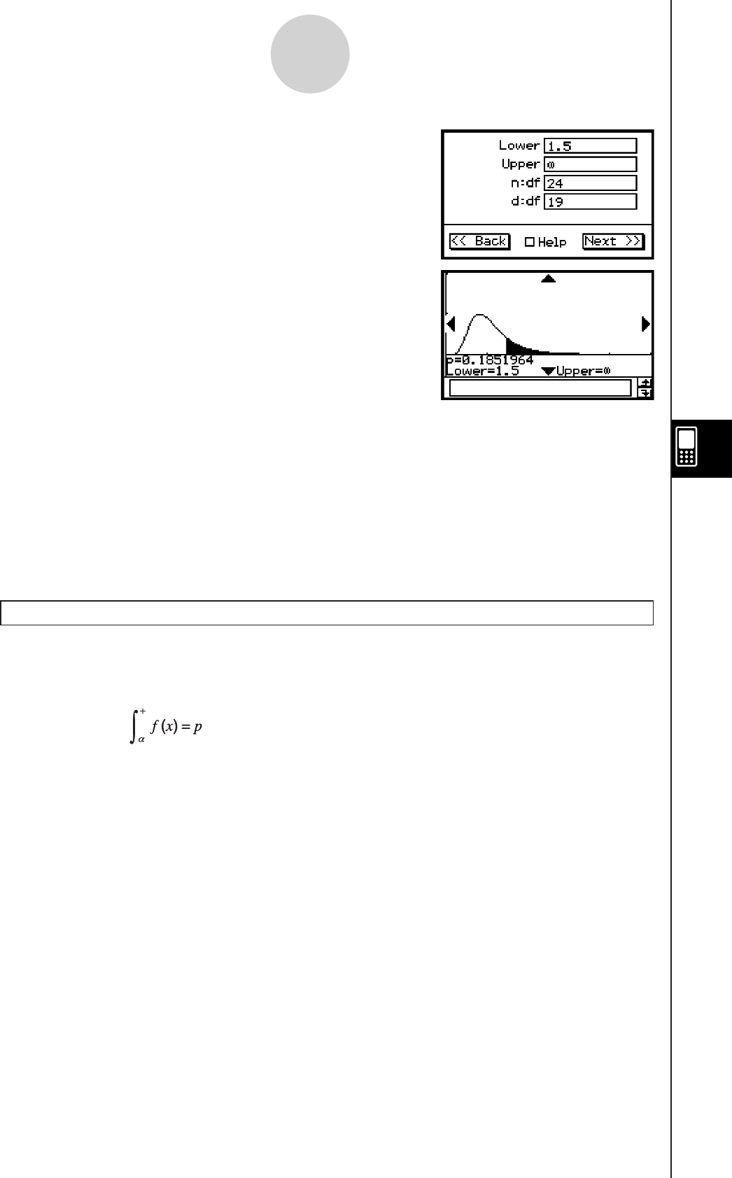
20090601

Example

Lower bound : 1.5 (upper bound : ∞)

Degrees of freedom of numerator : 24

Degrees of freedom of denominator : 19

• Statistics Wizard Operation

(1) On the menu bar, tap [Calc] and then [Distribution].

(2) Select [F CD] and then tap [Next >>].

(3) Input values.

(4) Tap [Next >>].

(5) To display the graph, tap $.

uProgram, eActivity or Main Application

Command: FCD

Command Syntax

Lower value, Upper value, n:df value, d:df value

Input Example:

FCD 1.5,∞,24,19

Inverse F Cumulative Distribution

Menu: [Inv. Distribution]-[Inverse F CD]

Description: This command calculates the inverse of the F cumulative distribution.

This command returns the lower bound of integration value  that satisfies the

equation above.

Definition of Terms

prob : F cumulative probability (p, 0 < p < 1)

n:df : degrees of freedom of numerator (positive integer)

d:df : degrees of freedom of denominator (positive integer)

Calculation Result Output

xInv : inverse F cumulative distribution

∞∞

7-11-13

Distributions

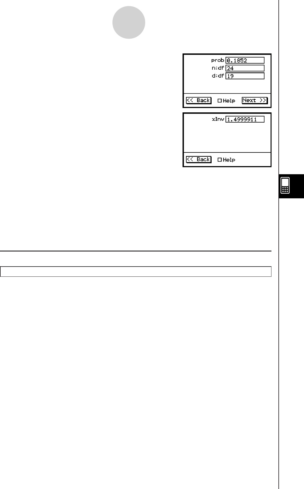
20090601

Example

Probability : 0.1852

Degrees of freedom of numerator : 24

Degrees of freedom of denominator : 19

• Statistics Wizard Operation

(1) On the menu bar, tap [Calc] and then [Distribution].

(2) Select [Inverse F CD] and then tap [Next >>].

(3) Input values.

(4) Tap [Next >>].

uProgram, eActivity or Main Application

Command: InvFCD

Command Syntax

prob value, n:df value, d:df value

Input Example:

InvFCD 0.1852,24,19

k Binomial Distribution

Binomial Distribution Probability

Menu: [Distribution]-[Binomial PD]

Description: This command calculates the probability the random variable that follows a

binomial distribution will be a given x value. For example, it determines the

probability of x successes when the probability of success p-trial is performed

n times.

f (x) =

(1–p)

n – x

(x = 0, 1, ·······, n) p

: probability of success

< p < 1)

: number of trials

Definition of Terms

x : specified trial (integer from 0 to n)

Numtrial : number of trials n (integer, n > 0)

pos : probability of success p (0 < p < 1)

Calculation Result Output

prob : binomial probability

7-11-14

Distributions

20090601

Example

Trials : 5

Specified trial : 3

Probability of success : 0.63

• Statistics Wizard Operation

(1) On the menu bar, tap [Calc] and then [Distribution].

(2) Select [Binomial PD] and then tap [Next >>].

(3) Input values.

(4) Tap [Next >>].

(5) To display the graph, tap $.

uProgram, eActivity or Main Application

Command: BinomialPD

Command Syntax

x value, Numtrial value, pos value

Input Example:

BinomialPD 3,5,0.63

Binomial Cumulative Distribution

Menu: [Distribution]-[Binomial CD]

Description: This command calculates the probability the random variable that follows a

binomial distribution will fall between given upper bound and lower bound

values. For example, it can be used to determine the probability a test with a

success probability of 0.5 (50%) that is performed ten times will be successful

at least three times but no more than five times.

Definition of Terms

Lower : lower bound (Lower < Upper integer)

Upper : upper bound (Lower < Upper integer)

Numtrial : number of trials n (integer, n > 1)

pos : probability of success p (0 < p < 1)

Calculation Result Output

prob : binomial cumulative probability

Graphing may take a long

time when the absolute value

of the argument is large.

Graphing may take a long

time when the absolute value

of the argument is large.

7-11-15

Distributions

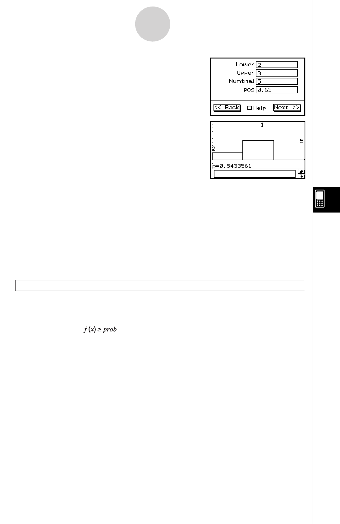
2009060120091101

Example

Trials : 5

Lower bound : 2

Upper bound : 3

Probability of success : 0.63

• Statistics Wizard Operation

(1) On the menu bar, tap [Calc] and then [Distribution].

(2) Select [Binomial CD] and then tap [Next >>].

(3) Input values.

(4) Tap [Next >>].

(5) To display the graph, tap $.

uProgram, eActivity or Main Application

Command: BinomialCD

Command Syntax

Lower value, Upper value, Numtrial value, pos value

Input Example:

BinomialCD 2,3,5,0.63

Inverse Binomial Cumulative Distribution

Menu: [Inv. Distribution]-[Inverse Binomial CD]

Description: This command calculates the inverse of the binomial cumulative distribution.

This command returns the minimum value (positive integer) of m (Σ upper

bound) that satisfies the inequality formula above.

Definition of Terms

prob : binomial cumulative probability (0 < prob < 1)

Numtrial : number of trials n (integer, n > 0)

pos : probability of success

p (0 < p < 1)

Calculation Result Output

xInv : inverse binomial cumulative distribution

*xInv : recalculation value (Displayed only when there may be a possibility of

rounding error.)

• To account for possible rounding error, ClassPad additionally obtains the

result using the probability that is next lowest for the least significant digit. For

example, if the probability is 0.61, ClassPad would recalculate using 0.60. The

recalculation result is only shown if it is different from the original one.

Graphing may take a long

time when the absolute value

of the argument is large.

Graphing may take a long

time when the absolute value

of the argument is large.

= 0

7-11-16

Distributions

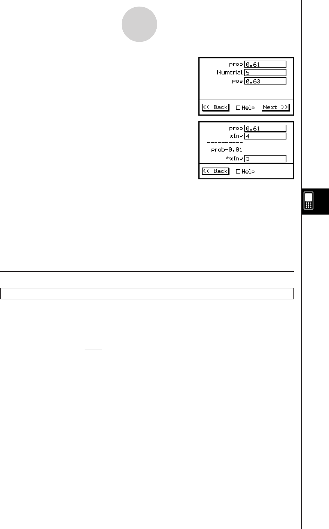
20090601

Example

Binomial cumulative probability : 0.61

Trials : 5

Probability of success : 0.63

• Statistics Wizard Operation

(1) On the menu bar, tap [Calc] and then [Distribution].

(2) Select [Inverse Binomial CD] and then tap [Next >>].

(3) Input values.

(4) Tap [Next >>].

uProgram, eActivity or Main Application

Command: InvBinomialCD

Command Syntax

prob value, Numtrial value, pos value

Input Example:

InvBinomialCD 0.609,5,0.63

k Poisson Distribution

Poisson Distribution Probability

Menu: [Distribution]-[Poisson PD]

Description: This command calculates the probability the random variable that follows a

Poisson distribution will be a given x value.

(x)

= x!

–

␭

(

x = 0, 1, 2, ···) ␭: mean (␭ > 0)

Definition of Terms

x : specified trial (integer,

x > 0)

␭ : mean (␭ > 0)

Calculation Result Output

prob : Poisson probability

7-11-17

Distributions

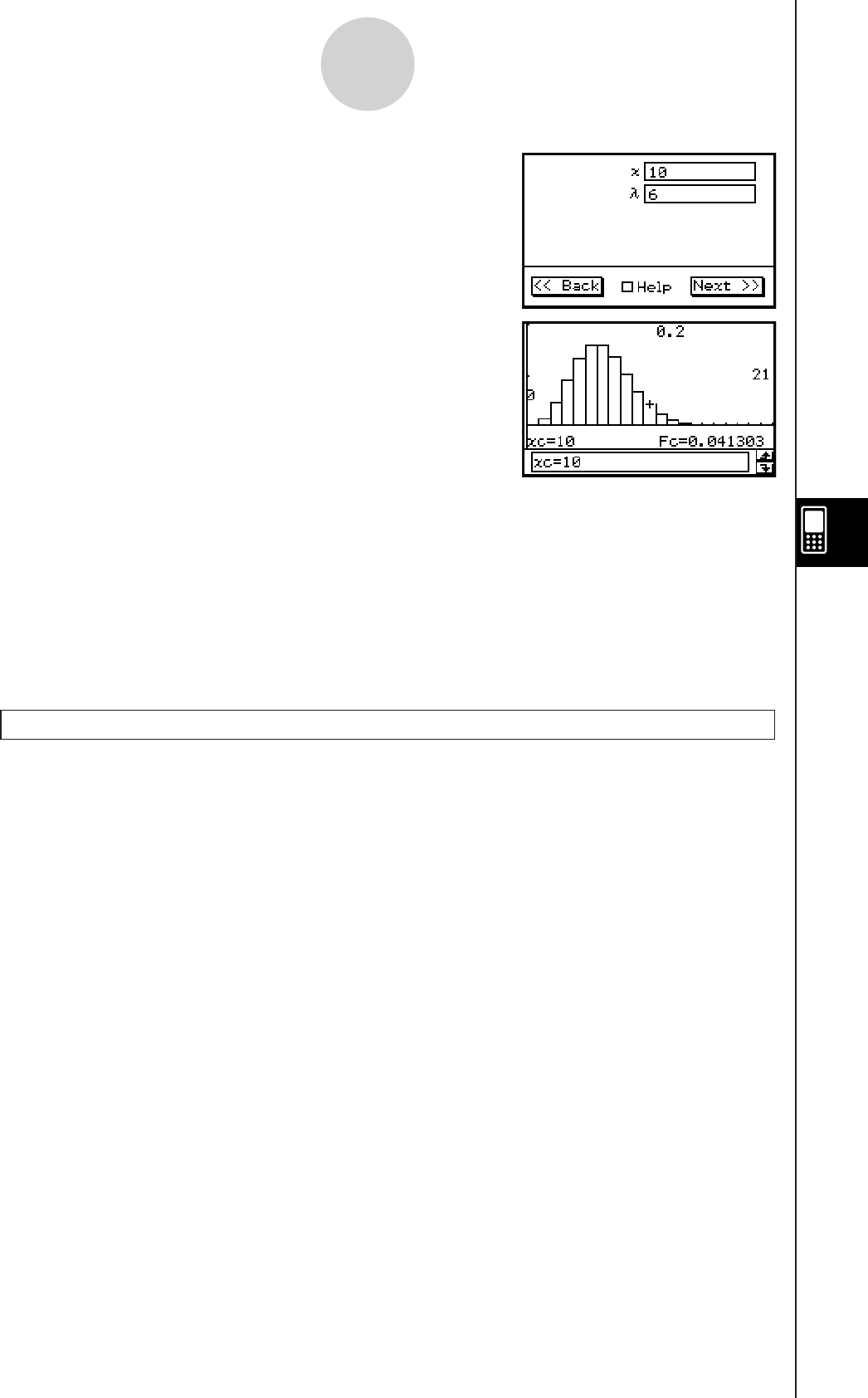
20090601

Example

Specified trial : 10

Mean : 6

• Statistics Wizard Operation

(1) On the menu bar, tap [Calc] and then [Distribution].

(2) Select [Poisson PD] and then tap [Next >>].

(3) Input values.

(4) Tap [Next >>].

(5) To display the graph, tap $.

uProgram, eActivity or Main Application

Command: PoissonPD

Command Syntax

x value, ␭ value

Input Example:

PoissonPD 10,6

Poisson Cumulative Distribution

Menu: [Distribution]-[Poisson CD]

Description: This command calculates the probability the random variable that follows a

Poisson distribution will fall between given upper bound and lower bound

values.

Definition of Terms

Lower : lower bound (Lower < Upper integer)

Upper : upper bound (Lower < Upper integer)

␭ : mean (␭ > 0)

Calculation Result Output

prob : Poisson cumulative probability

Graphing may take a long

time when the absolute value

of the argument is large.

Graphing may take a long

time when the absolute value

of the argument is large.

7-11-18

Distributions

20090601

Example

Lower bound : 2

Upper bound : 3

Mean : 2.26

• Statistics Wizard Operation

(1) On the menu bar, tap [Calc] and then [Distribution].

(2) Select [Poisson CD] and then tap [Next >>].

(3) Input values.

(4) Tap [Next >>].

(5) To display the graph, tap $.

uProgram, eActivity or Main Application

Command: PoissonCD

Command Syntax

Lower value, Upper value, ␭ value

Input Example:

PoissonCD 2,3,2.26

Inverse Poisson Cumulative Distribution

Menu: [Inv. Distribution]-[Inverse Poisson CD]

Description: This command calculates the inverse of the Poisson cumulative distribution.

This command returns the minimum value (positive integer) of m (Σ upper

bound) that satisfies the inequality formula above.

Definition of Terms

prob : Poisson cumulative probability (0 < prob < 1)

␭ : mean (␭ > 0)

Calculation Result Output

xInv : inverse Poisson cumulative distribution

*xInv : recalculation value (Displayed only when there may be a possibility of

rounding error.)

• To account for possible rounding error, ClassPad additionally obtains the result

using the probability that is next lowest for the least significant digit.

For example, if the probability is 0.99999, ClassPad would recalculate using

0.99998. The recalculation result is only shown if it is different from the original

one.

Graphing may take a long

time when the absolute value

of the argument is large.

Graphing may take a long

time when the absolute value

of the argument is large.

= 0

7-11-19

Distributions

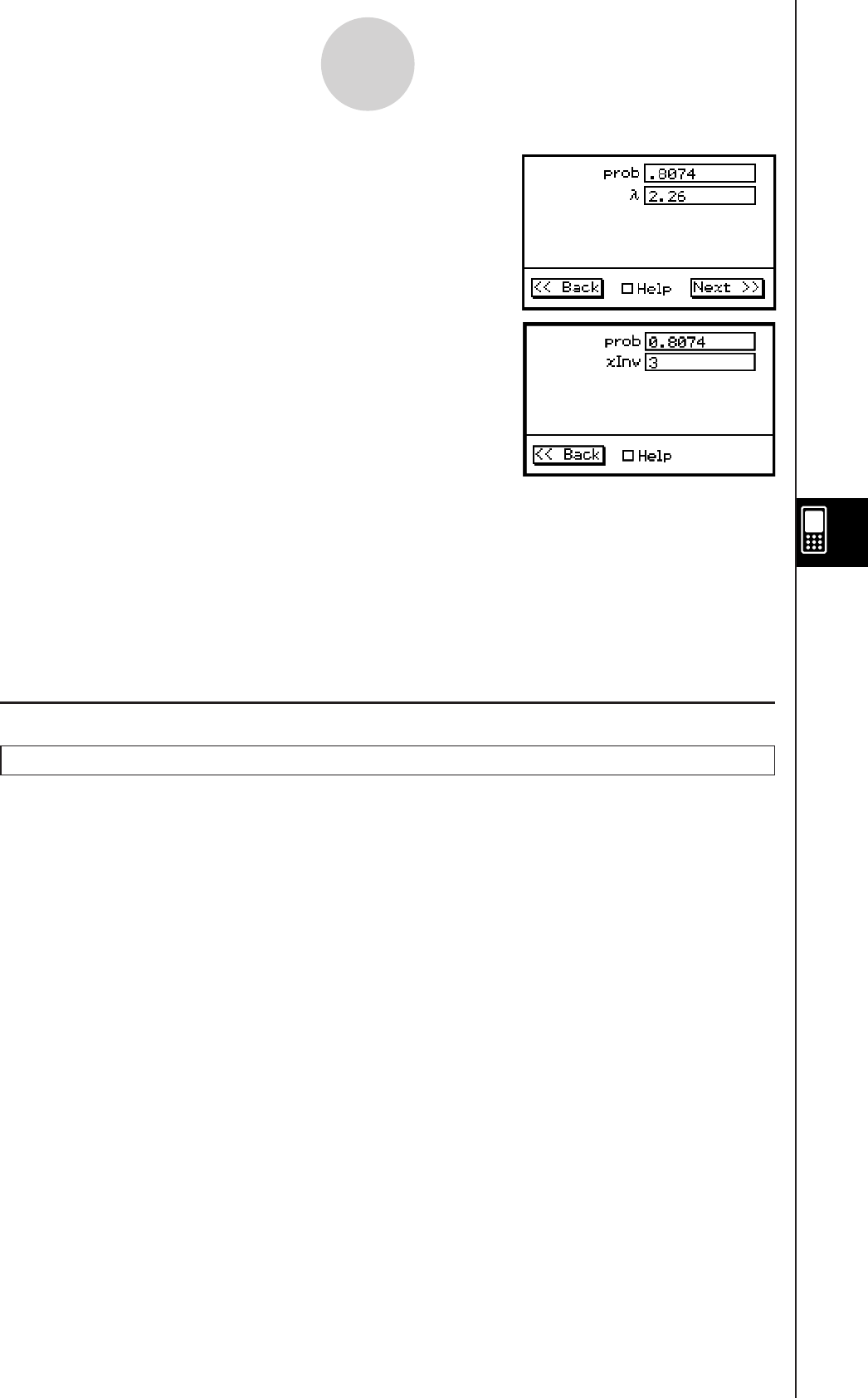
20090601

Example

Poisson cumulative probability : 0.8074

Mean : 2.26

• Statistics Wizard Operation

(1) On the menu bar, tap [Calc] and then [Distribution].

(2) Select [Inverse Poisson CD] and then tap [Next >>].

(3) Input values.

(4) Tap [Next >>].

uProgram, eActivity or Main Application

Command: InvPoissonCD

Command Syntax

prob value, ␭ value

Input Example:

InvPoissonCD 0.8074,2.26

k Geometric Distribution

Geometric Distribution Probability

Menu: [Distribution]-[Geometric PD]

Description: This command calculates the probability the random variable that follows a

geometric distribution will be a given x value.

(x)

= p(1– p)

x – 1

(

x = 1, 2, 3, ···) p : probability of success

(0 < p < 1)

Definition of Terms

x : specified trial (positive integer)

pos : probability of success p (0 < p < 1)

Calculation Result Output

prob : geometric probability

7-11-20

Distributions

20090601

Example

Specified trial : 6

Probability of success : 0.4

• Statistics Wizard Operation

(1) On the menu bar, tap [Calc] and then [Distribution].

(2) Select [Geometric PD] and then tap [Next >>].

(3) Input values.

(4) Tap [Next >>].

(5) To display the graph, tap $.

uProgram, eActivity or Main Application

Command: GeoPD

Command Syntax

x value, pos value

Input Example:

GeoPD 6,0.4

Geometric Cumulative Distribution

Menu: [Distribution]-[Geometric CD]

Description: This command calculates the probability the random variable that follows a

geometric distribution will fall between given upper bound and lower bound

values.

Definition of Terms

Lower : lower bound (Lower < Upper integer)

Upper : upper bound (Lower < Upper integer)

pos : probability of success p (0 < p < 1)

Calculation Result Output

prob : geometric cumulative probability

Graphing may take a long

time when the absolute value

of the argument is large.

Graphing may take a long

time when the absolute value

of the argument is large.

7-11-21

Distributions

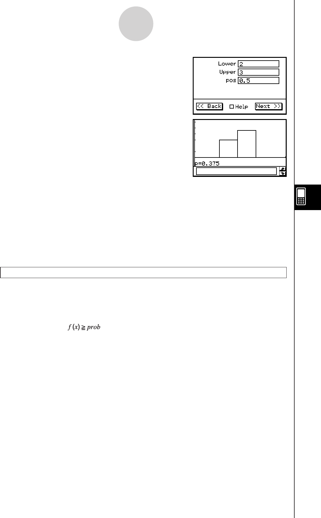
20090601

Example

Lower bound : 2

Upper bound : 3

Probability of success : 0.5

• Statistics Wizard Operation

(1) On the menu bar, tap [Calc] and then [Distribution].

(2) Select [Geometric CD] and then tap [Next >>].

(3) Input values.

(4) Tap [Next >>].

(5) To display the graph, tap $.

uProgram, eActivity or Main Application

Command: GeoCD

Command Syntax

Lower value, Upper value, pos value

Input Example:

GeoCD 2,3,0.5

Inverse Geometric Cumulative Distribution

Menu: [Inv. Distribution]-[Inverse Geo CD]

Description: This command calculates the inverse of the geometric cumulative

distribution.

This command returns the minimum value (positive integer) of m (Σ upper

bound) that satisfies the inequality formula above.

Definition of Terms

prob : geometric cumulative probability (0 < prob < 1)

pos : probability of success p (0 < p < 1)

Calculation Result Output

xInv : inverse geometric cumulative distribution

*xInv : recalculation value (Displayed only when there may be a possibility of

rounding error.)

• To account for possible rounding error, ClassPad additionally obtains the

result using the probability that is next lowest for the least significant digit.

For example, if the probability is 0.875, ClassPad would recalculate using 0.874.

The recalculation result is only shown if it is different from the original one.

Graphing may take a long

time when the absolute value

of the argument is large.

Graphing may take a long

time when the absolute value

of the argument is large.

= 1

7-11-22

Distributions

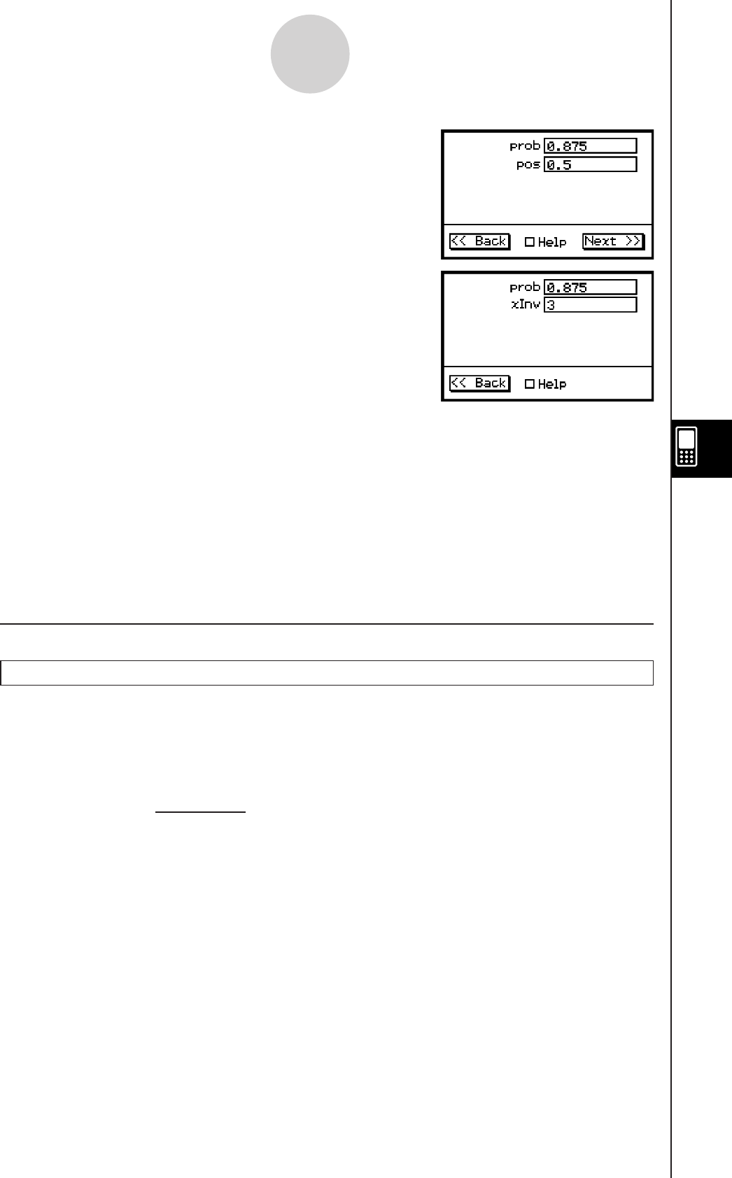
20090601

Example

Geometric cumulative probability : 0.875

Probability of success : 0.5

• Statistics Wizard Operation

(1) On the menu bar, tap [Calc] and then [Distribution].

(2) Select [Inverse Geo CD] and then tap [Next >>].

(3) Input values.

(4) Tap [Next >>].

uProgram, eActivity or Main Application

Command: InvGeoCD

Command Syntax

prob value, pos value

Input Example:

InvGeoCD 0.875,0.5

k Hypergeometric Distribution

Hypergeometric Distribution Probability

Menu: [Distribution]-[Hypergeometric PD]

Description: This command calculates the probability the random variable that follows a

hypergeometric distribution will be a given x value.

prob =

NCn

MCx×N–M Cn–x

Definition of Terms

x : specified trial (integer)

n : number of trials from population (0 < n integer)

M : number of successes in population (0 < M integer)

N : population size (n < N, M < N integer)

Calculation Result Output

prob : hypergeometric probability

7-11-23

Distributions

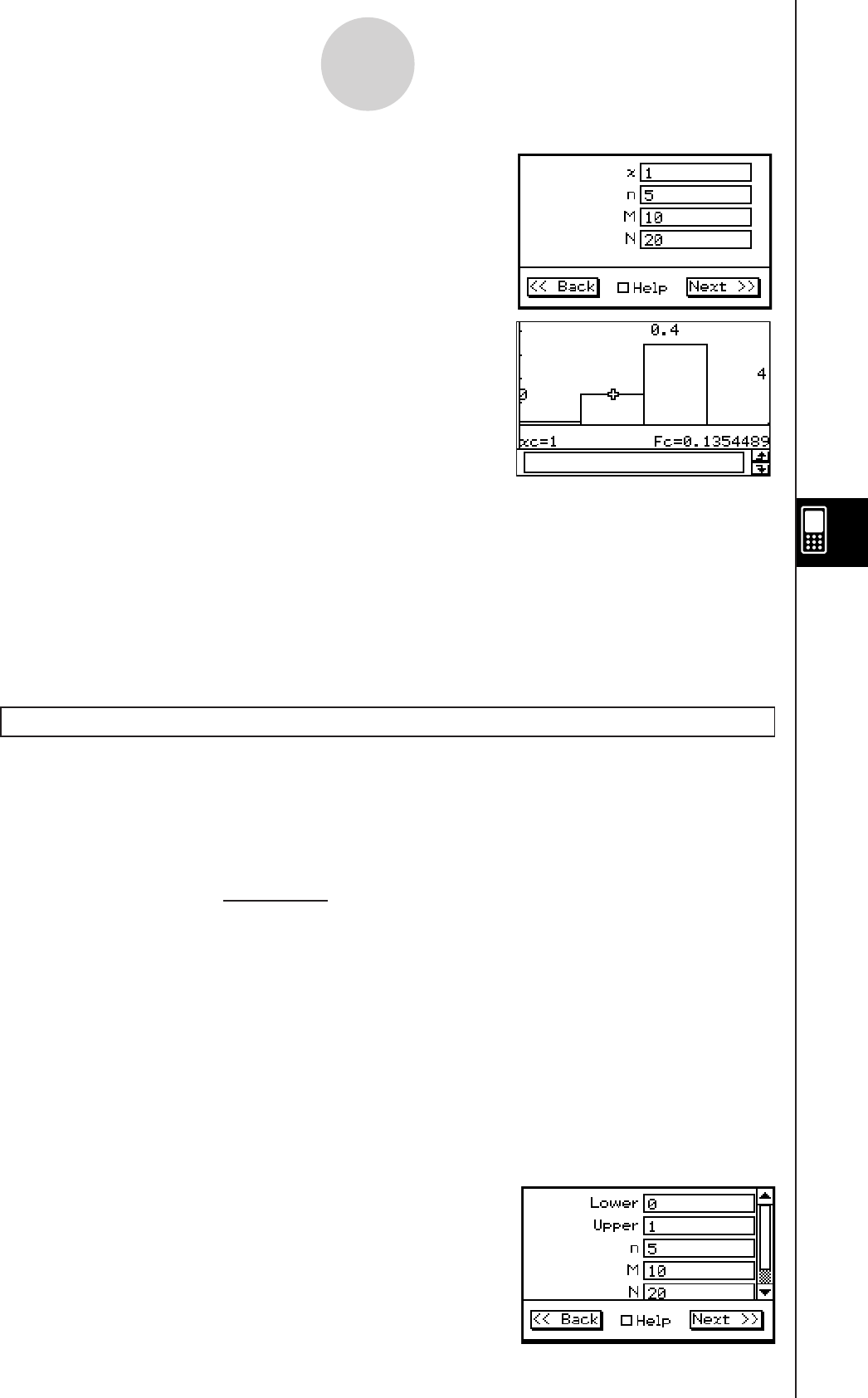
20090601

Example

Specified trial: 1

Number of trials from population: 5

Number of successes in population: 10

Population size: 20

• Statistics Wizard Operation

(1) On the menu bar, tap [Calc] and then [Distribution].

(2) Select [Hypergeometric PD] and then tap

[Next >>].

(3) Input values.

(4) Tap [Next >>].

(5) To display the graph, tap $.

uProgram, eActivity or Main Application

Command: HypergeoPD

Command Syntax

value, n value, M value, N value

Input Example:

HypergeoPD 1,5,10,20

Hypergeometric Cumulative Distribution

Menu: [Distribution]-[Hypergeometric CD]

Description: This command calculates the probability the random variable that follows a

hypergeometric distribution will fall between given lower bound and upper

bound values.

prob =

NCn

MCi ×N–M Cn–i

∑

Upper

i=Lower

Definition of Terms

Lower : lower bound (Lower < Upper integer)

Upper : upper bound (Lower < Upper integer)

n : number of trials from population (0 < n integer)

M : number of successes in population (0 < M integer)

N : population size (n < N, M < N integer)

Calculation Result Output

prob: hypergeometric cumulative probability

Example

Lower bound: 0

Upper bound: 1

Number of trials from population: 5

Number of successes in population: 10

Population size: 20

Graphing may take a long time

when the absolute value of the

argument is large.

Graphing may take a long time

when the absolute value of the

argument is large.

7-11-24

Distributions

20090601

• Statistics Wizard Operation

(1) On the menu bar, tap [Calc] and then [Distribution].

(2) Select [Hypergeometric CD] and then tap [Next >>].

(3) Input values.

(4) Tap [Next >>].

(5) To display the graph, tap $.

uProgram, eActivity or Main Application

Command: HypergeoCD

Command Syntax

Lower value, Upper value, n value, M value, N value

Input Example:

HypergeoCD 0,1,5,10,20

Inverse Hypergeometric Cumulative Distribution

Menu: [Inv. Distribution]-[Inverse Hypergeometric]

Description: This command calculates the inverse of the hypergeometric cumulative

distribution.

prob H

NCn

MCi ×N–M Cn–i

∑

i=0

This command returns the minimum value (positive integer) of X (Σ upper

bound) that satisfies the inequality formula above.

Definition of Terms

prob : hypergeometric cumulative probability (0 < prob < 1)

n : number of trials from population (0 < n integer)

M : number of successes in population (0 < M integer)

N : population size (n < N, M < N integer)

Calculation Result Output

xInv : inverse hypergeometric cumulative distribution

*xInv : recalculation value (Displayed only when there is the possibility of

rounding error.)

• To account for possible rounding error, ClassPad also obtains the result using

the probability that is next lowest for the least significant digit. For example, if

the probability is 0.3, ClassPad would recalculate using 0.29. The recalculation

result is only shown if it is different from the original one.

Graphing may take a long

time when the absolute value

of the argument is large.

Graphing may take a long

time when the absolute value

of the argument is large.

7-11-25

Distributions

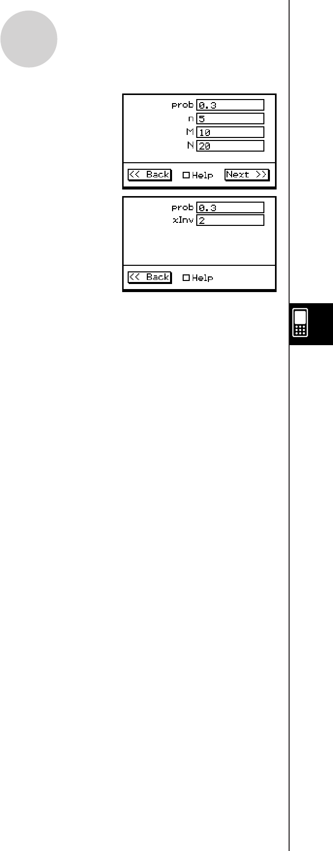
20090601

Example

Hypergeometric cumulative probability: 0.3

Number of trials from population: 5

Number of successes in population: 10

Population size: 20

• Statistics Wizard Operation

(1) On the menu bar, tap [Calc] and then [Distribution].

(2) Select [Inverse Hypergeometric] and then tap

[Next >>].

(3) Input values.

(4) Tap [Next >>].

• Program, eActivity or Main Application

Command: InvHypergeoCD

Command Syntax

prob value, n value, M value, N value

Input Example:

InvHypergeoCD 0.3,5,10,20

7-11-26

Distributions

20110401

7-12 Statistical System Variables

Performing a statistical calculation, graphing operation, or other operation causes calculation

results to be assigned to pre-arranged system variables. For more information, see the

“System Variable Table” on page α-2-1.

7-12-1

Statistical System Variables

20060301

Using the Geometry

Application

The Geometry application allows you to draw and analyze geometric

figures. You can draw a triangle and specify values to change the size

of its sides so they are 3:4:5, and then check the measurement of

each of its angles. Or you can draw a circle and then draw a line that

is tangent to a particular point on the circle. The Geometry application

also includes an animation feature that lets you watch how a figure

changes in accordance with conditions you define.

8-1 Geometry Application Overview

8-2 Drawing Figures

8-3 Editing Figures

8-4 Controlling Geometry Window Appearance

8-5 Working with Animations

8-6 Using the Geometry Application with Other Applications

8-7 Managing Geometry Application Files

Chapter

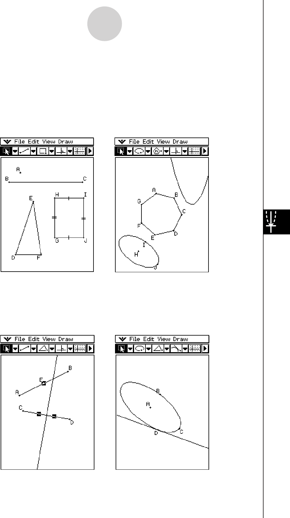
20060301

8-1-1

Geometry Application Overview

8-1 Geometry Application Overview

The Geometry application provides you with the following capabilities.

• The [Draw] menu provides commands for drawing points, lines, polygons, regular polygons,

circles, ellipses, and other geometric figures. You can also draw functions. Once drawn, a

figure can be moved or edited as required. See “Using the Draw Menu” on page 8-2-1 for

more information about this menu.

• The [Draw] menu also includes a [Construct] submenu (page 8-2-30) and a [Special Shape]

submenu (page 8-2-27). You can use items in the [Construct] submenu to add a midpoint,

draw a perpendicular bisector from a given point, create other geometric constructions and

even test geometric theorems. The [Special Shape] submenu allows you to draw special

figures, such as parallelograms, rectangles, kites and many others.

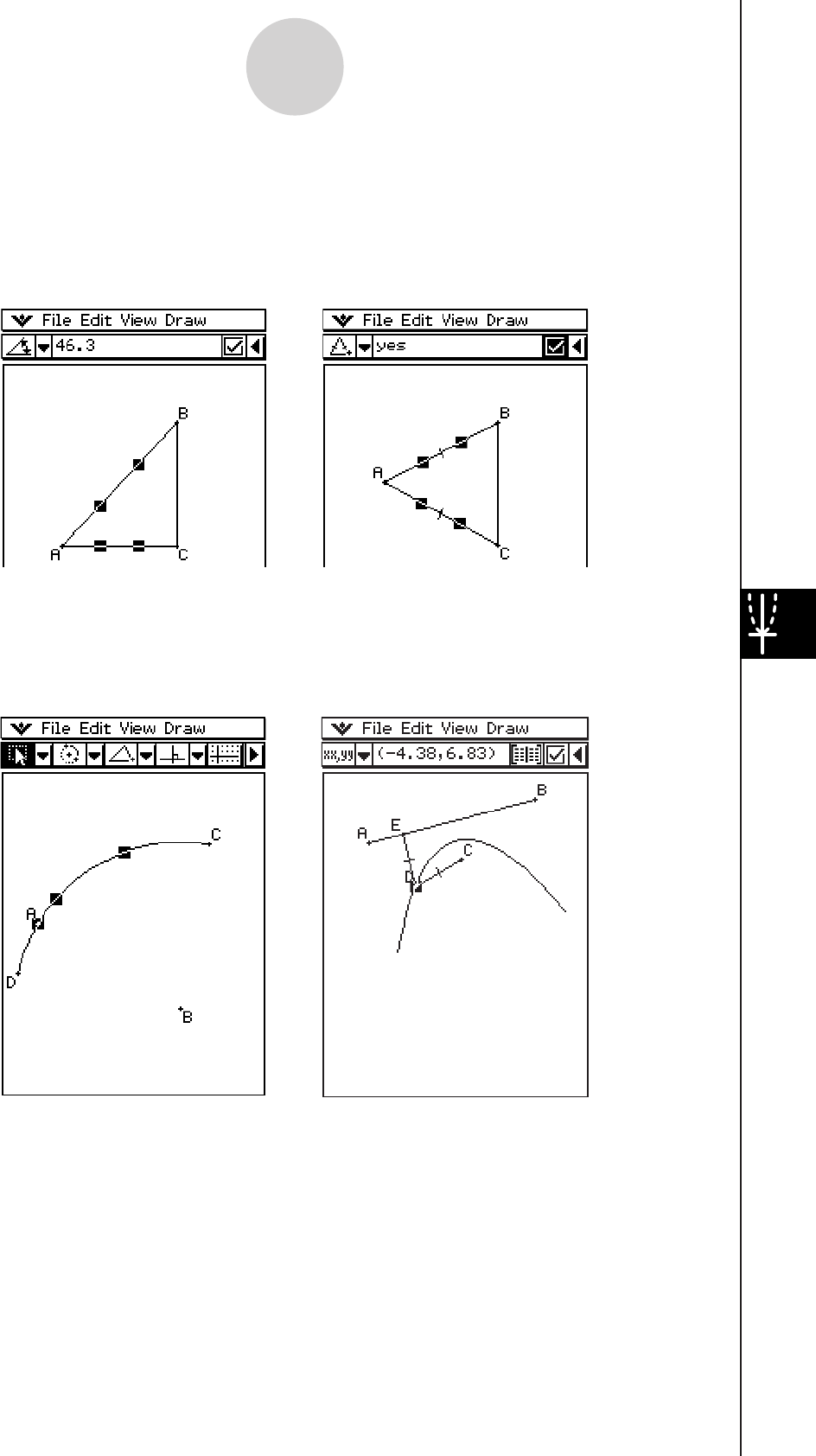
20060301

• Tapping the toolbar’s right arrow button displays a measurement box. The measurement

box displays information for the items that are selected on the window. For example, you

can view the coordinates of a point, the length and slope of a line segment, the size of an

angle, etc. You can also use the measurement box to change measurements, and to fix

measurements so they cannot be changed by other operations.

8-1-2

Geometry Application Overview

• The Animation feature makes it possible to see how a figure changes when a moving point

and its related figures are subjected to certain conditions. A point can move along a line or

curve, and can be anywhere along a line segment, the vertex of a triangle, or the center

point of a circle.

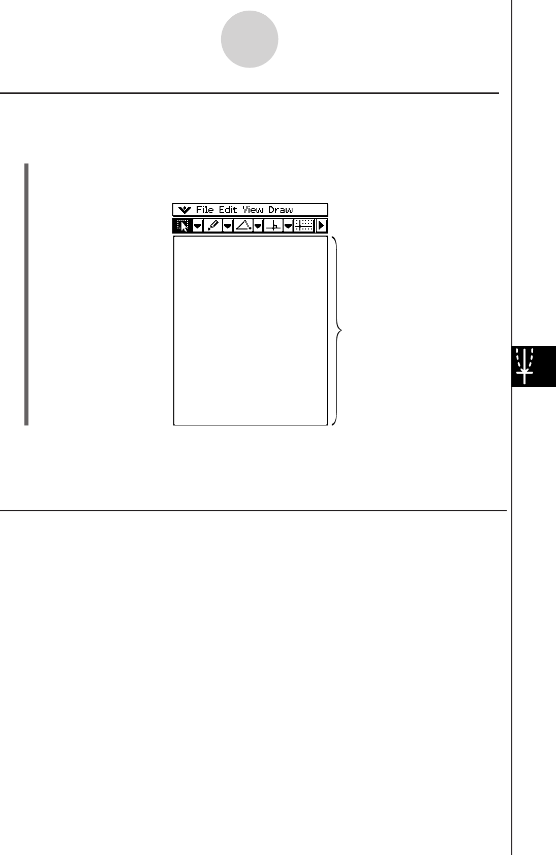
20060301

Geometry Application Menus and Buttons

This section describes the configuration of the Geometry application windows and provides

basic information about its menus and commands.

Tip

• O menu items are the same for all applications. For more information, see “ Using the O Menu”

on page 1-5-4.

• The View Window (O - [View Window]) and Geometry Format (O - [Geometry Format]) contain

settings that are unique to the Geometry application. For details, see “Configuring View Window

Settings” on page 8-4-1.

8-1-3

Geometry Application Overview

Starting Up the Geometry Application

Use the following procedure to start up the Geometry application.

u ClassPad Operation

On the application menu, tap G.

This causes a blank Geometry application window to appear.

Tip

• If you left figures on the Geometry window the last time you exited the Geometry application,

those figures will appear the next time you start it up.

Use this area to draw the figures

you want.

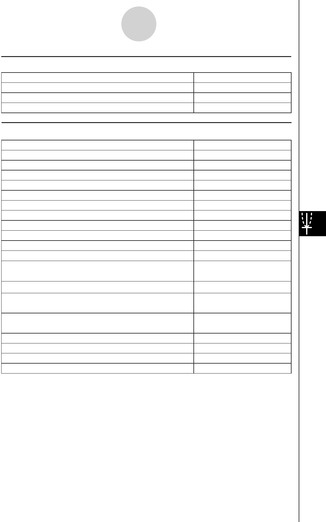
20060301

8-1-4

Geometry Application Overview

k Edit Menu

Undo or redo the last operation

Undo/Redo

Clear all settings fixed with the measurement box

Clear Constraints

Show hidden objects

Show All

Toggle polygon shading on and off

Shade On/Off

Hide the currently selected object

Properties - Hide

Show hidden names

Properties - Show Name

Hide the selected name

Properties - Hide Name

Make the lines of the selected figure thicker

Properties - Thicker

Make the lines of the selected figure thinner

Properties - Thinner

Pin an annotation position on the Geometry window

Properties - Pin

Unpin an annotation on the Geometry window

Properties - Unpin

Display the Animate submenu (page 8-5-1)

Animate

Cut the currently selected object and place it onto the

clipboard

Cut

Specify the number format for each measurement used

in the Geometry window

Properties - Number Format

Copy the currently selected object and place it onto the

clipboard

Copy

Paste the current clipboard contents onto the screen

Paste

Select all objects on the screen

Select All

Delete the currently selected object

Delete

Clear the screen

Clear All

Select this Edit menu item:

To do this:

k File Menu

Discard the current window contents and create a new file

New

Open an existing file

Open

Save the current window contents to a file

Save

Select this File menu item:

To do this

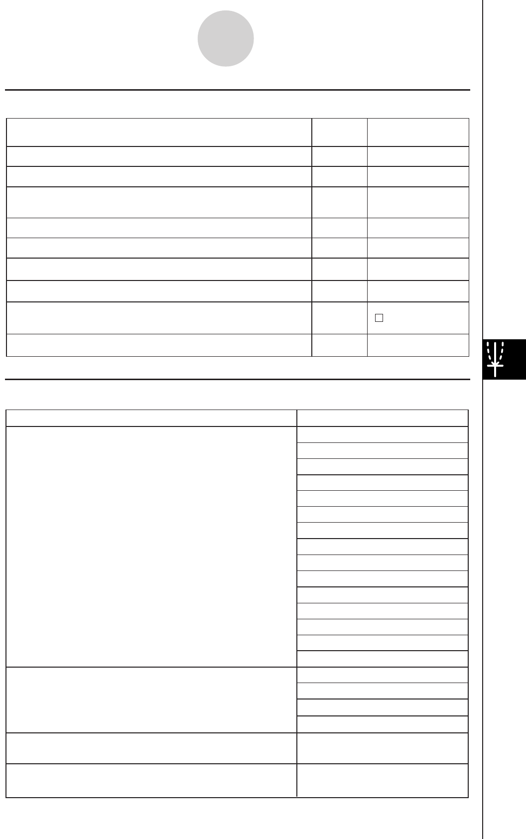
20060301

8-1-5

Geometry Application Overview

k View Menu

To do this: Tap this

button:

Or select this

View menu item:

Zoom Box

Activate the pan function for dragging the Graph

window with the stylus Pan

Enlarge the display image Zoom In

Reduce the size of the display image Zoom Out

Adjust the size of the display image so it fills the display Zoom to Fit

Turn display of axes and coordinate values on and off Toggle Axes

—

Toggle snapping to the nearest integer coordinate

point on and off

Start a box zoom operation

Select

Select a segment, line, or part of a figure (page 8-3-1)

Animation UI

—

Turn the Animation toolbar on and off

Integer Grid

To do this: Select this Draw menu item:

Point

Line Segment

Infinite Line

Vector

Ray

Circle

Arc

Ellipse - Axes

Ellipse - Foci

Hyperbola

Parabola

Function - f (x)

Polygon

Text

Attached Angle

Measurement

Expression

Display a submenu for drawing a figure of specially

shaped figures (page 8-2-27) Special Shape

Insert a value or text connected with a displayed figure

into the display (page 8-2-18)

Display a submenu for geometric constructions

(page 8-2-30) Construct

Draw a figure (page 8-2-1)

Function - Polar

Function - Parametric

k Draw Menu

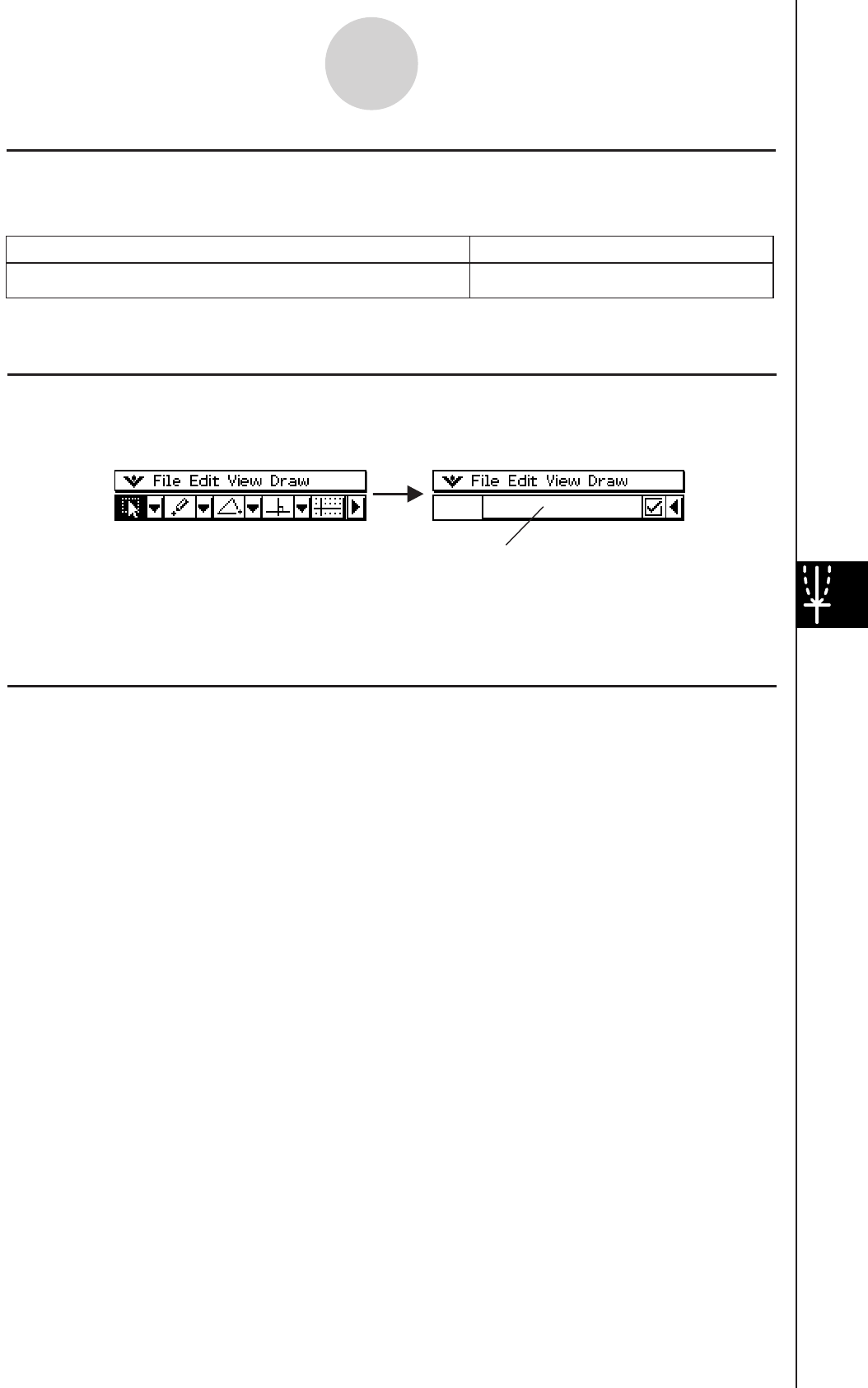
20060301

k Toolbar Button

The operation described below is available from the toolbar only.

8-1-6

Geometry Application Overview

Activate Toggle Select (page 8-3-2)

Tap i and then tap a figure.

Do this:

To do this:

Tapping a button highlights it, indicating that the button’s function is turned on.

k About the Measurement Box

Tapping the u button to the right of the toolbar takes you to the measurement box. Tap t to

return to the normal toolbar.

Normal toolbar Measurement box

For more information about the measurement box, see “Using the Measurement Box” on

page 8-3-6.

k About the Geometry Format Dialog Box

Settings for the Geometry application can be configured on the Geometry Format dialog

box which appears when you tap O and then [Geometry Format]. See “1-9 Configuring

Application Format Settings” for more information.

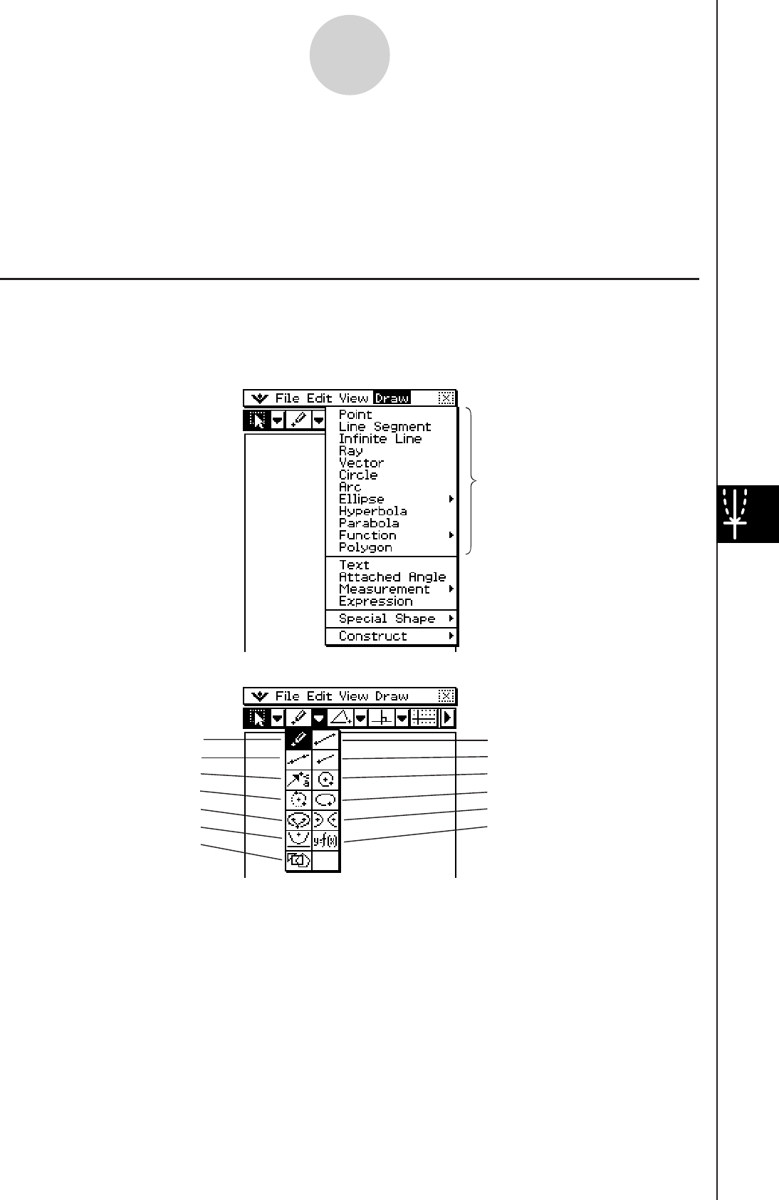
20060301

8-2-1

Drawing Figures

[Draw] menu commands

Toolbar

8-2 Drawing Figures

This section explains how to use the Geometry application to draw various types of figures.

It also explains how to use the geometric construction tools to investigate theorems and

properties in Geometry.

Using the Draw Menu

The [Draw] menu makes it easy to draw a variety of different figures. Each [Draw] menu

command is also available on the toolbar.

These [Draw] menu commands

correspond to the toolbar shown

below.

Point

Infinite Line

Vector

Arc

Ellipse Foci

Parabola

Polygon

Line Segment

Ray

Circle

Ellipse Axes

Hyperbola

Function

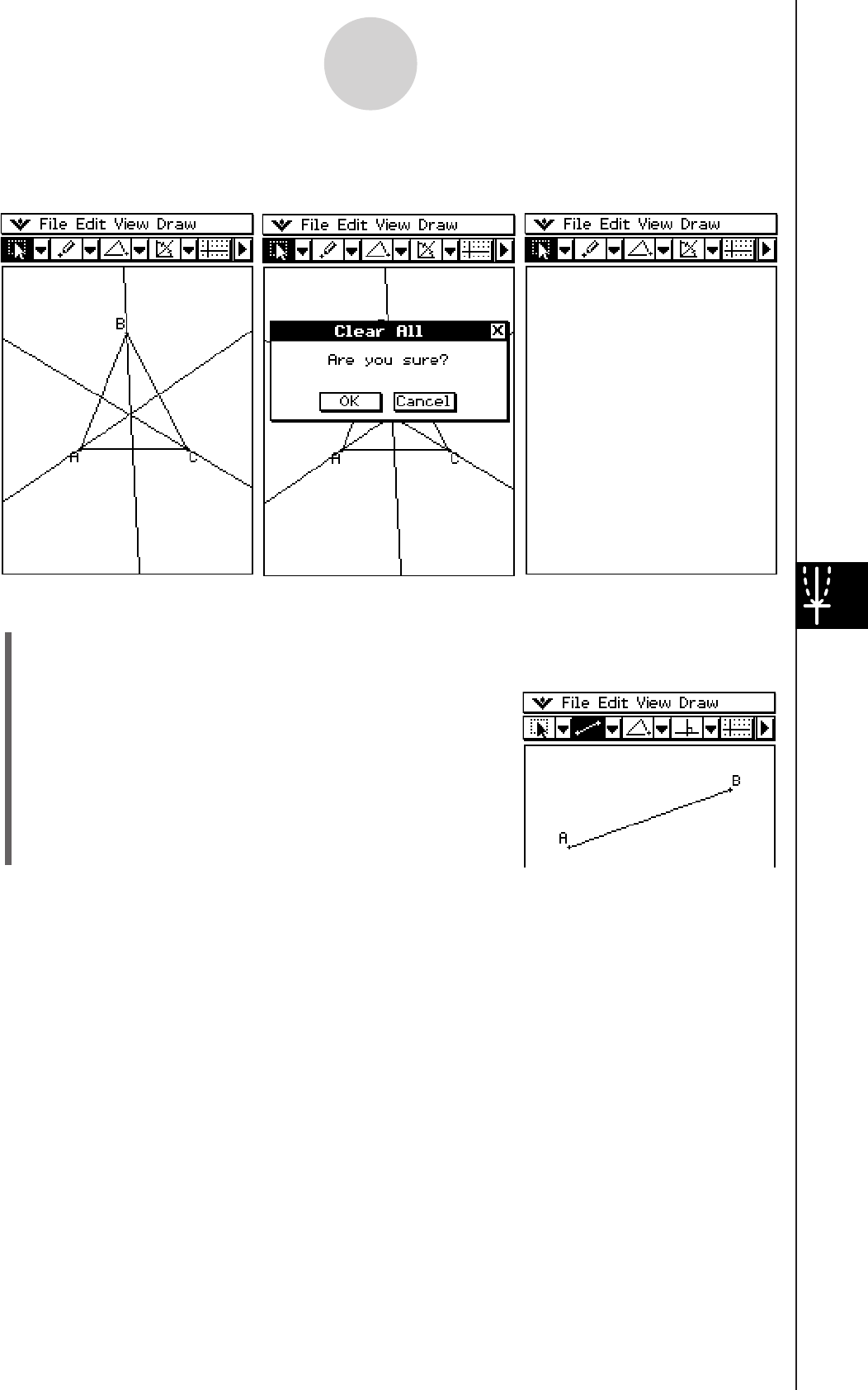
20060301

u To draw a line segment using the menu command

(1) Tap [Draw] and then [Line Segment].

• This highlights the line segment button on the toolbar.

(2) Tap the screen where you want the line segment to

begin, and a point will be drawn, and then tap the

point where you want it to end.

8-2-2

Drawing Figures

Tip

• Use [Edit] - [Clear All] to clear the screen after experimenting with a draw operation.

20060301

u To draw a line segment using the toolbar

(1) Tap the second down arrow on the toolbar. This opens the [Draw] menu’s icon palette.

(2) Tap the line segment button on the toolbar to highlight it.

(3) Tap the screen where you want the line segment to begin. This plots a point.

(4) Tap the beginning point again and, without lifting the stylus, drag to draw the line.

Or you could just tap the ending point.

(5) When the line segment is the way you want, remove the stylus from the screen.

8-2-3

Drawing Figures

u To plot a point

(1) Tap [Draw] and then [Point].

• This highlights the point button on the toolbar.

(2) Tap the location on the screen where you want to plot a point.

• This plots the point.

20060301

uTo add a labeled point to an existing line

You can use the following procedure to add a labeled point to an existing line, to a side of an

n-gon, to the periphery of a circle or ellipse, etc.

(1) Tap [Draw] and then [Point].

• This highlights the point button on the toolbar.

(2) Drag the stylus on the screen towards the line where you want to add the labeled point.

• This selects the line, which is indicated by “k”.

8-2-4

Drawing Figures

(3) Drag the stylus to the location on the line where you

want to add a labeled point, and then lift the stylus from

the screen.

u To draw an infinite line

(1) Tap [Draw] and then [Infinite Line].

• This highlights the infinite line button on the toolbar.

(2) Tap two points on the screen through which you want the infinite line to pass.

• You could also tap one point and then drag to the

second point.

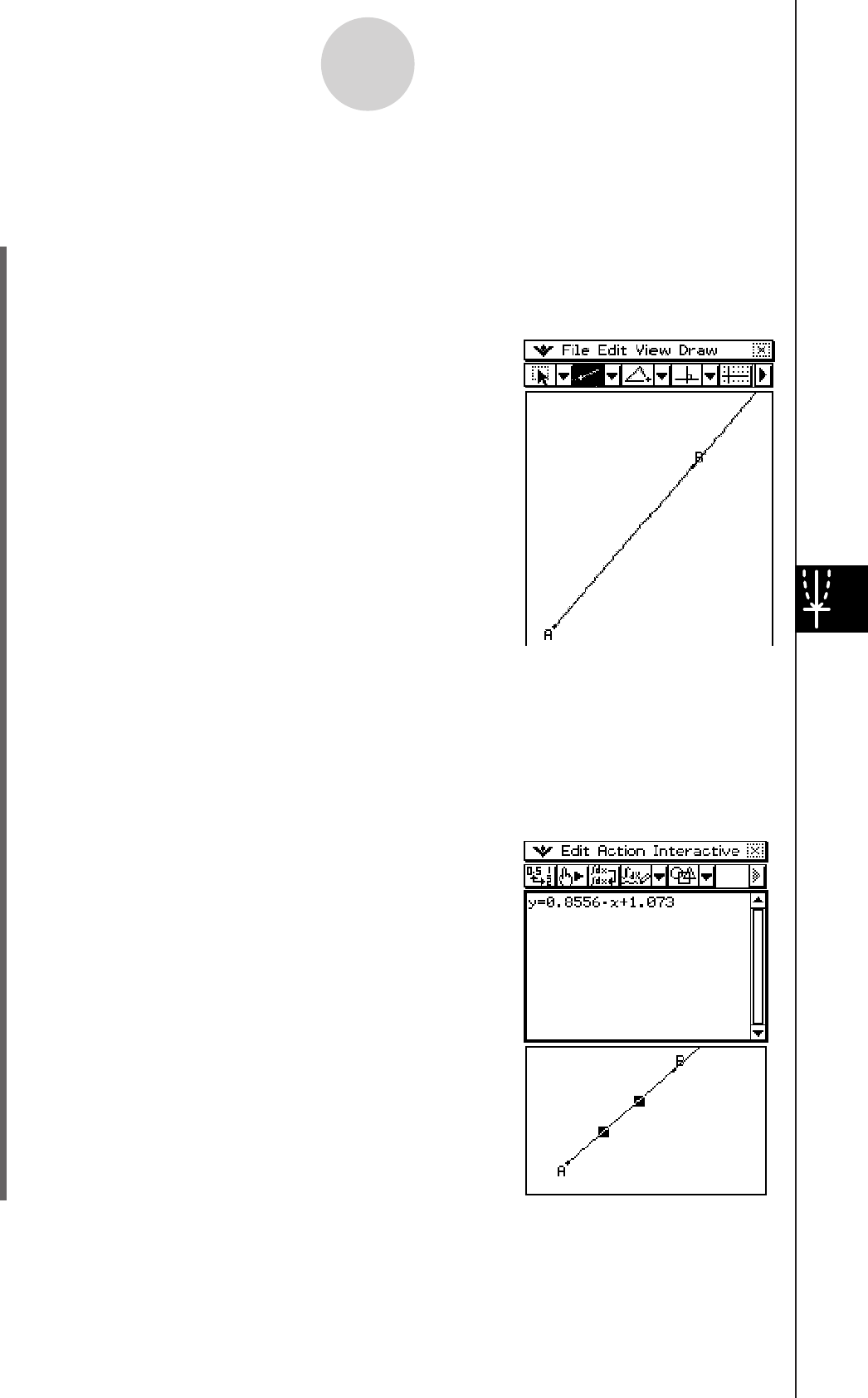
20060301

8-2-5

Drawing Figures

u To draw a ray

Example: To draw a ray and then determine its y = f(x) linear equation by dropping the ray

into the Main or eActivity application window

(1) Tap [Draw] and then [Ray].

• This highlights the ray button on the toolbar.

(2) Tap two points on the screen.

• You could also tap one point and then drag to the

second point.

(3) On the Icon panel, tap M to start up the Main application

(4) Tap the right most down arrow button on the Main application toolbar. On the button list

that appears, tap 3.

• This opens the Geometry application and displays the line drawn in the step (2),

above.

(5) Use the stylus to select ray AB and drop it into the Main application window.

• This displays a linear equation as shown here.

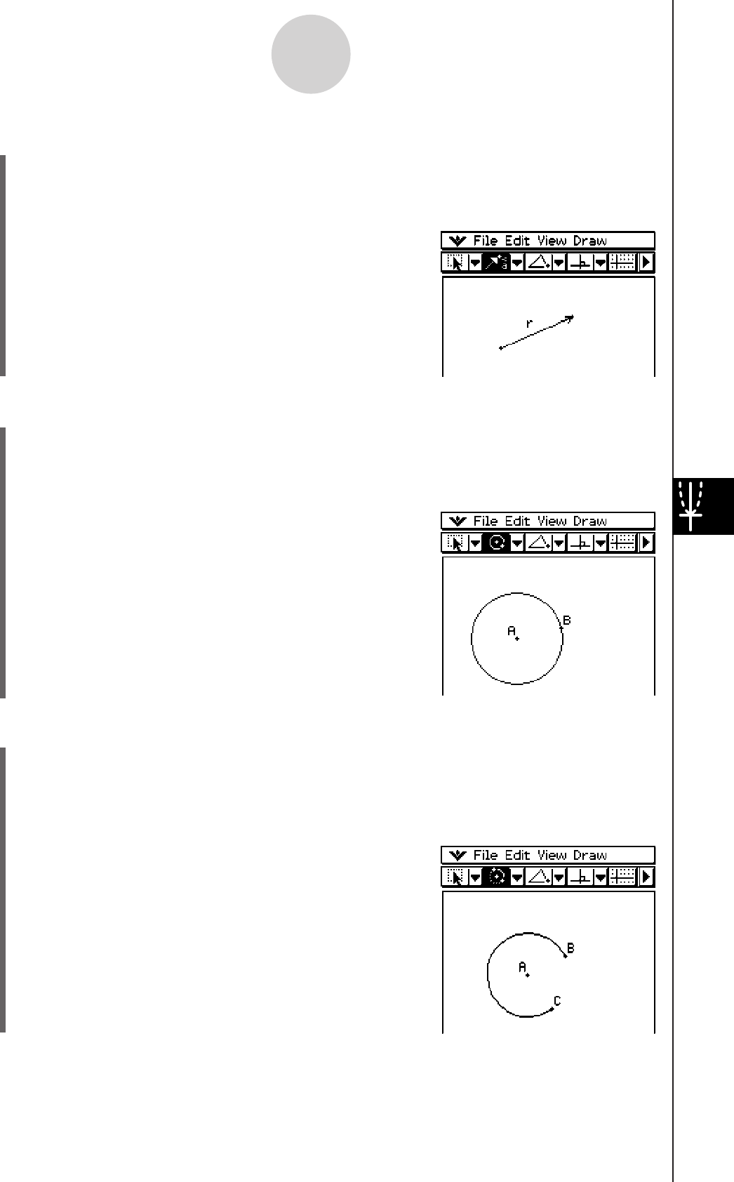
20060301

u To draw a vector

(1) Tap [Draw] and then [Vector].

• This highlights the vector button on the toolbar.

(2) Tap the point where you want the vector to start, and then its end point.

• You could also tap one point, and then drag to

the vector end point.

8-2-6

Drawing Figures

u To draw a circle

(1) Tap [Draw] and then [Circle].

• This highlights the circle button on the toolbar.

(2) Tap the point where you want the center of the circle to be, and then tap a second point

anywhere on the circle’s circumference.

• You could also tap the center point, and then

drag to the second point.

u To draw an arc

(1) Tap [Draw] and then [Arc].

• This highlights the arc button on the toolbar.

(2) Tap the point where you want the center of the arc to be, and then tap a second point

to designate where you want the arc to start.

(3) Tap a third point, which is where you want the arc to

end.

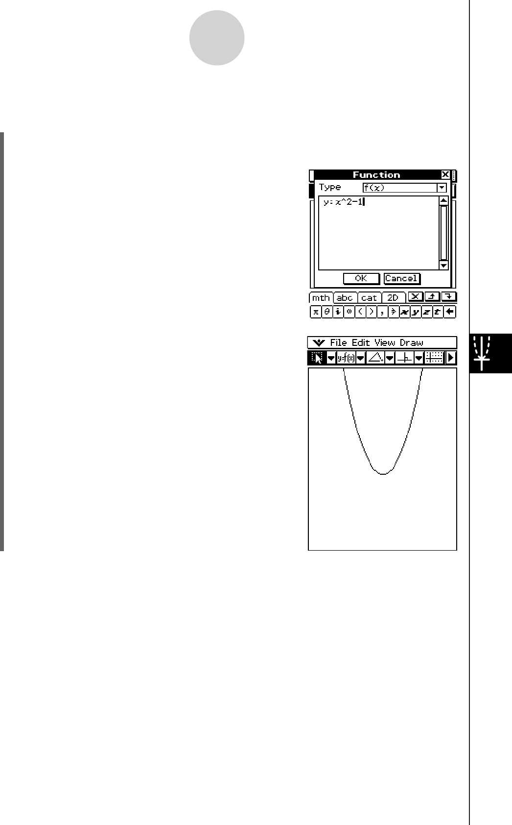
20060301

8-2-7

Drawing Figures

u To draw a function

Example: To draw

y(x) = x2 – 1

(1) Tap [Draw], [Function], and then [f(x)].

• This causes the Function dialog box and a soft keyboard to appear.

(2) Input the function.

(3) Tap [OK] to draw it.

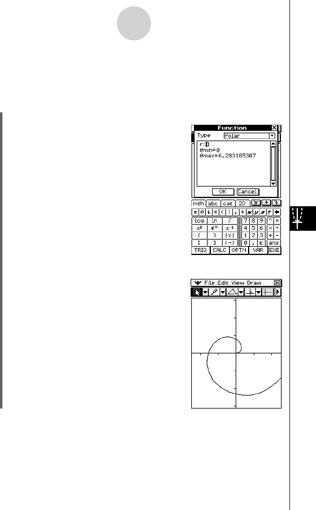
20060301

(1) Tap [Draw], [Function], and then [Polar].

• This displays the Function dialog box and a soft

keyboard as shown here.

8-2-8

Drawing Figures

u To draw a polar equation graph

Note

In this example the [Function Angle] setting of the Geometry Format dialog box is set to

“Radian”. See page 1-9-10 for more information.

(2) Input the equation “r=

” here and then tap [OK].

• This displays a polar equation graph as shown here.

20080201

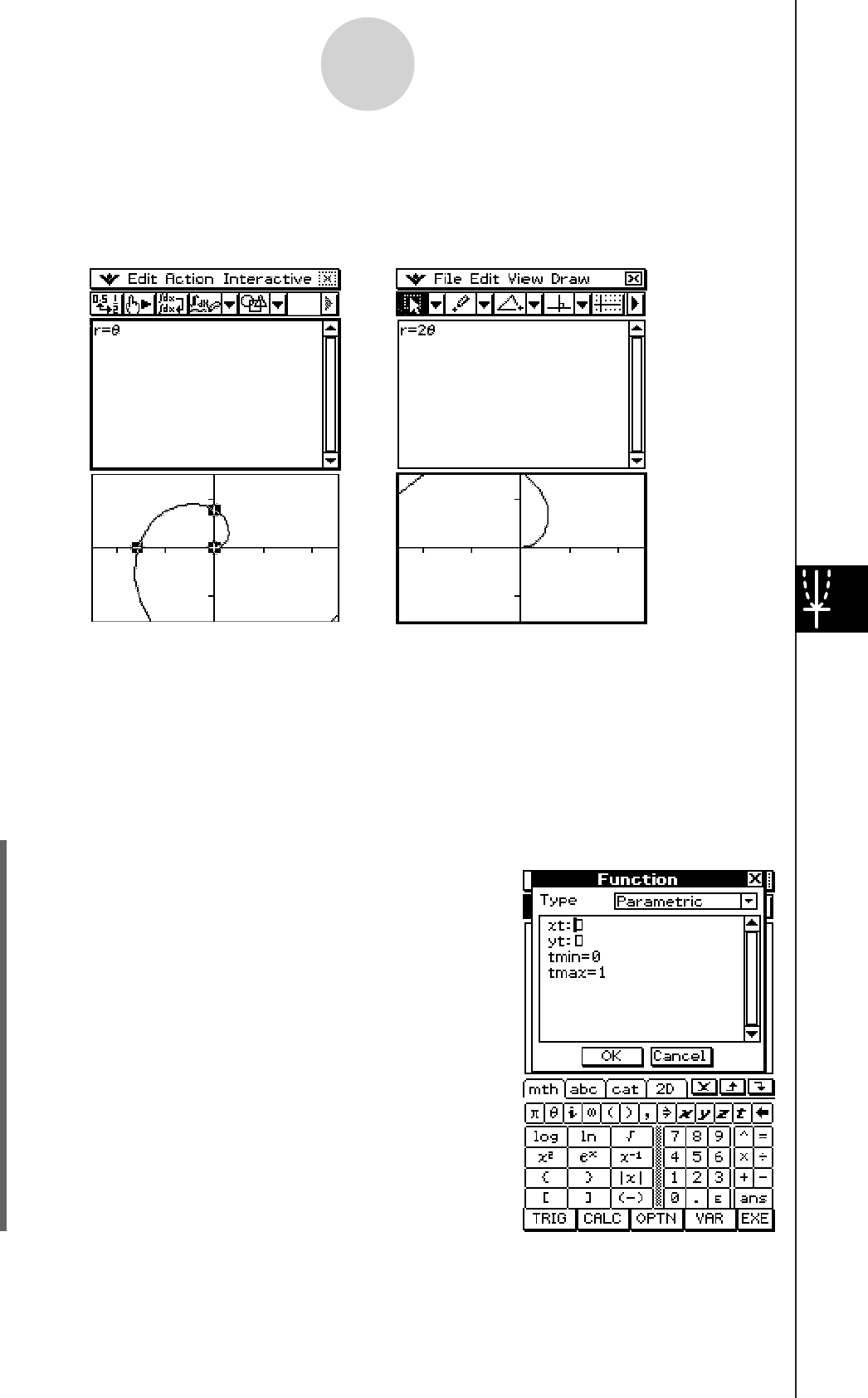
20060301

Tip

• You can drag a polar curve from the Geometry window and drop it into a Main or eActivity

window. Or, for example, you can drag the equation r = f() from the Main or eActivity window

and drop it into the Geometry window as shown below.

u To draw a parametric equation graph

8-2-9

Drawing Figures

Note

In this example the [Function Angle] setting of the Geometry Format dialog box is set to

“Degree”. See page 1-9-10 for more information.

(1) Tap [Draw], [Function], and then [Parametric].

• This displays the Function dialog box and a soft

keyboard.

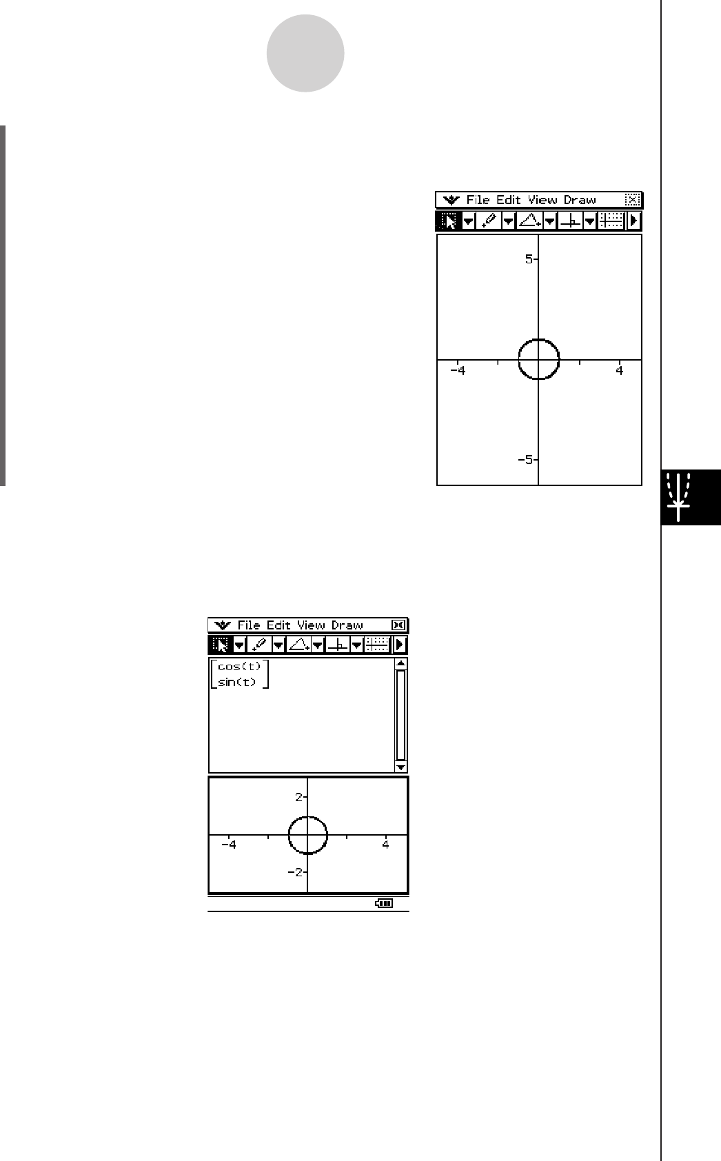
20101001

Tip

• You can display equations such as (x(t), y(t)) on the Geometry window by dragging the graph and

dropping it into the Main or eActivity window where it will appear as a matrix.

8-2-10

Drawing Figures

(2) Input the following expressions and values:

xt = cos(t), yt = sin(t), tmin = 0, tmax = 360

(3) Tap [OK].

• This displays a parametric equation graph as shown

here.

20060301

u To draw an ellipse using the [Ellipse] - [Axes] command

Note

When you draw an ellipse using the [Ellipse] - [Axes] command, you need to specify the

following three elements: center point, Point 1 and Point 2. Point 1 defines the minor axis

(nearest point on the edge from the center point) and Point 2 defines the major axis (farthest

point on the edge from the center point).

8-2-11

Drawing Figures

(1) Tap [Draw], [Ellipse], and then [Axes].

• This highlights the ellipse axes button on the toolbar.

(2) Tap the point you want to specify as the center point.

(3) Tap the point you want to specify as Point 1 (minor axis).

• This causes a line to appear between the center point and Point 1.

• Instead of tapping, you could drag the stylus from the center point to Point 1, viewing

the line that is drawn as you do.

(4) Tap or drag to the point you want to specify as Point 2 (major axis).

• This causes the ellipse to appear.

Center Point .....A

Point ................B

Point ................C

When AC is shorter than AB, Point 1 becomes the major axis and Point 2 becomes the minor

axis.

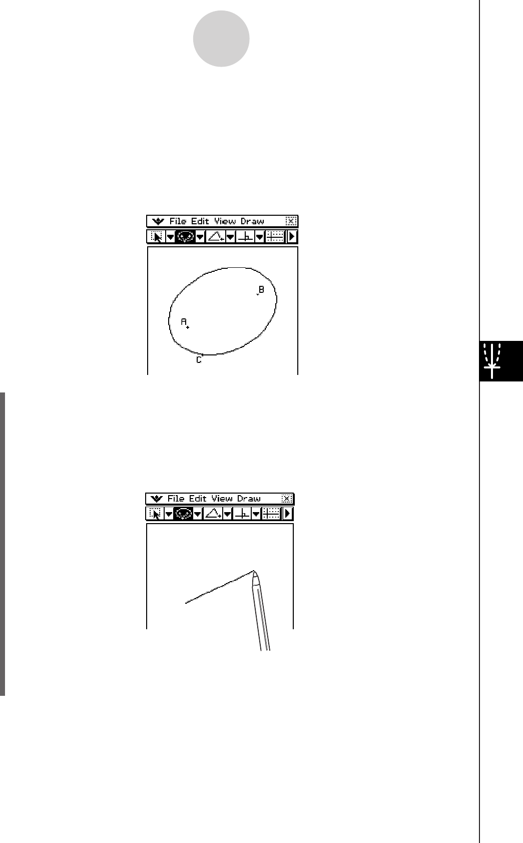
20060301

u To draw an ellipse using the [Ellipse] - [Foci] command

Note

An ellipse is the locus of points, the sum of whose distances from two fixed points (called

foci) is a constant. An ellipse drawn using the [Ellipse] - [Foci] command is drawn in

accordance with this definition. When you draw an ellipse with the [Foci] command, you need

to specify three different points: two foci (Point 1 and Point 2) and one point anywhere on the

ellipse (Point 3).

Point 1 .............A

Point 2 .............B

Point 3 .............C

(1) Tap [Draw], [Ellipse], and then [Foci].

• This highlights the ellipse foci button on the toolbar.

(2) On the screen, tap the two points that you want to specify as the foci of the ellipse (Point

1 and Point 2).

• This causes a line to appear between Point 1 and Point 2.

• Instead of tapping two points as described above, you could also specify the two foci

by tapping to define Point 1 and then dragging the stylus across the screen to Point 2.

8-2-12

Drawing Figures

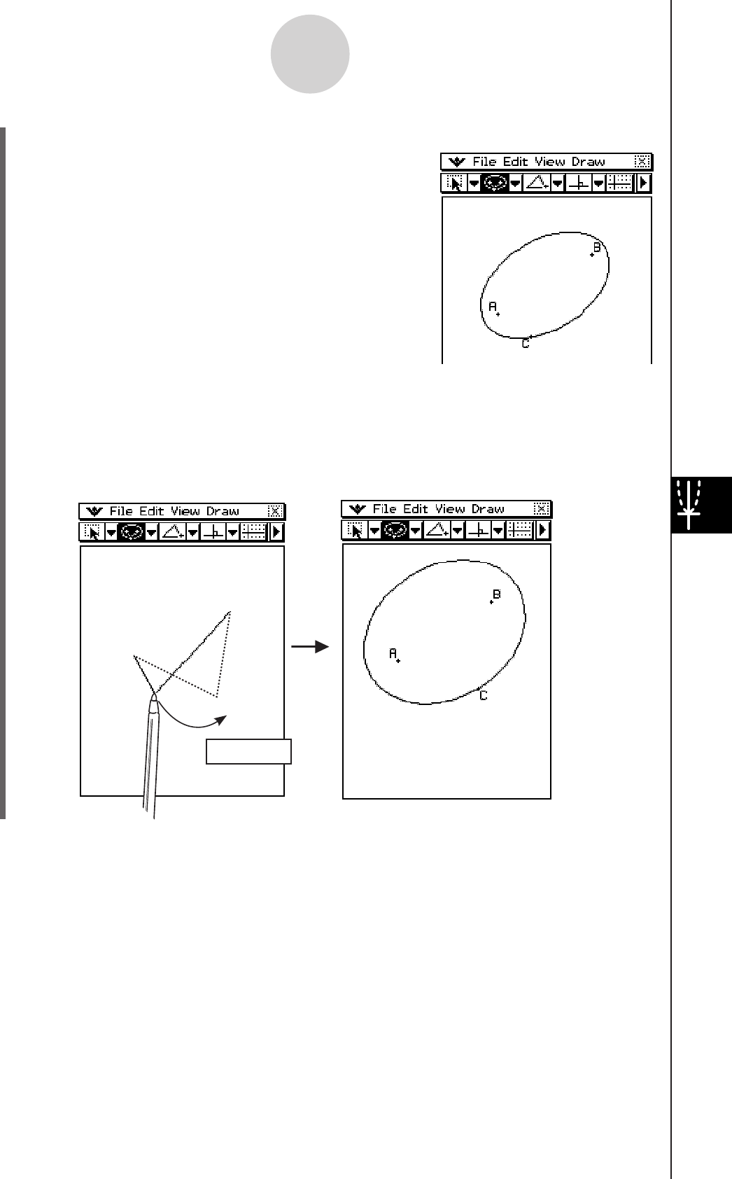
20060301

(3)Tap the point you want to specify as Point 3.

• This specifies the point you tap as Point 3 and draws

the ellipse.

• Instead of tapping the screen to specify Point 3, you could also drag the stylus on the

display. As soon as you tap and hold the stylus on the screen, the line connecting

Point 1 and Point 2 will bend to show the distance from the foci to the location of the

stylus, as shown below. Move the stylus to the location where you want Point 3 to be

and then remove it. This will cause the ellipse to be drawn.

Drag

8-2-13

Drawing Figures

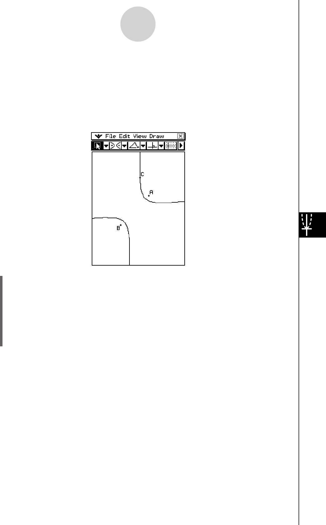
20060301

u To draw a hyperbola

Note

A hyperbola is the locus of points, the difference of whose distances from two fixed points

(called foci) is a given value. A hyperbola drawn using the [Hyperbola] command is drawn in

accordance with this definition. When you draw a hyperbola with the [Hyperbola] command,

you need to specify three different points: two foci (Point 1 and Point 2) and one point

anywhere on the hyperbola (Point 3).

Point 1 .............A

Point 2 .............B

Point 3 .............C

(1) Tap [Draw] and then [Hyperbola].

• This highlights the hyperbola button on the toolbar.

(2) On the screen, tap the two points that you want to specify as the foci of the hyperbola

(Point 1 and Point 2).

• This causes a line to appear between Point 1 and Point 2.

• Instead of tapping two points as described above, you could also specify the two foci

by tapping to define Point 1 and then dragging the stylus across the screen to Point 2.

8-2-14

Drawing Figures

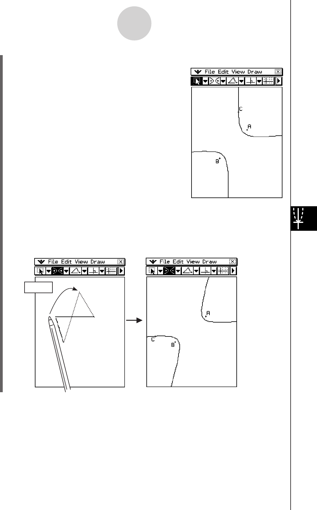
20060301

• Instead of tapping the screen to specify Point 3, you could also drag the stylus on the

display. As soon as you tap and hold the stylus on the screen, the line connecting

Point 1 and Point 2 will bend to show the distance from the foci to the location of the

stylus, as shown below. Move the stylus to the location where you want Point 3 to be

and then remove it. This will cause the hyperbola to be drawn.

Drag

8-2-15

Drawing Figures

(3) Tap the point you want to specify as Point 3.

• This specifies the point you tap as Point 3 and draws

the hyperbola.

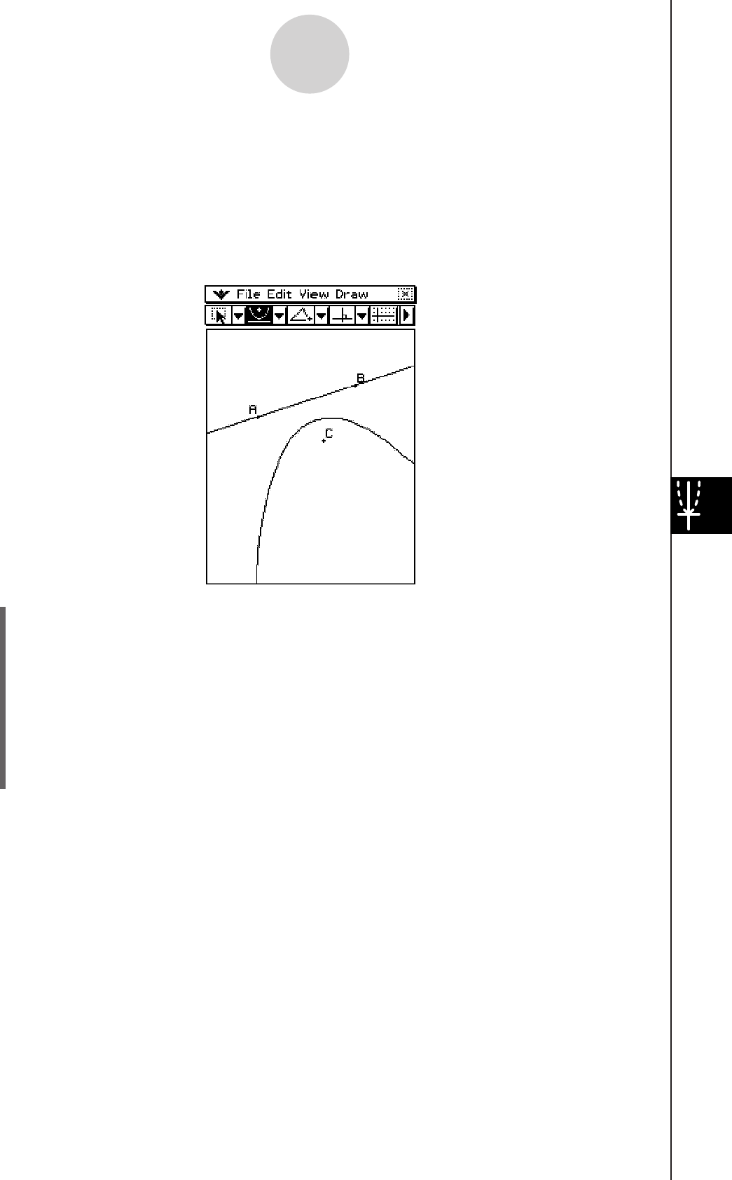
20060301

u To draw a parabola

Note

parabola

is the locus of points equidistant from a point (the focus) and a line (the directrix).

A parabola drawn using the [Parabola] command is drawn in accordance with this definition.

When you draw an parabola with the [Parabola] command, you need to specify three

different points: a line to define the directrix (Point 1 and Point 2) and one point for the focus.

Point 1 .............A

Point 2 .............B

Point 3 .............C

(1) Tap [Draw] and then [Parabola].

• This highlights the parabola button on the toolbar.

(2) On the screen, tap the two points that you want to specify the directrix (Point 1 and

Point 2).

• This causes a line to appear between Point 1 and Point 2.

(3) Tap the point you want to specify as Point 3.

• This specifies the point you tap as Point 3 and draws a parabola in relation to it and

the directrix.

8-2-16

Drawing Figures

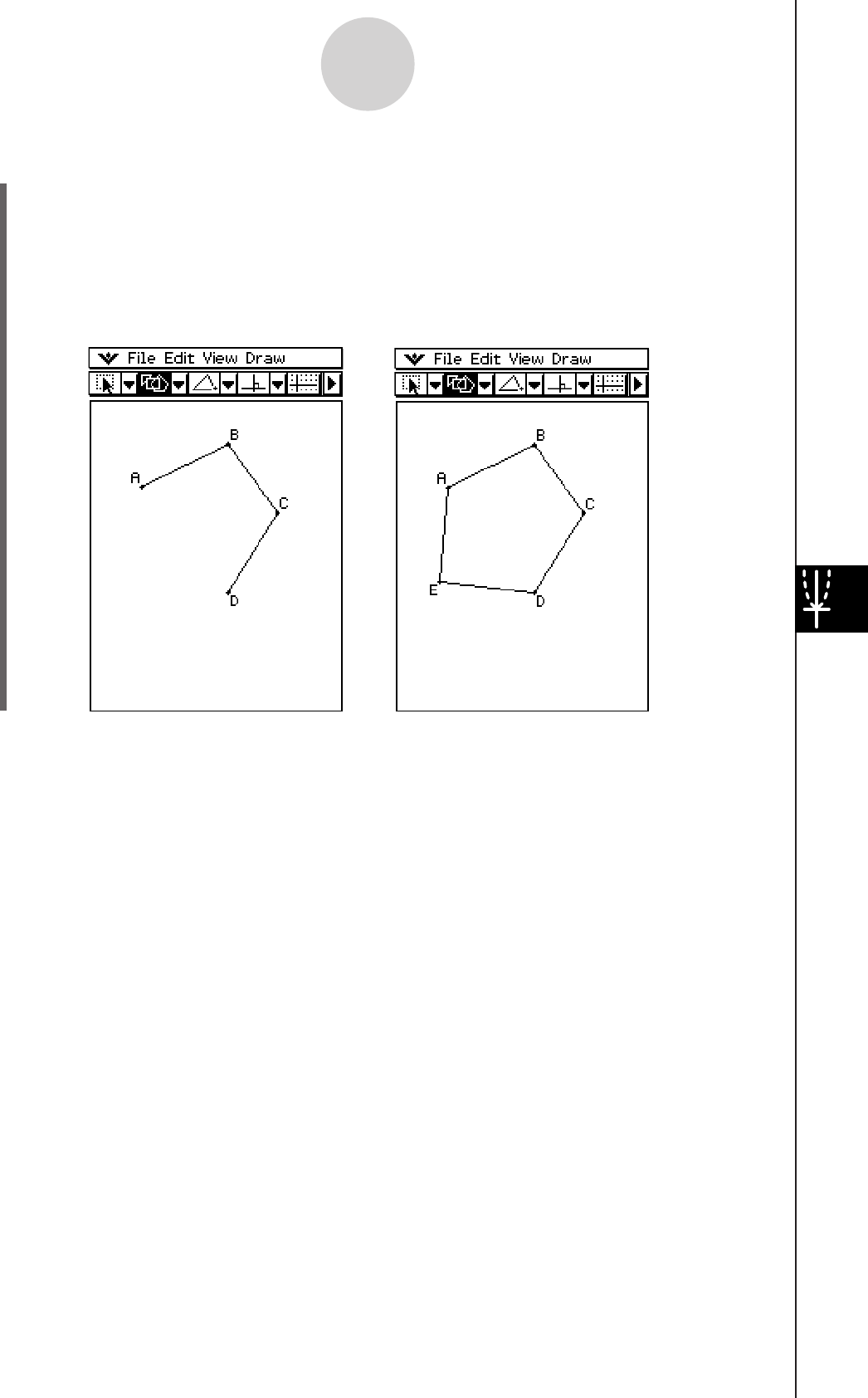
20060301

u To draw a polygon

(1) Tap [Draw] and then [Polygon].

• This highlights the polygon button on the toolbar.

(2) Tap the point from which you want the polygon to start.

(3) Sequentially tap each of the vertices of the polygon.

(4) Finally, tap the start point again to complete the polygon.

8-2-17

Drawing Figures

20090601

Inserting Text Strings into the Screen

You can insert text strings into the screen while working on the Geometry application

window.

u To insert a text string into a screen

(1) Tap [Draw] and [Text].

• This displays the Text dialog box and a soft keyboard.

(2) Input the text you want on the dialog box.

• You can input alphanumeric characters, and you can use the 2D keyboard to input

numeric expressions (see “Using the 2D Keyboard” on page 1-6-15).

(Alphanumeric Input) (Numeric Expression Input

Using the 2D Keyboard)

(3) Tap [OK] to insert the text into the screen.

8-2-18

Drawing Figures

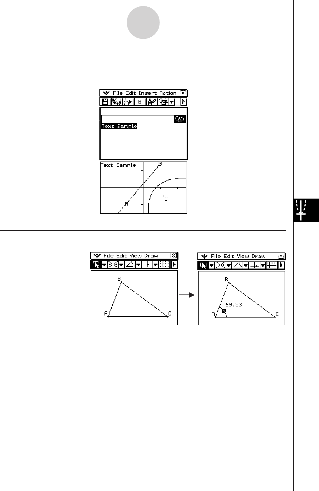
20060301

Drag and Drop

Text on the Geometry window can be dragged to the Main or eActivity window. You can also

drop text from these application windows into the Geometry window.

Attaching an Angle Measurement to a Figure

The measurement of

an angle formed by two

sides of a figure can be

attached to the figure as

shown here. To do so,

tap [Attached Angle] on

the [Draw] menu.

8-2-19

Drawing Figures

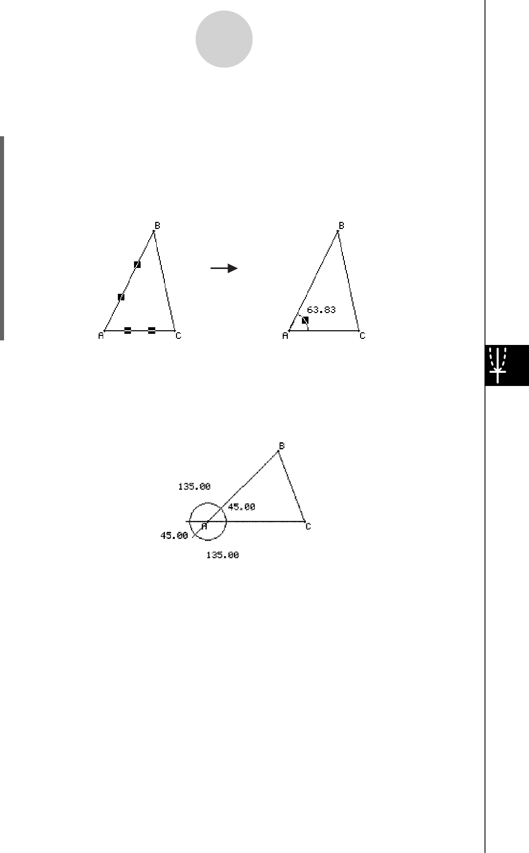
20060301

Tip

• The two sides of a figure actually forms four angles, numbered  through  in the illustration

shown here. After attaching an angle measurement using the [Attached Angle] command, you

can drag it to the position of any one of the other three angles as shown in the examples below.









u To attach an angle measurement to a figure

Example: To attach the measurement of angle A in the triangle ABC

(1) Draw the triangle.

(2) Tap

G. Next, tap side AB and then side AC to select them.

(3) Tap [Draw] and then [Attached Angle].

• This attaches the angle measurement to the figure.

8-2-20

Drawing Figures

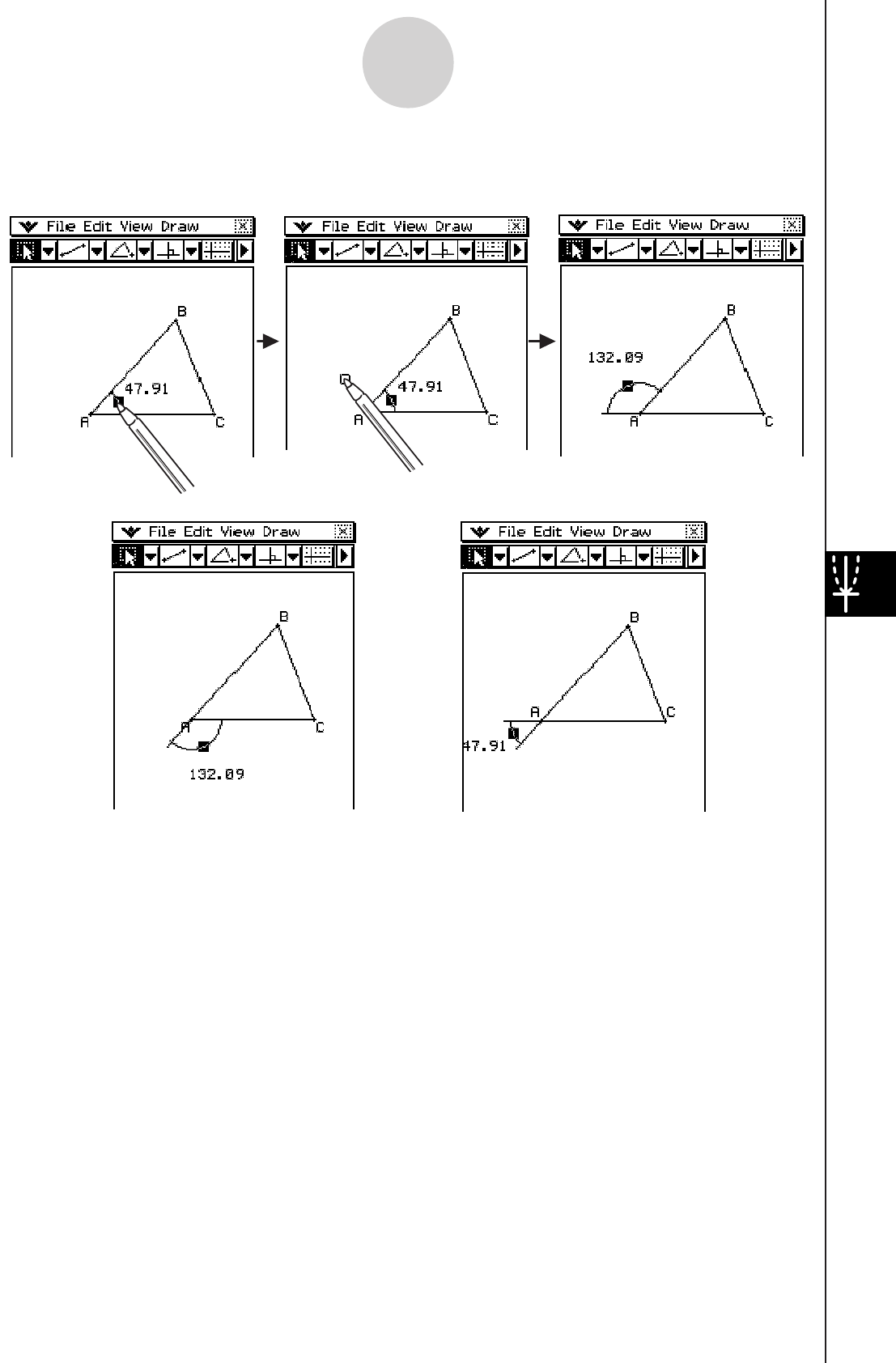
20101001

Example: To drag the angle measurement attached to interior angle A of triangle ABC to its

exterior supplementary angle

(Dragging to the supplementary

angle of the opposite angle of A)

(Dragging to the opposite angle of A)

8-2-21

Drawing Figures

Tip

• You can display more than one attached angle. To do this in the above example, first drag the

initial attached angle to the exterior position and then repeat steps 1 through 3 under “To attach

an angle measurement to a figure” on page 8-2-20.

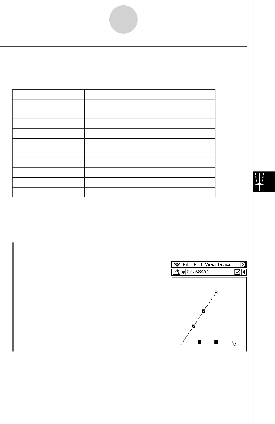
20060301

8-2-22

Drawing Figures

Displaying the Measurements of a Figure

You can display measurements on the Geometry application window. The measurements

change dynamically as you manipulate the figure.

A List of [Measurement] Submenu Commands on the [Draw] Menu

Names of Commands Meanings of Each Command

Angle Angle between two lines

Supplementary Angle Supplementary angle of extended lines

Area Area of selected figure

Circumference Circumference of selected figure

Coordinates Coordinates of selected point

Direction Direction of line or vector

Equation Equation of selected curve

Length Distance between two points, or length of line

Radius Radius of circle

Slope Slope of line or vector

Note

There are three ways to display measurements while you work on the Geometry application

window. The following examples show you each method.

Method 1: Selecting [Measurement] from the [Draw] menu

(1) Tap

G and select elements AB and AC.

(2) Tap the

u button to the right of the toolbar.

• This displays the measurement box, which indicates

the specified angle.

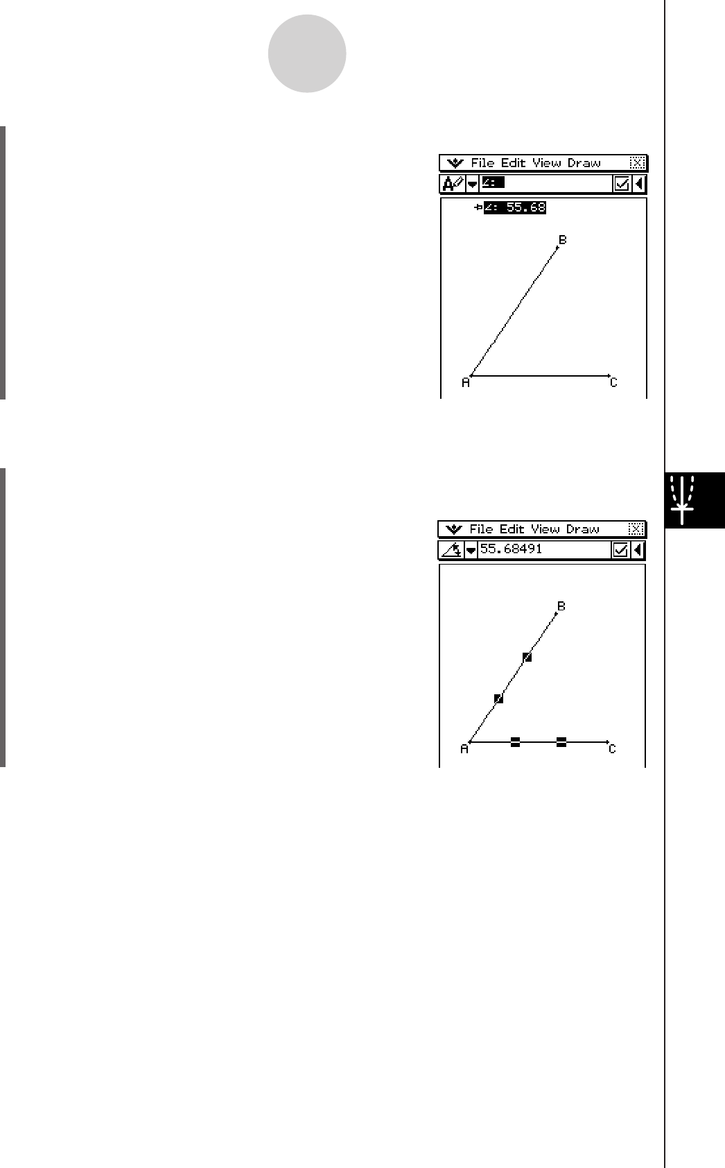
20060301

(3) Tap [Draw], [Measurement], and then [Angle].

• This shows the angle measurement on the screen.

Method 2: Selecting the value in the measurement box and dropping it directly into

the Geometry application window

(1) Tap

G and select elements AB and AC.

(2) Tap the

u button to the right of the toolbar.

• This displays the measurement box, which indicates

the specified angle.

8-2-23

Drawing Figures

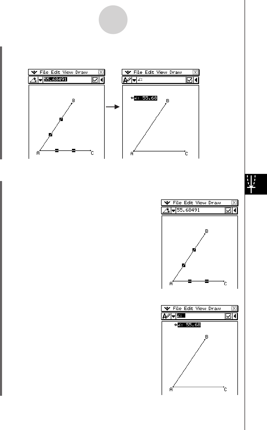
20060301

(3) Select (highlight) value in the measurement box and drop it into the screen below.

• This displays the specified angle measurement on the screen as shown below.

Method 3: Tapping the measurement icon button to the left of the measurement box

(1) Tap

G and select elements AB and AC.

(2) Tap the

u button to the right of the toolbar.

• This displays the measurement box, which indicates

the specified angle.

(3) Tap the

Q button on the far left of the measurement box.

• This displays the specified angle measurement on

the screen as shown here.

8-2-24

Drawing Figures

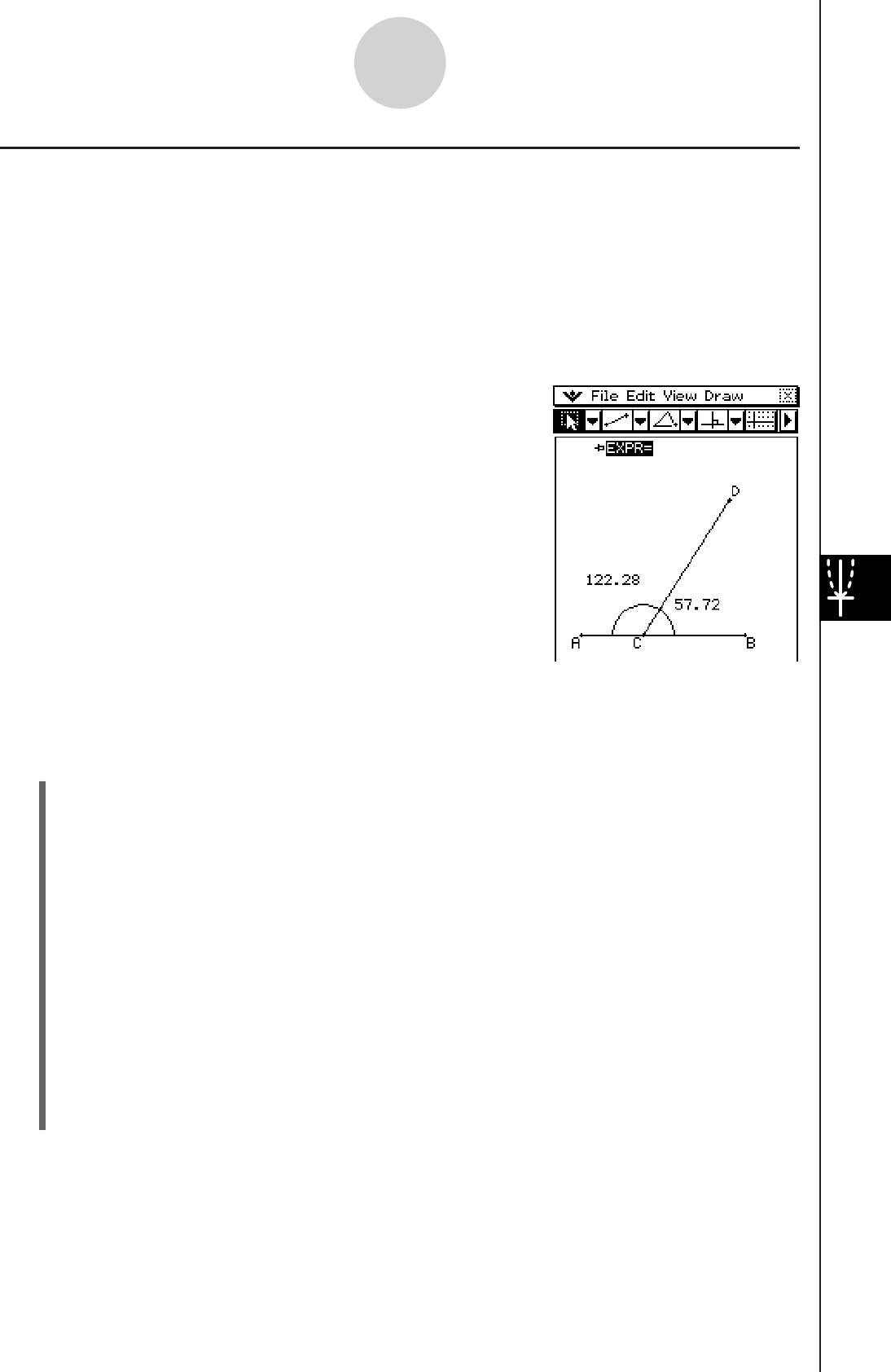
20060301

Displaying the Result of a Calculation that Uses On-screen Measurement

Values

You can use the [Expression] command and the commands on the [Measurement]

submenu to perform calculations using the angle value, line length, surface area, and other

measurement values attached to a figure, and display the result on the Geometry window.

u To display the result of a calculation that uses on-screen measurement

values

Example: With line segment AB and line segment CD (point

C being on AB) drawn on the display as shown

here, calculate the sum of attached angles DCB

and ACD, and display the result on the screen.

(57.72+122.28 = 180.00)

u ClassPad Operation

Steps (1) through (5) draw the figure shown above. The procedure from step (6) performs

the calculation using the on-screen measurement values.

(1) Tap [Draw] - [Line Segment] and then draw line segment AB.

• See “To draw a line segment using the menu command” on page 8-2-2.

(2) Draw line segment CD so that point C lies on line segment AB.

(3) Tap

(4) Select line segment AB and line segment CD, and then tap [Draw] - [Attached Angle].

• This displays the attached angle for ACD.

(5) Tap attached angle ACD and drag it inside of angle DCB.

• This moves the attached angle to angle DCB.

(6) Select line segments AB and CD again, and then tap [Draw] - [Attached Angle].

• This displays the attached angle for ACD.

(7) Tap [Draw] - [Expression].

• This displays an “EXPR=” object.

8-2-25

Drawing Figures

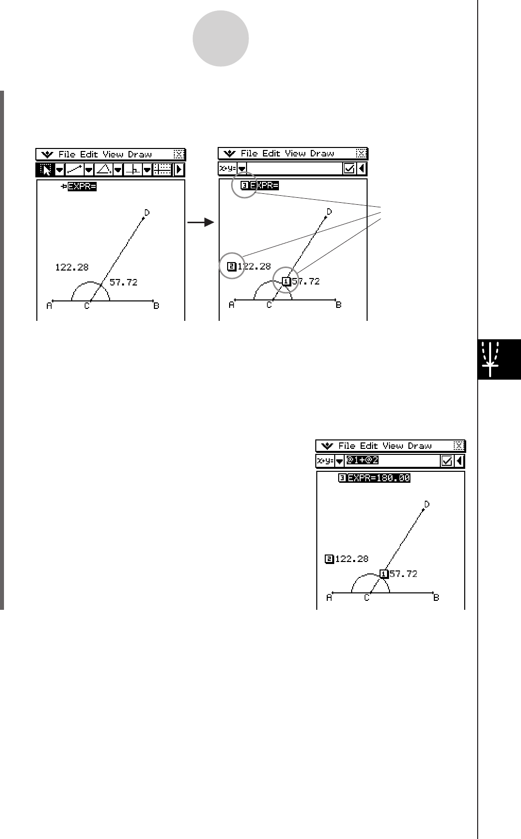
20060301

(8) Tap the u button to the right of the toolbar. This will display the measurement box.

• The above will also display numeric labels for each measurement currently on the

screen.

(9) Now you can use the numeric labels to specify measurement values in the calculation

you input in the measurement box.

• To input a measurement value in the measurement box, input the at sign (@) followed

by the numeric label of the value. To input value [1], for example, you would input “@1”.

• Since we want to calculate the sum of angles DCB ([1]) and ACD ([2]) here, you

would input the following: @1+@2.

(10) After inputting the calculation expression, press E.

• The calculation result is displayed to the right of

“EXPR=”.

Tip

In steps (8) and (9) above, you also can input the numeric label of a displayed measurement value

into the measurement box by tapping the label. Tapping [1], for example, will input “@1” into the

measurement box.

Numeric labels

8-2-26

Drawing Figures

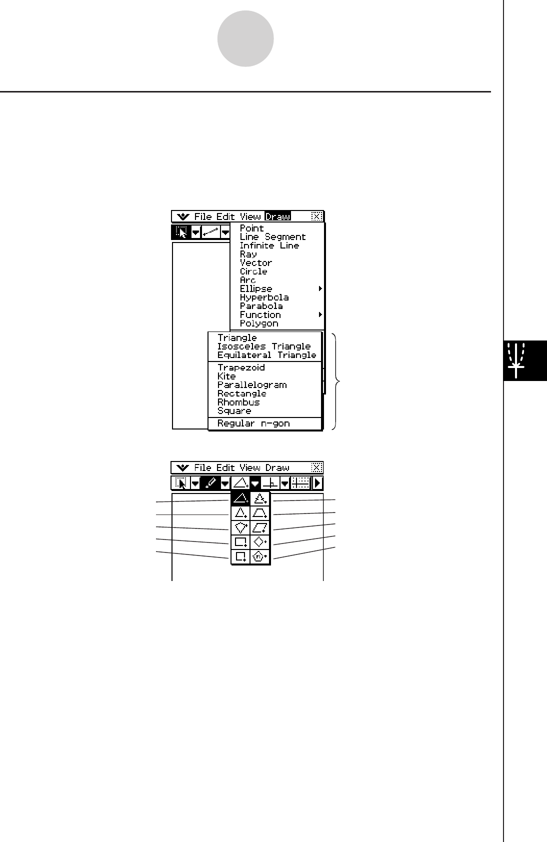
20060301

Using the Special Shape Submenu

The [Special Shape] submenu allows you to draw specially shaped figures automatically.

Simply select the type of figure you want from the menu, and then touch the screen with the

stylus to draw it. Or, touch the screen with your stylus and drag to create a box indicating the

size of the figure you would like to draw.

Each of the [Special Shape] submenu figures is also available on the toolbar.

[Draw] – [Special Shape]

[Special Shape] submenu

Isosceles Triangle

Trapezoid

Parallelogram

Rhombus

Regular n-gon

Toolbar

Triangle

Equilateral Triangle

Kite

Rectangle

Square

8-2-27

Drawing Figures

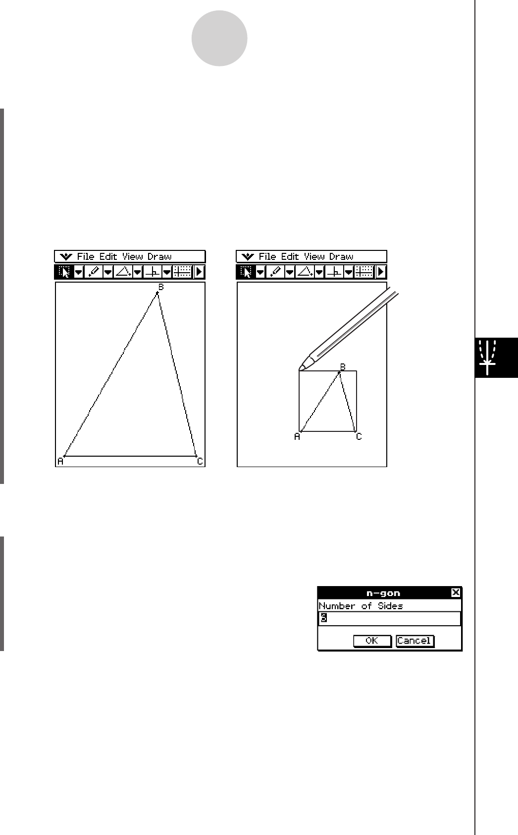
20060301

u To draw a triangle

(1) Tap [Draw], [Special Shape], and then [Triangle].

• This highlights the triangle button on the toolbar.

(2) Perform either of the following two operations to draw the triangle.

• Tap the screen with the stylus. This automatically draws the acute triangle you

selected.

• Place the stylus on the screen and drag diagonally in any direction. This causes a

selection boundary to appear, indicating the size of the triangle that will be drawn.

The triangle is drawn when you release the stylus.

8-2-28

Drawing Figures

u To draw a regular polygon

(1) Tap [Draw], [Special Shape], and then [Regular n-gon].

• This highlights the regular n-gon button on the toolbar, and displays the n-gon dialog

box.

(2) Enter a value indicating the number of sides of the

polygon, and then tap [OK].

Tapping the screen with the stylus Dragging with the stylus

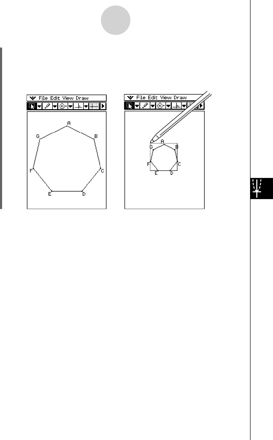
20060301

(3) Perform either of the following two operations to draw the regular polygon.

• Tap the screen with the stylus. This automatically draws the polygon you selected.

• Place the stylus on the screen and drag diagonally in any direction. This causes a

selection boundary to appear, indicating the size of the polygon that will be drawn.

The polygon is drawn when you release the stylus.

8-2-29

Drawing Figures

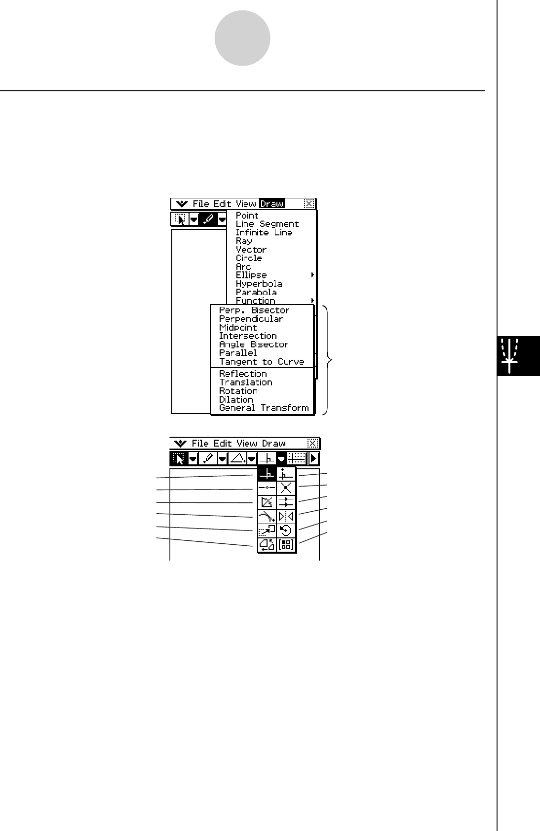
20060301

Using the Construct Submenu

The [Construct] submenu provides you with the means to study various geometric theorems.

In addition to tools for constructing a perpendicular bisector, perpendicular line, angle

bisector, midpoint, intersection, parallel lines and a tangent to a curve, you can also translate,

rotate, reflect, dilate, or transform a figure.

Each of the [Construct] submenu figures is also available on the toolbar.

[Draw] – [Construct]

[Construct] submenu

Toolbar

Perpendicular

Intersection

Parallel

Reflection

Rotation

General Transform

Perpendicular Bisector

Midpoint

Angle Bisector

Tangent to Curve

Translation

Dilation

8-2-30

Drawing Figures

Tip

• The following procedures include steps that require selection of a line segment or other figures.

For details about selecting figures, see “8-3 Editing Figures”.

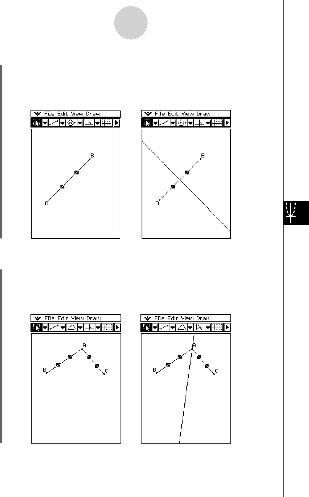
20060301

8-2-31

Drawing Figures

u To construct a perpendicular bisector

(1) Draw a line segment.

(2) Tap

G, and then select the line segment.

(3) Tap [Draw], [Construct], and then [Perp. Bisector].

• This draws a perpendicular bisector through your line segment.

u To construct an angle bisector

(1) Draw two line segments so they form an angle.

(2) Tap

G, and then select both line segments.

(3) Tap [Draw], [Construct], and then [Angle Bisector].

• This bisects the angle.

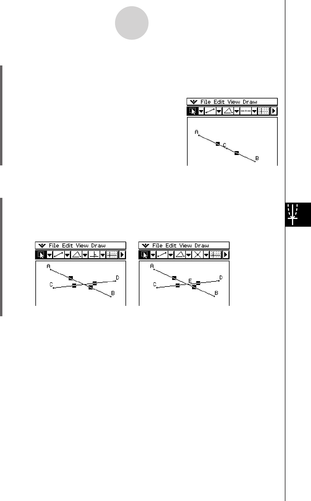
20060301

8-2-32

Drawing Figures

u To construct a midpoint

(1) Draw a line segment.

(2) Tap

G, and then select the line segment.

(3) Tap [Draw], [Construct], and then [Midpoint].

• This adds a midpoint to the segment.

u To construct the point of intersection of two lines

(1) Draw two lines that intersect.

(2) Tap

G, and then select both lines.

(3) Tap [Draw], [Construct], and then [Intersection].

• This adds the point of intersection.

(4) Try selecting the point of intersection and dragging it.

Tip

• The point(s) of intersection of two circles or of a line and a circle can be constructed in the same

manner.

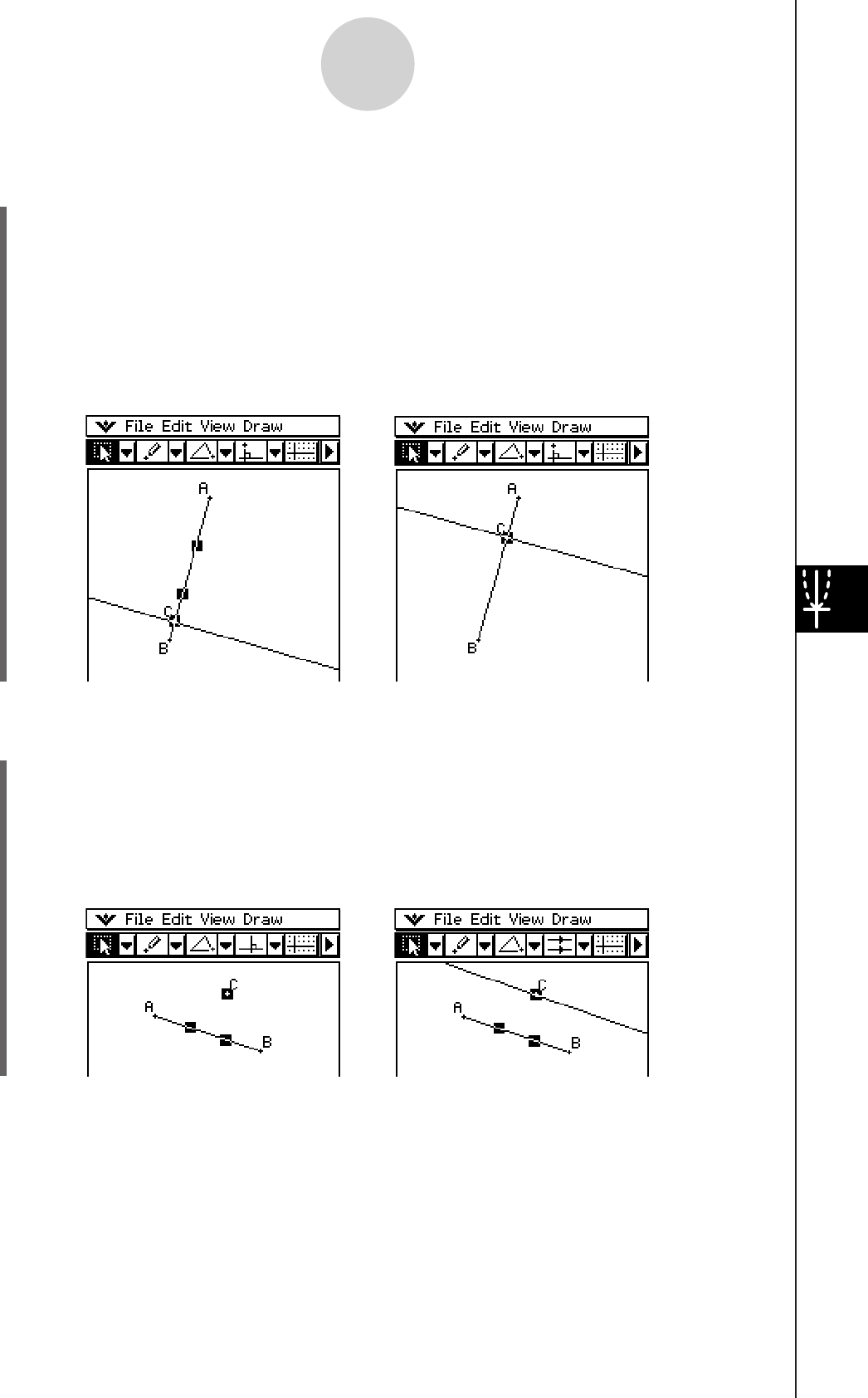
20060301

8-2-33

Drawing Figures

u To construct a perpendicular line that passes through a specified point on

a line

(1) Draw a line segment or an infinite line.

(2) Draw a point on the line through which you want the perpendicular line to pass.

(3) Tap

G, and then select the point and the line.

(4) Tap [Draw], [Construct], and then [Perpendicular].

• This draws a line that through the point you selected, which is perpendicular to the

line where is the point is located.

• Try selecting the point of intersection and dragging it.

u To construct a line parallel to another line through a specified point

(1) Draw a line and a point that is not on the line.

(2) Tap

G, and then select the line and the point.

(3) Tap [Draw], [Construct], and then [Parallel].

• The parallel line button is displayed on the toolbar, and a line passing through the

selected point is drawn parallel to the selected line.

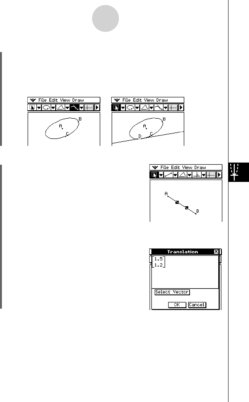
20060301

8-2-34

Drawing Figures

u To construct a tangent to a curve through a specified point

(1) Draw a curve, such as an ellipse.

(2) Tap [Draw], [Construct], and then [Tangent to Curve].

• This highlights the tangent to a curve button on the toolbar.

(3) Tap the point of tangency on the curve.

• This draws the tangent.

u To translate a line segment by inputting a vector

(1) Draw a line segment (AB), and then select it.

(2) Tap [Draw], [Construct], and then [Translation].

• This displays the Translation dialog box.

(3) Enter the vector for the translation.

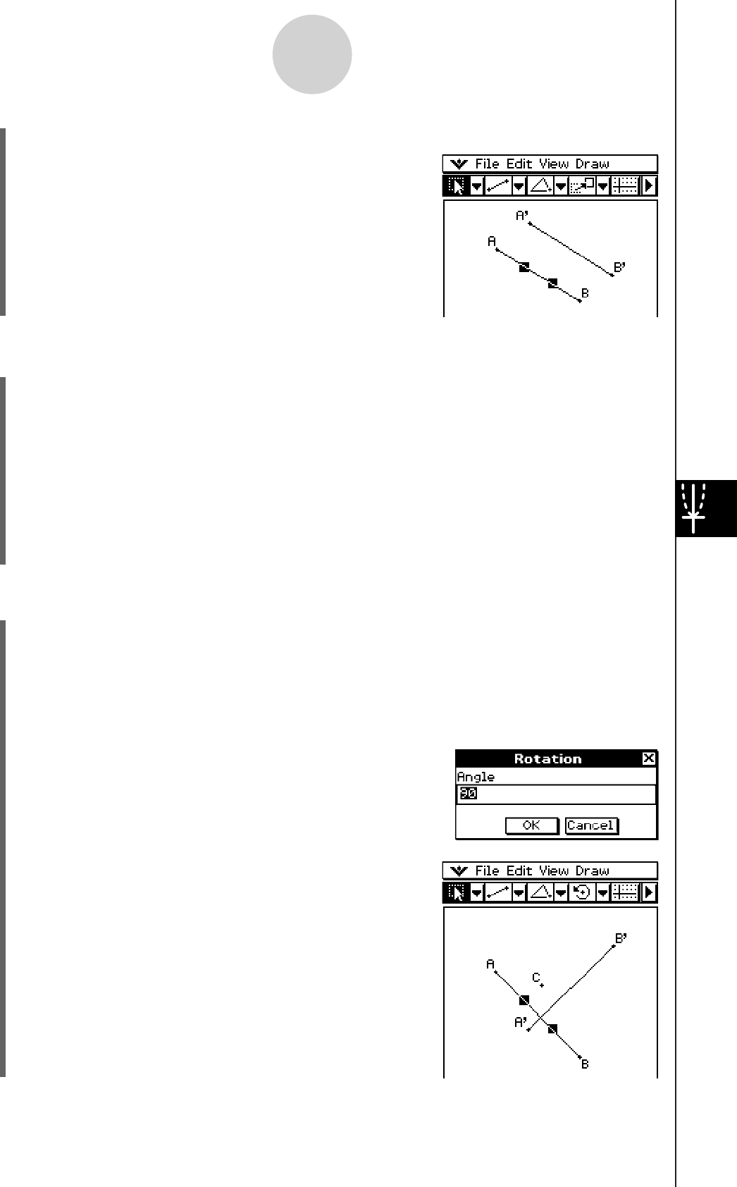
20060301

8-2-35

Drawing Figures

(1) Draw a line segment (AB), and a vector to use in the translation. Next, select the line

segment.

(2) Tap [Draw], [Construct], and then [Translation].

• This displays the Translation dialog box.

(3) Tap [Select Vector].

(4) Tap the vector on the screen.

• This translates line segment AB in accordance with the vector you selected, and

draws line segment A’B’.

u To rotate a line segment

(1) Draw a line segment, and then select it.

(2) Tap [Draw], [Construct], and then [Rotation].

• This highlights the rotate button on the toolbar.

(3) Tap the screen once to select the center of rotation.

• This displays the Rotation dialog box.

(4) Specify the angle of rotation in degrees.

u To translate a line segment by selecting a vector

(4) Tap [OK].

• This translates line segment AB in accordance with

the vector value you input, and draws line segment

A’B’.

(5) Tap [OK] to rotate the line segment.

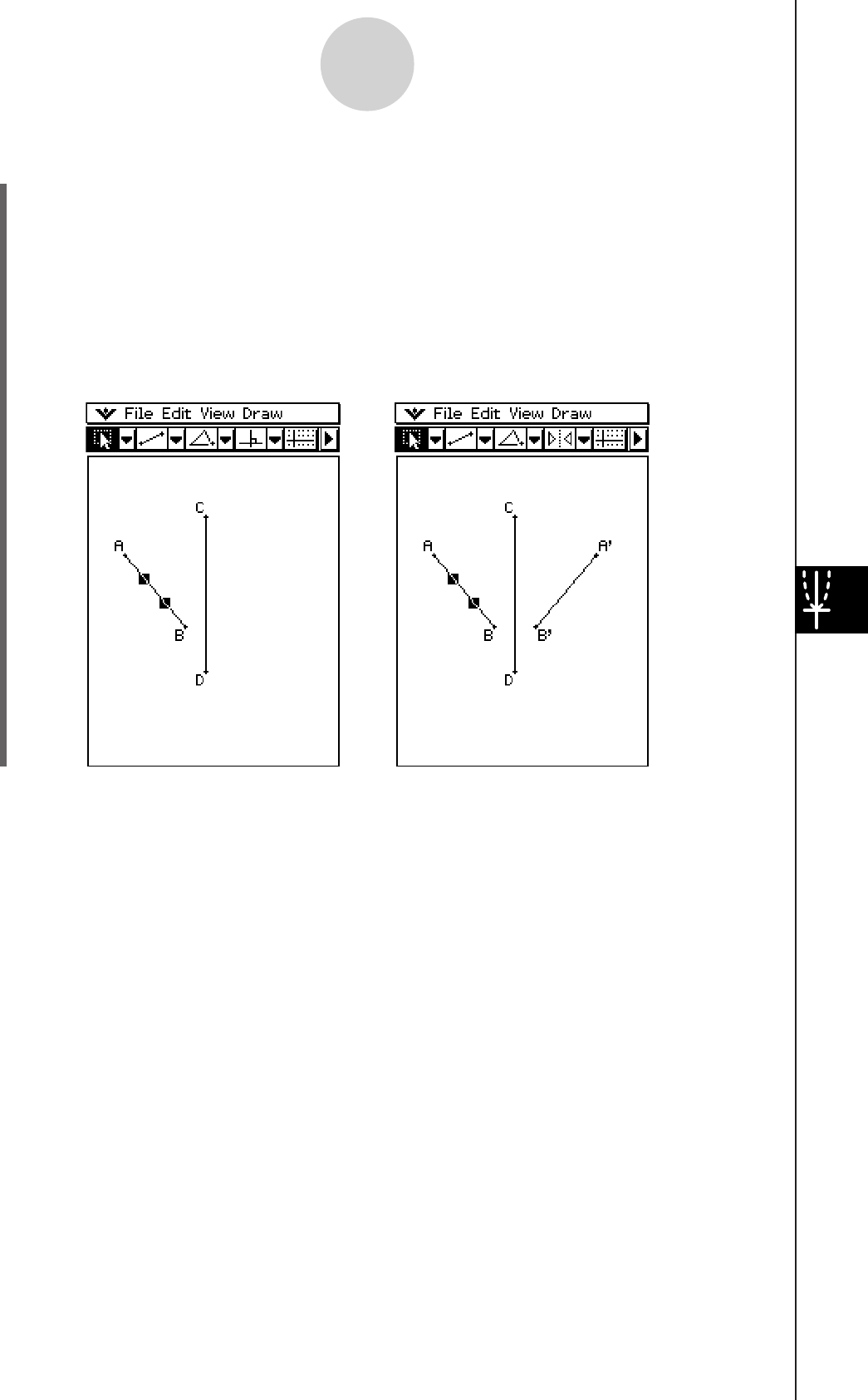
20060301

8-2-36

Drawing Figures

u To reflect a line segment with respect to a specified line of symmetry

(1) Draw a line segment.

(2) Draw a line to use as the line of symmetry.

(3) Tap

G, and then select the line segment.

(4) Tap [Draw], [Construct], and then [Reflection].

• This highlights the reflection button on the toolbar.

(5) Tap the line of symmetry.

• This reflects the line segment you drew in step (1) about the line of symmetry.

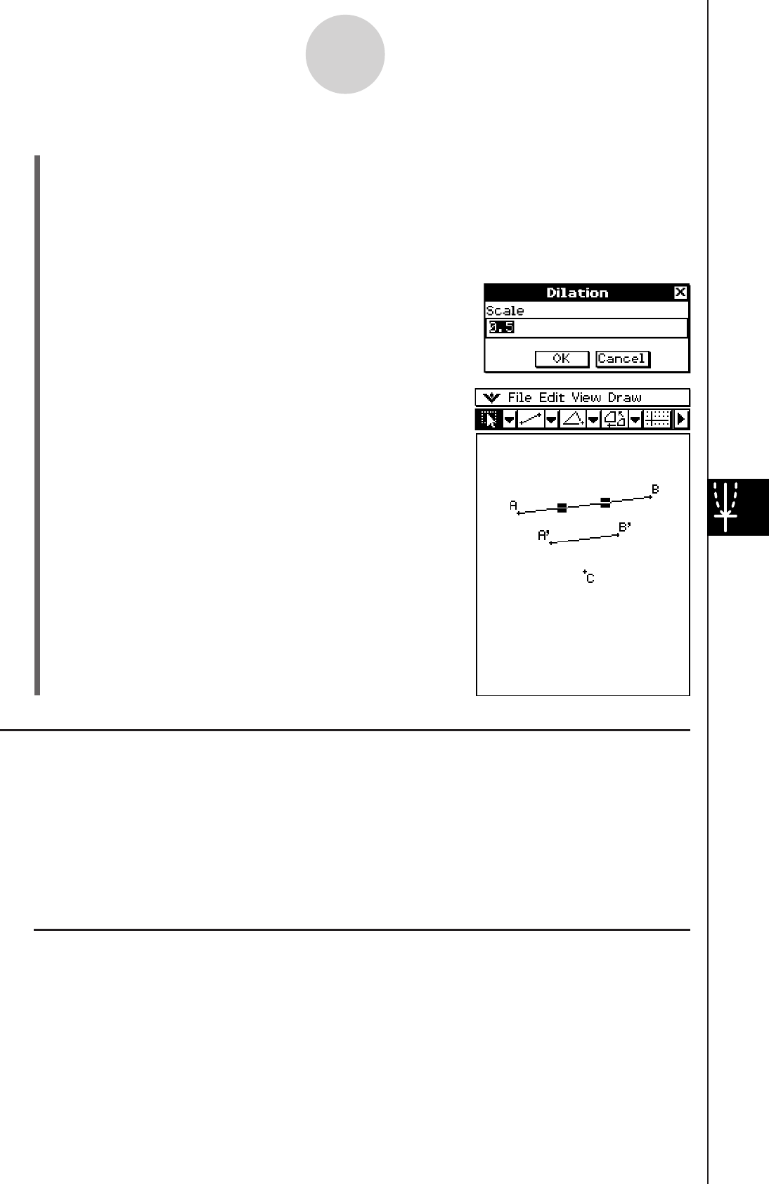
20060301

8-2-37

Drawing Figures

Transformation Using a Matrix or Vector (General Transform)

General Transform lets you input a matrix and/or vector to transform a figure. The result of

the transformation is drawn as a separate figure. For example, if you transform line segment

AB, the line segment A’B’ will be drawn.

You can perform the following types of transformations with General Transform.

• Matrix Transformation: x-axis/y-axis symmetry, rotation, enlargement, reduction, etc.

• Vector Transformation: Vertical and horizontal parallel displacement

k General Transform Example

In this example draw triangle ABC and then draw triangle A’B’C’, which is symmetrical

to ABC about the x-axis. Next, we will draw triangle A’’B’’C’’ by performing a parallel

displacement on triangle A’B’C’ of 1 unit along the x- and y-axis.

u To dilate a line segment toward a specified center point

(1) Draw a line segment, and then select it.

(2) Tap [Draw], [Construct], and then [Dilation].

• This highlights the dilation button on the toolbar.

(3) Tap the center of dilation.

• This displays the Dilation dialog box.

(4) Specify the dilation scale factor.

(5) Tap [OK].

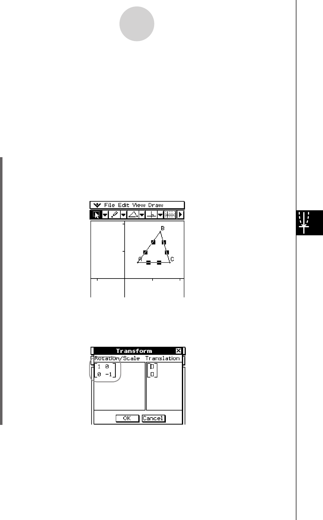
20060301

Tip

• All of the steps in the procedure below are performed using the Geometry application only. You

can also use the Main application or eActivity application to perform matrix calculations and

obtain the same transformation. You can drag a figure from Geometry to Main, which transforms

values (matrix) and performs calculation, and drag the values (matrix) obtained as a result from

Main to Geometry to draw the transformed figure. After performing the following procedure, see

“Transform Example Using the Main Application” (page 8-2-40).

If you need to, tap [Edit] and then [Clear All] before beginning this example.

u ClassPad Operation

(1) Tap

q to turn on coordinate display in the Geometry window.

• You can skip this step if you want, but turning on coordinate display helps you see

how coordinates are changed by the transform operations.

(2) Draw triangle ABC, and then select its three sides.

(3) Tap [Draw], [Construct], and then [General Transform].

• This displays the Transform dialog box.

(4) Since we want a triangle that is symmetrical about the x-axis to the original triangle,

input [[1, 0], [0, –1]].

8-2-38

Drawing Figures

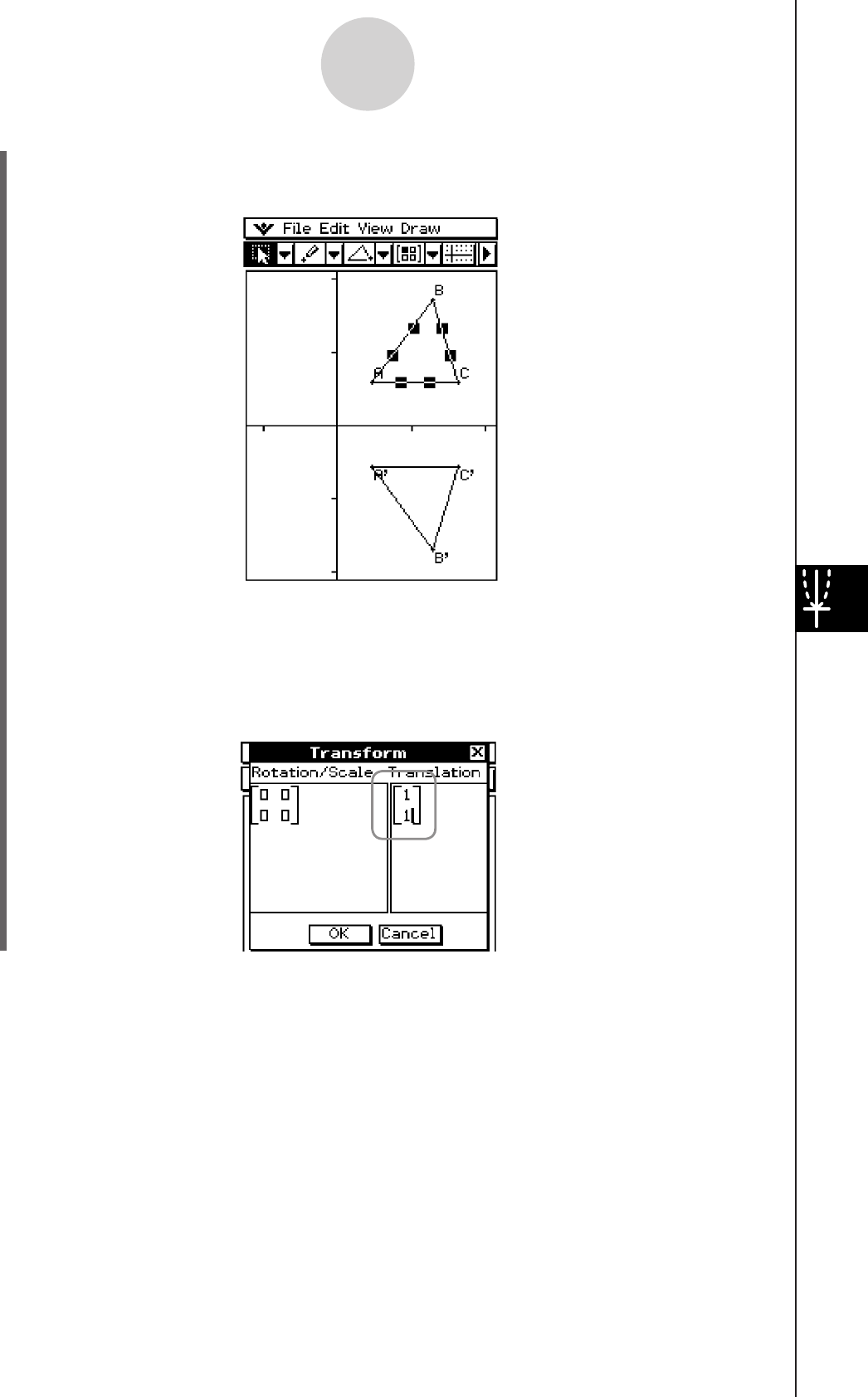
20060301

(5) Tap [OK].

• This draws triangle A’B’C’, which is symmetrical to triangle ABC about the x-axis.

(6) Tap anywhere outside of the triangles to deselect the currently selected triangle. Next,

select triangle A’B’C’.

(7) Tap [Draw], [Construct], and then [General Transform].

(8) Now, to perform parallel displacement on triangle A’B’C’ by 1 unit along the x- and

y-axis, input [1, 1].

8-2-39

Drawing Figures

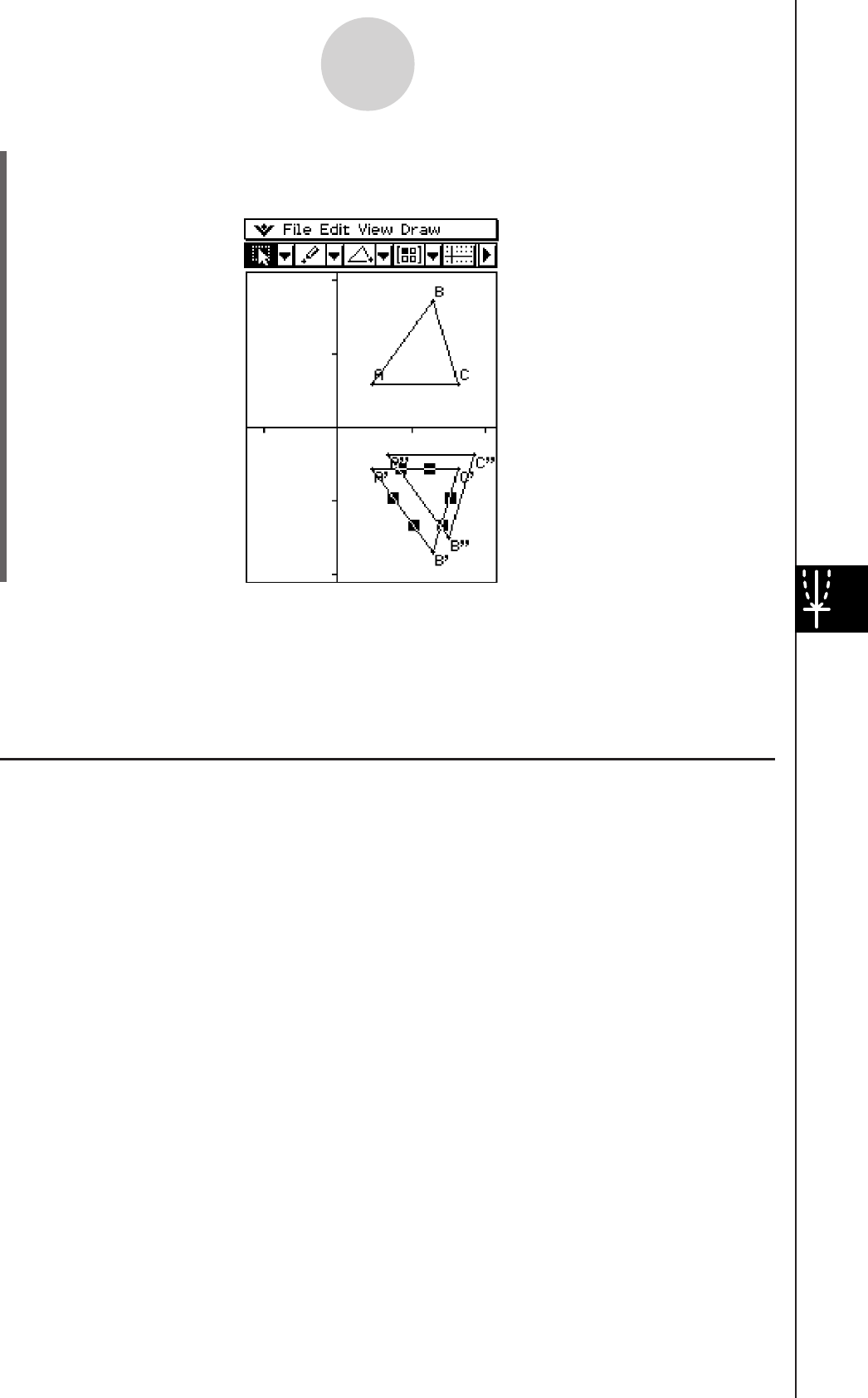
20060301

(9) Tap [OK].

• This performs the parallel displacement and draws triangle A’’B’’C’’.

Note

• In the above example, we performed the transformation and the parallel displacement

operations separately. You could also perform both operations at the same time, if you

want. To do so, input both the matrix [[1, 0], [0, –1]] and the vector [1, 1] in step (4), and

then tap [OK]. This will produce the result shown in step (9).

k Transform Example Using the Main Application

It might be easier to understand how General Transform works if you use the Main

application (or eActivity application) in combination with the Geometry application. This

makes it possible to perform the following types of operations.

(a) In the Geometry application, you can select a point on the figure obtained using

General Transform and the corresponding point on the original figure (for example,

point A on the original figure and point A’ on the transformed figure), drag them to the

Main application, and display the transformation expression in the Main application.

(b) You can select a triangle in the Geometry application and drag it to the Main

application to convert the triangle to a matrix (2-row × 3-column matrix that shows three

vertices). Conversely, you can drag a 2-row × 3-column matrix input (or produced by a

calculation) in the Main application to the Geometry application and draw the applicable

triangle.

Here we will show actual examples of (a) and (b).

Tip

• All of the above operations can also be performed using the eActivity application instead of the

Main application.

• For information about how to access the Geometry application from the Main application

and about the different operations you can perform between them, see “2-10 Using the Main

Application in Combination with Other Applications”.

8-2-40

Drawing Figures

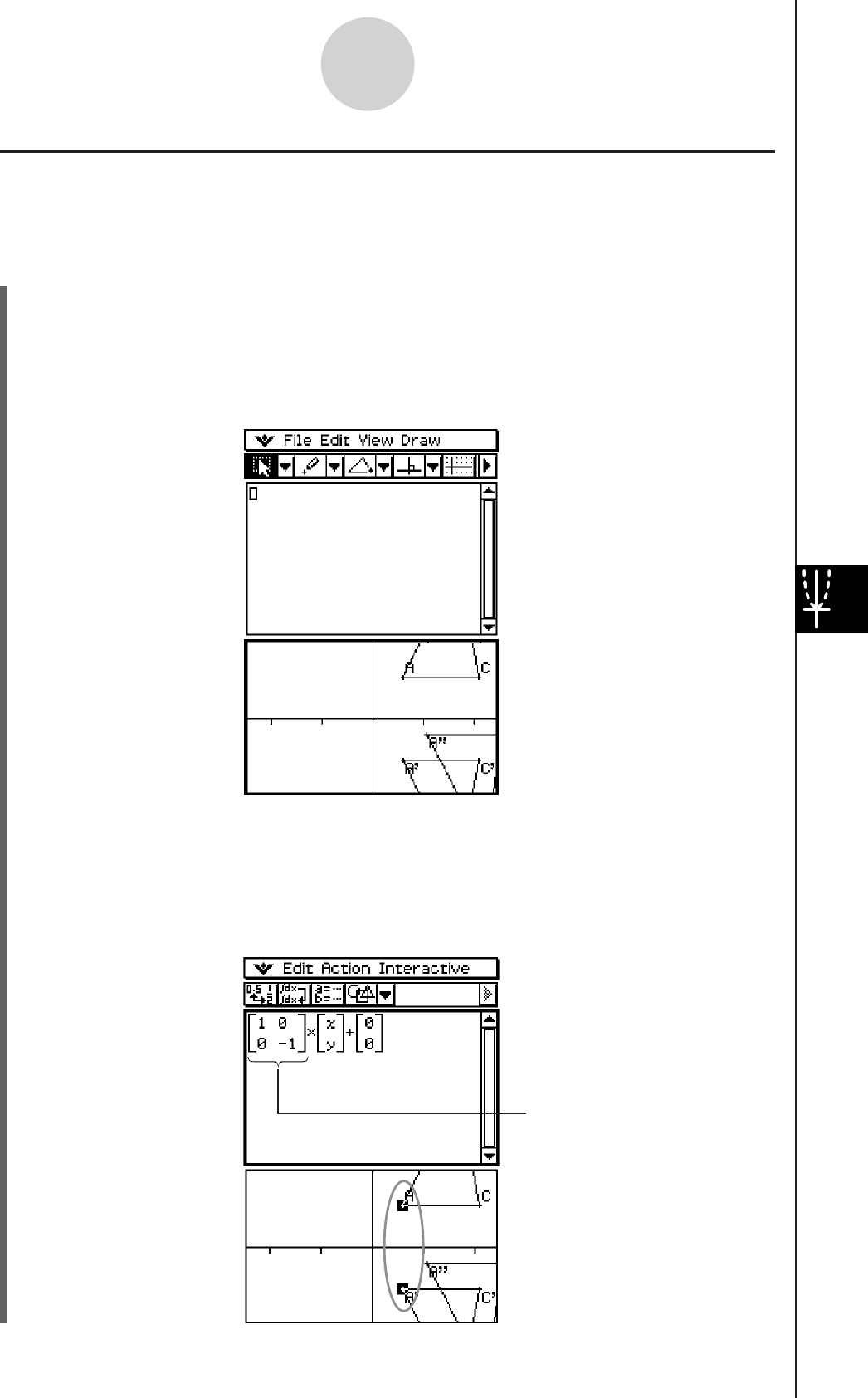
20060301

k (a) Operation Example

The following procedure assumes that the results produced by the procedure under “General

Transform Example” on page 8-2-37 are still on the Geometry application window.

u ClassPad Operation

(1) On the application menu, tap J to start up the Main application.

(2) Tap the right most down arrow button on the Main application toolbar. On the button list

that appears, tap 3.

• This opens the Geometry application and displays triangles ABC, A’B’C’, and A’’B’’C’’

on the Geometry window.

8-2-41

Drawing Figures

(3) Select points A and A’.

(4) While both points are selected, drag point A (or point A’) to the cursor position in the

Main application work area.

• This displays the expression that transformed the coordinates of point A to the

coordinates of point A’.

Observe this area of the

expression. This corresponds to

the matrix values you input when

executing General Transform.

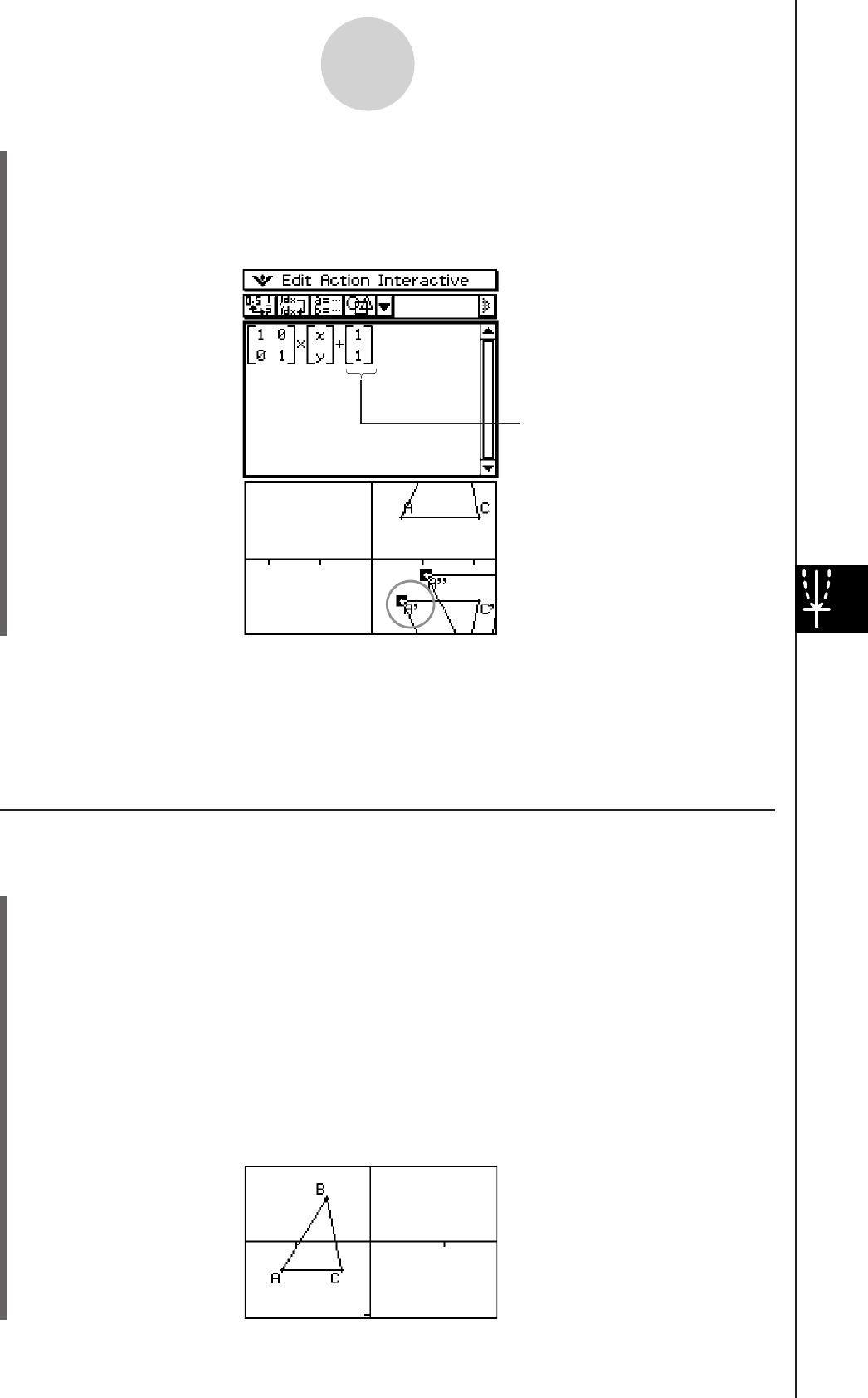
20060301

Important!

• This operation is valid only when a point in the original figure and the corresponding point in

the transformed figure are selected in the Geometry application. Nothing is displayed when

you select points A and A’’ in the above procedure and drag them to the Main application

work area.

Observe this area of the

expression. This corresponds to

the vector values you input when

executing General Transform.

8-2-42

Drawing Figures

(5) After clearing the Main application work area, try repeating steps (3) and (4) for points A’

and A’’.

• This displays the expression that transformed the coordinates of point A’ to the

coordinates of point A’’.

k (b) Operation Example

u ClassPad Operation

(1) On the application menu, tap J to start up the Main application.

(2) Tap the right most down arrow button on the Main application toolbar. On the button list

that appears, tap 3.

• This opens the Geometry application.

(3) On the Geometry window, tap [Edit] and then [Clear All].

• This clears the Geometry window.

(4) Draw a triangle on the Geometry window.

• After drawing a triangle, you can use the measurement box (page 8-3-6) to adjust the

coordinates of points A, B, and C. That will make the following steps easier.

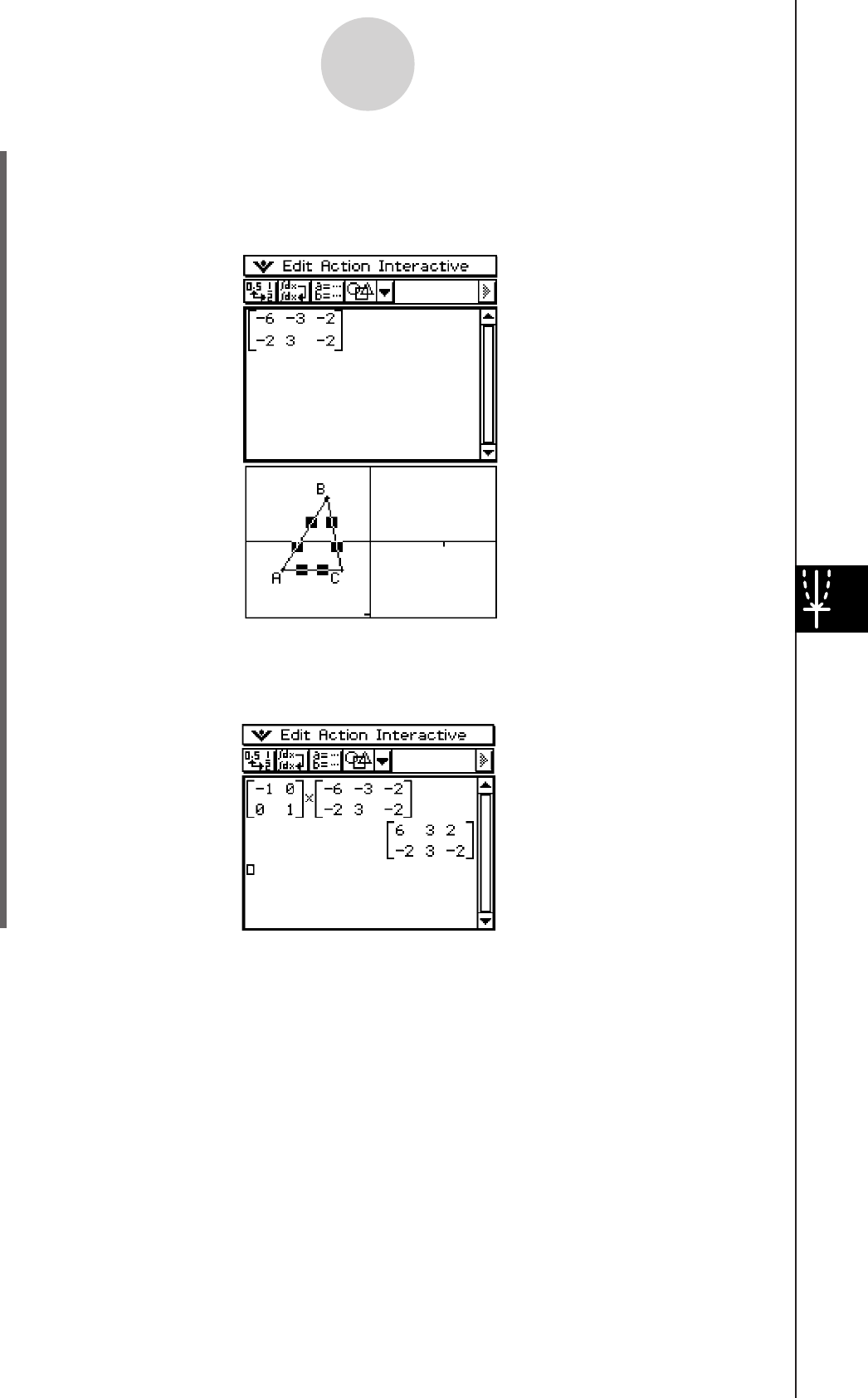
20060301

(5) Select the triangle and drag it to the cursor location in the Main application work area.

• This inputs a matrix that shows the coordinates of the triangle’s three vertices into the

work area.

8-2-43

Drawing Figures

(6) Here, try multiplying by the matrix [[–1, 0], [0, 1]] to transform the matrix obtained above

to a form that is symmetrical about the y-axis. Execute the calculation as shown in the

screenshot below.

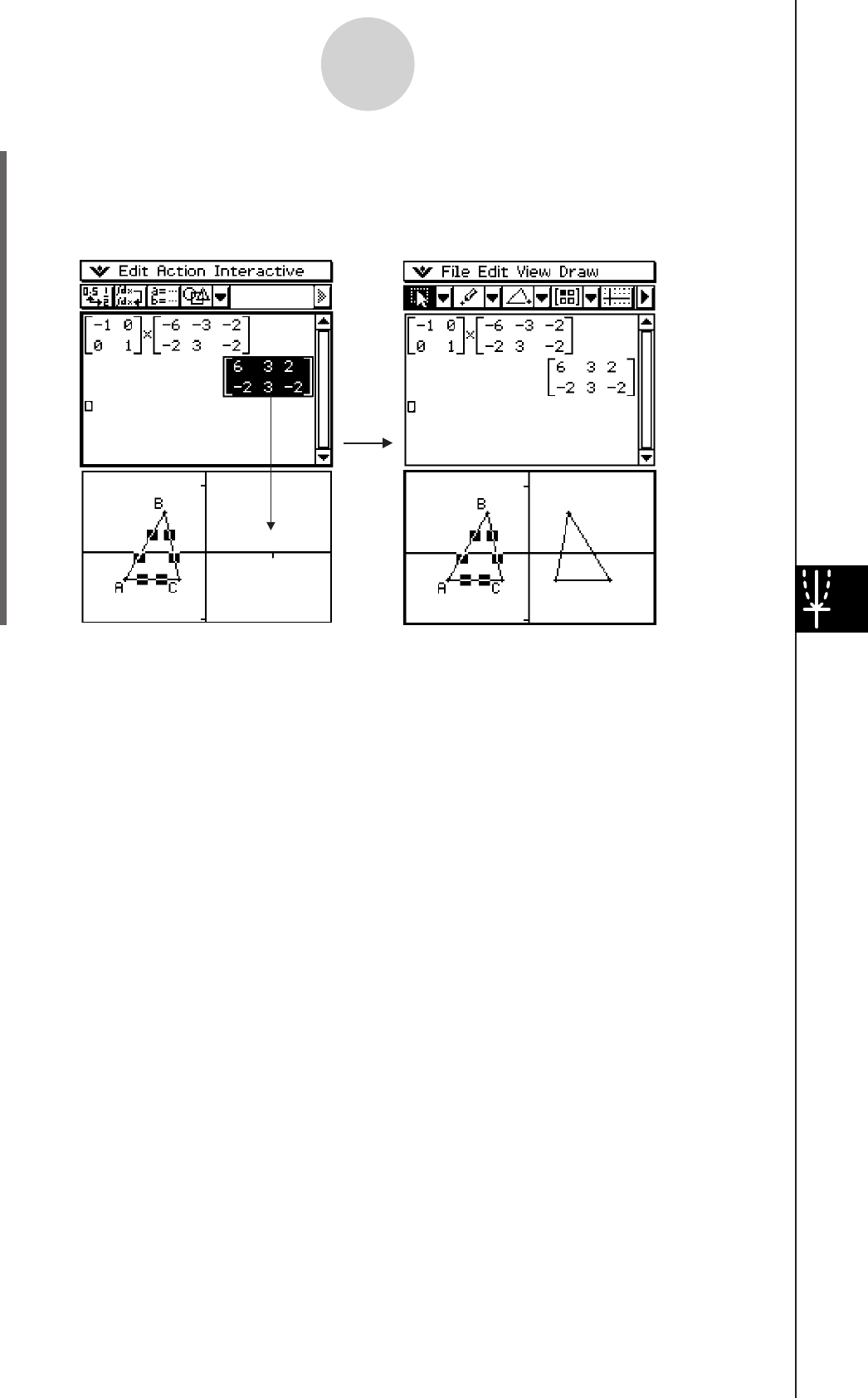
20060301

8-2-44

Drawing Figures

(7) Select the matrix obtained as the calculation result, and drag it to the Geometry

window.

• This draws a triangle that is symmetrical to the original triangle about the y-axis.

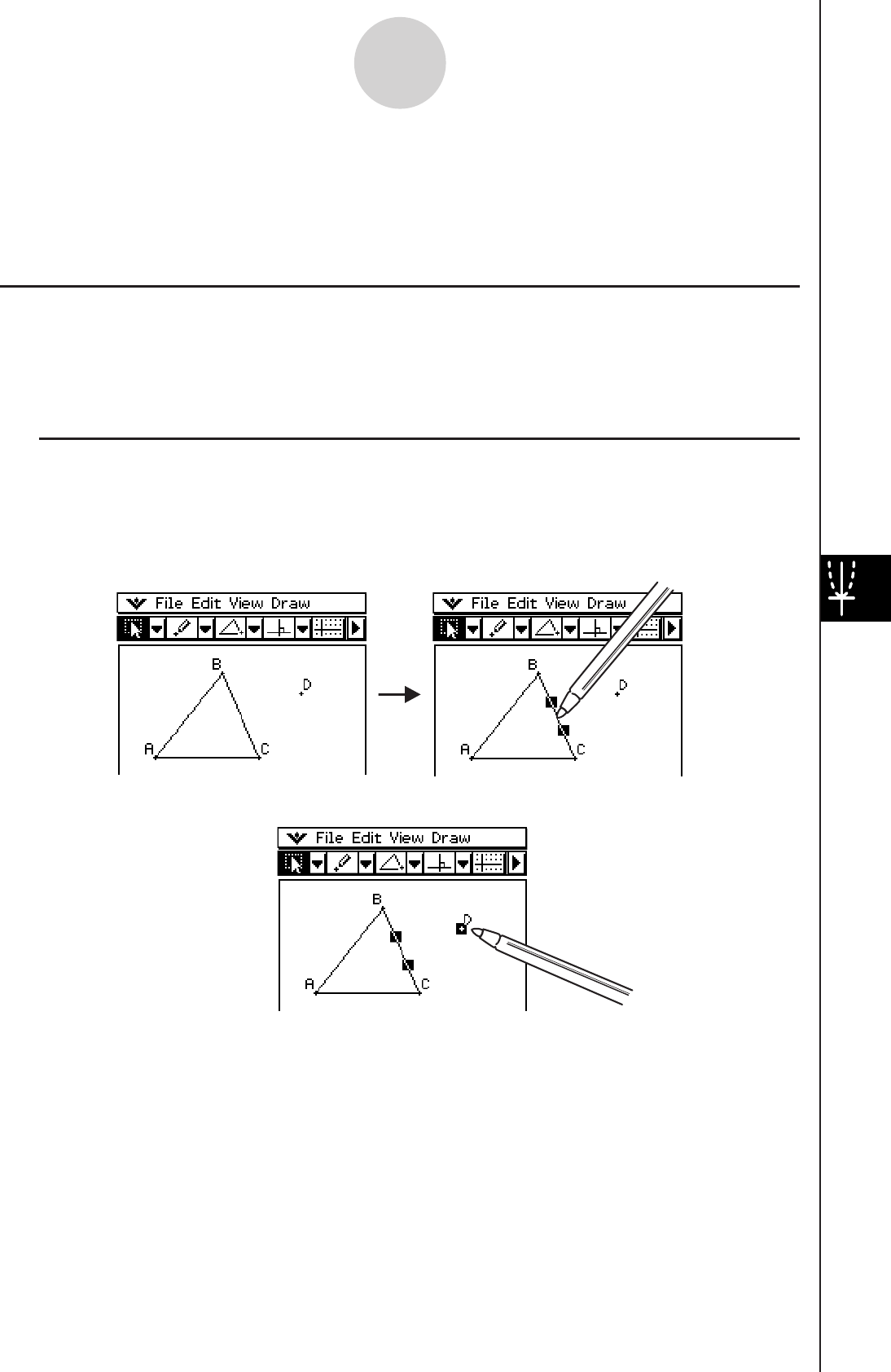
20060301

8-3 Editing Figures

This section provides details about moving, copying, and deleting Geometry application

figures.

Selecting and Deselecting Figures

Before you can execute certain editing commands, you must first select the figure you want

to edit. There are two figure selection modes: Select and Toggle Select, each of which is

described below.

k Using Select

Tap G on the toolbar. This causes the button to become highlighted, indicating that Select

is enabled. Select allows you to select as many figures as you would like, and then move,

copy, paste, or perform other operations on the selection as a single entity.

• To select side BC of the triangle, tap it.

8-3-1

Editing Figures

• Tapping point D selects it, leaving side BC of the triangle selected, too.

• To deselect all of the figures, tap anywhere on the screen where there are no figures.

Tip

• When Select is enabled, you can drag the currently selected figures to move them around the

display. For more information, see “Moving and Copying Figures” on page 8-3-3.

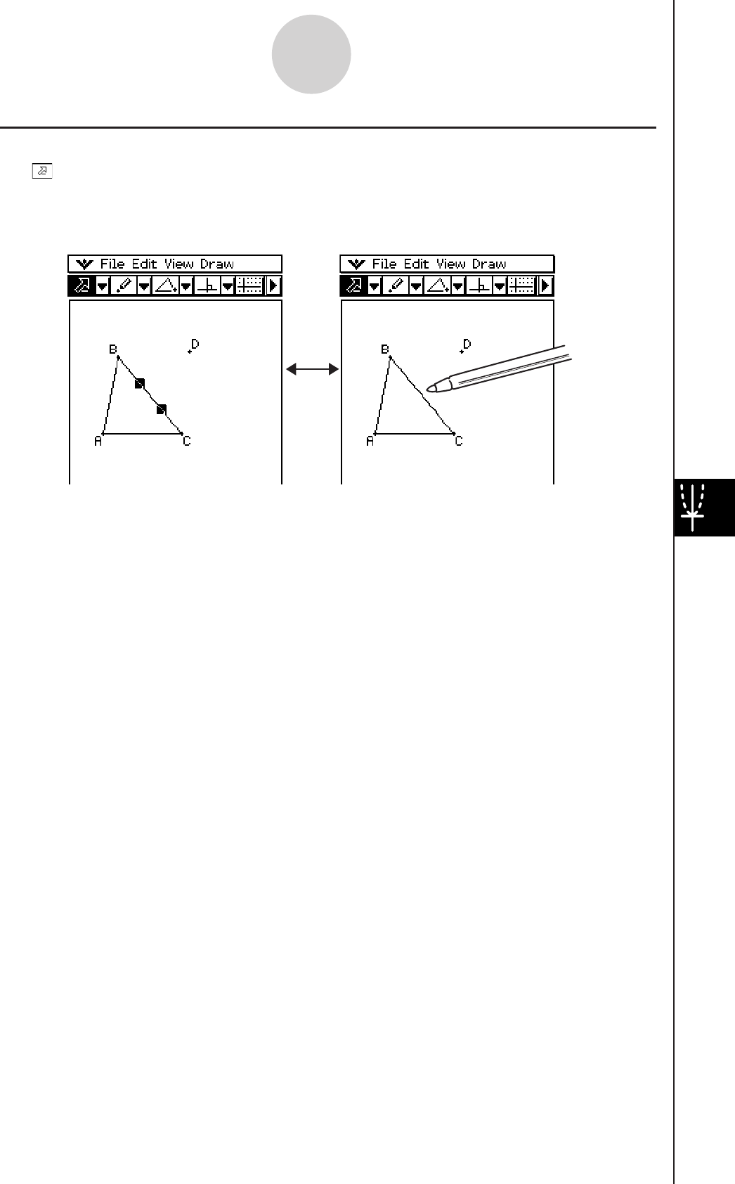
20060301

k Using Toggle Select

Tap on the toolbar. This causes the button to become highlighted, indicating that Toggle

Select is enabled. Toggle Select allows you to select and deselect figures. For example, if

you have multiple figures selected, Toggle Select will allow you to deselect a single part of

the selection. Tapping the part again will turn the selection back on.

Tip

• You cannot move figures around the window while Toggle Select is enabled. Also, the currently

selected figure does not become deselected if you tap an area of the window where there is no

figure. To move what you currently have selected, simply change to the regular Select mode.

8-3-2

Editing Figures

20060301

8-3-3

Editing Figures

u To copy a figure

(1) Draw a figure, and then select it.

(2) Tap [Edit], and then [Copy].

(3) Tap anywhere on the screen to deselect the figure.

(4) Tap [Edit], and then [Paste].

(5) Drag the pasted figure to the location you want.

Moving and Copying Figures

It is easy to move figures or copy and paste figures in Geometry.

u To move a figure

(1) Draw a figure.

(2) Tap

G, and then select the figure.

(3) Drag the figure to move it to the location you want.

(4) Remove the stylus from the screen.

Tip

• Note that a selection boundary appears around the figure when you drag it.

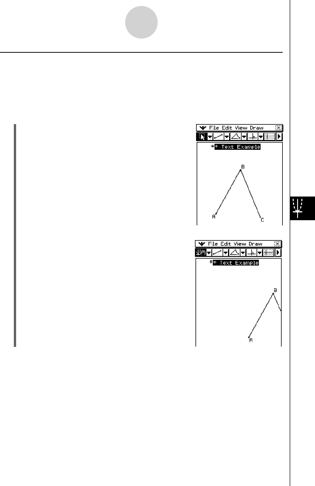
20060301

Pinning an Annotation on the Geometry Window

You can pin an annotation on the Geometry window using the Pin function. By default,

annotations are ‘Unpinned’, so they pan or zoom along with the Geometry window.

Pinning an annotation fixes its position on the screen so it is always displayed in the same

location on the Geometry window.

Example: To pin text at a particular location on the Geometry window

(1) Select (highlight) the text on the Geometry window.

(2) Tap [Edit], [Properties], and then [Pin].

(3) When text is pinned, it maintains its position as shown

here even when the window is panned.

8-3-4

Editing Figures

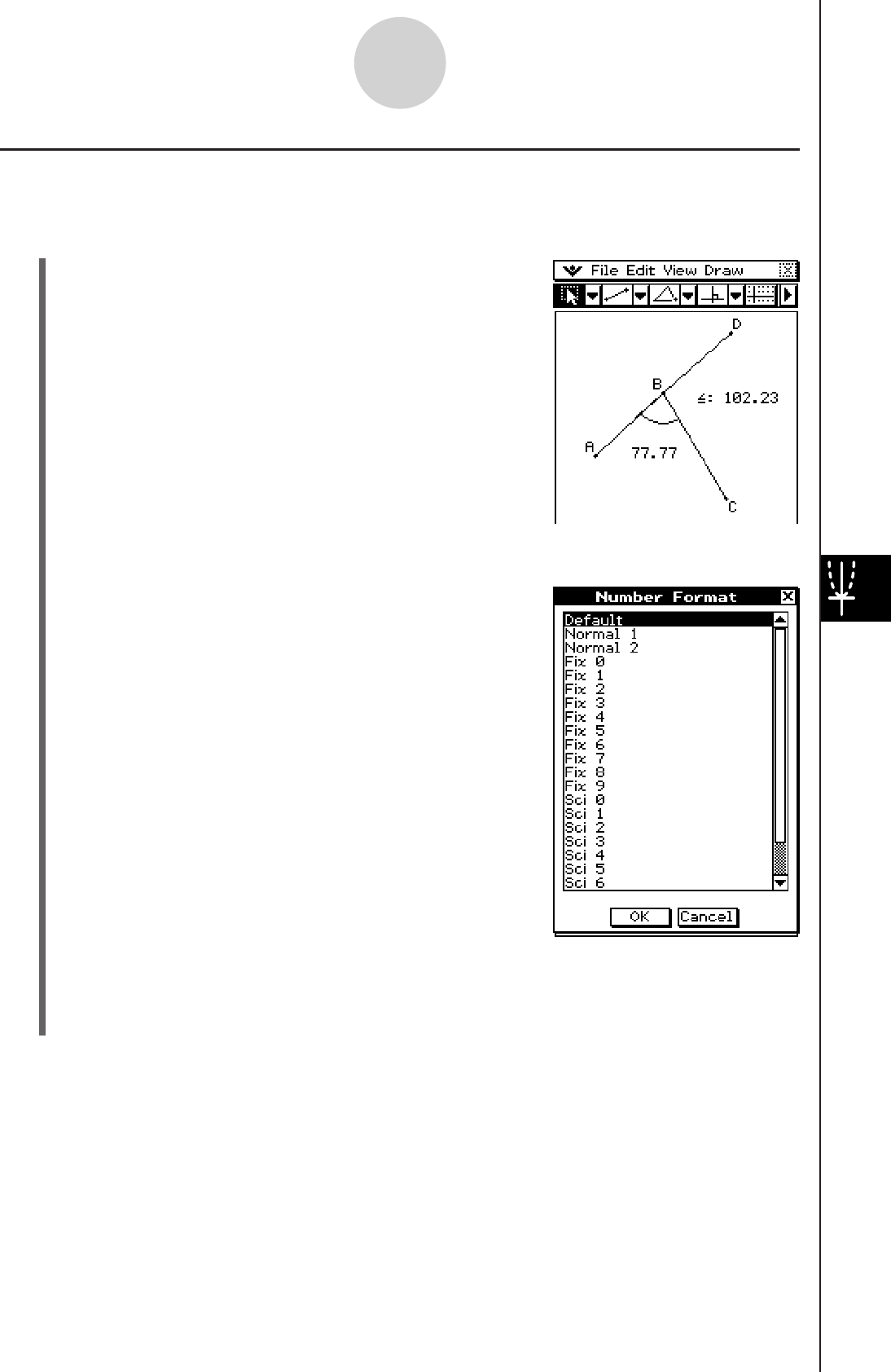
20060301

Specifying the Number Format of a Measurement

You can specify the number format for each measurement on the Geometry window.

Example: To specify zero decimal places for measurement values on the Geometry window

(1) Select (highlight) the measurement(s).

(2) Tap the [Edit], [Properties], and then [Number Format].

• This displays the Number Format dialog box as

shown here.

(3) Select the number format you want by tapping it. Since we want to specify zero decimal

places, we will select “Fix 0” here.

• For the meaning of each number format name, see “Number Format” on page 1-9-5.

8-3-5

Editing Figures

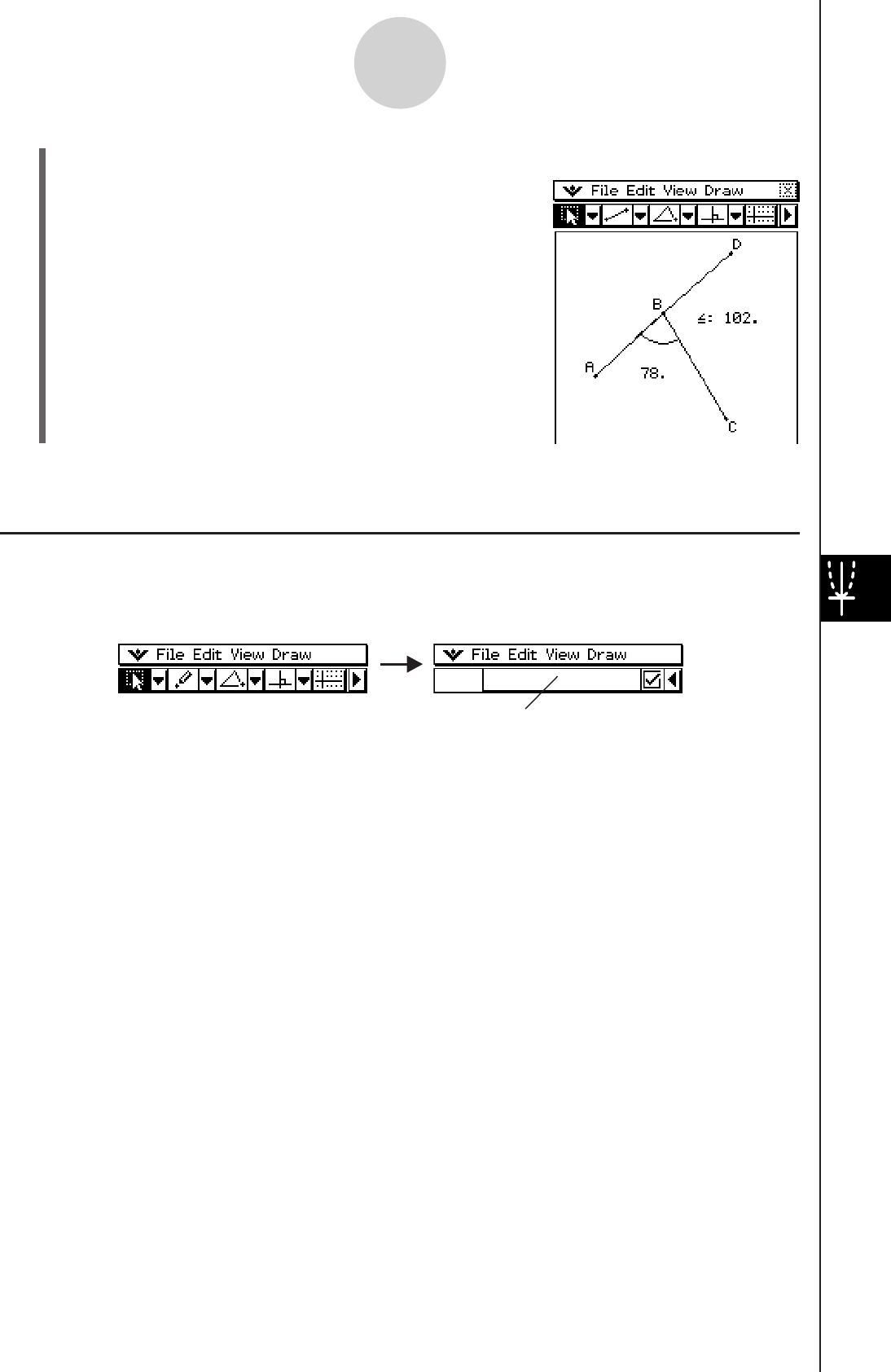
20060301

(4) Tap [OK].

• This will display the measurement value(s) you

selected in the step 1 using the specified number

format.

Tip

The initial default number format setting for measurement values is “Fix 2”.

Using the Measurement Box

Tapping the u button to the right of the toolbar displays the measurement box. Tap t to

return to the normal toolbar.

You can use the measurement box to perform the following operations.

View the measurements of a figure

Displaying the measurement box and selecting a figure displays combinations of the following

measurements, depending on the type of object you select: coordinates, distance, slope,

direction, equation, radius, circumference, area, perimeter, angle, tangency, congruence,

incidence, or point on curve.

Specify a measurement of a figure

After you display the measurement box, you can select part of a figure and then change

numeric values for the applicable measurement. You can specify the coordinates of a point,

the length of a line segment (distance between endpoints), the angle formed by two lines,

etc.

Fix a measurement of a figure

After you display the measurement box, you can select part of a figure and then fix the

applicable measurement. You can fix the coordinates of a point, the length of a line segment,

the angle formed by two lines, etc.

Name a figure

After you display the measurement box, you can select part or all of a figure and then give it

a name or change the existing name. You can name a point, line segment, circle, attached

angle, etc.

Normal toolbar Measurement box

8-3-6

Editing Figures

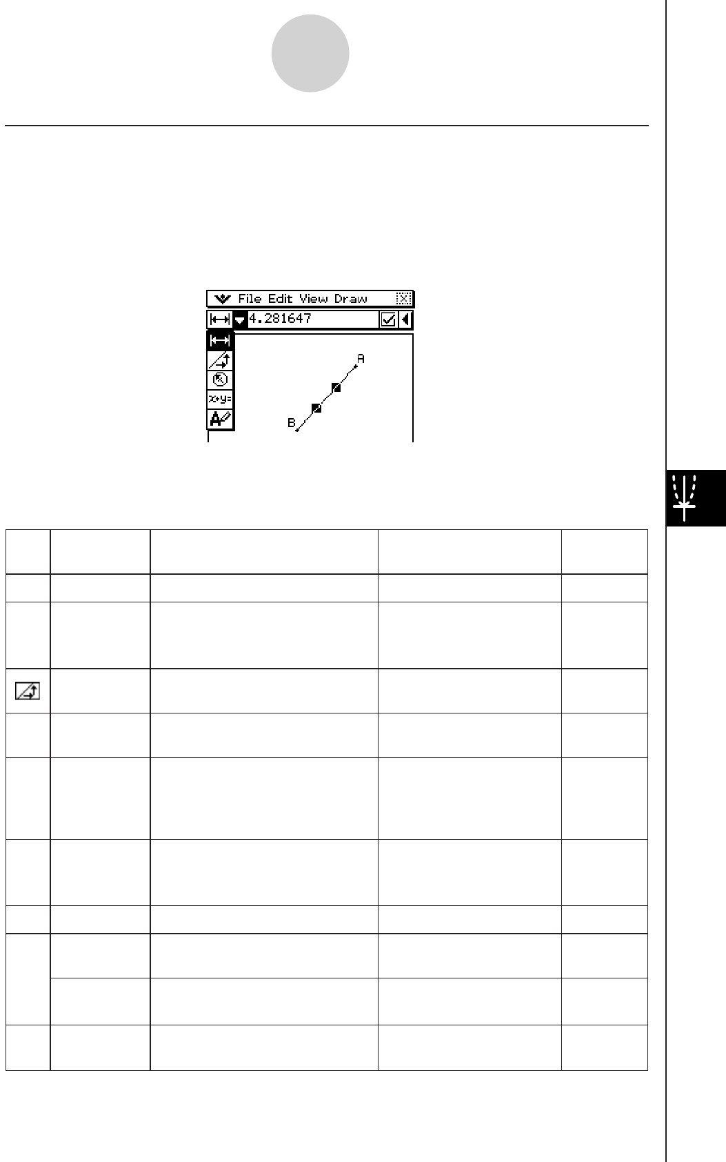
20060301

8-3-7

Editing Figures

k Viewing the Measurements of a Figure

The type of information that appears in the measurement box depends on the figure that is

currently selected on the display. If a line segment is selected, for example, the measurement

box shows the distance, slope, angle from the x-axis, and the equation for that line. You

can specify the type of information you want to view by tapping the down arrow button to the

left of the measurement box, and then tapping the appropriate icon on the icon palette that

appears.

The following table describes the information that appears when you tap each icon, and

explains when each icon is available for selection.

Icon Icon Name This icon appears when this

is selected:

Tapping this icon

displays: Lockable

Coordinates

Ye s

A single point Coordinates of the point

Distance/

length

Ye s

Two points on one figure or two

different figures, or a single line

segment or a vector

Distance between two

points, length of a line

segment or vector

Slope

Ye s

Single line, line segment, or

vector

Slope of the line, line

segment or vector

Direction

Ye s

Single line, line segment, or

vector

Direction angle of the

line (angle of inclination)

Equation

Ye s

Any single line or line segment,

vector, circle, arc, ellipse or any

other figure (parabola, etc.)

drawn by a function

Function of the figure

(using rectangular

coordinates)

Equation

edit

Single parabola or any other

figure drawn by a function

Equation of the figure in

the function editing

dialog box.

Radius

Ye s

]

Single circle or arc Radius of circle or arc

Circumference

Ye s

Single circle, arc or ellipse Length of the

circumference

Perimeter

Single polygon Sum of the lengths of

the sides

Area

Any three points, a single

circle, arc, ellipse, or polygon

Area

20060301

8-3-8

Editing Figures

Icon Icon Name This icon appears when this

is selected:

Tapping this icon

displays: Lockable

Angle

Yes

Two line segments Angle and its

supplement formed by

the line segments

Tangency

Yes

Two circles or arcs, or a line

and circle

Whether two items are

tangent

Congruence

Yes

Two line segments Whether line segments

are the same length

Incidence

Yes

Point and a line, arc, circle or

a vector

Whether a point is on

the line/curve

Point on

curve

Point and a function, curve, or

ellipse

Rotation

angle

Two points created by

[Rotation]

Angle of rotation

Scale of

dilation

Two points (like Point A and

Point A’) on a figure created

by [Dilation]

Scale of dilation

Text icon

An object that includes text or

an object that can be named

Editable text used to

name the selected image

u To display the area of a triangular area

You can use the measurement box to display the area of a triangle formed by any three

points you select on the display.

Example: To use the parallelogram ABCD, in which sides AD and BC are parallel, to

determine the areas of the triangles formed by side AD and point B, and side AD

and point C

(1) Draw the parallelogram.

• If you need to, select [Edit] and then [Clear All] before beginning this example.

(2) Tap

u on the toolbar to display the measurement box.

*1 The value in the measurement box is always locked while this tool is selected.

You can use the measurement box to determine certain measurements.

In the first example below, three points are selected on the screen and the measurement box

shows the area of the triangle formed by them.

The second example shows how to view the measurements of a line segment.

20080201

20060301

8-3-9

Editing Figures

(3) Select points A, D, and B.

• This causes the area of the triangle ADB to appear

in the measurement box.

(4) Tap anywhere outside of the parallelogram to deselect the current points, and then

select points A, D, and C.

• This causes the area of the triangle ADC to appear

in the measurement box. The above procedure

shows that the areas of the two triangles are

the same.

u To view the measurements of a line segment

(1) Draw a line segment.

(2) Tap

u on the toolbar to display the

measurement box.

(3) Select the line segment.

• This displays the length of the line segment.

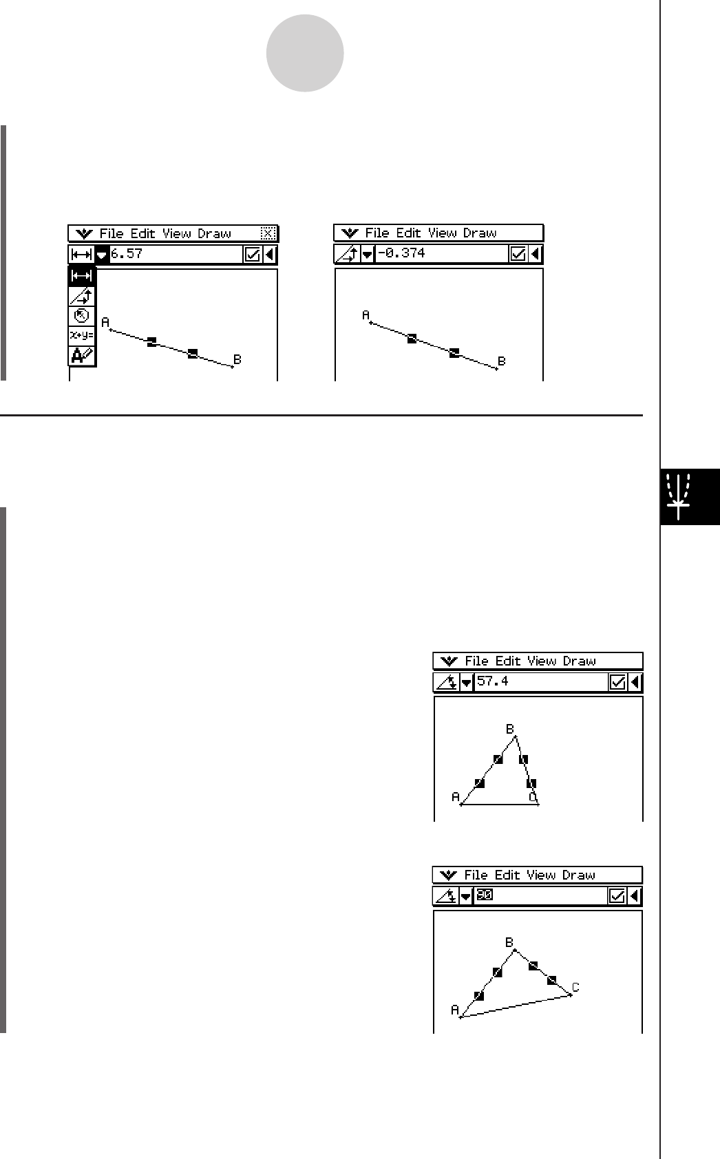
20060301

8-3-10

Editing Figures

(4) Tap the down arrow next to the measurement box to cycle through other

measurements.

• In the case of the line segment, for example, you can view its length, slope, direction,

and equation.

k Specifying a Measurement of a Figure

The following example shows how to specify an angle of a triangle.

u To specify the angle of a triangle

(1) Check to make sure the [Measure Angle] setting of the Geometry Format dialog box is

set to “Degree” (see page 1-9-10 for more information).

(2) Draw the triangle.

• If you need to, select [Edit] and then [Clear All] before beginning this example.

(3) Tap

u on the toolbar to display the measurement box.

(4) Select side AB and then select side BC.

• This displays the measure of angle B in the

measurement box.

(5) Input the value you want to specify for angle B into the measurement box and press E.

• In this example, we input 90, which makes angle B

90 degrees.

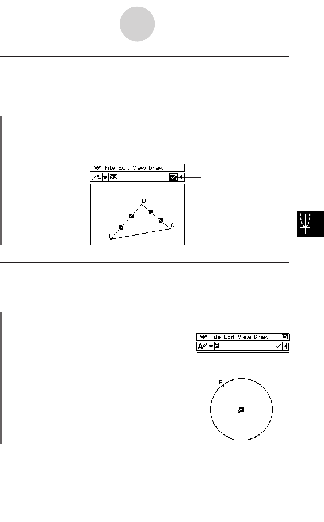
20060301

8-3-11

Editing Figures

A highlighted check box

indicates the measurement

is fixed (constrained).

k Fixing a Measurement of a Figure

By “fixing a measurement” we mean that a constraint is placed on the figure. For example, if

we fix (constrain) a point to a circle and move the circle, the point will also move.

The following example shows how to fix the size of an angle of a triangle.

u To fix the measure of an angle of a triangle

(1) Draw the triangle.

(2) Select side AB and then select side BC.

(3) Input 90 into the measurement box, and then select the check box to the right of it.

• This fixes the measure of angle B at 90 degrees.

k Changing a Label or Adding a Name to an Element

You can change the name of a point, or add a name to each element as explained in the

following example.

u ClassPad Operation

(1) Select (highlight) a point. Tap the down arrow to the right of icon palette on

measurement box and then u.

• This displays the current name of point A in the

measurement box. The displayed name is highlighted

so it can be edited.

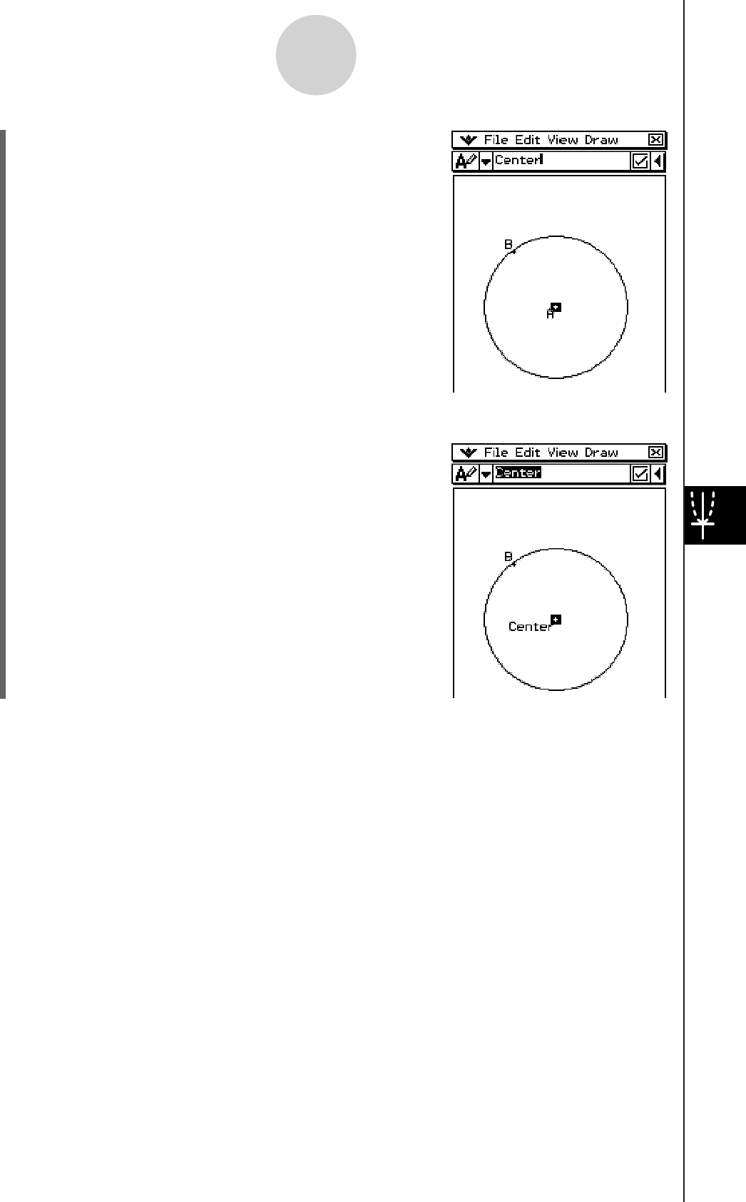
20060301

(2) Input a new name (“Center”) in the measurement box.

(3) Tap

E or the check box to the right side of measurement box.

• This displays the changed name on the screen as

shown here.

8-3-12

Editing Figures

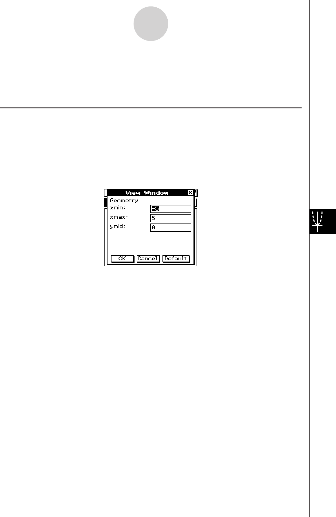
20101001

8-4 Controlling Geometry Window Appearance

This section provides information about how to control the appearance of the Geometry

application window by scrolling or zooming, and by showing or hiding axes and the grid.

Configuring View Window Settings

You can use the following procedures to configure settings that control the appearance of the

Geometry application window.

Tap O, and then [View Window] to display the View Window dialog box. The View Window

dialog box allows you to configure the x-axis range of values. The ymid value is used to

center the Graph window vertically. For example, if we set ymid = 2, then the y-axis will

appear 2 units below the center of the Graph window.

Note

• The following are the allowable ranges for the indicated View Window parameters.

−1 × 106 < xmin < 1 × 106

−1 × 106 < xmax < 1 × 106

−1 × 106 < ymid < 1 × 106

xmax − xmin

> 1 × 104

8-4-1

Controlling Geometry Window Appearance

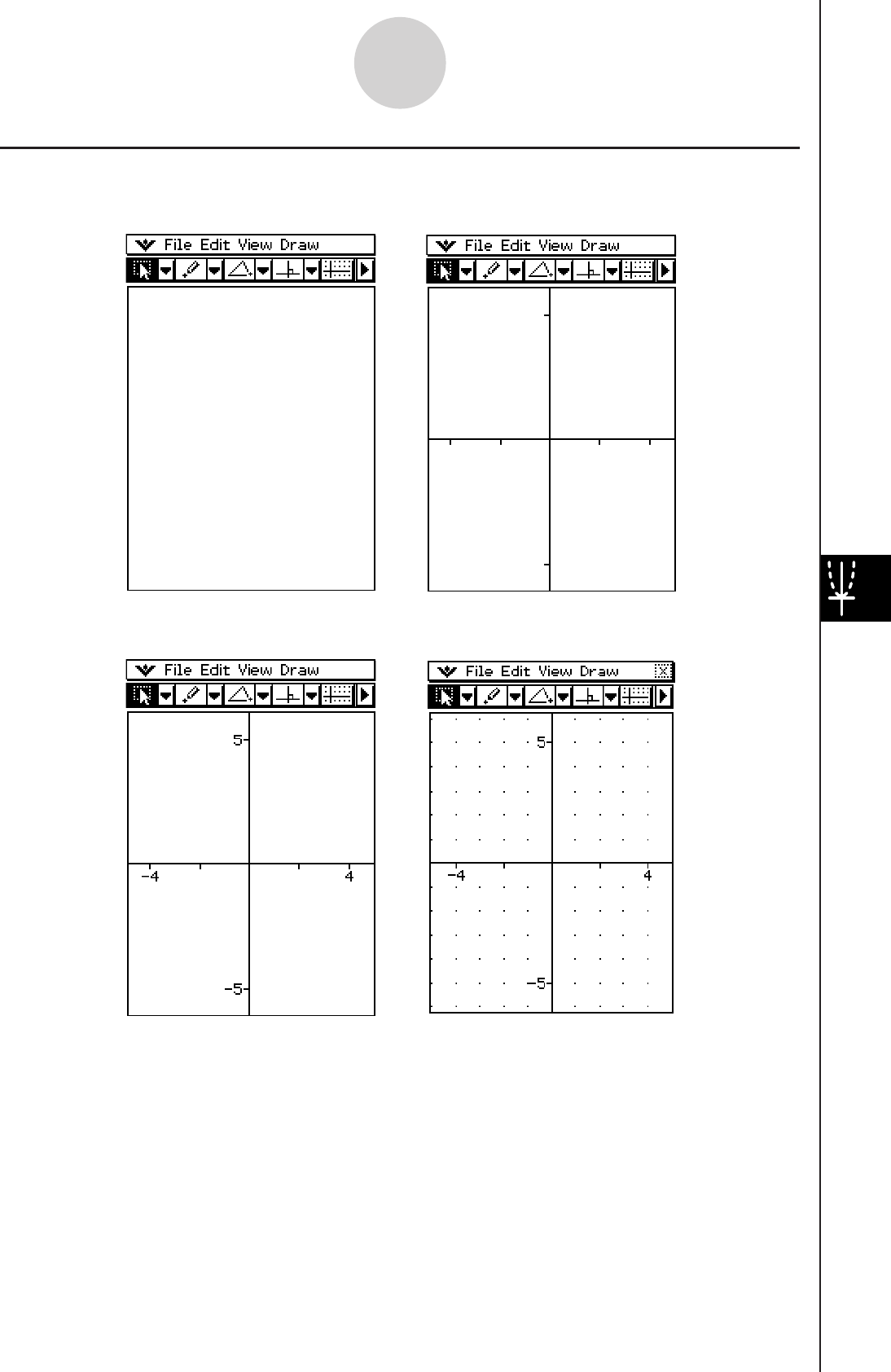
20060301

8-4-2

Controlling Geometry Window Appearance

Tip

• You can also turn on the Integer Grid by tapping [View] and then [Integer Grid]. See page 8-4-3

for more information.

Axes off, values off Axes on, values off

Axes on, values on

Selecting the Axis Setting

Tap q, or tap [View] and then [Toggle Axes] to cycle through the four settings shown below.

Axes on, values on and grid on

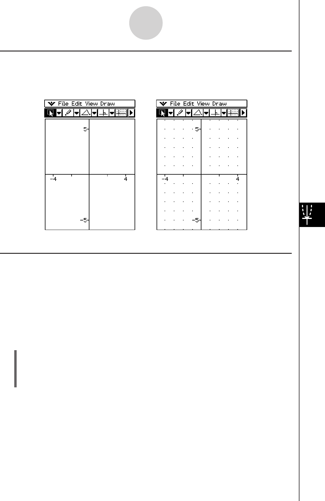
20060301

8-4-3

Controlling Geometry Window Appearance

Zooming

The Geometry application provides you with a selection of zoom commands that you can use

to enlarge or reduce an entire display image or a specific area of a figure.

Tip

• The screenshots in this section all use the “Axes on, values on” setting described under “Selecting

the Axis Setting” on page 8-4-2.

u To use Zoom Box

Example: To use zoom box to enlarge part of a circle

(1) Draw a circle.

(2) Tap [View] and then [Zoom Box], or tap Q.

(3) Drag the stylus on the screen to draw a selection boundary around the area you want

to enlarge.

Toggling Integer Grid Display On and Off

You can toggle integer grid display on and off by tapping [View] and then [Integer Grid]. The

[Integer Grid] command on the [View] menu has a check mark next to it while integer grid

display is turned on.

Grid off Grid on

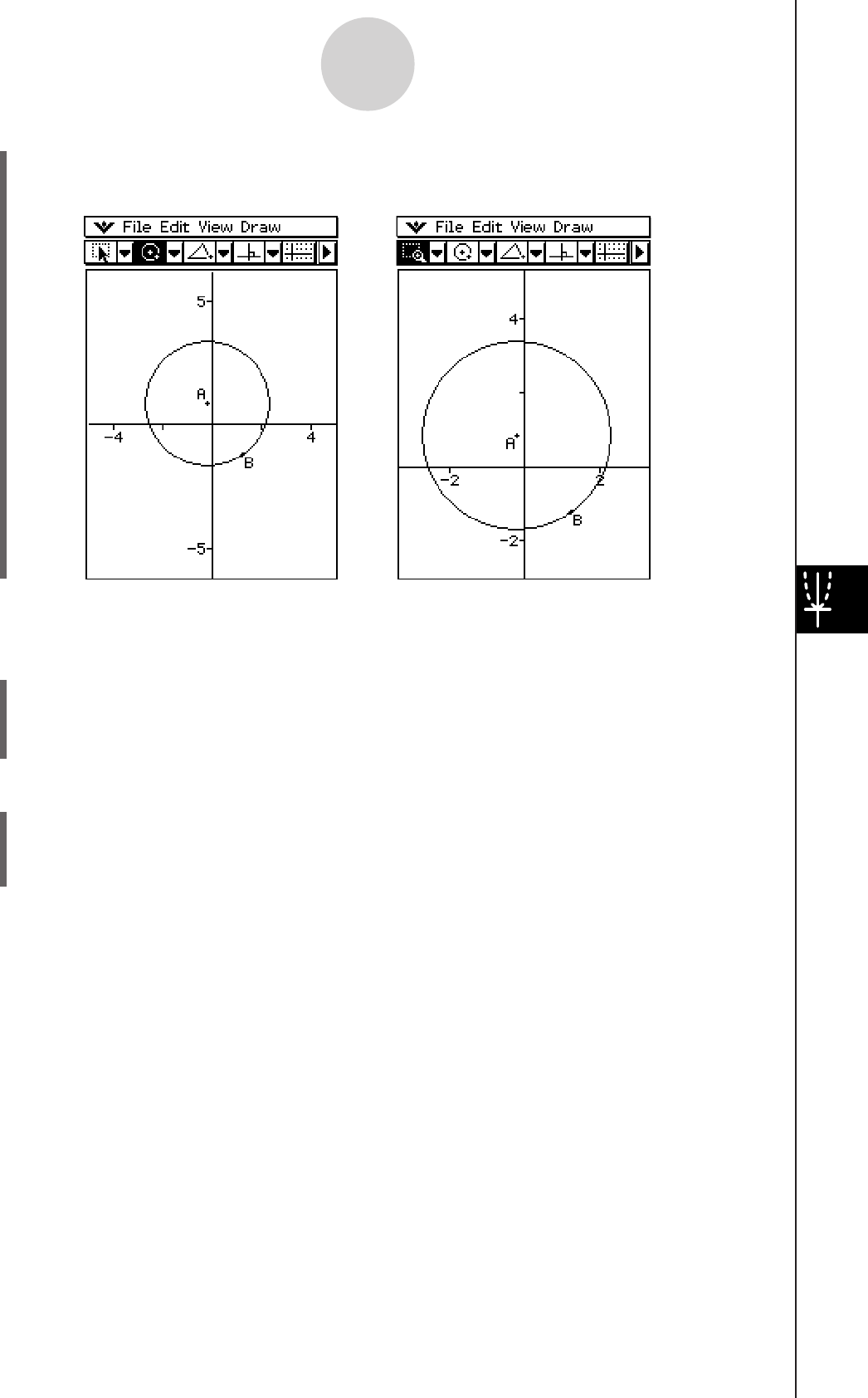
20060301

8-4-4

Controlling Geometry Window Appearance

u To use Zoom In and Out

Example 1: To zoom in on a circle

(1) Draw a circle.

(2) Tap [View] and then [Zoom In], or tap W.

• This enlarges the circle.

Example 2: To zoom out on a circle

(1) Draw a circle.

(2) Tap [View] and then [Zoom Out] or tap E.

• This reduces the size of the circle.

(4) Remove the stylus from the display and the area within the selection boundary expands

to fill the entire Graph window.

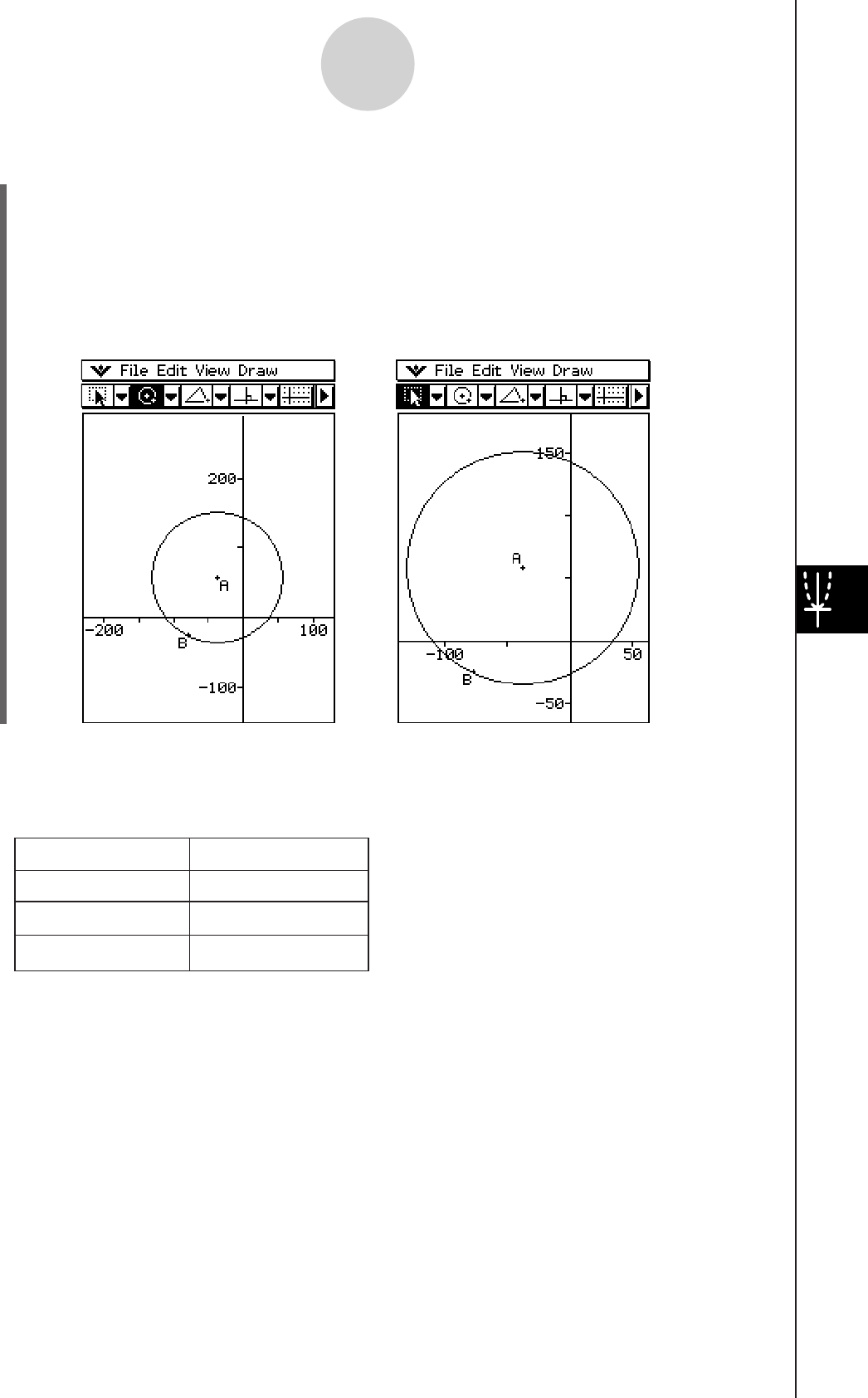
20060301

8-4-5

Controlling Geometry Window Appearance

Tip

• You can also perform the Zoom In, Zoom Out, and Zoom to Fit operations by pressing ClassPad

keys as described below.

To do this: Press this key:

Zoom In +

Zoom Out -

Zoom to Fit =

u To use Zoom to Fit

(1) Draw the figure or figures you want.

• If what you are drawing does not fit on the display, scroll the image as you draw it.

• For information about scrolling the screen, see “Using Pan to Shift the Display Image”

on page 8-4-6.

(2) Tap [View] and then [Zoom to Fit], or tap R.

• This enlarges or reduces the figure so it fills the display.

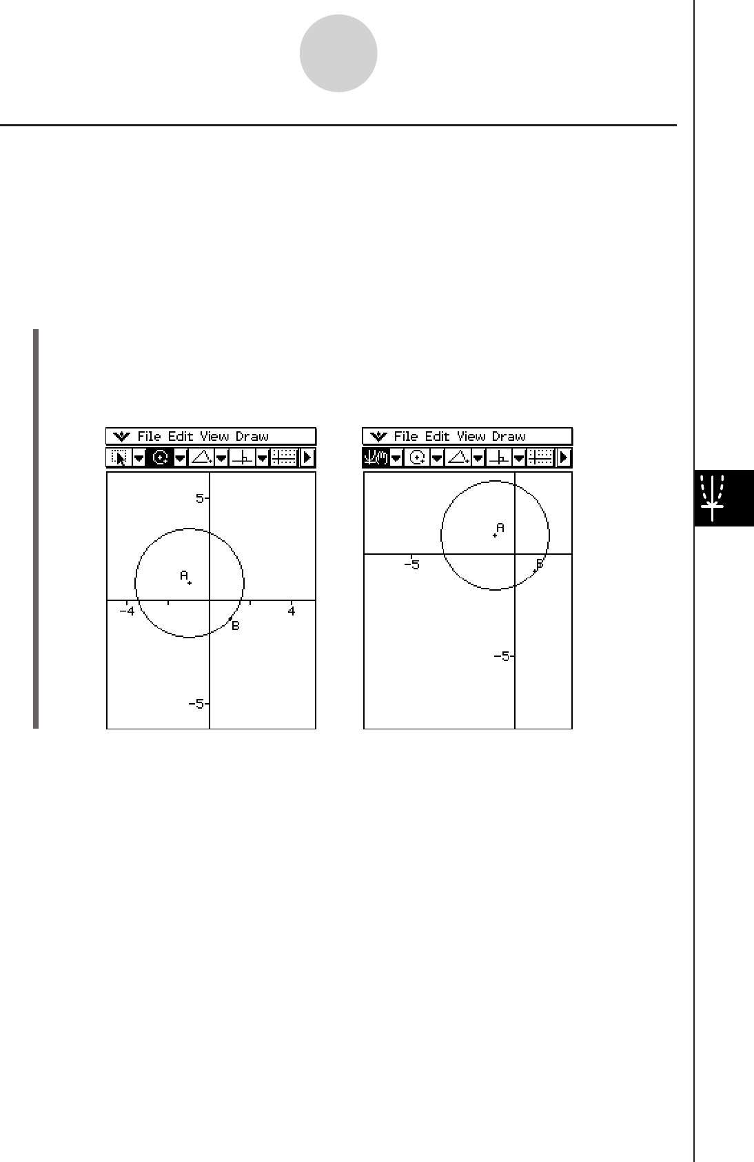
20060301

8-4-6

Controlling Geometry Window Appearance

Using Pan to Shift the Display Image

Panning makes it easy to shift the display image by dragging with the stylus.

Tip

• The screenshot in this section uses the “Axes on, values on” setting described under “Selecting

the Axis Setting” on page 8-4-2.

u To use Pan

Example: To pan the image of a circle

(1) Draw a circle.

(2) Tap [View] and then [Pan], or tap T.

(3) Place the stylus on the screen and drag in the direction you want to shift the image of

the circle.

Tip

• You can also scroll the window using the cursor keys.

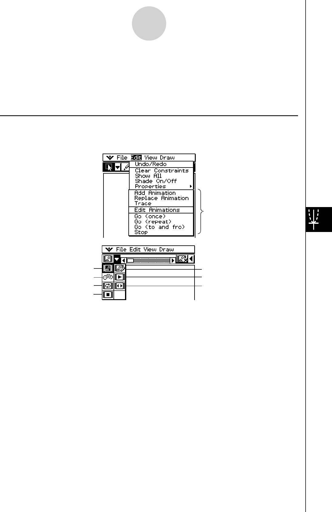
20060301

8-5 Working with Animations

An animation consists of one or more point/curve pairs, in which the curve can be a line

segment, circle, ellipse, or function. You build an animation by selecting a point/curve pair,

and then adding it to an animation.

Using Animation Commands

You can build and run an animation either by executing menu commands or by using the

animation toolbar that appears when you tap [View] and then [Animation UI].

[Edit] – [Animate]

8-5-1

Working with Animations

[View] – [Animation UI]

Tip

• Most of the procedures in this section are performed using the [Animate] submenu.

• All of the [Animate] menu commands can be accessed from the animation toolbar, except for

[Edit] - [Animate] - [Edit Animations].

• To close the animation toolbar and return to the normal toolbar, tap the = button on the right

side of the animation toolbar, or tap [View] and then [Animation UI].

[Animate] submenu

Add Animation

Trace

Go (repeat)

Stop

Replace Animation

Go (once)

Go (to and fro)

}

Animation toolbar

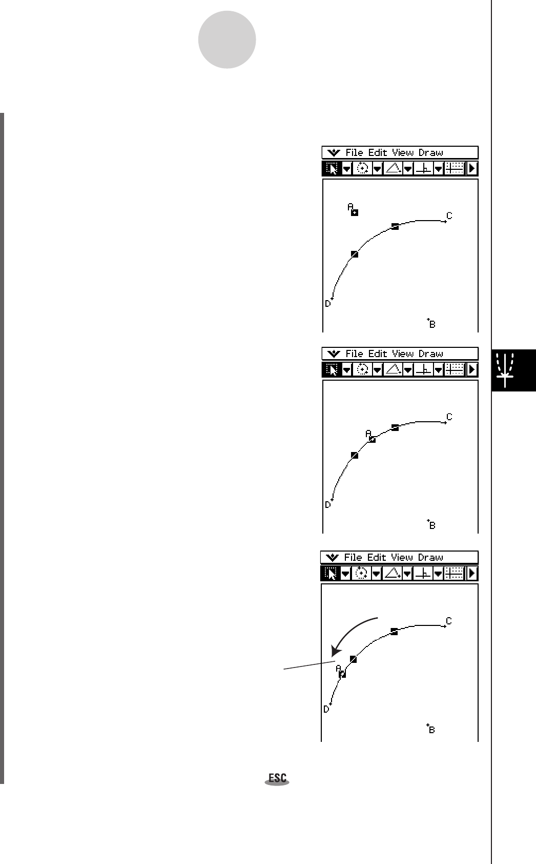
20060301

u To add an animation and run it

(1) Plot a point and draw an arc. Or, you could draw a circle, ellipse, line segment, or

function instead of an arc.

(2) Select the point and arc.

8-5-2

Working with Animations

(3) Tap [Edit], [Animate], and then [Add Animation].

(4) Tap [Edit], [Animate], and then [Go (once)],

[Go (repeat)], or [Go (to and fro)].

Point A moves along arc CD.

(5) Tap [Edit], [Animate], and then [Stop] to stop the animation.

• You can also stop the animation by tapping on the icon panel.

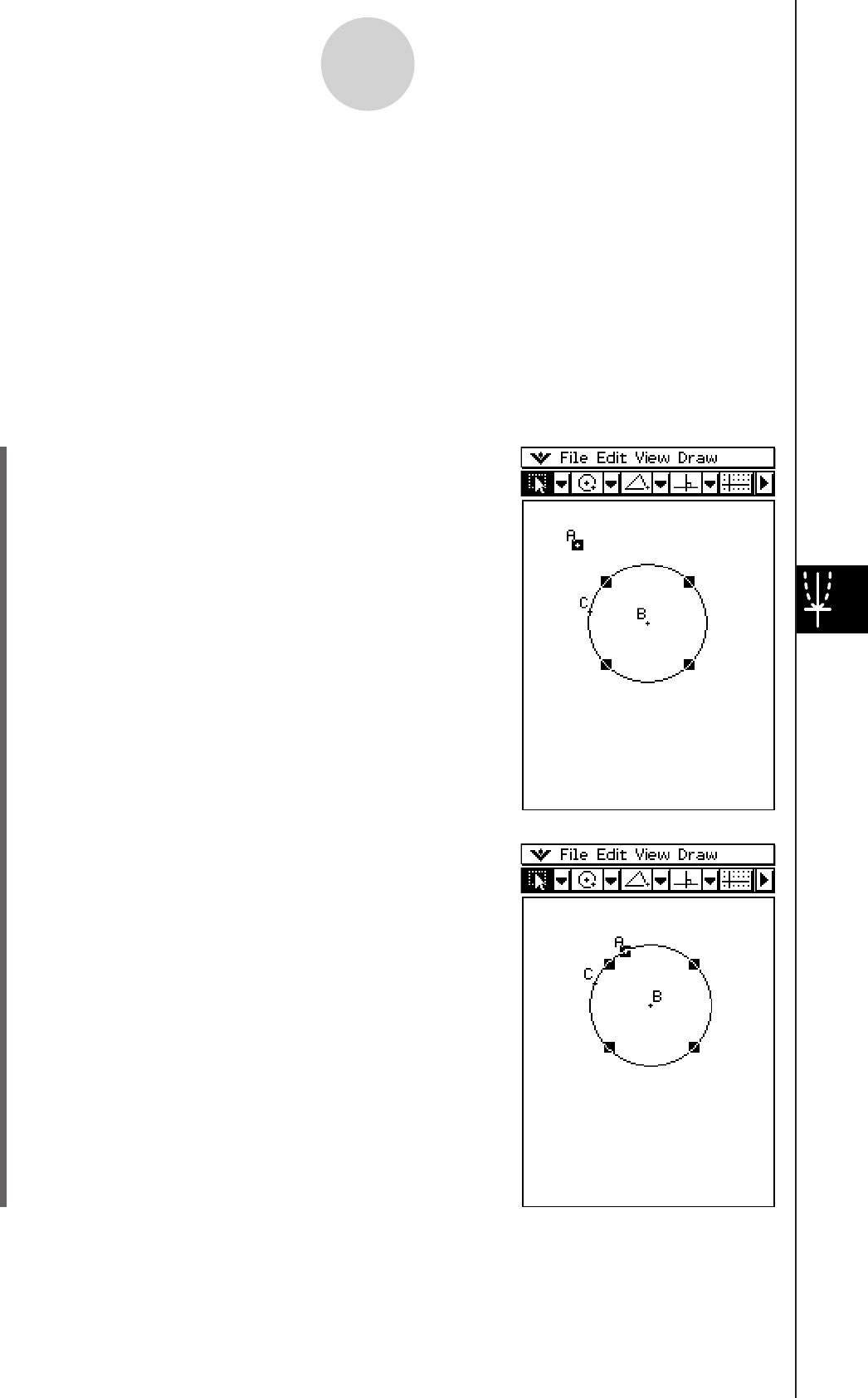
20060301

u To animate a point around a circle

(1) Plot a point and draw a circle, and then select them.

8-5-3

Working with Animations

Tip

• You can repeat the above procedure to create multiple points that move simultaneously.

Try this:

• Draw a line segment and plot another point.

• Select the line segment and the point.

• Repeat steps (3) and (4) on page 8-5-2.

Notice that both animations go at the same time!

• To start a new animation, perform the procedure under “To replace the current animation with a

new one” on page 8-5-4. Or, tap [Edit], [Animate] and then [Edit Animations]. On the dialog box

that appears tap [Remove].

(2) Tap [Edit], [Animate], and then [Add Animation].

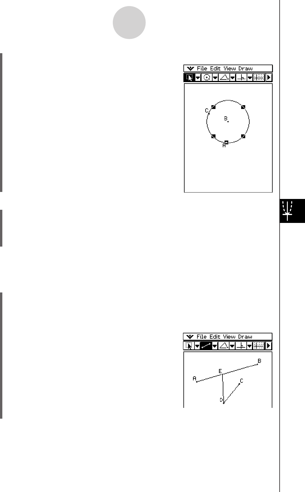
20060301

(3) Tap [Edit], [Animate], and then [Go (once)].

• This causes the point to travel around the

circumference of the circle.

u To replace the current animation with a new one

(1) Select the point and curve for the new animation.

(2) Tap [Edit], [Animate], and then [Replace Animation].

• This discards the currently set animation and sets up an animation for a new point

and curve set. Tap [Edit], [Animate], and then [Go (once)] to see your new animation.

u To trace a locus of points

Tip

• Using trace leaves a trail of points when the animation is run.

(1) Draw a line segment AB and plot point C, which is not on line segment AB.

(2) Plot point D, which should also not be on line segment AB, but should be on the same

side of the line segment as point C.

(3) Draw a line segment that connects point D with point C.

(4) Draw another line segment that connects point D with

line segment AB. This is line segment DE.

8-5-4

Working with Animations

(5) Tap the right arrow button to display the measurement box.

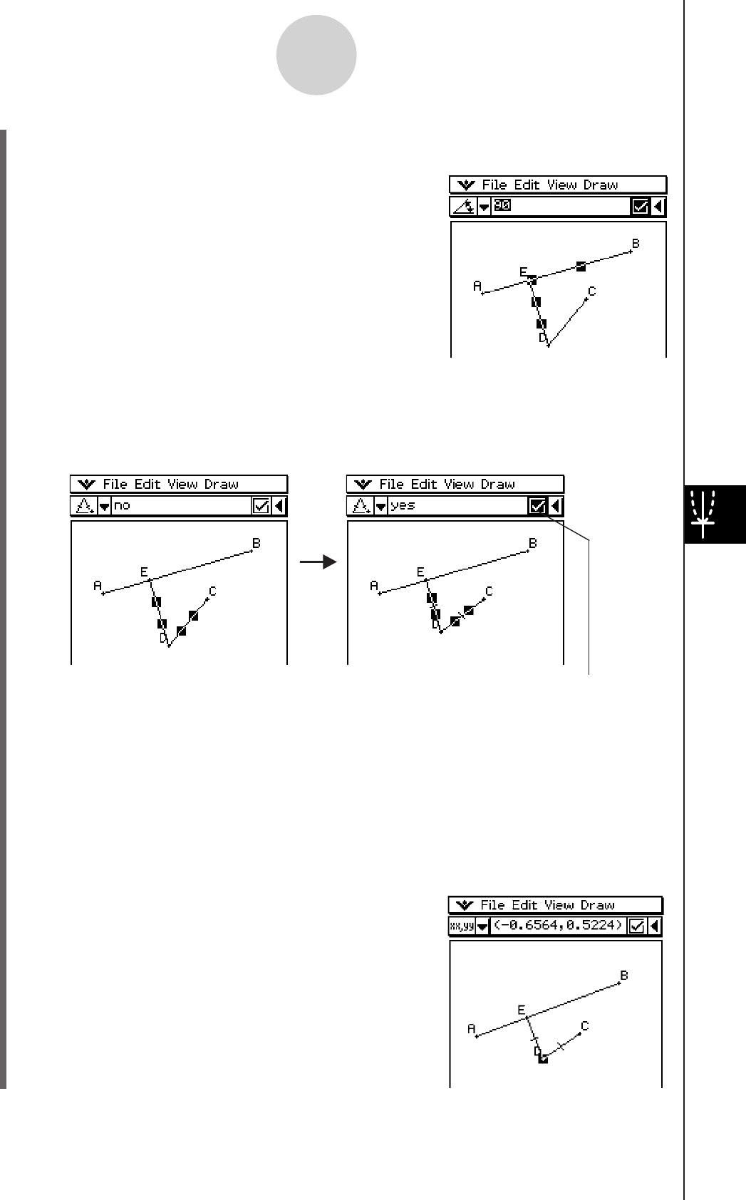
20060301

(6) Select line segments AB and DE, enter 90 in the measurement box, and tap the check

box next to the measurement box.

• This fixes the angle between AB and DE at 90

degrees.

8-5-5

Working with Animations

(7) Select only line segments DE and DC, and then tap the down arrow next to the

measurement box.

(8) Tap the

e icon, and then select the check box to the right of the measurement box.

• This makes line segments DE and DC congruent in length.

(9) Select point E and line segment AB.

(10) Tap [Edit], [Animate], and then [Add Animation].

(11) Tap the screen to deselect the currently selected items.

(12) Select point C.

(13) Select the check box to the right of the measurement box.

• This fixes the position of point C.

(14) Select point D.

A highlighted check box indicates the measurement

is fixed (constrained).

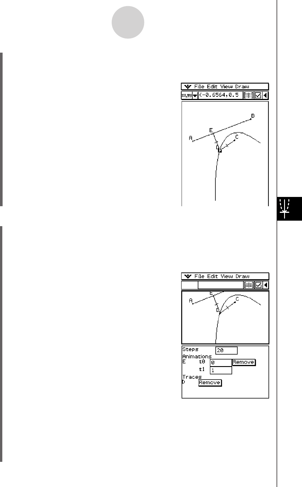
20060301

u To edit an animation

(1) While the animation you want to edit is on the display, tap [Edit], [Animate], and then [Edit

Animations].

• This displays the animation editing window in the lower window. The upper window

contains the animation that we just completed in “To trace a locus of points”. See

page 8-5-4 for information about specifying the trace point.

(2) Edit the animation following the procedure below.

Steps

This setting specifies how many steps point E takes to

move along line segment AB. The initial default value

is 20.

Animations

• The “E” under “Animations” indicates that point E is

the point moved by the animation. When you are

building multiple animations, a list of all applicable

points appears here.

• Tapping [Remove] deletes the applicable animation.

• “t0” and “t1” specify the range of movement of point

E on line segment AB. The initial default values are

t0 = 0 and t1 = 1.

• During animation, the length of AB is considered to

be one unit. The default values specify that movement of point E is from start point A

(point where length equals 0) up to end point B (point where length equals 1).

• Changing the value of t0 to 0.5, for example, causes point E to move from the middle

of line segment AB to point B.

• Changing the value of t0 to −1, causes point E to begin at a point outside line

segment AB (in this case, at a point a distance equivalent to the length of line

segment AB) and ending with point B.

8-5-6

Working with Animations

(15) Tap [Edit], [Animate], and then [Trace].

• This should cause a parabola to be traced on the display. Note that line segment AB

is the directrix and point C is the focus of the parabola.

(16) With point D still selected, tap [Edit], [Animate], and

then [Go (once)].

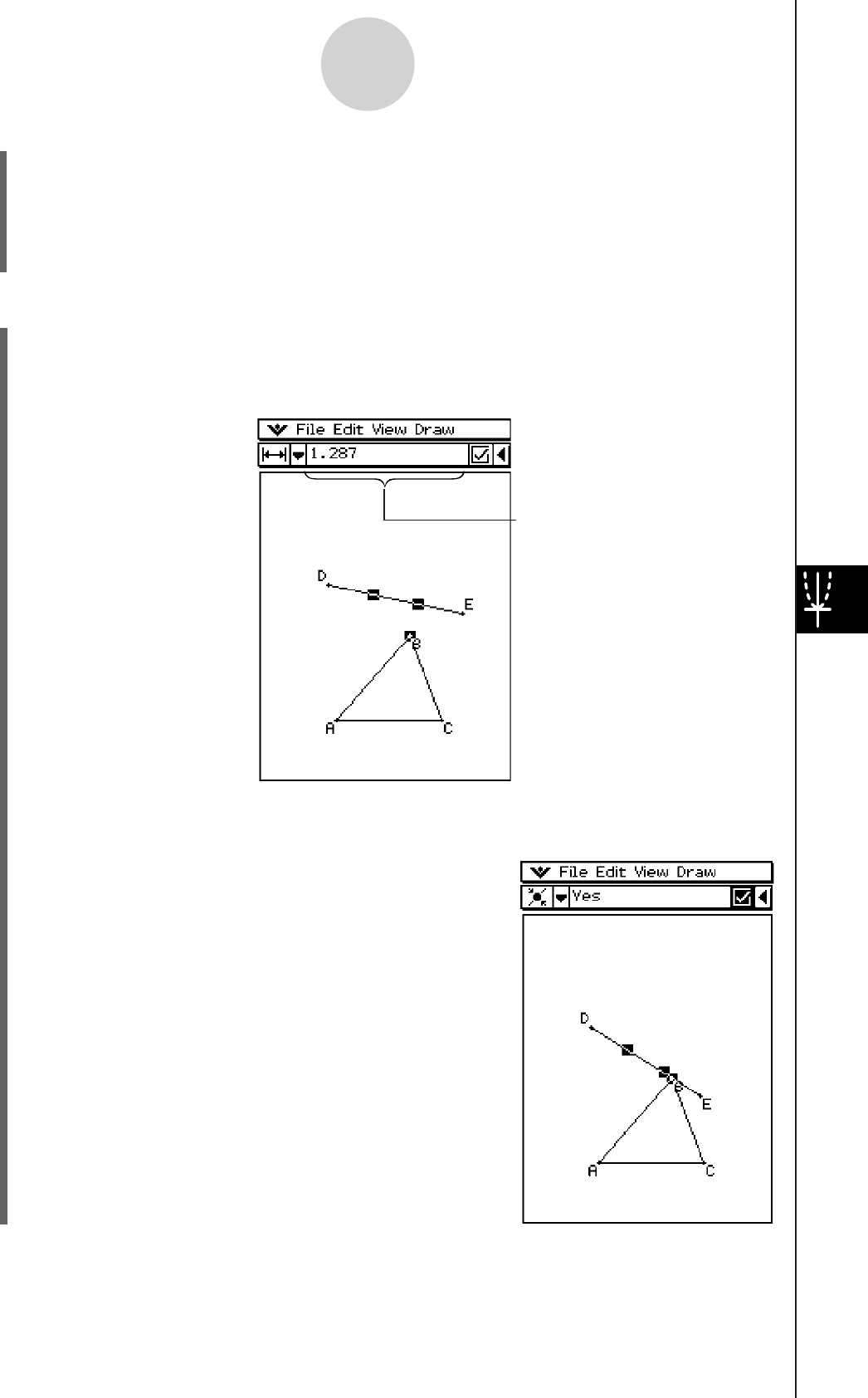
20060301

8-5-7

Working with Animations

Measurement box

Traces

This item shows the specified trace point. Tapping [Remove] cancels the trace point

setting.

(3) While the lower window is active, tap O and then [Close] to close the animation

editing window.

u To view an animation table

(1) Draw a triangle and a line segment above the triangle.

(2) Tap the right arrow button to display the measurement box.

(3) Select the line segment and the vertex point closest to the line.

(4) Tap the down arrow next to the measurement box.

(5) Tap the

6 icon, and then select the check box to the right of the measurement box.

• This connects the segment and vertex point.

20060301

8-5-8

Working with Animations

(6) With the line and vertex point still selected, tap [Edit], [Animate], and then [Add

Animation].

(7) Now, select only one side of the triangle.

(8) Tap [Edit], [Animate], and then [Go (once)].

(9) Tap

# next to the measurement box.

• While the animation is running, the lower window shows the table for the length of the

side you selected.

(10) Try selecting another side and running the animation again to view the table for that

side. Or, select another side and tap #.

(11) Select all three sides of the triangle and run the animation again.

• The table that appears in the lower window will show how the area of the triangle

changes while the animation runs.

20060301

8-6 Using the Geometry Application with Other

Applications

You can display the Geometry application from within the eActivity or Main application.

This is a great feature that allows you to visualize the relationship between Algebra and

Geometry. You can, for example, drag a figure from the Geometry window to the eActivity

window to see its corresponding mathematical expression. This section describes how to do

this and other useful things.

8-6-1

Using the Geometry Application with Other Applications

Drag and Drop

When you open Geometry within another application, you can drag and drop information

between the two application windows.

Example 1: To drag a circle from the Geometry window to the eActivity window

u ClassPad Operation

(1) Tap

m to display the application menu, and then tap A to start the eActivity

application.

(2) From the eActivity menu, tap [Insert], [Strip] and then [Geometry].

• This inserts a Geometry data strip, and displays the Geometry window in the lower

half of the screen.

Geometry data strip

Geometry window

• For details about Geometry data strips, see “Inserting an Application Data Strip” on

page 10-3-5.

(3) Draw a circle on the Geometry window.

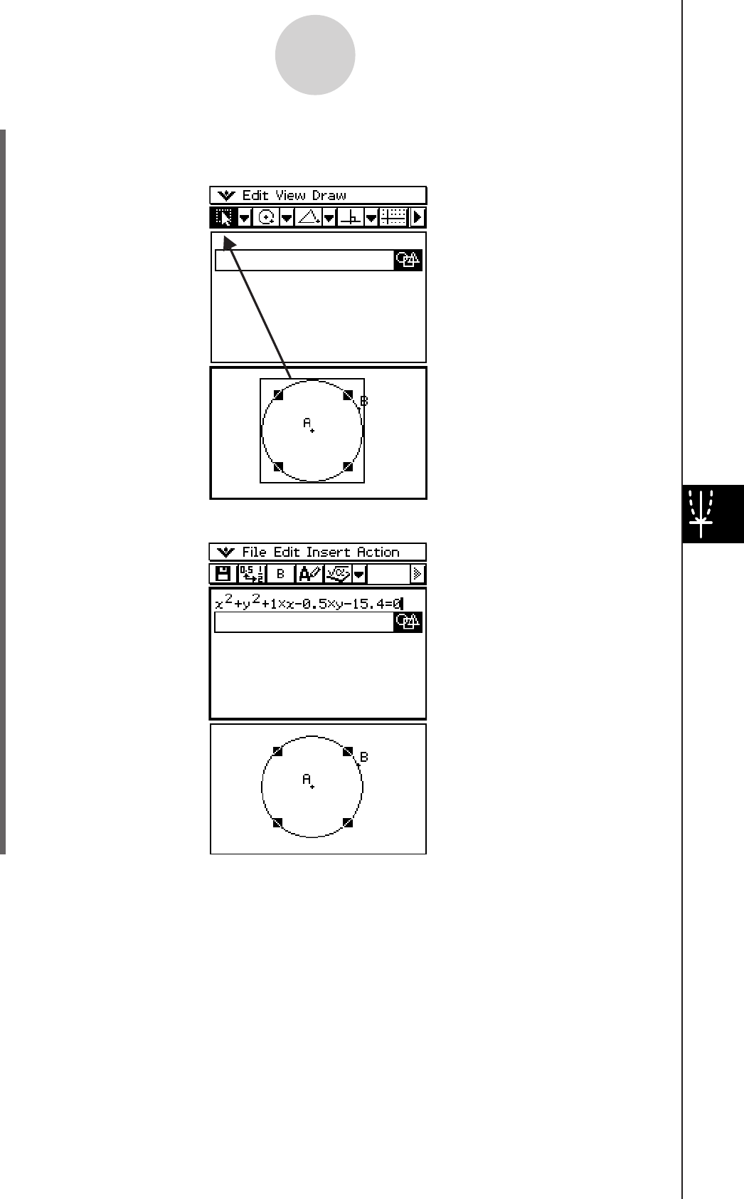
20060301

(4) Select the circle and drag it to the first available line in the eActivity window.

• This inserts the equation of the circle in the eActivity window.

(5) You can now experiment with the data in the eActivity window.

Tip

• Try modifying the radius of the circle in the eActivity window. Highlight your modified equation,

then drag it into the Geometry window.

8-6-2

Using the Geometry Application with Other Applications

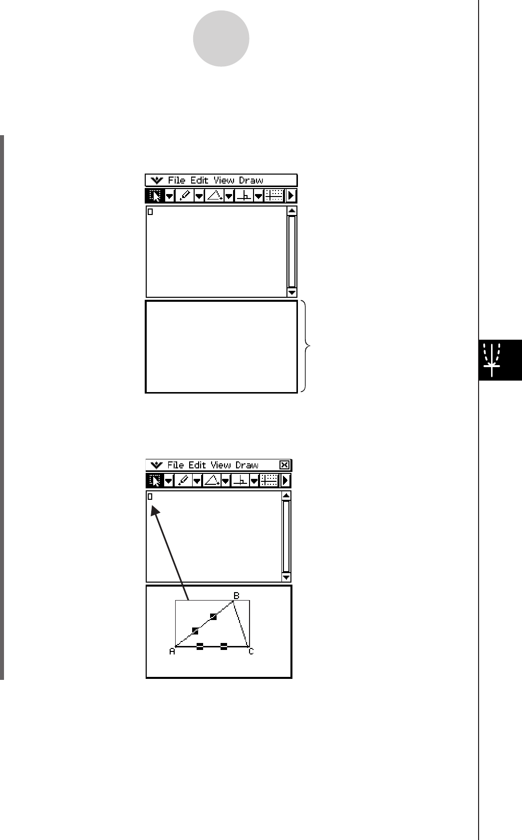
20060301

Example 2: To drag two sides of a triangle from the Geometry window to the Main window

u ClassPad Operation

(1) Tap

m to display the application menu, and then tap J to start the Main application.

(2) Tap

3 to display the Geometry window in the lower half of the screen.

Geometry window

(3) Draw a triangle on the Geometry window.

(4) Select two sides of the triangle and drag them to the Main window.

• This inserts the equations of the sides in the Main window.

8-6-3

Using the Geometry Application with Other Applications

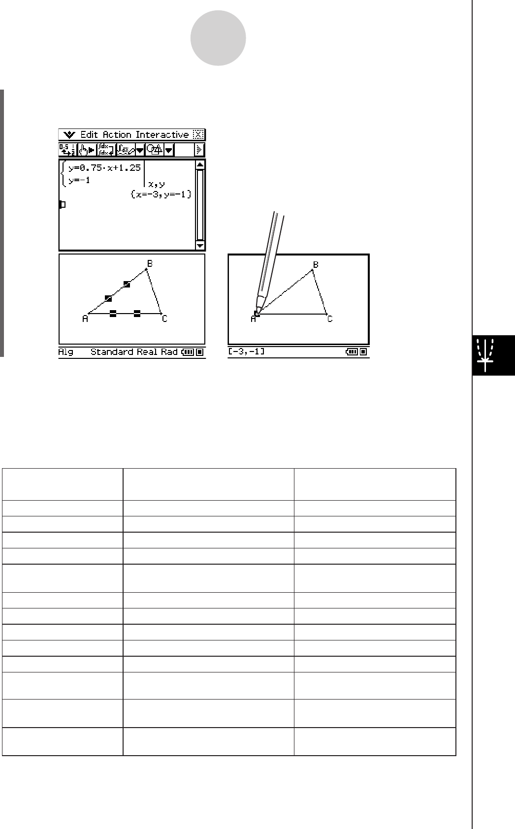
20060301

(5) Press

• Notice that the solution is the same as the coordinates of point A.

8-6-4

Using the Geometry Application with Other Applications

• To show the coordinates of A, just select

point A. Its coordinates will be displayed in

the status bar.

Tip

• Try using this drag and drop method to find the point of intersection of two lines. This is a great

way to find the solution to a system of equations.

• To view a fractional result as a decimal, tap the input row and then u.

• The information that appears when you drop a figure into another application depends on the

figure you are dragging. Many of the possible outcomes are listed in the table below.

Support for drag and drop into a

Geometry Link row* in an eActivity

Geometric Figure

Point

Line Segment

Infinite Line

Vector

Circle

Arc

Ellipse

Function (y=f

(x))

Two Lines

Polygon

Pairs of points related

by a transformation

Drag and drop into another

application transforms to:

An Ordered Pair

Linear Equation

An Ordered Pair (head of vector,

assuming the tail is at the origin)

Equation of a Circle

Equation of an Ellipse

Equation of the Function

System of Equations

Matrix Containing each Vertex

Point

Expression Showing Point

Relationship

yes

Open Polygon created

by Animation

Matrix Containing each Vertex

Point no

Ray Linear Equation yes

* For details about a Geometry Link row, see “Dynamically Linked Data” on page 8-6-5 and “Inserting

a Geometry Link Row” on page 10-3-17.

20080201

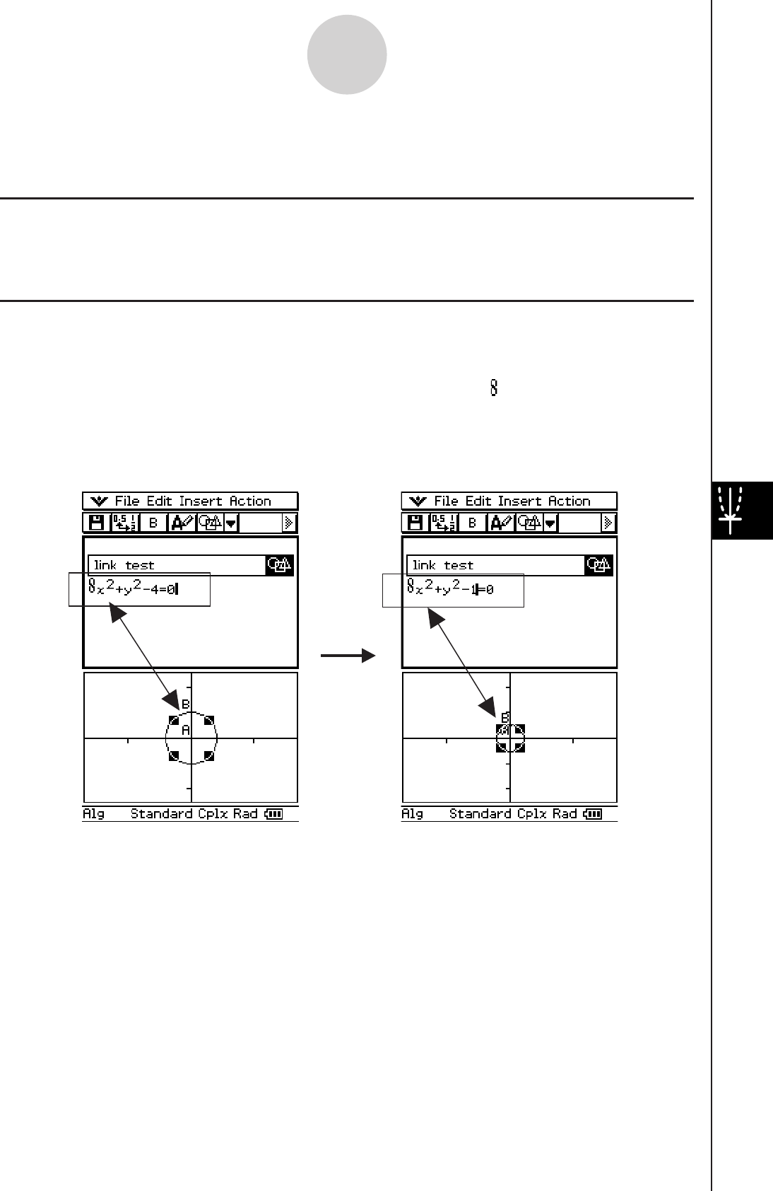
20060301

8-6-5

Using the Geometry Application with Other Applications

Copy and Paste

In addition to drag and drop, you can also copy figures or columns from an animation table,

and paste them into another application.

Example of dynamically linked data

For information on how to create a dynamic link between a geometric figure and its equation

in the eActivity window, see “Inserting a Geometry Link Row” on page 10-3-17.

Dynamically Linked Data

Another nice feature of the ClassPad is the ability to create a dynamic link between a

geometric figure and its equation in the eActivity window. When a geometric figure is

dynamically linked to an equation, you will notice a link symbol ( ) in front of the equation in

the eActivity window. Changing the graph in the Geometry window will automatically update

the linked data in the eActivity window. Also, changing the data in the eActivity window will

update the graph in the Geometry window. Note that this feature is available only within the

eActivity application.

•

When the Geometry application cannot determine what is dropped into it, the dropped data

is displayed as text.

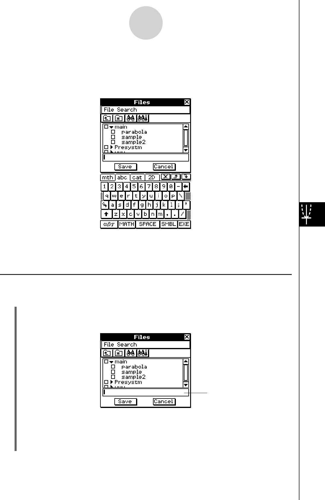
20090601

8-7 Managing Geometry Application Files

This section covers file management operations such as save, open, delete, rename, move,

etc.

8-7-1

Managing Geometry Application Files

Tip

• You can also use the Variable Manager (page 1-8-1) to manage Geometry application files.

File Operations

u To save a file

(1) Tap [File] and then [Save].

• This displays the Files dialog box.

File name edit box

(2) Tap the name of the folder where you want to save the file so it is selected.

(3) In the file name edit box, input up to 8 bytes for the file name.

(4) Tap [Save].

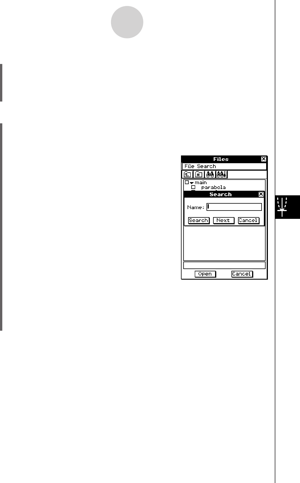
20060301

(3) Enter the file name you want to find and then tap [Search].

• File names that match the one you enter become highlighted on the display. Tapping

[Open] opens the highlighted file.

• To search for the next occurrence of the file name, tap [Search] again and then tap

[Next] on the Search dialog box.

u To open an existing file

(1) Tap [File] and then [Open].

• This displays the Files dialog box.

(2) Open the folder that contains the file you want to open.

(3) Tap the name of the file you want to open so it is selected, and then tap [Open].

u To search for a file

(1) Tap [File] and then [Open].

• This displays the Files dialog box.

(2) Tap [Search].

• This displays the Search dialog box.

8-7-2

Managing Geometry Application Files

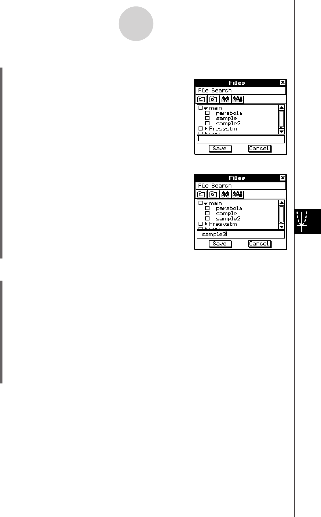
20060301

u To save a file under a different name

(1) Tap [File] and then [Save].

• This displays the Files dialog box.

8-7-3

Managing Geometry Application Files

(4) Tap [Save].

u To delete a file

(1) Tap [File] and then [Open].

• This displays the Files dialog box.

(2) Select the check box next to the file you want to delete.

• You can select multiple files for deletion, if you want.

• Selecting a check box next to a folder name automatically checks the boxes for all

files inside that folder.

(3) Tap [File] and then [Delete].

(4) In response to the confirmation dialog box that appears, tap [OK] to delete the file(s) or

[Cancel] to cancel.

(5) To close the Files dialog box, tap [Cancel].

Tip

• Selecting a folder in the above procedure deletes the folder and all of its contents. Note, however,

that the “main” folder cannot be deleted, even if you check it.

(3) Input up to 8 bytes for the new name under which

you want to save the file.

(2) Tap the name of the folder where you want to save the file so it is selected.

20060301

8-7-4

Managing Geometry Application Files

u To rename a file

(1) Tap [File] and then [Open].

• This displays the Files dialog box.

(2) Tap the name of the file you want to rename so it is selected.

(3) Tap [File] and then [Rename].

• This displays the Rename dialog box.

(4) Enter the new file name.

(5) In response to the confirmation dialog box that appears, tap [OK] to rename the file or

[Cancel] to cancel.

(6) To close the Files dialog box, tap [Cancel].

u To move a file to another folder

(1) Tap [File] and then [Open].

• This displays the Files dialog box.

(2) Select the check box next to the file you want to move.

• To move multiple files, select all of their check boxes.

(3) Tap [File] and then [Move].

• This causes a dialog box for selecting the destination folder to appear.

(4) On the dialog box, tap the down arrow button and then select the destination folder

from the list that appears.

(5) Tap [OK].

(6) To close the Files dialog box, tap [Cancel].

Folder Operations

u To create a new folder

(1) Tap [File] and then [Open].

• This displays the Files dialog box.

(2) Tap [File] and then [Create Folder], or tap {.

• This displays the Create Folder dialog box.

(3) Enter up to 8 bytes for the folder name.

(4) In response to the confirmation dialog box that appears, tap [OK] to create the folder or

[Cancel] to cancel.

(5) To close the Files dialog box, tap [Cancel].

20060301

u To delete a folder

Warning!

Deleting a folder also deletes all files inside of it. Please double-check to make sure you no

longer need the contents of a folder before deleting it.

(1) Tap [File] and then [Open].

• This displays the Files dialog box.

(2) Select the check box next to the folder you want to delete.

• You can select multiple folders for deletion, if you want.

• Selecting a check box next to a folder name automatically selects the check boxes for

all of the files inside that folder.

(3) Tap [File] and then [Delete].

(4) In response to the confirmation dialog box that appears, tap [OK] to delete the folder or

[Cancel] to cancel.

(5) To close the Files dialog box, tap [Cancel].

Tip

• You cannot delete the “main” folder.

u To rename a folder

Use the procedure under “To rename a file” on page 8-7-4 to rename a folder. Simply select

a folder instead of a file.

8-7-5

Managing Geometry Application Files

20060301

Using the Numeric

Solver Application

This chapter provides information about the functions of the

Numeric Solver application, referred to as NumSolve, and

explains how to perform Numeric Solver procedures. Numeric

Solver lets you obtain the value of any variable in an equation

without the need to transform or simplify the equation.

9-1 Numeric Solver Application Overview

9-2 Using Numeric Solver

Chapter

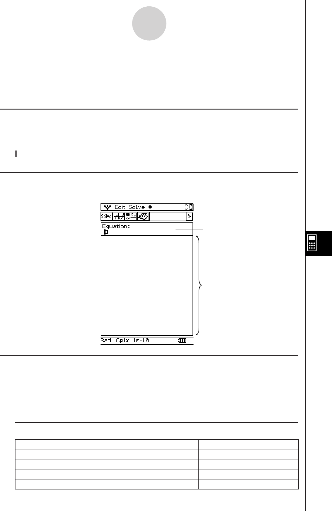
20060301

9-1-1

Numeric Solver Application Overview

9-1 Numeric Solver Application Overview

This section describes the configuration of the Numeric Solver application windows and

provides basic information about Numeric Solver menu and commands.

Numeric Solver Application Window

Starting up Numeric Solver application displays the window shown below.

Input equations here.

k O Menu

To do this: Select this O menu item:

Make the Num Solver window active NumSolve

Make the Graph Editor window active Graph Editor

Make the 3D Graph Editor window active 3D Graph Editor

Make the Main application active Main

Variable list

Starting Up the Numeric Solver Application

Use the following procedure to start up the Numeric Solver application.

u ClassPad Operation

On the application menu, tap N.

Numeric Solver Menus and Buttons

This section explains the operations you can perform using the menus and buttons of the

Numeric Solver window.

• For information about Format related items on OMenu, see “Application Format Settings”

on page 1-9-4.

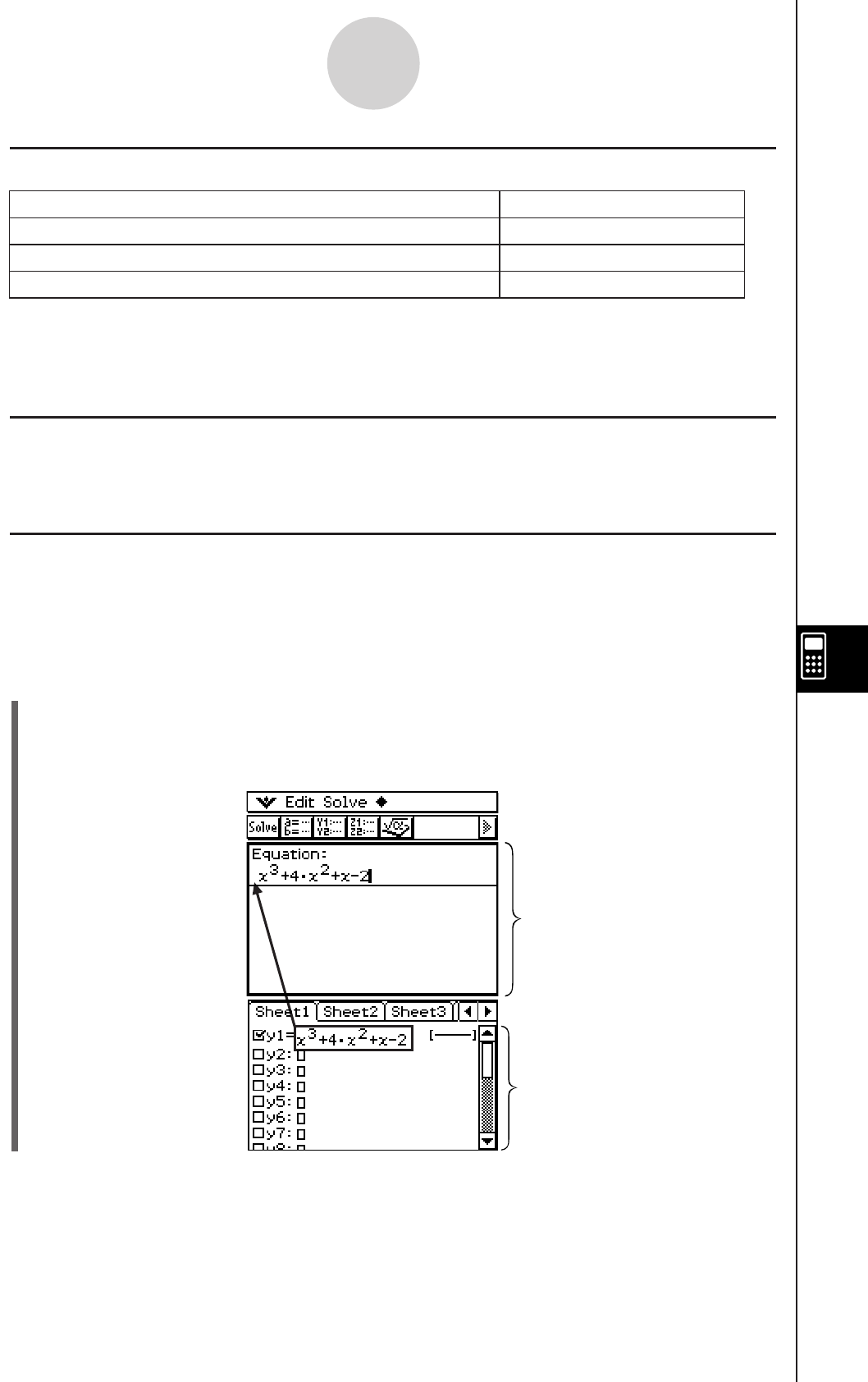
20060301

kToolbar

The toolbar provides you with easy access to the Main application, 3D Graph Editor, Graph

Editor, and, of course, Solve.

kDragging an Expression from the Other Application to the Numeric Solver

Window

You can drag expression and equations from the Main application window or Graph Editor

window and drop them into the Numeric Solver window.

uClassPad Operation

(1) On the Graph Editor window, input the equation x3 + 4·x2 + x – 2.

(2) Tap the equation to the right of “y1=”. Next, tap [Edit] and then [Select All].

(3) Drag the equation x3 + 4·x2 + x – 2 to the “Equation:” cursor position.

9-1-2

Numeric Solver Application Overview

kaMenu

To do this:

Clear all 1-character input variables (a through z)

Initialize the upper boundary and lower boundary

Change the convergence range

Select this a menu item:

Clear a–z

Initialize Bound

Convergence

Important!

• Performing “Clear a-z” operation clears all 1-character variables, regardless of variable data

type. Programs and functions with file names from “a” through “z” are also cleared.

Numeric Solver window

Graph Editor window

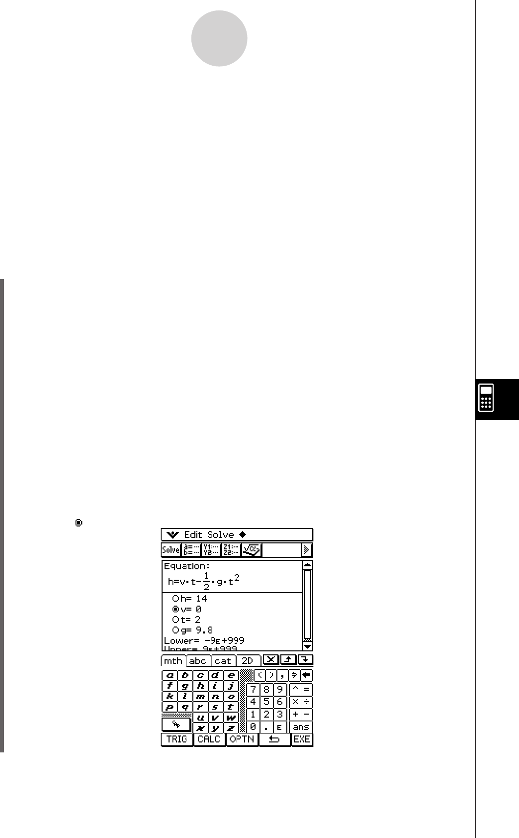
20060301

9-2 Using Numeric Solver

Numeric Solver lets you obtain the value of any variable in an equation, without the need to

transform or simplify the equation.

Example: t is the time it would take for an object thrown straight up with initial velocity v to

reach height h.

Use the formula below to calculate the initial velocity v for a height of h = 14

meters and a time of t = 2 seconds. Gravitational acceleration is g = 9.8 m/s2.

h = vt – 1/2 gt2

u ClassPad Operation

(1) Tap

m to display the application menu, and then tap N.

• This starts up the Numeric Solver application.

(2) k 9 V

(3) Input the equation as it is written, and then tap w.

h=vt-(b/c)gt{cw

• If you do not input an equal sign (=), the ClassPad assumes that the entire expression

is on the left side of the equal sign and that the right side is zero. Inputting more than

one equal sign causes an error.

(4) On the list of expression variables that appears, enter values for the variables you

want.

bewawcwj.iw

You can also specify upper and lower limit values for the solution.

• An error occurs if there is no solution within the range of values you specify.

(5) Select the variable for which you want to solve (so the button next to the variable

becomes ).

9-2-1

Using Numeric Solver

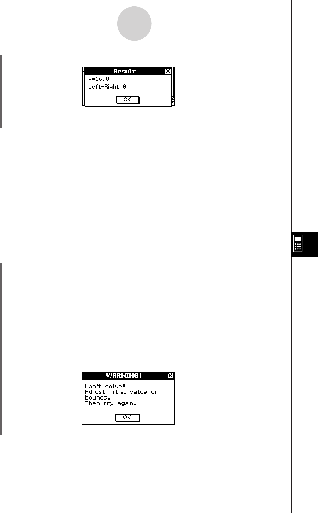
20060301

9-2-2

Using Numeric Solver

(6) Tap

1, or tap [Solve] and then [Execute] on the Numeric Solver menu.

• The [Left–Right] value shows the difference between the left side and right side

results.

Tip

• Numeric Solver solves functions by calculating approximations based on Newton’s method.

This means that solutions may include errors that are not actual solutions. The accuracy of

solutions can be determined by viewing the [Left–Right] value. The closer the [Left–Right]

value is to zero, the more accurate the results.

• If ClassPad judges that the displayed results are not converging sufficiently, it displays the

message “Did not converge. Do you wish to continue a calculation?” Tap [Yes] to continue, or

[No] to cancel the calculation.

Example: Solve the equation 86 = 56.01205897 log(61− x)

• In this example, the initial convergence value is 1E−13. This is the

default setting of the ClassPad unit.

u ClassPad Operation

(1) Tap

m to display the application menu, and then tap N.

(2) k 9

(3) Input the equation as written, then tap w.

86=56.0bc05897l6b-X)w

• The variable x is automatically selected because it is the only variable in the

equation.

(4) Tap 1, or tap [Solve] and then [Execute] on the Numeric Solver menu.

• This completes the procedure. If the software is unable to converge to a solution,

steps (5) through (8) apply.

(5) The error message appears.

Tap [OK].

20070301

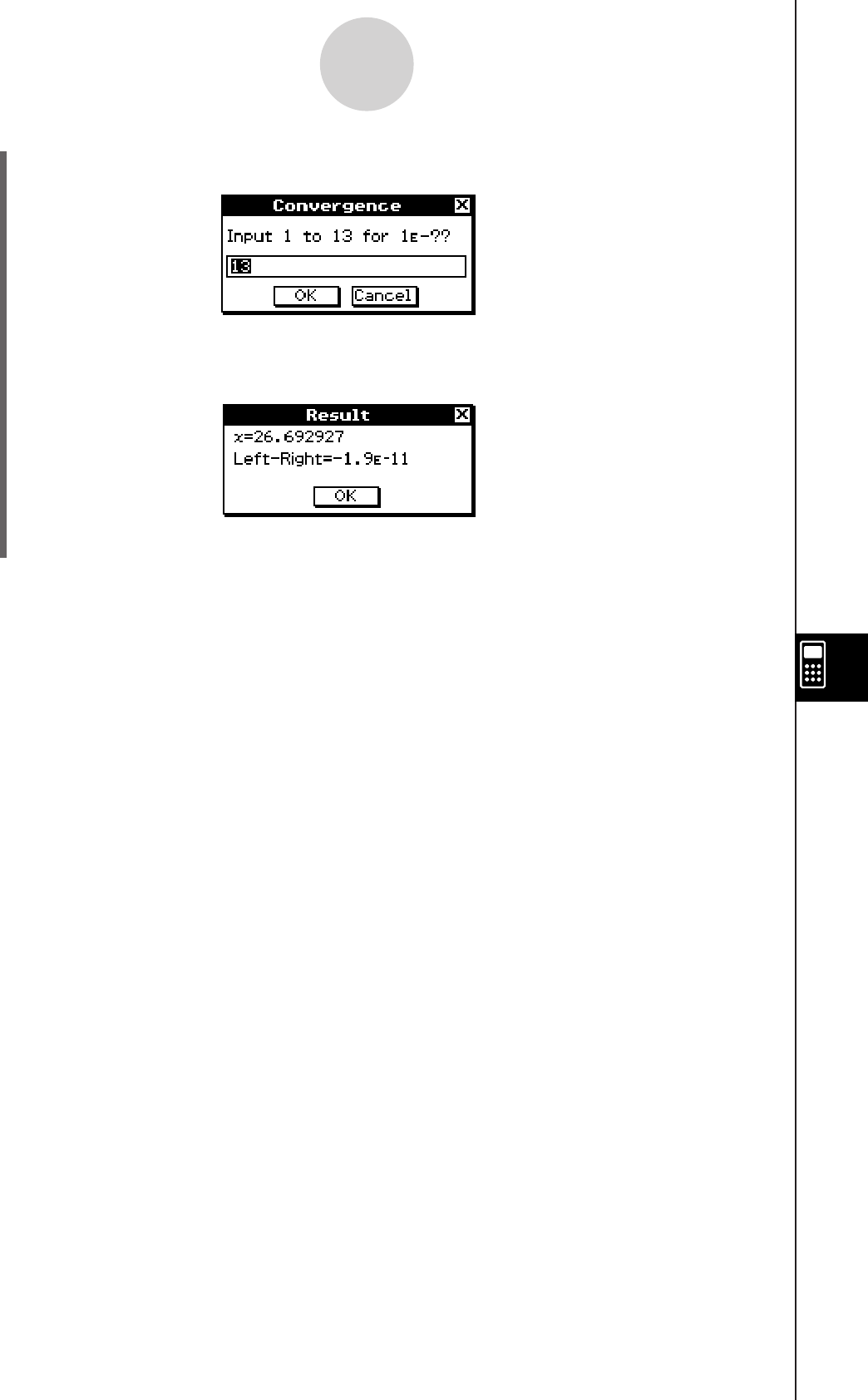
20060301

9-2-3

Using Numeric Solver

(6) Tap

a then [Convergence].

(7) Enter 10 and then tap [OK].

(8) Tap 1, or tap [Solve] and then [Execute] on the Numeric Solver menu.

• The software is now able to converge to a solution.

20060301

Using the eActivity

Application

An eActivity is both a documentation tool, and a student

notebook. As a documentation tool, a teacher can create

electronic examples and practice problems with accompanying

text, mathematical expressions, 2D and 3D graphs, geometric

drawings, and tables. eActivities provide the student the means

to explore problems, document their learning and problem solving

by entering notes, and share their learning by saving their work

to a file.

10-1 eActivity Application Overview

10-2 Creating an eActivity

10-3 Inserting Data into an eActivity

10-4 Working with eActivity Files

10-5 Transferring eActivity Files

Chapter

eActivity Data Download Center

A variety of eActivity files are available for download at the CASIO Website.

Visit the URL below for more information.

http://edu.casio.com/products/classpad/

• After you download an eActivity file, you will need to transfer it from your

computer to your ClassPad. See the instructions provided at the CASIO

Website for more information.

20110901

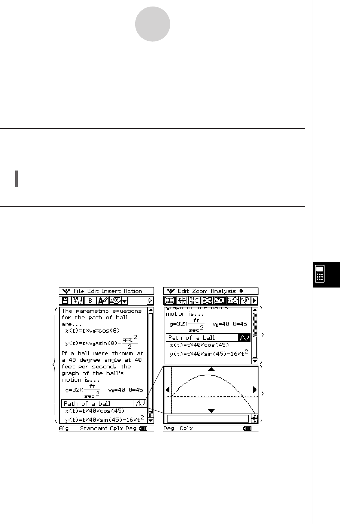
20060301

10-1-1

eActivity Application Overview

10-1 eActivity Application Overview

The eActivity application lets you input and edit text, mathematical expressions, and

ClassPad application data, and save your input in a file called an “eActivity”. The techniques

you will use are similar to those of a standard word processor, and they are easy to get used

to.

Starting Up the eActivity Application

Use the following procedure to start up the eActivity application.

u ClassPad Operation

On the application menu, tap A.

This starts the eActivity application and displays the eActivity window.

eActivity Application Window

The eActivity application can be used to create a file called an “eActivity”. A basic eActivity

can contain text along with application data, which is embedded as a row or a strip. A row

can be a “Text Row”, a “Calculation Row”, or a “Geometry Link”. A strip can be an “application

data strip” (Main, Geometry, Graph & Table, Conics, Sequence, and so on).

Creating an eActivity is as simple as typing in text and adding application data using the

toolbar.

eActivity

window

Graph strip

Expand button

Expanded

graph

window

Example eActivity Windows

eActivity

window

20060301

eActivity Application Menus and Buttons

This section explains the operations you can perform using the menus and toolbar buttons of

the eActivity application.

• For information about the O menu, see “Using the O Menu” on page 1-5-4.

k File Menu

10-1-2

eActivity Application Overview

k Edit Menu

New

Open

Save

Select this File

menu item:

To do this:

Start a new eActivity

Open an existing eActivity

Save the current eActivity to a file

Reload

Load the original file again

Undo/Redo

Cut

Copy

Paste the current clipboard contents onto the screen Paste

Select all rows and strips on the display Select All

Delete Line

Clear variables that contain numbers, lists and matrices Clear All Variables

Clear the eActivity window Clear All

Select this Edit

menu item:

To do this:

Undo the last operation or redo an operation that was just undone

Cut the currently selected string and place it onto the clipboard

Copy the currently selected string and place it onto the clipboard

Delete the contents of the line where the cursor is located

20060301

k Insert Menu

k Action Menu

10-1-3

eActivity Application Overview

Calculation Row

—

(

Text Row

Geometry Link

Insert an application data strip

Strip - Main

Strip - Geometry

Strip - Graph

Strip - Graph Editor

Strip - 3D Graph

Strip - 3D Graph Editor

Strip - Conics Graph

Strip - Conics Editor

Strip - Stat Graph

Strip - Stat Editor

OStrip - DiffEqGraph

AStrip - DiffEqGraph Editor

IStrip - Financial

rStrip - Picture

PStrip - Probability

Strip - NumSolve

Strip - Sequence Editor

Strip - Notes

Strip - Spreadsheet

Strip - Verify

Or select this

Insert menu item:

To do this:

Insert a calculation row

Insert a text row

Insert a Geometry-linked data row

—Add Strip Help

Add help text to the currently selected strip

Tap this

button

Tap [Action].

Do this: To do this:

Insert a command (page 2-8-1)

20060301

10-1-4

eActivity Application Overview

eActivity Application Status Bar

The information that appears in the eActivity application status bar is same as the Main

application status bar information. See “Using Main Application Modes” on page 2-1-4.

eActivity Key Operations

In the eActivity application, the cursor key, K key, and E key operate differently than

they do in other modes.

Cursor Key

• The cursor key moves the cursor around the eActivity window.

• Though you can always move the cursor up and down, you may not always be able to

move it left and right. The left and right cursor key operations move the cursor left and right

in the current row, but for the most part they cannot be used to move the cursor between

rows of different types.

• Up and down cursor operations move the cursor between rows, regardless of type.

K Key

• Pressing the K key deletes the character to the left of the current cursor position.

E Key

• Pressing the E key while the cursor is in a text row inserts a carriage return and adds a

new line.

• Pressing the E key while the cursor is in a calculation row re-calculates the expression of

the current calculation row as well as all of the calculation rows below the current row.

• Pressing the E key while the cursor is in a Geometry Link row re-calculates the data in

the link and updates the corresponding graph in the Geometry window.

k Other Buttons

The operations described below are available from the toolbar only.

There are no corresponding menu commands for these buttons.

{

Converts a text row to a calculation row

Converts a calculation row to a text row

Recalculate the equation just for the current line where the cursor is

currently located

Tap this button:To do this:

Open the Files dialog box (page 10-2-2)

Toggles a calculation result between standard (fractional result) and

decimal (approximate result)

Bold the text that is currently selected

20110401

10-1-5

eActivity Application Overview

Tip

When the shift operation is assigned to the ClassPad z key, you can select a range of characters

with the left and right cursor keys. Simply press the ClassPad z key and then press e or d.

Each press of the cursor key will select (highlight) the next character in the applicable direction.

Example: If the cursor is currently located between the “c” and “1” in “abc123”, press z and then

e e e will select 123.

For information about assigning key operations to the ClassPad’s hard keys, see page 16-11-1.

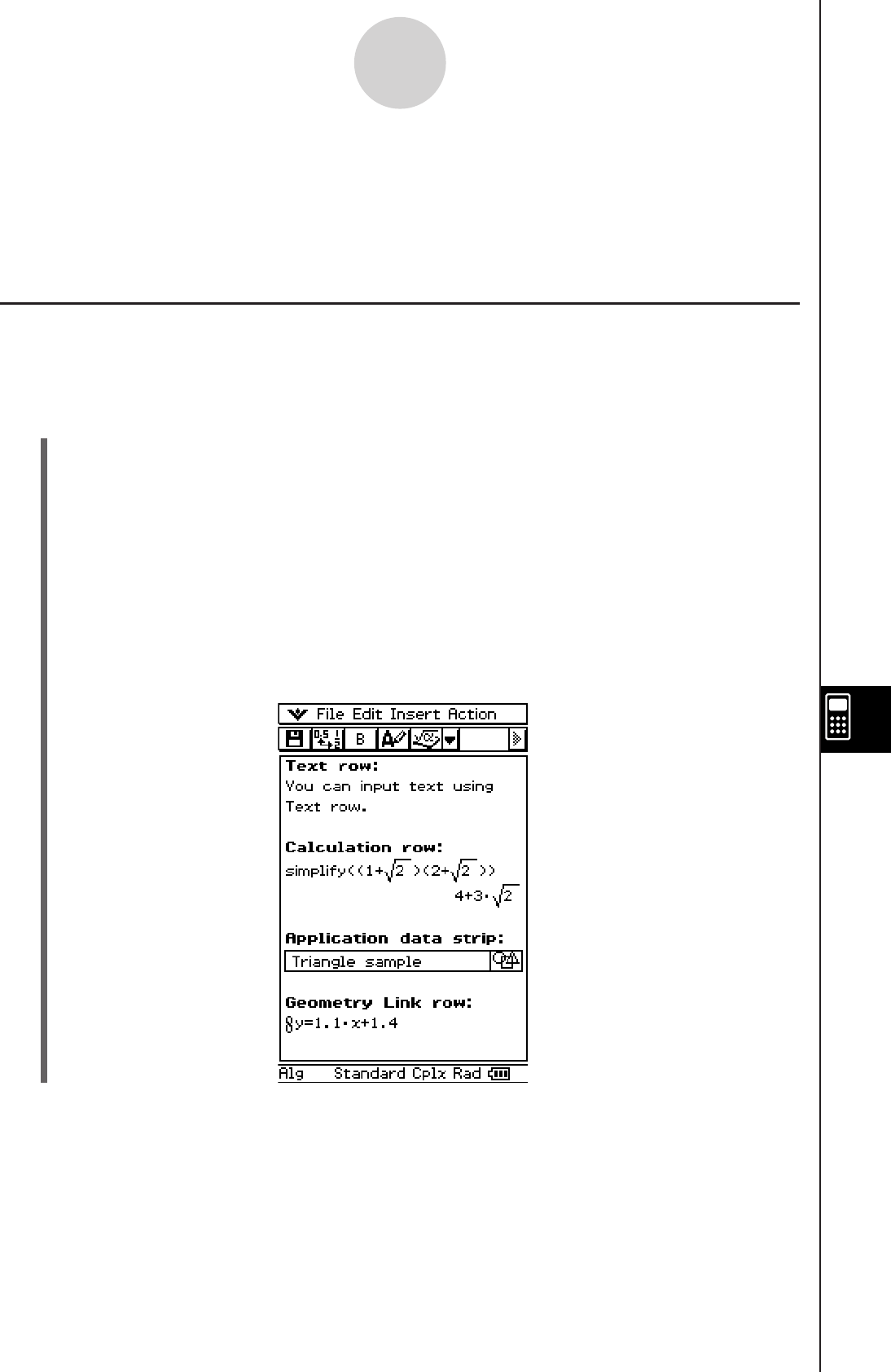
20060301

10-2 Creating an eActivity

This provides a general overview of eActivity operations, from starting up the eActivity

application to saving an eActivity file. It also presents precautions you need to keep in mind

when managing eActivity files.

Basic Steps for Creating an eActivity

The following are the basic steps you need to perform when creating an eActivity. Detailed

information about each step is provided in the other sections of this chapter.

u ClassPad Operation

(1) Tap

m to display the application menu, and then tap A to start the eActivity

application.

• This displays the eActivity window as it appeared the last time it was used.

• If you are already in the eActivity application and there is data on the display, tap [File]

and then [New]. Note that [New] clears data from the display without saving it.

(2) On the eActivity window, insert the text, expressions, application data, and other data

you want to include in the eActivity.

• There are four types of data you can insert into an eActivity: text rows, calculation

rows, Geometry Link rows, and application data strips. For details about inserting

each type of data, see “10-3 Inserting Data into an eActivity”.

10-2-1

Creating an eActivity

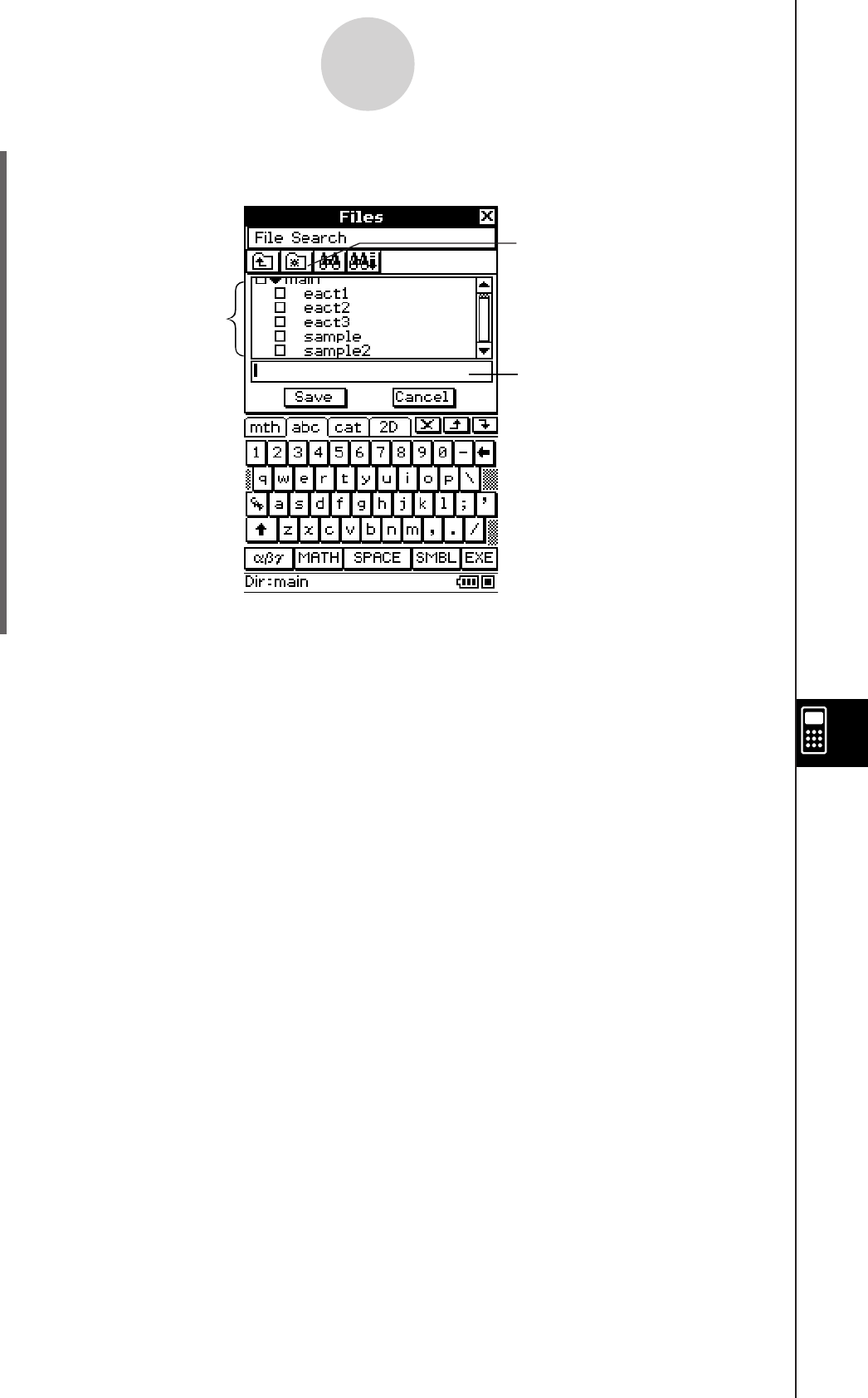
20090601

(3) After the eActivity is the way you want, tap [File] and then [Save].

• This displays the Files dialog box.

This is a list of folders

and files. Select the

name of the folder

where you want to

save the eActivity file

by tapping it.

Tap here to create a

new folder.

Enter up to 20 characters for

the eActivity file name.

10-2-2

Creating an eActivity

(4) After selecting a folder and entering a file name, tap [Save] to save the eActivity.

Warning!

• If you do not save the eActivity you are creating before tapping m on the icon panel to

display the application menu or before tapping M to display the Main application, the

unsaved eActivity data may be deleted.

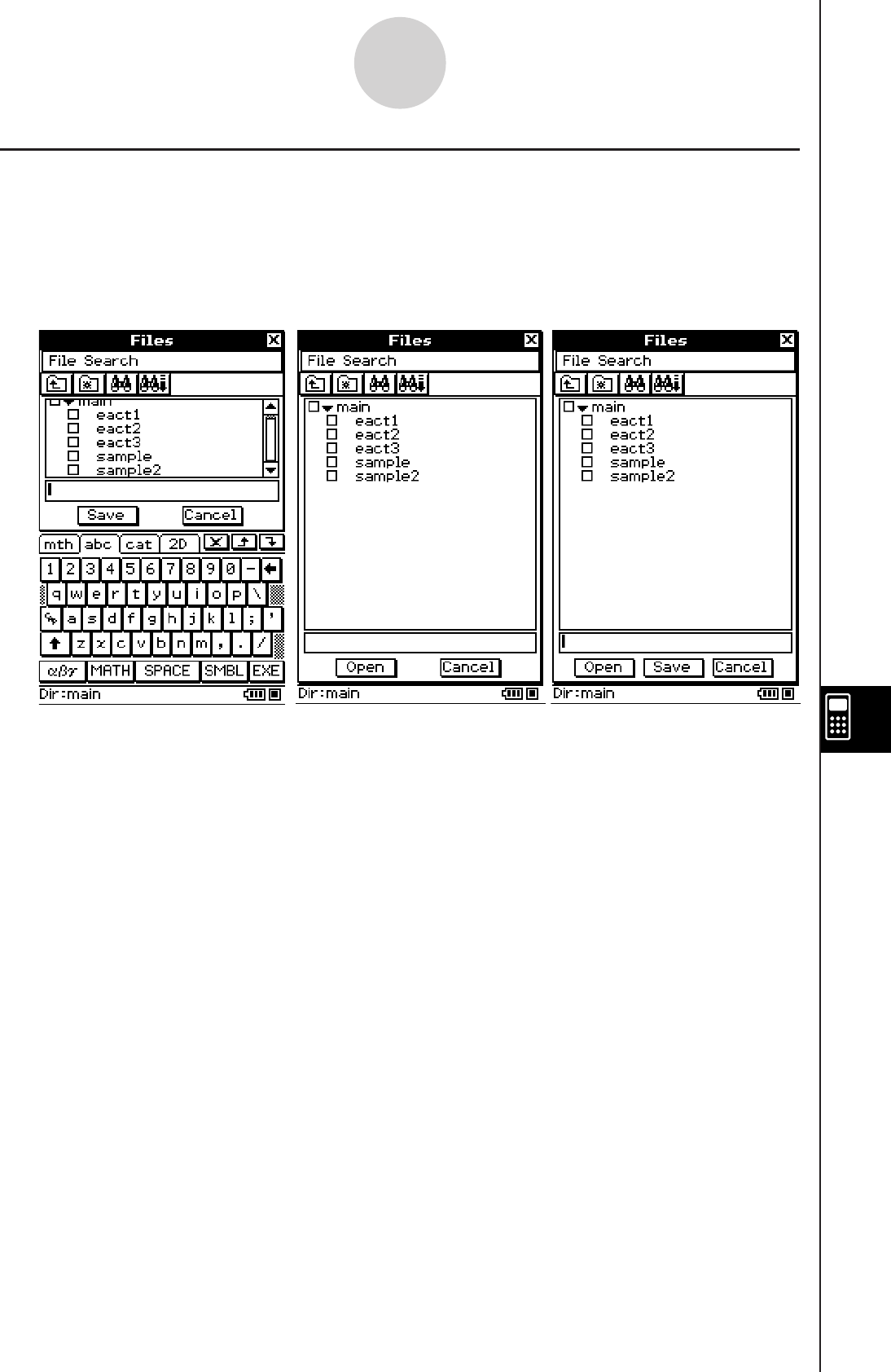
20111001

Managing eActivity Files

This section covers file management operations like save, open, delete, rename, move, etc.

Performing one of these operations displays a Files dialog box like the ones shown below.

The buttons that appear in the dialog box depend on the operation you performed to display

the Files dialog box.

10-2-3

Creating an eActivity

The operations you can perform on the Files dialog box are identical to those of the

Geometry application Files dialog box, except that eActivity file names can contain up to 20

characters (bytes). For details, see “8-7 Managing Geometry Application Files”.

Important!

• eActivity files are stored in a memory area that is separate from that used for storing other

types of data (variable data, Geometry data, Presentation data, etc.) Because of this,

you cannot access eActivity files data using the Variable Manager. You have to use the

eActivity application to perform eActivity file management operations.

• ClassPad Manager has a function for locking and unlocking eActivity files. If you transfer

a locked file from ClassPad Manager to your ClassPad, you will be able to open the file on

your ClassPad but you will not be able to overwrite it with an edited version. To save edits

to a locked file, save the file under a different name.

(Includes [Save] button.)

Tap [File] and then [Save].

(Includes [Open] button.)

Tap [File] and then [Open].

(Includes [Save] and [Open]

buttons.)

Tap {.

GY437Soft_E_10-2-3.pdf 1 11.10.7 2:33:22 PM

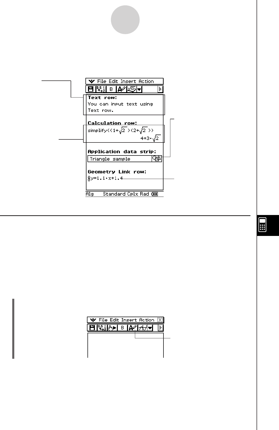
20060301

10-3 Inserting Data into an eActivity

The following describes the four types of data you can insert into an eActivity.

10-3-1

Inserting Data into an eActivity

Inserting a Text Row

Text rows make it possible to display and edit text directly in the eActivity window. Text rows

can contain multiple lines, as well as mathematical expressions. A mathematical expression

contained in a text row is not evaluated. Pressing E, while in the Text Input mode, will

advance you to the next line without displaying results.

Tip

• You can also use the ) soft keyboard to input mathematical expressions into a text row.

u To select the input mode

(1) On the eActivity window toolbar, tap the fifth button from the left (u / <) to toggle the

input mode between Text Input and Calculation Input.

Geometry Link Row

Use this row to insert data

that is linked with a Geometry

window figure.

Application data strip

The application data strip lets

you display a window from a

ClassPad application (Main,

Graph & Table, Geometry, etc.)

and use the window to create

data, which is inserted into the

eActivity.

u button indicates the Text Input

mode is selected.

Text Row

A text row can be

used to insert text data

and mathematical

expression text in

natural format. You

can also bold the text

in a text row.

Calculation Row

Use the calculation row to

insert any of the calculation

operations that are available

in the Main application.

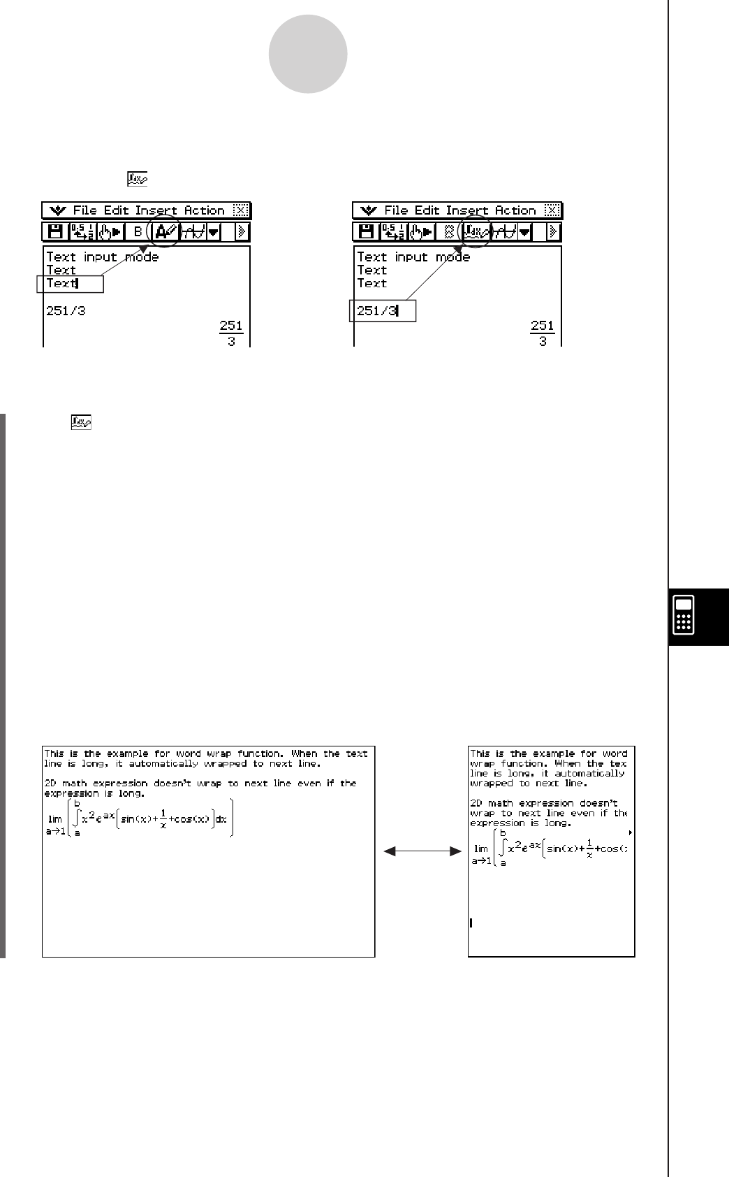
20060301

Tip

• The toolbar button for switching between input modes appears as u while the cursor is located

in a text row, and while the cursor is located in a calculation row.

10-3-2

Inserting Data into an eActivity

u To insert a Text Row

(1) Tap to change a row to the Text Input mode.

• If the cursor is located in a line that already contains input data, place the cursor at

the end of the line, tap [Insert] and then [Text Row]. This inserts a text row on the next

line.

(2) Use the soft keyboard or keypad keys to input the text you want.

• You can use the alphabet (abc) keyboard to input alphabetic characters.

• Use the other keyboards to input mathematical expressions, commands, etc. Note

that any mathematical expressions or commands you input into a text row are treated

as text. They are not executed.

• When the text that is input into a text row is too long to fit within the width of the

screen, it will wrap automatically to the next line. However, if you are using the 2D

soft keyboard to input an expression into a text row using natural display, your input

will not wrap to the next line if it does not fit. Instead, the expression will run off the

side of the display. Arrows (

]

) will appear on the display to indicate when there is

something running off the left or right side of the display.

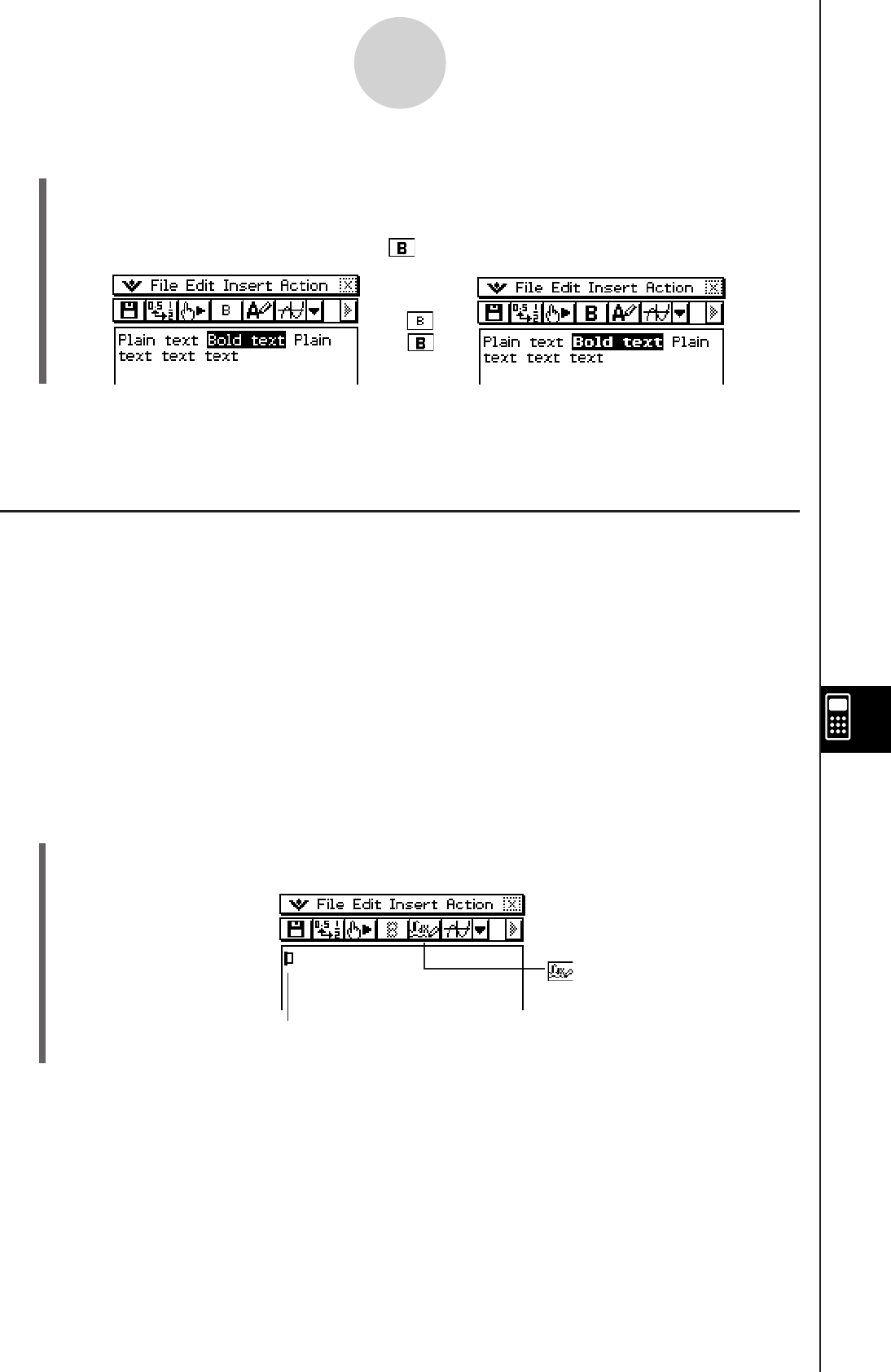
20060301

10-3-3

Inserting Data into an eActivity

Important!

• You cannot bold numeric expressions of a natural display expression that you input with the

2D soft keyboard.

Inserting a Calculation Row

Calculation rows let you perform calculations in an eActivity. When you input a mathematical

expression, the output expression (result) appears, right justified, in the next line. An eActivity

that contains only calculation rows looks very much like the Main application window. Note

that you can edit the input expression, but not the output expression (result). You can also

copy, paste, drag and drop input and output expressions. Both the input and output rows

scroll independently in a horizontal direction.

Tip

• If the input expression of a calculation row is not a valid expression, the row will contain only the

input expression, without an output expression.

u To select the input mode

(1) On the eActivity window toolbar, tap the fifth button from the left (u / <) to toggle the

input mode between Text Input and Calculation Input.

button indicates the Calculation

Input mode is selected.

This mark is displayed at the head of the line

while the Calculation Input mode is selected.

←

u To bold text

(1) Drag the stylus across the range of text you want to bold so it is selected (highlighted).

(2) Tap

(3) To unbold text, select it and then tap again.

→

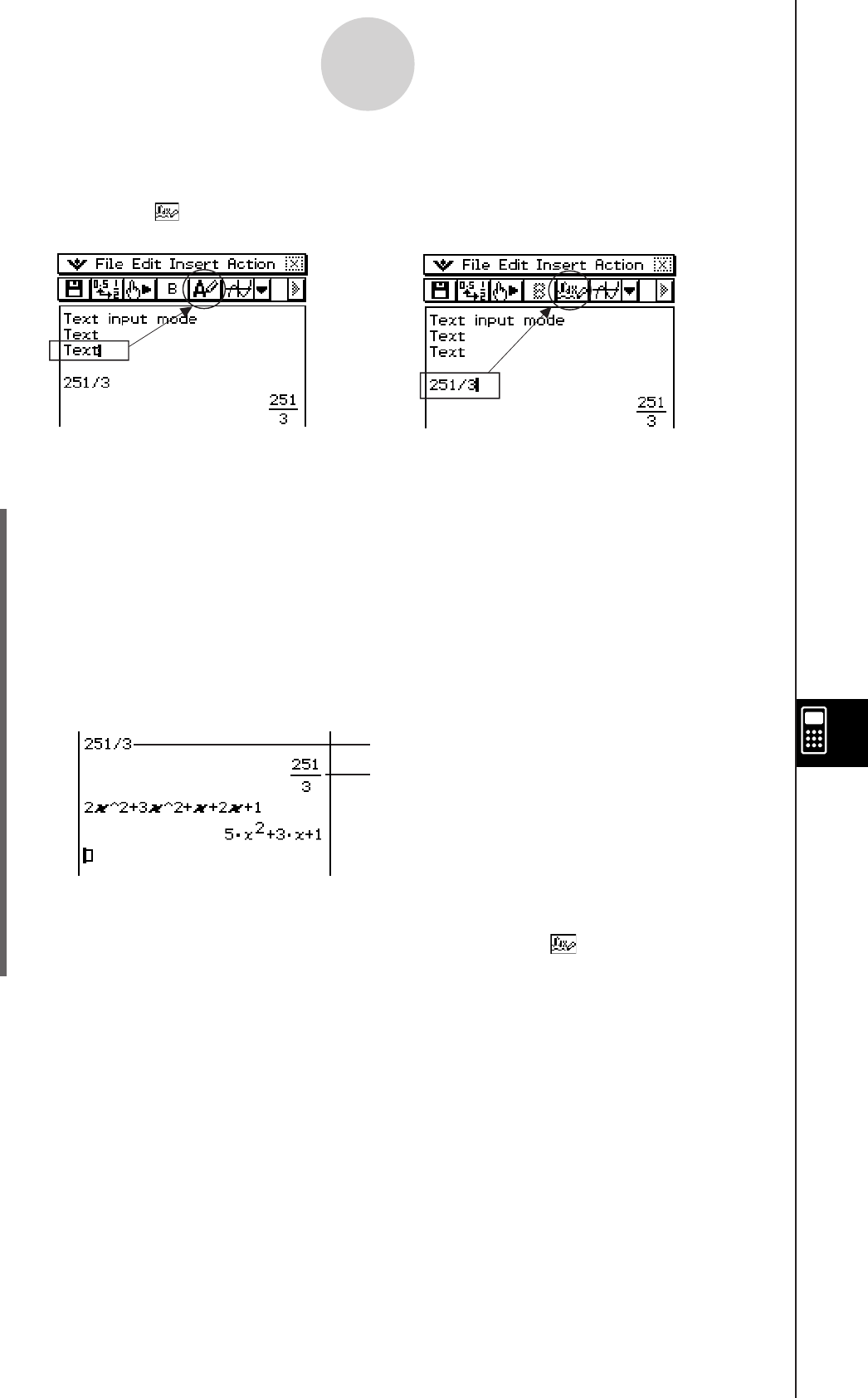
20060301

Tip

• The toolbar button for switching between input modes appears as u while the cursor is located

in a text row, and while the cursor is located in a calculation row.

Line 1: Expression you input

Line 2: Result

u To insert a Calculation Row

(1) Tap

u to change a row from the Text Input mode to the Calculation Input mode.

• If the cursor is located in a line that already contains input data, place the cursor at

the end of the line, tap [Insert] and then [Calculation Row]. This inserts a calculation

row on the next line.

(2) Use the soft keyboard or keypad keys to input the mathematical expression you want.

• Mathematical expression input techniques are identical to those in the Main

application. See Chapter 2 for more information.

(3) Press

E after inputting an expression to display its result.

• If you want to input an expression without displaying its result, do not press E.

Instead, tap [Insert] and then [Text Row] to input a text row. Or you could change the

current row from a calculation row to a text row by tapping while the cursor is in

the row.

Important!

• If you edit the expression in an existing calculation row and then press E, all of the

expressions following the line you edited are re-calculated and their results are refreshed.

Even mathematical expressions you originally input into the eActivity without calculating

their results are calculated, and their results appear.

10-3-4

Inserting Data into an eActivity

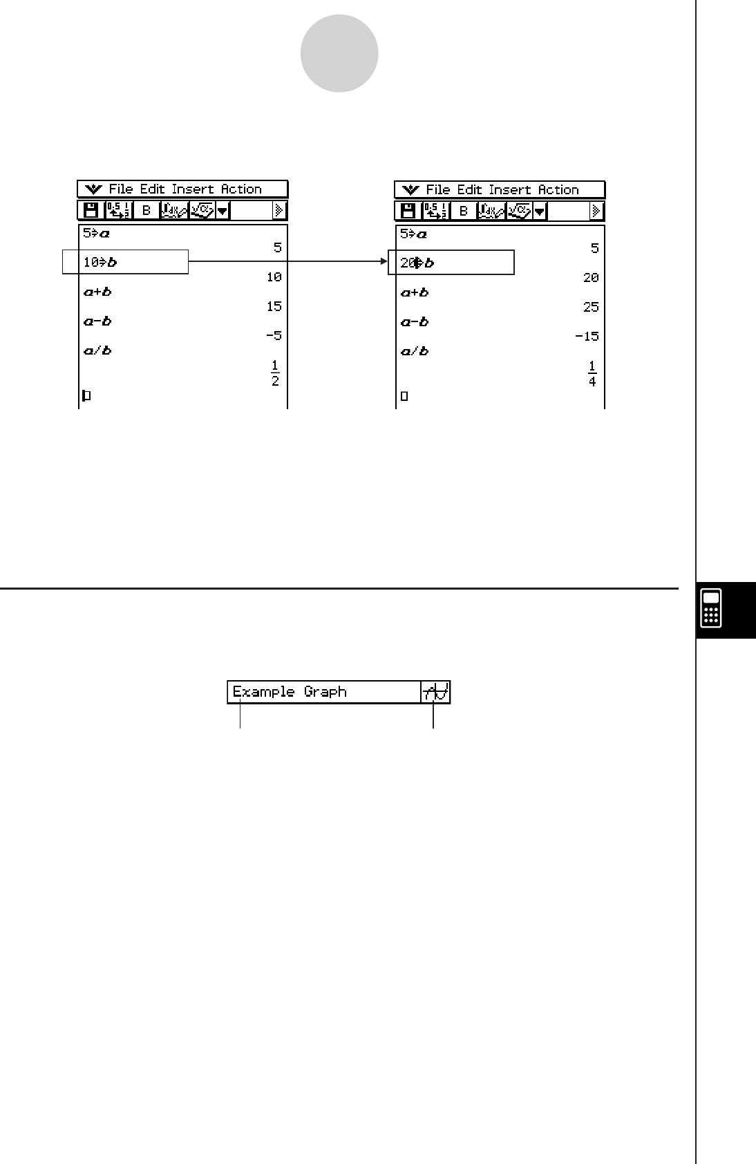
20060301

10-3-5

Inserting Data into an eActivity

Changing “10 S b” to “20 S b” in the example below and pressing E causes all of the

expressions under “20 S b” to be re-calculated.

• Tap to the right of “10”.

• Press K twice, and then

input “20”.

• Press E.

u To run a program in the eActivity application

You can use an eActivity application calculation row to specify a program name, and execute

the program. For more information, see “2-13 Running a Program in the Main Application.”

Inserting an Application Data Strip

An application data strip can be used to embed data from other ClassPad applications into

an eActivity. An application data strip contains the elements shown below.

Expand button

Tap here to display the application

data in the lower window.

Title

You can enter a title,

if you want.

20060301

10-3-6

Inserting Data into an eActivity

k Inserting an Application Data Strip into an eActivity

Tap the [Insert] menu or the right most toolbar down arrow button, and then select the

command or button that corresponds to the type of application data you want to insert.

Select this

[Insert] menu

item:

To insert this type of application data:

Strip - GraphGraph & Table application Graph window data

Strip - Graph EditorGraph & Table application Graph Editor window data

Strip - 3D Graph3D Graph application 3D Graph window data

Strip - 3D Graph Editor3D Graph application 3D Graph Editor window data

Strip - Conics GraphConics application Conics Graph window data

Strip - Conics EditorConics application Conics Editor window data

Strip - GeometryGeometry application Geometry window data

Strip - SpreadsheetSpreadsheet window data

Strip - Stat GraphStatistics application Statistical Graph window data

Strip - Stat EditorStatistics application Stat Editor window data

(

Strip - DiffEqGraph

Differential Equation application Differential Equation

Graph window data

Strip - DiffEqGraph Editor

Differential Equation application Differential Equation

Graph Editor window data

Strip - FinancialFinancial application window data

Strip - ProbabilityProbability window*1 data

Strip - NumSolveNumSolve application Numeric Solver window data

Strip - Sequence EditorSequence application Sequence Editor window data

Strip - PicturePicture Viewer window*2

Strip - NotesNotes window*2

Strip - MainMain application work area window data

Strip - VerifyVerify window*1 data

Or tap

this

button:

*1 The Probability window and Verify window can be used with the eActivity application

and Main application. For more information see “2-11 Using Verify” and “2-12 Using

Probability”.

*2 The Picture Viewer window and Notes window can be used with the eActivity application

only.

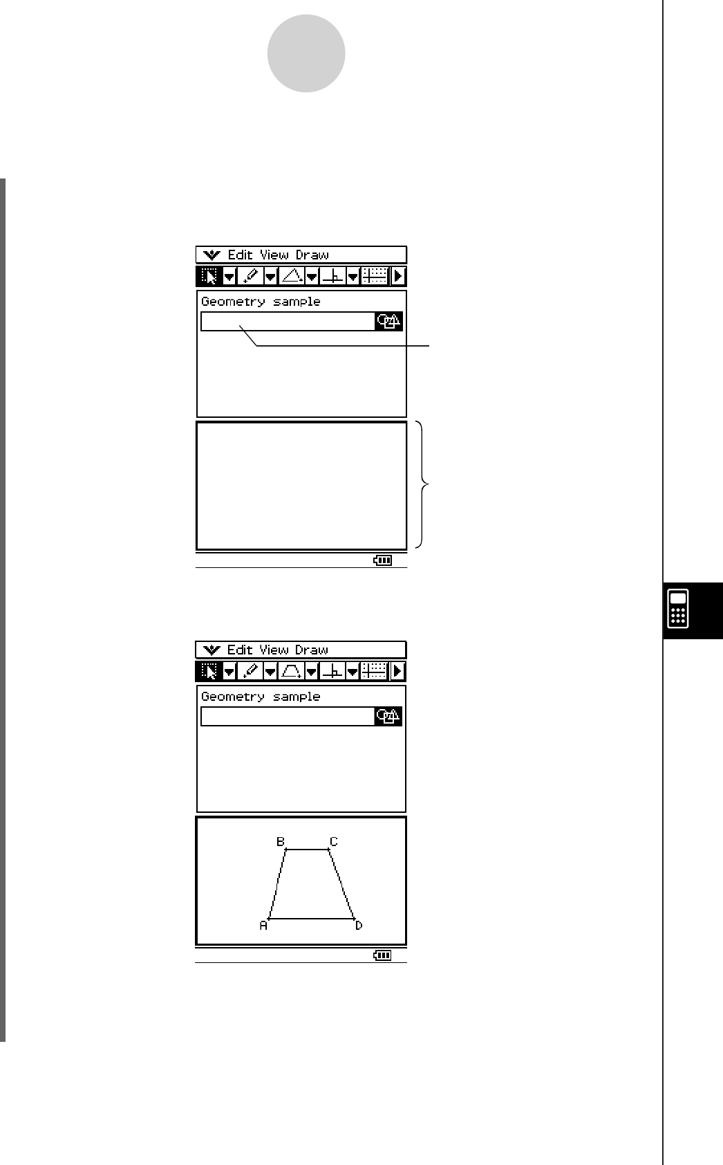
20060301

Example 1: To insert a Geometry data strip

u ClassPad Operation

(1) From the eActivity menu, tap [Insert], [Strip], and then [Geometry].

• This inserts a Geometry data strip, and displays the Geometry window in the lower

half of the screen.

10-3-7

Inserting Data into an eActivity

(2) On the Geometry window, draw the figure you want.

• For details about Geometry window operations, see Chapter 8.

Geometry data strip

Geometry window

(3) After you finish performing the operation you want on the Geometry window, tap S,

or tap O and then [Close] to close the Geometry window and return to the eActivity

window.

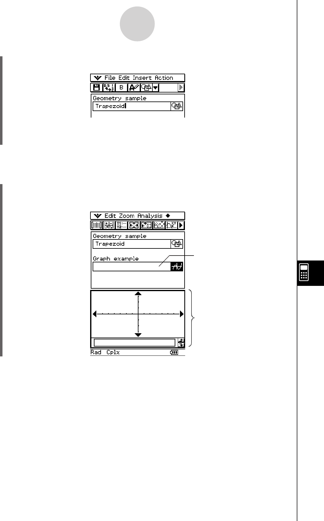
20060301

(4) Tap the title box of the Geometry data strip and enter the title you want.

10-3-8

Inserting Data into an eActivity

• If you want to input more data into the eActivity, tap the next line or use the [Insert]

menu to select the type of strip you want to insert next.

Example 2: To insert a Graph data strip

u ClassPad Operation

(1) On the eActivity window, tap [Insert], [Strip], and then [Graph].

• This inserts a Graph data strip, and displays the Graph window in the lower half of the

screen.

Graph data strip

Graph window

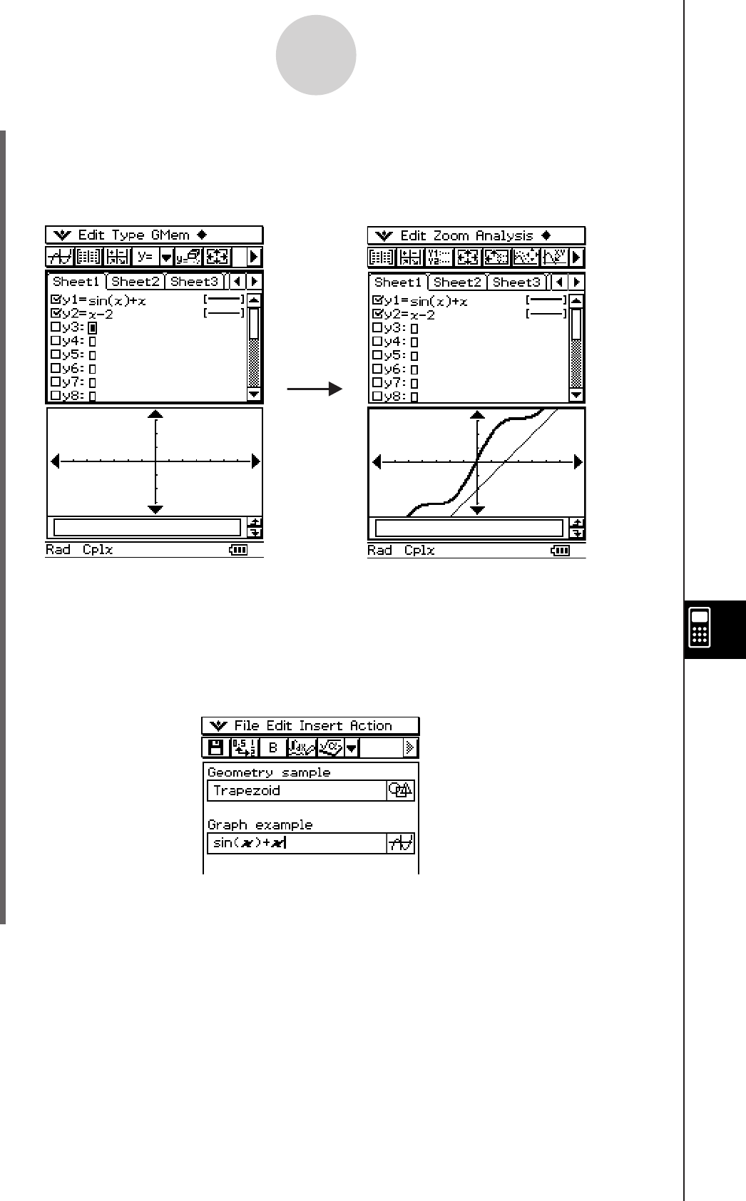
20060301

(3) After you finish performing the operation you want on the Graph window, tap S, or tap

O and then [Close] to close the Graph window. You will also need to tap the Graph

Editor window, and then select O then [Close] to return to the eActivity window.

(4) Tap the title box of the Graph data strip and enter the title you want.

10-3-9

Inserting Data into an eActivity

Display the Graph Editor window

and input the function.

Graph the function.

• If you want to input more data into the eActivity, tap the next line or use the [Insert]

menu to select the type of row or strip you want to insert next.

(2) On the Graph window, draw the graph you want.

• Tap the ! button to display the Graph & Table application’s Graph Editor window,

enter a function to graph, and then graph the function. For details about inputting

functions on the Graph Editor window and graphing functions, see Chapter 3.

Tap $.

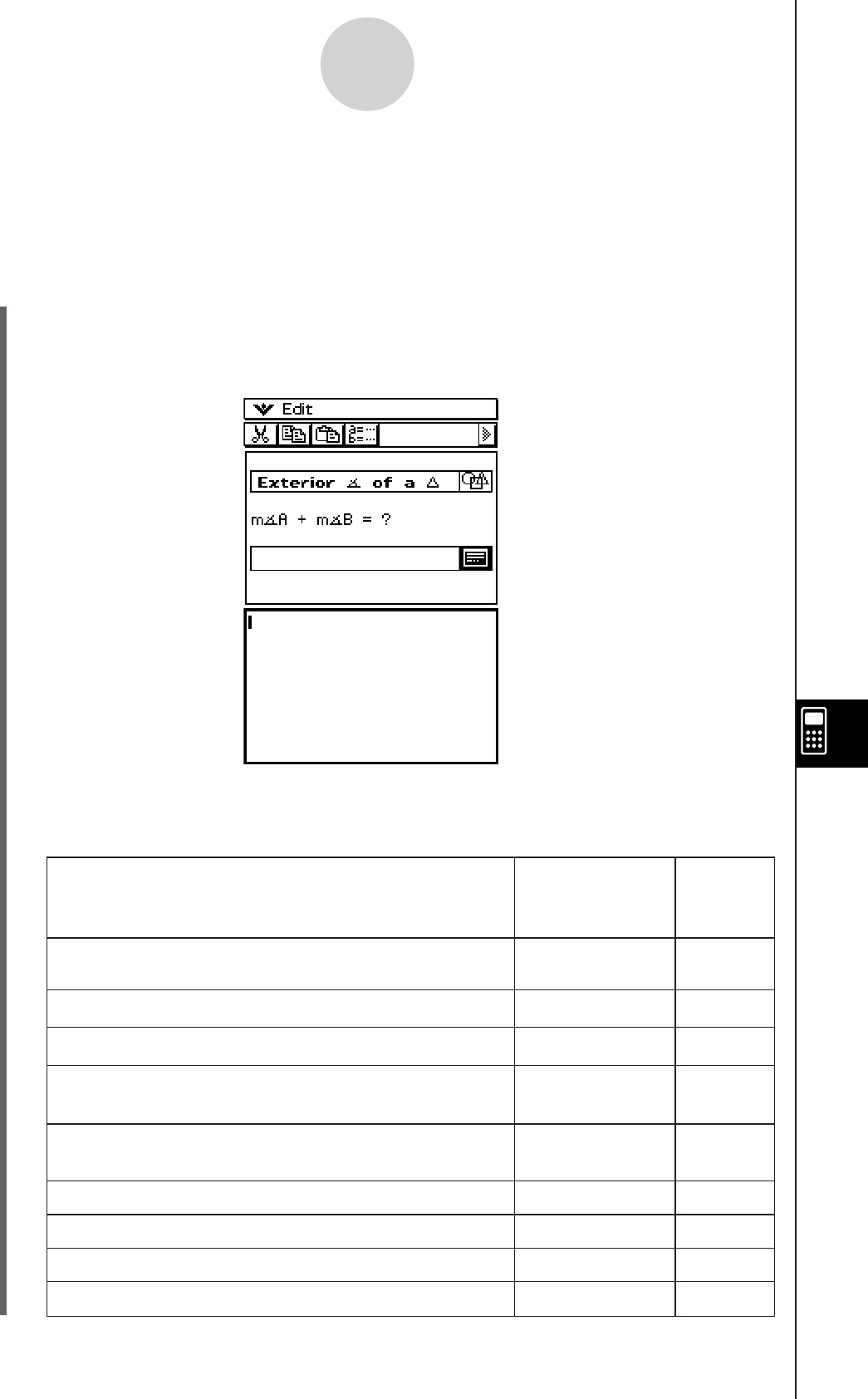
20060301

Example 3: To use Notes in an eActivity

Notes is a simple text editing tool for taking notes or including in-depth explanations within

an eActivity. You can use Notes to store information for later use, or as a place to jot down

ideas.

u ClassPad Operation

(1) On the eActivity window, tap [Insert], [Strip], and then [Notes].

• This inserts a Notes strip and displays the Notes window in the lower half of the

screen.

10-3-10

Inserting Data into an eActivity

(2) Enter text you want in the Notes window.

• You can use the Edit menu and toolbar to perform following operations while the

Notes window is on the display.

Undo/Redo —

Select this Edit

menu item:

To do this:

Undo the last operation or redo an operation that was

just undone

Cut r

Cut the currently selected string and place it onto the

clipboard

Copy t

Copy the currently selected string and place it onto

the clipboard

Paste y

Paste the current clipboard contents onto the screen

Bold a range of selected text

Select All —

Select all text on the Notes window

Clear All —

Clear all text from the Notes window

—

Unbold a range of selected text —

Display the Variable Manager (page 1-8-1)

Or tap

this

button:

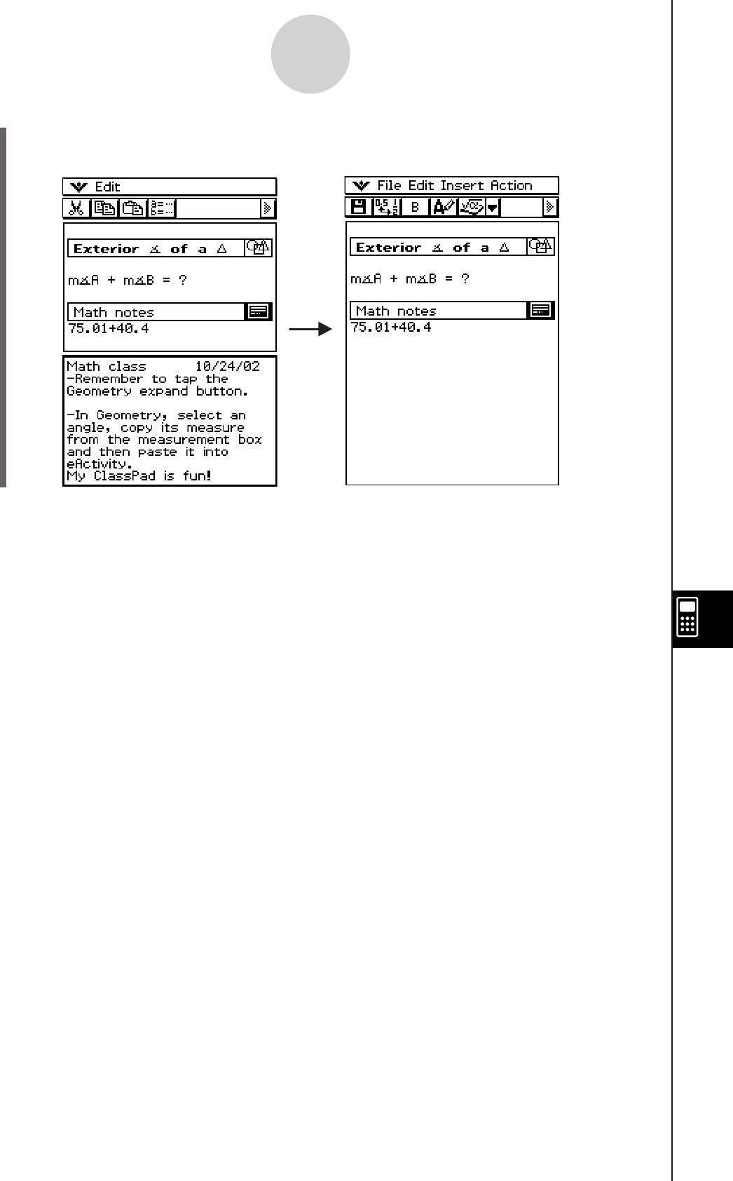
20060301

10-3-11

Inserting Data into an eActivity

Tip

• You can use the Notes window to enter notes, homework assignments, in-depth details, etc.

• All information you enter is treated as text.

• When inputting text into a Notes window, the cursor will jump down to the beginning of the next

line when the right edge of the current line is reached.

• The Notes application is available only in eActivity.

(3) After you finish entering text, you can close the Notes window by tapping S, or tapping

O and then [Close].

Example 4: To use the Picture Viewer with eActivity

You can use Picture to display a bitmap image (PICT data type) in an eActivity. You can also

save displayed images with a different name.

Tip

• For details about data whose data type is PICT, see “Variable Data Types” on page 1-7-3.

20070301

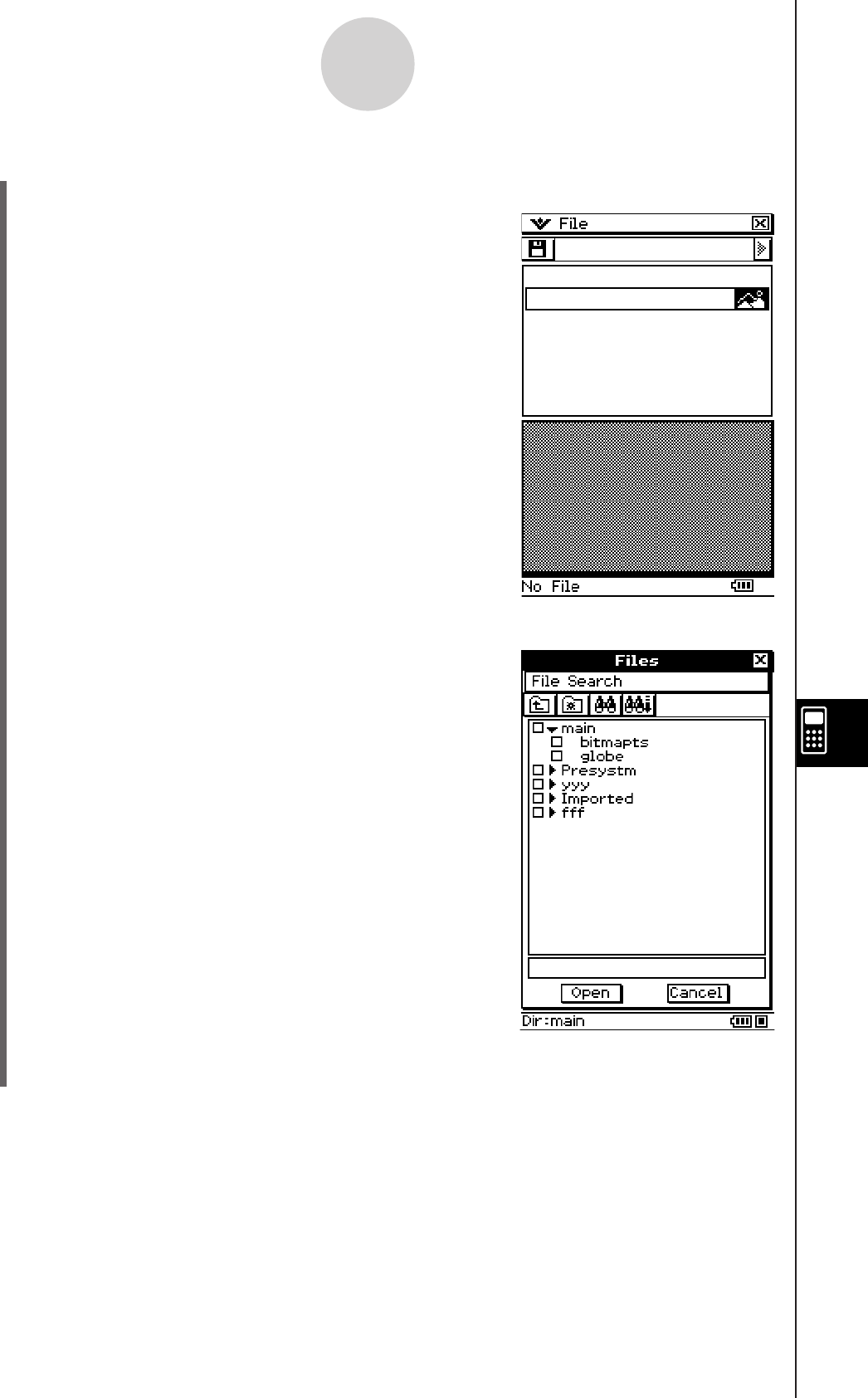
20060301

u ClassPad Operation

(1) On the eActivity window, tap [Insert], [Strip], and then [Picture].

• This will insert a Picture strip and display the Picture

window in the lower half of the display.

(2) Tap [File] - [Open].

• This displays the Files dialog box. The Files dialog

box displays only data whose data type is PICT.

(3) On the Picture window, tap the name of the PICT data you want to view.

10-3-12

Inserting Data into an eActivity

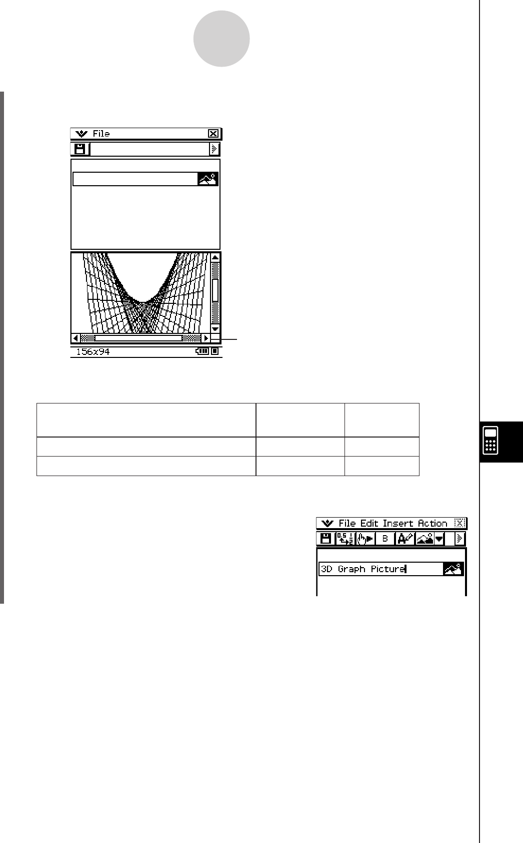
20060301

(4) Tap [Open].

• This will display the PICT data you selected in the Picture window.

• You can use the File menu and toolbar to perform following operations while the

Picture window is on the display.

To do this: Select this File

menu item:

Or tap this

button:

Open a bitmap (PICT data type) image Open –

Save an open bitmap image Save R

(5) After performing all the operations you want, tap the S button in upper right corner to

close the Picture window.

(6) Tap the title box of the Picture strip and enter the title

you want.

A scroll bar will appear along the bottom of the

window if the PICT data does not fit.

10-3-13

Inserting Data into an eActivity

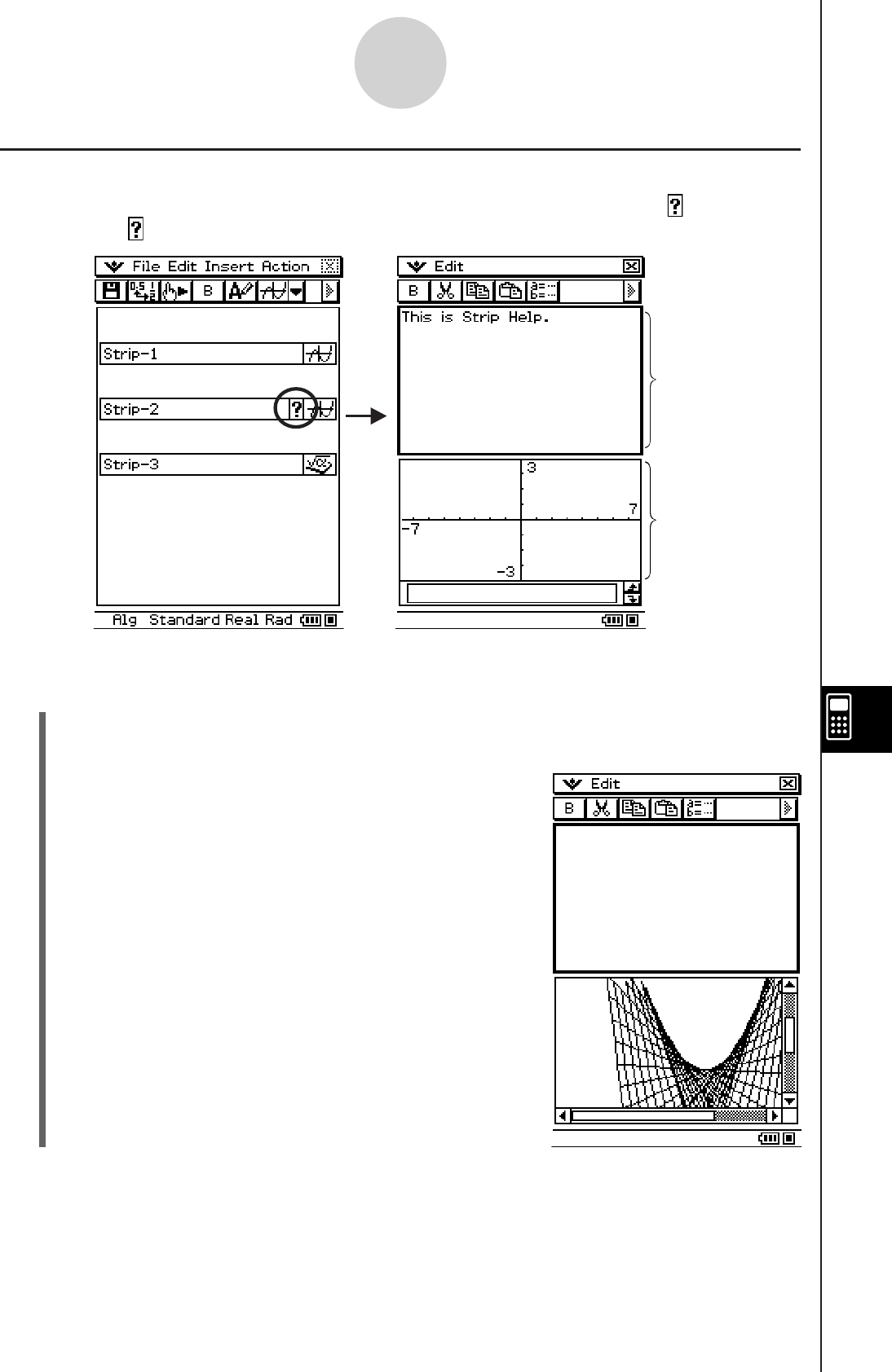
20060301

Strip Help Text

You can add help text to any strip. A strip that has help text is indicated by a button.

Tapping a button will display the help window along with the application window.

u To add help text to a strip

(1) Tap the title box of the strip to which you want to add help text.

(2) Tap [Insert] - [Add Strip Help].

• A help window appears in the upper half of the

display, while the application that was called from the

strip appears in the lower half of the display.

10-3-14

Inserting Data into an eActivity

Help window

Applicaiton window

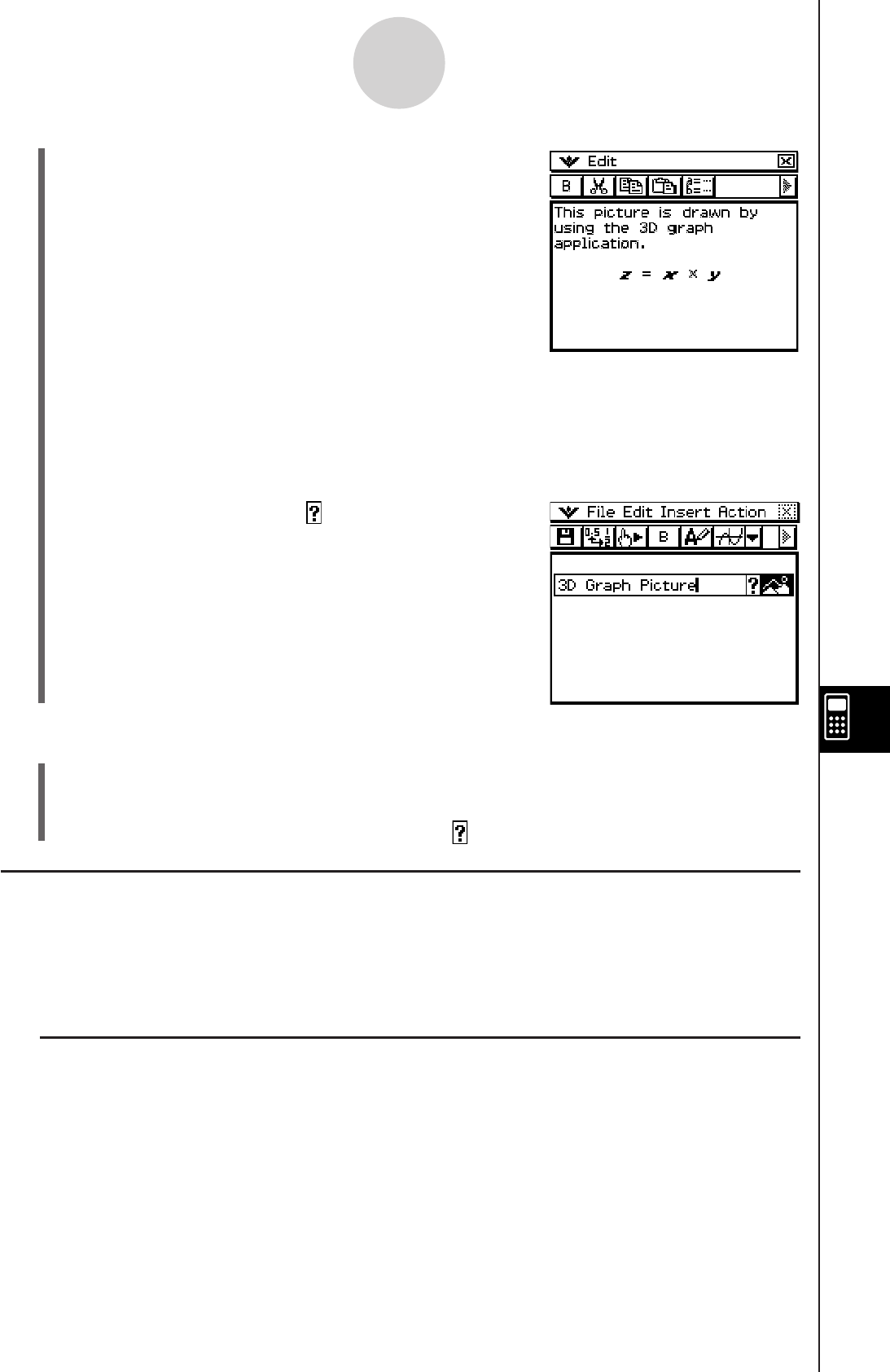
20060301

Moving Information Between eActivity and Applications

An eActivity is like an interactive notebook or textbook that allows you to explore the world of

mathematics right on the page. You can take almost any expression from an eActivity page

and send it to another application. You can also take information from an application and

insert it into an eActivity page.

k Cut, Copy, and Paste

You can cut, copy, or paste text or mathematical expressions between the eActivity and

any other application. You can also cut, copy, and paste text and mathematical expressions

inside an eActivity.

Depending on the application, you can cut or copy, and paste text and mathematical

expression data into an eActivity. For example, you can copy a line in the Geometry

measurement box and paste it into an eActivity as an expression.

(3) Input the help text into the help window.

• The operations you can perform while inputting help text are the same as those you

use for eActivity notes. For more information, see “Example 3: To use Notes in an

eActivity” on page 10-3-10.

(4) After inputting all the text you want, tap the S button in upper right corner to close the

help window.

• The strip will now have a button.

u To delete help text from a strip

(1) Tap the title box of the strip whose help text you want to delete.

(2) Tap [Insert] - [Remove Strip Help].

• This will delete the help text and cause the button to disappear.

10-3-15

Inserting Data into an eActivity

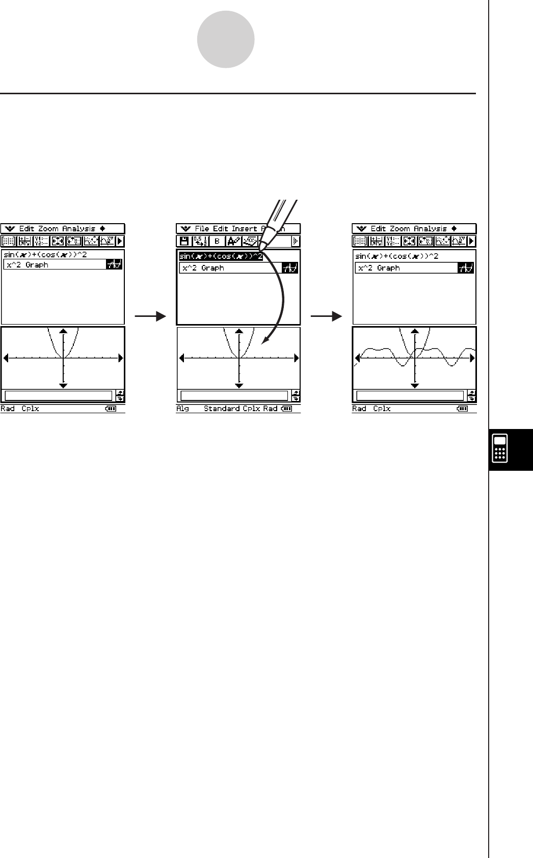
20060301

10-3-16

Inserting Data into an eActivity

k Drag and Drop

You can drag and drop text or mathematical expressions between eActivity and other

applications. You can also drag and drop within an eActivity. Depending on the application,

you can drag text and mathematical expressions from an eActivity to another application

window. For example, you can drag an equation from the eActivity directly onto a graph

window.

(1) Graph strip is

expanded in the lower

window.

(2) Expression is

selected in the

eActivity.

(3) Expression has

been dragged into

the graph window.

Tip

• For details about what you can drag and drop between the eActivity window and Geometry

window, see “8-6 Using the Geometry Application with Other Applications”.

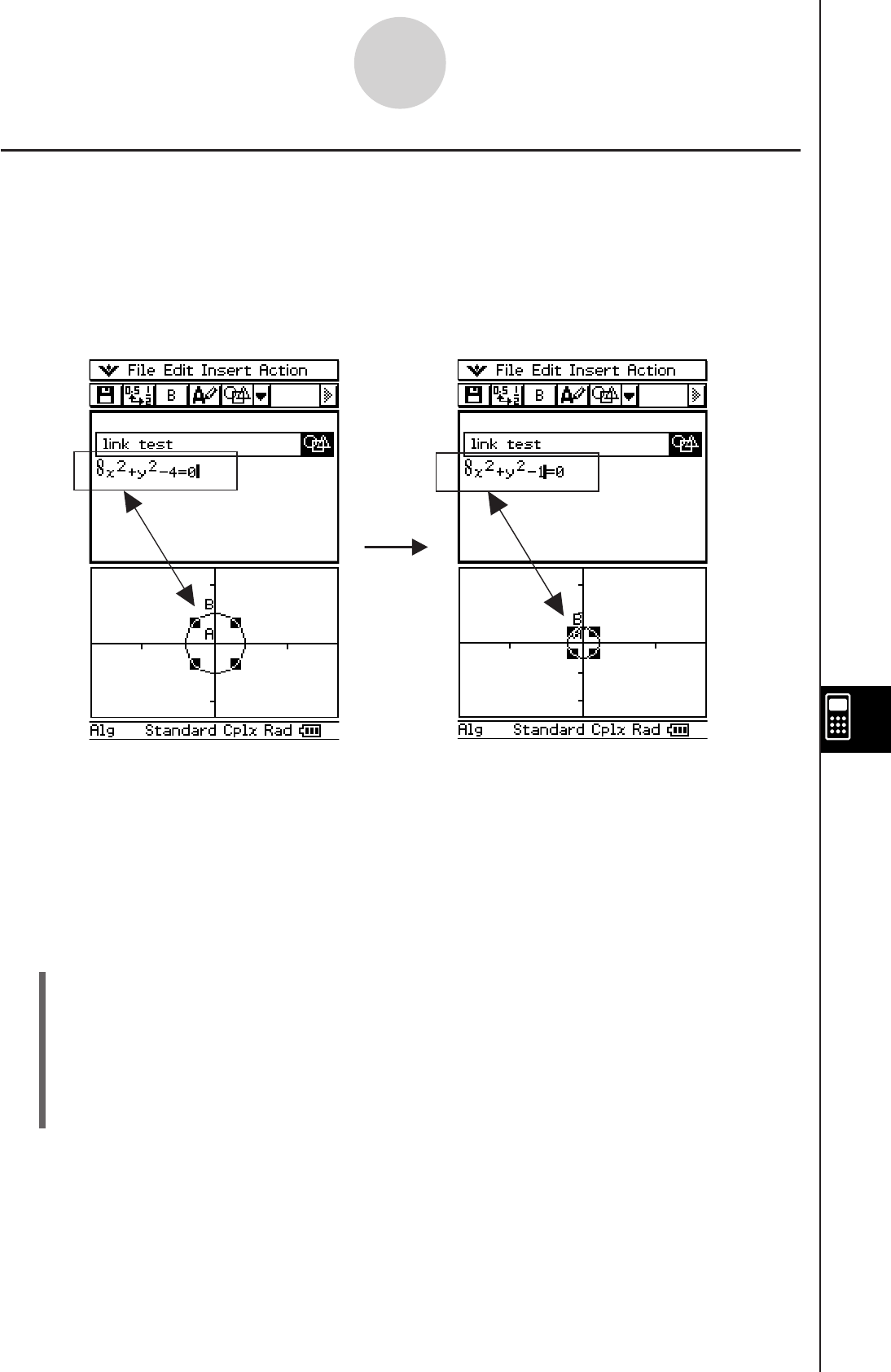
20060301

Inserting a Geometry Link Row

A Geometry Link row dynamically links data in the Geometry window with the corresponding

data in an eActivity. You can display lines and figures drawn in Geometry as values and

mathematical expressions in a Geometry Link row.

Dragging a line or figure from the Geometry window to a Geometry Link row in an eActivity

converts the line or figure to its mathematical expression. This expression is interlinked with

its Geometry window figure, so modifying one causes a corresponding change in the other.

u To input a Geometry Link row

Example: To drag one side of a triangle drawn on the Geometry window and link it to an

eActivity

(1) Open the eActivity application. Next, tap [Insert], [Strip], and then [Geometry] to insert a

Geometry strip.

(2) On the Geometry window that appears in the lower half of the screen, draw a triangle.

• For details about Geometry window operations, see Chapter 8.

(3) Tap the eActivity window just below the Geometry strip.

• This makes eActivity the active window.

Example of inserting a Geometry Link row

Modifying the equation in a Geometry Link updates the figure in the Geometry window.

Conversely, changing the shape, position, or some other parameter of the figure on the

Geometry window updates the equation in the Geometry Link.

10-3-17

Inserting Data into an eActivity

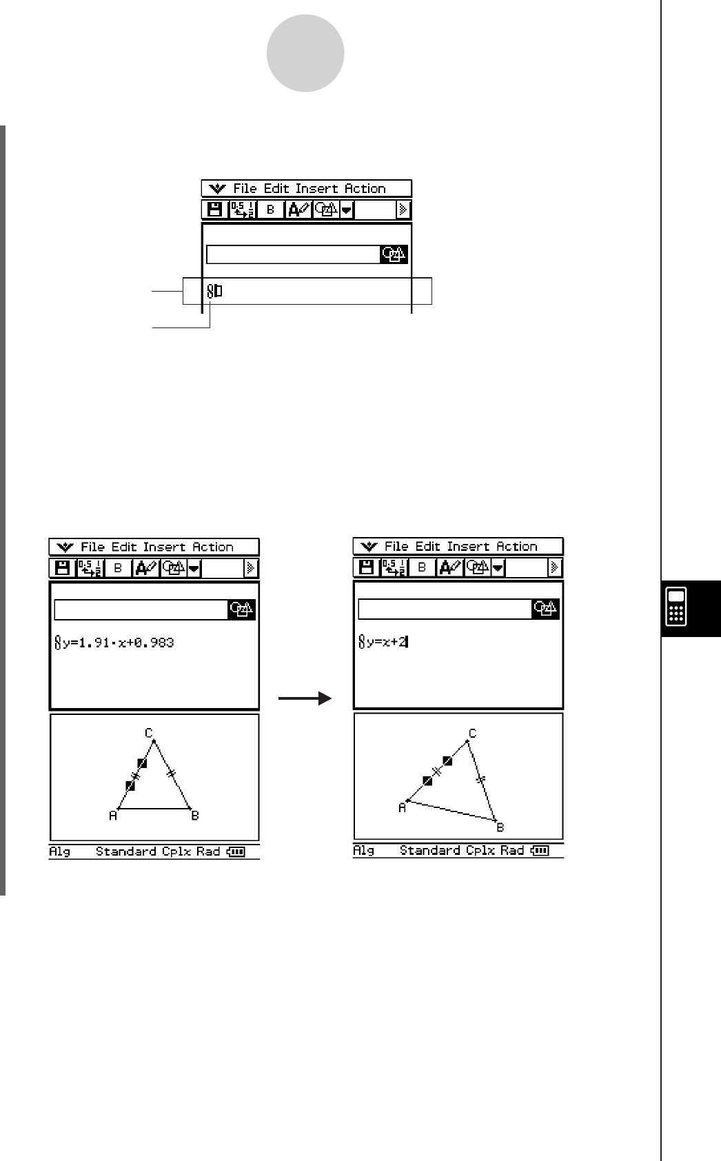
20060301

(4) Tap [Insert] and then [Geometry Link].

• This inserts a Geometry Link row in the next line.

10-3-18

Inserting Data into an eActivity

(5) Tap the Geometry window to make it active.

(6) Tap one side of the triangle to select it, and then drag it to the link symbol in the

eActivity window.

• This inputs the equation of the line that represents the side of the triangle into the link.

• Modifying the equation in the Geometry Link row and pressing E causes a

corresponding change in the Geometry window (lower right screenshot).

• The example below shows how the isosceles triangle ABC (CA = BC) changes when

the equation in the Geometry Link row is changed from y = 1.91x + 0.983 to y = x + 2.

Geometry Link row

Symbol

Tip

• Dragging a line or figure from the Geometry window to a text row or calculation row in an eActivity

also converts the figure to its value or equation. In this case, however, data in the text row or

calculation row is not interlinked with the Geometry window figure.

• Pressing

E after changing data in a Geometry Link updates the corresponding figure in the

Geometry window.

• Changing the figure in the Geometry window will cause the linked data in an eActivity to update

accordingly.

• Drag the stylus across

1.91x + 0.983.

• Input x + 2.

• Press E.

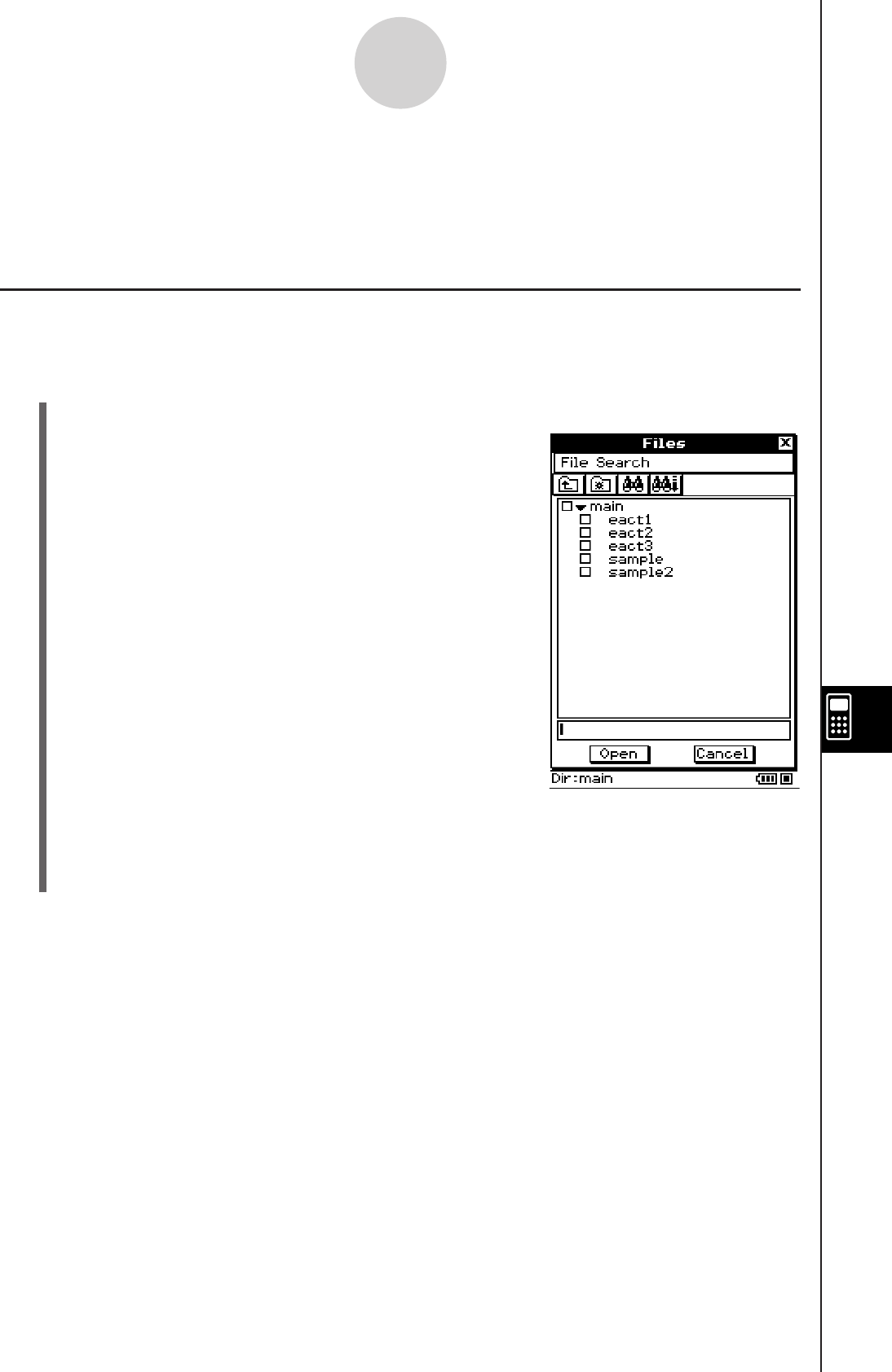
20060301

10-4 Working with eActivity Files

You can perform basic file operations on eActivity files. You can open previously saved files,

edit an existing file, and save a file under a new name.

Opening an Existing eActivity

Perform the following steps to open an existing eActivity file.

u ClassPad Operation

(1) On the eActivity window, tap [File] and then [Open].

• This displays the Files dialog box.

10-4-1

Working with eActivity Files

(2) Select the name of the eActivity file you want to open by tapping it.

(3) Tap [Open].

• This opens the eActivity you selected in step (2).

20060301

Editing the Contents of an eActivity

To edit an eActivity, you can use the same procedures that you used when you created it.

For more information, see “10-3 Inserting Data into an eActivity”.

Expanding an Application Data Strip

Tapping the expand button of an application data strip expands the application data in the

lower window. The expand button of a data strip is highlighted to indicate that it is expanded

in the lower window.

10-4-2

Working with eActivity Files

Indicates Example 1 is expanded. Indicates Example 2 is expanded.

Browsing the Contents of an eActivity

• When you first open an eActivity, its data appears on

the window starting from line 1. Use the scroll bar to

scroll the window contents if necessary.

• To view the contents of an application data strip in the

eActivity, tap the expand button (which is the icon in

the data strip). For more information, see “Expanding

an Application Data Strip” below.

Expand button

20090601

u To replace the original eActivity file with the newly edited version

(1) On the eActivity window, tap [File] and then [Save].

• This displays the Files dialog box.

10-4-3

Working with eActivity Files

(2) Tap [Save] without changing the displayed file name.

• This causes the original eActivity file to be replaced by the newly edited version.

Current eActivity file name

Modifying the Data in an Application Data Strip

Modifying application data on an application window in the lower eActivity window causes

the eActivity data to be modified as well. If you change the equation in the eActivity Graph

window, for example, the new graph will become the data of the eActivity.

This means that when you save and then reopen an eActivity file, tapping the application

data strip’s expand button again will cause the new graph to be displayed.

Saving an Edited eActivity

As with any other file, there are two ways to save an edited eActivity: resaving the original

eActivity with the newly edited eActivity, or saving the edited data under a different file name

as a new eActivity, without changing the originally opened eActivity.

20060301

u To save an edited eActivity under a different name

(1) On the eActivity window, tap {, or tap [File] and then [Save].

• This displays the Files dialog box.

(2) If you want, tap the name of the folder where you want the new eActivity file to be

saved.

(3) Tap the file name input box, and input the new file name you want to use.

(4) When everything is the way you want, tap [Save].

• This saves the eActivity as a new file under the file name you specified.

10-4-4

Working with eActivity Files

20060301

10-5 Transferring eActivity Files

Note the following precautions when using the ClassPad’s data communication function to

transfer eActivity files with another ClassPad unit or a computer.

Transferring eActivity Files between Two ClassPad Units

k Transferring eActivity Files to Another ClassPad Unit

To transfer an eActivity file to another ClassPad unit, the receiving unit must support all of

the following types of application data strips.*

10-5-1

Transferring eActivity Files

Application Data Strips

Graph, Graph Editor, 3D Graph, 3D Graph Editor, Conics Graph, Conics Editor, Geometry,

Spreadsheet, Stat Graph, Stat Editor, DiffEqGraph, DiffEqGraph Editor, Financial,

Probability, NumSolve, Sequence Editor, Picture Viewer, Notes, Main, Verify

*For details about application data strips, see “Inserting an Applicaiton Data Strip” on page

10-3-5.

Important!

• If you transfer an eActivity file to a ClassPad unit that does not support all of the application

data strips listed above, the receiving ClassPad unit will not be able to open the file.

• Do not transfer eActivity files to a ClassPad unit that does not support all of the application

data strips listed above.

• The functions of this ClassPad unit are different from the functions of a ClassPad unit

that does not support all of the application data strips listed above. Because of this their

eActivity files are incompatible with each other. Do not transfer eActivity files between two

ClassPad units that are equipped with different application data strips.

20110901

k Transferring eActivity Files from Another ClassPad Unit

To transfer an eActivity file from another ClassPad unit, your ClassPad unit must support all

of the application data strips that are supported by the sending unit.

Important!

• If you transfer an eActivity file from a ClassPad unit that supports application data strips

that are not supported by this ClassPad unit, your will not be able to open the file.

• Do not transfer eActivity files from another ClassPad unit if your ClassPad unit does not

support all of the application data strips of the sending unit.

• The functions of this ClassPad unit are different from the functions of a ClassPad unit that

supports application data strips not supported by this unit. Because of this their eActivity

files are incompatible with each other. Do not transfer eActivity files between two ClassPad

units that are equipped with different application data strips.

Transferring eActivity Files between a ClassPad Unit and a Computer

You can transfer eActivity files between ClassPad and a computer. For details, see

“Transferring Data between ClassPad and a Computer” (page 2-5-1) in the separate

Hardware User’s Guide.

10-5-2

Transferring eActivity Files

20110901

Using the Presentation

Application

The Presentation application lets you capture screenshots of

other application windows. Screenshots can be used in the

classroom or for other presentations simply by connecting the

ClassPad to a CASIO Projector.

11-1 Presentation Application Overview

11-2 Building a Presentation

11-3 Managing Presentation Files

11-4 Playing a Presentation

11-5 Editing Presentation Pages

11-6 Configuring Presentation Preferences

11-7 Presentation File Transfer

Chapter

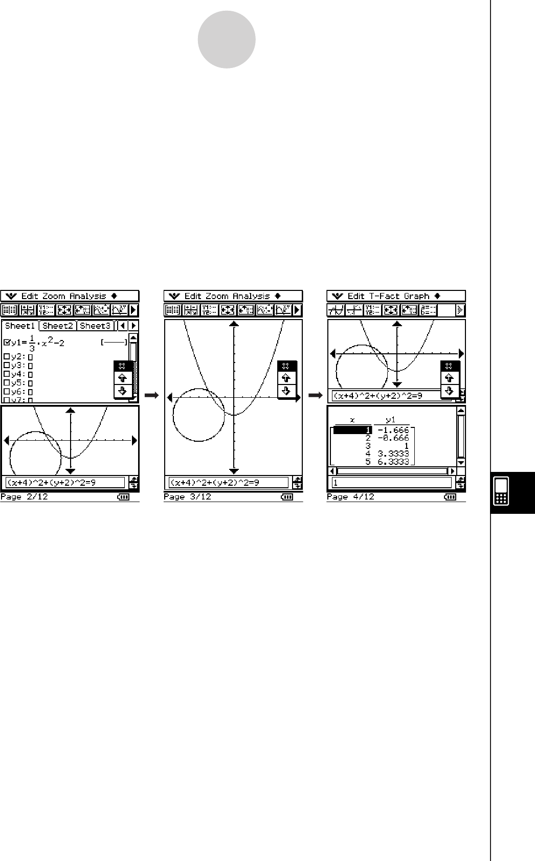
20060301

11-1-1

Presentation Application Overview

11-1 Presentation Application Overview

The Presentation application lets you capture screenshots produced by the ClassPad, and

arrange them into a “presentation” that you can play back. With this application you can build

and play a presentation, and edit the contents of a presentation. A presentation, for example,

can show how to obtain intermediate and final results of calculation operations.

Sample Presentation

...

Specifically, the Presentation application can be used as follows.

• A teacher can use Presentation to create materials that explain mathematical concepts,

and distribute them to students.

• A student can use Presentation as a tool to present reports, assignments, and projects.

• Students and teachers can use Presentation to store ClassPad screenshots for later

reference.

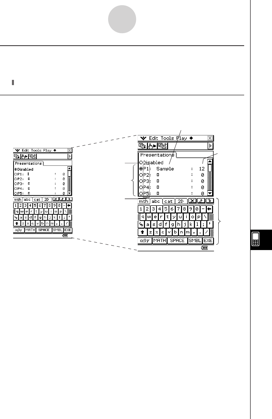
20090601

Presentation Application Window

Tapping P on the application menu starts the Presentation application and displays its

initial screen.

• Selecting [Disabled] will cause the [Screen Copy To] setting on the Presentation and

Communication dialog boxes to change automatically to [Outer Device]. For more

information, see “11-6 Configuring Presentation Preferences”.

• Files are numbered P1 through P20. These numbers are fixed and cannot be changed.

When creating a new presentation file, you can input the file name you want.

• The soft keyboard is automatically displayed when you open the Presentation application.

11-1-2

Presentation Application Overview

Disable button

File name

Number of

pages

File list

Soft

keyboard

Initial Screen

Starting Up the Presentation Application

Use the following procedure to start up the Presentation application.

u ClassPad Operation

On the application menu, tap P.

File number

20060301

Presentation Application Menus and Buttons

This section explains the operations you can perform using the menus and buttons of the

Presentation application’s initial screen.

k Initial Screen Menu Commands and Buttons

To do this: Tap this

button:

Or select this

menu item:

Delete the presentation file whose option button is currently

selected (page 11-3-1) – Edit - Delete

Delete all presentation files (page 11-3-1) – Edit - Delete All

Enter the Editing mode and display the editing tool palette

(page 11-5-1) 0Tools

Start auto play (page 11-4-1) 6Play - AutoPlay

Start manual play (page 11-4-2) 7Play - ManualPlay

Insert a white screen at the end of the selected presentation

file (page 11-2-3) –a - White Screen

Append PICT data to the end of the selected presentation

file (page 11-2-3) –a - Add

11-1-3

Presentation Application Overview

20060301

Screen Capture Precautions

Note the following precautions when capturing screens for a presentation.

• The operation that is performed when you tap h depends on the current [Screen Copy

To] setting as described below.

When the [Screen Copy To] setting is this: Tapping h does this:

Outer Device Sends the screenshot to an external device.

P1 - P20 Adds the screenshot to the presentation file.

To change the [Screen Copy To] setting, tap O, and then [Presentation] or

[Communication]. For more information, see “Presentation Dialog Box” on page 1-9-14.

• Tapping h will capture either the full screen or half the screen, depending on how you

have Presentation preferences configured. For more information, see “11-6 Configuring

Presentation Preferences”.

• Screen capture is disabled when any of the following conditions exists.

• While a calculation, graph draw, or similar operation is in progress

• While a data communication operation is in progress

• While the stylus (or your finger or other object) is in contact with the screen

• In addition to the conditions detailed above, screen capture may be disabled by other

operations that have a higher priority than screen capture.

• The status bar is not included in screen captures when [Screen Copy To] setting is

“P1” - “P20”.

11-1-4

Presentation Application Overview

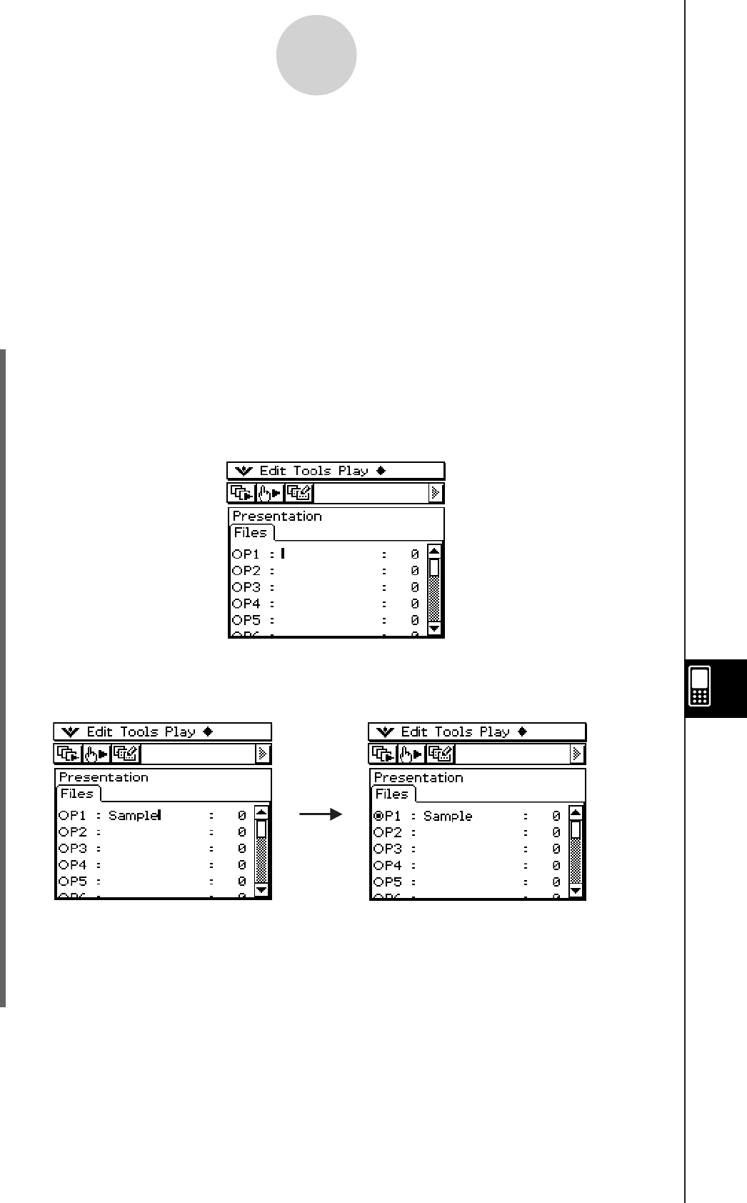
20060301

11-2 Building a Presentation

Presentations are created by capturing screenshots that are produced by the applications

of the ClassPad. Before actually beginning to capture the screenshots, it is important to

carefully think about and plan the type of information you want to include in your presentation

so that your screenshots display the information that you want.

This is not to say, however, that you must create a perfect presentation the first time around.

You can always change the sequence of pages or edit a pages at any time.

u To create a new presentation

(1) On the application menu, tap P to start the Presentation application.

(2) On the file list, tap the line (P1 through P20) where you want to store the new

presentation file.

• This causes a cursor to appear on the line you tap.

(3) Enter up to eight bytes for the presentation file name, and then tap w.

• Check to make sure that the file name you just input is selected (button is on).

(4) Tap

m to display the application menu, and then start the application whose screens

you want to capture.

(5) Perform the required operations in the application to display the screen you want to

capture.

11-2-1

Building a Presentation

20060301

(6) With the screen you want to capture on the display, tap h.

• The currently displayed screen is captured as soon as you tap h. Its image is added

to the pages of the presentation file you selected in step (3).

• If the capture is successful, “ ” appears in the status bar for about one second.

(7) Repeat steps (5) and (6) to capture other screens as required.

• Note that you can change to other applications as required.

(8) After capturing all of the images you want, tap m to display the application menu, and

then tap P to return to the Presentation application.

• Even after you return to the Presentation application, you can restart screen capture

to add more pages. To do so, simply return to step (4) of this procedure.

(9) To check the current contents of the presentation, tap 6.

• This starts auto play, which scrolls through the pages of the new presentation

automatically. For more information, see “Using Auto Play” on page 11-4-1.

Adding a Blank Page to a Presentation

Perform the procedure on page 11-2-3 when you want to add a blank page to the end of a

presentation. After adding a blank page, you can put text on it or move it to another location

inside the presentation.

You can use blank pages to indicate the end of a presentation, to separate a presentation

into sections, or to insert commentary text.

11-2-2

Building a Presentation

This value shows how many pages

(images) you have captured and added

to the presentation.

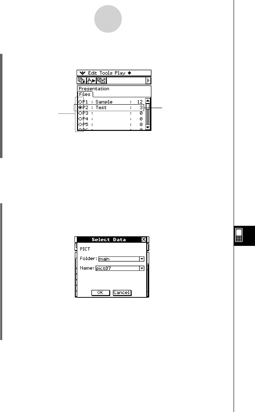
20060301

u To insert a blank page into a presentation

(1) On the Presentation application initial screen, tap the button next to the presentation

file into which you want to insert the blank page, so it is selected.

(2) Tap

a and then [White Screen].

• This inserts a blank page as the final page of the presentation file you selected in step

(1), and increases the number of pages for the presentation by one.

Tip

• For information about inserting text and moving the blank page, see “11-5 Editing Presentation

Pages”.

11-2-3

Building a Presentation

Button

This file is selected

u To append PICT data to the end of a presentation

(1) On the Presentation application initial screen, tap the button next to the presentation

file where you want to append the PICT data so it is selected.

(2) Tap a and then [Add].

• This displays the Select Data dialog box.

(3) On the Select Data dialog box, select the folder where the PICT data you want to insert

is stored, and specify the name of the date.

(4) Tap [OK].

• This closes the Select Data dialog box and appends the PICT data to the end of the

presentation.

Tip

• If the size of the PICT data is different from the ClassPad display size, the upper left corner of the

PICT data is aligned with the upper left corner of the ClassPad display, and any data that does

not fit is cut off.

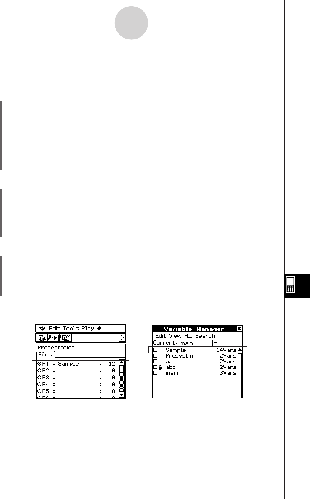
20060301

11-3 Managing Presentation Files

After you create a presentation file, you can rename it or delete it.

u To rename a presentation file

(1) On the Presentation application initial screen, tap the name of the file you want to

rename so it is selected.

(2) Press

• This causes a cursor to appear to the right of the last character of the file name.

(3) Change the file name.

• A file name can be up to eight bytes long.

(4) After the file name is the way you want, tap w.

u To delete a single presentation file

(1) On the Presentation application initial screen, tap the button next to the name of the file

you want to delete so it is selected.

(2) Tap [Edit] and then [Delete].

(3) In response to the confirmation message that appears, tap [OK].

• This deletes the file you selected in step (1).

11-3-1

Managing Presentation Files

Variable Manager Folder List

Presentation File List

• A presentation file is actually a user folder, so presentation files appear as folders on the

Variable Manager folder list.

For details about using the Variable Manager, see “1-8 Using the Variable Manager”.

u To delete all presentation files

(1) Display the Presentation application initial screen.

(2) Tap [Edit] and then [Delete All].

(3) In response to the confirmation message that appears, tap [OK].

• This deletes all of the presentation files.

20060301

11-3-2

Managing Presentation Files

Important!

• PICT format image data files (PICT data type variables) captured with the h icon are

stored in folder that is created when you create a Presentation file.

• The “Presystm” folder (whose contents you can view with the Variable Manager) contains

files for managing presentations. Normally, you should never edit or delete the “Presystm”

folder or any of its contents. If these files are damaged or deleted, they will be restored

when you run the presentation.

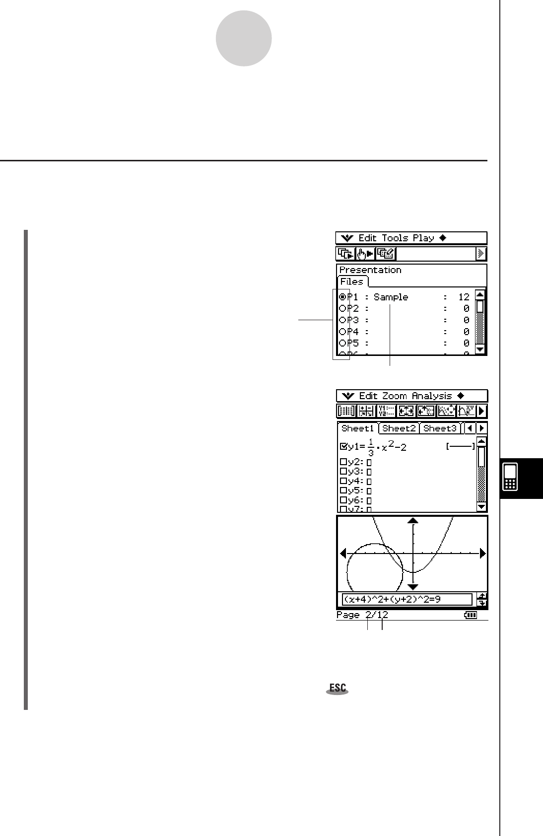
20060301

11-4 Playing a Presentation

This section explains the various methods you can use to play a presentation.

Using Auto Play

With auto play, the pages of the presentation are scrolled automatically at a fixed interval.

u ClassPad Operation

(1) On the Presentation application initial screen,

tap the button next to the presentation

file you want to play, so it is selected.

(2) Tap

6, or tap [Play] and then [AutoPlay].

• This starts auto play, which displays the

pages of the presentation in sequence.

Current page number Total number of pages

11-4-1

Playing a Presentation

This file is selected

(3) When playback reaches the final page it stops, and then the Presentation application

initial screen appears.

• To stop an auto play operation part way through, tap on the icon panel or press

the

c key.

Button

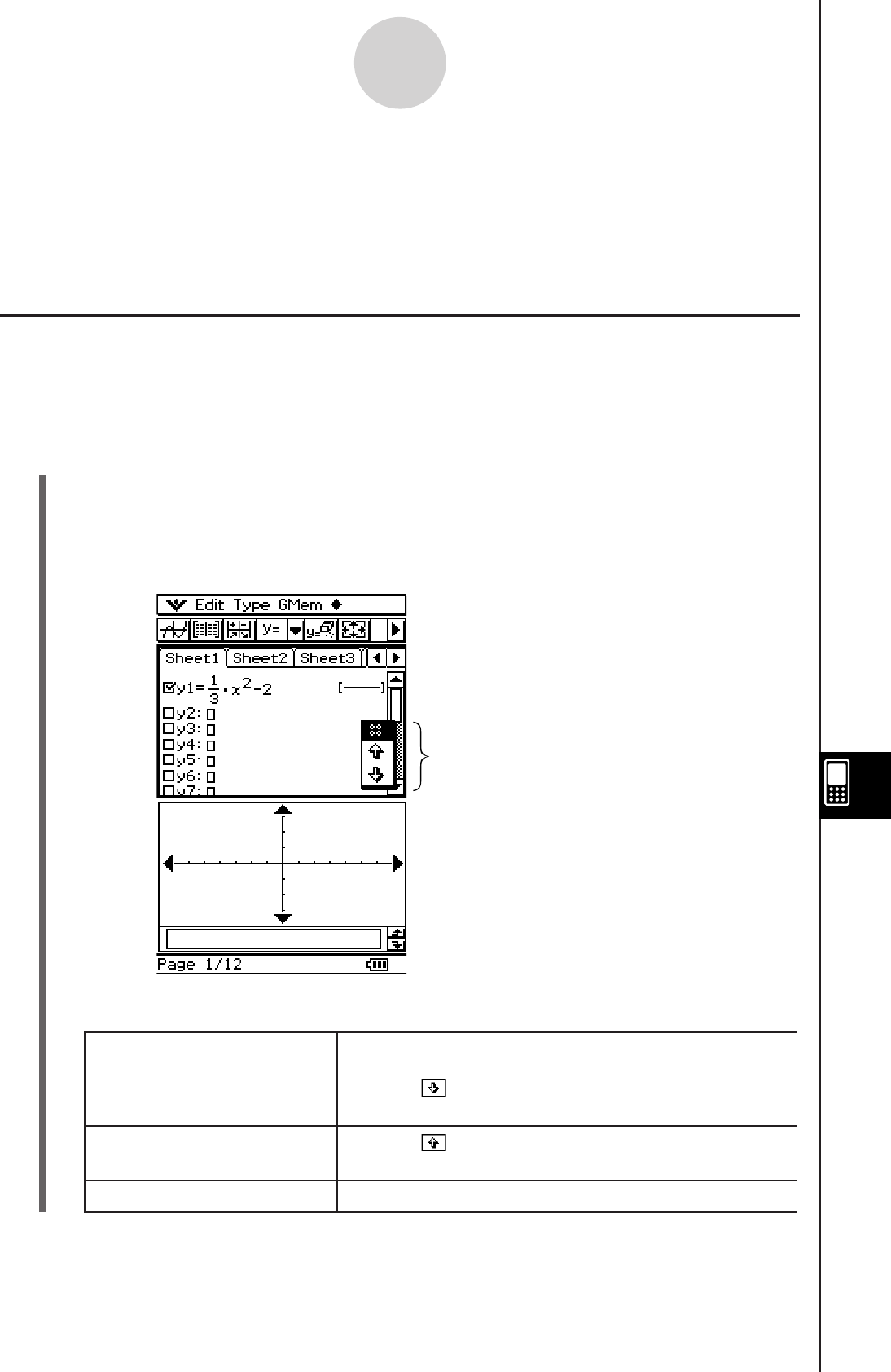
20060301

Using Manual Play

With manual play, you control when page change operations are performed during

presentation play. Manual play lets you scroll forward or back through presentation pages,

and you can display a pointer on a page.

u ClassPad Operation

(1) On the Presentation application initial screen, tap the button next to the presentation

file you want to play, so it is selected.

(2) Tap

7, or tap [Play] and then [ManualPlay].

• This starts manual play, which displays the first page of the presentation.

(3) You can perform the following operations while a manual play operation is in progress.

11-4-2

Playing a Presentation

When you want to do this: Do this:

Advance to the next page Tap the page scroll button or press the c

cursor key

Return to the previous page Tap the page scroll button or press the f

cursor key

Display a round pointer Hold or drag the stylus on the screen

Tip

• You can configure Presentation preferences to specify the page change speed and to turn

page number display in the status bar on or off. For more information, see “11-6 Configuring

Presentation Preferences”.

• You can also configure auto play so it repeats when the final page of a presentation is reached.

For more information, see “Using Repeat Play” on page 11-4-3.

Page scroll buttons

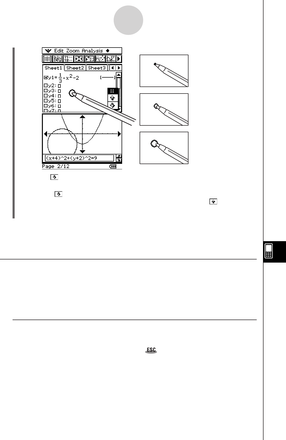
20060301

(4) Tapping while the final page of the presentation is displayed causes the message

“End of Files” to appear in the status bar.

• Tapping while the message “End of Files” is in the status bar exits the manual

play operation and displays the Presentation initial screen. Tapping while “End of

Files” is in the status bar returns you to the final page of the presentation and

continues the manual play operation.

Tip

• You can turn display of the page number in the status bar on and off. For more information, see

“11-6 Configuring Presentation Preferences”.

Using Repeat Play

Repeat play causes auto play to restarts the presentation from the beginning each time the

final page of a presentation is reached.

Use the Presentation dialog box (page 11-6-1) to turn repeat play on or off.

The initial default setting is repeat play off.

The following describes how repeat play works for auto play.

k Repeat Auto Play

• When the final page of the presentation is reached, the presentation is restarted from the

first page.

• The presentation continues playing until you tap on the icon panel or press the c

key to stop it.

11-4-3

Playing a Presentation

20060301

11-5 Editing Presentation Pages

This section explains how to use the Editing mode of the Presentation application to modify

the pages of an existing presentation.

About the Editing Tool Palette

An editing tool palette appears on the display whenever you enter the Editing mode. The

following describes how to use the editing tool palette.

Entering the Editing Mode

Perform the following steps to enter the Editing mode when you want to edit the pages of an

existing presentation.

u ClassPad Operation

(1) On the Presentation application initial screen, tap the button next to the presentation

file you want to edit, so it is selected.

(2) Tap

0, or tap [Tools].

• This enters the Editing mode and displays the editing tool palette and page scroll

buttons. Page 1 of the presentation file you selected in step (1) appears first.

11-5-1

Editing Presentation Pages

To do this:

Tap this tool

button:

Move the currently displayed page one page back 8

Move the currently displayed page one page forward 9

Delete the currently displayed page e

Copy the currently displayed page t

Paste a copied page into the location before the currently displayed page y

Delete the lower half of the screen -

Insert text into a page u

Draw a straight line on a page i

Draw an arrow on a page o

Use the eraser }

Save a page after editing it {

Exit the Editing mode and return to the Presentation application initial screen =

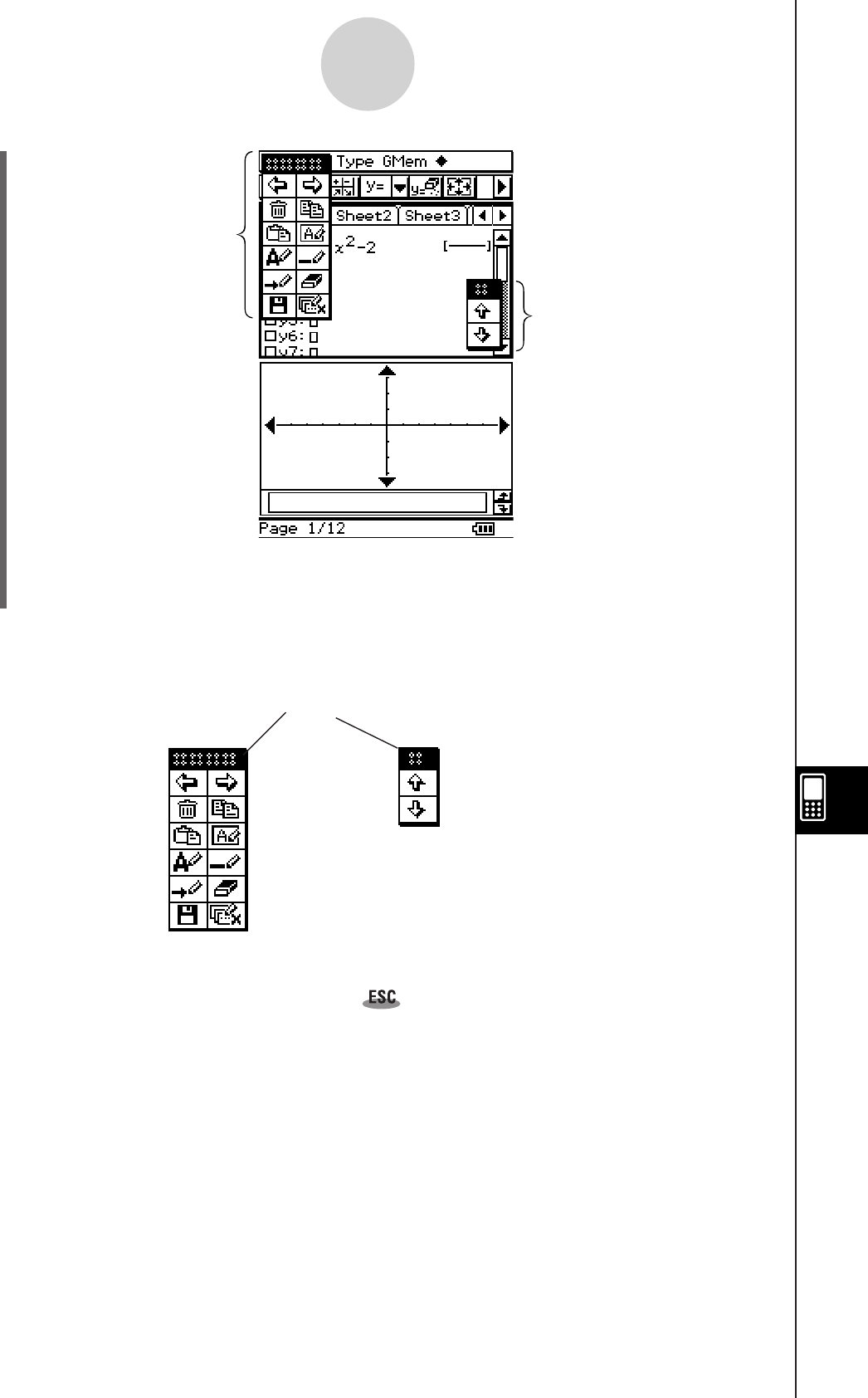
20060301

(3) Use the editing tool palette buttons to edit the pages.

• For details about editing operations, see “Editing Operations” on page 11-5-3.

• You can drag the editing tool palette and page scroll buttons to any location on the display.

Simply use the stylus to drag the handle of the palette or buttons.

u To exit the Editing mode

On the editing tool palette, tap =, or tap on the icon panel, or press c to exit

the Editing mode and return to the Presentation application initial screen.

Handle

11-5-2

Editing Presentation Pages

Editing tool palette

Page scroll buttons

20060301

Editing Operations

This section provides details about the page editing operations you can perform with the

Presentation application’s editing tool palette.

u To move a page

(1) Enter the Editing mode of the Presentation application (page 11-5-1).

(2) Use the page scroll buttons to display the page you want to move.

(3) Tap

8 to move the currently displayed page back one page, or tap 9 to move it

forward one page.

• The illustrations below show the effect of tapping 8 or 9 while page C of a five-

page presentation file is selected.

u To delete a page

(1) Enter the Editing mode of the Presentation application (page 11-5-1).

(2) Use the page scroll buttons to display the page you want to delete.

(3) Tap

(4) In response to the confirmation dialog box that appears, tap [OK] to delete the page or

[Cancel] to cancel.

• This deletes the currently displayed page and then displays the following page.

Deleting the final page of a presentation displays the page preceding the deleted

page.

11-5-3

Editing Presentation Pages

ABCDE

ACBDE

CABDE

ABCDE

ABDCE

ABDEC

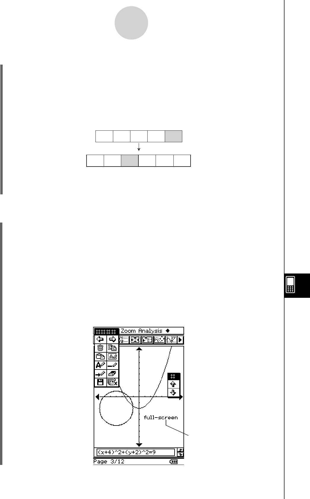
20060301

u To copy and paste a page

(1) Enter the Editing mode of the Presentation application (page 11-5-1).

(2) Use the page scroll buttons to display the page you want to copy, and then tap t.

• This copies the currently displayed page to the clipboard.

(3) Use the page scroll buttons to display the page that you want to follow the copied page.

• The illustrations below show the effect of copying page E of a five-page presentation

file and pasting it between pages B and C.

(4) Tap

• This pastes the page at the location in front of the currently displayed page.

u To insert text into a page

(1) Enter the Editing mode of the Presentation application (page 11-5-1).

(2) Use the page scroll buttons to display the page into which you want to insert text, and

then tap u.

• This displays a text input dialog box along with a soft keyboard.

(3) Enter the text and then tap [OK].

• In this example we input the text “full-screen”.

(4) Place the stylus on the screen and hold it there.

• This causes the text you input in step (3) to appear at the location where you are

pointing with the stylus.

(5) Drag the text to the location you want, and then lift the stylus from the screen.

11-5-4

Editing Presentation Pages

ABCDE

ABECDE

Inserted text

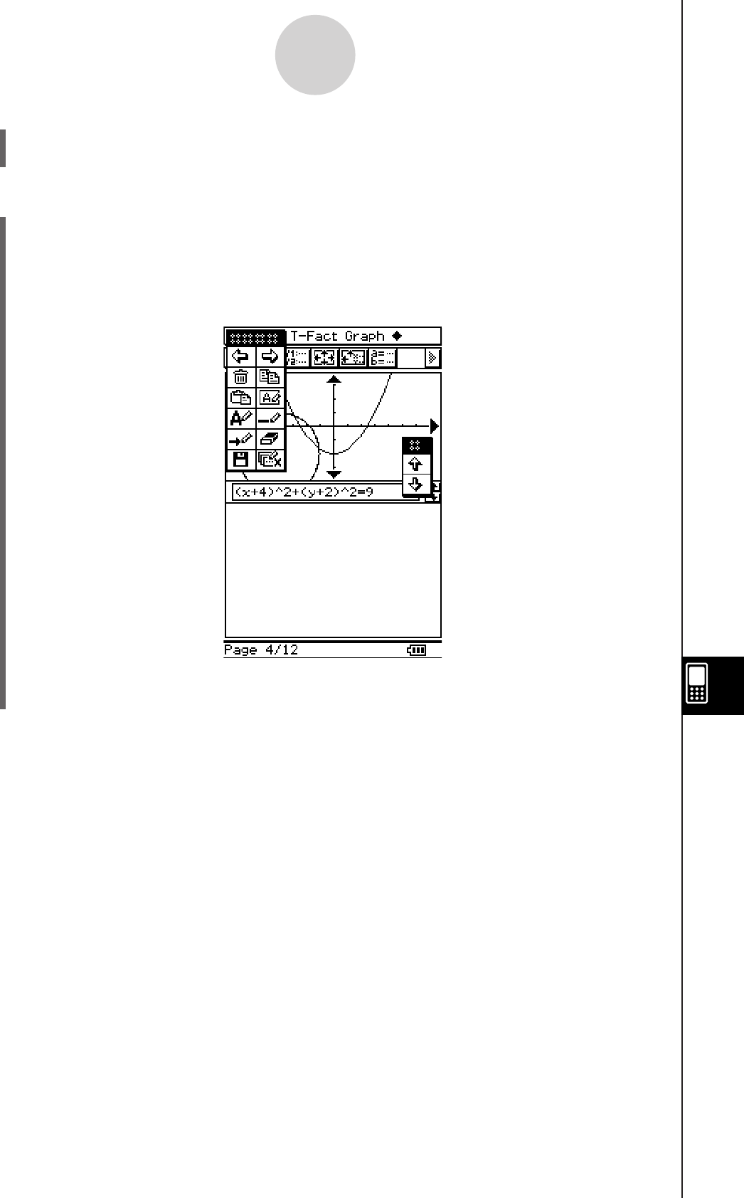
20060301

(6) To save the result of the text insert operation, tap { and then tap [OK] on the

confirmation dialog box that appears.

u To clear the bottom half of the screen

(1) Enter the Editing mode of the Presentation application (page 11-5-1).

(2) Use the page scroll buttons to display the page whose bottom half you want to clear.

(3) Tap

• This clears the bottom half of the displayed page.

11-5-5

Editing Presentation Pages

(4) To save the result of the operation, tap { and then tap [OK] on the confirmation dialog

box that appears.

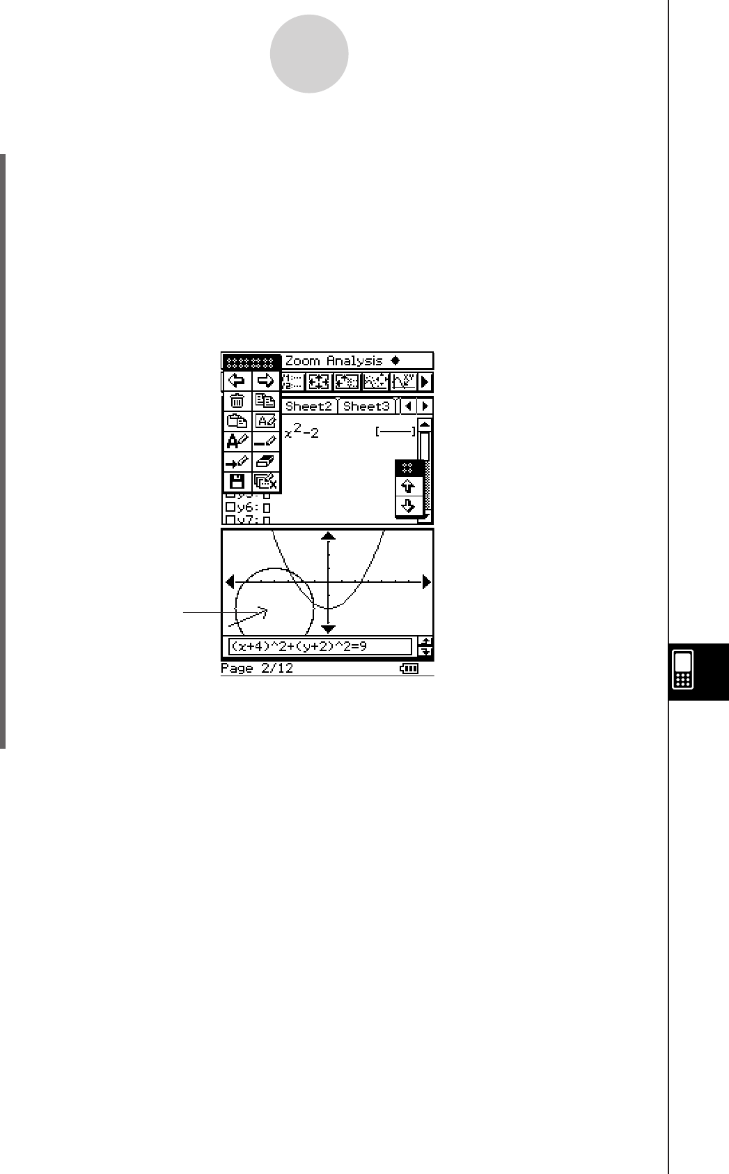
20060301

u To draw a straight line or an arrow on a page

(1) Enter the Editing mode of the Presentation application (page 11-5-1).

(2) Use the page scroll buttons to display the page on which you want to draw a straight

line or arrow.

(3) Tap

i if you want to draw a line or o if you want to draw an arrow.

(4) Tap the point where you want one end of the line segment or arrow to be, and then tap

the point where you want the other end to be.

• A line segment or arrow appears between the points you tapped.

• If you are drawing an arrow, the arrow head appears on the end you specify last.

(5) To save the result of the draw operation, tap { and then tap [OK] on the confirmation

dialog box that appears.

11-5-6

Editing Presentation Pages

Example of an arrow

20060301

Using the Eraser

The eraser allows you to erase parts of an image, text, arrows, or lines you have added to a

page.

u To erase part of a page with the eraser

(1) Enter the Editing mode of the Presentation application (page 11-5-1).

(2) Use the page scroll arrows to display the page that contains the figures you want to

erase.

(3) Tap

Important!

• Whenever the

} tool button is selected, dragging the stylus across the screen erases

a 3 × 3-pixel area (centered on the stylus).

(4) Drag the eraser across the screen to erase the figures you want.

(5) To save the result of the erase operation, tap {, and then tap [OK] on the

confirmation dialog box that appears.

11-5-7

Editing Presentation Pages

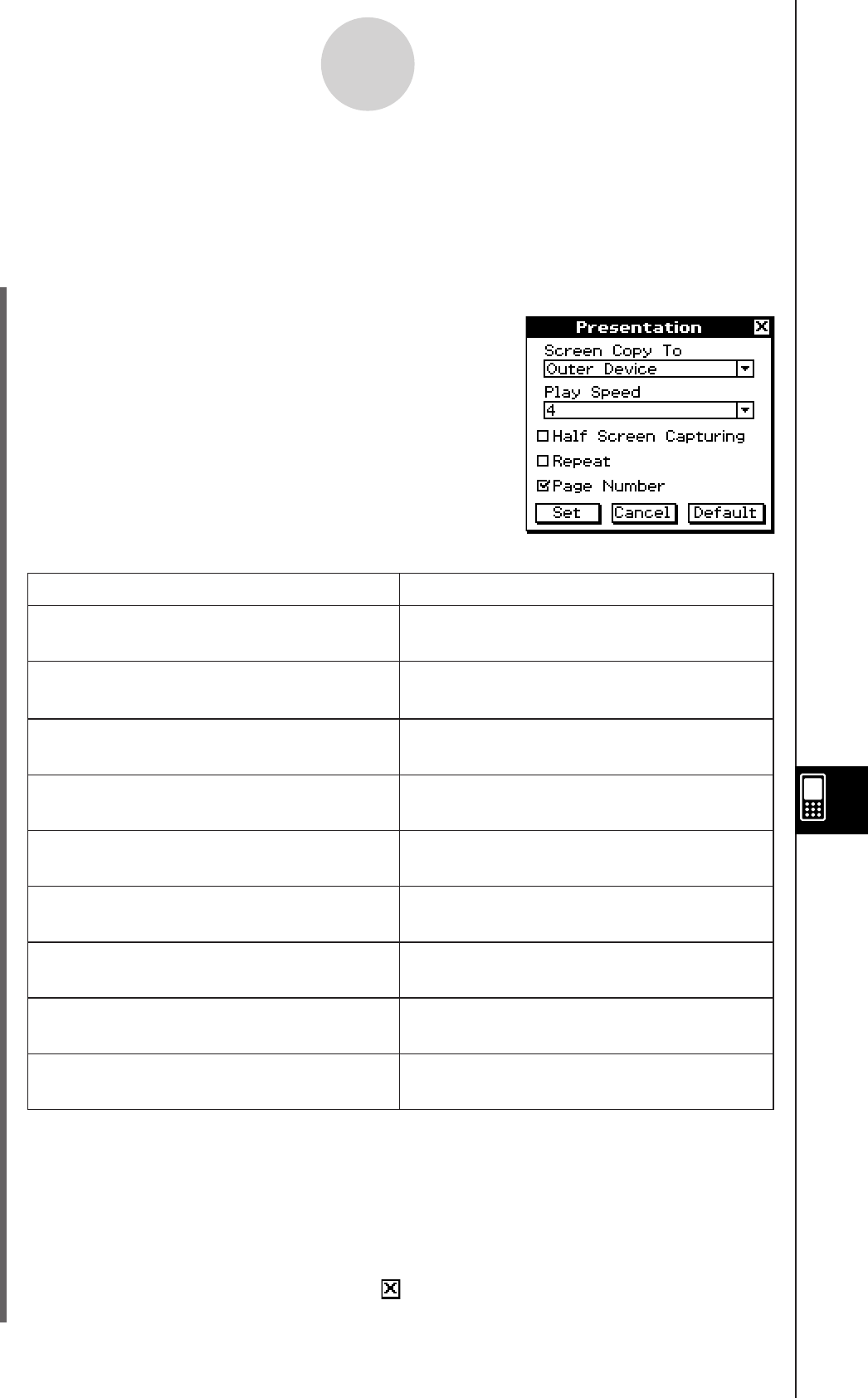
20060301

11-6 Configuring Presentation Preferences

You can use the procedure below to configure various Presentation application preferences.

u ClassPad Operation

(1) Tap

O, and then [Presentation].

• This displays the Presentation dialog box.

(2) Use the Presentation dialog box to configure the preferences you want.

To do this: Do this:

Send hard copy data generated by tapping

h to an external device

Select [Outer Device].*

Save hard copy data internally as

Presentation data

Select “P1:<File name>**” through

“P20:<File name>**” for [Screen Copy To].

Specify the page change speed for Auto

Play

Specify a [Play Speed] value from 1

(fastest) to 10 (slowest).

Capture the upper half of the screen when

h is tapped

Select the [Half Screen Capturing] check

box.

Capture the entire screen when h

is tapped

Clear the [Half Screen Capturing] check

box.*

Turn on repeat playback of files during

Auto Play

Select the [Repeat] check box.

Turn off repeat playback of files during

Auto Play

Clear the [Repeat] check box.*

Turn on page number display during

playback and editing

Select the [Page Number] check box.*

Turn off page number display during

playback and editing

Clear the [Page Number] check box.

11-6-1

Configuring Presentation Preferences

• Items marked with an asterisk (*) are initial defaults. The initial default [Play Speed]

setting is 4.

• Selecting [Disabled] on the Presentation application initial screen will cause the

[Screen Copy To] to change automatically to [Outer Device].

** <File name> will show the name of the presentation file.

(3) To close the dialog box and apply its settings, tap [Set]. To close the dialog box without

applying its settings, tap [Cancel] or the button in the upper right corner of the dialog

box. To restore all the settings on the dialog box to their initial defaults, tap [Default].

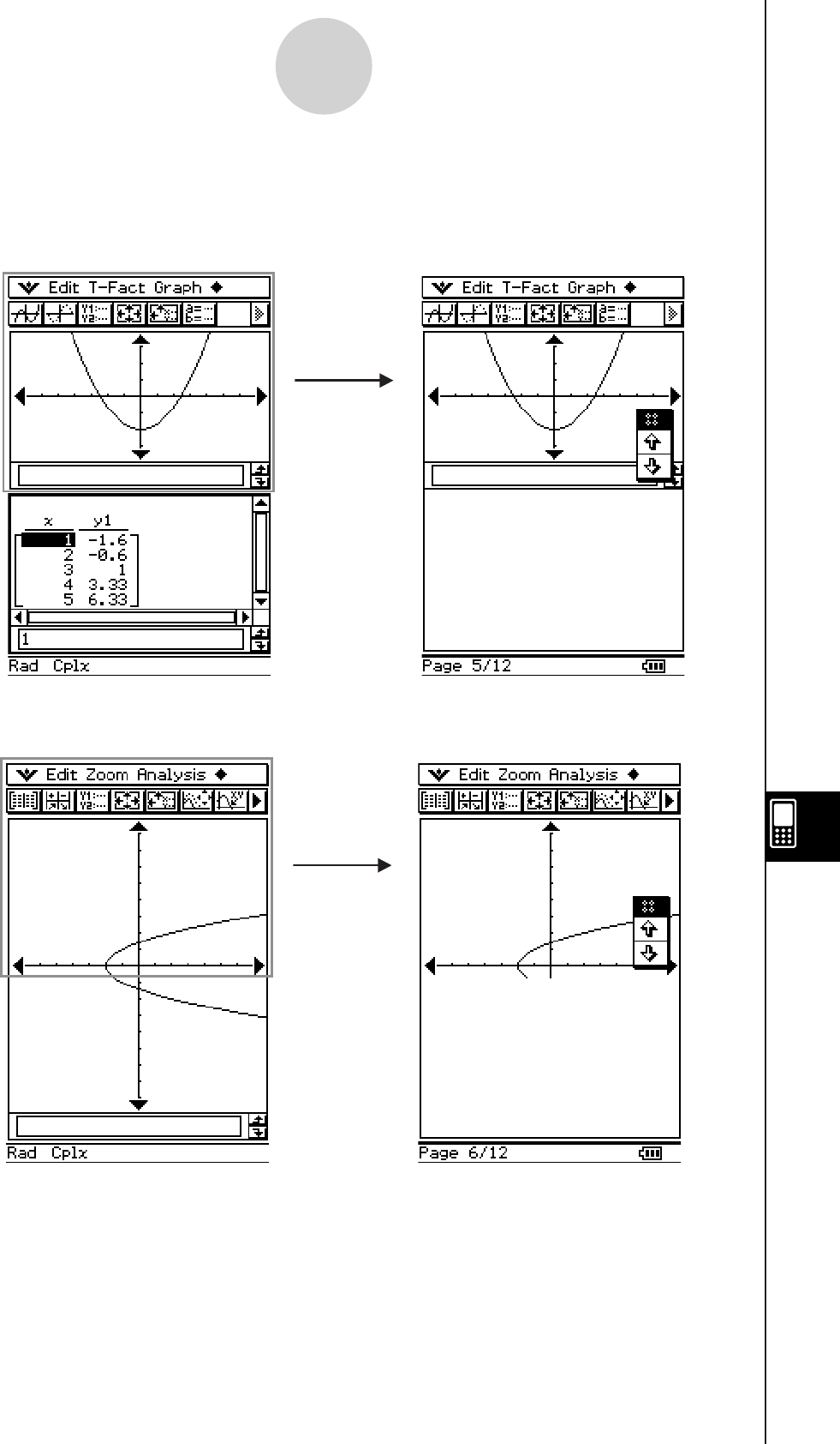
20060301

Tip

• The following examples show the area of the screen that is captured when you tap h while

the [Half Screen Capturing] check box is selected. The captured areas are indicated by the thick

boundaries in each example.

Sample Screenshot

Captured Image Data

11-6-2

Configuring Presentation Preferences

20060301

11-7 Presentation File Transfer

A presentation file is actually a kind of user folder (called a “presentation folder”) that

contains the images that make up the presentation. This folder may be transferred to another

ClassPad unit or a computer in order to play the presentation.

Caution

• A presentation created with Version 3.0 of the ClassPad software cannot be played on a

ClassPad or a computer that is running an earlier version.

11-7-1

Presentation File Transfer

20060301

Chapter

Using the Program

Application

The Program application comes in handy when you need to

perform the same calculation a number of times. You can create

programs that automate graphing and other operations.

12-1 Program Application Overview

12-2 Creating a New Program

12-3 Debugging a Program

12-4 Managing Files

12-5 User-defined Functions

12-6 Program Command Reference

12-7 Including ClassPad Functions in Programs

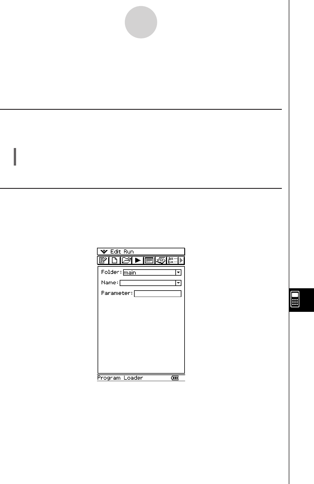
20060301

12-1 Program Application Overview

The Program application consists of a Program Editor for inputting and editing programs, and

a Program Loader for loading and executing existing programs.

Starting Up the Program Application

Use the following procedure to start up the Program application.

u ClassPad Operation

On the application menu, tap p.

This starts the Program application and displays the Program Loader window.

Program Loader Window

Use the Program Loader window to recall and run existing programs.

uTo display the Program Loader window

On the application menu, tap p to start up the Program application. The Program Loader

window appears when you start up the Program application.

12-1-1

Program Application Overview

20060301

12-1-2

Program Application Overview

k Program Loader Window Menus and Buttons

To do this: Tap this

button:

Or select this menu

item:

Display the Program Loader window — O - Program Loader

Display the Program Editor window PO - Program Editor

Display the Program Output window _O - Program Output

Display the Text File Contents window — O - Text File Contents

Display the Main application work area window ~O - Main

Display the Program Editor window PEdit - Open Editor

Create a new file OEdit - New File

Open an existing file ~Edit - Open File

Clear the screen — Edit - Clear All

Run a program pRun - Run Program

Display the Variable Manager (page 1-8-1) 5O - Variable Manager

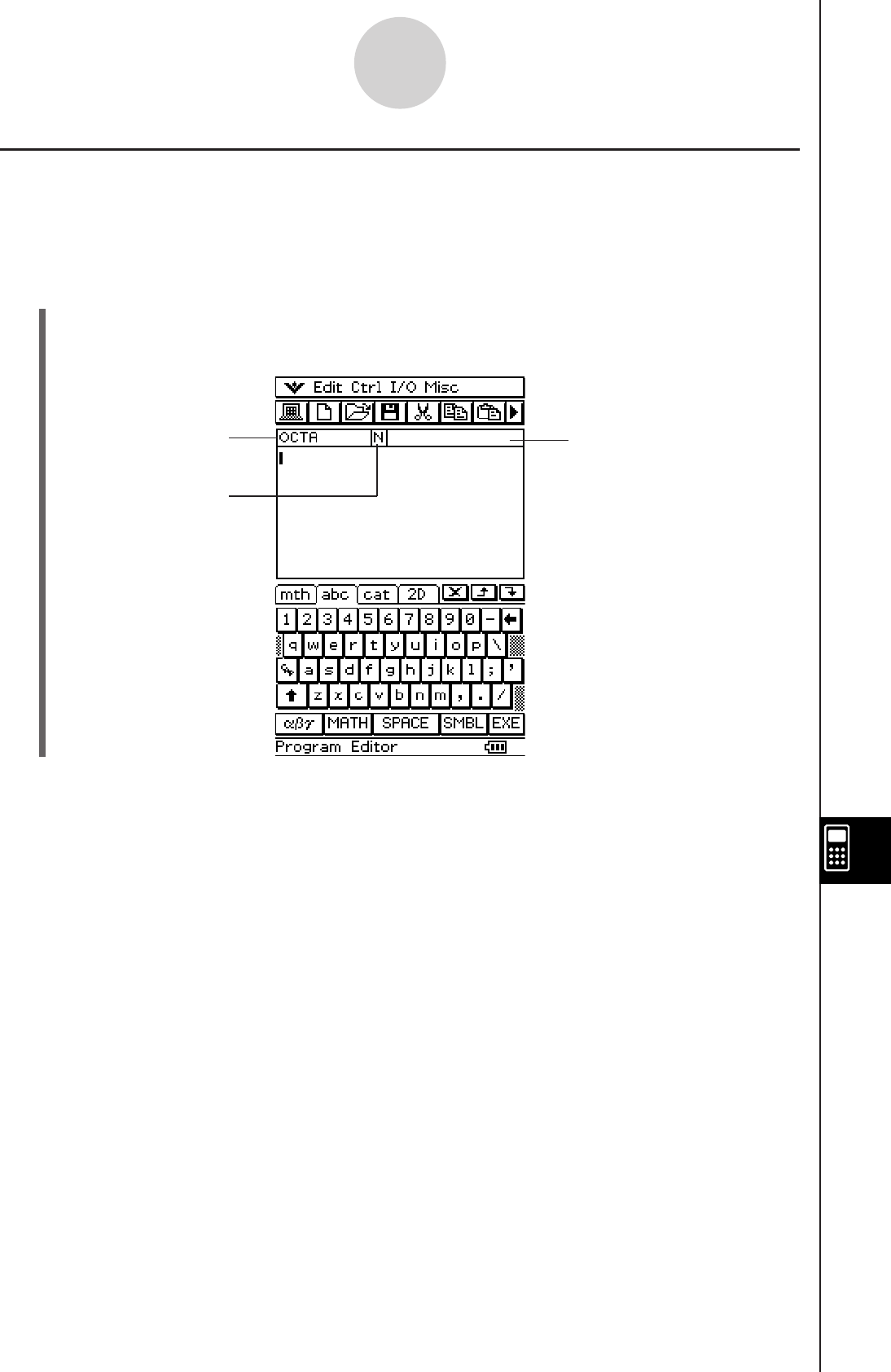
20090601

File type

N: Program file

T: Text file

F: User-defined

function file

File name Parameter variables

This box can be used to

specify variable names

used in user-defined

functions or programs.

For details, see

“Configuring Parameter

Variables and Inputting

Their Values” on page

12-2-7.

Program Editor Window

You can use the Program Editor window to input a new program or to edit an existing

program. You can also use the Program Editor window to input and edit user-defined

functions.

u To display the Program Editor window

(1) On the application menu, tap p to start up the Program application.

(2) On the window that appears, tap P, or tap O and then [Program Editor].

12-1-3

Program Application Overview

20060301

k Program Editor Window Menus and Buttons

The following describes the menu and button operations you can perform on the Program

Editor window.

12-1-4

Program Application Overview

To do this: Tap this button: Or select this menu item:

Display the Program Loader window

Display the Program Editor window

Display the Main application work area

window

Close the currently active window

Create a new file

Open an existing file

Save a file

Save a file under a new name

Close a file

Paste the clipboard contents

Convert a file to a program file

Convert a file to a text file

Convert a file to an edit prohibited

program file

Put a selection onto the clipboard and

delete the original

Put a selection onto the clipboard without

affecting the original

Display the Program Output

window

)

—

{

Select everything on the screen

Search for a newly specified text string

Search again for a previously specified

text string

Jump to the beginning of a program

Jump to the end of a program

Clear the contents of the Program Editor

window

—

Edit - Select All

Edit - Paste

Edit - Copy

Edit - Cut

Edit - Compress

Edit - Mode Change - 'Text

Edit - Mode Change - 'Normal

Edit - Close File

Edit - Save As

Edit - Save File

Edit - Open File

Edit - New File

- Close

- Main

O - Program Output

Display the Text File Contents

window

—O - Text File Contents

- Program Editor

- Program Loader

Edit - Search - Search Next

Edit - Search - Jump to Top

Edit - Search - Jump to Bottom

Edit - Clear All

Display the Variable Manager

(page 1-8-1)

Edit - Search - New Search

O - Variable Manager

20090601

To do this: Select this menu item:

Input a command from the

[Ctrl] menu

• For details about each

command, see “12-6

Program Command

Reference”.

Input a command from the

[I/O] menu

• For details about each

command, see “12-6

Program Command

Reference”.

—

Lbl, Goto

For, To, Step, Next

Do, LpWhile

While, WhileEnd

’, ”, Define

Switch, Case, Default,

SwitchEnd

Skip, Return, Break, Stop,

Wait, Pause

=, ≠, <, >, s, t, and, or, xor,

not

If, Then, ElseIf, Else, IfEnd

Input, InputStr, InputFunc,

GetKey, GetPen

Print, Locate, Message,

PrintNatural

DispText, DispFTable,

DispSmryTbl, DispSeqTbl,

DispDfrTbl, DispQutTbl,

DispDQTbl, DispFibTbl,

DispListEditor, DispStat

DrawGraph, DrawShade,

DrawFTGCon,

DrawFTGPlot,

DrawSeqCon, DrawSeqPlt,

DrawSeqEtrCon,

DrawSeqEtrPlt,

DrawConics, Draw3D,

DrawStat

Plot, PlotChg, PlotOff,

PlotOn, plotTest, PxlChg,

PxlOff, PxlOn, pxlTest,

Distance, Line, Circle,

Horizontal, Vertical,

TangentLine, NormalLine,

Inverse, Text

OpenComPort38k,

CloseComPort38k,

Send38k, Receive38k,

SendVar38k, GetVar38k

Cls, ClrText, ClrGraph

Select this submenu item:

Ctrl - :

Ctrl - Jump

Ctrl - For

Ctrl - Do

Ctrl - While

Ctrl - Switch

Ctrl - Control

Ctrl - Logic

Ctrl - Misc

Ctrl - If

Ctrl - ⇒

I/O - Input

I/O - Output

I/O - Display

I/O - Draw

I/O - Sketch

I/O - Clear

I/O - Communication

12-1-5

Program Application Overview

20090601

To do this: Select this menu item:

Input a command from the

[Misc] menu

• For details about each

command, see “12-6

Program Command

Reference”.

StatGraph, StatGraphSel,

Scatter, xyLine, NPPlot,

Histogram, MedBox,

ModBox, NDist, Broken,

LinearR, MedMed, QuadR,

CubicR, QuartR, LogR,

ExpR, abExpR, PowerR,

SinR, LogisticR

Square, Cross, Ldot, Dot,

DefaultListEditor

GraphType, GTSelOn,

GTSelOff, SmryTSelOn,

ViewWindow, LogP,

CallUndef, ZFactor, ZAuto,

PTCross, PTDot,

PTNormal, PTSquare,

PTBrokenThck, PTThick,

SheetActive, SheetName,

ClearSheet

StoGMem, StoPict,

StoVWin, RclGMem,

RclPict, RclVWin

SeqSelOn, SeqSelOff,

SeqType

SelOn3D, SheetName3D,

SheetActive3D,

ViewWindow3D,

ClearSheet3D

NewFolder, DelFolder,

LockFolder, UnlockFolder,

GetFolder, SetFolder,

MoveVar, CopyVar,

Rename, DelVar,

Clear_a_z, Lock, Unlock,

GetType, Local

ChrToNum, ExpToStr,

NumToChr, NumToStr,

StrJoin, StrCmp, StrInv,

StrLeft, StrLen, StrLwr,

StrMid, StrRight, StrRotate,

StrShift, StrSrc, strToExp,

StrUpr, #

Select this submenu item:

Misc - Statistics(1)

Misc - Statistics(2)

Misc - Graph&Table(1)

Misc - Graph&Table(2)

Misc - Sequence

Misc - 3D Graph

Misc - Variable

Misc - String

12-1-6

Program Application Overview

20090601

To do this: Select this menu item:

Input a command from the

[Misc] menu

• For details about each

command, see “12-6

Program Command

Reference”.

On, Off, DefaultSetup,

SetStandard, SetDecimal,

SetReal, SetComplex,

SetDegree, SetGrad,

SetRadian, SetNormal,

SetFix, SetSci

SetStatWinAuto,

SetCellWidth,

SetSequence, StepDisp,

Set

∑

disp, SetAxes3D, Box,

SetCoordOff3D,

SetCoordPol3D,

SetCoordRect3D,

SetLabel3D

SetDrawCon, SetDrawPlt,

SetSimulGraph,

SetDispGCon, SetAxes,

SetBG, SetCoord, SetDeriv,

SetFunc, SetGrid,

SetLabel, SetLeadCursor,

SetTVariable, TableInput,

SetSmryTable, VWin,

SetSmryTableQD

Select this submenu item:

Misc - Setup(1)

Misc - Setup(2)

Misc - Setup(3)

12-1-7

Program Application Overview

20060301

12-2 Creating a New Program

This section explains the steps you need to perform in order to create a new program.

General Programming Steps

The following are the general steps for creating and running a program.

1. Open a new file.

• Tap O, or select the [Edit] menu and then [New File].

2. Input a name and tap [OK].

3. Input the expressions and commands that make up the program.

4. Input display commands as required into the program.

If you do not include display commands in your program, calculation results will not appear

on the display.

5. Save the program.

6. Display the Program Loader window by tapping ).

7. Run the program by tapping p, or by selecting the [Run] menu and then [Run Program].

Creating and Saving a Program

Example: To create a program named “OCTA” that calculates the surface areas (cm2) and

volumes (cm3) of three regular octahedrons, the lengths of whose sides are 7, 10,

and 15 cm

The following formulas calculate the surface area S and volume V of a

regular octahedron for which the length of side A is known.

12-2-1

Creating a New Program

S = 2 3 A2, V =

3 A3

20060301

u ClassPad Operation

(1) Tap

m to display the application menu, and then p.

(2) Tap

O, or tap [Edit] and then [New File].

(3) Configure the settings for the new file as described below.

• Leave the [Type] setting as “Program(Normal)”.

• Tap the [Folder] down arrow button and then select the name of the folder where you

want to save the program file.

• In the [Name] box, use the soft keyboard to input up to eight bytes for the program file

name.

(4) Tap [OK].

(5) Input the necessary expressions and commands.

• Each mathematical expression and command must

be followed either by a carriage return or colon (:).

u To input the “SetDecimal” command

On the menu bar, tap [Misc], [Setup(1)] and then

[SetDecimal].

u To input the “Input” and “Print” commands

On the menu bar, tap [I/O] and then select the command you want to input.

[I/O] [Input] [Input]

[I/O] [Output] [Print]

u To input the variable name “A”

On the soft keyboard 0 tab, tap E and then A.

u To input a carriage return

Tap

w or press E.

Inputting a carriage return causes the cursor to move to the beginning of the next line.

No carriage return symbol appears on the display.

u To input values and symbols

On the soft keyboard 9 tab, tap the value or symbol you want.

12-2-2

Creating a New Program

20060301

12-2-3

Creating a New Program

(6) After the program is the way you want, tap {, or tap [Edit] and then [Save File] to

save it.

• To run this program see “Running a Program” on page 12-2-5.

• If a message appears when you try to save the program, make the necessary

corrections and try again. For details about making corrections to a program,

see “12-3 Debugging a Program”.

Tip

• The file name you input in step (3) of the above procedure is subject to the same rules as folder

names. For more information, see “Folder Name Rules” on page 1-7-5.

• Tapping [Cancel] in step (3) of the above procedure returns you to the Program Editor window.

• To input a program and save it without running it, perform the above procedure up to step (6),

and then tap [Edit] and then [Close File].

• When you close a program containing changes since you last saved the file, a dialog box appears

asking if you would like to save your changes.

• If the “WARNING! Save changes?” dialog box appears, perform one of the operations described

below.

Tapping [Yes] or [No] causes the message “No File” to appear on the display.

• You can use a calculation result obtained within a program in another calculation by using the S

command to assign the result to a variable. Then simply include the variable name in subsequent

calculations. Note that calculation results produced within programs are not stored in Ans

memory.

Save and close the program Ye s

Close the program without saving No

Return to the Program Editor window without saving the program Cancel

Tap this button:To do this:

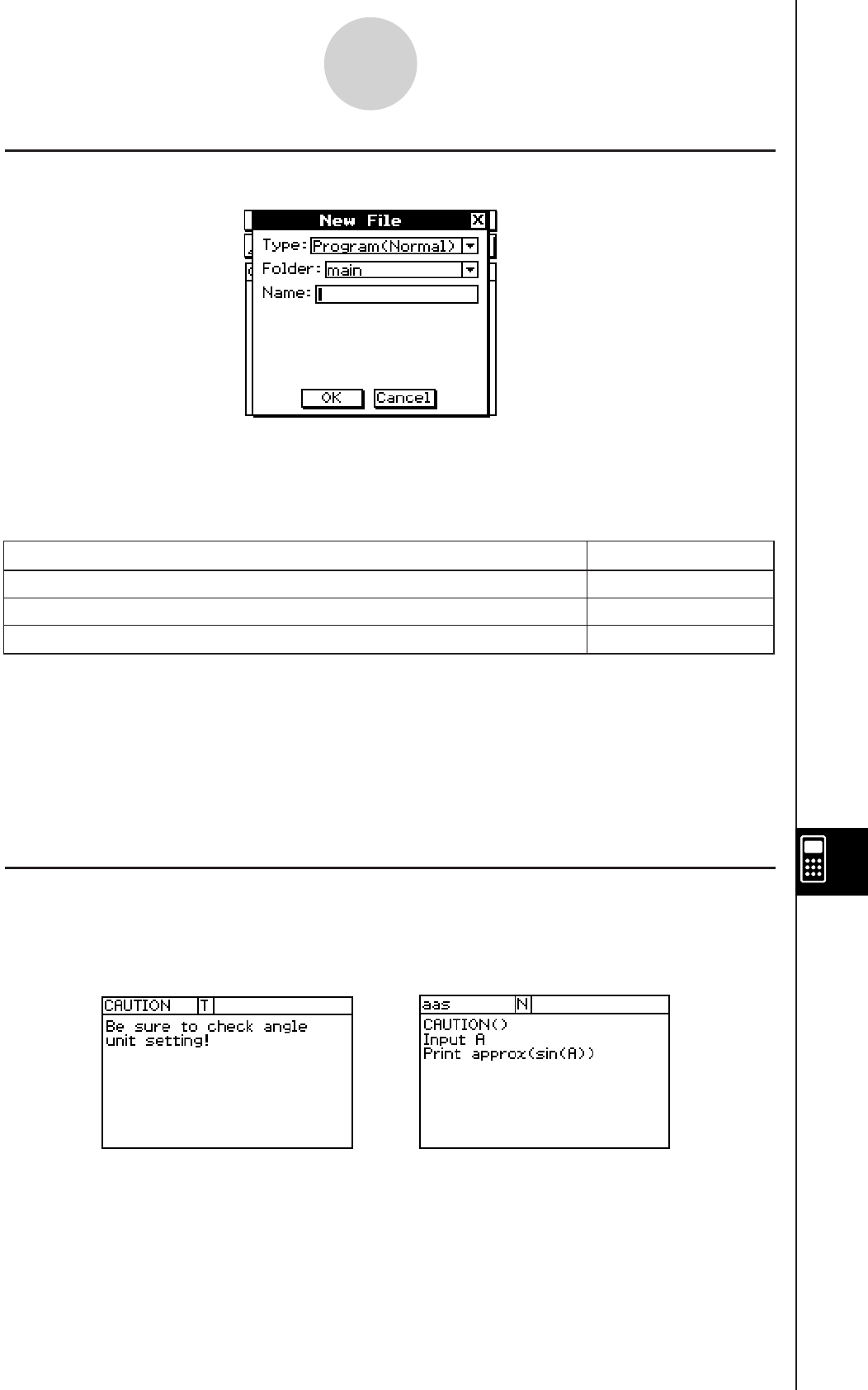
20060301

k Specifying the File Type

Tapping O or tapping [Edit] and then [New File] on the Program Editor window displays the

dialog box shown above.

Tap the [Type] down arrow button and then select one of the options described below from

the list of options that appears.

Tip

• For information about text files, see “Using Text Files” below.

• For information about user-defined functions, see page 12-5-1.

• Program files can be converted to text files, and vice versa. For more information, see “12-4

Managing Files”.

k Using Text Files

• Running a text file from the Program Loader window displays the contents of the file.

• Inserting a text file name inside a program causes the contents of the text file to be

displayed when execution reaches the name.

Example:

Program file Program(Normal)

Text file Program(Text)

User-defined function file Function

Select this option:To specify this type of file:

12-2-4

Creating a New Program

File Name: “CAUTION” Program that displays contents of

“CAUTION” file

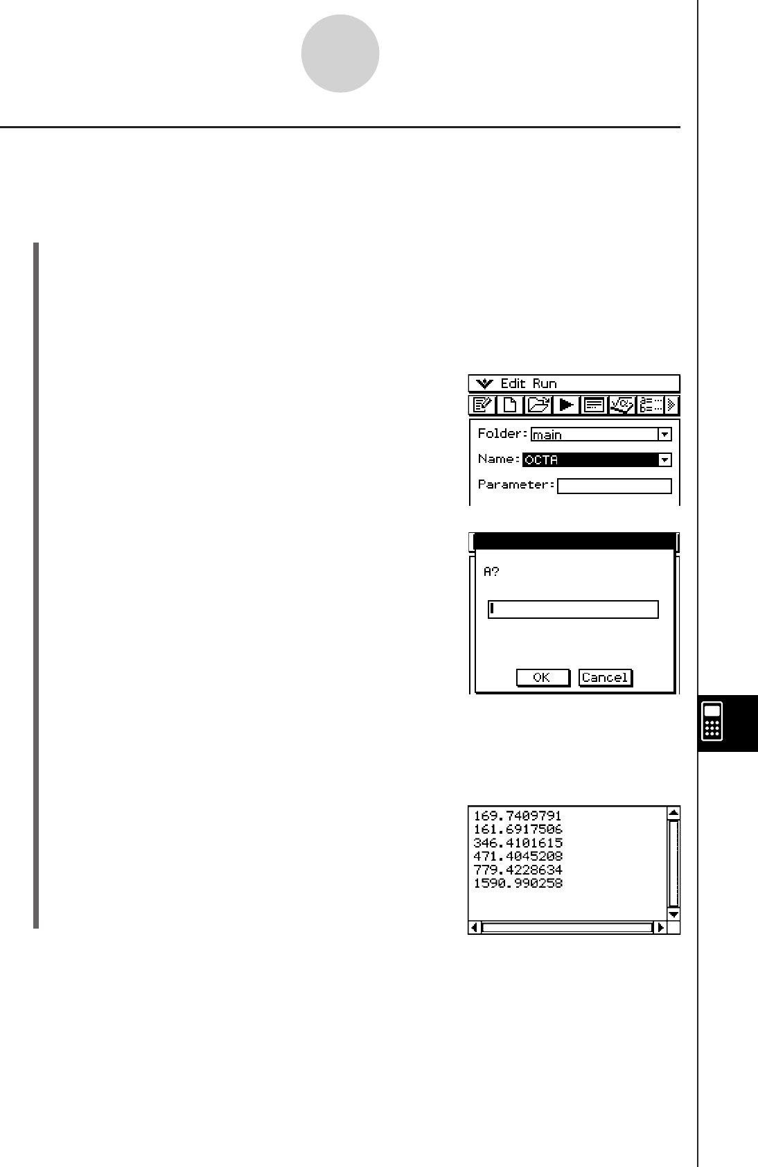
20060301

12-2-5

Creating a New Program

Running a Program

The following procedure shows how to run the sample program we input under “Creating and

Saving a Program” on page 12-2-1.

u ClassPad Operation

(1) Display the Program Loader window.

• From the Program Editor window, tap ), or tap O and then [Program Loader].

• From another application, tap m and then p.

• This causes the Program Loader window to appear.

(2) Tap the [Folder] down arrow button, and then select the name of the folder you want.

(3) Tap the [Name] down arrow button, and then tap

the name of the file you input in step (3) of the

example on page 12-2-2.

(4) Tap

p, or tap [Run] and then [Run Program] to

run the program.

(5) Input a side length of 7 and tap [OK] twice.

7 [OK] [OK]

(6) Tap the Program Loader window and repeat steps (4) and (5) for sides of length 10 and

15.

p10 [OK] [OK]

p15 [OK] [OK]

Tip

• In step (4) of the above procedure, you can specify parameters before running the program.

For more information, see “Configuring Parameter Variables and Inputting Their Values” on page

12-2-7.

• You can run a program from the Main application or the eActivity application. For more

information, see “2-13 Running a Program in the Main Application.”

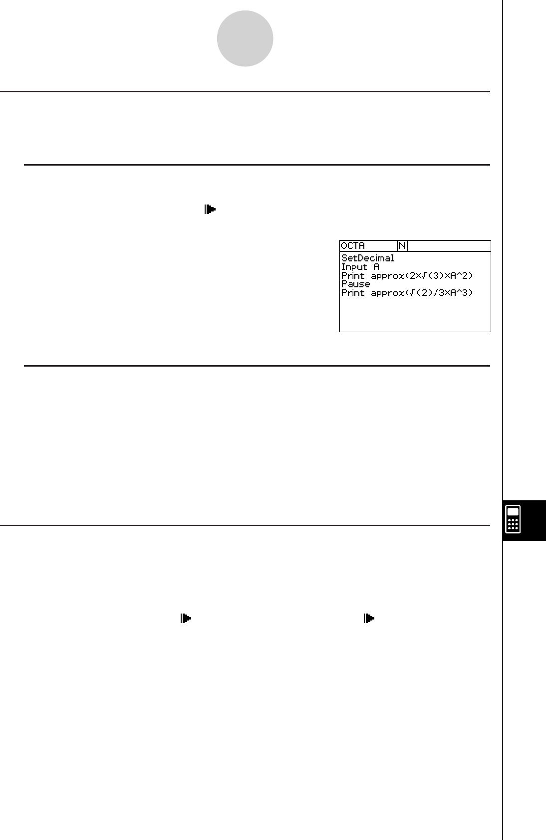
20060301

12-2-6

Creating a New Program

Pausing Program Execution

You can specify where execution of a program should pause by including either a Pause

command or a Wait command inside the program.

k Using the Pause Command

A Pause command causes program execution to pause when it reaches that point. To

resume program execution, tap the button on the right side of the status bar (which will

also cause the button to disappear).

Example

k Using the Wait Command

The syntax of the Wait command is: Wait

<seconds>. When program execution reaches

the Wait command, it pauses for the specified number of seconds and then resumes

automatically. If you do not specify a value for the number of seconds, execution remains

paused until you tap the screen or press a key.

Tip

• To input the Pause or Wait command, tap [Ctrl] on the menu bar, tap [Control], and then select

the command you want.

Terminating Program Execution

Pressing c while a program is running terminates the program.

Tip

• Pressing

c does not terminate the program if program execution is already paused by the

Pause command (indicated by on the status bar). In this case, tap to resume program

execution, and then press c.

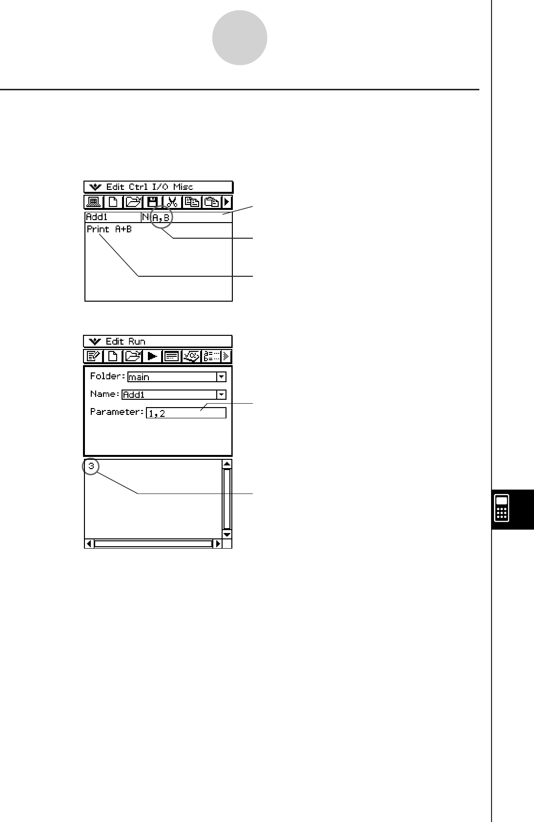
20060301

12-2-7

Creating a New Program

Configuring Parameter Variables and Inputting Their Values

If you input the names of variables used in a program into the parameter variable box when

inputting or editing a program on the Program Editor window, you will be able to input values

for the variables on the Program Loader window when you run the program.

Example

Tip

• When running a program that includes parameter variables, be sure to correctly specify the

values of the parameters. An error will occur if the number of values you input is not consistent

with the number of parameter variables.

Program Loader window

Program Input

Indicates variables named “A” and

“B” are used within the program.

When running the program, inputting

values for “A” and “B” calculates the

total of the two values.

Parameter value input box

Inputting 1, 2 before running the program assigns

A = 1 and B = 2.

Executing the program produces the result

A + B = 1 + 2 = 3.

Parameter variable box

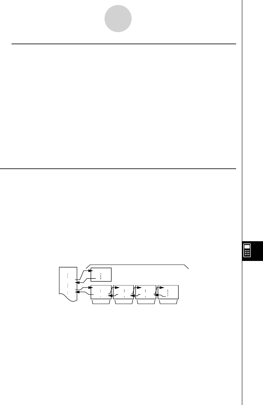
20060301

Using Subroutines

Including the name of another program file inside of a program causes execution to jump

to the specified program file. The program that execution jumps from is called the “main

program”, while the program to which execution jumps is called a “subroutine”.

When program execution returns to the main program, it resumes from the point immediately

after the command that jumped to the subroutine.

Tip

• Note that any program can be a subroutine. The thing that makes any program a subroutine is

being jumped to from another program.

Main Program Subroutines

Level 1 Level 2 Level 3 Level 4

Subroutines can be used in a variety of ways to help make calculations easier. Let’s say

you have a formula that needs to be calculated more than once in a program, or that needs

to be calculated by a number of different programs. Simply store the formula as a separate

program file (subroutine), and then you can jump to the program file that contains the formula

whenever you need it.

12-2-8

Creating a New Program

CEIJ

E ( ) I ( ) J ( )

D ( )

C ( )

kLocal Variables

A local variable is a variable that can be created temporarily and used in a program. Use the

Local command to create a local variable.

Syntax: Local

<variable name> ( indicates a space.)

Example: Local abc

The above creates a local variable named “abc”.

Tip

• Local variables are deleted automatically after execution of a program is complete.

• Note that local variables are stored in their own special folder, so local variable names do not

affect the names of other variables in ClassPad memory. Because of this, you do not need to

worry if you assign a local variable a name that is already being used by another type of variable.

• Variables that are specified as parameter variables within a program are automatically treated

as local variables. Variables created with the Define command are also automatically treated as

local variables.

20060301

Example 1: Jumping to a subroutine without assigning values to the subroutine’s parameter

variables

Main Program

Input A

Input B

Sub1( ) ← Jumps to subroutine program “Sub1”

Print C

Subroutine (Program Name: “Sub1”)

A+B S C

Return

Example 2: Jumping to a subroutine while assigning values to the subroutine’s parameter

variables

• In this example, the main program assigns values to parameter variable “E” in a subroutine

named “Sub1”, and to parameter variables “F” and “G” in a subroutine named “Sub2”.

Main Program

Input A

Input B

Sub1(A) ← Assigns the value of main program variable “A” to the parameter variable (E) in

subroutine “Sub1”, and then jumps to subroutine “Sub1”.

Print C

Sub2(A,B) ← Assigns the values of main program variables “A” and “B” to the parameter

variables (F and G) in subroutine “Sub2”, and then jumps to subroutine “Sub2”.

Print D

Subroutine Program 1 (Program Name “Sub1”)

E × 2 S C ← Requires input of variable name E into the parameter variable box.

Return

Subroutine Program 2 (Program Name “Sub2”)

F + G S D ← Requires input of variable names F and G into the parameter variable box.

Return

Tip

• The subroutine does not need to be located in the current folder. To specify a subroutine named

“Sub1” that is located in a folder named “f1”, for example, you would specify “f1\Sub1(

)”.

12-2-9

Creating a New Program

20060301

12-3 Debugging a Program

A programming error that causes a program to behave in a manner not intended by the writer

of the program is called a “bug”. Finding and eliminating such errors is called “debugging the

program”.

Any of the following conditions can indicate that your program has a bug and requires

debugging.

• If an error message appears when you try to save the program

• If an error message appears when you try to run the program

• When a program produces some abnormal or unexpected result

Debugging After an Error Message Appears

When an error occurs, a dialog box appears to explain the cause of the error. Carefully

read the text of the error message and then tap its [OK] button. This closes the dialog box

and positions the cursor on at the location where the error occurred. Make the necessary

corrections in accordance with the explanation provided by the error message.

Tip

• If the cause of the error cannot be specified for some reason, tapping [OK] on the error message

dialog box displays the Program Loader window, without positioning the cursor at the location of

the error.

• In the case of a program for which editing is prohibited (a program for which “EXE” is indicated

as the variable data type), tapping [OK] on the error message dialog box displays the Program

Loader window, without positioning the cursor at the location of the error.

Debugging a Program Following Unexpected Results

If execution of a program produces unexpected or abnormal results, carefully read through

the program and correct errors as required.

The following commands can come in handy when debugging a program to locate

unexpected results.

12-3-1

Debugging a Program

Move the cursor to the beginning of the program Edit - Search - Jump to Top

Move the cursor to the end of the program Edit - Search - Jump to Bottom

Execute this command:To do this:

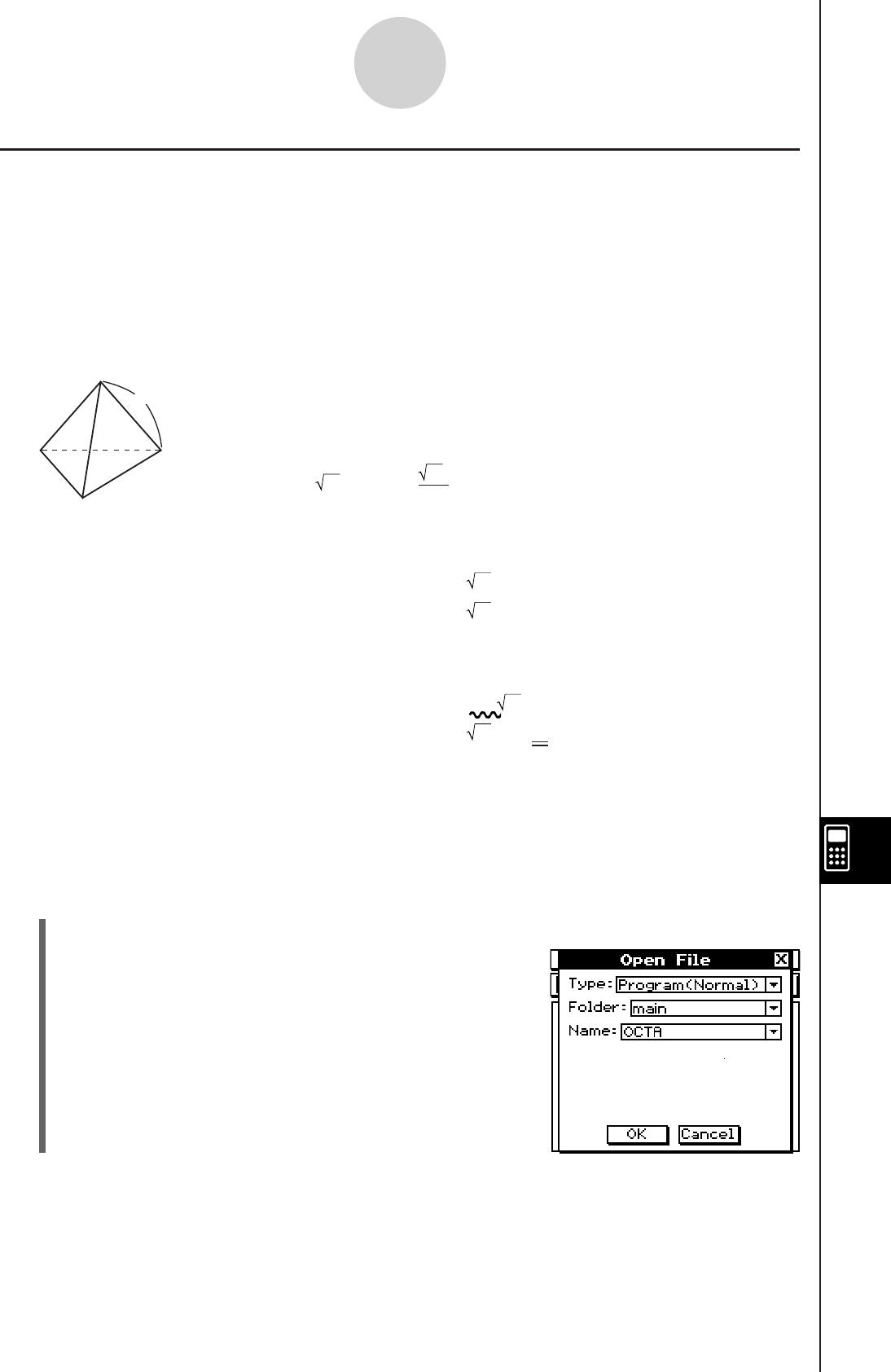
20060301

Modifying an Existing Program to Create a New One

You can use the procedure described below to recall an existing program, modify it, and then

run the result as a new program. This helps reduce key input requirements.

The following shows how to modify the “OCTA” program we created on page 12-2-1 to

handle tetrahedrons.

Example: To create a program named “TETRA” that calculates the surface areas (cm2) and

volumes (cm3) of three regular tetrahedrons, the lengths of whose sides are 7, 10,

and 15 cm

The following formulas calculate the surface area S and volume V of a

regular tetrahedron for which the length of one side A is known.

The following is the program required for this example.

Length of One Side A ..........Input A

Surface Area S ....................Print approx( (3) × A^2)

Volume V ............................Print approx( (2) ÷ 12 × A^3)

The following is the “OCTA” program (page 12-2-1).

Length of One Side A ..........Input A

Surface Area S ....................Print approx(2 × (3) × A^2)

Volume V ............................Print approx( (2) ÷ 3 × A^3)

A comparison of the two programs indicates that the following modifications of the “OCTA”

program will produce a program that performs the calculations required by this example.

• Delete “2×” (underlined with a wavy line above).

• Change 3 to 12 (underlined with double lines above).

u ClassPad Operation

(1) On the application menu, tap p.

(2) Tap

~, or tap [Edit] and then [Open File].

12-3-2

Debugging a Program

S = 3 A2, V =

12 A3

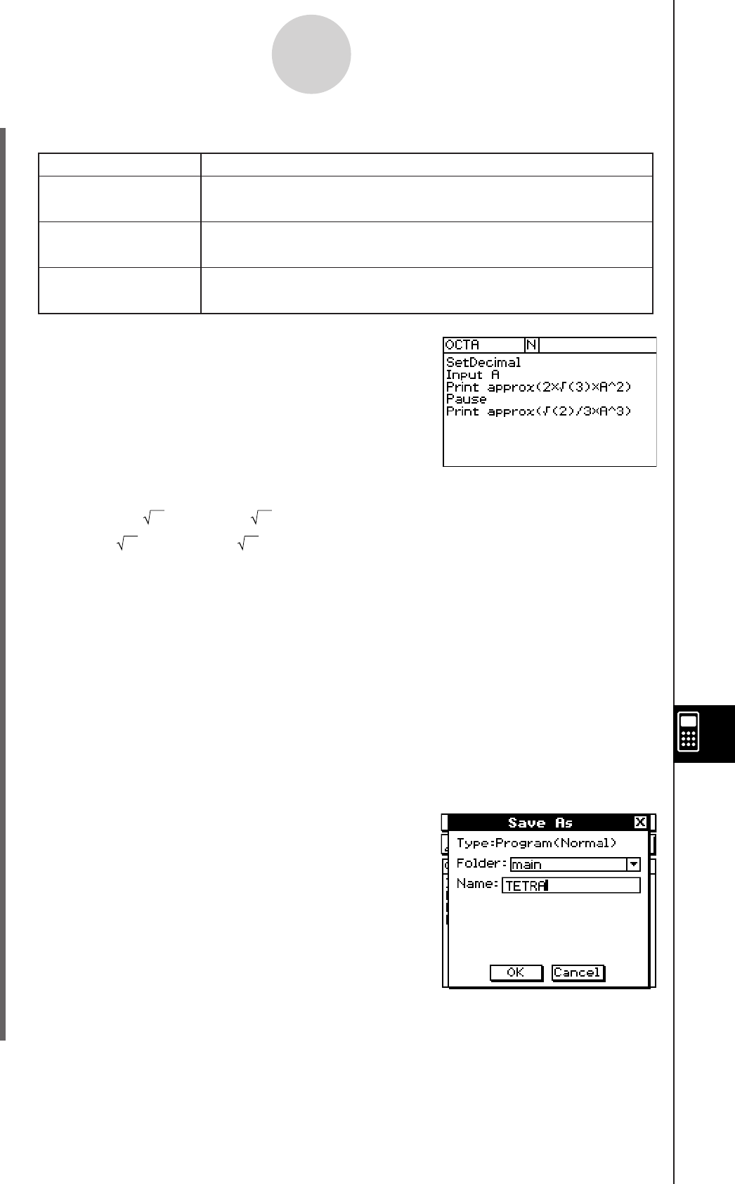
20060301

(3) Select the program you want to open and edit, as described below.

12-3-3

Debugging a Program

(4) Tap [OK].

Folder

Type Tap the down arrow button, and then select

“Program(Normal)”.

Tap the down arrow button, and then select the folder that

contains the program you want to edit.

Name Tap the down arrow button, and then select the name of the

program you want to open (OCTA).

Do this:

For this setting:

(5) Edit expressions and commands as required.

a. Change 2 × (3) × A^2 to (3) × A^2

b. Change (2)/3 × A^3 to (2)/12 × A^3

c. Delete Pause

u To delete data

Use the cursor key to move the cursor to the data you want to delete, and then press

K. Or, highlight the data you want to delete and press K.

u To input data

Use the cursor key or stylus to move the cursor to the location where you want to

insert data, and then use the soft keyboard or the keypad to make the changes you

want.

(6) Save the new program.

u To retain the original program and save the new program under a different

name

• Tap [Edit] and then [Save As].

• Use the soft keyboard to type the name you

want to assign to the new program into the

[Name] box.

• Tap [OK].

u To replace the original program with the new program

• Tap {, or tap [Edit] and then [Save File].

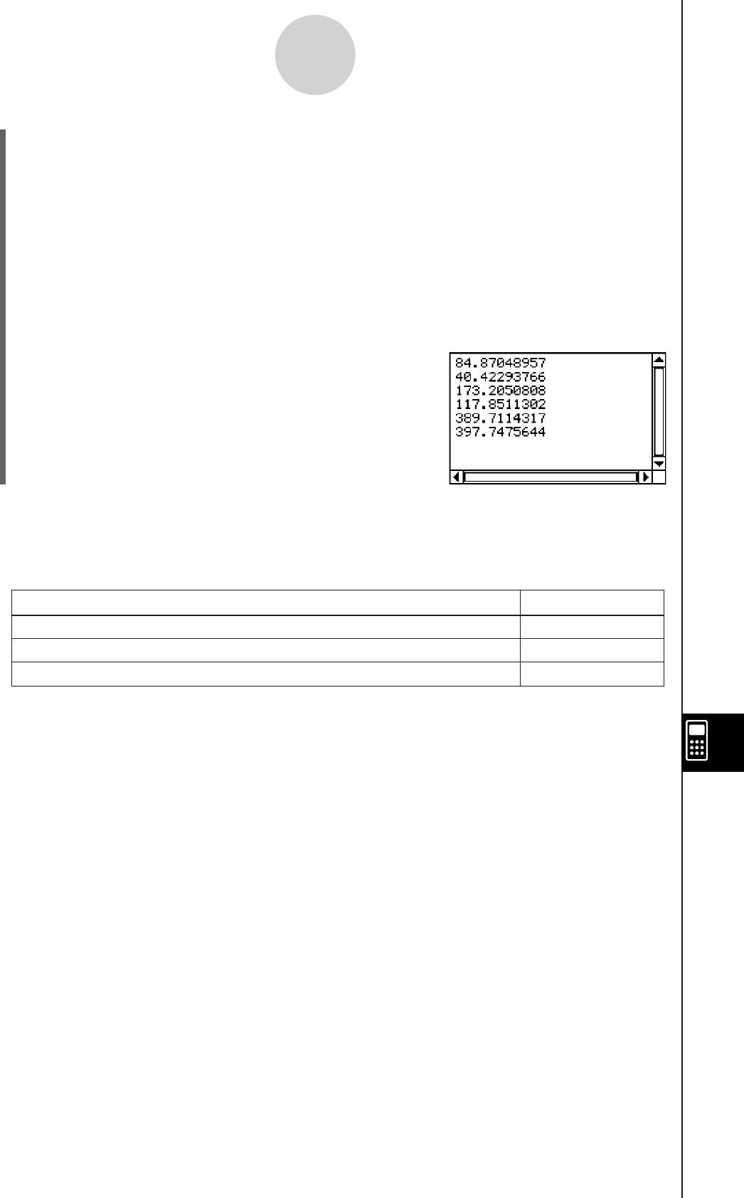
20060301

(7) After saving the program, tap ), or tap O and then [Program Loader] to display the

Program Loader window.

(8) On the dialog box that appears, tap the [Name] down arrow button, and then tap the

name of the file you input in step (6) (TETRA).

(9) Tap

p, or tap [Run] and then [Run Program].

• This runs the program.

(10) Input 7 for the length of side A and tap [OK] twice.

7 [OK] [OK]

(11) Repeat steps (9) and (10) for sides of length 10 and 15.

p10 [OK] [OK]

p15 [OK] [OK]

12-3-4

Debugging a Program

Tip

• To edit a program and save it without running it, perform the above procedure up to step (7),

and then tap [Edit] and then [Close File]. If the “WARNING! Save changes?” dialog box appears,

perform one of the operations described below.

Save and close the program Yes

Close the program without saving No

Return to the Program Editor window without saving the program Cancel

Tap this button:To do this:

Tapping [Yes] or [No] causes the message “No File” to appear on the display.

20060301

Searching for Data Inside a Program

You can search for data inside a program by specifying a keyword.

Example: To search for the letter “A” within the “OCTA” program

u ClassPad Operation

(1) From the Program Editor window, select the program you want to search (“OCTA” in

this example).

(2) Tap [Edit], [Search], and then [New Search]. Or, tap to scroll the toolbar and tap e.

• This displays a dialog box for inputting the search keyword.

(3) Enter the data you want to find and then tap [OK].

• This causes the cursor to appear in front of the data you specified (“A” in this

example).

(4) Tap [Edit], [Search], and then [Search Next]. Or, tap to scroll the toolbar and tap r.

• This causes the cursor to appear in front of the next instance of the data you specified

(“A” in this example).

(5) Repeat step (4) as many times as you want.

Tip

• The message “Not Found” appears if the keyword you specify does not exist in the program.

• The keyword you specify for [New Search] remains in effect until you close the Program Editor

window. Executing the [Search Next] command when there is no keyword specified by [New

Search] causes the error message “No word is specified” to appear.

12-3-5

Debugging a Program

20060301

12-4 Managing Files

Renaming a File

Use the following procedure when you want to change the name of a file.

u ClassPad Operation

(1) Tap

5 to display the Variable Manager.

• This displays a list of folders.

• You may need to tap the icon and scroll the toolbar to see the 5 icon.

(2) Tap the name of the folder that contains the file you want to rename.

• This displays all of the files/variables in the folder.

(3) Tap the name of the file you want to rename.

(4) Tap [Edit] and then [Rename].

• This displays a dialog box for inputting a file name.

(5) Enter the new file name and then tap [OK].

(6) Tap [Close] twice to close the Variable Manager.

Tip

• See “1-8 Using the Variable Manager”.

Deleting a Program

The following procedure deletes a program file name, which also deletes the program.

u ClassPad Operation

(1) Tap

5 to display the Variable Manager.

• This displays a list of folders.

(2) Tap the name of the folder that contains the file you want to delete.

• This displays all of the files/variables in the folder.

(3) Select the check box next to the file you want to delete.

• You can select one file or multiple files for deletion.

(4) Tap [Edit] and then [Delete].

(5) On the confirmation dialog box that appears, tap [OK] to delete the selected file, or

[Cancel] to cancel the operation without deleting anything.

(6) Tap [Close] twice to close the Variable Manager.

Tip

• Be sure to close a file before you try to rename or delete it. Trying to rename or delete an open

file will cause an error.

• See “1-8 Using the Variable Manager”.

12-4-1

Managing Files

20060301

Changing the File Type

You can use the following procedures to change the file type.

uTo change a program file to a text file

While a program file is open, tap [Edit], [Mode Change], and then ['Text].

uTo change a text file to a program file

While a text file is open, tap [Edit], [Mode Change], and then ['Normal].

Tip

• Note that the above operations are not possible while a user-defined function is open.

uTo change an editable file to an edit prohibited program file

(1) Open the program file you want to make edit prohibited.

(2) Tap [Edit] and then [Compress].

• This displays a dialog box for inputting the backup file name. The backup file is a

copy of the original (editable) file, which you can keep on hand if you have trouble

changing an edit prohibited program file back to an editable file.

(3) Enter the backup file name and then tap [OK].

• This saves two copies of the file. One is an edit prohibited program file under the name of

the original (editable) file. The other is an editable backup file, which is created under the

name you specify in step (3), above.

Original File (editable): sample

Specified File Name: sample2

Resulting Files: sample (non-editable)

sample2 (editable)

• An edit prohibited program file cannot be opened from the Program Editor window.

• Edit prohibited program files are displayed in the Variable Manager as “EXE” type files.

• Tapping [Cancel] instead of [OK] in step (3) quits the procedure without changing the file

type.

12-4-2

Managing Files

20060301

12-5 User-defined Functions

ClassPad lets you configure calculation operations as user-defined functions, which can then

be used inside of numeric expressions just like its built-in functions. User-defined functions

can also be called up in other applications.

• The Program Editor window is used for creating user-defined functions.

• User-defined functions are stored in ClassPad memory as “Function” type variables.

Naming, storage, and folder rules are identical to those for user variables.

Creating a New User-defined Function

This procedure is identical to that for storing a program.

• Anything you enter on the Program Editor window is stored as a user variable.

Example

• Function Name: f4

• Expression: x × (x + 1) × (x – 2)

u ClassPad Operation

(1) On the application menu, tap p.

(2) Tap

O, or tap [Edit] and then [New File].

(3) On the screen that appears, configure the settings described below.

12-5-1

User-defined Functions

(4) After everything is the way you want, tap [OK].

(5) Input the expression you want.

Do this:

For this setting:

Type

Folder

Name

Tap the down arrow button and then select “Function”.

Tap the [Folder] down arrow button and then select the name of

the folder where you want to save the user-defined function.

Enter up to eight bytes for the user-defined function name.

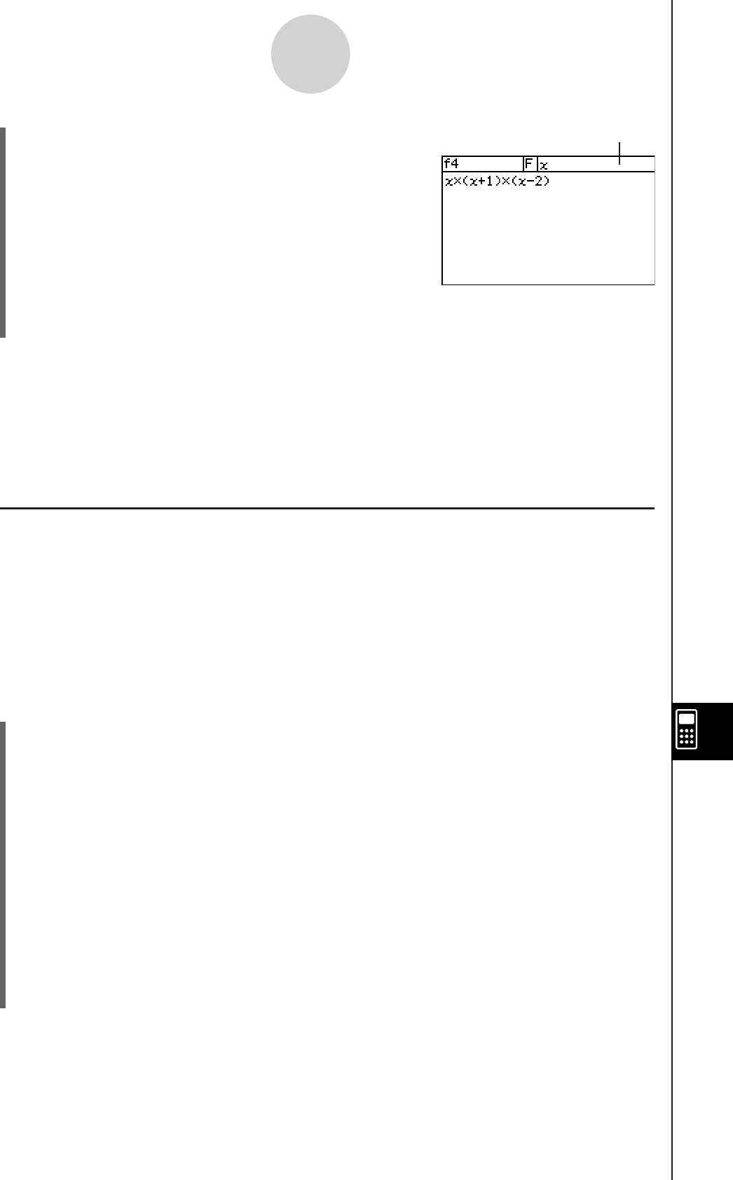
20060301

(6) After the function is the way you want, tap {, or tap [Edit] and then [Save File] to save

it.

Tip

• A user-defined function can contain only a single mathematical expression.

An error “Invalid in a Function or Current Expression” occurs if a user-defined function contains

multiple expressions, or is followed by a carriage return.

• A user-defined function cannot contain any command.

k Creating a User-defined Function Using the Define Command

The procedure below describes how to create a user-defined function by executing the

Define command from the Main application.

Syntax: Define



[<folder name>\ ]<function name>([<variable name>[,<variable name>...]])

=<expression>

• Items inside of brackets ([ ]) can be skipped.

•

 indicates a space.

u ClassPad Operation

(1) On the application menu, tap J.

(2) Press

k, and then tap the ( (catalog) tab.

(3) On the catalog (cat) keyboard that appears, tap the [Form] down arrow button, and

then select [Cmd].

(4) Scroll the list of commands until the Define command is visible, and then tap Define to

select it.

(5) Tap [INPUT] to input the Define command.

(6) Input the function you want to define.

Example 1: Define folder1 \ f1(x) = 2x + 1 (where folder1 is an existing folder)

Example 2: Define f2(x, y) = 2x + 3y + 1

Example 3: Define sen(x) = sin (x)

(7) Tap

w to store the function.

12-5-2

User-defined Functions

• Input user-defined function arguments as parameter

variables. For more information about parameter

variables, see page “Configuring Parameter Variables

and Inputting Their Values” on page 12-2-7.

Parameter variable

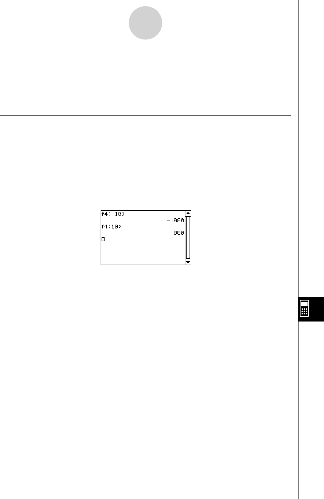
20060301

Tip

• You can include up to 99 arguments in a function.

• If you do not specify a folder, the function is stored in the current folder.

• A function defined using the Define command can contain only a single expression. You cannot

link multiple expressions or commands using colons (:) or carriage returns.

Executing a User-defined Function

The following is the syntax for executing a user-defined function.

<function name> ([<argument>[,<argument>...]])

The following shows an example of how to perform a manual calculation in the Main

application.

Example: The following is a function created under “Creating a New User-defined Function”

on page 12-5-1.

f4 (x) = x × (x + 1) × (x – 2)

12-5-3

User-defined Functions

Tip

• You can use the following steps to recall user-defined functions stored in the “library” folder using

the catalog (cat) keyboard. For more information about the “library” folder, see “1-7 Variables and

Folders”.

1. Press k.

2. Tap the ( (catalog) tab.

3. On the catalog (cat) keyboard, tap the [Form] down arrow button, and then select [USER].

4. Scroll the list of functions until the function you want is visible, and then tap the function name

you want.

5. Tap [INPUT].

20060301

Editing a User-defined Function

To edit an existing user-defined function, use the same procedures as those described under

“Modifying an Existing Program to Create a New One” on page 12-3-2. Editing procedures

are the same, regardless of whether you originally created the function using the Define

command or Program Editor.

Deleting a User-defined Function

To delete an existing user-defined function, use the same procedure as the one described

under “Deleting a Program” on page 12-4-1. The delete procedure is the same, regardless of

whether you originally created the function using the Define command or Program Editor.

12-5-4

User-defined Functions

20060301

12-6 Program Command Reference

Using This Reference

The following table shows the conventions that are used in the descriptions of this section.

12-6-1

Program Command Reference

A boldface word, like Input

It means this:If you see something like this:

The boldface word is a command.

10 This is a constant.

10 + 20 This is an arithmetic expression.

AThis is a variable.

"AB" This is a character string.

<string> You should input what is described inside the

angle brackets (< >). When inputting the

command, do not include the angle brackets.

{ } You need to select one of the multiple options

enclosed inside the braces ({ }). When inputting

the command, do not include the braces.

This indicates a space. Always make sure you

input one space between a command and its

parameters.

Example: GetKey<variable name>

[ ] Anything inside brackets ([ ]) is optional. You

can input the item inside the brackets or omit

it. When inputting the command, do not

include the brackets.

…The term to the left of ellipsis (…) can be input

more than once or repeated.

Tip

• In addition to program commands, this section also includes descriptions of the following

functions.

• pxlTest(

• plotTest(

• strToExp(

20060301

Program Application Commands

k Program Notation

(Carriage Return)

Function: Performs a carriage return operation.

Description

In Program Editor, tap the w button to input a carriage return.

• The carriage return can be used in a user program. It cannot, however, be used in a

manual calculation performed in the Main application.

’ (Comment)

Function: Any text following this symbol is not executed. You can use this command to

include comment text in your program.

Description

Any line that starts with the comment symbol (’) is treated as comment text, which is skipped

during program execution.

: (Multi-statement Command)

Function: Use this command to link a series of statements into a multi-statement (on a

single line).

Description

The multi-statement command can be used in a user program. It cannot, however, be used

in a manual calculation performed in the Main application.

12-6-2

Program Command Reference

20060301

k Input

GetKey

Syntax: GetKey



Function: This command assigns the code number of the last key pressed to the specified

variable.

Description

• This command assigns the code number of the last key pressed to the specified variable.

The following shows a list of available code numbers.

12-6-3

Program Command Reference

Key Code

048

149

250

351

452

553

654

755

856

957

.46

e147

+43

-45

*60944

/47

=61

Key Code

(40

)41

,44

z45

x60856

y60857

Z60858

{94

E13

f28

c29

d30

e31

k144

K (Back Space) 8

o145

c12

• 0 is assigned to the variable if no key was pressed.

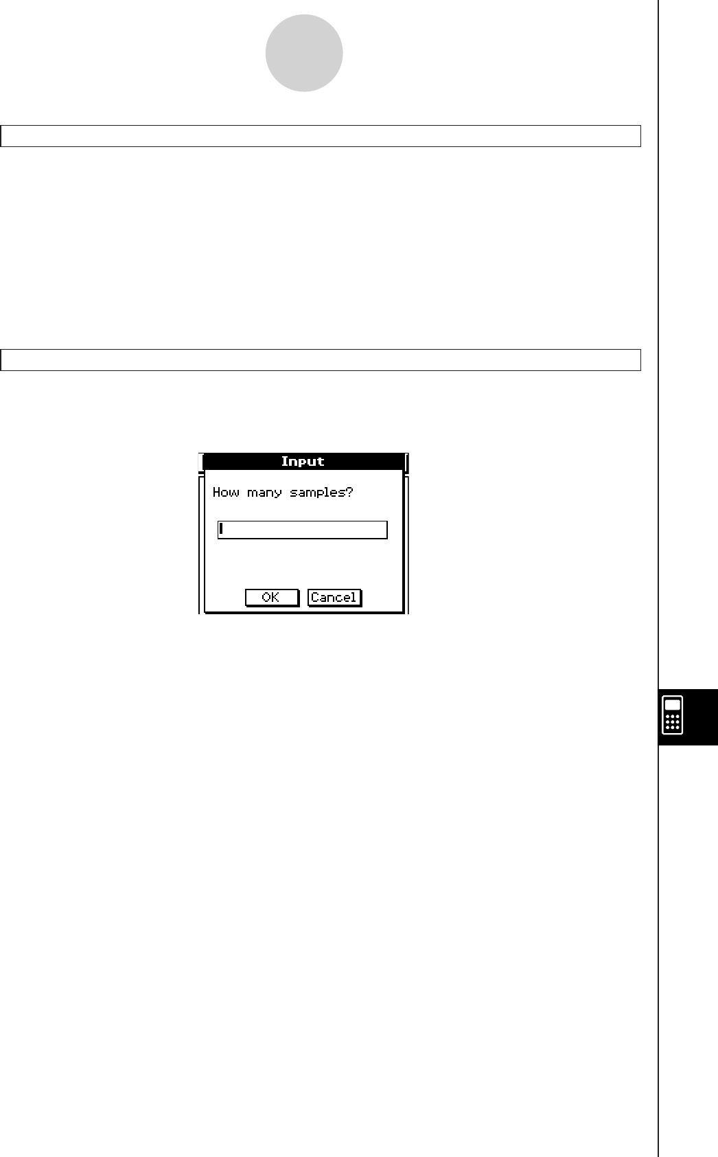
20060301

12-6-4

Program Command Reference

GetPen

Syntax: GetPen<variable name 1>, <variable name 2>

Function: This command assigns the coordinates of the point tapped on the screen to a

specified variable.

Description

This command assigns the x-coordinate (horizontal axis) to <variable 1> and the

y-coordinate (vertical axis) to <variable 2>. The coordinates at the point in the upper left

corner of the screen are (1, 1), and coordinate values are specified in the range of 1 to 160

for the x-coordinate and 1 to 240 for the y-coordinate.

Input

Syntax: Input



<variable name>[,"<string 1>"[,"<string 2>"]]

Function: When program execution reaches the Input command, the user is prompted for

input of a value, which is assigned to the specified variable.

Description

• If you do not specify anything for "<string 1>", the prompt “<variable name>?” appears by

default.

• The text specified for "<string 2>" is used as the input dialog box title.

• The Input command pauses program execution and displays a dialog box that contains the

text string indicated by "<string 1>" and an input box. A text string enclosed within quotation

marks (" ") or a variable name can be specified for "<string 1>".

• Specifying a long text string can cause part of it to be cut off when it is displayed in the

dialog box.

• When the dialog box appears, input a value into the input box and then tap [OK]. This

closes the dialog box, assigns the input value to the applicable variable and resumes

program execution.

• Tapping [Cancel] on the dialog box terminates program execution.

• During execution of the Input command, program execution is paused for input of data.

While a program is paused, you can input individual mathematical expressions only. You

cannot input commands or multiple expressions joined by colons (:).

20060301

InputFunc

Syntax: InputFunc



<user-defined function name> (<argument>[,<argument>…])

[,"<string 1>"[,"<string 2>"]]

Function: When program execution reaches the InputFunc command, the user is prompted

to input the contents of the user-defined function.

Example: InputFunc v(v0, t), "To define function v0(m/s), t(sec)", "define function"

Description

• If you do not specify anything for "<string 1>", the prompt “<variable name>?” appears by

default.

• The text specified for "<string 2>" is used as the input dialog box title.

• The InputFunc command pauses program execution and displays a dialog box that

contains the text string indicated by "<string 1>" and an input box. The dialog box that

appears is identical to the Input command dialog box. A text string enclosed within

quotation marks (" ") or a variable name can be specified for "<string 1>".

• Specifying a very long display text string can cause part of it to be cut off when it is

displayed in the dialog box.

• When the dialog box appears, input an expression into the input box and then tap [OK].

This closes the dialog box, assigns the input expression to the applicable variable and

resumes program execution.

• Tapping [Cancel] on the dialog box terminates program execution.

InputStr

Syntax: InputStr



<variable name>[,"<string 1>"[,"<string 2>"]]

Function: When program execution reaches the InputStr command, the user is prompted

for input of a string, which is assigned to a variable.

Description

• The InputStr command pauses program execution and displays a dialog box that contains

the text string indicated by "<string 1>" and an input box. The dialog box that appears is

identical to the Input command dialog box. A text string enclosed within quotation marks

(" ") or a variable name can be specified for "<string 1>".

• Specifying a long display text string can cause part of it to be cut off when it is displayed in

the dialog box.

• When the dialog box appears, input a string into the input box and then tap [OK]. This

closes the dialog box, assigns the input string to the applicable variable and resumes

program execution.

• Tapping [Cancel] on the dialog box terminates program execution.

• The text specified for "<string 2>" is used as the input dialog box title.

• If you do not specify anything for "<string 1>", the prompt “<variable name>?” appears by

default.

12-6-5

Program Command Reference

20060301

12-6-6

Program Command Reference

k Output

About the Program Output window

The “Program Output window” shows text displayed by program execution. The term “Program

Output window” does not include dialog boxes displayed by Message and other commands.

• Only one Program Output window can be stored at a time. Executing the ClrText command

or using Program Loader to execute a text file clears the currently stored Program Output

window.

• The Program Output window can be displayed by tapping O and then [Program Output],

or by tapping _ on the Program Loader window. The Program Output window also

appears whenever the DispText command is executed in a program.

ClrText

Syntax: ClrText

Function: This command clears text from the Program Output window.

DispText

Syntax: DispText

Function: This command displays the Program Output window.

Description: You can use this command to re-display the Program Output window following

display of the Graph window, Table window, or other window.

Example: To re-display the Program Output window after it has been cleared by a

graphing operation or some other operation

GraphType "y="

Define y1(x) = (x)

GTSelOn 1

ViewWindow –7.7, 7.7, 1, –3.8, 3.8, 1

0 S FStart

10 S FEnd

1 S FStep

ClrText ← Initializes the Program Output window.

Print "y1(x) = (x)" ← Displays the graph expression on the Program Output window.

Print "Tap Continue button." ←

Tells user what to do to continue program execution after reading the

message.

Pause ← Pauses program execution to allow user to read Program Output window message.

DrawGraph ← Draws the graph.

DispFTable ← Displays the table.

Pause ← Pauses program execution to allow for graph and table editing. Program Output window is not

displayed at this time.

DispText ← Re-displays the Program Output window.

Pause ← Pauses program execution to allow user to read Program Output window message.

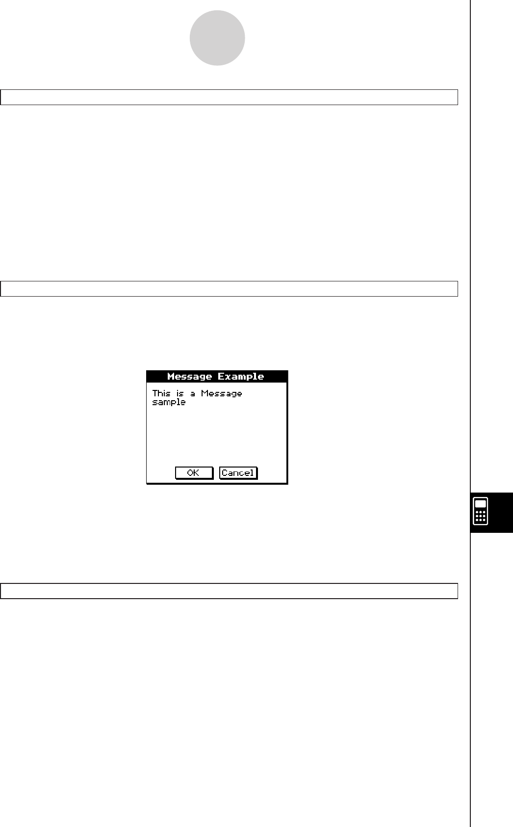
20060301

Locate

Syntax 1: Locate



<x-coordinate>, <y-coordinate>, <expression>

Syntax 2: Locate



<x-coordinate>, <y-coordinate>, "<string>"

Function: This command displays the result of the specified expression or the specified text

string at the specified coordinates on the display screen.

Description

• The coordinates of the point at the upper left corner of the effective area of the Locate

command are (1, 1), and coordinate values can be specified in the range of 1 to 290 for the

x-coordinate and 1 to 290 for the y-coordinate. Note, however, that the actual dot count of

the ClassPad screen is 160 × 240.

• An expression result is displayed as a single line.

Message

Syntax: Message



"<string 1>" [,"<string 2>"]

Function: This command pauses program execution and displays a dialog box containing

the text specified by "<string 1>". The text is positioned flush top left. The text

specified for "<string 2>" is used as the dialog box title.

12-6-7

Program Command Reference

Description

• Text strings enclosed within quotation marks (" ") or variable names can be specified for

"<string 1>" and "<string 2>".

• Tapping [OK] closes the dialog box and resumes program execution.

• Tapping [Cancel] terminates program execution.

Syntax 1: Print



Syntax 2: Print



"<string>"

Function: This command displays the result of the specified expression or the specified text

string.

Description

An expression result is displayed as a single line. When the result is a long expression,

fraction, or string, it may not fit on the display. In such a case, use the PrintNatural

command instead.

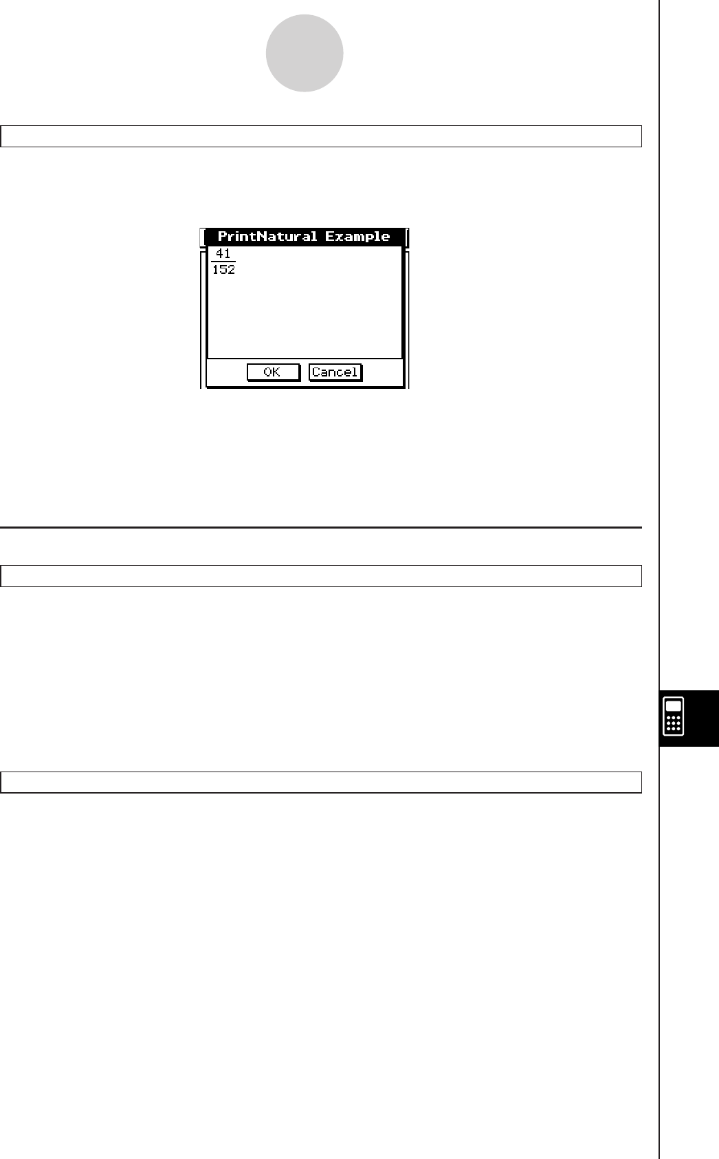
20060301

PrintNatural

Syntax: PrintNatural



<expression>[,"<string>"]

Function: This command pauses program execution and displays the result of the specified

expression in natural format.

12-6-8

Program Command Reference

Description

• A text string enclosed within quotation marks (" ") or a variable name can be specified for

"<string>".

• Tapping [OK] closes the dialog box and resumes program execution. Tapping [Cancel]

terminates program execution.

k Program Execution

Syntax: # <string variable name>

Function: This command specifies a string variable whose string is a variable name.

Example 1: When the content of variable exp1 is π and the content of variable str1 is “exp1”,

sin(#str1) calculates sin(π).

Example 2: To cause a folder to be created during program execution:

InputStr



name, "Foldername"

NewFolder



#name

Syntax 1:

S <variable name>

"<string>"

Syntax 2:

S <list element>

"<string>"

Syntax 3: <expression>

S <matrix element>

Function: With this command, the content of the expression on the left is evaluated, and the

result is assigned to the item on the right.

{ }

20060301

12-6-9

Program Command Reference

Break

Syntax: Break

Function: This command terminates a loop and causes execution to advance to the next

command following the loop process.

Description

• Break terminates a loop and causes execution to advance to the next command following

the loop process.

• Break can be used inside of a For, Do, While, or Switch process.

Define

Syntax: Define



[<folder name>\ ]<function name>([<variable name>[,<variable

name>...]]) =<expression>

• Items inside of brackets ([ ]) can be skipped.

Function: Creates a user-defined function.

Description: See page 12-5-2.

Do~LpWhile

Syntax: Do

[<statement>] …

LpWhile



<expression> is a condition that evaluates to true or false.

Function: The specified statements are repeated as long as the condition is true.

Description

• The statements between Do~LpWhile are repeated as long as the condition is true. When

the condition becomes false, execution jumps to the next command after the LpWhile

command.

• Since the condition comes after LpWhile, the condition is not evaluated until the end of the

loop is reached.

• You can use a multi-statement command (:) in place of the carriage return to separate

statements.

• It is always a bad idea to use the Goto command to exit a Do~LpWhile loop. Not only is it

poor programming, it can cause problems due to improper termination of internal processes

used by the loop operation.

20060301

For~To~(Step~)Next

Syntax:

For





[Step



<expression 3>]

[<statement>] …

<expression 1> is the initial value, <expression 2> is the end value, and <expression 3> is

the step.

Function

Anything between the For command and the Next command is repeated for a count starting

with the initial value of the control variable and ending when the control variable reaches the

end value. Each pass causes the value of the control variable to be changed by the value

specified by the step value. The loop is terminated whenever the control variable value

exceeds the end value.

Description

• 1 is used for the step if a step value is not specified.

• The initial value can be less than the end value, as long as a positive value is specified for

the step. In this case, the value of the control value is increased by the step with each pass.

• The initial value can be greater than the end value, as long as a negative value is specified

for the step. In this case, the value of the control value is decreased by the step with each

pass.

• You can use a multi-statement command (:) in place of the carriage return to separate

statements.

• It is always a bad idea to use the Goto command to exit a For~Next loop. Not only is it

poor programming, it can cause problems due to improper termination of internal processes

used by the loop operation.

Goto~Lbl

Syntax: Goto



Lbl



Function: This command causes program execution to jump to a specific location.

Description

• <label name> is a text string that is subject to the same rules as variable names.

• Goto and Lbl are used in pairs. Program execution jumps from Goto to the Lbl with the

same label name. A single Lbl can be used as the jump destination of multiple Goto

commands.

• This command can be used to loop back to the beginning of a program or to jump to any

location within the program.

• An error occurs if ClassPad is unable to find a Lbl with the same label as Goto.

• Note that the # command cannot be used in a label name.

12-6-10

Program Command Reference

20060301

If~Then~ElseIf~Else~IfEnd

Syntax 1: If



Then

[<statement>] …

IfEnd

Function 1

• If the expression is true, the statement in the Then block is executed. After that, execution

advances to the next statement after IfEnd.

• If the expression is false, execution advances to the next statement after IfEnd, without

executing the statement in the Then block.

Syntax 2: If



Then

[<statement>] …

Else

[<statement>] …

IfEnd

Function 2

• If the expression is true, the statement in the Then block is executed. After that, execution

advances to the next statement after IfEnd.

• If the expression is false, the statement in the Else block is executed instead of the Then

block. After that, execution advances to the next statement after IfEnd.

Syntax 3: If



Then

[<statement>]…

ElseIf



Then

[<statement>] …

IfEnd

Function 3

• If the expression is true, the statement in the If Then block is executed. After that,

execution advances to the next statement after IfEnd.

• If the If command expression is false, the ElseIf command expression is tested. If it is true,

the statement in the ElseIf Then block is executed. After that, execution advances to the

next statement after IfEnd. If it is false, execution advances to the next statement after

IfEnd.

12-6-11

Program Command Reference

}

Then <block>

}

Then <block>

}

Else <block>

}

If Then <block>

}

ElseIf Then <block>

20060301

Syntax 4: If



Then

[<statement>] …

ElseIf



Then

[<statement>] …

Else

[<statement>] …

IfEnd

Function 4

• If the expression is true, the statement in the If Then block is executed. After that, execution

advances to the next statement after IfEnd.

• If the If command expression is false, the ElseIf command expression is tested. If it is true,

the statement in the ElseIf Then block is executed. After that, execution advances to the

next statement after IfEnd. If it is false, the Else block statement is executed. After that,

execution advances to the next statement after IfEnd.

Description

• With all four of the syntaxes described above, you can use a multi-statement command (:)

in place of the carriage return to separate Then block statements.

• The If~IfEnd command can be nested.

Example: Input a

Input b

If a < 0

Then

S a

If b < 0

Then

S b

IfEnd

• The If~IfEnd loop can be exited using the Break command or Return command.

• It is always a bad idea to use the Goto command to exit an If~IfEnd loop. Not only is it

poor programming, it can cause problems due to improper termination of internal processes

used by If.

12-6-12

Program Command Reference

}

If Then <block>

}

ElseIf Then <block>

}

Else <block>

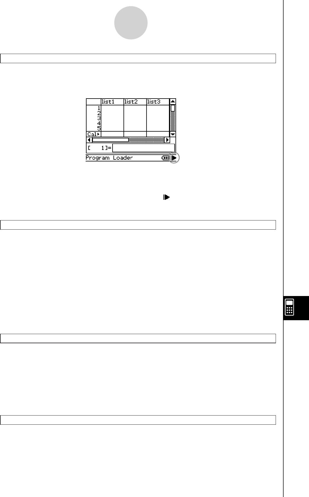
20060301

Description

• You can perform manual operations on the ClassPad display screen while program

execution is paused by the Pause command.

• Program execution remains paused until you tap the button on the status bar, or until

six minutes pass (after which program execution resumes automatically).

Return

Syntax: Return{<variable>}

Function 1 (Main Program)

This command terminates program execution.

Function 2 (Subroutine Program)

This command returns from a subroutine.

Tip

• The Return command can be executed during an If, For, Do, While, or Switch process.

• Appending a <variable> to the Return command in the Main application and executing the

command will cause the variable to be displayed when the program is complete.

Skip

Syntax: Skip

Function: This command causes execution to jump to the statement at the beginning of a

loop.

Description

• Skip causes execution to jump to the statement at the beginning of a loop.

• Skip can be used inside of a For, Do, or While process.

Stop

Syntax: Stop

Function: This command terminates program execution.

Description: This command terminates all program execution, including that of the main

program when a subroutine program is running.

Pause

Syntax: Pause

Function: This command pauses program execution and displays a pause indicator on the

right side of the status bar.

12-6-13

Program Command Reference

20080201

20060301

Switch~Case~Default~SwitchEnd

Syntax: Switch



Case



[<statement>] …

Break

Case



<expression 3> …

[<statement>] …

Break

…

Case



[<statement>] …

Break

[Default]

[<statement>] …

SwitchEnd

<expression 1> through <expression n> should be expressions that produce real

numbers.

Function: This command executes one of a series of processes based on the value of

<expression>.

Description

• This command executes the statement following the Case expression that matches the

Switch expression.

• If there is no matching Case expression, the statement following Default is executed. If

there is no Default specified, a non-match jumps to the statement following SwitchEnd.

• You can use a multi-statement command (:) in place of the carriage return to separate

statements.

• Switch~SwitchEnd can be exited using the Break command, Return command, or Goto

command.

Wait

Syntax: Wait



[<expression>]

Function: This command pauses program execution, and then restarts it after the number of

seconds specified by the expression passes.

Description

• If you do not specify any expression, program execution is paused until you tap the screen,

or press a key.

• The maximum valid specification for <expression> is 360 seconds (six minutes). Specifying

a value greater than 360 causes program execution to resume after 360 seconds,

regardless of the specified value.

• The ClassPad’s Auto Power Off function is disabled during a pause caused by the Wait

command.

• If the Auto Power Off trigger time is reached during the pause, program execution resumes.

12-6-14

Program Command Reference

20060301

While~WhileEnd

Syntax: While



[<statement>] …

WhileEnd

<expression> is a condition that evaluates to true or false.

Function: The specified statements are repeated as long as the condition is true.

Description

• The statements between While~WhileEnd are repeated as long as the condition is

true. When the condition becomes false, execution jumps to the next command after the

WhileEnd command.

• Since the condition comes after While, the condition is evaluated before the loop is started.

• You can use a multi-statement command (:) in place of the carriage return to separate

statements.

• It is always a bad idea to use the Goto command to exit a While~WhileEnd loop. Not

only is it poor programming, it can cause problems due to improper termination of internal

processes used by the loop operation.

Application Command List

The commands listed in this section can also be used in other ClassPad applications.

You can select these commands by selecting “All” for the [Form] setting on the catalog (cat)

soft keyboard. Or, you can simply type the command. Also, many of these commands appear

as menu items within the [Ctrl], [I/O] or [Misc] menus.

k Graph & Table

Circle

Syntax: Circle



<center x-coordinate>, <center y-coordinate>, radius

Function: Draws a circle.

Example: Circle –1, –1, 2

ClearSheet

Syntax: ClearSheet



{

"<sheet name>"

}

Function: Deletes the sheet name and expressions on the sheet, and returns its settings to

their default values. Omitting the argument causes all sheets to be cleared.

12-6-15

Program Command Reference

20060301

ClrGraph

Syntax: ClrGraph

Function: Clears the Graph window and returns View Window parameters to their initial

default settings.

Cls

Syntax: Cls

Function: Clears sketch elements (lines and other figures sketched on the Graph

window), and graphs drawn using drag and drop.

DispFTable

Syntax: DispFTable

Function: Creates and displays a function table.

DispSmryTbl

Syntax: DispSmryTbl

Function: Creates and displays a summary table.

Distance

Syntax: Distance



<x-coordinate 1>, <y-coordinate 1>, <x-coordinate 2>,

<y-coordinate 2>

Function: Determines the distance between two points.

Description: Executing this command makes the Graph window active, displays pointers

at the locations of coordinates 1 and 2, and displays the distance between the

pointers.

Tip

• An error occur if <x-coordinate> or <y-coordinate> is outside of the current Graph window.

DrawFTGCon, DrawFTGPlot

Syntax: DrawFTGCon

DrawFTGPlot

Function: Graphs a function using a generated number table, in accordance with the

conditions of each command.

Description: FTG stands for “Function Table Graph”. DrawFTGCon draws a connect type

graph, while DrawFTGPlot draws a plot type graph.

12-6-16

Program Command Reference

20060301

DrawGraph

Syntax: DrawGraph



[<expression>]

Function: Graphs the selected expression or an expression specified as a parameter.

Description: <expression> has a y= type expression on the right side. Graphing of any other

type of expression is not supported by this command.

Example: DrawGraph: Graphs the currently selected expressions.

DrawGraph sin(x): Graphs y = sin(x).

DrawShade

Syntax: DrawShade<expression 1>, <expression 2>[, <number 1>, <number 2>]

Function: Shades the area between expression 1 (lower curve) and expression 2 (upper

curve) from x-values of number 1 to number 2.

Description: Expression 1 and expression 2 have a y= type expression on the right side.

Graphing of any other type of expression is not supported by this command.

Example: DrawShade: Shades the area above the first expression and below the second

expression from −2 to 2.

DrawShade

x − 4, x^2, −2, 2

GraphType

Syntax: GraphType "

y="

r="

xt="

x="

y>"

y<"

y>"

y<"

x>"

x<"

x>"

x<"

Function: Specifies the graph expression input type.

Example: GraphType "r ="

GTSelOff

Syntax: GTSelOff



Function: Deselects a graph expression.

Description: Graph number range: 1 to 100

12-6-17

Program Command Reference

20060301

GTSelOn

Syntax: GTSelOn



Function: Selects a graph expression.

Description: Graph number range: 1 to 100

Horizontal

Syntax: Horizontal



<y-coordinate>

Function: Draws a horizontal line.

Inverse

Syntax: Inverse



Function: Graphs the inverse of a function.

Description: Graph number range: 1 to 100

Line

Syntax: Line



<start point x-coordinate>, <start point y-coordinate>, <end point

x-coordinate>, <end point y-coordinate>

Function: Draws a line between two specified coordinates.

Example: Line 1, –2, 2, 3

Tip

• The line is not drawn if a start point coordinate or end point coordinate is outside of the current

Graph window.

NormalLine

Syntax: NormalLine



Function: Draws a normal line.

Example: NormalLine 1, 2

Description: Draws a line normal to the graph at the specified x-value.

Plot

Syntax: Plot



<x-coordinate>, <y-coordinate>

Function: Displays a pointer at the location specified by the coordinates and plots a point

there.

PlotChg

Syntax: PlotChg



<x-coordinate>, <y-coordinate>

Function: Toggles display of the plot at the specified coordinates on and off.

12-6-18

Program Command Reference

20060301

PlotOff

Syntax: PlotOff



<x-coordinate>, <y-coordinate>

Function: Turns off display of the plot at the specified coordinates.

PlotOn

Syntax: PlotOn



<x-coordinate>, <y-coordinate>

Function: Turns on display of the plot at the specified coordinates.

plotTest(

Syntax: plotTest(<x-coordinate>, <y-coordinate>)

Function: Returns 1 when the dot at the specified coordinates is on, and 0 when it is off.

Example: plotTest(2,–3)S a. Result is placed in a.

Description: Only dots within the screen are valid.

PTBrokenThck

Syntax: PTBrokenThck



Function: Specifies “Broken Thick” ( ) as the graph line type.

Description: Graph number range: 1 to 100

PTCross

Syntax: PTCross



Function: Specifies “Cross Plot” ( ) as the graph line type.

Description: Graph number range: 1 to 100

PTDot

Syntax: PTDot



Function: Specifies “Dot Plot” ( ) as the graph line type.

Description: Graph number range: 1 to 100

PTNormal

Syntax: PTNormal



Function: Specifies “Normal” (—) as the graph line type.

Description: Graph number range: 1 to 100

PTSquare

Syntax: PTSquare



Function: Specifies “Square Plot” ( ) as the graph line type.

Description: Graph number range: 1 to 100

12-6-19

Program Command Reference

20060301

PTThick

Syntax: PTThick



Function: Specifies “Thick” (

) as the graph line type.

Description: Graph number range: 1 to 100

PxlChg

Syntax: PxlChg



<x-dot>, <y-dot>

Function: Toggles display of the specified pixel on and off.

Example: PxlChg 5,1

PxlOff

Syntax: PxlOff



<x-dot>, <y-dot>

Function: Turns off display of the specified pixel.

Example: PxlOff 3, 3

PxlOn

Syntax: PxlOn



<x-dot>, <y-dot>

Function: Turns on display of the specified pixel.

Example: PxlOn 63, 31

pxlTest(

Syntax: pxlTest

(<x-dot>, <y-dot>)

Function: Returns 1 when the specified pixel is on, and 0 when it is off.

RclGMem

Syntax: RclGMem



Function: Recalls GMem data (graph expression and related information), which was

previously saved under the specified name.

Example: RclGMem AZ

RclPict

Syntax: RclPict



Function: Recalls a Pict image, which was previously saved under the specified name.

Example: RclPict PIC1

12-6-20

Program Command Reference

20060301

RclVWin

Syntax: RclVWin



Function: Recalls View Window values, which were previously saved under the specified

name.

Example: RclVWin WIN1

SheetActive

Syntax: SheetActive



{

}

"<sheet name>"

Function: Selects the sheet that contains the expression to be graphed.

Description: Even after a sheet is renamed, it can still be specified using its previous sheet

number.

SheetName

Syntax: SheetName



"<sheet name string>", <sheet number>

Function: Assigns a name to a sheet

Description

• A sheet name can be up to eight characters long.

• Sheet number range: 1 to 5

Example: SheetName "Deriv", 1

SmryTSelOn

Syntax: SmryTSelOn



Function: Deselects all currently selected expressions and then selects only the specified

summary table expression.

StoGMem

Syntax: StoGMem



Function: Assigns a name to GMem data (graph expression and related information) and

stores it.

Example: StoGMem GMem1

12-6-21

Program Command Reference

20060301

StoPict

Syntax: StoPict



Function: Assigns a name to a Pict image and stores it.

Example: StoPict Pict1

StoVWin

Syntax: StoVWin



Function: Assigns a name to View Window values and stores them.

Example: StoVWin VWIN1

TangentLine

Syntax: TangentLine



Function: Draws a line tangent to the graph at the specified x-value.

Example: TangentLine 1, 1

Text

Syntax: Text

<horizontal pixel value>, <vertical pixel value>,

{

}

"<string>"

Function: Displays the specified text on the Graph window.

Example: Text 8, 2, "Graph"

Vertical

Syntax: Vertical



<x-coordinate>

Function: Draws a vertical line passing through the x-coordinate value.

12-6-22

Program Command Reference

20060301

ViewWindow

Syntax1: ViewWindow

 LogP



{

}

,[xmin value], [xmax value], [xscale value],

[ymin value], [ymax value], [yscale value], [t min value], [t max value],

[t step value]

Syntax 2: ViewWindow CallUndef

Syntax 3: ViewWindow

Function:

Syntax 1: Specifies View Window values.

Syntax 2: Makes all View Window values “Undefined”.

Syntax 3: Initializes View Window settings.

Description:

• LogP specifies logarithmic settings for the x-coordinate and y-coordinate.

• LogP and CallUndef are reserved words.

• Skipping values after xmin causes values previously set for each item to be used.

Example: ViewWindow , , 0.065, –0.2, 1.016, 0.01, 0.16

ZAuto

Syntax: ZAuto

Function: Performs Auto Zoom.

ZFactor

Syntax: ZFactor



Function: Specifies the Factor Zoom Factor value.

12-6-23

Program Command Reference

20060301

k 3D

ClearSheet3D

Syntax: ClearSheet3D



{

}

"<sheet name>"

Function: Deletes the sheet name and expressions on the sheet, and returns its settings

to their default values. Omitting the argument causes all sheets to be cleared.

Draw3D

Syntax: Draw3D

Function: Draws a 3D graph using current settings.

SelOn3D

Syntax: SelOn3D



Function: Selects a 3D graph function. Also makes the graph sheet that contains the

graph function active, and turns off graphing of all the other functions on the

sheet.

SheetActive3D

Syntax: SheetActive3D



{

}

"<sheet name>"

Function: Activates the specified 3D graph sheet.

SheetName3D

Syntax: SheetName3D



"<string>", <sheet number>

Function: Assigns a name to a 3D graph sheet.

ViewWindow3D

Syntax 1: ViewWindow3D



xmin value, xmax value, xgrid value, ymin value, ymax

value, ygrid value, zmin value, zmax value, angle, angle

Syntax 2: ViewWindow3D

Function

Syntax 1: Configures 3D graph View Window settings.

Syntax 2: Initializes 3D graph View Window settings.

Description: Skipping any value and inputting a comma only causes the previous setting

for that value to be used. Inputting values part way and then skipping input of

remaining values causes the previous settings for the remaining values to be

used.

12-6-24

Program Command Reference

20060301

k Conics

DrawConics

Syntax: DrawConics

Function: Draws a conics graph based on the data registered on the Conics Editor window.

k Sequence

DispDfrTbl

Syntax: DispDfrTbl

Function: Creates and displays an arithmetic sequence table.

DispDQTbl

Syntax: DispDQTbl

Function: Creates and displays a progression of difference table.

DispFibTbl

Syntax: DispFibTbl

Function: Creates and displays a Fibonacci sequence table.

DispQutTbl

Syntax: DispQutTbl

Function: Creates and displays a geometric sequence table.

DispSeqTbl

Syntax: DispSeqTbl

Function: Creates and displays a recursion table.

12-6-25

Program Command Reference

20060301

DrawSeqCon, DrawSeqPlt

Syntax: DrawSeqCon

DrawSeqPlt

Function: Graphs a recursion expression whose vertical axis is an (bn or cn) and whose

horizontal axis is n using a generated number table, in accordance with the

conditions of each command.

Description: DrawSeqCon draws a connect type graph, while DrawSeqPlt draws a plot

type graph.

DrawSeqEtrCon, DrawSeqEtrPlt

Syntax: DrawSeqEtrCon

DrawSeqEtrPlt

Function: Graphs a recursion expression whose vertical axis is Σan (Σbn or Σcn) and

whose horizontal axis is n using a generated number table, in accordance with

the conditions of each command.

Description: DrawSeqEtrCon draws a connect type graph, while DrawSeqEtrPlt draws a

plot type graph.

SeqSelOff

Syntax: SeqSelOff

 an+1

an+2

bn+1

bn+2

cn+1

cn+2

anE

bnE

cnE

Function: Deselects the specified sequence expression. Specifying “anE”, “bnE”, or “cnE”

as the argument activates [Explicit]. Specifying any other argument activates

[Recursive].

12-6-26

Program Command Reference

20060301

SeqSelOn

Syntax: SeqSelOn

 an+1

an+2

bn+1

bn+2

cn+1

cn+2

anE

bnE

cnE

Function: Selects the specified sequence expression. Specifying “anE”, “bnE”, or “cnE” as the

argument activates [Explicit]. Specifying any other argument activates [Recursive].

SeqType

Syntax: SeqType

 "n"

"an+1a0"

an+1a1"

an+2a0"

an+2a1"

Function: Specifies the recursion type.

Description: Specifying “n” as the argument activates [Explicit]. Specifying any other

argument activates [Recursive].

k Statistics

12-6-27

Program Command Reference

abExpReg

Syntax: abExpReg



xList, yList[,[FreqList (or 1)][, [<yn>][,

{

}

]]]

Off

Function: Performs y = a⋅bx regression.

Description

xList: Name of list for storing x-axis data

yList: Name of list for storing y-axis data

FreqList: Name of list for storing frequency of “xList” and “yList” data

• “FreqList” can be omitted. Doing so sets “1” for “FreqList”.

• “yn” is the Graph Editor name (y1, y2, ...) that is the copy destination of the regression

expression. Copy is not performed when “yn” is skipped.

• “On/Off” turns Residual calc on or off. Residual calc is turned off when this setting is

skipped.

20060301

DefaultListEditor

Syntax: DefaultListEditor

Function: Initializes the sort sequence and display contents of the list on the Stat Editor

window (list1 to list6).

DispListEditor

Syntax: DispListEditor

Function: Displays the Stat Editor window.

DispStat

Syntax: DispStat

Function: Displays previous statistical calculation results.

DrawStat

Syntax: DrawStat

Function: Draws a statistical graph.

12-6-28

Program Command Reference

CubicReg

Syntax: CubicReg



xList, yList[,[FreqList (or 1)][, [<yn>][,

{

}

]]]

Off

Function: Performs y = a⋅x3 + b⋅x2 + c⋅x + d regression.

Description

xList: Name of list for storing x-axis data

yList: Name of list for storing y-axis data

FreqList: Name of list for storing frequency of “xList” and “yList” data

• “FreqList” can be omitted. Doing so sets “1” for “FreqList”.

• “yn” is the Graph Editor name (y1, y2, ...) that is the copy destination of the regression

expression. Copy is not performed when “yn” is skipped.

• “On/Off” turns Residual calc on or off. Residual calc is turned off when this setting is

skipped.

ExpReg

Syntax: ExpReg



xList, yList[,[FreqList (or 1)][, [<yn>][,

{

}

]]]

Off

Function: Performs y = a⋅eb

⋅x regression.

Description

xList: Name of list for storing x-axis data

yList: Name of list for storing y-axis data

FreqList: Name of list for storing frequency of “xList” and “yList” data

• “FreqList” can be omitted. Doing so sets “1” for “FreqList”.

• “yn” is the Graph Editor name (y1, y2, ...) that is the copy destination of the regression

expression. Copy is not performed when “yn” is skipped.

• “On/Off” turns Residual calc on or off. Residual calc is turned off when this setting is

skipped.

20060301

LinearReg

Syntax: LinearReg



xList, yList[,[FreqList (or 1)][, [<yn>][,

{

Off

}

]]]

Function: Performs y = a⋅x + b regression.

Description

xList: Name of list for storing x-axis data

yList: Name of list for storing y-axis data

FreqList: Name of list for storing frequency of “xList” and “yList” data

• “FreqList” can be omitted. Doing so sets “1” for “FreqList”.

• “yn” is the Graph Editor name (y1, y2, ...) that is the copy destination of the regression

expression. Copy is not performed when “yn” is skipped.

• “On/Off” turns Residual calc on or off. Residual calc is turned off when this setting is

skipped.

LogisticReg

Syntax: LogisticReg



xList, yList[,[<yn>][,

{

Off

}

]]

Function: Performs y = c/(1 + a⋅e(−b

•x)) regression.

Description

xList: Name of list for storing x-axis data

yList: Name of list for storing y-axis data

• “yn” is the Graph Editor name (y1, y2, ...) that is the copy destination of the regression

expression. Copy is not performed when “yn” is skipped.

• “On/Off” turns Residual calc on or off. Residual calc is turned off when this setting is

skipped.

LogReg

Syntax: LogReg



xList, yList[,[FreqList (or 1)][,[<yn>][,

{

Off

}

]]]

Function: Performs y = a + b⋅ln(x) regression.

Description

xList: Name of list for storing x-axis data

yList: Name of list for storing y-axis data

FreqList: Name of list for storing frequency of “xList” and “yList” data

• “FreqList” can be omitted. Doing so sets “1” for “FreqList”.

• “yn” is the Graph Editor name (y1, y2, ...) that is the copy destination of the regression

expression. Copy is not performed when “yn” is skipped.

• “On/Off” turns Residual calc on or off. Residual calc is turned off when this setting is

skipped.

MedMedLine

Syntax: MedMedLine



xList, yList[,[FreqList (or 1)][,[<yn>][,

{

Off

}

]]]

Function: Performs y = a⋅x + b Med-Med calculation.

Description

xList: Name of list for storing x-axis data

yList: Name of list for storing y-axis data

FreqList: Name of list for storing frequency of “xList” and “yList” data

• “FreqList” can be omitted. Doing so sets “1” for “FreqList”.

• “yn” is the Graph Editor name (y1, y2, ...) that is the copy destination of the regression

expression. Copy is not performed when “yn” is skipped.

• “On/Off” turns Residual calc on or off. Residual calc is turned off when this setting is

skipped.

12-6-29

Program Command Reference

20060301

MultiSortA

Syntax 1: MultiSortA



Syntax 2: MultiSortA



<base list name>, <subordinate list name>,

<subordinate list name>, ...

Function: Sorts a statistical list in ascending order.

Description

• Syntax 1 performs a simple list sort.

• Syntax 2 sorts multiple lists on the base list. Up to five subordinate lists can be specified.

MultiSortD

Syntax 1: MultiSortD



Syntax 2: MultiSortD



<base list name>, <subordinate list name>,

<subordinate list name>, ...

Function: Sorts a statistical list in descending order.

Description

• Syntax 1 performs a simple list sort.

• Syntax 2 sorts multiple lists on the base list. Up to five subordinate lists can be specified.

12-6-30

Program Command Reference

OneVariable

Syntax: OneVariable



xList [,FreqList (or 1)]

Function: Single variable statistics calculation

Description

xList: Name of list for storing x-axis data

FreqList: Name of list for storing frequency of “xList” data

• “FreqList” can be omitted. Doing so sets “1” for “FreqList”.

PowerReg

Syntax: PowerReg



xList, yList[,[FreqList (or 1)][, [<yn>][,

{

Off

}

]]]

Function: Performs y = a⋅xb regression.

Description

xList: Name of list for storing x-axis data

yList: Name of list for storing y-axis data

FreqList: Name of list for storing frequency of “xList” and “yList” data

• “FreqList” can be omitted. Doing so sets “1” for “FreqList”.

• “yn” is the Graph Editor name (y1, y2, ...) that is the copy destination of the regression

expression. Copy is not performed when “yn” is skipped.

• “On/Off” turns Residual calc on or off. Residual calc is turned off when this setting is

skipped.

20060301

QuadReg

Syntax: QuadReg



xList, yList[,[FreqList (or 1)][,[<yn>][,

{

Off

}

]]]

Function: Performs y = a⋅x2 + b⋅x + c regression.

Description

xList: Name of list for storing x-axis data

yList: Name of list for storing y-axis data

FreqList: Name of list for storing frequency of “xList” and “yList” data

• “FreqList” can be omitted. Doing so sets “1” for “FreqList”.

• “yn” is the Graph Editor name (y1, y2, ...) that is the copy destination of the regression

expression. Copy is not performed when “yn” is skipped.

• “On/Off” turns Residual calc on or off. Residual calc is turned off when this setting is

skipped.

QuartReg

Syntax: QuartReg



xList, yList[,[FreqList (or 1)][,[<yn>][,

{

Off

}

]]]

Function: Performs y = a⋅x4 + b⋅x3 + c⋅x2 + d⋅x + e regression.

Description

xList: Name of list for storing x-axis data

yList: Name of list for storing y-axis data

FreqList: Name of list for storing frequency of “xList” and “yList” data

• “FreqList” can be omitted. Doing so sets “1” for “FreqList”.

• “yn” is the Graph Editor name (y1, y2, ...) that is the copy destination of the regression

expression. Copy is not performed when “yn” is skipped.

• “On/Off” turns Residual calc on or off. Residual calc is turned off when this setting is

skipped.

SinReg

Syntax: SinReg



xList, yList[,[<yn>][,

{

Off

}

]]

Function: Performs y = a⋅sin(b⋅x + c) + d regression.

Description

xList: Name of list for storing x-axis data

yList: Name of list for storing y-axis data

• “yn” is the Graph Editor name (y1, y2, ...) that is the copy destination of the regression

expression. Copy is not performed when “yn” is skipped.

• “On/Off” turns Residual calc on or off. Residual calc is turned off when this setting is

skipped.

12-6-31

Program Command Reference

20060301

StatGraph

Syntax 1: StatGraph



<StatGraph number 1 to 9>,

{

Off

}

, Graph Type 1, xList, yList,

FreqList (or 1), Plot Type

Syntax 2: StatGraph



<StatGraph number 1 to 9>,

{

Off

}

, Graph Type 2, xList, yList,

FreqList (or 1)

Syntax 3: StatGraph



<StatGraph number 1 to 9>,

{

Off

}

, Graph Type 3, xList, yList

Syntax 4: StatGraph



<StatGraph number 1 to 9>,

{

Off

}

, Graph Type 4, xList,

FreqList (or 1)

Syntax 5: StatGraph



<StatGraph number 1 to 9>,

{

Off

}

, Graph Type 5, xList,

Plot Type

Function: Configures statistical graph settings.

Description

xList: Name of list for storing x-axis data

yList: Name of list for storing y-axis data

FreqList: Name of list for storing frequency of “xList” and “yList” data

Graph Type 1: Scatter/xyLine

Graph Type 2: LinearR/MedMed/QuadR/CubicR/QuartR/LogR/ExpR/abExpR/PowerR

Graph Type 3: SinR/LogisticR

Graph Type 4: Histogram/MedBox/ModBox/NDist/Broken

Graph Type 5: NPPlot

Plot Type: Square/Cross/Dot/Ldot

StatGraphSel

Syntax: StatGraphSel



{

Off

} {

,"Reg,"

,"Graph"

}

Function: Turns statistical graphing on or off.

Description

• Reg selects Previous Reg.

• Graph selects Graph Function.

• Skipping Reg and Graph turns StatGraph, Previous Reg, and Graph Function on or off.

12-6-32

Program Command Reference

TwoVariable

Syntax: TwoVariable



xList, yList[, FreqList (or 1)]

Function: Paired variable statistics calculation

Description

xList: Name of list for storing x-axis data

yList: Name of list for storing y-axis data

FreqList: Name of list for storing frequency of “xList” and “yList” data

• “FreqList” can be omitted. Doing so sets “1” for “FreqList”.

20060301

12-6-33

Program Command Reference

k Setup

DefaultSetup

Syntax: DefaultSetup

Function: Initializes all setup data settings.

SetAxes

Syntax: SetAxes



{

Number

Off

}

Function: Turns display of Graph window axes on or off.

SetAxes3D

Syntax: SetAxes3D



{

Off

Box

}

Function: Turns display of axes on (normal), off, or Box (box type coordinate) for 3D

graphing. Specifying Box displays the draw area in box form.

SetBG

Syntax: SetBG



{

}

Off

Function: Specifies a PICT image for the background. Background image display is turned

off when “Off” is specified.

SetCellWidth

Syntax: SetCellWidth



{

}

Function: Specifies the number of rows displayed on the Stat Editor and data table

windows.

SetComplex

Syntax: SetComplex

Function: Specifies the Complex mode (to perform complex number calculations).

20060301

SetCoord

Syntax: SetCoord



{

Off

}

Function: Turns display of Graph window pointer coordinates on or off.

SetCoordOff3D

Syntax: SetCoordOff3D

Function: Turns off display of pointer coordinates for 3D graphing.

SetCoordPol3D

Syntax: SetCoordPol3D

Function: Specifies use of polar coordinates for coordinate display during 3D graphing.

SetCoordRect3D

Syntax: SetCoordRect3D

Function: Specifies use of rectangular coordinates for coordinate display during 3D

graphing.

SetDecimal

Syntax: SetDecimal

Function: Specifies the Decimal mode (displays results in decimal format).

SetDegree

Syntax: SetDegree

Function: Specifies “Degree” for the angle unit.

SetDeriv

Syntax: SetDeriv



{

Off

}

Function: Turns display of Graph window pointer coordinates and ordered pair table

derivative on or off.

12-6-34

Program Command Reference

20060301

SetDispGCon

Syntax: SetDispGCon



{

Off

}

Function: Turns display of graph controller arrows during graphing on or off.

SetDrawCon

Syntax: SetDrawCon

Function: Specifies graphing by connecting plotting points with lines.

SetDrawPlt

Syntax: SetDrawPlt

Function: Specifies graphing by plotting points only.

SetFix

Syntax: SetFix



Function: Specifies the fixed number of decimal places.

SetFunc

Syntax: SetFunc



{

Off

}

Function: Turns display of graph function name and function on or off.

SetGrad

Syntax: SetGrad

Function: Specifies “Grad” for the angle unit.

SetGrid

Syntax: SetGrid



{

Off

}

Function: Turns display of the Graph window grid on or off.

SetLabel

Syntax: SetLabel



{

Off

}

Function: Turns display of Graph window axis labels on or off.

12-6-35

Program Command Reference

20060301

SetLabel3D

Syntax: SetLabel3D



{

Off

}

Function: Turns display of Graph window axis labels for 3D graphing on or off.

SetLeadCursor

Syntax: SetLeadCursor



{

Off

}

Function: Turns display of the leading cursor during graphing on or off.

SetNormal

Syntax: SetNormal



{

}

Function: Specifies Normal 1 or Normal 2 as the auto exponential display setting for values.

SetRadian

Syntax: SetRadian

Function: Specifies “Radian” for the angle unit.

SetReal

Syntax: SetReal

Function: Specifies the Real mode (to perform real number calculations).

SetSci

Syntax: SetSci



Function: Specifies the fixed number of significant digits.

12-6-36

Program Command Reference

20060301

SetSequence

Syntax: SetSequence



{

Off

StepDisp

}

Function: Turns display of expressions created after graphing on or off or specifies “step

display” (StepDisp).

Description: When StepDisp is selected, the expression does not appear until you press E.

SetSimulGraph

Syntax: SetSimulGraph



{

Off

}

Function: Turn simultaneous drawing of multiple graphs on or off.

SetSmryTable

Syntax: SetSmryTable



{

}

VWin

Function: Specifies whether summary table generation is View Window dependent or List

dependent. Using VWin specifies View Window dependent.

SetSmryTableQD

Syntax: SetSmryTableQD



{

Off

}

Function: Specifies whether the second derivative will appear in summary tables.

SetStandard

Syntax: SetStandard

Function: Specifies the Standard mode (to leave calculation results as expressions).

SetStatWinAuto

Syntax: SetStatWinAuto



{

Off

}

Function: Turns automatic setup of Statistics application View Window on or off.

12-6-37

Program Command Reference

20060301

SetTVariable

Syntax: SetTVariable



{

}

TableInput

Function: Specifies the variable reference location for table generation.

Description: Use TableInput to specify a range and generate a table.

SetΣdisp

Syntax: SetΣdisp



{

Off

}

Function: Turns display of subtotals for tables on or off.

k Folder/Variable

Clear_a_z

Syntax: Clear_a_z

[<folder name>]

Function: Deletes all single letter lower-case named variables from a through z from the

specified folder.

Description

• If you don’t specify a folder name, the variables of the current folder are cleared.

• Deletes all variables, regardless of type (program, etc.), that have the specified variable

name. See GetType for information about variable types (page 12-6-39).

• Keep in mind that this command clears all data types, including programs, functions, etc.

CopyVar

Syntax: CopyVar

<source variable name>, <copy destination variable name>

Function

• Copies the contents of a variable to another variable.

• If the copy destination variable has the same name as the source variable name, the

destination variable is replaced with the source variable.

12-6-38

Program Command Reference

20060301

DelFolder

Syntax: DelFolder

<folder name>

Function: Deletes a folder.

DelVar

Syntax: DelVar

<variable name>, <variable name> ...

Function: Deletes a variable.

Description: Deletes all variables, regardless of type (program, etc.), that have the specified

variable name. See GetType for information about variable types.

GetFolder

Syntax: GetFolder

<storage variable name>

Function: Gets the current folder name and assigns it to a variable as a text string.

GetType

Syntax: GetType

<variable name>, <storage variable name>

Function: Gets the type of the specified variable and assigns it to a storage variable as a

text string.

Description: The following is a list of variable types.

• NUM (real number type)

• EXPR (expression type)

• STR (string type)

• LIST (list type)

• MAT (matrix type)

• PRGM (program type)

• EXE (execute only program type)

• TEXT (text type)

• FUNC (function type)

• PICT (picture type)

• GMEM (graph expression memory type)

• GEO (geometric type)

• MEM (universal data type)

• OTHR (unrecognizable items)

• NONE (no applicable variable)

12-6-39

Program Command Reference

20060301

Local

Syntax: Local

<variable name>, <variable name> ...

Function: Defines a local variable.

Description

The following are the merits of local variables.

• Since local variables are deleted automatically, use of local variables for temporary storage

avoids unnecessary use of available memory.

• Since local variables do not affect general variables, you can name local variables without

worrying about whether the name you are using is already used by another variable.

Lock

Syntax: Lock

<variable name>, <variable name> ...

Function: Locks variables.

LockFolder

Syntax: LockFolder

<folder name>

Function: Locks the specified folder and all the files currently inside of it.

MoveVar

Syntax: MoveVar

<variable name>, <current folder name>, <destination folder name>

Function: Moves a variable to the specified folder.

NewFolder

Syntax: NewFolder

<folder name>

Function: Creates a new folder.

Rename

Syntax: Rename

<current variable name>, <new variable name>

Function: Renames a variable.

12-6-40

Program Command Reference

20110401

SetFolder

Syntax: SetFolder

<folder name> [,<storage variable name>]

Function

• Makes the specified folder the current folder. Including a variable name at the end of this

command assigns the name of the previous current folder to the variable as a text string.

• If the specified folder does not exist, this command creates a new folder with the specified

name, and makes it the current folder.

Unlock

Syntax: Unlock

<variable name>, <variable name> ...

Function: Unlocks variables.

UnlockFolder

Syntax: UnlockFolder

<folder name>

Function: Unlocks the specified folder and all the files currently inside of it.

k Strings

A string is a series of characters inside of quotation marks. In a program, strings are used to

specify display text.

A string made up of numbers (like “123”) or an expression (like “x–1”) cannot be processed

as a calculation.

To include quotation marks (") or a backslash (\) in a string, put a backslash (\) in front of the

quotation marks (") or backslash (\).

Example 1: To include Japan: “Tokyo” in a string

"Japan:\"Tokyo\""

Example 2: To include main\abc in a string

"main\\abc"

ChrToNum

Syntax: ChrToNum

"<string>", <storage variable name>[,n]

Function: Converts the characters up to the nth character of a string to their character

code values and assigns the string to the specified variable.

Description: Omitting “n” starts conversion from the first character of the string. For

information about character codes, see Appendix page -1-1.

12-6-41

Program Command Reference

20110401

ExpToStr

Syntax: ExpToStr

<expression>,<storage variable name>

Function: Converts the result of an input expression to a string and assigns the string to

the specified variable.

NumToChr

Syntax: NumToChr



n,<storage variable name>

Function: Converts numeric value n to the corresponding text character(s) in accordance

with the character code table, and assigns the character(s) as a string to the

specified variable. For information about character codes, see Appendix page

-1-1.

NumToStr

Syntax: NumToStr

<value>,

{

"Fix <integer from 0 to 9>"

}

, <storage variable name>

"Sci <integer from 0 to 9>"

Function: Converts a numeric value to a string of the specified format, and assigns the

resulting string to the specified variable.

Example: NumToStr 1.234, "Fix2", x

StrCmp

Syntax: StrCmp



"<string 1>", "<string 2>", <storage variable name>

Function: Compares "<string 1>" and "<string 2>" (character code comparison) and

assigns the resulting value to the specified variable.

Description

• Returns 0 when "<string 1>" = "<string 2>".

• Returns 1 when "<string 1>" > "<string 2>".

• Returns –1 when "<string 1>" < "<string 2>".

StrInv

Syntax: StrInv



"<string>", <storage variable name>

Function: Inverts the sequence of a string and assigns the resulting string to a variable.

12-6-42

Program Command Reference

20060301

StrJoin

Syntax: StrJoin



"<string 1>", "<string 2>", <storage variable name>

Function: Joins "<string 1>" and "<string 2>" and then assigns the resulting string to the

specified variable.

StrLeft

Syntax: StrLeft



"<string>", n, <storage variable name>

Function: Copies a string up to the nth character from the left, and assigns the resulting

string to the specified variable.

StrLen

Syntax: StrLen



"<string>", <storage variable name>

Function: Determines the length of a string (the number of its characters) and assigns

the resulting value to the specified variable.

StrLwr

Syntax: StrLwr



"<string>", <storage variable name>

Function: Converts all the characters of a string to lower case and assigns the resulting

string to the specified variable.

StrMid

Syntax: StrMid



"<string>", n, <storage variable name> [,<number of characters>]

Function: Copies a specific number of characters of a string, starting from the nth

character, and assigns the resulting string to the specified variable.

Description: Omitting the number of characters causes the string to be copied up to the

end.

StrRight

Syntax: StrRight



"<string>", n, <storage variable name>

Function: Copies a string up to the nth character from the right, and assigns the resulting

string to the specified variable.

12-6-43

Program Command Reference

20060301

StrRotate

Syntax: StrRotate



"<string>", <storage variable name> [,n]

Function: Rotates the left side part and right side part of a string at the nth character, and

assigns the resulting string to the specified variable.

Description: Rotation is to the left when “n” is positive, and to the right when “n” is negative.

Omitting “n” uses a default value of +1.

Example: StrRotate "abcde", DDD, –2 ← Assigns the string “deabc” to variable DDD.

StrShift

Syntax: StrShift



"<string>", <storage variable name> [,n]

Function: Shifts a string left or right n characters, and assigns the resulting string to the

specified variable.

Description: Shift is to the left when “n” is positive, and to the right when “n” is negative.

Omitting “n” uses a default value of +1.

Example: StrShift "abcde", DDD, –2 ← Assigns the string “ abc” to variable DDD.

StrSrc

Syntax: StrSrc



"<string 1>", "<string 2>", <storage variable name>

[,<search start location>]

Function: Searches "<string 1>" starting from the specified point (nth character from

beginning of string) to determine if it contains the data specified by "<string

2>". If the data is found, this command returns the location of the first character

of "<string 2>", starting from the beginning of "<string 1>".

Description: Omitting the start point causes the search to start from the beginning of

"<string 1>".

strToExp(

Syntax: strToExp("<string>")

Function: Converts a string to an expression, and executes the expression.

StrUpr

Syntax: StrUpr



"<string>", <storage variable name>

Function: Converts all the characters of a string to upper case and assigns the resulting

string to the specified variable.

12-6-44

Program Command Reference

20060301

k Other

CloseComPort38k

Syntax: CloseComPort38k

Function: Closes the 3-pin COM port.

Example: See the GetVar38k command.

GetVar38k

Syntax: GetVar38k

<variable name>

Function: Receives variable names and variable contents.

Description

• The OpenComPort38k command must be executed before this command is executed.

• The CloseComPort38k command must be executed after this command is executed.

Example: To connect two ClassPad units with an SB-62 cable, and transfer the contents

of the sending unit’s variable “s” to the receiving unit’s variable “g”

Sending Unit Program

123

S s

OpenComPort38k

SendVar38k s

CloseComPort38k

Receiving Unit Program

OpenComPort38k

GetVar38k g

CloseComPort38k

Notes

• Run the receiving unit’s program first, and then run the sending unit’s

program.

• You can use any commands beside the four data communication commands

(Send38k, Receive38k, SendVar38k, or GetVar38k) between the

OpenComPort38k and CloseComPort38k commands.

12-6-45

Program Command Reference

20060301

OpenComPort38k

Syntax: OpenComPort38k

Function: Opens the 3-pin COM port.

Example: See the GetVar38k command on page 12-6-45.

Receive38k

Syntax: Receive38k

<variable name>

Function: Receives EA-200 data.

Description

• The OpenComPort38k command must be executed before this command is executed.

• The CloseComPort38k command must be executed after this command is executed.

• For details about using this command, see the user documentation that comes with the

EA-200.

• Note that you need to replace all instances of the Receive command in the examples

provided in the EA-200 user documentation with the command Receive38k. You should

also adjust the other commands in the EA-200 examples so they conform to the ClassPad

command syntax and usage as described in this manual.

Send38k

Syntax: Send38k

<variable name>

Function: Sends EA-200 data.

Description

• The OpenComPort38k command must be executed before this command is executed.

• The CloseComPort38k command must be executed after this command is executed.

• For details about using this command, see the user documentation that comes with the

EA-200.

• Note that you need to replace all instances of the Send command in the examples provided

in the EA-200 user documentation with the command Send38k. You should also adjust

the other commands in the EA-200 examples so they conform to the ClassPad command

syntax and usage as described in this manual.

• <variable name> must be a variable that contains a real number or a list. Anything else

results in an error.

SendVar38k

Syntax: SendVar38k

<variable name>

Function: Sends variable names and variable contents.

Description

• The OpenComPort38k command must be executed before this command is executed.

• The CloseComPort38k command must be executed after this command is executed.

Example: See the GetVar38k command on page 12-6-45.

12-6-46

Program Command Reference

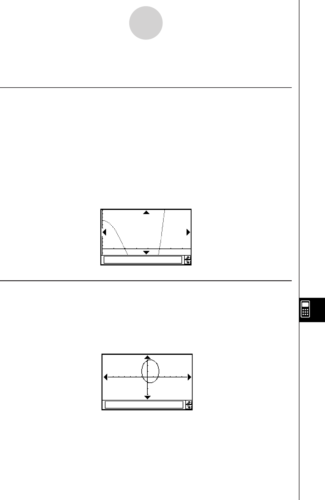
20060301

12-7 Including ClassPad Functions in Programs

Including Graphing Functions in a Program

Graphing functions let your program graph multiple equations, or overlay multiple graphs on

the same screen.

Example: DefaultSetup

ClrGraph

ViewWindow 0, 7.7, 1, –14, 110, 10

GraphType "y="

Define y1(x) = x^4 – x^3 – 24x^2 + 4x + 80

GTSelOn 1

PTDot 1

SheetActive 1

DrawGraph

12-7-1

Including ClassPad Functions in Programs

Using Conics Functions in a Program

Conics functions make it possible for your program to draw conics graphs.

Example: ClrGraph

ViewWindow –15.4, 15.4, 2, –7.6, 7.6, 2

"(x – 1)^2/3^2 + (y – 2)^2/4^2 = 1" S ConicsEq

DrawConics

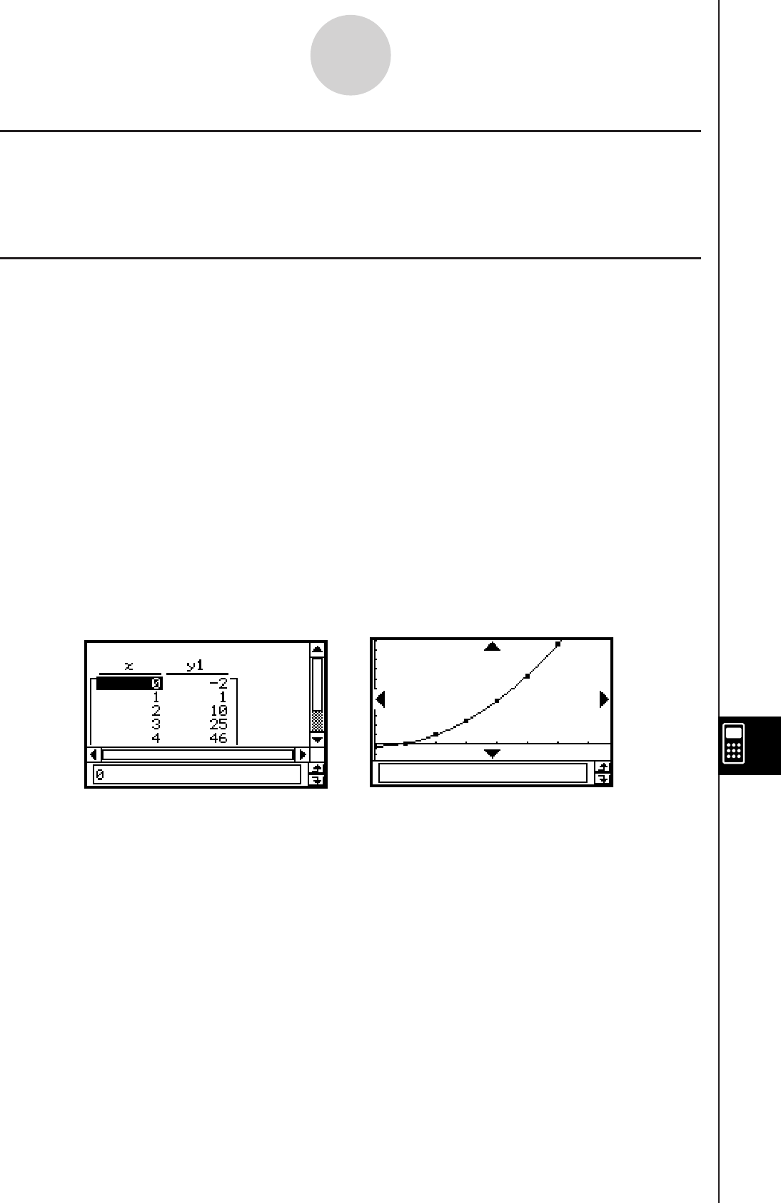
20060301

Including 3D Graphing Functions in a Program

The methods for using 3D graphing functions in a program are identical to those for normal

(non-3D) graphing functions, except that you can only graph one 3D graph at a time. For

information about commands that are unique to 3D graphing, see “3D” on page 12-6-24.

Including Table & Graph Functions in a Program

Table & Graph functions can be included in a program to generate number tables and draw

graphs.

Example: DefaultSetup

ClrGraph

ViewWindow 0, 7.7, 1, –14, 110, 10

GraphType "y="

Define y1(x) = 3 × x^2 – 2

GTSelOn 1

S FStart

S FEnd

S FStep

SheetActive 1

DispFTable

Pause

DrawFTGCon

12-7-2

Including ClassPad Functions in Programs

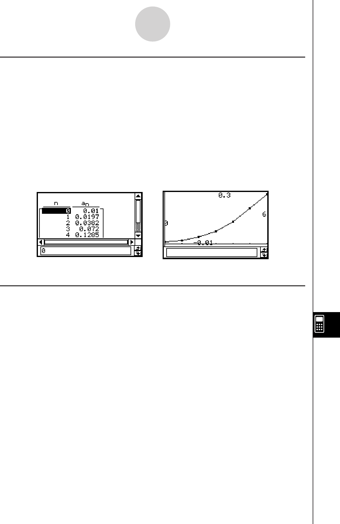
20101001

12-7-3

Including ClassPad Functions in Programs

Including Recursion Table and Recursion Graph Functions in a Program

Recursion table and recursion graph functions can be included in a program to generate

number tables and draw graphs.

Example: DefaultSetup

ViewWindow 0, 6, 1, – 0.01, 0.3, 1

SeqType "an+1a0"

"–3an^2 + 2an" S an+1

S SqStart

S SqEnd

0.01

S a0

DispSeqTbl

Pause

DrawSeqCon

Including List Sort Functions in a Program

List sort functions let you sort list data into either ascending or descending order. Make sure

the list contains data before executing a sort function.

u To sort data of a single list in ascending order

MultiSortA <list name>

u To sort multiple lists in ascending order, based on the data in one list

MultiSortA <base list name>,<list name>,…

• Up to six list names can be specified, including the base list name.

u To sort data of a single list in descending order

MultiSortD <list name>

u To sort multiple lists in descending order, based on the data in one list

MultiSortD <base list name>,<list name>,…

• Up to six list names can be specified, including the base list name.

20060301

12-7-4

Including ClassPad Functions in Programs

Including Statistical Graphing and Calculation Functions in a Program

Including statistical graphs and calculation functions in a program allows the program to draw

statistical graphs and display statistical calculation results.

u To perform statistical graphing

Example 1: Scatter Diagram

{0.5, 1.2, 2.4, 4, 5.2} S list1

{–2.1, 0.3, 1.5, 2, 2.4} S list2

StatGraph 1, On, Scatter, list1, list2, 1, Square

DrawStat

Note that

xyLine can also be specified in instead of Scatter for the graph type.

Example 2: Normal Probability Plot

{0.5, 1.2, 2.4, 4, 5.2} S list1

StatGraph 1, On, NPPlot, list1, Square

DrawStat

Example 3: Single-variable statistical graphing

{0.5, 1.2, 2.4, 4, 5.2} S list1

StatGraph 1, On, Histogram, list1, list1

DrawStat

Note that MedBox, ModBox, NDist, or Broken can also be specified in instead

of Histogram for the graph type.

Example 4: Paired-variable statistical graphing

{0.5, 1.2, 2.4, 4, 5.2} S list1

{–2.1, 0.3, 1.5, 2, 2.4} S list2

StatGraph 1,On, LinearR, list1, list2,1

DrawStat

Note that MedMed, QuadR, CubicR, QuartR, LogR, ExpR, abExpR, or

PowerR can also be specified in instead of LinearR for the graph type.

Example 5: Paired-variable statistical graphing (Sinusoidal Regression / Logistic

Regression)

{0.5, 1.2, 2.4, 4, 5.2} S list1

{2.9, 3.8, 3.3, 0.4, 0.2} S list2

StatGraph 1, On, SinR, list1, list2

DrawStat

Note that LogisticR can also be specified in instead of SinR for the graph type.

20060301

u To use statistical calculation functions

You can perform the following types of statistical calculations using program commands.

• Single-variable statistics

• Paired-variable statistics

• Regression

• Tests

• Confidence interval

• Probability

See “Chapter 7 – Using the Statistics Application” for more information.

u To explore statistical data

Example: Exploring data with regression

StatGraphSel Off

{0.5, 1.2, 2.4, 4, 5.2} S list1

{–2.1, 0.3, 1.5, 2, 2.4} S list2

StatGraph 1, On, Scatter, list1, list2, 1, Square

DrawStat

LogReg list1, list2, 1

DispStat

DrawStat

12-7-5

Including ClassPad Functions in Programs

20090601

Chapter

Using the Spreadsheet

Application

The Spreadsheet application provides you with powerful, take-

along-anywhere spreadsheet capabilities on your ClassPad.

13-1 Spreadsheet Application Overview

13-2 Spreadsheet Application Menus and Buttons

13-3 Basic Spreadsheet Window Operations

13-4 Editing Cell Contents

13-5 Using the Spreadsheet Application with the

eActivity Application

13-6 Statistical Calculations

13-7 Cell and List Calculations

13-8 Formatting Cells and Data

13-9 Graphing

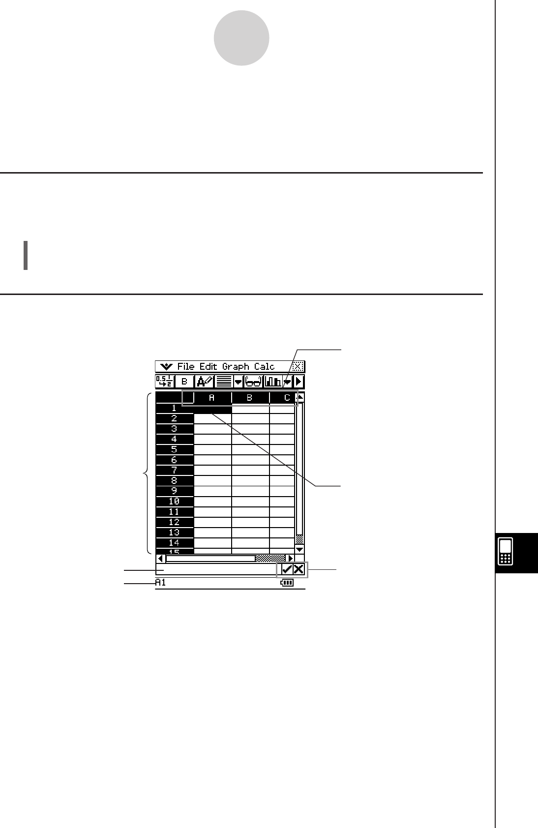
20090601

13-1-1

Spreadsheet Application Overview

13-1 Spreadsheet Application Overview

This section describes the configuration of the Spreadsheet application window, and provides

basic information about its menus and commands.

Starting Up the Spreadsheet Application

Use the following procedure to start up the Spreadsheet application.

u ClassPad Operation

On the application menu, tap R.

This starts the Spreadsheet application and displays its window.

Spreadsheet Window

The Spreadsheet window shows a screen of cells and their contents.

Row numbers (1 to 999)

Column letters (A to BL)

Edit buttons

Edit box

Cell cursor

Status area

• Each cell can contain a value, expression, text, or a formula. Formulas can contain a

reference to a specific cell or a range of cells.

20060301

13-2-1

Spreadsheet Application Menus and Buttons

13-2 Spreadsheet Application Menus and

Buttons

This section explains the operations you can perform using the menus and buttons of the

Spreadsheet application window.

• For information about the O menu, see “Using the O Menu” on page 1-5-4.

k File Menu

To do this:

Select this

[File] menu item:

Create a new, empty spreadsheet New

Open an existing spreadsheet Open

Save the currently displayed spreadsheet Save

Import data to spreadsheet Import

Export spreadsheet data Export

Recalculate the contents of the cell(s) on the spreadsheet Recalculate

20090601

13-2-2

Spreadsheet Application Menus and Buttons

k Edit Menu

To do this:

Select this

[Edit] menu item:

Undo the last action, or redo the action you have just undone Undo/Redo

Display a dialog box that lets you show or hide scrollbars, and specify the

direction the cursor advances when inputting data

Options

Automatically resize columns to fit the data into the selected cells AutoFit Selection

Display a dialog box for specifying column width Column Width

Display a dialog box for specifying the number format of the selected cell(s)

Number Format

Display or hide the Cell Viewer window Cell Viewer

Display a dialog box for specifying a cell to jump to Goto Cell

Display a dialog box for specifying a range of cells to select Select Range

Display a dialog box for specifying cell contents and a range of cells to fill Fill Range

Display a dialog box for specifying a sequence to fill a range of cells Fill Sequence

Insert row(s) Insert - Rows

Insert column(s) Insert - Columns

Delete the currently selected row(s) Delete - Rows

Delete the currently selected column(s) Delete - Columns

Delete the contents of the currently selected cells Delete - Cells

Cut the current selection and place it onto the clipboard Cut

Copy the current selection and place it onto the clipboard Copy

Paste the clipboard contents at the current cell cursor location Paste

Select everything in the spreadsheet Select All

Sort cell(s) on the spreadsheet Sort

Search for strings in the cell(s) on the spreadsheet Search

Search for strings in the cell(s) on the spreadsheet again Search Again

Clear all data from the spreadsheet Clear All

k Graph Menu

You can use the [Graph] menu to graph the data contained in selected cells. See

“13-9 Graphing” for more information.

k Calc Menu

The [Calc] menu includes commands to perform the following calculations.

• Statistical calculations (Single-variable and paired-variable statistics, regression, tests,

confidence interval, distribution, inverse distribution)

• Cell calculations (row, col, count, cellIf) and list calculations

For more information, see “13-6 Statistical Calculations” and “13-7 Cell and List Calculations”.

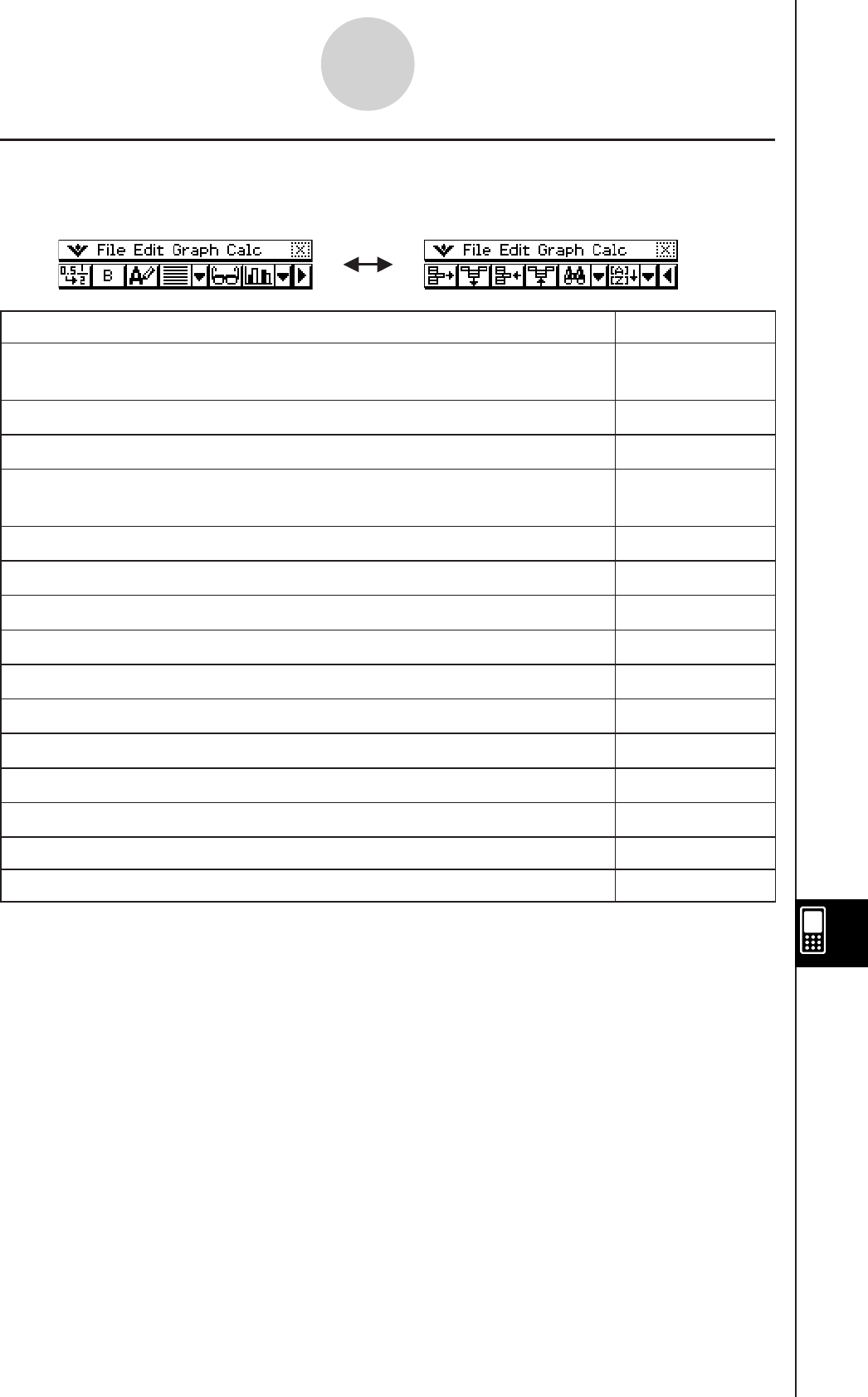
20090601

k Spreadsheet Toolbar Buttons

Not all of the Spreadsheet buttons can fit on a single toolbar, tap the u/t button on the far

right to toggle between the two toolbars.

To do this: Tap this button:

Toggle the selected cell(s) between decimal (floating point) and exact

display*1.

Toggle the selected cell(s) between bold and normal M

Toggle the data type of the selected cell(s) between text and calculation u

Specify left-justified text and right-justified values for selected cell(s)

(default) [

Specify left-justified for selected cell(s) p

Specify centered for selected cell(s) x

Specify right-justified for selected cell(s) ]

Display or hide the Cell Viewer window A

Display the Spreadsheet Graph window (page 13-9-1) o

Delete the currently selected row(s) H

Delete the currently selected column(s) J

Insert row(s) K

Insert column(s) a

Search for strings in the cell(s) on the spreadsheet e/

Sort cell(s) on the spreadsheet L

*1 When cell(s) are calculation data types.

Tip

• During cell data input and editing, the toolbar changes to a data input toolbar. See “Edit Mode

Screen” on page 13-4-1 for more information.

13-2-3

Spreadsheet Application Menus and Buttons

20090601

13-3-1

Basic Spreadsheet Window Operations

13-3 Basic Spreadsheet Window Operations

This section contains information about how to control the appearance of the Spreadsheet

window, and how to perform other basic operations.

About the Cell Cursor

The cell cursor causes the current selected cell or group of cells to become highlighted.

The location of the current selection is indicated in the status bar, and the value or formula

located in the selected cell is shown in the edit box.

• You can select multiple cells for group formatting, deletion, or insertion.

• See “Selecting Cells” on page 13-3-5 for more information about selecting cells.

Controlling Cell Cursor Movement

Use the following procedure to specify whether the cell cursor should stay at the current cell,

move down to the next line, or move right to the next column when you register data in a

Spreadsheet cell.

u ClassPad Operation

(1) On the [Edit] menu, tap [Options].

20060301

13-3-2

Basic Spreadsheet Window Operations

(2) On the dialog box that appears, tap the [Cursor Movement] down arrow button, and

then select the setting you want.

To have the cell cursor behave this way when you register

input:

Select this

setting:

Remain at the current cell Off

Move to the next row below the current cell Down

Move to the next column to the right of the current cell Right

(3) After the setting is the way you want, tap [OK].

Navigating Around the Spreadsheet Window

The simplest way to select a cell is to tap it with the stylus. You can also drag the stylus

across a range of cells to select all of them. If you drag to the edge of the screen, it will scroll

automatically, until you remove the stylus from the screen.

The following are other ways you can navigate around the Spreadsheet window.

k Cursor Keys

When a single cell is selected, you can use the cursor key to move the cell cursor up, down,

left, or right.

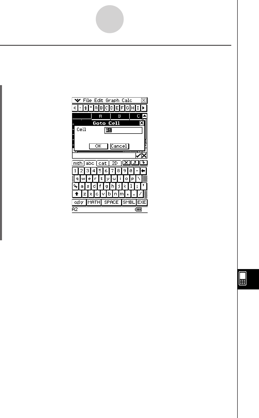
20090601

13-3-3

Basic Spreadsheet Window Operations

k Jumping to a Cell

You can use the following procedure to jump to a specific cell on the Spreadsheet screen by

specifying the cell’s column and row.

u ClassPad Operation

(1) On the [Edit] menu, select [Goto Cell].

(2) On the dialog box that appears, type in a letter to specify the column of the cell to which

you want to jump, and a value for its row number.

(3) After the column and row are the way you want, tap [OK] to jump to the cell.

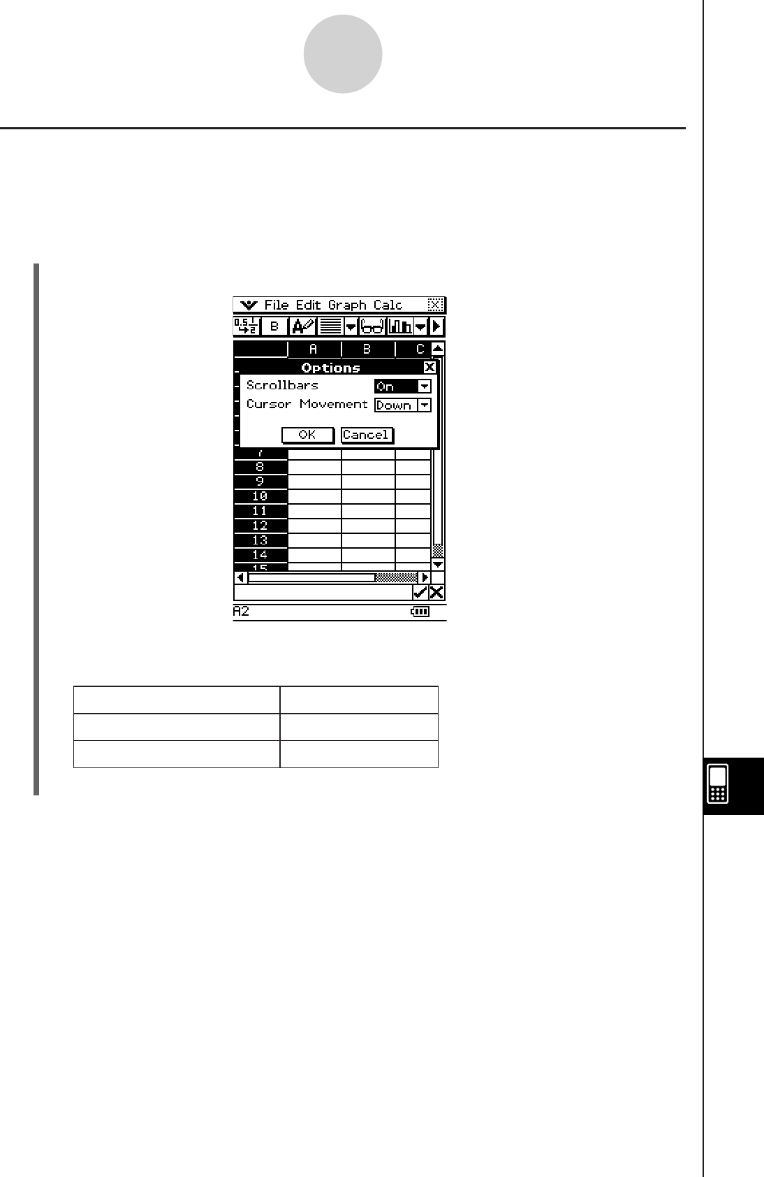
20090601

13-3-4

Basic Spreadsheet Window Operations

Hiding or Displaying the Scrollbars

Use the following procedure to turn display of Spreadsheet scrollbars on and off.

By turning off the scrollbars, you make it possible to view more information in the

spreadsheet.

u ClassPad Operation

(1) On the [Edit] menu, tap [Options].

(2) On the dialog box that appears, tap the [Scrollbars] down arrow button, and then select

the setting you want.

To do this: Select this setting:

Display the scrollbars On

Hide the scrollbars Off

(3) After the setting is the way you want, tap [OK].

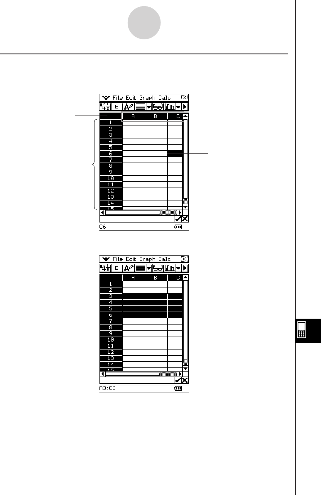
20090601

13-3-5

Basic Spreadsheet Window Operations

Tap a row heading to

select the row.

Tap a column

heading to select

the column.

Tap a cell to select it.

Tap here to select the

entire spreadsheet.

Selecting Cells

Before performing any operation on a cell, you must first select it. You can select a single

cell, a range of cells, all the cells in a row or column, or all of the cells in the spreadsheet.

• To select a range of cells, drag the stylus across them.

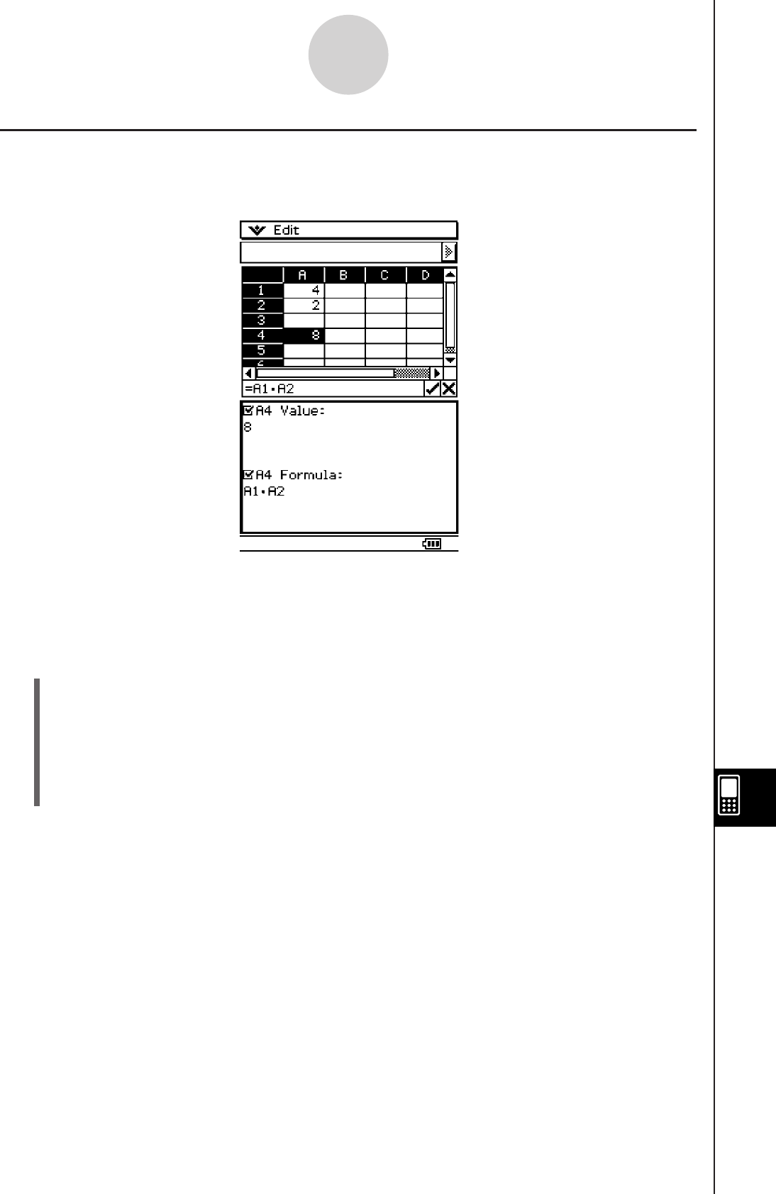
20060301

13-3-6

Basic Spreadsheet Window Operations

Using the Cell Viewer Window

The Cell Viewer window lets you view both the formula contained in a cell, as well as the

current value produced by the formula.

While the Cell Viewer window is displayed, you can select or clear its check boxes to toggle

display of the value and/or formula on or off. You can also select a value or formula and then

drag it to another cell.

u To view or hide the Cell Viewer window

On the Spreadsheet toolbar, tap A. Or, on the Spreadsheet [Edit] menu, select [Cell

Viewer].

• The above operation toggles display of the Cell Viewer window on and off.

• You can control the size and location of the Cell Viewer window using the r and S

icons on the icon panel below the touch screen. For details about these icons, see “1-3

Using the Icon Panel”.

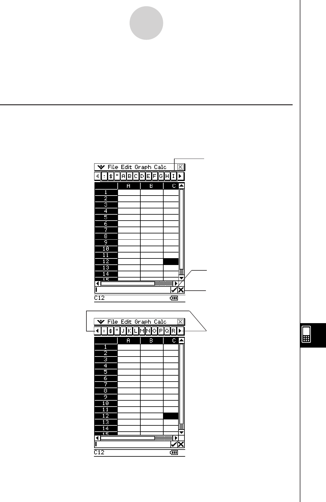
20090601

13-4-1

Editing Cell Contents

13-4 Editing Cell Contents

This section explains how to enter the edit mode for data input and editing, and how to input

various types of data and expressions into cells.

Edit Mode Screen

The Spreadsheet application automatically enters the edit mode whenever you tap a cell to

select it and input something from the keypad.

Entering the edit mode (see page 13-4-2) displays the editing cursor in the edit box and the

data input toolbar.

Tap to apply your input

or edits.

Tap to cancel input or

editing without making

any changes.

Data input toolbar

Tap to scroll the

character buttons.

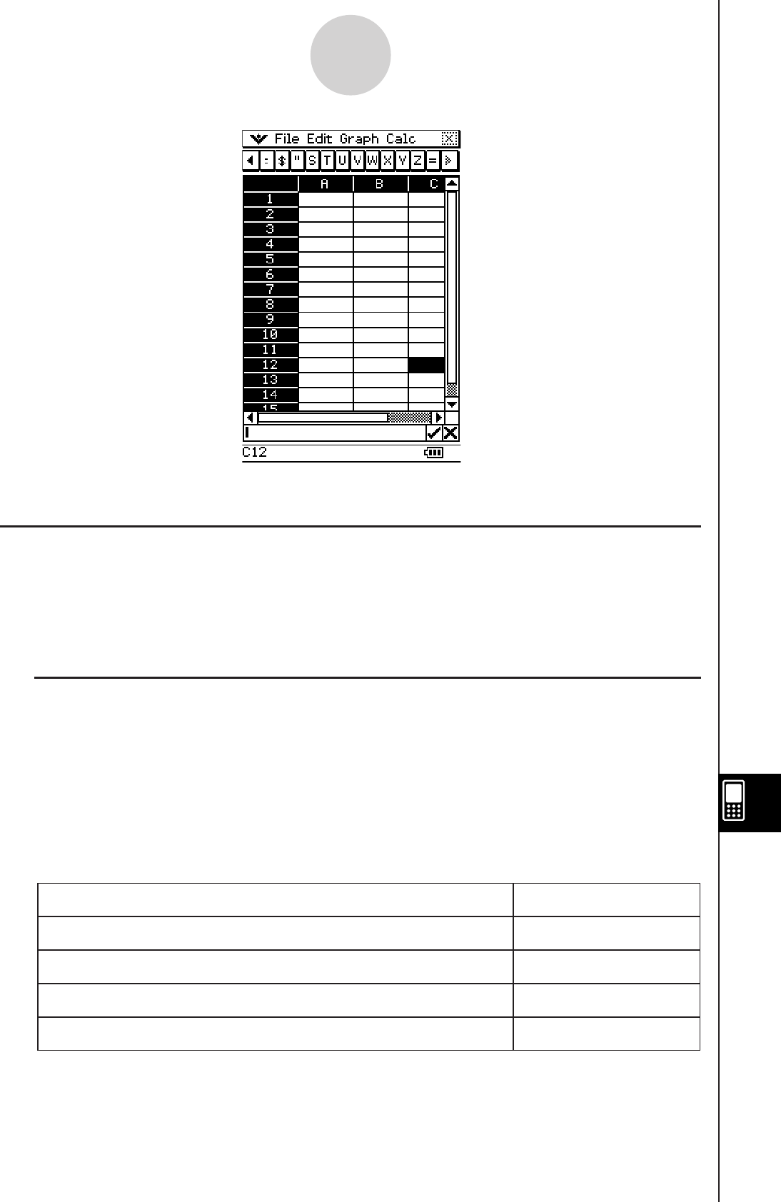
20090601

• You can tap the data input toolbar buttons to input letters and symbols into the edit box.

Entering the Edit Mode

There are two ways you can enter the edit mode:

• Tapping a cell and then tapping inside the edit box

• Tapping a cell and inputting something on the keypad

The following explains the difference between these two techniques.

k Tapping a cell and then tapping the edit box

• This enters the “standard” edit mode.

• Tapping the edit box selects (highlights) all of the text in the edit box. Tapping the edit

box again deselects (unhighlights) the text and displays the editing cursor (a solid blinking

cursor).

• Be sure to use this standard editing mode when you want to correct or change the existing

contents of a cell.

• The following explains the operation of the cursor key after entering the standard editing

mode.

To move the editing cursor here in the edit box text: Press this cursor key:

One character left d

One character right e

To the beginning (far left) f

To the end (far right) c

13-4-2

Editing Cell Contents

20090601

k Tapping a cell and then inputting something from the keypad

• This enters the “quick” edit mode, indicated by a dashed blinking cursor. Anything you input

with the keypad will be displayed in the edit box.

• If the cell you selected already contains something, anything you input with the quick edit

mode replaces the existing content with the new input.

• In the quick editing mode, pressing the cursor key registers your input and moves the cell

cursor in the direction of the cursor key you press.

• Note that you can change to the standard edit mode at any time during the quick edit mode

by tapping inside of the edit box.

Basic Data Input Steps

The following are the basic steps you need to perform whenever inputting or editing cell data.

u ClassPad Operation

(1) Enter the edit mode.

•

Either tap a cell (quick edit), or tap a cell and then tap the edit box (standard edit).

• See “Selecting Cells” on page 13-3-5 for more information about selecting cells.

(2) Input the data you want.

• You can input data using the keypad, the [Calc] menu, and the input toolbar. See the

following sections for more information.

(3) After you are finished, finalize the input using one of the procedures below.

If you are using this edit mode: Do this to finalize your input:

Standard Edit • Tap the s button next to the edit box.

• Press the E key.

Quick Edit • Press a cursor key.

• Or tap the s button next to the edit box.

• Or press the E key.

• This causes the entire spreadsheet to be re-calculated.

• If you want to cancel data input without saving your changes, tap the S button next to

the edit box or tap on the icon panel.

Important!

• You can also finalize input into a cell by tapping a different cell, as long as the first character

in the edit box is not an equal sign (=). Tapping another cell while the first character in the

edit box is an equal sign (=) inserts a reference to the tapped cell into the edit box. See

“Inputting a Cell Reference” on page 13-4-6 for more information.

13-4-3

Editing Cell Contents

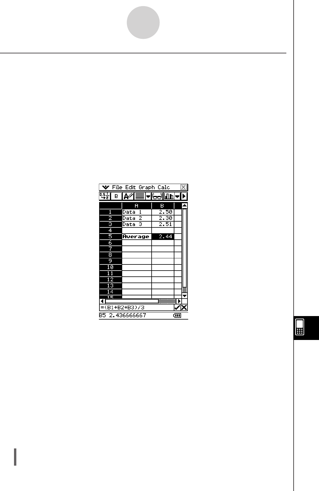
20090601

Inputting a Formula

A formula is an expression that the Spreadsheet application calculates and evaluates when

you input it, when data related to the formula is changed, etc.

A formula always starts with an equal sign (=), and can contain any one of the following.

• Values

• Mathematical expressions

• Cell references

• ClassPad soft keyboard functions (cat page of keyboard)

• [Calc] menu functions (page 13-7-4)

Formulas are calculated dynamically whenever related values are changed, and the latest

result is always displayed in the spreadsheet.

The following shows a simple example where a formula in cell B5 calculates the average of

the values in cells B1 through B3.

13-4-4

Editing Cell Contents

Important!

• Tapping another cell while the first character in the edit box is an equal sign (=) inserts a

reference to the tapped cell into the edit box. Dragging across a range of cells will input a

reference to the selected range. See “Inputting a Cell Reference” on page 13-4-6 for more

information.

• When a cell is set to text data type, formulas are displayed as text when they are not

preceded by an equal sign (=).

• When a cell is set to calculation data type, an error occurs when a formula is not preceded

by an equal sign (=).

u To use the soft keyboards to input a function

Example: To input the following

Cell A1:

x^row(A1)

Cell B1: diff(A1, x, 1)

(1) Tap cell A1 to select it.

(2) Press

=, x, and then {.

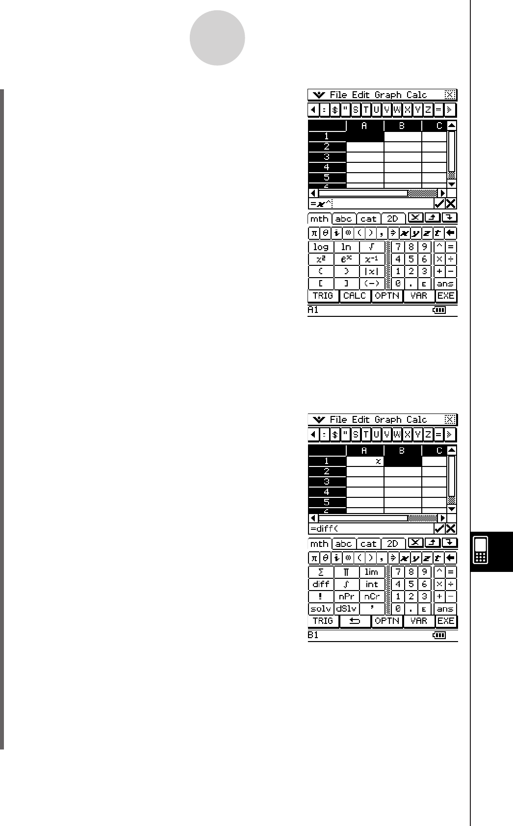
20090601

(3) Press

k to display the soft keyboard.

(4) Tap the

0 tab and then tap r, o, w, then press (, or on the [Calc] menu, tap

[row].

(5) Tap cell A1, and then press ).

(6) Press

(7) Tap cell B1 and then press =.

(8) On the soft keyboard, tap the 9 tab, tap -,

and then tap -.

(9) Tap cell A1, press ,, x, ,, 1, and then press ).

(10) Press

(11) Press

k to hide the soft keyboard.

(12) Select (highlight) cells A1 and B1.

(13) On the [Edit] menu, tap [Copy].

(14) Select cells A2 and B2.

13-4-5

Editing Cell Contents

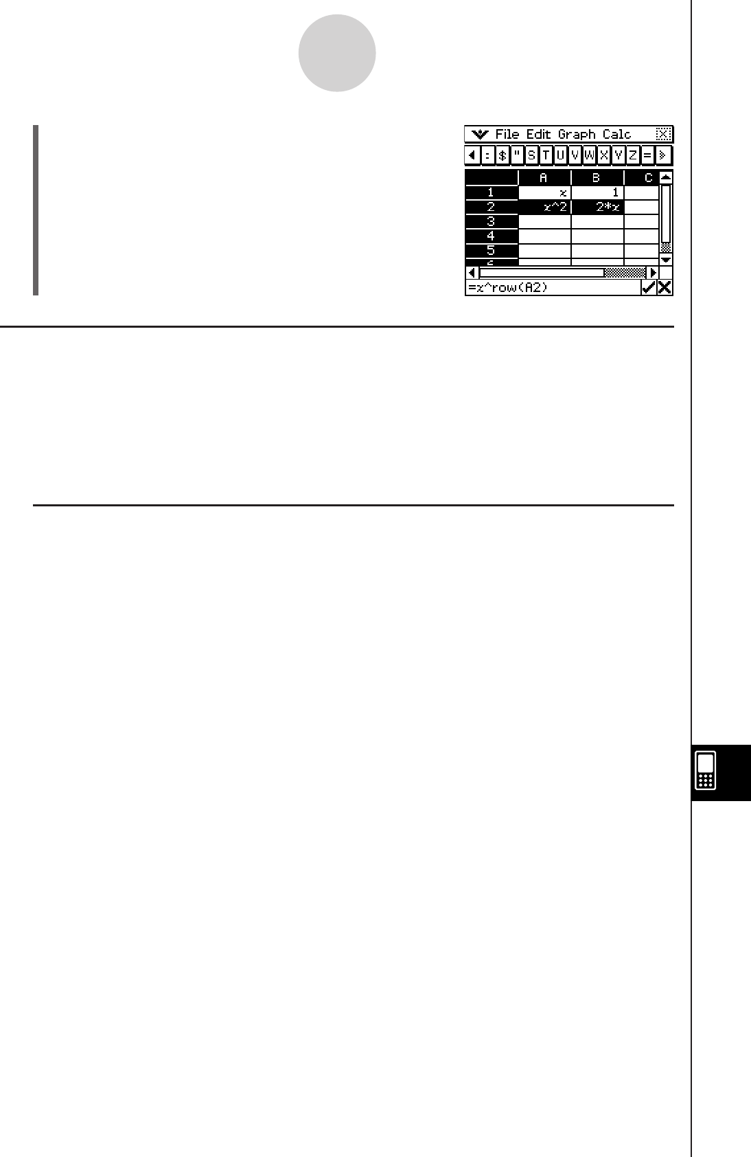
20090601

(15) On the [Edit] menu, tap [Paste].

•

Learn more about cell referencing below.

Inputting a Cell Reference

A cell reference is a symbol that references the value of one cell for use by another cell. If

you input “=A1 + B1” into cell C2, for example, the Spreadsheet will add the current value of

cell A1 to the current value of cell B1, and display the result in cell C2.

There are two types of cell references: relative and absolute. It is very important that you

understand the difference between relative and absolute cell references. Otherwise, your

spreadsheet may not produce the results you expect.

k Relative Cell Reference

A relative cell reference is one that changes according to its location on the spreadsheet. The

cell reference “=A1” in cell C2, for example, is a reference to the cell located “two columns to

the left and one cell up” from the current cell (C2, in this case). Because of this, if we copy or

cut the contents of cell C2 and paste them into cell D12, for example, the cell reference will

change automatically to “=B11”, because B11 is two columns to the left and one cell up from

cell D12.

Be sure to remember that relative cell references always change dynamically in this way

whenever you move them using cut and paste, or drag and drop.

Important!

• When you cut or copy a relative cell reference from the edit box, it is copied to the clipboard

as text and pasted “as-is” without changing. If “=A1” is in cell C2 and you copy “=A1” from

the edit box and paste it into cell D12, for example, D12 will also be “=A1”.

13-4-6

Editing Cell Contents

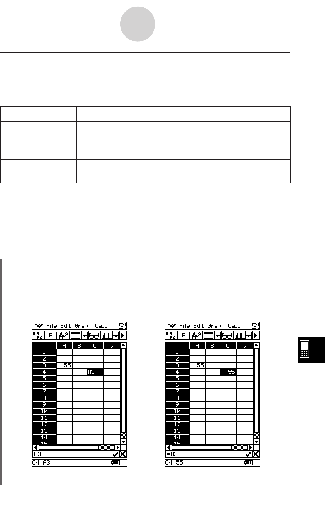
20090601

k Absolute Cell References

An absolute cell reference is the one that does not change, regardless of where it is located

or where it is copied to or moved to. You can make both the row and column of a cell

reference absolute, or you can make only the row or only the column of a cell reference

absolute, as described below.

This cell reference: Does this:

$A$1 Always refers to column A, row 1

$A1 Always refers to column A, but the row changes dynamically when

moved, as with a relative cell reference

A$1 Always refers to row 1, but the column changes dynamically when

moved, as with a relative cell reference

Let’s say, for example, that a reference to cell A1 is in cell C1. The following shows what

each of the above cell references would become if the contents of cell C1 were copied to cell

D12.

$A$1 → $A$1

$A1 → $A12

A$1 → B$1

u To input a cell reference

(1) Select the cell where you want to insert the cell reference.

(2) Tap inside the edit box.

(3) If you are inputting new data, input an equal sign (=) first. If you are editing existing

data, make sure that its first character is an equal sign (=).

• Inputting a cell name like “A3” without an equal sign (=) at the beginning will cause

“A” and “3” to be input as text, without referencing the data in cell A3.

13-4-7

Editing Cell Contents

Incorrect cell reference (no “=” sign) Correct cell reference

20060301

A constant is data whose value is defined when it is input. When you input something into a

cell for which text is specified as the data type without an equal sign (=) at the beginning, a

numeric value is treated as a constant and non-numeric values are treated as text.

Note the following examples for cells of u type:

This input: Is interpreted as: And is treated as:

sin(1) A numeric expression A constant value

1+1/2 A numeric expression A constant value

1.02389 A numeric expression A constant value

sin(x) A symbolic expression Text

x+yA symbolic expression Text

Result A string expression Text

sin( Invalid expression context Text

• When text is too long to fit in a cell, it spills over into the next cell to the right if the

neighboring cell is empty. If the cell to the right is not empty, the text is cut off and “...” is

displayed to indicate that non-displayed text is contained in the cell.

13-4-8

Editing Cell Contents

(4) Tap the cell you want to reference (which will input its name into the edit box

automatically) or use the editing toolbar and keypad to input its name.

Important!

• The above step always inputs a relative cell reference. If you want to input an

absolute cell reference, use the stylus or cursor keys to move the editing cursor to the

appropriate location, and then use the editing toolbar to input a dollar ($) symbol. See

“Inputting a Cell Reference” on page 13-4-6 for more information about relative and

absolute cell references.

(5) Repeat step (4) as many times as necessary to input all of the cell references you

want. For example, you could input “=A1 + A2”. You can also input a range of cells into

the edit box by dragging across a group of cells.

(6) After your input is the way you want, tap the s button next to the edit box or press the

E key to save it.

Inputting a Constant

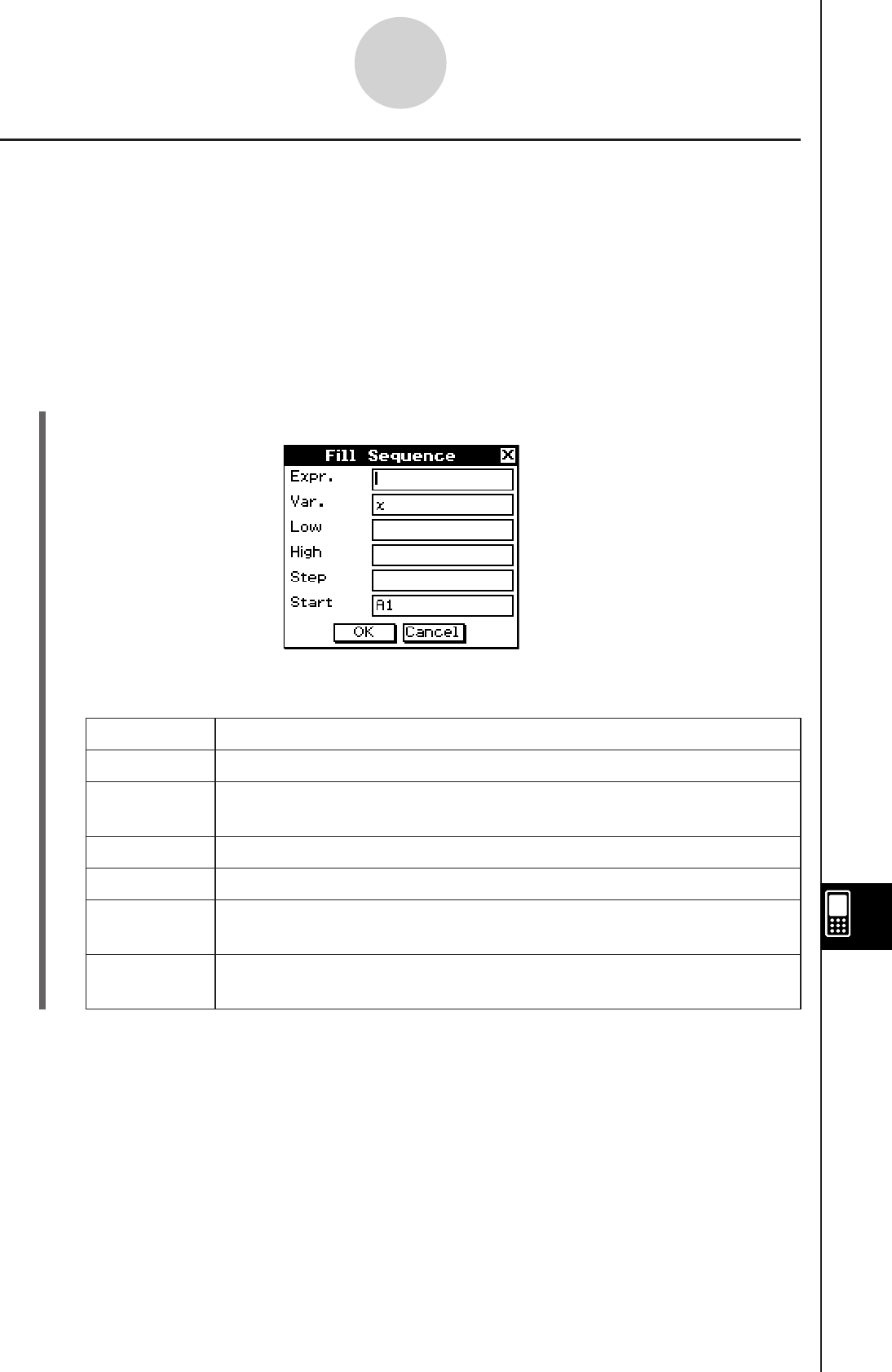
20060301

13-4-9

Editing Cell Contents

Using the Fill Sequence Command

The Fill Sequence command lets you set up an expression with a variable, and input a range

of values based on the calculated results of the expression.

u To input a range of values using Fill Sequence

Example: To configure a Fill Sequence operation according to the following parameters

Expression: 1/x

Change of

x Value: From 1 to 25

Step: 1

Input Location: Starting from A1

(1) On the [Edit] menu, tap [Fill Sequence].

(2) Use the dialog box that appears to configure the Fill Sequence operation as described

below.

Parameter Description

Expr. Input the expression whose results you want to input.

Var. Specify the name of the variable whose value will change with each

step.

Low Specify the smallest value to be assigned to the variable.

High Specify the greatest value to be assigned to the variable.

Step Specify the value that should be added to the variable value with

each step.

Start Specify the starting cell from which the results of the expression

should be inserted.

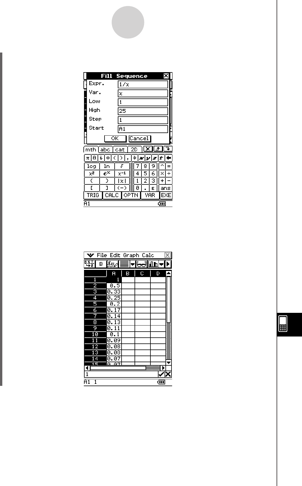
20090601

• The following shows how the Fill Sequence dialog box should appear after configuring

the parameters for our example.

13-4-10

Editing Cell Contents

(3) After everything is the way you want, tap [OK].

• This performs all the required calculations according to your settings, and inserts the

results into the spreadsheet.

• The following shows the results for our example.

20060301

Cut and Copy

You can use the [Cut] and [Copy] commands on the Spreadsheet application [Edit] menu

to cut and copy the contents of the cells currently selected (highlighted) with the cell cursor.

You can also cut and copy text from the edit box.

The following types of cut/copy operations are supported.

• Single cell cut/copy

• Multiple-cell cut/copy

• Selected edit box text cut/copy

• Cell Viewer values and formulas copy only

Cutting or copying data places it onto the clipboard. You can use the [Paste] command to

paste the clipboard contents at the current cell cursor or editing cursor location.

Paste

The [Edit] menu’s [Paste] command lets you paste the data that is currently on the clipboard

at the current cell cursor or editing cursor location.

Important!

• Pasting cell data will cause all relative cell references contained in the pasted data to be

changed in accordance with the paste location. See “Inputting a Cell Reference” on page

13-4-6 for more information.

• Relative cell references in data copied or cut from the edit box do not change when pasted

into another cell.

The following summarizes how different types of data can be pasted.

k When the clipboard contains data from a single cell or the edit box

If you do this: Executing the [Paste] command will do this:

Select a single cell with the cell cursor Paste the clipboard data into the selected cell

Select multiple cells with the cell cursor Paste the clipboard data into each of the

selected cells

Locate the editing cursor inside the edit

box

Paste the clipboard data at the editing cursor

location

k When the clipboard contains data from multiple cells

If you do this: Executing the [Paste] command will do this:

Select a single cell with the cell cursor Paste the clipboard data starting from the

selected cell

Select multiple cells with the cell cursor Paste the clipboard data starting from the first

(top left) cell

Locate the editing cursor inside the edit

box

Paste the clipboard data at the editing cursor

location in matrix format

13-4-11

Editing Cell Contents

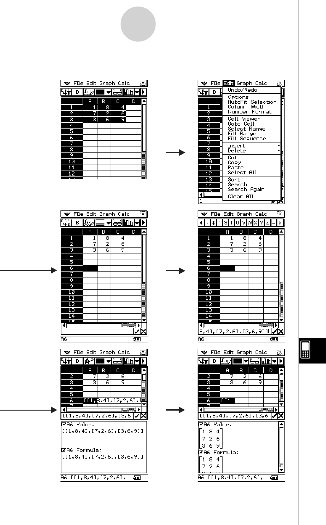
20090601

• The following shows how cell data is converted to a matrix format when pasted into the edit

box.

13-4-12

Editing Cell Contents

Select the cell where

you want to insert

the text (A6 in this

example), and then

tap inside the edit

box.

Tap [Edit],

and then

[Paste].

To view the matrix

as text, tap the cell

(A6) and then A.

To view the

matrix as

2D, tap u

to change

data types.

20060301

13-4-13

Editing Cell Contents

Specifying Text or Calculation as the Data Type for a Particular Cell

A simple toolbar button operation lets you specify that the data contained in the currently

selected cell or cells should be treated as either text or calculation data. The following shows

how the specified data type affects how a calculation expression is handled when it is input

into a cell.

When this data type is

specified: Inputting this into the cell: Causes this to be

displayed:

Text u

(toolbar button for text)

=2+2 4

2+2 2+2

Calculation <

(toolbar button for math)

=2+2 4

2+2 4

Important!

• Unless noted otherwise, all of the input examples in this chapter assume that input is

being performed into a cell for which text is specified as the data type. Because of this,

calculations that evaluate will be preceded with an equal sign (=).

u ClassPad Operation

(1) Select the cell(s) whose data type you want to specify.

• See “Selecting Cells” on page 13-3-5 for information about selecting cells.

(2) On the toolbar, tap the third button from the left (u / <) to toggle the data type

between text and calculation.

20090601

Using Drag and Drop to Copy Cell Data within a Spreadsheet

You can also copy data from one cell to another within a spreadsheet using drag and drop. If

the destination cell already contains data, it is replaced with the newly dropped data.

• When performing this operation, you can drag and drop between cells, or from one location

to another within the edit box only. You cannot drag and drop between cells and the edit

box.

Important!

• Remember that moving cell data within a spreadsheet using drag and drop will cause

all relative cell references in the data to be changed accordingly. See “Inputting a Cell

Reference” on page 13-4-6 for more information.

u To drag and drop between cells within a spreadsheet

(1) Use the stylus to select the cell or range of cells you want to copy so it is highlighted.

Lift the stylus from the screen after you select the cell(s).

• See “Selecting Cells” on page 13-3-5 for information about selecting cells.

(2) Hold the stylus against the selected cell(s).

Selection boundary

• Check to make sure that a white selection boundary appears where you hold the

stylus against the screen.

• If you have multiple cells selected (highlighted), the selection boundary will appear

only around the single cell where the stylus is located. See “Dragging and Dropping

Multiple Cells” on page 13-4-15 for more information.

(3) Drag the stylus to the desired location and then lift the stylus to drop the cell(s) in place.

13-4-14

Editing Cell Contents

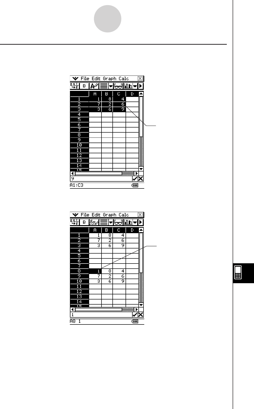
20090601

13-4-15

Editing Cell Contents

Selection boundary

(cursor held against C2)

k Dragging and Dropping Multiple Cells

• When dragging multiple cells, only the cell where the stylus is located has a selection

boundary around it.

Selection boundary

dropped here (A8)

• When you release the stylus from the screen, the top left cell of the group (originally A1 in

the above example) will be located where you drop the selection boundary.

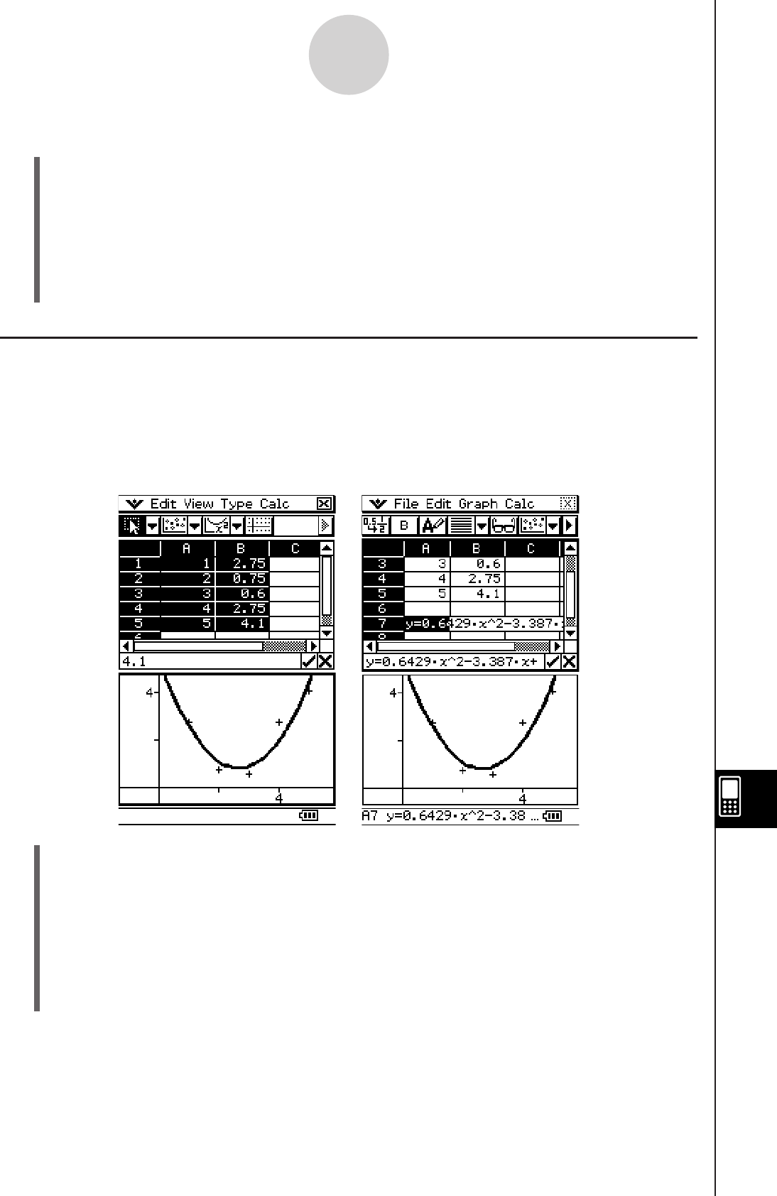
20101001

13-4-16

Editing Cell Contents

u To drag and drop within the edit box

(1) Select the cell whose contents you want to edit.

(2) Tap the edit box to enter the edit mode.

(3) Tap the edit box again to display the editing cursor (a solid blinking cursor).

(4) Drag the stylus across the characters you want to move, so they are highlighted.

(5) Holding the stylus against the selected characters, drag to the desired location.

(6) Lift the stylus to drop the characters in place.

Using Drag and Drop to Obtain Spreadsheet Graph Data

The following examples show how you can drag graph data from a Spreadsheet application

Graph window to obtain the graph’s function or the values of the graph’s data.

u To use drag and drop to obtain the function of a graph

Example: To obtain the function of the regression graph shown below

(1) Input data and plot the scatter graph.

(2) On the [Calc] menu, clear the check box next to [DispStat] by tapping it.

(3) Draw a regression curve. For example, tap [Calc] and then [Quadratic Reg] here.

• See “Regression Graph Operations (Curve Fitting)” on page 13-9-15 for more

information on drawing regression graph.

(4) Tap the graph curve and then drag to the cell you want in the Spreadsheet window.

• This will cause the graph’s function to appear inside the cell.

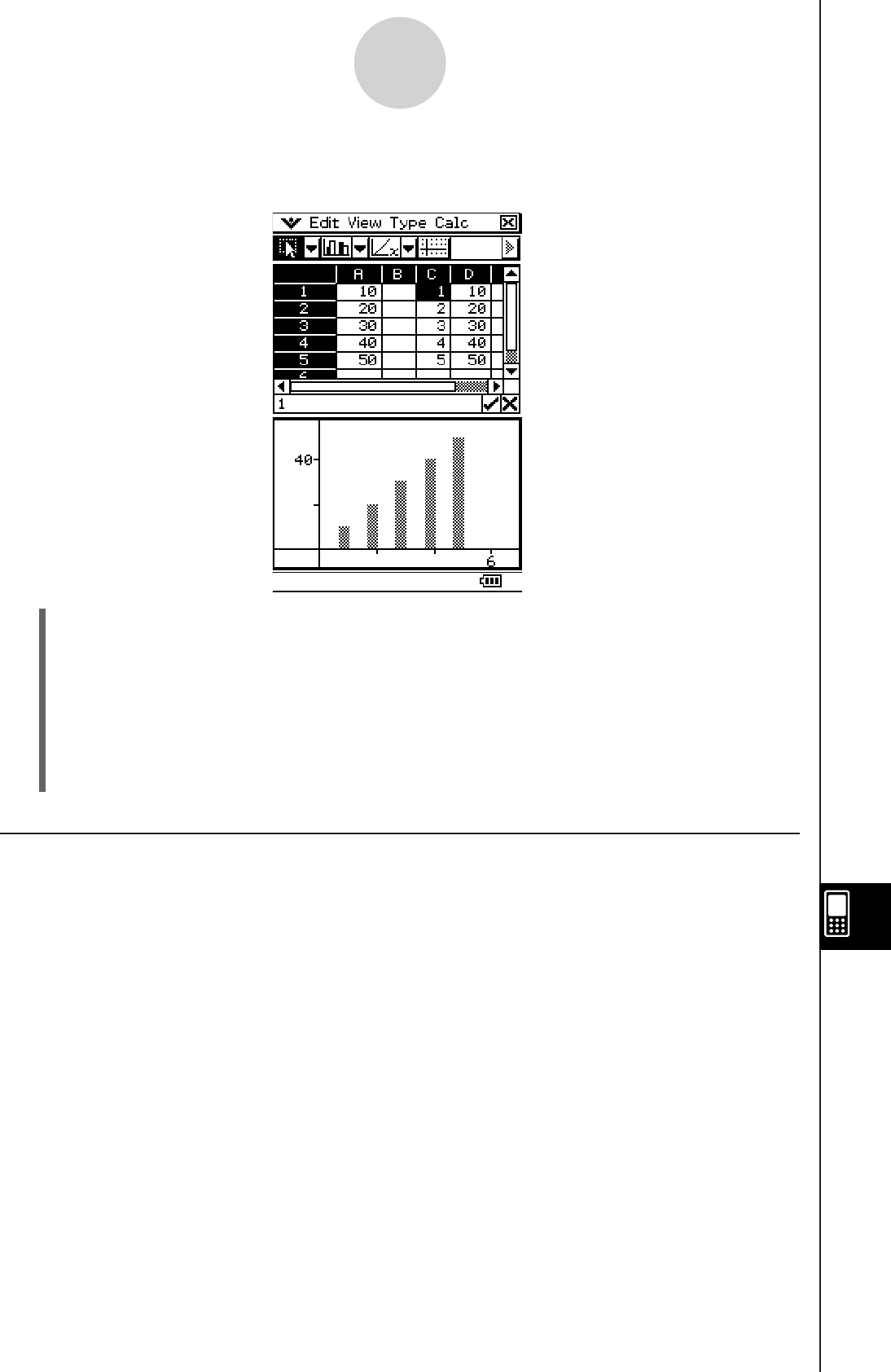
20090601

u To use drag and drop to obtain the data points of a graph

Example: To obtain the data points of the bar graph shown below

13-4-17

Editing Cell Contents

(1) Input data and draw a bar graph.

• See “Other Graph Window Operations” on page 13-9-16 for more information on

graphing.

(2) Tap the Graph window to make it active.

(3) Tap the top of any bar within the Graph window, and then drag to the cell you want in

the Spreadsheet window.

• This will cause the bar graph’s data to appear beginning at the cell you tapped.

Recalculating Spreadsheet Expressions

You can use the Recalculate command to recalculate the cells in a spreadsheet.

You should use Recalculate as described below.

• Let’s say there is a calculation expression (like = a + 1) that includes a variable input in a

spreadsheet cell. When you assign a new value to the variable in the calculation expression

(“a” in this example), the new value is not immediately reflected in calculation result that

is displayed as the cell’s value. After assigning a value to a variable in a calculation

expression, you need to execute the Recalculate command to update the calculation result.

• While the Spreadsheet application is being accessed from the Main application, changes

you make to values assigned to variables on the Main application window are not reflected

immediately on the Spreadsheet application window. In this case, you need to make the

Spreadsheet application window active and execute the Recalculate command to update

its contents.

Tip

• Recalculate is executed automatically whenever you switch to the Spreadsheet application from

another application, and whenever you open a spreadsheet file.

• For information about accessing the Spreadsheet application or another application from the Main

application, see “2-10 Using the Main Application in Combination with Other Applications.”

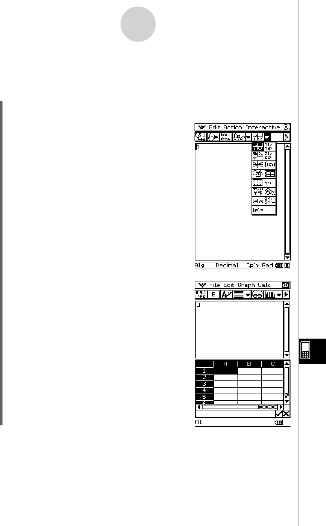
20090601

Example: To assign values to variables and recalculate expressions that contain them.

The following procedure shows the recalculate operation while the Spreadsheet

application is being accessed from the Main application.

u ClassPad Operation

(1) On the application menu, tap J.

This starts the Main application and displays the work area.

(2) On the toolbar, tap the down arrow button next to $.

This displays a palette of application icons.

(3) Tap the

Q button.

This splits the display with a Main application window

above and a Spreadsheet window below.

13-4-18

Editing Cell Contents

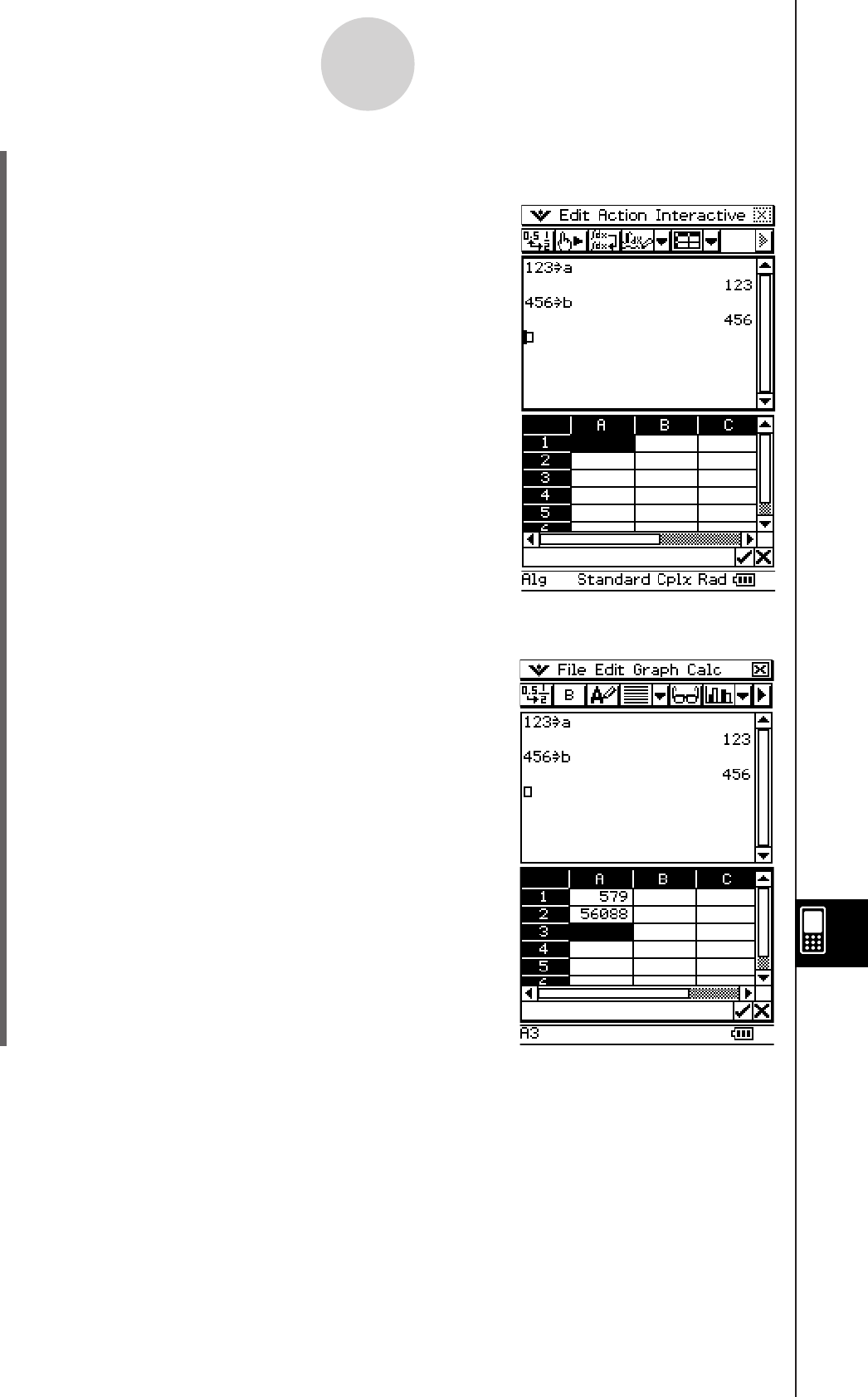
20090601

(4) On the Main application window, use the following operation to assign values to the

variables.

9bcdW0aE

9efgW0bE

(5) On the Spreadsheet window, tap cell A1 and input =a+b. Next, tap cell A2 and input

=a×b.

When you input the above expressions, the results will

appear dynamically in cells A1 and A2.

13-4-19

Editing Cell Contents

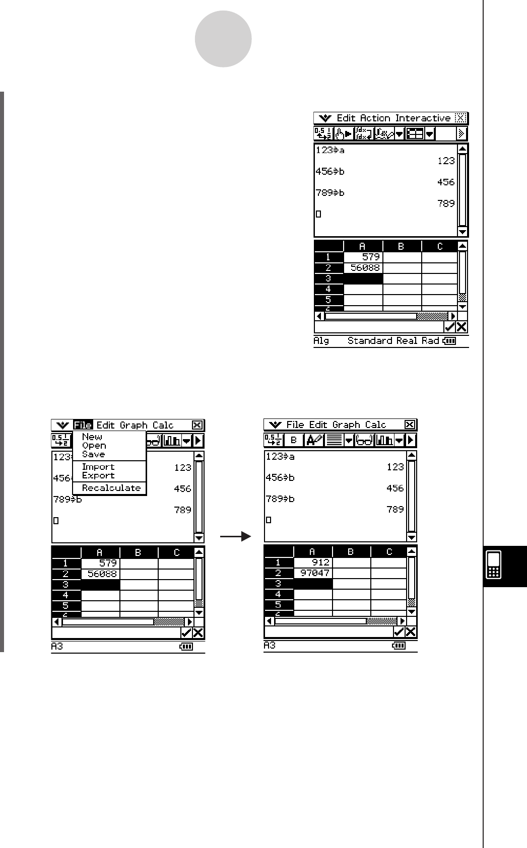
20090601

(6) On the Main application window, assign different values to the variables.

Here, assign 789 to variable b as shown below.

9hijW0bE

(7) Tap the Spreadsheet application window to make it active. On the [File] menu, tap

[Recalculate].

This recalculates the expressions in the Spreadsheet window and displays their results.

13-4-20

Editing Cell Contents

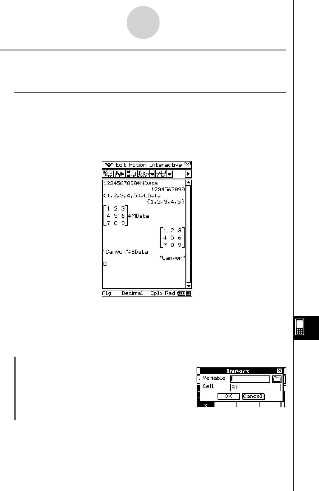
20060301

13-4-21

Editing Cell Contents

Importing and Exporting Variable Values

You can use the procedures in this section to import the data currently assigned to a variable

into a spreadsheet, and to export data in a spreadsheet to a variable.

k Importing data assigned to a variable into a spreadsheet

You can import the data assigned to a variable into a specific cell or a range of cells in the

spreadsheet that is currently open on the ClassPad display. Import of variable data from

the following data types is supported: LIST (list data), MAT (matrix data), EXPR (numeric or

expression data), and STR (string data).

The procedures in this section assume that the variables (NData, LData, MData, SData)

shown in the screen below are already present on the Main application.

Tip

• For details about data types, see “Variable Data Types” on page 1-7-3.

• For details about creating variables, see “Creating a New Variable” on page 1-7-6.

u To import the data assigned to an EXPR variable

Example: To import the data assigned to the NData variable into cell A1

(1) Tap cell A1 to select it.

(2) On the [File] menu, tap [Import].

This displays the Import dialog box along with a soft

keyboard.

(3) Type the variable name (in this case “NData”) into the [Variable] box.

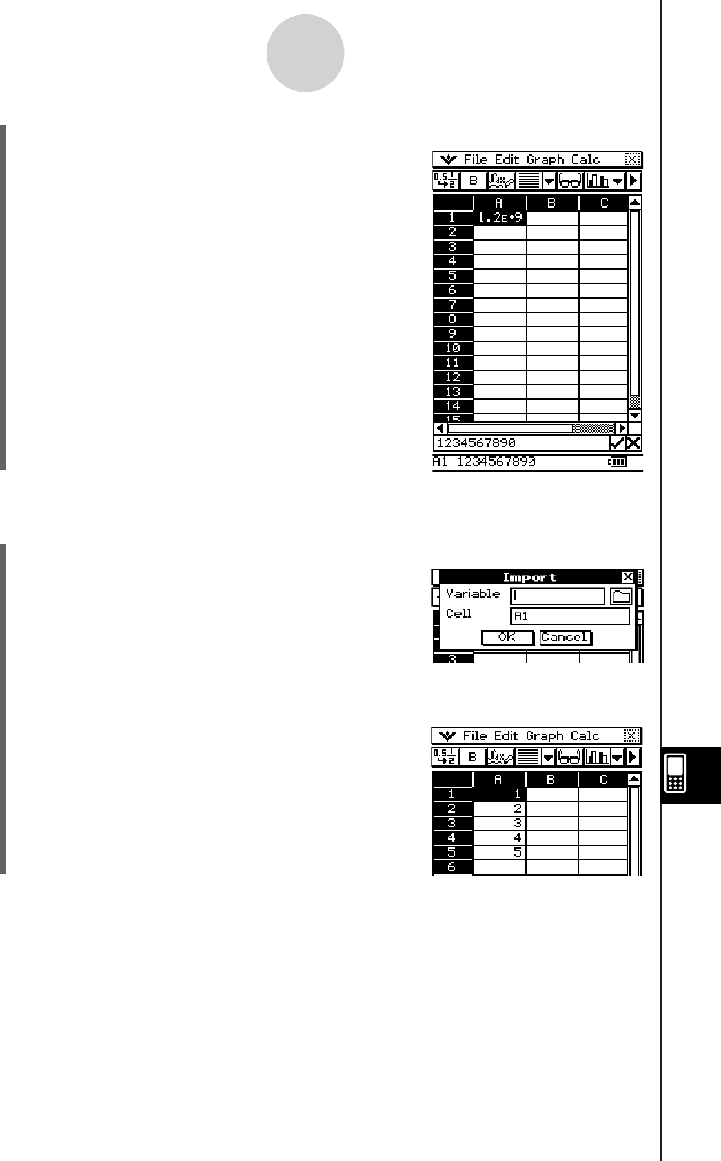
20090601

13-4-22

Editing Cell Contents

(4) After confirming that everything is the way you want, tap [OK].

• This will input the data assigned to the NData variable

(in this case, 1234567890) into spreadsheet cell A1

as shown here.

u To import the data assigned to a LIST variable

Example: To import the list data {1, 2, 3, 4, 5} assigned to the LData variable at cell A1

(1) Tap cell A1 to select it.

(2) On the [File] menu, tap [Import].

• This displays the Import dialog box along with a soft

keyboard.

(3) Type the variable name (in this case “LData”) into the [Variable] box.

(4) After confirming that everything is the way you want, tap [OK].

• This will input the data assigned to the LData variable

(in this case, {1, 2, 3, 4, 5}) into spreadsheet cells A1

through A5 as shown here.

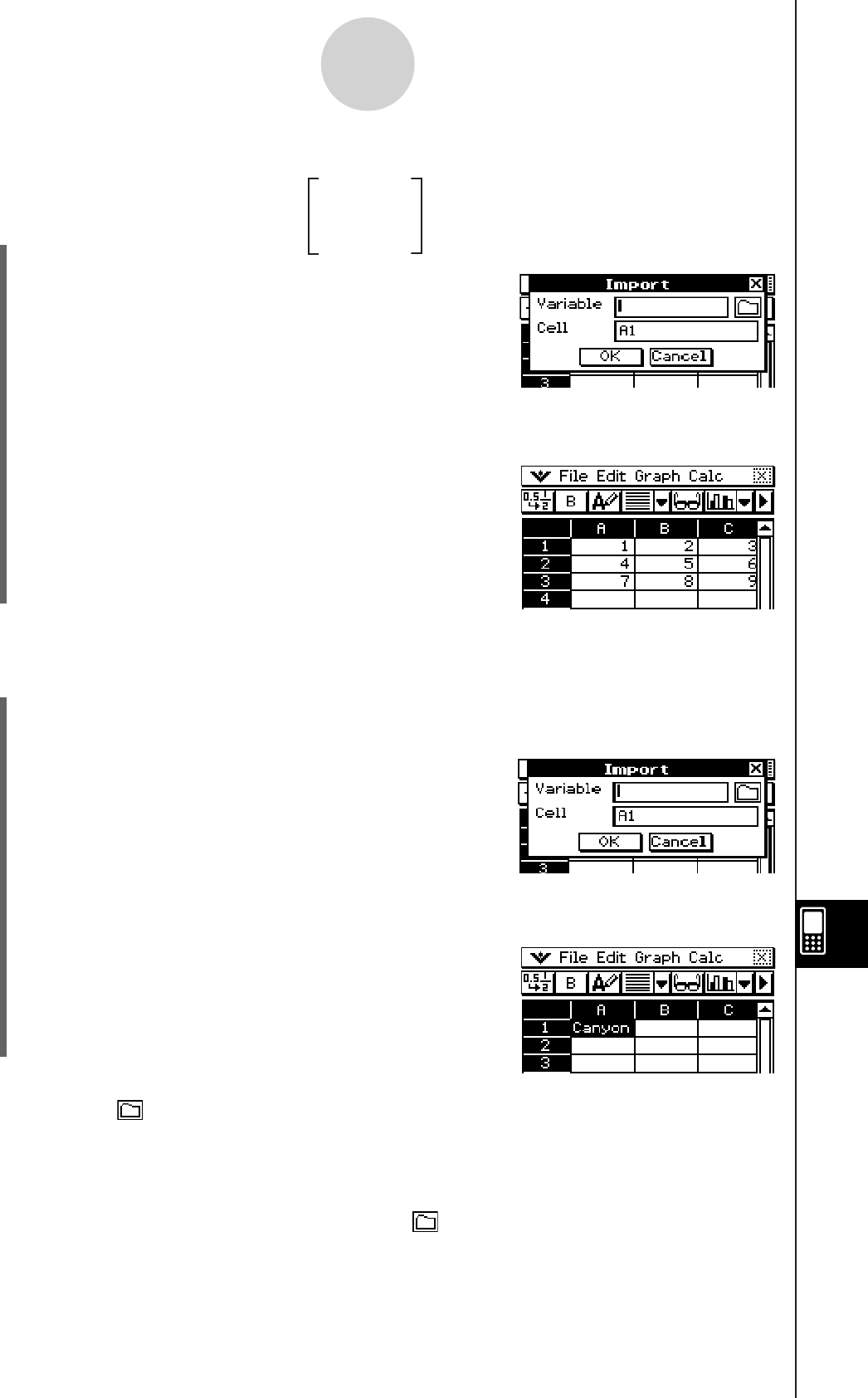
20090601

13-4-23

Editing Cell Contents

u To import the data assigned to a MAT variable

Example: To import the matrix data assigned to the MData variable at cell A1

(1) Tap cell A1 to select it.

(2) On the [File] menu, tap [Import].

• This displays the Import dialog box along with a soft

keyboard.

(3) Type the variable name (in this case “MData”) into the [Variable] box.

(4) After confirming that everything is the way you want, tap [OK].

• This will input the data assigned to the MData

variable into the spreadsheet starting from cell A1 as

shown here.

u To import the data assigned to a STR variable

Example: To import the data assigned to the SData variable into cell A1

(1) Tap cell A1 to select it.

(2) On the [File] menu, tap [Import].

• This displays the Import dialog box along with a soft

keyboard.

(3) Type the variable name (in this case “SData”) into the [Variable] box.

(4) After confirming that everything is the way you want, tap [OK].

• This will input the data assigned to the SData variable

into spreadsheet cell A1 as shown here.

Tip

• Tapping the icon on the import dialog box will display the Variable Manager, which you can

use to select the variable you want. See “1-8 Using the Variable Manager” for more information.

• The error message “Variable not found” will appear if the variable whose name you input on the

Import dialog box cannot be found for some reason. If this happens, check to make sure that

you input the variable name correctly and that the variable you specified is located in the current

folder. If this does not correct the problem, tap the icon on the Import dialog box and use the

Variable Manager to select the variable you want. For information about the current folder, see “1-7

Variables and Folders”.

1 2 3

4 5 6

7 8 9

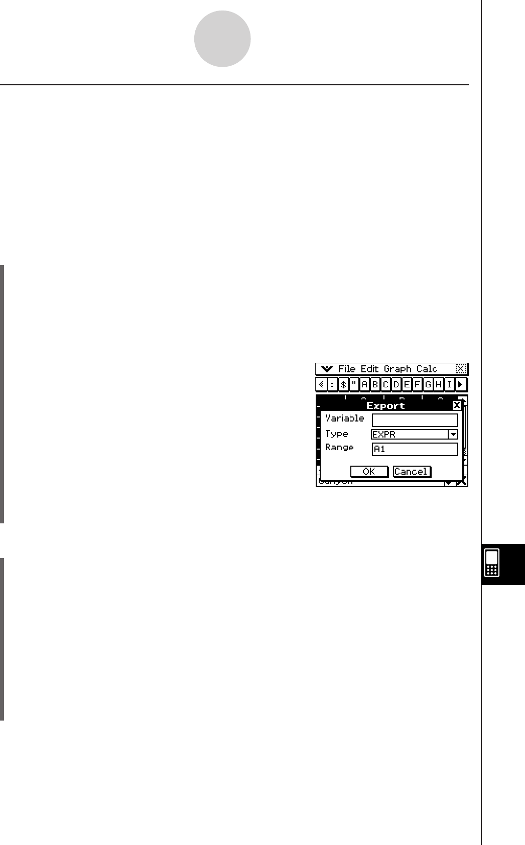
20090601

13-4-24

Editing Cell Contents

k Exporting Spreadsheet Data to a Variable

You can use the procedures in this section to export the data contained in a specific cell or

range of cells in the spreadsheet that is currently open on the ClassPad display. Export of

spreadsheet data to the variables of the following data types is supported: LIST (list data),

MAT (matrix data), and EXPR (numeric or expression data).

Tip

• For details about data types, see “Variable Data Types” on page 1-7-3.

• For information about using variables, see “1-7 Variables and Folders” and “1-8 Using the

Variable Manager”.

u To export spreadsheet data to an EXPR variable

(1) Select a single cell that contains the data you want to export to an EXPR variable.

• You cannot export data from multiple cells to an EXPR variable. Be sure to select

only one cell for this procedure.

• It makes no difference whether the cell you select contains a value, expression, or

string. Note that string data exported from a cell is exported as EXPR type data, not

STR type data.

(2) On the [File] menu, tap [Export].

• This displays the Export dialog box along with a soft

keyboard.

• In this case, “EXPR” will be automatically selected in

the [Type] box.

(3) Type the variable name into the [Variable] box.

(4) After confirming that everything is the way you want, tap [OK].

u To export spreadsheet data to a LIST variable

(1) Select the range of cells that contains the data you want to export to a LIST variable.

(2) On the [File] menu, tap [Export].

• This displays the Export dialog box along with a soft keyboard.

(3) Tap the [Type] box down arrow button, and then select “LIST” from the list of variable

types that appears.

• If the range of cells you selected in step 1 consists of columns in a single line

or multiple lines in a single column, “LIST” will be selected as the variable type

automatically.

(4) Type the variable name into the [Variable] box.

(5) After confirming that everything is the way you want, tap [OK].

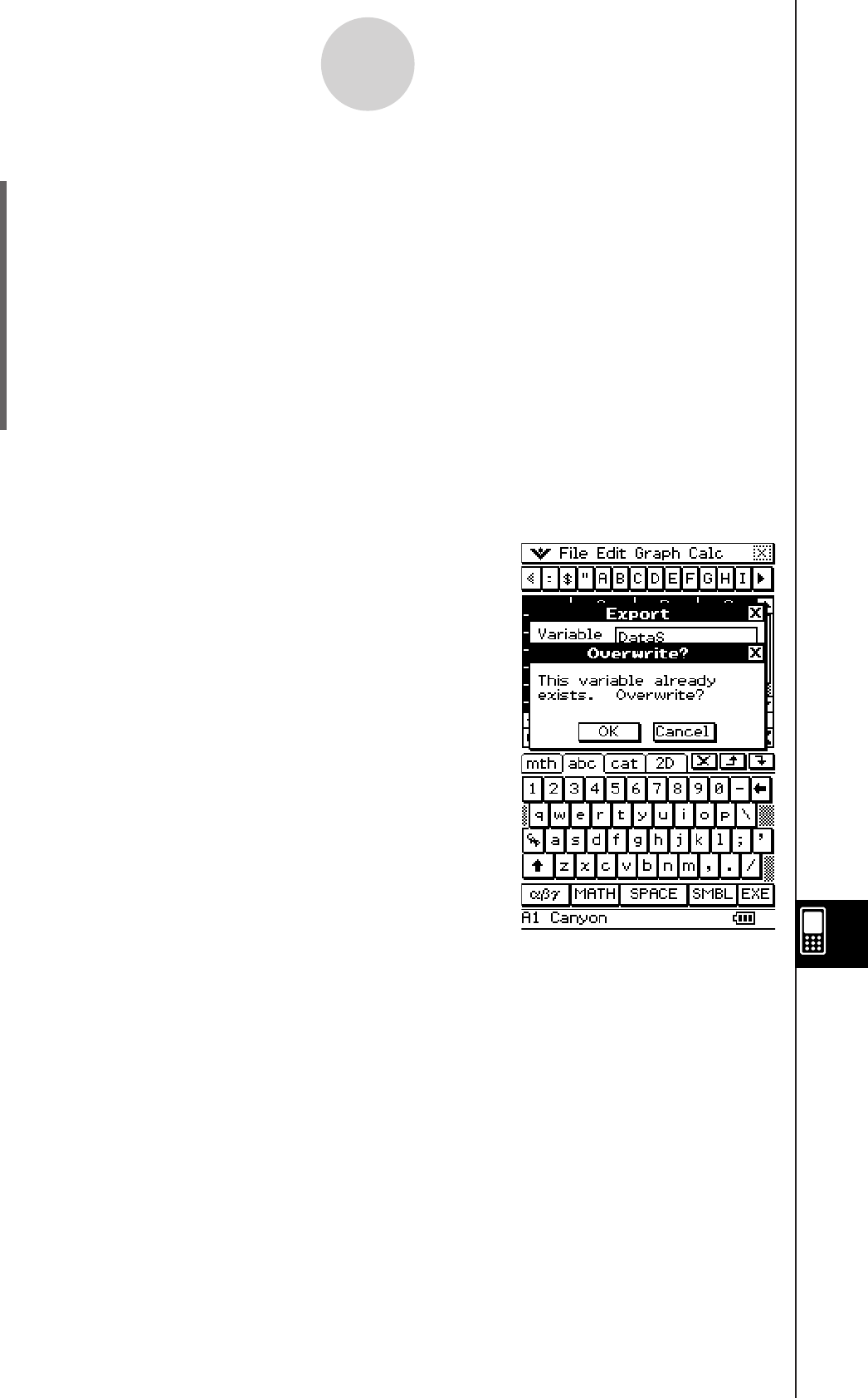
20090601

13-4-25

Editing Cell Contents

u To export spreadsheet data to a MAT (Matrix) variable

(1) Select the range of cells that contains the data you want to export to a Mat variable.

(2) On the [File] menu, tap [Export].

This displays the Export dialog box along with a soft keyboard.

(3) Tap the [Type] box down arrow button, and then select “MATRIX” from the list of

variable types that appears.

• If the range of cells you selected in step 1 consists of multiple columns and multiple

lines, “MATRIX” will be selected as the variable type automatically.

(4) Type the variable name into the [Variable] box.

(5) After confirming that everything is the way you want, tap [OK].

Tip

• A confirmation dialog box like the one shown below will appear when you tap [OK] if the name in

the [Variable] box on the Export dialog box is already being used by another variable.

To overwrite the existing variable with the new one, tap [OK]. If you do not want to overwrite the

existing variable, tap [Cancel] to appear to the Export dialog box. Type a different name into the

[Variable] box.

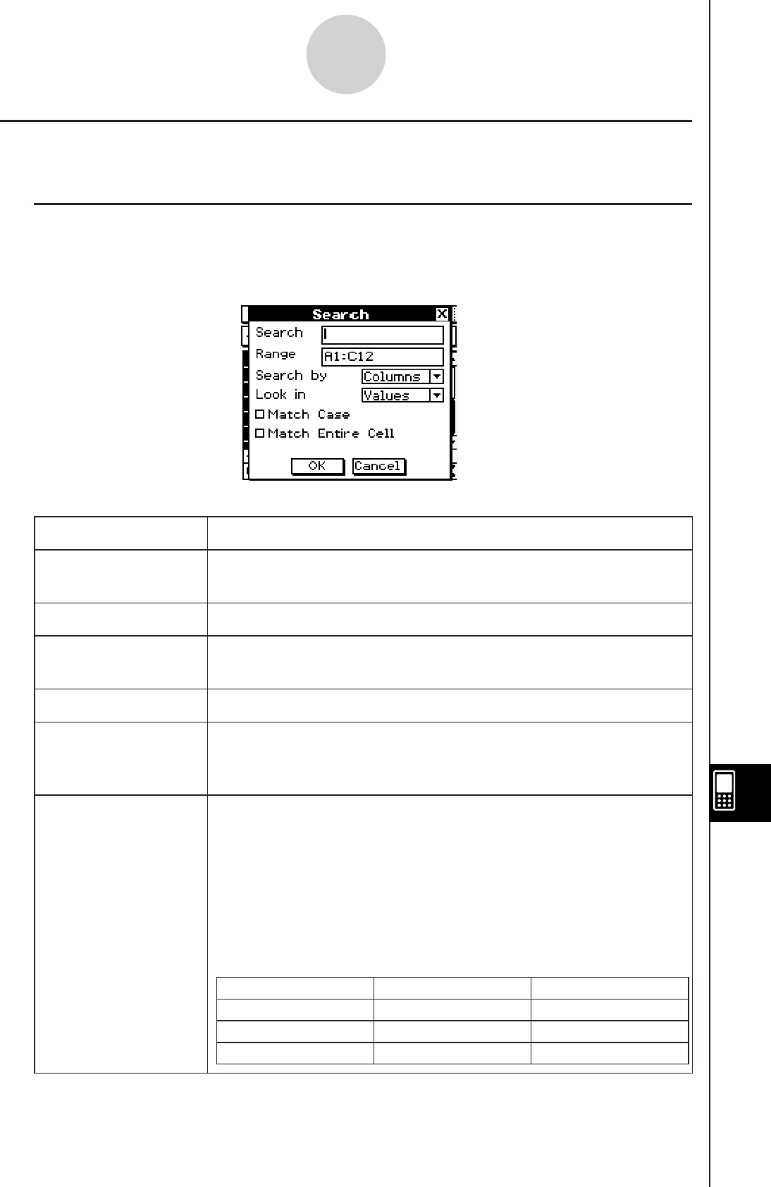
20060301

13-4-26

Editing Cell Contents

Searching for Data in a Spreadsheet

The Search command helps you locate specific data in a spreadsheet quickly and easily.

k Search Dialog Box

The Search command can be executed either by tapping [Search] on the [Edit] menu or by

tapping the e button on the toolbar. Executing the Search command displays a search

dialog box like the one shown below, along with a soft keyboard.

The following explains the meaning of each item on the search dialog box.

Item Description

Search Enter the character string, value, or expression you want to search

for. What you enter is called the “search string”.

Range Specifies the range of cells to be searched.

Search by Specifies whether the search should be line-by-line or column-by-

column.

Look in Specifies whether values or formulas should be searched.

 Match Case Select this check box to find exact matches, including uppercase

and lowercase characters, of what is specified in the [Search] box.

Clear the checkbox to search for matches, regardless of case.

 Match Entire Cell Select this check box to find cells that contain only what is

specified in the [Search] box, and nothing else. Clear the check

box to find cells that contain what is specified in the [Search] box,

even if it is mixed with other data.

The following table shows a number of examples of what happens

for each of the [Match Entire Cell] settings when “bcd” is specified

in the [Search] box. “” indicates that the cell is a match, while “”

is not a match.

Cell Contents Not Selected Selected

abcdef 

bcd 

bcdef 

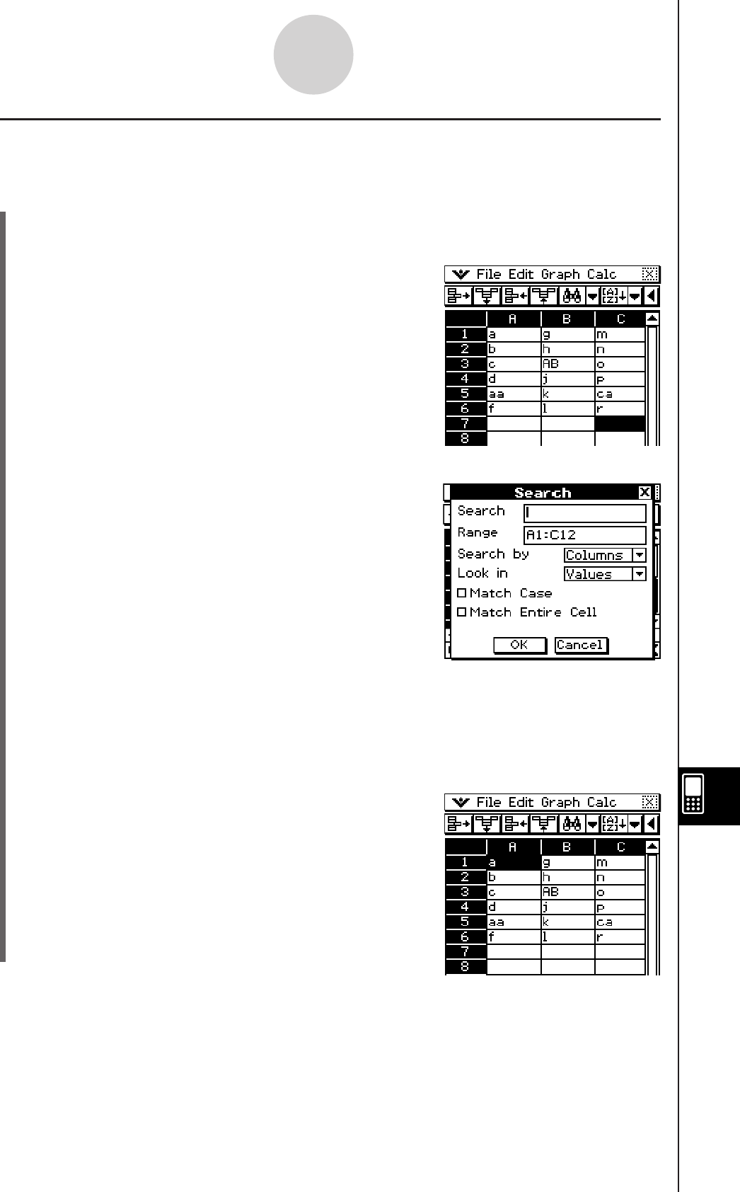
20090601

13-4-27

Editing Cell Contents

k Search Examples

Example 1: To search for the letter “a”, regardless of case

u ClassPad Operation

(1) Display the spreadsheet you want to search.

• This example is based on a spreadsheet that contains the data shown below.

(2) Tap [Search] on the [Edit] menu or tap the toolbar e button.

• This displays the Search dialog box.

• The initial default setting for the [Range] box is the

range of cells that contains data (A1:C12 in this

example).

(3) Enter the search string in the [Search] box.

• Here we will enter “a”.

• Since we want to find the letter “a” regardless of case and since we do not care if

there is other data in a cell, we will not select the [Match Case] and [Match Entire Cell]

check boxes.

(4) After all the settings are the way you want, tap [OK].

• This will start the search and the cursor will jump

to the first cell found that contains a match for the

search string.

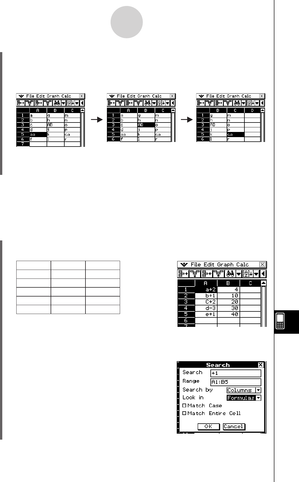
20090601

13-4-28

Editing Cell Contents

(5) To search for the next instance of the search string, tap [Search Again] on the [Edit]

menu or tap the toolbar r button.

• Each time you tap the [Search Again] command or the r toolbar button, the search

will jump to the next cell that contains the specified search string.

• The message “Search String not found in range.” will appear if the string you specified

does not exist within the specified range of cells. Tap [OK] to clear the message from

the screen.

Example 2: To search for calculation expressions that contain the string “+1”

In this example, we want the spreadsheet cells that contain a calculation

expression ( like =1+2 ) to show the expression, not the calculation result ( 3, for

example ). To do this, select “Formulas” for the [Look in] option on the Search

dialog box.

u ClassPad Operation

(1) Display the spreadsheet you want to search.

• This example is based on a spreadsheet that contains the data shown below.

1 =a+2 =3+1

2 =b+1 =8+2

3 =C+2 =18+2

4 =d−3 =28+2

5 =e+1 =39+1

(2) Tap [Search] on the [Edit] menu or tap the toolbar e button.

• This displays the Search dialog box.

(3) Configure the search dialog box settings as

shown here.

Expressions in each cell

Displayed spreadsheet

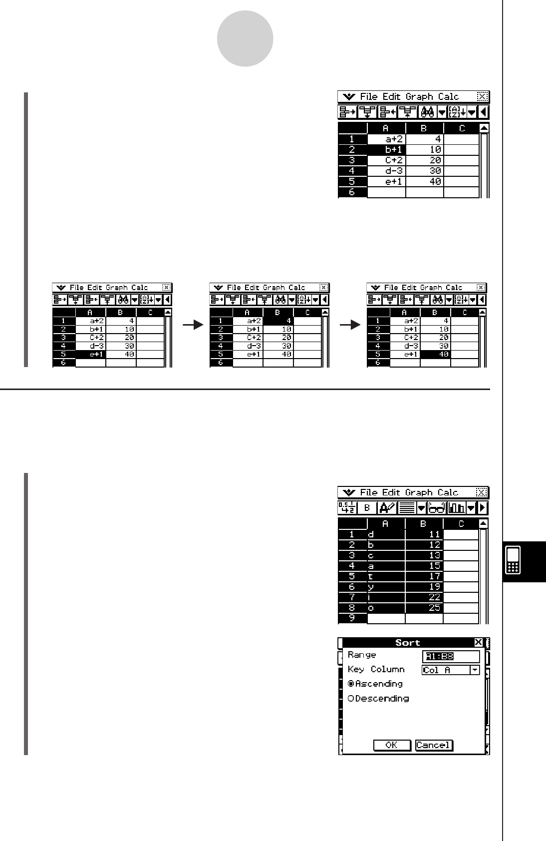
20090601

13-4-29

Editing Cell Contents

(4) Tap [OK].

• This will start the search and the cursor will jump

to the first cell found that contains a match for the

search string.

(5) To search for the next instance of the search string, tap [Search Again] on the [Edit]

menu or tap the toolbar r button.

• Each time you tap the [Search Again] command or the r toolbar button, the search

will jump to the next cell that contains the specified search string.

Sorting Spreadsheet Data

You can use the procedures in this section to sort spreadsheet data in either ascending or

descending order.

u To sort spreadsheet data using the [Sort] menu command

(1) Select the range of cells that contains the data you want to sort.

(2) On the [Edit] menu, tap [Sort].

• This displays the Sort dialog box. The [Range] box

will show the range of cells you selected in step 1.

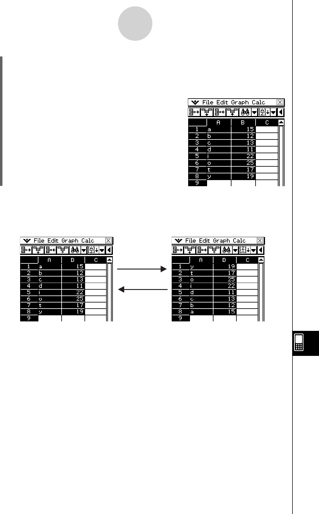
20090601

13-4-30

Editing Cell Contents

(3) Tap the [Key Column] box down arrow button. On the list that appears, select the

column you want the sort to be based upon.

(4) Tap either [Ascending] (a, b, c...) or [Descending] (z, y, x...).

(5) After confirming that everything is the way you want, tap [OK].

• This will execute the sort and rearrange the data

based on the column you specified for [Key Column].

u To sort using the sort toolbar button

After selecting the range of cells, tap either the L (ascending) or : (descending) toolbar

button to execute the sort without displaying a dialog box. In this case, the data is sorted

using the leftmost column of the selected range as the key column.

(Descending)

(Ascending)

(Descending)

(Ascending)

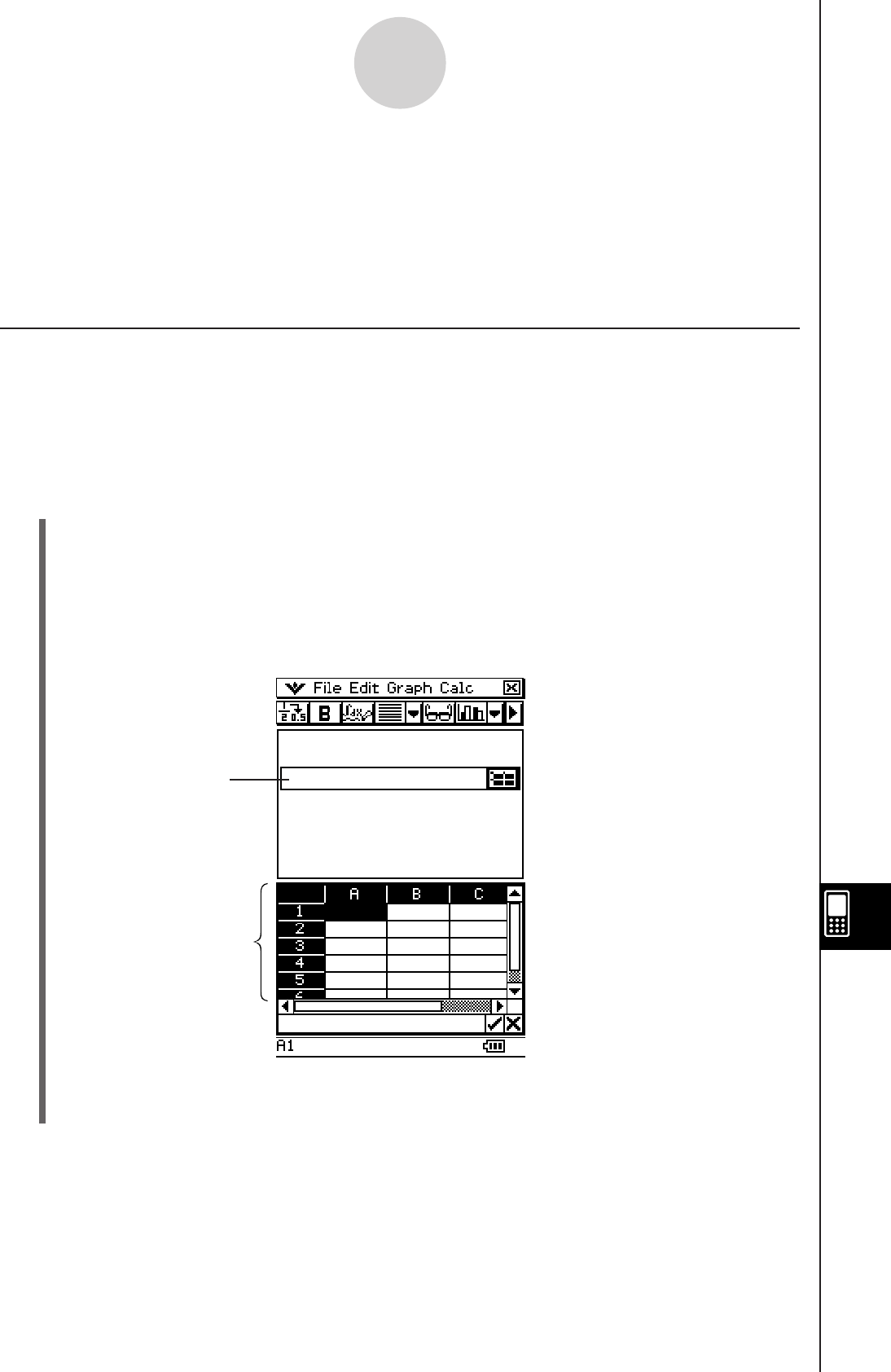
20090601

13-5-1

Using the Spreadsheet Application with the eActivity Application

13-5 Using the Spreadsheet Application with the

eActivity Application

You can display the Spreadsheet application from within the eActivity application. This makes

it possible to drag data between the Spreadsheet and eActivity windows as desired.

Drag and Drop

After you open Spreadsheet within eActivity, you can drag and drop information between the

two application windows.

Example 1: To drag the contents of a single cell from the Spreadsheet window to the

eActivity window

u ClassPad Operation

(1) Tap

m to display the application menu, and then tap A to start the eActivity

application.

(2) From the eActivity application menu, tap [Insert] and [Strip], and then tap [Spreadsheet]

on the submenu.

• This inserts a Spreadsheet data strip, and displays the Spreadsheet window in the

lower half of the screen.

• Note that a Spreadsheet data strip works the same way as the Spreadsheet.

(3) Input the text or value you want into the Spreadsheet window.

Spreadsheet

data strip

Spreadsheet window

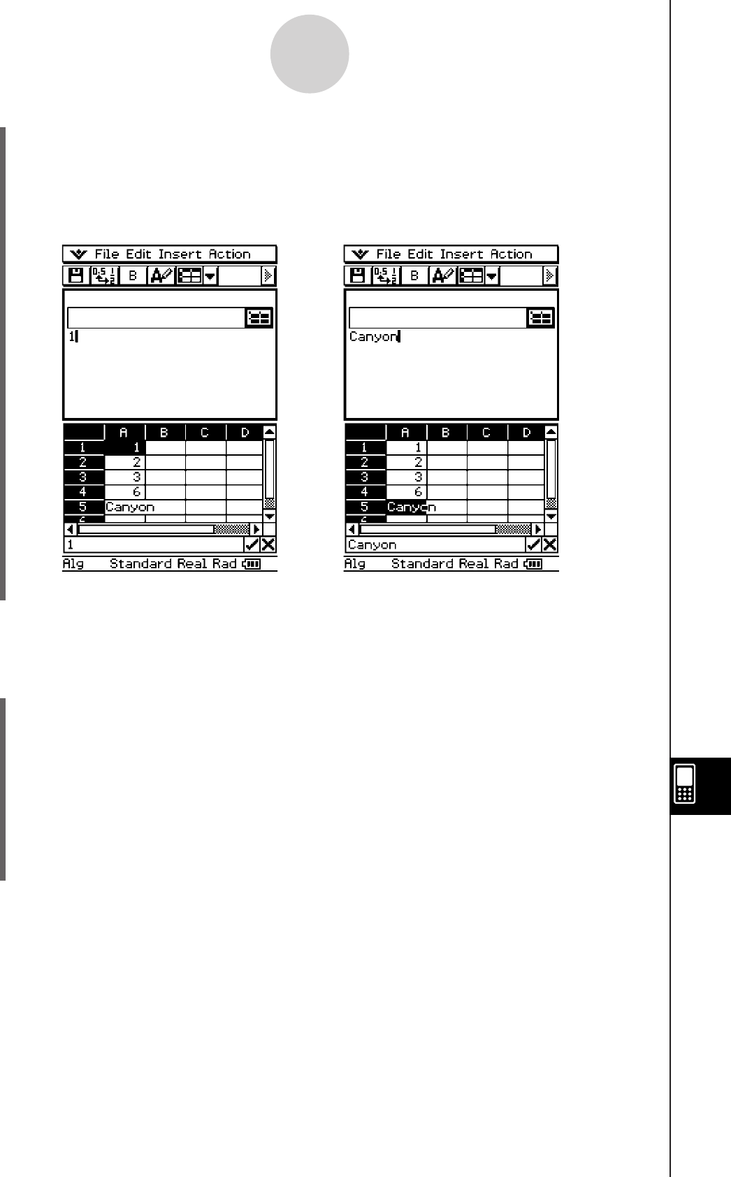
20090601

13-5-2

Using the Spreadsheet Application with the eActivity Application

(4) Select the cell you want and drag it to the first available line in the eActivity window.

• This inserts the contents of the cell in the eActivity window.

• You can also select something in the edit box and drag it to the eActivity window. If

you do, the edit box contents will become deselected after you drop them into the

eActivity window.

(5) You can now experiment with the data in the eActivity window.

Example 2: To drag a calculation expression from the Spreadsheet edit box to the eActivity

window

u ClassPad Operation

(1) Tap

m to display the application menu, and then tap A to start the eActivity

application.

(2) From the eActivity application menu, tap [Insert] and [Strip], and then tap [Spreadsheet]

on the submenu.

• This inserts a Spreadsheet data strip, and displays the Spreadsheet window in the

lower half of the screen.

(3) Select a Spreadsheet cell and input the expression you want.

(4) Tap the edit box to select (highlight) all of the contents of the edit box.

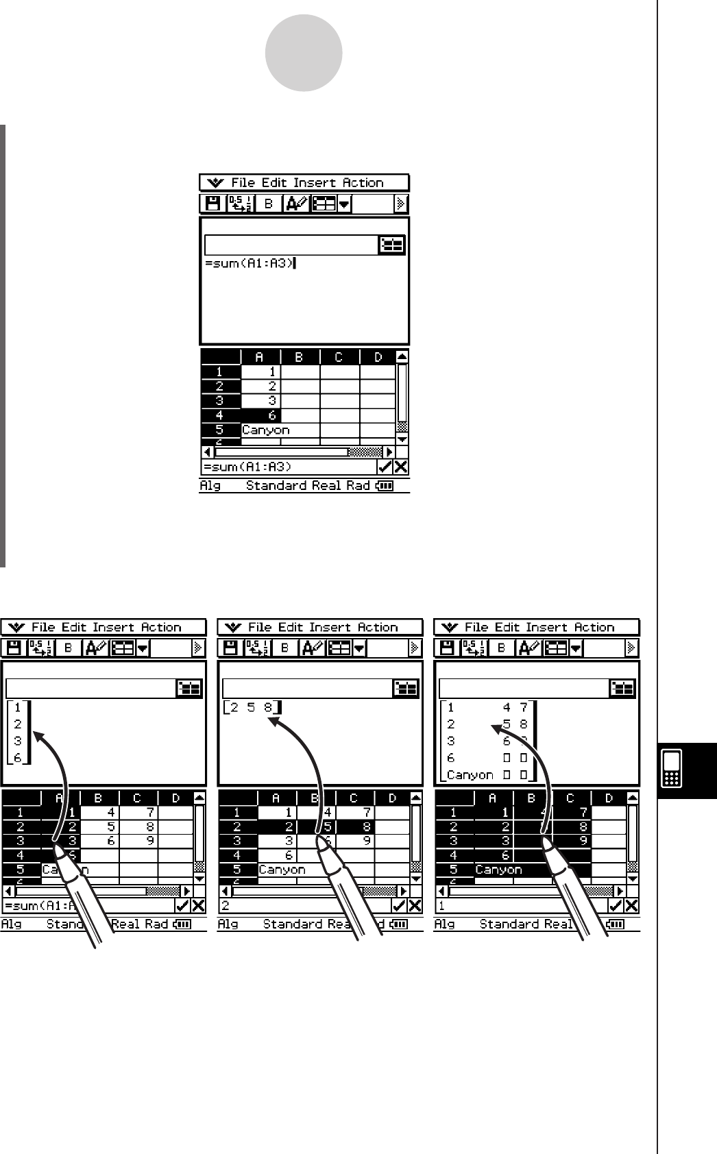
20060301

13-5-3

Using the Spreadsheet Application with the eActivity Application

(5) Drag the contents of the edit box to the first available line in the eActivity window.

• This inserts the contents of the edit box in the eActivity window as a text string.

(6) You can now experiment with the data in the eActivity window.

• The basic operations for the following example are the same for the other examples

described above.

Example 3: Dragging multiple Spreadsheet cells to the eActivity window

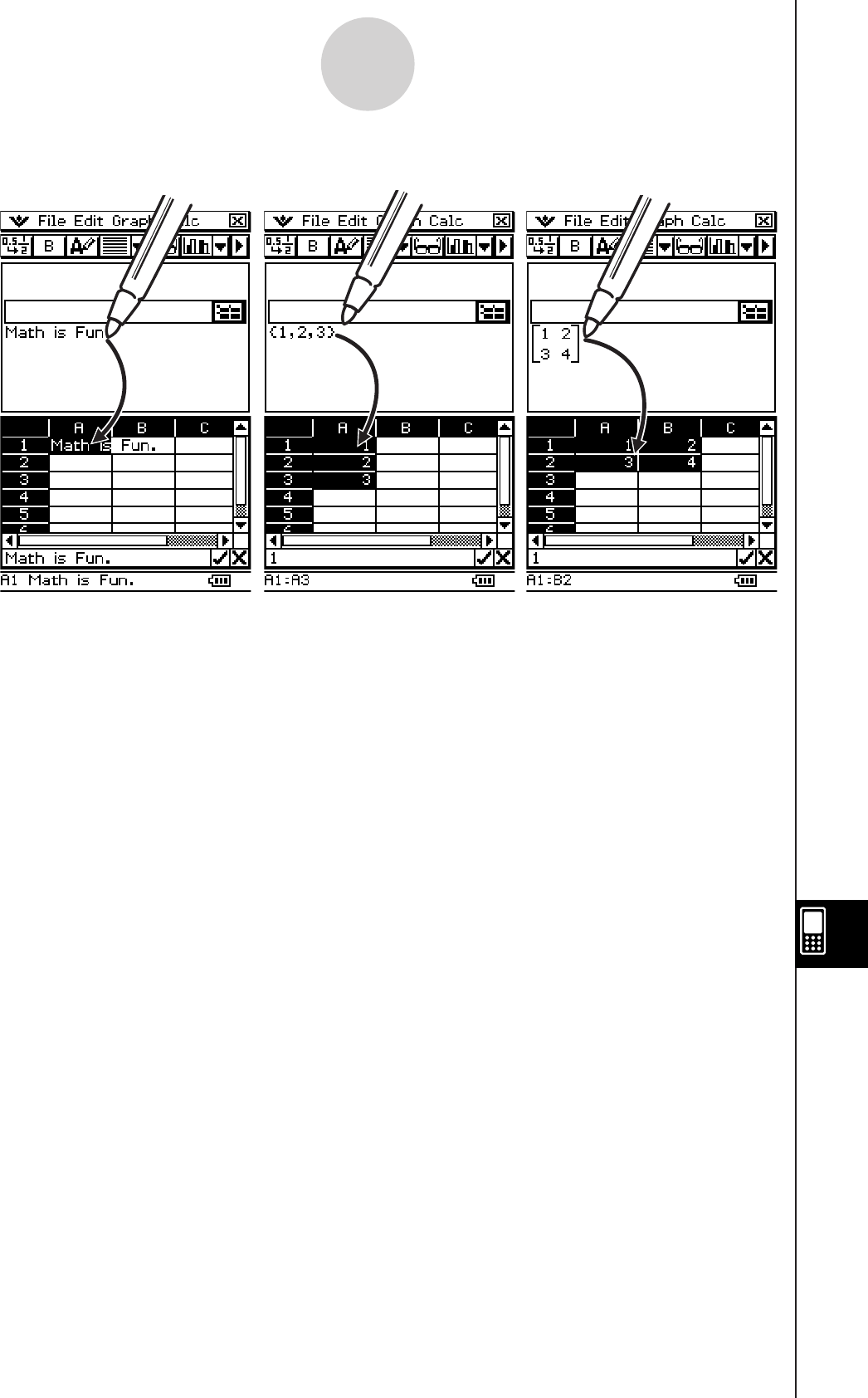
20090601

Example 4: Dragging data from eActivity to the Spreadsheet window

13-5-4

Using the Spreadsheet Application with the eActivity Application

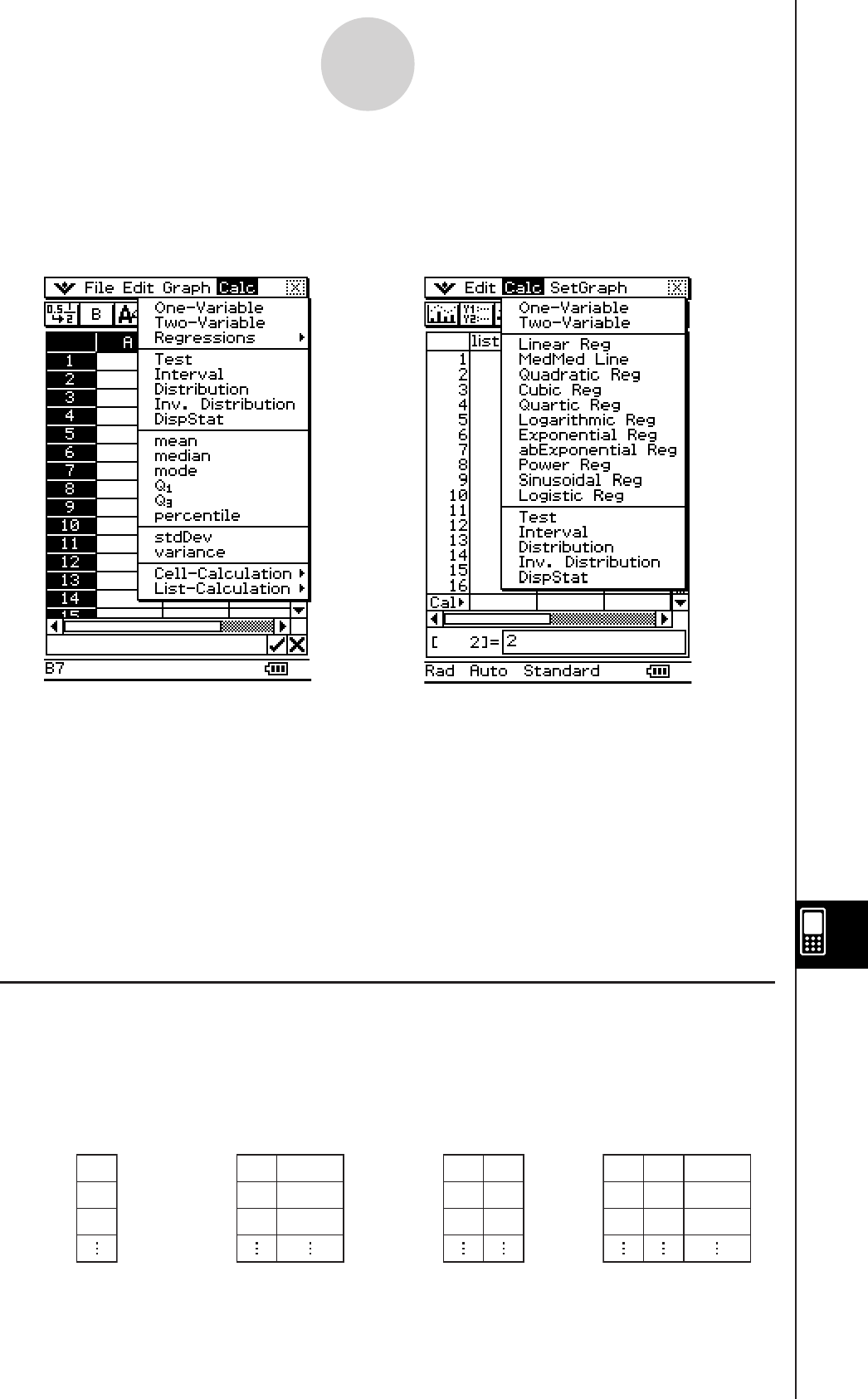
20090601

13-6-1

Statistical Calculations

13-6 Statistical Calculations

The upper part of the [Calc] menu includes the same menu items as the Statistics Application

[Calc] menu.

Spreadsheet Application Statistics Application

Menu items with the same name perform the same functions, but there are some differences

between the Statistics Application and Spreadsheet Application in terms of operation

procedures, calculation result display, etc. This section explains statistical operations and

functions that are peculiar to the Spreadsheet Application.

Tip

For information about the Test, Interval, Distribution and DispStat commands, and the commands

that appear on the One-Variable, Two-Variable and Regressions submenus, see “Chapter 7

Using the Statistics Application”.

k Single-variable and Paired-variable Statistical Calculations

You can enter single-variable or paired-variable data into Spreadsheet cells and display a list

of statistical values.

Single-variable

Data

Frequencies for

Single-variable Data

Paired-variable

Data

Frequencies for

Paired-variable Data

Freq 1

Freq 2

Freq 3

Freq 1

Freq 2

Freq 3

•

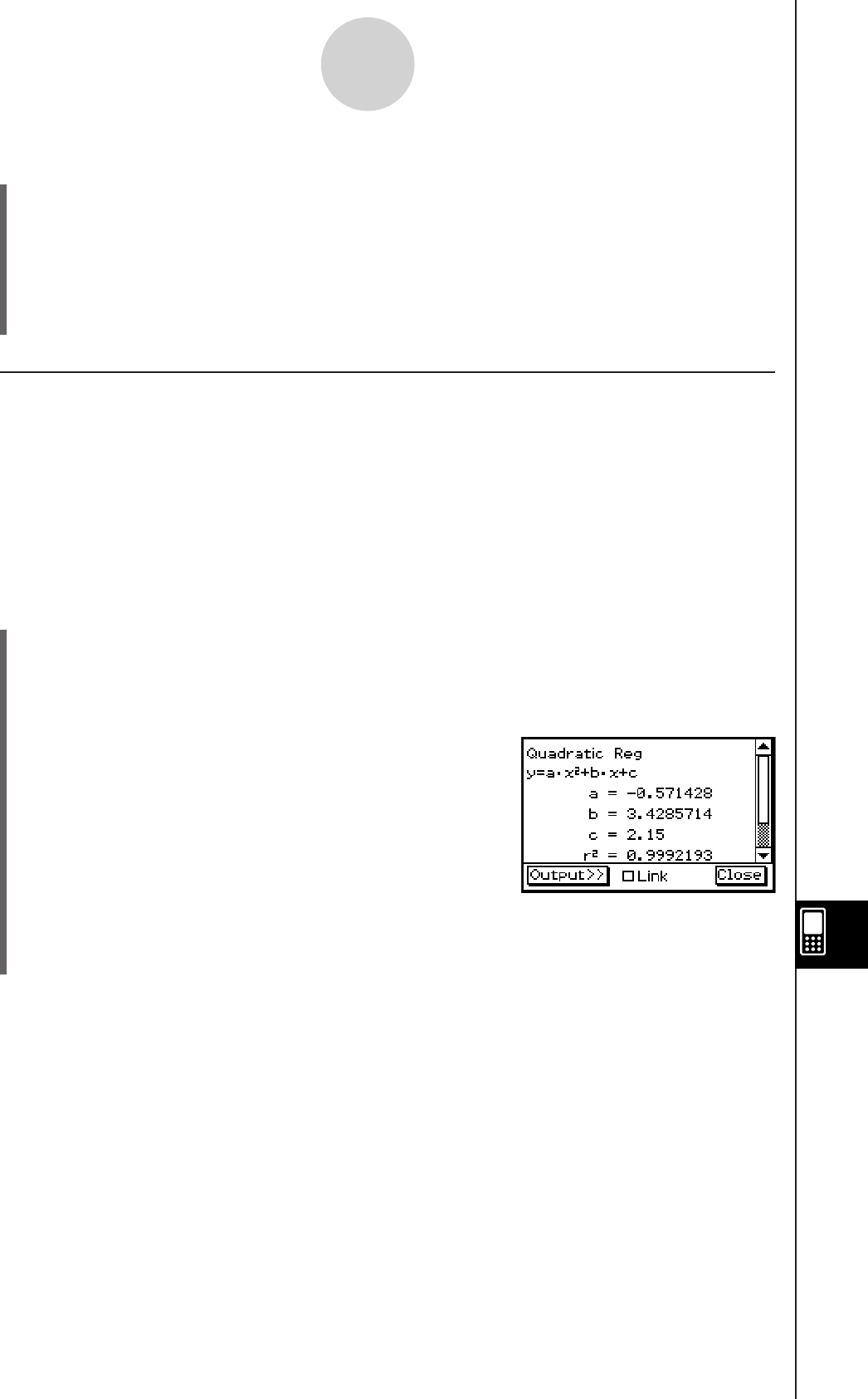
20101001

Example: To execute paired-variable calculations and display a list of statistical values

(1) Enter the paired-variable data into the spreadsheet, and then select the range of cells

where it is located.

(2) On the menu bar, tap [Calc] and then [Two-Variable].

• For details about the meaning of each value that appears as a statistical calculation

result, see “Viewing Single-variable Statistical Calculation Results” (page 7-7-1) and

“Viewing Paired-variable Statistical Calculation Results” (page 7-7-4).

k Regression Calculations

You can use regression calculation to determine the regression formula that approximates

paired-variable spreadsheet data. Regression calculations results are displayed as a list of

coefficients for the regression model formula.

Tip

For information about regression graphing, see “Regression Graph Operations (Curve Fitting)”

(page 13-9-15).

u To perform a regression calculation

(1) Enter the paired-variable data into the spreadsheet, and then select the range of cells

where it is located.

(2) On the menu bar, tap [Calc] and then [Regression]. Next, on the submenu that appears,

tap the desired regression type.

• The regression calculation result window will appear

in the lower half of the display.

• For details about the model formula for the selected regression type and the meaning

of each coefficient that appears, see pages 7-5-5 through 7-5-14 in “7-5 Graphing

Paired-Variable Statistical Data”.

Tip

Changing the range of data you selected in step (1) above and performing the regression

calculation again will cause the regression calculation results displayed on the window to be

updated automatically. You can disable automatic updating (if you feel that updating is taking too

long or for any other reason) by clearing the Link check box on the regression calculation result

window.

•

13-6-2

Statistical Calculations

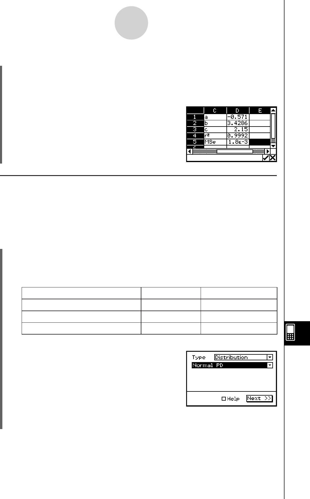
20090601

u To paste a list of regression calculation results into a spreadsheet

(1) Perform the procedure under “To perform a regression calculation” and display the

regression calculation result window.

(2) On the regression calculation result window, tap the [Output>>] button.

(3) On the output window, tap [Paste].

• This pastes a table of system variables to which

regression calculation results are assigned and the

results.

k Distribution Calculation

You can use spreadsheet data to perform the same distribution calculations you can perform

with the Statistics Application. For details about the different types of distribution calculations

and the meanings of the variables that are displayed for calculation results, see “7-11

Distributions”.

u To perform a distribution calculation

(1) Enter the single-variable or paired-variable data into the spreadsheet, and then select

the range of cells where it is located.

• The following shows the types of data that correspond to each type of distribution

calculation, and the variables that will be assigned the range of selected data.

Distribution Type Data Variable Assignment

Probability Density Single-variable x

Cumulative Distribution Paired-variable Lower, Upper

Inverse Cumulative Distribution Single-variable prob

(2) On the menu bar, tap [Calc] and then [Distribution].

• The Distribution Calculation Wizard will appear

in the lower half of the display.

(3) Tap the

v button to the right of the second item from the top and then select the

desired distribution calculation from the menu that appears.

13-6-3

Statistical Calculations

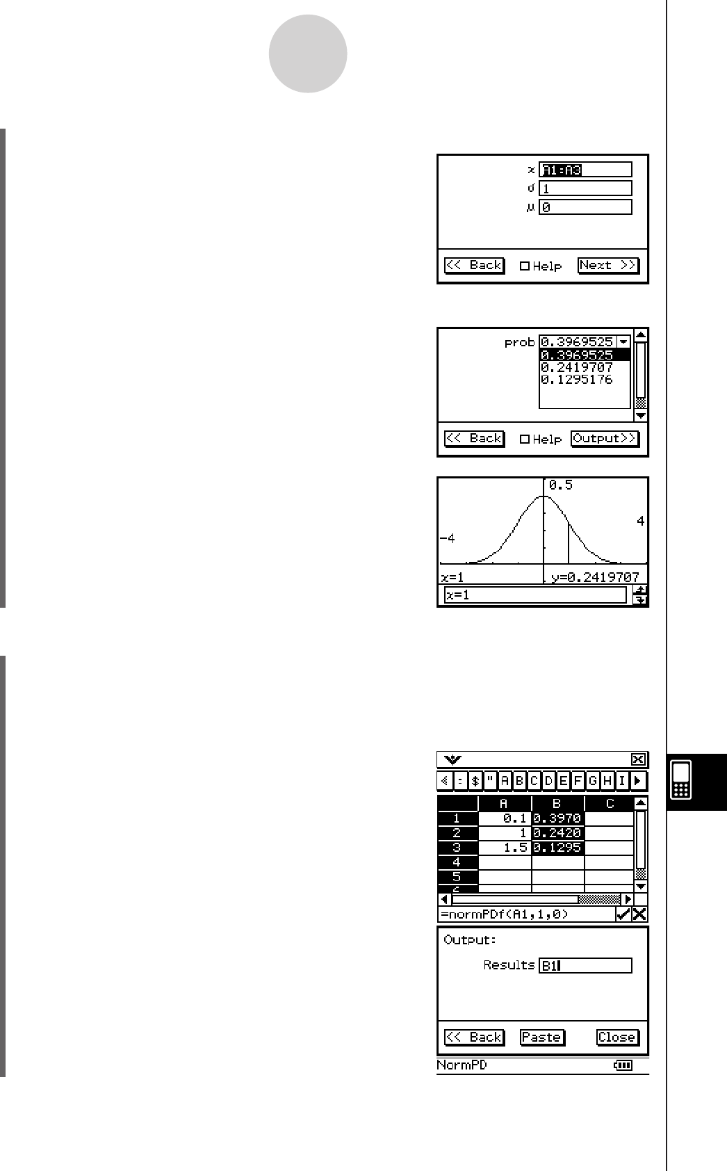
20090601

(4) Tap [Next >>].

• This will display a screen with the variable

assignments for the range you selected in step 1 of

this procedure entered automatically in the input

fields as the initial defaults.

(5) Enter values for the other variables and then tap [Next >>].

• This displays the calculation results. If there are

multiple calculation results, tap v to view them.

(6) You can tap $ here to display the distribution graph.

u To paste distribution calculation results into a spreadsheet

(1) Perform the procedure under “To perform a distribution calculation” and display the

distribution calculation result window.

(2) On the calculation result window, tap the [Output>>] button.

(3) On the output window, tap [Paste].

• This pastes the calculation results in formula format.

13-6-4

Statistical Calculations

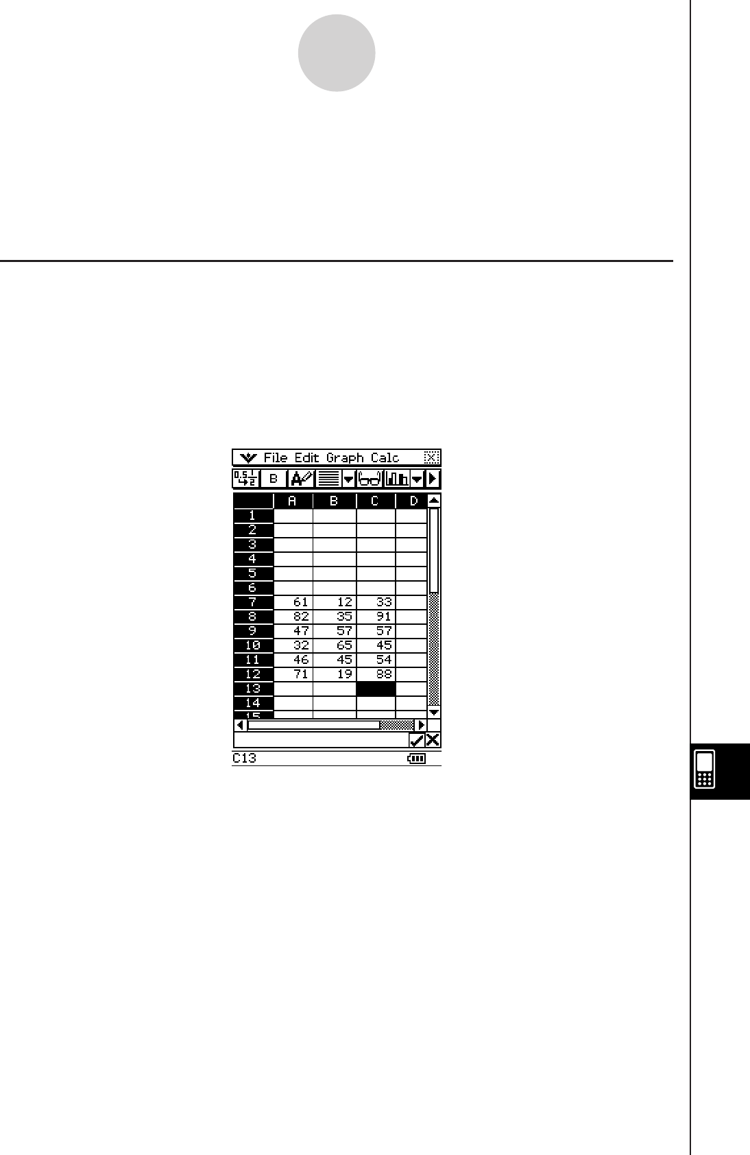
20090601

13-7 Cell and List Calculations

Use the [Calc] menu to perform cell and list calculations.

The [Calc] menu provides access to a [Cell-Calculation] submenu for cell calculations and a

[List-Calculation] submenu for list calculations.

Spreadsheet [List-Calculation] Submenu Basics

The menu items on the [List-Calculation] submenu are the same as those on the [Action] -

[List-Calculation] submenu of the Main Application. Menu items with the same name perform

the same functions, but there are some differences between the Main Application and

Spreadsheet Application in terms of operation procedures.

The following example demonstrates the basic procedure for using functions in the [List-

Calculation] submenu.

Example: To calculate the sum of the following data, and then to add 100 to it

13-7-1

Cell and List Calculations

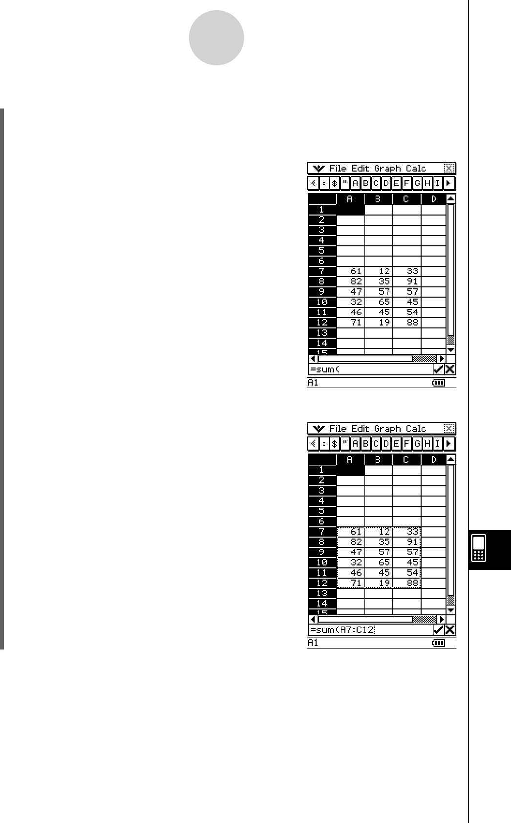
20090601

uClassPad Operation

(1) With the stylus, tap the cell where you want the result to appear.

• In this example, we would tap cell A1.

(2) On the [Calc] menu, tap [List-Calculation] and then [sum] on the submenu.

• This inputs the sum function ([sum(]) into the edit box.

(3) Use the stylus to drag across the range of data cells from A7 to C12 to select them.

• “A7:C12” appears to the right of the open parenthesis

of the [sum] function.

13-7-2

Cell and List Calculations

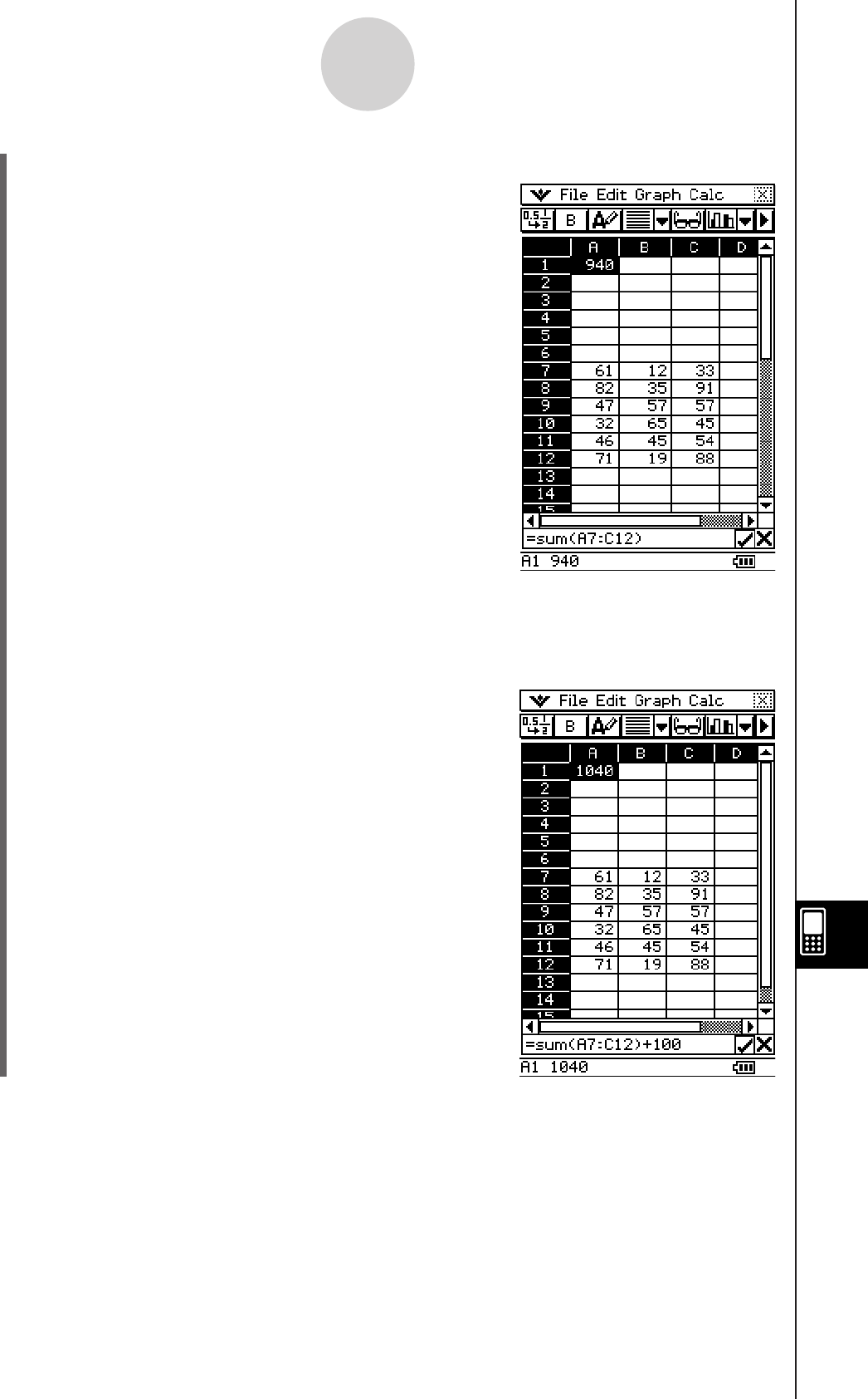
20090601

(4) Tap the

s button to the right of the edit box.

• This automatically closes the parentheses, calculates

the sum of the values in the selected range, and

displays the result in cell A1.

• You could skip this step and input the closing

parentheses by pressing the ) key on the keypad,

if you want.

(5) Tap the edit box to activate it again, and then tap to the right of the last parenthesis.

(6) Press the + key and then input 100.

(7) Tap the s button to the right of the edit box.

• This calculates the result and displays it in cell A1.

13-7-3

Cell and List Calculations

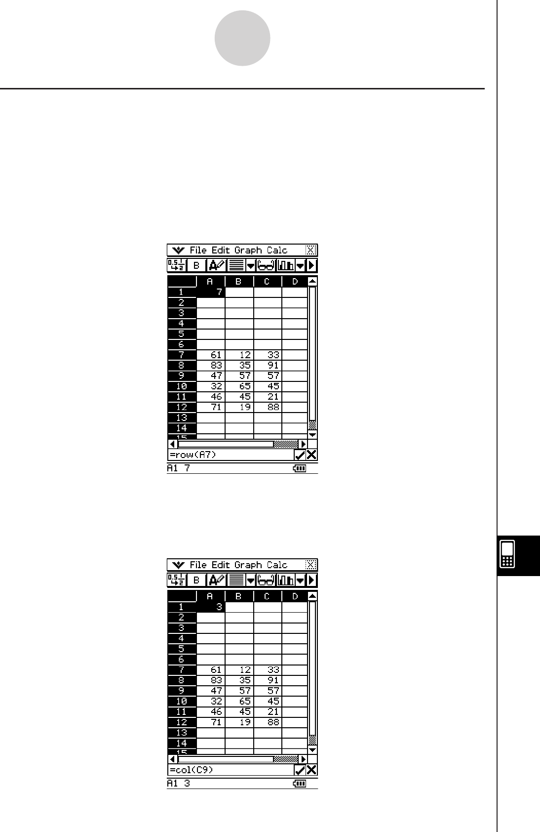
20090601

Cell Calculation and List Calculation Functions

This section provides explanations of the functions, input syntax, and examples for each of

the cell calculation and list calculation functions included on the [Calc] menu. Please note

that “start cell:end cell” is equivalent to entering a list.

u Cell-Calculation - row

Function: Returns the row number of a specified cell.

Syntax: row(cell)

Example: To determine the row number of cell A7 and input the result in cell A1:

u Cell-Calculation - col

Function: Returns the column number of a specified cell.

Syntax: col(cell)

Example: To determine the column number of cell C9 and input the result in cell A1:

13-7-4

Cell and List Calculations

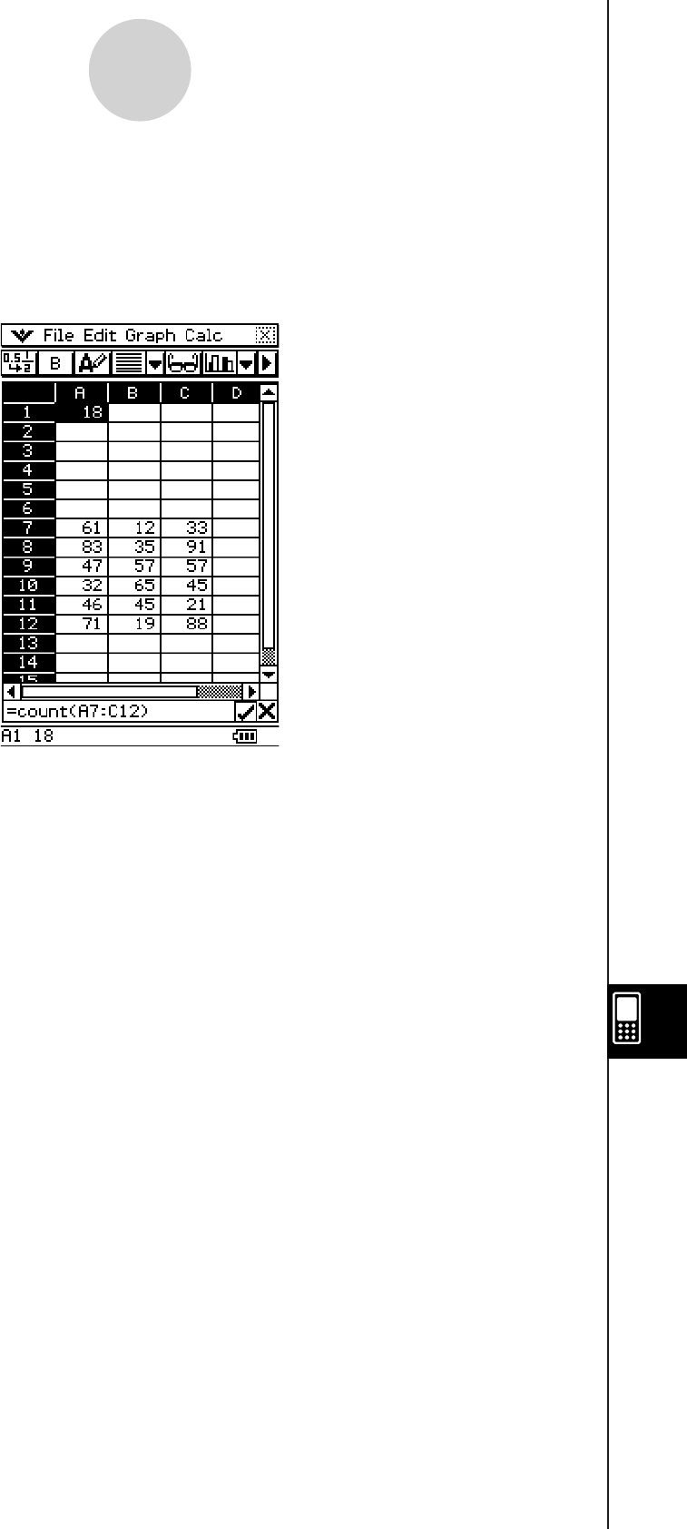
20090601

u Cell-Calculation - count

Function: Returns a count of the number of cells in the specified range.

Syntax: count(start cell[:end cell])

Example: To count the number of cells in the block whose upper left corner is located at

A7 and whose lower right corner is located at C12, and input the result in cell A1:

13-7-5

Cell and List Calculations

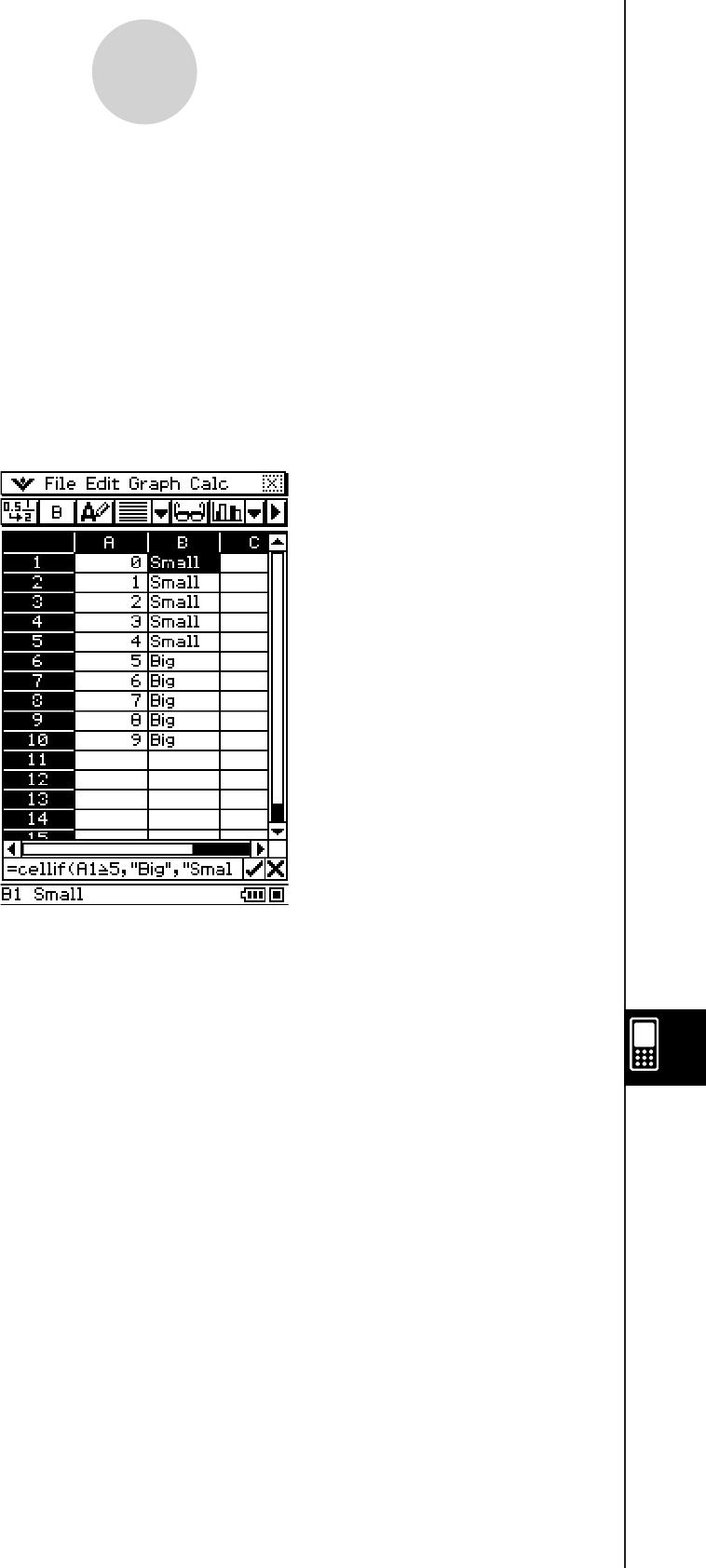
20090601

u Cell-Calculation - cellif

Function: Evaluates an equality or inequality, and returns one of three different expressions

based on whether the equality/inequality is true (expression 1), false (expression

2), or inconclusive (expression 3).

With this function, the equality/inequality can include a string as in the following

example: cellif(A1="Red", 0,1,2).

Syntax: cellif(equation, expression 1, expression 2, expression 3)

cellif(inequality, expression 1, expression 2, expression 3)

Example: For each value in cells A1 through A10, to display “Big” in the neighboring

B-column cell for values of 5 and greater, and “Small” for values less than 5:

(=cellif(A1>5,"Big","Small"))

• Expression 3 is optional for both equation and inequality.

13-7-6

Cell and List Calculations

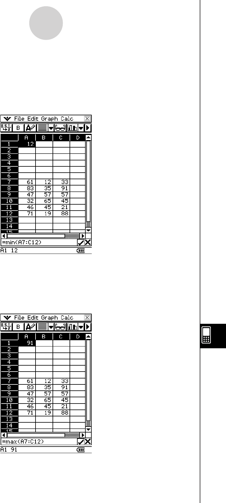
20090601

u List-Calculation - min

Function: Returns the lowest value contained in the range of specified cells.

Syntax: min(start cell[:end cell][,start cell[:end cell]]

[,value])

Example: To determine the lowest value in the block whose upper left corner is located at

A7 and whose lower right corner is located at C12, and input the result in cell

A1:

u List-Calculation - max

Function: Returns the greatest value contained in the range of specified cells.

Syntax: max(start cell[:end cell][,start cell[:end cell]]

[,value])

Example: To determine the greatest value in the block whose upper left corner is located at

A7 and whose lower right corner is located at C12, and input the result in cell A1:

13-7-7

Cell and List Calculations

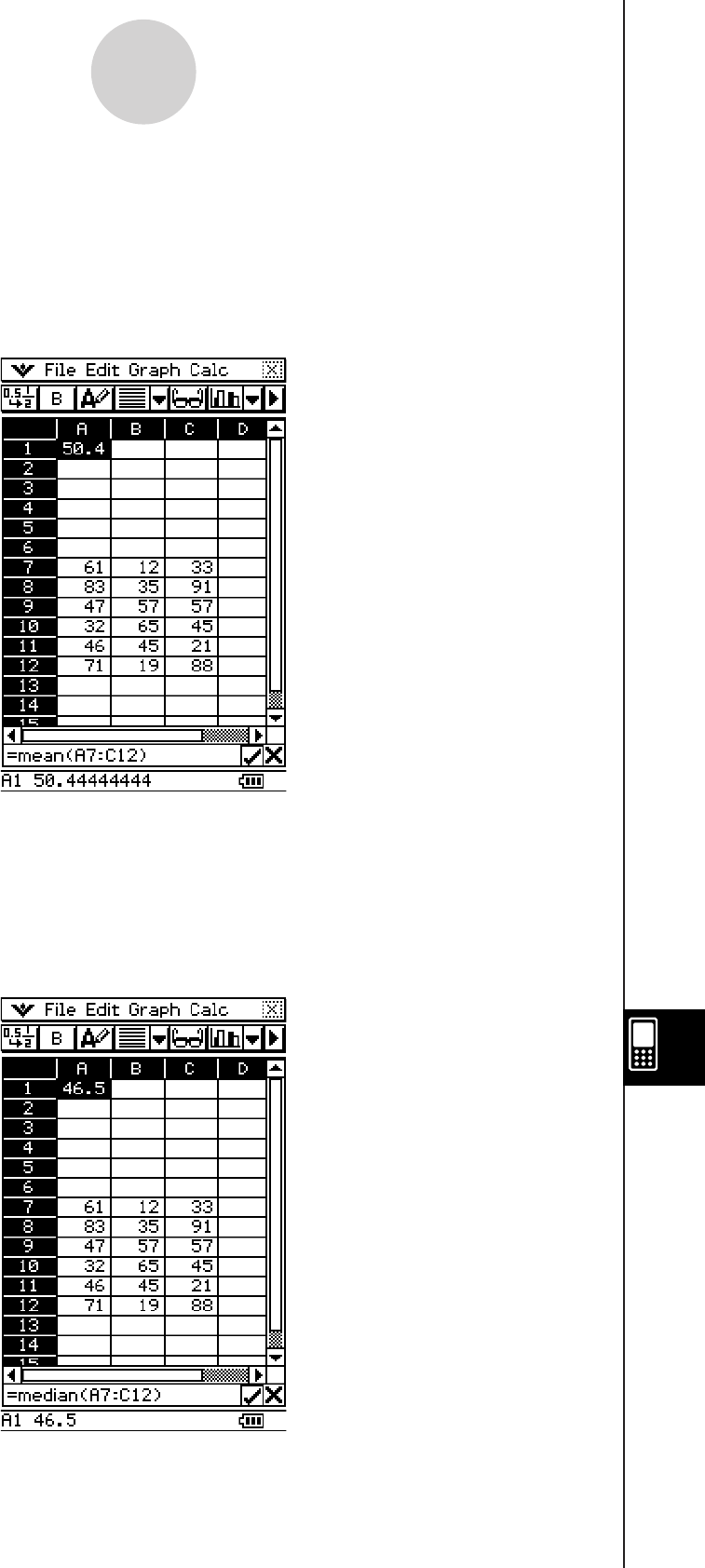
20090601

u mean

Function: Returns the mean of the values contained in the range of specified cells.

Syntax: mean(start cell:end cell[,start cell:end cell])

Example: To determine the mean of the values in the block whose upper left corner is

located at A7 and whose lower right corner is located at C12, and input the result

in cell A1:

u median

Function: Returns the median of the values contained in the range of specified cells.

Syntax: median(start cell:end cell[,start cell:end cell])

Example: To determine the median of the values in the block whose upper left corner

is located at A7 and whose lower right corner is located at C12, and input the

result in cell A1:

13-7-8

Cell and List Calculations

20090601

u mode

Function: Returns the mode of the values contained in the range of specified cells.

Syntax: mode(start cell:end cell[,start cell:end cell])

Example: To determine the mode of the values in the block whose upper left corner is

located at A7 and whose lower right corner is located at C12, and input the result

in cell A1:

u Q1

Function: Returns the first quartile of the values contained in the range of specified cells.

Syntax: Q1(start cell:end cell[,start cell:end cell])

Example: To determine the first quartile of the values in the block whose upper left corner

is located at A7 and whose lower right corner is located at C12, and input the

result in cell A1:

13-7-9

Cell and List Calculations

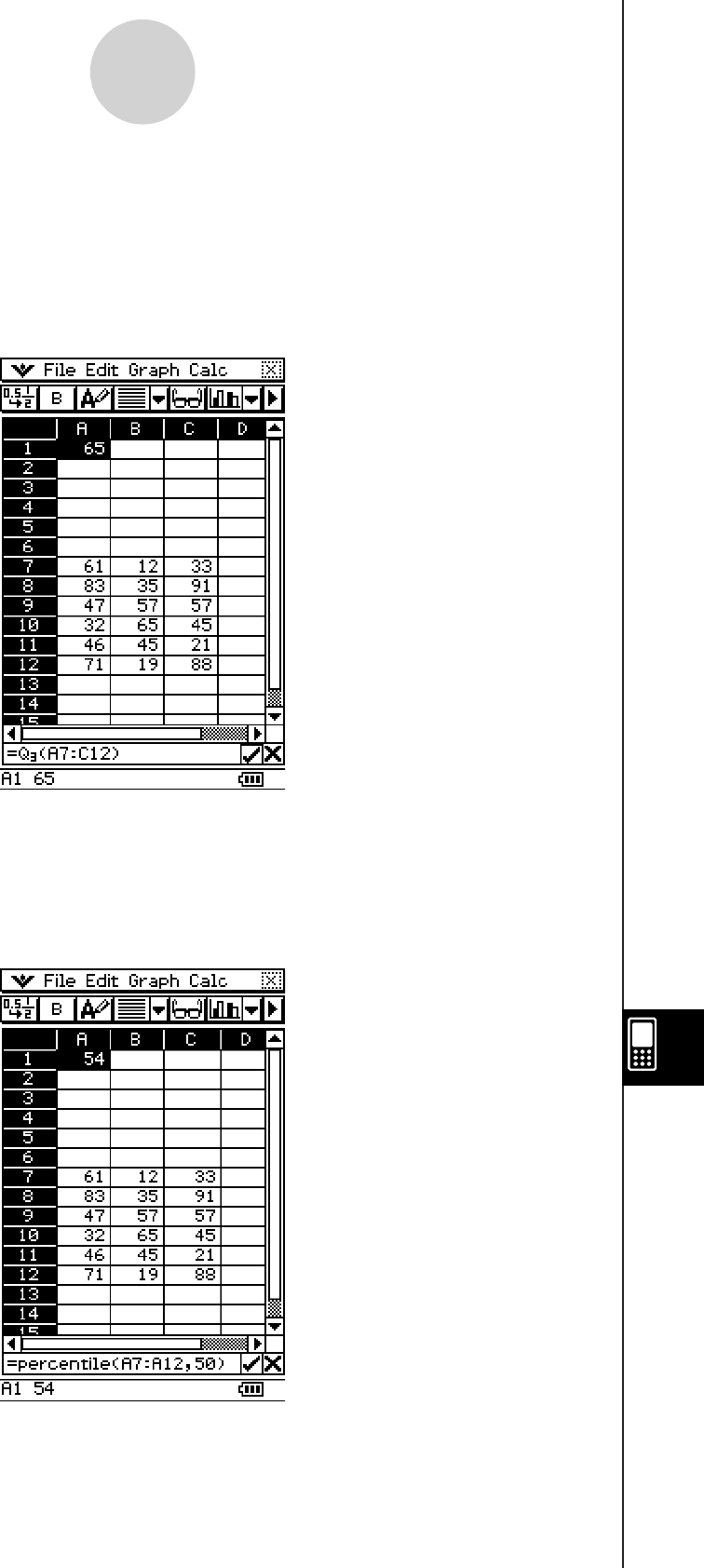
20090601

u Q3

Function: Returns the third quartile of the values contained in the range of specified cells.

Syntax: Q3(start cell:end cell[,start cell:end cell])

Example: To determine the third quartile of the values in the block whose upper left corner

is located at A7 and whose lower right corner is located at C12, and input the

result in cell A1:

u percentile

Function: Returns the nth percentile in the range of specified cells.

Syntax: percentile(start cell[:end cell],value)

Example: To determine the 50th percentile of the values in cells A7 through A12 and input

the result in cell A1:

13-7-10

Cell and List Calculations

20090601

u stdDev

Function: Returns the sample standard deviation of the values contained in the range of

specified cells.

Syntax: stdDev(start cell:end cell)

Example: To determine the sample standard deviation of the values in the block whose

upper left corner is located at A7 and whose lower right corner is located at C12,

and input the result in cell A1:

u variance

Function: Returns the sample variance of the values contained in the range of specified

cells.

Syntax: variance(start cell:end cell)

Example: To determine the sample variance of the values in the block whose upper left

corner is located at A7 and whose lower right corner is located at C12, and input

the result in cell A1:

13-7-11

Cell and List Calculations

20090601

u List-Calculation - sum

Function: Returns the sum of the values contained in the range of specified cells.

Syntax: sum(start cell:end cell[,start cell:end cell])

Example: To determine the sum of the values in the block whose upper left corner is

located at A7 and whose lower right corner is located at C12, and input the result

in cell A1:

u List-Calculation - prod

Function: Returns the product of the values contained in the range of specified cells.

Syntax: prod(start cell:end cell[,start cell:end cell])

Example: To determine the product of the values in cells A7 and A8, and input the result in

cell A1:

13-7-12

Cell and List Calculations

20090601

u List-Calculation - cuml

Function: Returns the cumulative sums of the values contained in the range of specified

cells.

Syntax: cuml(start cell:end cell)

Example: To determine the cumulative sums of the values in cells B1 through B3, and

input the result in cell A1:

u List-Calculation - Alist

Function: Returns the differences between values in each of the adjacent cells in the range

of specified cells.

Syntax: Alist(start cell:end cell)

Example: To determine the differences of the values in cells B1 through B3, and input the

result in cell A1:

13-7-13

Cell and List Calculations

20090601

u List-Calculation - percent

Function: Returns the percentage of each value in the range of specified cells, the sum of

which is 100%.

Syntax: percent(start cell:end cell)

Example: To determine the percentage of the values in cells B1 through B4, and input the

result in cell A1:

u List-Calculation - polyEval

Function: Returns a polynomial arranged in descending order. The coefficients correspond

sequentially to each value in the range of specified cells.

Syntax: polyEval(start cell:end cell[,start cell:end cell]

[,variable])

Example: To create a second degree polynomial with coefficients that correspond to the

values in cells B1 through B3, and input the result in cell A1:

13-7-14

Cell and List Calculations

20090601

• “x” is the default variable when you do not specify one above.

• To specify “y” as the variable, for example, enter “=polyEval(B1:B3, y)”.

u List-Calculation - sequence

Function: Returns the lowest-degree polynomial that generates the sequence expressed

by the values in a list or range of specified cells. If we evaluate the polynomial at

2, for example, the result will be the second value in our list.

Syntax: sequence(start cell:end cell[,start cell:end cell][,variable])

Example: To determine a polynomial for the sequence values in cells B1 through B4 and a

variable of “y”, and input the result in cell A1:

• “x” is the default variable when you do not specify one above.

13-7-15

Cell and List Calculations

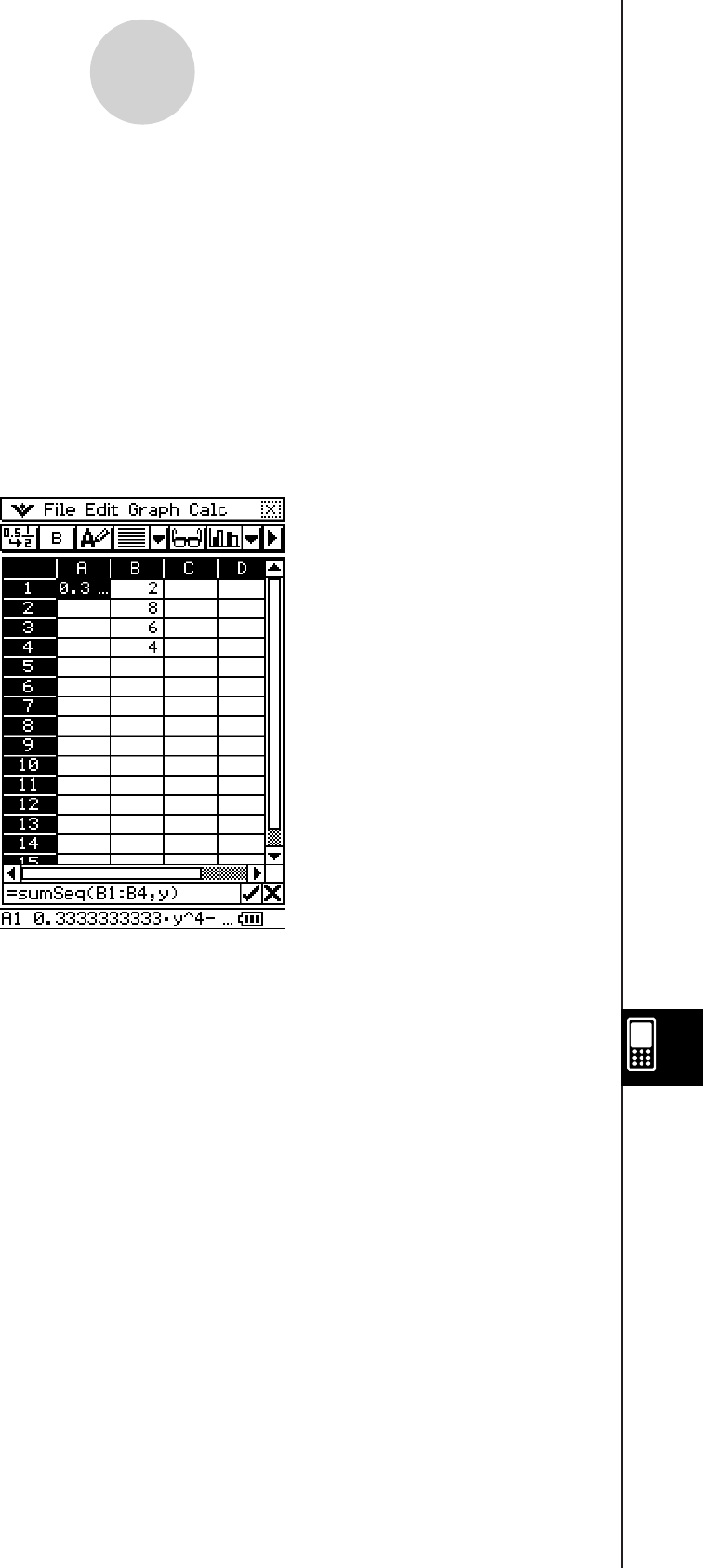
20090601

u List-Calculation - sumSeq

Function: Determines the lowest-degree polynomial that generates the sum of the first

n terms of your sequence. If we evaluate the resulting polynomial at 1, for

example, the result will be the first value in your list. If we evaluate the resulting

polynomial at 2, the result will be the sum of the first two values in your list.

When two columns of values or two lists are specified, the resulting polynomial

returns a sum based on a sequence.

Syntax: sumSeq(start cell:end cell[,start cell:end cell][,variable])

Example: To determine a polynomial that generates the sum of the first n terms for the

sequence expressed by the values in cells B1 through B4 with a variable of “y”,

and input the result in cell A1:

• “x” is the default variable when you do not specify one above.

13-7-16

Cell and List Calculations

20090601

13-8-1

Formatting Cells and Data

13-8 Formatting Cells and Data

This section explains how to control the format of the spreadsheet and the data contained in

the cells.

Standard (Fractional) and Decimal (Approximate) Modes

You can use the following procedure to control whether a specific cell, row, or column, or

the entire spreadsheet should use the standard mode (fractional format) or decimal mode

(approximate value).

uClassPad Operation

(1) Select the cell(s) whose format you want to specify.

• See “Selecting Cells” on page 13-3-5 for information about selecting cells.

(2) On the toolbar, tap the left button (,

.) to toggle between the standard mode and

the decimal mode.

Plain Text and Bold Text

Use the following procedure to toggle the text of a specific cell, row, or column, or the entire

spreadsheet between plain and bold.

uClassPad Operation

(1) Select the cell(s) whose text setting you want to specify.

• See “Selecting Cells” on page 13-3-5 for information about selecting cells.

(2) On the toolbar, tap the M

B button to toggle between bold and plain text.

Text and Calculation Data Types

Make use of the following procedure to toggle a specific cell, row, or column, or the entire

spreadsheet for either text or calculation data types.

uClassPad Operation

(1) Select the cell(s) whose format you want to specify.

• See “Selecting Cells” on page 13-3-5 for information about selecting cells.

(2) On the toolbar, tap the u

< button to toggle between Text Input mode and

Calculation Input mode.

20090601

Text Alignment

With the following procedure, you can specify justified, align left, center, or align right for a

specific cell, row, or column, or the entire spreadsheet.

uClassPad Operation

(1) Select the cell(s) whose alignment setting you want to specify.

• See “Selecting Cells” on page 13-3-5 for information about selecting cells.

(2) On the toolbar, tap the down arrow button next to the [ button.

(3) On the button menu that appears, tap the text alignment option you want to use.

For this type of alignment: Tap this option:

Left and right justified [

Left p

Center x

Right ]

Number Format

Use the following procedure to specify the number format (Normal 1, Normal 2, Fix 0 – 9,

Sci 0 – 9) of a specific cell, row, or column, or the entire spreadsheet.

uClassPad Operation

(1) Select the cell(s) whose number format setting you want to specify.

• See “Selecting Cells” on page 13-3-5 for information about selecting cells.

(2) On the [Edit] menu, tap [Number Format].

(3) On the dialog box that appears, select the number format you want to use.

(4) Tap [OK].

13-8-2

Formatting Cells and Data

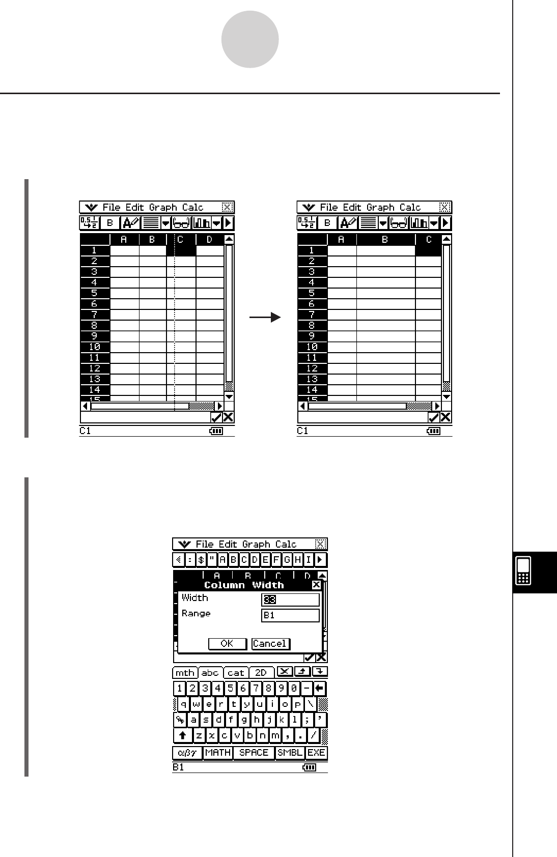
20090601

Changing the Width of a Column

There are three different methods you can use to control the width of a column: dragging with

the stylus, using the [Column Width] command, or using the [AutoFit Selection] command.

u To change the width of a column using the stylus

Use the stylus to drag the edge of a column header left or right until it is the desired width.

u To change the width of a column using the Column Width command

(1) Tap any cell in the column whose width you want to change.

• You could also drag the stylus to select multiple columns, if you want.

(2) On the [Edit] menu, tap [Column Width].

13-8-3

Formatting Cells and Data

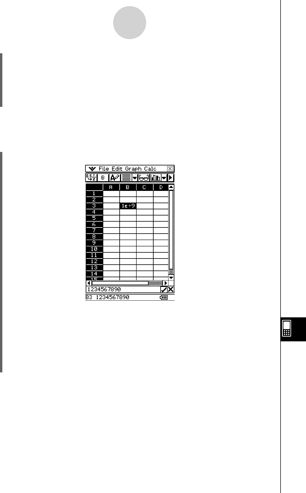
20090601

(3) On the dialog box that appears, enter a value in the [Width] box to specify the desired

width of the column in pixels.

• You can also use the [Range] box to specify a different column from the one you

selected in step (1) above, or a range of columns. Entering B1:D1 in the [Range] box,

for example, will change columns B, C, and D to the width you specify.

(4) After everything is the way you want, tap [OK] to change the column width.

u To change the width of a column using the AutoFit Selection command

Example: To use [AutoFit Selection] to adjust the column width to display the value

1234567890

(1) Tap a cell and input the value.

• Since the value is too long to fit in the cell, it is converted automatically to exponential

format. Notice, however, that the entire value appears in the edit box.

(2) Select the cell you want to auto fit.

• You can also select a range of cells in the same column or an entire column. In this

case, the column width is adjusted to fit the largest data value in the column.

• You can also select a range of cells or an entire row. In this case, each column width

is adjusted to fit the largest data in its column.

13-8-4

Formatting Cells and Data

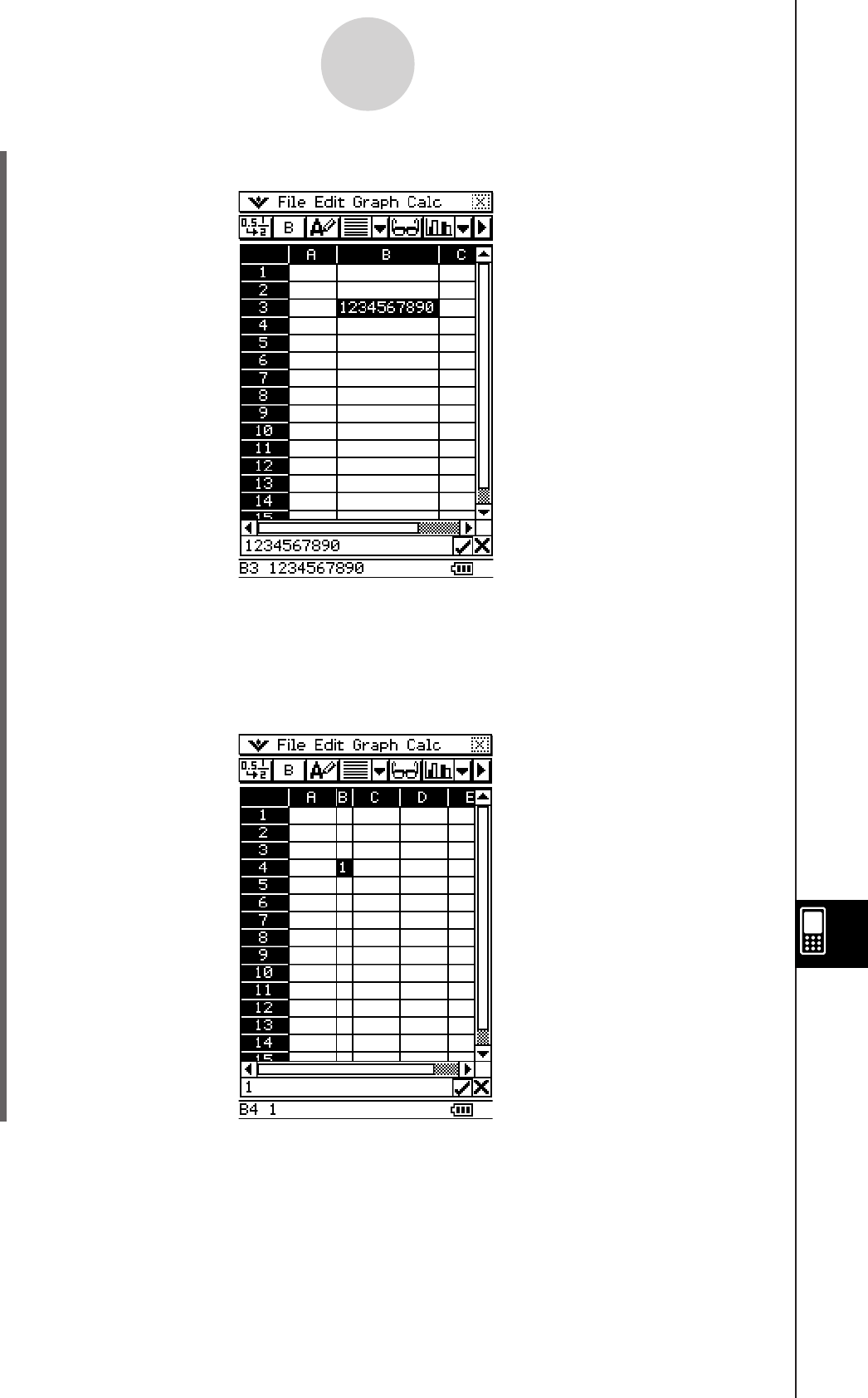
20090601

(3) On the [Edit] menu, tap [AutoFit Selection].

• This causes the column width to be adjusted automatically so the entire value can be

displayed.

• Note that [AutoFit Selection] also will reduce the width of a column, if applicable. The

following shows what happens when [AutoFit Selection] is executed while a cell that

contains a single digit is selected.

13-8-5

Formatting Cells and Data

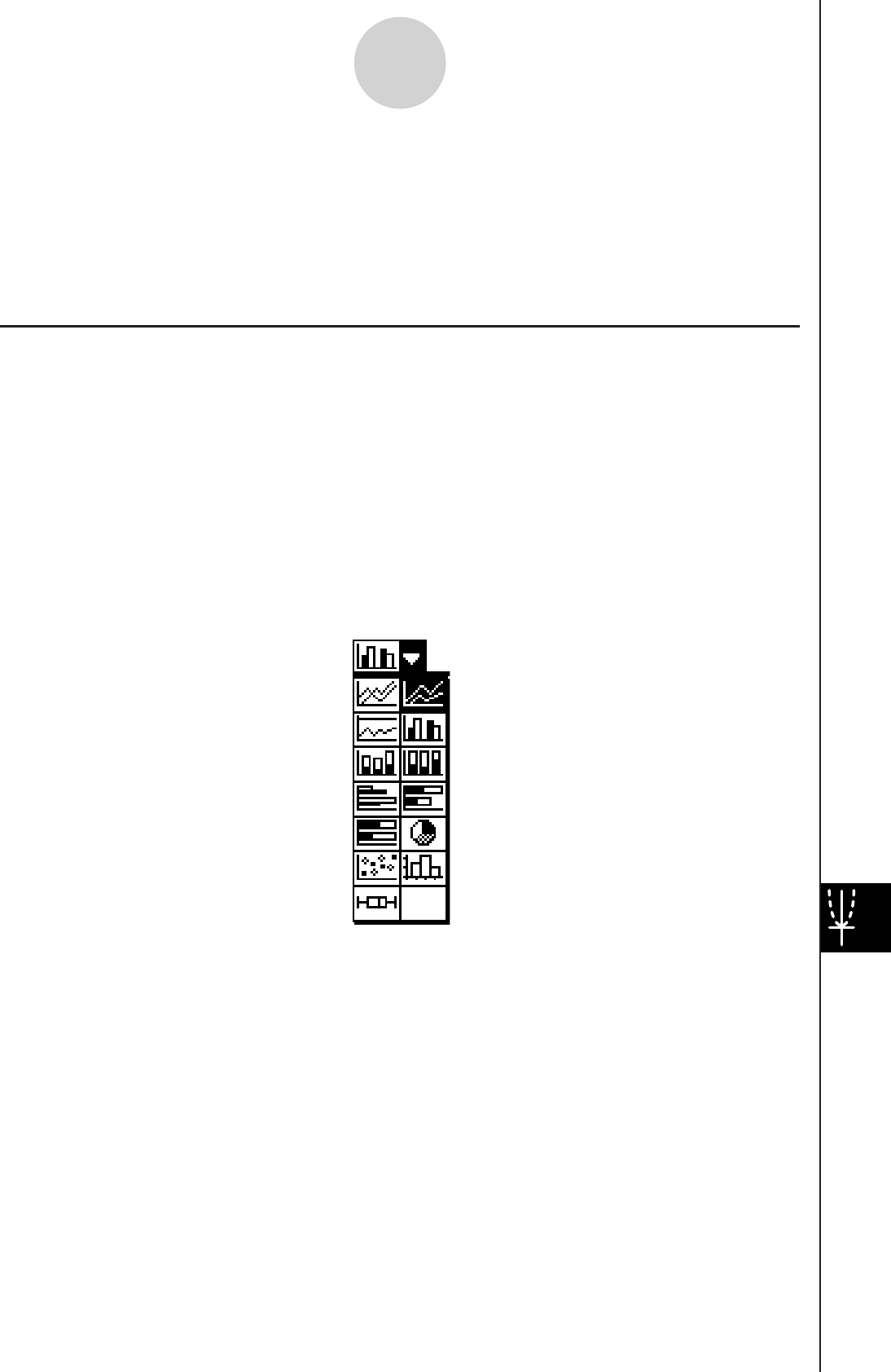
20090601

13-9-1

Graphing

13-9 Graphing

The Spreadsheet application lets you draw a variety of different graphs for analyzing data.

You can combine line and column graphs, and the interactive editing feature lets you change

a graph by dragging its points on the display.

Graph Menu

After selecting data on the spreadsheet, use the [Graph] menu to select the type of graph

you want to draw. You can also use the [Graph] menu to specify whether to graph data by

column or row.

The following explains each of the [Graph] menu commands, and shows examples of what

happens to the Graph window when you execute a command.

Note

• The following examples show the appearance of graph screens after tapping r on the

icon panel so the Graph window fills the entire screen.

• Each command is followed by a button in parentheses to show the graph toolbar button

that performs the same action as the command.

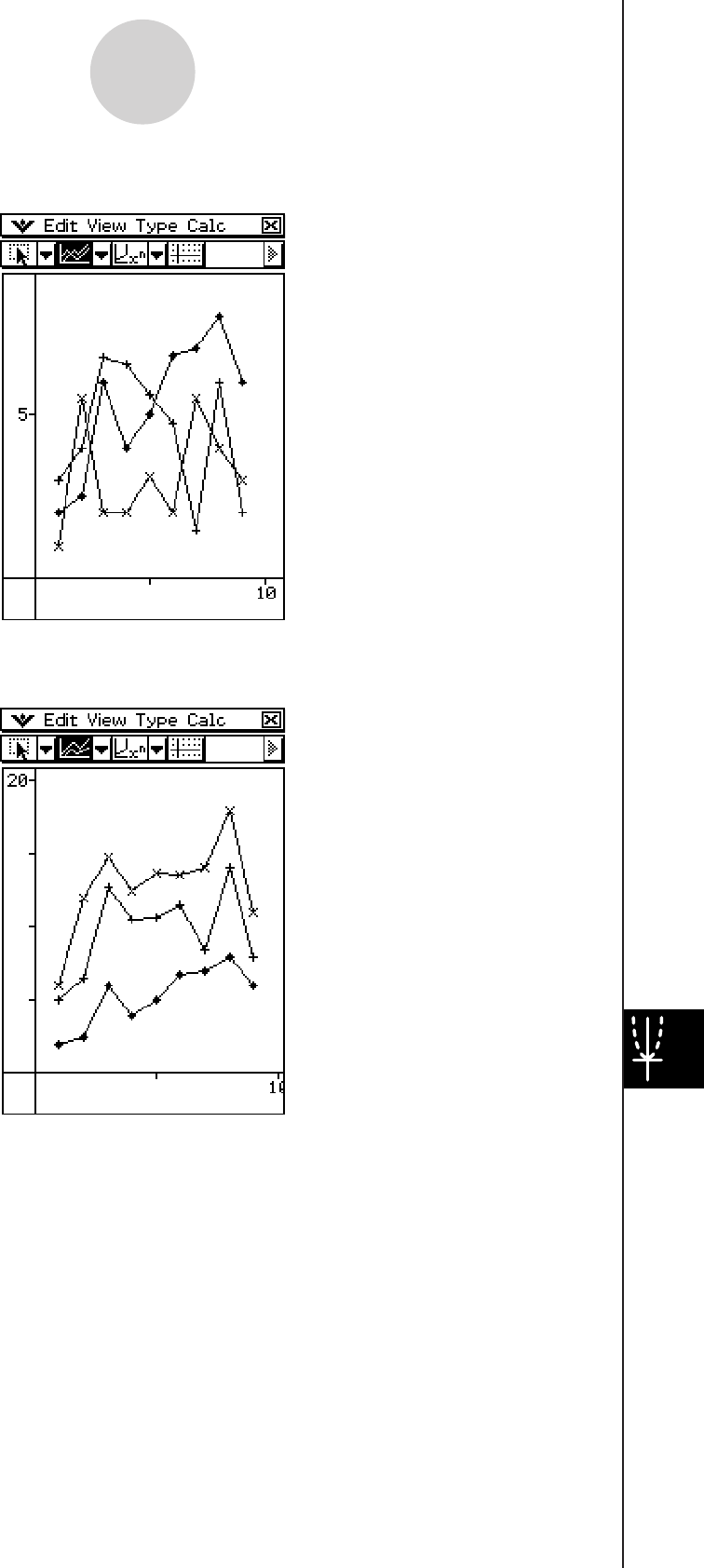
20090601

u [Graph] - [Line] - [Clustered] ( D )

u [Graph] - [Line] - [Stacked] ( F )

13-9-2

Graphing

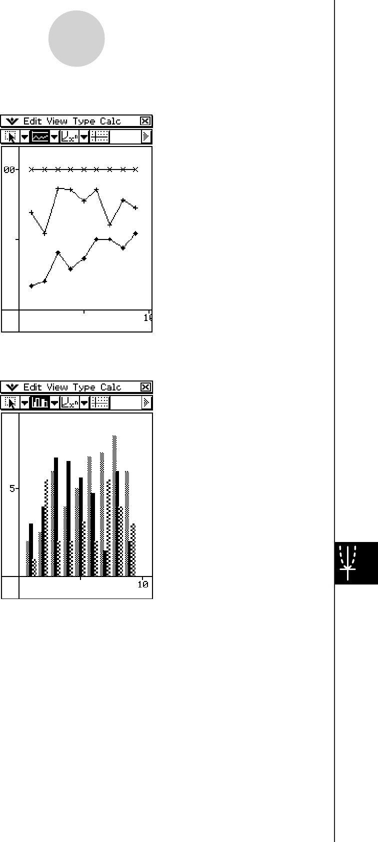
20090601

u [Graph] - [Line] - [100% Stacked] ( G )

u [Graph] - [Column] - [Clustered] ( H )

13-9-3

Graphing

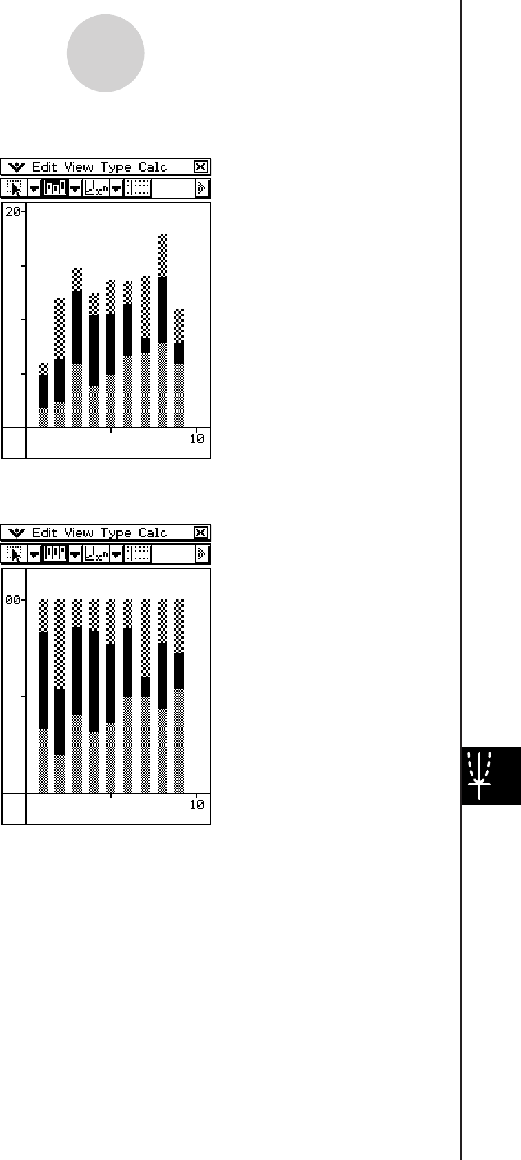
20090601

u [Graph] - [Column] - [Stacked] ( J )

u [Graph] - [Column] - [100% Stacked] ( K )

13-9-4

Graphing

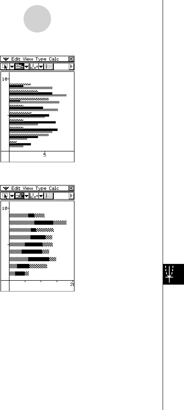
20090601

u [Graph] - [Bar] - [Clustered] ( L )

u [Graph] - [Bar] - [Stacked] ( : )

13-9-5

Graphing

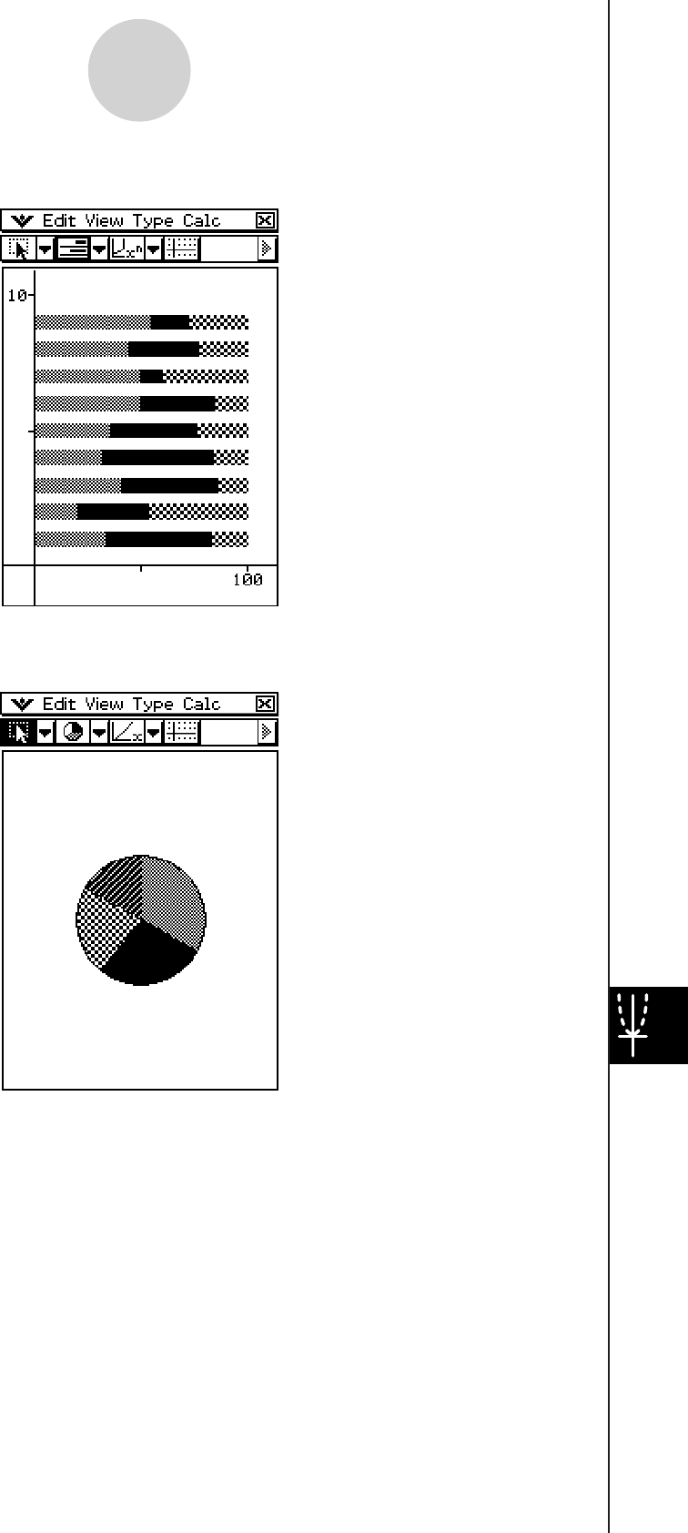
20090601

u [Graph] - [Bar] - [100% Stacked] ( " )

u [Graph] - [Pie] ( Z )

• When you select a pie chart, only the first series (row or column) of the selected data is

used.

• Tapping any of the sections of a pie graph causes three values to appear at the bottom of

the screen: the cell location, a data value for the section, and a percent value that indicates

the portion of the total data that the data value represents.

13-9-6

Graphing

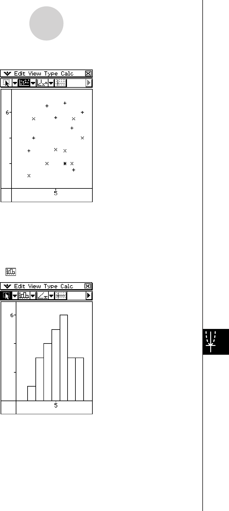
20090601

u [Graph] - [Scatter] ( X )

• In the case of a scatter graph, the first series (column or row) of selected values is used

as the x-values for all plots. The other selected values are used as the y-value for each of

the plots. This means if you select four columns of data (like Columns A, B, C, and D), for

example, there will be three different plot point types: (A, B), (A, C), and (A, D).

• Scatter graphs initially have plotted points only. You can add lines by selecting [Lines] on

the [View] menu.

u [Graph] - [Histogram] ( )

• When you select a histogram graph, only the first column of the selected data is used.

13-9-7

Graphing

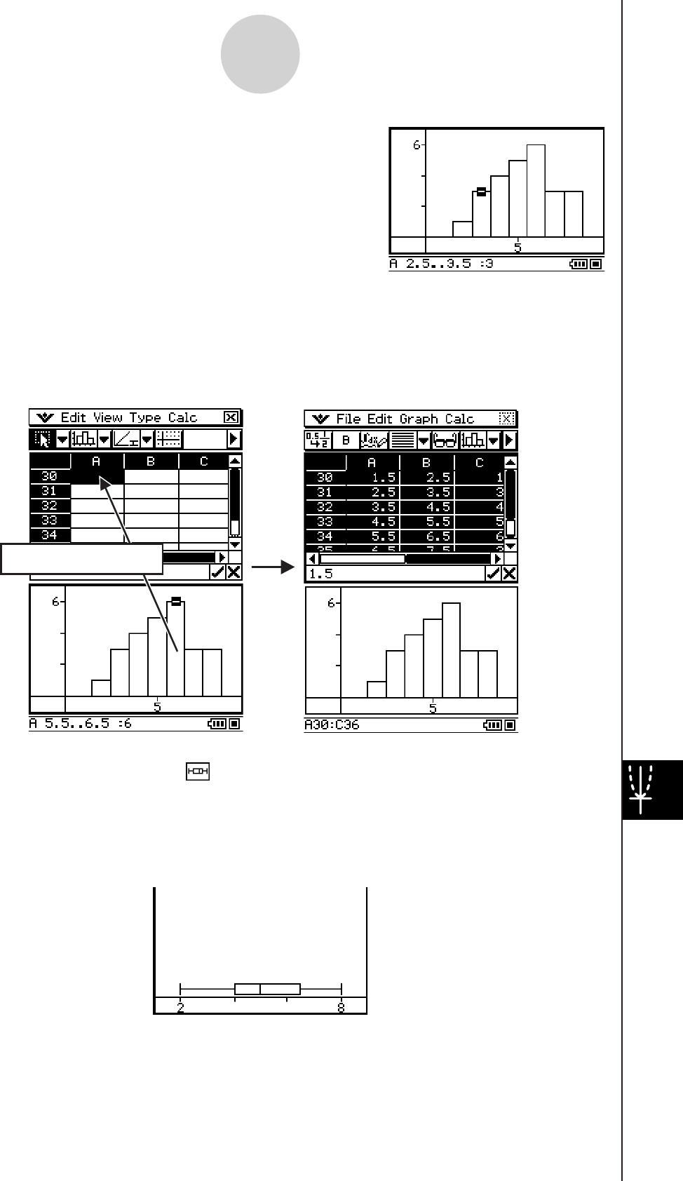
20090601

• Tapping any of the bins of a histogram graph causes three

values to appear at the bottom of the screen. The first two

values (from the left) indicate the range of the selected bin,

while the third value indicates the quantity of the selected

bin.

• You can specify the bin width after drawing a histogram graph. On the Graph window that

shows the histogram, tap [Bin Width] on the [Calc] menu.

• Dragging any of the bins of a histogram graph to a cell in the spreadsheet window will

create a table containing the values of the histogram graph, starting from the cell where you

dropped the data.

Drag & drop

u [Graph] - [Box Whisker] ( )

This type of graph lets you see how a large number of data items are grouped within specific

ranges. A box encloses all the data in an area from the first quartile (Q1) to the third quartile

(Q3), with a line drawn at the median (Med). Lines (called whiskers) extend from either end

of the box up to the minimum (Min) and maximum (Max) of the data.

• When you select a box whisker graph, each column will be displayed as a separate box

whisker.

13-9-8

Graphing

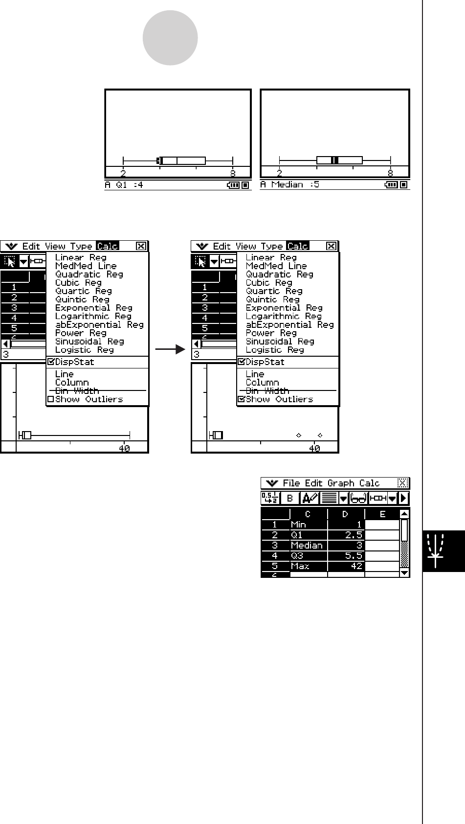
20090601

• Tapping the Q1, Q3, Med,

Min, or Max location of

a box whisker graph will

cause the applicable value

to appear at the bottom of

the screen.

• On the Graph window, checking [Calc] - [Show Outliers] displays outliers instead of

whiskers on graph.

• Dragging a box whisker graph to a cell in the spreadsheet

window will create a table containing the graph’s values

(Min, Q1, Median, Q3, Max), starting from the cell where

you drop the graph.

13-9-9

Graphing

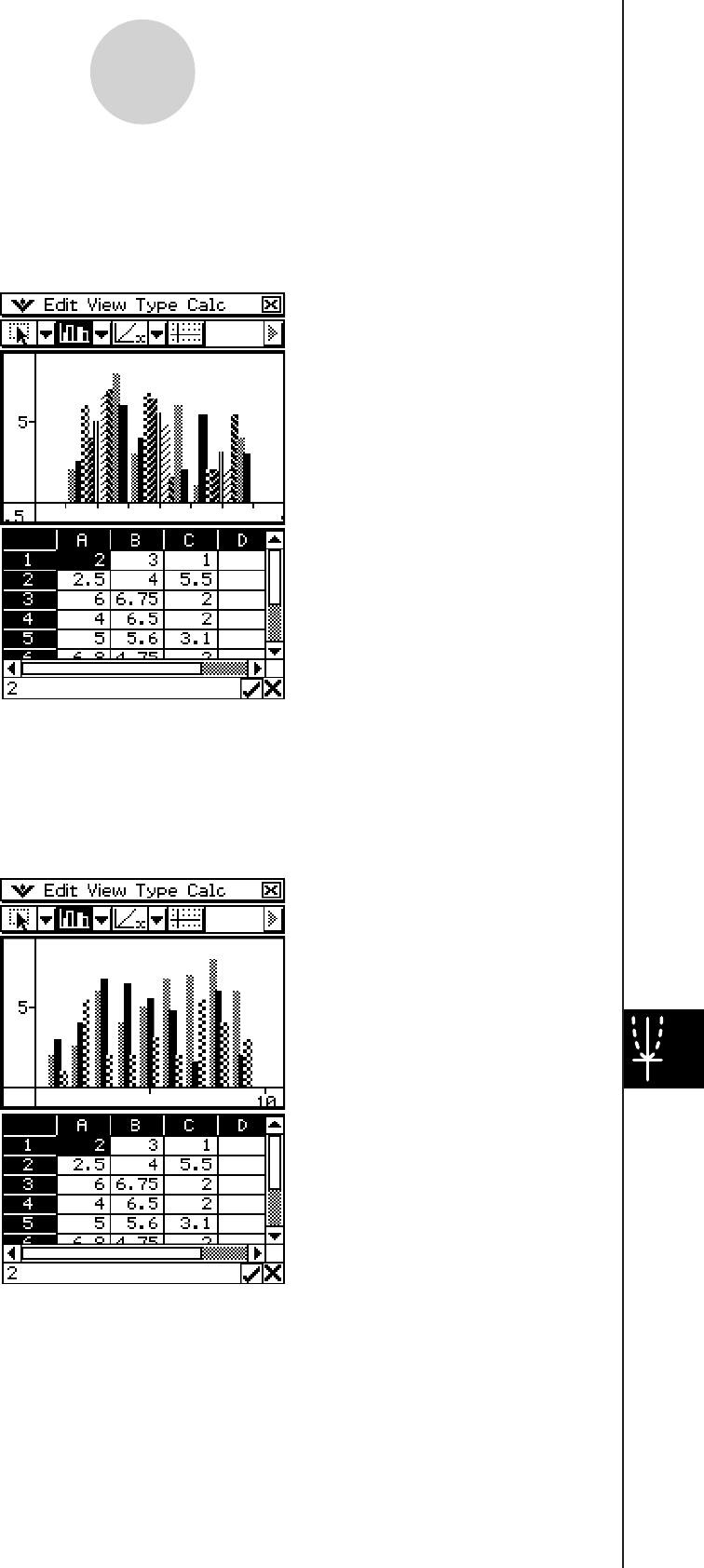
20090601

u [Graph] - [Row Series]

Selecting this option treats each row as a set of data. The value in each column is plotted as

a vertical axis value. The following shows a graph of the same data as the above example,

except this time [Row Series] is selected.

u [Graph] - [Column Series]

Selecting this option treats each column as a separate set of data. The value in each row is

plotted as a vertical axis value. The following shows a typical clustered column graph while

[Column Series] is selected, and the data that produced it.

13-9-10

Graphing

20090601

Graph Window Menus and Toolbar

The following describes the special menus and toolbar that appears whenever the

Spreadsheet application Graph window is on the display.

k O Menu

• See “Using the O Menu” on page 1-5-4.

k Edit Menu

• See “Edit Menu” on page 13-2-2.

k View Menu

Many of the [View] menu commands can also be executed by tapping Spreadsheet

application Graph window toolbar buttons.

To do this: Tap this

toolbar button:

Or select this

[View] menu item:

Change the function of the stylus so it can be

used to select and move points on the displayed

graph

GSelect

Start a box zoom operation QZoom Box

Activate the pan function for dragging the Graph

window with the stylus TPan

Enlarge the display image WZoom In

Reduce the size of the display image EZoom Out

Adjust the size of the display image so it fits the

display RZoom to Fit

Toggle display of axes and coordinate values on

and off qToggle Axes

Toggle line graph and scatter graph plot markers

on and off — Markers

Toggle line graph and scatter connecting lines

on and off — Lines

13-9-11

Graphing

20090601

k Type Menu

• The [Type] menu is identical to the [Graph] menu described on page 13-9-1.

k Calc Menu

To do this: Tap this button: Or select this [Calc]

menu item:

Display a linear regression curve dLinear Reg

Display a Med-Med graph 2MedMed Line

Display a quadratic regression curve fQuadratic Reg

Display a cubic regression curve gCubic Reg

Display a quartic regression curve hQuartic Reg

Display a quintic regression curve 3Quintic Reg

Display a logarithmic Aln(x) + B regression curve lLogarithmic Reg

Display an exponential AeBx regression curve kExponential Reg

Display an exponential ABx regression curve 4abExponential Reg

Display a power AxB regression curve ;Power Reg

Display a sinusoidal regression curve 5Sinusoidal Reg

Display a logistic regression curve 6Logistic Reg

Convert the data of the selected column to a

line graph zLine

Convert the data of the selected line to a column

graph 'Column

Set bin width for a histogram — Bin Width

Show outlying data for box whisker graph — Show Outliers

Important!

• Exponential and logarithmic regression curves ignore negative values when calculating

the curve. A message appears in the status bar to let you know when negative values are

ignored.

13-9-12

Graphing

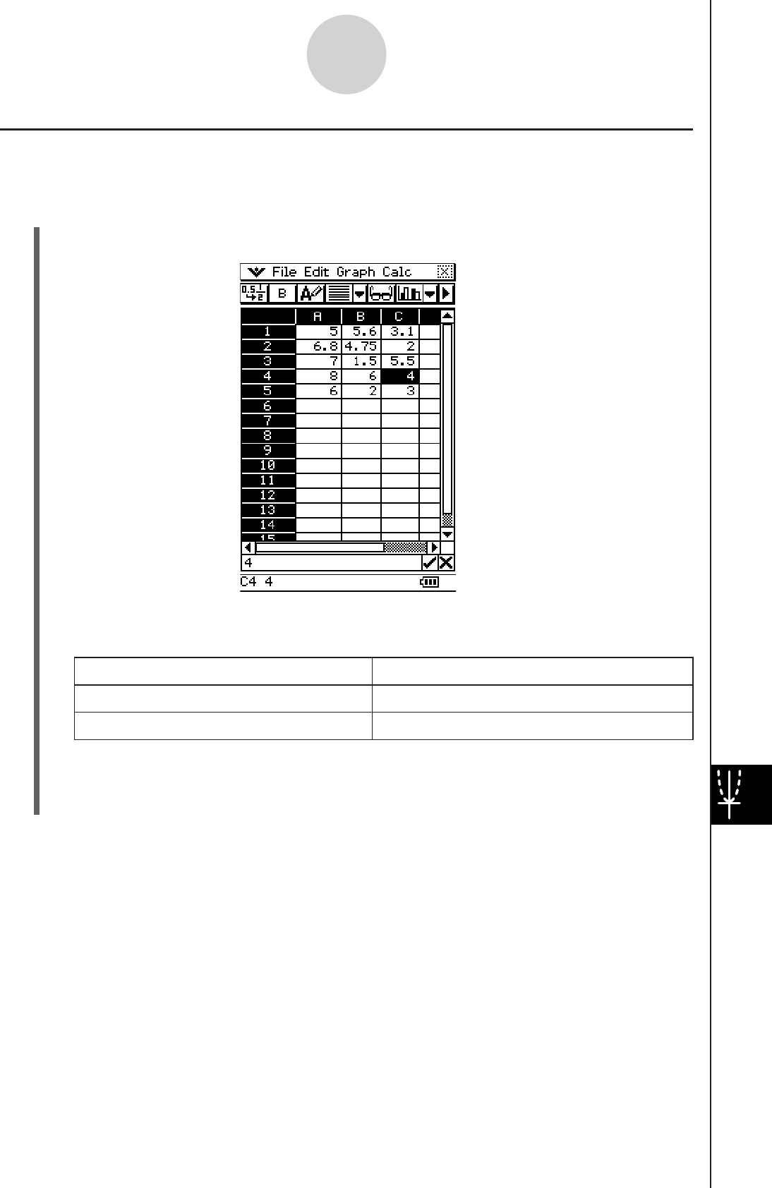
20090601

Basic Graphing Steps

The following are the basic steps for graphing spreadsheet data.

u ClassPad Operation

(1) Input the data you want to graph into the spreadsheet.

(2) Use the [Graph] menu to specify whether you want to graph the data by row or by

column.

To do this: Select this [Graph] menu option:

Graph the data by row Row Series

Graph the data by column Column Series

• See “Graph Menu” on page 13-9-1 for more information.

(3) Select the cells that contain the data you want to graph.

• See “Selecting Cells” on page 13-3-5 for information about selecting data.

13-9-13

Graphing

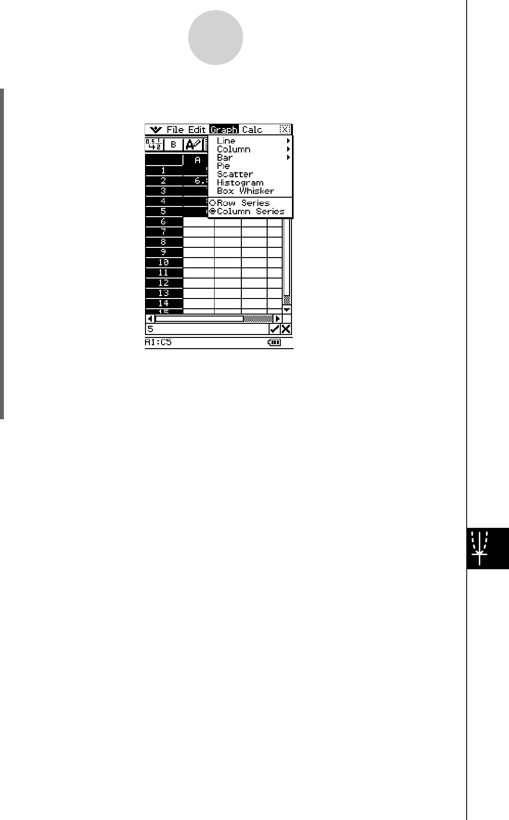
20090601

(4) On the [Graph] menu, select the type of graph you want to draw. Or you can tap the

applicable icon on the toolbar.

• This draws the selected graph. See “Graph Menu” on page 13-9-1 for examples of

the different types of graphs that are available.

• You can change to another type of graph at any time by selecting the graph type you

want on the [Type] menu. Or you can tap the applicable icon on the toolbar.

13-9-14

Graphing

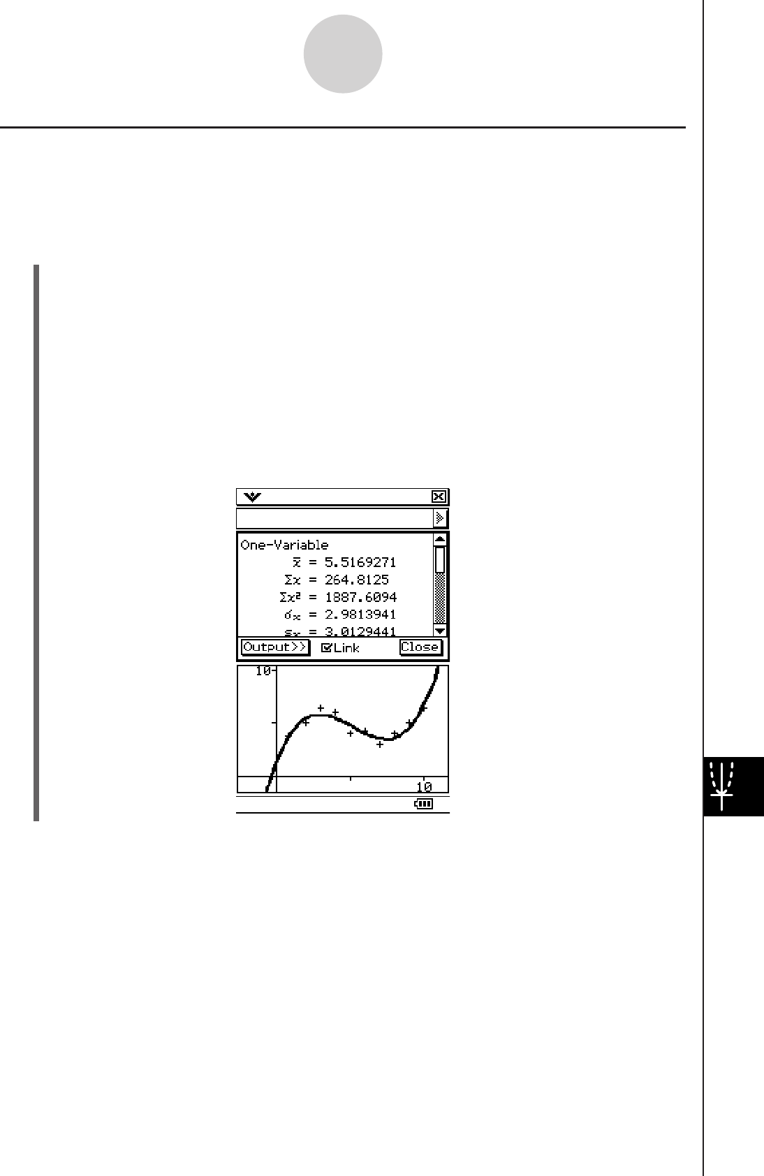
20101001

Regression Graph Operations (Curve Fitting)

After plotting a scatter graph of paired-variable spreadsheet data (Single-variable and

Paired-variable Statistical Calculations, page 13-6-1), you can draw a regression graph that

approximates the scatter graph and determine the regression formula.

u To plot a scatter graph and then draw its regression graph

(1) Enter the paired-variable data into the spreadsheet, and then select the range of cells

where it is located.

(2) Tap [Graph] and then [Scatter].

• This plots the scatter graph for the data you selected in step 1.

(3) On the menu bar, tap [Calc] and then use the menu that appears to select the desired

regression type (Linear Reg, MedMed Line, Quadratic Reg, Cubic Reg, Quartic Reg,

Quintic Reg, Logarithmic Reg, Exponential Reg, abExponential Reg, Power Reg,

Sinusoidal Reg, Logistic Reg).

• This superimposes the regression graph on the scatter graph. Also, the regression

calculation result window will appear in the half of the display.

Tip

For details about how to use the Link check box and [Output>>] button on the regression

calculation result window, see “Regression Calculations” (page 13-6-2).

Note that the regression calculation result window is not available for Quintic Reg.

•

13-9-15

Graphing

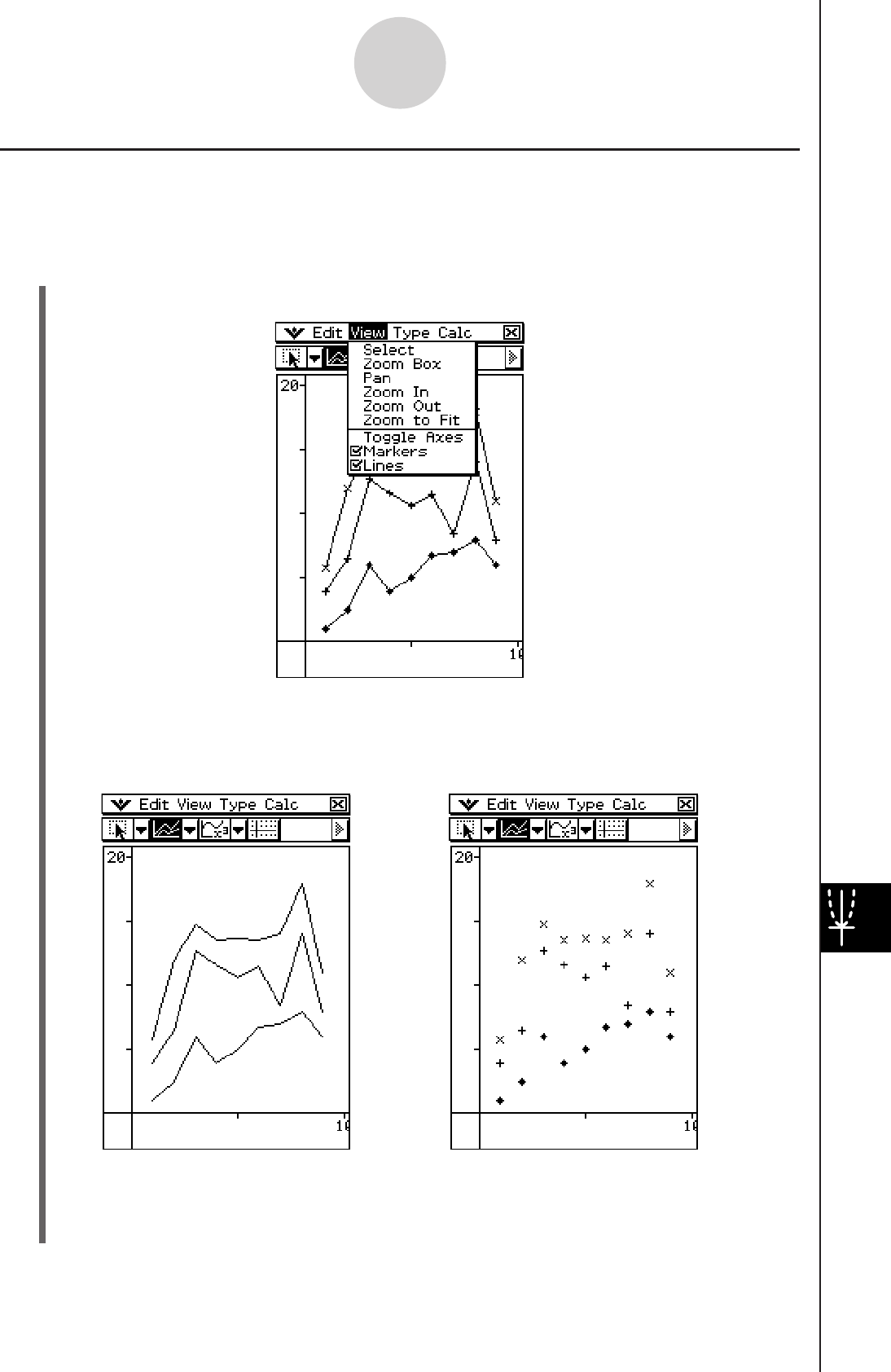
20090601

Other Graph Window Operations

This section provides more details about the types of operations you can perform while the

Graph window is on the display.

u To show or hide lines and markers

(1) While a line graph or a scatter graph is on the Graph window, tap the [View] menu.

Lines and markers both turned on

(2) Tap the [Markers] or [Lines] item to toggle it between show (checkbox selected) and

hide (checkbox cleared).

Lines turned on, markers hidden Markers turned on, lines hidden

• Line and scatter graphs can have markers only, lines only, or both markers and lines.

You cannot turn off both markers and lines at the same time.

13-9-16

Graphing

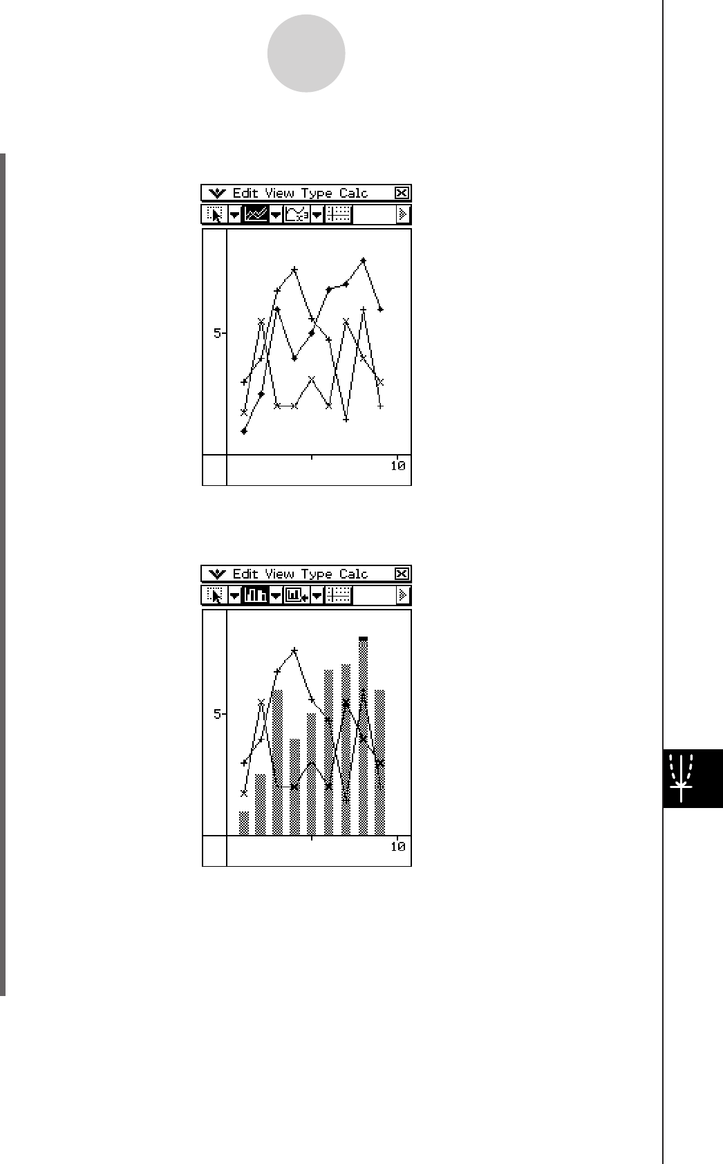
20090601

u To change a line in a clustered line graph to a column graph

(1) Draw the clustered line graph.

(2) With the stylus, tap any data point on the line you wish to change to a column graph.

(3) On the [Calc] menu, tap [Column].

• You could also tap the down arrow button next to the third tool button from the left,

and then tap '.

• You can change more than one line to a column graph, if you want.

• You can change a column graph back to a line graph by selecting one of its columns

and tapping [Line] on the [Calc] menu.

13-9-17

Graphing

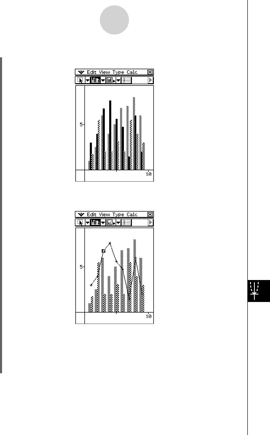
20090601

u To change a column in a clustered column graph to a line

(1) Draw the clustered column graph.

(2) With the stylus, tap any one of the columns you wish to change to a line graph.

(3) On the [Calc] menu, tap [Line].

• You could also tap the down arrow button next to the third tool button from the left,

and then tap z.

• You can change more than one column to a line graph, if you want.

• You can change a line graph back to a column graph by selecting one of its data

points and tapping [Column] on the [Calc] menu.

13-9-18

Graphing

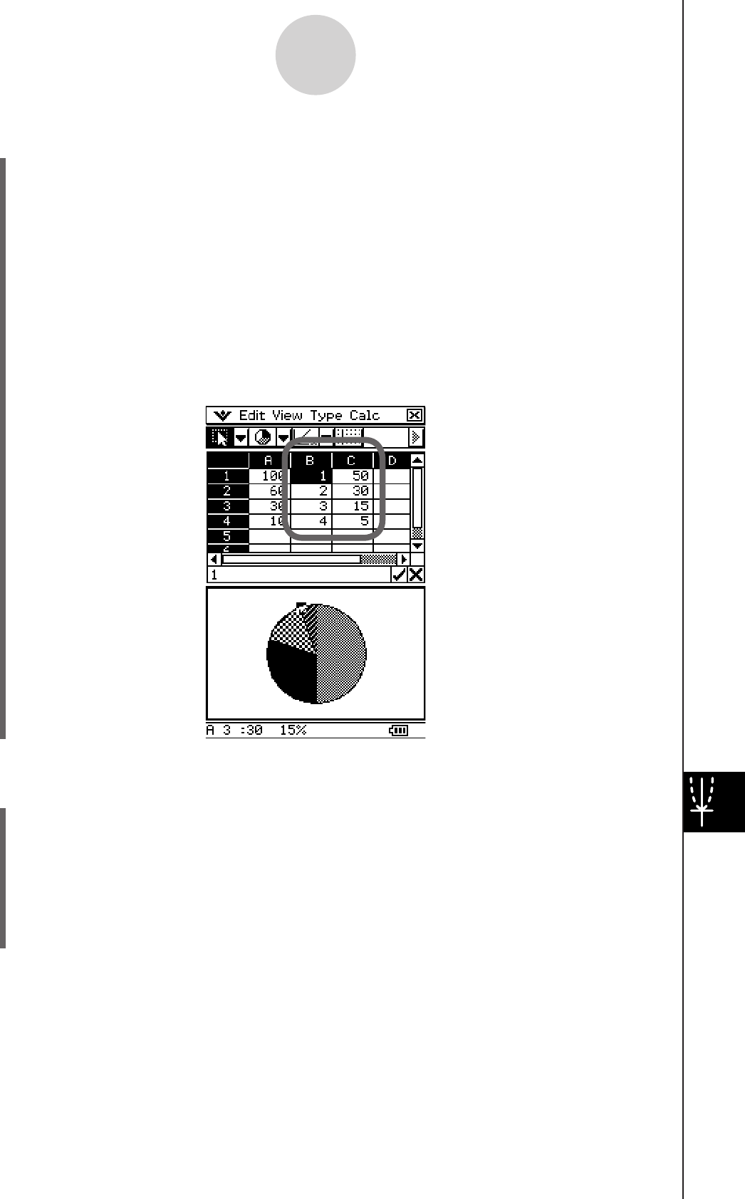
20090601

u To find out the percentage of data for each pie graph section

(1) While the display is split between the pie graph and the Spreadsheet windows, tap the

pie graph to select it.

(2) On the [Edit] menu, tap [Copy].

(3) Tap the Spreadsheet window to make it active.

(4) Tap the cell where you want to paste the data.

• The cell you tap will be the upper left cell of the group of cells that will be pasted.

(5) On the [Edit] menu, tap [Paste].

• This pastes two columns of values. The numbers in the left column are pie graph

section numbers. The values in the right column are the percentages that the data in

each section of the pie graph represents.

u To change View Window settings

(1) While a graph is on the Graph window, tap O, and then [View Window].

• This displays the current View Window settings.

(2) Change the View Window settings, if you want.

• See “Configuring View Window Parameters for the Graph Window” on page 3-2-1 for

information about using the View Window.

(3) After the settings are the way you want, tap [OK] to apply them.

13-9-19

Graphing

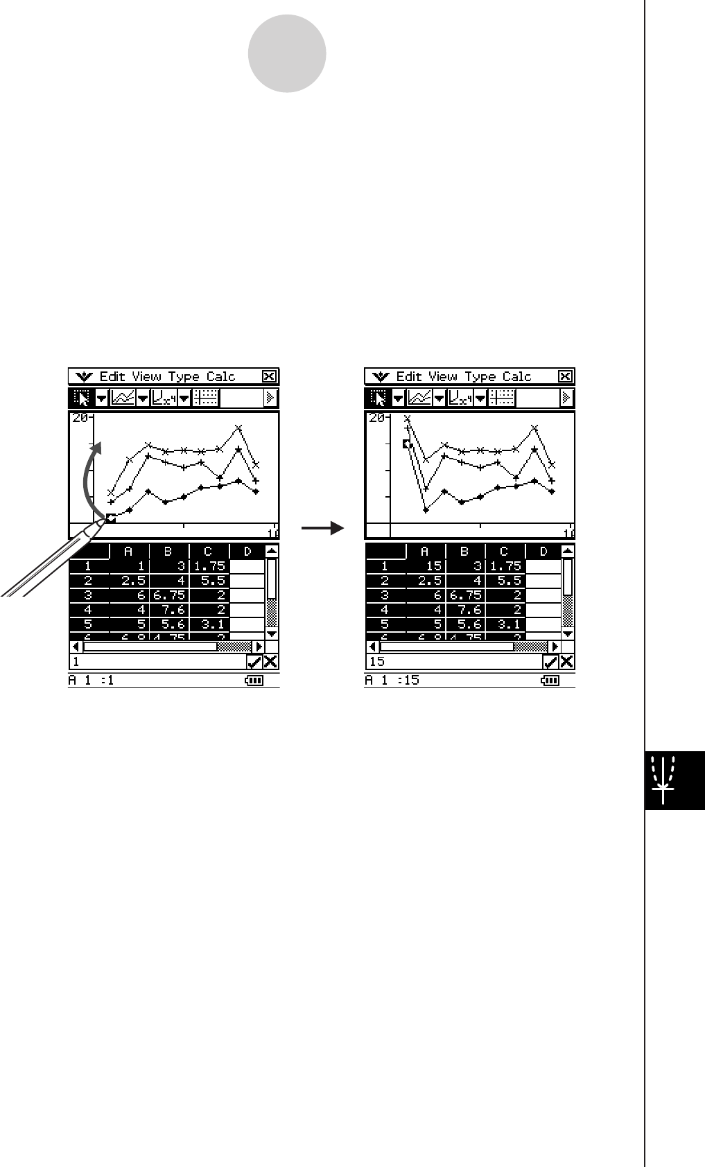
20090601

u To change the appearance of the axes

While a graph is on the Graph window, select [Toggle Axes] on the [View] menu or tap the

q toolbar button to cycle through axes settings in the following sequence: axes on → axes

and values on → axes and values off →.

u To change the appearance of a graph by dragging a point

While a graph is on the Graph window, use the stylus to drag any one of its data points to

change the configuration of the graph.

• You can change curves, make bars or columns longer or shorter, or change the size of pie

graph sections.

• Changing a graph automatically changes the graph’s data on the Spreadsheet window.

ChangesDrag

13-9-20

Graphing

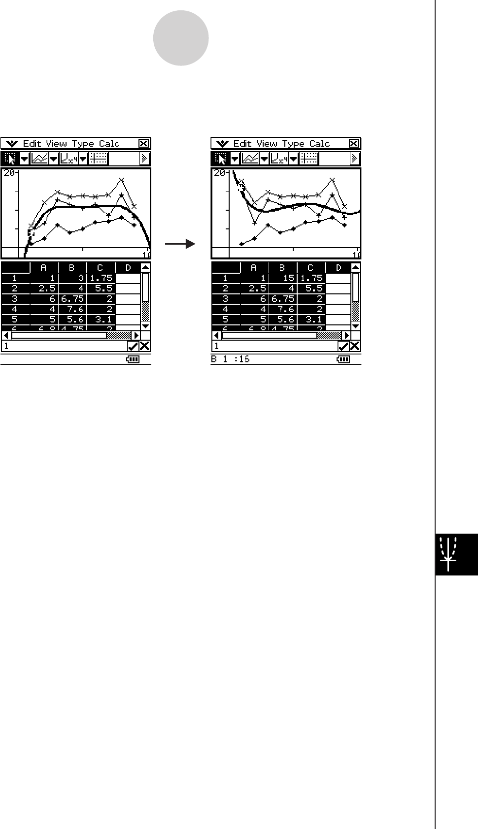
20090601

• If a regression curve is displayed for the data whose graph is being changed by dragging,

the regression curve also changes automatically in accordance with the drag changes.

• When you edit data in the spreadsheet and press E, your graph will update automatically.

Important!

• You can drag a point only if it corresponds to a fixed value on the spreadsheet. You cannot

drag a point if it corresponds to a formula.

• You may encounter the message “Insufficient System Memory to Run...” if you are using a

large amount of data and formulas.

13-9-21

Graphing

20060301

Chapter

Using the Differential

Equation Graph

Application

This chapter explains how to use the Differential Equation Graph

application, which you can use to investigate families of solutions

to ordinary differential equations (ODE).

14-1 Differential Equation Graph Application Overview

14-2 Graphing a First Order Differential Equation

14-3 Graphing a Second Order Differential Equation

14-4 Graphing an Nth-order Differential Equation

14-5 Drawing f

(x) Type Function Graphs and Parametric

Function Graphs

14-6 Configuring Differential Equation Graph View

Window Parameters

14-7 Differential Equation Graph Window Operations

20060301

14-1-1

Differential Equation Graph Application Overview

14-1 Differential Equation Graph Application

Overview

This section explains how to use the Differential Equation Graph application screen, and

describes the basic configuration of the Differential Equation Graph application windows.

Differential Equation Graph Application Features

You can use the Differential Equation Graph application to draw the following types of

graphs.

1st-order differential equation graphs

• Slope field of a first order differential equation (y’ = dy/dx = f

(x, y))

• Solution curves when initial conditions are imposed on a first order differential equation

2nd-order differential equation graphs

• Phase plane of two first order differential equations (x’ = dx/dt = f

(x, y); y’ = dy/dt = f

(x, y))

• Solution curves when initial conditions are imposed on a set of two first order differential

equations

Nth-order differential equation graphs

• Solution curves when initial conditions are imposed on a set of multiple first order

differential equations (y1’ = dy1/dx = f

(x, y) ; y2’ = dy2/dx = f

(x, y) ; ... ; yn’ = dyn/dx = f

(x, y))

General graphs

•

(x) type function graphs

• Parametric function graphs

20060301

14-1-2

Differential Equation Graph Application Overview

Differential Equation Graph Application Window

The Differential Equation Graph application has two windows, which are described below.

Differential Equation Editor window

Use this window to input expressions and initial

conditions for graphing.

Differential Equation Graph window

This window shows the graph of the expression

that you input into the Editor window.

Starting Up the Differential Equation Graph Application

Use the following procedure to start up the Differential Equation Graph application.

u ClassPad Operation

On the application menu, tap .

This starts the Differential Equation Graph application and displays the Differential

Equation Editor window and the Differential Equation Graph window.

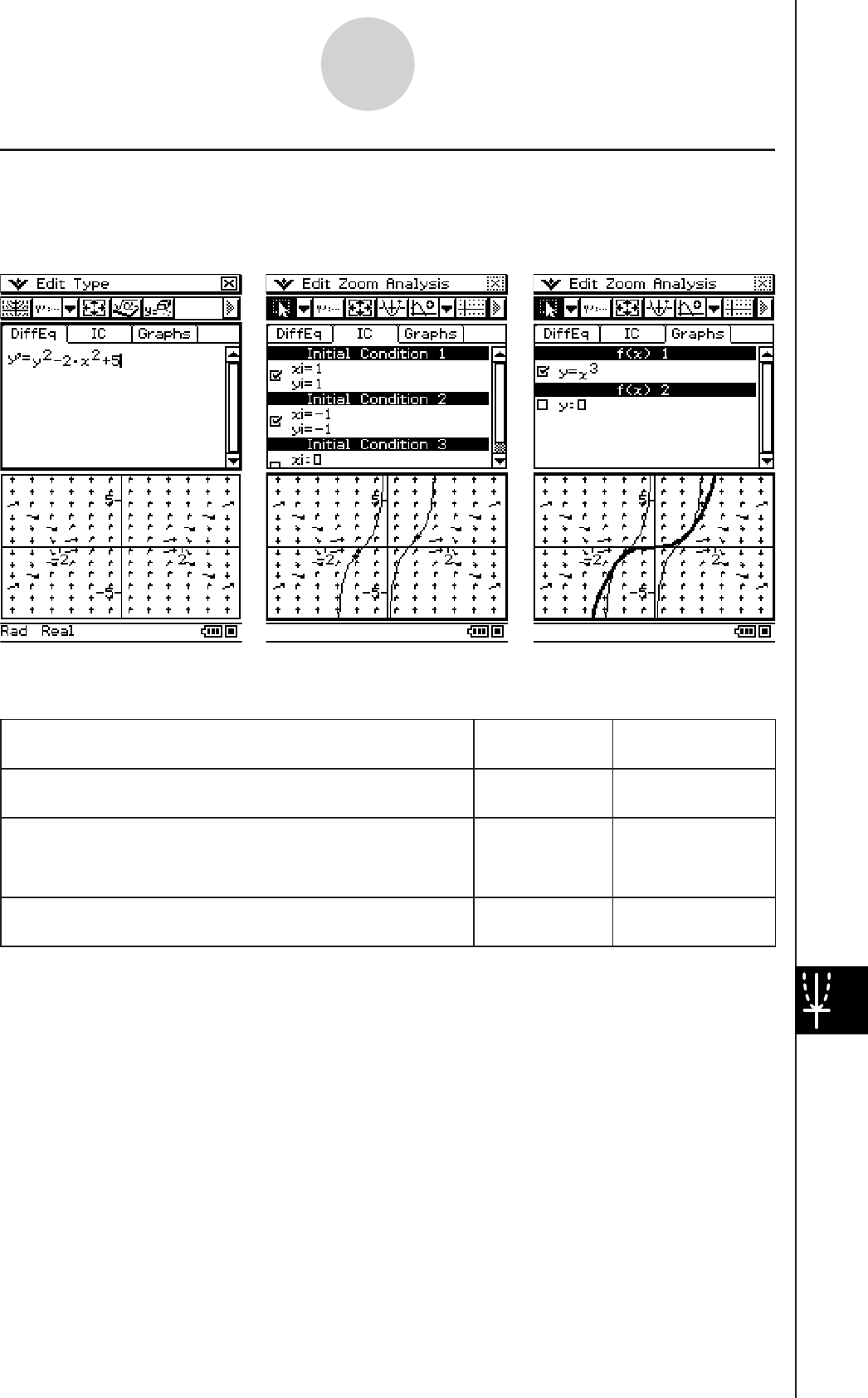
20060301

14-1-3

Differential Equation Graph Application Overview

k Differential Equation Editor Window Screens

The Differential Equation Editor window has three different editor screens. The editor screen

you should use depends on what you want to input, as described below.

To input this: Tap this tab: To display this

editor screen:

Differential equation or a set of differential equations [DiffEq] Differential

equation editor

Initial conditions to graph solution curves of a

differential equation (or a set of differential equations)

input on the [DiffEq] tab

[IC] Initial condition

editor

(x) type functions or parametric functions [Graphs] General graph

editor

Differential equation editor

([DiffEq] tab)

Initial condition editor

([IC] tab)

General graph editor

([Graphs] tab)

20060301

14-1-4

Differential Equation Graph Application Overview

Differential Equation Editor Window Menus and Buttons

This section provides basic information about Differential Equation Editor window menus and

commands.

• For information about the O menu, see “Using the O Menu” on page 1-5-4.

Edit Menu ([DiffEq], [IC], [Graphs])

To do this: Select this Edit menu

item:

Cut the selected character string and place it onto the clipboard Cut

Copy the selected character string and place it onto the

clipboard Copy

Paste the contents of the clipboard at the current cursor

position on the Differential Equation Editor window Paste

Select the entire expression you are editing Select All

Delete the line of data at the current cursor location Delete Line

Clear all input data from the currently displayed tab ([DiffEq],

[IC], or [Graphs]) Clear All

Type Menu ([DiffEq])

To input this: Select this Type menu

item:

A single first order differential equation 1st (Slope Field)

A single second order differential equation or a set of two first

order differential equations 2nd (Phase Plane)

A higher order differential equation or a set of multiple

differential equations Nth (No Field)

Type Menu ([Graphs])

To input this: Select this Type menu

item:

(x) type functions f

(x)

Parametric functions Parametric

20060301

14-1-5

Differential Equation Graph Application Overview

Toolbar Buttons ([DiffEq], [IC], [Graphs])

To do this: Tap this button:

Graph the selected function(s) O

Display the View Window dialog box to configure Differential

Equation Graph window settings 6

Display the Main application window ~

Delete the line of data at the current cursor location q

Toolbar Buttons ([DiffEq])

To input this: Tap this button:

A single first order differential equation A

A single second order differential equation or a set of two first

order differential equations B

A higher order differential equation or a set of multiple

differential equations

Toolbar Buttons ([IC], [Graphs])

To select this graph line thickness: Tap this button:

Normal F

Thick G

Toolbar Buttons ([Graphs])

To input this: Tap this button:

(x) coordinate type functions d

Parametric functions g

20060301

14-1-6

Differential Equation Graph Application Overview

Differential Equation Graph Window Menus and Buttons

This section provides basic information about Differential Equation Graph window

menus and commands.

Edit Menu

To do this: Select this Edit menu

item:

Toggle arrows to indicate the direction of slope field or phase

plane vectors on and off Arrows

Toggle the use of unit vectors for slope field or phase plane

graphing on and off Unit Vectors

Display the Differential Equation Editor window [DiffEq] tab Editor - DiffEq.Editor

Display the Differential Equation Editor window [IC] tab Editor - IC Editor

Display the Differential Equation Editor window [Graphs] tab Editor - Graph Editor

Clear all currently registered initial conditions (and, as a result,

all solution curves) Clear All

Zoom Menu

To do this: Select this Zoom menu

item:

Enlarge the part of the screen bounded by a box Box

Zoom in by the zoom factor Zoom In

Zoom out by the zoom factor Zoom Out

Return a graph to its original size Original

Adjust View Window x-axis values so they are identical to the

y-axis values Square

Return View Window parameters to their settings prior to the

last zoom operation Previous

Return the Differential Equation Graph window to its initial

default state Quick Initialize

20060301

14-1-7

Differential Equation Graph Application Overview

Analysis Menu

To do this: Select this Analysis

menu item:

Pan the graph window Pan

Select and move initial condition point Select

Trace the graph of a solution curve Trace

Differential Equation Graph window as the initial condition, and

graph the solution curve based on that initial condition

Modify

Toolbar Buttons

To do this: Tap this button:

Select and move the initial condition point G

Pan the graph window T

Zoom in by the zoom factor W

Zoom out by the zoom factor E

Enlarge the part of the screen bounded by a box Q

Make the Differential Equation Editor window active A

Display the View Window dialog box to configure Differential

Equation Graph window settings 6

Differential Equation Graph window as the initial condition, and

graph the solution curve based on that initial condition

Display a trace cursor that can be positioned on any x, y

coordinate K

Display a trace cursor that can be positioned on any grid point

that has a field line L

Display a trace cursor that can be positioned on any solution

curve =

Turn display of axes and coordinate values on and off q

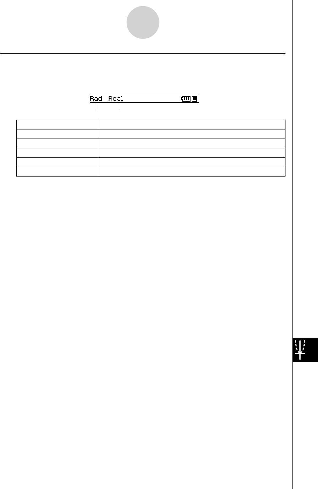
20060301

14-1-8

Differential Equation Graph Application Overview

Differential Equation Graph Application Status Bar

The status bar at the bottom of the Differential Equation Graph application shows the current

angle unit setting and [Complex Format] setting (page 1-9-5).

Rad

Deg

Cplx

Real

The angle unit setting is radians.

The angle unit setting is degrees.

The Complex (complex number calculation) mode is selected.

Gra The angle unit setting is grads.

The Real (real number calculation) mode is selected.

If you see this: It means this:

Angle unit Real mode

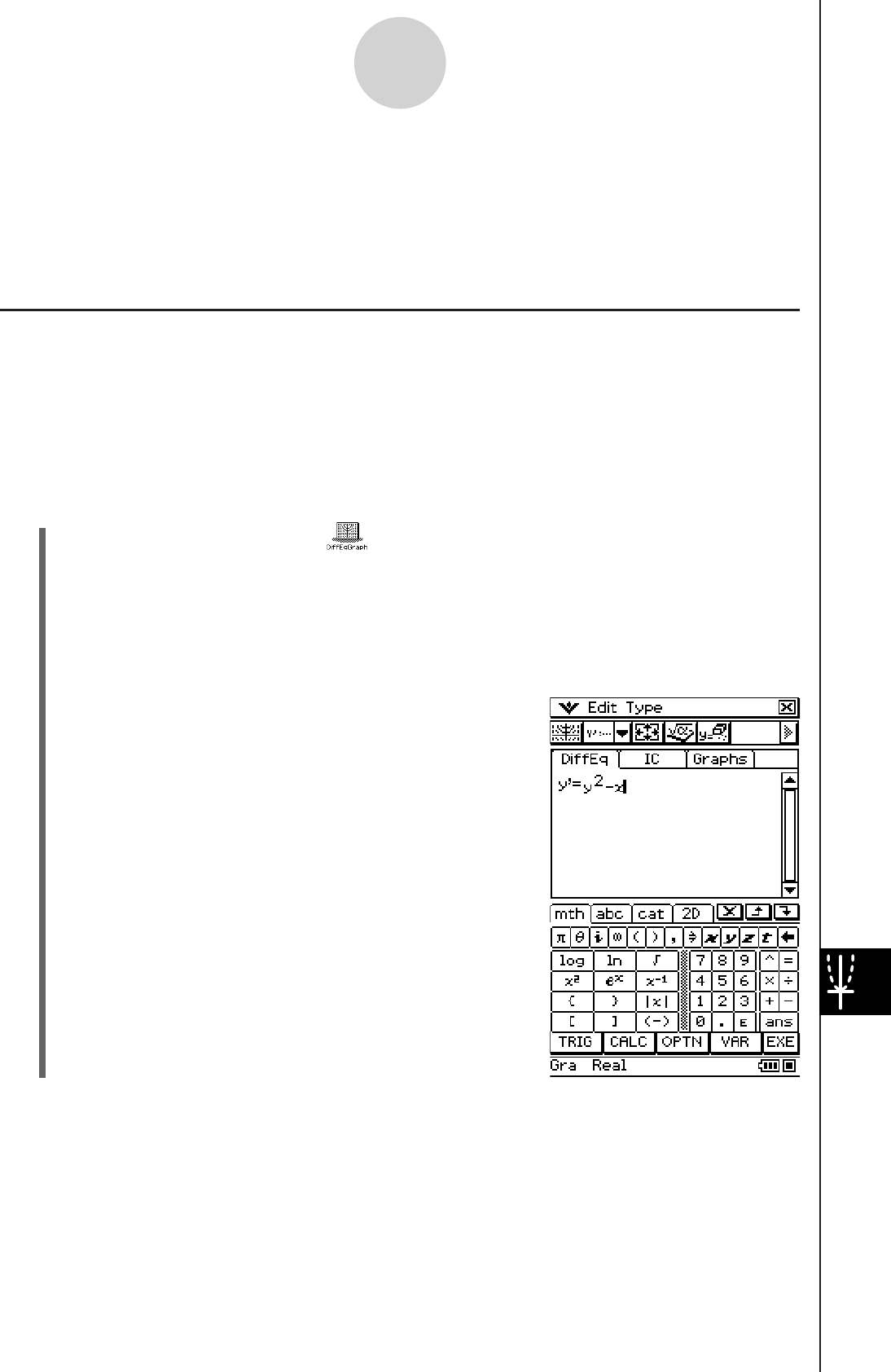
20060301

14-2-1

Graphing a First Order Differential Equation

14-2 Graphing a First Order Differential Equation

This section explains how to input a first order differential equation and draw a slope field,

and how to graph the solution curve(s) of a first order differential equation based on given

initial conditions.

Inputting a First Order Differential Equation and Drawing a Slope Field

A slope field is the family of solutions of a single, first order differential equation of the form

y’= f

(x, y). It is a grid of solution lines where each line has the slope y’ for a given grid value of

x and y. It is often referred to as a “slope field” or “direction field” because only the direction

of the field at any given point in known, not the magnitude.

Example: To input y’ = y2 − x and draw its slope field

u ClassPad Operation

(1) On the application menu, tap .

• This starts up the Differential Equation Graph application and activates the differential

equation editor ([DiffEq] tab).

(2) Tap [Type] - [1st (Slope Field)] or the A toolbar button.

(3) Press the

k key to display the soft keyboard.

(4) Input

y’ = y2 − x.

9Y{c-Xw

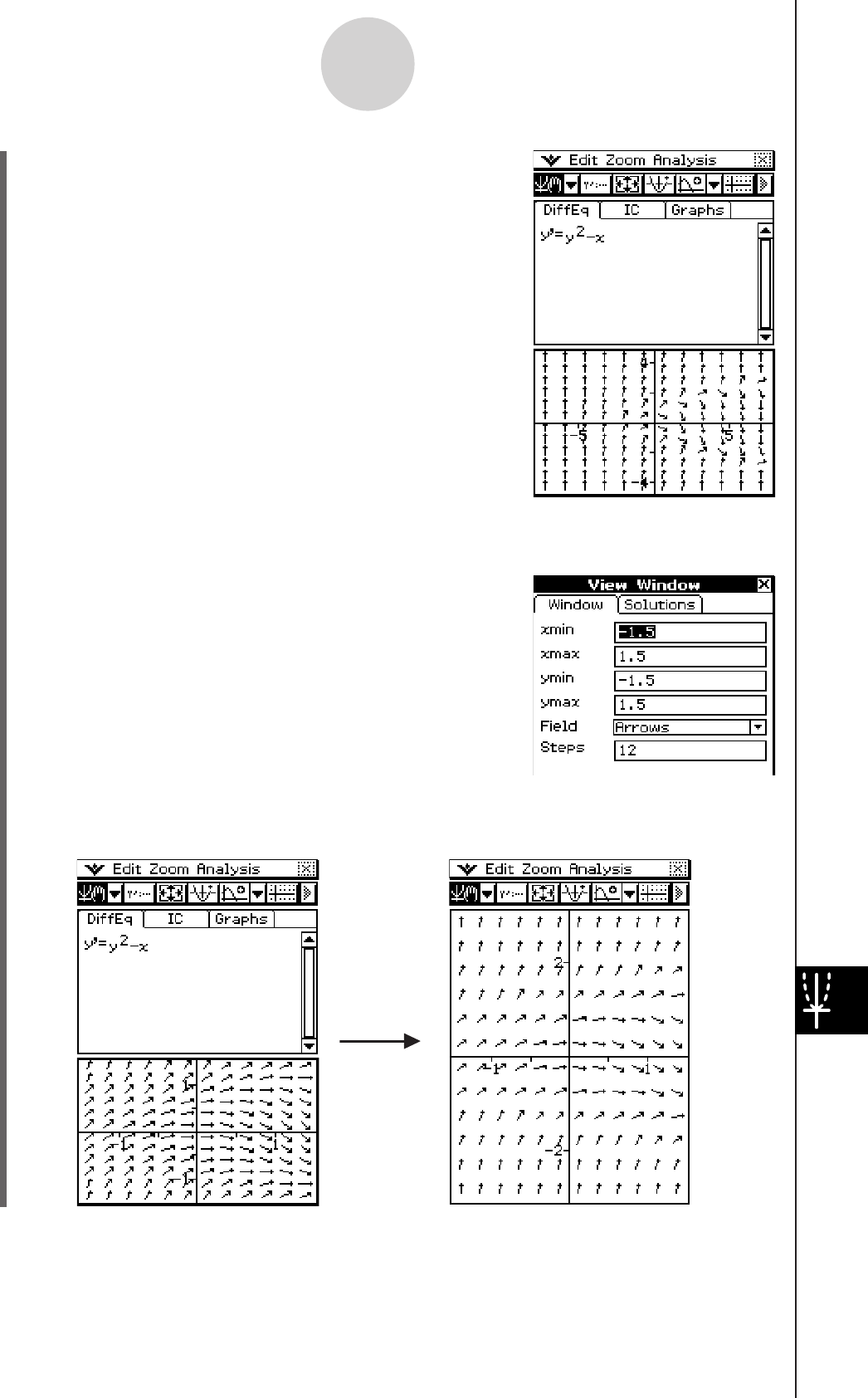
20060301

14-2-2

Graphing a First Order Differential Equation

(5) Tap

• This draws the slope field of y’ = y2 – x.

(6) Tap

6, or tap O and then tap [View Window] to display the View Window dialog

box, and configure the View Window settings as shown below.

• For details about View Window settings, see

“Configuring Differential Equation Graph View Window

Parameters” on page 14-6-1.

(7) After the settings are the way you want, tap [OK].

• This updates the slope field in accordance with the new View Window settings.

[Edit] - [Redraw]

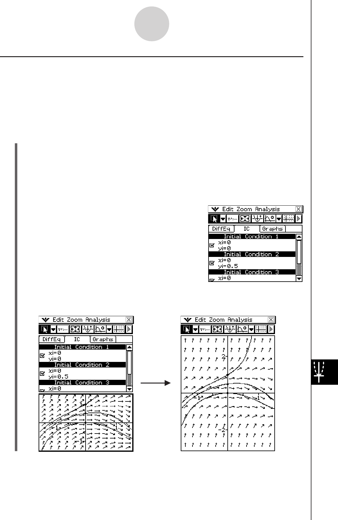
20060301

14-2-3

Graphing a First Order Differential Equation

Inputting Initial Conditions and Graphing the Solution Curves of a First

Order Differential Equation

You can use the procedure in this section to overlay, onto the slope field, solution curves of

the first order differential equation input on the [DiffEq] tab for given initial conditions.

Example: To input the first order differential equation y’ = y2 – x, draw its slope field, and then

graph three solution curves for the initial conditions (xi, yi) = (0,0), (0,0.5), (0,1)

u ClassPad Operation

(1) Use the procedure under “Inputting a First Order Differential Equation and Drawing a

Slope Field” on page 14-2-1 to draw the slope field for y’ = y2 – x.

(2) Activate the Differential Equation Editor window and then tap the [IC] tab.

• This displays the initial condition editor.

(3) On the initial condition editor, input the following initial conditions: (xi, yi) = (0,0), (0,0.5),

(0,1). Perform the following operations.

awaw awa.fw awbw

(4) Tap

• This graphs the three solution curves over the slope field of y’ = y2 – x.

[Edit] - [Redraw]

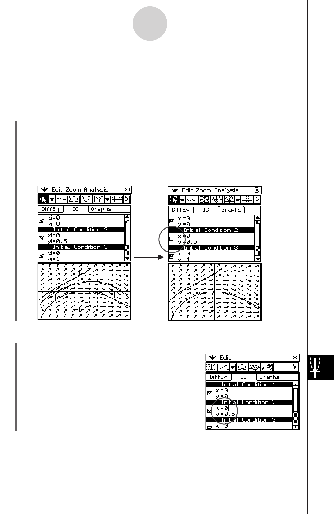
20060301

14-2-4

Graphing a First Order Differential Equation

Configuring Solution Curve Graph Settings

You can specify whether or not a solution curve should be drawn for each initial condition

input on the initial condition editor. You can also specify either a normal or thick line for

solution curves.

u To configure the solution curve draw setting

Use the initial condition editor to select the check box to the left of each initial condition

input box (Initial Condition 1, Initial Condition 2, etc.) whose solution curve you want to

graph. The solution curve of any initial condition whose check box is not selected will not

be graphed.

Example: To perform the operation under “Inputting Initial Conditions and Graphing the

Solution Curves of a First Order Differential Equation” on page 14-2-3, clear the

Initial Condition 2 checkbox, and then draw the graph

u To specify the line thickness for drawing a solution curve

(1) Tap the input box of the initial condition whose line thickness you want to change.

• This displays the cursor in the initial condition input

box you tapped.

20060301

14-2-5

Graphing a First Order Differential Equation

(2) Tap the down arrow button on the toolbar.

(3) Tap

F on the toolbar to draw the solution curve with a thin line, or G to draw with a

thick line.

(4) To apply your setting to the graph, tap O.

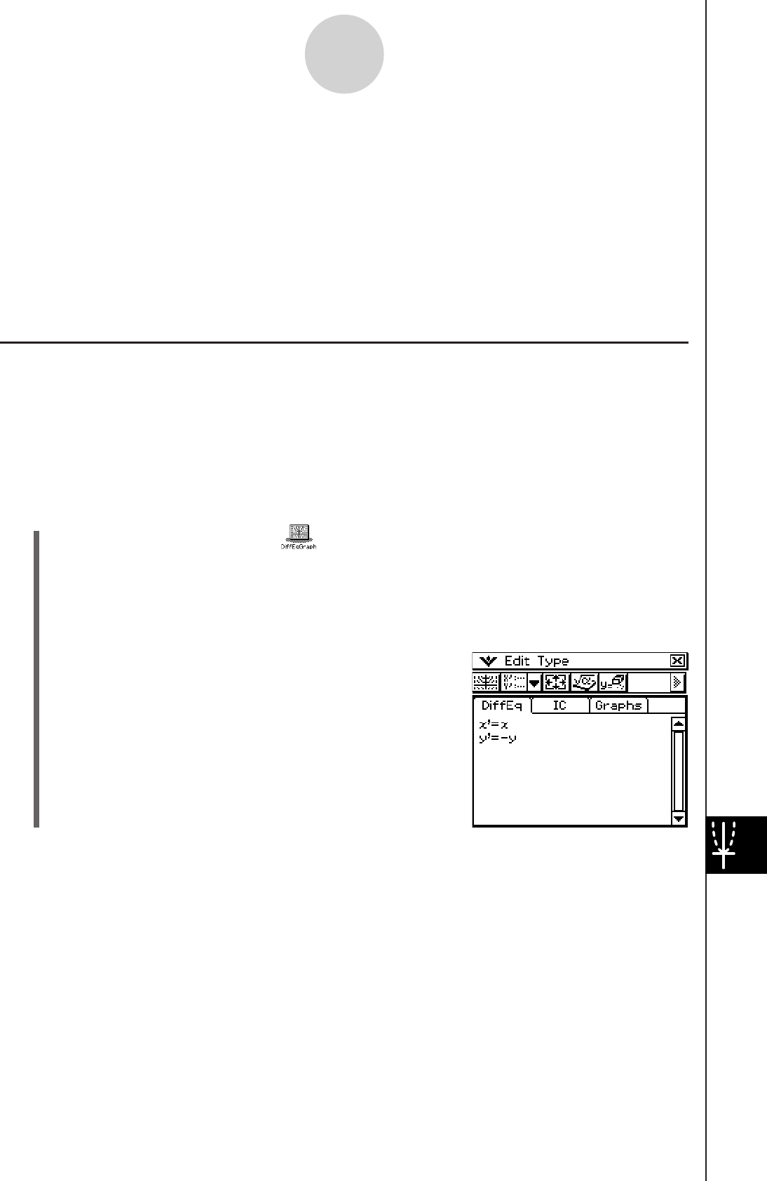
20060301

14-3-1

Graphing a Second Order Differential Equation

14-3 Graphing a Second Order Differential

Equation

This section explains how to input a second order differential equation and draw a slope

field, and how to graph the solution curve(s) for a second order differential equation based

on given initial conditions.

With this application, a second order differential equation is input in the form of a set of two

first order differential equations.

Drawing the Phase Plane of a Second Order Differential Equation

A phase plane is the family of solutions of either a second order differential equation or two

first order differential equations of the form x’ = dx/dt = f

(x,y) and y’ = dy/dt = g(x,y). A single

second order differential equation can also be graphed, but it must be written as two first

order differential equations.

Example: To input {x’ = x, y’ = −y} and draw its phase plane

u ClassPad Operation

(1) On the application menu, tap .

• This starts up the Differential Equation Graph application and activates the differential

equation editor ([DiffEq] tab).

(2) Tap [Type] - [2nd (Phase Plane)] or the B toolbar button.

(3) Use the differential equation editor to input x’ = x, y’ = −y.

9Xw-Yw

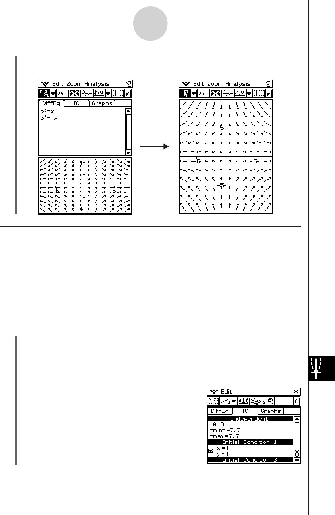
20060301

14-3-2

Graphing a Second Order Differential Equation

(4) Tap

• This draws the phase plane of x’ = x, y’ = −y.

Inputting Initial Conditions and Graphing the Solution Curve of a Second

Order Differential Equation

You can use the procedure in this section to overlay, onto the slope field, solution curve of

the second order differential equation input on the [DiffEq] tab for given initial conditions.

Example: To input the second order differential equation {x’ = x, y’ = −y}, draw the phase

plane, and then graph the solution curve of the initial condition (xi, yi) = (1, 1)

The independent variable minimum value (tmin) = −7.7, maximum value (tmax) =

7.7, and initial value (t0) = 0.

u ClassPad Operation

(1) Use the procedure under “Drawing the Phase Plane of a Second Order Differential

Equation” on page 14-3-1 to draw the phase plane for {x’ = x, y’ = −y}.

(2) Activate the Differential Equation Editor window and then tap the [IC] tab.

• This displays the initial condition editor.

(3) Input (xi, yi) = (1, 1) into the initial condition editor.

Select the check box next to “xi=” and then tap

bwbw.

[Edit] - [Redraw]

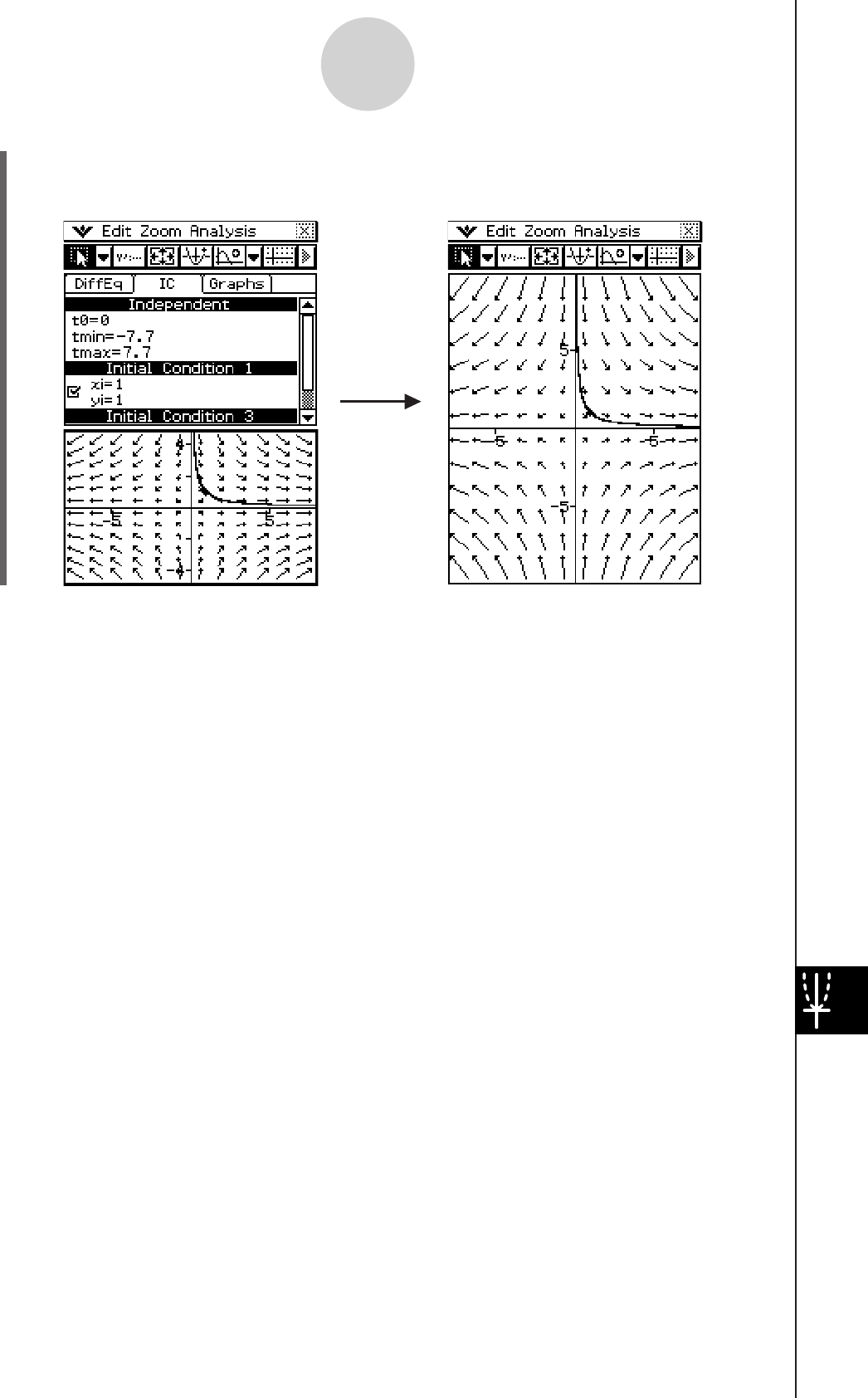
20060301

14-3-3

Graphing a Second Order Differential Equation

(4) Tap

• This graphs the solution curve and overlays it on the phase plane of {x’ = x, y’ = −y}.

[Edit] - [Redraw]

Tip

• You can also draw a solution curve using [Modify] in the Analysis menu (page 14-1-7).

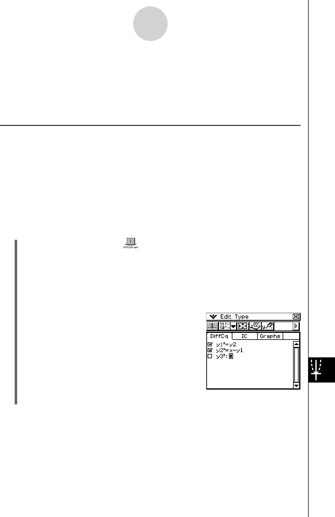
20060301

14-4-1

Graphing an Nth-order Differential Equation

14-4 Graphing an Nth-order Differential Equation

This section explains how to graph the solution curve(s) for an nth order (higher order)

differential equation based on specified initial conditions.

With this application, an nth order differential equation is input in the form of a set of multiple

first order differential equations.

Inputting an Nth-order Differential Equation and Initial Conditions, and

then Graphing the Solutions

You can use the procedure in this section to graph the solution curves of the Nth-order

differential equation input on the [DiffEq] tab for given initial conditions.

Note

• For Nth-order differential equations, only solution curves are drawn.

Example: To specify the three initial conditions (xi, y1i, y2i) = (0, −1, 0), (0, 0, 0), (0, 1, 0) for

the differential equation y’’ = x − y and graph its solution curves

u ClassPad Operation

(1) On the application menu, tap .

• This starts up the Differential Equation Graph application and activates the differential

equation editor ([DiffEq] tab).

(2) Tap [Type] - [Nth (No Field)] or the ! toolbar button.

(3) Use the differential equation editor to input y’’ = x − y.

• Input

y’’ = x − y by dividing it into two first order differential equations. If we let y1 = y

and

y2 = y’, we see that y1’ = y’ = y2 and y2’ = y’’ = x − y1.

9Ycw

X-Ybw

(4) Tap the [IC] tab to display the initial condition editor.

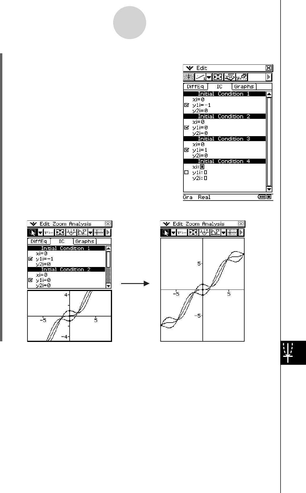
20060301

14-4-2

Graphing an Nth-order Differential Equation

(5) Use the initial condition editor to input (xi, y1i, y2i) = (0, −1, 0), (0, 0, 0), (0, 1, 0).

awybwaw

awawaw

awbwaw

(6) Tap

(Tapping r on this screen will cause the initial

condition editor to fill the entire window.)

[Edit] - [Redraw]

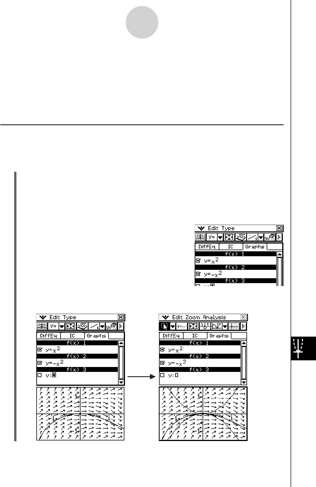
20060301

14-5-1

Drawing f(x) Type Function Graphs and Parametric Function Graphs

14-5 Drawing f(x) Type Function Graphs and

Parametric Function Graphs

You can use the Differential Equation Graph application to graph f

(x) type function graphs

and parametric function graphs, the same way as you do with the Graph & Table application.

These types of graphs can be overlaid on differential equation graphs.

Drawing an f

(x) Type Function Graph

Example: To overlay a differential equation graph with the graphs of y = x2 and y = −x2

u ClassPad Operation

(1) Graph a differential equation.

• See sections 14-2, 14-3, and 14-4.

(2) Tap the [Graphs] tab to display the general graph editor.

(3) Tap [Type] – [ f (x)] or the d toolbar button.

(4) Input

y = x2 and y = −x2.

9X{cw

yX{cw

(5) Tap

• This will overlay the graphs of y = x2 and y = −x2 on the differential equation graph.

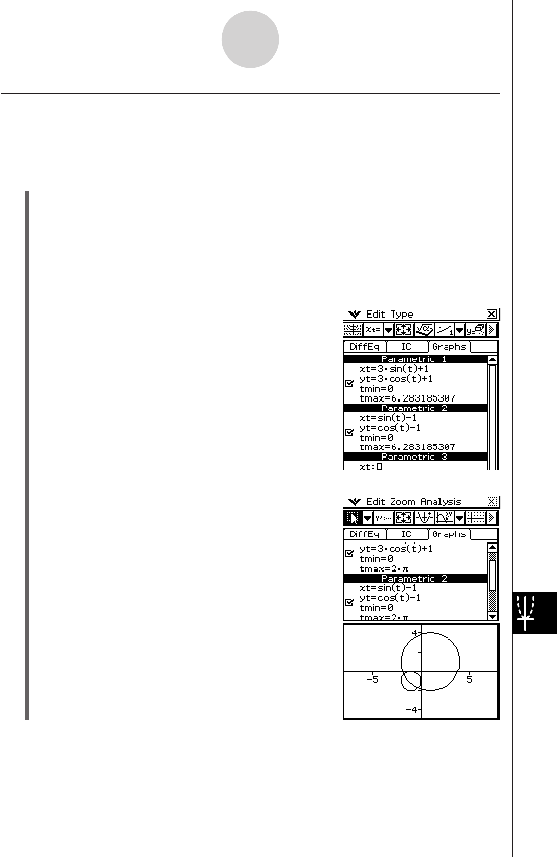
20060301

14-5-2

Drawing f(x) Type Function Graphs and Parametric Function Graphs

Drawing a Parametric Function Graph

Example: To graph {xt = 3sin(t) + 1, yt = 3cos(t) + 1} and {xt = sin(t) − 1, yt = cos(t) − 1}

(Angle Unit Setting: radian, 0 < t < 2π)

u ClassPad Operation

(1) Tap the [Graphs] tab to display the general graph editor.

(2) Confirm that “Rad” is displayed as the angle unit setting on the left side of the status

bar. If it isn’t, tap the angle setting until “Rad” is displayed.

• For details about the information that appears in the status bar, see “Differential

Equation Graph Application Status Bar” on page 14-1-8.

(3) Tap [Type] - [Parametric] or the g toolbar button.

(4) Input the expression for each graph, and (0 < t < 2π) for the range of t.

9dTs([)+bw

dc([)+bw

awc7w

9s([)-bw

c([)-bw

awc7w

(5) Tap

O to draw the graph.

• To adjust the graph window, tap [Zoom] and then

[Quick Initialize].

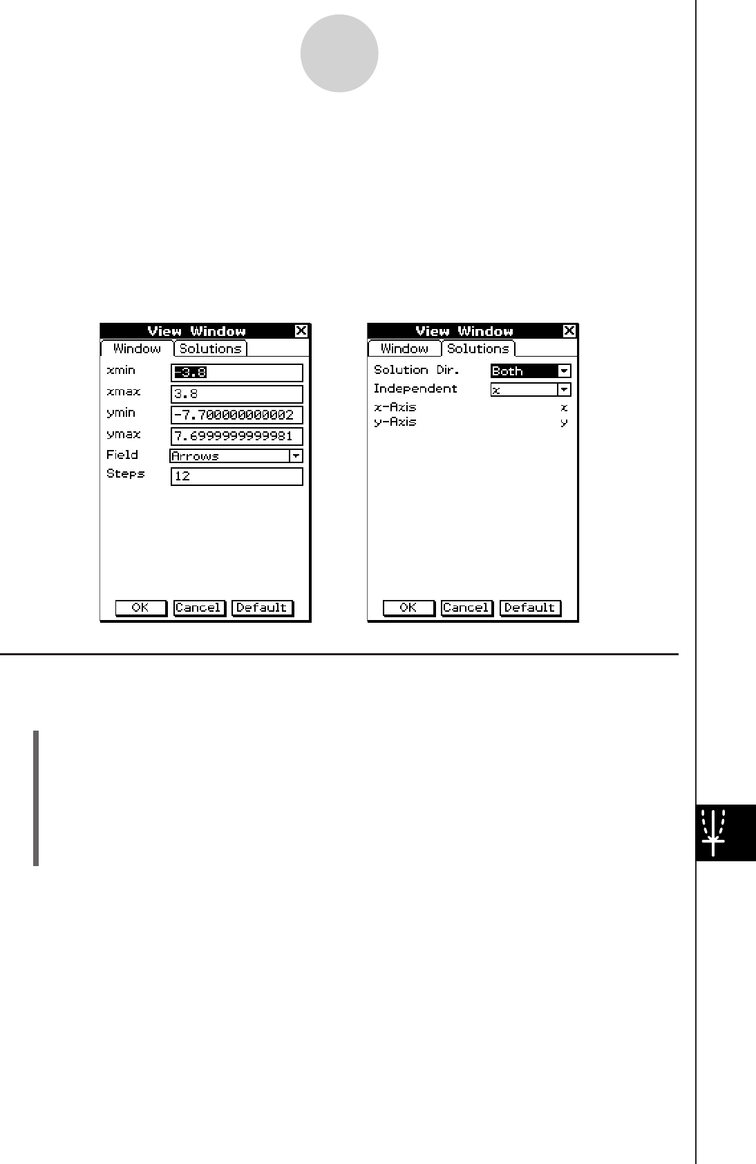
20060301

14-6-1

Configuring Differential Equation Graph View Window Parameters

14-6 Configuring Differential Equation Graph

View Window Parameters

You can set the x- and y-axis window settings, as well as a number of other general graphing

parameters on the View Window dialog box. This dialog box contains two tabs. The first

tab lets you set the window values and steps used for graphing a field. The second tab

contains parameters used for graphing solution curves, such as solution curve direction and

independent variable(s).

Configuring Differential Equation Graph View Window Settings

u ClassPad Operation

(1) Tap

O and then [View Window], or tap 6.

• This displays the View Window dialog box [Window] tab.

(2) Input the required parameters on the [Window] and [Solutions] tabs.

• For details about each setting, see “Differential Equation Graph View Window

Parameters” on page 14-6-2.

(3) After the settings are the way you want, tap [OK].

20060301

14-6-2

Configuring Differential Equation Graph View Window Parameters

Differential Equation Graph View Window Parameters

k Window Tab

Setting Description

xmin minimum value along the (horizontal) x-axis

xmax maximum value along the (horizontal) x-axis

ymin minimum value along the (vertical) y-axis

ymax maximum value along the (vertical) y-axis

Field for showing arrow, line or nothing

Steps number of steps, or field lines, used for graphing a field

k Variable Assignment

The variable assignments available on the Solutions tab vary depending on the graph

type selected in the Graph Editor. Some graph types have preset assignments for the

independent, x-axis, and y-axis variables. If the value is preset for the current graph type the

value will still be displayed on the Solutions tab, but you will not be able to change it. The

possible assignments for each graph type are shown in the tables below.

Graph Type Setting Possible Values

1st-order Slope Field Independent Variable x or t

x-Axis Variable Same as independent variable

y-Axis Variable y

2nd-order Phase Plane Independent Variable t

x-Axis Variable x

y-Axis Variable y

Nth-order Independent Variable x or t

x-Axis Variable independent variable or y1 through y10

y-Axis Variable independent variable or y1 through y10

20060301

14-6-3

Configuring Differential Equation Graph View Window Parameters

k Solutions Tab

Setting Description

Solution Dir.

A solution curve is graphed starting at the initial condition value t0 and

continues until it reaches a target value, which can be either tmin or

tmax. The solution direction determines the target values. Forward will

graph the solution from t0 to tmax. Backward will graph the solution

from t0 to tmin. Both will graph the solution from t0 to tmin, and then t0

to tmax.

Independent Assignment of the independent variable for differential equations. The

possible values are x or t. If you are graphing a phase plane you cannot

choose the independent variable. It will automatically be set to t.

t0 (or x0) If the independent variable is different from the x-axis variable then you

can enter the initial value for the independent variable, unless you are

graphing a slope field.

tmin (or xmin) If the independent variable is different from the x-axis variable then you

can enter the minimum value for the independent variable.

tmax (or xmax) If the independent variable is different from the x-axis variable then you

can enter the maximum value for the independent variable.

x-Axis Assignment for the (horizontal) x-axis. If you are graphing a slope field

or phase plane you will not be able to choose the x-axis variable but it

will still be displayed in this dialog box.

y-Axis Assignment for the (vertical) y-axis. If you are graphing a slope field or

phase plane you will not be able to choose the y-axis variable but it will

still be displayed in this dialog box.

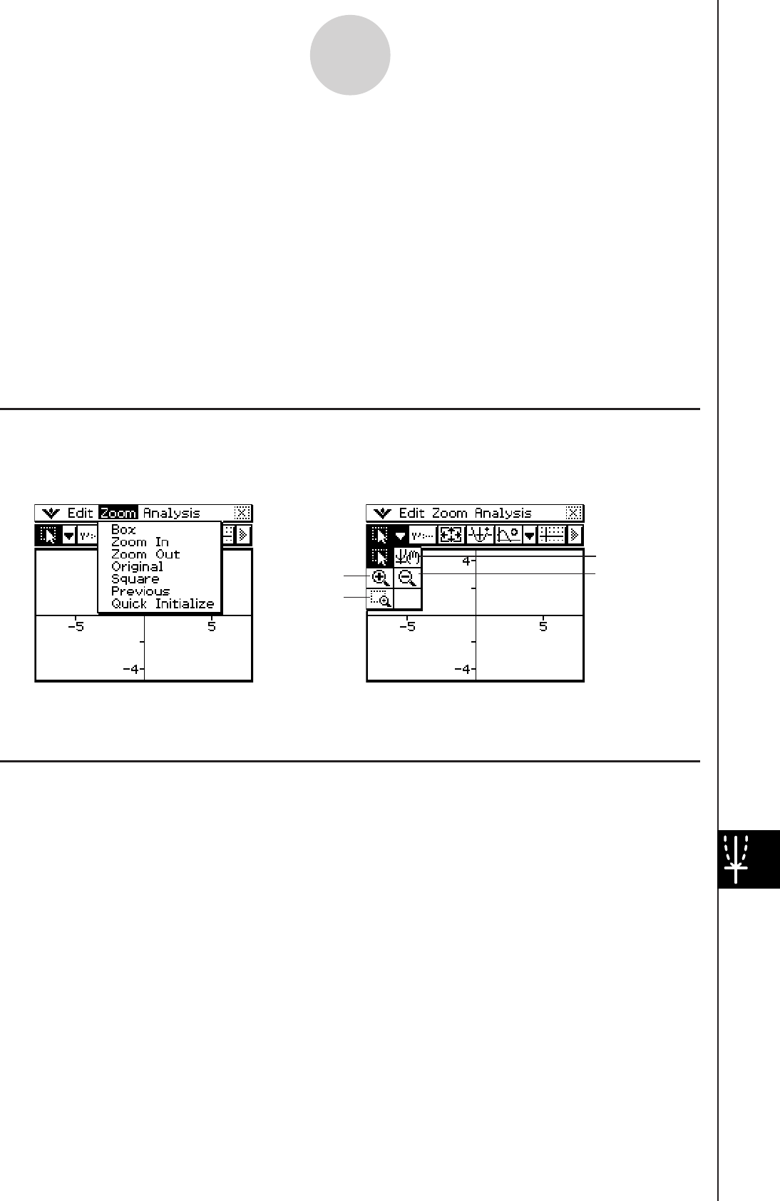
20060301

14-7-1

Differential Equation Graph Window Operations

14-7 Differential Equation Graph Window

Operations

You can perform the following operations on the Differential Equation Graph window.

• Graph zooming and scrolling

• Modification of initial conditions (shifting the initial condition coordinates by dragging it)

• Configuring new initial conditions

• Tracing coordinates on a graph

• Graphing (slope field, phase plane, solution curves, general graphs) of an expression

or value dragged from an eActivity application or Main application to the Differential

Equation Graph window

Graph Zooming and Scrolling

You can use the menu commands and toolbar buttons shown below on the Differential

Equation Graph window to zoom and scroll a graph.

Pan

Zoom Out

Zoom In

Box

For details about these operations, see the applicable menu commands and toolbar buttons

in “Chapter 3 Using the Graph&Table Application”.

Configuring and Modifying Initial Conditions

You can modify existing initial conditions and configure new initial conditions on the

Differential Equation Graph window.

u To modify an initial condition on the Differential Equation Graph window

Example: Input the Nth-order differential equation and initial conditions, and then draw the

solution curves. Next, modify an initial condition by dragging it on the Differential

Equation Graph window.

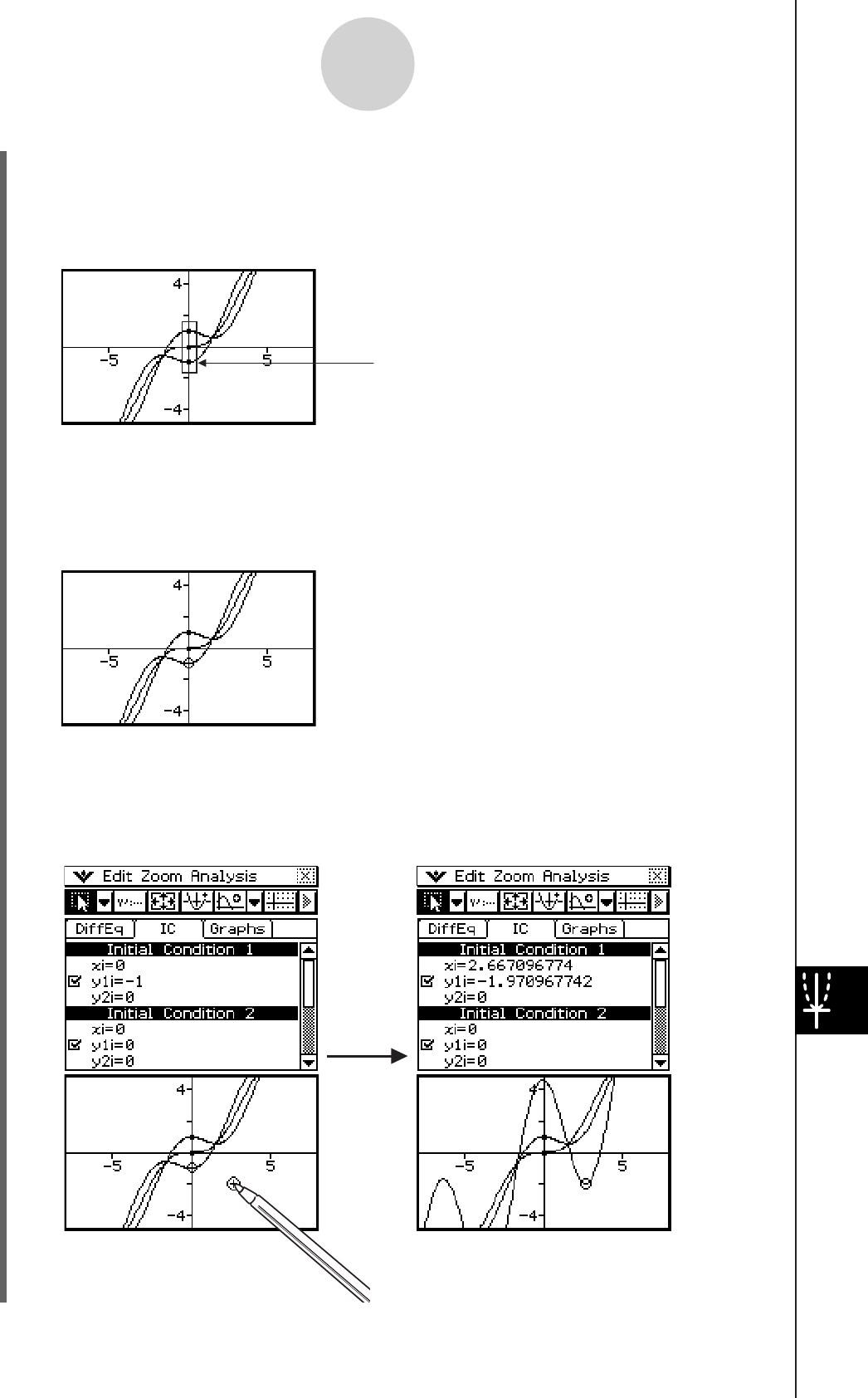
20060301

14-7-2

Differential Equation Graph Window Operations

(1) Perform the operation under “Inputting an Nth-order Differential Equation and Initial

Conditions, and then Graphing the Solutions” on page 14-4-1.

• Performing all of the steps will produce a graph like the one shown below to appear

on the Differential Equation Graph window.

(2) Tap [Analysis] - [Select] or the toolbar G button.

(3) Tap one of the initial condition dots to select it.

• Here we will tap the bottom dot, which is the Initial Condition 1 setting (xi, y1i, y2i) =

(0, −1, 0).

These dots are the currently configured

initial conditions.

The dot you tap becomes a white circle (),

which indicates that it is selected.

(4) Use the stylus to drag the dot to another location.

• The applicable initial location will change to the coordinates of the location where you

release the stylus after dragging the dot. After modifying an initial condition, the

solution will be redrawn accordingly.

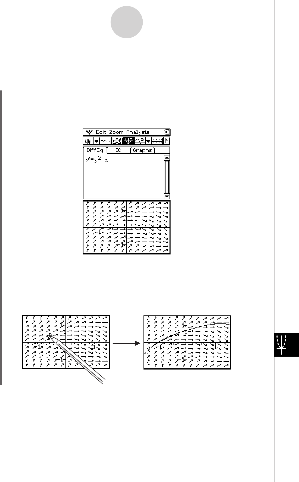
20060301

14-7-3

Differential Equation Graph Window Operations

u To configure new initial conditions on the Differential Equation Graph

window

Example: After drawing the slope field of a first order differential equation, to configure initial

condition settings on the Differential Equation Graph window

(1) Perform the operation under “Inputting a First Order Differential Equation and Drawing

a Slope Field” on page 14-2-1.

• Performing all of the steps will produce a slope field like the one shown below to

appear on the Differential Equation Graph window.

(2) Tap [Analysis] - [Modify] or the toolbar J button.

• This will cause the J button to become highlighted.

(3) On the Differential Equation Graph window, tap the coordinates that you want to specify

as the new initial condition.

• This will set the coordinates as the new initial condition and draw a solution curve.

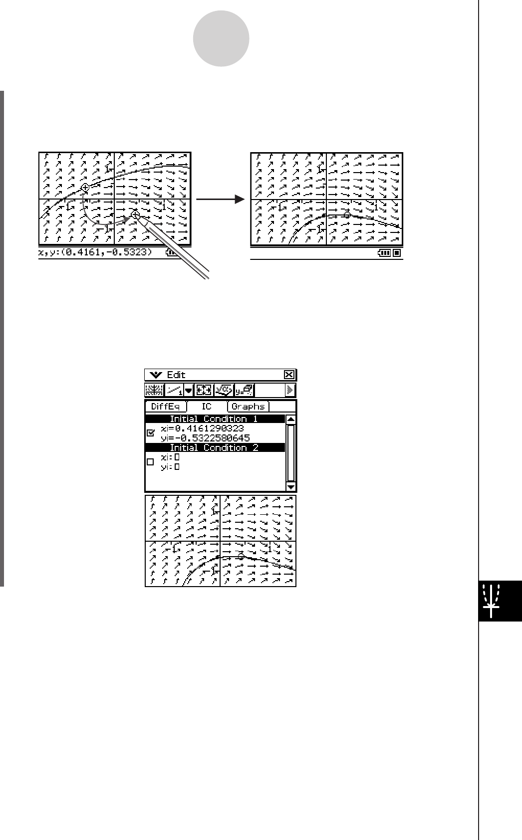
20060301

14-7-4

Differential Equation Graph Window Operations

The procedure for modifying the initial condition is the same as steps 3 and 4 under

“To modify an initial condition on the Differential Equation Graph window” on page

14-7-1.

• The newly configured initial condition is added to the initial condition editor. To view it,

tap the [IC] tab.

• After the solution curve is drawn, J button highlighting turns off, and the

G button becomes highlighted. At this time, you can change the initial

condition by tapping the dot that represents it and dragging the dot to a different

location.

20060301

14-7-5

Differential Equation Graph Window Operations

u To start a field trace

(1) Draw a slope field or a phase plane.

• See sections 14-2 and 14-3 for information about drawing a slope field or phase

plane.

(2) Tap

• This will cause the L button to become highlighted, and will display a crosshair

pointer ( ) near field line in the center of the display (in the center of the field

line). The coordinates of the field cursor’s location will be shown in the status bar.

Using Trace to Read Graph Coordinates

The following three types of trace operations are available for reading graph coordinates.

Point Trace

Displays a trace cursor that can be positioned on any x, y coordinate. This trace cursor can

be moved freely on the screen with either the stylus or cursor keys.

Field Trace

Displays a trace cursor that can be positioned on any grid point that has a field line. This

trace cursor will snap to a field lines when moved with either the stylus or cursor keys.

Graph/Curve Trace

Displays a trace cursor that can be positioned on any graph or solution curve. This trace

cursor will snap to a graph or curve when moved with either the stylus or cursor keys.

u To start a point trace

(1) Make the Differential Equation Graph window active.

(2) Tap

• This will cause the K button to become highlighted, and will display a crosshair

pointer ( ) in the center of the display. The coordinates of the crosshair pointer’s

location will be shown in the status bar.

(3) To move the crosshair pointer around the display, tap the destination on the Differential

Equation Graph window or use the cursor keys.

• The coordinates in the status bar will change whenever the crosshair pointer is

moved.

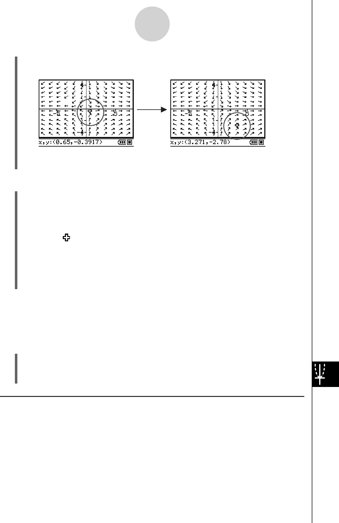
20060301

14-7-6

Differential Equation Graph Window Operations

u To perform a graph/curve trace operation

(1) Draw a solution curve or general graph.

• See sections 14-2 through 14-5 for information about drawing.

(2) Tap

= or [Analysis] - [Trace].

• This will cause the = button to become highlighted, and will display a crosshair

pointer ( ) near the center of the display on the graph or solution curve.

The coordinates of the field cursor’s location will be shown in the status bar.

(3) To move the crosshair pointer on the graph or solution curve, tap the destination on the

Differential Equation Graph window or use the cursor keys.

• The coordinates in the status bar will change whenever the crosshair pointer is

moved.

Tip

• When there are multiple graph or solution curves on the display, you can use the f and c

cursor keys to move the crosshair pointer jump between graphs.

u To exit a trace operation

To exit an ongoing trace operation at any time, tap G, or perform any one of the

following menu or button operations.

[Analysis] - [Pan] (T), [Analysis] - [Modify] (J), [Zoom] - [Box] (Q), [Edit] - [Clear All]

Graphing an Expression or Value by Dropping it into the Differential

Equation Graph Window

You can use the procedures in this section to graph an expression or value by dragging it

from the eActivity application window or the Main application window and dropping it into the

Differential Equation Graph window.

(3) To move the cross cursor to another field line, tap the destination on the Differential

Equation Graph window or use the cursor keys.

• The coordinates in the status bar will change whenever the crosshair pointer is

moved.

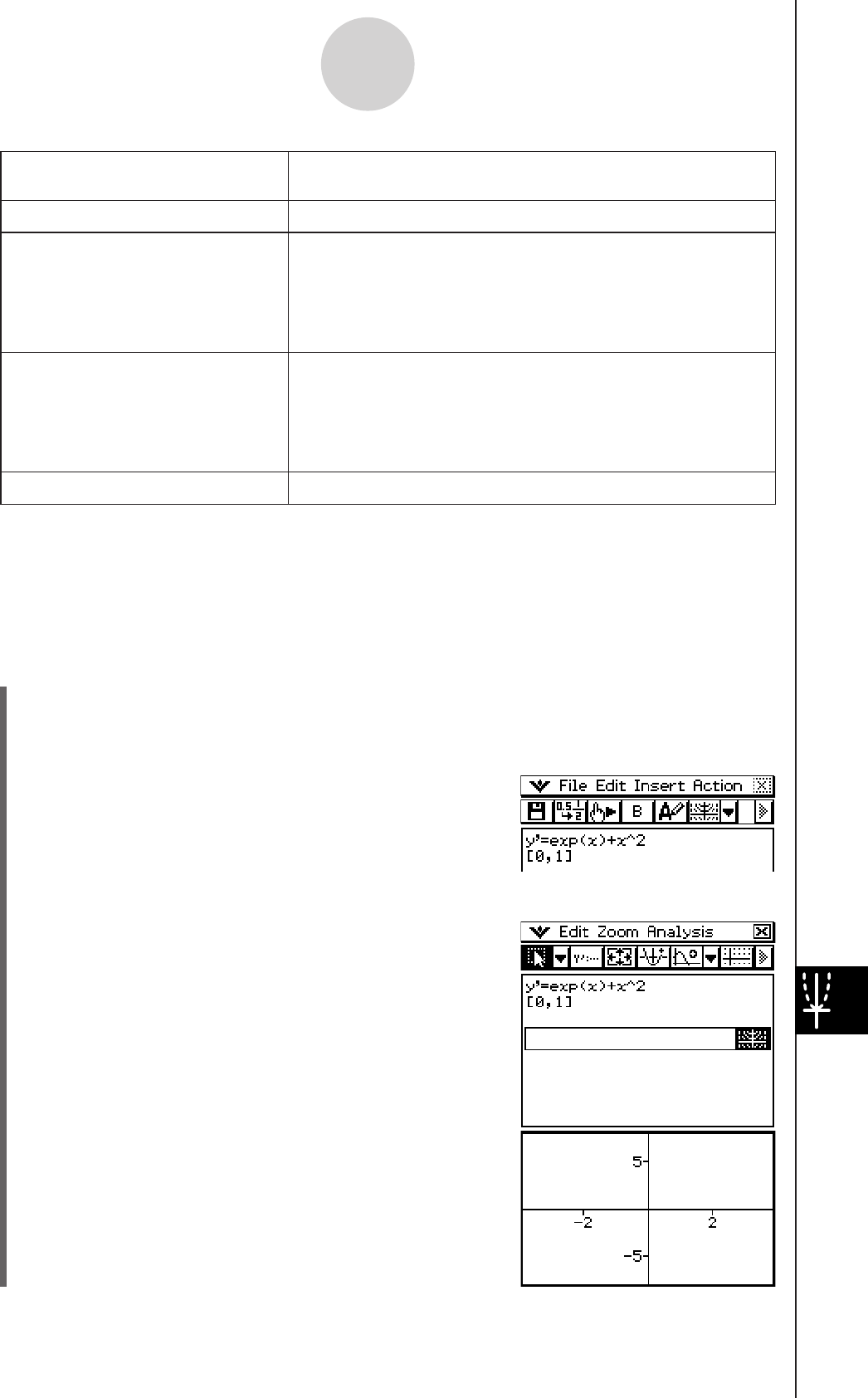
20060301

14-7-7

Differential Equation Graph Window Operations

(3) From the eActivity application menu, tap [Insert], [Strip], and then [DiffEqGraph].

• This inserts a Differential Equation Graph data strip,

and displays the Differential Equation Graph window

in the lower half of the screen.

u To graph the slope field and solution curves by dropping a 1st-order

differential equation and matrix into the Differential Equation Graph

window

Example: To drag the 1st-order differential equation y’ = exp(x) + x2 and then the initial

condition matrix [0,1] from the eActivity application window to the Differential

Equation Graph window, and graph the applicable slope field and solution curve

(1) On the application menu, tap A.

• This starts up the eActivity application.

(2) On the eActivity application window, input the following expression and matrix.

y’ = exp(x) + x2

[0,1]

To draw this type of graph: Drop this type of expression or value into the

Differential Equation Graph window:

Slope field 1st-order differential equation in the form of y' = f

(x, y)

Solution curve(s) of a 1st-order

differential equation

Matrix of initial conditions in the following form:

[[x1, y(x1)][x2, y(x2)], .... [xn, y(xn)]]

• Slope field must already have been graphed. If not,

only points will be plotted and initial conditions are

registered in the initial condition editor ([IC] tab).

Solution curve(s) of an Nth-order

differential equation

1) Nth-order differential equation such as y’’+ y’+ y =

sin(x), followed by

2) Matrix of initial conditions in the following form:

[[x1, y1(x1)],[x2, y1(x2)], .... [xn, y1(xn)]] or [[x1, y1(x1),

y2(x1)],[x2, y1(x2), y2(x2)], .... [xn, y1(xn), y2(xn)]]

(x) type function graph Function in the form y = f

(x)

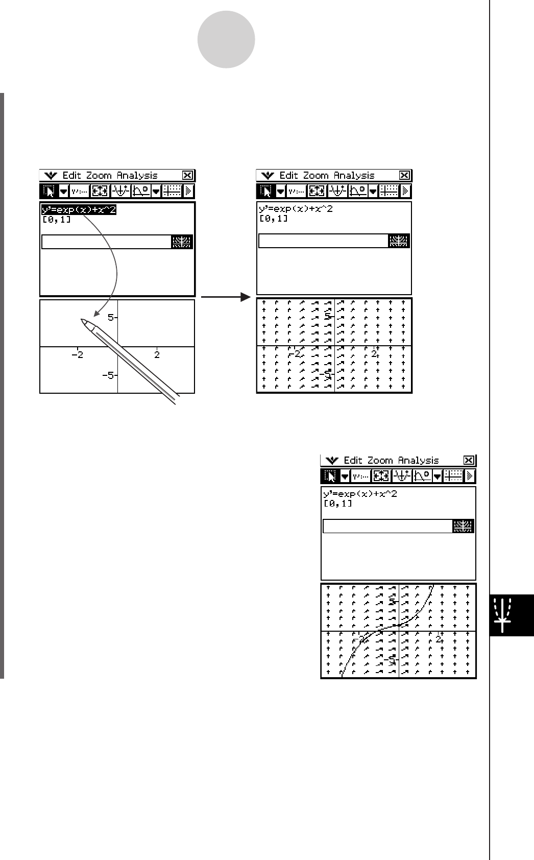
20060301

14-7-8

Differential Equation Graph Window Operations

(6) Drag the stylus across “[0,1]” on the eActivity application window to select it.

(7) Drag the selected matrix to the Differential Equation Graph window.

• This graphs the solution curves of y’ = exp(x) + x2 in

accordance with the initial condition defined by the

matrix and registers the initial condition in the initial

condition editor ([IC] tab).

(4) Drag the stylus across “y’ = exp(x) + x2” on the eActivity application window to select it.

(5) Drag the selected expression to the Differential Equation Graph window.

• This draws the slope field of y’ = exp(x) + x2 and registers the equation in the

differential equation editor ([DiffEq] tab).

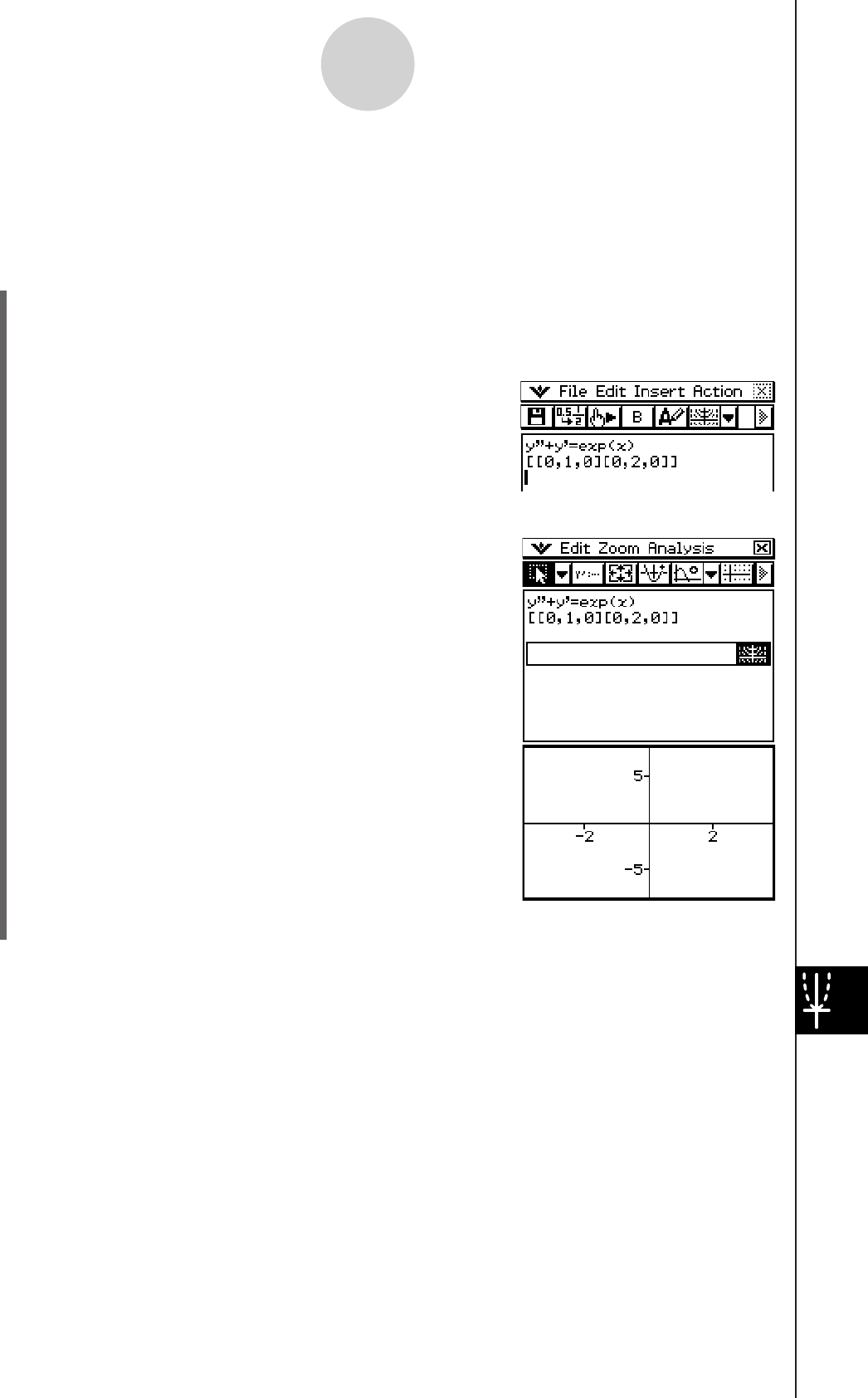
20060301

14-7-9

Differential Equation Graph Window Operations

u To graph the solution curves by dropping an Nth-order differential

equation and matrix into the Differential Equation Graph window

Example: To drag the Nth-order differential equation y” + y’ = exp(x) and then the initial

condition matrix [[0, 1, 0][0, 2, 0]] from the eActivity application window to the

Differential Equation Graph window, and graph the applicable solution curves

(1) On the application menu, tap A.

• This starts up the eActivity application.

(2) On the eActivity application window, input the following expression and matrix.

y” + y’ = exp(x)

[[0,1,0][0,2,0]]

(3) From the eActivity application menu, tap [Insert], [Strip], and then [DiffEqGraph].

• This inserts a Differential Equation Graph data strip,

and displays the Differential Equation Graph window

in the lower half of the screen.

(4) Drag the stylus across “y” + y’ = exp(x)” on the eActivity application window to select it.

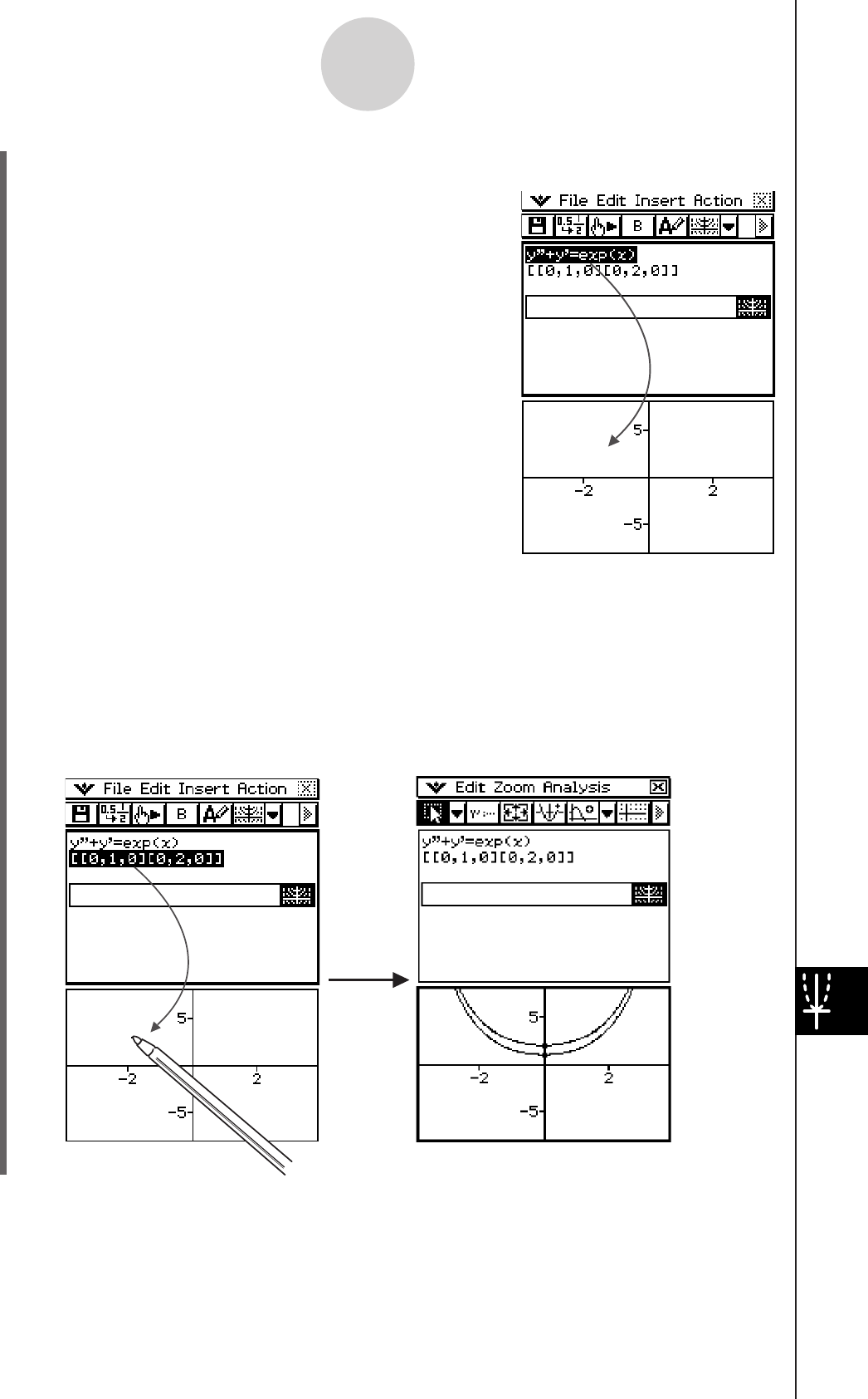
20060301

(5) Drag the selected expression to the Differential Equation Graph window.

• This registers y” + y’ = exp(x) on the differential equation editor ([DiffEq] tab). The

Differential Equation Graph window contents do not change at this time.

(6) Drag the stylus across “[[0,1,0][0,2,0]]” on the eActivity application window to select it.

(7) Drag the selected matrix to the Differential Equation Graph window.

• This graphs the solution curves of y” + y’ = exp(x) in accordance with the initial

condition defined by the matrix, and registers the initial condition in the initial

condition editor ([IC] tab).

Tip

• An Nth-order differential equation of the form f (y’, y’’…,x) dropped into the Differential

Equation Graph Window will be treated as f (y’, y’’…,x) = 0.

14-7-10

Differential Equation Graph Window Operations

20101001

Chapter

Using the Financial

Application

This chapter explains how to use the Financial application. You

can use the Financial application to perform a variety of financial

calculations.

15-1 Financial Application Overview

15-2 Simple Interest

15-3 Compound Interest

15-4 Cash Flow

15-5 Amortization

15-6 Interest Conversion

15-7 Cost/Sell/Margin

15-8 Day Count

15-9 Depreciation

15-10 Bond Calculation

15-11 Break-even Point

15-12 Margin of Safety

15-13 Operating Leverage

15-14 Financial Leverage

15-15 Combined Leverage

15-16 Quantity Conversion

15-17 Performing Financial Calculations Using Commands

Important!

• Financial calculation rules and practices can differ according to country, geographic area, or

financial institution. It is up to you to determine whether the calculation results produced by this

calculator are compatible with the financial calculation rules that apply to you.

20060301

15-1-1

Financial Application Overview

15-1 Financial Application Overview

This section explains how to use the Financial application initial screen, and describes the

basic configuration of the Financial application windows. It also provides information on using

the Financial application’s Help and Format features.

Starting Up the Financial Application

Use the following procedure to start up the Financial application.

u ClassPad Operation

On the application menu, tap F.

This starts the Financial application and displays the Financial application screen.

k Financial Application Initial Screen

The screen shown below appears whenever you start up the Financial application when

there are no pages from a previous session (page 15-1-5), or if you execute the [Edit]

menu’s “Clear All” command while the Financial application is running.

20060301

Financial Application Menus and Buttons

This section describes the basic configuration of Financial application windows, and provides

basic information about its menus and commands.

• For information about the O menu, see “Using the O Menu” on page 1-5-4.

k Edit Menu

To do this: Select this Edit menu item:

Cut the currently selected value and place it onto the

clipboard Cut

Copy the currently selected value and place it onto the

clipboard Copy

Paste the current clipboard contents at the cursor location Paste

Delete the currently selected value Delete

Delete the currently displayed Financial application page Delete Page

Clear all the values from the displayed Financial application

page Clear Page

Delete all the Financial application pages and display the

Financial application initial screen Clear All

k Calculations Menu

To perform this type of calculation: Select this Calculations

menu item:

Interest without compounding based on the number of days

money is invested Simple Interest

Interest based on compounding parameters specified by you Compound Interest

Value of money paid out or received in varying amounts over

time Cash Flow

Interest and principal portions of a payment or payments Amortization

Effective or nominal interest rate for interest compounded

multiple times during a year Interest Conversion

Cost, selling price, or margin of profit on an item given the

other two values Cost/Sell/Margin

Number of days between two dates, or the date that is a

specified number of days from another date Day Count

15-1-2

Financial Application Overview

20060301

To perform this type of calculation: Select this Calculations

menu item:

Amount that a business expense can be offset by income

(depreciated) over a given year Depreciation

Purchase price or annual yield of a bond Bond Calculation

Amount you must sell to break even or to obtain a specified

profit, as well as amount of profit or loss on particular sales Break-Even Point

How much sales can be reduced before incurring losses Margin of Safety

Degree of change in net earnings arising from a change in

sales amount Operating Leverage

Degree of change in net earning arising from a change in

interest paid Financial Leverage

Combined effects of operating and financial leverages Combined Leverage

Number of items sold, selling price, or sales amount given

other two values; number of items manufactured, unit

variable cost, or total variable cost given other two values

Quantity Conversion

k Toolbar Buttons

To do this: Tap this button:

Scroll back through Financial application pages (page

15-1-5) <

Scroll forward through Financial application pages (page

15-1-5) >

Cut the currently selected value and place it onto the

clipboard r

Copy the currently selected value and place it onto the

clipboard t

Paste the current clipboard contents at the cursor location y

Open the Stat Editor window for Cash Flow calculations (

Open the Spreadsheet window for Cash Flow calculations Q

• The ( and Q buttons are at the same location on the toolbar. If you cannot see the

button you want, tap the down arrow next to the button and select the option you want from

the list that appears.

15-1-3

Financial Application Overview

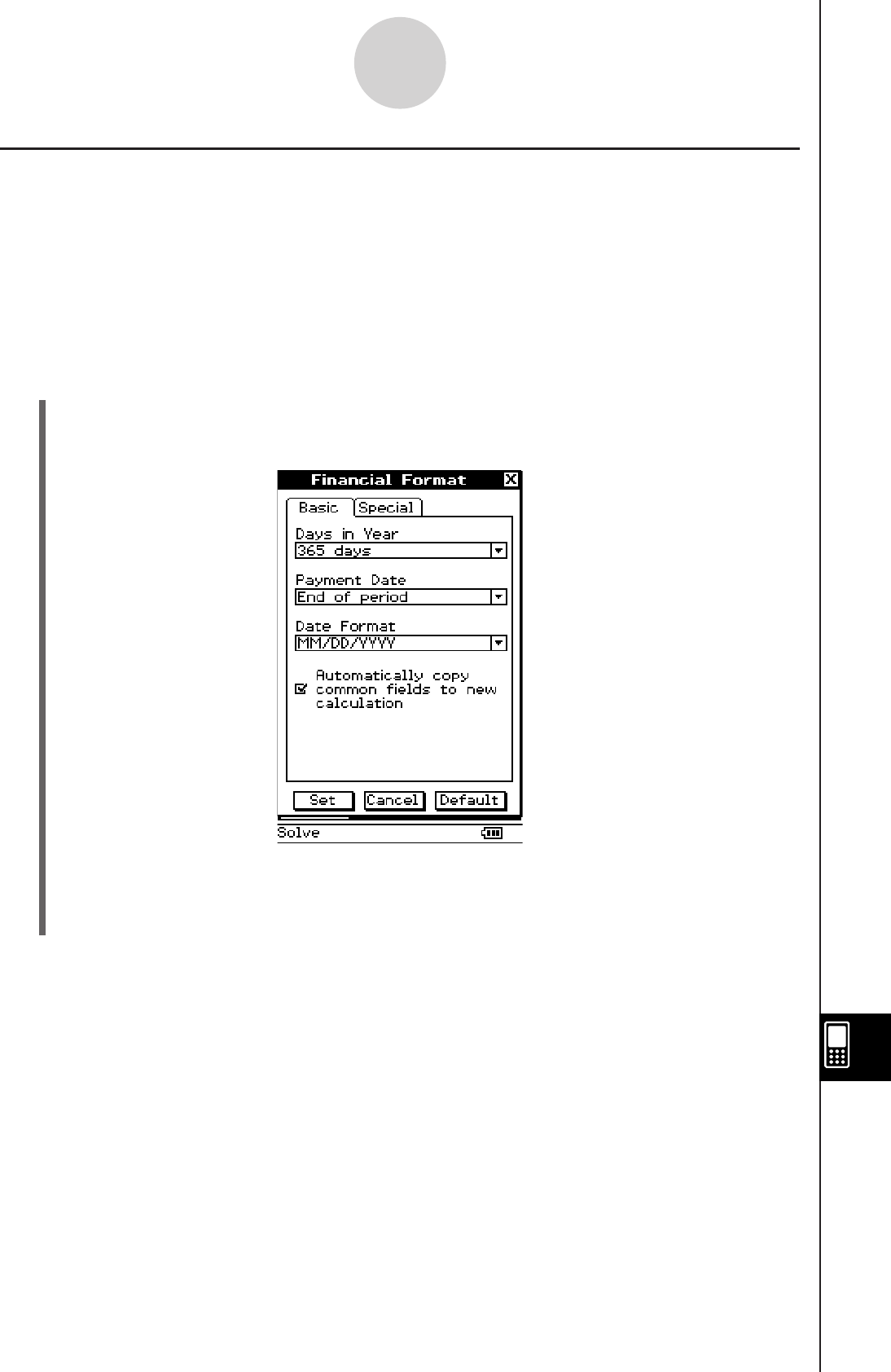
20110401

Configuring Default Financial Application Settings

Most financial calculations require that you define certain general parameters that affect

the results they produce. For example, you need to specify whether you use a 360-day or

365-day year, whether payments are made at the beginning of a period or end of a period,

whether interest is compounded annually or semi-annually, etc.

With the Financial application, you use the Financial Format dialog box to configure default

settings for financial calculations. Use the following procedure to display the Financial Format

dialog box.

u ClassPad Operation

On the Financial application O menu, tap [Financial Format].

This will display the Financial Format dialog box.

Note that this window has two tabs: Basic and Special. Tap a tab to display its contents

and then configure the settings you want. To configure a setting, tap the down arrow

button next to it and then select the setting you want from the list that appears.

Tip

• The settings you should configure depend on the legal requirements in your area, financial

conventions, your particular needs, etc.

• After configuring your settings, tap [Set] to apply them. Tap [Cancel] to close the window without

changing any settings. Tap [Default] to restore all the settings of the Financial Format dialog box

to their initial defaults.

• For details about each of the setting items, see “Financial Format Dialog Box” (page 1-9-12).

15-1-4

Financial Application Overview

20101001

Financial Application Pages

Selecting a calculation type from the Financial application [Calculations] menu will create and

display a new “page”.

Note the following rules that apply to Financial application pages.

• You can scroll between pages using the toolbar < and > buttons.

• Selecting the same calculation type as the calculation on the currently displayed (original)

page will create a new page that is a duplicate of the original page. You can then change

the values in the new page without affecting the values of the original page.

• Selecting a different calculation type as the calculation on the currently displayed (original)

page will create a new page that contains the applicable fields for the selected calculation.

Any fields on the new page that are also on the original page will contain the same value as

the corresponding field on the original page.

• If the currently displayed page is part way through a series of pages that are in memory,

selecting a calculation from the [Calculations] menu will create a new page in the series

and delete everything after it. If you select a new calculation while page 3 of 5 is displayed,

for example, the newly created page will become 4 of 4.

• To delete a particular page, display it and then select “Delete Page” on the [Edit] menu.

• To delete all pages, select “Clear All” on the [Edit] menu while any page is displayed.

• Financial application pages remain in memory until you delete them as described above.

15-1-5

Financial Application Overview

20101001

• While the cursor is located in a calculation box, you can tap the button next to the box or

tap “Solve” in the status bar to perform the calculation.

k Help Tab

Tapping the [Help] tab at the bottom of a financial calculation screen will display help about

the box where the cursor is currently located. You can leave the [Help] tab displayed, and its

text will change each time you move the cursor from one box to another.

The [Help] tab also explains why a calculation cannot be performed if you tap a calculation

button premature.

To close the [Help] tab, tap it again.

k Format Tab

Tapping the [Format] tab at the bottom of a financial calculation screen will display all of

the default financial calculation settings (page 15-1-4) that apply to the currently displayed

calculation. You can use the [Format] tab to change the settings, if you want.

To close the [Format] tab, tap it again.

15-1-6

Financial Application Overview

Financial Calculation Screen Basics

Each calculation has a unique screen format.

This section provides general information that applies to the screens for all Financial

application calculations.

Help tab

Tap to display help about

the box where the cursor

is located.

Format tab

Tap to display a tab for

modifying financial calculation

default settings (page 15-1-4)

that apply to the current

calculation.

Input box

Input/calculation box

Status Bar

Tap the status bar to change the format or solve a calculation.

Input values in the box.

Input values when required. For

calculation, tap the button to

the left of the box.

20060301

15-1-7

Financial Application Overview

k Status Bar

The status bar shows the settings that apply to the calculations on the currently active

page. You can change the settings by tapping them on the status bar. If the cursor is in an

input/calculation box, “Solve” will appear on the left side of the status bar. You can tap this to

complete this calculation instead of tapping the box to the left of the input/calculation box.

Variables

The following sections explain how to perform each of the Financial application calculations

found on the [Calculations] menu.

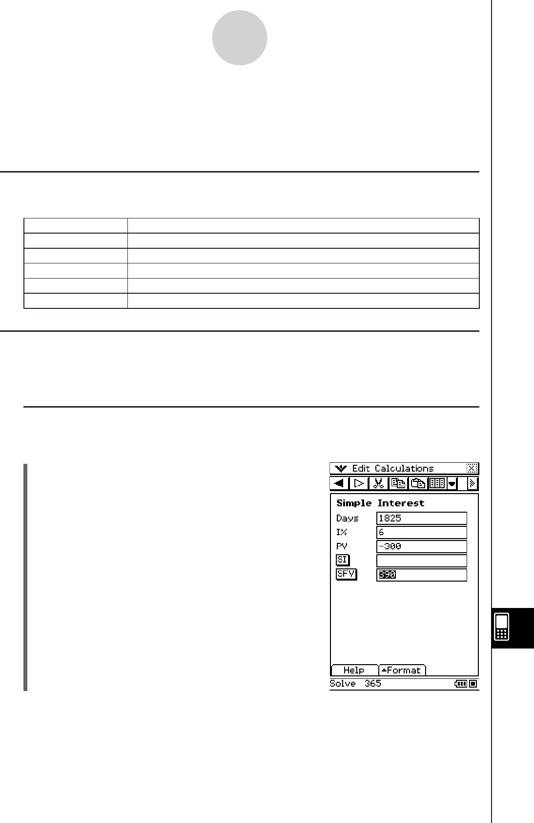
20060301

15-2 Simple Interest

Simple Interest lets you calculate interest (without compounding) based on the number of

days money is invested.

Simple Interest Fields

The following fields appear on the Simple Interest calculation page.

Field Description

Days Number of days in investment period

I% Annual interest rate (as a percent)

PV Present value (initial investment)

SI Calculates and displays simple interest

SFV Calculates and displays simple future value (principal + interest)

Financial Application Default Setup for Examples

You can use the [Format] tab to change the following setting.

Days in Year: 365 days

k Example 1

What is the final value ([SFV]) after five years (1,825 days) of a $300 investment (PV)

earning 6.0% simple interest (I%)?

(1) Tap [Calculations] and then [Simple Interest].

(2) Input 1825 (or 5 × 365) for Days.

(3) Input 6 for I%.

(4) Input −300 for PV.

(5) Tap the [SFV] button.

• This indicates a final value of $390.

15-2-1

Simple Interest

Tip

• Tapping the [SI] button shows the interest earned.

• To find the interest earned on $3,000 instead of $300, change −300 to −3000 and tap the [SI]

button again.

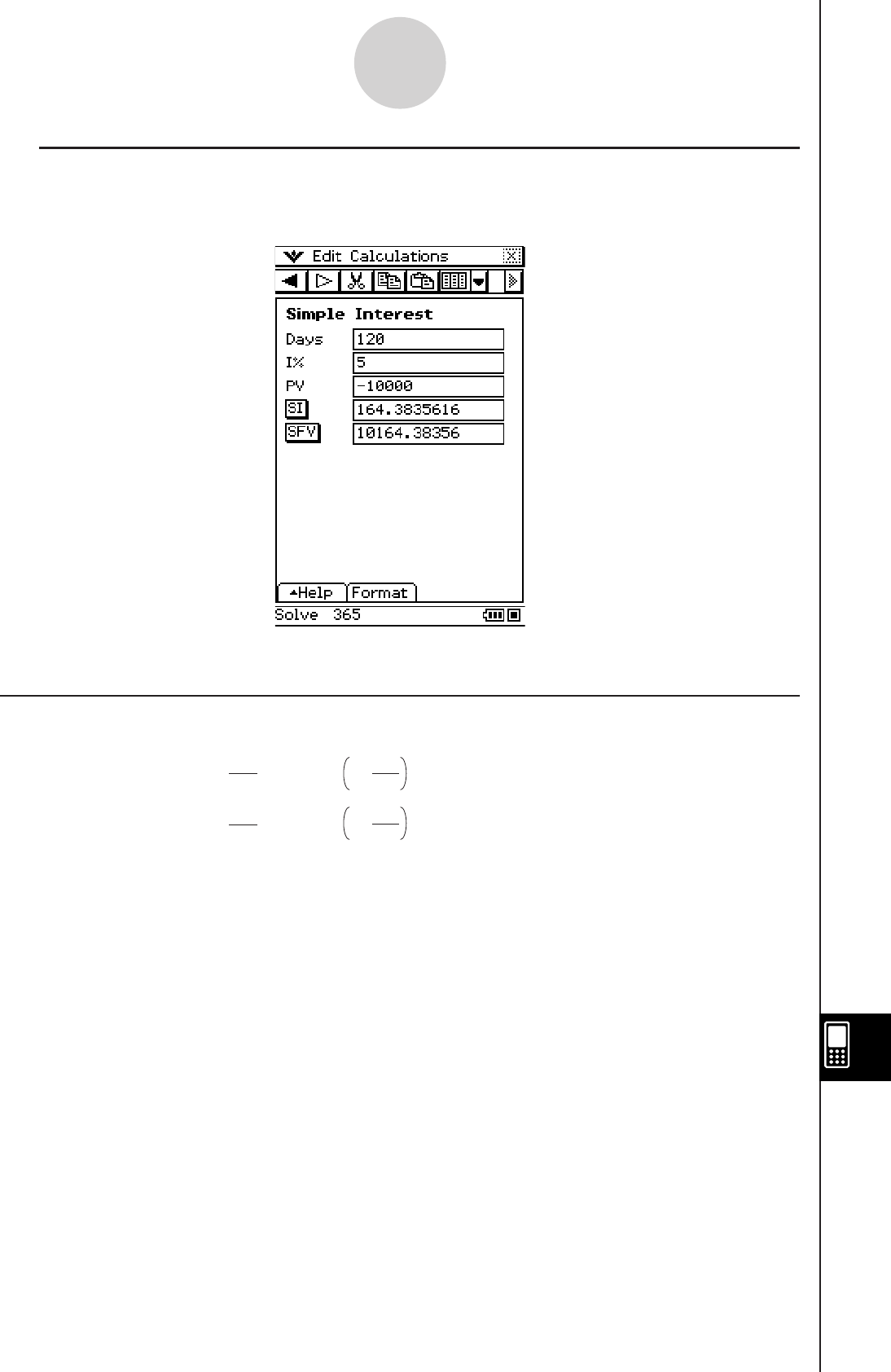
20060301

k Example 2

What is the simple interest ([SI]) on a principal amount of $10,000 (PV) invested or borrowed

for 120 days (Days) at 5% per annum (I%)?

• This indicates that the simple interest is $164.3835616.

Calculation Formulas

365-day Mode

SI' =

Dys

365 × PV × iI%

100

i =

360-day Mode

SI' = Dys

360 × PV × iI%

100

i =

SI = –SI'

SFV = –(PV + SI' )

15-2-2

Simple Interest

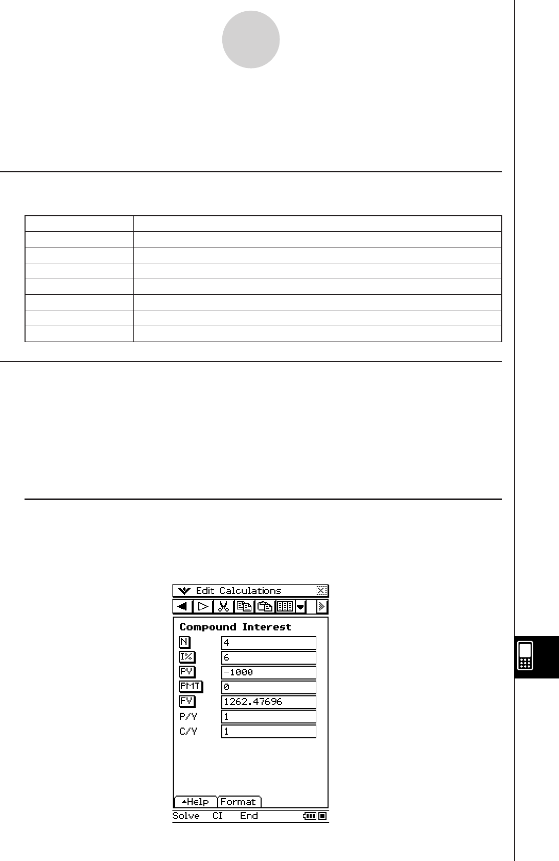
20060301

15-3 Compound Interest

Compound Interest lets you calculate interest based on compounding parameters you

specify.

Compound Interest Fields

The following fields appear on the Compound Interest calculation page.

Field Description

N Number of installment periods

I% Annual interest rate (as a percent)

PV Present value (initial investment)

PMT Amount paid each period

FV Future value

P/Y Number of installment periods per year

C/Y Number of times interest is compounded per year

Financial Application Default Setup for Examples

You can use the [Format] tab to change the following settings.

Odd Period: Compound (CI)

Payment Date: End of period

Tip

• You can look at the status bar to see if it displays “CI” and “End”. If those are not displayed, you

can tap the status bar to switch the settings.

k Example 1

What is the future value (FV) on a principal amount of $1,000 (PV = −1000) invested or

borrowed for four years at 6% per annum, compounded yearly (C/Y = 1)? The entire payment

is due at the end of three years so the amount paid each year (PMT) is 0 and the number of

installment periods per year (P/Y) can be 1.

15-3-1

Compound Interest

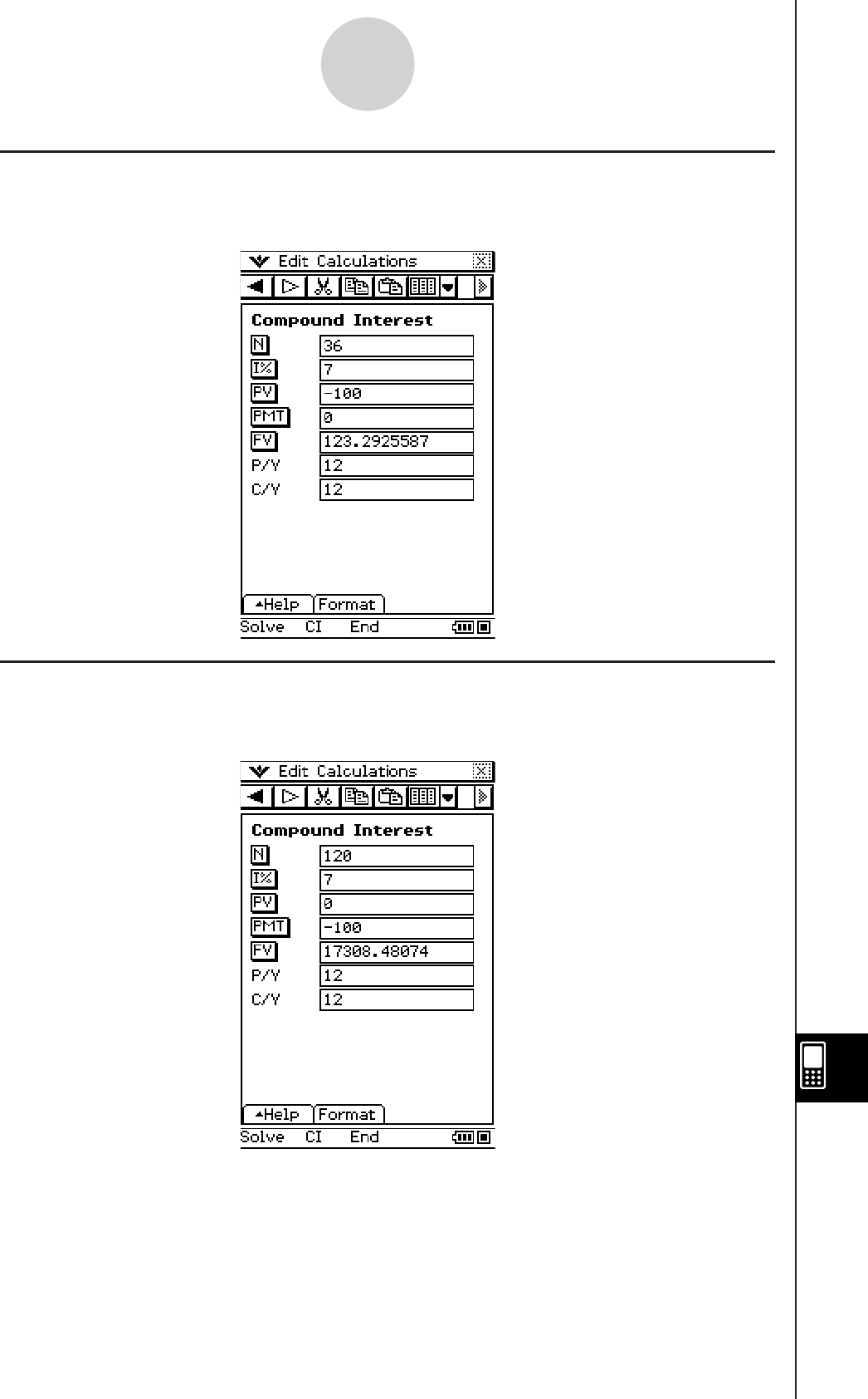
20060301

15-3-2

Compound Interest

k Example 3

What will be the value of an ordinary annuity at the end of 10 years if $100 is deposited each

month into an account that earns 7% compounded monthly?

k Example 2

If you deposit $100 into an account that earns 7% compounded monthly, how much will be in

the account after three years?

20060301

15-3-3

Compound Interest

Calculation Formulas

u PV, PMT, FV, n

% G 0

% = 0

PV = – (PMT × n + FV )

FV = – (PMT × n + PV )

PV = –

× PMT – × FV

PMT = – × PV – × F

FV = – × PV –

× PMT

n =

log (1+ iS ) × PMT – FV × i

(1+ iS ) × PMT + PV × i

{}

log (1+ i)

PMT = – n

PV + FV

n = PMT

PV + FV

–

u I

(effective interest rate)

(effective interest rate) is calculated using Newton’s Method.

× PV +

× PMT +

× FV = 0

% from i (effective interest rate)

Tip

• Interest (I%) calculations are performed using Newton’s Method, which produces approximate

values whose precision can be affected by various calculation conditions. Interest calculation

results produced by this application should be used keeping the above in mind, or results should

be confirmed separately.

= (1+ i × S ) × i

1 –

i = 100

{

(1+ ) –1

C/Y

P/Y

100 × [C/Y ]

............................... (P/Y = C/Y = 1)

(Other than those above)

0 ............................ Payment : End (Format tab)

1 ............................ Payment : Begin (Format tab)

{

S =

.....

1 ........................... Off (Format tab)

(1+ i )

Frac

(

)

........... CI (Format tab)

1+ i ×

Frac (n) ....... SI (Format tab)

{

(1+ i )

−

n ................. Off (Format tab)

(1+ i)

−Intg

(

)

............ CI or SI (Format tab)

{

ß =

{ }

× C/Y × 100...

I% = (1+ i )–1

P/Y

C/Y

(Other than those above)

i × 100 ................................. (P/Y = C/Y = 1)

{

20060301

15-4-1

Cash Flow

15-4 Cash Flow

Cash Flow lets you calculate the value of money paid out or received in varying amounts

over time.

Cash Flow Fields

The following fields appear on the Cash Flow calculation page.

Field Description

Cash List of income or expenses (up to 80 entries)

I% Annual interest rate (as a percent)

NPV Net present value

IRR Interest rate of return

PBP Payback period

NFV Net future value

Inputting Cash Flow Values

Cash flow calculations require that you input a list of cash flow values for multiple periods.

The following shows the cash flow values used in the examples of this section, and the

procedure you should use to input them.

k Cash Flow Values

Period Cash Flow

1 100

2 200

3 300

4 400

5 500

u To input cash flow values from the Cash Flow calculation page

(1) On the Financial application toolbar, tap (.

• This will open the Stat Editor window in the lower half of the display.

• The ( icon shares the same location on the toolbar as the Q icon. If you see the

Q icon, tap the down arrow button to the right of it and then tap ( on the menu

that appears.

(2) In cells 1 through 6 under “list1”, input the cash flow values.

(3) Tap the “Cash” field (which currently shows “<empty>”).

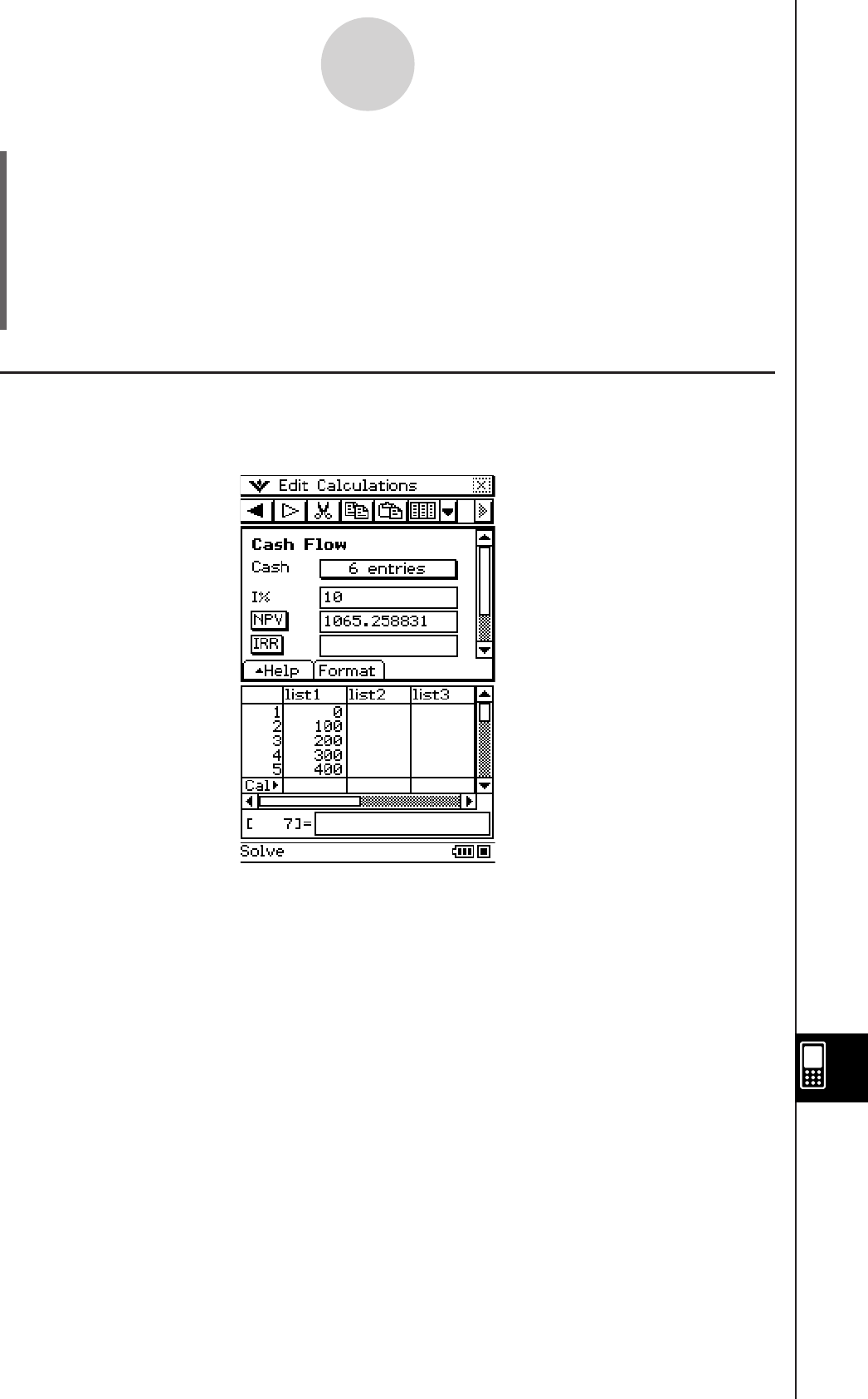
20060301

(4) On the dialog box that appears, make sure “list1” is selected for “List variables”, and

then tap [OK].

• You can now use the list of values in cash flow calculation.

• To close the Stat Editor window, tap anywhere in the Stat Editor window and then tap

the close box (S) in the upper right corner of the screen.

• For details about using the Stat Editor and about the list variables, see “7-2 Using

Stat Editor”.

k Example 1

How much should you be willing to pay (NPV) for an investment with a specific cash flow

(Cash), if your required rate of return (I%) is 10% per year?

15-4-2

Cash Flow

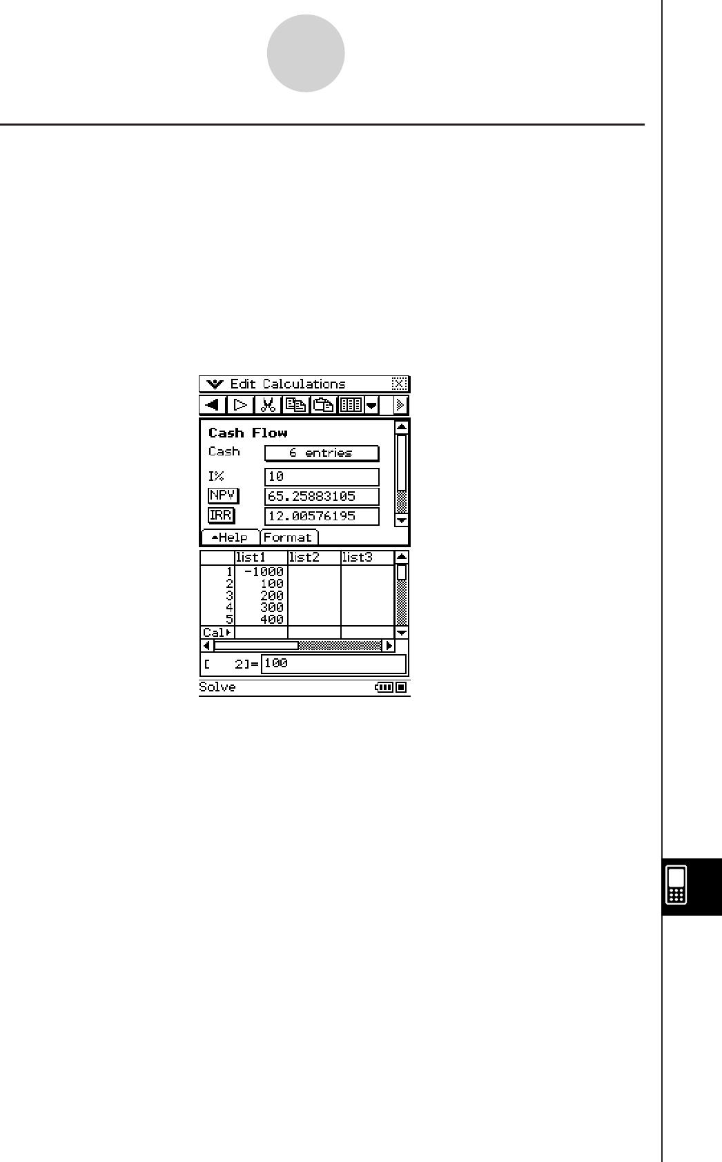
20060301

k Example 2

Suppose you were offered the investment in Example 1 at a cost of $1,000. What is the net

present value (NPV) of the investment? What is the internal rate of return (IRR)?

Note

• When performing the calculations for Example 2, you need to enter the cost, as a negative

value (–1000), in cell 1 of list1 in the stat editor. After that tap the “Cash” field.

On the dialog box that appears, make sure “list1” is selected for “List variables”, and

then tap [OK]. After that you can tap [NPV] and [IRR] to obtain the required values.

• To close the Stat Editor window, tap anywhere in the Stat Editor window and then tap the

close box (S) in the upper right corner of the screen.

15-4-3

Cash Flow

20060301

uIRR

IRR is calculated using Newton’s Method.

In this formula, NPV = 0, and the value of IRR is equivalent to i × 100. It should be

noted, however, that minute fractional values tend to accumulate during the subsequent

calculations performed automatically by the calculator, so NPV never actually reaches

exactly zero. IRR becomes more accurate the closer that NPV approaches to zero.

uPBP

n: Smallest positive integer that satisfies the conditions

NPVn < 0, NPVn+1 > 0, or 0.

15-4-4

Cash Flow

PBP =

NPVn = Σ

{

0 .................................. (CF0 > 0)

n – NPVn

k = 0

NPVn+1 – NPVn

CFk

(1 + i)k

(Other than those above)

...

0 = CF0 + + + + .... +

(1+ i )

CF1

(1+ i )2

CF2

(1+ i )3

CF3

(1+ i )n

CFn

NPV = CF0 + + + +

(1+ i )

CF1

(1+ i )2

CF2

(1+ i )3

CF3

(1+ i )n

CFn

.... + i = 100

I %

NFV = NPV × (1 + i )n

Calculation Formulas

uNPV

n: natural number up to 79

uNFV

20060301

15-5-1

Amortization

15-5 Amortization

Amortization lets you calculate the interest and principal portions of a payment or payments.

Amortization Fields

The following fields appear on the Amortization calculation page.

Field Description

PM1 Number of first installment period in interval under consideration

PM2 Number of last installment period in interval under consideration

I% Annual interest rate (as a percent)

PV Present value (initial investment)

PMT Amount paid each period

P/Y Number of installment periods per year

C/Y Number of times interest is compounded per year

BAL Balance of principal after PM2

INT Interest portion of PM1

PRN Principal portion of PM1

sumINT Total interest paid from PM1 to PM2 (inclusive)

sumPRN Total principal paid from PM1 to PM2 (inclusive)

Financial Application Default Setup for Examples

You can use the [Format] tab to change the following setting.

Payment Date: End of period

Important!

• The calculation for Example 1 is performed using a Compound Interest page. The payment

result you obtain here will be used for the Amortization page calculations in Example 2.

20060301

k Example 1 (Compound Interest)

Use a Compound Interest page (page 15-3-1) to determine the monthly payment ([PMT]) on

a 20-year (N = 20 × 12 = 240) mortgage with a loan amount (PV) of $100,000 at an annual

rate (I%) of 8.025%, compounded monthly (C/Y = 12). There are 12 payment periods per

year (P/Y). Be sure to input zero for the future value (FV), which indicates that the loan will

be completely paid off at the end of 20 years (240 months).

15-5-2

Amortization

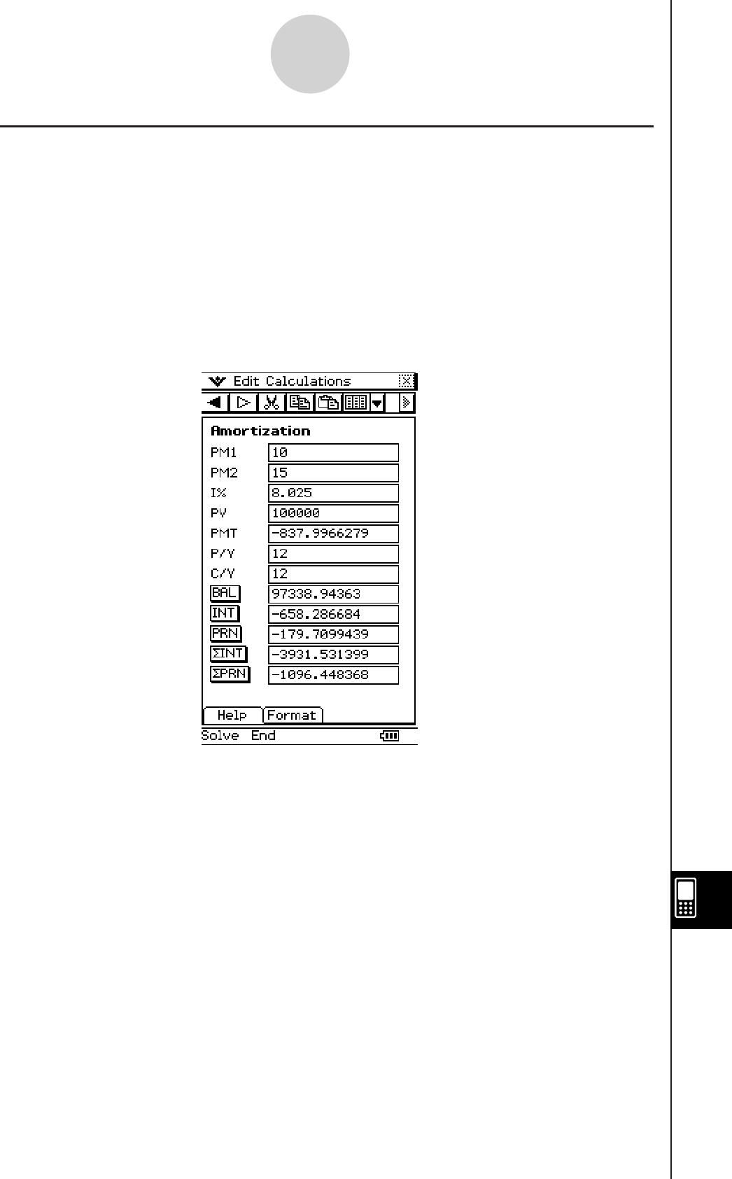
20110401

15-5-3

Amortization

k Example 2 (Amortization)

Use the monthly payment value you obtained in Example 1 (PMT = –837.9966279) to

determine the following information for payment 10 (PM1) through 15 (PM2).

As in Example 1, the mortgage has a loan amount (PV) of $100,000 at an annual rate (I%) of

8.025%, compounded monthly (C/Y = 12) for 20 years.

There are 12 payment periods per year (P/Y).

• The balance (BAL) of the principal remaining after payment 15

• The interest amount (INT) included in payment 10

• The principal amount (PRN) included in payment 10

• Total interest to be paid (sumINT) from payment 10 to payment 15

• Total principal to be paid (sumPRN) from payment 10 to payment 15

20060301

15-5-4

Amortization

I%' = I%

(1+ ) –1

[C / Y ]

[P / Y ]

100 × [C / Y ]

{ }

×100

i = I%'÷100

Calculation Formulas

a: Interest portion of payment PM1 (INT)

b: Principal portion of payment PM1 (PRN)

c: Principal balance upon completion of payment PM2 (BAL)

d: Total principal paid from payment PM1 to payment PM2 (ΣPRN)

e: Total interest paid from payment PM1 to payment PM2 (ΣINT)

• a + b = one repayment (PMT)

Converting between the Nominal Interest Rate and Effective Interest Rate

The nominal interest rate (I

% value input by user) is converted to an effective interest rate

%') for installment loans where the number of annual payments is different from the number

of annual compoundings calculation periods.

The following calculation is performed after conversion from the nominal interest rate to the

effective interest rate, and the result is used for all subsequent calculations.

1 payment

Number of Payments

1 PM1 PM2 Last............... .................. ...............

INTPM1 = I BALPM1–1 × i I × (PMT sign)

PRNPM1 = PMT + BALPM1–1 ×

BALPM2 = BALPM2–1 + PRNPM2

Σ PRN = PRNPM1 + PRNPM1+1 + .... + PRNPM2

PM2

PM1

Σ INT = INTPM1 + INTPM1+1 + .... + INTPM2

PM2

PM1

BAL0 = PV ....................... Payment: End (Format tab)

INT1 = 0, PRN1 = PMT ... Payment: Begin (Format tab)

1 payment

Number of Payments

1 PM1 PM2 Last.............. ..................... ............

20060301

15-6-1

Interest Conversion

15-6 Interest Conversion

Interest Conversion lets you calculate the effective or nominal interest rate for interest that is

compounded multiple times during a year.

Interest Conversion Fields

The following fields appear on the Interest Conversion calculation page.

Field Description

N Number of times interest is compounded per year

EFF Effective interest rate (as a percent)

APR Nominal interest rate (as a percent)

k Example 1

What is the annual effective interest rate ([EFF]) on a certificate that offers a nominal interest

rate of 3% ([APR]), compounded quarterly (N = 4)?

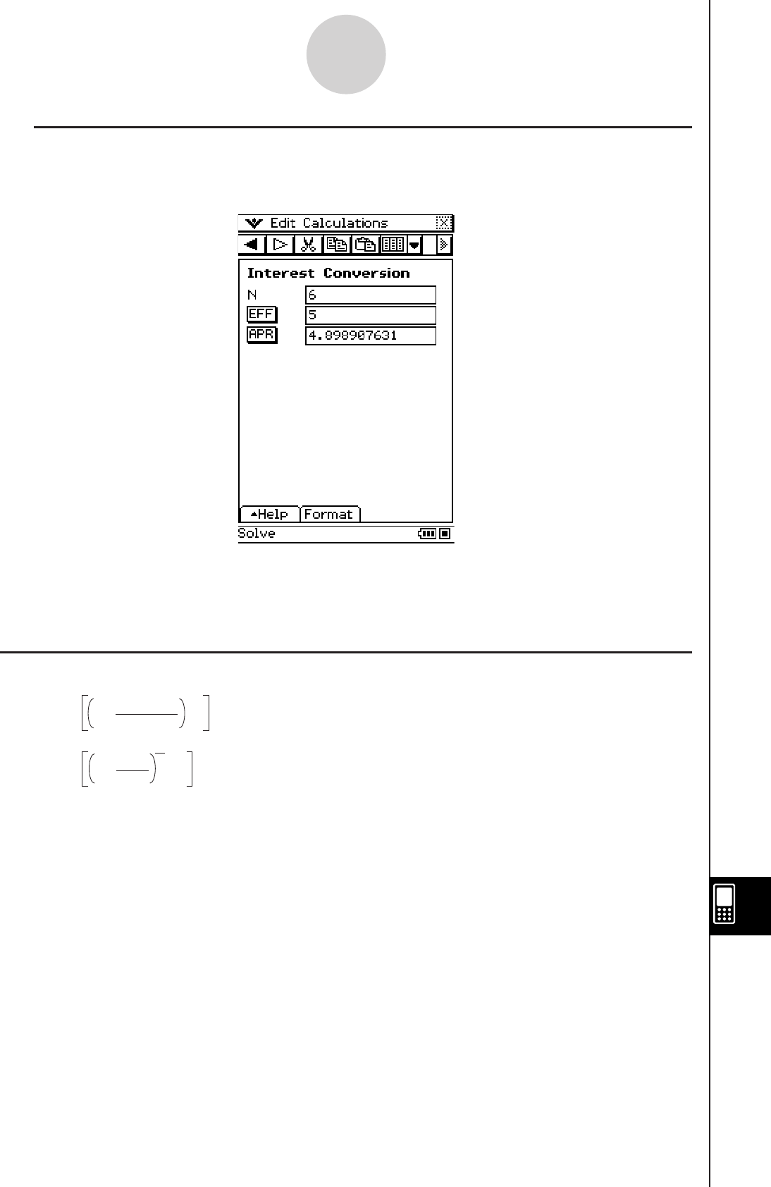
20060301

Tip

• You can change any value and then tap a button to recalculate.

Calculation Formulas

EFF = n

APR/100

1+ –1 × 100

PR = 100

EFF

1+ –1 × n ×100

15-6-2

Interest Conversion

k Example 2

What is the nominal interest rate ([APR]) on a certificate that offers an annual effective

interest rate ([EFF]) of 5%, compounded bi-monthly (N = 6)?

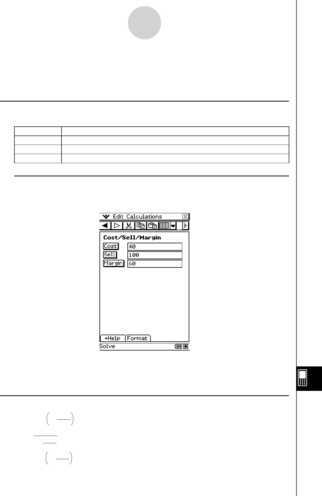
20060301

15-7-1

Cost/Sell/Margin

15-7 Cost/Sell/Margin

Cost/Sell/Margin lets you calculate the cost, selling price, or margin of profit on an item,

given the other two values.

Cost/Sell/Margin Fields

The following fields appear on the Cost/Sell/Margin calculation page.

Field Description

Cost Production cost

Sell Selling price

Margin Margin of profit (portion of selling price not absorbed by cost of production)

k Example

What is the selling price ([Sell]) required to obtain a margin of profit ([Margin]) of 60% on an

item that cost $40 ([Cost])?

Tip

• Any of the values on this page can be calculated by inputting values for the other two, and then

tapping the button for the value you want to obtain.

Calculation Formulas

CST = SEL 100

MRG

1–

SEL =

100

MRG

1–

CST

RG(%) = SEL

CST

1– ×100

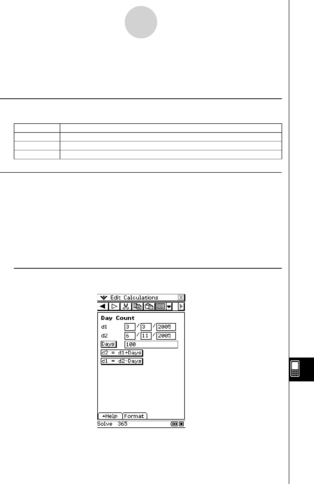
20060301

15-8-1

Day Count

15-8 Day Count

Day Count lets you calculate the number of days between two dates, or the date that is a

specified number of days from another date.

Day Count Fields

The following fields appear on the Day Count calculation page.

Field Description

d1 Month (1-12); Day (1-31); Year (1902-2097)

d2 Month (1-12); Day (1-31); Year (1902-2097)

Days Number of days from d1 to d2

Financial Application Default Setup for Examples

You can use the [Format] tab to change the following setting.

Days in Year: 365 days

Important!

• The format used for the date on the Day Count screen is the one you select under

“Configuring Default Financial Application Settings” on page 15-1-4.

• Calculating the date that is a specified number of days from another date is valid only when

Days in Year is set to 365.

k Example 1

How many days ([Days]) are there from March 3, 2005 (d1) to June 11, 2005 (d2)?

Tip

• Pressing

E after inputting a value advances to the next field.

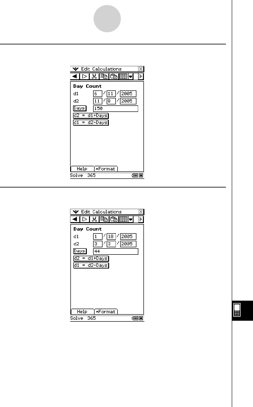
20060301

k Example 3

What date (d1) comes 44 days ([Days]) before March 3, 2005 (d2)?

15-8-2

Day Count

k Example 2

What date (d2) comes 150 days ([Days]) after June 11, 2005 (d1)?

20060301

15-9-1

Depreciation

15-9 Depreciation

Depreciation lets you calculate the amount that a business expense can be offset by income

(depreciated) over a given year.

You can use a Depreciation page to calculate depreciation using one of four methods:

straight-line, fixed-percentage, sum-of-the-years’-digits, or declining-balance.

Depreciation Fields

The following fields appear on the Depreciation calculation page.

Field Description

N Number of years over which depreciation occurs

I% Annual interest rate (as a percent)

PV Present value (initial investment)

FV Future value

jYear for which depreciation is being calculated

YR1 Number of depreciable months in first year

SL Calculate depreciation for year j using the straight-line method

FP Calculate depreciation for year j using the fixed-percentage method

SYD Calculate depreciation for year j using the sum-of-the-years’-digits method

DB Calculate depreciation for year j calculated using the declining-balance

method

RDV Residual value after depreciation for year j

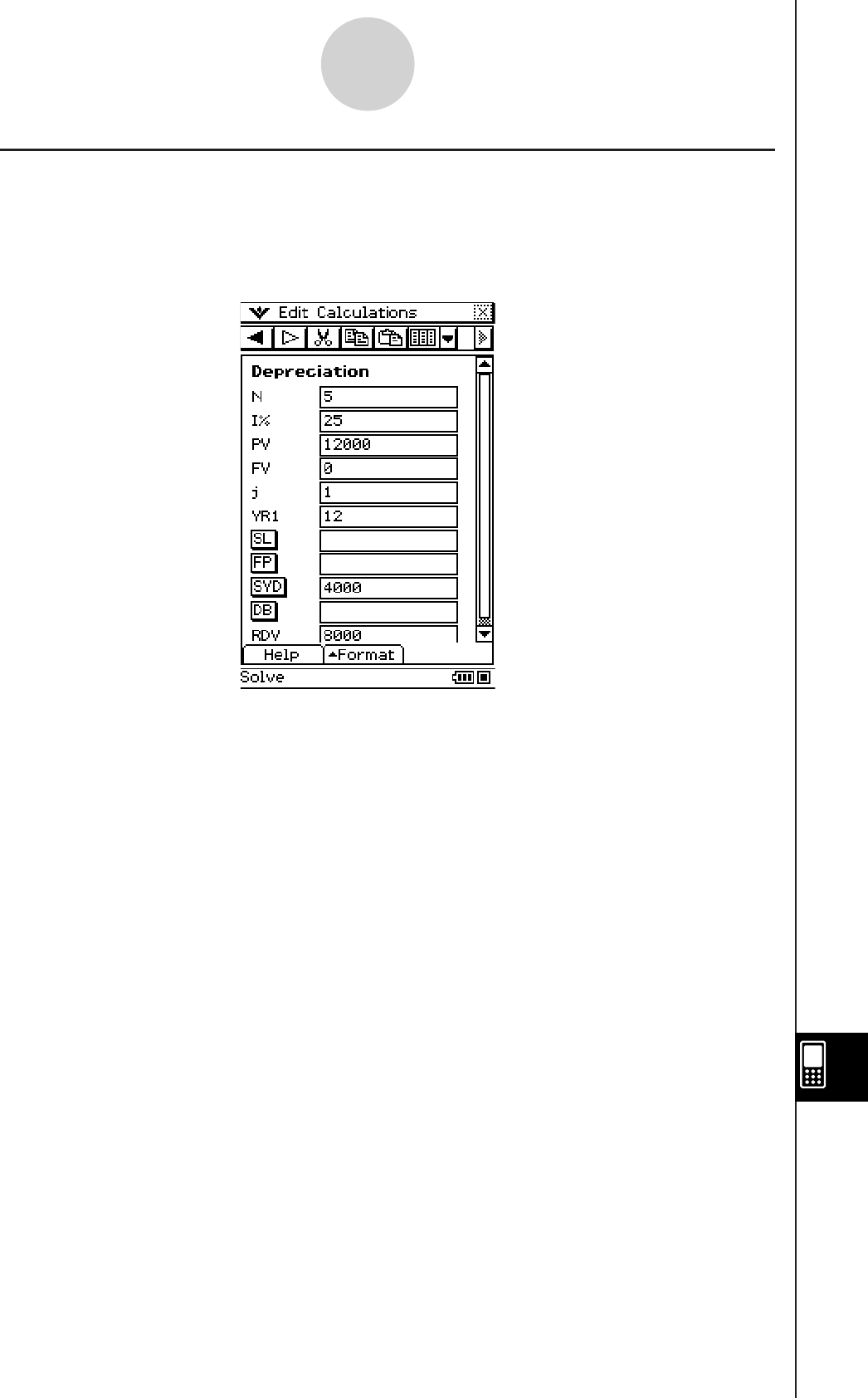
20060301

15-9-2

Depreciation

Tip

• At the end of the useful life the value of the computer will be 0, so we enter 0 in the FV field.

k Example 1

Use the sum-of-the-years’-digits method ([SYD]) to calculate the first year (j = 1) of

depreciation on an $12,000 (PV) computer, with a useful life (N) of five years. Use a

depreciation ratio (I%) of 25%, and assume that the computer can be depreciated for a full

12 months in the first year (YR1).

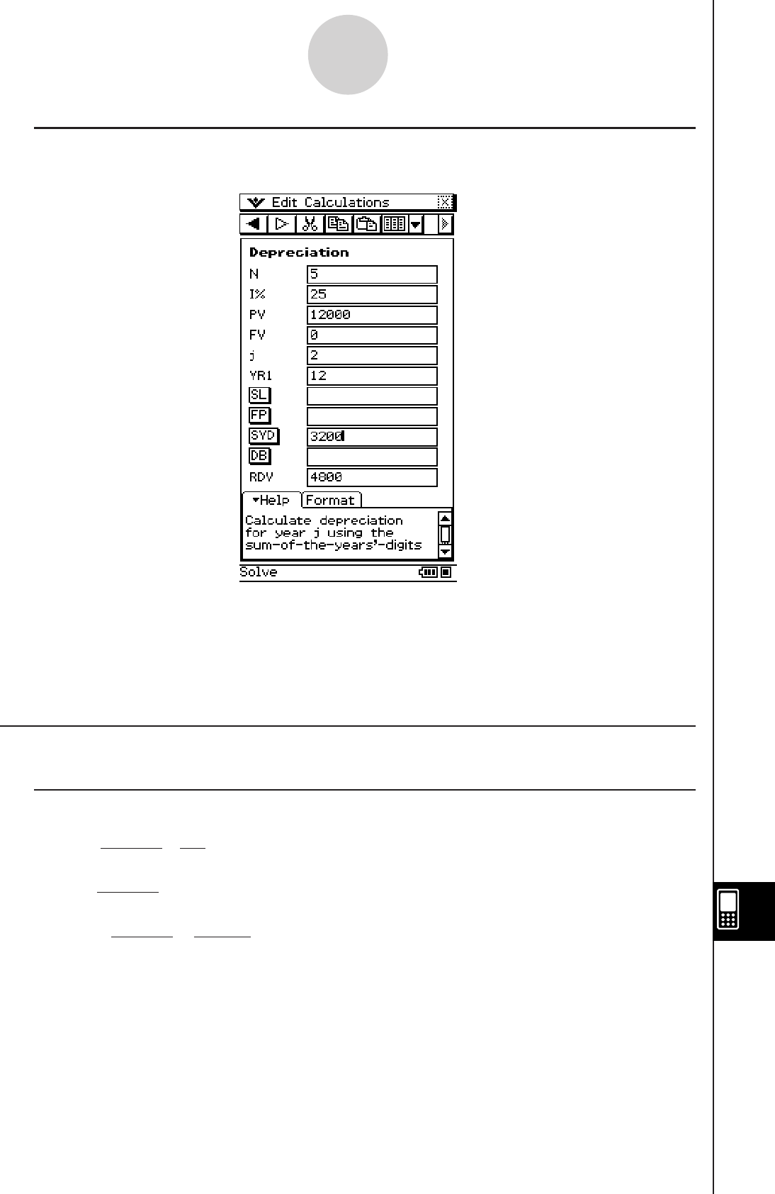
20060301

k Example 2

Now calculate the depreciation amount ([SYD]) for the second year (j = 2).

Note

• You can also tap [SL] to calculate depreciation using straight-line method, [FP] using fixed-

percentage method, or [DB] using declining-balance method.

• Each depreciation method will produce a different residual value after depreciation (RDV)

for the applicable year (j).

Calculation Formulas

k Straight-Line Method

YR1

(PV–FV )

SL1 = n12

(PV–FV )

SLj = n

12– YR1

(YR1G12)

(PV–FV )

n12

SLn+1 =

15-9-3

Depreciation

20060301

k Fixed-Percentage Method

k Sum-of-the-Years’-Digits Method

k Declining-Balance Method

100

FPj = (RDVj–1 + FV ) ×

100

YR1I%

FP1 = PV × 12

FPn+1 = RDVn (YR1G12)

RDV1 = PV – FV – FP1

RDVj = RDVj–1 – FPj

RDVn+1 = 0 (YR1G12)

YR1

n' = n –

n (n +1)

Z = 2

(Intg (n' ) +1) (Intg (n' )+2 × Frac(n' ))

SYD1 = YR1

Z×(PV – FV )

n'– j+2

Z' )(PV – FV – SYD1)( jG1)SYDj = (

RDV1 = PV – FV – SYD1

RDVj = RDVj –1 – SYDj

n'– (n +1)+2

Z' )(PV – FV – SYD1) ×(YR1G12)

12–YR1

SYDn+1 = (

Z' =

RDV1 = PV – FV – DB1

(YR1G12)

100n

YR1I%

DB1 = PV ×

100n

DBj = (RDVj–1 + FV )

RDVj = RDVj–1 – DBj

DBn +1 = RDVn

RDVn+1 = 0

15-9-4

Depreciation

20060301

15-10-1

Bond Calculation

15-10 Bond Calculation

Bond Calculation lets you calculate the purchase price or the annual yield of a bond.

Bond Calculation Fields

The following fields appear on the Bond Calculation page.

Field Description

d1 Month (1-12); Day (1-31); Year (1902-2097)

d2 Month (1-12); Day (1-31); Year (1902-2097)

N Number of periods

RDV Redemption value

CPN Annual coupon rate

PRC Price of bond

YLD Yield to maturity (as a percent)

INT Interest accumulated during partial year portion of investment period

Cost Cost of bond (price plus partial year interest)

Financial Application Default Setup for Examples

You can use the [Format] tab to change the following settings.

Days in Year: 360 days

Compounding Frequency: Semi-annual

Bond Interval: Date

20110401

15-10-2

Bond Calculation

k Example 1

You want to purchase a semiannual (Compounding Frequency = Semi-annual) corporate

bond that matures on 12/15/2006 (d2) to settle on 6/1/2004 (d1). The bond is based on

the 30/360 day-count method (Days in Year = 360 days) with a coupon rate (CPN) of 3%.

The bond will be redeemed at 100% of its par value (RDV). For 4% yield to maturity (YLD),

calculate the bond’s price ([PRC]) and accrued interest (INT).

• Before performing the calculation, you should use the [Format] tab to change the [Bond

Interval] setting to “Date” and the [Compounding Frequency] to “Semi-annual”.

• You can also look at the status bar to see if the settings are correct. If they are not, tap the

settings in the status bar to switch to the correct ones.

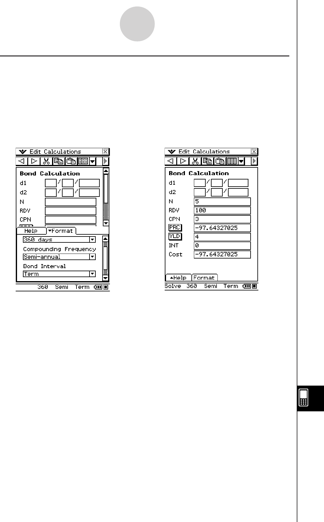
20060301

15-10-3

Bond Calculation

k Example 2

For the same type of bond described in Example 1, calculate the price on the bond (PRC)

based on a specific number of coupon payments (Term).

• Before performing the calculation, you should use the [Format] tab to change the [Bond

Interval] setting to “Term”, or tap “Date” in the status bar.

The bond is based on the 30/360 day-count method (Days in Year = 360 days) with a coupon

rate (CPN) of 3%. The bond will be redeemed at 100% of its par value (RDV) after 3 periods

(N). For 4% yield to maturity (YLD), calculate the bond’s price ([PRC]).

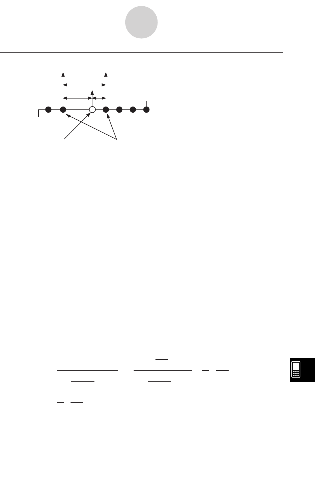
20060301

PRC : price per $100 of face value

CPN : coupon rate (%)

YLD : annual yield (%)

A : accrued days

M : number of coupon payments per year (1 = Annual, 2 = Semi-annual)

N : number of coupon payments until maturity

(

n is used when “Term” is specified for [Bond Interval] in the [Format] tab.)

RDV : redemption price per $100 of face value

D : number of days in coupon period where settlement occurs

B : number of days from purchase date until next coupon payment date = D – A

INT : accrued interest

CST : price including interest

u Price per $100 of face value (PRC)

Bond Interval Setting: Date

• For one or fewer coupon period to redemption

• For more than one coupon period to redemption

15-10-4

Bond Calculation

PRC = – + ( )

RDV +M

CPN

1+ ( ×)

YLD/100 ×

CPN

A CPN

RC = –

NT = –

–

RDV

(1+ )

YLD/100 (1+ )

YLD/100

CPN

k=1

(N–1+B/D) (k–1+B/D)

= PRC + INT

Calculation Formulas

Issue date

Redemption date (d2)

Purchase date (d1) Coupon Payment dates

A B

20060301

Bond Interval Setting: Term

u Annual Yield (YLD)

YLD is calculated using Newton’s Method.

Note

• The Financial application performs annual yield (YLD) calculations using Newton’s Method,

which produces approximate values whose precision can be affected by various calculation

conditions. Because of this, annual yield calculation results produced by this application

should be used keeping the above in mind, or results should be confirmed separately.

PRC = – –

RDV M

CPN

(1+ )

YLD/100 n(1+ )

YLD/100 k

INT

= 0

CST

= PRC

k=1

15-10-5

Bond Calculation

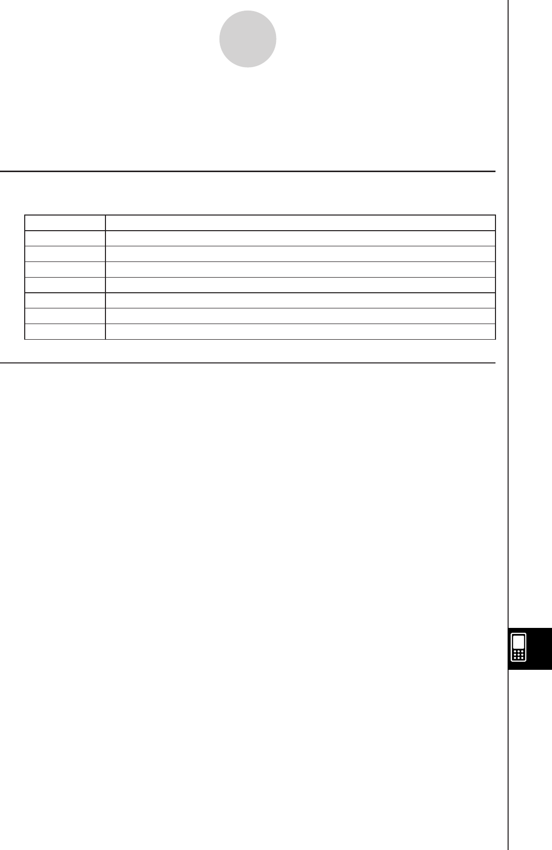
20060301

15-11-1

Break-Even Point

15-11 Break-Even Point

Break-Even Point lets you calculate the amount you must sell to break even or to obtain a

specified profit, as well as the profit or loss on particular sales.

Break-Even Point Fields

The following fields appear on the Break-Even Point calculation page.

Field Description

PRC Selling price per unit

VCU Variable cost per unit

FC Fixed costs

PRF Amount of profit realized

QBE Number of units to be sold

SBE Amount that must be obtained from sales to break even

r% Proportion of sales amount retained as a profit (as a percent)

Financial Application Default Setup for Examples

You can use the [Format] tab to change the following settings. You can also change these

settings by tapping the status bar.

Profit Amount/Ratio: Amount (PRF)

Break-Even Value: Quantity

Scenario

Your company is producing items with a unit variable cost ([VCU]) of $50/unit and fixed costs

([FC]) of $100,000. The items will be sold for a sales price ([PRC]) of $100/unit.

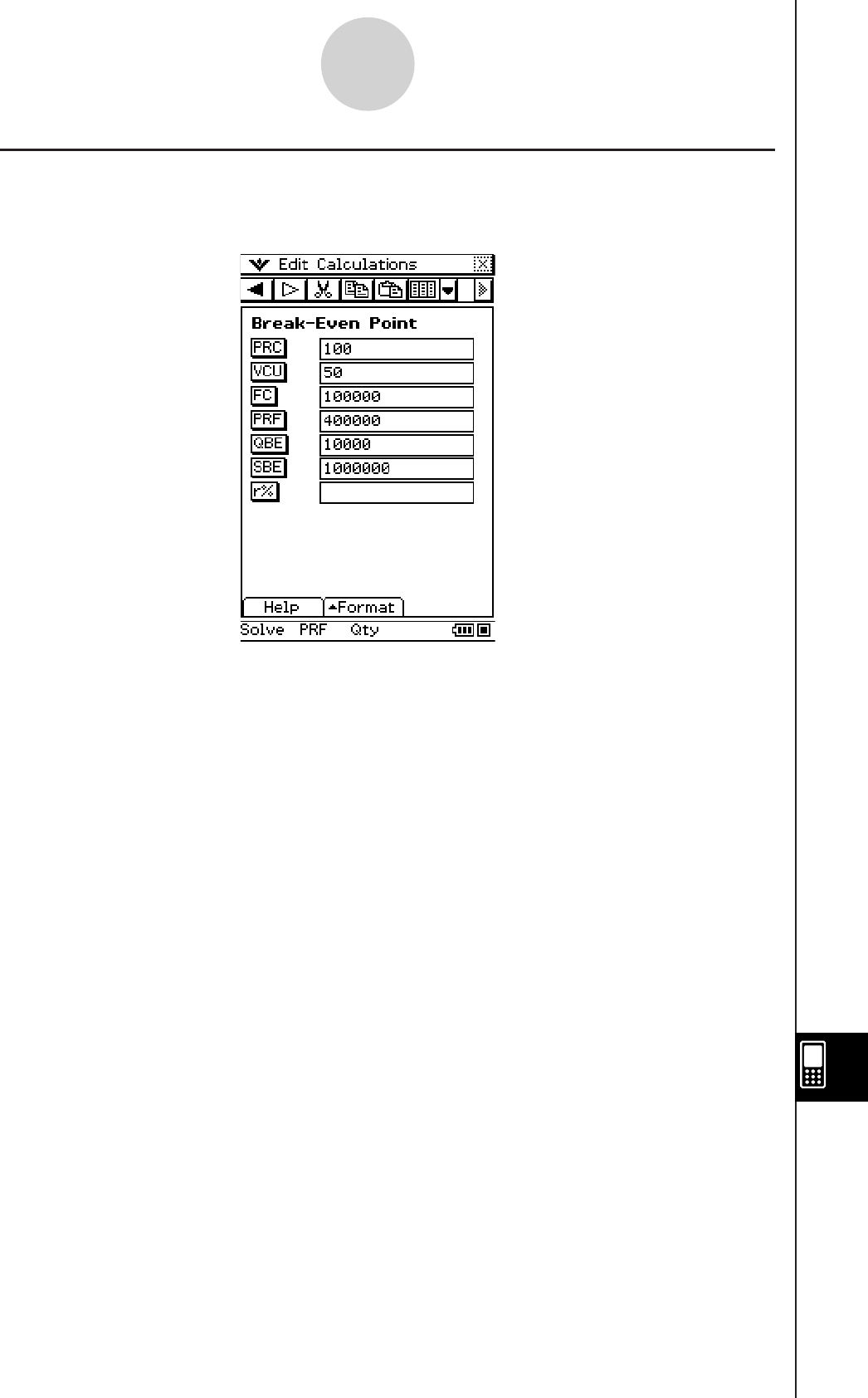
20060301

15-11-2

Break-Even Point

k Example 1

What is the break-even point sales amount ([SBE]) and sales quantity ([QBE]) required for a

profit ([PRF]) of $400,000?

Note

• You need to calculate the break-even point sales quantity ([QBE]) before you will be able to

calculate the break-even sales amount ([SBE]).

20060301

k Example 2

What is the break-even point sales amount ([SBE]) and sales quantity ([QBE]) to attain a

profit ratio ([r%]) of 40%?

• For this example, use the [Format] tab to change the [Profit Amount/Ratio] setting to

“Ratio (r%)” or tap “PRF” in the status bar to change it to “r%”.

Calculation Formulas

u Profit (Profit Amount/Ratio Setting: Amount (PRF))

u Profit Ratio (Profit Amount/Ratio Setting: Ratio (r%))

PRC – VCU

FC + PRF

QBE =

PRC – VCU

FC + PRF

SBE =× PRC

PRC × – VCU

QBE = FC

× PRC

100

1–

PRC × – VCU

SBE =FC

100

1–

15-11-3

Break-Even Point

20060301

15-12-1

Margin of Safety

15-12 Margin of Safety

Margin of Safety lets you calculate how much sales can be reduced before losses are

incurred.

Margin of Safety Fields

The following fields appear on the Margin of Safety calculation page.

Field Description

SAL Amount obtained from sales

SBE Break-even sales (amount that must be obtained from sales to break even)

MOS Margin of safety (portion of sales amount above break-even point)

k Example

What is the margin of safety ([MOS]) when the sales amount ([SAL]) is $1,200,000 and the

break-even sales amount ([SBE]) is $1,000,000?

• You can calculate the break-even sales amount ([SBE]) using Break-Even Point (page

15-11-1).

• You can also calculate the sales amount ([SAL]) or break-even sales amount ([SBE]) by

inputting the other two values and tapping the button for the result you want.

Calculation Formulas

SAL

OS = SAL – SBE

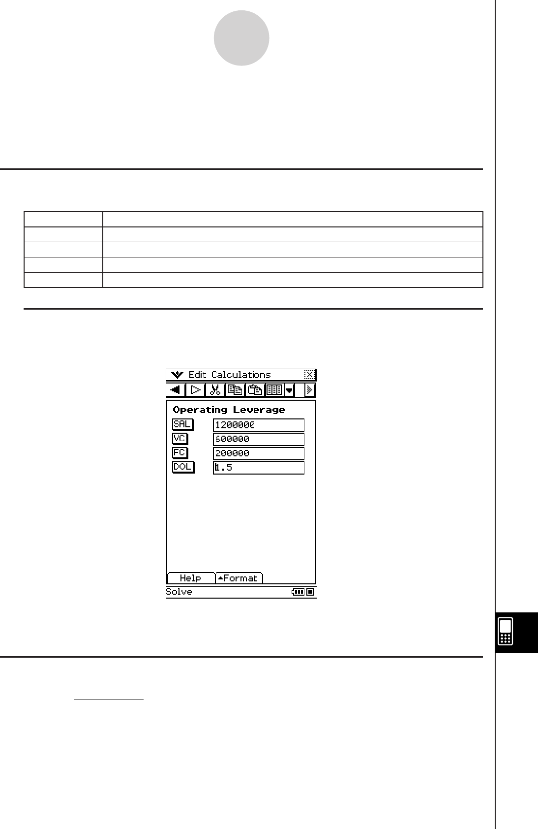
20060301

15-13-1

Operating Leverage

15-13 Operating Leverage

Operating leverage lets you calculate the degree of change in net earnings arising from a

change in sales amount.

Operating Leverage Fields

The following fields appear on the Operating Leverage calculation page.

Field Description

SAL Amount currently obtained from sales

VC Variable cost for this level of production

FC Fixed costs

DOL Degree of operating leverage

k Example

What is the degree of operating leverage for a company with sales ([SAL]) of $1,200,000,

variable costs ([VC]) of $600,000, and fixed costs ([FC]) of $200,000?

• You can also calculate sales amount ([SAL]), variable costs ([VC]), or fixed costs ([FC]) by

inputting the other three values and tapping the button for the result you want.

Calculation Formulas

SAL – VC – FC

OL = SAL – VC

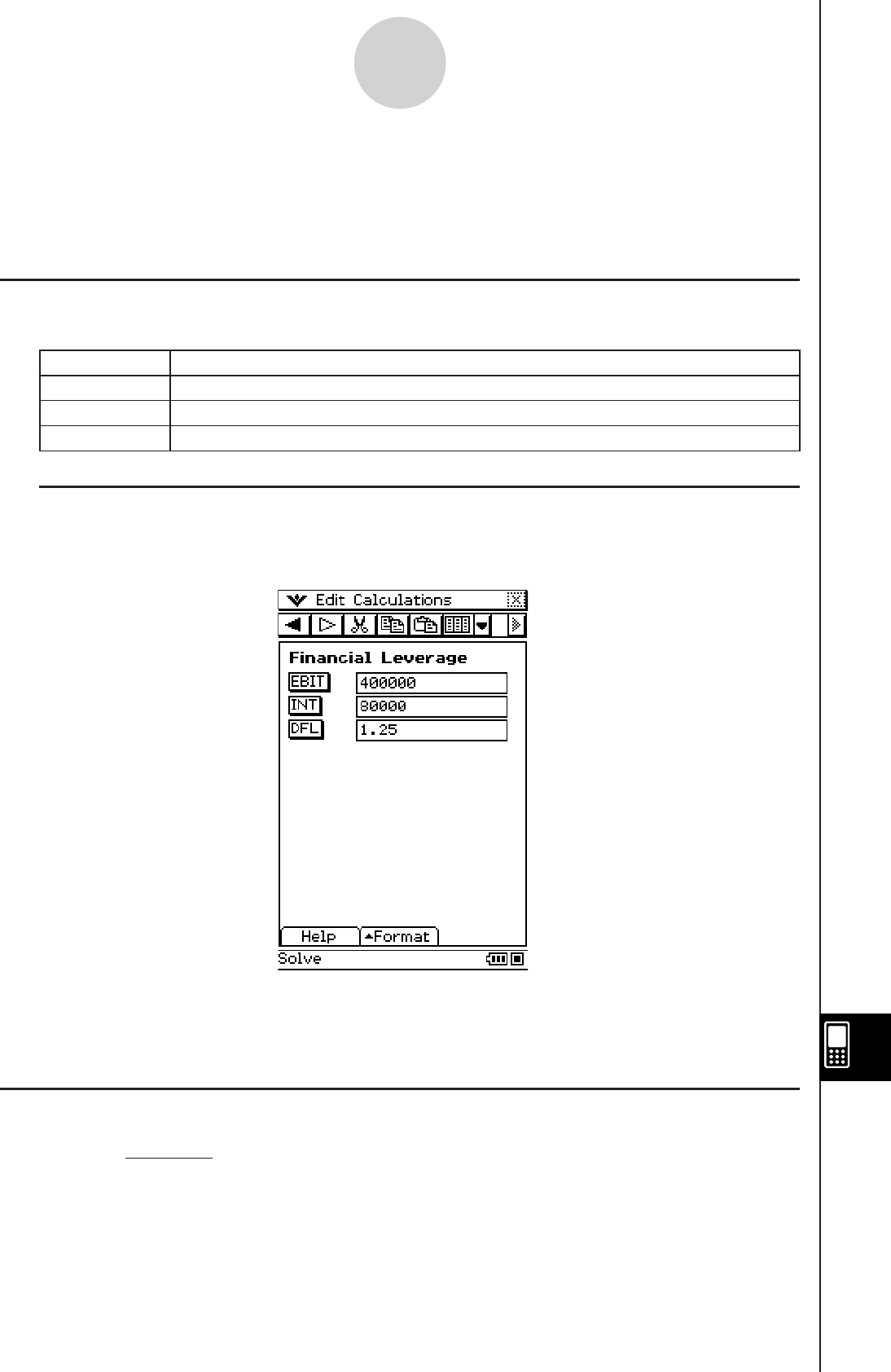
20060301

15-14-1

Financial Leverage

15-14 Financial Leverage

Financial Leverage lets you calculate the degree of change in net earnings arising from a

change in interest paid.

Financial Leverage Fields

The following fields appear on the Financial Leverage calculation page.

Field Description

EBIT Earnings before interest and taxes

INT Interest to be paid to bondholders

DFL Degree of financial leverage

k Example

Calculate the financial leverage ([DFL]) for a company that earns $400,000 before interest

and taxes ([EBIT]), $80,000 of which is paid to bondholders ([INT]).

• You can also calculate earnings before interest and taxes ([EBIT]) or interest to be paid to

bondholders ([INT]) by inputting the other two values and tapping the button for the result

you want.

Calculation Formulas

EBIT – ITR

DFL = EBIT

20060301

15-15-1

Combined Leverage

15-15 Combined Leverage

Combined Leverage lets you calculate the combined effects of operation and financial

leverages.

Combined Leverage Fields

The following fields appear on the Combined Leverage calculation page.

Field Description

SAL Amount obtained from sales

VC Variable cost for this level of production

FC Fixed costs

INT Interest to be paid to bondholders

DCL Degree of combined leverage

k Example

Calculate the Combined Leverage ([DCL]) for a company with variable costs ([VC]) of

$6,000, fixed costs ([FC]) of $2,000, and sales ([SAL]) of $12,000, of which $1,000 is paid to

bondholders ([INT]).

• You can also calculate variable costs ([VC]), fixed costs ([FC]), sales ([SAL]), or the amount

or paid to bondholders ([INT]) by inputting the other four values and tapping the button for

the result you want.

Calculation Formulas

SAL – VC – FC – ITR

DCL = SAL – VC

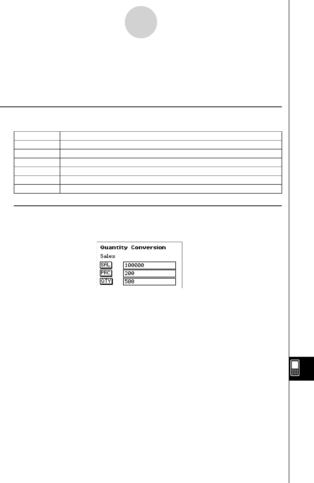
20060301

15-16-1

Quantity Conversion

15-16 Quantity Conversion

Quantity Conversion lets you calculate the number of items sold, selling price, or sales

amount given the other two values. It also lets you calculate the number of items

manufactured, unit variable cost, or total variable cost given the other two values.

Quantity Conversion Fields

The following fields appear on the Quantity Conversion calculation page.

Field Description

SAL Amount obtained from sales

PRC Selling price per unit

QTY Number of units sold

VC Variable cost for this level of production

VCU Variable cost per unit

QTY Number of units manufactured

k Example 1

Calculate the sales quantity (Sales: [QTY]) when the sales amount ([SAL]) is $100,000 and

the sales price ([PRC]) is $200 per unit.

• You can also calculate the sales amount ([SAL]) or sales price ([PRC]) by inputting the

other two values and tapping the button for the result you want.

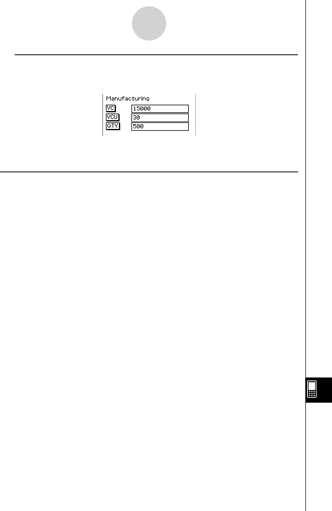
20060301

15-16-2

Quantity Conversion

• You can also calculate the variable cost per unit ([VCU]) or number of units manufactured

([QTY]) by inputting the other two values and tapping the button for the result you want.

Calculation Formulas

k Example 2

Calculate the total variable costs of production (Manufacturing: [VC]) when the variable cost

per unit ([VCU]) is $30 and the number of units manufactured ([QTY]) is 500.

SAL = PRC × QT

VC = VCU × QT

20101001

15-17-1

Performing Financial Calculations Using Commands

15-17 Performing Financial Calculations Using

Commands

You can perform the following types of financial calculations using program commands in

Program, eActivity or Main application.

u Simple Interest

u Compound Interest

u Cash Flow

u Amortization

u Interest Conversion

u Cost/Sell/Margin

u Day Count

u Bond Calculation

Financial Application Setup Commands

For details about each of the setting items, see “Financial Format Dialog Box” (page 1-9-12).

To do this: Use this command:

Specify a 360-day year DateMode360

Specify a 365-day year DateMode365

Specify beginning of period for the payment date PmtBgn

Specify end of period for the payment date PmtEnd

Specify annual for the bond calculation payment periods PeriodsAnnual

Specify semiannual for the bond calculation payment periods PeriodsSemi

Financial Calculation Commands

For information about financial calculation commands, see “Using the Financial Submenu”

on page 2-8-57.

20110901

Chapter

Configuring System

Settings

The ClassPad unit’s System application lets you configure global

system settings and access system information.

You can also import and export data (variable and eActivity) between

main memory and the eActivity area, and the mass storage area (USB

Flash Drive).

16-1 System Setting Overview

16-2 Managing Memory Usage

16-3 Using the Reset Dialog Box

16-4 Initializing Your ClassPad

16-5 Specifying the Display Language

16-6 Specifying the Font Set

16-7 Specifying the Alphabetic Keyboard Arrangement

16-8 Viewing Version Information

16-9 Registering a User Name on a ClassPad

16-10 Specifying the Complex Number Imaginary Unit

16-11 Assigning Shift Mode Key Operations to Hard Keys

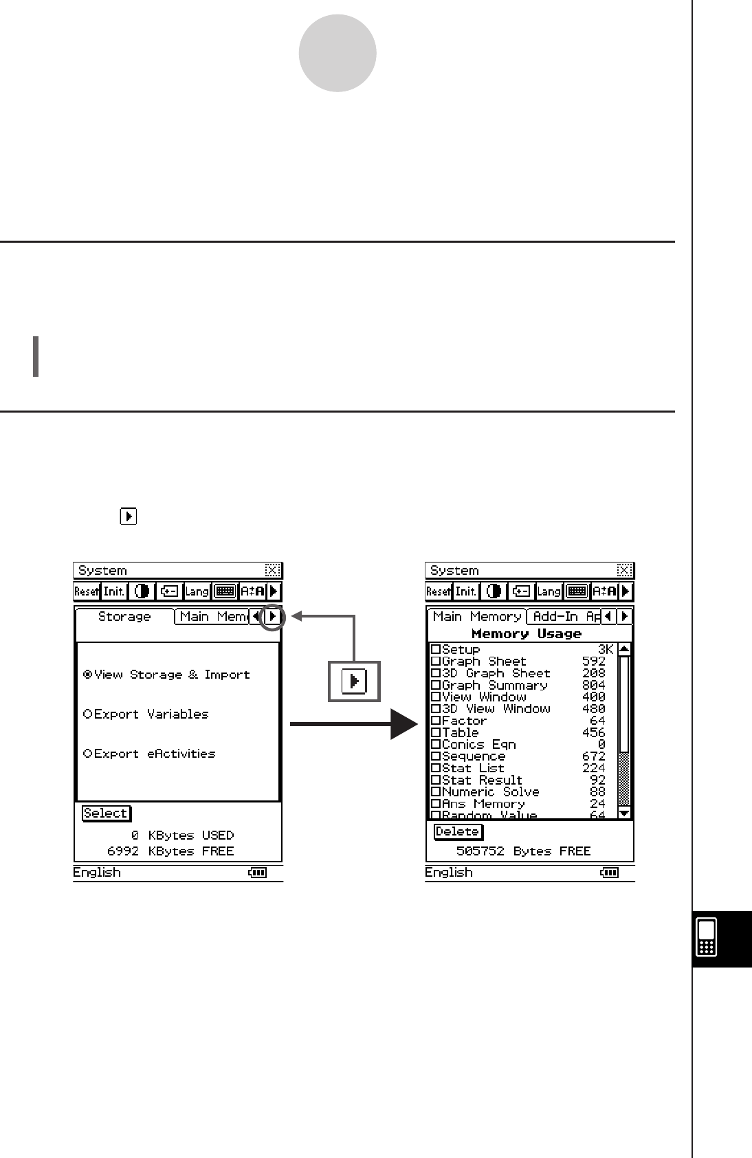
20110901

16-1-1

System Setting Overview

16-1 System Setting Overview

This section describes the configuration of the System application window, and provides

information about its menus and commands.

Starting Up the System Application

Use the following procedure to start up the System application.

u ClassPad Operation

On the application menu, tap Y.

This starts the System application and displays the [Storage] sheet.

System Application Window

The [Storage] sheet appears first whenever the System application is started up. This sheet

can be used to import and export files. For details, see “Importing and Exporting XCP Files”

(page 2-6-5) in the separate Hardware User’s Guide.

Tapping the button displays the Memory Usage sheet. The memory usage sheet shows

main memory, Add-in application, eActivities, and built-in languages.

[Storage] sheet Memory Usage

20110901

System Application Menus and Buttons

To perform an operation in the System application, select it on the [System] menu or tap the

applicable toolbar button.

To do this: Tap this

button:

Or select this System

menu item:

Reset the ClassPad unit (which deletes all variable

and program data in main memory and the eActivity

area)

;Reset

Initialize the ClassPad unit (which returns all Flash

ROM data to its factory default state) 'Initialize

Adjust display contrast* ZContrast

Configure auto power off setting* XPower Properties

Change the display text language CLanguage

Specify the complex number imaginary unit — Imaginary Unit

Change the font set >Font Select

Change the arrangement of the alphabet (abc) soft

keyboard VKeyboard

Optimize eActivity area and mass storage area* <Memory Management

Select the image data for the ending screen that

appears when the ClassPad unit is turned off* NEnding Screen

Adjust the alignment of the touch panel* MTouch Panel Alignment

Specify the battery type being used* Battery Settings

Display software version information >Version

Assign shift mode key operations to hard keys — Shift Keys

• Details about each of the above settings can be found in the following sections of this

chapter.

* See Chapter 1 in the separate Hardware User’s Guide.

16-1-2

System Setting Overview

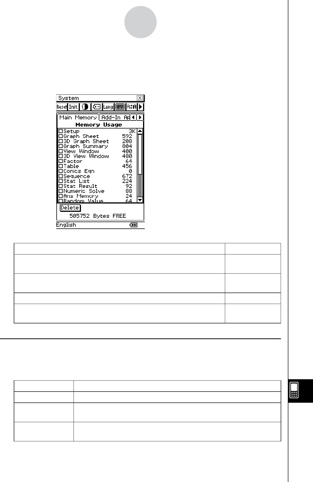
20110901

16-2 Managing Memory Usage

You can use [Memory Usage] to determine how much data is stored in the main memory, the

mass storage area, and the eActivity area, and to delete data.

[Memory Usage] contains the following four sheets.

To view this: Select this tab:

Memory usage of variable data and program data stored in main

memory Main Memory

Names and memory usage of add-in applications stored in the mass

storage area Add-In App.

Names and memory usage of eActivity data stored in the eActivity area eActivity

Names and memory usage of language data stored in the mass storage

area Language

Memory Usage Sheets

The following sections explain the meaning of each of the sheets in [Memory Usage].

Main Memory Tab

This item: Shows how much memory is used by this type of data:

Setup All setup data and other setup information (page 1-9-1)

Graph Sheet 2-dimensional function data (including sheet name data and function

selection data)

3D Graph Sheet 3-dimensional function data (including sheet name data and function

selection data)

See “Memory Usage Sheets” below for

details about [Memory Usage] contents.

Displayed values are all approximate.

16-2-1

Managing Memory Usage

20110901

This item: Shows how much memory is used by this type of data:

Graph Summary Summary table data

View Window 2-dimensional View Window parameter values

3D View Window 3-dimensional View Window parameter values

Factor Zoom factor values

Table Range values and table result values

Conics Eqn Conics expressions

Sequence

Sequential and recursion data (including function selection and other

information), and sequence data (including initial value and range

information)

Stat List list1 through list6

Stat Result Statistical calculation results

Numeric Solve Solve expression and solve range

Ans Memory Main application Ans data

Random Value Random command setting data

Main History Main application history data

User Defined User-defined variables and user-created folders

Library “library” folder data

eActivity eActivity application temporary data*

Geometry Geometry application temporary data*

Spreadsheet Spreadsheet application temporary data*

System Other system data

Clipboard Clipboard data

Financial Financial application data

DiffEqGraph DiffEqGraph function data

* “temporary data” is data that is created by an application but not saved in memory.

16-2-2

Managing Memory Usage

20110901

Deleting Memory Usage Data

You can use the following procedure to delete memory usage data.

u ClassPad Operation

(1) Tap the memory usage tab (Main Memory, Add-In App., eActivity, or Language) that

contains the data you want to delete.

(2) Select the check box next to the item whose data you want to delete.

(3) Tap the [Delete] button.

(4) On the confirmation dialog box that appears, tap [OK] to delete the selected data, or

[Cancel] to cancel the delete operation.

• Tapping [OK] displays the message “Now deleting...” while the data is being deleted.

• The above procedure deletes all of the data you selected, and updates memory

usage values accordingly.

Tip

• You cannot delete any data that has a dimmed check box.

• For information about deleting all variable data and program data, and deleting all eActivity data,

see “16-3 Using the Reset Dialog Box”.

• After you delete an eActivity file, the displayed remaining memory capacity value may not change

until you optimize Flash ROM. For information about optimizing Flash ROM, see page 1-8-1 in

the separate Hardware User’s Guide.

16-2-3

Managing Memory Usage

This item: Shows the data for this language:

Deutsch

English

Español

Français

Português

German

English

Spanish

French

Portuguese

Add-In App. Tab

This sheet lists all of the add-in applications currently installed on your ClassPad, and shows

the size of each application.

eActivity Tab

This sheet lists the names of all the files that have been created with the eActivity application,

and shows the size of each file.

Language Tab

This sheet lists language data used for the ClassPad menus and messages.

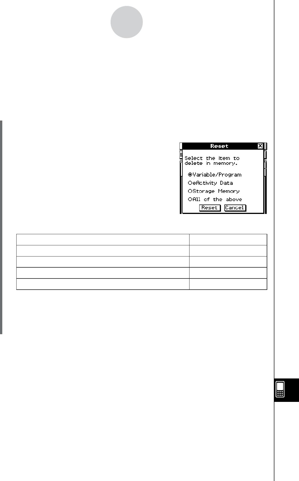
20110901

16-3 Using the Reset Dialog Box

You can perform the following operations from the Reset dialog box.

• Delete all variable and program data in main memory

• Delete all eActivity data

• Delete data other than add-ins in storage memory

u ClassPad Operation

(1) On the application menu, tap Y.

• This starts up the System application.

(2) Tap

; to display the Reset dialog box.

• To cancel the reset operation at any time before you

execute it in step (5) of this procedure, tap [Cancel].

(3) On the Reset dialog box, select the type of reset operation you want to perform.

To delete this type of data: Select this option:

All variable and program data in main memory Variable/Program

All eActivity data eActivity Data

Data other than add-ins in storage memory Storage Memory

All of the above three types All of the above

(4) After selecting the type of reset operation you want to perform, tap [Reset].

(5) In response to the confirmation message that appears, tap [OK] to perform the reset

operation, or [Cancel] to cancel.

(6) Follow the instructions that appear on the display.

16-3-1

Using the Reset Dialog Box

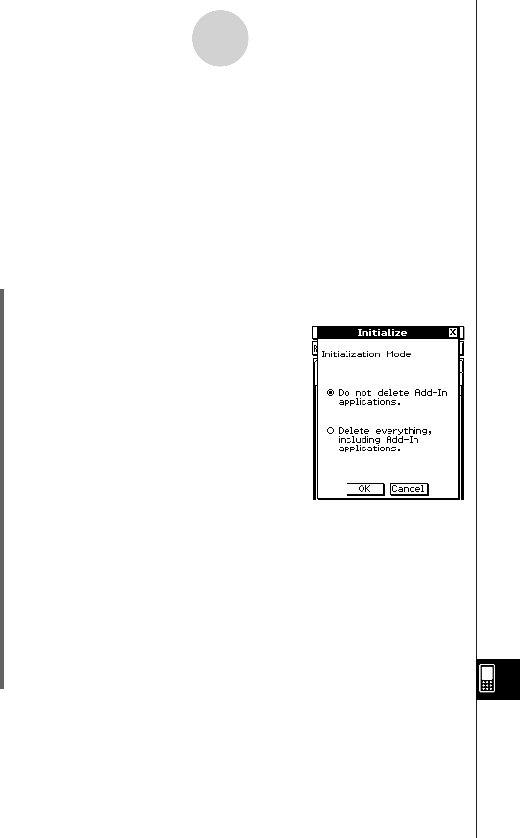
20110401

16-4 Initializing Your ClassPad

The initialization procedure provides you with a choice of two options. You can either clear

the Flash ROM entire and return its data to the factory default state, or you can specify

deletion of all user formulas and data, without deleting any currently installed add-in

applications.

Warning!

Initializing the ClassPad deletes anything you have input and stored in memory (including

eActivity data) since you purchased the ClassPad or last initialized it.

Before initializing the ClassPad, double-check to make sure you do not need any of the data

that will be deleted.

u ClassPad Operation

(1) On the application menu, tap Y.

• This starts up the System application.

(2) Tap

• This displays a dialog box asking if you want to retain

or delete add-in applications.

(3) Tap the button next to the initialization mode you want to select, and then tap [OK].

• This displays a confirmation asking if you really want to initialize your ClassPad.

(4) On the message dialog box, press E.

• This causes the ClassPad to restart.

(5) Perform the touch panel alignment, contrast adjustment, display language selection,

and keyboard configuration operations as their dialog boxes appear on the ClassPad

display.

• The application menu appears after you finish all of the settings in step (5).

• For more information about the procedures you need to perform in step (5), see

“Replacing Batteries and Setting Up the ClassPad” in the separate Hardware User’s

Guide.

16-4-1

Initializing Your ClassPad

20110401

16-5 Specifying the Display Language

You can use the following procedure to specify German, English, Spanish, French, or

Portuguese as the display language.

u ClassPad Operation

(1) On the application menu, tap Y.

• This starts up the System application.

(2) Tap

C to display the Language dialog box.

(3) In the list of languages, tap the one you want to use as the display language.

(4) After the setting is the way you want, tap [Set] to apply it and close the Language

dialog box, or tap [Cancel] to close without changing the setting.

• Tapping [Set] returns you to the application menu.

Tapping [Cancel] returns you to [Memory Usage].

16-5-1

Specifying the Display Language

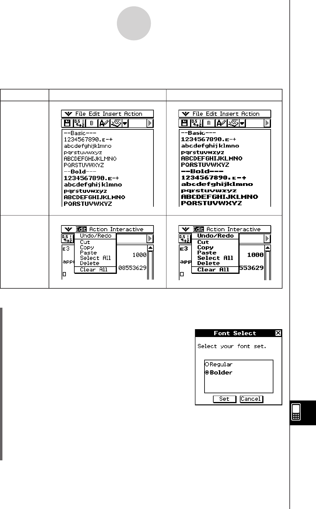
20110401

16-6-1

Specifying the Font Set

16-6 Specifying the Font Set

You can select either “Regular” or “Bolder” as the display font type.

Regular Bolder

Text Input

u ClassPad Operation

(1) On the application menu, tap Y.

• This starts up the System application.

(2) Tap

> to display the Font Select dialog box.

(3) In the list of font sets, tap the one you want to use.

(4) After the setting is the way you want, tap [Set] to apply it and close the Font Select

dialog box, or tap [Cancel] to close without changing the setting.

• Tapping [Set] returns you to the application menu.

Tapping [Cancel] returns you to [Memory Usage].

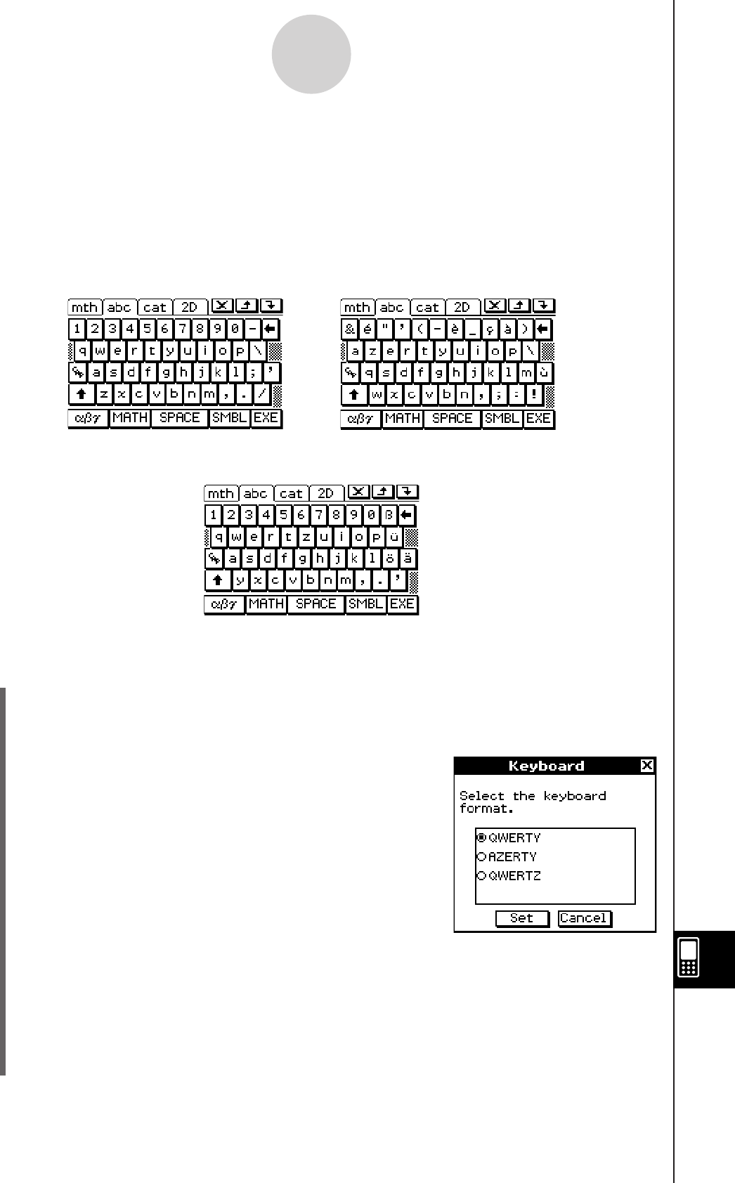
20110401

16-7 Specifying the Alphabetic Keyboard

Arrangement

The Keyboard dialog box lets you select from among three different key arrangements for the

alphabetic (abc) soft keyboard: QWERTY, AZERTY, or QWERTZ. The initial default setting

is QWERTY.

QWERTZ

u ClassPad Operation

(1) On the application menu, tap Y.

• This starts up the System application.

(2) Tap

V to display the Keyboard dialog box.

(3) In the list of keyboard arrangements, tap the one you want to use for the alphabetic (abc)

soft keyboard.

(4) After the setting is the way you want, tap [Set] to apply it and close the Keyboard dialog

box, or tap [Cancel] to close without changing the setting.

• Tapping [Set] returns you to the application menu.

Tapping [Cancel] returns you to [Memory Usage].

16-7-1

Specifying the Alphabetic Keyboard Arrangement

AZERTYQWERTY

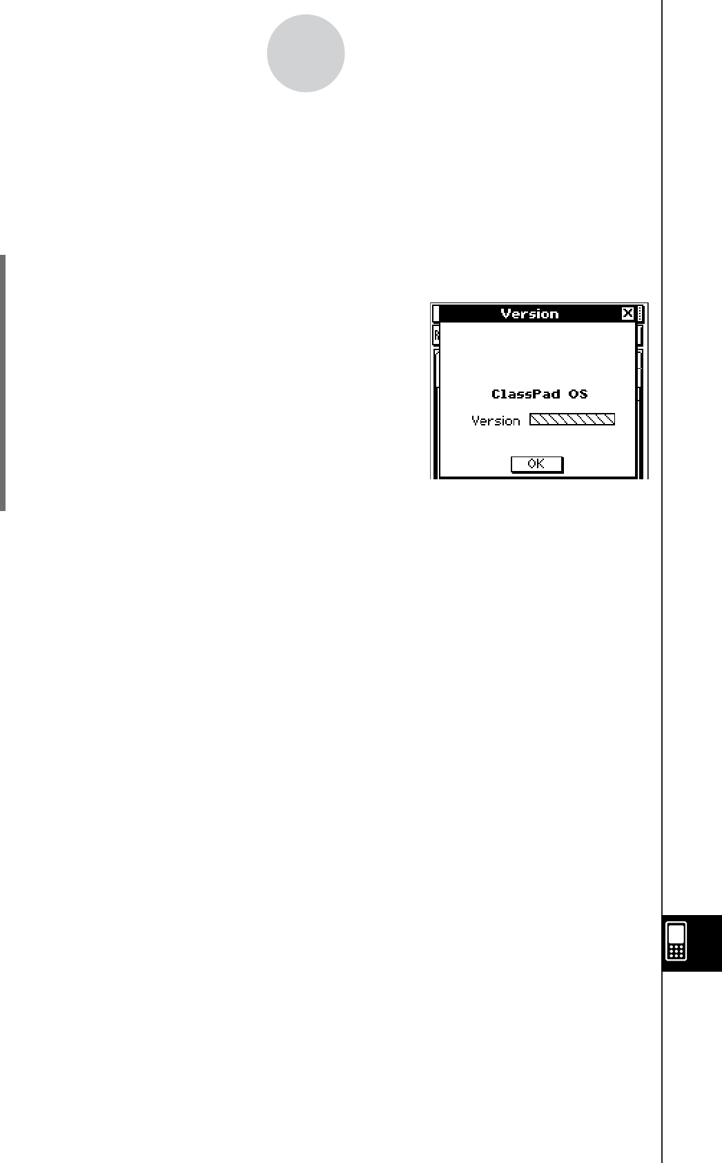
20110901

16-8 Viewing Version Information

Use the following procedure when you want to view version information about your

ClassPad’s operating system.

u To view software version information

(1) On the application menu, tap Y.

• This starts up the System application.

(2) Tap

> to display the Version dialog box.

(3) To close the Version dialog box, tap [OK]. This returns you to [Memory Usage].

16-8-1

Viewing Version Information

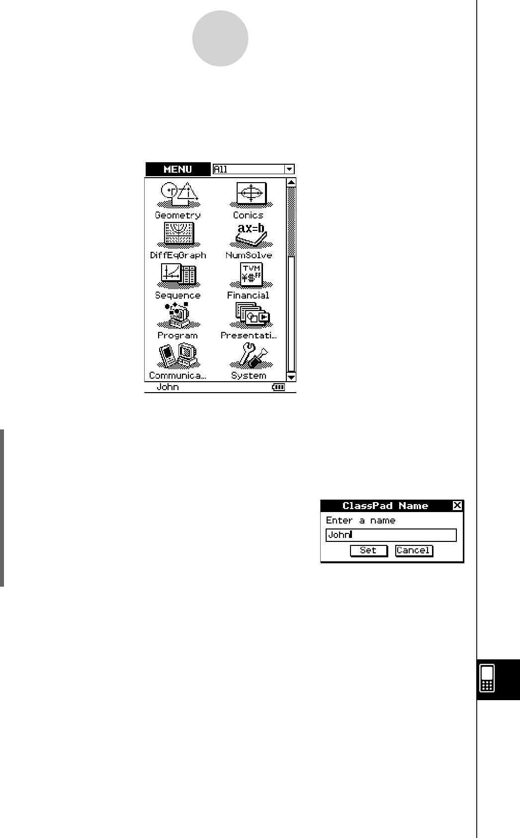
20110401

u ClassPad Operation

(1) On the application menu, tap Y.

• This starts up the System application.

(2) Tap [System] and then [ClassPad Name] to display the

ClassPad Name dialog box.

(3) Enter your name on the dialog box.

16-9 Registering a User Name on a ClassPad

You can register your name on your ClassPad so it appears at the bottom of the application

menu screen.

(4) Tap [Set] to register your name or [Cancel] to cancel.

16-9-1

Registering a User Name on a ClassPad

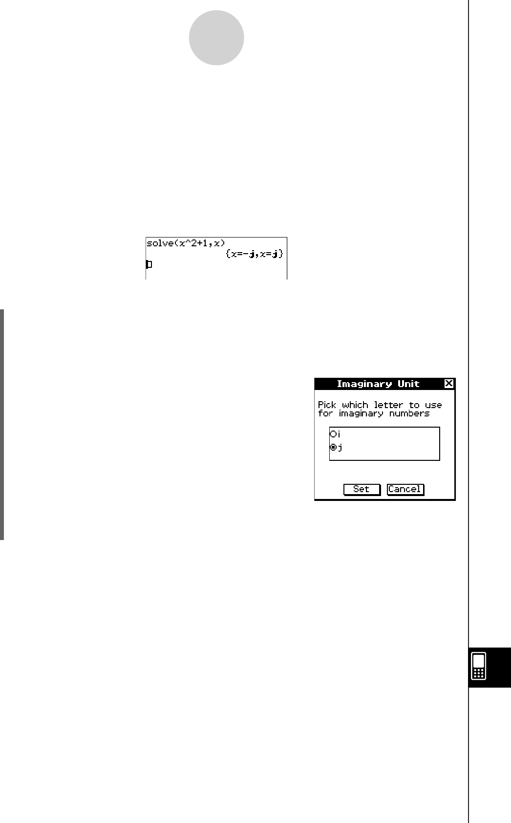
20110401

u ClassPad Operation

(1) On the application menu, tap Y.

• This starts up the System application.

(2) Tap [System] and then [Imaginary Unit] to display the

Imaginary Unit dialog box.

(3) On the Imaginary Unit dialog box, select the type of

imaginary unit you want to use.

16-10 Specifying the Complex Number

Imaginary Unit

In mathematics, the imaginary unit i allows the real number system R to be extended to the

complex number system C.

In electrical engineering and related fields, the imaginary unit is often written as j to avoid

confusion with a changing current, traditionally denoted by i.

Your ClassPad lets you specify either “i” or “j” for the imaginary unit.

(4) After the setting is the way you want, tap [Set] to apply it and close the Imaginary Unit

dialog box, or tap [Cancel] to close without changing the setting.

16-10-1

Specifying the Complex Number Imaginary Unit

20110401

u ClassPad Operation

(1) On the application menu, tap Y.

• This starts up the System application.

(2) Tap [System] and then [Shift Keys] to display the Shift Key Assign dialog box.

(3) On the Shift Key Assign dialog box, select the “Set ( – ) as shift key” check box.

(4) Tap the down arrow button then select the hard key to

which you want to assign a shift mode character string.

(5) Input the character string or function name, or specify

the operation you want to assign to the hard key.

• Use the soft keyboard to assign a character string or

function name.

16-11 Assigning Shift Mode Key Operations to

Hard Keys

You can configure your ClassPad so the z key functions as a shift key, and assign shift

mode key operations (such as character strings or function names, or operations) to the hard

keys. Then you can access a hard key shift mode operation by pressing the z key and then

the hard key.

16-11-1

Assigning Shift Mode Key Operations to Hard Keys

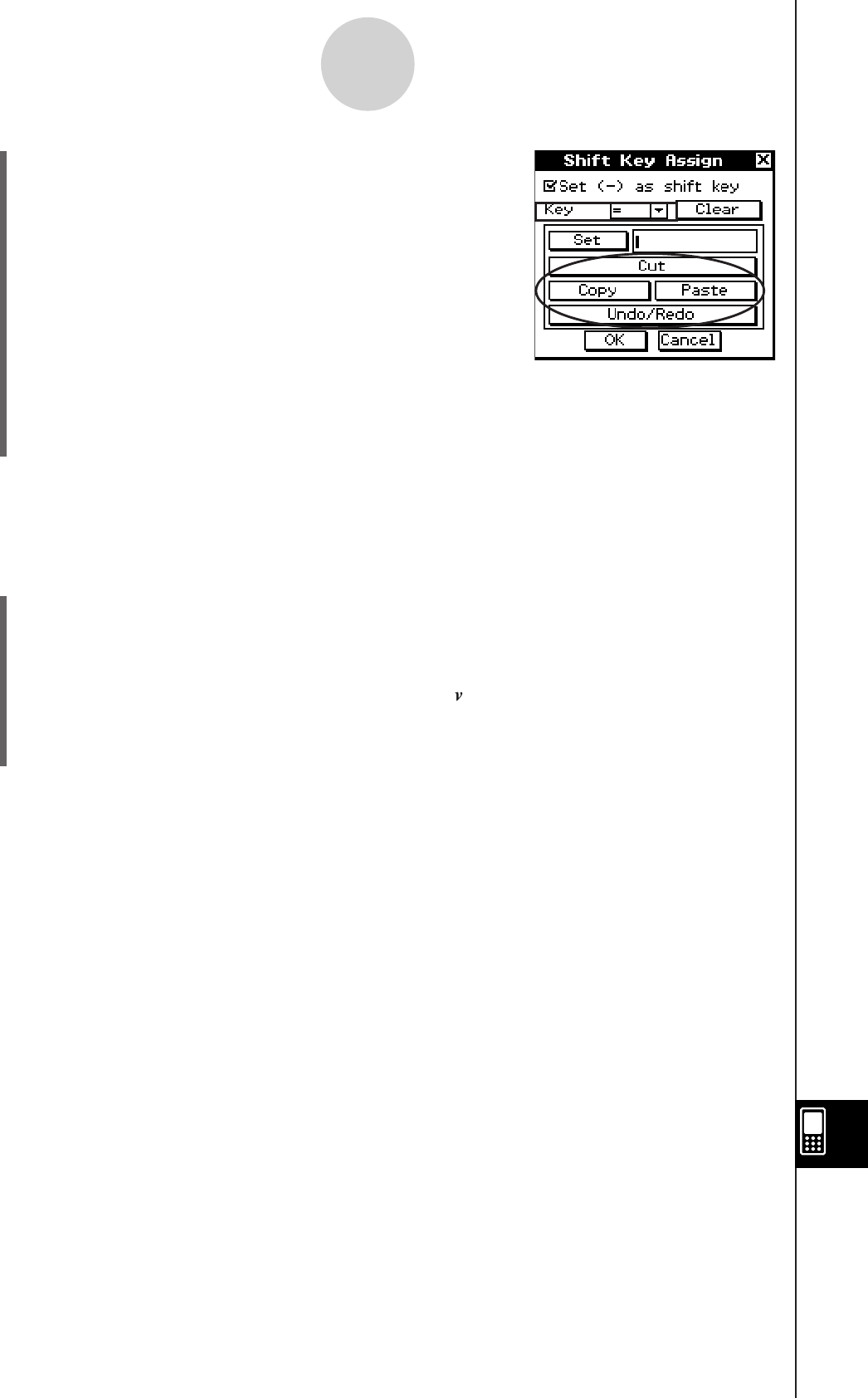
20110401

16-11-2

Assigning Shift Mode Key Operations to Hard Keys

• To assign the Cut, Copy, Paste, or Undo/Redo

operation, tap the applicable button on the dialog box.

• To clear the current assignment from the hard key, tap [Clear Assignment].

(6) After all the settings are the way you want, tap [OK] to apply them and close the Shift

Key Assign dialog box.

Example : To configure a shift operation that inserts the variable assignment character “v”

automatically when

z and = key are pressed.

u ClassPad Operation

(1) Perform steps (1) through (3) of the above operation to enable shift key assignment.

(2) Tap the down arrow button and select [=].

(3)

k9V

(4) Tap inside the box next to the [Set] button. Tap [ in the soft keyboard.

(5) Tap the [OK] button.

• Now When you press z and then = , the “v” will appear.

u Using the Shift Mode with a Cursor Key

When the shift function of the z key is enabled, you can use it with cursor key.

• Shift

f: Moves the cursor to the beginning of the current line

• Shift

c: Moves the cursor to the end of the current line

• Shift

d or e: Select the expression in the current line to the right or left of the

cursor

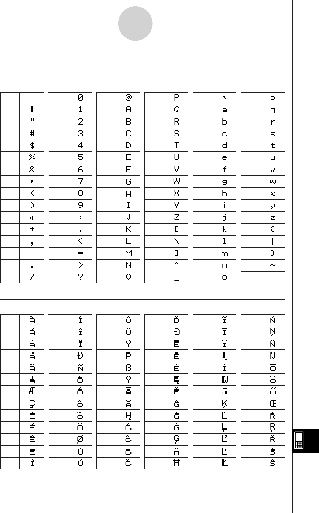
20110401

Appendix

1 Character Code Table

2 System Variable Table

3 Command and Function Index

4 Graph Types and Executable Functions

5 Error Message Table

20110401

1 Character Code Table

Characters from character code 257 onwards are 2-byte characters.

100

101

102

103

104

105

106

107

108

109

110

111

112

113

114

115

116

117

118

119

120

121

122

123

124

125

126

257

258

259

260

261

262

263

264

265

266

267

268

269

270

271

272

273

274

275

276

277

278

279

280

281

282

283

284

285

286

287

288

289

290

291

292

293

294

295

296

297

298

299

300

301

302

303

304

305

306

307

308

309

310

311

312

313

314

315

316

317

318

319

320

321

322

323

324

325

326

327

328

329

330

331

332

333

334

-1-1

Character Code Table

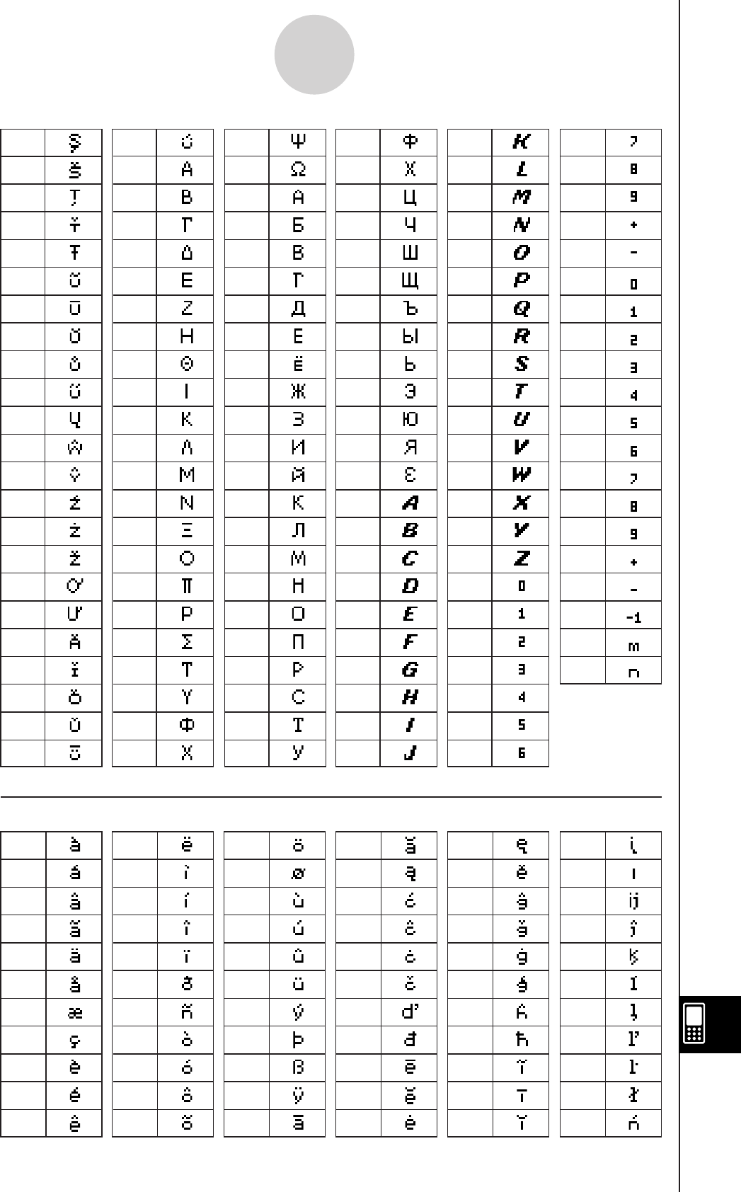
20110401

335

336

337

338

339

340

341

342

343

344

345

346

347

348

349

350

351

352

353

354

355

356

357

358

359

360

361

362

363

364

365

366

367

368

369

370

371

372

373

374

375

376

377

378

379

380

381

382

383

384

385

386

387

388

389

390

391

392

393

394

395

396

397

398

399

400

401

402

403

404

405

406

407

408

409

410

411

412

413

414

415

416

417

418

419

420

421

422

423

424

425

426

427

428

429

430

431

432

433

434

435

436

437

438

439

440

441

442

480

481

482

483

484

485

486

487

488

489

490

491

496

497

498

499

500

501

502

503

504

505

506

507

508

509

510

513

514

515

516

517

518

519

520

521

522

523

524

525

526

527

528

529

530

531

532

533

534

535

536

537

538

539

540

541

542

543

544

545

546

547

548

549

550

551

552

553

554

555

556

557

558

559

560

561

562

563

564

565

566

567

568

569

570

571

572

573

574

575

576

577

578

-1-2

Character Code Table

20110401

579

580

581

582

583

584

585

586

587

588

589

590

591

592

593

594

595

596

597

598

599

600

601

602

603

604

605

606

607

608

609

610

611

612

613

614

615

616

617

618

619

620

621

622

623

624

625

626

627

628

629

630

631

632

633

634

635

636

637

638

639

640

641

642

643

644

645

646

647

648

649

650

651

652

653

654

655

656

657

658

659

660

661

662

663

664

665

666

667

668

669

670

671

672

673

674

675

676

677

678

679

680

681

682

683

684

685

686

687

688

689

690

691

692

693

694

695

696

697

698

736

737

738

739

740

741

742

743

744

745

746

752

753

754

755

756

757

758

759

760

761

762

763

764

765

766

769

770

771

772

773

774

775

776

777

778

779

780

781

782

783

784

785

786

787

788

789

790

791

792

793

794

795

796

797

798

799

800

801

802

803

804

805

806

807

808

809

810

811

812

813

814

815

816

817

818

819

820

821

822

-1-3

Character Code Table

20110401

823

824

825

826

827

828

829

830

831

832

833

834

835

836

837

838

839

840

841

843

844

845

846

847

848

849

850

851

852

853

854

855

856

857

858

859

860

861

862

863

864

865

866

867

868

869

870

871

872

873

874

875

876

877

878

879

880

881

882

883

884

885

886

887

888

889

890

891

892

893

894

895

896

897

898

899

900

901

902

903

904

905

906

907

908

909

910

911

912

913

914

915

916

917

918

919

920

921

922

923

924

925

926

927

928

929

930

931

932

933

934

935

936

937

938

939

940

941

943

-1-4

Character Code Table

20110401

2 System Variable Table

Name Description Input Delete Data Type Default

a0Sequence Variable – EXPR (Real Number) 0

a1Sequence Variable – EXPR (Real Number) 0

a2Sequence Variable – EXPR (Real Number) 0

aCoef Regression Coefficient a– – EXPR (Real Number)

acSeq Sequence Graph Trace Variable – – EXPR (Real Number)

anRecursion Expression Variable – – STR

an+1 Recursion Expression Variable 

STR

an+2 Recursion Expression Variable 

STR

an0Recursion Internal Variable – – EXPR (Real Number)

an1Recursion Internal Variable – – EXPR (Real Number)

an2Recursion Internal Variable – – EXPR (Real Number)

anE Sequence Expression 

STR

anE0Recursion Internal Variable – – EXPR (Real Number)

angleθAngle between Line of Vision and

x-axis of 3D Graph View Window Value – EXPR (Real Number) 20

angleϕAngle between Line of Vision and

z-axis of 3D Graph View Window Value – EXPR (Real Number) 70

ans Latest Result Output by Main/eActivity

Applications – – EXPR/LIST/MAT/STR

anStart Sequence Variable – EXPR (Real Number) 0

b0Sequence Variable – EXPR (Real Number) 0

b1Sequence Variable – EXPR (Real Number) 0

b2Sequence Variable – EXPR (Real Number) 0

bCoef Regression Coefficient b– – EXPR (Real Number)

bcSeq Sequence Graph Trace Variable – – EXPR (Real Number)

bnRecursion Expression Variable – – STR

bn+1 Recursion Expression Variable 

STR

bn+2 Recursion Expression Variable 

STR

bn0Recursion Internal Variable – – EXPR (Real Number)

bn1Recursion Internal Variable – – EXPR (Real Number)

bn2Recursion Internal Variable – – EXPR (Real Number)

-2-1

System Variable Table

: Possible –: Not possible <blank>: No default

• Items in parentheses (( )) indicate limiting conditions of corresponding data type.

• Braces ({ }) indicate items that can be specified for elements.

20110401

Name Description Input Delete Data Type Default

bnE Sequence Expression 

STR

bnE0Recursion Internal Variable – – EXPR (Real Number)

bnStart Sequence Variable – EXPR (Real Number) 0

c0Sequence Variable – EXPR (Real Number) 0

c1Sequence Variable – EXPR (Real Number) 0

c2Sequence Variable – EXPR (Real Number) 0

cCoef Regression Coefficient c– – EXPR (Real Number)

ccSeq Sequence Graph Trace Variable – – EXPR (Real Number)

cnRecursion Expression Variable – – STR

cn+1 Recursion Expression Variable 

STR

cn+2 Recursion Expression Variable 

STR

cn0Recursion Internal Variable – – EXPR (Real Number)

cn1Recursion Internal Variable – – EXPR (Real Number)

cn2Recursion Internal Variable – – EXPR (Real Number)

cnE Sequence Expression 

STR

cnE0Recursion Internal Variable – – EXPR (Real Number)

cnStart Sequence Variable – EXPR (Real Number) 0

ConicsEq Conics Expression 

STR

dCoef Regression Coefficient d– – EXPR (Real Number)

df Degrees of Freedom – – EXPR (Real Number)

dfADegrees of Freedom for Factor A – – EXPR (Real Number)

dfAB Degrees of Freedom for Factor A

× Factor B – – EXPR (Real Number)

dfBDegrees of Freedom for Factor B – – EXPR (Real Number)

dfErr Degrees of Freedom for Error – – EXPR (Real Number)

eCoef Regression Coefficient e– – EXPR (Real Number)

Expected Expected Matrix for χ2 Test – – MAT{Real Number}

FEnd Table Creation Variable – EXPR (Real Number) 5

FResult Table Result Variable – – MAT

FStart Table Creation Variable – EXPR (Real Number) 1

FStep Table Creation Variable – EXPR (Real Number) 1

Fvalue F Value – – EXPR (Real Number)

FvalueA F Value for Factor A – – EXPR (Real Number)

FvalueAB F Value for Factor A × Factor B – – EXPR (Real Number)

FvalueB F Value for Factor B – – EXPR (Real Number)

GconHEnd Graph Transformation Vertical End

Point – – EXPR (Real Number) 5

-2-2

System Variable Table

20110401

Name Description Input Delete Data Type Default

GconHStart Graph Transformation Vertical Start

Point – – EXPR (Real Number) 1

GconHStep Graph Transformation Vertical Step

Value – – EXPR (Real Number) 1

GconWEnd Graph Transformation Horizontal End

Point – – EXPR (Real Number) 5

GconWStart Graph Transformation Horizontal Start

Point – – EXPR (Real Number) 1

GconWStep Graph Transformation Horizontal Step

Value – – EXPR (Real Number) 1

HStart Start Value for Histogram – EXPR (Real Number) 0

HStep Step Value for Histogram – EXPR (Real Number) 1

LInterval Lower Limit of Confidence Interval – – EXPR (Real Number)

list1 Default List 

LIST

{ }

(blank

list)

list2 Default List 

LIST { }

list3 Default List 

LIST { }

list4 Default List 

LIST { }

list5 Default List 

LIST { }

list6 Default List 

LIST { }

maxX Maximum Value of x

(Statistics Calculation) – – EXPR (Real Number)

maxY Maximum Value of y

(Statistics Calculation) – – EXPR (Real Number)

MeanSA Mean Square for Factor A – – EXPR (Real Number)

MeanSAB Mean Square for Factor A × Factor B – – EXPR (Real Number)

MeanSB Mean Square for Factor B – – EXPR (Real Number)

MeanSErr Mean Square for Error – – EXPR (Real Number)

MedStat Median Value (Statistics Calculation) – – EXPR (Real Number)

medx1MedMed Graph Summary Point – – EXPR (Real Number)

medx2MedMed Graph Summary Point – – EXPR (Real Number)

medx3MedMed Graph Summary Point – – EXPR (Real Number)

medy1MedMed Graph Summary Point – – EXPR (Real Number)

medy2MedMed Graph Summary Point – – EXPR (Real Number)

medy3MedMed Graph Summary Point – – EXPR (Real Number)

minX Minimum Value of x

(Statistics Calculation) – – EXPR (Real Number)

minY Minimum Value of y

(Statistics Calculation) – – EXPR (Real Number)

-2-3

System Variable Table

20110401

Name Description Input Delete Data Type Default

ModeFStat Frequency of Mode Values

(Statistics Calculation) – – EXPR (Real Number)

ModeNStat Number of Mode Values

(Statistics Calculation) – – EXPR (Real Number)

ModeStat Mode Value (Statistics Calculation) – – LIST {Real Number}

MSe Mean Square Error for Regression – – EXPR (Real Number)

n1Stat

Size of Sample 1 (Statistics Calculation)

– – EXPR (Real Number)

n2Stat

Size of Sample 2 (Statistics Calculation)

– – EXPR (Real Number)

ncSeq Sequence Graph Trace Variable – – EXPR (Real Number)

nSeq Sequence Variable – – EXPR (Real Number)

nStat Sample Size (Statistics Calculation) – – EXPR (Real Number)

Observed Observed Matrix for χ2 Test – – MAT {Real Number}

p Estimated Proportion – – EXPR (Real Number)

p1 Estimated Proportion of Sample 1 – – EXPR (Real Number)

p2 Estimated Proportion of Sample 2 – – EXPR (Real Number)

prob p-value – – EXPR (Real Number)

probA p-value of Factor A – – EXPR (Real Number)

probAB p-value of Factor A × Factor B – – EXPR (Real Number)

probB p-value of Factor B – – EXPR (Real Number)

Q1Stat First Quartile Point

(Statistics Calculation) – – EXPR (Real Number)

Q3Stat Third Quartile Point

(Statistics Calculation) – – EXPR (Real Number)

r1(θ)~r100(θ)

Graph Expression Input Variable,

r= Expression Type



(

Define

)FUNC

r2Corr Coefficient of Determination – – EXPR (Real Number)

randResult Internal Variable Used for Calculation

of Next Random Number – – EXPR (Real Number) –1

rc Graph Coordinate Value Storage

Variable – – EXPR (Real Number) 0

rCorr Correlation Coefficient – – EXPR (Real Number)

residual Residual Data Storage List – – LIST {Real Number}

Seed Random Seed Value – – EXPR (Real Number) 0

smin3D 3D Graph View Window Display

s Minimum Value – EXPR(Real Number) −π

smax3D 3D Graph View Window Display

s Maximum Value – EXPR(Real Number) π

spPooled Sample Standard Deviation – – EXPR (Real Number)

SqEnd Sequence Creation Variable – EXPR (Real Number) 5

-2-4

System Variable Table

20110401

-2-5

System Variable Table

Name Description Input Delete Data Type Default

SqResult Sequence Result Variable – – MAT

SqStart Sequence Creation Variable – EXPR (Real Number) 1

Sres11 Calculation Result for StatGraph1 – – LIST {Real Number}

Sres12 Calculation Result for StatGraph1 – – LIST {Real Number}

Sres21 Calculation Result for StatGraph2 – – LIST {Real Number}

Sres22 Calculation Result for StatGraph2 – – LIST {Real Number}

Sres31 Calculation Result for StatGraph3 – – LIST {Real Number}

Sres32 Calculation Result for StatGraph3 – – LIST {Real Number}

Sres41 Calculation Result for StatGraph4 – – LIST {Real Number}

Sres42 Calculation Result for StatGraph4 – – LIST {Real Number}

Sres51 Calculation Result for StatGraph5 – – LIST {Real Number}

Sres52 Calculation Result for StatGraph5 – – LIST {Real Number}

Sres61 Calculation Result for StatGraph6 – – LIST {Real Number}

Sres62 Calculation Result for StatGraph6 – – LIST {Real Number}

Sres71 Calculation Result for StatGraph7 – – LIST {Real Number}

Sres72 Calculation Result for StatGraph7 – – LIST {Real Number}

Sres81 Calculation Result for StatGraph8 – – LIST {Real Number}

Sres82 Calculation Result for StatGraph8 – – LIST {Real Number}

Sres91 Calculation Result for StatGraph9 – – LIST {Real Number}

Sres92 Calculation Result for StatGraph9 – – LIST {Real Number}

sStat Standard Error Value for LinReg

TTest Calculation – – EXPR (Real Number)

SumSA Sum of Squares for Factor A – – EXPR (Real Number)

SumSAB

Sum of Squares for Factor A × Factor

– – EXPR (Real Number)

SumSB Sum of Squares for Factor B – – EXPR (Real Number)

SumSErr Sum of Squares for Error – – EXPR (Real Number)

sxSample Standard Deviation of x

(Statistics Calculation) – – EXPR (Real Number)

sx1Sample Standard Deviation of Data 1 – – EXPR (Real Number)

sx2Sample Standard Deviation of Data 2 – – EXPR (Real Number)

sySample Standard Deviation of y

(Statistics Calculation) – – EXPR (Real Number)

tc Graph Coordinate Value Storage

Variable – – EXPR (Real Number) 0

tLower Result of TCD Calculation – – EXPR (Real Number)

tmin3D 3D Graph View Window Display

t Minimum Value – EXPR(Real Number) −π

tmax3D 3D Graph View Window Display

t Maximum Value – EXPR(Real Number) π

20110401

-2-6

System Variable Table

Name Description Input Delete Data Type Default

tUpper Result of TCD Calculation – – EXPR (Real Number)

Tvalue t Value – – EXPR (Real Number)

tθmax View Window Tθ

Maximum Value – EXPR (Real Number) 2π

tθmin View Window Tθ

Minimum Value – EXPR (Real Number) 0

tθStep View Window Tθ

Step Value Variable – EXPR (Real Number) π /60

UInterval Upper Limit of Confidence Interval – – EXPR (Real Number)

oMean of x (Statistics Calculation) – – EXPR (Real Number)

Inv Result of Inverse Cumulative

Distribution Calculations – – EXPR(Real Number)

o1Mean of Data 1 – – EXPR (Real Number)

x1(y)~x100(y)

Graph Expression Input Variable,

X= Type



(

Define

)FUNC

x1InvN Result of InvNorm Calculation – – EXPR (Real Number)

o2Mean of Data 2 – – EXPR (Real Number)

x2InvN Result of InvNorm Calculation – – EXPR (Real Number)

xc Graph Coordinate Value Storage

Variable – – EXPR (Real Number) 0

xdot View Window 1-dot x-axis Value – EXPR (Real Number) 0.1

xfact Factor Zoom X-factor Value – EXPR (Real Number) 2

xgrid3D 3D Graph View Window Value – EXPR (Real Number) 25

xmax View Window Display Range x-axis

Maximum Value – EXPR (Real Number) 7.7

xmax3D 3D Graph View Window Display

Range x-axis Maximum Value – EXPR (Real Number) 3

xmin View Window Display Range x-axis

Minimum Value – EXPR (Real Number) –7.7

xmin3D 3D Graph View Window Display

Range x-axis Minimum Value – EXPR (Real Number) –3

xscl View Window Display Range XScale – EXPR (Real Number) 1

xt1(t)~

xt100(t)

Graph Expression Input Variable,

Param Type



(

Define

)FUNC

pMean of y (Statistics Calculation) – – EXPR (Real Number)

y1(x)~

y100(x)

Graph Expression Input Variable,

Y= Expression Type



(

Define

)FUNC

ycGraph Coordinate Value Storage

Variable – – EXPR (Real Number) 0

ydot View Window 1-dot y-axis Value – EXPR (Real Number) 0.1

yfact Factor Zoom Y-factor Value – EXPR (Real Number) 2

ygrid3D 3D Graph View Window Value – EXPR (Real Number) 25

20110401

-2-7

System Variable Table

Name Description Input Delete Data Type Default

ymax View Window Display Range y-axis

Maximum Value – EXPR (Real Number) 3.8

ymax3D 3D Graph View Window Display

Range y-axis Maximum Value – EXPR (Real Number) 3

ymin View Window Display Range y-axis

Minimum Value – EXPR (Real Number) –3.8

ymin3D 3D Graph View Window Display

Range y-axis Minimum Value  – EXPR (Real Number) –3

yscl View Window Display Range YScale – EXPR (Real Number) 1

yt1(t)~

yt100(t)

Graph Expression Input Variable,

Param Type



(

Define

)FUNC

z1(x,y)~

z100(x,y)3D Graph Function Expression 

(

Define

)FUNC

zc Graph Coordinate Value Storage

Variable – – EXPR (Real Number) 0

zLower Result of NormCD Calculation – – EXPR (Real Number)

zmax3D 3D Graph View Window Display

Range z-axis Maximum Value  – EXPR (Real Number) 3

zmin3D 3D Graph View Window Display

Range z-axis Minimum Value  – EXPR (Real Number) –3

zUpper Result of NormCD Calculation – – EXPR (Real Number)

Zvalue z Value – – EXPR (Real Number)

θcGraph Coordinate Value Storage

Variable – – EXPR (Real Number) 0

ȸxSum of x (Statistics Calculation) – – EXPR (Real Number)

σxPopulation Standard Deviation of x

(Statistics Calculation) – – EXPR (Real Number)

ȸx2Sum of x2 (Statistics Calculation) – – EXPR (Real Number)

ȸxy Sum of xy Data (Statistics Calculation) – – EXPR (Real Number)

ȸySum of y (Statistics Calculation) – – EXPR (Real Number)

σyPopulation Standard Deviation of y

(Statistics Calculation) – – EXPR (Real Number)

ȸy2Sum of y2– – EXPR (Real Number)

χ2value χ2 Value – – EXPR (Real Number)

20110501

3 Command and Function Index

-3-1

Command and Function Index

Command/Function Form Page Command/Function Form Page

abExpR Cmd 12-6-32

abExpReg Cmd 12-6-27

abs Func 2-4-5

absExpand Func 2-8-45

amortBal Func 2-8-60

amortInt Func 2-8-61

amortPrn Func 2-8-61

amortSumInt Func 2-8-61

amortSumPrn Func 2-8-61



and Cmd 2-8-46

andConnect Func 2-8-45

angle Func 2-8-40

approx Func 2-8-3

arcLen Func 2-8-16

arg Func 2-8-19

arrange Func 2-8-47

augment Func 2-8-22,

2-8-31,

2-8-39

baseConvert Func 2-7-5

BinomialCD Cmd 7-11-16

binomialCDf Func 2-8-53

BinomialPD Cmd 7-11-15

binomialPDf Func 2-8-52

bondPriceDate Func 2-8-63

bondPriceTerm Func 2-8-63

bondYieldDate Func 2-8-64

bondYieldTerm Func 2-8-64

Box Cmd 12-6-33

Break Cmd 12-6-9

Broken Cmd 12-6-32

CallUndef Cmd 12-6-23

cashIRR Func 2-8-59

cashNFV Func 2-8-60

cashNPV Func 2-8-60

cashPBP Func 2-8-60

cExpand Func 2-8-20

ChiCD Cmd 7-11-10

chiCDf Func 2-8-51

ChiGOFTest Cmd 7-9-15

ChiPD Cmd 7-11-9

chiPDf Func 2-8-51

ChiTest Cmd 7-9-14

ChrToNum Cmd 12-6-41

Circle Cmd 12-6-15

Clear_a_z Cmd 2-8-48,

12-6-38

ClearSheet Cmd 12-6-15

ClearSheet3D Cmd 12-6-24

CloseComPort38k Cmd 12-6-45

ClrGraph Cmd 12-6-16

ClrText Cmd 12-6-6

Cls Cmd 12-6-16

cmpdFV Func 2-8-58

cmpdIR Func 2-8-58

cmpdN Func 2-8-59

cmpdPmt Func 2-8-59

cmpdPV Func 2-8-59

convEff Func 2-8-62

convNom Func 2-8-62

colDim Func 2-8-37

collect Func 2-8-5

colNorm Func 2-8-38

combine Func 2-8-5

compToPol Func 2-8-21

compToRect Func 2-8-21

compToTrig Func 2-8-21

conjg Func 2-8-20

const Func 2-4-15

constn Func 2-4-15

CopyVar Cmd 12-6-38

cos Func 2-4-2

cos–1 Func 2-4-2

cosh Func 2-4-4

cosh–1 Func 2-4-4

Cross Cmd 12-6-32

crossP Func 2-8-40

CubicR Cmd 12-6-32

CubicReg Cmd 12-6-28

cuml Func 2-8-29

20110501

-3-2

Command and Function Index

Command/Function Form Page Command/Function Form Page

DateMode360 Func 15-17-1

DateMode365 Func 15-17-1

dayCount Func 2-8-63

DefaultListEditor Cmd 12-6-28

DefaultSetup Cmd 12-6-33

Define Cmd 2-8-64,

12-6-9

DelFolder Cmd 12-6-39

DelVar Cmd 2-8-64,

12-6-39

delta Func 2-4-16

denominator Func 2-8-19

det Func 2-8-33

diag Func 2-8-32

diff Func 2-8-13

dim Func 2-8-28,

2-8-33,

2-8-39

DispDfrTbl Cmd 12-6-25

DispDQTbl Cmd 12-6-25

DispFibTbl Cmd 12-6-25

DispFTable Cmd 12-6-16

DispListEditor Cmd 12-6-28

DispQutTbl Cmd 12-6-25

DispSeqTbl Cmd 12-6-25

DispSmryTbl Cmd 12-6-16

DispStat Cmd 2-8-64,

12-6-28

DispText Cmd 12-6-6

Distance Cmd 12-6-16

dms Func 2-8-7

Do~LpWhile Cmd 12-6-9

Dot Cmd 12-6-32

dotP Func 2-8-40

DrawConics Cmd 12-6-25

DrawFTGCon, DrawFTGPlot

Cmd 12-6-16

DrawGraph Cmd 12-6-17

DrawSeqCon, DrawSeqPlt Cmd 12-6-26

DrawSeqEtrCon, DrawSeqEtrPlt

Cmd 12-6-26

DrawShade Cmd 12-6-17

DrawStat Cmd 12-6-28

Draw3D Cmd 12-6-24

dSolve Func 2-8-8,

2-8-44

E Cmd

Func 2-4-3

eigVc Func 2-8-35

eigVl Func 2-8-34

eliminate Func 2-8-45

exchange Func 2-8-45

expand Func 2-8-4

ExpR Cmd 12-6-32

ExpReg Cmd 12-6-28

ExpToStr Cmd 12-6-42

expToTrig Func 2-8-6

factor Func 2-8-4

factorOut Func 2-8-5

FCD Cmd 7-11-13

fCDf Func 2-8-52

FFT Func 2-8-11

fill Func 2-8-22,

2-8-32,

2-8-39

fMax Func 2-8-18

fMin Func 2-8-17

For~To~(Step~)Next Cmd 12-6-10

fourier Func 2-8-9

FPD Cmd 7-11-12

fPDf Func 2-8-52

frac Func 2-4-5

fRound Func 2-4-5

gamma Func 2-4-18

gcd Func 2-8-18

GeoCD Cmd 7-11-22

geoCDf Func 2-8-55

GeoPD Cmd 7-11-21

geoPDf Func 2-8-55

GetFolder Cmd 12-6-39

GetKey Cmd 12-6-3

getLeft Func 2-8-46

GetPen Cmd 12-6-4

getRight Func 2-8-45

GetType Cmd 12-6-39

GetVar38k Cmd 12-6-45

Goto~Lbl Cmd 12-6-10

20110501

-3-3

Command and Function Index

Command/Function Form Page Command/Function Form Page

GraphType Cmd 12-6-17

GTSelOff Cmd 12-6-17

GTSelOn Cmd 12-6-18

heaviside Func 2-4-17

Histogram Cmd 12-6-32

Horizontal Cmd 12-6-18

HypergeoCD Cmd 7-11-25

hypergeoCDf Func 2-8-56

HypergeoPD Cmd 7-11-24

hypergeoPDf Func 2-8-56

i Cmd

ident Func 2-8-31

IFFT Func 2-8-11

If~Then~ElseIf~Else ~IfEnd Cmd 12-6-11

iGcd Func 2-4-9

iLcm Func 2-4-10

im Func 2-8-20

iMod Func 2-4-10

impDiff Func 2-8-13

Input Cmd 12-6-4

InputFunc Cmd 12-6-5

InputStr Cmd 12-6-5

int Func 2-4-5

intg Func 2-4-5

InvBinomialCD Cmd 7-11-17

invBinomialCDf Func 2-8-53

InvChiCD Cmd 7-11-11

invChiCDf Func 2-8-51

Inverse Cmd 12-6-18

invert Func 2-8-47

InvFCD Cmd 7-11-14

invFCDf Func 2-8-52

InvFourier Func 2-8-9

InvGeoCD Cmd 7-11-23

invGeoCDf Func 2-8-55

InvHypergeoCD Cmd 7-11-26

invHypergeoCDf Func 2-8-56

invLaplace Func 2-8-8

InvNorm Cmd 7-11-6

InvNormCD Cmd 7-11-6

invNormCDf Func 2-8-50

InvPoissonCD Cmd 7-11-20

invPoissonCDf Func 2-8-54

InvTCD Cmd 7-11-8

invTCDf Func 2-8-51

isPrime Func 2-4-13

judge Func 2-4-12

laplace Func 2-8-8

lcm Func 2-8-19

Ldot Cmd 12-6-32

lim Func 2-8-15

Line Cmd 12-6-18

LinearR Cmd 12-6-32

LinearReg Cmd 12-6-29

LinRegTTest Cmd 7-9-13

listToMat Func 2-8-24,

2-8-32

In Func 2-4-3

Local Cmd 12-6-40

Locate Cmd 12-6-7

Lock Cmd 12-6-40

LockFolder Cmd 12-6-40

log Func 2-4-3

LogisticR Cmd 12-6-32

LogisticReg Cmd 12-6-29

LogP Cmd 12-6-23

LogR Cmd 12-6-32

LogReg Cmd 12-6-29

LU Func 2-8-35

matToList Func 2-8-24,

2-8-33

max Func 2-8-25

mean Func 2-8-26

MedBox Cmd 12-6-32

median Func 2-8-26

MedMed Cmd 12-6-32

MedMedLine Cmd 12-6-29

Message Cmd 12-6-7

min Func 2-8-25

mod Func 2-8-16

ModBox Cmd 12-6-32

mode Func 2-8-26

MoveVar Cmd 12-6-40

mRow Func 2-8-36

mRowAdd Func 2-8-37

MultiSortA Cmd 12-6-30

20110501

-3-4

Command and Function Index

Command/Function Form Page Command/Function Form Page

MultiSortD Cmd 12-6-30

nCr Func 2-4-11

NDist Cmd 12-6-32

NewFolder Cmd 12-6-40

norm Func 2-8-34,

2-8-40

normal Func 2-8-16

NormalLine Cmd 12-6-18

NormCD Cmd 7-11-5

normCDf Func 2-8-50

NormPD Cmd 7-11-4

normPDf Func 2-8-49

not Func 2-8-46

NPPlot Cmd 12-6-32

nPr Func 2-4-11

Number Cmd 12-6-33

numerator Func 2-8-19

NumToChr Cmd 12-6-42

NumToStr Cmd 12-6-42

Off Cmd

On Cmd

OnePropZInt Cmd 7-10-6

OnePropZTest Cmd 7-9-6

OneSampleTInt Cmd 7-10-8

OneSampleTTest Cmd 7-9-9

OneSampleZInt Cmd 7-10-3

OneSampleZTest Cmd 7-9-3

OneVariable Cmd 12-6-30

OneWayANOVA Cmd 7-9-18

OpenComPort38k Cmd 12-6-46



or Cmd 2-8-46

Pause Cmd 12-6-13

percent Func 2-8-29

percentile Func 2-8-27

PeriodsAnnual Func 15-17-1

PeriodsSemi Func 15-17-1

piecewise Func 2-4-12

Plot Cmd 12-6-18

PlotChg Cmd 12-6-18

PlotOff Cmd 12-6-19

PlotOn Cmd 12-6-19

plotTest( Func 12-6-19

PmtBgn Func 15-17-1

PmtEnd Func 15-17-1

PoissonCD Cmd 7-11-19

poissonCDf Func 2-8-54

PoissonPD Cmd 7-11-18

poissonPDf Func 2-8-54

polyEval Func 2-8-29

PowerR Cmd 12-6-32

PowerReg Cmd 12-6-30

priceCost Func 2-8-62

priceMargin Func 2-8-63

priceSell Func 2-8-62

Print Cmd 12-6-7

PrintNatural Cmd 12-6-8

prod Func 2-8-28

propFrac Func 2-8-7

PTBrokenThck Cmd 12-6-19

PTCross Cmd 12-6-19

PTDot Cmd 12-6-19

PTNormal Cmd 12-6-19

PTSquare Cmd 12-6-19

PTThick Cmd 12-6-20

PxlChg Cmd 12-6-20

PxlOff Cmd 12-6-20

PxlOn Cmd 12-6-20

pxlTest( Func 12-6-20

Q1 Func 2-8-27

Q3 Func 2-8-27

QR Func 2-8-36

QuadR Cmd 12-6-32

QuadReg Cmd 12-6-31

QuartR Cmd 12-6-32

QuartReg Cmd 12-6-31

rand Func 2-4-7

randBin Func 2-4-8

randList Func 2-4-7

randNorm Func 2-4-7

RandSeed Cmd 2-4-9

rangeAppoint Func 2-8-16

rank Func 2-8-34

RclGMem Cmd 12-6-20

RclPict Cmd 12-6-20

RclVWin Cmd 12-6-21

re Func 2-8-20

20110501

-3-5

Command and Function Index

Command/Function Form Page Command/Function Form Page

Receive38k Cmd 12-6-46

ref Func 2-8-34

Rename Cmd 12-6-40

replace Func 2-8-47

Return Cmd 12-6-13

rewrite Func 2-8-44

rFactor Func 2-8-5

rotate Func 2-8-23

rowAdd Func 2-8-37

rowDim Func 2-8-37

rowNorm Func 2-8-37

rref Func 2-8-34

rSolve Func 6-3-5

Scatter Cmd 12-6-32

SelOn3D Cmd 12-6-24

Send38k Cmd 12-6-46

SendVar38k Cmd 12-6-46

seq Func 2-8-22

SeqSelOff Cmd 12-6-26

SeqSelOn Cmd 12-6-27

SeqType Cmd 12-6-27

sequence Func 2-8-30

SetAxes Cmd 12-6-33

SetAxes3D Cmd 12-6-33

SetBG Cmd 12-6-33

SetCellWidth Cmd 12-6-33

SetComplex Cmd 12-6-33

SetCoord Cmd 12-6-34

SetCoordOff3D Cmd 12-6-34

SetCoordPol3D Cmd 12-6-34

SetCoordRect3D Cmd 12-6-34

SetDecimal Cmd 12-6-34

SetDegree Cmd 12-6-34

SetDeriv Cmd 12-6-34

SetDispGCon Cmd 12-6-35

SetDrawCon Cmd 12-6-35

SetDrawPlt Cmd 12-6-35

SetFix Cmd 12-6-35

SetFolder Cmd 12-6-41

SetFunc Cmd 12-6-35

SetGrad Cmd 12-6-35

SetGrid Cmd 12-6-35

SetLabel Cmd 12-6-35

SetLabel3D Cmd 12-6-36

SetLeadCursor Cmd 12-6-36

SetNormal Cmd 12-6-36

SetRadian Cmd 12-6-36

SetReal Cmd 12-6-36

SetSci Cmd 12-6-36

SetSequence Cmd 12-6-37

SetSimulGraph Cmd 12-6-37

SetSmryTable Cmd 12-6-37

SetSmryTableQD Cmd 12-6-37

SetStandard Cmd 12-6-37

SetStatWinAuto Cmd 12-6-37

SetTVariable Cmd 12-6-38

SetΣdisp Cmd 12-6-38

SheetActive Cmd 12-6-21

SheetActive3D Cmd 12-6-24

SheetName Cmd 12-6-21

SheetName3D Cmd 12-6-24

shift Func 2-8-23

signum Func 2-4-5

simpFV Func 2-8-58

simplify Func 2-8-4

simpInt Func 2-8-58

sin Func 2-4-2

sin–1 Func 2-4-2

sinh Func 2-4-4

sinh–1 Func 2-4-4

SinR Cmd 12-6-32

SinReg Cmd 12-6-31

Skip Cmd 12-6-13

SmryTSelOn Cmd 12-6-21

solve Func 2-8-8,

2-8-43

sortA Func 2-8-23

sortD Func 2-8-24

Square Cmd 12-6-32

sRound Func 2-4-5

StatGraph Cmd 12-6-32

StatGraphSel Cmd 12-6-32

stdDev Func 2-8-27

StepDisp Cmd 12-6-37

StoGMem Cmd 12-6-21

Stop Cmd 12-6-13

20110501

-3-6

Command and Function Index

Command/Function Form Page

StoPict Cmd 12-6-22

StoVWin Cmd 12-6-22

StrCmp Cmd 12-6-42

StrInv Cmd 12-6-42

StrJoin Cmd 12-6-43

StrLeft Cmd 12-6-43

StrLen Cmd 12-6-43

StrLwr Cmd 12-6-43

StrMid Cmd 12-6-43

StrRight Cmd 12-6-43

StrRotate Cmd 12-6-44

StrShift Cmd 12-6-44

StrSrc Cmd 12-6-44

strToExp( Func 12-6-44

StrUpr Cmd 12-6-44

subList Func 2-8-23

subMat Func 2-8-32

sum Func 2-8-28

sumSeq Func 2-8-30

swap Func 2-8-36

Switch~Case~Default~SwitchEnd

Cmd 12-6-14

TableInput Cmd 12-6-38

tan Func 2-4-2

tan–1 Func 2-4-2

TangentLine Cmd 12-6-22

tanh Func 2-4-4

tanh–1 Func 2-4-4

tanLine Func 2-8-16

taylor Func 2-8-8

TCD Cmd 7-11-8

tCDf Func 2-8-51

tCollect Func 2-8-6

tExpand Func 2-8-6

Text Cmd 12-6-22

toCyl Func 2-8-42

toDMS Func 2-8-7

toFrac Func 2-8-6

toPol Func 2-8-41

toRect Func 2-8-41

toSph Func 2-8-41

TPD Cmd 7-11-7

tPDf Func 2-8-50

trigToExp Func 2-8-6

Command/Function Form Page

trn Func 2-8-31

TwoPropZInt Cmd 7-10-7

TwoPropZTest Cmd 7-9-7

TwoSampleFTest Cmd 7-9-17

TwoSampleTInt Cmd 7-10-10

TwoSampleTTest Cmd 7-9-11

TwoSampleZInt Cmd 7-10-4

TwoSampleZTest Cmd 7-9-5

TwoVariable Cmd 12-6-32

TwoWayANOVA Cmd 7-9-19

unitV Func 2-8-39

Unlock Cmd 12-6-41

UnlockFolder Cmd 12-6-41

variance Func 2-8-28

Vertical Cmd 12-6-22

ViewWindow Cmd 12-6-23

ViewWindow3D Cmd 12-6-24

VWin Cmd 12-6-37

Wait Cmd 12-6-14

While~WhileEnd Cmd 12-6-15



xor Cmd 2-8-46

xyLine Cmd 12-6-32

ZAuto Cmd 12-6-23

ZFactor Cmd 12-6-23

+ Cmd

– Cmd

× Cmd

/ Cmd

^ Cmd 2-4-3

^2 Cmd 2-4-5

^(–1) Cmd 2-4-5

= Cmd 2-4-14

≠ Cmd 2-4-14

< Cmd 2-4-14

> Cmd 2-4-14

s Cmd 2-4-14

t Cmd 2-4-14

! Cmd 2-4-5

% Cmd 2-4-5

| (with) Cmd 2-4-14

r Cmd 2-4-1

° Cmd 2-4-1

S Cmd 12-6-8

20110501

# Cmd 12-6-8

’ Cmd 2-4-13,

12-6-2

" Cmd 12-6-41

π Cmd

∞ Cmd 2-4-15

∠ Func 2-4-13

Func 2-4-5

Σ Func 2-8-15

Π Func 2-8-15

∫ Func 2-8-14

Alist Func 2-8-29

(Multi-statement Command)

12-6-2

(Carriage Return) 12-6-2

Command/Function Form Page

-3-7

Command and Function Index

20110401

-4-1

Graph Types and Executable Functions

4 Graph Types and Executable Functions

: Executable −: Not executable D: Executable with some conditions

Zoom

Graph Type

Function

Analysis

Sketch

G-Solve

Modify

Box

Out

Auto

Original

Square

Round

Integer

Quick Types

Trace

Cls

Plot

Line

Text

Normal

Inverse

Circle

Vertical

Horizontal

Root

Max

Min

Intersect

Inflection

Distance

π ∫ f(x)2dx

∫ dx

x-cal

y-cal

y-Intercept

Tangent

Dynamic Modify

Direct Modify



r=xt=



−



−



−



−



−



−



−



−



−



−



−



−



−



−



−



−



−



−



−



−



−



−



−



−



−



−



−



−



−

fMax

fMin



−



−



−



−

(Both

logarithms

only)

(Both

logarithms

only)

(Both

logarithms

only)

During

Log

Graphing

During

Log

Graphing

During

Log

Graphing

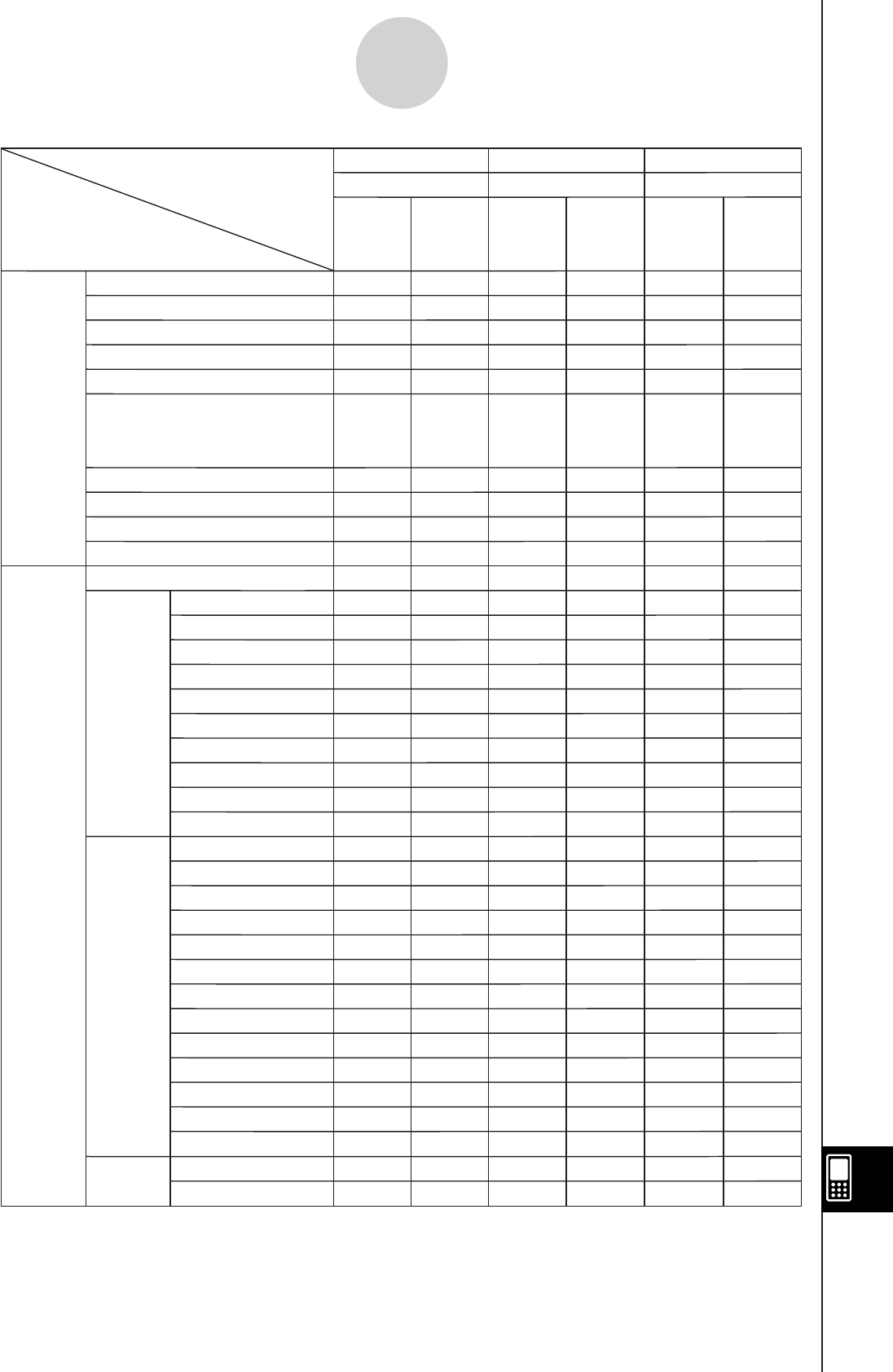
20110401

-4-2

Graph Types and Executable Functions

Zoom

Graph Type

Function

Analysis

Sketch

G-Solve

Modify

Box

Out

Auto

Original

Square

Round

Integer

Quick Types

Trace

Cls

Plot

Line

Text

Normal

Inverse

Circle

Vertical

Horizontal

Root

Max

Min

Intersect

Inflection

Distance

π ∫ f(x)2dx

∫ dx

x-cal

y-cal

y-Intercept

Tangent

Dynamic Modify

Direct Modify



y Inequality x Inequality



−



−



−



−



−



−



−



−



−



−



−



−



−



−



−



−



−



−



−



−



−



−



−



−



−



−



−



−



−



−

fMax

fMin

−

−



−



−



−

(Both

logarithms

only)

(Both

logarithms

only)

(Both

logarithms

only)

During

Log

Graphing

During

Log

Graphing

During

Log

Graphing

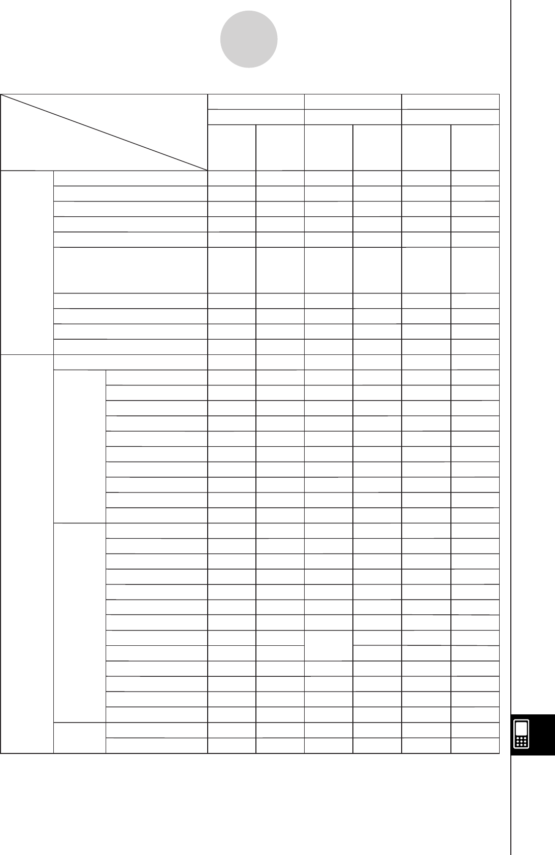
20110401

-4-3

Graph Types and Executable Functions

• Histogram

• Broken

Zoom

Graph Type

Function

Analysis

Sketch

G-Solve

Modify

Box

Out

Auto

Original

Square

Round

Integer

Quick Types

Trace

Cls

Plot

Line

Text

Normal

Inverse

Circle

Vertical

Horizontal

Root

Max

Min

Intersect

Inflection

Distance

π ∫ f(x)2dx

∫ dx

x-cal

y-cal

y-Intercept

Tangent

Dynamic Modify

Direct Modify



y ◆



−



−



−



−



−



−



−



−



−

fMax

fMin

−



−



−

(Both

logarithms

only)

During

Log

Graphing

−

Statistical - Plot

−



−

−−

−



−



−



−



−



−



−



−



−



−



−



−

(Both

logarithms

only)

During

Log

Graphing

During

Log

Graphing

(z-cal)

• Scatter

• xyLine

• NPPlot

Statistical - Plot

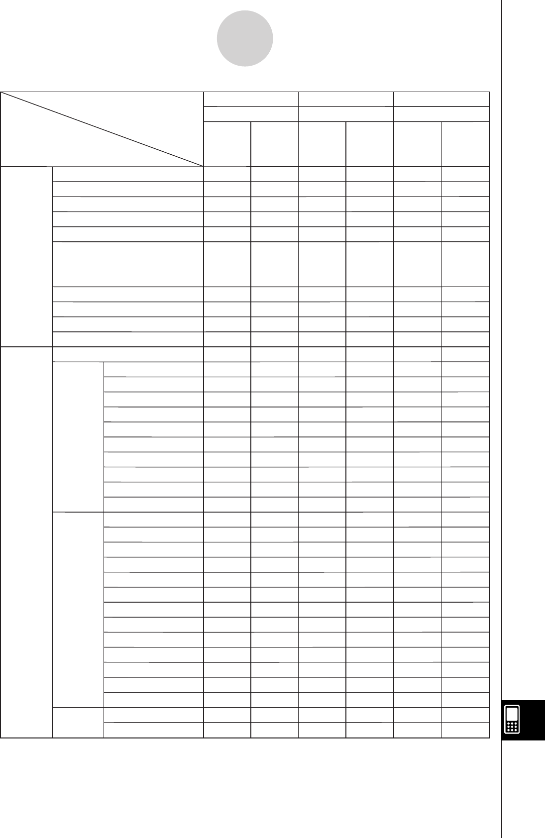
20110401

-4-4

Graph Types and Executable Functions

Statistical - Box

• MedBox

• ModBox

Zoom

Graph Type

Function

Analysis

Sketch

G-Solve

Modify

Box

Out

Auto

Original

Square

Round

Integer

Quick Types

Trace

Cls

Plot

Line

Text

Normal

Inverse

Circle

Vertical

Horizontal

Root

Max

Min

Intersect

Inflection

Distance

π ∫ f(x)2dx

∫ dx

x-cal

y-cal

y-Intercept

Tangent

Dynamic Modify

Direct Modify

fMax

fMin



Statistical Regression



−



−

(Both

logarithms

only)

During

Log

Graphing

Statistical - Box



Conics



−



−



−



−

−−

−

−−

−

(Both

logarithms

only)

(Both

logarithms

only)

During

Log

Graphing

During

Log

Graphing





























• NDist

• LinearR

• MedMed

• QuadR

• CubicR

• QuartR

• LogR

• ExpR

• abExpR

• PowerR

• SinR

• LogisticR

Statistical Regression

20110401

-5-1

Error Message Table

5 Error Message Table

k Error Message Table

Error Message Description

A single presentation can contain up to 60

pages. –

Access to Flash ROM –

Argument must be a variable name –

Can’t Create –

Can’t Delete –

Can’t Edit –

Can’t Rename –

Can’t Transform into This Type –

Circular Reference Circular reference exists for a variable.

Communication Failure –

Compressed Program.

Impossible to Edit. –

Current Folder You attempted to perform an operation

that is prohibited for the current folder.

Data size –

Delete or store operation is invalid for

program/function type –

Dependent Value –

Division by 0 –

Domain An argument value is outside of the

specified Domain range.

Duplicate Name –

Exceeds Maximum Length of Line A line in your program exceeds the

allowable length.

Exceeds Maximum Number of Folders –

Exceeds Maximum Number of Variables The operation you are attempting creates

variables that cause the maximum number

of allowable variables to be exceeded.

Exception Error Occurred –

Failed in Undefined Window Calculation –

Failed to capture. Select a presentation

file to save pages. –

Flash ROM!

Initialize Flash ROM immediately at

System application!

–

20110401

-5-2

Error Message Table

Error Message Description

Folder The folder name you specified for a

command argument does not exist.

Or you have input the name of a folder that

cannot be specified (“library” folder, etc.)

Function has invalid variable name –

Function Type The expression type that is selected

cannot execute a function.

History Full The operation you are performing creates a

history entry that causes history contents

to exceed the allowable limit.

Incorrect Argument –

Incorrect Jump A “Goto” command is used without a

corresponding “Lbl” command.

Incorrect Number of Arguments –

Incorrect Number of Parenthesis –

Incorrect Program Call –

Insufficient Elements –

Insufficient Memory There is not enough memory to complete

the operation you are trying to perform.

Invalid Bounds The specified boundary conditions are

not appropriate for the operation being

performed.

Invalid Code –

Invalid Data Type The calculation you are trying to perform

has an invalid data type as an argument.

Invalid Dimension The two lists or matrices you are trying

to perform a calculation between have

different dimensions.

Invalid for Local Variable You attempted to perform an operation

that is prohibited for a local variable.

Invalid in a Function or Current Expression You are trying to perform a calculation

using a expression that contains an illegal

command (or function).

Invalid Name You are trying to use an improper folder

name, variable name (including functions

and programs), or label name.

20110401

-5-3

Error Message Table

Error Message Description

Invalid Outside Function or Program You are trying to execute a command that

must be used inside of a program as a

local command, outside of a program.

Invalid Path You are trying to specify an invalid path.

This error occurs when you include a

system folder in a path, when you include

a system variable in a path, or when

you try to specify a path where path

specification is not allowed.

Invalid String The command you are trying to execute

has an invalid string specified as an

argument.

Invalid Syntax The syntax you are trying to use is not

correct.

Invalid Table Input Value –

Invalid Variable Reference The variable you are trying to access does

not exist. This error occurs when you try to

read the contents of a system variable that

does not contain any data, etc.

Invalid View Window Value –

Locked or Protected –

Maximum value needs to be larger than

minimum –

Memory is full Memory has become full during a data

communication operation.

Missing ” –

Name is up to 8 bytes –

Negative Value Set in Scale –

Nesting of subroutines exceeds 40 levels –

No file is specified –

No Formula Selected –

No Item(s) Checked –

No Sequences Selected –

No Sheet Name –

No Solution –

No Stat Graphs Selected –

No Variable –

No word is specified –

Non-Algebraic Variable in Expression You are attempting to use a variable that

cannot be used in a calculation.

20110401

-5-4

Error Message Table

Error Message Description

Non-Real in Calc The ClassPad is in the Real mode but

the value you are inputting or the result

produced by a calculation is a complex

number.

Not a Local Variable The variable you are trying to assign data

to is not a local variable.

Not a Numerical Value Result –

Not an Empty Folder You are trying to delete or perform some

other operation on a folder that is not

empty.

Not Appropriate Numerical Value Input –

Not Found –

Not Function Name or Program Name –

Over 30 factors have occurred The number of factors in a summary table

has exceeded 30.

Overflow –

Page Size –

Presentation file is not selected or does

not exist. –

Receiving Failure –

Reserved Name or System Variable –

Stack –

Stat Calculation –

Stat Graph Setting –

This name already exists –

Too Long Sheet Name –

Too Long String –

Transmission Failure –

Undefined Result in Condition Judgment A condition judgment program control

command has performed comparison with

an undefined variable, which returns a

condition judgment of “Undefined”.

Undefined Variable –

Variable in Use –

View Window settings for log contain a 0

or negative value. –

View Window value is out of range –

Wrong Argument Type –

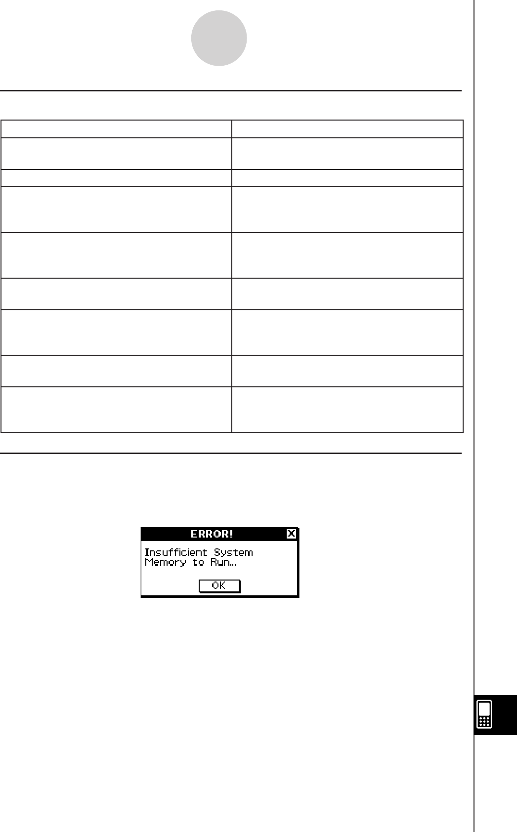
20110401

k Warning Message Table

-5-5

Error Message Table

kLow Memory Error Processing

An error occurs on the ClassPad if it is unable to reserve enough work area memory to

perform a particular operation. When a low memory error occurs, any application in use at

that point is shut down and an error message like the one shown below appears.

Tapping the [OK] button clears the error.

Important!

• To avoid loss of data, you should make it a regular habit to periodically perform the save

operation.

You may lose some of the data you are inputting with an application that shuts down due to

a low memory error. When the low memory error occurs while you are using the eActivity

application to create data, for example, any unsaved data you have input is lost.

Warning Message Description

Batteries are extremely low!

Replace batteries immediately! –

Can’t Solve! –

Can’t solve!

Adjust initial value or bounds.

Then try again.

NumSolve cannot solve an expression.

Insufficient memory for unit-to-unit

communication.

Delete unnecessary eActivity contents.

–

Only the first selected function will be

done. –

This operation will make your presentation

files unavailable.

Are you sure?

–

Time out.

The end of condition was not satisfied. –

Too Many eActivity Files The data communication operation you are

trying to perform is not possible because

there are too many eActivity files.

Manufacturer:

CASIO COMPUTER CO., LTD.

6-2, Hon-machi 1-chome, Shibuya-ku, Tokyo 151-8543, Japan

Responsible within the European Union:

CASIO EUROPE GmbH

Casio-Platz 1, 22848 Norderstedt, Germany

This mark applies in EU countries only.

CASIO COMPUTER CO., LTD.

6-2, Hon-machi 1-chome

Shibuya-ku, Tokyo 151-8543, Japan

One or more of the following patents may be used in the product.

U.S.Pats. 5,539,867

SA1110-B

GY437Soft_E_H4.pdf 1 11.10.7 2:33:43 PM

Casio Graphing Calculator Calculators And Translators Classpad330Plus Users Manual ClassPad 330 PLUS_Software_Eng

CLASSPAD330PLUS to the manual df552c66-4575-4408-aa4e-07dc73f78b54

CP330PLUSver310_Soft CP330PLUSver310_Soft_EN ClassPad 330 PLUS | Calculators | Manuals | CASIO

Navigation menu

Versions of this User Manual:

Views

Navigation