5968 9661E 7 03 A_16534A A 16534A
A_16522A A_16522A
User Manual: A_16534A
Open the PDF directly: View PDF ![]() .
.
Page Count: 132 [warning: Documents this large are best viewed by clicking the View PDF Link!]
- 16700 Series Logic Analysis System
- Table of Contents
- System Overview
- Mainframes
- Probing Solutions
- Data Acquisition and Stimulus
- Post-Processing and Analysis Tool Sets
- Time Correlation with Agilent Infiniium Oscilloscopes
- Mainframe Specifications and Characteristics
- Probing Solutions Specifications and Characteristics
- State/Timing Modules Specifications and Characteristics
- Oscilloscope Modules Specifications and Characteristics
- Pattern Generation Modules Specifications and Characteristics
- Trade-In, Trade-Up
- Ordering Information
- Third-Party Solutions
- Support, Warranty and Related Literature
- Support, Services, and Assistance
16700 Series
Logic Analysis System
Catalog
Debugging today's digital systems
is tougher than ever. Increased
product requirements, complex
software, and innovative hardware
technologies make it difficult to
meet your time-to-market goals.
The Agilent Technologies
16700 Series logic analysis systems
provide the simplicity and power you
need to conquer complex systems
by combining state/timing analysis,
oscilloscopes, pattern generators,
post-processing tool sets, and
emulation in one integrated system.

2

3
Table of Contents
System Overview
Modular Design page 4
Features and Benefits page 5
Selecting the Right System page 7
Mainframes
Display page 8
Back Panel page 9
System Screens page 10
IntuiLink page 13
Probing Solutions
Criteria for Selection page 14
Technologies page 15
Data Acquisition and Stimulus
State/Timing Modules page 18
Oscilloscope Modules page 31
Pattern Generation Modules page 34
Emulation Modules page 38
Post-Processing and Analysis Tool Sets
Software Tool Sets page 40
Source Correlation page 42
Data Communications page 47
System Performance Analysis page 55
Serial Analysis page 62
Tool Development Kit page 68
Licensing Information page 74
Time Correlation with Agilent Infiniium Oscilloscopes
E5850A Logic Analyzer - Oscilloscope Time Correlation Fixture page 75
Technical Specifications and Characteristics
Mainframe page 76
Probing Solutions page 83
State/Timing Modules page 85
Oscilloscope Modules page 108
Pattern Generation Modules page 111
Trade-In, Trade-Up page 122
Ordering Information page 123
Third-Party Solutions page 130
Support, Warranty and Related Literature page 131
Sales Offices Information page 132
4
Modular Design Protects Your
Long-Term Investment
Modularity is the key to the Agilent
16700 Series logic analysis systems'
long term value. You purchase only
the capability you need now, then
expand as your needs evolve. All
modules are tightly integrated to
provide time-correlated, cross
domain measurements.
Module Choices User Benefits
State/Timing Agilent offers a wide variety of state/timing modules for a range
of applications, from high-speed glitch capture to multi-channel
bus analysis.
Oscilloscopes Identify signal integrity issues and characterize signals quickly
with automatic measurements of rise time, voltage, pulse width,
and frequency.
Pattern Generation Use stimulus to substitute for missing system components or to
provide a stimulus-response test environment.
Emulation An emulation module connects to the debug port (BDM or JTAG)
on your target. You have full access to processor execution
control features of the module through the built-in emulation
control interface or a third-party debugger.
External Ports
Target Control Port Use the target control port to force a reset of your target or
activate a target interrupt.
Port-in/Port-out A BNC connector allows you to trigger or arm external devices
or to receive signals that can be used to arm acquisition
modules within your logic analyzer.
System Overview
Modular Design
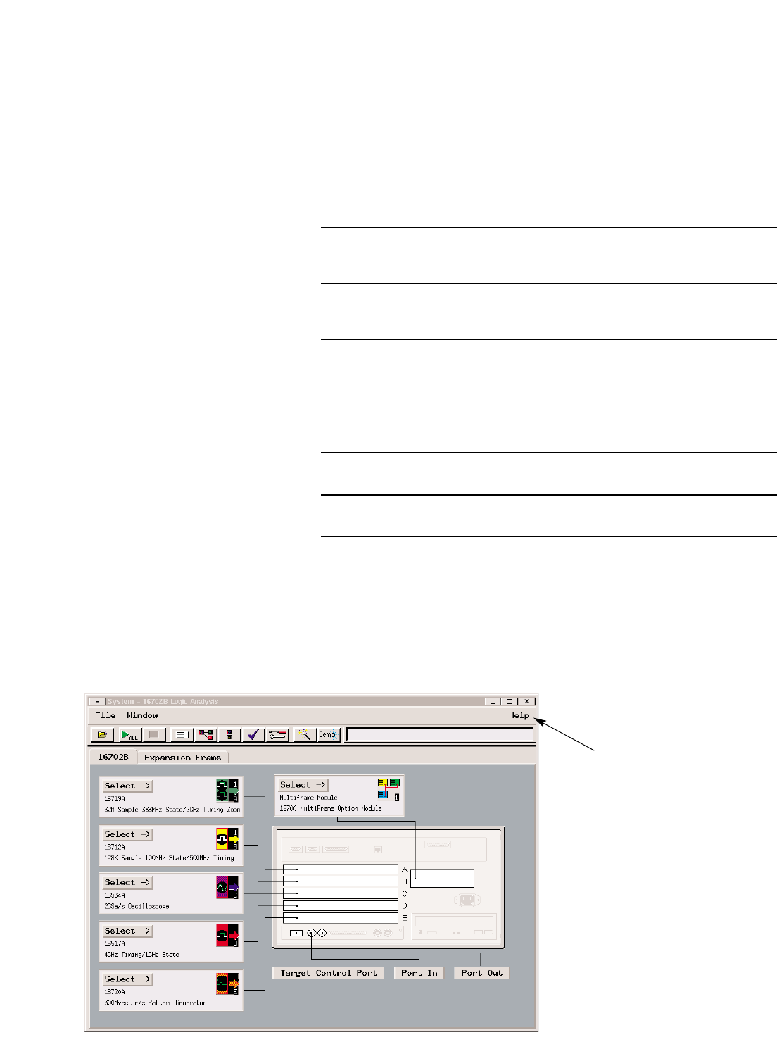
Figure 1.1. The system boot up screen shows you
what modules are configured into your logic
analysis system.
Help
enables you to
access the online
user’s guide and
measurement
examples.

5
System Overview
Features and Benefits
System Capability
Touch Screen Interface The Agilent 16702B mainframe supports a large, 12.1 inch LCD touch screen and redesigned front panel
controls for an easy-to-operate, self-contained unit requiring minimal bench space and offering simple
portability.
Multiframe Configuration By connecting up to eight mainframes and expanders you can simultaneously view 8,160 time-correlated traces
for buses in a large channel count, multibus system.
Enhanced Mainframe Hardware Mainframe now includes a 40X CD-ROM drive, a 18 GB hard disk drive, 100BaseT-X LAN, and 128 MB of
internal system RAM (optional 256 MB total).
Scalable System
• State/timing analyzers • Select the optimum combination of performance, features, and price that you need for your specific
• Oscilloscopes application today, with the flexibility to add to your system as your measurement needs change.
• Pattern generators • View system activity from signals to source code.
• Post-processing tool sets
• Emulation modules
Measurement Modules/Interfaces
The Agilent 16760A With up to 1.5 Gb/s state speed, the 16760A lets you debug today’s and tomorrow’s ultra-high-speed
State/Timing Module digital buses. NEW Eye scan gives a rapid comprehensive overview of signal integrity on hundreds of
channels simultaneously
NEW The Agilent 16750 Series With up to 600 MHz state speed and up to 64 MBytes of trace depth these modules help you address today’s
State/Timing Modules high-performance measurement requirements. (See page 20)
The Agilent 16720A With up to 16 MVectors depth and 300 MVectors/sec operation and up to 240 channels[1] of stimulus, the
Pattern Generator 16720A provides a new level of capability that makes complex device substitution a reality. Supports TTL,
CMOS, 3.3V, 1.8V, LVDS, 3-state, ECL, PECL, and LVPECL.
High-Speed Bus Measurements Agilent’s eye finder technology automatically adjusts the setup and hold on every channel, eliminating the
Made Simple with Eye Finder need for manual adjustment and ensuring accurate state measurements on high-speed buses.
Technology
Timing Zoom Technology Simultaneously acquire data at up to 4 GHz timing and 600 MHz state through the same connection. Timing
Zoom is available across all channels, all the time. (See page 24)
VisiTrigger Technology • Use graphical views and sentence-like structure to help you define a trace event.
• Select trigger functions as individual trigger conditions or as building blocks to easily customize a trigger
for your specific task.
Processor and Bus Support • Get control over your microprocessor’s internal and external data.
• Quickly and reliably connect to the device under test. (See page 38)
Direct Links to Industry Standard • Debuggers provide visibility into software execution for systems running software written in C and C++ as
Debuggers and High-Level well as active microprocessor execution control (run control).
Language Tools • Import symbol files created by your language tool. Symbols allow you to set up trigger conditions and review
waveform and state listings in easily recognized terms that relate directly to the names used for signals on
your target and the functions and variables in your code.
Direct Links to EDA Tools • Use captured logic analysis waveforms to generate simulation test vectors.
• Easily find problems by comparing captured waveforms with simulated waveforms.
[1] 240 channel system consists of five 16720A pattern generator modules with 48 channels per module. Full channel mode runs at 180 MVectors/s and 8 MVectors depth.
300 MVectors/s and 16 MVectors depth are offered in half channel mode.

6
System Overview
Features and Benefits
Data Transfer, Documentation, and Remote Programming
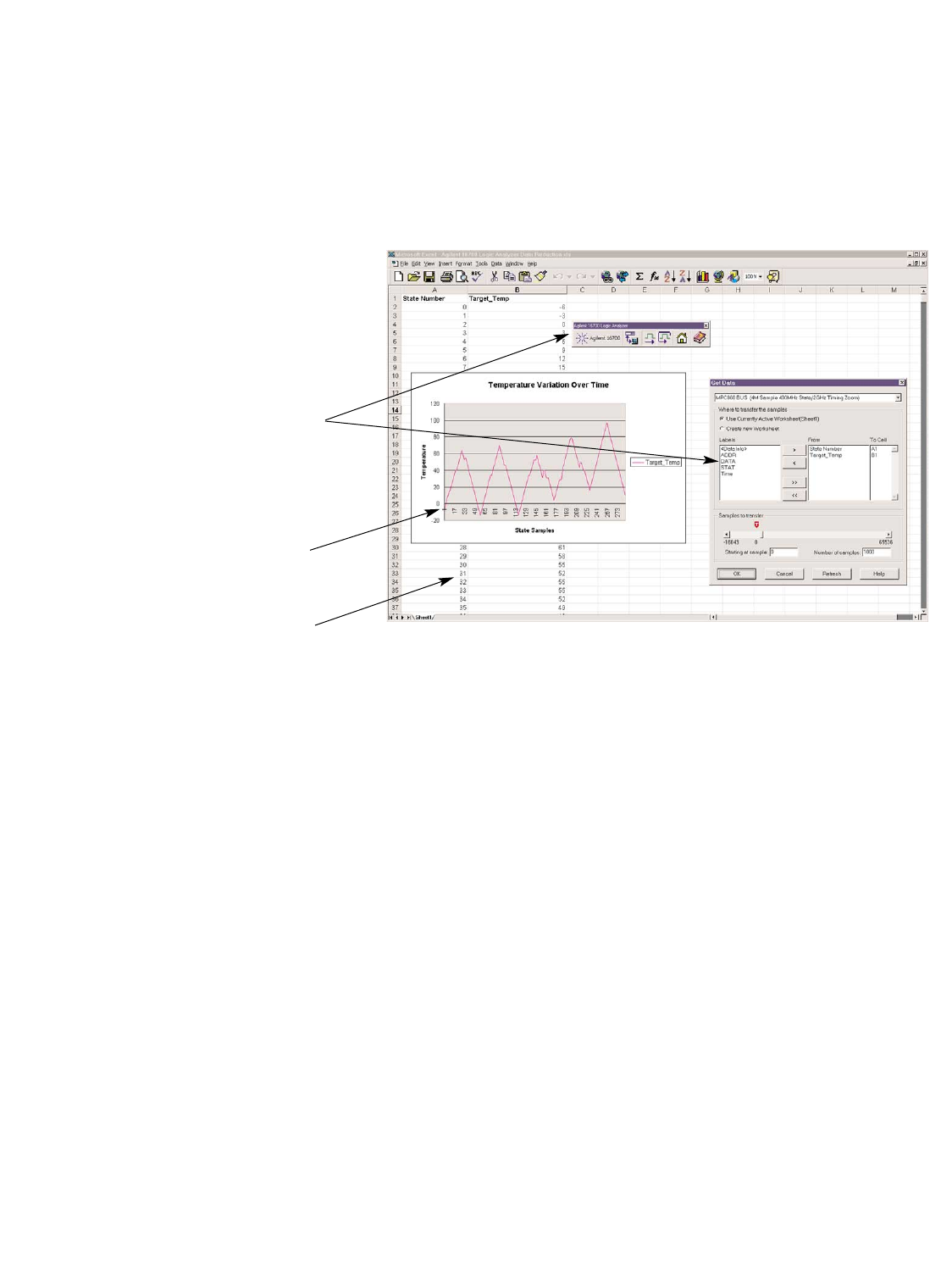
Direct Link to Microsoft®Excel via • Automatically move your data from the logic analyzer into Microsoft Excel with just a click of the mouse.
Agilent IntuiLink (See page 13)
• Use Microsoft Excel’s powerful functions to post-process captured trace data to get the insight you need.
Transfer Data for Offline Analysis - • Fast binary (compressed binary) from the FileOut tool provides highest performance transfer rate.
Data Export • ASCII format provides same format as listing display, including inverse-assembled data.
Transparent File System Access • Access, transfer, and archive files.
• Stay synchronized with your source code by mapping shared directories and file systems from your
Windows 95/98/NT/2000/XP-based PC directly onto the logic analyzer and vice versa.
• Move data files to and from the logic analyzer for archiving or use elsewhere.
Documentation Capability • Save graphics in standard TIFF, PCX, and EPS formats.
• Print screen shots and trace listings to a local or networked printer.
• Save your lab notes and trace data in the same file by entering relevant information in the Comments tab of
the display.
Remote Programming with • Perform pass/fail analysis, stimulus response tests, data acquisition for offline analysis, and system
Microsoft’s COM Using verification and characterization tests.
Microsoft Visual Basic or • Powerful-yet-efficient command set focuses on your programming tasks, resulting in a shorter learning
Visual C++ curve while maintaining necessary functionality.
System Software Features
Post-Processing Analysis Tools Rapidly consolidate large amounts of data into displays that provide insight into your system’s behavior.
(See page 40)
Setup Assistant Quickly configure the logic analysis system for your target microprocessor. (See page 10)
Tabbed Interface • Groups like tasks together so you can quickly find and complete the task you want to perform.
• Spend your time solving problems, not setting up a measurement.
Multi-Windowed View of • View your cross-domain measurements, time-corrected on the same screen. (See page 11)
Target System Activity • Debug faster because you can view system activity at a glance.
Global Markers Track a symptom in one domain (e.g., timing) to its cause in another domain (e.g., analog).
Resizable Windows and Data Views • Magnify your view or zoom in on a boxed area of interest.
• Resize waveforms and data or quickly change colors to highlight areas of interest.
Web-Enabled System • Directly access the instrument’s web page from your web browser. (See page 12)
• Remotely check the instrument’s measurement status without disturbing the acquisition.
• Remotely access, monitor and control your logic analysis system.
Network Security • Protect your networked assets and comply with your company’s security requirements with individual user
logins that provide system integrity.
NEW Time Correlation with • Make time-correlated measurements using an Agilent 16700 Series logic analyzer and an
Infiniium 54800 Series Oscilloscopes Agilent Infiniium 54800 Series oscilloscope.
• View Infiniium oscilloscope waveforms in the 16700 logic analyzer’s waveform display.
• Use the 16700 logic analyzer’s global markers to measure time between any domain in the 16700 and voltage
waveforms acquired by the Infiniium oscilloscope.
7
System Overview
Selecting the Right System
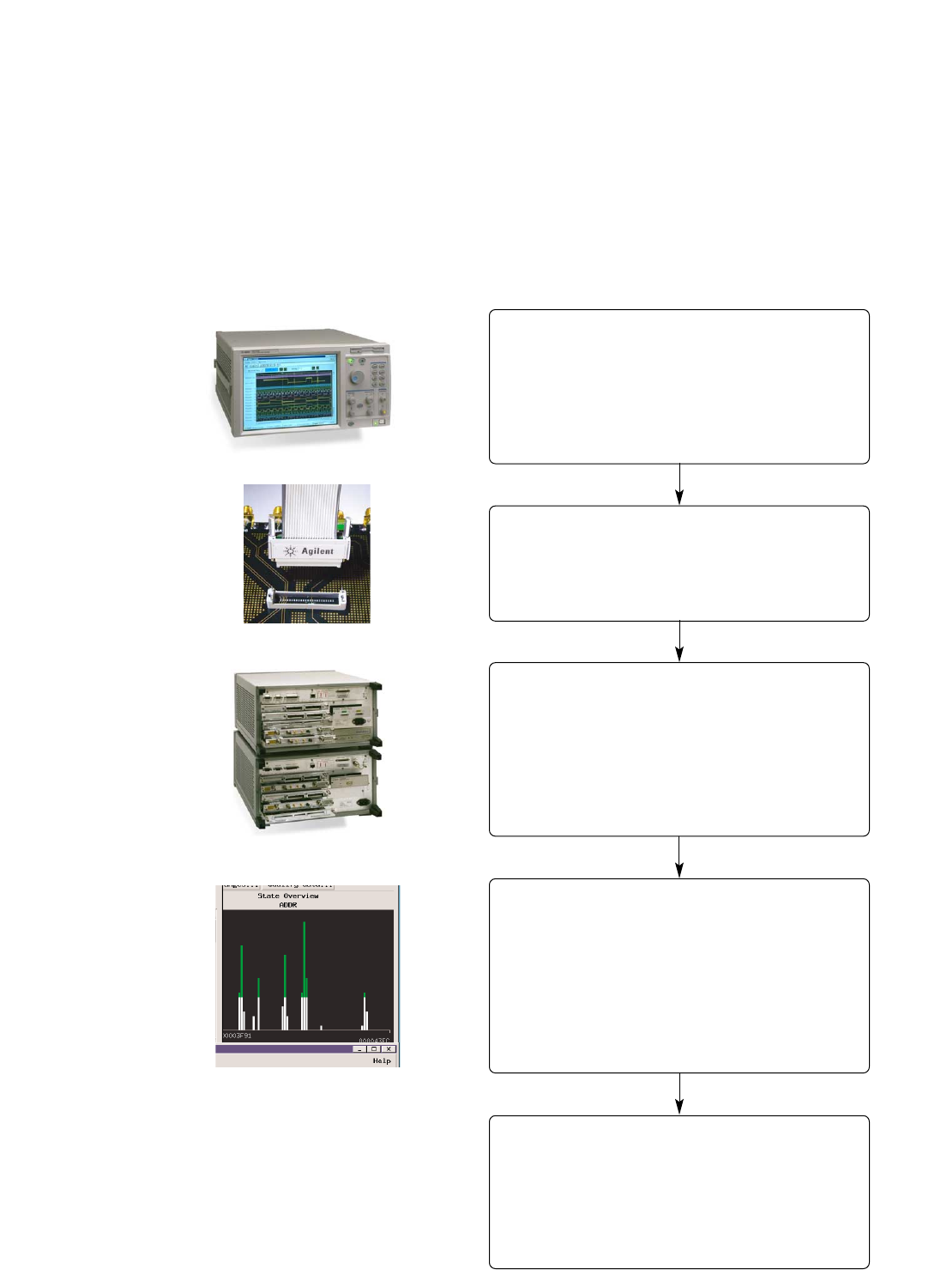
Select a mainframe (page 8)
Choose a system based on your needs:
• Self-contained unit or a unit with
external mouse, keyboard, and monitor
• Expander frame for large channel count
requirements
Selecting a system for your application
Determine your probing requirements (page 14)
• Are you analyzing a microprocessor?
• Do you need to probe a specific package type?
Select the measurement modules to meet your
application needs
• State/Timing Logic Analyzers (page 18)
• Oscilloscopes (page 31)
• Pattern Generation (page 34)
• Emulation (page 38)
Add post-processing tool sets for analysis and
insight (page 40)
• Source correlation
• Data communications
• System performance analysis
• Serial analysis
• Tool development kit
Support, services, and assistance (page 131)
• Training classes
• Consulting
• On-line support
• Warranty extension
8
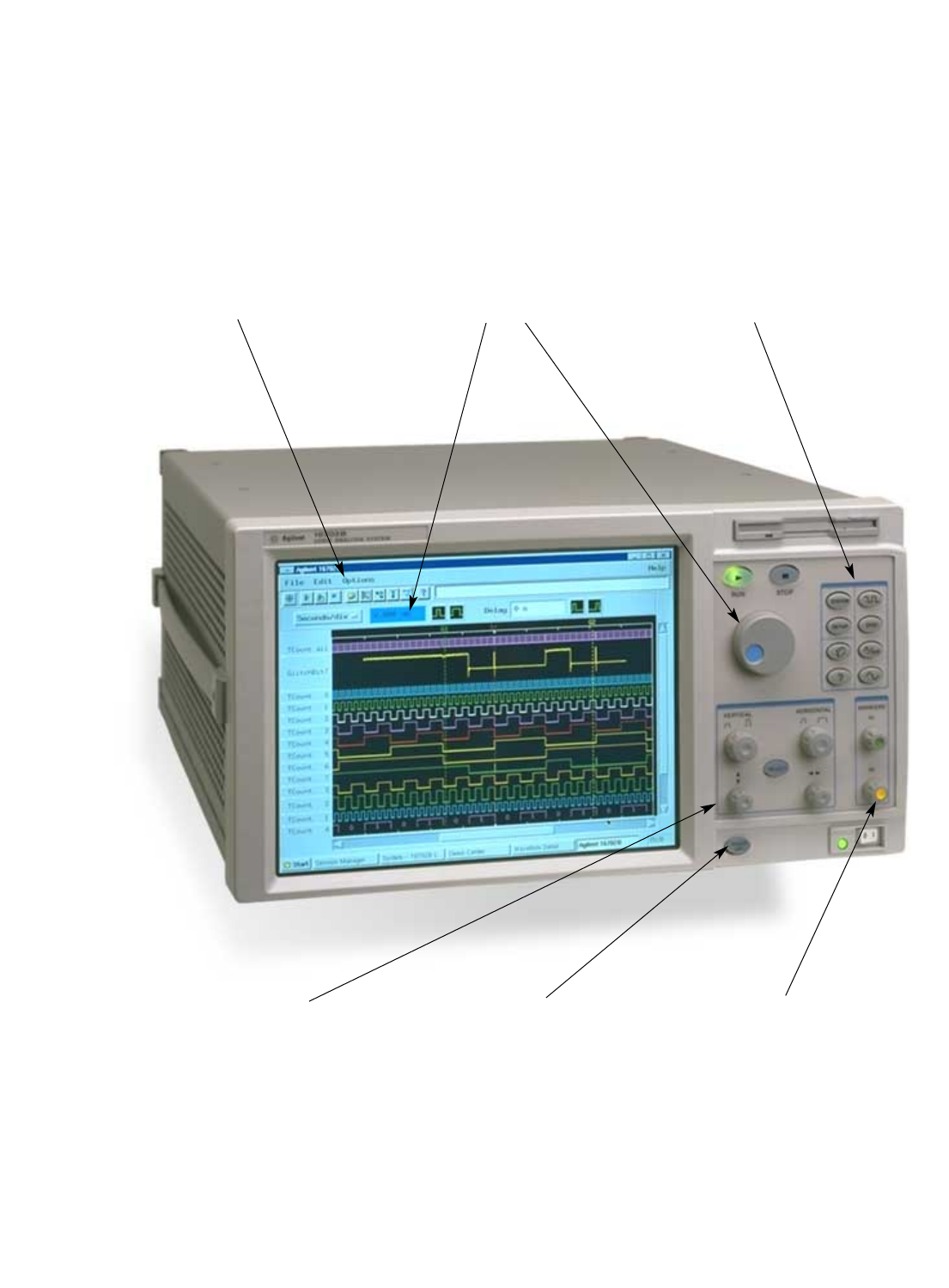
12.1" LCD display with touch screen on
the 16702B makes it easy to view a large
number of waveforms or states.
Dedicated hot keys give instant access to
the most frequently used menus, displays,
and on-line help.
"Touch Off" button disables the touch
screen and allows you to point out
anomalies to a colleague without altering
the display settings.
Dedicated knobs for horizontal and vertical
scaling and scrolling. Adjust the display to
get just the information you need to solve
your problem.
Mainframes
Display
Select a modifiable variable by touching
it, then turn the knob to quickly step
through values for the variable.
Figure 2.1. The Agilent 16702B quickly tracks down problems in your design while saving precious bench space.
Dedicated knobs for global markers help
track down tough problems. A symptom
seen in one domain (e.g., timing) can be
tied to its cause in another domain
(e.g., analog).
9
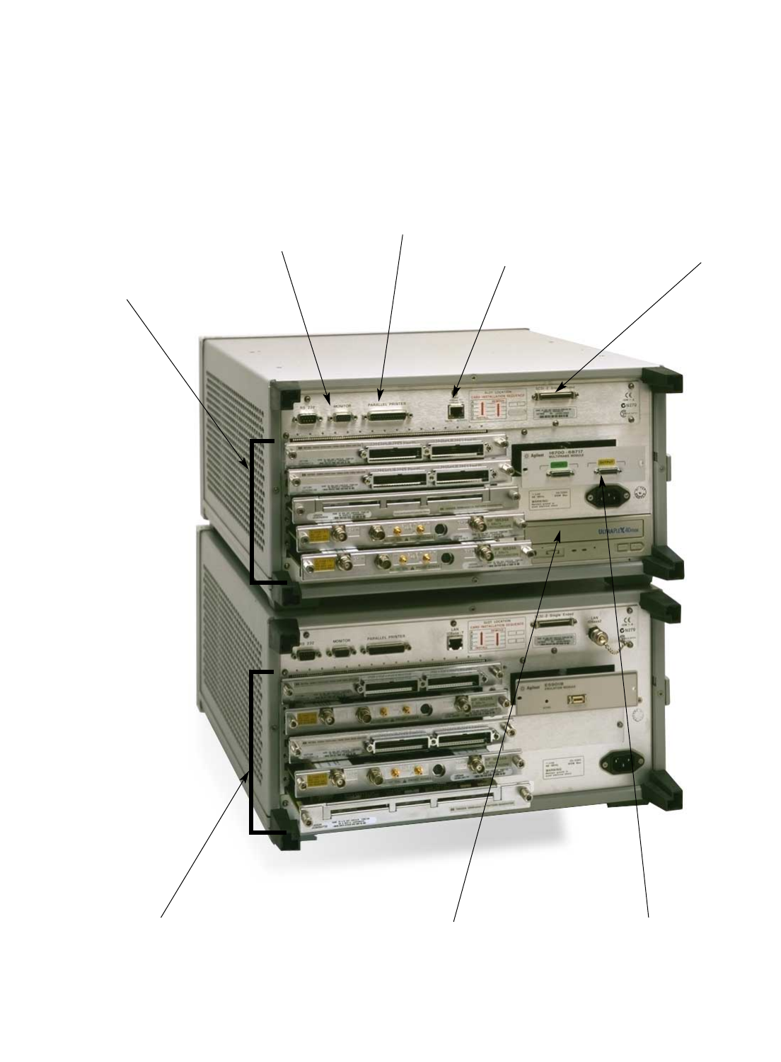
Connection for optional monitor.
(Up to 1600x1200 video
resolution with option 003) 10/100BaseT LAN - autosensing
Parallel printer port SCSI-II connection for an
external 18 GByte data drive or
external removable hard drive
Expander frame connection provides an
additional five slots for measurement
modules.
Built-in 40x CD-ROM drive makes it easy
to install or update system software,
processor support, or tool sets.
Option slot for an emulation module or
for a multiframe module. Multiframe
option allows up to eight mainframes
and expanders to be combined so that
you can see all the buses in a complex
target system.
Mainframes
Back Panel
Figure 2.2. The mainframe and expander frame provide advanced capabilities for debugging complex target systems.
Five slots for
measurement
modules
10
Mainframes
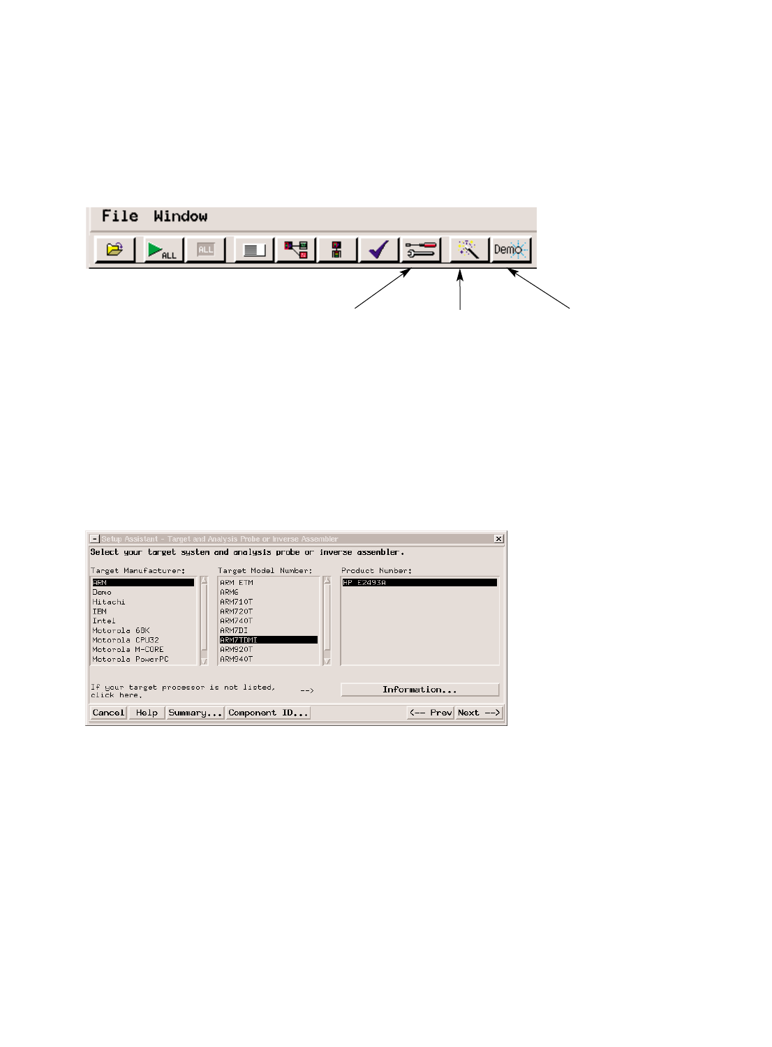
System Screens
Figure 2.4. Setup Assistant gets you up and
running quickly.
System Admin
allows you to quick-
ly set up the instru-
ment on your net-
work, configure
print servers, set up
user accounts for
security or install
software updates.
Demo Center
provides simple
demos of the most
commonly used
features.
Setup Assistant
is a guided menu
system that helps
you configure the
logic analysis sys-
tem for your target
microprocessor or
bus. Online infor-
mation guides you
through the setup.
(See figure 2.4)
Figure 2.3. Icons in the power-up screen give you
quick access to common tasks.
11
Mainframes
System Screens
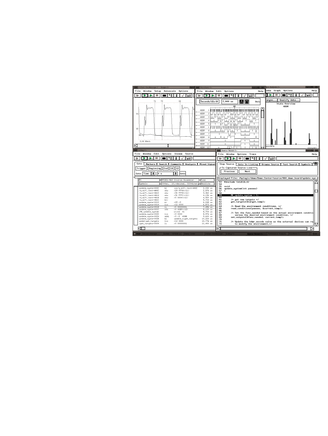
See the Big Picture of Your
Prototype System's Behavior
A large external display (option 001)
with multiple, resizable windows
allows you to see at a glance more of
your target system's operation. A
built-in, flat-panel display in the
16702B fits in environments with
limited space. Color lets you highlight
critical information so you can find
it quickly.
Use one system to examine target
operation from different perspec-
tives. Multiple time-correlated views
of data let you confirm both signal
integrity and software execution
flow. These views are invaluable in
solving cross-domain problems.
Figure 2.5. You can quickly isolate the root cause of system problems by examining target operation across a wide
analysis domain, from signals to source code.
12
...access Agilent's Web site for the latest
online manuals and technical information
...install Agilent IntuiLink to seamlessly
transfer data from the system to a PC
Mainframes
System Screens
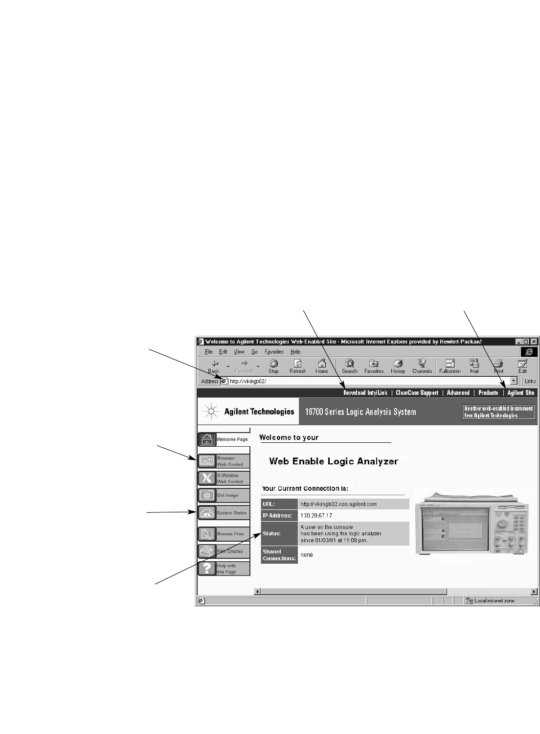
Expanding Possibilities with
Network Connectivity
Web-enabled instrumentation gives
you the freedom to access the
system—anywhere, anytime. Have
you ever needed to check on a
measurement's status while you were
in a remote location? Now you can.
Figure 2.6. Your logic analyzer is its own web site. From the Home Page, you can perform multiple remote functions.
With a Web Enabled Logic
Analysis System You Can...
...access the logic analysis
system's Web page from
your browser by using the
instrument's hostname as
a URL
...access the system’s user
interface directly from with-
in your browser, giving you
full control of all analysis
functions
...remotely check current
measurement status to find
out if the system has
triggered
...quickly check instrument
status to determine if the
system is available for use
13
Programming
IntuiLink also includes an Active-X
automation server to provide
programmatic control of the logic
analysis system from an external
environment, such as LabVIEW or the
Microsoft VisualStudio environment
of Visual Basic and Visual C++ tools.
The instrument's Remote
Programming Interface (or RPI) also
allows you to write Perl or other
scripts to control the logic analyzer.
Use the sample programs provided
to assist you in creating your own
custom programs.
Mainframes
IntuiLink
Figure 2.7. Transfer data into Microsoft Excel with just a click of the mouse.
Agilent IntuiLink Moves Your
Data Automatically into
Microsoft®Excel for
Advanced Offline Analysis
IntuiLink is shipped with each logic
analysis system and can be down-
loaded to your PC from the system’s
own web page. Use the Agilent
IntuiLink tool bar to connect to a
logic analysis system. Select from
the available labels and specify
the destination cell location in
Microsoft Excel.
Use Microsoft Excel's powerful
functions to post-process captured
trace data for the insight you need.
Import data from a current
acquisition or data previously saved
to a file via the File Out tool.
14
Probing Solutions
Criteria for Selection
Why is Probing Important?
Your debugging tools perform three
important tasks: probing your target
system, acquiring data, and analyzing
data. Data acquisition and analysis
tools are only as effective as the
physical interface to your target
system. Use the following criteria to
see how your probing measures up.
How to Determine Your
Requirements
To determine what probing method
is best to use you need to take the
following into consideration:
• The number of signals to be
probed
• The ability to design probing
connectors on the target PC board
itself
• Mechanical probing clearance
requirements
• Signal loading effects
• Ease of attachment
• Package type to be probed
DIP Dual In-line Package
PGA Pin Grid Array
BGA Ball Grid Array
PLCC Plastic Leaded Chip
Carrier
PQFP Plastic Quad Flat Pack
TQFP Thin Quad Flat Pack
SOP Small Outline Package
TSOP Thin Small Outline
Package
• Package Pin Pitch (distance
between pin centers)
Immunity to Noise EMF noise is everywhere and can corrupt your data. Active
attenuator probing can be particularly susceptible to noise effects.
Agilent Technologies designs probing solutions with high immunity to
transient noise.
Impedance High input impedance will minimize the effect of probing on your
circuit. Although many probes are acceptable for lower frequencies,
capacitive loading dominates at higher frequencies.
Ruggedness A flimsy probe will give you unintended open circuits. Agilent
Technologies' probes are mechanically designed to relieve strain and
ensure a rugged and reliable connection.
Connectivity A multitude of device packages exist in the digital electronics industry.
Check our large selection of probing solutions designed for specific
chip packages or buses. As an alternative, we offer reliable
termination adapters that work with standard on-target connectors.
Figure 3.1. A rugged connection lets you focus on debugging your target, not your probe.
15
Probing Solutions
Technologies
Choose the Optimum Probing
Strategy for Your Application
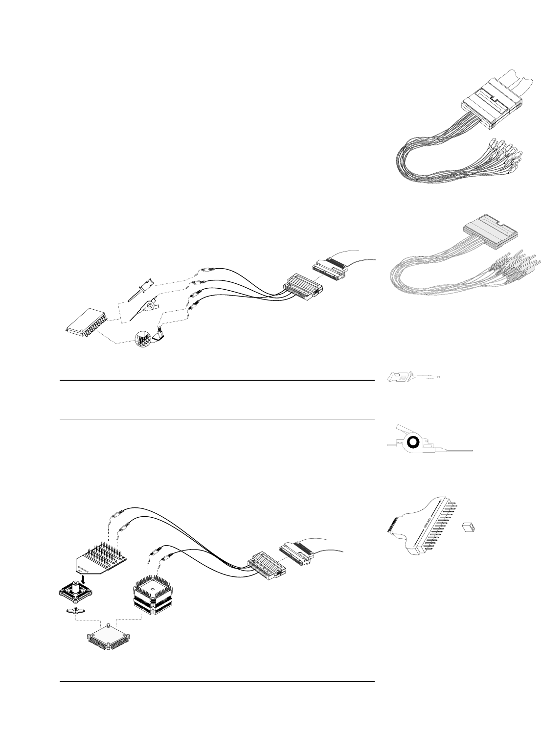
Advantages Limitations
Most flexible method. Can be time-consuming to connect a large
Flying-lead probes are included with logic number of channels. Least space-efficient
analyzer module (except 16760A). method.
Figure 3.2.
Figure 3.4. Surface mount IC clip.
5090-4356 (20 clips).
Figure 3.5. 0.5 mm IC clip.
10467-68701 (4 clips).
Figure 3.6. Wedge adapters connect to multiple
pins of 0.5 mm or 0.65 mm QFP ICs. Refer to
“Probing Solutions for Agilent Technologies
Logic Analysis Systems,” publication number
5968-4632E, for specific part numbers.
Connecting to individual test
points with flying leads
Advantages Limitations
Rapid access to all pins of fine-pitch Requires minimal keepout area.
QFP package.
Very reliable connections.
Figure 3.7.
Refer to “Probing Solutions for
Agilent Technologies Logic Analysis
Systems,” publication number
5968-4632E, for specific solutions.
Connecting to all the pins of a
quad flat pack (QFP) package
NEW Figure 3.3. The E5381A (differential) and
E5382A (single-ended) flying lead probe sets provide
connections for 17 channels of the 16753A, 16754A,
16755A, 16756A and 16760A logic analyzers.
16
Probing Solutions
Technologies
Advantages Limitations
Very reliable connections. Requires advance planning in the design stage.
Saves time in making multiple connections. Requires some dedicated board space.
Moderate incremental cost.
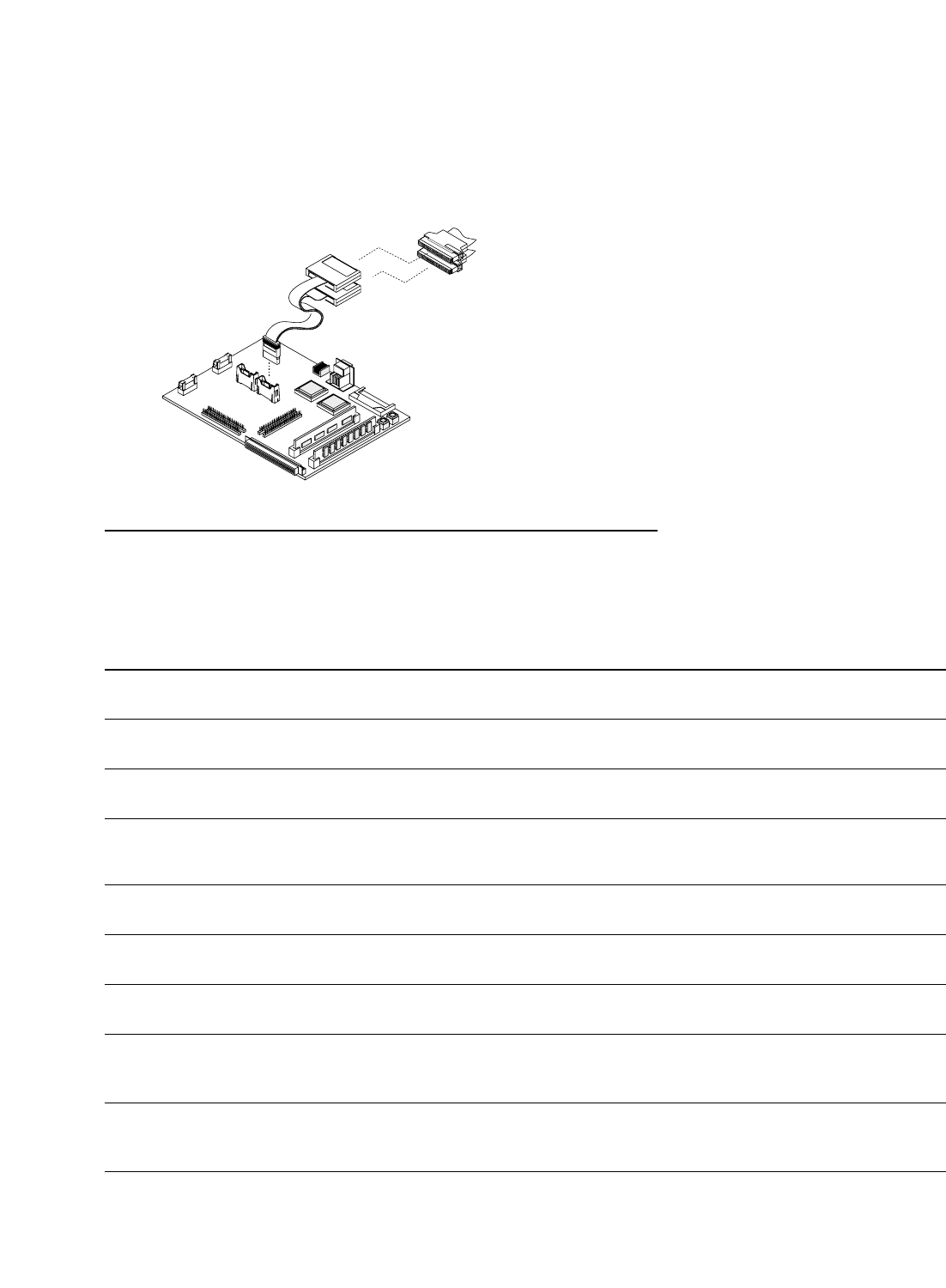
Figure 3.8. NEW Agilent’s soft-touch
connectorless probes provide high-density,
low capacitive loading, and high reliability,
without requiring a connector.
High-density probing solutions
Model Description Requires kit of 5 Usable with
number connectors and 5 shrouds logic analyzers
E5385A 100-pin probe with built-in isolation networks 16760-68701 All that use 40-pin 3M-style
for the logic analyzer mid-cable connector
E5346A 34-channel, 38-pin probe with built-in E5346-68701 All that use 40-pin 3M-style
isolation networks for the logic analyzer. mid-cable connector
E5351A 34-channel 38-pin adapter cable, requires logic E5346-68701 All that use 40-pin 3M-style
analyzer isolation networks on the target. mid-cable connector
E5339A 34-channel 38-pin low-voltage probe with built-in E5346-68701 All that use 40-pin 3M-style
isolation networks for the logic analyzer. Designed for mid-cable connector
signals with peak-to-peak amplitude as small as 250 mV.
E5378A 34-channel 100-pin single-ended probe 16760-68701 All that use 90-pin high-density
mid-cable connector
E5379A 17-channel 100-pin differential probe 16760-68701 All that use 90-pin high-density
mid-cable connector
E5380A 34-channel 38-pin single-ended probe E5346-68701 All that use 90-pin high-density
mid-cable connector
E5387A 17-channel differential soft touch connectorless probe Kit of 5 retention modules All that use 90-pin high-density
supplied with probe. Part number mid-cable connector
for additional kit of 5: E5387-68701
E5390A 34-channel single-ended soft touch connectorless probe Kit of 5 retention modules All that use 90-pin high-density
supplied with probe. Part number mid-cable connector
for additional kit of 5: E5387-68701
Designing connections
into the target system
17
Probing Solutions
Technologies
Advantages Limitations
Easiest and fastest connection to supported Moderate to significant incremental cost.
processors and buses. Only useable for the specific processor or bus.
May require moderate clearance around
processor or bus.
Figure 3.10.
Refer to “Processor and Bus Support
for Agilent Technologies Logic
Analyzers,” publication number
5966-4365E, for specific solutions.
Using a processor- or bus-specific
analysis probe
Moderate-density probing solutions The Agilent 01650-63203 isolation
adapter contains the termination
networks for the logic analyzer. The
01650-63203 connects to a 3M 20-pin
connector on the target PC board.
Refer to "Probing Solutions for
Agilent Technologies Logic Analysis
Systems," publication number
5968-4632E, for design guidelines
and part numbers for mating
connectors.
You may also add the isolation
networks to the target PC board and
connect the logic analyzer cable
directly to a 40-pin 3M connector on
the PC board. Refer to "Probing
Solutions for Agilent Technologies
Logic Analysis Systems," publication
number 5968-4632E, for design
guidelines in addition to part
numbers for mating connectors
and isolation networks.
Figure 3.9. 01650-63203 termination adapter.

18
Data Acquisition and Stimulus
State/Timing Modules
Selecting the Correct Modules
to Meet Your Needs
Selecting the proper logic analyzer
modules for your needs requires a
series of choices concerning
performance, cost, and the amount of
data you will be able to capture. The
following table explains these factors
in greater detail.
Considerations for Choosing Modules
Microprocessor/ Will you be using an analysis probe for a particular processor or bus? If so, a good starting point is the document Processor
Bus Support and Bus Support for Agilent Technologies Logic Analyzers, publication number 5966-4365E, available on the worldwide web
at www.agilent.com/find/logicanalyzer. This document provides the number of channels and state speed required for any
particular analysis probe. It also indicates which analysis modules are supported and how many are required.
Timing Resolution Timing analysis uses the logic analyzer's internal clock to determine when to sample. Since timing analysis samples
asynchronously to the system under test, you should consider what accuracy you will need to verify your system.
Accuracy is made up of two elements: sample speed and channel-to-channel skew. Remember to evaluate both of these
elements and be careful of logic analyzers that have a fast sample speed with a large channel-to-channel skew.
State Speed • State analysis uses a clock or strobe signal from your system under test to determine when to sample. Because state
analysis samples are synchronous with the system under test, they provide a view of how your system is executing. You can
use state analysis to capture bus cycles from a microprocessor or I/0 bus and convert the data into processor mnemonics
or bus transactions using an Agilent Technologies inverse assembler.
• Select a state acquisition system that provides the speed and headroom you need without breaking your budget. Remember
that a microprocessor will have an internal core frequency that is normally 2X-5X the speed of the external bus.
Headroom You may realize a better return on your investment if you consider possible future needs when purchasing analysis modules.
The things to consider are primarily state speed and memory depth.
Setup/Hold • Logic analyzers require time for the data at the inputs to become valid (setup time), and time to capture the data (hold time).
A lengthy setup and hold can make the difference between capturing valid data or data in transition.
• Your device under test will ensure that data is valid on the bus for a defined length of time. This is known as the data valid
window. Your target's data valid window must be large enough to meet the setup/hold specifications of the logic analyzer.
The data valid window of most devices is generally less than half of the clock period. Don't be fooled by "typical" setup and
hold specifications for logic analyzers.
• As bus speeds increase, the time window during which data is stable decreases. Jitter, skew, and pattern-dependent ISI
add more uncertainty and consume a greater portion of the data-valid window at high speeds. A logic analyzer with eye finder
technology to automatically adjust the sampling position on each channel to the center of the data valid window provides
unparalleled measurement accuracy at high frequencies.
Transitional Timing If your system has bursts of activity followed by times with little activity, you can use transitional timing to capture a longer
trace. In transitional timing, the analyzer samples data at regular intervals, but only stores the data when there is a transition
on one of the signals.

19
Data Acquisition and Stimulus
State/Timing Modules
Considerations for Choosing Modules (continued)
Channel Count Determine the number of signals you want to analyze on your system under test. You will need this number of channels in
your logic analyzer. Even if you have enough channels to view all the signals in your system today, you should consider logic
analysis systems that allow you to add more channels for your future application needs.
Memory Depth • Complex architectures and bus protocols make your debugging job increasingly challenging. Split transactions, multiple
outstanding transactions, pipelining, out-of-order execution, and deep FIFOs, all mean that the flow of data related to a
problem can be distributed over thousands or millions of bus cycles.
• The keys to useful insight are the combination of deep memory with responsive display refresh, search, rescaling, and
scrolling to help you find information and answers quickly. Hardware-assisted memory management in the Agilent 16740 Series
and 16750 Series state and timing analysis modules makes quick work of refreshing the display, rescaling, scrolling, and search-
ing. It takes only a few seconds to refresh, rescale, or scroll a 64M sample record. Agilent Technologies offers a range of state
and timing analyzer modules with memory depths up to 128M samples, at prices to meet your budget.
Triggering • The logic analyzer memory system is similar to a circular buffer. When the acquisition is started, the analyzer continuously
gathers data samples and stores them in memory. When memory becomes full, it simply wraps around and stores each new
sample in the place of the sample that has been in memory the longest. This process will continue until the logic analyzer
finds the trigger point. The logic analyzer trigger stops the acquisition at the point you specify and provides a view into the
system under test. The primary responsibility of the trigger is to stop the acquisition, but it can also be used to control the
selective storage of data. Consider a logic analyzer with the trigger resources you need to quickly set up your
measurements.
• After memory depth, triggering is the most important aspect of a logic analyzer to consider. On the one hand, powerful
triggering resources and algorithms will allow you to focus on potential problem sources without using up valuable memory.
On the other hand, to be useful, the trigger must be easy to set up.
Other In addition to the measurements made with an analysis probe, consider whether you need to monitor other signals. Be sure to
Measurements allow enough channels to make those measurements. For state measurements, the state speed of the analyzer must be at least
as high as the clock speed of your circuit. You may want to test the margin in your circuit by operating it at higher than the
nominal clock speed to determine if the analyzer has sufficient clock speed. For timing measurements, the timing analyzer rate
should be from 2-10X the clock speed of your target.

20
Data Acquisition and Stimulus
State/Timing Modules
Key Features of Agilent’s
State/Timing Modules
• Memory depth up to 128M
samples at a price to meet your
budget
• State analysis up to 1.5 Gb/s
• Timing Zoom 4-GHz (250ps)
timing on all channels
• VisiTrigger combines powerful
functionality with an intuitive
user interface
• Eye finder for automatic setup
and hold on all channels
• Eye scan for rapid insight into
signal integrity
Multichannel Eye scan allows you to make eye diagram measurements, quickly and easily,
Eye measurements on hundreds of channels simultaneously (Available on 16753/54/55/56A and
16760A modules)
High-speed Timing Zoom provides up to 250ps timing resolution at 64K depth on all
timing on channels simultaneous with state through the same probe.
all channels
Triggering for the VisiTrigger combines powerful trigger functionality with a user interface
most elusive that is easy to understand and use. Capturing complex sequences of
problems events is as simple as pointing to the function you want to use and filling in
the blanks to customize it to your specific situation.
Reliable Eye finder automatically adjusts the setup and hold on every channel,
measurements eliminating the need for manual adjustment and ensuring the highest
on high-speed confidence in accurate state measurements on high-speed buses.
buses
Choose the Logic Analyzer and Measurement Modules that Best Fit Your Application
State/Timing General- 8/16 Bit 32/64 Bit High- Timing Deep trace High- Analysis of
Modules purpose processor processor speed margin capture speed data intensive
hardware debug debug or bus analysis or with timing computer systems and
debug channel analysis characterize or state debug performance
intensive setup/hold analysis
systems
16710A/11A/12A √√
16715A √√√
16716A √√√ √ √
16717A √√√√√
16740A/41A/42A √√√√√√
16750B/51B/52B/
53A/54A/55A/56A √√√√√√
16760A √√√
A variety of measurement modules allow you to select the optimum combination of performance, features, and price to meet your specific needs now and in the future.
21
Data Acquisition and Stimulus
State/Timing Modules
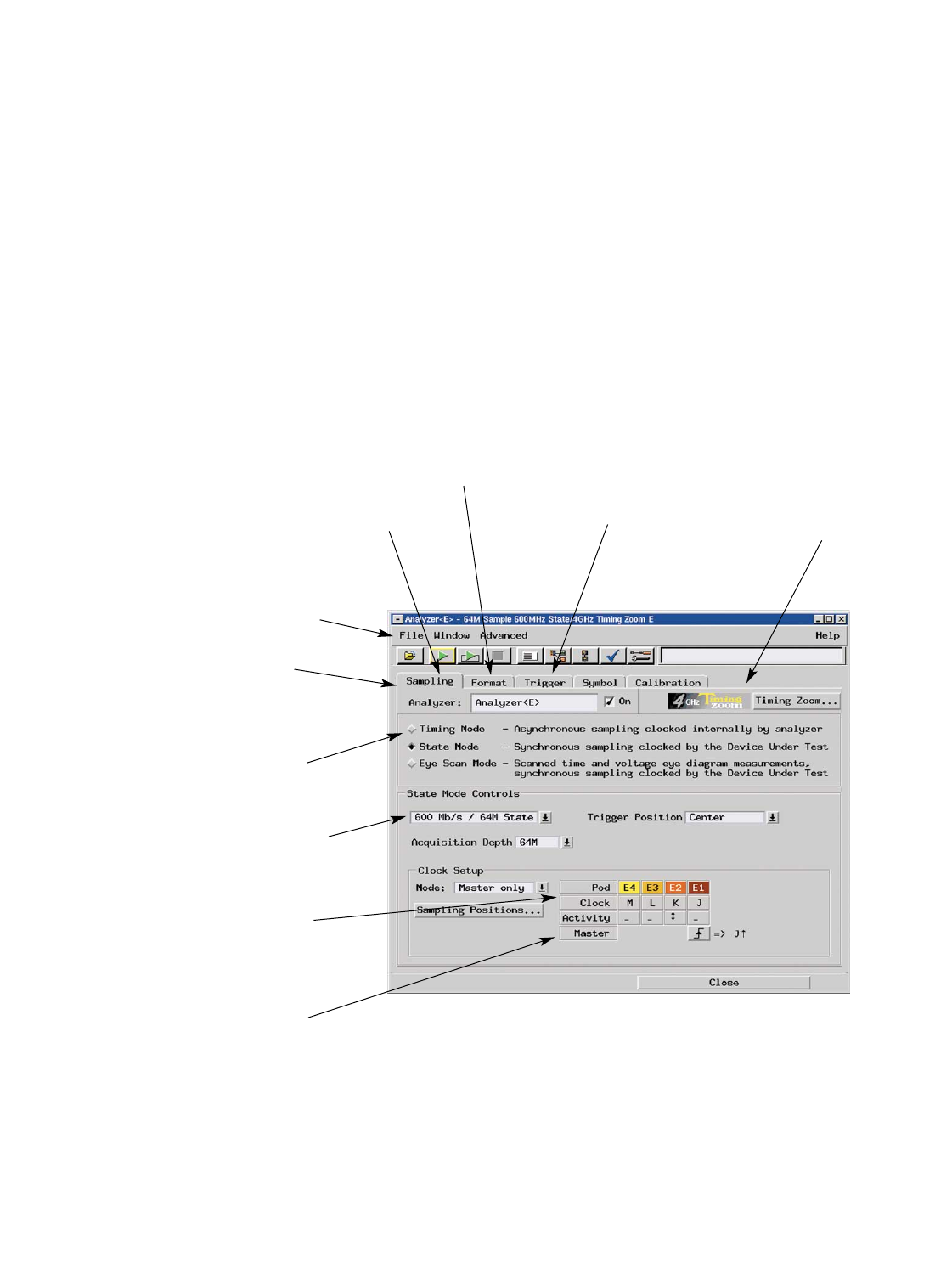
Improve Your Productivity with an
Intuitive User Interface
Agilent Technologies has made the
user interface easy to understand
and use. Now you can spend more
time making measurements and less
time setting up the logic analyzer.
Measurement configuration and
data files can be loaded directly into
the logic analyzer
Menu tabs provide a logical
progression through the setup of
your measurement.
State and timing mode selections
specify how data is sampled.
Single location for access to all state
acquisition options.
Convenient color coding helps you
identify the signals in the interface
with the physical connection to your
device under test.
Clocking for state measurements
can be quickly defined using the
clock setup menu.
Sampling defines how the logic
analyzer will acquire the data.
Format allows you to
group signals into buses.
Trigger defines what
data is acquired.
Timing Zoom provides up to 4 GHz
timing analysis simultaneous with
state or conventional timing analysis
on all channels. (16716A, 16717A,
16740 Series, and 16750 Series only).
Figure 4.1. Setting up your logic analyzer has never been this easy.
22
Data Acquisition and Stimulus
State/Timing Modules
VisiTrigger Quickly Locates
Your Most Elusive Problems
VisiTrigger technology is a break-
through in logic analysis usability. It
combines increased trigger function-
ality with a user interface that is easy
to understand and use. Now with
VisiTrigger, capturing complex events
is as simple as pointing to the trigger
function and filling-in-the-blanks.
Features and Applications
VisiTrigger • Use graphical views and sentence-like structures to help you
(available in the define a trace event.
16715A, 16716A, 16717A, • Select trigger functions as individual trigger conditions or as
16740 Series, 16750 Series building blocks to easily customize a trigger for your specific task.
and 16760A state/timing • Set global counters to count events such as the number of times a
modules) function executes, or the number of accesses to an l/O port.
• Set, clear or evaluate flags by any module in the frame. Flags allow
you to set up a trigger that is dependent on activity from more than
one bus in the system.
• Specify four-way arbitrary IF/THEN/ELSE branching.
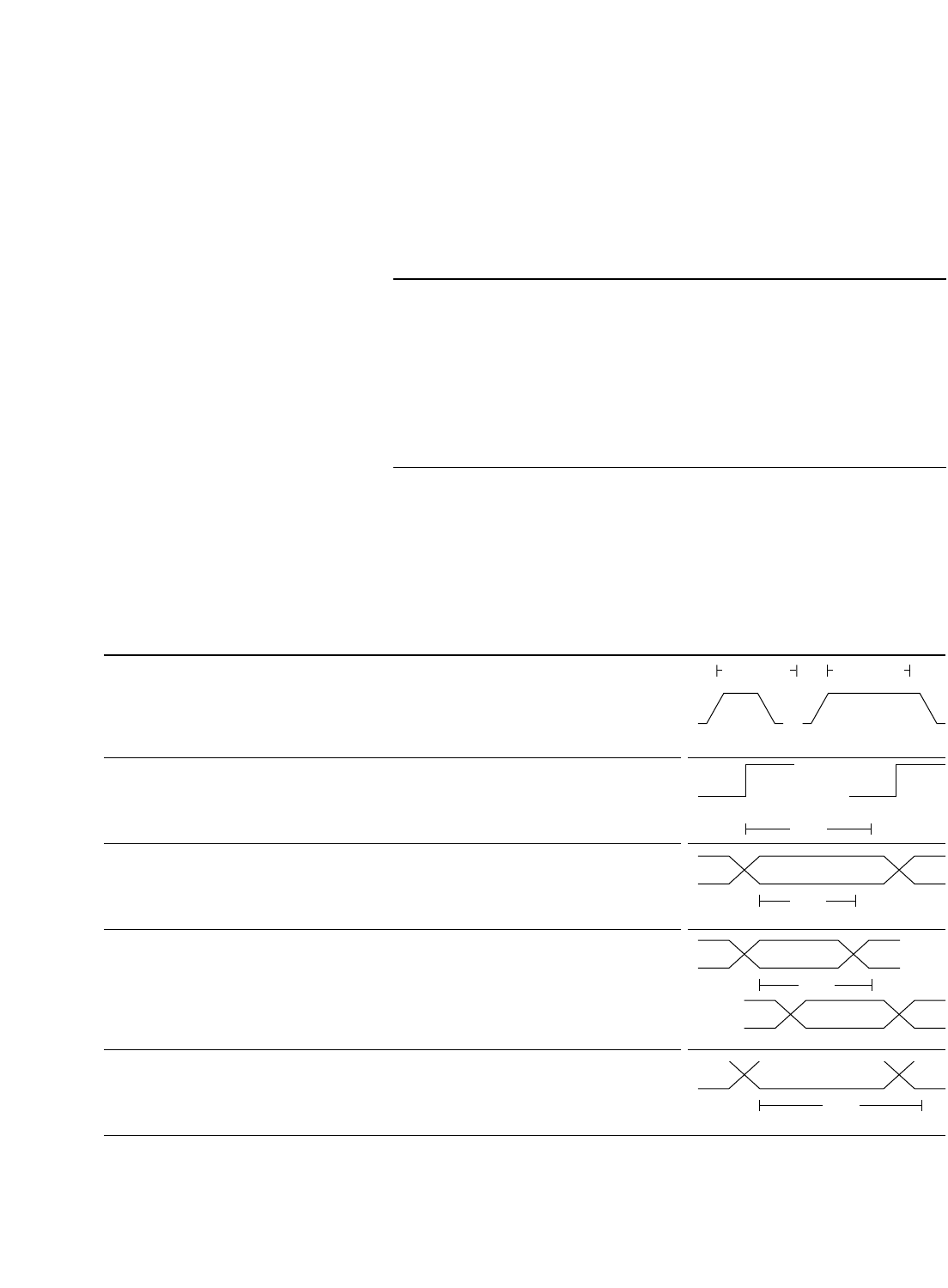
Examples of Problems that Can be Captured Easily with VisiTrigger
Description Typical Applications Graphic
Pulse too narrow or too wide • Line hangs at wrong level (high or low).
• Asynchronous input (for example, an interrupt) persists too long.
• Strobe width is too narrow or too wide.
Time between two edges is • Excessive delay in responding to a bus grant request.
longer than specified • Excessive delay in responding to a data valid with a data
acknowledged.
Pattern lasts longer than a • A bus hangs up at a given value.
specified time
Pattern two exists within a • An incorrect response to a read or write.
specified time after pattern • An incorrect output from a FIFO or bridge.
one is detected
A pattern exists for less • A driver is not holding a bus value long enough for a receiver to
than a specified time respond.
Pulse too narrow Pulse too wide
Min width
Max width
OR
time
edge 1 edge 2
pattern
time
pattern 1
pattern 2
time
pattern
time
23
Data Acquisition and Stimulus
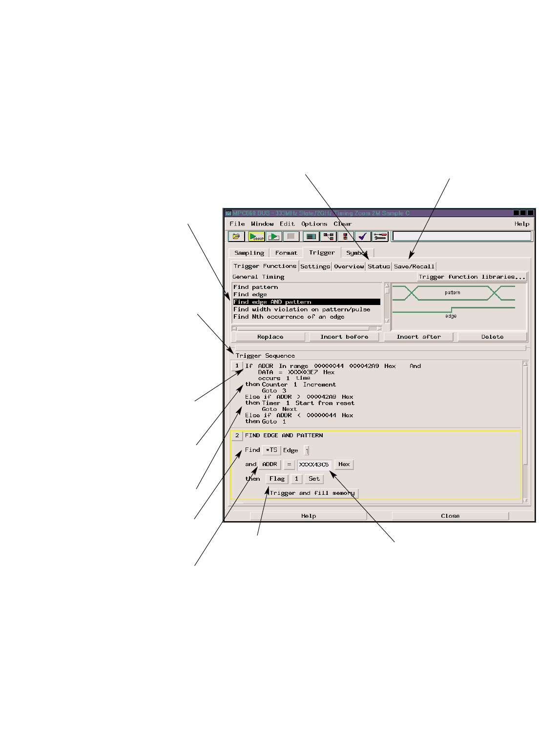
State/Timing Modules
Save and recall up to ten of your
custom trigger setups without loading
a new configuration file.
View current information on the state of
the timers, counters, flags, and the trigger
sequence level.
VisiTrigger
Your most commonly used triggers are
just a mouse click away with the built-in
trigger functions. VisiTrigger’s graphical
representation shows you how the
trigger condition will be defined. You can
use trigger functions as building blocks
to easily customize a trigger for your
specific task.
Sequence levels allow you to develop a
sequence of analyzer instructions to
specify a trigger point or to qualify data
and store only the information that
interests you. Each step in the sequence
contains an "IF/THEN/ELSE" structure
that can evaluate up to four logic
events. Each event can specify a
combination of actions such as: store
sample, increment counters, reset
timers, trigger, or go to another step
in the sequence level.
Ranges provide a way to monitor
program and data accesses within a
specified area in memory.
Global counters can count events such
as the number of times a function
executes or accesses an I/O port.
Timers can be set up to evaluate when
one event happens too late or too soon
with respect to another event.
In timing mode, edge terms let you
trigger on a rising edge, falling edge,
either edge, or a glitch.
Patterns and their logical combinations
let you identify which states to store,
when to branch and when to trigger.
Flags can be set, cleared and evaluated by
any 16715A/16A/17A/16740 Series/
16750 Series/16760A module in the frame.
This allows you to set up a trigger that
is dependent on activity from more than
one bus in the system.
Values can be easily entered directly into
the trigger description.
Figure 4.2. Set up your trigger in terms of the measurements you want to make.
24
Data Acquisition and Stimulus
State/Timing Modules
4 GHz Timing Zoom Provides
High-Speed Timing Analysis
Across All Channels, All the Time
When you're pushing the speed
envelope, you may run into elusive
hardware problems. Capturing
glitches and verifying that your
design meets critical setup/hold
times can be difficult without the
proper tools. With Timing Zoom you
have access to the industry's most
powerful tool for high-speed
digital debug.
Features and Applications
Timing Zoom • Simultaneously acquire up to 64K of data at 4 GHz timing and
(available in the 600 MHz state across all channels, all the time, through the same
16716A, 16717A, connection (16753/54/55/56A)
16740 Series and • Vary the placement of Timing Zoom data around the trigger point
16750 Series • Efficiently characterize hardware with 250 ps resolution
state/timing modules)
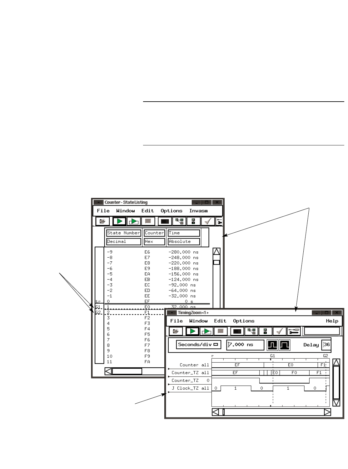
Now it’s easy to capture simultaneous
4 GHz timing and high-speed state
information through a single connection.
Use the global
markers to
time-correlate
events across
multiple displays.
Timing Zoom labels are automatically
created and marked with an _TZ extension.
Figure 4.3. Verifying critical edge timing in your system is easy with Agilent Technologies' 4 GHz Timing Zoom technology.
25
Data Acquisition and Stimulus
State/Timing Modules
Eye Finder
Agilent’s eye finder examines the
signals coming from the circuit under
test and automatically adjusts the
logic analyzer’s setup and hold
window on each channel. Eye finder,
combined with 100 ps adjustment
resolution (10 ps on 16760A) on
Agilent’s logic analyzer modules,
yields the highest confidence in
accurate state measurements on
high-speed buses.
It takes less than a minute to run
eye finder. No special setup or
additional equipment is required.
You only need to run eye finder
once, when the logic analyzer is set
up and connected to the target.
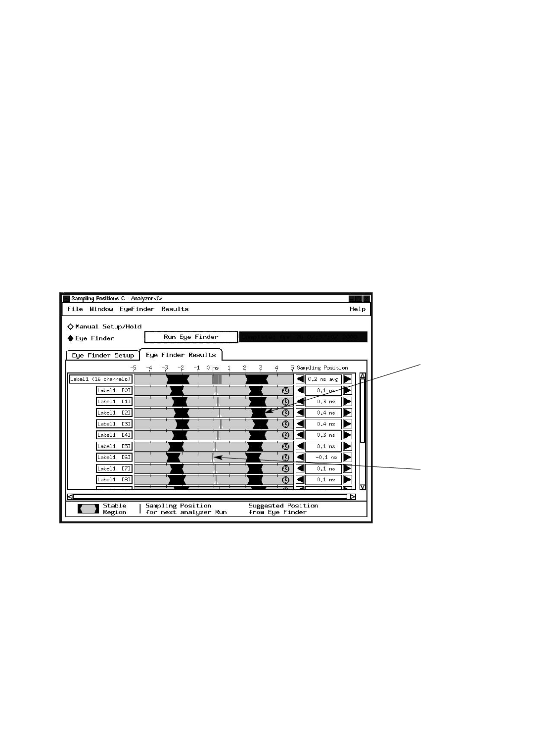
Figure 4.4. The eye finder display.
Gray shading indicates
regions where
transitions are detected.
Blue bars indicate
the sampling point
selected by eye finder.
The eye finder display shows:
• Regions of transitions that were
discovered on all channels
selected
• The sampling point selected by eye
finder
If you want to select a different
sample point on any individual
channel, just drag and drop the blue
"sample" bar at the desired point.
Times in the eye finder display are
referenced to the incoming clock
transitions. The center of the display
(labeled "0 ns") corresponds to the
clock transitions.

26
Data Acquisition and Stimulus
State/Timing Modules
Eye Finder as an Analytical Tool
Eye finder is very useful as a first-
pass screening test for data valid
windows. Because eye finder quickly
examines all channels, it is
considerably faster than examining
each channel with an oscilloscope.
After running eye finder, you may
want to use an oscilloscope to
examine only those signals that are
close to your desired specifications
for setup and hold.
Eye finder also can quickly provide
useful diagnostic or troubleshooting
information. If a channel has an
unexpectedly small data valid
window, or an anomalous offset
relative to clock, this could be an
indication of a problem, or could be
used to validate the cause of an
intermittent timing problem.
Differences in the position of the
stable region from one signal to
another on a bus indicate skew. An
indication of excessive skew on eye
finder can help isolate which
channels you want to check with an
oscilloscope, or with the Timing
Zoom 4 GHz timing analysis mode
in your logic analyzer.
When Do You Need Eye Finder?
Eye finder becomes critical when
the data valid window is <2.5 ns. If
you’re unsure where your clock edge
is relative to the data valid window,
you can run eye finder for maximum
confidence. If the clock in your
system runs at 100 MHz or slower,
and the clock transitions are
approximately centered in the data
valid window, you may not see any
transition zones indicated in the eye
finder display. This is because eye
finder only examines a time span of
10 ns (16760A: 6 ns) centered about
the clock.
Examples of When to Run Eye Finder
You should use eye finder in the
following situations:
Probing a new target, or probing
different signals in the same target
• Because eye finder examines the
actual signals in the circuit under
test, you should run it whenever
you probe a different bus or a
different target.
Significant change of target
temperature
• The propagation delays and
signal levels in your target system
may vary with temperature. If,
for example, you place your
target system in a controlled
temperature chamber to evaluate
its operation over a range of
temperatures or to trouble-shoot
a problem that only occurs at high
or low temperatures, you should
run eye finder after the target
system stabilizes at the new
ambient temperature.

27
Data Acquisition and Stimulus
State/Timing Modules
Features Supported in Agilent State and Timing Analysis Modules
Agilent Module Number 16710A, 16711A, 16715A 16716A, 16717A, 16760A 16753A, 16754A,
16712A 16740A, 16741A, 16755A, 16756A
16742A, 16750B
16751B, 16752B
Eye finder √√√√
VisiTrigger √√√√
Timing Zoom √√
Transitional timing √√√√√
Context Store √
Eye Scan √√
Single-ended inputs √√√√√
Differential inputs √√

28
Data Acquisition and Stimulus
State/Timing Modules
Agilent 16760A: Extending Logic
Analysis to New Realms
• Differential inputs (single-ended
probes also available).
• State analysis up to 1.5 Gb/s.
• Setup-and-hold time of 500 ps.
• Input signal amplitude as low as
200 mV p-p.
Logic analysis at state speeds up to
1.5 Gb/s imposes a stringent set of
criteria for a logic analyzer.
• Probing
Agilent’s 16760A uses an innovative
probing system with only 1.5 pF of
probe tip capacitance, including the
connector. The connector is a joint
design between Agilent and Samtec,
optimized especially for logic analysis
measurements.
Ground pins located between every
pair of signal pins provide excellent
channel-to-channel isolation at high
speeds.
• Setup and hold
As state speeds go up, the data valid
window shrinks. To make reliable
measurements, a logic analyzer’s
combined setup and hold window
must be smaller than the data valid
window of the signals it is acquiring.
Agilent’s 16760A has a combined
setup and hold time of 500 ps to
match the data valid window of
very high-speed buses.
To position the analyzer’s setup-and-
hold window inside the data valid
window requires very fine adjust-
ment resolution. The 16760A gives
you the ability to position the setup-
and-hold window with 10 ps resolu-
tion.
• Small-amplitude signals
Many high-speed designs use small
signal amplitudes to limit slew rates
and reduce power. Agilent’s 16760A
can make reliable measurements on
signals as small as 200 mV p-p.
• Differential signals
Many high-speed designs use differen-
tial signaling to minimize simultane-
ous switching noise and to provide
immunity to crosstalk and noise. The
Agilent 16760A has differential inputs
to allow you to acquire differential
signals with complete confidence.
Single-ended probes are also available.
Agilent helps you get started in the
design stage.
To probe high-speed signals with a
logic analyzer, you need to design the
probe in when you are designing your
PC board. The following document
from Agilent will help you design your
system to take maximum advantage
of the capabilities of the 16760A logic
analyzer:
• Logic signal standards supported
TTL LVTTL
HSTL Class I & II HSTL CLass III & IV
SSTL2 SSTL3
AGP-2X LVCMOS 1.5V
LVCMOS 1.8V LVCMOS 2.5V
LVCMOS3.3V CMOS 5V
ECL LVPECL
PECL
User defined from -3V to +5V in 10mV
increments
Publication Title Description Publication Number
User’s Guide, Agilent Technologies E5378A, E5379A, Mechanical drawings, electrical models, 16760-97010
E5380A, and E5386A Probes for the 16760A Logic Analyzer general information on probes for the 16760A
Designing High-Speed Digital Systems for Guidelines and design examples for designing 5988-2989EN
Logic Analyzer Probing logic analyzers probing into your target system
29
Data Acquisition and Stimulus
State/Timing Modules
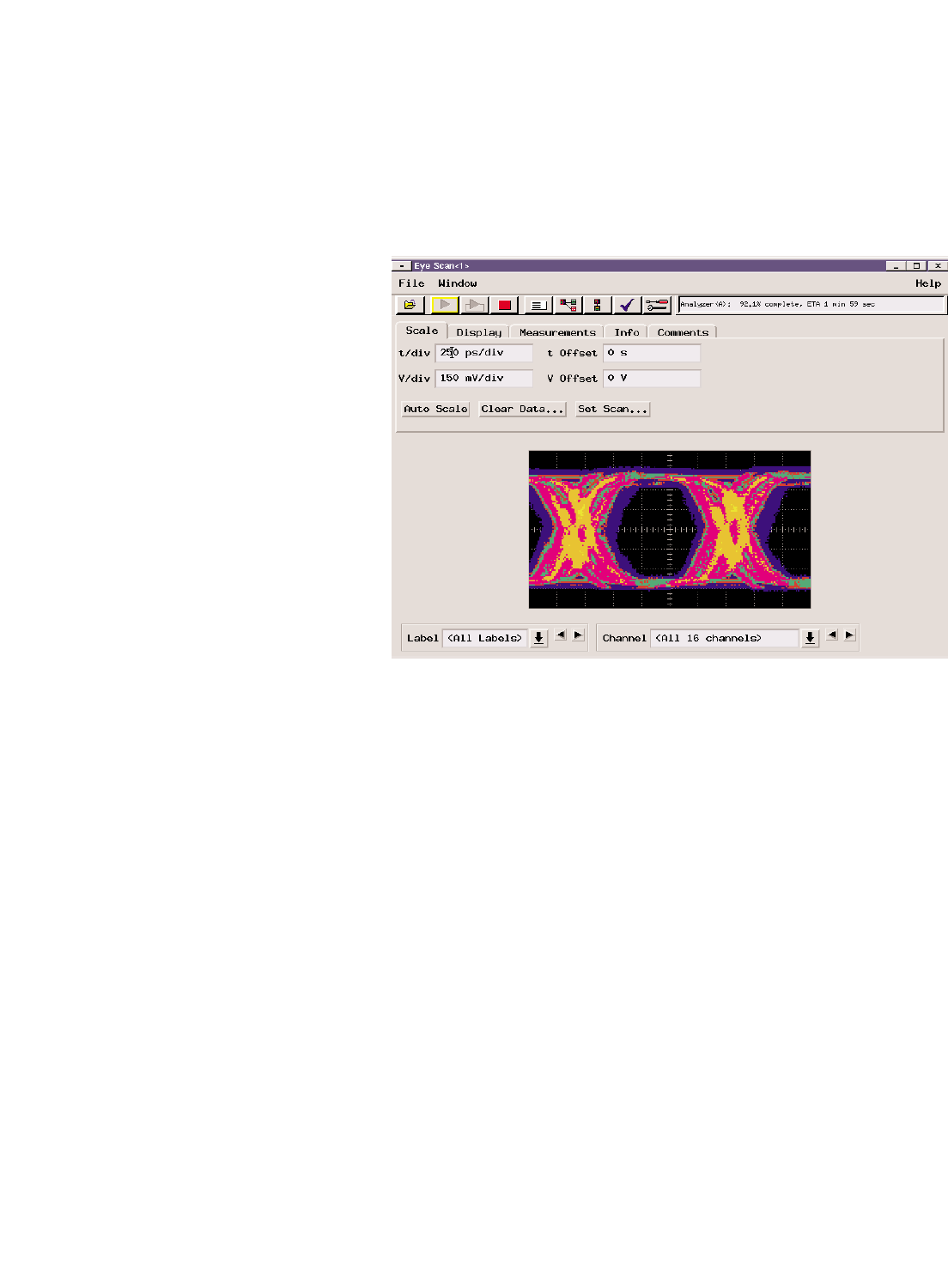
Eye scan
In the eye scan mode, the Agilent
16753A, 16754A, 16755A, 16756A,
and 16760A scans all incoming
signals for activity in a time range
centered on the clock and over the
entire voltage range of the signal.
The results are displayed in a graph
similar to an eye diagram as seen
on an oscilloscope.
As timing and voltage margins
continue to shrink, confidence in
signal integrity becomes an
increasingly vital requirement of
the design verification process.
Eye scan lets you acquire comprehen-
sive signal integrity information on
all the buses in your design, under a
wide variety of operating conditions,
in minimum time.
Qualified eye scan
In the qualified eye scan mode
(16760A only), a single qualifier
input defines what clock cycles are
to be acquired and what cycles are
to be ignored in the eye scan
acquisition. For example, you may
wish to examine the eye diagram
for read cycles only, ignoring
write cycles.
Cursors
Two manually positioned cursors
are available. The readout indicates
the time and voltage coordinates of
each cursor.
Eye limit
The eye limit tool is a single point
cursor that can be positioned manu-
ally. The readout indicates the inner
eye limits detected at the time and
voltage coordinates of the cursor.
Histogram
The histogram tool indicates the rela-
tive number of transitions along a
selected line. The time range and
voltage levels of the histogram are
selected by manually positioning a
pair of cursors. The cursors indicate
the voltage level and the beginning
and end times of the histogram.
Polygon
A 4-point or 6-point polygon can be
defined manually.
Slope
The slope tool indicates DV/DT
between two manually - positions
cursors.
Eye scan allows the user to set the
following variables:
• The number of clock cycles to be
evaluated at each time and voltage
region
• The display mode
• Color graded
• Intensity shaded
• Solid color
• Aspect ratio of the display
• Time/division
• Time offset
• Volts/division
• Voltage offset
• Time resolution of measurement
• Voltage resolution of
measurement
Results can be viewed for each
individual channel. A composite
display of multiple channels and/
or multiple labels is also available.
Individual channels can be
highlighted in the composite view.
Eye scan data can be stored
and recalled for later comparison
or analysis.

30
Probing solutions to match the
measurement capabilities
Multiple probing options are
available for the Agilent 16753A,
16754A, 16755A, 16756A, and
16760A. Each probe can be ordered
by its individual model number.
Some probes are also available as an
option to the logic analyzer module.
The following table indicates both
the model number and the
option number.
Probes are not supplied as part of
the standard logic analyzer module.
Probes must be ordered separately,
either as options to the logic analyzer
module or individually by their
respective model numbers.
Data Acquisition and Stimulus
State/Timing Modules
Agilent Model Number Module Option Number Description Notes
E5378A 010 100-pin single-ended probe Requires a kit of mating connectors and shrouds
(see the next table) to connect to target system.
E5379A 011 100-pin differential probe Requires a kit of mating connectors and shrouds
(see the next table) to connect to target system.
E5380A 012 38-pin single-ended probe, compatible Maximum state analysis speed is 600 Mb/s.
with target systems designed for the Minimum input amplitude is 300 mV p-p.
Agilent E5346A Mictor adapter cable Requires a kit of mating connectors and shrouds
(see the next table) to connect to target system.
E5382A 013 17-channel, single-ended flying lead
probe set
E5381A 17-channel, differential flying lead
probe set
E5387A 17-channel, differential soft touch Includes 5 retention modules
connectorless probe
E5390A 34-channel single-ended soft touch Includes 5 retention modules
connectorless probe
Connector and shroud kits for probes
For probe model number For PC board thickness Probing connector kit part number
(each contains 5 mating connectors and 5 support shrouds)
E5378A Up to 1.57 mm (0.062") 16760-68702
Up to 3.05 mm (0.120") 16760-68703
E5379A Up to 1.57 mm (0.062") 16760-68702
Up to 3.05 mm (0.120") 16760-68703
E5380A Up to 1.57 mm (0.062") E5346-68701
Up to 3.18 mm (0.125") E5346-68700
31
Data Acquisition and Stimulus
Oscilloscope Modules
When integrated into the
16700 Series logic analysis systems,
the oscilloscope modules make
powerful measurement and analysis
more accessible, so you can find the
answers to tough debugging problems
in less time. Oscilloscope controls are
easy to find and use.
Scope controls
and waveform
display are inte-
grated into a
single window,
making interac-
tive adjustment
easy.
Time and voltage
markers allow you
to measure signal
details precisely.
Multiple Views of Target Behavior
Isolate Problems Quicker
Frequently a problem is detected in
one measurement domain, while the
clues to the cause of the problem are
found in another. That’s why the abil-
ity to view your prototype's behavior
from all angles simultaneously—from
software execution to analog signals—
is essential for quickly gaining insight
into problems.
For example, using a state analyzer
you may observe a failed bus cycle. A
timing problem caused by a reflection
on an incorrectly terminated line
may be causing the bus cycle to fail.
By triggering an oscilloscope from the
state analyzer, you can quickly identi-
fy the cause. The ability to cross-trig-
ger and time-correlate state, timing,
and analog measurements can help
you in solving these tough problems.
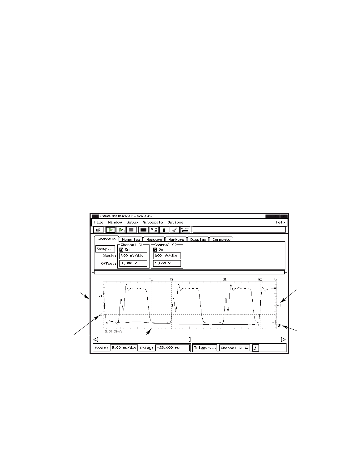
Figure 4.5. All primary oscilloscope control settings, including scale factors and trigger settings, are visible
simultaneously.
Trigger icon
indicates trigger
level, making it
easy for you to
adjust trigger
level.
Ground icon
always shows
you where ground
is relative
to signal.
32
Data Acquisition and Stimulus
Oscilloscope Modules
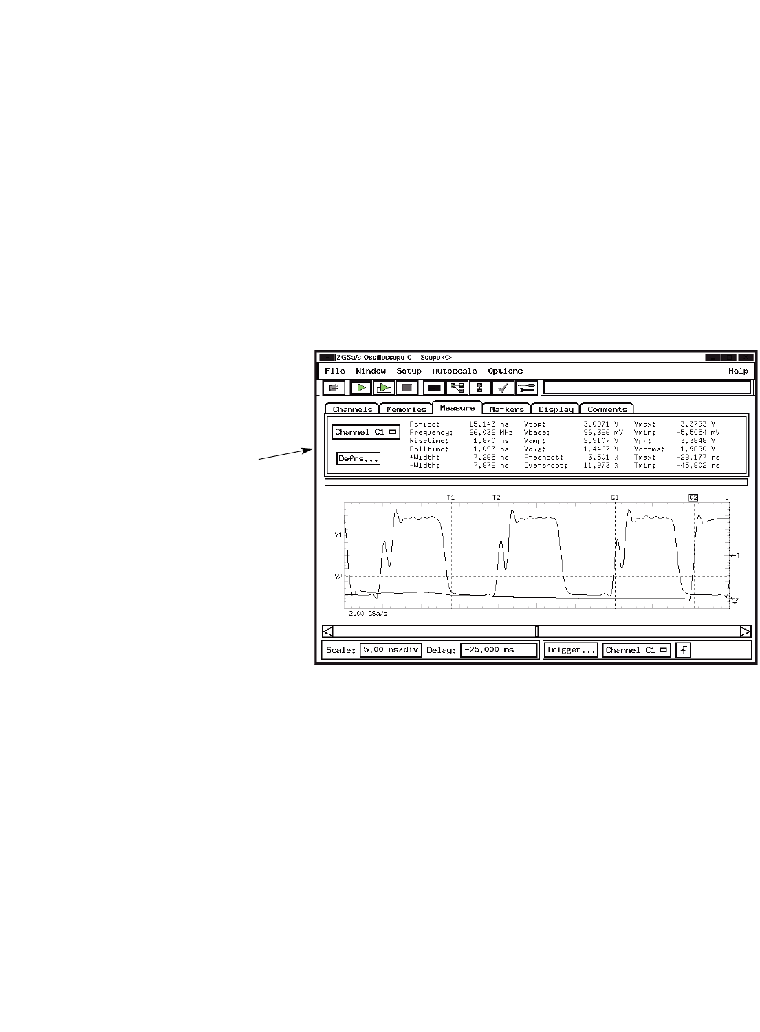
Automatic Measurements Quickly
Characterize Signals
The Agilent Technologies 16534A
oscilloscope modules quickly
characterize signals with automatic
measurements of rise time, voltage,
pulse width, and frequency.
Markers Easily Set Up Timing and
Voltage Margin Measurements
Four independent voltage markers
and two local time markers are avail-
able to quickly set up measurements
of voltage and timing margins.
The global time markers of the
16700 Series logic analysis systems
let you correlate state, timing, and
oscilloscope measurements to
track problems across multiple
measurement domains.
Automatic measurements
save time in characterizing
signal parameters.
Figure 4.6. Automatic measurements and markers let you make faster analysis.
33
Data Acquisition and Stimulus
Oscilloscope Modules
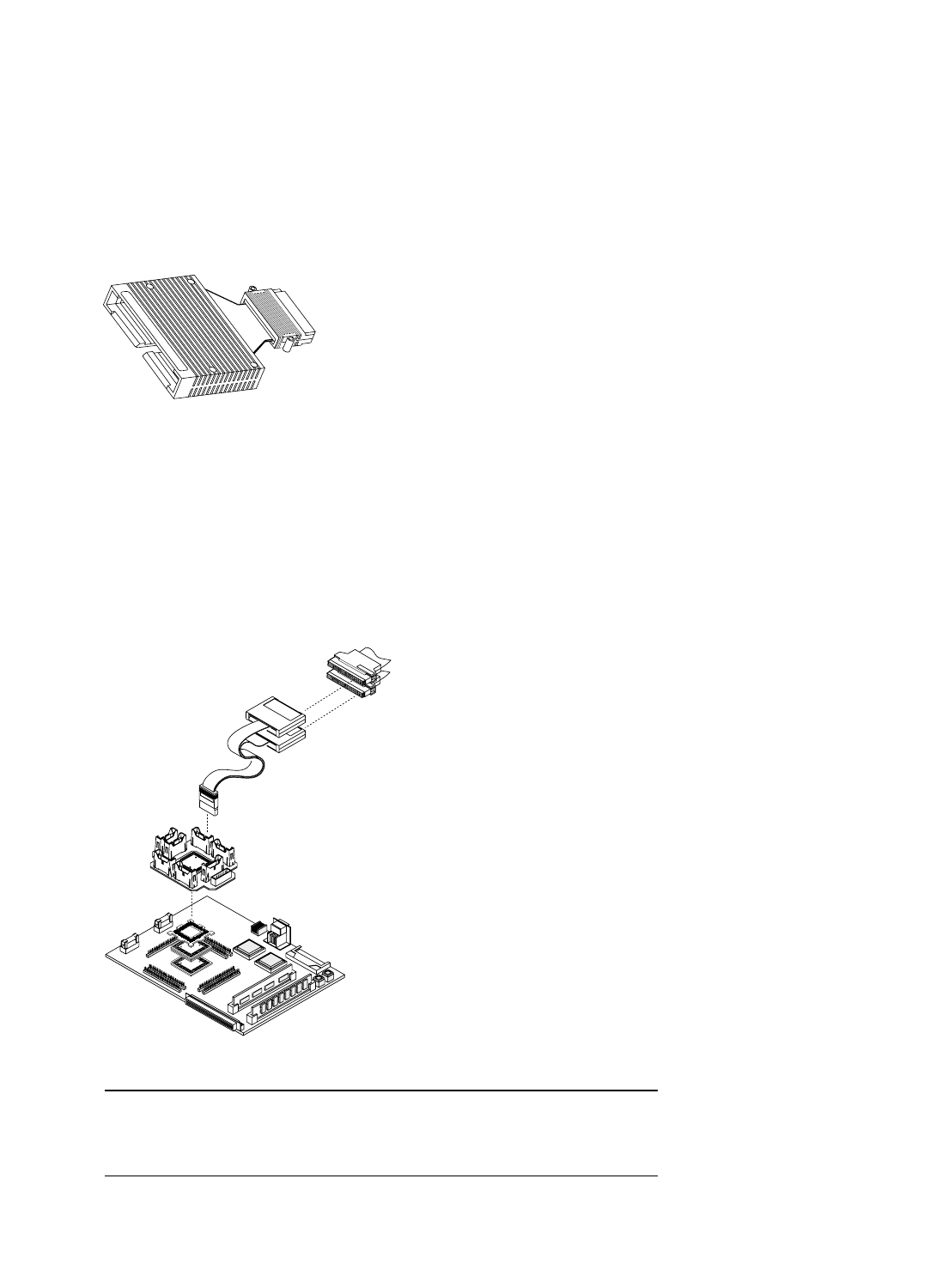
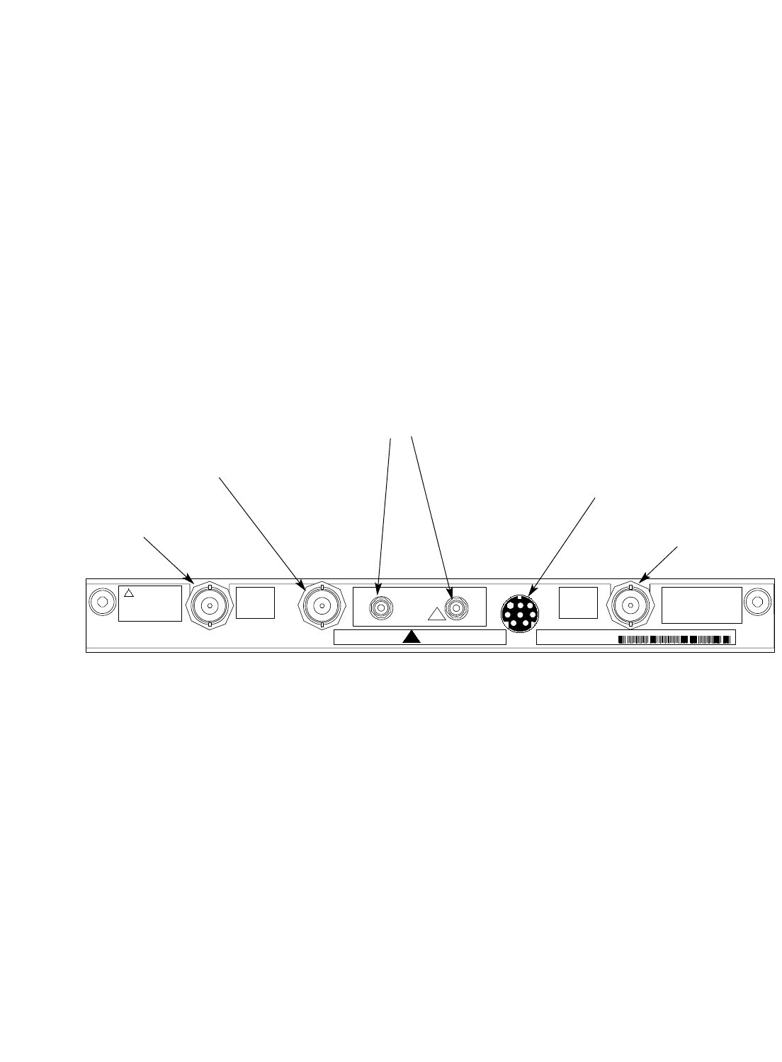
More Channels When You Need Them
You can combine up to four 16534A
oscilloscope modules to provide up
to eight channels on a single time
base. When you operate in this
mode, you can use the master module
for triggering.
CHAN 1 & 2
1MW = 7pF
250V MAX OR
50W 5Vrms MAX
!16534A
2 GSa / s
OSCILLOSCOPE
CHAN
1
CHAN
2
IN OUTECL EXT
TRIG
!SN US35021924
16534A MADE IN THE USA
! PROBE POWER
AC/DC CAL
!
Channel 1 input
Figure 4.7. Connector panel of the 16534A oscilloscope module.
Calibrator output used
for operational accuracy
calibration
Probe power output provides power
for 1145A dual active probe or two
1141A active probes
Channel 2 input
External trigger input and output are
used to connect up to four oscilloscope
modules, providing up to eight channels
on a single time base.

34
Data Acquisition and Stimulus
Pattern Generation Modules
Digital Stimulus and Response in a
Single Instrument
Configure the logic analysis system to
provide both stimulus and response
in a single instrument. For example,
the pattern generator can simulate a
circuit initialization sequence and
then signal the state or timing analyz-
er to begin measurements. Use the
compare mode on the state analyzer
to determine if the circuit or subsys-
tem is functioning as expected. An
oscilloscope module can help locate
the source of timing problems or
troubleshoot signal problems due to
noise, ringing, overshoot, crosstalk,
or simultaneous switching.
Key Characteristics
Agilent Model 16720A
Maximum clock (full/half channel) 180/300 MHz
Number of data channels (full/half channel) 48/24 Channels
Memory depth (full/half channels) 8/16 MVectors
Maximum vector width 240/120 Bits
(5 module system, full/half channel)
Logic levels supported 5V TTL, 3-state TTL, 3-state TTL/CMOS,
3-state 1.8V, 3-state 2.5V, 3-state 3.3V, ECL, 5V PECL,
3.3V LVPECL, LVDS
Maximum binary vector set size 16 MVectors (24 channels)
Editable ASCII vector set size 1 MVectors
Parallel Testing of Subsystems
Reduces Time to Market
By testing system subcomponents
before they are complete, you can fix
problems earlier in the development
process. Use the Agilent 16720A as a
substitute for missing boards,
integrated circuits (ICs), or buses
instead of waiting for the missing
pieces. Software engineers can create
infrequently encountered test
conditions and verify that their code
works—before complete hardware is
available. Hardware engineers can
generate the patterns necessary to
put their circuit in the desired state,
operate the circuit at full speed or
step the circuit through a series
of states.

35
Data Acquisition and Stimulus
Pattern Generation Modules
Vectors Up To 240 Bits Wide
Vectors are defined as a "row" of
labeled data values, with each data
value from one to 32 bits wide. Each
vector is output on the rising edge of
the clock.
Up to five, 48-channel 16720A mod-
ules can be interconnected within a
16700 Series mainframe or expansion
frame. This configuration supports
vectors of any width up to 240 bits
with excellent channel-to-channel
skew characteristics (see specific
data pod characteristics in Pattern
Generation Modules Specifications
starting on page 112). The modules
operate as one time-base with one
master clock pod. Multiple modules
also can be configured to operate
independently with individual clocks
controlling each module.
Depth Up to 16 MVectors
With the 16720A pattern generator,
you can load and run up to
16 MVectors of stimulus. Depth on
this scale is most useful when cou-
pled with powerful stimulus
generated by electronic design
automation tools, such as
SynaptiCAD's WaveFormer and
VeriLogger. These tools create
stimulus using a combination of
graphically drawn signals, timing
parameters that constrain edges,
clock signals, and temporal and
Boolean equations for describing
complex signal behavior. The
stimulus also can be created from
design simulation waveforms. To take
advantage of the full depth of the
16720A pattern generator, data must
be loaded into the module in the
Pattern Generator Binary (.PGB) for-
mat. The SynaptiCAD tools allow you
to convert .VCD files into .PGB files
directly, offering you an integrated
solution that saves you time.
Synchronized Clock Output
You can output data synchronized
to either an internal or external
clock. The external clock is input
via a clock pod, and has no
minimum frequency (other than a
2 ns minimum high time).
The internal clock is selectable
between 1 MHz and 300 MHz in
1 MHz steps. A Clock Out signal is
available from the clock pod and can
be used as an edge strobe with a
variable delay of up to 8 ns.
Initialize (INIT) Block for
Repetitive Runs
When running repetitively, the vec-
tors in the initialize (init) sequence
are output only once, while the main
sequence is output as a continually
repeating sequence. This "init"
sequence is very useful when the
circuit or subsystem needs to be
initialized. The repetitive run capabil-
ity is especially helpful when operat-
ing the stimulus module independent
of the other modules in the logic
analysis system.
"Signal IMB" Coordinates System
Module Activity
A "Signal IMB" (intermodule bus)
instruction acts as a trigger arming
event for other logic analysis modules
to begin measurements. IMB setup
and trigger setup of the other logic
analysis modules determine the
action initiated by "Signal IMB".
"Wait" for Input Pattern
The clock pod also accepts a 3-bit
input pattern. These inputs are level-
sensed so that any number of "Wait"
instructions can be inserted into a
stimulus program. Up to four pattern
conditions can be defined from the
OR-ing of the eight possible 3-bit
input patterns. A "Wait" also can be
defined to wait for an intermodule
bus event. This intermodule bus
event signal can come from any other
module in the logic analysis system.
36
Data Acquisition and Stimulus
Pattern Generation Modules
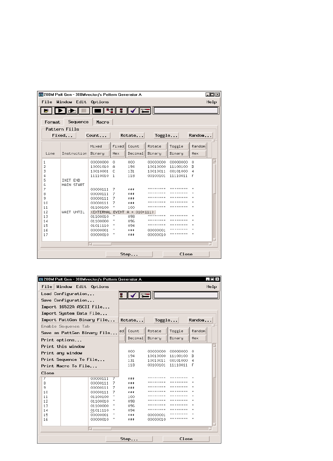
Figure 4.8. Stimulus vectors are defined in the
Sequence menu tab. In this example, vector output
halts until the WAIT UNTIL condition is satisfied.
Figure 4.9. To fill the 16720A pattern generator's 8 MVector
deep memory (16 MVector in half channel mode) with data,
the stimulus must be in 'pattern generator binary' format.
Stimulus files in .PGB format can be loaded directly from
the user interface.

37
Data Acquisition and Stimulus
Pattern Generation Modules
"User Macro" and "Loop" Simplify
Creation of Stimulus Programs
User macros permit you to define a
pattern sequence once, then insert
the macro by name wherever it is
needed. Passing parameters to the
macro will allow you to create a more
generic macro. For each call to the
macro you can specify unique values
for the parameters. Each macro can
have up to 10 parameters. Up to 100
different macros can be defined for
use in a single stimulus program.
Loops enable you to repeat a defined
block of vectors for a specified
number of times. The repeat counter
can be any value from 1 to 20,000.
Loops and macros can be nested,
except that a macro can not be nested
within another macro. When nested,
each invocation of a loop or a macro
is counted towards the 1,000 invoca-
tion limit. At compile time, loops and
macros are expanded in memory to a
linear sequence.
Convenient Data Entry and Editing
Feature
You can conveniently enter patterns
in hex, octal, binary, decimal, and
two's complement bases. The data
associated with an individual label
can be viewed with multiple radixes
to simplify data entry. Delete, Insert,
Copy, and Merge commands are
provided for easy editing. Fast and
convenient Pattern Fills give the
programmer useful test patterns with
a few key strokes. Fixed, Count,
Rotate, Toggle, and Random are
available to quickly create a test
pattern, such as "walking ones".
Pattern parameters, such as Step
Size and Repeat Frequency, can be
specified in the pattern setup.
ASCII Input File Format: Your Design
Tool Connection
The 16720A supports an ASCII file
format to facilitate connectivity to
other tools in your design environ-
ment. Because the ASCII format does
not support the instructions listed
earlier, they cannot be edited into the
ASCII file. User macros and loops
also are not supported, so the vectors
need to be fully expanded in the
ASCII file. Many design tools will
generate ASCII files and output the
vectors in this linear sequence. Data
must be in Hex format, and each label
must represent a set of contiguous
output channels. Data in this ASCII
format is limited to 1 MVectors in
the 16720A.
Configuration
The 16720A pattern generators
require a single slot in a logic
analysis system frame. The pattern
generator operates with the clock
pods, data pods, and lead sets
described later in this section. At
least one clock pod and one data pod
must be selected to configure a func-
tional system. Users can select from a
variety of pods to provide the signal
source needed for their logic devices.
The data pods, clock pods and data
cables use standard connectors. The
electrical characteristics of the data
cables also are described for users
with specialized applications who
want to avoid the use of a data pod.
The 16720A can be configured in
systems with up to five cards for a
total of 240 channels of stimulus.
Direct Connection to Your Target
System
The pattern generator pods can be
directly connected to a standard
connector on your target system. Use
a 3M brand #2520 Series, or similar
connector. The 16720A clock or data
pods will plug right in. Short, flat
cable jumpers can be used if the
clearance around the connector is
limited. Use a 3M #3365/20, or equiv-
alent, ribbon cable; a 3M #4620
Series, or equivalent, connector on
the 16720A pod end of the cable; and
a 3M #3421 Series, or equivalent,
connector at your target system end
of the cable.
Probing Accessories
The probe tips of the Agilent 10474A,
10347A, and 10498A lead sets plug
directly into any 0.1 inch grid with
0.026 inch to 0.033 inch diameter
round pins or 0.025 inch square pins.
These probe tips work with the
Agilent 5090-4356 surface mount
grabbers and with the Agilent
5959-0288 through-hole grabbers.
Other compatible probing accessories
are listed in ordering information on
page 129.
38
Speed Problem Solving With
Off-the-Shelf Solutions for Many
Common Microprocessors
To help you design and debug your
microprocessor-based target systems,
Agilent offers different microproces-
sor specific products that let you get
control and visibility over your
microprocessor’s internal and
external data.
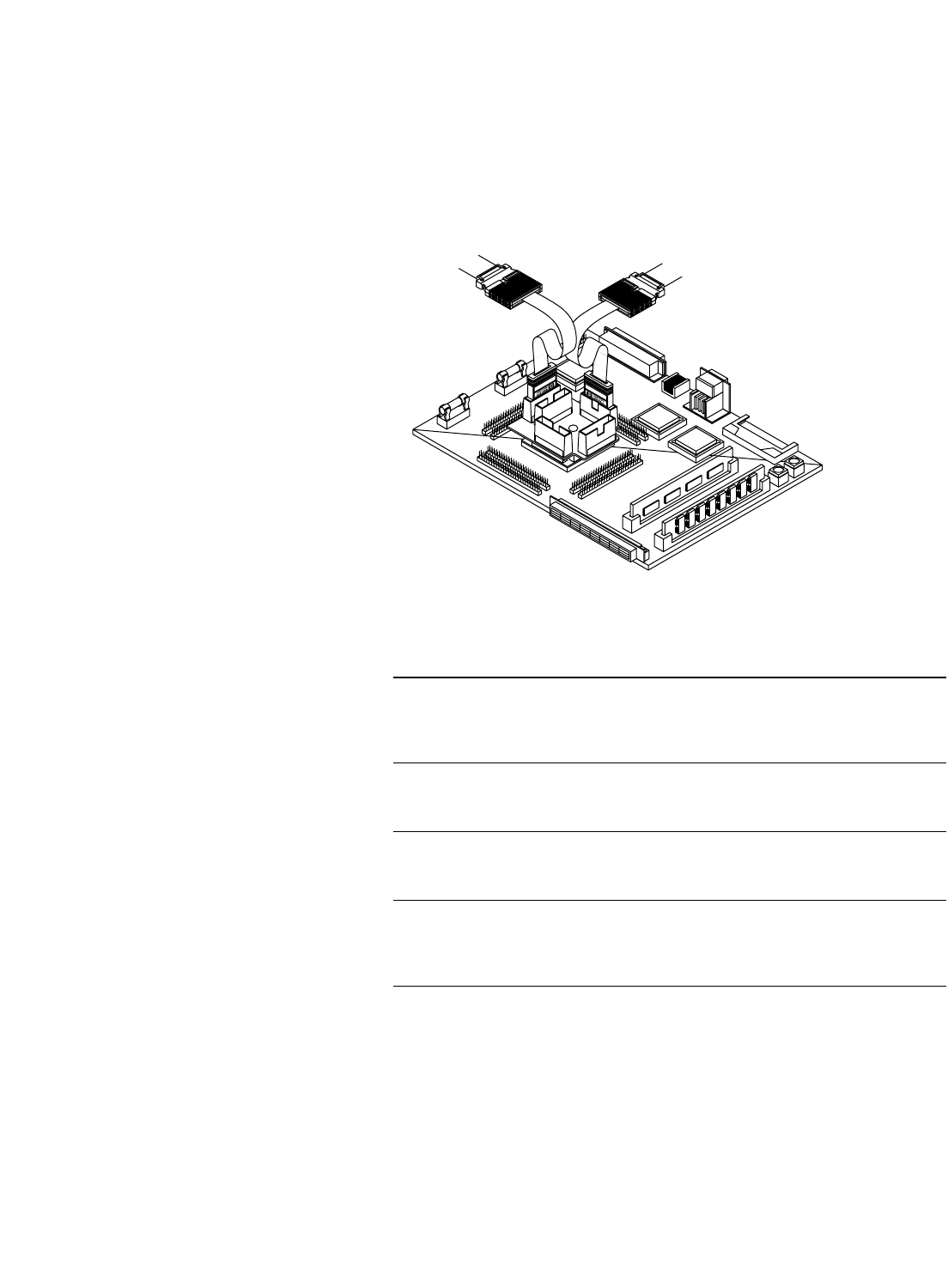
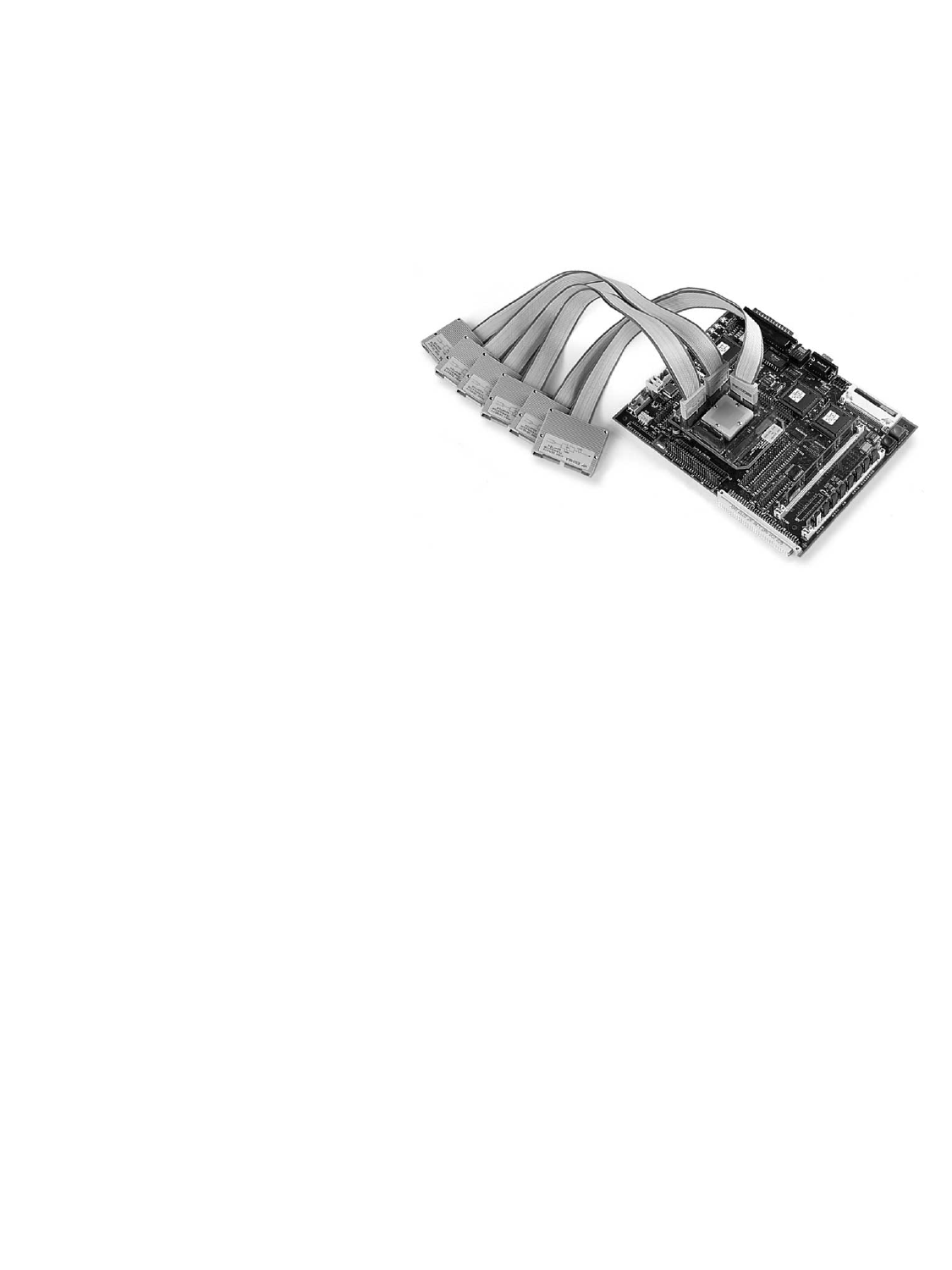
An analysis probe allows you to
quickly connect an Agilent logic
analyzer to your target system. The
analysis probe provides non-intrusive
capture and disassembly of micro-
processor and bus activity
Analysis probes are available for over
200 microprocessors and microcon-
trollers. Bus probes allow probing of
popular bus architectures such as
PCI, AGP, USB, VXI, SCSI, and many
others.
Flexible physical probing schemes
give quick and reliable connections to
almost any device on your prototype.
On-Chip Emulation Tools Make Fixing
Bugs Easier
For specific microprocessor families
that feature on-chip emulation, you
can add a processor emulation
module to your system to connect
the on-board debugging resources
of the microprocessor to the logic
analysis system.
The microprocessor’s BDM or JTAG
technology provides control over
processor operation even if there is
no software monitor on the target
system. This feature is particularly
helpful during the development of
your target system’s boot code.
Data Acquisition and Stimulus
Emulation Modules
Figure 4.10. Agilent analysis probes make it easy to connect a logic analyzer to your target system.
39
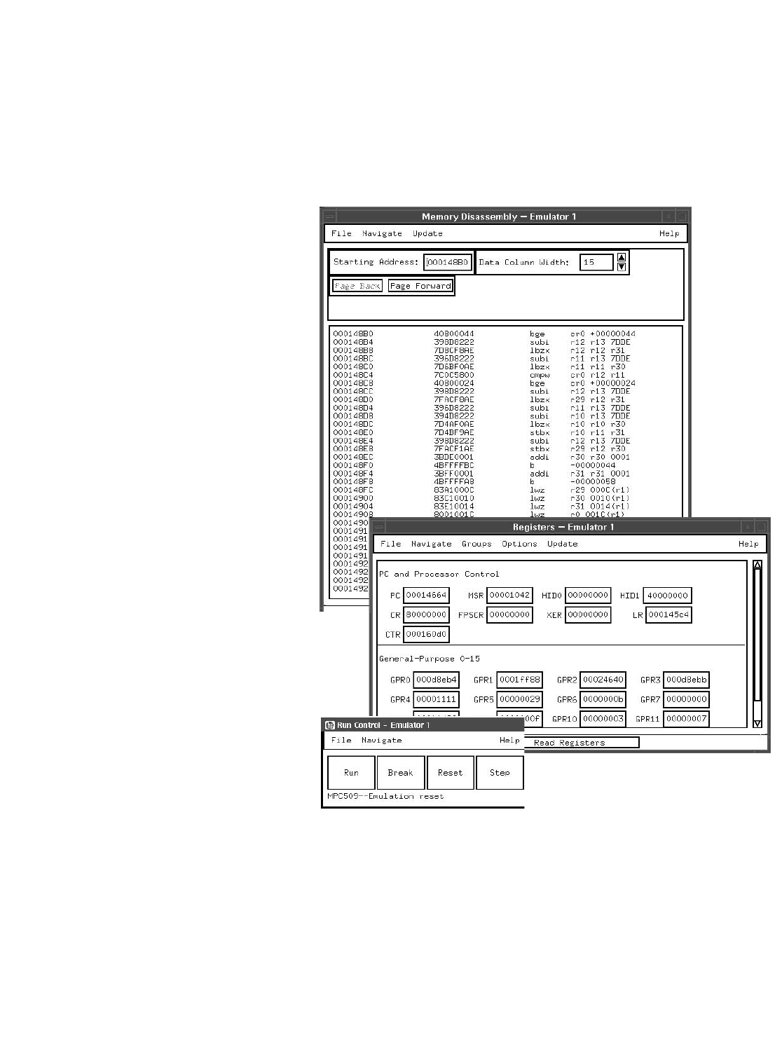
Data Acquisition and Stimulus
Emulation Modules
Emulation Control Interface
The emulation control interface is
accessed from the power up screen of
the Agilent 16700 Series system. The
interface is included with the Agilent
E5901A/B emulation modules.
Designed for hardware engineers,
this graphical user interface provides
the following features:
• Control over processor execution:
run/break/reset/step.
• Register display/modification.
• Memory display/modification in
various formats including disas-
sembly for code visualization.
Memory modification or memory
block fill can be done to check
processor memory access or to
reinitialize memory areas.
• Multiple breakpoint configuration:
hardware, software, and processor
internal breakpoint registers.
• Code download to the target.
• Command scripts to reproduce
test sequences.
• The ability to trigger a measure-
ment module on a processor break
or to receive a trigger from the
logic analysis system’s measure-
ment modules.
Integrated Debugger Support
When the hardware turn-on phase is
completed, the same Agilent emula-
tion module can be connected to
high-level debuggers for C or C++
software development.
You can achieve the functionality of
a full-featured emulator by using a
third-party debugger to drive the
installed Agilent emulation module.
This gives you complete microproces-
sor execution control (run control).
Figure 4.11. Emulation control interface.

40
Post-Processing and Analysis Tool Sets
Software Tool Sets
Once the data is acquired, you can
rely on the post-processing tools to
rapidly consolidate data into displays
that provide insight into your sys-
tem's behavior. The tool sets
described in the following pages are
optional, post-processing software
packages for the 16700 Series logic
analysis systems.
Selecting the Right Tool Set
Take a look at the tool set descrip-
tions below to see if they meet your
needs. If you don't immediately see
what you need there is also the
option of writing your own analysis
application using the tool develop-
ment kit. Best of all, you can try out
any one of these tool sets with no
obligation to buy.
Application Product Name Model Number Detailed Information
Debug your real-time code at the source level Source Correlation B4620B Page 42
Correlate a logic analyzer trace with the high-level source Tool Set
code that produced it. Set up the logic analyzer trace by
simply pointing and clicking on a line of source code.
Debug your parallel data communication buses Data Communications B4640B Page 47
Display logic analyzer trace information at a protocol level. Tool Set
Powerful trigger macros allow triggering on standard or
custom protocol fields. Data bus width is limited only by
the number of available channels.
Optimize your target system's performance System Performance B4600B Page 55
Profile your target system's performance to identify system Analysis Tool Set
bottlenecks and to identify areas needing optimization.
Solve your serial communication problems Serial Analysis B4601B Page 62
Convert serial bit streams to parallel format for easy viewing Tool Set
and analysis. Supports serial data with or without an external
clock reference and protocols that use bit stuffing to maintain
clock synchronization. Works at speeds up to 1.5 Gbits/s.
Customize your trace for greater insight Tool Development B4605B Page 68
Create custom tools using the C programming language. Kit
Custom tools can analyze captured data and present it in
a form that makes sense to you. Analysis systems do not
require the tool development kit to run generated tools.
41
Post-Processing and Analysis Tool Sets
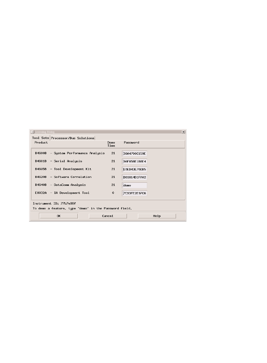
Software Tool Sets
Figure 5.1. For a free, one-time, 21-day trial of any tool set, simply type “demo” in the password field for the product
you want to evaluate.
Free Tool Set Evaluation
To see which tool sets best fit your
needs, Agilent Technologies offers a
free 21-day trial period that lets you
evaluate any tool set as your work
schedule permits. Once you receive
your tool, you obtain a password that
temporarily enables the tool.
42
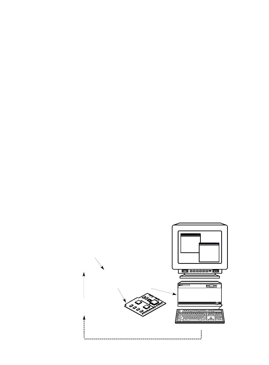
Post-Processing and Analysis Tool Sets
Source Correlation
Debug Your Source Code
The Agilent B4620B source correla-
tion tool set correlates a microproces-
sor execution trace window with a
corresponding high-level source code
window. The source correlation tool
set enhances your software develop-
ment environment by providing mul-
tiple views of code execution and
variable content under severe real-
time constraints.
Using the B4620B you can obtain
answers to many of your questions
concerning software code execution,
data tracking, and software-hardware
integration.
Obtain Answers to the Following
Questions:
Software Code Execution
• What happened just before the
target system crashed?
• What source code was executed at
a specific point in time?
• What is the exact time between
two user-defined system events?
• What is the execution history
leading up to or occurring after an
area of interest?
Data Tracking
• What is the exact history of a
variable's value over time?
• Which routine(s) corrupted the
data?
Software-Hardware Integration
• What is the root cause of a system
failure—hardware or software?
• Are timing anomalies found by the
hardware engineer the cause of
software problems?
• Is the software engineer working
on the same problem as the hard-
ware engineer?
• What portion of the source code
correlates to the problem the
hardware engineer reported?
Product Description
The tool set's main advantage is its
ability to allow you to observe soft-
ware execution without halting the
system or adding instructions to the
code. The tool set uses information
provided in your compiler's object file
to build a database of source files,
line numbers and symbol information
to reference to logic analyzer traces.
The tool set can also be used to set up
the logic analyzer trace by simply
pointing and clicking on a source
line.
Once the tool set is enabled on your
16700 Series system, you can support
new processors by changing analysis
probes and verifying object file com-
patibility. Multiple-processor systems
are also supported.
Source
Analyzer
Trace
Figure 5.2. The source correlation tool set allows you to observe software execution without halting the system or
adding instructions to the code.
Debug
Your Development Environment
Compile
Relocatable
Object Code
Link
Absolute
Object Code
Edit
Source File
Symbol File
Download
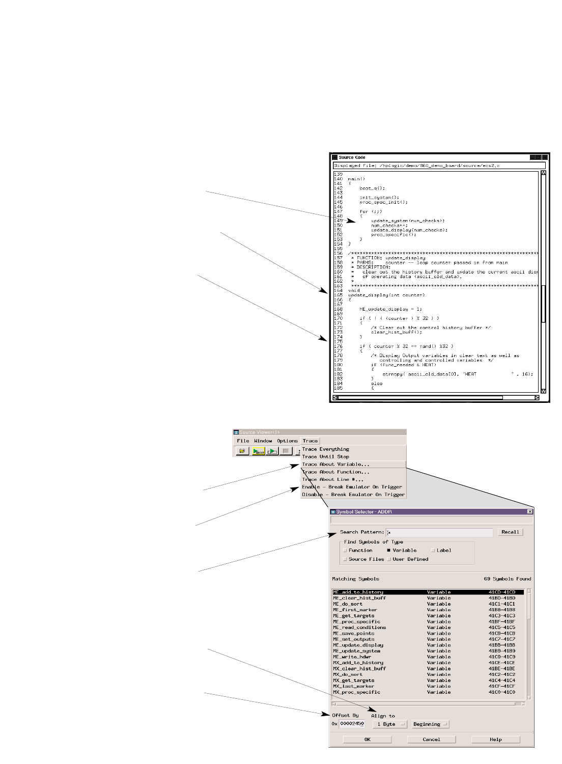
43
Post-Processing and Analysis Tool Sets
Source Correlation
When You Want
to Trace . . .
...on a variable to see what caused data
corruption.
...on a function to determine where it is being
called from in order to understand the context
of a system error.
...on a line number to determine if a
specific code segment is ever executed.
Simply Click . . .
... to trace about a variable, function, or
line number.
... to halt processor execution with an
integrated emulation module when the trace
event occurs.
...to use text search to quickly navigate
through hundreds of symbols. To recall
previous entries when rotating through debug
tests.
...to specify alignment conditions for
processors that don’t include lower address
bits on the bus. This is necessary if your
processor uses bursting or byte enables when
fetching instructions.
...to use address offsets for code that is
dynamically loaded or moved from ROM to
RAM during a boot-up sequence.
Figure 5.3.
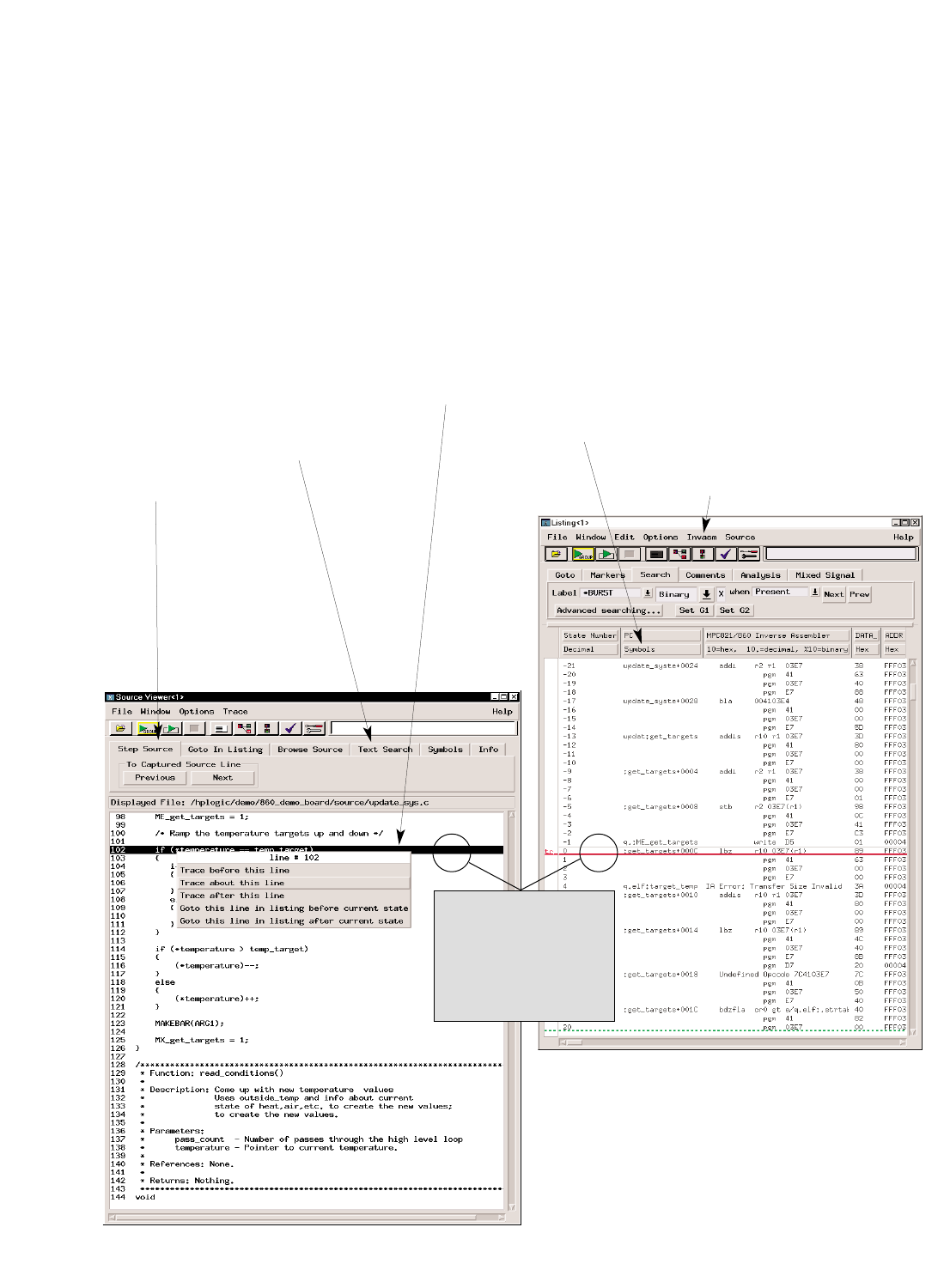
44
Post-Processing and Analysis Tool Sets
Source Correlation
Once You Acquire
the Trace . . .
...filter out unexe-
cuted code fetches
from the inverse
assembled trace to
view executed code
only, using Agilent’s
advanced inverse
assembly filtering for
popular processors.
...quickly locate a
specific function,
variable, or text
string. The system
maintains a history
of previous text
searches for quick
recall.
Also...
Analyze a function’s behavior without viewing
calls to subroutines or interrupts by using the
analyzer’s filtering capabilities to focus on a
specific part of the executed software.
...scroll or step through
the time-correlated
source code (left) or
inverse assembled trace
listing (right)
...“step” through the
trace at the source-
code level or the
assembly level.
Locate the cause of a
problem by “stepping
backward” from the
point where you see
a problem to its root
cause.
...set the data type to
“Symbols” to view
file and symbol
names or ”line #s” to
view file name and
line number.
...click the source line
which you want to
trace about on your
next acquisition.
Figure 5.4.

45
Post-Processing and Analysis Tool Sets
Source Correlation
Product Characteristics
Data Sources
All state and timing measurement
modules supported by the 16700
Series logic analysis systems (except
the 16517A/518A) serve as data
sources for the source correlation
tool set.
Microprocessor Support
The source correlation tool set sup-
ports many of the most popular
embedded microprocessors Non-
intrusive analysis probes for the
16700 Series systems provide reli-
able, fast and convenient connections
to your target system.
New microprocessors are constantly
being added to the list of supported
CPUs. For the most current informa-
tion about supported microproces-
sors, please contact your Agilent
Technologies sales representative
or visit our web site:
http://www.agilent.com/find/logicanalyzer.
Object File Format Compatibility
The 16700 Series logic analysis sys-
tems quickly and reliably read your
specific object file format. Agilent
Technologies' extensive experience
with different file formats and sym-
bol representations ensures that your
source code files are accurately cor-
related and your system is precisely
characterized.
Source correlation and system per-
formance measurements do not
require any change in your software
generation process. No modification
or recompilation of your source code
is required.
You can load multiple object files.
Address offsets are also supported,
enabling system performance meas-
urements and source-code level views
of dynamically loaded software exe-
cution or code moved from ROM to
RAM during a boot-up sequence.
High-level language tools that pro-
duce the following file formats are
supported:
• Agilent(HP)/MRI IEEE696
• ELF/DWARF*
• ELF/Stabs*
• TI_COFF
• COFF/Stabs*
• Intel OMF86
• Intel OMF96
• Intel OMF 286
• Intel OMF 386 (which supports
Intel80486 and Pentium Language)
*Supports C++ name de-mangling
If your language system does not
generate output in one of the listed
formats, a generic ASCII file format
is also supported.
For the most current information
about supported compiler file for-
mats and processor support, please
contact your Agilent Technologies
sales representative.
Source File Access
The source correlation tool set must
be able to access source files to pro-
vide source line referencing.
Source files can reside in multiple
directories on the hard drive of your
workstation, PC, or on the 16700
Series mainframe's internal hard
disk. You can access the files via NFS-
mounted disks or CIFS mounted
disks. To display the source file, the
tool set first looks for the source path
name in the object file, follows the
path to access the source file and, if
not found, looks for the source file in
alternate user-defined directories.
The 16700 Series logic analysis
systems automatically place the
following in the directory search
path:
• NFS mounted directories
• Directory paths specified in
loaded symbol files
• Directory paths specified in
loaded source files
Source Correlation Functionality
• Source code and inverse
assembled trace listing are time-
correlated.
• User can alternate between source
viewer and browsing of other
source files.
• Trace specification can be set up
from the source viewer or file
browser.
• For multiple-processor systems,
each trace window can be
time-correlated to a source viewer.

46
Post-Processing and Analysis Tool Sets
Data Communications
Monitor Packet Information on
Parallel Data Buses
The data communications tool set
shows parallel bus data at a protocol
level on the logic analyzer. Developers
have the capability to find complex,
system-level bus interaction problems
in applications such as a switching or
routing system.
Obtain Answers to the Following
Questions:
• What is the time difference
between two or more data paths
and/or a microprocessor?
• Did a packet make it through the
switch or router?
• Why did a packet take so long to
go through the switch or router?
• Where did an illegal packet come
from?
• What is the latency on packet
information?
• What is corrupting packets?
Product Description
The Agilent Technologies B4640B
data communications tool set adds
protocol analysis capabilities to the
logic analyzer for viewing parallel
data buses (e.g, UTOPIA or a propri-
etary data bus) in a switching or
routing system. Each protocol layer is
displayed with a different color in the
logic analyzer lister display to allow
easy viewing of the protocol data.
Payload information is included after
the header in a raw hex format.
Filters are included to allow many
different views of the data. Protocol
layers can be collapsed or expanded
to create a custom view of the data
acquired in the logic analyzer.
With the filters, you can concentrate
on the data of interest for a
particular measurement.
The powerful protocol trigger macro
allows easy trigger setup by eliminat-
ing the need to manually configure
the trigger sequencer for complex
measurements. All custom-defined
protocol fields or layers are support-
ed in the trigger macro.
All packets or cells are time-stamped
in the logic analyzer for time-correla-
tion measurements with other system
buses, such as a microprocessor,
memory interface, PCI bus, or other
UTOPIA bus. All state listing and
waveform displays in the logic ana-
lyzer are time-correlated with global
markers for a complete view of the
system. With this tool, it is possible
to trigger the logic analyzer with a
microprocessor event and see what is
happening on a parallel data bus with
protocol information.
By monitoring multiple time-correlat-
ed data buses, you can monitor a
packet entering one ASIC and see
how long it takes for the packet to
reach another part of the system. The
powerful trigger can also monitor a
packet entering one port and trigger
if the packet has not reached another
port by a designated time.
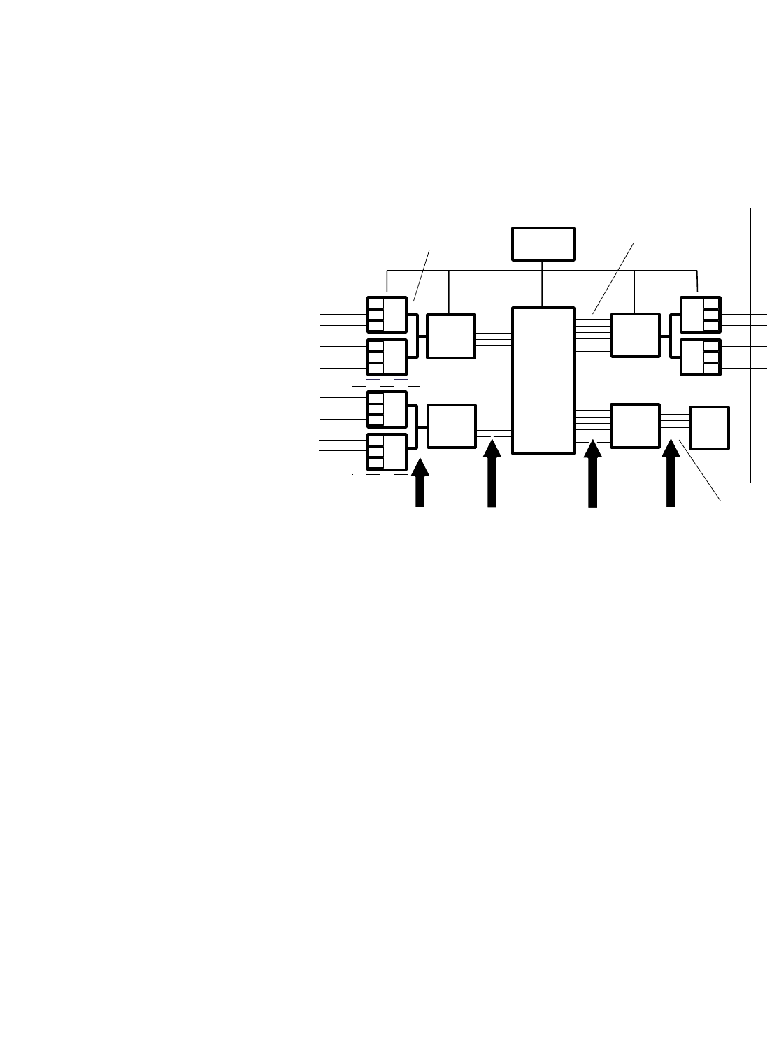
47
Post-Processing and Analysis Tool Sets
Data Communications
Theory of Operation
Use a logic analyzer to probe the
system’s parallel data buses (e.g.,
UTOPIA).
The analyzer needs access to:
• Data signals
• Qualifying signals
• Start of cell or packet bit
• Synchronous clock for the bus
The synchronous bus clock samples
data into the logic analyzer.
Qualifiers such as "Data Valid" allow
the logic analyzer to sample only on
events of interest instead of all
cycles.
With access to the "Start of Cell" or
"Start of Packet" bit on the data bus,
the analyzer starts looking at the
beginning of a cell or packet. With the
protocol definition set up by the user,
the logic analyzer can sequence down
into the cell or packet to find the
desired protocol field to trigger on.
UTOPIA Level 2 CPU Custom/UTOPIA
PHY
PHY
PHY
PHY
PHY
PHY
PHY
ATM
Layer
ATM
Layer
ATM
Layer
ATM
Layer
Switch
Fabric
UTOPIA Level 1
Figure 5.5. Typical ATM Switch Design.

48
Post-Processing and Analysis Tool Sets
Data Communications
Product Characteristics Additional Information
Requires 16700 Series logic analysis system with
system software version A.01.50.00 or higher
Applications Trigger on a processor event and see what
is happening on a parallel data bus with
protocol information or vice versa.
Supported Measurement Modules 16715A, 16716A, 16717A, 16718A, 16719A,
16750A/B, 16751A/B, 16752A/B, 16740A, 16741A,
16742A, 16753A, 16754A, 16755A, 16756A, 16760A
Protocols Supported • Ethernet • Example files for these protocols are provided with the
• ATM product. These standard files can be edited to include
• TCP/IP Stack any custom protocol "wrapper" layers or fields.
• Custom • Custom protocols are supported by entering the protocol
setup information via the logic analyzer interface or a text
file. Custom protocol definitions are used in both the
trigger definition and packet display.
Trigger Macro All custom-defined protocol fields or layers
are supported in the trigger macro
Maximum Parallel Bus Width Limited only by the number of available channels
Display Features • Color • Each protocol layer is displayed with a different color in
the analyzer’s lister display to allow easy viewing of
protocol data.
• Filters and preferences • Specific protocol layers and fields can be selected for
viewing in the trace. Provides many different views of the
data. Allows you to concentrate on the data of interest
for a particular measurement.
• Payload information • Included after the header in a raw hex format
• Protocol layers • Can be collapsed or expanded to create a custom view of
the acquired data
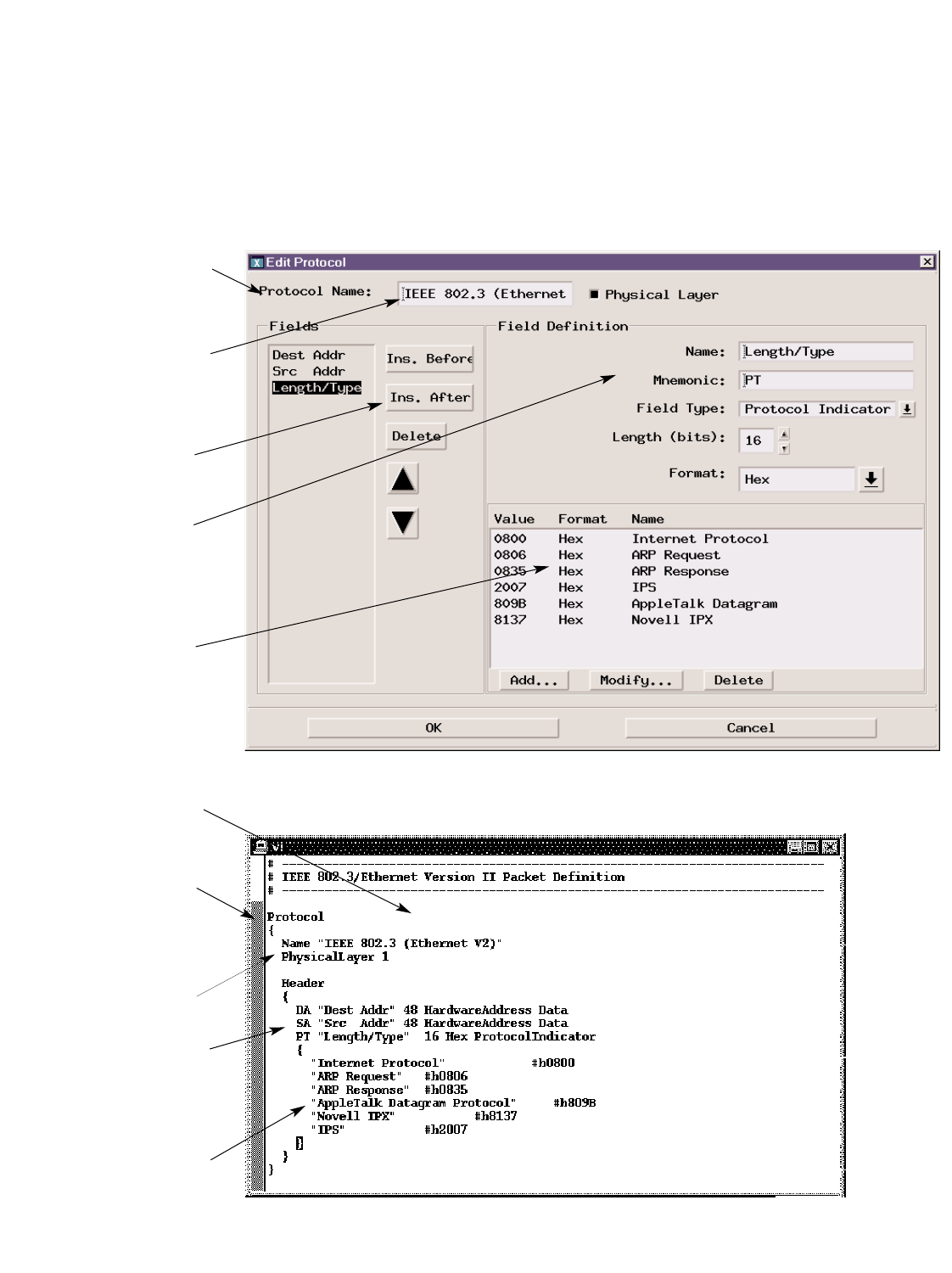
49
Post-Processing and Analysis Tool Sets
Data Communications
Edit or create a
protocol using the
logic analyzer
user interface.
Select a known
protocol and add
proprietary fields.
Insert custom
wrapper or
field here.
Insert name, num-
ber of bits and
format for trigger
and
display.
Define any sym-
bols for both
trigger and
display of
packets.
Edit or create a
protocol using a
text file.
Start with stan-
dard protocol
definition and add
custom fields with
text file.
Insert protocol
layer name.
Define protocol
fields, number of
bits, and format
for trigger and
display.
Define any user
symbols to make
triggering and dis-
play easier to use.
Figure 5.6.
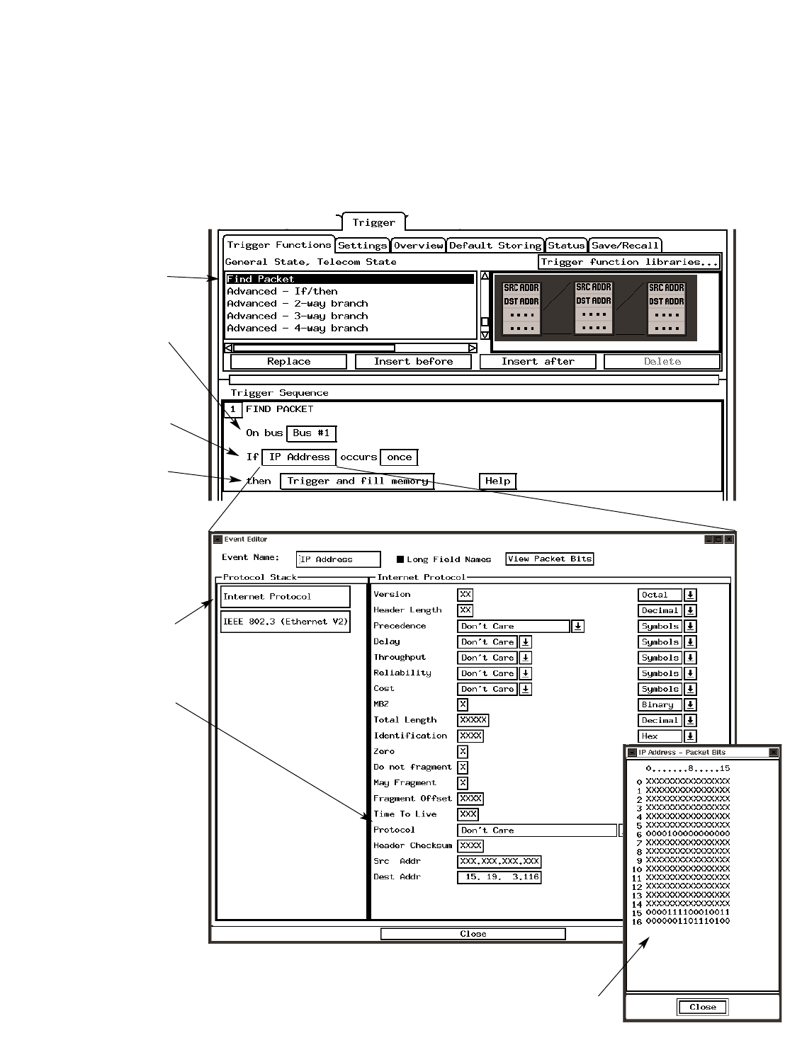
50
Post-Processing and Analysis Tool Sets
Data Communications
New packet
trigger macros.
Choose from a list
of buses.
Trigger on simple
IP address instead
of setting up trig-
ger sequencer.
Specify what
action to perform
once a packet is
found.
Specify protocol
layer to trigger on.
Use any defined
protocol fields as
a trigger, such as
source address,
destination
address, etc.
Physical representation of bit fields to be triggered on.
This window is automatically updated when fields are edited.
Figure 5.7.
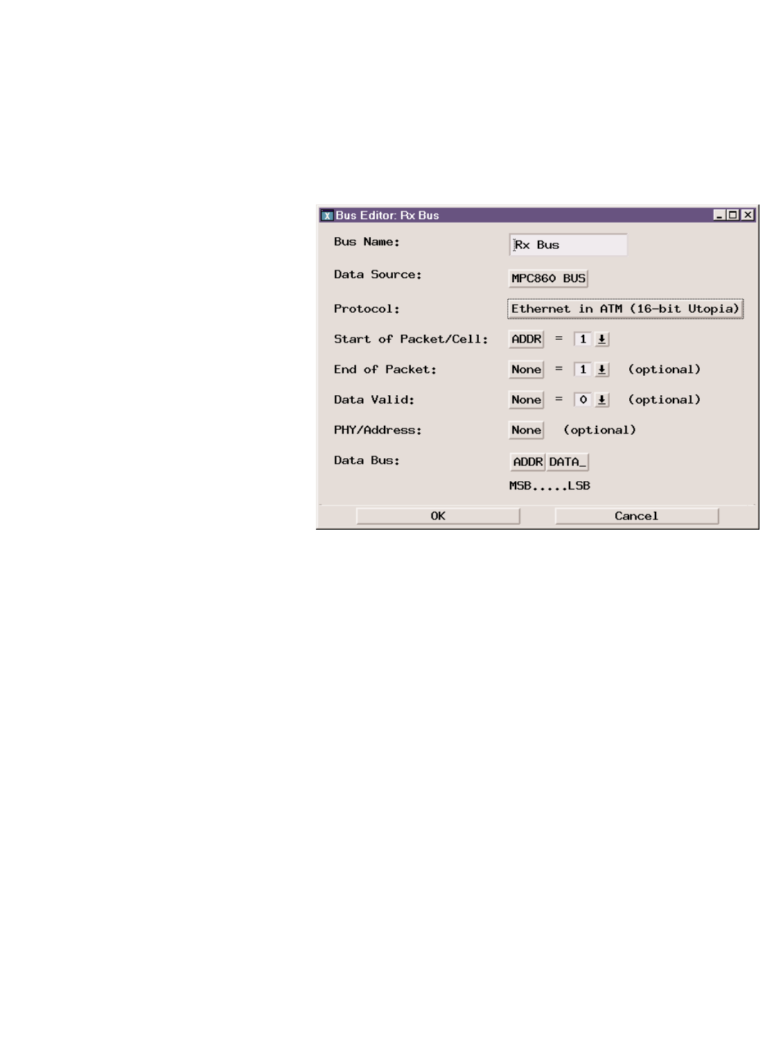
51
Post-Processing and Analysis Tool Sets
Data Communications
Use the bus editor feature to specify
what protocol runs on your bus.
This is helpful when probing more
than one bus with a single state/
timing module.
Figure 5.8.
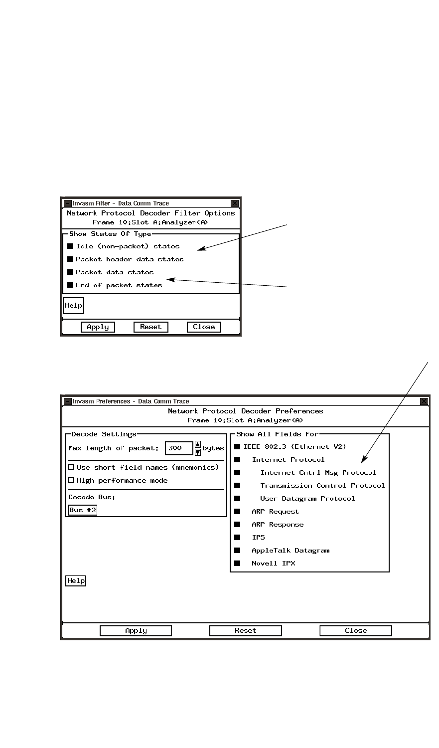
52
Post-Processing and Analysis Tool Sets
Data Communications
Protocol Filters and Viewing
Preferences
Filter captured data to
only view key data for
measurement.
Choose to view payload
data with header
information.
Select which protocol
layers and fields to
view in trace.
Figure 5.9.
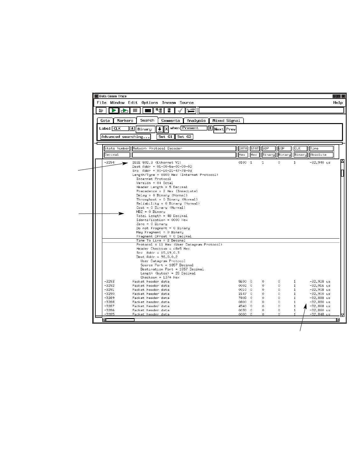
53
Post-Processing and Analysis Tool Sets
Data Communications
Display of
protocol levels.
Protocol view of
data acquired in
logic analyzer.
Time tags for system level correlation of other data
buses, memory interfaces, microprocessors, etc.
Figure 5.10.
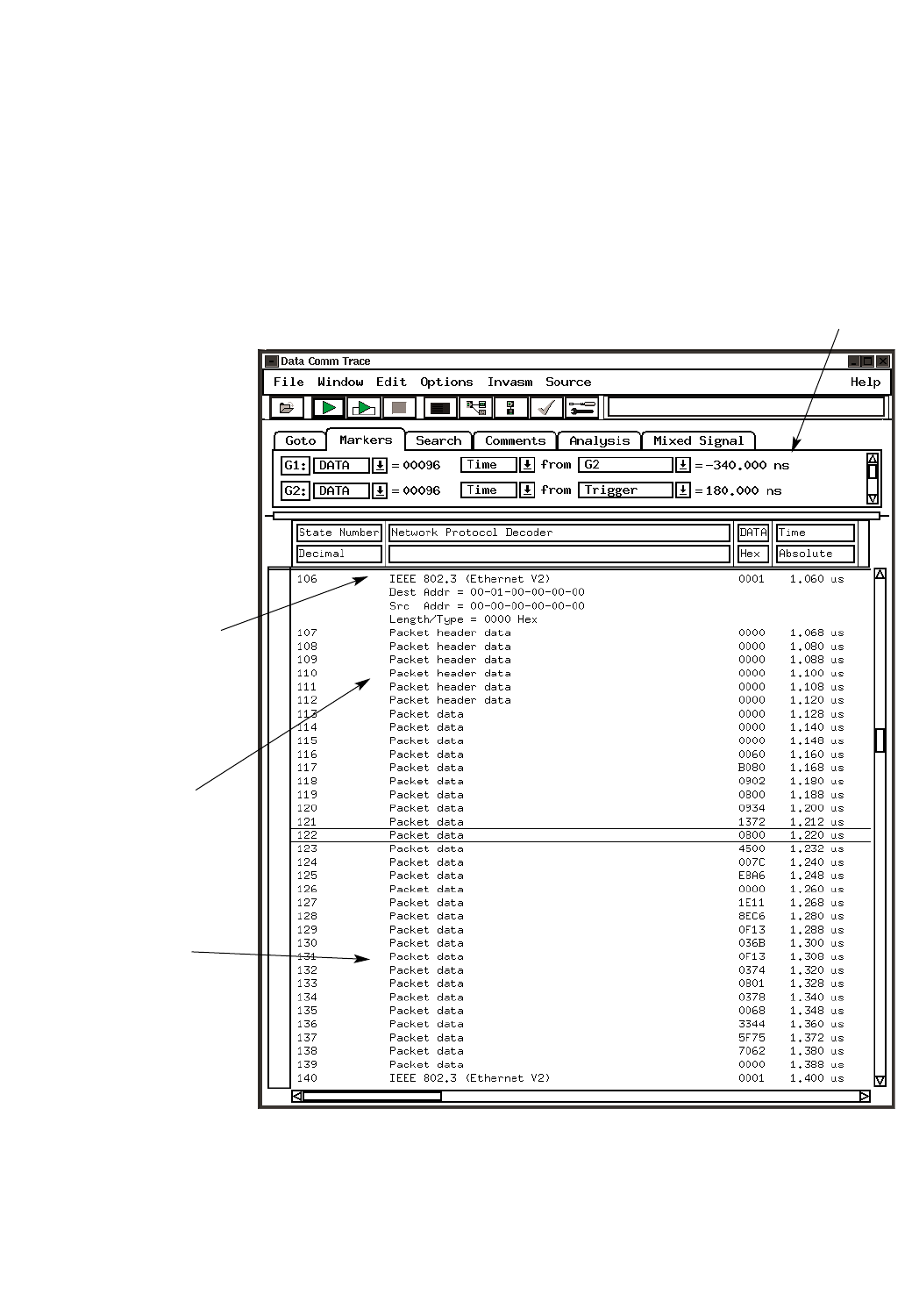
54
Post-Processing and Analysis Tool Sets
Data Communications
Global markers measure time intervals between
packets on separate parallel interfaces or timing
between the data path and a microprocessor.
Collapsed view
of protocol infor-
mation using pref-
erences.
Raw packet
header
information.
Raw payload
information.
Figure 5.11.

55
Post-Processing and Analysis Tool Sets
System Performance Analysis
Optimize System Performance
Your design has to meet consistent
performance requirements over a
range of operating conditions and
over a specific time period. Using the
system performance analysis tool set,
you can obtain answers to many of
your questions concerning perform-
ance and responsiveness, software
execution coverage, debug and
system parameter analysis, etc.
Obtain Answers to the Following
Questions:
Performance and Responsiveness
• What functions monopolize micro-
processor bandwidth?
• What functions are never execut-
ed? What is the relative workload
of each processor in a multiple-
processor system?
• What is the minimum, maximum,
and average execution time of a
function (including calls)?
• How many interrupts does the
system receive per consecutive
time slice?
• What is the response time of the
target system to an external
event?
Software Execution Coverage
• Do test suites provide thorough
coverage of the application?
• Is this function or variable
accessed by the application?
Debug and System Parameter
Analysis
• Does this pointer address the right
memory buffer?
• How does the system react when it
receives too many simultaneous
interrupts?
• Is the stack size adequate?
• Is the cache size adequate?
Analog, Timing, and Bus
Measurements
• What is the setup/hold time of this
signal or group of signals?
• Is the distribution of voltages for
this analog signal acceptable?
• Is this signal spending too much
time in the switching region?
• What bus states occur most often?
• What is the bus loading?
• How does the bus affect overall
system performance?
• How much time is spent in bus
arbitration?
• What is the histogram of bus
transfer times?
Processor/Cache Measurements
• Which microprocessor bus states
occur most often?
• Which peripherals are used most
often?
• What is the profile of load sharing
in a multiple-processor system?
• How does the cache size affect
system performance?
Product Description
The Agilent Technologies B4600B sys-
tem performance analysis (SPA) tool
set profiles an entire target system at
all levels of abstraction—from signals
to high-level source code. It clearly
identifies the components that affect
the behavior of your system. In addi-
tion to performance analysis, it can
be used at any time to test and docu-
ment many other characteristics,
such as memory coverage and
response time.
The SPA tool set generates statistical
representations of the captured data.
It shows the amount and percent of
time spent in each of the targeted
functions or data locations. Data is
conveniently displayed in histograms
and bar charts, reducing the time you
spend analyzing results and identify-
ing system bottlenecks.

56
Post-Processing and Analysis Tool Sets
System Performance Analysis
Product Characteristics
SPA Tools
State Interval Display Time Interval Display Time Overview Display State Overview Display
Generates Statistical representations of the captured data
Shows the amount and percent of time spent in each of the targeted functions or data locations.
Provides Histogram of event Histogram of event times. Overview of occurrence Overview of bus/memory
activity. Display shows Display shows a rates over time. activity. Display shows the
the percentage of hits distribution of the Measurements of the number of hits for each
for each procedure, execution time of a occurrence rate of any possible bus state.
function, or event specific function or of event, including
(states). Events are the time between two interrupts, over time.
defined as patterns or user-defined events.
ranges associated with
any set of data (labels,
symbols).
Usage Helps prioritize functions Determines a specific Views the frequency of First step of analysis or
that are candidates for routine’s execution times events over time. optimization process to
duration measurements and verifies signal timing identify which events occur
using the time interval tool. specifications most frequently.
Applications Cache hit and miss Measures setup and hold Isolates defects such as
analysis. Bus headroom times, the jitter between invalid pointers (filtering).
analysis can be made by two edges, or the Distribution of signal
examining ratio of active variation between two voltages can tell whether a
to idle status states. bus states. digital signal is spending too
Examines workload of much time in the switching
each processor in a region. Evaluates the
multi-processor system linearity of the output of a
to determine if system D/A converter.
is balanced.
Displays Include Ability to be viewed simultaneously
Filtering capabilities for removing portions of a trace that are not applicable to the analysis
Maximum Number of Events No theoretical limit. Number of events limited by size of the window
Up to 10,000 events tested with a standard configuration (e.g. pixels on the screen)

57
Post-Processing and Analysis Tool Sets
System Performance Analysis
Product Characteristics (continued)
SPA Tools
State Interval Display Time Interval Display Time Overview Display State Overview Display
Supplemental Information Number of hits Minimum time Number of hits Number of hits
Maximum time Time bucket width State bucket width
Average time
Standard deviation
Display Modes Sort by number of hits Sort by time Autoscale zoom
Sort alphabetically by Sort alphabetically by
event name event name
Accumulate Mode No theoretical limit to the number of acquisitions in accumulate mode.
Any modification of the display will cause the display to revert back to the last data acquisition.
Object File Format Object file formats are identical for SPA and the source correlation tool sets. See page 45.
Compatibility
Off-Line Analysis and All measurements can be saved using the file out tool.
Post-Processing Data can be recalled at any time for later analysis using any SPA or other tool.
Performance measurements can be exported to your host computer as histograms or as tabular formatted text files.
Processor Support Supports any analysis probe listed in Processor and Bus Support for Agilent Technologies Logic Analyzers
(pub no. 5966-4365E)
Data Sources All measurement modules supported by the 16700 Series logic analysis systems serve without modification as data
sources for the B4600B.
The particular module determines time resolution and accuracy.
Sample rate, channel count, memory depth and triggering are controlled by the user independent of the SPA tool set.
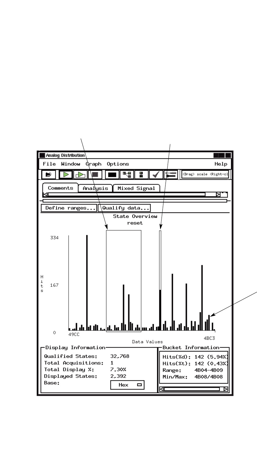
58
Post-Processing and Analysis Tool Sets
System Performance Analysis
State Overview Tool
Narrow in on an area of interest
using built-in qualification and zoom
functions.
Pinpoint regions of high memory activity to
determine which routines or operations are
responsible for throughput bottlenecks.
Measure memory coverage or stack
usage by observing whether memory
locations are accessed. You can also
detect which peripherals are most fre-
quently used.
Figure 5.12. Identify which events occur most frequently.
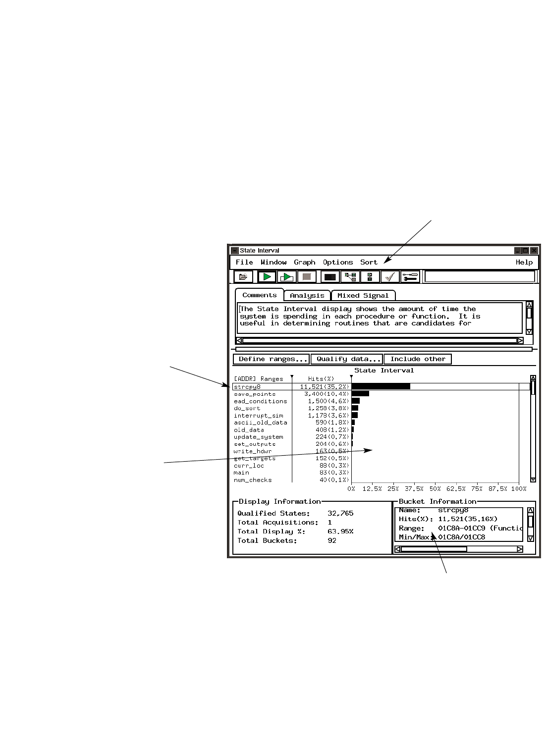
59
Post-Processing and Analysis
System Performance Analysis
State Interval Tool
Sort and display symbols alphabetically by event
name or by the number of hits.
Display just the symbols you
want to evaluate by using the
symbol-navigation utility. The util-
ity automatically configures the
tool for the selected function and
variable names from large symbol
files created by complex software
projects.
To help simplify your display,
delete all functions below a
selected point with a single
mouse click.
Pass the mouse over a histogram bar and
bucket information gives you detailed
information for each event.
Figure 5.13. Determine which functions use the most CPU cycles.
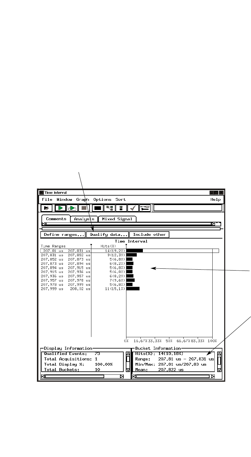
60
Post-Processing and Analysis
System Performance Analysis
Time Interval Tool
Data is displayed in histograms, which
can be exported to your host computer
either as histograms or as tabular
formatted text files.
Statistics such as maximum time,
minimum time, standard deviation and
mean help you document system behav-
ior. Use “accumulate mode” to analyze
the behavior of your system over a long
period of time.
Because time interval measurements often
depend upon hardware-software interaction,
the event definition can be a combination
of symbolics and hardware events. Data
qualification can be used to define the
specific hardware context in which the
analysis will be made.
Figure 5.14. Determine a specific routine's execution times.
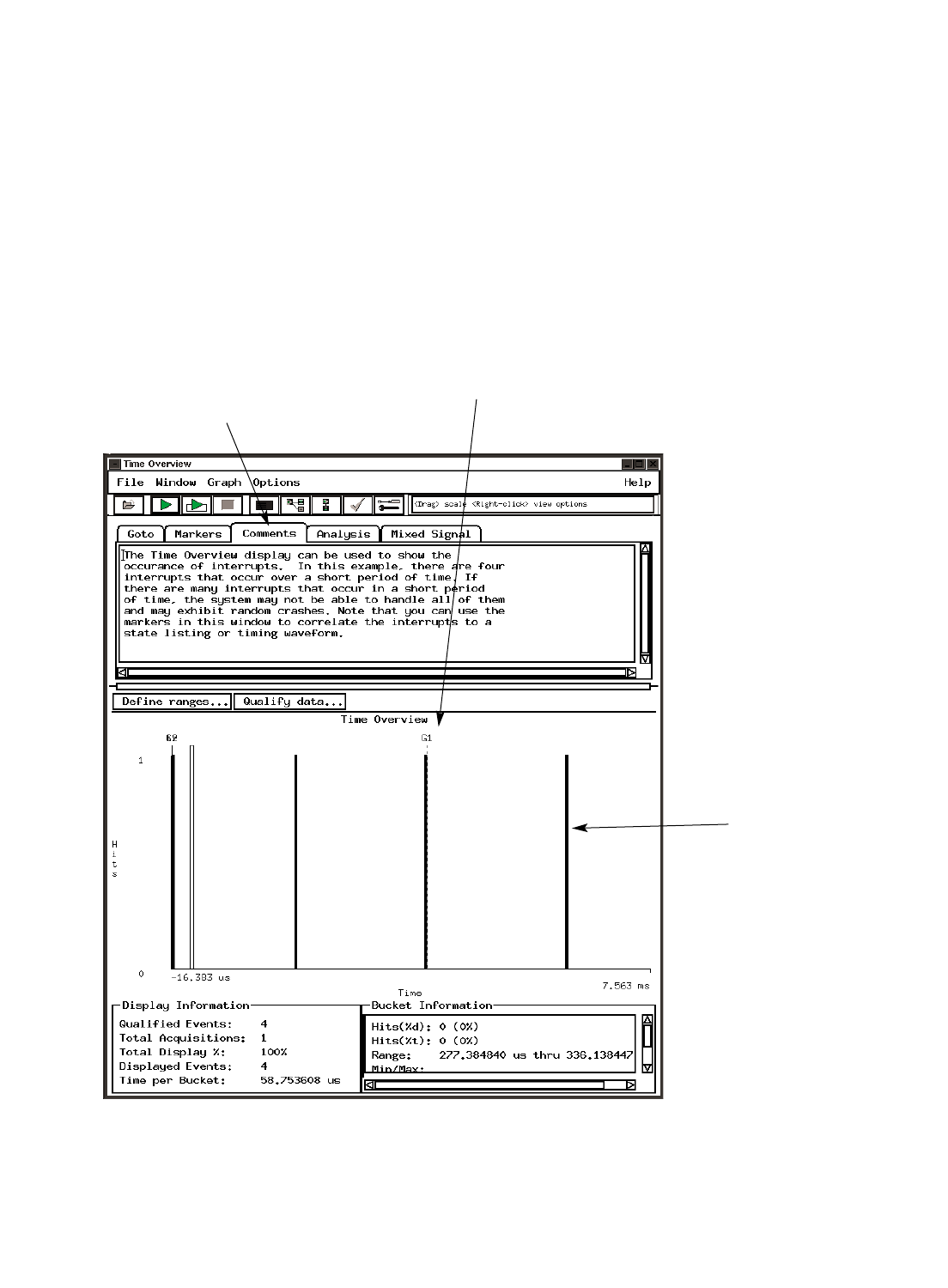
61
Post-Processing and Analysis Tool Sets
System Performance Analysis
Time Overview Tool
Elusive system crashes are often
caused by too many interrupts occur-
ring over a short period of time. If the
software cannot handle all simultane-
ous service requests, the system can
exhibit random defects while leaving
no clues as to their cause. In this situ-
ation, you need a tool that can meas-
ure and display interrupt loading.
Use “Comments” to document your trace. The
“Comments” field contents are saved with the
configuration and data.
Use the markers in this window to correlate
interrupts to a state listing or timing waveform.
Figure 5.15. View the frequency of events over time.

62
Solve Serial Communication Problems
Your system may use serial buses to
communicate between ICs and to
transfer data to and from peripheral
devices. Sifting through thousands of
serial bits by looking at long vertical
columns of captured 1's and 0's can
be very tedious, time-consuming, and
error-prone.
Obtain Answers to the Following
Questions:
• Is the software sending the correct
message?
• Is the communication hardware
acting as expected?
• When multiple messages are
involved, in what order is data
being transmitted?
• How does the serial bus activity
correlate to the target system
processor?
• What is causing the data corrup-
tion in the target system?
Product Description
The Agilent Technologies B460lB
serial analysis tool set is a general-
purpose tool that allows easy viewing
and analysis of serial data.
The tool set enables you to:
• Convert acquired serial bit
streams into readable parallel
word formats
• Time-correlate real-time serial
traces to system activity
• Remove stuffed bits from the data
block
• Process frame and data portions
separately
• Process serial data from a signal
with or without an external clock
reference
• Capture and analyze high-speed
(1.5 Gbits/s) serial buses
Post-Processing and Analysis Tool Sets
Serial Analysis
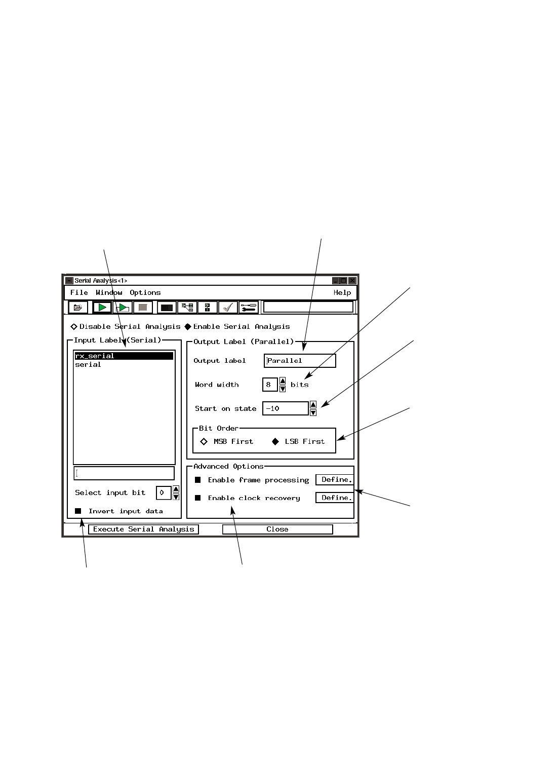
63
Post-Processing and Analysis Tool Sets
Serial Analysis
...specify which signal you want to
convert to parallel format by
selecting a specific bit of any
available label.
...capture serial data with or with-
out an external clock reference.
Enable clock recovery for an
incoming serial bit stream that has
no external clock reference.
(RS-232 is an example of a bus
with clocking embedded within the
serial bit stream).
...accept the default output
label“Parallel” or modify the
label name for easy recognition.
...set the output parallel word
width (up to 32 bits).
...select the specific state in
the trace where conversion
begins.
...specify the order in which
the bits occur in the serial
data stream
MSB = Most Significant
Bit first
LSB = Least Significant
Bit first.
...enable frame processing to
extract all instances of a
defined frame.
...maintain or invert the
input serial bit stream.
When You Want to Analyze Serial
Bit Streams . . .
Figure 5.16.
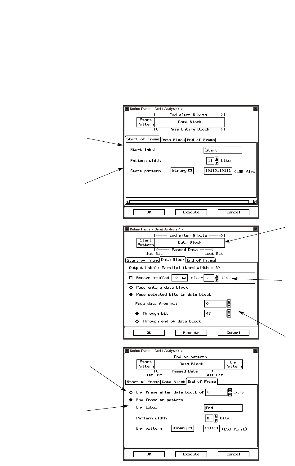
64
Post-Processing and Analysis Tool Sets
Serial Analysis
...accept the default
start of frame label
“Start” or modify the
label to a name of your
choosing.
...specify the pattern
that designates the start
of a frame.
...get immediate feed-
back as you configure
the tool set for your
data. This diagram
changes as you make
your framing and data
block selections.
...remove stuffed 0s or
0/1s from the trace
before other serial
analysis functions are
performed. Some proto-
cols use bit stuffing to
maintain clock
synchronization.
...specify the portion of
the data block for the
serial-to-parallel
conversion.
...specify whether the
end of frame occurs at
the end of a data block
of X bits or on a speci-
fied pattern.
...accept the default
end of frame label
“End” or enter a
different name.
To Separate Frame Information
from the Data Block . . .
Figure 5.17.
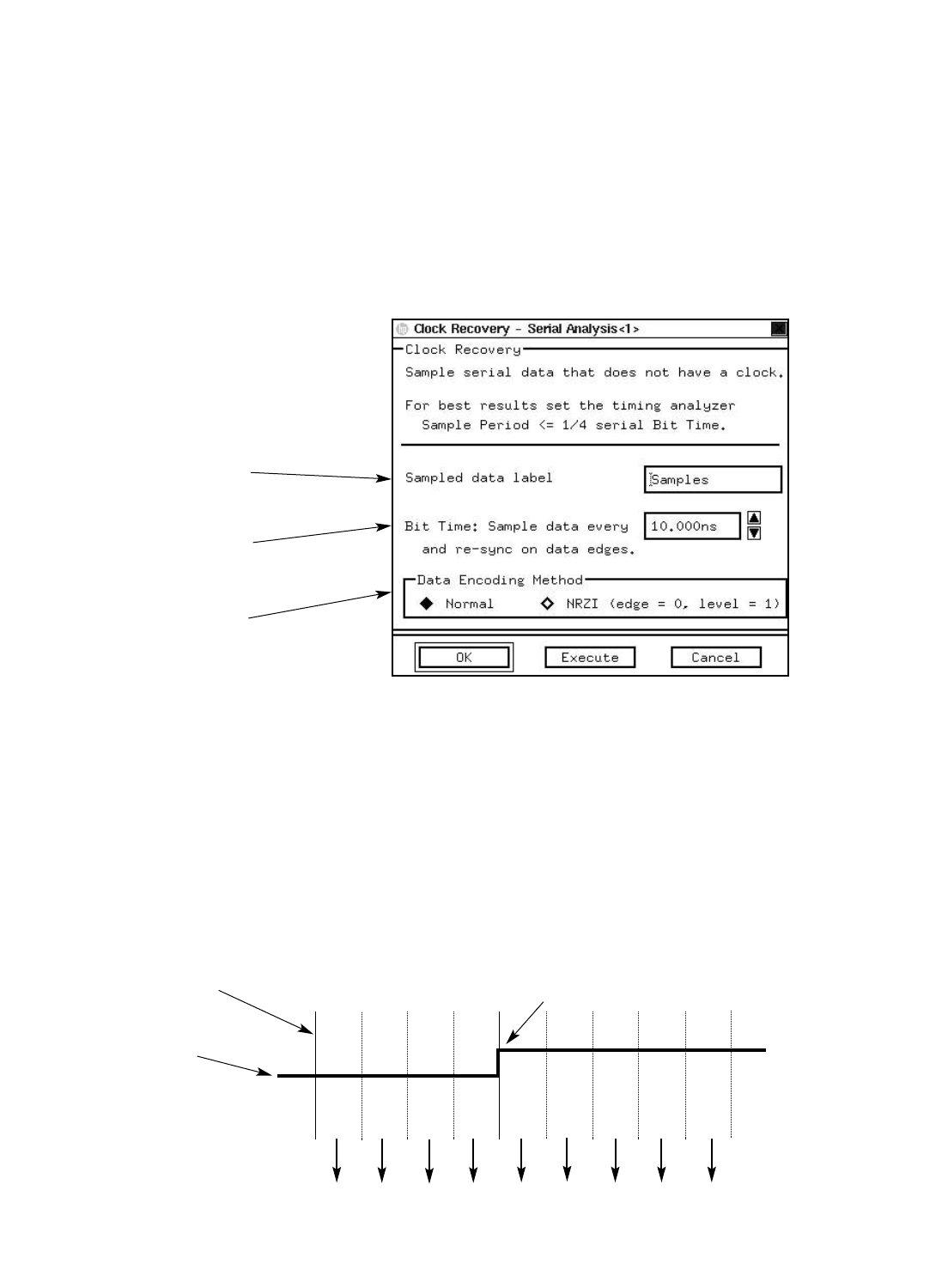
65
Post-Processing and Analysis Tool Sets
Serial Analysis
Clock Recovery Algorithm
1. For analysis purposes the data is
captured in conventional timing
mode using the internal timing
analyzer clock as the clock refer-
ence. Set the sample period of the
timing analyzer to take four or
more samples for each serial bit.
2. The timing analyzer data is sam-
pled in the middle of each bit
according to the serial bit rate
defined in the clock recovery
window.
3. Data edges (transitions from 0 to 1
or 1 to 0 in the timing analyzer
trace) are used to resynchronize
the sampling.
To Acquire a Serial Bit Stream
without an External Clock
Reference . . .
...set the sample period of
your timing analyzer to take
four or more samples for
each serial bit.
...accept the “Samples”
default label or enter a new
label name.
...specify the embedded bit
time of the serial bit
stream.
...specify the incoming
signal’s data encoding
method, normal or NRZI.
How Clock Recovery Works
Embedded bit time
Incoming serial
bit stream
Timing analyzer samples
(with timing analyzer set
to take five samples for
each serial bit)
New “Samples”serial data
0000000000000000000001111111111111111111111111111
000011 11 1
Resynchronize on edge
Figure 5.18.
Figure 5.19.
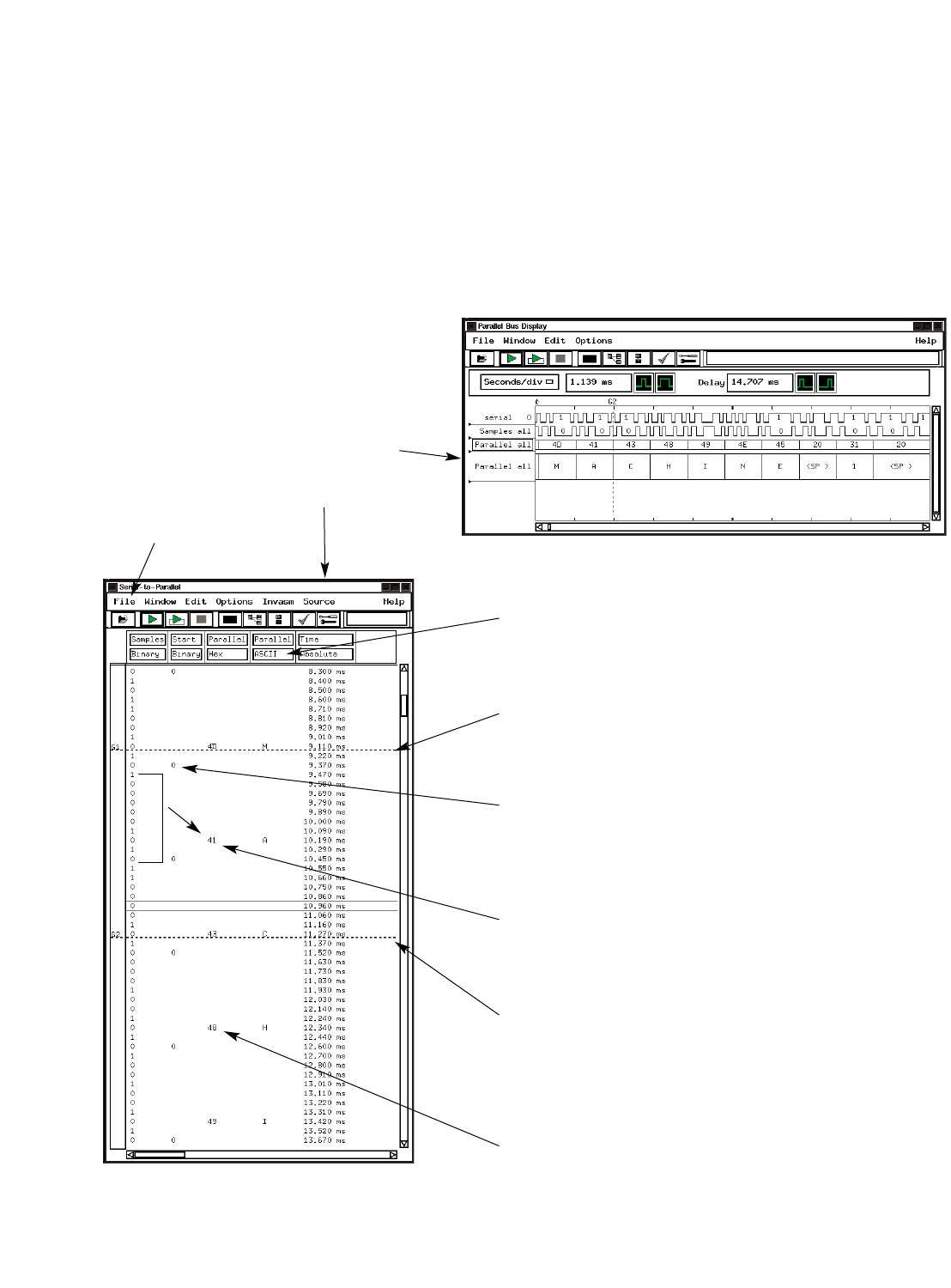
66
Post-Processing and Analysis Tool Sets
Serial Analysis
Once the Serial Bit Stream is
Acquired . . .
This example shows the conversion of an
RS-232 serial bit stream. The data sent to
the printer includes the column header
”MACHINE”.
...display the parallel data in binary, hex, octal, deci-
mal, ASCII or Twos Complement.
...use the global markers and time tags to correlate
real-time serial traces to other system activity.
...synchronize the start of the serial-to-parallel con-
version to the start of the frame pattern for your spe-
cific bus.
...convert the data block into parallel words, in this
case 8-bit words.
...find the Nth occurrence of specific frames or data
relative to the trigger, other markers, or the begin-
ning or end of the trace. Markers allow you to quick-
ly search from frame to frame in the data.
...view the data in the order in which the bits occur
in the serial stream, in this case LSB.
...configure the
serial tool once for
your specific bus,
then save the con-
figuration for
future uses.
...view the serial-to-parallel
conversion in the format that
is easiest for you — wave-
form or listing.
Figure 5.20.

67
Post-Processing and Analysis Tool Sets
Serial Analysis
Product Characteristics
Data Sources
All state and timing measurement
modules supported by the 16700
Series logic analysis systems serve
without modification as data sources
for the B4601B serial analysis tool
set. The particular measurement
module used determines time resolu-
tion and accuracy. Sample rate, chan-
nel count, memory depth and trigger-
ing are controlled by the user inde-
pendent of the serial analysis tool.
Because every trace is non-intrusive,
and every event captured in the trace
is time-stamped, you can correlate
activity from your serial bus with
other events in the target system.
The Agilent Technologies 16720A and
16522A pattern generator modules
can be used to generate your own
serial test data.
Maximum Parallel Word Width
32 bits
Parallel Data Display Types
Binary, Octal, Hex, Decimal, ASCII,
Twos Complement
Off-line Analysis and Post-Processing
All measurements can be saved using
the file out tool. Data can be recalled
at any time for later analysis using
any analysis or display tool. Serial
measurement data can be exported to
your host computer as ASCII files.
Serial Measurement Characteristics
16517A/ 16710A/ 16715A 16716A 16717A/ 16750A/B/ 16753A/ 16760A
18A 11A/12A 18A/19A 51A/B/ 54A/55A/
52A/B 56A
Maximum Clocked 64 Kbits 8 Kbits/ 2 Mbits 512 Mbits 2 Mbits/ 4 Mbits/ 1 Mbit/4 Mbits/ 64 Mbits
serial data [1] 32 Kbits/ 8 Mbits/ 16 Mbits/ 16 Mbits/32 Mbits
trace depth 128 Kbits 32 Mbits 32 Mbits
Unclocked 16-32 Kbits 4 Kbits/ 1 Mbit 256 Mbit 1 Mbit/ 2 Mbits/ 500Kbits/2 Mbits/ 32 Mbits
data [2] 16Kbits/ 4 Mbits/ 8 Mbits/ 8 Mbits/32 Mbits
64 Kbits 16 Mbits 16 Mbits
Maximum Clocked 1 Gbit/s 100 Mbits/s 167 Mbits/s 167 Mbits/s 333 Mbits/s 400 Mbits/s 600 Mbits/s 1.5 Gbits/s
serial bus data [3]
frequency
Unclocked 1 Gbit/s 125 Mbits/s 167 Mbits/s 167 Mbits/s 167 Mbits/s 200 Mbits/s 300 Mbits/s 200 Mbits/s
data [4]
Minimum Clocked 20 Mbit/s No limit No limit No limit No limit No limit No limit No limit
serial bus data
frequency
Unclocked 765 Mbits/s 5 Kbits/s 50 bits/s 50 bits/s 50 bits/s 50 bits/s 50 bits/s 50 bits/s
data [5]
Information in Table above calculated according to notes [1] to [5]
[1] =Maximum State Memory Depth
[2] =Maximum Timing Memory Depth/4
[3] =Maximum State Frequency
[4] =Maximum Timing Frequency/4
[5] =1/(Maximum sample period x 20)

68
Post-Processing and Analysis Tool Sets
Tool Development Kit
Customize Your Measurements
The ability to interpret and display
information is vital to your project.
At times the information you need
can be buried in the raw data of your
measurement. This might be due to
one of several reasons:
• The use of a protocol, encoded
data, or proprietary bus
• Events that happen only under
certain conditions
• The need to analyze system
performance
• The need to analyze data across
a large number of repetitive
measurements
Product Description
The Agilent Technologies B4605B tool
development kit provides a complete
environment for creating custom
tools that process data using the
powerful search and filtering capabil-
ities of the logic analysis system.
Features of the tool kit include:
• Fast, compiled and optimized
C code
• Push button compiling, no make
files
• A rich library of functions that
speeds development
• Extensive examples of code
• The creation of installable tools
Data is processed quickly by the cus-
tom tools, because they consist of
compiled, optimized C code. A C lan-
guage programming background is
highly recommended. A tutorial,
extensive examples, and a rich
library of functions are provided that
help you easily access analyzer data
and the tool's interface.
The custom tools can be used on any
16700 Series logic analysis system.
This allows you to purchase just one
or two copies of the development kit
and develop custom tools to support
a large number of analyzers.
Enhance Data Displays
• Color-code specific states of your
trace.
• Display some of your trace data in
engineering units.
• Convert the raw trace of a propri-
etary bus to a transaction-level
trace of that bus.
Manipulate Data
• Unravel interleaved data into two
or more columns of data.
• Combine the traces of two differ-
ent analyzers into one trace, with
each column being combined or
separately displayed as prescribed
by you.
• Modify your scope trace using an
algorithm developed by you, such
as an analog filter, beat frequency,
or DSP algorithm.
Read or Write External Files
• Accumulate information from
repetitive traces taken by the ana-
lyzer in a file on your PC or UNIX
workstation.
• Write specific types of states or
trace data that have been analyzed
to an Excel consumable ASCII file
on your PC or UNIX workstation.
• Use information read from a file
on your PC or UNIX workstation
to modify the display of an
analyzer trace.
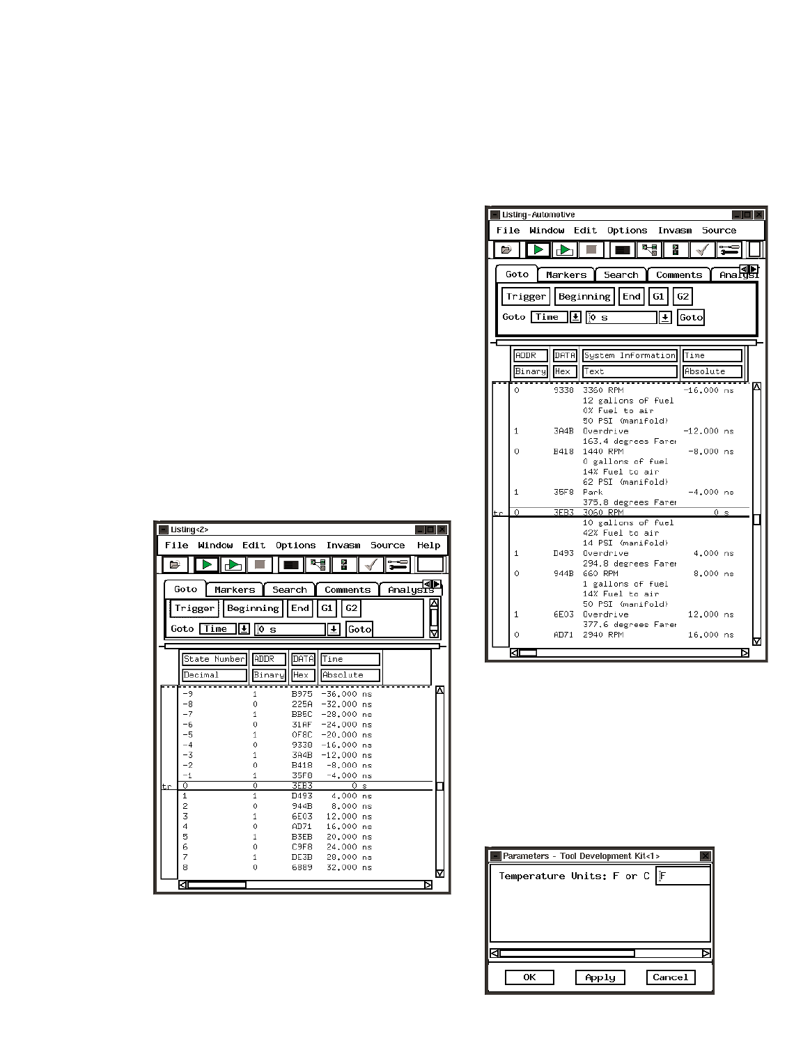
69
Post-Processing and Analysis Tool Sets
Tool Development Kit
Custom Tool Example, Added Text in
Trace
This example shows how a custom
tool can convert data to text to
present information in an easy-to-
understand form.
The original trace comes from a
control unit in an automobile.
Embedded in the data is information
about the engine and transmission.
When MODE = 0, DATA represents
engine information, including RPM,
fuel level, fuel to air ratio, and mani-
fold pressure. When MODE = 1,
DATA represents transmission infor-
mation, including gear position and
temperature.
This custom tool allows the user to
specify Fahrenheit or Centigrade for
the engine temperature data.
Output of Custom Tool
Original Trace
Parameter Interface of Custom Tool
Figure 5.21.
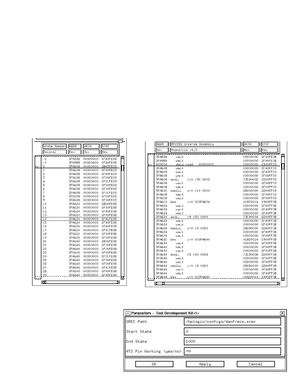
70
Post-Processing and Analysis Tool Sets
Tool Development Kit
Custom Tool Example, Microprocessor
Code Reconstruction
The original trace came from the bus
of a MPC 555 processor. As you can
see, no data was placed on the bus at
the time of the trace because cache
memory was turned on. Normally, it
would not be possible to inverse
assemble this trace.
The output of the custom tool in this
example is shown. Notice that there
is now data in the DATA column. The
custom tool was able to reconstruct
the code flow after the trace was
taken. The code was reconstructed by
using the branch trace messages and
information in the SRecord file creat-
Original Trace Output of Custom Tool
Parameter Window of Custom Tool
By entering information here, users can direct
the tool to the correct SRecord file and control
how much of the data the tool is to operate on.
They can also indicate if the AT2 pin of the MPC
555 processor is in use.
ed when the code was compiled. The
tool took the address of the appropri-
ate states in the trace data and found
the corresponding code (data) in the
SRecord file. This created a trace that
the MPC 555 inverse assembler could
operate on properly.
Figure 5.22. Code reconstruction
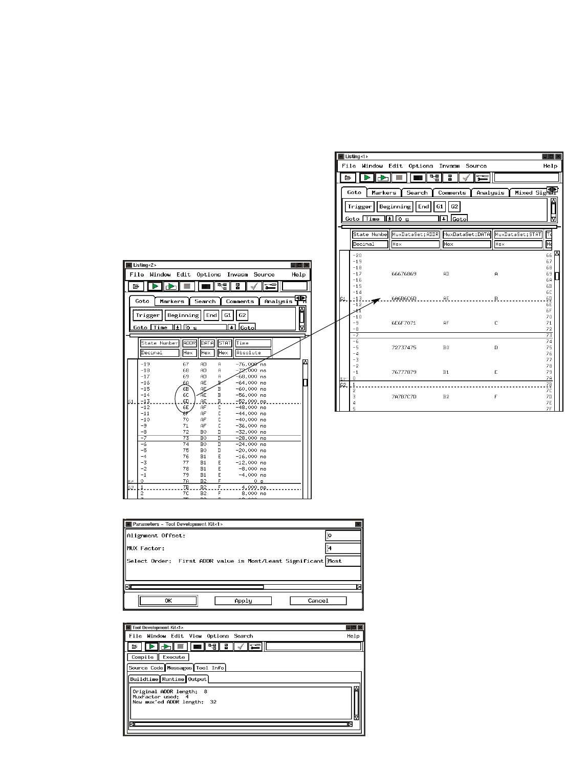
71
Post-Processing and Analysis Tool Sets
Tool Development Kit
Custom Tool Example, Multiplex Data
Custom tools can combine several
lines of data acquired sequentially
under one label into one line of data.
However the data to be combined
does not have to come from the same
label, it can come from different
labels. The labels can even come from
different analyzers.
At left are the parameter window and
message display created by the custom
tool in this example. Parameters allow the
user to control different aspects of what
the tool does to the acquired trace. The
user can change the parameters and hit
the execute button to change the output
of the tool. The output dialog to the
left displays information generated by
the tool.
Original Trace
Output of Custom Tool
Parameter and Output Windows
Figure 5.23.
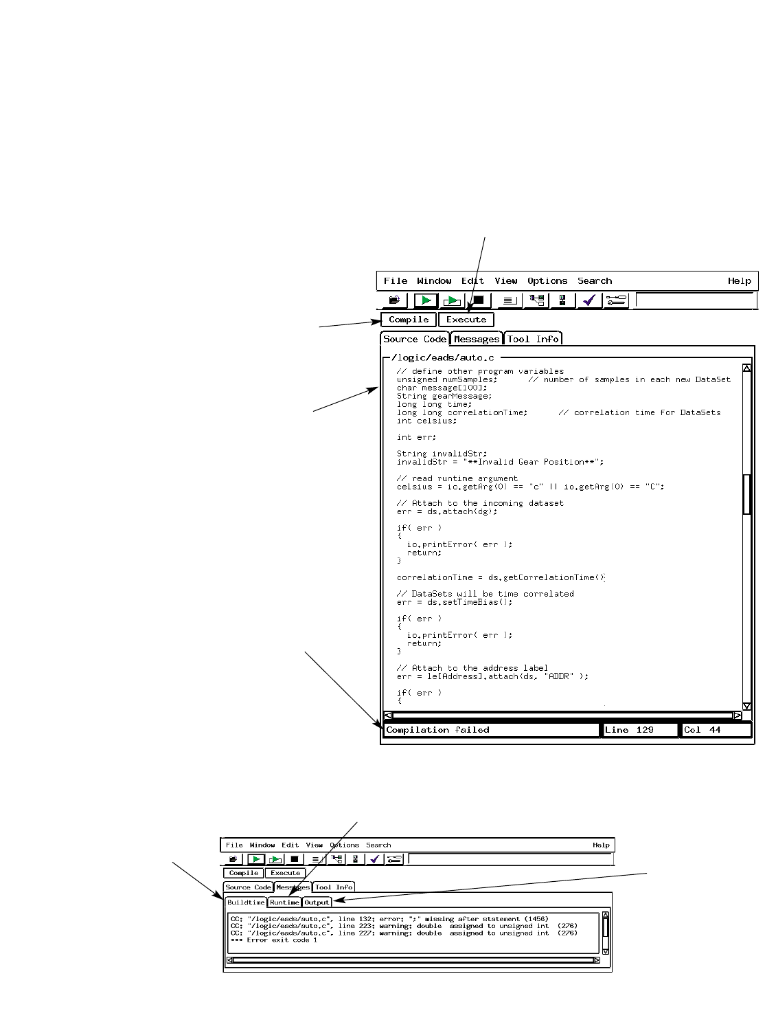
72
Post-Processing and Analysis Tool Sets
Tool Development Kit
Custom Tool Development
Environment
This is the main window for
developing code with the tool
development kit.
Select this button to cause the compiled code
to operate on the acquired data.
Select this button to compile the
code displayed in the “Source
Code” tab.
Load a file created on another
system or create your code here
using the “Source Code” editor.
Compilation status is shown
at the bottom of the tool
development kit Display window.
Runtime errors are displayed in
the “Runtime” tab.
Output generated
during the tool’s
execution are
displayed in the
“Output” tab.
Figure 5.24. TDK development environment
Errors generated
during a compile
are displayed in
the “Buildtime”
tab.

73
Post-Processing and Analysis Tool Sets
Tool Development Kit
Product Characteristics
Analyzer compatible custom tools
will run on any 16700 Series analyzer
running version A.01.40.00 or
greater. In some rare instances,
changes in the operating system can
require that your tools be recompiled
in order to run on that version of the
operating system.
Analysis and Stimulus Modules
The tool development kit supports
the following Agilent Technologies
measurement modules:
• 16715A, 16716A, 16717A, 16718A,
16719A, 16750A/B, 16751A/B,
16752A/B
• 16710A, 16711A, 16712A
• 16557D
• 16556A/D, 16555A/D
• 16554A
• 16550A
• 16534A, 16533A
• 16517A, 16518A
• 16522A, 16720A
• 16740A, 16741A, 16742A
• 16753A, 16754A, 16755A, 16756A
• 16760A
C Compiler
The libraries provided with the C
compiler allow you to perform stan-
dard operations such as creating
ASCII or binary files, reading from
these files, writing or appending to
these files, and IEEE 764 floating
point operations.
Provided Functions
Agilent Technologies provides a rich
library of functions that allow you to
copy data sets, create new data sets
with new labels, and to reorganize
the acquired data under these new
labels or to include data or text
derived from the acquired data.
The functions allow:
• Stopping a repetitive run
• Filtering of the data
• Randomly accessing the data
• Searching the data
• Displaying the data in one of eight
colors
• Accessing the trigger point
• Accessing the acquired time or
state of the data
• Outputting text strings to the
tool's display window
• Outputting errors to the runtime
window
By using two of the provided func-
tions, a simple user interface can eas-
ily be created that consists of label
strings and input fields. This allows
the input of parameters during the
tool's execution.

74
Post-Processing and Analysis Tool Sets
Licensing Information
Licensing and Miscellaneous
Description
System Configuration Requirements • 16700 Series logic analysis system
• Desired tool set(s)
• Supported and compatible measurement hardware
Tool Set Control • Locally control and view tool set measurements
• Remotely access any tool set from a PC or workstation through a web browser or X-window emulation
software.
File Access • Access source files or other development environment applications (compiler, debugger) from the logic
analyzer via Telnet, NFS, or mapped file systems, and X-Windows client/server protocols.
• Save or access files via the standard network capabilities of the logic analyzer, such as FTP, NFS, or CIFS
(Common Internet File System for Windows 95/98/NT/2000/XP-based PCs).
Ordering and Shipment • When a tool set is ordered with a 16700 Series mainframe, the tool set is shipped installed and ready to
run (Unless option 0D4 is ordered.)
• Tool set proof-of-receipt is provided by the entitlement certificate.
See page 129 for ordering information.
Tool Set Licensing Information
License Policy The 16700 Series logic analysis systems’ tool set software is licensed for single-unit use only. Licenses
are valid for the life of the tool set. Software updates do not affect the license.
Nodelock Mode • Tool set licenses are shipped or first installed as nodelocked applications. Nodelocked means that use of
the tool set license is only allowed on the single node (16700 Series analyzer on which it is installed). Tool
sets ordered with a 16700 Series mainframe will be installed with a permanent password and are ready to
run.
• For tool sets purchased as upgrades to existing 16700 Series mainframes, you must access the Agilent
password redemption web site to obtain a password. Your entitlement certificate provides the web URL
and alternate contact information. Password turnaround is generally the same business day.
Free Tool Set Evaluation A single temporary license is available for any tool set type not previously licensed on a node. The
(Temporary Demo License) temporary password for any node on any tool set is "demo". The temporary license is valid for 21 calendar
days from first entry of the password in the license management window of the 16700 Series logic
analysis system.
License Management Licenses are managed from ‘Licensing…’ in the Admin tab of System Admin. Licenses are reserved at the
start of a measurement session. They remain in use until the measurement session is terminated.
Password Backup Passwords can be backed up to a floppy disk or network file. Should the passwords on your 16700 Series
logic analysis system hard drive become corrupted, the tool set passwords can be reinstated by copying
your backed up password file to: /system/licensing/license.dat
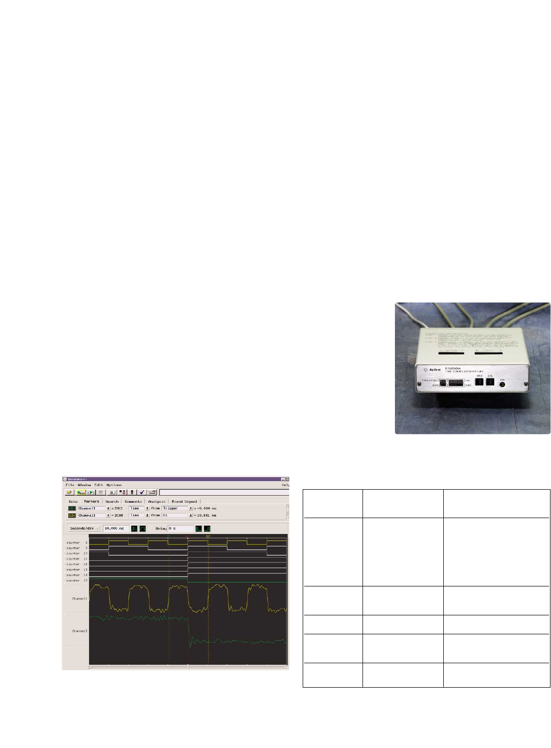
75
Time Correlation with Agilent Infiniium Oscilloscopes
E5850A Logic Analyzer - Oscilloscope Time Correlation Fixture
• Automatic de-skew.
Measurements between the logic
analyzer and Infiniium oscillo-
scope are automatically de-skewed
in time. This saves you time and
gives you confidence in the meas-
urement results.
• Combined waveform display.
The Infiniium oscilloscope wave-
forms are displayed in the wave-
form display window on the 16700
logic analyzer, along with timing
analyzer waveforms. This allows
you to instantly visualize time
relationships among oscilloscope
and timing measurements.
• Global markers.
The global markers in the 16700
may be used to measure time
among all measurements made in
the logic analyzer and Infiniium
oscilloscope measurements.
E5850A Logic Analyzer – Oscilloscope
Time Correlation Fixture
The Agilent E5850A time correlation
fixture allows you to make time-
correlated measurements between a
16700 logic analyzer and an Agilent
548XX Series Infiniium oscilloscope
to solve the following types of prob-
lems more effectively:
• Verifying signal integrity
• Tracking down problems caused
by signal integrity
• Verifying correct operation of A/D
and D/A converters
• Verifying correct logical and tem-
poral relationships between the
analog and digital portions of a
design
Agilent’s E5850A time correlation
fixture works in conjunction with
software in the 16700 family logic
analyzers, and any Agilent Infiniium
54800 Series oscilloscope, to deliver
the following features:
Figure 5.25. Infiniium oscilloscope waveforms are displayed in the 16700 logic
analyzer waveform display window along with logic analyzer timing wave-
forms, accurately time-correlated.
• Tracking markers.
The Infiniium oscilloscope’s time
markers track the global markers
in the 16700 logic analyzer. If you
wish to view a waveform in
greater detail on the oscilloscope’s
display, or measure a voltage level
using the oscilloscope’s voltage
markers, this feature allows you to
relate information on the oscillo-
scope’s display precisely to corre-
sponding information on the logic
analyzer display.
Figure 5.26. E5850A time correlation fixture.
For Infiniium Software version Software version for
oscilloscope for 16700 series Infiniium oscilloscope
model number logic analyzer
54810A A.02.20.00 or higher A.04.00 or higher
54815A
54820A
54825A
54835A
54845A
54846A
54830B A.02.50.00 or higher A.01.00 or higher
54831B
54832B
54845B A.02.50.00 or higher A.04.35 or higher
54846B
54830B A.02.50.00 or higher A.02.10 or higher
54831B
54832B
54854A A.02.70.00 or higher A.03.00 or higher
54855A
The E5850A requires the versions of operating software indicated in the table
Compatibility

76
Agilent 16700 Series Technical
Information
System Software
All features and functionality
described in this document are
available with system software
version A.02.70.00 or higher.
Mainframe Specifications and
Characteristics
Mass Storage
Hard Disk Drive 18 GB formatted disk drive
Floppy Disk Drive
• Capacity 1.44 MB formatted
• Media 3.5 inch floppy
• Formats MS-D0S (Read, write, format), LIF (Read only)
Internal System RAM
Standard 128 MB
Option 003 (Must be ordered at 256 MB total
time of frame purchase)
Supported Monitor Resolutions
Standard 640 x 480 through 1280 x 1024
(The 16702B has a built-in 800 x 600, 12.1”
(26.2mm) diagonal monitor.)
Option 003 (Must be ordered at Adds support for up to 1600 x 1200
time of frame purchase)
LAN, IEEE 802.3
Physical Connectors 16700B Series:
10BaseT/100BaseT-X (ethertwist): RJ-45
16700A Series:
10BaseT (ethertwist): RJ-45; 10Base2: BNC
Protocols Supported TCP/IP
NFS
CIFS (Windows® 95/98/NT/2000/XP) [1]
FTP
NTP
PCNFS
X-Window Support X Window system version 11, release 6, as a client and
server
[1] User and share level control supported for Windows NT®4.0. Share level control only supported for
Windows 95/98.

77
Mainframe Specifications and
Characteristics
Agilent 16700 Series Technical
Information (continued)
Web Server
Supported from Instrument Measurement status check,remote display, installation
Web Page of PC application software, link to Agilent’s Test and
Measurement site
PC Requirements Pentium® (family) PC (200 MHz, 32 MB RAM) running
Windows 95, Windows 98, Windows NT 4.0 with
service pack 3 or higher, Windows 2000 or Windows XP
Supported Web Browsers Internet Explorer 4.0 or higher,
(on Your PC or Workstation) Netscape 4.0 or higher
IntuiLink Support
Installation of PC Application Software Directly from instrument web page
MS Excel Excel 97 Version 7.0 or later. Excel limits maximum trace
depth to 64K per sheet.
Available Data Formats
Fast Binary (Compressed High performance transfer rate. Includes source code to
Binary Format) parse data. Available via File Out.
Uncompressed Binary Includes utility routines. Available via RPI.
ASCII Provides same format as listing display, including
inverse-assembled data. Available via RPI and File Out.
Pattern Generator Binary Used to load large amount of stimulus (> 1M) into the
16720A pattern generator
Intermodule Bus (IMB)
Time Correlation Resolution 2 ns
Port In/Out
Connectors BNC

78
Port In
Levels TTL, ECL, or user defined
Input Resistance 4 KΩ
Input Voltage –6V at –1.5 mA to +6V at 1.6 mA
Port Out
Levels 3V TTL compatible into 50 Ω
Functions Latched (latch operation is module dependent)
Pulsed, width from 66 ns to 143 ns
Target Control Port
Number of signals 8
Levels 3V TTL compatible
Connector 2 rows of 5 pins, 0.1-inch centers
Operating Environment
Temperature
• Instrument 0°C to 50°C (32°F to 122°F)
• Disk Media 10°C to 40°C (50°F to 104°F)
• Probes/Cables O°C to 65°C (32°F to 149°F)
Altitude To 3000m (10,000 ft)
Humidity 8 to 80% relative humidity at 40°C (104°F)
Printing
Printer Interface Parallel interface for Centronics compatible printers
Printers Supported PostScript printers and printers which support the
HP Printer Control Language (PCL)
Graphics Graphics can be printed directly to the printer or to a file.
Graphic files can be created in black-and-white or color
TIFF format, PostScript, PCX, or XWD formats
Mainframe Specifications and
Characteristics
Agilent 16700 Series Technical
Information (continued)

79
Remote Programming Interface (RPI)
RPI Overview
Typical Applications Manufacturing Test
Data Acquisition for Offline Analysis
System Verification and Characterization
Pass/Fail Analysis
Stimulus Response Tests
Remote Programming 1.Set up the logic analyzer and save the test configuration.
Steps 2.Create a program that remotely:
Loads a test configuration
Starts the acquisition process
Checks measurement status (verifies completion)
Acts on the results of the data acquisition
• Saves configuration and captured data
• Exports data
• Executes a compare
• Modifies the trigger setup or trigger value for the next
acquisition
• Accesses the oscilloscope’s automatic measurements
Physical Connection Remote programming is done via the LAN connection
Requirements
16700B Series RPI is standard with system software version A.02.00.00 or
Analysis Systems higher
PC Programming is done via Microsoft® ActiveX/COM
automation
Pentium (family) PC with one of the following:
• Windows 95
• Windows 98
• Windows NT 4.0 with Service Pack 3 or higher
• Windows 2000
• Windows XP
Visual Basic or Visual C++ (Version 5.0 or higher)
UNIX®Programming is done via TCP/IP socket based
ASCII commands
Mainframe Specifications and
Characteristics

80
Mainframe Specifications and
Characteristics
Remote Programming Interface (RPI) (continued)
Command Set Summary - Commands available on both UNIX and PC
System System Configuration Query
Load/Save Configuration and Data
Start/Stop Measurement
Current Run Status
Start/Stop/Query a Session
Logic Analysis Modules Load/Save Configuration and Data
Trigger Setup
Acquisition Data and Parameters
Set/Query Acquisition Mode
Set/Query Acquisition Depth
Set/Query Pod Assignment
Add/Delete/Load/Query Labels
Set/Query Trigger Position
Modify Occurrence Count
Oscilloscope Modules Load/Save Configuration and Data
Acquisition Data / Parameters
Query Automatic Measurements
Trigger Setup
Pattern Generator Load/Save Configuration and Data
Load ASCII file (vectors) or PGB (pattern generator binary)
files (16720A only)
Modify Vector
Set/Query Clock Frequency
Set/Query Clock Out Delay
Insert New Vector at Specific Position
Delete Specific Vector
Emulation Module Reset Processor
Run Processor
Break Processor
Single Step
Listing Tool Status
Acquisition Data and Parameters
Transfer Data (includes inverse assembled information)
Compare Tool Execute Compare
Set Compare Mask
Query Compare Result
Specify Range to Compare
Abort Compare After Specified Number of Differences
Return Labels and Values Where Differences Occur
File Out Tool Transfer Data to File
Select Range to Expert
Additional Information
Instrument Online Help Programming Information in instrument online help
Web Sites Full remote programming documentation (pdf) available on
the hard drive. Sample programs are provided

81
IntuiLink
Programming Examples Provided with IntuiLink
Visual Basic Examples have been included for use with Visual Basic 5.0
or higher. These examples perform simple functions such
as: system checks, oscilloscope measurements, pass/fail
tests using stored configuration and pattern generator
stimulus files, and stimulus/response tests. They also can
capture and retrieve data for off-line analysis.
Visual C++ Examples have been included for use with Visual C++ 5.0 or
higher to perform simple functions such as: system check,
capturing and retrieving data for off-line analysis.
LabVIEW An instrument library has been included for use with
LabVIEW 5.1 or higher. This library contains five LabVIEW
samples that provide a starting point for creating your own
LabVIEW programs.
• Load/Run/Save - loads a configuration, runs a
measurement, then saves results to a file
• Analyzer Listing - runs the logic analyzer and displays
data in a table
• Pass/Fail - runs the logic analyzer and compares the
measurement data against a standard
• Scope Waveform - runs the oscilloscope module and
displays waveform data
• Scope Measurements - runs the oscilloscope module
and displays a number of oscilloscope measurements
HP VEE An instrument library has been included for use with
HP VEE 5.0 or higher that provides a starting point for
creating your own application.
• Load/Run/Save - loads a configuration, runs a
measurement, then saves results to a file
Mainframe Specifications and
Characteristics
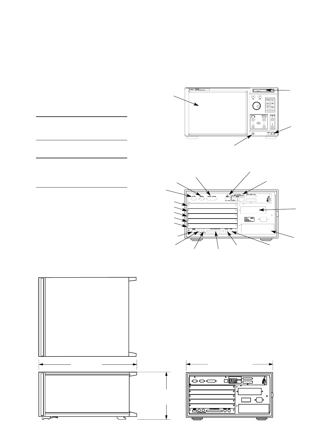
82
Mainframe Specifications and
Characteristics
Agilent 16700B Series Physical
Characteristics
Power
16700B 115/230 V, 48 to 66 Hz, 610 W max
16701B 115/230 V, 48 to 66 Hz, 545 W max
16702B 115/230 V, 48 to 66 Hz, 610 W max
Weight*
Max Net Max Shipping
16700B 12.7 kg (27.0 lb) 34.2 kg (75.4 lbs)
16701B 10.4 kg (23.0 lb) 32.0 kg (70.6 lbs)
16702B 15.2 kg (32.4 lb) 36.7 kg (80.8 lbs)
* Weight of modules ordered with mainframes will add
0.9 kg (2.0 lb) per module.
12.1” Built-in LCD
Display with Touch
Screen
3.5 Inch Floppy
Disk Drive
On/Off
Power Switch
Touch Screen On/Off
Parallel Port
Monitor
RS-232
LAN 10BaseT/100BaseT-X
SCSI-2 Single Ended
One Slot for
Emulation or
Multiframe
Module
MouseKeyboard
Expansion Frame Cable Connector
Five Slots for
Measurement
Modules
Target Control Port
Port IN
Port OUT
Dimensions: mm (inches)
A
B
C
D
E
551.2 (21.7”)
234.2
(9.22”)
425.7 (16.75”)
Figure 6.3. Exterior dimensions for the 16700B Series mainframe.
Figure 6.1. Agilent 16702B front panel.
Figure 6.2. Back panel for Agilent models 16700B and 16702B.
40x CD-ROM
Drive
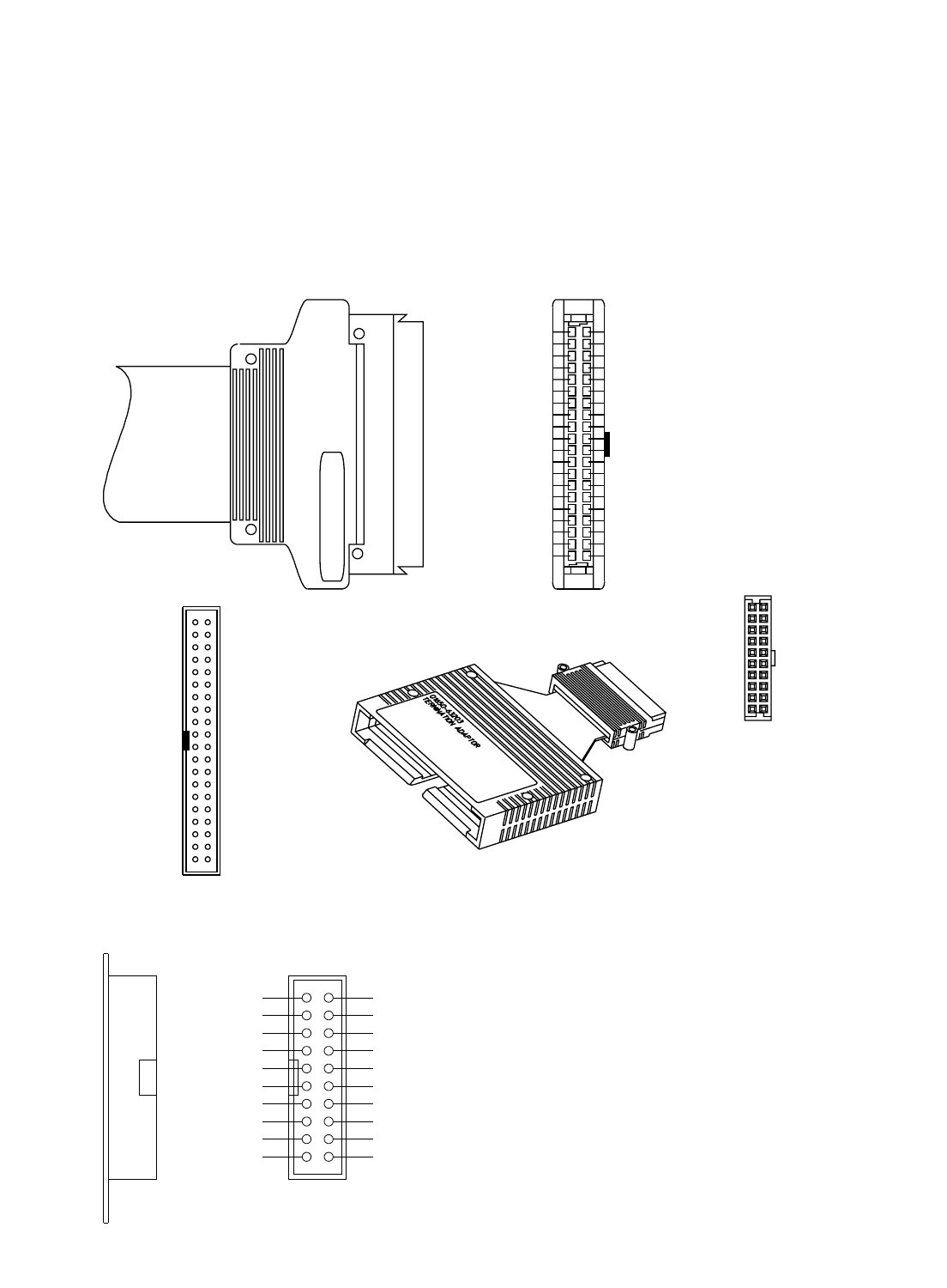
83
Probing Solutions Specifications and
Characteristics
SIGNAL GND 4
SIGNAL GND 6
SIGNAL GND 8
SIGNAL GND 10
POWER GND 2
SIGNAL GND 12
SIGNAL GND 14
SIGNAL GND 16
SIGNAL GND 18
SIGNAL GND 20
SIGNAL GND 22
SIGNAL GND 24
SIGNAL GND 26
SIGNAL GND 28
SIGNAL GND 30
SIGNAL GND 32
SIGNAL GND 34
SIGNAL GND 36
SIGNAL GND 38
POWER GND 40
1 +5V
3 CLK1
5 CLK2
7 D15
9 D14
11 D13
13 D12
15 D11
17 D10
19 D9
21 D8
23 D7
25 D6
27 D5
29 D4
31 D3
33 D2
35 D1
37 D0
39 +5V
2 POWER GND
4 SIGNAL GND
6 SIGNAL GND
8 SIGNAL GND
10 SIGNAL GND
12 SIGNAL GND
14 SIGNAL GND
16 SIGNAL GND
18 SIGNAL GND
20 SIGNAL GND
22 SIGNAL GND
24 SIGNAL GND
26 SIGNAL GND
28 SIGNAL GND
30 SIGNAL GND
32 SIGNAL GND
34 SIGNAL GND
36 SIGNAL GND
38 SIGNAL GND
40 POWER GND
+5V 1
CLK1 3
CLK2 5
D15 7
D14 9
D13 11
D12 13
D11 15
D10 17
D9 19
D8 21
D7 23
D6 25
D5 27
D4 29
D3 31
D2 33
D1 35
D0 37
+5V 39
1 +5V
3 CLK 1
5 D14
7 D12
9 D10
11 D8
13 D6
15 D4
17 D2
19 D0
CLK 2 2
D15 4
D13 6
D11 8
D9 10
D7 12
D5 14
D3 16
D1 18
GND 20
Probing Technical Specifications
+5V 1
CLK1 3
D14 5
D12 7
D10 9
D8 11
D6 13
D4 15
D2 17
D0 19
2 CLK2
4 D15
6 D13
8 D11
10 D9
12 D7
14 D5
16 D3
18 D1
20 GND
Figure 6.4. Pinout for state/timing module pod cable and 100 KΩisolation adapter. (Agilent 01650-63203)
Figure 6.5. Pinout for 20-pin connector. (Agilent 1251-8106)
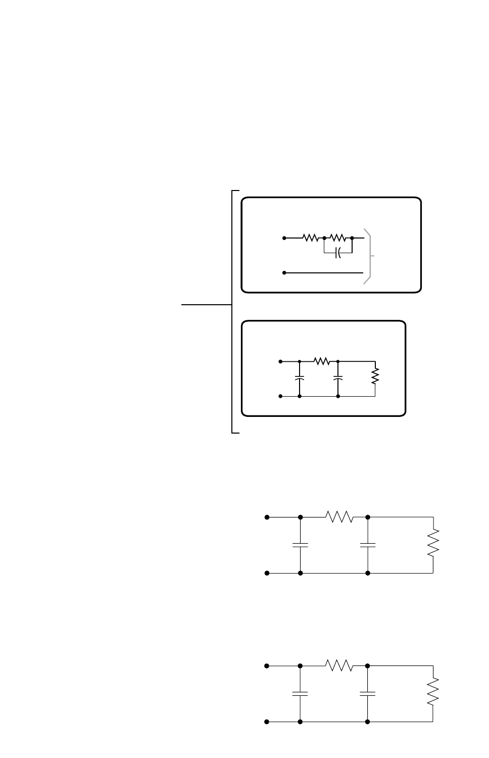
84
Probing Solutions Specifications and
Characteristics
Figure 6.6. 01650-63203 Termination adapter and equivalent load.
250
ohm
90.9k
ohm
To Logic
Analyzer
Pod
8.2pF
Signal
Ground
Adapter RC Network
370
ohm
Signal
Ground
Equivalent Load
4.6pF 7.4pF 100k
ohm
Includes logic analyzer
Isolation Adapters
Isolation adapters that connect to
the end of the probe cable are
designed to perform two functions.
The first is to reduce the number of
pins required for the header on the
target board. This process reduces
the board area dedicated to the
probing connection. The second
function is to provide the proper
RC isolation networks in a very
convenient package.
370 ohm
Signal
Ground
3pF 9pF 100k
ohm
Figure 6.7. E5346A equivalent load.
E5346A 38-pin Probe
01650-63203 20-pin Probe
220 ohm
Signal
Ground
3pF 18pF 50.5k
ohm
Figure 6.8. E5339A equivalent load.
E5339A 38-pin Low Voltage Probe

85
State/Timing Modules Specifications and
Characteristics
Key Specifications* and Characteristics
Agilent Model Number 16715A, 16716A, 16717A 16740A, 16741A, 16742A 16750B, 16751B, 16752B 16760A
Maximum state acquisition rate on 16715A, 16716A: 167 Mb/s 200 Mb/s 400 Mb/s [1] Full channel: 800 Mb/s
each channel 16717A, 333 Mb/s [1] Half channel: 1.5 Gb/s
Maximum timing sample rate Timing Zoom: 2 GHz (16716A, Timing Zoom: 2 GHz Timing Zoom: 2 GHz Conventional: 800 MHz
(half/full channel) 16717A only) Conventional: 800/400 MHz Conventional: 800/400 MHz Transitional: 400 MHz
Conventional: 667/333 MHz Transitional: 400 MHz Transitional: 400 MHz
Transitional: 333 MHz
Channels/module 68 68 68 34
Maximum channels on a 340 (5 modules) 340 (5 modules) 340 (5 modules) 170 (5 modules)
single time base and trigger
Memory depth 16715A, 16717A: 4/2M [2] 16740A: 2/1 M [2] 16750B: 8/4M [2] 128/64M [5]
(half/full channel) 16716A: 1M/512K [2] 16741A: 8/4 M [2] 16751B: 32/16M [2]
16742A 32/16 M [2] 16752B: 64/32M [2]
Trigger resources Patterns: 16 Pattern: 16 Patterns: 16 At 800 Mb/s: 4 patterns or
Ranges: 15 Ranges: 15 Ranges: 15 2 ranges, 4 flags, arm in
Edge & Glitch: 2 Edge & Glitch: 2 Edge & Glitch: 2 At 200 Mb/s: same as
Timers: (2 per module) -1 Timers: (2 per module) -1 Timers: (2 per module) -1 16750B/51B/52B
Occurrence Counter: [4] Occurrence Counter: 2 Occurrence Counter: [4] Other speeds: refer to
Global Counters: 2 Global Counter: 2 Global Counters: 2 synchronous state analysis
Flags: 4 Flags: 4 Flags: 4 (page 97) and asynchronous
timing analysis (page 100)
Maximum trigger sequence levels 16 16 16 1.5 Gb/s: 2
800 Mb/s: 4
200 or 400 Mb/s: 16
Maximum trigger sequence speed 16715A, 16716A: 167 MHz 200 MHz 400 MHz 1.5 GHz
16717A: 333 MHz
Trigger sequence level branching 4-way arbitrary “IF/THEN/ELSE” 4-way arbitrary 4-way arbitrary “IF/THEN/ELSE” 800 or 1.5 Gb/s: none
branching “IF/THEN/ELSE” branching 200 Mb/s: arbitrary
branching “IF/THEN/ELSE” branching
400 Mb/s: dedicated next-
state branch or reset
Number of state clocks/qualifiers 4 4 4 1 (state clock only)
Setup/hold time* 2.5 ns window adjustable from 2.5 ns windows adjustable from 2.5 ns window adjustable from 1 ns window adjustable from
4.5/-2.0 ns to -2.0/4.5 ns in 100 ps 4.5/2.0 ns to -2.0/4.5 ns in 100 ps 4.5/-2.0 ns to -2.0/4.5 ns in 100 ps 2.5/-1.5 ns to -1.5/2.5 ns
increments per channel [3] increments per channel [3] increments per channel [3] 10 ps increments per channel
Threshold range TTL, ECL, user-definable ±6.0 V TTL, ECL, user-definable ±6.0 V TTL, ECL, user-definable ±6.0 V -3.0 V to 5.0 V adjustable in
adjustable in 10-mV increments adjustable in 10-mV increments adjustable in 10-mV increments 10-mV increments
* All specifications noted by an asterisk are the performance standards against which the product is tested.
[1] State speeds greater than 167 MHz (16717A) or 200 MHz (16750B, 16751B, 16752B, 16760A) require a trade-off in features.
Refer to “Supplemental Specifications and Characteristics” on page 93 for more information.
[2] Memory depth doubles in half-channel timing mode only.
[3] Minimum setup/hold time specified for a single clock, single edge acquisition. Multi-clock, multi-edge setup/hold window add 0.5 ns.
[4] There is one occurrence counter per trigger sequence level.
[5] Memory depth doubles in half-channel 1.25 Gb/s and 1.5 Gb/s modes only.

86
Key Specifications* and Characteristics (continued)
Agilent Model Number 16710A, 16711A, 16712A 16753A, 16754A, 16755A, 16756A
Maximum state acquisition rate on 100 Mb/s 600 Mb/s
each channel
Maximum timing sample rate Conventional: 500/250 MHz Timing Zoom: 4 GHz
(half/full channel) Transitional: 125 MHz Conventional: 1200/600 MHz
Transitional: 600 MHz
Channels/module 102 68
Maximum channel count on a 204 (2 modules) 340 (5 modules)
single time base and trigger
Memory depth 16710A: 16/8K [1] 16753A: 2/1M [1]
(half/full channel) 16711A: 64/32K [1] 16754A: 8/4M [1]
16712A: 256/128k [1] 16755A: 32/16M [1]
16756A: 128/64M [1]
Trigger resources Patterns: 10 Patterns: 16
Ranges: 2 Ranges: 15
Edge & Glitch: 2 Edge & Glitch: 2
Timers: 2 Timers: (2 per module) -1
Occurrence Counter: [3]
Global Counters: 2
Flags: 4
Maximum trigger sequence levels State mode: 12 Patterns: 16
Timing mode: 10 Ranges: 15
Edge & Glitch: 2
Timers: (2 per module) -1
Occurrence Counter: [3]
Global Counters: 2
Flags: 4
Maximum trigger sequence speed 125 MHz 600 MHz
Trigger sequence level branching Dedicated next state or 4-way arbitrary
single arbitrary branching “IF/THEN/ELSE” branching
Number of state clocks/qualifiers 6 4
Setup/hold time* 4.0 ns window adjustable from 1 ns window (600ps typical) adjustable
4.0/0 ns to 0/4.0 ns in 500 ps in 80ps increments
increments [2] per 34 channels
Threshold range TTL, ECL, user-definable ±6.0 V -3.0 V to +5.0 V adjustable in
adjustable in 50 mV increments 10-mV increments
* All specifications noted by an asterisk are the performance standards against which the product is tested.
[1] Memory depth doubles in half-channel timing mode only.
[2] Minimum setup/hold time specified for single-clock, single-edge acquisition. Single-clock, multi-edge setup/hold add 0.5 ns.
Multi-clock, multi-edge setup/hold window add 1.0 ns.
[3] There is one occurrence counter per trigger sequence level.
State/Timing Modules Specifications and
Characteristics
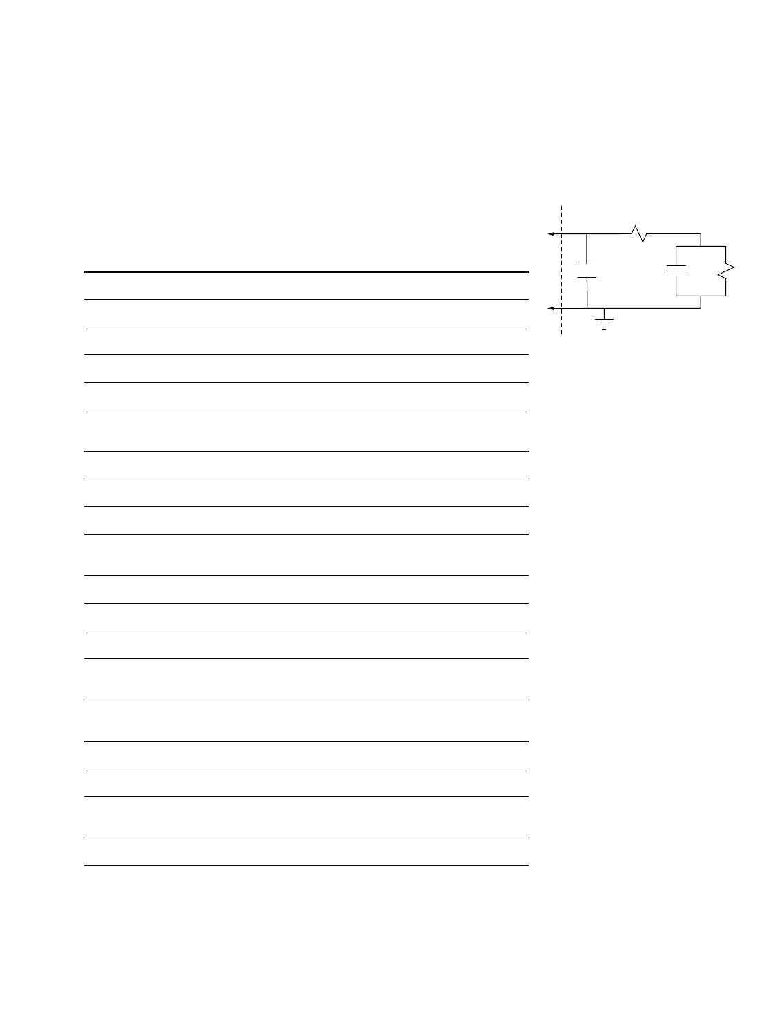
87
State/Timing Modules Specifications and
Characteristics
Agilent Technologies 16710A, 16711A, 16712A
Supplemental Specifications* and Characteristics
Probes (general-purpose lead set)
Input resistance 100 KΩ, ±2%
Parasitic tip capacitance 1.5 pF
Minimum voltage swing 500 mV, peak-to-peak
Threshold accuracy* ±(100 mV + 3% of threshold setting)
Maximum input voltage ±40 V peak
State Analysis
Minimum state clock pulse width 3.5 ns
Time tag resolution [1] 8 ns
Maximum time count between states 34 seconds
Maximum state tag 4.29 x 10⁹states
count between states [1]
Minimum master to master clock time* 16710A, 16711A, 16712A: 10 ns
Minimum master to slave clock time 0.0 ns
Minimum slave to master clock time 4.0 ns
Context store block sizes 16, 32, 64 states
16710A/11A/12A only
Timing Analysis
Sample period accuracy 0.01% of sample period
Channel-to-channel skew 2 ns, typical
Time interval accuracy ± (sample period + channel-to-channel
skew + 0.01% of time interval reading)
Minimum detectable glitch 3.5 ns
* All specifications noted by an asterisk are the performance standards against which the product is tested.
[1] Time or state tags halve the acquisition memory when there are no unassigned pods.
1.5pF
370 ohms
7.4pF
GROUND
100K
ohm
Figure 6.9. Equivalent probe load for the
Agilent 16710A, 16711A and 16712A, general-
purpose lead set.

88
State/Timing Modules Specifications and
Characteristics
Agilent Technologies 16710A, 16711A, 16712A
Supplemental Specifications* and Characteristics (continued)
Triggering
Maximum trigger sequence speed 125 MHz, maximum
Maximum occurrence counter 1,048,575
Range width 32 bits each
Timer value range 400 ns to 500 seconds
Timer resolution 16 ns or 0.1% whichever is greater
Timer accuracy ±32 ns or ±0.1% whichever is greater
Operating Environment
Temperature Agilent 16700 Series mainframes:
• Instrument 0˚C to 50˚C (+32˚F to 122˚F)
• Probe lead sets and cables, 0˚C to 65˚C (+32˚F to 149˚F)
Humidity 80% relative humidity at +40˚C
Altitude Operating 4600m (15,000ft)
Nonoperating 15,300m (50,000ft)
* All specifications noted by an asterisk are the performance standards against which the product is tested.
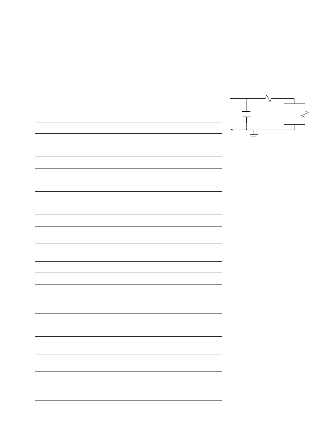
89
State/Timing Modules Specifications and
Characteristics
Agilent Technologies 16715A, 16716A, 16717A, 16740A, 16741A,
16742A, 16750B, 16751B, 16752B Supplemental Specifications*
and Characteristics
Probes (general-purpose lead set)
Input resistance 100 KΩ, ± 2%
Parasitic tip capacitance 1.5 pF
Minimum voltage swing 500 mV, peak-to-peak
Minimum input overdrive 250 mV
Threshold range -6V to +6V in 10 mV increments
Threshold accuracy* ± (65 mV + 1.5% of settings)
Input dynamic range ± 10V about threshold
Maximum input voltage ± 40V peak
+5V Accessory current 1/3 amp maximum per pod
Channel assignment Each group of 34 channels can be assigned to
Analyzer 1, Analyzer 2 or remain unassigned
2 GHz Timing Zoom (Agilent 16716A, 16717A, 16740A, 16741A, 16742A, 16750B, 16751B, 16752B only)
Timing analysis sample rate 2 GHz/1 GHz/500 MHz/250 MHz
Sample period accuracy ± 50 ps
Channel-to-channel skew < 1.0 ns
Time interval accuracy ± (sample period + channel-to-channel skew + 0.01% of
time interval reading)
Memory depth 16 K
Trigger position Start, center, end, or user defined
Operating Environment
Temperature Agilent 16700 Series frame: 0˚C to 50˚C (+32˚F to 122˚F)
Probe lead sets and cables: 0˚C to 65˚C (+32˚F to 149˚F)
Humidity 80% relative humidity at + 40˚C
Altitude Operating 4600 m (15,000 ft)
Non-operating 15,300 m (50,000 ft)
* All specifications noted by an asterisk are the performance standards against which the product is tested.
1.5pF
370 ohms
7.4pF
GROUND
100K
ohm
Figure 6.10. Equivalent probe load for the
Agilent 16715A, 16716A, 16717A, 16718A,
16719A, 16750B, 16751B, 16752B general-
purpose lead set.

90
State/Timing Modules Specifications and
Characteristics
Agilent Technologies 16715A, 16716A, 16717A, 16740A, 16741A, 16742A,
16750B, 16751B, 16752B Supplemental Specifications* and Characteristics
State Mode 16715A, 16716A, 16717A 16740A, 16741A, 16742A
167 Mb/s State Mode 16750B, 16751B, 16752B
200 Mb/s State Mode
Maximum state acquisition rate on 167 Mb/s 200 Mb/s
each channel
Channel count 68 per module 68 per module
Maximum channels on a single 340 340
time base and trigger
Number of independent analyzers 2, can be set up in state or timing modes 2, can be set up in state or timing modes
Minimum master to 5.988 ns 5 ns
master clock time* [1]
Minimum master to slave clock time 2 ns 2 ns
Minimum slave to master clock time 2 ns 2 ns
Minimum slave to slave clock time 5.988 ns 5 ns
Setup/hold time* [1] 2.5 ns window adjustable from 4.5/-2.0 ns to 2.5 ns window adjustable from 4.5/-2.0 ns to
(single-clock, single-edge) -2.0/4.5 ns in 100 ps increments per channel -2.0/4.5 ns in 100 ps increments per channel
Setup/hold time* [1] 3.0 ns window adjustable from 5.0/-2.0 ns to 3.0 ns window adjustable from 5.0/-2.0 ns to
(multi-clock, multi-edge) -1.5/4.5 ns in 100 ps increments per channel -1.5/4.5 ns in 100 ps increments per channel
Setup/hold time (on individual channels, 1.25 ns window 1.25 ns window
after running eye finder)
Minimum state clock pulse width 1.2 ns 1.2 ns
Time tag resolution [2] 4 ns 4 ns
Maximum time count between states 17 seconds 17 seconds
Maximum state tag count 232 232
between states [2]
Number of state clocks/qualifiers 4 4
Maximum memory depth 16716A: 512K 16740A: 1M 16750B: 4M
16715A, 16717A: 2M 16741A: 4M 16751B: 16M
16742A: 16M 16752B: 32M
Maximum trigger sequence speed 167 MHz 200 MHz
Maximum trigger sequence levels 16 16
* All specifications noted by an asterisk are the performance standards against which the product is tested.
[1] Tested at input signal VH=-0.9V, VL=-1.7V, Slew rate=1V/ns, and threshold=-1.3V.
[2] Time or state tags halve the acquisition memory when there are no unassigned pods.

91
State/Timing Modules Specifications and
Characteristics
Agilent Technologies 16715A, 16716A, 16717A, 16740A, 16741A, 16742A,
16750B, 16751B, 16752B Supplemental Specifications* and Characteristics (continued)
State Mode 16715A, 16716A, 16717A 16740A, 16741A, 16742A
167 Mb/s State Mode 16750B, 16751B, 16752B
200 Mb/s State Mode
Trigger sequence level branching 4 way arbitrary “IF/THEN/ELSE” branching 4 way arbitrary “IF/THEN/ELSE” branching
Trigger position Start, center, end, or user defined Start, center, end, or user defined
Trigger resources 16 Patterns evaluated as =, ≠, >, <, ≥, ≤16 Patterns evaluated as =, ≠, >, <, ≥, ≤
15 Ranges evaluated as in range, not in range 15 Ranges evaluated as in range, not in range
(2 Timers per module) -1 (2 Timers per module) -1
2 Global counters 2 Global counters
1 Occurrence counter per sequence level 1 Occurrence counter per sequence level
4 Flags 4 Flags
Trigger resource conditions Arbitrary Boolean combinations Arbitrary Boolean combinations
Trigger actions Goto Goto
Trigger and fill memory Trigger and fill memory
Trigger and goto Trigger and goto
Store/don’t store sample Store/don’t store sample
Turn on/off default storing Turn on/off default storing
Timer start/stop/pause/resume Timer start/stop/pause/resume
Global counter increment/reset Global counter increment/reset
Occurrence counter reset Occurrence counter reset
Flag set/clear Flag set/clear
Store qualification Default and per sequence level Default and per sequence level
Maximum global counter 16,777,215 16,777,215
Maximum occurrence counter 16,777,215 16,777,215
Maximum pattern/range width 32 bits 32 bits
Timers value range 100 ns to 5497 seconds 100 ns to 5497 seconds
Timer resolution 5 ns 5 ns
Timer accuracy 10 ns + .01% 10 ns + .01%
Timer reset latency 70 ns 70 ns
Data in to trigger out (BNC port) 150 ns, typical 150 ns, typical
Flag set/reset to evaluation 110 ns, typical 110 ns, typical
* All specifications noted by an asterisk are the performance standards against which the product is tested.

92
State/Timing Modules Specifications and
Characteristics
Agilent Technologies 16715A, 16716A, 16717A, 16740A, 16741A, 16742A,
16750B, 16751B, 16752B Supplemental Specifications* and Characteristics (continued)
State Mode 16717A 16750B, 16751B, 16752B
333 Mb/s State Mode 400 Mb/s State Mode
Maximum state acquisition rate 333 Mb/s 400 Mb/s
on each channel
Channel count (Number of modules x 68) - 34 (Number of modules x 68) - 34
Maximum channels on a single 306 306
time base and trigger
Number of independent analyzers 1, when 333 MHz state mode is selected 1, when 400 MHz state mode is selected
the second analyzer is turned off the second analyzer is turned off
Minimum master to master clock time* [1] 3.003 ns 2.5 ns
Setup/hold time* [1] 2.5 ns window adjustable from 4.5/-2.0 ns to 2.5 ns window adjustable from 4.5/-2.0 ns to
(single-clock, single-edge) -2.0/4.5 ns in 100 ps increments per channel -2.0/4.5 ns in 100 ps increments per channel
Setup/hold time* [1] 3.0 ns window adjustable from 5.0/-2.0 ns to 3.0 ns window adjustable from 5.0/-2.0 ns to
(single-clock, multi-edge) -1.5/4.5 ns in 100 ps increments per channel -1.5/4.5 ns in 100 ps increments per channel
Setup/hold time (on individual channels 1.25 ns window 1.25 ns window
after running eye finder)
Minimum state clock pulse width 1.2 ns 1.2 ns
Time tag resolution [2] 4 ns 4 ns
Maximum time count between states 17 seconds 17 seconds
Number of state clocks 1 1
Maximum memory depth 16717A: 2M 16750B: 4M
16751B: 16M
16752B: 32M
Maximum trigger sequence speed 333 MHz 400 MHz
Maximum trigger sequence levels 15 15
Trigger sequence level branching Dedicated next state branch or reset Dedicated next state branch or reset
Trigger position Start, center, end, or user defined Start, center, end, or user defined
* All specifications noted by an asterisk are the performance standards against which the product is tested.
[1] Tested at input signal VH=-0.9V, VL=-1.7V, Slew rate=1V/ns, and threshold=-1.3V.
[2] Time or state tags halve the acquisition memory when there are no unassigned pods.

93
State/Timing Modules Specifications and
Characteristics
Agilent Technologies 16715A, 16716A, 16717A, 16740A, 16741A, 16742A,
16750B, 16751B, 16752B Supplemental Specifications* and Characteristics (continued)
State Mode 16717A 16750B, 16751B, 16752B
333 Mb/s State Mode 400 Mb/s State Mode
Trigger resources 8 Patterns evaluated as =, ≠, >, <, ≥, ≤8 Patterns evaluated as =, ≠, >, <, ≥, ≤
4 Ranges evaluated as in range, not in range 4 Ranges evaluated as in range, not in range
2 Occurrence counters 2 Occurrence counters
4 Flags 4 Flags
Trigger resource conditions Arbitrary Boolean combinations Arbitrary Boolean combinations
Trigger actions Goto Goto
Trigger and fill memory Trigger and fill memory
Store qualification Default Default
Maximum occurrence counter 16,777,215 16,777,215
Maximum pattern/range width 32 bits 32 bits
Data in to trigger out (BNC port) 150 ns, typical 150 ns, typical
Flag set/reset to evaluation 110 ns, typical 110 ns, typical
Timing Mode 16715A, 16716A, 16717A 16740A, 16741A, 16742A, 16750B, 16751B, 16752B
Timing analysis sample rate 667/333 MHz 800/400 MHz
(half/full channel)
Channel count 68 per module 68 per module
Maximum channels on 340 340
a single time base and trigger
Number of independent analyzers 2, can be setup in state or timing modes 2, can be setup in state or timing modes
Sample period (full channel) 3 ns to 1 ms 2.5 ns to 1 ms
Sample period (half channel) 1.5 ns 1.25 ns
Minimum data pulse width
for data capture
Conventional timing 1.75 ns 1.5 ns
Transitional timing 3.9 ns 3.8 ns
For trigger sequencing 6.1 ns 5.1 ns
Sample period accuracy ±(100 ps + .01% of sample period) ±(100 ps + .01% of sample period)
Channel-to-channel skew < 1.5 ns < 1.5 ns
Time interval accuracy ± (sample period + channel-to-channel ± (sample period + channel-to-channel
skew + .01% of time interval reading) skew + .01% of time interval reading)
Minimum detectable glitch 1.5 ns 1.5 ns
Memory depth (half/full channel) 16716A: 1M/512K 16750B: 8/4M
16715A, 16717A: 4/2M 16751B: 32/16M
16752B: 64/32M
* All specifications noted by an asterisk are the performance standards against which the product is tested.

94
State/Timing Modules Specifications and
Characteristics
Agilent Technologies 16715A, 16716A, 16717A, 16740A, 16741A, 16742A, 16750B,
16751B, 16752B Supplemental Specifications* and Characteristics (continued)
Timing Mode (continued) 16715A, 16716A, 16717A 16740A, 16741A, 16742A
16750B, 16751B, 16752B
Maximum trigger sequence speed 167 MHz 200 MHz
Maximum trigger sequence levels 16 16
Trigger sequence level branching 4 way arbitrary “IF/THEN/ELSE” branching 4 way arbitrary “IF/THEN/ELSE” branching
Trigger position Start, center, end, or user defined Start, center, end, or user defined
Trigger resources 16 Patterns evaluated as =, ≠, >, <, ≥, ≤16 Patterns evaluated as =, ≠, >, <, ≥, ≤
15 Ranges evaluated as in range, not in range 15 Ranges evaluated as in range, not in range
2 Edge/glitch 2 Edge/glitch
(2 Timers per module) -1 (2 Timers per module) -1
2 Global counters 2 Global counters
1 Occurrence counter per sequence level 1 Occurrence counter per sequence level
4 Flags 4 Flags
Trigger resource conditions Arbitrary Boolean combinations Arbitrary Boolean combinations
Trigger actions Goto Goto
Trigger and fill memory Trigger and fill memory
Trigger and goto Trigger and goto
Timer start/stop/pause/resume Timer start/stop/pause/resume
Global counter increment/reset Global counter increment/reset
Occurrence counter reset Occurrence counter reset
Flag set/clear Flag set/clear
Maximum global counter 16,777,215 16,777,215
Maximum occurrence counter 16,777,215 16,777,215
Maximum pattern/range width 32 bits 32 bits
Timer value range 100 ns to 5497 seconds 100 ns to 5497 seconds
Timer resolution 5 ns 5 ns
Timer accuracy ±10 ns + .01% ±10 ns + .01%
Greater than duration 6 ns to 100 ms in 6 ns increments 6 ns to 100 ms in 6 ns increments
Less than duration 12 ns to 100 ms in 6 ns increments 12 ns to 100 ms in 6 ns increments
Timer reset latency 70 ns 70 ns
Data in to trigger out (BNC port) 150 ns, typical 150 ns, typical
Flag set/reset to evaluation 110 ns, typical 110 ns, typical
* All specifications noted by an asterisk are the performance standards against which the product is tested.

95
State/Timing Modules Specifications and
Characteristics
Probes for 16753A, 16754A, 16755A, 16756A, 16760A
Supplemental Specifications* and Characteristics
Probes E5378A 100-pin Single-ended E5379A 100-pin Differential E5380A 35-pin Single-ended E5382A Single-Ended Flying Leads
Input resistance and Refer to figure 6.11 Refer to figure 6.11 Refer to figure 6.11 Refer to figure 6.12
capacitance
Maximum state data 1.5 Gb/s 1.5 Gb/s 600 Mb/s 1.5 Gb/s
rate supported
Mating connector Agilent part number Agilent part number Amp Mictor 38 [2] None required
1253-3620 [1] 1253-3620 [1]
Minimum voltage swing 250 mV p-p Vin+- Vin->= 200 mV p-p 300 mV p-p 250 mV p-p
Input dynamic range -3 Vdc to +5 Vdc -3 Vdc to +5 Vdc -3 Vdc to +5 Vdc -3 Vdc to +5 Vdc
Threshold accuracy +/- (30 mV + 1% of setting)* +/- (30 mV + 1% of setting) [3] +/- (30 mV + 1% of setting) +/- (30 mV + 1% of setting)
Threshold range -3.0 V to +5.0 V -3.0 V to +5.0 V -3.0 V to +5.0 V -3.0 V to +5.0 V
User-supplied threshold -3.0 V to +5.0 V N/A N/A N/A
input range
User-supplied threshold >= 100K ohms N/A N/A N/A
input resistance
Threshold control options • User-provided input If operated single-ended Adjustable from user Adjustable from user
• Adjustable from user (minus inputs grounded), interface interface
interface the threshold can be adjusted
from the user interface
Maximum nondestructive +/-40 Vdc +/-40 Vdc +/-40 Vdc +/-40 Vdc
input voltage
Maximum input slew rate 5 V/ns 5 V/ns 5 V/ns 5 V/ns
Clock input Differential Differential Single-ended Differential
Number of inputs [4] 34 (32 data and 2 clock/data) 17 (16 data and 1 clock/data) 34 (32 data and 2 clock/data) 17 (16 data and 1 clock/data)
* All specifications noted by an asterisk are the performance standards against which the product is tested.
[1] A support shroud, Agilent part number 16760-02302 (for boards up to 0.062" thick) or 16760-02303 (for boards up to 0.120" thick) is recommended.
A kit of 5 shrouds and 5 connectors is available as Agilent part number 16760-68702 (for boards up to 0.062" thick) or 16760-68703 (for boards up to 0.120" thick).
[2] A kit of 5 Amp Mictor connectors and 5 support shrouds is available, Agilent part number E5346-68701.
A support shroud is available separately, Agilent part number E5346-44701.
[3] If operated single-ended (minus inputs grounded), the threshold can be adjusted from the user interface.
[4] Refer to specifications on specific modes of operation for details on how inputs can be used.
[5] Soft touch probes use a retention module attached to the target PC board. A kit of 5 retention modules is included with each probe. Additional kits of 5 retention modules
can be ordered using Agilent part number E5387-68701.
150
1.5pF 0.7pF
20k
+0.75 V
Model Number C1 R1R2
E5378A, E5379A 1.5pF 120 30
E5380A 3pF 120 60
Figure 6.11. E5378A, E5379A, E5380A input
equivalent probe load.
121215
30
1pF 0.6pF
20k
+0.75 V
Figure 6.12. E5382A input equivalent probe load, with
5cm damped wire (see user’s guide for load models
with other accessories).
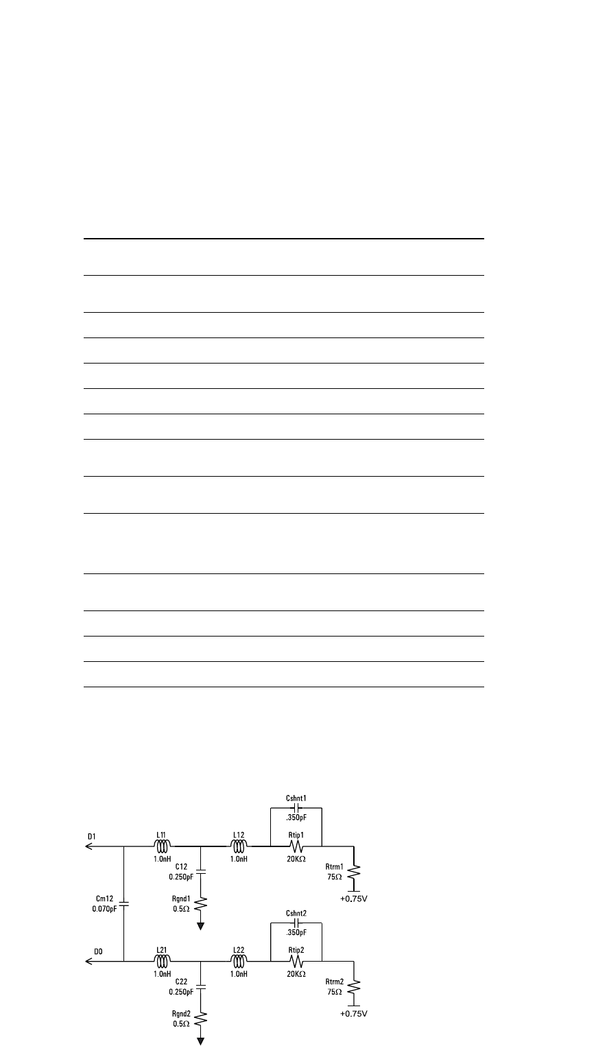
96
State/Timing Modules Specifications and
Characteristics
Probes for 16753A, 16754A, 16755A, 16756A, 16760A
Supplemental Specifications* and Characteristics (continued)
Probes E5387A Differential Soft Touch E5390A Single-Ended Soft Touch
Input resistance and Refer to figure 6.13 Refer to figure 6.13
capacitance
Maximum state data 1.5 Gb/s 1.5 Gb/s
rate supported
Mating connector None required [5] None required [5]
Minimum voltage swing Vin+- Vin->= 200 mV p-p 250 mV p-p
Input dynamic range -3 Vdc to +5 Vdc -3 Vdc to +5 Vdc
Threshold accuracy +/- (30 mV + 2% of setting)* +/- (30 mV + 2% of setting) [3]
Threshold range -3.0 V to +5.0 V -3.0 V to +5.0 V
User-supplied threshold N/A -3.0 V to +5.0 V
input range
User-supplied threshold N/A >= 100K ohms
input resistance
Threshold control options If operated single-ended • User-provided input
(minus inputs grounded), • Adjustable from user
the threshold can be adjusted interface
from the user interface
Maximum nondestructive +/-40 Vdc +/-40 Vdc
input voltage
Maximum input slew rate 5 V/ns 5 V/ns
Clock input Differential Differential
Number of inputs [4] 17 (16 data and 1 clock/data) 34 (32 data and 2 clock/data)
* All specifications noted by an asterisk are the performance standards against which the product is tested.
[1] A support shroud, Agilent part number 16760-02302 (for boards up to 0.062" thick) or 16760-02303 (for boards up to 0.120" thick) is recommended.
A kit of 5 shrouds and 5 connectors is available as Agilent part number 16760-68702 (for boards up to 0.062" thick) or 16760-68703 (for boards up to 0.120" thick).
[2] A kit of 5 Amp Mictor connectors and 5 support shrouds is available, Agilent part number E5346-68701. A support shroud is available separately, Agilent part number E5346-44701.
[3] If operated single-ended (minus inputs grounded), the threshold can be adjusted from the user interface.
[4] Refer to specifications on specific modes of operation for details on how inputs can be used.
[5] Soft touch probes use a retention module attached to the target PC board. A kit of 5 retention modules is included with each probe. Additional kits of 5 retention modules
can be ordered using Agilent part number E5387-68701.
Figure 6.13. E5387A and E5390A Probe Load Model.
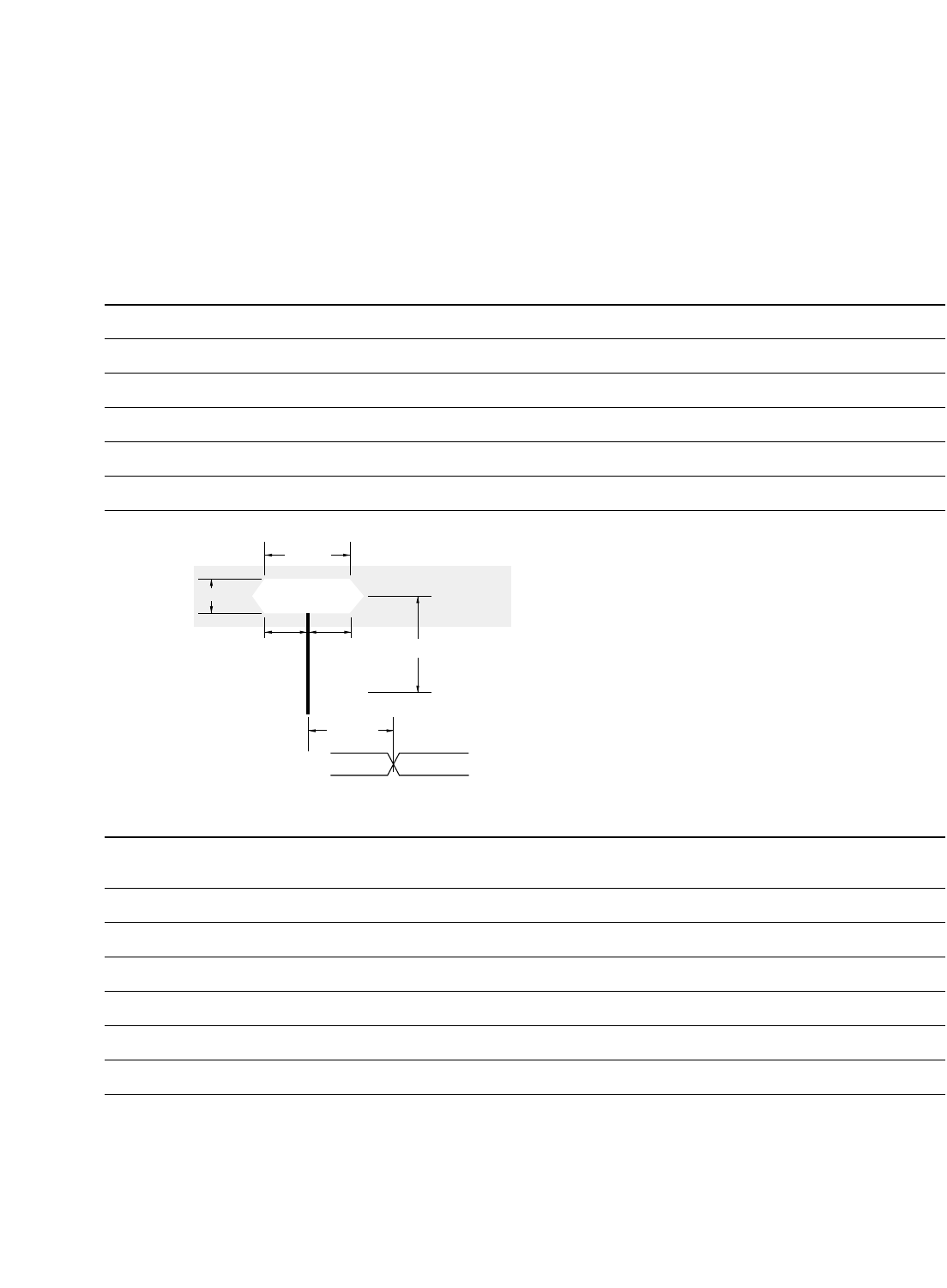
97
Timing Zoom
Timing analysis sample rate 4 GHz
Time interval accuracy, within a pod pair +/- (750 ps + 0.01% of time interval reading)
Time interval accuracy, between pod pairs +/- (1.5 ns + 0.01% of time interval reading)
Memory depth 64 K samples
Trigger position Start, center, end, or user defined
Minimum data pulse width 750 ps
State (synchronous) analysis mode 300 Mb/s State Mode 600 Mb/s State Mode
tWidth*[1,2] with E5378A, E5379A, E5387A, 1 ns*, 600 ps typical 1 ns*, 600 ps typical
or E5390A probes
tWidth[1] with E5380A or E5382A probes 1.5 ns, 1 ns typical 1.5 ns, 1 ns typical
tSetup 0.5 tWidth 0.5 tWidth
tHold 0.5 tWidth 0.5 tWidth
tSample range [3] -4 ns to +4 ns -4 ns to +4 ns
tSample adjustment resolution 80 ps (typical) 80 ps (typical)
tSample accuracy, manual adjustment +/- 300 ps +/- 300 ps [4]
State/Timing Modules Specifications and
Characteristics
Individual
Data Channel
vHeight
tWidth
tSetup
Sampling
Position
Clock Channel Note (1)
tHold vThreshold*
*User Adjustable
—0V—
tSample*
Data Eye
[1] Minimum eye width in system under test
[2] The choice of probe can limit system performance. Select a probe rated at 600 Mb/s or greater to maintain system bandwidth.
[3] Sample positions are independently adjustable for each data channel input. A negative sample position causes the input to be synchronously sampled by that amount before
each active clock edge. A positive sample position causes the input to be synchronously sampled by that amount after each active clock edge. A sampling position of zero
causes the input to be synchronously sampled coincident with each clock edge.
[4] Use of eye finder is recommended in 600 Mb/s mode
Items marked with an asterisk * are specifications. All others are characteristics.
"Typical" represents the average or median value of the parameter based on measurements from a significant number of units.
Agilent 16753A, 16754A, 16755A, 16756A
Supplemental Specifications* and Characteristics
Figure 6.14. Data Sampling.

98
State (synchronous) analysis mode (continued) 300 Mb/s State Mode 600 Mb/s State Mode
Maximum state acquisition rate on each channel 300 Mb/s 600 Mb/s
Number of channels with time tags 68 * (number of modules) - 68 * (number of modules) - 35
on at full memory depth [5] (number of clocks) - 34
Number of data channels with time tags off 68 * (number of modules) - 68 * (number of modules) - 1
(number of clocks)
Maximum channels on a single time base and trigger 340 340
Memory depth [5] 16753A: 1 M samples 16753A: 1 M samples
16754A: 4 M samples 16754A: 4 M samples
16755A: 16 M samples 16755A: 16 M samples
16756A: 64 M samples 16756A: 64 M samples
Number of independent analyzers [6] 2 1
Number of clocks [7] 4 1
Number of clock qualifiers [7] 4 N/A
Minimum master to master clock time* [6] 3.33 ns 1.67 ns
Minimum master to slave clock time 1 ns N/A
Minimum slave to master clock time 1 ns N/A
Minimum slave to slave clock time 3.33 ns N/A
Minimum state clock pulse width, single edge 1 ns 500 ps
Minimum state clock pulse width, multiple edge 1 ns 1.67 ns
Clock qualifier setup time 500 ps N/A
Clock qualifier hold time 0 N/A
Time tag resolution 2 ns 1.5 ns
Maximum time count between stored states 32 days 32 days
Maximum state count 2E+32 2E+32
[1] Minimum eye width in system under test
[2] The choice of probe can limit system performance. Select a probe rated at 600 Mb/s or greater to maintain system bandwidth.
[3] Sample positions are independently adjustable for each data channel input. A negative sample position causes the input to be synchronously sampled by that amount before
each active clock edge. A positive sample position causes the input to be synchronously sampled by that amount after each active clock edge. A sampling position of zero
causes the input to be synchronously sampled coincident with each clock edge.
[4] Use of eye finder is recommended in 600 Mb/s mode
[5] With time or state tags on and all pods assigned, memory depth is half the maximum memory depth. With time or state tags on and one pod (34 channels) unassigned, the
memory depth is full.
[6] Independent analyzers may be either state or timing. When the 600 Mb/s state mode is selected, only one analyzer may be used.
[7] In the 300 Mb/s state mode, the total number of clocks and qualifiers is 4. All clock and qualifier inputs must be on the master module.
[8] Tested with input signal Vh = 0.9 V, Vl = -1.7 V, slew rate = 1 V/ns, threshold = -1.3 V
[9] Calculated from rise time
Items marked with an asterisk * are specifications. All others are characteristics.
"Typical" represents the average or median value of the parameter based on measurements from a significant number of units.
State/Timing Modules Specifications and
Characteristics
Agilent 16753A, 16754A, 16755A, 16756A
Supplemental Specifications* and Characteristics (continued)

99
[1] Minimum eye width in system under test
[2] The choice of probe can limit system performance. Select a probe rated at 600 Mb/s or greater to maintain system bandwidth.
[3] Sample positions are independently adjustable for each data channel input. A negative sample position causes the input to be synchronously sampled by that amount before
each active clock edge. A positive sample position causes the input to be synchronously sampled by that amount after each active clock edge. A sampling position of zero
causes the input to be synchronously sampled coincident with each clock edge.
[4] Use of eye finder is recommended in 600 Mb/s mode
[5] With time or state tags on and all pods assigned, memory depth is half the maximum memory depth. With time or state tags on and one pod (34 channels) unassigned, the
memory depth is full.
[6] Independent analyzers may be either state or timing. When the 600 Mb/s state mode is selected, only one analyzer may be used.
[7] In the 300 Mb/s state mode, the total number of clocks and qualifiers is 4. All clock and qualifier inputs must be on the master module.
[8] Tested with input signal Vh = 0.9 V, Vl = -1.7 V, slew rate = 1 V/ns, threshold = -1.3 V
[9] Calculated from rise time
Items marked with an asterisk * are specifications. All others are characteristics.
"Typical" represents the average or median value of the parameter based on measurements from a significant number of units.
State/Timing Modules Specifications and
Characteristics
Agilent 16753A, 16754A, 16755A, 16756A
Supplemental Specifications* and Characteristics (continued)
State (synchronous) analysis mode (continued) 300 Mb/s State Mode 600 Mb/s State Mode
Maximum trigger sequence speed 300 MHz 600 MHz
Maximum trigger sequence levels 16 16
Trigger sequence level branching Arbitrary 4-way "IF/THEN/ELSE" 2-way "IF/THEN/ELSE"
Trigger position Start, center, end, or user -defined Start, center, end, or user -defined
Trigger resources 16 patterns evaluated as =, =/, >, >=, <, <= 14 patterns evaluated as =, =/, >, >=, <, <=
14 double-bounded ranges evaluated as in range, 7 double-bounded ranges evaluated as in range,
not in range not in range
2 timers per module 1 occurrence counter per sequence level
2 global counters 4 flags
1 occurrence counter per sequence level
4 flags
Trigger resource conditions Arbitrary Boolean combinations Arbitrary Boolean combinations
Trigger actions Goto Goto
Trigger and fill memory Trigger and fill memory
Trigger and Goto
Store/don't store sample
Turn on/off default storing
Timer start/stop/pause/resume
Global counter increment/decrement/reset
Occurrence counter reset
Flag set/clear
Store qualification Default (global) and per sequence level Default (global)
Maximum global counter 2E+24 N/A
Maximum occurrence counter 2E+24 2E+24
Maximum pattern/range width 32 bits 32 bits
Timers range 40 ns to 2199 seconds N/A
Timer resolution 2 ns N/A
Timer accuracy +/- (5 ns +0.01%) N/A
Timer reset latency 40 ns N/A

100
[1] Minimum eye width in system under test
[2] The choice of probe can limit system performance. Select a probe rated at 600 Mb/s or greater to maintain system bandwidth.
[3] Sample positions are independently adjustable for each data channel input. A negative sample position causes the input to be synchronously sampled by that amount before
each active clock edge. A positive sample position causes the input to be synchronously sampled by that amount after each active clock edge. A sampling position of zero
causes the input to be synchronously sampled coincident with each clock edge.
[4] Use of eye finder is recommended in 600 Mb/s mode
[5] With time or state tags on and all pods assigned, memory depth is half the maximum memory depth. With time or state tags on and one pod (34 channels) unassigned, the
memory depth is full.
[6] Independent analyzers may be either state or timing. When the 600 Mb/s state mode is selected, only one analyzer may be used.
[7] In the 300 Mb/s state mode, the total number of clocks and qualifiers is 4. All clock and qualifier inputs must be on the master module.
[8] Tested with input signal Vh = 0.9 V, Vl = -1.7 V, slew rate = 1 V/ns, threshold = -1.3 V
[9] Calculated from rise time
Items marked with an asterisk * are specifications. All others are characteristics.
"Typical" represents the average or median value of the parameter based on measurements from a significant number of units.
State/Timing Modules Specifications and
Characteristics
Agilent 16753A, 16754A, 16755A, 16756A
Supplemental Specifications* and Characteristics (continued)
Timing (asynchronous) analysis mode Conventional timing Transitional timing
Sample rate on all channels 600 MHz 600 MHz
Sample rate in half channel mode 1200 MHz N/A
Number of channels 68 x (number of modules) For sample rates <600 MHz:
68 x (number of modules)
For 600 MHz sample rate:
68 x (number of modules) - 34
Maximum channels on a single time base and trigger 340 340
Number of independent analyzers [6] 2 2
Sample period (half channel) 833 ps N/A
Sample period (full channel) 1.67 ns 1.67 ns
Minimum data pulse width 1 sample period + 500 ps 1 sample period + 500 ps
Time interval accuracy +/- (1 sample period + 1.25 ns + +/- (1 sample period + 1.25 ns +
0.01% of time interval reading) 0.01% of time interval reading)
Memory depth in full channel mode 16753A: 1 M 16753A: 1 M
16754A: 4 M 16754A: 4 M
16755A: 16 M 16755A: 16 M
16756A: 64 M 16756A: 64 M
Memory depth in half channel mode 16753A: 2 M N/A
16754A: 8 M
16755A: 32 M
16756A: 128 M
Maximum trigger sequence speed 300 MHz 300 MHz
Maximum trigger sequence levels 16 16
Trigger sequence level branching Arbitrary 4-way "IF/THEN/ELSE" Arbitrary 4-way "IF/THEN/ELSE"
Trigger position Start, center, end, or user -defined Start, center, end, or user -defined

101
[1] Minimum eye width in system under test
[2] The choice of probe can limit system performance. Select a probe rated at 600 Mb/s or greater to maintain system bandwidth.
[3] Sample positions are independently adjustable for each data channel input. A negative sample position causes the input to be synchronously sampled by that amount before
each active clock edge. A positive sample position causes the input to be synchronously sampled by that amount after each active clock edge. A sampling position of zero
causes the input to be synchronously sampled coincident with each clock edge.
[4] Use of eye finder is recommended in 600 Mb/s mode
[5] With time or state tags on and all pods assigned, memory depth is half the maximum memory depth. With time or state tags on and one pod (34 channels) unassigned, the
memory depth is full.
[6] Independent analyzers may be either state or timing. When the 600 Mb/s state mode is selected, only one analyzer may be used.
[7] In the 300 Mb/s state mode, the total number of clocks and qualifiers is 4. All clock and qualifier inputs must be on the master module.
[8] Tested with input signal Vh = 0.9 V, Vl = -1.7 V, slew rate = 1 V/ns, threshold = -1.3 V
[9] Calculated from rise time
Items marked with an asterisk * are specifications. All others are characteristics.
"Typical" represents the average or median value of the parameter based on measurements from a significant number of units.
State/Timing Modules Specifications and
Characteristics
Agilent 16753A, 16754A, 16755A, 16756A
Supplemental Specifications* and Characteristics (continued)
Timing (asynchronous) analysis mode Conventional timing Transitional timing
Trigger resources 16 patterns evaluated as =, =/, >, >=, <, <= 16 patterns evaluated as =, =/, >, >=, <, <=
14 double-bounded ranges evaluated as in range, 14 double-bounded ranges evaluated as in range,
not in range not in range
3 edge/glitch — per pod pair 3 edge/glitch — per pod pair
2 timers per module 2 timers per module
2 global counters 2 global counters
1 occurrence counter per sequence level 1 occurrence counter per sequence level
4 flags 4 flags
Trigger resource conditions Arbitrary Boolean combinations Arbitrary Boolean combinations
Trigger actions Goto Goto
Trigger and fill memory Trigger and fill memory
Trigger and Goto Trigger and Goto
Turn on/off default storing Turn on/off default storing
Timer start/stop/pause/resume Timer start/stop/pause/resume
Global counter increment/decrement/reset Global counter increment/decrement/reset
Occurrence counter reset Occurrence counter reset
Flag set/clear Flag set/clear
Maximum global counter 2E+24 2E+24
Maximum occurrence counter 2E+24 2E+24
Maximum pattern/range width 32 bits 32 bits
Timer value range 40 ns to 2199 seconds 40 ns to 2199 seconds
Timer resolution 2 ns 2 ns
Timer accuracy +/- (5 ns +0.01%) +/- (5 ns +0.01%)
Greater than duration 3.33 ns to 55 ms in 3.3 ns increments 3.33 ns to 55 ms in 3.3 ns increments
Less that duration 6.67 ns to 55 ms in 3.3 ns increments 6.67 ns to 55 ms in 3.3 ns increments
Timer reset latency 40 ns 40 ns

102
[1] Minimum eye width in system under test
[2] The choice of probe can limit system performance. Select a probe rated at 600 Mb/s or greater to maintain system bandwidth.
[3] Sample positions are independently adjustable for each data channel input. A negative sample position causes the input to be synchronously sampled by that amount before
each active clock edge. A positive sample position causes the input to be synchronously sampled by that amount after each active clock edge. A sampling position of zero
causes the input to be synchronously sampled coincident with each clock edge.
[4] Use of eye finder is recommended in 600 Mb/s mode
[5] With time or state tags on and all pods assigned, memory depth is half the maximum memory depth. With time or state tags on and one pod (34 channels) unassigned, the
memory depth is full.
[6] Independent analyzers may be either state or timing. When the 600 Mb/s state mode is selected, only one analyzer may be used.
[7] In the 300 Mb/s state mode, the total number of clocks and qualifiers is 4. All clock and qualifier inputs must be on the master module.
[8] Tested with input signal Vh = 0.9 V, Vl = -1.7 V, slew rate = 1 V/ns, threshold = -1.3 V
[9] Calculated from rise time
Items marked with an asterisk * are specifications. All others are characteristics.
"Typical" represents the average or median value of the parameter based on measurements from a significant number of units.
State/Timing Modules Specifications and
Characteristics
Agilent 16753A, 16754A, 16755A, 16756A
Supplemental Specifications* and Characteristics (continued)
Eye scan mode
Equivalent rise time 150 ps
Equivalent bandwidth [9] 2.33 GHz
Sample position range relative to clock -5 ns to +5 ns
Sample (time) position resolution 10 ps
Sample (time) position accuracy +/- (50 ps + 0.01 * sample position)
Number of channels 68 * (number of modules) - 1
Input dynamic range -3.0 Vdc to +5.0 Vdc
Threshold range -3.0 Vdc to +5.0 Vdc
Threshold resolution 1 mV
Threshold accuracy +/- (30 mV + 2% of setting)
Minimum detectable pulse width at
minimum signal amplitude 600 ps
Jitter 40 ps RMS
Noise floor 40 mV p-p
Channel-to-channel skew,
maximum between any two channels 100 ps
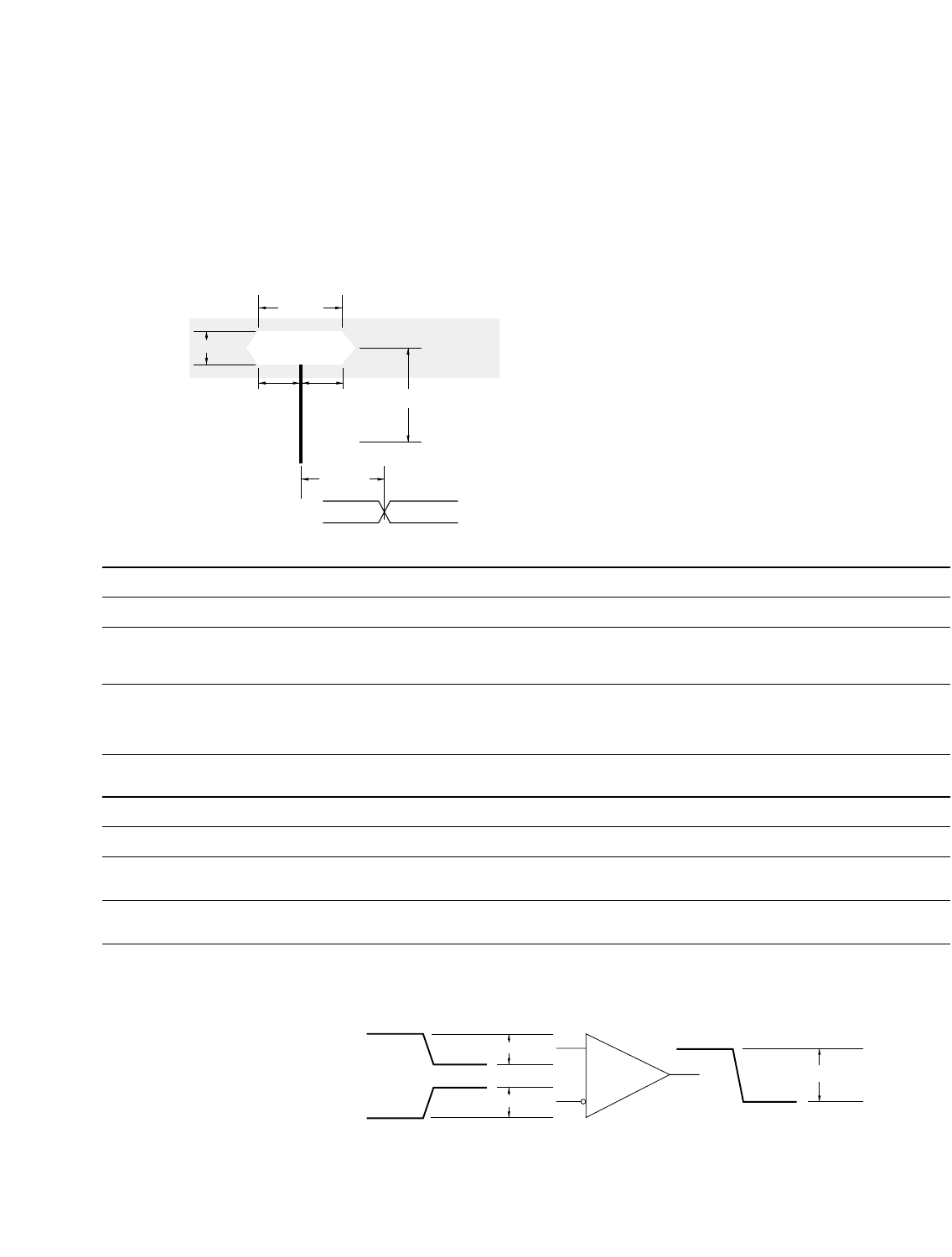
103
State/Timing Modules Specifications and
Characteristics
Specifications for Each Input
Parameter Minimum Description/Notes
800, 1250, 1500 Mb/s modes 200, 400 Mb/s modes
Data tWidth 500 ps 1.25 ns Eye width in system under test [2]
to Clock tSetup 250 ps 625 ps Data setup time required before tSample
tHold 250 ps 625 ps Data hold time required after tSample
All vHeight [1] 100mV 100mV E5379A 100-pin differential probe [3]
Inputs 250 mV 250 mV E5378A 100-pin single-ended probe [4],
E5382A single-ended flying-lead probe set
300mV 300mV E5380A 38-pin single-ended probe
User Adjustable Settings for Each Input
Parameter Adjustment Range
1500 Mb/s mode 1250 Mb/s mode 800 Mb/s mode 400 Mb/s mode 200 Mb/s mode
Data Adjustment Resolution 10 ps 10 ps 10 ps 100 ps 100 ps
to Clock tSample [5] 0 to +4 ns -2.5 to +2.5 ns -2.5 to +2.5 ns -3.2 to +3.2 ns -3.5 to +3 ns
All vThreshold [6] 10 mV resolution 10 mV resolution 10 mV resolution 10 mV resolution 10 mV resolution
Inputs -3 to +5 V -3 to +5 V -3 to +5 V -3 to +5 V -3 to +5 V
Individual
Data Channel
vHeight
tWidth
tSetup
Sampling
Position
Clock Channel Note (1)
tHold vThreshold*
*User Adjustable
—0V—
tSample*
Data Eye
Figure 6.15. Data Sampling.
* All specifications noted by an asterisk in the table are the performance standards against which the product is tested.
[1] The analyzer can be configured to sample on the rising edge, the falling edge, or both edges of the clock. If both edges are used with a single ended clock input, take care to set the
clock threshold accurately to avoid phase error.
[2] Eye width and height are specified at the probe tip. Eye width as measured by eye finder in the analyzer may be less, and still sample reliably.
[3] For each side of a differential signal.
[4] The clock inputs in the E5378A and the E5382A may be connected differentially or single ended. Use the E5379A vHeight spec for clock channel(s) connected differentially.
[5] Sample positions are independently adjustable for each data channel input. A negative sample position causes the input to be synchronously sampled by that amount before each
active clock edge. A positive sample position causes the input to be synchronously sampled by that amount after each active clock edge. A sampling position of zero causes synchro-
nous sampling coincident with each active clock edge.
[6] Threshold applies to single-ended input signals. Thresholds are independently adjustable for the clock input of each pod and for each set of 16 data inputs for each pod. Threshold lim-
its apply to both the internal reference and to the external reference input on the E5378A.
vHeight
2X vHeight
vHeight
⌺
nSignal
pSignal
——0V——
Agilent Technologies 16760A
Supplemental Specifications* and Characteristics (continued)
Synchronous Data Sampling

104
State/Timing Modules Specifications and
Characteristics
Agilent Technologies 16760A
Supplemental Specifications* and Characteristics (continued)
Synchronous state analysis 1.5 Gb/s mode 1.25 Gb/s mode 800 Mb/s mode 400 Mb/s mode 200 Mb/s mode
Maximum data rate 1.5 Gb/s 1.25 Gb/s 800 Mb/s 400 Mb/s 200 Mb/s
on each channel [3]
Minimum clock interval, 667 ps 800 ps 1.25 ns 2.5 ns 5 ns
active edge to active edge* [3]
Minimum state clock pulse N/A N/A 600 ps 1.5 ns 1.5 ns
width with clock polarity
rising or falling [3]
Clock periodicity Clock must be periodic Clock must be periodic Periodic or aperiodic Periodic or aperiodic Periodic or aperiodic
Number of clocks 1 1 1 1 1
Clock polarity Both edges Both edges Rising, falling, or both Rising, falling, or both Rising, falling, or both
Minimum data pulse width* 600 ps 750 ps E5378A, E5379A, E5382A 1.5 ns 1.5 ns
probes: 750 ps
E5380A probe: 1.5 ns
Number of channels [1]
•With time tags 16 x (number of modules) -8 16 x (number of modules) -8 34 x (number of modules) -16 34 x (number of modules) -16 34 x (number of modules)
•Without time tags 16 x (number of modules) 16 x (number of modules) 34 x (number of modules) -1 34 x (number of modules) 34 x (number of modules)
Maximum channels on a 80 (5 modules) 80 (5 modules) 170 (5 modules) 153 (5 modules) 170 (5 modules)
single time base and trigger
Maximum memory depth 128M samples 128M samples 64M samples 32M samples 32M samples
Time tag resolution 4 ns [2] 4 ns [2] 4 ns [2] 4 ns [2] 4 ns
Maximum time count 17 seconds 17 seconds 17 seconds 17 seconds 17 seconds
between states
Trigger resources 3 Patterns on each pod 3 Patterns on each pod 4 Patterns on each pod 8 Patterns evaluated as 16 Patterns evaluated as
evaluated as =, ≠, >, <, evaluated as =, ≠, >, <, evaluated as =, ≠, >, <, =, ≠, >, <, ≥, ≤=, ≠, >, <, ≥, ≤
≥, ≤on one pod; or ≥, ≤on one pod; or ≥, ≤on one pod; or 4 Ranges evaluated as 15 Ranges evaluated as
evaluated as =, ≠across evaluated as =, ≠across evaluated as =, ≠across in range, not in range in range, not in range
multiple pods; or multiple pods; or multiple pods; or 2 Occurrence counters Timers: 2 x (number of
1 range on each pod 1 range on each pod 2 ranges on each pod 4 Flags modules) – 1
4 Flags 4 Flags 4 Flags Arm in 2 Global counters
Arm in Arm in Arm in 1 Occurrence counter per
sequence level
4 Flags
Arm in
Trigger actions Trigger and fill memory Trigger and fill memory Trigger and fill memory Goto Goto
Trigger and fill memory Trigger and fill memory
Trigger and goto
Store/don’t store sample
Turn default storing on/off
Timer start/stop/pause/resume
Global counter increment/reset
Occurrence counter reset
Flag set/clear
* All specifications noted by an asterisk are the performance standards against which the product is tested.
[1] In 1.25 Gb/s and 1.5 Gb/s modes, only the even-numbered channels (0, 2, 4, etc.) are acquired.
[2] The resolution of the hardware used to assign time tags is 4 ns. Times of intermediate states are calculated.
[3] The choice of probe can limit system performance. Select a probe rated at the speed of the selected mode (or greater) to maintain system bandwidth.

105
State/Timing Modules Specifications and
Characteristics
Agilent Technologies 16760A
Supplemental Specifications and Characteristics (continued)
Synchronous state 1.5 Gb/s mode 1.25 Gb/s mode 800 Mb/s mode 400 Mb/s mode 200 Mb/s mode
analysis (continued) [4]
Maximum trigger 2 2 4 16 16
sequence levels
Maximum trigger 1.5 Gb/s 1.25 Gb/s 800 MHz 400 MHz 200 MHz
sequencer speed
Store qualification Default Default Default Default Default and per
sequence level
Maximum global counter N/A N/A N/A N/A 16,777,215
Maximum occurrence N/A N/A N/A N/A 16,777,215
counter
Maximum pattern/range 32 bits [3] 32 bits [3] 32 bits [3] 32 bits [3] 32 bits [3]
term width
Timer value range N/A N/A N/A N/A 100 ns to 4397 seconds
Timer resolution N/A N/A N/A N/A 4 ns
Timer accuracy N/A N/A N/A N/A ±(10 ns + 0.01% of value)
Timer reset latency N/A N/A N/A N/A 65 ns
Data in to BNC port out 150 ns 150 ns 150 ns 150 ns 150 ns
latency
Flag set/reset to evaluation N/A N/A N/A N/A 110 ns
latency
[1] In 1.25 Gb/s and 1.5 Gb/s modes, only the even-numbered channels (0, 2, 4, etc.) are acquired.
[2] The resolution of the hardware used to assign time tags is 4 ns. Times of intermediate states are calculated.
[3] Maximum label width is 32 bits. Wider patterns can be created by “Anding” multiple labels together.
[4] The choice of probe can limit system performance. Select a probe rated at the speed of the selected mode (or greater) to maintain system bandwidth.
Asynchronous Timing Analysis Conventional Timing Analysis Transitional Timing Analysis
Maximum timing analysis sample rate 800 MHz 400 MHz
Number of channels 34 x (number of modules) Sampling rates < 400 MHz: 34 x (number of modules)
Sampling rates = 400 MHz:
34 x (number of modules) - 17 [1]
Maximum channels on a 170 (5 modules) 170 (5 modules)
single time base and trigger
Sample period 1.25 ns 2.5 ns to 1 ms [1]
Memory Depth 64 M Samples 32 M Samples [1]
[1] With all pods assigned in transitional/store qualified timing, minimum sample period is 5 ns and maximum memory depth is 16 M samples.

106
State/Timing Modules Specifications and
Characteristics
Agilent Technologies 16760A
Supplemental Specifications and Characteristics (continued)
Asynchronous Timing Analysis Conventional Timing Analysis Transitional Timing Analysis
(continued)
Sample period accuracy ±(250 ps + 0.01% of sample period) ±(250 ps + 0.01% of sample period)
Channel-to-channel skew < 1.5 ns < 1.5 ns
Time interval accuracy ±[sample period + (channel-to-channel skew) + ±[sample period + (channel-to-channel skew) +
(0.01% of time interval)] (0.01% of time interval)]
Minimum data pulse width 1.5 ns for data capture 3.8 ns for data capture
5.1 ns for trigger sequencing 5.1 ns for trigger sequencing
Maximum trigger sequencer speed 200 MHz 200 MHz
Trigger resources 16 Patterns evaluated as =, ≠, >, <, ≥, ≤16 Patterns evaluated as =, ≠, >, <, ≥, ≤
15 Ranges evaluated as in range, not in range 15 Ranges evaluated as in range, not in range
2 Edge/glitch 2 Edge/glitch
(2 Timers per module) -1 (2 Timers per module) -1
2 Global counters 2 Global counters
1 Occurrence counter per sequence level 1 Occurrence counter per sequence level
4 Flags, Arm In 4 Flags, Arm In
Trigger resource conditions Arbitrary Boolean combinations Arbitrary Boolean combinations
Trigger actions Goto Goto
Trigger and fill memory Trigger and fill memory
Trigger and goto Trigger and goto
Timer start/stop/pause/resume Timer/start/stop/pause/resume
Global counter increment/reset Global counter increment/reset
Occurrence counter reset Occurrence counter reset
Maximum global counter 16,777,215 16,777,215
Maximum occurrence counter 16,777,215 16,777,215
Timer value range 100 ns to 4397 seconds 100 ns to 4397 seconds
Timer resolution 4 ns 4 ns
Timer accuracy ±(10 ns + 0.01%) ±(10 ns + 0.01%)
Greater than duration 5 ns to 83 ms in 5 ns increments 5 ns to 83 ms in 5 ns increments
Less than duration 10 ns to 83 ms in 5 ns increments 10 ns to 83 ms in 5 ns increments
Timer reset latency 60 ns 60 ns
Data in to BNC port out delay latency 150 ns 150 ns
Flag set/reset to evaluation latency 110 ns 110 ns
Environmental
Operating temperature 0 deg C to 45 deg C

107
State/Timing Modules Specifications and
Characteristics
Agilent Technologies 16760A
Supplemental Specifications and Characteristics (continued)
Eye scan mode 1.5 Gb/s mode 800 Mb/s mode
Maximum clock rate 1.5 Gb/s 800 Mb/s
Sample position range relative +5ns to 10 ns -4 ns to +4 ns
to clock
Sample (time) position resolution 12 ps 12 ps
Sample position (time) accuracy +/- (50 ps + 0.01 * sample position) +/- (50 ps + 0.01 * sample position)
Number of channels 16*(number of modules) 34*(number of modules)-1
Input dynamic range -3.0 Vdc to +5.0 Vdc -3.0 Vdc to +5.0 Vdc
Threshold range -3.0 Vdc to +5.0 Vdc -3.0 Vdc to +5.0 Vdc
Threshold resolution 1 mV 1 mV
Threshold accuracy +/-(30 mV + 1% of setting) +/-(30 mV + 1% of setting)
Equivalent rise time [1] 150 ps 150 ps
Equivalent bandwidth [1] 2.33 GHz 2.33 GHz
Minimum detectable pulse width 500 ps 750 ps
at minimum signal amplitude [1]
Jitter 10 ps RMS 10 ps RMS
Noise floor 25 mV p-p 25 mV p-p
Channel-to-channel skew, maximum 100 ps 100 ps
between any two channels
[1] E5378A, E5379A, and E5382A probes only.
Qualified eye scan mode
In the qualified eye scan mode, a
single qualifier input defines what
clock cycles are to be acquired and
what cycles are to be ignored in eye
scan acquisition.
Qualified eye scan is supported in
the 16760A in 800 Mb/s eye scan
mode only. Qualified eye scan is
only available for double-edged clock
(double-data-rate).
Channels available
The following channels are not
available for qualified eye scan
measurements.
Master module, Pod 1
Master module, Pod 2, Bit 0, Bit 14,
Bit 1, Bit 15, Bit 2, K-clock
(the qualifier input itself).
All channels on all boards other than
the master board are available for
qualified eye scans.
Timing
The analyzer samples the qualifica-
tion signal at the beginning of each
clock cycle (i.e. at the first of each
pair of data transfers). The analyzer
can be configured to treat either the
rising edge or the falling edge of the
clock as the first edge of each clock
cycle. The qualifier should remain
stable for the entire duration of
each burst.
The qualifier must be pipelined
(delayed) by one clock cycle before
transmittal to the analyzer.

108
16534A Specifications*
Bandwidth dc to 500 MHz
dc offset accuracy ±(1% of offset + 2% of full scale)
dc voltage measurement accuracy ±(1.5% of full scale + offset accuracy)
Time interval measurement ±[(0.005% of D T) + (2E–6 x delay setting) + 100 ps]
accuracy at maximum sampling rate,
on a single scope card, on a single
acquisition
Trigger sensitivity (See notes)
•dc to 50 MHz •0.06 full scale
•50 MHz to 500 MHz •0.13 full scale
Input resistance 1 MΩ±1% 50 Ω±1%
* Specifications refer to the input to the BNC connector
Notes:
•Specifications apply only within ± 10°C of the temperature at which the most recent calibration was performed.
•Specifications apply only after operational accuracy calibration is performed in the frame in which the
oscilloscope module is installed.
•Display magnification is used below 56 mV full scale. For sensitivities from 16 mV to 56 mV full scale, full scale is
defined as 56 mV.
Characteristics
General
Maximum sampling rate 2 GSa/s
Number of channels •2 to 8 using the same
time base and trigger.
•Up to 10 channels may be installed in a single
16700 frame, or up to 20 in a single system using a
16701 expansion frame.
Waveform record length 32768 points
Oscilloscope Modules Specifications and
Characteristics

109
Oscilloscope Modules Specifications and
Characteristics
16534A Characteristics*
Vertical (Voltage)
Vertical sensitivity range 16 mV full scale to 40 V full scale
Vertical resolution 8 bits full scale
Rise time (calculated from bandwidth) 700 ps
dc gain accuracy ±(1.25% of full scale + 0.08% per °C difference from
calibration temperature)
dc offset range
Vertical sensitivity Offset range
•16 mV full scale to 400 mV full scale •±2 V
•400 mV full scale to 2.0 V full scale •±10 V
•2.0 V full scale to 10 V full scale •±50 V
•10 V full scale to 40 V full scale •±250 V
Probe attenuation Any ratio from 1:1E-9 to 1:1E+6
Channel-to-channel isolation (with channel sensitivities equal)
•dc–50 MHz •40 dB
•50 MHz–500 MHz •30 dB
Maximum safe input voltage
•1 MΩ•±250 V dc + peak ac (<10 kHz)
•50 Ω•5 Vrms
* Characteristics refer to the input at the BNC connector

110
Oscilloscope Modules Specifications and
Characteristics
16534A Characteristics
Horizontal (Time)
Time base ranges 0.5 ns/div to 5 s/div
Time base resolution 10 ps
Delay range
•pretrigger •-32 K x sample period
•posttrigger •320 ms or 1.6E7 x sample period, whichever is greater
Time interval measurement accuracy ±{(0.005% of ∆T) + (2E–6 x delay setting)
for sampling rates other than maximum, + [0.15/(sample rate)]}
for bandwidth-limited signals [signal
rise time > 1.4/(sampling rate)], on a
single card, on a single acquisition
Time interval measurement accuracy ± [(0.005% of ∆T) + (2E–6 x delay setting) + 300 ps
for 2, 3, or 4 Agilent 16533As or 16534As
operating on a single time base, for
measurements made between channels
on different cards, at maximum
sampling rate
Trigger
Trigger level range (See notes) ±1.5 x full scale from center of screen
Trigger modes
•Immediate •Triggers immediately after arming condition is met
•Edge •Triggers on rising or falling edge on channel 1 or
channel 2
•Pattern •Triggers on entering or exiting a specified pattern
across both channels
•Auto condition •Self-triggers if trigger is not satisfied within
approximately 50 ms after arming
•Events delay •The trigger can be set to occur on the nth occurrence
of an edge or pattern, n ≤32000
•Intermodule •Arms another measurement module or activates the
port out BNC connector when the trigger condition is
met
Notes:
•Specifications apply only within ± 10°C of the temperature at which the most recent calibration was performed.
•Specifications apply only after operational accuracy calibration is performed in the frame in which the
oscilloscope module is installed.
•Display magnification is used below 56 mV full scale. For sensitivities from 16 mV to 56 mV full scale, full scale is
defined as 56 mV.

111
Pattern Generation Modules Specifications
and Characteristics
16720A Pattern Generator Characteristics
Maximum memory depth 16 MVectors
Number of output channels at ≤300 MHz clock 24
Number of output channels at ≤180 MHz clock 48
Number of output channels at ≤200 MHz clock 24
Number of output channels at ≤100 MHz clock 48
Number of different macros 100
Maximum number of lines in a macro 1024
Maximum number of parameters in a macro 10
Maximum number of macro invocations 1000
Maximum loop count in a repeat loop 20000
Maximum number of repeat loop invocations 1000
Maximum number of "Wait" event patterns 4
Number of input lines to define a pattern 3
Maximum number of modules in a system 5
Maximum width of a vector (in a 5 module system) 240 bits
Maximum width of a label 32 bits
Maximum number of labels 126
Maximum number of vectors in binary format 16 MVectors
Minimum number of vectors in binary format 4096
Lead Set Characteristics
Agilent 10474A 8-channel Provides most cost effective lead set for the 16522A and
probe lead set 16720A clock and data pods. Grabbers are not included.
Lead wire length is 12 inches.
Agilent 10347A 8-channel Provides 50 Ωcoaxial lead set for unterminated signals,
probe lead set required for 10465A ECL Data Pod (unterminated).
Grabbers are not included.
Agilent 10498A 8-channel Provides most cost effective lead set for the 16522A and
probe lead set 16720A clock and data pods. Grabbers are not included.
Lead wire length is 6 inches.
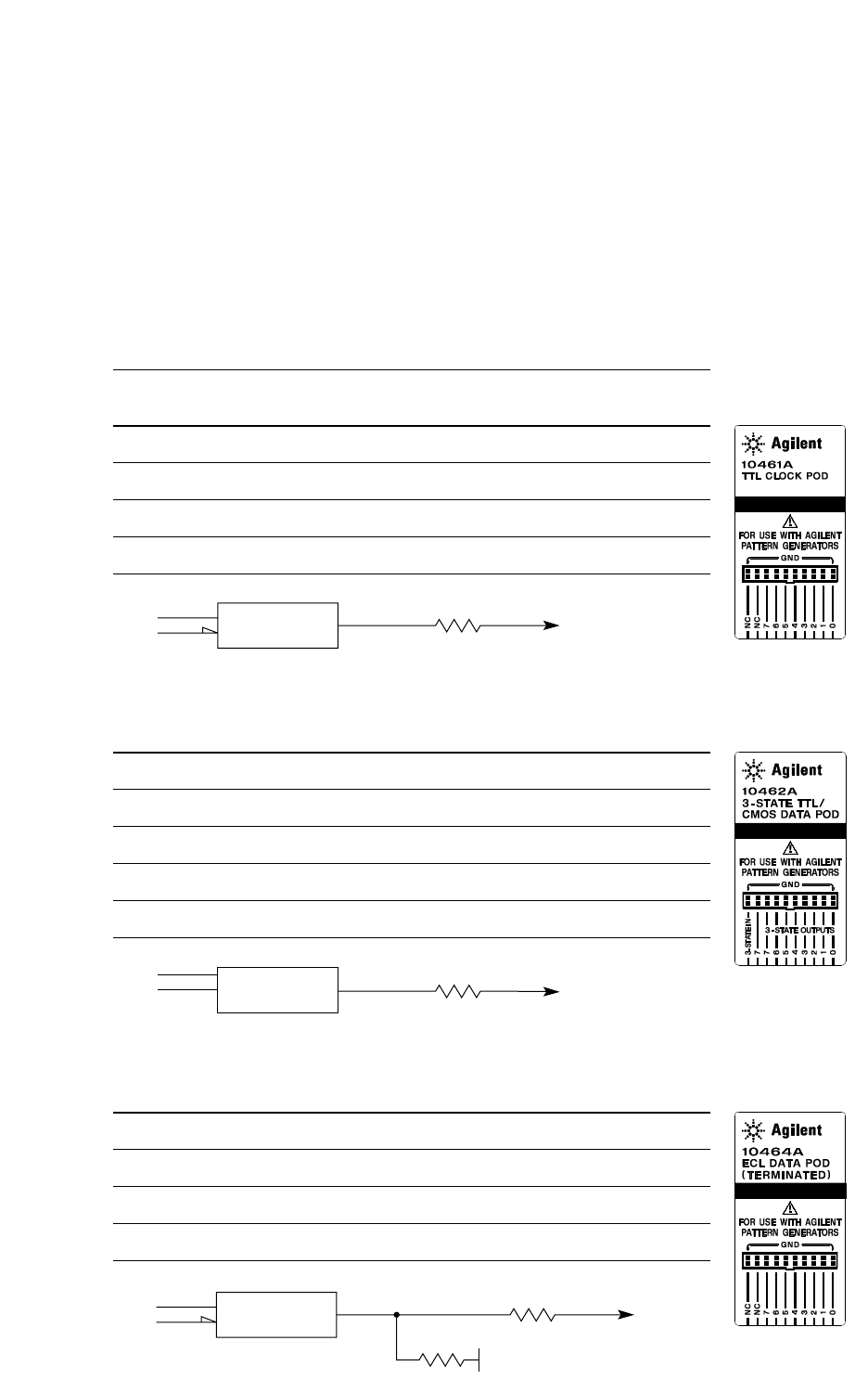
112
Pattern Generation Modules Specifications
and Characteristics
Data Pod Characteristics
Note: Data Pod output parametrics depend on the output driver and the impedance load of the target
system. Check the device data book for the specific drivers listed for each pod.
Agilent 10461A TTL Data Pod
Output type 10H125 with 100 Ωseries
Maximum clock 200 MHz
Skew [1] typical < 2 ns; worst case = 4 ns
Recommended lead set Agilent 10474A
Agilent 10462A 3-State TTL/CMOS Data Pod
Output type 74ACT11244 with 100 Ωseries; 10H125 on non 3-state channel 7 [2]
3-state enable negative true, 100 KΩto GND, enabled on no connect
Maximum clock 100 MHz
Skew [1] typical < 4 ns; worst case = 12 ns
Recommended lead set Agilent 10474A
Agilent 10464A ECL Data Pod (terminated)
Output type 10H115 with 330 Ωpulldown, 47 Ωseries
Maximum clock 300 MHz
Skew [1] typical < 1 ns; worst case = 2 ns
Recommended lead set Agilent 10474A
ECL/TTL 100 Ω
10H125
100 Ω
74ACT11244
42 Ω
10H115
– 5.2 V
348 Ω
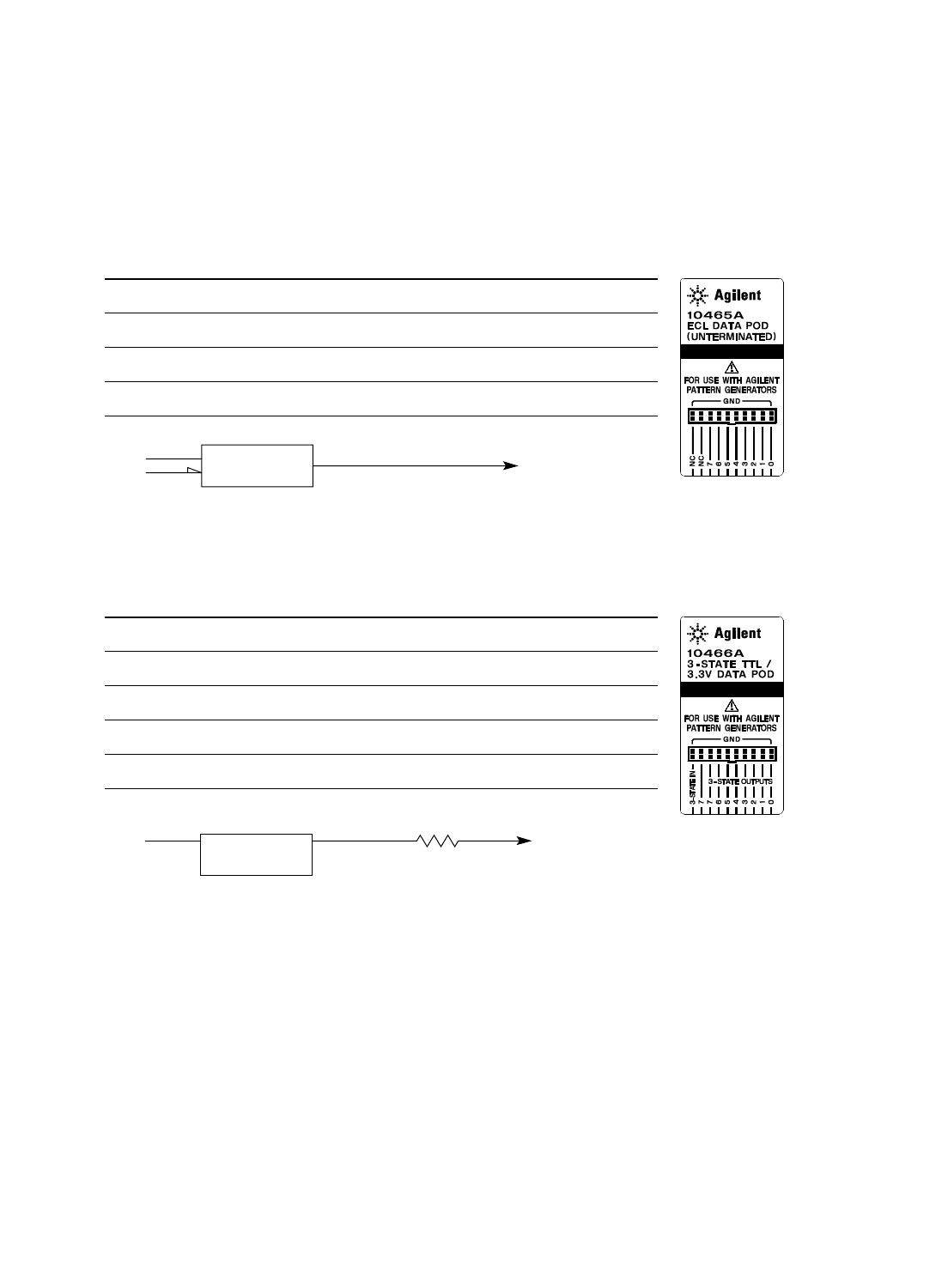
113
Pattern Generation Modules Specifications
and Characteristics
[1] Typical skew measurements made at pod connector with approximately 10 pF/50 KΩload to GND; worst case
skew numbers are a calculation of worst case conditions through circuits. Both numbers apply to any channel
within a single or multiple module system.
[2] Channel 7 on the 3-state pods has been brought out in parallel as a non 3-state signal. By looping this output back
into the 3-state enable line, the channel can be used as a 3-state enable.
Agilent 10465A ECL Data Pod (unterminated)
Output type 10H115 (no termination)
Maximum clock 300 MHz
Skew [1] typical < 1 ns; worst case = 2 ns
Recommended lead set Agilent 10347A
Agilent 10466A 3-State TTL/3.3 volt Data Pod
Output type 74LVT244 with 100 Ωseries; 10H125 on non 3-state channel 7 [2]
3-state enable negative true, 100 KΩto GND, enabled on no connect
Maximum clock 200 MHz
Skew [1] typical < 3 ns; worst case = 7 ns
Recommended lead set Agilent 10474A
10H115
100 Ω
74LVT244
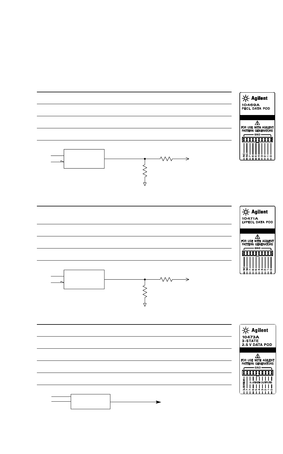
114
Pattern Generation Modules Specifications
and Characteristics
Agilent 10473A 3-State 2.5 Volt Data Pod
Output type 74AVC16244
3-state enable negative true, 38 KΩto GND, enabled on no connect
Maximum clock 300 MHz
Skew [1] typical < 1.5 ns; worst case = 2 ns
Recommended lead set Agilent 10498A
74AVC16244
[1] Typical skew measurements made at pod connector with approximately 10 pF/50 KΩload to GND; worst case
skew numbers are a calculation of worst case conditions through circuits. Both numbers apply to any channel
within a single or multiple module system.
[2] Channel 7 on the 3-state pods has been brought out in parallel as a non 3-state signal. By looping this output back
into the 3-state enable line, the channel can be used as a 3-state enable.
Agilent 10469A 5 volt PECL Data Pod
Output type 100EL90 (5V) with 348 ohm pulldown to ground and 42 ohm in series
Maximum clock 300 MHz
Skew [1] typical < 500 ps; worst case = 1 ns
Recommended lead set Agilent 10498A
Agilent 10471A 3.3 volt LVPECL Data Pod
Output type 100LVEL90 (3.3V) with 215 ohm pulldown to ground and
42 ohm in series
Maximum clock 300 MHz
Skew [1] typical < 500 ps; worst case = 1 ns
Recommended lead set Agilent 10498A
42 Ω
348 Ω
100EL90
42 Ω
215 Ω
100LVEL90
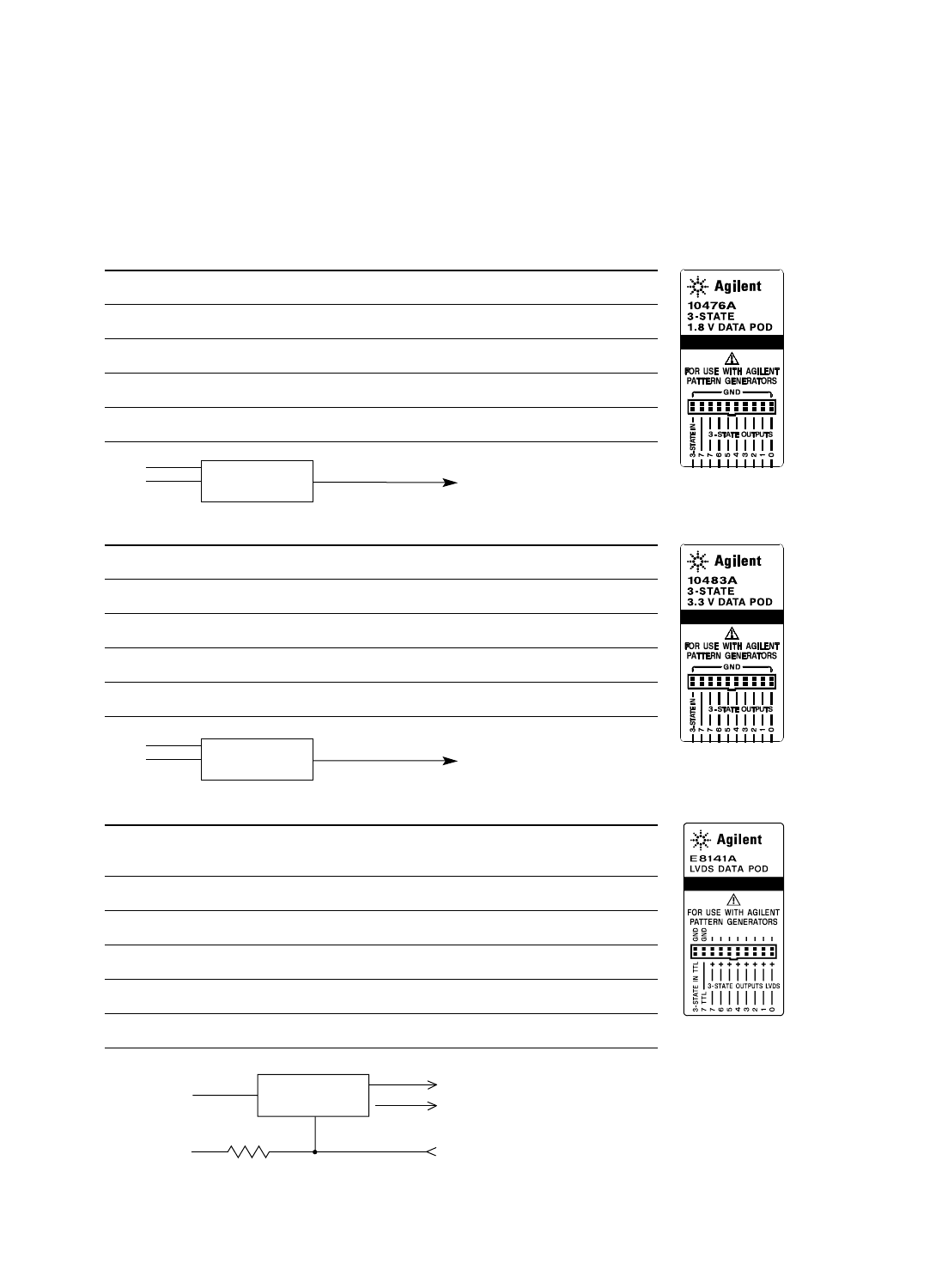
115
Pattern Generation Modules Specifications
and Characteristics
Agilent E8141A LVDS Data Pod
Output type 65LVDS389 (LVDS data lines)
10H125 (TTL non-3-state channel 7)
3-state enable positive true TTL; no connect=enabled
Maximum clock 300 MHz
Skew typical < 1 ns; worst case = 2 ns
Recommended lead set: E8142A
Recommended lead set Agilent 10498A
10 KΩ
65LVDS389
ENABLE °
3.3 V
LVDS DATA OUT
3-STATE IN TTL
Agilent 10476A 3-State 1.8 Volt Data Pod
Output type 74AVC16244
3-state enable negative true, 38 KΩto GND, enabled on no connect
Maximum clock 300 MHz
Skew [1] typical < 1.5 ns; worst case = 2 ns
Recommended lead set Agilent 10498A
Agilent 10483A 3-State 3.3 Volt Data Pod
Output type 74AVC16244
3-state enable negative true, 38 KΩto GND, enabled on no connect
Maximum clock 300 MHz
Skew [1] typical < 1.5 ns; worst case = 2 ns
Recommended lead set Agilent 10498A
74AVC16244
74AVC16244
[1] Typical skew measurements made at pod connector with approximately 10 pF/50 KΩload to GND; worst case
skew numbers are a calculation of worst case conditions through circuits. Both numbers apply to any channel
within a single or multiple module system.
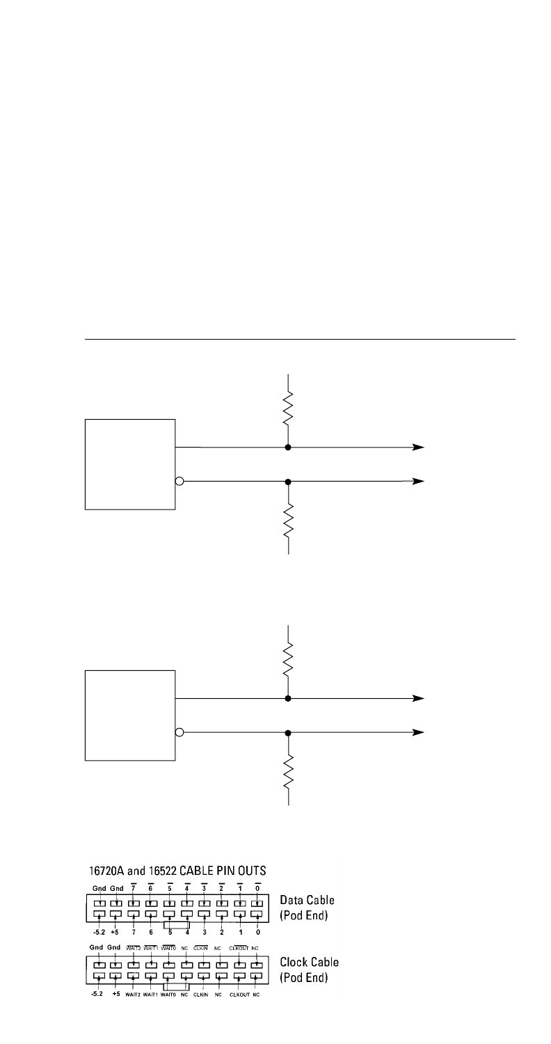
116
Pattern Generation Modules Specifications
and Characteristics
Data Cable Characteristics Without a Data Pod
The Agilent 16720A and 16522A data cables without a data pod provide an ECL terminated (1 KΩto
–5.2V) differential signal (from a type 10E156 or 10E154 driver). These are usable when received by
a differential receiver, preferably with a 100 Ωtermination across the lines. These signals should
not be used single ended due to the slow fall time and shifted voltage threshold (they are not ECL
compatible).
–3.25 V
470 Ω
470 Ω
Differential
Output
10E156
or
10E154
–3.25 V
–5.2 V
1 kΩ
1 kΩ
Differential
Output
10E156
or
10E154
–5.2 V
16720A
16522A
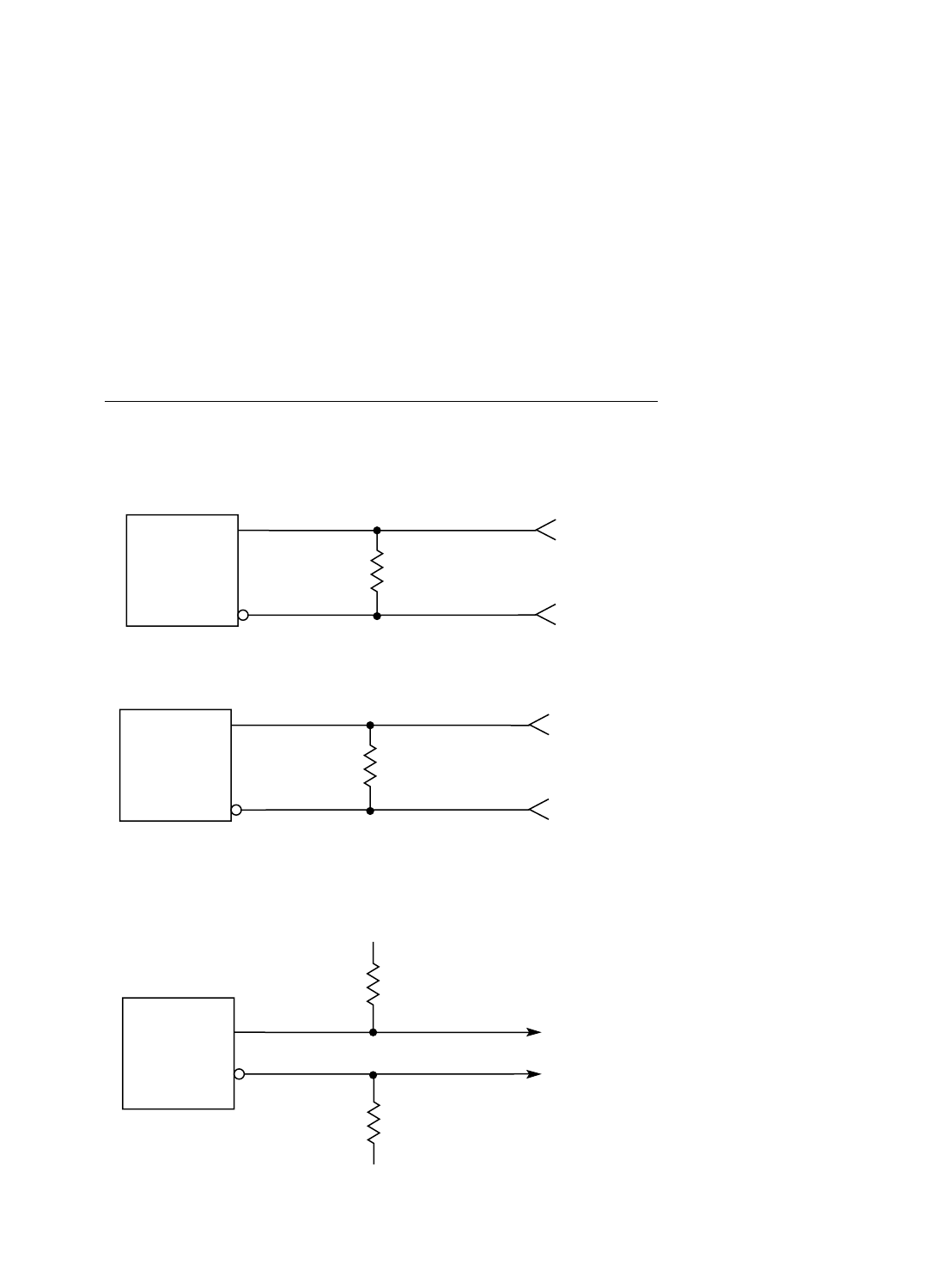
117
Pattern Generation Modules Specifications
and Characteristics
Clock Cable Characteristics Without a Clock Pod
The Agilent 16720A and 16522A clock cables without a clock pod provide an ECL terminated
(1 KΩto –5.2V) differential signal (from a type 10E164 driver). These are usable when received by a
differential receiver, preferably with a 100 Ωtermination across the lines. These signals should not be
used single ended due to the slow fall time and shifted voltage threshold (they are not ECL compatible).
100 ΩClock In
10E116
7
8
100 ΩWait 1, 2, 3 IN
10H125
11, 13, 15
12, 14, 16
–3.25 V
215 Ω
215 Ω
Clock Out
10E164
–3.25 V
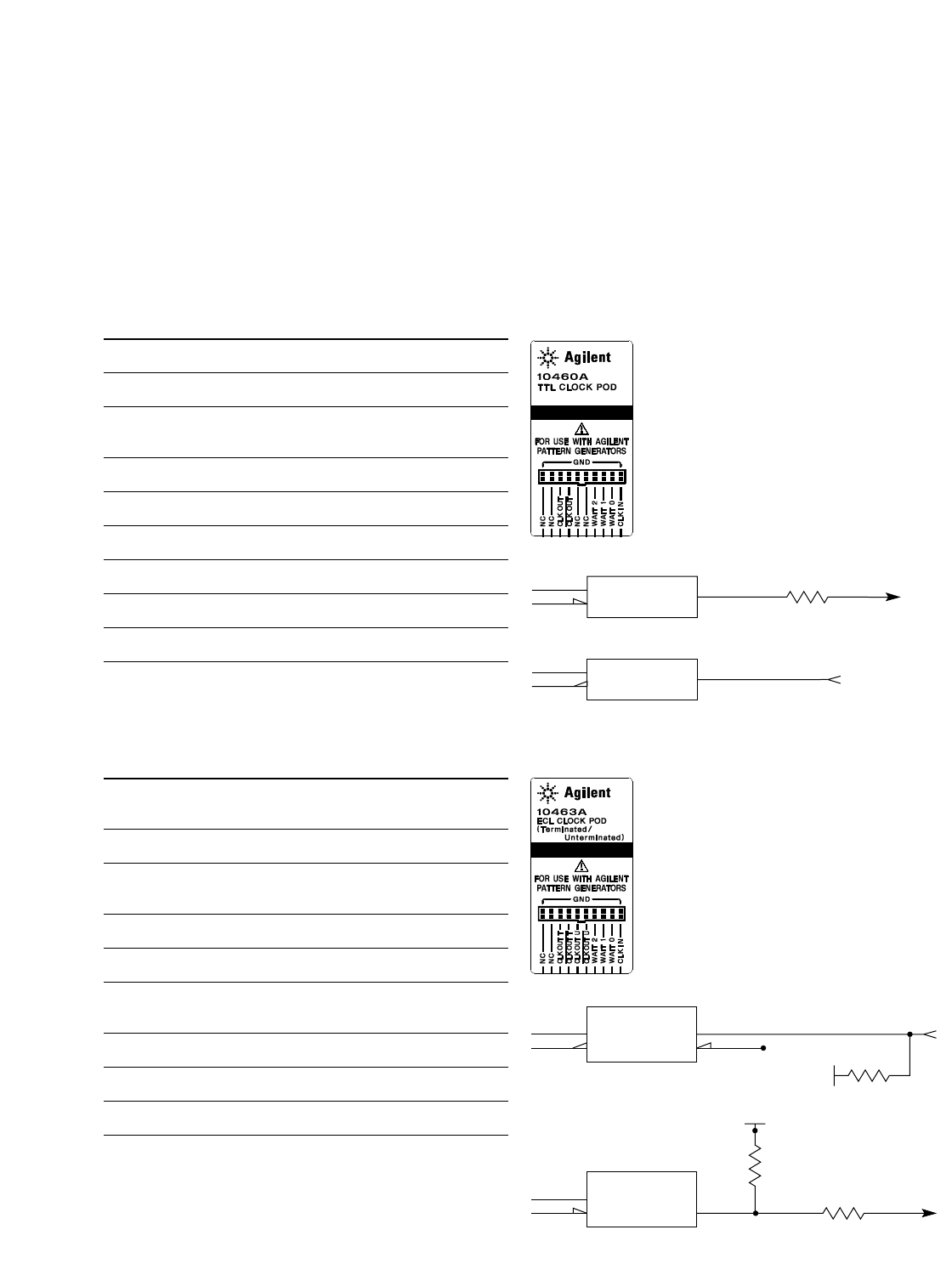
118
10463A ECL Clock Pod
Clock output type 10H116 differential unterminated; and differ-
ential with 330 Ωto –5.2V and 47 Ωseries
Clock output rate 300 MHz maximum
Clock out delay approximately 8 ns total in 14 steps (16720A
only); 11 ns maximum in 9 steps (16522A only)
Clock input type ECL – 10H116 with 50 KΩto –5.2v
Clock input rate dc to 300 MHz
Pattern input type ECL – 10H116 with 50 KΩ(no connect is
logic 0)
Clock-in to clock-out approximately 30 ns
Pattern-in to recognition approximately 15 ns + 1 clk period
Recommended lead set Agilent 10474A
10H116
–5.2 V
VBB 50 kΩ
CLKin
10H116
–5.2 V
330 Ω
47 Ω CLKout
Pattern Generation Modules Specifications
and Characteristics
Clock Pod Characteristics
10460A TTL Clock Pod
Clock output type 10H125 with 47 Ωseries; true & inverted
Clock output rate 100 MHz maximum
Clock out delay approximately 8 ns total in 14 steps (16720A
only); 11 ns maximum in 9 steps (16522A only)
Clock input type TTL – 10H124
Clock input rate dc to 100 MHz
Pattern input type TTL – 10H124 (no connect is logic 1)
Clock-in to clock-out approximately 30 ns
Pattern-in to recognition approximately 15 ns + 1 clk period
Recommended lead set Agilent 10474A
47Ω CLKout
10H125
WAIT
10H124 CLKin
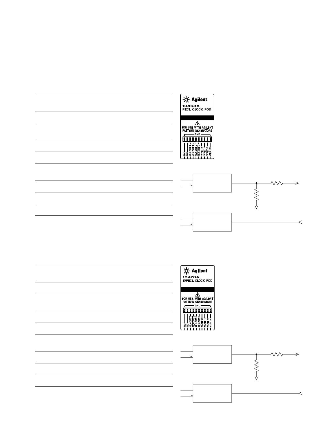
119
Pattern Generation Modules Specifications
and Characteristics
10468A 5 volt PECL Clock Pod
Clock output type 100EL90 (5V) with 348 ohm pulldown to
ground and 42 ohm in series
Clock output rate 300 MHz maximum
Clock out delay approximately 8 ns total in 14 steps (16720A
only); 11 ns maximum in 9 steps (16522A only)
Clock input type 100EL91 PECL (5V), no termination
Clock input rate dc to 300 MHz
Pattern input type 100EL91 PECL (5V), no termination (no
connect is logic 0)
Clock-in to clock-out approximately 30 ns
Pattern-in to recognition approximately 15 ns + 1 clk period
Recommended lead set Agilent 10498A
10470A 3.3 volt LVPECL Clock Pod
Clock output type 100LVEL90 (3.3V) with 215 ohm pulldown to
ground and 42 ohm in series
Clock output rate 300 MHz maximum
Clock out delay approximately 8 ns total in 14 steps (16720A
only); 11 ns maximum in 9 steps (16522A only)
Clock input type 100LVEL91 LVPECL (3.3V), no termination
Clock input rate dc to 300 MHz
Pattern input type 100LVEL91 LVPECL (3.3V), no termination
(no connect is logic 0)
Clock-in to clock-out approximately 30 ns
Pattern-in to recognition approximately 15 ns + 1 clk period
Recommended lead set Agilent 10498A
42 Ω
348 Ω
CLKout
CLKin
100EL91
100EL90
42 Ω
215 Ω
CLKout
CLKin
100LVEL91
100LVEL90
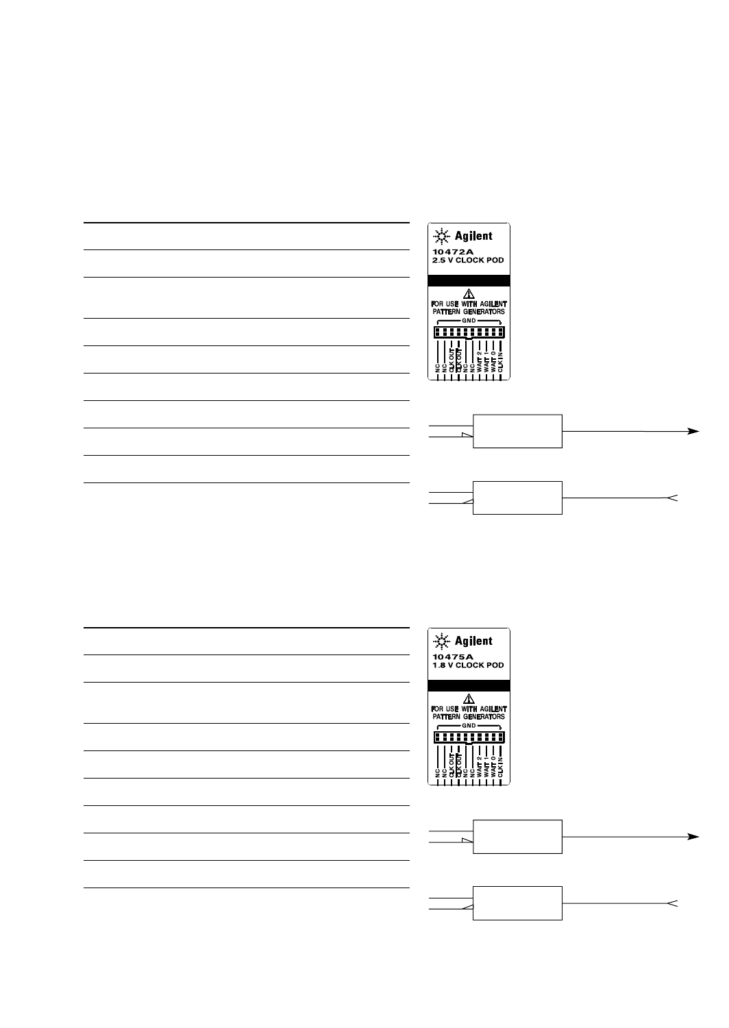
120
Pattern Generation Modules Specifications
and Characteristics
10472A 2.5 volt Clock Pod
Clock output type 74AVC16244
Clock output rate 200 MHz maximum
Clock out delay approximately 8 ns total in 14 steps (16720A
only); 11 ns maximum in 9 steps (16522A only)
Clock input type 74AVC16244 (3.6V max)
Clock input rate dc to 200 MHz
Pattern input type 74AVC16244 (3.6V max; no connect is logic 0)
Clock-in to clock-out approximately 30 ns
Pattern-in to recognition approximately 15 ns + 1 clk period
Recommended lead set Agilent 10498A
10475A 1.8 volt Clock Pod
Clock output type 74AVC16244
Clock output rate 200 MHz maximum
Clock out delay approximately 8 ns total in 14 steps (16720A
only); 11 ns maximum in 9 steps (16522A only)
Clock input type 74AVC16244 (3.6V max)
Clock input rate dc to 200 MHz
Pattern input type 74AVC16244 (3.6V max; no connect is logic 0)
Clock-in to clock-out approximately 30 ns
Pattern-in to recognition approximately 15 ns + 1 clk period
Recommended lead set Agilent 10498A
CLKout
74AVC16244
74AVC16244
WAIT
CLKin
CLKout
74AVC16244
74AVC16244
WAIT
CLKin
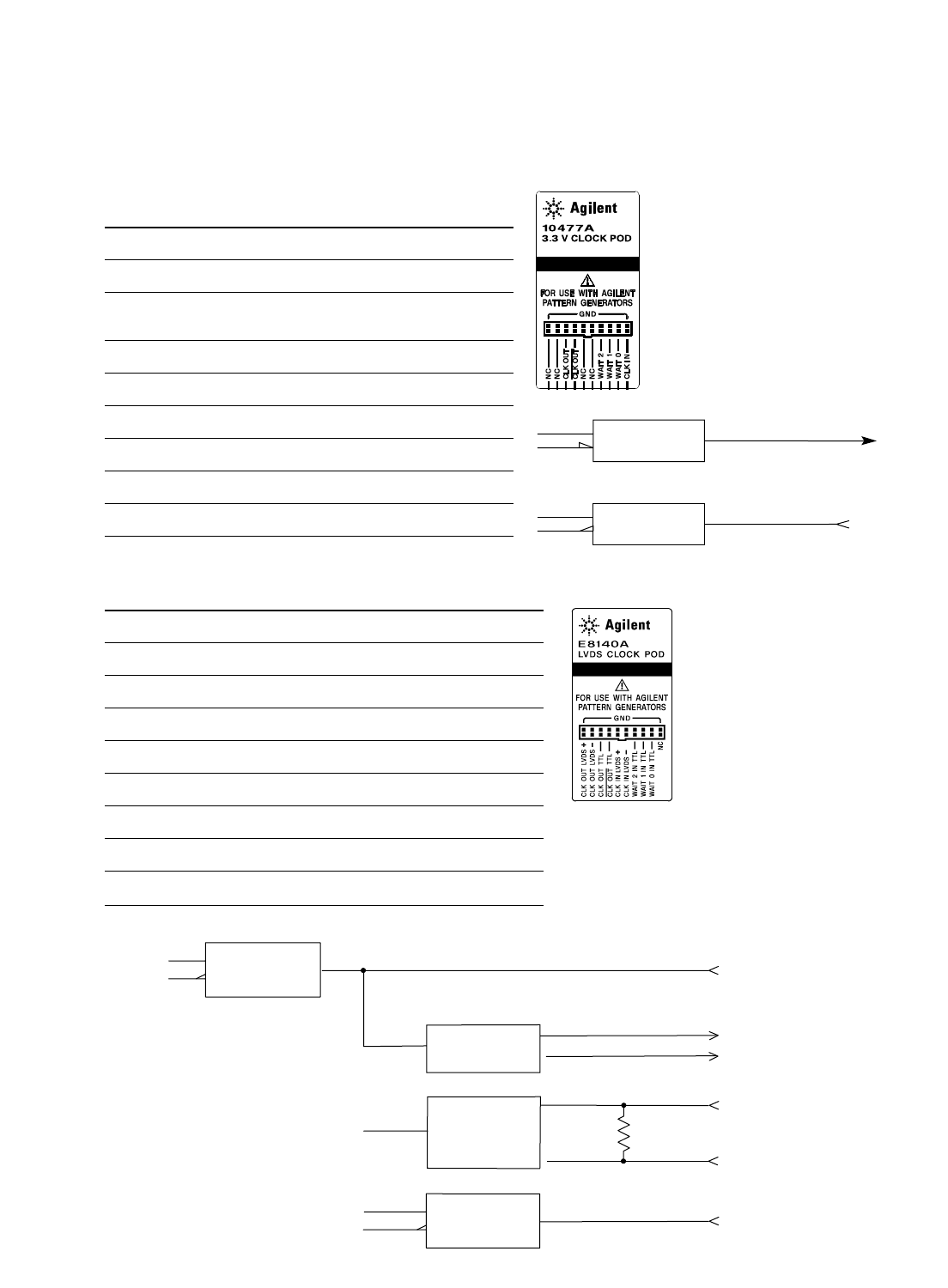
121
Pattern Generation Modules Specifications
and Characteristics
10477A 3.3 volt Clock Pod
Clock output type 74AVC16244
Clock output rate 200 MHz maximum
Clock out delay approximately 8 ns total in 14 steps (16720A
only); 11 ns maximum in 9 steps (16522A only)
Clock input type 74AVC16244 (3.6V max)
Clock input rate dc to 200 MHz
Pattern input type 74AVC16244 (3.6V max; no connect is logic 0)
Clock-in to clock-out approximately 30 ns
Pattern-in to recognition approximately 15 ns + 1 clk period
Recommended lead set Agilent 10498A
CLKout
74AVC16244
74AVC16244
WAIT
CLKin
E8140A LVDS Clock Pod
Clock output type 65LVDS179 (LVDS) and 10H125 (TTL)
Clock output rate 200 MHz maximum (LVDS and TTL)
Clock out delay approximately 8 ns total in 14 steps
Clock input type 65LVDS179 (LVDS with 100 ohm)
Clock input rate dc to 150 MHz (LVDS)
Pattern input type 10H124 (TTL) (no connect = logic 1)
Clock-in to clock-out approximately 30 ns
Pattern-in to recognition approximately 15 ns + 1 clk period
Recommended lead set Agilent 10498A
100 Ω
10H125
65LBDS179 °
CLK OUT TTL
CLK OUT LVDS
65LVDS179
°
CLK IN LVDS
10H124
CLK IN LVDS
WAIT IN TTL

122
Trade-In, Trade-Up
Advance to the Latest Technology with Agilent’s “Trade-Up” Program
Comprehensive Economical Convenient
•Purchase from an extensive •Upgrade for less •Simply call your local Agilent
list of Agilent test and •Stretch your test sales office
measurement products equipment budget •Let us evaluate your savings
•Trade in a wide variety of •Reduce support costs for opportunities
test equipment for aging equipment
substantial credit
How to Upgrade for Less:
Purchase... Trade in... Receive...
Eligible New Agilent Product Similar[1] Agilent Product Agilent’s “buy-back” price[2]
[1] A “similar” product is considered to be part of the same product family (for example, oscilloscope for
oscilloscope) with comparable functionality and application.
[2] Agilent’s “buy-back” price varies based on the model, option configuration, and age of the trade-in product.
Terms and Conditions
• This offer is void where prohibit-
ed.
• This offer applies to end-user cus-
tomers only. Rental companies
and equipment brokers are exclud-
ed.
• This offer is applicable to the
return of fewer than 10 products
or $100,000 (U.S. dollars) in trade-
in credit.
• The total trade-in credit may not
exceed 100% of the cost of the eli-
gible new product(s). Any credit in
excess of that amount may not be
applied toward a later purchase.
• Trade-in credit amounts and prod-
uct eligibility are subject to change
at any time without advance
notice.
• Refurbished Agilent equipment is
not eligible for purchase under
this program.
• All trade-in products must be in
working condition and have no
interior, exterior, or performance
modifications.
• To ensure timely release of credit,
all trade-in products must be
returned to Agilent within 30 days
after receipt of the newly pur-
chased Agilent product.
• Customer is responsible for all
costs associated with shipping the
trade-in product(s) to Agilent.
• Additional requirements may
apply. Please contact your
local Agilent sales office for
information.

123
Ordering Information
Mainframes and Mainframe Accessories
Product Number Description Includes
16700B Modular mainframe with five measurement •One DIN keyboard
module slots and one emulation or multiframe •One three-button DIN mouse
module slot •One ten-conductor, flying lead cable for target control port
•Training kit
•One internal CD ROM drive
•One internal 3.5" floppy drive
16702B Modular frame with built-in 800x600 LCD display Same as 16700B plus:
with touchscreen. Includes five measurement •12.1” touchscreen display
slots and one emulation or multiframe •Display knobs
module slot •Dedicated hot keys
16701B Expansion frame with five measurement module 1 ft. and 3 ft. interface cables
slots and two emulation module slots. Requires a
16700A/B or 16702A/B
1184A Testmobile 4 wheeled equipment cart specifically designed Drawer, keyboard tray, mouse tray, strap for
to carry the 16700 Series logic analyzer, stabilizing monitor
expansion frame, and monitor
Mainframe Options
Option Description 16700B or 16701B
Number 16702B
001 Add 17-inch 1280x1024 monitor √
003 Performance option. Up to 256 MBytes total system √
RAM, 4 MBytes total video RAM. (256 MB)
008 External, auxiliary 18 GByte hard disk drive √
009 Removable internal hard disk √
012 Multiframe option √
0B3 Add service guide
1CM Add rack-mount kit (all but 16702B) √√
AXC Equipment shelf (16702B only) √
ABJ Japanese localization
W17 Convert standard warranty to one year on-site warranty √√
W30 Extend standard warranty to three year return-to-Agilent warranty √√
W50 Extend standard warranty to five year return-to-Agilent warranty √√
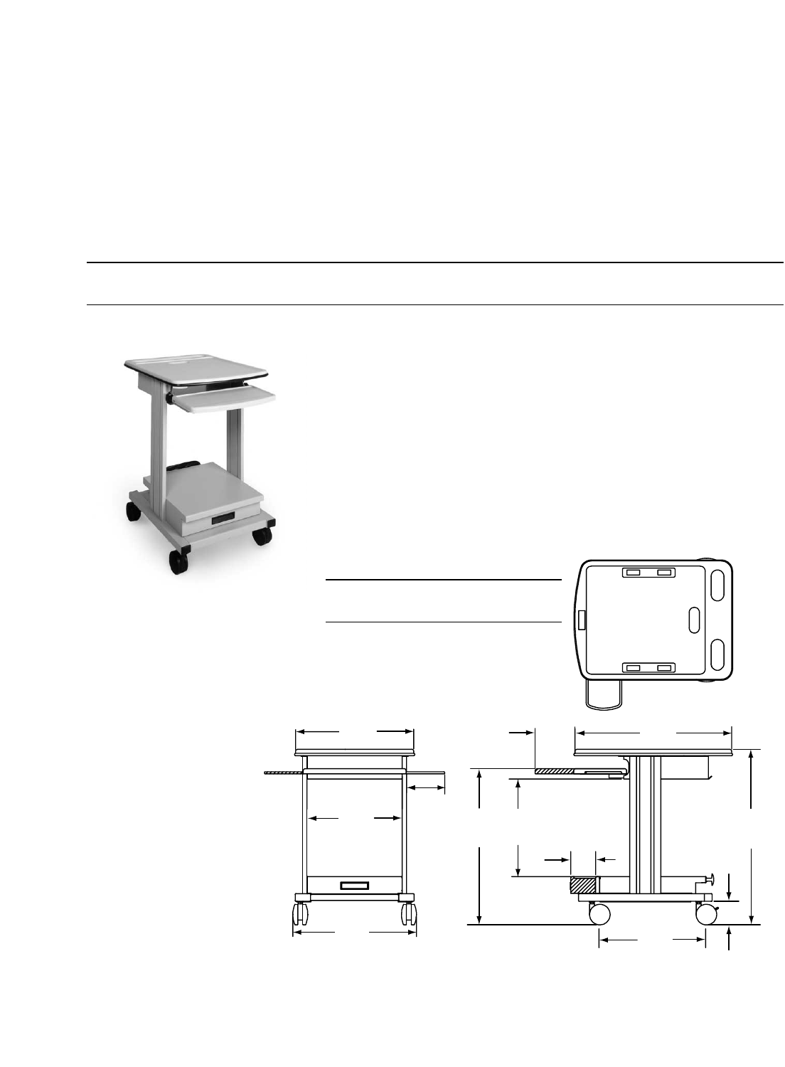
124
Ordering Information
Agilent 1184A Testmobile
The Agilent 1184A testmobile gives
you a convenient means of organizing
and transporting your logic analysis
system mainframes and accessories.
The testmobile includes the following:
• Drawer for accessories (probes,
cables, power cords)
Figure 7.1. Agilent 1184A testmobile cart.
Figure 7.2. Agilent 1184A testmobile cart dimensions.
Weight
Max Net Max Shipping
1184A 48.0 kg (106.0 lb) 59.0 kg (130.0 lbs)
Dimensions: mm (inches)
772.2
(30.4)
482.6
(19.0) 254
(10.0)
243.8
(9.6)
774.7
(30.5)
866.1
(34.1)
116.8
(4.6)
594.4
(23.4)
190.5
(7.5)
469.9
(18.5)
652.8
(25.7)
584.2
(23.0)
E5850A Logic Analyzer - Infiniium Oscilloscope Correlation Time Fixture
Product Number Description Includes
E5850A Logic analyzer - Infiniium oscilloscope time All BNC cables needed to connect to logic analyzer and
correlation fixture oscilloscope
• Keyboard tray with adjustable tilt
and height
• Mouse extension on keyboard
tray for either right or left hand
operation
• Locking casters for stability on
uneven surfaces
• Strap to stabilize the monitor
• Load limits: Top tray: 68.2 kg
(150.0 lb.) Lower tray: 68.2 kg
(150.0 lb.) Total: 136.4 kg
(300.0 lb.)

125
Ordering Information
Measurement Module Compatibility Table
Measurement Model Description 16700 16600A* 16500C* 16500A/B*
Module Category Number Series Series
State and Timing 16510A* 25 MHz State; 100 MHz Timing; 1 K memory depth √√
16510B* 35 MHz State; 100 MHz Timing; 1 K memory depth √√
16540A/16541A* 100 MHz State; 100 MHz Timing; 4 K memory depth √√
16540D/16541D* 100 MHz State; 100 MHz Timing; 16 K memory depth √√
16542A* 100 MHz State; 100 MHz Timing; 1 M memory depth √√
16550A* 100 MHz State; 500 MHz Timing; 4/8 K memory depth √√√√
16554A* 100 MHz State; 250 MHz Timing; 512 K/1 M memory depth √√√
16555A/16555D* 110 MHz State; 500 MHz Timing; 2/4 M memory depth √√√
16556A/16556D* 100 MHz State; 400 MHz Timing; 2/4 M memory depth √√√
16557D* 140 MHz State; 500 MHz Timing; 2/4 M memory depth √√√
16710A 100 MHz State; 500 MHz Timing; 8 K memory depth √√
16711A 100 MHz State; 500 MHz Timing; 32 K memory depth √√
16712A 100 MHz State; 500 MHz Timing; 128 K memory depth √√
16715A 167 MHz State; 667 MHz Timing; 2/4 M memory depth √
16716A 167 MHz State; 667 MHz Timing; 2 GHz Timing Zoom; √
512 K/1 M memory depth
16717A 333 MHz State; 667 MHz Timing; 2 GHz Timing Zoom; √
2/4 M memory depth
16718A* 333 MHz State; 667 MHz Timing; 2 GHz Timing Zoom; √
8/16 M memory depth
16719A* 333 MHz State; 667 MHz Timing; 2 GHz Timing Zoom; √
32/64 M memory depth
16740A 200 MHz State; 800 MHz Timing; 2 GHz Timing Zoom √
2/1 M memory depth
16741A 200 MHz State; 800 MHz Timing; 2 GHz Timing Zoom √
8/4 M memory depth
16742A 200 MHz State; 800 MHz Timing; 2 GHz Timing Zoom √
32/16 M memory depth
16750A/B 400 MHz State; 800 MHz Timing; 2 GHz Timing Zoom; √
4/8 M memory depth
16751A/B 400 MHz State; 800 MHz Timing; 2 GHz Timing Zoom; √
16/32 M memory depth
16752A/B 400 MHz State; 800 MHz Timing; 2 GHz Timing Zoom; √
32/64 M memory depth
16753A 600 MHz State; 1200 MHz Timing; 4 GHz Timing Zoom; √
1 M memory depth
* Discontinued products.

126
Ordering Information
Measurement Module Compatibility Table (continued)
Measurement Model Description 16700 16600 16500C* 16500A/B*
Module Category Number Series Series
State and Timing 16754A 600 MHz State; 1200 MHz Timing; 4 GHz Timing Zoom; √
(continued) 4 M memory depth
16755A 600 MHz State; 1200 MHz Timing; 4 GHz Timing Zoom; √
16 M memory depth
16756A 600 MHz State; 1200 MHz Timing; 4 GHz Timing Zoom; √
64 M memory depth
16760A 1.5 Gb/s State; 800 MHz Timing; 34 channel; √
64 M memory depth
Oscilloscope 16530A/16531A* 2 Channel; 100 MHz Bandwidth; 400 MSa/s; √√
4 K memory depth
16532A* 2 Channel; 250 MHz Bandwidth; 1 GSa/s; √√
8 K memory depth
16533A* 2 Channel; 250 MHz Bandwidth; 1 GSa/s; √√√
32 K memory depth
16534A 2 Channel; 500 MHz Bandwidth; 2 GSa/s; √√√
32 K memory depth
High Speed Timing 16515A/16516A* 1 GHz Timing; 8 K memory depth √√
16517A/16518A* 4 GHz Timing; 1GHz Synchronous State; √√√√
64 K memory depth
Pattern Generator 16520A/16521A* 50 MV/s; 4 K memory; 12 Channel √√
16522A* 200 MV/s; 258 K memory; 100 MHz in 40 Channel; √√√
200 MHz in 20 Channel
16720A 300 MV/s; 180 MHz in 48 Channel, 16 MV memory; √
300 MHz in 24 Channel, 8 MV memory
Emulation E5901A Emulation Module Products √√
E5901B Emulation Module Products √
* Discontinued products.

127
Ordering Information
Agilent Wedge Probe Adapters
IC Leg Spacing Number of Quantity of Probe Model
Signals Probes Shipped Number
0.5 mm 3 1 E2613A
0.5 mm 3 2 E2613B
0.5 mm 8 1 E2614A
0.5 mm 16 1 E2643A
0.65 mm 3 1 E2615A
0.65 mm 3 2 E2615B
0.65 mm 8 1 E2616A
0.65 mm 16 1 E26144A
Agilent Elastomeric Probing Solutions
Package Type IC Leg Spacing Probe Model Number
240-pin PQFP/CQFP 0.5 mm E5363A Probe. E5371A 1/4 flexible cable
208-pin PQFP/CQFP 0.5 mm E5374A Probe. E5371A 1/4 flexible cable
176-pin PQFP 0.5 mm E5348A Probe. E5349A 1/4 flexible cable
160-pin QFP 0.5 mm E5377A Probe. E5349A 1/4 flexible cable
160-pin PQFP/CQFP 0.65 mm E5373A Probe. E5349A 1/4 flexible cable
144-pin PQFP/CQFP 0.65 mm E5361A Probe. E5340A 1/4 flexible cable
144-pin TQFP 0.65 mm E5336A Probe. E5340A 1/4 flexible cable
Options for Agilent 16700 Series State/Timing Modules
Agilent Module Product Numbers Option Option Description
16710A 0B3 Add service manual
16711A 1BP MIL-STD-45662A calibration with test data
16712A W17 Convert standard warranty to one-year on-site warranty
16715A
16716A
16717A
16750A/B
16751A/B
16752A/B
16760A 010 add one E5378A, single-ended, 34-channel probe
16753A 011 add one E5379A, differential, 17-channel probe
16754A 012 add one E5380A, Mictor-compatible probe
16755A 013 add one E5382A, single-ended flying lead probe set
16756A 0B3 Add service manual
A6J MIL-STD-45662A calibration with test data
W17 Convert standard warranty to one-year on-site warranty

128
Ordering Information
Options and Accessories for Agilent 16534A Oscilloscope Modules
Agilent Option Option Description
•001 •Add one Agilent 1145A, dual, active 750 MHz probe
•ABJ •Japanese user's reference
•0B0 •Delete manuals
•1BP •MIL-STD 45662A calibration with test data
•0B3 •Add service manual
•0BF •Add programming manual set for a 16500 (not required for a 16700)
•W17 •Convert standard warranty to one-year-on-site warranty
•W03 •Convert standard warranty to 90-day-on-site warranty
Agilent Model Number Accessory Description
1144A 800 MHz active probe (power for two Agilent 1144A active probes is provided by the
Agilent 16533A and 16534A) (requires 01144-61604 power splitter to operate two 1144As)
01144-61604 Power splitter. Allows operation of two Agilent 1144A active probes from one Agilent 16533A or 16534A
1145A 750-MHz dual, active probe (power for Agilent 1145A active probes is provided by the Agilent 16533A and 16534A)
1141A 200 MHz differential probe (requires an Agilent 1142A power supply)
1142A Probe power supply
10442A 10:1, 500-ohm 1.2pF oscilloscope probe
10443A 20:1, 1000-ohm, 1.2pF oscilloscope probe
Options for Agilent 16720A Pattern Generator Modules
Agilent Option Option Description
•011 •TTL clock pod and 6” lead set (10460A and 10498A)
•013 •3-state TTL/CMOS data pod and 6” lead set (10462A and 10498A)
•014 •TTL data pod and 6” lead set (10461A and 10498A)
•015 •2.5 V clock pod and 6” lead set (10472A and 10498A)
•016 •2.5 V 3-state data pod and 6” lead set (10473A and 10498A)
•017 •3.3 V clock pod and 6” lead set (10477A and 10498A)
•018 •3-state TTL/3.3 V data pod and 6” lead set (10483A and 10498A)
•021 •ECL clock pod and 6” lead set (10463A and 10498A)
•022 •ECL terminated pod and 6” lead set (10464A and 10498A)
•023 •ECL unterminated pod and 50 Ωshield coaxial lead set (10465A and 10347A)
•031 •5 V PECL clock pod and 6” lead set (10468A and 10498A)
•032 •5 V PECL data pod and 6” lead set (10469A and 10498A)
•033 •3.3 V LVPECL clock pod and 6” lead set (10470A and 10498A)
•034 •3.3 V LVPECL data pod and 6” lead set (10471A and 10498A)
•041 •1.8 V clock pod and 6” lead set (10475 and 10498A)
•042 •1.8 V 3-state data pod and 6” lead set (10476 and 10498A)
•051 •LVDS clock pod and 6” LVDS lead set (E8140A and E8142A)
•052 •LVDS data pod and 6” LVDS lead set (E8141A and E8142A)
•0B3 •Add service manual
•W17 •Convert to one-year on-site warranty
•W30 •3 years return for repair service
•W50 •5 years return for repair service

129
Ordering Information
Accessories for Agilent 16720A Pattern Generator Modules
Product Numbers and Option(s) for Agilent 16700 Series
Post-Processing Tool Sets
Product or Option Number Description
B4600B •System Performance Analysis (SPA) Tool Set
B4601B •Serial Analysis Tool Set
B4605B •Tool Development Kit
B4620B •Source Correlation Tool Set
B4640B •Data Communications Tool Set
Available for all Tool Sets
#0D4 Do not install tool set (instructs factory to ship tool set
separately from any 16700 Series system on the order)
Accessories Description
Model Number
10460A TTL clock pod
10461A TTL data pod
10462A 3-state TTL/CMOS data pod
10463A 10463A ECL clock pod
10464A ECL data pod (terminated)
10465A ECL data pod (unterminated)
10466A 3-state TTL/3.3V data pod
10468A 5 volt PECL clock pod
10469A 5 volt PECL data pod
10470A 3.3 volt LVPECL clock pod
10471A 3.3 volt LVPECL data pod
10472A 2.5 volt clock pod
10473A 3-state 2.5 volt data pod
10474A 8-channel probe lead set, 12" long
10475A 1.8 volt clock pod
Accessories Description
Model Number
10476A 3-state 1.8 volt data pod
10477A 3.3 volt clock pod
10483A 3-state TTL/3.3 volt data pod
10498A 8-channel probe lead set, 6" long
10347A 8-channel 50-ohm shielded coaxial probe lead set
5090-4356 Grabbers, surface mount, package of 20
5959-0288 Grabbers, through hole, package of 20
10211A IC probe clip, 24-pin dual in-line package
10024A IC probe clip, 16 pin dual in-line package
E2421A SOIC clip adapter test kit (Pomona 5514)
E2422A Quad clip adapter test kit (Pomona 5515)
E8140A LVDS clock pod
E8141A LVDS data pod
E8142A LVDS lead set

130
Third-Party Solutions
Our solutions partners offer a wide
array of accessory products for the
Agilent Technologies logic analysis
systems. Agilent's solution partners
offer complementary products cover-
ing probing clips, specialized analysis
probes for over 200 microprocessors,
and software tools for ASIC emula-
tion and test system design.
See the Processor and Bus Support
For Agilent Technologies Logic
Analyzers (p/n 5966-4365) document
for contact information concerning
these vendors.
Solutions Partner Application Focus Contact Information
Advanced Logic Design (ALD) Product design services (digital) www.ald.com
Aptix ASIC emulation www.aptix.com
JM Engineering (JME) Probing (solutions for www.jmecorp.com
SMT parts)
American Arium Intel emulators and probes www.arium.com
Advanced RISC Machines Microprocessor core IP www.arm.com
(ARM)
CAD-UL Software programming tools www.cadul.com
Corelis Analysis probes for various www.corelis.com
microprocessors and buses
Diagonal Manufacturing test suite www.diagonal.com
software
Emulation Technologies (ET) Probing www.emulation.com
Europe Technologies Embedded system design www.europe-technologies.com
tools and services
FuturePlus Systems Analysis probes for computer www.futureplus.com
buses
Green Hills Software, Inc Debugger and compiler www.ghs.com
(GHS) software for Motorola
microprocessors
Ironwood High-density VLSI www.ironwoodelectronics.com
interconnect solutions
Lital Electronics, Inc. Mil-spec computer boards www.lital.com
Microtec (Mentor Graphics Debuggers and compilers www.mentor.com/embedded
Embedded Software Division)
Pomona Electronics Supplier of accessories for www.pomonaelectronics.com
electronic test instruments
DIAB-SDS Debuggers, compilers www.diabsds.com
SynaptiCAD Waveform simulation www.syncad.com
analysis software
WindRiver Embedded RTOS www.windriver.com
development tools

131
Support, Warranty and Related Literature
Warranty
Agilent hardware products are war-
ranted against defects in materials
and workmanship for a period of one
year from date of shipment. Some
newly manufactured Agilent products
may contain remanufactured parts,
which are equivalent to new in per-
formance. If you send us a notice of
such defects during the warranty
period, we will either repair or
replace hardware products that prove
to be defective.
Related Literature
Publication Title Publication Type Publication Number
Processor and Bus Support For Configuration Guide 5966-4365E
Agilent Technologies Logic Analyzers
Probing Solutions for Product Overview 5968-4632E
Agilent Technologies Logic Analysis Systems
www.agilent.com/find/la-systems
Agilent software and firmware prod-
ucts that are designated by Agilent
for use with a hardware product are
warranted for a period of one year
from date of shipment to execute
their programming instructions when
properly installed. If you send us
notice of defects in materials or
workmanship during the warranty
period, we will repair or replace
these products, so long as the defect
does not result from buyer supplied
hardware or interfacing. The
warranty period is controlled by the
warranty statement included with
the product and begins on the date
of shipment.
Support and Services
Agilent's support services comple-
ment your logic analysis system
to provide a complete solution to
your digital design and debug
problems. By taking advantage
of Agilent's expertise you can
concentrate on your particular
design projects and applications,
rather than your debug tools,
resulting in increased productivity.

Agilent Technologies’ Test and Measurement Support, Services, and Assistance
Agilent Technologies aims to maximize the value you receive, while minimizing your risk and
problems. We strive to ensure that you get the test and measurement capabilities you paid
for and obtain the support you need. Our extensive support resources and services can help
you choose the right Agilent products for your applications and apply them successfully.
Every instrument and system we sell has a global warranty. Support is available for at least
five years beyond the production life of the product. Two concepts underlie Agilent's overall
support policy: "Our Promise" and "Your Advantage."
Our Promise
Our Promise means your Agilent test and measurement equipment will meet its advertised
performance and functionality. When you are choosing new equipment, we will help you
with product information, including realistic performance specifications and practical
recommendations from experienced test engineers. When you use Agilent equipment, we
can verify that it works properly, help with product operation, and provide basic measurement
assistance for the use of specified capabilities, at no extra cost upon request. Many self-help
tools are available.
Your Advantage
Your Advantage means that Agilent offers a wide range of additional expert test and
measurement services, which you can purchase according to your unique technical and
business needs. Solve problems efficiently and gain a competitive edge by contracting with
us for calibration, extra-cost upgrades, out-of-warranty repairs, and on-site education and
training, as well as design, system integration, project management, and other professional
engineering services. Experienced Agilent engineers and technicians worldwide can help
you maximize your productivity, optimize the return on investment of your Agilent
instruments and systems, and obtain dependable measurement accuracy for the life of
those products.
By internet, phone, or fax, get assistance with
all your test & measurement needs
Online assistance:
www.agilent.com/find/assist
Phone or Fax
United States:
(tel) 800 452 4844
Canada:
(tel) 877 894 4414
(fax) 905 282 6495
China:
(tel) 800 810 0189
(fax) 800 820 2816
Europe:
(tel) (31 20) 547 2323
(fax) (31 20) 547 2390
Japan:
(tel) (81) 426 56 7832
(fax) (81) 426 56 7840
Korea:
(tel) (82 2) 2004 5004
(fax) (82 2) 2004 5115
Latin America:
(tel) (305) 269 7500
(fax) (305) 269 7599
Taiwan:
(tel) 0800 047 866
(fax) 0800 286 331
Other Asia Pacific Countries:
(tel) (65) 6375 8100
(fax) (65) 6836 0252
Email: tm_asia@agilent.com
Product specifications and descriptions in this
document subject to change without notice.
© Agilent Technologies, Inc. 2003
Printed in USA July 11, 2003
5968-9661E
www.agilent.com
www.agilent.com/find/emailupdates
Get the latest information on the products and applications you select.
Agilent T&M Software and Connectivity
Agilent's Test and Measurement software and connectivity products, solutions and
developer network allows you to take time out of connecting your instruments to your
computer with tools based on PC standards, so you can focus on your tasks, not on your
connections. Visit www.agilent.com/find/connectivity for more information.
