AASTex Instructions

User Manual:

Open the PDF directly: View PDF .
Page Count: 16

Draft version February 28, 2019

Typeset using L

Xtwocolumn style in AASTeX62

An Example Article using AAST

Xv6.2∗

Greg J. Schwarz1and August Muench1

(AAS Journals Data Scientists collaboration)

Butler Burton2, 3

—

Amy Hendrickson4, †

(LaTeX collaboration)

Julie Steffen5, 1 and Jeff Lewandowski6, 7

1American Astronomical Society

2000 Florida Ave., NW, Suite 300

Washington, DC 20009-1231, USA

2National Radio Astronomy Observatory

3AAS Journals Associate Editor-in-Chief

4TeXnology Inc.

5AAS Director of Publishing

6IOP Senior Publisher for the AAS Journals

7IOP Publishing, Washington, DC 20005

(Revised February 28, 2019)

ABSTRACT

This example manuscript is intended to serve as a tutorial and template for authors to use when

writing their own AAS Journal articles. The manuscript includes a history of AAST

X and documents

the new features in the previous versions as well as the new features in version 6.2. This manuscript

includes many ﬁgure and table examples to illustrate these new features. Information on features

not explicitly mentioned in the article can be viewed in the manuscript comments or more extensive

online documentation. Authors are welcome replace the text, tables, ﬁgures, and bibliography with

their own and submit the resulting manuscript to the AAS Journals peer review system. The ﬁrst

lesson in the tutorial is to remind authors that the AAS Journals, the Astrophysical Journal (ApJ),

the Astrophysical Journal Letters (ApJL), and Astronomical Journal (AJ), all have a 250 word limit

for the abstract. If you exceed this length the Editorial oﬃce will ask you to shorten it.

Keywords: editorials, notices — miscellaneous — catalogs — surveys

1. INTRODUCTION

LaT

X1is a document markup language that is par-

ticularly well suited for the publication of mathemati-

cal and scientiﬁc articles (Lamport 1994). LaT

X was

written in 1985 by Leslie Lamport who based it on the

X typesetting language which itself was created by

Donald E. Knuth in 1978. In 1988 a suite of LaT

Corresponding author: August Muench

greg.schwarz@aas.org, gus.muench@aas.org

∗Released on January, 8th, 2018

†Creator of AASTeX v6.2

1http://www.latex-project.org/

macros were developed to investigate electronic submis-

sion and publication of AAS Journal articles (Hanisch &

Biemesderfer 1989). Shortly afterwards, Chris Biemes-

defer merged these macros and more into a LaT

X 2.08

style ﬁle called AAST

X. These early AAST

X versions

introduced many common commands and practices that

authors take for granted today. Substantial revisions

were made by Lee Brotzman and Pierre Landau when

the package was updated to v4.0. AASTeX v5.0, written

in 1995 by Arthur Ogawa, upgraded to LaT

X 2e which

uses the document class in lieu of a style ﬁle. Other

improvements to version 5 included hypertext support,

landscape deluxetables and improved ﬁgure support to

facilitate electronic submission. AAST

X v5.2 was re-

2Schwarz et al.

leased in 2005 and introduced additional graphics sup-

port plus new mark up to identiﬁer astronomical objects,

datasets and facilities.

In 1996 Maxim Markevitch modiﬁed the AAS preprint

style ﬁle, aaspp4.sty, to closely emulate the very tight,

two column style of a typeset Astrophysical Journal arti-

cle. The result was emulateapj.sty. A year later Alexey

Vikhlinin took over development and maintenance. In

2001 he converted emulateapj into a class ﬁle in LaT

2e and in 2003 Vikhlinin completely rewrote emulateapj

based on the APS Journal’s RevTEX class.

During this time emulateapj gained growing ac-

ceptance in the astronomical community as it ﬁlled

an author need to obtain an approximate number of

manuscript pages prior to submission for cost and length

estimates. The tighter typeset also had the added ad-

vantage of saving paper when printing out hard copies.

Even though author publication charges are no longer

based on print pages 2the emulateapj class ﬁle has

proven to be extremely popular with AAS Journal

authors. An informal analysis of submitted LaT

manuscripts in 2015 revealed that ∼65% either called

emulateapj or have a commented emulateapj class-

ﬁle call indicating it was used at some stage of the

manuscript construction. Clearly authors want to have

access to a tightly typeset version of the article when

corresponding with co-authors and for preprint submis-

sions.

When planning the next AAST

X release the popular-

ity of emulateapj played an important roll in the decision

to drop the old base code and adopt and modify emu-

lateapj for AAST

X v6.+ instead. The change brings

AAST

X inline with what the majority of authors are

already using while still delivering new and improved

features. AAST

X v6.0 through v6.2 were written by

Amy Hendrickson and released in January 2016 (v6.0),

October 2016 (v6.1), and January 2018 (v6.2), respec-

tively. Some of the new features in v6.0 included:

1. improved citations for third party data reposito-

ries and software,

2. easier construction of matrix ﬁgures consisting

of multiple encapsulated postscript (EPS) or

portable document format (PDF) ﬁles,

3. ﬁgure set mark up for large collections of similar

ﬁgures,

4. color mark up to easily enable/disable revised text

highlighting,

2see Section Bin the Appendix for more details about how

current article costs are calculated.

5. improved url support, and

6. numerous table options such as the ability to hide

columns, column decimal alignment, automatic

column math mode and numbering, plus splitting

of wide tables.

The features in v6.1 were:

1. ORCID support for preprints,

2. improved author, aﬃliation and collaboration

mark up,

3. reintroduced the old AASTeX v5.2 \received,

\revised,\accepted, and \published com-

mands plus added the new \submitjournal

command to document which AAS Journal the

manuscript was submitted to, plus

4. new typeset style options.

The new features in v6.2 are:

1. A new RNAAS style option for Research Note

manuscripts,

2. Titles no longer put in all caps,

3. No page skip between the title page and article

body,

4. re-introduce RevTeX’s widetext environment for

long lines in two column style formats, and

5. upgrade to the \doi command.

The rest of this article provides information and exam-

ples on how to create your own AAS Journal manuscript

with v6.2. Special emphasis is placed on how to use the

full potential of AAST

X v6+. The next section de-

scribes the diﬀerent manuscript styles available and how

they diﬀer from past releases. Section 3describes how

tables and ﬁgures are placed in a LaT

X document. Spe-

ciﬁc examples of tables, Section 3.1, and ﬁgures, Section

3.2, are also provided. Section 4discusses how to dis-

play math and incorporate equations in a manuscript

while Section 5discuss how to use the new revision

mark up. The last section, 6, shows how recognize soft-

ware and external data as ﬁrst class references in the

manuscript bibliography. An appendix is included to

show how to construct one and provide some informa-

tion on how article charges are calculated. Additional

information is available both embedded in the comments

of this LaT

X ﬁle and in the online documentation at

http://journals.aas.org/authors/aastex.html.

Sample article 3

2. MANUSCRIPT STYLES

The default style in AAST

X v6.2 is a tight single col-

umn style, e.g. 10 point font, single spaced. The single

column style is very useful for article with wide equa-

tions. It is also the easiest to style to work with since

ﬁgures and tables, see Section 3, will span the entire

page, reducing the need for address ﬂoat sizing.

To invoke a two column style similar to the what is

produced in the published PDF copy use

\documentclass[twocolumn]{aastex62}.

Note that in the two column style ﬁgures and tables will

only span one column unless speciﬁcally ordered across

both with the “*” ﬂag, e.g.

\begin{figure*}... \end{figure*},

\begin{table*}... \end{table*}, and

\begin{deluxetable*}... \end{deluxetable*}.

This option is ignored in the onecolumn style.

Some other style options are outlined in the com-

mented sections of this article. Any combination of style

options can be used.

Two style options that are needed to fully use the new

revision tracking feature, see Section 5, are linenumbers

which uses the lineno style ﬁle to number each article line

in the left margin and trackchanges which controls the

revision and commenting highlight output.

There is also a new modern option that uses a Daniel

Foreman-Mackey and David Hogg design to produce

stylish, single column output that has wider left and

right margins. It is designed to have fewer words per

line to improve reader retention. It also looks better on

devices with smaller displays such as smart phones.

For a Research Note use the RNAAS option which

will produce a manuscript with no abstract and in the

modern style.

3. FLOATS

Floats are non-text items that generally can not be

split over a page. They also have captions and can be

numbered for reference. Primarily these are ﬁgures and

tables but authors can deﬁne their own. LaT

X tries

to place a ﬂoat where indicated in the manuscript but

will move it later if there is not enough room at that

location, hence the term “ﬂoat”.

Authors are encouraged to embed their tables and ﬁg-

ures within the text as they are mentioned. Please do

not place the ﬁgures and text at the end of the article

as was the old practice. Editors and the vast majority

of referees ﬁnd it much easier to read a manuscript with

embedded ﬁgures and tables.

Depending on the number of ﬂoats and the particular

amount of text and equations present in a manuscript

the ultimate location of any speciﬁc ﬂoat can be hard

to predict prior to compilation. It is recommended that

authors textbfnot spend signiﬁcant time trying to get

ﬂoat placement perfect for peer review. The AAS Jour-

nal’s publisher has sophisticated typesetting software

that will produce the optimal layout during production.

Note that authors of Research Notes are only allowed

one ﬂoat, either one table or one ﬁgure.

Table 1. ApJ costs from 1991 to 2013a

Year Subscription Publication

cost chargesb

($) ($/page)

(1) (2) (3)

1991 600 100

1992 650 105

1993 550 103

1994 450 110

1995 410 112

1996 400 114

1997 525 115

1998 590 116

1999 575 115

2000 450 103

2001 490 90

2002 500 88

2003 450 90

2004 460 88

2005 440 79

2006 350 77

2007 325 70

2008 320 65

2009 190 68

2010 280 70

2011 275 68

2012 150 56

2013 140 55

Table 1 continued

4Schwarz et al.

Table 1 (continued)

Year Subscription Publication

cost chargesb

($) ($/page)

(1) (2) (3)

aAdjusted for inﬂation

bAccounts for the change from page

charges to digital quanta in April, 2011

Note—Note that \colnumbers does not

work with the vertical line alignment to-

ken. If you want vertical lines in the

headers you can not use this command

at this time.

For authors that do want to take the time to opti-

mize the locations of their ﬂoats there are some tech-

niques that can be used. The simplest solution is to

placing a ﬂoat earlier in the text to get the position right

but this option will break down if the manuscript is al-

tered, see Table 1. A better method is to force LaT

to place a ﬂoat in a general area with the use of the

optional [placement specifier] parameter for ﬁgures

and tables. This parameter goes after \begin{figure},

\begin{table}, and \begin{deluxetable}. The main

arguments the speciﬁer takes are “h”, “t”, “b”, and “!”.

These tell LaT

X to place the ﬂoat here (or as close as

possible to this location as possible), at the top of the

page, and at the bottom of the page. The last argu-

ment, “!”, tells LaT

X to override its internal method

of calculating the ﬂoat position. A sequence of rules can

be created by using multiple arguments. For example,

\begin{figure}[htb!] tells LaT

X to try the current

location ﬁrst, then the top of the page and ﬁnally the

bottom of the page without regard to what it thinks the

proper position should be. Many of the tables and ﬁg-

ures in this article use a placement speciﬁer to set their

positions.

Note that the LaT

Xtabular environment is not

a ﬂoat. Only when a tabular is surrounded by

\begin{table}... \end{table}is it a true ﬂoat and

the rules and suggestions above apply.

In AASTeX v6.2 all deluxetables are ﬂoat tables

and thus if they are longer than a page will spill oﬀ

the bottom. Long deluxetables should begin with the

\startlongtable command. This initiates a longtable

environment. Authors might have to use \clearpage

to isolate a long table or optimally place it within the

surrounding text.

3.1. Tables

Tables can be constructed with LaT

X’s standard ta-

ble environment or the AAST

X’s deluxetable environ-

ment. The deluxetable construct handles long tables

better but has a larger overhead due to the greater

amount of deﬁned mark up used set up and manipu-

late the table structure. The choice of which to use is

up to the author. Examples of both environments are

used in this manuscript. Table 1is a simple deluxetable

example that gives the approximate changes in the sub-

scription costs and author publication charges from 1991

to 2013.

Tables longer than 200 data lines and complex ta-

bles should only have a short example table with the

full data set available in the machine readable format.

The machine readable table will be available in the

HTML version of the article with just a short exam-

ple in the PDF. Authors are required to indicate to

the reader where the data can be obtained in the ta-

ble comments. Suggested text is given in the comments

of Table 2. Authors are encouraged to create their

own machine readable tables using the online tool at

http://authortools.aas.org/MRT/upload.html.

AAST

X v6 introduces ﬁve new table features that

are designed to make table construction easier and the

resulting display better for AAS Journal authors. The

items are:

1. Declaring math mode in speciﬁc columns,

2. Column decimal alignment,

3. Automatic column header numbering,

4. Hiding columns, and

5. Splitting wide tables into two or three parts.

Each of these new features are illustrated in following

Table examples. All ﬁve features work with the regular

LaT

X tabular environment and in AAST

X’s delux-

etable environment. The examples in this manuscript

also show where the two process diﬀer.

3.1.1. Column math mode

Both the LaT

X tabular and AAST

X deluxetable re-

quire an argument to deﬁne the alignment and number

of columns. The most common values are “c”, “l” and

“r” for center, left, and right justiﬁcation. If these values

are capitalized, e.g. “C”, “L”, or “R”, then that speciﬁc

column will automatically be in math mode meaning

that $s are not required. Note that having embedded

dollar signs in the table does not aﬀect the output. The

third and forth columns of Table 2shows how this math

mode works.

Sample article 5

Table 2. Column math mode in an observation log

UT start timeaMJD start timeaSeeing Filter Inst.

(YYYY-mm-dd) (d) (arcsec)

2012-03-26 56012.997 ∼0.005 HαNOT

2012-03-27 56013.944 1.005 grism SMARTS

2012-03-28 56014.984 · · · F814M HST

2012-03-30 56016.978 1.005±0.25 B&C Bok

aAt exposure start.

Note—The “C” command column identiﬁer in the 3 column turns on math mode for that speciﬁc column. One could do the

same for the next column so that dollar signs would not be needed for Hαbut then all the other text would also be in math

mode and thus typeset in Latin Modern math and you will need to put it back to Roman by hand. Note that if you do change

this column to math mode the dollar signs already present will not cause a problem. Table 2is published in its entirety in the

machine readable format. A portion is shown here for guidance regarding its form and content.

6Schwarz et al.

3.1.2. Decimal alignment

Aligning a column by the decimal point can be diﬃcult

with only center, left, and right justiﬁcation options. It

is possible to use phantom calls in the data, e.g. \phn,

to align columns by hand but this can be tedious in long

or complex tables. To address this AAST

X introduces

the \decimals command and a new column justiﬁca-

tion option, “D”, to align data in that column on the

decimal. In deluxetable the \decimals command is in-

voked before the \startdata call but can be anywhere

in LaT

X’s tabular environment.

Two other important thing to note when using decimal

alignment is that each decimal column must end with a

space before the ampersand, e.g. “&&” is not allowed.

Empty decimal columns are indicated with a decimal,

e.g. “.”. Do not use deluxetable’s \nodata command.

The “D” alignment token works by splitting the col-

umn into two parts on the decimal. While this is invis-

ible to the user one must be aware of how it works so

that the headers are accounted for correctly. All deci-

mal column headers need to span two columns to get the

alignment correct. This can be done with a multicolumn

call, e.g \multicolumn2c{} or \multicolumn{2}{c}{},

or use the new \twocolhead{} command in deluxetable.

Since LaT

X is splitting these columns into two it is im-

portant to get the table width right so that they ap-

pear joined on the page. You may have to run the

LaT

X compiler twice to get it right. Table 3illustrates

how decimal alignment works in the tabular environ-

ment with a ±symbol embedded between the last two

columns.

Table 3. Decimal alignment made easy

Column Value Uncertainty

A 1234 ±100.0

B 123.4 ±10.1

C 12.34 ±1.01

D 1.234 ±0.101

E .1234±0.01001

F 1.0 ±

NOTE. - Two decimal aligned columns

3.1.3. Automatic column header numbering

The command \colnumbers can be included to au-

tomatically number each column as the last row in

the header. Per the AAS Journal table format stan-

dards, each column index numbers will be surrounded

by parentheses. In a LaT

X tabular environment the

\colnumbers should be invoked at the location where

the author wants the numbers to appear, e.g. after

the last line of speciﬁed table header rows. In delux-

etable this command has to come before \startdata.

\colnumbers will not increment for columns hidden by

the “h” command, see Section 3.1.4. Table 1uses this

command to automatically generate column index num-

bers.

Note that when using decimal alignment in a table the

command \decimalcolnumbers must be used instead

of \colnumbers and \decimals. Table 4illustrates this

speciﬁc functionality.

3.1.4. Hiding columns

Entire columns can be hidden from display simply by

changing the speciﬁed column identiﬁer to “h”. In the

LaT

X tabular environment this column identiﬁer con-

ceals the entire column including the header columns.

In AAST

X’s deluxetables the header row is speciﬁcally

declared with the \tablehead call and each header col-

umn is marked with \colhead call. In order to make a

speciﬁc header disappear with the “h” column identiﬁer

in deluxetable use \nocolhead instead to suppress that

particular column header.

Authors can use this option in many diﬀerent ways.

Since column data can be easily suppressed authors can

include extra information and hid it based on the com-

ments of co-authors or referees. For wide tables that will

have a machine readable version, authors could put all

the information in the LaT

X table but use this option

to hid as many columns as needed until it ﬁts on a page.

This concealed column table would serve as the example

table for the full machine readable version. Regardless

of how columns are obscured, authors are responsible

for removing any unneeded column data or alerting the

editorial oﬃce about how to treat these columns during

production for the ﬁnal typeset article.

Table 4provides some basic information about the

ﬁrst ten Messier Objects and illustrates how many of

these new features can be used together. It has auto-

matic column numbering, decimal alignment of the dis-

tances, and one concealed column. The Common name

column is the third in the LaT

X deluxetable but does

not appear when the article is compiled. This hidden

column can be shown simply by changing the “h” in the

column identiﬁer preamble to another valid value. This

table also uses \tablenum to renumber the table because

a LaT

X tabular table was inserted before it.

3.1.5. Splitting a table into multiple horizontal components

Since the AAS Journals are now all electronic with no

print version there is no reason why tables can not be

as wide as authors need them to be. However, there are

some artiﬁcial limitations based on the width of a print

page. The old way around this limitation was to rotate

Sample article 7

Table 4. Fun facts about the ﬁrst 10 messier objects

Messier NGC/IC Object Distance V

Number Number Type (kpc) Constellation (mag)

(1) (2) (3) (4) (5) (6)

M1 NGC 1952 Supernova remnant 2 Taurus 8.4

M2 NGC 7089 Cluster, globular 11.5 Aquarius 6.3

M3 NGC 5272 Cluster, globular 10.4 Canes Venatici 6.2

M4 NGC 6121 Cluster, globular 2.2 Scorpius 5.9

M5 NGC 5904 Cluster, globular 24.5 Serpens 5.9

M6 NGC 6405 Cluster, open 0.31 Scorpius 4.2

M7 NGC 6475 Cluster, open 0.3 Scorpius 3.3

M8 NGC 6523 Nebula with cluster 1.25 Sagittarius 6.0

M9 NGC 6333 Cluster, globular 7.91 Ophiuchus 8.4

M10 NGC 6254 Cluster, globular 4.42 Ophiuchus 6.4

Note—This table “hides” the third column in the LaT

X when compiled. The

Distance is also centered on the decimals. Note that when using decimal alignment

you need to include the \decimals command before \startdata and all of the

values in that column have to have a space before the next ampersand.

into landscape mode and use the smallest available table

font sizes, e.g. \tablewidth, to get the table to ﬁt.

Unfortunately, this was not alway enough but now along

with the hide column option outlined in Section 3.1.4

there is a new way to break a table into two or three

components so that it ﬂows down a page by invoking a

new table type, splittabular or splitdeluxetable. Within

these tables a new “B” column separator is introduced.

Much like the vertical bar option, “|”, that produces a

vertical table lines, e.g. Table 1, the new “B” separator

indicates where to Break a table. Up to two “B”s may

be included.

Table 5 shows how to split a wide deluxetable into

three parts with the \splitdeluxetable command.

The \colnumbers option is on to show how the auto-

matic column numbering carries through the second ta-

ble component, see Section 3.1.3.

The last example, Table 6, shows how to split the

same table but with a regular LaT

X tabular call and

into two parts. Decimal alignment is included in the

third column and the “Component” column is hidden

to illustrate the new features working together.

3.2. Figures

Authors can include a wide number of diﬀerent graph-

ics with their articles in encapsulated postscript (EPS)

or portable document format (PDF). These range from

general ﬁgures all authors are familiar with to new en-

hanced graphics that can only be fully experienced in

HTML. The later include animations, ﬁgure sets and

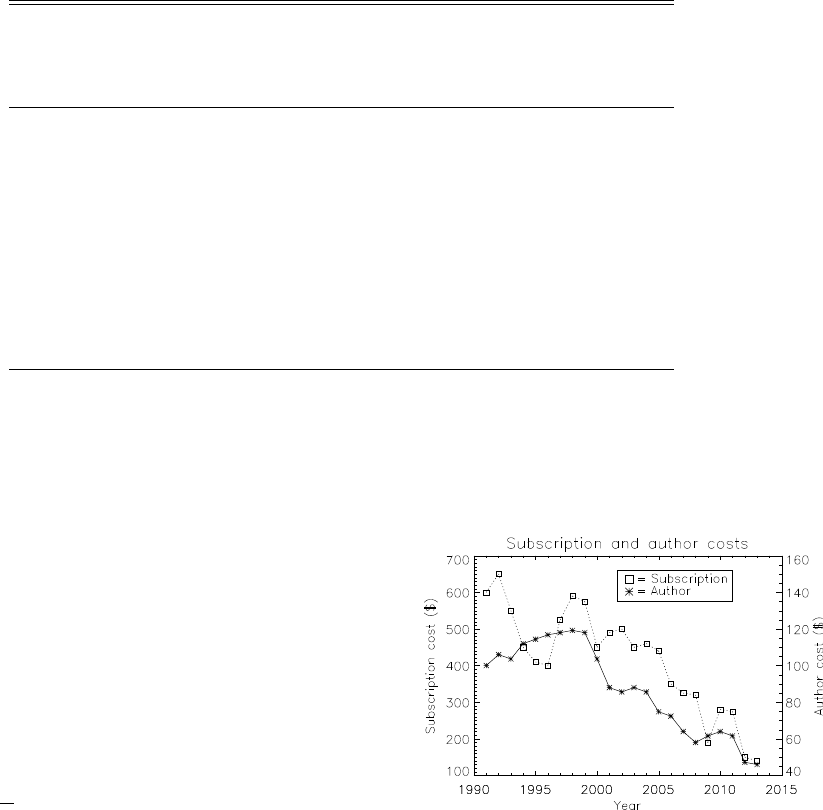
Figure 1. The subscription and author publication costs

from 1991 to 2013. The data comes from Table 1.

interactive ﬁgures. This portion of the article provides

examples for setting up all these graphics in with the

latest version of AAST

3.3. General ﬁgures

AAST

X has a \plotone command to display a ﬁgure

consisting of one EPS/PDF ﬁle. Figure 1is an example

which uses the data from Table 1. For a general ﬁgure

consisting of two EPS/PDF ﬁles the \plottwo command

can be used to position the two image ﬁles side by side.

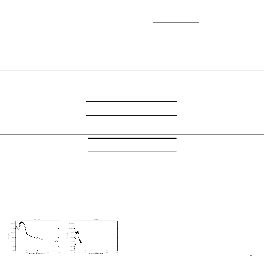
Figure 2shows the Swift/XRT X-ray light curves of two

recurrent novae. The data from Figures 2through 4are

taken from Table 2 of Schwarz et al. (2011).

Both \plotone and \plottwo take a \caption and

an optional \figurenum command to specify the ﬁg-

8Schwarz et al.

Table 5. Measurements of Emission Lines: two breaks

Model Component Shift FWHM Flux

(km s−1) (km s−1) (10−17 erg s−1cm−2)

Lyα

(1) (2) (3) (4) (5)

BELs -97.13 9117±38 1033±33

Model 1 IELs -4049.123 1974±22 2495±30

NELs ··· 641±4 449±23

BELs -85 8991±41 988±29

Model 2 IELs -51000 2025±26 2494±32

NELs 52 637±10 477±17

NVSi IV CIV Mg II Hγ

(6) (7) (8) (9) (10)

<35 <166 637±31 1951±26 991±30

<42 <109 995±186 83±30 75±23

<6<9 – 275±18 150±11

<24 <173 623±28 1945±29 989±27

<37 <124 1005±190 72±28 72±21

<4<8 – 278±17 153±10

HβHαHe IPaγ

(11) (12) (13) (14)

3502±42 20285±80 2025±116 1289±107

130±25 357±94 194±64 36±23

313±12 958±43 318±34 151±17

3498±37 20288±73 2047±143 1376±167

113±18 271±85 205±72 34±21

317±15 969±40 325±37 147±22

Note—This is an example of how to split a deluxetable. You can split any table with this command into two or three parts. The location of the

split is given by the author based on the placement of the “B” indicators in the column identiﬁer preamble. For more information please look at

the new AAST

X instructions.

Figure 2. Swift/XRT X-ray light curves of RS Oph and U

Sco which represent the two canonical recurrent types, a long

period system with a red giant secondary and a short period

system with a dwarf/sub-dwarf secondary, respectively.

ure number3. Each is based on the graphicx package

3It is better to not use \figurenum and let LaTeX auto-

increment all the ﬁgures. If you do use this command you need to

mark all of them accordingly.

command, \includegraphics. Authors are welcome

to use \includegraphics along with its optional argu-

ments that control the height, width, scale, and position

angle of a ﬁle within the ﬁgure. More information on

the full usage of \includegraphics can be found at

https://en.wikibooks.org/wiki/LaTeX/Importing Graphics#

Including graphics.

3.4. Grid ﬁgures

Including more than two EPS/PDF ﬁles in a single ﬁg-

ure call can be tricky easily format. To make the process

easier for authors AAST

X v6 oﬀers \gridline which

allows any number of individual EPS/PDF ﬁle calls

within a single ﬁgure. Each ﬁle cited in a \gridline

will be displayed in a row. By adding more \gridline

calls an author can easily construct a matrix X by Y

individual ﬁles as a single general ﬁgure.

Sample article 9

Table 6. Measurements of Emission Lines: one break

Model Shift FWHM Flux

(km s−1) (km s−1) (10−17 erg s−1cm−2)

LyαNVSi IV

(1) (2) (3) (4) (5) (6)

−97.13 9117±38 1033±33 <35 <166

Model 1 −4049.123 1974±22 2495±30 <42 <109

641±4 449±23 <6<9

−85 8991±41 988±29 <24 <173

Model 2 −51000 2025±26 2494±32 <37 <124

52 637±10 477±17 <4<8

CIV Mg II HγHβHαHe IPaγ

(7) (8) (9) (10) (11) (12) (13)

637±31 1951±26 991±30 3502±42 20285±80 2025±116 1289±107

995±186 83±30 75±23 130±25 357±94 194±64 36±23

– 275±18 150±11 313±12 958±43 318±34 151±17

623±28 1945±29 989±27 3498±37 20288±73 2047±143 1376±167

1005±190 72±28 72±21 113±18 271±85 205±72 34±21

– 278±17 153±10 317±15 969±40 325±37 147±22

10 Schwarz et al.

For each \gridline command a EPS/PDF ﬁle is

called by one of four diﬀerent commands. These are

\fig,\rightfig,\leftfig, and \boxedfig. The ﬁrst

ﬁle call speciﬁes no image position justiﬁcation while the

next two will right and left justify the image, respec-

tively. The \boxedfig is similar to \fig except that

a box is drawn around the ﬁgure ﬁle when displayed.

Each of these commands takes three arguments. The

ﬁrst is the ﬁle name. The second is the width that ﬁle

should be displayed at. While any natural LaT

X unit

is allowed, it is recommended that author use fractional

units with the \textwidth. The last argument is text

for a subcaption.

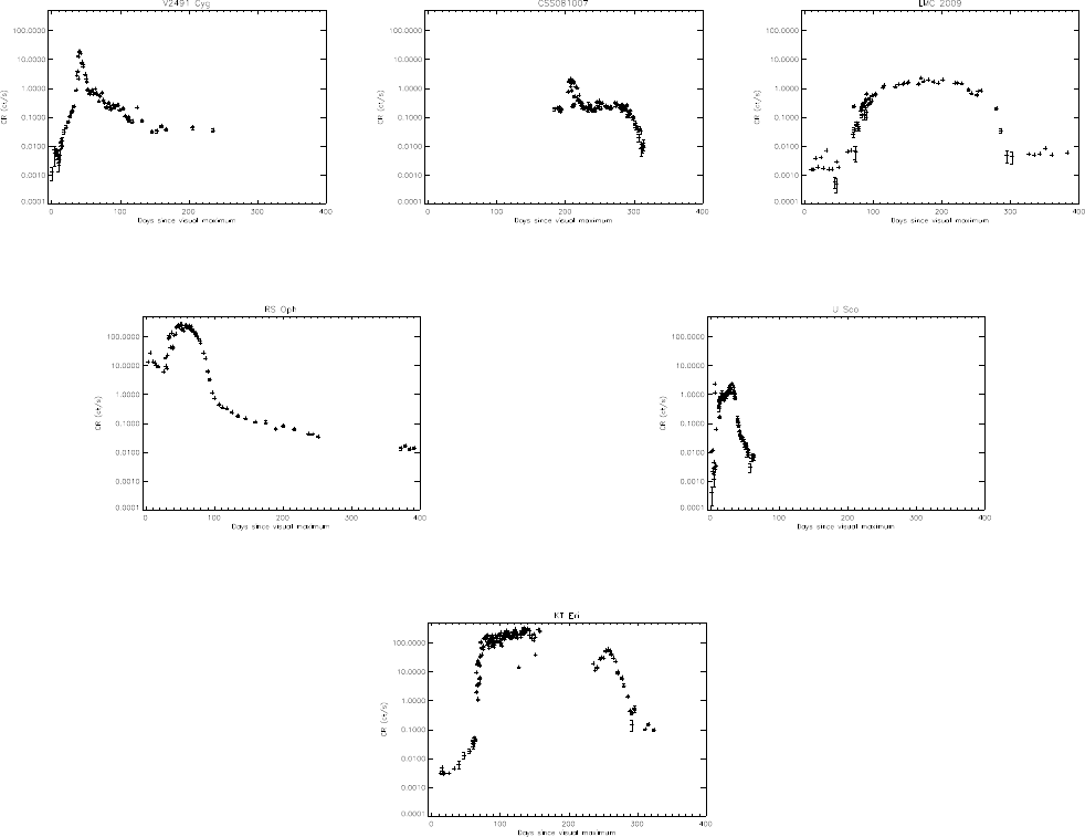
Figure 3shows an inverted pyramid of individual ﬁg-

ure constructed with six individual EPS ﬁles using the

\gridline option.

3.5. Figure sets

A large collection of similar style ﬁgures should be

grouped together as a ﬁgure set. The derived PDF arti-

cle will only shows an example ﬁgure while the enhanced

content is available in the ﬁgure set in the electronic

edition. The advantage of a ﬁgure set gives the reader

the ability to easily sort through the ﬁgure collection to

ﬁnd individual component ﬁgures. All of the ﬁgure set

components, along with their html framework, are also

available for download in a .tar.gz package.

Special LaT

X mark up is required to create a ﬁgure

set. Prior to AAST

X v6 the underlying mark up com-

mands had to be inserted by hand but is now included.

Note that when an article with ﬁgure set is compiled in

LaT

X none of the component ﬁgures are shown and a

ﬂoating Figure Set caption will appear in the resulting

PDF.

Fig. Set 4. Swift X-ray light curves

Authors are encouraged to use an online tool at

http://authortools.aas.org/FIGSETS/make-ﬁgset.html

to generate their own speciﬁc ﬁgure set mark up to

incorporate into their LaT

X articles.

3.6. Animations

Authors may include animations in their articles. A

single still frame from the animation should be included

as a regular ﬁgure to serve as an example. The associ-

ated ﬁgure caption should indicate to the reader exactly

what the animation shows and that the animation is

available online.

3.7. Interactive ﬁgures

Interactive ﬁgures give the reader the ability to ma-

nipulate the information contained in an image which

can add clarity or help further the author’s narrative.

These ﬁgures consist of two parts, the ﬁgure ﬁle in a

speciﬁc format and a javascript and html frame work

that provides the interactive control. An example of an

interactive ﬁgure is a 3D model. The underlying ﬁg-

ure is a X3D ﬁle while x3dom.js is the javascript driver

that displays it. An author created interface is added

via a html wrapper. The ﬁrst 3D model published by

the AAS Journals using this technique was Vogt et al.

(2014). Authors should consult the online tutorials for

more information on how to construct their own inter-

active ﬁgures.

As with animations authors should include a non-

interactive regular ﬁgure to use as an example. The

example ﬁgure should also indicate to the reader that

the enhanced ﬁgure is interactive and can be accessed

online.

4. DISPLAYING MATHEMATICS

The most common mathematical symbols and formu-

las are in the amsmath package. AAST

X requires this

package so there is no need to speciﬁcally call for it in

the document preamble. Most modern LaT

X distribu-

tions already contain this package. If you do not have

this package or the other required packages, revtex4-1,

latexsym, graphicx, amssymb, longtable, and epsf, they

can be obtained from http://www.ctan.org

Mathematics can be displayed either within the text,

e.g. E=mc2, or separate from in an equation. In order

to be properly rendered, all inline math text has to be

declared by surrounding the math by dollar signs ($).

A complex equation example with inline math as part

of the explanation follows.

¯v(p2, σ2)P−τˆa1ˆa2· · · ˆanu(p1, σ1),(1)

where pand σlabel the initial e±four-momenta and

helicities (σ=±1), ˆai=aµ

iγνand Pτ=1

2(1 + τγ5) is

a chirality projection operator (τ=±1). This produces

a single line formula. LaT

X will auto-number this and

any subsequent equations. If no number is desired then

the equation call should be replaced with displaymath.

LaT

X can also handle a a multi-line equation. Use

eqnarray for more than one line and end each line with

a\\. Each line will be numbered unless the \\ is pre-

ceded by a \nonumber command. Alignment points can

be added with ampersands (&). There should be two

ampersands per line. In the examples they are centered

on the equal symbol.

γµ= 0σµ

σµ

−0!, γ5= −1 0

0 1!,(2)

σµ

±= (1,±σ),(3)

Sample article 11

(a) (b) (c)

(d) (e)

(f)

Figure 3. Inverted pyramid ﬁgure of six individual ﬁles. The nova are (a) V2491 Cyg, (b) HV Cet, (c) LMC 2009, (d) RS

Oph, (e) U Sco, and (f) KT Eri.

ˆa= 0 (ˆa)+

(ˆa)−0!,

(ˆa)±=aµσµ

±(4)

5. REVISION TRACKING AND COLOR

HIGHLIGHTING

Authors sometimes use color to highlight changes to

their manuscript in response to editor and referee com-

ments. In AAST

X new commands have been intro-

duced to make this easier and formalize the process.

The ﬁrst method is through a new set of editing

mark up commands that speciﬁcally identify what has

been changed. These commands are \added{<text>},

\deleted{<text>}, and \replaced{<old text>}{<replaced

text>}. To activate these commands the trackchanges

option must be used in the \documentclass call.

When compiled this will produce the marked text in

red. The \explain{<text>}can be used to add text

to provide information to the reader describing the

change. Its output is purple italic font. To see how

\added{<important added info>},\deleted{<this

can be deleted text>},\replaced{<old data>}{<replaced

data>}, and

\explain{<text explaining the change>}commands

will produce important added information and replaced

data, toggle between versions compiled with and with-

out the trackchanges option.

A summary list of all these tracking commands can

be produced at the end of the article by adding the

\listofchanges just before the \end{document}call.

The page number for each change will be provided. If

12 Schwarz et al.

Figure 4. The Swift/XRT X-ray light curve for the ﬁrst year

after outburst of the suspected recurrent nova KT Eri. At a

maximum count rate of 328 ct/s, KT Eri was the brightest

nova in X-rays observed to date. All the component ﬁgures

are available in the Figure Set.

Figure 5. Example image from the animation which is avail-

able in the electronic edition.

the linenumbers option is also included in the docu-

mentcall call then not only will all the lines in the article

be numbered for handy reference but the summary list

will also include the line number for each change.

The second method does not have the ability to high-

light the speciﬁc nature of the changes but does allow

the author to document changes over multiple revisions.

The commands are \edit1{<text>},\edit2{<text>}

and \edit3{<text>}and they produce <text> that

is highlighted in bold red, italic blue and underlined

purple, respectively. Authors should use the ﬁrst com-

mand to indicated which text has been changed

from the ﬁrst revision. The second command is

to highlight new or modiﬁed text from a second re-

vision. If a third revision is needed then the last

command should be used to show this changed text.

Since over 90% of all manuscripts are accepted af-

ter the 3rd revision these commands make it easy to

identify what text has been added and when. Once

the article is accepted all the highlight color can be

turned oﬀ simply by adding the \turnoffediting

command in the preamble. Likewise, the new com-

mands \turnoffeditone,\turnoffedittwo, and

\turnoffeditthree can be used to only turn oﬀ the

\edit1{<text>},\edit2{<text>}and \edit3{<text>},

respectively.

Similar to marking editing changes with the \edit

options there are also the \authorcomments1{<text>},

\authorcomments2{<text>}and \authorcomments3{<text>}

commands. These produce the same bold red, italic blue

and underlined purple text but when the \turnoffediting

command is present the <text> material does not ap-

pear in the manuscript. Authors can use these com-

mands to mark up text that they are not sure should

appear in the ﬁnal manuscript or as a way to commu-

nicate comments between co-authors when writing the

article.

6. SOFTWARE AND THIRD PARTY DATA

REPOSITORY CITATIONS

The AAS Journals would like to encourage authors to

change software and third party data repository refer-

ences from the current standard of a footnote to a ﬁrst

class citation in the bibliography. As a bibliographic

citation these important references will be more easily

captured and credit will be given to the appropriate peo-

ple.

The ﬁrst step to making this happen is to have the

data or software in a long term repository that has made

these items available via a persistent identiﬁer like a Dig-

ital Object Identiﬁer (DOI). A list of repositories that

satisfy this criteria plus each one’s pros and cons are

given at

https://github.com/AASJournals/Tutorials/tree/master/

Repositories.

In the bibliography the format for data or code follows

this format:

author year, title, version, publisher, preﬁx:identiﬁer

Corrales (2015) provides a example of how the ci-

tation in the article references the external code at

Sample article 13

https://doi.org/10.5281/zenodo.15991. Unfortunately,

bibtex does not have speciﬁc bibtex entries for these

types of references so the “@misc” type should be

used. The Repository tutorial explains how to code

the “@misc” type correctly. The most recent aasjour-

nal.bst ﬁle, available with AAST

X v6, will output bib-

tex “@misc” type properly.

We thank all the people that have made this AAS-

TeX what it is today. This includes but not limited to

Bob Hanisch, Chris Biemesderfer, Lee Brotzman, Pierre

Landau, Arthur Ogawa, Maxim Markevitch, Alexey

Vikhlinin and Amy Hendrickson. Also special thanks

to David Hogg and Daniel Foreman-Mackey for the

new ”modern” style design. Considerable help was pro-

vided via bug reports and hacks from numerous people

including Patricio Cubillos, Alex Drlica-Wagner, Sean

Lake, Michele Bannister, Peter Williams, and Jonathan

Gagne.

Facilities: HST(STIS), Swift(XRT and UVOT),

AAVSO, CTIO:1.3m, CTIO:1.5m,CXO

Software: astropy(AstropyCollaborationetal.2013),

Cloudy(Ferlandetal.2013),SExtractor(Bertin&Arnouts

1996)

APPENDIX

A. APPENDIX INFORMATION

Appendices can be broken into separate sections just like in the main text. The only diﬀerence is that each appendix

section is indexed by a letter (A, B, C, etc.) instead of a number. Likewise numbered equations have the section letter

appended. Here is an equation as an example.

I=1

1 + dP(1+d2)

(A1)

Appendix tables and ﬁgures should not be numbered like equations. Instead they should continue the sequence from

the main article body.

B. AUTHOR PUBLICATION CHARGES

Finally some information about the AAS Journal’s publication charges. In April 2011 the traditional way of cal-

culating author charges based on the number of printed pages was changed. The reason for the change was due to

a recognition of the growing number of article items that could not be represented in print. Now author charges are

determined by a number of digital “quanta”. A single quantum is 350 words, one ﬁgure, one table, and one enhanced

digital item. For the latter this includes machine readable tables, ﬁgure sets, animations, and interactive ﬁgures. The

current cost is $27 per word quantum and $30 for all other quantum type.

C. ROTATING TABLES

The process of rotating tables into landscape mode is slightly diﬀerent in AAST

Xv6.2. Instead of the \rotate

command, a new environment has been created to handle this task. To place a single page table in a landscape mode

start the table portion with \begin{rotatetable}and end with \end{rotatetable}.

Tables that exceed a print page take a slightly diﬀerent environment since both rotation and long table printing are

required. In these cases start with \begin{longrotatetable}and end with \end{longrotatetable}. Table 7is an

example of a multi-page, rotated table.

14 Schwarz et al.

Table 7. Observable Characteristics of Galactic/Magellanic Cloud novae with X-ray observations

Name Vmax Date t2FWHM E(B-V) NHPeriod D Dust? RN?

(mag) (JD) (d) (km s−1) (mag) (cm−2) (d) (kpc)

CI Aql 8.83 (1) 2451665.5 (1) 32 (2) 2300 (3) 0.8±0.2 (4) 1.2e+22 0.62 (4) 6.25±5 (4) N Y

CSS081007 ··· 2454596.5 ··· ··· 0.146 1.1e+21 1.77 (5) 4.45±1.95 (6) ··· ···

GQ Mus 7.2 (7) 2445352.5 (7) 18 (7) 1000 (8) 0.45 (9) 3.8e+21 0.059375 (10) 4.8±1 (9) N (7) ···

IM Nor 7.84 (11) 2452289 (2) 50 (2) 1150 (12) 0.8±0.2 (4) 8e+21 0.102 (13) 4.25±3.4 (4) N Y

KT Eri 5.42 (14) 2455150.17 (14) 6.6 (14) 3000 (15) 0.08 (15) 5.5e+20 ··· 6.5 (15) N M

LMC 1995 10.7 (16) 2449778.5 (16) 15±2 (17) ··· 0.15 (203) 7.8e+20 ··· 50 ··· ···

LMC 2000 11.45 (18) 2451737.5 (18) 9±2 (19) 1700 (20) 0.15 (203) 7.8e+20 ··· 50 ··· ···

LMC 2005 11.5 (21) 2453700.5 (21) 63 (22) 900 (23) 0.15 (203) 1e+21 ··· 50 M (24) ···

LMC 2009a 10.6 (25) 2454867.5 (25) 4±1 3900 (25) 0.15 (203) 5.7e+20 1.19 (26) 50 N Y

SMC 2005 10.4 (27) 2453588.5 (27) ··· 3200 (28) ··· 5e+20 ··· 61 ··· ···

QY Mus 8.1 (29) 2454739.90 (29) 60: ··· 0.71 (30) 4.2e+21 ··· ··· M···

RS Oph 4.5 (31) 2453779.44 (14) 7.9 (14) 3930 (31) 0.73 (32) 2.25e+21 456 (33) 1.6±0.3 (33) N (34) Y

U Sco 8.05 (35) 2455224.94 (35) 1.2 (36) 7600 (37) 0.2±0.1 (4) 1.2e+21 1.23056 (36) 12±2 (4) N Y

V1047 Cen 8.5 (38) 2453614.5 (39) 6 (40) 840 (38) ··· 1.4e+22 ··· ··· ··· ···

V1065 Cen 8.2 (41) 2454123.5 (41) 11 (42) 2700 (43) 0.5±0.1 (42) 3.75e+21 ··· 9.05±2.8 (42) Y (42) ···

V1187 Sco 7.4 (44) 2453220.5 (44) 7: (45) 3000 (44) 1.56 (44) 8.0e+21 ··· 4.9±0.5 (44) N ···

V1188 Sco 8.7 (46) 2453577.5 (46) 7 (40) 1730 (47) ··· 5.0e+21 ··· 7.5 (39) ··· ···

V1213 Cen 8.53 (48) 2454959.5 (48) 11±2 (49) 2300 (50) 2.07 (30) 1.0e+22 ··· ··· ··· ···

V1280 Sco 3.79 (51) 2454147.65 (14) 21 (52) 640 (53) 0.36 (54) 1.6e+21 ··· 1.6±0.4 (54) Y (54) ···

V1281 Sco 8.8 (55) 2454152.21 (55) 15: 1800 (56) 0.7 (57) 3.2e+21 ··· ··· N···

V1309 Sco 7.1 (58) 2454714.5 (58) 23±2 (59) 670 (60) 1.2 (30) 4.0e+21 ··· ··· ··· ···

V1494 Aql 3.8 (61) 2451515.5 (61) 6.6±0.5 (61) 1200 (62) 0.6 (63) 3.6e+21 0.13467 (64) 1.6±0.1 (63) N ···

V1663 Aql 10.5 (65) 2453531.5 (65) 17 (66) 1900 (67) 2: (68) 1.6e+22 ··· 8.9±3.6 (69) N ···

V1974 Cyg 4.3 (70) 2448654.5 (70) 17 (71) 2000 (19) 0.36±0.04 (71) 2.7e+21 0.081263 (70) 1.8±0.1 (72) N ···

V2361 Cyg 9.3 (73) 2453412.5 (73) 6 (40) 3200 (74) 1.2: (75) 7.0e+21 ··· ··· Y (40) ···

V2362 Cyg 7.8 (76) 2453831.5 (76) 9 (77) 1850 (78) 0.575±0.015 (79) 4.4e+21 0.06577 (80) 7.75±3 (77) Y (81) ···

V2467 Cyg 6.7 (82) 2454176.27 (82) 7 (83) 950 (82) 1.5 (84) 1.4e+22 0.159 (85) 3.1±0.5 (86) M (87) ···

V2468 Cyg 7.4 (88) 2454534.2 (88) 10: 1000 (88) 0.77 (89) 1.0e+22 0.242 (90) ··· N···

V2491 Cyg 7.54 (91) 2454567.86 (91) 4.6 (92) 4860 (93) 0.43 (94) 4.7e+21 0.09580: (95) 10.5 (96) N M

V2487 Oph 9.5 (97) 2450979.5 (97) 6.3 (98) 10000 (98) 0.38±0.08 (98) 2.0e+21 ··· 27.5±3 (99) N (100) Y (101)

V2540 Oph 8.5 (102) 2452295.5 (102) ··· ··· ··· 2.3e+21 0.284781 (103) 5.2±0.8 (103) N ···

V2575 Oph 11.1 (104) 2453778.8 (104) 20: 560 (104) 1.4 (105) 3.3e+21 ··· ··· N (105) ···

V2576 Oph 9.2 (106) 2453832.5 (106) 8: 1470 (106) 0.25 (107) 2.6e+21 ··· ··· N···

V2615 Oph 8.52 (108) 2454187.5 (108) 26.5 (108) 800 (109) 0.9 (108) 3.1e+21 ··· 3.7±0.2 (108) Y (110) ···

V2670 Oph 9.9 (111) 2454613.11 (111) 15: 600 (112) 1.3: (113) 2.9e+21 ··· ··· N (114) ···

V2671 Oph 11.1 (115) 2454617.5 (115) 8: 1210 (116) 2.0 (117) 3.3e+21 ··· ··· M (117) ···

V2672 Oph 10.0 (118) 2455060.02 (118) 2.3 (119) 8000 (118) 1.6±0.1 (119) 4.0e+21 ··· 19±2 (119) ··· M

Table 7 continued

Sample article 15

Table 7 (continued)

Name Vmax Date t2FWHM E(B-V) NHPeriod D Dust? RN?

(mag) (JD) (d) (km s−1) (mag) (cm−2) (d) (kpc)

V351 Pup 6.5 (120) 2448617.5 (120) 16 (121) ··· 0.72±0.1 (122) 6.2e+21 0.1182 (123) 2.7±0.7 (122) N ···

V382 Nor 8.9 (124) 2453447.5 (124) 12 (40) 1850 (23) ··· 1.7e+22 ··· ··· ··· ···

V382 Vel 2.85 (125) 2451320.5 (125) 4.5 (126) 2400 (126) 0.05: (126) 3.4e+21 0.146126 (127) 1.68±0.3 (126) N ···

V407 Cyg 6.8 (128) 2455266.314 (128) 5.9 (129) 2760 (129) 0.5±0.05 (130) 8.8e+21 15595 (131) 2.7 (131) ··· Y

V458 Vul 8.24 (132) 2454322.39 (132) 7 (133) 1750 (134) 0.6 (135) 3.6e+21 0.06812255 (136) 8.5±1.8 (133) N (135) ···

V459 Vul 7.57 (137) 2454461.5 (137) 18 (138) 910 (139) 1.0 (140) 5.5e+21 ··· 3.65±1.35 (138) Y (140) ···

V4633 Sgr 7.8 (141) 2450895.5 (141) 19±3 (142) 1700 (143) 0.21 (142) 1.4e+21 0.125576 (144) 8.9±2.5 (142) N ···

V4643 Sgr 8.07 (145) 2451965.867 (145) 4.8 (146) 4700 (147) 1.67 (148) 1.4e+22 ··· 3 (148) N ···

V4743 Sgr 5.0 (149) 2452537.5 (149) 9 (150) 2400 (149) 0.25 (151) 1.2e+21 0.281 (152) 3.9±0.3 (151) N ···

V4745 Sgr 7.41 (153) 2452747.5 (153) 8.6 (154) 1600 (155) 0.1 (154) 9.0e+20 0.20782 (156) 14±5 (154) ··· ···

V476 Sct 10.3 (157) 2453643.5 (157) 15 (158) ··· 1.9 (158) 1.2e+22 ··· 4±1 (158) M (159) ···

V477 Sct 9.8 (160) 2453655.5 (160) 3 (160) 2900 (161) 1.2: (162) 4e+21 ··· ··· M (163) ···

V5114 Sgr 8.38 (164) 2453081.5 (164) 11 (165) 2000 (23) ··· 1.5e+21 ··· 7.7±0.7 (165) N (166) ···

V5115 Sgr 7.7 (167) 2453459.5 (167) 7 (40) 1300 (168) 0.53 (169) 2.3e+21 ··· ··· N (169) ···

V5116 Sgr 8.15 (170) 2453556.91 (170) 6.5 (171) 970 (172) 0.25 (173) 1.5e+21 0.1238 (171) 11±3 (173) N (174) ···

V5558 Sgr 6.53 (175) 2454291.5 (175) 125 (176) 1000 (177) 0.80 (178) 1.6e+22 ··· 1.3±0.3 (176) N (179) ···

V5579 Sgr 5.56 (180) 2454579.62 (180) 7: 1500 (23) 1.2 (181) 3.3e+21 ··· ··· Y (181) ···

V5583 Sgr 7.43 (182) 2455051.07 (182) 5: 2300 (182) 0.39 (30) 2.0e+21 ··· 10.5 ··· ···

V574 Pup 6.93 (183) 2453332.22 (183) 13 (184) 2800 (184) 0.5±0.1 6.2e+21 ··· 6.5±1 M (185) ···

V597 Pup 7.0 (186) 2454418.75 (186) 3: 1800 (187) 0.3 (188) 5.0e+21 0.11119 (189) ··· N (188) ···

V598 Pup 3.46 (14) 2454257.79 (14) 9±1 (190) ··· 0.16 (190) 1.4e+21 ··· 2.95±0.8 (190) ··· ···

V679 Car 7.55 (191) 2454797.77 (191) 20: ··· ··· 1.3e+22 ··· ··· ··· ···

V723 Cas 7.1 (192) 2450069.0 (192) 263 (2) 600 (193) 0.5 (194) 2.35e+21 0.69 (195) 3.86±0.23 (196) N ···

V838 Her 5 (197) 2448340.5 (197) 2 (198) ··· 0.5±0.1 (198) 2.6e+21 0.2975 (199) 3±1 (198) Y (200) ···

XMMSL1 J06 12 (201) 2453643.5 (202) 8±2 (202) ··· 0.15 (203) 8.7e+20 ··· 50 ··· ···

16 Schwarz et al.

A handy ”cheat sheat” that provides the neces-

sary LaTeX to produce 17 diﬀerent types of tables

is available at http://journals.aas.org/authors/aastex/

aasguide.html#table cheat sheet.

REFERENCES

Astropy Collaboration, Robitaille, T. P., Tollerud, E. J., et

al. 2013, A&A, 558, A33

Bertin, E., & Arnouts, S. 1996, A&AS, 117, 393

Corrales, L. 2015, ApJ, 805, 23

Ferland, G. J., Porter, R. L., van Hoof, P. A. M., et al.

2013, RMxAA, 49, 137

Hanisch, R. J., & Biemesderfer, C. D. 1989, BAAS, 21, 780

Lamport, L. 1994, LaTeX: A Document Preparation

System, 2nd Edition (Boston, Addison-Wesley

Professional)

Schwarz, G. J., Ness, J.-U., Osborne, J. P., et al. 2011,

ApJS, 197, 31

Vogt, F. P. A., Dopita, M. A., Kewley, L. J., et al. 2014,

ApJ, 793, 127

AASTex Instructions

Navigation menu

Versions of this User Manual:

Views

Navigation