Analytics In A Big Data World Bart Baesens The Essential Guide To Science And Its Applicati

Analytics in a Big

Data World

Wiley & SAS

Business Series

The Wiley & SAS Business Series presents books that help senior‐level

mana

g

ers with their critical mana

g

ement decisions.

Tit

l

es in t

h

e Wi

l

e

y

& SAS Business Series inc

l

u

d

e:

A

ctivity‐Base

d

Mana

g

ement

f

or Financia

l

Institutions: Drivin

g

Bottom‐

L

ine

R

esults

b

y

Brent Bahnub

Bank Fraud: Using Technology to Combat Losse

s

by Revathi Subramanian

Big Data Analytics: Turning Big Data into Big Money b

y

Frank Ohlhorst

Branded! How Retailers En

g

a

g

e Consumers with Social Media and Mobil-

it

y

by Bernie Brennan and Lori Schafer

Business Analytics for Customer Intelligence b

y

Gert Laursen

Business Analytics for Mana

g

ers: Takin

g

Business Intelli

g

ence beyond

Reporting by Gert Laursen and Jesper Thorlund

The Business Forecasting Deal: Exposing Bad Practices and Providing

Practical Solutions by Michael Gilliland

Business Intelligence Applied: Implementing an Effective Information and

Communications Technolo

g

y Infrastructure b

y

Michael Gendron

Business Intelligence in the Cloud: Strategic Implementation Guide by

Michael S. Gendron

Business Intelli

g

ence Success Factors: Tools for Ali

g

nin

g

Your Business in

the Global Economy by Olivia Parr Rud

CIO Best Practices: Enabling Strategic Value with Information Technology,

secon

d

e

d

ition

b

y Joe Stenze

l

Connectin

g

Or

g

anizationa

l

Si

l

os: Ta

k

in

g

Know

l

e

dg

e F

l

ow Mana

g

ement to

t

h

e

N

ext Leve

l

wit

h

Socia

l

Me

d

ia

by

Fran

k

Leistner

Cre

d

it Ris

k

Assessment: T

h

e New Len

d

ing System

f

or Borrowers, Len

d

ers,

and

I

nvestors

by

C

l

ar

k

A

b

ra

h

ams an

d

Min

gy

uan Z

h

an

g

Cre

d

it Ris

k

Scorecar

d

s: Deve

l

opin

g

an

d

Imp

l

ementin

g

Inte

ll

i

g

ent Cre

d

it

Scoring b

y

Naeem Siddi

q

i

The Data Asset: How Smart Companies Govern Their Data for Business

Success by Tony Fisher

Delivering Business Analytics: Practical Guidelines for Best Practice by

Evan Stubbs

Demand‐Driven Forecasting: A Structured Approach to Forecasting,

S

ec-

ond Edition by Charles Chase

Demand‐Driven Inventory Optimization and Replenishment: Creating a

M

ore E

f

cient Supp

l

y C

h

ain

b

y Ro

b

ert A. Davis

T

h

e Executive’s Gui

d

e to Enterprise Socia

l

Me

d

ia Strategy: How Socia

l

Net-

works Are Radically Transformin

g

Your Busines

s

b

y

David Thomas and

Mike Barlo

w

Economic and Business Forecastin

g

: Analyzin

g

and Interpretin

g

Econo-

metric Results b

y

John Silvia, Azhar I

q

bal, Ka

y

l

y

n Swankoski, Sarah

Watt

,

and Sam Bullard

Executive’s Guide to Solvency II

by David Buckham, Jason Wahl, and

I

St

uar

t

Rose

Fair Lendin

g

Compliance: Intelli

g

ence and Implications for Credit Risk

Management

by Clark R. Abrahams and Mingyuan Zhang

t

Forei

g

n Currency Financial Reportin

g

from Euros to Yen to Yuan: A Guide

to Fundamental Conce

p

ts and Practical A

pp

lications b

y

Robert Rowan

Health Analytics: Gainin

g

the Insi

g

hts to Transform Health Car

e

by Jason

Burke

Heuristics in Analytics: A Practical Perspective of What In uences Ou

r

Analytical World

by Carlos Andre Reis Pinheiro and Fiona McNeill

d

Human Capital Analytics: How to Harness the Potential of Your Or

g

aniza

-

t

i

on’s

G

reatest Asse

t

by Gene Pease, Boyce Byerly, and Jac Fitz‐enz

t

Imp

l

ement, Improve an

d

Expan

d

Your Statewi

d

e Longitu

d

ina

l

Data Sys-

tem: Creating a Cu

l

ture o

f

Data in E

d

ucation

b

y Jamie McQuiggan an

d

Armistea

d

Sa

pp

In

f

ormation Revo

l

ution: Using t

h

e In

f

ormation Evo

l

ution Mo

d

e

l

to Grow

Your Bus

in

es

s

by

Jim Davis, G

l

oria J. Mi

ll

er, an

d

A

ll

an Russe

ll

Killer Analytics: Top 20 Metrics Missing from Your Balance Sheet

b

y

Mark

t

B

ro

w

n

M

anufacturin

g

Best Practices: Optimizin

g

Productivity and Product Qual-

it

y

by Bobby Hull

M

arketing Automation: Practical Steps to More Effective Direct Marketing

b

y Jeff LeSueur

M

astering Organizational Knowledge Flow: How to Make Knowledge

Sharing Work

by Frank Leistner

k

The New Know: Innovation Powered by Analytics by Thornton May

Per

f

ormance Management: Integrating Strategy Execution, Met

h

o

d

o

l

ogies,

Ris

k

, an

d

Ana

l

ytics

b

y Gary Co

k

ins

Predictive Business Analytics: Forward‐Lookin

g

Capabilities to Improve

Business Per

f

ormance b

y

Lawrence Maisel and Gar

y

Cokins

Retail Analytics: The Secret Weapon by Emmett Cox

Social Network Anal

y

sis in Telecommunications b

y

Carlos Andre Reis

Pinh

e

ir

o

Statistical Thinkin

g

: Improvin

g

Business Performance

,

second edition by

Ro

g

er W. Hoerl and Ronald D. Snee

Tamin

g

the Bi

g

Data Tidal Wave: Findin

g

Opportunities in Hu

g

e Data

Streams with Advanced Analytics by Bill Franks

Too Bi

g

to I

g

nore: The Business Case for Bi

g

Dat

a

b

y

Phil Simon

The Value of Business Analytics: Identifyin

g

the Path to Pro tabilit

y

b

y

Evan Stubbs

Visual Six Si

g

ma: Makin

g

Data Analysis Lea

n

b

y

Ian Cox, Marie A.

Gaudard, Philip J. Ramsey, Mia L. Stephens, and Leo Wright

Win with Advanced Business Analytics: Creatin

g

Business Value from

Your

Data

b

y

Jean Paul Isson and Jesse Harriott

For more in

f

ormation on an

y

o

f

t

h

e a

b

ove tit

l

es,

pl

ease visit ww

w

.wi

l

e

y

.com .

Analytics in a Big

Data World

The Essential

G

uide to Data

S

cience

and Its Application

s

B

ar

t

Baesen

s

Cover ima

g

e: ©iStoc

kph

oto/v

l

astos

Cover desi

g

n: Wile

y

Co

py

ri

gh

by

Bart Baesens. A

ll

ri

gh

ts reserve

d

.

Pu

bl

is

h

e

d

by

Jo

h

n Wi

l

e

y

& Sons, Inc., Ho

b

o

k

en, New Jerse

y

.

Published simultaneousl

y

in Canada.

No part o

f

t

h

is pu

bl

ication may

b

e repro

d

uce

d

, store

d

in a retrieva

l

system,

or transmitte

d

in any

f

orm or

b

y any means, e

l

ectronic, mec

h

anica

l

,

photocopying, recording, scanning, or otherwise, except as permitted under

Section 107 or 108 of the 1976 United States Copyright Act, without either the

prior written permission of the Publisher, or authorization through payment

of the appropriate per-copy fee to the Copyright Clearance Center, Inc., 222

Rosewood Drive, Danvers, MA 01923, (978) 750-8400, fax (978) 646-8600, or

on the Web at www.copyright.com. Requests to the Publisher for permission

should be addressed to the Permissions Department, John Wiley & Sons, Inc.,

111 River Street, Hoboken, NJ 07030,

(

201

)

748-6011, fax

(

201

)

748-6008, or

online at http://www.wiley.com/go/permissions.

Limit of Liability/Disclaimer of Warranty: While the publisher and author have

used their best efforts in preparing this book, they make no representations

or warranties with respect to the accuracy or completeness of the contents of

this book and s

p

eci call

y

disclaim an

y

im

p

lied warranties of merchantabilit

y

or  tness for a

p

articular

p

ur

p

ose. No warrant

y

ma

y

be created or extended

by

sales re

p

resentatives or written sales materials. The advice and strate

g

ies

contained herein ma

y

not be suitable for

y

our situation. You should consult

with a

p

rofessional where a

pp

ro

p

riate. Neither the

p

ublisher nor author shall

b

e liable for an

y

loss of

p

ro t or an

y

other commercial dama

g

es, includin

g

but

not limited to s

p

ecial, incidental, conse

q

uential, or other dama

g

es.

For

g

eneral information on our other

p

roducts and services or for technical

su

pp

ort,

p

lease contact our Customer Care De

p

artment within the United

States at

(

800

)

762-2974, outside the United States at

(

317

)

572-3993 or

fax (317) 572-4002.

Wile

y

p

ublishes in a variet

y

of

p

rint and electronic formats and b

y

p

rint-on

-

demand. Some material included with standard

p

rint versions of this book

ma

y

not be included in e-books or in

p

rint-on-demand. If this book refers to

media such as a CD or DVD that is not included in the version

y

ou

p

urchased,

y

ou ma

y

download this material at htt

p

://booksu

pp

ort.wile

y

.com. For more

information about Wile

y

p

roducts, visit www.wile

y

.com.

Library of Congress Cataloging-in-Publication Data:

Baesens

,

Bart.

Anal

y

tics in a bi

g

data world : the essential

g

uide to data science and its

applications / Bart Baesens.

1 online resource. — (Wile

y

& SAS business series

)

Descri

p

tion based on

p

rint version record and CIP data

p

rovided b

y

p

ublisher;

resource not viewe

d

.

ISBN 978-1-118-89271-8

(

ebk

)

; ISBN 978-1-118-89274-9

(

ebk

)

;

ISBN 978-1-118-89270-1 (c

l

ot

h

) 1. Big

d

ata. 2. Management—Statistica

l

met

h

o

d

s. 3. Mana

g

ement—Data

p

rocessin

g

. 4. Decision ma

k

in

g

—Data

processing. I. Tit

l

e.

HD

30.215

658.4’038

d

c23

2014004

7

28

Printe

d

in t

h

e Unite

d

States o

f

America

1

0

9

8

7

6

5

4

3

2

1

T

o m

y

won

d

er

f

u

l

wi

f

e, Katrien, an

d

m

y

k

i

d

s,

A

nn-So

ph

ie, Victor, an

d

Hanne

l

ore.

To my parents an

d

parents-in-

l

aw

.

ix

Contents

Preface xii

i

Acknowledgments xv

C

h

apter 1 B

i

g Data an

d

Ana

l

yt

i

cs

1

E

xam

pl

e

Appli

cat

i

ons 2

Basic

No

m

e

n

cla

t

u

r

e

4

A

na

ly

t

i

cs

P

rocess

M

o

d

e

l

4

Job

P

r

o

les

I

nv

ol

v

ed

6

A

na

ly

t

i

cs

7

A

na

ly

t

i

ca

l

M

o

d

e

l

R

e

q

u

i

rements

9

No

t

es

1

0

Chapter 2 Data Collection, Sampling,

an

d

Preprocess

i

ng 13

Typ

es of Data

S

ources 13

S

ampling 1

5

T

ypes o

f

D

ata

El

ements 17

Vi

sua

l

D

ata

E

x

pl

orat

i

on an

d

E

x

pl

orator

y

S

tatistical Anal

y

sis 1

7

Mi

ss

i

ng

V

a

l

ues 1

9

Ou

tli

e

r D

e

t

ec

ti

o

n

a

n

d

Tr

ea

tm

e

nt 2

0

S

tandardizin

g

Data 2

4

C

ate

g

orization 2

4

Wei

g

hts of Evidence

C

odin

g

28

V

ariable

S

election 2

9

x

▸

CO

NTENT

S

egmentation 3

2

N

otes 3

3

Chapter 3 Predictive Analytics 35

T

arget De nition 35

Linear Regression 3

8

Logistic Regression 3

9

D

ec

i

s

i

o

n Tr

ees

4

2

N

eu

r

a

l N

e

tw

o

rk

s

4

8

S

u

pp

ort Vector Machines 5

8

En

se

m

b

l

e

M

e

th

ods

6

4

Multiclass Classi cation Techni

q

ues 67

E

va

l

uat

i

ng

P

re

di

ct

i

ve

M

o

d

e

l

s 7

1

No

t

es

8

4

Chapter 4 Descriptive Analytics 87

Associa

t

io

n

Rules

87

S

e

q

uence Rules 9

4

S

egmentation 9

5

No

t

es

1

0

4

Chapter 5 Survival Analysis 10

5

S

urvival Anal

y

sis Measurements 106

K

a

pl

an

M

e

i

er

A

na

ly

s

i

s 109

Parametric Survival Anal

y

sis 111

P

roport

i

ona

l

H

azar

d

s

R

egress

i

on 114

Extensions of

S

urvival Anal

y

sis Models 116

Evaluating Survival Analysis Models 11

7

No

t

es

11

7

Chapter 6 Social Network Analytics 11

9

Soc

i

a

l N

e

tw

o

rk D

e

 niti

o

n

s

11

9

Soc

i

a

l N

e

tw

o

rk M

e

tri

cs

121

S

ocial Network Learnin

g

12

3

Relational Nei

g

hbor

C

lassi er 124

C

ONTENTS ◂x

i

Probabilistic Relational Nei

g

hbor

C

lassi er 12

5

R

e

l

at

i

ona

l

L

og

i

st

i

c

R

egress

i

on 126

Collective Inferencing 12

8

E

gonets 12

9

Bigraphs 130

N

o

t

es

1

32

Chapter 7 Anal

y

tics: Puttin

g

It All to Work 13

3

Backtesting Analytical Models 134

Benchmarking 146

Data

Q

ualit

y

14

9

So

ftw

a

r

e

1

53

P

r

i

vac

y

15

5

M

o

d

e

l

D

es

i

gn an

d

D

ocumentat

i

on 15

8

Cor

p

orate Governance 159

No

t

es

1

59

Cha

p

ter 8 Exam

p

le A

pp

lications 161

Credit Risk Modeling 16

1

F

r

aud

De

t

ec

t

io

n 1

65

N

et

Lif

t

R

esponse

M

o

d

e

li

ng 16

8

C

h

u

rn Pr

ed

i

c

ti

o

n 17

2

Recommender

Sy

stems 176

W

e

b

A

na

ly

t

i

cs 18

5

S

ocial Media Anal

y

tics 195

B

us

i

ness

P

rocess

A

na

ly

t

i

cs 204

No

t

es

22

0

About the Author 223

In

de

x 22

5

x

iii

Preface

C om

p

anies are bein

g

 ooded with tsunamis of data collected in a

multichannel business environment, leavin

g

an unta

pp

ed

p

oten

-

tia

l

f

or ana

ly

tics to

b

etter un

d

erstan

d

, mana

g

e, an

d

strate

g

ica

lly

ex

pl

oit t

h

e com

pl

ex

dy

namics o

f

customer

b

e

h

avior. In t

h

is

b

oo

k

, we

wi

ll

d

iscuss

h

ow ana

ly

tics can

b

e use

d

to create strate

g

ic

l

evera

g

e an

d

identif

y

new business o

pp

ortunities.

The focus of this book is not on the mathematics or theor

y

, but on

the practical application. Formulas and equations will only be included

when absolutel

y

needed from a

p

ractitioner’s

p

ers

p

ective. It is also not

our aim to

p

rovide exhaustive covera

g

e of all anal

y

tical techni

q

ues

previously developed, but rather to cover the ones that really provide

added value in a business settin

g

.

The book is written in a condensed, focused wa

y

because it is tar

-

geted at the business professional. A reader’s prerequisite knowledge

should consist of some basic ex

p

osure to descri

p

tive statistics (e.

g

.,

mean, standard deviation, correlation, con dence intervals, hypothesis

testing), data handling (using, for example, Microsoft Excel, SQL, etc.),

and data visualization (e.

g

., bar

p

lots,

p

ie charts, histo

g

rams, scatter

plots). Throughout the book, many examples of real‐life case studies

will be included in areas such as risk mana

g

ement, fraud detection,

customer relationshi

p

mana

g

ement, web anal

y

tics, and so forth. The

author will also integrate both his research and consulting experience

throu

g

hout the various cha

p

ters. The book is aimed at senior data ana

-

l

ysts, consu

l

tants, ana

l

ytics practitioners, an

d

P

h

D researc

h

ers starting

to ex

pl

ore t

h

e



e

ld

.

C

h

a

p

ter 1

d

iscusses

b

i

g

d

ata an

d

ana

ly

tics. It starts wit

h

some

examp

l

e app

l

ication areas,

f

o

ll

owe

d

b

y an overview o

f

t

h

e ana

l

ytics

p

rocess mo

d

e

l

an

d

j

o

b

p

ro



l

es invo

l

ve

d

, an

d

conc

l

u

d

es

by

d

iscussin

g

k

e

y

ana

ly

tic mo

d

e

l

re

q

uirements. C

h

a

p

ter 2

p

rovi

d

es an overview o

f

x

iv

▸

P

REFA

C

E

data collection, sam

p

lin

g

, and

p

re

p

rocessin

g

. Data is the ke

y

in

g

redi-

ent to an

y

anal

y

tical exercise, hence the im

p

ortance of this cha

p

ter.

It discusses sampling, types of data elements, visual data exploration

and exploratory statistical analysis, missing values, outlier detection

and treatment, standardizing data, categorization, weights of evidence

coding, variable selection, and segmentation. Chapter 3 discusses pre

-

dictive analytics. It starts with an overview of the target de nition

and then continues to discuss various analytics techniques such as

linear regression, logistic regression, decision trees, neural networks,

su

pp

ort vector machines, and ensemble methods (ba

gg

in

g

, boost

-

ing, ran

d

om

f

orests). In a

dd

ition, mu

l

tic

l

ass c

l

assi



cation tec

h

niques

are covere

d

, suc

h

as mu

l

tic

l

ass

l

ogistic regression, mu

l

tic

l

ass

d

eci

-

sion trees, mu

l

tic

l

ass neura

l

networ

k

s, an

d

mu

l

tic

l

ass support vector

machines. The chapter concludes by discussing the evaluation of pre

-

dictive models. Cha

p

ter 4 covers descri

p

tive anal

y

tics. First, association

rules are discussed that aim at discoverin

g

intratransaction

p

atterns.

This is followed by a section on sequence rules that aim at discovering

intertransaction

p

atterns. Se

g

mentation techni

q

ues are also covered.

Cha

p

ter 5 introduces survival anal

y

sis. The cha

p

ter starts b

y

introduc

-

ing some key survival analysis measurements. This is followed by a

discussion of Ka

p

lan Meier anal

y

sis,

p

arametric survival anal

y

sis, and

p

ro

p

ortional hazards re

g

ression. The cha

p

ter concludes b

y

discussin

g

various extensions and evaluation of survival analysis models. Chap

-

ter 6 covers social network anal

y

tics. The cha

p

ter starts b

y

discussin

g

exam

p

le social network a

pp

lications. Next, social network de nitions

and metrics are given. This is followed by a discussion on social network

learnin

g

. The relational nei

g

hbor classi er and its

p

robabilistic variant

together with relational logistic regression are covered next. The chap-

ter ends by discussing egonets and bigraphs. Chapter 7 provides an

overview of ke

y

activities to be considered when

p

uttin

g

anal

y

tics to

wor

k

. It starts wit

h

a reca

p

itu

l

ation o

f

t

h

e ana

ly

tic mo

d

e

l

re

q

uirements

an

d

t

h

en continues wit

h

a

d

iscussion o

f

b

ac

k

testin

g

,

b

enc

h

mar

k

in

g

,

d

ata qua

l

ity, so

f

tware, privacy, mo

d

e

l

d

esign an

d

ocumentation, an

d

cor

p

orate

g

overnance. C

h

a

p

ter 8 conc

l

u

d

es t

h

e

b

oo

k

by

d

iscussin

g

var

-

ious exam

pl

e a

ppl

ications suc

h

as cre

d

it ris

k

mo

d

e

l

in

g

,

f

rau

d

etection,

net

l

i

f

t response mo

d

e

l

ing, c

h

urn pre

d

iction, recommen

d

er systems,

we

b

ana

ly

tics, socia

l

me

d

ia ana

ly

tics, an

d

b

usiness

p

rocess ana

ly

tics.

xv

Acknowledgments

I would like to acknowled

g

e all m

y

collea

g

ues who contributed to

this text: Se

pp

e vanden Broucke, Alex Seret, Thomas Verbraken,

Aimée Backiel, Véroni

q

ue Van Vlasselaer, Helen Mo

g

es, and Barbara

D

er

g

ent.

Analytics in a Big

Data World

1

C

HAPTER

1

Big Data and

Analytics

D ata are ever

y

w

h

ere. IBM

p

ro

j

ects t

h

at ever

y

d

a

y

we

g

enerate 2.5

quinti

ll

ion

b

ytes o

f

d

ata.

1

In re

l

ative terms, t

h

is means 90 percent

o

f

t

h

e

d

ata in t

h

e wor

ld

h

as

b

een create

d

in t

h

e

l

ast two

y

ears.

Gartner

p

ro

j

ects t

h

at

by

2015, 85

p

ercent o

f

Fortune 500 or

g

anizations

wi

ll

b

e una

bl

e to exp

l

oit

b

ig

d

ata

f

or competitive a

d

vantage an

d

a

b

out

4.4 mi

ll

ion

j

o

b

s wi

ll

b

e create

d

aroun

d

b

i

g

d

ata.

2

A

l

t

h

ou

gh

t

h

ese esti

-

mates s

h

ou

ld

not

b

e inter

p

rete

d

in an a

b

so

l

ute sense, t

h

e

y

are a stron

g

in

d

ication o

f

t

h

e u

b

iquity o

f

b

ig

d

ata an

d

t

h

e strong nee

d

f

or ana

l

ytica

l

s

k

i

ll

s an

d

resources

b

ecause, as t

h

e

d

ata

p

i

l

es u

p

, mana

g

in

g

an

d

ana

ly

z-

in

g

t

h

ese

d

ata resources in t

h

e most o

p

tima

l

wa

y

b

ecome critica

l

suc

-

cess

f

actors in creating competitive a

d

vantage an

d

strategic

l

everage.

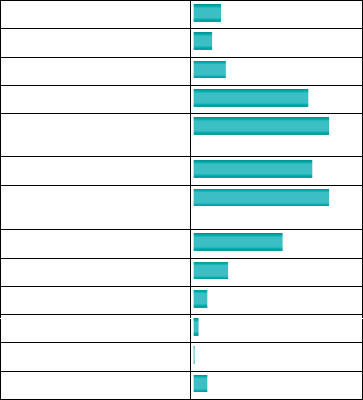
Fi

g

ure 1.1 s

h

ows t

h

e resu

l

ts o

f

a KDnu

gg

ets

3

p

o

ll

con

d

ucte

d

ur

-

in

g

A

p

ri

l

2013 a

b

out t

h

e

l

ar

g

est

d

ata sets ana

ly

ze

d

. T

h

e tota

l

num

b

er

o

f

respon

d

ents was 322 an

d

t

h

e num

b

ers per category are in

d

icate

d

b

etween

b

rac

k

ets. T

h

e me

d

ian was estimate

d

to

b

e in t

h

e 40 to 50

g

i

g

a

-

by

te (GB) ran

g

e, w

h

ic

h

was a

b

out

d

ou

bl

e t

h

e me

d

ian answer

f

or a simi

-

l

ar

p

o

ll

run in 2012 (20 to 40 GB). T

h

is c

l

ear

ly

s

h

ows t

h

e

q

uic

k

increase

in size of data that analysts are working on. A further regional break-

down of the

p

oll showed that U.S. data miners lead other re

g

ions in bi

g

data, with about 28% of them workin

g

with terab

y

te (TB) size databases.

A main obstacle to fully harnessing the power of big data using ana-

l

y

tics is the lack of skilled resources and “data scientist” talent re

q

uired to

2

▸ANALYTI

CS

IN A BI

G

DATA W

O

RL

D

ex

pl

oit

b

i

g

d

ata. In anot

h

er

p

o

ll

ran

by

KDnu

gg

ets in Ju

ly

2013, a stron

g

nee

d

emerge

d

f

or ana

l

ytics/

b

ig

d

ata/

d

ata mining/

d

ata science e

d

uca

-

tion.

4

It is t

h

e

p

ur

p

ose o

f

t

h

is

b

oo

k

to tr

y

an

d



ll

t

h

is

g

a

p

by

p

rovi

d

in

g

a

concise an

d

f

ocuse

d

overview o

f

ana

ly

tics

f

or t

h

e

b

usiness

p

ractitioner.

EXAMPLE APPLICATIONS

Ana

l

ytics is everyw

h

ere an

d

strong

l

y em

b

e

dd

e

d

into our

d

ai

l

y

l

ives. As I

am writin

g

t

h

is

p

art, I was t

h

e su

bj

ect o

f

various ana

ly

tica

l

mo

d

e

l

s to

d

a

y

.

W

h

en I c

h

ec

k

e

d

my p

h

ysica

l

mai

lb

ox t

h

is morning, I

f

oun

d

a cata

l

ogue

sent to me most

p

ro

b

a

bly

as a resu

l

t o

f

a res

p

onse mo

d

e

l

in

g

ana

ly

tica

l

exercise t

h

at in

d

icate

d

t

h

at,

g

iven m

y

c

h

aracteristics an

d

p

revious

p

ur

-

c

h

ase

b

e

h

avior, I am

l

i

k

e

l

y to

b

uy one or more pro

d

ucts

f

rom it. To

d

ay,

I was t

h

e su

bj

ect o

f

a

b

e

h

aviora

l

scorin

g

mo

d

e

l

o

f

m

y



nancia

l

institu

-

tion. T

h

is is a mo

d

e

l

t

h

at wi

ll

l

oo

k

at, among ot

h

er t

h

ings, my c

h

ec

k-

in

g

account

b

a

l

ance

f

rom t

h

e

p

ast 12 mont

h

s an

d

m

y

cre

d

it

p

a

y

ments

d

urin

g

t

h

at

p

erio

d

, to

g

et

h

er wit

h

ot

h

er

k

in

d

s o

f

in

f

ormation avai

l

a

bl

e

to my

b

an

k

, to pre

d

ict w

h

et

h

er I wi

ll

d

e

f

au

l

t on my

l

oan

d

uring t

h

e

ear. M

y

b

an

k

nee

d

s to

k

now t

h

is

f

or

p

rovisionin

g

p

ur

p

oses. A

l

so

to

d

a

y

, m

y

te

l

e

ph

one services

p

rovi

d

er ana

ly

ze

d

m

y

ca

ll

in

g

b

e

h

avior

Fi

g

ure 1.1 Results

f

rom a KDnu

gg

ets Poll about Lar

g

est Data Sets Anal

y

ze

d

S

ource: www.

kd

nuggets.com/po

ll

s/2013/

l

argest‐

d

ataset‐ana

l

yze

d

‐

d

ata‐m

i

ne

d

‐2013.

h

tm

l

.

Less than 1 MB (12) 3.7%

1.1 to 10 MB (8) 2.5%

11 to 100 MB (14) 4.3%

101 MB to 1 GB (50) 15.5%

1.1 to 10 GB (59)

18%

11 to 100 GB (52) 16%

101 GB to 1 TB

(59) 18%

1.1 to 10 TB (39) 12%

11 to 100 TB (15) 4.7%

101 TB to 1 PB (6) 1.9%

1.1 to 10 PB (2) 0.6%

11 to 100 PB (0) 0%

Over 100 PB (6) 1.9%

B

I

G

DATA AND ANALYTI

CS

◂

3

an

d

m

y

account in

f

ormation to

p

re

d

ict w

h

et

h

er I wi

ll

c

h

urn

d

urin

g

t

h

e

next three months. As I lo

gg

ed on to m

y

Facebook

p

a

g

e, the social ads

appearing there were based on analyzing all information (posts, pictures,

my friends and their behavior, etc.) available to Facebook. My Twitter

posts will be analyzed (possibly in real time) by social media analytics to

understand both the subject of my tweets and the sentiment of them.

As I checked out in the supermarket, my loyalty card was scanned  rst,

followed by all my purchases. This will be used by my supermarket to

analyze my market basket, which will help it decide on product bun

-

dlin

g

, next best offer, im

p

rovin

g

shelf or

g

anization, and so forth. As I

ma

d

e t

h

e payment wit

h

my cre

d

it car

d

, my cre

d

it car

d

provi

d

er use

d

a

f

rau

d

etection mo

d

e

l

to see w

h

et

h

er it was a

l

egitimate transaction.

W

h

en I receive my cre

d

it car

d

statement

l

ater, it wi

ll

b

e accompanie

d

b

y

various vouchers that are the result of an analytical customer segmenta

-

tion exercise to better understand m

y

ex

p

ense behavior.

To summarize, the relevance, im

p

ortance, and im

p

act of anal

y

tics

are now bigger than ever before and, given that more and more data

are bein

g

collected and that there is strate

g

ic value in knowin

g

what

is hidden in data, anal

y

tics will continue to

g

row. Without claimin

g

to

b

e exhaustive, Table 1.1 presents some examples of how analytics is

a

pp

lied in various settin

g

s.

Ta

bl

e 1.1 Examp

l

e Ana

l

yt

i

cs App

li

cat

i

ons

Marketing Risk

Management Government Web Logistics Other

R

es

p

onse

m

odelin

g

C

redit ris

k

modelin

g

T

ax avo

id

anc

e

W

e

b

ana

ly

t

i

c

s

D

eman

d

forecastin

g

T

ext

anal

y

tic

s

Net li

f

t

m

odelin

g

M

ar

k

et r

i

s

k

modelin

g

Social

s

ecurity

f

rau

d

Social media

analytic

s

Supply chain

analytic

s

B

us

i

ness

process

analytic

s

R

e

t

e

nti

o

n

m

o

d

e

li

n

g

O

p

erational

r

i

s

k

mo

d

e

li

n

g

M

one

y

l

aun

d

er

i

n

g

Mu

ltiv

a

ri

a

t

e

t

est

i

n

g

Ma

r

ke

t

baske

t

a

na

l

ys

is

F

r

aud

d

etect

i

o

n

Te

rr

o

r

is

m

d

etect

i

o

n

R

eco

mm

e

n

de

r

s

y

stem

s

Cus

t

o

m

e

r

se

g

mentat

i

o

n

4

▸ANALYTI

CS

IN A BI

G

DATA W

O

RL

D

It is the

p

ur

p

ose of this book to discuss the underl

y

in

g

techni

q

ues

and ke

y

challen

g

es to work out the a

pp

lications shown in Table 1.1

using analytics. Some of these applications will be discussed in further

detail in Chapter 8 .

BASIC NOMENCLATURE

In order to start doing analytics, some basic vocabulary needs to be

de ned. A  rst important concept here concerns the basic unit of anal

-

y

sis. Customers can be considered from various

p

ers

p

ectives. Customer

l

i

f

etime va

l

ue (CLV) can

b

e measure

d

f

or eit

h

er in

d

ivi

d

ua

l

customers

or at t

h

e

h

ouse

h

o

ld

l

eve

l

. Anot

h

er a

l

ternative is to

l

oo

k

at account

b

e

h

avior. For examp

l

e, consi

d

er a cre

d

it scoring exercise

f

or w

h

ic

h

the aim is to predict whether the applicant will default on a particular

mort

g

a

g

e loan account. The anal

y

sis can also be done at the transac

-

tion level. For exam

p

le, in insurance fraud detection, one usuall

y

p

er-

forms the analysis at insurance claim level. Also, in web analytics, the

b

asic unit of anal

y

sis is usuall

y

a web visit or session.

It is also im

p

ortant to note that customers can

p

la

y

different roles.

For example, parents can buy goods for their kids, such that there is

a clear distinction between the

p

a

y

er and the end user. In a bankin

g

settin

g

, a customer can be

p

rimar

y

account owner, secondar

y

account

owner, main debtor of the credit, codebtor, guarantor, and so on. It

is ver

y

im

p

ortant to clearl

y

distin

g

uish between those different roles

when de nin

g

and/or a

gg

re

g

atin

g

data for the anal

y

tics exercise.

Finally, in case of predictive analytics, the target variable needs to

b

e a

pp

ro

p

riatel

y

de ned. For exam

p

le, when is a customer considered

to be a churner or not, a fraudster or not, a responder or not, or how

should the CLV be appropriately de ned?

ANALYTICS PROCESS MODEL

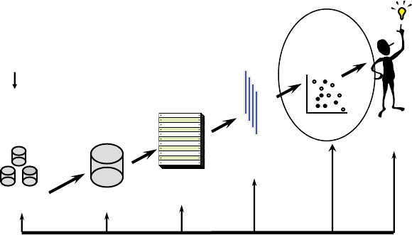
Figure 1.2 gives a

h

ig

h

‐

l

eve

l

overview o

f

t

h

e ana

l

ytics process mo

d

e

l

.

5

As a



rst ste

p

, a t

h

orou

gh

d

e



nition o

f

t

h

e

b

usiness

p

ro

bl

em to

b

e

so

l

ve

d

wit

h

ana

ly

tics is nee

d

e

d

. Next, a

ll

source

d

ata nee

d

to

b

e i

d

enti-



e

d

t

h

at cou

ld

b

e o

f

potentia

l

interest. T

h

is is a very important step, as

d

ata is t

h

e

k

e

y

in

g

re

d

ient to an

y

ana

ly

tica

l

exercise an

d

t

h

e se

l

ection o

f

B

I

G

DATA AND ANALYTI

CS

◂

5

data will have a deterministic im

p

act on the anal

y

tical models that will

b

e built in a subse

q

uent ste

p

. All data will then be

g

athered in a sta

g-

ing area, which could be, for example, a data mart or data warehouse.

Some basic exploratory analysis can be considered here using, for

example, online analytical processing (OLAP) facilities for multidimen

-

sional data analysis (e.g., roll‐up, drill down, slicing and dicing). This

will be followed by a data cleaning step to get rid of all inconsistencies,

such as missing values, outliers, and duplicate data. Additional trans-

formations may also be considered, such as binning, alphanumeric to

numeric codin

g

,

g

eo

g

ra

p

hical a

gg

re

g

ation, and so forth. In the anal

y

t-

ics step, an ana

l

ytica

l

mo

d

e

l

wi

ll

b

e estimate

d

on t

h

e preprocesse

d

an

d

trans

f

orme

d

ata. Di

ff

erent types o

f

ana

l

ytics can

b

e consi

d

ere

d

h

ere

(e.g., to

d

o c

h

urn pre

d

iction,

f

rau

d

etection, customer segmentation,

market basket analysis). Finally, once the model has been built, it will

b

e inter

p

reted and evaluated b

y

the business ex

p

erts. Usuall

y

, man

y

trivial

p

atterns will be detected b

y

the model. For exam

p

le, in a market

b

asket analysis setting, one may  nd that spaghetti and spaghetti sauce

are often

p

urchased to

g

ether. These

p

atterns are interestin

g

because

the

y

p

rovide some validation of the model. But of course, the ke

y

issue

here is to  nd the unexpected yet interesting and actionable patterns

(sometimes also referred to as knowled

g

e diamond

s

) that can

p

rovide

added value in the business settin

g

. Once the anal

y

tical model has

b

een appropriately validated and approved, it can be put into produc-

tion as an anal

y

tics a

pp

lication (e.

g

., decision su

pp

ort s

y

stem, scorin

g

en

g

ine). It is im

p

ortant to consider here how to re

p

resent the model

output in a user‐friendly way, how to integrate it with other applica-

tions (e.

g

., cam

p

ai

g

n mana

g

ement tools, risk en

g

ines), and how to

make sure the analytical model can be appropriately monitored and

b

acktested on an ongoing basis.

It is im

p

ortant to note that the

p

rocess model outlined in Fi

g

-

ure 1.2 is iterative in nature, in t

h

e sense t

h

at one ma

y

h

ave to

g

o

b

ac

k

to

p

revious ste

p

s

d

urin

g

t

h

e exercise. For exam

pl

e,

d

urin

g

t

h

e ana

ly

t-

ics step, t

h

e nee

d

f

or a

dd

itiona

l

d

ata may

b

e i

d

enti



e

d

, w

h

ic

h

may

necessitate a

dd

itiona

l

c

l

eanin

g

, trans

f

ormation, an

d

so

f

ort

h

. A

l

so, t

h

e

most time consumin

g

ste

p

is t

h

e

d

ata se

l

ection an

d

p

re

p

rocessin

g

ste

p

;

t

h

is usua

ll

y ta

k

es aroun

d

80% o

f

t

h

e tota

l

e

ff

orts nee

d

e

d

to

b

ui

ld

an

ana

ly

tica

l

mo

d

e

l

.

6

▸ANALYTI

CS

IN A BI

G

DATA W

O

RL

D

JOB PROFILES INVOLVED

Anal

y

tics is essentiall

y

a multidisci

p

linar

y

exercise in which man

y

different

j

ob

p

ro les need to collaborate to

g

ether. In what follows, we

will discuss the most important job pro les.

The database or data warehouse administrator (DBA) is aware of

all the data available within the  rm, the stora

g

e details, and the data

de nitions. Hence, the DBA plays a crucial role in feeding the analyti

-

cal modelin

g

exercise with its ke

y

in

g

redient, which is data. Because

anal

y

tics is an iterative exercise, the DBA ma

y

continue to

p

la

y

an

important role as the modeling exercise proceeds.

Another ver

y

im

p

ortant

p

ro le is the business ex

p

ert. This could,

for exam

p

le, be a credit

p

ortfolio mana

g

er, fraud detection ex

p

ert,

b

rand manager, or e‐commerce manager. This person has extensive

b

usiness experience an

d

b

usiness common sense, w

h

ic

h

is very va

l

u-

able. It is

p

recisel

y

this knowled

g

e that will hel

p

to steer the anal

y

tical

mo

d

e

l

in

g

exercise an

d

inter

p

ret its

k

e

y



n

d

in

g

s. A

k

e

y

c

h

a

ll

en

g

e

h

ere

is t

h

at muc

h

o

f

t

h

e expert

k

now

l

e

d

ge is tacit an

d

may

b

e

h

ar

d

to e

l

icit

at t

h

e start o

f

t

h

e mo

d

e

l

in

g

exercise.

Le

g

a

l

ex

p

erts are

b

ecomin

g

more an

d

more im

p

ortant

g

iven t

h

at

not a

ll

d

ata can

b

e use

d

in an ana

l

ytica

l

mo

d

e

l

b

ecause o

f

privacy,

Fi

g

ure 1.2 The Anal

y

tics Process Model

Understanding

what data is

needed for the

application

Data Cleaning

Interpretation

and

Evaluation

Data

Transformation

(binning, alpha to

numeric, etc.)

Analytics

Data

Selection

Source

Data

Analytics

Application

Preprocessed

Data

Transformed

Data

Patterns

Data Mining

Mart

Dumps of Operational Data

B

IG DATA AND ANALYTICS ◂

7

discrimination, and so forth. For exam

p

le, in credit risk modelin

g

, one

can t

yp

icall

y

not discriminate

g

ood and bad customers based u

p

on

gender, national origin, or religion. In web analytics, information is

typically gathered by means of cookies, which are  les that are stored

on the user’s browsing computer. However, when gathering informa-

tion using cookies, users should be appropriately informed. This is sub-

j

ect to regulation at various levels (both national and, for example,

European). A key challenge here is that privacy and other regulation

highly vary depending on the geographical region. Hence, the legal

ex

p

ert should have

g

ood knowled

g

e about what data can be used

w

h

en, an

d

w

h

at regu

l

ation app

l

ies in w

h

at

l

ocation.

T

h

e

d

ata scientist,

d

ata miner, or

d

ata ana

l

yst is t

h

e person respon

-

si

bl

e

f

or

d

oing t

h

e actua

l

ana

l

ytics. T

h

is person s

h

ou

ld

possess a t

h

or

-

ough understanding of all techniques involved and know how to

im

p

lement them usin

g

the a

pp

ro

p

riate software. A

g

ood data scientist

should also have

g

ood communication and

p

resentation skills to re

p

ort

the analytical  ndings back to the other parties involved.

The software tool vendors should also be mentioned as an

im

p

ortant

p

art of the anal

y

tics team. Different t

yp

es of tool vendors can

b

e distinguished here. Some vendors only provide tools to automate

s

p

eci c ste

p

s of the anal

y

tical modelin

g

p

rocess (e.

g

., data

p

re

p

rocess-

in

g

). Others sell software that covers the entire anal

y

tical modelin

g

process. Some vendors also provide analytics‐based solutions for spe-

ci c a

pp

lication areas, such as risk mana

g

ement, marketin

g

anal

y

tics

and cam

p

ai

g

n mana

g

ement, and so on.

ANALYTICS

A

nal

y

tics is a term that is often used interchan

g

eabl

y

with

d

ata science

,

data mining, knowledge discovery

,

and others. The distinction between

all those is not clear cut. All of these terms essentiall

y

refer to extract-

ing use

f

u

l

b

usiness patterns or mat

h

ematica

l

d

ecision mo

d

e

l

s

f

rom a

p

re

p

rocesse

d

ata set. Di

ff

erent un

d

er

ly

in

g

tec

h

ni

q

ues can

b

e use

d

f

or

t

h

is

p

ur

p

ose, stemmin

g

f

rom a variet

y

o

f

d

i

ff

erent

d

isci

pl

ines, suc

h

as:

■ Statistics (e.g.,

l

inear an

d

l

ogistic regression)

■ Mac

h

ine

l

earnin

g

(e.

g

.,

d

ecision trees)

8

▸ANALYTI

CS

IN A BI

G

DATA W

O

RL

D

■ Biolo

gy

(e.

g

., neural networks,

g

enetic al

g

orithms, swarm intel

-

l

i

g

ence)

■ Kernel methods (e.

g

., su

pp

ort vector machines)

Basically, a distinction can be made between predictive and descrip

-

tive analytics. In predictive analytics, a target variable is typically avail

-

able, which can either be categorical (e.g., churn or not, fraud or not)

or continuous (e.g., customer lifetime value, loss given default). In

descriptive analytics, no such target variable is available. Common

exam

p

les here are association rules, se

q

uence rules, and clusterin

g

.

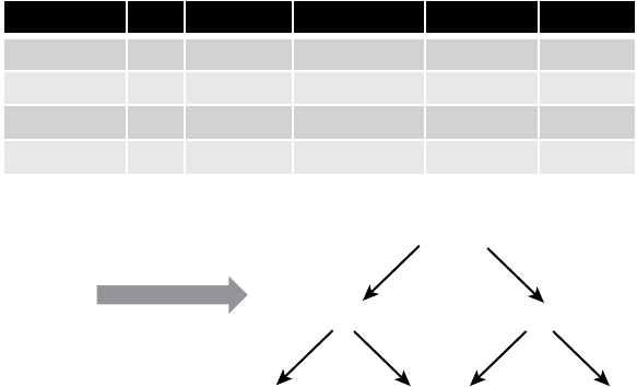
Figure 1.3 provi

d

es an examp

l

e o

f

a

d

ecision tree in a c

l

assi



cation

pre

d

ictive ana

l

ytics setting

f

or pre

d

icting c

h

urn.

More t

h

an ever

b

e

f

ore, ana

l

ytica

l

mo

d

e

l

s steer t

h

e strategic ris

k

decisions of companies. For example, in a bank setting, the mini-

mum e

q

uit

y

and

p

rovisions a  nancial institution holds are directl

y

determined b

y

, amon

g

other thin

g

s, credit risk anal

y

tics, market risk

analytics, operational risk analytics, fraud analytics, and insurance

risk anal

y

tics. In this settin

g

, anal

y

tical model errors directl

y

affect

p

ro tabilit

y

, solvenc

y

, shareholder value, the macroeconom

y

, and

society as a whole. Hence, it is of the utmost importance that analytical

F

i

gure 1.3 Example o

f

Classi



cation Predictive Analytics

Customer Age Recency Frequency Monetary Churn

John 35 5 6 100 Yes

Sophie 18 10 2 150 No

Victor 38 28 8 20 No

Laura 44 12 4 280 Yes

Analytics

Software

Age < 40

Yes

Churn No Churn Churn No Churn

Yes

No

No No

Recency < 10 Frequency < 5

B

I

G

DATA AND ANALYTI

CS

◂

9

models are develo

p

ed in the most o

p

timal wa

y

, takin

g

into account

various re

q

uirements that will be discussed in what follows.

ANALYTICAL MODEL REQUIREMENTS

A good analytical model should satisfy several requirements, depend-

ing on the application area. A  rst critical success factor is business

relevance. The analytical model should actually solve the business

problem for which it was developed. It makes no sense to have a work

-

in

g

anal

y

tical model that

g

ot sidetracked from the ori

g

inal

p

roblem

statement. In or

d

er to ac

h

ieve

b

usiness re

l

evance, it is o

f

k

ey impor-

tance t

h

at t

h

e

b

usiness pro

bl

em to

b

e so

l

ve

d

is appropriate

l

y

d

e



ne

d

,

qua

l

i



e

d

, an

d

agree

d

upon

b

y a

ll

parties invo

l

ve

d

at t

h

e outset o

f

t

h

e

analysis.

A second criterion is statistical

p

erformance. The model should

have statistical si

g

ni cance and

p

redictive

p

ower. How this can be mea-

sured will depend upon the type of analytics considered. For example,

in a classi cation settin

g

(churn, fraud), the model should have

g

ood

discrimination

p

ower. In a clusterin

g

settin

g

, the clusters should be as

homogenous as possible. In later chapters, we will extensively discuss

various measures to

q

uantif

y

this.

De

p

endin

g

on the a

pp

lication, anal

y

tical models should also be

interpretable and justi able. Interpretability refers to understanding

the

p

atterns that the anal

y

tical model ca

p

tures. This as

p

ect has a

certain de

g

ree of sub

j

ectivism, since inter

p

retabilit

y

ma

y

de

p

end on

the business user’s knowledge. In many settings, however, it is con

-

sidered to be a ke

y

re

q

uirement. For exam

p

le, in credit risk modelin

g

or medical diagnosis, interpretable models are absolutely needed to

get good insight into the underlying data patterns. In other settings,

such as res

p

onse modelin

g

and fraud detection, havin

g

inter

p

retable

mo

d

e

l

s ma

y

b

e

l

ess o

f

an issue.

J

usti



a

b

i

l

it

y

re

f

ers to t

h

e

d

e

g

ree to

w

h

ic

h

a mo

d

e

l

corres

p

on

d

s to

p

rior

b

usiness

k

now

l

e

dg

e an

d

intu

-

i

t

i

on.

6

For examp

l

e, a mo

d

e

l

stating t

h

at a

h

ig

h

er

d

e

b

t ratio resu

l

ts

in more cre

d

itwort

hy

c

l

ients ma

y

b

e inter

p

reta

bl

e,

b

ut is not

j

usti



-

a

bl

e

b

ecause it contra

d

icts

b

asic



nancia

l

intuition. Note t

h

at

b

ot

h

interpreta

b

i

l

ity an

d

justi



a

b

i

l

ity o

f

ten nee

d

to

b

e

b

a

l

ance

d

against

statistica

l

p

er

f

ormance. O

f

ten one wi

ll

o

b

serve t

h

at

h

i

gh

p

er

f

ormin

g

10

▸

A

NALYTI

CS

IN A BI

G

DATA W

O

RL

D

anal

y

tical models are incom

p

rehensible and black box in nature.

A

p

o

p

ular exam

p

le of this is neural networks, which are universal

approximators and are high performing, but offer no insight into the

underlying patterns in the data. On the contrary, linear regression

models are very transparent and comprehensible, but offer only

limited modeling power.

Analytical models should also be

operationally ef cient

. This refers to

t

the efforts needed to collect the data, preprocess it, evaluate the model,

and feed its outputs to the business application (e.g., campaign man-

a

g

ement, ca

p

ital calculation). Es

p

eciall

y

in a real‐time online scorin

g

environment (e.g.,

f

rau

d

etection) t

h

is may

b

e a crucia

l

c

h

aracteristic.

Operationa

l

e

f

ciency a

l

so entai

l

s t

h

e e

ff

orts nee

d

e

d

to monitor an

d

b

ac

k

test t

h

e mo

d

e

l

, an

d

reestimate it w

h

en necessary.

Another key attention point is the

e

co

n

omic cos

t

needed to set up

t

the anal

y

tical model. This includes the costs to

g

ather and

p

re

p

rocess

the data, the costs to anal

y

ze the data, and the costs to

p

ut the result-

ing analytical models into production. In addition, the software costs

and human and com

p

utin

g

resources should be taken into account

here. It is im

p

ortant to do a thorou

g

h cost–bene t anal

y

sis at the start

of the project.

Finall

y

, anal

y

tical models should also com

p

l

y

with both local and

in

t

erna

t

ional re

g

ulation and le

g

islation . For exam

p

le, in a credit risk set

-

ting, the Basel II and Basel III Capital Accords have been introduced

to a

pp

ro

p

riatel

y

identif

y

the t

yp

es of data that can or cannot be used

to build credit risk models. In an insurance settin

g

, the Solvenc

y

II

Accord plays a similar role. Given the importance of analytics nowa

-

da

y

s, more and more re

g

ulation is bein

g

introduced relatin

g

to the

development and use of the analytical models. In addition, in the con-

text of privacy, many new regulatory developments are taking place at

various levels. A

p

o

p

ular exam

p

le here concerns the use of cookies in

a we

b

ana

ly

tics context.

NOTES

1. IBM, www.i

b

m.com/

b

i

g

‐

d

ata/us/en , 2013.

2. www.

g

artner.com/tec

h

no

l

o

gy

/to

p

ics/

b

i

g

‐

d

ata.

j

s

p

.

3. www.

kd

nu

gg

ets.com/

p

o

ll

s/2013/

l

ar

g

est‐

d

ataset‐ana

ly

ze

d

‐

d

ata‐mine

d

‐2013.

h

tm

l

.

4. www.

kd

nu

gg

ets.com/

p

o

ll

s/2013/ana

ly

tics‐

d

ata‐science‐e

d

ucation.

h

tm

l

.

BI

G

DATA AND ANALYTI

CS

◂

11

5. J. Han an

d

M. Kam

b

er, Data Minin

g

: Concepts an

d

Tec

h

niques

,

2n

d

e

d

. (Mor

g

an

Kaufmann, Waltham, MA, US, 2006); D. J. Hand, H. Mannila, and P. Sm

y

th, Prin-

ciples of Data Minin

g

(MIT Press, Cambrid

g

e

,

Massachusetts, London, En

g

land, 2001);

P. N. Tan, M. Steinbach, and V. Kumar, Introduction to Data Mining (Pearson, Upper

Saddle River, New Jerse

y

, US, 2006).

6. D. Martens, J. Vanthienen, W. Verbeke, and B. Baesens, “Performance of Classi ca

-

tion Models from a User Perspective.” Special issue,

D

ecision Support System

s

51, no. 4

(

2011

)

: 782–793.

13

C

HAPTER

2

Data Collection,

Sampling, and

Preprocessing

D ata are

k

ey ingre

d

ients

f

or any ana

l

ytica

l

exercise. Hence, it is

im

p

ortant to t

h

orou

ghly

consi

d

er an

d

l

ist a

ll

d

ata sources t

h

at are

o

f

p

otentia

l

interest

b

e

f

ore startin

g

t

h

e ana

ly

sis. T

h

e ru

l

e

h

ere is

t

h

e more

d

ata, t

h

e

b

etter. However, rea

l

i

f

e

d

ata can

b

e

d

irty

b

ecause

o

f

inconsistencies, incom

pl

eteness,

d

u

pl

ication, an

d

mer

g

in

g

p

ro

bl

ems.

T

h

rou

gh

out t

h

e ana

ly

tica

l

mo

d

e

l

in

g

ste

p

s, various

d

ata



l

terin

g

mec

h

a

-

nisms wi

ll

b

e app

l

ie

d

to c

l

ean up an

d

re

d

uce t

h

e

d

ata to a managea

bl

e

an

d

re

l

evant size. Wort

h

mentionin

g

h

ere is t

h

e

g

ar

b

a

g

e in,

g

ar

b

a

g

e

out (GIGO)

p

rinci

pl

e, w

h

ic

h

essentia

lly

states t

h

at mess

y

d

ata wi

ll

y

ie

ld

messy ana

l

ytica

l

mo

d

e

l

s. It is o

f

t

h

e utmost importance t

h

at every

d

ata

p

re

p

rocessin

g

ste

p

is care

f

u

lly

j

usti



e

d

, carrie

d

out, va

l

i

d

ate

d

, an

d

oc

-

umente

d

b

e

f

ore

p

rocee

d

in

g

wit

h

f

urt

h

er ana

ly

sis. Even t

h

e s

l

i

gh

test

mista

k

e can ma

k

e t

h

e

d

ata tota

ll

y unusa

bl

e

f

or

f

urt

h

er ana

l

ysis. In w

h

at

f

o

ll

ows, we wi

ll

e

l

a

b

orate on t

h

e most im

p

ortant

d

ata

p

re

p

rocessin

g

steps t

h

at s

h

ou

ld

b

e consi

d

ere

d

uring an ana

l

ytica

l

mo

d

e

l

ing exercise.

TYPES OF DATA SOURCES

As previously mentioned, more data is better to start off the analysis.

Data can ori

g

inate from a variet

y

of different sources, which will be

ex

p

lored in what follows.

1

4

▸

A

NALYTI

CS

IN A BI

G

DATA W

O

RL

D

Transactions are the  rst im

p

ortant source of data. Transactional

data consist of structured, low‐level, detailed information ca

p

turin

g

the key characteristics of a customer transaction (e.g., purchase, claim,

cash transfer, credit card payment). This type of data is usually stored

in massive online transaction processing (OLTP) relational databases.

It can also be summarized over longer time horizons by aggregating it

into averages, absolute/relative trends, maximum/minimum values,

and so on.

Unstructured data embedded in text documents (e.g., emails, web

p

a

g

es, claim forms) or multimedia content can also be interestin

g

to

ana

l

yze. However, t

h

ese sources typica

ll

y require extensive preprocess

-

ing

b

e

f

ore t

h

ey can

b

e success

f

u

ll

y inc

l

u

d

e

d

in an ana

l

ytica

l

exercise.

Anot

h

er important source o

f

d

ata is qua

l

itative, expert‐

b

ase

d

data. An expert is a person with a substantial amount of subject mat-

ter ex

p

ertise within a

p

articular settin

g

(e.

g

., credit

p

ortfolio mana

g

er,

b

rand mana

g

er). The ex

p

ertise stems from both common sense and

b

usiness experience, and it is important to elicit expertise as much as

p

ossible before the anal

y

tics is run. This will steer the modelin

g

in the

ri

g

ht direction and allow

y

ou to inter

p

ret the anal

y

tical results from

the right perspective. A popular example of applying expert‐based

validation is checkin

g

the univariate si

g

ns of a re

g

ression model. For

exam

p

le, one would ex

p

ect a

p

rior

i

that higher debt has an adverse

i

impact on credit risk, such that it should have a negative sign in the

 nal scorecard. If this turns out not to be the case (e.

g

., due to bad

data

q

ualit

y

, multicollinearit

y

), the ex

p

ert/business user will not be

tempted to use the analytical model at all, since it contradicts prior

ex

p

ectations.

Nowadays, data poolers are becoming more and more important

in the industry. Popular examples are Dun & Bradstreet, Bureau Van

Di

j

ck, and Thomson Reuters. The core business of these com

p

anies

is to

g

at

h

er

d

ata in a

p

articu

l

ar settin

g

(e.

g

., cre

d

it ris

k

, mar

k

etin

g

),

b

ui

ld

mo

d

e

l

s wit

h

it, an

d

se

ll

t

h

e out

p

ut o

f

t

h

ese mo

d

e

l

s (e.

g

., scores),

possi

bl

y toget

h

er wit

h

t

h

e un

d

er

l

ying raw

d

ata, to intereste

d

custom

-

ers. A

p

o

p

u

l

ar exam

pl

e o

f

t

h

is in t

h

e Unite

d

States is t

h

e FICO score,

w

h

ic

h

is a cre

d

it score ran

g

in

g

b

etween 300 an

d

850 t

h

at is

p

rovi

d

e

d

b

y t

h

e t

h

ree most important cre

d

it

b

ureaus: Experian, Equi

f

ax, an

d

Transunion. Man

y



nancia

l

institutions use t

h

ese FICO scores eit

h

er

D

ATA

CO

LLE

C

TI

O

N

,

S

AMPLIN

G,

AND PREPR

OC

E

SS

IN

G

◂

15

as their  nal internal model, or as a benchmark a

g

ainst an internall

y

develo

p

ed credit scorecard to better understand the weaknesses of

the latter.

Finally, plenty of publicly available data can be included in the

analytical exercise. A  rst important example is macroeconomic data

about gross domestic product (GDP), in ation, unemployment, and so

on. By including this type of data in an analytical model, it will become

possible to see how the model varies with the state of the economy.

This is especially relevant in a credit risk setting, where typically all

models need to be thorou

g

hl

y

stress tested. In addition, social media

d

ata

f

rom Face

b

oo

k

, Twitter, an

d

ot

h

ers can

b

e an important source

o

f

in

f

ormation. However, one nee

d

s to

b

e care

f

u

l

h

ere an

d

ma

k

e sure

t

h

at a

ll

d

ata gat

h

ering respects

b

ot

h

l

oca

l

an

d

internationa

l

privacy

regulations.

SAMPLING

The aim of sam

p

lin

g

is to take a subset of

p

ast customer data and use

that to build an anal

y

tical model. A  rst obvious

q

uestion concerns the

need for sampling. With the availability of high performance comput-

in

g

facilities (e.

g

.,

g

rid/cloud com

p

utin

g

), one could also directl

y

ana-

l

y

ze the full data set. However, a ke

y

re

q

uirement for a

g

ood sam

p

le

is that it should be representative of the future customers on which

the anal

y

tical model will be run. Hence, the timin

g

as

p

ect becomes

im

p

ortant because customers of toda

y

are more similar to customers

of tomorrow than customers of yesterday. Choosing the optimal time

window for the sam

p

le involves a trade‐off between lots of data (and

hence a more robust analytical model) and recent data (which may be

more representative). The sample should also be taken from an aver-

a

g

e business

p

eriod to

g

et a

p

icture of the tar

g

et

p

o

p

ulation that is as

accurate as

p

ossi

bl

e.

It s

p

ea

k

s

f

or itse

lf

t

h

at sam

pl

in

g

b

ias s

h

ou

ld

b

e avoi

d

e

d

as muc

h

as possi

bl

e. However, t

h

is is not a

l

ways straig

h

t

f

orwar

d

. Let’s ta

k

e

t

h

e exam

pl

e o

f

cre

d

it scorin

g

. Assume one wants to

b

ui

ld

an a

ppl

ica-

tion scorecar

d

to score mort

g

a

g

e a

ppl

ications. T

h

e

f

uture

p

o

p

u

l

ation

t

h

en consists o

f

a

ll

customers w

h

o come to t

h

e

b

an

k

an

d

app

l

y

f

or

a mort

g

a

g

e—t

h

e so‐ca

ll

e

d

t

h

rou

gh

‐t

h

e‐

d

oor (TTD)

p

o

p

u

l

ation. One

16

▸

A

NALYTI

CS

IN A BI

G

DATA W

O

RL

D

then needs a subset of the historical TTD population to build an ana

-

l

ytica

l

mo

d

e

l

. However, in t

h

e past, t

h

e

b

an

k

was a

l

rea

d

y app

l

ying

a cre

d

it po

l

icy (eit

h

er expert

b

ase

d

or

b

ase

d

on a previous ana

l

ytica

l

mo

d

e

l

). T

h

is imp

l

ies t

h

at t

h

e

h

istorica

l

TTD popu

l

ation

h

as two su

b

sets:

the customers that were acce

p

ted with the old

p

olic

y

, and the ones that

were re

j

ected (see Fi

g

ure 2.1 ). Obviousl

y

, for the latter, we don’t know

the target value since they were never granted the credit. When build

-

in

g

a sam

p

le, one can then onl

y

make use of those that were acce

p

ted,

which clearl

y

im

p

lies a bias. Procedures for re

j

ect inference have been

suggested in the literature to deal with this sampling bias problem.

1

Unfortunatel

y

, all of these

p

rocedures make assum

p

tions and none of

them works

p

erfectl

y

. One of the most

p

o

p

ular solutions is bureau

‐

based inference, whereby a sample of past customers is given to the

credit bureau to determine their tar

g

et label (

g

ood or bad

p

a

y

er).

When thinkin

g

even closer about the tar

g

et

p

o

p

ulation for credit

scoring, another forgotten subset are the withdrawals. These are

the customers who were offered credit but decided not to take it

(

des

p

ite the fact that the

y

ma

y

have been classi ed as

g

ood b

y

the

old scorecard). To be representative, these customers should also be

included in the develo

p

ment sam

p

le. However, to the best of our

knowled

g

e, no

p

rocedures for withdrawal inference are t

yp

icall

y

a

pp

lied in the industr

y

.

In strati



e

d

samp

l

ing, a samp

l

e is ta

k

en accor

d

ing to pre

d

e



ne

d

strata. Consi

d

er,

f

or exam

pl

e, a c

h

urn

p

re

d

iction or

f

rau

d

etection

context in w

h

ic

h

d

ata sets are t

yp

ica

lly

ver

y

s

k

ewe

d

(e.

g

., 99

p

ercent

nonc

h

urners an

d

1 percent c

h

urners). W

h

en strati

f

ying accor

d

ing to

t

h

e tar

g

et c

h

urn in

d

icator, t

h

e sam

pl

e wi

ll

contain exact

ly

t

h

e same

p

ercenta

g

es o

f

c

h

urners an

d

nonc

h

urners as in t

h

e ori

g

ina

l

d

ata.

Figure 2.1 The Reject Inference Problem in Credit Scoring

Through-the-Door

Rejects Accepts

Bads Goods ? Bads ? Goods

D

ATA COLLECTION, SAMPLING, AND PREPROCESSING ◂

17

TYPES OF DATA ELEMENTS

It is important to appropriately consider the different types of data ele

-

ments at the start of the anal

y

sis. The followin

g

t

yp

es of data elements

can be considered:

■ Continuous: These are data elements that are de ned on an

interval that can be limited or unlimited. Examples include

income, sales, RFM (recency, frequency, monetary).

■ Categorical

■ Nomina

l

: T

h

ese are

d

ata e

l

ements t

h

at can on

l

y ta

k

e on a

l

imite

d

set o

f

va

l

ues wit

h

no meaning

f

u

l

or

d

ering in

b

etween.

Examp

l

es inc

l

u

d

e marita

l

status, pro

f

ession, purpose o

f

l

oan.

■ Ordinal: These are data elements that can onl

y

take on a lim

-

ited set of values with a meaningful ordering in between.

Exam

p

les include credit ratin

g

; a

g

e coded as

y

oun

g

, middle

aged, and old.

■ Binar

y

: These are data elements that can onl

y

take on two

values. Examples include gender, employment status.

A

pp

ro

p

riatel

y

distin

g

uishin

g

between these different data elements

is of ke

y

im

p

ortance to start the anal

y

sis when im

p

ortin

g

the data

into an analytics tool. For example, if marital status were to be incor-

rectl

y

s

p

eci ed as a continuous data element, then the software would

calculate its mean, standard deviation, and so on, which is obviousl

y

meaningless.

VISUAL DATA EXPLORATION AND EXPLORATORY

STATISTICAL ANALYSIS

Visual data ex

p

loration is a ver

y

im

p

ortant

p

art of

g

ettin

g

to know

y

our

d

ata in an “in

f

orma

l

” wa

y

. It a

ll

ows

y

ou to

g

et some initia

l

insig

h

ts into t

h

e

d

ata, w

h

ic

h

can t

h

en

b

e use

f

u

ll

y a

d

opte

d

t

h

roug

h

out

t

h

e mo

d

e

l

in

g

. Di

ff

erent

pl

ots/

g

ra

ph

s can

b

e use

f

u

l

h

ere. A



rst

p

o

p

u-

l

ar exam

pl

e is

p

ie c

h

arts. A

p

ie c

h

art re

p

resents a varia

bl

e’s

d

istri

b

u

-

tion as a pie, w

h

ere

b

y eac

h

section represents t

h

e portion o

f

t

h

e tota

l

p

ercent ta

k

en

by

eac

h

va

l

ue o

f

t

h

e varia

bl

e. Fi

g

ure 2.2 re

p

resents a

p

ie

c

h

art

f

or a

h

ousin

g

varia

bl

e

f

or w

h

ic

h

one’s status can

b

e own, rent, or

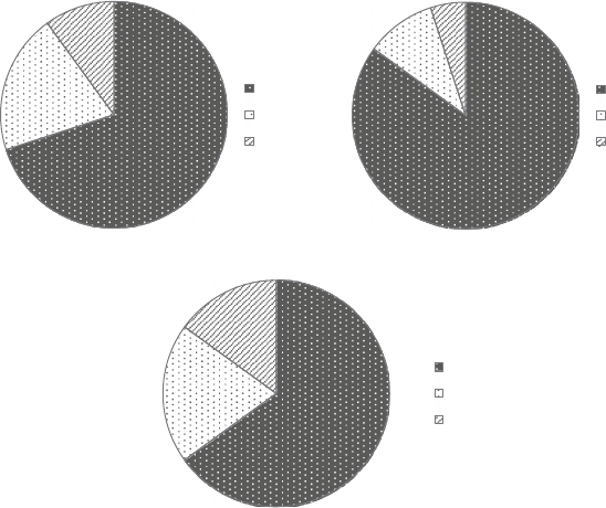
1

8

▸

A

NALYTI

CS

IN A BI

G

DATA W

O

RL

D

for free (e.

g

., live with

p

arents). B

y

doin

g

a se

p

arate

p

ie chart anal

y

sis

for the goods and bads, respectively, one can see that more goods own

their residential

p

ro

p

ert

y

than bads, which can be a ver

y

useful start

-

in

g

insi

g

ht. Bar charts re

p

resent the fre

q

uenc

y

of each of the values

(

either absolute or relative) as bars. Other handy visual tools are histo

-

g

rams and scatter

p

lots. A histo

g

ram

p

rovides an eas

y

wa

y

to visualize

the central tendency and to determine the variability or spread of the

data. It also allows you to contrast the observed data with standard

known distributions (e.

g

., normal distribution). Scatter

p

lots allow

y

ou

to visua

l

ize one varia

bl

e a

g

ainst anot

h

er to see w

h

et

h

er t

h

ere are an

y

corre

l

ation

p

atterns in t

h

e

d

ata. A

l

so, OLAP‐

b

ase

d

mu

l

ti

d

imensiona

l

d

ata ana

l

ysis can

b

e use

f

u

ll

y a

d

opte

d

to exp

l

ore patterns in t

h

e

d

ata.

A next ste

p

a

f

ter visua

l

ana

ly

sis cou

ld

b

e ins

p

ectin

g

some

b

asic

statistica

l

measurements, suc

h

as avera

g

es, stan

d

ar

d

eviations, mini-

mum, maximum, percenti

l

es, an

d

con



d

ence interva

l

s. One cou

ld

ca

l

cu

l

ate t

h

ese measures se

p

arate

ly

f

or eac

h

o

f

t

h

e tar

g

et c

l

asses

Fi

g

ure 2.2 Pie Charts

f

or Explorator

y

Data Anal

y

sis

Total Population

Own

Rent

For Free

Goods

Own

Rent

For Free

Bads

Own

Rent

For Free

D

ATA

CO

LLE

C

TI

O

N

,

S

AMPLIN

G,

AND PREPR

OC

E

SS

IN

G

◂

19

(e.

g

.,

g

ood versus bad customer) to see whether there are an

y

interest-

in

g

p

atterns

p

resent (e.

g

., whether bad

p

a

y

ers usuall

y

have a lower

average age than good payers).

MISSING VALUES

Missing values can occur because of various reasons. The information

can be nonapplicable. For example, when modeling time of churn,

this information is only available for the churners and not for the non-

churners because it is not applicable there. The information can also

b

e un

d

isc

l

ose

d

. For examp

l

e, a customer

d

eci

d

e

d

not to

d

isc

l

ose

h

is or

h

er income

b

ecause o

f

privacy. Missing

d

ata can a

l

so originate

b

ecause

o

f

an error

d

uring merging (e.g., typos in name or ID).

Some anal

y

tical techni

q

ues (e.

g

., decision trees) can directl

y

deal

with missin

g

values. Other techni

q

ues need some additional

p

re

p

ro-

cessing. The following are the most popular schemes to deal with miss-

in

g

values:

2

■ Replace (impute). This implies replacing the missing value

with a known value (e.

g

., consider the exam

p

le in Table 2.1 ).

One could im

p

ute the missin

g

credit bureau scores with the

average or median of the known values. For marital status, the

mode can then be used. One could also a

pp

l

y

re

g

ression‐based

im

p

utation whereb

y

a re

g

ression model is estimated to model

a target variable (e.g., credit bureau score) based on the other

information available (e.

g

., a

g

e, income). The latter is more

sophisticated, although the added value from an empirical view

-

point (e.g., in terms of model performance) is questionable.

■

Delete.

This is the most straightforward option and consists of

deletin

g

observations or variables with lots of missin

g

values. This,

of course, assumes that information is missin

g

at random and has

no meanin

gf

u

l

inter

p

retation an

d

/or re

l

ations

h

i

p

to t

h

e tar

g

et.

■

K

ee

p

. Missing va

l

ues can

b

e meaning

f

u

l

(e.g., a customer

d

i

d

not

d

isc

l

ose

h

is or

h

er income

b

ecause

h

e or s

h

e is current

ly

unem

pl

o

y

e

d

). O

b

vious

ly

, t

h

is is c

l

ear

ly

re

l

ate

d

to t

h

e tar

g

et

(e.g., goo

d

/

b

a

d

ris

k

or c

h

urn) an

d

nee

d

s to

b

e consi

d

ere

d

as a

se

p

arate cate

g

or

y

.

20

▸

A

NALYTI

CS

IN A BI

G

DATA W

O

RL

D

As a

p

ractical wa

y

of workin

g

, one can  rst start with statisticall

y

testing whether missing information is related to the target variable

(

usin

g

, for exam

p

le, a chi‐s

q

uared test, discussed later). If

y

es, then we

can ado

p

t the kee

p

strate

gy

and make a s

p

ecial cate

g

or

y

for it. If not,

one can, depending on the number of observations available, decide to

either delete or im

p

ute.

OUTLIER DETECTION AND TREATMENT

Outliers are extreme observations that are very dissimilar to the rest of

the

p

o

p

ulation. Actuall

y

, two t

yp

es of outliers can be considered:

1. Valid observations (e.g., salary of boss is $1 million)

2. Invalid observations (e.

g

., a

g

e is 300

y

ears)

Both are univariate outliers in the sense that they are outlying on

one dimension. However

,

outliers can be hidden in unidimensional

views of the data. Multivariate outliers are observations that are outl

y

-

in

g

in mu

l

ti

pl

e

d

imensions. Fi

g

ure 2.3

g

ives an exam

pl

e o

f

two out

ly

-

in

g

o

b

servations consi

d

erin

g

b

ot

h

t

h

e

d

imensions o

f

income an

d

a

g

e.

Two important steps in

d

ea

l

ing wit

h

out

l

iers are

d

etection an

d

treat

-

ment. A



rst o

b

vious c

h

ec

k

f

or out

l

iers is to ca

l

cu

l

ate t

h

e minimum

an

d

maximum va

l

ues

f

or eac

h

o

f

t

h

e

d

ata e

l

ements. Various

g

ra

ph

ica

l

T

able

2.1 Dea

li

ng w

i

t

h

M

i

ss

i

ng Va

l

ues

ID Age Income Marital

Status Credit Bureau

Score Class

1

34 1,80

0

?

62

0

Churne

r

2

28 1

,

20

0

Sin

g

l

e

?

Nonchurne

r

3

22

1,000

Sin

g

l

e

?

No

n

chu

rn

er

4

60

2

,

200

Wid

owe

d

7

00

Churne

r

5

58 2,00

0

M

arr

i

e

d

?

N

onc

h

urne

r

6

44

?

N

o

n

c

h

u

rn

er

7

22 1,20

0

Singl

e

?

N

onc

h

urne

r

8

2

6

1,50

0

Ma

rri

ed

350

N

o

n

c

h

u

rn

er

9

3

4

?

Sin

g

l

e

?

C

h

u

rn

er

1

0

50

2,10

0

Div

o

r

ced

?

N

o

n

c

h

u

rn

er

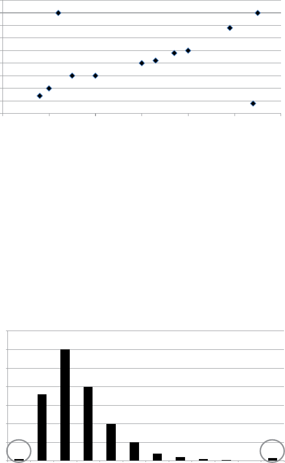
D

ATA COLLECTION, SAMPLING, AND PREPROCESSING ◂

21

tools can be used to detect outliers. Histo

g

rams are a  rst exam

p

le.

Fi

g

ure 2.4

p

resents an exam

p

le of a distribution for a

g

e whereb

y

the

circled areas clearly represent outliers.

Another useful visual mechanism are box plots. A box plot repre

-

sents three ke

y

q

uartiles of the data: the  rst

q

uartile (25

p

ercent of

the observations have a lower value), the median (50 percent of the

observations have a lower value), and the third

q

uartile (75

p

ercent

of the observations have a lower value). All three

q

uartiles are re

p-

resented as a box. The minimum and maximum values are then also

Fi

g

ure 2.3 Multivariate

O

utliers

0

500

1,000

1,500

2,000

2,500

3,000

3,500

4,000

4,500

10 20 30 40 50 60 70

Income and Age

Figure 2.4 Histograms

f

or Outlier Detection

0

500

1,000

1,500

2,000

2,500

3,000

3,500

0–5 20–25 25–30 30–35 35–40 40–45 45–50 50–55 55–60 60–65 65–70 150–200

Age

Frequency

22

▸

A

NALYTICS IN A BIG DATA WORL

D

added unless they are too far away from the edges of the box. Too

far away is then quanti ed as more than 1.5 * Interquartile Range

(

IQR = Q

3

−

Q

1 ). Figure 2.5 gives an examp

l

e o

f

a

b

ox p

l

ot in w

h

ic

h

t

hree ou

t

liers can be seen.

Another wa

y

is to calculate z‐scores, measurin

g

how man

y

stan

-

dard deviations an observation lies awa

y

from the mean, as follows:

=−μ

σ

zx

i

where

μ

represents the average of the variable and

σ

its standard devi

-

ation. An exam

p

le is

g

iven in Table 2.2 . Note that b

y

de nition, the

z

‐scores will have 0 mean and unit standard deviation.

z

A

p

ractical rule of thumb then de nes outliers when the absolute

v

alue of the

z

‐

sco

r

e

z

|

z

|

is bi

gg

er than 3. Note that the

z

‐score relies on

z

t

he normal dis

t

ribu

t

ion.

The above methods all focus on univariate outliers. Multivariate

outliers can be detected b

y

 ttin

g

re

g

ression lines and ins

p

ectin

g

the

Table 2.2 Z‐Scores

f

or Outlier Detection

ID Age Z ‐Score

13

0

(

30 − 40

)

/10 = −

1

2

50

(50 − 40)/10 = +

1

3

1

0

(

10 − 40

)

/10 = −

3

4

40

(40 − 40)

/

10 =

0

5

6

0

(

60 − 40

)

/10 = +

2

6

80

(80 − 40)

/

10 = +

4

…

μ

= 4

0

σ

=

1

0

μ

=

0

σ

=

1

Fi

g

ure 2.5 Box Plots for

O

utlier Detection

Min Q1Q3

M

1.5 * IQR

Outliers

D

ATA COLLECTION

,

SAMPLING

,

AND PREPROCESSING ◂

23

o

b

servations wit

h

l

arge errors (using,

f

or examp

l

e, a resi

d

ua

l

p

l

ot).

A

l

ternative met

h

o

d

s are c

l

ustering or ca

l

cu

l

ating t

h

e Ma

h

a

l

ano

b

is

d

is-

tance. Note, however, that although potentially useful, multivariate

outlier detection is t

yp

icall

y

not considered in man

y

modelin

g

exer-

cises due to the t

yp

ical mar

g

inal im

p

act on model

p

erformance.

Some analytical techniques (e.g., decision trees, neural net

-

works, Su

pp

ort Vector Machines (SVMs)) are fairl

y

robust with

res

p

ect to outliers. Others (e.

g

., linear/lo

g

istic re

g

ression) are more

s

ensitive to them. Various schemes exist to deal with outliers. It

hi

g

hl

y

de

p

ends on whether the outlier re

p

resents a valid or invalid

observation. For invalid observations (e.

g

., a

g

e is 300

y

ears), one

could treat the outlier as a missing value using any of the schemes

discussed in the

p

revious section. For valid observations (e.

g

.,

income is $1 million), other schemes are needed. A popular scheme

is truncation/capping/winsorizing. One hereby imposes both a

lower and u

pp

er limit on a variable and an

y

values below/above

are brought back to these limits. The limits can be calculated using

t

he

z

‐scores (see Figure 2.6 ), or the IQR (which is more robust than

z

t

he

z

‐scores), as follows:

z

Upper/lower limit M 3s, with M median and s IQR/(2 0.6745).3

=± = = ×

A si

g

moi

d

trans

f

ormation ran

g

in

g

b

etween 0 an

d

1 can a

l

so

b

e

use

d

f

or capping, as

f

o

ll

ows:

=+−

fx ex

() 1

1

μ + 3σμ – 3σ μ

F

i

gure 2.6 Using the Z‐Scores for Truncation

2

4

▸

A

NALYTI

CS

IN A BI

G

DATA W

O

RL

D

In addition, ex

p

ert‐based limits based on business knowled

g

e and

/

or ex

p

erience can be im

p

osed.

STANDARDIZING DATA

Standardizing data is a data preprocessing activity targeted at scaling

variables to a similar range. Consider, for example, two variables: gen

-

der (coded as 0/1) and income (ranging between $0 and $1 million).

When building logistic regression models using both information ele-

ments, the coef cient for income might become very small. Hence, it

cou

ld

ma

k

e sense to

b

ring t

h

em

b

ac

k

to a simi

l

ar sca

l

e. T

h

e

f

o

ll

owing

stan

d

ar

d

ization proce

d

ures cou

ld

b

e a

d

opte

d

:

■ Min

/

max s

t

andardiza

t

ion

■ =−

−−+XXX

XX

newmax newmin newmin

new

old old

min( )

max( ) min( )(),

whereby newmax and newmin are the newly imposed maxi-

m

um and minimum (e.

g

., 1 and 0).

■

Z

‐score standardization

Z

■

C

alcula

t

e

t

he

z

‐scores (see the previous section)

z

■ Decimal scalin

g

■ Dividin

g

b

y

a

p

ower of 10 as follows: =XX

new

old

n

10

,

with

n

t

he

n

umber of digits of the maximum absolute value.

A

g

ain note that standardization is es

p

eciall

y

useful for re

g

ression

‐

b

ased approaches, but is not needed for decision trees, for example.

CATEGORIZATION

Cate

g

orization (also known as coarse classi cation, classin

g

,

g

rou

p

in

g

,

b

innin

g

, etc.) can

b

e

d

one

f

or various reasons. For cate

g

orica

l

vari-

a

bl

es, it is nee

d

e

d

to re

d

uce t

h

e num

b

er o

f

cate

g

ories. Consi

d

er,

f

or

examp

l

e, t

h

e varia

bl

e “purpose o

f

l

oan”

h

aving 50

d

i

ff

erent va

l

ues.

W

h

en t

h

is varia

bl

e wou

ld

b

e

p

ut into a re

g

ression mo

d

e

l

, one wou

ld

nee

d

49

d

umm

y

varia

bl

es (50 − 1

b

ecause o

f

t

h

e co

ll

inearit

y

), w

h

ic

h

wou

ld

necessitate t

h

e estimation o

f

49 parameters

f

or on

l

y one vari-

a

bl

e. Wit

h

cate

g

orization, one wou

ld

create cate

g

ories o

f

va

l

ues suc

h

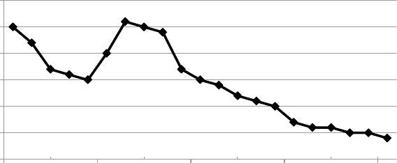
D

ATA COLLECTION

,

SAMPLING

,

AND PREPROCESSING ◂

25

that fewer

p

arameters will have to be estimated and a more robust

model is ob

t

ained.

For continuous variables, categorization may also be very bene

-

cial. Consider, for exam

p

le, the a

g

e variable and its risk as de

p

icted in

Fi

g

ure 2.7 . Clearl

y

, there is a nonmonotonous relation between risk

and age. If a nonlinear model (e.g., neural network, support vector

machine) were to be used, then the nonlinearit

y

can be

p

erfectl

y

mod-

eled. However, if a re

g

ression model were to be used (which is t

yp

i

-

cally more common because of its interpretability), then since it can

onl

y

 t a line, it will miss out on the nonmonotonicit

y

. B

y

cate

g

orizin

g

the variable into ran

g

es,

p

art of the nonmonotonicit

y

can be taken

into account in the regression. Hence, categorization of continuous

variables can be useful to model nonlinear effects into linear models.

Various methods can be used to do categorization. Two very basic

methods are equal interval binning and equal frequency binning.

Consider, for exam

p

le, the income values 1,000, 1,200, 1,300, 2,000,

1,800, and 1,400. Equal interval binning would create two bins with

the same ran

g

e—Bin 1: 1,000, 1,500 and Bin 2: 1,500, 2,000—whereas

e

q

ual fre

q

uenc

y

binnin

g

would create two bins with the same num-

b

er o

f

o

b

servations—Bin 1: 1,000, 1,200, 1,300; Bin 2: 1,400, 1,800,

2,000. However,

b

ot

h

met

h

o

d

s are

q

uite

b

asic an

d

o not ta

k

e into

account a target varia

bl

e (e.g., c

h

urn,

f

rau

d

, cre

d

it ris

k

).

C

h

i‐s

q

uare

d

ana

ly

sis is a more so

ph

isticate

d

wa

y

to

d

o coarse c

l

as

-

si



cation. Consi

d

er t

h

e exam

pl

e

d

e

p

icte

d

in Ta

bl

e 2.3

f

or coarse c

l

as

-

si

f

ying a resi

d

entia

l

status varia

bl

e.

0

5

10

15

20

25

30

16 26 38 51 64 75

F

i

gure 2.7 Default Risk versus Age

26

▸

A

NALYTICS IN A BIG DATA WORL

D

Suppose we want t

h

ree categories an

d

consi

d

er t

h

e

f

o

ll

owing

opt

i

ons:

■ Option 1: owner, renters, ot

h

ers

■ O

p

tion 2: owner, with

p

arents, others

Both options can now be investigated using chi‐squared analysis.

The

p

ur

p

ose is to com

p

are the em

p

iricall

y

observed with the inde

p

en-

dence fre

q

uencies. For o

p

tion 1, the em

p

iricall

y

observed fre

q

uencies

are depicted in Table 2.4 .

The inde

p

endence fre

q

uencies can be calculated as follows. The

number of

g

ood owners,

g

iven that the odds are the same as in the

whole population, is 6,300/10,000

×

9

,

000/10

,

000

×

10

,

000 = 5

,

670.

O

ne

t

hen ob

t

ains Table 2.5 .

The more the numbers in both tables differ, the less inde

p

endence,

hence better dependence and a better coarse classi cation. Formally,

one can calculate the chi‐s

q

uared distance as follows:

χ= −+−+−+−

+−+−=

(6000 5670)

5670

(300 630)

630

(1950 2241)

2241

(540 249)

249

(1050 1089)

1089

(160 121)

121 583

222 22

22

Ta

bl

e 2.3 Coarse Classi

f

ying the Residential Status Variable

Attribute Owner Rent

Unfurnished Rent

Furnished With

Parents Other No

Answer Total

6

,00

0

1

,60

0

3

5

0

9

5

0

9

0

1

0

9

,00

0

B

ads

30

0

4

0

14

0

10

0

5

0

1

0

1,

00

0

Goo

d:

b

a

d

odds

20

:

1

4

:

1

2

.

5

:

1

9

.

5

:

1

.

8

:

1

:

1

9

:

1

Source

:

L. C. Thomas

,

D. Edelman

,

and J. N. Crook

,

Credit Scoring and its Applications

(Society for Industrial and Applied

s

Mathematics, Philadelphia, Penn., 2002).

T

able

2.4 Empirical Frequencies Option 1

f

or Coarse Classi

fy

in

g

Residential Status

Attribute Owner Renters Others Total

G

ood

s

6,00

0

1,95

0

1

,05

0

9

,00

0

B

a

ds

300

5

40

160

1

,

000

Tota

l

6

,

30

0

2

,

49

0

1,

21

0

1

0

,

00

0

D

ATA

CO

LLE

C

TI

O

N,

S

AMPLIN

G

, AND PREPR

OC

E

SS

IN

G

◂

2

7

T

able

2.

5

Independence Frequencies Option 1 for Coarse Classif

y

in

g

Residential Status

Attribute Owner Renters Others Total

G

ood

s

5,67

0

2,24

1

1,08

9

,00

0

B

ads

630

24

9

12

1

,

00

0

T

ota

l

6

,30

0

2,49

0

1,21

0

1

0,00

0

Ta

bl

e 2.6 Coarse Classifying the Purpose Variable

Customer ID Age Purpose … G/B

C

1

44 Ca

r

G

C2

20

Cash

G

C3

58

Tr

a

v

el

B

C

42

6

Car

G

C5

30

Stud

y

B

C

6

32

H

ous

e

G

C

74

8

Cash

B

C

8

60

C

a

r

G

…

Likewise, for option 2, the calculation becomes

:

χ= −+−+−+−

+−+−=

(6000 5670)

5670

(300 630)

630

(950 945)

945

(100 105)

105

(2050 2385)

2385

(600 265)

265 662

22222

22

So, based u

p

on the chi‐s

q

uared values, o

p

tion 2 is the better cat

-

egorization. Note that formally, one needs to compare the value with

a chi‐s

q

uared distribution with

k

− 1 degrees of freedom with

k

being

k

the number of

v

alues of the characteristic.

Many analytics software tools have built‐in facilities to do catego

-

rization usin

g

chi‐s

q

uared anal

y

sis. A ver

y

hand

y

and sim

p

le a

pp

roach

(available in Microsoft Excel) is

p

ivot tables. Consider the exam

p

le

shown in Table 2.6

.

One can then construct a

p

ivot table and calculate the odds as

sho

w

n in Table 2.7

.

2

8

▸

A

NALYTI

CS

IN A BI

G

DATA W

O

RL

D

We can then categorize the values based on similar odds. For

example, category 1 (car, study), category 2 (house), and category 3

(

cash, travel).

WEIGHTS OF EVIDENCE CODING

Categorization reduces the number of categories for categorical vari

-

ables. For continuous variables, cate

g

orization will introduce new

variables. Consider a re

g

ression model with a

g

e (4 cate

g

ories, so 3

parameters) and purpose (5 categories, so 4 parameters) characteris-

tics. The model then looks as follows:

YAge Age Age Purp

Purp Purp Purp

01 12 23 34 1

526374

=β +β +β +β +β

+β +β +β

Des

p

ite havin

g

onl

y

two characteristics, the model still needs 8

p

arameters to be estimated. It would be hand

y

to have a monotonic

transformation

f

(

.) such that our model could be rewritten as follows:

f

=β +β +βYf f(Age , Age , Age ) (Purp , Purp , Purp , Purp )

01 1 2 3 2 1 2 3 4

The transformation should have a monotonically increasing or

decreasing relationship with

Y

. Weights‐of‐evidence coding is one

exam

p

le of a transformation that can be used for this

p

ur

p

ose. This is

illus

t

ra

t

ed in Table 2.8 .

The WOE is calculated as: ln(Distr. Good/Distr. Bad). Because of

t

h

e

l

ogarit

h

mic trans

f

ormation, a positive (negative) WOE means

Distr. Goo

d

> (<) Distr. Ba

d

. T

h

e WOE trans

f

ormation t

h

us im

pl

e

-

ments a trans

f

ormation monotonica

lly

re

l

ate

d

to t

h

e tar

g

et varia

bl

e.

T

h

e mo

d

e

l

can t

h

en

b

e re

f

ormu

l

ate

d

as

f

o

ll

ows

:

YWOE WOE

0 1 age 2 purpose

=β +β +β

Table 2.7 Pivot Table for Coarse Classifying the Purpose Variable

Car Cash Travel Study House …

G

ood

1

,00

0

2

,00

0

3,00

0

10

0

5

,00

0

B

ad

50

0

1

0

20

0

80 80

0

Odds

2

20

1

5

1.2

5

6

.2

5

D

ATA

CO

LLE

C

TI

O

N

,

S

AMPLIN

G,

AND PREPR

OC

E

SS

IN

G

◂

29

T

h

is gives a more concise mo

d

e

l

t

h

an t

h

e mo

d

e

l

wit

h

w

h

ic

h

we

started this section. However, note that the interpretability of the

model becomes somewhat less strai

g

htforward when WOE variables

are bein

g

used.

VARIABLE SELECTION

Many analytical modeling exercises start with tons of variables, of

which t

yp

icall

y

onl

y

a few actuall

y

contribute to the

p

rediction of

the tar

g

et variable. For exam

p

le, the avera

g

e a

pp

lication/behavioral

scorecard in credit scoring has somewhere between 10 and 15 vari-

ables. The ke

y

q

uestion is how to  nd these variables. Filters are a

very handy variable selection mechanism. They work by measuring

univariate correlations between each variable and the target. As such,

the

y

allow for a

q

uick screenin

g

of which variables should be retained

for further analysis. Various  lter measures have been suggested in the

literature. One can categorize them as depicted in Table 2.9.

The Pearson correla

t

ion ρPis calculated as follo

w

s:

∑

∑∑

ρ= −−

−−

=

==

XXYY

XX YY

P

i

n

i

n

i

n

()()

() ()

1

2

1

2

1

varies

b

etween −1 an

d

+1. To app

l

y it as a



l

ter, one cou

ld

se

l

ect a

ll

varia

bl

es

f

or w

h

ic

h

t

h

e Pearson corre

l

ation is si

g

ni



cant

ly

d

i

ff

erent

Ta

bl

e 2.8 Calculating Weights o

f

Evidence (WOE)

Age Count Distr.

Count Goods Distr.

Good Bads Distr.

Bad WOE

50 2.50

%

4

2

.33

%

8

4

.12

%

−

57.28

%

18–2

2

20

0

10.00

%

15

2

8

.42

%

4

8

2

4.74

%

−107.83

%

23

–

26

300

1

5.

00%

246

13

.

62%

5

4

2

7.

84%

−

7

1

.

4

7

%

2

7–

29

4

5

0

22

.5

0%

405

22

.

43%

45

23

.

20%

−3

.

38%

3

0–3

5

50

0

25.00

%

47

5

26.30

%

2

5

1

2.89

%

71.34

%

35

–4

4

350

17.

50%

339

1

8

.77

%

11

5

.

6

7

%

11

9

.71

%

44

+

1

5

0

7

.50

%

14

7

8

.14

%

3

1

.55

%

166.08

%

2,00

0

1

,80

6

1

94

30

▸

A

NALYTI

CS

IN A BI

G

DATA W

O

RL

D

from 0 (according to the

p

‐value), or, for example, the ones where

|ρ

P

|

>

0.50.

The Fisher score can be calculated as follo

w

s

:

−

+

22

XX

ss

GB

,

w

here XGXB

()

re

p

resents the avera

g

e value of the variable for the

Goods (Bads) and sG

2sB

()

2 the corresponding variances. High values of

the Fisher score indicate a predictive variable. To apply it as a  lter,

one could, for exam

p

le, kee

p

the to

p

10

p

ercent. Note that the Fisher

score may generalize to a well‐known analysis of variance (ANOVA) in

case a variable has multi

p

le cate

g

ories.

The information value (IV)  lter is based on wei

g

hts of evidence

and is calculated as follows:

∑

=−

=

IV Dist Good Dist Bad WOE

ii

i

k

i

()*

1

k

represents the number of categories of the variable. For the

k

example discussed in Table 2.8 , the calculation becomes as depicted in

Table 2.10 .

The followin

g

rules of thumb a

pp

l

y

for the information value:

■ < 0.02: unpredictive

■ 0.02–0.1: weak

p

redictive

■ 0.1–0.3: me

d

ium pre

d

ictive

■ > 0.3: stron

g

p

re

d

ictive

Note t

h

at t

h

e in

f

ormation va

l

ue assumes t

h

at t

h

e varia

bl

e

h

as

b

een cate

g

orize

d

. It can actua

lly

a

l

so

b

e use

d

to a

dj

ust/steer t

h

e cat-

e

g

orization so as to o

p

timize t

h

e IV. Man

y

so

f

tware too

l

s wi

ll

p

rovi

d

e

T

able

2.9 Filters

f

or Variable Selection

Continuous Target

(e.g., CLV, LGD) Categorical Target (e.g.,

churn, fraud, credit risk)

C

o

ntinu

o

us variabl

e

Pearson correlatio

n

Fisher scor

e

Cate

g

orical variabl

e

Fisher score/ANOV

A

Information value

(

IV

)

Cramer’s V

Gain/entrop

y

D

ATA COLLECTION, SAMPLING, AND PREPROCESSING ◂

31

interactive support to

d

o t

h

is, w

h

ere

b

y t

h

e mo

d

e

l

er can a

d

just t

h

e

categories and gauge the impact on the IV. To apply it as a  lter, one

can calculate the information value of all (cate

g

orical) variables and

onl

y

kee

p

those for which the IV > 0.1 or, for exam

p

le, the to

p

10%.

Another  lter measure based upon chi‐squared analysis is Cramer’s

V. Consider the contin

g

enc

y

table de

p

icted in Table 2.11 for marital

status versus

g

ood/bad.

Similar to the example discussed in the section on categorization,

the chi‐s

q

uared value for inde

p

endence can then be calculated as

follo

w

s

:

χ= −+−+−+−=

(500 480)

480

(100 120)

120

(300 320)

320

(100 80)

80 10.41

222 22

k

− 1 degrees of free-

k

dom

,

with

k

being the number of classes of the characteristic. The

k

Cramer’s V measure can then be calculated as follows:

Cramer s V n0.10,

2

′=χ=

Ta

bl

e 2.10 Calculating the In

f

ormation Value Filter Measure

Age Count Distr.

Count Goods Distr.

Good Bads Distr.

Bad WOE IV

M

issin

g

50

2

.50

%

4

2

.33

%

8

4.12

%

−

57.28

%

0.010

3

1

8–2

2

20

0

1

0.00

%

15

2

8

.42

%

4

8 24.74

%

−107.83

%

0.176

0

23

–

26

300

1

5.

00%

246

13

.

62%

54

2

7.

84%

−

7

1

.

4

7

%

0

.

1016

27–2

9

45

0

2

2.50

%

4

0

5

22.43

%

4

5 23.20

%

−3.38

%

0.000

3

0–3

5

50

0

2

5.00

%

4

7

5

26.30

%

2

5 12.89

%

7

1.34

%

0.095

7

3

5–4

4

35

0

1

7.50

%

33

9

18.77

%

1

1 5.67

%

119.71

%

0.156

8

4

+

15

0

7

.50

%

14

7

8

.14

%

3 1.55

%

166.08

%

0.109

5

I

nf

o

rm

a

ti

o

n V

a

l

ue

0

.

6502

T

ab

l

e

2.11 Contin

g

enc

y

Table for Marital Status versus Good/Bad Customer

Good Bad Total

Ma

rri

ed

500

1

00

600

N

ot

M

arr

i

e

d

3

0

10

0

40

0

T

ota

l

8

0

2

0

1,00

0

32

▸

A

NALYTI

CS

IN A BI

G

DATA W

O

RL

D

w

ith

n

bein

g

the number of observations in the data set. Cramer’s V

is alwa

y

s bounded between 0 and 1 and hi

g

her values indicate bet

-

ter predictive power. As a rule of thumb, a cutoff of 0.1 is commonly

adopted. One can then again select all variables where Cramer’s V is

b

igger than 0.1, or consider the top 10 percent. Note that the informa-

tion value and Cramer’s V typically consider the same characteristics

as most important.

Filters are very handy because they allow you to reduce the num

-

b

er of dimensions of the data set early in the analysis in a quick way.

Their main drawback is that the

y

work univariatel

y

and t

yp

icall

y

do

not consi

d

er,

f

or examp

l

e, corre

l

ation

b

etween t

h

e

d

imensions in

d

i

-

vi

d

ua

ll

y. Hence, a

f

o

ll

ow-up input se

l

ection step

d

uring t

h

e mo

d

e

l

ing

p

h

ase wi

ll

b

e necessary to

f

urt

h

er re



ne t

h

e c

h

aracteristics. A

l

so wort

h

mentioning here is that other criteria may play a role in selecting vari

-

ables. For exam

p

le, from a re

g

ulator

y

com

p

liance view

p

oint, some

variables ma

y

not be used in anal

y

tical models (e.

g

., the U.S. E

q

ual

Credit Opportunities Act states that one cannot discriminate credit

b

ased on a

g

e,

g

ender, marital status, ethnic ori

g

in, reli

g

ion, and so on,

so these variables should be left out of the anal

y

sis as soon as

p

ossible).

Note that different regulations may apply in different geographical

re

g

ions and hence should be checked. Also, o

p

erational issues could

b

e considered (e.

g

., trend variables could be ver

y

p

redictive but ma

y

require too much time to be computed in a real‐time online scoring

environment).

SEGMENTATION

Sometimes the data is segmented before the analytical modeling

starts. A  rst reason for this could be strategic (e.g., banks might

want to ado

p

t s

p

ecial strate

g

ies to s

p

eci c se

g

ments of customers).

It cou

ld

a

l

so

b

e motivate

d

f

rom an o

p

erationa

l

view

p

oint (e.

g

., new

customers must

h

ave se

p

arate mo

d

e

l

s

b

ecause t

h

e c

h

aracteristics

in t

h

e stan

d

ar

d

mo

d

e

l

d

o not ma

k

e sense operationa

ll

y

f

or t

h

em).

Se

g

mentation cou

ld

a

l

so

b

e nee

d

e

d

to ta

k

e into account si

g

ni



cant

varia

bl

e interactions (e.

g

., i

f

one varia

bl

e stron

gly

interacts wit

h

a

num

b

er o

f

ot

h

ers, it mig

h

t

b

e sensi

bl

e to segment accor

d

ing to t

h

is

varia

bl

e).

D

ATA COLLECTION

,

SAMPLING

,

AND PREPROCESSING ◂

33

The se

g

mentation can be conducted usin

g

the ex

p

erience and

knowled

g

e from a business ex

p

ert, or it could be based on statistical

analysis using, for example, decision trees (see Chapter 3 ), k‐means, or

self‐organizing maps (see Chapter 4 ).

Segmentation is a very useful preprocessing activity because one

can now estimate different analytical models each tailored to a speci c

segment. However, one needs to be careful with it because by seg-

menting, the number of analytical models to estimate will increase,

which will obviously also increase the production, monitoring, and

main

t

enance cos

t

s.

NOTES

1. J. Banasik, J. N. Crook, and L. C. Thomas, “Sam

p

le Selection Bias in Credit Scor

-

in

g

Models” in Proceedin

g

s of the Seventh Conference on Credit Scorin

g

and Credit Control

(Edinbur

g

h Universit

y

, 2001).

2. R. J. A. Little and D. B. Rubin

,

Statistical Analysis with Missin

g

Data (Wile

y

-Inter

-

science, Hoboken, New Jerse

y

, 2002).

3. T. Van Gestel and B. Baesens

,

C

redit Risk Mana

g

ement: Basic Concepts: Financial Risk

Components, Ratin

g

Analysis, Models, Economic and Re

g

ulatory Capital, Oxford Universit

y

Press, Oxford, En

g

land, ISBN 978-0-19-954511-7, 2009.

35

C

HAPTER

3

Predictive

Analytics

I n

p

re

d

ictive ana

ly

tics, t

h

e aim is to

b

ui

ld

an ana

ly

tica

l

mo

d

e

l

p

re-

d

icting a target measure o

f

interest.

1

T

h

e target is t

h

en typica

ll

y

use

d

to steer t

h

e

l

earnin

g

p

rocess

d

urin

g

an o

p

timization

p

roce

d

ure.

Two t

yp

es o

f

p

re

d

ictive ana

ly

tics can

b

e

d

istin

g

uis

h

e

d

: re

g

ression an

d

c

l

assi



cation. In regression, t

h

e target varia

bl

e is continuous. Popu

-

l

ar exam

pl

es are

p

re

d

ictin

g

stoc

k

p

rices,

l

oss

g

iven

d

e

f

au

l

t (LGD), an

d

customer

l

i

f

etime va

l

ue (CLV). In c

l

assi



cation, t

h

e tar

g

et is cate

g

ori-

ca

l

. It can

b

e

b

inary (e.g.,

f

rau

d

, c

h

urn, cre

d

it ris

k

) or mu

l

tic

l

ass (e.g.,

p

re

d

ictin

g

cre

d

it ratin

g

s). Di

ff

erent t

yp

es o

f

p

re

d

ictive ana

ly

tics tec

h

-

ni

q

ues

h

ave

b

een su

gg

este

d

in t

h

e

l

iterature. In w

h

at

f

o

ll

ows, we wi

ll

d

iscuss a se

l

ection o

f

tec

h

niques wit

h

a particu

l

ar

f

ocus on t

h

e practi-

tioner’s

p

ers

p

ective.

TARGET DEFINITION

Because t

h

e tar

g

et varia

bl

e

pl

a

y

s an im

p

ortant ro

l

e in t

h

e

l

earnin

g

p

rocess, it is o

f

k

e

y

im

p

ortance t

h

at it is a

pp

ro

p

riate

ly

d

e



ne

d

. In w

h

at

follows, we will give some examples.

In a customer attrition settin

g

, churn can be de ned in vari

-

ous wa

y

s. Active churn im

p

lies that the customer sto

p

s the relation-

ship with the  rm. In a contractual setting (e.g., postpaid telco),

36

▸

A

NALYTI

CS

IN A BI

G

DATA W

O

RL

D

this can be easil

y

detected when the customer cancels the contract.

In a noncontractual settin

g

(e.

g

., su

p

ermarket), this is less obvious

and needs to be operationalized in a speci c way. For example, a

customer churns if he or she has not purchased any products during

the previous three months. Passive churn occurs when a customer

decreases the intensity of the relationship with the  rm, for exam

-

ple, by decreasing product or service usage. Forced churn implies

that the company stops the relationship with the customer because

he or she has been engaged in fraudulent activities. Expected churn

occurs when the customer no lon

g

er needs the

p

roduct or service

(

e.g.,

b

a

b

y pro

d

ucts).

In cre

d

it scoring, a

d

e

f

au

l

ter can

b

e

d

e



ne

d

in various ways. For

examp

l

e, accor

d

ing to t

h

e Base

l

II/Base

l

III regu

l

ation, a

d

e

f

au

l

ter

is de ned as someone who is 90 days in payment arrears. In the

United States, this has been chan

g

ed to 180 da

y

s for mort

g

a

g

es and

q

ualif

y

in

g

revolvin

g

ex

p

osures, and 120 da

y

s for other retail ex

p

o

-

sures. Other countries (e.g., the United Kingdom) have made similar

ad

j

ustments.

In fraud detection, the tar

g

et fraud indicator is usuall

y

hard to

determine because one can never be fully sure that a certain transac-

tion (e.

g

., credit card) or claim (e.

g

., insurance) is fraudulent. T

yp

icall

y

,

the decision is then made based on a le

g

al

j

ud

g

ment or a hi

g

h sus

p

i-

cion by a business expert.

2

In res

p

onse modelin

g

, the res

p

onse tar

g

et can be de ned in vari

-

ous wa

y

s. Gross res

p

onse refers to the customers who

p

urchase after

having received the marketing message. However, it is more interest-

in

g

to de ne the tar

g

et as the

n

et res

p

onse

,

bein

g

the customers who

purchase because of having received the marketing message, the so‐

called swingers.

Customer lifetime value (CLV) is a continuous tar

g

et variable and

is usua

lly

d

e



ne

d

as

f

o

ll

ows:

3

∑

=−

+

=

CLV RCs

d

ttt

t

i

n()

(1 )

1

w

h

ere

n

re

p

resents t

h

e time

h

orizon consi

d

ere

d

(t

yp

ica

lly

two to t

h

ree

years

)

,

R

t

the revenue at time

t

(both direct and indirect),

t

C

t

C

the costs

t

incurre

d

a

t

ime

t

(both direct and indirect),

t

s

t

the survival probability

t

P

REDI

C

TIVE ANALYTI

CS

◂

3

7

a

t

ime

t

(see Chapter 5 ), and

t

d

the discounting factor (typically the

d

weighted average cost of capital [WACC]). De ning all these param

-

eters is b

y

no means a trivial exercise and should be done in close

collaboration with the business ex

p

ert. Table 3.1

g

ives an exam

p

le of

calculating CLV.

Loss

g

iven default (LGD) is an im

p

ortant credit risk

p

arameter in a

Basel II/Basel III setting.

4

It represents the percentage of the exposure

likely to be lost upon default. Again, when de ning it, one needs to

decide on the time horizon (t

yp

icall

y

two to three

y

ears), what costs

to inc

l

u

d

e (

b

ot

h

d

irect an

d

in

d

irect), an

d

w

h

at

d

iscount

f

actor to a

d

o

p

t

(t

yp

ica

lly

t

h

e contract rate).

Be

f

ore starting t

h

e ana

l

ytica

l

step, it is rea

ll

y important to c

h

ec

k

t

h

e ro

b

ustness an

d

sta

b

i

l

it

y

o

f

t

h

e tar

g

et

d

e



nition. In cre

d

it scorin

g

,

one common

ly

a

d

o

p

ts ro

ll

rate ana

ly

sis

f

or t

h

is

p

ur

p

ose as i

ll

ustrate

d

in Figure 3.1 . T

h

e purpose

h

ere is to visua

l

ize

h

ow customers move

f

rom one

d

e

l

in

q

uenc

y

state to anot

h

er

d

urin

g

a s

p

eci



c time

f

rame. It

T

ab

l

e



3

.1 Exam

p

le CLV Calculation

Month t Revenue in

Month t ( R

t ) Cost in Month

t ( C

t )

Survival

Probability in

Month t ( s

t ) ( R

t − C

t ) *

s

t / (1 + d )

t

115

0

5 0.9

4

135.2

2

210

0

10 0.9

2

82.80

3

12

0

5 0.8

8

101.2

0

4

100

0

.

84

.

00

5

13

0

10 0.8

2

98.40

6

14

0

5

0

.7

4

99

.

90

7

80

1

5

0

.

7

4

5.5

0

8

10

0

10 0.6

8

61.20

9

12

0

1

0

.

66

72.

60

10

90

20

0

.

6

42

.

00

11 1

00

0

.

55

.

00

12

130

10

0

.

5

60

.

00

C

LV

93

7.

82

Y

earl

y

WAC

C

1

0

%

Monthl

y

WAC

C

1

%

38

▸

A

NALYTI

CS

IN A BI

G

DATA W

O

RL

D

can be easil

y

seen from the

p

lot that once the customer has reached

90 or more da

y

s of

p

a

y

ment arrears, he or she is unlikel

y

to recover.

LINEAR REGRESSION

Linear regression is a baseline modeling technique to model a continu

-

ous tar

g

et variable. For exam

p

le, in a CLV modelin

g

context, a linear

re

g

ression model can be de ned to model CLV in terms of the RFM

(

recency, frequency, monetary value) predictors as follows:

=β +β +β +βCLV R F M

01 2 3

The β parameters are then typically estimated using ordinary least

squares (OLS) to minimize the sum of squared errors. As part of the

estimation, one then also obtains standard errors,

p

‐values indicatin

g

varia

bl

e im

p

ortance (remem

b

er im

p

ortant varia

bl

es

g

et

l

ow

p

‐va

l

ues),

an

d

con



d

ence interva

l

s. A

k

e

y

a

d

vanta

g

e o

f

l

inear re

g

ression is t

h

at it

is simp

l

e an

d

usua

ll

y wor

k

s very we

ll

.

Note t

h

at more so

ph

isticate

d

variants

h

ave

b

een su

gg

este

d

in t

h

e

l

iterature (e.

g

., ri

dg

e re

g

ression,

l

asso re

g

ression, time series mo

d

-

e

l

s [ARIMA, VAR, GARCH], mu

l

tivariate a

d

aptive regression sp

l

ines

[MARS]).

Fi

g

ure3.1 Roll Rate Anal

y

sis

S

ource

:

N. S

iddiqi

, Cre

di

t R

i

s

k

Scorecar

d

s: Deve

l

op

i

ng an

d

Imp

l

ement

i

ng Inte

lli

gent Cre

di

t Scor

i

n

g

(Ho

b

o

k

en, NJ: Jo

h

n W

il

ey & Sons, 2005).

100%80%60%40%20%0%

Worst—Next 12 Months

Curr/x day

30 day

60 day

90+

Worst—Previous 12 Months

Roll Rate

Curr/x day 30 day 60 day 90+

P

REDI

C

TIVE ANALYTI

CS

◂

39

LOGISTIC REGRESSION

Consider a classi cation data set for response modeling as depicted in

Table 3.2 .

When modeling the response using linear regression, one gets

:

=β +β +β +βYAge Income Gende

r

01 2 3

When estimating this using OLS, two key problems arise:

1. The errors/target are not normally distributed but follow a

Bernoulli dis

t

ribu

t

ion.

2. T

h

ere is no guarantee t

h

at t

h

e target is

b

etween 0 an

d

1, w

h

ic

h

wou

ld

b

e

h

an

d

y

b

ecause it can t

h

en

b

e interprete

d

as a pro

b

-

abilit

y

.

Consider now the following bounding function:

=+−

fz ez

() 1

1

which can be seen in Figure 3.2 .

For ever

y

p

ossible value of z

,

the outcome is alwa

y

s between

0 and 1. Hence, b

y

combinin

g

the linear re

g

ression with the boundin

g

function, we get the following logistic regression model:

P response yes age income gender e

(|,,) 1

1( age income gender)

01 2 3

==

+− β +β +β +β

The outcome of the above model is alwa

y

s bounded between 0

and 1, no matter what values of age, income, and gender are being

used, and can as such be inter

p

reted as a

p

robabilit

y

.

Table3.2 Exam

p

le Classi cation Data Set

Customer Age Income Gender . . . Response Y

J

o

hn

30

1

,

200

M

No

0

S

ara

h

25

8

0

F

Yes

1

S

ophi

e

5

2

,20

0

F

Yes

1

D

av

id

48

2

,

000

M

No

0

Pe

t

er

3

4

1,

80

0

M

Y

es

1

40

▸

A

NALYTI

CS

IN A BI

G

DATA W

O

RL

D

T

h

e genera

l

f

ormu

l

ation o

f

t

h

e

l

ogistic regression mo

d

e

l

t

h

en

b

ecomes

:

PY X X e

nXX

NN

(1|,,) 1

1,

1()

011



=…=

+−β+β + +β

or, a

l

ternate

l

y,

PY X X PY X X

ee

NN

XX XX

NN N

N

(0|,,)1(1|,,)

11

1

11

()(

011 011



=…=−=…

=−+=+

− β +β + +β β +β + +β

Hence,

b

ot

h

=…PY X X

N

(1|,,)

1 an

d

=…PY X X

N

(0|,,)

1 are

b

oun

d

e

d

b

etween 0 an

d

1.

Re

f

ormu

l

ating in terms o

f

t

h

e o

dd

s, t

h

e mo

d

e

l

b

ecomes:

PY X X

PY X X e

N

XX

NN

(1|,,)

(0|,,)

1

()

011



=…

=…=β+β + +β

or, in terms of lo

g

odds (lo

g

it)

,

=…

⎛

⎝

⎜⎞

⎠

⎟=β +β + +β

PY X X

PY X X XX

N

NN

ln (1|,,)

(0|,,)

1

011

Fi

g

ure3.2 Boundin

g

Function for Lo

g

istic Re

g

ression

0

0.1

0.2

0.3

0.4

0.5

0.6

0.7

0.8

0.9

1

7531–1–3–5–7

P

REDI

C

TIVE ANALYTI

CS

◂

41

The

β

i

parameters of a logistic regression model are then estimated

i

by

o

p

timizin

g

a maximum likelihood function. Just as with linear

re

g

ression, the o

p

timization comes with standard errors,

p

‐values for

variable screening and con dence intervals.

Since lo

g

istic re

g

ression is linear in the lo

g

odds (lo

g

it), it basicall

y

estimates a linear decision boundar

y

to se

p

arate both classes. This is

illustrated in Figure 3.3 .

To inter

p

ret a lo

g

istic re

g

ression model, one can calculate the odds

ratio. Suppose variable

X

i

XX

increases with one unit with all other vari-

i

ables being kept constant (

c

eteris paribus

)

, then the new logit becomes

the old lo

g

it with

β

i

added. Likewise, the new odds become the old

i

odds multi

p

lied b

y

e

β

i

. The latter represents the odds ratio, that is, the

i

multiplicative increase in the odds when

X

i

XX

increases by 1 (

i

c

eteris pari-

bus ). Hence,

■

β

i

> 0 implies

e

β

i

> 1 and the odds and probability increase with

X

i

X

■

β

i

< 0 im

p

lies e

β

i

< 1 and the odds and

p

robabilit

y

decrease

with

X

i

XX

Anot

h

er way o

f

interpreting a

l

ogistic regression mo

d

e

l

is

b

y ca

l-

cu

l

atin

g

t

h

e

d

ou

bl

in

g

amount. T

h

is re

p

resents t

h

e amount o

f

c

h

an

g

e

re

q

uire

d

f

or

d

ou

bl

in

g

t

h

e

p

rimar

y

outcome o

dd

s. It can

b

e easi

ly

seen that for a particular variable

X

i

XX

, t

h

e

d

ou

bl

ing amount equa

l

s

l

o

g

(2)

/

β

i

.

Figure3.3 Decision Boundary of Logistic Regression

Income

Age

G

GG

G

GG

GGG

G

GG

G

GG

B

G

GG

G

GG

G

B

BB

B

BB

G

B

G

B

4

2

▸

A

NALYTI

CS

IN A BI

G

DATA W

O

RL

D

Note that next to the

f

(

f

z

) transformation discussed above, other

z

transformations also have been su

gg

ested in the literature. Po

p

ular

examples are the probit and cloglog transformation as follows:

∫

=π−∞

−

fz e dt

zt

() 1

2

=−−

fz eez

() 1

The probit transformation was used in Moody’s RiskCalc tool for

predicting probability of default for  rms.

5

Note, however, that empiri

-

ca

l

evi

d

ence suggests t

h

at a

ll

t

h

ree trans

f

ormations typica

ll

y per

f

orm

equa

ll

y we

ll

.

DECISION TREES

Decision trees are recursive partitioning algorithms (RPAs) that come

u

p

with a tree-like structure re

p

resentin

g

p

atterns in an underl

y

in

g

da

t

a se

t

.

6

Fi

g

ure 3.4

p

rovides an exam

p

le of a decision tree.

The top node is the root node specifying a testing condition

of which the outcome corres

p

onds to a branch leadin

g

u

p

to an

internal node. The terminal nodes of the tree assi

g

n the classi ca

-

t

ions and are also referred

t

o as

t

he leaf nodes

.

Many algorithms

have been su

gg

ested to construct decision trees. Amon

g

st the most

p

o

p

ular are: C4.5 (See5),

7

CART

,

8

and

C

HAID.

9

These al

g

orithms

differ in their way of answering the key decisions to build a tree,

w

hich are:

■ S

p

littin

g

decision: Which variable to s

p

lit at what value (e.

g

.,

age < 30 or not, income < 1,000 or not; marital status = married

or not)

■ Sto

pp

in

g

decision: When to sto

p

g

rowin

g

a tree?

■ Assi

g

nment decision: What class (e.

g

.,

g

ood or bad customer) to

assi

g

n to a

l

ea

f

no

d

e?

Usua

lly

, t

h

e assi

g

nment

d

ecision is t

h

e most strai

gh

t

f

orwar

d

to

ma

k

e since one t

yp

ica

lly

l

oo

k

s at t

h

e ma

j

orit

y

c

l

ass wit

h

in t

h

e

l

ea

f

no

d

e to ma

k

e t

h

e

d

ecision. T

h

e ot

h

er two

d

ecisions to

b

e ma

d

e are

l

ess

strai

gh

t

f

orwar

d

an

d

are e

l

a

b

orate

d

on in w

h

at

f

o

ll

ows.

P

REDI

C

TIVE ANALYTI

CS

◂

43

In or

d

er to answer t

h

e sp

l

itting

d

ecision, one nee

d

s to

d

e



ne t

h

e

concept o

f

impurity or c

h

aos. Consi

d

er,

f

or examp

l

e, t

h

e t

h

ree

d

ata sets

o

f

Figure 3.5 , eac

h

o

f

w

h

ic

h

contains goo

d

(un



ll

e

d

circ

l

es) an

d

b

a

d

( lled circles) customers. Minimal impurity occurs when all customers

are either

g

ood or bad. Maximal im

p

urit

y

occurs when one has the same

number of

g

ood and bad customers (i.e., the data set in the middle).

Decision trees will now aim at minimizing the impurity in the data.

In order to do so a

pp

ro

p

riatel

y

, one needs a measure to

q

uantif

y

im

p

u

-

rit

y

. Various measures have been introduced in the literature, and the

most popular are:

■ Entro

py

: E(S) = −

p

G

lo

g

2

(

p

G

)−

p

B

lo

g

2

(

p

B

) (C4.5/See5)

■ Gini: Gini(S) = 2p

G

p

B

(CART)

■ Chi‐s

q

uared anal

y

sis (CHAID)

with p

G

(p

B

) being the proportions of good and bad, respectively. Both

measures are de

p

icted in Fi

g

ure 3.6 , where it can be clearl

y

seen that

the entropy (Gini) is minimal when all customers are either good or bad,

and maximal in the case of the same number of good and bad customers.

F

ig

ure3.4 Exam

pl

e Dec

i

s

i

on Tree

Income > $50,000

Employed Age < 40

No

No No

Respond

Yes

Not Respond

Yes

Not RespondRespond

Yes

F

i

gure3.5 Example Data Sets

f

or Calculating Impurity

Minimal ImpurityMinimal Impurity Maximal Impurity

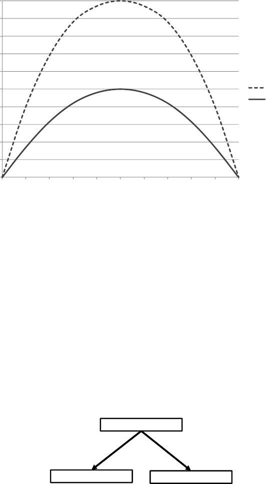
44

▸

A

NALYTI

CS

IN A BI

G

DATA W

O

RL

D

In answerin

g

the s

p

littin

g

decision, various candidate s

p

lits will

now be evaluated in terms of their decrease in im

p

urit

y

. Consider, for

exam

p

le, a s

p

lit on a

g

e as de

p

icted in Fi

g

ure 3.7 .

The ori

g

inal data set had maximum entro

py

. The entro

py

calcula

-

t

ions become:

■ Entro

py

to

p

node = −1/2 × lo

g

2

(1/2) – 1/2 × lo

g

2

(

1/2

)

= 1

■ Entro

py

left node = −1/3 × lo

g

2

(1/3) – 2/3 × lo

g

2

(

2/3

)

= 0.91

■ Entro

py

ri

g

ht node = −1 × lo

g

2

(1) – 0 × lo

g

2

(0) = 0

Figure3.6 Entropy versus Gini

0

0.1

0.2

0.3

0.4

0.5

0.6

0.7

0.8

0.9

1

10.90.80.70.60.50.40.30.20.10

Entropy

Gini

F

i

gure3.7 Calculating the Entropy

f

or Age Split

BG

GBGB

Age Age < 30 ≥ 30

400 400

200 400 200 0

P

REDI

C

TIVE ANALYTI

CS

◂

45

The weighted decrease in entropy, also known as the

gain,

can

then be calculated as follo

w

s:

=− × − ×=Gain 1 (600/800) 0.91 (200/800) 0 0.32

It speaks for itself that a larger gain is to be preferred. The decision

tree algorithm will now consider different candidate splits for its root

node and adopt a greedy strategy by picking the one with the biggest

gain. Once the root node has been decided on, the procedure contin-

ues in a recursive way to continue tree growing.

The third decision relates to the stopping criterion. Obviously, if the

tree continues to sp

l

it, it wi

ll

b

ecome very

d

etai

l

e

d

wit

h

l

ea

f

no

d

es con

-

taining on

l

y a

f

ew o

b

servations. In ot

h

er wor

d

s, t

h

e tree wi

ll

start to



t

h

e s

p

eci



cities or noise in t

h

e

d

ata, w

h

ic

h

is a

l

so re

f

erre

d

to as over



t

-

tin

g.

In order to avoid this, the data will be s

p

lit into a trainin

g

sam

p

le

and a validation sample. The training sample will be used to make the

sp

littin

g

decision. The validation sam

p

le is an inde

p

endent sam

p

le, set

aside to monitor the misclassi cation error (or an

y

other

p

erformance

metric). One then typically observes a pattern as depicted in Figure 3.8 .

The error on the trainin

g

sam

p

le kee

p

s on decreasin

g

as the s

p

lits

b

ecome more and more s

p

eci c toward it. On the validation sam

p

le,

the error will initially decrease, but at some point it will increase back

a

g

ain since the s

p

lits become too s

p

eci c for the trainin

g

sam

p

le as the

tree starts to memorize it. Where the

v

alidation set cur

v

e reaches its

minimum, the procedure should be stopped or over tting will occur.

Note that besides classi cation error, one mi

g

ht also use accurac

y

or

F

i

gure3.8 Us

i

ng a Va

lid

at

i

on Set to Stop Grow

i

ng a Dec

i

s

i

on Tree

Validation set

Training set

Minimum

Misclassification error

STOP growing tree!

Number of tree nodes

46

▸

A

NALYTI

CS

IN A BI

G

DATA W

O

RL

D

p

ro t based measures on the Y‐axis to make the sto

pp

in

g

decision.

Also note that, sometimes, sim

p

licit

y

is

p

referred above accurac

y

, and

one can select a tree that does not necessarily have minimum valida

-

tion set error, but a lower number of nodes.

In the example of Figure 3.4 , every node had only two branches.

The advantage of this is that the testing condition can be implemented

as a simple yes/no question. Multiway splits allow for more than two

b

ranches and can provide trees that are wider but less deep. In a read

once decision tree, a particular attribute can be used only once in a

certain tree

p

ath. Ever

y

tree can also be re

p

resented as a rule set since

every pat

h

f

rom a root no

d

e to a

l

ea

f

no

d

e ma

k

es up a simp

l

e i

f

/t

h

en

ru

l

e. T

h

ese ru

l

es can t

h

en

b

e easi

l

y imp

l

emente

d

in a

ll

k

in

d

s o

f

so

f

t-

ware pac

k

ages (e.g., Microso

f

t Exce

l

).

Decision trees essentially model decision boundaries orthogonal to

the axes. This is illustrated in Fi

g

ure 3.9 for an exam

p

le decision tree.

Decision trees can also be used for continuous tar

g

ets. Consider

the example in Figure 3.10 of a regression tree for predicting LGD.

Other criteria need now be used to make the s

p

littin

g

decision

b

ecause the im

p

urit

y

will need to be measured in another wa

y

. One

way to measure impurity in a node is by calculating the mean squared

error (MSE) as follows:

∑−

=

nYY

i

n

1(),

2

1

where

n

represents the number of observations in a leave node, Yi

t

he

v

alue of obser

v

ation i

,

and Y

,

the avera

g

e of all values in the leaf node.

F

i

gure3.9 Decision Boundary o

f

a Decision Tree

G

GG

B

BB

B

BBB

G

GG

GGG

G

GG

GG GG G

G

GG

G

GGGG

G

GG

GGG

G

GGG

1,200

30

Age

Income

Age

G

Income

GB

1,200 1,200

30 30

P

REDI

C

TIVE ANALYTI

CS

◂

4

7

Anot

h

er wa

y

is

by

con

d

uctin

g

a sim

pl

e ana

ly

sis o

f

variance

(ANOVA) test and calculate an F‐statistic as follows:

=−

−−−

∼FSS B

SS n B F

between

within

nBB

/( 1)

/( ) ,

,1

whereb

y

∑

=−

=

SS n Y Y

between b

b

B

b

()

1

2

∑∑

=−

==

SS Y Y

within bi b

i

n

b

Bb

()

2

11

with

B

bein

g

the number of branches of the s

p

lit, nb

t

he number of

observations in branch b

,

Yb the avera

g

e in branch b

,

Ybi the

v

alue of

observation

i

in branch

i

b

,

and Y the overall average. Good splits will

then result in a hi

g

h

F

value, or low corresponding p‐value.

F

The stopping decision can be made in a similar way as for classi

-

cation trees, but using a regression‐based performance measure (e.g.,

mean s

q

uared error, mean absolute deviation,

R

‐s

q

uared) on the

Y

‐

Y

axis. T

h

e assi

g

nment

d

ecision can

b

e ma

d

e

by

assi

g

nin

g

t

h

e mean (or

me

d

ian) to eac

h

l

ea

f

no

d

e. Note a

l

so t

h

at con



d

ence interva

l

s ma

y

b

e

compute

d

f

or eac

h

o

f

t

h

e

l

ea

f

no

d

es.

Decision trees can

b

e use

d

f

or various

p

ur

p

oses in ana

ly

tics. First,

t

h

e

y

can

b

e use

d

f

or in

p

ut se

l

ection

b

ecause attri

b

utes t

h

at occur at t

h

e

top o

f

t

h

e tree are more pre

d

ictive o

f

t

h

e target. One cou

ld

a

l

so sim-

ply

ca

l

cu

l

ate t

h

e

g

ain o

f

a c

h

aracteristic to

g

au

g

e its

p

re

d

ictive

p

ower.

F

i

gure3.10 Example Regression Tree

f

or Predicting LGD

Loan Collateral

LGD = 18%

LGD = 30%

Geographic Region LGD = 72%

Known Client

LGD = 42% LGD = 55%

None

Cash

Real Estate

EU

United

States No

Yes

48

▸

A

NALYTI

CS

IN A BI

G

DATA W

O

RL

D

Next, the

y

can also be used for initial se

g

mentation. One then t

yp

icall

y

b

uilds a tree of two or three levels dee

p

as the se

g

mentation scheme

and then uses second stage logistic regression models for further

re nement. Finally, decision trees can also be used as the  nal analyti

-

cal model to be used directly into production. A key advantage here is

that the decision tree gives a white box model with a clear explanation

b

ehind how it reaches its classi cations. Many software tools will also

allow you to grow trees interactively by providing a splitting option at

each level of the tree (e.g., a top  ve, or more, of splits amongst which

the modeler can choose). This allows us to choose s

p

lits not onl

y

based

upon impurity re

d

uction,

b

ut a

l

so on t

h

e interpreta

b

i

l

ity an

d

/or com-

putationa

l

comp

l

exity o

f

t

h

e sp

l

it criterion.

NEURAL NETWORKS

A  rst

p

ers

p

ective on the ori

g

in of neural networks states that the

y

are mathematical representations inspired by the functioning of the

human brain. Another more realistic

p

ers

p

ective sees neural networks

as

g

eneralizations of existin

g

statistical models. Let’s take lo

g

istic

regression as an example:

PY X X e

NXX

NN

(1|,,) 1

1,

1()

011



=…=

+−β+β + +β

This model can be seen in Fi

g

ure 3.11 .

The processing element or neuron in the middle basically per

-

forms two o

p

erations: it takes the in

p

uts and multi

p

lies them with the

weights (including the intercept term

β

0

,

which is called the bias term

F

i

gure3.11 Neural Network Representation o

f

Logistic Regression

X1

X2

X

N–1

XN

...

1

1–( 0 + 1X1 + ... + NXN)

+

1

),...,|( N

e

XXYP =

N–1

N

0

β

1

2

P

REDI

C

TIVE ANALYTI

CS

◂

49

in neural networks) and then

p

uts this into a nonlinear transforma

-

tion function similar to the one we discussed in the section on lo

g

istic

regression. So, logistic regression is a neural network with one neuron.

Similarl

y

, we could visualize linear re

g

ression as a one neuron neural

network with the identity transformation

f

(

ff

z

) =

z

. We can now gener-

z

alize the above picture to a multilayer perceptron (MLP) neural net-

work b

y

addin

g

more la

y

ers and neurons as shown in Fi

g

ure 3.12 .

1

0

The exam

p

le in Fi

g

ure 3.12 is an MLP with one in

p

ut la

y

er, one

hidden layer, and one output layer. The hidden layer has a nonlinear

transformation function

f

(

f

.

) and the out

p

ut la

y

er a linear transforma

-

tion function. The most

p

o

p

ular transformation functions (also called

squashing, activation functions) are:

■ Lo

g

istic, =+−

fz ez

() 1

1

,

ran

g

in

g

between 0 and 1

■ Hyperbolic tangent, =−

+

−

fz ee

ee

zz

() , ranging between –1 and +1

■ Linear

,

=fz z() , ranging between −∞ and +∞

For classi cation (e.

g

., churn, res

p

onse, fraud), it is common

p

rac

-

tice to a

d

o

p

t a

l

o

g

istic trans

f

ormation in t

h

e out

p

ut

l

a

y

er, since t

h

e

out

p

uts can t

h

en

b

e inter

p

rete

d

as

p

ro

b

a

b

i

l

ities.

1

For re

g

ress

i

on tar

-

gets (e.g., CLV, LGD), one cou

ld

use any o

f

t

h

e trans

f

ormation

f

unc

-

tions

l

iste

d

a

b

ove. T

yp

ica

lly

, one wi

ll

use

hyp

er

b

o

l

ic tan

g

ent activation

f

unctions in t

h

e

h

i

dd

en

l

a

y

er.

In terms o

f

h

i

dd

en

l

ayers, t

h

eoretica

l

wor

k

s

h

ave s

h

own t

h

at

neura

l

networ

k

s wit

h

one

h

i

dd

en

l

a

y

er are universa

l

a

pp

roximators,

F

i

gure3.12 A Mu

l

t

il

ayer Perceptron (MLP) Neura

l

Networ

k

b1

b2

b3

b4

h1

h2

h3

v1

v3

v2

x

1

x2

W

11

W

23

z = Σvjhj + b4

j = 1

3

hj = f(Σxiwij + bj)

i = 1

2

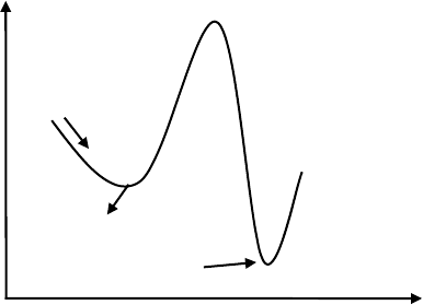
50

▸

A

NALYTICS IN A BIG DATA WORL

D

ca

p

able of a

pp

roximatin

g

an

y

function to an

y

desired de

g

ree of accu-

rac

y

on a com

p

act interval.

12

Onl

y

for discontinuous functions (e.

g

., a

saw tooth pattern), it could make sense to try out more hidden layers,

although these patterns rarely occur in real‐life data sets.

For simple statistical models (e.g., linear regression), there exists a

closed‐form mathematical formula for the optimal parameter values.

However, for neural networks, the optimization is a lot more com

-

plex and the weights sitting on the connections need to be estimated

using an iterative algorithm. The algorithm then optimizes a cost func-

tion, which ma

y

be similar to linear re

g

ression (mean s

q

uared error)

or

l

ogistic regression (maximum

l

i

k

e

l

i

h

oo

d

b

ase

d

). T

h

e proce

d

ure

typica

ll

y starts

f

rom a set o

f

ran

d

om weig

h

ts t

h

at are t

h

en iterative

l

y

a

d

juste

d

to t

h

e patterns in t

h

e

d

ata using an optimization a

l

gorit

h

m.

Popular optimization algorithms here are backpropagation learning,

con

j

u

g

ate

g

radient, and Levenber

g

‐Mar

q

uardt.

13

A ke

y

issue to note

here is the curvature of the ob

j

ective function, which is not convex

and may be multimodal as illustrated in Figure 3.13 . The error func

-

tion can thus have multi

p

le local minima but t

yp

icall

y

onl

y

one

g

lobal

minimum. Hence, if the startin

g

wei

g

hts are chosen in a subo

p

timal

way, one may get stuck in a local minimum. One way to deal with this

is to tr

y

out different startin

g

wei

g

hts, start the o

p

timization

p

rocedure

for a few ste

p

s, and then continue with the best intermediate solution.

The optimization procedure then continues until the error function

shows no further

p

ro

g

ress, the wei

g

hts sto

p

chan

g

in

g

substantiall

y

, or

after a  xed number of o

p

timization ste

p

s (also called e

p

och

s

).

Figure3.13 Local versus Global Minima

w

E

Local minimum!

Global minimum!

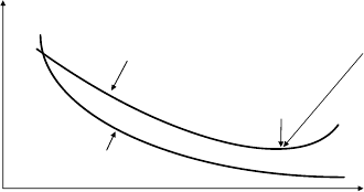
P

REDICTIVE ANALYTIC

S

◂

51

Althou

g

h multi

p

le out

p

ut neurons could be used (

p

redictin

g

, for

exam

p

le, churn and CLV simultaneousl

y

), it is hi

g

hl

y

advised to use

only one. The hidden neurons, however, should be carefully tuned

and depend on the nonlinearity in the data. More complex, nonlinear

patterns will require more hidden neurons. Although various proce-

dures (e.g., cascade correlation, genetic algorithms, Bayesian methods)

have been suggested in the scienti c literature to do this, the most

straightforward yet ef cient procedure is as follows:

1

4

■ Split the data into a training, validation, and test set.

■ Vary t

h

e num

b

er o

f

h

i

dd

en neurons

f

rom 1 to 10 in steps o

f

1

or

more

.

■ Train a neura

l

networ

k

on t

h

e training set an

d

measure t

h

e per

-

formance on the validation set (ma

y

be train multi

p

le neural

networks to deal with the local minimum issue).

■ Choose the number of hidden neurons with o

p

timal validation

set

p

erformance.

■ Measure the

p

erformance on the inde

p

endent test set.

Neural networks can model ver

y

com

p

lex

p

atterns and decision

b

oundaries in the data and, as such, are very powerful. In fact, they

are so

p

owerful that the

y

can even model the noise in the trainin

g

data, which is somethin

g

that de nitel

y

should be avoided. One wa

y

to avoid this over tting is by using a validation set in a similar way as

with decision trees. This is illustrated in Fi

g

ure 3.14 . The trainin

g

set

is used here to estimate the weights and the validation set is again an

independent data set used to decide when to stop training. Another

scheme to

p

revent a neural network from over ttin

g

is wei

g

ht re

g

u-

larization, whereby the idea is to keep the weights small in absolute

Figure3.14 Using a Validation Set for Stopping Neural Network Training

Validation set

Training set

Minimum

Error

STOP training!

Training steps

52

▸

A

NALYTICS IN A BIG DATA WORL

D

sense because otherwise the

y

ma

y

be  ttin

g

the noise in the data. This

is t

h

en im

pl

emente

d

by

a

dd

in

g

a wei

gh

t size term (e.

g

., Euc

l

i

d

ean

norm) to the objective function of the neural network.

15

Although neural networks have their merits in terms of modeling

power, they are commonly described as black box techniques because

they relate the inputs to the outputs in a mathematically complex, non-

transparent, and opaque way. In application areas where interpretabil

-

ity may not be required (e.g., fraud detection, response modeling), they

can be very successfully adopted as high‐performance analytical tools.

However, in a

pp

lication areas where ex

p

lanation is im

p

ortant

(

e.g., cre

d

it ris

k

, me

d

ica

l

d

iagnosis), one nee

d

s to

b

e care

f

u

l

wit

h

neu-

ra

l

networ

k

s

b

ecause insig

h

t an

d

compre

h

ensi

b

i

l

ity in t

h

e un

d

er

l

ying

patterns is crucia

l

.

1

6

Two ways to open up t

h

e neura

l

networ

k

bl

ac

k

b

ox are rule extraction and two‐stage models.

The

p

ur

p

ose of rule extraction is to extract if/then classi cation

rules mimickin

g

the behavior of the neural network.

17

Two im

p

or

-

tant approaches here are decompositional and pedagogical techniques.

Decom

p

ositional rule extraction a

pp

roaches decom

p

ose the network’s

internal workin

g

s b

y

ins

p

ectin

g

wei

g

hts and/or activation values. A

typical  ve‐step approach here could be:18

1. Train a neural network and

p

rune it as much as

p

ossible in

t

erms of connec

t

ions.

2. Cate

g

orize the hidden unit activation values usin

g

clusterin

g

.

3. Extract rules that describe the network outputs in terms of the

cate

g

orized hidden unit activation values.

4. Extract rules that describe the categorized hidden unit activa

-

tion values in terms of the network in

p

uts.

5. Merge the rules obtained in steps 3 and 4 to directly relate the

in

p

uts to the out

p

uts.

T

h

is is i

ll

ustrate

d

in Fi

g

ure 3.15 .

Note t

h

at ste

p

s 3 an

d

4 can

b

e

d

one simu

l

taneous

ly

by

b

ui

ld

in

g

a

d

ecision tree re

l

ating t

h

e networ

k

outputs to t

h

e

h

i

dd

en unit acti

-

vation va

l

ues. Fi

g

ure 3.16

g

ives an exam

pl

e o

f

a

pply

in

g

a

d

ecom

p

o

-

sitiona

l

neura

l

networ

k

ru

l

e extraction a

pp

roac

h

in a cre

d

it scorin

g

sett

i

n

g

.

Fi

g

ure3.15 Decom

p

ositional A

pp

roach for Neural Network Rule Extraction

Response

…GenderIncomeAgeCustomer

NoF1,00028Emma

YesM1,50044Will

NoM1,20030Dan

YesM2,40058Bob

Response

h3h2h1h3h2h1GenderIncomeAgeCustomer

F28Emma 231

232M44Will

M30Dan 213

M

1,000

1,500

1,200

2,40058Bob

2.34

1.22

–0.18

0.8

–1.20

0.78

2.1

–0.1

No

Yes

No

Yes121

0.66

0.82

0.16

–2.34

If h1 = 1 and h2 = 3, then response = No

If h2 = 2, then response = Yes

If age < 28 and income < 1,000, then h1 = 1

If gender = F, then h2 = 3

If age > 34 and income > 1,500, then h2 = 2

If age < 28 and income < 1,000 and gender = F then response = No

If age > 34 and income > 1,500 then response = Yes

Step 1: Start from original data.

Step 2: Build a neural network

(e.g, 3 hidden neurons).

Step 3: Categorize hidden unit activations.

Step 4: Extract rules relating network outputs

to categorized hidden units.

Step 5: Extract rules relating categorized

hidden units to inputs.

Step 6: Merge both rule sets

53

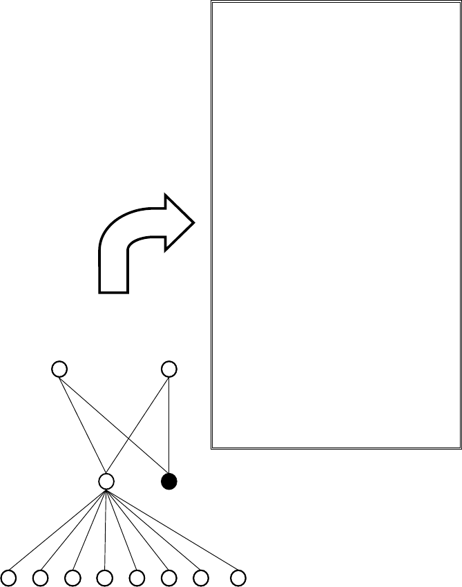
Fi

g

ure3.16 Exam

p

le of Decom

p

ositional Neural Network Rule Extraction

Economical sector = sector C

Term > 12 Months

Purpose = cash provisioning

Purpose = second hand car

Income > 719 Euro

Savings account > 12.40 Euro

Years client > 3 years

Property = No

–0.202

–0.287

–0.102

0.278

–0.081

–0.162

0.137

–0.289

0.457

–0.453

0.611

0.380

Applicant = good

Applicant = bad

If term > 12 months and purpose = cash provisioning and savings account ≤ 12.40

Euro and years client ≤ 3, then applicant = bad

If term > 12 months and purpose = cash provisioning and owns property = no and

savings account ≤ 12.40 Euro and years client ≤ 3, then applicant = bad

If purpose = cash provisioning and income > 719 and owns property = no and savings

account ≤ 12.40 Euro and years client ≤ 3, then applicant = bad

If purpose = secondhand car and income > 719 Euro and owns property = no and

savings account ≤ 12.40 Euro and years client ≤ 3, then applicant = bad

If savings account ≤ 12.40 Euro and economical sector = sector C, then

applicant = bad

Default class: applicant = good

5

4

P

REDICTIVE ANALYTIC

S

◂

55

Peda

g

o

g

ical rule extraction techni

q

ues consider the neural net

-

wor

k

as a

bl

ac

k

b

ox an

d

use t

h

e neura

l

networ

k

p

re

d

ictions as in

p

ut

to a white box analytical technique such as decision trees.

1

9 This is

illustrated in Figure 3.17 .

In this approach, the learning data set can be further augmented

with arti cial data, which is then labeled (e.g., classi ed or predicted)

b

y the neural network, so as to further increase the number of obser-

vations to make the splitting decisions when building the decision tree.

When using either decompositional or pedagogical rule extraction

a

pp

roaches, the rule sets should be evaluated in terms of their accurac

y

,

conciseness (e.g., num

b

er o

f

ru

l

es, num

b

er o

f

con

d

itions per ru

l

e), an

d



d

e

l

ity. T

h

e

l

atter measures to w

h

at extent t

h

e extracte

d

ru

l

e set per-

f

ect

l

y mimics t

h

e neura

l

networ

k

an

d

is ca

l

cu

l

ate

d

as

f

o

ll

ows:

Neural Network Classification

R

u

l

e set

classi cati

on

G

ood

B

a

d

Good

a

b

B

ad

c

d

=+ +Fidelity (a d)/(b c).

It is a

l

so im

p

ortant to a

l

wa

y

s

b

enc

h

mar

k

t

h

e extracte

d

ru

l

es/trees

wit

h

a tree

b

ui

l

t

d

irect

ly

on t

h

e ori

g

ina

l

d

ata to see t

h

e

b

ene



t o

f

g

oin

g

t

h

rou

gh

t

h

e neura

l

networ

k

.

Anot

h

er approac

h

to ma

k

e neura

l

networ

k

s more interpreta

bl

e

is

by

usin

g

a two‐sta

g

e mo

d

e

l

setu

p

.

20

T

h

e i

d

ea

h

ere is

t

o es

t

ima

t

e an

eas

y

to un

d

erstan

d

mo

d

e

l



rst (e.

g

.,

l

inear re

g

ression,

l

o

g

istic re

g

res

-

sion). T

h

is wi

ll

g

ive us t

h

e inter

p

reta

b

i

l

it

y

p

art. In a secon

d

sta

g

e, a

n

eura

l

networ

k

is use

d

to

p

re

d

ict t

h

e errors ma

d

e

by

t

h

e sim

pl

e mo

d

e

l

usin

g

t

h

e same set o

f

p

re

d

ictors. Bot

h

mo

d

e

l

s are t

h

en com

b

ine

d

in an

a

dd

itive wa

y

,

f

or exam

pl

e, as

f

o

ll

ows:

■

Target = linear regression (

X

1

,

X

2

XX

, …

X

N

X

) + neural network

N

(

X

1

,

X

2

XX

, …

X

N

X

)

N

■

Score = logistic regression (

X

1

,

X

2

XX

, …

X

N

X

) + neural network

N

(

X

1

,

X

2

XX

, …

X

N

X

)

N

This setu

p

rovides an ideal balance between model inter

p

retabil

-

i

t

y

(which comes from the  rst

p

art) and model

p

erformance (which

comes from the second

p

art). This is illustrated in Fi

g

ure 3.18 .

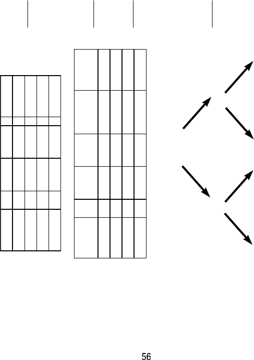
Fi

g

ure3.17 Peda

g

o

g

ical Approach for Rule Extraction

Response…GenderIncomeAgeCustomer

1,00028Emma

1,50044Will

1,20030Dan

No

Yes

No

Yes

F

M

M2,40058Bob

GenderIncomeAgeCustomer

Network

Prediction Response

1,00028Emma

1,50044Will

1,20030Dan

No

Yes

No

Yes

No

Yes

F

M

M2,40058Bob

Step 1: Start from original data.

Step 2: Build a neural network.

Step 3: Get the network predictions and

add them to the data set.

Step 4: Extract rules relating network

predictions to original inputs. Generate

additional data where necessary.

Income > 1,500

Gender = Female Age < 30

No

No No

Network prediction

response = yes

Network prediction

response = no

Network prediction

response = yes

Yes

Network prediction

response = no

Yes

F

i

gure 3.18 Two‐Stage Mo

d

e

l

s

ResponseGenderIncomeAgeCustomer

No1,00028Emma

Yes1,50044Will

No1,20030Dan

Yes

F

M

M2,40058Bob

ResponseIncome GenderAgeCustomer

Logistic

Regression

Output

1,00028Emma 0.44

1,50044Will 0.76

1,20030Dan 0.18

0.88

No(=0)

Yes(=1)

No(=0)

Yes (=1)

F

M

M2,40058Bob

Income Gender Response…AgeCustomer

Logistic

Regression

Output Error

28Emma 0.44

44Will 0.76

30Dan 0.18

−0.44

0.24

−0.18

0.120.88

No(=0)

Yes(=1)

No(=0)

Yes (=1)

F

M

1,000

1,500

1,200

2,40058Bob

Income GenderCustomer Age

Logistic

Regression

Output NNOutput

Final

Output

0.68F1,00028Bart −0.32 0.36

Step 1: Start from original data.

Step 2: Build logistic regression model.

Step 3: Calculate errors from logistic

regression model.

Step 4: Build NN predicting errors from

logistic regression model.

Step 5: Score new observations by adding up

logistic regression and NN scores.

…

5

7

58

▸

A

NALYTICS IN A BIG DATA WORL

D

SUPPORT VECTOR MACHINES

Two key shortcomings of neural networks are the fact that the objective

function is nonconvex (and hence ma

y

have multi

p

le local minima)

and the effort that is needed to tune the number of hidden neurons.

Support vector machines (SVMs) deal with both of these issues.

21

The origins of classi cation SVMs date back to the early dates of

linear programming.

22 Consider the following linear program (LP) for

classi cation

:

+++ ++ee e e

ng nb

min 12

su

b

ject t

o

wx wx wx c e i n

ii nini g

,1

11 2 2 +++≥−≤≤

+ + + ≤+ +≤≤ +wx wx wx c e n i n n

ii ninig gb

,1

11 2 2

≥ei0

The LP assi

g

ns the

g

ood customers a score above the cut‐off value

c,

and the bad customers a score below

c. n

g

n

and

n

b

represent the number

of

g

oods and bads, res

p

ectivel

y

. The error variables

e

i

are needed to be

i

able to solve the

p

ro

g

ram because

p

erfect se

p

aration will t

yp

icall

y

not be

possible. Linear programming has been very popular in the early days of

credit scorin

g

. One of its bene ts is that it is eas

y

to include domain or

b

usiness knowled

g

e b

y

addin

g

extra constraints to the model.

A key problem with linear programming is that it can estimate

multi

p

le o

p

timal decision boundaries, as illustrated in Fi

g

ure 3.19 , for

a

p

erfectl

y

linearl

y

se

p

arable case.

SVMs add an extra objective to the analysis. Consider, for exam

-

p

le, the situation de

p

icted in Fi

g

ure 3.20 . It has two h

yp

er

p

lanes sit-

tin

g

at the ed

g

es of both classes and a h

yp

er

p

lane in between, which

wi

ll

serve as t

h

e c

l

assi



cation

b

oun

d

ar

y

. T

h

e

p

er

p

en

d

icu

l

ar

d

istance

f

rom t

h

e



rst

h

yperp

l

ane H1 to t

h

e origin equa

l

s

|

b

−1

|

/

||

w

||, whereby

w

||

w

|| represents the Euclidean norm of

w

calculated as

w

www|| || 1

2

=+

.

Li

k

ewise, t

h

e

p

er

p

en

d

icu

l

ar

d

istance

f

rom H2 to t

h

e ori

g

in e

q

ua

l

s

|

b

+

1

|

/

||

w

||. Hence, the margin between both hyperplanes equals 2/||

w

||.

w

SVMs wi

ll

now aim at maximizin

g

t

h

is mar

g

in to

p

u

ll

b

ot

h

c

l

asses as

f

ar a

p

art as

p

ossi

bl

e. Maximizin

g

t

h

e mar

g

in is simi

l

ar to minimizin

g

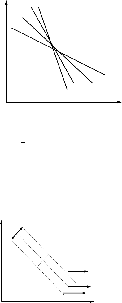
P

REDI

C

TIVE ANALYTI

CS

◂

59

||

w

||, or minimizing

w

∑

=

wi

i

N

1

2

1

. In case of

p

erfect linear se

p

aration, the

SV

M classi er

t

hen

becomes

i

1

as follo

w

s.

Consider a trainin

g

set: ∈∈−+

=

{,} with and {1;1}

1

xy x R y

kkk

n

k

N

k

The

g

oods (e.

g

., class +1) should be above h

yp

er

p

lane H1, and the

b

ads (e.

g

., class−1) below h

yp

er

p

lane H2, which

g

ives:

wx b ify

T

kk

1, 1+≥ =+

wx b ify

T

kk

1, 1+≤ =−

F

i

gure3.19 Mu

l

t

i

p

l

e Separat

i

ng Hyperp

l

anes

x

xx

x

++

+

Class1

Class2

x1

x

2

F

i

gure3.20 SVM Classi



er

f

or the Per

f

ectly Linearly Separable Case

x1

x

xx

x

++

+

Class 1

Class 2

x2

H1: wTx + b = + 1

H0: wTx + b = 0

H2: wTx + b = –1

2/||w||

60

▸

A

NALYTI

CS

IN A BI

G

DATA W

O

RL

D

Both can be combined as follo

w

s:

+≥ywx b

k

T

k

()1

The optimization problem then becomes

:

∑

=

Minimize wi

i

N

1

2

1

s

ubject to ywx b k n

k

T

k

()1,1…+≥ =

This quadratic programming (QP) problem can now be solved

usin

g

La

g

ran

g

ian o

p

timization.

2

3

It is im

p

ortant to note that the

optimization pro

bl

em

h

as a qua

d

ratic cost

f

unction, giving a convex

optimization pro

bl

em wit

h

no

l

oca

l

minima an

d

on

l

y one g

l

o

b

a

l

mini-

mum. Training points t

h

at

l

ie on one o

f

t

h

e

h

yperp

l

anes H1 or H2 are

called

support vectors

and are essen

t

ial

t

o

t

he classi ca

t

ion. The classi -

cation h

yp

er

p

lane itself is H0 and, for new observations, it needs to be

checked whether the

y

are situated above H0, in which case the

p

re-

diction is +1 or below (prediction −1). This can be easily accomplished

using the sign operator as follows:

y

(

x

) = sign (

x

w

T

x + b

T

).

The SVM classi er discussed thus far assumed

p

erfect se

p

aration is

possible, which will of course rarely be the case for real‐life data sets.

In case of overla

pp

in

g

class distributions (as illustrated in Fi

g

ure 3.21 ),

the SVM classi er can be extended

w

ith error terms as follo

w

s

:

∑∑

+

==

Minimize w C e

i

N

i

n

1

2

11

F

i

gure3.21 SVM Classi



er in Case o

f

Overlapping Distributions

x

xx

x

++

+

Class 1

Class 2

x

22/||w||

x

+

x1

H1: wTx + b = + 1

H0: wTx + b = 0

H2: wTx + b = –1

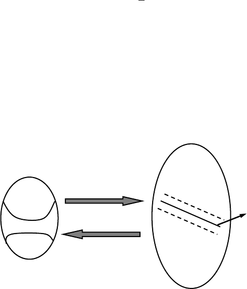
P

REDICTIVE ANALYTIC

S

◂

6

1

sub

j

ect to ywx b ek n

k

T

kk

()1,1…+≥− =

≥ek0.

The error variables

e

k

are needed to allow for misclassi cations.

k

Th

e

C

hyperparameter in the objective function balances the impor-

C

tance of maximizing the margin versus minimizing the error on the

data. A hi

g

h (low) value of

C

implies a higher (lower) risk of over t-

C

ting. We will come back to it in due course. Note that again a qua

-

dratic programming (QP) problem is obtained that can be solved using

La

g

ran

gi

an o

p

t

i

m

i

zat

i

on.

Fina

lly

, t

h

e non

l

inear SVM c

l

assi



er wi

ll



rst ma

p

t

h

e in

p

ut

d

ata

to a

h

i

gh

er

d

imensiona

l

f

eature s

p

ace usin

g

some ma

pp

in

g

x().ϕ T

h

is

is illustrated in Fi

g

ure 3.22 .

The SVM problem formulation now becomes

:

∑∑

+

==

Minimize w C e

i

N

i

n

1

2

11

sub

j

ect to yw x b ek n

k

T

kk

(())1,1…ϕ+≥− =

≥ek0.

When workin

g

out the La

g

ran

g

ian o

p

timization,

24

it turns out that

the ma

pp

in

g

ϕx()

is never ex

p

licitl

y

needed, but onl

y

im

p

licitl

y

b

y

means of the kernel function

K

de ned as follows:

K

=ϕ ϕKx x x x

kl k

T

l

(,) ()()

.

Fi

g

ure3.22 The Feature Space Mappin

g

X

XX

X

OOO

O

OO

X

O

Input Space

XX

X

XX

X

O

Feature Space

K(x1,x2) = (x1)T

φ

(x2)

φ

WT(xi) + b = 0

φ

x →(x)

φ

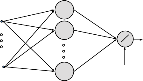
62

▸

A

NALYTI

CS

IN A BI

G

DATA W

O

RL

D

Hence, the feature s

p

ace does not need to be ex

p

licitl

y

s

p

eci ed. The

nonlinear

SV

M classi er

t

hen becomes

:

∑

=α +

⎡

⎣

⎢⎤

⎦

⎥

=

y x sign y K x x b

k

n

kk

() (, )

1

whereby αk are the Lagrangian multipliers stemming from the optimi

-

zation. Support vectors will have nonzero αk since they are needed to

construct the classi cation line. All other observations have zero αk

,

which is often referred to as the

sparseness property

of SVMs. Different

types of kernel functions can be used. The most popular are:

■ Linear

k

erne

l

: =Kxx x x

kk

T

(, )

■ Po

l

ynomia

l

k

erne

l

:=+Kxx x x

kk

Td

(, ) (1 )

■ Radial basis function (RBF) kernel: Kxx x x

kk

(, ) exp{ || ||/ }

22

=−− σ

Empirical evidence has shown that the RBF kernel usually per

-

forms best, but note that it includes an extra

p

arameter

σ

t

o be

t

uned.

25

An SVM classi er can be ver

y

easil

y

re

p

resented as a neural net

-

work, as depicted in Figure 3.23 .

The hidden la

y

er uses, for exam

p

le, RBF activation functions,

whereas the out

p

ut la

y

er uses a linear activation function. Note that

the number of hidden neurons now corresponds to the number of

su

pp

ort vectors and follows automaticall

y

from the o

p

timization. This

is in stron

g

contrast to neural networks where the number of hidden

neurons needs to be tuned manually.

F

i

gure3.23 Representing an SVM Classi



er as a Neural Network

xn

x1

b

α

ns

α

2

α

1

K(x,xns)

K(x,x2)

K(x,x1)

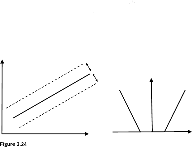
P

REDICTIVE ANALYTIC

S

◂

63

A ke

y

q

uestion to answer when buildin

g

SVM classi ers is the tun-

in

g

of the h

yp

er

p

arameters. For exam

p

le, su

pp

ose one has an RBF

S

VM that has two hyperparameters, C and

σ

. Both can be tuned using

the following procedure:

26

■ Partition the data into 40/30/30 percent training, validation,

and test data.

■ Build an RBF SVM classi er for each (

σ

,

C

) combination from

C

the sets

σ

∈ {0.5, 5, 10, 15, 25, 50, 100, 250, 500} and

C

∈

{

0.01,

0.05, 0.1, 0.5, 1, 5, 10, 50, 100, 500}.

■ C

h

oose t

h

e

(

σ

,

C

) combination with the best validation set per-

C

f

ormance.

■ Bui

ld

an RBF SVM c

l

assi



er wit

h

t

h

e o

p

tima

l

(

σ

,

C

) combination

C

on the combined trainin

g

+ validation data set.

■ Calculate the

p

erformance of the estimated RBF SVM classi er

on

t

he

t

es

t

se

t

.

In case of linear or polynomial kernels, a similar procedure can be

ado

p

ted.

SVMs can also be used for re

g

ression a

pp

lications with a continu

-

ous target. The idea here is to  nd a function

f

(

f

x

) that has at most

x

ε

deviation from the actual targets

y

i

for all the training data, and is at

i

the same time as  at as

p

ossible. Hence, errors less (hi

g

her) than

ε

w

ill

b

e tolerated (penalized). This is visualized in Figure 3.24 .

Consider a trainin

g

set: xy x R y R

kkk

n

k

N

k

{,}with and

1∈∈

=

SVMs

f

or Re

g

ression

x

+ε–ε

ε

Loss

function

64

▸

A

NALYTI

CS

IN A BI

G

DATA W

O

RL

D

The

SV

M formula

t

ion

t

hen becomes

:

∑∑

+ε+ε

==

Minimize w C

i

N

kk

i

n

1

2()

2

1

*

1

subject t

o

−ϕ −≤ε+εywx b

k

T

kk

()

ϕ+−≤ε+εwx by

T

kkk

() *

εε ε ≥

kk

,, 0.

*

T

h

e

h

yperparameter

C

determines the trade‐off between the  at-

C

ness of

f

and the amount to which deviations larger than

f

ε

are

t

o

l

er

-

ate

d

. Note t

h

e

f

eature space mapping ϕx(), w

h

ic

h

is a

l

so use

d

h

ere.

Using Lagrangian optimization, t

h

e resu

l

ting non

l

inear regression

func

t

ion becomes:

∑

=α−α +

=

fx Kx x b

kk

i

n

k

() ( )( ,) ,

*

1

whereb

y

αk

a

n

d

αk

* re

p

resent the La

g

ran

g

ian multi

p

liers. The h

yp

er

-

parameters

C

and

C

ε

can be tuned using a procedure similar to the one

ou

t

lined for classi ca

t

ion

SV

Ms.

Just as with neural networks, SVMs have a universal a

pp

roxima-

tion property. As an extra bene t, they do not require tuning of the

number of hidden neurons and are characterized b

y

convex o

p

timiza-

tion. However, the

y

are also ver

y

com

p

lex to be used in settin

g

s where

interpretability is important. Since an SVM can be represented as a

neural network (see Fi

g

ure 3.23 ), one could use an

y

of the rule extrac

-

tion methods (decompositional, pedagogical) discussed in the section

on neural networks to make them more comprehensible.

27 Also

,

two

‐

sta

g

e models could be used to achieve this aim, whereb

y

a second‐

stage SVM is estimated to correct for the errors of a simple (e.g., linear

or lo

g

istic re

g

ression) model.

ENSEMBLE METHODS

Ensem

bl

e met

h

o

d

s aim at estimatin

g

mu

l

ti

pl

e ana

ly

tica

l

mo

d

e

l

s

instea

d

o

f

using on

l

y one. T

h

e i

d

ea

h

ere is t

h

at mu

l

tip

l

e mo

d

e

l

s can

cover

d

i

ff

erent

p

arts o

f

t

h

e

d

ata in

p

ut s

p

ace an

d

, as suc

h

, com

pl

ement

eac

h

ot

h

er’s

d

e



ciencies. In or

d

er to success

f

u

lly

accom

pl

is

h

t

h

is, t

h

e

P

REDI

C

TIVE ANALYTI

CS

◂

65

anal

y

tical techni

q

ue needs to be sensitive to chan

g

es in the underl

y

in

g

d

ata. T

h

is is es

p

ecia

lly

t

h

e case

f

or

d

ecision trees, an

d

t

h

at’s w

hy

t

h

e

y

are commonly used in ensemble methods. In what follows, we will

discuss bagging, boosting, and random forests.

Bagging

Bagging (bootstrap aggregating) starts by taking B bootstraps from the

underlying sample.

2

8 Note that a bootstrap is a sample with replacement

(see section on evaluatin

g

p

redictive models). The idea is then to build

a c

l

assi



er (e.g.,

d

ecision tree)

f

or every

b

ootstrap. For c

l

assi



cation, a

new o

b

servation wi

ll

b

e c

l

assi



e

d

b

y

l

etting a

ll

B c

l

assi



ers vote, using,

f

or

examp

l

e, a majority voting sc

h

eme w

h

ere

b

y ties are reso

l

ve

d

ar

b

itrari

l

y.

For regression, the prediction is the average of the outcome of the B mod

-

els (e.

g

., re

g

ression trees). Also note that here a standard error, and thus

con dence interval, can be calculated. The number of bootstra

p

s B can

either be  xed (e.g., 30) or tuned via an independent validation data set.

The ke

y

element for ba

gg

in

g

to be successful is the instabilit

y

of the

anal

y

tical techni

q

ues. If

p

erturbin

g

the data set b

y

means of the boot-

strapping procedure can alter the model constructed, then bagging will

im

p

rove the accurac

y

.

2

9

Boosting

Boosting works by estimating multiple models using a weighted sample

of

t

he da

t

a.

30

Starting from uniform weights, boosting will iteratively

rewei

g

ht the data accordin

g

to the classi cation error, whereb

y

mis

-

classi ed cases get higher weights. The idea here is that dif cult obser

-

vations should get more attention. Either the analytical technique can

directl

y

work with wei

g

hted observations or, if not, we can

j

ust sam

p

le

a new

d

ata set accor

d

in

g

to t

h

e wei

gh

t

d

istri

b

ution. T

h

e



na

l

ensem

bl

e

mo

d

e

l

is t

h

en a wei

gh

te

d

com

b

ination o

f

a

ll

t

h

e in

d

ivi

d

ua

l

mo

d

e

l

s.

A popu

l

ar imp

l

ementation o

f

t

h

is is t

h

e a

d

aptive

b

oosting/a

d

a

b

oost

p

roce

d

ure, w

h

ic

h

wor

k

s as

f

o

ll

ows:

1. Given the following observations: (

x

1

,

y

1

), …, (

x

n

x

,

y

n

) where

x

i

is

i

t

h

e attri

b

ute vector o

f

o

b

servation

i

and

i

y

i

∈

{

1,−1

}

2. Initia

l

ize t

h

e wei

gh

ts as

f

o

ll

ows:

W

1

WW

(

i

)=1/

i

n, i

= 1, …,

i

n

66

▸

A

NALYTI

CS

IN A BI

G

DATA W

O

RL

D

3. F

o

r

t

= 1…

t

T

a. Train a weak classi er (e.

g

., decision tree) usin

g

the wei

g

hts

W

t

WW

b

. Get weak classi er

C

t

CC

with classi cation error

t

ε

t

c. Choose t

t

1

2ln 1

α= −ε

ε

⎛

⎝

⎜⎞

⎠

⎟

d. Update the weights as follows:

i

.

Wi Wi

ZeifCxy

t

ti

t

() () ()

1==

+−α

ii

.

Wi Wi

ZeifCx y

t

ti

t

() () ()

1=≠

+α

4. Output t

h

e



na

l

ensem

bl

e mo

d

e

l

: E x sign C x

t

T

tt

() ( ())

1

∑

=α

⎛

⎝

⎜⎞

⎠

⎟

=

Note that in the above

p

rocedure,

T

represents the number of boost-

T

in

g

runs,

α

t

measures the importance that is assigned to classi er

t

C

t

CC

and

t

increases as

ε

t

gets smaller,

t

Z

t

is a normalization factor needed to make

t

sure that the wei

g

hts in ste

p

t

make up a distribution and as such sum to

t

1

,

and Cx

t()

re

p

resents the classi cation of the classi er built in ste

p

t

for

t

observation

x

. Multiple loss functions may be used to calculate the error

x

ε

t

, although the misclassi cation rate is undoubtedly the most popular.

t

In subste

p

i of ste

p

d, it can be seen that correctl

y

classi ed observa

-

tions get lower weights, whereas substep ii assigns higher weights to

the incorrectl

y

classi ed cases. A

g

ain, the number of boostin

g

runs

T

can be  xed or tuned usin

g

an inde

p

endent validation set. Note that

various variants of this adaboost procedure exist, such as adaboost.M1,

adaboost.M2 (both for multiclass classi cation), and adaboost.R1 and

adaboost.R2 (both for regression).31 A key advantage of boosting is that

it is really easy to implement. A potential drawback is that there may be

a risk of over ttin

g

to the hard (

p

otentiall

y

nois

y

) exam

p

les in the data,

which will get higher weights as the algorithm proceeds.

Random Forests

Ran

d

om

f

orests was



rst intro

d

uce

d

by

Breiman.

32

It creates a

f

orest o

f

d

ecision trees as

f

o

ll

ows:

1. Gi

v

en a

d

ata set

w

it

h

n

o

b

ser

v

ations an

d

N

inputs

N

2

.

m

= constant c

h

osen on

b

e

f

ore

h

an

d

P

REDI

C

TIVE ANALYTI

CS

◂

6

7

3. F

o

r

t

= 1,…,

t

T

a. Take a bootstra

p

sam

p

le with

n

obser

v

ations

b

. Build a decision tree whereby for each node of the tree,

randomly choose m inputs on which to base the splitting

decision

c. Split on the best of this subset

d. Fully grow each tree without pruning

Common choices for

m

are 1, 2, or  oor(log

2

(

N

) + 1), which is rec-

N

ommended. Random forests can be used with both classi cation trees

an

d

regression trees. Key in t

h

is approac

h

is t

h

e

d

issimi

l

arity amongst

t

h

e

b

ase c

l

assi



ers (i.e.,

d

ecision trees), w

h

ic

h

is o

b

taine

d

b

y a

d

opting

a

b

ootstrapping proce

d

ure to se

l

ect t

h

e training samp

l

es o

f

t

h

e in

d

i-

vidual base classi ers

,

the selection of a random subset of attributes

at each node, and the stren

g

th of the individual base models. As such,

the diversit

y

of the base classi ers creates an ensemble that is su

p

erior

in performance compared to the single models.

More recentl

y

, an alternative to random forests was

p

ro

p

osed:

rotation forests. This ensemble techni

q

ue takes the idea of random

forests one step further. It combines the idea of pooling a large num-

b

er of decision trees built on a subset of the attributes and data

,

with

the a

pp

lication of

p

rinci

p

al com

p

onent anal

y

sis

p

rior to decision tree

b

uilding, explaining its name. Rotating the axes prior to model build-

in

g

was found to enhance base classi er accurac

y

at the ex

p

ense of los

-

in

g

the abilit

y

of rankin

g

individual attributes b

y

their im

p

ortance.

3

Empirical evidence has shown that random forests can achieve excel

-

lent

p

redictive

p

erformance at the cost of decreased com

p

rehensibilit

y

.

MULTICLASS CLASSIFICATION TECHNIQUES

A

ll

o

f

t

h

e tec

h

ni

q

ues

p

revious

ly

d

iscusse

d

can

b

e easi

ly

exten

d

e

d

to a

mu

l

tic

l

ass settin

g

, w

h

ere

by

more t

h

an two tar

g

et c

l

asses are avai

l

a

bl

e.

Multiclass Logistic Regression

W

h

en estimating a mu

l

tic

l

ass

l

ogistic regression mo

d

e

l

, one



rst nee

d

s

to

k

now w

h

et

h

er t

h

e tar

g

et varia

bl

e is nomina

l

or or

d

ina

l

. Exam

pl

es

68

▸

A

NALYTI

CS

IN A BI

G

DATA W

O

RL

D

of nominal tar

g

ets could be

p

redictin

g

blood t

yp

e and

p

redictin

g

votin

g

behavior. Exam

p

les of ordinal tar

g

ets could be

p

redictin

g

credit ratin

g

s

and predicting income as high, medium, or low.

For nominal target variables, one of the target classes (say class

K

)

K

will be chosen as the base class as follows:

PY X X

PY K X X e

N

XX X

NN

(1|,,)

(|,,)

1

0

1

12

1

2

1



=…

=

()

β+β +β + β

PY X X

PY K X X e

N

XX X

NN

(2|,,)

(|,,)

1

0

2

1

2

12

2



=…

=

()

β+β +β + β

.

PY K X X

PY K X X e

N

XX X

KK K

N

K

N

(1|,,)

(|,,)

1

0

1

12

1

2

1



=− …

=… =

()

β+β +β +β

−− − −

Usin

g

the fact that all

p

robabilities must sum to 1, one can obtain

the followin

g:

PY X X e

e

N

XX X

k

K

NN

kk k

N

k

N

(1|,,)

1

0

1

12

1

2

1

01122



∑

=…=

+

()

β+β +β + β

=

−

PY X X e

e

N

XX X

k

K

NN

kk k

N

k

N

(2|,,)

1

0

2

1

2

12

2

01122



∑

=…=

+

()

β+β +β + β

=

−

PY K X X

e

NXX X

k

Kkk k

N

k

N

(|,,) 1

1

101122



∑

=…=

+

()

β+β +β + β

=

−

The β parameters are then usually estimated using maximum

aposteriori estimation, which is an extension of maximum likelihood

estimation. As with binar

y

lo

g

istic re

g

ression, the

p

rocedure comes

with standard errors, con dence intervals, and p‐values.

In case of ordinal targets, one could estimate a cumulative logistic

re

g

ression as follows:

PY eXX

NN

(1) 1

1111



≤=

+−θ +β + +β

PY eXX

NN

(2) 1

1211



≤=

+−θ +β + +β

PY K eXX

KNN

(1) 1

1111



≤−=

+−θ +β + +β

−

P

REDI

C

TIVE ANALYTI

CS

◂

69

or,

PY

PY eXX

NN

(1)

1( 1)

111



≤

−≤

=−θ +β + +β

PY

PY eXX

NN

(2)

1( 2)

211



≤

−≤

=−θ +β + +β

.

. .

PY K

PY K eXX

KNN

(1)

1( 1)

111



≤−

−≤−

=−θ +β + +β

−

Note t

h

at since ≤=PY K()1

,

θ=+∞

K

.

T

h

e in

d

ivi

d

ua

l

pro

b

a

b

i

l

ities can t

h

en

b

e o

b

taine

d

as

f

o

ll

ows:

== ≤PY PY(1)(1)

== ≤− ≤PY PY PY(2)(2)(1)

.

. .

==− ≤−PY K PY K()1( 1)

Also for this model

,

the β parameters can be estimated using a

maximum likelihood

p

rocedure.

Multiclass Decision Trees

Decision trees can be easil

y

extended to a multiclass settin

g

. For the

splitting decision, assuming

K

classes, the impurity criteria become:

K

∑

=−

=

Entropy S p log p

k

K

k

() ( )

1

2

∑

=−

=

Gini S p p

k

K

k

() (1 )

1

The sto

pp

in

g

decision can be made in a similar wa

y

as for binar

y

target decision trees by using an independent validation data set. The

assi

g

nment decision then looks for the most

p

revalent class in each of

t

h

e

l

ea

f

no

d

es.

Multiclass Neural Networks

A straig

h

t

f

orwar

d

option

f

or training a mu

l

tic

l

ass neura

l

networ

k

fo

r

K

classes, is to create

K

output neurons, one for each class. An

K

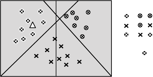
7

0

▸

A

NALYTI

CS

IN A BI

G

DATA W

O

RL

D

observation is then assi

g

ned to the out

p

ut neuron with the hi

g

hest

activation value (winner take all learnin

g

). Another o

p

tion is to use a

s

oftmax activation function.

34

Multiclass Support Vector Machines

A common practice to estimate a multiclass support vector machine is

to map the multiclass classi cation problem to a set of binary classi ca

-

tion problems. Two well‐known schemes here are one‐versus‐one and

one‐versus‐all codin

g

.

35

For

K

classes, one‐versus‐one coding estimates

K

(

K

− 1)/2 binary

K

SVM c

l

assi



ers contrasting every possi

bl

e pair o

f

c

l

asses. Every c

l

as

-

s

i



er as suc

h

can cast a vote on t

h

e target c

l

ass an

d

t

h

e



na

l

c

l

assi-

 cation is then the result of a (weighted) voting procedure. Ties are

resolved arbitraril

y

. This is illustrated in Fi

g

ure 3.25 .

F

o

r

K

classes, one‐versus‐all coding estimates

K

binary SVM clas-

K

s

i ers each time contrasting one particular class against all the other

ones. A classi cation decision can then be made b

y

assi

g

nin

g

a

p

ar

-

ticular observation to the class for which one of the binar

y

classi ers

assigns the highest posterior probability. Ties are less likely to occur

with this scheme. This is illustrated in Fi

g

ure 3.26 .

N

ote that one‐versus‐one and one‐versus‐all are meta schemes

that can be used with other base classi ers as well.

F

i

gure3.25 One‐versus‐One Coding

f

or Multiclass Problems

x1

x

2

a) or :

b) or :

c) or :

Class is !

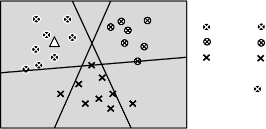
P

REDICTIVE ANALYTIC

S

◂

71

EVALUATING PREDICTIVE MODELS

In this section, we will discuss how to evaluate the performance of

predictive models. First, we will discuss how to split up the data set.

This will be followed b

y

a discussion of

p

erformance metrics.

Splitting Up the Data Set

When evaluating predictive models, two key decisions need to be

made. A  rst decision concerns the data set s

p

lit u

p

, which s

p

eci es

on what

p

art of the data the

p

erformance will be measured. A second

decision concerns the performance metric. In what follows, we will

elaborate on both.

The decision how to s

p

lit u

p

the data set for

p

erformance mea

-

surement depends upon its size. In case of large data sets (say more

than 1,000 observations), the data can be s

p

lit u

p

into a trainin

g

and

a test sam

p

le. The trainin

g

sam

p

le (also called

development

o

r

t

estimation

s

am

pl

e) wi

ll

b

e use

d

to

b

ui

ld

t

h

e mo

d

e

l

, w

h

ereas t

h

e test sam

pl

e (a

l

so

ca

ll

e

d

t

h

e

h

o

ld

out samp

l

e ) wi

ll

b

e use

d

to ca

l

cu

l

ate its per

f

ormance (see

Fi

g

ure 3.27 ). T

h

ere s

h

ou

ld

b

e a strict se

p

aration

b

etween trainin

g

an

d

test sam

pl

e. Note t

h

at in case o

f

d

ecision trees or neura

l

networ

k

s, t

h

e

va

l

i

d

ation samp

l

e s

h

ou

ld

b

e part o

f

t

h

e training samp

l

e

b

ecause it is

active

ly

b

ein

g

use

d

urin

g

mo

d

e

l

d

eve

l

o

p

ment (i.e., to ma

k

e t

h

e sto

p

-

p

in

g

d

ecision).

Figure3.26 One‐versus‐All Coding for Multiclass Problems

a) or other; p( ) = 0.92

b) or other; p( ) = 0.18

c) or other; p( ) = 0.30

Class is !

x

2

x1

7

2

▸

A

NALYTI

CS

IN A BI

G

DATA W

O

RL

D

In the case of small data sets (sa

y

, less than 1,000 observations),

s

pecia

l

sc

h

emes nee

d

to

b

e a

d

opte

d

. A very popu

l

ar sc

h

eme is cross‐

validation (see Fi

g

ure 3.28 ). In cross‐validation, the data is s

p

lit into

K

folds (e.g., 10). A model is then trained on

K

− 1 training folds and

K

teste

d

on t

h

e remaining va

l

i

d

ation

f

o

ld

. T

h

is is repeate

d

f

or a

ll

possi

bl

e

va

l

i

d

ation

f

o

ld

s resu

l

tin

g

in

K

performance estimates that can then be

K

avera

g

e

d

. Note a

l

so t

h

at a stan

d

ar

d

eviation an

d

/or con



d

ence inter

-

va

l

can

b

e ca

l

cu

l

ate

d

i

f

d

esire

d

. Common c

h

oices

f

or

K

are 5 and 10. In

K

its most extreme case

,

cross‐validation becomes leave‐one‐out cross‐

validation whereb

y

ever

y

observation is left out in turn and a model is

estimated on the remaining

K

− 1 observations. This gives

K

analytical

K

models in total. In strati ed cross‐validation, s

p

ecial care is taken to

make sure the

g

ood/bad odds are the same in each fold.

F

i

gure3.27 Training versus Test Sample Set Up for Performance Estimation

Data

Build Model

Apply

Model

Target…Good/BadGenderIncomeAgeCustomer

0BadM1,20030John

1GoodF80025Sarah

1GoodF2,20052Sophie

0BadM2,00048David

1GoodM1,80034Peter

ScoreGood/Bad…GenderIncomeAgeCustomer

0.44GoodF1,00028Emma

0.76BadM1,50044Will

0.18GoodM1,20030Dan

0.88GoodM2,40058Bob

Train Data

Test Data

1

−(0.10+0.50age+0.0034income +...)

+e

P(Good | age,income,...) =

F

i

gure3.28 Cross‐Validation

f

or Per

f

ormance Measurement

Validation fold

Training fold

.

P

REDICTIVE ANALYTIC

S

◂

73

A

k

e

y

q

uestion to answer w

h

en

d

oin

g

cross‐va

l

i

d

ation is w

h

at

should be the  nal model that is bein

g

out

p

ut from the

p

rocedure.

Because cross‐validation gives multiple models, this is not an obvi-

ous question. Of course, one could let all models collaborate in an

ensemble setup. A more pragmatic answer would be to, for example,

do leave‐one‐out cross‐validation and pick one of the models at ran-

dom. Because the models differ up to one observation, they will be

quite similar anyway. Alternatively, one may also choose to build one

 nal model on all observations but report the performance coming out

of the cross‐validation

p

rocedure as the best inde

p

endent estimate.

For sma

ll

samp

l

es, one may a

l

so a

d

opt

b

ootstrapping proce

d

ures.

In

b

ootstrapping, one ta

k

es samp

l

es wit

h

rep

l

acement

f

rom a

d

ata set D

(see F

i

gure 3.29 ).

The probability that a customer is not sampled equals 1/

n

,

with

n

b

ein

g

the number of observations in the data set. Assumin

g

a bootstra

p

w

ith

n

sam

p

les, the fraction of customers that is not sam

p

led e

q

uals

:

n

11.−

⎛

⎝

⎜⎞

⎠

⎟

We then have:

−

⎛

⎝

⎜⎞

⎠

⎟==

→∞

−

ne

n

lim 1 10.368

1

whereby the approximation already works well for small values of

n

. So

,

0.368 is the

p

robabilit

y

that a customer does not a

pp

ear in the sam

p

le

and 0.632 is the

p

robabilit

y

that a customer does a

pp

ear. If we then take

the bootstrap sample as the training set, and the test set as all samples in

D but not in the bootstra

p

, we can calculate the

p

erformance as follows

:

Error estimate 0.368 error(training) 0.632 error(test),=+

whereb

y

obviousl

y

a hi

g

her wei

g

ht is bein

g

p

ut on the test set

p

erfor-

mance.

Figure3.29 Bootstrapping

C3 C3 C5 C3 C2C2

Bootstrap 1

D

C1

C2

C4

C5

C1 C2 C1 C2C4

Bootstrap 2

7

4

▸

A

NALYTICS IN A BIG DATA WORL

D

Performance Measures for Classi cation Models

Consi

d

er,

f

or examp

l

e, t

h

e

f

o

ll

owing c

h

urn pre

d

iction examp

l

e

f

or

a



ve customer

d

ata set. T

h

e



rst co

l

umn in Ta

bl

e 3.3

d

epicts t

h

e

true status

,

whereas the second column is the churn score as it

comes from a logistic regression, decision tree, neural network, and

so on.

One can now ma

p

the scores to a

p

redicted classi cation label b

y

assuming a default cutoff of 0.5 as shown in Figure 3.30 .

A confusion matrix can now be calculated and is shown in

T

ab

l

e

3.4 .

Based upon this matrix, one can now calculate the following per

-

formance measures:

■ Classi cation accurac

y

= (TP + TN)/(TP + FP + FN + TN) = 3/5

■ Classi cation error = (FP + FN)/(TP + FP + FN + TN) = 2/5

■ Sens

i

t

i

v

i

ty = TP/(TP + FN) = 1/2

■ S

p

eci cit

y

= TN/(FP + TN) = 2/3

However, note that all these classi cation measures depend on

the cut‐off. For exam

p

le, for a cut off of 0 (1), classi cation accurac

y

Ta

bl

e3.3 Exam

p

le Data Set

f

or Per

f

ormance Calculation

Churn Score

J

o

hn

Y

es 0.7

2

Sophi

e

N

o

0.5

6

D

av

id

Y

es 0.4

4

E

mm

a

No

0.1

8

B

o

b

No

0.3

6

Figure3.30 Calculating Predictions Using a Cut‐Of

f

Cutoff = 0.50

Churn Score

John Yes 0.72

Sophie No 0.56

David Yes 0.44

Emma No 0.18

Bob No 0.36

Churn Score Predicted

John Yes 0.72 Yes

Sophie No 0.56 Yes

David Yes 0.44 No

Emma No 0.18 No

Bob No 0.36 No

P

REDICTIVE ANALYTIC

S

◂

75

T

able



3

.4 The Con

f

usion Matrix

Actual Status

Positive (churn) Negative (no churn)

Pred

i

cted statu

s

Positive

(

churn

)

T

rue positive

(

John

)

False positive

(

Sophie

)

Ne

g

ative

(

no churn

)

F

a

l

se ne

g

at

i

ve

(D

av

id)

T

rue ne

g

at

i

ve

(E

mma,

B

o

b)

Table3.5 ROC Anal

y

sis

Cutoff Sensitivity Specificity 1−Specificity

0

1

0

1

0

.

01

0

.

02

…

.

0

.

99

1

0

1

0

b

ecomes 40 percent (60 percent), the error 60 percent (40 percent),

the sensitivity 100 percent (0), and the speci city 0 (100 percent).

It would be nice to have a performance measure that is indepen

-

d

ent

f

rom t

h

e cut‐o

ff

. One cou

ld

construct a ta

bl

e wit

h

t

h

e sensi

-

tivity, speci



city, an

d

1−speci



city

f

or various cut-o

ff

s as s

h

own in

Ta

bl

e 3.5 .

The receiver operating characteristic (ROC) curve then plots the

sensitivit

y

versus 1−s

p

eci cit

y

as illustrated in Fi

g

ure 3.31 .

3

6

Note that a

p

erfect model has a sensitivit

y

of 1 and a s

p

eci cit

y

of

1, and is thus represented by the upper left corner. The closer the curve

a

pp

roaches this

p

oint, the better the

p

erformance. In Fi

g

ure 3.31 ,

scorecard A has a better

p

erformance than scorecard B. A

p

roblem

arises

,

however

,

if the curves intersect. In this case

,

one can calcu

-

late the area under the ROC curve (AUC) as a

p

erformance metric.

The AUC

p

rovides a sim

p

le 

g

ure‐of‐merit for the

p

erformance of

the constructed classi er. The higher the AUC, the better the per-

formance. The AUC is alwa

y

s bounded between 0 and 1 and can be

inter

p

reted as a

p

robabilit

y

. In fact, it re

p

resents the

p

robabilit

y

that a

randomly chosen churner gets a higher score than a randomly chosen

nonchurner.

3

7 Note that the dia

g

onal re

p

resents a random scorecard

whereby sensitivity equals 1−speci city for all cut off points. Hence, a

7

6

▸

A

NALYTI

CS

IN A BI

G

DATA W

O

RL

D

g

ood classi er should have an ROC above the dia

g

onal and AUC bi

g

-

g

er than 50%. Table 3.6

p

resents some AUC benchmarks for various

analytics applications.

38

A lift curve is another im

p

ortant

p

erformance metric. It starts b

y

sortin

g

the

p

o

p

ulation from low score to hi

g

h score. Su

pp

ose now

that in the top 10% lowest scores there are 60 percent bads, whereas

the total

p

o

p

ulation has 10% bads. The lift value in the to

p

decile

then becomes 60/10

p

ercent or 6. In other words, the lift value re

p-

resents the cumulative percentage of bads per decile, divided by the

overall

p

o

p

ulation

p

ercenta

g

e of bads. Usin

g

no model, or a random

sortin

g

, the bads would be e

q

uall

y

s

p

read across the entire ran

g

e and

the lift value would always equal 1. Obviously, the lift curve always

decreases as one considers bi

gg

er deciles, until it will reach 1. This is

illustrated in Figure 3.32 . Note that a lift curve can also be expressed

in a noncumulative way, and is also often summarized as the top

decile lif

t

.

T

ab

l

e



3

.

6

Performance Benchmarks in Terms of AUC

Application Number of

Characteristics AUC Ranges

A

pplication credit scorin

g

1

0

–1

5

70

–

85%

Behavioral credit scorin

g

1

0

–1

5

80

–

90%

C

hurn detection (telco

)

6

–

10

70

–

90%

Fraud detection (insurance

)

10–1

5

7

0–90

%

F

i

gure3.31 T

h

e Rece

i

ver Operat

i

ng C

h

aracter

i

st

i

c Curve

0

0.2

0.4

0.6

0.8

1

0 0.2 0.4 0.6 0.8 1

Sensitivity

(1–Specificity)

ROC Curve

Scorecard A Random Scorecard B

P

REDI

C

TIVE ANALYTI

CS

◂

77

T

h

e cumu

l

ative accurac

y

p

ro



l

e (CAP), Lorenz, or

p

ower curve is

very c

l

ose

l

y re

l

ate

d

to t

h

e

l

i

f

t curve (see Figure 3.33 ). It a

l

so starts

b

y

sortin

g

t

h

e

p

o

p

u

l

ation

f

rom

l

ow score to

h

i

gh

score an

d

t

h

en measures

t

h

e cumu

l

ative

p

ercenta

g

e o

f

b

a

d

s

f

or eac

h

d

eci

l

e on t

h

e Y‐axis. T

h

e

per

f

ect mo

d

e

l

gives a

l

inear

l

y increasing curve up to t

h

e samp

l

e

b

a

d

rate an

d

t

h

en



attens out. T

h

e

d

ia

g

ona

l

a

g

ain re

p

resents t

h

e ran

d

om

mo

d

e

l

.

T

h

e CAP curve can

b

e summarize

d

in an Accuracy Ratio (AR) as

d

e

p

icte

d

in Fi

g

ure 3.34 .

T

h

e accuracy ratio is t

h

en

d

e



ne

d

as

f

o

ll

ows:

(Area

b

e

l

ow

p

ower curve

f

or current mo

d

e

l

−Area

b

e

l

ow

p

ower

curve

f

or ran

d

om mo

d

e

l)

/

(Area

b

e

l

ow

p

ower curve

f

or

p

er

f

ect mo

d

e

l

−Area

b

e

l

ow

p

ower

curve

f

or ran

d

om mo

d

e

l

)

A per

f

ect mo

d

e

l

wi

ll

t

h

us

h

ave an AR o

f

1 an

d

a ran

d

om mo

d

e

l

an

AR o

f

0. Note t

h

at t

h

e accurac

y

ratio is a

l

so o

f

ten re

f

erre

d

to as t

h

e

G

ini

coe

f

cient. T

h

ere is a

l

so a

l

inear re

l

ation

b

etween t

h

e AR an

d

t

h

e AUC

as

f

o

ll

ows: AR = 2 * AUC−1.

Figure3.32 The Li

f

t Curve

0

1

2

3

4

5

6

10 20 30 40 50 60 70 80 90 100

% of Sorted Population

Scorecard

Baseline

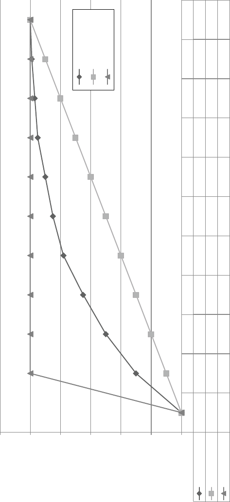
0 0.1 0.2 0.3 0.4 0.5 0.6 0.7 0.8 0.9 1

Scorecard 0 0.3 0.5 0.65 0.78 0.85 0.9 0.95 0.97 0.99 1

Random model 0 0.1 0.2 0.3 0.4 0.5 0.6 0.7 0.8 0.9 1

Perfect Model 01111111111

0

0.2

0.4

0.6

0.8

1

1. 2

Percentage of Bads

Percentage of sorted population

Scorecard

Random model

Perfect Model

Fi

g

ure3.33 The Cumulative Accurac

y

Pro le

78

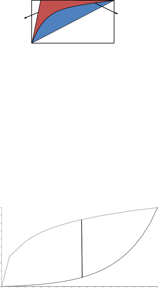
P

REDICTIVE ANALYTIC

S

◂

79

The Kolmo

g

orov‐Smirnov distance is a se

p

aration measure calcu

-

latin

g

the maximum distance between the cumulative score distribu-

tions P(s | B) and P(s | G) de ned as follows (see Fi

g

ure 3.35 ):

∑

=

≤

PsG pxG

xs

(| ) ( | )

∑

=

≤

PsB pxB

xs

(| ) ( | )

Note that by de nition

P

(

P

s

|

G

) equals 1−sensitivity, and

P

(

P

s

|

B

)

e

q

uals the s

p

eci cit

y

. Hence, it can easil

y

be veri ed that the KS dis

-

tance can also be measured on an ROC graph. It fact, it is equal to the

maximum vertical distance between the ROC curve and the dia

g

onal.

B

A

AR = B/(A + B)

Current model

Perfect model

F

i

gure3.34 Ca

l

cu

l

at

i

ng t

h

e Accuracy Rat

i

o

Fi

g

ure3.35 The Kolmo

g

orov‐Smirnov Statistic

0

0.1

0.2

0.3

0.4

0.5

0.6

0.7

0.8

0.9

1

Score

P(s|G)

P(s|B)

KS distance

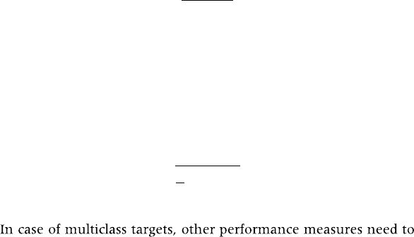
80

▸

A

NALYTI

CS

IN A BI

G

DATA W

O

RL

D

Anot

h

er

p

er

f

ormance measure is t

h

e Ma

h

a

l

ano

b

is

d

istance

b

etween the score distributions

,

de ned as follows:

MGB

||

,=μ−μ

σ

w

h

ere

b

yμG

(

μB) represents t

h

e mean score o

f

t

h

e goo

d

s (

b

a

d

s) an

d

σ the

p

ooled standard deviation. Obviousl

y

, a hi

g

h Mahalanobis

d

istance is pre

f

erre

d

b

ecause it means

b

ot

h

score

d

istri

b

utions are

we

ll

se

p

arate

d

. C

l

ose

ly

re

l

ate

d

is t

h

e

d

iver

g

ence metric, ca

l

cu

l

ate

d

as follo

w

s:

DGB

GB

()

1

2()

2

22

=μ−μ

σ+σ

b

e a

d

o

p

te

d

. Fi

g

ure 3.36

p

resents an exam

pl

e o

f

a mu

l

tic

l

ass con

f

usion

ma

t

r

i

x.

T

h

e on‐

d

ia

g

ona

l

e

l

ements re

p

resente

d

in

g

ra

y

corres

p

on

d

to t

h

e

correct classi cations. Off‐dia

g

onal elements re

p

resent errors. Note,

however, that not all errors have equal impact. Given the ordinal

nature o

f

t

h

e tar

g

et varia

bl

e, t

h

e

f

urt

h

er awa

y

f

rom t

h

e

d

ia

g

ona

l

,

the bi

gg

er the im

p

act of the error. For exam

p

le, in Fi

g

ure 3.36 ,

t

h

ere are 34 C+ o

b

servations pre

d

icte

d

as C, w

h

ic

h

is not as

b

a

d

as

t

h

e one C+

p

re

d

icte

d

as D. One cou

ld

summarize t

h

is in a notc

h

d

i

f-

ference graph that depicts the cumulative accuracy for increasing

notc

h

d

i

ff

erences. Figure 3.37 gives an examp

l

e o

f

a notc

h

d

i

ff

er

-

ence

g

ra

p

h.

At the 0 notch difference level, the performance equals about

35

p

ercent, w

h

ic

h

ma

y

not seem ver

y

g

oo

d

. However,

by

a

ll

owin

g

for a one‐notch difference, the

p

erformance almost doubles to around

75percent, w

h

ic

h

is a

l

ot

b

etter!

T

h

e AUC can

b

e genera

l

ize

d

to t

h

e mu

l

tic

l

ass setting

b

y p

l

ot

-

ting an ROC grap

h

f

or eac

h

c

l

ass against a

ll

ot

h

er c

l

asses, ca

l

cu

l

ating

t

h

e AUC, an

d

ta

k

ing t

h

e overa

ll

average. Anot

h

er option is to ca

l-

cu

l

ate an AUC

f

or eac

h

possi

bl

e c

l

ass comparison an

d

t

h

en ta

k

e t

h

e

a

v

erage

.

39

A+ A A– B+ B B– C+ C C– D+ D D– E+ E E–

A+ 000000000000000

A0140400000000000

A– 000200000000000

B+ 0705000550100000

B 0225401258170510100

B– 0006061060100000

C+ 0001303993401110000

C0105013715111240000

C– 000200383400000

D+ 0001007202131240310

D0001002913212201370

D– 000000000002100

E+ 000000040122603750

E0000000404905480

E– 000000000000000

Predicted

True

F

i

gure3.36 Confusion Matrix for a Multiclass Example

8

1

F

i

gure3.37 A Cumulative Notch Di

ff

erence Graph

0

10

20

30

40

50

60

70

80

90

100

0123456

Cumulative Accuracy (%)

Notch Difference

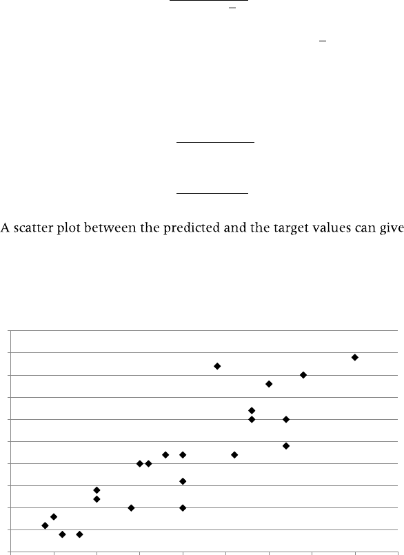
P

REDICTIVE ANALYTIC

S

◂

83

Performance Measures for Regression Models

Mu

l

tip

l

e measures exist to ca

l

cu

l

ate t

h

e per

f

ormance o

f

regression

models. A  rst key metric is the

R

‐squared, de ned as follows:

Ryy

yy

ii

i

n

i

n

1(ˆ)

()

,

2

1

2

1

∑

=− −

−

=

whereby yi is the true value, yi

ˆ the predicted value, and y the average.

The R2 always varies between 0 and 1, and higher values are to be pre

-

ferred. Two other popular measures are the mean squared error (MSE)

an

d

mean a

b

so

l

ute

d

eviation (MAD),

d

e



ne

d

as

f

o

ll

ows:

∑

=−

=

MSE yy

n

ii

i

n(ˆ)2

1

a visual re

p

resentation of model

p

erformance (see Fi

g

ure 3.38 ). The

more the

p

lot a

pp

roaches a strai

g

ht line throu

g

h the ori

g

in, the better

the performance of the model. It can be summarized by calculating the

Pearson correla

t

ion coef cien

t

.

∑

=−

=

MAD yy

n

i

n

ii

|ˆ|

1

0

5

10

15

20

25

30

35

40

45

50

0 5 10 15 20 25 30 35 40 45

P

r

e

d

i

c

t

e

d

C

L

V

CLV

Figure3.38 Scatter Plot for Measuring Model Performance

8

4▸

A

NALYTICS IN A BIG DATA WORL

D

NOTES

1. T. Hastie, R. Ti

b

s

h

irani, an

d

J. Frie

d

man, E

l

ements o

f

Statistica

l

Learning: Data Mining,

Inference and Prediction (Springer‐Verlag, Berlin, Germany, 2001).

2. S. Viaene et al., “A Comparison of State‐of‐the‐Art Classi cation Techniques for

Expert Automobile Insurance Fraud Detection.” Special issue, Journal of Risk and

In

sura

n

ce 69, no. 3

(

2002

)

: 433–443.

3. S. Gupta et al., “Modeling Customer Lifetime Value,”

J

ournal of Service Researc

h

9,

no. 2 (2006): 139–155; N. Glady, C. Croux, and B. Baesens, “Modeling Churn Using

Customer Lifetime Value,” European Journal of Operational Researc

h

197, no. 1

(

2009

)

:

402–411.

4. T. Van Gestel and B. Baesens, Credit Risk Management: Basic Concepts: Financial Risk

Components, Rating Analysis, Models, Economic and Regulatory Capital

(Oxford University

l

Press, 2009); G. Loterman et al., “Benchmarking Regression Algorithms for Loss

Given Default Modeling,”

I

nternational Journal of Forecasting 28, no. 1

(

2012

)

: 161

–

170; E. Tobback et al., “Forecasting Loss Given Default Models: Impact of Account

Characteristics and the Macroeconomic State,” Journal of the Operational Research

Societ

y,

forthcomin

g

2014.

5. D. W. Dwyer, A. Kocagi

l

, an

d

R. Stein, T

h

e Moo

d

y’s KMV EDF™ Ris

k

Ca

l

c™ v3.1 Mo

d

e

l

Next Generation Technology for Predicting Private Firm Credit Risk

(W

h

ite

p

a

p

er, 2004).

k

6. R. O. Du

d

a

,

P. E. Hart

,

an

d

D. G. Stor

k,

Pattern C

l

assi



cation (Jo

h

n Wi

l

e

y

& Sons,

Ho

b

o

k

en, New Jerse

y

, US, 2001).

7. J. R. Quin

l

an, C4.5 Programs

f

or Mac

h

ine Learning (Mor

g

an Kau

ff

man Pu

bl

is

h

ers,

Bur

l

ington, Massac

h

usetts, Unite

d

States, 1993).

8. L. Breiman et a

l

., C

l

assi



cation an

d

Regression Trees (Monterey, CA: Wa

d

swort

h

&

Broo

k

s/Co

l

e A

d

vance

d

Boo

k

s & So

f

tware, 1984

)

.

9. J. A. Harti

g

an, C

l

usterin

g

A

lg

orit

h

ms (New Yor

k

: Jo

h

n Wi

l

e

y

& Sons, 1975).

10. C. M. Bis

h

o

p

, Neura

l

Networ

k

s

f

or Pattern Reco

g

nitio

n

(Ox

f

or

d

Universit

y

Press, Ox

f

or

d

,

En

gl

an

d

, 1995); J. M. Zura

d

a,

I

ntro

d

uction to Arti



cia

l

Neura

l

S

y

stems

(

Boston: PWS

Pu

bl

is

h

in

g

, 1992).

11. B. Baesens et a

l

., “Ba

y

esian Neura

l

Networ

k

Learnin

g

f

or Re

p

eat Purc

h

ase Mo

d

e

l

-

l

in

g

in Direct Mar

k

etin

g

,” Euro

p

ean Journa

l

o

f

O

p

erationa

l

Researc

h

138, no. 1

(

2002

)

:

191–211.

12. K. Horni

k

, M. Stinc

h

com

b

e, an

d

H. W

h

ite, “Mu

l

ti

l

a

y

er Fee

df

orwar

d

Networ

k

s Are

Universa

l

A

pp

roximators,” Neura

l

Networ

ks

2, no. 5

(

1989

)

: 359–366.

13. See C. M. Bis

h

o

p

,

N

eura

l

Networ

k

s

f

or Pattern Recognitio

n

(Ox

f

or

d

Universit

y

Press,

Ox

f

or

d

, En

gl

an

d

, 1995)

f

or more

d

etai

l

s.

14. J. Moo

dy

an

d

J. Utans. “Arc

h

itecture Se

l

ection Strate

g

ies

f

or Neura

l

Networ

k

s:

A

ppl

ication to Cor

p

orate Bon

d

Ratin

g

Pre

d

iction,” in

N

eura

l

Networ

k

s in t

h

e Ca

p

ita

l

M

ar

k

ets, A. N. Re

f

enes (e

d

itor) (New Yor

k

: Jo

h

n Wi

l

e

y

& Sons, 1994).

15. P. L. Bart

l

ett, “For Va

l

i

d

Genera

l

ization, t

h

e Size o

f

t

h

e Wei

gh

ts Is More Im

p

ortant

than the Size of the Network,” in

Advances in Neural Information Processing Systems 9,

e

d

. M. C, Mozer, M. I. Jor

d

an, an

d

T. Petsc

h

e (Cam

b

ri

d

ge, MA: MIT Press, 1997),

134

–

140.

16. B. Baesens, D. et a

l

., “W

h

ite Box Non

l

inear Pre

d

iction Mo

d

e

l

s.” Specia

l

issue,

IEEE

Transactions on Neura

l

Networ

k

s 22, no. 12

(

2011

)

: 2406–2408.

17. B. Baesens, “Deve

l

o

p

in

g

Inte

ll

i

g

ent S

y

stems

f

or Cre

d

it Scorin

g

usin

g

Mac

h

ine Learn-

ing Tec

h

niques” (P

h

D t

h

esis, Kat

h

o

l

ie

k

e Universiteit Leuven, 2003); B. Baesens et a

l

.,

P

REDI

C

TIVE ANALYTI

CS

◂

85

“Usin

g

Neura

l

Networ

k

Ru

l

e Extraction an

d

Decision Ta

bl

es

f

or Cre

d

it‐Ris

k

Eva

l

ua-

tion

,

”

Management Science

49, no. 3

(

2003

)

: 312–329; R. Setiono, B. Baesens, and C.

Mues, “A Note on Knowled

g

e Discover

y

Usin

g

Neural Networks and Its A

pp

lication

to Credit Card Screening,” European Journal of Operational Research 192, no. 1 (2009):

326–332.

18. H. Lu, R. Setiono, and H. Liu, “NeuroRule: A Connectionist Approach to Data

Mining,” in

P

roceedings of 21st International Conference on Very Large Data Base

s

(Zurich,

Switzerland, Morgan Kaufmann, 1995), 478–489.

19. M. Craven and J. Shavlik, “Extracting Tree‐Structured Representations of Trained

Networks,” in

Advances in Neural Information Processing Systems

(Cambridge, MA: MIT

Press, 1996

)

.

20. T. Van Gestel et al., “Linear and Nonlinear Credit Scoring by Combining Logistic

Regression and Support Vector Machines,”

Journal of Credit Risk

1, no. 4

(

2005

)

; T.

k

Van Gestel et al., “A Process Model to Develop an Internal Rating System: Sovereign

Credit Ratings,” Decision Support Systems 42, no. 2

(

2006

)

: 1131–1151.

21. N. Cristianini and J. S. Taylor,

An Introduction to Support Vector Machines and Other

Kernel‐based Learning Method

s

(Cambridge University Press, 2000); B. Schölkopf and

A. Smola

,

Learning with Kernels (Cambrid

g

e, MA: MIT Press, 2001); V. Va

p

nik, T

he

Nature of Statistical Learnin

g

Theory (New York: S

p

rin

g

er‐Verla

g

, 1995).

22. O. L. Man

g

asarian, “Linear and Non‐linear Se

p

aration of Patterns b

y

Linear Pro

-

g

rammin

g

,” O

p

erations Researc

h

13, Ma

y

‐June (1965): 444–452.

23. N. Cristianini and J. S. Taylor,

An Introduction to Support Vector Machines and Other

Kernel‐based Learnin

g

Method

s

(Cambrid

g

e Universit

y

Press, 2000); B. Schölko

p

f and

A. Smola

,

Learnin

g

with Kernels (Cambrid

g

e, MA: MIT Press, 2001); V. Va

p

nik, T

he

Nature of Statistical Learnin

g

Theory (New York: S

p

rin

g

er‐Verla

g

, 1995).

24. N. Cristianini and J. S. Taylor,

An Introduction to Support Vector Machines and Other

Kernel‐based Learnin

g

Method

s

(Cambrid

g

e Universit

y

Press, 2000); B. Schölko

p

f and

A. Smola

,

Learnin

g

with Kernels (Cambrid

g

e, MA: MIT Press, 2001); V. Va

p

nik, T

he

Nature of Statistical Learnin

g

Theory (New York: S

p

rin

g

er‐Verla

g

, 1995).

25. T. Van Gestel et al., “Benchmarkin

g

Least S

q

uares Su

pp

ort Vector Machine Classi

-

 ers,”

Machine Learning

54, no. 1

(

2004

)

: 5–32.

26. I

b

i

d

.

27. D. Martens et al., “Com

p

rehensible Credit Scorin

g

Models Usin

g

Rule Extraction

From Su

pp

ort Vector Machines,” Euro

p

ean Journal o

f

O

p

erational Research 183

(

2007

)

:

1466–1476; D. Martens, B. Baesens, and T. Van Gestel, “Decompositional Rule

Extraction from Su

pp

ort Vector Machines b

y

Active Learnin

g

,” IEEE T

ransactions

on

Knowledge and Data Engineering 21, no. 1,

(

2009

)

: 178–191.

28. L. Breiman, “Bagging Predictors,”

Machine Learning

24, no. 2

(

1996

)

: 123–140.

29. Ibid.

30. Y. Freund and R. E. Scha

p

ire, “A Decision‐Theoretic Generalization of On‐Line

Learnin

g

an

d

an A

ppl

ication to Boostin

g

,” Journa

l

o

f

Com

p

uter an

d

S

y

stem Sciences

55, no. 1 (1997): 119–139; Y. Freun

d

an

d

R. E. Sc

h

apire, “A S

h

ort Intro

d

uction

to Boost

i

ng,” Journa

l

o

f

Japanese Society

f

or Arti



cia

l

Inte

ll

igenc

e

14, no. 5

(

1999

)

:

7

71–7

80.

31. See Y. Freun

d

an

d

R. E. Sc

h

a

p

ire, “A Decision‐T

h

eoretic Genera

l

ization o

f

On‐Line

Learning an

d

an App

l

ication to Boosting,” Journa

l

o

f

Computer an

d

System Sciences

55, no. 1 (1997): 119–139, an

d

Y. Freun

d

an

d

R. E. Sc

h

apire, “A S

h

ort Intro

d

uc

-

tion to Boostin

g

,”

J

ourna

l

o

f

Japanese Society

f

or Arti



cia

l

Inte

ll

igence 14, no. 5 (1999):

7

71–780,

f

or more

d

etai

l

s.

86

▸

A

NALYTI

CS

IN A BI

G

DATA W

O

RL

D

32. L. Breiman, “Random Forests,”

Machine Learning

45, no. 1

(

2001

)

: 5–32.

33. J. J. Rodri

g

uez, L. I. Kuncheva, and C. J. Alonso, “Rotation Forest: A New Classi er

Ensemble Method

,

” IEEE Transactions on Pattern Analysis and Machine Intelligenc

e

28

,

no. 10

(

2006

)

: 1619–1630.

34. C. M. Bishop, Neural Networks for Pattern Recognitio

n

(Oxford University Press, Oxford,

England, 1995).

35. T. Van Gestel, “From Linear to Kernel Based Methods for Classi cation, Modelling

and Prediction” (PhD Thesis, Katholieke Universiteit Leuven, 2002).

36. T. Fawcett, “ROC Graphs: Notes and Practical Considerations for Researchers,”

H

P

Labs Tech Report HPL‐2003–4 , HP Laboratories, Palo Alto, US

(

2003

)

.

37. E. R. Delong, D. M. Delong, and D. L. Clarke‐Pearson, “Comparing the Areas Under

T

wo or More Correlated Receiver Operating Characteristic Curves: A Nonparamet-

ric Approach,”

Biometrics

44 (1988): 837–845; J. A, Hanley and B. J. McNeil, “The

Meaning and Use of Area under the ROC Curve,”

R

adiology 143

(

1982

)

: 29–36.

38. B. Baesens et al., “Benchmarking State of the Art Classi cation Algorithms for

Credit Scoring,” Journal of the Operational Research Societ

y

54, no. 6

(

2003

)

: 627–635;

W. Verbeke et al., “New Insi

g

hts into Churn Prediction in the Telecommunication

Sector: A Pro t Driven Data Minin

g

A

pp

roach,”

E

uro

p

ean Journal o

f

O

p

erational

R

esearch

218, no. 1

(

2012

)

: 211–229.

39. D. Hand and R. J. Till, “A Sim

p

le Generalization of the Area under the ROC Curve to

Multiple Class Classi cation Problems,”

Machine Learning

45, no. 2

(

2001

)

: 171–186.

8

7

C

HAPTER

4

Descriptive

Analytics

I n

d

escri

p

tive ana

ly

tics, t

h

e aim is to

d

escri

b

e

p

atterns o

f

customer

b

e

h

avior. Contrary to pre

d

ictive ana

l

ytics, t

h

ere is no rea

l

target

v

aria

bl

e (e.

g

., c

h

urn or

f

rau

d

in

d

icator) avai

l

a

bl

e. Hence,

d

escri

p

tive

ana

ly

tics is o

f

ten re

f

erre

d

to as

u

nsupervise

d

l

earnin

g

b

ecause t

h

ere is no

target varia

bl

e to steer t

h

e

l

earning process. T

h

e t

h

ree most common

t

yp

es o

f

d

escri

p

tive ana

ly

tics are summarize

d

in Ta

bl

e 4.1 .

ASSOCIATION RULES

In t

h

is section, we wi

ll

a

dd

ress

h

ow to mine association ru

l

es

f

rom

d

ata. First, t

h

e

b

asic setting wi

ll

b

e

d

iscusse

d

. T

h

is wi

ll

b

e

f

o

ll

owe

d

b

y a

d

iscussion o

f

su

pp

ort an

d

con



d

ence, w

h

ic

h

are two

k

e

y

measures

f

or

association ru

l

e minin

g

. Next, we wi

ll

zoom into t

h

e association ru

l

e

mining process. T

h

e

l

i

f

t measure wi

ll

t

h

en

b

e intro

d

uce

d

. T

h

e section

wi

ll

b

e conc

l

u

d

e

d

by

d

iscussin

g

p

ost

p

rocessin

g

, extensions, an

d

vari-

ous a

ppl

ications o

f

association ru

l

es.

Basic Setting

Association rules t

yp

icall

y

start from a database of transactions,

D

. Each

transaction consists of a transaction identi er and a set of items (e.g.,

88

▸

A

NALYTI

CS

IN A BI

G

DATA W

O

RL

D

p

roducts, Web

p

a

g

es, courses) {

i

1

,

i

2

,

…

,

i

n

} selected from all

p

ossible

items (

I

). Table 4.2 gives an example of a transactions database in a

I

su

p

ermarket settin

g

.

An association rule is then an implication of the form

X

⇒

Y

,

Y

whereby

X

⊂

I

,

I

Y

⊂

I

and

I

X

∩

Y

=

Y

∅

.

X

is referred to as the rule

X

Ta

bl

e 4.2 Examp

l

e Transact

i

on Data Set

Transaction Identifier Items

1

Beer, milk, diapers, baby

f

oo

d

2

Coke, beer, dia

p

er

s

3

Ci

g

arettes, diapers, baby foo

d

4 Chocolates, dia

p

ers, milk, a

pp

le

s

5

T

omatoes, water, app

l

es,

b

eer

6

Spaghetti, diapers, baby food, bee

r

7

Water, beer, baby foo

d

8

Diapers, baby

f

ood, spaghett

i

9

Baby

f

ood, beer, diapers, mil

k

10

A

pples, wine, baby foo

d

Ta

bl

e 4.1 Examples o

f

Descriptive Anal

y

tics

Type of Descriptive

Analytics Explanation Example

A

ssoc

i

at

i

on ru

l

e

s

Detect frequently

occurr

i

n

g

patterns between

item

s

Detectin

g

what products are frequently purchased

t

o

g

et

h

er

i

n a supermar

k

et contex

t

Detectin

g

what words frequently co‐occur in a

t

ext documen

t

Detectin

g

what elective courses are frequently

chosen to

g

ether in a university settin

g

Sequence rule

s

D

etect

se

q

uences of

event

s

Detecting sequences of purchase behavior in a

s

u

p

ermarket contex

t

Detecting sequences of web page visits in a web

mi

n

i

ng contex

t

Detecting sequences of words in a text documen

t

C

lusterin

g

Detect

h

omogeneous

segments of

o

b

servat

i

on

s

Di

ff

erentiate between brands in a marketing

p

ortfoli

o

S

egment customer population for targeted

m

ar

k

et

i

n

g

DESCRIPTIVE ANALYTIC

S

◂

89

antecedent

,

whereas

Y

is referred to as the rule consequent. Examples

Y

of associa

t

ion rules are:

■ If a customer has a car loan and car insurance

,

then the cus-

tomer has a checking account in 80% of the cases.

■ If a customer buys spaghetti, then the customer buys red wine

in 70 percent of the cases.

■ If a customer visits web page A, then the customer will visit web

page B in 90% of the cases.

It is hereby important to note that association rules are stochastic

in nature, w

h

ic

h

means t

h

ey s

h

ou

ld

not

b

e interprete

d

as a univer

-

sa

l

trut

h

an

d

are c

h

aracterize

d

b

y statistica

l

measures quanti

f

ying t

h

e

strengt

h

o

f

t

h

e association. A

l

so, t

h

e ru

l

es measure corre

l

ationa

l

asso-

ciations and should not be inter

p

reted in a causal wa

y

.

Support and Con dence

Su

pp

ort and con dence are two ke

y

measures to

q

uantif

y

the stren

g

th

of an association rule. The support of an item set is de ned as the per

-

centa

g

e of total transactions in the database that contains the item set.

Hence, the rule

X

⇒

Y

has support (

Y

s

) if 100

s

%

of the transactions in

D

contain

X

∪

Y

. It can be formally de ned as follows:

Y

∪= ∪

support X Y number of transactions supporting X Y

total number of transactions

() ()

When considerin

g

the transaction database in Table 4.2 , the association

rule baby food and diapers

⇒

beer has support 3/10 or 30 percent.

A frequent item set is one for which the support is higher than a

threshold (minsu

p

) that is t

yp

icall

y

s

p

eci ed u

p

front b

y

the business

user or data analyst. A lower (higher) support will obviously generate

more (less) fre

q

uent item sets. The con dence measures the stren

g

th of

the association and is de ned as the conditional

p

robabilit

y

of the rule

consequent, given the rule antecedent. The rule

X

⇒

Y

has con dence

Y

(

c

) if 100

c

% of the transactions in

c

D

that contain

X

also contain

X

Y

.

Y

It can

b

e

f

orma

ll

y

d

e



ne

d

as

f

o

ll

ows

:

→= = ∪

confidence X Y P Y X support X Y

support X

()(|) ()

()

90

▸

A

NALYTI

CS

IN A BI

G

DATA W

O

RL

D

A

g

ain, the data anal

y

st has to s

p

ecif

y

a minimum con dence (min

-

conf) in order for an association rule to be considered interestin

g

.

When considering Table 4.2 , the association rule baby food and

diapers ⇒ beer has con dence 3/5 or 60 percent.

Association Rule Mining

Mining association rules from data is essentially a two‐step process as

follows:

1. Identi cation of all item sets having support above minsup (i.e.,

“

f

requent” item sets)

2. Discovery o

f

a

ll

d

erive

d

association ru

l

es

h

aving con



d

ence

a

b

ove mincon

f

As said before, both minsu

p

and minconf need to be s

p

eci ed

b

eforehand b

y

the data anal

y

st. The  rst ste

p

is t

yp

icall

y

p

erformed

using the Apriori algorithm.

1

The basic no

t

ion of a prior

i

states that every

i

subset of a fre

q

uent item set is fre

q

uent as well or, conversel

y

, ever

y

su

p

erset of an infre

q

uent item set is infre

q

uent. This im

p

lies that can-

didate item sets with

k

items can be found by pairwise joining frequent

k

item sets with

k

− 1 items and deleting those sets that have infrequent

k

subsets. Thanks to this

p

ro

p

ert

y

, the number of candidate subsets to

b

e evaluated can be decreased, which will substantially improve the

p

erformance of the al

g

orithm because fewer databases

p

asses will be

re

q

uired. The A

p

riori al

g

orithm is illustrated in Fi

g

ure 4.1 .

Once the frequent item sets have been found, the association rules

can be

g

enerated in a strai

g

htforward wa

y

, as follows:

■ For each frequent item set k

,

generate all nonempty subsets of

k

■

For every nonempty subset

s

of

k,

output the rule

s

⇒

k

−

k

s

if

t

he

con dence > minconf

Note t

h

at t

h

e con



d

ence can

b

e easi

ly

com

p

ute

d

usin

g

t

h

e su

pp

ort

va

l

ues t

h

at were o

b

taine

d

urin

g

t

h

e

f

re

q

uent item set minin

g

.

For t

h

e

f

requent item set {

b

a

b

y

f

oo

d

,

d

iapers,

b

eer}, t

h

e

f

o

ll

owing

association ru

l

es can

b

e

d

eri

v

e

d

:

d

iapers,

b

eer

⇒

b

a

b

y

f

oo

d

[

conf

= 75

%

]

f

b

a

by

f

oo

d

,

b

eer

⇒

d

ia

p

ers [

conf

= 75

%]

f

D

E

SC

RIPTIVE ANALYTI

CS

◂

91

b

a

b

y

f

oo

d

,

d

iapers

⇒

b

eer

[

conf

= 60

%]

f

b

eer

⇒

b

a

b

y

f

oo

d

an

d

iapers [

conf

= 50

%

]

f

b

a

b

y

f

oo

d

⇒

d

iapers an

d

b

eer [

conf

= 43

%

]

f

d

iapers

⇒

b

a

b

y

f

oo

d

an

d

b

eer [

conf

= 43

%]

f

I

f

t

h

e mincon

f

is set to 70 percent, on

l

y t

h

e



rst two association

ru

l

es wi

ll

b

e

k

ept

f

or

f

urt

h

er ana

l

ysis.

The Lift Measure

Ta

bl

e 4.3 provi

d

es an examp

l

e

f

rom a supermar

k

et transactions

d

ata

-

b

ase to i

ll

ustrate t

h

e

l

i

f

t measure.

Let’s now consi

d

er t

h

e association ru

l

e tea

⇒

co

ff

ee. T

h

e support

o

f

t

h

is ru

l

e is 100/1,000, or 10 percent. T

h

e con



d

ence o

f

t

h

e ru

l

e is

Ta

bl

e 4.3 The Li

f

t Measure

Tea Not Tea Total

Co

ff

ee

1

50

750

900

Not co

ff

e

5

0

5

0

100

T

o

t

a

l 2

00

800

1

,

00

0

Fi

g

ure 4.1 The Apriori Al

g

orithm

ItemsTID

1, 3, 4100

2, 3, 5200

1, 2, 3, 5300

2, 5400

SupportItemsets

2/4{1, 3}

2/4{2, 3}

3/4{2, 5}

2/4{3, 5}

L2

SupportItemsets

1/4{1, 2}

2/4{1, 3}

1/4{1, 5}

2/4{2, 3}

3/4{2, 5}

2/4{3, 5}

C2

SupportItemsets

2/4{2, 3, 5}

C3

Result = {{1},{2},{3},{5},{1,3},{2,3},{2,5},{3,5},{2,3,5}}

SupportItemsets

2/4{2, 3, 5}

L3

Minsup = 50%

Database SupportItemsets

2/4{1}

3/4{2}

3/4{3}

3/4{5}

L1

{1,3} and {2,3} give

{1,2,3}, but because {1,2}

is not frequent, you do not

have to consider it!

92

▸

A

NALYTI

CS

IN A BI

G

DATA W

O

RL

D

150/200, or 75

p

ercent. At  rst si

g

ht, this association rule seems ver

y

a

pp

ealin

g

iven its hi

g

h con dence. However, closer ins

p

ection reveals

that the prior probability of buying coffee equals 900/1,000, or 90 per-

cent. Hence, a customer who buys tea is less likely to buy coffee than a

customer about whom we have no information. The lift, also referred

to as the

i

nterest

i

ngness measure

,

takes this into account by incorporating

the prior probability of the rule consequent, as follows:

→= ∪

i

Lift X Y support X Y

support X support Y

() ()

A

l

i

f

t va

l

ue

l

ess (

l

arger) t

h

an 1 in

d

icates a negative (positive)

d

epen

d

ence or su

b

stitution (comp

l

ementary) e

ff

ect. In our examp

l

e,

t

h

e

l

i

f

t va

l

ue equa

l

s 0.89, w

h

ic

h

c

l

ear

l

y in

d

icates t

h

e expecte

d

su

b

sti-

tution effect between coffee and tea.

Post Processing Association Rules

Typically, an association rule mining exercise will yield lots of associa

-

tion rules such that

p

ost

p

rocessin

g

will become a ke

y

activit

y

. Exam-

p

le ste

p

s that can be considered here are:

■ Filter out the trivial rules that contain already known patterns

(e.

g

., bu

y

in

g

s

p

a

g

hetti and s

p

a

g

hetti sauce). This should be done

in collaboration with a business ex

p

ert.

■ Perform a sensitivit

y

anal

y

sis b

y

var

y

in

g

the minsu

p

and min

-

conf values. Es

p

eciall

y

for rare but

p

ro table items (e.

g

., Rolex

w

atches), it could be interesting to lower the minsup value and

 nd the interestin

g

associations.

■ Use appropriate visualization facilities (e.g., OLAP based) to  nd

the unex

p

ected rules that mi

g

ht re

p

resent novel and actionable

b

ehavior in the data.

■ Measure the economic im

p

act (e.

g

.,

p

ro t, cost) of the associa

-

t

ion ru

l

es.

Association Rule Extensions

Since t

h

e intro

d

uction o

f

association ru

l

es, various extensions

h

ave

b

een

p

ro

p

ose

d

. A



rst extension wou

ld

b

e to inc

l

u

d

e item

q

uantities

DESCRIPTIVE ANALYTIC

S

◂

93

and/or price. This can be easily accomplished by adding discretized

q

uantitative variables (e.

g

., three bottles of milk) to the transaction

data set and mine the fre

q

uent item sets usin

g

the A

p

riori al

g

orithm.

Another extension is to also include the absence of items. Also

,

this

can be achieved b

y

addin

g

the absence of items to the transactions

data set and a

g

ain mine usin

g

the A

p

riori al

g

orithm. Finall

y

, multilevel

association rules mine association rules at different concept levels of a

p

roduct taxonom

y

, as illustrated in Fi

g

ure 4.2 .

2

A similar a

pp

roach can

a

g

ain be followed here b

y

addin

g

taxonom

y

information to the trans-

actions data set. Note that different support levels may have to be set

for different levels of the

p

roduct taxonom

y

.

Applications of Association Rules

The most popular application of association rules is market basket

anal

y

sis. The aim here is to detect which

p

roducts or services are

fre

q

uentl

y

p

urchased to

g

ether b

y

anal

y

zin

g

market baskets. Findin

g

t

h

ese associations can

h

ave im

p

ortant im

pl

ications

f

or tar

g

ete

d

mar-

k

etin

g

(e.

g

., next

b

est o

ff

er),

p

ro

d

uct

b

un

dl

in

g

, store an

d

s

h

e

lf

l

a

y

out,

an

d

/or cata

l

og

d

esign.

Anot

h

er

p

o

p

u

l

ar a

ppl

ication is recommen

d

er s

y

stems. T

h

ese are

t

h

e s

y

stems a

d

o

p

te

d

by

com

p

anies suc

h

as Amazon an

d

Net



ix to

g

ive

a recommen

d

ation

b

ase

d

on

p

ast

p

urc

h

ases an

d

/or

b

rowsin

g

b

e

h

avior.

Fi

g

ure 4.2 A Product Taxonom

y

for Association Rule Minin

g

. . .

Beverages

Non-Gassy

Drinks Milk Carbonated

Drinks Beer

UHT Milk Fresh Milk

Strawberry

Milk

Chocolate

Milk

Vanilla

Milk Plain

Milk

94

▸

A

NALYTI

CS

IN A BI

G

DATA W

O

RL

D

SEQUENCE RULES

Given a database

D

of customer transactions, the problem of mining

s

e

q

uential rules is to  nd the maximal se

q

uences amon

g

all se

q

uences

that have certain user‐speci ed minimum support and con dence. An

example could be a sequence of web page visits in a web analytics

setting, as follows:

Home page ⇒ Electronics

⇒

Cameras and Camcorders ⇒ Digital

C

ameras ⇒ Shopping cart ⇒ Order con rmatio

n

⇒

Return to shopping

It is important to note t

h

at a transaction time or sequence



e

ld

wi

ll

now

b

e inc

l

u

d

e

d

in t

h

e ana

l

ysis. W

h

ereas association ru

l

es are

concerne

d

a

b

out w

h

at items appear toget

h

er at t

h

e same time (intra-

transaction

p

atterns), se

q

uence rules are concerned about what

items appear at different times (intertransaction patterns). To mine

the se

q

uence rules, one can a

g

ain make use of the

a priori

property

i

b

ecause if a sequential pattern of length

k

is infrequent, its supersets of

k

length

k

+ 1 cannot be frequent.

k

Consider the followin

g

exam

p

le of a transactions data set in a web

analytics setting (see Table 4.4 ). The letters A, B, C, … refer to web pages.

Ta

bl

e 4.4 Example Transactions Data Set

f

or Sequence Rule Minin

g

Session ID Page Sequence

1

A

1

B

2

1

C

3

2

B

1

2

C

2

3

A

1

3

C

2

3

D

3

4

A

1

4

B

2

4

D

3

5

D

1

5

C

1

5

A

1

D

ESCRIPTIVE ANALYTIC

S

◂

95

A se

q

uential version can then be obtained as follows:

Sess

i

on 1: A, B, C

Session 2: B

,

C

Session 3: A, C, D

Session 4: A, B, D

Session 5: D, C, A

One can now calculate the support in two different ways. Con

-

sider, for example, the sequence rule A

⇒

C. A  rst approach would

b

e to ca

l

cu

l

ate t

h

e support w

h

ere

b

y t

h

e consequent can appear in any

su

b

sequent stage o

f

t

h

e sequence. In t

h

is case, t

h

e support

b

ecomes

2/5 (40%). Anot

h

er approac

h

wou

ld

b

e to on

l

y consi

d

er sessions in

which the conse

q

uent a

pp

ears ri

g

ht after the antecedent. In this case,

the su

pp

ort becomes 1/5 (20%). A similar reasonin

g

can now be fol-

lowed for the con dence, which can then be 2/4 (50%) or 1/4 (25%),

res

p

ectivel

y

.

Remember

t

ha

t

he con dence of a rule A

1

⇒

A

2

is de ned as

t

he

probability P(A

2

|

A

1

) = support(A

1

∪

A

2

)/support(A

1

). For a rule with

multi

p

le items, A

1

⇒

A

2

⇒

…

A

n

–

1

⇒

A

n

,

the con dence is de ned as

P(A

n

|

A

1

,

A

2

,

…

,

A

n

–

1

), or su

pp

ort(A1

∪

A

2

∪

…

∪

A

n

–

1

∪

A

n

)/su

pp

ort

(A

1

∪

A

2

∪

…

∪

A

n

–

1

).

SEGMENTATION

The aim of se

g

mentation is to s

p

lit u

p

a set of customer observa

-

tions into segments such that the homogeneity within a segment is

maximized (cohesive) and the heterogeneity between segments is

maximized (se

p

arated). Po

p

ular a

pp

lications include:

■ Understanding a customer population (e.g., targeted marketing

or advertisin

g

[mass customization])

■ E

f

cient

ly

a

ll

ocatin

g

mar

k

etin

g

resources

■ Di

ff

erentiating

b

etween

b

ran

d

s in a port

f

o

l

io

■ I

d

enti

fy

in

g

t

h

e most

p

ro



ta

bl

e customers

■ I

d

enti

fy

in

g

s

h

o

pp

in

g

p

atterns

■ I

d

enti

fy

in

g

t

h

e nee

d

f

or new

p

ro

d

ucts

96

▸

A

NALYTI

CS

IN A BI

G

DATA W

O

RL

D

Various types o

f

c

l

ustering

d

ata can

b

e use

d

, suc

h

as

d

emograp

h

ic,

lifest

y

le, attitudinal, behavioral, RFM, ac

q

uisitional, social network,

a

n

d

so

o

n.

Clustering techniques can be categorized as either hierarchical or

nonhierarchical (see Fi

g

ure 4.3 ).

Hierarchical Clustering

In what follows, we will  rst discuss hierarchical clusterin

g

. Divisive

hierarchical clustering starts from the whole data set in one clus

-

ter, and then breaks this u

p

in each time smaller clusters until one

observation

p

er cluster remains (ri

g

ht to left in Fi

g

ure 4.4 ). A

gg

lom

-

erative clustering works the other way around, starting from all

Figure 4.3 Hierarchical versus Nonhierarchical Clustering Techniques

Clustering

NonhierarchicalHierarchical

DivisiveAgglomerative k‐means SOM

Divisive versus A

gg

lomerative Hierarchical Clusterin

g

Step 4Step 3Step 2Step 0 Step 1

C2

C3

C4

C5

C1

C2

C3

C4

C5

C4

C5

C1

C2

C3

C4

C5

Step 0Step 2Step 3 Step 1Step 4

Agglomerative

Divisive

C1

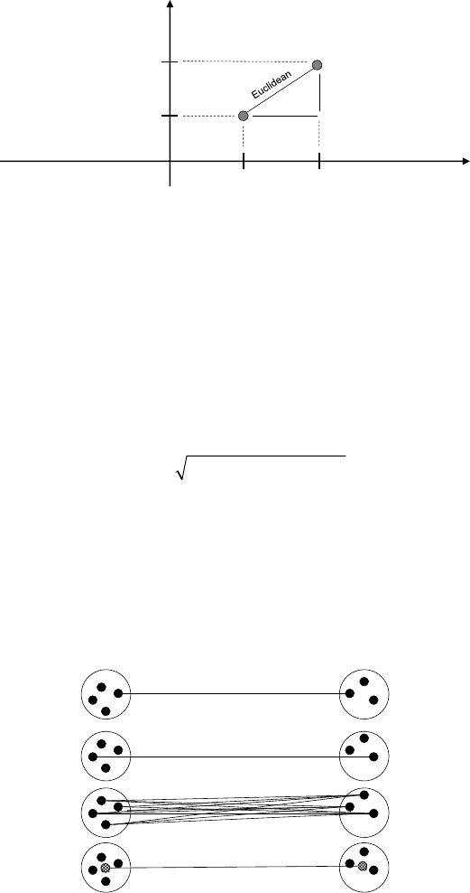
DE

SC

RIPTIVE ANALYTI

CS

◂

9

7

o

b

servations in one c

l

uster an

d

continuing to merge t

h

e ones t

h

at

are most simi

l

ar unti

l

a

ll

o

b

servations ma

k

e up one

b

ig c

l

uster (

l

e

f

t to

rig

h

t in Figure 4.4 ).

In order to decide on the merger or splitting, a similarity rule is

needed. Exam

p

les of

p

o

p

ular similarit

y

rules are the Euclidean distance

and Manhattan (cit

y

block) distance. For the exam

p

le in Fi

g

ure 4.5 ,

b

oth are calculated as follows:

−+−=Euclidean : (50 30) (20 10) 22

22

⎢−⎢+⎢−⎢=Manhattan: 50 30 20 10 30

It is obvious that the Euclidean distance will alwa

y

s be shorter

t

han

t

he Manha

tt

an dis

t

ance.

Various schemes can now be ado

p

ted to calculate the distance

b

etween two clusters (see Figure 4.6 ). The single linkage method

Figure 4.5 E

uc

li

dea

n v

e

r

sus

M

a

nh

atta

n Di

sta

n

ce

Manhattan

5030

10

20

Monetary

Recency

F

i

gure 4.6 Ca

l

cu

l

at

i

ng D

i

stances

b

etween C

l

usters

Single linkage

Complete linkage

Average linkage

Centroid method

98

▸

A

NALYTI

CS

IN A BI

G

DATA W

O

RL

D

de nes the distance between two clusters as the shortest possible

distance, or the distance between the two most similar ob

j

ects. The

com

p

lete linka

g

e method de nes the distance between two clusters as

the biggest distance, or the distance between the two most dissimilar

ob

j

ects. The avera

g

e linka

g

e method calculates the avera

g

e of all

p

os-

sible distances. The centroid method calculates the distance bet

w

een

the centroids of both clusters. Finally, Ward’s method merges the pair

of clusters that leads to the minimum increase in total

w

ithin‐cluster

variance after merging.

In order to decide on the optimal number of clusters, one could

use a dendro

g

ram or scree

p

lot. A dendro

g

ram is a tree‐like dia

g

ram

t

h

at recor

d

s t

h

e se

q

uences o

f

mer

g

es. T

h

e vertica

l

(or

h

orizonta

l

sca

l

e) t

h

en

g

ives t

h

e

d

istance

b

etween two c

l

usters ama

lg

amate

d

. One

can t

h

en cut t

h

e

d

en

d

rogram at t

h

e

d

esire

d

l

eve

l

to



n

d

t

h

e optima

l

c

l

usterin

g

. T

h

is is i

ll

ustrate

d

in Fi

g

ure 4.7 an

d

Fi

g

ure 4.8

f

or a

b

ir

d

s

c

l

usterin

g

exam

pl

e. A scree

pl

ot is a

pl

ot o

f

t

h

e

d

istance at w

h

ic

h

c

l

us

-

ters are merge

d

. T

h

e e

lb

ow point t

h

en in

d

icates t

h

e optima

l

c

l

ustering.

T

h

is is i

ll

ustrate

d

in Fi

g

ure 4.9 .

Fi

g

ure 4.7 Example for Clusterin

g

Birds

1

6

2

4

3

5

Chicken

Duck

Pigeon

Parrot

Owl

Eagle

Canary

The

num

b

ers

i

n

di

cate t

h

e c

l

uster

i

ng steps

.

DE

SC

RIPTIVE ANALYTI

CS

◂

99

K‐Means Clustering

K

‐means clustering is a nonhierarchical procedure that works along

the followin

g

ste

p

s:

1. Select

k

observations as initial cluster centroids (seeds).

k

2. Assi

g

n each observation to the cluster that has the closest cen

-

troid (for example, in Euclidean sense).

3. When all observations have been assi

g

ned, recalculate the

p

osi-

tions of the

k

centroids.

k

4. Re

p

eat until the cluster centroids no lon

g

er chan

g

e.

A key requirement here is that the number of clusters,

k,

needs to

be s

p

eci ed before the start of the anal

y

sis. It is also advised to tr

y

out

different seeds to verif

y

the stabilit

y

of the clusterin

g

solution.

F

ig

ure 4.8 Dendro

g

ram for Birds Example

PigeonChicken Duck Owl Eagle

CanaryParrot

1

2

3

4

5

6

F

i

gure 4.9 Scree Plot

f

or Clustering

Number ofClusters

Distance

T

he

bl

ac

k

li

ne

i

n

di

cates t

h

e opt

i

ma

l

c

l

uster

i

ng

.

1

00

▸ANALYTI

CS

IN A BI

G

DATA W

O

RL

D

Self‐Organizing Maps

A self‐organizing map (SOM) is an unsupervised learning algorithm

that allows

y

ou to visualize and cluster hi

g

h‐dimensional data on a

low‐dimensional grid of neurons.

3

An SOM is a feedforward neural

network with two layers. The neurons from the output layer are usu-

ally ordered in a two‐dimensional rectangular or hexagonal grid (see

Figure 4.10 ). For the former, every neuron has at most eight neigh

-

b

ors, whereas for the latter every neuron has at most six neighbors.

Each input is connected to all neurons in the output layer with

weig

h

ts

w

= [

w

1

,

…,

w

N

w

], with

N

the number of variables. All weights

N

are randomly initialized. When a training vector

x

is presented, the

x

weig

h

t vector

w

c

of each neuron

c

is compared with

c

x

,

using,

f

or

examp

l

e, t

h

e Euc

l

i

d

ean

d

istance metric (

b

eware to stan

d

ar

d

ize t

h

e

data  rst):

dxw x w

cici

i

N

(, ) ( )

2

1

∑

=−

=

x

in Euclidean sense is called

x

the best matchin

g

unit (BMU). The wei

g

ht vector of the BMU

and its neighbors in the grid are then adapted using the following

learnin

g

rule:

wt wt h t xt wt

iici i

( 1) ( 1) () () ()

[]

+= ++ −

whereb

y

t

represents the time index during training and

t

h

ci

(

i

t

) de nes

t

the nei

g

hborhood of the BMU

c,

s

p

ecif

y

in

g

the re

g

ion of in uence. The

F

ig

ure 4.10 Rectan

g

u

l

ar versus Hexa

g

ona

l

SOM Gr

id

RectangularSOMGrid HexagonalSOMGrid

DE

SC

RIPTIVE ANALYTI

CS

◂1

0

1

nei

g

hborhood function

h

ci

(

i

t

) should be a nonincreasing function of

t

time and the distance from the BMU. Some

p

o

p

ular choices are:

=α − −

σ

⎛

⎝

⎜⎞

⎠

⎟

ht t rr

t

ci

() ()exp 2()

2

=α − ≤ht t r r

ci c i

( ) ( ) if threshold,0 otherwise,

2

whereb

y

r

c

and

c

r

i

represent the location of the BMU and neuron

i

on

i

t

h

e map,

σ

2

(

t

) represents the decreasing radius, and 0 ≤

t

α

(

t

) ≤ 1, the

t

l

earning rate (e.g.,

α

(

t

) =

t

A

/

(

t

+

t

B

)

,

α

(

t

) = exp(–

t

At

–

)). The decreasing

t

l

earning rate an

d

ra

d

ius wi

ll

give a sta

bl

e map a

f

ter a certain amount

of training. Training is stopped when the BMUs remain stable, or after

a  xed number of iterations (e.

g

., 500 times the number of SOM neu-

rons). The neurons will then move more and more toward the in

p

ut

observations and interesting segments will emerge.

SOMs can be visualized b

y

means of a U‐matrix or com

p

onent

p

lane.

■ A U (uni ed distance)‐matrix essentially superimposes a height

Z

dimension on top of each neuron visualizing the average dis-

Z

tance between the neuron and its nei

g

hbors, whereb

y

t

yp

icall

y

dark colors indicate a large distance and can be interpreted as

clus

t

er boundaries.

■ A component plane visualizes the weights between each spe

-

ci c in

p

ut variable and its out

p

ut neurons, and as such

p

rovides

a visual overview of the relative contribution of each input attri-

b

ute to the output neurons.

Fi

g

ure 4.11

p

rovides an SOM exam

p

le for clusterin

g

countries

b

ase

d

on a corru

p

tion

p

erce

p

tion in

d

ex (CPI). T

h

is is a score

b

etween 0

(

h

i

ghly

corru

p

t) an

d

10 (

h

i

ghly

c

l

ean) assi

g

ne

d

to eac

h

countr

y

in t

h

e

wor

ld

. T

h

e CPI is com

b

ine

d

wit

h

d

emograp

h

ic an

d

macroeconomic

in

f

ormation

f

or t

h

e

y

ears 1996, 2000, an

d

2004. U

pp

er case countries

(e.

g

., BEL)

d

enote t

h

e situation in 2004,

l

owercase (e.

g

.,

b

e

l

) in 2000,

an

d

sentence case (e.g., Be

l

) in 1996. It can

b

e seen t

h

at many o

f

t

h

e

Euro

p

ean countries are situate

d

in t

h

e u

pp

er ri

gh

t corner o

f

t

h

e ma

p

.

102

▸ANALYTICS IN A BIG DATA WORL

D

Fi

g

ure 4.12

p

rovides the com

p

onent

p

lane for literac

y

whereb

y

darker

regions score worse on literacy. Figure 4.13 provides the component

p

lane for

p

olitical ri

g

hts whereb

y

darker re

g

ions corres

p

ond to better

p

olitical ri

g

hts. It can be seen that man

y

of the Euro

p

ean countries

score good on both literacy and political rights.

SOMs are a ver

y

hand

y

tool for clusterin

g

hi

g

h‐dimensional data

sets because of the visualization facilities. However

,

since there is no

real objective function to minimize, it is harder to compare various

SOM solutions a

g

ainst each other. Also, ex

p

erimental evaluation and

ex

p

ert inter

p

retation are nee

d

e

d

to

d

eci

d

e on t

h

e o

p

tima

l

size o

f

t

h

e

SOM. Un

l

i

k

e

k

‐means c

l

usterin

g

, an SOM

d

oes not

f

orce t

h

e num

b

er

o

f

c

l

usters to

b

e equa

l

to t

h

e num

b

er o

f

output neurons.

Using and Interpreting Clustering Solutions

In or

d

er to use a c

l

usterin

g

sc

h

eme, one can assi

g

n new o

b

servations

to t

h

e c

l

uster

f

or w

h

ic

h

t

h

e centroi

d

is c

l

osest (e.

g

., in Euc

l

i

d

ean or

Fi

g

ure 4.11 Clusterin

g

Countries Usin

g

SOMs

sgp

SGP

SWE

nor

Nor

NOR Fin

Usa

usa

USA

fin

swe

FIN

SWE

NID

Nld

AUT

BEL

JPN

NLD

GBR

Gbr

FRA

DEU Dnk

dnk

DNK

frabel

ITA Fra

deu

GRC

Bel

ESP

Aut

aut

CHE

Che

che

jpn

Aus

CAN

AUS

Can

aus

Hkg

hkg

HKG Nzl

nzl

NZL

can

TWN

Tw n

twn ISR CHL

irl

IRL

ita

esp Ita

Esp

Prt

hun

HUN

POL

Hun

Pol

Rus

rus

RUS

IND

KOR

Kor

kor

Chl

chl

ARG THA

Arg

arg BRA tha

Tha

TUR

MEX

jor

JOR Mys

MYS Mex mex

Ven ECU

COL

bra

Bra

ZafBOLPHL

Col

col

mys

VEN

IDNven

idn

Idn

EGY Tu r

Chn

CHN chn

Ecu

ecu

Phl

phl

bol

Jor Bol

Egy

egy

Ken

ken

pak

PA K Pak

Bgd

nga

NGA

Uga

uga

UGA

Cmr

Nga

cmh

CMR

ind Ind KENtur

bgd

BGD

zaf

ZAF

CZE

CZe

cze

pol

Irl

Jpn prt

Deu

PRT

Grc

grc

gbrsgp ISR

iSR

Fi

g

ure 4.12 Component Plane

f

or Literac

y

Figure 4.13 Component Plane for Political Rights

1

0

4▸ANALYTICS IN A BIG DATA WORL

D

Manhattan sense). To facilitate the inter

p

retation of a clusterin

g

solu-

tion, one could do the followin

g

:

■ Compare cluster averages with population averages for all vari

-

ables using histograms, for example.

■ Build a decision tree with the cluster ID as the target and the

clustering variables as the inputs (can also be used to assign new

observations to clusters).

It is also important to check cluster stability by running different

clusterin

g

techni

q

ues on different sam

p

les with different

p

arameter

settings an

d

c

h

ec

k

t

h

e ro

b

ustness o

f

t

h

e so

l

ution.

NOTES

1. R. A

g

rawal, T. Imielinski, and A. Swami, “Minin

g

Association Rules between Sets of

I

tems in Massive Databases

,

” in Proceedin

g

s of the ACM SIGMOD International Confer-

ence on Mana

g

ement of Data (Washin

g

ton, DC, ACM, 1993).

2. R. Srikant and R. A

g

rawal, “Minin

g

Generalized Association Rules,” in Proceedin

g

s of

the 1995 International Conference on Very Lar

g

e Data Base

s

(

Zurich, 1995

)

.

3. T. Kohonen, “Self‐Or

g

anized Formation of To

p

olo

g

icall

y

Correct Feature Ma

p

s,”

Bio

-

lo

g

ical Cybernetic

s

43 (1982): 59–69; J. Hu

y

smans et al., “Usin

g

Self Or

g

anizin

g

Ma

p

s

for Credit Scorin

g

,” S

p

ecial issue on Intelli

g

ent Information S

y

stems for Financial

En

g

ineerin

g

, Ex

p

ert S

y

stems With A

pp

lications, 30, no. 3 (2006): 479–487; A. Seret

et al., “A New SOM‐Based Method for Pro le Generation: Theor

y

and an A

pp

lica

-

tion in Direct Marketin

g

,” Euro

p

ean Journal o

f

O

p

erational Researc

h

220, no. 1 (2012):

1

99

–2

09.

105

C

HAPTER

5

Survival Analysis

S urviva

l

ana

l

ysis is a set o

f

statistica

l

tec

h

niques

f

ocusing on t

h

e

occurrence an

d

timin

g

o

f

events.

1

As t

h

e name su

gg

ests, it ori

g

i-

n

ates

f

rom a me

d

ica

l

context w

h

ere it was use

d

to stu

d

y surviva

l

times o

f

p

atients t

h

at

h

a

d

receive

d

certain treatments. In

f

act, man

y

c

l

assi



cation ana

ly

tics

p

ro

bl

ems we

h

ave

d

iscusse

d

b

e

f

ore a

l

so

h

ave a

time aspect inc

l

u

d

e

d

, w

h

ic

h

can

b

e ana

l

yze

d

using surviva

l

ana

l

ysis

tec

h

ni

q

ues. Some exam

pl

es are:

2

■ Pre

d

ict w

h

en customers c

h

urn

■ Pre

d

ict w

h

en customers ma

k

e t

h

eir next

p

urc

h

ase

■ Pre

d

ict w

h

en customers

d

e

f

au

l

t

■ Pre

d

ict w

h

en customers

p

a

y

o

ff

t

h

eir

l

oan ear

ly

■ Pre

d

ict w

h

en customer wi

ll

visit a we

b

site next

Two t

yp

ica

l

p

ro

bl

ems com

pl

icate t

h

e usa

g

e o

f

c

l

assica

l

statistica

l

tec

h

niques suc

h

as

l

inear regression. A



rst

k

ey pro

bl

em is censoring.

Censorin

g

re

f

ers to t

h

e

f

act t

h

at t

h

e tar

g

et time varia

bl

e is not a

l

wa

y

s

k

nown

b

ecause not a

ll

customers may

h

ave un

d

ergone t

h

e event yet at

the time of the anal

y

sis. Consider, for exam

p

le, the exam

p

le de

p

icted

i

n F

ig

ure 5.1 . At t

i

me T

,

Laura an

d

Jo

h

n

h

ave not c

h

urne

d

y

et an

d

t

h

us

have no value for the tar

g

et time indicator. The onl

y

information avail

-

able is that the

y

will churn at some later date after T

.

Note also that

Sophie is censored at the time she moved to Australia. In fact, these are

all exam

p

les of ri

g

ht censorin

g

. An observation on a variable

T

is right

T

censored if all

y

ou know about

T

is that it is greater than some value

T

c.

1

06

▸ANALYTI

CS

IN A BI

G

DATA W

O

RL

D

Li

k

ewise, an o

b

servation on a varia

bl

e

T

is left censored if all you know

T

a

b

out

T

is that it is smaller than some value

T

c.

An exam

pl

e

h

ere cou

ld

b

e a stu

dy

investi

g

atin

g

smo

k

in

g

b

e

h

avior an

d

some

p

artici

p

ants at

a

g

e 18 a

l

rea

dy

b

e

g

an smo

k

in

g

b

ut can no

l

on

g

er remem

b

er t

h

e exact

date. Interval censorin

g

means the onl

y

information available on

T

is

T

that it belongs to some interval a <

T

<

T

b.

Returning to the previous

smokin

g

exam

p

le, one could be more

p

recise and sa

y

14 <

T

< 18. Cen-

T

sorin

g

occurs because man

y

databases onl

y

contain current or rather

recent customers for whom the behavior has not yet been completely

observed, or because of database errors when, for exam

p

le, the event

dates are missin

g

. Usin

g

classical statistical anal

y

sis techni

q

ues such as

linear regression, the censored observations would have to be left out

from the anal

y

sis, since the

y

have no value for the tar

g

et time vari

-

a

bl

e. However, wit

h

surviva

l

ana

l

ysis, t

h

e partia

l

in

f

ormation avai

l

a

bl

e

for the censored observations giving either a lower and/or an upper

b

ound on the timin

g

of the event will be included in the estimation.

Time‐varying covariates are variables that change value during the

course of the stud

y

. Exam

p

les are account balance, income, and credit

scores. Survival anal

y

sis techni

q

ues will be able to accommodate this

in the model formulation

,

as will be discussed in what follows.

SURVIVAL ANALYSIS MEASUREMENTS

A



rst im

p

ortant conce

p

t is t

h

e event time

d

istri

b

ution

d

e



ne

d

as a

continuous pro

b

a

b

i

l

ity

d

istri

b

ution, as

f

o

ll

ows:

=≤<+Δ

Δ

Δ→

ft Pt T t T

t

( ) lim ()

0

Example o

f

Right Censoring

f

or Churn Prediction

Bart

John

Sophie

Victor

Laura Churn

Churn

Moves to

Australia

Churn

Time

T

SU

RVIVAL ANALY

S

I

S

◂

10

7

The corres

p

ondin

g

cumulative event time distribution is then

de ned as follo

w

s

:

∫

=≤=Ft PT t fudu

t

() ( ) ( )

0

Closely related is the survival function

:

∫

=− = > =

∞

St Ft PT t f udu

t

() 1 () ( ) ( )

(

S

t

) is a monotonically decreasing function with

t

S

(0)

S

=

1 and

S

(

S

∞)

=

0.

T

h

e

f

o

ll

owing re

l

ations

h

ips

h

o

ld

:

==−ft dF t

dt

dS t

dt

() () ()

Figure 5.2 provides an example of a discrete event time distri

-

bution, with the corres

p

ondin

g

cumulative event time and survival

distribution de

p

icted in Fi

g

ure 5.3 .

Another important measure in survival analysis is the hazard func

-

tion

,

de ned as follows

:

=≤<+Δ ≥

Δ

Δ→

ht Pt T t T T t

t

() lim (|)

0

The hazard function tries to

q

uantif

y

the instantaneous risk that

an event will occur at time

t,

given that the individual has survived up

t

o

t

ime t

.

Hence, it tries to measure the risk of the event occurring at

time

p

oint

t

. The hazard function is closel

y

related to the event time

F

i

gure 5.2 Example o

f

a Discrete Event Time Distribution

0%

10%

20%

30%

40%

50%

60%

87654321

Frequency

Month

1

08

▸ANALYTI

CS

IN A BI

G

DATA W

O

RL

D

distribution u

p

to the conditionin

g

on Tt≥

.

That is wh

y

it is often also

referred

t

o as a conditional density

.

Fi

g

ure 5.4

p

rovides some exam

p

les of hazard sha

p

es, as follows:

■ Constant hazard, whereb

y

the risk remains the same at all times.

■ Increasin

g

hazard, re ectin

g

an a

g

in

g

effect.

■ Decreasing hazard, re ecting a curing effect.

■ Convex bathtub sha

p

e, which is t

yp

icall

y

the case when stud

y-

ing human mortality, since mortality declines after birth and

infanc

y

, remains low for a while, and increases with elder

y

ears.

It is also a

p

ro

p

ert

y

of some mechanical s

y

stems to either fail

soon after operation, or much later, as the system ages.

The probability density function

f

(

f

t

), survivor function

t

S

(

t

), and the

t

hazard func

t

ion

h

(

t

) are mathematically equivalent ways of describing

t

a continuous probability distribution with the following relationships:

=ht ft

St

() ()

()

=−ht dlogS t

dt

() ()

∫

=−

⎛

⎝

⎜⎞

⎠

⎟

St hudu

t

( ) exp ( )

0

Cumulative Distribution and Survival Function for the Event Time

D

i

str

ib

ut

i

on

i

n F

i

gure 5.2

0%

10%

20%

30%

40%

50%

60%

70%

80%

90%

100%

987654321

Frequency

Month

Survivalfunction

Cumulativedistribution

S

URVIVAL ANALY

S

I

S

◂

109

KAPLAN MEIER ANALYSIS

A  rst t

yp

e of survival anal

y

sis is Ka

p

lan Meier (KM) anal

y

sis, which

is also known as the product limit estimator or nonparametric maxi

-

mum likelihood estimator for

S

(

S

t

). If no censoring is available in the data

t

set

,

the KM estimator for

S

(

S

t

) is just the sample proportion with event

t

times greater than

t

. If censoring is present, the KM estimator starts with

t

orderin

g

the event times in ascendin

g

order

t

1

<

t

2

t

<

…

<

t

k

t

.

k

At each time

t

j

t

, there are

j

n

j

n

individuals who are at risk of the event. At risk means that

j

they have not undergone the event, nor have they been censored prior

to

t

j

t

. Let

j

d

j

d

be the number of individuals who die (e.g., churn, respond,

j

default) at

t

j

t

. The KM estimator is then de ned as follows:

j

ii

∏

=−

⎛

⎝

⎜⎞

⎠

⎟=− −

⎛

⎝

⎜⎞

⎠

⎟=− −

≤

ˆ() 1 ˆ(1)1 ˆ(1)(1 ())

:

St d

nSt d

nSt ht

j

jt t

t

j

f

or

t

1

≤

t

≤

t

k

t

. The intuition of the KM estimator is very straightforward

k

b

ecause it

b

asica

ll

y states t

h

at in or

d

er to survive time

t,

one must

surv

i

ve t

i

me

t

− 1 and cannot die during time

t

t.

Fi

g

ure 5.5

g

ives an exam

pl

e o

f

Ka

pl

an Meier ana

ly

sis

f

or c

h

urn

pre

d

iction.

F

i

gure 5.4 Examp

l

e Hazar

d

S

h

apes

110

▸

A

NALYTICS IN A BIG DATA WORL

D

I

f

t

h

ere are man

y

uni

q

ue event times, t

h

e KM estimator can

b

e

a

d

juste

d

b

y using t

h

e

l

i

f

e ta

bl

e (a

l

so

k

nown as

actuarial

) method to

l

g

rou

p

event times into interva

l

s as

f

o

ll

ows:

∏

=−

−

⎡

⎣

⎢⎤

⎦

⎥

≤

ˆ() 1 /2

:

St d

nc

j

jj

jt t

j

w

h

ic

h

b

asica

lly

assumes t

h

at censorin

g

occurs uni

f

orm

ly

across

t

h

e time interva

l

, suc

h

t

h

at t

h

e average num

b

er at ris

k

equa

l

s (

n

j

n

+

j

(

n

j

n

−

j

c

j

c

))/2 or

j

n

j

n

−

j

c

j

cc

/

2.

Ka

pl

an Meier ana

ly

sis can a

l

so

b

e exten

d

e

d

wit

h

hyp

ot

h

esis test

-

ing to see w

h

et

h

er t

h

e surviva

l

curves o

f

d

i

ff

erent groups (e.g., men

versus women, em

pl

o

y

e

d

versus unem

pl

o

y

e

d

) are statistica

lly

d

i

ff

er-

ent. Popu

l

ar test statistics

h

ere are t

h

e

l

og‐ran

k

test (a

l

so

k

nown as t

h

e

Mantel‐Haenzel test

), the Wilcoxon test, and the likelihood ratio statistic,

t

w

h

ic

h

are a

ll

rea

d

i

ly

avai

l

a

bl

e in an

y

commercia

l

ana

ly

tics so

f

tware.

KM ana

l

ysis is a goo

d

way to start

d

oing some exp

l

oratory surviva

l

ana

ly

sis. However, it wou

ld

b

e nice to

b

e a

bl

e to a

l

so

b

ui

ld

p

re

d

ictive

surviva

l

ana

ly

sis mo

d

e

l

s t

h

at ta

k

e into account customer

h

etero

g

eneit

y

by

inc

l

u

d

in

g

p

re

d

ictive varia

bl

es or covariates.

Figure 5.5 Kaplan Meier Example

Customer TimeofChurnor

Censoring

Churnor

Censored

Churn6C1

Censored3C2

Churn12C3

Censored15C4

Censored18C5

Churn12C6

Churn3C7

Churn12C8

Censored9C9

Churn15C10

Time CustomersatRisk

att(n )

t

Customers

Churned att(dt)

CustomersCensored

attS(t)

100100

0.91110

0.9* 7/8 = 0.79018

6

0.79* 7/7 = 0.791079

0.79* 3/6 = 0.3903612

0.39* 2/3 = 0.2611315

0.26* 1/1 = 0.2610118

3

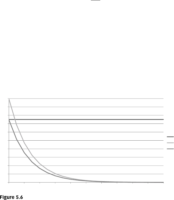
SU

RVIVAL ANALY

S

I

S

◂

111

PARAMETRIC SURVIVAL ANALYSIS

As the name suggests, parametric survival analysis models assume a

p

arametric sha

p

e for the event time distribution. A  rst

p

o

p

ular choice

is an exponential distribution, de ned as follows

:

=λ −λ

ft e t

()

Using the relationships de ned earlier, the survival function then

b

ecomes

:

=−λ

St e t

()

an

d

th

e

h

azar

d

ra

t

e

==λht ft

St

() ()

()

It is worth notin

g

that the hazard rate is inde

p

endent of time such

that the risk always remains the same. This is often referred to as the

memoryless property of an exponential distribution. Figure 5.6 shows an

exam

p

le of an ex

p

onential event time distribution to

g

ether with its

cumulative distribution and hazard function.

When takin

g

into account covariates, the model becomes:

=μ+β +β + βlog( ( , )) 11 2 2

ht x x x x

iiiNiN

Ex

p

onential Event Time Distribution, with Cumulative Distribution and

H

a

z

a

r

d

F

u

n

ct

i

o

n

0

0.1

0.2

0.3

0.4

0.5

0.6

0.7

0.8

0.9

1

109876543210

Hazard

S(t)

f(t)

112

▸ANALYTI

CS

IN A BI

G

DATA W

O

RL

D

Note t

h

at t

h

e

l

o

g

arit

h

mic trans

f

orm is use

d

h

ere to ma

k

e sure t

h

at

the hazard rate is alwa

y

s

p

ositive.

The Weibull distribution is another popular choice for a parametric

survival analysis model. It is de ned as follows

:

=κρρ −ρ

κ− κ

ft t t() () exp[()]

1

The survival function then becomes

:

=−ρ

κ

St t( ) exp[ ( ) ]

and

t

he hazard ra

t

e

==κρρ

κ−

ht ft

St t() ()

() ()1

Note that in this case the hazard rate does de

p

end on time and can

be either increasin

g

or decreasin

g

(de

p

endin

g

u

p

on κ

a

n

d

ρ).

When including covariates, the model becomes

:



()

=μ+α +β +β + βlog (, ) log( ) 11 2 2

ht x tx x x

iii NiN

Other

p

o

p

ular choices for the event time distribution are the

g

amma, lo

g

‐lo

g

istic, and lo

g

‐normal distribution.

3

Parametric survival analysis models are typically estimated using

maximum likelihood

p

rocedures. In case of no censored observations,

t

he likelihood func

t

ion becomes:

∏

=

Lft

i

n

i

()

1

When censorin

g

is

p

resent, the likelihood function becomes:

LftSt

i

n

ii

∏

()

=

δ−δ

()

1

i

δ e

q

uals 0 if observation

i

is censored, and 1 if the observa-

i

t

ion dies a

t

ime t

i

.

i

It is im

p

ortant to note here that the censored obser

-

vations

d

o enter t

h

e

l

i

k

e

l

i

h

oo

d

f

unction an

d

, as suc

h

,

h

ave an im

p

act

on t

h

e estimates. For exam

pl

e,

f

or t

h

e ex

p

onentia

l

d

istri

b

ution, t

h

e

l

i

k

e

l

i

h

oo

d

f

unction

b

ecomes:

Lee

t

i

n

t

ii i i

∏

=λ

−λ δ

=

−λ −δ

[][]

1

SURVIVAL ANALYSI

S

◂11

3

This maximum likelihood function is then t

yp

icall

y

o

p

timized b

y

further takin

g

the lo

g

arithm and then usin

g

a Newton Ra

p

hson o

p

ti

-

mization procedure.

A key question concerns the appropriate event time distribution

for a given set of survival data. This question can be answered both in

a graphical and a statistical way.

In order to solve it graphically, we can start from the following

relationships:

=−ht dlogS t

dt

() ()

or

∫

−=St hudu

t

log( ( )) ( )

0

Because of this relationshi

p

, the lo

g

survivor function is commonl

y

referred

t

o as

t

he cumulative hazard

f

unction, deno

t

ed as

Λ

t()

. I

t

can be

interpreted as the sum of the risks that are faced when going from time

0

t

o

t

ime t. If the survival times are ex

p

onentiall

y

distributed, then

the hazard is constant

,

=λht()

,

hence Λ=λtt() and a

p

lot of –lo

g

(

S

(

t

))

t

versus

t

should yield a straight line through the origin at 0. Similarly,

t

it can be shown that if the survival times are Weibull distributed

,

then a

p

lot of lo

g

(−lo

g

(

S

(

t

)) versus log(

t

) should yield a straight line

t

(not through the origin) with a slope of κ. These plots can typically

b

e asked for in an

y

commercial anal

y

tics software im

p

lementin

g

sur-

vival analysis. Note, however, that this graphical method is not a very

precise method because the lines will never be perfectly linear or go

throu

g

h the ori

g

in.

A more precise method for testing the appropriate event time

distribution is a likelihood ratio test. In fact

,

the likelihood ratio

test can be used to com

p

are models if one model is a s

p

ecial case of

anot

h

er (neste

d

mo

d

e

l

s). Consi

d

er t

h

e

f

o

ll

owin

g

enera

l

ize

d

g

amma

d

istri

b

ution

:

ft t

te

kt

=β

Γθθ

⎛

⎝

⎜⎞

⎠

⎟

β− −θ

⎛

⎝

⎜⎞

⎠

⎟

β

() ()

1

114

▸ANALYTI

CS

IN A BI

G

DATA W

O

RL

D

Let’s now use the followin

g

shortcut notations: k

σ=β

1

a

n

d

k

δ= 1, then the Weibull, exponential, standard gamma, and log

‐

normal model are all special versions of the generalized gamma model,

as follows:

■ σ=δ

: standard gamma

■ δ=1: Weibull

■ σ=δ=1

:

exponential

■ δ=0: lo

g

‐normal

L

e

t

L

ful

l

now

b

e t

h

e

l

i

k

e

l

i

h

oo

d

o

f

t

h

e

f

u

ll

mo

d

e

l

(e.

g

.,

g

enera

l

ize

d

g

amma) an

d

L

re

d

b

e t

h

e

l

i

k

e

l

i

h

oo

d

o

f

t

h

e re

d

uce

d

(s

p

ecia

l

ize

d

) mo

d

e

l

(

e.g., exponentia

l

). T

h

e

l

i

k

e

l

i

h

oo

d

ratio test statistic t

h

en

b

ecomes:

−⎛

⎝

⎜⎞

⎠

⎟χ∼

L

Lk

red

full

2log  ( )

2

whereb

y

the de

g

rees of freedom

k

depends on the number of parame-

k

ters that need to be set to

g

o from the full model to the reduced model.

In other words

,

it is set as follows:

■ Ex

p

onential versus Weibull: one de

g

ree of freedom

■ Exponential versus standard gamma: one degree of freedom

■ Exponential versus generalized gamma: two degrees of freedom

■ Weibull versus

g

eneralized

g

amma: one de

g

ree of freedom

■ Log‐normal versus generalized gamma: one degree of freedom

■ Standard gamma versus generalized gamma: one degree of

freedom

Th

e

χ

2

‐test statistic can then be calculated to

g

ether with the cor-

responding

p

‐value and a decision can be made about what is the most

a

pp

ro

p

riate event time distribution.

PROPORTIONAL HAZARDS REGRESSION

T

h

e proportiona

l

h

azar

d

s mo

d

e

l

is

f

ormu

l

ate

d

as

f

o

ll

ows:

=β+β++β

…

ht x h t x x x

iiiNiN

(, ) ()exp( )

01122

SU

RVIVAL ANALY

S

I

S

◂

115

so the hazard of an indi

v

idual

i

with characteristics

i

x

i

a

t

ime

t

is the

t

p

roduct of a baseline hazard function

h

t

()

0 and a linear func

t

ion of a se

t

of  xed covariates, which is exponentiated. In fact,

h

0

(

t

) can be consid-

t

ered as the hazard for an individual with all covariates equal to 0. Note

that if a variable

j

increases with one unit and all other variables keep

j

their values ( ceteris paribus ), then the hazards for all

t

increase with

t

exp( j

β), which is called the hazard ratio (HR). If

j

β > 0 then HR > 1,

j

β < 0 then HR < 1; j

β = 0 then HR = 1. This is one of the most popular

models for doing survival analysis.

The name

proportional hazards

s

t

ems from

t

he fac

t

ha

t

he hazard

o

f

any in

d

ivi

d

ua

l

is a



xe

d

proportion o

f

t

h

e

h

azar

d

o

f

any ot

h

er

in

d

ivi

d

ua

l

.

=β−+β−++β−

ht

ht xx xx x x

i

j

ij i j niNjN

()

() exp( ( ) ( ) ( )).

11 1 12 2

Hence, the sub

j

ects most at risk at an

y

one time remain the sub

-

jects most at risk at any one other time (see also Figure 5.7 ).

Takin

g

lo

g

arithms from the ori

g

inal

p

ro

p

ortional hazards model

g

ives:

=α +β +β + +βlog ( , ) ( ) 11 2 2

ht x t x x x

iiiNiN

N

ote that if one chooses α=αt()

,

one

g

ets the ex

p

onential model,

whereas if α=αtt() log()

,

the Weibull model is obtained. A nice prop-

ert

y

of the

p

ro

p

ortional hazards model is that, usin

g

the idea of

p

artial

likelihood

,

the sβ can be estimated without having to explicitly specify

t

he baseline hazard func

t

ion

h

t

()

0.

4

This is useful if one is only inter-

ested in anal

y

zin

g

the im

p

act of the covariates on the hazard rates and/

or survival probabilities. However, if one wants to make predictions

F

i

gure 5.7 T

h

e Proport

i

ona

l

Hazar

d

s Mo

d

e

l

Logh(t)

Subjecti

Subjectj

11

6

▸ANALYTI

CS

IN A BI

G

DATA W

O

RL

D

with the

p

ro

p

ortional hazards model, the baseline hazard needs to be

ex

p

licitl

y

s

p

eci ed.

The survival function that comes with the proportional hazards

model looks like this:



∫

=− β+β++β

⎡

⎣

⎢

⎤

⎦

⎥

(, ) exp ( )exp( ) ,

0

11 2 2

St x h u x x x du

i

t

ii NiN

or



=β+β ++β

(, ) () ,

0exp( )

1122

St x S t

ixx x

ii NiN with

∫

=−

⎛

⎝

⎜⎞

⎠

⎟

St hudu

t

( ) exp ( )

00

0

S

0

(

t

) is referred to as the

t

b

ase

l

ine survivor

f

unction

,

t

h

at is, t

h

e survivor

f

unction

f

or an in

d

ivi

d

ua

l

w

h

ose covariates are a

ll

0. Note t

h

at i

f

a

variable

j

increases with one unit (

j

ceteris paribus ), the survival proba

-

b

ilities are raised to the

p

ower ex

p

(j

β), which is the hazard ratio (HR).

EXTENSIONS OF SURVIVAL ANALYSIS MODELS

A  rst extension of the models we

p

reviousl

y

discussed is the inclu

-

sion of time‐varying covariates. These are variables that change value

throu

g

hout the course of the stud

y

. The model then becomes:

=β+β++β(, ) ()exp( () () ())

01122

ht x h t x t x t x t

iiiNiN

Note that the proportional hazards assumption here no longer

holds because the time‐var

y

in

g

covariates ma

y

chan

g

e at different

rates for different subjects, so the ratios of their hazards will not remain

cons

t

an

t

.

O

ne could also le

t

he β parameters vary in time, as follows:

=β+β++β(, ) ()exp( () () () () () ())

01122

ht x h t t x t t x t t x t

iiiNiN

T

h

e

p

artia

l

i

k

e

l

i

h

oo

d

estimation met

h

o

d

re

f

erre

d

to ear

l

ier can

easi

ly

b

e exten

d

e

d

to accommo

d

ate t

h

ese c

h

an

g

es in t

h

e mo

d

e

l

f

or-

mu

l

ation, suc

h

t

h

at t

h

e coe

f

cients can a

l

so

b

e estimate

d

wit

h

out

ex

pl

icit

ly

s

p

eci

fy

in

g

t

h

e

b

ase

l

ine

h

azar

d

ht()

0

.

Anot

h

er extension is t

h

e i

d

ea o

f

com

p

etin

g

ris

k

s.

5

O

f

ten, an

o

b

servation can experience any o

f

k

competing events. In medicine,

k

customers ma

y

d

ie

b

ecause o

f

cancer or a

g

ein

g

. In a

b

an

k

settin

g

, a

SU

RVIVAL ANALY

S

I

S

◂

11

7

customer can default,

p

a

y

off earl

y

, or churn at a

g

iven time. As lon

g

as a customer has not under

g

one an

y

of the events, he or she remains

at risk for any event. Once a customer has undergone the event, he or

she is no longer included in the population at risk for any of the other

risk groups, hence he or she becomes censored for the other risks.

Although the ideas of time‐varying covariates and competing risks

seem attractive at  rst sight, the number of successful business applica-

tions of both remains very limited, due to the extra complexity intro-

duced in the model(s).

EVALUATING SURVIVAL ANALYSIS MODELS

A surviva

l

ana

l

ysis mo

d

e

l

can

b

e eva

l

uate

d

b

y



rst consi

d

ering t

h

e sta

-

tistical signi cance of both the model as a whole and the individual

covariates. (Remember: Signi cant covariates have low

p

‐values.) One

could also

p

redict the time of the event when the survival curve

S

(

S

t

)

t

drops below 0,50 and compare this with the real event time. Another

o

p

tion is to take a sna

p

shot of the survival

p

robabilities at a s

p

eci c time

t

(e.g., 12 months), compare this with the event time indicator, and cal-

t

culate the corresponding ROC curve and its area beneath. The AUC will

then indicate how well the model ranks the observations for a s

p

eci c

timestam

p

t

. Finall

y

, one could also evaluate the inter

p

retabilit

y

of the

survival analysis model by using univariate sign checks on the covari

-

ates and seein

g

whether the

y

corres

p

ond to business ex

p

ert knowled

g

e.

The survival anal

y

sis models we have discussed in this cha

p

ter are

classical statistical models. Hence, some important drawbacks are that

the functional relationshi

p

remains linear or some mild extension

thereof, interaction and nonlinear terms have to be speci ed ad hoc,

extreme hazards may occur for outlying observations, and there is the

assum

p

tion of

p

ro

p

ortional hazards that ma

y

not alwa

y

s be the case.

Ot

h

er met

h

o

d

s

h

ave

b

een

d

escri

b

e

d

in t

h

e

l

iterature to tac

kl

e t

h

ese

s

h

ortcomin

g

s,

b

ase

d

on,

f

or exam

pl

e, s

pl

ines an

d

neura

l

networ

k

s.

6

NOTES

1. P. D. A

ll

ison, Surviva

l

Ana

l

ysis Using t

h

e SAS System (SAS Inst

i

tute Inc., Cary, NC, US,

1995); D. R. Cox, “Regression Mo

d

e

l

s an

d

Li

f

e Ta

bl

es,”

J

ourna

l

o

f

t

h

e Roya

l

Statistica

l

Societ

y

, series B (1972); D. R. Cox and D. Oakes,

Analysis of Survival Data

(C

h

a

p

man

118

▸ANALYTI

CS

IN A BI

G

DATA W

O

RL

D

an

d

Ha

ll

, 1984

)

; D. Ka

lb

eisc

h

an

d

R. L. Prentice,

Th

e Statistica

l

Ana

ly

sis o

f

Fai

l

ure

T

ime

D

ata

(New York: Wile

y

, 2003).

2. J. Banasik

,

J. N. Crook

,

and L. C. Thomas

,

“Not If but When Borrowers Will Default

,

”

Journal of the Operational Research Society 50, no. 12

(

1999

)

: 1185–1190; L. C. Thomas

an

d

M. Stepanova, “Surviva

l

Ana

l

ysis Met

h

o

d

s

f

or Persona

l

Loan Data,” Operat

i

ons

Researc

h

50 (2002): 277–289.

3. P. D. Allison,

S

urvival Analysis using the SAS Syste

m

(SAS Inst

i

tute Inc., Cary, NC, US,

1995).

4. P. D. Allison, Survival Analysis Using the SAS System (SAS Institute Inc., Cary, NC,

US,1995); D. R. Cox, “Regression Models and Life Tables,” Journal of the Royal

Statistical Society

, series B (1972); D. R. Cox and D. Oakes,

Analysis of Survival Data

(Chapman and Hall, 1984); D. Kalb eisch and R. L. Prentice,

T

he Statistical Analysis of

F

ailure

T

ime

D

ata

(New York: Wiley, 2003).

5. M. J. Crowder,

C

lassical Competing Risks (London: Chapman and Hall, 2001).

6. B. Baesens et al., “Neural Network Survival Analysis for Personal Loan Data.” Spe-

cial issue, Journal of the Operational Research Society 59, no. 9 (2005): 1089–1098.

1

9

C

HAPTER

6

Social Network

Analytics 

M an

y

t

yp

es o

f

socia

l

networ

k

s exist. T

h

e most

p

o

p

u

l

ar are

un

d

ou

b

te

dl

y Face

b

oo

k

, Twitter, Goog

l

e+, an

d

Lin

k

e

d

In. How

-

ever, socia

l

networ

k

s are more t

h

an t

h

at. It cou

ld

b

e an

y

set o

f

no

d

es (a

l

so re

f

erre

d

to as

vertices

) connecte

d

by

e

dg

es in a

p

articu

l

ar

b

usiness setting. Examp

l

es o

f

socia

l

networ

k

s cou

ld

b

e:

■ We

b

p

a

g

es connecte

d

by

hyp

er

l

in

k

s

■ Emai

l

tra

f

c

b

etween peop

l

e

■ Researc

h

p

a

p

ers connecte

d

by

citations

■ Te

l

e

ph

one ca

ll

s

b

etween customers o

f

a te

l

co

p

rovi

d

er

■ Ban

k

s connecte

d

b

y

l

iqui

d

ity

d

epen

d

encies

■ S

p

rea

d

o

f

i

ll

ness

b

etween

p

atients

T

h

ese examp

l

es c

l

ear

l

y i

ll

ustrate t

h

at socia

l

networ

k

ana

l

ytics can

b

e a

ppl

ie

d

in a wi

d

e variet

y

o

f

d

i

ff

erent settin

g

s.

SOCIAL NETWORK DEFINITIONS

A social network consists of both nodes (vertices) and edges. Both

need to be clearl

y

de ned at the outset of the anal

y

sis. A node (vertex)

could be de ned as a customer (

p

rivate/

p

rofessional), household

/

family, patient, doctor, paper, author, terrorist, web page, and so forth.

An ed

g

e can be de ned as a friend relationshi

p

, a call, transmission

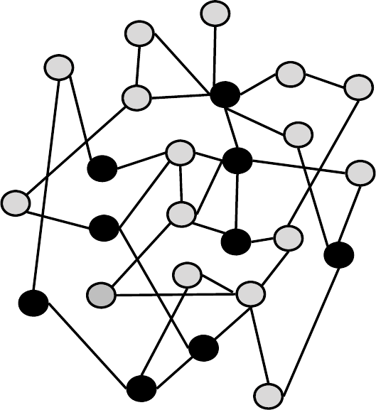
12

0

▸ANALYTI

CS

IN A BI

G

DATA W

O

RL

D

o

f

a

d

isease, re

f

erence, an

d

so on. Note t

h

at t

h

e e

dg

es can a

l

so

b

e

weig

h

te

d

b

ase

d

on interaction

f

requency, importance o

f

in

f

ormation

exc

h

an

g

e, intimac

y

, an

d

emotiona

l

intensit

y

. For exam

pl

e, in a c

h

urn

pre

d

iction setting, t

h

e e

d

ge can

b

e weig

h

te

d

accor

d

ing to t

h

e time two

customers ca

ll

e

d

eac

h

ot

h

er

d

uring a speci



c perio

d

. Socia

l

networ

k

s

can

b

e re

p

resente

d

as a socio

g

ram. T

h

is is i

ll

ustrate

d

in Fi

g

ure 6.1 ,

w

h

ere

by

t

h

e co

l

or o

f

t

h

e no

d

es corres

p

on

d

s to a s

p

eci



c status (e.

g

.,

churner or nonchurner

)

.

Socio

g

rams are

g

ood for small‐scale networks. For lar

g

er‐scale

networks, the network will t

yp

icall

y

be re

p

resented as a matrix, as

illustrated in Table 6.1 . These matrices will be s

y

mmetrical and t

yp

i

-

call

y

ver

y

s

p

arse (with lots of zeros). The matrix can also contain the

wei

g

hts in case of wei

g

hted connections.

Fi

g

ure 6.1 Example Socio

g

ram

SOC

IAL NETW

O

RK ANALYTI

CS

◂

121

T

able

6

.1 Matrix Re

p

resentation o

f

a Social Networ

k

C1 C2 C3 C4

C1 —1

1

0

C2 1

—

0

1

C3 10—

0

C4

0

1

0

—

Table 6.2 Network Centralit

y

Measures

Geodes

i

c

S

hortest

p

ath between two

no

d

es

i

n t

h

e networ

k

Degre

e

N

u

m

be

r

of

co

nn

ec

ti

o

n

s

of

a

node (in‐ versus out‐degree i

f

t

he connections are directed

)

Closenes

s

The avera

g

e distance o

f

a

n

ode

t

o

a

ll

o

th

e

r n

odes

in

t

he network (reciprocal o

f

arness

)

dnn

g

j

g

ij

∑

⎡

⎣

⎢

⎤

⎦

⎥

=

−

()

1

B

etweennes

s

C

ounts the number of times

a

n

ode

o

r

co

nn

ec

ti

o

n li

es

o

n

t

he shortest

p

ath between

an

y

two nodes in the networ

k

gn

g

jk i

jk

∑

<

()

Gra

p

h theoretic cente

r

The

n

ode

w

i

t

h

t

he

s

m

alles

t

m

a

x

i

m

u

m

dis

t

a

n

ce

t

o

all

o

t

he

r n

odes

i

n t

he

n

e

tw

o

r

k

SOCIAL NETWORK METRICS

A socia

l

networ

k

can

b

e c

h

aracterize

d

b

y various socia

l

networ

k

metrics. T

h

e most important centra

l

ity measures are

d

epicte

d

in

Table 6.2 . Assume a network with

g

no

d

es

n

i

, i

= 1, …,

g

.

g

jk

g

repre

-

sents the number of geodesics from node

j

t

o node k

,

whereas

g

jk

g

(

n

i

)

represents the number of geodesics from node

j

to node k pass

i

ng

throu

g

h node

n

i

. The formulas each time calculate the metric for

node

n

i

.

These metrics can now be illustrated with the well‐known Kite

networ

k

d

epicte

d

in Figure 6.2 .

Ta

bl

e 6.3 reports t

h

e centra

l

ity measures

f

or t

h

e Kite networ

k

.

Base

d

on

d

egree, Diane

h

as t

h

e most connections. S

h

e wor

k

s as a

122

▸ANALYTICS IN A BIG DATA WORL

D

connector or hub. Note, however, that she onl

y

connects those

already connected to each other. Fernando and Garth are the closest

to all others. The

y

are the best

p

ositioned to communicate messa

g

es

that need to  ow

q

uickl

y

throu

g

h to all other nodes in the network.

Heather has the highest betweenness. She sits in between two impor

-

tant communities (Ike and Jane versus the rest). She

p

la

y

s a broker

role between both communities but is also a sin

g

le

p

oint of failure.

Note that the betweenness measure is often used for community

T

ab

l

e

6

.

3

Centralit

y

Measures for the Kite Networ

k

Degree Closeness Betweenness

6

Di

a

n

e

0

.

64

F

e

rn

a

n

do

14 H

ea

th

er

5

F

e

rn

a

n

do

0

.

64

Ga

rt

h

8

.

33

F

e

rn

a

n

do

5

Gart

h

0

.

6

Di

an

e

8

.

33

G

art

h

4

A

n

d

r

e

0

.

6

Hea

t

her

8

Ike

4

B

ever

ly

0

.

53

A

n

d

r

e

3

.

6

7

Dia

n

e

3

C

aro

l

0

.5

3

B

ever

ly

0

.

83

A

n

d

r

e

3

E

d

0

.

5

Ca

r

ol

0

.

83

Beverl

y

3

H

ea

th

er

0

.

5

E

d

0

Ca

r

ol

2

Ike

0.4

3

Ike

0

Ed

1 Jan

e

0.3

1

J

an

e

0

J

an

e

JaneIkeHeather

Fernando

Beverly

Garth

Ed

Carol

Diane

Andre

Fi

g

ure 6.2 The Kite Network

SOC

IAL NETW

O

RK ANALYTI

CS

◂12

3

minin

g

. A

p

o

p

u

l

ar tec

h

ni

q

ue

h

ere is t

h

e Girvan‐Newman a

lg

orit

h

m,

w

hich

w

orks as follo

w

s:

1

1. The betweenness of all existing edges in the network is calcu-

lated  rst.

2. The edge with the highest betweenness is removed.

3. The betweenness of all edges affected by the removal is

recalculated.

4. Steps 2 and 3 are repeated until no edges remain.

T

h

e resu

l

t o

f

t

h

is proce

d

ure is essentia

ll

y a

d

en

d

rogram, w

h

ic

h

can

t

h

en

b

e use

d

to

d

eci

d

e on t

h

e optima

l

num

b

er o

f

communities.

SOCIAL NETWORK LEARNING

In social network learning, the goal is within‐network classi cation to

com

p

ute the mar

g

inal class membershi

p

robabilit

y

of a

p

articular node

g

iven the other nodes in the network. Various im

p

ortant challen

g

es arise

when learning in social networks. A  rst key challenge is that the data are

not inde

p

endent and identicall

y

distributed (IID), an assum

p

tion often

made in classical statistical models (e.

g

., linear and lo

g

istic re

g

ression).

The correlational behavior between nodes implies that the class mem-

b

ershi

p

of one node mi

g

ht in uence the class membershi

p

of a related

node. Next, it is not eas

y

to come u

p

with a se

p

aration into a trainin

g

set for model development and a test set for model validation, since the

whole network is interconnected and cannot

j

ust be cut into two

p

arts.

Also, there is a strong need for collective inferencing procedures because

inferences about nodes can mutually in uence one another. Moreover,

man

y

networks are hu

g

e in scale (e.

g

., a call

g

ra

p

h from a telco

p

ro

-

vider), and ef cient computational procedures need to be developed to

do the learnin

g

.2 Finall

y

, one should not for

g

et the traditional wa

y

of

doin

g

anal

y

tics usin

g

onl

y

node‐s

p

eci c information because this can

sti

ll

p

rove to

b

e ver

y

va

l

ua

bl

e in

f

ormation

f

or

p

re

d

iction as we

ll

.

Given t

h

e a

b

ove remar

k

s, a socia

l

networ

k

l

earner wi

ll

usua

lly

consist o

f

t

h

e

f

o

ll

owing components:

3

■ A

l

oca

l

mo

d

e

l

: T

h

is is a mo

d

e

l

usin

g

on

ly

no

d

e‐s

p

eci



c c

h

arac

-

teristics, t

yp

ica

lly

estimate

d

usin

g

a c

l

assica

l

p

re

d

ictive ana

ly

tics

mo

d

e

l

(e.

g

.,

l

o

g

istic re

g

ression,

d

ecision tree).

124

▸ANALYTI

CS

IN A BI

G

DATA W

O

RL

D

■ A net

w

ork model: This is a model that

w

ill make use of the con

-

nections in the network to do the inferencin

g

.

■ A collective inferencin

g

p

rocedure: This is a

p

rocedure to deter

-

mine how the unknown nodes are estimated together, hereby

in uencing each other.

In order to facilitate the computations, one often makes use of the

Markov property, stating that the class of a node in the network only

depends on the class of its direct neighbors (and not of the neighbors

of the nei

g

hbors). Althou

g

h this assum

p

tion ma

y

seem limitin

g

at  rst

s

ig

h

t, empirica

l

eva

l

uation

h

as

d

emonstrate

d

t

h

at it is a reasona

bl

e

assumption to

b

e ma

d

e.

RELATIONAL NEIGHBOR CLASSIFIER

The relational nei

g

hbor classi er makes use of the homo

p

hil

y

assum

p-

tion, which states that connected nodes have a propensity to belong to the

same class. This idea is also referred to as

guilt by association.

If two nodes

are associated, the

y

tend to exhibit similar behavior. The

p

osterior class

probability for node

n

to belong to class

c

is then calculated as follows:

c

Pcn Zwnn

n Neighborhood class n c

j

jnj

∑

=

∈=

(|) 1(, )

{|()}

whereb

y

Nei

g

hborhood

n

re

p

resents the nei

g

hborhood of node

n

,

w

(

w

n

,

n

j

n

) the weight of the connection between

j

n

a

n

d

n

j

n

, and

j

Z

is a

Z

normalization factor to make sure all probabilities sum to one.

For exam

p

le, consider the network de

p

icted in Fi

g

ure 6.3 , whereb

y

C

and

C

N

C

represent churner and nonchurner nodes, respectively.

C

?

NC

C

Figure 6.3 Example Social Network

f

or Relational Neighbor Classi



er

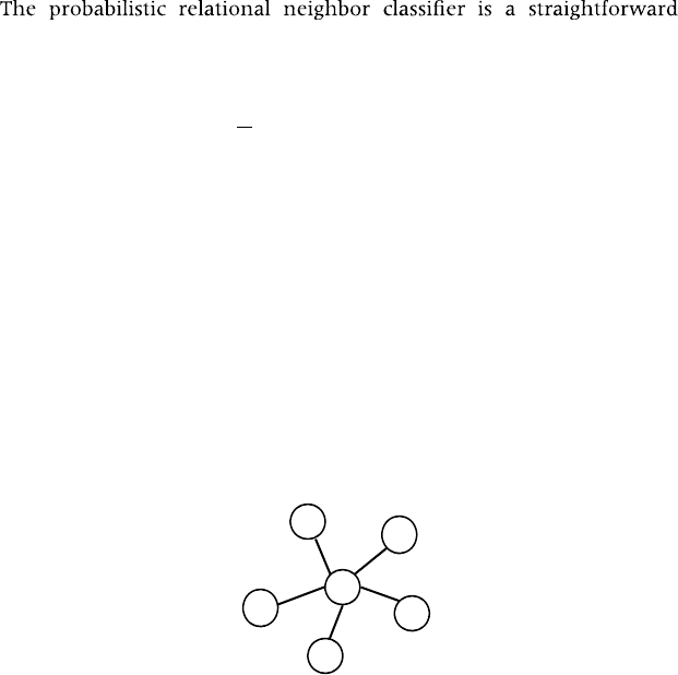
SOC

IAL NETW

O

RK ANALYTI

CS

◂

125

The calcula

t

ions

t

hen become:

PC =+Z(|?) 1/(11)

Z

PNC =++( |?) 1/(111)

Since both probabilities have to sum to 1,

Z

equals 5, so the prob-

Z

abilities become:

PC =( |?) 2/5

PNC =( |?) 3/5

PROBABILISTIC RELATIONAL NEIGHBOR CLASSIFIER

extension of the relational nei

g

hbor classi er, whereb

y

the

p

osterior

class

p

robabilit

y

for node

n

to belon

g

to class

c

is calculated as follows:

c

Pcn Zwnn Pcn

n Neighborhood

jj

jn

∑

=

{}

∈

(|) 1(, )(| )

Note that the summation now ranges over the entire neighbor

-

hood of nodes. The

p

robabilities Pc n

j

(| ) can be

t

he resul

t

of a local

model or of a

p

reviousl

y

a

pp

lied network model. Consider the net-

work of Figure 6.4 .

The calcula

t

ions

t

hen become:

PC Z Z= ++++ =( |?) 1/ (0.25 0.80 0.10 0.20 0.90) 2.25/

PNC Z Z= ++++ =( |?) 1/ (0.75 0.20 0.90 0.80 0.10) 2.75/

C

?

NC

C

P(C) = 0.80

P(NC) = 0.20

P(C) = 0.25

P(NC) = 0.75

P(C) = 0.10

P(NC) = 0.90

P(C) = 0.20

P(NC) = 0.80

P(C) = 0.90

P(NC) = 0.10

F

i

gure 6.4 Example Social Network for Probabilistic Relational Neighbor Classi er

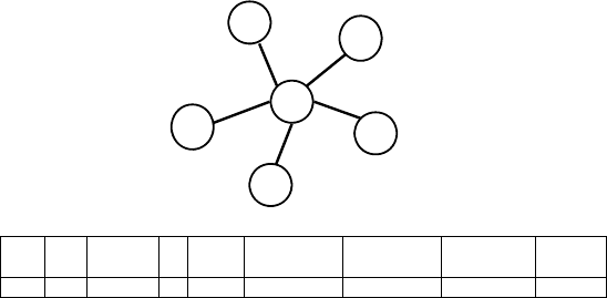
126

▸ANALYTI

CS

IN A BI

G

DATA W

O

RL

D

Since both

p

robabilities have to sum to 1,

Z

equals 5, so the prob-

Z

abili

t

ies become:

PC ==( |?) 2.25/5 0.45

PNC ==( |?) 2.75/5 0.55

RELATIONAL LOGISTIC REGRESSION

Relational logistic regression was introduced by Lu and Getoor.

4

It

b

asica

ll

y starts o

ff

f

rom a

d

ata set wit

h

l

oca

l

no

d

e‐speci



c c

h

aracteris

-

tics an

d

a

dd

s networ

k

c

h

aracteristics to it, as

f

o

ll

ows:

■ Most

f

requent

l

y occurring c

l

ass o

f

neig

hb

or (mo

d

e‐

l

in

k

)

■ Fre

q

uenc

y

of the classes of the nei

g

hbors (count‐link)

■ Binar

y

indicators indicatin

g

class

p

resence (binar

y

‐link)

This is illustrated in Fi

g

ure 6.5

.

A logistic regression model is then estimated using the data set

with both local and network characteristics.

N

ote that there is some

correlation between the network characteristics added

,

which should

be  ltered out during an input selection procedure (e.g., using step

-

wise lo

g

istic re

g

ression). This idea is also referred to as featuriza

-

tion, since the network characteristics are basicall

y

added as s

p

ecial

Mode …Income Age CID

link

Frequency

no churn

Frequency

churn

Binary no

churn

Binary

churn

1 1 2 3 NC 1,000 33 Bart

C

?

NC

C

F

i

gure 6.5 Re

l

at

i

ona

l

Log

i

st

i

c Regress

i

on

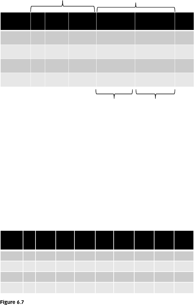
SOC

IAL NETW

O

RK ANALYTI

CS

◂127

features to the data set. These features can measure the behavior of

the nei

g

hbors in terms of the tar

g

et variable (e.

g

., churn or not) or in

terms of the local node‐s

p

eci c characteristics (e.

g

., a

g

e,

p

romotions,

RFM). Figure 6.6 provides an example, whereby features are added

describin

g

the tar

g

et behavior (i.e., churn) of the nei

g

hbors. Fi

g

ure 6.7

p

rovides an exam

p

le, whereb

y

features are added describin

g

the local

node behavior of the neighbors.

RecencyAgeCustomer Number of

contacts

Contactswith

churners

Contacts with

contactsof

churners

Churn

Yes9318535John

No6171018Sophie

No51112838Victor

Yes7091244Laura

Local variables Network variables

First-order

network variable

Second-order

network variable

Fi

g

ure 6.6 Example of Featurization with Features Describin

g

Tar

g

et Behavior of

Nei

g

hbors

AgeCustomer Average

duration

Average

revenue

Promotions

Average

age

friends

Average

duration

friends

Average

revenue

friends

Promotions

friends

Churn

YesX2505520X1235025John

NoY664418Y556535

Sophie

X,Y503350None851250

Victor No

NoX1895565X2306618

Laura

Example of Featurization with Features Describin

g

Local Node Behavior of

Ne

ighb

ors

12

8

▸ANALYTI

CS

IN A BI

G

DATA W

O

RL

D

COLLECTIVE INFERENCING

Given a network initialized by a local model and a relational model, a

collective inference

p

rocedure infers a set of class labels/

p

robabilities

for the unknown nodes by taking into account the fact that inferences

about nodes can mutually affect one another. Some popular examples

of collective inferencing procedures are:

■ Gibbs sampling5

■ Iterative classi cation

6

■ Re

l

axation

l

a

b

e

l

ing

7

■ Loopy

b

e

l

ie

f

propagation

8

As an example, Gibbs sampling works as follows:

1. Given a network with known and unknown nodes

,

initialize

every unknown node using the local classi er to obtain the

(local)

p

osterior

p

robabilities

P

(

P

c

=

c

k

),

k

= 1, …,

k

m

(

m

= number

of classes).

2. Sam

p

le the class value of each node accordin

g

to the

p

robabili

-

t

i

es

P

(

P

c

=

c

k

).

k

3. Generate a random orderin

g

for the unknown nodes.

4. For each node

i

in the ordering

i

a. Apply the relational learner to node

i

to obtain new posterior

i

p

robabilities

P

(

P

c

=

c

k

).

k

b

. Sample the class value of each node according to the new

p

robabilities

P

(

P

c

=

c

k

).

k

5. Repeat step 5 during 200 iterations without keeping any statis

-

tics (burnin

g

p

eriod).

6. Repeat step 5 during 2,000 iterations counting the number

o

f

times eac

h

c

l

ass is assigne

d

to a particu

l

ar no

d

e. Norma

l

izing

these counts

g

ives us the  nal class

p

robabilit

y

estimates.

Note,

h

owever, t

h

at em

p

irica

l

evi

d

ence

h

as s

h

own t

h

at co

ll

ective

in

f

erencin

g

usua

lly

d

oes not su

b

stantia

lly

a

dd

to t

h

e

p

er

f

ormance o

f

a

socia

l

networ

k

l

earner.

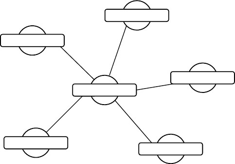
SOC

IAL NETW

O

RK ANALYTI

CS

◂12

9

EGONETS

While real‐life networks often contain billions of nodes and millions

of links, sometimes the direct nei

g

hborhood of nodes

p

rovides enou

g

h

information on which to base decisions. An ego‐centered network,

or egonet

,

represents the one‐hop neighborhood of the node of inter

-

est. In other words, an egonet consists of a particular node and its

immediate neighbors. The center of the egonet is the ego, and the sur-

rounding nodes are the alters. An example of an egonet is illustrated

in Figure 6.8 . Especially when networks are highly characterized by

h

omop

h

i

l

y, egonets can

b

e very use

f

u

l

. Homop

h

i

l

y is t

h

e ten

d

ency o

f

peop

l

e to associate wit

h

ot

h

ers w

h

om t

h

ey perceive as

b

eing simi

l

ar

to t

h

emse

l

ves in some way.9 In suc

h

omop

h

i

l

ic networ

k

s, t

h

e in



u

-

ences o

f

t

h

e

d

irect neig

hb

or

h

oo

d

are so intense t

h

at t

h

ey

d

iminis

h

t

h

e

effect of the rest of the network. Restrictin

g

the anal

y

sis to the e

g

onet

already gives a good indication of the behavior and interests of the sur

-

veyed individual: If all of John’s friends have a  amboyant personality

what does this sa

y

about John? The same reasonin

g

holds in fraud

networks: If all of Mary’s friends are fraudsters, what kind of behavior

d

o you expect

f

rom Mary?

John

Charlie

Elise

Lauren

Bart

Victor

Fi

g

ure 6.8 John’s E

g

onet: The Center o

f

the E

g

onet Is the E

g

o, the Surroundin

g

Nodes

Are the Alters of the E

g

onet

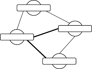
130

▸ANALYTI

CS

IN A BI

G

DATA W

O

RL

D

BIGRAPHS

Nodes in networks represent real‐life objects, such as customers,

p

atients, Internet routers, com

p

anies, and so forth. These ob

j

ects are

connected to each other through links. As in real‐life applications,

some of these relationships are stronger than others. This is re ected in

the weight of the link. In call behavior data for example, two users are

more closely related when they call each other more often. Authors

who write various papers together have a stronger connection. Com-

panies rely more on each other when they share more resources. All

t

h

is in

f

ormation can

b

e summarize

d

in a networ

k

representation con-

necting no

d

es

d

irect

l

y to eac

h

ot

h

er an

d

weig

h

ing t

h

e

l

in

k

s

b

etween

th

em. T

h

is is a unipartit

e

grap

h

, as t

h

e grap

h

on

l

y contains one type

o

f

no

d

es. A unipartite grap

h

f

or t

h

e aut

h

or networ

k

is i

ll

ustrate

d

in

Fi

g

ure 6.9 . The wei

g

hts between nodes are re

p

resented b

y

the thick

-

ness of the lines connecting the two nodes. Tina is more closely con

-

nected to Peter and Monique than Louis. In some applications, it can

b

e interestin

g

to

g

ather more detailed information about the ob

j

ect

that connects these nodes. In the author network, authors are explic-

itl

y

connected with each other throu

g

h

p

a

p

ers. For the com

p

an

y

net-

work, a relationshi

p

between com

p

anies onl

y

exists when the

y

utilize

a common resource. Adding a new type of node to the network does

not onl

y

enrich the ima

g

inative

p

ower of

g

ra

p

hs, but also creates new

insi

g

hts in the network structure and

p

rovides additional information

F

i

gure 6.9 Aut

h

or Networ

k

Louis

Peter

Tina

Monique

SOC

IAL NETW

O

RK ANALYTI

CS

◂

131

ne

g

lected before. However, includin

g

a second t

yp

e of nodes results in

an increasing complexity for analysis.

If a network consists of two t

yp

es of nodes, we call the network a

bi

p

artite

g

ra

p

h or a bi

g

raph . For exam

p

le, in an author–

p

a

p

er network,

there are two types of nodes: authors and papers. This is illustrated

in Fi

g

ure 6.10 . Mathematicall

y

, a bi

p

artite

g

ra

p

h is re

p

resented b

y

a

matrix

M

with

M

n

ro

w

s and

m

columns. The rows refer to the t

yp

e‐one

nodes, while the columns specify the type‐two nodes. The correspond

-

in

g

matrix of Fi

g

ure 6.10 is

g

iven in Fi

g

ure 6.11 .

Louis

Peter

Tina

Monique

Text Mining

Paper



SNA Paper



Fraud

Detection

Paper

Fi

g

ure 6.10 Re

p

resentation o

f

a Small Author–Pa

p

er Network

FDSNATM

1Louis ––

111Tina

1Peter – 1

Monique – 11

Paper

Author

F

i

gure 6.11 Mathematical Representation o

f

the Author–Paper Networ

k

132

▸

A

NALYTICS IN A BIG DATA WORL

D

While the wei

g

ht of the links in the uni

p

artite

g

ra

p

h was used to

re

p

resent the fre

q

uenc

y

that both nodes were associated to a similar

object (e.g., the number of papers written together), the bipartite graph

allows one to include additional information in the link weight, like

the recency, intensity, and information exchange. For example, in the

author–paper network, instead of using a binary link (0/1 or writer

/

nonwriter) to specify relationships between authors and papers, the

link weight can now represent the contributions of each author to the

paper. When analyzing the in uence of one node on another, the link

wei

g

hts should refer to the recenc

y

of the relationshi

p

. Authors will

h

ave muc

h

l

ess in



uence on eac

h

ot

h

er i

f

t

h

ey wrote a paper toget

h

er

severa

l

years ago t

h

an i

f

t

h

ey

h

a

d

written t

h

e paper on

l

y yester

d

ay.

NOTES

1. M. Girvan and M. E. J. Newman, “Communit

y

Structure in Social and Biolo

g

ical

Networks

,

” in

P

roceedin

g

s of the National Academy of Sciences

(

2002

)

, 7821–7826.

2. W. Verbeke, D. Martens, and B. Baesens, “Social Network Anal

y

sis for Customer

Churn Prediction,”

Applied Soft Computing,

forthcomin

g

, 2014.

3. S. A. Macskass

y

and F. Provost, “Classi cation in Networked Data: A Toolkit and

a Univariate Case Stud

y

,” Journal of Machine Learnin

g

Research 8 (2007): 935–983;

W. Verbeke, D. Martens, and B. Baesens, “Social Network Anal

y

sis for Customer

Churn Prediction,” A

pp

lied Soft Com

p

utin

g

, forthcomin

g

, 2014; T. Verbraken et al.,

“Predictin

g

Online Channel Acce

p

tance Usin

g

Social Network Data,” Decision Su

pp

ort

S

y

stems, forthcomin

g

, 2014.

4.

Q

. Lu and L. Getoor, “Link‐based Classi cation,” in

P

roceedin

g

s of the Twentieth Confer-

ence on Machine Learnin

g

(ICML‐2003) (Washin

g

ton, DC, 2003).

5. S. Geman and D. Geman

,

“Stochastic Relaxation

,

Gibbs Distributions

,

and the

Ba

y

esian Restoration of Ima

g

es,”

I

EEE Transactions on Pattern Anal

y

sis and Machine

Intelligence 6

(

1984

)

: 721–741.

6.

Q

. Lu and L. Getoor, “Link‐based Classi cation,” in

P

roceedings of the Twentieth Confer-

ence on Machine Learnin

g

(ICML‐2003) (Washin

g

ton, DC, 2003).

7. S. Chakrabarti, B. Dom, and P. Ind

y

k, “Enhanced H

yp

ertext Cate

g

orization Usin

g

H

yp

erlinks,” in Proceedings of the 1998 ACM SIGMOD International Conference on Man-

agement of Dat

a

(1998), ACM, Seattle, WA, US, 307–319.

8. J. Pear

l

, Pro

b

a

b

i

l

istic Reasonin

g

in Inte

ll

i

g

ent Systems (Mor

g

an Kau

f

mann, 1988).

9

. M. E. J. Newman, Networ

k

s: An Intro

d

uction (Ox

f

or

d

Universit

y

Press, 2010).

133

C

HAPTER

7

Analytics: Putting

It All to Work 

I n C

h

a

p

ter 1 , we

d

iscusse

d

t

h

e

f

o

ll

owin

g

k

e

y

re

q

uirements o

f

ana

ly

ti-

ca

l

mo

d

e

l

s:

■ Business re

l

evance

■ Statistica

l

per

f

ormance

■ Inter

p

reta

b

i

l

it

y

an

d

j

usti



a

b

i

l

it

y

■ O

p

erationa

l

e

f

cienc

y

■ Economica

l

cost

■ Re

g

u

l

ator

y

com

pl

iance

W

h

en on

l

y consi

d

ering statistica

l

per

f

ormance as t

h

e

k

ey o

b

jec

-

tive, ana

ly

tica

l

tec

h

ni

q

ues suc

h

as neura

l

networ

k

s, SVMs, an

d

ran-

d

om

f

orests are amon

g

t

h

e most

p

ower

f

u

l

. However, w

h

en inter

-

preta

b

i

l

ity an

d

justi



a

b

i

l

ity are t

h

e goa

l

, t

h

en

l

ogistic regression an

d

ecision trees s

h

ou

ld

b

e consi

d

ere

d

. O

b

vious

ly

, t

h

e i

d

ea

l

mix o

f

t

h

ese

re

q

uirements

l

ar

g

e

ly

d

e

p

en

d

s on t

h

e settin

g

in w

h

ic

h

ana

ly

tics is to

b

e use

d

. For exam

pl

e, in

f

rau

d

etection, res

p

onse an

d

/or retention

modeling, interpretability, and justi ability are less of an issue. Hence,

it is common to see techni

q

ues such as neural networks, SVMs, and/or

random forests a

pp

lied in these settin

g

s. In domains such as credit risk

modeling and medical diagnosis, comprehensibility is a key require

-

ment. Techni

q

ues such as lo

g

istic re

g

ression and decision trees are

134

▸ANALYTICS IN A BIG DATA WORL

D

ver

y

p

o

p

ular here. Neural networks and/or SVMs can also be a

pp

lied

if the

y

are com

p

lemented with white box ex

p

lanation facilities usin

g

,

for example, rule extraction and/or two‐stage models, as explained in

Chapter 3 .

BACKTESTING ANALYTICAL MODELS

Backesting is an important model monitoring activity that aims at

comparing ex‐ante made predictions with ex‐post observed num

-

b

ers.

1

For example, consider the example in Table 7.1 of a churn pre

-

d

iction mo

d

e

l

. T

h

e purpose

h

ere is to

d

eci

d

e w

h

et

h

er t

h

e o

b

serve

d

c

h

urn rates

d

i

ff

er signi



cant

l

y

f

rom t

h

e estimate

d

pro

b

a

b

i

l

ity o

f

c

h

urn.

Durin

g

model develo

p

ment, one t

yp

icall

y

p

erforms out‐of

‐

sam

p

le validation. This means that the trainin

g

set and test set basi

-

cally stem from the same underlying time period. Backtesting is

done usin

g

an out‐of‐sam

p

le/out‐of‐time data set, as illustrated in

Fi

g

ure 7.1 . Out of universe validation refers to testin

g

the model

on another population. An example of this could be a model devel

-

o

p

ed on Euro

p

ean customers that is bein

g

validated on American

cus

t

omers.

Many challenges arise during backtesting. Different reasons could

b

e behind the differences between the

p

redicted and observed churn

rates re

p

orted in Table 7.1 . A  rst reason could be sam

p

le variation.

This is the variation due to the fact that the predictions are typically

b

ased on a limited sam

p

le. Su

pp

ose one onl

y

considers sam

p

le varia-

tion and the churn rate for a cluster is 1 percent, and one wants to be

95 percent con dent that the actual churn rate is no more than 20

Table 7.1 Backtestin

g

a Churn Prediction Model

Cluster

Estimated

Probability of

Churn No. of Customers

Observed No. of Churners

Observed Observed

Churn Rate

A

2

%

1,00

0

3

03%

B

4

%

2,00

0

12

0

6%

C

10%

4

,

000

5

00

12

.5

%

D

30

%

2,00

0

75

0

3

7.5

%

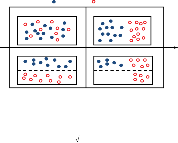
ANALYTI

CS

: P

U

TTIN

G

IT ALL T

O

W

O

RK ◂

135

b

asis

p

oints off from that estimate. The number of observations needed

w

ould be:

()

=−

⎛

⎝

⎜⎞

⎠

⎟=

1.96 1

0.002 9,500

2

nPP

When dealin

g

with lar

g

e data sets, this number can be easil

y

obtained. However, for smaller data sets (as is typically the case in

credit risk modelin

g

), a lower number of observations mi

g

ht be avail-

able, hereb

y

in atin

g

the standard errors and makin

g

the uncertaint

y

on the predictions bigger.

External effects could also be a reason for the difference bet

w

een

predicted and observed churn rates. A typical example here is the

impact of macroeconomic up‐ or downturns.

Finall

y

, internal effects could also

p

la

y

a role. Exam

p

les here are a

strategy change or a merger and/or acquisition. Both have an impact

on the com

p

osition of the data sam

p

les and, as such, also on the

o

b

serve

d

c

h

urn rates.

W

h

en

b

ac

k

testin

g

ana

ly

tica

l

mo

d

e

l

s, one o

f

ten a

d

o

p

ts a tra

f

c

l

i

gh

t

in

d

icator a

pp

roac

h

to enco

d

e t

h

e outcome o

f

a

p

er

f

ormance metric or

test statistic. A green tra

f

c

l

ig

h

t means t

h

at t

h

e mo

d

e

l

pre

d

icts we

ll

an

d

no c

h

an

g

es are nee

d

e

d

. A

y

e

ll

ow

l

i

gh

t in

d

icates an ear

ly

warnin

g

t

h

at a

p

otentia

l

p

ro

bl

em ma

y

arise soon. An oran

g

e

l

i

gh

t is a more

Figure 7.1 Out‐of‐Sample versus Out‐of‐Sample/Out‐of‐Time Validation

Out of Sample/Out of TimeOut of Sample

Out of Universe/Out of Time Out of Universe

: Training Set :Test Set

Time

136

▸ANALYTI

CS

IN A BI

G

DATA W

O

RL

D

severe warnin

g

t

h

at a

p

ro

bl

em is ver

y

l

i

k

e

ly

to arise. A re

d

l

i

gh

t t

h

en

indicates a serious

p

roblem that needs immediate attention and action.

Depending on the implementation, more or fewer traf c lights can be

adopted.

Backtesting Classi cation Models

When backtesting classi cation models, one should  rst clearly state

whether the goal of the classi cation model is scoring/ranking or provid

-

in

g

well-calibrated

p

osterior class

p

robabilities. In res

p

onse and/or reten

-

tion mo

d

e

l

ing, one is typica

ll

y intereste

d

in scores/ran

k

ing customers,

w

h

ereas in cre

d

it ris

k

mo

d

e

l

ing, we

ll

‐ca

l

i

b

rate

d

pro

b

a

b

i

l

ities are nee

d

e

d

.

W

h

en t

h

e mo

d

e

l

purpose is scoring,

b

ac

k

testing s

h

ou

ld

c

h

ec

k

b

ot

h

d

ata

stability and model ranking. When the model is aimed at providing well

‐

calibrated

p

robabilities, the calibration itself should also be backtested.

When validatin

g

data stabilit

y

, one should check whether inter

-

nal or external environmental changes will impact the classi cation

model. Exam

p

les of external environmental chan

g

es are new devel

-

o

p

ments in economic,

p

olitical, or le

g

al environment; chan

g

es in

commercial law; or new bankruptcy procedures. Examples of inter

-

nal environmental chan

g

es are chan

g

es of business strate

gy

, ex

p

lora

-

tion of new market se

g

ments, or chan

g

es in or

g

anizational structure

(

internal). A two‐step approach can be suggested as follows:

1. Check whether the

p

o

p

ulation on which the model is currentl

y

b

eing used is similar to the population that was used to develop

t

he model.

2. If differences occur in step 1, verify the stability of the individual

variables.

For ste

p

1, a s

y

stem stabilit

y

index (SSI) can be calculated as

f

o

ll

ows:

.

()ln

1

SSI observed expected observed

expected

ii

i

ki

i

∑

=−

=

T

h

is is i

ll

ustrate

d

in Ta

bl

e 7.2

.

Note t

h

at t

h

e system sta

b

i

l

ity in

d

ex is a

l

so re

f

erre

d

to as t

h

e

d

evia-

tion

index

. It is i

d

entica

l

to t

h

e in

f

ormation

v

a

l

ue measure

d

iscusse

d

ANALYTI

CS

: PUTTIN

G

IT ALL T

O

W

O

RK ◂1

3

7

in Cha

p

ter 2 for variable screenin

g

. A rule of thumb can be de ned

as follows:

■ SSI < 0.10: no si

g

ni cant shift (

g

reen traf c li

g

ht)

■ 0.10 ≤ SSI < 0.25: moderate shift (yellow traf c light)

■ SSI ≥ 0.25: si

g

ni cant shift (red traf c li

g

ht)

It is also recommended to monitor the SSI through time as illus-

t

ra

t

ed in Table 7.3 .

When

p

o

p

ulation instabilit

y

has been dia

g

nosed, one can then

verify the stability of the individual variables. Again, a system stability

index can be calculated at the

v

ariable le

v

el as illustrated in Table 7.4 .

Note also that histograms and/or

t

‐tests can be used for this purpose.

t

Backtesting model ranking veri es whether high (low) scores are

assi

g

ned to

g

ood (bad) customers. Rankin

g

is then t

yp

icall

y

used in

com

b

ination wit

h

p

ro



t measures to

d

eci

d

e on t

h

e

d

esire

d

action (e.

g

.,

w

h

o to mai

l

in a

d

irect mai

l

in

g

cam

p

ai

g

n). Per

f

ormance measures

common

l

y a

d

opte

d

h

ere

h

ave

b

een

d

iscusse

d

in C

h

apter 3 : ROC, CAP,

l

i

f

t, an

d

/or Ko

l

mo

g

orov‐Smirnov curves. In terms o

f

area un

d

er t

h

e

ROC curve, one can a

d

o

p

t t

h

e tra

f

c

l

i

gh

t in

d

icator a

pp

roac

h

g

iven in

Ta

bl

e 7.5 . Note t

h

at an AUC o

f

b

igger t

h

an 0.95 can

b

e regar

d

e

d

as too

g

oo

d

to

b

e true an

d

mi

gh

t

b

e a si

g

n t

h

at somet

h

in

g

h

as

g

one wron

g

in

T

able

7.2 Ca

l

cu

l

at

i

ng t

h

e System Sta

bili

ty In

d

ex (SSI)

Score Range Expected

(Training) % Observed

(Actual) % SSI

0–16

9

6%

7

% 0.001

5

17

0

–17

9

1

0%

8%

0

.

00

4

5

180–18

9

9%

7

% 0.005

0

190–19

9

12

%

9

% 0.008

6

2

00

–2

09

12

%

11

%

0

.

0009

210–21

9

8

%11

%

0.009

6

220–22

9

7

%10

%

0.010

7

230–23

9

8

%12

%

0.016

2

240–24

9

12

%

11

%

0.000

9

2

50+

1

6%

14

%

0

.

00

2

7

100%

0

.

060

5

138

▸ANALYTICS IN A BIG DATA WORL

D

Ta

bl

e 7.4 Calculating the SSI

f

or Individual Variables

Range Expected

(Training)% Observed

(Actual)% at t Observed (Actual)

% at t + 1

I

ncom

e

0

–

1,000

16%

18%

10%

1

,

001

–

2

,

000

23%

25%

12%

2

,

001

–

3

,

000

22%

20%

3,

001–4

,

00

0

1

9%

1

7

%

25%

4,001–5,00

0

1

5%

1

2

%

20%

5,000

+

5% 8%

1

3

%

SS

I Re

f

erenc

e

0.02

9

0.20

8

SS

I

t −

1

0

.

238

Y

ea

r

s

c

l

ie

n

t

U

nkn

o

wn

c

li

e

n

t

15%

10%

5%

0–2

y

ear

s

2

0%

25%

15%

2–5

y

ear

s

2

5%

30%

40%

5–

10

year

s

30%

20%

10+ year

s

1

0%

5%

20%

SS

I Re

f

erenc

e

0

.

0

7

5

0

.

304

SS

I

t

− 1

t

0

.

362

Ta

bl

e 7.3 Mon

i

tor

i

ng t

h

e SSI t

h

roug

h

T

i

me

Score Range Expected

(Training) % Observed

(Actual) % at t Observed

(Actual) % at t + 1

0–16

9

6% 7%

6

%

170–17

9

10

%

8%

7

%

180

–

189

9%

7

%

10%

190

–

199

12%

9%

11%

200–20

9

12

%

11

%

10

%

21

0

–21

9

8%

11

%

9%

220–22

9

7

%10

%

11

%

2

30

–2

39

8%

12

%

11

%

24

0

–24

9

12

%

11

%

1

0%

2

50+

1

6%

14

%

1

5%

SSI versus

Ex

p

ecte

d

0

.

0605

0

.

0494

SSI versus

t

− 1

t

0

.

0260

ANALYTI

CS

: P

U

TTIN

G

IT ALL T

O

W

O

RK ◂

139

the setup of the model (e.g., information about the dependent variable

was use

d

in one o

f

t

h

e in

d

epen

d

ent varia

bl

es).

One can t

h

en monitor t

h

e AUC or accuracy ratio (AR) t

h

roug

h

time using a report as

d

epicte

d

in Ta

bl

e 7.6 . A ru

l

e o

f

t

h

um

b

t

h

at cou

ld

b

e app

l

ie

d

h

ere is t

h

at a

d

ecrease o

f

l

ess t

h

an 5% in terms o

f

AR is

considered green (normal script), between 5% and 10% yellow (bold

face), and more than 10% red (bold face and underlined).

For backtestin

g

p

robabilit

y

calibration, one can  rst use the Brier

score de ned as follows

:

nPii

i

n

∑−θ

=

1(ˆ)2

1

Table 7.5 Tra

f

c Li

g

ht Codin

g

o

f

AUC

Area under the ROC Curve Quality

0 < AUC ≤ 0.5

N

o discriminatio

n

0.5 < AUC ≤ 0.7

P

oor discriminatio

n

0

.7 < A

UC

≤

0

.

8

A

cceptable discriminatio

n

0.8 < AU

C

≤ 0.9

E

xce

ll

ent

di

scr

i

m

i

nat

i

o

n

0.9 < AUC ≤ 1

E

xcept

i

ona

l

Table 7.6 Monitorin

g

Accurac

y

Ratio (AR) throu

g

h Time

Number of

Observations Number of

Defaulters AR

A

R m

odel

5,

86

6

105

0

.

85

A

R 2

0

1

2

5

,67

7

9

7

0

.

81

A

R 201

1

5

,46

2

1

0

8

0

.8

0

AR

201

0

5

,23

4

1

0

.8

3

A

R 2

009

5,260

123

0

.7

9

A

R 2

008

5

,

365

113

0

.7

9

AR

2

007

5

,35

4

1

2

0

.7

5

AR

200

6

5

,

306

119

0

.

82

A

R 200

5

4,97

0

9

8

0

.7

8

AR

2

004

4,50

1

6

2

0

.

80

AR

200

3

,

983

60

0

.

83

A

vera

g

e AR

5,

179.

8

10

1.

5

0

.

8

140

▸ANALYTI

CS

IN A BI

G

DATA W

O

RL

D

whereb

y

n

is the number of customers

,

Pi

ˆ the calibrated

p

robabilit

y

for cus

t

omer

i,

a

n

d

i

θ

is 1 if the event of interest (e.

g

. churn, fraud,

default) took place and 0 otherwise. The Brier score always varies

b

etween 0 and 1, and lower values indicate a better calibration ability.

Another very popular test for measuring calibration performance

is the binomial test. The binomial test assumes an experiment with

only two outcomes (e.g., head or tail), whereby the experiment is

repeated multiple times and the individual outcomes are independent.

Although the last assumption is not always nicely ful lled because of,

for example, social network effects, the binomial test is often used as a

h

euristic

f

or ca

l

i

b

ration. It wor

k

s as

f

o

ll

ows:

H

0

HH

: T

h

e estimate

d

pro

b

a

b

i

l

ity o

f

t

h

e event (e.g., c

h

urn,

f

rau

d

,

d

e

f

au

l

t), P

ˆ , equa

l

s t

h

e true pro

b

a

b

i

l

ity

P

.

P

H

A

H

: T

h

e estimate

d

pro

b

a

b

i

l

ity o

f

t

h

e event P

ˆ is

b

igger/sma

ll

er/not

e

q

ua

l

to t

h

e true

p

ro

b

a

b

i

l

it

y

.

Note t

h

at t

h

e estimate

d

pro

b

a

b

i

l

ity

P

ˆ is typica

ll

y t

h

e pro

b

a

b

i

l

ity wit

h

in

a

p

articu

l

ar customer se

g

ment or

p

oo

l

. De

p

en

d

in

g

on t

h

e ana

ly

tica

l

tec

h

-

ni

q

ue, t

h

e

p

oo

l

can

b

e o

b

taine

d

in various wa

y

s. It cou

ld

b

e a

l

ea

f

no

d

e

o

f

a

d

ecision tree, or a c

l

ustere

d

range output

f

rom a

l

ogistic regression.

Assumin

g

a ri

gh

t‐tai

l

e

d

test an

d

g

iven a si

g

ni



cance

l

eve

l

, α

,

(e.

g

.,

α=99% ),

H

0

HH

is re

j

ecte

d

i

f

t

h

e num

b

er o

f

events is

g

reater t

h

an or

equa

l

to

k

*, which is obtained as follows:

k

kk

n

kPP

ik

n

ii

∑

=⎛

⎝

⎜⎞

⎠

⎟−≤−α

⎧

⎨

⎪

⎩

⎪

⎫

⎬

⎪

⎭

⎪

=

min | ˆ(1 ˆ)1 .

*

For

l

ar

g

e

n

,

nP >

ˆ5

a

n

d

nP−>(1 ˆ) 5, t

h

e

b

inomia

l

d

istri

b

ution can

b

e approximate

d

b

y a norma

l

d

istri

b

ution as

N

(

N

nP

ˆ

,

nP P−

ˆ(1 ˆ)) .

H

ence,

one o

b

tains:

Pz knP

nP P

≤−

−

⎛

⎝

⎜

⎞

⎠

⎟

⎟=α

ˆ

ˆ(1 ˆ)

,

*

with

z

a standard normally distributed variable. The critical value,

z

k

*,

k

can then be obtained as follows:

knPN nP P=+ α −

−

ˆ() ˆ(1 ˆ)

*1

ANALYTI

CS

: P

U

TTIN

G

IT ALL T

O

W

O

RK ◂

141

w

ith α

−

N()

1 the in

v

erse cumulati

v

e standard normal distribution. In

terms of a critical event rate,

p

*, one t

h

en

h

as

:

=+ α −

−

pPN PP

n

*ˆ() ˆ(1 ˆ)

1

H

0

can then be rejected at signi cance level

α

, if the observed

event rate is higher than

p

*. Remember that the binomial test

assumes that all observations are independent. If the observations

are correlated, then the binomial test has a higher probability to

erroneousl

y

re

j

ect

H

0 (t

yp

e I error), so that’s wh

y

it is often used

as an ear

l

y warning system. It can

b

e co

d

e

d

using tra

f

c

l

ig

h

ts, as

f

o

ll

ows:

■ Green (norma

l

f

ont): no statistica

l

d

i

ff

erence at 90 percent

■ Yellow (italics): statistical difference at 90

p

ercent but not at

95

p

ercent

■ Oran

g

e (bold face): statistical difference at 95

p

ercent but not

at 99

p

ercent

■ Red

(

bold face and underlined

)

: statistical difference at

99

p

ercent

Table 7.7 shows an example of using the binomial test for backtest

-

in

g

calibrated

p

robabilities of default (PDs) a

g

ainst observed default

rates

(

DRs

)

. It can be seen that from 2001 onwards, the calibration is

no longer satisfactory.

The Hosmer‐Lemeshow test is a closel

y

related test that will test

calibrated versus observed event rates across multi

p

le se

g

ments/

p

ools

simultaneously. It also assumes independence of the events, and the

test statistic is de ned as follo

w

s:

knP

nP P

ii i

i

k

∑

χ= −θ

−

=

() (ˆ)

ˆ(1 ˆ)

22

1

whereb

y

ni is the number of observations in

p

ool i

,

Pi

ˆ is the estimated

p

robabilit

y

of the event for

p

ool

i,

a

n

d

i

θ is the number of obser

v

ed

events. The test statistic follows a chi‐s

q

uared distribution with

k

degrees

k

of freedom. It can be coded usin

g

traf c li

g

hts in a similar wa

y

as for the

b

inomial test.

Table 7.7 The Binomial Test for Backtesting PDs versus DRs

PD Baa1 Baa2 Baa3 Ba1 Ba2 Ba3 B1 B2 B3 Caa‐C Av

0

.26%

0

.17%

0

.42%

0

.53%

0

.54%

1

.36%

2

.46% 5.76% 8.76%

2

0.89% 3.05%

DR

Baa

1

Baa

2

Baa3

Ba

1

Ba

2

Ba3

B1

B

2

B3

Caa

‐

C

Av

1993

0

.

00%

0

.

00%

0

.

00%

0

.

83%

0

.

00%

0

.7

6%

3

.

24%

5

.

04%

11.29

%

28.57

%

3

.

24%

1

99

4

0

.

00%

0

.

00%

0

.

00%

0

.

00%

0

.

00%

0

.

59%

1.

88%

3

.7

5%

7.

95%

5

.1

3%

1

.

88%

1995

0

.

00%

0

.

00%

0

.

00%

0

.

00%

0

.

00%

1

.7

6%

4.35

%

6

.

42%

4

.

06%

11

.57

%

2

.5

1%

1996

0

.

00%

0

.

00%

0

.

00%

0

.

00%

0

.

00%

0

.

00%

1

.

1

7

%

0

.

00%

3

.

28%

13

.

99%

0

.7

8%

199

7

0

.

00%

0

.

00%

0

.

00%

0

.

00%

0

.

00%

0

.

4

7

%

0

.

00%

1

.

54%

7.

22%

14

.

6

7

%

1

.

41%

1998

0

.

00%

0

.

31%

0

.

00%

0

.

00%

0

.

62%

1

.

12%

2

.

11%

7.55

%

5

.

52%

15

.

09%

2

.

83%

1

999

0

.

00%

0

.

00%

0

.

3

4

%

0

.47

%

0

.

00%

2

.

00%

3.28

%

6.91

%

9

.

63%

2

0

.44

%

3.35

%

2

000

0

.28

%

0.00% 0.97

%

0.94

%

0

.63

%

1

.04% 3.24

%

4.10% 10.88

%

19.65%

3

.01%

2

001

0

.27

%

0

.27

%

0.00% 0.51%

1

.38

%

2.93

%

3.19

%

11.07

%

16.38

%

34.45

%

5.48

%

200

2 1.26

%

0.72

%

1

.78

%

1.58

%

1.41

%

1.

58%

2.

00%

6.81

%

6

.

86%

29.45

%

3.70

%

Av

0

.2

6%

0

.17

%

0

.42

%

0

.

53%

0

.

5

4

%

1

.

36%

2.4

6%

5

.7

6%

8

.7

6%

2

0

.

9%

3

.

05%

1

42

ANALYTI

CS

: PUTTIN

G

IT ALL T

O

W

O

RK ◂

143

Backtesting Regression Models

In backtesting regression models, one can also make a distinction

b

etween model ranking and model calibration. When predicting

CLV, one might especially be interested in model ranking, since it is

typically hard to accurately quantify CLV. However, in the majority

of the cases, the aim is model calibration. For ranking, one could  rst

consider a s

y

stem stabilit

y

index (SSI), as discussed before, a

pp

lied

to the categorized output. Also

t

‐tests and/or histograms can be used

t

here. For rankin

g

, one could create a scatter

p

lot and summarize it

into a Pearson correlation coef cient (see Cha

p

ter 3 ). For calibra

-

tion, one can ca

l

cu

l

ate t

h

e

R

‐s

q

uare

d

, mean s

q

uare

d

error (MSE),

or mean a

b

so

l

ute

d

eviation (MAD) as a

l

so

d

iscusse

d

in C

h

a

p

ter 3 .

Table 7.8

g

ives an exam

p

le of a table that can be used to monitor

t

he M

S

E.

Backtesting Clustering Models

When backtestin

g

clusterin

g

models, one can  rst check the data

stabilit

y

b

y

com

p

arin

g

the number of observations

p

er cluster dur

-

ing model design with the number observed now and calculate a

s

y

stem stabilit

y

index (SSI) across all clusters. One can also measure

how the distance/

p

roximit

y

measures have chan

g

ed on new obser-

vations by creating histograms of distances per cluster and compare

the histo

g

rams of the model desi

g

n data with those of new data. The

Table 7.8 Monitorin

g

Model Calibration Usin

g

MSE

MSE Number of

Observations Number of

Events Traffic Light

MS

E m

odel

M

SE

y

ear

t

MS

E year

t

+ 1

t

M

SE

y

ear

t

+ 2

t

…

A

vera

g

e MSE period 1

A

verage M

S

E period 2

144

▸ANALYTI

CS

IN A BI

G

DATA W

O

RL

D

distances can then be statisticall

y

tested usin

g

, for exam

p

le, a

t

‐test.

t

One can also statisticall

y

com

p

are the intracluster similarit

y

with the

intercluster similarity using an F‐test to see whether reclustering is

needed.

Developing a Backtesting Framework

In order to setup a backtesting framework, one needs to decide on the

following:

■ Diagnose

b

ac

k

testing nee

d

s

■ Wor

k

out

b

ac

k

testing activities

■ Desi

g

n timetable for backtestin

g

activities

■ Specify tests and analyses to be performed

■ De ne actions to be taken in res

p

onse to  ndin

g

s

■ Identif

y

wh

y

/what/who/how/when

All of the above should be described in a backtesting policy.

Fi

g

ure 7.2

p

resents an exam

p

le of a di

g

ital dashboard a

pp

lication that

could be develo

p

ed for backtestin

g

classi cation models. Note also that

qualitative checks are included that are based on a judgment made by

one or more business ex

p

erts. These sub

j

ective evaluations are consid-

ered to be ver

y

im

p

ortant.

Once a backtesting framework has been developed, it should be

com

p

lemented with an action

p

lan. This

p

lan will s

p

ecif

y

what to do

in res

p

onse to what  ndin

g

of the backtestin

g

exercise. Fi

g

ure 7.3

gives an example of this. If the model calibration is okay, one can

continue to use the model. If not, one needs to verif

y

the model

discrimination or rankin

g

. If this is oka

y

, then the solution mi

g

ht be

to sim

p

l

y

recalibrate the

p

robabilities u

p

ward or downward usin

g

a sca

l

ing

f

actor. I

f

not, t

h

e next step is to c

h

ec

k

t

h

e

d

ata sta

b

i

l

ity. I

f

t

h

e

d

ata sta

b

i

l

it

y

is sti

ll

o

k

a

y

, one ma

y

consi

d

er twea

k

in

g

t

h

e mo

d

e

l

.

Note t

h

at t

h

is is,

h

owever, not t

h

at strai

gh

t

f

orwar

d

an

d

wi

ll

o

f

ten

b

oi

l

d

own to reestimating t

h

e mo

d

e

l

(as is t

h

e case w

h

en t

h

e

d

ata

stabilit

y

is not oka

y

)

.

ANALYTI

CS

: P

U

TTIN

G

IT ALL T

O

W

O

RK ◂

145

F

i

gure 7.2 A Backtesting Digital Dashboard

f

or Classi



cation Models

Level0:Data

Quantitative

RedYellowGreen

SSI(currentversus

trainingsample)

SSI<0.10 0.10< SSI<0.25 SSI>0.25

SSIattribute level SSI<0.10 0.10< SSI<0.25 SSI>0.25

t-test attributelevel p-value >0.10 p-valuebetween

0.10and0.01

p-value<0.01

Qualitative

NochangeCharacteristic

analysis

Moderate

change

Majorchange

Attributehistogram Noshift Moderateshift Majorshift

Level2:

Calibration

Quantitative

RedYellowGreen

significantNotBinomial

at95%level

Significantat

95%butnot at

99%level

Hosmer-Lemeshow Notsignificant

at95%level

Significantat

95%butnotat

99%level

Vasicek Notsignificant

at95%level

Significantat

95%butnotat

99%level

Significant at99%

level

Significant at99%

level

Significant at99%

level

Significant at99%

level

NotsignificantNormal

at95%level

Significantat

95%butnotat

99%level

Qualitative

Portfoliodistribution Minorshift Moderateshift Majorshift

UnderestimationOverestimationCorrectDifference

MinorstabilityPortfolio

migrations

Moderate

migrations

Majormigrations

Level1:

Discrimination

Quantitative

RedYellowGreen

AR differencewith

referencemodel

<5% Between5%

and 10%

>10%

AUCdifferencewith

referencemodel

<2.5% Between2.5%

and5%

>5%

Modelsignificance p-value <0.01 p-valuebetween

0.01and0.10

p-value>0.10

Qualitative

Preprocessing

(missingvalues,

outliers)

PartiallyConsidered

considered

Ignored

Coefficientsigns Allasexpected Minor

exceptions

exceptionsMajor

Numberofoverrides MajorModerateMinor

MinorissuesSufficientDocumentation Majorissues

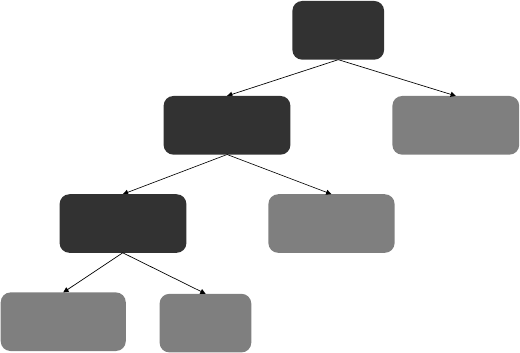
146

▸ANALYTI

CS

IN A BI

G

DATA W

O

RL

D

BENCHMARKING

The idea of benchmarkin

g

is to com

p

are the out

p

ut and

p

erformance

of the anal

y

tical model with a reference model or benchmark. This is

needed as an extra validity check to make sure that the current analyt-

ical is the o

p

timal one to be used. The benchmark can be externall

y

or

internall

y

develo

p

ed. A

p

o

p

ular exam

p

le of an external benchmark in

credit risk modeling could be the FICO score. This is a credit score that

ran

g

es between 300 and 850 and is develo

p

ed b

y

Ex

p

erian, E

q

uifax,

and Transunion in the United States. It is often used as a benchmark to

compare application and/or behavioral credit scoring models. A closely

related score is the Vanta

g

e score, also available in the United States.

Credit ratin

g

a

g

encies (e.

g

., Mood

y

’s, S&P, and Fitch) could also be

considered as benchmarking partners. These agencies typically provide

in

f

ormation on cre

d

it ratings an

d

e

f

au

l

t pro

b

a

b

i

l

ities t

h

at are very

useful in a credit risk modelin

g

context.

Note t

h

at a

l

t

h

ou

gh

externa

l

b

enc

h

mar

k

in

g

ma

y

seem a

pp

ea

l

in

g

at



rst sig

h

t, one s

h

ou

ld

b

e aware o

f

potentia

l

pro

bl

ems,

f

or examp

l

e,

un

k

nown

q

ua

l

it

y

o

f

t

h

e externa

l

b

enc

h

mar

k

,

d

i

ff

erent un

d

er

ly

in

g

d

ata

sam

pl

es an

d

/or met

h

o

d

o

l

o

g

ies,

d

i

ff

erent tar

g

et

d

e



nitions, an

d

l

e

g

a

l

constraints. One s

h

ou

ld

a

l

so

b

e vigi

l

ant

f

or c

h

erry‐pic

k

ing, w

h

ere

b

y

Model

calibration

Model

discrimination

Continueusing

model

Datastability Recalibrate

model

Reestimate

model

Tweak

model

Okay

Not Okay

Okay

Not Okay

OkayNot Okay

Figure 7.3 Example Backtesting Action Plan

ANALYTI

CS

: PUTTIN

G

IT ALL T

O

W

O

RK ◂147

the external benchmark is selected so as to corres

p

ond as closel

y

as

p

ossible to the internal model.

The benchmark can also be internally developed, either statisti

-

cally or expert based. For example, one could benchmark a logis

-

tic regression model against a neural network benchmark to see

whether there are any signi cant nonlinearities in the data. If it

turns out that this is indeed the case, then nonlinear transforma-

tions and/or interaction terms can be added to the logistic regres

-

sion model to come as close as possible to the neural network per

-

formance. An ex

p

ert-based benchmark is a

q

ualitative model based

on expert experience an

d

/or common sense. An examp

l

e o

f

t

h

is

cou

ld

b

e an expert committee ran

k

ing a set o

f

sma

ll

‐ an

d

me

d

ium

‐

size

d

enterprises (SMEs) in terms o

f

d

e

f

au

l

t ris

k

b

y mere

l

y inspect

-

ing their balance sheet and  nancial statement information in an

ex

p

ert‐based, sub

j

ective wa

y

.

When benchmarkin

g

, one commonl

y

ado

p

ts a cham

p

ion–

challenger approach. The current analytical model serves as the

cham

p

ion and the benchmark as the challen

g

er. The

p

ur

p

ose of the

challen

g

er is to  nd the weaknesses of the cham

p

ion and to beat it.

Once the benchmark outperforms the champion, one could consider

makin

g

it the new cham

p

ion, and the old cham

p

ion then becomes the

new benchmark. The

p

ur

p

ose of this a

pp

roach is to continuousl

y

chal-

lenge the current model so as to continuously perfect it.

Po

p

ular a

g

reement statistics for benchmarkin

g

are S

p

earman’s

rank order correlation

,

Kendall’s τ

,

and the Goodman‐Kruskal γ

.

Spearman’s rank order correlation measures the degree to which a

monotonic relationshi

p

exists between the scores or ratin

g

s

p

rovided

b

y an internal scoring system and those from a benchmark. It starts by

assigning 1 to the lowest score, 2 to the second lowest score, and so

on. In case of tied scores, the avera

g

e is taken. S

p

earman’s rank order

corre

l

ation is t

h

en com

p

ute

d

as

f

o

ll

ows:

d

nn

s

i

n

∑

ρ=− −

=

16

(1)

2

1

2

w

h

ere

by

n

is t

h

e num

b

er o

f

o

b

servations an

d

i

the difference between

i

t

h

e scores. Spearman’s ran

k

or

d

er corre

l

ation a

l

ways ranges

b

etween

−1 (

p

er

f

ect

d

isa

g

reement) an

d

+1 (

p

er

f

ect a

g

reement).

14

8

▸ANALYTI

CS

IN A BI

G

DATA W

O

RL

D

K

e

n

da

ll’

s

τ works b

y

 rst calculatin

g

the concordant and discor

-

dant

p

airs of observations. Two observations are said to be concor

-

dant if the observation that has a higher score assigned by the internal

model also has a higher score assigned by the external model. If there

is disagreement in the scores, then the pair is said to be discordant.

Note that if the pair is neither concordant nor discordant, it is tied,

meaning the two observations have identical scores assigned by the

internal model, or b

y

the benchmark, or b

y

both. Kendall’s τ is then

calculated as follo

w

s:

AB

nn

τ= −

−

1

2(1)

,

whereby

n

is the number of observations,

A

the number of concordant

pairs, an

d

B

t

h

e num

b

er o

f

d

iscor

d

ant pairs. Note t

h

at t

h

e

d

enomina-

tor gives a

ll

possi

bl

e pairs

f

or

n

o

b

servations. Ken

d

a

ll

’s τ is 1

f

or per

f

ect

agreement an

d

−1

f

or per

f

ect

d

isagreement.

Ken

d

a

ll

’s τ

b

asica

ll

y

l

oo

k

s at a

ll

possi

bl

e pairs o

f

o

b

servations. T

h

e

Goo

d

man‐Krus

k

a

l

γ wi

ll

on

l

y consi

d

er t

h

e untie

d

pairs (i.e., eit

h

er

concor

d

ant or

d

iscor

d

ant), as

f

o

ll

ows:

AB

γ= −

+

T

h

e Goo

d

man‐Krus

k

a

l

γis +1 i

f

t

h

ere are no

d

iscor

d

ant pairs (per-

f

ect agreement), −1 i

f

t

h

ere are no concor

d

ant pairs (per

f

ect

d

isagree-

ment), an

d

0 i

f

t

h

ere are equa

l

num

b

ers o

f

concor

d

ant an

d

iscor

d

ant

pa

i

rs.

For examp

l

e, consi

d

er t

h

e examp

l

e in Ta

bl

e 7.9 .

Spearman’s ran

k

or

d

er corre

l

ation t

h

en

b

ecomes −0.025. T

h

e con

-

cor

d

ant pairs are as

f

o

ll

ows: C1,C3; C1,C4; C3,C4; C3,C5; an

d

C4,C5.

T

h

e

d

iscor

d

ant pairs are: C1,C2; C2,C3; C3,C4; an

d

C2,C5. T

h

e pair

C1,C5 is a tie. Ken

d

a

ll

’s

τ t

h

us

b

ecomes: (5 − 4)/10 or 0.1 an

d

t

h

e

G

oo

d

man‐Krus

k

a

l

γ

b

ecomes (5 − 4)/(5 + 4) or 0.11.

In case of disagreement between the current analytical model

and the benchmark, it becomes interestin

g

to see which is the best

model overall, or whether there are certain se

g

ments of observa

-

tions where either the internal model or benchmark proves to be

su

p

erior. Based on this anal

y

sis, it can be decided to further

p

erfect

ANALYTICS: PUTTING IT ALL TO WORK ◂

149

the current analytical model or simply proceed with the benchmark

as the new model.

DATA QUALITY

Cor

p

orate information s

y

stems consist of man

y

databases linked

b

y real-time and batch data feeds.

2

The databases are continuously

u

p

dated, as are the a

pp

lications

p

erformin

g

data exchan

g

e. This

d

y

namism has a ne

g

ative im

p

act on data

q

ualit

y

(DQ), which is ver

y

disadvantageous since DQ determines the value of the data to the ana

-

l

y

tical techni

q

ue. Information and communication technolo

gy

can be

used to further improve intrinsic value. Hence, high-quality data in

combination with good technology gives added value, whereas poor

-

q

ualit

y

data with

g

ood technolo

gy

is a bi

g

p

roblem (remember the

garbage in, garbage out idea discussed in Chapter 2 ). Decisions made

b

ased on bad data can create hi

g

h losses for com

p

anies. Poor DQ

im

p

acts or

g

anizations in man

y

wa

y

s. At the o

p

erational level, it has

an im

p

act on customer satis

f

action, increases o

p

erationa

l

ex

p

enses,

an

d

wi

ll

l

ea

d

to

l

owere

d

em

pl

o

y

ee

j

o

b

satis

f

action. Simi

l

ar

ly

, at t

h

e

strategic

l

eve

l

, it a

ff

ects t

h

e qua

l

ity o

f

t

h

e (ana

l

ytica

l

)

d

ecision ma

k-

in

g

p

rocess.

3

Poor DQ are o

f

ten ex

p

erience

d

in ever

yd

a

y

l

i

f

e. For exam

-

pl

e, t

h

e mista

k

en

d

e

l

iver

y

o

f

a

l

etter is o

f

ten associate

d

wit

h

Ta

bl

e 7.9 Example

f

or Calculating Agreement Statistics

Customer Internal

Credit Score FICO Rank Internal

Score

Rank

External

Score d

i

2

068

0

2

.

5

3

0.2

5

2

35

5

8

0

5

1

16

3

15

640

1

2

1

4

2

5

720

4

5

1

5

2

0

7

0

2

.

5

4

2.2

5

di

i

n

2

1

∑

=

2

0

.

5

1

50

▸ANALYTI

CS

IN A BI

G

DATA W

O

RL

D

malfunctionin

g

p

ostal services. However, one of the causes of this

mistaken deliver

y

can be an error in the address. Similarl

y

, two

similar emails sent to the same recipient can be an indication of a

duplication error.

Moreover, the magnitude of DQ problems is continuously growing

following the exponential increase in the size of databases. This cer-

tainly quali es DQ management as one of the most important business

challenges in today’s information‐based economy.

Data quality is often de ned as “ tness for use,” which implies

the relative nature of the conce

p

t.

4

Data with

q

ualit

y

for one use

may not

b

e appropriate

f

or anot

h

er use. For instance, t

h

e extent

to w

h

ic

h

d

ata is require

d

to

b

e comp

l

ete

f

or accounting tas

k

s may

not

b

e require

d

f

or ana

l

ytica

l

sa

l

es pre

d

iction tas

k

s. More genera

ll

y,

data that are of acceptable quality in one decision context may be

p

erceived to be of

p

oor

q

ualit

y

in another decision context, even

by

the same individual. This is mainl

y

because DQ is a multidi

-

mensional concept in which each dimension represents a single

as

p

ect or construct of data items and also com

p

rises both ob

j

ec

-

tive and sub

j

ective as

p

ects. Some as

p

ects are inde

p

endent while

others depend on the type of task and/or experience of the data

user. Therefore, it is useful to de ne D

Q

in terms of its dimensions.

Table 7.10 shows the different DQ dimensions, their cate

g

ories, and

de ni

t

ions.

5

Accurac

y

indicates whether the data stored are the correct val

-

ues. For exam

p

le if m

y

birthdate is Februar

y

27, 1975, for a data

-

b

ase that expects dates in USA format, 02/27/1975 is the correct

value. However, for a database that ex

p

ects a Euro

p

ean re

p

resen

-

tation

,

the date 02/27/1975 is incorrect

;

instead 27/02/1975 is the

correct value.

6

Another interestin

g

dimension concerns the com

p

leteness of data.

T

h

e com

pl

eteness

d

imension can

b

e consi

d

ere

d

f

rom

d

i

ff

erent

p

er-

s

p

ectives. Sc

h

ema com

pl

eteness re

f

ers to t

h

e extent to w

h

ic

h

entities

an

d

attri

b

utes are not

l

ac

k

ing

f

rom t

h

e sc

h

ema. Co

l

umn comp

l

eteness

veri



es w

h

et

h

er a co

l

umn o

f

a ta

bl

e

h

as missin

g

va

l

ues or not. Fina

lly

,

p

o

p

u

l

ation com

pl

eteness re

f

ers to t

h

e

d

e

g

ree to w

h

ic

h

mem

b

ers o

f

t

h

e popu

l

ation are not present. As an examp

l

e, popu

l

ation comp

l

ete-

ness is

d

e

p

icte

d

in Ta

bl

e 7.11 .

7

ANALYTI

CS

: P

U

TTIN

G

IT ALL T

O

W

O

RK ◂1

5

1

Ta

bl

e 7.10 Data Qua

li

ty D

i

mens

i

ons

Category Dimension Definition: The Extent to Which . . .

Intrinsi

c

A

ccurac

y

D

ata are re

g

ar

d

e

d

as correc

t

Believabilit

y

Data are accepted or re

g

arded as true, real, and

credibl

e

Objectivit

y

D

ata are un

bi

ase

d

an

d

i

mpart

i

a

l

Reputatio

n

Data are trusted or highly regarded in terms o

f

their

s

ource an

d

conten

t

Co

nt

e

xt

ual

Va

l

ue

‐

added

Data are bene cial and provide advanta

g

es for

t

heir us

e

C

ompletenes

s

D

ata va

l

ues are presen

t

R

e

l

evanc

y

Data are a

pp

licable and use

f

ul

f

or the task at han

d

A

ppropr

i

ate

a

m

ou

nt

of

da

t

a

T

he quantity or volume o

f

available data is appropriat

e

Re

p

resentat

i

ona

l

I

nter

p

reta

bili

t

y

D

ata are

i

n appropr

i

ate

l

anguage an

d

un

i

t an

d

t

h

e

d

ata de



nitions are clear

E

ase

of

un

d

erstan

di

n

g

Data are clear without ambiguity and easily

com

p

re

h

en

d

e

d

Access

i

b

i

l

i

t

y

Accessibilit

y

Data are available or easil

y

and

q

uickl

y

retrieve

d

S

ecurit

y

A

ccess to data can be restricted and hence kept

secu

r

e

Table 7.11 Po

p

ulation Com

p

leteness

ID Name Surname Birth Date Email

1

Mo

n

ica

S

mit

h

0

4

/

1

0/

1

9

7

8

s

mith

@abc

.i

t

2

Y

u

ki

T

usno

da

04

/

03

/

196

8

N

u

ll

a

3

Rose

Da

v

id

0

2

/0

1

/

1

937

Null

b

4

J

o

hn

Ed

war

d

1

4/12/195

5

N

u

ll

c

a

N

ot ex

i

st

i

ng

b

E

x

i

st

i

ng

b

ut un

k

nown

c

Not known i

f

existing

152

▸ANALYTI

CS

IN A BI

G

DATA W

O

RL

D

Tu

p

le 2: Since the

p

erson re

p

resented b

y

tu

p

le 2 has no email

address, we can sa

y

that the tu

p

le is com

p

lete.

Tuple 3: Since the person represented by tuple 3 has an email, but

its value is not known, we can say that the tuple is incomplete.

Tuple 4: If we do not know the person represented by tuple 4 has

an email or not, incompleteness may not be the case.

A next data quality dimension is believability, which is the extent

to which data is regarded as true and credible.

Accessibility refers to how easy the data can be located and

retrieve

d

. From a

d

ecision ma

k

ing viewpoint, it is important t

h

at t

h

e

d

ata can

b

e accesse

d

an

d

e

l

ivere

d

on time, so as to not nee

dl

ess

l

y

d

e

l

a

y

im

p

ortant

d

ecisions.

The dimension of consistenc

y

can be considered from various

p

er

-

spectives. A  rst example is the presence of redundant data (e.g. name,

address, …) in multi

p

le data sources.

Another

p

ers

p

ective is the consistenc

y

between related data attri-

b

utes. For example, city name and zip code should be corresponding.

Another consistenc

y

p

ers

p

ective concerns the data format used. For

exam

p

le,

g

ender can be encoded as male/female, M/F, or 0/1. It is of

key importance that a uniform coding scheme is adopted so as to have

a consistent cor

p

orate wide data re

p

resentation.

The timeliness dimension re ects how u

p

‐to‐date the data is with

respect to the task for which it is used.

There are different DQ

p

roblem causes such as:

■ Multiple data sources: Multiple sources of the same data may

produce duplicates; a consistency problem.

■ Subjective judgment: Subjective judgment can create data bias;

ob

j

ectivit

y

p

roblem.

■ Limite

d

com

p

utin

g

f

aci

l

ities: Lac

k

o

f

su

f

cient com

p

utin

g

f

aci

l

i

-

ties

l

imits

d

ata access; accessi

b

i

l

it

y

p

ro

bl

em.

■ Size o

f

d

ata: Bi

g

d

ata can

g

ive

h

i

gh

res

p

onse times; accessi

b

i

l

it

y

p

ro

bl

em.

Data qua

l

ity can

b

e improve

d

t

h

roug

h

a tota

l

d

ata qua

l

ity manage

-

ment

p

ro

g

ram. It consists o

f

t

h

e

f

our

ph

ases, as s

h

own in Fi

g

ure 7.4 .

8

ANALYTI

CS

: P

U

TTIN

G

IT ALL T

O

W

O

RK ◂

153

SOFTWARE

Different t

yp

es of software can be used for doin

g

anal

y

tics. A  rst dis

-

tinction can be made between open source and commercial software.

Po

p

ular o

p

en source anal

y

tical workbenches are Ra

p

idMiner (for-

merl

y

Yale), R, and Weka. Es

p

eciall

y

the latter has

g

ained in im

p

or

-

tance and usage nowadays. In the commercial area, SAS, SPSS, Mat-

lab, and Microsoft are well‐known vendors of anal

y

tical software.

Man

y

of these vendors actuall

y

p

rovide anal

y

tical solutions tar

g

eted

at speci c industries (e.g., churn prediction in telco, fraud detection

in insurance) and hereb

y

p

rovide full covera

g

e of the whole ran

g

e of

anal

y

tical activities needed in the s

p

eci c business settin

g

.

Table 7.12

p

resents an overview of a KDnu

gg

ets

p

oll askin

g

about

so

f

tware use

d

in 2012 an

d

2013.

Base

d

on Ta

bl

e 7.12 , it can

b

e conc

l

u

d

e

d

t

h

at Rapi

d

Miner an

d

R,

two open source so

f

tware so

l

utions, are t

h

e most popu

l

ar too

l

s

f

or

ana

l

ytics. T

h

e

d

istinction

b

etween open source an

d

commercia

l

is get-

ting more an

d

more

d

i

f

cu

l

t to ma

k

e, since ven

d

ors

l

i

k

e Rapi

d

Miner

h

ave a

l

so starte

d

provi

d

ing commercia

l

versions o

f

t

h

eir so

f

tware.

Fi

g

ure 7.4 Data Qualit

y

Mana

g

ement Pro

g

ram

• Analyze• Improve

• Assess• Define

Identifying

importantDQ

dimensions

Assessing/

measuringDQ

levelusingthe

importantDQ

dimensions

Investigating

DQproblems

andanalyzing

theirmajor

causes

Suggesting

improvement

actions

1

54

▸

A

NALYTI

CS

IN A BI

G

DATA W

O

RL

D

Table 7.12 Results o

f

KDnuggets Poll on So

f

tware Tools Used in Analytics in 2012 and 2013.

Legend: Bold: Free/Open Source tools

Normal case: Commercial tools First bar: % users in 2013

Second bar: % users in 2012

Rapid‐I RapidMiner/RapidAnalytics free

editi

on

(

737

)

, 30.9% a

l

on

e

39.2%

26.7%

R

(

704

)

, 6.5% alone 37.4

%

30.7%

E

xce

l

(

527

)

, 0.9% a

l

on

e

28.0%

29

.

8%

Weka/Pentaho

(

269

)

, 5.6% a

l

on

e

14.3

%

14

.

8%

P

y

thon with an

y

of num

py

/sci

py/

pandas/iPython package

s

(

250

)

, 0% a

l

one

13.3

%

14.9

%

Ra

p

id‐I Ra

p

idAnal

y

tics/Ra

p

idMiner

Commercial Edition (225), 52.4% alon

e

12.

0%

SAS (202), 2.0% alon

e

10

.7

%

12

.7

%

MATLAB

(

186

)

, 1.6% alone 9.9

%

1

0

.

0%

S

tat

S

oft

S

tatistica (170), 45.9% alon

e

9

.

0%

14

.

0%

IBM

S

P

SS

S

tatistics (164), 1.8% alon

e

8.7

%

7.8

%

Microsoft

SQ

L

S

erver (131), 1.5% alon

e

7.

0%

5

.

0%

Tableau (118), 0% alon

e

6

.

3%

4

.

4%

IBM

S

P

SS

Modeler

(

114

)

, 6.1% alon

e

6

.

1%

6

.

8%

KNIME

f

ree editio

n

(

110

)

, 1.8% a

l

one 5.

9%

21.8

%

SAS Enterprise Miner (110), 0% alon

e

5

.

9%

5

.

8%

Rattl

e

(84), 0% alone

4

.

5%

JMP

(

77

)

, 7.8% a

l

on

e

4

.

1%

4.

0%

Oran

ge

(

67

)

, 13.4% a

l

one

3

.

6%

5.3

%

O

ther

f

ree analytics

/

data mining

so

ftw

a

r

e

(

64

)

, 3.1% alon

e

3

.4

%

4.

9%

G

nu Octav

e

(

54

)

, 0% a

l

on

e

2

.

9%

Source:

www.kdnuggets.com/polls/2013/analytics‐big‐data‐mining‐data‐science‐software.html.

:

ANALYTI

CS

: PUTTIN

G

IT ALL T

O

W

O

RK ◂1

55

In addition, Microsoft Excel is still

q

uite

p

o

p

ular for doin

g

anal

y

tics.

The avera

g

e number of tools used was 3.

PRIVACY

The introduction of new technology, such as data analytics, brings

new privacy concerns. Privacy issues can arise in two ways.

9

First, data

about individuals can be collected without these individuals being

aware of it. Second, people may be aware that data is collected about

them, but have no sa

y

in how the data is bein

g

used. Furthermore, it

is important to note t

h

at

d

ata ana

l

ytics

b

rings extra concerns regar

d

ing

privacy as compare

d

to simp

l

e

d

ata co

ll

ection an

d

ata retrieva

l

f

rom

d

ata

b

ases.

Data analytics entails the use of massive amounts of data—possibly

combined from several sources, includin

g

the Internet—to mine for

hidden

p

atterns. Hence, this technolo

gy

allows for the discover

y

of

previously unknown relationships without the customer and com-

p

an

y

bein

g

able to antici

p

ate this knowled

g

e. Consider an exam

p

le in

which three inde

p

endent

p

ieces of information about a certain cus-

tomer lead to the customer being classi ed as a long‐term credit risk,

whereas the individual

p

ieces of information would never have led to

this conclusion. It is exactl

y

this kind of discover

y

of hidden

p

atterns

that forms an additional threat to citizens’ privacy.

Moreover,

p

revious work has shown that it is

p

ossible to construct

p

artial

p

ro les of a

p

erson b

y

crawlin

g

the web for small amounts of

nonsensitive information that is publicly available; often this informa

-

tion is voluntaril

y

p

ublished b

y

individuals throu

g

h social networkin

g

si

t

es.

1

0

Also, the individual pieces of nonsensitive information are not

harmful for one’s privacy. However, when all information is aggre

-

g

ated into a

p

artial

p

ro le, this information can be used for crimi-

na

l

activities—suc

h

as sta

lk

in

g

,

k

i

d

na

pp

in

g

, i

d

entit

y

t

h

e

f

t,

ph

is

h

in

g

,

scams—or

f

or

d

irect mar

k

etin

g

by

l

e

g

itimate com

p

anies. It is a

g

ain

important to note t

h

at t

h

is use o

f

d

ata is not anticipate

d

b

y citizens,

h

ence

p

rivac

y

issues arise.

As i

ll

ustrate

d

by

t

h

e

p

revious exam

pl

es,

d

ata ana

ly

tics is more t

h

an

just

d

ata co

ll

ection an

d

in

f

ormation retrieva

l

f

rom vast

d

ata

b

ases. T

h

is

is reco

g

nize

d

by

t

h

e

d

e



nition o

f

d

ata minin

g

in severa

l

g

overnment

1

56

▸ANALYTI

CS

IN A BI

G

DATA W

O

RL

D

re

p

orts. For exam

p

le, the U.S. Government Accountabilit

y

Of ce

11

de ned data minin

g

as:

the application of database technology and techniques—

such as statistical analysis and modeling—to uncover hidden

patterns and subtle relationships in data and to infer rules

that allow for the prediction of future results.

In the August 2006 Survey of DHS Data Mining Activities, the

Department of Homeland Security (DHS) Of ce of the Inspector Gen-

eral (OIG) de ned data minin

g

as:

1

2

t

h

e process o

f

k

now

l

e

d

ge

d

iscovery, pre

d

ictive mo

d

e

l

ing,

an

d

ana

l

ytics. Tra

d

itiona

ll

y, t

h

is invo

l

ves t

h

e

d

iscovery o

f

patterns an

d

re

l

ations

h

ips

f

rom structure

d

ata

b

ases o

f

his

t

orical occurrences.

Several other de nitions have been given, and generally these def

-

initions im

p

l

y

the discover

y

of hidden

p

atterns and the

p

ossibilit

y

for

p

redictions. Thus, sim

p

l

y

summarizin

g

historical data is not considered

data mining.

There are several re

g

ulations in

p

lace in order to

p

rotect an individ

-

ual’s

p

rivac

y

. The Fair Information Practice Princi

p

les (FIPPs), which

were stated in a report of the U.S Department of Health, Education

and Welfare in 1973

,

1

3

have served as the main ins

p

iration for the Pri

-

vac

y

Act of 1974. In 1980, the Or

g

anization for Economic Coo

p

eration

and Development (OECD) de ned its “Guidelines on the Protection of

Privac

y

and Transborder Flows of Personal Data.” The followin

g

basic

principles are de ned to safeguard privacy:

14

■ Collection limitation principle: Data collection should be done

lawfull

y

and with knowled

g

e and consent of the data sub

j

ect.

■ Data

q

ualit

y

p

rinci

p

le: The data should be relevant for the

p

ur

-

p

ose it is collected for, accurate, com

p

lete, and u

p

‐to‐date.

■ Pur

p

ose s

p

eci



cation

p

rinci

pl

e: T

h

e

p

ur

p

oses o

f

t

h

e

d

ata s

h

ou

ld

b

e speci



e

d

b

e

f

ore

d

ata co

ll

ection an

d

t

h

e use s

h

ou

ld

b

e

l

imite

d

to t

h

ese

p

ur

p

oses.

■ Use

l

imitation princip

l

e: T

h

e

d

ata s

h

ou

ld

not

b

e use

d

f

or ot

h

er

p

ur

p

oses t

h

an s

p

eci



e

d

, neit

h

er s

h

ou

ld

it

b

e

d

isc

l

ose

d

to ot

h

er

ANALYTI

CS

: PUTTIN

G

IT ALL T

O

W

O

RK ◂1

5

7

p

arties without consent of the data sub

j

ect (or b

y

the authorit

y

of law

)

.

■ Safet

y

safe

g

uards

p

rinci

p

le: The data should be

p

rotected a

g

ainst

risks of loss

,

unauthorized access

,

use

,

modi cation

,

or disclo-

sure of data.

■ Openness principle: There should be a policy of openness about

the developments, practices, and policies with respect to per-

sonal data.

■ Individual participation principle: An individual has the right

to o

b

tain con



rmation w

h

et

h

er

d

ata exists a

b

out

h

im or

h

er, to

receive t

h

e

d

ata, to c

h

a

ll

enge

d

ata re

l

ating to

h

im or

h

er an

d

to

h

ave it erase

d

or comp

l

ete

d

s

h

ou

ld

t

h

e c

h

a

ll

enge

b

e success

f

u

l

.

■ Accountability principle: A data controller can be held account

-

able for com

p

liance with the above

p

rinci

p

les.

These

g

uidelines are widel

y

acce

p

ted, have been endorsed b

y

the

U.S. Department of Commerce, and are the foundation of privacy laws

in man

y

other countries (e.

g

., Australia, Bel

g

ium).

Given the increasin

g

im

p

ortance and awareness of

p

rivac

y

in

the context of analytics, more and more research is being conducted

on

p

rivac

y

p

reservin

g

data minin

g

al

g

orithms. The

p

arties that are

t

yp

icall

y

involved are: the record owner, the data

p

ublisher, and

the data recipient.1

5

A data publisher can be untrusted, in which case

the collection of records needs to be done anon

y

mousl

y

. When the

data

p

ublisher is trusted, the record owners are willin

g

to share their

information with the data publisher, but not necessarily with third

p

arties, and it is necessar

y

to anon

y

mize the data. This can be further

complicated when the data publisher is a nonexpert in the sense that

he or she is not aware that (and how) the data recipient can mine

t

he da

t

a.

T

h

e

p

rivac

y

o

f

an in

d

ivi

d

ua

l

is

b

reac

h

e

d

w

h

en an attac

k

er can

l

earn an

y

t

h

in

g

extra a

b

out a recor

d

owner,

p

ossi

bly

wit

h

t

h

e

p

res

-

ence o

f

any

b

ac

k

groun

d

k

now

l

e

d

ge

f

rom ot

h

er sources.

1

6

Consi

d

er an

exam

pl

e in w

h

ic

h

ex

pl

icit i

d

enti



ers are remove

d

f

rom a

d

ata set,

b

ut

t

h

ere is a com

b

ination o

f

a num

b

er o

f

varia

bl

es (e.

g

., a

g

e, zi

p

co

d

e,

gen

d

er), w

h

ic

h

serves as a quasi‐i

d

enti



er (QID). T

h

is means t

h

at it

is

p

ossi

bl

e to

l

in

k

t

h

e recor

d

owner,

by

means o

f

t

h

e QID, to a recor

d

158

▸ANALYTI

CS

IN A BI

G

DATA W

O

RL

D

owner in another data set. To

p

reserve

p

rivac

y

, there should be several

recor

d

s in t

h

e

d

ata set wit

h

t

h

e same QID.

T

h

ere are severa

l

c

l

asses o

f

met

h

o

d

s to anonymize

d

ata.

1

7

A



rs

t

c

l

ass o

f

met

h

o

d

s is genera

l

ization an

d

suppression. T

h

ese met

h

o

d

s wi

ll

remove information from the quasi‐identi ers, until the records are

not individually identi able, as illustrated in Figure 7.5

.

Another

g

rou

p

of techni

q

ues consists of anatomization and

p

er

-

mutation, which groups and shuf es sensitive values within a QID

group, in order to remove the relationship between the QID and sensi-

tive attributes. Perturbation methods chan

g

e the data b

y

addin

g

noise,

swapping values, creating synthetic data, and so forth, based on the

statistical

p

ro

p

erties of the real data.

18

MODEL DESIGN AND DOCUMENTATION

Some exam

p

le

q

uestions that need to be answered from a model

design perspective are:

■ When was the model desi

g

ned, and b

y

who?

■ What is the perimeter of the model (e.g., counterparty types,

g

eo

g

ra

p

hical re

g

ion, industr

y

sectors)?

■ What are the stren

g

ths and weaknesses of the model?

■ What data were used to build the model? How was the sam

p

le

constructe

d

? W

h

at is t

h

e time

h

orizon o

f

t

h

e sam

pl

e?

■ Is

h

uman

j

u

dg

ment use

d

, an

d

h

ow?

It is im

p

ortant t

h

at a

ll

o

f

t

h

is is a

pp

ro

p

riate

ly

d

ocumente

d

. In

f

act,

a

ll

steps o

f

t

h

e mo

d

e

l

d

eve

l

opment an

d

monitoring process s

h

ou

ld

b

e

a

d

e

q

uate

ly

d

ocumente

d

. T

h

e

d

ocumentation s

h

ou

ld

b

e trans

p

arent

Age Gender Zip Code Age Gender

26 M 836** 2* M

23 M 836** 2* M

Zip Code

83661

83659

83645 58 F 836** 5* F

Example of Generalization and Suppression to Anonymize Data

ANALYTI

CS

: P

U

TTIN

G

IT ALL T

O

W

O

RK ◂

159

and com

p

rehensive. It is advised to use document mana

g

ement s

y

s-

tems with a

pp

ro

p

riate versionin

g

facilities to kee

p

track of the differ-

ent versions of the documents. An ambitious goal here is to aim for a

documentation test, which veri es whether a newly hired analytical

team could use the existing documentation to continue development

or production of the existing analytical model(s).

CORPORATE GOVERNANCE

From a corporate governance perspective, it is also important that the

owners

h

ip o

f

t

h

e ana

l

ytica

l

mo

d

e

l

s is c

l

ear

l

y c

l

aime

d

. A goo

d

practice

h

ere is to

d

eve

l

op mo

d

e

l

b

oar

d

s t

h

at ta

k

e

f

u

ll

responsi

b

i

l

ity o

f

one

or more ana

l

ytica

l

mo

d

e

l

s in terms o

f

t

h

eir

f

unctioning, interpreta

-

tion, and follow-u

p

. Also, it is of ke

y

im

p

ortance that the board of

directors and senior mana

g

ement are involved in the im

p

lementa

-

tion and monitoring processes of the analytical models developed.

Of course, one cannot ex

p

ect them to know all underl

y

in

g

technical

details, but the

y

should be res

p

onsible for sound

g

overnance of the

analytical models. Without appropriate management support, analyti

-

cal models are doomed to fail. Hence, the board and senior mana

g

e

-

ment should have a

g

eneral understandin

g

of the anal

y

tical models.

They should demonstrate active involvement on an ongoing basis,

assi

g

n clear res

p

onsibilities, and

p

ut into

p

lace or

g

anizational

p

roce-

dures and

p

olicies that will allow the

p

ro

p

er and sound im

p

lementa

-

tion and monitoring of the analytical models. The outcome of the

monitorin

g

and backtestin

g

exercise must be communicated to senior

management and, if needed, accompanied by appropriate (strategic)

response. Given the strategic importance of analytical models nowa

-

da

y

s, one sees a stron

g

need to add a Chief Anal

y

tics Of cer (CAO) to

the board of directors to oversee analytic model development, imple-

mentation, and monitorin

g

.

NOTES

1. E. Lima, C. Mues, an

d

B. Baesens, “Monitorin

g

an

d

Bac

k

testin

g

C

h

urn Mo

d

e

l

s,”

Expert Systems wit

h

App

l

ication

s

38, no. 1 (2010): 975–982; G. Castermans et a

l

., “An

Overview an

d

Framewor

k

f

or PD Bac

k

testing an

d

Benc

h

mar

k

ing.” Specia

l

issue,

Journa

l

o

f

t

h

e O

p

erationa

l

Researc

h

Societ

y

61 (2010): 359–373.

160

▸ANALYTI

CS

IN A BI

G

DATA W

O

RL

D

2. H. T. Mo

g

es et a

l

., “A Mu

l

ti

d

imensiona

l

Ana

ly

sis o

f

Data Qua

l

it

y

f

or Cre

d

it Ris

k

Mana

g

ement: New Insi

g

hts and Challen

g

es,”

I

nformation and Management, 50:1

,

43–58

,

2014.

3. A. Maydanchik,

Data Quality Assessment

(Bradley Beach, NJ: Technics Publications,

t

2007), 20–21.

4. R. Y. Wang and D. M. Strong, “Beyond Accuracy: What Data Quality Means to Data

Consumers,” Journal of Management Information Systems 12, no. 4 (1996): 5–33.

5. Ibid.

6. Y. W. Lee, L. L. Pipino, J. D. Funk, and R. Y. Wang,

J

ourney to Data Quality (London:

MIT Press, 2006

)

, 67–108.

7. C. Batini and M. Scannapieco,

D

ata Quality: Concepts, Methodologies and Techniques

(New York: Springer, 2006), 20–50.

8. G. Shankaranarayanan, M. Ziad, and R. Y. Wang, “Managing Data Quality in

Dynamic Decision Environments: An Information Product Approach,”

J

ournal of

Database Management

14, no. 4

(

2003

)

: 14–32.

t

9. H. T. Tavani, “Informational Privacy, Data Mining, and the Internet,” Ethics and Infor-

mation Tec

h

no

l

og

y

1, no. 2

(

1999

)

: 137–145.

10. M. Pontual et al., “The Privac

y

in the Time of the Internet: Secrec

y

vs Trans

p

arenc

y

,”

in

Proceedin

g

s of the Second ACM Conference on Data and Application Security and Privacy

(ACM, 2012), ACM, New York, US, 133–140.

11. U.S. General Accountin

g

Of ce (GAO), “Data Minin

g

: Federal Efforts Cover a Wide

Ran

g

e of Uses,” GAO‐04‐548 (Ma

y

2004), www.

g

ao.

g

ov/new.items/d04548.

p

df.

12. U.S. De

p

artment of Homeland Securit

y

, Surve

y

of DHS Data Minin

g

Activities,

Au

g

ust 2006.

13. The re

p

ort is entitled “Records, Com

p

uters and the Ri

g

hts of Citizens.”

14. The documentation can be found at www.oecd.or

g

/internet/ieconom

y

/oecd

g

uideli

nesonthe

p

rotectionof

p

rivac

y

andtransborder owsof

p

ersonaldata.htm.

15. B. Fun

g

et al., “Privac

y

‐Preservin

g

Data Publishin

g

: A Surve

y

of Recent Develo

p-

ments

,

”

ACM Computing Surveys (CSUR)

42, no. 4

(

2010

)

: 14.

16. T. Dalenius, “Findin

g

a Needle in a Ha

y

stack—or Identif

y

in

g

Anon

y

mous Census

Record

,

J

ournal o

f

O

f

cial Statistics 2, no. 3

(

1986

)

: 329–336.

17. B. Fun

g

et al., “Privac

y

‐Preservin

g

Data Publishin

g

: A Surve

y

of Recent Develo

p-

ments

,

”

ACM Computing Surveys (CSUR)

42, no. 4

(

2010

)

: 14.

18. For more details about the s

p

eci c techni

q

ues, the reader is referred to overview

papers such as J. Wang et al., “A Survey on Privacy Preserving Data Mining,” in

F

irst

International Workshop on Database Technolo

g

y and Applications (IEEE, Washin

g

ton, DC,

US, 2009), 111–114; and B. Fun

g

et al., “Privac

y

‐Preservin

g

Data Publishin

g

: A Sur

-

vey of Recent Developments,”

ACM Computing Surveys (CSUR)

42, no. 4 (2010): 14.

16

1

C

HAPTER

8

Example

Applications

A na

ly

tics is

h

ot an

d

is

b

ein

g

a

ppl

ie

d

in a wi

d

e variet

y

o

f

settin

g

s.

Wit

h

out c

l

aiming to

b

e ex

h

austive, in t

h

is c

h

apter, we wi

ll

b

rie



y

zoom into some

k

e

y

a

ppl

ication areas. Some o

f

t

h

em

h

ave

b

een

aroun

d

f

or

q

uite some time, w

h

ereas ot

h

ers are more recent.

CREDIT RISK MODELING

T

h

e intro

d

uction o

f

com

pl

iance

g

ui

d

e

l

ines suc

h

as Base

l

II/Base

l

III

h

as

rein

f

orce

d

t

h

e interest in cre

d

it scorecar

d

s. Di

ff

erent t

yp

es o

f

ana

ly

tica

l

mo

d

e

l

s wi

ll

b

e

b

ui

l

t in a cre

d

it ris

k

setting.

1

A



rst examp

l

e are app

l

ica-

tion scorecar

d

s. T

h

ese are mo

d

e

l

s t

h

at score cre

d

it a

ppl

ications

b

ase

d

on t

h

eir cre

d

itwort

h

iness. T

h

e

y

are t

yp

ica

lly

constructe

d

by

ta

k

in

g

two

snaps

h

ots o

f

in

f

ormation: app

l

ication an

d

cre

d

it

b

ureau in

f

ormation

at

l

oan ori

g

ination an

d

e

f

au

l

t status in

f

ormation 12 or 18 mont

h

s

a

h

ea

d

. T

h

is is i

ll

ustrate

d

in Fi

g

ure 8.1 .

Ta

bl

e 8.1 provi

d

es an examp

l

e o

f

an app

l

ication scorecar

d

.

Lo

g

istic re

g

ression is a ver

y

p

o

p

u

l

ar a

ppl

ication scorecar

d

construction

techni

q

ue due to its sim

p

licit

y

and

g

ood

p

erformance.

2

For

t

he scorecard

in Table 8.1 , the followin

g

lo

g

istic re

g

ression with WOE codin

g

was used:

P Customer good age employment salary

eWOE WOE WOE

age employment salary

(|,,)

1

101 2 3

=

=+

()

− β +β +β +β

162

▸ANALYTI

CS

IN A BI

G

DATA W

O

RL

D

Typically, the model will then be re‐expressed in terms of the log

odds

,

as follows:

=

⎛

⎝

⎜⎞

⎠

⎟

=β +β +β +β

P Customer good age employment salary

P Customer bad age employment salary

WOE WOE WOE

age employment salary

log (|,,)

(|,,)

01 2 3

One then commonl

y

a

pp

lies a scorecard scalin

g

b

y

calculatin

g

a

score as a linear function of the lo

g

odds, as follows:

=+Score offset factor *log(odds)

Ta

bl

e 8.1 Examp

l

e App

li

cat

i

on Scorecar

d

Characteristic Name Attribute Points

A

ge

1

Up

to 2

6

1

0

A

ge

2

26

−

3

5

1

2

0

A

ge

3

35

−

3

7

185

Ag

e

4

3

7

+

2

5

Employment status

1

E

mploye

d

90

E

m

pl

o

y

ment status

2

U

nem

pl

o

y

e

d

180

S

alar

y

1

Up

to 50

0

1

2

0

S

alar

y

2

501

−

1

,

000

1

4

0

S

alary

3

1,00

1

−

1,50

0

1

6

0

S

alary

4

1,50

1

−

2

,00

0

2

0

S

alary

5

2,00

1

+

240

Fi

g

ure 8.1 Constructin

g

a Data Set for Application Scorin

g

Age

Income

Marital status

Savings amount

….

Bureau score

Delinquency history

Number of bureau checks

Number of outstanding credits

….

Application

Data

Credit

Bureau

Data

Snapshot 2Snapshot 1

t0t18

Good or Bad Payer?

EXAMPLE APPLICATION

S

◂1

63

Assume that we want a score of 600 for odds of 50:1

,

and a score

of 620 for odds of 100:1. This

g

ives the followin

g

:

=+600 offset factor * log(50)

=+620 offset factor * log(100)

The offset and factor then become

:

factor 20/ln 2=()

=−offset 600 factor * ln(50)

Once t

h

ese va

l

ues are

k

nown, t

h

e score

b

ecomes:

∑

=β+β

⎛

⎝

⎜⎞

⎠

⎟+

=

WOE

i

N

ii

Score ( * ) * factor offset

1

0

∑

=β+

β

⎛

⎝

⎜⎞

⎠

⎟

⎛

⎝

⎜⎞

⎠

⎟+

=

WOE N

ii

i

N

Score * * factor offset

0

1

∑

=β+

β

⎛

⎝

⎜⎞

⎠

⎟+

⎛

⎝

⎜⎞

⎠

⎟

=

WOE NN

ii

i

N

Score * * factor offset

0

1

Hence, the

p

oints for each attribute are calculated b

y

multi

p

l

y

in

g

the

wei

g

ht of evidence of the attribute with the re

g

ression coef cient of the

characteristic, then adding a fraction of the regression intercept, multi

-

p

l

y

in

g

the result b

y

the factor, and  nall

y

addin

g

a fraction of the offset.

In addition to a

pp

lication scorecards, behavioral scorecards are

also typically constructed. These are analytical models that are used

to score the default behavior of an existin

g

p

ortfolio of customers. On

top of the application characteristics, behavioral characteristics, such

as trends in account balance or bureau score, delinquency history,

credit limit increase/decrease, and address chan

g

es, can also be used.

Because behavioral scorecards have more data available than applica-

tion scorecards, their

p

erformance (e.

g

., measured usin

g

AUC) will be

hi

g

her. Next to debt

p

rovisionin

g

, behavioral scorecards can also be

use

d

f

or mar

k

etin

g

(e.

g

., u

p

/

d

own/cross‐se

ll

in

g

) an

d

/or

p

roactive

d

e

b

t

co

ll

ection. Fi

g

ure 8.2

g

ives an exam

pl

e o

f

h

ow a

d

ata set

f

or

b

e

h

aviora

l

scoring is typica

ll

y constructe

d

.

Bot

h

a

ppl

ication an

d

b

e

h

aviora

l

scorecar

d

s are t

h

en use

d

to ca

l-

cu

l

ate t

h

e

p

ro

b

a

b

i

l

it

y

o

f

d

e

f

au

l

t (PD)

f

or a

p

ort

f

o

l

io o

f

customers. T

h

is

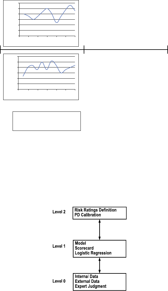
164

▸

A

NALYTI

CS

IN A BI

G

DATA W

O

RL

D

is done b

y

 rst se

g

mentin

g

the scores into risk ratin

g

s and then cal-

culatin

g

a historicall

y

observed default rate for each ratin

g

, which is

then used to project the probability of default (PD) for (typically) the

u

p

comin

g

y

ear. Fi

g

ure 8.3

g

ives an exam

p

le of how credit risk models

are commonl

y

a

pp

lied in man

y

bank settin

g

s.

3

F

i

gure 8.2 Constructing a Data Set

f

or Behavioral Scoring

3000

2500

2000

1500

1000

500

0

Checking account

246

Month

81012

800

750

700

650

600

550

500

0

Bureau score

246

Month

81012

t0t12

Observation

Point

Good/Bad?

Snapshot

t24

Number of products purchased

Number of times changed home address

Delinquency history (all credits)

…

Fi

g

ure 8.3 Three Level Credit Risk Model

EXAMPLE APPLI

C

ATI

O

N

S

◂1

65

Ot

her measures

t

ha

t

need

t

o be calcula

t

ed in credi

t

risk model

-

in

g

are the loss

g

iven default (LGD) and ex

p

osure at default (EAD).

LGD measures the economic loss expressed as a percentage of the

outstanding loan amount and is typically estimated using linear regres

-

sion or regression trees. EAD represents the outstanding balance for

on‐ balance sheet items (e.g., mortgages, installment loans). For off‐

b

alance sheet items (e.g., credit cards, credit lines), the EAD is typically

calculated as follows: EAD

=

DRAW

N

+ CCF * (LIMIT−DRAWN),

whereby DRAWN represents the already drawn balance, LIMIT the

credit limit, and CCF the credit conversion factor, which is ex

p

ressed

as a percentage

b

etween 0 an

d

1. CCF is typica

ll

y mo

d

e

l

e

d

using eit

h

er

averages,

l

inear regression, or regression trees.

Once t

h

e PD, LGD, an

d

EAD

h

ave

b

een estimate

d

, t

h

ey wi

ll

b

e

input into a capital requirements formula provided in the Basel II/III

accord, calculatin

g

the necessar

y

amount of ca

p

ital needed to

p

rotect

a

g

ainst unex

p

ected losses.

FRAUD DETECTION

Fraud detection comes in many  avors. Typical examples for which

fraud detection is relevant are: credit card fraud

,

insurance claim

fraud, mone

y

launderin

g

, tax evasion,

p

roduct warrant

y

fraud, and

click fraud. A  rst important challenge in fraud detection concerns

the labelin

g

of the transactions as fraudulent or not. A hi

g

h sus

p

i-

cion does not mean absolute certaint

y

, althou

g

h this is often used to

do the labeling. Alternatively, if available, one may also rely on court

j

ud

g

ments to make the decision.

Supervised, unsupervised, and social network learning can be used

for fraud detection. In supervised learning, a labeled data set with fraud

transactions is available. A common

p

roblem here is the skewness of

t

h

e

d

ata set

b

ecause t

yp

ica

lly

on

ly

a

f

ew transactions wi

ll

b

e

f

rau

d

u

l

ent.

Hence, a

d

ecision tree a

l

rea

dy

starts

f

rom a ver

y

p

ure root no

d

e (sa

y

,

99 percent non

f

rau

d

u

l

ent/1 percent

f

rau

d

u

l

ent) an

d

one may not

b

e

a

bl

e to



n

d

an

y

meanin

gf

u

l

s

pl

its to

f

urt

h

er re

d

uce t

h

e im

p

urit

y

. Simi

-

l

ar

ly

, ot

h

er ana

ly

tica

l

tec

h

ni

q

ues ma

y

h

ave a ten

d

enc

y

to sim

ply

p

re

-

d

ict t

h

e majority c

l

ass

b

y

l

a

b

e

l

ing eac

h

transaction as non

f

rau

d

u

l

ent.

Common sc

h

emes to

d

ea

l

wit

h

t

h

is are over‐ an

d

un

d

ersam

pl

in

g

. In

1

66

▸ANALYTI

CS

IN A BI

G

DATA W

O

RL

D

oversam

p

lin

g

, the fraudulent transactions in the trainin

g

data set (not

the test data set!) are re

p

licated to increase their im

p

ortance. In under

-

sampling, nonfraudulent transactions are removed from the training

data set (not test data set!) to increase the weight and importance of the

fraudulent transactions. Both procedures are useful to help the analyti

-

cal technique in  nding a discriminating pattern between fraudulent

and nonfraudulent transactions. Note that it is important to remember

that the test set remains untouched during this. However, if an analyti

-

cal technique is built using under‐ or oversampling, the predictions it

p

roduces on the test data set ma

y

be biased and need to be ad

j

usted.

One way to a

d

just t

h

e pre

d

ictions is as

f

o

ll

ows:

4

x

pC

pC pC

pC

pC pC

i

ti

j

tj

j

m

tj

()

()()

()

1

∑

⎢=⎢

⎢

=

whereb

y

C

i

re

p

resents the tar

g

et class (e.

g

.,

C

1

is fraudulen

t

and

C

2

C

is

nonfraudulent), xpC

ti

(|) re

p

resents the

p

robabilit

y

estimated on the

over‐ or undersampled training data set, pC

ti

()

is the prior probability of

class

C

i

CC

on the over‐ or undersampled training data set, and

i

pC

i

()

re

p

re-

sents the ori

g

inal

p

riors (e.

g

., 99/1

p

ercent). The denominator is intro

-

duced to make sure that the probabilities sum to one for all classes.

Unsu

p

ervised learnin

g

can also be used to detect clusters of outl

y-

in

g

transactions. The idea here is to build, for exam

p

le, a SOM and

look for cells containing only a few observations that might potentially

indicate anomalies re

q

uirin

g

further ins

p

ection and attention.

Finally, social network analysis might also be handy for fraud

detection. Although fraud may be hard to detect based on the avail-

able variables, it is often ver

y

useful to anal

y

ze the relationshi

p

s

b

etween

f

rau

d

sters. Rat

h

er t

h

an a stan

d

a

l

one

ph

enomenon,

f

rau

d

is

o

f

ten a care

f

u

lly

or

g

anize

d

crime. Ex

pl

oitin

g

re

l

ationa

l

in

f

ormation

provi

d

es some interesting insig

h

ts in crimina

l

patterns an

d

activities.

Fi

g

ure 8.4 i

ll

ustrates a

f

rau

d

networ

k

. Note t

h

at t

h

is networ

k

is con

-

structe

d

aroun

d

no

d

e 1 (in t

h

e center o

f

t

h

e



g

ure). No

d

es in t

h

e net-

wor

k

t

h

at are green are

l

egitimate no

d

es. Re

d

no

d

es are

f

rau

d

u

l

ent.

T

h

e networ

k

visua

l

ization

g

ives a

g

oo

d

im

p

ression o

f

t

h

e

d

i

ff

erence

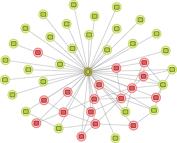
EXAMPLE APPLI

C

ATI

O

N

S

◂1

6

7

in network structure between le

g

itimate and fraudulent nodes. While

legitimate nodes only sparsely connect to each other, fraudulent nodes

are characterized b

y

a dense structure, with man

y

links between all the

members. Such structures have been investi

g

ated b

y

Van Vlasselaer,

Meskens

,

Van Dromme

,

and Baesens

5

and are called

spider construc-

tio

ns

in the domain of social securit

y

fraud. The name s

p

ider construc-

tions is derived from their appearance: The fraudulent constructions

look like a dense web in which all nodes are closely connected to each

other. Based on the e

g

onet conce

p

t, discussed earlier, both local and

network variables are constructed to characterize each node. Local

variables de ne the node of interest usin

g

onl

y

individual characteris

-

tics, in

d

epen

d

ent o

f

its surroun

d

ing neig

hb

ors. Networ

k

varia

bl

es are

d

e

p

en

d

ent on t

h

e networ

k

structure, an

d

inc

l

u

d

e:

■ Frau

d

u

l

ent

d

e

g

ree. In t

h

e networ

k

d

omain, t

h

e



rst‐or

d

er

d

egree re

f

ers to t

h

e num

b

er o

f

imme

d

iate contacts a no

d

e

h

as.

T

he

n

‐

d

e

g

ree

d

e



nes t

h

e num

b

er o

f

no

d

es t

h

e surve

y

e

d

no

d

e

F

i

gure 8.4 Frau

d

Networ

k

.

L

i

g

ht

Gray Nodes Refer to Legitimate Individuals, While Dark Gray Nodes Represent Fraud

21

10

24

20

15

29

31

43

47

46

44

45

41

42

40

37

39

38

33

34

32

35

36

26

5

3

9

17

13

27

18

28

30

6

2

16

19

22

4

7

23

8

1

14

25

11

12

1

68

▸ANALYTI

CS

IN A BI

G

DATA W

O

RL

D

can reach in a

t

mos

t

n

ho

p

s. Instead of calculatin

g

the overall

de

g

ree, one can make a distinction based on the label of each of

the surrounding nodes. For the fraud domain, this means that

the fraudulent  rst‐order degree corresponds to counting the

number of direct fraudulent neighbors.

■ Triangles. A triangle in a network is de ned as a structure in

w

hich three nodes of the network are connected to each other.

Especially triangles containing at least two fraudulent nodes are

a good indicator of potential suspicious activities of the third

node. Nodes that are involved in many suspicious triangles have

a

h

ig

h

er pro

b

a

b

i

l

ity to commit

f

rau

d

t

h

emse

l

ves.

■ C

l

iques. A c

l

ique is an extension o

f

a triang

l

e. Newman (2010)

de nes a cli

q

ue as the maximal subset of the vertices in an undi

-

rected network such that ever

y

member of the set is connected

b

y an edge to every other. While fraudulent triangles appear

re

g

ularl

y

in a network, fraudulent

k

‐cliques (with

k

> 3) will

k

a

pp

ear less often. However, such cli

q

ues are extremel

y

p

recise

indica

t

ors of fu

t

ure fraud.

Althou

g

h network variables as such can be ver

y

useful in detect

-

in

g

p

otential future fraud, these characteristics can also be converted

in aggregated variables characterizing each node (e.g., total number

of trian

g

les/cli

q

ues, avera

g

e de

g

ree wei

g

ht, avera

g

e trian

g

le/cli

q

ue

wei

g

ht). Afterward, these network variables should be enriched b

y

local variables as discussed before. Using all the available attributes,

standard learnin

g

techni

q

ues like lo

g

istic re

g

ression, random forests,

and neural networks are able to estimate future fraud based on both

network‐related information and personal information. Such a com-

b

ined a

pp

roach ex

p

loits all

p

otential information and returns the rel-

evance, in terms of variable weight, of each characteristic.

NET LIFT RESPONSE MODELING

In res

p

onse mo

d

e

l

in

g

, t

h

e

f

ocus

l

ies on

d

ee

p

enin

g

or recoverin

g

customer re

l

ations

h

i

p

s, or new customer ac

q

uisition

by

means o

f

targete

d

or win‐

b

ac

k

campaigns. T

h

e campaign can

b

e a mai

l

cata-

l

o

g

, emai

l

, cou

p

on, or A/B or mu

l

tivariate testin

g

. T

h

e

p

ur

p

ose is to

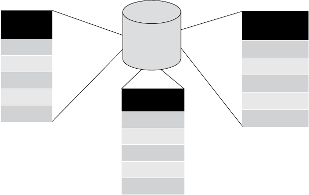
EXAMPLE APPLI

C

ATI

O

N

S

◂1

69

identif

y

the customers most likel

y

to res

p

ond based on the followin

g

informa

t

ion:

■ Demographic variables (e.g., age, gender, marital status)

■ Relationship variables (e.g., length of relationship, number of

products purchased)

■ Social network information

■ RFM variables

RFM has been popularized by Cullinan

6

as follows:

■ Recency: Time

f

rame (

d

ays, wee

k

s, mont

h

s) since

l

ast purc

h

ase

■ Frequency: Num

b

er o

f

purc

h

ases wit

h

in a given time

f

rame

■ Monetary: Do

ll

ar va

l

ue o

f

purc

h

ases

Each of these constructs can be operationalized in various ways;

for exam

p

le, one can consider the minimum/maximum/avera

g

e/most

recent monetar

y

value of

p

urchases. The constructs can be used se

p

a-

rately or combined into an RFM score by either independent or depen-

dent sortin

g

. For the former (see Fi

g

ure 8.5 ), the customer database

is sorted into inde

p

endent

q

uintiles based on RFM (e.

g

., recenc

y

quintile 1 is the 20 percent most ancient buyers). The  nal RFM score

F

i

gure 8.5 Construct

i

ng an RFM Score (In

d

epen

d

ent Sort

i

ng)

Frequency score

5

4

3

2

1

Recency

score

5

4

3

2

1

Monetary score

5

4

3

2

1

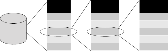
17

0

▸ANALYTI

CS

IN A BI

G

DATA W

O

RL

D

(

e.

g

., 325) can then be used as a

p

redictor for the res

p

onse model. For

d

epen

d

ent sorting, t

h

e customer

d

ata

b

ase is



rst sorte

d

into quinti

l

es

b

ase

d

on recency (see Figure 8.6 ). Eac

h

recency quinti

l

e is t

h

en

f

urt

h

er

d

ivi

d

e

d

into

f

requency quinti

l

es an

d

t

h

en into monetary quinti

l

es.

This again yields an RFM score (e.g., 335) that can be used as a predic-

tor for a res

p

onse model.

A  rst a

pp

roach to res

p

onse modelin

g

is b

y

s

p

littin

g

the

p

revi

-

ous campaign population into a test group and a control group (see

Fi

g

ure 8.7 ). The test

g

rou

p

receives the marketin

g

cam

p

ai

g

n and a

model is built on a trainin

g

subset and evaluated on a holdout subset.

Traditionally, the impact of such a marketing campaign is measured by

com

p

arin

g

the

p

urchase rate of a test

g

rou

p

a

g

ainst the

p

urchase rate

of a control

g

rou

p

. If the

p

urchase rate of the test

g

rou

p

exceeds the

purchase rate of the control group, the marketing campaign is said to

b

e effective. Althou

g

h such methods concentrate on maximizin

g

the

g

ross

p

urchase rate (i.e.,

p

urchase rate test

g

rou

p

minus

p

urchase rate

control group), they do not differentiate between different customers

and therefore i

g

nore the net or incremental im

p

act of the cam

p

ai

g

n.

In general, three types of customers can be distinguished. First, there

are those people who would never buy the product, whether they

are ex

p

osed to a marketin

g

offer or not. Tar

g

etin

g

these

p

eo

p

le would

not ma

k

e an

y

sense

b

ecause t

h

e

y

won’t

b

u

y

t

h

e

p

ro

d

uct an

y

wa

y

. A

secon

d

g

rou

p

o

f

customers is t

h

ose w

h

o a

l

wa

y

s

b

u

y

t

h

e

p

ro

d

uct. Tar

-

geting t

h

ese peop

l

e wi

ll

cause a pro



t

l

oss

b

ecause t

h

ey wi

ll

a

l

ways

b

u

y

t

h

e

p

ro

d

uct; t

h

ere

f

ore, o

ff

erin

g

t

h

em a mar

k

etin

g

incentive (e.

g

.,

a

d

iscount) wi

ll

re

d

uce t

h

e

p

ro



t mar

g

in. A

l

ast cate

g

or

y

o

f

customers

is t

h

e so‐ca

ll

e

d

swing c

l

ients. T

h

ese types o

f

customers wi

ll

not

b

uy

t

h

e

p

ro

d

uct s

p

ontaneous

ly

,

b

ut nee

d

to

b

e motivate

d

to ta

k

e action.

Fi

g

ure 8.6 Constructin

g

an RFM Score (Dependent Sortin

g

)

Frequency

score

35

34

33

32

31

Recency

score

5

4

3

2

1

Monetary

score

335

334

333

332

331

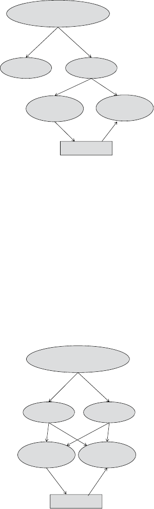
EXAMPLE APPLI

C

ATI

O

N

S

◂171

Because the

y

are still undecided on whether to bu

y

the

p

roduct, a

marketing campaign is especially effective for these people. Focusing

on onl

y

these customers will maximize the true im

p

act of the market-

in

g

cam

p

ai

g

n and is the

g

oal of net lift modelin

g

. Net lift modelin

g

tries to measure the true im

p

act b

y

the incremental

p

urchases, that is,

p

urchases that are onl

y

attributable to the cam

p

ai

g

n and that would

not be made other

w

ise.

7

Net lift modelin

g

aims at  ndin

g

a model

such that the difference between the test

g

rou

p

urchase rate and the

control

g

rou

p

urchase rate is maximized so as to identif

y

the swin

g

clients (see Fi

g

ure 8.8 ). B

y

im

p

lementin

g

this methodolo

gy

, marketers

Fi

g

ure 8.7 Gross Lift Response Modelin

g

Previous campaign data

Control Tes t

Training

data

Holdout

data

Model

F

ig

ure 8.8 Net Lift Response Modelin

g

Previous campaign data

Control Tes t

Training

data

Holdout

data

Model

172

▸ANALYTICS IN A BIG DATA WORL

D

not on

l

y optimize t

h

e true

b

usiness o

b

jective—maximizing pro



t—

b

ut

also

g

ain a better insi

g

ht in the different customer se

g

ments.

In the test and control

g

rou

p

, the tar

g

et will then be observed as

indicated in Figure 8.9 .

One could then build a difference score model

,

as follows:

■ Build a lo

g

istic re

g

ression model estimatin

g

p

robabilit

y

of

p

ur

-

chase given marketing message,

P

(purchase|test).

P

■ Build a logistic regression model estimating probability of pur

-

chase given control,

P

(purchase|control).

P

■ Incremental score

=

P

(purchase|test)−

P

(purchase|control).

P

To further understand the im

p

act of the

p

redictors, one can then

re

g

ress the incremental lift scores on the ori

g

inal data.

Another option could be to build only one logistic regression model

with an additional binar

y

p

redictor s

p

ecif

y

in

g

whether an observation

b

elon

g

s to the control or test

g

rou

p

. The model can then also include

all possible interaction terms with this binary variable.

CHURN PREDICTION

Customer churn

,

also called

a

ttritio

n

or

defection, is

t

he loss of cus

t

om

-

ers. In saturated markets, there are limited o

pp

ortunities to attract new

customers, so retainin

g

existin

g

customers is essential to

p

ro tabilit

y

and stability. It is estimated that attracting a new customer costs  ve to

Fi

g

ure 8.9 Observed Tar

g

et in Net Lift Modelin

g

Self-selectors

Converted

swing clients

No purchase

Self-selectors

Swing clients

No purchase

Test group

Control group

Y = 1

Y = 0

Y = 1

EXAMPLE APPLI

C

ATI

O

N

S

◂17

3

six times more than retainin

g

a customer.

8

Es

t

ablished cus

t

omers are

more

p

ro table due to the lower cost to serve them. In addition, brand

loyalty developed over time makes them less likely to churn. Satis ed

customers also serve as word‐of‐mouth advertisement, referring new

customers to the company.

Research on customer churn can take two perspectives: the over

-

all company level and the individual customer level. Identifying the

determinants of churn, or reasons why customers may churn, can

give insight into company‐level initiatives that may reduce the issues

that lead to hi

g

her churn. One such stud

y

9

p

erformed a surve

y

of the

Korean mo

b

i

l

e te

l

ep

h

one mar

k

et. Service attri

b

utes suc

h

as ca

ll

qua

l

-

ity an

d

tari

ff

l

eve

l

are negative

l

y corre

l

ate

d

wit

h

c

h

urn in t

h

at mar-

k

et. Natura

ll

y, i

f

it is possi

bl

e to improve ca

ll

qua

l

ity,

f

ewer customers

would be expected to churn. The results of this and similar studies

certainl

y

indicate that mana

g

ement must focus on the

q

ualit

y

of attri-

b

utes that are most im

p

ortant to customers.

1

0

However, continuall

y

improving in these areas may not always be feasible due to cost or

o

t

her limi

t

a

t

ions.

As a com

p

lementar

y

a

pp

roach, switchin

g

the focus to the individual

customer level can yield high returns for a relatively low investment.

It is

p

ossible to use churn

p

rediction models to identif

y

individual cus-

tomers who are likel

y

to churn and attem

p

t to

p

revent them from

leaving the company. These models assign each customer an expected

p

robabilit

y

of churn. Then it is relativel

y

strai

g

htforward to offer those

customers with the

g

reatest

p

robabilit

y

a discount or other

p

romo

-

tion to encourage them to extend their contract or keep their account

active. In the followin

g

section, several techni

q

ues and a

pp

roaches to

churn prediction will be discussed.

Churn Prediction Models

Man

y

we

ll

‐

k

nown an

d

l

ess common mo

d

e

l

s

h

ave

b

een a

ppl

ie

d

to

c

h

urn pre

d

iction, inc

l

u

d

ing

d

ecision trees,

l

ogistic regression, support

vector mac

h

ines, Ba

y

esian networ

k

s, surviva

l

ana

ly

sis, se

lf

‐ or

g

anizin

g

ma

p

s, an

d

re

l

ationa

l

c

l

assi



ers, amon

g

ot

h

ers. Bot

h

accurac

y

an

d

com-

pre

h

ensi

b

i

l

ity are crucia

l

f

or t

h

e

d

ecision‐ma

k

ing process, so care

f

u

l

consi

d

eration s

h

ou

ld

b

e use

d

w

h

en c

h

oosin

g

a tec

h

ni

q

ue. Accurate

174 ▸ANALYTI

CS

IN A BI

G

DATA W

O

RL

D

p

redictions are

p

erha

p

s the most a

pp

arent

g

oal, but learnin

g

the

reasons

,

or at least the indicators

,

for churn is also invaluable to the

company. Understanding why a model makes the predictions it does

serves several purposes. Comprehensibility allows for domain experts

to evaluate the model and ensure that it is intuitively correct. In this

way, it can be veri ed or con rmed by the business. More comprehen

-

sible models also offer insight into the correlation between customer

attributes and propensity to churn,

1

1 allowing management to address

the factors leading to churn in addition to targeting the customers

b

efore the

y

decide to churn. Finall

y

, understandable and intuitive

mo

d

e

l

s may

b

e more easi

l

y a

d

opte

d

wit

h

in a company. I

f

managers

are accustome

d

to ma

k

ing

d

ecisions

b

ase

d

on t

h

eir own experience

an

d

k

now

l

e

d

ge, t

h

ey wi

ll

b

e more inc

l

ine

d

to trust pre

d

ictions ma

d

e

b

y a model that is not only comprehensible but also in line with their

own reasonin

g

.

Lo

g

istic re

g

ression is a statistical classi cation model that is often

used for churn prediction, either as a model on its own or as a com

-

p

arison for other models. The coef cients for this model indicate the

correlation between the customer attributes and the

p

robabilit

y

of

churn. It is a well understood and accepted model both in research

and

p

ractice. It is both eas

y

to inter

p

ret and

p

rovides

g

ood results

when com

p

ared with other methods. It has been shown to out

p

er-

form more complex methods in many cases. Decision trees can also be

used for churn

p

rediction. The

y

also offer inter

p

retabilit

y

and robust-

ness. Neural networks and su

pp

ort vector machines have also been

applied to churn prediction; however, these methods are seen as black

b

oxes, offerin

g

little insi

g

ht into how the

p

redictions are made. Sur-

vival analysis offers the interpretability of logistic regression in the

form of hazard ratios that can be interpreted similarly to odds ratios in

lo

g

istic re

g

ression. In addition, the tar

g

et of interest is time‐to‐event

rat

h

er t

h

an a

b

inar

y

varia

bl

e. It is t

h

ere

f

ore

p

ossi

bl

e to ma

k

e

p

re

d

ic

-

tions a

b

out

h

ow

l

on

g

a customer wi

ll

remain active

b

e

f

ore t

h

e

y

c

h

urn.

Re

l

ationa

l

c

l

assi



ers can a

l

so

b

e use

d

f

or c

h

urn pre

d

iction. Homop

h

-

i

ly

in networ

k

s is

b

ase

d

on t

h

e i

d

ea t

h

at simi

l

ar in

d

ivi

d

ua

l

s are more

l

i

k

e

ly

to interact, an

d

f

rom t

h

at it is ex

p

ecte

d

t

h

at in

d

ivi

d

ua

l

s t

h

at are

connecte

d

in a networ

k

wi

ll

b

e

h

ave simi

l

ar

l

y. In c

h

urn pre

d

iction, i

f

customers are

l

in

k

e

d

wit

h

c

h

urners, t

h

e

y

ma

y

a

l

so

b

e

l

i

k

e

ly

to c

h

urn.

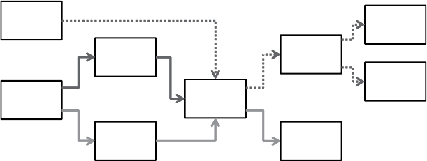
EXAMPLE APPLICATION

S

◂17

5

Socia

l

net

w

or

k

f

eatures can a

l

so

b

e use

d

in a tra

d

itiona

l

c

l

assi



er

l

i

k

e

l

o

g

istic re

g

ression or survival anal

y

sis. In order to do this, measures of

connectedness can be extracted from the network and used as input

features for the other model.

12

Churn Prediction Process

Regardless of the particular technique, churn prediction modeling fol

-

l

ows a standard classi cation process as illustrated in Figure 8.10 . The

 rst ste

p

is to de ne churn for the

p

articular situation. This ma

y

be nat-

ura

ll

y present in t

h

e

d

ata: contract termination, service cance

ll

ation,

or nonrenewa

l

. In ot

h

er settings, it wi

ll

not

b

e so c

l

ear: A customer

n

o

l

onger s

h

ops at t

h

e store or we

b

site, or a customer stops purc

h

as

-

i

ng credits. In these cases, the analyst or researcher must choose a

de ni

t

ion of churn

t

ha

t

makes sense in

t

he con

t

ex

t

.

O

ne common

solution is to select an a

pp

ro

p

riate len

g

th of time of inactivit

y

on the

account. In the previous examples, a number of days or months with-

out a

p

urchase mi

g

ht de ne churn. Of course, a customer ma

y

not

b

u

y

somethin

g

within that time frame but still return a

g

ain at a later

date. Setting too short of a time period may lead to nonchurn cus-

tomers bein

g

tar

g

eted as

p

otential churners. Too lon

g

of a

p

eriod ma

y

mean churnin

g

customers are not identi ed in a timel

y

manner. In

most cases, a shorter time period may be preferable, if the cost of the

i

ntervention cam

p

ai

g

n is much lower than the cost of a lost customer.

After de nin

g

churn, the ori

g

inal set of customers should be

l

abeled according to their true churn status. The data set is split for

Fi

g

ure 8.10 The Churn Prediction Process

6

8

73

21

5

4

Define

Churn

TrainingSet

TestSet

Model

Unknown

Data

Predictions

Model

Performance

Retention

Campaign

No

Campaign

17

6

▸ANALYTI

CS

IN A BI

G

DATA W

O

RL

D

validation and the customer attributes from the trainin

g

set can be

used

t

o

t

rain

t

he selec

t

ed model. The cus

t

omer a

tt

ribu

t

es from

t

he

test set are then used to compare the model’s results with the actual

churn label. This allows for an evaluation of the model performance.

The model may also be evaluated by domain experts to gauge whether

the predictive attributes seem in line with business knowledge. If the

performance is acceptable, the attributes of current customers can be

entered into the model to predict their churn class. A group of custom-

ers with the highest predicted churn probability can then be contacted

with the retention cam

p

ai

g

n. Other customers who are less likel

y

to

c

h

urn are not contacte

d

wit

h

t

h

e promotion.

RECOMMENDER SYSTEMS

Peo

p

le are in uenced b

y

recommendations in their dail

y

decisions.

Salesmen tr

y

to sell us the

p

roduct we like, restaurants are bein

g

eval-

uated and rated, and so on. Recommender systems can support us in

our online commercial activities b

y

su

gg

estin

g

s

p

eci c items from a

wide ran

g

e of o

p

tions. A considerable number of different techni

q

ues

are available to build a recommender system, of which the following

are the most im

p

ortant: collaborative  lterin

g

, content‐based  lterin

g

,

demo

g

ra

p

hic  lterin

g

, knowled

g

e‐based  lterin

g

, and h

y

brid  lter

-

ing. Case studies presenting all these techniques have greatly multi-

p

lied in recent

y

ears. A lot of these deal with movies,

13 tourism

,

1

4

and

res

t

auran

t

s.15

In this section, the  ve main techniques are introduced and fol-

lowed b

y

some of their advanta

g

es and disadvanta

g

es. Some other

issues concerning recommender systems are then brie y discussed.

Collaborative Filtering

Collaborative  ltering, also called

social  ltering,

h

as

b

een t

h

e a

pp

roac

h

t

h

at is associate

d

t

h

e most wit

h

recommen

d

er systems. T

h

e main i

d

ea

is to recommen

d

items

b

ase

d

on t

h

e o

p

inions o

f

ot

h

er users. A

d

is

-

tinction can

b

e ma

d

e

b

etween user‐

b

ase

d

co

ll

a

b

orative



l

terin

g

an

d

item‐

b

ase

d

co

ll

a

b

orative



l

tering. In case o

f

user‐

b

ase

d

co

ll

a

b

orative



l

terin

g

, items wi

ll

b

e recommen

d

e

d

to a user

b

ase

d

on

h

ow simi

l

ar

EXAMPLE APPLI

C

ATI

O

N

S

◂177

users rated these items. When o

p

tin

g

for item‐based collaborative  l-

terin

g

, items will be recommended to a user based on how this user

rated similar items. One way to calculate similarity between users or

items is to use a user‐item matrix that contains information on which

user bought what item. Any similarity measure can then be used to

create a similarity matrix (e.g., Pearson correlation and cosine).

To build a collaborative recommender system, ratings are required.

These ratings form the link between a user and an item.

16

A distinc

-

tion can be made between three types of ratings. A scalar rating can

b

e a number or an ordinal ratin

g

. A binar

y

ratin

g

consists of two

p

os-

si

b

i

l

ities, suc

h

as goo

d

or

b

a

d

. Fina

ll

y, unary ratings in

d

icate t

h

at a user

h

as

h

a

d

an interaction wit

h

an item, suc

h

as a c

l

ic

k

on an item or a

purc

h

ase.

1

7

We can

d

istinguis

h

b

etween two types o

f

met

h

o

d

s

f

or t

h

e

collection of ratings. Explicit ratings can be obtained by requesting a

user to rate a certain item. Im

p

licit ratin

g

s are obtained b

y

associatin

g

a ratin

g

with a certain action, such as bu

y

in

g

an item.

1

8

Typically, neighborhood‐based algorithms are applied, in which the

followin

g

three ste

p

s can be distin

g

uished.

19 First, a similarit

y

measure

is used to calculate similarit

y

between users (in case of a user‐based

algorithm) or items (in case of an item‐based algorithm). Second, a

subset of users or items is selected that functions as the nei

g

hborhood

of the active user or item. Third, the al

g

orithm

p

redicts a ratin

g

based

on the active user’s or item’s neighborhood, typically giving the high-

est wei

g

ht to the most similar nei

g

hbors.

As is often the case with anal

y

tics, different techni

q

ues can be

used to solve the same problem, with their respective advantages and

disadvanta

g

es. Three main advanta

g

es of collaborative recommender

systems are identi ed. First, collaborative  ltering does not restrict the

type of items to be recommended. It is indeed enough to construct a

matrix linkin

g

items to users to start the recommendation. A second

a

d

vanta

g

e,

l

in

k

e

d

to t

h

e



rst, is t

h

at it mana

g

es to

d

e

l

iver recommen-

d

ations to a user even w

h

en it is

d

i

f

cu

l

t to



n

d

out w

h

ic

h

s

p

eci



c

f

eature o

f

t

h

e item ma

k

es it interesting to t

h

e user or w

h

en t

h

ere is no

eas

y

wa

y

to extract suc

h

a

f

eature automatica

lly

. A t

h

ir

d

a

d

vanta

g

e

h

as

to

d

o wit

h

nove

l

t

y

or seren

d

i

p

it

y

: Co

ll

a

b

orative



l

terin

g

is

b

e

l

ieve

d

to

recommen

d

more unexpecte

d

items (t

h

at are equa

ll

y va

l

ua

bl

e) t

h

an

content‐

b

ase

d

tec

h

ni

q

ues.

20

A

l

t

h

ou

gh

co

ll

a

b

orative



l

terin

g

met

h

o

d

s

1

7

8

▸ANALYTICS IN A BIG DATA WORL

D

are the most commonl

y

used techni

q

ues because of their

p

ower, some

disadvanta

g

es or weak

p

oints should be noted. First, s

p

arse data can

b

e a problem for such a technique. A critical mass of ratings is indeed

necessary in order to build meaningful similarity matrices. In cases in

which the items are not frequently bought by the users (e.g., recom-

mending mobile phones or apartments), it may indeed be dif cult to

obtain representative neighborhoods, hence lowering the power of the

technique. A second disadvantage is known as the cold start problem,

which means that new items cannot easily be recommended because

the

y

have not been rated

y

et; therefore, new users cannot easil

y

receive

recommen

d

ations

b

ecause t

h

ey

h

ave not yet rate

d

items. Some minor

d

isa

d

vantages are,

f

or examp

l

e, t

h

e

f

act t

h

at items purc

h

ase

d

a

l

ong

time ago may

h

ave a su

b

stantia

l

impact i

f

ew items

h

ave

b

een rate

d

,

which may lead to wrong conclusions in a changing environment.

Privac

y

could also be a

p

roblem because collaborative  lterin

g

needs

data on users to

g

ive recommendations or could

g

enerate trust issues

b

ecause a user cannot question the recommendation.

Content‐Based Filtering

Content‐based recommender s

y

stems recommend items based on two

information sources: features of

p

roducts and ratin

g

s

g

iven b

y

users.

Different kinds of data can be encountered, requiring different strate-

g

ies to obtain usable in

p

ut. In the case of structured data, each item

consists of the same attributes and the

p

ossible values for these attri-

b

utes are known. It is then straightforward to apply content‐based

a

pp

roaches. When onl

y

unstructured data are available, such as text,

different techniques have to be used in order to learn the user pro les.

Because no standard attributes and values are available, typical prob-

lems arise, such as s

y

non

y

ms and

p

ol

y

semous words. Free text can

t

h

en

b

e trans

l

ate

d

into more structure

d

ata

by

usin

g

a se

l

ection o

f

ree text terms as attri

b

utes. Tec

h

ni

q

ues

l

i

k

e TF‐IDF (term

f

re

q

uenc

y/

inverse

d

ocument

f

requency) can t

h

en

b

e use

d

to assign weig

h

ts to

t

h

e

d

i

ff

erent terms o

f

an item. Sometimes,

d

ata is semistructure

d

, con-

sistin

g

o

f

some attri

b

utes wit

h

restricte

d

va

l

ues an

d

some

f

ree text.

One approac

h

to

d

ea

l

wit

h

t

h

is

k

in

d

o

f

d

ata is to convert t

h

e text into

s

t

ruc

t

ure

d

a

t

a.

21

EXAMPLE APPLI

C

ATI

O

N

S

◂17

9

When items can be re

p

resented in a usable wa

y

, machine learnin

g

techni

q

ues are a

pp

lied to learn a user

p

ro le. T

yp

icall

y

, a classi cation

algorithm is invoked for each user based on his or her ratings on items

and their attributes. This allows the recommender system to predict

whether a user will like an item with a speci c representation. As with

collaborative  ltering methods, explicit or implicit ratings are required.

When explicit ratings are considered, the ratings are directly used for

the classi cation task, whereas implicit ratings can be obtained using

the item–user interactions.

The classi cation

p

roblem mentioned above can be im

p

lemented

using a

l

arge num

b

er o

f

d

i

ff

erent mac

h

ine

l

earning tec

h

niques. Some

examp

l

es are

l

ogistic regression, neura

l

networ

k

s,

d

ecision trees, asso-

ciation ru

l

es, an

d

Bayesian networ

k

s. Nearest neig

hb

or met

h

o

d

s can

also be used

t

o de

t

ermine

t

he labeled i

t

ems

t

ha

t

are mos

t

similar

t

o

a new unlabeled item in order to label this new item based on the

labels of the nearest nei

g

hbors. Concernin

g

the similarit

y

metric used

in nearest neighbor methods, Euclidean distance is often used when

data are structured, whereas cosine similarit

y

ma

y

p

rove its use when

the vector s

p

ace model is a

pp

lied. Other a

pp

roaches are linear classi-

 ers, support vector machines, and Naïve Bayes.

22

A  rst advanta

g

e of content‐based recommender s

y

stems is that

there is no cold start

p

roblem for new items. Indeed, new items

(which have not received ratings before) can be recommended,

which was not the case in a collaborative  lterin

g

a

pp

roach. Sec

-

ond, items can also be recommended to users that have uni

q

ue

preferences. A third important advantage is the possibility to give

an ex

p

lanation to the user about his or her recommendations, for

example, by means of displaying a list of features that led to the

item being recommended. A fourth advantage is that only ratings

of the active user are used in order to build the

p

ro le, which is not

t

h

e case

f

or co

ll

a

b

orative recommen

d

er s

y

stems.

23

Concernin

g

t

h

e

d

isa

d

vanta

g

es, a



rst

l

imitation is t

h

at content‐

b

ase

d

tec

h

ni

q

ues are

on

l

y suita

bl

e i

f

t

h

e rig

h

t

d

ata are avai

l

a

bl

e. It is in

d

ee

d

necessary to

h

ave enou

gh

in

f

ormation a

b

out t

h

e items to

d

etermine w

h

et

h

er a

user wou

ld

l

i

k

e an item or not. T

h

e co

ld

start

p

ro

bl

em

f

or new users

f

orms a secon

d

l

imitation as we

ll

, as o

ld

ratings potentia

ll

y in



uence

t

h

e recommen

d

ation too muc

h

. Fina

lly

, over‐s

p

ecia

l

ization can

b

e a

1

80

▸ANALYTI

CS

IN A BI

G

DATA W

O

RL

D

p

roblem because such techni

q

ues will focus on items similar to the

p

reviousl

y

bou

g

ht items.

Demographic Filtering

Demographic  ltering recommends items based on demographic infor

-

mation of the user. The main challenge is to obtain the data. This can

b

e explicitly done by asking for information from users such as age,

gender, address, and so on. If this approach is not possible, analytical

techni

q

ues could be used to extract information linked to the interac-

tions o

f

t

h

e users wit

h

t

h

e system. A user pro



l

e can t

h

en

b

e

b

ui

l

t an

d

use

d

t

o recommen

d

i

t

ems.

2

4

T

h

e main a

d

vantage o

f

d

emograp

h

ic recommen

d

er systems is t

h

at

there is not always a need for a history of user ratings of the type that is

re

q

uired in collaborative and content‐based a

pp

roaches. Se

g

ments can

b

e used in combination

w

ith user–item interactions in order to obtain

a high‐level recommender system. Some disadvantages are the cold

start

p

roblem for new users and new items, as well as the dif cult

y

in

ca

p

turin

g

the data, which is hi

g

hl

y

de

p

endent on the

p

artici

p

ation of

t

he users.

Knowledge‐Based Filtering

Com

p

ared with collaborative  lterin

g

and content‐based recommender

s

y

stems, it is more dif cult to brie

y

summarize the characteristics of

knowledge‐based recommender systems. The main difference with

re

g

ard to the other techni

q

ues resides in the data sources used. With

this approach, additional inputs consisting of constraints or require-

ments are provided to the recommender system typically by allowing

a dialo

g

between the user and the s

y

stem. Knowled

g

e‐based recom

-

men

d

er s

y

stems can

b

e

d

ivi

d

e

d

in two main cate

g

ories: constraint

‐

b

ase

d

recommen

d

ers an

d

case‐

b

ase

d

recommen

d

ers. Constraint‐

b

ase

d

recommen

d

ers are systems meeting a set o

f

constraints impose

d

b

y

b

ot

h

users an

d

t

h

e item

d

omain. A mo

d

e

l

o

f

t

h

e customer re

q

uirements,

t

h

e

p

ro

d

uct

p

ro

p

erties, an

d

ot

h

er constraints t

h

at

l

imit t

h

e

p

ossi

bl

e

requirements is



rst constructe

d

an

d

f

orma

l

ize

d

. Any tec

h

nique can

t

h

en

b

e use

d

an

d

wi

ll

h

ave to meet t

h

e re

q

uirements, or at

l

east

EXAMPLE APPLI

C

ATI

O

N

S

◂1

8

1

minimize the violations. When dealin

g

with case‐based recommend

-

ers, the

g

oal is to  nd the item that is most similar to the ones the

user requires. Similarity is then often based on knowledge of the item

domain. The system will then start with an example provided by the

user and will generate a user pro le based on it. Based on this user

pro le gathering information and additional knowledge sources, rec

-

ommendations can then be proposed.

2

5

A  rst advantage of knowledge‐based recommender systems is

that they can be used when there is only limited information about

the user, hence avoidin

g

the cold start

p

roblem. Another advanta

g

e

is t

h

at expert

k

now

l

e

d

ge is use

d

in t

h

e recommen

d

er system. It is a

l

so

possi

bl

e to

f

unction in an environment wit

h

comp

l

ex, in

f

requent

l

y

b

oug

h

t items. In a

dd

ition, a constraint‐

b

ase

d

recommen

d

er system

can help customers actively, for example, by explaining products or

su

gg

estin

g

chan

g

es in case no recommendation is

p

ossible. Concernin

g

disadvanta

g

es, a knowled

g

e‐based recommender s

y

stem ma

y

re

q

uire

some effort concerning knowledge acquisition, knowledge engineer-

in

g

, and develo

p

ment of the user interface. A second disadvanta

g

e is

that it can be dif cult when the user is asked to

p

rovide the s

y

stem

with an example if the number of items in the recommendation sys-

tem is ver

y

hi

g

h. Similarl

y

, it ma

y

be dif cult or im

p

ossible for the user

to

p

rovide an exam

p

le that  ts the user’s needs.

Hybrid Filtering

Hybrid recommender systems combine the advantages of content

‐

b

ased, knowled

g

e‐based, demo

g

ra

p

hic, and collaborative  lterin

g

recommender systems. The main reason that hybrid recommender

systems have been developed is to avoid the cold start problem.

B

u

rk

e

26

ex

p

lains seven t

yp

es of h

y

brid techni

q

ues. A  rst t

yp

e is

wei

gh

te

d

. In t

h

is case, t

h

e recommen

d

ation scores o

f

severa

l

recom-

men

d

ers are com

b

ine

d

by

a

pply

in

g

s

p

eci



c wei

gh

ts. Switc

h

in

g

is a sec

-

on

d

h

y

b

ri

d

tec

h

nique in w

h

ic

h

recommen

d

ations are ta

k

en

f

rom one

recommen

d

er at a time,

b

ut not a

l

wa

y

s t

h

e same one. A t

h

ir

d

t

yp

e o

f

hyb

ri

d

tec

h

ni

q

ue is mixe

d

. W

h

en suc

h

a

hyb

ri

d

tec

h

ni

q

ue is a

ppl

ie

d

,

recommen

d

ations

f

or mu

l

tip

l

e recommen

d

ers are s

h

own to t

h

e user.

Feature com

b

ination is a

f

ourt

h

t

yp

e o

f

hyb

ri

d

tec

h

ni

q

ue. In t

h

is case,

1

82

▸ANALYTI

CS

IN A BI

G

DATA W

O

RL

D

different knowled

g

e sources are used to obtain features, and these are

then

g

iven to the recommendation al

g

orithm. A  fth t

yp

e is feature

augmentation: A  rst recommender computes the features while the

next recommender computes the remainder of the recommendation.

For example, Melville, Mooney, and Nagarajan

2

7

use a content‐based

model to generate ratings for items that are unrated and then col-

laborative  ltering uses these to make the recommendation. Cascade

is the sixth type of hybrid technique. In this case, each recommender

is assigned a certain priority and if high priority recommenders pro-

duce a different score, the lower

p

riorit

y

recommenders are decisive.

Fina

ll

y, a meta‐

l

eve

l

h

y

b

ri

d

recommen

d

er system consists o

f

a



rst

recommen

d

er t

h

at gives a mo

d

e

l

as output t

h

at is use

d

as input

b

y

t

h

e next recommen

d

er. For examp

l

e, Pazzani

2

8

d

iscusses a restaurant

recommender that  rst uses a content‐based technique to build user

p

ro les. Afterward, collaborative  lterin

g

is used to com

p

are each

user and identif

y

nei

g

hbors. Burke

29 states that a meta‐level h

y

brid is

different from a feature augmentation hybrid because the meta‐level

h

y

brid does not use an

y

ori

g

inal

p

ro le data; the ori

g

inal knowled

g

e

source is re

p

laced in its entiret

y

.

Evaluation of Recommender Systems

Two categories of evaluation metrics are generally considered:

30

t

he

g

oodness or badness of the out

p

ut

p

resented b

y

a recommender

s

y

stem and its time and s

p

ace re

q

uirements. Recommender s

y

stems

generating predictions (numerical values corresponding to users’ rat-

in

g

s for items) should be evaluated se

p

aratel

y

from recommender

systems that propose a list of

N

items that a user is expected to  nd

N

interesting (top‐

N

recommendation). The  rst category of evaluation

N

metrics that we consider is the

g

oodness or badness of the out

p

ut

p

re-

sente

d

by

a recommen

d

er s

y

stem. Concernin

g

recommen

d

er s

y

stems

t

h

at ma

k

e

p

re

d

ictions,

p

re

d

iction accurac

y

can

b

e measure

d

usin

g

statistica

l

accuracy metrics (o

f

w

h

ic

h

mean a

b

so

l

ute

d

eviation [MAD]

is t

h

e most

p

o

p

u

l

ar one) an

d

usin

g

d

ecision su

pp

ort accurac

y

met-

rics (o

f

w

h

ic

h

area un

d

er t

h

e receiver o

p

eratin

g

c

h

aracteristic curve

is t

h

e most popu

l

ar one). Coverage

d

enotes

f

or w

h

ic

h

percentage o

f

t

h

e items t

h

e recommen

d

er s

y

stem can ma

k

e a

p

re

d

iction. Covera

g

e

EXAMPLE APPLI

C

ATI

O

N

S

◂1

83

mi

g

ht decrease in case of data s

p

arsit

y

in the user–item matrix. Con-

cern

i

n

g

to

p

‐

N

recommendation, important metrics are recall pre-

N

cision–related measures. Data is  rst divided in a training set and a

test set. The algorithm runs on the training set, giving a list of recom-

mended items. The concept of “hit set”

3

1

is considered, containing only

the recommended (top‐

N

) items that are also in the test set. Recall and

N

precision are then determined as follows:

=Recall size of hit set

size of test set

=N

Precision size of hit set

A pro

bl

em wit

h

reca

ll

an

d

precision is t

h

at usua

ll

y reca

ll

increases

as

N

is increased, while precision decreases as

N

is increased. There-

N

fore

,

the

F

1 metric combines both measures:

F

32

=+

F12 * recall * precision

recall precision

F

1 for each user and then taking the average gives the

F

score of the top‐

N

recommendation list.

N

The other cate

g

or

y

of evaluation metrics is dealin

g

with the

p

erformance of a recommender s

y

stem in terms of time and s

p

ace

requirements. Response time is the time that is needed for a system

to formulate a res

p

onse to a user’s re

q

uest. Stora

g

e re

q

uirements can

b

e considered in two wa

y

s: main memor

y

re

q

uirement (online s

p

ace

needed by the system) and secondary storage requirement (of ine

s

p

ace needed b

y

the s

y

stem).

Additional metrics can also be considered and will depend on

the type of recommender system faced and the domain in which it

is used. For exam

p

le, it is a common

p

ractice in a direct marketin

g

context to

b

ui

ld

a cumu

l

ative

l

i

f

t curve or ca

l

cu

l

ate t

h

e AUC. One

a

l

so

h

as to

d

eci

d

e w

h

et

h

er on

l

ine or o

f

ine eva

l

uations wi

ll

b

e ma

d

e.

A

l

t

h

oug

h

o

f

ine eva

l

uation is typica

ll

y app

l

ie

d

, it is o

f

ten mis

l

ea

d

ing

b

ecause t

h

e context o

f

t

h

e recommen

d

ation is not consi

d

ere

d

. Ho

w

-

ever, t

h

e costs

l

in

k

e

d

wit

h

on

l

ine eva

l

uations are t

yp

ica

lly

h

i

gh

er an

d

are accompanie

d

b

y

d

i

ff

erent ris

k

s (e.g.,

b

a

d

recommen

d

ations may

im

p

act customers’ satis

f

action).

184

▸

A

NALYTI

CS

IN A BI

G

DATA W

O

RL

D

Examples

Different cases applying recommendation techniques have been

re

p

orted,

p

rovidin

g

the

p

ractitioners with best

p

ractices and success

stories. Some references are provided in what follows, showing a small

subset of the available cases. A  rst case that is relevant in the context

of collaborative  ltering is Amazon.com. Linden, Smith, and York

33

describe the use of recommendation algorithms at Amazon.com.

They see recommendation systems as a type of targeted marketing

b

ecause the needs of the customer can be met in a personalized way.

A secon

d

case t

h

at is re

l

evant in t

h

e context o

f

co

ll

a

b

orative



l

ter

-

ing is PITTCULT, a cu

l

tura

l

event recommen

d

er

b

ase

d

on a networ

k

o

f

trust. In anot

h

er case, Mooney an

d

Roy

3

4 app

l

y a content‐

b

ase

d

approac

h

on

b

oo

k

recommen

d

ations. Semistructure

d

text is extracte

d

from web

p

a

g

es at Amazon.com and text cate

g

orization is then a

pp

lied

to it. Users rate books of the training set, which allows the system

to learn the user pro le using a Bayesian learning algorithm. A  rst

case that is relevant in the context of knowled

g

e‐based recommender

systems is “virtual advisor,” the constraint‐based recommender sys-

tem

p

ro

p

osed b

y

Jannach, Zanker, and Fuchs.

3

5 Virtual advisor is a

knowled

g

e‐based tourism recommender s

y

stem that has been devel-

oped for a premium spa resort in Austria. The authors show that using

a dialo

g

, user re

q

uirements and

p

references are derived. Durin

g

the

dialo

g

, the internal user model is anal

y

zed and the next dialo

g

action

is determined. When enough information is gathered about the user’s

re

q

uirements and

p

references, the s

y

stem shows the items that meet

the user’s constraints. If necessar

y

, it shows which constraints have

to be relaxed. A second case that is relevant in the context of knowl-

ed

g

e‐based recommender s

y

stems is Intelli

g

ent Travel Recommender

(

ITR), discussed b

y

Ricci, Arslan, Mirzadeh, and Venturini.

3

6 ITR i

s

a

case‐based travel advisor

y

s

y

stem that recommends a travel

p

lan to a

user, starting

f

rom some wis

h

es an

d

constraints t

h

at t

h

is user enters in

t

h

e s

y

stem. T

h

e current session is consi

d

ere

d

a case an

d

it

h

as simi

l

ari

-

ties wit

h

cases o

f

ot

h

er users t

h

at are a

l

rea

dy



nis

h

e

d

. T

h

ese

p

revious

cases can

h

ave an impact on t

h

e recommen

d

ation to t

h

e users. One

a

d

vanta

g

e o

f

t

h

is a

pp

roac

h

is t

h

at users

d

o not nee

d

a

l

o

g

in

b

ecause

t

h

e set o

f

p

ast cases t

h

at in



uence t

h

e user’s recommen

d

ation is

b

ase

d

EXAMPLE APPLI

C

ATI

O

N

S

◂

185

on similarit

y

between the user’s case and

p

ast cases. A second advan-

ta

g

e is that a limited user

p

ro le is suf cient, which is not the case

when applying a content‐based approach (as it is then assumed that

users and products share features).

WEB ANALYTICS

The Digital Analytics Association (DAA) de nes web analytics as:

3

7

the measurement, collection, anal

y

sis, and re

p

ortin

g

o

f

Internet

d

ata

f

or t

h

e purposes o

f

un

d

erstan

d

ing an

d

optimizing We

b

usage.

In w

h

at

f

o

ll

ows, we



rst e

l

a

b

orate on we

b

d

ata co

ll

ection an

d

t

h

en

illustrate how this can be analyzed.

Web Data Collection

A ke

y

challen

g

e in web anal

y

tics is to collect data about web visits.

3

8

A

 rst o

p

tion here is web server lo

g

anal

y

sis, which is essentiall

y

a server‐

side data collection technique making use of the web server’s logging

functionalit

y

. Ever

y

HTTP re

q

uest

p

roduces an entr

y

in one or more web

server lo

g

 les. The lo

g

 le can then be

p

arsed and

p

rocessed on a set

schedule to provide useful information. This is illustrated in Figure 8.11 .

Common lo

g

 le formats are:

■ Apache/NCSA log formats: Common Log Format or Combined

L

og

F

ormat

■ W3C (World Wide Web Consortium) Extended Log File Format

and its Microsoft IIS implementation

Fi

g

ure 8.11 Web Server Lo

g

Anal

y

sis

User

Web server(s)

Log file(s)

HTTP request, for

example, get page

HTML code

186

▸ANALYTI

CS

IN A BI

G

DATA W

O

RL

D

A log entry (Apache combined log format) typically looks like

Figure 8.12 .

The data recorded includes:

■ Remote host: IP address or domain name; hel

p

s identif

y

the

g

eo

g

ra

ph

ica

l

ocation o

f

t

h

e c

l

ient com

p

uter

■ Remote

l

o

g

name (“‐”); user name (“‐” i

f

no aut

h

entication)

■ Date an

d

time (can inc

l

u

d

e o

ff

set

f

rom Greenwic

h

Mean Time)

■ HTTP request met

h

o

d

(GET or POST)

■ Resource requeste

d

■ Re

l

ative to t

h

e root

d

irectory

l

ocation on t

h

e we

b

server

■ Mig

h

t inc

l

u

d

e query string (parameters a

f

ter t

h

e ?) “GET

/

d

utc

h

/s

h

op/

d

etai

l

.

h

tm

l

?Pro

d

ID

=

112 HTTP

/

1.1

”

■ HTTP status co

d

e

■ 200 range: success

f

u

l

(200

f

or GET request means requeste

d

resource

h

as

b

een sent)

■ 300 range: re

d

irect

■ 400 range: c

l

ient error (404 means not

f

oun

d

)

■ 5

00

range: server error

■ Num

b

er o

f

b

ytes trans

f

erre

d

■ Re

f

errer: we

b

page

f

rom w

h

ic

h

user c

l

ic

k

e

d

on

l

in

k

to arrive

h

ere

■ “

h

ttp://www.msn.

b

e/s

h

opping/

f

oo

d

/“

■ “

h

ttp://www.goog

l

e.com/searc

h

?

q

=

b

uy&p

l

us;wine&

hl

=

en&

l

r

=

“

■ Browser and

p

latform (user a

g

ent)

■ Can also be a search bot, for exam

p

le, Goo

g

lebot

C

ookies can also be used for da

t

a collec

t

ion. A cookie is a small

text strin

g

that

Figure 8.12 Example Log Entr

y

EXAMPLE APPLI

C

ATI

O

N

S

◂1

8

7

■ A web server can send to a visitor’s web browser (as

p

art of its

HTTP res

p

onse)

■ The browser can store on the user’s hard disk in the form of a

small text  le

■ The browser sends back unchanged to that server each time a

new request is sent to it (for example, when user visits another

page of the site)

A cookie typically contains a unique user ID along with other cus

-

tomized data, domain,

p

ath (s

p

ecif

y

in

g

from where it can be read),

an

d

expiration

d

ate (optiona

l

). Coo

k

ies can

b

e set an

d

rea

d

b

y (an

d

t

h

eir contents s

h

are

d

b

etween) c

l

ient‐si

d

e (e.g., JavaScript) as we

ll

as

server‐si

d

e (e.g., PHP) scripts. A we

b

server cannot retrieve coo

k

ies

from other sites (unless by exploiting vulnerabilities, i.e., cookie steal-

in

g

). Cookies are t

yp

icall

y

used for:

■ Implementing virtual shopping carts

■ Rememberin

g

user details or

p

rovidin

g

a customized user

ex

p

erience without havin

g

to lo

g

in each time

■ Gathering accurate information about the site’s visitors (session

identi cation, re

p

eat visitors)

■ Banner ad tracking

A distinction can be made between session and persistent cookies.

A session cookie is used to kee

p

state info for the duration of a visit

and disa

pp

ears after

y

ou close the session/browser. A

p

ersistent cookie

is saved to a  le and kept long after the end of the session (until the

s

p

eci ed ex

p

iration date). Another distinction relates to the ori

g

inator

of the cookie. A  rst‐party cookie is set from the same domain that

hosts the web page that is being visited. A third‐party cookie is set by

a web server from another domain, such as an ad network servin

g

b

anner a

d

s on t

h

e site t

h

at is

b

ein

g

visite

d

. T

h

ir

d

‐

p

art

y

coo

k

ies are

t

yp

ica

lly

use

d

to trac

k

users across mu

l

ti

pl

e sites an

d

f

or

b

e

h

aviora

l

target

i

ng.

Anot

h

er

d

ata co

ll

ection mec

h

anism in we

b

ana

ly

tics is

p

a

g

e ta

g-

g

in

g

. T

h

is is c

l

ient‐si

d

e

d

ata co

ll

ection an

d

usua

lly

invo

l

ves “ta

gg

in

g

” a

we

b

page wit

h

a co

d

e snippet re

f

erencing a separate JavaScript



l

e t

h

at

d

e

p

osits an

d

rea

d

s a coo

k

ie an

d

sen

d

s

d

ata t

h

rou

gh

to a

d

ata co

ll

ection

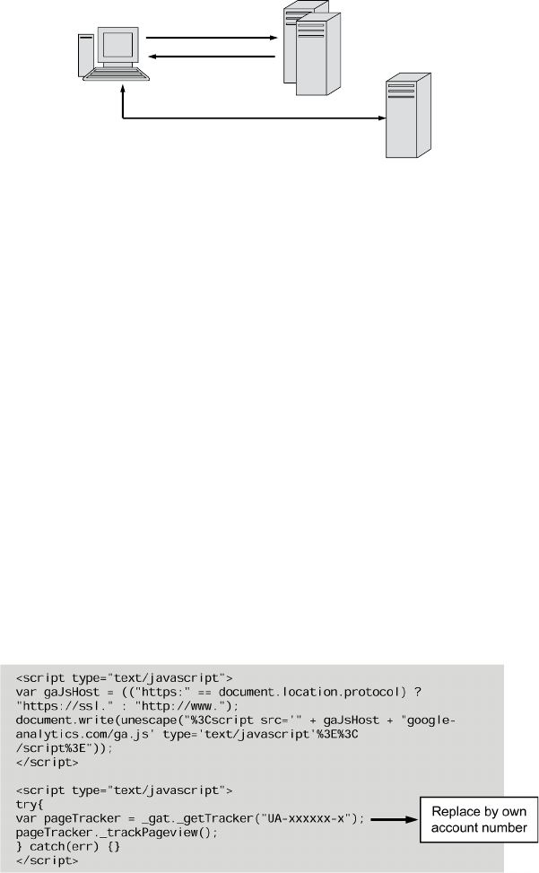
1

88

▸ANALYTICS IN A BIG DATA WORL

D

F

i

gure 8.13 Page Tagg

i

ng

User

Web server(s)

request page

HTML code with

JavaScript tag

Data collection

server(s)

When page is loaded, script is run

that collects and sends on data

F

ig

ure 8.14 Examp

l

e Goo

gl

e Ana

ly

t

i

cs Pa

g

e Ta

g

server. T

h

is is i

ll

ustrate

d

in Figure 8.13 . An examp

l

e Goog

l

e Ana

l

ytics

page tag

i

s g

i

ven

i

n F

i

gure 8.14 .

With

p

a

g

e ta

gg

in

g

, the anal

y

tics vendor often

p

rovides a hosted

service whereby the client is provided with a web interface to access

re

p

orts or run anal

y

ses. A

p

o

p

ular exam

p

le of this is Goo

g

le Anal

y

tics.

Tables 8.2 and 8.3 illustrate the advanta

g

es and disadvanta

g

es, res

p

ec

-

tively, of page tagging versus web log analysis.

Other techni

q

ues have also been su

gg

ested for web data collection

b

ut are less commonl

y

used, such as web beacons,

p

acket snif n

g

, web

server plug‐ins, and/or hybrid solutions.

Web KPIs

Once the data has been collected, it can be anal

y

zed and summarized

into various web key performance indicators (KPIs). Page views are

EXAMPLE APPLICATION

S

◂

189

the number of times a page (where

page

is an analyst‐de nable unit of

content) was viewed. It is an im

p

ortant buildin

g

block for other met-

rics, but it is not that meaningful on its own because we don’t know

whether the customer met his or her purpose after having visited a

p

a

g

e. Also, in toda

y

’s web environment, it mi

g

ht not be that strai

g

ht-

forward to de ne a web page unambiguously. The next step is iden

-

tif

y

in

g

and countin

g

visits or sessions. An exam

p

le of a visit could be:

index.h

t

ml

⇒

p

roducts.html

⇒

re

v

ie

w

s.html

⇒

exi

t

.

S

essioniza

t

ion

Ta

bl

e 8.2 Advantages o

f

Page Tagging versus Web Server Log Analysis

Page Tagging Web Server Log Analysis

■ Breaks through proxy servers and browser

cac

hi

n

g

■ Tracks client side events (JavaScript, Flash,

etc.

)

■ Easy client‐side collection o

f

outcome data

(custom tags on order con



rmation page)

■

F

ac

ili

tates rea

l

‐t

i

me

d

ata co

ll

ect

i

on an

d

processing

■ Often hosted service available: potential cost

a

d

vantages

■ Data capture separated from web design

/

programming: Java

S

cript code for data

co

ll

ect

i

on can

l

arge

l

y

b

e up

d

ate

d

b

y

i

n‐

h

ouse

ana

ly

sts or ana

ly

t

i

cs serv

i

ce

p

rov

id

er w

i

t

h

out

IT

department having to implement changes

■ More innovation e

ff

orts put in by web analytics

ven

d

ors

■ Proxy/caching inaccuracies

:

i

f a pa

g

e is cached, no record is

l

ogge

d

on your we

b

server

■

N

o c

li

ent‐s

id

e event trac

ki

ng

■ Most o

f

ten will choose to integrate

wi

t

h

anot

h

er

d

ata

b

ase to o

b

ta

i

n

addi

t

i

ona

l

d

ata

■ Log



les analyzed in batch (unless

s

erver p

l

ug‐

i

ns use

d)

■

I

n‐

h

ouse

d

ata co

ll

ect

i

on an

d

p

rocess

i

ng

■

L

arger re

li

ance on

IT

d

epartment to

i

mp

l

ement c

h

anges to capture more

d

ata

■ Extensive preprocessing required:

“stitch” together log



les

f

rom

d

i

ff

erent servers and



lter them

Table 8.3 Disadvanta

g

es of Pa

g

e Ta

gg

in

g

versus Web Server Lo

g

Anal

y

sis

Page tagging Web server log analysis

■ Not including correct tags, run‐time errors,

an

d

so on, mean

d

ata

i

s

l

ost; cannot go

bac

k

■ Firewalls and browser privacy/security

sett

i

ngs can

hi

n

d

er

d

ata co

ll

ect

i

on

■

C

annot track search engine bots

/

spiders

/

craw

l

ers

(b

ots

d

o not execute ta

g

s

)

■ Less straight

f

orward to capture technical

in

f

o such as errors, bandwidth, download

time, and so

f

orth

■ Loss of control if hosted

■ Hi

s

t

o

ri

ca

l

da

t

a

r

e

m

a

in

s

a

v

a

il

ab

l

e

fo

r

reprocess

i

ng

■ Server‐side data collected regardless of

client con



g

uration

■ Bots

/

spiders

/

crawlers show up in log

■

D

es

i

gne

d

to automat

i

ca

ll

y capture

tec

hni

ca

l in

fo

■

I

n‐

h

ouse so

l

ut

i

on

1

90

▸ANALYTI

CS

IN A BI

G

DATA W

O

RL

D

is a

p

rocedure for determinin

g

which

p

a

g

e views are

p

art of the same

visit. In de nin

g

sessions, one will make use of a combination of IP

address, user agent, cookies, and/or URI parameters. Once the sessions

have been de ned, one could start looking at the visitors. New visitors

are the unique visitors with activity including a  rst‐ever visit to the

site during a reporting period. Return visitors are the unique visitors

during a reporting period who had also visited the site prior to that

period. This can be interesting to determine loyalty and af nity of visi-

tors. A next obvious question is how long/deep the visits were. This

can be measured with the followin

g

metrics:

■ Page views per visit (or a

l

so visit

d

ept

h

, page

l

oa

d

activity);

f

or

examp

l

e, t

h

e visitor

b

rowse

d

t

h

roug

h

t

h

ree

d

i

ff

erent pages

■ Time on page

■ Time on site (also called visit duration or len

g

th); for exam

p

le,

the visit lasted  ve minutes in total

It is im

p

ortant to note that these metrics should be inter

p

reted in

the a

pp

ro

p

riate wa

y

. For exam

p

le, a su

pp

ort site mi

g

ht want to solve

the problem quickly and aim for a short time on site and/or call avoid

-

ance, whereas a content site mi

g

ht want to

g

et customers en

g

a

g

ed and

aim for a lon

g

er time on site.

Another very important metric is the bounce rate. It is de ned as

the ratio of visits where a visitor left instantl

y

after havin

g

seen the

 rst

p

a

g

e. It can be further re ned as follows:

■ Bounce rate of the site: ratio of single page view visits (or

b

ounces) over total visits

■ Bounce rate of a speci c page: single page view visits of that

p

a

g

e over number of visits where that

p

a

g

e was the entr

y

p

a

g

e

It is also important to consider the referring web page URI because

it also includes search ke

y

words and ke

y

p

hrases for search en

g

ine

tra

f

c sources. Ot

h

er interesting measures are:

■ Most viewe

d

p

a

g

es (to

p

content,

p

o

p

u

l

ar

p

a

g

es)

■

T

op entry pages

■ To

p

exit

p

a

g

es (

l

ea

k

a

g

e)

■ To

p

d

estinations (exit

l

in

k

s)

EXAMPLE APPLICATION

S

◂1

9

1

Finall

y

, a ver

y

im

p

ortant metric is the conversion rate. A conver-

sion is a visitor

p

erformin

g

an action that is s

p

eci ed as a useful out-

come considering the purpose of the site. The conversion rate is then

de ned as the percentage of visits or of unique visitors for which we

observed the action (e.g., order received, lead collected, newsletter

sign up). It is hereby important to combine the conversion rate also

with other outcome data, such as sales price, revenue, ROI, and so on.

For a checkout process, one could consider the following metrics:

■ Cart abandonment rate

=

1

−

number of people who start

c

h

ec

k

out/tota

l

A

dd

to Cart c

l

ic

k

s

■

Ch

ec

k

ou

t

a

b

an

d

onmen

t

ra

t

e

=

1

−

num

b

er o

f

peop

l

e w

h

o

comp

l

ete c

h

ec

k

out/num

b

er o

f

peop

l

e w

h

o start c

h

ec

k

out

It is important to note that small improvements in these metrics

can usuall

y

lead to substantial revenue

g

ains.

The avera

g

e visits or da

y

s to

p

urchase is a

p

an‐session metric

g

iv

-

ing insight into how long it takes people to buy from your website (or

submit a lead).

Turning Web KPIs into Actionable Insights

Ultimatel

y

, it is the

p

ur

p

ose to transform the metrics discussed earlier

into actionable insights. Each metric should be compared in time to

see whether there are an

y

si

g

ni cant chan

g

es. For exam

p

le,

p

o

p

ular

referrers are disa

pp

earin

g

, new referrers come in, to

p

 ve referrers

changed, top destinations changed, and so forth. Trend analysis is very

useful here. It is im

p

ortant to verif

y

whether there is an u

p

ward/down

-

ward trend, or any seasonalities or daily/weekly/monthly patterns to

observe. This is illustrated in Figure 8.15 for the conversion rate.

Dashboards will be used to effectivel

y

monitor and communicate

t

h

e we

b

KPIs. T

h

e

y

o

f

ten

p

rovi

d

e intuitive in

d

icators suc

h

as

g

au

g

es,

sto

pl

i

gh

ts, an

d

a

l

erts an

d

can

b

e

p

ersona

l

ize

d

.

Figure 8.15 Monitoring the Conversion Rate

KPI

Conversion rate

…

Last week

2.0%

This week

1.6%

Percent change

–20%

1

92

▸ANALYTI

CS

IN A BI

G

DATA W

O

RL

D

Benchmarkin

g

can also be ver

y

useful to com

p

are internal web

KPIs a

g

ainst industr

y

standards. Po

p

ular benchmark service

p

roviders

are Fireclick and Google Analytics’s benchmarking service.

Segmentation is also very important in order to turn web KPIs into

actionable insights. Any measure can be broken down into segments

of interest and aggregate (total, proportion, average) numbers can

b

e computed per segment. For example, one could segment bounce/

conversion rates by:

■ Top  ve referrers

■

S

earc

h

t

ra

f

c or no

t

■ Geograp

h

ica

l

region

■ Ac

q

uisition strate

gy

(i.e.,

d

irect mar

k

etin

g

, PPC, SEO/or

g

anic

search, email marketin

g

, newsletter, af liates)

This can be very ef ciently supported by means of OLAP facilities

to

p

erform interactive anal

y

sis of lar

g

e volumes of web KPI data from

multi

p

le dimensions.

Site search reports are also very useful because they provide a basic

understandin

g

of the usa

g

e of the internal search en

g

ine. This is a basic

form of market research because the users tell

y

ou exactl

y

what the

y

are looking for. It is interesting to consider the following:

■ Site search usa

g

e

■ How much is the search function used?

■ What ke

y

words are used most?

■ Site search

q

ualit

y

■ Calculate bounce rate for site search (% search exits)

Navigation Analysis

Navi

g

ation ana

ly

sis a

ll

ows us to un

d

erstan

d

h

ow users navi

g

ate

t

h

roug

h

t

h

e we

b

site.

Pat

h

ana

ly

sis

g

ives insi

gh

t into

f

re

q

uent navi

g

ation

p

atterns. It

ana

ly

zes,

f

rom a

g

iven

p

a

g

e, w

h

ic

h

ot

h

er

p

a

g

es a

g

rou

p

o

f

users visit

next in

x

percent of the times. Note, however, that this assumes that

x

t

h

e users

f

o

ll

ow a

l

inear

p

at

h

, w

h

ic

h

is not a

l

wa

y

s t

h

e case.

EXAMPLE APPLI

C

ATI

O

N

S

◂1

93

A funnel

p

lot focuses on a

p

redetermined se

q

uence (e.

g

., a check

out

p

rocess) and measures entr

y

/abandonment at each sta

g

e.

A page overlay/click density analysis shows clicks or other metrics

(e.g., bounce/conversion rates) overlaid directly on actual pages such

that one can traverse through the website as a group of users typically

navigates through it. Heat maps then have colors indicating the click

frequencies.

Again, it is important to combine all these plots with segmentation

to give actionable insights.

Search Engine Marketing Analytics

Web anal

y

tics can also be used to measure the ef cienc

y

of search

en

g

ine marketin

g

. Two t

yp

es of search en

g

ine marketin

g

are search

engine optimization (SEO) and pay per click (PPC). In SEO, the

p

ur

p

ose is to im

p

rove or

g

anic search results in a search en

g

ine (e.

g

.,

Goo

g

le, Yahoo!) without

p

a

y

in

g

for it. This can be accom

p

lished b

y

carefully designing the website. In PPC, one pays a search engine for

a link/ad to the website to a

pp

ear in the search results. The link/ad is

then listed de

p

endin

g

on the search en

g

ine al

g

orithm, the bid, and the

competitor’s bids. Popular examples are Google AdWords and Yahoo!

Search Marketin

g

. SEO efforts can be measured as follows:

■ Inclusion ra

t

io

=

number of

p

a

g

es indexed/number of

p

a

g

es on

your website. Note that sometimes you do not want pages to be

indexed, to avoid users arrivin

g

too dee

p

within a website.

■ Robot/crawl statistics report. See how frequently your website

is bein

g

visited b

y

search en

g

ine robots and how dee

p

the

y

g

et.

Note that this should be done based on seb log analysis, since

robots do not run JavaScri

p

t

p

a

g

e ta

g

s.

■ Trac

k

in

b

oun

d

l

in

k

s

by

usin

g

www.m

y

site.com in Goo

gl

e.

■ Goog

l

e we

b

master too

l

s t

h

at s

h

ow,

f

or t

h

e most popu

l

ar searc

h

k

e

y

wor

d

s or

ph

rases t

h

at

h

ave returne

d

p

a

g

es

f

rom

y

our site,

t

h

e num

b

er o

f

im

p

ressions or user

q

ueries

f

or w

h

ic

h

y

our

we

b

site appeare

d

in t

h

e searc

h

resu

l

ts an

d

t

h

e num

b

er o

f

users

w

h

o actua

lly

c

l

ic

k

e

d

an

d

came to

y

our we

b

site.

1

9

4▸ANALYTICS IN A BIG DATA WORL

D

■ Track rankin

g

s for

y

our to

p

ke

y

words/ke

y

p

hrases.

■ See whether ke

y

words link to

y

our most im

p

ortant

p

a

g

es.

PPC efforts can be tracked as follo

w

s:

■ Reports that differentiate bid terms versus search terms when

users enter site through PPC campaign (e.g., bid term is “laptop”

but search term is “cheap laptops”)

■ Analyze additional data obtained about ad impressions, clicks,

cost

■ Keywor

d

position report (

f

or examp

l

e, A

d

Wor

d

s position report)

■ Speci



es position your a

d

was in w

h

en c

l

ic

k

e

d

■ Can s

h

ow any metric (e.g., unique visitors, conversion rate,

bounce rate) per position

A/B and Multivariate Testing

The

p

ur

p

ose here is to set u

p

an ex

p

eriment whereb

y

different

p

a

g

es

or

p

a

g

e elements are shown to randoml

y

sam

p

led visitors. Exam

p

le

pages that could be considered are landing page ( rst page of a visit),

p

a

g

e in checkout

p

rocess, most

p

o

p

ular

p

a

g

e(s), or

p

a

g

es with hi

g

h

b

ounce ra

t

es.

In A/B testing, one tests two alternative versions of a web page

on a random sam

p

le of visitors and com

p

ares a

g

ainst a control

g

rou

p

(who

g

ets the ori

g

inal

p

a

g

e). This is illustrated in Fi

g

ure 8.16 .

F

ig

ure 8.16 A/B Test

i

n

g

Conversion

rate

50%

25%

Clicked

on link

to page

Original

Version

A

Version

B

Conversion

page

Random

sample

2.0%

1.9%

3.0%

Test significance!

EXAMPLE APPLI

C

ATI

O

N

S

◂1

95

Mu

l

tivariate testing aims at testing more t

h

an one e

l

ement on a

page at t

h

e same time (see Figure 8.17 ). Note t

h

at one can a

l

so test

price sensitivity or

d

i

ff

erent pro

d

uct

b

un

dl

es, w

h

ic

h

requires integra-

tion with back‐end data sources.

Parametric data anal

y

sis can then be used to understand the effect

of individual page elements and their interactions on a target measure

of interest (e.

g

., bounce or conversion rate). Also, techni

q

ues from

ex

p

erimental desi

g

n can be used to intelli

g

entl

y

decide on the various

page versions to be used.

SOCIAL MEDIA ANALYTICS

With the rising popularity of the web, people are closer connected to

each other than ever before. While it onl

y

has been a few

y

ears since

p

eo

p

le communicated with each other on the street, the demo

g

ra

p

hic

b

oundaries are fading away through the recently trending online

communication channels. The mar

g

inal effect of traditional word‐of‐

mouth advertising is replaced by the enormous spread of information

and in uence through the wires of the World Wide Web. Web users

have been

p

uttin

g

billions of data online on websites like Facebook

an

d

M

y

S

p

ace (socia

l

networ

k

sites), Twitter (micro

bl

o

g

site), YouTu

b

e

an

d

Dai

ly

Motion (mu

l

time

d

ia‐s

h

arin

g

), F

l

ic

k

r an

d

S

h

utterF

ly

(

ph

oto

s

h

aring), Lin

k

e

d

In an

d

ZoomIn

f

o (

b

usiness‐oriente

d

socia

l

networ

k

site), Wi

k

i

p

e

d

ia an

d

O

p

en Director

y

Pro

f

oun

d

(user‐

g

enerate

d

enc

y

-

c

l

o

p

e

d

ia), Re

dd

it (content votin

g

site), an

d

man

y

ot

h

ers.

Users are no

l

onger re

l

uctant to s

h

are persona

l

in

f

ormation a

b

out

t

h

emse

l

ves, t

h

eir

f

rien

d

s, t

h

eir co

ll

ea

g

ues, t

h

eir i

d

o

l

s, an

d

t

h

eir

p

o

l

itica

l

Figure 8.17 Multivariate Testing

X1: headline

X2: sales

copy

X4: button text

X3: image

(e.g., “hero

shot”)

1

96

▸ANALYTI

CS

IN A BI

G

DATA W

O

RL

D

p

references with an

y

bod

y

who is interested in them. Nowada

y

s, with

the boomin

g

rise of mobile a

pp

lications, web users are 24/7 connected

to all kinds of social media platforms, giving real‐time information

about their whereabouts. As such, a new challenging research domain

arises: social media analytics. While these data sources offer invaluable

knowledge and insights in customer behavior and enable marketers

to more carefully pro le, track, and target their customers, crawling

through such data sources is far from evident because social media

data can take immense magnitudes never seen before.

From a sales‐oriented

p

oint of view, social media offers advanta

g

es

f

or

b

ot

h

parties in t

h

e

b

usiness–consumer re

l

ations

h

ip. First, peop

l

e

s

h

are t

h

oug

h

ts an

d

opinions on we

bl

ogs, micro

bl

ogs, on

l

ine

f

orums,

an

d

review we

b

sites, creating a strong e

ff

ect o

f

d

igita

l

wor

d

‐o

f

‐mout

h

advertising. Web users can use others’ experience to gain informa-

tion and make

p

urchase decisions. As such, consumers are no lon-

g

er fallin

g

for trans

p

arent business tricks of a sales re

p

resentative, but

they are well‐informed and make conscious choices like true experts.

Public o

p

inions are volatile. Toda

y

’s zeroes are tomorrow’s heroes.

Com

p

anies are forced to kee

p

offerin

g

hi

g

h‐

q

ualit

y

p

roducts and ser-

vices, and only a small failure can have disastrous consequences for

the future. Kee

p

in

g

one ste

p

ahead of the com

p

etition is a tou

g

h and

intensive

p

rocess, es

p

eciall

y

when re

g

ional com

p

etitors are also able

to enter the game. On a large scale, the main competitors for an indus

-

tr

y

used to consists of the bi

g

p

la

y

ers of the market, while local busi-

nesses were too small and

p

la

y

in

g

to

g

ether with the bi

g

u

y

s re

q

uired

capital‐intensive investments. The Internet changed the competitive

environment drasticall

y

, and consumers can easil

y

com

p

are

p

roduct

and service characteristics of both local and global competitors.

Although the merciless power of the public cannot be underes

-

timated, com

p

anies should embrace and de

p

lo

y

social media data.

Peo

pl

e trust socia

l

me

d

ia

pl

at

f

orms wit

h

t

h

eir

p

ersona

l

d

ata an

d

inter-

ests, ma

k

in

g

it an inva

l

ua

bl

e

d

ata source

f

or a

ll

t

yp

es o

f

sta

k

e

h

o

ld

ers.

Mar

k

eters w

h

o are searc

h

ing

f

or t

h

e most promising an

d

pro



ta

bl

e

consumers to tar

g

et are now a

bl

e to ca

p

ture more concrete consumer

c

h

aracteristics, an

d

h

ence

d

eve

l

o

p

a

b

etter un

d

erstan

d

in

g

o

f

t

h

eir cus

-

tomers.

Z

eng

39

d

escri

b

e

d

socia

l

me

d

ia as an essentia

l

component o

f

t

h

e next‐

g

eneration

b

usiness inte

ll

i

g

ence

pl

at

f

orm. Po

l

iticians an

d

EXAMPLE APPLI

C

ATI

O

N

S

◂1

9

7

g

overnmental institutions can

g

et an im

p

ression of the

p

ublic o

p

inion

throu

g

h the anal

y

sis of social media. Durin

g

election cam

p

ai

g

ns, stud-

ies claim that political candidates with a higher social media engage-

ment got relatively more votes within most political parties.

4

0

Social

media analytics is a select tool to acquire and propagate one’s reputa-

tion. Also, nonpro t organizations such as those in the health sector

b

ene t from the dissemination power of social media, anticipating, for

example, disease outbreaks, identifying disease carriers, and setting up

a right vaccination policy.

4

1

Social media anal

y

tics is a multifaceted domain. Data available on

socia

l

me

d

ia p

l

at

f

orms contain

d

iverse in

f

ormation ga

l

ore, an

d

f

ocusing

on t

h

e re

l

evant pieces o

f

d

ata is

f

ar

f

rom o

b

vious an

d

o

f

ten un

f

easi

bl

e.

W

h

i

l

e certain socia

l

me

d

ia p

l

at

f

orms a

ll

ow one to craw

l

pu

bl

ic

l

y acces

-

sible data through their API (application programming interface), most

social networkin

g

sites are

p

rotective toward data sharin

g

and offer

b

uilt‐in advertisement tools to set u

p

ersonalized marketin

g

cam

-

paigns. This is brie y discussed in the  rst subsection. The next subsec

-

tions introduce some basic conce

p

ts of sentiment and network anal

y

sis.

Social Networking Sites: B2B Advertisement Tools

A new business‐to‐business (B2B) billion‐dollar industr

y

is launched

b

y capturing users’ information in social network websites, enabling

p

ersonalized advertisin

g

and offerin

g

services for bud

g

et and im

p

act

mana

g

ement.

Facebook Advertising

42

is a far‐evolved marketing tool with an

extensive variet

y

of facilities and services (see Fi

g

ure 8.18 ). De

p

endin

g

on the goal of the advertising campaign, Facebook Advertising calcu-

lates the impact and spread of the digital word‐of‐mouth advertising.

Facebook Advertisin

g

not onl

y

su

pp

orts sim

p

le marketin

g

cam

p

ai

g

ns

suc

h

as increasin

g

t

h

e num

b

er o

f

c

l

ic

k

s to a we

b

site (c

l

ic

k

rate) or

p

a

g

e

l

i

k

es (

l

i

k

e rate) an

d

strivin

g

f

or more reactions on messa

g

es

p

oste

d

by

t

h

e user (comment an

d

s

h

are rate),

b

ut a

l

so more a

d

vance

d

options

l

i

k

e mo

b

i

l

e a

pp

en

g

a

g

ement (

d

own

l

oa

d

an

d

usa

g

e rate) an

d

we

b

site

conversion (conversion rate) are

p

rovi

d

e

d

. T

h

e conversion rate o

f

a

mar

k

eting campaign re

f

ers to t

h

e proportion o

f

peop

l

e w

h

o un

d

erta

k

e

a

p

re

d

e



ne

d

action. T

h

is action can

b

e an enro

ll

ment

f

or a news

l

etter,

198

▸ANALYTI

CS

IN A BI

G

DATA W

O

RL

D

l

eavin

g

an emai

l

a

dd

ress,

b

u

y

in

g

a

p

ro

d

uct,

d

own

l

oa

d

in

g

a tria

l

ver

-

sion, an

d

so on, an

d

is s

p

eci



c

f

or eac

h

mar

k

etin

g

cam

p

ai

g

n. Face

b

oo

k

measures conversion rates

b

y inc

l

u

d

ing a conversion‐trac

k

ing pixe

l

on t

h

e we

b

p

a

g

e w

h

ere conversion wi

ll

ta

k

e

pl

ace. A

p

ixe

l

is a sma

ll

p

iece o

f

co

d

e communicatin

g

wit

h

t

h

e Face

b

oo

k

servers an

d

trac

k

in

g

w

h

ic

h

users saw a we

b

page an

d

per

f

orme

d

a certain action. As suc

h

,

Face

b

oo

k

A

d

vertisin

g

matc

h

es t

h

e users wit

h

t

h

eir Face

b

oo

k

p

ro



l

e

an

d

p

rovi

d

es a

d

etai

l

e

d

overview o

f

customer c

h

aracteristics an

d

t

h

e

campa

i

gn

i

mpact.

Face

b

oo

k

A

d

vertisin

g

a

ll

ows users to create

p

ersona

l

ize

d

a

d

s an

d

tar

g

et a s

p

eci



c

p

u

bl

ic

by

se

l

ectin

g

t

h

e a

pp

ro

p

riate c

h

aracteristics in

terms o

f

d

emograp

h

ics, interests,

b

e

h

avior, an

d

re

l

ations

h

ips. T

h

is is

s

h

own in Fi

g

ure 8.19 . A

d

vertisements are

d

is

pl

a

y

e

d

accor

d

in

g

to a

b

i

d-

d

ing system, w

h

ere t

h

e most eye‐catc

h

ing spots o

f

a page are t

h

e most

expensive ones. W

h

en a user opens

h

is or

h

er Face

b

oo

k

page, a virtua

l

auction

d

eci

d

es w

h

ic

h

a

d

wi

ll

b

e

pl

ace

d

w

h

ere on t

h

e

p

a

g

e. De

p

en

d

in

g

on t

h

e ma

g

nitu

d

e an

d

t

h

e

p

o

p

u

l

arit

y

o

f

(a

p

art o

f

) t

h

e c

h

osen au

d

ience,

Face

b

oo

k

su

gg

ests a

b

i

dd

in

g

amount. A sa

f

er so

l

ution is to



x a maxi

-

mum

b

i

d

amount in a

d

vance. T

h

e

h

i

gh

er t

h

e amount o

f

t

h

e

b

i

d

, t

h

e

h

i

gh

er t

h

e

p

ro

b

a

b

i

l

it

y

o

f

g

ettin

g

a

g

oo

d

a

d

pl

acement. Notice,

h

owever,

t

h

at t

h

e winnin

g

b

i

d

oes not necessari

ly

h

ave to

p

a

y

t

h

e maximum

b

i

d

amount. On

ly

w

h

en man

y

a

d

s are com

p

etin

g

d

o a

d

p

rices rise

d

rasti

-

ca

lly

. As suc

h

, t

h

e

p

rice o

f

an a

d

i

ff

ers

d

e

p

en

d

in

g

on t

h

e tar

g

et user.

Figure 8.18 Determining Advertising Objective in Facebook Advertising

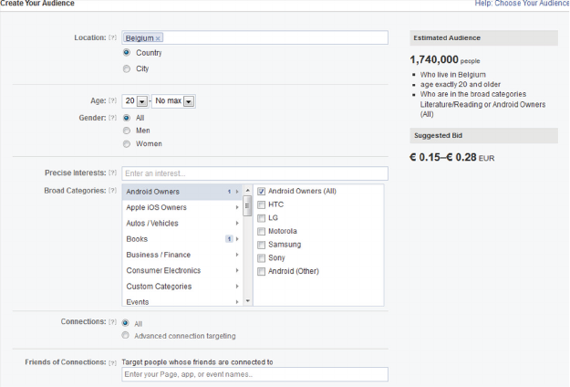
EXAMPLE APPLI

C

ATI

O

N

S

◂

199

The business‐oriented social networkin

g

site LinkedIn offers simi

-

lar services as Facebook. The LinkedIn Campaign Manager

43 allows

the marketer to create

p

ersonalized ads and to select the ri

g

ht custom

-

ers. Com

p

ared to Facebook, LinkedIn Cam

p

ai

g

n Mana

g

ers offers ser-

vices to target individuals based on the characteristics of the companies

the

y

are workin

g

at and the

j

ob function the

y

have (see Fi

g

ure 8.20 ).

While Facebook Advertisin

g

is

p

articularl

y

suitable for Business‐to

‐

Consumer (B2C) marketing, LinkedIn Campaign Manager is aimed at

advertisements for Business‐to Business (B2B) and Human Resource

Mana

g

ement (HRM)

p

ur

p

oses.

As most tools are self-explanatory, the reader must be careful when

d

ep

l

oying t

h

ese a

d

vertisement too

l

s since t

h

ey may

b

e so user

f

rien

dl

y

that the user no lon

g

er realizes what he/she is actuall

y

doin

g

with them.

Ma

k

e sure t

h

at

y

ou s

p

eci

fy

a maximum

b

u

dg

et an

d

c

l

ose

ly

monitor a

ll

activities an

d

a

d

vertisement costs,

d

e



nite

l

y at t

h

e start o

f

a mar

k

et

-

in

g

cam

p

ai

g

n. A sma

ll

error can resu

l

t in a cost o

f

t

h

ousan

d

s or even

mi

ll

ions o

f

d

o

ll

ars in on

ly

a

f

ew secon

d

s. Goo

d

k

now

l

e

dg

e o

f

a

ll

t

h

e

f

aci

l

ities is essentia

l

to pursue a

h

ea

l

t

h

y on

l

ine mar

k

eting campaign.

F

i

gure 8.19 Choosing the Audience

f

or Facebook Advertising Campaign

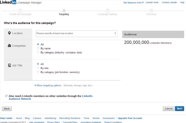
2

00

▸ANALYTI

CS

IN A BI

G

DATA W

O

RL

D

Sentiment Analysis

Certain social media platforms allow external servers to capture data

from a

p

ortion of the users. This

g

atewa

y

for external a

pp

lications is

called the API. An API has multiple functions. It offers an embedded

interface to other

p

ro

g

rams. For exam

p

le, the Twitter API

44

can be

used on other sites to identif

y

visitors b

y

their Twitter account. Inte

-

grated tweet  elds and buttons on web pages allow users to directly

p

ost a reaction without leavin

g

the web

p

a

g

e. Like buttons are directl

y

connected to

y

our Facebook

p

a

g

e throu

g

h the Facebook API

45

a

n

d

immediately share the like with all of your friends. However, APIs

often

p

ermit external servers to connect and mine the

p

ublicl

y

avail-

a

bl

e

d

ata. Un

d

e

l

imite

d

user‐

g

enerate

d

content

l

i

k

e text,

ph

otos, music,

vi

d

eos, an

d

s

l

i

d

es

h

ows is not eas

y

to inter

p

ret

by

com

p

uter‐contro

ll

e

d

a

lg

orit

h

ms.

Sentiment ana

ly

sis an

d

o

p

inion minin

g

f

ocus on t

h

e ana

ly

sis o

f

text an

d

eterminin

g

t

h

e

gl

o

b

a

l

sentiment o

f

t

h

e text. Be

f

ore t

h

e

actua

l

sentiment o

f

a text

f

ra

g

ment can

b

e ana

ly

ze

d

, text s

h

ou

ld

b

e

Fi

g

ure 8.20 LinkedIn Campai

g

n Mana

g

er

EXAMPLE APPLICATION

S

◂2

0

1

preprocessed in terms of tag removal, tokenization, stopword removal,

and stemming. Afterward, each word is associated with a sentiment.

The dominant

p

olarit

y

of the text de nes the  nal sentiment.

Because text contains many irrelevant words and symbols, unnec-

essar

y

ta

g

s are remove

d

f

rom t

h

e text, suc

h

as URLs an

d

p

unctua

-

tion mar

k

s. Fi

g

ure 8.21 re

p

resents an exam

pl

e o

f

a tweet. T

h

e

l

in

k

in

t

h

e tweet

d

oes not contain an

y

use

f

u

l

in

f

ormation, t

h

us it s

h

ou

ld

b

e

remove

d

f

or sentiment ana

ly

sis. T

h

e to

k

enization ste

p

converts t

h

e

text into a stream o

f

wor

d

s. For t

h

e tweet s

h

own in Figure 8.21 , t

h

is

wi

ll

resu

l

t in:

Data Science / roc

k

s / exce

ll

ent /

b

oo

k

/ written /

b

y / my / goo

d

/

f

rien

d

s / Foster Provost / an

d

/ Tom Fawcett / a / must / rea

d

In a next step, stopwor

d

s are

d

etecte

d

an

d

remove

d

f

rom t

h

e

sentence.

A

stopword

is a wor

d

in a sentence t

h

at

h

as no in

f

ormative

d

meaning,

l

i

k

e artic

l

es, conjunctions, prepositions, an

d

so

f

ort

h

. Using

a pre

d

e



ne

d

mac

h

ine‐rea

d

a

bl

e

l

ist, stopwor

d

s can easi

l

y

b

e i

d

enti



e

d

an

d

remove

d

. A

l

t

h

oug

h

suc

h

a stop

l

ist can

b

e constructe

d

manua

ll

y,

wor

d

s wit

h

an IDF (inverse

d

ocument

f

requency) va

l

ue c

l

ose to zero

are automatica

ll

y a

dd

e

d

to t

h

e

l

ist. T

h

ese IDF va

l

ues are compute

d

b

ase

d

on t

h

e tota

l

set o

f

text

f

ragments t

h

at s

h

ou

ld

b

e ana

l

yze

d

. T

h

e

more a wor

d

appears in t

h

e tota

l

text, t

h

e

l

ower its va

l

ue. T

h

is gives:

Data Science / roc

k

s / exce

ll

ent /

b

oo

k

/ written / goo

d

/

f

rien

d

s /

Foster Provost / Tom Fawcett / rea

d

Many variants o

f

a wor

d

exist. Stemming converts eac

h

wor

d

b

ac

k

to its stem or root: A

ll

conjugations are trans

f

orme

d

to t

h

e correspon

d-

in

g

verb, all nouns are converted to their sin

g

ular form, and adverbs

and ad

j

ectives are brou

g

ht back to their base form. A

pp

lied to the

p

re-

vious exam

p

le, this results in:

Data Science / rock / excellent / book /

w

rite / friend / Foster Pro

v

ost /

Tom Fa

w

cett / read

F

i

gure 8.21 Sentiment Analysis for Tweet

202

▸ANALYTICS IN A BIG DATA WORL

D

Each word has a

p

ositive

(

+

), ne

g

ative (−) or neutral (o)

p

olarit

y

.

A

g

ain, al

g

orithms use

p

rede ned dictionaries to assi

g

n a sentiment to

a word. The example contains many positive and neutral words, as

shown below

:

Data Scienc

e

/

r

oc

k

/

e

xcellen

t

/

b

oo

k

/ writ

e

/

f

rien

d

/

Foster Provos

t

/ Tom Fawcett

/

r

ea

d

o

+

o

+

o

The overall sentiment of the above tweet is thus positive. Although

this procedure could easily capture the sentiment of a text fragment,

more advanced analysis techniques merge different opinions from

mu

l

tip

l

e users toget

h

er an

d

are a

bl

e to summarize g

l

o

b

a

l

pro

d

uct or

service a

f

nity, as we

ll

as assign a genera

l

f

ee

l

ing towar

d

neutra

l

‐

po

l

arize

d

wor

d

s.

Network Analytics

Instea

d

o

f

ana

l

yzing user‐generate

d

content, networ

k

ana

l

ytics

f

ocuses

on t

h

e re

l

ations

h

ips

b

etween users on socia

l

me

d

ia p

l

at

f

orms. Many

socia

l

me

d

ia

pl

at

f

orms a

ll

ow t

h

e user to i

d

enti

fy

t

h

eir ac

q

uaintances.

Five types o

f

re

l

ations

h

ips can

b

e

d

istinguis

h

e

d

:

4

6

1.

Friends

.

T

h

ere is a mutua

l

p

ositive re

l

ations

h

i

p

b

etween two

users. Bot

h

users

k

now eac

h

ot

h

er, an

d

ac

k

now

l

e

dg

e t

h

e asso

-

ciation

b

etween t

h

em.

2

.

Admirers

.

A user receives reco

g

nition

f

rom anot

h

er user,

b

ut

t

h

e re

l

ations

h

ip is not reciproca

l

.

3.

Idols

.

A user ac

k

now

l

e

dg

es a certain

p

ositive connecte

d

ness

w

it

h

anot

h

er user,

b

ut t

h

e re

l

ations

h

ip is not reciproca

l

.

4

.

N

eutrals

.

T

w

o users

d

o not

k

no

w

eac

h

ot

h

er an

d

o not com-

municate wit

h

eac

h

ot

h

er.

5

. Enem

i

es. T

h

ere is a ne

g

ative re

l

ations

h

i

p

b

etween two users.

Bot

h

users

k

now eac

h

ot

h

er,

b

ut t

h

ere is a ne

g

ative s

ph

ere.

A

l

t

h

ou

gh

in most socia

l

networ

k

in

g

sites on

ly

f

rien

d

s

h

i

p

re

l

ation

-

s

h

i

p

s are ex

pl

oite

d

, Twitter incor

p

orates a

d

mirers (

f

o

ll

owers) an

d

i

d

o

l

s

(

f

o

ll

owees)

by

ena

bl

in

g

users to

d

e



ne t

h

e

p

eo

pl

e t

h

e

y

are intereste

d

in. A

d

mirers receive t

h

e tweets o

f

t

h

eir i

d

o

l

s. Enem

y

re

l

ations

h

i

p

s are

not common in socia

l

networ

k

in

g

sites, exce

p

t

f

or Enem

y

Gra

ph

.

4

7

T

h

e

EXAMPLE APPLI

C

ATI

O

N

S

◂

203

p

ower of social network sites de

p

ends on the true re

p

resentation of

rea

l

‐wor

ld

re

l

ations

h

i

p

s

b

etween

p

eo

pl

e. Lin

k

p

re

d

iction is one su

b

-

domain of network analytics where one tries to predict which neutral

links are actually friendship, admirer, or idol relationships. Tie strength

prediction is used to determine the intensity of a relationship between

t

wo users.

Homophily , a concept from sociology, states that people tend to

connect to other similar people and they are unlikely to connect with

dissimilar people. Similarity can be expressed in terms of the same

demo

g

ra

p

hics, behavior, interests, brand af nit

y

, and so on. As such,

in networ

k

s c

h

aracterize

d

b

y

h

omop

h

i

l

y, peop

l

e connecte

d

to eac

h

ot

h

er are more

l

i

k

e

l

y to

l

i

k

e t

h

e same pro

d

uct or service. Gat

h

ering t

h

e

true

f

rien

d

s

h

ip, a

d

mirer, an

d

i

d

o

l

re

l

ations

h

ips

b

etween peop

l

e ena

bl

es

marketers to make more informed decisions for customer acquisition

and retention. An individual surrounded b

y

man

y

lo

y

al customers

has a hi

g

h

p

robabilit

y

of bein

g

a future customer. Customer ac

q

ui-

sition projects should identify those high‐potential customers based

on the users’ nei

g

hborhoods and focus their marketin

g

resources on

them. This is shown in Fi

g

ure 8.22 (a). However, a customer whose

friends have churned to the competition is likely to be a churner as

well, and should be offered additional incentives to

p

revent him or her

Fi

g

ure 8.22 Social Media Anal

y

tics for Customer Acquisition (a) and Retention (b). Gre

y

nodes are in

f

avor o

f

a s

p

eci



c brand, black nodes are brand‐averse.

(a) (b)

2

0

4▸ANALYTI

CS

IN A BI

G

DATA W

O

RL

D

from leavin

g

. Similar to customer ac

q

uisition, these customers can be

detected usin

g

relational information available on social media

p

lat-

forms. This is shown in Figure 8.22 (b). In uence propagates through

the network. The aforementioned analysis techniques focus on the

properties of the direct neighborhood (one hop). Although direct asso-

ciates contain important information, more advanced algorithms focus

on in uence propagation of the whole network, revealing interesting

patterns impossible to detect with the bare eye.

Although social media analytics nowadays is indispensable in

com

p

anies’ market research

p

ro

j

ects, it is hi

g

hl

y

advised to verif

y

the

regiona

l

, nationa

l

, an

d

internationa

l

privacy regu

l

ations

b

e

f

ore start-

ing (see privacy section). In t

h

e past, some companies

d

i

d

not comp

l

y

wit

h

t

h

e prevai

l

ing privacy

l

egis

l

ation an

d

ris

k

e

d

very steep



nes.

BUSINESS PROCESS ANALYTICS

In recent years, the concept of business process management (BPM)

has been

g

ainin

g

traction in modern com

p

anies.

4

8

Broadl

y

p

ut, the

mana

g

ement  eld aims to

p

rovide an encom

p

assin

g

a

pp

roach in order

to align an organization’s business processes with the concerns of every

involved stakeholder. A business

p

rocess is then a collection of struc-

tured

,

interrelated activities or tasks that are to be executed to reach a

particular goal (produce a product or deliver a service). Involved par-

ties in business

p

rocesses include, amon

g

others, mana

g

ers (“

p

rocess

owners”), who ex

p

ect work to be dele

g

ated swiftl

y

and in an o

p

timal

manner; employees, who desire clear and understandable guidelines

and tasks that are in line with their skillset

;

and clients who

,

natu-

rally, expect ef ciency and quality results from their suppliers. Fig

-

ure 8.23 gives an example business process model for an insurance

claim intake

p

rocess shown in the business

p

rocess modelin

g

lan

g

ua

g

e

(

BPMN) stan

d

ar

d

. Numerous visua

l

ization

f

orms exist to

d

esi

g

n an

d

mo

d

e

l

b

usiness

p

rocesses,

f

rom eas

y



owc

h

art‐

l

i

k

e

d

ia

g

rams to com-

p

l

ex

f

orma

l

mo

d

e

l

s.

Put t

h

is wa

y

, BPM is o

f

tentimes

d

escri

b

e

d

as a “

p

rocess o

p

timiza

-

tion” met

h

o

d

o

l

o

gy

an

d

is t

h

ere

f

ore mentione

d

to

g

et

h

er wit

h

re

l

ate

d

qua

l

ity contro

l

terms suc

h

as tota

l

qua

l

ity management (TQM), six

si

g

ma e

ff

orts, or continuous

p

rocess im

p

rovement met

h

o

d

o

l

o

g

ies.

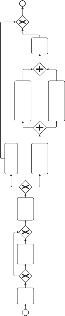
Figure 8.23 Example Business Process Model

Claim

intake

Review

policy

Evaluate

claim

Propose

settlement

Close

claim

Calculate new

premium

Approve damage

payment

Reject claim

205

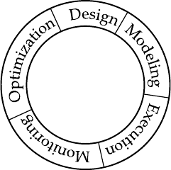
206

▸ANALYTI

CS

IN A BI

G

DATA W

O

RL

D

However, t

h

is

d

escription is somew

h

at

l

ac

k

ing. In

d

ee

d

, one signi



-

cant focal

p

oint of BPM is the actual im

p

rovement and o

p

timization of

p

rocesses, but the conce

p

t also encom

p

asses best

p

ractices toward the

design and modeling of business processes, monitoring (consider for

instance com

p

liance re

q

uirements), and

g

ainin

g

insi

g

hts b

y

unleash-

in

g

anal

y

tical tools on recorded business activities. All these activities

are grouped within the “business process lifecycle,” starting with the

desi

g

n and anal

y

sis of a business

p

rocess (modelin

g

and validation), its

con

g

uration (im

p

lementation and testin

g

), its enactment (execution

and monitoring), and  nally, the evaluation, which in turn leads again

to the desi

g

n of new

p

rocesses (see Fi

g

ure 8.24 ).

Process Intelligence

It is mainly in the last part of the BPM life cycle (i.e., evaluation)

where the concepts of process analytics and process intelligence  t in.

Just as with business intelli

g

ence (BI) in

g

eneral,

p

rocess intelli

g

ence

is a very broad term describing a plethora of tools and techniques, and

can include an

y

thin

g

that

p

rovides information to su

pp

ort decision

makin

g

.

As suc

h

,

j

ust as wit

h

tra

d

itiona

l

(“



at”)

d

ata‐oriente

d

too

l

s, man

y

ven

d

ors an

d

consu

l

tants

h

ave

d

e



ne

d

p

rocess inte

ll

i

g

ence to

b

e s

y

n-

onymous wit

h

process‐aware query an

d

reporting too

l

s, o

f

tentimes

com

b

ine

d

wit

h

sim

pl

e visua

l

izations in or

d

er to

p

resent a

gg

re

g

ate

d

overviews o

f

a

b

usiness’s actions. In man

y

cases, a

p

articu

l

ar s

y

stem

F

i

gure 8.24 Business Process Management Lifecycle

EXAMPLE APPLI

C

ATI

O

N

S

◂

20

7

will

p

resent itself as bein

g

a hel

p

ful tool toward

p

rocess monitorin

g

and im

p

rovement b

y

p

rovidin

g

KPI dashboards and scorecards, thus

presenting a “health report” for a particular business process. Many

process‐aware information support systems also provide online ana-

lytical processing (OLAP) tools to view multidimensional data from

different angles and to drill down into detailed information. Another

term that has become commonplace in a process intelligence context

is business activity monitoring (BAM), which refers to real‐time monitor

-

ing of business processes and immediate reaction if a process displays a

p

articular

p

attern.

Corporate performance management

(CPM) is another

t

popu

l

ar term

f

or measuring t

h

e per

f

ormance o

f

a process or t

h

e orga

-

nization as a w

h

o

l

e.

A

l

t

h

oug

h

a

ll

t

h

e too

l

s previous

l

y

d

escri

b

e

d

, toget

h

er wit

h

a

ll

t

h

e

three‐letter acronym jargon, are a  ne way to measure and query many

as

p

ects of a business’s activities, most tools unfortunatel

y

suffer from

the

p

roblem that the

y

are unable to

p

rovide real insi

g

hts or uncover

meaningful, newly emerging patterns. Just as for non‐process‐related

data sets (althou

g

h re

p

ortin

g

,

q

uer

y

in

g

, a

gg

re

g

atin

g

and drillin

g

, and

ins

p

ectin

g

dashboard indicators are

p

erfectl

y

reasonable for o

p

era-

tional day‐to‐day management), these tools all have little to do with

real

p

rocess anal

y

tics. The main issues lies in the fact that such tools

inherentl

y

assume that users and anal

y

sts alread

y

know what to look

for. That is, writing queries to derive indicators assumes that one

alread

y

knows the indicators of interest. As such,

p

atterns that can

onl

y

be detected b

y

a

pp

l

y

in

g

real anal

y

tical a

pp

roaches remain hid-

den. Moreover, whenever a report or indicator does signal a problem,

users often face the issue of then havin

g

to

g

o on a scaven

g

er hunt

in order to pinpoint the real root cause behind the problem, working

all the way down starting from a high‐level aggregation toward the

source data. Fi

g

ure 8.25

p

rovides an exam

p

le of a

p

rocess intelli

g

ence

d

as

hb

oar

d

.

C

l

ear

ly

, a stron

g

nee

d

is emer

g

in

g

to

g

o

f

urt

h

er t

h

an strai

gh

t

f

orwar

d

reporting in to

d

ay’s

b

usiness processes an

d

to start a t

h

oroug

h

ana

l

ysis

d

irect

ly

f

rom t

h

e ava

l

anc

h

e o

f

d

ata t

h

at is

b

ein

g

l

o

gg

e

d

, recor

d

e

d

, an

d

store

d

an

d

is rea

d

i

ly

avai

l

a

bl

e in mo

d

ern in

f

ormation su

pp

ort s

y

stems,

l

ea

d

ing us to t

h

e areas o

f

process mining an

d

ana

l

ytics.

208

▸ANALYTICS IN A BIG DATA WORL

D

Process Mining and Analytics

In the

p

ast decade, a new research  eld has emer

g

ed, denoted as “

p

rocess

minin

g

,” which

p

ositions itself between BPM and traditional data min

-

ing. The discipline aims to provide a comprehensive set of tools to pro

-

vide

p

rocess‐centered insi

g

hts and to drive

p

rocess im

p

rovement efforts.

Contrar

y

to business intelli

g

ence a

pp

roaches, the  eld em

p

hasizes a

b

ottom‐up approach, starting from real‐life data to drive analytical tasks.

As

p

reviousl

y

stated,

p

rocess minin

g

builds on existin

g

a

pp

roaches,

such as data minin

g

and model‐driven a

pp

roaches, but is more than

j

ust the sum of these components. For example, as seen previously,

traditional existin

g

data minin

g

techni

q

ues are too data‐centric to

p

ro-

vide a solid understandin

g

of the end‐to‐end

p

rocesses in an or

g

aniza

-

tion, w

h

ereas

b

usiness inte

ll

i

g

ence too

l

s

f

ocus on sim

pl

e

d

as

hb

oar

d

s

an

d

reporting. It is exact

l

y t

h

is gap t

h

at is narrowe

d

b

y process mining

too

l

s, t

h

us ena

bl

in

g

true

b

usiness

p

rocess ana

ly

tics.

The most common task in the area of process mining is called

pro-

cess

d

iscovery

,

in w

h

ic

h

ana

l

ysts aim to

d

erive an as‐is process mo

d

e

l

startin

g

f

rom t

h

e

d

ata as it is recor

d

e

d

in

p

rocess‐aware in

f

ormation

su

pp

ort s

y

stems instea

d

o

f

startin

g

f

rom a to‐

b

e

d

escri

p

tive mo

d

e

l

, an

d

Figure 8.25 Example Process Intelligence Dashboard

S

ource: htt

p

://dashboardmd.net.

EXAMPLE APPLI

C

ATI

O

N

S

◂

209

tr

y

in

g

to ali

g

n the actual data to this model. A si

g

ni cant advanta

g

e of

p

rocess discover

y

is the fact that onl

y

a limited amount of initial data

is required to perform a  rst exploratory analysis.

Consider, for example, the insurance claim handling process as it

was previously depicted. To perform a process discovery task, we start

our analysis from a so‐called “event log”: a data table listing the activi

-

ties that have been executed during a certain time period, together

with the case (the process instance) to which they belong. A simple

event fragment log for the insurance claim handling process might look

as de

p

icted in Table 8.4 . Activities are sorted based on the startin

g

time.

Note t

h

at mu

l

tip

l

e process instances can

b

e active at t

h

e same moment

in time. Note a

l

so t

h

at t

h

e execution o

f

some activities can over

l

ap.

Base

d

on rea

l

‐

l

i

f

e

d

ata as it was store

d

in

l

og repositories, it is pos-

sible to derive an as‐is process model that provides an overview of

how the

p

rocess was actuall

y

executed. To do this, activities are sorted

b

ased on their startin

g

time. Next, an al

g

orithm iterates over all

p

ro-

cess cases and creates “ ows of work” between the activities. Activities

that follow each other distinctl

y

(no overla

pp

in

g

start and end times)

Table 8.4 Example Insurance Claim Handlin

g

Event Lo

g

Case

Identifier Start Time Completion Time Activity

Z

100

1

8

‐

13

‐

2013

09

:

43

:

33

8

‐

13

‐

2013

10

:

11

:

21

C

laim intak

e

Z1

004

8

‐1

3

‐2

0

1

3

11:

55

:1

2

8

‐1

3

‐2

0

1

3

1

5

:4

3

:4

1

C

l

a

im int

a

k

e

Z1

001

8

‐1

3

‐2

0

1

3

14:

3

1:

05

8

‐1

6

‐2

0

1

3

1

0

:

55

:1

3

Ev

a

l

ua

t

e

c

l

a

i

m

Z

100

4

8‐13‐2013 16:11:1

4

8‐16‐2013 10:51:2

4

R

ev

i

ew

p

o

li

c

y

Z1

001

8

‐17‐2

0

1

3

11:

08

:

51

8

‐17‐2

0

1

3

17:11:

53

Propose settlemen

t

Z1

001

8

‐

18

‐

2013

14

:

23

:

31

8

‐

21

‐

2013

09

:

13

:

41

Calculate new premiu

m

Z

100

4

8

‐

19

‐

2013

09

:

0

5:

01

8

‐

21

‐

2013

14

:

42

:

11

P

ropose sett

l

emen

t

Z

1

001

8

‐1

9

‐2

0

1

3

12:1

3

:2

5

8

‐22‐2

0

1

3

11:1

8

:2

6

A

pprove

d

amage paymen

t

Z

1

004

8

‐21‐2

0

1

3

11:1

5

:4

3

8

‐2

5

‐2

0

1

3

1

3

:

30

:

08

A

pprove

d

ama

g

e paymen

t

Z1

001

8

‐24‐2

0

1

3

1

0

:

06

:

08

8

‐24‐2

0

1

3

12:12:1

8

C

l

ose

c

l

a

i

m

Z

100

4

8‐24‐2013 12:15:1

2

8‐25‐2013 10:36:4

2

Calculate new

p

remiu

m

Z1

0

1

8

‐2

5

‐2

0

1

3

17:12:

02

8

‐2

6

‐2

0

1

3

14:4

3

:

32

C

l

a

im int

a

k

e

Z

100

4

8‐28‐2013 12:43:4

1

8‐28‐2013 13:13:1

1

C

lose clai

m

Z

101

1

8‐26‐2013 15:11:0

5

8‐26‐2013 15:26:5

5

R

e

j

ect c

l

a

im

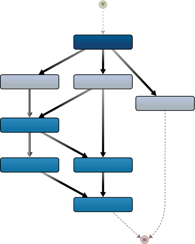
21

0

▸ANALYTI

CS

IN A BI

G

DATA W

O

RL

D

wi

ll

b

e

p

ut in a se

q

uence. W

h

en t

h

e same activit

y

is

f

o

ll

owe

d

by

d

i

f-

ferent activities over various

p

rocess instances, a s

p

lit is created. When

two or more activities’ executions overlap in time, they are executed

in parallel and are thus both  owing from a common predecessor.

After executing the process discovery algorithm, a process map

such as the one depicted in Figure 8.26 can be obtained (using the

Fi

g

ure 8.26 Example of a Discovered Process Map Annotated with Frequenc

y

Counts

Claim intake

3

1

2

1

3

1

111

1

2

Review Policy

Evaluate claim

Propose settlement

Close claim

Calculate new premium Approve damage payment

Reject claim

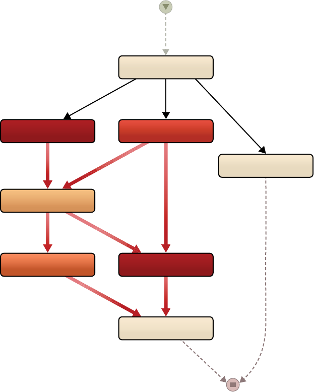
EXAMPLE APPLICATION

S

◂211

Disco software

p

acka

g

e). The

p

rocess ma

p

can be annotated with vari

-

ous information, such as fre

q

uenc

y

counts of an activit

y

’s execution.

Figure 8.27 shows the same process map now annotated with perfor

-

mance‐based information (mean execution time). Note that, together

with solid  ltering capabilities, visualizations such as these provide an

excellent means to perform an exploratory analytics task to determine

Fi

g

ure 8.27 Exam

p

le Process Ma

p

Annotated with Per

f

ormance In

f

ormation

Claim intake

8.6 hrs

66.7 hrs

68.4 hrs

15.8 mins

35 d

77.8 mins

59 hrs

45.4 hrs

3.1 d

5 d

70.2 hrs

24.2 hrs

4.3 hrs 27.6 mins 27.6 mins

43 hrs

29.8 hrs

44.6 hrs

Review Policy

Evaluate claim

Propose settlement

Close claim

Calculate new premium Approve damage payment

Reject claim

212

▸ANALYTI

CS

IN A BI

G

DATA W

O

RL

D

b

ottlenecks and

p

rocess deviations, com

p

ared to havin

g

to work with

 at data–based tools (e.

g

., anal

y

zin

g

the ori

g

inal event lo

g

table usin

g

spreadsheet software).

As can be seen from the  gures, process discovery provides an

excellent means to perform an initial exploratory analysis of the data

at hand, showing actual and true information. This allows practitio-

ners to quickly determine bottlenecks, deviations, and exceptions in

the day‐to‐day work ows.

Other, more advanced process discovery tools exist to extract

other forms of

p

rocess models. We discuss here the so‐called Al

p

ha

a

l

gorit

h

m, w

h

ic

h

was put

f

orwar

d

b

y Wi

l

van

d

er Aa

l

st as one o

f

t

h

e



rst

f

orma

l

met

h

o

d

s to extract process mo

d

e

l

s containing sp

l

it/join

semantics, meaning t

h

at t

h

is

d

iscovery a

l

gorit

h

m aims to

d

iscover

explicitly which tasks occur in parallel; in the process maps shown in

Fi

g

ures 8.26 and 8.27 , onl

y

hi

g

h level “ ows” between activities are

de

p

icted, which

p

rovides a solid, hi

g

h‐level overview of the

p

rocess

b

ut can be made more speci c.

4

9

The Al

p

ha al

g

orithm assumes three sets of activities: Tw is

t

he

set containin

g

all activities, Ti is the set containin

g

all activities

that occur as a starting activity in a process instance (e.g., “claim

intake”), and To is the set of all activities that occur as an endin

g

activit

y

in a

p

rocess instance (e.

g

., “re

j

ect claim” and “close claim”).

Next, basic ordering relations are determined, starting with 

.

It

is said

t

ha

t

ab holds when activit

y

a

directl

y

p

recedes

b

in some

p

rocess instance. Based on this set of orderin

g

s, it is said that ab→

(sequence) holds if and only if abba∧/

.

Also

,

ab# (exclu

-

sion) if and onl

y

if abba

/∧/



and ab|| (inclusion) if and onl

y

if

abba∧. Based on this set of relations, a “footprint” of the log

can be constructed, denoting the relation between each pair of

activities, as de

p

icted in Fi

g

ure 8.28 .

F

i

gure 8.28 Footpr

i

nt Construct

i

on

i

n t

h

e A

l

p

h

a A

l

gor

i

t

h

m

a b c

a #→→

b←#||

c ←|| #

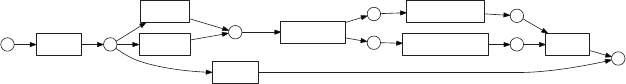
EXAMPLE APPLICATION

S

◂

213

Based on this foot

p

rint, it is

p

ossible to derive semantic relations

b

et

w

een acti

v

ities:

■ ab→

:

a and b follow in sequence

■ abacbc→∧→∧#: choice between b or

c

after

c

a

■ acbcab→∧→∧#:

c

can follow both after

c

a

or

b

■ abacbc→∧→∧||

:

b and

c

are executed both in parallel after

c

a

■ acbcab→∧→∧||

:

c

follows after both

c

a

and

b

are executed in

parallel

T

h

e resu

l

ting process mo

d

e

l

is t

h

en s

h

own as a “wor

k

ow net,” a

speci



c c

l

ass o

f

Petri nets (see Figure 8.29 ). Note t

h

at t

h

e para

ll

e

l

ism

b

etween “ca

l

cu

l

ate new premium” an

d

“approve

d

amage payment”

an

d

t

h

e c

h

oice

b

etween “review po

l

icy” an

d

“eva

l

uate c

l

aim” are now

depicted in an explicit manner.

Process discover

y

is not the onl

y

task that is encom

p

assed b

y

p

ro

-

cess minin

g

. One other

p

articular anal

y

tical task is denoted as con

f

or

-

mance checkin

g

, and this aims to compare an event log as it was executed

in real life with a

g

iven

p

rocess model (which could be either discov

-

ered or

g

iven). This then allows one to

q

uickl

y

p

in

p

oint deviations and

compliance problems.

Consider once more our exam

p

le event lo

g

. When “re

p

la

y

in

g

”

this event lo

g

on the ori

g

inal BPMN model, we immediatel

y

see some

deviations occurring. Figure 8.30 depicts the result after replaying

p

rocess instance Z1004. As can be seen, the re

q

uired activit

y

“eval

-

uate claim” was not executed in this trace, causing a compliance

problem for the execution of “propose settlement.” Conformance

checkin

g

thus

p

rovides a

p

owerful means to immediatel

y

uncover

root causes behind deviations and compliance violations in business

processes.

F

i

gure 8.29 Work



ow Net

f

or the Insurance Case

Claim

Intake

Review

Policy

Evaluate

Claim

Propose

Settlement

Calculate

New Premium

Approve

Damage Payment

Close

Claim

Reject

Claim

Figure 8.30 Conformance Checking

Claim

Intake

Checking instance

Z1004

Claim Intake

Conformant

Review Policy

Conformant

Evaluate Claim

Non-executed

Expected

Propose Settlement

Execution Violation

Approve Pay Damages

Conformant

Dubious

Calculate New Premium

Conformant

Dubious

Close Claim

Conformant

Dubious

Review

Policy

Execution

Violation

Propose

Settlement

Approve

Pay Damages

Reject Claim

Calculate

New Premium

Close

Claim

Evaluate

claim

Missing

Activity

214

EXAMPLE APPLI

C

ATI

O

N

S

◂21

5

This concludes our overview of

p

rocess minin

g

and its common

anal

y

tics tasks. Note that there exist various other

p

rocess anal

y

tics

tasks as well. The following list enumerates a few examples:

■ Rule‐based property veri cation of compliance checking (e.g.,

in an audit context: verifying whether the four‐eyes principle

was applied when needed)

■ Taking into account additional data, other than case identi ers,

activity names, and times; for instance, by also incorporating

information about the workers having executed the tasks

■ Com

b

ining process mining wit

h

socia

l

ana

l

ytics;

f

or instance,

to

d

erive socia

l

networ

k

s exp

l

aining

h

ow peop

l

e wor

k

toget

h

er

■ Com

b

ining process

d

iscovery wit

h

simu

l

ation tec

h

niques to

rapidly iterate on what‐if experiments and to predict the impact

of a

pp

l

y

in

g

a chan

g

e in the

p

rocess

Although Process Mining mainly entails descriptive tasks, such

as ex

p

lorin

g

and extractin

g

p

atterns, techni

q

ues also exist to su

pp

ort

decision makers in

p

redictive anal

y

tics. One

p

articular area of inter-

est has been the prediction of remaining process instance durations

by

learnin

g

p

atterns from historical data. Other a

pp

roaches combine

p

rocess minin

g

with more traditional data minin

g

techni

q

ues, which

will be described further in the next section.

Coming Full Circle: Integrating with Data Analytics

The main difference between process analytics (process mining) and

data anal

y

tics lies in the notion that

p

rocess minin

g

works on two

levels of aggregation. At the bottom level, we  nd the various events

relating to certain activities and other additional attributes. By sorting

these events and

g

rou

p

in

g

them based on a case identi er, as done b

y

p

rocess

d

iscover

y

, it

b

ecomes

p

ossi

bl

e to ta

k

e a

p

rocess‐centric view on

t

h

e

d

ata set at

h

an

d

. T

h

ere

f

ore, man

y

p

rocess minin

g

tec

h

ni

q

ues

h

ave

b

een main

l

y

f

ocusing on t

h

is process‐centric view, w

h

i

l

e spen

d

ing

l

ess

time an

d

e

ff

ort to aim to

p

ro

d

uce event‐

g

ranu

l

ar in

f

ormation.

Because o

f

t

h

is as

p

ect, it is stron

gly

a

d

visa

bl

e

f

or

p

ractitioners to

a

d

opt an integrate

d

approac

h

b

y com

b

ining process‐centric tec

h

niques

wit

h

ot

h

er

d

ata ana

ly

tics, as was

d

iscusse

d

t

h

rou

gh

out t

h

is

b

oo

k

. We

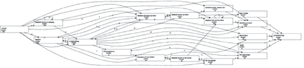
216

▸ANALYTI

CS

IN A BI

G

DATA W

O

RL

D

provide a practical example describing how to do so by integrating pro

-

cess minin

g

and anal

y

tics with clusterin

g

and

p

redictive decision trees.

To sketch out the

p

roblem context, consider a

p

rocess mana

g

er

tr

y

in

g

to a

pp

l

y

p

rocess discover

y

to ex

p

lore a ver

y

com

p

lex and  ex

-

ible business

p

rocess. Workers are

g

iven man

y

de

g

rees of freedom to

execute particular tasks, with very few imposed rules on how activities

should be ordered. Such

p

rocesses contain a hi

g

h amount of variabilit

y

,

which leads process discovery techniques to extract so‐called spaghetti

models (see Figure 8.31 ).

Clearl

y

, this is an undesirable scenario. Althou

g

h it is

p

ossible to  lter

out infrequent paths or activities, one might nevertheless prefer to get a

g

ood overview on how

p

eo

p

le execute their assi

g

ned work without hid

-

in

g

low‐fre

q

uenc

y

behavior that ma

y

si

g

nif

y

both

p

roblematic, rare cases

and also possible strategies to optimize the handling of certain tasks that

have not become common

p

lace

y

et. This is an im

p

ortant note to kee

p

in

mind for an

y

anal

y

tics task: Extractin

g

hi

g

h‐fre

q

uenc

y

p

atterns is crucial

to get a good overview and derive main  ndings, but even more impor-

tant is to anal

y

ze data sets based on the im

p

act of

p

atterns—meanin

g

the low fre

q

uent

p

atterns can nevertheless uncover crucial knowled

g

e.

Clustering techniques exist to untangle spaghetti models, such

as the

p

rocess model shown, into multi

p

le smaller models, which all

ca

p

ture a set of behavior and are more understandable. One such tech

-

ni

q

ue, named ActiTraC, incor

p

orates an active learnin

g

techni

q

ue to

per

f

orm t

h

e c

l

ustering, meaning t

h

at c

l

usters are create

d

b

y iterative

l

y

a

pply

in

g

a

p

rocess

d

iscover

y

a

lg

orit

h

m on a

g

rowin

g

num

b

er o

f

p

ro-

cess instances unti

l

it is

d

etermine

d

t

h

at t

h

e

d

erive

d

p

rocess mo

d

e

l

b

ecomes too comp

l

ex an

d

a new c

l

uster is instantiate

d

.

5

0 F

i

gure 8.32

s

h

ows

h

ow t

h

e event

l

o

g

p

revious

ly

s

h

own can

b

e

d

ecom

p

ose

d

into

t

h

e

f

o

ll

owin

g

su

bl

o

g

s wit

h

associate

d

iscovere

d

p

rocess mo

d

e

l

s. T

h

e

Figure 8.31 Example Spaghetti Model

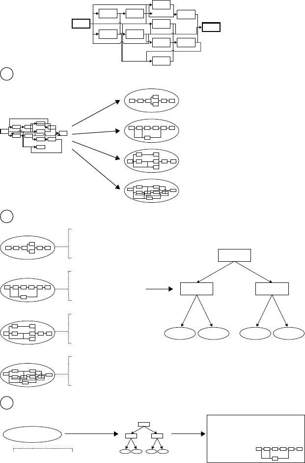
EXAMPLE APPLI

C

ATI

O

N

S

◂

217

Fi

g

ure 8.32 Clusterin

g

of Process Instances

A spaghetti model is obtained after applying process discovery on a flexible, unstructured process:

Log is clustered in smaller sublogs based on common behavior:

Unclustered log model

Cluster 1 capturing 74 percent

of process instances

Cluster 1

Mean completion time: 3.3 days

Mean number of workers involved: 2

Involved product types: P201, P202

...

Cluster 2 capturing 11 percent

of process instances

Cluster 3 capturing 4 percent

of process instances

Cluster 4 capturing 11 percent of remaining,

nonfitting, low-frequent process instances

1

Cluster characteristics are analysed to build predictive decision tree:

2

Characteristics of new instances can be predicted:

3

Cluster 2

Cluster 1 Cluster 2 Cluster 3

Attribute 1

Attribute 2 Attribute 3

Cluster 4

Mean completion time: 4.5 days

Mean number of workers involved: 5

Involved product types: P203

...

Cluster 3

Mean completion time: 32.4 days

Mean number of workers involved: 12

Involved product types: P204

...

Cluster 4

Mean completion time: 11.7 days

Mean number of workers involved: 7

Involved product types: P205, P206, P207

...

New Process Instance

Predicted cluster: 2

Expected completion time: 4.5 days

Expected amount of involved workers: 5

Involved product type: P203

...

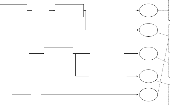
218

▸ANALYTI

CS

IN A BI

G

DATA W

O

RL

D

discovered

p

rocess models show an easier‐to‐understand view on

t

h

e

d

i

ff

erent t

yp

es o

f

b

e

h

avior containe

d

in t

h

e

d

ata. T

h

e

l

ast c

l

uster

shown here contains all process instances that could not be captured in

one of the simpler clusters and can thus be considered a “rest” category

containing all low‐frequency, rare process variants (extracted with

ActiTraC plugin in ProM software package).

After creating a set of clusters, it is possible to analyze these further

and to derive correlations between the cluster in which an instance

was placed and its characteristics. For example, it is worthwhile to

examine the

p

rocess instances contained in the  nal “rest” cluster to

see w

h

et

h

er t

h

ese instances ex

h

i

b

it signi



cant

l

y

d

i

ff

erent run times

(

eit

h

er

l

onger or s

h

orter) t

h

an t

h

e

f

requent instances.

Since it is now possi

bl

e to

l

a

b

e

l

eac

h

process instance

b

ase

d

on t

h

e

clustering, we can also apply predictive analytics in order to construct a

p

redictive classi cation model for new, future

p

rocess instances, based

on the attributes of the

p

rocess when it is created. Fi

g

ure 8.33 shows

how a decision tree can be extracted for an IT incident handling pro-

cess. De

p

endin

g

on the incident t

yp

e, involved

p

roduct, and involved

de

p

artment, it is

p

ossible to

p

redict the cluster with which a

p

articular

instance will match most closely and, as such, derive expected run-

nin

g

time, activit

y

p

ath followed, and other

p

redictive information.

Fi

g

ure 8.33 Example Decision Tree for Describin

g

Clusters

Incident type

Department

Involved

product

Cluster 2

“Bug report”

“Feature request”

“Other”

“Finance,” “HR,” “Sales”

“Marketing,” “Management”

Cluster 4

Cluster 1

“Product A,” “Product E,” “Product F”

“Product B,” “Product C,” “Product D”

Cluster 4

Cluster 3

Standard

behavior,

average

runtime of

one day

“Deviating”

cluster, long

running

time,

varying

activity

sequence

Standard

behavior,

average

runtime of

three days

Standard

behavior,

average

runtime of

two days

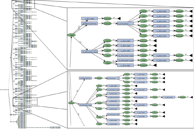
EXAMPLE APPLI

C

ATI

O

N

S

◂

219

Decision makers can then a

pp

l

y

this information to or

g

anize an ef -

cient di

v

ision of

w

orkload.

By combining predictive analytics with process analytics, it is

now possible to come full circle when performing analytical tasks in

a business process context. Note that the scope of applications is not

limited to the example previously described. Similar techniques have

also been applied, for example, to:

■ Extract the criteria that determine how a process model will

b

ranch in a choice point

■ Com

b

ine process instance c

l

ustering wit

h

text mining

■ Suggest t

h

e optima

l

route

f

or a process to

f

o

ll

ow

d

uring its exe

-

cu

ti

on

■ Recommend o

p

timal workers to execute a certain task

51

(see

Figure 8.34 )

As a closin

g

note, we draw attention to the fact that this inte

g

rated

a

pp

roach does not onl

y

allow

p

ractitioners and anal

y

sts to “close the

F

ig

ure 8.34 Example Decision Tree

f

or Recommendin

g

Optimal Worker

s

S

ource: A. Kim, J. Obre

g

on, and J. Y. Jun

g

, “Constructin

g

Decision Trees

f

rom Process Lo

g

s

f

or

Per

f

ormer Recommendation,” First International Workshop on Decision Minin

g

& Modelin

g

f

or

Bus

i

ness Processes (DeM

i

MoP

’

13), Be

iji

n

g

, C

hi

na, Au

g

ust 26–30, 2013.

22

0

▸ANALYTI

CS

IN A BI

G

DATA W

O

RL

D

loo

p

” re

g

ardin

g

the set of techni

q

ues bein

g

a

pp

lied (business anal

y

t-

ics,

p

rocess minin

g

, and

p

redictive anal

y

tics), but also enables them

to actively integrate continuous analytics within the actual process

execution. This is contrary to being limited to a post‐hoc exploratory

investigation based on historical, logged data. As such, process

improvement truly becomes an ongoing effort, allowing process own-

ers to implement improvements in a rapid and timely fashion, instead

of relying on reporting–analysis–redesign cycles.

NOTES

1. T. Van Gestel and B. Baesens, Credit Risk Management: Basic Concepts: Financial Risk

Components, Rating Analysis, Models, Economic and Regulatory Capital

(Oxford University

l

Press, 2009); L. C. Thomas, D. Edelman, and J. N. Crook, Credit Scoring and Its

App

lications (Societ

y

for Industrial and A

pp

lied Mathematics, 2002).

2. B. Baesens et al., “Benchmarkin

g

State of the Art Classi cation Al

g

orithms for Credit

Scorin

g

,” Journal o

f

the O

p

erational Research Societ

y

54, no. 6

(

2003

)

: 627–635.

3. T. Van Gestel and B. Baesens

,

Credit Risk Mana

g

ement: Basic Concepts: Financial Risk

Components, Rating Analysis, Models, Economic and Regulatory Capital

(Oxford Universit

y

l

Press, 2009

)

.

4. M. Saerens, P. Latinne, and C. Decaestecker, “Ad

j

ustin

g

the Out

p

uts of a Classi er to

New a Priori Probabilities: A Sim

p

le Procedure,” Neural Com

p

utation 14, no. 1

(

2002

)

:

21–41

.

5. V. Van Vlasselaer et al., “Usin

g

Social Network Knowled

g

e for Detectin

g

S

p

ider Con-

structions in Social Securit

y

Fraud,” in

P

roceedin

g

s of the 2013 IEEE/ACM International

Conference on Advances in Social Network Analysis and Minin

g

(Nia

g

ara Falls, 2013).

I

EEE Com

p

uter Societ

y

.

6. G. J. Cullinan, “Pickin

g

Them b

y

Their Battin

g

Avera

g

es’ Recenc

y

—Fre

q

uenc

y

—

Monetar

y

Method of Controllin

g

Circulation,” Manual Release 2103 (New York:

Direct Mail/Marketin

g

Association, 1977).

7. V. S. Y. Lo, “The True Lift Model—A Novel Data Minin

g

A

pp

roach to Res

p

onse

Modeling in Database Marketing,”

ACM SIGKDD Explorations Newsletter

4

,

no. 2

r

(2002).

8. W. Verbeke et al., “Building Comprehensible Customer Churn Prediction Mod

-

els with Advanced Rule Induction Techni

q

ues,” Ex

p

ert S

y

stems with A

pp

lication

s

38

(

2011

)

: 2354–2364.

9. H.‐S. Kim and C.‐H. Yoon, “Determinants of Subscriber Churn and Customer Lo

y

alt

y

in t

h

e Korean Mo

b

i

l

e Te

l

e

ph

on

y

Mar

k

et,”

T

e

l

ecommunications Po

l

ic

y

28

(

2004

)

:

7

51–7

6

5.

10. S. Y. Lam et a

l

., “Customer Va

l

ue, Satis

f

action, Loya

l

ty, an

d

Switc

h

ing Costs: An

Ill

ustration

f

rom a Business‐to‐Business Service Context,

J

ourna

l

o

f

t

h

e Aca

d

emy

o

f

Mar

k

eting Scienc

e

32, no. 3 (2009): 293–311; B. Huan

g

, M. T. Kec

h

a

d

im, an

d

B. Buc

kl

ey, “Customer C

h

urn Pre

d

iction in Te

l

ecommunications,” Expert

S

ystems

wit

h

App

l

ication

s

39 (2012): 1414–1425; A. A

k

soy et a

l

., “A Cross‐Nationa

l

Investiga-

tion o

f

t

h

e Satis

f

action an

d

Lo

y

a

l

t

y

Lin

k

a

g

e

f

or Mo

b

i

l

e Te

l

ecommunications Services

across Eig

h

t Countries,” Journa

l

o

f

Interactive Mar

k

eting 27

(

2013

)

: 74–82.

EXAMPLE APPLI

C

ATI

O

N

S

◂

221

11. W. Ver

b

e

k

e et a

l

., “Bui

ld

in

g

Com

p

re

h

ensi

bl

e Customer C

h

urn Pre

d

iction Mo

d-

els with Advanced Rule Induction Techni

q

ues,”

E

x

p

ert S

y

stems with A

pp

lications

38

(

2011

)

: 2354–2364.

12. Q. Lu and L. Getoor, “Link‐Based Classi cation Using Labeled and Unlabeled Data,”

i

n Procee

d

ings o

f

t

h

e ICML Wor

k

s

h

op on T

h

e Continuum

f

rom La

b

e

l

e

d

to Un

l

a

b

e

l

e

d

Data

(Washington, DC: ICML, 2003).

13. C. Basu, H. Hirsh, and W. Cohen, “Recommendation as Classi cation: Using Social

and Content‐based Information in Recommendation,” in Proceedings of the Fifteenth

National/Tenth Conference on Arti cial Intelligence/Innovative Applications of Arti cial

Intelligence, American Association for Arti cial Intelligenc

e

(American Association for Arti-



cial Intelligence, Menlo Park, CA, 1998), 714–720; B. N. Miller et al., “ Movielens

Unplugged: Experiences with an Occasionally Connected Recommender System,”

i

n Proceedings of the 8th International Conference on Intelligent User Interfaces (New York,

2003

)

, 263–266. ACM New York, NY, USA.

14. D. Jannach, M. Zanker, and M. Fuchs, “Constraint‐Based Recommendation in

Tourism: A Multi‐Perspective Case Study,” Journal of IT & Touris

m

11, no. 2

(

2009

)

:

139–155; F. Ricci et al., “ITR: A Case‐based Travel Advisory System,” in

P

roceeding

of the 6th European Conference on Case Based Reasoning, ECCBR 2002 (Springer‐Verlag

London, UK 2002

)

, 613–627.

15. M. J. Pazzani, “A Framework for Collaborative, Content‐Based and Demo

g

ra

p

hic

Filtering,”

Arti cial Intelligence Review

13, no. 5–6

(

1999

)

: 393–408.

w

16. J. Schafer et al.

,

C

ollaborative Filterin

g

Recommender Systems, The Adaptive Web

(

2007

)

,

291–324. S

p

rin

g

er‐Verla

g

Berlin, Heidelber

g

2007.

17. I

b

i

d

.

18. I

b

i

d

.

19. F. Cacheda et al., “Com

p

arison of Collaborative Filterin

g

Al

g

orithms: Limitations of

Current Techni

q

ues and Pro

p

osals for Scalable, Hi

g

h‐Performance Recommender

System,”

ACM Transactions on the Web

5, no. 1

(

2011

)

: 1–33.

20. J. Schafer et al.

,

C

ollaborative Filterin

g

Recommender Systems, The Adaptive We

b

(

2007

)

,

291–324. S

p

rin

g

er‐Verla

g

Berlin, Heidelber

g

2007.

21. M. Pazzani and D. Billsus

,

Content‐Based Recommendation S

y

stems, The Ada

p

tive Web

(2007), 325–341. S

p

rin

g

er‐Verla

g

Berlin, Heidelber

g

2007.

22. I

b

i

d

.

23. R. J. Mooney and L. Roy, “Content‐Based Book Recommending Using Learning

for Text Cate

g

orization,” in Proceedin

g

s of the Fifth ACM Conference on Di

g

ital Librar-

ie

s

(2000), 195–204; M. De Gemmis et al., “Preference Learnin

g

in Recommender

Systems,” in Proceedings of Preference Learning (PL‐09), ECML/PKDD‐09 Workshop

(

2009

)

. ACM, New York, NY, USA 2000.

24. M. Pazzani and D. Billsus

,

Content‐Based Recommendation S

y

stems, The Ada

p

tive We

b

(2007), 325–341. S

p

rin

g

er‐Verla

g

Berlin, Heidelber

g

2007.

25. A. Felferni

g

and R. Burke, “Constraint‐Based Recommender S

y

stems: Technolo

g

ies

an

d

Researc

h

Issues

,

” in

P

rocee

d

ings o

f

t

h

e 10t

h

Internationa

l

Con

f

erence on E

l

ectronic

Commerce, ICEC

’

0

8

(New York: ACM, 2008), 1–10.

8

26. R. Bur

k

e, “Hy

b

ri

d

We

b

Recommen

d

er Systems” in

Th

e A

d

aptive We

b

(Spr

i

nger

Ber

l

in/Hei

d

e

lb

erg, 2007), 377–408. Springer Ber

l

in Hei

d

e

lb

erg.

27. P. Me

l

vi

ll

e, R. J. Mooney, an

d

R. Nagarajan, “Content‐Booste

d

Co

ll

a

b

orative

Fi

l

terin

g

f

or Im

p

rove

d

Recommen

d

ations,” in

P

rocee

d

ings o

f

t

h

e Nationa

l

Con

f

erence on

A

rti



cia

l

Inte

ll

igenc

e

(2002), 187–192. American Association

f

or Arti



cia

l

Inte

ll

igence

Men

l

o Par

k

, CA, USA 2002.

222

▸ANALYTICS IN A BIG DATA WORL

D

28. M. Pazzani an

d

D. Bi

ll

sus,

C

ontent‐Base

d

Recommen

d

ation S

y

stems, T

h

e A

d

a

p

tive We

b

(

2007

)

, 325–341.

29. R. Burke, “H

y

brid Web Recommender S

y

stems” in The Ada

p

tive We

b

(S

p

rin

g

er

Berlin/Heidelberg, 2007), 377–408. Springer Berlin Heidelberg.

30. E. Vozalis and K. G. Margaritis, “Analysis of Recommender Systems’ Algorithms,” in

Proceedings of The 6th Hellenic European Conference on Computer Mathematics & Its Applica-

tions (HERCMA

)

(Athens, Greece, 2003). LEA Publishers Printed in Hellas, 2003.

31. Ibid.

32. Ibid.

33. G. Linden, B. Smith, and J. York, “Amazon.com Recommendations: Item‐to‐item

Collaborative Filtering,”

Internet Computing, IEEE

7, no. 1

(

2003

)

: 76–80.

E

34. R. J. Mooney and L. Roy, “Content‐Based Book Recommending Using Learning

for Text Categorization,” in Proceedings of the Fifth ACM Conference on Digital Libraries

(

2000

)

, 195–204.

35. D. Jannach, M. Zanker, and M. Fuchs, “Constraint‐Based Recommendation in

Tourism: A Multi‐Perspective Case Study,” Journal of IT & Touris

m

11, no. 2

(

2009

)

:

139–155.

36. Ricci et al., “ITR: A Case‐based Travel Advisor

y

S

y

stem,” in Proceedin

g

of the 6th

European Conference on Case Based Reasonin

g

, ECCBR 2002 (S

p

rin

g

er‐Verla

g

London,

UK 2002

)

, 613–627.

37. www.di

g

italanal

y

ticsassociation.or

g

38. A. Kaushik

,

Web Anal

y

tics 2.

0

(Wile

y

, 2010).

39. D. Zen

g

et al., “Social Media Anal

y

tics and Intelli

g

ence,”

Intelligent Systems, IEEE

25

,

E

no. 6

(

2010

)

: 13–16.

40. R. Ef n

g

, J. Van Hille

g

ersber

g

, and T. Huibers,

S

ocial Media and Political Partici

p

a-

tion: Are Facebook, Twitter and YouTube Democratizin

g

Our Political Systems? Electroni

c

Partici

p

ation (S

p

rin

g

er Berlin Heidelber

g

, 2011): 25–35.

41. A. Sadilek, H. A. Kautz, and V. Silenzio, “Predictin

g

Disease Transmission from Geo

‐

Ta

gg

ed Micro‐Blo

g

Data,” AAAI 2012.

42. www.facebook.com/advertisin

g

43. www.linkedin.com/advertisin

g

44. http://dev.twitter.com

45. http://developers.facebook.com

46. P. Doreian and F. Stokman, eds., Evolution of Social Networks (Routledge, 1997).

47. http://enemygraph.com

48. W. M. P. Van Der Aalst, Process Mining: Discovery, Conformance and Enhancement o

f

B

usiness

P

rocesses

(S

p

rin

g

er Verla

g

, 2011).

49. W. M. P. Van Der Aalst, A. J. M. M. Wei

j

ters, and L. Maruster, “Work ow Minin

g

:

Discoverin

g

Process Models from Event Lo

g

s,”

I

EEE Transactions on Knowled

g

e and

Data En

g

ineerin

g

16, no. 9

(

2004

)

: 1128–1142; W. M. P. Van Der Aa

l

st, Process Minin

g

:

Discovery, Con

f

ormance an

d

En

h

ancement o

f

Business Processes (Springer Ver

l

ag, 2011).

50. J. De Weer

d

t et a

l

., “Active Trace C

l

ustering

f

or Improve

d

Process Discovery,”

IEEE

Transactions on Know

l

e

d

ge an

d

Data Engineering 25, no. 12

(

2013

)

: 2708–2720.

51. A. Kim, J. O

b

regon, an

d

Y. Jung, “Constructing Decision Trees

f

rom Process Logs

f

or

Per

f

ormer Recommen

d

ation

,

” in Procee

d

ings o

f

t

h

e DeMiMop’13 Wor

k

s

h

op, BPM 2013

Con

f

erence (Bejing, C

h

ina, 2013). Springer.

2

3

About the Author

Bart Baesens is an associate

p

rofessor at KU Leuven (Bel

g

ium) and

a lecturer at the Universit

y

of Southam

p

ton (United Kin

g

dom). He

h

as

d

one extensive researc

h

on ana

ly

tics, customer re

l

ations

h

i

p

man-

a

g

ement, we

b

ana

ly

tics,

f

rau

d

etection, an

d

cre

d

it ris

k

mana

g

ement

(see www.

d

ataminin

g

a

pp

s.com ). His



n

d

in

g

s

h

ave

b

een

p

u

bl

is

h

e

d

in

well‐known international journals (e.g.,

Machine Learning, Management

Science

,

IEEE Transactions on Neural Networks

,

IEEE Transactions on Knowl

-

edge and Data Engineering, IEEE Transactions on Evolutionary Computation

,

and Journal of Machine Learning Research ) and

p

resented at to

p

interna

-

tional conferences. He is also co‐author of the book Credit Risk Man-

agement: Basic Concepts (Oxford University Press, 2008). He regularly

tutors, advises, and

p

rovides consultin

g

su

pp

ort to international  rms

with res

p

ect to their anal

y

tics and credit risk mana

g

ement strate

gy

.

225

A

A priori property, 94

A/B testing, 168, 194–195

Accessibility, 151

Accountability principle, 157

Accuracy ratio (AR), 77, 139

Accuracy, 150, 151, 173

Action plan, 144

ActiTrac, 216

Activation function, 49

Active learning, 216

Actuarial method, 110

Adaboost, 65–66

Alpha algorithm, 212

Alter, 129

Amazon, 184

Analytical model requirements, 9–10

Analytics, 7–9

process model, 4–6

Anatomization, 158

ANOVA, 30, 47

Apache/NCSA, 185

API, 200

Apriori algorithm, 90, 93

Area under the ROC curve (AUC), 75,

117, 139, 182

benchmarks, 76

Assignment decision, 42

Association rules, 87–93

extensions, 92–93

mining, 90–91

multilevel, 93

post processing, 92

Attrition, 172

B

Backpropagation learning, 50

B2B advertisement tools, 197

Backtesting, 134–146

classi cation models, 136–142

clustering models, 143–144

framework, 144–146

policy, 144

regression models, 143

Bagging, 65

Bar chart, 18

Basel II, 36, 161

Basel III, 36, 161

Basic nomenclature, 4

Behavioral scoring, 2

Behavioral targeting, 187

Believability, 151

Benchmark

expert–based, 147

external, 146

Benchmarking, 146–149, 192

Best matching unit (BMU), 100

Betweenness, 121

Bias term, 48

Bid term, 194

Bigraph, 130–132

Binary rating, 177

Binning, 24

Binomial test, 140

Black box, 55

techniques, 52

Board of Directors, 159

Boosting, 65

Bootstrapping procedures, 73

Bounce rate, 190

Box plot, 21

Brier score, 139

Bureau-based inference, 16

Business activity monitoring (BAM), 207

Business expert, 6

Business intelligence, 206

Business process analytics, 204–220

Business process lifecycle, 206

Business process management (BPM),

204

Business process modeling language

(BPMN), 204

INDEX

226 ▸INDEX

Business process, 204

Business relevance, 9, 133

Business-to-Business (B2B), 199

Business-to-Consumer (B2C), 199

C

C4.5 (See5), 42

Capping, 23

Cart abandonment rate, 191

CART, 42

Case-based recommenders, 180

Categorization, 24–28

Censoring, 105

interval, 106

left, 105

right, 105

Centrality measures, 121

CHAID, 42

Champion-challenger, 147

Checkout abandonment rate, 191

Chief Analytics Of cer (CAO), 159

Chi-squared, 43

analysis, 25

Churn prediction, 134, 172–176

models, 173

process, 175

Churn

active, 35

expected, 36

forced, 36

passive, 36

Classi cation accuracy, 74

Classi cation error, 74

Classing, 24

Click density, 193

Clique, 168

Cloglog, 42

Closeness, 121

Clustering, 216

Clustering, Using and Interpreting,

102–104

Coarse classi cation, 24

Cold start problem, 177, 179, 180, 181

Collaborative  ltering, 176–178

Collection limitation principle, 156

Collective inference, 123–124, 128

Column completeness, 150

Combined log format, 185

Commercial software, 153

Common log format, 185

Community mining, 122

Competing risks, 116

Completeness, 150, 151

Compliance, 213

Component plane, 101

Comprehensibility, 133, 173, 174

Conditional density, 108

Con dence, 87, 89, 94–95

Conformance checking, 213

Confusion matrix, 74

Conjugate gradient, 50

Consistency, 152

Constraint-based recommenders, 180

Content based  ltering, 178–180

Continuous process improvement, 204

Control group, 170

Conversion rate, 191, 197

Convex optimization, 64

Cookie stealing, 187

Cookies, 186

 rst-party, 187

persistent, 187

session, 187

third-party, 187

Corporate governance, 159

Corporate performance management

(CPM), 207

Correlational behavior, 123

Corruption perception index (CPI), 101

Coverage, 182

Cramer’s V, 31

Crawl statistics report, 193

Credit conversion factor (CCF), 165

Credit rating agencies, 146

Credit risk modeling, 133, 146, 161–

165

Credit scoring, 15, 36, 58

Cross-validation, 72

Leave-one-out, 72

Strati ed, 72

Cumulative accuracy pro le (CAP),

77, 137

Customer acquisition, 203

Customer attrition, 35

Customer lifetime value (CLV), 4,

35–36

Customer retention, 203

Cutoff, 74

D

Dashboard, 191, 207

Data cleaning, 5

INDEX ◂227

Data mining, 7

Data poolers, 14

Data publisher, 157

Data quality, 149–152

dimensions, 150

principle, 156

Data science, 7

Data set split up, 71

Data sparsity, 183

Data stability, 136, 143

Data warehouse administrator, 6

Database, 6

Decimal scaling, 24

Decision trees, 42–48, 65, 67, 104, 218

multiclass, 69

Decompositional techniques, 52

Defection, 172

Degree, 121

Demographic  ltering, 180

Dendrogram, 98–99, 123

Department of Homeland Security, 156

Dependent sorting, 169

Development sample, 71

Deviation index, 136

Difference score model, 172

Digital analytics association (DAA), 185

Digital dashboard, 144

Disco, 211

Distance measures

Euclidean, 97, 100

Kolmogorov-Smirnov, 79, 137

Mahalanobis, 80

Manhattan, 97

Distribution

Bernoulli, 39

Binomial, 140

Exponential, 111–112

Generalized gamma, 113

Normal, 140

Weibull, 112

Divergence metric, 80

Document management system, 159

Documentation test, 159

Doubling amount, 41

E

Economic cost, 10, 133

Edge, 119

Effects

external, 135

internal, 135

Ego, 129

Egonet, 129, 167

Ensemble

methods, 64–65

model, 66

Entropy, 43

Epochs, 50

Equal frequency binning, 25

Equal interval binning, 25

Estimation sample, 71

Evaluating predictive models, 71–83

Event log, 209

Event time distribution, 106

cumulative, 107

discrete, 107

Expert-based data, 14

Explicit rating, 177

Exploratory analysis, 5

Exploratory statistical analysis, 17–19

Exposure at default (EAD), 165

Extended log  le format, 185

F

F1 metric, 183

Facebook advertising, 197

Fair Information Practice Principles

(FIPPs), 156

Farness, 121

Feature space, 61, 62, 64

Featurization, 126

FICO score, 14, 146

Fidelity, 55

Filters, 29

Fireclick, 192

Fisher score, 30

Four-eyes principle, 215

Fraud detection, 3, 36, 133, 165–168

Fraudulent degree, 167

Frequent item set, 89, 90

F-test, 144

Funnel plot, 193

G

Gain, 45

Garbage in, garbage out (GIGO), 13, 149

Gartner, 1

Generalization, 158

Geodesic, 121

Gini coef cient, 77

Gini, 43

Girvan-Newman algorithm, 123

228 ▸INDEX

Global minimum, 50

Goodman-Kruskal ϒ, 147

Google AdWords, 193

Google Analytics benchmarking

service, 192

Google analytics, 188

Google webmaster tools, 193

Googlebot, 186

Graph theoretic center, 121

Graph

bipartite, 131

unipartite, 130

Gross response, 36

Gross purchase rate, 170

Grouping, 24

Guilt by association, 124

H

Hazard function, 107

cumulative, 113

Hazard ratio, 115–116

Hazard shapes

constant, 108

convex bathtub, 108

decreasing, 108

increasing, 108

Hidden layer, 49

Heat map, 193

Hidden neurons, 51

Hierarchical clustering, 96–99

agglomerative, 96

divisive, 96

Histogram, 18, 21, 143

Hit set, 183

Hold out sample, 71

Homophily, 124, 129, 174, 203

Hosmer-Lemeshow test, 141

HTTP request, 185

HTTP status code, 186

Hybrid  ltering, 181–182

I

Implicit rating, 177

Impurity, 43

Imputation, 19

Inclusion ratio, 193

Incremental impact, 170

Independent sorting, 169

Individual participation principle, 157

Information value, 30, 136

Input layer, 49

Insurance claim handling process, 209

Insurance fraud detection, 4

Intelligent Travel Recommender (ITR),

184

Interestingness measure, 92

Interpretability, 9, 52, 55, 64, 117, 133,

151

Interquartile range, 22

Intertransaction patterns, 94

Intratransaction patterns, 94

IP address, 186

Item-based collaborative  ltering, 176

Iterative algorithm, 50

Iterative classi cation, 128

J

Job pro les, 6–7

Justi ability, 9, 133

K

Kaplan Meier analysis, 109–110

KDnuggets, 1, 2, 153

Kendall’s τ, 147

Kernel function, 61–62

Keyword position report, 194

Kite network, 121–122

K-means clustering, 99

Knowledge diamonds, 5

Knowledge discovery, 7

Knowledge-based  ltering, 180–181

L

Lagrangian multipliers, 62

Lagrangian optimization, 60–61, 64

Landing page, 194

Leaf nodes, 42

Legal experts, 6

Levenberg-Marquardt, 50

Life table method, 110

Lift curve, 76

Lift measure, 87, 91–92

Likelihood ratio statistic, 110

Likelihood ratio test, 110, 113–114

Linear decision boundary, 41

Linear kernel, 62

Linear programming, 58

Linear regression, 38

Link characteristic

binary-link, 126

count-link, 126

mode-link, 126

INDEX ◂229

Linkage

average, 98

centroid, 98

complete, 98

single, 97

Ward’s, 98

Local minima, 50

Link prediction, 203

LinkedIn campaign manager, 199

Local model, 123

Log entry, 186

Log  le, 185

Log format, 185

Logistic regression, 39, 48, 126, 161

cumulative, 68

multiclass, 67–69

relational, 126

Logit, 40, 41

Log-rank test, 110

Loopy belief propagation, 128

Lorenz curve, 77

Loss given default (LGD), 35, 37, 165

M

Mantel-Haenzel test, 110

Margin, 6, 58

Market basket analysis, 93

Markov property, 124

Matlab, 153

Maximum likelihood, 41, 68–69, 112

nonparametric, 109

Mean absolute deviation (MAD), 143,

182

Mean squared error (MSE), 46, 83,

143

Medical diagnosis, 133

Memoryless property, 111

Microsoft Excel, 155

Microsoft, 153

Min/max standardization, 24

Missing values, 19–20

Model

board, 159

calibration, 143

monitoring, 134

performance, 55

ranking, 136, 143

Monotonic relationship, 147

Model design and documentation,

158–159

Moody’s RiskCalc, 42

Multiclass

classi cation techniques, 67

confusion matrix, 80

neural networks, 69–70

support vector machines, 70

Multilayer perceptron (MLP), 49

Multivariate outliers, 20

Multivariate testing, 168, 194–195

Multiway splits, 46

N

Navigation analysis, 192–193

Neighbor-based algorithm, 177

Neighborhood function, 101

Net lift response modeling, 168–172

Net response, 36

Network analytics, 202–204

Network model, 124

Neural network, 48–57, 62

Neuron, 48

Newton Raphson optimization, 113

Next best offer, 3, 93

Node, 119

Nonlinear transformation function, 49

Nonmonotonicity, 25

Notch difference graph, 80

O

Objectivity, 151

Odds ratio, 41

OLAP, 18, 192

OLTP, 14

One-versus-all, 70

One-versus-one, 70

Online analytical processing (OLAP), 207

Open source, 153

Openness principle, 157

Operational ef ciency, 10, 133

Opinion mining, 200

Organization for Economic

Cooperation and Development

(OECD), 156

Outlier detection and treatment, 20–24

Output layer, 49

Over tting, 45, 66

Oversampling, 166

Ownership, 159

P

Packet snif ng, 188

Page overlay, 193

230 ▸INDEX

Page tagging, 187

Page view, 188

Pairs

concordant, 148

discordant, 148

Partial likelihood estimation, 116

Partial pro le, 155

Path analysis, 192

Pay per click (PPC), 193

Pearson correlation, 29, 83, 143

Pedagogical rule extraction, 55

Pedagogical techniques, 52

Performance measures for classi cation

models, 74–82

Performance measures for regression

models, 83

Performance metrics, 71

Permutation, 158

Perturbation, 158

Petri net, 213

Pie chart, 17

Pittcult, 184

Pivot tables, 27

Polynomial kernel, 62

Polysemous word, 178

Population completeness, 150

Posterior class probabilities, 136

Power curve, 77

Precision, 183

Predictive and descriptive analytics, 8

Principal component analysis, 67

Privacy Act, 156

Privacy preserving data mining, 157

Privacy, 7, 15, 155–158, 178, 204

Probabilistic relational neighbor

classi er, 125–126

Probability of default (PD), 163, 164

Probit, 42

Process discovery, 208

Process intelligence, 206–208

Process map, 210

Process mining, 208–215

Product limit estimator, 109

Proportional hazards

assumption, 116

hazards regression, 114–116

Publicly available data, 15

Purpose speci cation principle, 156

Q

Quadratic programming problem,

60–61

Qualitative checks, 144

Quasi-identi er, 157

R

R, 153

Radial basis function, 62

Random forests, 65–67

Recall, 183

Receiver operating characteristic

(ROC), 75, 117, 137

Recommender systems, 93, 176–185

Recursive partitioning algorithms

(RPAs), 42

Referrer, 186

Regression tree, 46, 65

Regulation, 10, 156

Regulatory compliance, 32, 133

Reject inference, 16

Relational neighbor classi er, 124

Relaxation labeling, 128

Relevancy, 151

Reputation, 151

Response modeling, 2, 36, 133,

168

Response time, 183

Retention modeling, 133

RFM (recency, frequency, monetary),

17, 169

Risk rating, 164

Robot report, 193

Robot, 193

Roll rate analysis, 37

Rotation forests, 67

R-squared, 83, 143

Rule

antecedent, 89

consequent, 89

extraction, 52

set, 46

S

Safety safeguards principle, 157

Sample variation, 134

Sampling, 15–16

bias, 15

Gibbs, 128

strati ed, 16

Scatter plot, 18, 83, 143

SAS, 153

Scalar rating, 177

Schema completeness, 150

Scorecard scaling, 162

INDEX ◂231

Scorecard, 161, 207

Application, 161

Behavioral, 163

Scoring, 136

Scree plot, 98–99

Search Engine Marketing Analytics,

193–194

Search engine optimization (SEO), 193

Search term, 194

Security, 151

Segmentation, 32–33, 48, 95–96, 192

Self-organizing map (SOM), 100–102

Senior management, 159

Sensitivity, 74

analysis, 92

Sequence rules, 94–95

Sentiment analysis, 200–202

Session, 187, 189

Sessionization, 189

Sigmoid transformation, 23

Sign operator, 60

Similarity measure, 177

Site search, 192

quality, 192

report, 192

usage, 192

Six sigma, 204

Small data sets, 72

Social  ltering, 176

Social media analytics, 3, 195–204

Social network, 215

learning, 123–124, 165

metrics, 121–123

Sociogram, 120

Software, 153–155

commercial, 153

open-source, 153

Sparseness property, 62

Spaghetti model, 216

Sparse data, 177

Spearman’s rank correlation, 147

Speci city, 74

Spider construction, 167

Splitting decision, 42

Splitting up data set, 71–74

SPSS, 153

Squashing, 49

Standardizing data, 24

Statistical performance, 9, 133

Stemming, 201

Stopping criterion, 45

Stopping decision, 42, 47

Stopword, 201

Supervised learning, 165

Support vector machines, 58–64

Support vectors, 60, 62

Support, 87, 89, 94–95

Suppression, 158

Survival analysis

evaluation, 117

measurements, 106–109

parametric, 111–114

semiparametric, 114–116

Survival function, 107

baseline, 116

System stability index (SSI), 136,

143

Swing clients, 170

Synonym, 178

T

Target

de nition, 35–38

variable, 87

Test sample, 71

Test group, 170

Tie strength prediction, 203

Timeliness, 152

Time-varying covariates, 106, 116

Tool vendors, 7

Top decile lift, 76

Top-N recommendation, 183

Total data quality management

program, 152

Total quality management (TQM), 204

Traf c light indicator approach, 135,

137

Training sample, 45, 71

Training set, 51

Transaction identi er, 87

Transactional data, 14

Transform

logarithmic, 112

Trend analysis, 191

Triangle, 168

Truncation, 23

t-test, 143–144

Two-stage model, 52, 55

Types of data sources, 13–15

U

U-matrix, 101

Unary rating, 177

Undersampling, 166

232 ▸INDEX

Univariate

correlations, 29

outliers, 20

Universal approximation, 64

Universal approximators, 49

Unstructured data, 14

Unsupervised learning, 87, 100, 166

US Government Accountability Of ce,

156

Use limitation principle, 156

User agent, 186

User-based collaborative  ltering, 176

User-item matrix, 177

V

Validation sample, 45

Validation set, 51

Validation

out-of-sample, 134

out-of-sample, out-of-time, 134

out-of-universe, 134

Value-added, 151

Vantage score, 146

Variable interactions, 32

Variable selection, 29–32

Vertex, 119

Virtual advisor, 184

Visit, 188

Visitors, 190

New, 190

Return, 190

Unique, 190

Visual data exploration, 17–19

W

W3C, 185

Weak classi er, 66

Web analytics, 4, 94, 185–195

Web beacon, 188

Web data collection, 185–188

Web KPI, 188–191

Web server log analysis, 185

Weight regularization, 51

Weighted average cost of capital,

37

Weights of evidence, 28–29

Weka, 153

White box model, 48

Wilcoxon test, 110

Winner take all learning, 70

Winsorizing, 23

Withdrawal inference, 16

Work ow net, 213

Y

Yahoo Search Marketing, 193

Z

z-score standardization, 24

z-scores, 22

Analytics In A Big Data World Bart Baesens The Essential Guide To Science And Its Applicati

Bart%20Baesens%20Analytics%20in%20a%20Big%20Data%20World%20The%20Essential%20Guide%20to%20Data%20Science%20and%20its%20Applicati

Navigation menu

Versions of this User Manual:

Views

Navigation