CP5261 DATA ANALYTICS LABORATORY MANUAL ME CSE

CP5261%20%20%20DATA%20ANALYTICS%20LABORATORY%20MANUAL%20ME%20CSE

User Manual:

Open the PDF directly: View PDF .
Page Count: 80

CP5261 DATA ANALYTICS LABORATORY MANUAL

1 | DR. D. SENTHIL KUMAR (AP/CSE) UCE, ANNA UNIVERSITY- BITCAMPUS TRICHY

CP5261 DATA ANALYTICS LABORATORY LTPC0042

OBJECTIVES:

 To implement Map Reduce programs for processing big data

 To realize storage of big data using H base, Mongo DB

 To analyze big data using linear models

 To analyze big data using machine learning techniques such as SVM / Decision tree

classification and clustering

LIST OF EXPERIMENTS

Hadoop

1. Install, configure and run Hadoop and HDFS

2. Implement word count / frequency programs using MapReduce

3. Implement an MR program that processes a weather dataset

4. Implement Linear and logistic Regression

5. Implement SVM / Decision tree classification techniques

6. Implement clustering techniques

7. Visualize data using any plotting framework

8. Implement an application that stores big data in Hbase / MongoDB / Pig using Hadoop / R.

TOTAL: 60 PERIODS

OUTCOMES:

Upon Completion of this course, the students will be able to:

 Process big data using Hadoop framework

 Build and apply linear and logistic regression models

 Perform data analysis with machine learning methods

 Perform graphical data analysis

CP5261 DATA ANALYTICS LABORATORY MANUAL

2 | DR. D. SENTHIL KUMAR (AP/CSE) UCE, ANNA UNIVERSITY- BITCAMPUS TRICHY

Step by step Hadoop 2.8.0 installation on Windows 10 Prepare:

These software’s should be prepared to install Hadoop 2.8.0 on window 10 64 bits.

1) Download Hadoop 2.8.0

(Link: http://wwweu.apache.org/dist/hadoop/common/hadoop-

2.8.0/hadoop-2.8.0.tar.gz OR

http://archive.apache.org/dist/hadoop/core//hadoop-2.8.0/hadoop-

2.8.0.tar.gz)

2) Java JDK 1.8.0.zip

(Link: http://www.oracle.com/technetwork/java/javase/downloads/jdk8-

downloads-2133151.html)

Set up:

1) Check either Java 1.8.0 is already installed on your system or not, use “Javac -

version" to check Java version

2) If Java is not installed on your system then first install java under "C:\JAVA" Java

setup

3) Extract files Hadoop 2.8.0.tar.gz or Hadoop-2.8.0.zip and place under

"C:\Hadoop-2.8.0" hadoop

4) Set the path HADOOP_HOME Environment variable on windows 10(see Step 1,

2, 3 and 4 below) hadoop

5) Set the path JAVA_HOME Environment variable on windows 10(see Step 1, 2,

3 and 4 below) java

6) Next we set the Hadoop bin directory path and JAVA bin directory path

EX. NO: 1

Install, configure and run Hadoop and HDFS

CP5261 DATA ANALYTICS LABORATORY MANUAL

3 | DR. D. SENTHIL KUMAR (AP/CSE) UCE, ANNA UNIVERSITY- BITCAMPUS TRICHY

Configuration

a) File C:/Hadoop-2.8.0/etc/hadoop/core-site.xml, paste below xml paragraph and

save this file.

<name>fs.defaultFS</name>

<value>hdfs://localhost:9000</value>

</property>

</configuration>

b)Rename "mapred-site.xml.template" to "mapred-site.xml" and edit this file

C:/Hadoop-2.8.0/etc/hadoop/mapred-site.xml, paste below xml paragraph and save

this file.

<name>mapreduce.framework.name</name>

</property>

</configuration>

c) Create folder "data" under "C:\Hadoop-2.8.0"

1) Create folder "datanode" under "C:\Hadoop-2.8.0\data"

2) Create folder "namenode" under "C:\Hadoop-2.8.0\data" data

d) Edit file C:\Hadoop-2.8.0/etc/hadoop/hdfs-site.xml, paste below xml paragraph

and save this file.

CP5261 DATA ANALYTICS LABORATORY MANUAL

4 | DR. D. SENTHIL KUMAR (AP/CSE) UCE, ANNA UNIVERSITY- BITCAMPUS TRICHY

<name>dfs.replication</name>

</property>

<name>dfs.namenode.name.dir</name>

<value>C:\hadoop-2.8.0\data\namenode</value>

</property>

<name>dfs.datanode.data.dir</name>

<value>C:\hadoop-2.8.0\data\datanode</value>

</property>

</configuration>

e) Edit file C:/Hadoop-2.8.0/etc/hadoop/yarn-site.xml, paste below xml paragraph

and save this file.

<name>yarn.nodemanager.aux-services</name>

<value>mapreduce_shuffle</value>

</property>

<name>yarn.nodemanager.auxservices.mapreduce.shuffle.class</name>

<value>org.apache.hadoop.mapred.ShuffleHandler</value>

</property>

</configuration>

CP5261 DATA ANALYTICS LABORATORY MANUAL

5 | DR. D. SENTHIL KUMAR (AP/CSE) UCE, ANNA UNIVERSITY- BITCAMPUS TRICHY

f) Edit file C:/Hadoop-2.8.0/etc/hadoop/hadoop-env.cmd by closing the command

line "JAVA_HOME=%JAVA_HOME%" instead of set "JAVA_HOME=C:\Java"

(On C:\java this is path to file jdk.18.0)

Hadoop Configuration

7) Download file Hadoop Configuration.zip (Link:

https://github.com/MuhammadBilalYar/HADOOP-INSTALLATION-ON-

WINDOW-10/blob/master/Hadoop%20Configuration.zip)

8) Delete file bin on C:\Hadoop-2.8.0\bin, replaced by file bin on file just download

(from Hadoop Configuration.zip).

9) Open cmd and typing command "hdfs namenode –format" .You will see hdfs

namenode –format

Testing

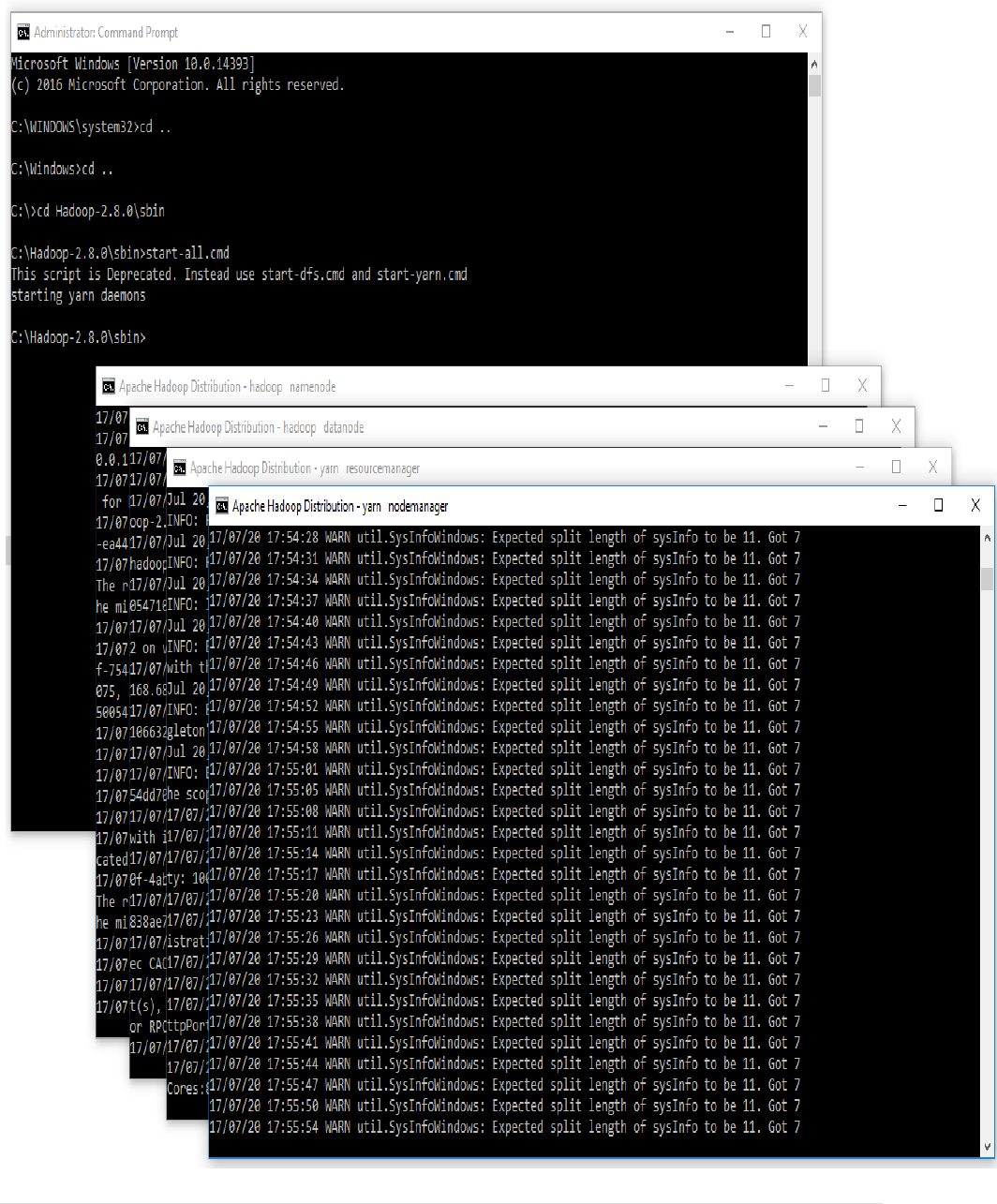
10) Open cmd and change directory to "C:\Hadoop-2.8.0\sbin" and type "start-

all.cmd" to start apache.

11) Make sure these apps are running.

a) Name node

b)Hadoop data node

c) YARN Resource Manager

d)YARN Node Manager hadoop nodes

12) Open: http://localhost:8088

13) Open: http://localhost:50070

CP5261 DATA ANALYTICS LABORATORY MANUAL

6 | DR. D. SENTHIL KUMAR (AP/CSE) UCE, ANNA UNIVERSITY- BITCAMPUS TRICHY

Ex. No: 2

Date:

Implementation of word count programs using MapReduce

Procedure:

Prepare:

1. Download MapReduceClient.jar

(Link: https://github.com/MuhammadBilalYar/HADOOP-

INSTALLATION-ON-WINDOW-10/blob/master/MapReduceClient.jar)

2. Download Input_file.txt

(Link: https://github.com/MuhammadBilalYar/HADOOP-

INSTALLATION-ON-WINDOW-10/blob/master/input_file.txt)

Place both files in "C:/"

Hadoop Operation:

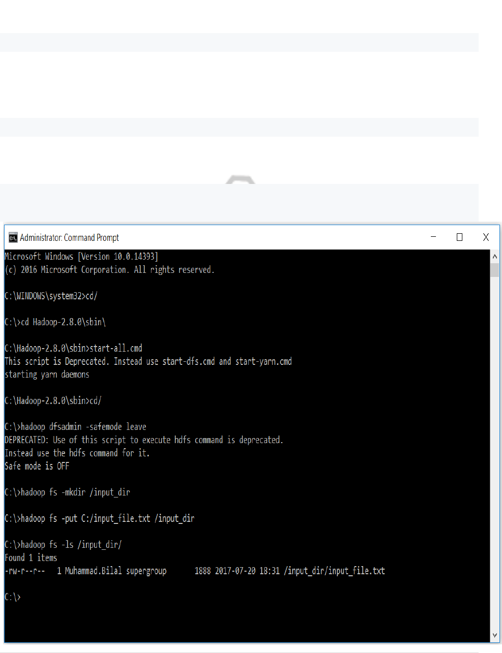
1. Open cmd in Administrative mode and move to "C:/Hadoop-2.8.0/sbin" and

start cluster

Start-all.cmd

CP5261 DATA ANALYTICS LABORATORY MANUAL

7 | DR. D. SENTHIL KUMAR (AP/CSE) UCE, ANNA UNIVERSITY- BITCAMPUS TRICHY

CP5261 DATA ANALYTICS LABORATORY MANUAL

8 | DR. D. SENTHIL KUMAR (AP/CSE) UCE, ANNA UNIVERSITY- BITCAMPUS TRICHY

2. Create an input directory in HDFS.

hadoop fs -mkdir /input_dir

3. Copy the input text file named input_file.txt in the input directory (input_dir)

of HDFS.

hadoop fs -put C:/input_file.txt /input_dir

4. Verify input_file.txt available in HDFS input directory (input_dir).

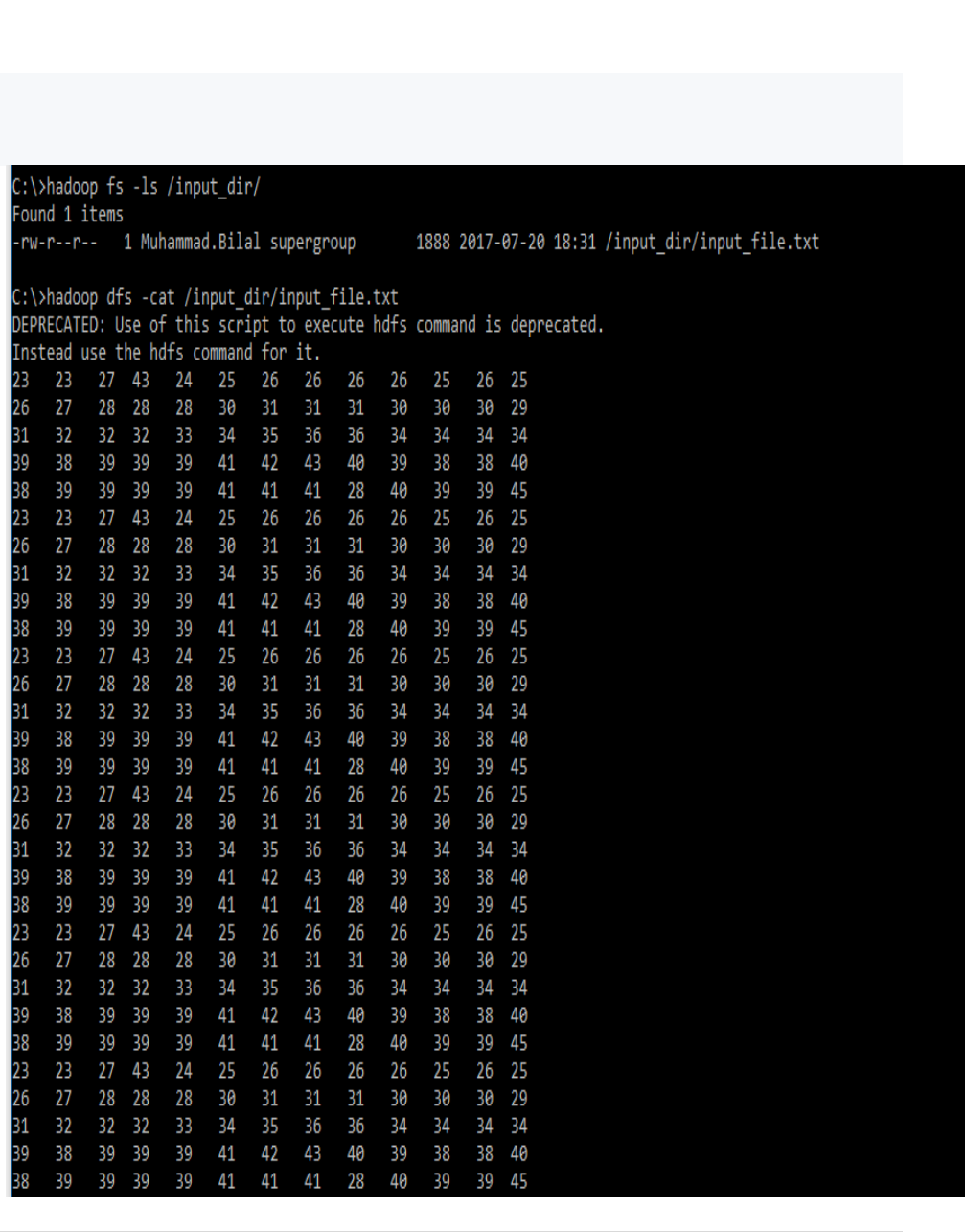
hadoop fs -ls /input_dir/

CP5261 DATA ANALYTICS LABORATORY MANUAL

9 | DR. D. SENTHIL KUMAR (AP/CSE) UCE, ANNA UNIVERSITY- BITCAMPUS TRICHY

5. Verify content of the copied file.

hadoop dfs -cat /input_dir/input_file.txt

CP5261 DATA ANALYTICS LABORATORY MANUAL

10 | DR. D. SENTHIL KUMAR (AP/CSE) UCE, ANNA UNIVERSITY- BITCAMPUS TRICHY

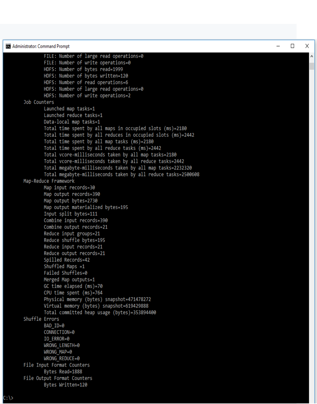
6. Run MapReduceClient.jar and also provide input and out directories.

hadoop jar C:/MapReduceClient.jar wordcount /input_dir /output_dir

CP5261 DATA ANALYTICS LABORATORY MANUAL

11 | DR. D. SENTHIL KUMAR (AP/CSE) UCE, ANNA UNIVERSITY- BITCAMPUS TRICHY

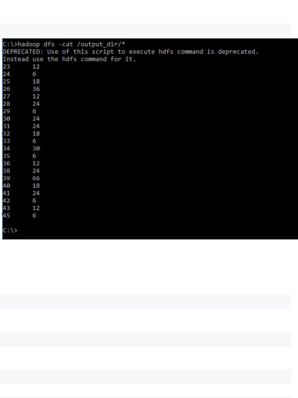
7. Verify content for generated output file.

hadoop dfs -cat /output_dir/*

Some Other useful commands

8) To leave Safe mode

hadoop dfsadmin –safemode leave

9) To delete file from HDFS directory

hadoop fs -rm -r /iutput_dir/input_file.txt

10) To delete directory from HDFS directory

hadoop fs -rm -r /iutput_dir

CP5261 DATA ANALYTICS LABORATORY MANUAL

12 | DR. D. SENTHIL KUMAR (AP/CSE) UCE, ANNA UNIVERSITY- BITCAMPUS TRICHY

CP5261 DATA ANALYTICS LABORATORY MANUAL

13 | DR. D. SENTHIL KUMAR (AP/CSE) UCE, ANNA UNIVERSITY- BITCAMPUS TRICHY

Ex. No: 3

Date:

Implementation of an MR program that processes a weather dataset

Aim:

Program

AverageMapper.java

import org.apache.hadoop.io.*;

import org.apache.hadoop.mapreduce.*;

import java.io.IOException;

public class AverageMapper extends Mapper <LongWritable, Text, Text, IntWritable>

{

public static final int MISSING = 9999;

public void map(LongWritable key, Text value, Context context) throws

IOException, InterruptedException

{

String line = value.toString();

String year = line.substring(15,19);

int temperature;

if (line.charAt(87)=='+')

temperature = Integer.parseInt(line.substring(88, 92));

else

temperature = Integer.parseInt(line.substring(87, 92));

String quality = line.substring(92, 93);

if(temperature != MISSING && quality.matches("[01459]"))

context.write(new Text(year),new IntWritable(temperature));

}

CP5261 DATA ANALYTICS LABORATORY MANUAL

14 | DR. D. SENTHIL KUMAR (AP/CSE) UCE, ANNA UNIVERSITY- BITCAMPUS TRICHY

}

AverageReducer.java

import org.apache.hadoop.mapreduce.*;

import java.io.IOException;

public class AverageReducer extends Reducer <Text, IntWritable,Text, IntWritable >

{

public void reduce(Text key, Iterable<IntWritable> values, Context context) throws IOException,

InterruptedException

{

int max_temp = 0;

int count = 0;

for (IntWritable value : values)

{

max_temp += value.get();

count+=1;

}

context.write(key, new IntWritable(max_temp/count));

} }

AverageDriver.java

import org.apache.hadoop.io.*;

import org.apache.hadoop.fs.*;

import org.apache.hadoop.mapreduce.*;

import org.apache.hadoop.mapreduce.lib.input.FileInputFormat;

import org.apache.hadoop.mapreduce.lib.output.FileOutputFormat;

public class AverageDriver

{

CP5261 DATA ANALYTICS LABORATORY MANUAL

15 | DR. D. SENTHIL KUMAR (AP/CSE) UCE, ANNA UNIVERSITY- BITCAMPUS TRICHY

public static void main (String[] args) throws Exception

{

if (args.length != 2)

{

System.err.println("Please Enter the input and output parameters");

System.exit(-1);

}

Job job = new Job();

job.setJarByClass(AverageDriver.class);

job.setJobName("Max temperature");

FileInputFormat.addInputPath(job,new Path(args[0]));

FileOutputFormat.setOutputPath(job,new Path (args[1]));

job.setMapperClass(AverageMapper.class);

job.setReducerClass(AverageReducer.class);

job.setOutputKeyClass(Text.class);

job.setOutputValueClass(IntWritable.class);

System.exit(job.waitForCompletion(true)?0:1);

}

CP5261 DATA ANALYTICS LABORATORY MANUAL

16 | DR. D. SENTHIL KUMAR (AP/CSE) UCE, ANNA UNIVERSITY- BITCAMPUS TRICHY

R – PROGRAMMING INTRODUCTION AND BASICS

 What is R?

 R Data Types & Operator

 R Matrix Tutorial: Create, Print, Add Column, Slice

 What is Factor in R? Categorical & Continuous

 R Data Frames: Create, Append, Select, Subset

 Lists in R: Create, Select [Example]

 If, Else, Elif Statement in R

 For Loop Syntax and Examples

 While Loop In R With Example

 Apply(), Sapply(), Tapply() in R With Examples

 Import Data into R: Read Csv, Excel, SPSS, STATA, SAS Files

 R Exporting Data to Csv, Excel, STATA, SAS and Text File

 R Select(), Filter(), Arrange():

WHAT IS R?

R is a programming language developed by Ross Ihaka and Robert Gentleman in 1993. R

possesses an extensive catalog of statistical and graphical methods. It includes machine learning

algorithm, linear regression, time series, statistical inference to name a few. Most of the R libraries

are written in R, but for heavy computational task, C, C++ and Fortran codes are preferred. R is

not only entrusted by academic, but many large companies also use R programming language,

including Uber, Google, Airbnb, Facebook and so on.

Data analysis with R is done in a series of steps; programming, transforming, discovering,

modeling and communicate the results

 Program: R is a clear and accessible programming tool

 Transform: R is made up of a collection of libraries designed specifically for data science

EX. NO: 4.A

R – PROGRAMMING INTRODUCTION AND BASICS

CP5261 DATA ANALYTICS LABORATORY MANUAL

17 | DR. D. SENTHIL KUMAR (AP/CSE) UCE, ANNA UNIVERSITY- BITCAMPUS TRICHY

 Discover: Investigate the data, refine your hypothesis and analyze them

 Model: R provides a wide array of tools to capture the right model for your data

 Communicate: Integrate codes, graphs, and outputs to a report with R Markdown or build

 Shiny apps to share with the world

What is R used for?

 Statistical inference

 Data analysis

 Machine learning algorithm

R DATA TYPES & OPERATOR

Basic data types

 R works with numerous data types, including

 Scalars

 Vectors (numerical, character, logical)

 Matrices

 Data frames

 Lists

Basics types

 4.5 is a decimal value called numerics.

 4 is a natural value called integers. Integers are also numerics.

 TRUE or FALSE is a Boolean value called logical.

 The value inside " " or ' ' are text (string). They are called characters.

 We can check the type of a variable with the class function

Data Types

R Code

Output

# Numeric

x <‐ 28

class(x)

## [1] "numeric"

# String

y <‐ "R is Fantastic"

class(y)

## [1] "character"

# Boolean

z <‐ TRUE

class(z)

## [1] "logical"

CP5261 DATA ANALYTICS LABORATORY MANUAL

18 | DR. D. SENTHIL KUMAR (AP/CSE) UCE, ANNA UNIVERSITY- BITCAMPUS TRICHY

Variables

Variables store values and are an important component in programming, especially for a

data scientist. A variable can store a number, an object, a statistical result, vector, dataset, a model

prediction basically anything R outputs. We can use that variable later simply by calling the name

of the variable. To declare a variable, we need to assign a variable name. The name should not

have space. We can use _ to connect to words. To add a value to the variable, use <- or =.

SYNTAX:

SYNTAX

RCODE

OUTPUT

# First way to declare a variable: use the `<‐`

name_of_variable <‐ value

# Second way to declare a variable: use the

`=`

name_of_variable = value

# Print variable x

x <‐ 42

## [1] 42

y <‐ 10

## [1] 10

# We call x and y and apply a

subtraction

x‐y

## [1] 32

Vectors

A vector is a one-dimensional array. We can create a vector with all the basic data type

we learnt before. The simplest way to build a vector in R, is to use the c command.

Vectors

Type – Rcode

OUTPUT

# Numerical

vec_num <‐ c(1, 10, 49)

vec_num

## [1] 1 10 49

# Character

vec_chr <‐ c("a", "b", "c")

vec_chr

## [1] "a" "b" "c"

# Boolean

vec_bool <‐ c(TRUE, FALSE, TRUE)

vec_bool

##[1] TRUE FALSE TRUE

# Create the

vectors

vect_1 <‐ c(1, 3, 5)

vect_2 <‐ c(2, 4, 6)

# Take the sum of A_vector and B_vector

[1] 3 7 11

CP5261 DATA ANALYTICS LABORATORY MANUAL

19 | DR. D. SENTHIL KUMAR (AP/CSE) UCE, ANNA UNIVERSITY- BITCAMPUS TRICHY

sum_vect <‐ vect_1 + vect_2

# Print out total_vector

sum_vect

# Slice the

first 5 rows

of the vector

slice_vector <‐ c(1,2,3,4,5,6,7,8,9,10)

slice_vector[1:5]

## [1] 1 2 3 4 5

# Faster way

to create

adjacent

values

c(1:10)

## [1] 1 2 3 4 5 6 7 8 9

Operator Description

RCode

OUTPUT

Arithmetic

+ Addition

- Subtraction

* Multiplication

/ Division

^ or ** Exponentiation

3 + 4

4-2

3*5

(5+5)/2

2^5

## [1] 7

## [1] 2

## [1] 15

## [1] 5

## [1] 32

Logical

logical_vector <‐ c(1:10)

logical_vector>5

logical_vector[(logical_vector>5)]

## [1]FALSE FALSE

FALSE FALSE FALSE

TRUE TRUE TRUE TRUE

TRUE

## [1] 6 7 8 9 10

# Print 5 and 6

logical_vector <‐ c(1:10)

logical_vector[(logical_vector>4) &

(logical_vector<7)]

## [1] 5 6

R MATRIX TUTORIAL: CREATE, PRINT, ADD COLUMN, SLICE

What is a Matrix?

A matrix is a 2-dimensional array that has m number of rows and n number of columns.

In other words, matrix is a combination of two or more vectors with the same data type. Note: It

is possible to create more than two dimensions arrays with R.

SYNTAX: matrix(data, nrow, ncol, byrow = FALSE) Arguments:

CP5261 DATA ANALYTICS LABORATORY MANUAL

20 | DR. D. SENTHIL KUMAR (AP/CSE) UCE, ANNA UNIVERSITY- BITCAMPUS TRICHY

 ‐ data: The collection of elements that R will arrange into the rows and columns

of the matrix

 ‐ nrow: Number of rows

 ‐ ncol: Number of columns

 ‐ byrow: The rows are filled from the left to the right. We use `byrow = FALSE`

(default values), if we want the matrix to be filled by the columns i.e. the values

are filled top to bottom.

# Construct a matrix

with 5 rows that

contain the numbers

1 up to 10 and byrow

= TRUE

matrix_a <‐matrix(1:10, byrow = TRUE,

nrow = 5)

matrix_a

# Print dimension of

the matrix

dim(matrix_a)

## [1] 5 2

# Construct a matrix

with 5 rows that

contain the numbers

1 up to 10 and byrow

= FALSE

matrix_b <‐matrix(1:10, byrow =

FALSE, nrow = 5)

matrix_b

matrix_c <‐matrix(1:12, byrow =

FALSE, ncol = 3)

matrix_c

## [,1] [,2] [,3]

## [1,] 1 5 9

## [2,] 2 6 10

## [3,] 3 7 11

## [4,] 4 8 12

# concatenate c(1:5)

to the matrix_a

matrix_a1 <‐ cbind(matrix_a, c(1:5))

# Check the dimension

dim(matrix_a1)

## [1] 5 3

Slice a Matrix

We can select elements one or many elements from a matrix by using the square brackets

[ ]. This is where slicing comes into the picture.

For example:

 matrix_c[1,2] selects the element at the first row and second column.

 matrix_c[1:3,2:3] results in a matrix with the data on the rows 1, 2, 3 and columns 2, 3,

CP5261 DATA ANALYTICS LABORATORY MANUAL

21 | DR. D. SENTHIL KUMAR (AP/CSE) UCE, ANNA UNIVERSITY- BITCAMPUS TRICHY

 matrix_c[,1] selects all elements of the first column.

 matrix_c[1,] selects all elements of the first row.

WHAT IS FACTOR IN R? CATEGORICAL & CONTINUOUS

What is Factor in R?

Factors are variables in R which take on a limited number of different values; such

variables are often referred to as categorical variables. In a dataset, we can distinguish two types

of variables: categorical and continuous. In a categorical variable, the value is limited and usually

based on a particular finite group. For example, a categorical variable can be countries, year,

gender, occupation. A continuous variable, however, can take any values, from integer to decimal.

For example, we can have the revenue, price of a share, etc..

Categorical variables

R stores categorical variables into a factor. Let's check the code below to convert a

character variable into a factor variable. Characters are not supported in machine learning

algorithm, and the only way is to convert a string to an integer.

SYNTAX:

RCODE:

# Create gender vector

gender_vector <‐ c("Male", "Female", "Female", "Male", "Male")

class(gender_vector)

# Convert gender_vector to a factor

CP5261 DATA ANALYTICS LABORATORY MANUAL

22 | DR. D. SENTHIL KUMAR (AP/CSE) UCE, ANNA UNIVERSITY- BITCAMPUS TRICHY

factor_gender_vector <‐factor(gender_vector)

class(factor_gender_vector)

OUTPUT:

## [1] "character"

## [1] "factor"

Nominal categorical variable

A categorical variable has several values but the order does not matter. For instance, male

or female categorical variable do not have ordering.

RCODE:

# Create a color vector

color_vector <‐ c('blue', 'red', 'green', 'white', 'black', 'yellow')

# Convert the vector to factor

factor_color <‐ factor(color_vector)

factor_color

OUTPUT:

## [1] blue red green white black yellow

## Levels: black blue green red white yellow

Ordinal categorical variable

Ordinal categorical variables do have a natural ordering. We can specify the order, from

the lowest to the highest with order = TRUE and highest to lowest with order = FALSE. We can

use summary to count the values for each factor.

RCODE:

# Create Ordinal categorical vector

day_vector <‐ c('evening', 'morning', 'afternoon', 'midday', 'midnight', 'evening')

# Convert `day_vector` to a factor with ordered level

CP5261 DATA ANALYTICS LABORATORY MANUAL

23 | DR. D. SENTHIL KUMAR (AP/CSE) UCE, ANNA UNIVERSITY- BITCAMPUS TRICHY

factor_day <‐ factor(day_vector, order = TRUE, levels =c('morning', 'midday',

'afternoon', 'evening', 'midnight'))

# Print the new variable

factor_day

OUTPUT:

## [1] evening morning afternoon midday

midnight evening

## Levels: morning < midday < afternoon < evening < midnight

# Append the line to above code

# Count the number of occurence of each level

summary(factor_day)

## Morning midday afternoon evening midnight

## 1 1 1 2 1

Continuous variables

Continuous class variables are the default value in R. They are stored as numeric or integer.

We can see it from the dataset below. mtcars is a built-in dataset. It gathers information on different

types of car. We can import it by using mtcars and check the class of the variable mpg, mile per

gallon. It returns a numeric value, indicating a continuous variable.

RCODE:

dataset <‐ mtcars

class(dataset)

OUTPUT:

## [1] "numeric"

R DATA FRAMES: CREATE, APPEND, SELECT, SUBSET

What is a Data Frame?

A data frame is a list of vectors which are of equal length. A matrix contains only one

type of data, while a data frame accepts different data types (numeric, character, factor, etc.).

CP5261 DATA ANALYTICS LABORATORY MANUAL

24 | DR. D. SENTHIL KUMAR (AP/CSE) UCE, ANNA UNIVERSITY- BITCAMPUS TRICHY

SYNTAX:

Create a data frame

RCODE:

# Create a, b, c, d variables

a <‐ c(10,20,30,40)

b <‐ c('book', 'pen', 'textbook', 'pencil_case')

c <‐ c(TRUE,FALSE,TRUE,FALSE)

d <‐ c(2.5, 8, 10, 7)

# Join the variables to create a data frame

df <‐ data.frame(a,b,c,d)

OUTPUT:

## a b c d

## 1 1 book TRUE 2.5

## 2 2 pen TRUE 8.0

## 3 3 textbook TRUE 10.0

## 4 4 pencil_case FALSE 7.0

# Name the data frame

names(df) <‐ c('ID', 'items', 'store', 'price')

OUTPUT:

## ID items store price

## 1 10 book TRUE 2.5

## 2 20 pen FALSE 8.0

## 3 30 textbook TRUE 10.0

## 4 40 pencil_case FALSE 7.0

# Print the structure

str(df)

CP5261 DATA ANALYTICS LABORATORY MANUAL

25 | DR. D. SENTHIL KUMAR (AP/CSE) UCE, ANNA UNIVERSITY- BITCAMPUS TRICHY

OUTPUT:

## 'data.frame': 4 obs. of 4 variables:

## $ ID : num 10 20 30 40

## $ items: Factor w/ 4 levels "book","pen","pencil_case",..: 1 2 4 3

## $ store: logi TRUE FALSE TRUE FALSE

## $ price: num 2.5 8 10 7

Slice Data Frame

It is possible to SLICE values of a Data Frame. We select the rows and columns to return

into bracket precede by the name of the data frame.

RCODE:

## Select Rows 1 to 3 and columns 3 to 4

df[1:3, 3:4]

OUTPUT:

## store price

## 1 TRUE 2.5

## 2 FALSE 8.0

## 3 TRUE 10.0

Append a Column to Data Frame

You can also append a column to a Data Frame. You need to use the symbol $ to append

a new Variable.

RCODE:

# Create a new vector

quantity <‐ c(10, 35, 40, 5)

# Add `quantity` to the `df` data frame

df$quantity <‐ quantity

OUTPUT:

## ID items store price quantity

## 1 10 book TRUE 2.5 10

## 2 20 pen FALSE 8.0 35

## 3 30 textbook TRUE 10.0 40

## 4 40 pencil_case FALSE 7.0 5

CP5261 DATA ANALYTICS LABORATORY MANUAL

26 | DR. D. SENTHIL KUMAR (AP/CSE) UCE, ANNA UNIVERSITY- BITCAMPUS TRICHY

Note: The number of elements in the vector has to be equal to the no of elements in data frame. Executing the

following statement

RCODE:

quantity <‐ c(10, 35, 40)

# Add `quantity` to the `df` data frame

df$quantity <‐ quantity

Select a column of a data frame

Sometimes, we need to store a column of a data frame for future use or perform operation

on a column. We can use the $ sign to select the column from a data frame.

RCODE:

# Select the column ID

df$ID

OUTPUT:

## [1] 1 2 3 4

Subset a data frame

In the previous section, we selected an entire column without condition. It is possible to

subset based on whether or not a certain condition was true.

We use the subset() function.

SYNTAX:

We want to return only the items with price above 10, we can do

RCODE:

# Select price above 5

subset(df, subset = price > 5)

OUTPUT:

ID items store price

2 20 pen FALSE 8

3 30 textbook TRUE 10

CP5261 DATA ANALYTICS LABORATORY MANUAL

27 | DR. D. SENTHIL KUMAR (AP/CSE) UCE, ANNA UNIVERSITY- BITCAMPUS TRICHY

4 40 pencil_case FALSE 7

LISTS IN R: CREATE, SELECT [EXAMPLE]

What is a List?

A list is a great tool to store many kinds of object in the order expected. We can include

matrices, vectors data frames or lists. We can imagine a list as a bag in which we want to put many

different items. When we need to use an item, we open the bag and use it. A list is similar; we can

store a collection of objects and use them when we need them.

We can use list() function to create a list.

SYNTAX:

RCODE:

# Vector with numeric from 1 up to 5

vect <‐ 1:5

# A 2x 5 matrix

mat <‐ matrix(1:9, ncol = 5)

dim(mat)

# select the 10th row of the built‐in R data set EuStockMarkets

df <‐ EuStockMarkets[1:10,]

# Construct list with these vec, mat, and df:

my_list <‐ list(vect, mat, df)

my_list

CP5261 DATA ANALYTICS LABORATORY MANUAL

28 | DR. D. SENTHIL KUMAR (AP/CSE) UCE, ANNA UNIVERSITY- BITCAMPUS TRICHY

OUTPUT:

IF, ELSE, ELIF STATEMENT IN R

The if, else, ELIF statement

An if-else statement is a great tool for the developer trying to return an output based on a

condition.

SYNTAX:

if (condition1) {

expr1

} else it (condition2) {

expr2

} else if (condition3) {

expr3

} else {

expr4

}

VAT has different rate according to the product purchased. Imagine we have three different

kind of products with different VAT applied:

Categories Products VAT

A Book, magazine, newspaper, etc.. 8%

B Vegetable, meat, beverage, etc.. 10%

C Tee-shirt, jean, pant, etc.. 20%

We can write a chain to apply the correct VAT rate to the product a customer bought.

CP5261 DATA ANALYTICS LABORATORY MANUAL

29 | DR. D. SENTHIL KUMAR (AP/CSE) UCE, ANNA UNIVERSITY- BITCAMPUS TRICHY

RCODE:

category <‐ 'A'

price <‐ 10

if (category =='A'){

cat('A vat rate of 8% is applied.','The total price is',price *1.08)

} else if (category =='B'){

cat('A vat rate of 10% is applied.','The total price is',price *1.10)

} else {

cat('A vat rate of 20% is applied.','The total price is',price *1.20)

}

OUTPUT:

# A vat rate of 8% is applied. The total price is 10.8

FOR LOOP SYNTAX AND EXAMPLES

# Create fruit vector

fruit <‐ c('Apple', 'Orange', 'Passion fruit', 'Banana')

# Create the for statement

for ( i in fruit){

print(i)

}

OUTPUT:

## [1] "Apple"

## [1] "Orange"

## [1] "Passion fruit"

## [1] "Banana"

For Loop over a matrix

A matrix has 2-dimension, rows and columns. To iterate over a matrix, we have to define two for

loop, namely one for the rows and another for the column.

SYNTAX:

# Create a matrix

mat <‐ matrix(data = seq(10, 20, by=1), nrow = 6, ncol =2)

# Create the loop with r and c to iterate over the matrix

CP5261 DATA ANALYTICS LABORATORY MANUAL

30 | DR. D. SENTHIL KUMAR (AP/CSE) UCE, ANNA UNIVERSITY- BITCAMPUS TRICHY

for (r in 1:nrow(mat))

for (c in 1:ncol(mat))

print(paste("Row", r, "and column",c, "have values of", mat[r,c]))

OUTPUT:

WHILE LOOP IN R WITH EXAMPLE

A loop is a statement that keeps running until a condition is satisfied. The syntax for a

while loop is the following:

SYNTAX:

#Create a variable with value 1

begin <‐ 1

#Create the loop

while (begin <= 10){

#See which we are

cat('This is loop number',begin)

#add 1 to the variable begin after each loop

begin <‐ begin+1

print(begin)

}

OUTPUT:

## This is loop number 1[1] 2

## This is loop number 2[1] 3

CP5261 DATA ANALYTICS LABORATORY MANUAL

31 | DR. D. SENTHIL KUMAR (AP/CSE) UCE, ANNA UNIVERSITY- BITCAMPUS TRICHY

## This is loop number 3[1] 4

## This is loop number 4[1] 5

## This is loop number 5[1] 6

## This is loop number 6[1] 7

## This is loop number 7[1] 8

## This is loop number 8[1] 9

## This is loop number 9[1] 10

## This is loop number 10[1] 11

APPLY(), SAPPLY(), TAPPLY() IN R WITH EXAMPLES

apply() function

We use apply() over a matrice. This function takes 5 arguments:

SYNTAX:

The simplest example is to sum a matrices over all the columns. The code apply(m1, 2,

sum) will apply the sum function to the matrix 5x6 and return the sum of each column accessible

in the dataset.

RCODE:

m1 <‐ matrix(C<‐(1:10),nrow=5, ncol=6)

a_m1 <‐ apply(m1, 2, sum)

a_m1

OUTPUT:

CP5261 DATA ANALYTICS LABORATORY MANUAL

32 | DR. D. SENTHIL KUMAR (AP/CSE) UCE, ANNA UNIVERSITY- BITCAMPUS TRICHY

lapply() function

SYNTAX:

l in lapply() stands for list. The difference between lapply() and apply() lies between the

output return. The output of lapply() is a list. lapply() can be used for other objects like data frames

and lists. lapply() function does not need MARGIN.

A very easy example can be to change the string value of a matrix to lower case with to

lower function. We construct a matrix with the name of the famous movies. The name is in upper

case format.

RCODE:

movies <‐ c("SPYDERMAN","BATMAN","VERTIGO","CHINATOWN")

movies_lower <‐lapply(movies, tolower)

str(movies_lower)

We can use unlist() to convert the list into a vector.

movies_lower <‐unlist(lapply(movies,tolower))

str(movies_lower)

OUTPUT:

## List of 4

## $:chr"spyderman"

CP5261 DATA ANALYTICS LABORATORY MANUAL

33 | DR. D. SENTHIL KUMAR (AP/CSE) UCE, ANNA UNIVERSITY- BITCAMPUS TRICHY

## $:chr"batman"

## $:chr"vertigo"

## $:chr"chinatown"

## chr [1:4] "spyderman" "batman" "vertigo" "chinatown"

sapply() function

SYNTAX:

sapply() function does the same jobs as lapply() function but returns a vector.

We can measure the minimum speed and stopping distances of cars from the cars dataset.

RCODE:

dt <‐ cars

lmn_cars <‐ lapply(dt, min)

smn_cars <‐ sapply(dt, min)

lmn_cars

smn_cars

lmxcars <‐ lapply(dt, max)

smxcars <‐ sapply(dt, max)

lmxcars

smxcars

We can use a user built-in function into lapply() or sapply(). We create a function

named avg to compute the average of the minimum and maximum of the vector.

avg <‐ function(x) {

( min(x) + max(x) ) / 2}

fcars <‐ sapply(dt, avg)

fcars

OUTPUT:

## $speed

## [1] 4

## $dist

## [1] 2

## speed dist

## 4 2

CP5261 DATA ANALYTICS LABORATORY MANUAL

34 | DR. D. SENTHIL KUMAR (AP/CSE) UCE, ANNA UNIVERSITY- BITCAMPUS TRICHY

## $speed

## [1] 25

## $dist

## [1] 120

## speed dist

## 25 120

## speed dist

## 14.5 61.0

Function

Arguments

Objective

Input

Output

apply

apply(x,

MARGIN, FUN)

Apply a function

to the rows or

columns or both

Data frame or

matrix

vector, list,

array

lapply

lapply(X, FUN)

Apply a function

to all the

elements of the

input

List, vector or

data frame

list

sapply

sappy(X FUN)

Apply a function

to all the

elements of the

input

List, vector or

data frame

vector or

matrix

Slice vector

We can use lapply() or sapply() interchangeable to slice a data frame. We create a function,

below_average(), that takes a vector of numerical values and returns a vector that only contains

the values that are strictly above the average. We compare both results with the identical() function.

RCODE:

below_ave <‐ function(x) {

ave <‐ mean(x)

return(x[x > ave])

}

dt_s<‐ sapply(dt, below_ave)

CP5261 DATA ANALYTICS LABORATORY MANUAL

35 | DR. D. SENTHIL KUMAR (AP/CSE) UCE, ANNA UNIVERSITY- BITCAMPUS TRICHY

dt_l<‐ lapply(dt, below_ave)

identical(dt_s, dt_l)

OUTPUT:

## [1] TRUE

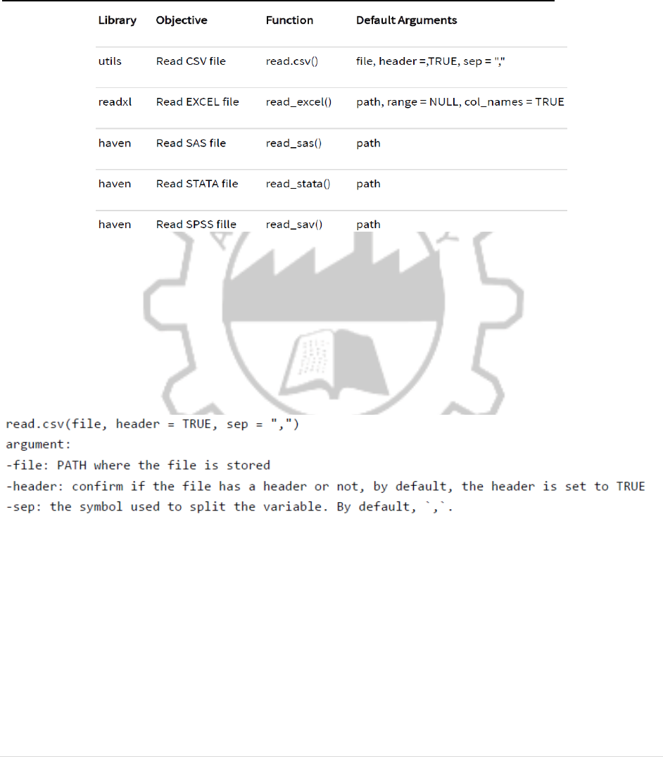
IMPORT DATA INTO R: READ CSV, EXCEL, SPSS, STATA, SAS FILES

Read CSV

One of the most widely data store is the .csv (comma-separated values) file formats. R

loads an array of libraries during the start-up, including the utils package. This package is

convenient to open csv files combined with the reading.csv () function.

SYNTAX:

RCODE:

PATH <‐

'https://raw.githubusercontent.com/vincentarelbundock/Rdatasets/master/csv/datasets/m

ars.csv'

df <‐ read.csv(PATH, header = TRUE, sep = ',', stringsAsFactors =FALSE)

length(df)

class(df$X)

CP5261 DATA ANALYTICS LABORATORY MANUAL

36 | DR. D. SENTHIL KUMAR (AP/CSE) UCE, ANNA UNIVERSITY- BITCAMPUS TRICHY

OUTPUT:

## [1] 12

## [1] "factor"

Read Excel files

Excel files are very popular among data analysts. Spreadsheets are easy to work with and

flexible. R is equipped with a library readxl to import Excel spreadsheet.

SYNTAX:

RCODE:

require(readxl)

library(readxl)

readxl_example()

readxl_example("geometry.xls")

We can import the spreadsheets from the readxl library and count the number of columns in the first sheet.

# Store the path of `datasets.xlsx`

example <‐ readxl_example("datasets.xlsx")

# Import the spreadsheet

df <‐ read_excel(example)

# Count the number of columns

length(df)

OUTPUT

## [1] 5

CP5261 DATA ANALYTICS LABORATORY MANUAL

37 | DR. D. SENTHIL KUMAR (AP/CSE) UCE, ANNA UNIVERSITY- BITCAMPUS TRICHY

Read excel_sheets()

The file datasets.xlsx is composed of 4 sheets. We can find out which sheets are available

in the workbook by using excel_sheets() function

RCODE:

example <‐ readxl_example("datasets.xlsx")

excel_sheets(example)

If a worksheet includes many sheets, it is easy to select a particular sheet by using the sheet

arguments. We can specify the name of the sheet or the sheet index. We can verify if both function

returns the same output with identical().

example <‐ readxl_example("datasets.xlsx")

quake <‐ read_excel(example, sheet = "quakes")

quake_1 <‐read_excel(example, sheet = 4)

identical(quake, quake_1)

OUTPUT:

[1] "iris" "mtcars" "chickwts" "quakes"

## [1] TRUE

R EXPORTING DATA TO CSV, EXCEL, SAS, STATA, AND TEXT FILE

Export to Hard drive

To begin with, you can save the data directly into the working directory. The following code

prints the path of your working directory:

RCODE:

directory <‐getwd()

directory

OUTPUT:

## [1] "/Users/15_Export_to_do"

Create data frame

First of all, let's import the mtcars dataset and get the mean of mpg and disp grouped by

gear

RCODE:

library(dplyr)

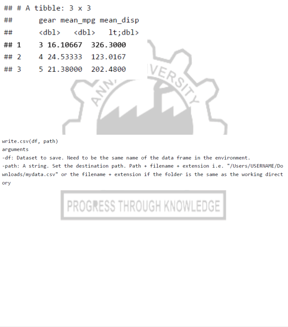
CP5261 DATA ANALYTICS LABORATORY MANUAL

38 | DR. D. SENTHIL KUMAR (AP/CSE) UCE, ANNA UNIVERSITY- BITCAMPUS TRICHY

df <‐mtcars % > %

select(mpg, disp, gear) % > %

group_by(gear) % > %

summarize(mean_mpg = mean(mpg), mean_disp = mean(disp))

OUTPUT:

The table contains three rows and three columns. You can create a CSV file with the function

write.csv().

Export CSV

SYNTAX:

RCODE:

write.csv(df, "table_car.csv")

Code Explanation

write.csv(df, "table_car.csv"): Create a CSV file in the hard drive:

df: name of the data frame in the environment

"table_car.csv": Name the file table_car and store it as csv

Note: You can use the function write.csv2() to separate the rows with a semicolon.

write.csv2(df, "table_car.csv")

Note: For pedagogical purpose only, we created a function called open_folder() to open the

directory folder for you. You just need to run the code below and see where the csv file is

stored. You should see a file names table_car.csv.

CP5261 DATA ANALYTICS LABORATORY MANUAL

39 | DR. D. SENTHIL KUMAR (AP/CSE) UCE, ANNA UNIVERSITY- BITCAMPUS TRICHY

# Run this code to create the function

RCODE:

open_folder <‐function(dir){

if (.Platform['OS.type'] == "windows"){

shell.exec(dir)

} else {

system(paste(Sys.getenv("R_BROWSER"), dir))

}

# Call the function to open the folder

open_folder(directory)

Export to Excel file

Export data to Excel is trivial for Windows users and trickier for Mac OS user.

Both users will use the library xlsx to create an Excel file. The slight difference comes

from the installation of the library. Indeed, the library xlsx uses Java to create the file.

Java needs to be installed if not present in your machine.

Windows users

If you are a Windows user, you can install the library directly with conda:

conda install ‐c r r‐xlsx

library(xlsx)

write.xlsx(df, "table_car.xlsx")

library(haven)

write_sav(df, "table_car.sav" ## spss file

write_sas(df, "table_car.sas7bdat")

write_dta(df, "table_car.dta") ## STATA File

save(df, file ='table_car.RData')

CP5261 DATA ANALYTICS LABORATORY MANUAL

40 | DR. D. SENTHIL KUMAR (AP/CSE) UCE, ANNA UNIVERSITY- BITCAMPUS TRICHY

R SELECT(), FILTER(), ARRANGE():

Verb

Objective

Code

Explanation

glimpse

check the structure of a df

glimpse(df)

Identical to str()

select()

Select/exclude the variables

select(df, A, B,C)

select(df, A:C)

select(df, ‐C)

Select the variables A, B and C

Select all variables from A to C

Exclude C

arrange()

Sort the dataset with one

or many variables

arrange(A)

arrange(desc (A), B)

Descending sort of variable A

and ascending sort of B

CP5261 DATA ANALYTICS LABORATORY MANUAL

41 | DR. D. SENTHIL KUMAR (AP/CSE) UCE, ANNA UNIVERSITY- BITCAMPUS TRICHY

EX. NO:4.b

DATE:

IMPLEMENT LINEAR AND LOGISTIC REGRESSION

AIM:

PROGRAM:

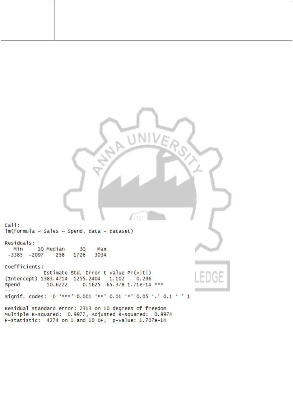
****SIMPLE LINEAR REGRESSION****

dataset = read.csv("data-marketing-budget-12mo.csv", header=T,

colClasses = c("numeric", "numeric", "numeric"))

head(dataset,5)

#/////Simple Regression/////

simple.fit = lm(Sales~Spend,data=dataset)

summary(simple.fit)

OUTPUT:

****MULTIPLE LINEAR REGRESSION ****

multi.fit = lm(Sales~Spend+Month, data=dataset)

summary(multi.fit)

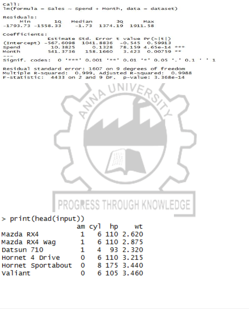
CP5261 DATA ANALYTICS LABORATORY MANUAL

42 | DR. D. SENTHIL KUMAR (AP/CSE) UCE, ANNA UNIVERSITY- BITCAMPUS TRICHY

MULTIPLE LINEAR REGRESSION OUTPUT:

****Logistic Regression ****

#selects some column from mtcars

input<- mtcars [,c("am","cyl","hp","wt")]

print(head(input))

input<- mtcars [,c("am","cyl","hp","wt")]

am.data =glm(formula = am ~ cyl+hp+wt,data = input,family = binomial)

print(summary(am.data))

OUTPUT:

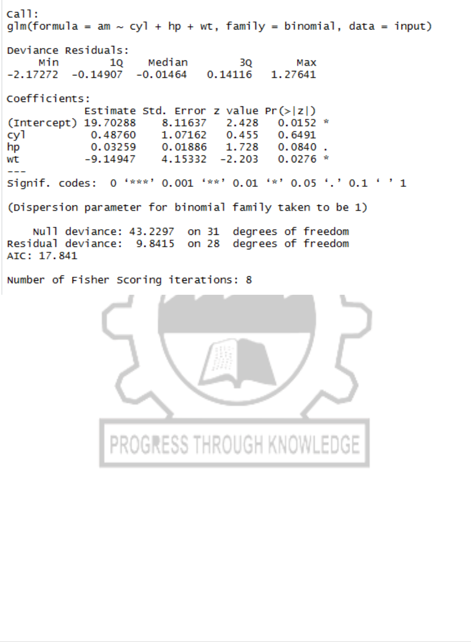
CP5261 DATA ANALYTICS LABORATORY MANUAL

43 | DR. D. SENTHIL KUMAR (AP/CSE) UCE, ANNA UNIVERSITY- BITCAMPUS TRICHY

RESULT:

CP5261 DATA ANALYTICS LABORATORY MANUAL

44 | DR. D. SENTHIL KUMAR (AP/CSE) UCE, ANNA UNIVERSITY- BITCAMPUS TRICHY

EX. NO: 5

DATE:

IMPLEMENT SVM CLASSIFICATION TECHNIQUES

AIM

To implement support vector machine (SVM) to find optimum hyper plane (Line in 2D, 3D

hyper plane) which maximize the margin between two classes.

Program

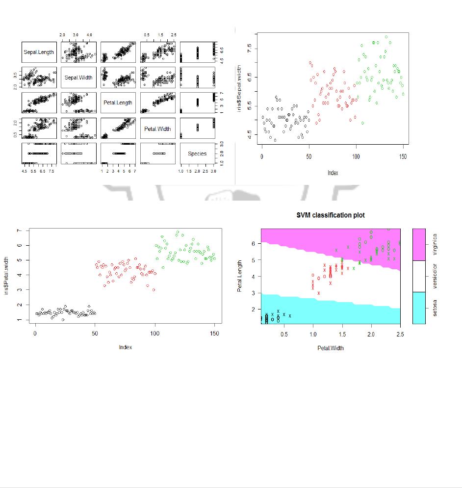
library(e1071)

plot(iris)

iris

plot(iris$Sepal.Length, iris$Sepal.width, col=iris$Species)

plot(iris$Petal.Length, iris$Petal.width, col=iris$Species)

s<-sample(150,100)

col<- c("Petal.Length", "Petal.Width", "Species")

iris_train<- iris[s,col]

iris_test<- iris[-s,col]

svmfit<- svm(Species ~., data = iris_train, kernel = "linear", cost = .1, scale = FALSE)

print(svmfit)

plot(svmfit, iris_train[,col])

tuned <- tune(svm, Species~., data = iris_train, kernel = "linear", ranges=

list(cost=c(0.001,0.01,.1,.1,10,100)))

summary(tuned)

CP5261 DATA ANALYTICS LABORATORY MANUAL

45 | DR. D. SENTHIL KUMAR (AP/CSE) UCE, ANNA UNIVERSITY- BITCAMPUS TRICHY

p<-predict(svmfit, iris_test[,col], type="class")

plot(p)

table(p,iris_test[,3] )

mean(p== iris_test[,3])

OUTPUT:

CP5261 DATA ANALYTICS LABORATORY MANUAL

46 | DR. D. SENTHIL KUMAR (AP/CSE) UCE, ANNA UNIVERSITY- BITCAMPUS TRICHY

RESULT:

CP5261 DATA ANALYTICS LABORATORY MANUAL

47 | DR. D. SENTHIL KUMAR (AP/CSE) UCE, ANNA UNIVERSITY- BITCAMPUS TRICHY

EX. NO:6

DATE:

IMPLEMENT DECISION TREE CLASSIFICATION

TECHNIQUES

AIM

To implement a decision tree used to representing a decision situation in visually and show all

those factors within the analysis that are considered relevant to the decision

PROGRAM

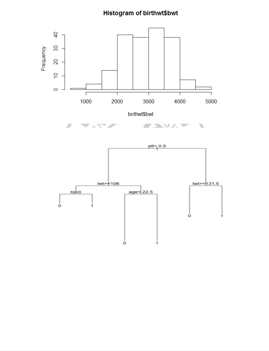
library(MASS)

library(rpart)

head(birthwt)

hist(birthwt$bwt)

table(birthwt$low)

cols <- c('low', 'race', 'smoke', 'ht', 'ui')

birthwt[cols] <- lapply(birthwt[cols], as.factor)

set.seed(1)

train<- sample(1:nrow(birthwt), 0.75 * nrow(birthwt))

birthwtTree<- rpart(low ~ . - bwt, data = birthwt[train, ], method = 'class')

plot(birthwtTree)

text(birthwtTree, pretty = 0)

summary(birthwtTree)

birthwtPred<- predict(birthwtTree, birthwt[-train, ], type = 'class')

table(birthwtPred, birthwt[-train, ]$low)

CP5261 DATA ANALYTICS LABORATORY MANUAL

48 | DR. D. SENTHIL KUMAR (AP/CSE) UCE, ANNA UNIVERSITY- BITCAMPUS TRICHY

OUTPUT:

RESULT

CP5261 DATA ANALYTICS LABORATORY MANUAL

49 | DR. D. SENTHIL KUMAR (AP/CSE) UCE, ANNA UNIVERSITY- BITCAMPUS TRICHY

EX. NO:7

DATE:

IMPLEMENTATION OF CLUSTERING TECHNIQUES

AIM:

PROGRAM:

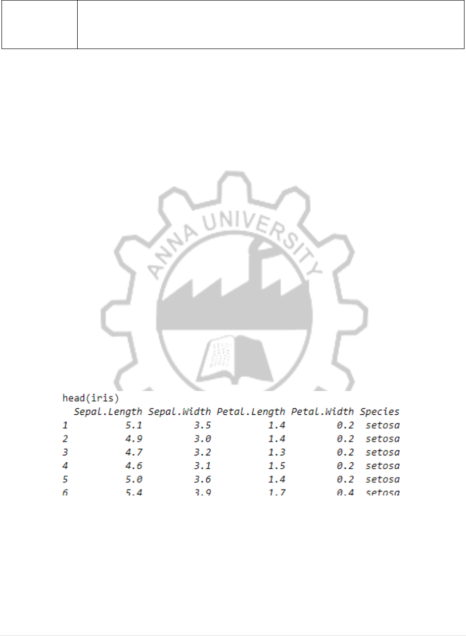
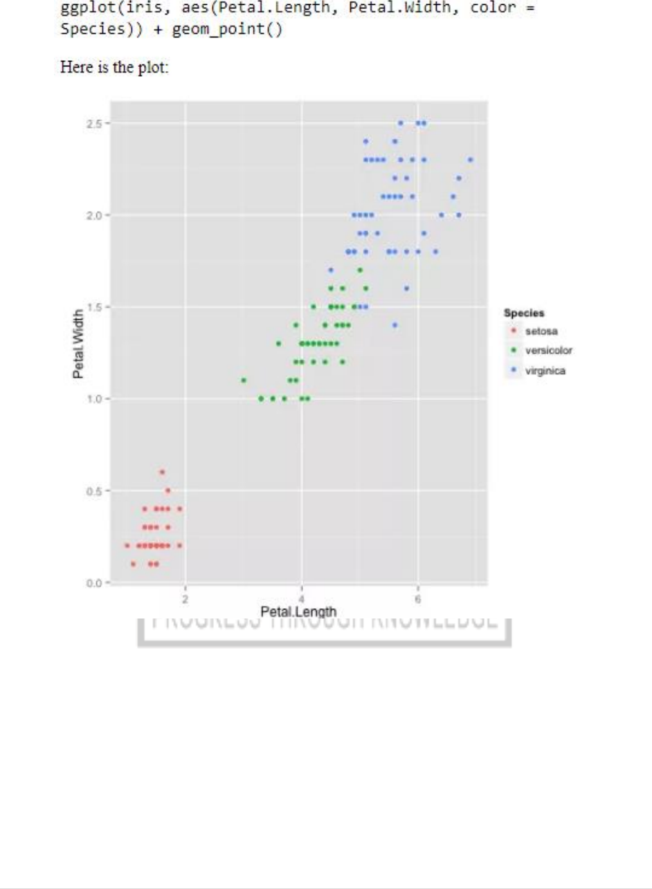
library(datasets)

head(iris)

library(ggplot2)

ggplot(iris, aes(Petal.Length, Petal.Width, color = Species)) + geom_point()

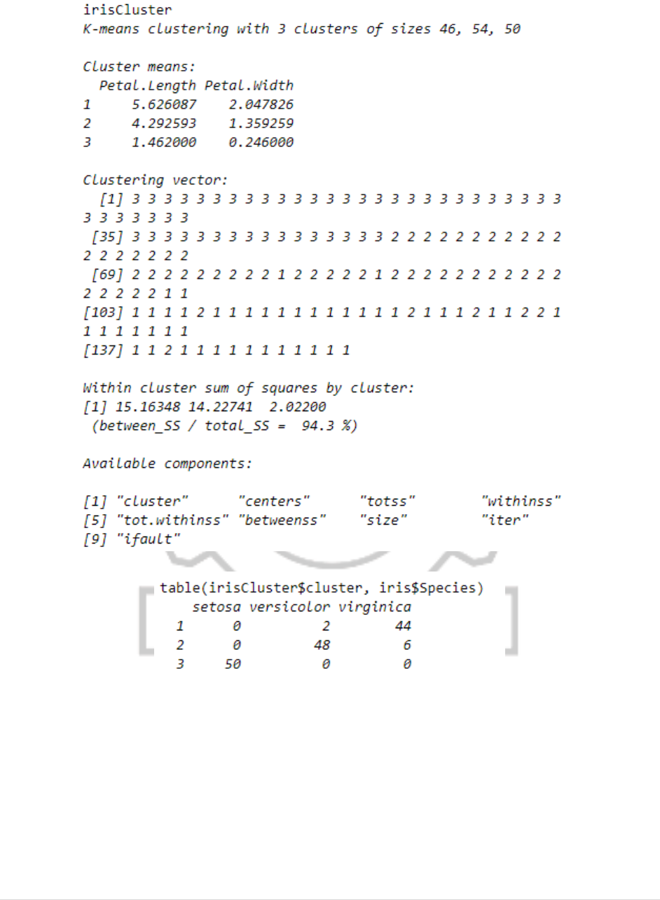
set.seed(20)

irisCluster <- kmeans(iris[, 3:4], 3, nstart = 20)

irisCluster

table(irisCluster$cluster, iris$Species)

OUTPUT:

CP5261 DATA ANALYTICS LABORATORY MANUAL

50 | DR. D. SENTHIL KUMAR (AP/CSE) UCE, ANNA UNIVERSITY- BITCAMPUS TRICHY

CP5261 DATA ANALYTICS LABORATORY MANUAL

51 | DR. D. SENTHIL KUMAR (AP/CSE) UCE, ANNA UNIVERSITY- BITCAMPUS TRICHY

RESULT:

CP5261 DATA ANALYTICS LABORATORY MANUAL

52 | DR. D. SENTHIL KUMAR (AP/CSE) UCE, ANNA UNIVERSITY- BITCAMPUS TRICHY

EX. NO:8

DATE:

IMPLEMENTATION OF VISUALIZE DATA USING ANY

PLOTTING FRAMEWORK

AIM

To implement Data visualization is to provide an efficient graphical display for summarizing

and reasoning about quantitative information.

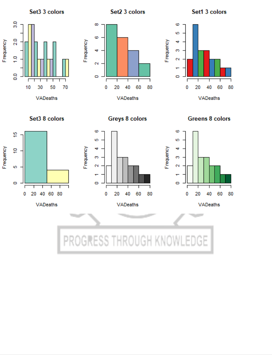
1. Histogram

Histogram is basically a plot that breaks the data into bins (or breaks) and shows frequency

distribution of these bins. You can change the breaks also and see the effect it has data visualization

in terms of understandability.

Note: We have used par(mfrow=c(2,5)) command to fit multiple graphs in same page for

sake of clarity( see the code below).

PROGRAM:

library(RColorBrewer)

data(VADeaths)

par(mfrow=c(2,3))

hist(VADeaths,breaks=10, col=brewer.pal(3,"Set3"),main="Set3 3 colors")

hist(VADeaths,breaks=3 ,col=brewer.pal(3,"Set2"),main="Set2 3 colors")

hist(VADeaths,breaks=7, col=brewer.pal(3,"Set1"),main="Set1 3 colors")

hist(VADeaths,,breaks= 2, col=brewer.pal(8,"Set3"),main="Set3 8 colors")

hist(VADeaths,col=brewer.pal(8,"Greys"),main="Greys 8 colors")

hist(VADeaths,col=brewer.pal(8,"Greens"),main="Greens 8 colors")

CP5261 DATA ANALYTICS LABORATORY MANUAL

53 | DR. D. SENTHIL KUMAR (AP/CSE) UCE, ANNA UNIVERSITY- BITCAMPUS TRICHY

OUTPUT:

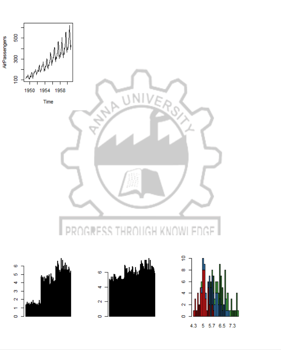
2.1. Line Chart

Below is the line chart showing the increase in air passengers over given time period. Line Charts

are commonly preferred when we are to analyses a trend spread over a time period. Furthermore,

line plot is also suitable to plots where we need to compare relative changes in quantities across

some variable (like time). Below is the code:

PROGRAM:

data(AirPassengers)

plot(AirPassengers,type="l") #Simple Line Plot

CP5261 DATA ANALYTICS LABORATORY MANUAL

54 | DR. D. SENTHIL KUMAR (AP/CSE) UCE, ANNA UNIVERSITY- BITCAMPUS TRICHY

OUTPUT:

2.2. Bar Chart

Bar Plots are suitable for showing comparison between cumulative totals across several groups.

Stacked Plots are used for bar plots for various categories. Here’s the code:

PROGRAM:

data("iris")

barplot(iris$Petal.Length) #Creating simple Bar Graph

barplot(iris$Sepal.Length,col = brewer.pal(3,"Set1"))

barplot(table(iris$Species,iris$Sepal.Length),col = brewer.pal(3,"Set1")) #Stacked Plot

OUTPUT:

CP5261 DATA ANALYTICS LABORATORY MANUAL

55 | DR. D. SENTHIL KUMAR (AP/CSE) UCE, ANNA UNIVERSITY- BITCAMPUS TRICHY

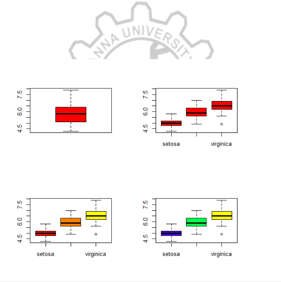
3. Box Plot

Box Plot shows 5 statistically significant numbers the minimum, the 25th percentile, the

median, the 75th percentile and the maximum. It is thus useful for visualizing the spread of the

data is and deriving inferences accordingly.

PROGRAM:

data(iris)

par(mfrow=c(2,2))

boxplot(iris$Sepal.Length,col="red")

boxplot(iris$Sepal.Length~iris$Species,col="red")

boxplot(iris$Sepal.Length~iris$Species,col=heat.colors(3))

boxplot(iris$Sepal.Length~iris$Species,col=topo.colors(3))

boxplot(iris$Petal.Length~iris$Species) #Creating Box Plot between two variable

OUTPUT:

CP5261 DATA ANALYTICS LABORATORY MANUAL

56 | DR. D. SENTHIL KUMAR (AP/CSE) UCE, ANNA UNIVERSITY- BITCAMPUS TRICHY

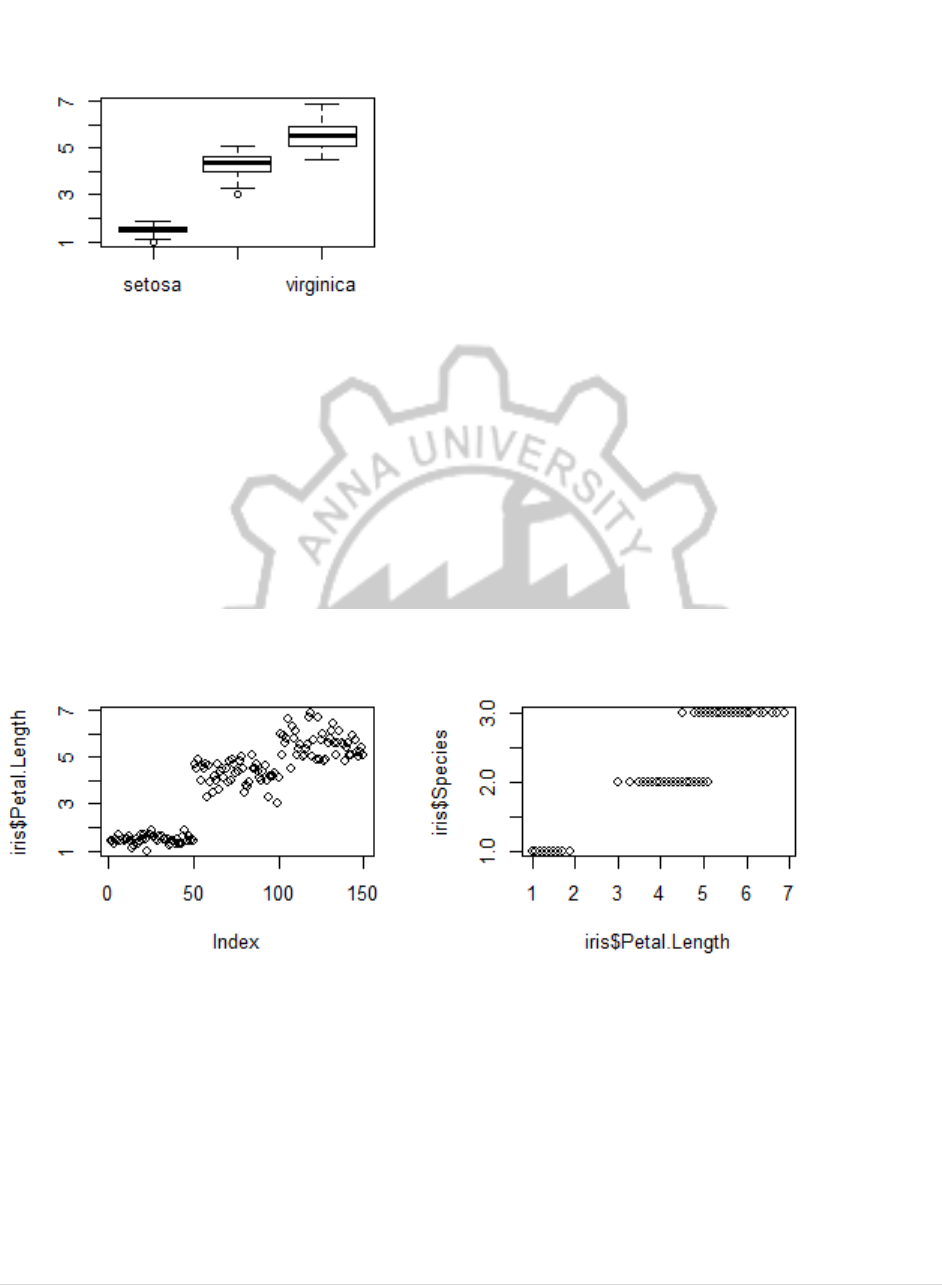
4. Scatter Plot (including 3D and other features)

Scatter plots help in visualizing data easily and for simple data inspection. Here’s the code for

simple scatter and multivariate scatter plot:

PROGRAM:

plot(x=iris$Petal.Length) #Simple Scatter Plot

plot(x=iris$Petal.Length,y=iris$Species) #Multivariate Scatter Plot

OUTPUT:

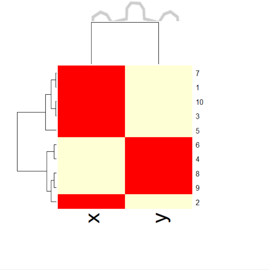
5. Heat Map

One of the most innovative data visualizations in R, the heat map emphasizes color

intensity to visualize relationships between multiple variables. The result is an attractive 2D image

that is easy to interpret. As a basic example, a heat map highlights the popularity of competing

items by ranking them according to their original market launch date. It breaks it down further by

providing sales statistics and figures over the course of time.

CP5261 DATA ANALYTICS LABORATORY MANUAL

57 | DR. D. SENTHIL KUMAR (AP/CSE) UCE, ANNA UNIVERSITY- BITCAMPUS TRICHY

PROGRAM:

# simulate a dataset of 10 points

x<‐rnorm(10,mean=rep(1:5,each=2),sd=0.7)

y<‐rnorm(10,mean=rep(c(1,9),each=5),sd=0.1)

dataFrame<‐data.frame(x=x,y=y)

set.seed(143)

dataMatrix<‐as.matrix(dataFrame)[sample(1:10),] # convert to class 'matrix', then shuffle the

rows of the matrix

heatmap(dataMatrix) # visualize hierarchical clustering via a heatmap

OUTPUT:

CP5261 DATA ANALYTICS LABORATORY MANUAL

58 | DR. D. SENTHIL KUMAR (AP/CSE) UCE, ANNA UNIVERSITY- BITCAMPUS TRICHY

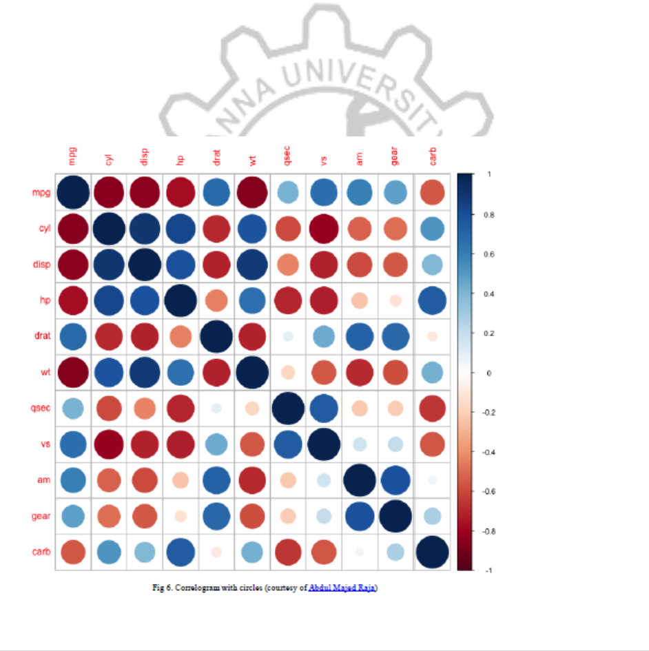
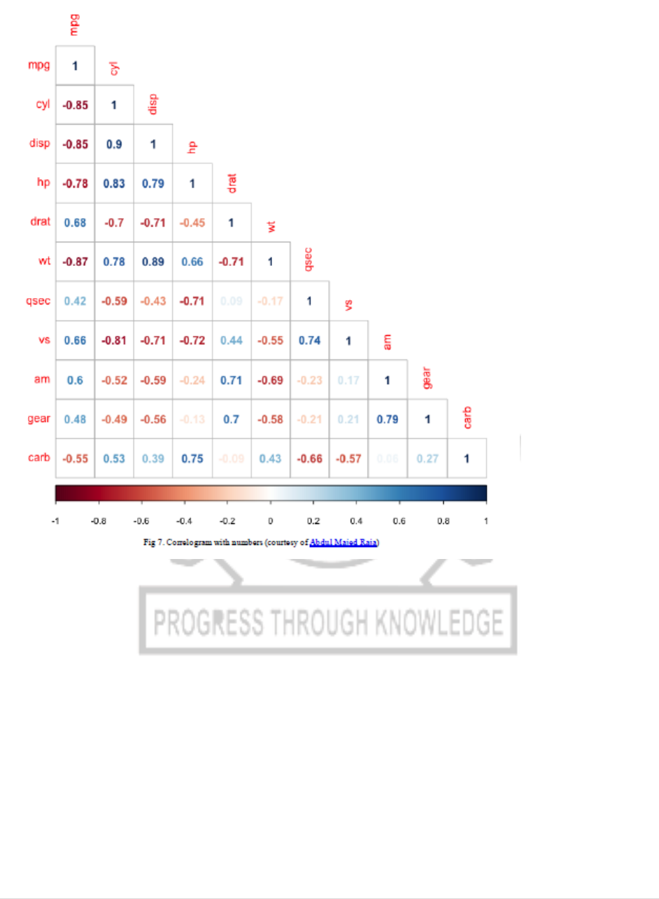
6. Correlogram

Correlated data is best visualized through corrplot. The 2D format is similar to a heat map, but it

highlights statistics that are directly related.

Most correlograms highlight the amount of correlation between datasets at various points in time.

Comparing sales data between different months or years is a basic example.

PROGRAM:

#data("mtcars")

corr_matrix <‐ cor(mtcars)

# with circles

corrplot(corr_matrix)

# with numbers and lower

corrplot(corr_matrix,method = 'number',type = "lower")

OUTPUT:

CP5261 DATA ANALYTICS LABORATORY MANUAL

59 | DR. D. SENTHIL KUMAR (AP/CSE) UCE, ANNA UNIVERSITY- BITCAMPUS TRICHY

7. Area Chart

Area charts express continuity between different variables or data sets. It's akin to the traditional

line chart you know from grade school and is used in a similar fashion.

Most area charts highlight trends and their evolution over the course of time, making them highly

effective when trying to expose underlying trends whether they're positive or negative.

PROGRAM:

data("airquality") #dataset used

airquality %>%

group_by(Day) %>%

summarise(mean_wind = mean(Wind)) %>%

ggplot() +

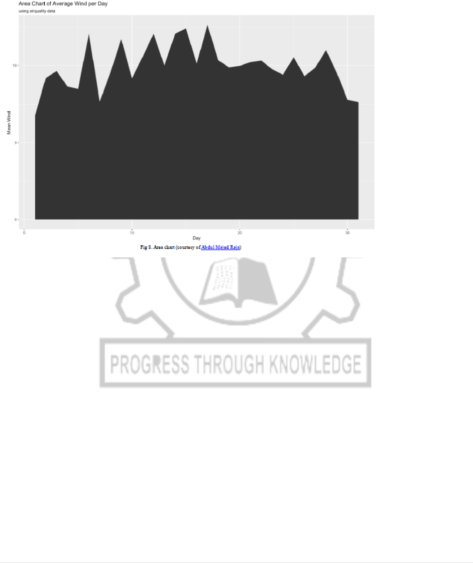
CP5261 DATA ANALYTICS LABORATORY MANUAL

60 | DR. D. SENTHIL KUMAR (AP/CSE) UCE, ANNA UNIVERSITY- BITCAMPUS TRICHY

geom_area(aes(x = Day, y = mean_wind)) +

labs(title = "Area Chart of Average Wind per Day",

subtitle = "using airquality data", y = "Mean Wind")

OUTPUT:

RESULT:

CP5261 DATA ANALYTICS LABORATORY MANUAL

61 | DR. D. SENTHIL KUMAR (AP/CSE) UCE, ANNA UNIVERSITY- BITCAMPUS TRICHY

EX. NO:9

DATE:

Implement an application that stores big data in Hbase /

MongoDB / Pig using Hadoop / R

MongoDB with R

1) To use MongoDB with R, first, we have to download and install MongoDB

Next, start MongoDB. We can start MongoDB like so:

mongod

2) Inserting data

Let’s insert the crimes data from data.gov to MongoDB. The dataset reflects

reported incidents of crime (with the exception of murders where data exists for each

victim) that occurred in the City of Chicago since 2001.

library (ggplot2)

library (dplyr)

library (maps)

library (ggmap)

library (mongolite)

library (lubridate)

library (gridExtra)

crimes=data.table::fread("Crimes_2001_to_present.csv")

names (crimes)

CP5261 DATA ANALYTICS LABORATORY MANUAL

62 | DR. D. SENTHIL KUMAR (AP/CSE) UCE, ANNA UNIVERSITY- BITCAMPUS TRICHY

'Output:

ID' 'Case Number' 'Date' 'Block' 'IUCR' 'Primary Type' 'Description' 'Location

Description' 'Arrest''Domestic' 'Beat' 'District' 'Ward' 'Community Area' 'FBI Code' 'X

Coordinate' 'Y Coordinate' 'Year' 'Updated On' 'Latitude' 'Longitude' 'Location'

3) Let’s remove spaces in the column names to avoid any problems when we query it

from MongoDB.

names(crimes) = gsub(" ","",names(crimes))

names(crimes)

'ID' 'CaseNumber' 'Date' 'Block' 'IUCR' 'PrimaryType' 'Description'

'LocationDescription' 'Arrest' 'Domestic' 'Beat' 'District' 'Ward' 'CommunityArea'

'FBICode' 'XCoordinate' 'YCoordinate' 'Year' 'UpdatedOn' 'Latitude' 'Longitude'

'Location'

4) Let’s use the insert function from the mongolite package to insert rows to a collection

in MongoDB.Let’s create a database called Chicago and call the collection crimes.

my_collection = mongo(collection = "crimes", db = "Chicago") # create

connection, database and collection

my_collection$insert(crimes)

CP5261 DATA ANALYTICS LABORATORY MANUAL

63 | DR. D. SENTHIL KUMAR (AP/CSE) UCE, ANNA UNIVERSITY- BITCAMPUS TRICHY

5) Let’s check if we have inserted the “crimes” data.

my_collection$count()

6261148

We see that the collection has 6261148 records.

6) First, let’s look what the data looks like by displaying one record:

my_collection$iterate()$one()

$ID

1454164

$Case Number

' G185744'

$Date

' 04/01/2001 06:00:00 PM'

$Block

' 049XX N MENARD AV'

$IUCR

CP5261 DATA ANALYTICS LABORATORY MANUAL

64 | DR. D. SENTHIL KUMAR (AP/CSE) UCE, ANNA UNIVERSITY- BITCAMPUS TRICHY

' 0910'

$Primary Type

' MOTOR VEHICLE THEFT'

$Description

' AUTOMOBILE'

$Location Description

' STREET'

$Arrest

' false'

$Domestic

' false'

$Beat

1622

$District

$FBICode

' 07'

$XCoordinate

1136545

CP5261 DATA ANALYTICS LABORATORY MANUAL

65 | DR. D. SENTHIL KUMAR (AP/CSE) UCE, ANNA UNIVERSITY- BITCAMPUS TRICHY

$YCoordinate

1932203

$Year

2001

$Updated On

' 08/17/2015 03:03:40 PM'

$Latitude

41.970129962

$Longitude

87.773302309

$Location

'(41.970129962, -87.773302309)'

7) How many distinct “Primary Type” do we have?

length(my_collection$distinct("PrimaryType"))

As shown above, there are 35 different crime primary types in the database. We will

see the patterns of the most common crime types below.

CP5261 DATA ANALYTICS LABORATORY MANUAL

66 | DR. D. SENTHIL KUMAR (AP/CSE) UCE, ANNA UNIVERSITY- BITCAMPUS TRICHY

8) Now, let’s see how many domestic assaults there are in the collection.

my_collection$count('{"PrimaryType":"ASSAULT", "Domestic" : "true" }')

82470

9) To get the filtered data and we can also retrieve only the columns of interest.

query1= my_collection$find('{"PrimaryType" : "ASSAULT", "Domestic" :

"true" }')

query2= my_collection$find('{"PrimaryType" : "ASSAULT", "Domestic" :

"true" }',

fields = '{"_id":0, "PrimaryType":1, "Domestic":1}')

ncol(query1) # with all the columns

ncol(query2) # only the selected columns

CP5261 DATA ANALYTICS LABORATORY MANUAL

67 | DR. D. SENTHIL KUMAR (AP/CSE) UCE, ANNA UNIVERSITY- BITCAMPUS TRICHY

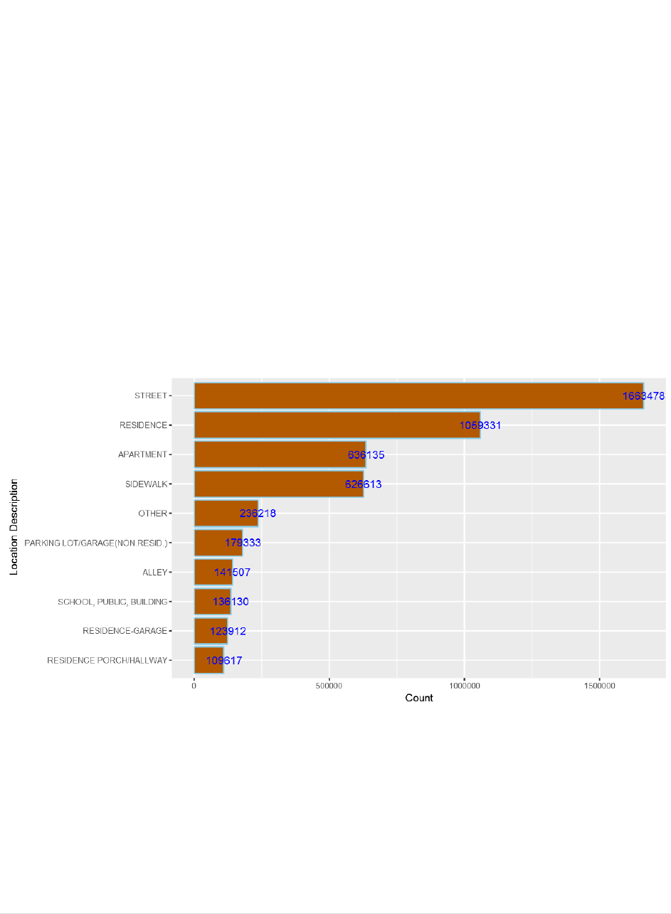
10) To find out “Where do most crimes take place?” use the following command.

my_collection$aggregate('[{"$group":{"_id":"$LocationDescription", "Count":

{"$sum":1}}}]')%>%na.omit()%>%

arrange(desc(Count))%>%head(10)%>%

ggplot(aes(x=reorder(`_id`,Count),y=Count))+

geom_bar(stat="identity",color='skyblue',fill='#b35900')+geom_text(aes(label =

Count), color = "blue") +coord_flip()+xlab("Location Description")

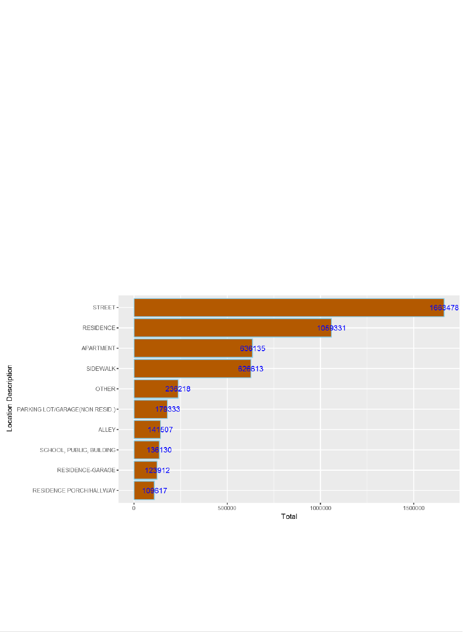
CP5261 DATA ANALYTICS LABORATORY MANUAL

68 | DR. D. SENTHIL KUMAR (AP/CSE) UCE, ANNA UNIVERSITY- BITCAMPUS TRICHY

11)If loading the entire dataset we are working with does not slow down our

analysis, we can use data.table or dplyr but when dealing with big data, using

MongoDB can give us performance boost as the whole data will not be loaded into

memory. We can reproduce the above plot without using MongoDB, like so:

crimes%>%group_by(`LocationDescription`)%>%summarise(Total=n())%>%

arrange(desc(Total))%>%head(10)%>%

ggplot(aes(x=reorder(`LocationDescription`,Total),y=Total))+

geom_bar(stat="identity",color='skyblue',fill='#b35900')+geom_text(aes(label =

Total), color = "blue") +coord_flip()+xlab("Location Description")

12) What if we want to query all records for certain columns only? This helps us to

load only the columns we want and to save memory for our analysis.

CP5261 DATA ANALYTICS LABORATORY MANUAL

69 | DR. D. SENTHIL KUMAR (AP/CSE) UCE, ANNA UNIVERSITY- BITCAMPUS TRICHY

query3= my_collection$find('{}', fields = '{"_id":0, "Latitude":1,

"Longitude":1,"Year":1}')

13) We can explore any patterns of domestic crimes. For example, are they common in

certain days/hours/months?

domestic=my_collection$find('{"Domestic":"true"}', fields = '{"_id":0,

"Domestic":1,"Date":1}')

domestic$Date= mdy_hms(domestic$Date)

domestic$Weekday = weekdays(domestic$Date)

domestic$Hour = hour(domestic$Date)

domestic$month = month(domestic$Date,label=TRUE)

WeekdayCounts = as.data.frame(table(domestic$Weekday))

WeekdayCounts$Var1 = factor(WeekdayCounts$Var1, ordered=TRUE,

levels=c("Sunday", "Monday", "Tuesday", "Wednesday", "Thursday",

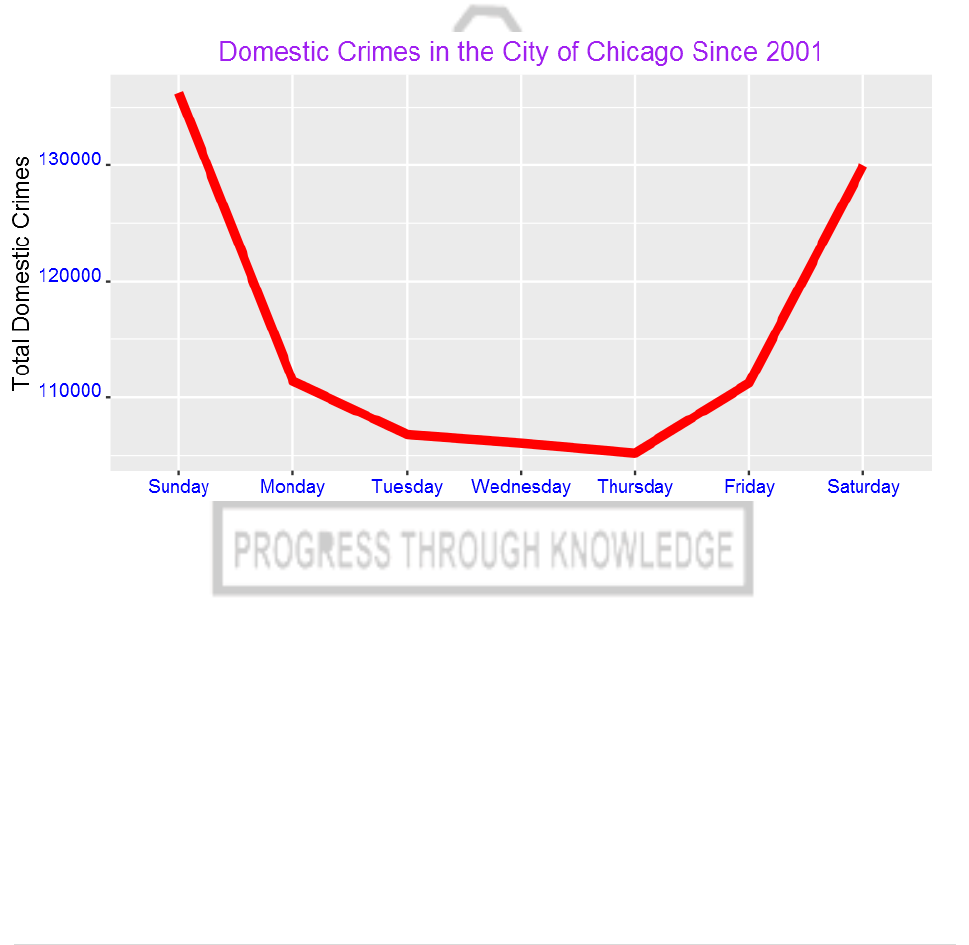
"Friday","Saturday"))

ggplot(WeekdayCounts, aes(x=Var1, y=Freq)) +

geom_line(aes(group=1),size=2,color="red") + xlab("Day of the Week") +

ylab("Total Domestic Crimes")+

ggtitle("Domestic Crimes in the City of Chicago Since 2001")+

CP5261 DATA ANALYTICS LABORATORY MANUAL

70 | DR. D. SENTHIL KUMAR (AP/CSE) UCE, ANNA UNIVERSITY- BITCAMPUS TRICHY

theme(axis.title.x=element_blank(),axis.text.y =

element_text(color="blue",size=11,angle=0,hjust=1,vjust=0),

axis.text.x = element_text(color="blue",size=11,angle=0,hjust=.5,vjust=.5),

axis.title.y = element_text(size=14),

plot.title=element_text(size=16,color="purple",hjust=0.5))

14) Domestic crimes are common over the weekend than in weekdays? What could be

the reason?

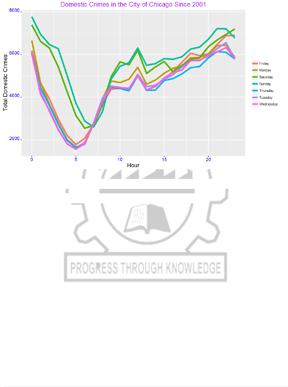
We can also see the pattern for each day by hour:

DayHourCounts = as.data.frame(table(domestic$Weekday, domestic$Hour))

DayHourCounts$Hour = as.numeric(as.character(DayHourCounts$Var2))

CP5261 DATA ANALYTICS LABORATORY MANUAL

71 | DR. D. SENTHIL KUMAR (AP/CSE) UCE, ANNA UNIVERSITY- BITCAMPUS TRICHY

ggplot(DayHourCounts, aes(x=Hour, y=Freq)) + geom_line(aes(group=Var1,

color=Var1), size=1.4)+ylab("Count")+

ylab("Total Domestic Crimes")+ggtitle("Domestic Crimes in the City of Chicago

Since 2001")+

theme(axis.title.x=element_text(size=14),axis.text.y =

element_text(color="blue",size=11,angle=0,hjust=1,vjust=0),

axis.text.x = element_text(color="blue",size=11,angle=0,hjust=.5,vjust=.5),

axis.title.y = element_text(size=14),

legend.title=element_blank(),

plot.title=element_text(size=16,color="purple",hjust=0.5))

CP5261 DATA ANALYTICS LABORATORY MANUAL

72 | DR. D. SENTHIL KUMAR (AP/CSE) UCE, ANNA UNIVERSITY- BITCAMPUS TRICHY

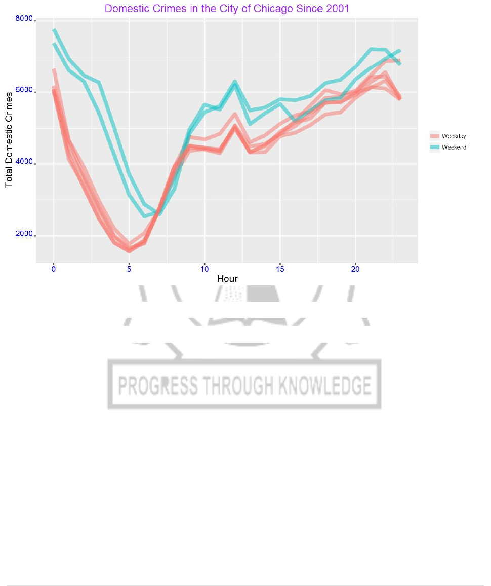
15) The crimes peak mainly around mid-night. We can also use one color for

weekdays and another color for weekend as shown below.

DayHourCounts$Type = ifelse((DayHourCounts$Var1 == "Sunday") |

(DayHourCounts$Var1 == "Saturday"), "Weekend", "Weekday")

ggplot(DayHourCounts, aes(x=Hour, y=Freq)) + geom_line(aes(group=Var1,

color=Type), size=2, alpha=0.5) +

ylab("Total Domestic Crimes")+ggtitle("Domestic Crimes in the City of Chicago

Since 2001")+

theme(axis.title.x=element_text(size=14),axis.text.y =

element_text(color="blue",size=11,angle=0,hjust=1,vjust=0),

axis.text.x = element_text(color="blue",size=11,angle=0,hjust=.5,vjust=.5),

axis.title.y = element_text(size=14),

CP5261 DATA ANALYTICS LABORATORY MANUAL

73 | DR. D. SENTHIL KUMAR (AP/CSE) UCE, ANNA UNIVERSITY- BITCAMPUS TRICHY

legend.title=element_blank(),

plot.title=element_text(size=16,color="purple",hjust=0.5))

16) The difference between weekend and weekdays are clearer from this figure than

from the previous plot. We can also see the above pattern from a heat map.

DayHourCounts$Var1 = factor(DayHourCounts$Var1, ordered=TRUE,

levels=c("Monday", "Tuesday", "Wednesday", "Thursday", "Friday",

"Saturday", "Sunday"))

ggplot(DayHourCounts, aes(x = Hour, y = Var1)) + geom_tile(aes(fill = Freq)) +

scale_fill_gradient(name="Total MV Thefts", low="white", high="red") +

ggtitle("Domestic Crimes in the City of Chicago Since 2001")+theme(axis.title.y =

element_blank())+ylab("")+theme(axis.title.x=element_text(size=14),axis.text.y =

element_text(size=13),axis.text.x = element_text(size=13), axis.title.y =

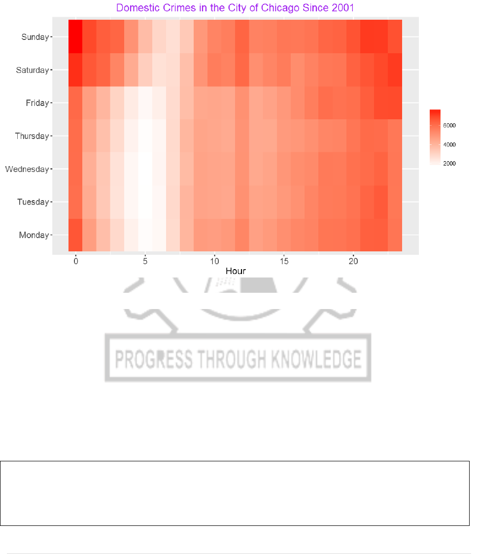
CP5261 DATA ANALYTICS LABORATORY MANUAL

74 | DR. D. SENTHIL KUMAR (AP/CSE) UCE, ANNA UNIVERSITY- BITCAMPUS TRICHY

element_text(size=14),

legend.title=element_blank(),plot.title=element_text(size=16,color="purple",hjus

t=0.5))

17) Let’s see the pattern of other crime types. Let’s focus on four of the most common

ones.

crimes=my_collection$find('{}', fields = '{"_id":0, "PrimaryType":1,"Year":1}')

crimes%>%group_by(PrimaryType)%>%summarize(Count=n())%>%arrange

(desc(Count))%>%head(4)

Imported 6261148 records. Simplifying into dataframe...

PrimaryType Count

CP5261 DATA ANALYTICS LABORATORY MANUAL

75 | DR. D. SENTHIL KUMAR (AP/CSE) UCE, ANNA UNIVERSITY- BITCAMPUS TRICHY

THEFT 1301434

BATTERY 1142377

CRIMINAL DAMAGE 720143

NARCOTICS 687790

18) As shown in the table above, the most common crime type is theft followed by

battery. Narcotics is fourth most common while criminal damage is the third most

common crime type in the city of Chicago.

Now, let’s generate plots by day and hour.

four_most_common=crimes%>%group_by(PrimaryType)%>%summarize(Cou

nt=n())%>%arrange(desc(Count))%>%head(4)

four_most_common=four_most_common$PrimaryType

crimes=my_collection$find('{}', fields = '{"_id":0, "PrimaryType":1,"Date":1}')

crimes=filter(crimes,PrimaryType %in%four_most_common)

crimes$Date= mdy_hms(crimes$Date)

crimes$Weekday = weekdays(crimes$Date)

crimes$Hour = hour(crimes$Date)

crimes$month=month(crimes$Date,label = TRUE)

g = function(data){WeekdayCounts = as.data.frame(table(data$Weekday))

CP5261 DATA ANALYTICS LABORATORY MANUAL

76 | DR. D. SENTHIL KUMAR (AP/CSE) UCE, ANNA UNIVERSITY- BITCAMPUS TRICHY

WeekdayCounts$Var1 = factor(WeekdayCounts$Var1, ordered=TRUE,

levels=c("Sunday", "Monday", "Tuesday", "Wednesday", "Thursday",

"Friday","Saturday"))

ggplot(WeekdayCounts, aes(x=Var1, y=Freq)) +

geom_line(aes(group=1),size=2,color="red") + xlab("Day of the Week") +

theme(axis.title.x=element_blank(),axis.text.y =

element_text(color="blue",size=10,angle=0,hjust=1,vjust=0),

axis.text.x = element_text(color="blue",size=10,angle=0,hjust=.5,vjust=.5),

axis.title.y = element_text(size=11),

plot.title=element_text(size=12,color="purple",hjust=0.5)) }

g1=g(filter(crimes,PrimaryType=="THEFT"))+ggtitle("Theft")+ylab("Total

Count")

g2=g(filter(crimes,PrimaryType=="BATTERY"))+ggtitle("BATTERY")+ylab("

Total Count")

g3=g(filter(crimes,PrimaryType=="CRIMINAL

DAMAGE"))+ggtitle("CRIMINAL DAMAGE")+ylab("Total Count")

g4=g(filter(crimes,PrimaryType=="NARCOTICS"))+ggtitle("NARCOTICS")+

ylab("Total Count")

grid.arrange(g1,g2,g3,g4,ncol=2)

CP5261 DATA ANALYTICS LABORATORY MANUAL

77 | DR. D. SENTHIL KUMAR (AP/CSE) UCE, ANNA UNIVERSITY- BITCAMPUS TRICHY

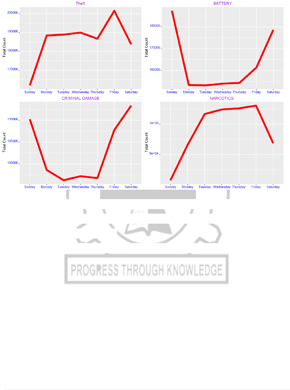
From the plots above, we see that theft is most common on Friday. Battery and

criminal damage, on the other hand, are highest at weekend. We also observe that

narcotics decreases over weekend.

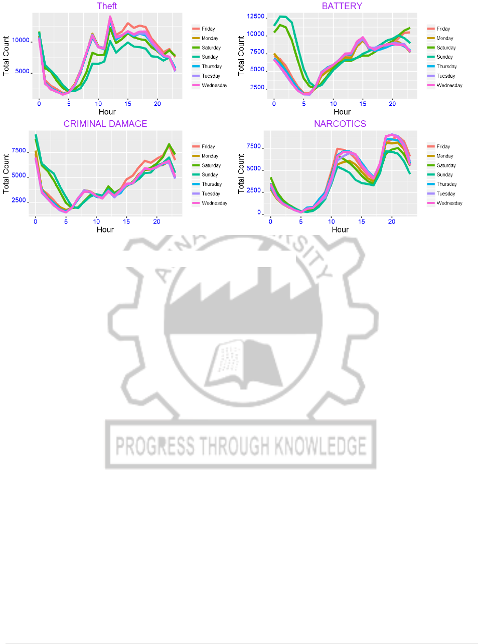
We can also see the pattern of the above four crime types by hour:

CP5261 DATA ANALYTICS LABORATORY MANUAL

78 | DR. D. SENTHIL KUMAR (AP/CSE) UCE, ANNA UNIVERSITY- BITCAMPUS TRICHY

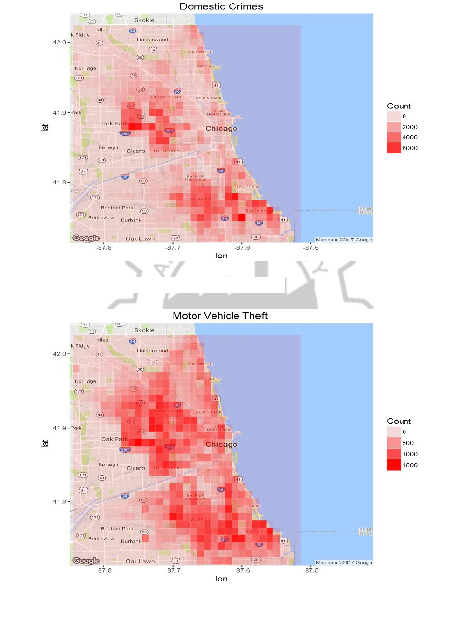
19) We can also see a map for domestic crimes only:

domestic=my_collection$find('{"Domestic":"true"}', fields = '{"_id":0,

"Latitude":1, "Longitude":1,"Year":1}')

LatLonCounts=as.data.frame(table(round(domestic$Longitude,2),round(domest

ic$Latitude,2)))

LatLonCounts$Long = as.numeric(as.character(LatLonCounts$Var1))

LatLonCounts$Lat = as.numeric(as.character(LatLonCounts$Var2))

ggmap(chicago) + geom_tile(data = LatLonCounts, aes(x = Long, y = Lat, alpha

= Freq), fill="red")+

ggtitle("Domestic Crimes")+labs(alpha="Count")+theme(plot.title =

element_text(hjust=0.5))

CP5261 DATA ANALYTICS LABORATORY MANUAL

79 | DR. D. SENTHIL KUMAR (AP/CSE) UCE, ANNA UNIVERSITY- BITCAMPUS TRICHY

20) Let’s see where motor vehicle theft is common:

Domestic crimes show concentration over two areas whereas motor vehicle theft is

wide spread over large part of the city of Chicago.

CP5261 DATA ANALYTICS LABORATORY MANUAL

80 | DR. D. SENTHIL KUMAR (AP/CSE) UCE, ANNA UNIVERSITY- BITCAMPUS TRICHY

CP5261 DATA ANALYTICS LABORATORY MANUAL ME CSE

CP5261%20%20%20DATA%20ANALYTICS%20LABORATORY%20MANUAL%20ME%20CSE

CP5261%20%20%20DATA%20ANALYTICS%20LABORATORY%20MANUAL%20ME%20CSE

Navigation menu

Versions of this User Manual:

Views

Navigation