Climate App Instructions

Instructions

User Manual:

Open the PDF directly: View PDF .
Page Count: 4

Climate App Instructions

Climate App instructions

December 20, 2018

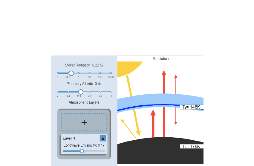
Figure 1: Screenshot of the application

What is this ?

This is a web application that is used to demonstrate the effects of greenhouse gases

on the temperature of a planet. By choosing the value of different setting shown

in the options panel, the user can see a visual representation of the effect on the

radiation and temperature.

How does it work ?

Left Panel

This panel lets you specify values for the settings of the system.

Stellar Radiation

Also known as "Insolation", this value is the amount of radiation from the star that

reaches the planet. The units of this measure are "S0", which is the amount of solar

radiation on earth. For example, a value of 2 would mean that the planet receives

twice the amount of stellar radiation that we have on earth. The slider is a log scale,

which allows for value as high as 1000 S0 and as low as 0.01 S0.

Planetary albedo

You can use this slider to choose how reflective the planet is. A value of 1 would

mean that the planet reflects all the incoming radiation. A value of zero would mean

that the planet is very dark and it absorbs all the incoming radiation. The default

value is set to the earth’s albedo, which is 0.3

1

Climate App Instructions

Atmospheric Layers

In this box, you will find settings for the atmospheric layers. You can click the "+"

box to add a new layer, and the "x" on a layer to remove it. For each layer, you can

set the value of emissivity, which is its effectiveness in emitting energy as thermal

radiation. A value of zero would mean that the energy that radiates from the surface

entirely goes through the atmospheric layer. A value of one would mean that all of

the radiation is absorbed by the layer. A maximum of three layers is possible.

Right Panel

In this panel, we can see a visual representation of the system. The yellow arrows

represent the shortwave emissivity, and the red arrows represent the longwave emis-

sivity. By modifying the input variables, it is possible to see the arrows’ size varying

in real time.

Please note that the effect of the stellar radiation on the radiation is not rep-

resented on the arrow. The reason is that since the insolation is a log scale, if we

try to include that setting in the width of the arrows, all the other modification

(albedo and emissivity of the layers) would have negligible effects and there would

be no visible variation. The arrow size is then proportional to the radiation that

they illustrate, assuming constant stellar radiation.

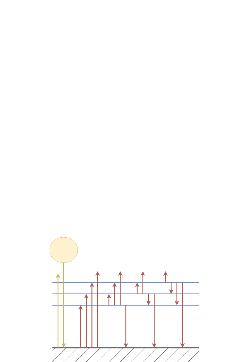
Since there would be a lot of arrows between each layer (see figure 2), the display

of the layers is abstracted in a thick pale blue line. We can still see each layer inside,

and their thickness is proportional to their emissivity, but the radiation between

themselves is not shown. The resulting temperatures are shown at the surface and

at each layer.

Figure 2:

2

Climate App Instructions

Why does it work ?

There are two concepts that we need to be familiar with to understand how to derive

the equations:

Stefan-Boltzmann Law

The Stefan-Boltzmann gives a relation between the temperature of an object and

the amount of energy it radiates.

j=σT 4(1)

where is the emissivity (We assume = 1 at the surface), Tis the temperature

in Kelvin, jis the total energy radiated and σis the Stefan-Boltzmann constant:

σ= 5.6703 ×10−8watt/m2K4

Radiative equilibrium

The amount of incoming radiation at any given layer must be equivalent to the

outgoing radiation at that layer

Deriving the equations

Figure 2 gives an illustration of the model that we are analyzing. At the surface,

there is incoming stellar radiation, and some of it is reflected back into space (We

assume atmospheric layers have no impact on shortwave radiation), as shown by the

yellow arrows. The surface then heats and radiates back. Some of this radiation is

absorbed by each of the three atmospheric layers, and some of it also makes it into

space. The same effect happens for each layer: they heat and then radiates back,

both towards space and back to the surface of the planet.

For the surface, using the Stefan-Boltzmann law, we know that the energy radi-

ated is σT 4

0, where T0is the temperature of the surface (Remember that we assume

that the planet is a blackbody, that is: 0= 1). According to the radiative equi-

librium, if the surface of the planet emits that much radiation, it is because it has

absorbed this much. We know that the planet absorbs energy from the star and

from each layer. We can then write the following equation:

S0(1 −α) + 1σT 4

1+2σT 4

2(1 −1) + 3σT 4

3(1 −2)(1 −1) = σT 4

0(2)

where S0is the stellar radiation, Tiand iare the temperature and emissivity at

atmospheric layer irespectively, i= 0 being the surface. The first term is the stellar

radiation that is not reflected, and other terms are the radiation that the surface

receives from each layer. We can also find those values using the Stefan-Boltzmann

law multiplied by the amount of radiation that goes through the other layers.

In a similar fashion, it is possible to get equations for each layer, taking into

account that the radiation is emitted both upward and downward:

3

Climate App Instructions

Layer 1:

1σT 4

0+12σT 4

2+13σT 4

3(1 −e) = 21σT 4

1(3)

Layer 2:

2σT 4

0(1 −1) + 21σT 4

1+23σT 4

3= 22σT 4

2(4)

Layer 3:

3σT 4

0(1 −1)(1 −2) + 31σT 4

1(1 −2) + 32σT 4

2= 23σT 4

3(5)

Solving the equations

We now have a system of 4 equations and 4 unknown temperature. Solving the

system for the fourth power of the temperature yields the following results:

Surface:

T4

0=2S0(α−1)(4 −12−13−23+123)

σ(1−2)(2−2)(3−2) (6)

Layer 1:

T4

1=S0(α−1)(4 + 22−212+ 23−213−323+ 2123)

σ(1−2)(2−2)(3−2) (7)

Layer 2:

T4

2=S0(α−1)(−2−3+23)

σ(2−2)(3−2) (8)

Layer 3:

T4

3=S0(α−1)

σ(3−2) (9)

Those are the equations that are used in the application to predict the temper-

ature of the system with the given input variables.

4