Digital Signal Processing Solutions Manual
User Manual:
Open the PDF directly: View PDF ![]() .
.
Page Count: 431 [warning: Documents this large are best viewed by clicking the View PDF Link!]

Chapter 1
1.1
(a) One dimensional, multichannel, discrete time, and digital.
(b) Multi dimensional, single channel, continuous-time, analog.
(c) One dimensional, single channel, continuous-time, analog.
(d) One dimensional, single channel, continuous-time, analog.
(e) One dimensional, multichannel, discrete-time, digital.
1.2
(a) f=0.01π
2π=1
200 ⇒periodic with Np= 200.
(b) f=30π
105 (1
2π) = 1
7⇒periodic with Np= 7.
(c) f=3π
2π=3
2⇒periodic with Np= 2.
(d) f=3
2π⇒non-periodic.
(e) f=62π
10 (1
2π) = 31
10 ⇒periodic with Np= 10.
1.3
(a) Periodic with period Tp=2π
5.
(b) f=5
2π⇒non-periodic.
(c) f=1
12π⇒non-periodic.
(d) cos(n
8) is non-periodic; cos(πn
8) is periodic; Their product is non-periodic.
(e) cos(πn
2) is periodic with period Np=4
sin(πn
8) is periodic with period Np=16
cos(πn
4+π
3) is periodic with period Np=8
Therefore, x(n) is periodic with period Np=16. (16 is the least common multiple of 4,8,16).
1.4
(a) w=2πk
Nimplies that f=k
N. Let
α= GCD of (k, N),i.e.,
k=k′α, N =N′α.
Then,
f=k′
N′,which implies that
N′=N
α.
3
© 2007 Pearson Education, Inc., Upper Saddle River, NJ. All rights reserved. This material is protected under all copyright laws
as they currently exist. No portion of this material may be reproduced, in any form or by any means, without permission in
writing from the publisher. For the exclusive use of adopters of the book Digital Signal Processing, Fourth Edition, by John G.
Proakis and Dimitris G. Manolakis. ISBN 0-13-187374-1.
(b)
N= 7
k= 01234567
GCD(k, N) = 71111117
Np= 17777771
(c)
N= 16
k= 0123456789101112 ... 16
GCD(k, N) = 16121412181214 ... 16
Np= 1 6 8 16 4 16 8 16 2 16 8 16 4 ... 1
1.5
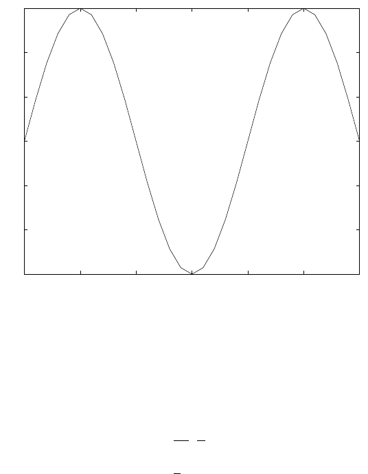
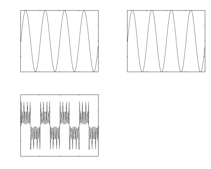
(a) Refer to fig 1.5-1
(b)
0 5 10 15 20 25 30
−3
−2
−1
0
1
2
3
−−−> t (ms)
−−−> xa(t)
Figure 1.5-1:
x(n) = xa(nT )
=xa(n/Fs)
= 3sin(πn/3) ⇒
f=1
2π(π
3)
=1
6, Np= 6
4
© 2007 Pearson Education, Inc., Upper Saddle River, NJ. All rights reserved. This material is protected under all copyright laws
as they currently exist. No portion of this material may be reproduced, in any form or by any means, without permission in
writing from the publisher. For the exclusive use of adopters of the book Digital Signal Processing, Fourth Edition, by John G.
Proakis and Dimitris G. Manolakis. ISBN 0-13-187374-1.
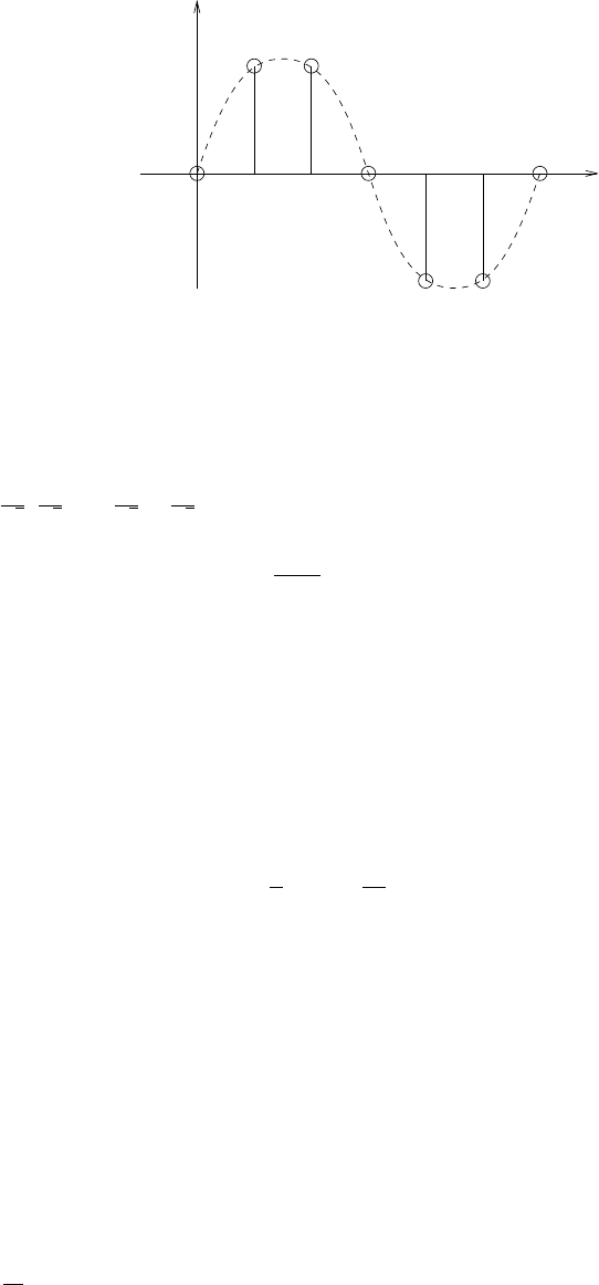
010 20 t (ms)
3
-3
Figure 1.5-2:
(c)Refer to fig 1.5-2
x(n) = n0,3
√2,3
√2,0,−3
√2,−3
√2o, Np= 6.
(d) Yes.
x(1) = 3 = 3sin(100π
Fs
)⇒Fs= 200 samples/sec.
1.6
(a)
x(n) = Acos(2πF0n/Fs+θ)
=Acos(2π(T/Tp)n+θ)
But T/Tp=f⇒x(n) is periodic if f is rational.
(b) If x(n) is periodic, then f=k/N where N is the period. Then,
Td= ( k
fT) = k(Tp
T)T=kTp.
Thus, it takes k periods (kTp) of the analog signal to make 1 period (Td) of the discrete signal.
(c) Td=kTp⇒NT =kTp⇒f=k/N =T/Tp⇒f is rational ⇒x(n) is periodic.
1.7
(a) Fmax = 10kHz ⇒Fs≥2Fmax = 20kHz.
(b) For Fs= 8kHz, Ffold =Fs/2 = 4kHz ⇒5kHz will alias to 3kHz.
(c) F=9kHz will alias to 1kHz.
1.8
(a) Fmax = 100kHz, Fs≥2Fmax = 200Hz.
(b) Ffold =Fs
2= 125Hz.
5
© 2007 Pearson Education, Inc., Upper Saddle River, NJ. All rights reserved. This material is protected under all copyright laws
as they currently exist. No portion of this material may be reproduced, in any form or by any means, without permission in
writing from the publisher. For the exclusive use of adopters of the book Digital Signal Processing, Fourth Edition, by John G.
Proakis and Dimitris G. Manolakis. ISBN 0-13-187374-1.

1.9
(a) Fmax = 360Hz, FN= 2Fmax = 720Hz.
(b) Ffold =Fs
2= 300Hz.
(c)
x(n) = xa(nT )
=xa(n/Fs)
=sin(480πn/600) + 3sin(720πn/600)
x(n) = sin(4πn/5) −3sin(4πn/5)
=−2sin(4πn/5).
Therefore, w= 4π/5.
(d) ya(t) = x(Fst) = −2sin(480πt).
1.10
(a)
Number of bits/sample = log21024 = 10.
Fs=[10,000 bits/sec]
[10 bits/sample]
= 1000 samples/sec.
Ffold = 500Hz.
(b)
Fmax =1800π
2π
= 900Hz
FN= 2Fmax = 1800Hz.
(c)
f1=600π
2π(1
Fs
)
= 0.3;
f2=1800π
2π(1
Fs
)
= 0.9;
But f2= 0.9>0.5⇒f2= 0.1.
Hence, x(n) = 3cos[(2π)(0.3)n] + 2cos[(2π)(0.1)n]
(d) △=xmax−xmin
m−1=5−(−5)
1023 =10
1023 .
1.11
x(n) = xa(nT )
= 3cos 100πn
200 + 2sin 250πn
200
6
© 2007 Pearson Education, Inc., Upper Saddle River, NJ. All rights reserved. This material is protected under all copyright laws
as they currently exist. No portion of this material may be reproduced, in any form or by any means, without permission in
writing from the publisher. For the exclusive use of adopters of the book Digital Signal Processing, Fourth Edition, by John G.
Proakis and Dimitris G. Manolakis. ISBN 0-13-187374-1.

= 3cos πn
2−2sin 3πn
4
T′=1
1000 ⇒ya(t) = x(t/T ′)
= 3cos π1000t
2−2sin 3π1000t
4
ya(t) = 3cos(500πt)−2sin(750πt)
1.12
(a) For Fs= 300Hz,
x(n) = 3cos πn
6+ 10sin(πn)−cos πn
3
= 3cos πn
6−3cos πn
3
(b) xr(t) = 3cos(10000πt/6) −cos(10000πt/3)
1.13
(a)
Range = xmax −xmin = 12.7.
m= 1 + range
△
= 127 + 1 = 128 ⇒log2(128)
= 7 bits.
(b) m= 1 + 127
0.02 = 636 ⇒log2(636) ⇒10 bit A/D.
1.14
R= (20samples
sec )×(8 bits
sample)
= 160bits
sec
Ffold =Fs
2= 10Hz.
Resolution = 1volt
28−1
= 0.004.
1.15
(a) Refer to fig 1.15-1. With a sampling frequency of 5kHz, the maximum frequency that can be
represented is 2.5kHz. Therefore, a frequency of 4.5kHz is aliased to 500Hz and the frequency of
3kHz is aliased to 2kHz.
7
© 2007 Pearson Education, Inc., Upper Saddle River, NJ. All rights reserved. This material is protected under all copyright laws
as they currently exist. No portion of this material may be reproduced, in any form or by any means, without permission in
writing from the publisher. For the exclusive use of adopters of the book Digital Signal Processing, Fourth Edition, by John G.
Proakis and Dimitris G. Manolakis. ISBN 0-13-187374-1.
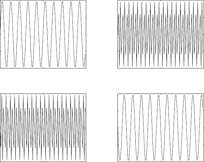
0 50 100
−1
−0.5
0
0.5
1Fs = 5KHz, F0=500Hz
0 50 100
−1
−0.5
0
0.5
1Fs = 5KHz, F0=2000Hz
0 50 100
−1
−0.5
0
0.5
1Fs = 5KHz, F0=3000Hz
0 50 100
−1
−0.5
0
0.5
1Fs = 5KHz, F0=4500Hz
Figure 1.15-1:
(b) Refer to fig 1.15-2. y(n) is a sinusoidal signal. By taking the even numbered samples, the
sampling frequency is reduced to half i.e., 25kHz which is still greater than the nyquist rate. The
frequency of the downsampled signal is 2kHz.
1.16
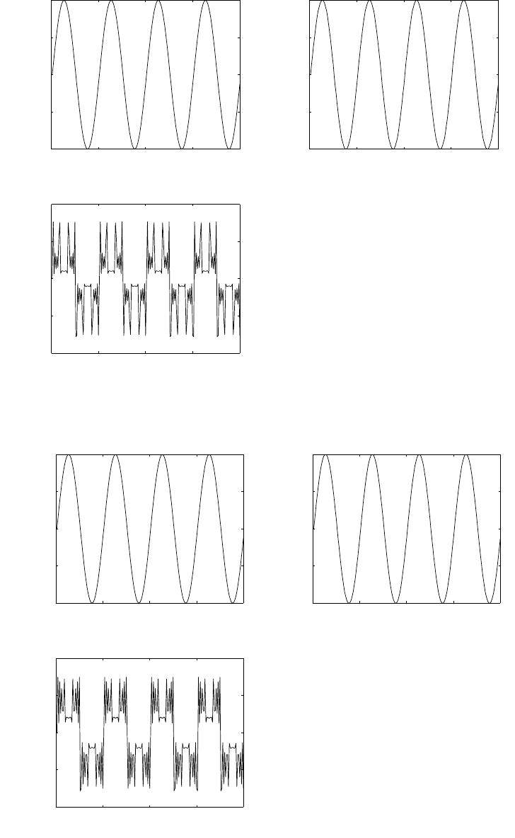
(a) for levels = 64, using truncation refer to fig 1.16-1.
for levels = 128, using truncation refer to fig 1.16-2.
for levels = 256, using truncation refer to fig 1.16-3.
8
© 2007 Pearson Education, Inc., Upper Saddle River, NJ. All rights reserved. This material is protected under all copyright laws
as they currently exist. No portion of this material may be reproduced, in any form or by any means, without permission in
writing from the publisher. For the exclusive use of adopters of the book Digital Signal Processing, Fourth Edition, by John G.
Proakis and Dimitris G. Manolakis. ISBN 0-13-187374-1.
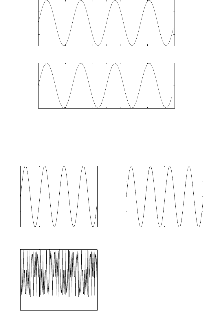
0 10 20 30 40 50 60 70 80 90 100
−1
−0.5
0
0.5
1F0 = 2KHz, Fs=50kHz
0 5 10 15 20 25 30 35 40 45 50
−1
−0.5
0
0.5
1F0 = 2KHz, Fs=25kHz
Figure 1.15-2:
0 50 100 150 200
−1
−0.5
0
0.5
1
levels = 64, using truncation, SQNR = 31.3341dB
−−> n
−−> x(n)
0 50 100 150 200
−1
−0.5
0
0.5
1
−−> n
−−> xq(n)
0 50 100 150 200
−0.04
−0.03
−0.02
−0.01
0
−−> n
−−> e(n)
Figure 1.16-1:
9
© 2007 Pearson Education, Inc., Upper Saddle River, NJ. All rights reserved. This material is protected under all copyright laws
as they currently exist. No portion of this material may be reproduced, in any form or by any means, without permission in
writing from the publisher. For the exclusive use of adopters of the book Digital Signal Processing, Fourth Edition, by John G.
Proakis and Dimitris G. Manolakis. ISBN 0-13-187374-1.

0 50 100 150 200
−1
−0.5
0
0.5
1
levels = 128, using truncation, SQNR = 37.359dB
−−> n
−−> x(n)
0 50 100 150 200
−1
−0.5
0
0.5
1
−−> n
−−> xq(n)
0 50 100 150 200
−0.02
−0.015
−0.01
−0.005
0
−−> n
−−> e(n)
Figure 1.16-2:
0 50 100 150 200
−1
−0.5
0
0.5
1
levels = 256, using truncation, SQNR=43.7739dB
−−> n
−−> x(n)
0 50 100 150 200
−1
−0.5
0
0.5
1
−−> n
−−> xq(n)
0 50 100 150 200
−8
−6
−4
−2
0x 10−3
−−> n
−−> e(n)
Figure 1.16-3:
10
© 2007 Pearson Education, Inc., Upper Saddle River, NJ. All rights reserved. This material is protected under all copyright laws
as they currently exist. No portion of this material may be reproduced, in any form or by any means, without permission in
writing from the publisher. For the exclusive use of adopters of the book Digital Signal Processing, Fourth Edition, by John G.
Proakis and Dimitris G. Manolakis. ISBN 0-13-187374-1.
(b) for levels = 64, using rounding refer to fig 1.16-4.
for levels = 128, using rounding refer to fig 1.16-5.
for levels = 256, using rounding refer to fig 1.16-6.
0 50 100 150 200
−1
−0.5
0
0.5
1
levels = 64, using rounding, SQNR=32.754dB
−−> n
−−> x(n)
0 50 100 150 200
−1
−0.5
0
0.5
1
−−> n
−−> xq(n)
0 50 100 150 200
−0.04
−0.02
0
0.02
0.04
−−> n
−−> e(n)
Figure 1.16-4:
11
© 2007 Pearson Education, Inc., Upper Saddle River, NJ. All rights reserved. This material is protected under all copyright laws
as they currently exist. No portion of this material may be reproduced, in any form or by any means, without permission in
writing from the publisher. For the exclusive use of adopters of the book Digital Signal Processing, Fourth Edition, by John G.
Proakis and Dimitris G. Manolakis. ISBN 0-13-187374-1.
0 50 100 150 200
−1
−0.5
0
0.5
1
levels = 128, using rounding, SQNR=39.2008dB
−−> n
−−> x(n)
0 50 100 150 200
−1
−0.5
0
0.5
1
−−> n
−−> xq(n)
0 50 100 150 200
−0.02
−0.01
0
0.01
0.02
−−> n
−−> e(n)
Figure 1.16-5:
0 50 100 150 200
−1
−0.5
0
0.5
1
levels = 256, using rounding, SQNR=44.0353dB
−−> n
−−> x(n)
0 50 100 150 200
−1
−0.5
0
0.5
1
−−> n
−−> xq(n)
0 50 100 150 200
−0.01
−0.005
0
0.005
0.01
−−> n
−−> e(n)
Figure 1.16-6:
12
© 2007 Pearson Education, Inc., Upper Saddle River, NJ. All rights reserved. This material is protected under all copyright laws
as they currently exist. No portion of this material may be reproduced, in any form or by any means, without permission in
writing from the publisher. For the exclusive use of adopters of the book Digital Signal Processing, Fourth Edition, by John G.
Proakis and Dimitris G. Manolakis. ISBN 0-13-187374-1.
(c) The sqnr with rounding is greater than with truncation. But the sqnr improves as the number
of quantization levels are increased.
(d)
levels 64 128 256
theoretical sqnr 43.9000 49.9200 55.9400
sqnr with truncation 31.3341 37.359 43.7739
sqnr with rounding 32.754 39.2008 44.0353
The theoretical sqnr is given in the table above. It can be seen that theoretical sqnr is much
higher than those obtained by simulations. The decrease in the sqnr is because of the truncation
and rounding.
13
© 2007 Pearson Education, Inc., Upper Saddle River, NJ. All rights reserved. This material is protected under all copyright laws
as they currently exist. No portion of this material may be reproduced, in any form or by any means, without permission in
writing from the publisher. For the exclusive use of adopters of the book Digital Signal Processing, Fourth Edition, by John G.
Proakis and Dimitris G. Manolakis. ISBN 0-13-187374-1.
14
© 2007 Pearson Education, Inc., Upper Saddle River, NJ. All rights reserved. This material is protected under all copyright laws
as they currently exist. No portion of this material may be reproduced, in any form or by any means, without permission in
writing from the publisher. For the exclusive use of adopters of the book Digital Signal Processing, Fourth Edition, by John G.
Proakis and Dimitris G. Manolakis. ISBN 0-13-187374-1.

Chapter 2
2.1
(a)
x(n) = ...0,1
3,2
3,1
↑,1,1,1,0,...
. Refer to fig 2.1-1.
(b) After folding s(n) we have
-3 -2 -1 01234
1111
1/3
2/3
Figure 2.1-1:
x(−n) = ...0,1,1,1,1
↑,2
3,1
3,0,....
After delaying the folded signal by 4 samples, we have
x(−n+ 4) = ...0,0
↑,1,1,1,1,2
3,1
3,0,....
On the other hand, if we delay x(n) by 4 samples we have
x(n−4) = ...0
↑,0,1
3,2
3,1,1,1,1,0,....
Now, if we fold x(n−4) we have
x(−n−4) = ...0,1,1,1,1,2
3,1
3,0,0
↑,...
15
© 2007 Pearson Education, Inc., Upper Saddle River, NJ. All rights reserved. This material is protected under all copyright laws
as they currently exist. No portion of this material may be reproduced, in any form or by any means, without permission in
writing from the publisher. For the exclusive use of adopters of the book Digital Signal Processing, Fourth Edition, by John G.
Proakis and Dimitris G. Manolakis. ISBN 0-13-187374-1.

(c)
x(−n+ 4) = ...0
↑,1,1,1,1,2
3,1
3,0, . . .
(d) To obtain x(−n+k), first we fold x(n). This yields x(−n). Then, we shift x(−n) by k
samples to the right if k > 0, or ksamples to the left if k < 0.
(e) Yes.
x(n) = 1
3δ(n−2) + 2
3δ(n+ 1) + u(n)−u(n−4)
2.2
x(n) = ...0,1,1
↑,1,1,1
2,1
2,0,...
(a)
x(n−2) = ...0,0
↑,1,1,1,1,1
2,1
2,0, . . .
(b)
x(4 −n) =
...0,1
2
↑
,1
2,1,1,1,1,0, . . .
(see 2.1(d))
(c)
x(n+ 2) = ...0,1,1,1,1
↑,1
2,1
2,0, . . .
(d)
x(n)u(2 −n) = ...0,1,1
↑,1,1,0,0, . . .
(e)
x(n−1)δ(n−3) = ...0
↑,0,1,0, . . .
(f)
x(n2) = {...0, x(4), x(1), x(0), x(1), x(4),0,...}
=...0,1
2,1,1
↑,1,1
2,0,...
(g)
xe(n) = x(n) + x(−n)
2,
x(−n) = ...0,1
2,1
2,1,1,1
↑,1,0,...
=...0,1
4,1
4,1
2,1,1,1,1
2,1
4,1
4,0,...
16
© 2007 Pearson Education, Inc., Upper Saddle River, NJ. All rights reserved. This material is protected under all copyright laws
as they currently exist. No portion of this material may be reproduced, in any form or by any means, without permission in
writing from the publisher. For the exclusive use of adopters of the book Digital Signal Processing, Fourth Edition, by John G.
Proakis and Dimitris G. Manolakis. ISBN 0-13-187374-1.

(h)
xo(n) = x(n)−x(−n)
2
=...0,−1
4,−1
4,−1
2,0,0,0,1
2,1
4,1
4,0,...
2.3
(a)
u(n)−u(n−1) = δ(n) =
0, n < 0
1, n = 0
0, n > 0
(b)
n
X
k=−∞
δ(k) = u(n) = 0, n < 0
1, n ≥0
∞
X
k=0
δ(n−k) = 0, n < 0
1, n ≥0
2.4
Let
xe(n) = 1
2[x(n) + x(−n)],
xo(n) = 1
2[x(n)−x(−n)].
Since
xe(−n) = xe(n)
and
xo(−n) = −xo(n),
it follows that
x(n) = xe(n) + xo(n).
The decomposition is unique. For
x(n) = 2,3,4
↑,5,6,
we have
xe(n) = 4,4,4
↑,4,4
and
xo(n) = −2,−1,0
↑,1,2.
17
© 2007 Pearson Education, Inc., Upper Saddle River, NJ. All rights reserved. This material is protected under all copyright laws
as they currently exist. No portion of this material may be reproduced, in any form or by any means, without permission in
writing from the publisher. For the exclusive use of adopters of the book Digital Signal Processing, Fourth Edition, by John G.
Proakis and Dimitris G. Manolakis. ISBN 0-13-187374-1.
2.5
First, we prove that
∞
X
n=−∞
xe(n)xo(n) = 0
∞
X
n=−∞
xe(n)xo(n) = ∞
X
m=−∞
xe(−m)xo(−m)
=−∞
X
m=−∞
xe(m)xo(m)
=−∞
X
n=−∞
xe(n)xo(n)
=∞
X
n=−∞
xe(n)xo(n)
= 0
Then,
∞
X
n=−∞
x2(n) = ∞
X
n=−∞
[xe(n) + xo(n)]2
=∞
X
n=−∞
x2
e(n) + ∞
X
n=−∞
x2
o(n) + ∞
X
n=−∞
2xe(n)xo(n)
=Ee+Eo
2.6
(a) No, the system is time variant. Proof: If
x(n)→y(n) = x(n2)
x(n−k)→y1(n) = x[(n−k)2]
=x(n2+k2−2nk)
6=y(n−k)
(b) (1)
x(n) = 0,1
↑,1,1,1,0,...
(2)
y(n) = x(n2) = . . . , 0,1,1
↑,1,0,...
(3)
y(n−2) = . . . , 0,0
↑,1,1,1,0,...
18
© 2007 Pearson Education, Inc., Upper Saddle River, NJ. All rights reserved. This material is protected under all copyright laws
as they currently exist. No portion of this material may be reproduced, in any form or by any means, without permission in
writing from the publisher. For the exclusive use of adopters of the book Digital Signal Processing, Fourth Edition, by John G.
Proakis and Dimitris G. Manolakis. ISBN 0-13-187374-1.
(4)
x(n−2) = . . . , 0
↑,0,1,1,1,1,0,...
(5)
y2(n) = T[x(n−2)] = . . . , 0,1,0,0
↑,0,1,0,...
(6)
y2(n)6=y(n−2) ⇒system is time variant.
(c) (1)
x(n) = 1
↑,1,1,1
(2)
y(n) = 1
↑,0,0,0,0,−1
(3)
y(n−2) = 0
↑,0,1,0,0,0,0,−1
(4)
x(n−2) = 0
↑,0,1,1,1,1,1
(5)
y2(n) = 0
↑,0,1,0,0,0,0,−1
(6)
y2(n) = y(n−2).
The system is time invariant, but this example alone does not constitute a proof.
(d) (1)
y(n) = nx(n),
x(n) = . . . , 0,1
↑,1,1,1,0,...
(2)
y(n) = . . . , 0
↑,1,2,3,...
(3)
y(n−2) = . . . , 0
↑,0,0,1,2,3,...
(4)
x(n−2) = . . . , 0,0
↑,0,1,1,1,1,...
19
© 2007 Pearson Education, Inc., Upper Saddle River, NJ. All rights reserved. This material is protected under all copyright laws
as they currently exist. No portion of this material may be reproduced, in any form or by any means, without permission in
writing from the publisher. For the exclusive use of adopters of the book Digital Signal Processing, Fourth Edition, by John G.
Proakis and Dimitris G. Manolakis. ISBN 0-13-187374-1.
(5)
y2(n) = T[x(n−2)] = {. . . , 0,0,2,3,4,5,...}
(6)
y2(n)6=y(n−2) ⇒the system is time variant.
2.7
(a) Static, nonlinear, time invariant, causal, stable.
(b) Dynamic, linear, time invariant, noncausal and unstable. The latter is easily proved.
For the bounded input x(k) = u(k),the output becomes
y(n) =
n+1
X
k=−∞
u(k) = 0, n < −1
n+ 2, n ≥ −1
since y(n)→ ∞ as n→ ∞, the system is unstable.
(c) Static, linear, timevariant, causal, stable.
(d) Dynamic, linear, time invariant, noncausal, stable.
(e) Static, nonlinear, time invariant, causal, stable.
(f) Static, nonlinear, time invariant, causal, stable.
(g) Static, nonlinear, time invariant, causal, stable.
(h) Static, linear, time invariant, causal, stable.
(i) Dynamic, linear, time variant, noncausal, unstable. Note that the bounded input
x(n) = u(n) produces an unbounded output.
(j) Dynamic, linear, time variant, noncausal, stable.
(k) Static, nonlinear, time invariant, causal, stable.
(l) Dynamic, linear, time invariant, noncausal, stable.
(m) Static, nonlinear, time invariant, causal, stable.
(n) Static, linear, time invariant, causal, stable.
2.8
(a) True. If
v1(n) = T1[x1(n)] and
v2(n) = T1[x2(n)],
then
α1x1(n) + α2x2(n)
yields
α1v1(n) + α2v2(n)
by the linearity property of T1. Similarly, if
y1(n) = T2[v1(n)] and
y2(n) = T2[v2(n)],
then
β1v1(n) + β2v2(n)→y(n) = β1y1(n) + β2y2(n)
by the linearity property of T2. Since
v1(n) = T1[x1(n)] and
20
© 2007 Pearson Education, Inc., Upper Saddle River, NJ. All rights reserved. This material is protected under all copyright laws
as they currently exist. No portion of this material may be reproduced, in any form or by any means, without permission in
writing from the publisher. For the exclusive use of adopters of the book Digital Signal Processing, Fourth Edition, by John G.
Proakis and Dimitris G. Manolakis. ISBN 0-13-187374-1.
v2(n) = T2[x2(n)],
it follows that
A1x1(n) + A2x2(n)
yields the output
A1T[x1(n)] + A2T[x2(n)],
where T=T1T2. Hence Tis linear.
(b) True. For T1, if
x(n)→v(n) and
x(n−k)→v(n−k),
For T2,if
v(n)→y(n)
andv(n−k)→y(n−k).
Hence, For T1T2,if
x(n)→y(n) and
x(n−k)→y(n−k)
Therefore, T=T1T2is time invariant.
(c) True. T1is causal ⇒v(n) depends only on x(k) for k≤n.T2is causal ⇒y(n) depends only on v(k) for k≤
n. Therefore, y(n) depends only on x(k) for k≤n. Hence, Tis causal.
(d) True. Combine (a) and (b).
(e) True. This follows from h1(n)∗h2(n) = h2(n)∗h1(n)
(f) False. For example, consider
T1:y(n) = nx(n) and
T2:y(n) = nx(n+ 1).
Then,
T2[T1[δ(n)]] = T2(0) = 0.
T1[T2[δ(n)]] = T1[δ(n+ 1)]
=−δ(n+ 1)
6= 0.
(g) False. For example, consider
T1:y(n) = x(n) + band
T2:y(n) = x(n)−b, where b6= 0.
Then,
T[x(n)] = T2[T1[x(n)]] = T2[x(n) + b] = x(n).
Hence Tis linear.
(h) True.
T1is stable ⇒v(n) is bounded if x(n) is bounded.
T2is stable ⇒y(n) is bounded if v(n) is bounded .
21
© 2007 Pearson Education, Inc., Upper Saddle River, NJ. All rights reserved. This material is protected under all copyright laws
as they currently exist. No portion of this material may be reproduced, in any form or by any means, without permission in
writing from the publisher. For the exclusive use of adopters of the book Digital Signal Processing, Fourth Edition, by John G.
Proakis and Dimitris G. Manolakis. ISBN 0-13-187374-1.
Hence, y(n) is bounded if x(n) is bounded ⇒ T =T1T2is stable.
(i) Inverse of (c). T1and for T2are noncausal ⇒ T is noncausal. Example:
T1:y(n) = x(n+ 1) and
T2:y(n) = x(n−2)
⇒ T :y(n) = x(n−1),
which is causal. Hence, the inverse of (c) is false.
Inverse of (h): T1and/or T2is unstable, implies Tis unstable. Example:
T1:y(n) = ex(n),stable and T2:y(n) = ln[x(n)],which is unstable.
But T:y(n) = x(n),which is stable. Hence, the inverse of (h) is false.
2.9
(a)
y(n) =
n
X
k=−∞
h(k)x(n−k), x(n) = 0, n < 0
y(n+N) =
n+N
X
k=−∞
h(k)x(n+N−k) =
n+N
X
k=−∞
h(k)x(n−k)
=
n
X
k=−∞
h(k)x(n−k) +
n+N
X
k=n+1
h(k)x(n−k)
=y(n) +
n+N
X
k=n+1
h(k)x(n−k)
For a BIBO system, limn→∞|h(n)|= 0.Therefore,
limn→∞
n+N
X
k=n+1
h(k)x(n−k) = 0 and
limn→∞y(n+N) = y(N).
(b) Let x(n) = xo(n) + au(n),where ais a constant and
xo(n) is a bounded signal with lim
n→∞ xo(n) = 0.
Then,
y(n) = a∞
X
k=0
h(k)u(n−k) + ∞
X
k=0
h(k)xo(n−k)
=a
n
X
k=0
h(k) + yo(n)
clearly, Pnx2
o(n)<∞ ⇒ Pny2
o(n)<∞(from (c) below) Hence,
limn→∞|yo(n)|= 0.
22
© 2007 Pearson Education, Inc., Upper Saddle River, NJ. All rights reserved. This material is protected under all copyright laws
as they currently exist. No portion of this material may be reproduced, in any form or by any means, without permission in
writing from the publisher. For the exclusive use of adopters of the book Digital Signal Processing, Fourth Edition, by John G.
Proakis and Dimitris G. Manolakis. ISBN 0-13-187374-1.
and, thus, limn→∞y(n) = aPn
k=0 h(k) = constant.
(c)
y(n) = X
k
h(k)x(n−k)
∞
X
−∞
y2(n) = ∞
X
−∞ "X
k
h(k)x(n−k)#2
=X
kX
l
h(k)h(l)X
n
x(n−k)x(n−l)
But X
n
x(n−k)x(n−l)≤X
n
x2(n) = Ex.
Therefore,
X
n
y2(n)≤ExX
k|h(k)|X
l|h(l)|.
For a BIBO stable system,
X
k|h(k)|< M.
Hence,
Ey≤M2Ex,so that
Ey<0 if Ex<0.
2.10
The system is nonlinear. This is evident from observation of the pairs
x3(n)↔y3(n) and x2(n)↔y2(n).
If the system were linear, y2(n) would be of the form
y2(n) = {3,6,3}
because the system is time-invariant. However, this is not the case.
2.11
since
x1(n) + x2(n) = δ(n)
and the system is linear, the impulse response of the system is
y1(n) + y2(n) = 0,3
↑,−1,2,1.
If the system were time invariant, the response to x3(n) would be
3
↑,2,1,3,1.
But this is not the case.
23
© 2007 Pearson Education, Inc., Upper Saddle River, NJ. All rights reserved. This material is protected under all copyright laws
as they currently exist. No portion of this material may be reproduced, in any form or by any means, without permission in
writing from the publisher. For the exclusive use of adopters of the book Digital Signal Processing, Fourth Edition, by John G.
Proakis and Dimitris G. Manolakis. ISBN 0-13-187374-1.
2.12
(a) Any weighted linear combination of the signals xi(n), i = 1,2,...,N.
(b) Any xi(n−k), where k is any integer and i= 1,2,...,N.
2.13
A system is BIBO stable if and only if a bounded input produces a bounded output.
y(n) = X
k
h(k)x(n−k)
|y(n)| ≤ X
k|h(k)||x(n−k)|
≤MxX
k|h(k)|
where |x(n−k)| ≤ Mx. Therefore, |y(n)|<∞for all n, if and only if
X
k|h(k)|<∞.
2.14
(a) A system is causal ⇔the output becomes nonzero after the input becomes non-zero. Hence,
x(n) = 0 for n < no⇒y(n) = 0 for n < no.
(b)
y(n) =
n
X
−∞
h(k)x(n−k),where x(n) = 0 for n < 0.
If h(k) = 0 for k < 0, then
y(n) =
n
X
0
h(k)x(n−k),and hence, y(n) = 0 for n < 0.
On the other hand, if y(n) = 0 for n < 0, then
n
X
−∞
h(k)x(n−k)⇒h(k) = 0, k < 0.
2.15
(a)
For a= 1,
N
X
n=M
an=N−M+ 1
for a6= 1,
N
X
n=M
an=aM+aM+1 +...+aN
(1 −a)
N
X
n=M
an=aM+aM+1 −aM+1 +...+aN−aN−aN+1
=aM−aN+1
24
© 2007 Pearson Education, Inc., Upper Saddle River, NJ. All rights reserved. This material is protected under all copyright laws
as they currently exist. No portion of this material may be reproduced, in any form or by any means, without permission in
writing from the publisher. For the exclusive use of adopters of the book Digital Signal Processing, Fourth Edition, by John G.
Proakis and Dimitris G. Manolakis. ISBN 0-13-187374-1.

(b) For M= 0,|a|<1, and N→ ∞,
∞
X
n=0
an=1
1−a,|a|<1.
2.16
(a)
y(n) = X
k
h(k)x(n−k)
X
n
y(n) = X
nX
k
h(k)x(n−k) = X
k
h(k)∞
X
n=−∞
x(n−k)
= X
k
h(k)! X
n
x(n)!
(b) (1)
y(n) = h(n)∗x(n) = {1,3,7,7,7,6,4}
X
n
y(n) = 35,X
k
h(k) = 5,X
k
x(k) = 7
(2)
y(n) = {1,4,2,−4,1}
X
n
y(n) = 4,X
k
h(k) = 2,X
k
x(k) = 2
(3)
y(n) = 0,1
2,−1
2,3
2,−2,0,−5
2,−2
X
n
y(n) = −5,X
n
h(n) = 2.5,X
n
x(n) = −2
(4)
y(n) = {1,2,3,4,5}
X
n
y(n) = 15,X
n
h(n) = 1,X
n
x(n) = 15
(5)
y(n) = {0,0,1,−1,2,2,1,3}
X
n
y(n) = 8,X
n
h(n) = 4,X
n
x(n) = 2
(6)
y(n) = {0,0,1,−1,2,2,1,3}
X
n
y(n) = 8,X
n
h(n) = 2,X
n
x(n) = 4
(7)
y(n) = {0,1,4,−4,−5,−1,3}
25
© 2007 Pearson Education, Inc., Upper Saddle River, NJ. All rights reserved. This material is protected under all copyright laws
as they currently exist. No portion of this material may be reproduced, in any form or by any means, without permission in
writing from the publisher. For the exclusive use of adopters of the book Digital Signal Processing, Fourth Edition, by John G.
Proakis and Dimitris G. Manolakis. ISBN 0-13-187374-1.

X
n
y(n) = −2,X
n
h(n) = −1,X
n
x(n) = 2
(8)
y(n) = u(n) + u(n−1) + 2u(n−2)
X
n
y(n) = ∞,X
n
h(n) = ∞,X
n
x(n) = 4
(9)
y(n) = {1,−1,−5,2,3,−5,1,4}
X
n
y(n) = 0,X
n
h(n) = 0,X
n
x(n) = 4
(10)
y(n) = {1,4,4,4,10,4,4,4,1}
X
n
y(n) = 36,X
n
h(n) = 6,X
n
x(n) = 6
(11)
y(n) = [2(1
2)n−(1
4)n]u(n)
X
n
y(n) = 8
3,X
n
h(n) = 4
3,X
n
x(n) = 2
2.17
(a)
x(n) = 1
↑,1,1,1
h(n) = 6
↑,5,4,3,2,1
y(n) =
n
X
k=0
x(k)h(n−k)
y(0) = x(0)h(0) = 6,
y(1) = x(0)h(1) + x(1)h(0) = 11
y(2) = x(0)h(2) + x(1)h(1) + x(2)h(0) = 15
y(3) = x(0)h(3) + x(1)h(2) + x(2)h(1) + x(3)h(0) = 18
y(4) = x(0)h(4) + x(1)h(3) + x(2)h(2) + x(3)h(1) + x(4)h(0) = 14
y(5) = x(0)h(5) + x(1)h(4) + x(2)h(3) + x(3)h(2) + x(4)h(1) + x(5)h(0) = 10
y(6) = x(1)h(5) + x(2)h(4) + x(3)h(2) = 6
y(7) = x(2)h(5) + x(3)h(4) = 3
y(8) = x(3)h(5) = 1
y(n) = 0, n ≥9
y(n) = 6
↑,11,15,18,14,10,6,3,1
26
© 2007 Pearson Education, Inc., Upper Saddle River, NJ. All rights reserved. This material is protected under all copyright laws
as they currently exist. No portion of this material may be reproduced, in any form or by any means, without permission in
writing from the publisher. For the exclusive use of adopters of the book Digital Signal Processing, Fourth Edition, by John G.
Proakis and Dimitris G. Manolakis. ISBN 0-13-187374-1.

(b) By following the same procedure as in (a), we obtain
y(n) = 6,11,15,18
↑,14,10,6,3,1
(c) By following the same procedure as in (a), we obtain
y(n) = 1,2
↑,2,2,1
(d) By following the same procedure as in (a), we obtain
y(n) = 1
↑,2,2,2,1
2.18
(a)
x(n) = 0
↑,1
3,2
3,1,4
3,5
3,2
h(n) = 1,1,1
↑,1,1
y(n) = x(n)∗h(n)
=1
3,1
↑,2,10
3,5,20
3,6,5,11
3,2
(b)
x(n) = 1
3n[u(n)−u(n−7)],
h(n) = u(n+ 2) −u(n−3)
y(n) = x(n)∗h(n)
=1
3n[u(n)−u(n−7)] ∗[u(n+ 2) −u(n−3)]
=1
3n[u(n)∗u(n+ 2) −u(n)∗u(n−3) −u(n−7) ∗u(n+ 2) + u(n−7) ∗u(n−3)]
y(n) = 1
3δ(n+ 1) + δ(n) + 2δ(n−1) + 10
3δ(n−2) + 5δ(n−3) + 20
3δ(n−4) + 6δ(n−5)
+5δ(n−6) + 5δ(n−6) + 11
3δ(n−7) + δ(n−8)
2.19
y(n) =
4
X
k=0
h(k)x(n−k),
x(n) = α−3, α−2, α−1,1
↑,α,...,α5
h(n) = 1
↑,1,1,1,1
27
© 2007 Pearson Education, Inc., Upper Saddle River, NJ. All rights reserved. This material is protected under all copyright laws
as they currently exist. No portion of this material may be reproduced, in any form or by any means, without permission in
writing from the publisher. For the exclusive use of adopters of the book Digital Signal Processing, Fourth Edition, by John G.
Proakis and Dimitris G. Manolakis. ISBN 0-13-187374-1.

y(n) =
4
X
k=0
x(n−k),−3≤n≤9
= 0,otherwise.
Therefore,
y(−3) = α−3,
y(−2) = x(−3) + x(−2) = α−3+α−2,
y(−1) = α−3+α−2+α−1,
y(0) = α−3+α−2+α−1+ 1
y(1) = α−3+α−2+α−1+ 1 + α,
y(2) = α−3+α−2+α−1+ 1 + α+α2
y(3) = α−1+ 1 + α+α2+α3,
y(4) = α4+α3+α2+α+ 1
y(5) = α+α2+α3+α4+α5,
y(6) = α2+α3+α4+α5
y(7) = α3+α4+α5,
y(8) = α4+α5,
y(9) = α5
2.20
(a) 131 x 122 = 15982
(b) {1↑,3,1} ∗ {1↑,2,2}={1,5,9,8,2}
(c) (1 + 3z+z2)(1 + 2z+ 2z2) = 1 + 5z+ 9z2+ 8z3+ 2z4
(d) 1.31 x 12.2 = 15.982.
(e) These are different ways to perform convolution.
2.21
(a)
y(n) =
n
X
k=0
aku(k)bn−ku(n−k) = bn
n
X
k=0
(ab−1)k
y(n) = bn+1−an+1
b−au(n), a 6=b
bn(n+ 1)u(n), a =b
(b)
x(n) = 1,2,1
↑,1
h(n) = 1
↑,−1,0,0,1,1
y(n) = 1,1,−1
↑,0,0,3,3,2,1
28
© 2007 Pearson Education, Inc., Upper Saddle River, NJ. All rights reserved. This material is protected under all copyright laws
as they currently exist. No portion of this material may be reproduced, in any form or by any means, without permission in
writing from the publisher. For the exclusive use of adopters of the book Digital Signal Processing, Fourth Edition, by John G.
Proakis and Dimitris G. Manolakis. ISBN 0-13-187374-1.

(c)
x(n) = 1,1
↑,1,1,1,0,−1,
h(n) = 1,2,3
↑,2,1
y(n) = 1,3,6,8
↑,9,8,5,1,−2,−2,−1
(d)
x(n) = 1
↑,1,1,1,1,
h′(n) = 0
↑,0,1,1,1,1,1,1
h(n) = h′(n) + h′(n−9),
y(n) = y′(n) + y′(n−9),where
y′(n) = 0
↑,0,1,2,3,4,5,5,4,3,2,1
2.22
(a)
yi(n) = x(n)∗hi(n)
y1(n) = x(n) + x(n−1)
={1,5,6,5,8,8,6,7,9,12,12,15,9},similarly
y2(n) = {1,6,11,11,13,16,14,13,15,21,25,28,24,9}
y3(n) = {0.5,2.5,3,2.5,4,4,3,3.5,4.5,6,6,7.5,4.5}
y4(n) = {0.25,1.5,2.75,2.75,3.25,4,3.5,3.25,3.75,5.25,6.25,7,6,2.25}
y5(n) = {0.25,0.5,−1.25,0.75,0.25,−1,0.5,0.25,0,0.25,−0.75,1,−3,−2.25}
(b)
y3(n) = 1
2y1(n),because
h3(n) = 1
2h1(n)
y4(n) = 1
4y2(n),because
h4(n) = 1
4h2(n)
(c) y2(n) and y4(n) are smoother than y1(n),but y4(n) will appear even smoother because of the
smaller scale factor.
(d) System 4 results in a smoother output. The negative value of h5(0) is responsible for the
non-smooth characteristics of y5(n)
(e)
y6(n) = 1
2,3
2,−1,1
2,1,−1,0,1
2,1
2,1,−1
2,3
2,−9
2
y2(n) is smoother than y6(n).
29
© 2007 Pearson Education, Inc., Upper Saddle River, NJ. All rights reserved. This material is protected under all copyright laws
as they currently exist. No portion of this material may be reproduced, in any form or by any means, without permission in
writing from the publisher. For the exclusive use of adopters of the book Digital Signal Processing, Fourth Edition, by John G.
Proakis and Dimitris G. Manolakis. ISBN 0-13-187374-1.
2.23
We can express the unit sample in terms of the unit step function as δ(n) = u(n)−u(n−1).
Then,
h(n) = h(n)∗δ(n)
=h(n)∗(u(n)−u(n−1)
=h(n)∗u(n)−h(n)∗u(n−1)
=s(n)−s(n−1)
Using this definition of h(n)
y(n) = h(n)∗x(n)
= (s(n)−s(n−1)) ∗x(n)
=s(n)∗x(n)−s(n−1) ∗x(n)
2.24
If
y1(n) = ny1(n−1) + x1(n) and
y2(n) = ny2(n−1) + x2(n) then
x(n) = ax1(n) + bx2(n)
produces the output
y(n) = ny(n−1) + x(n),where
y(n) = ay1(n) + by2(n).
Hence, the system is linear. If the input is x(n−1), we have
y(n−1) = (n−1)y(n−2) + x(n−1).But
y(n−1) = ny(n−2) + x(n−1).
Hence, the system is time variant. If x(n) = u(n), then |x(n)| ≤ 1. But for this bounded input,
the output is
y(0) = 1, y(1) = 1 + 1 = 2, y(2) = 2x2 + 1 = 5,...
which is unbounded. Hence, the system is unstable.
2.25
(a)
δ(n) = γ(n)−aγ(n−1) and,
δ(n−k) = γ(n−k)−aγ(n−k−1).Then,
x(n) = ∞
X
k=−∞
x(k)δ(n−k)
=∞
X
k=−∞
x(k)[γ(n−k)−aγ(n−k−1)]
30
© 2007 Pearson Education, Inc., Upper Saddle River, NJ. All rights reserved. This material is protected under all copyright laws
as they currently exist. No portion of this material may be reproduced, in any form or by any means, without permission in
writing from the publisher. For the exclusive use of adopters of the book Digital Signal Processing, Fourth Edition, by John G.
Proakis and Dimitris G. Manolakis. ISBN 0-13-187374-1.

x(n) = ∞
X
k=−∞
x(k)γ(n−k)−a∞
X
k=−∞
x(k)γ(n−k−1)
x(n) = ∞
X
k=−∞
x(k)γ(n−k)−a∞
X
k=−∞
x(k−1)γ(n−k)
=∞
X
k=−∞
[x(k)−ax(k−1)]γ(n−k)
Thus, ck=x(k)−ax(k−1)
(b)
y(n) = T[x(n)]
=T[∞
X
k=−∞
ckγ(n−k)]
=∞
X
k=−∞
ckT[γ(n−k)]
=∞
X
k=−∞
ckg(n−k)
(c)
h(n) = T[δ(n)]
=T[γ(n)−aγ(n−1)]
=g(n)−ag(n−1)
2.26
With x(n) = 0, we have
y(n−1) + 4
3y(n−1) = 0
y(−1) = −4
3y(−2)
y(0) = (−4
3)2y(−2)
y(1) = (−4
3)3y(−2)
.
.
.
y(k) = (−4
3)k+2y(−2) ←zero-input response.
2.27
Consider the homogeneous equation:
y(n)−5
6y(n−1) + 1
6y(n−2) = 0.
The characteristic equation is
λ2−5
6λ+1
6= 0.λ =1
2,1
3.
31
© 2007 Pearson Education, Inc., Upper Saddle River, NJ. All rights reserved. This material is protected under all copyright laws
as they currently exist. No portion of this material may be reproduced, in any form or by any means, without permission in
writing from the publisher. For the exclusive use of adopters of the book Digital Signal Processing, Fourth Edition, by John G.
Proakis and Dimitris G. Manolakis. ISBN 0-13-187374-1.

Hence,
yh(n) = c1(1
2)n+c2(1
3)n
The particular solution to
x(n) = 2nu(n) is
yp(n) = k(2n)u(n).
Substitute this solution into the difference equation. Then, we obtain
k(2n)u(n)−k(5
6)(2n−1)u(n−1) + k(1
6)(2n−2)u(n−2) = 2nu(n)
For n = 2,
4k−5k
3+k
6= 4 ⇒k=8
5.
Therefore, the total solution is
y(n) = yp(n) + yh(n) = 8
5(2n)u(n) + c1(1
2)nu(n) + c2(1
3)nu(n).
To determine c1and c2, assume that y(−2) = y(−1) = 0. Then,
y(0) = 1 and
y(1) = 5
6y(0) + 2 = 17
6
Thus,
8
5+c1+c2= 1 ⇒c1+c2=−3
5
16
5+1
2c1+1
3c2=17
6⇒3c1+ 2c2=−11
5
and, therefore,
c1=−1, c2=2
5.
The total solution is
y(n) = 8
5(2)n−(1
2)n+2
5(1
3)nu(n)
32
© 2007 Pearson Education, Inc., Upper Saddle River, NJ. All rights reserved. This material is protected under all copyright laws
as they currently exist. No portion of this material may be reproduced, in any form or by any means, without permission in
writing from the publisher. For the exclusive use of adopters of the book Digital Signal Processing, Fourth Edition, by John G.
Proakis and Dimitris G. Manolakis. ISBN 0-13-187374-1.
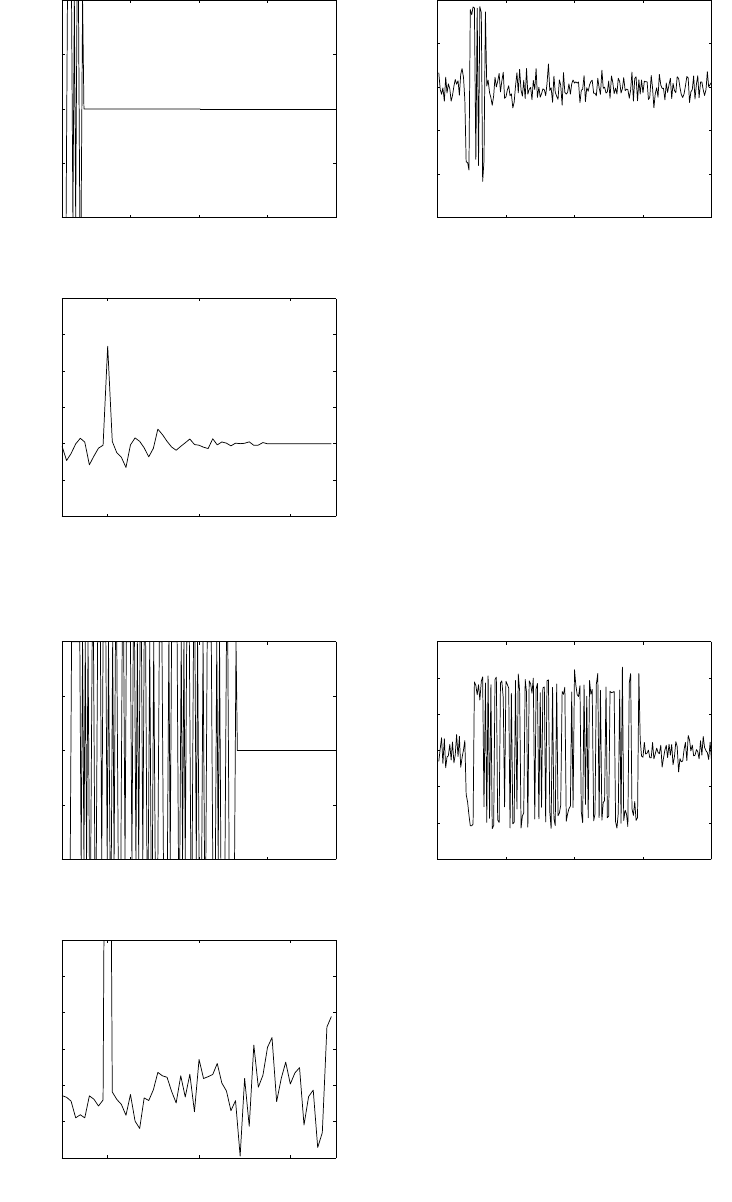
2.28
Fig. 2.28-1 shows the transient response, yzi(n), for y(−1) = 1 and the steady state response,
yzs(n).
0 5 10 15 20 25 30 35 40 45 50
0
0.2
0.4
0.6
0.8
1
Normalized Transient Response
0 5 10 15 20 25 30 35 40 45 50
0
2
4
6
8
10
Steady State Response
Figure 2.28-1:
2.29
h(n) = h1(n)∗h2(n)
=∞
X
k=−∞
ak[u(k)−u(k−N)][u(n−k)−u(n−k−M)]
=∞
X
k=−∞
aku(k)u(n−k)−∞
X
k=−∞
aku(k)u(n−k−M)
−∞
X
k=−∞
aku(k−N)u(n−k) + ∞
X
k=−∞
aku(k−N)u(n−k−M)
= n
X
k=0
ak−
n−M
X
k=0
ak!− n
X
k=N
ak−
n−M
X
k=N
ak!
= 0
33
© 2007 Pearson Education, Inc., Upper Saddle River, NJ. All rights reserved. This material is protected under all copyright laws
as they currently exist. No portion of this material may be reproduced, in any form or by any means, without permission in
writing from the publisher. For the exclusive use of adopters of the book Digital Signal Processing, Fourth Edition, by John G.
Proakis and Dimitris G. Manolakis. ISBN 0-13-187374-1.

2.30
y(n)−3y(n−1) −4y(n−2) = x(n) + 2x(n−1)
The characteristic equation is
λ2−3λ−4 = 0.
Hence, λ= 4,−1 and
yh(n) = c1(n)4n+c2(−1)n.
Since 4 is a characteristic root and the excitation is
x(n) = 4nu(n),
we assume a particular solution of the form
yp(n) = kn4nu(n).
Then
kn4nu(n)−3k(n−1)4n−1u(n−1) −4k(n−2)4n−2u(n−2)
= 4nu(n) + 2(4)n−1u(n−1)
. For n= 2,
k(32 −12) = 42+ 8 = 24 →k=6
5.
The total solution is
y(n) = yp(n) + yh(n)
=6
5n4n+c14n+c2(−1)nu(n)
To solve for c1and c2, we assume that y(−1) = y(−2) = 0. Then,
y(0) = 1 and
y(1) = 3y(0) + 4 + 2 = 9
Hence,
c1+c2= 1 and
24
5+ 4c1−c2= 9
4c1−c2=21
5
Therefore,
c1=26
25 and c2=−1
25
The total solution is
y(n) = 6
5n4n+26
254n−1
25(−1)nu(n)
34
© 2007 Pearson Education, Inc., Upper Saddle River, NJ. All rights reserved. This material is protected under all copyright laws
as they currently exist. No portion of this material may be reproduced, in any form or by any means, without permission in
writing from the publisher. For the exclusive use of adopters of the book Digital Signal Processing, Fourth Edition, by John G.
Proakis and Dimitris G. Manolakis. ISBN 0-13-187374-1.

2.31
From 2.30, the characteristic values are λ= 4,−1.Hence
yh(n) = c14n+c2(−1)n
When x(n) = δ(N),we find that
y(0) = 1 and
y(1) −3y(0) = 2 or
y(1) = 5.
Hence,
c1+c2= 1 and 4c1−c2= 5
This yields, c1=6
5and c2=−1
5. Therefore,
h(n) = 6
54n−1
5(−1)nu(n)
2.32
(a) L1=N1+M1and L2=N2+M2
(b) Partial overlap from left:
low N1+M1high N1+M2−1
Full overlap: low N1+M2high N2+M1
Partial overlap from right:
low N2+M1+ 1 high N2+M2
(c)
x(n) = 1,1,1
↑,1,1,1,1
h(n) = 2,2
↑,2,2
N1=−2,
N2= 4,
M1=−1,
M2= 2,
Partial overlap from left: n=−3n=−1L1=−3
Full overlap: n= 0 n= 3
Partial overlap from right:n= 4 n= 6 L2= 6
35
© 2007 Pearson Education, Inc., Upper Saddle River, NJ. All rights reserved. This material is protected under all copyright laws
as they currently exist. No portion of this material may be reproduced, in any form or by any means, without permission in
writing from the publisher. For the exclusive use of adopters of the book Digital Signal Processing, Fourth Edition, by John G.
Proakis and Dimitris G. Manolakis. ISBN 0-13-187374-1.

2.33
(a)
y(n)−0.6y(n−1) + 0.08y(n−2) = x(n).
The characteristic equation is
λ2−0.6λ+ 0.08 = 0.
λ= 0.2,0.4 Hence,
yh(n) = c1
1
5
n
+c2
2
5
n
.
With x(n) = δ(n),the initial conditions are
y(0) = 1,
y(1) −0.6y(0) = 0 ⇒y(1) = 0.6.
Hence,c1+c2= 1 and
1
5c1+2
5= 0.6⇒c1=−1, c2= 3.
Therefore h(n) = −(1
5)n+ 2(2
5)nu(n)
The step response is
s(n) =
n
X
k=0
h(n−k), n ≥0
=
n
X
k=0 2(2
5)n−k−(1
5)n−k
=1
0.12 (2
5
n+1
−1−1
0.16 (1
5
n+1
−1u(n)
(b)
y(n)−0.7y(n−1) + 0.1y(n−2) = 2x(n)−x(n−2).
The characteristic equation is
λ2−0.7λ+ 0.1 = 0.
λ=1
2,1
5Hence,
yh(n) = c1
1
2
n
+c2
1
5
n
.
With x(n) = δ(n),we have
y(0) = 2,
y(1) −0.7y(0) = 0 ⇒y(1) = 1.4.
Hence,c1+c2= 2 and
1
2c1+1
5= 1.4 = 7
5
⇒c1+2
5c2=14
5.
These equations yield
c1=10
3, c2=−4
3.
h(n) = 10
3(1
2)n−4
3(1
5)nu(n)
36
© 2007 Pearson Education, Inc., Upper Saddle River, NJ. All rights reserved. This material is protected under all copyright laws
as they currently exist. No portion of this material may be reproduced, in any form or by any means, without permission in
writing from the publisher. For the exclusive use of adopters of the book Digital Signal Processing, Fourth Edition, by John G.
Proakis and Dimitris G. Manolakis. ISBN 0-13-187374-1.

The step response is
s(n) =
n
X
k=0
h(n−k),
=10
3
n
X
k=0
(1
2)n−k−4
3
n
X
k=0
(1
5)n−k
=10
3(1
2)n
n
X
k=0
2k−4
3(1
5)n
n
X
k=0
5k
=10
3(1
2
n
(2n+1 −1)u(n)−1
3(1
5
n
(5n+1 −1)u(n)
2.34
h(n) = 1
↑,1
2,1
4,1
8,1
16
y(n) = 1
↑,2,2.5,3,3,3,2,1,0
x(0)h(0) = y(0) ⇒x(0) = 1
1
2x(0) + x(1) = y(1) ⇒x(1) = 3
2
By continuing this process, we obtain
x(n) = 1,3
2,3
2,7
4,3
2,...
2.35
(a) h(n) = h1(n)∗[h2(n)−h3(n)∗h4(n)]
(b)
h3(n)∗h4(n) = (n−1)u(n−2)
h2(n)−h3(n)∗h4(n) = 2u(n)−δ(n)
h1(n) = 1
2δ(n) + 1
4δ(n−1) + 1
2δ(n−2)
Hence h(n) = 1
2δ(n) + 1
4δ(n−1) + 1
2δ(n−2)∗[2u(n)−δ(n)]
=1
2δ(n) + 5
4δ(n−1) + 2δ(n−2) + 5
2u(n−3)
(c)
x(n) = 1,0,0
↑,3,0,−4
y(n) = 1
2,5
4,2
↑,25
4,13
2,5,2,0,0,...
37
© 2007 Pearson Education, Inc., Upper Saddle River, NJ. All rights reserved. This material is protected under all copyright laws
as they currently exist. No portion of this material may be reproduced, in any form or by any means, without permission in
writing from the publisher. For the exclusive use of adopters of the book Digital Signal Processing, Fourth Edition, by John G.
Proakis and Dimitris G. Manolakis. ISBN 0-13-187374-1.

2.36
First, we determine
s(n) = u(n)∗h(n)
s(n) = ∞
X
k=0
u(k)h(n−k)
=
n
X
k=0
h(n−k)
=∞
X
k=0
an−k
=an+1 −1
a−1, n ≥0
For x(n) = u(n+ 5) −u(n−10), we have the response
s(n+ 5) −s(n−10) = an+6 −1
a−1u(n+ 5) −an−9−1
a−1u(n−10)
From figure P2.33,
y(n) = x(n)∗h(n)−x(n)∗h(n−2)
Hence, y(n) = an+6 −1
a−1u(n+ 5) −an−9−1
a−1u(n−10)
−an+4 −1
a−1u(n+ 3) + an−11 −1
a−1u(n−12)
2.37
h(n) = [u(n)−u(n−M)] /M
s(n) = ∞
X
k=−∞
u(k)h(n−k)
=
n
X
k=0
h(n−k) = n+1
M, n < M
1, n ≥M
2.38
∞
X
n=−∞ |h(n)|=∞
X
n=0,neven |a|n
=∞
X
n=0 |a|2n
=1
1− |a|2
Stable if |a|<1
38
© 2007 Pearson Education, Inc., Upper Saddle River, NJ. All rights reserved. This material is protected under all copyright laws
as they currently exist. No portion of this material may be reproduced, in any form or by any means, without permission in
writing from the publisher. For the exclusive use of adopters of the book Digital Signal Processing, Fourth Edition, by John G.
Proakis and Dimitris G. Manolakis. ISBN 0-13-187374-1.

2.39
h(n) = anu(n).The response to u(n) is
y1(n) = ∞
X
k=0
u(k)h(n−k)
=
n
X
k=0
an−k
=an
n
X
k=0
a−k
=1−an+1
1−au(n)
Then, y(n) = y1(n)−y1(n−10)
=1
1−a(1 −an+1)u(n)−(1 −an−9)u(n−10)
2.40
We may use the result in problem 2.36 with a=1
2. Thus,
y(n) = 2 1−(1
2)n+1u(n)−21−(1
2)n−9u(n−10)
2.41
(a)
y(n) = ∞
X
k=−∞
h(k)x(n−k)
=
n
X
k=0
(1
2)k2n−k
= 2n
n
X
k=0
(1
4)k
= 2n1−(1
4)n+1(4
3)
=2
32n+1 −(1
2)n+1u(n)
(b)
y(n) = ∞
X
k=−∞
h(k)x(n−k)
=∞
X
k=0
h(k)
=∞
X
k=0
(1
2)k= 2, n < 0
39
© 2007 Pearson Education, Inc., Upper Saddle River, NJ. All rights reserved. This material is protected under all copyright laws
as they currently exist. No portion of this material may be reproduced, in any form or by any means, without permission in
writing from the publisher. For the exclusive use of adopters of the book Digital Signal Processing, Fourth Edition, by John G.
Proakis and Dimitris G. Manolakis. ISBN 0-13-187374-1.

y(n) = ∞
X
k=n
h(k)
=∞
X
k=n
(1
2)k
=∞
X
k=0
(1
2)k−
n−1
X
k=0
(1
2)k
= 2 −(1−(1
2)n
1
2
)
= 2(1
2)n, n ≥0.
2.42
(a)
he(n) = h1(n)∗h2(n)∗h3(n)
= [δ(n)−δ(n−1)] ∗u(n)∗h(n)
= [u(n)−u(n−1)] ∗h(n)
=δ(n)∗h(n)
=h(n)
(b) No.
2.43
(a) x(n)δ(n−n0) = x(n0).Thus, only the value of x(n) at n=n0is of interest.
x(n)∗δ(n−n0) = x(n−n0).Thus, we obtain the shifted version of the sequence x(n).
(b)
y(n) = ∞
X
k=−∞
h(k)x(n−k)
=h(n)∗x(n)
Linearity:x1(n)→y1(n) = h(n)∗x1(n)
x2(n)→y2(n) = h(n)∗x2(n)
Then x(n) = αx1(n) + βx2(n)→y(n) = h(n)∗x(n)
y(n) = h(n)∗[αx1(n) + βx2(n)]
=αh(n)∗x1(n) + βh(n)∗x2(n)
=αy1(n) + βy2(n)
Time Invariance:
x(n)→y(n) = h(n)∗x(n)
x(n−n0)→y1(n) = h(n)∗x(n−n0)
=X
k
h(k)x(n−n0−k)
=y(n−n0)
(c) h(n) = δ(n−n0).
40
© 2007 Pearson Education, Inc., Upper Saddle River, NJ. All rights reserved. This material is protected under all copyright laws
as they currently exist. No portion of this material may be reproduced, in any form or by any means, without permission in
writing from the publisher. For the exclusive use of adopters of the book Digital Signal Processing, Fourth Edition, by John G.
Proakis and Dimitris G. Manolakis. ISBN 0-13-187374-1.
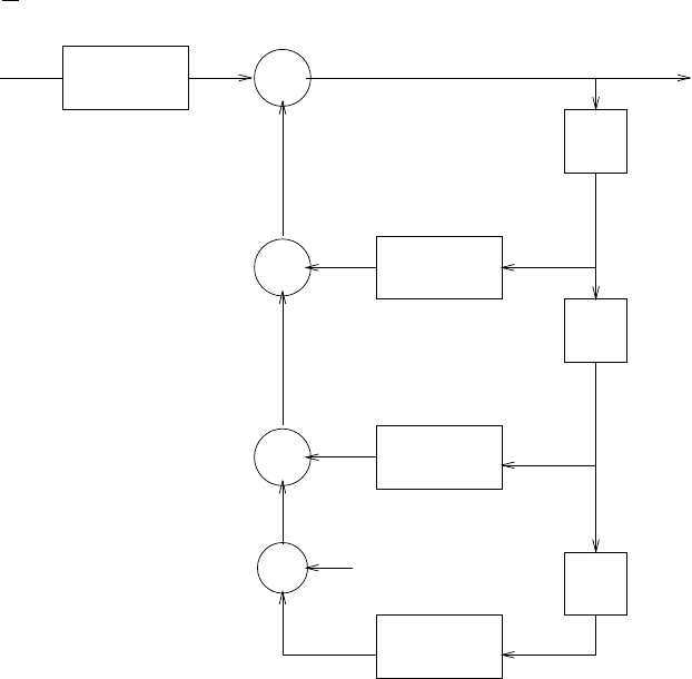
2.44
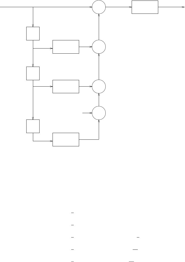
(a) s(n) = −a1s(n−1) −a2s(n−2) −...−aNs(n−N) + b0v(n).Refer to fig 2.44-1.
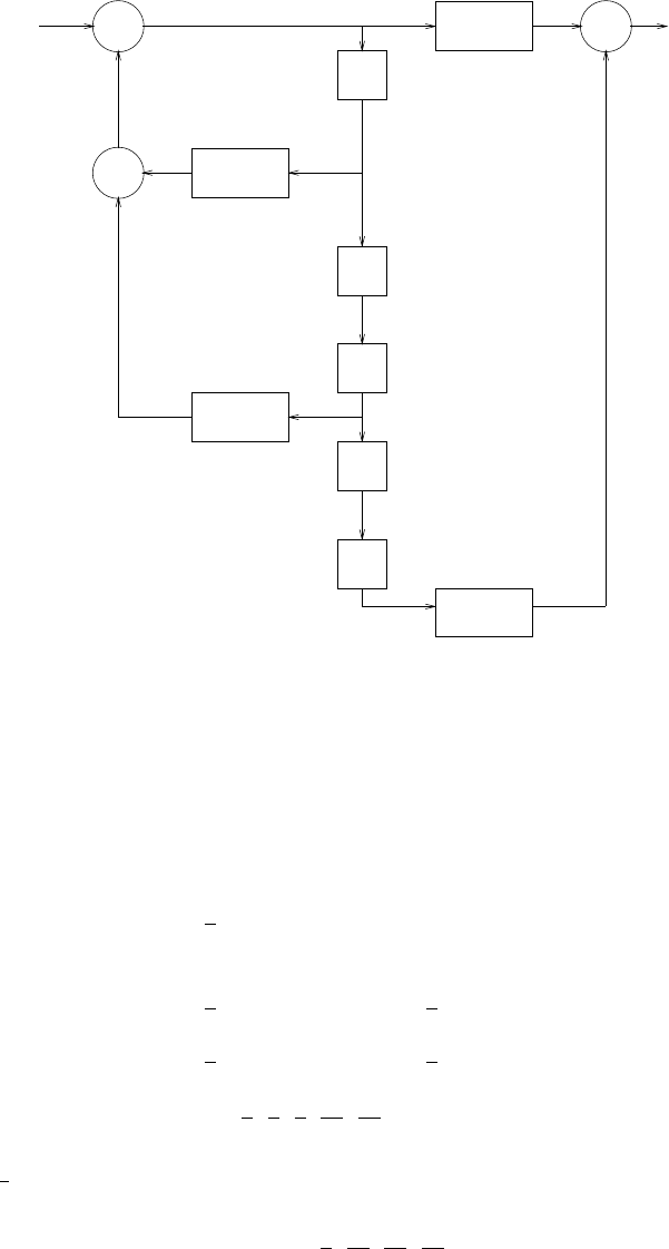
(b) v(n) = 1
b0[s(n) + a1s(n−1) + a2s(n−2) + ...+aNs(n−N)] .Refer to fig 2.44-2
v(n) +
+
+
+
z
-1
z
-1
z-1
-a 1
-a 2
-aN
s(n)
b0
Figure 2.44-1:
41
© 2007 Pearson Education, Inc., Upper Saddle River, NJ. All rights reserved. This material is protected under all copyright laws
as they currently exist. No portion of this material may be reproduced, in any form or by any means, without permission in
writing from the publisher. For the exclusive use of adopters of the book Digital Signal Processing, Fourth Edition, by John G.
Proakis and Dimitris G. Manolakis. ISBN 0-13-187374-1.
s(n)
1/b0
v(n)
a1
a2
a
N
z -1
z-1
z
-1
+
+
+
+
Figure 2.44-2:
2.45
y(n) = −1
2y(n−1) + x(n) + 2x(n−2)
y(−2) = −1
2y(−3) + x(−2) + 2x(−4) = 1
y(−1) = −1
2y(−2) + x(−1) + 2x(−3) = 3
2
y(0) = −1
2y(−1) + 2x(−2) + x(0) = 17
4
y(1) = −1
2y(0) + x(1) + 2x(−1) = 47
8,etc
2.46
(a) Refer to fig 2.46-1
(b) Refer to fig 2.46-2
42
© 2007 Pearson Education, Inc., Upper Saddle River, NJ. All rights reserved. This material is protected under all copyright laws
as they currently exist. No portion of this material may be reproduced, in any form or by any means, without permission in
writing from the publisher. For the exclusive use of adopters of the book Digital Signal Processing, Fourth Edition, by John G.
Proakis and Dimitris G. Manolakis. ISBN 0-13-187374-1.
x(n) 1/2
-1/2
+
+
2
z
-1
z
-1
z-1
z-1
z-1
3/2
+y(n)
Figure 2.46-1:
2.47
(a)
x(n) = 1
↑,0,0,...
y(n) = 1
2y(n−1) + x(n) + x(n−1)
y(0) = x(0) = 1,
y(1) = 1
2y(0) + x(1) + x(0) = 3
2
y(2) = 1
2y(1) + x(2) + x(1) = 3
4.Thus, we obtain
y(n) = 1,3
2,3
4,3
8,3
16,3
32,...
(b) y(n) = 1
2y(n−1) + x(n) + x(n−1)
(c) As in part(a), we obtain
y(n) = 1,5
2,13
4,29
8,61
16,...
(d)
y(n) = u(n)∗h(n)
=X
k
u(k)h(n−k)
43
© 2007 Pearson Education, Inc., Upper Saddle River, NJ. All rights reserved. This material is protected under all copyright laws
as they currently exist. No portion of this material may be reproduced, in any form or by any means, without permission in
writing from the publisher. For the exclusive use of adopters of the book Digital Signal Processing, Fourth Edition, by John G.
Proakis and Dimitris G. Manolakis. ISBN 0-13-187374-1.

x(n) y(n)
z-1
z-1
z-1
z-1
-1
-2
-3
+
+
+
Figure 2.46-2:
=
n
X
k=0
h(n−k)
y(0) = h(0) = 1
y(1) = h(0) + h(1) = 5
2
y(2) = h(0) + h(1) + h(2) = 13
4,etc
(e) from part(a), h(n) = 0 for n < 0⇒the system is causal.
∞
X
n=0 |h(n)|= 1 + 3
2(1 + 1
2+1
4+...) = 4 ⇒system is stable
2.48
(a)
y(n) = ay(n−1) + bx(n)
⇒h(n) = banu(n)
∞
X
n=0
h(n) = b
1−a= 1
⇒b= 1 −a.
44
© 2007 Pearson Education, Inc., Upper Saddle River, NJ. All rights reserved. This material is protected under all copyright laws
as they currently exist. No portion of this material may be reproduced, in any form or by any means, without permission in
writing from the publisher. For the exclusive use of adopters of the book Digital Signal Processing, Fourth Edition, by John G.
Proakis and Dimitris G. Manolakis. ISBN 0-13-187374-1.

(a)
s(n) =
n
X
k=0
h(n−k)
=b1−an+1
1−au(n)
s(∞) = b
1−a= 1
⇒b= 1 −a.
(c) b= 1 −ain both cases.
2.49
(a)
y(n) = 0.8y(n−1) + 2x(n) + 3x(n−1)
y(n)−0.8y(n−1) = 2x(n) + 3x(n−1)
The characteristic equation is
λ−0.8 = 0
λ= 0.8.
yh(n) = c(0.8)n
Let us first consider the response of the sytem
y(n)−0.8y(n−1) = x(n)
to x(n) = δ(n).Since y(0) = 1, it folows that c= 1. Then, the impulse response of the original
system is
h(n) = 2(0.8)nu(n) + 3(0.8)n−1u(n−1)
= 2δ(n) + 4.6(0.8)n−1u(n−1)
(b) The inverse system is characterized by the difference equation
x(n) = −1.5x(n−1) + 1
2y(n)−0.4y(n−1)
Refer to fig 2.49-1
2.50
y(n) = 0.9y(n−1) + x(n) + 2x(n−1) + 3x(n−2)
(a)For x(n) = δ(n), we have
y(0) = 1,
y(1) = 2.9,
y(2) = 5.61,
y(3) = 5.049,
y(4) = 4.544,
y(5) = 4.090,...
45
© 2007 Pearson Education, Inc., Upper Saddle River, NJ. All rights reserved. This material is protected under all copyright laws
as they currently exist. No portion of this material may be reproduced, in any form or by any means, without permission in
writing from the publisher. For the exclusive use of adopters of the book Digital Signal Processing, Fourth Edition, by John G.
Proakis and Dimitris G. Manolakis. ISBN 0-13-187374-1.

y(n)
-1.5 -0.4
z-1
0.5 +
x(n)
+
Figure 2.49-1:
(b)
s(0) = y(0) = 1,
s(1) = y(0) + y(1) = 3.91
s(2) = y(0) + y(1) + y(2) = 9.51
s(3) = y(0) + y(1) + y(2) + y(3) = 14.56
s(4) =
4
X
0
y(n) = 19.10
s(5) =
5
X
0
y(n) = 23.19
(c)
h(n) = (0.9)nu(n) + 2(0.9)n−1u(n−1) + 3(0.9)n−2u(n−2)
=δ(n) + 2.9δ(n−1) + 5.61(0.9)n−2u(n−2)
2.51
(a)
y(n) = 1
3x(n) + 1
3x(n−3) + y(n−1)
for x(n) = δ(n),we have
h(n) = 1
3,1
3,1
3,2
3,2
3,2
3,2
3,...
(b)
y(n) = 1
2y(n−1) + 1
8y(n−2) + 1
2x(n−2)
with x(n) = δ(n),and
y(−1) = y(−2) = 0,we obtain
h(n) = 0,0,1
2,1
4,3
16,1
8,11
128,15
256,41
1024,...
46
© 2007 Pearson Education, Inc., Upper Saddle River, NJ. All rights reserved. This material is protected under all copyright laws
as they currently exist. No portion of this material may be reproduced, in any form or by any means, without permission in
writing from the publisher. For the exclusive use of adopters of the book Digital Signal Processing, Fourth Edition, by John G.
Proakis and Dimitris G. Manolakis. ISBN 0-13-187374-1.

(c)
y(n) = 1.4y(n−1) −0.48y(n−2) + x(n)
with x(n) = δ(n),and
y(−1) = y(−2) = 0,we obtain
h(n) = {1,1.4,1.48,1.4,1.2496,1.0774,0.9086,...}
(d) All three systems are IIR.
(e)
y(n) = 1.4y(n−1) −0.48y(n−2) + x(n)
The characteristic equation is
λ2−1.4λ+ 0.48 = 0 Hence
λ= 0.8,0.6.and
yh(n) = c1(0.8)n+c2(0.6)nFor x(n) = δ(n).We have,
c1+c2= 1 and
0.8c1+ 0.6c2= 1.4
⇒c1= 4,
c2=−3.Therefore
h(n) = [4(0.8)n−3(0.6)n]u(n)
2.52
(a)
h1(n) = c0δ(n) + c1δ(n−1) + c2δ(n−2)
h2(n) = b2δ(n) + b1δ(n−1) + b0δ(n−2)
h3(n) = a0δ(n) + (a1+a0a2)δ(n−1) + a1a2δ(n−2)
(b) The only question is whether
h3(n)?
=h2(n) = h1(n)
Let a0=c0,
a1+a2c0=c1,
a2a1=c2.Hence
c2
a2
+a2c0−c1= 0
⇒c0a2
2−c1a2+c2= 0
For c06= 0,the quadratic has a real solution if and only if
c2
1−4c0c2≥0
2.53
(a)
y(n) = 1
2y(n−1) + x(n) + x(n−1)
For y(n)−1
2y(n−1) = δ(n),the solution is
h(n) = (1
2)nu(n) + (1
2)n−1u(n−1)
47
© 2007 Pearson Education, Inc., Upper Saddle River, NJ. All rights reserved. This material is protected under all copyright laws
as they currently exist. No portion of this material may be reproduced, in any form or by any means, without permission in
writing from the publisher. For the exclusive use of adopters of the book Digital Signal Processing, Fourth Edition, by John G.
Proakis and Dimitris G. Manolakis. ISBN 0-13-187374-1.

(b) h1(n)∗[δ(n) + δ(n−1)] = (1
2)nu(n) + (1
2)n−1u(n−1).
2.54
(a)
convolution: y1(n) = 1
↑,3,7,7,7,6,4
correlation: γ1(n) = 1,3,7,7,7
↑,6,4
(b)
convolution: y2(n) = 1
2,0
↑,3
2,−2,1
2,−6,−5
2,−2
correlation: γ1(n) = 1
2,0
↑,3
2,−2,1
2,−6,−5
2,−2
Note that y2(n) = γ2(n),because h2(−n) = h2(n) (c)
convolution: y3(n) = 4
↑,11,20,30,20,11,4
correlation: γ1(n) = 1,4,10,20
↑,25,24,16
(c)
convolution: y4(n) = 1
↑,4,10,20,25,24,16
correlation: γ4(n) = 4,11,20,30
↑,20,11,4
Note that h3(−n) = h4(n+ 3),
hence, γ3(n) = y4(n+ 3)
and h4(−n) = h3(n+ 3),
⇒γ4(n) = y3(n+ 3)
2.55
Obviously, the length of h(n) is 2, i.e.
h(n) = {h0, h1}
h0= 1
3h0+h1= 4
⇒h0= 1, h1= 1
2.56
(2.5.6) y(n) = −
N
X
k=1
aky(n−k) +
M
X
k=0
bkx(n−k)
48
© 2007 Pearson Education, Inc., Upper Saddle River, NJ. All rights reserved. This material is protected under all copyright laws
as they currently exist. No portion of this material may be reproduced, in any form or by any means, without permission in
writing from the publisher. For the exclusive use of adopters of the book Digital Signal Processing, Fourth Edition, by John G.
Proakis and Dimitris G. Manolakis. ISBN 0-13-187374-1.

(2.5.9) w(n) = −
N
X
k=1
akw(n−k) + x(n)
(2.5.10) y(n) =
M
X
k=0
bkw(n−k)
From (2.5.9) we obtain
x(n) = w(n) +
N
X
k=1
akw(n−k) (A)
By substituting (2.5.10) for y(n) and (A) into (2.5.6), we obtain L.H.S = R.H.S.
2.57
y(n)−4y(n−1) + 4y(n−2) = x(n)−x(n−1)
The characteristic equation is
λ2−4λ+ 4 = 0
λ= 2,2.Hence,
yh(n) = c12n+c2n2n
The particular solution is
yp(n) = k(−1)nu(n).
Substituting this solution into the difference equation, we obtain
k(−1)nu(n)−4k(−1)n−1u(n−1) + 4k(−1)n−2u(n−2) = (−1)nu(n)−(−1)n−1u(n−1)
For n= 2, k(1 + 4 + 4) = 2 ⇒k=2
9. The total solution is
y(n) = c12n+c2n2n+2
9(−1)nu(n)
From the initial condtions, we obtain y(0) = 1, y(1) = 2. Then,
c1+2
9= 1
⇒c1=7
9,
2c1+ 2c2−2
9= 2
⇒c2=1
3,
2.58
From problem 2.57,
h(n) = [c12n+c2n2n]u(n)
With y(0) = 1, y(1) = 3,we have
c1= 1
2c1+ 2c2= 3
49
© 2007 Pearson Education, Inc., Upper Saddle River, NJ. All rights reserved. This material is protected under all copyright laws
as they currently exist. No portion of this material may be reproduced, in any form or by any means, without permission in
writing from the publisher. For the exclusive use of adopters of the book Digital Signal Processing, Fourth Edition, by John G.
Proakis and Dimitris G. Manolakis. ISBN 0-13-187374-1.

⇒c2=1
2
Thus h(n) = 2n+1
2n2nu(n)
2.59
x(n) = x(n)∗δ(n)
=x(n)∗[u(n)−u(n−1)]
= [x(n)−x(n−1)] ∗u(n)
=∞
X
k=−∞
[x(k)−x(k−1)] u(n−k)
2.60
Let h(n) be the impulse response of the system
s(k) =
k
X
m=−∞
h(m)
⇒h(k) = s(k)−s(k−1)
y(n) = ∞
X
k=−∞
h(k)x(n−k)
=∞
X
k=−∞
[s(k)−s(k−1)] x(n−k)
2.61
x(n) = 1, n0−N≤n≤n0+N
0,otherwise
y(n) = 1,−N≤n≤N
0,otherwise
γxx(l) = ∞
X
n=−∞
x(n)x(n−l)
The range of non-zero values of γxx(l) is determined by
n0−N≤n≤n0+N
n0−N≤n−l≤n0+N
which implies
−2N≤l≤2N
For a given shift l, the number of terms in the summation for which both x(n) and x(n−l) are
non-zero is 2N+ 1 − |l|, and the value of each term is 1. Hence,
γxx(l) = 2N+ 1 − |l|,−2N≤l≤2N
0,otherwise
50
© 2007 Pearson Education, Inc., Upper Saddle River, NJ. All rights reserved. This material is protected under all copyright laws
as they currently exist. No portion of this material may be reproduced, in any form or by any means, without permission in
writing from the publisher. For the exclusive use of adopters of the book Digital Signal Processing, Fourth Edition, by John G.
Proakis and Dimitris G. Manolakis. ISBN 0-13-187374-1.

For γxy (l) we have
γxy(l) = 2N+ 1 − |l−n0|, n0−2N≤l≤n0+ 2N
0,otherwise
2.62
(a)
γxx(l) = ∞
X
n=−∞
x(n)x(n−l)
γxx(−3) = x(0)x(3) = 1
γxx(−2) = x(0)x(2) + x(1)x(3) = 3
γxx(−1) = x(0)x(1) + x(1)x(2) + x(2)x(3) = 5
γxx(0) =
3
X
n=0
x2(n) = 7
Also γxx(−l) = γxx(l)
Therefore γxx(l) = 1,3,5,7
↑,5,3,1
(b)
γyy (l) = ∞
X
n=−∞
y(n)y(n−l)
We obtain
γyy (l) = {1,3,5,7,5,3,1}
we observe that y(n) = x(−n+ 3), which is equivalent to reversing the sequence x(n). This has
not changed the autocorrelation sequence.
2.63
γxx(l) = ∞
X
n=−∞
x(n)x(n−l)
=2N+ 1 − |l|,−2N≤l≤2N
0,otherwise
γxx(0) = 2N+ 1
Therefore, the normalized autocorrelation is
ρxx(l) = 1
2N+ 1(2N+ 1 − |l|),−2N≤l≤2N
= 0,otherwise
2.64
(a)
γxx(l) = ∞
X
n=−∞
x(n)x(n−l)
51
© 2007 Pearson Education, Inc., Upper Saddle River, NJ. All rights reserved. This material is protected under all copyright laws
as they currently exist. No portion of this material may be reproduced, in any form or by any means, without permission in
writing from the publisher. For the exclusive use of adopters of the book Digital Signal Processing, Fourth Edition, by John G.
Proakis and Dimitris G. Manolakis. ISBN 0-13-187374-1.
=∞
X
n=−∞
[s(n) + γ1s(n−k1) + γ2s(n−k2)] ∗
[s(n−l) + γ1s(n−l−k1) + γ2s(n−l−k2)]
= (1 + γ2
1+γ2
2)γss(l) + γ1[γss(l+k1) + γss(l−k1)]
+γ2[γss(l+k2) + γss(l−k2)]
+γ1γ2[γss(l+k1−k2) + γss(l+k2−k1)]
(b) γxx(l) has peaks at l= 0,±k1,±k2and ±(k1+k2). Suppose that k1< k2. Then, we can
determine γ1and k1. The problem is to determine γ2and k2from the other peaks.
(c) If γ2= 0, the peaks occur at l= 0 and l=±k1.Then, it is easy to obtain γ1and k1.
2.65
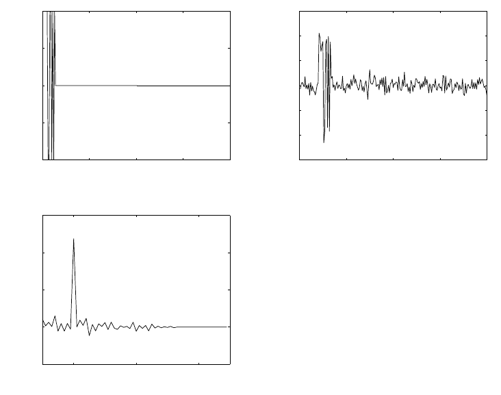
(a) The shift at which the crosscorrelation is maximum is the amount of delay D.
(b) variance = 0.01. Refer to fig 2.65-1.
(b) Delay D = 20. Refer to fig 2.65-1.
0 50 100 150 200
−1
−0.5
0
0.5
1
−−> n
−−> x(n)
0 50 100 150 200
−1.5
−1
−0.5
0
0.5
1
1.5
−−> n
−−> y(n)
−20 0 20
−5
0
5
10
15
−−> l
−−> rxy(l)
Figure 2.65-1: variance = 0.01
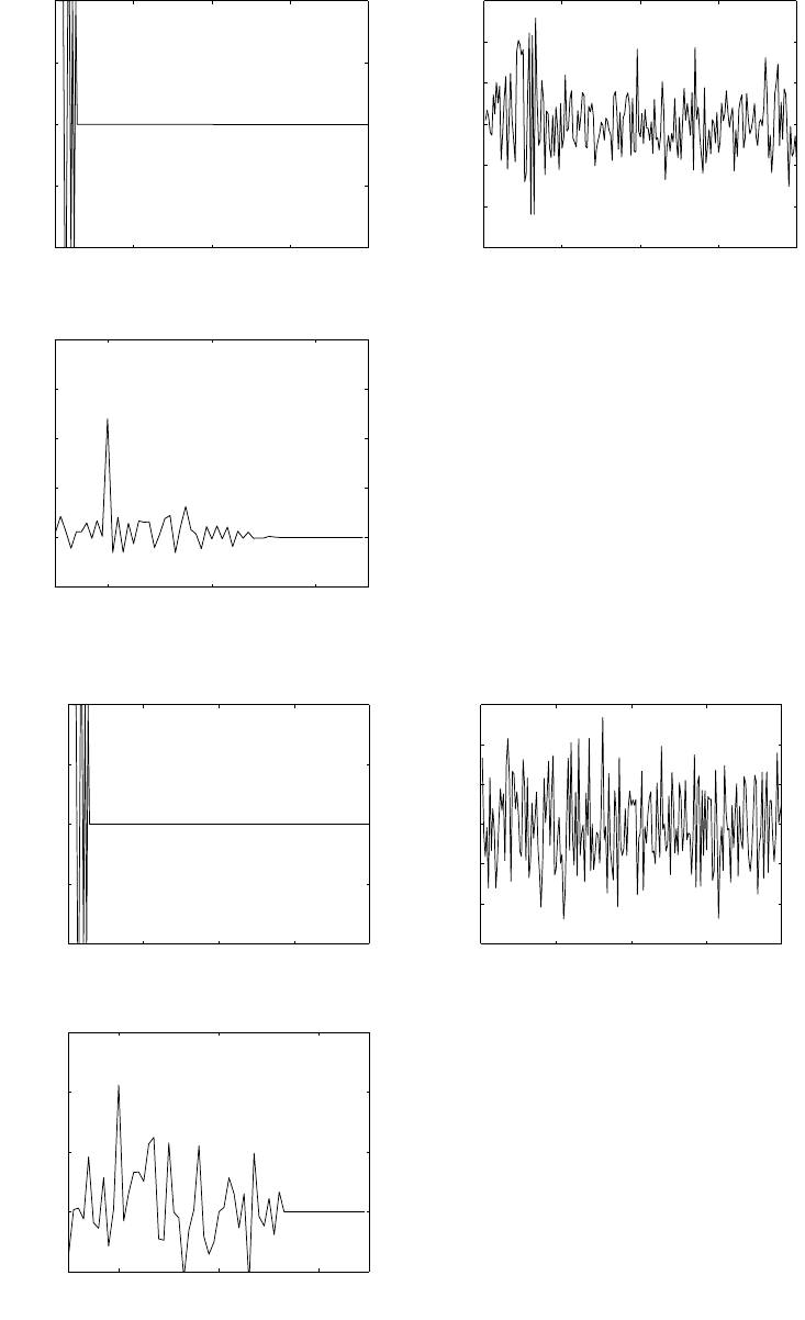
(c) variance = 0.1. Delay D = 20. Refer to fig 2.65-2.
(d) Variance = 1. delay D = 20. Refer to fig 2.65-3.
(e) x(n) = {−1,−1,−1,+1,+1,+1,+1,−1,+1,−1,+1,+1,−1,−1,+1}. Refer to fig 2.65-4.
(f) Refer to fig 2.65-5.
52
© 2007 Pearson Education, Inc., Upper Saddle River, NJ. All rights reserved. This material is protected under all copyright laws
as they currently exist. No portion of this material may be reproduced, in any form or by any means, without permission in
writing from the publisher. For the exclusive use of adopters of the book Digital Signal Processing, Fourth Edition, by John G.
Proakis and Dimitris G. Manolakis. ISBN 0-13-187374-1.
0 50 100 150 200
−1
−0.5
0
0.5
1
−−> n
−−> x(n)
0 50 100 150 200
−1.5
−1
−0.5
0
0.5
1
1.5
−−> n
−−> y(n)
−20 0 20
−5
0
5
10
15
20
−−> rxy(l)
Figure 2.65-2: variance = 0.1
0 50 100 150 200
−1
−0.5
0
0.5
1
−−> n
−−> x(n)
0 50 100 150 200
−3
−2
−1
0
1
2
3
−−> n
−−> y(n)
−20 0 20
−5
0
5
10
15
−−> l
−−> rxy(l)
Figure 2.65-3: variance = 1
53
© 2007 Pearson Education, Inc., Upper Saddle River, NJ. All rights reserved. This material is protected under all copyright laws
as they currently exist. No portion of this material may be reproduced, in any form or by any means, without permission in
writing from the publisher. For the exclusive use of adopters of the book Digital Signal Processing, Fourth Edition, by John G.
Proakis and Dimitris G. Manolakis. ISBN 0-13-187374-1.
0 50 100 150 200
−1
−0.5
0
0.5
1
−−> n
−−> x(n)
0 50 100 150 200
−1.5
−1
−0.5
0
0.5
1
−−> n
−−> y(n)
−20 0 20
−10
−5
0
5
10
15
20
−−> n
−−> rxy(l)
Figure 2.65-4:
0 50 100 150 200
−1
−0.5
0
0.5
1
−−> n
−−> x(n)
0 50 100 150 200
−1.5
−1
−0.5
0
0.5
1
1.5
−−> n
−−> y(n)
−20 0 20
−10
−5
0
5
10
15
20
−−> n
−−> rxy(l)
Figure 2.65-5:
54
© 2007 Pearson Education, Inc., Upper Saddle River, NJ. All rights reserved. This material is protected under all copyright laws
as they currently exist. No portion of this material may be reproduced, in any form or by any means, without permission in
writing from the publisher. For the exclusive use of adopters of the book Digital Signal Processing, Fourth Edition, by John G.
Proakis and Dimitris G. Manolakis. ISBN 0-13-187374-1.
2.66
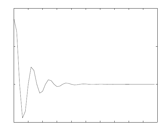
(a) Refer to fig 2.66-1.
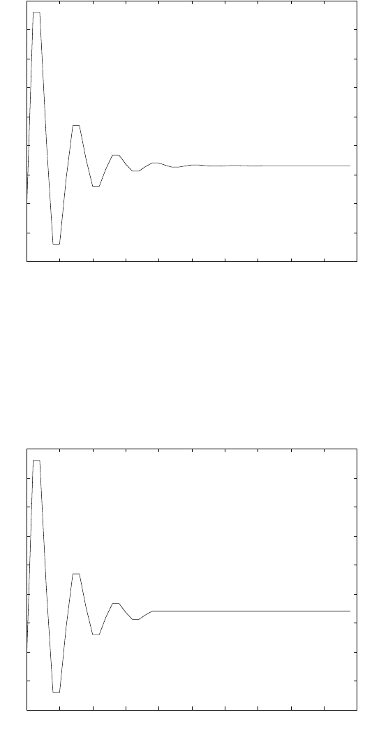
(b) Refer to fig 2.66-2.
0 5 10 15 20 25 30 35 40 45 50
−0.5
0
0.5
1
−−> n
−−> h(n)
impulse response h(n) of the system
Figure 2.66-1:
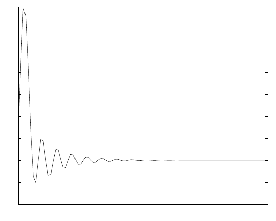
(c) Refer to fig 2.66-3.
(d) The step responses in fig 2.66-2 and fig 2.66-3 are similar except for the steady state value
after n=20.
55
© 2007 Pearson Education, Inc., Upper Saddle River, NJ. All rights reserved. This material is protected under all copyright laws
as they currently exist. No portion of this material may be reproduced, in any form or by any means, without permission in
writing from the publisher. For the exclusive use of adopters of the book Digital Signal Processing, Fourth Edition, by John G.
Proakis and Dimitris G. Manolakis. ISBN 0-13-187374-1.
0 5 10 15 20 25 30 35 40 45 50
0.7
0.8
0.9
1
1.1
1.2
1.3
1.4
1.5
1.6
−−> n
−−> s(n)
zero−state step response s(n)
Figure 2.66-2:
0 5 10 15 20 25 30 35 40 45 50
0.7
0.8
0.9
1
1.1
1.2
1.3
1.4
1.5
1.6
−−> n
−−> s(n)
step response
Figure 2.66-3:
56
© 2007 Pearson Education, Inc., Upper Saddle River, NJ. All rights reserved. This material is protected under all copyright laws
as they currently exist. No portion of this material may be reproduced, in any form or by any means, without permission in
writing from the publisher. For the exclusive use of adopters of the book Digital Signal Processing, Fourth Edition, by John G.
Proakis and Dimitris G. Manolakis. ISBN 0-13-187374-1.
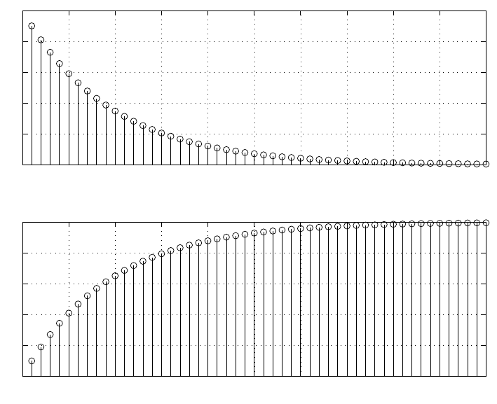
2.67
Refer to fig 2.67-1.
0 10 20 30 40 50 60 70 80 90 100
−2
−1
0
1
2
3
4
5
6
7
−−> n
−−> h(n)
Figure 2.67-1:
57
© 2007 Pearson Education, Inc., Upper Saddle River, NJ. All rights reserved. This material is protected under all copyright laws
as they currently exist. No portion of this material may be reproduced, in any form or by any means, without permission in
writing from the publisher. For the exclusive use of adopters of the book Digital Signal Processing, Fourth Edition, by John G.
Proakis and Dimitris G. Manolakis. ISBN 0-13-187374-1.
58
© 2007 Pearson Education, Inc., Upper Saddle River, NJ. All rights reserved. This material is protected under all copyright laws
as they currently exist. No portion of this material may be reproduced, in any form or by any means, without permission in
writing from the publisher. For the exclusive use of adopters of the book Digital Signal Processing, Fourth Edition, by John G.
Proakis and Dimitris G. Manolakis. ISBN 0-13-187374-1.

Chapter 3
3.1
(a)
X(z) = X
n
x(n)z−n
= 3z5+ 6 + z−1−4z−2ROC: 0 <|z|<∞
(b)
X(z) = X
n
x(n)z−n
=∞
X
n=5
(1
2)nz−n
=∞
X
n=5
(1
2z)n
=∞
X
m=0
(1
2z−1)m+5
= (z−1
2)51
1−1
2z−1
= ( 1
32)z−5
1−1
2z−1ROC: |z|>1
2
3.2
(a)
X(z) = X
n
x(n)z−n
=∞
X
n=0
(1 + n)z−n
=∞
X
n=0
z−n+∞
X
n=0
nz−n
But ∞
X
n=0
z−n=1
1−z−1ROC: |z|>1
59
© 2007 Pearson Education, Inc., Upper Saddle River, NJ. All rights reserved. This material is protected under all copyright laws
as they currently exist. No portion of this material may be reproduced, in any form or by any means, without permission in
writing from the publisher. For the exclusive use of adopters of the book Digital Signal Processing, Fourth Edition, by John G.
Proakis and Dimitris G. Manolakis. ISBN 0-13-187374-1.

and ∞
X
n=0
nz−n=z−1
(1 −z−1)2ROC: |z|>1
Therefore, X(z) = 1−z−1
(1 −z−1)2+z−1
(1 −z−1)2
=1
(1 −z−1)2
(b)
X(z) = ∞
X
n=0
(an+a−n)z−n
=∞
X
n=0
anz−n+∞
X
n=0
a−nz−n
But ∞
X
n=0
anz−n=1
1−az−1ROC: |z|>|a|
and ∞
X
n=0
a−nz−n=1
(1 −1
az−1)2ROC: |z|>1
|a|
Hence, X(z) = 1
1−az−1+1
1−1
az−1
=2−(a+1
a)z−1
(1 −az−1)(1 −1
az−1)ROC: |z|>max (|a|,1
|a|)
(c)
X(z) = ∞
X
n=0
(−1
2)nz−n
=1
1 + 1
2z−1,|z|>1
2
(d)
X(z) = ∞
X
n=0
nansinw0nz−n
=∞
X
n=0
nanejw0n−e−jw0n
2jz−n
=1
2jaejw0z−1
(1 −aejw0z−1)2−ae−jw0z−1
(1 −ae−jw0z−1)2
=az−1−(az−1)3sinw0
(1 −2acosw0z−1+a2z−2)2,|z|> a
(e)
X(z) = ∞
X
n=0
nancosw0nz−n
=∞
X
n=0
nanejw0n+e−jw0n
2z−n
60
© 2007 Pearson Education, Inc., Upper Saddle River, NJ. All rights reserved. This material is protected under all copyright laws
as they currently exist. No portion of this material may be reproduced, in any form or by any means, without permission in
writing from the publisher. For the exclusive use of adopters of the book Digital Signal Processing, Fourth Edition, by John G.
Proakis and Dimitris G. Manolakis. ISBN 0-13-187374-1.

=1
2aejw0z−1
(1 −aejw0z−1)2+ae−jw0z−1
(1 −ae−jw0z−1)2
=az−1+ (az−1)3sinw0−2a2z−2
(1 −2acosw0z−1+a2z−2)2,|z|> a
(f)
X(z) = A∞
X
n=0
rncos(w0n+φ)z−n
=A∞
X
n=0
rnejw0nejφ +e−jw0ne−jφ
2z−n
=A
2ejφ
1−rejw0z−1+e−jφ
1−re−jw0z−1
=Acosφ −rcos(w0−φ)z−1
1−2rcosw0z−1+r2z−2,|z|> r
(g)
X(z) = ∞
X
n=1
1
2(n2+n)(1
3)n−1z−n
But ∞
X
n=1
n(1
3)n−1z−1=(1
3)3z−1
(1 −1
3z−1)2=z−1
(1 −1
3z−1)2
∞
X
n=1
n2(1
3)n−1z−n=z−1+1
3z−2
(1 −1
3z−1)3
Therefore, X(z) = 1
2z−1
(1 −1
3z−1)2+z−1+1
3z−2
(1 −1
3z−1)3
=z−1
(1 −1
3z−1)3,|z|>1
3
(h)
X(z) = ∞
X
n=0
(1
2)nz−n−∞
X
n=10
(1
2)nz−n
=1
1−1
2z−1−(1
2)10z−10
1−1
2z−1
=1−(1
2z−1)10
1−1
2z−1,|z|>1
2
The pole-zero patterns are as follows:
(a) Double pole at z= 1 and a zero at z= 0.
(b) Poles at z=aand z=1
a. Zeros at z= 0 and z=1
2(a+1
a).
(c) Pole at z=−1
2and zero at z= 0.
(d) Double poles at z=aejw0and z=ae−jw0and zeros at z= 0, z=±a.
(e) Double poles at z=aejw0and z=ae−jw0and zeros are obtained by solving the quadratic
acosw0z2−2a2z+a3cosw0= 0.
(f) Poles at z=rejw0and z=ae−jw0and zeros at z= 0, and z=rcos(w0−φ)/cosφ.
(g) Triple pole at z=1
3and zeros at z= 0 and z=1
3. Hence there is a pole-zero cancellation so
61
© 2007 Pearson Education, Inc., Upper Saddle River, NJ. All rights reserved. This material is protected under all copyright laws
as they currently exist. No portion of this material may be reproduced, in any form or by any means, without permission in
writing from the publisher. For the exclusive use of adopters of the book Digital Signal Processing, Fourth Edition, by John G.
Proakis and Dimitris G. Manolakis. ISBN 0-13-187374-1.

that in reality there is only a double pole at z=1
3and a zero at z= 0.
(h) X(z) has a pole of order 9 at z= 0. For nine zeros which we find from the roots of
1−(1
2z−1)10 = 0
or, equivalently, (1
2)10 −z10 = 0
Hence, zn=1
2ej2πn
10 , n = 1,2,...,k.
Note the pole-zero cancellation at z=1
2.
3.3
(a)
X1(z) = ∞
X
n=0
(1
3)nz−n+
0
X
n=−∞
(1
2)nz−n−1
=1
1−1
3z−1+∞
X
n=0
(1
2)nzn−1
=1
1−1
3z−1+1
1−1
2z−1,
=
5
6
(1 −1
3z−1)(1 −1
2z)
The ROC is 1
3<|z|<2.
(b)
X2(z) = ∞
X
n=0
(1
3)nz−n−∞
X
n=0
2nz−n
=1
1−1
3z−1−1
1−2z−1,
=−5
3z−1
(1 −1
3z−1)(1 −2z−1)
The ROC is |z|>2.
(c)
X3(z) = ∞
X
n=−∞
x1(n+ 4)z−n
=z4X1(z)
=
5
6z4
(1 −1
3z−1)(1 −1
2z)
The ROC is 1
3<|z|<2.
(d)
X4(z) = ∞
X
n=−∞
x1(−n)z−n
62
© 2007 Pearson Education, Inc., Upper Saddle River, NJ. All rights reserved. This material is protected under all copyright laws
as they currently exist. No portion of this material may be reproduced, in any form or by any means, without permission in
writing from the publisher. For the exclusive use of adopters of the book Digital Signal Processing, Fourth Edition, by John G.
Proakis and Dimitris G. Manolakis. ISBN 0-13-187374-1.

=∞
X
m=−∞
x1(m)zm
=X1(z−1)
=
5
6
(1 −1
3z)(1 −1
2z−1)
The ROC is 1
2<|z|<3.
3.4
(a)
X(z) = ∞
X
n=0
n(−1)nz−n
=−zd
dz
∞
X
n=0
(−1)nz−n
=−zd
dz 1
1 + z−1
=−z−1
(1 + z−1)2,|z|>1
(b)
X(z) = ∞
X
n=0
n2z−n
=z2d2
dz2
∞
X
n=0
z−n
=z2d2
dz21
1−z−1
=−z−1
(1 −z−1)2+2z−1
(1 −z−1)3
=z−1(1 + z−1)
(1 −z−1)3,|z|>1
(c)
X(z) = −1
X
n=−∞ −nanz−n
=−zd
dz
−1
X
n=−∞
a(n)z−n
=−zd
dz 1
1−az−1
=az−1
(1 −az−1)2,|z|<|a|
(d)
X(z) = ∞
X
n=0
(−1)ncos(π
3n)z−n
63
© 2007 Pearson Education, Inc., Upper Saddle River, NJ. All rights reserved. This material is protected under all copyright laws
as they currently exist. No portion of this material may be reproduced, in any form or by any means, without permission in
writing from the publisher. For the exclusive use of adopters of the book Digital Signal Processing, Fourth Edition, by John G.
Proakis and Dimitris G. Manolakis. ISBN 0-13-187374-1.

From formula (9) in table 3.3 with a=−1,
X(z) = 1 + z−1cosπ
3
1 + 2z−1cosπ
3+z−2
=1 + 1
2z−1
1 + z−1+z−2,ROC: |z|>1
(e)
X(z) = ∞
X
n=0
(−1)nz−n
=1
1 + z−1,|z|>1
(f)
x(n) = 1
↑,0,−1,0,1,−1
X(z) = 1 −z−2+z−4−z−5, z 6= 0
3.5
Right-sided sequence :xr(n) = 0, n < n0
Xr(z) = −1
X
n=n0
xr(n)z−n+∞
X
n=0
xr(n)z−n
The term P−1
n=n0xr(n)z−nconverges for all zexcept z=∞.
The term P∞
n=0 xr(n)z−nconverges for all |z|> r0where some r0. Hence Xr(z) converges for
r0<|z|<∞when n0<0 and |z|> r0for n0>0
Left-sided sequence :xl(n) = 0, n > n0
Xl(z) =
0
X
n=−∞
xl(n)z−n+
n0
X
n=1
xl(n)z−n
The first term converges for some |z|< rl. The second term converges for all z, except z= 0.
Hence, Xl(z) converges for 0 <|z|< rlwhen n0>0, and for |z|< rlwhen n0<0.
Finite-Duration Two-sided sequence :x(n) = 0, n > n0and n < n1,where n0> n1
X(z) =
n0
X
n=n1
x(n)z−n
=−1
X
n=n1
x(n)z−n+
n=n0
X
n=0
x(n)z−n
The first term converges everywhere except z=∞.
The second term converges everywhere except z= 0. Therefore, X(z) converges for 0 <|z|<∞.
64
© 2007 Pearson Education, Inc., Upper Saddle River, NJ. All rights reserved. This material is protected under all copyright laws
as they currently exist. No portion of this material may be reproduced, in any form or by any means, without permission in
writing from the publisher. For the exclusive use of adopters of the book Digital Signal Processing, Fourth Edition, by John G.
Proakis and Dimitris G. Manolakis. ISBN 0-13-187374-1.

3.6
y(n) =
n
X
k=−∞
x(k)
⇒y(n)−y(n−1) = x(n)
Hence,Y(z)−Y(z)z−1=X(z)
Y(z) = X(z)
1−z−1
3.7
x1(n) = (1
3)n, n ≥0
(1
2)−n, n < 0
X1(z) = ∞
X
n=0
(1
3)nz−n+−1
X
n=−∞
(1
2)−nz−n
=1
1−1
3z−1+1
1−1
2z−1
=
5
6
(1 −1
3z−1)(1 −1
2z)
X2(z) = ∞
X
n=0
(1
2)nz−n
=1
1−1
2z−1,1
2<|z|<2
Then,Y(z) = −2
1−1
3z−1+
10
3
1−1
2z−1+−4
3
1−2z−1
Hence,y(n) = −2(1
3)n+10
3(1
2)n, n ≥0
4
3(2)n, n < 0
3.8
(a)
y(n) =
n
X
k=−∞
x(k)
=∞
X
k=−∞
x(k)u(n−k)
=x(n)∗u(n)
Y(z) = X(z)U(z)
=X(z)
1−z−1
(b)
u(n)∗u(n) = ∞
X
k=−∞
u(k)u(n−k)
65
© 2007 Pearson Education, Inc., Upper Saddle River, NJ. All rights reserved. This material is protected under all copyright laws
as they currently exist. No portion of this material may be reproduced, in any form or by any means, without permission in
writing from the publisher. For the exclusive use of adopters of the book Digital Signal Processing, Fourth Edition, by John G.
Proakis and Dimitris G. Manolakis. ISBN 0-13-187374-1.

=
n
X
k=−∞
u(k) = (n+ 1)u(n)
Hence,x(n) = u(n)∗u(n)
andX(z) = 1
(1 −z−1)2,|z|>1
3.9
y(n) = x(n)ejw0n. From the scaling theorem, we have Y(z) = X(e−jw0z). Thus, the poles and
zeros are phase rotated by an angle w0.
3.10
x(n) = 1
2[u(n) + (−1)nu(n)]
X+(z) = (1
1−z−1+1
1+z−1)
2
From the final value theorem
x(∞) = lim
z→1(z−1)X+(z)
= lim
z→1(z+z(z−1)
z+ 1 )
=1
2
3.11
(a)
X(z) = 1 + 2z4
1−2z−1+z−2
= 1 + 4z−1+ 7z−2+ 10z−3+...
Therefore,x(n) = 1
↑,4,7,10,...,3n+ 1,...
(b)
X(z) = 2z+ 5z2+ 8z3+...
Therefore,x(n) = . . . , −(3n+ 1),...,11,8,5,2,0
↑
3.12
X(z) = 1
(1 −2z−1)(1 −z−1)2
=A
(1 −2z−1)+B
(1 −z−1)+Cz−1
(1 −z−1)2
A= 4, B =−3, C =−1
Hence,x(n) = [4(2)n−3−n]u(n)
66
© 2007 Pearson Education, Inc., Upper Saddle River, NJ. All rights reserved. This material is protected under all copyright laws
as they currently exist. No portion of this material may be reproduced, in any form or by any means, without permission in
writing from the publisher. For the exclusive use of adopters of the book Digital Signal Processing, Fourth Edition, by John G.
Proakis and Dimitris G. Manolakis. ISBN 0-13-187374-1.

3.13
(a)
x1(n) = x(n
2), n even
0, n odd
X1(z) = ∞
X
n=−∞
x1(n)z−n
=∞
X
n=−∞
x(n
2)z−n
=∞
X
k=−∞
x(k)z−2k
=X(z2)
(b)
x2(n) = x(2n)
X2(z) = ∞
X
n=−∞
x2(n)z−n
=∞
X
n=−∞
x(2n)z−n
=∞
X
k=−∞
x(k)z−k
2
=∞
X
k=−∞ x(k) + (−1)kx(k)
2z−k
2, k even
=1
2
∞
X
k=−∞
x(k)z−k
2+1
2
∞
X
k=−∞
x(k)(−z1
2)−k
=1
2X(√z+X(−√z)
3.14
(a)
X(z) = 1−3z−1
1 + 3z−1+ 2z−2
=A
(1 + z−1)+B
(1 + 2z−1)
A= 2, B =−1
Hence,x(n) = [2(−1)n−(−2)n]u(n)
(b)
X(z) = 1
1−z−1+1
2z−2
=A(1 −1
2z−1) + B(1
2z−1)
1−z−1+1
2z−2
67
© 2007 Pearson Education, Inc., Upper Saddle River, NJ. All rights reserved. This material is protected under all copyright laws
as they currently exist. No portion of this material may be reproduced, in any form or by any means, without permission in
writing from the publisher. For the exclusive use of adopters of the book Digital Signal Processing, Fourth Edition, by John G.
Proakis and Dimitris G. Manolakis. ISBN 0-13-187374-1.

A= 1, B = 1
Hence,X(z) = 1−1
√2(cosπ
4)z−1
1−21
√2(cosπ
4)z−1+ ( 1
√2)2z−2
+
1
√2(sinπ
4)z−1
1−21
√2(cosπ
4)z−1+ ( 1
√2)2z−2
Hence,x(n) = (1
√2)ncosπ
4n+ ( 1
√2)nsinπ
4nu(n)
(c)
X(z) = z−6
1−z−1+z−7
1−z−1
x(n) = u(n−6) + u(n−7)
(d)
X(z) = 1
1 + z−2+ 2 z−2
1 + z−2
X(z) = 2 −1
1 + z−2
x(n) = cosπ
2nu(n) + 2cosπ
2(n−2)u(n−2)
x(n) = 2δ(n)−cosπ
2nu(n)
(e)
X(z) = 1
4
1 + 6z−1+z−2
(1 −2z−1+ 2z−2)(1 −1
2z−1)
=A(1 −z−1)
1−2z−1+ 2z−2+Bz−1
1−2z−1+ 2z−2+C
1−1
2z−1
A=−3
5, B =23
10, C =17
20
Hence,x(n) = −3
5(1
√2)ncosπ
4n+23
10(1
√2)nsinπ
4n+17
20(1
2)nu(n)
(f)
X(z) = 2−1.5z−1
1−1.5z−1+ 0.5z−2
=1
1−1
2z−1+1
1−z−1
x(n) = (1
2)n+ 1u(n)
(g)
X(z) = 1 + 2z−1+z−2
1 + 4z−1+ 4z−2
= 1 −2z−1+ 3z−2
(1 + 2z−1)(1 + 2z−1)
68
© 2007 Pearson Education, Inc., Upper Saddle River, NJ. All rights reserved. This material is protected under all copyright laws
as they currently exist. No portion of this material may be reproduced, in any form or by any means, without permission in
writing from the publisher. For the exclusive use of adopters of the book Digital Signal Processing, Fourth Edition, by John G.
Proakis and Dimitris G. Manolakis. ISBN 0-13-187374-1.

= 1 −2z−1
1 + 2z−1+z−2
(1 + 2z−1)2
x(n) = δ(n)−2(−2)n−1u(n−1) + (n−1)(−2)n−1u(n−1)
=δ(n) + (n−3)(−2)n−1u(n−1)
(h)
X(z) = 1
4
(z+1
2)(z+1
4)
(z−1
2)(z−1
√2ejπ
4)(z−1
√2e−jπ
4)
=1
4
(1 + 3
4z−1+1
8z−2)z−1
(1 −1
2z−1)(1 −z−1+1
2z−2)
=A(1 −1
2z−1)z−1
1−z−1+1
2z−2+A(1
2z−1)z−1
1−z−1+1
2z−2+Cz−1
1−1
2z−1
A=−1
2, B =7
8, C =3
4
Hence,x(n) = −1
2(1
2)n−1
2cosπ
4(n−1) + 7
8(1
2)n−1
2sinπ
4(n−1) + 3
4(1
2)n−1u(n−1)
(i)
X(z) = 1−1
4z−1
1 + 1
2z−1
=1
1 + 1
2z−1−1
4
z−1
1 + 1
2z−1
x(n) = (−1
2)nu(n) + 1
4(−1
2)n−1u(n−1)
(j)
X(z) = 1−az−1
z−1−a
=−1
a1−az−1
1−1
az−1
=−1
a1
1−1
az−1−az−1
1−1
az−1
x(n) = −1
a(1
a)nu(n) + ( 1
a)n−1u(n−1)
= (−1
a)n+1u(n) + ( 1
a)n−1u(n−1)
3.15
X(z) = 5z−1
(1 −2z−1)(3 −z−1)
=1
1−2z−1+1
1−1
3z−1
If |z|>2, x(n) = 2n−(1
3)nu(n)
69
© 2007 Pearson Education, Inc., Upper Saddle River, NJ. All rights reserved. This material is protected under all copyright laws
as they currently exist. No portion of this material may be reproduced, in any form or by any means, without permission in
writing from the publisher. For the exclusive use of adopters of the book Digital Signal Processing, Fourth Edition, by John G.
Proakis and Dimitris G. Manolakis. ISBN 0-13-187374-1.

If 1
3<|z|<2, x(n) = −(1
3)nu(−n−1) −2nu(−n−1)
If |z|<1
3, x(n) = (1
3)nu(−n−1) −2nu(−n−1)
3.16
(a)
x1(n) = 1
4(1
4)n−1u(n−1)
⇒X1(z) = (1
4)z−1
1−1
4z−1,|z|>1
4
x2(n) = 1 + (1
2)nu(n)
⇒X2(z) = 1
1−z−1+1
1−1
2z−1,|z|>1
Y(z) = X1(z)X2(z)
=−4
3
1−1
4z−1+
1
3
1−z−1+1
1−1
2z−1
y(n) = −4
3(1
4)n+1
3+ (1
2)nu(n)
(b)
x1(n) = u(n)
⇒X1(z) = 1
1−z−1,
x2(n) = δ(n) + (1
2)nu(n)
⇒X2(z) = 1 + 1
1−1
2z−1
Y(z) = X1(z)X2(z)
=3
1−z−1−1
1−1
2z−1
y(n) = 3−(1
2)nu(n)
(c)
x1(n) = (1
2)nu(n)
⇒X1(z) = 1
1−1
2z−1,
x2(n) = cosπnu(n)
⇒X2(z) = 1 + z−1
1 + 2z−1+z−2
Y(z) = X1(z)X2(z)
=1 + z−1
(1 −1
2z−1)(1 + 2z−1+z−2)
70
© 2007 Pearson Education, Inc., Upper Saddle River, NJ. All rights reserved. This material is protected under all copyright laws
as they currently exist. No portion of this material may be reproduced, in any form or by any means, without permission in
writing from the publisher. For the exclusive use of adopters of the book Digital Signal Processing, Fourth Edition, by John G.
Proakis and Dimitris G. Manolakis. ISBN 0-13-187374-1.

=A(1 + z−1)
1 + 2z−1+z−2+B
1−1
2z−1
A=2
3, B =1
3
y(n) = 2
3cosπn +1
3(1
2)nu(n)
(d)
x1(n) = nu(n)
⇒X1(z) = z−1
(1 −z−1)2,
x2(n) = 2nu(n−1)
⇒X2(z) = 2z−1
1−2z−1
Y(z) = X1(z)X2(z)
=2z−2
(1 −z−1)2(1 −2z−1)
=−2
1−z−1−−2z−1
(1 −z−1)2+2
1−2z−1
y(n) = −2(n+ 1) + 2n+1u(n)
3.17
z+[x(n+ 1)] = zX+(z)−x(0)
=zX+(z)−zx(0)
Therefore, zX+(z) = ∞
X
n=0
x(n+ 1)z−n+zx(0)
(z−1)X+(z) = −∞
X
n=0
x(n)z−n+∞
X
n=0
x(n+ 1)z−n+zx(0)
limz→1X+(z)(z−1) = x(0) + ∞
X
n=0
x(n+ 1) −∞
X
n=0
x(n)
=limm→∞ [x(0) + x(1) + x(2) + ...+x(m)
−x(0) −x(1)x(2) −...−x(m)]
=limm→∞x(m+ 1)
=x(∞)
3.18
(a)
∞
X
n=−∞
x∗(n)z−n=∞
X
n=−∞ x(n)(z∗)−n∗
=X∗(z∗)
71
© 2007 Pearson Education, Inc., Upper Saddle River, NJ. All rights reserved. This material is protected under all copyright laws
as they currently exist. No portion of this material may be reproduced, in any form or by any means, without permission in
writing from the publisher. For the exclusive use of adopters of the book Digital Signal Processing, Fourth Edition, by John G.
Proakis and Dimitris G. Manolakis. ISBN 0-13-187374-1.

(b)
1
2[X(z) + X∗(z∗)] = 1
2[z{x(n)}+z{x∗(n)}]
=zx(n) + x∗(n)
2
=z[Re {x(n)}]
(c)
1
2j[X(z)−X∗(z∗)] = zx(n)−x∗(n)
2j
=z[Im {x(n)}]
(d)
Xk(z) = ∞
X
n=−∞,n/kinteger
x(n
k)z−n
=∞
X
m=−∞
x(m)z−mk
=X(zk)
(e)
∞
X
n=−∞
ejw0nx(n)z−n=∞
X
n=−∞
x(n)(e−jw0z)−n
=X(ze−jw0)
3.19
(a)
X(z) = log(1 −2z),|z|<1
2
Y(z) = −zdX(z)
dz
=−1
1−1
2z−1,|z|<1
2
⇒y(n) = (1
2)n, n < 0
Then,x(n) = 1
ny(n)
=1
n(1
2)nu(−n−1)
(b)
X(z) = log(1 −1
2z−1),|z|>1
2
Y(z) = −zdX(z)
dz
72
© 2007 Pearson Education, Inc., Upper Saddle River, NJ. All rights reserved. This material is protected under all copyright laws
as they currently exist. No portion of this material may be reproduced, in any form or by any means, without permission in
writing from the publisher. For the exclusive use of adopters of the book Digital Signal Processing, Fourth Edition, by John G.
Proakis and Dimitris G. Manolakis. ISBN 0-13-187374-1.

=−1
2z−1
1−1
2z−1,|z|>1
2
Hence,y(n) = −1
2(1
2)n−1u(n−1)
x(n) = 1
ny(n)
=−1
n(1
2)nu(n−1)
3.20
(a)
x1(n) = rnsinw0nu(n),0< r < 1
X1(z) = rsinw0z−1
1−2rcosw0z−1+r2z−2
Zero at z= 0 and poles at z=re±jw0=r(cosw0±jsinw0).
(b)
X2(z) = z
(1 −rejw0z−1)(1 −re−jw0z−1)
=z
1−2rcosw0z−1+r2z−2
(c) X1(z) and X2(z) differ by a constant, which can be determined by giving the value of X1(z)
at z= 1.
3.21
Assume that the polynomial has real coefficients and a complex root and prove that the complex
conjugate of the root will also be a root. Hence, let p(z) be a polynomial and z1is a complex
root. Then,
anzn
1+an−1zn−1
1+...+a1z1+a0= 0 (1)
The complex conjugate of (1) is
an(z∗
1)n+an−1(z∗
1)n−1+...+a1(z∗
1) + a0= 0
Therefore, z∗
1is also a root.
3.22
Convolution property:
z{x1(n)∗x2(n)}=∞
X
n=−∞ "∞
X
k=−∞
x1(k)x2(n−k)#z−n
=∞
X
k=−∞
x1(k)∞
X
n=−∞
x2(n−k)z−n
73
© 2007 Pearson Education, Inc., Upper Saddle River, NJ. All rights reserved. This material is protected under all copyright laws
as they currently exist. No portion of this material may be reproduced, in any form or by any means, without permission in
writing from the publisher. For the exclusive use of adopters of the book Digital Signal Processing, Fourth Edition, by John G.
Proakis and Dimitris G. Manolakis. ISBN 0-13-187374-1.

=∞
X
k=−∞
x1(k)z−kX2(z)
=X1(z)X2(z)
Correlation property:
r12(l) = x1(n)∗x2(−n)
R12(z) = z{x1(n)∗x2(−n)}
=X1(z)z{x2(−n)}
=X1(z)X2(z−1)
3.23
X(z) = 1 + z+z2
2! +z3
3! +...
+1 + z−1+z−2
2! +z−3
3! +...
x(n) = δ(n) + 1
n!
3.24
(a)
X(z) = 1
1 + 1.5z−1−0.5z−2
=0.136
1−0.28z−1+0.864
1 + 1.78z−1
Hence, x(n) = [0.136(0.28)n+ 0.864(−1.78)n]u(n)
(b)
X(z) = 1
1−0.5z−1+ 0.6z−2
=1−0.25z−1
1−0.5z−1+ 0.6z−2+ 0.3412 0.7326z−1
1−0.5z−1+ 0.6z−2
Then, x(n) = (0.7746)n[cos1.24n+ 0.3412sin1.24n]u(n)
partial check: x(0) = 1, x(1) = 0.5016, x(2) = −0.3476, x(∞) = 0. From difference equation,
x(n)−0.5x(n−1) + 0.6x(n−2) = δ(n) we obtain, x(0) = 1, x(1) = 0.5, x(2) = −0.35, x(∞) = 0.
3.25
(a)
X(z) = 1
1−1.5z−1+ 0.5z−2
=2
1−z−1−1
1−0.5z−1
For |z|<0.5, x(n) = [(0.5)n−2] u(−n−1)
74
© 2007 Pearson Education, Inc., Upper Saddle River, NJ. All rights reserved. This material is protected under all copyright laws
as they currently exist. No portion of this material may be reproduced, in any form or by any means, without permission in
writing from the publisher. For the exclusive use of adopters of the book Digital Signal Processing, Fourth Edition, by John G.
Proakis and Dimitris G. Manolakis. ISBN 0-13-187374-1.

For |z|>1, x(n) = [2 −(0.5)n]u(n)
For 0.5<|z|<1, x(n) = −(0.5)nu(n)−2u(−n−1)
(b)
X(z) = 1
(1 −0.5z−1)2
=0.5z−1
(1 −0.5z−1)22z
For |z|>0.5, x(n) = 2(n+ 1)(0.5)n+1u(n+ 1)
= (n+ 1)(0.5)nu(n)
For |z|<0.5, x(n) = −2(n+ 1)(0.5)n+1u(−n−2)
=−(n+ 1)(0.5)nu(−n−1)
3.26
X(z) = 3
1−10
3z−1+z−2
=−3
8
1−1
3z−1+
27
8
1−3z−1
ROC: 1
3<|z|<3, x(n) = 3
8(1
3)nu(n)−27
83nu(−n−1)
3.27
X(z) = ∞
X
n=−∞
x(n)z−n
=∞
X
n=−∞
x1(n)x∗
2(n)z−n
=∞
X
n=−∞
1
2πj Ic
X1(v)vn−1dvx∗
2(n)z−n
=1
2πj Ic
X1(v)dv "∞
X
n=−∞
x∗
2(n)(z
v)−n#v−1
=1
2πj Ic
X1(v)"∞
X
n=−∞
x2(n)(z∗
v∗)−n#∗
v−1dv
=1
2πj Ic
X1(v)X∗
2(z∗
v∗)v−1dv
3.28
Conjugation property:
75
© 2007 Pearson Education, Inc., Upper Saddle River, NJ. All rights reserved. This material is protected under all copyright laws
as they currently exist. No portion of this material may be reproduced, in any form or by any means, without permission in
writing from the publisher. For the exclusive use of adopters of the book Digital Signal Processing, Fourth Edition, by John G.
Proakis and Dimitris G. Manolakis. ISBN 0-13-187374-1.

∞
X
n=−∞
x∗(n)z−n="∞
X
n=−∞
x(n)(z∗)−n#∗
=X∗(z∗)
Parseval’s relation:
∞
X
n=−∞
x1(n)x∗
2(n) = ∞
X
n=−∞
1
2πj Ic
X1(v)vn−1dvx∗
2(n)
=1
2πj Ic
X1(v)"∞
X
n=−∞
x∗
2(n)( 1
v)−n#v−1dv
=1
2πj Ic
X1(v)X∗
2(1
v∗)dv
3.29
x(n) = 1
2πj Ic
zndz
z−a,
where the radius of the contour cis rc>|a|. For n < 0, let w=1
z. Then,
x(n) = 1
2πj Ic′
1
aw−n−1
w−1
a
dw,
where the radius of c′is 1
rc. Since 1
rc<|a|, there are no poles within c′and, hence x(n) = 0 for
n < 0.
3.30
x(n) = x(N−1−n),since x(n) is even. Then
X(z) =
N−1
X
n=0
x(n)z−n
=x(0) + x(1)z−1+...+x(N−2)z−N+2 +x(N−1)z−N+1
=z−(N−1)/2
N
2−1
X
n=0
x(n)hz(N−1−2n)/2+z−(N−1−2n)/2iNeven
If we substitute z−1for zand multiply both sides by z−(N−1) we obtain
z−(N−1)X(z−1) = X(z)
Hence, X(z) and X(z−1) have identical roots. This means that if z1is root (or a zero) of X(z)
then 1
z1is also a root. Since x(n) is real, then z∗
1must also be a root and so must 1
z∗
1
3.31
From the definition of the Fibonacci sequence, y(n) = y(n−1) + y(n−2), y(0) = 1.This is
equivalent to a system described by the difference equation y(n) = y(n−1) + y(n−2) + x(n),
76
© 2007 Pearson Education, Inc., Upper Saddle River, NJ. All rights reserved. This material is protected under all copyright laws
as they currently exist. No portion of this material may be reproduced, in any form or by any means, without permission in
writing from the publisher. For the exclusive use of adopters of the book Digital Signal Processing, Fourth Edition, by John G.
Proakis and Dimitris G. Manolakis. ISBN 0-13-187374-1.

where x(n) = δ(n) and y(n) = 0, n < 0. The z-transform of this difference equation is Y(z) =
z−1Y(z) + z−2Y(z) = X(z) Hence, for X(z) = 1,we have
Y(z) = 1
1−z−1−z−2
Y(z) = A
1−√5+1
2z−1+B
1−1−√5
2z−1
where A=√5 + 1
2√5, B =√5−1
2√5=−1−√5
2√5
Hence, y(n) = √5 + 1
2√5(√5 + 1
2)nu(n)−1−√5
2√5(1−√5
2)nu(n)
=1
√5"(1 + √5
2)n+1 −(1−√5
2)n+1#u(n)
3.32
(a)
Y(z)1−0.2z−1=X(z)1−0.3z−1−0.02z−2
Y(z)
X(z)=(1 −0.1z−1)(1 −0.2z−1)
1−0.2z−1
= 1 −0.1z−1
(b)
Y(z) = X(z)1−0.1z−1
Y(z)
X(z)= 1 −0.1z−1
Therefore, (a) and (b) are equivalent systems.
3.33
X(z) = 1
1−az−1
⇒x1(n) = anu(n)
or x2(n) = −anu(−n−1)
Both x1(n) and x2(n) have the same autocorrelation sequence. Another sequence is obtained
from X(z−1) = 1
1−az
X(z−1) = 1
1−az
= 1 −1
1−1
az−1
Hence x3(n) = δ(n)−(1
a)nu(n)
We observe that x3(n) has the same autocorrelation as x1(n) and x2(n)
77
© 2007 Pearson Education, Inc., Upper Saddle River, NJ. All rights reserved. This material is protected under all copyright laws
as they currently exist. No portion of this material may be reproduced, in any form or by any means, without permission in
writing from the publisher. For the exclusive use of adopters of the book Digital Signal Processing, Fourth Edition, by John G.
Proakis and Dimitris G. Manolakis. ISBN 0-13-187374-1.

3.34
H(z) = −∞
X
n=−1
3nz−n+∞
X
n=0
(2
5)nz−n
=−1
1−3z−1+1
1−2
5z−1,ROC: 2
5<|z|<3
X(z) = 1
1−z−1
Y(z) = H(z)X(z)
=−13
5z−1
(1 −z−1)(1 −3z−1)(1 −2
5z−1),ROC: 1 <|z|<2
=
13
6
1−z−1−
3
2
1−3z−1−
2
3
1−2
5z−1
Therefore,
y(n) = 3
23nu(−n−1) + 13
6−2
3(2
5)nu(n)
3.35
(a)
h(n) = (1
3)nu(n)
H(z) = 1
1−1
3z−1
x(n) = (1
2)ncosπn
3u(n)
X(z) = 1−1
4z−1
1−1
2z−1+1
4z−2
Y(z) = H(z)X(z)
=1−1
4z−1
(1 −1
3z−1)(1 −1
2z−1+1
4z−2)
=
1
7
1−1
3z−1+
6
7(1 −1
4z−1
1−1
2z−1+1
4z−2+3√3
7
√3
4z−1
1−1
2z−1+1
4z−2
Therefore,
y(n) = "1
7(1
3)n+6
7(1
2)ncosπn
3+3√3
7(1
2)nsinπn
3#u(n)
(b)
h(n) = (1
2)nu(n)
H(z) = 1
1−1
2z−1
x(n) = (1
3)nu(n) + (1
2)−nu(−n−1)
78
© 2007 Pearson Education, Inc., Upper Saddle River, NJ. All rights reserved. This material is protected under all copyright laws
as they currently exist. No portion of this material may be reproduced, in any form or by any means, without permission in
writing from the publisher. For the exclusive use of adopters of the book Digital Signal Processing, Fourth Edition, by John G.
Proakis and Dimitris G. Manolakis. ISBN 0-13-187374-1.

X(z) = 1
1−1
3z−1−1
1−2z−1
Y(z) = H(z)X(z)
=−5
3z−1
(1 −1
2z−1)(1 −1
3z−1)(1 −2z−1)
=
10
3
1−1
2z−1+−2
1−1
3z−1+−4
3
1−2z−1
Therefore,
y(n) = 10
3(1
2)n−2(1
3)nu(n) + 4
32nu(−n−1)
(c)
y(n) = −0.1y(n−1) + 0.2y(n−2) + x(n) + x(n−1)
H(z) = 1 + z−1
1 + 0.1z−1−0.2z−2
x(n) = (1
3)nu(n)
X(z) = 1
1−1
3z−1
Y(z) = H(z)X(z)
=1 + z−1
(1 −1
3z−1)(1 + 0.1z−1−0.2z−2)
=−8
1−1
3z−1+
28
3
1−0.4z−1+−1
3
1 + 0.5z−1
Therefore,
y(n) = −8(1
3)n+28
3(2
5)n−1
3(1
2)nu(n)
(d)
y(n) = 1
2x(n)−1
2x(n−1)
⇒Y(z) = 1
2(1 −z−1)X(z)
X(z) = 10
1 + z−2
Hence, Y(z) = 10(1 −z−1)/2
1 + z−2
y(n) = 5cosπn
2u(n)−5cosπ(n−1)
2u(n−1)
=h5cosπn
2−5sinπn
2iu(n−1) + 5δ(n)
= 5δ(n) + 10
√2sin(πn
2+π
4)u(n−1)
=10
√2sin(πn
2+π
4)u(n)
(e)
y(n) = −y(n−2) + 10x(n)
79
© 2007 Pearson Education, Inc., Upper Saddle River, NJ. All rights reserved. This material is protected under all copyright laws
as they currently exist. No portion of this material may be reproduced, in any form or by any means, without permission in
writing from the publisher. For the exclusive use of adopters of the book Digital Signal Processing, Fourth Edition, by John G.
Proakis and Dimitris G. Manolakis. ISBN 0-13-187374-1.

Y(z) = 10
1 + z−2X(z)
X(z) = 10
1 + z−2
Y(z) = 100
(1 + z−2)2
=50
1 + jz−1+50
1−jz−1+−25jz−1
(1 + jz−1)2+25jz−1
(1 −jz−1)2
Therefore,
y(n) = {50 [jn+ (−j)n]−25n[jn+ (−j)n]}u(n)
= (50 −25n)(jn+ (−j)n)u(n)
= (50 −25n)2cosπn
2u(n)
(f)
h(n) = (2
5)nu(n)
H(z) = 1
1−2
5z−1
x(n) = u(n)−u(n−7)
X(z) = 1−z−n
1−z−1
Y(z) = H(z)X(z)
=1−z−n
(1 −2
5z−1)(1 −z−1)
=
5
3
1−z−1+−2
3
1−2
5z−1−5
3
1−z−1+−2
3
1−2
5z−1z−7
Therefore,
y(n) = 1
35−2(2
5)nu(n)−1
35−2(2
5)n−7u(n−7)
(g)
h(n) = (1
2)nu(n)
H(z) = 1
1−1
2z−1
x(n) = (−1)n,− ∞ < n < ∞
=cosπn, − ∞ < n < ∞
x(n) is periodic sequence and its z-transform does not exist.
y(n) = |H(w0)|cos[πn + Θ(w0)], w0=π
H(z) = 1
1−1
2e−jw
H(π) = 1
1 + 1
2
=2
3,Θ = 0.
Hence, y(n) = 2
3cosπn, − ∞ < n < ∞
80
© 2007 Pearson Education, Inc., Upper Saddle River, NJ. All rights reserved. This material is protected under all copyright laws
as they currently exist. No portion of this material may be reproduced, in any form or by any means, without permission in
writing from the publisher. For the exclusive use of adopters of the book Digital Signal Processing, Fourth Edition, by John G.
Proakis and Dimitris G. Manolakis. ISBN 0-13-187374-1.

(h)
h(n) = (1
2)nu(n)
H(z) = 1
1−1
2z−1
x(n) = (n+ 1)(1
4)nu(n)
X(z) = 1
1−1
4z−1+
1
4z−1
(1 −1
4z−1)2
Y(z) = H(z)X(z)
=1
(1 −1
2z−1)(1 −1
4z−1)2
=4
1−1
2z−1+−1
4z−1
(1 −1
4z−1)2+−3
1−1
4z−1
Therefore,
y(n) = 4(1
2)n−n(1
4)n−3(1
4)nu(n)
3.36
H(z) = 1−2z−1+ 2z−2−z−3
(1 −z−1)(1 −1
2z−1)(1 −1
5z−1),1
2<|z|<1
=1−z−1+z−2
(1 −1
2z−1)(1 −1
5z−1),1
2<|z|<1
(a) Z1,2=1±j√3
2, p1=1
2, p2=1
5
(b) H(z) = 1 + 5
2
1−1
2z−1+−2.8
1−1
5z−1z−1
h(n) = δ(n) + 5(1
2)n−14(1
5)nu(n)
3.37
y(n) = 0.7y(n−1) −0.12y(n−2) + x(n−1) + x(n−2)
Y(z) = z−1+z−2
1−0.7z−1+ 0.12z−2X(z)
x(n) = nu(n)
X(z) = z−1
(1 −z−1)2
Y(z) = z−2+z−3
(1 −z−1)2(1 −3
10 z−1)(1 −2
50 z−2)
⇒System is stable
Y(z) = 4.76z−1
(1 −z−1)2+−12.36
(1 −z−1)+−26.5
(1 −3
10 z−1)+38.9
(1 −2
5z−1)
81
© 2007 Pearson Education, Inc., Upper Saddle River, NJ. All rights reserved. This material is protected under all copyright laws
as they currently exist. No portion of this material may be reproduced, in any form or by any means, without permission in
writing from the publisher. For the exclusive use of adopters of the book Digital Signal Processing, Fourth Edition, by John G.
Proakis and Dimitris G. Manolakis. ISBN 0-13-187374-1.

y(n) = 4.76n−12.36 −26.5( 3
10)n+ 38.9( 2
5)nu(n)
3.38
(a)
y(n) = 3
4y(n−1) −1
8y(n−2) + x(n)
Y(z) = 1
1−3
4z−1+1
8z−2X(z)
Impulse Response: X(z) = 1
Y(z) = 2
1−1
2z−1−1
1−1
4z−1
⇒h(n) = 2(1
2)n−(1
4)nu(n)
Since the poles of H(z) are inside the unit circle, the system is stable (poles at z=1
2,1
4).
Step Response: X(z) = 1
1−z−1
Y(z) =
8
3
1−z−1−2
1−1
2z−1+
1
3
1−1
4z−1
y(n) = 8
3−2(1
2)n+1
3(1
4)nu(n)
(b)
y(n) = y(n−1) −1
2y(n−2) + x(n) + x(n−1)
Y(z) = 1 + z−1
1−z−1+1
2z−2X(z)
H(z) has zeros at z= 0,1, and poles at z=1±j
2. Hence, the system is stable.
Impulse Response: X(z) = 1
Y(z) = 1−(√2)−1cosπ
4z−1
1−2(√2)−1cosπ
4z−1+ ( 1
√2)2z−2+
3
2z−1
1−z−1+1
2z−2
⇒y(n) = h(n) = ( 1
√2)nhcosπ
4n+sinπ
4niu(n)
Step Response: X(z) = 1
1−z−1
Y(z) = 1 + z−1
(1 −z−1)(1 −z−1+1
2z−2
=−(1 −1
2z−1)
1−z−1+1
2z−2+
1
2z−1
1−z−1+1
2z−2+2
1−z−1
y(n) = ( 1
√2)nhsinπ
4n−cosπ
4niu(n) + 2u(n)
(c)
H(z) = z−1(1 + z−1)
(1 −z−1)3
82
© 2007 Pearson Education, Inc., Upper Saddle River, NJ. All rights reserved. This material is protected under all copyright laws
as they currently exist. No portion of this material may be reproduced, in any form or by any means, without permission in
writing from the publisher. For the exclusive use of adopters of the book Digital Signal Processing, Fourth Edition, by John G.
Proakis and Dimitris G. Manolakis. ISBN 0-13-187374-1.

⇒h(n) = n2u(n)
Triple pole on the unit circle ⇒the system is unstable.
Step Response: X(z) = 1
1−z−1
Y(z) = z−1(1 + z−1)
(1 −z−1)4
=1
3
z−1(1 + 4z−1+z−2)
(1 −z−1)4+1
2
z−1(1 + z−1)
(1 −z−1)3+1
6
z−1
(1 −z−1)2
y(n) = (1
3n3+1
2n2+1
6n)u(n)
=1
6n(n+ 1)(2n+ 1)u(n)
(d)
y(n) = 0.6y(n−1) −0.08y(n−2) + x(n)
Y(z) = 1
1−0.6z−1+ 0.08z−2X(z)
Impulse Response: X(z) = 1
H(z) = 1
(1 −1
5z−1)(1 −2
5z−1)
⇒zeros at z= 0, poles at p1=1
2, p2=2
5system is stable.
H(z) = −1
1−1
5z−1+2
1−2
5z−1
⇒h(n) = 2(2
5)n−(1
5)nu(n)
Step Response: X(z) = 1
1−z−1
Y(z) = 1
(1 −1
5z−1)(1 −2
5z−1)(1 −z−1)
Y(z) =
25
12
1−z−1+
1
4
1−1
5z−1+−4
3
1−2
5z−1
y(n) = 25
12 +1
4(1
5)n−4
3(2
5)nu(n)
(e)
y(n) = 0.7y(n−1) −0.1y(n−2) + 2x(n)−x(n−2)
Y(z) = 2−z−2
1−0.7z−1+ 0.1z−2X(z)
=2−z−2
(1 −1
5z−1)(1 −1
2z−1)X(z)
zeros at z= 0,2, and poles at z=1
2,1
5. Hence, the system is stable.
Impulse Response: X(z) = 1
H(z) = 2 + −5
3
1−1
2z−1+
46
15
1−1
5z−1z−1
83
© 2007 Pearson Education, Inc., Upper Saddle River, NJ. All rights reserved. This material is protected under all copyright laws
as they currently exist. No portion of this material may be reproduced, in any form or by any means, without permission in
writing from the publisher. For the exclusive use of adopters of the book Digital Signal Processing, Fourth Edition, by John G.
Proakis and Dimitris G. Manolakis. ISBN 0-13-187374-1.

⇒h(n) = 2δ(n)−5
3(1
2)n−1u(n−1) + 46
15(1
5)n−1u(n−1)
Step Response: X(z) = 1
1−z−1
Y(z) = 2−z−2
(1 −z−1)(1 −1
2z−1)(1 −1
5z−1)
=
5
2
1−z−1+
10
3
1−1
2z−1+−23
6
1−1
5z−1
y(n) = 5
2+10
3(1
2)n−23
6(1
5)nu(n)
3.39
X(z) = (1 + z−1)
(1 −1
2z−1)(1 −pz−1)(1 −p∗z−1), p =−1
2+j
2
(a)
x1(n) = x(−n+ 2)
X1(z) = z−2X(z−1)
=z−2(1 + z)
(1 −1
2z)(1 −pz)(1 −p∗z),ROC:|z|<2
Zero at z=−1, Poles at z= 2,1
p,1
p∗and z= 0.
(b)
x2(n) = ejπn
3x(n)
X2(z) = X(e−jπ
3z)
=1 + ejπ
3z−1
(1 −1
2ejπ
3z−1)(1 −pejπ
3z−1)(1 −p∗ejπ
3z−1)
All poles and zeros are rotated by π
3in a counterclockwise direction. The ROC for X2(z) is
the same as the ROC of X(z).
3.40
x(n) = (1
2)nu(n)−1
4(1
2)n−1u(n−1)
X(z) = 1
1−1
2z−1−1
4
z−1
1−1
2z−1
=1−1
4z−1
1−1
2z−1
y(n) = (1
3)nu(n)
Y(z) = 1
1−1
3z−1
84
© 2007 Pearson Education, Inc., Upper Saddle River, NJ. All rights reserved. This material is protected under all copyright laws
as they currently exist. No portion of this material may be reproduced, in any form or by any means, without permission in
writing from the publisher. For the exclusive use of adopters of the book Digital Signal Processing, Fourth Edition, by John G.
Proakis and Dimitris G. Manolakis. ISBN 0-13-187374-1.
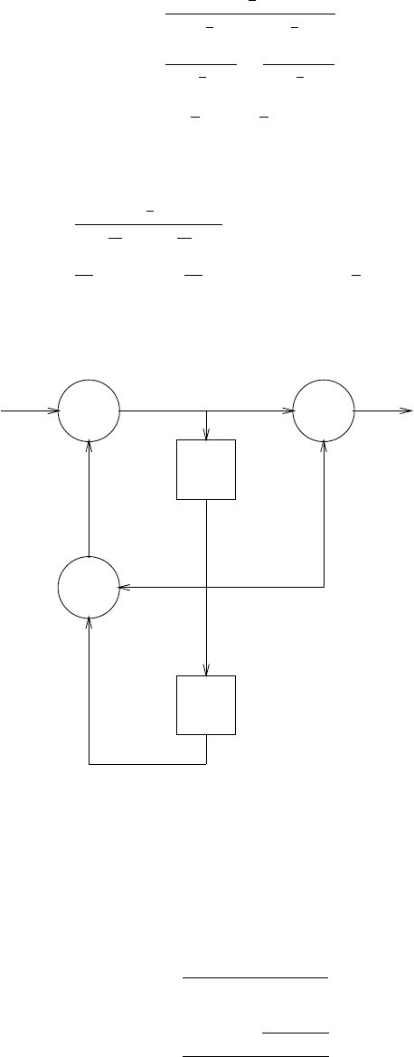
(a)
H(z) = Y(z)X(z)
=1−1
2z−1
(1 −1
4z−1)(1 −1
3z−1)
=3
1−1
4z−1−2
1−1
3z−1
h(n) = 3(1
4)n−2(1
3)nu(n)
(b)
H(z) = 1−1
2z−1
1−7
12 z−1+1
12 z−2
y(n) = 7
12y(n−1) −1
12y(n−2) + x(n)−1
2x(n−1)
(c) Refer to fig 3.40-1.
(d) The poles of the system are inside the unit circle. Hence, the system is stable.
x(n)
7/12
-1/12
-1/2
+
+
+
z-1
z
-1
y(n)
Figure 3.40-1:
3.41
H(z) = 1
1 + a1z−1+a2z−2
If a2
1−4a2<0,there are two complex poles
p1,2=−a1±jp4a2−a2
1
2
85
© 2007 Pearson Education, Inc., Upper Saddle River, NJ. All rights reserved. This material is protected under all copyright laws
as they currently exist. No portion of this material may be reproduced, in any form or by any means, without permission in
writing from the publisher. For the exclusive use of adopters of the book Digital Signal Processing, Fourth Edition, by John G.
Proakis and Dimitris G. Manolakis. ISBN 0-13-187374-1.
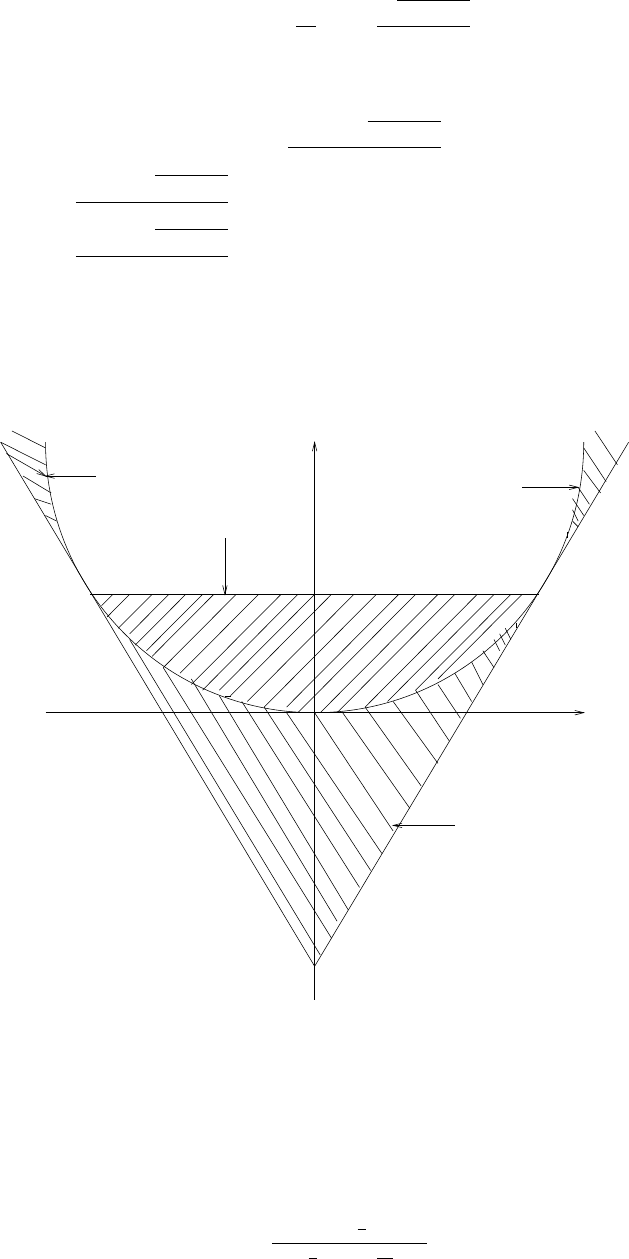
|p1,2|2= (a1
2)2+ p4a2−a2
1
2!2
<1
⇒a2<1
If a2
1−a4a2≥0,there are two real poles
p1,2=−a1±pa2
1−4a2
2
−a1+pa2
1−4a2
2<1 and
−a1−pa2
1−4a2
2>−1
⇒a1−a2<1 and
a1+a2>1
Refer to fig 3.41-1.
real
real
real
-1-2 1 2
complex
a2
a1
-1
a1
+a2=-1 a1
-a 2=1
a2
=1/4 a
12
Figure 3.41-1:
3.42
H(z) = z−1+1
2z−2
1−3
5z−1+2
25 z−2
86
© 2007 Pearson Education, Inc., Upper Saddle River, NJ. All rights reserved. This material is protected under all copyright laws
as they currently exist. No portion of this material may be reproduced, in any form or by any means, without permission in
writing from the publisher. For the exclusive use of adopters of the book Digital Signal Processing, Fourth Edition, by John G.
Proakis and Dimitris G. Manolakis. ISBN 0-13-187374-1.

(a)
H(z) = z−1−7
2
1−1
5z−1+
9
2
1−2
5z−1
h(n) = −7
2(1
5)n−1+9
2(2
5)n−1u(n−1)
(b)
Y(z) = H(z)X(z)
X(z) = 1
1−z−1
Y(z) =
25
8
1−z−1+
7
8
1−1
5z−1+−3
1−2
5z−1
y(n) = 25
8+7
8(1
5)n−3(2
5)nu(n)
(c) Determine the response caused by the initial conditions and add it to the response in (b).
y(n)−3
5y(n−1) + 2
25y(n−2) = 0
Y+(z)−3
5Y+(z)z−1+ 1+2
25 Y+(z)z−2+z−1+ 2= 0
Y+(z) =
2
25 z−1−11
25
(1 −1
5z−1)(1 −2
5z−1)
=
1
25
1−1
5z−1+−12
25
1−2
5z−1
y+(n) = 1
25(1
5)n−12
25(2
5)nu(n)
Therefore, the total step response is
y(n) = 25
8+33
200(1
5)n−87
25(2
5)nu(n)
3.43
[aY (z) + X(z)] z−2=Y(z)
Y(z) = z−2
1−az−2X(z)
Assume that a > 0. Then
H(z) = −1
a+
1
a
(1 −√az−1)(1 + √az−1)
=−1
a+1
2a
1
1−√az−1+1
2a
1
1 + √az−1
h(n) = −1
aδ(n) + 1
2a(√a)n+ (−√a)nu(n)
Step Response: X(z) = 1
1−z−1
Y(z) = z−2
(1 −z−1)(1 −√az−1)(1 + √az−1)
87
© 2007 Pearson Education, Inc., Upper Saddle River, NJ. All rights reserved. This material is protected under all copyright laws
as they currently exist. No portion of this material may be reproduced, in any form or by any means, without permission in
writing from the publisher. For the exclusive use of adopters of the book Digital Signal Processing, Fourth Edition, by John G.
Proakis and Dimitris G. Manolakis. ISBN 0-13-187374-1.

=
1
(a−1)
1−z−1+
1
2(a−√a)
1−√az−1+
1
2(a+√a)
1 + √az−1
y(n) = 1
a−1+1
2(a−√a)(√a)n+1
2(a+√a)(−√a)nu(n)
3.44
y(n) = −a1y(n−1) + b0x(n) + b1x(n−1)
Y(z) = b0+b1z−1
1 + a1z−1X(z)
(a)
H(z) = b0+b1z−1
1 + a1z−1⇒h(n) = b0(−a1)nu(n) + b1(−a1)n−1u(n−1)
=b0+(b1−b0a1)z−1
1 + a1z−1⇒h(n) = b0δ(n) + (b1−b0a1)(−a1)n−1u(n−1)
(b)
Step Response: X(z) = 1
1−z−1
Y(z) = b0+b1z−1
(1 −z−1)(1 + a1z−1)
=b0+b1
1 + a1
1
1−z−1+a1b0−b1
1 + a1
1
1 + a1z−1
y(n) = b0+b1
1 + a1
+a1b0−b1
1 + a1
(−a1)nu(n)
(c) Let us compute the zero-input response and add it to the response in (b). Hence,
Y+(z) + a1z−1Y+(z) + A= 0
Y+(z) = −a1A
1 + a1z−1
⇒yzi(n) = −a1A(−a1)nu(n)
The total response to a unit step is
y(n) = b0+b1
1 + a1
+a1b0−b1−a1A(1 + a1)
1 + a1
(−a1)nu(n)
(d)
x(n) = cosw0nu(n)
X(z) = 1−z−1cosw0
1−2z−1cosw0+z−2
Y(z) = (b0+b1z−1)(1 −z−1cosw0)
(1 + a1z−1)(1 −2z−1cosw0+z−2)
=A
1 + a1z−1+B(1 −z−1cosw0)
1−2z−1cosw0+z−2+C(z−1cosw0)
1−2z−1cosw0+z−2
Then, y(n) = [A(−a1)n+Bcosw0+Csinw0]u(n)
88
© 2007 Pearson Education, Inc., Upper Saddle River, NJ. All rights reserved. This material is protected under all copyright laws
as they currently exist. No portion of this material may be reproduced, in any form or by any means, without permission in
writing from the publisher. For the exclusive use of adopters of the book Digital Signal Processing, Fourth Edition, by John G.
Proakis and Dimitris G. Manolakis. ISBN 0-13-187374-1.

where A, B and Care determined from the equations
A+B=b0
(2cosw0)A+ (a1−cosw0)B+ (sinw0)C=b1−b0cosw0
A−(a1−cosw0)B+ (sinw0)C=−b1cosw0
3.45
y(n) = 1
2y(n−1) + 4x(n) + 3x(n−1)
Y(z) = 4 + 3z−1
1−1
2z−1X(z)
x(n) = ejw0nu(n)
X(z) = 1
1−ejw0z−1
Y(z) = 4 + 3z−1
(1 −1
2z−1)(1 −ejw0z−1)
Y(z) = A
1−1
2z−1+B
1−ejw0z−1
where A=5
1
2−ejw0
B=4ejw0+ 3
ejw0−1
2
Then y(n) = A(1
2)n+Bejw0nu(n)
The steady state response is
limn→∞y(n)≡yss(n) = Bejw0n
3.46
(a)
H(z) = C(z−rejΘ)(z−re−jΘ)
z(z+ 0.8)
=C1−2rcosΘz−1+r2z−2
(1 + 0.8z1)
H(z)|z=1 = 1 ⇒C=1.8
1−2rcosΘ + r2= 2.77
(b) The poles are inside the unit circle, so the system is stable.
(c) y(n) = −0.8y(n−1) + Cx(n)−1.5√3Cx(n−1) + 2.25Cx(n−2). Refer to fig 3.46-1.
3.47
(a)
X1(z) = z2+z+ 1 + z−1+z−2
89
© 2007 Pearson Education, Inc., Upper Saddle River, NJ. All rights reserved. This material is protected under all copyright laws
as they currently exist. No portion of this material may be reproduced, in any form or by any means, without permission in
writing from the publisher. For the exclusive use of adopters of the book Digital Signal Processing, Fourth Edition, by John G.
Proakis and Dimitris G. Manolakis. ISBN 0-13-187374-1.
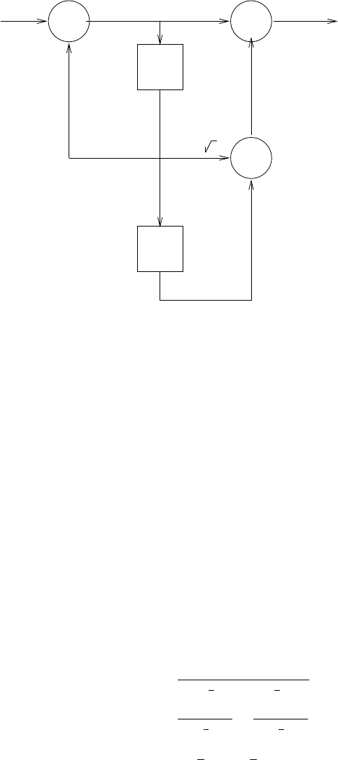
x(n)
-0.8 -1.5 3
2.25
+
++
z-1
z-1
cy(n)
Figure 3.46-1:
X2(z) = 1 + z−1+z−2
Y(z) = X1(z)X2(z)
=z2+ 2z+ 3 + 3z−1+ 3z−2+ 2z−3+z−4
Hence, x1(n)∗x2(n) = y(n)
=1,2,3
↑,3,3,2,1
By one-sided transform:
X+
1(z) = 1 + z−1+z−2
X+
2(z) = 1 + z−1+z−2
Y+(z) = 1 + 2z−1+ 3z−2+ 2z−3+z−4
Hence, y(n) = {1,2,3,2,1}
(b) Since both x1(n) and x2(n) are causal, the one-sided and two-sided transform yield identical
results. Thus,
Y(z) = X1(z)X2(z)
=1
(1 −1
2z−1)(1 −1
3z−1)
=3
1−1
2z−1−2
1−1
3z−1
Therefore, y(n) = 3(1
2)n−2(1
3)nu(n)
(c)
By convolution,
y(n) = x1(n)∗x2(n)
=4,11,20,30
↑,20,11,4
90
© 2007 Pearson Education, Inc., Upper Saddle River, NJ. All rights reserved. This material is protected under all copyright laws
as they currently exist. No portion of this material may be reproduced, in any form or by any means, without permission in
writing from the publisher. For the exclusive use of adopters of the book Digital Signal Processing, Fourth Edition, by John G.
Proakis and Dimitris G. Manolakis. ISBN 0-13-187374-1.

By one-sided z-transform,
X+
1(z) = 2 + 3z−1+ 4z−2
X+
2(z) = 2 + z−1
Y+(z) = X+
1(z)X+
2(z)
= 4 + 8z−1+ 11z−2+ 4z−3
Therefore, y(n) = 4
↑,8,11,4
(d) Both x1(n) and x2(n) are causal. Hence, both types of transform yield the same result, i.e,
X1(z) = 1 + z−1+z−2+z−3+z−4
X2(z) = 1 + z−1+z−2
Then, Y(z) = X1(z)X2(z)
= 1 + 2z−1+ 3z−2+ 3z−3+ 3z−4+ 2z−5+z−6
Therefore, y(n) = 1
↑,2,3,3,3,2,1
3.48
X+(z) = ∞
X
n=0
x(n)z−n
=∞
X
n=0
z−n
=1
1−z−1,|z|>1
3.49
(a)
Y+(z) + 1
2z−1Y+(z) + y(−1)−1
4z−2Y+(z) + z−1y(−1) + y(−2)= 0
(a)
Hence, Y+(z) =
1
4z−1−1
4
1 + 1
2z−1−1
4z−2
=0.154
1−0.31z−1−0.404
1 + 0.81z−1
Therefore, y(n) = [0.154(0.31)n−0.404(0.81)n]u(n)
(b)
Y+(z)−1.5z−1Y+(z) + 1+ 0.5z−2Y+(z) + z−1+ 0= 0
Y+(z) = 1.5−0.5z−1
1−1.5z−1+ 0.5z−2
=2
1−z−1−0.5
1−0.5z−1
Therefore, y(n) = [2 −0.5(0.5)n]u(n)
=2−(0.5)n+1u(n)
91
© 2007 Pearson Education, Inc., Upper Saddle River, NJ. All rights reserved. This material is protected under all copyright laws
as they currently exist. No portion of this material may be reproduced, in any form or by any means, without permission in
writing from the publisher. For the exclusive use of adopters of the book Digital Signal Processing, Fourth Edition, by John G.
Proakis and Dimitris G. Manolakis. ISBN 0-13-187374-1.

(c)
Y+(z)−0.5z−1Y+(z) + 1=1
1−1
3z−1
Y+(z) = 1.5−1
6z−1
(1 −1
3z−1)(1 −0.5z−1)
=
7
2
1−0.5z−1−2
1−1
3z−1
Hence, y(n) = 7
2(0.5)n−2(1
3)nu(n)
(d)
Y+(z)−1
4z−2Y+(z) + 1=1
1−z−1
Y+(z) =
5
4−1
4z−1
(1 −z−1)(1 −1
4z−2)
=
4
3
1−z−1+−3
8
1−1
2z−1+
7
24
1 + 1
2z−1
Hence, y(n) = 4
3−3
8(1
2)n+7
24(−1
2)nu(n)
3.50
If h(n) is real, even and has a finite duration 2N+ 1, then (with M= 2N+ 1)
H(z) = h(0) + h(1)z−1+h(2)z−2+...+h(M−1)z−(M−1)/2
since h(n) = h(M−n−1),then
H(z) = z−(M−1)/2(h(0) hz(M−1)/2+z−(M−1)/2i
+h(1) hz(M−3)/2+z−(M−3)/2i+. . . +h(M−1/2))
with M= 2N+ 1, the expression becomes
H(z) = z−N(h(0) zN+z−N
+h(1) hzN−1+z−(N−1)i
+h(2) hzN−2+z−(N−2)i+...+h(N))
=z−N(h(N) +
N−1
X
n=0
h(n)zN−n+
N−1
X
n=0
h(n)z−(N−n))
=z−Nh(N) + P(z) + P(z−1)
Now, suppose z1is a root of H(z), i.e.,
H(z1) = z−N
1h(N) + P(z1) + P(z−1
1)= 0
Then, h(N) + P(z1) + P(z−1
1) = 0.
This implies that H(1
z1) = 0 since we again have
h(N) + P(z−1
1) + P(z1) = 0.
92
© 2007 Pearson Education, Inc., Upper Saddle River, NJ. All rights reserved. This material is protected under all copyright laws
as they currently exist. No portion of this material may be reproduced, in any form or by any means, without permission in
writing from the publisher. For the exclusive use of adopters of the book Digital Signal Processing, Fourth Edition, by John G.
Proakis and Dimitris G. Manolakis. ISBN 0-13-187374-1.

3.51
(a)
H(z) = z−1
(z+1
2)(z+ 3)(z−2),ROC: 1
2<|z|<2
(b) The system can be causal if the ROC is |z|>3, but it cannot be stable.
(c)
H(z) = A
1 + 1
2z−1+B
1 + 3z−1+C
1−2z−1
(1) The system can be causal; (2) The system can be anti-causal; (3) There are two other
noncausal responses.The corresponding ROC for each of these possibilities are :
ROC1:|z|>3; ROC2:|z|<3; ROC3:1
2<|z|<2; ROC4: 2 <|z|<3;
3.52
x(n) is causal.
(a)
X(z) = ∞
X
n=0
x(n)z−n
limz→∞X(z) = x(0)
(b)(i) X(z) = (z−1
2)4
(z−1
3)3⇒limz→∞X(z) = ∞ ⇒ x(n) is not causal.
(ii) X(z) = (1−1
2z−2)2
1−1
3z−1⇒limz→∞X(z) = 1 Hence X(z) can be associated wih a causal
sequence.
(iii) X(z) = (z−1
3)2
(z−1
2)3⇒limz→∞X(z) = 0. Hence X(z) can be associated wih a causal
sequence.
3.53
The answer is no. For the given system h1(n) = anu(n)⇒H1(z) = 1
1−az−1,|a|<1.This system
is causal and stable. However when h2(n) = anu(n+ 3) ⇒H2(z) = a−3z3
1−az−1the system is stable
but is not causal.
3.54
Initial value theorem for anticausal signals: If x(n) is anticausal, then x(0) = limz→0X(z)
Proof: X(z) = P0
n=−∞ x(n)z−n=x(0) + x(−1)z+x(−2)z2+... Then limz→0X(z) = x(0)
3.55
s(n) = (1
3)n−2u(n+ 2)
(a)
h(n) = s(n)−s(n−1)
93
© 2007 Pearson Education, Inc., Upper Saddle River, NJ. All rights reserved. This material is protected under all copyright laws
as they currently exist. No portion of this material may be reproduced, in any form or by any means, without permission in
writing from the publisher. For the exclusive use of adopters of the book Digital Signal Processing, Fourth Edition, by John G.
Proakis and Dimitris G. Manolakis. ISBN 0-13-187374-1.

= (1
3)n−2u(n+ 2) −(1
3)n−3u(n+ 1)
= 34δ(n+ 2) −54δ(n+ 1) −18(1
3)nu(n)
H(z) = 81z2−54z+−18
1−1
3z−1
=81z(z−1)
1−1
3z−1
H(z) has zeros at z= 0,1 and a pole at z=1
3.
(b) h(n) = 81δ(n+ 2) −54δ(n+ 1) −18(1
3)nu(n)
(c) The system is not causal, but it is stable since the pole is inside the unit circle.
3.56
(a)
x(n) = 1
2πj Ic
zn−1
1−1
2z−1dz
=1
2πj Ic
zn
z−1
2
dz
for n≥0, x(n) = (1
2)n
for n < 0, x(−1) = 1
2πj Ic
1
z(z−1
2)dz
=1
z−1
2|z=0 +1
z|z=1
2= 0
x(−2) = 1
2πj Ic
1
z2(z−1
2)dz
=d
dz 1
z−1
2|z=0 +1
z2|z=1
2= 0
By continuing this process, we find that x(n) = 0 for n < 0.
(b)
X(z) = 1
1−1
2z−1,|z|<1
2
x(n) = 1
2πj Ic
zn
z−1
2
dz, where c is contour of radius less than1
2
For n≥0, there are no poles enclosed in c and, hence, x(n) = 0. For n < 0, we have
x(−1) = 1
2πj Ic
1
z(z−1
2)dz
=1
z−1
2|z=0 =−2
x(−2) = 1
2πj Ic
1
z2(z−1
2)dz
=d
dz 1
z−1
2|z=0 =−4
94
© 2007 Pearson Education, Inc., Upper Saddle River, NJ. All rights reserved. This material is protected under all copyright laws
as they currently exist. No portion of this material may be reproduced, in any form or by any means, without permission in
writing from the publisher. For the exclusive use of adopters of the book Digital Signal Processing, Fourth Edition, by John G.
Proakis and Dimitris G. Manolakis. ISBN 0-13-187374-1.

Alternatively, we may change variables by letting w=z−1. Then,
x(n) = −1
2πj Ic′
w−n
w−1−1
2
(−1
w2)dw,
=−1
2πj Ic′
−1
wn+1(1 −1
2w)dw
=−1
2πj Ic′
2w−n−1
w−2) dw
=−(2)−n, n < 0
(c)
X(z) = z−a
1−az ,|z|>1
|a|
x(n) = 1
2πj Ic
zn−1z−a
1−az dz, c has a radius greater than 1
|a|
=1
2πj Ic
−1
a
zn−1(z−a)
z−1
a
dz
For n≥0, x(n) = −1
a(1
a)n−1(1
a−a)
= ( 1
a)n−1−(1
a)n+1
For n= 0, x(n) = 1
2πj Ic
−1
a
(z−a)
z(z−1
a)dz
=−1
a−a
−1
a
+
1
a−a
1
a
=−1
a(a2+ 1 −a2)
=−1
a
For n < 0,we let w=z−1.Then
x(n) = 1
2πj Ic′
−w−n−1(w−1−a)
1−aw−1(−1
w2)dw,
= 0,for n < 0
(d)
X(z) = 1−1
4z−1
1−1
6z−1−1
6z−2,|z|>1
2
=
3
10
1−1
2z−1+
7
10
1 + 1
3z−1
x(n) = 1
2πj Ic
3
10 zn
z−1
2
dz +1
2πj Ic
7
10 zn
z+1
3
dz
where the radius of the contour c is greater than |z|=1
2. Then, for n≥0
x(n) = 3
10(1
2)n+7
10(−1
3)nu(n)
For n < 0, x(n) = 0
95
© 2007 Pearson Education, Inc., Upper Saddle River, NJ. All rights reserved. This material is protected under all copyright laws
as they currently exist. No portion of this material may be reproduced, in any form or by any means, without permission in
writing from the publisher. For the exclusive use of adopters of the book Digital Signal Processing, Fourth Edition, by John G.
Proakis and Dimitris G. Manolakis. ISBN 0-13-187374-1.

3.57
X(z) = 1−a2
(1 −az)(1 −az−1), a < |z|<1
a,0< a < 1
=1
1−az−1+−1
1−1
az−1
x(n) = 1
2πj Ic
zn
z−adz −1
2πj Ic
zn
z−1
a
dz
For n≥0,1
2πj Ic
zn
z−adz =anand
1
2πj Ic
zn
z−1
a
dz = 0
For n < 0,1
2πj Ic
zn
z−adz = 0 and
1
2πj Ic
zn
z−1
a
dz =−a−n
3.58
X(z) = z20
(z−1
2)(z−2)5(z+5
2)2(z+ 3),1
2<|z|<2
x(n) = 1
2πj Ic
zn−1z20
(z−1
2)(z−2)5(z+5
2)2(z+ 3)dz
x(−18) = 1
2πj Ic
z
(z−1
2)(z−2)5(z+5
2)2(z+ 3)dz
=
1
2
(1
2−2)5(1
2+5
2)2(1
2+ 3)
=−1
2
(3
2)5(3)2(7
2)
=−25
(37)(7)
=−32
15309
96
© 2007 Pearson Education, Inc., Upper Saddle River, NJ. All rights reserved. This material is protected under all copyright laws
as they currently exist. No portion of this material may be reproduced, in any form or by any means, without permission in
writing from the publisher. For the exclusive use of adopters of the book Digital Signal Processing, Fourth Edition, by John G.
Proakis and Dimitris G. Manolakis. ISBN 0-13-187374-1.

Chapter 4
4.1
(a) Since xa(t) is periodic, it can be represented by the fourier series
xa(t) = ∞
X
k=−∞
ckej2πkt/τ
where ck=1
τZτ
0
Asin(πt/τ)ej2πkt/τ dt
=A
j2τZτ
0hejπt/τ −e−jπt/τ ie−j2πkt/τ dt
=A
j2τejπ(1−2k)t/τ
jπ
2(1 −2k)−e−jπ(1+2k)t/τ
−jπ
2(1 + 2k)τ
0
=A
π1
1−2k+1
1 + 2k
=2A
π(1 −4k2)
Then, Xa(F) = Z∞
−∞
xa(t)e−j2π(F−k
τ)tdt
=∞
X
k=−∞
ckZ∞
−∞
e−j2π(F−k
τ)tdt
=∞
X
k=−∞
ckδ(F−k
τ)
Hence, the spectrum of xa(t) consists of spectral lines of frequencies k
τ, k = 0,±1,±2,...with
amplitude |ck|and phases 6ck.
(b) Px=1
τRτ
0x2
a(t)dt =1
τRτ
0A2sin2(πt
τ)dt =A2
2
(c) The power spectral density spectrum is |ck|2, k = 0,±1,±2,.... Refer to fig 4.1-1.
(d) Parseval’s relation
Px=1
τZτ
0
x2
a(t)dt
=|ck|2
∞
X
k=−∞ |ck|2=4A2
π2
∞
X
k=−∞
1
(4k2−1)2
97
© 2007 Pearson Education, Inc., Upper Saddle River, NJ. All rights reserved. This material is protected under all copyright laws
as they currently exist. No portion of this material may be reproduced, in any form or by any means, without permission in
writing from the publisher. For the exclusive use of adopters of the book Digital Signal Processing, Fourth Edition, by John G.
Proakis and Dimitris G. Manolakis. ISBN 0-13-187374-1.

.
.
.
.
.
...
..
.
|c
-2 |2
|c-1 |2
|c
0|
2
|c
1|2
|c 2|2
-1 0 1 2-2 k
Figure 4.1-1:
=4A2
π21 + 2
32+2
152+...
1 + 2
32+2
152+...= 1.2337(Infinite series sum to π2
8)
Hence, ∞
X
k=−∞ |ck|2=4A2
π2(1.2337)
=A2
2
4.2
(a)
xa(t) = Ae−atu(t), a > 0
Xa(F) = Z∞
0
Ae−ate−j2πF tdt
=A
−a−j2πF e−(a+j2πF )t∞
0
=A
a+j2πF
|Xa(F)|=A
pa2+ (2πF )2
98
© 2007 Pearson Education, Inc., Upper Saddle River, NJ. All rights reserved. This material is protected under all copyright laws
as they currently exist. No portion of this material may be reproduced, in any form or by any means, without permission in
writing from the publisher. For the exclusive use of adopters of the book Digital Signal Processing, Fourth Edition, by John G.
Proakis and Dimitris G. Manolakis. ISBN 0-13-187374-1.
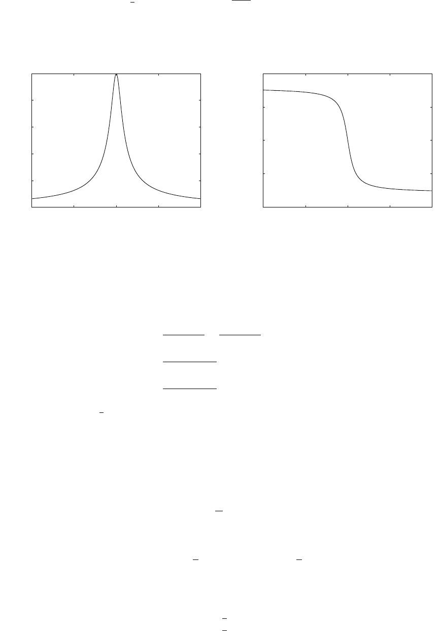
6Xa(F) = −tan−1(2πF
a)
Refer to fig 4.2-1
−10 −5 0 5 10
0
0.1
0.2
0.3
0.4
0.5 A = 2, a = 4
−−> F
|Xa(F)|
−10 −5 0 5 10
−2
−1
0
1
2
−−> F
phase of Xa(F)
Figure 4.2-1:
(b)
Xa(F) = Z∞
0
Aeate−j2πF tdt +Z∞
0
Ae−ate−j2πF tdt
=A
a−j2πF +A
a+j2πF
=2aA
a2+ (2πF )2
|Xa(F)|=2aA
a2+ (2πF )2
6Xa(F) = 0
Refer to fig 4.2-2
4.3
(a) Refer to fig 4.3-1.
x(t) = 1−|t|
τ,|t| ≤ τ
0,otherwise
Xa(F) = Z0
−τ
(1 + t
τ)e−j2πF tdt +Zτ
0
(1 −t
τ)e−j2πF tdt
Alternatively, we may find the fourier transform of
y(t) = x′(t) = 1
τ,−τ < t ≤0
1
τ,0< t ≤τ
99
© 2007 Pearson Education, Inc., Upper Saddle River, NJ. All rights reserved. This material is protected under all copyright laws
as they currently exist. No portion of this material may be reproduced, in any form or by any means, without permission in
writing from the publisher. For the exclusive use of adopters of the book Digital Signal Processing, Fourth Edition, by John G.
Proakis and Dimitris G. Manolakis. ISBN 0-13-187374-1.
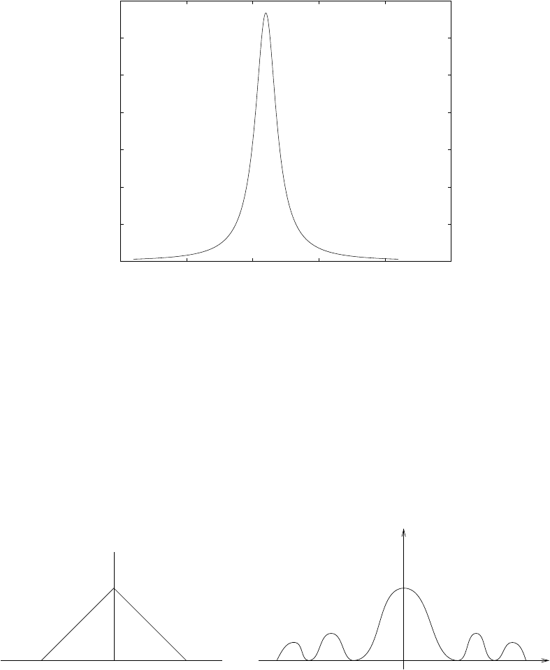
0 5 10 15 20 25
0
0.1
0.2
0.3
0.4
0.5
0.6
0.7 A = 2, a = 6
−−−> F
|Xa(F)|
Figure 4.2-2:
x(t)
t
0τ
−τ 0 1/τ 2/τ
|X(F)|
F
Figure 4.3-1:
100
© 2007 Pearson Education, Inc., Upper Saddle River, NJ. All rights reserved. This material is protected under all copyright laws
as they currently exist. No portion of this material may be reproduced, in any form or by any means, without permission in
writing from the publisher. For the exclusive use of adopters of the book Digital Signal Processing, Fourth Edition, by John G.
Proakis and Dimitris G. Manolakis. ISBN 0-13-187374-1.

Then,
Y(F) = Zτ
−τ
y(t)e−j2πF tdt
=Z0
−τ
1
τe−j2πF tdt +Zτ
0
(−1
τ)e−j2πF tdt
=−2sin2πF τ
jπF τ
and X(F) = 1
j2πF Y(F)
=τsinπF τ
πF τ 2
|X(F)|=τsinπF τ
πF τ 2
6Xa(F) = 0
(b)
ck=1
TpZTp/2
−Tp/2
x(t)e−j2πkt/Tpdt
=1
TpZ0
−τ
(1 + t
τ)e−j2πkt/Tpdt +Zτ
0
(1 −t
τ)e−j2πkt/Tpdt
=τ
Tpsinπkτ/Tp
πkτ /Tp2
(c) From (a) and (b), we have ck=1
TpXa(k
Tp)
4.4
(a)
x(n) = . . . , 1,0,1,2,3
↑,2,1,0,1,...
N= 6
ck=1
6
5
X
n=0
x(n)e−j2πkn/6
=h3 + 2e−j2πk
6+e−j2πk
3+e−j4πk
3+ 2e−j10πk
6i
=1
63 + 4cosπk
3+ 2cos2πk
3
Hence, c0=9
6, c1=4
6, c2= 0, c3=1
6, c4= 0, c5=4
6
(b)
Pt=1
6
5
X
n=0 |x(n)|2
=1
6(32+ 22+ 12+ 02+ 12+ 22)
101
© 2007 Pearson Education, Inc., Upper Saddle River, NJ. All rights reserved. This material is protected under all copyright laws
as they currently exist. No portion of this material may be reproduced, in any form or by any means, without permission in
writing from the publisher. For the exclusive use of adopters of the book Digital Signal Processing, Fourth Edition, by John G.
Proakis and Dimitris G. Manolakis. ISBN 0-13-187374-1.

=19
16
Pf=
5
X
n=0 |c(n)|2
=(9
16)2+ ( 4
6)2+ 02+ (1
6)2+ 02+ (4
6)2)
=19
16
Thus, Pt=Pf
=19
16
4.5
x(n) = 2 + 2cosπn/4 + cosπn/2 + 1
2cos3πn/4,⇒N= 8
(a)
ck=1
8
7
X
n=0
x(n)e−jπkn/4
x(n) = 11
2,2 + 3
4√2,1,2−3
4√2,1
2,2−3
4√2,1,2 + 3
4√2
Hence, c0= 2, c1=c7= 1, c2=c6=1
2, c3=c5=1
4, c4= 0
(b)
P=
7
X
i=0 |c(i)|2
= 4 + 1 + 1 + 1
4+1
4+1
16 +1
16
=53
8
4.6
(a)
x(n) = 4sinπ(n−2)
3
= 4sin2π(n−2)
6
ck=1
6
5
X
n=0
x(n)e−2jπkn/6
=4
6
5
X
n=0
sin2π(n−2)
6e−2jπkn/6
=1
√3h−e−j2πk/3−e−jπk/3+e−jπk/3+e−j2πk/3i
102
© 2007 Pearson Education, Inc., Upper Saddle River, NJ. All rights reserved. This material is protected under all copyright laws
as they currently exist. No portion of this material may be reproduced, in any form or by any means, without permission in
writing from the publisher. For the exclusive use of adopters of the book Digital Signal Processing, Fourth Edition, by John G.
Proakis and Dimitris G. Manolakis. ISBN 0-13-187374-1.

=1
√3(−j2) sin2πk
6+sinπk
3e−j2πk/3
Hence, c0= 0, c1=−j2e−j2π/3, c2=c3=c4= 0, c5=c∗
1
and |c1|=|c5|= 2,|c0|=|c2|=|c3|=|c4|= 0
6c1=π+π
2−2π
3=5π
6
6c5=−5π
6
6c0=6c2=6c3=6c4= 0
(b)
x(n) = cos2πn
3+sin2πn
5⇒N= 15
ck=c1k+c2k
where c1kis the DTFS coefficients of cos 2πn
3and c2kis the DTFS coefficients of sin 2πn
5. But
cos2πn
3=1
2(ej2πn
3+e−j2πn
3)
Hence,
c1k=1
2, k = 5,10
0,otherwise
Similarly,
sin2πn
5=1
2j(ej2πn
5−e−j2πn
5).
Hence,
c2k=
1
2j, k = 3
−1
2j, k = 12
0,otherwise
Therefore,
ck=c1k+c2k
1
2j, k = 3
1
2, k = 5
1
2, k = 10
−1
2j, k = 12
0,otherwise
(c) x(n) = cos2πn
3sin2πn
5=1
2sin16πn
15 −1
2sin4πn
15 . Hence, N= 15. Following the same method
as in (b) above, we find that
ck=
−1
4j, k = 2,7
1
4j, k = 8,13
0,otherwise
(d)
N= 5
ck=1
5
4
X
n=0
x(n)e−j2πnk
5
=1
5he−j2πk
5+ 2e−j4πk
5−2e−j6πk
5−e−j8πk
5i
=2j
5−sin(2πk
5)−2sin(4πk
5)
103
© 2007 Pearson Education, Inc., Upper Saddle River, NJ. All rights reserved. This material is protected under all copyright laws
as they currently exist. No portion of this material may be reproduced, in any form or by any means, without permission in
writing from the publisher. For the exclusive use of adopters of the book Digital Signal Processing, Fourth Edition, by John G.
Proakis and Dimitris G. Manolakis. ISBN 0-13-187374-1.

Therefore, c0= 0,
c1=2j
5−sin(2π
5) + 2sin(4π
5)
c2=2j
5sin(4π
5)−2sin(2π
5)
c3=−c2
c4=−c1
(e)
N= 6
ck=1
6
5
X
n=0
x(n)e−j2πnk
6
=1
6h1 + 2e−jπk
3−e−j2πk
3−e−j4πk
3+ 2e−j5πk
3i
=1
61 + 4cos(πk
3)−2cos(2πk
3)
Therefore, c0=1
2
c1=2
3
c2= 0
c3=−5
6
c4= 0
c5=2
3
(f)
N= 5
ck=1
5
4
X
n=0
x(n)e−j2πnk
5
=1
5h1 + e−j2πk
5i
=2
5cos(πk
5)e−jπk
5
Therefore, c0=2
5
c1=2
5cos(π
5)e−jπ
5
c2=2
5cos(2π
5)e−j2π
5
c3=2
5cos(3π
5)e−j3π
5
c4=2
5cos(4π
5)e−j4π
5
(g) N= 1 ck=x(0) = 1 or c0= 1
(h)
N= 2
104
© 2007 Pearson Education, Inc., Upper Saddle River, NJ. All rights reserved. This material is protected under all copyright laws
as they currently exist. No portion of this material may be reproduced, in any form or by any means, without permission in
writing from the publisher. For the exclusive use of adopters of the book Digital Signal Processing, Fourth Edition, by John G.
Proakis and Dimitris G. Manolakis. ISBN 0-13-187374-1.

ck=1
2
1
X
n=0
x(n)e−jπnk
=1
2(1 −e−jπk)
⇒c0= 0, c1= 1
4.7
(a)
x(n) =
7
X
k=0
ckej2πnk
8
Note that if ck=ej2πpk
8,then
7
X
k=0
ej2πpk
8ej2πnk
8=
7
X
n=0
ej2π(p+n)k
8
= 8, p =−n
= 0, p 6=−n
Since ck=1
2hej2πk
8+e−j2πk
8i+1
2jhej6πk
8−e−j6πk
8i
We have x(n) = 4δ(n+ 1) + 4δ(n−1) −4jδ(n+ 3) + 4jδ(n−3),−3≤n≤5
(b)
c0= 0, c1=√3
2, c2=√3
2, c3= 0, c4=−√3
2, c5=−√3
2, c6=c7= 0
x(n) =
7
X
k=0
ckej2πnk
8
=√3
2hejπn
4+ej2πn
4−ej4πn
4−ej5πn
4i
=√3hsinπn
2+sinπn
4iejπ(3n−2)
4
(c)
x(n) =
4
X
k=−3
ckej2πnk
8
= 2 + ejπn
4+e−jπn
4+1
2ejπn
2+1
2e−jπn
2+1
4ej3πn
4+1
4e−j3πn
4
= 2 + 2cosπn
4+cosπn
2+1
2cos3πn
4
4.8
(a)
If k= 0,±N, ±2N,...
N−1
X
n=0
ej2πkn/N =
N−1
X
n=0
1 = N
105
© 2007 Pearson Education, Inc., Upper Saddle River, NJ. All rights reserved. This material is protected under all copyright laws
as they currently exist. No portion of this material may be reproduced, in any form or by any means, without permission in
writing from the publisher. For the exclusive use of adopters of the book Digital Signal Processing, Fourth Edition, by John G.
Proakis and Dimitris G. Manolakis. ISBN 0-13-187374-1.
If k6= 0,±N, ±2N, . . .
N−1
X
n=0
ej2πkn/N =1−ej2πk
1−ej2πk/N
= 0
(b) Refer to fig 4.8-1.
(c)
s3
s3(0)
(2)
s3(4)
s3(1)
s3(3)
s3(5)
k=3
s2(1)
s2(0)
s2(2)
s2(5)
s2(4)
s2(3)
k=2
s1
(2) s1(1)
s1(0)
s1
(5)
s1
(4)
s1
(3)
k=1
s
s (0)
s
s
s
s (3)
s s
s(0)
s
s
s(3)
4(5)
4(2)
4(1)
4(4)
4
4
5(4) 5(5)
5
5(1)
5(2)
5
s6(0)
.
.
.
s6(5)
k=6k=4 k=5
Figure 4.8-1:
N−1
X
n=0
sk(n)s∗
i(n) =
N−1
X
n=0
ej2πkn/N e−j2πin/N
=
N−1
X
n=0
ej2π(k−i)n/N
=N, k =i
= 0, k 6=i
Therefore, the {sk(n)}are orthogonal.
4.9
(a)
x(n) = u(n)−u(n−6)
106
© 2007 Pearson Education, Inc., Upper Saddle River, NJ. All rights reserved. This material is protected under all copyright laws
as they currently exist. No portion of this material may be reproduced, in any form or by any means, without permission in
writing from the publisher. For the exclusive use of adopters of the book Digital Signal Processing, Fourth Edition, by John G.
Proakis and Dimitris G. Manolakis. ISBN 0-13-187374-1.

X(w) = ∞
X
n=−∞
x(n)e−jwn
=
5
X
n=0
e−jwn
=1−e−j6w
1−e−jw
(b)
x(n) = 2nu(−n)
X(w) =
0
X
n=−∞
2ne−jwn
=∞
X
m=0
(ejw
2)n
=2
2−ejw
(c)
x(n) = (1
4)nu(n+ 4)
X(w) = ∞
X
n=−4
(1
4)ne−jwn
= ( ∞
X
m=0
(1
4)me−jwm)44ej4w
=44ej4w
1−1
4e−jw
(d)
x(n) = αnsinw0nu(n),|α|<1
X(w) = ∞
X
n=0
αnejw0n−e−jw0n
2je−jwn
=1
2j
∞
X
n=0 hαe−j(w−w0)in−1
2j
∞
X
n=0 hαe−j(w+w0)in
=1
2j1
1−αe−j(w−w0)−1
1−αe−j(w+w0)
=αsinw0e−jw
1−2αcosw0e−jw +α2e−j2w
(e)
x(n) = |α|nsinw0n, |α|<1
Note that ∞
X
n=−∞ |x(n)|=∞
X
n=−∞ |α|n|sinw0n|
Suppose that w0=π
2,so that |sinw0n|= 1.
∞
X
n=−∞ |α|n=∞
X
n=−∞ |x(n)| → ∞.
107
© 2007 Pearson Education, Inc., Upper Saddle River, NJ. All rights reserved. This material is protected under all copyright laws
as they currently exist. No portion of this material may be reproduced, in any form or by any means, without permission in
writing from the publisher. For the exclusive use of adopters of the book Digital Signal Processing, Fourth Edition, by John G.
Proakis and Dimitris G. Manolakis. ISBN 0-13-187374-1.

Therefore, the fourier transform does not exist.
(f)
x(n) = 2−(1
2)n,|n| ≤ 4
0,otherwise
X(w) =
4
X
n=−4
x(n)e−jwn
=
4
X
n=−42−(1
2)ne−jwn
=2ej4w
1−e−jw
−1
2−4ej4w+ 4e−j4w−3ej3w+e−j3w−2ej2w+ 2e−j2w−ejw +e−jw
=2ej4w
1−e−jw +j[4sin4w+ 3sin3w+ 2sin2w+sinw]
(g)
X(w) = ∞
X
n=−∞
x(n)e−jwn
=−2ej2w−ejw +ejw + 2e−j2w
=−2j[2sin2w+sinw]
(h)
x(n) = A(2M+ 1 − |n|),|n| ≤ M
0,|n|> M
X(w) =
M
X
n=−M
x(n)e−jwn
=A
M
X
n=−M
(2M+ 1 − |n|)e−jwn
= (2M+ 1)A+A
M
X
k=1
(2M+ 1 −k)(e−jwk +ejwk)
= (2M+ 1)A+ 2A
M
X
k=1
(2M+ 1 −k)coswk
4.10
(a)
x(n) = 1
2πZπ
−π
X(w)ejwndw
=1
2πZ−w0
−π
ejwndw +1
2πZπ
w0
ejwndw
x(0) = 1
2π(π−w0) + 1
2π(π−w0)
108
© 2007 Pearson Education, Inc., Upper Saddle River, NJ. All rights reserved. This material is protected under all copyright laws
as they currently exist. No portion of this material may be reproduced, in any form or by any means, without permission in
writing from the publisher. For the exclusive use of adopters of the book Digital Signal Processing, Fourth Edition, by John G.
Proakis and Dimitris G. Manolakis. ISBN 0-13-187374-1.

=π−w0
π
For n6= 0,Z−w0
−π
ejwndw =1
jnejwn|−w0
−π
=1
jn(e−jw0n−e−jπn)
Zπ
w0
ejwndw =1
jnejwn|π
w0
=1
jn(ejπn −ejw0n)
Hence, x(n) = −sinnw0
nπ , n 6= 0
(b)
X(w) = cos2(w)
= (1
2ejw +1
2e−jw)2
=1
4(ej2w+ 2 + e−j2w)
x(n) = 1
2πZπ
−π
X(w)ejwndw
=1
8π[2πδ(n+ 2) + 4πδ(n) + 2πδ(n−2)]
=1
4[δ(n+ 2) + 2δ(n) + δ(n−2)]
(c)
x(n) = 1
2πZπ
−π
X(w)ejwndw
=1
2πZw0+δw
2
w0−δw
2
ejwndw
=2
πδw sin(nδw/2)
nδw/2ejnw0
(d)
x(n) = 1
2πRe (Zπ/8
0
2ejwndw +Z3π/8
π/8
ejwndw +Z7π/8
6π/8
ejwndw +Zπ
7π/8
ejwndw)
=1
π"Zπ/8
0
2coswndw +Z3π/8
π/8
coswndw +Z7π/8
6π/8
coswndw +Zπ
7π/8
2coswndw#
=1
nπ sin7πn
8+sin6πn
8−sin3πn
8−sinπn
8
4.11
xe(n) = x(n) + x(−n)
2
109
© 2007 Pearson Education, Inc., Upper Saddle River, NJ. All rights reserved. This material is protected under all copyright laws
as they currently exist. No portion of this material may be reproduced, in any form or by any means, without permission in
writing from the publisher. For the exclusive use of adopters of the book Digital Signal Processing, Fourth Edition, by John G.
Proakis and Dimitris G. Manolakis. ISBN 0-13-187374-1.

=1
2,0,1,2
↑,1,0,1
2
xo(n) = x(n)−x(−n)
2
=1
2,0,−2,0
↑,2,0,1
2
Then, XR(w) =
3
X
n=−3
xe(n)e−jwn
jXI(w) =
3
X
n=−3
xo(n)e−jwn
Now, Y(w) = XI(w) + XR(w)ej2w.Therefore,
y(n) = F−1{XI(w)}+F−1XR(w)ej2w
=−jxo(n) + xe(n+ 2)
=1
2,0,1−j
2,2,1 + j
2,0
↑,1
2−j2,0,j
2
4.12
(a)
x(n) = 1
2π"Z9π/10
8π/10
ejwndw +Z−8π/10
−9π/10
ejwndw + 2 Zπ
9π/10
ejwndw + 2 Z−9π/10
−π
ejwndw#
=1
2π1
jn(ej9πn/10 −e−j9πn/10 −ej8πn/10 +e−j8πn/10)
+2
jn(−ej9πn/10 +e−j9πn/10 +ejπn −e−jπn)
=1
nπ [sinπn −sin8πn/10 −sin9πn/10]
=−1
nπ [sin4πn/5 + sin9πn/10]
(b)
x(n) = 1
2πZ0
−π
X(w)ejwndw +1
2πZπ
0
X(w)ejwndw
=1
2πZ0
−π
(w
π+ 1)ejwndw +1
2πZπ
0
w
πejwndw
=1
2πw
jnπ ejwn|π
−π+ejwn
jn |0
−π
=1
πn sin πn
2e−jnπ/2
(c)
x(n) = 1
2πZwc+w
2
wc−w
2
2ejwndw +1
2πZ−wc+w
2
−wc−w
2
2ejwndw
=1
π1
jnπ ejwn|wc+w
2
wc−w
2+ejwn
jn |−wc+w
2
−wc−w
2
110
© 2007 Pearson Education, Inc., Upper Saddle River, NJ. All rights reserved. This material is protected under all copyright laws
as they currently exist. No portion of this material may be reproduced, in any form or by any means, without permission in
writing from the publisher. For the exclusive use of adopters of the book Digital Signal Processing, Fourth Edition, by John G.
Proakis and Dimitris G. Manolakis. ISBN 0-13-187374-1.

=2
πn ej(wc+w
2)n−ej(wc−w
2)n+e−j(wc−w
2)n−e−j(wc+w
2)n
2j
=2
πn hsin(wc+w
2)n−sin(wc−w
2)ni
4.13
x1(n) = 1,0≤n≤M
0,otherwise
X1(w) =
M
X
n=0
e−jwn
=1−e−jw(M+1)
1−e−jw
x2(n) = 1,−M≤n≤ −1
0,otherwise
X2(w) = −1
X
n=−M
e−jwn
=
M
X
n=1
ejwn
=1−ejwM
1−ejw ejw
X(w) = X1(w) + X2(w)
=1 + ejw −ejw −1−e−jw(M+1) −ejw(M+1) +ejwM +e−jwM
2−e−jw −ejw
=2coswM −2cosw(M+ 1)
2−2cosw
=2sin(wM +w
2)cosw
2
2sin2w
2
=sin(M+1
2)w
sin(w
2)
4.14
(a) X(0) = Pnx(n) = −1
(b) 6X(w) = πfor all w
(c) x(0) = 1
2πRπ
−πX(w)dw Hence, Rπ
−πX(w)dw = 2πx(0) = −6π
(d)
X(π) = ∞
X
n=−∞
x(n)e−jnπ =X
n
(−1)nx(n) = −3−4−2 = −9
(e) Rπ
−π|X(w)|2dw = 2πPn|x(n)|2= (2π)(19) = 38π
111
© 2007 Pearson Education, Inc., Upper Saddle River, NJ. All rights reserved. This material is protected under all copyright laws
as they currently exist. No portion of this material may be reproduced, in any form or by any means, without permission in
writing from the publisher. For the exclusive use of adopters of the book Digital Signal Processing, Fourth Edition, by John G.
Proakis and Dimitris G. Manolakis. ISBN 0-13-187374-1.

4.15
(a)
X(w) = X
n
x(n)e−jwn
X(0) = X
n
x(n)
dX(w)
dw |w=0 =−jX
n
nx(n)e−jwn|w=0
=−jX
n
nx(n)
Therefore, c=jdX(w)
dw |w=0
X(0)
(b) See fig 4.15-1 X(0) = 1 Therefore, c=0
1= 0.
w
dX(w)
dw
Figure 4.15-1:
4.16
x1(n)≡anu(n)
F
↔1
1−ae−jw
112
© 2007 Pearson Education, Inc., Upper Saddle River, NJ. All rights reserved. This material is protected under all copyright laws
as they currently exist. No portion of this material may be reproduced, in any form or by any means, without permission in
writing from the publisher. For the exclusive use of adopters of the book Digital Signal Processing, Fourth Edition, by John G.
Proakis and Dimitris G. Manolakis. ISBN 0-13-187374-1.

Now, suppose that
xk(n) = (n+k−1)!
n!(k−1)! anu(n)
F
↔1
(1 −ae−jw)k
holds. Then
xk+1(n) = (n+k)!
n!k!anu(n)
=n+k
kxk(n)
Xk+1(w) = 1
kX
n
nxk(n)e−jwn +X
n
xk(n)e−jwn
=1
kjdXk(w)
dw +Xk(w)
=ae−jw
(1 −ae−jw)k+1 +1
(1 −ae−jw)k
4.17
(a) X
n
x∗(n)e−jwn = (X
n
x(n)e−j(−w)n)∗=X∗(−w)
(b)
X
n
x∗(−n)e−jwn =∞
X
n=−∞
x∗(n)ejwn =X∗(w)
(c)
X
n
y(n)e−jwn =X
n
x(n)e−jwn −X
n
x(n−1)e−jwn
Y(w) = X(w) + X(w)e−jw
= (1 −e−jw)X(w)
(d)
y(n) =
n
X
k=−∞
x(k)
=y(n)−y(n−1)
=x(n)
Hence, X(w) = (1 −e−jw)Y(w)
⇒Y(w) = X(w)
1−e−jw
(e)
Y(w) = X
n
x(2n)e−jwn
=X
n
x(n)e−jw
2n
=X(w
2)
113
© 2007 Pearson Education, Inc., Upper Saddle River, NJ. All rights reserved. This material is protected under all copyright laws
as they currently exist. No portion of this material may be reproduced, in any form or by any means, without permission in
writing from the publisher. For the exclusive use of adopters of the book Digital Signal Processing, Fourth Edition, by John G.
Proakis and Dimitris G. Manolakis. ISBN 0-13-187374-1.

(f)
Y(w) = X
n
x(n
2)e−jwn
=X
n
x(n)e−j2wn
=X(2w)
4.18
(a)
X1(w) = X
n
x(n)e−jwn
=ej2w+ejw + 1 + e−jw +e−j2w
= 1 + 2cosw + 2cos2w
(b)
X2(w) = X
n
x2(n)e−jwn
=ej4w+ej2w+ 1 + e−j2w+e−j4w
= 1 + 2cos2w+ 2cos4w
(c)
X3(w) = X
n
x3(n)e−jwn
=ej6w+ej3w+ 1 + e−j3w+e−j6w
= 1 + 2cos3w+ 2cos6w
(d) X2(w) = X1(2w) and X3(w) = X1(3w). Refer to fig 4.18-1
(e) If
xk(n) = x(n
k),n
kan integer
0,otherwise
Then,
Xk(w) = X
n, n
kan integer
xk(n)e−jwn
=X
n
x(n)e−jkwn
=X(kw)
4.19
(a)
x1(n) = 1
2(ejπn/4+e−jπn/4)x(n)
X1(w) = 1
2hX(w−π
4) + X(w+π
4)i
114
© 2007 Pearson Education, Inc., Upper Saddle River, NJ. All rights reserved. This material is protected under all copyright laws
as they currently exist. No portion of this material may be reproduced, in any form or by any means, without permission in
writing from the publisher. For the exclusive use of adopters of the book Digital Signal Processing, Fourth Edition, by John G.
Proakis and Dimitris G. Manolakis. ISBN 0-13-187374-1.
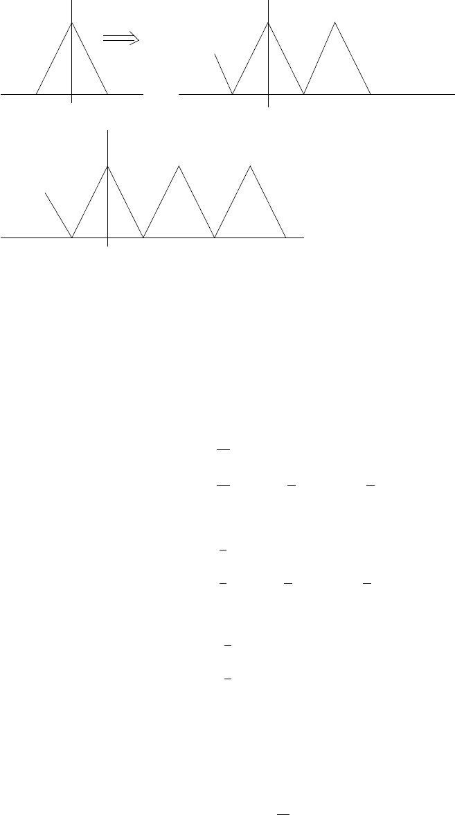
X(w)
2
X(w)
1
X(w)
3
w
w
−π 0 π −0.5π 00.5π π
−π/3 0 π/3 π
Figure 4.18-1:
(b)
x2(n) = 1
2j(ejπn/2+e−jπn/2)x(n)
X2(w) = 1
2jhX(w−π
2) + X(w+π
2)i
(c)
x3(n) = 1
2(ejπn/2+e−jπn/2)x(n)
X3(w) = 1
2hX(w−π
2) + X(w+π
2)i
(d)
x4(n) = 1
2(ejπn +e−jπn)x(n)
X4(w) = 1
2[X(w−π) + X(w+π)]
=X(w−π)
4.20
cy
k=1
N
N−1
X
n=0
y(n)e−j2πkn/N
115
© 2007 Pearson Education, Inc., Upper Saddle River, NJ. All rights reserved. This material is protected under all copyright laws
as they currently exist. No portion of this material may be reproduced, in any form or by any means, without permission in
writing from the publisher. For the exclusive use of adopters of the book Digital Signal Processing, Fourth Edition, by John G.
Proakis and Dimitris G. Manolakis. ISBN 0-13-187374-1.

=1
N
N−1
X
n=0 "∞
X
l=−∞
x(n−lN )#e−j2πkn/N
=1
N
∞
X
l=−∞
N−1−lN
X
m=−lN
x(m)e−j2πk(m+lN )/N
But ∞
X
l=−∞
N−1−lN
X
m=−lN
x(m)e−jw(m+lN)=X(w)
Therefore, cy
k=1
NX(2πk
N)
4.21
Let xN(n) = sinwcn
πn ,−N≤n≤N
=x(n)w(n)
where x(n) = sinwcn
πn ,− ∞ ≤ n≤ ∞
w(n) = 1,−N≤n≤N
= 0,otherwise
Then sinwcn
πn
F
↔X(w)
= 1,|w| ≤ wc
= 0,otherwise
XN(w) = X(w)∗W(w)
=Zπ
−π
X(Θ)W(w−Θ)dΘ
=Zwc
−wc
sin(2N+ 1)(w−Θ)/2
sin(w−Θ)/2dΘ
4.22
(a)
X1(w) = X
n
x(2n+ 1)e−jwn
=X
k
x(k)e−jwk/2ejw/2
=X(w
2)ejw/2
=ejw/2
1−aejw/2
(b)
X2(w) = X
n
x(n+ 2)eπn/2e−jwn
=−X
k
x(k)e−jk(w+jπ/2)ej2w
116
© 2007 Pearson Education, Inc., Upper Saddle River, NJ. All rights reserved. This material is protected under all copyright laws
as they currently exist. No portion of this material may be reproduced, in any form or by any means, without permission in
writing from the publisher. For the exclusive use of adopters of the book Digital Signal Processing, Fourth Edition, by John G.
Proakis and Dimitris G. Manolakis. ISBN 0-13-187374-1.

=−X(w+jπ
2)ej2w
(c)
X3(w) = X
n
x(−2n)e−jwn
=−X
k
x(k)e−jkw/2)
=X(−w
2)
(d)
X4(w) = X
n
1
2(ej0.3πn +e−j0.3πn)x(n)e−jwn
=1
2X
n
x(n)he−j(w−0.3π)n+e−j(w+0.3π)ni
=1
2[X(w−0.3π) + X(w+ 0.3π)]
(e) X5(w) = X(w)X(w)e−jw=X2(w)e−jw
(f)
X6(w) = X(w)X(−w)
=1
(1 −ae−jw)(1 −aejw)
=1
(1 −2acosw +a2)
4.23
(a) Y1(w) = Pny1(n)e−jwn =Pn,n even x(n)e−jwn The fourier transform Y1(w) can easily be
obtained by combining the results of (b) and (c).
(b)
y2(n) = x(2n)
Y2(w) = X
n
y2(n)e−jwn
=X
n
x(2n)e−jwn
=X
m
x(m)e−jwm/2
=X(w
2)
Refer to fig 4.23-1.
(c)
y3(n) = x(n/2), n even
0,otherwise
Y3(w) = X
n
y3(n)e−jwn
117
© 2007 Pearson Education, Inc., Upper Saddle River, NJ. All rights reserved. This material is protected under all copyright laws
as they currently exist. No portion of this material may be reproduced, in any form or by any means, without permission in
writing from the publisher. For the exclusive use of adopters of the book Digital Signal Processing, Fourth Edition, by John G.
Proakis and Dimitris G. Manolakis. ISBN 0-13-187374-1.
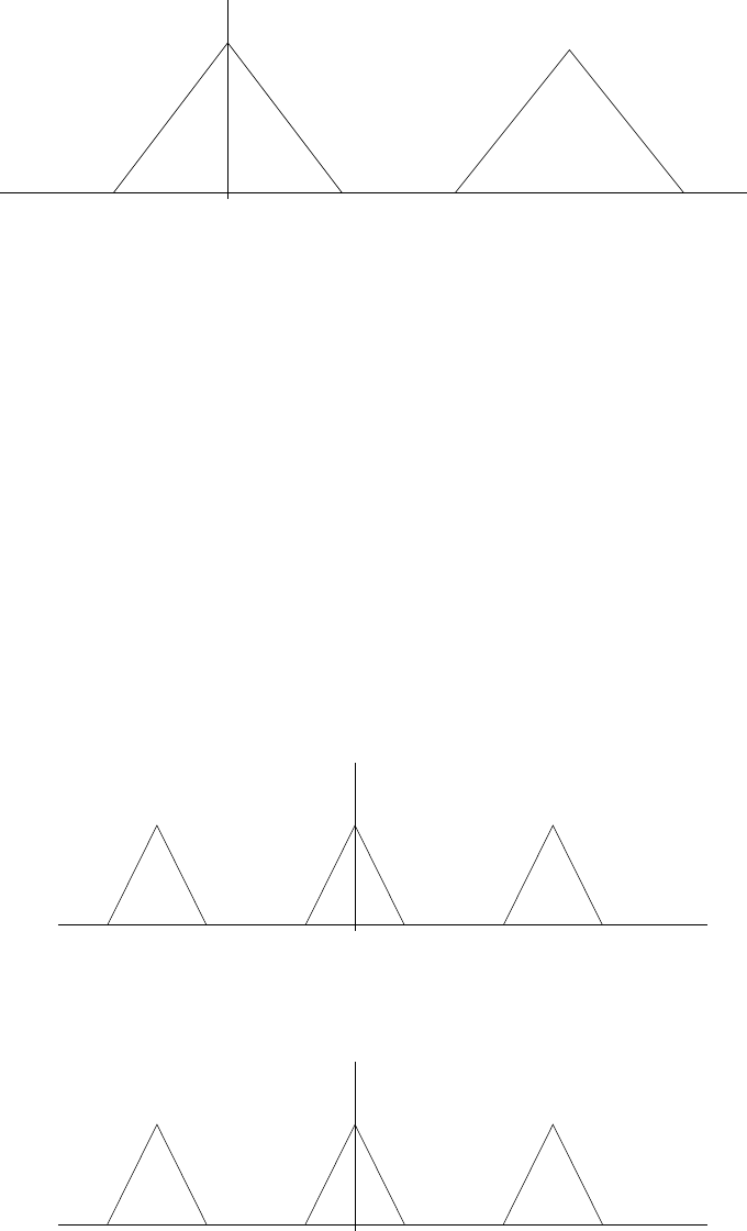
−π −π/2 0 π/2 π 3π/2 2π
Y(w)
2
Figure 4.23-1:
=X
neven
x(n/2)e−jwn
=X
m
x(m)e−j2wm
=X(2w)
We now return to part(a). Note that y1(n) may be expressed as
y1(n) = y2(n/2), n even
0, n odd
Hence, Y1(w) = Y2(2w). Refer to fig 4.23-2.
Y(w)
3
Y(w)
1
−π/8 0π/8 π/2 7π/8 π
−π −7π/8
−π −3π/4 −π/2 −π/4 0 π/4 π/2 3π/4 π
Figure 4.23-2:
118
© 2007 Pearson Education, Inc., Upper Saddle River, NJ. All rights reserved. This material is protected under all copyright laws
as they currently exist. No portion of this material may be reproduced, in any form or by any means, without permission in
writing from the publisher. For the exclusive use of adopters of the book Digital Signal Processing, Fourth Edition, by John G.
Proakis and Dimitris G. Manolakis. ISBN 0-13-187374-1.

Chapter 5
5.1
(a) Because the range of nis (−∞,∞), the fourier transforms of x(n) and y(n) do not exist.
However, the relationship implied by the forms of x(n) and y(n) is y(n) = x3(n). In this case,
the system H1is non-linear.
(b) In this case,
X(w) = 1
1−1
2e−jw ,
Y(w) = 1
1−1
8e−jw ,
Hence, H(w) = Y(w)
X(w)
=1−1
2e−jw
1−1
8e−jw
⇒System is LTI
Note however that the system may also be nonlinear, e.g., y(n) = x3(n).
(c) and (d). Clearly, there is an LTI system that produces y(n) when excited by x(n), e.g.
H(w) = 3, for all w, or H(π
5) = 3.
(e) If this system is LTI, the period of the output signal would be the same as the period of the
input signal, i.e., N1=N2. Since this is not the case, the system is nonlinear.
5.2
(a)
WR(w) =
M
X
n=0
wR(n)e−jwn
=
M
X
n=0
e−jwn
=1−e−j(M+1)w
1−e−jw
=e−jMw/2sin(M+1
2)w
sinw
2
119
© 2007 Pearson Education, Inc., Upper Saddle River, NJ. All rights reserved. This material is protected under all copyright laws
as they currently exist. No portion of this material may be reproduced, in any form or by any means, without permission in
writing from the publisher. For the exclusive use of adopters of the book Digital Signal Processing, Fourth Edition, by John G.
Proakis and Dimitris G. Manolakis. ISBN 0-13-187374-1.
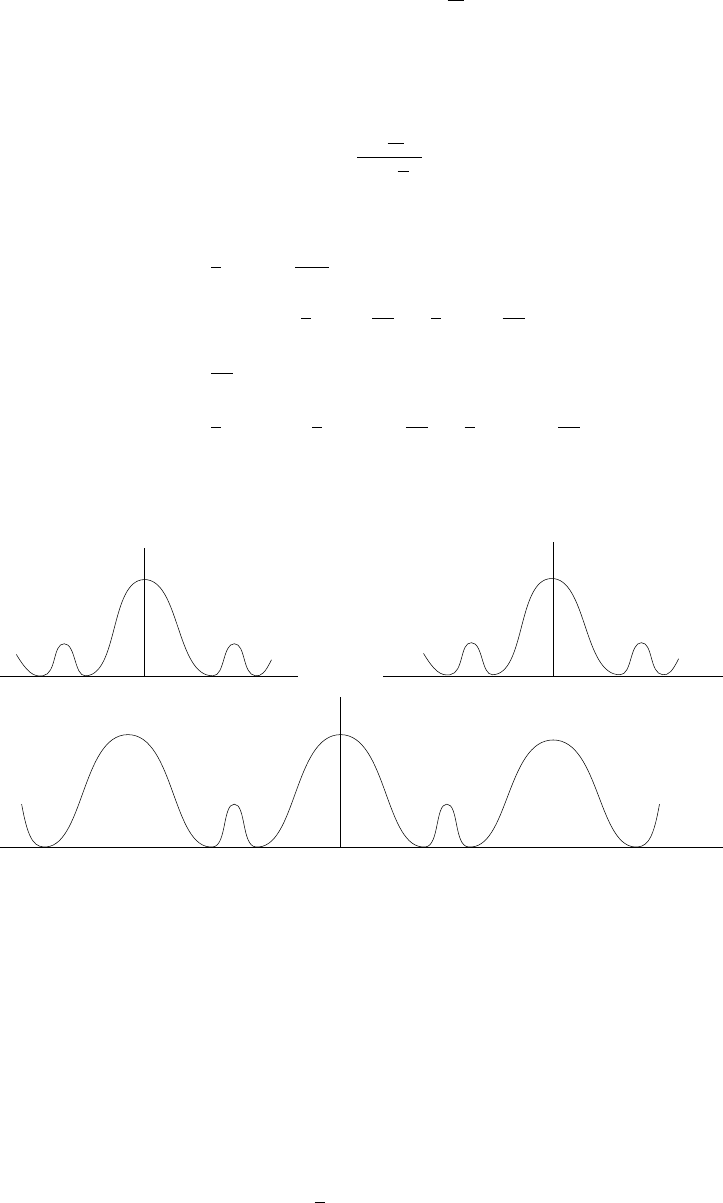
(b) Let wT(n) = hR(n)∗hR(n−1),
hR(n) = 1,0≤n≤M
2−1
0,otherwise
Hence,
WT(w) = H2
R(w)e−jw
= sinM
4w
sinw
2!2
e−jwM/2
(c)
Let c(n) = 1
2(1 + cos2πn
M)
Then, C(w) = πδ(w) + 1
2δ(w−2π
M) + 1
2δ(w+2π
M)−π≤w≤π
Wc(w) = 1
2πZπ
−π
c(Θ)WR(w−Θ)dΘ
=1
2WR(w) + 1
2WR(w−2π
M) + 1
2WR(w+2π
M)
Refer to fig 5.2-1
−2π/Μ+1 0 2π/Μ+1 −4π/Μ 0 4π/Μ
−2π/Μ −2π/Μ+1 0 2π/Μ+1 2π/Μ
|W(w)|
R
|W(w)|
T
|W(w)|
c
w w
w
Figure 5.2-1:
5.3
(a)
h(n) = (1
2)nu(n)
120
© 2007 Pearson Education, Inc., Upper Saddle River, NJ. All rights reserved. This material is protected under all copyright laws
as they currently exist. No portion of this material may be reproduced, in any form or by any means, without permission in
writing from the publisher. For the exclusive use of adopters of the book Digital Signal Processing, Fourth Edition, by John G.
Proakis and Dimitris G. Manolakis. ISBN 0-13-187374-1.

H(w) = ∞
X
n=0
(1
2)ne−jwn
=∞
X
n=0
(1
2e−jw)n
=1
1−1
2e−jw
|H(w)|=1
(1 −1
2cosw)2+ (1
2sinw)21
2
=1
5
4−cosw1
2
6H(w) = −tan−1
1
2sinw
1−1
2cosw
≡Θ(w)
(b) (1)
For the input x(n) = cos 3π
10 n
=1
2(ej3πn
10 +e−j3πn
10 )
X(w) = πδ(w−3π
10 ) + δ(w+3π
10 ),|w| ≤ π
Y(w) = H(w)X(w)
=H(3π
10 )πδ(w−3π
10 ) + δ(w+3π
10 )
y(n) = |H(3π
10 )|cos 3πn
10 + Θ(3π
10 )
(2)
x(n) = . . . , 1,0,0,1
↑,1,1,0,1,1,1,0, . . .
First, determine xe(n) = x(n) + x(−n)
2
and xo(n) = x(n)−x(−n)
2
Then, XR(w) = X
n
xe(n)e−jwn
XI(w) = X
n
xo(n)e−jwn
|H(w)|=X2
R(w) + X2
I(w),
Θ(w) = tan−1XI(w)
XR(w)
and Y(w) = H(w)X(w)
121
© 2007 Pearson Education, Inc., Upper Saddle River, NJ. All rights reserved. This material is protected under all copyright laws
as they currently exist. No portion of this material may be reproduced, in any form or by any means, without permission in
writing from the publisher. For the exclusive use of adopters of the book Digital Signal Processing, Fourth Edition, by John G.
Proakis and Dimitris G. Manolakis. ISBN 0-13-187374-1.
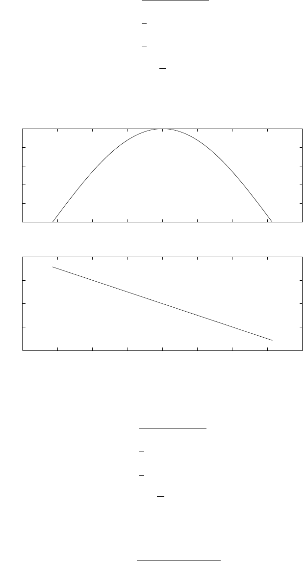
5.4
(a)
y(n) = x(n) + x(n−1)
2
Y(w) = 1
2(1 + e−jw)X(w)
H(w) = 1
2(1 + e−jw)
= (cosw
2)e−jw/2
Refer to fig 5.4-1.
(b)
−4 −3 −2 −1 0 1 2 3 4
0
0.2
0.4
0.6
0.8
1
−−> w
−−> |H(w)|
−4 −3 −2 −1 0 1 2 3 4
−2
−1
0
1
2
−−> w
−−> theta(w)
Figure 5.4-1:
y(n) = x(n)−x(n−1)
2
Y(w) = 1
2(1 −e−jw)X(w)
H(w) = 1
2(1 −e−jw)
= (sinw
2)e−jw/2ejπ/2
Refer to fig 5.4-2.
(c)
y(n) = x(n+ 1) −x(n−1)
2
122
© 2007 Pearson Education, Inc., Upper Saddle River, NJ. All rights reserved. This material is protected under all copyright laws
as they currently exist. No portion of this material may be reproduced, in any form or by any means, without permission in
writing from the publisher. For the exclusive use of adopters of the book Digital Signal Processing, Fourth Edition, by John G.
Proakis and Dimitris G. Manolakis. ISBN 0-13-187374-1.
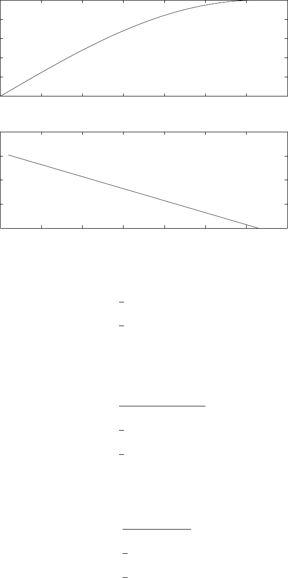
0 0.5 1 1.5 2 2.5 3 3.5
0
0.2
0.4
0.6
0.8
1
−−> w
−−> |H(w)|
0 0.5 1 1.5 2 2.5 3 3.5
0
0.5
1
1.5
2
−−> w
−−> theta(w)
Figure 5.4-2:
Y(w) = 1
2(ejw −e−jw )X(w)
H(w) = 1
2(ejw −e−jw )
= (sinw)ejπ/2
Refer to fig 5.4-3.
(d)
y(n) = x(n+ 1) + x(n−1)
2
Y(w) = 1
2(ejw +e−jw )X(w)
H(w) = 1
2(ejw +e−jw )
=cosw
Refer to fig 5.4-4
(e)
y(n) = x(n) + x(n−2)
2
Y(w) = 1
2(1 + e−j2w)X(w)
H(w) = 1
2(1 + e−j2w)
= (cosw)e−jw
Refer to fig 5.4-5.
(f)
123
© 2007 Pearson Education, Inc., Upper Saddle River, NJ. All rights reserved. This material is protected under all copyright laws
as they currently exist. No portion of this material may be reproduced, in any form or by any means, without permission in
writing from the publisher. For the exclusive use of adopters of the book Digital Signal Processing, Fourth Edition, by John G.
Proakis and Dimitris G. Manolakis. ISBN 0-13-187374-1.
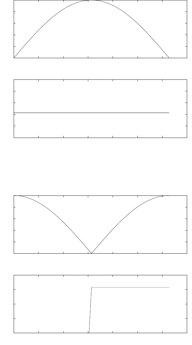
0 0.5 1 1.5 2 2.5 3 3.5
0
0.2
0.4
0.6
0.8
1
−−> w
−−> |H(w)|
0 0.5 1 1.5 2 2.5 3 3.5
0.5
1
1.5
2
2.5
3
−−> w
−−> theta(w)
Figure 5.4-3:
0 0.5 1 1.5 2 2.5 3 3.5
0
0.2
0.4
0.6
0.8
1
−−> w
−−> |H(w)|
0 0.5 1 1.5 2 2.5 3 3.5
0
1
2
3
4
−−> w
−−> theta(w)
Figure 5.4-4:
124
© 2007 Pearson Education, Inc., Upper Saddle River, NJ. All rights reserved. This material is protected under all copyright laws
as they currently exist. No portion of this material may be reproduced, in any form or by any means, without permission in
writing from the publisher. For the exclusive use of adopters of the book Digital Signal Processing, Fourth Edition, by John G.
Proakis and Dimitris G. Manolakis. ISBN 0-13-187374-1.
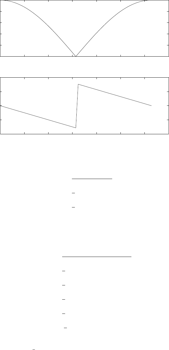
0 0.5 1 1.5 2 2.5 3 3.5
0
0.2
0.4
0.6
0.8
1
−−> w
−−> |H(w)|
0 0.5 1 1.5 2 2.5 3 3.5
−2
−1
0
1
2
−−> w
−−> theta(w)
Figure 5.4-5:
y(n) = x(n)−x(n−2)
2
Y(w) = 1
2(1 −e−j2w)X(w)
H(w) = 1
2(1 −e−j2w)
= (sinw)e−jw+jπ/2
Refer to fig 5.4-6
(g)
y(n) = x(n) + x(n−1) + x(n−2)
3
Y(w) = 1
3(1 + e−jw +e−j2w)X(w)
H(w) = 1
3(1 + e−jw +e−j2w)
=1
3(1 + ejw +e−jw )e−jw
=1
3(1 + 2cosw)e−jw
|H(w)|=|1
3(1 + 2cosw)|
6H(w) = −w, 1 + 2cosw > 0
π−w, 1 + 2cosw < 0
Refer to fig 5.4-7.
(h)
125
© 2007 Pearson Education, Inc., Upper Saddle River, NJ. All rights reserved. This material is protected under all copyright laws
as they currently exist. No portion of this material may be reproduced, in any form or by any means, without permission in
writing from the publisher. For the exclusive use of adopters of the book Digital Signal Processing, Fourth Edition, by John G.
Proakis and Dimitris G. Manolakis. ISBN 0-13-187374-1.
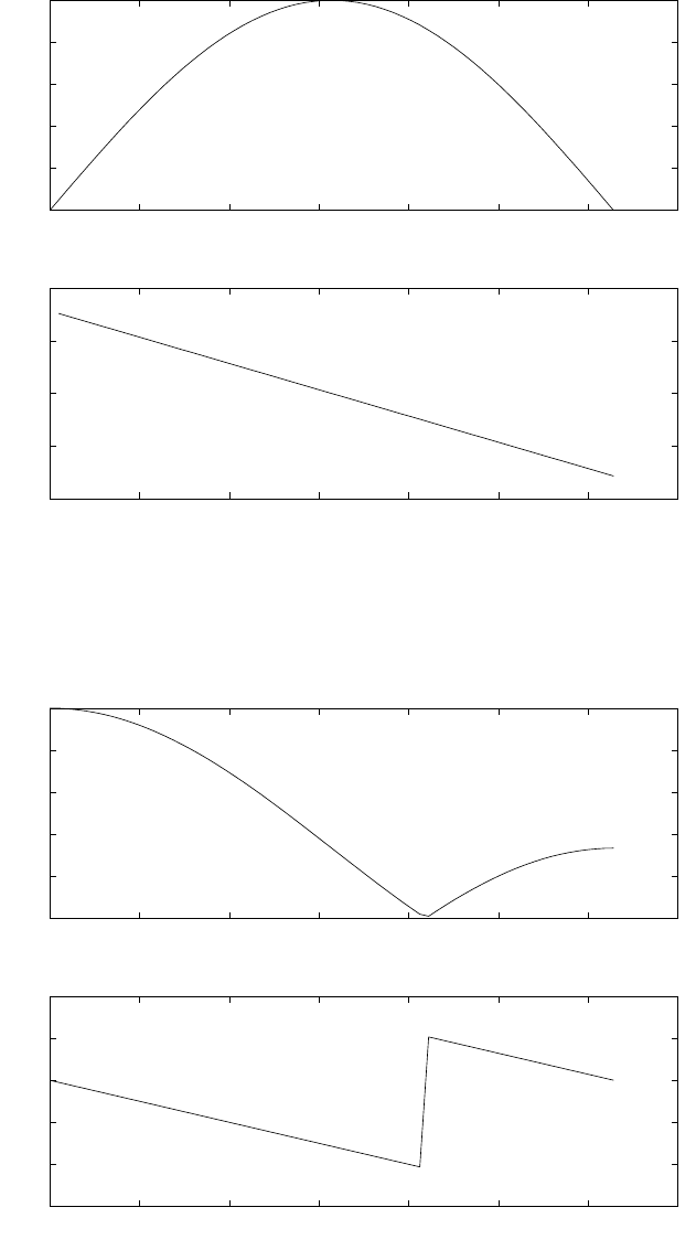
0 0.5 1 1.5 2 2.5 3 3.5
0
0.2
0.4
0.6
0.8
1
−−> w
−−> |H(w)|
0 0.5 1 1.5 2 2.5 3 3.5
−2
−1
0
1
2
−−> w
−−> theta(w)
Figure 5.4-6:
0 0.5 1 1.5 2 2.5 3 3.5
0
0.2
0.4
0.6
0.8
1
−−> w
−−> |H(w)|
0 0.5 1 1.5 2 2.5 3 3.5
−3
−2
−1
0
1
2
−−> w
−−> theta(w)
Figure 5.4-7:
126
© 2007 Pearson Education, Inc., Upper Saddle River, NJ. All rights reserved. This material is protected under all copyright laws
as they currently exist. No portion of this material may be reproduced, in any form or by any means, without permission in
writing from the publisher. For the exclusive use of adopters of the book Digital Signal Processing, Fourth Edition, by John G.
Proakis and Dimitris G. Manolakis. ISBN 0-13-187374-1.
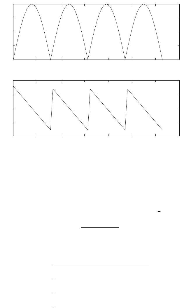
y(n) = x(n)−x(n−8)
Y(w) = (1 −e−j8w)X(w)
H(w) = (1 −e−j8w)
= 2(sin4w)ej(π/2−4w)
Refer to fig 5.4-8.
(i)
0 0.5 1 1.5 2 2.5 3 3.5
0
0.5
1
1.5
2
−−> w
−−> |H(w)|
0 0.5 1 1.5 2 2.5 3 3.5
−2
−1
0
1
2
−−> w
−−> theta(w)
Figure 5.4-8:
y(n) = 2x(n−1) −x(n−2)
Y(w) = (2e−jw −e−j2w)X(w)
H(w) = (2e−jw −e−j2w)
= 2cosw −cos2w−j(2sinw −sin2w)
|H(w)|=(2cosw −cos2w)2+ (2sinw −sin2w)21
2
Θ(w) = −tan−12sinw −sin2w
2cosw −cos2w
Refer to fig 5.4-9.
(j)
y(n) = x(n) + x(n−1) + x(n−2) + x(n−3)
4
Y(w) = 1
4(1 + e−jw +e−j2w+e−j3w)X(w)
H(w) = 1
3e−jw(ejw +e−jw ) + e−j2w(ejw +e−jw)
=1
2(e−jw +e−j2w)cosw
127
© 2007 Pearson Education, Inc., Upper Saddle River, NJ. All rights reserved. This material is protected under all copyright laws
as they currently exist. No portion of this material may be reproduced, in any form or by any means, without permission in
writing from the publisher. For the exclusive use of adopters of the book Digital Signal Processing, Fourth Edition, by John G.
Proakis and Dimitris G. Manolakis. ISBN 0-13-187374-1.
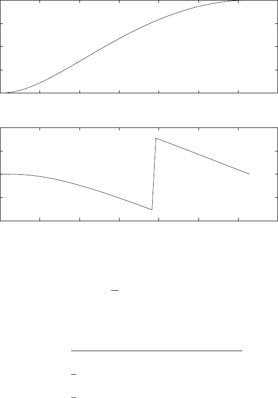
0 0.5 1 1.5 2 2.5 3 3.5
1
1.5
2
2.5
3
−−> w
−−> |H(w)|
0 0.5 1 1.5 2 2.5 3 3.5
−2
−1
0
1
2
−−> w
−−> theta(w)
Figure 5.4-9:
= (cosw)(cosw
2)e−j3w/2
Refer to fig 5.4-10.
(k)
y(n) = x(n) + 3x(n−1) + 3x(n−2) + x(n−3)
8
Y(w) = 1
8(1 + 3e−jw + 3e−j2w+e−j3w)X(w)
H(w) = 1
8(1 + e−jw)3
= (cosw/2)3e−j3w/2
Refer to fig 5.4-11.
(l)
y(n) = x(n−4)
Y(w) = e−j4wX(w)
H(w) = e−j4w
|H(w)|= 1
Θ(w) = −4w
Refer to fig 5.4-12.
(m)
y(n) = x(n+ 4)
Y(w) = ej4wX(w)
H(w) = ej4w
128
© 2007 Pearson Education, Inc., Upper Saddle River, NJ. All rights reserved. This material is protected under all copyright laws
as they currently exist. No portion of this material may be reproduced, in any form or by any means, without permission in
writing from the publisher. For the exclusive use of adopters of the book Digital Signal Processing, Fourth Edition, by John G.
Proakis and Dimitris G. Manolakis. ISBN 0-13-187374-1.
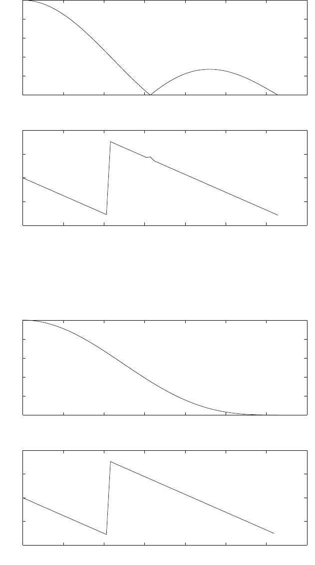
0 0.5 1 1.5 2 2.5 3 3.5
0
0.2
0.4
0.6
0.8
1
−−> w
−−> |H(w)|
0 0.5 1 1.5 2 2.5 3 3.5
−2
−1
0
1
2
−−> w
−−> theta(w)
Figure 5.4-10:
0 0.5 1 1.5 2 2.5 3 3.5
0
0.2
0.4
0.6
0.8
1
−−> w
−−> |H(w)|
0 0.5 1 1.5 2 2.5 3 3.5
−2
−1
0
1
2
−−> w
−−> theta(w)
Figure 5.4-11:
129
© 2007 Pearson Education, Inc., Upper Saddle River, NJ. All rights reserved. This material is protected under all copyright laws
as they currently exist. No portion of this material may be reproduced, in any form or by any means, without permission in
writing from the publisher. For the exclusive use of adopters of the book Digital Signal Processing, Fourth Edition, by John G.
Proakis and Dimitris G. Manolakis. ISBN 0-13-187374-1.
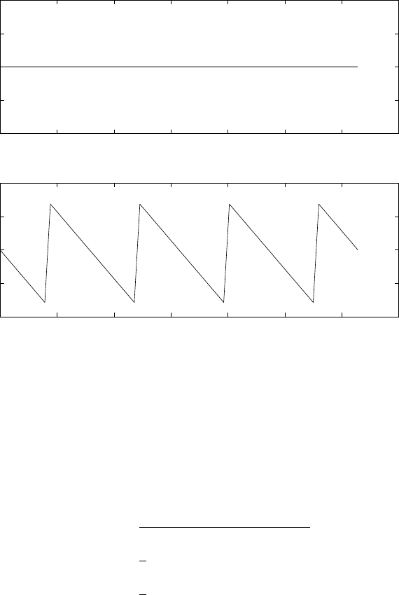
0 0.5 1 1.5 2 2.5 3 3.5
0
0.5
1
1.5
2
−−> w
−−> |H(w)|
0 0.5 1 1.5 2 2.5 3 3.5
−2
−1
0
1
2
−−> w
−−> theta(w)
Figure 5.4-12:
|H(w)|= 1
Θ(w) = 4w
Refer to fig 5.4-13.
(n)
y(n) = x(n)−2x(n−1) + x(n−2)
4
Y(w) = 1
4(1 −2e−jw +e−j2w)X(w)
H(w) = 1
4(1 −e−jw)2
= (sin2w/2)e−j(w−π)
Refer to fig 5.4-14.
5.5
(a)
y(n) = x(n) + x(n−10)
Y(w) = (1 + e−j10w)X(w)
H(w) = (2cos5w)e−j5w
Refer to fig 5.5-1.
(b)
130
© 2007 Pearson Education, Inc., Upper Saddle River, NJ. All rights reserved. This material is protected under all copyright laws
as they currently exist. No portion of this material may be reproduced, in any form or by any means, without permission in
writing from the publisher. For the exclusive use of adopters of the book Digital Signal Processing, Fourth Edition, by John G.
Proakis and Dimitris G. Manolakis. ISBN 0-13-187374-1.
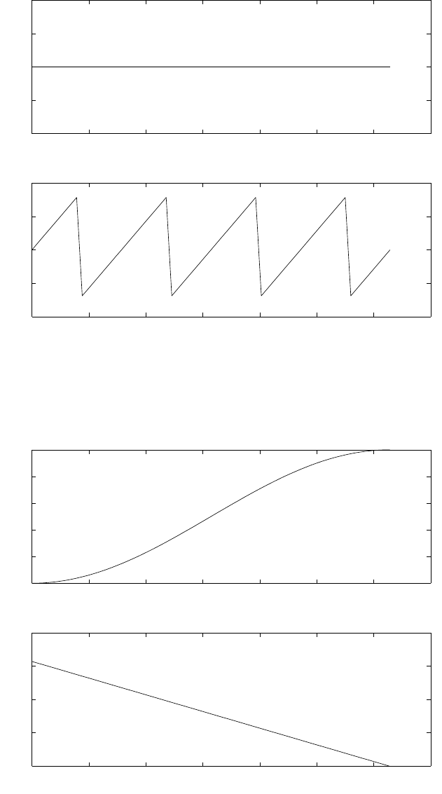
0 0.5 1 1.5 2 2.5 3 3.5
0
0.5
1
1.5
2
−−> w
−−> |H(w)|
0 0.5 1 1.5 2 2.5 3 3.5
−2
−1
0
1
2
−−> w
−−> theta(w)
Figure 5.4-13:
0 0.5 1 1.5 2 2.5 3 3.5
0
0.2
0.4
0.6
0.8
1
−−> w
−−> |H(w)|
0 0.5 1 1.5 2 2.5 3 3.5
0
1
2
3
4
−−> w
−−> theta(w)
Figure 5.4-14:
131
© 2007 Pearson Education, Inc., Upper Saddle River, NJ. All rights reserved. This material is protected under all copyright laws
as they currently exist. No portion of this material may be reproduced, in any form or by any means, without permission in
writing from the publisher. For the exclusive use of adopters of the book Digital Signal Processing, Fourth Edition, by John G.
Proakis and Dimitris G. Manolakis. ISBN 0-13-187374-1.

0 0.5 1 1.5 2 2.5 3 3.5
0
0.5
1
1.5
2
−−> w
−−> |H(w)|
0 0.5 1 1.5 2 2.5 3 3.5
−2
−1
0
1
2
−−> w
−−> theta(w)
Figure 5.5-1:
H(π
10) = 0
H(π
3) = (2cos5π
3)e−j5π
3
y(n) = (6cos5π
3)sin(π
3+π
10 −5π
3)
= (6cos5π
3)sin(π
3−47π
30 )
(c)
H(0) = 2
H(4π
10 ) = 2
y(n) = 20 + 10cos2πn
5+π
2
5.6
h(n) = δ(n) + 2δ(n−2) + δ(n−4)
H(w) = 1 + 2e−j2w+e−j4w
= (1 + e−j2w)2
= 4(cosw)2e−j2w
Steady State Response: H(π
2) = 0
Therefore, yss(n) = 0,(n≥4)
132
© 2007 Pearson Education, Inc., Upper Saddle River, NJ. All rights reserved. This material is protected under all copyright laws
as they currently exist. No portion of this material may be reproduced, in any form or by any means, without permission in
writing from the publisher. For the exclusive use of adopters of the book Digital Signal Processing, Fourth Edition, by John G.
Proakis and Dimitris G. Manolakis. ISBN 0-13-187374-1.
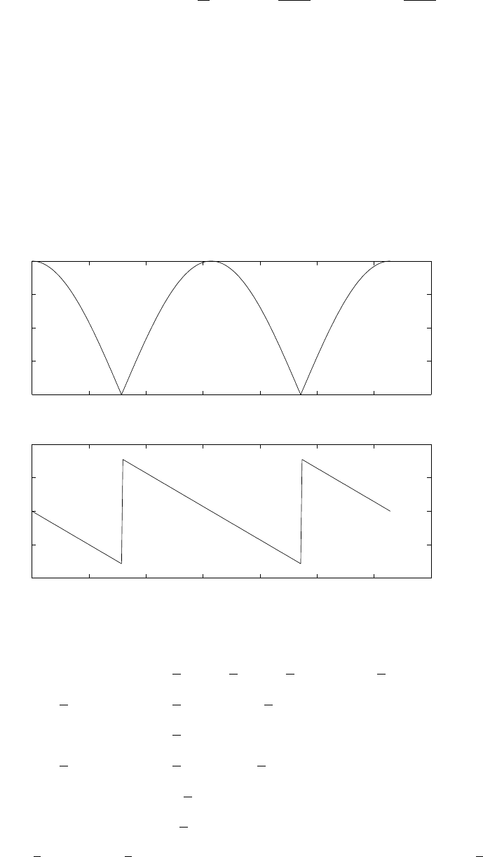
Transient Response:
ytr(n) = 10eπn
2u(n) + 20eπ(n−2)
2u(n−2) + 10eπ(n−4)
2u(n−4)
= 10δ(n) + j10δ(n−1) + 10δ(n−2) + j10δ(n−3)
5.7
(a)
y(n) = x(n) + x(n−4)
Y(w) = (1 + e−j4w)X(w)
H(w) = (2cos2w)e−j2w
Refer to fig 5.7-1.
(b)
0 0.5 1 1.5 2 2.5 3 3.5
0
0.5
1
1.5
2
−−> w
−−> |H(w)|
0 0.5 1 1.5 2 2.5 3 3.5
−2
−1
0
1
2
−−> w
−−> theta(w)
Figure 5.7-1:
y(n) = cosπ
2n+cosπ
4n+cosπ
2(n−4) + cosπ
4(n−4)
But cosπ
2(n−4) = cosπ
2ncos2π+sinπ
2nsin2π
=cosπ
2n
and cosπ
4(n−4) = cosπ
4ncosπ −sinπ
4nsinπ
=−cosπ
4n
Therefore, y(n) = 2cosπ
2n
(c) Note that H(π
2) = 2 and H(π
4) = 0. Therefore, the filter does not pass the signal cos(π
4n).
133
© 2007 Pearson Education, Inc., Upper Saddle River, NJ. All rights reserved. This material is protected under all copyright laws
as they currently exist. No portion of this material may be reproduced, in any form or by any means, without permission in
writing from the publisher. For the exclusive use of adopters of the book Digital Signal Processing, Fourth Edition, by John G.
Proakis and Dimitris G. Manolakis. ISBN 0-13-187374-1.

5.8
y(n) = 1
2[x(n)−x(n−2)]
Y(w) = 1
2(1 −e−j2w)X(w)
H(w) = 1
2(1 −e−j2w)
= (sinw)ej(π
2−w)
H(0) = 0, H(π
2) = 1
Hence, yss(n) = 3cos(π
2n+ 60o)
ytr(n) = 0
5.9
x(n) = Acosπ
4n
(a) y(n) = x(2n) = Acosπ
2n⇒w=π
2
(b) y(n) = x2(n) = A2cos2π
4n=1
2A2+1
2A2cosπ
2n. Hence, w= 0 and w=π
2
(c)
y(n) = x(n)cosπn
=Acosπ
4ncosπn
=A
2cos5π
4n+A
2cos3π
4n
Hence, w=3π
4and w=5π
4
5.10
(a)
y(n) = 1
2[x(n) + x(n−1)]
Y(w) = 1
2(1 + e−jw)X(w)
H(w) = 1
2(1 + e−jw)
=cos(w
2)e−jw
2
Refer to fig 5.10-1.
(b)
y(n) = −1
2[x(n)−x(n−1)]
Y(w) = −1
2(1 −e−jw)X(w)
|H(w)|=sinw
2
Θ(w) = ej(π
2−w
2)
134
© 2007 Pearson Education, Inc., Upper Saddle River, NJ. All rights reserved. This material is protected under all copyright laws
as they currently exist. No portion of this material may be reproduced, in any form or by any means, without permission in
writing from the publisher. For the exclusive use of adopters of the book Digital Signal Processing, Fourth Edition, by John G.
Proakis and Dimitris G. Manolakis. ISBN 0-13-187374-1.
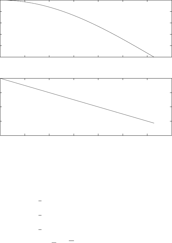
0 0.5 1 1.5 2 2.5 3 3.5
0
0.2
0.4
0.6
0.8
1
−−> w
−−> |H(w)|
0 0.5 1 1.5 2 2.5 3 3.5
−2
−1.5
−1
−0.5
0
−−> w
−−> theta(w)
Figure 5.10-1:
Refer to fig 5.10-2.
(c)
y(n) = 1
8[x(n) + 3x(n−1) + 3x(n−2) + x(n−3)]
Y(w) = 1
8(1 + e−jw)3X(w)
H(w) = 1
8(1 + e−jw)3
=cos3(w
2)e−j3w
2
Refer to fig 5.10-3.
135
© 2007 Pearson Education, Inc., Upper Saddle River, NJ. All rights reserved. This material is protected under all copyright laws
as they currently exist. No portion of this material may be reproduced, in any form or by any means, without permission in
writing from the publisher. For the exclusive use of adopters of the book Digital Signal Processing, Fourth Edition, by John G.
Proakis and Dimitris G. Manolakis. ISBN 0-13-187374-1.
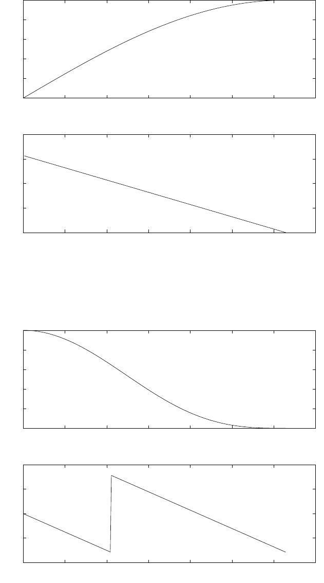
0 0.5 1 1.5 2 2.5 3 3.5
0
0.2
0.4
0.6
0.8
1
−−> w
−−> |H(w)|
0 0.5 1 1.5 2 2.5 3 3.5
0
0.5
1
1.5
2
−−> w
−−> theta(w)
Figure 5.10-2:
0 0.5 1 1.5 2 2.5 3 3.5
0
0.2
0.4
0.6
0.8
1
−−> w
−−> |H(w)|
0 0.5 1 1.5 2 2.5 3 3.5
−2
−1
0
1
2
−−> w
−−> theta(w)
Figure 5.10-3:
136
© 2007 Pearson Education, Inc., Upper Saddle River, NJ. All rights reserved. This material is protected under all copyright laws
as they currently exist. No portion of this material may be reproduced, in any form or by any means, without permission in
writing from the publisher. For the exclusive use of adopters of the book Digital Signal Processing, Fourth Edition, by John G.
Proakis and Dimitris G. Manolakis. ISBN 0-13-187374-1.

5.11
y(n) = x(n) + x(n−M)
Y(w) = (1 + e−jwM )X(w)
H(w) = (1 + e−jwM )
H(w) = 0,at wM
2= (k+1
2)π, k = 0,1,...
or w= (2k+ 1)π/M, k = 0,1,...
|H(w)|=|2coswM
2|
5.12
y(n) = 0.9y(n−1) + bx(n)
(a)
Y(w) = 0.9e−jwY(w) + bX(w)
H(w) = Y(w)
X(w)
=b
1−0.9e−jw
|H(0)|= 1,⇒b=±0.1
Θ(w) = −wM
2, coswM
2>0
π−wM
2, coswM
2<0
(b) |H(w0)|2=1
2⇒b2
1.81−1.8cosw0=1
2⇒w0= 0.105
(c) The filter is lowpass.
(d) For |H(w0)|2=1
2⇒w0= 3.036. This filter is a highpass filter.
5.13
(a)
Px=1
N
N−1
X
n=0 |x(n)|2
=
N−1
X
k=0 |ck|2
=c2
0+ 2
N
2−1
X
k=1 |ck|2
Spurious power = Px−2|ck0|2
THD = Px−2|ck0|2
Px
= 1 −2|ck0|2
Px
137
© 2007 Pearson Education, Inc., Upper Saddle River, NJ. All rights reserved. This material is protected under all copyright laws
as they currently exist. No portion of this material may be reproduced, in any form or by any means, without permission in
writing from the publisher. For the exclusive use of adopters of the book Digital Signal Processing, Fourth Edition, by John G.
Proakis and Dimitris G. Manolakis. ISBN 0-13-187374-1.
(b) for f0 = 1
96 , refer to fig 5.13-1
for f0 = 1
32 , refer to fig 5.13-2
for f0 = 1
256 , refer to fig 5.13-3
(c) for f0 = 1
96 , refer to fig 5.13-4
for f0 = 1
32 , refer to fig 5.13-5
for f0 = 1
256 , refer to fig 5.13-6
The total harmonic distortion(THD) reduces as the number of terms in the Taylor approxi-
mation is increased.
0 50 100
−20
−10
0
10
−−> x(n)
terms= 2
0 50 100
−50
0
50
−−> x(n)
terms= 3
0 50 100
−40
−20
0
20
−−> x(n)
terms= 4
0 50 100
−10
0
10
20
−−> x(n)
terms= 5
0 50 100
−5
0
5
−−> x(n)
terms= 6
0 50 100
−2
0
2
4
−−> x(n)
terms= 7
0 50 100
−2
−1
0
1
−−> x(n)
terms= 8
Figure 5.13-1:
138
© 2007 Pearson Education, Inc., Upper Saddle River, NJ. All rights reserved. This material is protected under all copyright laws
as they currently exist. No portion of this material may be reproduced, in any form or by any means, without permission in
writing from the publisher. For the exclusive use of adopters of the book Digital Signal Processing, Fourth Edition, by John G.
Proakis and Dimitris G. Manolakis. ISBN 0-13-187374-1.
0 20 40
−20
−10
0
10
−−> x(n)
terms= 2
0 20 40
−20
0
20
40
−−> x(n)
terms= 3
0 20 40
−40
−20
0
20
−−> x(n)
terms= 4
0 20 40
−10
0
10
20
−−> x(n)
terms= 5
0 20 40
−4
−2
0
2
−−> x(n)
terms= 6
0 20 40
−1
0
1
2
−−> x(n)
terms= 7
0 20 40
−2
−1
0
1
−−> x(n)
terms= 8
Figure 5.13-2:
0 100 200 300
−20
−10
0
10
−−> x(n)
terms= 2
0 100 200 300
−50
0
50
−−> x(n)
terms= 3
0 100 200 300
−40
−20
0
20
−−> x(n)
terms= 4
0 100 200 300
−20
0
20
40
−−> x(n)
terms= 5
0 100 200 300
−10
−5
0
5
−−> x(n)
terms= 6
0 100 200 300
−2
0
2
4
−−> x(n)
terms= 7
0 100 200 300
−2
−1
0
1
−−> x(n)
terms= 8
Figure 5.13-3:
139
© 2007 Pearson Education, Inc., Upper Saddle River, NJ. All rights reserved. This material is protected under all copyright laws
as they currently exist. No portion of this material may be reproduced, in any form or by any means, without permission in
writing from the publisher. For the exclusive use of adopters of the book Digital Signal Processing, Fourth Edition, by John G.
Proakis and Dimitris G. Manolakis. ISBN 0-13-187374-1.
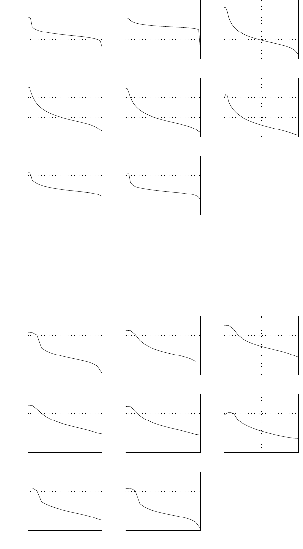
0 0.5 1
−200
−100
0
100
psd
orig cos thd=2.22e−16
0 0.5 1
−400
−200
0
200
psd
terms=2 thd=0.06186
0 0.5 1
−100
−50
0
50
psd
terms=3 thd=0.4379
0 0.5 1
−100
−50
0
50
psd
terms=4 thd=0.5283
0 0.5 1
−100
−50
0
50
psd
terms=5 thd=0.6054
0 0.5 1
−100
−50
0
50
psd
terms=6 thd=0.6295
0 0.5 1
−200
−100
0
100
psd
terms=7 thd=0.06924
0 0.5 1
−200
−100
0
100
psd
terms=8 thd=0.002657
Figure 5.13-4:
0 0.5 1
−100
−50
0
50
psd
orig cos thd=0
0 0.5 1
−100
−50
0
50
psd
terms=2 thd=0.07905
0 0.5 1
−100
−50
0
50
psd
terms=3 thd=0.4439
0 0.5 1
−100
−50
0
50
psd
terms=4 thd=0.5312
0 0.5 1
−100
−50
0
50
psd
terms=5 thd=0.5953
0 0.5 1
−100
−50
0
50
psd
terms=6 thd=0.6509
0 0.5 1
−100
−50
0
50
psd
terms=7 thd=0.05309
0 0.5 1
−100
−50
0
50
psd
terms=8 thd=0.001794
Figure 5.13-5:
140
© 2007 Pearson Education, Inc., Upper Saddle River, NJ. All rights reserved. This material is protected under all copyright laws
as they currently exist. No portion of this material may be reproduced, in any form or by any means, without permission in
writing from the publisher. For the exclusive use of adopters of the book Digital Signal Processing, Fourth Edition, by John G.
Proakis and Dimitris G. Manolakis. ISBN 0-13-187374-1.
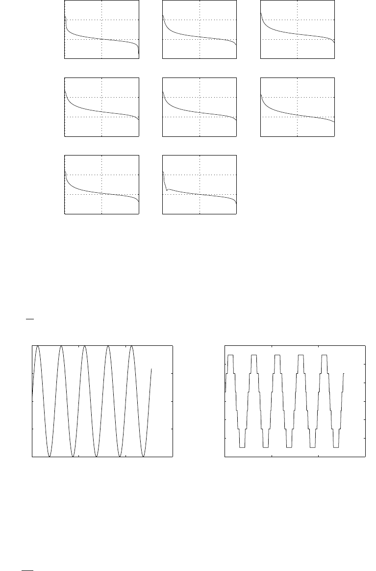
0 0.5 1
−200
−100
0
100
psd
orig cos thd=−6.661e−16
0 0.5 1
−200
−100
0
100
psd
terms=2 thd=0.05647
0 0.5 1
−200
−100
0
100
psd
terms=3 thd=0.4357
0 0.5 1
−200
−100
0
100
psd
terms=4 thd=0.5271
0 0.5 1
−200
−100
0
100
psd
terms=5 thd=0.6077
0 0.5 1
−200
−100
0
100
psd
terms=6 thd=0.6238
0 0.5 1
−200
−100
0
100
psd
terms=7 thd=0.07458
0 0.5 1
−200
−100
0
100
psd
terms=8 thd=0.002976
Figure 5.13-6:
5.14
(a) Refer to fig 5.14-1
(b) f0=1
50
0 100 200 300
−1
−0.5
0
0.5
1
−−> n
−−> x(n)
0 100 200 300
−1.5
−1
−0.5
0
0.5
1
1.5
−−> n
−−> xq(n)
Figure 5.14-1:
bits 4 6 8 16
THD 9.4616e−04 5.3431e−05 3.5650e−06 4.2848e−11
(c) f0=1
100
bits 4 6 8 16
THD 9.1993e−04 5.5965e−05 3.0308e−06 4.5383e−11
141
© 2007 Pearson Education, Inc., Upper Saddle River, NJ. All rights reserved. This material is protected under all copyright laws
as they currently exist. No portion of this material may be reproduced, in any form or by any means, without permission in
writing from the publisher. For the exclusive use of adopters of the book Digital Signal Processing, Fourth Edition, by John G.
Proakis and Dimitris G. Manolakis. ISBN 0-13-187374-1.
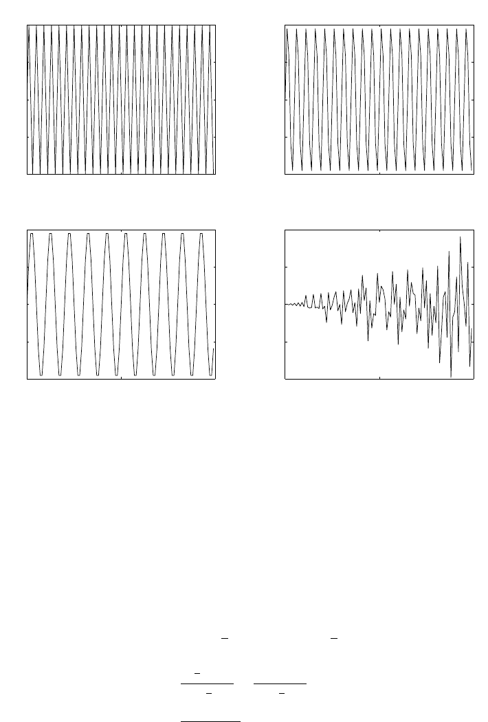
(d) As the number of bits are increased, THD is reduced considerably.
5.15
(a) Refer to fig 5.15-1
(b) Refer to fig 5.15-2
0 50 100
−1
−0.5
0
0.5
1f=0.25
0 50 100
−1
−0.5
0
0.5
1f=0.2
0 50 100
−1
−0.5
0
0.5
1f=0.1
0 50 100
−4
−2
0
2
4x 10⁻¹⁴ f=0.5
Figure 5.15-1:
The response of the system to xi(n) can be seen from fig 5.15-3
5.16
(a)
H(w) = ∞
X
n=−∞
h(n)e−jwn
=−1
X
n=−∞
(1
3)−ne−jwn +∞
X
n=0
(1
3)ne−jwn
=
1
2ejw
1−1
3ejw +1
1−1
3ejw
=4
5−3cosw
142
© 2007 Pearson Education, Inc., Upper Saddle River, NJ. All rights reserved. This material is protected under all copyright laws
as they currently exist. No portion of this material may be reproduced, in any form or by any means, without permission in
writing from the publisher. For the exclusive use of adopters of the book Digital Signal Processing, Fourth Edition, by John G.
Proakis and Dimitris G. Manolakis. ISBN 0-13-187374-1.
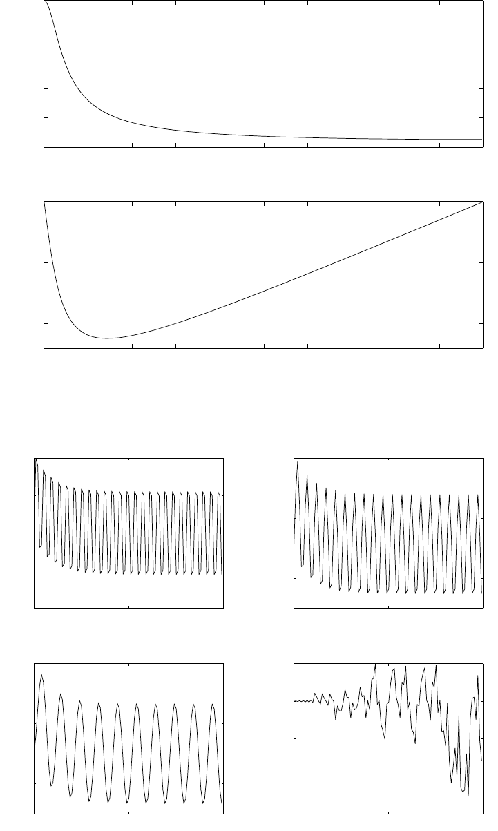
0 0.05 0.1 0.15 0.2 0.25 0.3 0.35 0.4 0.45 0.5
0
0.2
0.4
0.6
0.8
1
freq(Hz)
magnitude
0 0.05 0.1 0.15 0.2 0.25 0.3 0.35 0.4 0.45 0.5
−1
−0.5
0
freq(Hz)
phase
Figure 5.15-2:
0 50 100
−0.1
−0.05
0
0.05
0.1 f=0.25
0 50 100
−0.1
−0.05
0
0.05
0.1
0.15 f=0.2
0 50 100
−0.2
−0.1
0
0.1
0.2
0.3 f=0.1
0 50 100
−6
−4
−2
0
2x 10⁻¹⁵ f=0.5
Figure 5.15-3:
143
© 2007 Pearson Education, Inc., Upper Saddle River, NJ. All rights reserved. This material is protected under all copyright laws
as they currently exist. No portion of this material may be reproduced, in any form or by any means, without permission in
writing from the publisher. For the exclusive use of adopters of the book Digital Signal Processing, Fourth Edition, by John G.
Proakis and Dimitris G. Manolakis. ISBN 0-13-187374-1.

|H(w)|=4
5−3cosw
6H(w) = 0
(b) (1)
x(n) = cos3πn
8
X(w) = πδ(w−3πn
8) + δ(w+3πn
8),−π≤w≤π
Y(w) = H(w)X(w)
=4π
5−3cos3π
8δ(w−3πn
8) + δ(w+3πn
8)
Hence, the output is simply y(n) = Acos3πn
8
where A=H(w)|w=3π
8=H(3π
8)
(2)
x(n) = . . . , −1,1,−1,1
↑,−1,1,−1,1,−1,...
=cosπn, −∞ < n < ∞
H(w)|w=π=4
5−3cosπ =4
8=1
2
y(n) = 1
2cosπn
Y(w) = π
2[δ(w−π) + δ(w+π)]
5.17
(a)
y(n) = x(n)−2cosw0x(n−1) + x(n−2)
h(n) = δ(n)−2cosw0δ(n−1) + δ(n−2)
(b)
H(w) = 1 −2cosw0e−jw +e−j2w
= (1 −e−jw0e−jw )(1 −ejw0ejw)
=−4e−jwsinw+w0
2sinw−w0
2
=−2e−jw(cosw −cosw0)
|H(w)|= 2|cosw −cosw0|
⇒ |H(w)|= 0 at w=±w0
Refer to fig 5.17-1.
(c)
when w0=π/2, H(w) = 1 −ej2w
at w=π/3, H(π/3) = 1 −ej2π/3= 1ejπ/3
y(n) = |H(π/3)|3cos(π
3n+ 30o−60o)
= 3cos(π
3n−30o)
144
© 2007 Pearson Education, Inc., Upper Saddle River, NJ. All rights reserved. This material is protected under all copyright laws
as they currently exist. No portion of this material may be reproduced, in any form or by any means, without permission in
writing from the publisher. For the exclusive use of adopters of the book Digital Signal Processing, Fourth Edition, by John G.
Proakis and Dimitris G. Manolakis. ISBN 0-13-187374-1.

0 0.5 1 1.5 2 2.5 3 3.5
0
0.5
1
1.5
2
2.5
3w0 = pi/3
−−> w
−−> |H(w)|
0 0.5 1 1.5 2 2.5 3 3.5
−2
−1
0
1
2
−−> w
−−> theta(w)
Figure 5.17-1:
5.18
(a)
y(n) = x(n)−x(n−4)
H(w) = 1 −e−j4w
= 2e−j2wejπ/2sin2w
Refer to fig 5.18-1.
(b)
x(n) = cosπ
2n+cosπ
4n, H(π
2n) = 0
y(n) = 2cosπ
4n, H(π
4) = 2,6H(π
4) = 0
(c) The filter blocks the frequency at w=π
2.
5.19
y(n) = 1
2[x(n)−x(n−2)]
H(w) = 1
2(1 −e−j2w)
=e−jwejπ/2sinw
145
© 2007 Pearson Education, Inc., Upper Saddle River, NJ. All rights reserved. This material is protected under all copyright laws
as they currently exist. No portion of this material may be reproduced, in any form or by any means, without permission in
writing from the publisher. For the exclusive use of adopters of the book Digital Signal Processing, Fourth Edition, by John G.
Proakis and Dimitris G. Manolakis. ISBN 0-13-187374-1.
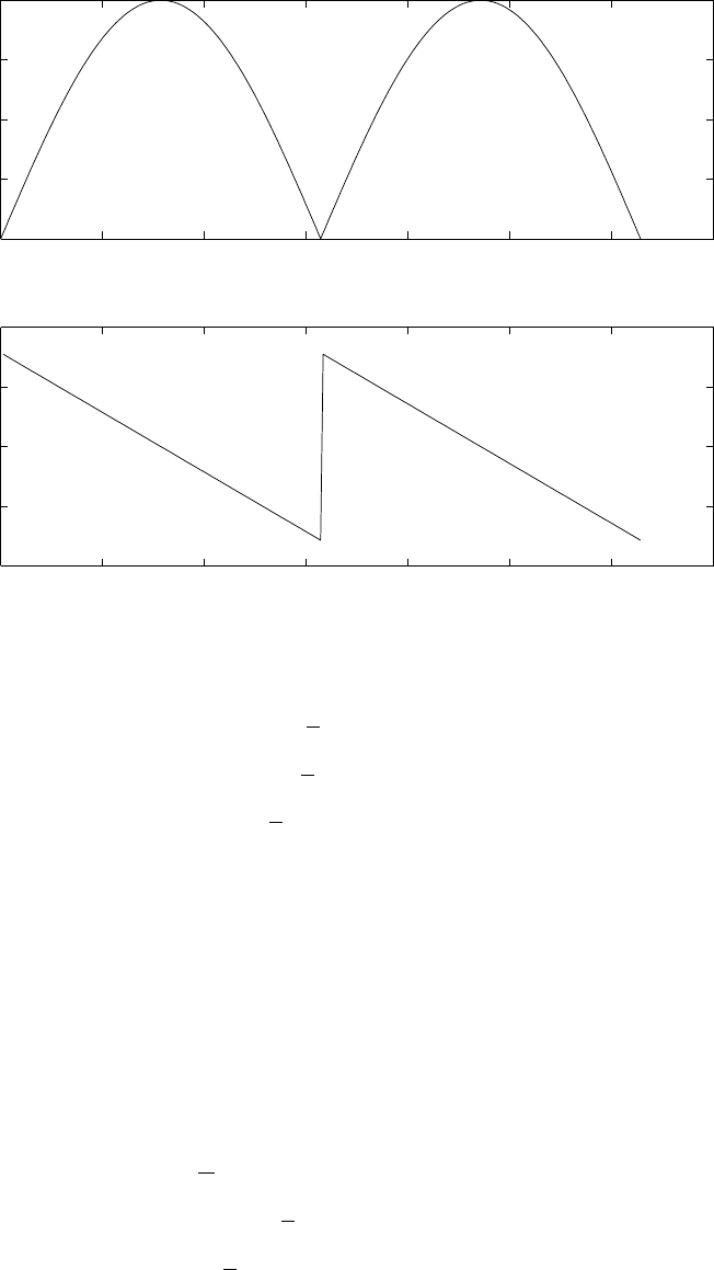
0 0.5 1 1.5 2 2.5 3 3.5
0
0.5
1
1.5
2
−−> w
−−> |H(w)|
0 0.5 1 1.5 2 2.5 3 3.5
−2
−1
0
1
2
−−> w
−−> theta(w)
Figure 5.18-1:
x(n) = 5 + 3sin(π
2n+ 60o) + 4sin(πn + 45o)
H(0) = 0, H(π
2) = 1, H(π) = 0
y(n) = 3sin(π
2n+ 60o)
5.20
(a)
y(n) = x(2n)⇒This is a linear, time-varying system
Y(w) = ∞
X
n=−∞
y(n)e−jwn
=∞
X
n=−∞
x(2n)e−jwn
=X(w
2)
= 1,|w| ≤ π
2
= 0,π
2≤ |w| ≤ π
(b)
y(n) = x2(n)⇒This is a non-linear, time-invariant system
146
© 2007 Pearson Education, Inc., Upper Saddle River, NJ. All rights reserved. This material is protected under all copyright laws
as they currently exist. No portion of this material may be reproduced, in any form or by any means, without permission in
writing from the publisher. For the exclusive use of adopters of the book Digital Signal Processing, Fourth Edition, by John G.
Proakis and Dimitris G. Manolakis. ISBN 0-13-187374-1.
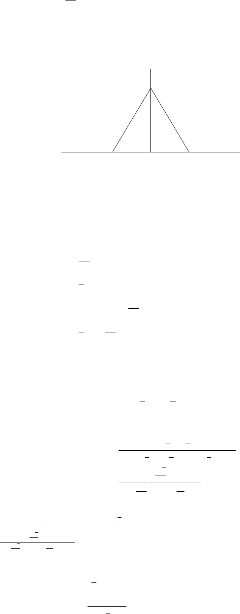
Y(w) = 1
2πX(w)∗X(w)
Refer to fig 5.20-1.
(c)
Y(w)
w
1/4
−π/2 0 π/2
Figure 5.20-1:
y(n) = (cosπn)x(n)⇒This is a time-varying system
Y(w) = 1
2π[πδ(w−π) + πδ(w+π)] ∗X(w)
=1
2[X(w−π) + X(w+π)]
= 0,|w| ≤ 3π
4
=1
2,3π
4≤ |w| ≤ π
5.21
h(n) = (1
4)ncosπ
4nu(n)
(a)
H(z) = 1−1
4cosπ
4z−1
1−2(1
4)cosπ
4z−1+ (1
4)2z−2
=1−√2
8z−1
1−√2
4z−1+1
16 z−2
(b) Yes. Refer to fig 5.21-1
(c) Poles at z=1
4e±jπ
4, zeros at z=√2
8.
H(w) = 1−√2
8e−jw
1−√2
4e−jw +1
16 e−j2w. Refer to fig 5.21-2.
(d)
x(n) = (1
4)nu(n)
X(z) = 1
1−1
4z−1
147
© 2007 Pearson Education, Inc., Upper Saddle River, NJ. All rights reserved. This material is protected under all copyright laws
as they currently exist. No portion of this material may be reproduced, in any form or by any means, without permission in
writing from the publisher. For the exclusive use of adopters of the book Digital Signal Processing, Fourth Edition, by John G.
Proakis and Dimitris G. Manolakis. ISBN 0-13-187374-1.
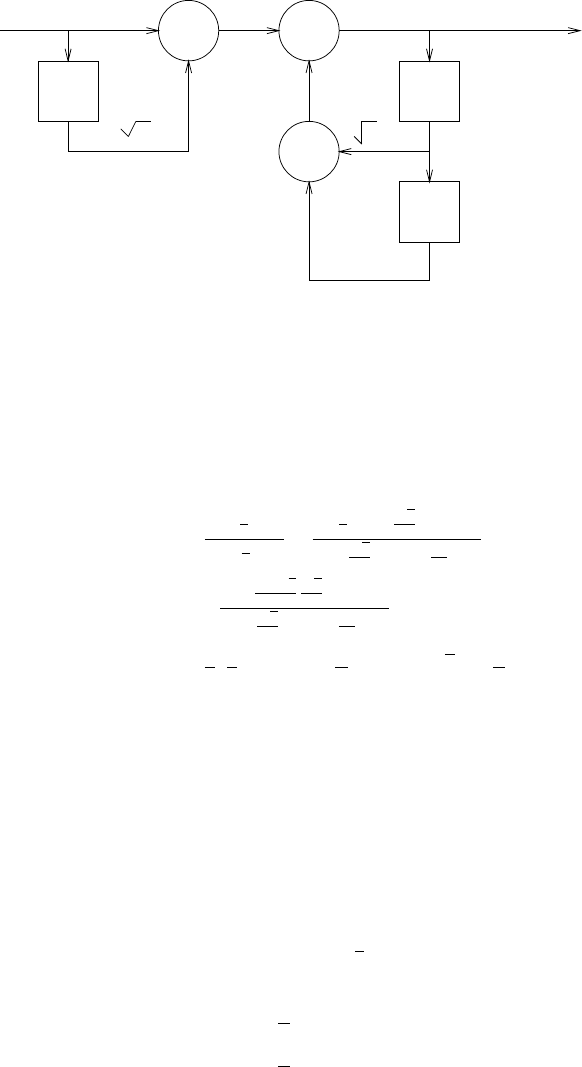
x(n)
z-1
++
+
z-1
z-1
y(n)
- 2 /8
-1/16
2 /4
Figure 5.21-1:
Y(z) = X(z)H(z)
=
1
2
1−1
4z−1+
1
2(1 −√2
8z−1)
1−√2
4z−1+1
16 z−2
+
1+√2
2
√2
8z−1
1−√2
4z−1+1
16 z−2
y(n) = 1
2(1
4)nh1 + cosπ
4n+ (1 + √2)sinπ
4niu(n)
5.22
y(n) = x(n)−x(n−10)
(a)
H(w) = 1 −e−j10w
= 2e−j5wejπ
2sin5w
|H(w)|= 2|sin5w|,
Θ(w) = π
2−5w, for sin5w > 0
=π
2−5w+π, for sin5w < 0
Refer to fig 5.22-1.
(b)
148
© 2007 Pearson Education, Inc., Upper Saddle River, NJ. All rights reserved. This material is protected under all copyright laws
as they currently exist. No portion of this material may be reproduced, in any form or by any means, without permission in
writing from the publisher. For the exclusive use of adopters of the book Digital Signal Processing, Fourth Edition, by John G.
Proakis and Dimitris G. Manolakis. ISBN 0-13-187374-1.
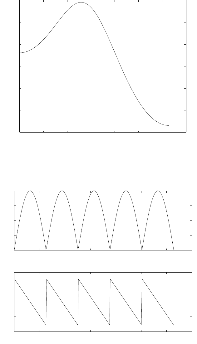
0 0.5 1 1.5 2 2.5 3 3.5
0.8
0.9
1
1.1
1.2
1.3
1.4
−−> w
−−> |H(w)|
Figure 5.21-2:
0 0.5 1 1.5 2 2.5 3 3.5
0
0.5
1
1.5
2
−−> w
−−> |H(w)|
0 0.5 1 1.5 2 2.5 3 3.5
−2
−1
0
1
2
−−> w
−−> theta(w)
Figure 5.22-1:
149
© 2007 Pearson Education, Inc., Upper Saddle River, NJ. All rights reserved. This material is protected under all copyright laws
as they currently exist. No portion of this material may be reproduced, in any form or by any means, without permission in
writing from the publisher. For the exclusive use of adopters of the book Digital Signal Processing, Fourth Edition, by John G.
Proakis and Dimitris G. Manolakis. ISBN 0-13-187374-1.

|H(π
10)|= 2,6H(π
10) = 0
|H(π
3)|=√3,Θ(π
3) = 6H(π
3) = −π
6
(1) Hence, y(n) = 2cos π
10n+ 3√3sin(π
3n−π
15)
H(0) = 0, H(2π
5) = 0
(2) Hence, y(n) = 0
5.23
(a)
h(n) = 1
2πZπ
−π
X(w)ejwndw
=1
2π"Z3π
8
−3π
8
ejwndw −Zπ
8
−π
8
e−jwndw#
=1
πn sin 3π
8n−sinπ
8n
=2
πn sin π
8ncosπ
4n
(b) Let
h1(n) = 2sinπ
8n
nπ
Then,
H1(w) = 2,|w| ≤ π
8
0,π
8<|w|< π
and
h(n) = h1(n)cosπ
4n
5.24
y(n) = 1
2y(n−1) + x(n) + 1
2x(n−1)
Y(z) = 1
2z−1Y(z) + X(z) + 1
2z−1X(z)
H(z) = Y(z)
X(z)
=1 + 1
2z−1
1−1
2z−1
(a)
H(z) = 2
1−1
2z−1−1
h(n) = 2(1
2)nu(n)−δ(n)
150
© 2007 Pearson Education, Inc., Upper Saddle River, NJ. All rights reserved. This material is protected under all copyright laws
as they currently exist. No portion of this material may be reproduced, in any form or by any means, without permission in
writing from the publisher. For the exclusive use of adopters of the book Digital Signal Processing, Fourth Edition, by John G.
Proakis and Dimitris G. Manolakis. ISBN 0-13-187374-1.

(b)
H(w) = ∞
X
n=0
h(n)e−jwn
=2
1−1
2e−jw −1
=1 + 1
2e−jw
1−1
2e−jw
=H(z)|z=ejw
(c)
H(π
2) = 1 + 1
2e−jπ
2
1−1
2e−jπ
2
=1−j1
2
1 + j1
2
= 1e−j2tan−11
2
Hence, y(n) = cos(π
2n+π
4−2tan−11
2)
5.25
Refer to fig 5.25-1.
5.26
H(z) = (1 −ejπ
4z−1)(1 −e−jπ
4z−1)
= 1 −√2z−1+z−2
H(w) = 1 −√2e−jw +e−2jw
= 2e−jw(cosw −√2
2)
y(n) = x(n)−√2x(n−1) + x(n−2)
for x(n) = sinπ
4u(n)
y(0) = x(0) = 0
y(1) = x(1) −√2x(0) + x(−1) = √2
2
y(2) = x(2) −√2x(1) + x(0) = 1 −√2√2
2+ 0 = 0
y(3) = x(3) −√2x(2) + x(1) = √2
2−√2 + √2
2= 0
y(4) = 0
151
© 2007 Pearson Education, Inc., Upper Saddle River, NJ. All rights reserved. This material is protected under all copyright laws
as they currently exist. No portion of this material may be reproduced, in any form or by any means, without permission in
writing from the publisher. For the exclusive use of adopters of the book Digital Signal Processing, Fourth Edition, by John G.
Proakis and Dimitris G. Manolakis. ISBN 0-13-187374-1.
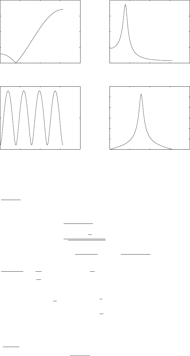
01234
0
1
2
3
4|X(w)| for (a)
magnitude
01234
0
2
4
6
8|X(w)| for (b)
magnitude
01234
0.5
1
1.5 |X(w)| for (c)
magnitude
01234
0
2
4
6
8
10
12 |X(w)| for (d)
magnitude
Figure 5.25-1:
5.27
(a) H(z) = k1−z−1
1+0.9z−1. Refer to fig 5.27-1.
(b)
H(w) = k1−e−jw
1 + 0.9e−jw
|H(w)|=k2|sinw
2|
√1.81 + 1.8cosw
Θ(w) = tan−1sinw
1−cosw +tan−10.9sinw
1 + 0.9cosw
(c) H(π) = k1−e−jπ
1+0.9e−jπ =k2
0.1= 20k= 1 ⇒k=1
20
(d) y(n) = −0.9y(n−1) + 1
20 [x(n)−x(n−1)]
(e)
H(π
6) = 0.014ejΘ( π
6)
y(n) = 0.028cos(π
6n+ 134.2o)
5.28
(a) H(z) = b01+bz−1
1+az−1. Refer to fig 5.28-1.
(b) For a= 0.5, b =−0.6, H(z) = b01−0.6z−1
1+0.5z−1. Since the pole is inside the unit circle and the
152
© 2007 Pearson Education, Inc., Upper Saddle River, NJ. All rights reserved. This material is protected under all copyright laws
as they currently exist. No portion of this material may be reproduced, in any form or by any means, without permission in
writing from the publisher. For the exclusive use of adopters of the book Digital Signal Processing, Fourth Edition, by John G.
Proakis and Dimitris G. Manolakis. ISBN 0-13-187374-1.

Figure 5.27-1:
filter is causal, it is also stable. Refer to fig 5.28-2.
(c)
H(z) = b0
1 + 0.5z−1
1−0.5z−1
⇒ |H(w)|2=b2
0
5
4+cosw
5
4−cosw
The maximum occurs at w= 0. Hence,
H(w)|w=0 =b2
0
9
4
1
4
= 9b2
0= 1
⇒b0=±1
3
(d) Refer to fig 5.28-3.
(e) Refer to fig 5.28-4.
obviously, this is a highpass filter. By selecting b=−1, the frequency response of the
highpass filter is improved.
5.29
|H(w)|2=A
[1 + r2−2rcos(w−Θ)] [1 + r2−2rcos(w+ Θ)]
d
dw
1
|H(w)|2=1
A[2rsin(w−Θ)(1 + r2−2rcos(w+ Θ))
+2rsin(w+ Θ)(1 + r2−2rcos(w−Θ))]
153
© 2007 Pearson Education, Inc., Upper Saddle River, NJ. All rights reserved. This material is protected under all copyright laws
as they currently exist. No portion of this material may be reproduced, in any form or by any means, without permission in
writing from the publisher. For the exclusive use of adopters of the book Digital Signal Processing, Fourth Edition, by John G.
Proakis and Dimitris G. Manolakis. ISBN 0-13-187374-1.
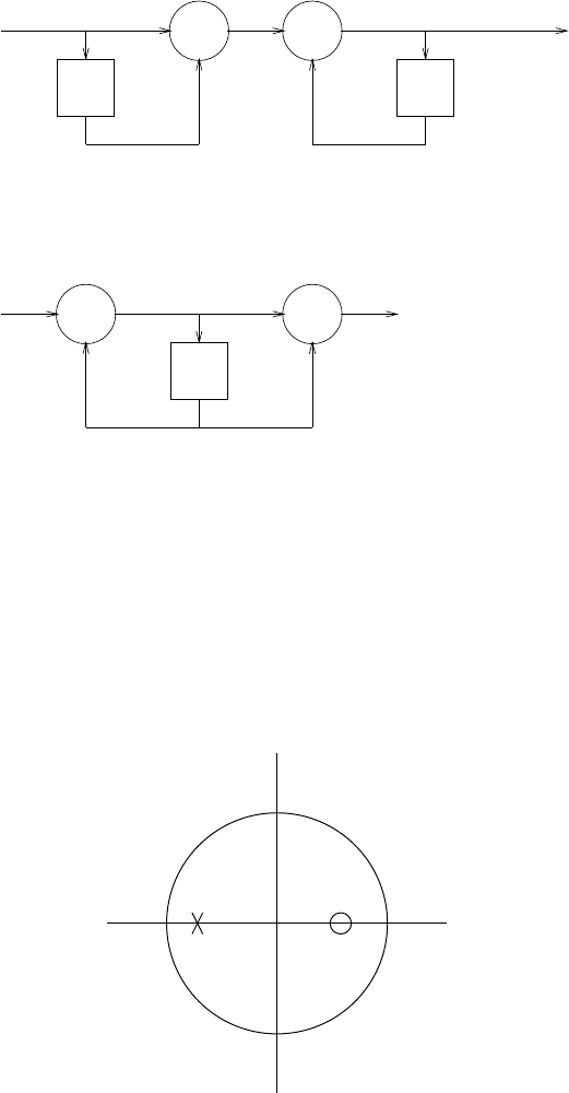
x(n) b 0
b b0
z-1 z-1
+ +
-a
y(n)
+ +
z-1
b-a
b0y(n)
x(n)
Direct form I:
Direct form II :
Figure 5.28-1:
z-plane
Figure 5.28-2:
154
© 2007 Pearson Education, Inc., Upper Saddle River, NJ. All rights reserved. This material is protected under all copyright laws
as they currently exist. No portion of this material may be reproduced, in any form or by any means, without permission in
writing from the publisher. For the exclusive use of adopters of the book Digital Signal Processing, Fourth Edition, by John G.
Proakis and Dimitris G. Manolakis. ISBN 0-13-187374-1.
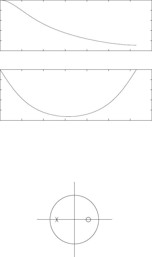
0 0.5 1 1.5 2 2.5 3 3.5
0
0.2
0.4
0.6
0.8
1|H(w)|
|H(w)|
w
0 0.5 1 1.5 2 2.5 3 3.5
−1
−0.8
−0.6
−0.4
−0.2
0phase
phase
w
Figure 5.28-3:
z-plane
-b-0.8
Figure 5.28-4:
155
© 2007 Pearson Education, Inc., Upper Saddle River, NJ. All rights reserved. This material is protected under all copyright laws
as they currently exist. No portion of this material may be reproduced, in any form or by any means, without permission in
writing from the publisher. For the exclusive use of adopters of the book Digital Signal Processing, Fourth Edition, by John G.
Proakis and Dimitris G. Manolakis. ISBN 0-13-187374-1.

= 0
(1 + r2)(sin(w−Θ) + sin(w+ Θ)) = 2r[sin(w−Θ)cos(w+ Θ) + sin(w+ Θ)cos(w−Θ)]
(1 + r2)2sinwcosΘ = 2rsin2w
= 4rsinwcosw
Therefore, cosw =1 + r2
2rcosΘ
wr=cos−11 + r2
2rcosΘ
5.30
y(n) = 1
4x(n) + 1
2x(n−1) + 1
4x(n−2)
H(w) = 1
4+1
2e−jw +1
4e−j2w
= (1 + e−jw
2)2
=e−jwcos2w
2
|H(w)|=cos2w
2
Θ(w) = 6H(w) = −w
Refer to fig 5.30-1
5.31
(a)
x(n) = (1
4)nu(n) + u(−n−1)
X(z) = 1
1−1
4z−1+−1
1−z−1,ROC: 1
4<|z|<1
Hence, H(z) = Y(z)
X(z)
=1−z−1
1 + z−1,ROC: |z|<1
(b)
Y(z) = −3
4z−1
(1 −1
4z−1)(1 + z−1)
=−3
5
1−1
4z−1+
3
5
1 + z−1
y(n) = −3
5(1
4)nu(n)−3
5(−1)nu(−n−1)
156
© 2007 Pearson Education, Inc., Upper Saddle River, NJ. All rights reserved. This material is protected under all copyright laws
as they currently exist. No portion of this material may be reproduced, in any form or by any means, without permission in
writing from the publisher. For the exclusive use of adopters of the book Digital Signal Processing, Fourth Edition, by John G.
Proakis and Dimitris G. Manolakis. ISBN 0-13-187374-1.
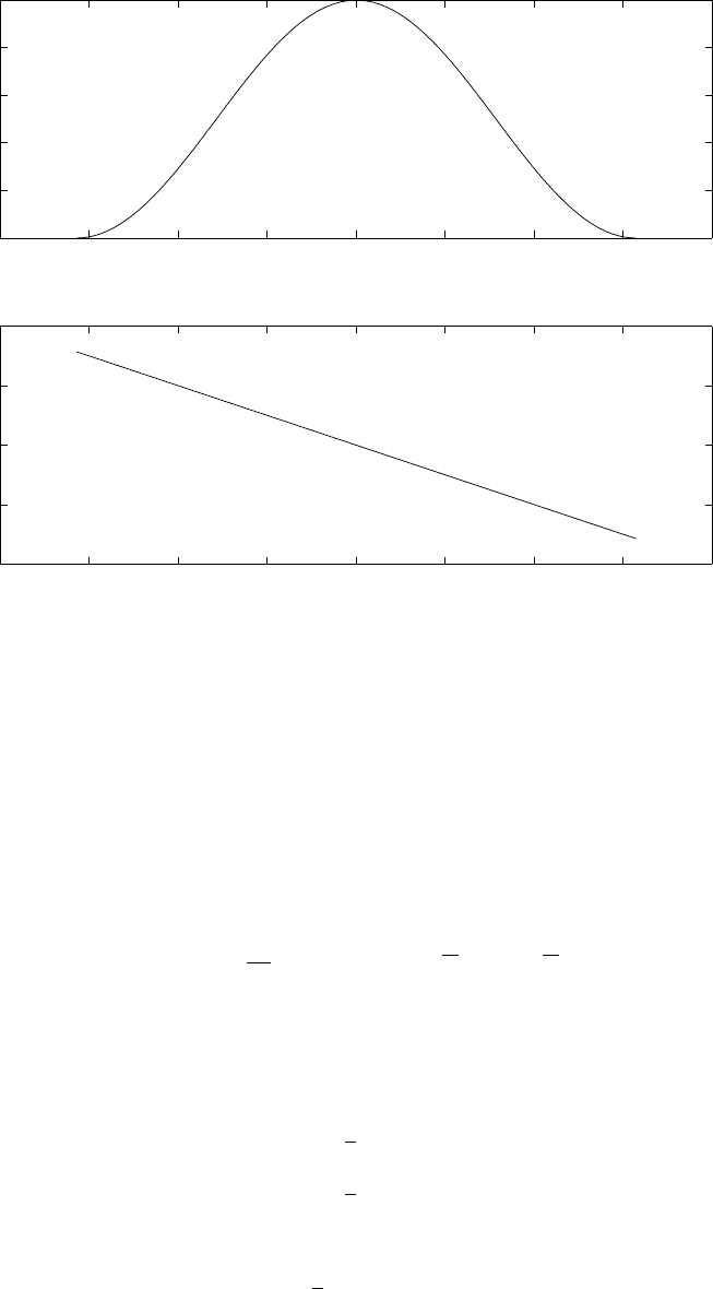
−4 −3 −2 −1 0 1 2 3 4
0
0.2
0.4
0.6
0.8
1
−−> w
−−> |H(w)|
−4 −3 −2 −1 0 1 2 3 4
−4
−2
0
2
4
−−> w
−−> theta(w)
Figure 5.30-1:
5.32
y(n) = b0x(n) + b1x(n−1) + b2x(n−2)
H(w) = b0+b1e−jw +b2e−j2w
(a)
H(2π
3) = b0+b1e−j2π
3+b2e−j4π
3= 0
H(0) = b0+b1+b2= 1
For linear phase, b0=±b2.
select b0=b2(otherwise b1= 0).
These conditions yield
b0=b1=b2=1
3
Hence, H(w) = 1
3e−jw(1 + 2cosw)
(b)
H(w) = 1
3(1 + 2cosw)
Θ(w) = −w, for 1 + 2cosw > 0
−w+π, for 1 + 2cosw < 0
157
© 2007 Pearson Education, Inc., Upper Saddle River, NJ. All rights reserved. This material is protected under all copyright laws
as they currently exist. No portion of this material may be reproduced, in any form or by any means, without permission in
writing from the publisher. For the exclusive use of adopters of the book Digital Signal Processing, Fourth Edition, by John G.
Proakis and Dimitris G. Manolakis. ISBN 0-13-187374-1.
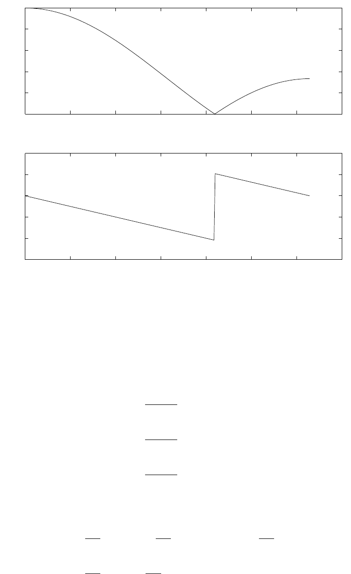
Refer to fig 5.32-1.
0 0.5 1 1.5 2 2.5 3 3.5
0
0.2
0.4
0.6
0.8
1
−−> w
−−> |H(w)|
0 0.5 1 1.5 2 2.5 3 3.5
−3
−2
−1
0
1
2
−−> w
−−> theta(w)
Figure 5.32-1:
5.33
(a)
y(n) = 1
2M+ 1
M
X
k=−M
x(n−k)
H(w) = 1
2M+ 1
M
X
k=−M
e−jwk
=1
2M+ 1 "1 + 2
M
X
k=1
coswk#
(b)
y(n) = 1
4Mx(n+M) + 1
2M
M−1
X
k=−M+1
x(n−k) + 1
4Mx(n−M)
H(w) = 1
2McosMw +1
2M"1 + 2
M−1
X
k=1
coswk#
158
© 2007 Pearson Education, Inc., Upper Saddle River, NJ. All rights reserved. This material is protected under all copyright laws
as they currently exist. No portion of this material may be reproduced, in any form or by any means, without permission in
writing from the publisher. For the exclusive use of adopters of the book Digital Signal Processing, Fourth Edition, by John G.
Proakis and Dimitris G. Manolakis. ISBN 0-13-187374-1.

The filter in (b) provides somewhat better smoothing because of its sharper attenuation at
the high frequencies.
5.34
H(z) = 1 + z+z2+...+z8
=1−z9
1−z−1
H(w) = 1−e−j9w
1−e−jw
=e−j9w/2
e−jw/2
sin9w/2
sinw/2
=e−j4wsin9w/2
sinw/2
|H(w)|=|sin9w/2
sinw/2|
Θ(w) = −4w, when sin9w/2>0
=−4w+π, when sin9w/2<0
H(w) = 0,at w=2πk
9, k = 1,2,...,8
The corresponding analog frequencies are kFs
9, k = 1,2,3,4, or 1
9kHz, 2
9kHz, 3
9kHz, 4
9kHz.
5.35
Refer to fig 5.35-1.
l
1/2
Figure 5.35-1:
159
© 2007 Pearson Education, Inc., Upper Saddle River, NJ. All rights reserved. This material is protected under all copyright laws
as they currently exist. No portion of this material may be reproduced, in any form or by any means, without permission in
writing from the publisher. For the exclusive use of adopters of the book Digital Signal Processing, Fourth Edition, by John G.
Proakis and Dimitris G. Manolakis. ISBN 0-13-187374-1.

H(z) = G(1 −ej3π/4z−1)(1 −e−j3π/4z−1)
(1 −1
2z−1)2
H(w) = H(z)|z=ejw
H(0) = G(1 −ej3π/4)(1 −e−j3π/4)
(1 −1
2)2
|H(w)|= 1 ⇒Gl2
1
4
= 1
l2= 2 + √2
G=1
4(2 + √2) = 0.073
5.36
Hz(w) = 1 −rejθe−jw
= 1 −rcos(w−θ) + jrsin(w−θ)
(a)
|Hz(w)|={[1 −rcos(w−θ)]2+ [rsin(w−θ)]2}1
2
= [1 + r2−2rcos(w−θ)]1
2
20log10|Hz(w)|= 10log10[1 −2rcos(w−θ) + r2]
Hence proved.
(b)
Θz(w) = tan−1imag. part
real part
=tan−1rsin(w−θ)
1−rcos(w−θ)
Hence proved.
(c)
τz
g(w) = −dΘz(w)
dw
=−1
1 + r2sin2(w−θ)
[1−rcos(w−θ)]2
[1 −rcos(w−θ)]rcos(w−θ)−rsin(w−θ)(rsin(w−θ))
[1 −rcos(w−θ)]2
=r2−rcos(w−θ)
1 + r2−2rcos(w−θ)
Hence proved.
(d) Refer to fig 5.36-1.
5.37
Hp(w) = 1
1−rejθe−jw , r < 1
160
© 2007 Pearson Education, Inc., Upper Saddle River, NJ. All rights reserved. This material is protected under all copyright laws
as they currently exist. No portion of this material may be reproduced, in any form or by any means, without permission in
writing from the publisher. For the exclusive use of adopters of the book Digital Signal Processing, Fourth Edition, by John G.
Proakis and Dimitris G. Manolakis. ISBN 0-13-187374-1.
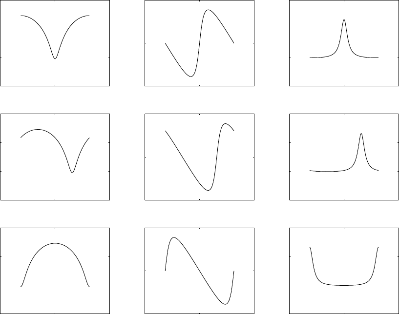
−5 0 5
−20
−10
0
10 magnitude theta=0
−5 0 5
−1
0
1phase theta=0
−5 0 5
−10
0
10
20 group delay theta=0
−5 0 5
−20
−10
0
10 magnitude theta=1.571
−5 0 5
−1
0
1phase theta=1.571
−5 0 5
−10
0
10
20group delay theta=1.571
−5 0 5
−20
−10
0
10 magnitude theta=3.142
−5 0 5
−1
0
1phase theta=3.142
−5 0 5
−10
0
10
20group delay theta=3.142
Figure 5.36-1:
161
© 2007 Pearson Education, Inc., Upper Saddle River, NJ. All rights reserved. This material is protected under all copyright laws
as they currently exist. No portion of this material may be reproduced, in any form or by any means, without permission in
writing from the publisher. For the exclusive use of adopters of the book Digital Signal Processing, Fourth Edition, by John G.
Proakis and Dimitris G. Manolakis. ISBN 0-13-187374-1.

(a)
|Hp(w)|=1
{[1 −rcos(w−θ)]2+ [rsin(w−θ)]2}1
2
=1
|Hz(w)|
|Hp(w)|dB = 20log10(1
|Hz(w)|)
=−20log10|Hz(w)|
=−|Hz(w)|dB
Hence proved.
(b)
Hp(w) = 1−rcos(w−θ)−jrsin(w−θ)
[1 −rcos(w−θ)]2+ [rsin(w−θ)]2
Θp(w) = −tan−1rsin(w−θ)
1−rcos(w−θ)
=−Θz(w)
Hence proved.
(c)
τp
g(w) = −dΘp(w)
dw
=−d(−Θz(w))
dw
=dΘz(w)
dw
=−τz
g(w)
Hence proved.
5.38
Hz(w) = (1 −rejθe−jw)(1 −re−jθe−jw)
= (1 −re−j(w−θ))(1 −re−j(w+θ))
=A(w)B(w)
(a)
|Hz(w)|=|A(w)b(w)|
=|A(w)||B(w)|
|Hz(w)|dB = 20log10|Hz(w)|
= 10log10[1 −2rcos(w−θ) + r2] + 10log10[1 −2rcos(w+θ) + r2]
(b)
6Hz(w) = 6A(w) + 6B(w)
=tan−1rsin(w−θ)
1−rcos(w−θ)+tan−1rsin(w+θ)
1−rcos(w+θ)
162
© 2007 Pearson Education, Inc., Upper Saddle River, NJ. All rights reserved. This material is protected under all copyright laws
as they currently exist. No portion of this material may be reproduced, in any form or by any means, without permission in
writing from the publisher. For the exclusive use of adopters of the book Digital Signal Processing, Fourth Edition, by John G.
Proakis and Dimitris G. Manolakis. ISBN 0-13-187374-1.
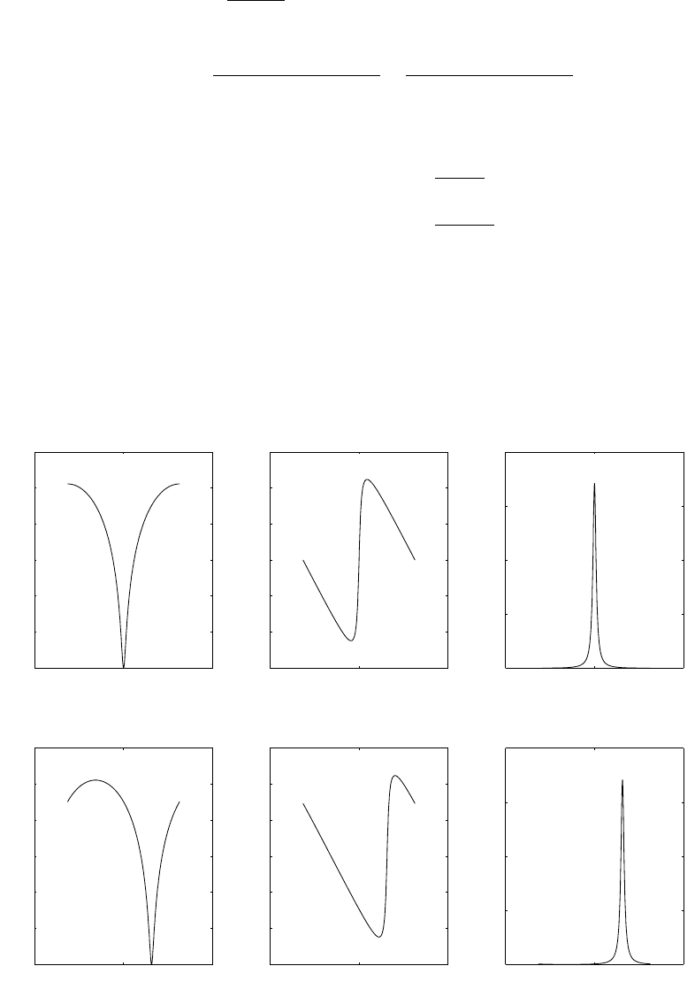
(c)
τz
g(w) = −dΘz(w)
dw
=τz
A(w) + τB
g(w)
=r2−rcos(w−θ)
1 + r2−2rcos(w−θ)+r2−rcos(w+θ)
1 + r2−2rcos(w+θ)
(d)
Hp(w) = 1
Hz(w)
Therefore, |Hp(w)|=1
|Hz(w)|
|Hp(w)|dB =−|Hz(w)|dB
on the same lines of prob4.62
Θp(w) = −Θz(w) and
τp
g(w) = −τz
g(w)
(e) Refer to fig 5.38-1.
−5 0 5
−20
−15
−10
−5
0
5
10 magnitude theta=0
−5 0 5
−1.5
−1
−0.5
0
0.5
1
1.5 phase theta=0
−5 0 5
0
50
100
150
200 group delay theta=0
−5 0 5
−20
−15
−10
−5
0
5
10 magnitude theta=1.571
−5 0 5
−1.5
−1
−0.5
0
0.5
1
1.5 phase theta=1.571
−5 0 5
0
50
100
150
200group delay theta=1.571
Figure 5.38-1:
163
© 2007 Pearson Education, Inc., Upper Saddle River, NJ. All rights reserved. This material is protected under all copyright laws
as they currently exist. No portion of this material may be reproduced, in any form or by any means, without permission in
writing from the publisher. For the exclusive use of adopters of the book Digital Signal Processing, Fourth Edition, by John G.
Proakis and Dimitris G. Manolakis. ISBN 0-13-187374-1.

5.39
(a)
|H1(w)|2=(1 −a)2
(1 −acosw)2+a2sin2w
=(1 −a)2
1 + a2−2acosw
|H1(w)|2=1
2⇒cosw1=4a−1−a2
2a
(b)
|H2(w)|2= (1−a
2)2(1 + cosw)2+sin2w
(1 −acosw)2+a2sin2w
=(1 −a)2
2
2(1 + cosw)
1 + a2−2acosw
|H2(w)|2=1
2⇒cosw2=2a
1 + a2
By comparing the results of (a) and (b), we find that cosw2> cosw1and, hence w2< w1
Therefore, the second filter has a smaller 3dB bandwidth.
5.40
h(n) = cos(w0n+ Θ)
=cosw0ncosΘ−sinw0nsinΘ
use the coupled-form oscillator shown in figure 5.38 and multiply the two outputs by cosΘ
and sinΘ, respectively, and add the products, i.e.,
yc(n)cosΘ + ys(n)sinΘ = cos(w0n+ Θ)
5.41
(a)
y(n) = ejw0y(n−1) + x(n)
= (cosw0+jsinw0) [yR(n−1) + jyI(n−1)] + x(n)
yR(n−1) + jyI(n−1) = yR(n−1)cosw0−yI(n−1)sinw0+x(n)
+j[yR(n−1)sinw0+yI(n−1)cosw0]
(b)Refer to fig 5.41-1.
(c)
Y(z) = ejw0z−1Y(z) + 1
=1
1−ejw0z−1
y(n) = ejnw0u(n)
= [cosw0n+jsinw0n]u(n)
Hence, yR(n) = cosw0nu(n)
yI(n) = sinw0nu(n)
164
© 2007 Pearson Education, Inc., Upper Saddle River, NJ. All rights reserved. This material is protected under all copyright laws
as they currently exist. No portion of this material may be reproduced, in any form or by any means, without permission in
writing from the publisher. For the exclusive use of adopters of the book Digital Signal Processing, Fourth Edition, by John G.
Proakis and Dimitris G. Manolakis. ISBN 0-13-187374-1.

+ +
+
x(n) y
R(n)
yI(n)
z
z-1
-1
-sin w0
cos w
0
sin w0
cos w 0
Figure 5.41-1:
(d)
n0 1 2 3 4 5 6 7 8 9
yR(n) 1 √3
2
1
20−1
2−√3
2−1−√3
2−1
20
yI(n) 0 1
2
√3
21√3
2
1
20−1
2−√3
21
5.42
(a) poles: p1,2=re±jw0
zeros: z1,2=e±jw0
(b) For w=w0, H(w0) = 0 For w6=w0, the poles and zeros factors in H(w) cancel, so that
H(w) = 1. Refer to fig 5.42-1.
(c)
|H(w)|2=G2|1−ejw0e−jw |2|1−e−jw0e−jw|2
|1−rejw0e−jw |2|1−re−jw0e−jw|2
=G22(1 −cos(w−w0))
1 + r2−2rcos(w−w0) 2(1 −rcos(w+w0))
1 + r2−2rcos(w+w0)
where w0=π
3.Then
d|H(w)|2
dw = 0 ⇒w=π
|H(π)|2= 4G2(
3
2
1 + r+r2)2= 1
165
© 2007 Pearson Education, Inc., Upper Saddle River, NJ. All rights reserved. This material is protected under all copyright laws
as they currently exist. No portion of this material may be reproduced, in any form or by any means, without permission in
writing from the publisher. For the exclusive use of adopters of the book Digital Signal Processing, Fourth Edition, by John G.
Proakis and Dimitris G. Manolakis. ISBN 0-13-187374-1.

Figure 5.42-1:
G=1
3(1 + r+r2)
(d) Refer to fig 5.42-2.
(e)
|H(w)|2=G2|1−ejw0e−jw |2|1−e−jw0e−jw|2
|1−rejw0e−jw |2|1−re−jw0e−jw|2
In the vicinity of w=w0,we have
|H(w)|2≈G2|1−ejw0e−jw |2
|1−rejw0e−jw |2
=G22(1 −cos(w−w0))
1 + r2−2rcos(w−w0)=1
2
cos(w−w0) = 1 + r2−4G2
2r−4G2
w1,2=w0±cos−1(1 + r2−4G2
2r−4G2)
B3dB =w1−w2= 2cos−1(1 + r2−4G2
2r−4G2)
= 2cos−1(1 −(r−1
√2)2)
= 2s2(1−r
√2)2
= 2√1−r
166
© 2007 Pearson Education, Inc., Upper Saddle River, NJ. All rights reserved. This material is protected under all copyright laws
as they currently exist. No portion of this material may be reproduced, in any form or by any means, without permission in
writing from the publisher. For the exclusive use of adopters of the book Digital Signal Processing, Fourth Edition, by John G.
Proakis and Dimitris G. Manolakis. ISBN 0-13-187374-1.

+
+ +
+
z-1
z-1
x(n) y(n)
-2r cos w0
r2
-2cos w
0
1+r+r2
3
Figure 5.42-2:
5.43
For the sampling frequency Fs= 500samples/sec., the rejected frequency should be w1=
2π(60
100 ) = 6
25 π. The filter should have unity gain at w2= 2π(200
500 ) = 4
5π. Hence,
H(6
25π) = 0
and H(4
5π) = 1
H(w) = G(1 −ej6π
25 e−jw)(1 −e−j6π
25 e−jw)
=Ge−jw[2cosw −2cos6π
25 ]
H(4
5π) = 2G|[cos(4
5π)−cos(6
25π)]|= 1
Hence, G=
1
2
cos 6
25 π−cos4
5π
5.44
From (5.4.22) we have,
H(w) = b0
1−e−j2w
(1 −rej(w0−w))(1 −re−j(w0−w))
|H(w0)|2=b2
0|1−e−j2w|2
(1 −r)2[(1 −rcos2w0)2+ (rsin2w0)2]= 1
167
© 2007 Pearson Education, Inc., Upper Saddle River, NJ. All rights reserved. This material is protected under all copyright laws
as they currently exist. No portion of this material may be reproduced, in any form or by any means, without permission in
writing from the publisher. For the exclusive use of adopters of the book Digital Signal Processing, Fourth Edition, by John G.
Proakis and Dimitris G. Manolakis. ISBN 0-13-187374-1.

Hence, b0=p(1 −r)2(1 −2rcos2w0+r2)
2|sinw0|
5.45
From α= (n+ 1)w0
β= (n−1)w0
and cosα +cosβ = 2cosα+β
2cosα−β
2,we obtain
cos(n+ 1)w0+cos(n−1)w0= 2cosnw0cosw0
with y(n) = cosw0n, it follows that
y(n+ 1) + y(n−1) = 2cosw0y(n) or equivalently,
y(n) = 2cosw0y(n−1) −y(n−2)
5.46
sinα +sinβ = 2sinα+β
2cosα−β
2,we obtain
when α=nw0and β= (n−2)w0,we obtain
sinnw0+sin(n−2)w0= 2sin(n−1)w0cosw0
If y(n) = Asinw0n, then
y(n) = 2cosw0y(n−1) −y(n−2)
Initial conditions: y(−1) = −Asinw0, y(−2) = −Asin2w0
5.47
For h(n) = Acosw0nu(n)
H(z) = A1−z−1cosw0
1−2cosw0z−1+z−2
Hence, y(n) = 2cosw0y(n−1) −y(n−2) + Ax(n)−Acosw0x(n−1)
For h(n) = Asinnw0u(n)
H(z) = Az−1sinw0
1−2cosw0z−1+z−2
Hence, y(n) = 2cosw0y(n−1) + y(n−2) + Ax(n)−Asinw0x(n−1)
5.48
Refer to fig 5.48-1. y1(n) = Acosnw0u(n), y2(n) = Asinnw0u(n)
168
© 2007 Pearson Education, Inc., Upper Saddle River, NJ. All rights reserved. This material is protected under all copyright laws
as they currently exist. No portion of this material may be reproduced, in any form or by any means, without permission in
writing from the publisher. For the exclusive use of adopters of the book Digital Signal Processing, Fourth Edition, by John G.
Proakis and Dimitris G. Manolakis. ISBN 0-13-187374-1.

+
+
+
x(n)
2r cos w
0
-1
z-1
z-1
y1(n)
-A cos w0
A sin w
0
y2(n)
Figure 5.48-1:
5.49
(a) Replace zby z8. We need 8 zeros at the frequencies w= 0,±π
4,±π
2,±3π
4, π Hence,
H(z) = 1−z−8
1−az−8
=Y(z)
X(z)
Hence, y(n) = ay(n−8) + x(n)−x(n−8)
(b) Zeros at 1, e±jπ
4, e±jπ
2, e±j3π
4,−1
Poles at a1
8, a1
8e±jπ
4, a1
8e±jπ
2, a1
8e±j3π
4,−1. Refer to fig 5.49-1.
(c)
|H(w)|=2|cos4w|
√1−2acos8w+a2
6H(w) = −tan−1asin8w
1−acos8w, cos4w≥0
π−tan−1asin8w
1−acos8w, cos4w < 0
Refer to fig 5.49-2.
5.50
We use Fs/L = 1cycle/day. We also choose nulls of multiples of 1
14 = 0.071, which results in a
narrow passband of k±0.067. Thus, M+ 1 = 14 or, equivalently M= 13
169
© 2007 Pearson Education, Inc., Upper Saddle River, NJ. All rights reserved. This material is protected under all copyright laws
as they currently exist. No portion of this material may be reproduced, in any form or by any means, without permission in
writing from the publisher. For the exclusive use of adopters of the book Digital Signal Processing, Fourth Edition, by John G.
Proakis and Dimitris G. Manolakis. ISBN 0-13-187374-1.
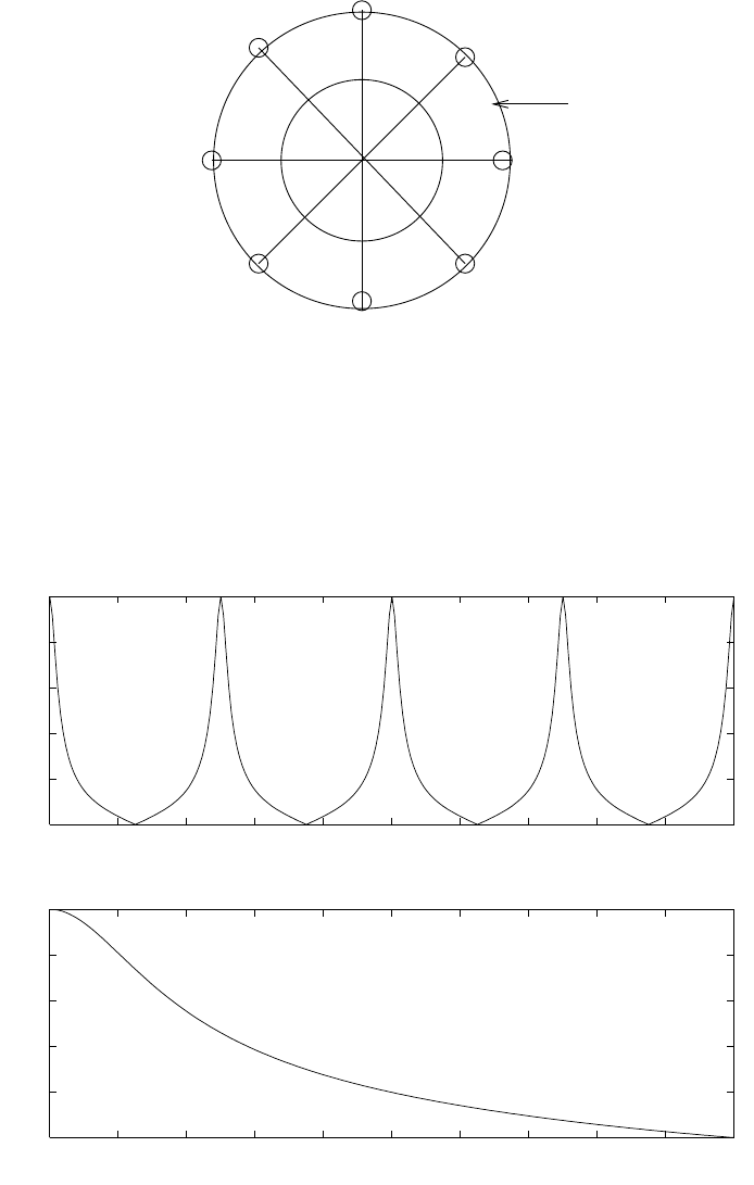
XX
X
X
X
XXX
-1 1
Unit circle
Figure 5.49-1:
0 0.05 0.1 0.15 0.2 0.25 0.3 0.35 0.4 0.45 0.5
0
2
4
6
8
10 magnitude of notch filter
−−> f
−−> |H(f)|
0 0.05 0.1 0.15 0.2 0.25 0.3 0.35 0.4 0.45 0.5
0
2
4
6
8
10 magnitude of a high pass filter
−−> f
−−> |H(f)|
Figure 5.49-2:
170
© 2007 Pearson Education, Inc., Upper Saddle River, NJ. All rights reserved. This material is protected under all copyright laws
as they currently exist. No portion of this material may be reproduced, in any form or by any means, without permission in
writing from the publisher. For the exclusive use of adopters of the book Digital Signal Processing, Fourth Edition, by John G.
Proakis and Dimitris G. Manolakis. ISBN 0-13-187374-1.

5.51
(a)
H(w) = 1−1
ae−jw
1−ae−jw
|H(w)|2=(1 −1
acosw)2+ ( 1
asinw)2
(1 −acosw)2+ (asinw)2
=1 + 1
a2−2
acosw
1 + a2−2acosw
=1
a2for all w
Hence, |H(w)|=1
a
For the two-pole, two-zero system,
H(w) = (1 −1
rejw0e−jw )(1 −1
re−jw0e−jw )
(1 −re−jw0e−jw )(1 −rejw0e−jw)
=1−2
rcosw0e−jw +1
r2e−j2w
1−2rcosw0e−jw +r2e−j2w
Hence, |H(w)|=1
r2
(b) H(z) = 1−2
rcosw0z−1+1
r2z−2
1−2rcosw0z−1+r2z−2
Hence, we need two delays and four multiplies per output point.
5.52
(a)
w0=60
200.2π=6π
50
H(z) = (1 −ej6π
50 z−1)(1 −e−j6π
50 z−1)b0
=b0(1 −2cos6π
50 z−1+z−2)
H(w) = 2b0e−jw(cosw −cos6π
50 )
|H(0)|= 2b0(1 −cos6π
25 ) = 1
b0=1
2(1 −cos6π
25 )
(b)
H(z) = b0
(1 −ej6π
25 z−1)(1 −e−j6π
25 z−1)
(1 −rej6π
25 z−1)(1 −re−j6π
25 z−1)
|H(0)|=2b0(1 −cos6π
25 )
1−2rcos6π
25 +r2= 1
b0=1−2rcos6π
25 +r2
2(1 −cos6π
25 )
171
© 2007 Pearson Education, Inc., Upper Saddle River, NJ. All rights reserved. This material is protected under all copyright laws
as they currently exist. No portion of this material may be reproduced, in any form or by any means, without permission in
writing from the publisher. For the exclusive use of adopters of the book Digital Signal Processing, Fourth Edition, by John G.
Proakis and Dimitris G. Manolakis. ISBN 0-13-187374-1.

5.53
h(n) = {h(0), h(1), h(2), h(3)}where h(0) = −h(3), h(1) = −h(2)
Hence, Hr(w) = 2(h(0)sin3w
2+h(1)sinw
2)
Hr(π
4) = 2h(0)sin3π
8+ 2h(1)sinπ
8) = 1
2
Hr(3π
4) = 2h(0)sin9π
8+ 2h(1)sin3π
8) = 1
1.85h(0) + 0.765h(1) = 1
2
−0.765h(0) + 1.85h(1) = 1
h(1) = 0.56, h(0) = 0.04
5.54
(a)
H(z) = b0
(1 −z−1)(1 + z−1)(1 −2cos3π
4z−1+z−2)
(1 −1.6cos2π
9z−1+ 0.64z−2)(1 −1.6cos4π
9z−1+ 0.64z−2)
H(w) = b0
(2je−jwsinw)(2e−jw)(cosw −cos3π
4)
(1 −1.6cos2π
9e−jw + 0.64e−j2w)(1 −1.6cos 4π
9e−jw + 0.64e−j2w)
|H(w)|=b0
4|sinw||cosw −cos 3π
4|
|1−1.6cos2π
9e−jw + 0.64e−j2w||1−1.6cos 4π
9e−jw + 0.64e−j2w|
|H(5π
12 )|= 1 ⇒b0= 0.089
(b) H(z) as given above.
(c) Refer to fig 5.54-1. The filter designed is not a good approximation of the desired response.
5.55
Y(w) = e−jwX(w) + dX(w)
dw
(a)
For x(n) = δ(n), X(w) = 1.
Hence, dX(w)
dw = 0,and Y(w) = e−jw
h(n) = 1
2πZπ
−π
Y(w)ejwndw
=1
2πZπ
−π
ejw(n−1)dw
=1
2πj(n−1) ejw(n−1)|π
−π
=sinπ(n−1)
π(n−1)
(b) y(n) = x(n−1) −jnx(n). the system is unstable and time-variant.
172
© 2007 Pearson Education, Inc., Upper Saddle River, NJ. All rights reserved. This material is protected under all copyright laws
as they currently exist. No portion of this material may be reproduced, in any form or by any means, without permission in
writing from the publisher. For the exclusive use of adopters of the book Digital Signal Processing, Fourth Edition, by John G.
Proakis and Dimitris G. Manolakis. ISBN 0-13-187374-1.
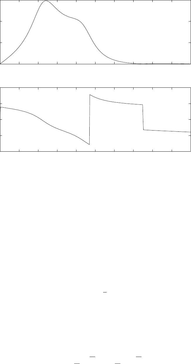
0 0.05 0.1 0.15 0.2 0.25 0.3 0.35 0.4 0.45 0.5
0
0.5
1
1.5
−−> f
−−> |H(f)|
0 0.05 0.1 0.15 0.2 0.25 0.3 0.35 0.4 0.45 0.5
−4
−2
0
2
4
−−> f
−−> phase
Figure 5.54-1:
5.56
H(w) = ∞
X
n=−∞
h(n)e−jwn
= 1,|w| ≤ wc
= 0, wc<|w|π
G(w) = ∞
X
n=−∞
g(n)e−jwn
=∞
X
n=−∞
h(n
2)e−jwn
=∞
X
m=−∞
h(m)e−j2wm
=H(2w)
Hence,
G(w) = 1,|w| ≤ wc
2and |w| ≥ π−wc
2
0,wc
2<|w|< π −wc
2
173
© 2007 Pearson Education, Inc., Upper Saddle River, NJ. All rights reserved. This material is protected under all copyright laws
as they currently exist. No portion of this material may be reproduced, in any form or by any means, without permission in
writing from the publisher. For the exclusive use of adopters of the book Digital Signal Processing, Fourth Edition, by John G.
Proakis and Dimitris G. Manolakis. ISBN 0-13-187374-1.
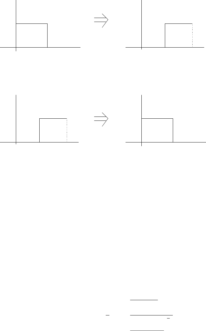
5.57
y(n) = x(n)−x(n)∗h(n) = [δ(n)−h(n)] ∗x(n) The overall system function is 1 −H(z) and the
frequency response is 1 −H(w). Refer to fig 5.57-1.
H(w) 1-H(w)
H(w) 1-H(w)
1
0 wc
w
1
wcw
1
0wcw
1
0 wc
w
π
π0
Figure 5.57-1:
5.58
(a) Since X(w) and Y(w) are periodic, it is observed that Y(w) = X(w−π). Therefore,
y(n) = ejπnx(n) = (−1)nx(n)
(b) x(n) = (−1)ny(n).
5.59
y(n) = 0.9y(n−1) + 0.1x(n)
(a)
H(z) = 0.1
1−0.9z−1
Hbp(w) = H(w−π
2) = 0.1
1−0.9e−j(w−π
2)
=0.1
1−j0.9e−jw
174
© 2007 Pearson Education, Inc., Upper Saddle River, NJ. All rights reserved. This material is protected under all copyright laws
as they currently exist. No portion of this material may be reproduced, in any form or by any means, without permission in
writing from the publisher. For the exclusive use of adopters of the book Digital Signal Processing, Fourth Edition, by John G.
Proakis and Dimitris G. Manolakis. ISBN 0-13-187374-1.

(b) h(n) = 0.1(0.9ejπ
2)nu(n)
(c) Since the impulse response is complex, a real input signal produces a complex-valued output
signal. For the output to be real, the bandpass filter should have a complex conjugate pole.
5.60
(a)
Let g(n) = nh(n)
Then, G(w) = jdH(w)
dw
D=∞
X
n=−∞ |g(n)|2
=1
2πZπ
−π|G(w)|2dw
=1
2πZπ
−π
G(w)G∗(w)dw
=1
2πZπ
−πjdH(w)
dw (−j)dH(w)
dw ∗dw
But dH(w)
dw =dH(w)
dw +j|H(w)|dΘ(w)
dw ejΘ(w)
Therefore,
D=1
2πZπ
−π(dH(w)
dw 2
+|H(w)|2dΘ(w)
dw 2)dw
(b) Dconsists of two terms, both of which are positive. For |H(w)| 6= 0, Dis minimized by
selecting Θ(w) = 0, in which case the second term becomes zero.
5.61
y(n) = ay(n−1) + bx(n),0< a < 1
H(z) = b
1−az−1
(a)
H(w) = b
1−ae−jw
|H(0)|=|b|
1−a= 1
b=±(1 −a)
(b)
|H(w)|2=b2
1 + a2−2acosw =1
2
⇒2b2= 1 + a2−2acosw
cosw =1
2a1 + a2−2(1 −a)2
175
© 2007 Pearson Education, Inc., Upper Saddle River, NJ. All rights reserved. This material is protected under all copyright laws
as they currently exist. No portion of this material may be reproduced, in any form or by any means, without permission in
writing from the publisher. For the exclusive use of adopters of the book Digital Signal Processing, Fourth Edition, by John G.
Proakis and Dimitris G. Manolakis. ISBN 0-13-187374-1.

=1
2a(4a−1−a2)
w3=cos−1(4a−1−a2
2a)
(c)
w3=cos−1(1 −(a−1)2
2a)
Let f(a) = 1 −(a−1)2
2a
Then f′(a) = −a2−1
2a2
=1−a2
2a2>0
Therefore f(a) is maximum at a= 1 and decreases monotonically as a→0. Consequently,
w3increases as a→0.
(d)
b=±(1 −a)
w3=cos−1(4a−1−a2
2a)
The 3-dB bandwidth increases as a→0.
5.62
y(n) = x(n) + αx(n−M), α > 0
H(w) = 1 + αe−jwM
|H(w)|=p1 + 2αcoswM +α2
Θ(w) = tan−1−αsinwM
1 + αcoswM
Refer to fig 5.62-1.
5.63
(a)
Y(z) = 1
2X(z) + z−1X(z)
H(z) = Y(z)
X(z)
=1
2(1 + z−1)
=z+ 1
2z
176
© 2007 Pearson Education, Inc., Upper Saddle River, NJ. All rights reserved. This material is protected under all copyright laws
as they currently exist. No portion of this material may be reproduced, in any form or by any means, without permission in
writing from the publisher. For the exclusive use of adopters of the book Digital Signal Processing, Fourth Edition, by John G.
Proakis and Dimitris G. Manolakis. ISBN 0-13-187374-1.
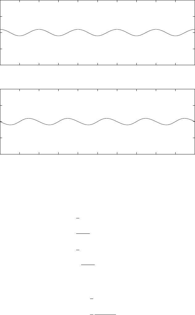
0 0.05 0.1 0.15 0.2 0.25 0.3 0.35 0.4 0.45 0.5
0
0.5
1
1.5
2M=10, alpha = 0.1
−−> f
−−> |H(f)|
0 0.05 0.1 0.15 0.2 0.25 0.3 0.35 0.4 0.45 0.5
−1
−0.5
0
0.5
1
−−> f
−−> phase
Figure 5.62-1:
Zero at z=−1 and a pole at z= 0. The system is stable.
(b)
Y(z) = 1
2−X(z) + z−1X(z)
H(z) = Y(z)
X(z)
=1
2(−1 + z−1)
=−z−1
2z
Zero at z= 1 and a pole at z= 0. The system is stable.
(c)
Y(z) = 1
8(1 + z−1)3
=1
8
(1 + z)3
z3
Three zeros at z=−1 and three poles at z= 0. The system is stable.
5.64
Y(z) = X(z) + bz−2X(z) + z−4X(z)
177
© 2007 Pearson Education, Inc., Upper Saddle River, NJ. All rights reserved. This material is protected under all copyright laws
as they currently exist. No portion of this material may be reproduced, in any form or by any means, without permission in
writing from the publisher. For the exclusive use of adopters of the book Digital Signal Processing, Fourth Edition, by John G.
Proakis and Dimitris G. Manolakis. ISBN 0-13-187374-1.
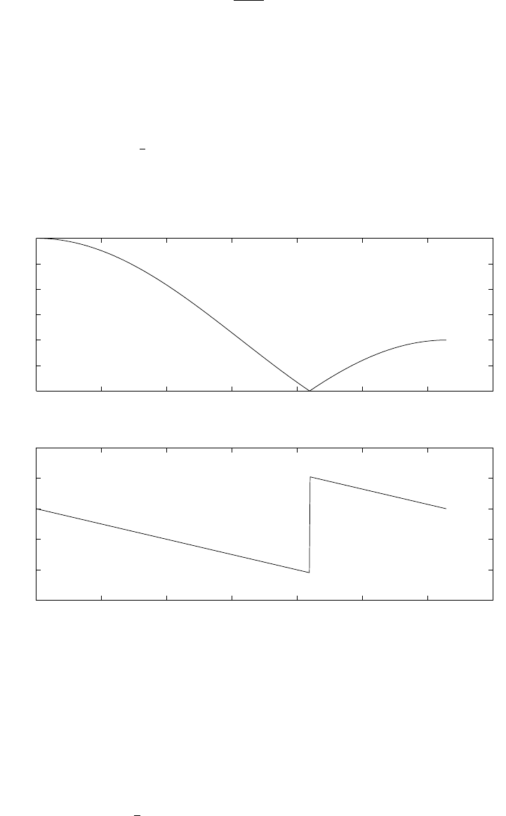
H(z) = Y(z)
X(z)
= 1 + bz−2+z−4
For b= 1, H(w) = 1 + ej2w+e−j4w
= (1 + 2cosw)e−jw
|H(w)|=|1 + 2cosw|
6H(w) = −w, 1 + 2cosw ≥0
π−w, 1 + 2cosw < 0
Refer to fig 5.64-1.
0 0.5 1 1.5 2 2.5 3 3.5
0
0.5
1
1.5
2
2.5
3
−−> w
−−> |H(w)|
0 0.5 1 1.5 2 2.5 3 3.5
−3
−2
−1
0
1
2
−−> w
−−> phase
Figure 5.64-1:
b=−1, H(w) = 1 −e−jw +e−j2w
= (2cosw −1)e−jw
|H(w)|=|2cosw −1|
6H(w) = −w, −1 + 2cosw ≥0
π−w, −1 + 2cosw < 0
Refer to fig 5.64-2.
178
© 2007 Pearson Education, Inc., Upper Saddle River, NJ. All rights reserved. This material is protected under all copyright laws
as they currently exist. No portion of this material may be reproduced, in any form or by any means, without permission in
writing from the publisher. For the exclusive use of adopters of the book Digital Signal Processing, Fourth Edition, by John G.
Proakis and Dimitris G. Manolakis. ISBN 0-13-187374-1.
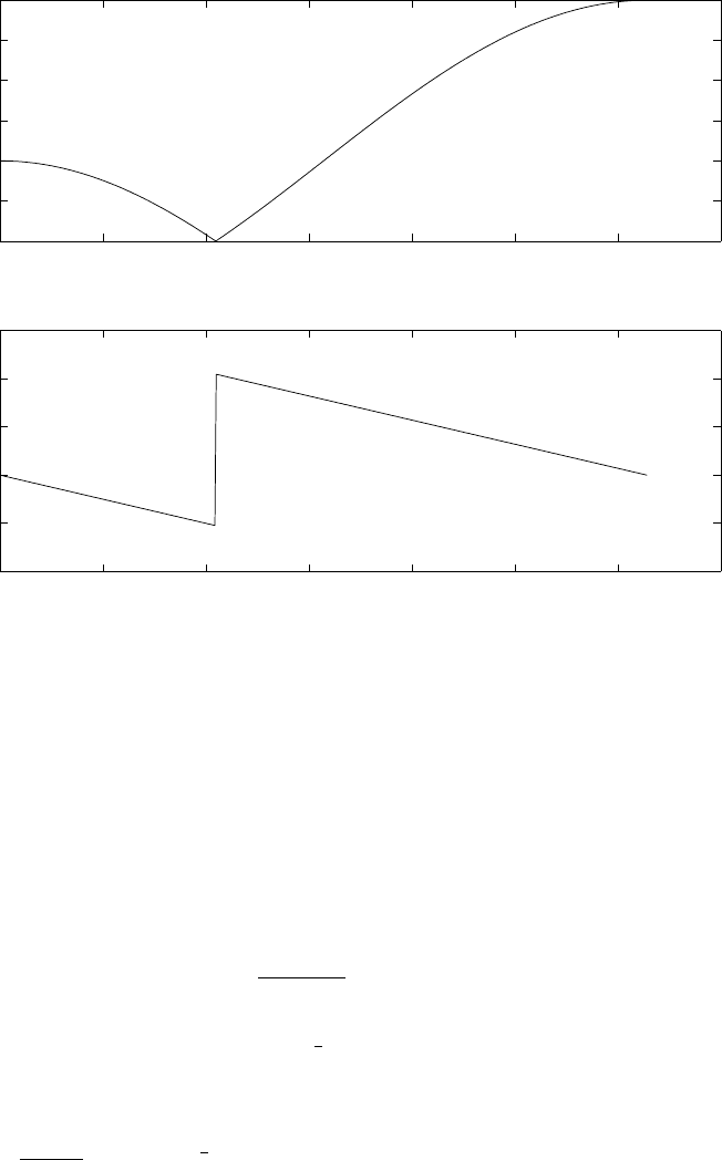
0 0.5 1 1.5 2 2.5 3 3.5
0
0.5
1
1.5
2
2.5
3
−−> w
−−> |H(w)|
0 0.5 1 1.5 2 2.5 3 3.5
−2
−1
0
1
2
3
−−> w
−−> phase
Figure 5.64-2:
5.65
y(n) = x(n)−0.95x(n−6)
(a)
Y(z) = X(z)(1 −0.95z−6)
H(z) = (1 −0.95z−6)
=z6−0.95
z6
z6= 0.95
z= (0.95)1
6ej2πk/6, k = 0,1,...,5
6th order pole at z= 0. Refer to fig 5.65-1.
(b)Refer to fig 5.65-2.
(c) Hin(z) = z6
z6−0.95 .r= (0.95)1
6. Refer to fig 5.65-3.
(d)Refer to fig 5.65-4.
179
© 2007 Pearson Education, Inc., Upper Saddle River, NJ. All rights reserved. This material is protected under all copyright laws
as they currently exist. No portion of this material may be reproduced, in any form or by any means, without permission in
writing from the publisher. For the exclusive use of adopters of the book Digital Signal Processing, Fourth Edition, by John G.
Proakis and Dimitris G. Manolakis. ISBN 0-13-187374-1.
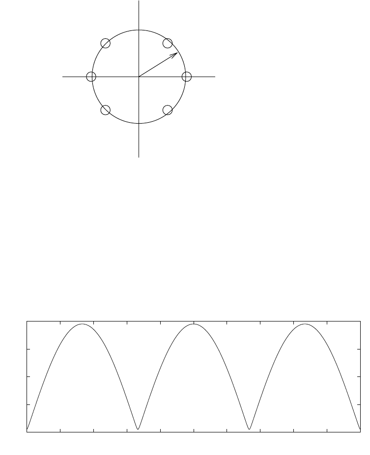
X
rr=(0.95)
1/6
Figure 5.65-1:
0 0.05 0.1 0.15 0.2 0.25 0.3 0.35 0.4 0.45 0.5
0
0.5
1
1.5
2
−−> f
−−> |H(f)|
Figure 5.65-2:
180
© 2007 Pearson Education, Inc., Upper Saddle River, NJ. All rights reserved. This material is protected under all copyright laws
as they currently exist. No portion of this material may be reproduced, in any form or by any means, without permission in
writing from the publisher. For the exclusive use of adopters of the book Digital Signal Processing, Fourth Edition, by John G.
Proakis and Dimitris G. Manolakis. ISBN 0-13-187374-1.
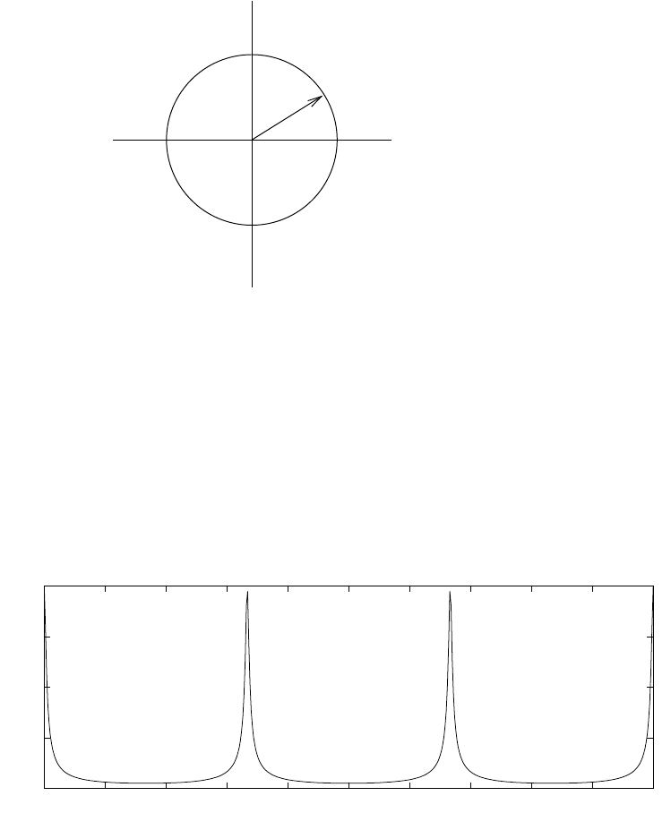
rr=(0.95)
1/6
X
X
XX
X
X
Figure 5.65-3:
0 0.05 0.1 0.15 0.2 0.25 0.3 0.35 0.4 0.45 0.5
0
5
10
15
20
−−> f
−−> |H(f)|
Figure 5.65-4:
181
© 2007 Pearson Education, Inc., Upper Saddle River, NJ. All rights reserved. This material is protected under all copyright laws
as they currently exist. No portion of this material may be reproduced, in any form or by any means, without permission in
writing from the publisher. For the exclusive use of adopters of the book Digital Signal Processing, Fourth Edition, by John G.
Proakis and Dimitris G. Manolakis. ISBN 0-13-187374-1.

5.66
(a)
H(z) = z−1
1−z−1−z−2
=z−1
(1 −1+√5
2z−1)(1 −1−√5
2z−1)
=
1
√5
1−1+√5
2z−1+−1
√5
1−1−√5
2z−1
If |z|>1−1 + √5
2is ROC, then
h(n) = "1
√5(1 + √5
2)n−1
√5(1−√5
2)n#u(n)
If ROC is √5−1
2<|z|<√5 + 1
2,then
h(n) = −1
√5(1−√5
2)nu(n)−1
√5(1 + √5
2)nu(−n−1)
If |z|<1−√5−1
2is ROC, then
h(n) = "−1
√5(1 + √5
2)n+1
√5(1−√5
2)n#u(−n−1)
From H(z),the difference equation is
y(n) = y(n−1) + y(n−2) + x(n−1)
(b)
H(z) = 1
1−e−4az−4
The difference equation is
y(n) = e−4ay(n−1) + x(n)
H(z) = 1
(1 −e−az−1)(1 −ejπ
2e−az−1)(1 + e−az−1)(1 + je−az−1)
=
1
4
1−e−az−1+
1
4
1−je−az−1+
1
4
1 + e−az−1+
1
4
1 + je−az−1
If ROC is |z|>1,then
h(n) = 1
4[1 + (j)n+ (−1)n+ (−j)n]e−anu(n)
If ROC is |z|<1,then
h(n) = −1
4[1 + (j)n+ (−1)n+ (−j)n]e−anu(−n−1)
5.67
Y(z) = 1 −z−1+ 3z−2−z−3+ 6z−4
= (1 + z−1+ 2z−2)(1 −2z−1+ 3z−2)
182
© 2007 Pearson Education, Inc., Upper Saddle River, NJ. All rights reserved. This material is protected under all copyright laws
as they currently exist. No portion of this material may be reproduced, in any form or by any means, without permission in
writing from the publisher. For the exclusive use of adopters of the book Digital Signal Processing, Fourth Edition, by John G.
Proakis and Dimitris G. Manolakis. ISBN 0-13-187374-1.

X(z) = 1 + z−1+ 2z−2
Therefore, H(z) = Y(z)
X(z)
= 1 −2z−1+ 3z−2
h(n) = 1
↑,−2,3
5.68
y(n) = 1
2y(n−1) + x(n)
x(n) = (1
4)nu(n)
H(z) = Y(z)
X(z)
=1
1−1
2z−1
X(z) = 1
1−1
4z−1
Y(z) = 1
(1 −1
4z−1)(1 −1
2z−1)
Rxx(z) = X(z)X(z−1)
=1
(1 −1
4z−1)(1 −1
4z)
=−4z−1
(1 −1
4z−1)(1 −4z−1)
=16
15
1
1−1
4z−1−16
15
1
1−4z−1
Hence, rxx(n) = 16
15(1
4)nu(n) + 16
15(4)nu(−n−1)
Rhh(z) = H(z)H(z−1)
=1
(1 −1
2z−1)(1 −1
2z)
=−2z−1
(1 −1
2z−1)(1 −2z−1)
=4
3
1
1−1
2z−1−4
3
1
1−2z−1
Hence, rhh(n) = 4
3(1
2)nu(n) + 4
3(2)nu(−n−1)
Rxy(z) = X(z)Y(z−1)
=1
(1 −1
4z−1)(1 −1
4z)(1 −1
2z)
=−16
17
1
1−2z−1+16
15
1
1−4z−1+128
105
1
1−1
4z−1
Hence, rxy(n) = 16
17(2)nu(−n−1) −16
15(4)nu(−n−1) + 128
105(1
4)nu(n)
183
© 2007 Pearson Education, Inc., Upper Saddle River, NJ. All rights reserved. This material is protected under all copyright laws
as they currently exist. No portion of this material may be reproduced, in any form or by any means, without permission in
writing from the publisher. For the exclusive use of adopters of the book Digital Signal Processing, Fourth Edition, by John G.
Proakis and Dimitris G. Manolakis. ISBN 0-13-187374-1.

Ryy(z) = Y(z)Y(z−1)
=1
(1 −1
4z−1)(1 −1
2z−1)(1 −1
4z)(1 −1
2z)
=−64
21
1
1−2z−1+128
105
1
1−4z−1+64
21
1
1−1
2z−1−128
105
1
1−1
4z−1
Hence, ryy (n) = 64
21(2)nu(−n−1) −128
105(4)nu(−n−1) + 64
21(1
2)nu(n)−128
105(1
4)nu(n)
5.69
(a)
h(n) = 10
↑,9,−7,−8,0,5,3
The roots(zeros) are 0.8084 ±j0.3370,−0.3750 ±j0.6074,−1.0,−0.7667
All the roots of H(z) are inside the unit circle. Hence, the system is minimum phase.
(b) h(n) = {5,4,−3,−4,0,2,1}H(z) = 5 + 4z−1−3z−2−4z−3+ 2z−5+z−6
The roots(zeros) are 0.7753 ±j0.2963,−0.4219 ±j0.5503,−0.7534 ±j0.1900
All the roots of H(z) are inside the unit circle. Hence, the system is minimum phase.
5.70
The impulse response satisfies the difference equation
N
X
k=0
akh(n−k) = δ(n), a0= 1
n= 0,⇒
N
X
k=0
akh(−k) = a0h(0) = 1
a0=1
h(0)
n= 1,⇒a0h(1) + a0h(0) = 0
a1=−a0h(1)
h(0) =−h(1)
h2(0)
.
.
.
n=N, ⇒a0h(N) + a1h(N−1) + ...+aNh(0) ⇒yields aN
It is apparent that the coefficients {an}can be determined if we know the order N and the values
h(0), h(1),...,h(N). If we do not know the filter order N, we cannot determine the {an}.
5.71
h(n) = b0δ(n) + b1δ(n−D) + b2δ(n−2D) (a) If the input to the system is x(n), the output is
y(n) = b0x(n) + b1x(n−D) + b2x(n−2D). Hence, the output consists of x(n), which is the input
signal, and the delayed signals x(n−D) and x(n−2D). The latter may be thought of as echoes
of x(n).
(b)
H(w) = b0+b1e−jwD +b2e−j2wD
184
© 2007 Pearson Education, Inc., Upper Saddle River, NJ. All rights reserved. This material is protected under all copyright laws
as they currently exist. No portion of this material may be reproduced, in any form or by any means, without permission in
writing from the publisher. For the exclusive use of adopters of the book Digital Signal Processing, Fourth Edition, by John G.
Proakis and Dimitris G. Manolakis. ISBN 0-13-187374-1.
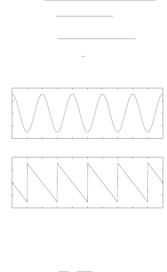
=b0+b1coswD +b2cos2wD −j(b1sinwD +b2sin2wD)
|H(w)|=qb02+b12+b22+ 2b1(b0+b2)coswD + 2b0b2cos2wD
Θ(w) = −tan−1b1sinwD +b2sin2wD
b0+b1coswD +b2cos2wD
(c) If |b0+b2|<< |b1|, then the dominant term is b1e−jwD and
|H(w)|=qb02+b12+b22+ 2b1(b0+b2)coswD
and |H(w)|has maxima and minima at w=±k
Dπ, k = 0,1,2,...
(d) The phase Θ(w) is approximately linear with a slope of −D. Refer to fig 5.71-1.
0 0.05 0.1 0.15 0.2 0.25 0.3 0.35 0.4 0.45 0.5
0.8
0.9
1
1.1
1.2
−−> f
−−> |H(f)|
0 0.05 0.1 0.15 0.2 0.25 0.3 0.35 0.4 0.45 0.5
−4
−2
0
2
4
−−> f
−−> phase
Figure 5.71-1:
5.72
H(z) = B(z)
A(z)=1 + bz1
1 + az1=∞
X
n=0
h(n)z−n
(a)
H(z) = 1 + (b−a)z−1+ (a2−ab)z−2+ (a2b−a3)z−3+ (a4−a3b)z−5+...
Hence, h(0) = 1,
185
© 2007 Pearson Education, Inc., Upper Saddle River, NJ. All rights reserved. This material is protected under all copyright laws
as they currently exist. No portion of this material may be reproduced, in any form or by any means, without permission in
writing from the publisher. For the exclusive use of adopters of the book Digital Signal Processing, Fourth Edition, by John G.
Proakis and Dimitris G. Manolakis. ISBN 0-13-187374-1.

h(1) = b−a,
h(2) = a2−ab,
h(3) = a2b−a3,
h(4) = a4−a3b
(b)
y(n) + ay(n−1) = x(n) + bx(n−1)
For x(n) = δ(n),
h(n) + ah(n−1) = δ(n) + bδ(n−1)
Multiply both sides by h(n) and sum. Then
rhh(0) + arhh(1) = h(0) + bh(1)
rhh(1) + arhh(0) = bh(0)
rhh(2) + arhh(1) = 0
rhh(3) + arhh(2) = 0
By solving these equations recursively, we obtain
rhh(0) = b2−2ab + 1
1−a2
rhh(1) = (ab −1)(a−b)
1−a2
rhh(2) = −a(ab −1)(a−b)
1−a2
rhh(3) = a2(ab −1)(a−b)
1−a2
5.73
x(n) is a real-valued, minimum-phase sequence. The sequence y(n) must satisfy the conditions,
y(0) = x(0),|y(n)|=|x(n)|, and must be minimum phase. The solution that satisfies the
condition is y(n) = (−1)nx(n). The proof that y(n) is minimum phase proceeds as follows:
Y(z) = X
n
y(n)z−n
=X
n
(−1)nx(n)z−n
=X
n
x(n)(−z−1)n
=X(−z)
This preserves the minimum phase property since a factor (1 −αz−1)→(1 + αz−1)
5.74
Consider the system with real and even impulse response h(n) = 1
4,1,1
4and frequency response
H(w) = 1 + 1
2cosw. Then H(z) = z−1(1
4z2+z+1
4). The system has zeros at z=−2±√3.
We observe that the system is stable, and its frequency response is real and even. However, the
inverse system is unstable. Therefore, the stability of the inverse system is not guaranteed.
186
© 2007 Pearson Education, Inc., Upper Saddle River, NJ. All rights reserved. This material is protected under all copyright laws
as they currently exist. No portion of this material may be reproduced, in any form or by any means, without permission in
writing from the publisher. For the exclusive use of adopters of the book Digital Signal Processing, Fourth Edition, by John G.
Proakis and Dimitris G. Manolakis. ISBN 0-13-187374-1.

5.75
(a)
g(n) = h(n)∗x(n)⇒G(w) = H(w)X(w)
f(n) = h(n)∗g(−n)⇒F(w) = H(w)G(−w)
Y(w) = F(−w)
Then, Y(w) = H(−w)G(w)
=H(−w)H(w)X(w)
=H∗(w)H(w)X(w)
=|H(w)|2X(w)
But Ha(w)≡ |H(w)|2is a zero-phase system.
(b)
G(w) = H(w)X(w)
F(w) = H(w)X(−w)
Y(w) = G(w) + F(−w)
=H(w)X(w) + H(−w)X(w)
=X(w)(H(w) + H∗(−w))
= 2X(w)Re(H(w))
But Hb(w) = 2Re {H(w)}is a zero-phase system.
5.76
(a) Correct. The zeros of the resulting system are the combination of the zeros of the two systems.
Hence, the resulting system is minimum phase if the inividual system are minimum phase.
(b) Incorrect. For example, consider the two minimum-phase systems.
H1(z) = 1−1
2z−1
1−1
3z−1
and H2(z) = −2(1 + 1
3z−1)
1−1
3z−1
Their sum is H1(z) + H2(z) = −1−7
6z−1
1−1
3z−1,which is not minimum phase.
5.77
(a)
|H(w)|2=
5
4−cosw
10
9−2
3cosw
=H(z)H(z−1)|z=e−jw
Hence, H(z)H(z−1) =
5
4−1
2(z+z−1)
10
9−1
3(z+z−1)
=1−1
2z−1
1−1
3z−1
187
© 2007 Pearson Education, Inc., Upper Saddle River, NJ. All rights reserved. This material is protected under all copyright laws
as they currently exist. No portion of this material may be reproduced, in any form or by any means, without permission in
writing from the publisher. For the exclusive use of adopters of the book Digital Signal Processing, Fourth Edition, by John G.
Proakis and Dimitris G. Manolakis. ISBN 0-13-187374-1.

(b)
|H(w)|2=2(1 −a2)
1 + a2−2acosw
H(z)H(z−1) = 2(1 −a2)
1 + a2−a(z+z−1)
H(z)H(z−1) = 2(1 + a)(1 −a)
(1 −az−1)(1 −az)
Hence, H(z) = p2(1 −a2)
1−az−1
or H(z) = p2(1 −a2)
1−az
5.78
H(z) = (1 −0.8ejπ/2z−1)(1 −0.8e−jπ/2z−1)(1 −1.5ejπ/4z−1)(1 −1.5e−jπ/4z−1)
= (1 + 0.64z−2)(1 −3
√2z−1+ 2.25z−2)
(a) There are four different FIR systems with real coefficients:
H1(z) = (1 + 0.64z−2)(1 −3
√2z−1+ 2.25z−2)
H2(z) = (1 + 0.64z−2)(1 −3
√2z−1+ 2.25z−2)
H3(z) = (1 + 0.64z−2)(1 −3
√2z−1+ 2.25z−2)
H4(z) = (1 + 0.64z−2)(1 −3
√2z−1+ 2.25z−2)
H(z) is the minimum-phase system.
(b)
H1(z) = 1 −3
√2z−1+ 2.89z−2−1.92
√2z−3+ 1.44z−4
h1(n) = 1
↑,−3
√2,2.89,−1.92
√2,1.44
H2(z) = 0.64z2−1.92
√2z+ 2.44 −3
√2z−1+ 2.25z−2
h2(n) = 0.64,−1.92
√2,2.44
↑,−3
√2,2.25
H3(z) = 2.25z2−3
√2z+ 2.44 −1.92
√2z−1+ 0.64z−2
h3(n) = 2.25,−3
√2,2.44
↑,−1.92
√2,0.64
H4(z) = 1.44z4−1.92
√2z3+ 2.89z2−3
√2z+ 1
h4(n) = 1.44,−1.92
√2,2.89,−3
√2,1
↑,
188
© 2007 Pearson Education, Inc., Upper Saddle River, NJ. All rights reserved. This material is protected under all copyright laws
as they currently exist. No portion of this material may be reproduced, in any form or by any means, without permission in
writing from the publisher. For the exclusive use of adopters of the book Digital Signal Processing, Fourth Edition, by John G.
Proakis and Dimitris G. Manolakis. ISBN 0-13-187374-1.
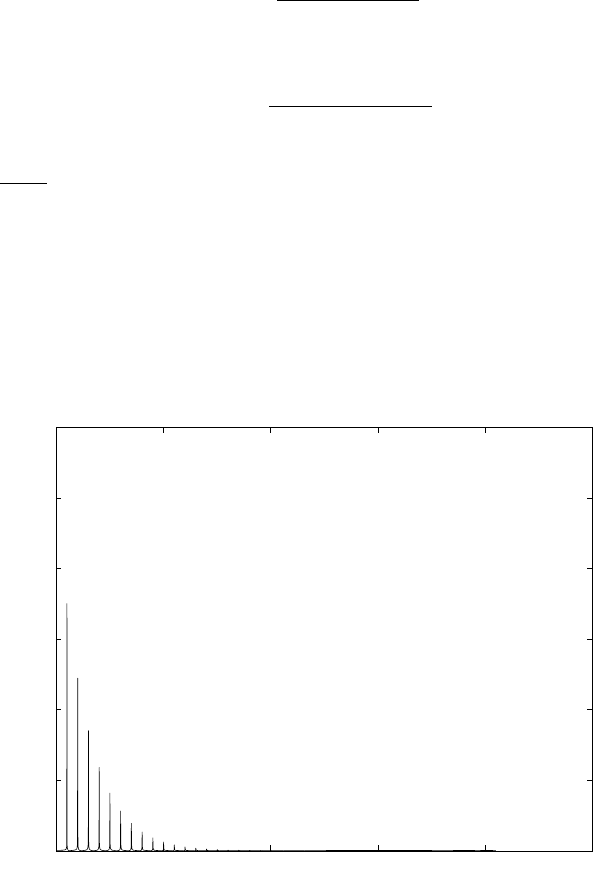
(c)
E1(n) = {1,5.5,13.85,15.70,17.77}
E2(n) = {0.64,2.48,8.44,12.94,18.0}
E3(n) = {2.25,6.75,12.70,14.55,14.96}
E4(n) = {1.44,3.28,11.64,16.14,17.14}
Clearly, h3(n) is minimum phase and h2(n) is maximum phase.
5.79
H(z) = 1
1 + PN
k=1 akz−k
(a) The new system function is H′(z) = H(λ−1z)
H′(z) = 1
1 + PN
k=1 akλkz−k
If pkis a pole of H(z), then λpkis a pole of H′(z).
Hence, λ < 1
|pmax|is selected then |pkλ|<1 for all kand, hence the system is stable.
(b) y(n) = −PN
k=1 akλky(n−k) = x(n)
5.80
(a) The impulse response is given in pr10fig 5.80-1.
(b) Reverberator 1: refer to fig 5.80-2.
0 500 1000 1500 2000 2500
0
0.2
0.4
0.6
0.8
1
1.2
−−> n
−−> magnitude
Figure 5.80-1:
189
© 2007 Pearson Education, Inc., Upper Saddle River, NJ. All rights reserved. This material is protected under all copyright laws
as they currently exist. No portion of this material may be reproduced, in any form or by any means, without permission in
writing from the publisher. For the exclusive use of adopters of the book Digital Signal Processing, Fourth Edition, by John G.
Proakis and Dimitris G. Manolakis. ISBN 0-13-187374-1.
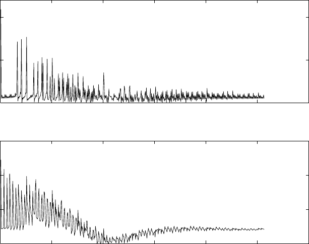
0 100 200 300 400 500 600
0
0.5
1
impulse response for unit1
−−> n
−−> magnitude
0 100 200 300 400 500 600
0
0.5
1
1.5 impulse response for unit2
−−> n
−−> magnitude
Figure 5.80-2:
Reverberator 2: refer to fig 5.80-2.
(c) Unit 2 is a better reverberator.
(d) For prime number of D1, D2, D3, the reverberations of the signal in the different sections do
not overlap which results in the impulse response of the unit being more dense.
(e) Refer to fig 5.80-3.
(f) Refer to fig 5.80-4 for the delays being prime numbers.
5.81
(a) Refer to fig 5.81-1.
(b) Refer to fig 5.81-2.
190
© 2007 Pearson Education, Inc., Upper Saddle River, NJ. All rights reserved. This material is protected under all copyright laws
as they currently exist. No portion of this material may be reproduced, in any form or by any means, without permission in
writing from the publisher. For the exclusive use of adopters of the book Digital Signal Processing, Fourth Edition, by John G.
Proakis and Dimitris G. Manolakis. ISBN 0-13-187374-1.
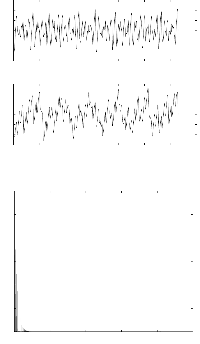
0 1 2 3 4 5 6 7
−3
−2
−1
0
1
2
3phase response for unit1
−−> w
−−> phase
0 1 2 3 4 5 6 7
−3
−2
−1
0
1
2
3phase response for unit2
−−> w
−−> phase
Figure 5.80-3:
0 500 1000 1500 2000 2500
0
0.2
0.4
0.6
0.8
1
1.2
−−> n
−−> magnitude
Figure 5.80-4:
191
© 2007 Pearson Education, Inc., Upper Saddle River, NJ. All rights reserved. This material is protected under all copyright laws
as they currently exist. No portion of this material may be reproduced, in any form or by any means, without permission in
writing from the publisher. For the exclusive use of adopters of the book Digital Signal Processing, Fourth Edition, by John G.
Proakis and Dimitris G. Manolakis. ISBN 0-13-187374-1.
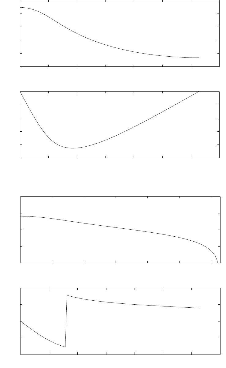
0 0.5 1 1.5 2 2.5 3 3.5
−20
−10
0
10
20
30
−−> w(rad)
−−> magnitude
0 0.5 1 1.5 2 2.5 3 3.5
−2.5
−2
−1.5
−1
−0.5
0
−−> w(rad)
−−> phase
Figure 5.81-1:
0 0.5 1 1.5 2 2.5 3
−100
−50
0
50
100
−−> w(rad)
−−> magnitude
0 0.5 1 1.5 2 2.5 3 3.5
−4
−2
0
2
4
−−> w(rad)
−−> phase
Figure 5.81-2:
192
© 2007 Pearson Education, Inc., Upper Saddle River, NJ. All rights reserved. This material is protected under all copyright laws
as they currently exist. No portion of this material may be reproduced, in any form or by any means, without permission in
writing from the publisher. For the exclusive use of adopters of the book Digital Signal Processing, Fourth Edition, by John G.
Proakis and Dimitris G. Manolakis. ISBN 0-13-187374-1.
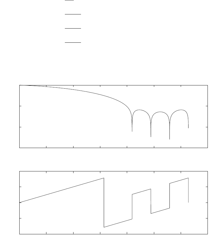
5.82
(a)
B= 10kHz
Fs= 20kHz
z1=10k
20k= 0.5
z2=7.778k
20k= 0.3889
z3=8.889k
20k= 0.4445
z4=6.667k
20k= 0.3334
H(z) = (z−0.5)(z−0.3889)(z−0.4445)(z−0.3334)
(b) Refer to fig 5.82-1.
(c) It satisfies the objectives but this filter is not recommended in a practical application because
0 0.5 1 1.5 2 2.5 3 3.5
−150
−100
−50
0
−−> w(rad)
−−> magnitude
0 0.5 1 1.5 2 2.5 3 3.5
−4
−2
0
2
4
−−> w(rad)
−−> phase
Figure 5.82-1:
in a speech application linear phase for the filter is desired and this filter does not provide linear
phase for all frequencies.
5.83
Refer to fig 5.83-1.
Practical:
193
© 2007 Pearson Education, Inc., Upper Saddle River, NJ. All rights reserved. This material is protected under all copyright laws
as they currently exist. No portion of this material may be reproduced, in any form or by any means, without permission in
writing from the publisher. For the exclusive use of adopters of the book Digital Signal Processing, Fourth Edition, by John G.
Proakis and Dimitris G. Manolakis. ISBN 0-13-187374-1.
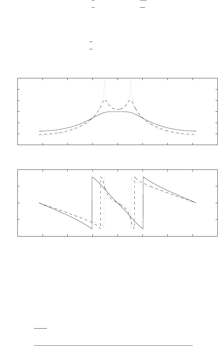
r= 0.99 wr=π
6Bandwidth = π
128 = 0.0245
r= 0.9wr=π
6Bandwidth = 5π
32 = 0.49
r= 0.6wr= 0 Bandwidth = 1.1536
Theoretical:
r= 0.99, wr=π
6Bandwidth = 2(1 −r) = 0.02
r= 0.9, wr=π
6Bandwidth = 2(1 −r) = 0.2
For rvery close to 1, the theoretical and practical values match.
−4 −3 −2 −1 0 1 2 3 4
−20
−10
0
10
20
30
40
−−> w(rad)
−−> magnitude
.... r = 0.99
−−−− r = 0.9
__ r = 0.6
−4 −3 −2 −1 0 1 2 3 4
−4
−2
0
2
4
−−> w(rad)
−−> phase
.... r = 0.99
−−−− r = 0.9
__ r = 0.6
Figure 5.83-1:
5.84
H(z) = (1 −0.9ej0.4πz−1)(1 −0.9e−j0.4πz−1)(1 −1.5ej0.6πz−1)(1 −1.5e−j0.6πz−1)
H(z) = B(z)
A(z)
=(z−0.9ej0.4π)(z−0.9e−j0.4π)(z−1.5ej0.6π)(z−1.5e−j0.6π)
z4
Let B1(z) = (z−0.9ej0.4π)(z−0.9e−j0.4π)
B2(z) = (z−1.5ej0.6π)(z−1.5e−j0.6π)
A(z) = z4
194
© 2007 Pearson Education, Inc., Upper Saddle River, NJ. All rights reserved. This material is protected under all copyright laws
as they currently exist. No portion of this material may be reproduced, in any form or by any means, without permission in
writing from the publisher. For the exclusive use of adopters of the book Digital Signal Processing, Fourth Edition, by John G.
Proakis and Dimitris G. Manolakis. ISBN 0-13-187374-1.

Hmin(z) = B1(z)B2(z)
A(z)
=(z−0.9ej0.4π)(z−0.9e−j0.4π)(z−1−1.5ej0.6π)(z−1−1.5e−j0.6π)
z4
Hap(z) = B2(z)
B2(z−1)
=(z−1.5ej0.6π)(z−1.5e−j0.6π)
(z−1−1.5ej0.6π)(z−1−1.5e−j0.6π)
Hap(z) has a flat magnitude response. To get a flat magnitude response for the system, connect
a system which is the inverse of Hmin(z), i.e.,
Hc(z) = 1
Hmin(z)
=z4
(z−0.9ej0.4π)(z−0.9e−j0.4π)(z−1−1.5ej0.6π)(z−1−1.5e−j0.6π)
(b) Refer to fig 5.84-1 and fig 5.84-2.
pole−zero plots for Hc(z)
0.5
1
1.5
30
210
60
240
90
270
120
300
150
330
180 0
pole−zero plots for compensated system
0.5
1
1.5
30
210
60
240
90
270
120
300
150
330
180 0
Figure 5.84-1:
195
© 2007 Pearson Education, Inc., Upper Saddle River, NJ. All rights reserved. This material is protected under all copyright laws
as they currently exist. No portion of this material may be reproduced, in any form or by any means, without permission in
writing from the publisher. For the exclusive use of adopters of the book Digital Signal Processing, Fourth Edition, by John G.
Proakis and Dimitris G. Manolakis. ISBN 0-13-187374-1.
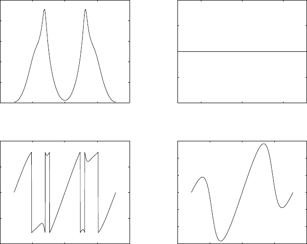
−4 −2 0 2 4
−15
−10
−5
0
5
10
−−> w(rad)
−−> magnitude
mag for Hc(z)
−2 0 2
−2
−1
0
1
2
−−> w(rad)
−−> magnitude
mag of compensated system
−4 −2 0 2 4
−4
−2
0
2
4
−−> w(rad)
−−> phase
phase for Hc(z)
−4 −2 0 2 4
−1.5
−1
−0.5
0
0.5
1
1.5
−−> w(rad)
−−> phase
phase of compensated system
Figure 5.84-2:
196
© 2007 Pearson Education, Inc., Upper Saddle River, NJ. All rights reserved. This material is protected under all copyright laws
as they currently exist. No portion of this material may be reproduced, in any form or by any means, without permission in
writing from the publisher. For the exclusive use of adopters of the book Digital Signal Processing, Fourth Edition, by John G.
Proakis and Dimitris G. Manolakis. ISBN 0-13-187374-1.

Chapter 6
6.1
(a) Fourier transform of dxa(t)/dt is ˆ
Xa(F) = j2πF Xa(F), then Fs≥2B
(b) Fourier transform of x2
a(t) is ˆ
Xa(F) = Xa(F)∗Xa(F), then Fs≥4B
(c) Fourier transform of xa(2t) is ˆ
Xa(F) = 2Xa(F/2), then Fs≥4B
(d) Fourier transform of xa(t) cos(6πBt) is ˆ
Xa(F) = 1
2Xa(F+ 3B) + 1
2Xa(F−3B) resulting in
FL= 2Band FH= 4B. Hence, Fs= 2B
(d) Fourier transform of xa(t) cos(7πBt) is ˆ
Xa(F) = 1
2Xa(F+ 3.5B) + 1
2Xa(F−3.5B) resulting
in FL= 5B/2 and FH= 9B/2. Hence, kmax =⌊FH
B⌋= 2 and Fs= 2FH/kmax = 9B/2
6.2
(a) Fs= 1/T ≥2B⇒A=T, Fc=B.
(b) Xa(F) = 0 for |F| ≥ 3B.Fs= 1/T ≥6B⇒A=T, Fc= 3B.
(c) Xa(F) = 0 for |F| ≥ 5B.Fs= 1/T ≥10B⇒A=T, Fc= 5B.
6.3
xa(t) = ∞
X
k=−∞ 1
2|k|ej2πkt/Tp(6.1)
Since filter cut-off frequency, Fc= 102.5, then terms with |n|/Tp> Fcwill be filtered resulting
ya(t) =
10
X
k=−10 1
2|k|ej2πkt/Tp
Ya(F) =
10
X
k=−10 1
2|k|δ(F−k/Tp)
Sampling this signal with F s = 1/T = 1/0.005 = 200 = 20/Tpresults in aliasing
Y(F) = 1
3
∞
X
n=−∞
Xa(F−nF s)
=1
3
∞
X
n=−∞ 9
X
k=−91
2|k|δ(F−k/Tp−nFs) + 1
29
δ(F−10/Tp−nFs)!
197
© 2007 Pearson Education, Inc., Upper Saddle River, NJ. All rights reserved. This material is protected under all copyright laws
as they currently exist. No portion of this material may be reproduced, in any form or by any means, without permission in
writing from the publisher. For the exclusive use of adopters of the book Digital Signal Processing, Fourth Edition, by John G.
Proakis and Dimitris G. Manolakis. ISBN 0-13-187374-1.

6.4
(a)
x(n) = xa(nT ) = nT e−nT ua(nT )
=nT anua(nT )
where a=e−T.
Define x1(n) = anua(n). The Fourier transform of x1(n) is
X1(F) = ∞
X
n=0
ane−j2πF n
=1
1−ae−j2πF
Using the differentiation in frequency domain property of the Fourier transform
X(F) = T j X1(F)
dF
=T ae−j2πF
(1 −ae−j2πF )2
=T
e(T+j2πF )+e−(T+j2πF )−2
(b) The Fourier transform of xa(t) is
Xa(F) = 1
(1 + j2πF )2
Fig. 6.4-1(a) shows the original signal xa(t) and its spectrum Xa(F). Sampled signal x(n) and
its spectrum X(F) are shown for Fs= 3 Hz and Fs= 1 Hz in Fig. 6.4-1(b) and Fig. 6.4-1(c),
respectively.
(c) Fig. 6.4-2 illustrates the reconstructed sugnal ˆxa(t) and its spectrum for Fs= 3 Hz and
Fs= 1 Hz.
ˆxa(t) = ∞
X
n=−∞
xa(nT )sin (π(t−nT )/T )
π(t−nT )/T
6.5
The Fourier transfrom of y(t) = Rt
−∞ x(τ)dτ is
Y(w) = X(w)
jw +πX(j0)δ(w)
Then,
H(w) = 1
jw +πδ(w),0≤n≤I
0, otherwise
198
© 2007 Pearson Education, Inc., Upper Saddle River, NJ. All rights reserved. This material is protected under all copyright laws
as they currently exist. No portion of this material may be reproduced, in any form or by any means, without permission in
writing from the publisher. For the exclusive use of adopters of the book Digital Signal Processing, Fourth Edition, by John G.
Proakis and Dimitris G. Manolakis. ISBN 0-13-187374-1.
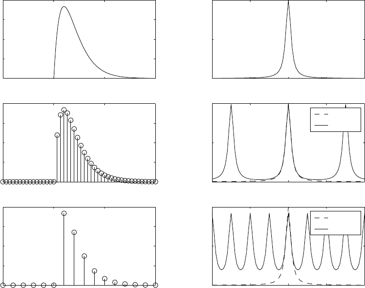
−5 0 5 10
0
0.1
0.2
0.3
0.4
t(sec)
xa(t)
−4 −2 0 2 4
0
0.5
1
F(Hz)
Xa(F)
−5 0 5 10
0
0.1
0.2
0.3
0.4
t(sec)
x(n)=xa(nT)
−4 −2 0 2 4
0
0.5
1
F(Hz)
|Xa(F)|
|X(F)|
−5 0 5 10
0
0.1
0.2
0.3
0.4
t(sec)
x(n)=xa(nT)
−4 −2 0 2 4
0
0.5
1
F(Hz)
|Xa(F)|
|X(F)|
Figure 6.4-1:
199
© 2007 Pearson Education, Inc., Upper Saddle River, NJ. All rights reserved. This material is protected under all copyright laws
as they currently exist. No portion of this material may be reproduced, in any form or by any means, without permission in
writing from the publisher. For the exclusive use of adopters of the book Digital Signal Processing, Fourth Edition, by John G.
Proakis and Dimitris G. Manolakis. ISBN 0-13-187374-1.
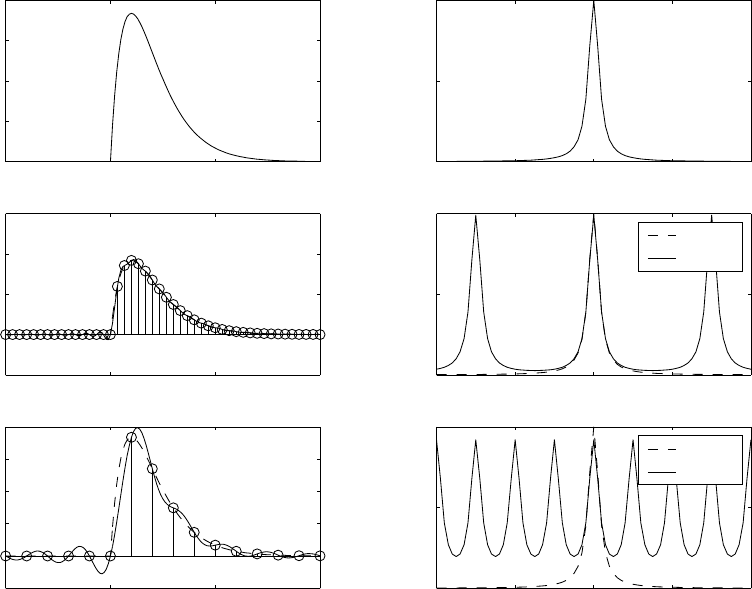
−5 0 5 10
0
0.1
0.2
0.3
0.4
t(sec)
xa(t)
−4 −2 0 2 4
0
0.5
1
F(Hz)
Xa(F)
−5 0 5 10
−0.2
0
0.2
0.4
0.6
t(sec) −4 −2 0 2 4
0
0.5
1
F(Hz)
|Xa(F)|
|X(F)|
−5 0 5 10
−0.1
0
0.1
0.2
0.3
t(sec) −4 −2 0 2 4
0
0.5
1
F(Hz)
|Xa(F)|
|X(F)|
Figure 6.4-2:
200
© 2007 Pearson Education, Inc., Upper Saddle River, NJ. All rights reserved. This material is protected under all copyright laws
as they currently exist. No portion of this material may be reproduced, in any form or by any means, without permission in
writing from the publisher. For the exclusive use of adopters of the book Digital Signal Processing, Fourth Edition, by John G.
Proakis and Dimitris G. Manolakis. ISBN 0-13-187374-1.

6.6
(a) B=F2−F1is the bandwidth of the signal. Based on arbitrary band positioning for first-order
sampling,
Fs,min =2FH
kmax
where
kmax =⌊F2
B⌋.
(b)
ˆxa(t) = ∞
X
n=−∞
xa(nT )ga(t−nT )
where
ga(t) = sin πBt
πBt cos 2πFct
and Fc= (F1+F2)/2.
6.7
ga(t) = Z∞
−∞
Ga(F)ej2πF tdF
=ZFL−mB
−(FL−B)
1
1−γm+1 ej2πF tdF +Z−FL
FL−mB
1
1−γmej2πF tdF
+Z−FL+mB
FL
1
1−γ−mej2πF tdF +ZFL+B
−FL+mB
1
1−γ−(m+1) ej2πF tdF
=A+B+C+D
A=1
j2πBt(1 −γm+1)ej2π(FL−mB)t−e−j2π(FL+B)t
=ejπB∆(m+1)
j2πBt(ejπB∆(m+1) −e−jπB∆(m+1))ej2π(FL−mB)t−e−j2π(FL+B)t
B=ejπB∆m
j2πBt(ejπB∆m−e−jπB∆m)e−j2πFLt−ej2π(FL−mB)t
C=e−jπB∆m
j2πBt(ejπB∆m−e−jπB∆m)ej2πFLt−e−j2π(FL−mB)t
D=e−jπB∆(m+1)
j2πBt(ejπB∆(m+1) −e−jπB∆(m+1))e−j2π(FL−mB)t−ej2π(FL+B)t
Combining Aand D, and Band C, we obtain,
A+D=1
πBt sin(πB∆(m+ 1)) ej[2π(FL+B)t−πB∆(m+1)] +e−j[2π(FL+B)t−πB∆(m+1)]
−ej[2π(FL−mB)t+πB∆(m+1)] −e−j[2π(FL−mB)t+πB∆(m+1)]
201
© 2007 Pearson Education, Inc., Upper Saddle River, NJ. All rights reserved. This material is protected under all copyright laws
as they currently exist. No portion of this material may be reproduced, in any form or by any means, without permission in
writing from the publisher. For the exclusive use of adopters of the book Digital Signal Processing, Fourth Edition, by John G.
Proakis and Dimitris G. Manolakis. ISBN 0-13-187374-1.

=cos [2π(FL+B)t−π(m+ 1)B∆] −cos [2π(mB −FL)t−π(m+ 1)B∆]
2πBt sin [π(m+ 1)B∆]
B+C=1
πBt sin(πB∆m)) ej[2π(FL−mB)t+πB∆m]+e−j[2π(FL−mB)t+πB∆m]
−ej[2πFLt−πB∆m]−e−j[2πFLt−πB∆m]
=cos [2π(mB −FL)t−πmB∆] −cos [2πFLt−πmB∆]
2πBt sin(πmB∆)
We observe that a(t) = B+Cand b(t) = A+D. Q.E.D.
6.8
1.
gSH (n) = 1,0≤n≤I
0, otherwise
2.
GSH (w) = ∞
X
n=−∞
gSH (n)e−jwn
=
I
X
n=0
e−jwn
=e−jw(I−1)/2sin [wI/2]
sin(w/2)
3. The linear interpolator is defined as
glin[n] = 1− |n|/I, |n| ≤ I
0, otherwise
Taking the Fourier transform, we obtain
Glin(w) = 1
Isin(wI/2)
sin(w/2) 2
Fig. 6.8-1 shows magnitude and phase responses of the ideal interpolator (dashed-dotted line),
the linear interpolator (dashed line), and the sample-and-hold interpolator (solid line).
6.9
(a)
xa(t) = e−j2πF0t
Xa(F) = Z∞
0
xa(t)e−j2πF tdt
=Z∞
0
e−j2πF0te−j2πtdt
=Z∞
0
e−j2π(F+F0)tdt
=e−j2π(F+F0)t
−j2π(F+F0)|∞
0
Xa(F) = 1
j2π(F+F0)
202
© 2007 Pearson Education, Inc., Upper Saddle River, NJ. All rights reserved. This material is protected under all copyright laws
as they currently exist. No portion of this material may be reproduced, in any form or by any means, without permission in
writing from the publisher. For the exclusive use of adopters of the book Digital Signal Processing, Fourth Edition, by John G.
Proakis and Dimitris G. Manolakis. ISBN 0-13-187374-1.
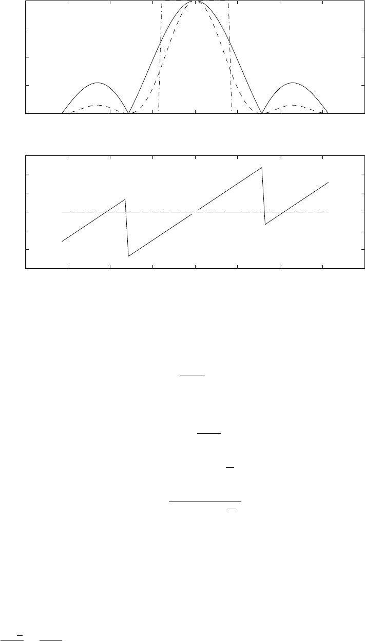
−4 −3 −2 −1 0 1 2 3 4
0
1
2
3
4
F
|G|
−4 −3 −2 −1 0 1 2 3 4
−3
−2
−1
0
1
2
3
F
angle(G)
Figure 6.8-1:
(b)
x(n) = e−j2πF0n
Fs
X(f) = ∞
X
n=−∞
x(n)e−j2πf n
=∞
X
n=0
e−j2πF0n
Fse−j2πf n
=∞
X
n=0
e−j2π(F+F0
Fs)n
=1
1−e−j2π(F+F0
Fs)
(c) Refer to fig 6.9-1
(d) Refer to fig 6.9-2
(e) Aliasing occurs at Fs= 10Hz.
6.10
Since Fc+B
2
B=50+10
20 = 3 is an integer, then Fs= 2B= 40Hz
203
© 2007 Pearson Education, Inc., Upper Saddle River, NJ. All rights reserved. This material is protected under all copyright laws
as they currently exist. No portion of this material may be reproduced, in any form or by any means, without permission in
writing from the publisher. For the exclusive use of adopters of the book Digital Signal Processing, Fourth Edition, by John G.
Proakis and Dimitris G. Manolakis. ISBN 0-13-187374-1.
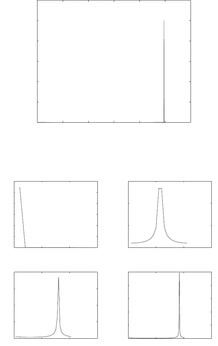
0 200 400 600 800 1000 1200
0
200
400
600
800
1000
1200
−−> |Xa(F)|
Figure 6.9-1:
0 5 10 15
0
2
4
6
8
10
12 Fs= 10
−−> |X(F)|
0 10 20 30
0
5
10
15 Fs= 20
−−> |X(F)|
0 20 40 60
0
10
20
30
40 Fs= 40
−−> |X(F)|
0 50 100 150
0
20
40
60
80
100 Fs= 100
−−> |X(F)|
Figure 6.9-2:
204
© 2007 Pearson Education, Inc., Upper Saddle River, NJ. All rights reserved. This material is protected under all copyright laws
as they currently exist. No portion of this material may be reproduced, in any form or by any means, without permission in
writing from the publisher. For the exclusive use of adopters of the book Digital Signal Processing, Fourth Edition, by John G.
Proakis and Dimitris G. Manolakis. ISBN 0-13-187374-1.
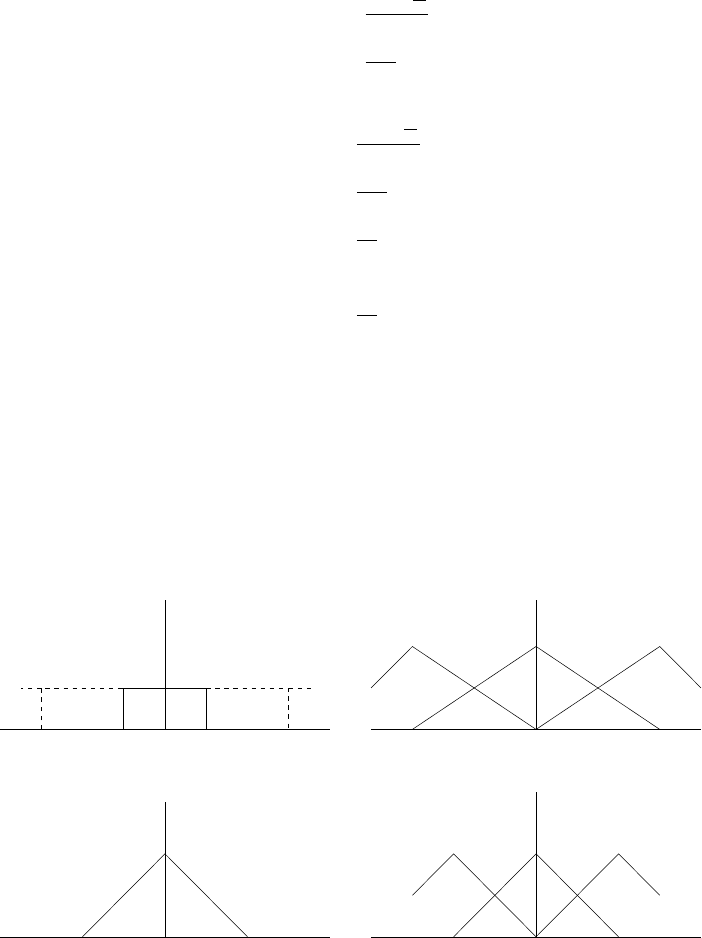
6.11
Fc= 100
B= 12
r=⌈Fc+B
2
B⌉
=⌈106
12 ⌉
=⌈8.83⌉= 8
B′=Fc+B
2
r
=106
8
=53
4
Fs= 2B′
=53
2Hz
6.12
(a)
x(n)↔X(w)
x2(n)↔X(w)∗X(w)
The output y1(t) is basically the square of the input signal ya(t). For the second system,
X(w)
w
−3π −2π −π 0 π 2π 3π −2π −π 0π 2π
X(w) * X(w)
w
spectrum of x
a2(t)
-2B 0 2B -2B 0 2B
spectrum of sampled xa
2(t),
(i.e.), s(n) = x
a2(nT)
Figure 6.12-3:
x2
a(t)↔X(w)∗X(w), the bandwidth is basically 2B. The spectrum of the sampled signal is
205
© 2007 Pearson Education, Inc., Upper Saddle River, NJ. All rights reserved. This material is protected under all copyright laws
as they currently exist. No portion of this material may be reproduced, in any form or by any means, without permission in
writing from the publisher. For the exclusive use of adopters of the book Digital Signal Processing, Fourth Edition, by John G.
Proakis and Dimitris G. Manolakis. ISBN 0-13-187374-1.

given in fig 6.12-3.
(b)
xa(t) = cos40πt
x(n) = cos40πn
50
=cos4πn
5
y(n) = x2(n)
=cos24πn
5
=1
2+1
2cos8πn
5
=1
2+1
2cos2πn
5
y1(t) = 1
2+1
2cos20πt
sa(t) = x2
a(t)
=cos240πt
=1
2+1
2cos80πt
s(n) = 1
2+1
2cos80πn
50
=1
2+1
2cos8πn
5
=1
2+1
2cos2πn
5
Hence, y2(t) = 1
2+1
2cos20πt
For Fs= 30,
x(n) = cos4πn
3
=cos2πn
3
y(n) = x2(n)
=cos22πn
3
=1
2+1
2cos4πn
3
=1
2+1
2cos2πn
3
y1(t) = 1
2+1
2cos20πt
sa(t) = x2
a(t)
=cos240πt
=1
2+1
2cos80πt
s(n) = 1
2+1
2cos80πn
30
=1
2+1
2cos2πn
3
206
© 2007 Pearson Education, Inc., Upper Saddle River, NJ. All rights reserved. This material is protected under all copyright laws
as they currently exist. No portion of this material may be reproduced, in any form or by any means, without permission in
writing from the publisher. For the exclusive use of adopters of the book Digital Signal Processing, Fourth Edition, by John G.
Proakis and Dimitris G. Manolakis. ISBN 0-13-187374-1.

Hence, y2(t) = 1
2+1
2cos20πt
6.13
sa(t) = xa(t) + αxa(t−τ),|α|<1
sa(n) = xa(n) + αxa(n−τ
T)
Sa(w)
Xa(w)= 1 + αe−jτ w
T
If τ
Tis an integer, then we may select
H(z) = 1
1−αz−2where τ
T=L
6.14
∞
X
n=−∞
x2(n) = 1
2πZπ
−π|X(w)|2dw
X(w) = 1
T
∞
X
k=−∞
Xaw−2πk
T
=1
T
∞
X
k=−∞
Xaw
T,|w| ≤ π
∞
X
n=−∞
x2(n) = 1
2πZπ
−π
1
T2|Xa(w
T)|2dw
=1
2πT 2Zπ
T
−π
T|Xa(λ)|2T dλ
=1
2πT Zπ
T
−π
T|Xa(λ)|2dλ
Also, Ea=Z∞
−∞
x2
a(t)dt
=Z∞
−∞ |Xa(f)|2df
=ZFs
2
−Fs
2|Xa(f)|2df
Therefore, ∞
X
n=−∞
x2(n) = Ea
T
6.15
(a)
H(F) = Z∞
−∞
h(t)e−j2πf tdt
207
© 2007 Pearson Education, Inc., Upper Saddle River, NJ. All rights reserved. This material is protected under all copyright laws
as they currently exist. No portion of this material may be reproduced, in any form or by any means, without permission in
writing from the publisher. For the exclusive use of adopters of the book Digital Signal Processing, Fourth Edition, by John G.
Proakis and Dimitris G. Manolakis. ISBN 0-13-187374-1.

=ZT
0
t
Te−j2πf tdt
|{z }
A
+Z2T
T
2e−j2πf tdt
|{z }
B
−Z2T
T
t
Te−j2πf tdt
|{z }
C
Substituting a=−j2πf
A(F) = 1
TeaT
a2(aT −1) −1
a2(−1)
=eaT
a
|{z}
A1
−eaT
T a2
|{z}
A2
+1
T a2
|{z}
A3
B(F) = 2
aea2T−eaT
=2ea3T/2
πf sin(πf T )
C(F) = −1
Tea2T
a2(a2T−1) −eaT
a2(aT −1)
=−ea2T
a
|{z}
C1
−ea2T
a
|{z}
C2
+ea2T
T a2
|{z}
C3
+eaT
a
|{z}
C4
−eaT
T a2
|{z}
C5
A1(F) + C1(F) = −ea3T/2
πf sin(πf T )
A2(F) + C3(F) = ea3T/2
T aπf sin(πf T )
A3(F) + C5(F) = −eaT/2
T aπf sin(πf T )
C2(F) + c4(F) = −ea3T/2
πf sin(πf T )
Then,
H(F) = e−j2πf T
Tsin(πf T )
πf 2
(b)
6.16
(a)
d(n) = x(n)−ax(n−1)
E[d(n)] = E[x(n)] −aE[x(n−1)] = 0
E[d2(n)] ≡σ2
d=E[x(n)−ax(n−1)]2
=σ2
x+a2σ2
x−2aE[x(n)x(n−1)]
=σ2
x+a2σ2
x−2aγx(1)
=σ2
x(1 + a2−2aρx(1))
where ρx(1) = γx(1)
σ2
x
≡γx(1)
γx(0)
208
© 2007 Pearson Education, Inc., Upper Saddle River, NJ. All rights reserved. This material is protected under all copyright laws
as they currently exist. No portion of this material may be reproduced, in any form or by any means, without permission in
writing from the publisher. For the exclusive use of adopters of the book Digital Signal Processing, Fourth Edition, by John G.
Proakis and Dimitris G. Manolakis. ISBN 0-13-187374-1.
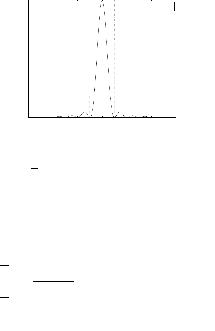
−6/T −5/T −4/T −3/T −2/T −1/T 0 1/T 2/T 3/T 4/T 5/T 6/T
0
T/2
T
F
|H|
H(F)
Hideal(F)
Figure 6.15-1:
(b)
d
da σ2
x(1 + a2−2aρx(1))= 2a−2ρx(1) = 0
a=ρx(1)
For this value of αwe have
σ2
d=σ2
x[1 + ρ2
x(1) −2ρ2
x(1)]
=σ2
x[1 −ρ2
x(1)]
(c) σ2
d< σ2
xis always true if |ρx(1)|>0. Note also that |ρx(1)| ≤ 1.
(d)
d(n) = x(n)−a1x(n−1) −a2x(n−2)
E[d2(n)] = E[x(n)−a1x(n−1) −a2x(n−2)]2
σ2
d=σ2
x(1 + a2
1+a2
2+ 2a1(a2−1)ρx(1) −2a2ρx(2))
d
da1
σ2
d= 0
⇒a1=ρx(1)[1 −ρx(2)]
1−ρ2
x(1)
d
da2
σ2
d= 0
⇒a2=ρx(2) −ρ2
x(1)
1−ρ2
x(1)
Then, σ2
d min =1−3ρ2
x(1) −ρ2
x(2) + 2ρ2
x(1)ρx(2) + 2ρ4
x(1) + ρ2
x(1)ρ2
x(2) −2ρ4
x(1)ρx(2)
[1 −ρ2
x(1)]2
6.17
x(t) = Acos2πF t
209
© 2007 Pearson Education, Inc., Upper Saddle River, NJ. All rights reserved. This material is protected under all copyright laws
as they currently exist. No portion of this material may be reproduced, in any form or by any means, without permission in
writing from the publisher. For the exclusive use of adopters of the book Digital Signal Processing, Fourth Edition, by John G.
Proakis and Dimitris G. Manolakis. ISBN 0-13-187374-1.
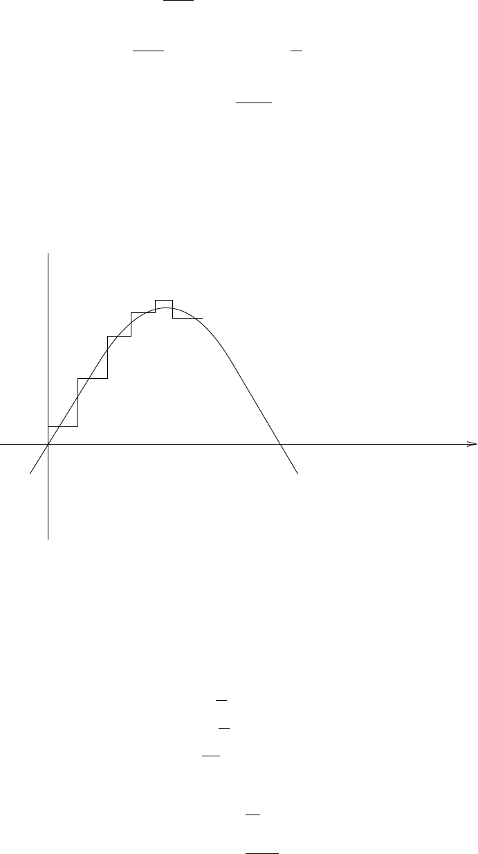
dx(t)
dt =−A(2πF )sin2πF t
=−2πAF sin2πF t
dx(t)
dt |max = 2πAF ≤△
T
Hence, △ ≥ 2πAF T
=2πAF
Fs
Refer to fig 6.17-1.
Figure 6.17-1:
6.18
Let Pddenote the power spectral density of the quantization noise. Then (a)
Pn=ZB
Fs
−B
Fs
Pddf
=2B
Fs
Pd
=σ2
e
SQNR = 10log10
σ2
x
σ2
e
= 10log10
σ2
xFs
2BPd
210
© 2007 Pearson Education, Inc., Upper Saddle River, NJ. All rights reserved. This material is protected under all copyright laws
as they currently exist. No portion of this material may be reproduced, in any form or by any means, without permission in
writing from the publisher. For the exclusive use of adopters of the book Digital Signal Processing, Fourth Edition, by John G.
Proakis and Dimitris G. Manolakis. ISBN 0-13-187374-1.

= 10log10
σ2
xFs
2BPd
+ 10log10Fs
Thus, SQNR will increase by 3dB if Fsis doubled.
(b) The most efficient way to double the sampling frequency is to use a sigma-delta modulator.
6.19
(a)
Se(F) = σ2
e
Fs
|Hn(F)|= 2|sinπF
Fs|
σ2
n=ZB
−B|Hn(F)|2Se(F)dF
= 2 ZB
0
4sin2(πF
Fs
)σ2
e
Fs
dF
=4σ2
e
FsZB
0
(1 −cos2πF
Fs
)dF
=4σ2
e
Fs
[B−Fs
2πsin2πB
Fs
]
=2σ2
e
π[2πB
Fs−sin2πB
Fs
]
(b)
For 2πB
Fs
<< 1,
sin2πB
Fs≈2πB
Fs−1
6(2πB
Fs
)3
Therefore, σ2
n=2σ2
e
π[2πB
Fs−2πB
Fs−1
6(2πB
Fs
)3]
=1
3π2σ2
e(2B
Fs
)3
6.20
(a)
{[X(z)−Dq(z)] 1
1−z−1−Dq(z)}z−1
1−z−1=Dq(z)−E(z)
Dq(z) = z−1X(z) + (1 −z−1)2E(z)
Therefore, Hs(z) = z−1
and Hn(z) = (1 −z−1)2
(b)
|Hn(F)|= 4sin2(πF
Fs
)
= 2(1 −cos(2πF
Fs
))
211
© 2007 Pearson Education, Inc., Upper Saddle River, NJ. All rights reserved. This material is protected under all copyright laws
as they currently exist. No portion of this material may be reproduced, in any form or by any means, without permission in
writing from the publisher. For the exclusive use of adopters of the book Digital Signal Processing, Fourth Edition, by John G.
Proakis and Dimitris G. Manolakis. ISBN 0-13-187374-1.

(c)
σ2
n=ZB
−B|Hn(F)|2σ2
e
Fs
dF
≈2ZB
0
[4(πF
Fs
)2]2σ2
e
Fs
dF
=32π4σ2
e
F5
sZB
0
F4dF
=1
5π4σ2
e(2B
Fs
)5
6.21
(a)
x(n) = cos2π
Nn
xa(t) = x(n)|n=t
T
=cos 2πt
NT
=cos2π(Fs
N)t
Therefore, F0=Fs
N
(b) Nanalog sinusoids can be generated. There are Npossible different starting phases.
6.22
(a)
h(t) = Z∞
−∞
H(F)ej2πF tdF
=Z∞
−∞
[c(F−Fc) + c∗(−F−Fc)]ej2πF tdF
=c(t)ej2πFct+c∗(t)e−j2πFct
= 2Re[c(t)ej2πFct]
(b)
H(F) = C(F−Fc) + C∗(−F−Fc)
X(F) = 1
2[U(F−Fc) + U∗(−F−Fc)]
Y(F) = X(F)H(F)
=1
2[C(F−Fc)U(F−Fc) + U∗(−F−Fc)C∗(−F−Fc)]
+1
2[C(F−Fc)U∗(−F−Fc) + U(F−Fc)C∗(−F−Fc)]
But C(F−Fc)U∗(−F−Fc) = U(F−Fc)C∗(−F−Fc) = 0
F−1[C(F)U(F)] = Z∞
−∞
c(τ)u(t−τ)dτ ≡v(t)
212
© 2007 Pearson Education, Inc., Upper Saddle River, NJ. All rights reserved. This material is protected under all copyright laws
as they currently exist. No portion of this material may be reproduced, in any form or by any means, without permission in
writing from the publisher. For the exclusive use of adopters of the book Digital Signal Processing, Fourth Edition, by John G.
Proakis and Dimitris G. Manolakis. ISBN 0-13-187374-1.
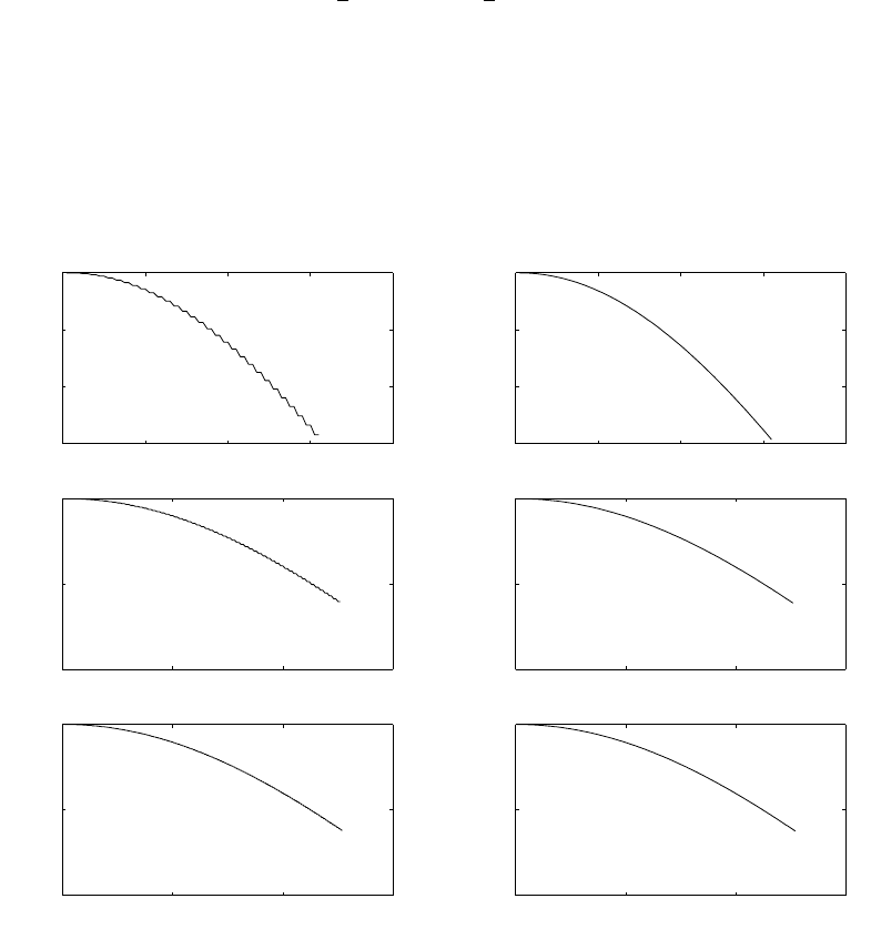
Hence, y(t) = 1
2v(t)ej2πFct+1
2v∗(t)e−j2πFct
= Re[v(t)ej2πFct]
6.23
(a) Refer to fig 6.23-1.
(b) Refer to fig 6.23-2.
0 20 40 60 80
0.4
0.6
0.8
1
−−−> x(n)
Zero Order hold: N = 32 thd = 0.1154
0 20 40 60 80
0.4
0.6
0.8
1
−−−> x(n)
First Order hold, N = 32 thd=0.1152
0 50 100 150
0
0.5
1
−−−> x(n)
Zero Order hold: N = 64 thd = 0.2331
0 50 100 150
0
0.5
1
−−−> x(n)
First Order hold, N = 64 thd=0.2329
0 100 200 300
0
0.5
1
−−−> n
−−−> x(n)
Zero Order hold: N = 128 thd = 0.4686
0 100 200 300
0
0.5
1
−−−> n
−−−> x(n)
First Order hold, N = 128 thd=0.4683
Figure 6.23-1:
(c) Refer to fig 6.23-3. The first order hold interpolator performs better than the zero order
interpolator because the frequency response of the first order hold is more closer to the ideal
interpolator than that of the zero order hold case.
(d) Refer to fig 6.23-4.
(e) Refer to fig 6.23-5. Higher order interpolators with more memory or cubic spline interpolators
would be a better choice.
213
© 2007 Pearson Education, Inc., Upper Saddle River, NJ. All rights reserved. This material is protected under all copyright laws
as they currently exist. No portion of this material may be reproduced, in any form or by any means, without permission in
writing from the publisher. For the exclusive use of adopters of the book Digital Signal Processing, Fourth Edition, by John G.
Proakis and Dimitris G. Manolakis. ISBN 0-13-187374-1.
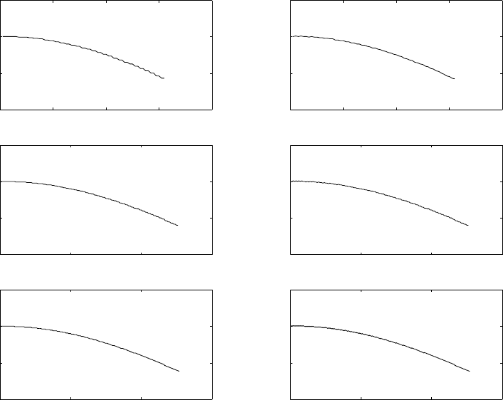
0 20 40 60 80
0
0.5
1
1.5
−−−> x(n)
Zero Order hold: N = 32 thd = 0.1154
0 20 40 60 80
0
0.5
1
1.5
−−−> x(n)
First Order hold, N = 32 thd=0.1153
0 50 100 150
0
0.5
1
1.5
−−−> x(n)
Zero Order hold: N = 64 thd = 0.2333
0 50 100 150
0
0.5
1
1.5
−−−> x(n)
First Order hold, N = 64 thd=0.2332
0 100 200 300
0
0.5
1
1.5
−−−> n
−−−> x(n)
Zero Order hold: N = 128 thd = 0.4689
0 100 200 300
0
0.5
1
1.5
−−−> n
−−−> x(n)
First Order hold, N = 128 thd=0.4687
Figure 6.23-2:
214
© 2007 Pearson Education, Inc., Upper Saddle River, NJ. All rights reserved. This material is protected under all copyright laws
as they currently exist. No portion of this material may be reproduced, in any form or by any means, without permission in
writing from the publisher. For the exclusive use of adopters of the book Digital Signal Processing, Fourth Edition, by John G.
Proakis and Dimitris G. Manolakis. ISBN 0-13-187374-1.
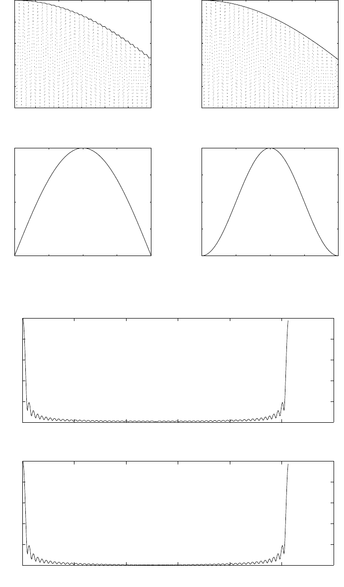
10 20 30 40 50
0
0.2
0.4
0.6
0.8
1Zero Order Hold
−1 −0.5 0 0.5 1
0
0.5
1
1.5
2Zero Order Hold, filter spectrum
10 20 30 40 50
0
0.2
0.4
0.6
0.8
1First Order Hold
−1 −0.5 0 0.5 1
0
0.5
1
1.5
2First Order Hold, filter spectrum
Figure 6.23-3:
0 100 200 300 400 500 600
0
10
20
30
40
50 Zero Order Hold, interpolated output
−−−−> |X(f)|
0 100 200 300 400 500 600
0
10
20
30
40
50 First Order Hold, Interpolated output
−−−−> n
−−−−> |X(f)|
Figure 6.23-4:
215
© 2007 Pearson Education, Inc., Upper Saddle River, NJ. All rights reserved. This material is protected under all copyright laws
as they currently exist. No portion of this material may be reproduced, in any form or by any means, without permission in
writing from the publisher. For the exclusive use of adopters of the book Digital Signal Processing, Fourth Edition, by John G.
Proakis and Dimitris G. Manolakis. ISBN 0-13-187374-1.
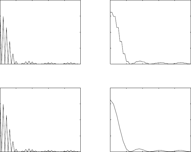
0 10 20 30 40
0
0.05
0.1
0.15
0.2 Zero Order Hold, xi(n)
−−−> xi(n)
0 10 20 30 40
0
0.05
0.1
0.15
0.2 Zero Order Hold, y(n)
−−−> y(n)
0 10 20 30 40
0
0.05
0.1
0.15
0.2 First Order Hold, xi(n)
−−−> xi(n)
0 10 20 30 40
0
0.05
0.1
0.15
0.2 First Order Hold, y(n)
−−−> y(n)
Figure 6.23-5:
216
© 2007 Pearson Education, Inc., Upper Saddle River, NJ. All rights reserved. This material is protected under all copyright laws
as they currently exist. No portion of this material may be reproduced, in any form or by any means, without permission in
writing from the publisher. For the exclusive use of adopters of the book Digital Signal Processing, Fourth Edition, by John G.
Proakis and Dimitris G. Manolakis. ISBN 0-13-187374-1.

6.24
(a) xp(t) = P∞
n=−∞ xa(t−nTs) is a periodic signal with period Ts. The fourier coefficients in a
fourier series representation are
ck=1
TsZTs
2
−Ts
2
xp(t)e−j2πkt
Tsdt
=1
TsZTs
2
−Ts
2
∞
X
n=−∞
xa(t−nTs)e−j2πkt
Tsdt
=1
Ts
∞
X
n=−∞ ZTs
2
−Ts
2
xa(t−nTs)e−j2πkt
Tsdt
=1
Ts
∞
X
n=−∞ ZnTs+Ts
2
nTs−Ts
2
xa(t′)e−j2πk(t′+nTs)
Tsdt′
=1
TsZ∞
−∞
xa(t′)e−j2πkt′
Tsdt′
=1
Ts
Xa(k
Ts
)
=1
Ts
Xa(kδF )
(b) Let
w(t) = 1,−Ts
2≤t≤Ts
2
0,otherwise
If Ts≥2τ, xa(t) = xp(t)w(t)
Xa(F) = Xp(F)∗W(F)
Xa(F) = "∞
X
k=−∞
ckδ(F−k
Ts
)#∗Ts
sinπF Ts
πF Ts
=Ts
∞
X
k=−∞
ck
sinπ(F−k
Ts)Ts
π(F−k
Ts)Ts
=∞
X
k=−∞
Xa(kδF )sinπ(F−k
Ts)Ts
π(F−k
Ts)Ts
, Ts=1
δF
(c) If T < 2τ, there will be aliasing in every period of xp(t). Hence, xa(t)6=xp(t)w(t) and
consequently, xa(t) cannot be recovered from xp(t).
(d) From (b) Xa(F) = P∞
k=−∞ Xa(kδF )sinπ (F−kδF )
δF
π(F−kδF )
δF
217
© 2007 Pearson Education, Inc., Upper Saddle River, NJ. All rights reserved. This material is protected under all copyright laws
as they currently exist. No portion of this material may be reproduced, in any form or by any means, without permission in
writing from the publisher. For the exclusive use of adopters of the book Digital Signal Processing, Fourth Edition, by John G.
Proakis and Dimitris G. Manolakis. ISBN 0-13-187374-1.
218
© 2007 Pearson Education, Inc., Upper Saddle River, NJ. All rights reserved. This material is protected under all copyright laws
as they currently exist. No portion of this material may be reproduced, in any form or by any means, without permission in
writing from the publisher. For the exclusive use of adopters of the book Digital Signal Processing, Fourth Edition, by John G.
Proakis and Dimitris G. Manolakis. ISBN 0-13-187374-1.

Chapter 7
7.1
Since x(n) is real, the real part of the DFT is even, imaginary part odd. Thus, the remaining
points are {0.125 + j0.0518,0,0.125 + j0.3018}
7.2
(a)
˜x2(l) = x2(l),0≤l≤N−1
=x2(l+N),−(N−1) ≤l≤ −1
˜x2(l) = sin(3π
8l),0≤l≤7
=sin(3π
8(l+ 8)),−7≤l≤ −1
=sin(3π
8|l|),|l| ≤ 7
Therefore, x1(n)8
x2(n) =
3
X
m=0
˜x2(n−m)
=sin(3π
8|n|) + sin(3π
8|n−1|) + ...+sin(3π
8|n−3|)
={1.25,2.55,2.55,1.25,0.25,−1.06,−1.06,0.25}
(b)
˜x2(n) = cos(3π
8n),0≤l≤7
=−cos(3π
8n),−7≤l≤ −1
= [2u(n)−1] cos(3π
8n),|n| ≤ 7
Therefore, x1(n)8
x2(n) =
3
X
m=0 1
4m
˜x2(n−m)
={0.96,0.62,−0.55,−1.06,−0.26,−0.86,0.92,−0.15}
(c)
for (a) X1(k) =
7
X
n=0
x1(n)e−jπ
4kn
219
© 2007 Pearson Education, Inc., Upper Saddle River, NJ. All rights reserved. This material is protected under all copyright laws
as they currently exist. No portion of this material may be reproduced, in any form or by any means, without permission in
writing from the publisher. For the exclusive use of adopters of the book Digital Signal Processing, Fourth Edition, by John G.
Proakis and Dimitris G. Manolakis. ISBN 0-13-187374-1.

={4,1−j2.4142,0,1−j0.4142,0,1 + j0.4142,0,1 + j2.4142}
similarly,
X2(k) = {1.4966,2.8478,−2.4142,−0.8478,−0.6682,−0.8478,
−2.4142,2.8478}
DFT of x1(n)8
x2(n) = X1(k)X2(k)
={5.9864,2.8478 −j6.8751,0,−0.8478 + j0.3512,0,
−0.8478 −j0.3512,0,2.8478 + j6.8751}
For sequences of part (b)
X1(k) = {1.3333,1.1612 −j0.2493,0.9412 −j0.2353,0.8310 −j0.1248,
0.8,0.8310 + j0.1248,0.9412 + j0.2353,1.1612 + j0.2493}
X2(k) = {1.0,1.0 + j2.1796,1.0−j2.6131,1.0−j0.6488,1.0,
1.0 + j0.6488,1.0 + j2.6131,1.0−j2.1796}
Consequently,
DFT of x1(n)8
x2(n) = X1(k)X2(k)
={1.3333,1.7046 + j2.2815,0.3263 −j2.6947,0.75 −j0.664,0.8,
0.75 + j0.664,0.3263 + j2.6947,1.7046 −j2.2815}
7.3
ˆx(k) may be viewed as the product of X(k) with
F(k) = 1,0≤k≤kc, N −kc≤k≤N−1
0, kc< k < N −kc
F(k) represents an ideal lowpass filter removing frequency components from (kc+ 1)2π
Nto π.
Hence ˆx(n) is a lowpass version of x(n).
7.4
(a)
x1(n) = 1
2ej2π
Nn+e−j2π
Nn
X1(k) = N
2[δ(k−1) + δ(k+ 1)]
also X2(k) = N
2j[δ(k−1) −δ(k+ 1)]
So X3(k) = X1(k)X2(k)
=N2
4j[δ(k−1) −δ(k+ 1)]
and x3(n) = N
2sin(2π
Nn)
(b)
˜
Rxy(k) = X1(k)X∗
2(k)
=N2
4j[δ(k−1) −δ(k+ 1)]
⇒˜rxy(n) = −N
2sin(2π
Nn)
220
© 2007 Pearson Education, Inc., Upper Saddle River, NJ. All rights reserved. This material is protected under all copyright laws
as they currently exist. No portion of this material may be reproduced, in any form or by any means, without permission in
writing from the publisher. For the exclusive use of adopters of the book Digital Signal Processing, Fourth Edition, by John G.
Proakis and Dimitris G. Manolakis. ISBN 0-13-187374-1.

(c)
˜
Rxx(k) = X1(k)X∗
1(k)
=N2
4[δ(k−1) + δ(k+ 1)]
⇒˜rxx(n) = N
2cos(2π
Nn)
(d)
˜
Ryy(k) = X2(k)X∗
2(k)
=N2
4[δ(k−1) + δ(k+ 1)]
⇒˜ryy(n) = N
2cos(2π
Nn)
7.5
(a)
N−1
X
n=0
x1(n)x∗
2(n) = 1
4
N−1
X
n=0 ej2π
Nn+e−j2π
Nn2
=1
4
N−1
X
n=0 ej4π
Nn+e−j4π
Nn+ 2
=1
42N
=N
2
(b)
N−1
X
n=0
x1(n)x∗
2(n) = −1
4j
N−1
X
n=0 ej2π
Nn+e−j2π
Nne−j2π
Nn−ej2π
Nn
=1
4j
N−1
X
n=0 ej4π
Nn−e−j4π
Nn
= 0
(c) PN−1
n=0 x1(n)x∗
2(n) = 1 + 1 = 2
7.6
w(n) = 0.42 −0.25 ej2π
N−1n+e−j2π
N−1n+ 0.04 ej4π
N−1n+e−j4π
N−1n
w(k) = 0.42
N−1
X
n=0
e−j2π
Nnk −0.25 "N−1
X
n=0
ej2π
N−1ne−j2π
Nnk +
N−1
X
n=0
e−j2π
N−1ne−j2π
Nnk#
+0.04 "N−1
X
n=0
ej4π
N−1ne−j2π
Nnk +
N−1
X
n=0
e−j4π
N−1ne−j2π
Nnk#
221
© 2007 Pearson Education, Inc., Upper Saddle River, NJ. All rights reserved. This material is protected under all copyright laws
as they currently exist. No portion of this material may be reproduced, in any form or by any means, without permission in
writing from the publisher. For the exclusive use of adopters of the book Digital Signal Processing, Fourth Edition, by John G.
Proakis and Dimitris G. Manolakis. ISBN 0-13-187374-1.

= 0.42Nδ(k)
−0.25 "1−ej2π[N
N−1−k]
1−ej2π[1
N−1−k
N]+1−e−j2π[N
N−1+k]
1−e−j2π[1
N−1+k
N]#
+0.04 "1−ej2π[2N
N−1−k]
1−ej2π[2
N−1−k
N]+1−e−j2π[2N
N−1+k]
1−e−j2π[2
N−1+k
N]#
= 0.42Nδ(k)
−0.25 "1−cos(2πN
N−1)−cos(2π(1
N−1+k
N)) + cos(2πk
N)
1−cos(2π(1
N−1+k
N)) #
+0.04 "1−cos(4πN
N−1)−cos(2π(2
N−1+k
N)) + cos(2πk
N)
1−cos(2π(2
N−1+k
N)) #
7.7
Xc(k) =
N−1
X
n=0
1
2x(n)ej2πk0n
N+e−j2πk0n
Ne−2πkn
N
=1
2
N−1
X
n=0
x(n)e−j2π(k−k0)n
N+1
2
N−1
X
n=0
x(n)e−j2π(k+k0)n
N
=1
2X(k−k0)modN+1
2X(k+k0)modN
similarly, Xs(k) = 1
2jX(k−k0)modN−1
2jX(k+k0)modN
7.8
y(n) = x1(n)4
x2(n)
=
3
X
m=0
x1(m)mod4x2(n−m)mod4
={17,19,22,19}
7.9
X1(k) = {7,−2−j, 1,−2 + j}
X2(k) = {11,2−j, 1,2 + j}
⇒X3(k) = X1(k)X2(k)
={17,19,22,19}
222
© 2007 Pearson Education, Inc., Upper Saddle River, NJ. All rights reserved. This material is protected under all copyright laws
as they currently exist. No portion of this material may be reproduced, in any form or by any means, without permission in
writing from the publisher. For the exclusive use of adopters of the book Digital Signal Processing, Fourth Edition, by John G.
Proakis and Dimitris G. Manolakis. ISBN 0-13-187374-1.

7.10
x(n) = 1
2ej2πkn
N+e−j2πkn
N
x(n)x∗(n) = 1
42 + ej4πkn
N+e−j4πkn
N
E=
N−1
X
n=0
x(n)x∗(n)
=1
4
N−1
X
n=0 2 + ej4πkn
N+e−j4πkn
N
=1
42N
=N
2
7.11
(a)
x1(n) = x(n−5)mod8
X1(k) = X(k)e−j2π5k
8
=X(k)e−j5πk
4
(b)
x2(n) = x(n−2)mod8
X2(k) = X(k)e−j2π2k
8
=X(k)e−jπk
2
7.12
(a)
s(k) = Wk
2X(k)
= (−1)kX(k)
s(n) = 1
6
5
X
k=0
(−1)kX(k)W−kn
NN= 6
=1
6
5
X
k=0
X(k)W−k(n−3)
N
=x(n−3)mod6
s(n) = {3,4,0,0,1,2}
(b)
y(n) = IDFT X(k) + X∗(k)
2
223
© 2007 Pearson Education, Inc., Upper Saddle River, NJ. All rights reserved. This material is protected under all copyright laws
as they currently exist. No portion of this material may be reproduced, in any form or by any means, without permission in
writing from the publisher. For the exclusive use of adopters of the book Digital Signal Processing, Fourth Edition, by John G.
Proakis and Dimitris G. Manolakis. ISBN 0-13-187374-1.

=1
2[IDFT {X(k)}+ IDFT {X∗(k)}]
=1
2x(n) + x∗(−n)modN
=x(0),x(1) + x(5)
2,x(2) + x(4)
2, x(3),x(4) + x(2)
2,x(5) + x(1)
2
=0,1
2,3,3,3,1
2
(c)
v(n) = IDFT X(k)−X∗(k)
2j
By similar means to (b)
v(n) = 0,−1
2j, j, 0,−j, 1
2j
7.13
(a)
X1(k) =
N−1
X
n=0
x(n)Wkn
N
X3(k) =
3N−1
X
n=0
x(n)Wkn
3N
=
N−1
X
n=0
x(n)Wkn
3N+
2N−1
X
n=N
x(n)Wkn
3N+
3N−1
X
n=2N
x(n)Wkn
3N
=
N−1
X
n=0
x(n)Wnk
3
N+
N−1
X
n=0
x(n)Wk
3Wnk
3
N+
N−1
X
n=0
x(n)W2k
3Wnk
3
N
=
N−1
X
n=0
x(n)1 + Wk
3+W2k
3Wnk
3
N
= (1 + Wk
3+W2k
3)X1(k)
(b)
X1(k) = 2 + Wk
2
X3(k) = 2 + Wk
6+ 2W2k
6+W3k
6+ 2W4k
6+W5k
6
= (2 + W
k
3
2) + W2k
6(2 + W
k
3
2) + W4k
6(2 + W
k
3
2)
= (1 + Wk
3+W2k
3)X1(k
3)
7.14
(a)
y(n) = x1(n)5
x2(n)
={4,0,1,2,3}
224
© 2007 Pearson Education, Inc., Upper Saddle River, NJ. All rights reserved. This material is protected under all copyright laws
as they currently exist. No portion of this material may be reproduced, in any form or by any means, without permission in
writing from the publisher. For the exclusive use of adopters of the book Digital Signal Processing, Fourth Edition, by John G.
Proakis and Dimitris G. Manolakis. ISBN 0-13-187374-1.

(b) Let x3(n) = {x0, x1,...,x4}. Then,
0 4 3 2 1
1 0 4 3 2
2 1 0 4 3
3 2 1 0 4
4 3 2 1 0
x0
x1
x2
x3
x4
=
1
0
0
0
0
Solving yields sequence
x3(n) = −0.18
↑,0.22,0.02,0.02,0.02
.
7.15
Define H1(z)△
=H−1(z) and corresponding time signal h1(n). The use of 64-pt DFTs of y(n)
and h1(n) yields x(n) = y(n)64
h1(n) whereas x(n) requires linear convolution. However we
can simply recognize that
X(z) = Y(z)H1(z)
=Y(z)−0.5Y(z)z−1
so x(n) = y(n)−0.5y(n−1),0≤n≤63
with y(−1) △
= 0
7.16
H(k) =
N−1
X
n=0
h(n)e−j2π
Nkn
= 1 + (1
4)e−j2π
4k0k0k
= 1 −1
4e−jπ
2k
G(k) = 1
H(k)
=1
1−1
4e−j2π
Nk
= 1 + 1
4e−jπ
2k+1
4e−jπ
2k2
+...
=4
3,16 −4j
17 ,4
5,16 + 4j
17 ,repeat k0times
g(n) = 1
N
N−1
X
n=0
G(k)ej2π
Nkn
=1
4k0
[
4k0−4
X
k=0,4,...
4
3ej2π
4k0kn +
4k0−3
X
k=1,5,... 16 −4j
17 ej2π
4k0kn
225
© 2007 Pearson Education, Inc., Upper Saddle River, NJ. All rights reserved. This material is protected under all copyright laws
as they currently exist. No portion of this material may be reproduced, in any form or by any means, without permission in
writing from the publisher. For the exclusive use of adopters of the book Digital Signal Processing, Fourth Edition, by John G.
Proakis and Dimitris G. Manolakis. ISBN 0-13-187374-1.

+
4k0−2
X
k=2,6,...
4
5ej2π
4k0kn +
4k0−1
X
k=3,7,... 16 + 4j
17 ej2π
4k0kn]
=1
4k04
3X+16 −4j
17 ej2π
4k0nX+4
5ej2π
4k02nX
+16 + 4j
17 ej2π
4k03nX
where X△
=
k0−1
X
i=0
ej2π
k0ni
But X= 1,yielding
g(0) = 1
44
3+16 −4j
17 +4
5+16 + 4j
17
=256
255
g(k0) = 1
44
3+j16 −4j
17 −4
5−j16 + 4j
17
=64
255
g(2k0) = 1
44
3−16 −4j
17 +4
5−16 + 4j
17
=16
255
g(3k0) = 1
44
3−j16 −4j
17 −4
5+j16 + 4j
17
=4
255
and g(n) = 0 for other nin [0,4k0).
Therefore, g(n)∗h(n) =
256
255,0,0,..., 0
↑
k0
,..., 0
↑
2k0
,..., 0
↑
3k0
,...,−1
255
↑
4k0
,0
g(.) represents a close approximation to an inverse system, but not an exact one.
7.17
X(k) =
7
X
n=0
x(n)e−j2π
8kn
={6,−0.7071 −j1.7071,1−j, 0.7071 + j0.2929,0,0.7071 −j0.2929,1 + j,
−0.7071 + j1.7071}
|X(k)|={6,1.8478,1.4142,0.7654,0,0.7654,1.4142,1.8478}
6X(k) = 0,−1.9635,−π
4,0.3927,0,−0.3927,π
4,1.9635
226
© 2007 Pearson Education, Inc., Upper Saddle River, NJ. All rights reserved. This material is protected under all copyright laws
as they currently exist. No portion of this material may be reproduced, in any form or by any means, without permission in
writing from the publisher. For the exclusive use of adopters of the book Digital Signal Processing, Fourth Edition, by John G.
Proakis and Dimitris G. Manolakis. ISBN 0-13-187374-1.

7.18
x(n) = ∞
X
i=−∞
δ(n−iN)
y(n) = X
m
h(m)x(n−m)
=X
m
h(m)"X
i
δ(n−m−iN)#
=X
i
h(n−iN)
Therefore, y(.) is a periodic sequence with period N. So
Y(k) =
N−1
X
n=0
y(n)Wkn
N
=H(w)|w=2π
Nk
Y(k) = H(2πk
N)k= 0,1,...,N −1
7.19
Call the two real even sequences xe1(.) and xe2(.), and the odd ones xo1(.) and xo2(.) (a)
Let xc(n) = [xe1(n) + xo1(n)] + j[xe2(n) + xo2(n)]
Then, Xc(k) = DFT {xe1(n)}+ DFT {xo1(n)}+jDFT {xe2(n)}+jDFT {xo2(n)}
= [Xe1(k) + Xo1(k)] + j[Xe2(k) + Xo2(k)]
where Xe1(k) = Re[Xc(k)] + Re[Xc(−k)]
2
Xo1(k) = Re[Xc(k)] −Re[Xc(−k)]
2
Xe2(k) = Im[Xc(k)] + Im[Xc(−k)]
2
Xo2(k) = Im[Xc(k)] −Im[Xc(−k)]
2
(b)
si(0) = xi(1) −xi(N−1) = 0
−si(N−n) = −xi(N−n+ 1) + xi(N−n−1)
=xi(n+ 1) −xi(n−1)
=si(n)
(c)
x(n) = [x1(n) + s3(n)] + j[x2(n) + s4(n)]
The DFT of the four sequences can be computed using the results of part (a)
For i= 3,4, si(k) =
N−1
X
n=0
si(n)Wkn
N
227
© 2007 Pearson Education, Inc., Upper Saddle River, NJ. All rights reserved. This material is protected under all copyright laws
as they currently exist. No portion of this material may be reproduced, in any form or by any means, without permission in
writing from the publisher. For the exclusive use of adopters of the book Digital Signal Processing, Fourth Edition, by John G.
Proakis and Dimitris G. Manolakis. ISBN 0-13-187374-1.

=
N−1
X
n=0
[xi(n+ 1) −xi(n−1)] Wkn
N
=W−k
NXi(k)−Wk
NXi(k)
= 2jsin(2π
Nk)Xi(k)
Therefore, X3(k) = s3(k)
2jsin(2π
Nk)
X4(k) = s4(k)
2jsin(2π
Nk)
(d) X3(0) and X4(0), because sin(2π
Nk) = 0.
7.20
X(k) =
N−1
X
n=0
x(n)Wkn
N
=
N
2−1
X
n=0
x(n)Wkn
N+
N
2−1
X
n=0
x(n+N
2)Wk(n+N
2)
N
=
N
2−1
X
n=0 x(n)−x(n)Wk
2Wkn
N
If kis even, Wk
2= 1,and X(k) = 0
(b) If kis odd, Wk
2=−1,Therefore,
X(k) =
N
2−1
X
n=0
2x(n)Wkn
N
= 2
N
2−1
X
n=0
x(n)Wnk
2
N
2
For k= 2l+ 1, l = 0,..., N
2−1
X(2l+ 1) = 2
N
2−1
X
n=0
x(n)Wln
N
2Wn
N
=N
2−pt DFT of sequence 2x(n)Wn
N
7.21
(a) Fs≡FN= 2B= 6000 samples/sec
(b)
T=1
Fs
=1
6000
228
© 2007 Pearson Education, Inc., Upper Saddle River, NJ. All rights reserved. This material is protected under all copyright laws
as they currently exist. No portion of this material may be reproduced, in any form or by any means, without permission in
writing from the publisher. For the exclusive use of adopters of the book Digital Signal Processing, Fourth Edition, by John G.
Proakis and Dimitris G. Manolakis. ISBN 0-13-187374-1.

1
LT ≤50
⇒L≥1
50T
=6000
50
= 120 samples
(c) LT =1
6000 ×120 = 0.02 seconds.
7.22
x(n) = 1
2ej2π
Nn+1
2e−j2π
Nn,0≤n≤N, N = 10
X(k) =
N−1
X
n=0
x(n)e−j2π
Nkn
=
N−1
X
n=0
1
2e−j2π
N(k−1)n+
N−1
X
n=0
1
2e−j2π
N(k+1)n
= 5δ(k−1) + 5δ(k−9),0≤k≤9
7.23
(a) X(k) = PN−1
n=0 δ(n)e−j2π
Nkn = 1,0≤k≤N−1
(b)
X(k) =
N−1
X
n=0
δ(n−n0)e−j2π
Nkn
=e−j2π
Nkn0,0≤k≤N−1
(c)
X(k) =
N−1
X
n=0
ane−j2π
Nkn
=
N−1
X
n=0
(ae−j2π
Nk)n
=1−aN
1−ae−j2π
Nk
(d)
X(k) =
N
2−1
X
n=0
e−j2π
Nkn
=1−e−j2π
N
N
2k
1−e−j2π
Nk
=1−(−1)k
1−e−j2π
Nk
229
© 2007 Pearson Education, Inc., Upper Saddle River, NJ. All rights reserved. This material is protected under all copyright laws
as they currently exist. No portion of this material may be reproduced, in any form or by any means, without permission in
writing from the publisher. For the exclusive use of adopters of the book Digital Signal Processing, Fourth Edition, by John G.
Proakis and Dimitris G. Manolakis. ISBN 0-13-187374-1.

(e)
X(k) =
N−1
X
n=0
ej2π
Nnk0e−j2π
Nkn
=
N−1
X
n=0
e−j2π
N(k−k0)n
=Nδ(k−k0)
(f)
x(n) = 1
2ej2π
Nnk0+1
2e−j2π
Nnk0
From (e) we obtain X(k) = N
2[δ(k−k0) + δ(k−N+k0)]
(g)
x(n) = 1
2jej2π
Nnk0−1
2je−j2π
Nnk0
Hence X(k) = N
2j[δ(k−k0)−δ(k−N+k0)]
(h)
X(k) =
N−1
X
n=0
x(n)e−j2π
Nnk( assume N odd )
= 1 + e−j2π
N2k+e−j2π
N4k+...+e−j2π
N(n−1)k
=1−(e−j2π
N2k)N+1
2
1−e−j2π
N2k
=1−e−j2π
Nk
1−e−j4π
Nk
=1
1−e−j2π
Nk
7.24
(a)
x(n) = 1
N
N−1
X
k=0
X(k)ej2π
Nnk
⇒
N−1
X
k=0
X(k)ej2π
Nnk =Nx(n)
X(0) + X(1) + X(2) + X(3) = 4
X(0) + X(1)ejπ
2+X(2)ejπ +X(3)ej3π
2= 8
X(0) + X(1)ejπ +X(2)ej2π+X(3)ej3π= 12
X(0) + X(1)ej3π
2+X(2)ej3π+X(3)ej9π
2= 4
1 1 1 1
1j−1−j
1−1 1 −1
1−j−1j
X(0)
X(1)
X(2)
X(3)
=
4
8
12
4
⇒
X(0)
X(1)
X(2)
X(3)
=
7
−2−j
1
−2 + j
230
© 2007 Pearson Education, Inc., Upper Saddle River, NJ. All rights reserved. This material is protected under all copyright laws
as they currently exist. No portion of this material may be reproduced, in any form or by any means, without permission in
writing from the publisher. For the exclusive use of adopters of the book Digital Signal Processing, Fourth Edition, by John G.
Proakis and Dimitris G. Manolakis. ISBN 0-13-187374-1.

(b)
X(k) =
3
X
n=0
x(n)e−j2π
4nk
X(0) =
3
X
n=0
x(n)
= 7
X(1) =
3
X
n=0
x(n)e−jπ
2n
=−2−j
X(2) =
3
X
n=0
x(n)e−jπn
= 1
X(3) =
3
X
n=0
x(n)e−j3π
2n
=−2 + j
7.25
(a)
X(w) = ∞
X
n=−∞
x(n)e−jwn
=ej2w+ 2ejw + 3 + 2e−jw +e−j2w
= 3 + 2cos(2w) + 4cos(4w)
(b)
V(k) =
5
X
n=0
v(n)e−j2π
6nk
= 3 + 2e−j2π
6k+e−j2π
62k+ 0 + e−j2π
64k+e−j2π
65k
= 3 + 4cos(π
3k) + 2cos(2π
3k)
(c) V(k) = X(w)|w=2πk
6=πk
3
This is apparent from the fact that v(n) is one period (0 ≤n≤7) of a periodic sequence
obtained by repeating x(n).
7.26
Let x(n) = ∞
X
l=−∞
δ(n+lN )
Hence, x(n) is periodic with period N, i.e.
x(n) = 1, n = 0,±N, ±2N,...
231
© 2007 Pearson Education, Inc., Upper Saddle River, NJ. All rights reserved. This material is protected under all copyright laws
as they currently exist. No portion of this material may be reproduced, in any form or by any means, without permission in
writing from the publisher. For the exclusive use of adopters of the book Digital Signal Processing, Fourth Edition, by John G.
Proakis and Dimitris G. Manolakis. ISBN 0-13-187374-1.

= 0,otherwise
Then X(k) =
N−1
X
n=0
x(n)e−j2π
Nnk = 1,0≤k≤N−1
and x(n) = 1
N
N−1
X
k=0
X(k)ej2π
Nnk
Hence, ∞
X
l=−∞
δ(n+lN ) = 1
N
N−1
X
k=0
ej2π
Nnk
7.27
(a)
Y(k) =
M−1
X
n=0
y(n)Wkn
M
=
M−1
X
n=0 X
l
x(n+lM )Wkn
M
Now X(w) = X
n
x(n)e−jwn,
so X(2π
Mk) = X
n
Wkn
M
=
M−1
X
n=0 X
l
x(n+lM )Wk(n+lM )
M
=
M−1
X
n=0 X
l
x(n+lM )Wkn
M
=Y(k)
Therefore, Y(k) = X(w)|w=2π
Mk
(b)
Y(k) = X(w)|w=2π
N
2
k
Y(k
2) = X(w)|w=2π
Nk
=X(k), k = 2,4,...,N −2
(c)
X1(k) = X(k+ 1)
⇒x1(n) = x(n)e−j2π
Nn
=x(n)Wn
N
Let y(n) = x1(n) + x1(n+N
2),0≤n≤N−1
= 0,elsewhere
Then X(k+ 1) = X1(k)
=Y(k
2), k = 0,2,...,N −2
232
© 2007 Pearson Education, Inc., Upper Saddle River, NJ. All rights reserved. This material is protected under all copyright laws
as they currently exist. No portion of this material may be reproduced, in any form or by any means, without permission in
writing from the publisher. For the exclusive use of adopters of the book Digital Signal Processing, Fourth Edition, by John G.
Proakis and Dimitris G. Manolakis. ISBN 0-13-187374-1.
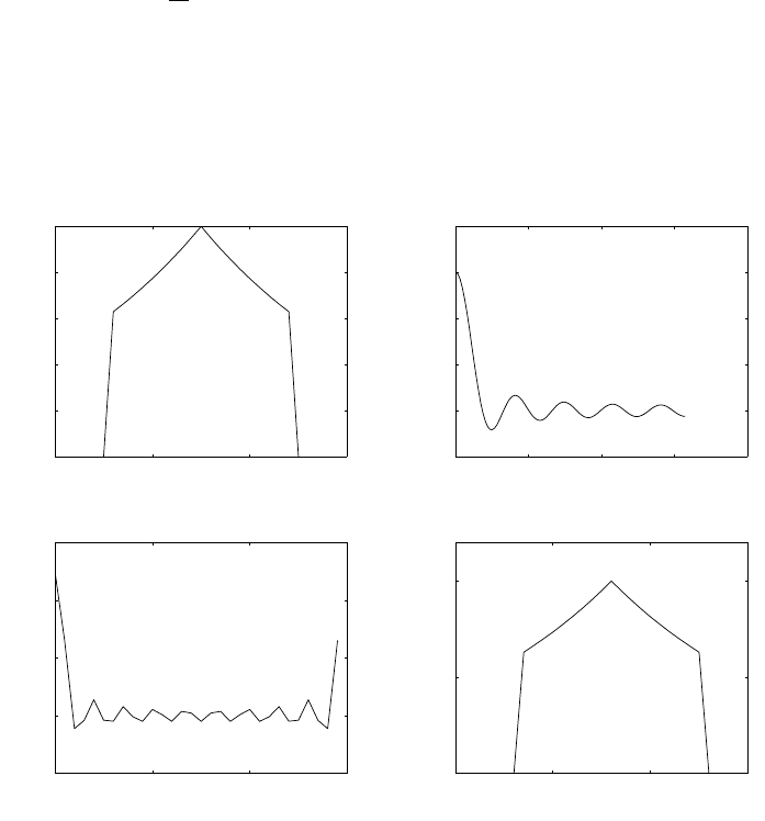
where Y(k) is the N
2-pt DFT of y(n)
7.28
(a) Refer to fig 7.28-1.
(b)
0 10 20 30
0
0.2
0.4
0.6
0.8
1
−−−> n
−−−> x(n)
x(n)
01234
−5
0
5
10
15
20
−−−> w
−−−> X(w)
X(w)
0 10 20 30
−0.2
0
0.2
0.4
0.6 ck
0 10 20 30
0
0.5
1
−−−> n
−−−> xtilde(n)
xtilde(n)
Figure 7.28-1:
∞
X
n=−∞
x(n)e−jwn =∞
X
n=−∞
a|n|e−jwn
=a+
1
X
−L
a−ne−jwn +
L
X
1
ane−jwn
=a+
L
X
1
anejwn +
L
X
1
ane−jwn
=a+ 2
L
X
n=1
ancos(wn)
=x(0) + 2
L
X
n=1
x(n)cos(wn)
(c) Refer to fig 7.28-1.
(d) Refer to fig 7.28-1.
233
© 2007 Pearson Education, Inc., Upper Saddle River, NJ. All rights reserved. This material is protected under all copyright laws
as they currently exist. No portion of this material may be reproduced, in any form or by any means, without permission in
writing from the publisher. For the exclusive use of adopters of the book Digital Signal Processing, Fourth Edition, by John G.
Proakis and Dimitris G. Manolakis. ISBN 0-13-187374-1.
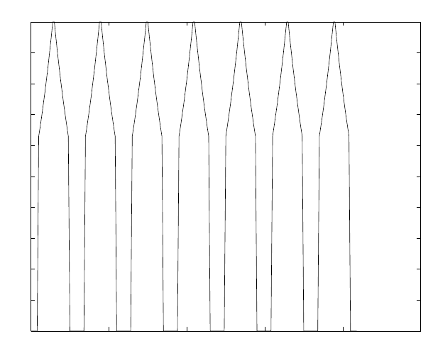
(e) Refer to fig 7.28-2.
(f) N=15. Refer to fig 7.28-3.
0 50 100 150 200 250
0
0.1
0.2
0.3
0.4
0.5
0.6
0.7
0.8
0.9
1
−−−> n
−−−> x(n)
x(n)
Figure 7.28-2:
234
© 2007 Pearson Education, Inc., Upper Saddle River, NJ. All rights reserved. This material is protected under all copyright laws
as they currently exist. No portion of this material may be reproduced, in any form or by any means, without permission in
writing from the publisher. For the exclusive use of adopters of the book Digital Signal Processing, Fourth Edition, by John G.
Proakis and Dimitris G. Manolakis. ISBN 0-13-187374-1.

−20 −10 0 10 20
0
0.2
0.4
0.6
0.8
1
−−−> n
−−−> x(n)
x(n)
0 1 2 3 4
−5
0
5
10
15
20
−−−> w
−−−> X(w)
X(w)
0 5 10 15
−0.5
0
0.5
1
1.5
−−−> w
−−−> ck
ck
−10 −5 0 5 10
0.6
0.8
1
1.2
1.4
−−−> n
−−−> xtilde(n)
xtilde(n)
Figure 7.28-3:
7.29
Refer to fig 7.29-1. The time domain aliasing is clearly evident when N=20.
7.30
Refer to fig 7.30-1.
(e)
xam(n) = x(n)cos(2πfcn)
Xam(w) =
N−1
X
n=0
x(n)cos(2πfcn)e−j2πfn
=1
2
N−1
X
n=0
x(n)he−j2π(f−fc)n+e−j2π(f+fc)ni
Xam(w) = 1
2[X(w−wc) + X(w+wc)]
7.31
(a) ck={2
π,−1
π,2
3π,−1
2π...}
(b) Refer to fig 7.31-1. The DFT of x(n) with N= 128 has a better resolution compared to one
with N= 64.
235
© 2007 Pearson Education, Inc., Upper Saddle River, NJ. All rights reserved. This material is protected under all copyright laws
as they currently exist. No portion of this material may be reproduced, in any form or by any means, without permission in
writing from the publisher. For the exclusive use of adopters of the book Digital Signal Processing, Fourth Edition, by John G.
Proakis and Dimitris G. Manolakis. ISBN 0-13-187374-1.
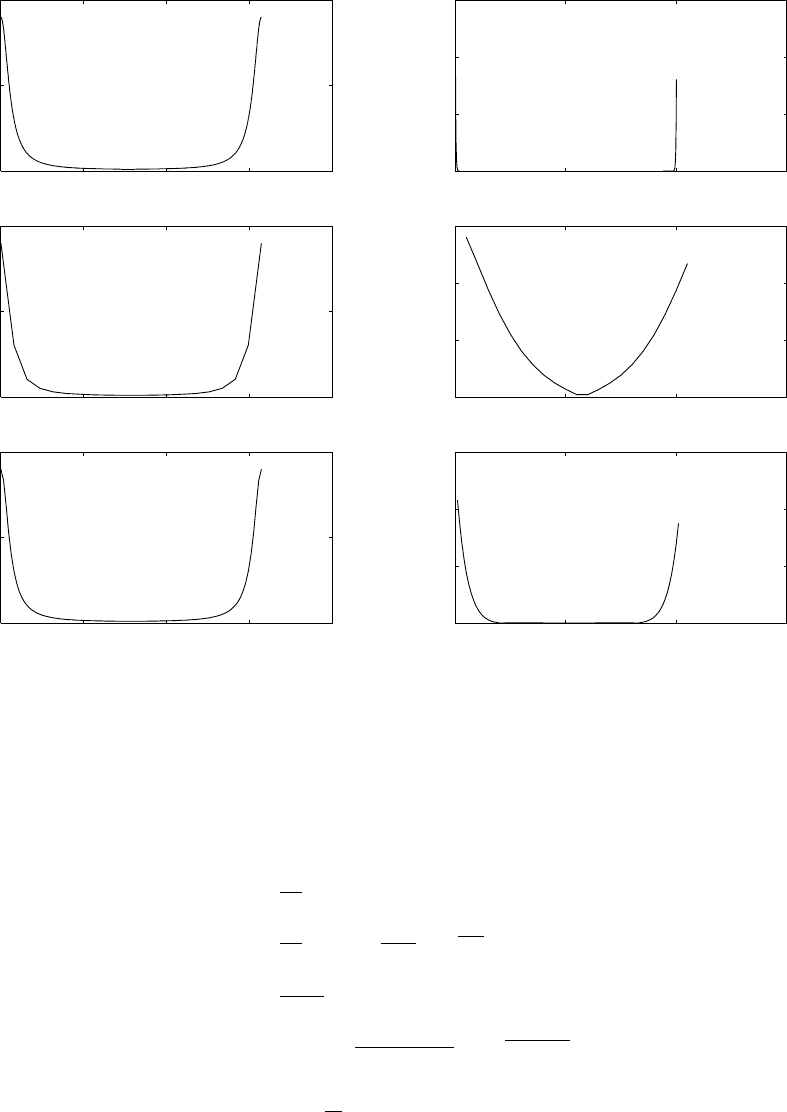
0 2 4 6 8
0
5
10 X(w)
−−> mag
0 1000 2000 3000
0
0.5
1
1.5 x(n)
−−> x(n)
0 2 4 6 8
0
5
10 X(w) with N=20
−−> mag
0 10 20 30
0
0.5
1
1.5 x(n) with N=20
−−> x(n)
0 2 4 6 8
0
5
10 X(w) with N=100
−−> w
−−> mag
0 50 100 150
0
0.5
1
1.5 x(n) with N=100
−−> n
−−> x(n)
Figure 7.29-1:
7.32
(a)
Y(jΩ) = 1
2πP(jΩ) ∗X(jΩ)
=1
2πT0sin(ΩT0
2)e−jΩT0
2∗[2πδ(Ω −Ω0)]
where sincx △
=sin x
x
Y(jΩ) = T0sinc T0(Ω −Ω0)
2e−jT0(Ω−Ω0)
2
(b) w0P= 2πk for an integer k, or w0=2k
Pπ
(c)
Y(w) =
N−1
X
n=0
ejw0ne−jwn
236
© 2007 Pearson Education, Inc., Upper Saddle River, NJ. All rights reserved. This material is protected under all copyright laws
as they currently exist. No portion of this material may be reproduced, in any form or by any means, without permission in
writing from the publisher. For the exclusive use of adopters of the book Digital Signal Processing, Fourth Edition, by John G.
Proakis and Dimitris G. Manolakis. ISBN 0-13-187374-1.
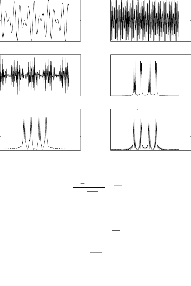
0 100 200 300
−2
0
2
x(n)
x(n)
0 100 200 300
−1
0
1
xc(n)
xc(n)
0 100 200 300
−2
0
2
xam(n)
xam(n)
0 50 100 150
0
20
40
mag
Xam(w) with N=128
0 50 100 150
0
10
20
30
mag
Xam(w) with N=100
0 100 200 300
0
20
40
60
mag
Xam(w) with N=180
Figure 7.30-1:
=sinN
2(w−w0)
sinw−w0
2
e−jN−1
2(w−w0)
Larger N⇒narrower main lobe of |Y(w)|.T0in Y(jΩ) has the same effect.
(d)
Y(k) = Y(w)|w=2π
Nk
=sinπ(k−l)
sinπ(k−l)
N
e−jN−1
Nπ(k−l)
|Y(k)|=|sinπ(k−l)|
|sinπ(k−l)
N|
=Nδ(k−l)
(e) The frequency samples 2π
Nkfall on the zeros of Y(w). By increasing the sampling by a factor
of two, for example, we will obtain a frequency sample between the nulls.
Y(w)|w=2π
2Nk=π
Nk, k=0,1,...,2N−1
237
© 2007 Pearson Education, Inc., Upper Saddle River, NJ. All rights reserved. This material is protected under all copyright laws
as they currently exist. No portion of this material may be reproduced, in any form or by any means, without permission in
writing from the publisher. For the exclusive use of adopters of the book Digital Signal Processing, Fourth Edition, by John G.
Proakis and Dimitris G. Manolakis. ISBN 0-13-187374-1.
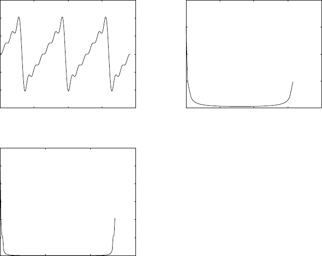
0 200 400 600 800
−1.5
−1
−0.5
0
0.5
1
1.5 x(n)
0 20 40 60 80
0
5
10
15
20 DFT of x(n) with N=64
0 50 100 150
0
10
20
30
40
50
60 DFT of x(n) with N=128
Figure 7.31-1:
238
© 2007 Pearson Education, Inc., Upper Saddle River, NJ. All rights reserved. This material is protected under all copyright laws
as they currently exist. No portion of this material may be reproduced, in any form or by any means, without permission in
writing from the publisher. For the exclusive use of adopters of the book Digital Signal Processing, Fourth Edition, by John G.
Proakis and Dimitris G. Manolakis. ISBN 0-13-187374-1.
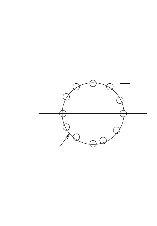
Chapter 8
8.1
Since (ej2π
Nk)N=ej2πk = 1, ej2π
Nksatisfies the equation XN= 1. Hence ej2π
Nkis an Nth root
of unity. Consider PN−1
n=0 ej2π
Nknej2π
Nln. If k6=l, the terms in the sum represent the N equally
spaced roots in the unit circle which clearly add to zero. However, if k=l, the sum becomes
PN−1
n=0 1 = N. see fig 8.1-1
π
12
eπ
12
e
unit circle
z-plane
Roots for N=12
j4 j2
Figure 8.1-1:
8.2
(a) Wq
NWq(l−1)
N=e−j2π
Nqe−j2π
Nq(l−1) =e−j2π
Nql =Wql
N
(b) Let ˆ
Wq
N=Wq
N+δwhere ˆ
Wq
Nis the truncated value of Wq
N. Now ˆ
Wql
N= (Wq
N+δ)l≈Wql
N+lδ.
239
© 2007 Pearson Education, Inc., Upper Saddle River, NJ. All rights reserved. This material is protected under all copyright laws
as they currently exist. No portion of this material may be reproduced, in any form or by any means, without permission in
writing from the publisher. For the exclusive use of adopters of the book Digital Signal Processing, Fourth Edition, by John G.
Proakis and Dimitris G. Manolakis. ISBN 0-13-187374-1.

Generally, single precision means a 32-bit length or δ= 5x10⁻¹⁰; while 4 significant digits means
δ= 5x10⁻⁵. Thus the error in the final results would be 105times larger.
(c) Since the error grows as lδ, after N iterations we have an error of Nδ. If Wql
Nis reset to -j
after every ql =N
4iterations, the error at the last step of the iteration is lδ =hN
4qiδ. Thus, the
error reduced by approximately a factor 4q.
8.3
X(k) =
N−1
X
n=0
x(n)Wkn
N0≤k≤N−1
=
N
2−1
X
n=0
x(n)Wkn
N+
N−1
X
n=N
2
x(n)Wkn
N
=
N
2−1
X
n=0
x(n)Wkn
N+
N
2−1
X
r=0
x(r+N
2)W(r+N
2)k
N
LetX′(k′) = X(2k+ 1),0≤k′≤N
2−1
Then, X′(k′) =
N
2−1
X
n=0 x(n)W(2k′+1)n
N+x(n+N
2)W(n+N
2)(2k′+1)
N
Using the fact that W2k′n
N=Wk′n
N
2, W N
N= 1
X′(k′) =
N
2−1
X
n=0 x(n)Wn
NWk′n
N
2+x(n+N
2)Wk′n
N
2Wn
NW
N
2
N
=
N
2−1
X
n=0 x(n)−x(n+N
2)Wn
NWk′n
N
2
8.4
Create three subsequences of 8-pts each
Y(k) =
21
X
n=0,3,6,...
y(n)Wkn
N+
22
X
n=1,4,7,...
y(n)Wkn
N+
23
X
n=2,5,...
y(n)Wkn
N
=
7
X
i=0
y(3i)Wki
N
3+
7
X
i=0
y(3i+ 1)Wki
N
3Wk
N+
7
X
i=0
y(3i+ 2)Wki
N
3W2k
N
△
=Y1(k) + Wk
NY2(k) + W2k
NY3(k)
where Y1, Y2, Y3represent the 8-pt DFTs of the subsequences.
8.5
X(z) = 1 + z−1+...+z−6
240
© 2007 Pearson Education, Inc., Upper Saddle River, NJ. All rights reserved. This material is protected under all copyright laws
as they currently exist. No portion of this material may be reproduced, in any form or by any means, without permission in
writing from the publisher. For the exclusive use of adopters of the book Digital Signal Processing, Fourth Edition, by John G.
Proakis and Dimitris G. Manolakis. ISBN 0-13-187374-1.

X(k) = X(z)|z=ej2π
5
= 1 + e−j2π
5+e−j4π
5+...+e−j12π
5
= 2 + 2e−j2π
5+e−j4π
5+...+e−j8π
5
x′(n) = {2,2,1,1,1}
x′(n) = X
m
x(n+ 7m), n = 0,1,...,4
Temporal aliasing occurs in first two points of x′(n) because X(z) is not sampled at sufficiently
small spacing on the unit circle.
8.6
(a) Zk= 0.8ej[2πk
8+π
8]see fig 8.6-1
(b)
circle of radius 0.8
z1
z0
z2
z3
z4
z5z6
z7
2π
8
π
8
z-plane
Figure 8.6-1:
X(k) = X(z)|z=zk
=
7
X
n=0
x(n)h0.8ej[2πk
8+π
8]i−n
s(n) = x(n) 0.8e−jπ
8n
241
© 2007 Pearson Education, Inc., Upper Saddle River, NJ. All rights reserved. This material is protected under all copyright laws
as they currently exist. No portion of this material may be reproduced, in any form or by any means, without permission in
writing from the publisher. For the exclusive use of adopters of the book Digital Signal Processing, Fourth Edition, by John G.
Proakis and Dimitris G. Manolakis. ISBN 0-13-187374-1.

8.7
Let M=N
2, L = 2.Then
F(0, q) =
N
2−1
X
n=0
x(0, m)Wmq
N
2
F(1, q) =
N
2−1
X
n=0
x(1, m)Wmq
N
2
which are the same as F1(k) and F2(k) in (8.1.26)
G(0, q) = F(0, q) = F1(k)
G(1, q) = Wq
NF(1, q) = F2(k)Wk
N
X(0, q) = x(k) = G(0, q) + G(1, q)W0
2
=F1(k) + F2(k)Wk
N
X1, q) = x(k) = G(0, q) + G(1, q)W1
2
=F1(k)−F2(k)Wk
N
8.8
W8=1
√2(1 −j)
Refer to Fig.8.1.9. The first stage of butterflies produces (2, 2, 2, 2, 0, 0, 0, 0). The twiddle
factor multiplications do not change this sequence. The nex stage produces (4, 4, 0, 0, 0, 0, 0,
0) which again remains unchanged by the twiddle factors. The last stage produces (8, 0, 0, 0, 0,
0, 0, 0). The bit reversal to permute the sequence into proper order unscrambles only zeros so
the result remains (8, 0, 0, 0, 0, 0, 0, 0).
8.9
See Fig. 8.1.13.
8.10
Using (8.1.45), (8.1.46), and (8.1.47) the fig 8.10-1 is derived:
8.11
Using DIT following fig 8.1.6:
1st stage outputs : 1
2,1
2,1
2,...,1
2
2nd stage outputs : 1,1
2(1 + W2
8),0,1
2(1 −W2
8),1,1
2(1 + W2
8),0,1
2(1 −W2
8)
242
© 2007 Pearson Education, Inc., Upper Saddle River, NJ. All rights reserved. This material is protected under all copyright laws
as they currently exist. No portion of this material may be reproduced, in any form or by any means, without permission in
writing from the publisher. For the exclusive use of adopters of the book Digital Signal Processing, Fourth Edition, by John G.
Proakis and Dimitris G. Manolakis. ISBN 0-13-187374-1.

x(0)
x(4)
x(8)
x(12)
x(1)
x(5)
x(9)
x(13)
x(2)
x(6)
x(10)
x(14)
x(3)
x(7)
x(11)
x(15)
x(0)
x(1)
x(2)
x(3)
x(4)
x(5)
x(6)
x(7)
x(8)
x(9)
x(10)
x(11)
x(12)
x(13)
x(14)
x(15)
0
0
0
0
0
0
0
0
0
0
0
0
0
0
0
0
0
1
2
3
0
2
4
6
0
3
6
9
Figure 8.10-1:
3rd stage outputs : 2,1
2(1 + W1
8+W2
8+W3
8),0,1
2(1 −W2
8+W3
8−W5
8),0,
1
2(1 −W1
8+W2
8−W3
8),0,1
2(1 −W2
8−W3
8+W5
8
Using DIF following fig 8.1.11:
1st stage outputs : 1
2,1
2,1
2,1
2,1
2,1
2,1
2W1
8,1
2W2
8,1
2W3
8
2nd stage outputs : 1,1,0,0,1
2(1 + W2
8),0,1
2(W1
8+W3
8),1
2(1 −W2
8),1
2(W3
8−W5
8)
3rd stage outputs : 2,0,0,0,1
2(1 + W1
8+W2
8+W3
8),1
2(1 −W1
8+W2
8−W3
8),
1
2(1 −W2
8+W3
8−W5
8),1
2(1 −W2
8−W3
8+W5
8
8.12
Let
A△
=
1 1 1 1
1−j−1j
1−1 1 −1
1j−1−j
x1△
=x(0) x(4) x(8) x(12) T
243
© 2007 Pearson Education, Inc., Upper Saddle River, NJ. All rights reserved. This material is protected under all copyright laws
as they currently exist. No portion of this material may be reproduced, in any form or by any means, without permission in
writing from the publisher. For the exclusive use of adopters of the book Digital Signal Processing, Fourth Edition, by John G.
Proakis and Dimitris G. Manolakis. ISBN 0-13-187374-1.

x2△
=x(1) x(5) x(9) x(13) T
x3△
=x(2) x(6) x(10) x(14) T
x4△
=x(3) x(7) x(11) x(15) T
F(0)
F(4)
F(8)
F(12)
=Ax1=
4
0
0
0
F(1)
F(5)
F(9)
F(13)
=Ax2=
0
0
0
0
F(2)
F(6)
F(10)
F(14)
=Ax3=
−4
0
0
0
F(3)
F(7)
F(11)
F(15)
=Ax4=
0
0
0
0
As every F(i) = 0 except F(0) = −F(2) = 4,
x(0)
x(7)
x(8)
x(12)
=Ax4
F(0)
F(1)
F(2)
F(3)
=
0
8
0
8
which means that X(4) = X(12) = 8. X(k) = 0 for other K.
8.13
(a) ”gain” = W0
8W0
8(−1)W2
8=−W2
8=j
(b) Given a certain output sample, there is one path from every input leading to it. This is true
for every output.
(c) X(3) = x(0) + W3
8x(1) −W2
8x(2) + W2
8W3
8x(3) −W0
8x(4) −W0
8W3
8x(5) + W0
8W2
8x(6) +
W0
8W2
8W3
8x(7)
8.14
Flowgraph for DIF SRFFT algorithm for N=16 is given in fig 8.14-1. There are 20 real, non
trivial multiplications.
244
© 2007 Pearson Education, Inc., Upper Saddle River, NJ. All rights reserved. This material is protected under all copyright laws
as they currently exist. No portion of this material may be reproduced, in any form or by any means, without permission in
writing from the publisher. For the exclusive use of adopters of the book Digital Signal Processing, Fourth Edition, by John G.
Proakis and Dimitris G. Manolakis. ISBN 0-13-187374-1.
x(0)
x(1)
x(2)
x(3)
x(4)
x(5)
x(6)
x(7)
x(8)
x(9)
x(10)
x(11)
x(12)
x(13)
x(14)
x(15)
X(0)
X(8)
X(4)
X(12)
X(2)
X(10)
X(6)
X(14)
X(1)
X(9)
X(5)
X(13)
X(3)
X(11)
X(7)
X(15)
-1
-1
-1
-1
-1
-1
-1
-1
+j
+j
+j
+j
w0
w1
w2
w
3
w
w
w
w
0
3
6
9
-1
-1
-1
+j
-1
-1
-1 +j
-1 +j
-1
w0
w2
w
0
w6
+j
+j
-1
-1
-1
-1
-1 +j
-1
-1
-j
-j
-j
-j
-j
-j
-j
-j
-j
-j
Figure 8.14-1:
8.15
For the DIT FFT, we have
X(k) =
N
2−1
X
n=0
x(2n)Wnk
N
2+
N
2−1
X
n=0
x(2n+ 1)W(2n+1)k
N
The first term can be obtained from an N
2-point DFT without any additional multiplications.
Hence, we use a radix-2 FFT. For the second term, we use a radix-4 FFT. Thus, for N=8, the
DFT is decomposed into a 4-point, radix-2 DFT and a 4-point radix-4 DFT. The latter is
N
2−1
X
n=0
x(2n+ 1)W(2n+1)k
N=
N
4−1
X
n=0
x(4n+ 1)Wk
NWk
N
4+
N
4−1
X
n=0
x(4n+ 3)W3k
NWk
N
4
The computation of X(k), X(k+N
4), X(k+N
2), X(k+3N
4) for k= 0,1,...,N
4−1 are performed
from the following:
X(k) =
N
2−1
X
n=0
x(2n)Wnk
N
2+
N
4−1
X
n=0
x(4n+ 1)Wk
NWnk
N
4+
N
4−1
X
n=0
x(4n+ 3)W3k
NWnk
N
4
X(k+N
4) =
N
2−1
X
n=0
x(2n)Wnk
N
2(−1)n+
N
4−1
X
n=0
x(4n+ 1)(−j)Wnk
N
4+
N
4−1
X
n=0
x(4n+ 3)W3k
N(j)Wnk
N
4
X(k+N
2) =
N
2−1
X
n=0
x(2n)Wnk
N
2+
N
4−1
X
n=0
x(4n+ 1)(−1)Wk
NWnk
N
4+
N
4−1
X
n=0
x(4n+ 3)(−1)W3k
NWnk
N
4
245
© 2007 Pearson Education, Inc., Upper Saddle River, NJ. All rights reserved. This material is protected under all copyright laws
as they currently exist. No portion of this material may be reproduced, in any form or by any means, without permission in
writing from the publisher. For the exclusive use of adopters of the book Digital Signal Processing, Fourth Edition, by John G.
Proakis and Dimitris G. Manolakis. ISBN 0-13-187374-1.
X(k+3N
4) =
N
2−1
X
n=0
x(2n)Wnk
N
2(−1)n+
N
4−1
X
n=0
x(4n+ 1)(j)Wn
NWnk
N
4+
N
4−1
X
n=0
x(4n+ 3)(−j)W3k
NWnk
N
4
The basic butterfly is given in fig 8.15-1
x(0)
x(4)
x(2)
x(6)
x(1)
x(5)
x(3)
x(7)
X(0)
X(1)
X(2)
X(3)
X(4)
X(5)
X(6)
X(7)
-1
-1
-1
-1
-1
-1
J
J
-J
-J
-1
-1
-1
-1
W
W
W
2
1
DIT/SRFFT
This graph looks like the transpose of
an N-point DIF FFT. The twiddle factors
come before the second stage.
x(2n+1)
x(4n+3)
from
from
WN
3k
WN
nfrom the use of
x(2n)
-1
-1
X(k)
X(k+N/4)
X(k+N/2)
X(k+3N/4)
j
-j
Note that this is a mirror image of DIF-SRFFT butterfly.
3
X
X
Figure 8.15-1:
8.16
x=xR+jxI
= (a+jb)(c+jd)
e= (a−b)d1 add ,1 mult
xR=e+ (c−d)a2 adds 1 mult
xI=e+ (c+d)b2 adds 1 mult
Total 5 adds 3 mult
8.17
X(z) =
N−1
X
n=0
x(n)z−n
246
© 2007 Pearson Education, Inc., Upper Saddle River, NJ. All rights reserved. This material is protected under all copyright laws
as they currently exist. No portion of this material may be reproduced, in any form or by any means, without permission in
writing from the publisher. For the exclusive use of adopters of the book Digital Signal Processing, Fourth Edition, by John G.
Proakis and Dimitris G. Manolakis. ISBN 0-13-187374-1.

Hence, X(zk) =
N−1
X
n=0
x(n)r−ne−j2π
Nkn
where zk=re−j2π
Nk, k = 0,1,...,N −1 are the N sample points. It is clear that X(zk), k =
0,1,...,N −1 is equivalent to the DFT (N-pt) of the sequence x(n)r−n, n ∈[0, N −1].
8.18
x′(n) = 1
LN
LN−1
X
k=0
X′(k)W−kn
LN
=1
LN "k0−1
X
k=0
X′(k)W−kn
LN +
LN−1
X
k=LN−k0+1
X′(k)W−kn
LN #
=1
LN "k0−1
X
k=0
X(k)W−kn
LN +
LN−1
X
k=LN−k0+1
X(k+N−LN)W−kn
LN #
=1
LN "k0−1
X
k=0
X(k)W−kn
LN +
N−1
X
k=N−k0−1
X(k)W−(k−N+LN)n
LN #
Therefore Lx′(Ln) = 1
N"k0−1
X
k=0
X(k)W−kn
N+
N−1
X
k=N−k0+1
X(k)W−kn
N#
=x(n)
L= 1 is a trivial case with no zeros inserted and
x′(n) = x(n) = 1
2,1
2+j1
2,0,1
2−j1
2
8.19
X(k) =
N−1
X
n=0
x(n)Wkn
N
Let F(t), t = 0,1,...,N −1 be the DFT of the sequence on k X(k).
F(t) =
N−1
X
k=0
X(k)Wtk
N
=
N−1
X
k=0 "N−1
X
n=0
x(n)Wkn
N#Wtk
N
=
N−1
X
n=0
x(n)"N−1
X
k=0
Wk(n+t)
N#
=
N−1
X
n=0
x(n)δ(n+t)mod N
247
© 2007 Pearson Education, Inc., Upper Saddle River, NJ. All rights reserved. This material is protected under all copyright laws
as they currently exist. No portion of this material may be reproduced, in any form or by any means, without permission in
writing from the publisher. For the exclusive use of adopters of the book Digital Signal Processing, Fourth Edition, by John G.
Proakis and Dimitris G. Manolakis. ISBN 0-13-187374-1.

=
N−1
X
n=0
x(n)δ(N−1−n−t)t= 0,1,...,N −1
={x(N−1), x(N−2),...,x(1), x(0)}
8.20
Y(k) =
2N−1
X
n=0
y(n)Wkn
Nk= 0,1,...,2N−1
=
2N−1
X
n=0,n even
y(n)Wkn
2N
=
N−1
X
m=0
y(2m)Wkm
N
=
N−1
X
m=0
x(m)Wkm
N
=X(k), k ∈[0, N −1]
=X(k−N), k ∈[N, 2N−1]
8.21
(a)
w(n) = 1
2(1 −cos 2πn
N−1),0≤n≤N−1
=1
2−1
4(ej2πn
N−1+e−j2πn
N−1)
W(z) =
N−1
X
n=0
w(n)z−n
=
N−1
X
n=0 1
2−1
4(ej2πn
N−1+e−j2πn
N−1)z−n
=1
2
1−z−N
1−z−1−1
4
1−(z−1ej2π
N−1)N
1−z−1ej2π
N−1
−1
4
1−(z−1e−j2π
N−1)N
1−z−1e−j2π
N−1
(b)
xw(n) = w(n)x(n)
⇒Xw(k) = W(k)NX(k)
8.22
The standard DFT table stores N complex values Wk
N, k = 0,1,...,N −1. However, since
Wk+N
2
N=−Wk
N, we need only store Wk
Nk= 0,1,...,N
2−1. Also, Wk+N
4
N=−jW k
Nwhich is
248
© 2007 Pearson Education, Inc., Upper Saddle River, NJ. All rights reserved. This material is protected under all copyright laws
as they currently exist. No portion of this material may be reproduced, in any form or by any means, without permission in
writing from the publisher. For the exclusive use of adopters of the book Digital Signal Processing, Fourth Edition, by John G.
Proakis and Dimitris G. Manolakis. ISBN 0-13-187374-1.

merely an interchange of real and imaginary parts of Wk
Nand a sign reversal. Hence all essential
quantities are easily obtained from Wk
Nk= 0,1,...,N
4−1
8.23
The radix-2 FFT algorithm for computing a 2N-pt DFT requires 2N
Nlog22N=N+N log2N
complex multiplications. The algorithm in (8.2.12) requires 2[N
2log2N+N
2] = N
2+log2Ncomplex
multiplications.
8.24
since H(z) = PM
k=0 bkz−k
1 + PN
k=1 akz−k
H(2π
N−1k) = PM
k=0 bkWkn
N+1
1 + PN
k=1 akWkn
N+1
△
=H(k), k = 0,...,N
Compute N+ 1-pt DFTs of sequences {b0, b1,...,bM,0,0,...,0}and {1, a1,...,aN}(assumes
N > M), say B(k) and A(k)k= 0,...,N
H(k) = B(k)
A(k)
8.25
Y(k) =
8
X
n=0
y(n)Wnk
9
=X
n=0,3,6
y(n)Wnk
9+X
n=1,4,7
y(n)Wnk
9+X
n=2,5,8
y(n)Wnk
9
=
2
X
m=0
y(3m)W3km
9+
2
X
m=0
y(3m+ 1)W(3m+1)k
9+
2
X
m=0
y(3m+ 2)W(3m+2)k
9
=
2
X
m=0
y(3m)Wkm
3+
2
X
m=0
y(3m+ 1)Wmk
3Wk
9+
2
X
m=0
y(3m+ 2)Wmk
3W2k
9
Total number of complex multiplies is 28 and the operations can be performed in-place. see
fig 8.25-1
8.26
X(k) =
8
X
n=0
x(n)Wnk
9
249
© 2007 Pearson Education, Inc., Upper Saddle River, NJ. All rights reserved. This material is protected under all copyright laws
as they currently exist. No portion of this material may be reproduced, in any form or by any means, without permission in
writing from the publisher. For the exclusive use of adopters of the book Digital Signal Processing, Fourth Edition, by John G.
Proakis and Dimitris G. Manolakis. ISBN 0-13-187374-1.
x(0)
x(1)
x(2)
x(3)
x(4)
x(5)
x(6)
x(7)
x(8)
X(0)
X(3)
X(6)
X(1)
X(4)
X(7)
X(2)
X(5)
X(8)
W3
1
W3
2
W3
W3
W3
1
W3
2
W3
W9
1
W9
2
W9
2
W9
1
1
2
1
Figure 8.25-1:
=
2
X
n=0
x(n)Wkn
9+
5
X
n=3
x(n)Wnk
9+
8
X
n=6
x(n)Wnk
9
=
2
X
n=0
x(n)Wkn
9+
2
X
n=0
x(n+ 3)Wnk
9Wk
3+
2
X
n=0
x(n+ 6)Wnk
9W2k
3
x(3l) =
2
X
n=0
x(n)Wnl
3+
2
X
n=0
x(n+ 3)Wnl
3+
2
X
n=0
x(n+ 6)Wnl
3
x(3l+ 1) =
2
X
n=0
x(n)Wnl
3Wn
9+
2
X
n=0
x(n+ 3)Wnl
3Wn
9W1
3+
2
X
n=0
x(n+ 6)Wnl
3Wn
9W2
3
=
2
X
n=0
Wn
9x(n) + W1
3x(n+ 3) + W2
3x(n+ 6)Wnl
3
x(3l+ 2) =
2
X
n=0
W2n
9x(n) + W2
3x(n+ 3) + W1
3x(n+ 6)Wnl
3
The number of required complex multiplications is 28. The operations can be performed in-place.
see fig 8.26-1
8.27
(a)Refer to fig 8.27-1
(b)Refer to fig 8.27-2
250
© 2007 Pearson Education, Inc., Upper Saddle River, NJ. All rights reserved. This material is protected under all copyright laws
as they currently exist. No portion of this material may be reproduced, in any form or by any means, without permission in
writing from the publisher. For the exclusive use of adopters of the book Digital Signal Processing, Fourth Edition, by John G.
Proakis and Dimitris G. Manolakis. ISBN 0-13-187374-1.
W
3
1
W
3
1
W3
2
W3
2
x(0)
x(1)
x(2)
x(3)
x(4)
x(5)
x(6)
x(7)
x(8)
X(0)
X(3)
X(6)
X(1)
X(4)
X(7)
X(2)
X(5)
X(8)
W3
1
W3
2
W
3
1
W3
2
W3
2
W3
1
W
3
1
W3
2
W
3
1
W9
1
W9
2
W9
2
W9
4
W3
1
W
32
W
3
1
W3
1
W3
2
W
32
W
31
Figure 8.26-1:
(c) DIF is preferable for computing all points. It is also better when only X(0), X(1), X(2), X(3)
are to be calculated. The rule is to compare the number of nontrivial complex multiplies and
choose the algorithm with the fewer.
(d) If M << N and L << N, the percentage of savings is
N
2log2N−M L
2log2N
N
2log2N×100% = (1 −ML
N)×100%
251
© 2007 Pearson Education, Inc., Upper Saddle River, NJ. All rights reserved. This material is protected under all copyright laws
as they currently exist. No portion of this material may be reproduced, in any form or by any means, without permission in
writing from the publisher. For the exclusive use of adopters of the book Digital Signal Processing, Fourth Edition, by John G.
Proakis and Dimitris G. Manolakis. ISBN 0-13-187374-1.
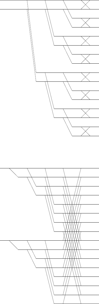
0
W
16
0
W
16
0
W
16
0
W
16
0
W
16
0
W
16
0
W
16
0
W
16
0
W
16
0
W
16
0
W
16
0
W
16
W
16
4
W
16
4
W
16
4
W
16
4
X(0)
X(8)
X(4)
X(12)
X(2)
X(10)
X(6)
X(14)
X(1)
X(9)
X(5)
X(13)
X(3)
X(11)
X(7)
X(15)
-1
-1
-1
-1
-1
-1
-1
-1
x(0)
x(1)
Figure 8.27-1:
x(0)
x(1)
X(0)
X(1)
X(2)
X(3)
X(4)
X(5)
X(6)
X(7)
X(8)
X(9)
X(10)
X(11)
X(12)
X(13)
X(14)
X(15)
-1
-1
-1
-1
-1
-1
-1
-1
W
16
W
16
W
16
W
16
W
16
W
16
W
16
W
16
0
1
2
3
4
5
6
7
Figure 8.27-2:
252
© 2007 Pearson Education, Inc., Upper Saddle River, NJ. All rights reserved. This material is protected under all copyright laws
as they currently exist. No portion of this material may be reproduced, in any form or by any means, without permission in
writing from the publisher. For the exclusive use of adopters of the book Digital Signal Processing, Fourth Edition, by John G.
Proakis and Dimitris G. Manolakis. ISBN 0-13-187374-1.

8.28
(a)Refer to fig 8.28-1. If data shuffling is not allowed, then X(0),...,X(3) should be computed
W
16
W
16
4
W
16
W
16
0
W
16
0
W
16
4
W
16
0
W
16
4
W
16
0
W
16
0
W
16
0
W
16
0
2
6
-1
-1
-1
-1
W
16
W
16
4
W
16
W
16
0
W
16
4
W
16
0
W
16
4
W
16
0
W
16
0
W
16
0
W
16
0
2
6
-1
-1
-1
-1
16
W0
16
W0
16
W
16
W
16
W
16
W
16
W
16
W
16
W
1
2
3
4
5
6
7
-1
-1
-1
-1
-1
-1
-1
-1
x(0)
x(1)
x(2)
x(3)
x(4)
x(5)
x(6)
x(7)
x(8)
x(9)
x(10)
x(11)
x(12)
x(13)
x(14)
x(15)
X(0)
X(8)
X(4)
X(12)
X(2)
X(10)
X(6)
X(14)
X(1)
X(9)
X(5)
X(13)
X(3)
X(11)
X(7)
X(15)
-1
-1
-1
-1
-1
-1
-1
-1
-1
-1
-1
-1
-1
-1
-1
-1
Figure 8.28-1:
by one DSP. Similarly for X(4),...,X(7) and X(8),...,X(11) and X(12), . . . , X(15). From the
flow diagram the output of every DSP requires all 16 inputs which must therefore be stored in
each DSP.
(b)Refer to fig 8.28-2
(c) The computations necessary for a general FFT are shown in the figure for part (a), Ng=
N
2log2N. Parallel computation of the DFTs requires
Np=1
2
N
Mlog2
N
M+
p−1
X
i=1
N
2
1
2i
=N
2Mlog2
N
M+N(1 −1
M)
Complex operations, as is seen in the figure for (b). Thus
S=Ng
Np
=
N
2log2N
N
2Mlog2N
M+N(1 −1
M)
=Mlog2N
log2N−log2M+ 2(M−1)
253
© 2007 Pearson Education, Inc., Upper Saddle River, NJ. All rights reserved. This material is protected under all copyright laws
as they currently exist. No portion of this material may be reproduced, in any form or by any means, without permission in
writing from the publisher. For the exclusive use of adopters of the book Digital Signal Processing, Fourth Edition, by John G.
Proakis and Dimitris G. Manolakis. ISBN 0-13-187374-1.

W
16
W
16
4
W
16
W
16
W
16
0
W
16
4
W
16
0
W
16
0
2
6
-1
-1
-1
-1
x(0)
x(1)
x(2)
x(3)
x(4)
x(5)
x(6)
x(7)
x(8)
x(9)
x(10)
x(11)
x(12)
x(13)
x(14)
x(15)
X(2)
X(10)
X(6)
X(14)
0
-1
-1
-1
-1
Figure 8.28-2:
8.29
Refer to fig 8.29-1
x(n) = 1
N
N−1
X
k=0
X(k)W−kn
N
=1
8X
keven
X(k)W−kn
8+1
8X
kodd
X(k)W−kn
8
=1
8
3
X
m=0
X(2m)W−mn
4+1
8
3
X
m=0
X(2m+ 1)W−mn
4W−n
8
=1
8
3
X
m=0 X(2m) + X(2m+ 1)W−n
8W−mn
4
x(n) = 1
8"3
X
m=0
X(2m)W−mn
4+W−n
8
3
X
m=0
X(2m+ 1)W−mn
4#,0≤n≤3
x(n+ 4) = 1
8"3
X
m=0
X(2m)W−mn
4−W−n
8
3
X
m=0
X(2m+ 1)W−mn
4#,0≤n≤3
This result can be obtained from the forward DIT FFT algorithm by conjugating each occurrence
of Wi
N→W−i
Nand multiplying each output by 1
8(or 1
2can be multiplied into the outputs of
each stage).
254
© 2007 Pearson Education, Inc., Upper Saddle River, NJ. All rights reserved. This material is protected under all copyright laws
as they currently exist. No portion of this material may be reproduced, in any form or by any means, without permission in
writing from the publisher. For the exclusive use of adopters of the book Digital Signal Processing, Fourth Edition, by John G.
Proakis and Dimitris G. Manolakis. ISBN 0-13-187374-1.

-1
-1
W8
W8
-0
-2 -1
-1
W8
-0
W8
-0
1/8
1/8
1/8
1/8
-1
-1
W8
W8
-0
-2 -1
-1
W8
-0
W8
-0
1/8
1/8
1/8
1/8
-1
-1
-1
-1
W8
-0
W8
W8
W8
-1
-2
-3
X(0)
X(4)
X(2)
X(6)
X(1)
X(5)
X(3)
X(7)
x(0)
x(1)
x(2)
x(3)
x(4)
x(5)
x(6)
x(7)
Figure 8.29-1:
8.30
x(n) = 1
8
7
X
k=0
X(k)W−kn
8
=1
8
3
X
k=0
X(k)W−kn
8+1
8
7
X
k=4
X(k)W−kn
8
=1
8"3
X
k=0
X(k)W−kn
8+ (−1)n
3
X
k=0
X(k+ 4)W−kn
8#
x(2l) = 1
8"3
X
k=0
X(k)W−lk
4+
3
X
k=0
X(k+ 4)W−lk
4#, l = 0,1,2,3
x(2l+ 1) = 1
8"3
X
k=0
X(k)W−lk
4W−k
8−
3
X
k=0
X(k+ 4)W−lk
4W−k
8#, l = 0,1,2,3
Similar to the DIT case (prob. 8.29) result can be obtained by conjugating each Wi
Nand scaling
by 1
8. Refer to fig 8.30-1
255
© 2007 Pearson Education, Inc., Upper Saddle River, NJ. All rights reserved. This material is protected under all copyright laws
as they currently exist. No portion of this material may be reproduced, in any form or by any means, without permission in
writing from the publisher. For the exclusive use of adopters of the book Digital Signal Processing, Fourth Edition, by John G.
Proakis and Dimitris G. Manolakis. ISBN 0-13-187374-1.

-1
-1
-1
-1
W8
W8
-0
W8
-0
W8
-0
1/8
1/8
1/8
1/8
-2
-1
-1
-1
-1
W8
W8
-0
W8
-0
W8
-0
1/8
1/8
1/8
1/8
-2
-1
-1
-1
-1
W8
-0
W8
W8
W8
-1
-2
-3
X(2)
X(3)
X(4)
X(5)
X(6)
X(7)
X(0)
X(1)
x(0)
x(4)
x(2)
x(6)
x(1)
x(5)
x(3)
x(7)
Figure 8.30-1:
8.31
x(n) = x∗(N−n)
IDFT(x∗(n)) = 1
N
N−1
X
n=0
x∗(n)W−kn
N
=1
N
N−1
X
n=0
x(N−n)W−kn
N
=1
N
1
X
m=N
x(m)W−k(N−m)
N
=1
N
N−1
X
m′=0
x(N−m′)W−km′
N
Since the IDFT of a Hermitian symmetric sequence is real, we may conjugate all terms in the
sum yielding
IDFT(x∗(n)) = 1
N
N−1
X
m′=0
x∗(N−m′)Wkm′
N
=1
N
N−1
X
n=0
x(n)Wkn
N
256
© 2007 Pearson Education, Inc., Upper Saddle River, NJ. All rights reserved. This material is protected under all copyright laws
as they currently exist. No portion of this material may be reproduced, in any form or by any means, without permission in
writing from the publisher. For the exclusive use of adopters of the book Digital Signal Processing, Fourth Edition, by John G.
Proakis and Dimitris G. Manolakis. ISBN 0-13-187374-1.

=1
NX(k)
In general, the IDFT of an N-length sequence can be obtained by reversing the flow of a forward
FFT and introducing a scale factor 1
N. Since the IDFT is apparently capable of producing the
(scaled) DFT for a Hermitian symmetric sequence, the reversed flow FFT will produce the desired
FFT.
8.32
X(k) =
N−1
X
m=0
x(m)Wkm
N
=
N−1
X
m=0
x(m)Wkm
NW−kN
Nsince W−kN
N= 1
=
N−1
X
m=0
x(m)W−k(N−m)
N
This can be viewed as the convolution of the N-length sequence x(n) with the impusle response
of a linear filter.
hk(n)△
=Wkn
Nu(n),evaluated at time N
Hk(z) = ∞
X
n=0
Wkn
Nz−n
=1
1−Wk
Nz−1
=Yu(z)
X(z)
yk(n) = Wk
Nyk(n−1) + x(n), yk(−1) = 0
yk(N) = X(k)
8.33
(a) 11 frequency points must be calculated. Radix-2 FFT requires 1024
2log21024 ≈5000 complex
multiplies or 20,000 real multiplies. FFT of radix-4 requires 0.75 ×5000 = 3,750 complex
multiplies or 15,000 real multiplies. Choose Goertzel.
(b) In this case, direct evaluation requires 106complex multiplies, chirp-z 22 ×103comples
multiplies, and FFT 1000 + 5000
2×13 = 33 ×103complex multiplies. Choose chirp-z.
8.34
In the DIF case, the number of butterflies affecting a given output is N
2in the first stage, N
4in
the second, .... The total number is
1 + 2 + ...+ 2ν−1= 2−ν(1 −(1
2)ν) = N−1
257
© 2007 Pearson Education, Inc., Upper Saddle River, NJ. All rights reserved. This material is protected under all copyright laws
as they currently exist. No portion of this material may be reproduced, in any form or by any means, without permission in
writing from the publisher. For the exclusive use of adopters of the book Digital Signal Processing, Fourth Edition, by John G.
Proakis and Dimitris G. Manolakis. ISBN 0-13-187374-1.

Every butterfly requires 4 real multiplies, and the eror variance is δ2
12 . Under the assumption that
the errors are uncorrelated, the variance of the total output quantization error is
σ2
q= 4(N−1) δ2
12 =Nδ2
3
8.35
(a)
Re[Xn+1(k)] = 1
2Xn+1(k) + 1
2X∗
n+1(k)
=1
2Xn(k) + 1
2Wm
NXn(l) + 1
2X∗
n(k)−1
2W−m
NX∗
n(l)
= Re[Xn(k)] + Re[Wm
NXn(l)]
since |Xn(k)|<1
2,|Re[Xn(k)]|<1
2
since |Xl(k)|<1
2,|Re[Wm
NXn(l)]|<1
2
so |Re[Wm
NXn(l)]|<1
2
Therefore |Re[Xn+1(k)]| ≤ |Re[Xn(k)]|+|Re[Wm
NXn(l)]|<1
The other inequalities are verified similarly. (b)
Xn+1(k) = Re[Xn(k)] + jIm[Xn(k)]
[cos(2π
Nm)−jsin(2π
Nm)][Re[Xn(l)] + jIm[Xn(l)]]
= Re[Xn(k)] + cos(.)Re[Xn(l)] + sin(.)Im[Xn(l)]
+j{Im[Xn(k)] + cos(.)Im[Xn(l)] + sin(.)Re[Xn(l)]}
Therefore, |Xn+1(k)|=|Xn(k)|+|Xn(l)|+A
where A△
= 2cos(.){Re[Xn(k)]Re[Xn(l)] + Im[Xn(k)]Im[Xn(l)]}
+2sin(.){Re[Xn(k)]Im[Xn(l)] −Im[Xn(k)]Re[Xn(l)]}
also |Xn+1(l)|2=|Xn(k)|2+|Xn(l)|2−A(∗)
Therefore, if A≥0,
max[|Xn+1(k)|,|Xn+1(l)|] = |Xn+1(k)|
=|Xn(k)|2+|Xn(l)|2+A1
2
>max[|Xn(k)|,|Xn(l)|]
By similar means using (*), it can be shown that the same inequality holds if A < 0. Also,
from the pair of equations fro computing the butterfly outputs, we have
2Xn(k) = Xn+1(k) + Xn+1(l)
2Xn(l) = W−m
NXn+1(k)−W−m
NXn+1(l)
By a similar method to that employed above, it can be shown that
2max[|Xn(k)|,|Xn(l)|]≥max[|Xn+1(k)|,|Xn+1(l)|]
258
© 2007 Pearson Education, Inc., Upper Saddle River, NJ. All rights reserved. This material is protected under all copyright laws
as they currently exist. No portion of this material may be reproduced, in any form or by any means, without permission in
writing from the publisher. For the exclusive use of adopters of the book Digital Signal Processing, Fourth Edition, by John G.
Proakis and Dimitris G. Manolakis. ISBN 0-13-187374-1.
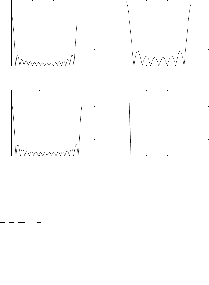
0 20 40 60 80
0
5
10
15
20
magnitude
(a) N=64 dc=16
0 20 40 60 80
0
2
4
6
8
magnitude
(b) N=64 dc=8
0 50 100 150
0
5
10
15
20
magnitude
(c) N=128 dc=16
0 20 40 60 80
0
200
400
600
800
magnitude
(d) N=64 dc=7.664e−14
Figure 8.36-1:
8.36
Refer to fig 8.36-1.
(d) (1) The frequency interval between successive samples for the plots in parts (a), (b), (c) and
(d) are 1
64 ,1
64 ,1
128 and 1
64 respectively.
(2) The dc values computed theoretically and from the plots are given below:
part a part b part c part d
theoretical 16 8 16 0
practical 16 8 16 8.203e−14
Both theoretical and practical dc values match except in the last case because of the finite word
length effects the dc value is not a perfect zero.
(3) Frequency interval = π
N1.
(4) Resolution is better with N= 128.
8.37
(a) Refer to fig 8.37-1.
(b) Refer to fig 8.37-1.
(c) Refer to fig 8.37-1.
(d) Refer to fig 8.37-1.
(e) Refer to fig 8.37-2.
259
© 2007 Pearson Education, Inc., Upper Saddle River, NJ. All rights reserved. This material is protected under all copyright laws
as they currently exist. No portion of this material may be reproduced, in any form or by any means, without permission in
writing from the publisher. For the exclusive use of adopters of the book Digital Signal Processing, Fourth Edition, by John G.
Proakis and Dimitris G. Manolakis. ISBN 0-13-187374-1.
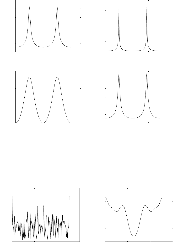
0 50 100 150
0
1
2
3
4
5
6r=0.9, Y(k)
magnitude
0 50 100 150
0
5
10
15
20
25 r=0.9, c=0.92, W(k)
magnitude
0 50 100 150
0.8
1
1.2
1.4 r=0.5, Y(k)
magnitude
0 50 100 150
0
1
2
3
4
5
6r=0.5 , c=0.55, W(k)
magnitude
Figure 8.37-1:
0 50 100 150
0
2
4
6
8
10
12 r = 0.5, Y(k)
magnitude
0 50 100 150
0
1
2
3
4x 1032 W(k)
magnitude
Figure 8.37-2:
260
© 2007 Pearson Education, Inc., Upper Saddle River, NJ. All rights reserved. This material is protected under all copyright laws
as they currently exist. No portion of this material may be reproduced, in any form or by any means, without permission in
writing from the publisher. For the exclusive use of adopters of the book Digital Signal Processing, Fourth Edition, by John G.
Proakis and Dimitris G. Manolakis. ISBN 0-13-187374-1.
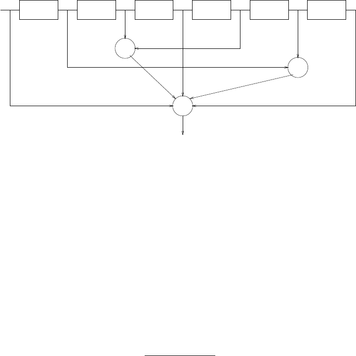
Chapter 9
9.1
(a) H(z) = 1 + 2z−1+ 3z−2+ 4z−3+ 3z−4+ 2z−5+z−6. Refer to fig 9.1-1
(b) H(z) = 1 + 2z−1+ 3z−2+ 3z−3+ 2z−4+z−5. Refer to fig 9.1-2
x(n) z-1 z-1 z-1 z-1 z-1 z-1
+
+
+
3
2
4
y(n)
Figure 9.1-1:
9.2
Refer to fig 9.2-1
A4(z) = H(z) = 1 + 2.88z−1+ 3.4048z−2+ 1.74z−3+ 0.4z−4
B4(z) = 0.4 + 1.74z−1+ 3.4048z−2+ 2.88z−3+z−4
Hence, K4= 0.4
A3(z) = A4(z)−k4B4(z)
1−k2
4
= 1 + 2.6z−1+ 2.432z−2+ 0.7z−3
261
© 2007 Pearson Education, Inc., Upper Saddle River, NJ. All rights reserved. This material is protected under all copyright laws
as they currently exist. No portion of this material may be reproduced, in any form or by any means, without permission in
writing from the publisher. For the exclusive use of adopters of the book Digital Signal Processing, Fourth Edition, by John G.
Proakis and Dimitris G. Manolakis. ISBN 0-13-187374-1.
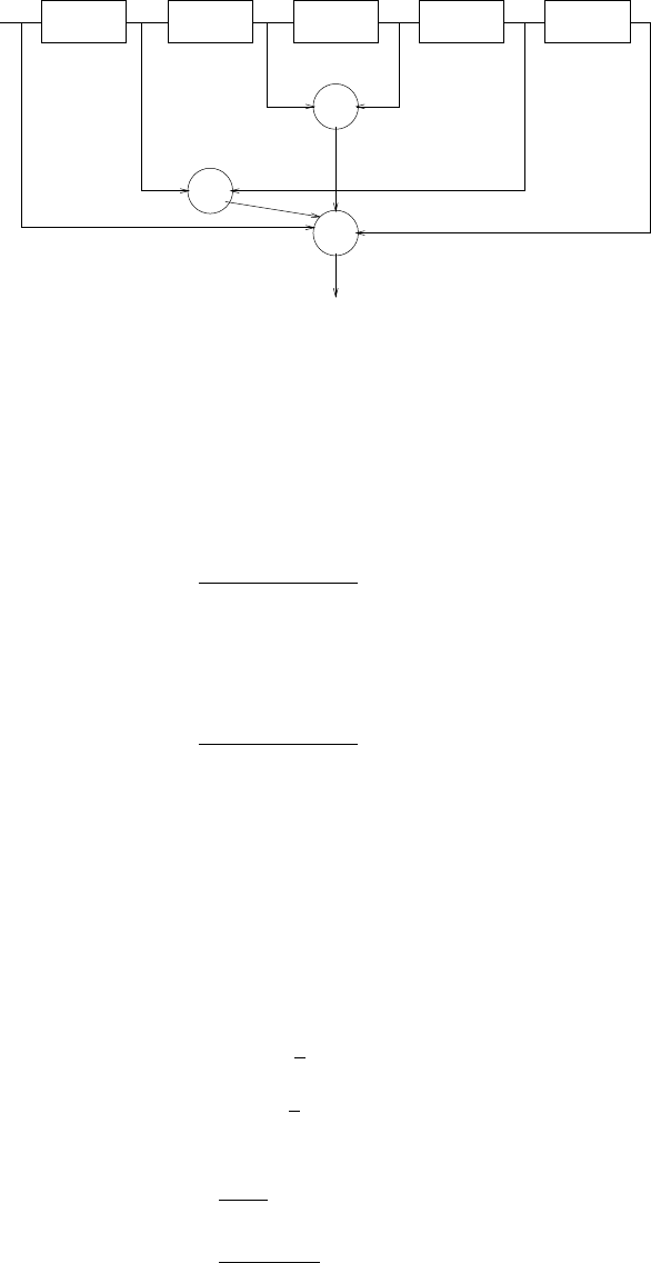
+
x(n) z-1 z-1 z-1 z-1 -1
z
y(n)
+
+2
3
Figure 9.1-2:
B3(z) = 0.7 + 2.432z−1+ 2.6z−2+z−3
Hence, K3= 0.7
A2(z) = A3(z)−k3B3(z)
1−k2
3
= 1 + 1.76z−1+ 1.2z−2
B2(z) = 1.2 + 1.76z−1+z−2
Then, K2= 1.2
A1(z) = A2(z)−k2B2(z)
1−k2
2
= 1 + 0.8z−1
Therefore, K1= 0.8
Since K2>1, the system is not minimum phase.
9.3
V(z) = X(z) + 1
2z−1V(z)
v(n) = x(n) + 1
2v(n−1)
Y(z) = 2[3X(z) + V(z)] + 2z−1V(z)
H(z) = Y(z)
X(z)
=8−z−1
1−0.5z−1
h(n) = 8(0.5)nu(n)−(0.5)n−1u(n−1)
262
© 2007 Pearson Education, Inc., Upper Saddle River, NJ. All rights reserved. This material is protected under all copyright laws
as they currently exist. No portion of this material may be reproduced, in any form or by any means, without permission in
writing from the publisher. For the exclusive use of adopters of the book Digital Signal Processing, Fourth Edition, by John G.
Proakis and Dimitris G. Manolakis. ISBN 0-13-187374-1.

+
z-1
z-1 + z-1 ++ z-1
+ ++
z-1 z-1 z-1
+++ y(n)
1 2.88 3.4048 1.74 0.4
x(n)
z-1
+
+
x(n)
k
1k
2k
3k
4
f1
(n) f2
(n) f3
(n) f 4(n) = y(n)
(a)
(b)
Figure 9.2-1: (a) Direct form. (b) Lattice form
9.4
H(z) = 5 + 3z1
1 + 1
3z−1+1 + 2z1
1−1
2z−1
h(n) = 5δ(n) + 3(−1
3)n−1u(n−1) + (1
2)nu(n) + 2(1
2)n−1u(n−1)
9.5
H(z) = 6 + 9
2z1−5
3z−2
(1 + 1
3z−1)(1 −1
2z−1)
=6 + 9
2z1−5
3z−2
1−1
6z1−1
6z−2
Refer to fig 9.5-1
9.6
For the first system, H(z) = 1
1−b1z−1+1
1−b2z−1
H(z) = 1−(b1+b2)z−1
(1 −b1z−1)(1 −b2z−1)
For the second system, H(z) = c0+c1z−1
(1 −d1z−1)(1 −a2z−1)
clearly, c0= 1
263
© 2007 Pearson Education, Inc., Upper Saddle River, NJ. All rights reserved. This material is protected under all copyright laws
as they currently exist. No portion of this material may be reproduced, in any form or by any means, without permission in
writing from the publisher. For the exclusive use of adopters of the book Digital Signal Processing, Fourth Edition, by John G.
Proakis and Dimitris G. Manolakis. ISBN 0-13-187374-1.
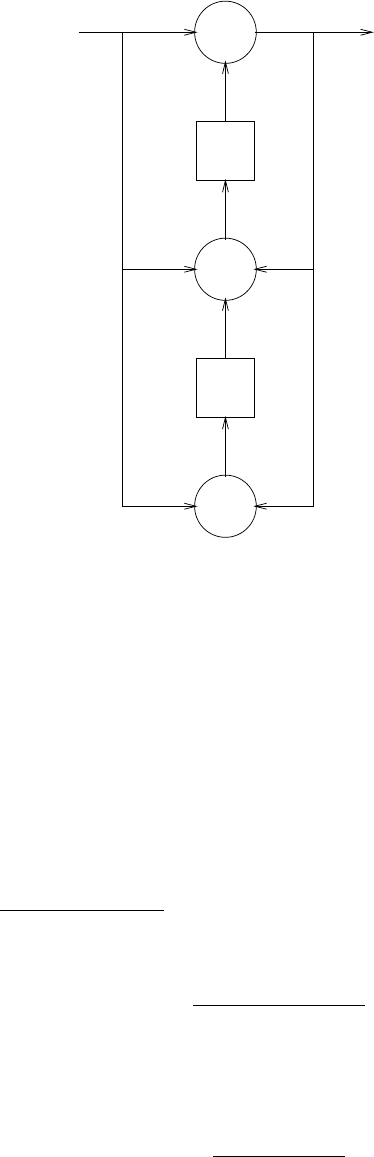
z-1
+
z-1
+
+
6
9/2
-5/3 1/6
1/6
y(n)x(n)
Figure 9.5-1:
c1=−(b1+b2)
d1=b1
a2=b2
9.7
(a)
y(n) = a1y(n−1) + a2y(n−2) + b0x(n) + b1x(n−1) + b2x(n−2)
H(z) = b0+b1z−1+b2z−2
1 + a1z−1+a2z−2
(b)
H(z) = 1 + 2z−1+z−2
1 + 1.5z−1+ 0.9z−2
Zeros at z=−1,−1
Poles at z=−0.75 ±j0.58
Since the poles are inside the unit circle, the system is stable.
H(z) = 1 + 2z−1+z−2
1 + z−1−2z−2
Zeros at z=−1,−1
Poles at z= 2,−1
264
© 2007 Pearson Education, Inc., Upper Saddle River, NJ. All rights reserved. This material is protected under all copyright laws
as they currently exist. No portion of this material may be reproduced, in any form or by any means, without permission in
writing from the publisher. For the exclusive use of adopters of the book Digital Signal Processing, Fourth Edition, by John G.
Proakis and Dimitris G. Manolakis. ISBN 0-13-187374-1.

The system is unstable.
(c)
x(n) = cos(π
3n)
H(z) = 1
1 + z−1−0.99z−2
H(w) = 1
1 + e−jw −0.99e−j2w
H(π
3) = 100e−jπ
3
Hence, y(n) = 100cos(π
3n−π
3)
9.8
y(n) = 1
4y(n−2) + x(n)
H(z) = 1
1−1
4z−2
(a)
h(n) = 1
2(1
2)n+ (−1
2)nu(n)
H(z) =
1
2
1−1
2z−1+
1
2
1 + 1
2z−1
(b)
x(n) = (1
2)n+ (−1
2)nu(n)
X(z) = 1
1−1
2z−1+1
1 + 1
2z−1
X(z) = 2
1−1
4z−2
Y(z) = X(z)H(z)
=1
1 + 1
2z−1+1
1−1
2z−1+−1
2z−1
(1 −1
2z−1)2+
1
2z−1
(1 + 1
2z−1)2
y(n) = (1
2)n+ (−1
2)n−n(1
2)n+n(−1
2)nu(n)
(c)Refer to fig 9.8-1
(d)
H(w) = 1
1−1
4e−j2w
=4
√17 −8cos2w6−tan−1sin2w
4−cos2w
Refer to fig 9.8-2.
265
© 2007 Pearson Education, Inc., Upper Saddle River, NJ. All rights reserved. This material is protected under all copyright laws
as they currently exist. No portion of this material may be reproduced, in any form or by any means, without permission in
writing from the publisher. For the exclusive use of adopters of the book Digital Signal Processing, Fourth Edition, by John G.
Proakis and Dimitris G. Manolakis. ISBN 0-13-187374-1.
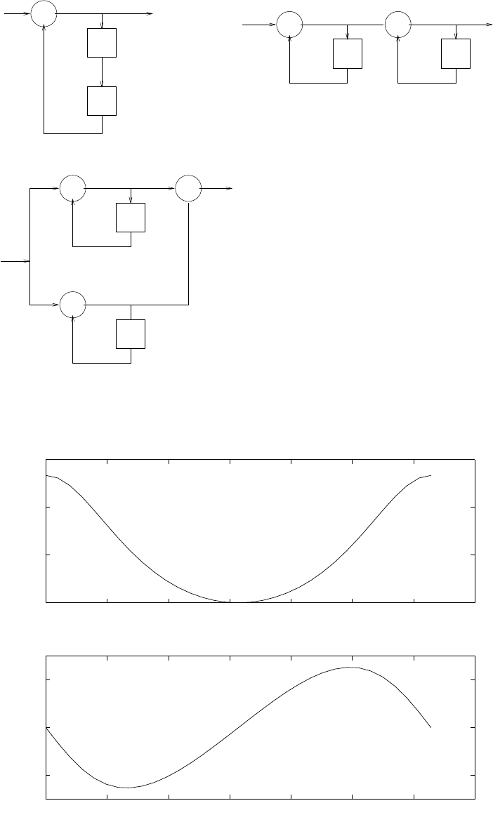
+
D
+
+
D
+
D
+
D
+
D
D
1/4
x(n) y(n)
Direct form 2
Parallel form
1/2
1/2
-1/2
y(n)
x(n)
x(n)
1/2 -1/2
y(n)
cascade form
1/2
Figure 9.8-1:
0 0.5 1 1.5 2 2.5 3 3.5
0.8
1
1.2
1.4 Magnitude of H(w)
−−−> w
−−−> |H(w)|
0 0.5 1 1.5 2 2.5 3 3.5
−0.2
0
0.2
Phase of H(w)
−−−> w
−−−> angle of H(w)
Figure 9.8-2:
266
© 2007 Pearson Education, Inc., Upper Saddle River, NJ. All rights reserved. This material is protected under all copyright laws
as they currently exist. No portion of this material may be reproduced, in any form or by any means, without permission in
writing from the publisher. For the exclusive use of adopters of the book Digital Signal Processing, Fourth Edition, by John G.
Proakis and Dimitris G. Manolakis. ISBN 0-13-187374-1.
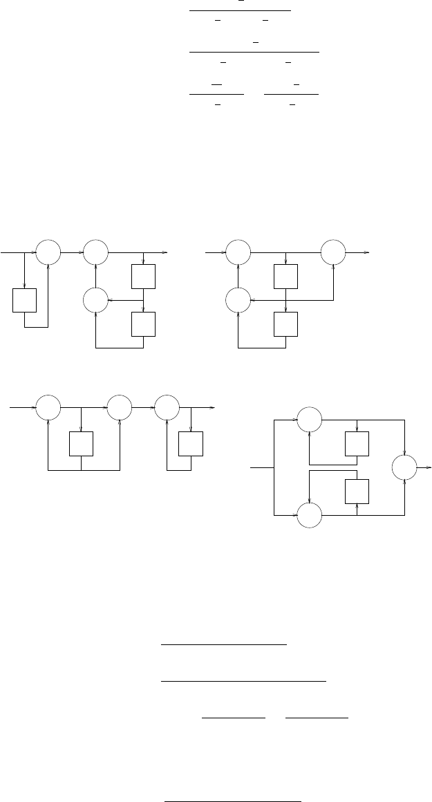
9.9
(a)
H(z) = 1 + 1
3z−1
1−3
4z−1+1
8z−2
=1 + 1
3z−1
(1 −1
2z−1)(1 −1
4z−1)
=
10
3
1−1
2z−1+−7
3
1−1
4z−1
Refer to fig 9.9-1
(b)
+
z-1
+
+
z-1
z-1
+
+
z-1
z-1
+
+ + +
z-1
z-1
+
z-1
z-1
+
+
Direct form I:
1/3
y(n)
x(n)
Direct form II:
3/4
-1/8
3/4
-1/8
y(n)
1/3
Cascade:
y(n)
1/2 1/3 1/4
x(n)
Parallel:
1/4
1/2
10/3
-7/3
x(n) y(n)
x(n)
Figure 9.9-1:
H(z) = 0.7(1 −0.36z−2)
1 + 0.1z−1−0.72z−2
=0.7(1 −0.6z−1)(1 + 0.6z−1)
(1 + 0.9z−1)(1 −0.8z−1)
= 0.35 −0.1647
1 + 0.9z−1−0.1853
1−0.8z−1
Refer to fig 9.9-2
(c)
H(z) = 3(1 + 1.2z−1+ 0.2z−2)
1 + 0.1z−1−0.2z−2
267
© 2007 Pearson Education, Inc., Upper Saddle River, NJ. All rights reserved. This material is protected under all copyright laws
as they currently exist. No portion of this material may be reproduced, in any form or by any means, without permission in
writing from the publisher. For the exclusive use of adopters of the book Digital Signal Processing, Fourth Edition, by John G.
Proakis and Dimitris G. Manolakis. ISBN 0-13-187374-1.

+ +
+
z-1
z-1
+
+
z-1
z-1
+
+ + +
z-1
z-1
+
z-1
z-1
+
+
z-1
z-1
+
Direct form I:
y(n)
x(n)
Direct form II:
y(n)
Cascade:
x(n)
x(n) y(n)
-0.36
-0.1
0.72
-0.1
0.72 -0.36
0.7
x(n)
-0.9 -0.6 0.8 0.6
0.7 y(n)
Parallel:
0.8
-0.9
0.35
-0.1853
0.1647
Figure 9.9-2:
=3(1 + 0.2z−1)(1 + z−1)
(1 + 0.5z−1)(1 −0.4z−1)
=−3 + 7
1−0.4z−1−1
1 + 0.5z−1
Refer to fig 9.9-3
(d)
H(z) = 2(1 −z−1)(1 + √2z−1+z−2)
(1 + 0.5z−1)(1 −0.9z−1+ 0.8z−2)
=2 + (2√2−2)z−1+ (2 −2√2)z−2−2z−3)
1−0.4z−1+ 0.36z−2+ 0.405z−3
=A
1 + 0.5z−1+B+Cz−1
1−0.9z−1+ 0.8z−1
Refer to fig 9.9-4
(e)
H(z) = 1 + z−1
1−1
2z−1−1
4z−2
=1 + z−1
(1 −0.81z−1)(1 + 0.31z−1)
=1.62
1−0.81z−1+−0.62
1 + 0.31z−1
Refer to fig 9.9-5
(f) H(z) = 1−z−1+z−2
1−z−1+0.5z−2⇒Complex valued poles and zeros.Refer to fig 9.9-6 All the above
268
© 2007 Pearson Education, Inc., Upper Saddle River, NJ. All rights reserved. This material is protected under all copyright laws
as they currently exist. No portion of this material may be reproduced, in any form or by any means, without permission in
writing from the publisher. For the exclusive use of adopters of the book Digital Signal Processing, Fourth Edition, by John G.
Proakis and Dimitris G. Manolakis. ISBN 0-13-187374-1.
+ +
+
z-1
z-1
+
+
z-1
z-1
+
+ + +
z-1
z-1
+
z-1
z-1
+
+
+
z-1
z-1
++
Direct form I:
y(n)
Direct form II:
y(n)
Cascade:
x(n)
x(n) y(n)
-0.1 -0.1
x(n)
y(n)
Parallel:
-0.5 0.2 0.4 1
3
7
-3
-1
-0.5
0.4
x(n)
1.2
0.2 0.2
3
0.2 0.2
1.2
3
Figure 9.9-3:
systems are stable.
269
© 2007 Pearson Education, Inc., Upper Saddle River, NJ. All rights reserved. This material is protected under all copyright laws
as they currently exist. No portion of this material may be reproduced, in any form or by any means, without permission in
writing from the publisher. For the exclusive use of adopters of the book Digital Signal Processing, Fourth Edition, by John G.
Proakis and Dimitris G. Manolakis. ISBN 0-13-187374-1.
+ + +
z-1
+
+ +
+
z-1
z-1
z-1
z-1
+
z-1
+ +
z-1
2
2
+
+
z-1
z-1
+
+
+ +
z-1
2 -1
1- 2
z-1
+
z-1
+
+
z-1
z-1
+
+
z-1
+
+
Direct form I: Direct form II:
x(n)
Cascade:
y(n)
-0.5
y(n)
x(n) 3
Parallel:
0.4
-0.36
-0.405
-1
1-
-1
y(n)x(n) 3
0.4
-0.36
-0.405 -1
2
-1 0.91.414
-0.81 1
x(n) -3 y(n)
-0.8
0.9 C
B
A
-0.5
Figure 9.9-4:
+
z-1
+
+
z-1
z-1
+
+
z-1
z-1
+
+ + +
z-1
z-1
+
z-1
z-1
+
+
Direct form I:
y(n)
x(n)
Direct form II:
y(n)
Cascade:
y(n)x(n)
Parallel:
x(n) y(n)
1/2
1/4
1/2
1/4
1
x(n)
0.81 1-0.31 0.81
-0.3
-0.62
1.62
Figure 9.9-5:
270
© 2007 Pearson Education, Inc., Upper Saddle River, NJ. All rights reserved. This material is protected under all copyright laws
as they currently exist. No portion of this material may be reproduced, in any form or by any means, without permission in
writing from the publisher. For the exclusive use of adopters of the book Digital Signal Processing, Fourth Edition, by John G.
Proakis and Dimitris G. Manolakis. ISBN 0-13-187374-1.
+ +
+
z-1
z-1
+
+
z-1
z-1
+
z-1
z-1
++
Direct form I:
y(n)x(n)
x(n)
-1
1
1
-1/2
1 -1
-0.5 1
Direct form II, cascade, parallel:
y(n)
Figure 9.9-6:
271
© 2007 Pearson Education, Inc., Upper Saddle River, NJ. All rights reserved. This material is protected under all copyright laws
as they currently exist. No portion of this material may be reproduced, in any form or by any means, without permission in
writing from the publisher. For the exclusive use of adopters of the book Digital Signal Processing, Fourth Edition, by John G.
Proakis and Dimitris G. Manolakis. ISBN 0-13-187374-1.

9.10
Refer to fig 9.10-1
+ + +
x(n) v(n) w(n) w(n-1) r sin w0y(n)
z-1
Figure 9.10-1:
H(z) = 1
1−2rcosw0z−1+r2z−2
(1) V(z) = X(z)−rsinw0z−1Y(z)
(2) W(z) = V(z)−rcosw0z−1W(z)
(3) Y(z) = rcosw0z−1Y(z)−rsinw0z−1W(z)
By combining (1) and (2) we obtain
(4) W(z) = 1
1−rcosw0z−1X(z)−rsinw0z−1
1−rcosw0z−1Y(z)
Use (4) to eliminate W(z) in (3). Thus,
Y(z)[(1 −rcosw0z−1)2+r2sin2w0z−2] = X(z)
Y(z)[1 −2rcosw0z−1+ (r2cos2w0+r2sin2w0)z−2] = X(z)
Y(z)
X(z)=1
1−2rcosw0z−1+r2z−2
9.11
A0(z) = B0(z) = 1
A1(z) = A0(z) + k1B0(z)z−1
= 1 + 1
2z−1
272
© 2007 Pearson Education, Inc., Upper Saddle River, NJ. All rights reserved. This material is protected under all copyright laws
as they currently exist. No portion of this material may be reproduced, in any form or by any means, without permission in
writing from the publisher. For the exclusive use of adopters of the book Digital Signal Processing, Fourth Edition, by John G.
Proakis and Dimitris G. Manolakis. ISBN 0-13-187374-1.
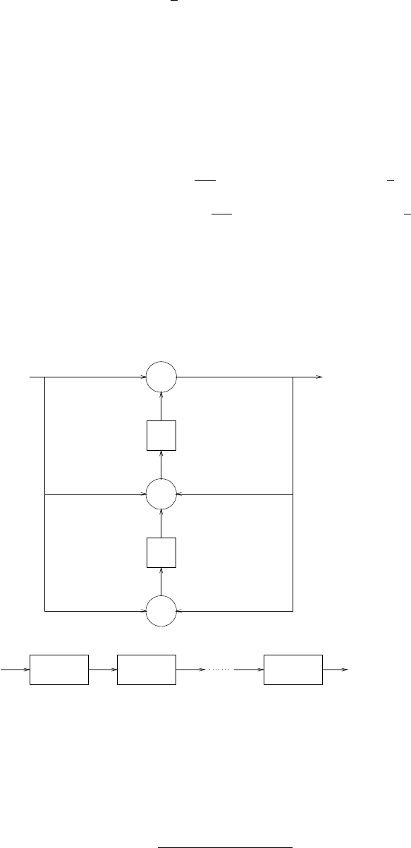
B1(z) = 1
2+z−1
A2(z) = A1(z) + k2B1(z)
= 1 + 0.3z−1+ 0.6z−2
B2(z) = 0.6 + 0.3z−1+z−2
A3(z) = A2(z) + k3B2(z)
= 1 −0.12z−1+ 0.39z−2−0.7z−3
B3(z) = −0.7 + 0.39z−1−0.12z−2+z−3
A4(z) = A3(z) + k4B3(z)
= 1 −53
150z−1+ 0.52z−2−0.74z−3+1
3z−4
Therefore, H(z) = C(1 −53
150z−1+ 0.52z−2−0.74z−3+1
3z−4)
where Cis a constant
9.12
Refer to fig 9.12-1
z-1
+
z-1
+
+
b0k
b1k
b2k
-a
1k
-a2k
w2k(n)
w1k (n)
y
k(n)
k
(n)x
x(n) =
x
1
(n) H1(z) H2
(z) x
N(n) HN(z) y(n)=y
N(n)
Figure 9.12-1:
Hk(z) = b0k+b1kz−1+b2kz−2
1 + a1kz−1+a2kz−2
yk(n) = b0kxk(n) + w1k(n−1)
273
© 2007 Pearson Education, Inc., Upper Saddle River, NJ. All rights reserved. This material is protected under all copyright laws
as they currently exist. No portion of this material may be reproduced, in any form or by any means, without permission in
writing from the publisher. For the exclusive use of adopters of the book Digital Signal Processing, Fourth Edition, by John G.
Proakis and Dimitris G. Manolakis. ISBN 0-13-187374-1.

w1k(n) = b1kx(n)−a1kyk(n) + w2k(n−1)
w2k(n) = b2kx(n)−a2kyk(n)
9.13
YJM1 = G * XIN
DO 20 J=1,K
YJ=B(J,0) * XIN + W1(J)
W1(J) = B(J,1)*XIN - A(J,1)*YJ + W2(J)
W2(J) = B(J,2)*XIN - A(J,2)*YJ
YJM1 = YJM1 + YJ
20 CONTINUE YOUT = YJM1 RETURN
9.14
YJM1 = XIN
DO 20 J=1,K
W = -A(J,1) * WOLD1 - A(J,2) * WOLD2 + YMJ1
YJ = W + B(J,1)*WOLD1 + B(J,2)*WOLD2
WOLD2 = WOLD1
WOLD1 = W
YJM1 = YJ
20 CONTINUE
YOUT = YJ
RETURN
9.15
H(z) = A2(z) = 1 + 2z−1+1
3z−2
B2(z) = 1
3+ 2z−1+z−2
k2=1
3
A1(z) = A2(z)−k2B2(z)
1−k2
2
= 1 + 3
2z−1
k1=3
2
9.16
(a) A1(z)
B1(z)=1k1
k11 1
z−1=1 + 1
2z−1
1
2+z−1
A2(z)
B2(z)=1−1
3
−1
31 A1(z)
z−1B1(z)=1 + 1
3z−1−1
3z−2
−1
3+1
3z−1+z−2
274
© 2007 Pearson Education, Inc., Upper Saddle River, NJ. All rights reserved. This material is protected under all copyright laws
as they currently exist. No portion of this material may be reproduced, in any form or by any means, without permission in
writing from the publisher. For the exclusive use of adopters of the book Digital Signal Processing, Fourth Edition, by John G.
Proakis and Dimitris G. Manolakis. ISBN 0-13-187374-1.
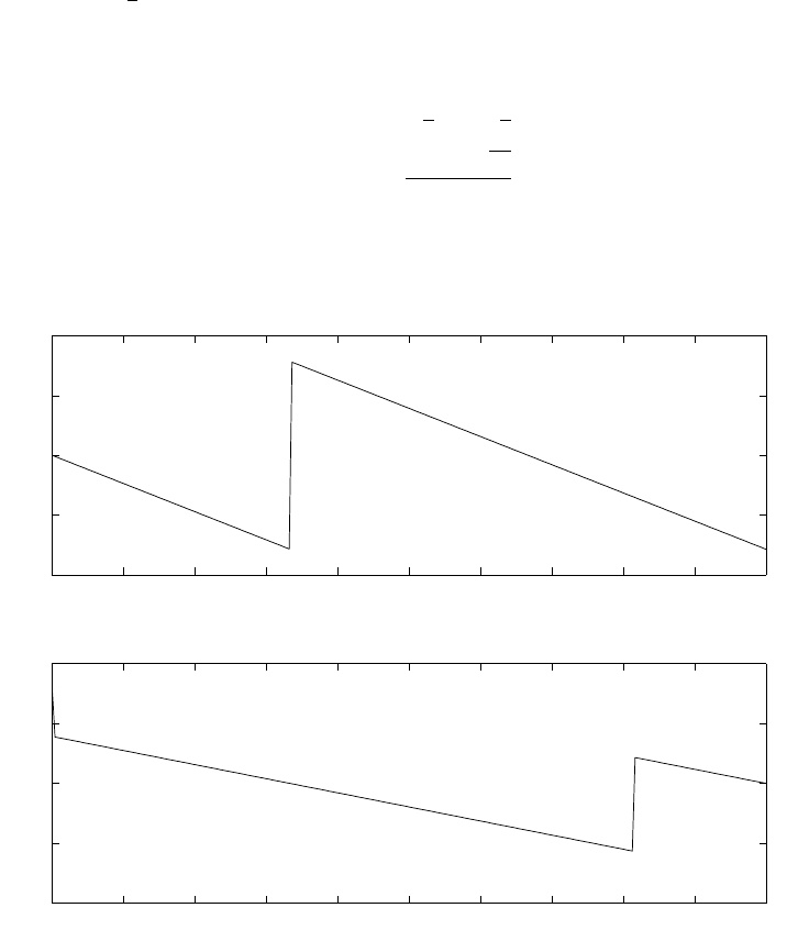
A3(z)
B3(z)=1 1
1 1 A2(z)
z−1B2(z)
H1(z) = A3(z) = 1 + z−3⇒
zeros at z=−1, e±jπ
3
(b)
H2(z) = A2(z)−z−1B2(z)
= 1 + 2
3z−1−2
3z−2−z−3
The zeros are z= 1,−5±j√11
6
(c) If the magnitude of the last coefficient |kN|= 1, i.e., kN=±1, all the zeros lie on the unit
circle.
(d) Refer to fig 9.16-1. We observe that the filters are linear phase filters with phase jumps at
0 0.05 0.1 0.15 0.2 0.25 0.3 0.35 0.4 0.45 0.5
−2
−1
0
1
2
−−−> freq(Hz)
−−−> phase of H1(w)
0 0.05 0.1 0.15 0.2 0.25 0.3 0.35 0.4 0.45 0.5
−4
−2
0
2
4
−−−> freq(Hz)
−−−> phase of H2(w)
Figure 9.16-1:
the zeros of H(z).
9.17
(a) Refer to fig 9.17-1
275
© 2007 Pearson Education, Inc., Upper Saddle River, NJ. All rights reserved. This material is protected under all copyright laws
as they currently exist. No portion of this material may be reproduced, in any form or by any means, without permission in
writing from the publisher. For the exclusive use of adopters of the book Digital Signal Processing, Fourth Edition, by John G.
Proakis and Dimitris G. Manolakis. ISBN 0-13-187374-1.
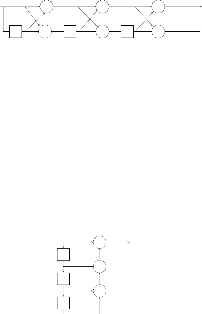
z-1 + z-1 +
++
z-1
+
+
x(n) f1
(n) f2
(n) f3
(n) = y(n)
g3(n)
g2(n)g
1(n)
0.65 -0.34 0.8
Figure 9.17-1:
x(n) = δ(n)
f1(n) = δ(n) + 0.65δ(n−1)
g1(n) = 0.65δ(n) + δ(n−1)
f2(n) = f1(n)−0.34g1(n−1)
=δ(n) + 0.429δ(n−1) −0.34δ(n−2)
g2(n) = −0.34f1(n) + g1(n−1)
=−0.34δ(n) + 0.429δ(n−1) + δ(n−2)
h(n) = f3(n) = f2(n) + 0.8g2(n−1)
=δ(n) + 0.157δ(n−1) + 0.0032δ(n−2) + 0.8δ(n−3)
(b) H(z) = 1 + 0.157z−1+ 0.0032z−2+ 0.8z−3. Refer to fig 9.17-2
z-1
+
+
z-1
+
z-1
0.157
0.0032
0.8
x(n) y(n)
Figure 9.17-2:
276
© 2007 Pearson Education, Inc., Upper Saddle River, NJ. All rights reserved. This material is protected under all copyright laws
as they currently exist. No portion of this material may be reproduced, in any form or by any means, without permission in
writing from the publisher. For the exclusive use of adopters of the book Digital Signal Processing, Fourth Edition, by John G.
Proakis and Dimitris G. Manolakis. ISBN 0-13-187374-1.

9.18
(a)
H(z) = C3(z)
A3(z)
A3(z) = 1 + 0.9z−1−0.8z−2+ 0.5z−3
B3(z) = 0.5−0.8z−1+ 0.9z−2+z−3
k3= 0.5
A2(z) = A3(z)−k3B3(z)
1−k2
3
= 1 + 1.73z−1−1.67z−2
B2(z) = −1.67 + 1.73z−1+z−2
k2=−1.67
A1(z) = A2(z)−k2B2(z)
1−k2
2
= 1 + 1.62z−1
B1(z) = 1.62 + z−1
k1= 1.62
C3(z) = 1 + 2z−1+ 3z−2+ 2z−3
D3(z) = 2 + 3z−1+ 2z−2+z−3
k3= 2
C2(z) = C3(z)−k3D3(z)
1−k2
3
= 1 + 4
3z−1+1
3z−2
D2(z) = 1
3+4
3z−1+z−2
k2=1
3
C1(z) = C2(z)−k2D2(z)
1−k2
2
= 1 + 3
4z−1
D1(z) = 3
4+z−1
k1=3
4
C3(z) = v0+v1D1(z) + v2D2(z) + v3D3(z)
= 1 + 2z−1+ 3z−2+ 2z−3
From the equations, we obtain
v0=−107
48
v1=−13
4
v2=−1
v3= 2
277
© 2007 Pearson Education, Inc., Upper Saddle River, NJ. All rights reserved. This material is protected under all copyright laws
as they currently exist. No portion of this material may be reproduced, in any form or by any means, without permission in
writing from the publisher. For the exclusive use of adopters of the book Digital Signal Processing, Fourth Edition, by John G.
Proakis and Dimitris G. Manolakis. ISBN 0-13-187374-1.

The equivalent lattice-ladder structure is: Refer to fig 9.18-1
(b) A3(z) = 1 + 0.9z−1−0.8z−2+ 0.5z−3,|k1|>1 and |k2|>1⇒the system is unstable.
+
+ z -1
+
+ z -1
+
+ z -1
+ + +
0.5 -1.67 1.62
v3= 2 v2=-1 v1= -13/4 v0=-107/48
x(n)
y(n)
Figure 9.18-1:
9.19
Refer to fig 9.19-1
Y(z) = [rsinΘX(z) + rcosΘY(z)−rsinΘC(z)] z−1
C(z) = [−rcosΘX(z) + rsinΘY(z) + rcosΘC(z)] z−1
H(z) = Y(z)
X(z)
=rsinΘz−1
1−2rcosΘz−1+r2z−2
Hence, h(n) = rnsin(Θn)u(n)
and y(n) = rsinΘx(n−1) + 2rcosΘy(n−1) −r2y(n−2)
The system has a zero at z= 0 and poles at z=re±jΘ.
9.20
H(z) = 1
1−2rcosw0z−1+r2z−2
= 1 + rcosw0−jrcos2w0
2sinw0
z−(rcosw0+jrsinw0)+rcosw0+jrcos2w0
2sinw0
z−(rcosw0−jrsinw0)
S(z) = rcosw0−jrcos2w0
2sinw0
z−(rcosw0+jrsinw0)X(z)
278
© 2007 Pearson Education, Inc., Upper Saddle River, NJ. All rights reserved. This material is protected under all copyright laws
as they currently exist. No portion of this material may be reproduced, in any form or by any means, without permission in
writing from the publisher. For the exclusive use of adopters of the book Digital Signal Processing, Fourth Edition, by John G.
Proakis and Dimitris G. Manolakis. ISBN 0-13-187374-1.
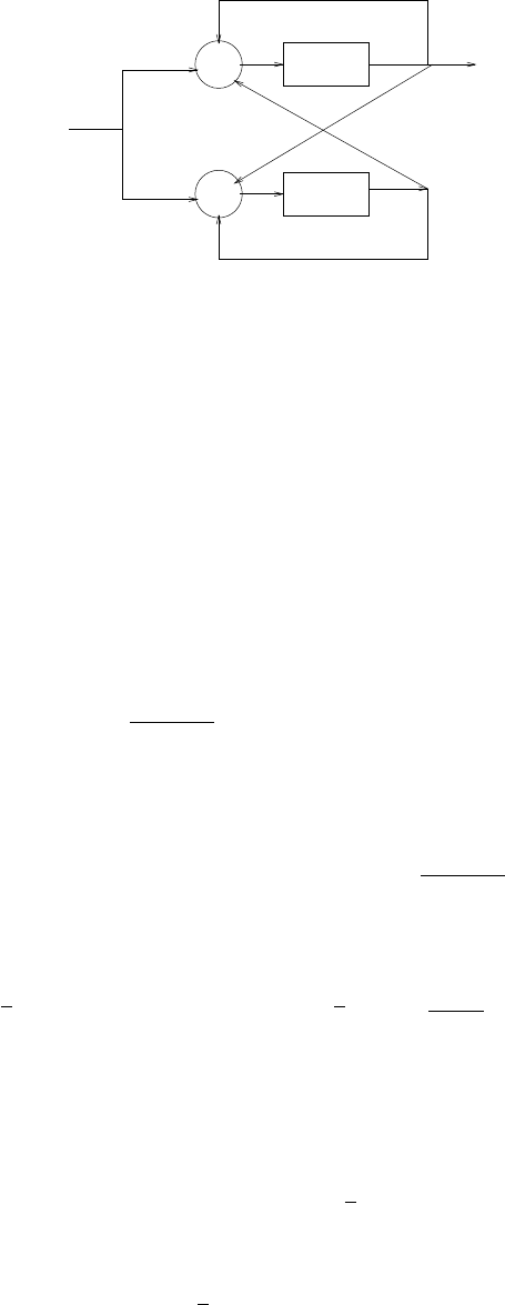
+ z-1
+ z-1
x(n)
-r cos θ
r cos
r cos
r sin y(n)
r sin
-r sin
c(n)
θ
θ
θ
θ
θ
Figure 9.19-1:
s(n) = v1(n) + jv2(n)
p=α1+jα2
⇒α1=rcosw0
α2=rsinw0
A=q1+jq2
⇒q1=rcosw0
q2=−rcosw0
2sinw0
v1(n+ 1) = α1v1(n)−α2v2(n) + q1x(n)
=rcosw0v1(n)−rsinw0v2(n) + rcosw0x(n)
v2(n) = α2v1(n) + α1v2(n) + q2x(n)
=rsinw0v1(n) + rcosw0v2(n) + −rcosw0
2sinw0
x(n)
or, equivalently,
v(n+ 1) = rcosw0−rsinw0
rsinw0rcosw0v(n) + rcosw0
rcosw0
2sinw0x(n)
y(n) = s(n) + s∗(n) + x(n)
= 2v1(n) + x(n)
or, equivalently,
y(n) = [2 0]v(n) + x(n)
where
v(n) = v1(n)
v2(n)
279
© 2007 Pearson Education, Inc., Upper Saddle River, NJ. All rights reserved. This material is protected under all copyright laws
as they currently exist. No portion of this material may be reproduced, in any form or by any means, without permission in
writing from the publisher. For the exclusive use of adopters of the book Digital Signal Processing, Fourth Edition, by John G.
Proakis and Dimitris G. Manolakis. ISBN 0-13-187374-1.
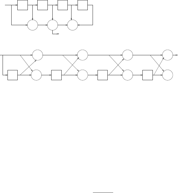
9.21
(a)
k1= 0.6
A1(z) = 1 + 0.6z−1
B1(z) = 0.6 + z−1
A2(z) = A1(z) + k2B1(z)z−1
= 1 + 0.78z−1+ 0.3z−2
B2(z) = 0.3 + 0.78z−1+z−2
A3(z) = A2(z) + k3B2(z)z−1
= 1 + 0.93z−1+ 0.69z−2+ 0.5z−3
B3(z) = 0.5 + 0.69z−1+ 0.93z−2+z−3
H(z) = A4(z) = A3(z) + k4B3(z)z−1
= 1 + 1.38z−1+ 1.311z−2+ 1.337z−3+ 0.9z−4
(b) Refer to fig 9.21-1
+
z-1
z-1 + z-1 ++ z-1
+ ++
z-1 z-1 z-1
++
1
x(n)
z-1
+
+
x(n)
Direct form:
Lattice form:
1.38 1.311 1.337 0.9
y(n)
0.6 0.3 0.5 0.9
--- -
y(n)
Figure 9.21-1:
9.22
(a)
From (9.3.38) we have
y(n) = −k1(1 + k2)y(n−1) −k2y(n−2) + x(n)
But, y(n) = 2rcosw0y(n−1) −r2y(n−2) + x(n)
Hence, k2=r2
and, k1(1 + k2) = −2rcosw0
k1+−2rcosw0
1 + r2
280
© 2007 Pearson Education, Inc., Upper Saddle River, NJ. All rights reserved. This material is protected under all copyright laws
as they currently exist. No portion of this material may be reproduced, in any form or by any means, without permission in
writing from the publisher. For the exclusive use of adopters of the book Digital Signal Processing, Fourth Edition, by John G.
Proakis and Dimitris G. Manolakis. ISBN 0-13-187374-1.

Refer to fig 9.22-1
(b) When r= 1, the system becomes an oscillator.
+
+ z -1
+
+ z -1
x(n)
- -
y(n)
k k12
Figure 9.22-1:
9.23
H(z) = 1−0.8z−1+ 0.15z−2
1 + 0.1z−1−0.72z−2
=B(z)
A(z)
For the all-pole system 1
A(z),we have
k1(1 + k2) = 0.1
k2=−0.72
⇒k1= 0.357
k2= 0.72
For the all-zero system, C2(z) = 1 −0.8z−1+ 0.15z−2
A2(z) = 1 −0.8z−1+ 0.15z−2
B2(z) = 0.15 −0.8z−1+z−2
k2= 0.15
A1(z) = A2(z)−k2B2(z)
1−k2
2
= 1 −0.696z−1
B1(z) = −0.696 + z−1
k1=−0.696
A0(z) = B0(z) = 1
281
© 2007 Pearson Education, Inc., Upper Saddle River, NJ. All rights reserved. This material is protected under all copyright laws
as they currently exist. No portion of this material may be reproduced, in any form or by any means, without permission in
writing from the publisher. For the exclusive use of adopters of the book Digital Signal Processing, Fourth Edition, by John G.
Proakis and Dimitris G. Manolakis. ISBN 0-13-187374-1.
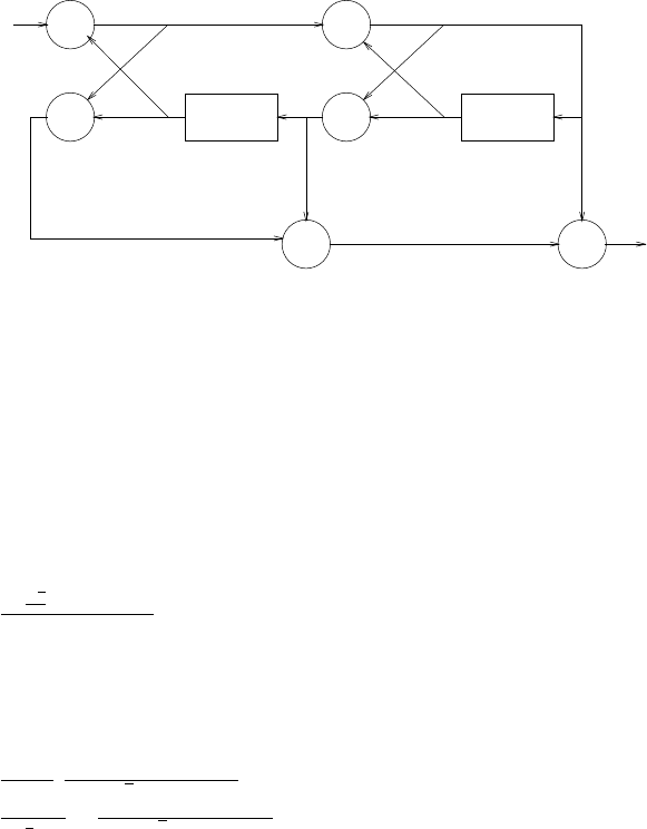
C2(z) =
2
X
m=0
vmBm(z)
=v0+v1B1(z) + v2B2(z)
= 1 −0.8z−1+ 0.15z−2
The solution is:
v2= 0.15
v1−0.18v2=−0.8
v0−0.696v1+ 0.15v2= 1
⇒v0= 1.5
v1=−0.68
v2= 0.15
Thus the lattice-ladder structure is: Refer to fig 9.23-1
+
+ z -1
+
+ z -1
+ +
x(n)
- -
0.15 -0.696
v2= 0.15 v1= -0.68 v0= 1.5
y(n)
Figure 9.23-1:
9.24
H(z) = 1−√2
2z−1+0.25z−2
1−0.8z−1+0.64z−2. Refer to fig 9.24-1
9.25
H(z) = 1+z−1
1−z−1.1
1−0.8√2z−1+0.64z−2
H(z) = 2.31
1−1
2z−1+−1.31+2.96z−1
1−0.8√2z−1+0.64z−2Refer to fig 9.25-1
282
© 2007 Pearson Education, Inc., Upper Saddle River, NJ. All rights reserved. This material is protected under all copyright laws
as they currently exist. No portion of this material may be reproduced, in any form or by any means, without permission in
writing from the publisher. For the exclusive use of adopters of the book Digital Signal Processing, Fourth Edition, by John G.
Proakis and Dimitris G. Manolakis. ISBN 0-13-187374-1.
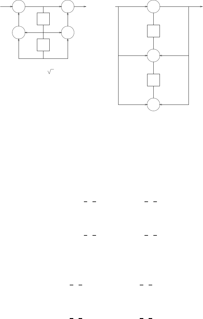
+
D
+
+ +
D
+
D
+
D
+
Direct form II :
a b
cd
y(n)
x(n)
where a=0.8, b = - 2 /2, c = 0.25 and d = -0.64
Transposed form :
b a
d
c
x(n) y(n)
Figure 9.24-1:
9.26
(a)
For positive numbers, range is
01.00 ...0
|{z }
11 ×21001 −01.11 ...1
|{z }
11 ×20111
or 7.8125 ×10⁻³−2.5596875 ×10²
negitive numbers
10.11 ...1
|{z }
11 ×21001 −10.00 ...0
|{z }
11 ×20111
or −7.8163 ×10⁻³− −2.56 ×10²
(b)
For positive numbers, range is
01.00 ...0
|{z }
23 ×210000001 −01.11 ...1
|{z }
23 ×201111111
or 5.8774717 ×10−39 −3.4028234 ×1038
negitive numbers
10.11 ...1
|{z }
23 ×210000001 −10.00 ...0
| {z }
23 ×201111111
or −5.8774724 ×10−39 − −3.4028236 ×1038
283
© 2007 Pearson Education, Inc., Upper Saddle River, NJ. All rights reserved. This material is protected under all copyright laws
as they currently exist. No portion of this material may be reproduced, in any form or by any means, without permission in
writing from the publisher. For the exclusive use of adopters of the book Digital Signal Processing, Fourth Edition, by John G.
Proakis and Dimitris G. Manolakis. ISBN 0-13-187374-1.
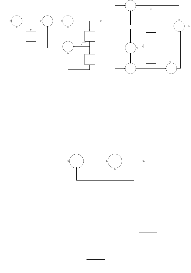
+ + +
z-1
+
z-1
z-1
+
z-1
z-1
+
+
z-1
+
+y(n)
Parallel:
x(n) 0.5
-0.64
0.8 2.96
-1.31
2.31
2
x(n)
Cascade:
1/2 1
y(n)
0.8 2
-0.64
Figure 9.25-1:
9.27
(a) Refer to fig 9.27-1
x(n) y(n)
z-1 z-1
-a 1-a 2
+ +
Figure 9.27-1:
HR(z) = (1 + a1z−1+a2z−2)−1
poles zp1,2=−a1±pa2
1−4a2
2
for stability
(i)a2
1−4a2≥0
if a1≥0,−a1−pa2
1−4a2
2≥ −1
⇒qa2
1−4a2≤2−a1
⇒a1≤2 and a1−a2≤1
284
© 2007 Pearson Education, Inc., Upper Saddle River, NJ. All rights reserved. This material is protected under all copyright laws
as they currently exist. No portion of this material may be reproduced, in any form or by any means, without permission in
writing from the publisher. For the exclusive use of adopters of the book Digital Signal Processing, Fourth Edition, by John G.
Proakis and Dimitris G. Manolakis. ISBN 0-13-187374-1.
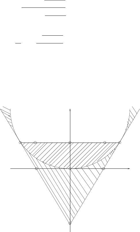
if a1<0,−a1−pa2
1−4a2
2≤1
⇒qa2
1−4a2≤2 + a1
⇒a1≥ −2 and a1+a2≥ −1
(ii)(−a1
2)2+ (p4a2−a2
1
2)≤1
a2≤1
Refer to fig 9.27-2. The region of stability in the a1−a2plane is shaded in the figure. There are
-1-2 1 2
a2
a1
-1
2
1
The stable area of (a
1, a2)
Figure 9.27-2:
nine integer pairs (a1, a2) which satisfy the stability conditions. These are (with corresponding
system functions):
(0,−1) HR1(z) = (1 −z−2)−1
(0,0) HR2(z) = 1
(0,1) HR3(z) = (1 + z−2)−1
(1,0) HR4(z) = (1 + z−1)−1
(1,1) HR5(z) = (1 + z−1+z−2)−1
(2,1) HR6(z) = (1 + 2z−1+z−2)−1
(−1,0) HR7(z) = (1 −z−1)−1
(−1,1) HR8(z) = (1 −z−1+z−2)−1
(−2,1) HR9(z) = (1 −2z−1+z−2)−1
285
© 2007 Pearson Education, Inc., Upper Saddle River, NJ. All rights reserved. This material is protected under all copyright laws
as they currently exist. No portion of this material may be reproduced, in any form or by any means, without permission in
writing from the publisher. For the exclusive use of adopters of the book Digital Signal Processing, Fourth Edition, by John G.
Proakis and Dimitris G. Manolakis. ISBN 0-13-187374-1.
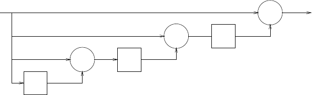
(b)
HR1(z) = HR4(z)HR7(z)
HR6(z) = HR4(z)HR4(z)
HR9(z) = HR7(z)HR7(z)
(c) Only the following cases can make h(n) FIR:
(i)
hR(n) = δ(n)
Then H(z) =
N
X
i=0
z−i
y(n) =
N
X
i=0
x(n−i)
(ii)
hR(n)∗hF(n) = δ(n)
Then H(z) = 1
y(n) = x(n)
(d) see above.
9.28
Refer to fig 9.28-1
Note that 4 multiplications and 3 additions are required to implement H1(z). The advantage
z-1
+ z-1
+ z-1
+
x(n) b
0
b1
b2
b3
Figure 9.28-1: Structure of H1(z)
of Horner’s method is in evaluating H1(z) for a specific z0. Thus, if
H1(z) = b0+b0b1z−1+b0b1b2z−2+b0b1b2b3z−3
=b0+z−1(b0b1+z−1(b0b1b2+z−1b0b1b2b3))
286
© 2007 Pearson Education, Inc., Upper Saddle River, NJ. All rights reserved. This material is protected under all copyright laws
as they currently exist. No portion of this material may be reproduced, in any form or by any means, without permission in
writing from the publisher. For the exclusive use of adopters of the book Digital Signal Processing, Fourth Edition, by John G.
Proakis and Dimitris G. Manolakis. ISBN 0-13-187374-1.

the 3 multiplications and 3 additions are required for the evaluation of 9.1 in the field of z.
If the various powers of zare prestored, then Horner’s scheme has no advantage over the direct
evaluation of 9.1. Refer to fig 9.28-2
This requires 4 multiplications and 3 additions. The linear-phase system is written as
+z-1
z-1
z-1
z-1 +z-1
+
z-1
b3b2
b1
b
0
Figure 9.28-2: Structure of H(z) = b0z−3+b0b1z−2+b0b1b2z−1+b0b1b2b3
H(z) = z2a3+za2+a1+z−1a0+z−2a1+z−3a2+z−4a3
By applying Horner’s scheme, we can rewrite this as
H(z) = z3(a3+z−1(a2+z−1(a1+z−1(a0+z−1(a1+z−1(a2+z−1a3))))))
Assuming that z−1and zare given, a direct evaluation of H(z) at z=z0requires 8 multiplications
and 6 additions. Using Horner’s scheme based on 9.28, requires the same number of operations
as direct evaluation of H(z). Hence, Horner’s scheme does not offer any savings in computation.
9.29
(a) When x1and x2are positive, the result is obvious. If x1and x2are negative, let
x1=−0n1n2. . . nb
=−0n1n2. . . nb+ 0 0 0 ... 0 1
x2=−0m1m2. . . mb
=−1m1m2. . . mb+ 0 0 0 ... 0 1
x3=x1+x2
=−0n10... 0 + 0 m10... 0 + c
where c= 0 0 n2. . . nb+ 0 0 m2. . . mb+ 0 0 0 ... 0 1 0
If the sign changes, there are two possibilities
(i)n1=m1= 0
287
© 2007 Pearson Education, Inc., Upper Saddle River, NJ. All rights reserved. This material is protected under all copyright laws
as they currently exist. No portion of this material may be reproduced, in any form or by any means, without permission in
writing from the publisher. For the exclusive use of adopters of the book Digital Signal Processing, Fourth Edition, by John G.
Proakis and Dimitris G. Manolakis. ISBN 0-13-187374-1.

⇒n1=m1= 1
⇒ |x1|>1
2,|x2|>1
2
⇒ |x3|>1,overflow
(ii)(n1= 1, m1= 0, c = 0) or (n1= 0, m1= 1, c = 0)
⇒(|0n10... 0)10|>1
2or (|0m10. . . 0)10|>1
2
and |c10|>1
2
⇒ |x3|>1,overflow
(b)
x1= 0 1 0 0
x2= 0 1 1 0
x3=−0 1 1 0 = 1 0 1 0
x1+x2= 1 0 1 0,overflow
x1+x2+x3= 0 1 0 0,correct result
9.30
(a)
H(z) = −a+z−1
1−az−1
|H(ejw)|2=|−a+e−jw
1−ae−jw |2
=(−a+cosw)2+ (−sinw)2
(1 −acosw)2+ (asinw)2
=a2−2acosw + 1
1−2acosw +a2= 1 ∀w
(b) Refer to fig 9.30-1
(c) If |ˆa|=| − ˆa|, where ˆameans the quantized value of a, then the filter remains all-pass.
x(n) y(n)
z-1
a1
-a
+ +
Figure 9.30-1:
(d) Refer to fig 9.30-2
(e) Yes, it is still all-pass.
288
© 2007 Pearson Education, Inc., Upper Saddle River, NJ. All rights reserved. This material is protected under all copyright laws
as they currently exist. No portion of this material may be reproduced, in any form or by any means, without permission in
writing from the publisher. For the exclusive use of adopters of the book Digital Signal Processing, Fourth Edition, by John G.
Proakis and Dimitris G. Manolakis. ISBN 0-13-187374-1.

x(n) y(n)
a
z-1
z-1
+-
++
+
Figure 9.30-2:
9.31
(a) y(n) = 2(1
2)n−(1
4)nu(n)
(b) Quantization table
x > 1−1
32 x= 1
31
32 ≥x > 29
32 x=15
16
29
32 ≥x > 27
32 x=14
16
...
1
32 ≥x > 1
32 x=14
16
...
x < −1 + 1
32 x=−1
Therefore x(n) = 1
↑,4
16,1
16,0,...,0
y(n) = 8
16y(n−1) + x(n)
y(n) = 1
↑,12
16,7
16,3
16,1
16,0,0,...
(c)
y(n) = 1
↑,3
4,7
16,15
64,31
256,63
1024,...
y(n) = 1
↑,3
4,7
16,12
64,16
256,0,0,...
Errors occur when number becomes small.
289
© 2007 Pearson Education, Inc., Upper Saddle River, NJ. All rights reserved. This material is protected under all copyright laws
as they currently exist. No portion of this material may be reproduced, in any form or by any means, without permission in
writing from the publisher. For the exclusive use of adopters of the book Digital Signal Processing, Fourth Edition, by John G.
Proakis and Dimitris G. Manolakis. ISBN 0-13-187374-1.

9.32
y(n) = 0.999y(n−1) + e(n)
e(n) is white noise, uniformly distributed in the interval −1
29,1
29
Ey2(n)= 0.9992Ey2(n−1)+Ee2(n)
(1 −0.9992)Ey2(n)=Ee2(n)
=Z△
2
−△
2
1
△e2de
=△2
12 where △= 2−8
Therefore, Ey2(n)=1
12(1
28)21
1−0.9992
= 6.361x10⁻⁴
9.33
(a) poles zp1= 0.695, zp2= 0.180 Refer to fig 9.33-1
(b) Truncation
+
D
+
D
x(n) y(n)
0.695 0.18
Figure 9.33-1:
0.695 →5
8= 0.625
0.180 →1
8= 0.125
poles zp1= 0.625, zp2= 0.125
(c) Rounding
0.695 →6
8= 0.75
0.180 →1
8= 0.125
poles zp1= 0.75, zp2= 0.125
290
© 2007 Pearson Education, Inc., Upper Saddle River, NJ. All rights reserved. This material is protected under all copyright laws
as they currently exist. No portion of this material may be reproduced, in any form or by any means, without permission in
writing from the publisher. For the exclusive use of adopters of the book Digital Signal Processing, Fourth Edition, by John G.
Proakis and Dimitris G. Manolakis. ISBN 0-13-187374-1.
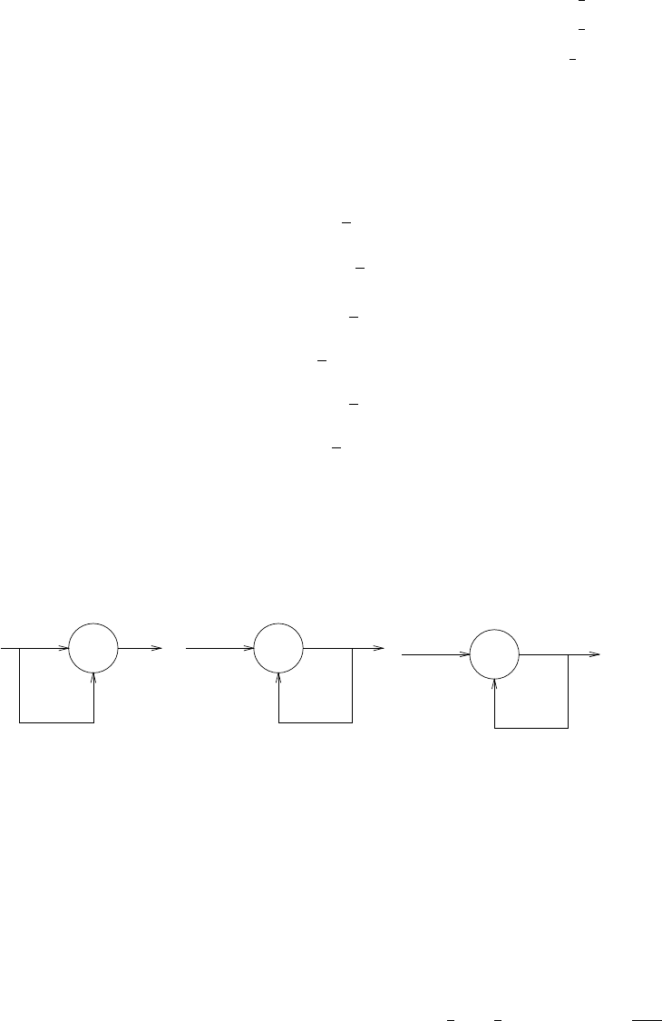
(d)
|0.75 −0.695|<|0.695 −0.625|
Rounding is better
|Ha(w)|= [(1.483 + 1.39cosw)(1.0324 + 0.36cosw)]−1
2
|Hb(w)|= [(1.391 + 1.25cosw)(1.0156 + 0.25cosw)]−1
2
|Hc(w)|= [(1.563 + 1.5cosw)(1.0156 + 0.25cosw)]−1
2
9.34
(a)
H1(z) = 1 −1
2z−1
h1(n) = 1,−1
2
H2(z) = (1 −1
4z−1)−1
h2(n) = (1
4)nu(n)
H3(z) = (1 + 1
4z−1)−1
h3(n) = (−1
4)nu(n)
Refer to fig 9.34-1 Cascade the three systems in six possible permutations to obtain six realiza-
+
z-1
H1(z)
+
z-1
1/4
H (z)
2
+
z-1
H (z)
3
-1/4
-1/2
Figure 9.34-1:
tions.
(b) Error sequence ei(n) is uniformly distributed over interval (1
22−b,1
22−b). So σ2
ei=2−2b
12 for
any i(call it σ2
e)
291
© 2007 Pearson Education, Inc., Upper Saddle River, NJ. All rights reserved. This material is protected under all copyright laws
as they currently exist. No portion of this material may be reproduced, in any form or by any means, without permission in
writing from the publisher. For the exclusive use of adopters of the book Digital Signal Processing, Fourth Edition, by John G.
Proakis and Dimitris G. Manolakis. ISBN 0-13-187374-1.

+++
+++
z-1 z-1 z -1
e1(n)
1/4-1/2 -1/4
e(n) e(n)
23
Figure 9.34-2:
(c) consider cascade H1-H2-H3Refer to fig 9.34-2
h4(n) = h2(n)∗h3(n)
=1,0,1
16,0,(1
16)2,0,...
σ2
q=σ2
e"2∞
X
n=0
h2
4(n) + ∞
X
n=0
h2
3(n)#
=σ2
e2
1−(1
16 )2+1
1−(1
4)2
= 3.0745σ2
e
using similar methods:
H1−H2−H3σ2
q= 3.0745σ2
e
H2−H1−H3σ2
q= 3.3882σ2
e
H2−H3−H1σ2
q= 3.2588σ2
e
H3−H1−H2σ2
q= 3.2627σ2
e
H3−H2−H1σ2
q= 3.3216σ2
e
9.35
y(n) = Q[0.1δ(n)] + Q[αy(n−1)]
(a)
y(n) = Q[0.1δ(n)] + Q[0.5y(n−1)]
y(0) = Q[0.1] = 1
8
292
© 2007 Pearson Education, Inc., Upper Saddle River, NJ. All rights reserved. This material is protected under all copyright laws
as they currently exist. No portion of this material may be reproduced, in any form or by any means, without permission in
writing from the publisher. For the exclusive use of adopters of the book Digital Signal Processing, Fourth Edition, by John G.
Proakis and Dimitris G. Manolakis. ISBN 0-13-187374-1.

y(1) = Q[1
16] = 0
y(2) = y(3) = y(4) = 0
no limit cycle
(b)
y(n) = Q[0.1δ(n)] + Q[0.75y(n−1)]
y(0) = Q[0.1] = 1
8
y(1) = Q[3
32] = 1
8
y(2) = Q[3
32] = 1
8
y(3) = y(4) = 1
8
limit cycle occurs
9.36
(a) σ2
x=rxx(0) = 3 ⇒Ax=1
√3
(b)
△= 2−6
σ2
e=△2
12
=1
12 ×212
so SNR = 10log10
1
σ2
e
= 10log10(12 ×212)
= 46.91dB
(c) left-justified.
(d)
σ2
q=σ2
e
∞
X
n=0
h2(n) + σ2
e1
∞
X
n=0
h2(n)
Now σ2
e1=1
12(1
28)2
and X
n
h2(n) = 1
1−0.752=16
7,
so σ2
q=16
71
12(1
28)2+1
12(1
26)2
=17
344,064
and SNR = 10log10
1
σ2
q
= 43.06dB
293
© 2007 Pearson Education, Inc., Upper Saddle River, NJ. All rights reserved. This material is protected under all copyright laws
as they currently exist. No portion of this material may be reproduced, in any form or by any means, without permission in
writing from the publisher. For the exclusive use of adopters of the book Digital Signal Processing, Fourth Edition, by John G.
Proakis and Dimitris G. Manolakis. ISBN 0-13-187374-1.

9.37
Define ρc△
=rcosθ, ρs△
=rsinθ for convenience, (a)
−ρsy(n−1) + e1(n) + x(n) + ρcv(n−1) + e2(n) = v(n)
ρsv(n−1) + e3(n) + ρcy(n−1) + e4(n) = y(n)
(b)
−ρsz−1Y(z) + E1(z) + X(z) + ρcz−1V(z) + E2(z) = V(z)
ρsz−1V(z) + E3(z) + ρcz−1Y(z) + E4(z) = Y(z)
Y(z) = ρsz−1
1−2ρcz−1+r2z−2[X(z) + E1(z) + E2(z)]
+1−ρcz−1
1−2ρcz−1+r2z−2[E3(z) + E4(z)]
=H1(z)X(z) + H1(z)[E1(z) + E2(z)]
+H2(z)[E3(z) + E4(z)]
when H1(z) and H2(z) are as defined in the problem statement
h1(n) = ρs
1
sinθ rn−1sinθnu(n−1)
=rnsin(nθ)u(n−1)
=rnsin(nθ)u(n)
h2(n) = 1
sinθ rnsin(n+ 1)θu(n) + ρc
1
sinθ rn−1sin(θn)u(n−1)
=δ(n) + rn
sinθ [sin(n+ 1)θ−cosθsin(nθ)]u(n−1)
=δ(n) + rncos(nθ)u(n−1)
=rncos(nθ)u(n)
(c)
σ2
e=σ2
e1=σ2
e2=σ2
e3=σ2
e4=△2
12
=1
12(2−b)2
=2−2b
12
σ2
q= 2σ2
e
∞
X
n=0
h2
1(n) + 2σ2
e
∞
X
n=0
h2
2(n)
= 2σ2
e
∞
X
n=0
[r2nsin2nθ +r2ncos2nθ]
= 2σ2
e
1
1−r2n
=2−2b
6
1
1−r2n
9.38
(a)
h1(n) = (1
2)nu(n)
294
© 2007 Pearson Education, Inc., Upper Saddle River, NJ. All rights reserved. This material is protected under all copyright laws
as they currently exist. No portion of this material may be reproduced, in any form or by any means, without permission in
writing from the publisher. For the exclusive use of adopters of the book Digital Signal Processing, Fourth Edition, by John G.
Proakis and Dimitris G. Manolakis. ISBN 0-13-187374-1.
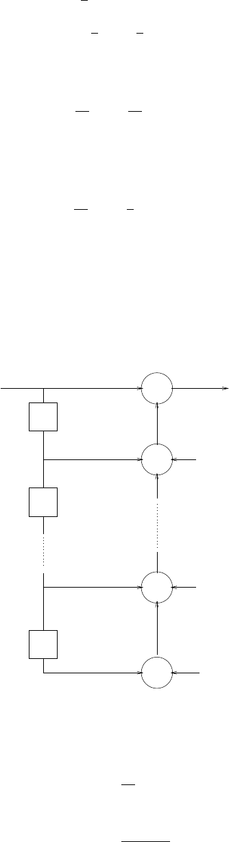
h2(n) = (1
4)nu(n)
h(n) = [2(1
2)n−(1
4)n]u(n)
σ2
q= 2σ2
e1
∞
X
n=0
h2
1(n) + 2σ2
e2
∞
X
n=0
h2
2(n)
=64
35σ2
e1+16
15σ2
e2
(b)
σ2
q=σ2
e1X
n
h2(n) + σ2
e2X
n
h2
1(n)
=64
35σ2
e1+4
3σ2
e2
9.39
Refer to fig 9.39-1
z-1
z-1
z-1
+
+
+
+
x(n) y(n)1
a1
aM-2
aM-1
e1(n)
eM-2 (n)
eM-1 (n)
Figure 9.39-1:
σ2
ei=1
122−2b∀i
σ2
q= (M−1)σ2
ei
=(M−1)
12 2−2b
295
© 2007 Pearson Education, Inc., Upper Saddle River, NJ. All rights reserved. This material is protected under all copyright laws
as they currently exist. No portion of this material may be reproduced, in any form or by any means, without permission in
writing from the publisher. For the exclusive use of adopters of the book Digital Signal Processing, Fourth Edition, by John G.
Proakis and Dimitris G. Manolakis. ISBN 0-13-187374-1.

9.40
H(z) = B(z)
A(z)
=G1
(1 −0.8ejπ
4)(1 −0.8e−jπ
4)
(1 −0.5z−1)(1 + 1
3z−1)
G2
(1 + 0.25z−1)(1 −5
8z−1)
(1 −0.8ejπ
3)(1 −0.8e−jπ
3)
=H1(z)H2(z)
(a)
z−1=e−jw
At w= 0, z−1= 1
H1(w)|w=0 = 1
G1
(1 −0.8ejπ
4)(1 −0.8e−jπ
4)
(1 −0.5)(1 + 1
3)= 1
G1= 1.1381
G2
(1 + 0.25)(1 −5
8)
(1 −0.8ejπ
3)(1 −0.8e−jπ
3)= 1
G2= 1.7920
(b) Refer to fig 9.40-1.
(c) Refer to fig 9.40-2.
Refer to fig 9.40-3.
Refer to fig 9.40-4.
296
© 2007 Pearson Education, Inc., Upper Saddle River, NJ. All rights reserved. This material is protected under all copyright laws
as they currently exist. No portion of this material may be reproduced, in any form or by any means, without permission in
writing from the publisher. For the exclusive use of adopters of the book Digital Signal Processing, Fourth Edition, by John G.
Proakis and Dimitris G. Manolakis. ISBN 0-13-187374-1.
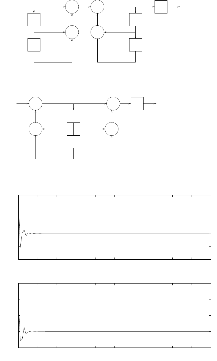
+
z-1
z-1
z-1
+
z-1
+
+
z-1
+
z-1
++
+
Direct for m I:
Direct form II and cascade structure:
-3/8
-5/32
x(n) 1
1/6
1/6
Gy(n)
-3/8
-5/32
Gy(n)
1/6
1/6
x(n)
Figure 9.40-1:
0 10 20 30 40 50 60 70 80 90 100
−1
−0.5
0
0.5
1
1.5
−−−> mag
Direct form I, impulse response
0 10 20 30 40 50 60 70 80 90 100
0.8
1
1.2
1.4
1.6
−−−> mag
Direct form I, step response
−−−> n
Figure 9.40-2:
297
© 2007 Pearson Education, Inc., Upper Saddle River, NJ. All rights reserved. This material is protected under all copyright laws
as they currently exist. No portion of this material may be reproduced, in any form or by any means, without permission in
writing from the publisher. For the exclusive use of adopters of the book Digital Signal Processing, Fourth Edition, by John G.
Proakis and Dimitris G. Manolakis. ISBN 0-13-187374-1.
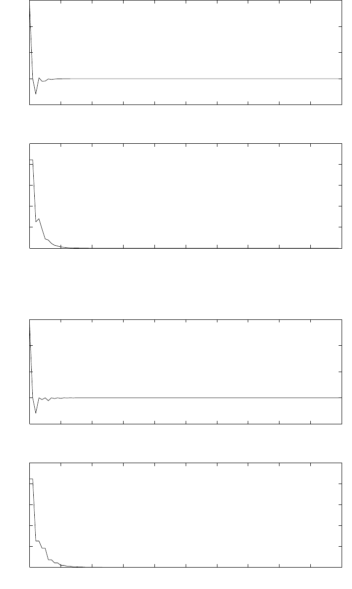
0 10 20 30 40 50 60 70 80 90 100
−0.5
0
0.5
1
1.5
−−−> mag
Direct form II, impulse response
0 10 20 30 40 50 60 70 80 90 100
1
1.1
1.2
1.3
1.4
1.5
−−−> mag
Direct form II, step response
−−−> n
Figure 9.40-3:
0 10 20 30 40 50 60 70 80 90 100
−0.5
0
0.5
1
1.5
−−−> mag
Cascade form , impulse response
0 10 20 30 40 50 60 70 80 90 100
1
1.1
1.2
1.3
1.4
1.5
−−−> mag
Cascade form, step response
−−−> n
Figure 9.40-4:
298
© 2007 Pearson Education, Inc., Upper Saddle River, NJ. All rights reserved. This material is protected under all copyright laws
as they currently exist. No portion of this material may be reproduced, in any form or by any means, without permission in
writing from the publisher. For the exclusive use of adopters of the book Digital Signal Processing, Fourth Edition, by John G.
Proakis and Dimitris G. Manolakis. ISBN 0-13-187374-1.
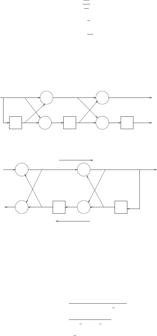
9.41
(a)
k1=−3
8
27
32
=−4
9
k2=−5
32
Refer to fig 9.41-1a.
(b)
+
z-1 + z-1
+
z-1
+
+ z-1 +
+
z-1
f (n)
1
k
2
k
1
k
2 k
1
f (n)
1f (n)
0
f (n)
0
+
f2(n) = y(n)
x(n)
(a)
--
y(n)
(n)
0
g
Forward
Reverse
(n)
f (n)
2
g
2
x(n)
(b)
Figure 9.41-1:
A(z) = 1
(1 −0.5z−1)(1 + 1
3z−1)
=1
1−1
6z−1−1
6z−2
k2=−1
6
299
© 2007 Pearson Education, Inc., Upper Saddle River, NJ. All rights reserved. This material is protected under all copyright laws
as they currently exist. No portion of this material may be reproduced, in any form or by any means, without permission in
writing from the publisher. For the exclusive use of adopters of the book Digital Signal Processing, Fourth Edition, by John G.
Proakis and Dimitris G. Manolakis. ISBN 0-13-187374-1.
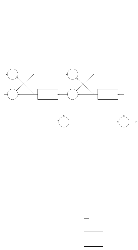
k1(1 + k2) = −1
6
k1=−1
5
Refer to fig 9.41-1b.
(c) Refer to fig 9.41-2.
(e) Refer to fig 9.41-3.
+
+ z -1
+
+ z -1
+ +
x(n)
- -
v2v1v0
y(n)
-1/6 -1/5
=-0.1563 =0.4336 =0.7829
Figure 9.41-2:
(f) Finite word length effects are visible in h(n) for part f.
9.42
Refer to fig 9.42-1.
c=15
16
H1(z) =
9
10
1−1
2z−1
H2(z) =
83
80
1 + 1
3z−1
300
© 2007 Pearson Education, Inc., Upper Saddle River, NJ. All rights reserved. This material is protected under all copyright laws
as they currently exist. No portion of this material may be reproduced, in any form or by any means, without permission in
writing from the publisher. For the exclusive use of adopters of the book Digital Signal Processing, Fourth Edition, by John G.
Proakis and Dimitris G. Manolakis. ISBN 0-13-187374-1.

0 50 100
−0.5
0
0.5
1IR for part a
h(n)
0 50 100
−0.5
0
0.5
1IR for part b
h(n)
0 50 100
−0.2
0
0.2
0.4
0.6
0.8 IR for part c
h(n)
−−> n 0 50 100
−0.5
0
0.5
1IR for part f
h(n)
−−> n
Figure 9.41-3:
301
© 2007 Pearson Education, Inc., Upper Saddle River, NJ. All rights reserved. This material is protected under all copyright laws
as they currently exist. No portion of this material may be reproduced, in any form or by any means, without permission in
writing from the publisher. For the exclusive use of adopters of the book Digital Signal Processing, Fourth Edition, by John G.
Proakis and Dimitris G. Manolakis. ISBN 0-13-187374-1.
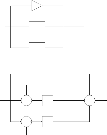
+ z -1
+ z -1
+
y(n)
c
H1(z)
H2(z)
x(n)
Parallel form structure:
Parallel form structure using 2nd-order coupled-form state-space sections
x(n)
1
1/2
A
B
-1/3
y(n)
Figure 9.42-1:
302
© 2007 Pearson Education, Inc., Upper Saddle River, NJ. All rights reserved. This material is protected under all copyright laws
as they currently exist. No portion of this material may be reproduced, in any form or by any means, without permission in
writing from the publisher. For the exclusive use of adopters of the book Digital Signal Processing, Fourth Edition, by John G.
Proakis and Dimitris G. Manolakis. ISBN 0-13-187374-1.

Chapter 10
10.1
(a) To obtain the desired length of 25, a delay of 25−1
2= 12 is incorporated into Hd(w). Hence,
Hd(w) = 1e−j12w,0≤ |w| ≤ π
6
= 0,otherwise
hd(n) = 1
2πZπ
6
−π
6
Hd(w)e−jwndw
=sinπ
6(n−12)
π(n−12)
Then, h(n) = hd(n)w(n)
where w(n) is a rectangular window of length N= 25.
(b)H(w) = P24
n=0 h(n)e−jwn ⇒plot |H(w)|and 6H(w). Refer to fig 10.1-1.
(c) Hamming window:
w(n) = (0.54 −0.46cosnπ
12 )
h(n) = hd(n)w(n) for 0 ≤n≤24
Refer to fig 10.1-2.
303
© 2007 Pearson Education, Inc., Upper Saddle River, NJ. All rights reserved. This material is protected under all copyright laws
as they currently exist. No portion of this material may be reproduced, in any form or by any means, without permission in
writing from the publisher. For the exclusive use of adopters of the book Digital Signal Processing, Fourth Edition, by John G.
Proakis and Dimitris G. Manolakis. ISBN 0-13-187374-1.
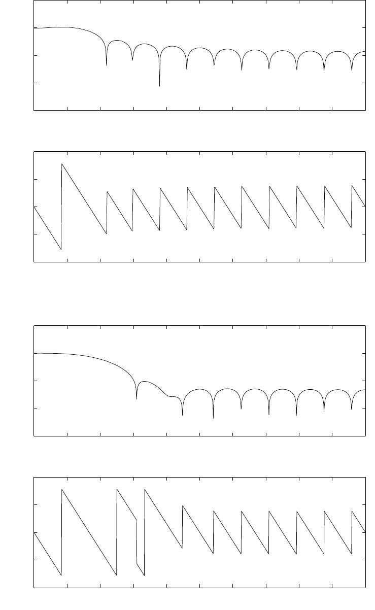
0 0.05 0.1 0.15 0.2 0.25 0.3 0.35 0.4 0.45 0.5
−150
−100
−50
0
50
−−−> Freq(Hz)
−−−> mag(dB)
0 0.05 0.1 0.15 0.2 0.25 0.3 0.35 0.4 0.45 0.5
−4
−2
0
2
4
−−−> Freq(Hz)
−−−> phase
Figure 10.1-1:
0 0.05 0.1 0.15 0.2 0.25 0.3 0.35 0.4 0.45 0.5
−150
−100
−50
0
50
−−−> Freq(Hz)
−−−> mag(dB)
0 0.05 0.1 0.15 0.2 0.25 0.3 0.35 0.4 0.45 0.5
−4
−2
0
2
4
−−−> Freq(Hz)
−−−> phase
Figure 10.1-2:
304
© 2007 Pearson Education, Inc., Upper Saddle River, NJ. All rights reserved. This material is protected under all copyright laws
as they currently exist. No portion of this material may be reproduced, in any form or by any means, without permission in
writing from the publisher. For the exclusive use of adopters of the book Digital Signal Processing, Fourth Edition, by John G.
Proakis and Dimitris G. Manolakis. ISBN 0-13-187374-1.
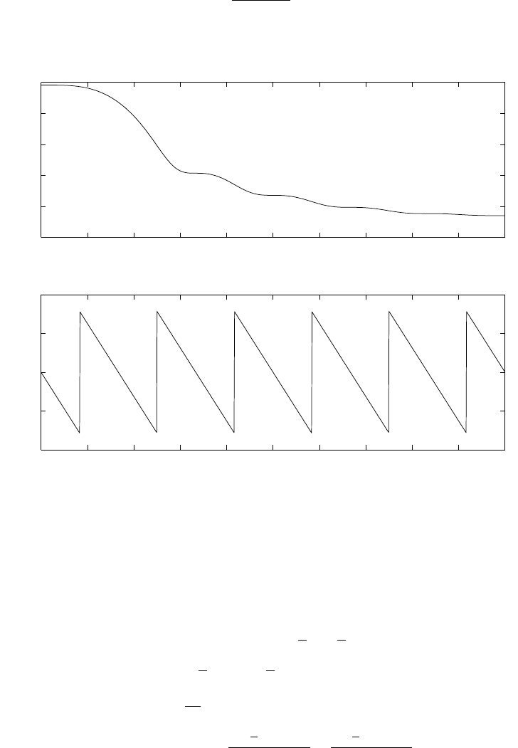
(d) Bartlett window:
w(n) = 1 −2(n−12)
24 0≤n≤24
Refer to fig 10.1-3.
0 0.05 0.1 0.15 0.2 0.25 0.3 0.35 0.4 0.45 0.5
−50
−40
−30
−20
−10
0
−−−> Freq(Hz)
−−−> mag(dB)
0 0.05 0.1 0.15 0.2 0.25 0.3 0.35 0.4 0.45 0.5
−4
−2
0
2
4
−−−> Freq(Hz)
−−−> phase
Figure 10.1-3:
10.2
(a)
Hd(w) = 1e−j12w,|w| ≤ π
6,π
3≤ |w| ≤ π
= 0,π
6≤ |w| ≤ π
3
hd(n) = 1
2πZπ
−π
Hd(w)e−jwndw
=δ(n)−sinπ
3(n−12)
π(n−12) +sinπ
6(n−12)
π(n−12)
(b) Rectangular window:
w(n) = 1,0≤n≤24
= 0,otherwise
305
© 2007 Pearson Education, Inc., Upper Saddle River, NJ. All rights reserved. This material is protected under all copyright laws
as they currently exist. No portion of this material may be reproduced, in any form or by any means, without permission in
writing from the publisher. For the exclusive use of adopters of the book Digital Signal Processing, Fourth Edition, by John G.
Proakis and Dimitris G. Manolakis. ISBN 0-13-187374-1.
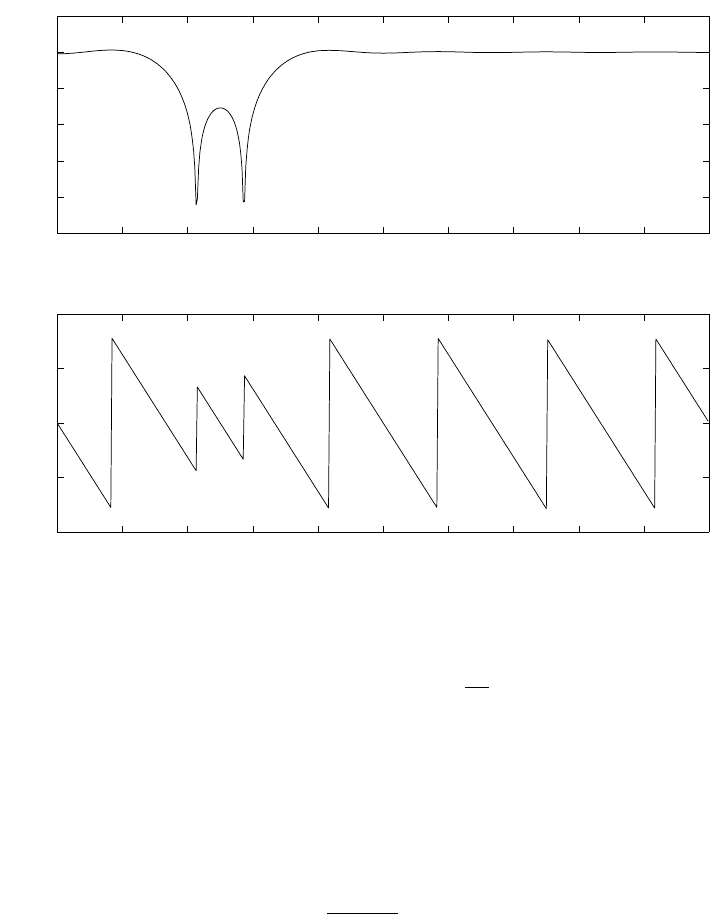
Refer to fig 10.2-1.
(c) Hamming window:
0 0.05 0.1 0.15 0.2 0.25 0.3 0.35 0.4 0.45 0.5
−50
−40
−30
−20
−10
0
10
−−−> Freq(Hz)
−−−> mag(dB)
0 0.05 0.1 0.15 0.2 0.25 0.3 0.35 0.4 0.45 0.5
−4
−2
0
2
4
−−−> Freq(Hz)
−−−> phase
Figure 10.2-1:
w(n) = (0.54 −0.46cosnπ
12 )
h(n) = hd(n)w(n)
H(w) =
24
X
n=0
h(n)e−jwn
Refer to fig 10.2-2.
(d) Bartlett window:
w(n) = 1 −(n−12)
12 ,0≤n≤24
Refer to fig 10.2-3.
Note that the magnitude responses in (c) and (d) are poor because the transition region is
wide. To obtain sharper cut-off, we must increase the length Nof the filter.
306
© 2007 Pearson Education, Inc., Upper Saddle River, NJ. All rights reserved. This material is protected under all copyright laws
as they currently exist. No portion of this material may be reproduced, in any form or by any means, without permission in
writing from the publisher. For the exclusive use of adopters of the book Digital Signal Processing, Fourth Edition, by John G.
Proakis and Dimitris G. Manolakis. ISBN 0-13-187374-1.
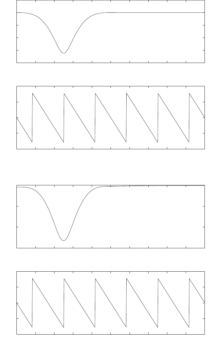
0 0.05 0.1 0.15 0.2 0.25 0.3 0.35 0.4 0.45 0.5
−20
−15
−10
−5
0
5
−−−> Freq(Hz)
−−−> mag(dB)
0 0.05 0.1 0.15 0.2 0.25 0.3 0.35 0.4 0.45 0.5
−4
−2
0
2
4
−−−> Freq(Hz)
−−−> phase
Figure 10.2-2:
0 0.05 0.1 0.15 0.2 0.25 0.3 0.35 0.4 0.45 0.5
−15
−10
−5
0
−−−> Freq(Hz)
−−−> mag(dB)
0 0.05 0.1 0.15 0.2 0.25 0.3 0.35 0.4 0.45 0.5
−4
−2
0
2
4
−−−> Freq(Hz)
−−−> phase
Figure 10.2-3:
307
© 2007 Pearson Education, Inc., Upper Saddle River, NJ. All rights reserved. This material is protected under all copyright laws
as they currently exist. No portion of this material may be reproduced, in any form or by any means, without permission in
writing from the publisher. For the exclusive use of adopters of the book Digital Signal Processing, Fourth Edition, by John G.
Proakis and Dimitris G. Manolakis. ISBN 0-13-187374-1.
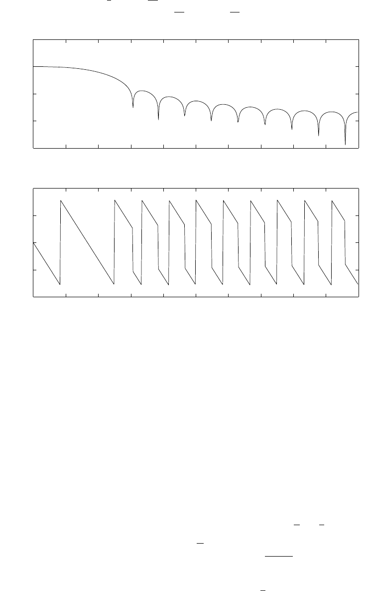
10.3
(a) Hanning window: w(n) = 1
2(1 −cosπn
12 ),0≤n≤24. Refer to fig 10.3-1.
(b) Blackman window: w(n) = 0.42 −0.5cos πn
12 + 0.08cosπn
6. Refer to fig 10.3-2.
0 0.05 0.1 0.15 0.2 0.25 0.3 0.35 0.4 0.45 0.5
−150
−100
−50
0
50
−−−> Freq(Hz)
−−−> mag(dB)
0 0.05 0.1 0.15 0.2 0.25 0.3 0.35 0.4 0.45 0.5
−4
−2
0
2
4
−−−> Freq(Hz)
−−−> phase
Figure 10.3-1:
10.4
(a) Hanning window: Refer to fig 10.4-1.
(b) Blackman window: Refer to fig 10.4-2.
The results are still relatively poor for these window functions.
10.5
M= 4, Hr(0) = 1, Hr(π
2) = 1
2
Hr(w) = 2
M
2−1
X
n=0
h(n)cos[w(M−1
2−n)]
= 2
1
X
n=0
h(n)cos[w(3
2−n)]
308
© 2007 Pearson Education, Inc., Upper Saddle River, NJ. All rights reserved. This material is protected under all copyright laws
as they currently exist. No portion of this material may be reproduced, in any form or by any means, without permission in
writing from the publisher. For the exclusive use of adopters of the book Digital Signal Processing, Fourth Edition, by John G.
Proakis and Dimitris G. Manolakis. ISBN 0-13-187374-1.
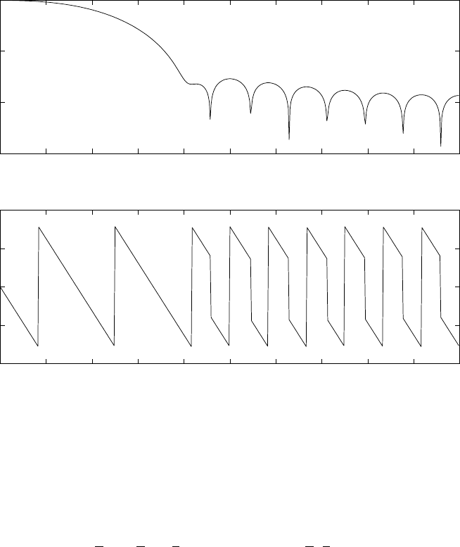
0 0.05 0.1 0.15 0.2 0.25 0.3 0.35 0.4 0.45 0.5
−150
−100
−50
0
−−−> Freq(Hz)
−−−> mag(dB)
0 0.05 0.1 0.15 0.2 0.25 0.3 0.35 0.4 0.45 0.5
−4
−2
0
2
4
−−−> Freq(Hz)
−−−> phase
Figure 10.3-2:
At w= 0, Hr(0) = 1 = 2
1
X
n=0
h(n)cos[0]
2[h(0) + h(1)] = 1 (1)
At w=π
2, Hr(π
2) = 1
2= 2
1
X
n=0
h(n)cos[π
2(3
2−n)]
−h(0) + h(1) = 0.354 (2)
Solving (1) and (2), we get
h(0) = 0.073 and
h(1) = 0.427
h(2) = h(1)
h(3) = h(0)
Hence, h(n) = {0.073,0.427,0.427,0.073}
309
© 2007 Pearson Education, Inc., Upper Saddle River, NJ. All rights reserved. This material is protected under all copyright laws
as they currently exist. No portion of this material may be reproduced, in any form or by any means, without permission in
writing from the publisher. For the exclusive use of adopters of the book Digital Signal Processing, Fourth Edition, by John G.
Proakis and Dimitris G. Manolakis. ISBN 0-13-187374-1.
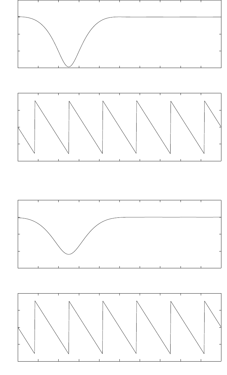
0 0.05 0.1 0.15 0.2 0.25 0.3 0.35 0.4 0.45 0.5
−15
−10
−5
0
5
−−−> Freq(Hz)
−−−> mag(dB)
0 0.05 0.1 0.15 0.2 0.25 0.3 0.35 0.4 0.45 0.5
−4
−2
0
2
4
−−−> Freq(Hz)
−−−> phase
Figure 10.4-1:
0 0.05 0.1 0.15 0.2 0.25 0.3 0.35 0.4 0.45 0.5
−15
−10
−5
0
5
−−−> Freq(Hz)
−−−> mag(dB)
0 0.05 0.1 0.15 0.2 0.25 0.3 0.35 0.4 0.45 0.5
−4
−2
0
2
4
−−−> Freq(Hz)
−−−> phase
Figure 10.4-2:
310
© 2007 Pearson Education, Inc., Upper Saddle River, NJ. All rights reserved. This material is protected under all copyright laws
as they currently exist. No portion of this material may be reproduced, in any form or by any means, without permission in
writing from the publisher. For the exclusive use of adopters of the book Digital Signal Processing, Fourth Edition, by John G.
Proakis and Dimitris G. Manolakis. ISBN 0-13-187374-1.

10.6
M= 15.Hr(2πk
15 ) = 1, k = 0,1,2,3
0, k = 4,5,6,7
Hr(w) = h(M−1
2) + 2
M−3
2
X
n=0
h(n)cosw(M−1
2−n)
h(n) = h(M−1−n)
h(n) = h(14 −n)
Hr(w) = h(7) + 2
6
X
n=0
h(n)cosw(7 −n)
Solving the above eqn yields,
h(n) = {0.3189,0.0341,−0.1079,−0.0365,0.0667,0.0412,−0.0498,0.4667
0.4667,−0.0498,0.0412,0.0667,−0.0365,−0.1079,0.0341,0.3189}
10.7
M= 15.Hr(2πk
15 ) =
1, k = 0,1,2,3
0.4, k = 4
0, k = 5,6,7
Hr(w) = h(M−1
2) + 2
M−3
2
X
n=0
h(n)cosw(M−1
2−n)
h(n) = h(M−1−n)
h(n) = h(14 −n)
Hr(w) = h(7) + 2
6
X
n=0
h(n)cosw(7 −n)
Solving the above eqn yields,
h(n) = {0.3133,−0.0181,−0.0914,0.0122,0.0400,−0.0019,−0.0141,0.52,
0.52,−0.0141,−0.0019,0.0400,0.0122,−0.0914,−0.0181,0.3133}
10.8
(a)
ya(t) = dxa(t)
dt
=d
dt[ej2πF t]
=j2πF ej2πF t
Hence, H(F) = j2πF
311
© 2007 Pearson Education, Inc., Upper Saddle River, NJ. All rights reserved. This material is protected under all copyright laws
as they currently exist. No portion of this material may be reproduced, in any form or by any means, without permission in
writing from the publisher. For the exclusive use of adopters of the book Digital Signal Processing, Fourth Edition, by John G.
Proakis and Dimitris G. Manolakis. ISBN 0-13-187374-1.
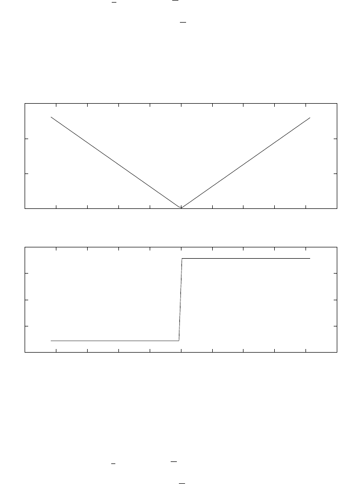
(b)
|H(F)|= 2πF
6H(F) = π
2, F > 0
=−π
2, F < 0
Refer to fig 10.8-1.
(c)
−0.1 −0.08 −0.06 −0.04 −0.02 0 0.02 0.04 0.06 0.08 0.1
0
0.2
0.4
0.6 B=pi/6
−−> Freq(Hz)
−−> magnitude
−0.1 −0.08 −0.06 −0.04 −0.02 0 0.02 0.04 0.06 0.08 0.1
−2
−1
0
1
2
−−> Freq(Hz)
−−> phase
Figure 10.8-1:
H(w) = jw, |w| ≤ π
|H(w)|=|w|
6H(w) = π
2, w > 0
=−π
2, w < 0
Refer to fig 10.8-2.
we note that the digital differentiator has a frequency response that resembles the response
of the analog differentiator.
(d)
y(n) = x(n)−x(n−1)
H(z) = 1 −z−1
H(w) = 1 −e−jw
312
© 2007 Pearson Education, Inc., Upper Saddle River, NJ. All rights reserved. This material is protected under all copyright laws
as they currently exist. No portion of this material may be reproduced, in any form or by any means, without permission in
writing from the publisher. For the exclusive use of adopters of the book Digital Signal Processing, Fourth Edition, by John G.
Proakis and Dimitris G. Manolakis. ISBN 0-13-187374-1.

−4 −3 −2 −1 0 1 2 3 4
0
1
2
3
4
−−> w
−−> magnitude
−4 −3 −2 −1 0 1 2 3 4
−2
−1
0
1
2
−−> w
−−> phase
Figure 10.8-2:
=e−jw
2(2jsinw
2)
|H(w)|= 2|sinw
2|
6H(w) = π
2−w
2
Refer to fig 10.8-3.
Note that for small w,sinw
2≈w
2and H(w)≈jwe−jw
2, which is a suitable approximation
to the differentiator in (c).
(e) The value H(w0) is obtained from (d) above. Then y(n) = A|H(w0)|cos(w0n+θ+π
2−w0
2)
10.9
Hd(w) = we−j10w,0≤w≤π
=−we−j10w,−π≤w≤0
hd(n) = 1
2πZπ
−π
Hd(w)e−jwndw
=cosπ(n−10)
(n−10) , n 6= 10
= 0, n = 10
hd(n) = cosπ(n−10)
(n−10) ,0≤n≤20, n 6= 10
313
© 2007 Pearson Education, Inc., Upper Saddle River, NJ. All rights reserved. This material is protected under all copyright laws
as they currently exist. No portion of this material may be reproduced, in any form or by any means, without permission in
writing from the publisher. For the exclusive use of adopters of the book Digital Signal Processing, Fourth Edition, by John G.
Proakis and Dimitris G. Manolakis. ISBN 0-13-187374-1.

−4 −3 −2 −1 0 1 2 3 4
0
0.5
1
1.5
2
−−> w
−−> magnitude
−4 −3 −2 −1 0 1 2 3 4
−2
−1
0
1
2
−−> w
−−> phase
Figure 10.8-3:
= 0, n = 10
With a Hamming window, we obtain the following frequency response: Refer to fig 10.9-1.
10.10
H(s) has two zeros at z1=−0.1 and z2=∞and two poles p1,2=−0.1±j3. The matched
z-transform maps these into:
˜z1=e−0.1T=e−0.01 = 0.99
˜z2=e−∞T= 0
˜p1=e(−0.1+j3)T= 0.99ej0.3
˜p2= 0.99e−j0.3
Hence, H(z) = 1−rz−1
1−2rcosw0z−1+r2z−2, w0= 0.3r= 0.99
From the impulse invariance method we obtain
H(s) = 1
21
s+ 0.1−j3+1
s+ 0.1 + j3
H(z) = 1
21
1−e−0.1Tej3Tz−1+1
1−e−0.1Te−j3Tz−1
=1−rcosw0z−1
1−2rcosw0z−1+r2z−2
314
© 2007 Pearson Education, Inc., Upper Saddle River, NJ. All rights reserved. This material is protected under all copyright laws
as they currently exist. No portion of this material may be reproduced, in any form or by any means, without permission in
writing from the publisher. For the exclusive use of adopters of the book Digital Signal Processing, Fourth Edition, by John G.
Proakis and Dimitris G. Manolakis. ISBN 0-13-187374-1.
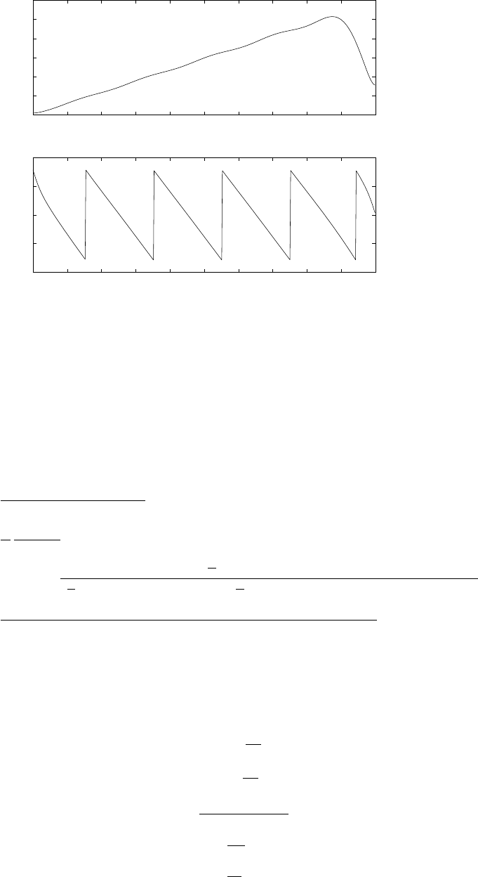
0 0.05 0.1 0.15 0.2 0.25 0.3 0.35 0.4 0.45 0.5
0
0.5
1
1.5
2
2.5
3
−−−> Freq(Hz)
−−−> mag(dB)
0 0.05 0.1 0.15 0.2 0.25 0.3 0.35 0.4 0.45 0.5
−4
−2
0
2
4
−−−> Freq(Hz)
−−−> phase
Figure 10.9-1:
The poles are the same, but the zero is different.
10.11
Ha(s) = (Ωu−Ωl)s
s2−(Ωu−Ωl)s+ ΩuΩl
s=2
T
1−z−1
1 + z−1
H(z) = (Ωu−Ωl)
2
T(1 −z−1)(1 + z−1)
(2
T)2(1 −z−1)2+ (Ωu−Ωl)( 2
T)(1 −z−1)(1 + z−1) + ΩuΩl(1 + z−1)2
=2(α−β)(1 −z−2)
[4 + 2(α−β) + αβ]−2(4 −αβ)z−1+ [4 −2(α−β) + αβ]z−2
where α= ΩuT, β = ΩlT
In order to compare the result with example 10.4.2, let
wu= ΩuT=3π
5
wl= ΩlT=2π
5
Then, H(z) = 0.245(1 −z−2)
1 + 0.509z−2( example 8.3.2 )
In our case, we have α= ΩuT= 2tanwu
2= 2.753
β= ΩlT= 2tanwl
2= 1.453
315
© 2007 Pearson Education, Inc., Upper Saddle River, NJ. All rights reserved. This material is protected under all copyright laws
as they currently exist. No portion of this material may be reproduced, in any form or by any means, without permission in
writing from the publisher. For the exclusive use of adopters of the book Digital Signal Processing, Fourth Edition, by John G.
Proakis and Dimitris G. Manolakis. ISBN 0-13-187374-1.

By substituting into the equation above, we obtain
H(z) = 2.599(1 −z−2)
10.599 + 5.401z−2
=0.245(1 −z−2)
1 + 0.509z−2
10.12
Let T= 2
(a) H(z) = 1+z−1
1−z−1⇒y(n) = y(n−1) + x(n) + x(n−1)
(b)
Ha(Ω) = 1
|Ω|6H(Ω) = −π
2,Ω≥0
π
2,Ω<0
(c)
|H(w)|=|cotw
2|6H(w) = −π
2,0≤w≤π
π
2,−π < w < 0
(d) The digital integrator closely matches the magnitude characteristics of the analog integrator.
The two phase characteristics are identical.
(e) The integrator has a pole at w= 0. To avoid overflow problems, we would have E[x(n)] = 0,
i.e., a signal with no dc component.
10.13
(a)
H(z) = A(1 + z−1)3
(1 −1
2z−1)(1 −1
2z−1+1
4z−2)
=A(1 + z−1)(1 + 2z−1+z−2)
(1 −1
2z−1)(1 −1
2z−1+1
4z−2)
H(z)|z=1 = 1
⇒A=3
64, b1= 2, b2= 1, a1= 1, c1=−1
2, d1=−1
2, d2=1
4
(b) Refer to fig 10.13-1
10.14
(a) There are only zeros, thus H(z) is FIR.
(b)
Zeros: z1=−4
3,
z2=−3
4,
z3,4=3
4e±jπ
3
z5,6=4
3e±jπ
3
316
© 2007 Pearson Education, Inc., Upper Saddle River, NJ. All rights reserved. This material is protected under all copyright laws
as they currently exist. No portion of this material may be reproduced, in any form or by any means, without permission in
writing from the publisher. For the exclusive use of adopters of the book Digital Signal Processing, Fourth Edition, by John G.
Proakis and Dimitris G. Manolakis. ISBN 0-13-187374-1.

+
+
z-1
z-1
+
+ +
z-1
+ + +
z-1
+
+
z-1
z-1
+
+
y(n)x(n)
-0.5
x(n)
3/64
-1 3
3
1
1/2
-1/8
y(n)
-1/2 2
1
1/4
1
3/64
Figure 10.13-1:
z7= 1
Hence, z2=1
z∗
1
z4=z∗
3
z5=1
z∗
3
z6=z∗
5
z1=1
z7
= 1
and H(z) = z−6H(z−1)
Therefore, H(w) is linear phase.
(c) Refer to fig 10.14-1
10.15
From the design specifications we obtain
ǫ= 0.509
δ= 99.995
fp=4
24 =1
6
fs=6
24 =1
4
317
© 2007 Pearson Education, Inc., Upper Saddle River, NJ. All rights reserved. This material is protected under all copyright laws
as they currently exist. No portion of this material may be reproduced, in any form or by any means, without permission in
writing from the publisher. For the exclusive use of adopters of the book Digital Signal Processing, Fourth Edition, by John G.
Proakis and Dimitris G. Manolakis. ISBN 0-13-187374-1.

x(n)
25/12
y(n)
(4/3)2+ (3/4)2+ 4 cos 260o= 481/144
-4/3 - 3/4 = -25/12
+ +
z-1
z-1 z-1
+
+
z-1 z-1
z-1
+
+
z-1
+
Figure 10.14-1:
Assume t= 1.Then, Ωp= 2tanwp
2
= 2tanπfp= 1.155
and Ωs= 2tanws
2
= 2tanπfs= 2
η=δ
ǫ= 196.5
k=Ωs
Ωp
= 1.732
Butterworth filter: Nmin ≥logη
logk = 9.613 ⇒N= 10
Chebyshev filter: Nmin ≥cosh−1η
cosh−1k= 5.212 ⇒N= 6
Elliptic filter: sinα =1
k= 0.577 ⇒α= 35.3o
sinβ =1
η= 0.577 ⇒β= 0.3o
Nmin ≥k(sinα)
k(cosα).k(cosβ)
k(sinβ)= 3.78 ⇒N= 4
318
© 2007 Pearson Education, Inc., Upper Saddle River, NJ. All rights reserved. This material is protected under all copyright laws
as they currently exist. No portion of this material may be reproduced, in any form or by any means, without permission in
writing from the publisher. For the exclusive use of adopters of the book Digital Signal Processing, Fourth Edition, by John G.
Proakis and Dimitris G. Manolakis. ISBN 0-13-187374-1.

10.16
From the design specifications we have
ǫ= 0.349
δ= 99.995
fp=1.2
8= 0.15
fs=2
8= 0.25
Ωp= 2tanwp
2= 1.019
Ωs= 2tanws
2= 2
η=δ
ǫ= 286.5
k=Ωs
Ωp
= 1.963
Butterworth filter: Nmin ≥logη
logk = 8.393 ⇒N= 9
Chebyshev filter: Nmin ≥cosh−1η
cosh−1k= 4.90 ⇒N= 5
Elliptic filter: Nmin ≥k(1
k)
k(q1−1
k2)
.
k(q1−1
η2)
k(1
η)⇒N= 4
10.17
Passband ripple = 1dB ⇒ǫ= 0.509
Stopband attenuation = 60dB ⇒δ= 1000
wp= 0.3π
ws= 0.35π
Ωp= 2tanwp
2= 1.019
Ωs= 2tanws
2= 1.226
η=δ
ǫ= 1965.226
k=Ωs
Ωp
= 1.203
Nmin ≥cosh−1η
cosh−1k=8.277
0.627 = 13.2⇒N= 14
Special software package, such as MATLAB or PC-DSP may be used to obtain the filter coeffi-
cients. Hand computation of these coefficients for N= 14 is very tedious.
319
© 2007 Pearson Education, Inc., Upper Saddle River, NJ. All rights reserved. This material is protected under all copyright laws
as they currently exist. No portion of this material may be reproduced, in any form or by any means, without permission in
writing from the publisher. For the exclusive use of adopters of the book Digital Signal Processing, Fourth Edition, by John G.
Proakis and Dimitris G. Manolakis. ISBN 0-13-187374-1.
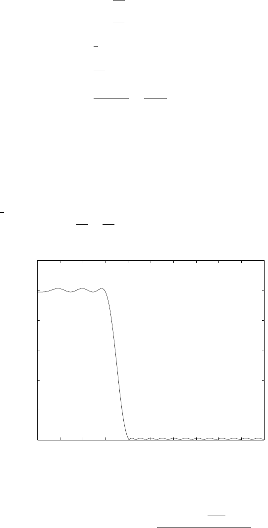
10.18
Passband ripple = 0.5dB ⇒ǫ= 0.349
Stopband attenuation = 50dB
wp= 0.24π
ws= 0.35π
Ωp= 2tanwp
2= 0.792
Ωs= 2tanws
2= 1.226
η=δ
ǫ= 906.1
k=Ωs
Ωp
= 1.547
Nmin ≥cosh−1η
cosh−1k=7.502
1.003 = 7.48 ⇒N= 8
Use a computer software package to determine the filter coefficients.
10.19
(a) MATLAB is used to design the FIR filter using the Remez algorithm. We find that a filter
of length M= 37 meets the specifications. We note that in MATLAB, the frequency scale is
normalized to 1
2of the sampling frequency. Refer to fig 10.19-1.
(b)δ1= 0.02, δ2= 0.01,△f=20
100 −15
100 = 0.05
0 0.1 0.2 0.3 0.4 0.5 0.6 0.7 0.8 0.9 1
0
0.2
0.4
0.6
0.8
1
1.2
−−> f
|H(w)|
Figure 10.19-1:
With equation (10.2.94) we obtain
ˆ
M=−20log10(√δ1δ2)−13
14.6△f+ 1 ≈34
320
© 2007 Pearson Education, Inc., Upper Saddle River, NJ. All rights reserved. This material is protected under all copyright laws
as they currently exist. No portion of this material may be reproduced, in any form or by any means, without permission in
writing from the publisher. For the exclusive use of adopters of the book Digital Signal Processing, Fourth Edition, by John G.
Proakis and Dimitris G. Manolakis. ISBN 0-13-187374-1.
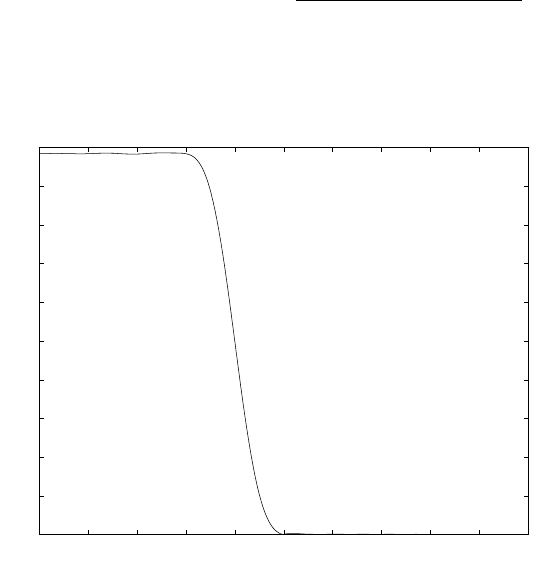
With equation (10.2.95) we obtain
D∞(δ1δ2) = 1.7371
f(δ1δ2) = 11.166
and ˆ
M=D∞(δ1δ2)−f(δ1δ2)(△f)2
△f+ 1 ≈36
Note (10.2.95) is a better approximation of M.
(c) Refer to fig 10.19-2.
Note that this filter does not satisfy the specifications.
0 0.1 0.2 0.3 0.4 0.5 0.6 0.7 0.8 0.9 1
0
0.1
0.2
0.3
0.4
0.5
0.6
0.7
0.8
0.9
1
−−> f
|H(w)|
Figure 10.19-2: M=37 FIR filter designed by window method with Hamming window
(d)The elliptic filter satisfies the specifications. Refer to fig 10.19-3.
(e)
FIR IIR
order 37 5
storage 19 16
No. of mult. 19 16
10.20
(a)
h(n) = 0
↑,1,2,3,4,5,4,3,2,1,0,...
H(z) =
10
X
n=0
h(n)z−n
=z−1+ 2z−2+ 3z−3+ 4z−4+ 5z−5+ 4z−6+ 3z−7+ 2z−8+z−9
H(w) = e−j9w[2cos4w+ 4cos3w+ 6cos2w+ 8cosw + 5]
(b)|H(w)|=|2cos4w+ 4cos3w+ 6cos2w+ 8cosw + 5|. Refer to fig 10.20-1.
321
© 2007 Pearson Education, Inc., Upper Saddle River, NJ. All rights reserved. This material is protected under all copyright laws
as they currently exist. No portion of this material may be reproduced, in any form or by any means, without permission in
writing from the publisher. For the exclusive use of adopters of the book Digital Signal Processing, Fourth Edition, by John G.
Proakis and Dimitris G. Manolakis. ISBN 0-13-187374-1.
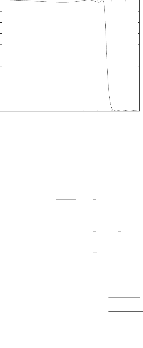
0 0.05 0.1 0.15 0.2 0.25 0.3 0.35 0.4 0.45 0.5
0
0.1
0.2
0.3
0.4
0.5
0.6
0.7
0.8
0.9
1
−−> f
|H(w)|
Figure 10.19-3:
10.21
(a)
dc gain: Ha(0) = 1
3dB frequency: |Ha(jΩ)|2=1
2
or α2
α2+ Ω2
c
=1
2
⇒Ωc=α
For all Ω,only H(j∞) = 0
ha(τ) = 1
eha(0) = 1
e
⇒e−αt =e−1
⇒τ=1
α
(b)
h(n) = ha(nT )
=e−αnT u(n)
H(z) = 1
1−e−αT z−1
H(w) = 1
1−e−αT e−jw
H(0) = H(w)|w=0
=1
1−e−αT
3dB frequency: |H(wc)|2=1
2|H(0)|2
(1 −αT αcoswc)2+ (e−αT sinwc)2= 2(1 −e−αT )2
322
© 2007 Pearson Education, Inc., Upper Saddle River, NJ. All rights reserved. This material is protected under all copyright laws
as they currently exist. No portion of this material may be reproduced, in any form or by any means, without permission in
writing from the publisher. For the exclusive use of adopters of the book Digital Signal Processing, Fourth Edition, by John G.
Proakis and Dimitris G. Manolakis. ISBN 0-13-187374-1.

0 0.05 0.1 0.15 0.2 0.25 0.3 0.35 0.4 0.45 0.5
0
5
10
15
20
25
−−> Freq(Hz)
−−> magnitude
Figure 10.20-1:
Hence, wc= 2sin−1(sinhαT
2)
Since |H(w)|2=1
1−2e−αT cosw +e−2αT
it oscillates between 1
(1 −e−αT )2and 1
(1 + e−αT )2
but never reaches zero
h(τ) = e−ατT =e−1
⇒τ≥1
αT
τis the smallest integer that is larger than 1
T
(c)
H(z) = α
2
T
1−z−1
1+z−1+α
=αT (1 + z−1)
2(1 −z−1) + αT (1 + z−1)
=αT (1 + z−1)
2 + αT + (αT −2)z−1
DC Gain: H(z)|z=1 = 1
At z=−1(w=π), H(z) = 0
since |Ha(jΩc)|2=1
2,we have Ωc=α
wc= 2tan−1Ωc
2T
= 2tan−1αT 2
Let a=2−αT
2 + αT
323
© 2007 Pearson Education, Inc., Upper Saddle River, NJ. All rights reserved. This material is protected under all copyright laws
as they currently exist. No portion of this material may be reproduced, in any form or by any means, without permission in
writing from the publisher. For the exclusive use of adopters of the book Digital Signal Processing, Fourth Edition, by John G.
Proakis and Dimitris G. Manolakis. ISBN 0-13-187374-1.

Then H(z) = 1−a
21 + (1 + a)z−1
1−az−1
h(n) = 1−a
2δ(n) + (1 + a)an−1u(n−1)
h(0) = 1−a
2
h(n)
h(0) =1
e
⇒(1 + a)an−1=1
e
n=ln a
1+a−1
lna
=ln(2−αT
4)−1
ln(2−αT
2+αT )
10.22
(a)
hd(n) = T
2πZπ
T
−π
T
Hd(w)ejwndw
=T
2π"Z−0.4π
T
−π
2T
ejwndw +Z0.5π
T
0.4π
T
ejwndw#
=T
nπ sin πn
2T−sin2πn
5T
(b)
Let hs(n) = hd(n)w(n),−100 ≤n≤100(M= 101)
Then, h(n) = hs(n−100) will be the impulse of the filter for 0 ≤n≤200
(c)
Hd(w) =
0,0≤w≤0.4π
T
e−j100w,0.4π
T≤w≤0.5π
T
0,0.5π
T< w < 1.5π
T
e−j100w,1.5π
T≤w≤1.6π
T
0,1.6π
T< w ≤2π
T
w=
2π
T
200k
=πk
100T
Then, H(k) = 0,0≤k < 40
= 0,50 < k < 150
= 0,160 < k ≤200
H(k) = e−jπk
T,40 ≤k≤50
=e−jπkT ,150 ≤k≤160
H(w) will match Hd(w) at 201 points in frequency. The filter will contain large ripples in
between the sampled frequencies. Transition values should be specified to reduce the ripples in
both the passbands and the stopband.
324
© 2007 Pearson Education, Inc., Upper Saddle River, NJ. All rights reserved. This material is protected under all copyright laws
as they currently exist. No portion of this material may be reproduced, in any form or by any means, without permission in
writing from the publisher. For the exclusive use of adopters of the book Digital Signal Processing, Fourth Edition, by John G.
Proakis and Dimitris G. Manolakis. ISBN 0-13-187374-1.

10.23
(a)
wl=5π
12
Ωl=tanwl
2( for T= 2)
wu=7π
12
Ωu=tanwu
2
Analog: lowpass to bandpass
s→s2+ ΩlΩu
s(Ωu−Ωl)
Bilinear: Analog to digital
s→z−1
z+ 1 =1−z−1
1 + z−1
combine the two steps:
s→1−z−1
1+z−12+ ΩlΩu
1−z−1
1+z−1(Ωu−Ωl)
=(1 −z−1)2+ ΩuΩl(1 + z−1)2
(1 −z−1)(Ωu−Ωl)
Therefore, H(z) = 1
h(1−z−1)2+ΩuΩl(1+z−1)2
(1−z−2)(Ωu−Ωl)i2+√2h(1−z−1)2+ΩuΩl(1+z−1)2
(1−z−2)(Ωu−Ωl)i+ 1
(b)
Ωu
Ωl
=tan7π
24
tan5π
24
= 1.7
(1)Ωu
Ωl
= 1.43
(2)Ωu
Ωl
= 1.8
(3)Ωu
Ωl
= 1.82
(4)Ωu
Ωl
= 1.7
filter (4) satisfies the constraint
10.24
(a)
H(z) = (1 −z−12)1
6
1 + z−1+
1
12 (1 −1
2z−1)
1−z−1+z−2+
1
12 (1 + 1
2z−1)
1 + z−1+z−2
=1
6(1 −z−12)2 + z−1+3
2z−2+1
2z−3+z−4
1 + z−1+z−2+z−3+z−4+z−5
=1
6(1 −z−6)(1 −z−1)(2 + z−1+3
2z−2+1
2z−3+z−4)
325
© 2007 Pearson Education, Inc., Upper Saddle River, NJ. All rights reserved. This material is protected under all copyright laws
as they currently exist. No portion of this material may be reproduced, in any form or by any means, without permission in
writing from the publisher. For the exclusive use of adopters of the book Digital Signal Processing, Fourth Edition, by John G.
Proakis and Dimitris G. Manolakis. ISBN 0-13-187374-1.
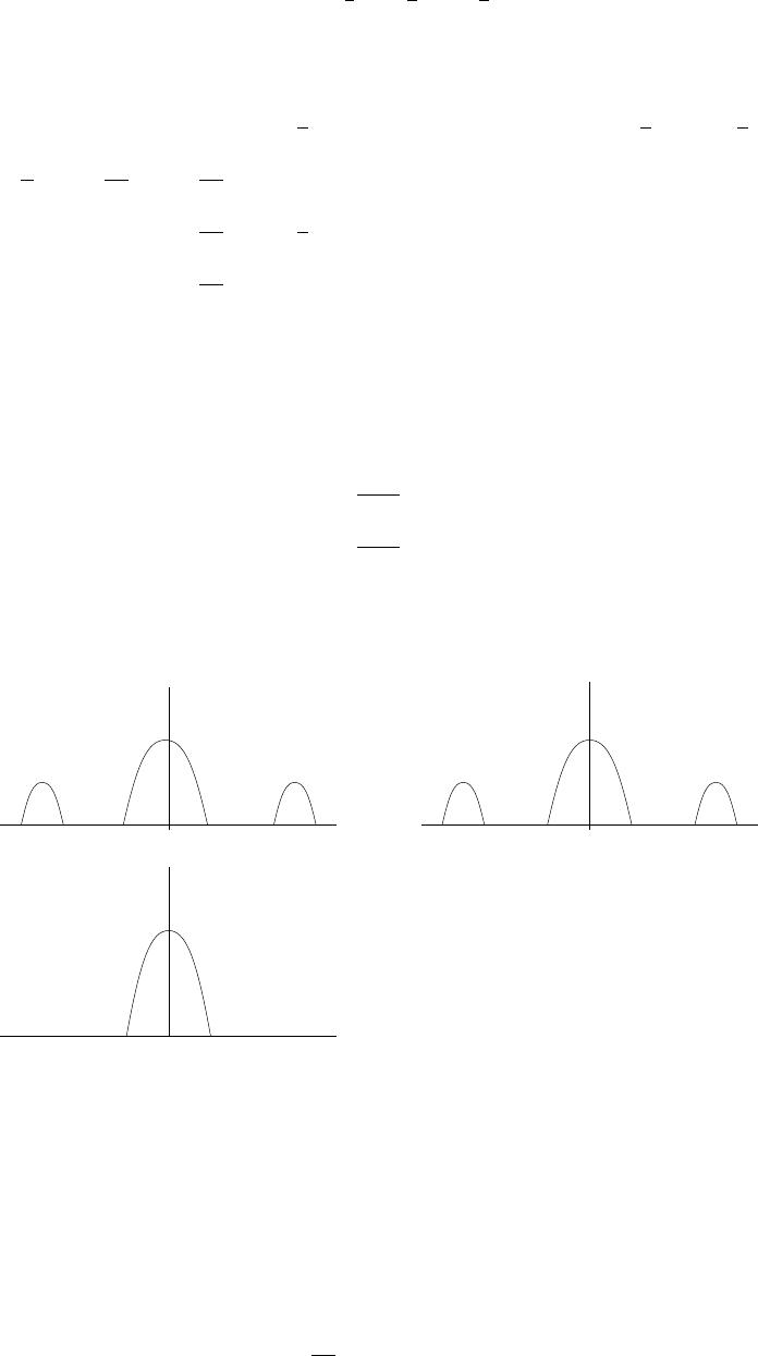
This filter is FIR with zeros at z= 1, e±jπ
6, e±jπ
2, e±j5π
6,−0.5528 ±j0.6823 and 0.3028 ±j0.7462
(b) It is a highpass filter.
(c)
H(w) = 1
6(1 −e−j6w)(1 −e−jw)(2 + e−jw +3
2e−j2w+1
2e−j3w+e−j4w)
H(0) = H(π
6) = H(3π
6) = H(3π
6) = 0
H(2π
6) = 1
2
H(4π
6) = 2
H(π) = 2
10.25
(a)
fL=900
2500 = 0.36
fH=1100
2500 = 0.44
Refer to fig 10.25-1.
(b) The ideal lowpass filter has a passband of −0.04 ≤f≤0.04. Hence,
X(f) W(f)
V(f)
f f
f
-0.4 0 0.360.40.44 -0.4 -0.04 0 0.04 0.4
-0.04 0 0.04
Figure 10.25-1:
Hd(w) = 1e−j15w−0.08π≤w≤0.08π
0,otherwise
Hence,
hd(n) = 1
2πZ0.08π
−0.08π
e−j15wejwndw
326
© 2007 Pearson Education, Inc., Upper Saddle River, NJ. All rights reserved. This material is protected under all copyright laws
as they currently exist. No portion of this material may be reproduced, in any form or by any means, without permission in
writing from the publisher. For the exclusive use of adopters of the book Digital Signal Processing, Fourth Edition, by John G.
Proakis and Dimitris G. Manolakis. ISBN 0-13-187374-1.

=1
2πZ0.08π
−0.08π
ejw(n−15)dw
=2sin0.08π(n−15)
(n−15)
h(n) = hd(n)wH(n)
wH(n) = 0.54 −0.46cos2π(n−15)
30
h(n) is the impulse response of the lowpass filter H(w)
(c) Rx= 1000
10.26
(a)
ˆy(n) =
M−1
X
k=0
h(k)x(n−k)
E=∞
X
n=0
[y(n)−ˆy(n)]2
=∞
X
n=0
[y(n)−
M−1
X
k=0
h(k)x(n−k)]2
By differentiating E with respect to each coefficient and setting the derivatives to zero, we obtain
M−1
X
k=0
h(k)rxx(k−l) = ryx(l), l = 0,1,...,M −1
where rxx(l) = ∞
X
n=0
x(n)x(n−l) and
ryx(l) = ∞
X
n=0
y(n)x(n−l)
(b)
E=∞
X
n=0
[y(n) + w(n)−
M−1
X
k=0
h(k)x(n−k)]2
By carrying out the minimization we obtain
M−1
X
k=0
h(k)rxx(k−l) = ryx(l) + rwx(l), l = 0,1,...,M −1
where rwx(l) = ∞
X
n=0
w(n)x(n−l)
10.27
x(n) =
N−1
X
k=0
ej2πkn/N =N, n = 0
0,1≤n≤N−1
327
© 2007 Pearson Education, Inc., Upper Saddle River, NJ. All rights reserved. This material is protected under all copyright laws
as they currently exist. No portion of this material may be reproduced, in any form or by any means, without permission in
writing from the publisher. For the exclusive use of adopters of the book Digital Signal Processing, Fourth Edition, by John G.
Proakis and Dimitris G. Manolakis. ISBN 0-13-187374-1.
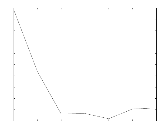
x(n) is a periodic sequence with period N. Hence, y(n) is also periodic with period N. Let
H2(z) = 1 +
p
X
k=1
akz−k
and h2(n) = {1, a1, a2,...,ap}
Then, h2(n)∗y(n) = x(n), n = 0,1,...,N −1
If p+ 1 ≤N, the Nequations above are sufficient to determine a1, a2,...,apand their order. If
p+ 1 > N, it is not possible to determine the {ak}and the order p.
10.28
(1) The set of linear equations are:
M−1
X
k=0
h(k)rxx(k−l) = ryx(l), l = 0,1, . . . , M −1
where rxx(l) = ∞
X
n=0
x(n)x(n−l) and
ryx(l) = ∞
X
n=0
y(n)x(n−l)
E=∞
X
n=−∞
[y(n)−
M−1
X
k=0
h(k)x(n−k)]2
(2) Refer to fig 10.28-1.
(3) Refer to fig 10.28-2.
8 9 10 11 12 13 14
8.08
8.1
8.12
8.14
8.16
8.18
8.2
8.22
8.24
8.26
8.28 Total squared error
error
filter order
Figure 10.28-1:
(4) v(n) = y(n) + 0.01w(n). Refer to fig 10.28-3.
328
© 2007 Pearson Education, Inc., Upper Saddle River, NJ. All rights reserved. This material is protected under all copyright laws
as they currently exist. No portion of this material may be reproduced, in any form or by any means, without permission in
writing from the publisher. For the exclusive use of adopters of the book Digital Signal Processing, Fourth Edition, by John G.
Proakis and Dimitris G. Manolakis. ISBN 0-13-187374-1.
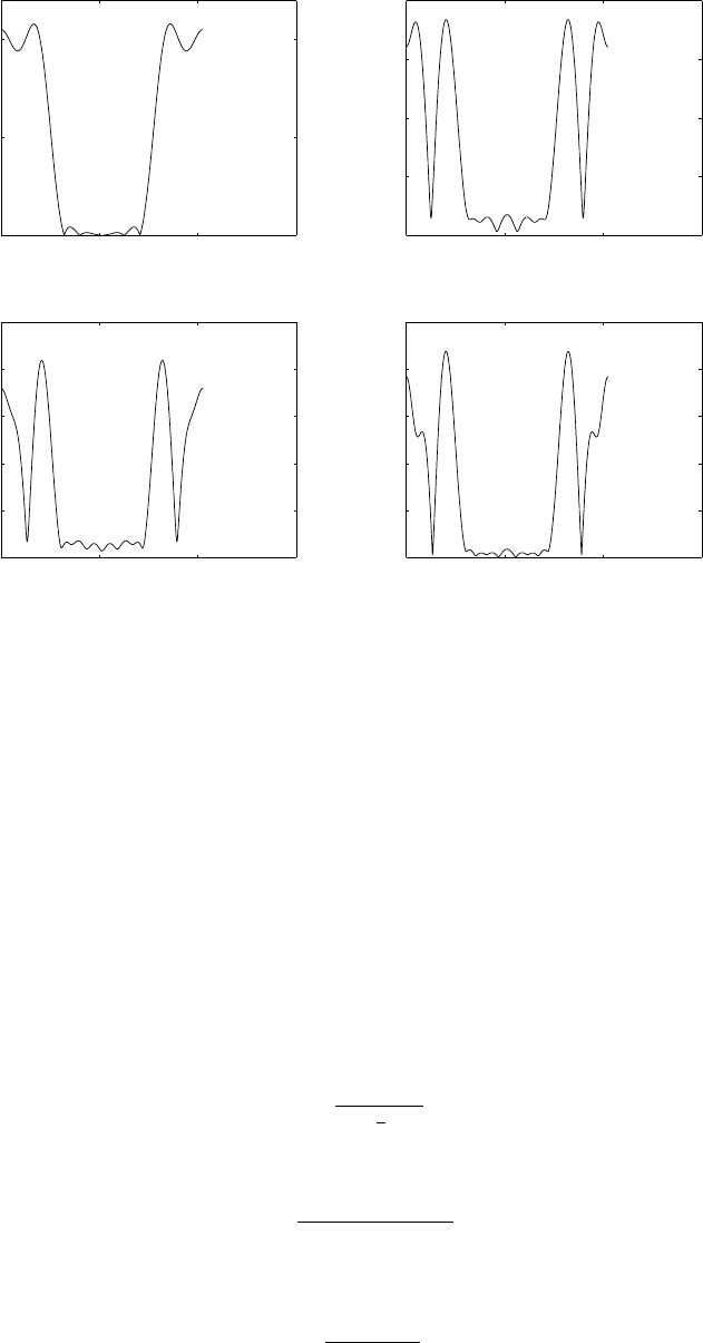
0 1000 2000 3000
0
0.5
1
fft of original h(n)
−−>|H(w)|
0 1000 2000 3000
0
0.1
0.2
0.3
0.4 M=11E=8.093
−−>|H(w)|
0 1000 2000 3000
0
0.1
0.2
0.3
0.4
0.5 M=12E=8.084
−−>|H(w)|
0 1000 2000 3000
0
0.1
0.2
0.3
0.4
0.5 M=13E=8.101
−−>|H(w)|
Figure 10.28-2:
10.29
(a) Since δ(n−k) = 0 except for n=k, equation (1) reduces to
h(n) = −a1h(n−1) −a2h(n−2) −...−aNh(n−N) + bn,0≤n≤M
(b) Since δ(n−k) = 0 except for n=k, equation (1) reduces to
h(n) = −a1h(n−1) −a2h(n−2) −...−aNh(n−N),0n > M
(c) We use the linear equation given in (b) to solve for the filter parameters {ak}. Then we use
values for the {ak}in the linear equation fiven in (a) and solve for the parameters {bk}.
10.30
Hd(z) = 2
1−1
2z−1
We can see that by setting M= 0 and N= 1 in
H(z) = PM
k=0 bkz−1
1 + PN
k=1 akz−1
we can provide a perfect match to Hd(z) as given in
H(z) = b0
1 + a1z−1.
329
© 2007 Pearson Education, Inc., Upper Saddle River, NJ. All rights reserved. This material is protected under all copyright laws
as they currently exist. No portion of this material may be reproduced, in any form or by any means, without permission in
writing from the publisher. For the exclusive use of adopters of the book Digital Signal Processing, Fourth Edition, by John G.
Proakis and Dimitris G. Manolakis. ISBN 0-13-187374-1.
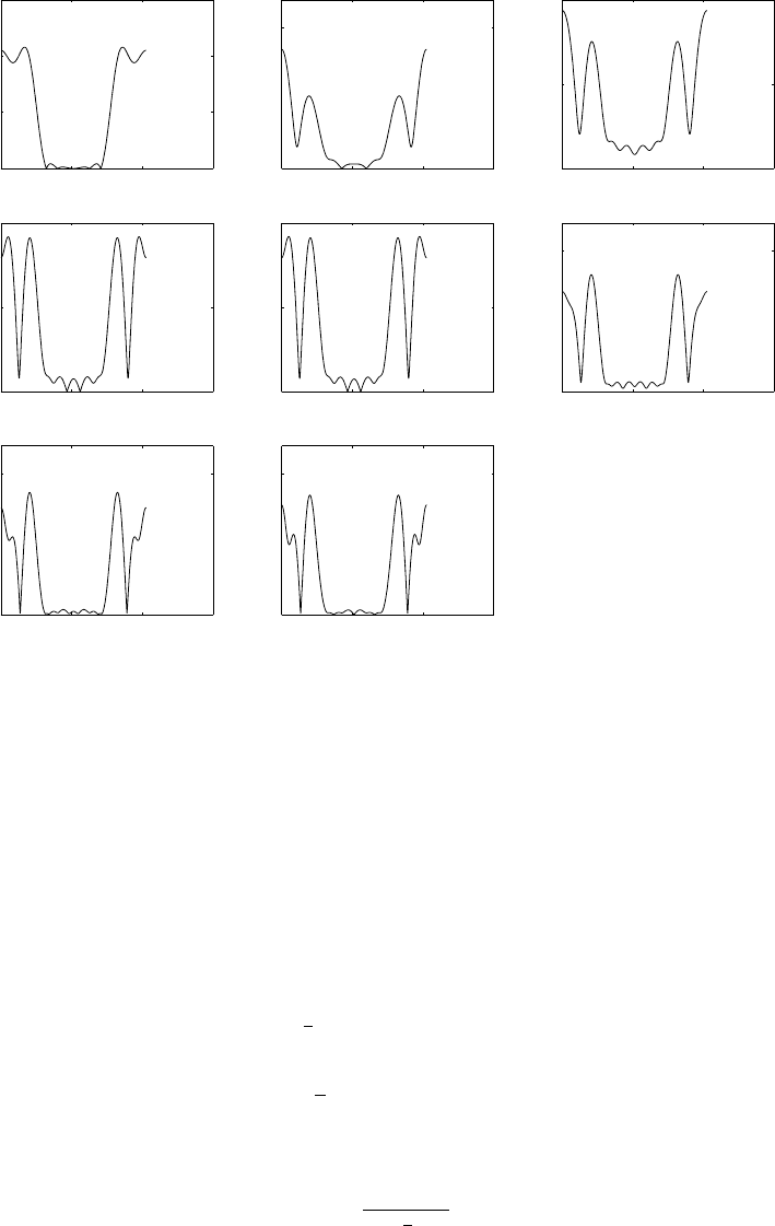
0 1000 2000 3000
0
0.5
1
1.5 fft of original h(n)
−−>|H(w)|
0 1000 2000 3000
0
0.5
M=8 E=8.42
0 1000 2000 3000
0
0.2
0.4 M=9 E=8.305
0 1000 2000 3000
0
0.2
0.4 M=10 E=8.228
0 1000 2000 3000
0
0.2
0.4 M=11 E=8.228
0 1000 2000 3000
0
0.5
M=12 E=8.221
0 1000 2000 3000
0
0.5
M=13 E=8.238
0 1000 2000 3000
0
0.5
M=14 E=8.24
Figure 10.28-3:
With δ(n) as the input to H(z), we obtain the output
h(n) = −a1h(n−1) + b0δ(n).
For n > M = 1, we have
h(n) = −a1h(n−1)
or, equivalently,
hd(n) = −a1hd(n−1).
Substituting for hd(n), we obtain a1=−1
2. To solve for b0, we use the equation given in 10.29(a)
with h(n) = hd(n),
hd(n) = 1
2hd(n−1) + b0δ(n).
For n= 0 this equation yields b0= 2. Thus
H(z) = 2
1−1
2z−1.
(b)
Hd(z) = H(z)
330
© 2007 Pearson Education, Inc., Upper Saddle River, NJ. All rights reserved. This material is protected under all copyright laws
as they currently exist. No portion of this material may be reproduced, in any form or by any means, without permission in
writing from the publisher. For the exclusive use of adopters of the book Digital Signal Processing, Fourth Edition, by John G.
Proakis and Dimitris G. Manolakis. ISBN 0-13-187374-1.
10.31
(a)
h(n) = −
N
X
k=1
akh(n−k) +
M
X
k=0
bkδ(n−k)n≥0
(b) Based on (a)
ˆ
hd(n) = −
N
X
k=1
akhd(n−k)n > M
ε1=∞
X
M+1 hhd(n)−ˆ
hd(n)i2
=∞
X
M+1 "hd(n)−
N
X
k=1
akhd(n−k)#2
By differentiating with respect to the parameters {ak}, we obtain the set of linear equations of
the form
N
X
k=1
akrhh(k, l) = −rhh(l, 0) l= 1,2,...,N
where,
rhh(k, l) = ∞
X
n=1
hd(n−k)hd(n−l)
=∞
X
n=0
hd(n)hd(n+k−l) = rhh(k−l)
The solution of these linear equations yield to the filter parameters {ak}.
(c) We can find the least-squares solution for {bk}from the minimization of
ε2=∞
X
n=0 "ˆ
hd(n)−
M
X
k=0
bkv(n−k)#2
Thus we obtain a set of linear equations for the parameters {bk}, in the form
M
X
k=0
bkrvv(k, l) = rhv (l)l= 0,1,...,M
where
rvv(k, l) = ∞
X
n=0
v(n−k)v(n−l)
rhv(k) = ∞
X
n=0
h(n)v(n−k)
331
© 2007 Pearson Education, Inc., Upper Saddle River, NJ. All rights reserved. This material is protected under all copyright laws
as they currently exist. No portion of this material may be reproduced, in any form or by any means, without permission in
writing from the publisher. For the exclusive use of adopters of the book Digital Signal Processing, Fourth Edition, by John G.
Proakis and Dimitris G. Manolakis. ISBN 0-13-187374-1.
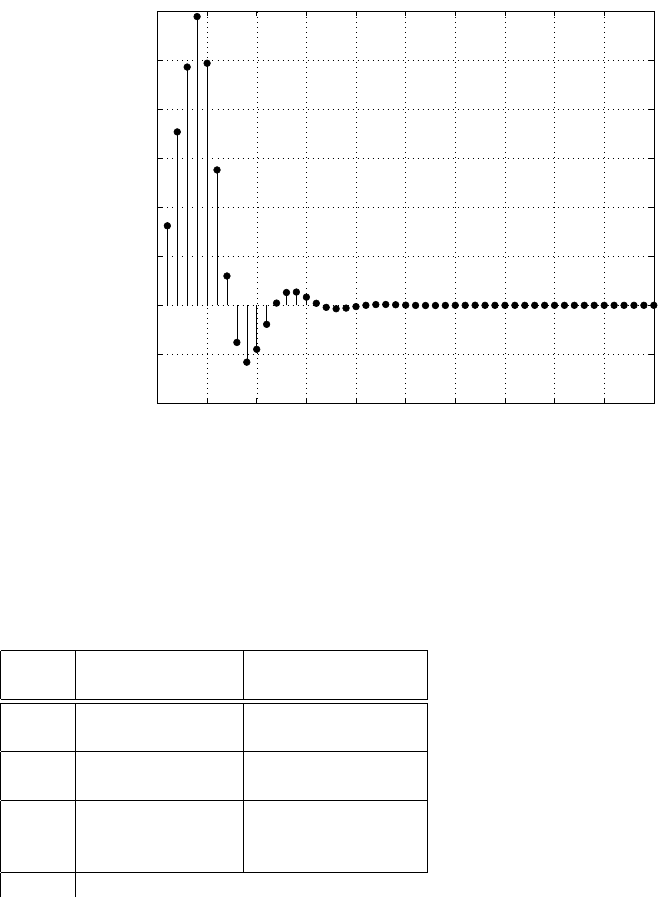
10.32
(a)
y(n) = 1.5198y(n−1) −0.9778y(n−2) + 0.2090y(n−3)
+0.0812x(n) + 0.0536x(n−1) + 0.0536x(n−2) + 0.0812x(n−3)
hd(n) can be found by substituting x(n) = δ(n). Fig 10.32-1 shows the hd(n).
0 5 10 15 20 25 30 35 40 45 50
−0.1
−0.05
0
0.05
0.1
0.15
0.2
0.25
0.3
n
hd(n)
Figure 10.32-1:
(b) The poles and zeros obtained using Shanks’ method are listed in Table 10.32. The magnitude
response for each case together with the desired response is shown in Fig. 10.32-2. The frequency
response characteristics illustrate that Shanks’ method yields very good designs when the number
of poles and zeros equals or exceeds the number of poles and zeros in the actual filter. Thus the
inclusion of zeros in the approximation has a significant effect in the resulting design.
Filter
Order Poles Zeros
N=3 0.5348
M=2 0.6646 ±j0.4306 −0.2437 ±j0.5918
N=3 0.3881 -1
M=3 0.5659 ±j0.4671 0.1738 ±j0.9848
N=4 -0.00014 -1
0.388
M=3 0.566 ±j0.4671 0.1738 ±j0.9848
332
© 2007 Pearson Education, Inc., Upper Saddle River, NJ. All rights reserved. This material is protected under all copyright laws
as they currently exist. No portion of this material may be reproduced, in any form or by any means, without permission in
writing from the publisher. For the exclusive use of adopters of the book Digital Signal Processing, Fourth Edition, by John G.
Proakis and Dimitris G. Manolakis. ISBN 0-13-187374-1.
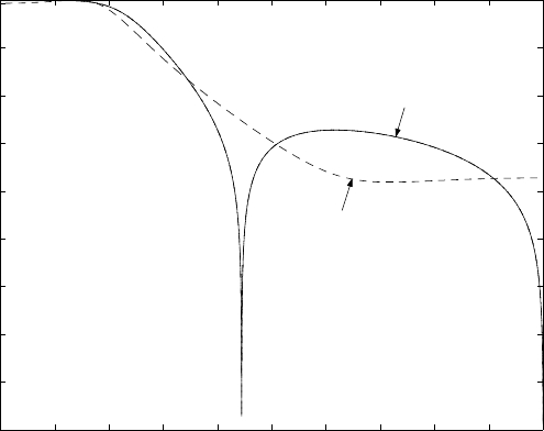
0 0.1 0.2 0.3 0.4 0.5 0.6 0.7 0.8 0.9 1
−90
−80
−70
−60
−50
−40
−30
−20
−10
0
Normalized Frequency (xπ rad/sample
Magnitude (dB)
Desired response
N=3, M=3
N=4, M=3
N=3, M=2
Figure 10.32-2:
333
© 2007 Pearson Education, Inc., Upper Saddle River, NJ. All rights reserved. This material is protected under all copyright laws
as they currently exist. No portion of this material may be reproduced, in any form or by any means, without permission in
writing from the publisher. For the exclusive use of adopters of the book Digital Signal Processing, Fourth Edition, by John G.
Proakis and Dimitris G. Manolakis. ISBN 0-13-187374-1.
334
© 2007 Pearson Education, Inc., Upper Saddle River, NJ. All rights reserved. This material is protected under all copyright laws
as they currently exist. No portion of this material may be reproduced, in any form or by any means, without permission in
writing from the publisher. For the exclusive use of adopters of the book Digital Signal Processing, Fourth Edition, by John G.
Proakis and Dimitris G. Manolakis. ISBN 0-13-187374-1.
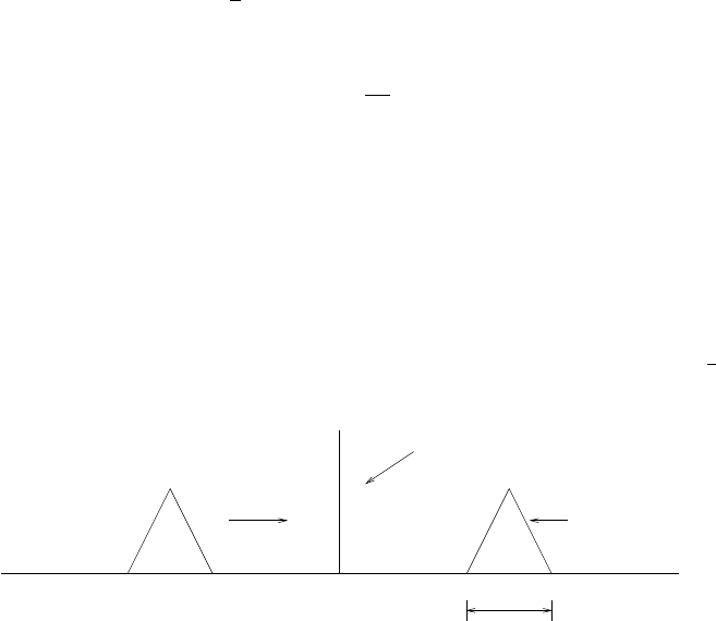
Chapter 11
11.1
(a) Let the corresponding baseband spectrum be called Xb(Ω). Then
Xa(Ω) = 1
2[Xb(Ω −2000π) + Xb(Ω + 2000π)]
With frequencies normalized to Fx,
w′=Ω
Fx
. The sequence x(n) has DTFT
X(w′) = ∞
X
q=−∞
Xa(w′−2πq)
=∞
X
q=−∞
[Xa(w′−0.8π−2πq) + Xb(w′+ 0.8π−2πq)]
modulation by cos(0.8π) causes shifts up and down by 0.8π(and scaling by 1
2) of each
|X(w’)|
0.5
Assumes peak of X
b(.) normalized to unity
Xb(w’) shifted to 0.8
w’
−π −0.8π 0 0.8π π
π
β=0.16π
period 2π
Figure 11.1-1:
component in the spectrum. Refer to fig 11.1-1. Ideal LPF preserves only the baseband spectrum
(of each period). Refer to fig 11.1
335
© 2007 Pearson Education, Inc., Upper Saddle River, NJ. All rights reserved. This material is protected under all copyright laws
as they currently exist. No portion of this material may be reproduced, in any form or by any means, without permission in
writing from the publisher. For the exclusive use of adopters of the book Digital Signal Processing, Fourth Edition, by John G.
Proakis and Dimitris G. Manolakis. ISBN 0-13-187374-1.
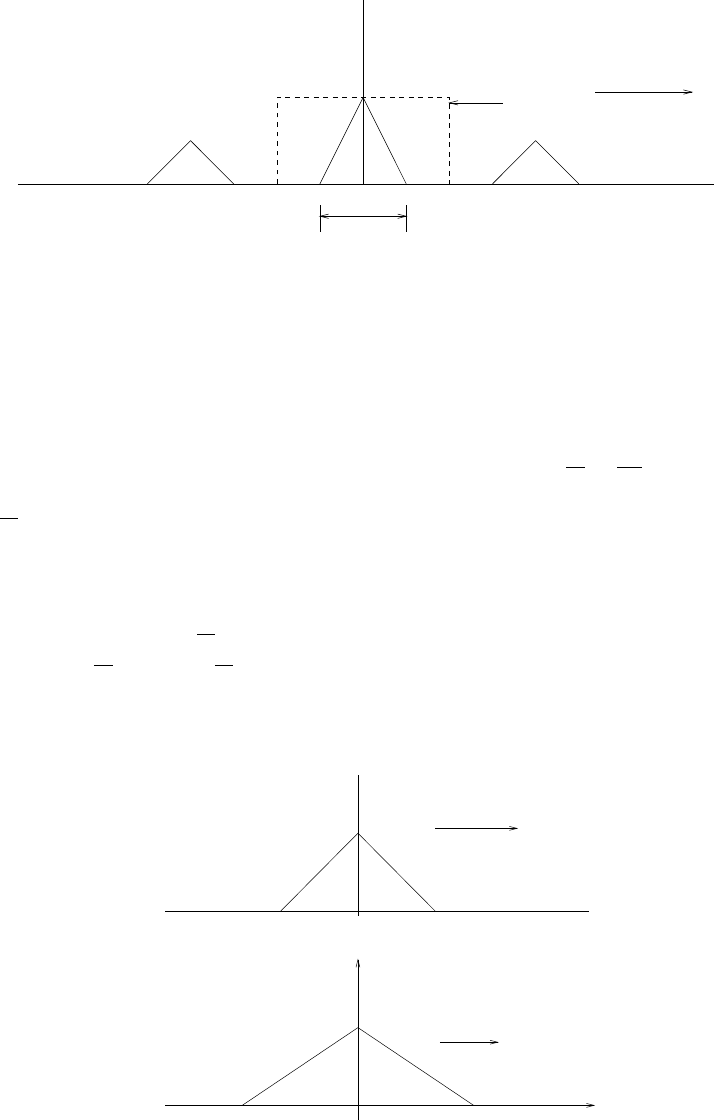
−π −0.4π 0.1π 0.4π π
0.5 0.5
1
w
|W(w’)|
H(w’) period 2π
β
Figure 11.1-2:
The downsampling produces the figure in fig 11.1, where w′′ =Ω
Fy=ΩD
Fx= 10w′. Note that
there is no aliasing in the spectrum |Y(w′′)|because the decimated sample rate, in terms of w′,
is 2π
10 >0.04π.
(b) The assumed spectral amplitude normalization in fig 11.1-1 implies that the analog FT
(magnitude spectrum) of xa(t) is (refer to fig 11.1-4).
The given sample rate is identical to Fyabove, Fy= 250Hz. The DTFT of samples taken
at this rate is ˜
Y(Ω) = 1
TyPqXa(Ω −qΩy) where Ωy= 2πFy. On a scaled frequency axis
w′′ = ΩTy=Ω
Fy,˜
Y(w′′) = 1
TyPqXa(w′′ −q2π). Consequently ˜y(n) = y(n).
0.08π π
|V(w’)|
w’
period 2π
0.8π π
0.1
period 2
w’’
|Y(w’’)| = 0.1 |V(0.1w’’)|
π
Figure 11.1-3:
336
© 2007 Pearson Education, Inc., Upper Saddle River, NJ. All rights reserved. This material is protected under all copyright laws
as they currently exist. No portion of this material may be reproduced, in any form or by any means, without permission in
writing from the publisher. For the exclusive use of adopters of the book Digital Signal Processing, Fourth Edition, by John G.
Proakis and Dimitris G. Manolakis. ISBN 0-13-187374-1.
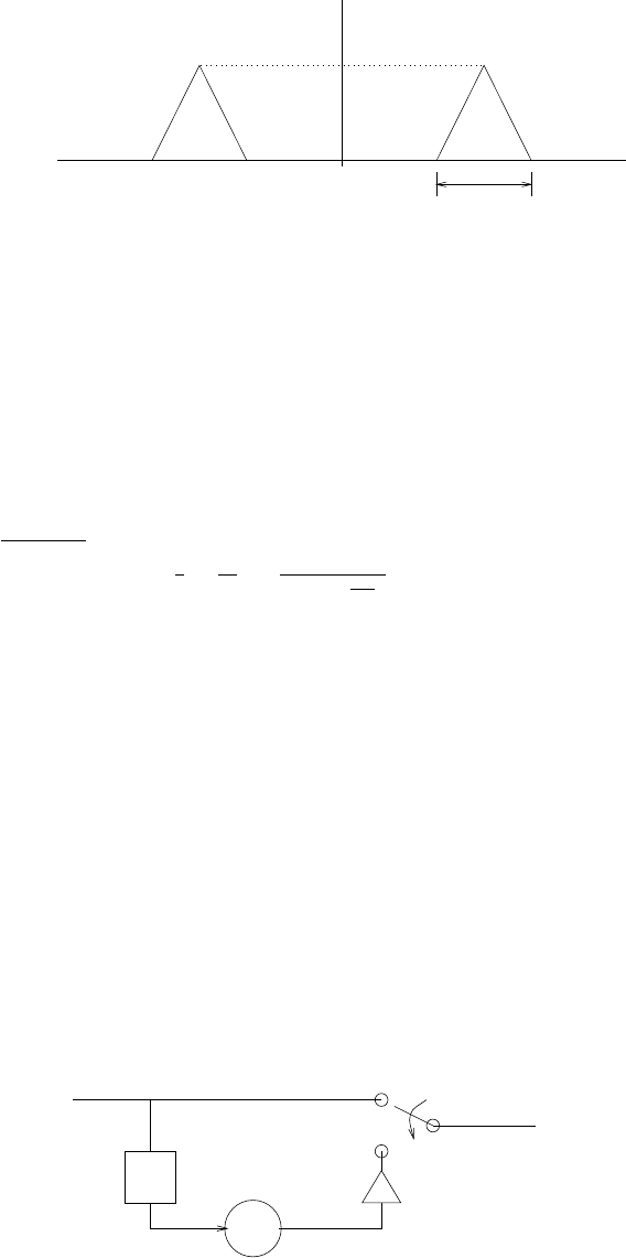
−Ω Ω Ω
400π
cc
T
x/2
|Xa(Ω) |
Figure 11.1-4:
11.2
(a) X(w) = 1
(1−ae−jw )
(b) After decimation Y(w′) = 1
2X(w′
2) = 1
2(1−ae−jw′
2)
(c)
DTFT {x(2n)}=X
n
x(2n)e−jw2n
=X
n
x(2n)e−jw′n
=Y(w′)
11.3
(a)Refer to fig 11.3-1
(b)
z-1
+
x(n)
F
x 1/2
y(m)
F
y= Fx
Figure 11.3-1:
337
© 2007 Pearson Education, Inc., Upper Saddle River, NJ. All rights reserved. This material is protected under all copyright laws
as they currently exist. No portion of this material may be reproduced, in any form or by any means, without permission in
writing from the publisher. For the exclusive use of adopters of the book Digital Signal Processing, Fourth Edition, by John G.
Proakis and Dimitris G. Manolakis. ISBN 0-13-187374-1.

Let w′=Ω
Fx
, w′′ =Ω
Fy
=w′
2
Y(w′′) = X
neven
x(n
2)e−jw′′n+X
nodd
1
2[x(n−1
2) + x(n+ 1
2)]e−jw′′n
=X
p
x(p)e−jw′′2p+1
2X
q
[x(q) + x(q+ 1)]e−jw′′(2q+1)
=X(2w′′) + 1
2e−jw′′ [X(2w′′) + ej2w′′ X(2w′′)]
=X(2w′′)[1 + cosw′′]
X(w′) = 1,0≤ |w′| ≤ 0.2π
0,otherwise
X(2w′′) = 1,0≤ |2w′′| ≤ 0.2π
0,otherwise
=1,0≤ |w′′| ≤ 0.1π
0,otherwise
Y(w′′) = 1 + cosw′′,0≤ |w′′| ≤ 0.1π
0,otherwise
(c) Refer to fig 11.3-2
X(.)
0 0.7 0.9 1.1 1.3 2 w ’
0 0.35 0.45 0.55 0.65 w ’’
π π πππ π
π π π π π
Figure 11.3-2:
Y(w′′) =
1 + cosw′′,0.35π≤ |w′′| ≤ 0.45π
or 0.55π≤ |w′′| ≤ 0.65π
0,otherwise
11.4
(a) Let w′=Ω
Fx, w′′ =ΩD
Fx. Refer to fig 11.4-1
Let x′′(n) be the downsampled sequence.
338
© 2007 Pearson Education, Inc., Upper Saddle River, NJ. All rights reserved. This material is protected under all copyright laws
as they currently exist. No portion of this material may be reproduced, in any form or by any means, without permission in
writing from the publisher. For the exclusive use of adopters of the book Digital Signal Processing, Fourth Edition, by John G.
Proakis and Dimitris G. Manolakis. ISBN 0-13-187374-1.

π
π
|X(w ’)|
1
-w ’
mw ’
mw ’
|X’’(w’’)|
1/D
-Dw’
mDw’
mw ’’
Figure 11.4-1:
x′′(n) = x(nD)
X′′(w′′) = 1
DX(w′′
D)
As long as Dw′
m≤π,X(w′) [hence x(n)] can be recovered from X′′(w′′)[x′′(n) = x(Dn)]
using interpolation by a factor D:
X(w′) = DX′′(Dw′)
The given sampling frequency is w′
s=2π
D. The condition Dw′
m≤π→2w′
m≤2π
D=w′
s
(b) Let xa(t) be the ral analog signal from which samples x(n) were taken at rate Fx. There exists
a signal, say x′
a(t′), such that x′
a(t′) = Xa(t
Tx). x(n) may be considered to be the samples of x′(t′)
taken at rate fx= 1. Likewise x′′(n) = x(nD) are samples of x′(t′) taken at rate f′′
x=fx
D=1
D.
From sampling theory, we know that x′(t′) can be reconstructed from its samples x′′(n) as long
as it is bandlimited to fm≤1
2D, or wm≤π
D, which is the case here. The reconstruction formula
is
x′(t′) = X
k
x′′(k)hr(t′−kD)
where
hr(t′) = sin(π
Dt′)
(π
Dt′)
Refer to fig 11.4-2
Actually the bandwidth of the reconstruction filter may be made as small as w′
m, or as large
as 2π
D−w′
m, so hrmay be
hr(t′) = sin(w′
ct′)
(w′
ct′)
where w′
m≤w′
c≤2π
D−w′
m. In particular x(n) = x′(t′=n) so
x(n) = X
k
x(kD)hr(n−kD)
339
© 2007 Pearson Education, Inc., Upper Saddle River, NJ. All rights reserved. This material is protected under all copyright laws
as they currently exist. No portion of this material may be reproduced, in any form or by any means, without permission in
writing from the publisher. For the exclusive use of adopters of the book Digital Signal Processing, Fourth Edition, by John G.
Proakis and Dimitris G. Manolakis. ISBN 0-13-187374-1.
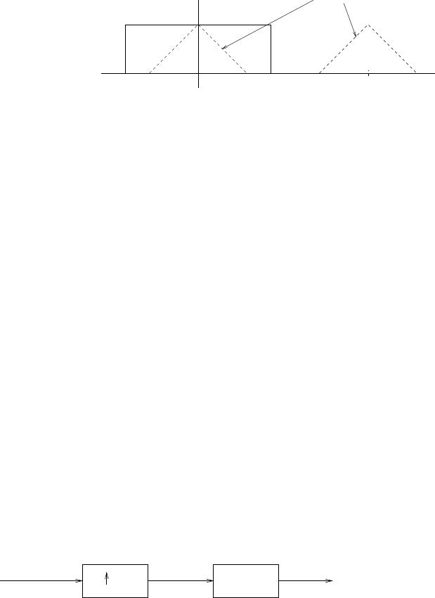
0w ’
mπ/D 2π/D - w ’
mw ’
Hr(w ’) |X(w ’)| period
2π/D
2π/D
Figure 11.4-2:
(c) Clearly if we define
v(p) = x(p),if p is an integer multiple of D
0,other p
then, we may write 11.4 as
x(n) = X
p
v(p)hr(n−p)
so x(n) is reconstructed as (see fig 11.4-3)
x’’(n)=x(kn) Dv(n) x(n)
hr(n)
Figure 11.4-3:
340
© 2007 Pearson Education, Inc., Upper Saddle River, NJ. All rights reserved. This material is protected under all copyright laws
as they currently exist. No portion of this material may be reproduced, in any form or by any means, without permission in
writing from the publisher. For the exclusive use of adopters of the book Digital Signal Processing, Fourth Edition, by John G.
Proakis and Dimitris G. Manolakis. ISBN 0-13-187374-1.
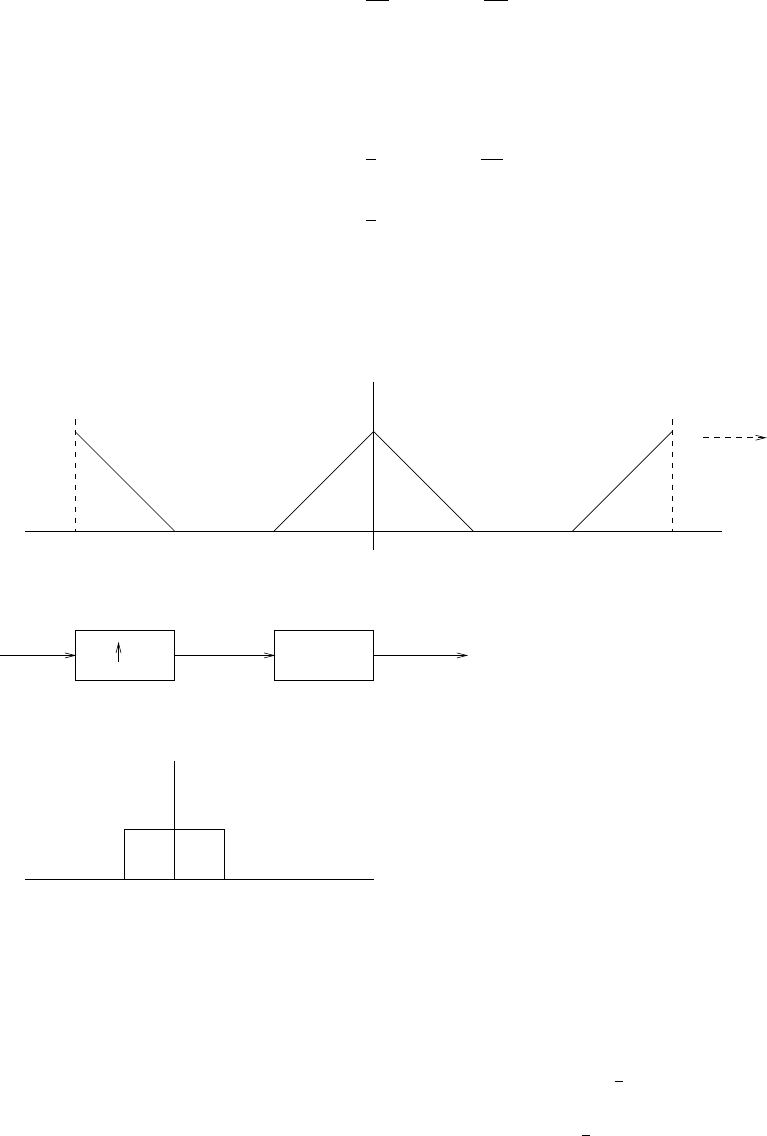
11.5
(a)
Let w=Ω
Fx
, w′′ =2Ω
Fx
Xs(w) = X
n
xs(n)e−jwn
=X
m
x(2m)e−jw2m
=1
2X
q
X(w−2π
2q)
=1
2X
q
X(w−πq)
To recover x(n) from xs(n): see fig 11.5-1
(b)
1/2
Xs(w)
period π
π/3 2π/3 π
−π −2π/3 −π/3 w
x
s(n) v(n) x(n)
hr(n)
2
where
Hr(w)
1
w
−π/2 π/2
Figure 11.5-1:
Recall w′= 2w
Xd(w′) = X
n
xd(n)e−jw′n
=X
neven
xs(n)e−jw′n
2
=X
n
xs(n)e−jw′n
2
341
© 2007 Pearson Education, Inc., Upper Saddle River, NJ. All rights reserved. This material is protected under all copyright laws
as they currently exist. No portion of this material may be reproduced, in any form or by any means, without permission in
writing from the publisher. For the exclusive use of adopters of the book Digital Signal Processing, Fourth Edition, by John G.
Proakis and Dimitris G. Manolakis. ISBN 0-13-187374-1.
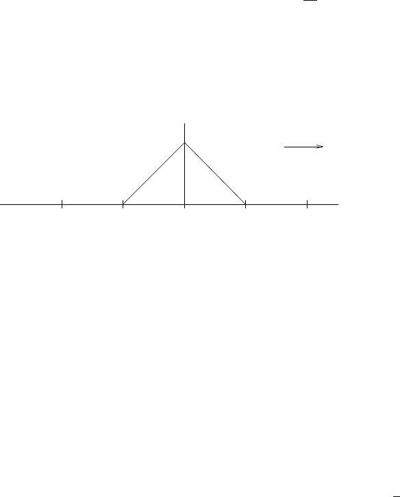
since xs(n) = 0 when nodd
=Xs(w′
2)
see fig 11.5-2
No information is lost since the decimated sample rate still exceeds twice the bandlimit of
−π 2π/3 π
period 21/2
w ’
π
Figure 11.5-2:
the original signal.
11.6
A filter of length 30 meets the specification. The cutoff frequency is wc=π
5and the coefficients
are given below:
h(1) = h(30) = 0.006399
h(2) = h(29) = −0.01476
h(3) = h(28) = −0.001089
h(4) = h(27) = −0.002871
h(5) = h(26) = 0.01049
h(6) = h(25) = 0.02148
h(7) = h(24) = 0.01948
h(8) = h(23) = −0.0003107
h(9) = h(22) = −0.03005
h(10) = h(21) = −0.04988
h(11) = h(20) = −0.03737
h(12) = h(19) = 0.01848
h(13) = h(18) = 0.1075
h(14) = h(17) = 0.1995
h(15) = h(16) = 0.2579
342
© 2007 Pearson Education, Inc., Upper Saddle River, NJ. All rights reserved. This material is protected under all copyright laws
as they currently exist. No portion of this material may be reproduced, in any form or by any means, without permission in
writing from the publisher. For the exclusive use of adopters of the book Digital Signal Processing, Fourth Edition, by John G.
Proakis and Dimitris G. Manolakis. ISBN 0-13-187374-1.
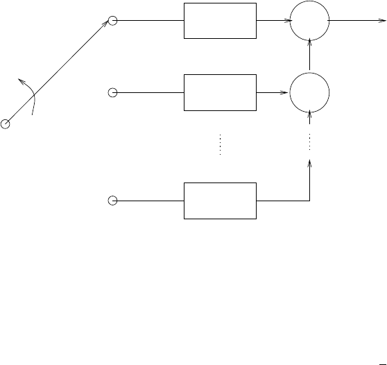
pk(n) = h(n+k), k = 0,1,...
corresponding polyphase filter structure (see fig 11.6-1)
+
p
0(n) +
p (n)
p (n)
1
4
y(n)
x(n)
F
xF
y= Fx/D
Figure 11.6-1:
11.7
A filter of length 30 meets the specification. The cutoff frequency is wc=π
2and the coefficients
are given below:
h(1) = h(30) = 0.006026
h(2) = h(29) = −0.01282
h(3) = h(28) = −0.002858
h(4) = h(27) = 0.01366
h(5) = h(26) = −0.004669
h(6) = h(25) = −0.01970
h(7) = h(24) = 0.01598
h(8) = h(23) = 0.02138
h(9) = h(22) = −0.03498
h(10) = h(21) = −0.01562
h(11) = h(20) = 0.06401
h(12) = h(19) = −0.007345
h(13) = h(18) = −0.1187
h(14) = h(17) = 0.09805
h(15) = h(16) = 0.4923
pk(n) = h(2n+k), k = 0,1; n= 0,1,...,14
343
© 2007 Pearson Education, Inc., Upper Saddle River, NJ. All rights reserved. This material is protected under all copyright laws
as they currently exist. No portion of this material may be reproduced, in any form or by any means, without permission in
writing from the publisher. For the exclusive use of adopters of the book Digital Signal Processing, Fourth Edition, by John G.
Proakis and Dimitris G. Manolakis. ISBN 0-13-187374-1.

corresponding polyphase filter structure (see fig 11.7-1)
p
0(n)
/DF
y= Fx
F
x
p (n)
1
y(n)
x(n)
Figure 11.7-1:
11.8
The FIR filter that meets the specifications of this problem is exactly the same as that in Problem
11.6. Its bandwidth is π
5. Its coefficients are
g(n, m) = h(nI + (mD)I)
=h(nI +mD −[mD
I]I)
=h(2n+ 5m−2[5m
2])
g(0, m) = {h(0), h(1)}
g(1, m) = {h(2), h(3)}
.
.
.
g(14, m) = {h(28), h(29)}
A polyphase filter would employ two subfilters, each of length 15
p0(n) = {h(0), h(2),...,h(28)}
p1(n) = {h(1), h(3),...,h(29)}
11.9
(a)
x(n) = {x0, x1, x2,...}
D=I= 2.Decimation first
344
© 2007 Pearson Education, Inc., Upper Saddle River, NJ. All rights reserved. This material is protected under all copyright laws
as they currently exist. No portion of this material may be reproduced, in any form or by any means, without permission in
writing from the publisher. For the exclusive use of adopters of the book Digital Signal Processing, Fourth Edition, by John G.
Proakis and Dimitris G. Manolakis. ISBN 0-13-187374-1.

z2(n) = {x0, x2, x4,...}
y2(n) = {x0,0, x2,0, x4,0,...}
Interpolation first
z1(n) = {x0,0, x1,0, x2,0,...}
y1(n) = {x0, x1, x2,...}
so y2(n)6=y1(n)
(b) suppose D=dk and I=ik and d, i are relatively prime.
x(n) = {x0, x1, x2,...}
Decimation first
z2(n) = {x0, xdk, x2dk,...}
y2(n) =
x0,0,...,0
|{z }
ik−1
, xdk,0,...,0
|{z }
ik−1
, x2dk,...
Interpolation first
z1(n) =
x0,0,...,0
| {z }
ik−1
, x1,0,...,0
|{z }
ik−1
, x2,0,...,0
|{z }
ik−1
,...
y1(n) =
x0,0,...,0
|{z }
d−1
, xd,0,...,0
|{z }
d−1
,...
Thus y2(n) = y1(n) iff d=dk or k= 1 which means that Dand Iare relatively prime.
11.10
(a) Refer to fig 11.10-1
y1(n) = h(n)∗w1(n)
=h(n)∗x(nD)
=∞
X
k=0
h(k)x[(n−k)D]
H(zD) = . . . h(0)z0+h(1)zD+h(2)z2D+...
H(zD)↔˜
h(n)
=
h0,0,...,0
|{z }
D−1
, H1,0,...,0
|{z }
D−1
, h(2),...
so w2(n) =
nD−1
X
k=0
˜
h(k)x(n−k)
=
n
X
k=0
˜
h(kD)x(n−kD)
=
n
X
k=0
h(k)x(n−kD)
345
© 2007 Pearson Education, Inc., Upper Saddle River, NJ. All rights reserved. This material is protected under all copyright laws
as they currently exist. No portion of this material may be reproduced, in any form or by any means, without permission in
writing from the publisher. For the exclusive use of adopters of the book Digital Signal Processing, Fourth Edition, by John G.
Proakis and Dimitris G. Manolakis. ISBN 0-13-187374-1.
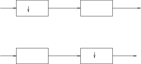
y
1(n)
x(n) w1
(n) H(z)
x(n) H(z
D)w2
(n) y
2(n)
D
D
Figure 11.10-1:
y2(n) = w2(nD)
=
n
X
k=0
h(k)x(nD −kD)
=
n
X
k=0
h(k)x[(n−k)D]
So y1(n) = y2(n)
(b)
w1(n) = ∞
X
k=0
h(k)x(n−k)
y1(n) = w1(p), n =pI(pan integer )
= 0,other n
w2(n) = x(p), n =pI
= 0,other n
Let ˜
h(n) be the IR corresponding to H(zI)
y2(n) = ∞
X
k=0
˜
h(k)w2(n−k)
=∞
X
k=0
˜
h(kI)w2(n−kI)
=∞
X
k=0
h(k)w2(n−kI)
for n=pI
y2(n) = ∞
X
k=0
h(k)w2((p−k)I)
346
© 2007 Pearson Education, Inc., Upper Saddle River, NJ. All rights reserved. This material is protected under all copyright laws
as they currently exist. No portion of this material may be reproduced, in any form or by any means, without permission in
writing from the publisher. For the exclusive use of adopters of the book Digital Signal Processing, Fourth Edition, by John G.
Proakis and Dimitris G. Manolakis. ISBN 0-13-187374-1.

=∞
X
k=0
h(k)x(p−k)
=w1(p)( see above )
for n6=pI
y2(n) = ∞
X
k=0
h(k).0 = 0
so we conclude y1(n) = y2(n)
11.11
(a)
H(z) = X
n
h(2n)z−2n+X
n
h(2n+ 1)z−2n−1
=X
n
h(2n)(z2)−n+z−1X
n
h(2n+ 1)(z2)−n
=H0(z2) + z−1H1(z2)
Therefore H0(z) = X
n
h(2n)z−n
H1(z) = X
n
h(2n+ 1)z−n
(b)
H(z) = X
n
h(nD)z−nD +X
n
h(nD + 1)z−nD−1+...
+X
n
h(nD +D−1)z−nD−D+1
=
D−1
X
k=0
z−kX
n
h(nD +k)(zD)−n
Therefore Hk(z) = X
n
h(nD +k)z−n
(c)
H(z) = 1
1−az−1
=∞
X
n=0
anz−n
H0(z) = ∞
X
n=0
a2nz−n
=1
1−a2z−1
H1(z) = ∞
X
n=0
a2n+1z−n
=a
1−a2z−1
347
© 2007 Pearson Education, Inc., Upper Saddle River, NJ. All rights reserved. This material is protected under all copyright laws
as they currently exist. No portion of this material may be reproduced, in any form or by any means, without permission in
writing from the publisher. For the exclusive use of adopters of the book Digital Signal Processing, Fourth Edition, by John G.
Proakis and Dimitris G. Manolakis. ISBN 0-13-187374-1.
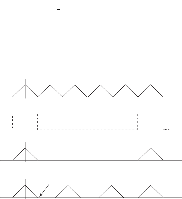
11.12
The output of the upsampler is X(z2). Thus, we have
Y1(z) = 1
2X(z)H1(z1/2) + X(z)H1(z1/2W1/2)
=1
2H1(z1/2) + H1(z1/2W1/2)X(z)
=H2(z)X(z)
11.13
(a) Refer to Fig. 11.13-1 for I/D = 5/3.
Fx5Fx
Fx5Fx
3Fy
Fy2Fy
(1/2)min(Fx,Fy)
Filter
DTFT[x(n)]
DTFT[y(m)]
Figure 11.13-1:
(b) Refer to Fig. 11.13-2 for I/D = 3/5.
11.14
(a) The desired implementation is given in Fig. 11.14-1
(b) The polyphase decomposition is given by
Hk(z) = (1 + z−1)5
= 1 + 5z−1+ 10z−2+ 10z−3+ 5z−4+z−5
= 1 + 10z−2+ 5z−4+ (5 + 10z−2+z−4)z−1
=P0(z) + P1(z)z−1
348
© 2007 Pearson Education, Inc., Upper Saddle River, NJ. All rights reserved. This material is protected under all copyright laws
as they currently exist. No portion of this material may be reproduced, in any form or by any means, without permission in
writing from the publisher. For the exclusive use of adopters of the book Digital Signal Processing, Fourth Edition, by John G.
Proakis and Dimitris G. Manolakis. ISBN 0-13-187374-1.
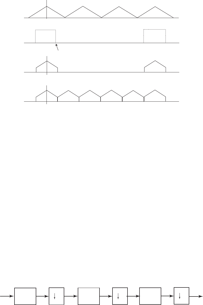
Fx
Fy5Fy
3Fx
3Fx
(1/2)min(Fx,Fy)
Filter
DTFT[x(n)]
DTFT[y(m)]
Figure 11.13-2:
11.15
(a)
H(z) =
N−1
X
n=0
z−nPn(zN)
where
Pn(z) = ∞
X
k=−∞
h(kN +n)z−k
Let m=N−1−n. Then
H(z) =
N−1
X
n=0
z−(N−1−m)PN−1−m(zN)
=
N−1
X
n=0
z−(N−1−m)Qm(zN)
(b)
2
()115
+−
z2
()115
+−
z2
()115
+−
z
Figure 11.14-1:
349
© 2007 Pearson Education, Inc., Upper Saddle River, NJ. All rights reserved. This material is protected under all copyright laws
as they currently exist. No portion of this material may be reproduced, in any form or by any means, without permission in
writing from the publisher. For the exclusive use of adopters of the book Digital Signal Processing, Fourth Edition, by John G.
Proakis and Dimitris G. Manolakis. ISBN 0-13-187374-1.
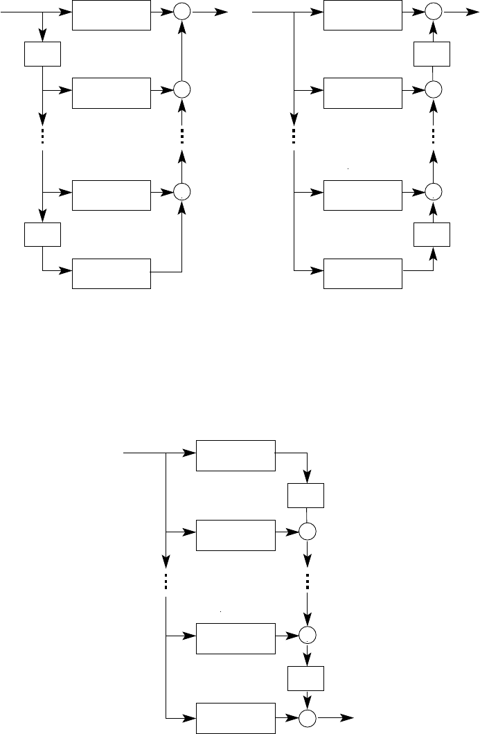
y(n)
N
0+
+
+
z−1
z−1
P (z )
N
0
z−1
z−1
+
+
+
P (z )
N
1
N−2
N−1
N
N
P (z )
P (z )
P (z )
N
1
N−2
N−1
N
N
P (z )
P (z )
y(n)
x(n) x(n) P (z )
Figure 11.15-1: Type 1 Polyphase Decomposition
N−1
+
+
z−1
z−1
+
0
Q (z )
N
N
N
N
x(n)
y(n)
Q (z )
Q (z )
Q (z )
1
N−2
Figure 11.15-2: Type 2 Polyphase Decomposition
350
© 2007 Pearson Education, Inc., Upper Saddle River, NJ. All rights reserved. This material is protected under all copyright laws
as they currently exist. No portion of this material may be reproduced, in any form or by any means, without permission in
writing from the publisher. For the exclusive use of adopters of the book Digital Signal Processing, Fourth Edition, by John G.
Proakis and Dimitris G. Manolakis. ISBN 0-13-187374-1.
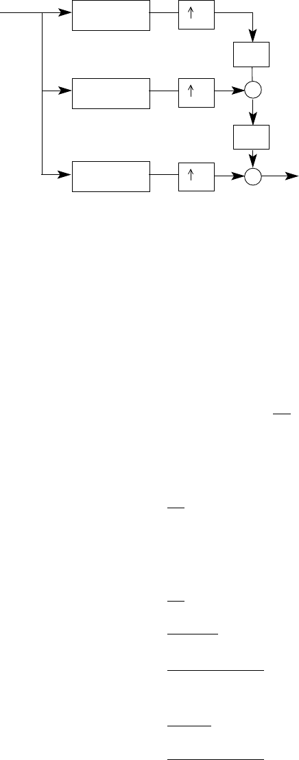
11.16
Q (z )
Q (z )
N
+
z−1
z−1
+
3
3
3
N
x(n)
Q (z )
1
y(n)
2 N
0
Figure 11.16-1:
11.17
D1= 25, D2= 4
F0= 10 kHz , F1=F0
D1
= 400 Hz
Passband 0 ≤F≤50
Transition band 50 < F ≤345
Stopband 345 < F ≤5000
F2=F1
D2
= 100 Hz
Passband 0 ≤F≤50
Transition band 50 < F ≤55
Stopband 55 < F ≤200
For filter 1, δ1=0.1
2= 0.05, δ2= 10−3
△f=345 −50
10,000 = 2.95x10⁻²
ˆ
M1=−10logδ1δ2−13
14.6△f+ 1 = 71
For filter 2, δ1= 0.05, δ2= 10−3
△f=55 −50
400 = 7.5x10⁻³
ˆ
M2=−10logδ1δ2−13
14.6△f+ 1 ≈275
The coefficients of the two filters can be obtained using a number of DSP software packages.
351
© 2007 Pearson Education, Inc., Upper Saddle River, NJ. All rights reserved. This material is protected under all copyright laws
as they currently exist. No portion of this material may be reproduced, in any form or by any means, without permission in
writing from the publisher. For the exclusive use of adopters of the book Digital Signal Processing, Fourth Edition, by John G.
Proakis and Dimitris G. Manolakis. ISBN 0-13-187374-1.

11.18
To avoid aliasing Fsc ≤Fx
2D. Thus D=I= 50.
Single stage
δ1= 0.1, δ2= 10−3
△f=65 −60
10,000 = 5x10⁻⁴
ˆ
M1=−10logδ1δ2−13
14.6△f+ 1 ≈3700
Two stages
D1= 25, D2= 2 I1= 2, I2= 25
stage 1:F1=10,000
25 = 400
Passband 0 ≤F≤60
Transition band 60 < F ≤335
Stopband 335 < F ≤5000
δ1= 0.1, δ2=10−3
4
△f= 2.75x10⁻²ˆ
M1= 84
stage 2:F2=400
2= 200
Passband 0 ≤F≤60
Transition band 60 < F ≤65
Stopband 65 < F ≤100
δ1= 0.1, δ2=10−3
4
△f= 0.1875 ˆ
M2= 13
Use DSP software to obtain filter coefficients.
11.19
b+(n) is nonzero for 0 ≤n≤2N−2 with Neven. Let c(n) = b+[n−(N−1)]. So c(n) is nonzero
for −(N−1) ≤n≤N−1. From (11.11.35)
B+(w) + (−1)N−1B+(w−π) = αe−jw(N−1)
or B+(z) + (−1)N−1B+(−z) = αz−(N−1)
Therefore, C(z)z−(N−1) + (−1)N−1C(−z)(−z)−(N−1) =αz−(N−1)
or C(z) + C(−z) = α
c(n) + c(−n) = αδ(n)
when n6= 0c(n) = −c(−n)
when nis odd c(n) = −c(−n)
when nis even but n6= 0, c(n) = 0
(half-band filter)
when n= 0, c(n) = α
2
352
© 2007 Pearson Education, Inc., Upper Saddle River, NJ. All rights reserved. This material is protected under all copyright laws
as they currently exist. No portion of this material may be reproduced, in any form or by any means, without permission in
writing from the publisher. For the exclusive use of adopters of the book Digital Signal Processing, Fourth Edition, by John G.
Proakis and Dimitris G. Manolakis. ISBN 0-13-187374-1.

11.20
one stage:
δ1= 0.01, δ2= 10−3
△f=100 −90
10,000 = 10−3
ˆ
M=−10logδ1δ2−13
14.6△f+ 1 ≈2536
two stages: F0= 2 ×10⁵Hz
I1= 1, I2= 2
F1=F0
I1
= 2 ×10⁴Hz
Passband 0 ≤F≤90
Transition band 90 < F ≤19,900
Therefore △f=19,900 −90
2×105= 0.09905
and δ11 =δ1
2, δ12 =δ2
ˆ
M1=−10logδ1δ2−13
14.6△f+ 1 ≈29
F2=F1
I2
= 1 ×10⁴Hz
Passband 0 ≤F≤90
Transition band 90 < F ≤9,900
Therefore △f=9,900 −90
2×104= 0.4905
and δ21 =δ1
2, δ22 =δ2
ˆ
M2=−10logδ1δ2−13
14.6△f+ 1 ≈7
11.21
Suppose the output of the analysis section is xa0(m) and xa1(m). After interpolation by 2, they
become y0(m) and y1(m). Thus
yk(m) = xak(m
2), m even k= 0,1
0, m odd
The final output is
z(m) = y0(m)∗2h(m) + y1(m)∗[−2(−1)mh(m)]
when mis even, say m= 2j,
z(m) = z(2j) = 2y0(m)∗h(m)−2y1(m)∗h(m)
= 2 X
k
y0(k)h(m−k)−2X
k
y1(k)h(m−k)
= 2 X
l
y0(2l)h(2j−2l)−2X
l
y1(2l)h(2j−2l)
353
© 2007 Pearson Education, Inc., Upper Saddle River, NJ. All rights reserved. This material is protected under all copyright laws
as they currently exist. No portion of this material may be reproduced, in any form or by any means, without permission in
writing from the publisher. For the exclusive use of adopters of the book Digital Signal Processing, Fourth Edition, by John G.
Proakis and Dimitris G. Manolakis. ISBN 0-13-187374-1.
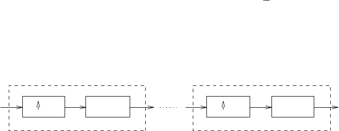
= 2 X
l
xa0(l)h[2(j−l)] −2X
l
xa1(l)h[2(j−l)]
= 2[xa0(j)−xa1(j)] ∗h(2j)
= 2[xa0(j)−xa1(j)] ∗p0(j)
In the same manner, it can be shown that
z(2j+ 1) = 2[xa0(j) + xa1(j)] ∗p1(j)
11.22
Refer to fig 11.22-1, where hi(n) is a lowpass filter with cutoff freq. π
Ii. After transposition (refer
I1h
1
(n)
Interpolator 1
I h(n)
L L
Interpolator L
Figure 11.22-1: I=I1I2. . . ILL-stage interpolator
to fig 11.22-2). As D=I, let Di=IL+1−i, then D=D1D2. . . DL. Refer to fig 11.22-3
Obviously, this is equivalent to the transposed form above.
354
© 2007 Pearson Education, Inc., Upper Saddle River, NJ. All rights reserved. This material is protected under all copyright laws
as they currently exist. No portion of this material may be reproduced, in any form or by any means, without permission in
writing from the publisher. For the exclusive use of adopters of the book Digital Signal Processing, Fourth Edition, by John G.
Proakis and Dimitris G. Manolakis. ISBN 0-13-187374-1.
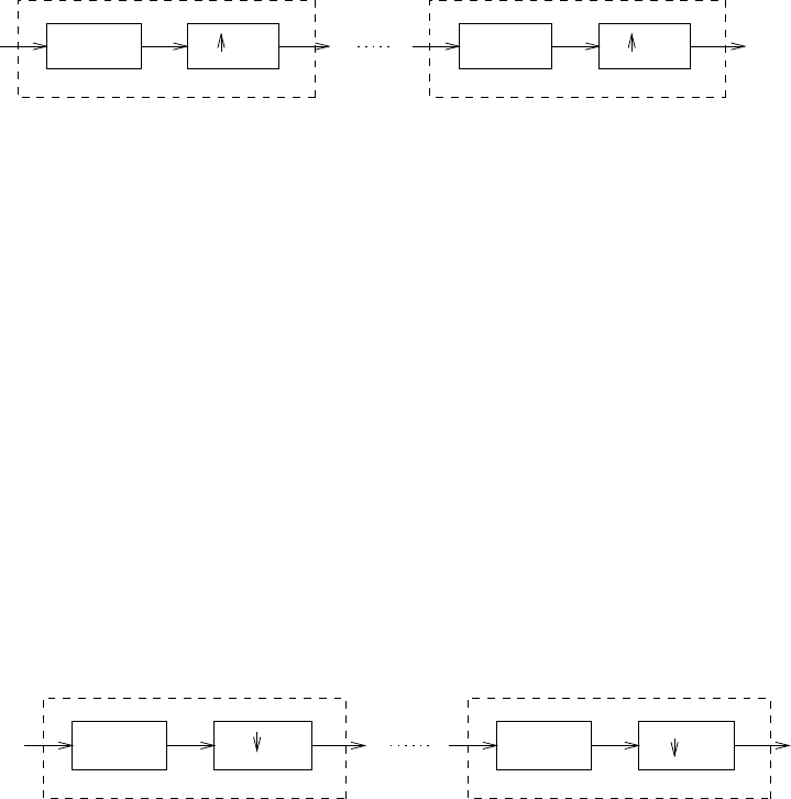
h(n)
Lh1(n)ILI
1
Figure 11.22-2:
h (n)
Lh1
(n)DLD1
Figure 11.22-3: L-stage decimator
355
© 2007 Pearson Education, Inc., Upper Saddle River, NJ. All rights reserved. This material is protected under all copyright laws
as they currently exist. No portion of this material may be reproduced, in any form or by any means, without permission in
writing from the publisher. For the exclusive use of adopters of the book Digital Signal Processing, Fourth Edition, by John G.
Proakis and Dimitris G. Manolakis. ISBN 0-13-187374-1.
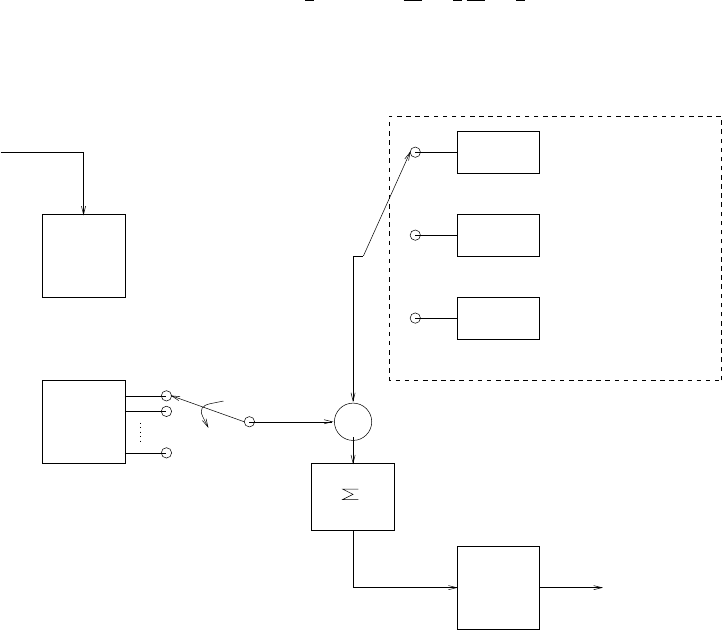
11.23
Suppose that output is y(n). Then Ty=k
ITx.Fy=1
Ty=I
k
1
Tx=I
kFx. Assume that the lowpass
filter is h(n) of length M=kI (see fig 11.23-4)
1
2
K
buffer
length K
input
buffer
length K
x(n) Fx
output
buffer
length I
y(n)
F
y=( I/k) F
x
K-1
n=0
+
g(n,0)
g(n,1)
g(n,I-1) n=0,1, ..., K-1
n=0,1, ..., K-1
n=0,1, ..., K-1
coefficient storage
Figure 11.23-4:
11.24
(a)
for any n=lI +j(0 ≤j≤I−1)
I−1
X
k=0
pk(n−k) =
I−1
X
k=0
pk(lI +j−k)
=pj(lI)
=pj(l)
=h(j+lI)
=h(n)
Therefore, h(n) =
I−1
X
k=0
pk(n−k)
356
© 2007 Pearson Education, Inc., Upper Saddle River, NJ. All rights reserved. This material is protected under all copyright laws
as they currently exist. No portion of this material may be reproduced, in any form or by any means, without permission in
writing from the publisher. For the exclusive use of adopters of the book Digital Signal Processing, Fourth Edition, by John G.
Proakis and Dimitris G. Manolakis. ISBN 0-13-187374-1.
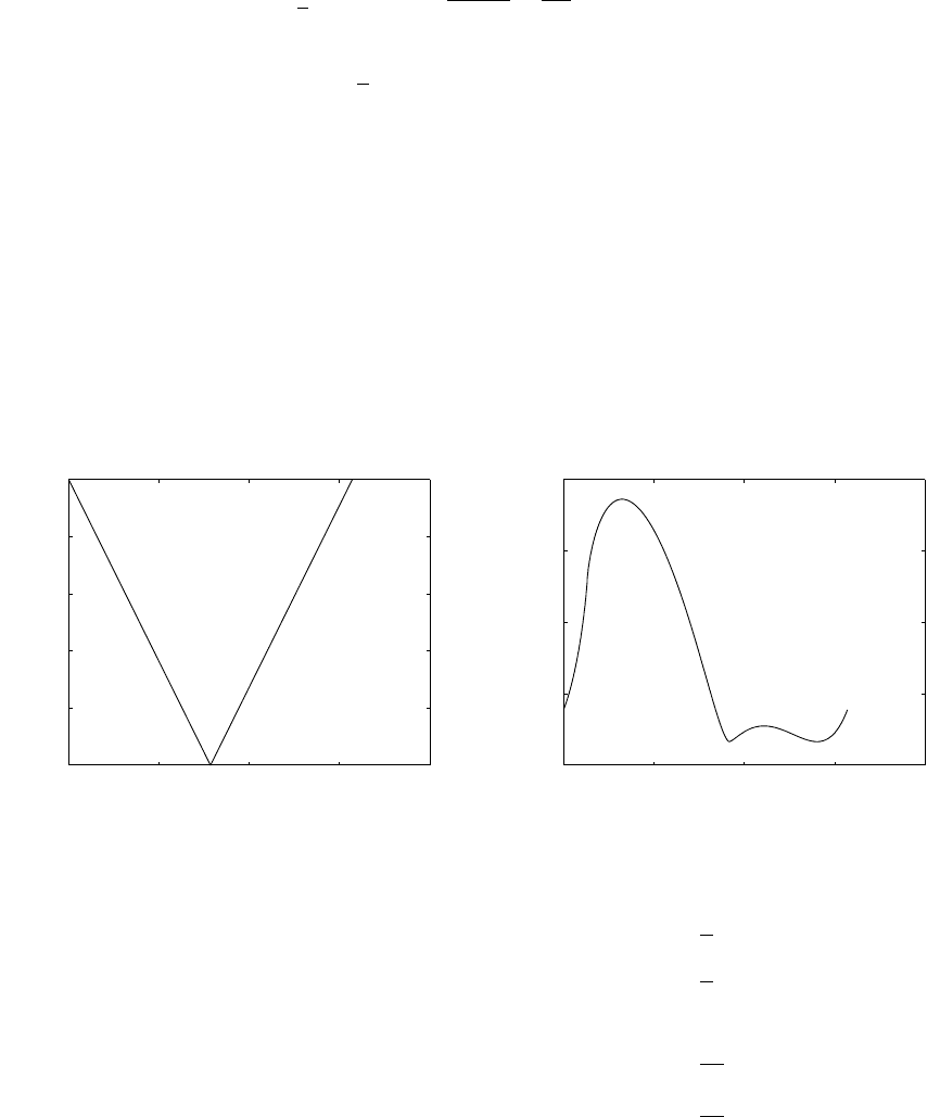
(b) z-transform both sides
H(z) =
I−1
X
k=0
z−kpk(z)
(c)
1
IX
n
I−1
X
l=0
h(n)ej2πl(n−k)
Iz−n−k
I
=1
IX
m
I−1
X
l=0
h(k+mI)ej2πlmz−m
=X
m
h(k+mI)z−m
=X
m
pk(m)z−m
=pk(z)
11.25
(a) Refer to fig 11.25-1.
(b)
0 2 4 6 8
0
0.2
0.4
0.6
0.8
1spectrum of x(n)
−−> w
−−> magnitude
0 2 4 6 8
0.4
0.5
0.6
0.7
0.8 spectrum of y(n)
−−> w
−−> magnitude
Figure 11.25-1:
Bandwidth = π
3
cut off freq = π
2
sampling freq of x(n) = 2π
sampling freq for the desired band of frequencies = 2π
2=π
Therefore, D=2π
2= 2
(c) Refer to fig 11.25-2.
(d) Refer to fig 11.25-3.
357
© 2007 Pearson Education, Inc., Upper Saddle River, NJ. All rights reserved. This material is protected under all copyright laws
as they currently exist. No portion of this material may be reproduced, in any form or by any means, without permission in
writing from the publisher. For the exclusive use of adopters of the book Digital Signal Processing, Fourth Edition, by John G.
Proakis and Dimitris G. Manolakis. ISBN 0-13-187374-1.
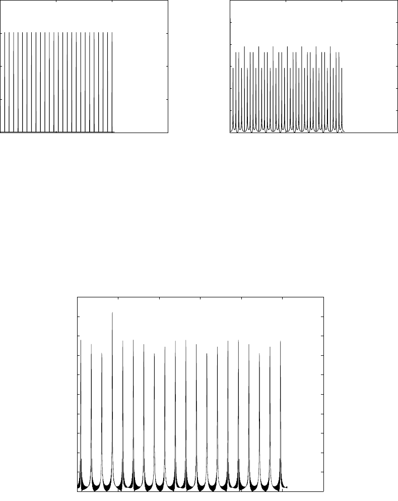
0 500 1000 1500
0
10
20
30
40 x(n)
−−>x(n)
−−−> n 0 500 1000 1500
0
200
400
600
800
1000
1200 |X(w)|
−−> magnitude
Figure 11.25-2:
0 200 400 600 800 1000 1200
0
100
200
300
400
500
600
700
800
900
1000
−−> magnitude
spectrum of s(n)
Figure 11.25-3:
358
© 2007 Pearson Education, Inc., Upper Saddle River, NJ. All rights reserved. This material is protected under all copyright laws
as they currently exist. No portion of this material may be reproduced, in any form or by any means, without permission in
writing from the publisher. For the exclusive use of adopters of the book Digital Signal Processing, Fourth Edition, by John G.
Proakis and Dimitris G. Manolakis. ISBN 0-13-187374-1.
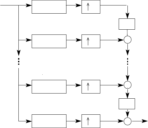
11.26
N−1
Q (z )
N
+
+
z−1
z−1
+y(n)
I
I
I
I
N
N
N
x(n)
Q (z )
Q (z )
Q (z )
1
N−2
0
Figure 11.26-1:
11.27
H0(z) =
N−1
X
n=0
z−nPn(zN)
where
Pn(z) = ∞
X
k=0
h0(kN +n)z−k,0≤k≤N−1
Then,
Hk(z) = H0(ze−j2πk/N ) = H0(zwk
N)
where wN=e−j2π/N .
(a)
Hk(z) =
N−1
X
l=0
z−lw−kl
NPl(zNwkN
N)
=
N−1
X
l=0
z−lw−kl
NPl(zN), k = 0,1,...,N −1
Therefore, Hk(z),0≤k≤N−1 can be expressed in matrix form as
Hk(z) = h1w−k
Nw−2k
N. . . w−(N−1)k
Ni
P0(zN)
z−1P1(zN)
.
.
.
z−1P1(zN)
359
© 2007 Pearson Education, Inc., Upper Saddle River, NJ. All rights reserved. This material is protected under all copyright laws
as they currently exist. No portion of this material may be reproduced, in any form or by any means, without permission in
writing from the publisher. For the exclusive use of adopters of the book Digital Signal Processing, Fourth Edition, by John G.
Proakis and Dimitris G. Manolakis. ISBN 0-13-187374-1.
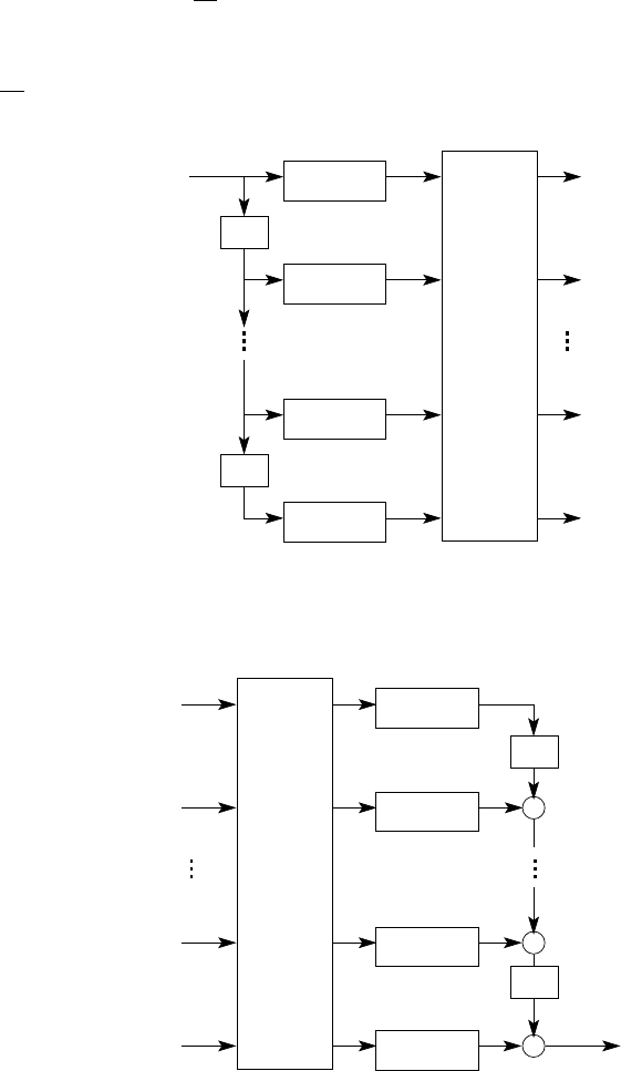
(b) From part (a), we have
H0(z)
H1(z)
.
.
.
HN−1(z)
=
1 1 1 ··· 1
1w−1
Nw−2
N··· w−(N−1)
N
.
.
..
.
..
.
..
.
.
1w−(N−1)
Nw−2(N−1)
N··· w−(N−1)(N−1)
N
P0(zN)
z−1P1(zN)
.
.
.
z−1P1(zN)
=NW −1
P0(zN)
z−1P1(zN)
.
.
.
z−1P1(zN)
where Wid the DFT matrix.
(c)
IDFT
N
0
z−1
z−1
P (z )
N
1
N−2
N−1
N
N
P (z )
P (z )
x(n)
y (n)
y (n)
1
N−2
N−1
y (n)
y (n)
0
N−point
P (z )
Figure 11.27-1:
(d)
DFT
0
y (n)
1
N−2
y (n)
N−1
y (n)
P (z )
N
0
P (z )
N
1
N−2
N−1
N
N
P (z )
P (z )
+
+
+
z−1
z−1
N−point
v(n)
y (n)
Figure 11.27-2:
360
© 2007 Pearson Education, Inc., Upper Saddle River, NJ. All rights reserved. This material is protected under all copyright laws
as they currently exist. No portion of this material may be reproduced, in any form or by any means, without permission in
writing from the publisher. For the exclusive use of adopters of the book Digital Signal Processing, Fourth Edition, by John G.
Proakis and Dimitris G. Manolakis. ISBN 0-13-187374-1.

11.28
H0(z) = 1 + z−1+ 3z−2+ 4z−3
(a)
Hk(z) = H0(zwk
4),1≤k≤3
=H0(ze−j2πk/4)
Then,
H1(z) = 1 + jz−1−3z−2+j4z−3
H2(z) = 1 −jz−1+ 3z−2−4z−3
H3(z) = 1 −jz−1−3z−2+j4z−3
Note that the impulse response hk(n) are complex-valued, in general. Consequently, |Hk(w)|is
not symmetric with respect to w= 0.
(b) Let us use the polyphase implementation of the uniform filter bank. We have
Pl(z) = ∞
X
n=0
h0(l+ 3n)z−n, l = 0,1,2,3
This yields P0(z) = 1, P1(z) = 1, P2(z) = 3, and P3(z) = 4. By using the results in Prob-
lem 11.27, we have the equation for the synthesis filter bank as
H0(z)
H1(z)
H2(z)
H3(z)
=
1 1 1 1
1j−1−j
1−1 1 −1
1−j−1j
P0(z4)
z−1P1(z4)
z−2P2(z4)
z−3P3(z4)
=
1 1 1 1
1j−1−j
1−1 1 −1
1−j−1j
1
z−1
3z−2
4z−3
= 4W−1
1
z−1
3z−2
4z−3
where Wdenotes the DFT matrix. Thus, we have the analysis filter bank given in fig 11.28-1.
(c) The synthesis filter bank in fig. 11.28-2
11.29
H(z) = −3 + 19z−2+ 32z−3+ 19z−4−3z−6
(a)
H(z−1) = −3 + 19z2+ 32z3+ 19z4−3z6
z−6H(z−1) = −3z−6+ 19z−4+ 32z−3+ 19z−2−3
=H(z)
Therefore, H(z−1) and H(z) hve roots that are symmetric, such that if ziis not a root, then
1/ziis also a root. This implies that H(z) has linera phase.
361
© 2007 Pearson Education, Inc., Upper Saddle River, NJ. All rights reserved. This material is protected under all copyright laws
as they currently exist. No portion of this material may be reproduced, in any form or by any means, without permission in
writing from the publisher. For the exclusive use of adopters of the book Digital Signal Processing, Fourth Edition, by John G.
Proakis and Dimitris G. Manolakis. ISBN 0-13-187374-1.
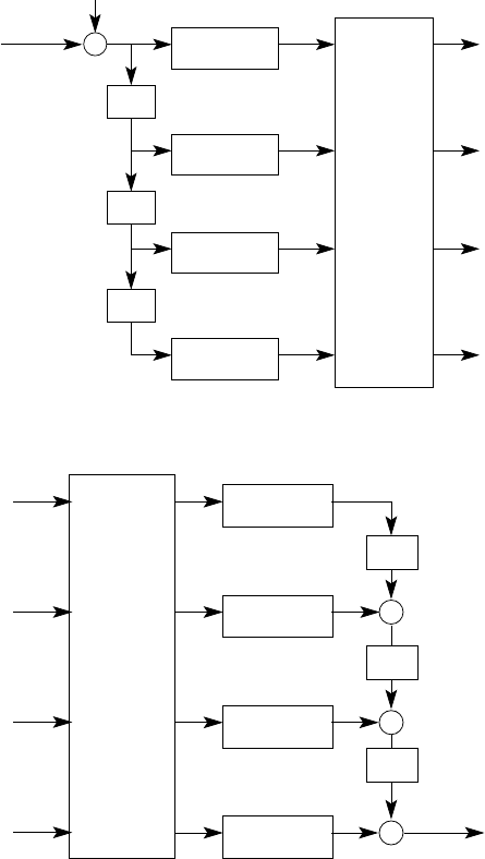
y (n)
−1
+
z−1
z−1
1
y (n)
y (n)
1
0
IDFT
x(n)
2
3
4−point
4
0
P (z )
4
P (z )
4
P (z )
4
P (z )
4
2
3
y (n)
z
Figure 11.28-1:
y (n)
+
z−1
y (n)
0
+
+
z−1
z−1
DFT
1
y (n)
1
0
P (z )
N
P (z )
N
v(n)
2
3
N
N
P (z )
P (z )
4−point
2
y (n)
3
Figure 11.28-2:
(b) We may express H(z) as:
H(z) = z−3−3z3+ 19z1+ 32 + 19z−1−3z−3
Thus, we have the coefficients:
h(2n) = 32, n = 0
0, n 6=
Therefore, H(z) is a half-band filter.
362
© 2007 Pearson Education, Inc., Upper Saddle River, NJ. All rights reserved. This material is protected under all copyright laws
as they currently exist. No portion of this material may be reproduced, in any form or by any means, without permission in
writing from the publisher. For the exclusive use of adopters of the book Digital Signal Processing, Fourth Edition, by John G.
Proakis and Dimitris G. Manolakis. ISBN 0-13-187374-1.
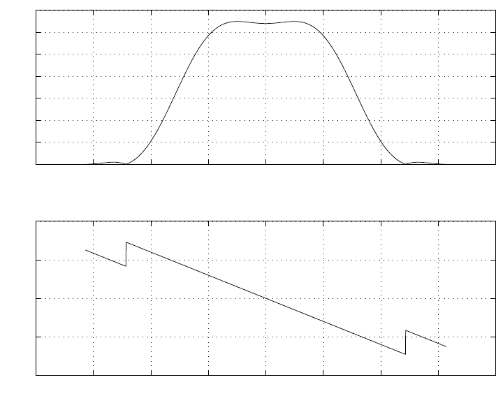
(c)
−4 −3 −2 −1 0 1 2 3 4
0
10
20
30
40
50
60
70
w
|H(w)|
−4 −3 −2 −1 0 1 2 3 4
−10
−5
0
5
10
w
angle(H(w))
Figure 11.29-1:
11.30
H0(z) = 1 + z−1
(a)
Pl(z) = ∞
X
n=0
h0(l+ 2n)z−n
P0(z) = ∞
X
n=0
h0(2n)z−n= 1
P1(z) = ∞
X
n=0
h0(l+ 2n)z−n= 1
363
© 2007 Pearson Education, Inc., Upper Saddle River, NJ. All rights reserved. This material is protected under all copyright laws
as they currently exist. No portion of this material may be reproduced, in any form or by any means, without permission in
writing from the publisher. For the exclusive use of adopters of the book Digital Signal Processing, Fourth Edition, by John G.
Proakis and Dimitris G. Manolakis. ISBN 0-13-187374-1.
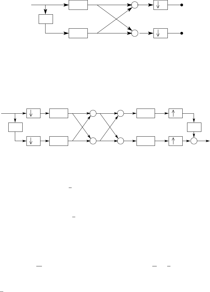
(b)
H1(z) = P0(z2)−z−1P1(z2)
= 1 −z−1
x(n) 1
1
z−1
+
+
2
2
Figure 11.30-1: Anaylsis section
(c)
G0(z) = P0(z2) + z−1P1(z2) = 1 + z−1
G1(z) = −P0(z2)−z−1P1(z)=−1 + z−1
−
−1
2
2
1
1
+
+
+
+
1
1
z−1
+
2
2x(n)
^
x(n)
−
z
Figure 11.30-2: QMF in a polyphase realization
(d) For perfect reconstruction,
Q(z) = 1
2[H0(z)G0(z) + H1(z)G1(z)] = Cz−k
where Cis a constant. We have
Q(z) = 1
2(1 + z−1)2−(1 −z−1)2= 2z−1
11.31
(a)
H(z) =
H0(z)
H1(z)
H2(z)
=
1 + z−1+z−2
1−z−1+z−2
1−z−2
=P(z3)a(z)
where a(z) =
1
z−1
z−2
. Then
1 + z−1+z−2
1−z−1+z−2
1−z−2
=
P00(z3)P01(z3)P02(z3)
P10(z3)P11(z3)P12(z3)
P20(z3)P21(z3)P22(z3)
1
z−1
z−2
364
© 2007 Pearson Education, Inc., Upper Saddle River, NJ. All rights reserved. This material is protected under all copyright laws
as they currently exist. No portion of this material may be reproduced, in any form or by any means, without permission in
writing from the publisher. For the exclusive use of adopters of the book Digital Signal Processing, Fourth Edition, by John G.
Proakis and Dimitris G. Manolakis. ISBN 0-13-187374-1.
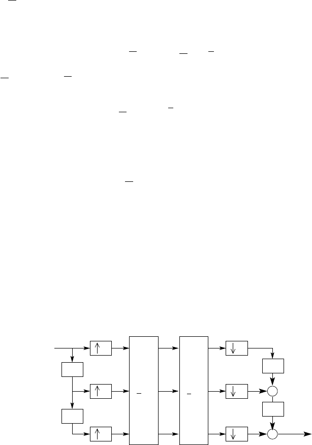
Clearly, P(z3) =
1 1 1
1−1 1
1 0 −1
(b) The synthesis filters are given as
G(z) = z−3Qt(z3)a(z−1)
where Q(z) = Cz−k[P(z)]−1. But
[P(z)]−1=1
4
1 1 2
2−2 0
1 1 −2
By selecting C= 4 and k= 1, we have
Q(z) = z
1 1 2
2−2 0
1 1 −2
Therefore,
G0(z)
G1(z)
G2(z)
=z−2
1 1 2
2−2 0
1 1 −2
1
z−1
z−2
=
1 + 2z−1+z−2
1−2z−1+z−2
−2 + 2z−1
(c)
3
P(z) Q(z)
3
z−1
3
3
z−1
+
z−1
z−1
+
x(n)
v(n)
3
3
Figure 11.31-1:
365
© 2007 Pearson Education, Inc., Upper Saddle River, NJ. All rights reserved. This material is protected under all copyright laws
as they currently exist. No portion of this material may be reproduced, in any form or by any means, without permission in
writing from the publisher. For the exclusive use of adopters of the book Digital Signal Processing, Fourth Edition, by John G.
Proakis and Dimitris G. Manolakis. ISBN 0-13-187374-1.
366
© 2007 Pearson Education, Inc., Upper Saddle River, NJ. All rights reserved. This material is protected under all copyright laws
as they currently exist. No portion of this material may be reproduced, in any form or by any means, without permission in
writing from the publisher. For the exclusive use of adopters of the book Digital Signal Processing, Fourth Edition, by John G.
Proakis and Dimitris G. Manolakis. ISBN 0-13-187374-1.

Chapter 12
12.1
(a)
Γxx(z) = 25
(1 −z−1+1
2z−2)(1 −z−1+1
2z−2)
H(z) = 1
1−z−1+1
2z−2
and σ2
w= 25
so x(n) = x(n−1) −1
2x(n−2) + w(n)
(b) The whitening filter is H−1(z) = 1 −z−1+1
2z−2
12.2
(a) Γxx(z) = 27
2
(1−1
3z1)(1−1
3z)
(1−1
2z1)(1−1
2z)
For a stable filter, denominator (1 −1
2z1) must be chose. However, either numerator factor
may be used. H(z) = (1 −1
3z1)
(1 −1
2z1)
|{z }
[min.pk.]
or (1−1
3z)
(1−1
2z)
(b) Must invert the min. pk. filter to obtain a stable whitening filter.
H−1(z) = (1 −1
2z1)
(1 −1
3z1)
12.3
(a)
H(z) = 1 + 0.9z−1
1−1.6z−1+ 0.63z−2
whitening filter, H−1(z) = 1−1.6z−1+ 0.63z−2
1 + 0.9z−1
zeros: z= 0.7 and 0.9
pole: z=−0.9
367
© 2007 Pearson Education, Inc., Upper Saddle River, NJ. All rights reserved. This material is protected under all copyright laws
as they currently exist. No portion of this material may be reproduced, in any form or by any means, without permission in
writing from the publisher. For the exclusive use of adopters of the book Digital Signal Processing, Fourth Edition, by John G.
Proakis and Dimitris G. Manolakis. ISBN 0-13-187374-1.

(b)
Γxx(w) = σ2
wH(w)H(−w)
=σ2
w|1 + 0.9e−jw|2
|1−1.6e−jw + 0.63e−2jw |2
12.4
A(z) = 1 + 13
24z−1+5
8z−2+1
3z−3
k3=1
3
B3(z) = 1
3+5
8z−1+13
24z−2+z−3
k3=1
2
B2(z) = 1
2+3
8z−1+z−2
A1(z) = A2(z)−k2B2(z)
1−k2
2
= 1 + 1
4z−1
k1=1
4
12.5
A2(z) = 1 + 2z−1+1
3z−2
B2(z) = 1
3+ 2z−1+z−2
k2=1
3
A1(z) = A2(z)−k2B2(z)
1−k2
2
= 1 + 3
2z−1
k1=3
2
12.6
(a)
A1(z) = 1 + 1
2z−1
B1(z) = 1
2+z−1
A2(z) = A1(z) + k2B1(z)z−1
368
© 2007 Pearson Education, Inc., Upper Saddle River, NJ. All rights reserved. This material is protected under all copyright laws
as they currently exist. No portion of this material may be reproduced, in any form or by any means, without permission in
writing from the publisher. For the exclusive use of adopters of the book Digital Signal Processing, Fourth Edition, by John G.
Proakis and Dimitris G. Manolakis. ISBN 0-13-187374-1.

= 1 + 1
3z−1−1
3z−2
B2(z) = −1
3+1
3z−1+z−2
H(z) = A3(z) = A2(z) + k3B2(z)z−1
= 1 + z−3
The zeros are at z=−1, e±jπ
3
Refer to fig 12.6-1
1
Figure 12.6-1:
(b)
If k3=−1,we have
H(z) = A3(z) = A2(z)−B2(z)z−1
= 1 + 2
3z−1−2
3z−2−z−3
The zeros are at z=−1,−5
6±j√11
6
(c) If |kp|= 1, the zeros of H(z) = Ap(z) are on the unit circle. Refer to fig 12.6-2.
369
© 2007 Pearson Education, Inc., Upper Saddle River, NJ. All rights reserved. This material is protected under all copyright laws
as they currently exist. No portion of this material may be reproduced, in any form or by any means, without permission in
writing from the publisher. For the exclusive use of adopters of the book Digital Signal Processing, Fourth Edition, by John G.
Proakis and Dimitris G. Manolakis. ISBN 0-13-187374-1.
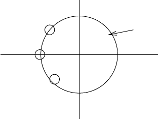
unit circle
Figure 12.6-2:
12.7
A1(z) = 1 + 0.6z−1
B1(z) = 0.6 + z−1
A2(z) = A1(z) + k2B1(z)z−1
= 1 + 0.78z−1+ 0.3z−2
B2(z) = 0.3 + 0.78z−1+z−2
A3(z) = A2(z) + 0.52B2(z)z−1
= 1 + 0.93z−1+ 0.69z−2+ 0.5z−3
B3(z) = 0.5 + 0.69z−1+ 0.93z−2+z−3
H3(z) = A3(z) + 0.9B3(z)z−1
= 1 + 1.38z−1+ 1.311z−2+ 1.337z−3+ 0.9z−4
h(n) = 1
↑,1.38,1.311,1.337,0.9,0,...
12.8
Let y(m) = x(2n−p−m). Then, the backward prediction of x(n−p) becomes the forward
prediction of y(n). Hence, its linear prediction error filter is just the noise whitening filter of the
corresponding anticausal AR(p) process.
12.9
ˆx(n+m) = −
p
X
k=1
ap(k)x(n−k)
370
© 2007 Pearson Education, Inc., Upper Saddle River, NJ. All rights reserved. This material is protected under all copyright laws
as they currently exist. No portion of this material may be reproduced, in any form or by any means, without permission in
writing from the publisher. For the exclusive use of adopters of the book Digital Signal Processing, Fourth Edition, by John G.
Proakis and Dimitris G. Manolakis. ISBN 0-13-187374-1.
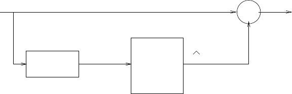
e(n) = x(n+m)−ˆx(n+m)
=x(n+m) +
p
X
k=1
ap(k)x(n−k)
E[e(n)x∗(n−l)] = 0, l = 1,2,...,p
⇒
p
X
k=1
ap(k)γxx(k−l) = −γxx(l+m), l = 1,2, . . . , p
The minimum error is
E{|e(n)|2}=E[e(n)x∗(n+m)]
=γxx(0) +
p
X
k=1
ap(k)γxx(m+k)
Refer to fig 12.9-1.
x(n+m) +
-
e(n)
z-m-1 forward
linear
predictor
x(n+m)
Figure 12.9-1:
12.10
ˆx(n−p−m) = −
p−1
X
k=0
bp(k)x(n−k)
e(n) = x(n−p−m)−ˆx(n−p−m)
=x(n−p−m) +
p−1
X
k=0
bp(k)x(n−k)
E[e(n)x∗(n−l)] = 0, l = 0,2,...,p−1
⇒
p−1
X
k=0
bp(k)γxx(l−k) = −γxx(l−p−m), l = 0,2, . . . , p −1
371
© 2007 Pearson Education, Inc., Upper Saddle River, NJ. All rights reserved. This material is protected under all copyright laws
as they currently exist. No portion of this material may be reproduced, in any form or by any means, without permission in
writing from the publisher. For the exclusive use of adopters of the book Digital Signal Processing, Fourth Edition, by John G.
Proakis and Dimitris G. Manolakis. ISBN 0-13-187374-1.
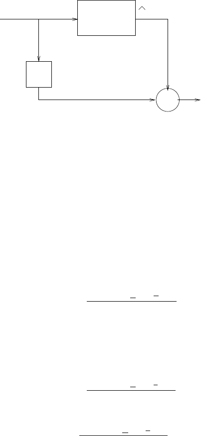
The minimum error is
E{|e(n)|2}=E[e(n)x∗(n−p−m)]
=γxx(0) +
p−1
X
k=0
bp(k)γxx(p+m−k)
Refer to fig 12.10-1.
x(n) Backward
linear
predictor
x(n-p-m) + -e(n)
x(n-p-m)
z-p-m
Figure 12.10-1:
12.11
The Levinson-Durbin algorithm for the forward filter coefficients is
am(m)≡km=−γxx(m) + γbt
m−1am−1
Ef
m
am(k) = am−1(k) + kma∗
m−1(m−k),
k= 1,2,...,m−1; m= 1,2,...,p
but bm(k) = a∗
m(m−k), k = 0,2,...,m
or am(k) = b∗
m(m−k)
Therefore, b∗
m(0) ≡km=−γxx(m) + γt
m−1b∗
m−1
Eb
m
b∗
m(m−k) = b∗
m−1(m−1−k) + kmbm−1(k)
Equivalently, bm(0) = k∗
m=γ∗
xx(m) + γ∗
m−1bt
m−1
Eb
m
bm(k) = bm−1(k−1) + k∗
mb∗
m−1(m−k)
This is the Levinson-Durbin algorithm for the backward filter.
372
© 2007 Pearson Education, Inc., Upper Saddle River, NJ. All rights reserved. This material is protected under all copyright laws
as they currently exist. No portion of this material may be reproduced, in any form or by any means, without permission in
writing from the publisher. For the exclusive use of adopters of the book Digital Signal Processing, Fourth Edition, by John G.
Proakis and Dimitris G. Manolakis. ISBN 0-13-187374-1.

12.12
Let
bm=bm−1
0+dm−1
bm(m)
Then, "Γm−1γb∗
m−1
γbt
m−1γxx(0) #bm=bm−1
0+dm−1
bm(m)=cm−1
cm(m)
Hence,
Γm−1bm−1+ Γm−1dm−1+bm(m)γb∗
m−1=cm−1
γbt
m−1bm−1+γbt
m−1dm−1+bm(m)γxx(0) = cm(m)
But Γm−1bm−1=cm−1
⇒Γm−1dm−1=−bm(m)γb∗
m−1
Hence, dm−1=−bm(m)Γ−1
m−1γb∗
m−1
Also, Γ−1
m−1γb∗
m−1=ab∗
m−1
Therefore, bm(m)γbt
m−1ab∗
m−1+bm(m)γxx(0) = cm(m)−γbt
m−1bm−1
solving for bm(m),we obtain
bm(m) = cm(m)−γbt
m−1bm−1
γxx(0) + γbt
m−1ab∗
m−1
=cm(m)−γbt
m−1bm−1
Ef
m−1
we also obtain the recursion
bm(k) = bm−1(k) + bm(m)a∗
m−1(m−k),
k= 1,2, . . . , m −1
12.13
Equations for the forward linear predictor:
Γmam=cm
where the elements of cmare γxx(l+m), l = 1,2,...,p. The solution of amis
am(m) = cm(m)−γbt
m−1am−1
γxx(0) + γbt
m−1ab∗
m−1
=cm(m)−γbt
m−1am−1
Ef
m−1
am(k) = am−1(k) + am(m)α∗
m−1(m−k),
k= 1,2,...,m−1; m= 1,2,...,p
where αmis the solution to Γmαm=γm
The coefficients for the m-step backward predictor are bm=ab
m.
373
© 2007 Pearson Education, Inc., Upper Saddle River, NJ. All rights reserved. This material is protected under all copyright laws
as they currently exist. No portion of this material may be reproduced, in any form or by any means, without permission in
writing from the publisher. For the exclusive use of adopters of the book Digital Signal Processing, Fourth Edition, by John G.
Proakis and Dimitris G. Manolakis. ISBN 0-13-187374-1.

12.14
(a)
ˆx(n) = −a1x(n−1) −a2x(n−2) −a3x(n−3)
But x(n) = 14
24x(n−1) + 9
24x(n−2) −1
24x(n−3) + w(n)
E{[x(n)−ˆx(n)]2}is minimized by selecting the coefficients as a1=−14
24 , a2=−9
24 , a3=1
24
(b)
γxx(m) = −
3
X
k=1
akγxx(m−k), m > 0
=−
p
X
k=1
akγxx(m−k) + σ2
w, m = 0
Since we know the {ak}we can solve for γxx(m), m = 0,1,2,3. Then we can obtain γxx(m)
for m > 3, by the above recursion. Thus,
γxx(0) = 4.93
γxx(1) = 4.32
γxx(2) = 4.2
γxx(3) = 3.85
γxx(4) = 3.65
γxx(5) = 3.46
(c)
A3(z) = 1 −14
24z−1−9
24z−2+1
24z−3
k3=1
24
B3(z) = 1
24 −9
24z−1−14
24z−2+z−3
A2(z) = A3(z)−k3B3(z)
1−k2
3
= 1 −0.569z−1−0.351z−2
k2=−0.351
B2(z) = −0.351 −0.569z−1+z−2
A1(z) = A2(z)−k2B2(z)
1−k2
2
= 1 −0.877z−1
k1=−0.877
12.15
(a)
Γxx(z) = 4σ2
w
9
(2 −z−1)(2 −z)
(3 −z−1)(3 −z)
=σ2
wH(z)H(z−1)
374
© 2007 Pearson Education, Inc., Upper Saddle River, NJ. All rights reserved. This material is protected under all copyright laws
as they currently exist. No portion of this material may be reproduced, in any form or by any means, without permission in
writing from the publisher. For the exclusive use of adopters of the book Digital Signal Processing, Fourth Edition, by John G.
Proakis and Dimitris G. Manolakis. ISBN 0-13-187374-1.

The minimum-phase system function H(z) is
H(z) = 2
3
2−z−1
3−z−1
=4
9
1−1
2z−1
1−1
3z−1
(b) The mixed-phase stable system has a system function
H(z) = 2
3
1−2z−1
3−z−1
=2
9
1−2z−1
1−1
3z−1
12.16
(a)
A2(z) = 1 −2rcosΘz−1+r2z−2
⇒k2=r2
B2(z) = r2−2rcosΘz−1+z−2
A1(z) = A2(z)−k2B2(z)
1−k2
2
= 1 −2rcosΘ
1 + r2z−1
Hence, k1=−2rcosΘ
1 + r2
(b) As r→1, k2→1 and k1→ −cosΘ
12.17
(a)
a1(1) = −1.25, a2(2) = 1.25, a3(3) = −1
Hence, A3(z) = 1 −1.25z−1+ 1.25z−2−z−3
First, we determine the reflection coefficients. Clearly, k3=−1, whcih implies that the roots
of A3(z) are on the unit circle. We may factor out one root. Thus,
A3(z) = (1 −z−1)(1 −1
4z−1+z−2)
= (1 −z−1)(1 −αz−1)(1 −α∗z−1)
where α=1 + j√63
8
Hence, the roots of A3(z) are z= 1, α, and α∗.
(b) The autocorrelation function satisfies the equations
γxx(m) +
3
X
k=1
a3(k)γxx(m−k) = σ2
w, m = 0
0,1≤m≤3
375
© 2007 Pearson Education, Inc., Upper Saddle River, NJ. All rights reserved. This material is protected under all copyright laws
as they currently exist. No portion of this material may be reproduced, in any form or by any means, without permission in
writing from the publisher. For the exclusive use of adopters of the book Digital Signal Processing, Fourth Edition, by John G.
Proakis and Dimitris G. Manolakis. ISBN 0-13-187374-1.

γxx(0) γxx(1) γxx(2) γxx(3)
γxx(1) γxx(0) γxx(1) γxx(2)
γxx(2) γxx(1) γxx(0) γxx(1)
γxx(3) γxx(2) γxx(1) γxx(0)
1
−1.25
1.25
−1
=
σ2
w
0
0
0
(c) Note that since k3=−1, the recursion Ef
m=Ef
m−1(1 − |km|2) implies that Ef
3= 0. This
implies that the 4x4 correlation matrix Γxx is singular. Since Ef
3= 0, then σ2
w= 0
12.18
γxx(0) = 1
γxx(1) = −0.5
γxx(2) = 0.625
γxx(3) = −0.6875
Use the Levinson-Durbin algorithm
a1(1) = −γxx(1)
γxx(0) =1
2
A1(z) = 1 + 1
2z−1
⇒k1=1
2
E1= (1 −a2
1(1))γxx(0) = 3
4
a2(2) = −γxx(2) + a1(1)γxx(1)
E1
=−1
2
a2(1) = a1(1) + a2(2)a1(1) = 1
4
Therefore,A2(z) = 1 + 1
4z−1−1
2z−2
⇒k2=−1
2
E2= (1 −a2
2(2))E1=9
16
a3(3) = −γxx(3) + a2(1)γxx(2) + a2(2)γxx(1)
E2
=1
2
a3(2) = a2(2) + a3(3)a2(1) = −3
8
a3(1) = a2(1) + a3(3)a2(2) = 0
Therefore,A3(z) = 1 −3
8z−2+1
2z−3
⇒k3=1
2
E3= (1 −a2
3(3))E2=27
64
376
© 2007 Pearson Education, Inc., Upper Saddle River, NJ. All rights reserved. This material is protected under all copyright laws
as they currently exist. No portion of this material may be reproduced, in any form or by any means, without permission in
writing from the publisher. For the exclusive use of adopters of the book Digital Signal Processing, Fourth Edition, by John G.
Proakis and Dimitris G. Manolakis. ISBN 0-13-187374-1.

12.19
(a)
Γxx(z) = ∞
X
−∞
γxx(m)z−m
=−1
X
−∞
(1
4)−mz−m+∞
X
0
(1
4)mz−m
=
1
4z
1−1
4z+1
1−1
4z−1
=
15
16
(1 −1
4z)(1 −1
4z−1)
since Γxx(z) = σ2H(z)H(z−1),
H(z) = 0.968
1−1
4z−1
is the minimum-phase solution. The difference equation is
x(n) = 1
4x(n−1) + 0.968w(n)
where w(n) is a white noise sequence with zero mean and unit variance.
(b) If we choose
H(z) = 1
1−1
4z
=z−1
z−1−1
4
=−4z−1
1−4z−1
then, x(n) = 4x(n−1) −4×0.968w(n−1)
12.20
γxx(0) = 1
γxx(1) = 0
γxx(2) = −a2
γxx(3) = 0
a1(1) = −γxx(1)
γxx(0) = 0
A1(z) = 1
⇒k1= 0
E1= (1 −a2
1(1))γxx(0) = 1
a2(2) = −γxx(2) + a1(1)γxx(1)
E1
=a2
a2(1) = a1(1) + a2(2)a1(1) = 0
377
© 2007 Pearson Education, Inc., Upper Saddle River, NJ. All rights reserved. This material is protected under all copyright laws
as they currently exist. No portion of this material may be reproduced, in any form or by any means, without permission in
writing from the publisher. For the exclusive use of adopters of the book Digital Signal Processing, Fourth Edition, by John G.
Proakis and Dimitris G. Manolakis. ISBN 0-13-187374-1.

Therefore,A2(z) = 1 + a2z−2
⇒k2=a2
E2= (1 −a2
2(2))E1= 1 −a4
a3(3) = −γxx(3) + a2(1)γxx(2) + a2(2)γxx(1)
E2
= 0
a3(2) = a2(2) + a3(3)a2(1) = a2
a3(1) = a2(1) + a3(3)a2(2) = 0
Therefore,A3(z) = A2(z) = 1 + a2z−2
⇒k3= 0
E3=E2= 1 −a4
12.21
Ap(z) = Ap−1(z) + kpBp−1(z)z−1
where Bp−1(z) is the reverse polynomial of Ap−1(z).
For |kp|<1, we have all the roots inside the unit circle as previously shown.
For |kp|= 1, Ap(z) is symmetric, which implies that all the roots are on the unit circle.
For |kp|>1, Ap(z) = As(z) + ǫBp−1(z)z−1, where As(z) is the symmetric polynomial with all
the roots on the unit circle and Bp−1(z) has all the roots outside the unit circle. Therefore, Ap(z)
will have all its roots outside the unit circle.
12.22
Vm=1km
k∗
m1
VmJVt∗
m=1km
k∗
m1 1 0
0−1 1km
k∗
m1
=1−km
k∗
m−1 1km
k∗
m1=1− |km|20
0−(1 − |km|2)
= (1 − |km|2)1 0
0−1= (1 − |km|2)J
12.23
(a)
E[fm(n)x(n−i)] = E[
m
X
k=0
am(k)x(n−k)x(n−i)]
= 0,by the orthogonality property
378
© 2007 Pearson Education, Inc., Upper Saddle River, NJ. All rights reserved. This material is protected under all copyright laws
as they currently exist. No portion of this material may be reproduced, in any form or by any means, without permission in
writing from the publisher. For the exclusive use of adopters of the book Digital Signal Processing, Fourth Edition, by John G.
Proakis and Dimitris G. Manolakis. ISBN 0-13-187374-1.
(b)
E[gm(n)x(n−i)] =
m
X
k=0
a∗
m(k)E[x(n−m+k)x(n−i)]
=
m
X
k=0
a∗
m(k)γxx(k−m+i)
= 0, i = 0,1,...,m−1
(c)
E[fm(n)x(n)] = E{fm(n)[fm(n)−
m
X
k=1
am(k)x(n−k)]}
=E{|fm(n)|2}
=Em
E[gm(n)x(n−m)] = E{gm(n)[gm(n)−
m−1
X
k=0
bm(k)x(n−k)]}
=E{|gm(n)|2}
=Em
(d)
E[fi(n)fj(n)] = E{fi(n)[x(n) +
j
X
k=1
aj(k)x(n−k)]}
=E{fi(n)x(n)}
=Ei
=Emax(i, j)
where i > j has been assumed
(e)
E[fi(n)fj(n−t)] = E{fi(n)[x(n−t) +
j
X
k=1
aj(k)x(n−t−k)]}
when 0 ≤t≤i−j, x(n−t−1), x(n−t−2),...,x(n−t−j) are just a subset of x(n−1), x(n−
2),...,x(n−i) Hence, from the orthogonality principle,
E[fi(n)fj(n−t)] = 0
Also, when −1≥t≥i−jholds, via the same method we have
E[fi(n)fj(n−t)] = 0
(f)
E[gi(n)gj(n−t)] = E{gi(n)[x(n−t−j) +
j−1
X
k=0
bj(k)x(n−t−k)]}
when 0 ≤t≤i−j, {x(n−t), x(n−t−1),...,x(n−t−j)}is a subset of {x(n),...,x(n−i+ 1)}
Hence, from the orthogonality principle,
E[gi(n)gj(n−t)] = 0
379
© 2007 Pearson Education, Inc., Upper Saddle River, NJ. All rights reserved. This material is protected under all copyright laws
as they currently exist. No portion of this material may be reproduced, in any form or by any means, without permission in
writing from the publisher. For the exclusive use of adopters of the book Digital Signal Processing, Fourth Edition, by John G.
Proakis and Dimitris G. Manolakis. ISBN 0-13-187374-1.
Also, when 0 ≥t≥i−j+ 1 we obtain the same result (g)
for i=j, E{fi(n+i)fj(n+j)}=E{f2
i(n+i)}
=Ei
for i6=j, suppose that i > j. Then
E{fi(n+i)fj(n+j)}=E{fi(n+i)[x(n+j) +
j
X
k=1
aj(k)x(n+j−k)]}
= 0
(h)
suppose i > j
E{gi(n+i)gj(n+j)}=E{gi(n+i)[x(n) +
j−1
X
k=0
bj(k)x(n+j−k)]}
=E[gi(n+i)x(n)]
=Ei
(i)
for i≥j
E{fi(n)gj(n)}=E{fi(n)[x(n−j) +
j−1
X
k=0
bj(k)x(n−k)]}
=E{fi(n)[bj(0)x(n)]}
=kjE[fi(n)x(n)]
=kjEi
for i < j,
E{fi(n)gj(n)}=E{gj(n)[x(n) +
i
X
k=1
ai(k)x(n−k)]}
= 0
(j)
E{fi(n)gi(n−1)}=E{fi(n)[x(n−1−j) +
i−1
X
k=0
bi(k)x(n−1−k)]}
=E[fi(n)x(n−1−i)]
=E{fi(n)[gi+1(n)−
i
X
k=0
bi+1(k)x(n−k)]}
=−E[fi(n)bi+1(0)x(n)]
=−ki+1Ei
(k)
E{gi(n−1)x(n)}=E{gi(n−1)[fi+1(n)−
i+1
X
k=1
ai+1(k)x(n−k)]}
=−E[gi(n−1)ai+1(i+ 1)x(n−1−i)]
=−ki+1Ei
E{fi(n+ 1)x(n−i)}=E{fi(n+ 1)[fi(n−i)−
i
X
k=1
ai(k)x(n−i−k)]}
380
© 2007 Pearson Education, Inc., Upper Saddle River, NJ. All rights reserved. This material is protected under all copyright laws
as they currently exist. No portion of this material may be reproduced, in any form or by any means, without permission in
writing from the publisher. For the exclusive use of adopters of the book Digital Signal Processing, Fourth Edition, by John G.
Proakis and Dimitris G. Manolakis. ISBN 0-13-187374-1.

(l)
suppose i > j
E{fi(n)gj(n−1)}=E{fi(n)[x(n−1−j) +
j−1
X
k=0
bj(k)x(n−1−k)]}
= 0
Now, let i≤j. then
E{fi(n)gj(n−1)}=E{gj(n−1)[x(n) +
i
X
k=1
ai(k)x(n−k)]}
=E{gj(n−1)x(n)}
=−kj+1Ejfrom (d)
12.24
(a) E[fm(n)x∗(n−i)] = 0,1≤i≤m
(b) E[gm(n)x∗(n−i)] = 0,0≤i≤m−1
(c) E[fm(n)x∗(n)] = E[gm(n)x∗(n−m)] = Em
(d) E[fi(n)f∗
j(n)] = Emax(i, j)
(e)
E[fi(n)f∗
j(n−t)] = 0,for 1≤t≤i−j, i > j
−1≥t≥i−j, i < j
(f)
E[gi(n)g∗
j(n−t)] = 0,for 0≤t≤i−j, i > j
0≥t≥i−j+ 1, i < j
(g)
E[fi(n+i)f∗
j(n+j)] = Ei, i =j
0, i 6=j
(h) E[gi(n+i)g∗
j(n+j)] = Emax(i, j)
(i)
E[fi(n)g∗
i(n)] = k∗
jEi, i ≥j
0, i < j
(j) E[fi(n)g∗
i(n−1)] = −k∗
i+1Ei
(k) E[gi(n−1)x∗(n)] = −k∗
i+1Ei
(l)
E[fi(n)g∗
j(n−1)] = 0, i < j
−k∗
j+1Ej, i ≤j
12.25
G0=0γxx(1) γxx(2) γxx(3)
γxx(0) γxx(1) γxx(2) γxx(3)
G1=0γxx(1) γxx(2) γxx(3)
0γxx(0) γxx(1) γxx(2)
381
© 2007 Pearson Education, Inc., Upper Saddle River, NJ. All rights reserved. This material is protected under all copyright laws
as they currently exist. No portion of this material may be reproduced, in any form or by any means, without permission in
writing from the publisher. For the exclusive use of adopters of the book Digital Signal Processing, Fourth Edition, by John G.
Proakis and Dimitris G. Manolakis. ISBN 0-13-187374-1.

k1=−γxx(1)
γxx(0) V1=1k1
k∗
11
V1G1=0 0 γxx(2) + k1γxx(1) γxx(3) + k1γxx(2)
0γxx(0) + k∗
1γxx(1) γxx(1) + k∗
1γxx(2) γxx(2) + k∗
1γxx(3)
G2=0 0 γxx(2) + k1γxx(1) γxx(3) + k1γxx(2)
0 0 γxx(0) + k∗
1γxx(1) γxx(1) + k∗
1γxx(2)
Therefore, k2=−γxx(2)+k1γxx (1)
γxx(0)+k∗
1γxx(1) =γxx (0)γxx (2)−γ2
xx(1)
γ2
xx(1)−γ2
xx(0)
Let,
V2=1k2
k∗
21
V2G2=0 0 0 A
0 0 k2[γxx(2) + k1γxx(1)] + γxx(0) + k1γxx(1) B
where A=γxx(3) + k1γxx(2) + k1k2γxx(2) + k2γxx(1),and
B=k2γxx(3) + k1k2γxx(2) + k1γxx(2) + γxx(1)
and therefore, G3=000γxx(3) + k1(1 + k2)γxx(2) + k2γxx(1)
000k2γxx(3) + k1(1 + k2)γxx(2) + γxx(1)
and
k3=−[γ2
xx(1) −γ2
xx(0)]γxx(3) + C
[γxx(0)γxx(2) −γ2
xx(1)]γxx(3) −γxx(1)γ2
xx(2) + D
where C= 2γxx(0)γxx(1)γxx(2) −γxx(1)γ2
xx(2) −γ3
xx(1) and
D=γxx(0)γxx(1)γxx(2) + γ3
xx(1) −γxx(1)γ2
xx(0)
This is the same result obtained from the Levinson Algorithm.
12.26
The results of section 11.1 apply directly to this problem. We may express Γxx(f) as
Γxx(f) = σ2
w|H(f)|2
where H(f) is a filter with transfer function
H(z) = exp[ ∞
X
m=1
v(m)z−m]
The prediction error filter whitens the input process, so that the output process is white with
spectral density σ2
w= exp[v(0)]. Therefore, the minimum MSE is
Ef
∞=Zπ
−π
σ2
wdw
=σ2
wZπ
−π
dw
382
© 2007 Pearson Education, Inc., Upper Saddle River, NJ. All rights reserved. This material is protected under all copyright laws
as they currently exist. No portion of this material may be reproduced, in any form or by any means, without permission in
writing from the publisher. For the exclusive use of adopters of the book Digital Signal Processing, Fourth Edition, by John G.
Proakis and Dimitris G. Manolakis. ISBN 0-13-187374-1.

= 2πσ2
w
= 2πev(0)
But v(0) = Z1
2
−1
2
lnΓxx(f)df
Therefore, Ef
∞= 2πexp[Z1
2
−1
2
lnΓxx(f)df]
12.27
Γxx(z) = σ2
w
(1 −az−1)(1 −az)
⇒G(z) = 1
1−az−1
Since d(n) = x(n+m),we have
γdx(k) = E{d(n)x(n−k)}
=E{x(n+m)x(n−k)}
=γxx(m+k)
Therefore, Γdx(z) = zMΓxx(z)
Γdx(z)
G(z−1)+
=zmσ2
w(1 −az)
(1 −az−1)(1 −az)+
=σ2
wzm
1−az−1+
=am
1−az−1σ2
w
Hopt(z) = 1
σ2
w
(1 −az−1)am
1−az−1σ2
w
=am
hopt(n) = amδ(n)
the output is y(n) = hopt(n)∗x(n)
=amx(m)
MMSE∞=γxx(0) −∞
X
k=0
hopt(k)γdx(k)
=γxx(0) −amγdx(0)
=γxx(0) −amγxx(m)
=σ2
w
1−a2−amamσ2
w
1−a2
=1−a2m
1−a2σ2
w
12.28
(a)
G0=01
2
1
8
1
64
11
2
1
8
1
64
383
© 2007 Pearson Education, Inc., Upper Saddle River, NJ. All rights reserved. This material is protected under all copyright laws
as they currently exist. No portion of this material may be reproduced, in any form or by any means, without permission in
writing from the publisher. For the exclusive use of adopters of the book Digital Signal Processing, Fourth Edition, by John G.
Proakis and Dimitris G. Manolakis. ISBN 0-13-187374-1.

G1=01
2
1
8
1
64
0 1 1
2
1
8⇒k1=−1
2
V1=1−1
2
−1
21
V1G1=0 0 −1
8−3
64
03
4
7
16
15
128
G2=0 0 −1
8−3
64
0 0 3
4
7
16 ⇒k2=2
3
V2=1−2
3
2
31
V2G2=0 0 0 47
192
0 0 2
3
13
32
G3=0 0 0 47
192
0 0 0 2
3⇒k3=47
128
(b)Refer to fig 12.28-1
12.29
Γxx(f) = ∞
X
k=−∞
γxx(k)e−j2πf k
Am(f) =
m
X
p=0
am(p)e−j2πf p
A∗
n(f) =
n
X
a=0
a∗
n(q)ej2πf q
Z1
2
−1
2
Γxx(f)Am(f)A∗
n(f)df =X
kX
pX
q
γxx(k)am(p)a∗
n(q)Z1
2
−1
2
e−j2πf (k+p+q)df
=∞
X
k=−∞
m
X
p=0
n
X
q=0
γxx(k)am(p)a∗
n(q)δ(q−p−k)
=
m
X
p=0
n
X
q=0
γxx(q−p)am(p)a∗
n(q)
=X
pX
q
E[x(l+q)x∗(l+p)]am(p)a∗
n(q)
384
© 2007 Pearson Education, Inc., Upper Saddle River, NJ. All rights reserved. This material is protected under all copyright laws
as they currently exist. No portion of this material may be reproduced, in any form or by any means, without permission in
writing from the publisher. For the exclusive use of adopters of the book Digital Signal Processing, Fourth Edition, by John G.
Proakis and Dimitris G. Manolakis. ISBN 0-13-187374-1.
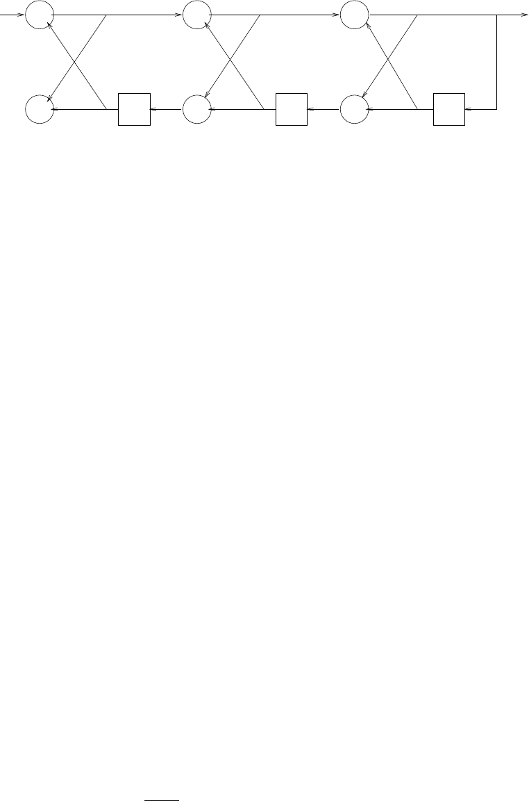
+
+ +z-1
+
z-1 +
+
z-1
w(n) x(n)
-47/128 -2/3 1/247/128 2/3 -1/2
Figure 12.28-1:
=E(m
X
p=0
am(p)x∗(l+p)
n
X
q=0
a∗
n(q)x(l+p))
=E{fm(l+m)f∗
n(l+n)}
=Emδmn
where the last step follows from prob. 12.24 property (g)
12.30
A1(z) = 1 + 0.6z−1
B1(z) = 0.6 + z−1
A2(z) = A1(z) + k2B1(z)z−1
= 1 + 0.78z−1+ 0.3z−2
B2(z) = 0.3 + 0.78z−1+z−2
A3(z) = A2(z) + k3B2(z)z−1
= 1 + 0.93z−1+ 0.69z−2+ 0.5z−3
B3(z) = 0.5 + 0.69z−1+ 0.93z−2+z−3
A4(z) = A3(z) + k4B3(z)z−1
= 1 + 1.38z−1+ 1.311z−2+ 1.337z−3+ 0.9z−4
H(z) = 1
A4(z)
385
© 2007 Pearson Education, Inc., Upper Saddle River, NJ. All rights reserved. This material is protected under all copyright laws
as they currently exist. No portion of this material may be reproduced, in any form or by any means, without permission in
writing from the publisher. For the exclusive use of adopters of the book Digital Signal Processing, Fourth Edition, by John G.
Proakis and Dimitris G. Manolakis. ISBN 0-13-187374-1.
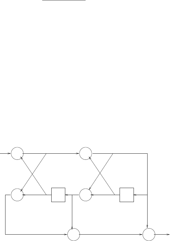
12.31
A2(z) = 1 + 0.1z−1−0.72z−2
k2=−0.72
B2(z) = −0.72 + 0.1z−1+z−2
A1(z) = A2(z)−k2B2(z)
1−k2
2
= 1 + 0.357z−1
k1= 0.357
B1(z) = 0.357 + z−1
A0(z) = B0(z) = 1
C2(z) = β0B0(z) + β1B1(z) + β2B3(z)
=β0+β1(0.357 + z−1) + β2(−0.72 + 0.1z−1+z−2)
= 1 −0.8z−1+ 0.15z−2
Hence, β0= 1.399
β1=−0.815
β2= 0.15
Refer to fig 12.31-1
+
+ +z-1
+
z-1
+ +
-0.72 0.357
0.15 -0.815 1.399
0.72 -0.357
output
input
Figure 12.31-1:
12.32
Refer to fig 12.32-1 ht(n) mininizes E[e2(n)] (wiener filter) length M= 2 (a)
386
© 2007 Pearson Education, Inc., Upper Saddle River, NJ. All rights reserved. This material is protected under all copyright laws
as they currently exist. No portion of this material may be reproduced, in any form or by any means, without permission in
writing from the publisher. For the exclusive use of adopters of the book Digital Signal Processing, Fourth Edition, by John G.
Proakis and Dimitris G. Manolakis. ISBN 0-13-187374-1.
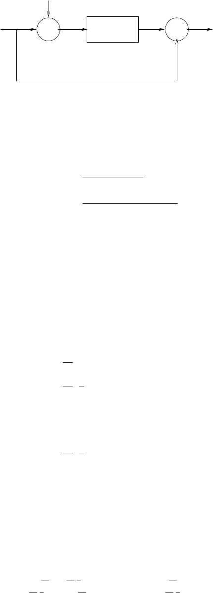
+ +h+
(n)
s(n)
w(n)
x(n) y(n) -
+
e(n)
d(n)
FIR
Figure 12.32-1:
Γss(w) = σ2
v|H(w)|2
=0.49
|1−0.8e−jw|2
Γss(z) = 0.49
(1 −0.8z−1)(1 −0.8z)
We can either formally invert this z-transform, or use the following idea: The inverse z-
transform of 12.1 will have the form
γss(m) = γss(0)(0.8)|m|
From the AR model for s(n) it is easy to show
γss(0) = 0.8γss(1) + γsv (0)
= 0.8γss(1) + δ2
and γss(1) = 0.8γss(0) + γsv (1)
= 0.8γss(0)
solve for γss(0) = 49
36
so γss(m) = 49
36(4
5)|m|
Now γss(m) = E[x(n)x(n−m)]
=E{[s(n) + w(n)][s(n−m) + w(n−m)]}
=γss(m) + σ2
wδ(m)
=49
36(4
5)|m|+δ(m)
(b)
d(n) = s(n)
γdx(l) = γsx(l) = E[s(n)x(n−l)]
=E{s(n)[s(n−l) + w(n−l)]}
=γss(l)
So the normal equations are
1 + 49
36
49
36
4
5
49
36
4
51 + 49
36 ht(0)
ht(1) =49
36
49
36
4
5
387
© 2007 Pearson Education, Inc., Upper Saddle River, NJ. All rights reserved. This material is protected under all copyright laws
as they currently exist. No portion of this material may be reproduced, in any form or by any means, without permission in
writing from the publisher. For the exclusive use of adopters of the book Digital Signal Processing, Fourth Edition, by John G.
Proakis and Dimitris G. Manolakis. ISBN 0-13-187374-1.

ht(0) = 0.462, ht(1) = 0.248
(c) ξ= MMSE2=49
36 −0.462 x 49
36 −0.248 x 49
36 x4
5= 0.462
12.33
Γdx(z) = Γss(z)
=0.49
(1 −0.8z−1)(1 −0.8z)
Γxx(z) = Γss(z) + 1
=1.78(1 −0.45z−1)(1 −0.45z)
(1 −0.8z−1)(1 −0.8z)
G(z) = (1 −0.45z−1)
(1 −0.8z−1)
Γdx(z)
G(z−1)+
=0.49
(1 −0.8z−1)(1 −0.45z)+
=0.766
1−0.8z−1+0.345z
1−0.45z+
=0.766
1−0.8z−1
H+
c(z) = 1
1.78
1−0.8z−1
1−0.45z−1
0.766
1−0.8z−1
=0.43
1−0.45z−1
h+
c(n) = 0.43(0.45)nu(n)
ξ+
c= MMSE∞=1
2πj Ic
[Γss(z)−Hc(z)Γss(z−1)]z−1dz
=1
2πj Ic
0.28
(z−0.45)(1 −0.8z)dz
= 0.438
12.34
Using quantities in prob. 12-33,
H+
nc(z) = Γdx(z)
Γxx(z)
=0.275
(1 −0.45z−1)(1 −0.45z)
ξ+
nc = MMSEnc =1
2πj Ic
[Γdd(z)−H+
nc(z)Γdx(z−1)]z−1dz
=1
2πj Ic
0.275
(z−0.45)(1 −0.45z−1)dz
= 0.345
388
© 2007 Pearson Education, Inc., Upper Saddle River, NJ. All rights reserved. This material is protected under all copyright laws
as they currently exist. No portion of this material may be reproduced, in any form or by any means, without permission in
writing from the publisher. For the exclusive use of adopters of the book Digital Signal Processing, Fourth Edition, by John G.
Proakis and Dimitris G. Manolakis. ISBN 0-13-187374-1.

12.35
γss(m) = (0.6)|m|
2 0.6 0.36
0.6 2 0.6
0.36 0.6 2
h+(0)
h+(1)
h+(2)
=
1
0.6
0.36
h+(0) = 0.455, h+(1) = 0.15, h+(2) = 0.055
ξ3= MMSE3= 1 −0.455 −0.15 x 0.6−0.055 x 0.36 = 0.435
Increasing the length of the filter decreases the MMSE.
12.36
γxx(0) γxx(1) γxx(2)
γxx(1) γxx(0) γxx(1)
γxx(2) γxx(1) γxx(0)
1
−1
0.6
=
1
0
0
σ2
w
⇒
1−1 0.6
−1 1.6 0
0.6−1 1
γxx(0)
γxx(1)
γxx(2)
=
1
0
0
σ2
w
γxx(0) = 2.5641, γxx(1) = 1.6026, γxx(2) = 0.064
For m≥3, γxx(m) = γxx(m−1) −0.6γxx(m−2)
For m < 0, γxx(m) = γxx(−m)
12.37
Γss(z) = σ2
v
(1 + Pp
k=1 ap(k)z−k)(1 + Pp
k=1 ap(k)zk)
Let ap(0) △
= 1
Γss(z) = σ2
v
(Pp
k=0 ap(k)z−k)(Pp
k=0 ap(k)zk)
Γss(z) = Γss(z) + σ2
w
=σ2
v+σ2
w(.)(.)
(.)(.)
389
© 2007 Pearson Education, Inc., Upper Saddle River, NJ. All rights reserved. This material is protected under all copyright laws
as they currently exist. No portion of this material may be reproduced, in any form or by any means, without permission in
writing from the publisher. For the exclusive use of adopters of the book Digital Signal Processing, Fourth Edition, by John G.
Proakis and Dimitris G. Manolakis. ISBN 0-13-187374-1.

x(n)is ARMA(p,p). Suppose
Γxx(z) = (Pp
k=0 bp(k)z−k)(Pp
k=0 bp(k)zk)
(Pp
k=0 ap(k)z−k)(Pp
k=0 ap(k)zk)
Comparing parameters of the two numerators
σ2
v+σ2
w
p
X
k=0
a2
p(k) = σ2
n
p
X
k=0
b2
p(k)
σ2
w
p−q
X
k=0
ap(k)ap(k+q) = σ2
n
p−q
X
k=0
bp(k)bp(k+q)q= 1,2,...,p
There are p+1 equations in p+1 unknown parameters σ2
n, bp(1),...,bp(p). Note that bp(0) = 1.
390
© 2007 Pearson Education, Inc., Upper Saddle River, NJ. All rights reserved. This material is protected under all copyright laws
as they currently exist. No portion of this material may be reproduced, in any form or by any means, without permission in
writing from the publisher. For the exclusive use of adopters of the book Digital Signal Processing, Fourth Edition, by John G.
Proakis and Dimitris G. Manolakis. ISBN 0-13-187374-1.
Chapter 13
13.1
E=
N
X
n=0 "y(n) + w(n)−
M−1
X
k=0
h(k)x(n−k)#2
By carrying out the minimization we obtain the set of linear equations:
M−1
X
k=0
h(k)rxx(l−k) = ryx(l) + rwx(l), l = 0,···, M −1
where,
rwx(l) =
N
X
n=0
w(n)x(n−l)
13.2
If we assume the presence of a near-end echo only, the received signal is
rA(t) = AsA(t−d1) + w(t) = A∞
X
k=0
a(k)p(t−d1−kTs) + w(t)
The receiver filter eliminates the noise outside the frequency band occupied by the signal and
after sampling at the symbol rate we obtain,
r(n) = A∞
X
k=0
a(k)p(nTs−d1−kTs) + w(nTs).
If we assume that the delay d1is a multiple of the symbol time interval, that is, d1=DTs,
then,
r(n) = Aa(n−D) + w(n)
The LS criterion minimizes
E=∞
X
n=0
r(n)−
M−1
X
k=0
h(k)a(n−k)
2
.
The equations for the coefficients of the adaptive echo canceler are
M−1
X
k=0
h(k)raa(l−k) = rra(l)l= 0,···, M −1
391
© 2007 Pearson Education, Inc., Upper Saddle River, NJ. All rights reserved. This material is protected under all copyright laws
as they currently exist. No portion of this material may be reproduced, in any form or by any means, without permission in
writing from the publisher. For the exclusive use of adopters of the book Digital Signal Processing, Fourth Edition, by John G.
Proakis and Dimitris G. Manolakis. ISBN 0-13-187374-1.

where,
raa(l−k) = X
n
a(n−k)a(n−l).
rra(l) = X
n
[Aa(n−D) + w(n)]a(n−l) = Araa(l−D) + rwa(l).
13.3
Assume that the sample autocorrelation and crosscorrelation are given by the unbiased estimates:
rvv(k) = 1
N
N−1
X
n=0
v(n)v(n−k)ryv (k) = 1
N
N−1
X
n=0
y(n)v(n−k)
Then,
rvv(k) = 1
N
N−1
X
n=0 ∞
X
l=0
w2(n−l)h(l) + w3(n)! ∞
X
p=0
w2(n−k−p)h(p) + w3(n−k)!
=1
N
N−1
X
n=0 ∞
X
l=0
∞
X
p=0
w2(n−l)w2(n−k−p)h(l)h(p)+
+∞
X
l=0
w2(n−l)w3(n−k)h(l) + ∞
X
p=0
h(p)w2(n−k−p)w3(n) + w3(n)w3(n−k)!
Since E[w2(n−l)w3(n−k)] = 0, we obtain
E[rvv (k)] = 1
N
N−1
X
n=0 ∞
X
l=0
∞
X
p=0
E[w2(n−l)w2(n−k−p)]h(l)h(p) + E[w3(n)w3(n−k)]!
or
E[rvv (k)] = ∞
X
l=0
∞
X
p=0
h(l)h(p)γw2w2(k+p−l) + γw3w3(k)
ryv(k) = 1
N
N−1
X
n=0
y(n)v(n−k)
=1
N
N−1
X
n=0
(x(n) + w1(n) + w2(n)) ∞
X
l=0
w2(n−k−l)h(l) + w3(n−k)!
=1
N
N−1
X
n=0
∞
X
l=0
(x(n) + w1(n) + w2(n))w2(n−k−l)h(l) +
+1
N
N−1
X
n=0
(x(n)w3(n−k) + w1(n)w3(n−k) + w2(n)w3(n−k))
=⇒E[ryv (k)] = ∞
X
l=0
[γxw2(k+l) + γw2w2(k+l)]h(l) + γxw3(k)
Further simplifications are obtained if w1, w2, w3are white and xis uncorrelated with w2.
392
© 2007 Pearson Education, Inc., Upper Saddle River, NJ. All rights reserved. This material is protected under all copyright laws
as they currently exist. No portion of this material may be reproduced, in any form or by any means, without permission in
writing from the publisher. For the exclusive use of adopters of the book Digital Signal Processing, Fourth Edition, by John G.
Proakis and Dimitris G. Manolakis. ISBN 0-13-187374-1.

13.4
We need to prove that
[1 aH
m(n)]Vm+1(n) = [b+
m(n−1) 1]Q∗
m+1(n) = K∗
m+1(n)
Vm+1(n) =
n
X
l=0
wn−lx(l−m−1)X∗
m+1(n) =
n
X
l=0
wn−lx(l−m−1)
x∗(l)
x∗(l−1)
.
.
.
x∗(l−m)
=
Pn
l=0 wn−lx(l−m−1)x∗(l)
···
Vm(n−1)
=
v
···
Vm(n−1)
Thus,
[1 aH
m(n)]Vm+1(n) = [1 −QH
m(n)R−1
m(n−1)]
v
···
Vm(n−1)
=v−QH
m(n)R−1
m(n−1)Vm(n−1) = v+QH
m(n)bm(n−1)
=v+bt
m(n−1)Q∗
m(n)
But,
Qm+1(n) =
n
X
l=0
wn−lX(l)X∗
m+1(l−1) =
Qm(n)
···
v∗
Hence,
[1 aH
m(n)]Vm+1(n) = [bt
m(n−1) 1]
Q∗
m(n)
···
v
= [bt
m(n−1) 1]Q∗
m+1(n)
From the definition of Km+1(n) in (13.3.29) we obtain
[1 aH
m(n)]Vm+1(n) = [bt
m(n−1) 1]Q∗
m+1(n) = K∗
m+1(n)
13.5
We need to prove that
ξm(n) = ξm(n−1) −am(n)g∗
m(n)em+1(n)
Eb
m(n)
By definition
ξm(n) = −δm(n)
Eb
m(n)
Use the relations:
δm(n) = wδm(n−1) + amg∗
m(n)em(n)
em+1(n) = em(n)−δm(n−1)gm(n)
Eb
m(n−1)
Eb
m(n) = wEb
m(n−1) + am|gm(n)|2
ξm(n) = −
wδm(n−1) + amg∗
m(n)em+1(n) + δm(n−1)gm(n)
Eb
m(n−1)
Eb
m(n)
393
© 2007 Pearson Education, Inc., Upper Saddle River, NJ. All rights reserved. This material is protected under all copyright laws
as they currently exist. No portion of this material may be reproduced, in any form or by any means, without permission in
writing from the publisher. For the exclusive use of adopters of the book Digital Signal Processing, Fourth Edition, by John G.
Proakis and Dimitris G. Manolakis. ISBN 0-13-187374-1.

=−δm(n−1)(wEb
m(n−1) + am(n)|gm(n)|2)
Eb
m(n)Eb
m(n−1) −am(n)g∗
m(n)em+1(n)
Eb
m(n)
=−δm(n−1)
Eb
m(n−1) −am(n)g∗
m(n)em+1(n)
Eb
m(n)
=ξm(n−1) −am(n)g∗
m(n)em+1(n)
Eb
m(n)
13.6
Km(n) = um(n)
vm(n)=wum(n−1) + 2fm−1(n)g∗
m−1(n−1)
vm(n)=⇒
vm(n)Km(n) = wum(n−1) + fm−1(n)g∗
m−1(n−1) + fm−1(n)g∗
m−1(n−1)
=wum(n−1) + [fm(n) + Km(n)gm−1(n−1)]g∗
m−1(n−1)
+ [g∗
m(n) + Km(n)f∗
m−1(n)]fm−1(n)
=wum(n−1) + fm(n)g∗
m−1(n−1) + g∗
m(n)fm−1(n)
+Km(n){|g2
m−1(n−1)|+|f2
m−1(n−1)|}
Km(n)[vm(n)− |g2
m−1(n−1)| − |f2
m−1(n−1)|]
=wum(n−1) + fm(n)g∗
m−1(n−1) + g∗
m(n)fm−1(n)
=⇒Km(n)wvm(n−1) = wum(n−1) + fm(n)g∗
m−1(n−1) + g∗
m(n)fm−1(n)
Km(n) = Km(n−1) + fm(n)g∗
m−1(n−1) + g∗
m(n)fm−1(n)
wvm(n−1)
13.7
We will derive the FAEST algorithm in Table 13.7 line by line. The alternative Kalman gain is
defined as
˜
Km(n) = 1
wPm(n−1)X∗
m(n)
From (13.2.74)
Km(n) = Pm(n−1)X∗
m(n)
w+Xt
m(n)Pm(n−1)X∗
m(n)=˜
Km(n)
1 + 1
wXt
m(n)Pm(n−1)X∗
m(n)
=˜
Km(n)am(n) (see13.3.57)
Define ˜am(n) = 1/am(n). Then,
˜am(n) = 1 + 1
wXt
m(n)Pm(n−1)X∗
m(n) = 1 + Xt
m(n)˜
Km(n).
FAEST-line 1:
fm−1(n) = x(n) + at
m−1(n−1)Xm−1(n−1)
FAEST-line 2:
˜
fm−1(n, n) = fm−1(n)am−1(n) = fm−1(n)
˜am−1(n−1).
FAEST-line 3: From (13.3.50)
am(n) = am(n−1) −Km(n−1)fm(n) =⇒
am−1(n) = am−1(n−1) −˜
Km−1(n)am−1(n−1)fm−1(n)
=am−1(n−1) −˜
Km−1(n)˜
fm−1(n, n)
394
© 2007 Pearson Education, Inc., Upper Saddle River, NJ. All rights reserved. This material is protected under all copyright laws
as they currently exist. No portion of this material may be reproduced, in any form or by any means, without permission in
writing from the publisher. For the exclusive use of adopters of the book Digital Signal Processing, Fourth Edition, by John G.
Proakis and Dimitris G. Manolakis. ISBN 0-13-187374-1.

FAEST-line 4: From (13.3.83)
Ef
m−1(n) = wEf
m−1(n−1) + am−1(n−1)fm−1(n)f∗
m−1(n)
But am−1(n−1)f∗
m−1(n) = ˜
f∗
m−1(n, n), thus,
Ef
m−1(n) = wEf
m−1(n−1) + fm−1(n)˜
f∗
m−1(n, n)
FAEST-line 5:
˜
Km(n) = 1
wR−1
m(n−1)X∗
m(n) and ˜
Km−1(n−1) = 1
wR−1
m−1(n−2)X∗
m−1(n−1)
Use the partition (13.3.32) to write
R−1
m(n−1) = 0 0
0R−1
m−1(n−2) +1
Ef
m−1(n−1) 1
am−1(n−1) [1 aH
m−1(n−1)].
Thus,
˜
Km(n) = (1
w0 0
0R−1
m−1(n−2) +1
wEf
m−1(n−1) 1
am−1(n−1) [1 aH
m−1(n−1)])
·x∗(n)
X∗
m−1(n−1)
=0
˜
Km−1(n−1) +f∗
m−1(n)
wEf
m−1(n−1) 1
am−1(n−1)
FAEST-line 6: We need to find the update formula for the step ˜
Km+1(n+ 1) −→ ˜
Km(n+ 1).
˜
Km(n) = 1
wPm(n−1)X∗
m(n).
Using partition (13.3.27) we obtain
Pm(n−1) = Pm−1(n−1) 0
0 0 +1
Eb
m−1(n−1) bm−1(n−1)
1[bH
m−1(n−1) 1]
Thus,
˜
Km(n) = 1
wPm−1(n−1) 0
0 0 X∗
m−1(n)
x∗(n−m+ 1) +1
wEb
m−1(n−1)
·bm−1(n−1)
1[bH
m−1(n−1) 1] ·X∗
m−1(n)
x∗(n−m+ 1)
=˜
Km−1(n−1)
0+g∗
m−1
wEb
m−1(n−1) bm−1(n−1)
1
Write
˜
Km(n) = ˜
Cm−1(n)
˜cmm(n)
We identify
˜cmm(n) = g∗
m−1(n)
wEb
m−1(n−1) =⇒gm−1(n) = wEb
m−1(n−1)˜c∗
mm(n).
395
© 2007 Pearson Education, Inc., Upper Saddle River, NJ. All rights reserved. This material is protected under all copyright laws
as they currently exist. No portion of this material may be reproduced, in any form or by any means, without permission in
writing from the publisher. For the exclusive use of adopters of the book Digital Signal Processing, Fourth Edition, by John G.
Proakis and Dimitris G. Manolakis. ISBN 0-13-187374-1.

FAEST-line 7: Using the partition of ˜
Km(n) in step-6 we obtain
˜
Cm−1(n) = ˜
Km−1(n) + ˜cmm(n)bm−1(n−1) =⇒˜
Km−1(n) = ˜
Cm−1(n)−˜cmm(n)bm−1(n−1)
FAEST-line 8: From (13.3.91)
am(n) = am−1(n−1) "1−f∗
m−1(n, n)fm−1(n)
Ef
m−1(n)#
But, am(n) = 1/˜am(n) and fm−1(n) = ˜
fm−1(n, n)˜am−1(n−1). Thus,
˜am(n) = ˜am−1(n−1) ·Ef
m−1(n)
Ef
m−1(n)−am−1(n−1)|fm−1(n)|2
= ˜am−1(n−1) ·wEf
m−1(n−1) + |fm−1(n)|2/˜am−1(n−1)
wEf
m−1(n)
= ˜am−1(n−1) "1 + 1
˜am−1(n−1) |fm−1(n)|2
wEf
m−1(n)#
= ˜am−1(n−1) + |fm−1(n)|2
wEf
m−1(n)
FAEST-line 9: ˜am(n) = 1 + ˜
Kt
m(n)Xm(n).If we use the partition of step-6 then
˜am(n) = 1 + [ ˜
Kt
m−1(n) 0]Xm(n) + g∗
m−1(n)
wEb
m−1(n−1)[bt
m−1(n−1) 1]Xm(n)
= ˜am−1(n) + ˜cmm(n)gm−1(n) =⇒
˜am−1(n) = ˜am(n)−˜cmm(n)gm−1(n)
FAEST-line 10: From (13.3.61)
˜gm−1(n, n) = gm−1(n)am−1(n) = gm−1(n)
˜am−1(n)
FAEST-line 11: From (13.3.84)
Eb
m(n) = wEb
m(n−1) + am(n)g∗
m(n)gm(n).
But, gm(n)am(n) = ˜gm(n, n), so that,
Eb
m(n) = wEb
m(n−1) + g∗
m(n)˜gm(n, n) = wEb
m(n−1) + gm(n)˜g∗
m(n, n)
FAEST-line 12: The time-update of bm(n) is given by (13.3.51)
bm(n) = bm(n−1) −Km(n)gm(n)
But, Km(n) = ˜
Km(n)am(n) and am(n)gm(n) = ˜gm(n, n), so that
bm(n) = bm(n−1) −˜
Km(n)˜gm(n, n)
FAEST-line 13: By definition eM(n) = d(n)−ht
m(n−1)Xm(n)
FAEST-line 14,15: From (13.2.76)
hm(n) = hm(n−1) + Km(n)em(n) = hm(n−1) + ˜
Km(n)am(n)em(n)
=hm(n−1) + ˜
Km(n)˜em(n, n)
where,
˜em(n, n) = am(n)em(n) = em(n)
˜am(n)
396
© 2007 Pearson Education, Inc., Upper Saddle River, NJ. All rights reserved. This material is protected under all copyright laws
as they currently exist. No portion of this material may be reproduced, in any form or by any means, without permission in
writing from the publisher. For the exclusive use of adopters of the book Digital Signal Processing, Fourth Edition, by John G.
Proakis and Dimitris G. Manolakis. ISBN 0-13-187374-1.

13.8
hm(n+ 1) = whm(n) + △e(n)X∗
m(n)
where
e(n) = d(n)−hT
m(n)Xm(n).
Thus,
hm(n+ 1) = whm(n) + △(d(n)−hT
m(n)Xm(n))X∗
m(n)
=whm(n) + △d(n)X∗
m(n)− △X∗
m(n)Xt
m(n)hm(n)
=⇒E[hm(n+ 1)] = (wI − △Rm)E[hm(n)] + △rm
where,
Rm=E[X∗
m(n)Xt
m(n)], rm=E[d(n)X∗
m(n)].
Since Rmis Hermitian, it assumes the decomposition Rm=UΛUH, where Λ is a diagonal matrix
with elements λk, 0 ≤k≤m−1, the eigenvalues of Rm, and Uis a normalized modal matrix
such that UUH=I.
Thus,
E[hm(n+ 1)] = U[wI − △Λ]UHE[hm(n)] + △rm.
Premultiplying the above by UHwe obtain
h0
m(n+ 1) = [wI − △Λ]h0
m(n) + △r0
m
where h0
m(n+ 1) = UHE[hm(n+ 1)], r0
m=UHrm. The values of △that ensure convergence of
the mean of the coefficient vector should satisfy
|w− △λk|<1, k = 0,···, m −1
or 1−w
λk
<△<1 + w
λk
, k = 0,···, m −1
or 1−w
λmin
<△<1 + w
λmax
.
13.9
ε(n) = |e(n)|2+ckhM(n)k2
=d(n)−XT
M(n)hM(n)hd∗(n)−hH
M(n)X∗
M(n)i+chH
M(n)hM(n)
=|d(n)|2−2Re hhH
M(n)X∗
M(n)id(n) + hH
M(n)X∗
M(n)XT
M(n)hM(n) + chH
M(n)hM(n)
The complex gradient vector is ∂ε(n)/∂hH
M:
∂ε(n)
∂hH
M
=−X∗
M(n)d(n) + X∗
M(n)XT
M(n)hM(n) + chM(n)
=−X∗
M(n)d(n) + XT
M(n)hM(n)+chM(n)
=−e(n)X∗
M(n) + chM(n)
397
© 2007 Pearson Education, Inc., Upper Saddle River, NJ. All rights reserved. This material is protected under all copyright laws
as they currently exist. No portion of this material may be reproduced, in any form or by any means, without permission in
writing from the publisher. For the exclusive use of adopters of the book Digital Signal Processing, Fourth Edition, by John G.
Proakis and Dimitris G. Manolakis. ISBN 0-13-187374-1.

Then, in the steepest-descent method, we update the coeficient vector as follows:
hM(n+ 1) = hM(n)−∆∂ε(n)
∂hH
M
=hM(n) + ∆ [e(n)X∗
M(n)−chM(n)]
= (1 −∆c)hM(n) + ∆e(n)X∗
M(n)
13.10
The normalized LMS algorithm is given as:
hM(n+ 1) = hM(n) + ∆
kX(n)k2X∗
M(n)e(n)
DEfine the error vector ε(n) as
ε(n) = hopt(n)−hM(n)
Also, define the mean square derivation of the error vector as
J(n) = Ekε(n)k2
Then,
J(n+ 1) = Ekε(n)−∆
kX(n)k2X∗
M(n)e(n)k2
=J(n)−2∆E(Re εH(n)X∗(n)e(n)
kX(n)k2)+ ∆2E|e(n)|2
kX(n)k2
Hence,
J(n+ 1) −J(n) = ∆2|e(n)|2
kX(n)k2−2∆E(Re εH(n)X∗(n)e(n)
kX(n)k2)
We observe that the mean square derivation decreases exponentially with an increase in n, pro-
vided that
0<∆<
ERe[εH(n)X∗(n)e(n)]
kX(n)k2
Eh|e(n)|2
kX(n)k2i
Approximation:
E|e(n)|2
kX(n)k2≈E|e(n)|2
E[kX(n)k2]
and
E(Re εH(n)X∗(n)e(n)
kX(n)k2)≈ERe εH(n)X∗(n)e(n)
E[kX(n)k2]
With the approximations, we obtain
0<∆<Re εH(n)X∗(n)e(n)
E[|e(n)|2]
398
© 2007 Pearson Education, Inc., Upper Saddle River, NJ. All rights reserved. This material is protected under all copyright laws
as they currently exist. No portion of this material may be reproduced, in any form or by any means, without permission in
writing from the publisher. For the exclusive use of adopters of the book Digital Signal Processing, Fourth Edition, by John G.
Proakis and Dimitris G. Manolakis. ISBN 0-13-187374-1.

13.11
We can reduce the number of computations needed by m−1 multiplications if we avoid the
update of the Kalman gain
Km−1(n) = xCm−1(n)−ybm−1(n−1).
If we use the alternative Kalman gain this step takes the form
˜
Km−1(n) = ˜
Cm−1(n)−ybm−1(n−1).
As in the a-priori case, the update of the alternative Kalman gain vector ˜
Km(n), is carried out
in two steps,
˜
Km(n)
step−up
−→ ˜
Km+1(n+ 1)
step−down
−→ ˜
Km(n+ 1)
using the following Levinson-type recursions:
˜
Km(n) = 0
˜
Km−1(n−1) +f∗
m−1
wEf
m−1(n−1) 1
am−1(n−1) (step −5ofprob.13 −8)
and
˜
Km(n) = ˜
Km−1(n)
0+g∗
m−1
wEb
m−1(n−1) bm−1(n−1)
1(step −6ofprob.13 −8)
With ˜
Km(n) we associate the scalar ˜am(n)
˜am(n) = 1
am(n)= 1 + X∗
m(n)˜
Km(n).
This parameter is updated as (see prob. 13.8)
˜am(n) = ˜am−1(n−1) + |fm−1(n)|2
wEf
m−1(n)
˜am−1(n−1) = ˜am(n)−gm−1(n)˜cmm(n).
FAST RLS algorithm: Version A (a-posteriori version)
fm−1(n) = x(n) + at
m−1(n−1)Xm−1(n−1)
gm−1(n) = x(n−M+ 1) + bt
m−1(n−1)Xm−1(n−1)
am−1(n) = am−1(n−1) −˜
Km−1(n−1) fm−1(n)
˜am−1(n−1)
fm−1(n, n) = x(n) + at
m−1(n−1)Xm−1(n−1)
Ef
m−1(n) = wEf
m−1(n−1) + fm−1(n)f∗
m−1(n, n)
˜
Km(n) = ˜
Cm−1(n)
˜cmm(n)=0
˜
Km−1(n−1) +f∗
m−1(n)
wEf
m−1(n−1) 1
am−1(n−1)
˜
Km−1(n) = ˜
Cm−1(n)−bm−1(n−1)˜cmm(n)
˜am(n) = ˜am−1(n−1) + |fm−1(n)|2
wEf
m−1(n−1)
˜am−1(n) = ˜am(n)−gm−1(n)˜cmm(n)
bm−1(n) = bm−1(n−1) −˜
Km−1(n−1) gm−1(n)
˜am−1(n)
399
© 2007 Pearson Education, Inc., Upper Saddle River, NJ. All rights reserved. This material is protected under all copyright laws
as they currently exist. No portion of this material may be reproduced, in any form or by any means, without permission in
writing from the publisher. For the exclusive use of adopters of the book Digital Signal Processing, Fourth Edition, by John G.
Proakis and Dimitris G. Manolakis. ISBN 0-13-187374-1.

ˆ
d(n) = ht
m(n−1)Xm(n)
em(n) = d(n)−ˆ
d(n)
hm(n) = hm(n−1) + ˜
Km(n)em(n)
˜am(n)
Initialization:
am−1(−1) = bm−1(−1) = 0,˜
Km−1(−1) = 0, hm−1(−1) = 0, Ef
m−1(−1) = E>0.
In this version we need 5 extra multiplications for the calculation of fm−1(n)
˜am−1(n−1) ,|fm−1(n)|2
wEf
m−1(n−1) ,
gm−1(n)˜cmm(n), gm−1(n)
˜am−1(n−1) ,em(n)
˜am(n)and we save mmultiplications from the estimation of ˜
Km−1(n).
FAST RLS algorithm: Version B (a-posteriori version)
fm−1(n) = x(n) + at
m−1(n−1)Xm−1(n−1)
gm−1(n) = x(n−M+ 1) + bt
m−1(n−1)Xm−1(n)
am−1(n) = am−1(n−1) −˜
Km−1(n−1) fm−1(n)
˜am−1(n−1)
˜
fm−1(n, n) = fm−1(n)
˜am−1(n−1)
Ef
m−1(n) = wEf
m−1(n−1) + |fm−1(n)|2
˜am−1(n−1)
˜
Km(n) = ˜
Cm−1(n)
˜cmm(n)=0
˜
Km−1(n−1) +f∗
m−1(n)
wEf
m−1(n−1) 1
am−1(n−1)
˜
Km−1(n) = ˜
Cm−1(n)−bm−1(n−1)˜cmm(n)
˜am(n) = ˜am−1(n−1) + |fm−1(n)|2
wEf
m−1(n−1)
˜am−1(n) = ˜am(n)−gm−1(n)˜cmm(n)
bm−1(n) = bm−1(n−1) −˜
Km−1(n−1) gm−1(n)
˜am−1(n)
ˆ
d(n) = ht
m(n−1)Xm(n)
em(n) = d(n)−ˆ
d(n)
hm(n) = hm(n−1) + ˜
Km(n)em(n)
˜am(n)
Initialization:
am−1(−1) = bm−1(−1) = 0,˜
Km−1(−1) = 0, hm−1(−1) = 0, Ef
m−1(−1) = E>0,˜am−1(−1) = 1.
In this version we need 3 extra multiplications for the calculation of fm−1(n)
˜am−1(n−1) ,gm−1(n)
˜am−1(n−1) ,em(n)
˜am(n)
and we save mmultiplications from the estimation of ˜
Km−1(n).
13.12
E=E
g−
M−1
X
n=0
h(n)x(n)!2
400
© 2007 Pearson Education, Inc., Upper Saddle River, NJ. All rights reserved. This material is protected under all copyright laws
as they currently exist. No portion of this material may be reproduced, in any form or by any means, without permission in
writing from the publisher. For the exclusive use of adopters of the book Digital Signal Processing, Fourth Edition, by John G.
Proakis and Dimitris G. Manolakis. ISBN 0-13-187374-1.

∂E
∂h(k)= 0 =⇒E"2 g−
M−1
X
n=0
h(n)x(n)!x(k)#= 0, k = 0,···, M −1.
Thus,
E[gx(k)] = E"M−1
X
n=0
h(n)x(n)x(k)#, k = 0,···, M −1.
E[gx(k)] = E[g(gv(k) + w(k))] = E[g2]v(k) + E[gw(k)]
=Gv(k) (ifg, w(k)areuncorrelated)
E"M−1
X
n=0
h(n)x(n)x(k)#=
M−1
X
n=0
h(n)E[x(n)x(k)]
=
M−1
X
n=0
h(n)E[(gv(n) + w(n))(gv(k) + w(k))]
=
M−1
X
n=0
h(n)E[g2v(n)v(k) + gv(n)w(k) + gv(k)w(n) + w(n)w(k)]
=G
M−1
X
n=0
h(n)v(k)v(n) + σ2
wh(k)
Hence,
Gv(k) = Gv(k)
M−1
X
n=0
h(n)v(n) + σ2
wh(k)
or
(GvvT+σ2
wI)h=Gv
where
v= [v(0),···, v(M−1)]T,h= [h(0),···, h(M−1)]T.
13.13
Let
H(z) =
M−1
X
k=0
hkz−kand Hn=H(z=ej2πn/M ) =
M−1
X
k=0
hke−j2πnk/M .
The sequence {hk}is related to the sequence {Hn}by the inverse discrete Fourier transform
hk=1
M
M−1
X
n=0
Hnej2πn/M , k = 0,···, M −1.
When hk, given above is substituted in the expression for H(z) the double sum that results can
be simplified to yield
H(z) = 1−z−M
M
M−1
X
k=0
Hk
1−ej2πk/M z−1.
The filter structure is shown in Fig. 13.13-1.
1. Let yk(n) be the output at time t=nT of the filter with transfer function
1−z−M
M
1
1−ej2πk/M z−1.
401
© 2007 Pearson Education, Inc., Upper Saddle River, NJ. All rights reserved. This material is protected under all copyright laws
as they currently exist. No portion of this material may be reproduced, in any form or by any means, without permission in
writing from the publisher. For the exclusive use of adopters of the book Digital Signal Processing, Fourth Edition, by John G.
Proakis and Dimitris G. Manolakis. ISBN 0-13-187374-1.

1 − z−1
1 − z−M
1 − z−1
H0
y0X
yM−1
HM−1
H1
y1
d(n)
^
1
1
1
M
1 − z−1
ej2πX
X
++
+
−
d(n)
e(n)
(M−1)
ej2π/M
/M
Figure 13.13-1:
Then the response of the recursive filter at t=nT is
ˆ
d(n) =
M−1
X
k=0
Hk(n)yk(n).
where {Hk(n)}are the filter coefficients at t=nT . If e(n) = d−ˆ
d(n) then, an algorithm
for adjusting the coefficients Hk(n) is given by
Hk(n+ 1) = Hk(n) + △e(n)yk(n)k= 0,···, M −1.
2. The cascade of the comb filter 1−z−M
Mwith each of the single-pole filter forms a system
with frequency response
Hk(f) = 1−ej2πf/M
M(1 −ej2π(k/M−f)).
Thus,
|Hk(f)|=1
M
e−j2πM f
ej2π(k/M−f)·
ej2πM f −e−j2πM f
e−j2π(k/M−f)−ej2π(k/M−f)
=1
M
2jsin(πMf)
−2jsin(π(k/M −f)) =1
M
sin(πMf)
sin(π(k/M −f)) .
We observe that |Hk(f)|= 0 at the frequencies f=n/M ,n6=kand |Hk(f)|= 1 at
f=k/M .
Thus, the kth system has a resonant frequency at f=k/M, and it is zero at the resonant
frequencies of all the other systems. This means that if the desired signal is
d(n) =
M−1
X
k=0
Akcos(ωkn), ωk=2πk
M,
the coefficient of each single-pole filter can be adjusted independently without any interac-
tion from the other filters.
402
© 2007 Pearson Education, Inc., Upper Saddle River, NJ. All rights reserved. This material is protected under all copyright laws
as they currently exist. No portion of this material may be reproduced, in any form or by any means, without permission in
writing from the publisher. For the exclusive use of adopters of the book Digital Signal Processing, Fourth Edition, by John G.
Proakis and Dimitris G. Manolakis. ISBN 0-13-187374-1.
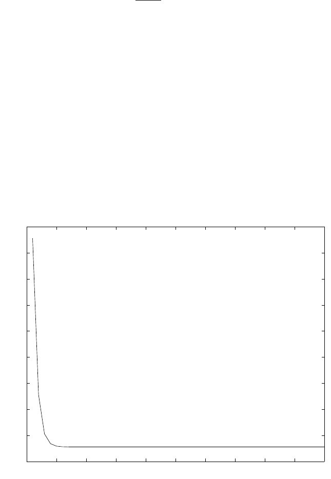
13.14
∂J
∂h(n)= 2h(n)−40
Thus,
h(n+ 1) = h(n)− △h(n) + 20△=h(n)(1 − △) + 20△.
1. For an overdamped system,
|1− △| <1 =⇒0<△<2.
2. Fig. 13.14-1 contains a plot of J(n) vs. n. The step △was set to 0.5 and the initial value
of hwas set to 0. In Fig. 13.14-2 we have plotted J(h(n)) vs. h(n). As it is observed from
the figures the minimum value of Jwhich is −372, is reached within 5 iterations of the
algorithm.
0 5 10 15 20 25 30 35 40 45 50
−400
−350
−300
−250
−200
−150
−100
−50
0
50
n
J(n)
Figure 13.14-1:
13.15
Normal Equations:
M−1
X
k=0
a(k)rvv (l−k) = ryv (l)l= 0,1,···, M −1
403
© 2007 Pearson Education, Inc., Upper Saddle River, NJ. All rights reserved. This material is protected under all copyright laws
as they currently exist. No portion of this material may be reproduced, in any form or by any means, without permission in
writing from the publisher. For the exclusive use of adopters of the book Digital Signal Processing, Fourth Edition, by John G.
Proakis and Dimitris G. Manolakis. ISBN 0-13-187374-1.
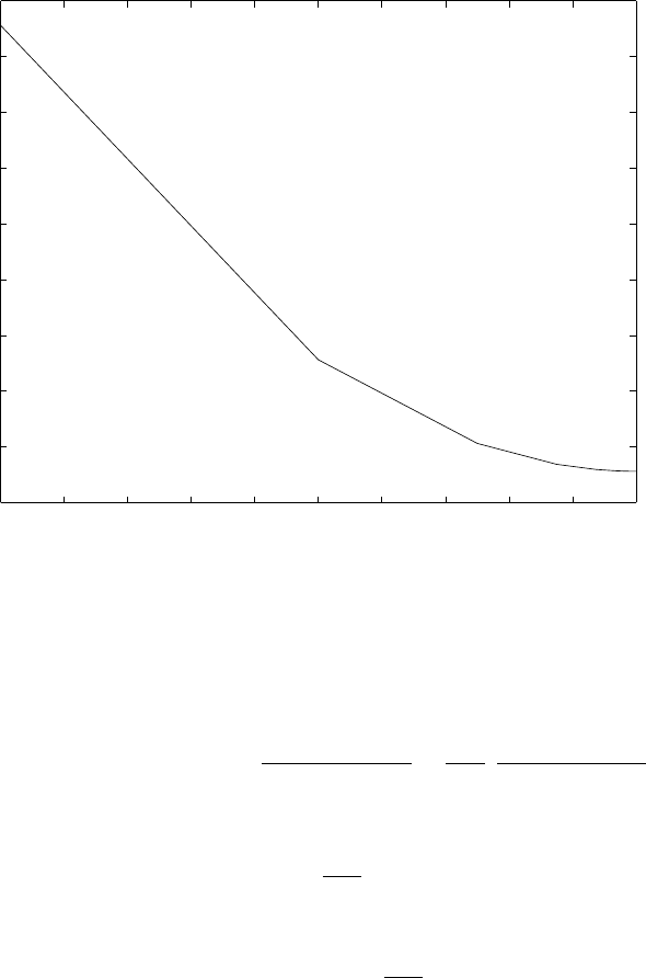
0 2 4 6 8 10 12 14 16 18 20
−400
−350
−300
−250
−200
−150
−100
−50
0
50
h(n)
J(h(n))
Figure 13.14-2:
rvv(l−k) = rw3w3(l−k) + rv2v2(l−k)
Power spectral density of v2(n):
Γv2v2(f) = σ2
w|H(f)|2=σ2
w
1
|1−0.5e−j2πf |2=σ2
w
0.75
0.75
1.25 −cos(2πf).
Thus,
rv2v2(m) = σ2
w
0.75(0.5)|m|.
Hence,
rvv(l−k) = σ2
wδ(l−k) + σ2
w
0.75(0.5)|l−k|.
Assuming that x(n), w1(n), w2(n), w3(n) are mutually uncorrelated, it follows that
E[y(n)v(n−l)] = E[w2v2(n−l)] = E"w2
∞
X
k=0
h(k)w2(n−l−k)#,
where h(k) = 0.5k. Thus,
E[y(n)v(n−l)] = ∞
X
k=0
h(k)E[w2(n)w2(n−l−k)] = ∞
X
k=0
h(k)σ2
wδ(l+k) = σ2
wδ(l).
404
© 2007 Pearson Education, Inc., Upper Saddle River, NJ. All rights reserved. This material is protected under all copyright laws
as they currently exist. No portion of this material may be reproduced, in any form or by any means, without permission in
writing from the publisher. For the exclusive use of adopters of the book Digital Signal Processing, Fourth Edition, by John G.
Proakis and Dimitris G. Manolakis. ISBN 0-13-187374-1.

+ + e(n)
−
y(n)=x(n) + w (n) + w (n)
w (n)
2v(n) A(z)
w (n)
v (n)
2
3
1
1−0.5 z−1
1 2
Figure 13.15-1:
The normal equations take the form
σ2
w+σ2
w
0.75
0.5σ2
w
0.75
0.25σ2
w
0.75
0.5σ2
w
0.75 σ2
w+σ2
w
0.75
0.5σ2
w
0.75
0.25σ2
w
0.75
0.5σ2
w
0.75 σ2
w+σ2
w
0.75
a(0)
a(1)
a(2)
=
σ2
w
0
0
=⇒a(0) = 15
32, a(1) = −4
32, a(2) = −1
32.
13.16
e(n) = x(n)−a1x(n−1) −a2x(n−2)
E=E[e2(n)] =⇒
∂E
∂a1
=E[(x(n)−a1x(n−1) −a2x(n−2))x(n−1)] = 0
∂E
∂a2
=E[(x(n)−a1x(n−1) −a2x(n−2))x(n−2)] = 0
=⇒E[x(n)x(n−1)] −a1E[x(n−1)x(n−1)] −a2E[x(n−2)x(n−1)] = 0
E[x(n)x(n−2)] −a1E[x(n−1)x(n−2)] −a2E[x(n−2)x(n−2)] = 0
But,
E[x(n)x(n−1)] = E[x(n−2)x(n−1)] = a
E[x(n−1)x(n−1)] = E[x(n−2)x(n−2)] = 1
E[x(n)x(n−2)] = a2
Thus, we obtain the system
1a
a1 a1
a2=a
a2
with solution a1=a,a2= 0.
405
© 2007 Pearson Education, Inc., Upper Saddle River, NJ. All rights reserved. This material is protected under all copyright laws
as they currently exist. No portion of this material may be reproduced, in any form or by any means, without permission in
writing from the publisher. For the exclusive use of adopters of the book Digital Signal Processing, Fourth Edition, by John G.
Proakis and Dimitris G. Manolakis. ISBN 0-13-187374-1.
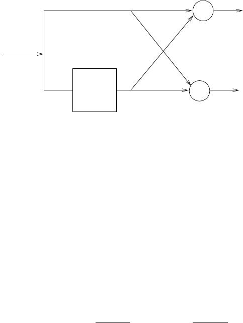
13.17
The optimum linear predictor in Prob. 13.16 is a first order filter with transfer function
A(z) = 1 −az−1.
Thus, the corresponding lattice has one stage with the forward and backward errors given by
f(n) = f0(n) + Kb0(n−1) b(n) = b0(n−1) + Kf0(n)
Since f0(n) = b0(n) = x(n), we obtain
f(n) = x(n) + Kx(n−1) b(n) = x(n−1) + Kx(n).
Comparing with the prediction error:
e(n) = x(n)−ax(n−1)
we identify Kas −a.
z −1
+
+
x(n) −a
−a
f(n)=e(n)
g(n)
Figure 13.17-1:
13.18
1
X
k=0
bkryy(l−k) = rdy (l) = rxy (l), l = 0,1
where y(n) is the input of the adaptive FIR filter B(z)
ryy(l−k) = rss(l−k) + rww(l−k) = rss(l−k) + σ2
wδ(l−k)
where s(n) is the output of the system C(z).
If x(n) is white with variance σ2
xthen,
rss(l−k) = σ2
x
1−0.92(−0.9)|l−k|=σ2
x
1−0.19(−0.9)|l−k|
rxy(l) = E[x(n)y∗(n−l)] = E[x(n)(s∗(n−l) + w∗(n−l))].
If x(n) and w(n) are uncorrelated then,
rxy(l) = E[x(n)s∗(n−l)] = σ2
xδ(l).
406
© 2007 Pearson Education, Inc., Upper Saddle River, NJ. All rights reserved. This material is protected under all copyright laws
as they currently exist. No portion of this material may be reproduced, in any form or by any means, without permission in
writing from the publisher. For the exclusive use of adopters of the book Digital Signal Processing, Fourth Edition, by John G.
Proakis and Dimitris G. Manolakis. ISBN 0-13-187374-1.

Thus, we obtain the system:
σ2
x
0.19 +σ2
w−σ2
x
0.19 (0.9)
−σ2
x
0.19 (0.9) σ2
x
0.19 +σ2
w
b0
b1=σ2
x
0.
With σ2
xand σ2
wknown, we can determine b0, b1.
13.19
(a)
fm(n) = fm−1(n)−kmgm−1(n−1)
gm(n) = gm−1(n−1) −k∗
mfm−1(n)
εLS
m=
n
X
l=0
wn−lh|fm(l)|2+|gm(l)|2i
dεLS
m
dk∗
m
=−2
n
X
l=0
wn−lg∗
m−1(l−1)fm(l) + fm−1(l)g∗
m(l)= 0
n
X
l=0
wn−lg∗
m−1(l−1) [fm−1(l)−kmgm−1(l−1)] + fm−1(l)g∗
m−1(l−1) −kmfm−1(l)
Solving for kM, we obtain
km(n) = 2Pn
l=0 wn−lfm−1(l)g∗
m−1(l−1)
Pn
l=0 wn−lh|fm−1(l)|2+|gm−1(l−1)|2i=um(n)
vm(n)
(b)
km(n) = wum(n−1) + 2fm−1(n)g∗
m−1(n−1)
wvm(n−1) + |fm−1(n)|2+|gm−1(n−1)|2
fm−1(n)gm−1(n−1) = fm−1(n)g∗
m(n) + km(n)f∗
m−1(n)
=fm−1(n)g∗
m(n) + km(n)|fm−1(n)|2
fm−1(n)gm−1(n−1) = gm−1(n) [fm(n) + km(n)gm−1(n−1)]
=gm−1(n−1)fm(n) + km(n)|gm−1(n−1)|2
Therefore,
2fm−1(n)g∗
m−1(n−1) = km(n)h|fm−1(n)|2+|gm−1(n)|2i+z(n)
where
z(n) = fm−1(n)gm(n) + fm(n)g∗
m−1(n−1)
Now,
2fm−1(n)g∗
m−1(n−1) = z(n) + km(n)hwvm(n) + |fm−1(n)|2+|gm−1(n)|2i
−km(n)wvm(n−1)
=z(n) + km(n)vm(n)−km(n)wvm(n−1)
407
© 2007 Pearson Education, Inc., Upper Saddle River, NJ. All rights reserved. This material is protected under all copyright laws
as they currently exist. No portion of this material may be reproduced, in any form or by any means, without permission in
writing from the publisher. For the exclusive use of adopters of the book Digital Signal Processing, Fourth Edition, by John G.
Proakis and Dimitris G. Manolakis. ISBN 0-13-187374-1.

Then,
2
n−1
X
l=0
wn−lfm−1(l)g∗
m−1(l−1) + 2fm−1(n)g∗
m−1(n−1) = wum(n−1)
+z(n) + km(n)vm(n)
−km(n)wvm(n−1)
But km(n) = um(n)/vm(n). Therefore,
km(n)wm(n) = z(n) + wum(n−1) + km(n)vm(n)−kmwvm(n−1)
and, then
km(n) = wum(n−1)
wvm(n−1) +z(n)
wvm(n−1)
km(n) = km(n−1) + z(n)
wvm(n−1)
408
© 2007 Pearson Education, Inc., Upper Saddle River, NJ. All rights reserved. This material is protected under all copyright laws
as they currently exist. No portion of this material may be reproduced, in any form or by any means, without permission in
writing from the publisher. For the exclusive use of adopters of the book Digital Signal Processing, Fourth Edition, by John G.
Proakis and Dimitris G. Manolakis. ISBN 0-13-187374-1.

Chapter 14
14.1
(a)
limT0→∞E"1
2T0|ZT0
−T0
x(t)e−j2πF tdt|2#
= limT0→∞E"1
2T0ZT0
−T0
x(t)e−j2πF tdt ZT0
−T0
x∗(τ)ej2πF τ dτ #
= limT0→∞
1
2T0ZT0
−T0ZT0
−T0
E[x(t)x∗(τ)]e−j2πF (t−τ)dtdτ
= limT0→∞
1
2T0ZT0
−T0ZT0
−T0
γxx(t−τ)e−j2πF (t−τ)dtdτ
= limT0→∞
1
2T0Zt+T0
t−T0ZT0
−T0
γxx(α)e−j2πF (α)dtdα
=Z∞
−∞
γxx(α)e−j2πF (α)dα
=γxx(F)
(b)
γxx(m) = 1
N
N−1
X
n=0
x(n+m)x∗(n)
N
X
m=−N
γxx(m)e−j2πf m =
N
X
m=−N
1
N
N−1
X
n=0
x(n+m)x∗(n)e−j2πf m
=
N−1
X
n=0
1
N
n+N
X
l=n−N
x(l)x∗(n)e−j2πf (l−n)
=1
N
N−1
X
n=0
N−1
X
l=0
x(l)x∗(n)e−j2πf lej2πf n
=1
N|
N−1
X
n=0
x(n)e−j2πf n|2
409
© 2007 Pearson Education, Inc., Upper Saddle River, NJ. All rights reserved. This material is protected under all copyright laws
as they currently exist. No portion of this material may be reproduced, in any form or by any means, without permission in
writing from the publisher. For the exclusive use of adopters of the book Digital Signal Processing, Fourth Edition, by John G.
Proakis and Dimitris G. Manolakis. ISBN 0-13-187374-1.

14.2
E[|γxx(m)|2] = 1
N2
N−|m|−1
X
n=0
N−|m|−1
X
n′=0
E[x∗(n)x(n+m)x(n′)x∗(n′+m)]
=1
N2X
nX
n′{E[x∗(n)x(n+m)]E[x(n′)x∗(n′+m)]
+E[x∗(n)x(n′)]E[x∗(n′+m)x(n+m)]
+E[x∗(n)x∗(n′+m)]E[x(n′)x(n+m)]}
=1
N2X
nX
n′
[γ2
xx(m) + γ2
xx(n−n′)
+γ∗
xx(n′+m−n)γxx(n+m−n′)]
Let p=n−n′.Then
E[|γxx(m)|2] = γ2
xx(m)N− |m|
N2
+1
N2X
nX
p
[γ2
xx(p)γ∗
xx(p−m)γxx(p+m)]
=|E[γxx(m)]|2+1
N2X
nX
p
[γ2
xx(p)γ∗
xx(p−m)γxx(p+m)]
Therefore,
var[γxx(m)] = 1
N2X
nX
p
[γ2
xx(p)γ∗
xx(p−m)γxx(p+m)]
≈1
N
∞
X
p=−∞
[γ2
xx(p)γ∗
xx(p−m)γxx(p+m)]
14.3
(a)
E[γxx(m)γ∗
xx(m′)] = E
1
N
N−|m|−1
X
n=0
x∗(n)x(n+m).
1
N
N−|m|−1
X
n′=0
x(n′)x∗(n′+m′)
=1
N2X
nX
n′
E{x∗(n)x(n+m)x(n′)x∗(n′+m′)}
=1
N2X
nX
n′{E[x∗(n)x(n+m)]E[x(n′)x∗(n′+m′)]
+E[x∗(n)x(n′)]E[x∗(n′+m′)x(n+m)]
+E[x∗(n)x∗(n′+m′)]E[x(n′)x(n+m)]}
=σ4
x
N2X
nX
n′
[δ(m)δ(m′) + δ(n−n′)δ(m−m′)
+δ(n′+m′−n)δ(n+m−n′)]
Hence, E[pxx(f1)pxx(f2)] =
N−1
X
m=−(N−1)
N−1
X
m′=−(N−1)
E[γxx(m)γxx(m′)]e−j2πmf1e−j2πm′f2
410
© 2007 Pearson Education, Inc., Upper Saddle River, NJ. All rights reserved. This material is protected under all copyright laws
as they currently exist. No portion of this material may be reproduced, in any form or by any means, without permission in
writing from the publisher. For the exclusive use of adopters of the book Digital Signal Processing, Fourth Edition, by John G.
Proakis and Dimitris G. Manolakis. ISBN 0-13-187374-1.

=σ4
x
N2X
mX
m′X
nX
n′
[δ(m)δ(m′) + δ(n−n′)δ(m−m′)
+δ(n′+m′−n)δ(n+m−n′)]e−j2πmf1e−j2πm′f2
=σ4
x(1 + sinπ(f1+f2)N
Nsinπ(f1+f2)2
+sinπ(f1−f2)N
Nsinπ(f1−f2)2)
(b)
cov[pxx(f1)pxx(f2)] = E[pxx(f1)pxx(f2)] −E[pxx(f1)]E[pxx(f2)]
=E[pxx(f1)pxx(f2)] −σ4
x
=σ4
x(sinπ(f1+f2)N
Nsinπ(f1+f2)2
+sinπ(f1−f2)N
Nsinπ(f1−f2)2)
(c)
var[pxx(f)] = cov[pxx(f1)pxx(f2)]|f1=f2=f
=σ4
x"1 + sin2πfN
Nsin2πf 2#
14.4
Assume that x(n) is the output of a linear system excited by white noise input w(n), where
σ2
x= 1. Then pxx(f) = Γxx(f)pww(f). From prob. 12.3, (a), (b) and (c), we have
E[pxx(f1)pxx(f2)] = Γxx(f1)Γxx(f2)E[pww (f1)pww(f2)]
= Γxx(f1)Γxx(f2)(1 + sinπ(f1+f2)N
Nsinπ(f1+f2)2
+sinπ(f1−f2)N
Nsinπ(f1−f2)2)
cov[pxx(f1)pxx(f2)] = Γxx(f1)Γxx(f2)cov[pww(f1)pww(f2)]
= Γxx(f1)Γxx(f2)(sinπ(f1+f2)N
Nsinπ(f1+f2)2
+sinπ(f1−f2)N
Nsinπ(f1−f2)2)
var[pxx(f)] = cov[pxx(f1)pxx(f2)]|f1=f2=f
= Γf
xx "1 + sin2πfN
Nsin2πf 2#
14.5
Let yk(n) = x(n)∗hk(n)
=
N−1
X
m=0
x(m)ej2πk(n−m)
N
=ej2πkn
N
N−1
X
m=0
x(m)e−j2πkm
N
yk(n)|n=N=
N−1
X
m=0
x(m)e−j2πkm
N
=X(k)
411
© 2007 Pearson Education, Inc., Upper Saddle River, NJ. All rights reserved. This material is protected under all copyright laws
as they currently exist. No portion of this material may be reproduced, in any form or by any means, without permission in
writing from the publisher. For the exclusive use of adopters of the book Digital Signal Processing, Fourth Edition, by John G.
Proakis and Dimitris G. Manolakis. ISBN 0-13-187374-1.

Note that this is just the Goertzel algorithm for computing the DFT. Then,
|yk(n)|2=|X(k)|2=|
N−1
X
m=0
x(m)e−j2πkm
N|2
14.6
From (14.2.18) we have
W(f) = 1
MU |
M−1
X
n=0
w(n)e−j2πf n|2
=1
MU
M−1
X
n=0
M−1
X
n′=0
w(n)w∗(n′)e−j2πf (n−n′)
Z1
2
−1
2
W(f)df =1
MU X
nX
n′
w(n)w∗(n′)Z1
2
−1
2
e−j2πf (n−n′)df
=1
MU X
nX
n′
w(n)w∗(n′)δ(n−n′)
=1
U"1
M
M−1
X
n=0 |w(n)|2#= 1
by the definition of U in (14.2.12)
14.7
(a) (1) Divide x(n) into subsequences of length M
2and overlapped by 50% to produce 4ksubse-
quences. Each subsequence is padded with M
2zeros.
(2) Compute the M-point DFT of each frame or subsequence.
(3) Compute the magnitude square of each DFT.
(4) Average the 4kM-point DFT’s.
(5) Perform the IDFT to obtain an estimate of the autocorrelation sequence.
(b)
X3(k) =
M−1
X
m=0
x3(m)e−j2πkm
M
=
M
2−1
X
m=0
x1(m)e−j2πkm
M+
M−1
X
m=M
2
x2(m−M
2)e−j2πkm
M
=
M−1
X
m=0
x1(m)e−j2πkm
M+e−jπk
M−1
X
m′=0
x2(m′)e−j2πkm′
M
X3(k) = X1(k) + e−jπkX2(k)
(c) Instead of zero-padding, we can combine two subsequences to produce a single M-point
subsequence and thus reduce the number of sequences form 4kto 2k. Then, we use the relation
in (b) for the DFT.
412
© 2007 Pearson Education, Inc., Upper Saddle River, NJ. All rights reserved. This material is protected under all copyright laws
as they currently exist. No portion of this material may be reproduced, in any form or by any means, without permission in
writing from the publisher. For the exclusive use of adopters of the book Digital Signal Processing, Fourth Edition, by John G.
Proakis and Dimitris G. Manolakis. ISBN 0-13-187374-1.

14.8
(a) Obviously, △f= 0.01. From (12.2.52), M=0.9
△f= 90.
(b) From (14.2.53), the quality factor is QB= 1.1N△f. This expression does not depend on M;
hence, there is no advantage to increasing the value of Mbeyond 90.
14.9
(a) From table 14.1, we have
QB= 1.11N△f
⇒ △f=QB
1.11N=1
111
Qw= 1.39N△f
⇒ △f=Qw
1.39N=1
139
QBT = 2.34N△f
⇒ △f=QBT
2.34N=1
234
(b)
For the Bartlett estimate,
QB=N
M
⇒M=N
QB
= 100
For the Welch estimate with 50% overlap,
Qw=16N
M
⇒M=16N
Qw
= 178
For the Blackman-Tukey estimate,
QBT =1.5N
M
⇒M=1.5N
QBT
= 150
14.10
(a) Suppose P(i)
B(f) is the periodogram based on the Bartlett method. Then,
P(i)
B(f) = 1
M|
M−1
X
n=0
xi(m)e−j2πf n|2, i = 0,1,...,k−1
P(0)
xx (f) = 0
P(1)
xx (f) = 1−w
M|
M−1
X
n=0
x1(m)e−j2πf n|2
= (1 −w)P(1)
B(f)
P(2)
xx (f) = wP (1)
xx (f) + (1 −w)P(1)
B(f)
413
© 2007 Pearson Education, Inc., Upper Saddle River, NJ. All rights reserved. This material is protected under all copyright laws
as they currently exist. No portion of this material may be reproduced, in any form or by any means, without permission in
writing from the publisher. For the exclusive use of adopters of the book Digital Signal Processing, Fourth Edition, by John G.
Proakis and Dimitris G. Manolakis. ISBN 0-13-187374-1.

= (1 −w)[wP (1)
B(f) + P(2)
B(f)]
P(m)
xx (f) = (1 −w)X
k=1
mwm−kP(k)
B(f)
Therefore, E{P(M)
xx (f)}= (1 −w)X
k=1
Mwm−kE[P(k)
B(f)]
= (1 −w)1−wM
1−w
1
MZ1
2
−1
2
Γxx(α)sinπ(f−α)M
sinπ(f−α)2
dα
= (1 −wM)1
MZ1
2
−1
2
Γxx(α)sinπ(f−α)M
sinπ(f−α)2
dα
var{P(M)
xx (f)}=E{[P(M)
xx (f)]2} − [E{P(M)
xx (f)}]2
var{P(M)
xx (f)}=E{[(1 −w)X
k=1
Mwm−kP(k)
B(f)]2}
−{E[(1 −w)X
k=1
Mwm−kP(k)
B(f)]}2
= (1 −w)2"X
k=1
Mw2(M−k)E{P(k)
B(f)}2− {E[P(k)
B(f)]}2#
= (1 −w)2X
k=1
Mw2(M−k)var[P(k)
B(f)]
= (1 −w)21−w2M
1−w2Γ2
xx(f)"1 + sin2πfM
Msin2πf 2#
= (1 −w2w)1−w
1 + wΓ2
xx(f)"1 + sin2πfM
Msin2πf 2#
(b)
E{P(M)
xx (f)}=E{P(w)
xx (f)}
=Z1
2
−1
2
Γxx(α)W(f−α)dα
where W(f) = 1
MU |
M−1
X
n=0
w(n)e−j2πf n|2
var[P(M)
xx (f)] = (1 −w)2
M
X
k=1
w2(M−k)var[ ˜
P(i)
xx (f)]
= (1 −w2M)1−w
1 + wΓ2
xx(f)
14.11
Let R(i)
xx be defined as follows:
R(i)
xx =1
M
r(i)
xx(0) r(i)
xx(1) ...
r(i)
xx(−1) r(i)
xx(0) ...
...
r(i)
xx(0)
414
© 2007 Pearson Education, Inc., Upper Saddle River, NJ. All rights reserved. This material is protected under all copyright laws
as they currently exist. No portion of this material may be reproduced, in any form or by any means, without permission in
writing from the publisher. For the exclusive use of adopters of the book Digital Signal Processing, Fourth Edition, by John G.
Proakis and Dimitris G. Manolakis. ISBN 0-13-187374-1.

Then,
E∗t(f)R(i)
xxE(f) =
M−1
X
k=0
M−1
X
k′=0
1
Mr(i)
xx(k−k′)e−j2π(k−k′)f
=1
M
M−1
X
k=0 X
m=k−(M−1)
r(i)
xx(m)e−j2πmf
=
(M−1)
X
−(M−1)
(M|m|)
Mr(i)
xx(m)e−j2πmf
=P(i)
xx (f)
Therefore, P(B)
xx (f) = 1
K
K
X
k=1
E∗t(f)R(k)
xx E(f)
14.12
To prove the recursive relation in (12.3.19) we make use of the following relations:
ˆ
Em=
N−1
X
n=m
[|fm(n)|2+|gm(n−1)|2] (1)
where fm(n) = fm−1(n) + kmgm−1(n−1)
gm(n) = ˆ
k∗
mfm−1(n) + gm−1(n−1) (2)
and ˆ
Em−1=
N−1
X
n=m−1
[|fm−1(n)|2+|gm−1(n−1)|2]
=|fm−1(m−1)|2+|gm−1(m−2)|2
+
N−1
X
n=m
[|fm−1(n)|2+|gm−1(n−1)|2]
Also,
N−1
X
n=m
[fm−1(n) + g∗
m−1(n−1)] = −1
2ˆ
kmˆ
Em−1
We substitute for fm(n) and gm(n−1) from (2) into (1), and we expand the expressions. Then,
use the relations for ˆ
Em−1and ˆ
kmto reduce the result.
14.13
x(n) = 1
2x(n−1) + w(n)−w(n−1)
E[x(n)] = 1
2E[x(n−1)] + E[w(n)] −E[w(n−1)]
since E[w(n)] = 0,it follows that E[x(n)] = 0
To determine the autocorrelation, we have
h(0) = 1
2h(−1) + δ(0) −δ(−1) = −1
h(1) = 1
2h(0) + δ(1) −δ(0) = −1
2
415
© 2007 Pearson Education, Inc., Upper Saddle River, NJ. All rights reserved. This material is protected under all copyright laws
as they currently exist. No portion of this material may be reproduced, in any form or by any means, without permission in
writing from the publisher. For the exclusive use of adopters of the book Digital Signal Processing, Fourth Edition, by John G.
Proakis and Dimitris G. Manolakis. ISBN 0-13-187374-1.

p=q= 1, a =−1
2, b0= 1, b1=−1
Hence, γxx(0) = 1
2γxx(1) + σ2
w(1 + 1
2)
γxx(1) = 1
2γxx(0) + σ2
w(−1)
and γxx(0) = 4
3σ2
w
γxx(1) = −1
3σ2
w
γxx(m) = −a1γxx(m−1)
=−1
3(1
2)m−1σ2
w, m > 1
γxx(m) = γxx(−m)
=−1
3(1
2)−m+1σ2
w, m < 0
14.14
x(n) = w(n)−2w(n−1) + w(n−2)
E[x(n)] = 0 since E[w(n)] = 0
γxx(m) = σ2
w
q
X
k=0
bkbk+m,0≤m≤q
where q= 2, b0= 1, b1=−2, b2= 1
Hence, γxx(0) = σ2
w
2
X
k=0
b2
k=bσ2
w
γxx(1) = σ2
w
2
X
k=0
bkbk+1 =−4σ2
w
γxx(2) = σ2
w
2
X
k=0
bkbk+2 =σ2
w
γxx(m) = 0,|m| ≥ 3,
γxx(−m) = γxx(m)
14.15
(a)
Γxx(z) = X
m
γxx(m)z−m
= 2z−2(z4−2z3+ 3z2−2z+ 1)
The four zeros are 1±j√3
2,1±j√3
2
The minimum-phase system is
H(z) = G(1 −z−1+z−2),where G=√2
Hence, H(z) = √2(1 −z−1+z−2)
416
© 2007 Pearson Education, Inc., Upper Saddle River, NJ. All rights reserved. This material is protected under all copyright laws
as they currently exist. No portion of this material may be reproduced, in any form or by any means, without permission in
writing from the publisher. For the exclusive use of adopters of the book Digital Signal Processing, Fourth Edition, by John G.
Proakis and Dimitris G. Manolakis. ISBN 0-13-187374-1.

(b) The solution is unique.
14.16
(a)
Γxx(z) = ∞
X
m=−∞
γxx(m)z−m
=z2
62(6 −35z−1+ 62z−2−35z−3+ 6z−4)
=z2
62(1 −3z−1)(1 −2z−1)(1 −1
2z−1)(1 −1
3z−1)
The four zeros are z= 3,2,1
3,1
2
The minimum phase system is H(z) = 6
√62(1 −1
2z−1)(1 −1
3z−1)
=1
√62(6 −5z−1+z−2)
(b) The maximum phase system is H(z) = 1
√62 (1 −5z−1+ 6z−2)
(c) There are two possible mixed-phase systems: H1(z) = 1
√62 (3 −7z−1+ 2z−2)H2(z) =
1
√62 (2 −7z−1+ 3z−2)
14.17
(a)
H(z) = 1 + z−1
1−0.8z−1
Γhh(f) = H(z)H(z−1)|z=ej2πf
=1 + e−j2πf
1−0.8e−j2πf
1 + ej2πf
1−0.8ej2πf
= 4 cos2πf
1.64 −1.6cos2πf
γxx(m) = ( 1
2)|m|
⇒Γxx(f) = ∞
X
m=−∞
(1
2)|m|e−j2πf m
=0.75
1.25 −cos2πf
Γyy(f) = Γxx(f)Γhh(f)
=3cos2πf
(1.64 −1.6cos2πf)(1.25 −cos2πf)
(b)
Γyy(f) = 54
1.64 −1.6cos2πf −
75
2
1.25 −cos2πf
417
© 2007 Pearson Education, Inc., Upper Saddle River, NJ. All rights reserved. This material is protected under all copyright laws
as they currently exist. No portion of this material may be reproduced, in any form or by any means, without permission in
writing from the publisher. For the exclusive use of adopters of the book Digital Signal Processing, Fourth Edition, by John G.
Proakis and Dimitris G. Manolakis. ISBN 0-13-187374-1.

= 150
9
25
1.64 −1.6cos2πf −50
3
4
1.25 −cos2πf
γyy (m) = 150(0.8)|m|−50( 1
2)|m|
(c) σ2
w=γxx(0) = 150 −50 = 100
14.18
proof is by contradiction.
(a) Assume the |km|>1. Since Em= (1 − |km|2)Em−1, this implies that either Em<0 or
Em−1<0. Hence, σ2
w<0, and
atΓxxa=at
σ2
w
0
.
.
.
0
⇒Γxx
is not positive definite.
(b) From the Schur-Cohn test, Ap(z) is stable if |km|<1. Hence, the roots of Ap(z) are inside
the unit circle.
14.19
(a)
γxx(0) γxx(1) γxx(2)
γxx(−1) γxx(0) γxx(1)
γxx(−2) γxx(−1) γxx(0)
1
0
−0.81
=
σ2
w
0
0
γxx(m) = 0.81γxx(m−2), m ≥3
Hence, γxx(m)
σ2
w
={2.91,0,2.36,0,1.91,0,1.55,0,...}
The values of the parameters dm=
q
X
k=0
bkbk+mare as follows:
MA(2) : dm={2.91,0,2,36}
MA(4) : dm={2.91,0,2,36,0,1.91}
MA(8) : dm={2.91,0,2,36,0,1.91,0,1.55,0}
(b) The MA(2), MA(4) and MA(8) models have spectra that contain negative values. On the
other hand, the spectrum of the AR process is shown below. Clearly, the MA models do not
provide good approximations to the AR process. Refer to fig 14.19-1.
14.20
γxx(m) = 1.656σ2
w,0,0.81σ2
w,0,....
For AR(2) process:
418
© 2007 Pearson Education, Inc., Upper Saddle River, NJ. All rights reserved. This material is protected under all copyright laws
as they currently exist. No portion of this material may be reproduced, in any form or by any means, without permission in
writing from the publisher. For the exclusive use of adopters of the book Digital Signal Processing, Fourth Edition, by John G.
Proakis and Dimitris G. Manolakis. ISBN 0-13-187374-1.

0 0.05 0.1 0.15 0.2 0.25 0.3 0.35 0.4 0.45 0.5
0
1
2
3
4
5
6
−−−> frequency(Hz)
−−−> magnitude
Figure 14.19-1:
1.656σ2
w0 0.81σ2
w
0 1.656σ2
w0
0.81σ2
w0 1.656σ2
w
1
a1
a2
=
gσ2
w
0
0
The solution is
g= 1.12
a1= 0
a2=−0.489
For the AR(4) process, we obtain g= 1.07 and
a={1,0,−0.643,0,0.314}
For the AR(8) process, we obtain g= 1.024 and
a={1,0,−0.75,0,0.536,0,−0.345,0,0.169}
Refer to fig 14.20-1.
14.21
(a) (1)
H(w) = 1−e−jw
1 + 0.81e−jw
Γxx(w) = |H(w)|2σ2
w
Γxx(w) = |1−e−jw
1 + 0.81e−jw |2σ2
w
(2)
H(w) = (1 −e−j2w)
Γxx(w) = |H(w)|2σ2
w
= 4σ2
wsin2w
(3)
H(w) = 1
1−0.81e−jw
419
© 2007 Pearson Education, Inc., Upper Saddle River, NJ. All rights reserved. This material is protected under all copyright laws
as they currently exist. No portion of this material may be reproduced, in any form or by any means, without permission in
writing from the publisher. For the exclusive use of adopters of the book Digital Signal Processing, Fourth Edition, by John G.
Proakis and Dimitris G. Manolakis. ISBN 0-13-187374-1.
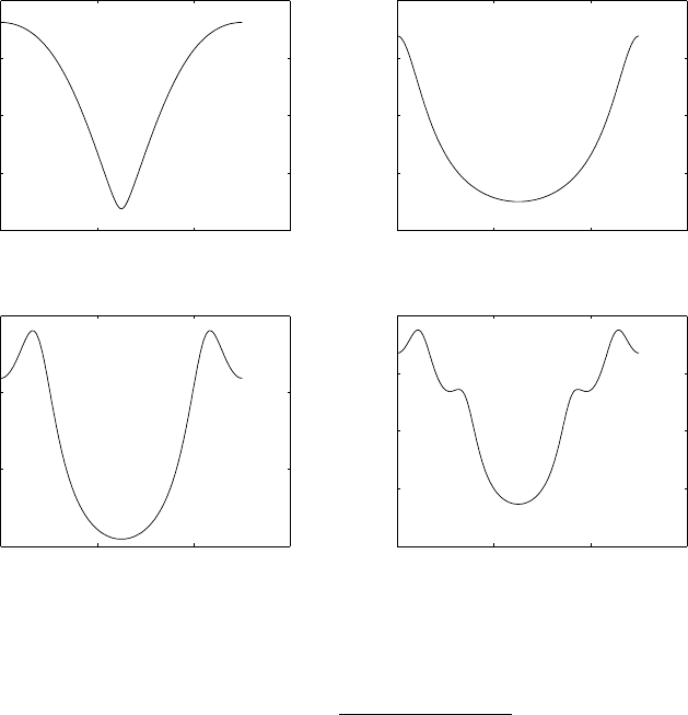
0 0.2 0.4 0.6
0
0.5
1
1.5
2MA(2)
−−−> frequency(Hz)
−−−> magnitude
0 0.2 0.4 0.6
0.5
1
1.5
2
2.5 AR(2)
−−−> frequency(Hz)
−−−> magnitude
0 0.2 0.4 0.6
0.5
1
1.5
2AR(4)
−−−> frequency(Hz)
−−−> magnitude
0 0.2 0.4 0.6
0
0.5
1
1.5
2AR(8)
−−−> frequency(Hz)
−−−> magnitude
Figure 14.20-1:
Γxx(w) = σ2
w
1.6561 −1.62cosw
(b) Refer to fig 14.21-1.
(c) For (2),
γxx(m) =
σ2
wP3
k=0 bkbk+m,0≤m≤2
0, m > 2
γ∗
xx(−m), m < 0
since b0= 1, b1= 0 and b2=−1,we have
γxx(0) = 2σ2
w
γxx(2) = −σ2
w
γxx(−2) = −σ2
w
γxx(m) = 0, m 6= 0,±2
For (3), the AR process has coefficients a0= 1, a1= 0 and a2= 0.81.
1 0 0.81
0 1.81 0
0.81 0 1
γxx(0)
γxx(1)
γxx(2)
=
σ2
w
0
0
γxx(0) = 2.9σ2
w
420
© 2007 Pearson Education, Inc., Upper Saddle River, NJ. All rights reserved. This material is protected under all copyright laws
as they currently exist. No portion of this material may be reproduced, in any form or by any means, without permission in
writing from the publisher. For the exclusive use of adopters of the book Digital Signal Processing, Fourth Edition, by John G.
Proakis and Dimitris G. Manolakis. ISBN 0-13-187374-1.
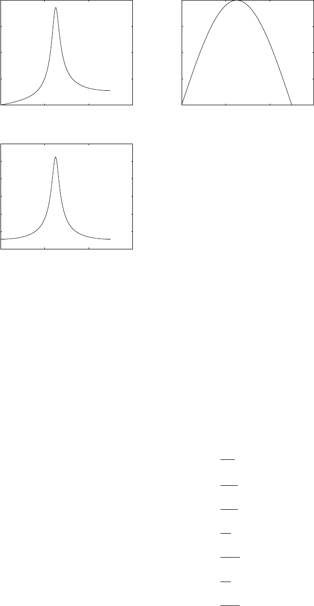
0 0.2 0.4 0.6
0
2
4
6
8(1)
−−−> frequency(Hz)
−−−> magnitude
0 0.2 0.4 0.6
0
0.5
1
1.5
2(2)
−−−> frequency(Hz)
−−−> magnitude
0 0.2 0.4 0.6
0
1
2
3
4
5
6(3)
−−−> frequency(Hz)
−−−> magnitude
Figure 14.21-1:
γxx(m) = 0, m odd
γxx(m) = 2.9(0.9)|m|σ2
w, m even
14.22
(a) For the Bartlett estimate,
M=0.9
△f
=0.9
0.01 = 90
(b)M=0.9
0.02 = 45
(c)for (a), QB=N
M
=2400
90 = 26.67
for (b), QB=N
M
=2400
45 = 53.33
421
© 2007 Pearson Education, Inc., Upper Saddle River, NJ. All rights reserved. This material is protected under all copyright laws
as they currently exist. No portion of this material may be reproduced, in any form or by any means, without permission in
writing from the publisher. For the exclusive use of adopters of the book Digital Signal Processing, Fourth Edition, by John G.
Proakis and Dimitris G. Manolakis. ISBN 0-13-187374-1.

14.23
Γxx(f) = σ2
w|ej2πf −0.9|2
|ej2πf −j0.9|2|ej2πf +j0.9|2
(a)
Γxx(z) = σ2
w
z−0.9
z2+ 0.81
z−1−0.9
z−2+ 0.81
Therefore, H(z) = z−0.9
z2+ 0.81
=z−1(1 −0.9z−1)
1 + 0.81z−2
(b) The inverse system is
1
H(z)=1 + 0.81z−2
z−1(1 −0.9z−1)
This is a stable system.
14.24
X(k) =
N−1
X
n=0
x(n)e−j2πnk
N
(a)
E[X(k)] = X
n
E[x(n)]e−j2πnk
N= 0
E[|X(k)|2] = X
nX
m
E[x(n)x∗(m)]e−j2πk(n−m)
N
=X
nX
m
σ2
xδ(n−m)e−j2πk(n−m)
N
=σ2
x
N−1
X
n=0
1
=Nσ2
x
(b)
E{X(k)X∗(k−m)}=X
nX
n′
E[x(n)x∗(n′)]e−j2πkn
Nej2πn′(k−n)
N
=σ2
xX
nX
n′
δ(n−n′)e−j2πmn′
Ne−j2πk(n−n′)
N
=σ2
xej2πmn
N
=Nσ2
x, m =pN
= 0,otherwise p= 0,±1,±2,...
422
© 2007 Pearson Education, Inc., Upper Saddle River, NJ. All rights reserved. This material is protected under all copyright laws
as they currently exist. No portion of this material may be reproduced, in any form or by any means, without permission in
writing from the publisher. For the exclusive use of adopters of the book Digital Signal Processing, Fourth Edition, by John G.
Proakis and Dimitris G. Manolakis. ISBN 0-13-187374-1.

14.25
γvv(m) = E[v∗(n)v(n+m)]
=
q
X
k′=0
q
X
k=0
b∗
kbk′E[w∗(n−k)w(n+m−k′)]
=σ2
w
q
X
k′=0
q
X
k=0
b∗
kbk′δ(m+k−k′)
=σ2
w
q
X
k=0
b∗
kbk+m
=σ2
wdm
Then, Γvv (f) = σ2
w
q
X
m=−q
dme−j2πf m
14.26
γxx(m) = E[x∗(n)x(n+m)]
=A2E{cos(w1n+φ)cos[w1(n+m) + φ]}
=A2
2E{cosw1m+cos[w1(2n+m) + 2φ]}
=A2
2cosw1n
14.27
(a)
x(n) = 0.81x(n−2) + w(n)
y(n) = x(n) + v(n)
⇒x(n) = y(n)−v(n)
y(n)−v(n) = 0.81y(n−2) −0.81v(n−2) + w(n)
Therefore, y(n) = 0.81y(n−2) + v(n)−0.81v(n−2) + w(n)
so that y(n) is an ARMA(2,2) process
(b)
x(n) = −
p
X
k=1
akx(n−k) + w(n)
y(n) = x(n) + v(n)
⇒x(n) = y(n)−v(n)
y(n)−v(n) = −
p
X
k=1
ak[y(n−k)−v(n−k)] + w(n)
y(n) +
p
X
k=1
aky(n−k) = v(n) +
p
X
k=1
akv(n−k) + w(n)
423
© 2007 Pearson Education, Inc., Upper Saddle River, NJ. All rights reserved. This material is protected under all copyright laws
as they currently exist. No portion of this material may be reproduced, in any form or by any means, without permission in
writing from the publisher. For the exclusive use of adopters of the book Digital Signal Processing, Fourth Edition, by John G.
Proakis and Dimitris G. Manolakis. ISBN 0-13-187374-1.

Hence, y(n) is an ARMA(p,p) process
Note that X(z)[1 +
p
X
k=1
akz−k] = W(z)
H(z) = 1
1 + Pp
k=1 akz−k
=1
Ap(z)
Γxx(z) = σ2
wH(z)H(z−1)
and Γyy (z) = σ2
wH(z)H(z−1) + σ2
v
=σ2
w
Ap(z)Ap(z−1)+σ2
v
=σ2
w+σ2
vAp(z)Ap(z−1)
Ap(z)Ap(z−1)
14.28
(a)
γxx(m) = E{[
K
X
k=1
Akcos(wkn+φk) + w(n)][
K
X
k′=1
Ak′cos(wk′(n+m) + φk′) + w(n+m)]}
=X
kX
k′
AkAk′E{cos(wkn+φk)cos(wk′(n+m) + φk′)}+E[w(n)w(n+m)]
=
K
X
k=1
A2
2cos(wkn) + σ2
wδ(m)
(b)
Γxx(w) = ∞
X
m=−∞
γxx(m)e−jwm
=
K
X
k=1
A2
4
∞
X
m=−∞
(ejwk+e−jwk)e−jwn +σ2
w
=
K
X
k=1
A2
4[2πδ(w−wk−2πm) + 2πδ(w+wk−2πm)] + σ2
w
=π
2
K
X
k=1
A2
k[δ(w−wk−2πm) + 2πδ(w+wk−2πm)] + σ2
w
14.29
E=a∗TΓyy a+λ(1 −a∗Ta)
dE
da = 0
⇒Γyya−λa = 0
or Γyy a=λa
424
© 2007 Pearson Education, Inc., Upper Saddle River, NJ. All rights reserved. This material is protected under all copyright laws
as they currently exist. No portion of this material may be reproduced, in any form or by any means, without permission in
writing from the publisher. For the exclusive use of adopters of the book Digital Signal Processing, Fourth Edition, by John G.
Proakis and Dimitris G. Manolakis. ISBN 0-13-187374-1.

Thus, ais an eigenvector corresponding to the eigenvalue λ. Substitute Γyya=λa into E. Then,
E=λ. To minimize E, we select th smallest eigenvalue, namely, σ2
w.
14.30
(a)
γxx(0) = P+σ2
w
γxx(1) = P cos2πf1
γxx(2) = P cos4πf
By the Levinson-Durbin algorithm,
a1(1) = −γxx(1)
γxx(0)
=−P cos2πf1
P+σ2
w
k1=a1(1)
E1= (1 −k2
1)γxx(0)
=P2sin22πf1+ 2P σ2
w+σ4
w
P+σ2
w
a2(2) = −γxx(2) + a1(1)γxx(1)
E1
=−P σ2
wcos4πf1−P2sin22πf1
P2sin22πf1+ 2P σ2
w+σ4
w
a2(1) = a1(1) + a2(2)a1(1)
=−P cos2πf1
P+σ2
w1 + P2sin22πf1−P σ2
wcos4πf1
P2sin22πf1+ 2P σ2
w+σ4
w
(b) k2=a2(2) k1=a1(1) as given above.
(c)
If σ2
w→0,we have
a2(1) = −(cos2πf1)(1 + 1)
=−2cos2πf1
a2(2) = 1
k2= 1
k1=−cos2πf1
14.31
ε(h) = hHΓxxh+µ(1 −EH(f)h) + µ∗(1 −hHE(f))
(a) To determine the optimum filter that minimizes σ2
ysubject to the constraint, we differentiate
ε(h) with respect to hH(compute the complex gradient):
ε(h)
hH= Γxxh−µ∗E(f) = 0
Thus,
hopt =µ∗Γ−1
xx E(f)
425
© 2007 Pearson Education, Inc., Upper Saddle River, NJ. All rights reserved. This material is protected under all copyright laws
as they currently exist. No portion of this material may be reproduced, in any form or by any means, without permission in
writing from the publisher. For the exclusive use of adopters of the book Digital Signal Processing, Fourth Edition, by John G.
Proakis and Dimitris G. Manolakis. ISBN 0-13-187374-1.

.
(b) To solve for the Langrange multipliers using the constraint, we have
EH(f)hopt =µ∗EH(f)Γ−1
xx E(f) = 1
Thus,
µ∗=1
EH(f)Γ−1
xx E(f)
By substituting for µ∗in the result given in (a) we obtain the optimum filter as
hopt =Γ−1
xx E(f)
EH(f)Γ−1
xx E(f)
14.32
The periodogram spectral estimate is
PXX (f) = 1
N|X(f)|2=1
NX(f)X∗(f)
where
X(f) =
N−1
X
n=0
x(n)e−j2πf n =EH(f)X(n)
By substituting X(f) into Pxx(f), we obtain
Pxx(f) = 1
NEH(f)X(n)X(n)HE(f)
Then,
E[Pxx(f)] = 1
NEH(f)EX(n)X(n)HE(f)
=1
NEH(f)ΓxxE(f)
14.33
We use the Pisasenko decomposition method. First, we compute the eigqnvalues of the correlation
matrix.
g(λ) =
3−λ0−2
0 3 −λ0
−2 0 3 −λ
= (3 −λ)
3−λ0
0 3 −λ−2
0 3 −λ
3−λ0
= (3 −λ)3−2(2)(3 −λ) = (3 −λ)(3 −λ)2−4= 0
Thus, λ= 5,3,1 and the noise varinace is λmin = 1. The corresponding eigenvector is
2 0 −2
020
−2 0 2
1
a1
a2
=
0
0
0
⇒a2= 1, a1= 0 ⇒
1
0
1
The frequency is found from the equation 1 + z−2= 0 ⇒z=±j. Therefore, ejw =±jyields
w=±π/2 and the power is P= 2.
426
© 2007 Pearson Education, Inc., Upper Saddle River, NJ. All rights reserved. This material is protected under all copyright laws
as they currently exist. No portion of this material may be reproduced, in any form or by any means, without permission in
writing from the publisher. For the exclusive use of adopters of the book Digital Signal Processing, Fourth Edition, by John G.
Proakis and Dimitris G. Manolakis. ISBN 0-13-187374-1.

14.34
The eigenvalues are found from
g(λ) =
2−λ−j−1
j2−λ−j
−1j2−λ⇒λ1= 1, λ2= 1, λ3= 4.
and the normalized eigenvectors are
v1=
−j/√3
1/√3
j/√3
v2=
0
j/√2
1/√2
v3=
p2/3
−j/√6
1/√6
By computing the denominator of (14.5.28), we find that the frequency is ω=π/2 or f= 1/4. We
may also find the frequency by using the eigenvectors v2and v3to construct the two polynomials
(Boot Music Method):
V2(z) = j
√2z−1
√2z−2
V3(z) = r2
3−1
√6z−1+1
√6z−2
Then, we form the polynomials
V2(z)V∗
2(1/z∗) + V3(z)V∗
3(1/z∗) = 1
3z2+2
3jz + 2 −2
3jz−1+1
3z−2
It is easily verified that the polynomial has a double root at z=jor, equivalently, at ω=π/2.
The other two roots are spurious roots that are neglected.
Finally, the power of the exponential signal is P1= 1.
14.35
PMU SIC (f) = 1
PM
k=p+1 |sH(f)vk|2
The denominator can be expressed as
M
X
k=p+1 sH(f)vk2=
M
X
k=p+1
sH(f)vkvH
ks(f)
=sH(f)
M
X
k=p+1
vkvH
k
s(f)
14.36
(a) Vk(z) = PM−1
n=0 vk(n+1)z−nand Vk(f) = Vk(z)|z=ej2πf Then, the denominator in PMU SI C (f)
may be expressed as
M
X
k=p+1
=sH(f)vk2=X
k=p+1
MVk(f)V∗
k(f)
=X
k=p+1
MVk(z)V∗
k(1/z∗)|z=ej2πf
427
© 2007 Pearson Education, Inc., Upper Saddle River, NJ. All rights reserved. This material is protected under all copyright laws
as they currently exist. No portion of this material may be reproduced, in any form or by any means, without permission in
writing from the publisher. For the exclusive use of adopters of the book Digital Signal Processing, Fourth Edition, by John G.
Proakis and Dimitris G. Manolakis. ISBN 0-13-187374-1.

(b) For the roots of Q(z), we consruct (from Problem 14.34) Q(z) as
Q(z) = V2(z)V∗
2(1/z∗) + V3(z)V∗
3(1/z∗)
=1
3z2+2
3jz + 2 −2
3jz−1+1
3z−2
Thus polynomial has a double root at z=jand two spurious roots. Therefore, the desired
frequency is ω=π/2.
14.37
(a)
γxy(n0) =
N−1
X
n=0
y(n−n0)[y(n−n0) + w(n)]
E[γxy(n0)] =
N−1
X
n=0
E[y2(n−n0)]
=
N−1
X
n=1
E[A2cos2w0(n−n0)] 0 ≤n≤M−1
=MA2
2
var[γxy (n0)] = E[γ2
xy(n0)]( MA2
2)2
=X
nX
n′
E{y(n−n0)[y(n−n0) + w(n)]y(n′−n0)[y(n′−n0) + w(n′)]} − (MA2
2)2
=MA2
2σ2
w
(b)
SNR = {E[γxy(n0)]}2
var[γxy (n0)]
=(MA2
2)2
MA2
2σ2
w
=MA2
2σ2
w
(c) As M increases, the SNR increases.
14.38
Refer to fig 14.38-1.
14.39
Refer to fig 14.39-1.
428
© 2007 Pearson Education, Inc., Upper Saddle River, NJ. All rights reserved. This material is protected under all copyright laws
as they currently exist. No portion of this material may be reproduced, in any form or by any means, without permission in
writing from the publisher. For the exclusive use of adopters of the book Digital Signal Processing, Fourth Edition, by John G.
Proakis and Dimitris G. Manolakis. ISBN 0-13-187374-1.
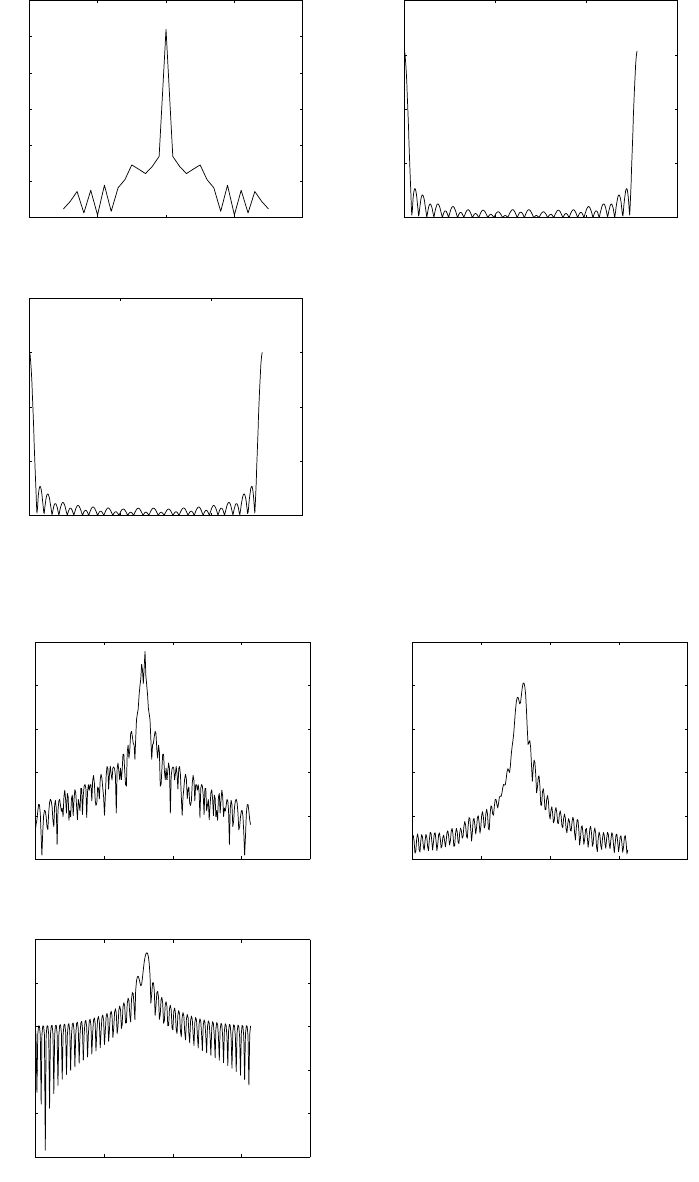
−20 −10 0 10 20
1.8
2
2.2
2.4
2.6
2.8
3autocor of w(n)
0 200 400 600
0
20
40
60
80 periodogram Pxx(f)
0 200 400 600
0
20
40
60
80 avg periodogram Pxx(f)
Figure 14.38-1:
0 1 2 3 4
−40
−20
0
20
40
60 theoretical psd with M = 100
0 1 2 3 4
20
40
60
80
100
120 Blackman−Tukey psd with lag=25
0 1 2 3 4
0
10
20
30
40
50 Bartlett with M = 50
Figure 14.39-1:
429
© 2007 Pearson Education, Inc., Upper Saddle River, NJ. All rights reserved. This material is protected under all copyright laws
as they currently exist. No portion of this material may be reproduced, in any form or by any means, without permission in
writing from the publisher. For the exclusive use of adopters of the book Digital Signal Processing, Fourth Edition, by John G.
Proakis and Dimitris G. Manolakis. ISBN 0-13-187374-1.
Co r rections to
Digital Signal Processing, 4t h Edition
by
John G . P roakis and Dimitris G. Manolakis
1. Page 18, two lines below equation (1.3.18)
sk(n) should be sk(n)
2. Page 34, Figure 1.4.8
The quantized value of the signal between 2T and 3T should be 4
3. Page 66, line below equation (2.2.43)
“is relaxed” should be “is non-relaxed”
4. Page 101, last term of equation (2.4.24)
n
n should be N
5. Page 147, last sentence above Section 3.1
Move this sentence to line above, just before the word “Finally, “
6. Page 161, figure 5.2.1
The mapping is w = a-1z
7. Page 237, line 2 from the top of page
“radian” should be “radial”
8. Page 321, Figure 5.2.3, magnitude plot
Scale on the ordinate should be multiplied by 5
9. Page 387, line 8 below equation (6.1.15)
X(Fs) should be X(F)
10. Page 390, Figure 6.1.3(b)
X(F/Fs) should be X(F)
11. Page 391, Figure 6.1.5 upper right-hand part of the figure
X(F/Xf) should be X(F)
12. Page 396, Figure 6.2.3, graph of Y(F)
For F<0, the Fs on the abscissa should be -Fs
13. Page 424, two lines below equation (6.4.68)
The word “envelop” should be “envelope”
14. Page 454, equation on line above Section 7.1.2
e-j2 kN should be e-j2 k/N
15.Page 463, line below equation (7.1.39)
(7.1.38) should be (7.1.39)
16.Page 506, problem 7.23(e)
The exponent should be j(2 /N) kon
17. Page 526, Figure 8.1.10
Delete the factor of 2 in the expression for B
18. Page 582, line 4 from the top
B2(z) = 1/2+3/8 z-1+z-2
19. Page 646, Problem 9.22
In the denominator of H(z), the term r2 should be r2
20. Page 672, two lines below equation (10.2.35)
G(k+x) should be ((k+ )
21. Page 679, line above equation (10.2.52) and in equation (10.2.52)
Add the term
˜ ˜
b (1) = 2b(1) -2 b(0); Then, in (10.2.52), k = 2,3,…,M/2 -2
22. Page 680, line above Case 4:
The equation should be
˜ ˜
c(0) – ½ c(2) = c(1)
23. Page 725, Figure 10.3.14, graph on left
The value of 1 is the peak value
24. Page 742, problem 10.2.3, lines 4 and 6
Add subscripts l and u on the expressions for
H(s) should b Ha(s)
25. Page 809, equation (11.12.15)
Q(zM) should be Qt(zM)
26. Page 811, in Solution of example 11.12.1
The matrix for G0(z), G1(z) and G2(z) should be transposed
Thus,
G0(z) = 1-z-1 + z-2, G1(z) = -1-z-1+3z-2, G2(z)=1+3z-1-5z-2
27. Page 818, problem 11.16
Change the statement of the problem to the following:
Use the result in Problem 11.15 to determine the type II form of the I=3
interpolator in Figure 11.5.12(b)
28. Page 821, third line from bottom of page
Should be f0 = 1/6 and f = 1/3
29. Page 958, problem 13.19
In the expression for the least squares error,
f(m)n should be fm(l) and gm(n) should be gm(l)
30. Page 962, equations (14.1.6), (14.1.7) and (14.1.8)
X(F/X(F)) should be X(F)
31. Page 964, in Solution of Example 14.1.1, line 2
Figure 10.2.2(a) should be Figure 10.2.2
32. Page 1038, problem 14.35
In the denominator of the equation, vkvk should be vkvkH
