Programming Hive Guide
User Manual:
Open the PDF directly: View PDF ![]() .
.
Page Count: 350 [warning: Documents this large are best viewed by clicking the View PDF Link!]
- Table of Contents
- Preface
- Chapter 1. Introduction
- Chapter 2. Getting Started
- Chapter 3. Data Types and File Formats
- Chapter 4. HiveQL: Data Definition
- Chapter 5. HiveQL: Data Manipulation
- Chapter 6. HiveQL: Queries
- SELECT … FROM Clauses
- WHERE Clauses
- GROUP BY Clauses
- JOIN Statements
- ORDER BY and SORT BY
- DISTRIBUTE BY with SORT BY
- CLUSTER BY
- Casting
- Queries that Sample Data
- UNION ALL
- Chapter 7. HiveQL: Views
- Chapter 8. HiveQL: Indexes
- Chapter 9. Schema Design
- Chapter 10. Tuning
- Chapter 11. Other File Formats and Compression
- Chapter 12. Developing
- Chapter 13. Functions
- Discovering and Describing Functions
- Calling Functions
- Standard Functions
- Aggregate Functions
- Table Generating Functions
- A UDF for Finding a Zodiac Sign from a Day
- UDF Versus GenericUDF
- Permanent Functions
- User-Defined Aggregate Functions
- User-Defined Table Generating Functions
- Accessing the Distributed Cache from a UDF
- Annotations for Use with Functions
- Macros
- Chapter 14. Streaming
- Chapter 15. Customizing Hive File and Record Formats
- Chapter 16. Hive Thrift Service
- Chapter 17. Storage Handlers and NoSQL
- Chapter 18. Security
- Chapter 19. Locking
- Chapter 20. Hive Integration with Oozie
- Chapter 21. Hive and Amazon Web Services (AWS)
- Why Elastic MapReduce?
- Instances
- Before You Start
- Managing Your EMR Hive Cluster
- Thrift Server on EMR Hive
- Instance Groups on EMR
- Configuring Your EMR Cluster
- Persistence and the Metastore on EMR
- HDFS and S3 on EMR Cluster
- Putting Resources, Configs, and Bootstrap Scripts on S3
- Logs on S3
- Spot Instances
- Security Groups
- EMR Versus EC2 and Apache Hive
- Wrapping Up
- Chapter 22. HCatalog
- Chapter 23. Case Studies
- m6d.com (Media6Degrees)
- Outbrain
- NASA’s Jet Propulsion Laboratory
- Photobucket
- SimpleReach
- Experiences and Needs from the Customer Trenches
- Glossary
- Appendix. References
- Index

Programming Hive
Edward Capriolo, Dean Wampler, and Jason Rutherglen
Beijing
•
Cambridge
•
Farnham
•
Köln
•
Sebastopol
•
Tokyo
Downloa d f r o m W o w ! e B o o k < w w w.woweb o o k . c o m >
Programming Hive
by Edward Capriolo, Dean Wampler, and Jason Rutherglen
Copyright © 2012 Edward Capriolo, Aspect Research Associates, and Jason Rutherglen. All rights re-
served.
Printed in the United States of America.
Published by O’Reilly Media, Inc., 1005 Gravenstein Highway North, Sebastopol, CA 95472.
O’Reilly books may be purchased for educational, business, or sales promotional use. Online editions
are also available for most titles (http://my.safaribooksonline.com). For more information, contact our
corporate/institutional sales department: 800-998-9938 or corporate@oreilly.com.
Editors: Mike Loukides and Courtney Nash
Production Editors: Iris Febres and Rachel Steely
Proofreaders: Stacie Arellano and Kiel Van Horn
Indexer: Bob Pfahler
Cover Designer: Karen Montgomery
Interior Designer: David Futato
Illustrator: Rebecca Demarest
October 2012: First Edition.
Revision History for the First Edition:
2012-09-17 First release
See http://oreilly.com/catalog/errata.csp?isbn=9781449319335 for release details.
Nutshell Handbook, the Nutshell Handbook logo, and the O’Reilly logo are registered trademarks of
O’Reilly Media, Inc. Programming Hive, the image of a hornet’s hive, and related trade dress are trade-
marks of O’Reilly Media, Inc.
Many of the designations used by manufacturers and sellers to distinguish their products are claimed as
trademarks. Where those designations appear in this book, and O’Reilly Media, Inc., was aware of a
trademark claim, the designations have been printed in caps or initial caps.
While every precaution has been taken in the preparation of this book, the publisher and authors assume
no responsibility for errors or omissions, or for damages resulting from the use of the information con-
tained herein.
ISBN: 978-1-449-31933-5
[LSI]
1347905436

Table of Contents
Preface .................................................................... xiii
1. Introduction ........................................................... 1
An Overview of Hadoop and MapReduce 3
Hive in the Hadoop Ecosystem 6
Pig 8
HBase 8
Cascading, Crunch, and Others 9
Java Versus Hive: The Word Count Algorithm 10
What’s Next 13
2. Getting Started ........................................................ 15
Installing a Preconfigured Virtual Machine 15
Detailed Installation 16
Installing Java 16
Installing Hadoop 18
Local Mode, Pseudodistributed Mode, and Distributed Mode 19
Testing Hadoop 20
Installing Hive 21
What Is Inside Hive? 22
Starting Hive 23
Configuring Your Hadoop Environment 24
Local Mode Configuration 24
Distributed and Pseudodistributed Mode Configuration 26
Metastore Using JDBC 28
The Hive Command 29
Command Options 29
The Command-Line Interface 30
CLI Options 31
Variables and Properties 31
Hive “One Shot” Commands 34
iii

Executing Hive Queries from Files 35
The .hiverc File 36
More on Using the Hive CLI 36
Command History 37
Shell Execution 37
Hadoop dfs Commands from Inside Hive 38
Comments in Hive Scripts 38
Query Column Headers 38
3. Data Types and File Formats ............................................. 41
Primitive Data Types 41
Collection Data Types 43
Text File Encoding of Data Values 45
Schema on Read 48
4. HiveQL: Data Definition ................................................. 49
Databases in Hive 49
Alter Database 52
Creating Tables 53
Managed Tables 56
External Tables 56
Partitioned, Managed Tables 58
External Partitioned Tables 61
Customizing Table Storage Formats 63
Dropping Tables 66
Alter Table 66
Renaming a Table 66
Adding, Modifying, and Dropping a Table Partition 66
Changing Columns 67
Adding Columns 68
Deleting or Replacing Columns 68
Alter Table Properties 68
Alter Storage Properties 68
Miscellaneous Alter Table Statements 69
5. HiveQL: Data Manipulation .............................................. 71
Loading Data into Managed Tables 71
Inserting Data into Tables from Queries 73
Dynamic Partition Inserts 74
Creating Tables and Loading Them in One Query 75
Exporting Data 76
iv | Table of Contents

6. HiveQL: Queries ........................................................ 79
SELECT … FROM Clauses 79
Specify Columns with Regular Expressions 81
Computing with Column Values 81
Arithmetic Operators 82
Using Functions 83
LIMIT Clause 91
Column Aliases 91
Nested SELECT Statements 91
CASE … WHEN … THEN Statements 91
When Hive Can Avoid MapReduce 92
WHERE Clauses 92
Predicate Operators 93
Gotchas with Floating-Point Comparisons 94
LIKE and RLIKE 96
GROUP BY Clauses 97
HAVING Clauses 97
JOIN Statements 98
Inner JOIN 98
Join Optimizations 100
LEFT OUTER JOIN 101
OUTER JOIN Gotcha 101
RIGHT OUTER JOIN 103
FULL OUTER JOIN 104
LEFT SEMI-JOIN 104
Cartesian Product JOINs 105
Map-side Joins 105
ORDER BY and SORT BY 107
DISTRIBUTE BY with SORT BY 107
CLUSTER BY 108
Casting 109
Casting BINARY Values 109
Queries that Sample Data 110
Block Sampling 111
Input Pruning for Bucket Tables 111
UNION ALL 112
7. HiveQL: Views ........................................................ 113
Views to Reduce Query Complexity 113
Views that Restrict Data Based on Conditions 114
Views and Map Type for Dynamic Tables 114
View Odds and Ends 115
Table of Contents | v

8. HiveQL: Indexes ...................................................... 117
Creating an Index 117
Bitmap Indexes 118
Rebuilding the Index 118
Showing an Index 119
Dropping an Index 119
Implementing a Custom Index Handler 119
9. Schema Design ....................................................... 121
Table-by-Day 121
Over Partitioning 122
Unique Keys and Normalization 123
Making Multiple Passes over the Same Data 124
The Case for Partitioning Every Table 124
Bucketing Table Data Storage 125
Adding Columns to a Table 127
Using Columnar Tables 128
Repeated Data 128
Many Columns 128
(Almost) Always Use Compression! 128
10. Tuning .............................................................. 131
Using EXPLAIN 131
EXPLAIN EXTENDED 134
Limit Tuning 134
Optimized Joins 135
Local Mode 135
Parallel Execution 136
Strict Mode 137
Tuning the Number of Mappers and Reducers 138
JVM Reuse 139
Indexes 140
Dynamic Partition Tuning 140
Speculative Execution 141
Single MapReduce MultiGROUP BY 142
Virtual Columns 142
11. Other File Formats and Compression . . . . . . . . . . . . . . . . . . . . . . . . . . . . . . . . . . . . . 145
Determining Installed Codecs 145
Choosing a Compression Codec 146
Enabling Intermediate Compression 147
Final Output Compression 148
Sequence Files 148
vi | Table of Contents

Compression in Action 149
Archive Partition 152
Compression: Wrapping Up 154
12. Developing .......................................................... 155
Changing Log4J Properties 155
Connecting a Java Debugger to Hive 156
Building Hive from Source 156
Running Hive Test Cases 156
Execution Hooks 158
Setting Up Hive and Eclipse 158
Hive in a Maven Project 158
Unit Testing in Hive with hive_test 159
The New Plugin Developer Kit 161
13. Functions ............................................................ 163
Discovering and Describing Functions 163
Calling Functions 164
Standard Functions 164
Aggregate Functions 164
Table Generating Functions 165
A UDF for Finding a Zodiac Sign from a Day 166
UDF Versus GenericUDF 169
Permanent Functions 171
User-Defined Aggregate Functions 172
Creating a COLLECT UDAF to Emulate GROUP_CONCAT 172
User-Defined Table Generating Functions 177
UDTFs that Produce Multiple Rows 177
UDTFs that Produce a Single Row with Multiple Columns 179
UDTFs that Simulate Complex Types 179
Accessing the Distributed Cache from a UDF 182
Annotations for Use with Functions 184
Deterministic 184
Stateful 184
DistinctLike 185
Macros 185
14. Streaming ........................................................... 187
Identity Transformation 188
Changing Types 188
Projecting Transformation 188
Manipulative Transformations 189
Using the Distributed Cache 189
Table of Contents | vii

Producing Multiple Rows from a Single Row 190
Calculating Aggregates with Streaming 191
CLUSTER BY, DISTRIBUTE BY, SORT BY 192
GenericMR Tools for Streaming to Java 194
Calculating Cogroups 196
15. Customizing Hive File and Record Formats . . . . . . . . . . . . . . . . . . . . . . . . . . . . . . . . 199
File Versus Record Formats 199
Demystifying CREATE TABLE Statements 199
File Formats 201
SequenceFile 201
RCFile 202
Example of a Custom Input Format: DualInputFormat 203
Record Formats: SerDes 205
CSV and TSV SerDes 206
ObjectInspector 206
Think Big Hive Reflection ObjectInspector 206
XML UDF 207
XPath-Related Functions 207
JSON SerDe 208
Avro Hive SerDe 209
Defining Avro Schema Using Table Properties 209
Defining a Schema from a URI 210
Evolving Schema 210
Binary Output 211
16. Hive Thrift Service .................................................... 213
Starting the Thrift Server 213
Setting Up Groovy to Connect to HiveService 214
Connecting to HiveServer 214
Getting Cluster Status 215
Result Set Schema 215
Fetching Results 215
Retrieving Query Plan 216
Metastore Methods 216
Example Table Checker 216
Administrating HiveServer 217
Productionizing HiveService 217
Cleanup 218
Hive ThriftMetastore 219
ThriftMetastore Configuration 219
Client Configuration 219
viii | Table of Contents

17. Storage Handlers and NoSQL ............................................ 221
Storage Handler Background 221
HiveStorageHandler 222
HBase 222
Cassandra 224
Static Column Mapping 224
Transposed Column Mapping for Dynamic Columns 224
Cassandra SerDe Properties 224
DynamoDB 225
18. Security ............................................................. 227
Integration with Hadoop Security 228
Authentication with Hive 228
Authorization in Hive 229
Users, Groups, and Roles 230
Privileges to Grant and Revoke 231
Partition-Level Privileges 233
Automatic Grants 233
19. Locking . ............................................................ 235
Locking Support in Hive with Zookeeper 235
Explicit, Exclusive Locks 238
20. Hive Integration with Oozie . ........................................... 239
Oozie Actions 239
Hive Thrift Service Action 240
A Two-Query Workflow 240
Oozie Web Console 242
Variables in Workflows 242
Capturing Output 243
Capturing Output to Variables 243
21. Hive and Amazon Web Services (AWS) . . . . . . . . . . . . . . . . . . . . . . . . . . . . . . . . . . . . 245
Why Elastic MapReduce? 245
Instances 245
Before You Start 246
Managing Your EMR Hive Cluster 246
Thrift Server on EMR Hive 247
Instance Groups on EMR 247
Configuring Your EMR Cluster 248
Deploying hive-site.xml 248
Deploying a .hiverc Script 249
Table of Contents | ix
Downloa d f r o m W o w ! e B o o k < w w w.woweb o o k . c o m >

Setting Up a Memory-Intensive Configuration 249
Persistence and the Metastore on EMR 250
HDFS and S3 on EMR Cluster 251
Putting Resources, Configs, and Bootstrap Scripts on S3 252
Logs on S3 252
Spot Instances 252
Security Groups 253
EMR Versus EC2 and Apache Hive 254
Wrapping Up 254
22. HCatalog ............................................................ 255
Introduction 255
MapReduce 256
Reading Data 256
Writing Data 258
Command Line 261
Security Model 261
Architecture 262
23. Case Studies ......................................................... 265
m6d.com (Media6Degrees) 265
Data Science at M6D Using Hive and R 265
M6D UDF Pseudorank 270
M6D Managing Hive Data Across Multiple MapReduce Clusters 274
Outbrain 278
In-Site Referrer Identification 278
Counting Uniques 280
Sessionization 282
NASA’s Jet Propulsion Laboratory 287
The Regional Climate Model Evaluation System 287
Our Experience: Why Hive? 290
Some Challenges and How We Overcame Them 291
Photobucket 292
Big Data at Photobucket 292
What Hardware Do We Use for Hive? 293
What’s in Hive? 293
Who Does It Support? 293
SimpleReach 294
Experiences and Needs from the Customer Trenches 296
A Karmasphere Perspective 296
Introduction 296
Use Case Examples from the Customer Trenches 297
x | Table of Contents


Preface
Programming Hive introduces Hive, an essential tool in the Hadoop ecosystem that
provides an SQL (Structured Query Language) dialect for querying data stored in the
Hadoop Distributed Filesystem (HDFS), other filesystems that integrate with Hadoop,
such as MapR-FS and Amazon’s S3 and databases like HBase (the Hadoop database)
and Cassandra.
Most data warehouse applications are implemented using relational databases that use
SQL as the query language. Hive lowers the barrier for moving these applications to
Hadoop. People who know SQL can learn Hive easily. Without Hive, these users must
learn new languages and tools to become productive again. Similarly, Hive makes it
easier for developers to port SQL-based applications to Hadoop, compared to other
tool options. Without Hive, developers would face a daunting challenge when porting
their SQL applications to Hadoop.
Still, there are aspects of Hive that are different from other SQL-based environments.
Documentation for Hive users and Hadoop developers has been sparse. We decided
to write this book to fill that gap. We provide a pragmatic, comprehensive introduction
to Hive that is suitable for SQL experts, such as database designers and business ana-
lysts. We also cover the in-depth technical details that Hadoop developers require for
tuning and customizing Hive.
You can learn more at the book’s catalog page (http://oreil.ly/Programming_Hive).
Conventions Used in This Book
The following typographical conventions are used in this book:
Italic
Indicates new terms, URLs, email addresses, filenames, and file extensions. Defi-
nitions of most terms can be found in the Glossary.
Constant width
Used for program listings, as well as within paragraphs to refer to program elements
such as variable or function names, databases, data types, environment variables,
statements, and keywords.
xiii

Constant width bold
Shows commands or other text that should be typed literally by the user.
Constant width italic
Shows text that should be replaced with user-supplied values or by values deter-
mined by context.
This icon signifies a tip, suggestion, or general note.
This icon indicates a warning or caution.
Using Code Examples
This book is here to help you get your job done. In general, you may use the code in
this book in your programs and documentation. You do not need to contact us for
permission unless you’re reproducing a significant portion of the code. For example,
writing a program that uses several chunks of code from this book does not require
permission. Selling or distributing a CD-ROM of examples from O’Reilly books does
require permission. Answering a question by citing this book and quoting example
code does not require permission. Incorporating a significant amount of example code
from this book into your product’s documentation does require permission.
We appreciate, but do not require, attribution. An attribution usually includes the title,
author, publisher, and ISBN. For example: “Programming Hive by Edward Capriolo,
Dean Wampler, and Jason Rutherglen (O’Reilly). Copyright 2012 Edward Capriolo,
Aspect Research Associates, and Jason Rutherglen, 978-1-449-31933-5.”
If you feel your use of code examples falls outside fair use or the permission given above,
feel free to contact us at permissions@oreilly.com.
Safari® Books Online
Safari Books Online (www.safaribooksonline.com) is an on-demand digital
library that delivers expert content in both book and video form from the
world’s leading authors in technology and business.
Technology professionals, software developers, web designers, and business and cre-
ative professionals use Safari Books Online as their primary resource for research,
problem solving, learning, and certification training.
xiv | Preface

Safari Books Online offers a range of product mixes and pricing programs for organi-
zations, government agencies, and individuals. Subscribers have access to thousands
of books, training videos, and prepublication manuscripts in one fully searchable da-
tabase from publishers like O’Reilly Media, Prentice Hall Professional, Addison-Wesley
Professional, Microsoft Press, Sams, Que, Peachpit Press, Focal Press, Cisco Press, John
Wiley & Sons, Syngress, Morgan Kaufmann, IBM Redbooks, Packt, Adobe Press, FT
Press, Apress, Manning, New Riders, McGraw-Hill, Jones & Bartlett, Course Tech-
nology, and dozens more. For more information about Safari Books Online, please visit
us online.
How to Contact Us
Please address comments and questions concerning this book to the publisher:
O’Reilly Media, Inc.
1005 Gravenstein Highway North
Sebastopol, CA 95472
800-998-9938 (in the United States or Canada)
707-829-0515 (international or local)
707-829-0104 (fax)
We have a web page for this book, where we list errata, examples, and any additional
information. You can access this page at http://oreil.ly/Programming_Hive.
To comment or ask technical questions about this book, send email to
bookquestions@oreilly.com.
For more information about our books, courses, conferences, and news, see our website
at http://www.oreilly.com.
Find us on Facebook: http://facebook.com/oreilly
Follow us on Twitter: http://twitter.com/oreillymedia
Watch us on YouTube: http://www.youtube.com/oreillymedia
What Brought Us to Hive?
The three of us arrived here from different directions.
Edward Capriolo
When I first became involved with Hadoop, I saw the distributed filesystem and Map-
Reduce as a great way to tackle computer-intensive problems. However, programming
in the MapReduce model was a paradigm shift for me. Hive offered a fast and simple
way to take advantage of MapReduce in an SQL-like world I was comfortable in. This
approach also made it easy to prototype proof-of-concept applications and also to
Preface | xv

champion Hadoop as a solution internally. Even though I am now very familiar with
Hadoop internals, Hive is still my primary method of working with Hadoop.
It is an honor to write a Hive book. Being a Hive Committer and a member of the
Apache Software Foundation is my most valued accolade.
Dean Wampler
As a “big data” consultant at Think Big Analytics, I work with experienced “data people”
who eat and breathe SQL. For them, Hive is a necessary and sufficient condition for
Hadoop to be a viable tool to leverage their investment in SQL and open up new op-
portunities for data analytics.
Hive has lacked good documentation. I suggested to my previous editor at O’Reilly,
Mike Loukides, that a Hive book was needed by the community. So, here we are…
Jason Rutherglen
I work at Think Big Analytics as a software architect. My career has involved an array
of technologies including search, Hadoop, mobile, cryptography, and natural language
processing. Hive is the ultimate way to build a data warehouse using open technologies
on any amount of data. I use Hive regularly on a variety of projects.
Acknowledgments
Everyone involved with Hive. This includes committers, contributors, as well as end
users.
Mark Grover wrote the chapter on Hive and Amazon Web Services. He is a contributor
to the Apache Hive project and is active helping others on the Hive IRC channel.
David Ha and Rumit Patel, at M6D, contributed the case study and code on the Rank
function. The ability to do Rank in Hive is a significant feature.
Ori Stitelman, at M6D, contributed the case study, Data Science using Hive and R,
which demonstrates how Hive can be used to make first pass on large data sets and
produce results to be used by a second R process.
David Funk contributed three use cases on in-site referrer identification, sessionization,
and counting unique visitors. David’s techniques show how rewriting and optimizing
Hive queries can make large scale map reduce data analysis more efficient.
Ian Robertson read the entire first draft of the book and provided very helpful feedback
on it. We’re grateful to him for providing that feedback on short notice and a tight
schedule.
xvi | Preface

John Sichi provided technical review for the book. John was also instrumental in driving
through some of the newer features in Hive like StorageHandlers and Indexing Support.
He has been actively growing and supporting the Hive community.
Alan Gates, author of Programming Pig, contributed the HCatalog chapter. Nanda
Vijaydev contributed the chapter on how Karmasphere offers productized enhance-
ments for Hive. Eric Lubow contributed the SimpleReach case study. Chris A. Matt-
mann, Paul Zimdars, Cameron Goodale, Andrew F. Hart, Jinwon Kim, Duane Waliser,
and Peter Lean contributed the NASA JPL case study.
Preface | xvii

CHAPTER 1
Introduction
From the early days of the Internet’s mainstream breakout, the major search engines
and ecommerce companies wrestled with ever-growing quantities of data. More re-
cently, social networking sites experienced the same problem. Today, many organiza-
tions realize that the data they gather is a valuable resource for understanding their
customers, the performance of their business in the marketplace, and the effectiveness
of their infrastructure.
The Hadoop ecosystem emerged as a cost-effective way of working with such large data
sets. It imposes a particular programming model, called MapReduce, for breaking up
computation tasks into units that can be distributed around a cluster of commodity,
server class hardware, thereby providing cost-effective, horizontal scalability. Under-
neath this computation model is a distributed file system called the Hadoop Distributed
Filesystem (HDFS). Although the filesystem is “pluggable,” there are now several com-
mercial and open source alternatives.
However, a challenge remains; how do you move an existing data infrastructure to
Hadoop, when that infrastructure is based on traditional relational databases and the
Structured Query Language (SQL)? What about the large base of SQL users, both expert
database designers and administrators, as well as casual users who use SQL to extract
information from their data warehouses?
This is where Hive comes in. Hive provides an SQL dialect, called Hive Query Lan-
guage (abbreviated HiveQL or just HQL) for querying data stored in a Hadoop cluster.
SQL knowledge is widespread for a reason; it’s an effective, reasonably intuitive model
for organizing and using data. Mapping these familiar data operations to the low-level
MapReduce Java API can be daunting, even for experienced Java developers. Hive does
this dirty work for you, so you can focus on the query itself. Hive translates most queries
to MapReduce jobs, thereby exploiting the scalability of Hadoop, while presenting a
familiar SQL abstraction. If you don’t believe us, see “Java Versus Hive: The Word
Count Algorithm” on page 10 later in this chapter.
1

Hive is most suited for data warehouse applications, where relatively static data is an-
alyzed, fast response times are not required, and when the data is not changing rapidly.
Hive is not a full database. The design constraints and limitations of Hadoop and HDFS
impose limits on what Hive can do. The biggest limitation is that Hive does not provide
record-level update, insert, nor delete. You can generate new tables from queries or
output query results to files. Also, because Hadoop is a batch-oriented system, Hive
queries have higher latency, due to the start-up overhead for MapReduce jobs. Queries
that would finish in seconds for a traditional database take longer for Hive, even for
relatively small data sets.1 Finally, Hive does not provide transactions.
So, Hive doesn’t provide crucial features required for OLTP, Online Transaction Pro-
cessing. It’s closer to being an OLAP tool, Online Analytic Processing, but as we’ll see,
Hive isn’t ideal for satisfying the “online” part of OLAP, at least today, since there can
be significant latency between issuing a query and receiving a reply, both due to the
overhead of Hadoop and due to the size of the data sets Hadoop was designed to serve.
If you need OLTP features for large-scale data, you should consider using a NoSQL
database. Examples include HBase, a NoSQL database integrated with Hadoop,2 Cas-
sandra,3 and DynamoDB, if you are using Amazon’s Elastic MapReduce (EMR) or
Elastic Compute Cloud (EC2).4 You can even integrate Hive with these databases
(among others), as we’ll discuss in Chapter 17.
So, Hive is best suited for data warehouse applications, where a large data set is main-
tained and mined for insights, reports, etc.
Because most data warehouse applications are implemented using SQL-based rela-
tional databases, Hive lowers the barrier for moving these applications to Hadoop.
People who know SQL can learn Hive easily. Without Hive, these users would need to
learn new languages and tools to be productive again.
Similarly, Hive makes it easier for developers to port SQL-based applications to
Hadoop, compared with other Hadoop languages and tools.
However, like most SQL dialects, HiveQL does not conform to the ANSI SQL standard
and it differs in various ways from the familiar SQL dialects provided by Oracle,
MySQL, and SQL Server. (However, it is closest to MySQL’s dialect of SQL.)
1. However, for the big data sets Hive is designed for, this start-up overhead is trivial compared to the actual
processing time.
2. See the Apache HBase website, http://hbase.apache.org, and HBase: The Definitive Guide by Lars George
(O’Reilly).
3. See the Cassandra website, http://cassandra.apache.org/, and High Performance Cassandra Cookbook by
Edward Capriolo (Packt).
4. See the DynamoDB website, http://aws.amazon.com/dynamodb/.
2 | Chapter 1: Introduction

So, this book has a dual purpose. First, it provides a comprehensive, example-driven
introduction to HiveQL for all users, from developers, database administrators and
architects, to less technical users, such as business analysts.
Second, the book provides the in-depth technical details required by developers and
Hadoop administrators to tune Hive query performance and to customize Hive with
user-defined functions, custom data formats, etc.
We wrote this book out of frustration that Hive lacked good documentation, especially
for new users who aren’t developers and aren’t accustomed to browsing project artifacts
like bug and feature databases, source code, etc., to get the information they need. The
Hive Wiki5 is an invaluable source of information, but its explanations are sometimes
sparse and not always up to date. We hope this book remedies those issues, providing
a single, comprehensive guide to all the essential features of Hive and how to use them
effectively.6
An Overview of Hadoop and MapReduce
If you’re already familiar with Hadoop and the MapReduce computing model, you can
skip this section. While you don’t need an intimate knowledge of MapReduce to use
Hive, understanding the basic principles of MapReduce will help you understand what
Hive is doing behind the scenes and how you can use Hive more effectively.
We provide a brief overview of Hadoop and MapReduce here. For more details, see
Hadoop: The Definitive Guide by Tom White (O’Reilly).
MapReduce
MapReduce is a computing model that decomposes large data manipulation jobs into
individual tasks that can be executed in parallel across a cluster of servers. The results
of the tasks can be joined together to compute the final results.
The MapReduce programming model was developed at Google and described in an
influential paper called MapReduce: simplified data processing on large clusters (see the
Appendix) on page 309. The Google Filesystem was described a year earlier in a paper
called The Google filesystem on page 310. Both papers inspired the creation of Hadoop
by Doug Cutting.
The term MapReduce comes from the two fundamental data-transformation operations
used, map and reduce. A map operation converts the elements of a collection from one
form to another. In this case, input key-value pairs are converted to zero-to-many
5. See https://cwiki.apache.org/Hive/.
6. It’s worth bookmarking the wiki link, however, because the wiki contains some more obscure information
we won’t cover here.
An Overview of Hadoop and MapReduce | 3

output key-value pairs, where the input and output keys might be completely different
and the input and output values might be completely different.
In MapReduce, all the key-pairs for a given key are sent to the same reduce operation.
Specifically, the key and a collection of the values are passed to the reducer. The goal
of “reduction” is to convert the collection to a value, such as summing or averaging a
collection of numbers, or to another collection. A final key-value pair is emitted by the
reducer. Again, the input versus output keys and values may be different. Note that if
the job requires no reduction step, then it can be skipped.
An implementation infrastructure like the one provided by Hadoop handles most of
the chores required to make jobs run successfully. For example, Hadoop determines
how to decompose the submitted job into individual map and reduce tasks to run, it
schedules those tasks given the available resources, it decides where to send a particular
task in the cluster (usually where the corresponding data is located, when possible, to
minimize network overhead), it monitors each task to ensure successful completion,
and it restarts tasks that fail.
The Hadoop Distributed Filesystem, HDFS, or a similar distributed filesystem, manages
data across the cluster. Each block is replicated several times (three copies is the usual
default), so that no single hard drive or server failure results in data loss. Also, because
the goal is to optimize the processing of very large data sets, HDFS and similar filesys-
tems use very large block sizes, typically 64 MB or multiples thereof. Such large blocks
can be stored contiguously on hard drives so they can be written and read with minimal
seeking of the drive heads, thereby maximizing write and read performance.
To make MapReduce more clear, let’s walk through a simple example, the Word
Count algorithm that has become the “Hello World” of MapReduce.7 Word Count
returns a list of all the words that appear in a corpus (one or more documents) and the
count of how many times each word appears. The output shows each word found and
its count, one per line. By common convention, the word (output key) and count (out-
put value) are usually separated by a tab separator.
Figure 1-1 shows how Word Count works in MapReduce.
There is a lot going on here, so let’s walk through it from left to right.
Each Input box on the left-hand side of Figure 1-1 is a separate document. Here are
four documents, the third of which is empty and the others contain just a few words,
to keep things simple.
By default, a separate Mapper process is invoked to process each document. In real
scenarios, large documents might be split and each split would be sent to a separate
Mapper. Also, there are techniques for combining many small documents into a single
split for a Mapper. We won’t worry about those details now.
7. If you’re not a developer, a “Hello World” program is the traditional first program you write when learning
a new language or tool set.
4 | Chapter 1: Introduction
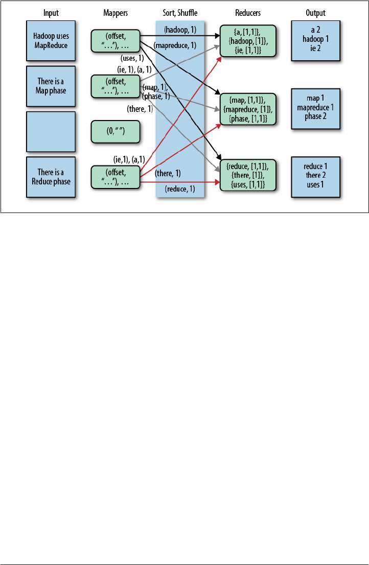
The fundamental data structure for input and output in MapReduce is the key-value
pair. After each Mapper is started, it is called repeatedly for each line of text from the
document. For each call, the key passed to the mapper is the character offset into the
document at the start of the line. The corresponding value is the text of the line.
In Word Count, the character offset (key) is discarded. The value, the line of text, is
tokenized into words, using one of several possible techniques (e.g., splitting on white-
space is the simplest, but it can leave in undesirable punctuation). We’ll also assume
that the Mapper converts each word to lowercase, so for example, “FUN” and “fun”
will be counted as the same word.
Finally, for each word in the line, the mapper outputs a key-value pair, with the word
as the key and the number 1 as the value (i.e., the count of “one occurrence”). Note
that the output types of the keys and values are different from the input types.
Part of Hadoop’s magic is the Sort and Shuffle phase that comes next. Hadoop sorts
the key-value pairs by key and it “shuffles” all pairs with the same key to the same
Reducer. There are several possible techniques that can be used to decide which reducer
gets which range of keys. We won’t worry about that here, but for illustrative purposes,
we have assumed in the figure that a particular alphanumeric partitioning was used. In
a real implementation, it would be different.
For the mapper to simply output a count of 1 every time a word is seen is a bit wasteful
of network and disk I/O used in the sort and shuffle. (It does minimize the memory
used in the Mappers, however.) One optimization is to keep track of the count for each
word and then output only one count for each word when the Mapper finishes. There
Figure 1-1. Word Count algorithm using MapReduce
An Overview of Hadoop and MapReduce | 5

are several ways to do this optimization, but the simple approach is logically correct
and sufficient for this discussion.
The inputs to each Reducer are again key-value pairs, but this time, each key will be
one of the words found by the mappers and the value will be a collection of all the counts
emitted by all the mappers for that word. Note that the type of the key and the type of
the value collection elements are the same as the types used in the Mapper’s output.
That is, the key type is a character string and the value collection element type is an
integer.
To finish the algorithm, all the reducer has to do is add up all the counts in the value
collection and write a final key-value pair consisting of each word and the count for
that word.
Word Count isn’t a toy example. The data it produces is used in spell checkers, language
detection and translation systems, and other applications.
Hive in the Hadoop Ecosystem
The Word Count algorithm, like most that you might implement with Hadoop, is a
little involved. When you actually implement such algorithms using the Hadoop Java
API, there are even more low-level details you have to manage yourself. It’s a job that’s
only suitable for an experienced Java developer, potentially putting Hadoop out of
reach of users who aren’t programmers, even when they understand the algorithm they
want to use.
In fact, many of those low-level details are actually quite repetitive from one job to the
next, from low-level chores like wiring together Mappers and Reducers to certain data
manipulation constructs, like filtering for just the data you want and performing SQL-
like joins on data sets. There’s a real opportunity to eliminate reinventing these idioms
by letting “higher-level” tools handle them automatically.
That’s where Hive comes in. It not only provides a familiar programming model for
people who know SQL, it also eliminates lots of boilerplate and sometimes-tricky
coding you would have to do in Java.
This is why Hive is so important to Hadoop, whether you are a DBA or a Java developer.
Hive lets you complete a lot of work with relatively little effort.
Figure 1-2 shows the major “modules” of Hive and how they work with Hadoop.
There are several ways to interact with Hive. In this book, we will mostly focus on the
CLI, command-line interface. For people who prefer graphical user interfaces, com-
mercial and open source options are starting to appear, including a commercial product
from Karmasphere (http://karmasphere.com), Cloudera’s open source Hue (https://git
hub.com/cloudera/hue), a new “Hive-as-a-service” offering from Qubole (http://qubole
.com), and others.
6 | Chapter 1: Introduction
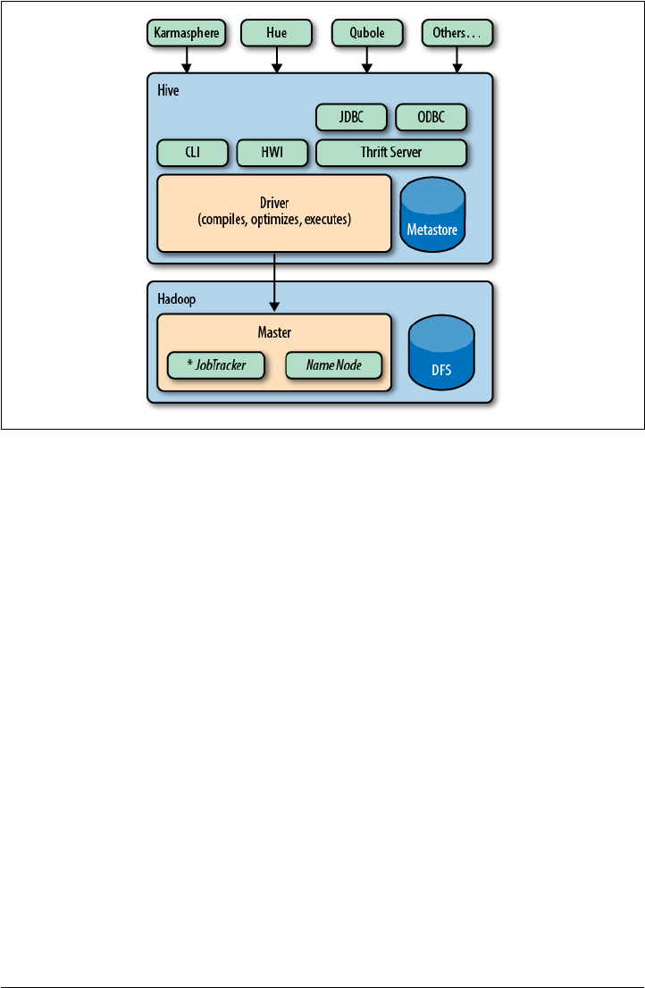
Bundled with the Hive distribution is the CLI, a simple web interface called Hive web
interface (HWI), and programmatic access through JDBC, ODBC, and a Thrift server
(see Chapter 16).
All commands and queries go to the Driver, which compiles the input, optimizes the
computation required, and executes the required steps, usually with MapReduce jobs.
When MapReduce jobs are required, Hive doesn’t generate Java MapReduce programs.
Instead, it uses built-in, generic Mapper and Reducer modules that are driven by an
XML file representing the “job plan.” In other words, these generic modules function
like mini language interpreters and the “language” to drive the computation is encoded
in XML.
Hive communicates with the JobTracker to initiate the MapReduce job. Hive does not
have to be running on the same master node with the JobTracker. In larger clusters,
it’s common to have edge nodes where tools like Hive run. They communicate remotely
with the JobTracker on the master node to execute jobs. Usually, the data files to be
processed are in HDFS, which is managed by the NameNode.
The Metastore is a separate relational database (usually a MySQL instance) where Hive
persists table schemas and other system metadata. We’ll discuss it in detail in Chapter 2.
While this is a book about Hive, it’s worth mentioning other higher-level tools that you
should consider for your needs. Hive is best suited for data warehouse applications,
where real-time responsiveness to queries and record-level inserts, updates, and deletes
Figure 1-2. Hive modules
Hive in the Hadoop Ecosystem | 7
Downloa d f r o m W o w ! e B o o k < w w w.woweb o o k . c o m >

are not required. Of course, Hive is also very nice for people who know SQL already.
However, some of your work may be easier to accomplish with alternative tools.
Pig
The best known alternative to Hive is Pig (see http://pig.apache.org), which was devel-
oped at Yahoo! about the same time Facebook was developing Hive. Pig is also now a
top-level Apache project that is closely associated with Hadoop.
Suppose you have one or more sources of input data and you need to perform a complex
set of transformations to generate one or more collections of output data. Using Hive,
you might be able to do this with nested queries (as we’ll see), but at some point it will
be necessary to resort to temporary tables (which you have to manage yourself) to
manage the complexity.
Pig is described as a data flow language, rather than a query language. In Pig, you write
a series of declarative statements that define relations from other relations, where each
new relation performs some new data transformation. Pig looks at these declarations
and then builds up a sequence of MapReduce jobs to perform the transformations until
the final results are computed the way that you want.
This step-by-step “flow” of data can be more intuitive than a complex set of queries.
For this reason, Pig is often used as part of ETL (Extract, Transform, and Load) pro-
cesses used to ingest external data into a Hadoop cluster and transform it into a more
desirable form.
A drawback of Pig is that it uses a custom language not based on SQL. This is appro-
priate, since it is not designed as a query language, but it also means that Pig is less
suitable for porting over SQL applications and experienced SQL users will have a larger
learning curve with Pig.
Nevertheless, it’s common for Hadoop teams to use a combination of Hive and Pig,
selecting the appropriate tool for particular jobs.
Programming Pig by Alan Gates (O’Reilly) provides a comprehensive introduction to
Pig.
HBase
What if you need the database features that Hive doesn’t provide, like row-level
updates, rapid query response times, and transactions?
HBase is a distributed and scalable data store that supports row-level updates, rapid
queries, and row-level transactions (but not multirow transactions).
HBase is inspired by Google’s Big Table, although it doesn’t implement all Big Table
features. One of the important features HBase supports is column-oriented storage,
where columns can be organized into column families. Column families are physically
8 | Chapter 1: Introduction

stored together in a distributed cluster, which makes reads and writes faster when the
typical query scenarios involve a small subset of the columns. Rather than reading entire
rows and discarding most of the columns, you read only the columns you need.
HBase can be used like a key-value store, where a single key is used for each row to
provide very fast reads and writes of the row’s columns or column families. HBase also
keeps a configurable number of versions of each column’s values (marked by time-
stamps), so it’s possible to go “back in time” to previous values, when needed.
Finally, what is the relationship between HBase and Hadoop? HBase uses HDFS (or
one of the other distributed filesystems) for durable file storage of data. To provide
row-level updates and fast queries, HBase also uses in-memory caching of data and
local files for the append log of updates. Periodically, the durable files are updated with
all the append log updates, etc.
HBase doesn’t provide a query language like SQL, but Hive is now integrated with
HBase. We’ll discuss this integration in “HBase” on page 222.
For more on HBase, see the HBase website, and HBase: The Definitive Guide by Lars
George.
Cascading, Crunch, and Others
There are several other “high-level” languages that have emerged outside of the Apache
Hadoop umbrella, which also provide nice abstractions on top of Hadoop to reduce
the amount of low-level boilerplate code required for typical jobs. For completeness,
we list several of them here. All are JVM (Java Virtual Machine) libraries that can be
used from programming languages like Java, Clojure, Scala, JRuby, Groovy, and Jy-
thon, as opposed to tools with their own languages, like Hive and Pig.
Using one of these programming languages has advantages and disadvantages. It makes
these tools less attractive to nonprogrammers who already know SQL. However, for
developers, these tools provide the full power of a Turing complete programming lan-
guage. Neither Hive nor Pig are Turing complete. We’ll learn how to extend Hive with
Java code when we need additional functionality that Hive doesn’t provide (Table 1-1).
Table 1-1. Alternative higher-level libraries for Hadoop
Name URL Description
Cascading http://cascading.org Java API with Data Processing abstractions. There are now
many Domain Specific Languages (DSLs) for Cascading in other
languages, e.g., Scala, Groovy, JRuby, and Jython.
Cascalog https://github.com/nathanmarz/casca
log
A Clojure DSL for Cascading that provides additional function-
ality inspired by Datalog for data processing and query ab-
stractions.
Crunch https://github.com/cloudera/crunch A Java and Scala API for defining data flow pipelines.
Hive in the Hadoop Ecosystem | 9

Because Hadoop is a batch-oriented system, there are tools with different distributed
computing models that are better suited for event stream processing, where closer to
“real-time” responsiveness is required. Here we list several of the many alternatives
(Table 1-2).
Table 1-2. Distributed data processing tools that don’t use MapReduce
Name URL Description
Spark http://www.spark-project.org/ A distributed computing framework based on the idea of dis-
tributed data sets with a Scala API. It can work with HDFS files
and it offers notable performance improvements over Hadoop
MapReduce for many computations. There is also a project to
port Hive to Spark, called Shark (http://shark.cs.berkeley.edu/).
Storm https://github.com/nathanmarz/storm A real-time event stream processing system.
Kafka http://incubator.apache.org/kafka/in
dex.html
A distributed publish-subscribe messaging system.
Finally, it’s important to consider when you don’t need a full cluster (e.g., for smaller
data sets or when the time to perform a computation is less critical). Also, many alter-
native tools are easier to use when prototyping algorithms or doing exploration with a
subset of data. Some of the more popular options are listed in Table 1-3.
Table 1-3. Other data processing languages and tools
Name URL Description
Rhttp://r-project.org/ An open source language for statistical analysis and graphing
of data that is popular with statisticians, economists, etc. It’s
not a distributed system, so the data sizes it can handle are
limited. There are efforts to integrate R with Hadoop.
Matlab http://www.mathworks.com/products/
matlab/index.html
A commercial system for data analysis and numerical methods
that is popular with engineers and scientists.
Octave http://www.gnu.org/software/octave/ An open source clone of MatLab.
Mathematica http://www.wolfram.com/mathema
tica/
A commercial data analysis, symbolic manipulation, and nu-
merical methods system that is also popular with scientists and
engineers.
SciPy, NumPy http://scipy.org Extensive software package for scientific programming in
Python, which is widely used by data scientists.
Java Versus Hive: The Word Count Algorithm
If you are not a Java programmer, you can skip to the next section.
If you are a Java programmer, you might be reading this book because you’ll need to
support the Hive users in your organization. You might be skeptical about using Hive
for your own work. If so, consider the following example that implements the Word
10 | Chapter 1: Introduction

Count algorithm we discussed above, first using the Java MapReduce API and then
using Hive.
It’s very common to use Word Count as the first Java MapReduce program that people
write, because the algorithm is simple to understand, so you can focus on the API.
Hence, it has become the “Hello World” of the Hadoop world.
The following Java implementation is included in the Apache Hadoop distribution.8 If
you don’t know Java (and you’re still reading this section), don’t worry, we’re only
showing you the code for the size comparison:
package org.myorg;
import java.io.IOException;
import java.util.*;
import org.apache.hadoop.fs.Path;
import org.apache.hadoop.conf.*;
import org.apache.hadoop.io.*;
import org.apache.hadoop.mapreduce.*;
import org.apache.hadoop.mapreduce.lib.input.FileInputFormat;
import org.apache.hadoop.mapreduce.lib.input.TextInputFormat;
import org.apache.hadoop.mapreduce.lib.output.FileOutputFormat;
import org.apache.hadoop.mapreduce.lib.output.TextOutputFormat;
public class WordCount {
public static class Map extends Mapper<LongWritable, Text, Text, IntWritable> {
private final static IntWritable one = new IntWritable(1);
private Text word = new Text();
public void map(LongWritable key, Text value, Context context)
throws IOException, InterruptedException {
String line = value.toString();
StringTokenizer tokenizer = new StringTokenizer(line);
while (tokenizer.hasMoreTokens()) {
word.set(tokenizer.nextToken());
context.write(word, one);
}
}
}
public static class Reduce extends Reducer<Text, IntWritable, Text, IntWritable> {
public void reduce(Text key, Iterable<IntWritable> values, Context context)
throws IOException, InterruptedException {
int sum = 0;
for (IntWritable val : values) {
sum += val.get();
}
context.write(key, new IntWritable(sum));
}
8. Apache Hadoop word count: http://wiki.apache.org/hadoop/WordCount.
Java Versus Hive: The Word Count Algorithm | 11

}
public static void main(String[] args) throws Exception {
Configuration conf = new Configuration();
Job job = new Job(conf, "wordcount");
job.setOutputKeyClass(Text.class);
job.setOutputValueClass(IntWritable.class);
job.setMapperClass(Map.class);
job.setReducerClass(Reduce.class);
job.setInputFormatClass(TextInputFormat.class);
job.setOutputFormatClass(TextOutputFormat.class);
FileInputFormat.addInputPath(job, new Path(args[0]));
FileOutputFormat.setOutputPath(job, new Path(args[1]));
job.waitForCompletion(true);
}
}
That was 63 lines of Java code. We won’t explain the API details.9 Here is the same
calculation written in HiveQL, which is just 8 lines of code, and does not require com-
pilation nor the creation of a “JAR” (Java ARchive) file:
CREATE TABLE docs (line STRING);
LOAD DATA INPATH 'docs' OVERWRITE INTO TABLE docs;
CREATE TABLE word_counts AS
SELECT word, count(1) AS count FROM
(SELECT explode(split(line, '\s')) AS word FROM docs) w
GROUP BY word
ORDER BY word;
We’ll explain all this HiveQL syntax later on.
9. See Hadoop: The Definitive Guide by Tom White for the details.
12 | Chapter 1: Introduction

In both examples, the files were tokenized into words using the simplest possible ap-
proach; splitting on whitespace boundaries. This approach doesn’t properly handle
punctuation, it doesn’t recognize that singular and plural forms of words are the same
word, etc. However, it’s good enough for our purposes here.10
The virtue of the Java API is the ability to customize and fine-tune every detail of an
algorithm implementation. However, most of the time, you just don’t need that level
of control and it slows you down considerably when you have to manage all those
details.
If you’re not a programmer, then writing Java MapReduce code is out of reach. How-
ever, if you already know SQL, learning Hive is relatively straightforward and many
applications are quick and easy to implement.
What’s Next
We described the important role that Hive plays in the Hadoop ecosystem. Now let’s
get started!
10. There is one other minor difference. The Hive query hardcodes a path to the data, while the Java code
takes the path as an argument. In Chapter 2, we’ll learn how to use Hive variables in scripts to avoid
hardcoding such details.
What’s Next | 13

CHAPTER 2
Getting Started
Let’s install Hadoop and Hive on our personal workstation. This is a convenient way
to learn and experiment with Hadoop. Then we’ll discuss how to configure Hive for
use on Hadoop clusters.
If you already use Amazon Web Services, the fastest path to setting up Hive for learning
is to run a Hive-configured job flow on Amazon Elastic MapReduce (EMR). We discuss
this option in Chapter 21.
If you have access to a Hadoop cluster with Hive already installed, we encourage
you to skim the first part of this chapter and pick up again at “What Is Inside
Hive?” on page 22.
Installing a Preconfigured Virtual Machine
There are several ways you can install Hadoop and Hive. An easy way to install a com-
plete Hadoop system, including Hive, is to download a preconfigured virtual ma-
chine (VM) that runs in VMWare1 or VirtualBox2. For VMWare, either VMWare
Player for Windows and Linux (free) or VMWare Fusion for Mac OS X (inexpensive)
can be used. VirtualBox is free for all these platforms, and also Solaris.
The virtual machines use Linux as the operating system, which is currently the only
recommended operating system for running Hadoop in production.3
Using a virtual machine is currently the only way to run Hadoop on
Windows systems, even when Cygwin or similar Unix-like software is
installed.
1. http://vmware.com.
2. https://www.virtualbox.org/.
3. However, some vendors are starting to support Hadoop on other systems. Hadoop has been used in
production on various Unix systems and it works fine on Mac OS X for development use.
15

Most of the preconfigured virtual machines (VMs) available are only designed for
VMWare, but if you prefer VirtualBox you may find instructions on the Web that
explain how to import a particular VM into VirtualBox.
You can download preconfigured virtual machines from one of the websites given in
Table 2-1.4 Follow the instructions on these web sites for loading the VM into VMWare.
Table 2-1. Preconfigured Hadoop virtual machines for VMWare
Provider URL Notes
Cloudera, Inc. https://ccp.cloudera.com/display/SUPPORT/Clou
dera’s+Hadoop+Demo+VM
Uses Cloudera’s own distribution
of Hadoop, CDH3 or CDH4.
MapR, Inc. http://www.mapr.com/doc/display/MapR/Quick
+Start+-+Test+Drive+MapR+on+a+Virtual
+Machine
MapR’s Hadoop distribution,
which replaces HDFS with the
MapR Filesystem (MapR-FS).
Hortonworks,
Inc.
http://docs.hortonworks.com/HDP-1.0.4-PREVIEW
-6/Using_HDP_Single_Box_VM/HDP_Single_Box
_VM.htm
Based on the latest, stable Apache
releases.
Think Big An-
alytics, Inc.
http://thinkbigacademy.s3-website-us-east-1.ama
zonaws.com/vm/README.html
Based on the latest, stable Apache
releases.
Next, go to “What Is Inside Hive?” on page 22.
Detailed Installation
While using a preconfigured virtual machine may be an easy way to run Hive, installing
Hadoop and Hive yourself will give you valuable insights into how these tools work,
especially if you are a developer.
The instructions that follow describe the minimum necessary Hadoop and Hive
installation steps for your personal Linux or Mac OS X workstation. For production
installations, consult the recommended installation procedures for your Hadoop
distributor.
Installing Java
Hive requires Hadoop and Hadoop requires Java. Ensure your system has a recent
v1.6.X or v1.7.X JVM (Java Virtual Machine). Although the JRE (Java Runtime Envi-
ronment) is all you need to run Hive, you will need the full JDK (Java Development
Kit) to build examples in this book that demonstrate how to extend Hive with Java
code. However, if you are not a programmer, the companion source code distribution
for this book (see the Preface) contains prebuilt examples.
4. These are the current URLs at the time of this writing.
16 | Chapter 2: Getting Started

After the installation is complete, you’ll need to ensure that Java is in your path and
the JAVA_HOME environment variable is set.
Linux-specific Java steps
On Linux systems, the following instructions set up a bash file in the /etc/profile.d/
directory that defines JAVA_HOME for all users. Changing environmental settings in
this folder requires root access and affects all users of the system. (We’re using $ as the
bash shell prompt.) The Oracle JVM installer typically installs the software in /usr/java/
jdk-1.6.X (for v1.6) and it creates sym-links from /usr/java/default and /usr/java/latest
to the installation:
$ /usr/java/latest/bin/java -version
java version "1.6.0_23"
Java(TM) SE Runtime Environment (build 1.6.0_23-b05)
Java HotSpot(TM) 64-Bit Server VM (build 19.0-b09, mixed mode)
$ sudo echo "export JAVA_HOME=/usr/java/latest" > /etc/profile.d/java.sh
$ sudo echo "PATH=$PATH:$JAVA_HOME/bin" >> /etc/profile.d/java.sh
$ . /etc/profile
$ echo $JAVA_HOME
/usr/java/latest
If you’ve never used sudo (“super user do something”) before to run a
command as a “privileged” user, as in two of the commands, just type
your normal password when you’re asked for it. If you’re on a personal
machine, your user account probably has “sudo rights.” If not, ask your
administrator to run those commands.
However, if you don’t want to make permanent changes that affect all
users of the system, an alternative is to put the definitions shown for
PATH and JAVA_HOME in your $HOME/.bashrc file:
export JAVA_HOME=/usr/java/latest
export PATH=$PATH:$JAVA_HOME/bin
Mac OS X−specific Java steps
Mac OS X systems don’t have the /etc/profile.d directory and they are typically
single-user systems, so it’s best to put the environment variable definitions in your
$HOME/.bashrc. The Java paths are different, too, and they may be in one of several
places.5
Here are a few examples. You’ll need to determine where Java is installed on your Mac
and adjust the definitions accordingly. Here is a Java 1.6 example for Mac OS X:
$ export JAVA_HOME=/System/Library/Frameworks/JavaVM.framework/Versions/1.6/Home
$ export PATH=$PATH:$JAVA_HOME/bin
5. At least that’s the current situation on Dean’s Mac. This discrepancy may actually reflect the fact that
stewardship of the Mac OS X Java port is transitioning from Apple to Oracle as of Java 1.7.
Detailed Installation | 17

Here is a Java 1.7 example for Mac OS X:
$ export JAVA_HOME=/Library/Java/JavaVirtualMachines/1.7.0.jdk/Contents/Home
$ export PATH=$PATH:$JAVA_HOME/bin
OpenJDK 1.7 releases also install under /Library/Java/JavaVirtualMachines.
Installing Hadoop
Hive runs on top of Hadoop. Hadoop is an active open source project with many re-
leases and branches. Also, many commercial software companies are now producing
their own distributions of Hadoop, sometimes with custom enhancements or replace-
ments for some components. This situation promotes innovation, but also potential
confusion and compatibility issues.
Keeping software up to date lets you exploit the latest performance enhancements and
bug fixes. However, sometimes you introduce new bugs and compatibility issues. So,
for this book, we’ll show you how to install the Apache Hadoop release v0.20.2. This
edition is not the most recent stable release, but it has been the reliable gold standard
for some time for performance and compatibility.
However, you should be able to choose a different version, distribution, or release
without problems for learning and using Hive, such as the Apache Hadoop v0.20.205
or 1.0.X releases, Cloudera CDH3 or CDH4, MapR M3 or M5, and the forthcoming
Hortonworks distribution. Note that the bundled Cloudera, MapR, and planned
Hortonworks distributions all include a Hive release.
However, we don’t recommend installing the new, alpha-quality, “Next Generation”
Hadoop v2.0 (also known as v0.23), at least for the purposes of this book. While this
release will bring significant enhancements to the Hadoop ecosystem, it is too new for
our purposes.
To install Hadoop on a Linux system, run the following commands. Note that we
wrapped the long line for the wget command:
$ cd ~ # or use another directory of your choice.
$ wget \
http://www.us.apache.org/dist/hadoop/common/hadoop-0.20.2/hadoop-0.20.2.tar.gz
$ tar -xzf hadoop-0.20.2.tar.gz
$ sudo echo "export HADOOP_HOME=$PWD/hadoop-0.20.2" > /etc/profile.d/hadoop.sh
$ sudo echo "PATH=$PATH:$HADOOP_HOME/bin" >> /etc/profile.d/hadoop.sh
$ . /etc/profile
To install Hadoop on a Mac OS X system, run the following commands. Note that we
wrapped the long line for the curl command:
$ cd ~ # or use another directory of your choice.
$ curl -o \
http://www.us.apache.org/dist/hadoop/common/hadoop-0.20.2/hadoop-0.20.2.tar.gz
$ tar -xzf hadoop-0.20.2.tar.gz
$ echo "export HADOOP_HOME=$PWD/hadoop-0.20.2" >> $HOME/.bashrc
18 | Chapter 2: Getting Started

$ echo "PATH=$PATH:$HADOOP_HOME/bin" >> $HOME/.bashrc
$ . $HOME/.bashrc
In what follows, we will assume that you added $HADOOP_HOME/bin to your path, as in
the previous commands. This will allow you to simply type the hadoop command
without the path prefix.
Local Mode, Pseudodistributed Mode, and Distributed Mode
Before we proceed, let’s clarify the different runtime modes for Hadoop. We mentioned
above that the default mode is local mode, where filesystem references use the local
filesystem. Also in local mode, when Hadoop jobs are executed (including most Hive
queries), the Map and Reduce tasks are run as part of the same process.
Actual clusters are configured in distributed mode, where all filesystem references that
aren’t full URIs default to the distributed filesystem (usually HDFS) and jobs are man-
aged by the JobTracker service, with individual tasks executed in separate processes.
A dilemma for developers working on personal machines is the fact that local mode
doesn’t closely resemble the behavior of a real cluster, which is important to remember
when testing applications. To address this need, a single machine can be configured to
run in pseudodistributed mode, where the behavior is identical to distributed mode,
namely filesystem references default to the distributed filesystem and jobs are managed
by the JobTracker service, but there is just a single machine. Hence, for example, HDFS
file block replication is limited to one copy. In other words, the behavior is like a single-
node “cluster.” We’ll discuss these configuration options in “Configuring Your Ha-
doop Environment” on page 24.
Because Hive uses Hadoop jobs for most of its work, its behavior reflects the Hadoop
mode you’re using. However, even when running in distributed mode, Hive can decide
on a per-query basis whether or not it can perform the query using just local mode,
where it reads the data files and manages the MapReduce tasks itself, providing faster
turnaround. Hence, the distinction between the different modes is more of an
execution style for Hive than a deployment style, as it is for Hadoop.
For most of the book, it won’t matter which mode you’re using. We’ll assume you’re
working on a personal machine in local mode and we’ll discuss the cases where the
mode matters.
When working with small data sets, using local mode execution
will make Hive queries much faster. Setting the property set
hive.exec.mode.local.auto=true; will cause Hive to use this mode more
aggressively, even when you are running Hadoop in distributed or pseu-
dodistributed mode. To always use this setting, add the command to
your $HOME/.hiverc file (see “The .hiverc File” on page 36).
Detailed Installation | 19

Testing Hadoop
Assuming you’re using local mode, let’s look at the local filesystem two different ways.
The following output of the Linux ls command shows the typical contents of the “root”
directory of a Linux system:
$ ls /
bin cgroup etc lib lost+found mnt opt root selinux sys user var
boot dev home lib64 media null proc sbin srv tmp usr
Hadoop provides a dfs tool that offers basic filesystem functionality like ls for the
default filesystem. Since we’re using local mode, the default filesystem is the local file-
system:6
$ hadoop dfs -ls /
Found 26 items
drwxrwxrwx - root root 24576 2012-06-03 14:28 /tmp
drwxr-xr-x - root root 4096 2012-01-25 22:43 /opt
drwx------ - root root 16384 2010-12-30 14:56 /lost+found
drwxr-xr-x - root root 0 2012-05-11 16:44 /selinux
dr-xr-x--- - root root 4096 2012-05-23 22:32 /root
...
If instead you get an error message that hadoop isn’t found, either invoke the command
with the full path (e.g., $HOME/hadoop-0.20.2/bin/hadoop) or add the bin directory to
your PATH variable, as discussed in “Installing Hadoop” on page 18 above.
If you find yourself using the hadoop dfs command frequently, it’s
convenient to define an alias for it (e.g., alias hdfs="hadoop dfs").
Hadoop offers a framework for MapReduce. The Hadoop distribution contains an
implementation of the Word Count algorithm we discussed in Chapter 1. Let’s run it!
Start by creating an input directory (inside your current working directory) with files
to be processed by Hadoop:
$ mkdir wc-in
$ echo "bla bla" > wc-in/a.txt
$ echo "bla wa wa " > wc-in/b.txt
Use the hadoop command to launch the Word Count application on the input directory
we just created. Note that it’s conventional to always specify directories for input and
output, not individual files, since there will often be multiple input and/or output files
per directory, a consequence of the parallelism of the system.
6. Unfortunately, the dfs -ls command only provides a “long listing” format. There is no short format, like
the default for the Linux ls command.
20 | Chapter 2: Getting Started

If you are running these commands on your local installation that was configured to
use local mode, the hadoop command will launch the MapReduce components in the
same process. If you are running on a cluster or on a single machine using pseudodis-
tributed mode, the hadoop command will launch one or more separate processes using
the JobTracker service (and the output below will be slightly different). Also, if you are
running with a different version of Hadoop, change the name of the examples.jar as
needed:
$ hadoop jar $HADOOP_HOME/hadoop-0.20.2-examples.jar wordcount wc-in wc-out
12/06/03 15:40:26 INFO input.FileInputFormat: Total input paths to process : 2
...
12/06/03 15:40:27 INFO mapred.JobClient: Running job: job_local_0001
12/06/03 15:40:30 INFO mapred.JobClient: map 100% reduce 0%
12/06/03 15:40:41 INFO mapred.JobClient: map 100% reduce 100%
12/06/03 15:40:41 INFO mapred.JobClient: Job complete: job_local_0001
The results of the Word count application can be viewed through local filesystem
commands:
$ ls wc-out/*
part-r-00000
$ cat wc-out/*
bla 3
wa 2
They can also be viewed by the equivalent dfs command (again, because we assume
you are running in local mode):
$ hadoop dfs -cat wc-out/*
bla 3
wa 2
For very big files, if you want to view just the first or last parts, there is
no -more, -head, nor -tail subcommand. Instead, just pipe the output
of the -cat command through the shell’s more, head, or tail. For exam-
ple: hadoop dfs -cat wc-out/* | more.
Now that we have installed and tested an installation of Hadoop, we can install Hive.
Installing Hive
Installing Hive is similar to installing Hadoop. We will download and extract a tarball
for Hive, which does not include an embedded version of Hadoop. A single Hive binary
is designed to work with multiple versions of Hadoop. This means it’s often easier and
less risky to upgrade to newer Hive releases than it is to upgrade to newer Hadoop
releases.
Hive uses the environment variable HADOOP_HOME to locate the Hadoop JARs and con-
figuration files. So, make sure you set that variable as discussed above before proceed-
ing. The following commands work for both Linux and Mac OS X:
Detailed Installation | 21

$ cd ~ # or use another directory of your choice.
$ curl -o http://archive.apache.org/dist/hive/hive-0.9.0/hive-0.9.0-bin.tar.gz
$ tar -xzf hive-0.9.0.tar.gz
$ sudo mkdir -p /user/hive/warehouse
$ sudo chmod a+rwx /user/hive/warehouse
As you can infer from these commands, we are using the latest stable release of Hive
at the time of this writing, v0.9.0. However, most of the material in this book works
with Hive v0.7.X and v0.8.X. We’ll call out the differences as we come to them.
You’ll want to add the hive command to your path, like we did for the hadoop command.
We’ll follow the same approach, by first defining a HIVE_HOME variable, but unlike
HADOOP_HOME, this variable isn’t really essential. We’ll assume it’s defined for some ex-
amples later in the book.
For Linux, run these commands:
$ sudo echo "export HIVE_HOME=$PWD/hive-0.9.0" > /etc/profile.d/hive.sh
$ sudo echo "PATH=$PATH:$HIVE_HOME/bin >> /etc/profile.d/hive.sh
$ . /etc/profile
For Mac OS X, run these commands:
$ echo "export HIVE_HOME=$PWD/hive-0.9.0" >> $HOME/.bashrc
$ echo "PATH=$PATH:$HIVE_HOME/bin" >> $HOME/.bashrc
$ . $HOME/.bashrc
What Is Inside Hive?
The core of a Hive binary distribution contains three parts. The main part is the Java
code itself. Multiple JAR (Java archive) files such as hive-exec*.jar and hive-meta
store*.jar are found under the $HIVE_HOME/lib directory. Each JAR file implements
a particular subset of Hive’s functionality, but the details don’t concern us now.
The $HIVE_HOME/bin directory contains executable scripts that launch various Hive
services, including the hive command-line interface (CLI). The CLI is the most popular
way to use Hive. We will use hive (in lowercase, with a fixed-width font) to refer to the
CLI, except where noted. The CLI can be used interactively to type in statements one
at a time or it can be used to run “scripts” of Hive statements, as we’ll see.
Hive also has other components. A Thrift service provides remote access from other
processes. Access using JDBC and ODBC are provided, too. They are implemented on
top of the Thrift service. We’ll describe these features in later chapters.
All Hive installations require a metastore service, which Hive uses to store table schemas
and other metadata. It is typically implemented using tables in a relational database.
By default, Hive uses a built-in Derby SQL server, which provides limited, single-
process storage. For example, when using Derby, you can’t run two simultaneous in-
stances of the Hive CLI. However, this is fine for learning Hive on a personal machine
22 | Chapter 2: Getting Started

and some developer tasks. For clusters, MySQL or a similar relational database is
required. We will discuss the details in “Metastore Using JDBC” on page 28.
Finally, a simple web interface, called Hive Web Interface (HWI), provides remote
access to Hive.
The conf directory contains the files that configure Hive. Hive has a number of con-
figuration properties that we will discuss as needed. These properties control features
such as the metastore (where data is stored), various optimizations, and “safety
controls,” etc.
Starting Hive
Let’s finally start the Hive command-line interface (CLI) and run a few commands!
We’ll briefly comment on what’s happening, but save the details for discussion later.
In the following session, we’ll use the $HIVE_HOME/bin/hive command, which is a
bash shell script, to start the CLI. Substitute the directory where Hive is installed on
your system whenever $HIVE_HOME is listed in the following script. Or, if you added
$HIVE_HOME/bin to your PATH, you can just type hive to run the command. We’ll make
that assumption for the rest of the book.
As before, $ is the bash prompt. In the Hive CLI, the hive> string is the hive prompt,
and the indented > is the secondary prompt. Here is a sample session, where we have
added a blank line after the output of each command, for clarity:
$ cd $HIVE_HOME
$ bin/hive
Hive history file=/tmp/myname/hive_job_log_myname_201201271126_1992326118.txt
hive> CREATE TABLE x (a INT);
OK
Time taken: 3.543 seconds
hive> SELECT * FROM x;
OK
Time taken: 0.231 seconds
hive> SELECT *
> FROM x;
OK
Time taken: 0.072 seconds
hive> DROP TABLE x;
OK
Time taken: 0.834 seconds
hive> exit;
$
The first line printed by the CLI is the local filesystem location where the CLI writes
log data about the commands and queries you execute. If a command or query is
Starting Hive | 23
Downloa d f r o m W o w ! e B o o k < w w w.woweb o o k . c o m >

successful, the first line of output will be OK, followed by the output, and finished by
the line showing the amount of time taken to run the command or query.
Throughout the book, we will follow the SQL convention of showing
Hive keywords in uppercase (e.g., CREATE, TABLE, SELECT and FROM), even
though case is ignored by Hive, following SQL conventions.
Going forward, we’ll usually add the blank line after the command out-
put for all sessions. Also, when starting a session, we’ll omit the line
about the logfile. For individual commands and queries, we’ll omit the
OK and Time taken:... lines, too, except in special cases, such as when
we want to emphasize that a command or query was successful, but it
had no other output.
At the successive prompts, we create a simple table named x with a single INT (4-byte
integer) column named a, then query it twice, the second time showing how queries
and commands can spread across multiple lines. Finally, we drop the table.
If you are running with the default Derby database for the metastore, you’ll notice that
your current working directory now contains a new subdirectory called metastore_db
that was created by Derby during the short hive session you just executed. If you are
running one of the VMs, it’s possible it has configured different behavior, as we’ll dis-
cuss later.
Creating a metastore_db subdirectory under whatever working directory you happen
to be in is not convenient, as Derby “forgets” about previous metastores when you
change to a new working directory! In the next section, we’ll see how to configure a
permanent location for the metastore database, as well as make other changes.
Configuring Your Hadoop Environment
Let’s dive a little deeper into the different Hadoop modes and discuss more configu-
ration issues relevant to Hive.
You can skip this section if you’re using Hadoop on an existing cluster or you are using
a virtual machine instance. If you are a developer or you installed Hadoop and Hive
yourself, you’ll want to understand the rest of this section. However, we won’t provide
a complete discussion. See Appendix A of Hadoop: The Definitive Guide by Tom White
for the full details on configuring the different modes.
Local Mode Configuration
Recall that in local mode, all references to files go to your local filesystem, not the
distributed filesystem. There are no services running. Instead, your jobs run all tasks
in a single JVM instance.
24 | Chapter 2: Getting Started
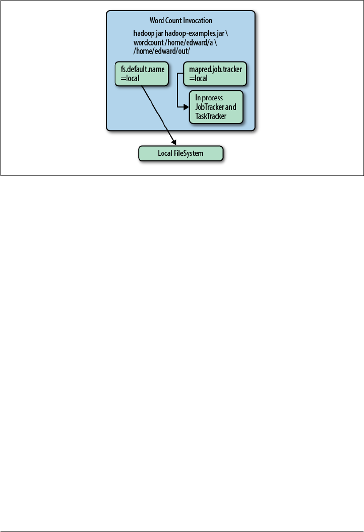
Figure 2-1 illustrates a Hadoop job running in local mode.
Figure 2-1. Hadoop in local mode
If you plan to use the local mode regularly, it’s worth configuring a standard location
for the Derby metastore_db, where Hive stores metadata about your tables, etc.
You can also configure a different directory for Hive to store table data, if you don’t
want to use the default location, which is file:///user/hive/warehouse, for local mode,
and hdfs://namenode_server/user/hive/warehouse for the other modes discussed next.
First, go to the $HIVE_HOME/conf directory. The curious may want to peek at the
large hive-default.xml.template file, which shows the different configuration properties
supported by Hive and their default values. Most of these properties you can safely
ignore. Changes to your configuration are done by editing the hive-site.xml file. Create
one if it doesn’t already exist.
Here is an example configuration file where we set several properties for local mode
execution (Example 2-1).
Example 2-1. Local-mode hive-site.xml
<?xml version="1.0"?>
<?xml-stylesheet type="text/xsl" href="configuration.xsl"?>
<configuration>
<property>
<name>hive.metastore.warehouse.dir</name>
<value>/home/me/hive/warehouse</value>
<description>
Local or HDFS directory where Hive keeps table contents.
</description>
</property>
<property>
<name>hive.metastore.local</name>
Configuring Your Hadoop Environment | 25

<value>true</value>
<description>
Use false if a production metastore server is used.
</description>
</property>
<property>
<name>javax.jdo.option.ConnectionURL</name>
<value>jdbc:derby:;databaseName=/home/me/hive/metastore_db;create=true</value>
<description>
The JDBC connection URL.
</description>
</property>
</configuration>
You can remove any of these <property>...</property> tags you don’t want to change.
As the <description> tags indicate, the hive.metastore.warehouse.dir tells Hive where
in your local filesystem to keep the data contents for Hive’s tables. (This value is ap-
pended to the value of fs.default.name defined in the Hadoop configuration and de-
faults to file:///.) You can use any directory path you want for the value. Note that this
directory will not be used to store the table metadata, which goes in the separate
metastore.
The hive.metastore.local property defaults to true, so we don’t really need to show
it in Example 2-1. It’s there more for documentation purposes. This property controls
whether to connect to a remote metastore server or open a new metastore server as part
of the Hive Client JVM. This setting is almost always set to true and JDBC is used to
communicate directly to a relational database. When it is set to false, Hive will
communicate through a metastore server, which we’ll discuss in “Metastore Meth-
ods” on page 216.
The value for the javax.jdo.option.ConnectionURL property makes one small but con-
venient change to the default value for this property. This property tells Hive how to
connect to the metastore server. By default, it uses the current working directory for
the databaseName part of the value string. As shown in Example 2-1, we use database
Name=/home/me/hive/metastore_db as the absolute path instead, which is the location
where the metastore_db directory will always be located. This change eliminates the
problem of Hive dropping the metastore_db directory in the current working directory
every time we start a new Hive session. Now, we’ll always have access to all our
metadata, no matter what directory we are working in.
Distributed and Pseudodistributed Mode Configuration
In distributed mode, several services run in the cluster. The JobTracker manages jobs
and the NameNode is the HDFS master. Worker nodes run individual job tasks, man-
aged by a TaskTracker service on each node, and then hold blocks for files in the
distributed filesystem, managed by DataNode services.
Figure 2-2 shows a typical distributed mode configuration for a Hadoop cluster.
26 | Chapter 2: Getting Started

We’re using the convention that *.domain.pvt is our DNS naming convention for the
cluster’s private, internal network.
Pseudodistributed mode is nearly identical; it’s effectively a one-node cluster.
We’ll assume that your administrator has already configured Hadoop, including your
distributed filesystem (e.g., HDFS, or see Appendix A of Hadoop: The Definitive
Guide by Tom White). Here, we’ll focus on the unique configuration steps required by
Hive.
One Hive property you might want to configure is the top-level directory for table
storage, which is specified by the property hive.metastore.warehouse.dir, which we
also discussed in “Local Mode Configuration” on page 24.
The default value for this property is /user/hive/warehouse in the Apache Hadoop and
MapR distributions, which will be interpreted as a distributed filesystem path when
Hadoop is configured for distributed or pseudodistributed mode. For Amazon Elastic
MapReduce (EMR), the default value is /mnt/hive_0M_N/warehouse when using Hive
v0.M.N (e.g., /mnt/hive_08_1/warehouse).
Specifying a different value here allows each user to define their own warehouse direc-
tory, so they don’t affect other system users. Hence, each user might use the following
statement to define their own warehouse directory:
set hive.metastore.warehouse.dir=/user/myname/hive/warehouse;
It’s tedious to type this each time you start the Hive CLI or to remember to add it to
every Hive script. Of course, it’s also easy to forget to define this property. Instead, it’s
Figure 2-2. Hadoop in distributed mode
Configuring Your Hadoop Environment | 27

best to put commands like this in the $HOME/.hiverc file, which will be processed
when Hive starts. See “The .hiverc File” on page 36 for more details.
We’ll assume the value is /user/hive/warehouse from here on.
Metastore Using JDBC
Hive requires only one extra component that Hadoop does not already have; the
metastore component. The metastore stores metadata such as table schema and parti-
tion information that you specify when you run commands such as create table
x..., or alter table y..., etc. Because multiple users and systems are likely to need
concurrent access to the metastore, the default embedded database is not suitable for
production.
If you are using a single node in pseudodistributed mode, you may not
find it useful to set up a full relational database for the metastore. Rather,
you may wish to continue using the default Derby store, but configure
it to use a central location for its data, as described in “Local Mode
Configuration” on page 24.
Any JDBC-compliant database can be used for the metastore. In practice, most instal-
lations of Hive use MySQL. We’ll discuss how to use MySQL. It is straightforward to
adapt this information to other JDBC-compliant databases.
The information required for table schema, partition information, etc.,
is small, typically much smaller than the large quantity of data stored in
Hive. As a result, you typically don’t need a powerful dedicated database
server for the metastore. However because it represents a Single Point
of Failure (SPOF), it is strongly recommended that you replicate and
back up this database using the standard techniques you would nor-
mally use with other relational database instances. We won’t discuss
those techniques here.
For our MySQL configuration, we need to know the host and port the service is running
on. We will assume db1.mydomain.pvt and port 3306, which is the standard MySQL
port. Finally, we will assume that hive_db is the name of our catalog. We define these
properties in Example 2-2.
Example 2-2. Metastore database configuration in hive-site.xml
<?xml version="1.0"?>
<?xml-stylesheet type="text/xsl" href="configuration.xsl"?>
<configuration>
<property>
<name>javax.jdo.option.ConnectionURL</name>
<value>jdbc:mysql://db1.mydomain.pvt/hive_db?createDatabaseIfNotExist=true</value>
</property>
28 | Chapter 2: Getting Started

<property>
<name>javax.jdo.option.ConnectionDriverName</name>
<value>com.mysql.jdbc.Driver</value>
</property>
<property>
<name>javax.jdo.option.ConnectionUserName</name>
<value>database_user</value>
</property>
<property>
<name>javax.jdo.option.ConnectionPassword</name>
<value>database_pass</value>
</property>
</configuration>
You may have noticed the ConnectionURL property starts with a prefix of jdbc:mysql.
For Hive to be able to connect to MySQL, we need to place the JDBC driver in our
classpath. Download the MySQL JDBC driver (Jconnector) from http://www.mysql
.com/downloads/connector/j/. The driver can be placed in the Hive library path,
$HIVE_HOME/lib. Some teams put all such support libraries in their Hadoop lib
directory.
With the driver and the configuration settings in place, Hive will store its metastore
information in MySQL.
The Hive Command
The $HIVE_HOME/bin/hive shell command, which we’ll simply refer to as hive from now
on, is the gateway to Hive services, including the command-line interface or CLI.
We’ll also assume that you have added $HIVE_HOME/bin to your environment’s PATH so
you can type hive at the shell prompt and your shell environment (e.g., bash) will find
the command.
Command Options
If you run the following command, you’ll see a brief list of the options for the hive
command. Here is the output for Hive v0.8.X and v0.9.X:
$ bin/hive --help
Usage ./hive <parameters> --service serviceName <service parameters>
Service List: cli help hiveserver hwi jar lineage metastore rcfilecat
Parameters parsed:
--auxpath : Auxiliary jars
--config : Hive configuration directory
--service : Starts specific service/component. cli is default
Parameters used:
HADOOP_HOME : Hadoop install directory
HIVE_OPT : Hive options
The Hive Command | 29

For help on a particular service:
./hive --service serviceName --help
Debug help: ./hive --debug --help
Note the Service List. There are several services available, including the CLI that we
will spend most of our time using. You can invoke a service using the --service name
option, although there are shorthand invocations for some of the services, as well.
Table 2-2 describes the most useful services.
Table 2-2. Hive services
Option Name Description
cli Command-line interface Used to define tables, run queries, etc. It is the default service
if no other service is specified. See “The Command-Line Inter-
face” on page 30.
hiveserver Hive Server A daemon that listens for Thrift connections from other pro-
cesses. See Chapter 16 for more details.
hwi Hive Web Interface A simple web interface for running queries and other com-
mands without logging into a cluster machine and using the
CLI.
jar An extension of the hadoop jar command for running an
application that also requires the Hive environment.
metastore Start an external Hive metastore service to support multiple
clients (see also “Metastore Using JDBC” on page 28).
rcfilecat A tool for printing the contents of an RCFile (see
“RCFile” on page 202).
The --auxpath option lets you specify a colon-separated list of “auxiliary” Java archive
(JAR) files that contain custom extensions, etc., that you might require.
The --config directory is mostly useful if you have to override the default configuration
properties in $HIVE_HOME/conf in a new directory.
The Command-Line Interface
The command-line interface or CLI is the most common way to interact with Hive.
Using the CLI, you can create tables, inspect schema and query tables, etc.
30 | Chapter 2: Getting Started

CLI Options
The following command shows a brief list of the options for the CLI. Here we show
the output for Hive v0.8.X and v0.9.X:
$ hive --help --service cli
usage: hive
-d,--define <key=value> Variable substitution to apply to hive
commands. e.g. -d A=B or --define A=B
-e <quoted-query-string> SQL from command line
-f <filename> SQL from files
-H,--help Print help information
-h <hostname> connecting to Hive Server on remote host
--hiveconf <property=value> Use value for given property
--hivevar <key=value> Variable substitution to apply to hive
commands. e.g. --hivevar A=B
-i <filename> Initialization SQL file
-p <port> connecting to Hive Server on port number
-S,--silent Silent mode in interactive shell
-v,--verbose Verbose mode (echo executed SQL to the
console)
A shorter version of this command is hive -h. However, that’s technically an unsup-
ported option, but it produces the help output with an additional line that complains
about Missing argument for option: h.
For Hive v0.7.X, the -d, --hivevar, and -p options are not supported.
Let’s explore these options in more detail.
Variables and Properties
The --define key=value option is effectively equivalent to the --hivevar key=value
option. Both let you define on the command line custom variables that you can refer-
ence in Hive scripts to customize execution. This feature is only supported in Hive
v0.8.0 and later versions.
When you use this feature, Hive puts the key-value pair in the hivevar “namespace” to
distinguish these definitions from three other built-in namespaces, hiveconf, system,
and env.
The terms variable or property are used in different contexts, but they
function the same way in most cases.
The namespace options are described in Table 2-3.
The Command-Line Interface | 31

Table 2-3. Hive namespaces for variables and properties
Namespace Access Description
hivevar Read/Write (v0.8.0 and later) User-defined custom variables.
hiveconf Read/Write Hive-specific configuration properties.
system Read/Write Configuration properties defined by Java.
env Read only Environment variables defined by the shell environment (e.g.,
bash).
Hive’s variables are internally stored as Java Strings. You can reference variables in
queries; Hive replaces the reference with the variable’s value before sending the query
to the query processor.
Inside the CLI, variables are displayed and changed using the SET command. For ex-
ample, the following session shows the value for one variable, in the env namespace,
and then all variable definitions! Here is a Hive session where some output has been
omitted and we have added a blank line after the output of each command for clarity:
$ hive
hive> set env:HOME;
env:HOME=/home/thisuser
hive> set;
... lots of output including these variables:
hive.stats.retries.wait=3000
env:TERM=xterm
system:user.timezone=America/New_York
...
hive> set -v;
... even more output!...
Without the -v flag, set prints all the variables in the namespaces hivevar, hiveconf,
system, and env. With the -v option, it also prints all the properties defined by Hadoop,
such as properties controlling HDFS and MapReduce.
The set command is also used to set new values for variables. Let’s look specifically at
the hivevar namespace and a variable that is defined for it on the command line:
$ hive --define foo=bar
hive> set foo;
foo=bar;
hive> set hivevar:foo;
hivevar:foo=bar;
hive> set hivevar:foo=bar2;
hive> set foo;
foo=bar2
32 | Chapter 2: Getting Started

hive> set hivevar:foo;
hivevar:foo=bar2
As we can see, the hivevar: prefix is optional. The --hivevar flag is the same as the
--define flag.
Variable references in queries are replaced in the CLI before the query is sent to the
query processor. Consider the following hive CLI session (v0.8.X only):
hive> create table toss1(i int, ${hivevar:foo} string);
hive> describe toss1;
i int
bar2 string
hive> create table toss2(i2 int, ${foo} string);
hive> describe toss2;
i2 int
bar2 string
hive> drop table toss1;
hive> drop table toss2;
Let’s look at the --hiveconf option, which is supported in Hive v0.7.X. It is used for
all properties that configure Hive behavior. We’ll use it with a property
hive.cli.print.current.db that was added in Hive v0.8.0. It turns on printing of the
current working database name in the CLI prompt. (See “Databases in
Hive” on page 49 for more on Hive databases.) The default database is named
default. This property is false by default:
$ hive --hiveconf hive.cli.print.current.db=true
hive (default)> set hive.cli.print.current.db;
hive.cli.print.current.db=true
hive (default)> set hiveconf:hive.cli.print.current.db;
hiveconf:hive.cli.print.current.db=true
hive (default)> set hiveconf:hive.cli.print.current.db=false;
hive> set hiveconf:hive.cli.print.current.db=true;
hive (default)> ...
We can even add new hiveconf entries, which is the only supported option for Hive
versions earlier than v0.8.0:
$ hive --hiveconf y=5
hive> set y;
y=5
hive> CREATE TABLE whatsit(i int);
hive> ... load data into whatsit ...
The Command-Line Interface | 33

hive> SELECT * FROM whatsit WHERE i = ${hiveconf:y};
...
It’s also useful to know about the system namespace, which provides read-write access
to Java system properties, and the env namespace, which provides read-only access to
environment variables:
hive> set system:user.name;
system:user.name=myusername
hive> set system:user.name=yourusername;
hive> set system:user.name;
system:user.name=yourusername
hive> set env:HOME;
env:HOME=/home/yourusername
hive> set env:HOME;
env:* variables can not be set.
Unlike hivevar variables, you have to use the system: or env: prefix with system prop-
erties and environment variables.
The env namespace is useful as an alternative way to pass variable definitions to Hive,
especially for Hive v0.7.X. Consider the following example:
$ YEAR=2012 hive -e "SELECT * FROM mytable WHERE year = ${env:YEAR}";
The query processor will see the literal number 2012 in the WHERE clause.
If you are using Hive v0.7.X, some of the examples in this book that use
parameters and variables may not work as written. If so, replace the
variable reference with the corresponding value.
All of Hive’s built-in properties are listed in $HIVE_HOME/conf/hive-
default.xml.template, the “sample” configuration file. It also shows the
default values for each property.
Hive “One Shot” Commands
The user may wish to run one or more queries (semicolon separated) and then have
the hive CLI exit immediately after completion. The CLI accepts a -e command argument
that enables this feature. If mytable has a string and integer column, we might see the
following output:
$ hive -e "SELECT * FROM mytable LIMIT 3";
OK
name1 10
name2 20
name3 30
34 | Chapter 2: Getting Started

Time taken: 4.955 seconds
$
A quick and dirty technique is to use this feature to output the query results to a file.
Adding the -S for silent mode removes the OK and Time taken ... lines, as well as other
inessential output, as in this example:
$ hive -S -e "select * FROM mytable LIMIT 3" > /tmp/myquery
$ cat /tmp/myquery
name1 10
name2 20
name3 30
Note that hive wrote the output to the standard output and the shell command redi-
rected that output to the local filesystem, not to HDFS.
Finally, here is a useful trick for finding a property name that you can’t quite remember,
without having to scroll through the list of the set output. Suppose you can’t remember
the name of the property that specifies the “warehouse” location for managed tables:
$ hive -S -e "set" | grep warehouse
hive.metastore.warehouse.dir=/user/hive/warehouse
hive.warehouse.subdir.inherit.perms=false
It’s the first one.
Executing Hive Queries from Files
Hive can execute one or more queries that were saved to a file using the -f file argu-
ment. By convention, saved Hive query files use the .q or .hql extension.
$ hive -f /path/to/file/withqueries.hql
If you are already inside the Hive shell you can use the SOURCE command to execute a
script file. Here is an example:
$ cat /path/to/file/withqueries.hql
SELECT x.* FROM src x;
$ hive
hive> source /path/to/file/withqueries.hql;
...
By the way, we’ll occasionally use the name src (“source”) for tables in queries when
the name of the table is irrelevant for the example. This convention is taken from the
unit tests in Hive’s source code; first create a src table before all tests.
For example, when experimenting with a built-in function, it’s convenient to write a
“query” that passes literal arguments to the function, as in the following example taken
from later in the book, “XPath-Related Functions” on page 207:
hive> SELECT xpath(\'<a><b id="foo">b1</b><b id="bar">b2</b></a>\',\'//@id\')
> FROM src LIMIT 1;
[foo","bar]
The Command-Line Interface | 35

The details for xpath don’t concern us here, but note that we pass string literals to the
xpath function and use FROM src LIMIT 1 to specify the required FROM clause and to limit
the output. Substitute src with the name of a table you have already created or create
a dummy table named src:
CREATE TABLE src(s STRING);
Also the source table must have at least one row of content in it:
$ echo "one row" > /tmp/myfile
$ hive -e "LOAD DATA LOCAL INPATH '/tmp/myfile' INTO TABLE src;
The .hiverc File
The last CLI option we’ll discuss is the -i file option, which lets you specify a file of
commands for the CLI to run as it starts, before showing you the prompt. Hive auto-
matically looks for a file named .hiverc in your HOME directory and runs the commands
it contains, if any.
These files are convenient for commands that you run frequently, such as setting
system properties (see “Variables and Properties” on page 31) or adding Java archives
(JAR files) of custom Hive extensions to Hadoop’s distributed cache (as discussed in
Chapter 15).
The following shows an example of a typical $HOME/.hiverc file:
ADD JAR /path/to/custom_hive_extensions.jar;
set hive.cli.print.current.db=true;
set hive.exec.mode.local.auto=true;
The first line adds a JAR file to the Hadoop distributed cache. The second line modifies
the CLI prompt to show the current working Hive database, as we described earlier in
“Variables and Properties” on page 31. The last line “encourages” Hive to be more
aggressive about using local-mode execution when possible, even when Hadoop is
running in distributed or pseudo-distributed mode, which speeds up queries for small
data sets.
An easy mistake to make is to forget the semicolon at the end of lines
like this. When you make this mistake, the definition of the property
will include all the text from all the subsequent lines in the file until the
next semicolon.
More on Using the Hive CLI
The CLI supports a number of other useful features.
36 | Chapter 2: Getting Started
Autocomplete
If you start typing and hit the Tab key, the CLI will autocomplete possible keywords
and function names. For example, if you type SELE and then the Tab key, the CLI will
complete the word SELECT.
If you type the Tab key at the prompt, you’ll get this reply:
hive>
Display all 407 possibilities? (y or n)
If you enter y, you’ll get a long list of all the keywords and built-in functions.
A common source of error and confusion when pasting statements into
the CLI occurs where some lines begin with a tab. You’ll get the prompt
about displaying all possibilities, and subsequent characters in the
stream will get misinterpreted as answers to the prompt, causing the
command to fail.
Command History
You can use the up and down arrow keys to scroll through previous commands. Ac-
tually, each previous line of input is shown separately; the CLI does not combine mul-
tiline commands and queries into a single history entry. Hive saves the last 100,00 lines
into a file $HOME/.hivehistory.
If you want to repeat a previous command, scroll to it and hit Enter. If you want to edit
the line before entering it, use the left and right arrow keys to navigate to the point
where changes are required and edit the line. You can hit Return to submit it without
returning to the end of the line.
Most navigation keystrokes using the Control key work as they do for
the bash shell (e.g., Control-A goes to the beginning of the line and
Control-E goes to the end of the line). However, similar “meta,” Option,
or Escape keys don’t work (e.g., Option-F to move forward a word at a
time). Similarly, the Delete key will delete the character to the left of the
cursor, but the Forward Delete key doesn’t delete the character under
the cursor.
Shell Execution
You don’t need to leave the hive CLI to run simple bash shell commands. Simply
type ! followed by the command and terminate the line with a semicolon (;):
hive> ! /bin/echo "what up dog";
"what up dog"
hive> ! pwd;
/home/me/hiveplay
The Command-Line Interface | 37

Don’t invoke interactive commands that require user input. Shell “pipes” don’t work
and neither do file “globs.” For example, ! ls *.hql; will look for a file named *.hql;,
rather than all files that end with the .hql extension.
Hadoop dfs Commands from Inside Hive
You can run the hadoop dfs ... commands from within the hive CLI; just drop the
hadoop word from the command and add the semicolon at the end:
hive> dfs -ls / ;
Found 3 items
drwxr-xr-x - root supergroup 0 2011-08-17 16:27 /etl
drwxr-xr-x - edward supergroup 0 2012-01-18 15:51 /flag
drwxrwxr-x - hadoop supergroup 0 2010-02-03 17:50 /users
This method of accessing hadoop commands is actually more efficient than using the
hadoop dfs ... equivalent at the bash shell, because the latter starts up a new JVM
instance each time, whereas Hive just runs the same code in its current process.
You can see a full listing of help on the options supported by dfs using this command:
hive> dfs -help;
See also http://hadoop.apache.org/common/docs/r0.20.205.0/file_system_shell.html or
similar documentation for your Hadoop distribution.
Comments in Hive Scripts
As of Hive v0.8.0, you can embed lines of comments that start with the string --, for
example:
-- Copyright (c) 2012 Megacorp, LLC.
-- This is the best Hive script evar!!
SELECT * FROM massive_table;
...
The CLI does not parse these comment lines. If you paste them into the
CLI, you’ll get errors. They only work when used in scripts executed
with hive -f script_name.
Query Column Headers
As a final example that pulls together a few things we’ve learned, let’s tell the CLI to
print column headers, which is disabled by default. We can enable this feature by setting
the hiveconf property hive.cli.print.header to true:
38 | Chapter 2: Getting Started

hive> set hive.cli.print.header=true;
hive> SELECT * FROM system_logs LIMIT 3;
tstamp severity server message
1335667117.337715 ERROR server1 Hard drive hd1 is 90% full!
1335667117.338012 WARN server1 Slow response from server2.
1335667117.339234 WARN server2 Uh, Dude, I'm kinda busy right now...
If you always prefer seeing the headers, put the first line in your $HOME/.hiverc file.
The Command-Line Interface | 39

CHAPTER 3
Data Types and File Formats
Hive supports many of the primitive data types you find in relational databases, as well
as three collection data types that are rarely found in relational databases, for reasons
we’ll discuss shortly.
A related concern is how these types are represented in text files, as well as alternatives
to text storage that address various performance and other concerns. A unique feature
of Hive, compared to most databases, is that it provides great flexibility in how data is
encoded in files. Most databases take total control of the data, both how it is persisted
to disk and its life cycle. By letting you control all these aspects, Hive makes it easier
to manage and process data with a variety of tools.
Primitive Data Types
Hive supports several sizes of integer and floating-point types, a Boolean type, and
character strings of arbitrary length. Hive v0.8.0 added types for timestamps and binary
fields.
Table 3-1 lists the primitive types supported by Hive.
Table 3-1. Primitive data types
Type Size Literal syntax examples
TINYINT 1 byte signed integer. 20
SMALLINT 2 byte signed integer. 20
INT 4 byte signed integer. 20
BIGINT 8 byte signed integer. 20
BOOLEAN Boolean true or false. TRUE
FLOAT Single precision floating point. 3.14159
DOUBLE Double precision floating point. 3.14159
41

Type Size Literal syntax examples
STRING Sequence of characters. The character
set can be specified. Single or double
quotes can be used.
'Now is the time', "for all
good men"
TIMESTAMP (v0.8.0+) Integer, float, or string. 1327882394 (Unix epoch seconds),
1327882394.123456789 (Unix ep-
och seconds plus nanoseconds), and
'2012-02-03
12:34:56.123456789' (JDBC-
compliant java.sql.Timestamp
format)
BINARY (v0.8.0+) Array of bytes. See discussion below
As for other SQL dialects, the case of these names is ignored.
It’s useful to remember that each of these types is implemented in Java, so the particular
behavior details will be exactly what you would expect from the corresponding Java
types. For example, STRING is implemented by the Java String, FLOAT is implemented
by Java float, etc.
Note that Hive does not support “character arrays” (strings) with maximum-allowed
lengths, as is common in other SQL dialects. Relational databases offer this feature as
a performance optimization; fixed-length records are easier to index, scan, etc. In the
“looser” world in which Hive lives, where it may not own the data files and has to be
flexible on file format, Hive relies on the presence of delimiters to separate fields. Also,
Hadoop and Hive emphasize optimizing disk reading and writing performance, where
fixing the lengths of column values is relatively unimportant.
Values of the new TIMESTAMP type can be integers, which are interpreted as seconds since
the Unix epoch time (Midnight, January 1, 1970), floats, which are interpreted as sec-
onds since the epoch time with nanosecond resolution (up to 9 decimal places), and
strings, which are interpreted according to the JDBC date string format convention,
YYYY-MM-DD hh:mm:ss.fffffffff.
TIMESTAMPS are interpreted as UTC times. Built-in functions for conversion to and from
timezones are provided by Hive, to_utc_timestamp and from_utc_timestamp, respec-
tively (see Chapter 13 for more details).
The BINARY type is similar to the VARBINARY type found in many relational databases.
It’s not like a BLOB type, since BINARY columns are stored within the record, not sepa-
rately like BLOBs. BINARY can be used as a way of including arbitrary bytes in a record
and preventing Hive from attempting to parse them as numbers, strings, etc.
Note that you don’t need BINARY if your goal is to ignore the tail end of each record. If
a table schema specifies three columns and the data files contain five values for each
record, the last two will be ignored by Hive.
42 | Chapter 3: Data Types and File Formats

What if you run a query that wants to compare a float column to a double column or
compare a value of one integer type with a value of a different integer type? Hive will
implicitly cast any integer to the larger of the two integer types, cast FLOAT to DOUBLE,
and cast any integer value to DOUBLE, as needed, so it is comparing identical types.
What if you run a query that wants to interpret a string column as a number? You can
explicitly cast one type to another as in the following example, where s is a string
column that holds a value representing an integer:
... cast(s AS INT) ...;
(To be clear, the AS INT are keywords, so lowercase would be fine.)
We’ll discuss data conversions in more depth in “Casting” on page 109.
Collection Data Types
Hive supports columns that are structs, maps, and arrays. Note that the literal syntax
examples in Table 3-2 are actually calls to built-in functions.
Table 3-2. Collection data types
Type Description Literal syntax examples
STRUCT Analogous to a C struct or an “object.” Fields can be accessed
using the “dot” notation. For example, if a column name is of
type STRUCT {first STRING; last STRING}, then
the first name field can be referenced using name.first.
struct('John', 'Doe')
MAP A collection of key-value tuples, where the fields are accessed
using array notation (e.g., ['key']). For example, if a column
name is of type MAP with key→value pairs
'first'→'John' and 'last'→'Doe', then the last
name can be referenced using name['last'].
map('first', 'John',
'last', 'Doe')
ARRAY Ordered sequences of the same type that are indexable using
zero-based integers. For example, if a column name is of type
ARRAY of strings with the value ['John', 'Doe'], then
the second element can be referenced using name[1].
array('John', 'Doe')
As for simple types, the case of the type name is ignored.
Most relational databases don’t support such collection types, because using them
tends to break normal form. For example, in traditional data models, structs might be
captured in separate tables, with foreign key relations between the tables, as
appropriate.
A practical problem with breaking normal form is the greater risk of data duplication,
leading to unnecessary disk space consumption and potential data inconsistencies, as
duplicate copies can grow out of sync as changes are made.
Collection Data Types | 43

However, in Big Data systems, a benefit of sacrificing normal form is higher processing
throughput. Scanning data off hard disks with minimal “head seeks” is essential when
processing terabytes to petabytes of data. Embedding collections in records makes re-
trieval faster with minimal seeks. Navigating each foreign key relationship requires
seeking across the disk, with significant performance overhead.
Hive doesn’t have the concept of keys. However, you can index tables,
as we’ll see in Chapter 7.
Here is a table declaration that demonstrates how to use these types, an employees table
in a fictitious Human Resources application:
CREATE TABLE employees (
name STRING,
salary FLOAT,
subordinates ARRAY<STRING>,
deductions MAP<STRING, FLOAT>,
address STRUCT<street:STRING, city:STRING, state:STRING, zip:INT>);
The name is a simple string and for most employees, a float is large enough for the salary.
The list of subordinates is an array of string values, where we treat the name as a “primary
key,” so each element in subordinates would reference another record in the table.
Employees without subordinates would have an empty array. In a traditional model,
the relationship would go the other way, from an employee to his or her manager. We’re
not arguing that our model is better for Hive; it’s just a contrived example to illustrate
the use of arrays.
The deductions is a map that holds a key-value pair for every deduction that will be
subtracted from the employee’s salary when paychecks are produced. The key is the
name of the deduction (e.g., “Federal Taxes”), and the key would either be a percentage
value or an absolute number. In a traditional data model, there might be separate tables
for deduction type (each key in our map), where the rows contain particular deduction
values and a foreign key pointing back to the corresponding employee record.
Finally, the home address of each employee is represented as a struct, where each field
is named and has a particular type.
Note that Java syntax conventions for generics are followed for the collection types. For
example, MAP<STRING, FLOAT> means that every key in the map will be of type STRING
and every value will be of type FLOAT. For an ARRAY<STRING>, every item in the array will
be a STRING. STRUCTs can mix different types, but the locations are fixed to the declared
position in the STRUCT.
44 | Chapter 3: Data Types and File Formats

Text File Encoding of Data Values
Let’s begin our exploration of file formats by looking at the simplest example, text files.
You are no doubt familiar with text files delimited with commas or tabs, the so-called
comma-separated values (CSVs) or tab-separated values (TSVs), respectively. Hive can
use those formats if you want and we’ll show you how shortly. However, there is a
drawback to both formats; you have to be careful about commas or tabs embedded in
text and not intended as field or column delimiters. For this reason, Hive uses various
control characters by default, which are less likely to appear in value strings. Hive uses
the term field when overriding the default delimiter, as we’ll see shortly. They are listed
in Table 3-3.
Table 3-3. Hive’s default record and field delimiters
Delimiter Description
\n For text files, each line is a record, so the line feed character separates records.
^A (“control” A) Separates all fields (columns). Written using the octal code \001 when explicitly
specified in CREATE TABLE statements.
^B Separate the elements in an ARRAY or STRUCT, or the key-value pairs in a MAP.
Written using the octal code \002 when explicitly specified in CREATE TABLE
statements.
^C Separate the key from the corresponding value in MAP key-value pairs. Written using
the octal code \003 when explicitly specified in CREATE TABLE statements.
Records for the employees table declared in the previous section would look like the
following example, where we use ^A, etc., to represent the field delimiters. A text editor
like Emacs will show the delimiters this way. Note that the lines have been wrapped in
the example because they are too long for the printed page. To clearly indicate the
division between records, we have added blank lines between them that would not
appear in the file:
John Doe^A100000.0^AMary Smith^BTodd Jones^AFederal Taxes^C.2^BState
Taxes^C.05^BInsurance^C.1^A1 Michigan Ave.^BChicago^BIL^B60600
Mary Smith^A80000.0^ABill King^AFederal Taxes^C.2^BState Taxes^C.
05^BInsurance^C.1^A100 Ontario St.^BChicago^BIL^B60601
Todd Jones^A70000.0^AFederal Taxes^C.15^BState Taxes^C.03^BInsurance^C.
1^A200 Chicago Ave.^BOak Park^BIL^B60700
Bill King^A60000.0^AFederal Taxes^C.15^BState Taxes^C.03^BInsurance^C.
1^A300 Obscure Dr.^BObscuria^BIL^B60100
This is a little hard to read, but you would normally let Hive do that for you, of course.
Let’s walk through the first line to understand the structure. First, here is what it would
Text File Encoding of Data Values | 45

look like in JavaScript Object Notation (JSON), where we have also inserted the names
from the table schema:
{
"name": "John Doe",
"salary": 100000.0,
"subordinates": ["Mary Smith", "Todd Jones"],
"deductions": {
"Federal Taxes": .2,
"State Taxes": .05,
"Insurance": .1
},
"address": {
"street": "1 Michigan Ave.",
"city": "Chicago",
"state": "IL",
"zip": 60600
}
}
You’ll note that maps and structs are effectively the same thing in JSON.
Now, here’s how the first line of the text file breaks down:
•John Doe is the name.
•100000.0 is the salary.
•Mary Smith^BTodd Jones are the subordinates “Mary Smith” and “Todd Jones.”
•Federal Taxes^C.2^BState Taxes^C.05^BInsurance^C.1 are the deductions, where
20% is deducted for “Federal Taxes,” 5% is deducted for “State Taxes,” and 10%
is deducted for “Insurance.”
•1 Michigan Ave.^BChicago^BIL^B60600 is the address, “1 Michigan Ave., Chicago,
60600.”
You can override these default delimiters. This might be necessary if another applica-
tion writes the data using a different convention. Here is the same table declaration
again, this time with all the format defaults explicitly specified:
CREATE TABLE employees (
name STRING,
salary FLOAT,
subordinates ARRAY<STRING>,
deductions MAP<STRING, FLOAT>,
address STRUCT<street:STRING, city:STRING, state:STRING, zip:INT>
)
ROW FORMAT DELIMITED
FIELDS TERMINATED BY '\001'
COLLECTION ITEMS TERMINATED BY '\002'
MAP KEYS TERMINATED BY '\003'
LINES TERMINATED BY '\n'
STORED AS TEXTFILE;
46 | Chapter 3: Data Types and File Formats

The ROW FORMAT DELIMITED sequence of keywords must appear before any of the other
clauses, with the exception of the STORED AS … clause.
The character \001 is the octal code for ^A. The clause ROW FORMAT DELIMITED FIELDS
TERMINATED BY '\001' means that Hive will use the ^A character to separate fields.
Similarly, the character \002 is the octal code for ^B. The clause ROW FORMAT DELIMITED
COLLECTION ITEMS TERMINATED BY '\002' means that Hive will use the ^B character to
separate collection items.
Finally, the character \003 is the octal code for ^C. The clause ROW FORMAT DELIMITED
MAP KEYS TERMINATED BY '\003' means that Hive will use the ^C character to separate
map keys from values.
The clause LINES TERMINATED BY '…' and STORED AS … do not require the ROW FORMAT
DELIMITED keywords.
Actually, it turns out that Hive does not currently support any character for LINES
TERMINATED BY … other than '\n'. So this clause has limited utility today.
You can override the field, collection, and key-value separators and still use the default
text file format, so the clause STORED AS TEXTFILE is rarely used. For most of this book,
we will use the default TEXTFILE file format.
There are other file format options, but we’ll defer discussing them until Chapter 15.
A related issue is compression of files, which we’ll discuss in Chapter 11.
So, while you can specify all these clauses explicitly, using the default separators most
of the time, you normally only provide the clauses for explicit overrides.
These specifications only affect what Hive expects to see when it reads
files. Except in a few limited cases, it’s up to you to write the data files
in the correct format.
For example, here is a table definition where the data will contain comma-delimited
fields.
CREATE TABLE some_data (
first FLOAT,
second FLOAT,
third FLOAT
)
ROW FORMAT DELIMITED
FIELDS TERMINATED BY ',';
Use '\t' for tab-delimited fields.
Text File Encoding of Data Values | 47

This example does not properly handle the general case of files in CSV
(comma-separated values) and TSV (tab-separated values) formats. They
can include a header row with column names and column string values
might be quoted and they might contain embedded commas or tabs,
respectively. See Chapter 15 for details on handling these file types more
generally.
This powerful customization feature makes it much easier to use Hive with files created
by other tools and various ETL (extract, transform, and load) processes.
Schema on Read
When you write data to a traditional database, either through loading external data,
writing the output of a query, doing UPDATE statements, etc., the database has total
control over the storage. The database is the “gatekeeper.” An important implication
of this control is that the database can enforce the schema as data is written. This is
called schema on write.
Hive has no such control over the underlying storage. There are many ways to create,
modify, and even damage the data that Hive will query. Therefore, Hive can only en-
force queries on read. This is called schema on read.
So what if the schema doesn’t match the file contents? Hive does the best that it can to
read the data. You will get lots of null values if there aren’t enough fields in each record
to match the schema. If some fields are numbers and Hive encounters nonnumeric
strings, it will return nulls for those fields. Above all else, Hive tries to recover from all
errors as best it can.
48 | Chapter 3: Data Types and File Formats

CHAPTER 4
HiveQL: Data Definition
HiveQL is the Hive query language. Like all SQL dialects in widespread use, it doesn’t
fully conform to any particular revision of the ANSI SQL standard. It is perhaps closest
to MySQL’s dialect, but with significant differences. Hive offers no support for row-
level inserts, updates, and deletes. Hive doesn’t support transactions. Hive adds ex-
tensions to provide better performance in the context of Hadoop and to integrate with
custom extensions and even external programs.
Still, much of HiveQL will be familiar. This chapter and the ones that follow discuss
the features of HiveQL using representative examples. In some cases, we will briefly
mention details for completeness, then explore them more fully in later chapters.
This chapter starts with the so-called data definition language parts of HiveQL, which
are used for creating, altering, and dropping databases, tables, views, functions, and
indexes. We’ll discuss databases and tables in this chapter, deferring the discussion of
views until Chapter 7, indexes until Chapter 8, and functions until Chapter 13.
We’ll also discuss the SHOW and DESCRIBE commands for listing and describing items as
we go.
Subsequent chapters explore the data manipulation language parts of HiveQL that are
used to put data into Hive tables and to extract data to the filesystem, and how to
explore and manipulate data with queries, grouping, filtering, joining, etc.
Databases in Hive
The Hive concept of a database is essentially just a catalog or namespace of tables.
However, they are very useful for larger clusters with multiple teams and users, as a
way of avoiding table name collisions. It’s also common to use databases to organize
production tables into logical groups.
If you don’t specify a database, the default database is used.
The simplest syntax for creating a database is shown in the following example:
49

hive> CREATE DATABASE financials;
Hive will throw an error if financials already exists. You can suppress these warnings
with this variation:
hive> CREATE DATABASE IF NOT EXISTS financials;
While normally you might like to be warned if a database of the same name already
exists, the IF NOT EXISTS clause is useful for scripts that should create a database on-
the-fly, if necessary, before proceeding.
You can also use the keyword SCHEMA instead of DATABASE in all the database-related
commands.
At any time, you can see the databases that already exist as follows:
hive> SHOW DATABASES;
default
financials
hive> CREATE DATABASE human_resources;
hive> SHOW DATABASES;
default
financials
human_resources
If you have a lot of databases, you can restrict the ones listed using a regular expres-
sion, a concept we’ll explain in “LIKE and RLIKE” on page 96, if it is new to you. The
following example lists only those databases that start with the letter h and end with
any other characters (the .* part):
hive> SHOW DATABASES LIKE 'h.*';
human_resources
hive> ...
Hive will create a directory for each database. Tables in that database will be stored in
subdirectories of the database directory. The exception is tables in the default database,
which doesn’t have its own directory.
The database directory is created under a top-level directory specified by the property
hive.metastore.warehouse.dir, which we discussed in “Local Mode Configura-
tion” on page 24 and “Distributed and Pseudodistributed Mode Configura-
tion” on page 26. Assuming you are using the default value for this property, /user/hive/
warehouse, when the financials database is created, Hive will create the directory /user/
hive/warehouse/financials.db. Note the .db extension.
You can override this default location for the new directory as shown in this example:
hive> CREATE DATABASE financials
> LOCATION '/my/preferred/directory';
You can add a descriptive comment to the database, which will be shown by the
DESCRIBE DATABASE <database> command.
50 | Chapter 4: HiveQL: Data Definition

hive> CREATE DATABASE financials
> COMMENT 'Holds all financial tables';
hive> DESCRIBE DATABASE financials;
financials Holds all financial tables
hdfs://master-server/user/hive/warehouse/financials.db
Note that DESCRIBE DATABASE also shows the directory location for the database. In this
example, the URI scheme is hdfs. For a MapR installation, it would be maprfs. For an
Amazon Elastic MapReduce (EMR) cluster, it would also be hdfs, but you could set
hive.metastore.warehouse.dir to use Amazon S3 explicitly (i.e., by specifying s3n://
bucketname/… as the property value). You could use s3 as the scheme, but the newer
s3n is preferred.
In the output of DESCRIBE DATABASE, we’re showing master-server to indicate the URI
authority, in this case a DNS name and optional port number (i.e., server:port) for the
“master node” of the filesystem (i.e., where the NameNode service is running for
HDFS). If you are running in pseudo-distributed mode, then the master server will be
localhost. For local mode, the path will be a local path, file:///user/hive/warehouse/
financials.db.
If the authority is omitted, Hive uses the master-server name and port defined by
the property fs.default.name in the Hadoop configuration files, found in the
$HADOOP_HOME/conf directory.
To be clear, hdfs:///user/hive/warehouse/financials.db is equivalent to hdfs://master-
server/user/hive/warehouse/financials.db, where master-server is your master node’s
DNS name and optional port.
For completeness, when you specify a relative path (e.g., some/relative/path), Hive will
put this under your home directory in the distributed filesystem (e.g., hdfs:///user/<user-
name>) for HDFS. However, if you are running in local mode, your current working
directory is used as the parent of some/relative/path.
For script portability, it’s typical to omit the authority, only specifying it when referring
to another distributed filesystem instance (including S3 buckets).
Lastly, you can associate key-value properties with the database, although their only
function currently is to provide a way of adding information to the output of DESCRIBE
DATABASE EXTENDED <database>:
hive> CREATE DATABASE financials
> WITH DBPROPERTIES ('creator' = 'Mark Moneybags', 'date' = '2012-01-02');
hive> DESCRIBE DATABASE financials;
financials hdfs://master-server/user/hive/warehouse/financials.db
hive> DESCRIBE DATABASE EXTENDED financials;
financials hdfs://master-server/user/hive/warehouse/financials.db
{date=2012-01-02, creator=Mark Moneybags);
Databases in Hive | 51

The USE command sets a database as your working database, analogous to changing
working directories in a filesystem:
hive> USE financials;
Now, commands such as SHOW TABLES; will list the tables in this database.
Unfortunately, there is no command to show you which database is your current
working database! Fortunately, it’s always safe to repeat the USE … command; there is
no concept in Hive of nesting of databases.
Recall that we pointed out a useful trick in “Variables and Properties” on page 31 for
setting a property to print the current database as part of the prompt (Hive v0.8.0 and
later):
hive> set hive.cli.print.current.db=true;
hive (financials)> USE default;
hive (default)> set hive.cli.print.current.db=false;
hive> ...
Finally, you can drop a database:
hive> DROP DATABASE IF EXISTS financials;
The IF EXISTS is optional and suppresses warnings if financials doesn’t exist.
By default, Hive won’t permit you to drop a database if it contains tables. You can either
drop the tables first or append the CASCADE keyword to the command, which will cause
the Hive to drop the tables in the database first:
hive> DROP DATABASE IF EXISTS financials CASCADE;
Using the RESTRICT keyword instead of CASCADE is equivalent to the default behavior,
where existing tables must be dropped before dropping the database.
When a database is dropped, its directory is also deleted.
Alter Database
You can set key-value pairs in the DBPROPERTIES associated with a database using the
ALTER DATABASE command. No other metadata about the database can be changed,
including its name and directory location:
hive> ALTER DATABASE financials SET DBPROPERTIES ('edited-by' = 'Joe Dba');
There is no way to delete or “unset” a DBPROPERTY.
52 | Chapter 4: HiveQL: Data Definition

Creating Tables
The CREATE TABLE statement follows SQL conventions, but Hive’s version offers sig-
nificant extensions to support a wide range of flexibility where the data files for tables
are stored, the formats used, etc. We discussed many of these options in “Text File
Encoding of Data Values” on page 45 and we’ll return to more advanced options later
in Chapter 15. In this section, we describe the other options available for the CREATE
TABLE statement, adapting the employees table declaration we used previously in “Col-
lection Data Types” on page 43:
CREATE TABLE IF NOT EXISTS mydb.employees (
name STRING COMMENT 'Employee name',
salary FLOAT COMMENT 'Employee salary',
subordinates ARRAY<STRING> COMMENT 'Names of subordinates',
deductions MAP<STRING, FLOAT>
COMMENT 'Keys are deductions names, values are percentages',
address STRUCT<street:STRING, city:STRING, state:STRING, zip:INT>
COMMENT 'Home address')
COMMENT 'Description of the table'
TBLPROPERTIES ('creator'='me', 'created_at'='2012-01-02 10:00:00', ...)
LOCATION '/user/hive/warehouse/mydb.db/employees';
First, note that you can prefix a database name, mydb in this case, if you’re not currently
working in the target database.
If you add the option IF NOT EXISTS, Hive will silently ignore the statement if the table
already exists. This is useful in scripts that should create a table the first time they run.
However, the clause has a gotcha you should know. If the schema specified differs from
the schema in the table that already exists, Hive won’t warn you. If your intention is
for this table to have the new schema, you’ll have to drop the old table, losing your
data, and then re-create it. Consider if you should use one or more ALTER TABLE state-
ments to change the existing table schema instead. See “Alter Table” on page 66 for
details.
If you use IF NOT EXISTS and the existing table has a different schema
than the schema in the CREATE TABLE statement, Hive will ignore the
discrepancy.
You can add a comment to any column, after the type. Like databases, you can attach
a comment to the table itself and you can define one or more table properties. In most
cases, the primary benefit of TBLPROPERTIES is to add additional documentation in a
key-value format. However, when we examine Hive’s integration with databases such
as DynamoDB (see “DynamoDB” on page 225), we’ll see that the TBLPROPERTIES can
be used to express essential metadata about the database connection.
Creating Tables | 53
Hive automatically adds two table properties: last_modified_by holds the username of
the last user to modify the table, and last_modified_time holds the epoch time in sec-
onds of that modification.
A planned enhancement for Hive v0.10.0 is to add a SHOW TBLPROPERTIES
table_name command that will list just the TBLPROPERTIES for a table.
Finally, you can optionally specify a location for the table data (as opposed to meta-
data, which the metastore will always hold). In this example, we are showing the default
location that Hive would use, /user/hive/warehouse/mydb.db/employees, where /user/
hive/warehouse is the default “warehouse” location (as discussed previously),
mydb.db is the database directory, and employees is the table directory.
By default, Hive always creates the table’s directory under the directory for the enclos-
ing database. The exception is the default database. It doesn’t have a directory un-
der /user/hive/warehouse, so a table in the default database will have its directory created
directly in /user/hive/warehouse (unless explicitly overridden).
To avoid potential confusion, it’s usually better to use an external table
if you don’t want to use the default location table. See “External
Tables” on page 56 for details.
You can also copy the schema (but not the data) of an existing table:
CREATE TABLE IF NOT EXISTS mydb.employees2
LIKE mydb.employees;
This version also accepts the optional LOCATION clause, but note that no other properties,
including the schema, can be defined; they are determined from the original table.
The SHOW TABLES command lists the tables. With no additional arguments, it shows the
tables in the current working database. Let’s assume we have already created a few
other tables, table1 and table2, and we did so in the mydb database:
hive> USE mydb;
hive> SHOW TABLES;
employees
table1
table2
If we aren’t in the same database, we can still list the tables in that database:
hive> USE default;
hive> SHOW TABLES IN mydb;
employees
54 | Chapter 4: HiveQL: Data Definition

table1
table2
If we have a lot of tables, we can limit the ones listed using a regular expression, a
concept we’ll discuss in detail in “LIKE and RLIKE” on page 96:
hive> USE mydb;
hive> SHOW TABLES 'empl.*';
employees
Not all regular expression features are supported. If you know regular expressions, it’s
better to test a candidate regular expression to make sure it actually works!
The regular expression in the single quote looks for all tables with names starting with
empl and ending with any other characters (the .* part).
Using the IN database_name clause and a regular expression for the table
names together is not supported.
We can also use the DESCRIBE EXTENDED mydb.employees command to show details about
the table. (We can drop the mydb. prefix if we’re currently using the mydb database.) We
have reformatted the output for easier reading and we have suppressed many details
to focus on the items that interest us now:
hive> DESCRIBE EXTENDED mydb.employees;
name string Employee name
salary float Employee salary
subordinates array<string> Names of subordinates
deductions map<string,float> Keys are deductions names, values are percentages
address struct<street:string,city:string,state:string,zip:int> Home address
Detailed Table Information Table(tableName:employees, dbName:mydb, owner:me,
...
location:hdfs://master-server/user/hive/warehouse/mydb.db/employees,
parameters:{creator=me, created_at='2012-01-02 10:00:00',
last_modified_user=me, last_modified_time=1337544510,
comment:Description of the table, ...}, ...)
Replacing EXTENDED with FORMATTED provides more readable but also more verbose
output.
The first section shows the output of DESCRIBE without EXTENDED or FORMATTED (i.e., the
schema including the comments for each column).
If you only want to see the schema for a particular column, append the column to the
table name. Here, EXTENDED adds no additional output:
hive> DESCRIBE mydb.employees.salary;
salary float Employee salary
Creating Tables | 55

Returning to the extended output, note the line in the description that starts with
location:. It shows the full URI path in HDFS to the directory where Hive will keep
all the data for this table, as we discussed above.
We said that the last_modified_by and last_modified_time table prop-
erties are automatically created. However, they are only shown in the
Detailed Table Information if a user-specified table property has also
been defined!
Managed Tables
The tables we have created so far are called managed tables or sometimes called inter-
nal tables, because Hive controls the lifecycle of their data (more or less). As we’ve seen,
Hive stores the data for these tables in a subdirectory under the directory defined by
hive.metastore.warehouse.dir (e.g., /user/hive/warehouse), by default.
When we drop a managed table (see “Dropping Tables” on page 66), Hive deletes
the data in the table.
However, managed tables are less convenient for sharing with other tools. For example,
suppose we have data that is created and used primarily by Pig or other tools, but we
want to run some queries against it, but not give Hive ownership of the data. We can
define an external table that points to that data, but doesn’t take ownership of it.
External Tables
Suppose we are analyzing data from the stock markets. Periodically, we ingest the data
for NASDAQ and the NYSE from a source like Infochimps (http://infochimps.com/da
tasets) and we want to study this data with many tools. (See the data sets named
infochimps_dataset_4777_download_16185 and infochimps_dataset_4778_download_
16677, respectively, which are actually sourced from Yahoo! Finance.) The schema we’ll
use next matches the schemas of both these data sources. Let’s assume the data files
are in the distributed filesystem directory /data/stocks.
The following table declaration creates an external table that can read all the data files
for this comma-delimited data in /data/stocks:
CREATE EXTERNAL TABLE IF NOT EXISTS stocks (
exchange STRING,
symbol STRING,
ymd STRING,
price_open FLOAT,
price_high FLOAT,
price_low FLOAT,
price_close FLOAT,
volume INT,
price_adj_close FLOAT)
ROW FORMAT DELIMITED FIELDS TERMINATED BY ','
LOCATION '/data/stocks';
56 | Chapter 4: HiveQL: Data Definition
Downloa d f r o m W o w ! e B o o k < w w w.woweb o o k . c o m >

The EXTERNAL keyword tells Hive this table is external and the LOCATION … clause is
required to tell Hive where it’s located.
Because it’s external, Hive does not assume it owns the data. Therefore, dropping the
table does not delete the data, although the metadata for the table will be deleted.
There are a few other small differences between managed and external tables, where
some HiveQL constructs are not permitted for external tables. We’ll discuss those when
we come to them.
However, it’s important to note that the differences between managed and external
tables are smaller than they appear at first. Even for managed tables, you know where
they are located, so you can use other tools, hadoop dfs commands, etc., to modify and
even delete the files in the directories for managed tables. Hive may technically own
these directories and files, but it doesn’t have full control over them! Recall, in “Schema
on Read” on page 48, we said that Hive really has no control over the integrity of the
files used for storage and whether or not their contents are consistent with the table
schema. Even managed tables don’t give us this control.
Still, a general principle of good software design is to express intent. If the data is shared
between tools, then creating an external table makes this ownership explicit.
You can tell whether or not a table is managed or external using the output of DESCRIBE
EXTENDED tablename. Near the end of the Detailed Table Information output, you will
see the following for managed tables:
... tableType:MANAGED_TABLE)
For external tables, you will see the following:
... tableType:EXTERNAL_TABLE)
As for managed tables, you can also copy the schema (but not the data) of an existing
table:
CREATE EXTERNAL TABLE IF NOT EXISTS mydb.employees3
LIKE mydb.employees
LOCATION '/path/to/data';
If you omit the EXTERNAL keyword and the original table is external, the
new table will also be external. If you omit EXTERNAL and the original
table is managed, the new table will also be managed. However, if you
include the EXTERNAL keyword and the original table is managed, the new
table will be external. Even in this scenario, the LOCATION clause will
still be optional.
Creating Tables | 57

Partitioned, Managed Tables
The general notion of partitioning data is an old one. It can take many forms, but often
it’s used for distributing load horizontally, moving data physically closer to its most
frequent users, and other purposes.
Hive has the notion of partitioned tables. We’ll see that they have important
performance benefits, and they can help organize data in a logical fashion, such as
hierarchically.
We’ll discuss partitioned managed tables first. Let’s return to our employees table and
imagine that we work for a very large multinational corporation. Our HR people often
run queries with WHERE clauses that restrict the results to a particular country or to a
particular first-level subdivision (e.g., state in the United States or province in Canada).
(First-level subdivision is an actual term, used here, for example: http://www.common
datahub.com/state_source.jsp.) We’ll just use the word state for simplicity. We have
redundant state information in the address field. It is distinct from the state partition.
We could remove the state element from address. There is no ambiguity in queries,
since we have to use address.state to project the value inside the address. So, let’s
partition the data first by country and then by state:
CREATE TABLE employees (
name STRING,
salary FLOAT,
subordinates ARRAY<STRING>,
deductions MAP<STRING, FLOAT>,
address STRUCT<street:STRING, city:STRING, state:STRING, zip:INT>
)
PARTITIONED BY (country STRING, state STRING);
Partitioning tables changes how Hive structures the data storage. If we create this table
in the mydb database, there will still be an employees directory for the table:
hdfs://master_server/user/hive/warehouse/mydb.db/employees
However, Hive will now create subdirectories reflecting the partitioning structure. For
example:
...
.../employees/country=CA/state=AB
.../employees/country=CA/state=BC
...
.../employees/country=US/state=AL
.../employees/country=US/state=AK
...
Yes, those are the actual directory names. The state directories will contain zero or more
files for the employees in those states.
58 | Chapter 4: HiveQL: Data Definition

Once created, the partition keys (country and state, in this case) behave like regular
columns. There is one known exception, due to a bug (see “Aggregate func-
tions” on page 85). In fact, users of the table don’t need to care if these “columns”
are partitions or not, except when they want to optimize query performance.
For example, the following query selects all employees in the state of Illinois in the
United States:
SELECT * FROM employees
WHERE country = 'US' AND state = 'IL';
Note that because the country and state values are encoded in directory names, there
is no reason to have this data in the data files themselves. In fact, the data just gets in
the way in the files, since you have to account for it in the table schema, and this data
wastes space.
Perhaps the most important reason to partition data is for faster queries. In the previous
query, which limits the results to employees in Illinois, it is only necessary to scan the
contents of one directory. Even if we have thousands of country and state directories,
all but one can be ignored. For very large data sets, partitioning can dramatically im-
prove query performance, but only if the partitioning scheme reflects common range
filtering (e.g., by locations, timestamp ranges).
When we add predicates to WHERE clauses that filter on partition values, these predicates
are called partition filters.
Even if you do a query across the entire US, Hive only reads the 65 directories covering
the 50 states, 9 territories, and the District of Columbia, and 6 military “states” used
by the armed services. You can see the full list here: http://www.50states.com/abbrevia
tions.htm.
Of course, if you need to do a query for all employees around the globe, you can still
do it. Hive will have to read every directory, but hopefully these broader disk scans will
be relatively rare.
However, a query across all partitions could trigger an enormous MapReduce job if the
table data and number of partitions are large. A highly suggested safety measure is
putting Hive into “strict” mode, which prohibits queries of partitioned tables without
a WHERE clause that filters on partitions. You can set the mode to “nonstrict,” as in the
following session:
hive> set hive.mapred.mode=strict;
hive> SELECT e.name, e.salary FROM employees e LIMIT 100;
FAILED: Error in semantic analysis: No partition predicate found for
Alias "e" Table "employees"
hive> set hive.mapred.mode=nonstrict;
hive> SELECT e.name, e.salary FROM employees e LIMIT 100;
Partitioned, Managed Tables | 59

John Doe 100000.0
...
You can see the partitions that exist with the SHOW PARTITIONS command:
hive> SHOW PARTITIONS employees;
...
Country=CA/state=AB
country=CA/state=BC
...
country=US/state=AL
country=US/state=AK
...
If you have a lot of partitions and you want to see if partitions have been defined for
particular partition keys, you can further restrict the command with an optional PARTI
TION clause that specifies one or more of the partitions with specific values:
hive> SHOW PARTITIONS employees PARTITION(country='US');
country=US/state=AL
country=US/state=AK
...
hive> SHOW PARTITIONS employees PARTITION(country='US', state='AK');
country=US/state=AK
The DESCRIBE EXTENDED employees command shows the partition keys:
hive> DESCRIBE EXTENDED employees;
name string,
salary float,
...
address struct<...>,
country string,
state string
Detailed Table Information...
partitionKeys:[FieldSchema(name:country, type:string, comment:null),
FieldSchema(name:state, type:string, comment:null)],
...
The schema part of the output lists the country and state with the other columns,
because they are columns as far as queries are concerned. The Detailed Table Infor
mation includes the country and state as partition keys. The comments for both of these
keys are null; we could have added comments just as for regular columns.
You create partitions in managed tables by loading data into them. The following ex-
ample creates a US and CA (California) partition while loading data into it from a local
directory, $HOME/california-employees. You must specify a value for each partition
column. Notice how we reference the HOME environment variable in HiveQL:
LOAD DATA LOCAL INPATH '${env:HOME}/california-employees'
INTO TABLE employees
PARTITION (country = 'US', state = 'CA');
60 | Chapter 4: HiveQL: Data Definition

The directory for this partition, …/employees/country=US/state=CA, will be created by
Hive and all data files in $HOME/california-employees will be copied into it. See
“Loading Data into Managed Tables” on page 71 for more information on populating
tables.
External Partitioned Tables
You can use partitioning with external tables. In fact, you may find that this is your
most common scenario for managing large production data sets. The combi-
nation gives you a way to “share” data with other tools, while still optimizing query
performance.
You also have more flexibility in the directory structure used, as you define it yourself.
We’ll see a particularly useful example in a moment.
Let’s consider a new example that fits this scenario well: logfile analysis. Most organ-
izations use a standard format for log messages, recording a timestamp, severity (e.g.,
ERROR, WARNING, INFO), perhaps a server name and process ID, and then an arbitrary text
message. Suppose our Extract, Transform, and Load (ETL) process ingests and aggre-
gates logfiles in our environment, converting each log message to a tab-delimited record
and also decomposing the timestamp into separate year, month, and day fields, and a
combined hms field for the remaining hour, minute, and second parts of the timestamp,
for reasons that will become clear in a moment. You could do this parsing of log mes-
sages using the string parsing functions built into Hive or Pig, for example. Alterna-
tively, we could use smaller integer types for some of the timestamp-related fields to
conserve space. Here, we are ignoring subsequent resolution.
Here’s how we might define the corresponding Hive table:
CREATE EXTERNAL TABLE IF NOT EXISTS log_messages (
hms INT,
severity STRING,
server STRING,
process_id INT,
message STRING)
PARTITIONED BY (year INT, month INT, day INT)
ROW FORMAT DELIMITED FIELDS TERMINATED BY '\t';
We’re assuming that a day’s worth of log data is about the correct size for a useful
partition and finer grain queries over a day’s data will be fast enough.
Recall that when we created the nonpartitioned external stocks table, a LOCATION …
clause was required. It isn’t used for external partitioned tables. Instead, an ALTER
TABLE statement is used to add each partition separately. It must specify a value for each
partition key, the year, month, and day, in this case (see “Alter Table” on page 66 for
more details on this feature). Here is an example, where we add a partition for January
2nd, 2012:
ALTER TABLE log_messages ADD PARTITION(year = 2012, month = 1, day = 2)
LOCATION 'hdfs://master_server/data/log_messages/2012/01/02';
Partitioned, Managed Tables | 61

The directory convention we use is completely up to us. Here, we follow a hierarchical
directory structure, because it’s a logical way to organize our data, but there is no
requirement to do so. We could follow Hive’s directory naming convention (e.g., …/
exchange=NASDAQ/symbol=AAPL), but there is no requirement to do so.
An interesting benefit of this flexibility is that we can archive old data on inexpensive
storage, like Amazon’s S3, while keeping newer, more “interesting” data in HDFS. For
example, each day we might use the following procedure to move data older than a
month to S3:
• Copy the data for the partition being moved to S3. For example, you can use the
hadoop distcp command:
hadoop distcp /data/log_messages/2011/12/02 s3n://ourbucket/logs/2011/12/02
• Alter the table to point the partition to the S3 location:
ALTER TABLE log_messages PARTITION(year = 2011, month = 12, day = 2)
SET LOCATION 's3n://ourbucket/logs/2011/01/02';
• Remove the HDFS copy of the partition using the hadoop fs -rmr command:
hadoop fs -rmr /data/log_messages/2011/01/02
You don’t have to be an Amazon Elastic MapReduce user to use S3 this way. S3 support
is part of the Apache Hadoop distribution. You can still query this data, even queries
that cross the month-old “boundary,” where some data is read from HDFS and some
data is read from S3!
By the way, Hive doesn’t care if a partition directory doesn’t exist for a partition or if
it has no files. In both cases, you’ll just get no results for a query that filters for the
partition. This is convenient when you want to set up partitions before a separate pro-
cess starts writing data to them. As soon as data is there, queries will return results from
that data.
This feature illustrates another benefit: new data can be written to a dedicated directory
with a clear distinction from older data in other directories. Also, whether you move
old data to an “archive” location or delete it outright, the risk of tampering with newer
data is reduced since the data subsets are in separate directories.
As for nonpartitioned external tables, Hive does not own the data and it does not delete
the data if the table is dropped.
As for managed partitioned tables, you can see an external table’s partitions with SHOW
PARTITIONS:
hive> SHOW PARTITIONS log_messages;
...
year=2011/month=12/day=31
year=2012/month=1/day=1
year=2012/month=1/day=2
...
62 | Chapter 4: HiveQL: Data Definition

Similarly, the DESCRIBE EXTENDED log_messages shows the partition keys both as part
of the schema and in the list of partitionKeys:
hive> DESCRIBE EXTENDED log_messages;
...
message string,
year int,
month int,
day int
Detailed Table Information...
partitionKeys:[FieldSchema(name:year, type:int, comment:null),
FieldSchema(name:month, type:int, comment:null),
FieldSchema(name:day, type:int, comment:null)],
...
This output is missing a useful bit of information, the actual location of the partition
data. There is a location field, but it only shows Hive’s default directory that would be
used if the table were a managed table. However, we can get a partition’s location as
follows:
hive> DESCRIBE EXTENDED log_messages PARTITION (year=2012, month=1, day=2);
...
location:s3n://ourbucket/logs/2011/01/02,
...
We frequently use external partitioned tables because of the many benefits they pro-
vide, such as logical data management, performant queries, etc.
ALTER TABLE … ADD PARTITION is not limited to external tables. You can use it with
managed tables, too, when you have (or will have) data for partitions in directories
created outside of the LOAD and INSERT options we discussed above. You’ll need to
remember that not all of the table’s data will be under the usual Hive “warehouse”
directory, and this data won’t be deleted when you drop the managed table! Hence,
from a “sanity” perspective, it’s questionable whether you should dare to use this fea-
ture with managed tables.
Customizing Table Storage Formats
In “Text File Encoding of Data Values” on page 45, we discussed that Hive defaults to
a text file format, which is indicated by the optional clause STORED AS TEXTFILE, and
you can overload the default values for the various delimiters when creating the table.
Here we repeat the definition of the employees table we used in that discussion:
CREATE TABLE employees (
name STRING,
salary FLOAT,
subordinates ARRAY<STRING>,
deductions MAP<STRING, FLOAT>,
address STRUCT<street:STRING, city:STRING, state:STRING, zip:INT>
)
ROW FORMAT DELIMITED
Partitioned, Managed Tables | 63

FIELDS TERMINATED BY '\001'
COLLECTION ITEMS TERMINATED BY '\002'
MAP KEYS TERMINATED BY '\003'
LINES TERMINATED BY '\n'
STORED AS TEXTFILE;
TEXTFILE implies that all fields are encoded using alphanumeric characters, including
those from international character sets, although we observed that Hive uses non-
printing characters as “terminators” (delimiters), by default. When TEXTFILE is used,
each line is considered a separate record.
You can replace TEXTFILE with one of the other built-in file formats supported by Hive,
including SEQUENCEFILE and RCFILE, both of which optimize disk space usage and I/O
bandwidth performance using binary encoding and optional compression. These for-
mats are discussed in more detail in Chapter 11 and Chapter 15.
Hive draws a distinction between how records are encoded into files and how columns
are encoded into records. You customize these behaviors separately.
The record encoding is handled by an input format object (e.g., the Java code behind
TEXTFILE.) Hive uses a Java class (compiled module) named org.apache
.hadoop.mapred.TextInputFormat. If you are unfamiliar with Java, the dotted name syn-
tax indicates a hierarchical namespace tree of packages that actually corresponds to the
directory structure for the Java code. The last name, TextInputFormat, is a class in the
lowest-level package mapred.
The record parsing is handled by a serializer/deserializer or SerDe for short. For TEXT
FILE and the encoding we described in Chapter 3 and repeated in the example above,
the SerDe Hive uses is another Java class called org.apache.hadoop.hive.serde2.lazy.
LazySimpleSerDe.
For completeness, there is also an output format that Hive uses for writing the
output of queries to files and to the console. For TEXTFILE, the Java class
named org.apache.hadoop.hive.ql.io.HiveIgnoreKeyTextOutputFormat is used for
output.
Hive uses an input format to split input streams into records, an output
format to format records into output streams (i.e., the output of quer-
ies), and a SerDe to parse records into columns, when reading, and
encodes columns into records, when writing. We’ll explore these dis-
tinctions in greater depth in Chapter 15.
Third-party input and output formats and SerDes can be specified, a feature which
permits users to customize Hive for a wide range of file formats not supported natively.
Here is a complete example that uses a custom SerDe, input format, and output format
for files accessible through the Avro protocol, which we will discuss in detail in “Avro
Hive SerDe” on page 209:
64 | Chapter 4: HiveQL: Data Definition

CREATE TABLE kst
PARTITIONED BY (ds string)
ROW FORMAT SERDE 'com.linkedin.haivvreo.AvroSerDe'
WITH SERDEPROPERTIES ('schema.url'='http://schema_provider/kst.avsc')
STORED AS
INPUTFORMAT 'com.linkedin.haivvreo.AvroContainerInputFormat'
OUTPUTFORMAT 'com.linkedin.haivvreo.AvroContainerOutputFormat';
The ROW FORMAT SERDE … specifies the SerDe to use. Hive provides the WITH SERDEPRO
PERTIES feature that allows users to pass configuration information to the SerDe. Hive
knows nothing about the meaning of these properties. It’s up to the SerDe to decide
their meaning. Note that the name and value of each property must be a quoted string.
Finally, the STORED AS INPUTFORMAT … OUTPUTFORMAT … clause specifies the Java classes
to use for the input and output formats, respectively. If you specify one of these formats,
you are required to specify both of them.
Note that the DESCRIBE EXTENDED table command lists the input and output formats,
the SerDe, and any SerDe properties in the DETAILED TABLE INFORMATION. For our ex-
ample, we would see the following:
hive> DESCRIBE EXTENDED kst
...
inputFormat:com.linkedin.haivvreo.AvroContainerInputFormat,
outputFormat:com.linkedin.haivvreo.AvroContainerOutputFormat,
...
serdeInfo:SerDeInfo(name:null,
serializationLib:com.linkedin.haivvreo.AvroSerDe,
parameters:{schema.url=http://schema_provider/kst.avsc})
...
Finally, there are a few additional CREATE TABLE clauses that describe more details about
how the data is supposed to be stored. Let’s extend our previous stocks table example
from “External Tables” on page 56:
CREATE EXTERNAL TABLE IF NOT EXISTS stocks (
exchange STRING,
symbol STRING,
ymd STRING,
price_open FLOAT,
price_high FLOAT,
price_low FLOAT,
price_close FLOAT,
volume INT,
price_adj_close FLOAT)
CLUSTERED BY (exchange, symbol)
SORTED BY (ymd ASC)
INTO 96 BUCKETS
ROW FORMAT DELIMITED FIELDS TERMINATED BY ','
LOCATION '/data/stocks';
The CLUSTERED BY … INTO … BUCKETS clause, with an optional SORTED BY … clause is used
to optimize certain kinds of queries, which we discuss in detail in “Bucketing Table
Data Storage” on page 125.
Partitioned, Managed Tables | 65

Dropping Tables
The familiar DROP TABLE command from SQL is supported:
DROP TABLE IF EXISTS employees;
The IF EXISTS keywords are optional. If not used and the table doesn’t exist, Hive
returns an error.
For managed tables, the table metadata and data are deleted.
Actually, if you enable the Hadoop Trash feature, which is not on by
default, the data is moved to the .Trash directory in the distributed
filesystem for the user, which in HDFS is /user/$USER/.Trash. To enable
this feature, set the property fs.trash.interval to a reasonable positive
number. It’s the number of minutes between “trash checkpoints”; 1,440
would be 24 hours. While it’s not guaranteed to work for all versions of
all distributed filesystems, if you accidentally drop a managed table with
important data, you may be able to re-create the table, re-create any
partitions, and then move the files from .Trash to the correct directories
(using the filesystem commands) to restore the data.
For external tables, the metadata is deleted but the data is not.
Alter Table
Most table properties can be altered with ALTER TABLE statements, which change
metadata about the table but not the data itself. These statements can be used to fix
mistakes in schema, move partition locations (as we saw in “External Partitioned
Tables” on page 61), and do other operations.
ALTER TABLE modifies table metadata only. The data for the table is
untouched. It’s up to you to ensure that any modifications are consistent
with the actual data.
Renaming a Table
Use this statement to rename the table log_messages to logmsgs:
ALTER TABLE log_messages RENAME TO logmsgs;
Adding, Modifying, and Dropping a Table Partition
As we saw previously, ALTER TABLE table ADD PARTITION … is used to add a new partition
to a table (usually an external table). Here we repeat the same command shown pre-
viously with the additional options available:
66 | Chapter 4: HiveQL: Data Definition

ALTER TABLE log_messages ADD IF NOT EXISTS
PARTITION (year = 2011, month = 1, day = 1) LOCATION '/logs/2011/01/01'
PARTITION (year = 2011, month = 1, day = 2) LOCATION '/logs/2011/01/02'
PARTITION (year = 2011, month = 1, day = 3) LOCATION '/logs/2011/01/03'
...;
Multiple partitions can be added in the same query when using Hive v0.8.0 and later.
As always, IF NOT EXISTS is optional and has the usual meaning.
Hive v0.7.X allows you to use the syntax with multiple partition speci-
fications, but it actually uses just the first partition specification, silently
ignoring the others! Instead, use a separate ALTER STATEMENT statement
for each partition.
Similarly, you can change a partition location, effectively moving it:
ALTER TABLE log_messages PARTITION(year = 2011, month = 12, day = 2)
SET LOCATION 's3n://ourbucket/logs/2011/01/02';
This command does not move the data from the old location, nor does it delete the old
data.
Finally, you can drop a partition:
ALTER TABLE log_messages DROP IF EXISTS PARTITION(year = 2011, month = 12, day = 2);
The IF EXISTS clause is optional, as usual. For managed tables, the data for the partition
is deleted, along with the metadata, even if the partition was created using ALTER TABLE
… ADD PARTITION. For external tables, the data is not deleted.
There are a few more ALTER statements that affect partitions discussed later
in “Alter Storage Properties” on page 68 and “Miscellaneous Alter Table State-
ments” on page 69.
Changing Columns
You can rename a column, change its position, type, or comment:
ALTER TABLE log_messages
CHANGE COLUMN hms hours_minutes_seconds INT
COMMENT 'The hours, minutes, and seconds part of the timestamp'
AFTER severity;
You have to specify the old name, a new name, and the type, even if the name or type
is not changing. The keyword COLUMN is optional as is the COMMENT clause. If you aren’t
moving the column, the AFTER other_column clause is not necessary. In the example
shown, we move the column after the severity column. If you want to move the column
to the first position, use FIRST instead of AFTER other_column.
As always, this command changes metadata only. If you are moving columns, the data
must already match the new schema or you must change it to match by some other
means.
Alter Table | 67

Adding Columns
You can add new columns to the end of the existing columns, before any partition
columns.
ALTER TABLE log_messages ADD COLUMNS (
app_name STRING COMMENT 'Application name',
session_id LONG COMMENT 'The current session id');
The COMMENT clauses are optional, as usual. If any of the new columns are in the wrong
position, use an ALTER COLUMN table CHANGE COLUMN statement for each one to move it
to the correct position.
Deleting or Replacing Columns
The following example removes all the existing columns and replaces them with the
new columns specified:
ALTER TABLE log_messages REPLACE COLUMNS (
hours_mins_secs INT COMMENT 'hour, minute, seconds from timestamp',
severity STRING COMMENT 'The message severity'
message STRING COMMENT 'The rest of the message');
This statement effectively renames the original hms column and removes the server and
process_id columns from the original schema definition. As for all ALTER statements,
only the table metadata is changed.
The REPLACE statement can only be used with tables that use one of the native SerDe
modules: DynamicSerDe or MetadataTypedColumnsetSerDe. Recall that the SerDe deter-
mines how records are parsed into columns (deserialization) and how a record’s col-
umns are written to storage (serialization). See Chapter 15 for more details on SerDes.
Alter Table Properties
You can add additional table properties or modify existing properties, but not remove
them:
ALTER TABLE log_messages SET TBLPROPERTIES (
'notes' = 'The process id is no longer captured; this column is always NULL');
Alter Storage Properties
There are several ALTER TABLE statements for modifying format and SerDe properties.
The following statement changes the storage format for a partition to be SEQUENCE
FILE, as we discussed in “Creating Tables” on page 53 (see “Sequence
Files” on page 148 and Chapter 15 for more information):
ALTER TABLE log_messages
PARTITION(year = 2012, month = 1, day = 1)
SET FILEFORMAT SEQUENCEFILE;
68 | Chapter 4: HiveQL: Data Definition

The PARTITION clause is required if the table is partitioned.
You can specify a new SerDe along with SerDe properties or change the properties for
the existing SerDe. The following example specifies that a table will use a Java class
named com.example.JSONSerDe to process a file of JSON-encoded records:
ALTER TABLE table_using_JSON_storage
SET SERDE 'com.example.JSONSerDe'
WITH SERDEPROPERTIES (
'prop1' = 'value1',
'prop2' = 'value2');
The SERDEPROPERTIES are passed to the SerDe module (the Java class com.example.JSON
SerDe, in this case). Note that both the property names (e.g., prop1) and the values (e.g.,
value1) must be quoted strings.
The SERDEPROPERTIES feature is a convenient mechanism that SerDe implementations
can exploit to permit user customization. We’ll see a real-world example of a JSON
SerDe and how it uses SERDEPROPERTIES in “JSON SerDe” on page 208.
The following example demonstrates how to add new SERDEPROPERTIES for the current
SerDe:
ALTER TABLE table_using_JSON_storage
SET SERDEPROPERTIES (
'prop3' = 'value3',
'prop4' = 'value4');
You can alter the storage properties that we discussed in “Creating Tables”
on page 53:
ALTER TABLE stocks
CLUSTERED BY (exchange, symbol)
SORTED BY (symbol)
INTO 48 BUCKETS;
The SORTED BY clause is optional, but the CLUSTER BY and INTO … BUCKETS are required.
(See also “Bucketing Table Data Storage” on page 125 for information on the use of
data bucketing.)
Miscellaneous Alter Table Statements
In “Execution Hooks” on page 158, we’ll discuss a technique for adding execution
“hooks” for various operations. The ALTER TABLE … TOUCH statement is used to trigger
these hooks:
ALTER TABLE log_messages TOUCH
PARTITION(year = 2012, month = 1, day = 1);
The PARTITION clause is required for partitioned tables. A typical scenario for this state-
ment is to trigger execution of the hooks when table storage files have been modified
outside of Hive. For example, a script that has just written new files for the 2012/01/01
partition for log_message can make the following call to the Hive CLI:
Alter Table | 69

hive -e 'ALTER TABLE log_messages TOUCH PARTITION(year = 2012, month = 1, day = 1);'
This statement won’t create the table or partition if it doesn’t already exist. Use the
appropriate creation commands in that case.
The ALTER TABLE … ARCHIVE PARTITION statement captures the partition files into a Ha-
doop archive (HAR) file. This only reduces the number of files in the filesystem, re-
ducing the load on the NameNode, but doesn’t provide any space savings (e.g., through
compression):
ALTER TABLE log_messages ARCHIVE
PARTITION(year = 2012, month = 1, day = 1);
To reverse the operation, substitute UNARCHIVE for ARCHIVE. This feature is only available
for individual partitions of partitioned tables.
Finally, various protections are available. The following statements prevent the parti-
tion from being dropped and queried:
ALTER TABLE log_messages
PARTITION(year = 2012, month = 1, day = 1) ENABLE NO_DROP;
ALTER TABLE log_messages
PARTITION(year = 2012, month = 1, day = 1) ENABLE OFFLINE;
To reverse either operation, replace ENABLE with DISABLE. These operations also can’t
be used with nonpartitioned tables.
70 | Chapter 4: HiveQL: Data Definition

CHAPTER 5
HiveQL: Data Manipulation
This chapter continues our discussion of HiveQL, the Hive query language, focusing
on the data manipulation language parts that are used to put data into tables and to
extract data from tables to the filesystem.
This chapter uses SELECT ... WHERE clauses extensively when we discuss populating
tables with data queried from other tables. So, why aren’t we covering SELECT ...
WHERE clauses first, instead of waiting until the next chapter, Chapter 6?
Since we just finished discussing how to create tables, we wanted to cover the next
obvious topic: how to get data into these tables so you’ll have something to query! We
assume you already understand the basics of SQL, so these clauses won’t be new to
you. If they are, please refer to Chapter 6 for details.
Loading Data into Managed Tables
Since Hive has no row-level insert, update, and delete operations, the only way to put
data into an table is to use one of the “bulk” load operations. Or you can just write files
in the correct directories by other means.
We saw an example of how to load data into a managed table in “Partitioned, Managed
Tables” on page 58, which we repeat here with an addition, the use of the OVERWRITE
keyword:
LOAD DATA LOCAL INPATH '${env:HOME}/california-employees'
OVERWRITE INTO TABLE employees
PARTITION (country = 'US', state = 'CA');
This command will first create the directory for the partition, if it doesn’t already exist,
then copy the data to it.
If the target table is not partitioned, you omit the PARTITION clause.
It is conventional practice to specify a path that is a directory, rather than an individual
file. Hive will copy all the files in the directory, which give you the flexibility of organ-
izing the data into multiple files and changing the file naming convention, without
71

requiring a change to your Hive scripts. Either way, the files will be copied to the ap-
propriate location for the table and the names will be the same.
If the LOCAL keyword is used, the path is assumed to be in the local filesystem. The data
is copied into the final location. If LOCAL is omitted, the path is assumed to be in the
distributed filesystem. In this case, the data is moved from the path to the final location.
LOAD DATA LOCAL ... copies the local data to the final location in the
distributed filesystem, while LOAD DATA ... (i.e., without LOCAL) moves
the data to the final location.
The rationale for this inconsistency is the assumption that you usually don’t want
duplicate copies of your data files in the distributed filesystem.
Also, because files are moved in this case, Hive requires the source and target files and
directories to be in the same filesystem. For example, you can’t use LOAD DATA to load
(move) data from one HDFS cluster to another.
It is more robust to specify a full path, but relative paths can be used. When running
in local mode, the relative path is interpreted relative to the user’s working directory
when the Hive CLI was started. For distributed or pseudo-distributed mode, the path
is interpreted relative to the user’s home directory in the distributed filesystem, which
is /user/$USER by default in HDFS and MapRFS.
If you specify the OVERWRITE keyword, any data already present in the target directory
will be deleted first. Without the keyword, the new files are simply added to the target
directory. However, if files already exist in the target directory that match filenames
being loaded, the old files are overwritten.
Versions of Hive before v0.9.0 had the following bug: when the OVER
WRITE keyword was not used, an existing data file in the target directory
would be overwritten if its name matched the name of a data file being
written to the directory. Hence, data would be lost. This bug was fixed
in the v0.9.0 release.
The PARTITION clause is required if the table is partitioned and you must specify a value
for each partition key.
In the example, the data will now exist in the following directory:
hdfs://master_server/user/hive/warehouse/mydb.db/employees/country=US/state=CA
Another limit on the file path used, the INPATH clause, is that it cannot contain any
directories.
72 | Chapter 5: HiveQL: Data Manipulation

Hive does not verify that the data you are loading matches the schema for the table.
However, it will verify that the file format matches the table definition. For example,
if the table was created with SEQUENCEFILE storage, the loaded files must be sequence
files.
Inserting Data into Tables from Queries
The INSERT statement lets you load data into a table from a query. Reusing our employ
ees example from the previous chapter, here is an example for the state of Oregon,
where we presume the data is already in another table called staged_employees. For
reasons we’ll discuss shortly, let’s use different names for the country and state fields
in staged_employees, calling them cnty and st, respectively:
INSERT OVERWRITE TABLE employees
PARTITION (country = 'US', state = 'OR')
SELECT * FROM staged_employees se
WHERE se.cnty = 'US' AND se.st = 'OR';
With OVERWRITE, any previous contents of the partition (or whole table if not parti-
tioned) are replaced.
If you drop the keyword OVERWRITE or replace it with INTO, Hive appends the data rather
than replaces it. This feature is only available in Hive v0.8.0 or later.
This example suggests one common scenario where this feature is useful: data has been
staged in a directory, exposed to Hive as an external table, and now you want to put it
into the final, partitioned table. A workflow like this is also useful if you want the target
table to have a different record format than the source table (e.g., a different field de-
limiter).
However, if staged_employees is very large and you run 65 of these statements to cover
all states, then it means you are scanning staged_employees 65 times! Hive offers an
alternative INSERT syntax that allows you to scan the input data once and split it multiple
ways. The following example shows this feature for creating the employees partitions
for three states:
FROM staged_employees se
INSERT OVERWRITE TABLE employees
PARTITION (country = 'US', state = 'OR')
SELECT * WHERE se.cnty = 'US' AND se.st = 'OR'
INSERT OVERWRITE TABLE employees
PARTITION (country = 'US', state = 'CA')
SELECT * WHERE se.cnty = 'US' AND se.st = 'CA'
INSERT OVERWRITE TABLE employees
PARTITION (country = 'US', state = 'IL')
SELECT * WHERE se.cnty = 'US' AND se.st = 'IL';
We have used indentation to make it clearer how the clauses group together. Each
record read from staged_employees will be evaluated with each SELECT … WHERE … clause.
Those clauses are evaluated independently; this is not an IF … THEN … ELSE … construct!
Inserting Data into Tables from Queries | 73

In fact, by using this construct, some records from the source table can be written to
multiple partitions of the destination table or none of them.
If a record satisfied a given SELECT … WHERE … clause, it gets written to the specified table
and partition. To be clear, each INSERT clause can insert into a different table, when
desired, and some of those tables could be partitioned while others aren’t.
Hence, some records from the input might get written to multiple output locations and
others might get dropped!
You can mix INSERT OVERWRITE clauses and INSERT INTO clauses, as well.
Dynamic Partition Inserts
There’s still one problem with this syntax: if you have a lot of partitions to create, you
have to write a lot of SQL! Fortunately, Hive also supports a dynamic partition feature,
where it can infer the partitions to create based on query parameters. By comparison,
up until now we have considered only static partitions.
Consider this change to the previous example:
INSERT OVERWRITE TABLE employees
PARTITION (country, state)
SELECT ..., se.cnty, se.st
FROM staged_employees se;
Hive determines the values of the partition keys, country and state, from the last two
columns in the SELECT clause. This is why we used different names in staged_employ
ees, to emphasize that the relationship between the source column values and the out-
put partition values is by position only and not by matching on names.
Suppose that staged_employees has data for a total of 100 country and state pairs. After
running this query, employees will have 100 partitions!
You can also mix dynamic and static partitions. This variation of the previous query
specifies a static value for the country (US) and a dynamic value for the state:
INSERT OVERWRITE TABLE employees
PARTITION (country = 'US', state)
SELECT ..., se.cnty, se.st
FROM staged_employees se
WHERE se.cnty = 'US';
The static partition keys must come before the dynamic partition keys.
Dynamic partitioning is not enabled by default. When it is enabled, it works in “strict”
mode by default, where it expects at least some columns to be static. This helps protect
against a badly designed query that generates a gigantic number of partitions. For ex-
ample, you partition by timestamp and generate a separate partition for each second!
Perhaps you meant to partition by day or maybe hour instead. Several other properties
are also used to limit excess resource utilization. Table 5-1 describes these properties.
74 | Chapter 5: HiveQL: Data Manipulation

Table 5-1. Dynamic partitions properties
Name Default Description
hive.exec.dynamic.parti
tion
false Set to true to enable dynamic partitioning.
hive.exec.dynamic.parti
tion.mode
strict Set to nonstrict to enable all partitions to be determined
dynamically.
hive.exec.max.dynamic.par
titions.pernode
100 The maximum number of dynamic partitions that can be cre-
ated by each mapper or reducer. Raises a fatal error if one
mapper or reducer attempts to create more than the threshold.
hive.exec.max.dynamic.par
titions
+1000 The total number of dynamic partitions that can be created by
one statement with dynamic partitioning. Raises a fatal error
if the limit is exceeded.
hive.exec.max.cre
ated.files
100000 The maximum total number of files that can be created globally.
A Hadoop counter is used to track the number of files created.
Raises a fatal error if the limit is exceeded.
So, for example, our first example using dynamic partitioning for all partitions might
actually look this, where we set the desired properties just before use:
hive> set hive.exec.dynamic.partition=true;
hive> set hive.exec.dynamic.partition.mode=nonstrict;
hive> set hive.exec.max.dynamic.partitions.pernode=1000;
hive> INSERT OVERWRITE TABLE employees
> PARTITION (country, state)
> SELECT ..., se.cty, se.st
> FROM staged_employees se;
Creating Tables and Loading Them in One Query
You can also create a table and insert query results into it in one statement:
CREATE TABLE ca_employees
AS SELECT name, salary, address
FROM employees
WHERE se.state = 'CA';
This table contains just the name, salary, and address columns from the employee table
records for employees in California. The schema for the new table is taken from the
SELECT clause.
A common use for this feature is to extract a convenient subset of data from a larger,
more unwieldy table.
This feature can’t be used with external tables. Recall that “populating” a partition for
an external table is done with an ALTER TABLE statement, where we aren’t “loading”
data, per se, but pointing metadata to a location where the data can be found.
Creating Tables and Loading Them in One Query | 75
Downloa d f r o m W o w ! e B o o k < w w w.woweb o o k . c o m >

Exporting Data
How do we get data out of tables? If the data files are already formatted the way you
want, then it’s simple enough to copy the directories or files:
hadoop fs -cp source_path target_path
Otherwise, you can use INSERT … DIRECTORY …, as in this example:
INSERT OVERWRITE LOCAL DIRECTORY '/tmp/ca_employees'
SELECT name, salary, address
FROM employees
WHERE se.state = 'CA';
OVERWRITE and LOCAL have the same interpretations as before and paths are interpreted
following the usual rules. One or more files will be written to /tmp/ca_employees,
depending on the number of reducers invoked.
The specified path can also be a full URI (e.g., hdfs://master-server/tmp/ca_employees).
Independent of how the data is actually stored in the source table, it is written to files
with all fields serialized as strings. Hive uses the same encoding in the generated output
files as it uses for the tables internal storage.
As a reminder, we can look at the results from within the hive CLI:
hive> ! ls /tmp/ca_employees;
000000_0
hive> ! cat /tmp/payroll/000000_0
John Doe100000.0201 San Antonio CircleMountain ViewCA94040
Mary Smith80000.01 Infinity LoopCupertinoCA95014
...
Yes, the filename is 000000_0. If there were two or more reducers writing output, we
would have additional files with similar names (e.g., 000001_0).
The fields appear to be joined together without delimiters because the ^A and ^B
separators aren’t rendered.
Just like inserting data to tables, you can specify multiple inserts to directories:
FROM staged_employees se
INSERT OVERWRITE DIRECTORY '/tmp/or_employees'
SELECT * WHERE se.cty = 'US' and se.st = 'OR'
INSERT OVERWRITE DIRECTORY '/tmp/ca_employees'
SELECT * WHERE se.cty = 'US' and se.st = 'CA'
INSERT OVERWRITE DIRECTORY '/tmp/il_employees'
SELECT * WHERE se.cty = 'US' and se.st = 'IL';
There are some limited options for customizing the output of the data (other than
writing a custom OUTPUTFORMAT, as discussed in “Customizing Table Storage For-
mats” on page 63). To format columns, the built-in functions include those for
formatting strings, such as converting case, padding output, and more. See “Other
built-in functions” on page 88 for more details.
76 | Chapter 5: HiveQL: Data Manipulation

The field delimiter for the table can be problematic. For example, if it uses the default
^A delimiter. If you export table data frequently, it might be appropriate to use comma
or tab delimiters.
Another workaround is to define a “temporary” table with the storage configured to
match the desired output format (e.g., tab-delimited fields). Then write a query result
to that table and use INSERT OVERWRITE DIRECTORY, selecting from the temporary table.
Unlike many relational databases, there is no temporary table feature in Hive. You have
to manually drop any tables you create that aren’t intended to be permanent.
Exporting Data | 77

CHAPTER 6
HiveQL: Queries
After learning the many ways we can define and format tables, let’s learn how to run
queries. Of course, we have assumed all along that you have some prior knowledge of
SQL. We’ve used some queries already to illustrate several concepts, such as loading
query data into other tables in Chapter 5. Now we’ll fill in most of the details. Some
special topics will be covered in subsequent chapters.
We’ll move quickly through details that are familiar to users with prior SQL experience
and focus on what’s unique to HiveQL, including syntax and feature differences, as
well as performance implications.
SELECT … FROM Clauses
SELECT is the projection operator in SQL. The FROM clause identifies from which table,
view, or nested query we select records (see Chapter 7).
For a given record, SELECT specifies the columns to keep, as well as the outputs of
function calls on one or more columns (e.g., the aggregation functions like count(*)).
Recall again our partitioned employees table:
CREATE TABLE employees (
name STRING,
salary FLOAT,
subordinates ARRAY<STRING>,
deductions MAP<STRING, FLOAT>,
address STRUCT<street:STRING, city:STRING, state:STRING, zip:INT>
)
PARTITIONED BY (country STRING, state STRING);
Let’s assume we have the same contents we showed in “Text File Encoding of Data
Values” on page 45 for four employees in the US state of Illinois (abbreviated IL). Here
are queries of this table and the output they produce:
hive> SELECT name, salary FROM employees;
John Doe 100000.0
Mary Smith 80000.0
79

Todd Jones 70000.0
Bill King 60000.0
The following two queries are identical. The second version uses a table alias e, which
is not very useful in this query, but becomes necessary in queries with JOINs (see “JOIN
Statements” on page 98) where several different tables are used:
hive> SELECT name, salary FROM employees;
hive> SELECT e.name, e.salary FROM employees e;
When you select columns that are one of the collection types, Hive uses JSON (Java-
Script Object Notation) syntax for the output. First, let’s select the subordinates, an
ARRAY, where a comma-separated list surrounded with […] is used. Note that STRING
elements of the collection are quoted, while the primitive STRING name column is not:
hive> SELECT name, subordinates FROM employees;
John Doe ["Mary Smith","Todd Jones"]
Mary Smith ["Bill King"]
Todd Jones []
Bill King []
The deductions is a MAP, where the JSON representation for maps is used, namely a
comma-separated list of key:value pairs, surrounded with {...}:
hive> SELECT name, deductions FROM employees;
John Doe {"Federal Taxes":0.2,"State Taxes":0.05,"Insurance":0.1}
Mary Smith {"Federal Taxes":0.2,"State Taxes":0.05,"Insurance":0.1}
Todd Jones {"Federal Taxes":0.15,"State Taxes":0.03,"Insurance":0.1}
Bill King {"Federal Taxes":0.15,"State Taxes":0.03,"Insurance":0.1}
Finally, the address is a STRUCT, which is also written using the JSON map format:
hive> SELECT name, address FROM employees;
John Doe {"street":"1 Michigan Ave.","city":"Chicago","state":"IL","zip":60600}
Mary Smith {"street":"100 Ontario St.","city":"Chicago","state":"IL","zip":60601}
Todd Jones {"street":"200 Chicago Ave.","city":"Oak Park","state":"IL","zip":60700}
Bill King {"street":"300 Obscure Dr.","city":"Obscuria","state":"IL","zip":60100}
Next, let’s see how to reference elements of collections.
First, ARRAY indexing is 0-based, as in Java. Here is a query that selects the first element
of the subordinates array:
hive> SELECT name, subordinates[0] FROM employees;
John Doe Mary Smith
Mary Smith Bill King
Todd Jones NULL
Bill King NULL
Note that referencing a nonexistent element returns NULL. Also, the extracted STRING
values are no longer quoted!
To reference a MAP element, you also use ARRAY[...] syntax, but with key values instead
of integer indices:
hive> SELECT name, deductions["State Taxes"] FROM employees;
John Doe 0.05
80 | Chapter 6: HiveQL: Queries

Mary Smith 0.05
Todd Jones 0.03
Bill King 0.03
Finally, to reference an element in a STRUCT, you use “dot” notation, similar to the
table_alias.column mentioned above:
hive> SELECT name, address.city FROM employees;
John Doe Chicago
Mary Smith Chicago
Todd Jones Oak Park
Bill King Obscuria
These same referencing techniques are also used in WHERE clauses, which we discuss in
“WHERE Clauses” on page 92.
Specify Columns with Regular Expressions
We can even use regular expressions to select the columns we want. The following query
selects the symbol column and all columns from stocks whose names start with the
prefix price:1
hive> SELECT symbol, `price.*` FROM stocks;
AAPL 195.69 197.88 194.0 194.12 194.12
AAPL 192.63 196.0 190.85 195.46 195.46
AAPL 196.73 198.37 191.57 192.05 192.05
AAPL 195.17 200.2 194.42 199.23 199.23
AAPL 195.91 196.32 193.38 195.86 195.86
...
We’ll talk more about Hive’s use of regular expressions in the section “LIKE and
RLIKE” on page 96.
Computing with Column Values
Not only can you select columns in a table, but you can manipulate column values
using function calls and arithmetic expressions.
For example, let’s select the employees’ names converted to uppercase, their salaries,
federal taxes percentage, and the value that results if we subtract the federal taxes por-
tion from their salaries and round to the nearest integer. We could call a built-in func-
tion map_values to extract all the values from the deductions map and then add them
up with the built-in sum function.
The following query is long enough that we’ll split it over two lines. Note the secondary
prompt that Hive uses, an indented greater-than sign (>):
hive> SELECT upper(name), salary, deductions["Federal Taxes"],
> round(salary * (1 - deductions["Federal Taxes"])) FROM employees;
1. At the time of this writing, the Hive Wiki shows an incorrect syntax for specifying columns using regular
expressions.
SELECT … FROM Clauses | 81

JOHN DOE 100000.0 0.2 80000
MARY SMITH 80000.0 0.2 64000
TODD JONES 70000.0 0.15 59500
BILL KING 60000.0 0.15 51000
Let’s discuss arithmetic operators and then discuss the use of functions in expressions.
Arithmetic Operators
All the typical arithmetic operators are supported. Table 6-1 describes the specific
details.
Table 6-1. Arithmetic operators
Operator Types Description
A + B Numbers Add A and B.
A - B Numbers Subtract B from A.
A * B Numbers Multiply A and B.
A / B Numbers Divide A with B. If the operands are in-
teger types, the quotient of the division
is returned.
A % B Numbers The remainder of dividing A with B.
A & B Numbers Bitwise AND of A and B.
A | B Numbers Bitwise OR of A and B.
A ^ B Numbers Bitwise XOR of A and B.
~A Numbers Bitwise NOT of A.
Arithmetic operators take any numeric type. No type coercion is performed if the two
operands are of the same numeric type. Otherwise, if the types differ, then the value of
the smaller of the two types is promoted to wider type of the other value. (Wider in the
sense that a type with more bytes can hold a wider range of values.) For example, for
INT and BIGINT operands, the INT is promoted to BIGINT. For INT and FLOAT operands,
the INT is promoted to FLOAT. Note that our query contained (1 - deductions[…]). Since
the deductions are FLOATS, the 1 was promoted to FLOAT.
You have to be careful about data overflow or underflow when doing arithmetic. Hive
follows the rules for the underlying Java types, where no attempt is made to automat-
ically convert a result to a wider type if one exists, when overflow or underflow will
occur. Multiplication and division are most likely to trigger this problem.
It pays to be aware of the ranges of your numeric data values, whether or not those
values approach the upper or lower range limits of the types you are using in the cor-
responding schema, and what kinds of calculations people might do with the data.
If you are concerned about overflow or underflow, consider using wider types in the
schema. The drawback is the extra memory each data value will occupy.
82 | Chapter 6: HiveQL: Queries

You can also convert values to wider types in specific expressions, called casting. See
Table 6-2 below and “Casting” on page 109 for details.
Finally, it is sometimes useful to scale data values, such as dividing by powers of 10,
using log values, and so on. Scaling can also improve the accuracy and numerical sta-
bility of algorithms used in certain machine learning calculations, for example.
Using Functions
Our tax-deduction example also uses a built-in mathematical function, round(), for
finding the nearest integer for a DOUBLE value.
Mathematical functions
Table 6-2 describes the built-in mathematical functions, as of Hive v0.8.0, for working
with single columns of data.
Table 6-2. Mathematical functions
Return type Signature Description
BIGINT round(d) Return the BIGINT for the rounded value of DOUBLE d.
DOUBLE round(d, N) Return the DOUBLE for the value of d, a DOUBLE, rounded to
N decimal places.
BIGINT floor(d) Return the largest BIGINT that is <= d, a DOUBLE.
BIGINT ceil(d), ceiling(DOUBLE d) Return the smallest BIGINT that is >= d.
DOUBLE rand(), rand(seed) Return a pseudorandom DOUBLE that changes for each row.
Passing in an integer seed makes the return value
deterministic.
DOUBLE exp(d) Return e to the d, a DOUBLE.
DOUBLE ln(d) Return the natural logarithm of d, a DOUBLE.
DOUBLE log10(d) Return the base-10 logarithm of d, a DOUBLE.
DOUBLE log2(d) Return the base-2 logarithm of d, a DOUBLE.
DOUBLE log(base, d) Return the base-base logarithm of d, where base and d are
DOUBLEs.
DOUBLE pow(d, p), power(d, p) Return d raised to the power p, where d and p are DOUBLEs.
DOUBLE sqrt(d) Return the square root of d, a DOUBLE.
STRING bin(i) Return the STRING representing the binary value of i, a
BIGINT.
STRING hex(i) Return the STRING representing the hexadecimal value of i, a
BIGINT.
STRING hex(str) Return the STRING representing the hexadecimal value of s,
where each two characters in the STRING s is converted to its
hexadecimal representation.
SELECT … FROM Clauses | 83

Return type Signature Description
STRING unhex(i) The inverse of hex(str).
STRING conv(i, from_base, to_base) Return the STRING in base to_base, an INT, representing the
value of i, a BIGINT, in base from_base, an INT.
STRING conv(str, from_base,
to_base)
Return the STRING in base to_base, an INT, representing the
value of str, a STRING, in base from_base, an INT.
DOUBLE abs(d) Return the DOUBLE that is the absolute value of d, a DOUBLE.
INT pmod(i1, i2) Return the positive module INT for two INTs, i1 mod i2.
DOUBLE pmod(d1, d2) Return the positive module DOUBLE for two DOUBLEs, d1 mod
d2.
DOUBLE sin(d) Return the DOUBLE that is the sin of d, a DOUBLE, in radians.
DOUBLE asin(d) Return the DOUBLE that is the arcsin of d, a DOUBLE, in radians.
DOUBLE cos(d) Return the DOUBLE that is the cosine of d, a DOUBLE, in radians.
DOUBLE acos(d) Return the DOUBLE that is the arccosine of d, a DOUBLE, in
radians.
DOUBLE tan(d) Return the DOUBLE that is the tangent of d, a DOUBLE, in radians.
DOUBLE atan(d) Return the DOUBLE that is the arctangent of d, a DOUBLE, in
radians.
DOUBLE degrees(d) Return the DOUBLE that is the value of d, a DOUBLE, converted
from radians to degrees.
DOUBLE radians(d) Return the DOUBLE that is the value of d, a DOUBLE, converted
from degrees to radians.
INT positive(i) Return the INT value of i (i.e., it’s effectively the expression \
+i).
DOUBLE positive(d) Return the DOUBLE value of d (i.e., it’s effectively the expression
\+d).
INT negative(i) Return the negative of the INT value of i (i.e., it’s effectively the
expression -i).
DOUBLE negative(d) Return the negative of the DOUBLE value of d; effectively, the
expression -d.
FLOAT sign(d) Return the FLOAT value 1.0 if d, a DOUBLE, is positive; return
the FLOAT value -1.0 if d is negative; otherwise return 0.0.
DOUBLE e() Return the DOUBLE that is the value of the constant e,
2.718281828459045.
DOUBLE pi() Return the DOUBLE that is the value of the constant pi,
3.141592653589793.
Note the functions floor, round, and ceil (“ceiling”) for converting DOUBLE to BIGINT,
which is floating-point numbers to integer numbers. These functions are the preferred
technique, rather than using the cast operator we mentioned above.
84 | Chapter 6: HiveQL: Queries

Also, there are functions for converting integers to strings in different bases (e.g.,
hexadecimal).
Aggregate functions
A special kind of function is the aggregate function that returns a single value resulting
from some computation over many rows. More precisely, this is the User Defined Ag-
gregate Function, as we’ll see in “Aggregate Functions” on page 164. Perhaps the two
best known examples are count, which counts the number of rows (or values for a
specific column), and avg, which returns the average value of the specified column
values.
Here is a query that counts the number of our example employees and averages their
salaries:
hive> SELECT count(*), avg(salary) FROM employees;
4 77500.0
We’ll see other examples when we discuss GROUP BY in the section “GROUP BY Clau-
ses” on page 97.
Table 6-3 lists Hive’s built-in aggregate functions.
Table 6-3. Aggregate functions
Return type Signature Description
BIGINT count(*) Return the total number of retrieved rows, including rows
containing NULL values.
BIGINT count(expr) Return the number of rows for which the supplied
expression is not NULL.
BIGINT count(DISTINCT expr[, expr_.]) Return the number of rows for which the supplied
expression(s) are unique and not NULL.
DOUBLE sum(col) Return the sum of the values.
DOUBLE sum(DISTINCT col) Return the sum of the distinct values.
DOUBLE avg(col) Return the average of the values.
DOUBLE avg(DISTINCT col) Return the average of the distinct values.
DOUBLE min(col) Return the minimum value of the values.
DOUBLE max(col) Return the maximum value of the values.
DOUBLE variance(col), var_pop(col) Return the variance of a set of numbers in a collection:
col.
DOUBLE var_samp(col) Return the sample variance of a set of numbers.
DOUBLE stddev_pop(col) Return the standard deviation of a set of numbers.
DOUBLE stddev_samp(col) Return the sample standard deviation of a set of numbers.
DOUBLE covar_pop(col1, col2) Return the covariance of a set of numbers.
DOUBLE covar_samp(col1, col2) Return the sample covariance of a set of numbers.
SELECT … FROM Clauses | 85

Return type Signature Description
DOUBLE corr(col1, col2) Return the correlation of two sets of numbers.
DOUBLE percentile(int_expr, p) Return the percentile of int_expr at p (range: [0,1]),
where p is a DOUBLE.
ARRAY<DOU
BLE>
percentile(int_expr,
[p1, ...])
Return the percentiles of int_expr at p (range: [0,1]),
where p is a DOUBLE array.
DOUBLE percentile_approx(int_expr,
p , NB)
Return the approximate percentiles of int_expr at p
(range: [0,1]), where p is a DOUBLE and NB is the number
of histogram bins for estimating (default: 10,000 if not
specified).
DOUBLE percentile_approx(int_expr,
[p1, ...] , NB)
Return the approximate percentiles of int_expr at p
(range: [0,1]), where p is a DOUBLE array and NB is the
number of histogram bins for estimating (default: 10,000
if not specified).
ARRAY<STRUCT
{'x','y'}>
histogram_numeric(col, NB) Return an array of NB histogram bins, where the x value
is the center and the y value is the height of the bin.
ARRAY collect_set(col) Return a set with the duplicate elements from collection
col removed.
You can usually improve the performance of aggregation by setting the following prop-
erty to true, hive.map.aggr, as shown here:
hive> SET hive.map.aggr=true;
hive> SELECT count(*), avg(salary) FROM employees;
This setting will attempt to do “top-level” aggregation in the map phase, as in this
example. (An aggregation that isn’t top-level would be aggregation after performing a
GROUP BY.) However, this setting will require more memory.
As Table 6-3 shows, several functions accept DISTINCT … expressions. For example, we
could count the unique stock symbols this way:
hive> SELECT count(DISTINCT symbol) FROM stocks;
0
Wait, zero?? There is a bug when trying to use count(DISTINCT col)
when col is a partition column. The answer should be 743 for NASDAQ
and NYSE, at least as of early 2010 in the infochimps.org data set we
used.
Note that the Hive wiki currently claims that you can’t use more than one function(DIS
TINCT …) expression in a query. For example, the following is supposed to be disallowed,
but it actually works:
hive> SELECT count(DISTINCT ymd), count(DISTINCT volume) FROM stocks;
12110 26144
86 | Chapter 6: HiveQL: Queries

So, there are 12,110 trading days of data, over 40 years worth.
Table generating functions
The “inverse” of aggregate functions are so-called table generating functions, which take
single columns and expand them to multiple columns or rows. We will discuss them
extensively in “Table Generating Functions” on page 165, but to complete the contents
of this section, we will discuss them briefly now and list the few built-in table generating
functions available in Hive.
To explain by way of an example, the following query converts the subordinate array
in each employees record into zero or more new records. If an employee record has an
empty subordinates array, then no new records are generated. Otherwise, one new
record per subordinate is generated:
hive> SELECT explode(subordinates) AS sub FROM employees;
Mary Smith
Todd Jones
Bill King
We used a column alias, sub, defined using the AS sub clause. When using table gen-
erating functions, column aliases are required by Hive. There are many other particular
details that you must understand to use these functions correctly. We’ll wait until
“Table Generating Functions” on page 165 to discuss the details.
Table 6-4 lists the built-in table generating functions.
Table 6-4. Table generating functions
Return type Signature Description
N rows explode(array) Return 0 to many rows, one row for each element from
the input array.
N rows explode(map) (v0.8.0 and later) Return 0 to many rows, one row for each
map key-value pair, with a field for each map key and a
field for the map value.
tuple json_tuple(jsonStr, p1, p2, …,
pn)
Like get_json_object, but it takes multiple names
and returns a tuple. All the input parameters and output
column types are STRING.
tuple parse_url_tuple(url, part
name1, partname2, …, partna
meN) where N >= 1
Extract N parts from a URL. It takes a URL and the part
names to extract, returning a tuple. All the input pa-
rameters and output column types are STRING. The valid
partnames are case-sensitive and should only contain
a minimum of white space: HOST, PATH, QUERY, REF,
PROTOCOL, AUTHORITY, FILE, USERINFO,
QUERY:<KEY_NAME>.
N rows stack(n, col1, …, colM) Convert M columns into N rows of size M/N each.
SELECT … FROM Clauses | 87

Here is an example that uses parse_url_tuple where we assume a url_table exists that
contains a column of URLs called url:
SELECT parse_url_tuple(url, 'HOST', 'PATH', 'QUERY') as (host, path, query)
FROM url_table;
Compare parse_url_tuple with parse_url in Table 6-5 below.
Other built-in functions
Table 6-5 describes the rest of the built-in functions for working with strings, maps,
arrays, JSON, and timestamps, with or without the recently introduced TIMESTAMP type
(see “Primitive Data Types” on page 41).
Table 6-5. Other built-in functions
Return type Signature Description
BOOLEAN test in(val1, val2, …) Return true if test equals one of the values in the list.
INT length(s) Return the length of the string.
STRING reverse(s) Return a reverse copy of the string.
STRING concat(s1, s2, …) Return the string resulting from s1 joined with s2, etc.
For example, concat('ab', 'cd') results in
'abcd'. You can pass an arbitrary number of string ar-
guments and the result will contain all of them joined
together.
STRING concat_ws(separator, s1, s2,
…)
Like concat, but using the specified separator.
STRING substr(s, start_index) Return the substring of s starting from the
start_index position, where 1 is the index of the first
character, until the end of s. For example,
substr('abcd', 3) results in 'cd'.
STRING substr(s, int start, int
length)
Return the substring of s starting from the start posi-
tion with the given length, e.g., substr('abc
defgh', 3, 2) results in 'cd'.
STRING upper(s) Return the string that results from converting all charac-
ters of s to upper case, e.g., upper('hIvE') results in
'HIVE'.
STRING ucase(s) A synonym for upper().
STRING lower(s) Return the string that results from converting all charac-
ters of s to lower case, e.g., lower('hIvE') results in
'hive'.
STRING lcase(s) A synonym for lower().
STRING trim(s) Return the string that results from removing whitespace
from both ends of s, e.g., trim(' hive ') results in
'hive'.
88 | Chapter 6: HiveQL: Queries

Return type Signature Description
STRING ltrim(s) Return the string resulting from trimming spaces from
the beginning (lefthand side) of s, e.g., ltrim(' hive
') results in 'hive '.
STRING rtrim(s) Return the string resulting from trimming spaces from
the end (righthand side) of s, e.g., rtrim(' hive
') results in ' hive'.
STRING regexp_replace(s, regex,
replacement)
Return the string resulting from replacing all substrings
in s that match the Java regular expression re with
replacement.a If replacement is blank, the
matches are effectively deleted, e.g.,
regexp_replace('hive', '[ie]', 'z')
returns 'hzvz'.
STRING regexp_extract(subject,
regex_pattern, index)
Returns the substring for the index’s match using the
regex_pattern.
STRING parse_url(url, partname, key) Extracts the specified part from a URL. It takes a URL and
the partname to extract. The valid partnames are
case-sensitive: HOST, PATH, QUERY, REF, PROTOCOL,
AUTHORITY, FILE, USERINFO, QUERY:<key>. The
optional key is used for the last QUERY:<key> request.
Compare with parse_url_tuple described in Ta-
ble 6-4.
int size(map<K.V>) Return the number of elements in the map.
int size(array<T>) Return the number of elements in the array.
value of type cast(<expr> as <type>) Convert (“cast”) the result of the expression expr to
type, e.g., cast('1' as BIGINT) will convert the
string '1' to its integral representation. A NULL is re-
turned if the conversion does not succeed.
STRING from_unixtime(int unixtime) Convert the number of seconds from the Unix epoch
(1970-01-01 00:00:00 UTC) to a string representing the
timestamp of that moment in the current system time
zone in the format of '1970-01-01 00:00:00'.
STRING to_date(timestamp) Return the date part of a timestamp string, e.g.,
to_date("1970-01-01 00:00:00") returns
'1970-01-01'.
INT year(timestamp) Return the year part as an INT of a timestamp string, e.g.,
year("1970-11-01 00:00:00") returns 1970.
INT month(timestamp) Return the month part as an INT of a timestamp string,
e.g., month("1970-11-01 00:00:00") returns
11.
INT day(timestamp) Return the day part as an INT of a timestamp string, e.g.,
day("1970-11-01 00:00:00") returns 1.
STRING get_json_object(json_string,
path)
Extract the JSON object from a JSON string based on the
given JSON path, and return the JSON string of the
SELECT … FROM Clauses | 89

Return type Signature Description
extracted object. NULL is returned if the input JSON string
is invalid.
STRING space(n) Returns n spaces.
STRING repeat(s, n) Repeats s n times.
STRING ascii(s) Returns the integer value for the first ASCII character in
the string s.
STRING lpad(s, len, pad) Returns s exactly len length, prepending instances of
the string pad on its left, if necessary, to reach len char-
acters. If s is longer than len, it is truncated.
STRING rpad(s, len, pad) Returns s exactly len length, appending instances of the
string pad on its right, if necessary, to reach len char-
acters. If s is longer than len, it is truncated.
ARRAY<STRING
>
split(s, pattern) Returns an array of substrings of s, split on occurrences
of pattern.
INT find_in_set(s, commaSeparated
String)
Returns the index of the comma-separated string where
s is found, or NULL if it is not found.
INT locate(substr, str, pos]) Returns the index of str after pos where substr is
found.
INT instr(str, substr) Returns the index of str where substr is found.
MAP<STRING,S
TRING>
str_to_map(s, delim1, delim2) Creates a map by parsing s, using delim1 as the sepa-
rator between key-value pairs and delim2 as the key-
value separator.
ARRAY<ARRAY<
STRING>>
sentences(s, lang, locale) Splits s into arrays of sentences, where each sentence is
an array of words. The lang and country arguments
are optional; if omitted, the default locale is used.
ARRAY<STRUCT
<STRING,DOU
BLE>>
ngrams(array<array<string>>,
N, K, pf)
Estimates the top-K n-grams in the text. pf is the precision
factor.
ARRAY<STRUCT
<STRING,DOU
BLE>>
con
text_ngrams(array<array<strin
g>>,array<string>,int K, int
pf)
Like ngrams, but looks for n-grams that begin with the
second array of words in each outer array.
BOOLEAN in_file(s, filename) Returns true if s appears in the file named filename.
aSee http://docs.oracle.com/javase/tutorial/essential/regex/ for more on Java regular expression syntax.
Note that the time-related functions (near the end of the table) take integer or string
arguments. As of Hive v0.8.0, these functions also take TIMESTAMP arguments, but they
will continue to take integer or string arguments for backwards compatibility.
90 | Chapter 6: HiveQL: Queries

LIMIT Clause
The results of a typical query can return a large number of rows. The LIMIT clause puts
an upper limit on the number of rows returned:
hive> SELECT upper(name), salary, deductions["Federal Taxes"],
> round(salary * (1 - deductions["Federal Taxes"])) FROM employees
> LIMIT 2;
JOHN DOE 100000.0 0.2 80000
MARY SMITH 80000.0 0.2 64000
Column Aliases
You can think of the previous example query as returning a new relation with new
columns, some of which are anonymous results of manipulating columns in
employees. It’s sometimes useful to give those anonymous columns a name, called a
column alias. Here is the previous query with column aliases for the third and fourth
columns returned by the query, fed_taxes and salary_minus_fed_taxes, respectively:
hive> SELECT upper(name), salary, deductions["Federal Taxes"] as fed_taxes,
> round(salary * (1 - deductions["Federal Taxes"])) as salary_minus_fed_taxes
> FROM employees LIMIT 2;
JOHN DOE 100000.0 0.2 80000
MARY SMITH 80000.0 0.2 64000
Nested SELECT Statements
The column alias feature is especially useful in nested select statements. Let’s use the
previous example as a nested query:
hive> FROM (
> SELECT upper(name), salary, deductions["Federal Taxes"] as fed_taxes,
> round(salary * (1 - deductions["Federal Taxes"])) as salary_minus_fed_taxes
> FROM employees
> ) e
> SELECT e.name, e.salary_minus_fed_taxes
> WHERE e.salary_minus_fed_taxes > 70000;
JOHN DOE 100000.0 0.2 80000
The previous result set is aliased as e, from which we perform a second query to select
the name and the salary_minus_fed_taxes, where the latter is greater than 70,000. (We’ll
cover WHERE clauses in “WHERE Clauses” on page 92 below.)
CASE … WHEN … THEN Statements
The CASE … WHEN … THEN clauses are like if statements for individual columns in query
results. For example:
hive> SELECT name, salary,
> CASE
> WHEN salary < 50000.0 THEN 'low'
SELECT … FROM Clauses | 91

> WHEN salary >= 50000.0 AND salary < 70000.0 THEN 'middle'
> WHEN salary >= 70000.0 AND salary < 100000.0 THEN 'high'
> ELSE 'very high'
> END AS bracket FROM employees;
John Doe 100000.0 very high
Mary Smith 80000.0 high
Todd Jones 70000.0 high
Bill King 60000.0 middle
Boss Man 200000.0 very high
Fred Finance 150000.0 very high
Stacy Accountant 60000.0 middle
...
When Hive Can Avoid MapReduce
If you have been running the queries in this book so far, you have probably noticed
that a MapReduce job is started in most cases. Hive implements some kinds of queries
without using MapReduce, in so-called local mode, for example:
SELECT * FROM employees;
In this case, Hive can simply read the records from employees and dump the formatted
output to the console.
This even works for WHERE clauses that only filter on partition keys, with or without
LIMIT clauses:
SELECT * FROM employees
WHERE country = 'US' AND state = 'CA'
LIMIT 100;
Furthermore, Hive will attempt to run other operations in local mode if the
hive.exec.mode.local.auto property is set to true:
set hive.exec.mode.local.auto=true;
Otherwise, Hive uses MapReduce to run all other queries.
Trust us, you want to add set hive.exec.mode.local.auto=true; to your
$HOME/.hiverc file.
WHERE Clauses
While SELECT clauses select columns, WHERE clauses are filters; they select which records
to return. Like SELECT clauses, we have already used many simple examples of WHERE
clauses before defining the clause, on the assumption you have seen them before. Now
we’ll explore them in a bit more detail.
92 | Chapter 6: HiveQL: Queries

WHERE clauses use predicate expressions, applying predicate operators, which we’ll de-
scribe in a moment, to columns. Several predicate expressions can be joined with AND
and OR clauses. When the predicate expressions evaluate to true, the corresponding
rows are retained in the output.
We just used the following example that restricts the results to employees in the state
of California:
SELECT * FROM employees
WHERE country = 'US' AND state = 'CA';
The predicates can reference the same variety of computations over column values that
can be used in SELECT clauses. Here we adapt our previously used query involving
Federal Taxes, filtering for those rows where the salary minus the federal taxes is greater
than 70,000:
hive> SELECT name, salary, deductions["Federal Taxes"],
> salary * (1 - deductions["Federal Taxes"])
> FROM employees
> WHERE round(salary * (1 - deductions["Federal Taxes"])) > 70000;
John Doe 100000.0 0.2 80000.0
This query is a bit ugly, because the complex expression on the second line is duplicated
in the WHERE clause. The following variation eliminates the duplication, using a column
alias, but unfortunately it’s not valid:
hive> SELECT name, salary, deductions["Federal Taxes"],
> salary * (1 - deductions["Federal Taxes"]) as salary_minus_fed_taxes
> FROM employees
> WHERE round(salary_minus_fed_taxes) > 70000;
FAILED: Error in semantic analysis: Line 4:13 Invalid table alias or
column reference 'salary_minus_fed_taxes': (possible column names are:
name, salary, subordinates, deductions, address)
As the error message says, we can’t reference column aliases in the WHERE clause. How-
ever, we can use a nested SELECT statement:
hive> SELECT e.* FROM
> (SELECT name, salary, deductions["Federal Taxes"] as ded,
> salary * (1 - deductions["Federal Taxes"]) as salary_minus_fed_taxes
> FROM employees) e
> WHERE round(e.salary_minus_fed_taxes) > 70000;
John Doe 100000.0 0.2 80000.0
Boss Man 200000.0 0.3 140000.0
Fred Finance 150000.0 0.3 105000.0
Predicate Operators
Table 6-6 describes the predicate operators, which are also used in JOIN … ON and
HAVING clauses.
WHERE Clauses | 93

Table 6-6. Predicate operators
Operator Types Description
A = B Primitive types True if A equals B. False otherwise.
A <> B, A != B Primitive types NULL if A or B is NULL; true if A is not equal to B; false
otherwise.
A < B Primitive types NULL if A or B is NULL; true if A is less than B; false
otherwise.
A <= B Primitive types NULL if A or B is NULL; true if A is less than or equal to
B; false otherwise.
A > B Primitive types NULL if A or B is NULL; true if A is greater than B; false
otherwise.
A >= B Primitive types NULL if A or B is NULL; true if A is greater than or equal
to B; false otherwise.
A IS NULL All types True if A evaluates to NULL; false otherwise.
A IS NOT NULL All types False if A evaluates to NULL; true otherwise.
A LIKE B String True if A matches the SQL simplified regular expression
specification given by B; false otherwise. B is interpreted
as follows: 'x%' means A must begin with the prefix 'x',
'%x' means A must end with the suffix 'x', and '%x
%' means A must begin with, end with, or contain the
substring 'x'. Similarly, the underscore '_' matches a
single character. B must match the whole string A.
A RLIKE B, A REGEXP B String True if A matches the regular expression given by B; false
otherwise. Matching is done by the JDK regular expression
library and hence it follows the rules of that library. For
example, the regular expression must match the entire
string A, not just a subset. See below for more information
about regular expressions.
We’ll discuss LIKE and RLIKE in detail below (“LIKE and RLIKE” on page 96). First,
let’s point out an issue with comparing floating-point numbers that you should
understand.
Gotchas with Floating-Point Comparisons
A common gotcha arises when you compare floating-point numbers of different types
(i.e., FLOAT versus DOUBLE). Consider the following query of the employees table, which
is designed to return the employee’s name, salary, and federal taxes deduction, but only
if that tax deduction exceeds 0.2 (20%) of his or her salary:
hive> SELECT name, salary, deductions['Federal Taxes']
> FROM employees WHERE deductions['Federal Taxes'] > 0.2;
John Doe 100000.0 0.2
Mary Smith 80000.0 0.2
94 | Chapter 6: HiveQL: Queries

Boss Man 200000.0 0.3
Fred Finance 150000.0 0.3
Wait! Why are records with deductions['Federal Taxes'] = 0.2 being returned?
Is it a Hive bug? There is a bug filed against Hive for this issue, but it actually reflects
the behavior of the internal representation of floating-point numbers when they are
compared and it affects almost all software written in most languages on all modern
digital computers (see https://issues.apache.org/jira/browse/HIVE-2586).
When you write a floating-point literal value like 0.2, Hive uses a DOUBLE to hold the
value. We defined the deductions map values to be FLOAT, which means that Hive will
implicitly convert the tax deduction value to DOUBLE to do the comparison. This should
work, right?
Actually, it doesn’t work. Here’s why. The number 0.2 can’t be represented exactly in
a FLOAT or DOUBLE. (See http://docs.oracle.com/cd/E19957-01/806-3568/ncg_goldberg
.html for an in-depth discussion of floating-point number issues.) In this particular case,
the closest exact value is just slightly greater than 0.2, with a few nonzero bits at the
least significant end of the number.
To simplify things a bit, let’s say that 0.2 is actually 0.2000001 for FLOAT and
0.200000000001 for DOUBLE, because an 8-byte DOUBLE has more significant digits (after
the decimal point). When the FLOAT value from the table is converted to DOUBLE by Hive,
it produces the DOUBLE value 0.200000100000, which is greater than 0.200000000001.
That’s why the query results appear to use >= not >!
This issue is not unique to Hive nor Java, in which Hive is implemented. Rather, it’s a
general problem for all systems that use the IEEE standard for encoding floating-point
numbers!
However, there are two workarounds we can use in Hive.
First, if we read the data from a TEXTFILE (see Chapter 15), which is what we have been
assuming so far, then Hive reads the string “0.2” from the data file and converts it to a
real number. We could use DOUBLE instead of FLOAT in our schema. Then we would be
comparing a DOUBLE for the deductions['Federal Taxes'] with a double for the literal
0.2. However, this change will increase the memory footprint of our queries. Also, we
can’t simply change the schema like this if the data file is a binary file format like
SEQUENCEFILE (discussed in Chapter 15).
The second workaround is to explicitly cast the 0.2 literal value to FLOAT. Java has a
nice way of doing this: you append the letter f or F to the end of the number (e.g.,
0.2f). Unfortunately, Hive doesn’t support this syntax; we have to use the cast
operator.
Here is a modified query that casts the 0.2 literal value to FLOAT. With this change, the
expected results are returned by the query:
hive> SELECT name, salary, deductions['Federal Taxes'] FROM employees
> WHERE deductions['Federal Taxes'] > cast(0.2 AS FLOAT);
WHERE Clauses | 95

Boss Man 200000.0 0.3
Fred Finance 150000.0 0.3
Note the syntax inside the cast operator: number AS FLOAT.
Actually, there is also a third solution: avoid floating-point numbers for anything in-
volving money.
Use extreme caution when comparing floating-point numbers. Avoid
all implicit casts from smaller to wider types.
LIKE and RLIKE
Table 6-6 describes the LIKE and RLIKE predicate operators. You have probably seen
LIKE before, a standard SQL operator. It lets us match on strings that begin with or end
with a particular substring, or when the substring appears anywhere within the string.
For example, the following three queries select the employee names and addresses
where the street ends with Ave., the city begins with O, and the street contains Chicago:
hive> SELECT name, address.street FROM employees WHERE address.street LIKE '%Ave.';
John Doe 1 Michigan Ave.
Todd Jones 200 Chicago Ave.
hive> SELECT name, address.city FROM employees WHERE address.city LIKE 'O%';
Todd Jones Oak Park
Bill King Obscuria
hive> SELECT name, address.street FROM employees WHERE address.street LIKE '%Chi%';
Todd Jones 200 Chicago Ave.
A Hive extension is the RLIKE clause, which lets us use Java regular expressions, a more
powerful minilanguage for specifying matches. The rich details of regular expression
syntax and features are beyond the scope of this book. The entry for RLIKE in Ta-
ble 6-6 provides links to resources with more details on regular expressions. Here, we
demonstrate their use with an example, which finds all the employees whose street
contains the word Chicago or Ontario:
hive> SELECT name, address.street
> FROM employees WHERE address.street RLIKE '.*(Chicago|Ontario).*';
Mary Smith 100 Ontario St.
Todd Jones 200 Chicago Ave.
The string after the RLIKE keyword has the following interpretation. A period (.) matches
any character and a star (*) means repeat the “thing to the left” (period, in the two cases
shown) zero to many times. The expression (x|y) means match either x or y.
Hence, there might be no characters before “Chicago” or “Ontario” and there might
be no characters after them. Of course, we could have written this particular example
with two LIKE clauses:
96 | Chapter 6: HiveQL: Queries
Downloa d f r o m W o w ! e B o o k < w w w.woweb o o k . c o m >

SELECT name, address FROM employees
WHERE address.street LIKE '%Chicago%' OR address.street LIKE '%Ontario%';
General regular expression matches will let us express much richer matching criteria
that would become very unwieldy with joined LIKE clauses such as these.
For more details about regular expressions as implemented by Hive using Java, see the
documentation for the Java regular expression syntax at http://docs.oracle.com/javase/
6/docs/api/java/util/regex/Pattern.html or see Regular Expression Pocket Reference by
Tony Stubblebine (O’Reilly), Regular Expressions Cookbook by Jan Goyvaerts and Ste-
ven Levithan (O’Reilly), or Mastering Regular Expressions, 3rd Edition, by Jeffrey E.F.
Friedl (O’Reilly).
GROUP BY Clauses
The GROUP BY statement is often used in conjunction with aggregate functions to
group the result set by one or more columns and then perform an aggregation over each
group.
Let’s return to the stocks table we defined in “External Tables” on page 56. The fol-
lowing query groups stock records for Apple by year, then averages the closing price
for each year:
hive> SELECT year(ymd), avg(price_close) FROM stocks
> WHERE exchange = 'NASDAQ' AND symbol = 'AAPL'
> GROUP BY year(ymd);
1984 25.578625440597534
1985 20.193676221040867
1986 32.46102808021274
1987 53.88968399108163
1988 41.540079275138766
1989 41.65976212516664
1990 37.56268799823263
1991 52.49553383386182
1992 54.80338610251119
1993 41.02671956450572
1994 34.0813495847914
...
HAVING Clauses
The HAVING clause lets you constrain the groups produced by GROUP BY in a way that
could be expressed with a subquery, using a syntax that’s easier to express. Here’s the
previous query with an additional HAVING clause that limits the results to years where
the average closing price was greater than $50.0:
GROUP BY Clauses | 97

hive> SELECT year(ymd), avg(price_close) FROM stocks
> WHERE exchange = 'NASDAQ' AND symbol = 'AAPL'
> GROUP BY year(ymd)
> HAVING avg(price_close) > 50.0;
1987 53.88968399108163
1991 52.49553383386182
1992 54.80338610251119
1999 57.77071460844979
2000 71.74892876261757
2005 52.401745992993554
...
Without the HAVING clause, this query would require a nested SELECT statement:
hive> SELECT s2.year, s2.avg FROM
> (SELECT year(ymd) AS year, avg(price_close) AS avg FROM stocks
> WHERE exchange = 'NASDAQ' AND symbol = 'AAPL'
> GROUP BY year(ymd)) s2
> WHERE s2.avg > 50.0;
1987 53.88968399108163
...
JOIN Statements
Hive supports the classic SQL JOIN statement, but only equi-joins are supported.
Inner JOIN
In an inner JOIN, records are discarded unless join criteria finds matching records in
every table being joined. For example, the following query compares Apple (symbol
AAPL) and IBM (symbol IBM). The stocks table is joined against itself, a self-join, where
the dates, ymd (year-month-day) values must be equal in both tables. We say that the
ymd columns are the join keys in this query:
hive> SELECT a.ymd, a.price_close, b.price_close
> FROM stocks a JOIN stocks b ON a.ymd = b.ymd
> WHERE a.symbol = 'AAPL' AND b.symbol = 'IBM';
2010-01-04 214.01 132.45
2010-01-05 214.38 130.85
2010-01-06 210.97 130.0
2010-01-07 210.58 129.55
2010-01-08 211.98 130.85
2010-01-11 210.11 129.48
...
The ON clause specifies the conditions for joining records between the two tables. The
WHERE clause limits the lefthand table to AAPL records and the righthand table to IBM
records. You can also see that using table aliases for the two occurrences of stocks is
essential in this query.
As you may know, IBM is an older company than Apple. It has been a publicly traded
stock for much longer than Apple. However, since this is an inner JOIN, no IBM records
98 | Chapter 6: HiveQL: Queries

will be returned older than September 7, 1984, which was the first day that Apple was
publicly traded!
Standard SQL allows a non-equi-join on the join keys, such as the following example
that shows Apple versus IBM, but with all older records for Apple paired up with each
day of IBM data. It would be a lot of data (Example 6-1)!
Example 6-1. Query that will not work in Hive
SELECT a.ymd, a.price_close, b.price_close
FROM stocks a JOIN stocks b
ON a.ymd <= b.ymd
WHERE a.symbol = 'AAPL' AND b.symbol = 'IBM';
This is not valid in Hive, primarily because it is difficult to implement these kinds of
joins in MapReduce. It turns out that Pig offers a cross product feature that makes it
possible to implement this join, even though Pig’s native join feature doesn’t support
it, either.
Also, Hive does not currently support using OR between predicates in ON clauses.
To see a nonself join, let’s introduce the corresponding dividends data, also
available from infochimps.org, as described in “External Tables” on page 56:
CREATE EXTERNAL TABLE IF NOT EXISTS dividends (
ymd STRING,
dividend FLOAT
)
PARTITIONED BY (exchange STRING, symbol STRING)
ROW FORMAT DELIMITED FIELDS TERMINATED BY ',';
Here is an inner JOIN between stocks and dividends for Apple, where we use the ymd
and symbol columns as join keys:
hive> SELECT s.ymd, s.symbol, s.price_close, d.dividend
> FROM stocks s JOIN dividends d ON s.ymd = d.ymd AND s.symbol = d.symbol
> WHERE s.symbol = 'AAPL';
1987-05-11 AAPL 77.0 0.015
1987-08-10 AAPL 48.25 0.015
1987-11-17 AAPL 35.0 0.02
...
1995-02-13 AAPL 43.75 0.03
1995-05-26 AAPL 42.69 0.03
1995-08-16 AAPL 44.5 0.03
1995-11-21 AAPL 38.63 0.03
Yes, Apple paid a dividend years ago and only recently announced it would start doing
so again! Note that because we have an inner JOIN, we only see records approximately
every three months, the typical schedule of dividend payments, which are announced
when reporting quarterly results.
You can join more than two tables together. Let’s compare Apple, IBM, and GE side
by side:
JOIN Statements | 99
hive> SELECT a.ymd, a.price_close, b.price_close , c.price_close
> FROM stocks a JOIN stocks b ON a.ymd = b.ymd
> JOIN stocks c ON a.ymd = c.ymd
> WHERE a.symbol = 'AAPL' AND b.symbol = 'IBM' AND c.symbol = 'GE';
2010-01-04 214.01 132.45 15.45
2010-01-05 214.38 130.85 15.53
2010-01-06 210.97 130.0 15.45
2010-01-07 210.58 129.55 16.25
2010-01-08 211.98 130.85 16.6
2010-01-11 210.11 129.48 16.76
...
Most of the time, Hive will use a separate MapReduce job for each pair of things to
join. In this example, it would use one job for tables a and b, then a second job to join
the output of the first join with c.
Why not join b and c first? Hive goes from left to right.
However, this example actually benefits from an optimization we’ll discuss next.
Join Optimizations
In the previous example, every ON clause uses a.ymd as one of the join keys. In this case,
Hive can apply an optimization where it joins all three tables in a single MapReduce
job. The optimization would also be used if b.ymd were used in both ON clauses.
When joining three or more tables, if every ON clause uses the same join
key, a single MapReduce job will be used.
Hive also assumes that the last table in the query is the largest. It attempts to buffer the
other tables and then stream the last table through, while performing joins on individual
records. Therefore, you should structure your join queries so the largest table is last.
Recall our previous join between stocks and dividends. We actually made the mistake
of using the smaller dividends table last:
SELECT s.ymd, s.symbol, s.price_close, d.dividend
FROM stocks s JOIN dividends d ON s.ymd = d.ymd AND s.symbol = d.symbol
WHERE s.symbol = 'AAPL';
We should switch the positions of stocks and dividends:
SELECT s.ymd, s.symbol, s.price_close, d.dividend
FROM dividends d JOIN stocks s ON s.ymd = d.ymd AND s.symbol = d.symbol
WHERE s.symbol = 'AAPL';
100 | Chapter 6: HiveQL: Queries

It turns out that these data sets are too small to see a noticeable performance difference,
but for larger data sets, you’ll want to exploit this optimization.
Fortunately, you don’t have to put the largest table last in the query. Hive also provides
a “hint” mechanism to tell the query optimizer which table should be streamed:
SELECT /*+ STREAMTABLE(s) */ s.ymd, s.symbol, s.price_close, d.dividend
FROM stocks s JOIN dividends d ON s.ymd = d.ymd AND s.symbol = d.symbol
WHERE s.symbol = 'AAPL';
Now Hive will attempt to stream the stocks table, even though it’s not the last table in
the query.
There is another important optimization called map-side joins that we’ll return to in
“Map-side Joins” on page 105.
LEFT OUTER JOIN
The left-outer join is indicated by adding the LEFT OUTER keywords:
hive> SELECT s.ymd, s.symbol, s.price_close, d.dividend
> FROM stocks s LEFT OUTER JOIN dividends d ON s.ymd = d.ymd AND s.symbol = d.symbol
> WHERE s.symbol = 'AAPL';
...
1987-05-01 AAPL 80.0 NULL
1987-05-04 AAPL 79.75 NULL
1987-05-05 AAPL 80.25 NULL
1987-05-06 AAPL 80.0 NULL
1987-05-07 AAPL 80.25 NULL
1987-05-08 AAPL 79.0 NULL
1987-05-11 AAPL 77.0 0.015
1987-05-12 AAPL 75.5 NULL
1987-05-13 AAPL 78.5 NULL
1987-05-14 AAPL 79.25 NULL
1987-05-15 AAPL 78.25 NULL
1987-05-18 AAPL 75.75 NULL
1987-05-19 AAPL 73.25 NULL
1987-05-20 AAPL 74.5 NULL
...
In this join, all the records from the lefthand table that match the WHERE clause are
returned. If the righthand table doesn’t have a record that matches the ON criteria,
NULL is used for each column selected from the righthand table.
Hence, in this result set, we see that the every Apple stock record is returned and the
d.dividend value is usually NULL, except on days when a dividend was paid (May 11th,
1987, in this output).
OUTER JOIN Gotcha
Before we discuss the other outer joins, let’s discuss a gotcha you should understand.
JOIN Statements | 101

Recall what we said previously about speeding up queries by adding partition filters in
the WHERE clause. To speed up our previous query, we might choose to add predicates
that select on the exchange in both tables:
hive> SELECT s.ymd, s.symbol, s.price_close, d.dividend
> FROM stocks s LEFT OUTER JOIN dividends d ON s.ymd = d.ymd AND s.symbol = d.symbol
> WHERE s.symbol = 'AAPL'
> AND s.exchange = 'NASDAQ' AND d.exchange = 'NASDAQ';
1987-05-11 AAPL 77.0 0.015
1987-08-10 AAPL 48.25 0.015
1987-11-17 AAPL 35.0 0.02
1988-02-12 AAPL 41.0 0.02
1988-05-16 AAPL 41.25 0.02
...
However, the output has changed, even though we thought we were just adding an
optimization! We’re back to having approximately four stock records per year and we
have non-NULL entries for all the dividend values. In other words, we are back to the
original inner join!
This is actually common behavior for all outer joins in most SQL implementations. It
occurs because the JOIN clause is evaluated first, then the results are passed through
the WHERE clause. By the time the WHERE clause is reached, d.exchange is NULL most of the
time, so the “optimization” actually filters out all records except those on the day of
dividend payments.
One solution is straightforward; remove the clauses in the WHERE clause that reference
the dividends table:
hive> SELECT s.ymd, s.symbol, s.price_close, d.dividend
> FROM stocks s LEFT OUTER JOIN dividends d ON s.ymd = d.ymd AND s.symbol = d.symbol
> WHERE s.symbol = 'AAPL' AND s.exchange = 'NASDAQ';
...
1987-05-07 AAPL 80.25 NULL
1987-05-08 AAPL 79.0 NULL
1987-05-11 AAPL 77.0 0.015
1987-05-12 AAPL 75.5 NULL
1987-05-13 AAPL 78.5 NULL
...
This isn’t very satisfactory. You might wonder if you can move the predicates from the
WHERE clause into the ON clause, at least the partition filters. This does not work for outer
joins, despite documentation on the Hive Wiki that claims it should work (https://cwiki
.apache.org/confluence/display/Hive/LanguageManual+Joins).
hive> SELECT s.ymd, s.symbol, s.price_close, d.dividend
> FROM stocks s LEFT OUTER JOIN dividends d
> ON s.ymd = d.ymd AND s.symbol = d.symbol
> AND s.symbol = 'AAPL' AND s.exchange = 'NASDAQ' AND d.exchange = 'NASDAQ';
...
1962-01-02 GE 74.75 NULL
1962-01-02 IBM 572.0 NULL
1962-01-03 GE 74.0 NULL
1962-01-03 IBM 577.0 NULL
102 | Chapter 6: HiveQL: Queries

1962-01-04 GE 73.12 NULL
1962-01-04 IBM 571.25 NULL
1962-01-05 GE 71.25 NULL
1962-01-05 IBM 560.0 NULL
...
The partition filters are ignored for OUTER JOINTS. However, using such filter predicates
in ON clauses for inner joins does work!
Fortunately, there is solution that works for all joins; use nested SELECT statements:
hive> SELECT s.ymd, s.symbol, s.price_close, d.dividend FROM
> (SELECT * FROM stocks WHERE symbol = 'AAPL' AND exchange = 'NASDAQ') s
> LEFT OUTER JOIN
> (SELECT * FROM dividends WHERE symbol = 'AAPL' AND exchange = 'NASDAQ') d
> ON s.ymd = d.ymd;
...
1988-02-10 AAPL 41.0 NULL
1988-02-11 AAPL 40.63 NULL
1988-02-12 AAPL 41.0 0.02
1988-02-16 AAPL 41.25 NULL
1988-02-17 AAPL 41.88 NULL
...
The nested SELECT statement performs the required “push down” to apply the partition
filters before data is joined.
WHERE clauses are evaluated after joins are performed, so WHERE clauses
should use predicates that only filter on column values that won’t be
NULL. Also, contrary to Hive documentation, partition filters don’t work
in ON clauses for OUTER JOINS, although they do work for INNER JOINS!
RIGHT OUTER JOIN
Right-outer joins return all records in the righthand table that match the WHERE clause.
NULL is used for fields of missing records in the lefthand table.
Here we switch the places of stocks and dividends and perform a righthand join, but
leave the SELECT statement unchanged:
hive> SELECT s.ymd, s.symbol, s.price_close, d.dividend
> FROM dividends d RIGHT OUTER JOIN stocks s ON d.ymd = s.ymd AND d.symbol = s.symbol
> WHERE s.symbol = 'AAPL';
...
1987-05-07 AAPL 80.25 NULL
1987-05-08 AAPL 79.0 NULL
1987-05-11 AAPL 77.0 0.015
1987-05-12 AAPL 75.5 NULL
1987-05-13 AAPL 78.5 NULL
...
JOIN Statements | 103

FULL OUTER JOIN
Finally, a full-outer join returns all records from all tables that match the WHERE clause.
NULL is used for fields in missing records in either table.
If we convert the previous query to a full-outer join, we’ll actually get the same results,
since there is never a case where a dividend record exists without a matching stock
record:
hive> SELECT s.ymd, s.symbol, s.price_close, d.dividend
> FROM dividends d FULL OUTER JOIN stocks s ON d.ymd = s.ymd AND d.symbol = s.symbol
> WHERE s.symbol = 'AAPL';
...
1987-05-07 AAPL 80.25 NULL
1987-05-08 AAPL 79.0 NULL
1987-05-11 AAPL 77.0 0.015
1987-05-12 AAPL 75.5 NULL
1987-05-13 AAPL 78.5 NULL
...
LEFT SEMI-JOIN
A left semi-join returns records from the lefthand table if records are found in the right-
hand table that satisfy the ON predicates. It’s a special, optimized case of the more general
inner join. Most SQL dialects support an IN ... EXISTS construct to do the same thing.
For instance, the following query in Example 6-2 attempts to return stock records only
on the days of dividend payments, but it doesn’t work in Hive.
Example 6-2. Query that will not work in Hive
SELECT s.ymd, s.symbol, s.price_close FROM stocks s
WHERE s.ymd, s.symbol IN
(SELECT d.ymd, d.symbol FROM dividends d);
Instead, you use the following LEFT SEMI JOIN syntax:
hive> SELECT s.ymd, s.symbol, s.price_close
> FROM stocks s LEFT SEMI JOIN dividends d ON s.ymd = d.ymd AND s.symbol = d.symbol;
...
1962-11-05 IBM 361.5
1962-08-07 IBM 373.25
1962-05-08 IBM 459.5
1962-02-06 IBM 551.5
Note that the SELECT and WHERE clauses can’t reference columns from the righthand
table.
Right semi-joins are not supported in Hive.
104 | Chapter 6: HiveQL: Queries

The reason semi-joins are more efficient than the more general inner join is as follows.
For a given record in the lefthand table, Hive can stop looking for matching records in
the righthand table as soon as any match is found. At that point, the selected columns
from the lefthand table record can be projected.
Cartesian Product JOINs
A Cartesian product is a join where all the tuples in the left side of the join are paired
with all the tuples of the right table. If the left table has 5 rows and the right table has
6 rows, 30 rows of output will be produced:
SELECTS * FROM stocks JOIN dividends;
Using the table of stocks and dividends, it is hard to find a reason for a join of this type,
as the dividend of one stock is not usually paired with another. Additionally, Cartesian
products create a lot of data. Unlike other join types, Cartesian products are not exe-
cuted in parallel, and they are not optimized in any way using MapReduce.
It is critical to point out that using the wrong join syntax will cause a long, slow-running
Cartesian product query. For example, the following query will be optimized to an
inner join in many databases, but not in Hive:
hive > SELECT * FROM stocks JOIN dividends
> WHERE stock.symbol = dividends.symbol and stock.symbol='AAPL';
In Hive, this query computes the full Cartesian product before applying the WHERE
clause. It could take a very long time to finish. When the property hive.mapred.mode is
set to strict, Hive prevents users from inadvertently issuing a Cartesian product query.
We’ll discuss the features of strict mode more extensively in Chapter 10.
Cartesian product queries can be useful. For example, suppose there is
a table of user preferences, a table of news articles, and an algorithm
that predicts which articles a user would like to read. A Cartesian prod-
uct is required to generate the set of all users and all pages.
Map-side Joins
If all but one table is small, the largest table can be streamed through the mappers while
the small tables are cached in memory. Hive can do all the joining map-side, since it
can look up every possible match against the small tables in memory, thereby elimi-
nating the reduce step required in the more common join scenarios. Even on smaller
data sets, this optimization is noticeably faster than the normal join. Not only does it
eliminate reduce steps, it sometimes reduces the number of map steps, too.
The joins between stocks and dividends can exploit this optimization, as the dividends
data set is small enough to be cached.
JOIN Statements | 105

Before Hive v0.7, it was necessary to add a hint to the query to enable this optimization.
Returning to our inner join example:
SELECT /*+ MAPJOIN(d) */ s.ymd, s.symbol, s.price_close, d.dividend
FROM stocks s JOIN dividends d ON s.ymd = d.ymd AND s.symbol = d.symbol
WHERE s.symbol = 'AAPL';
Running this query versus the original on a fast MacBook Pro laptop yielded times of
approximately 23 seconds versus 33 seconds for the original unoptimized query, which
is roughly 30% faster using our sample stock data.
The hint still works, but it’s now deprecated as of Hive v0.7. However, you still have
to set a property, hive.auto.convert.join, to true before Hive will attempt the opti-
mization. It’s false by default:
hive> set hive.auto.convert.join=true;
hive> SELECT s.ymd, s.symbol, s.price_close, d.dividend
> FROM stocks s JOIN dividends d ON s.ymd = d.ymd AND s.symbol = d.symbol
> WHERE s.symbol = 'AAPL';
Note that you can also configure the threshold size for table files considered small
enough to use this optimization. Here is the default definition of the property (in bytes):
hive.mapjoin.smalltable.filesize=25000000
If you always want Hive to attempt this optimization, set one or both of these properties
in your $HOME/.hiverc file.
Hive does not support the optimization for right- and full-outer joins.
This optimization can also be used for larger tables under certain conditions when
the data for every table is bucketed, as discussed in “Bucketing Table Data Stor-
age” on page 125. Briefly, the data must be bucketed on the keys used in the ON clause
and the number of buckets for one table must be a multiple of the number of buckets
for the other table. When these conditions are met, Hive can join individual buckets
between tables in the map phase, because it does not need to fetch the entire contents
of one table to match against each bucket in the other table.
However, this optimization is not turned on by default. It must be enabled by setting
the property hive.optimize.bucketmapjoin:
set hive.optimize.bucketmapjoin=true;
If the bucketed tables actually have the same number of buckets and the data is sorted
by the join/bucket keys, then Hive can perform an even faster sort-merge join. Once
again, properties must be set to enable the optimization:
set hive.input.format=org.apache.hadoop.hive.ql.io.BucketizedHiveInputFormat;
set hive.optimize.bucketmapjoin=true;
set hive.optimize.bucketmapjoin.sortedmerge=true;
106 | Chapter 6: HiveQL: Queries

ORDER BY and SORT BY
The ORDER BY clause is familiar from other SQL dialects. It performs a total ordering of
the query result set. This means that all the data is passed through a single reducer,
which may take an unacceptably long time to execute for larger data sets.
Hive adds an alternative, SORT BY, that orders the data only within each reducer, thereby
performing a local ordering, where each reducer’s output will be sorted. Better perfor-
mance is traded for total ordering.
In both cases, the syntax differs only by the use of the ORDER or SORT keyword. You can
specify any columns you wish and specify whether or not the columns are ascending
using the ASC keyword (the default) or descending using the DESC keyword.
Here is an example using ORDER BY:
SELECT s.ymd, s.symbol, s.price_close
FROM stocks s
ORDER BY s.ymd ASC, s.symbol DESC;
Here is the same example using SORT BY instead:
SELECT s.ymd, s.symbol, s.price_close
FROM stocks s
SORT BY s.ymd ASC, s.symbol DESC;
The two queries look almost identical, but if more than one reducer is invoked, the
output will be sorted differently. While each reducer’s output files will be sorted, the
data will probably overlap with the output of other reducers.
Because ORDER BY can result in excessively long run times, Hive will require a LIMIT
clause with ORDER BY if the property hive.mapred.mode is set to strict. By default, it is
set to nonstrict.
DISTRIBUTE BY with SORT BY
DISTRIBUTE BY controls how map output is divided among reducers. All data that flows
through a MapReduce job is organized into key-value pairs. Hive must use this feature
internally when it converts your queries to MapReduce jobs.
Usually, you won’t need to worry about this feature. The exceptions are queries that
use the Streaming feature (see Chapter 14) and some stateful UDAFs (User-Defined
Aggregate Functions; see “Aggregate Functions” on page 164). There is one other sce-
nario where these clauses are useful.
By default, MapReduce computes a hash on the keys output by mappers and tries to
evenly distribute the key-value pairs among the available reducers using the hash values.
Unfortunately, this means that when we use SORT BY, the contents of one reducer’s
output will overlap significantly with the output of the other reducers, as far as sorted
order is concerned, even though the data is sorted within each reducer’s output.
DISTRIBUTE BY with SORT BY | 107

Say we want the data for each stock symbol to be captured together. We can use
DISTRIBUTE BY to ensure that the records for each stock symbol go to the same reducer,
then use SORT BY to order the data the way we want. The following query demonstrates
this technique:
hive> SELECT s.ymd, s.symbol, s.price_close
> FROM stocks s
> DISTRIBUTE BY s.symbol
> SORT BY s.symbol ASC, s.ymd ASC;
1984-09-07 AAPL 26.5
1984-09-10 AAPL 26.37
1984-09-11 AAPL 26.87
1984-09-12 AAPL 26.12
1984-09-13 AAPL 27.5
1984-09-14 AAPL 27.87
1984-09-17 AAPL 28.62
1984-09-18 AAPL 27.62
1984-09-19 AAPL 27.0
1984-09-20 AAPL 27.12
...
Of course, the ASC keywords could have been omitted as they are the defaults. The
ASC keyword is placed here for reasons that will be described shortly.
DISTRIBUTE BY works similar to GROUP BY in the sense that it controls how reducers
receive rows for processing, while SORT BY controls the sorting of data inside the reducer.
Note that Hive requires that the DISTRIBUTE BY clause come before the SORT BY clause.
CLUSTER BY
In the previous example, the s.symbol column was used in the DISTRIBUTE BY clause,
and the s.symbol and the s.ymd columns in the SORT BY clause. Suppose that the same
columns are used in both clauses and all columns are sorted by ascending order (the
default). In this case, the CLUSTER BY clause is a shor-hand way of expressing the same
query.
For example, let’s modify the previous query to drop sorting by s.ymd and use CLUSTER
BY on s.symbol:
hive> SELECT s.ymd, s.symbol, s.price_close
> FROM stocks s
> CLUSTER BY s.symbol;
2010-02-08 AAPL 194.12
2010-02-05 AAPL 195.46
2010-02-04 AAPL 192.05
2010-02-03 AAPL 199.23
2010-02-02 AAPL 195.86
2010-02-01 AAPL 194.73
2010-01-29 AAPL 192.06
2010-01-28 AAPL 199.29
108 | Chapter 6: HiveQL: Queries

2010-01-27 AAPL 207.88
...
Because the sort requirements are removed for the s.ymd, the output reflects the original
order of the stock data, which is sorted descending.
Using DISTRIBUTE BY ... SORT BY or the shorthand CLUSTER BY clauses is a way to exploit
the parallelism of SORT BY, yet achieve a total ordering across the output files.
Casting
We briefly mentioned in “Primitive Data Types” on page 41 that Hive will perform
some implicit conversions, called casts, of numeric data types, as needed. For example,
when doing comparisons between two numbers of different types. This topic is dis-
cussed more fully in “Predicate Operators” on page 93 and “Gotchas with Floating-
Point Comparisons” on page 94.
Here we discuss the cast() function that allows you to explicitly convert a value of one
type to another.
Recall our employees table uses a FLOAT for the salary column. Now, imagine for a
moment that STRING was used for that column instead. How could we work with the
values as FLOATS?
The following example casts the values to FLOAT before performing a comparison:
SELECT name, salary FROM employees
WHERE cast(salary AS FLOAT) < 100000.0;
The syntax of the cast function is cast(value AS TYPE). What would happen in the
example if a salary value was not a valid string for a floating-point number? In this
case, Hive returns NULL.
Note that the preferred way to convert floating-point numbers to integers is to use the
round() or floor() functions listed in Table 6-2, rather than to use the cast operator.
Casting BINARY Values
The new BINARY type introduced in Hive v0.8.0 only supports casting BINARY to
STRING. However, if you know the value is a number, you can nest cast() invocations,
as in this example where column b is a BINARY column:
SELECT (2.0*cast(cast(b as string) as double)) from src;
You can also cast STRING to BINARY.
Casting | 109

Queries that Sample Data
For very large data sets, sometimes you want to work with a representative sample of
a query result, not the whole thing. Hive supports this goal with queries that sample
tables organized into buckets.
In the following example, assume the numbers table has one number column with
values 1−10.
We can sample using the rand() function, which returns a random number. In the first
two queries, two distinct numbers are returned for each query. In the third query, no
results are returned:
hive> SELECT * from numbers TABLESAMPLE(BUCKET 3 OUT OF 10 ON rand()) s;
2
4
hive> SELECT * from numbers TABLESAMPLE(BUCKET 3 OUT OF 10 ON rand()) s;
7
10
hive> SELECT * from numbers TABLESAMPLE(BUCKET 3 OUT OF 10 ON rand()) s;
If we bucket on a column instead of rand(), then identical results are returned on mul-
tiple runs:
hive> SELECT * from numbers TABLESAMPLE(BUCKET 3 OUT OF 10 ON number) s;
2
hive> SELECT * from numbers TABLESAMPLE(BUCKET 5 OUT OF 10 ON number) s;
4
hive> SELECT * from numbers TABLESAMPLE(BUCKET 3 OUT OF 10 ON number) s;
2
The denominator in the bucket clause represents the number of buckets into which
data will be hashed. The numerator is the bucket number selected:
hive> SELECT * from numbers TABLESAMPLE(BUCKET 1 OUT OF 2 ON number) s;
2
4
6
8
10
hive> SELECT * from numbers TABLESAMPLE(BUCKET 2 OUT OF 2 ON number) s;
1
3
5
7
9
110 | Chapter 6: HiveQL: Queries

Block Sampling
Hive offers another syntax for sampling a percentage of blocks of an input path as an
alternative to sampling based on rows:
hive> SELECT * FROM numbersflat TABLESAMPLE(0.1 PERCENT) s;
This sampling is not known to work with all file formats. Also, the
smallest unit of sampling is a single HDFS block. Hence, for tables less
than the typical block size of 128 MB, all rows will be retuned.
Percentage-based sampling offers a variable to control the seed information for block-
based tuning. Different seeds produce different samples:
<property>
<name>hive.sample.seednumber</name>
<value>0</value>
<description>A number used for percentage sampling. By changing this
number, user will change the subsets of data sampled.</description>
</property>
Input Pruning for Bucket Tables
From a first look at the TABLESAMPLE syntax, an astute user might come to the conclusion
that the following query would be equivalent to the TABLESAMPLE operation:
hive> SELECT * FROM numbersflat WHERE number % 2 = 0;
2
4
6
8
10
It is true that for most table types, sampling scans through the entire table and selects
every Nth row. However, if the columns specified in the TABLESAMPLE clause match the
columns in the CLUSTERED BY clause, TABLESAMPLE queries only scan the required hash
partitions of the table:
hive> CREATE TABLE numbers_bucketed (number int) CLUSTERED BY (number) INTO 3 BUCKETS;
hive> SET hive.enforce.bucketing=true;
hive> INSERT OVERWRITE TABLE numbers_bucketed SELECT number FROM numbers;
hive> dfs -ls /user/hive/warehouse/mydb.db/numbers_bucketed;
/user/hive/warehouse/mydb.db/numbers_bucketed/000000_0
/user/hive/warehouse/mydb.db/numbers_bucketed/000001_0
/user/hive/warehouse/mydb.db/numbers_bucketed/000002_0
Queries that Sample Data | 111

hive> dfs -cat /user/hive/warehouse/mydb.db/numbers_bucketed/000001_0;
1
7
10
4
Because this table is clustered into three buckets, the following query can be used to
sample only one of the buckets efficiently:
hive> SELECT * FROM numbers_bucketed TABLESAMPLE (BUCKET 2 OUT OF 3 ON NUMBER) s;
1
7
10
4
UNION ALL
UNION ALL combines two or more tables. Each subquery of the union query must pro-
duce the same number of columns, and for each column, its type must match all the
column types in the same position. For example, if the second column is a FLOAT, then
the second column of all the other query results must be a FLOAT.
Here is an example the merges log data:
SELECT log.ymd, log.level, log.message
FROM (
SELECT l1.ymd, l1.level,
l1.message, 'Log1' AS source
FROM log1 l1
UNION ALL
SELECT l2.ymd, l2.level,
l2.message, 'Log2' AS source
FROM log1 l2
) log
SORT BY log.ymd ASC;
UNION may be used when a clause selects from the same source table. Logically, the same
results could be achieved with a single SELECT and WHERE clause. This technique increases
readability by breaking up a long complex WHERE clause into two or more UNION queries.
However, unless the source table is indexed, the query will have to make multiple passes
over the same source data. For example:
FROM (
FROM src SELECT src.key, src.value WHERE src.key < 100
UNION ALL
FROM src SELECT src.* WHERE src.key > 110
) unioninput
INSERT OVERWRITE DIRECTORY '/tmp/union.out' SELECT unioninput.*
112 | Chapter 6: HiveQL: Queries

CHAPTER 7
HiveQL: Views
A view allows a query to be saved and treated like a table. It is a logical construct, as it
does not store data like a table. In other words, materialized views are not currently
supported by Hive.
When a query references a view, the information in its definition is combined with the
rest of the query by Hive’s query planner. Logically, you can imagine that Hive executes
the view and then uses the results in the rest of the query.
Views to Reduce Query Complexity
When a query becomes long or complicated, a view may be used to hide the complexity
by dividing the query into smaller, more manageable pieces; similar to writing a func-
tion in a programming language or the concept of layered design in software. Encap-
sulating the complexity makes it easier for end users to construct complex queries from
reusable parts. For example, consider the following query with a nested subquery:
FROM (
SELECT * FROM people JOIN cart
ON (cart.people_id=people.id) WHERE firstname='john'
) a SELECT a.lastname WHERE a.id=3;
It is common for Hive queries to have many levels of nesting. In the following example,
the nested portion of the query is turned into a view:
CREATE VIEW shorter_join AS
SELECT * FROM people JOIN cart
ON (cart.people_id=people.id) WHERE firstname='john';
Now the view is used like any other table. In this query we added a WHERE clause to the
SELECT statement. This exactly emulates the original query:
SELECT lastname FROM shorter_join WHERE id=3;
113

Views that Restrict Data Based on Conditions
A common use case for views is restricting the result rows based on the value of one or
more columns. Some databases allow a view to be used as a security mechanism. Rather
than give the user access to the raw table with sensitive data, the user is given access to
a view with a WHERE clause that restricts the data. Hive does not currently support this
feature, as the user must have access to the entire underlying raw table for the view to
work. However, the concept of a view created to limit data access can be used to protect
information from the casual query:
hive> CREATE TABLE userinfo (
> firstname string, lastname string, ssn string, password string);
hive> CREATE VIEW safer_user_info AS
> SELECT firstname,lastname FROM userinfo;
Here is another example where a view is used to restrict data based on a WHERE clause.
In this case, we wish to provide a view on an employee table that only exposes employees
from a specific department:
hive> CREATE TABLE employee (firstname string, lastname string,
> ssn string, password string, department string);
hive> CREATE VIEW techops_employee AS
> SELECT firstname,lastname,ssn FROM userinfo WERE department='techops';
Views and Map Type for Dynamic Tables
Recall from Chapter 3 that Hive supports arrays, maps, and structs datatypes. These
datatypes are not common in traditional databases as they break first normal form.
Hive’s ability to treat a line of text as a map, rather than a fixed set of columns, combined
with the view feature, allows you to define multiple logical tables over one physical table.
For example, consider the following sample data file that treats an entire row as a map
rather than a list of fixed columns. Rather than using Hive’s default values for separa-
tors, this file uses ^A (Control-A) as the collection item separator (i.e., between key-
value pairs in this case, where the collection is a map) and ^B (Control-B) as the sepa-
rator between keys and values in the map. The long lines wrap in the following listing,
so we added a blank line between them for better clarity:
time^B1298598398404^Atype^Brequest^Astate^Bny^Acity^Bwhite
plains^Apart\^Bmuffler
time^B1298598398432^Atype^Bresponse^Astate^Bny^Acity^Btarry-
town^Apart\^Bmuffler
time^B1298598399404^Atype^Brequest^Astate^Btx^Acity^Baus-
tin^Apart^Bheadlight
Now we create our table:
114 | Chapter 7: HiveQL: Views
Downloa d f r o m W o w ! e B o o k < w w w.woweb o o k . c o m >

CREATE EXTERNAL TABLE dynamictable(cols map<string,string>)
ROW FORMAT DELIMITED
FIELDS TERMINATED BY '\004'
COLLECTION ITEMS TERMINATED BY '\001'
MAP KEYS TERMINATED BY '\002'
STORED AS TEXTFILE;
Because there is only one field per row, the FIELDS TERMINATED BY value actually has
no effect.
Now we can create a view that extracts only rows with type equal to requests and get
the city, state, and part into a view called orders:
CREATE VIEW orders(state, city, part) AS
SELECT cols["state"], cols["city"], cols["part"]
FROM dynamictable
WHERE cols["type"] = "request";
A second view is created named shipments. This view returns the time and part column
from rows where the type is response:
CREATE VIEW shipments(time, part) AS
SELECT cols["time"], cols["parts"]
FROM dynamictable
WHERE cols["type"] = "response";
For another example of this feature, see http://dev.bizo.com/2011/02/columns-in-hive
.html#!/2011/02/columns-in-hive.html.
View Odds and Ends
We said that Hive evaluates the view and then uses the results to evaluate the query.
However, as part of Hive’s query optimization, the clauses of both the query and view
may be combined together into a single actual query.
Nevertheless, the conceptual view still applies when the view and a query that uses it
both contain an ORDER BY clause or a LIMIT clause. The view’s clauses are evaluated
before the using query’s clauses.
For example, if the view has a LIMIT 100 clause and the query has a LIMIT 200 clause,
you’ll get at most 100 results.
While defining a view doesn’t “materialize” any data, the view is frozen to any subse-
quent changes to any tables and columns that the view uses. Hence, a query using a
view can fail if the referenced tables or columns no longer exist.
There are a few other clauses you can use when creating views. Modifying our last
example:
CREATE VIEW IF NOT EXISTS shipments(time, part)
COMMENT 'Time and parts for shipments.'
TBLPROPERTIES ('creator' = 'me')
AS SELECT ...;
View Odds and Ends | 115

As for tables, the IF NOT EXISTS and COMMENT … clauses are optional, and have the same
meaning they have for tables.
A view’s name must be unique compared to all other table and view names in the same
database.
You can also add a COMMENT for any or all of the new column names. The comments are
not “inherited” from the definition of the original table.
Also, if the AS SELECT contains an expression without an alias—e.g., size(cols) (the
number of items in cols)—then Hive will use _CN as the name, where N is a number
starting with 0. The view definition will fail if the AS SELECT clause is invalid.
Before the AS SELECT clause, you can also define TBLPROPERTIES, just like for tables. In
the example, we defined a property for the “creator” of the view.
The CREATE TABLE … LIKE … construct discussed in “Creating Tables” on page 53 can
also be used to copy a view, that is with a view as part of the LIKE expression:
CREATE TABLE shipments2
LIKE shipments;
You can also use the optional EXTERNAL keyword and LOCATION … clause, as before.
The behavior of this statement is different as of Hive v0.8.0 and previous
versions of Hive. For v0.8.0, the command creates a new table, not a
new view. It uses defaults for the SerDe and file formats. For earlier
versions, a new view is created.
A view is dropped in the same way as a table:
DROP VIEW IF EXISTS shipments;
As usual, IF EXISTS is optional.
A view will be shown using SHOW TABLES (there is no SHOW VIEWS), however DROP TABLE
cannot be used to delete a view.
As for tables, DESCRIBE shipments and DESCRIBE EXTENDED shipments displays the usual
data for the shipment view. With the latter, there will be a tableType value in the
Detailed Table Information indicating the “table” is a VIRTUAL_VIEW.
You cannot use a view as a target of an INSERT or LOAD command.
Finally, views are read-only. You can only alter the metadata TBLPROPERTIES for a view:
ALTER VIEW shipments SET TBLPROPERTIES ('created_at' = 'some_timestamp');
116 | Chapter 7: HiveQL: Views

CHAPTER 8
HiveQL: Indexes
Hive has limited indexing capabilities. There are no keys in the usual relational database
sense, but you can build an index on columns to speed some operations. The index
data for a table is stored in another table.
Also, the feature is relatively new, so it doesn’t have a lot of options yet. However, the
indexing process is designed to be customizable with plug-in Java code, so teams can
extend the feature to meet their needs.
Indexing is also a good alternative to partitioning when the logical partitions would
actually be too numerous and small to be useful. Indexing can aid in pruning some
blocks from a table as input for a MapReduce job. Not all queries can benefit from an
index—the EXPLAIN syntax and Hive can be used to determine if a given query is aided
by an index.
Indexes in Hive, like those in relational databases, need to be evaluated carefully.
Maintaining an index requires extra disk space and building an index has a processing
cost. The user must weigh these costs against the benefits they offer when querying a
table.
Creating an Index
Let’s create an index for our managed, partitioned employees table we described in
“Partitioned, Managed Tables” on page 58. Here is the table definition we used previ-
ously, for reference:
CREATE TABLE employees (
name STRING,
salary FLOAT,
subordinates ARRAY<STRING>,
deductions MAP<STRING, FLOAT>,
address STRUCT<street:STRING, city:STRING, state:STRING, zip:INT>
)
PARTITIONED BY (country STRING, state STRING);
Let’s index on the country partition only:
117

CREATE INDEX employees_index
ON TABLE employees (country)
AS 'org.apache.hadoop.hive.ql.index.compact.CompactIndexHandler'
WITH DEFERRED REBUILD
IDXPROPERTIES ('creator = 'me', 'created_at' = 'some_time')
IN TABLE employees_index_table
PARTITIONED BY (country, name)
COMMENT 'Employees indexed by country and name.';
In this case, we did not partition the index table to the same level of granularity as the
original table. We could choose to do so. If we omitted the PARTITIONED BY clause
completely, the index would span all partitions of the original table.
The AS ... clause specifies the index handler, a Java class that implements indexing.
Hive ships with a few representative implementations; the CompactIndexHandler shown
was in the first release of this feature. Third-party implementations can optimize certain
scenarios, support specific file formats, and more. We’ll provide more information on
implementing your own index handler in “Implementing a Custom Index Han-
dler” on page 119.
We’ll discuss the meaning of WITH DEFERRED REBUILD in the next section.
It’s not a requirement for the index handler to save its data in a new table, but if it does,
the IN TABLE ... clause is used. It supports many of the options available when creating
other tables. Specifically, the example doesn’t use the optional ROW FORMAT, STORED AS,
STORED BY, LOCATION, and TBLPROPERTIES clauses that we discussed in Chapter 4. All
would appear before the final COMMENT clause shown.
Currently, indexing external tables and views is supported except for data residing
in S3.
Bitmap Indexes
Hive v0.8.0 adds a built-in bitmap index handler. Bitmap indexes are commonly used
for columns with few distinct values. Here is our previous example rewritten to use the
bitmap index handler:
CREATE INDEX employees_index
ON TABLE employees (country)
AS 'BITMAP'
WITH DEFERRED REBUILD
IDXPROPERTIES ('creator = 'me', 'created_at' = 'some_time')
IN TABLE employees_index_table
PARTITIONED BY (country, name)
COMMENT 'Employees indexed by country and name.';
Rebuilding the Index
If you specified WITH DEFERRED REBUILD, the new index starts empty. At any time, the
index can be built the first time or rebuilt using the ALTER INDEX statement:
118 | Chapter 8: HiveQL: Indexes

ALTER INDEX employees_index
ON TABLE employees
PARTITION (country = 'US')
REBUILD;
If the PARTITION clause is omitted, the index is rebuilt for all partitions.
There is no built-in mechanism to trigger an automatic rebuild of the index if the un-
derlying table or a particular partition changes. However, if you have a workflow that
updates table partitions with data, one where you might already use the ALTER TABLE ...
TOUCH PARTITION(...) feature described in “Miscellaneous Alter Table State-
ments” on page 69, that same workflow could issue the ALTER INDEX ... REBUILD
command for a corresponding index.
The rebuild is atomic in the sense that if the rebuild fails, the index is left in the previous
state before the rebuild was started.
Showing an Index
The following command will show all the indexes defined for any column in the indexed
table:
SHOW FORMATTED INDEX ON employees;
FORMATTED is optional. It causes column titles to be added to the output. You can also
replace INDEX with INDEXES, as the output may list multiple indexes.
Dropping an Index
Dropping an index also drops the index table, if any:
DROP INDEX IF EXISTS employees_index ON TABLE employees;
Hive won’t let you attempt to drop the index table directly with DROP TABLE. As always,
IF EXISTS is optional and serves to suppress errors if the index doesn’t exist.
If the table that was indexed is dropped, the index itself and its table is dropped. Sim-
ilarly, if a partition of the original table is dropped, the corresponding partition index
is also dropped.
Implementing a Custom Index Handler
The full details for implementing a custom index handler are given on the Hive Wiki
page, https://cwiki.apache.org/confluence/display/Hive/IndexDev#CREATE_INDEX,
where the initial design of indexing is documented. Of course, you can use the
source code for org.apache.hadoop.hive.ql.index.compact.CompactIndexHandler as an
example.
Implementing a Custom Index Handler | 119

When the index is created, the Java code you implement for the index handler has to
do some initial validation and define the schema for the index table, if used. It also has
to implement the rebuilding process where it reads the table to be indexed and writes
to the index storage (e.g., the index table). The handler must clean up any nontable
storage it uses for the index when the index is dropped, relying on Hive to drop the
index table, as needed. Finally, the handler must participate in optimizing queries.
120 | Chapter 8: HiveQL: Indexes

CHAPTER 9
Schema Design
Hive looks and acts like a relational database. Users have a familiar nomenclature such
as tables and columns, as well as a query language that is remarkably similar to SQL
dialects they have used before. However, Hive is implemented and used in ways that
are very different from conventional relational databases. Often, users try to carry over
paradigms from the relational world that are actually Hive anti-patterns. This section
highlights some Hive patterns you should use and some anti-patterns you should avoid.
Table-by-Day
Table-by-day is a pattern where a table named supply is appended with a timestamp
such as supply_2011_01_01, supply_2011_01_02, etc. Table-by-day is an anti-pattern in
the database world, but due to common implementation challenges of ever-growing
data sets, it is still widely used:
hive> CREATE TABLE supply_2011_01_02 (id int, part string, quantity int);
hive> CREATE TABLE supply_2011_01_03 (id int, part string, quantity int);
hive> CREATE TABLE supply_2011_01_04 (id int, part string, quantity int);
hive> .... load data ...
hive> SELECT part,quantity supply_2011_01_02
> UNION ALL
> SELECT part,quantity from supply_2011_01_03
> WHERE quantity < 4;
With Hive, a partitioned table should be used instead. Hive uses expressions in the
WHERE clause to select input only from the partitions needed for the query. This query
will run efficiently, and it is clean and easy on the eyes:
hive> CREATE TABLE supply (id int, part string, quantity int)
> PARTITIONED BY (int day);
hive> ALTER TABLE supply add PARTITION (day=20110102);
121

hive> ALTER TABLE supply add PARTITION (day=20110103);
hive> ALTER TABLE supply add PARTITION (day=20110102);
hive> .... load data ...
hive> SELECT part,quantity FROM supply
> WHERE day>=20110102 AND day<20110103 AND quantity < 4;
Over Partitioning
The partitioning feature is very useful in Hive. This is because Hive typically performs
full scans over all input to satisfy a query (we’ll leave Hive’s indexing out for this
discussion). However, a design that creates too many partitions may optimize some
queries, but be detrimental for other important queries:
hive> CREATE TABLE weblogs (url string, time long )
> PARTITIONED BY (day int, state string, city string);
hive> SELECT * FROM weblogs WHERE day=20110102;
HDFS was designed for many millions of large files, not billions of small files. The first
drawback of having too many partitions is the large number of Hadoop files and di-
rectories that are created unnecessarily. Each partition corresponds to a directory that
usually contains multiple files. If a given table contains thousands of partitions, it may
have tens of thousands of files, possibly created every day. If the retention of this table
is multiplied over years, it will eventually exhaust the capacity of the NameNode to
manage the filesystem metadata. The NameNode must keep all metadata for the file-
system in memory. While each file requires a small number of bytes for its metadata
(approximately 150 bytes/file), the net effect is to impose an upper limit on the total
number of files that can be managed in an HDFS installation. Other filesystems, like
MapR and Amazon S3 don’t have this limitation.
MapReduce processing converts a job into multiple tasks. In the default case, each task
is a new JVM instance, requiring the overhead of start up and tear down. For small
files, a separate task will be used for each file. In pathological scenarios, the overhead
of JVM start up and tear down can exceed the actual processing time!
Hence, an ideal partition scheme should not result in too many partitions and their
directories, and the files in each directory should be large, some multiple of the file-
system block size.
A good strategy for time-range partitioning, for example, is to determine the approxi-
mate size of your data accumulation over different granularities of time, and start with
the granularity that results in “modest” growth in the number of partitions over time,
while each partition contains files at least on the order of the filesystem block size or
multiples thereof. This balancing keeps the partitions large, which optimizes
throughput for the general case query. Consider when the next level of granularity is
122 | Chapter 9: Schema Design

appropriate, especially if query WHERE clauses typically select ranges of smaller
granularities:
hive> CREATE TABLE weblogs (url string, time long, state string, city string )
> PARTITIONED BY (day int);
hive> SELECT * FROM weblogs WHERE day=20110102;
Another solution is to use two levels of partitions along different dimensions. For ex-
ample, the first partition might be by day and the second-level partition might be by
geographic region, like the state:
hive> CREATE TABLE weblogs (url string, time long, city string )
> PARTITIONED BY (day int, state string);
hive> SELECT * FROM weblogs WHERE day=20110102;
However, since some states will probably result in lots more data than others, you could
see imbalanced map tasks, as processing the larger states takes a lot longer than pro-
cessing the smaller states.
If you can’t find good, comparatively sized partition choices, consider using bucket-
ing as described in “Bucketing Table Data Storage” on page 125.
Unique Keys and Normalization
Relational databases typically use unique keys, indexes, and normalization to store data
sets that fit into memory or mostly into memory. Hive, however, does not have the
concept of primary keys or automatic, sequence-based key generation. Joins should be
avoided in favor of denormalized data, when feasible. The complex types, Array, Map,
and Struct, help by allowing the storage of one-to-many data inside a single row. This
is not to say normalization should never be utilized, but star-schema type designs are
nonoptimal.
The primary reason to avoid normalization is to minimize disk seeks, such as those
typically required to navigate foreign key relations. Denormalizing data permits it to
be scanned from or written to large, contiguous sections of disk drives, which optimizes
I/O performance. However, you pay the penalty of denormalization, data duplication
and the greater risk of inconsistent data.
For example, consider our running example, the employees table. Here it is again with
some changes for clarity:
CREATE TABLE employees (
name STRING,
salary FLOAT,
subordinates ARRAY<STRING>,
deductions MAP<STRING, FLOAT>
address STRUCT<street:STRING, city:STRING, state:STRING, zip:INT>);
The data model of this example breaks the traditional design rules in a few ways.
Unique Keys and Normalization | 123

First, we are informally using name as the primary key, although we all know that names
are often not unique! Ignoring that issue for now, a relational model would have a single
foreign key relation from an employee record to the manager record, using the name
key. We represented this relation the other way around: each employee has an ARRAY
of names of subordinates.
Second, the value for each deduction is unique to the employee, but the map keys are
duplicated data, even if you substitute “flags” (say, integers) for the actual key strings.
A normal relational model would have a separate, two-column table for the deduction
name (or flag) and value, with a one-to-many relationship between the employees and
this deductions table.
Finally, chances are that at least some employees live at the same address, but we are
duplicating the address for each employee, rather than using a one-to-one relationship
to an addresses table.
It’s up to us to manage referential integrity (or deal with the consequences), and to fix
the duplicates of a particular piece of data that has changed. Hive does not give us a
convenient way to UPDATE single records.
Still, when you have 10s of terabytes to many petabytes of data, optimizing speed makes
these limitations worth accepting.
Making Multiple Passes over the Same Data
Hive has a special syntax for producing multiple aggregations from a single pass
through a source of data, rather than rescanning it for each aggregation. This change
can save considerable processing time for large input data sets. We discussed the details
previously in Chapter 5.
For example, each of the following two queries creates a table from the same source
table, history:
hive> INSERT OVERWRITE TABLE sales
> SELECT * FROM history WHERE action='purchased';
hive> INSERT OVERWRITE TABLE credits
> SELECT * FROM history WHERE action='returned';
This syntax is correct, but inefficient. The following rewrite achieves the same thing,
but using a single pass through the source history table:
hive> FROM history
> INSERT OVERWRITE sales SELECT * WHERE action='purchased'
> INSERT OVERWRITE credits SELECT * WHERE action='returned';
The Case for Partitioning Every Table
Many ETL processes involve multiple processing steps. Each step may produce one or
more temporary tables that are only needed until the end of the next job. At first it may
124 | Chapter 9: Schema Design

appear that partitioning these temporary tables is unnecessary. However, imagine a
scenario where a mistake in step’s query or raw data forces a rerun of the ETL process
for several days of input. You will likely need to run the catch-up process a day at a
time in order to make sure that one job does not overwrite the temporary table before
other tasks have completed.
For example, this following design creates an intermediate table by the name
of distinct_ip_in_logs to be used by a subsequent processing step:
$ hive -hiveconf dt=2011-01-01
hive> INSERT OVERWRITE table distinct_ip_in_logs
> SELECT distinct(ip) as ip from weblogs
> WHERE hit_date='${hiveconf:dt}';
hive> CREATE TABLE state_city_for_day (state string,city string);
hive> INSERT OVERWRITE state_city_for_day
> SELECT distinct(state,city) FROM distinct_ip_in_logs
> JOIN geodata ON (distinct_ip_in_logs.ip=geodata.ip);
This approach works, however computing a single day causes the record of the previous
day to be removed via the INSERT OVERWRITE clause. If two instances of this process are
run at once for different days they could stomp on each others’ results.
A more robust approach is to carry the partition information all the way through the
process. This makes synchronization a nonissue. Also, as a side effect, this approach
allows you to compare the intermediate data day over day:
$ hive -hiveconf dt=2011-01-01
hive> INSERT OVERWRITE table distinct_ip_in_logs
> PARTITION (hit_date=${dt})
> SELECT distinct(ip) as ip from weblogs
> WHERE hit_date='${hiveconf:dt}';
hive> CREATE TABLE state_city_for_day (state string,city string)
> PARTITIONED BY (hit_date string);
hive> INSERT OVERWRITE table state_city_for_day PARTITION(${hiveconf:df})
> SELECT distinct(state,city) FROM distinct_ip_in_logs
> JOIN geodata ON (distinct_ip_in_logs.ip=geodata.ip)
> WHERE (hit_date='${hiveconf:dt}');
A drawback of this approach is that you will need to manage the intermediate table
and delete older partitions, but these tasks are easy to automate.
Bucketing Table Data Storage
Partitions offer a convenient way to segregate data and to optimize queries. However,
not all data sets lead to sensible partitioning, especially given the concerns raised earlier
about appropriate sizing.
Bucketing is another technique for decomposing data sets into more manageable parts.
Bucketing Table Data Storage | 125

For example, suppose a table using the date dt as the top-level partition and the
user_id as the second-level partition leads to too many small partitions. Recall that if
you use dynamic partitioning to create these partitions, by default Hive limits the max-
imum number of dynamic partitions that may be created to prevent the extreme case
where so many partitions are created they overwhelm the filesystem’s ability to manage
them and other problems. So, the following commands might fail:
hive> CREATE TABLE weblog (url STRING, source_ip STRING)
> PARTITIONED BY (dt STRING, user_id INT);
hive> FROM raw_weblog
> INSERT OVERWRITE TABLE page_view PARTITION(dt='2012-06-08', user_id)
> SELECT server_name, url, source_ip, dt, user_id;
Instead, if we bucket the weblog table and use user_id as the bucketing column, the
value of this column will be hashed by a user-defined number into buckets. Records
with the same user_id will always be stored in the same bucket. Assuming the number
of users is much greater than the number of buckets, each bucket will have many users:
hive> CREATE TABLE weblog (user_id INT, url STRING, source_ip STRING)
> PARTITIONED BY (dt STRING)
> CLUSTERED BY (user_id) INTO 96 BUCKETS;
However, it is up to you to insert data correctly into the table! The specification in
CREATE TABLE only defines metadata, but has no effect on commands that actually pop-
ulate the table.
This is how to populate the table correctly, when using an INSERT … TABLE statement.
First, we set a property that forces Hive to choose the correct number of reducers cor-
responding to the target table’s bucketing setup. Then we run a query to populate the
partitions. For example:
hive> SET hive.enforce.bucketing = true;
hive> FROM raw_logs
> INSERT OVERWRITE TABLE weblog
> PARTITION (dt='2009-02-25')
> SELECT user_id, url, source_ip WHERE dt='2009-02-25';
If we didn’t use the hive.enforce.bucketing property, we would have to set the number
of reducers to match the number of buckets, using set mapred.reduce.tasks=96. Then
the INSERT query would require a CLUSTER BY clause after the SELECT clause.
As for all table metadata, specifying bucketing doesn’t ensure that the
table is properly populated. Follow the previous example to ensure that
you correctly populate bucketed tables.
Bucketing has several advantages. The number of buckets is fixed so it does not fluc-
tuate with data. Buckets are ideal for sampling. If two tables are bucketed by user_id,
126 | Chapter 9: Schema Design

Hive can create a logically correct sampling. Bucketing also aids in doing efficient map-
side joins, as we discussed in “Map-side Joins” on page 105.
Adding Columns to a Table
Hive allows the definition of a schema over raw data files, unlike many databases that
force the conversion and importation of data following a specific format. A benefit of
this separation of concerns is the ability to adapt a table definition easily when new
columns are added to the data files.
Hive offers the SerDe abstraction, which enables the extraction of data from input. The
SerDe also enables the output of data, though the output feature is not used as fre-
quently because Hive is used primarily as a query mechanism. A SerDe usually parses
from left to right, splitting rows by specified delimiters into columns. The SerDes tend
to be very forgiving. For example, if a row has fewer columns than expected, the missing
columns will be returned as null. If the row has more columns than expected, they will
be ignored. Adding new columns to the schema involves a single ALTER TABLE ADD COL
UMN command. This is very useful as log formats tend to only add more information to
a message:
hive> CREATE TABLE weblogs (version LONG, url STRING)
> PARTITIONED BY (hit_date int)
> ROW FORMAT DELIMITED FIELDS TERMINATED BY '\t';
hive> ! cat log1.txt
1 /mystuff
1 /toys
hive> LOAD DATA LOCAL INPATH 'log1.txt' int weblogs partition(20110101);
hive> SELECT * FROM weblogs;
1 /mystuff 20110101
1 /toys 20110101
Over time a new column may be added to the underlying data. In the following example
the column user_id is added to the data. Note that some older raw data files may not
have this column:
hive> ! cat log2.txt
2 /cars bob
2 /stuff terry
hive> ALTER TABLE weblogs ADD COLUMNS (user_id string);
hive> LOAD DATA LOCAL INPATH 'log2.txt' int weblogs partition(20110102);
hive> SELECT * from weblogs
1 /mystuff 20110101 NULL
1 /toys 20110101 NULL
2 /cars 20110102 bob
2 /stuff 20110102 terry
Adding Columns to a Table | 127

Note that with this approach, columns cannot be added in the beginning or the middle.
Using Columnar Tables
Hive typically uses row-oriented storage, however Hive also has a columnar SerDe that
stores information in a hybrid row-column orientated form. While this format can be
used for any type of data there are some data sets that it is optimal for.
Repeated Data
Given enough rows, fields like state and age will have the same data repeated many
times. This type of data benefits from column-based storage.
state uid age
NY Bob 40
NJ Sara 32
NY Peter 14
NY Sandra 4
Many Columns
The table below has a large number of columns.
state uid age server tz many_more …
NY Bob 40 web1 est stuff
NJ Sara 32 web1 est stuff
NY Peter 14 web3 pst stuff
NY Sandra 4 web45 pst stuff
Queries typically only use a single column or a small set of columns. Column-based
storage will make analyzing the table data faster:
hive> SELECT distinct(state) from weblogs;
NY
NJ
You can reference the section “RCFile” on page 202 to see how to use this format.
(Almost) Always Use Compression!
In almost all cases, compression makes data smaller on disk, which usually makes
queries faster by reducing I/O overhead. Hive works seamlessly with many compression
types. The only compelling reason to not use compression is when the data produced
128 | Chapter 9: Schema Design

is intended for use by an external system, and an uncompressed format, such as text,
is the most compatible.
But compression and decompression consumes CPU resources. MapReduce jobs tend
to be I/O bound, so the extra CPU overhead is usually not a problem. However, for
workflows that are CPU intensive, such as some machine-learning algorithms, com-
pression may actually reduce performance by stealing valuable CPU resources from
more essential operations.
See Chapter 11 for more on how to use compression.
(Almost) Always Use Compression! | 129

CHAPTER 10
Tuning
HiveQL is a declarative language where users issue declarative queries and Hive figures
out how to translate them into MapReduce jobs. Most of the time, you don’t need to
understand how Hive works, freeing you to focus on the problem at hand. While the
sophisticated process of query parsing, planning, optimization, and execution is the
result of many years of hard engineering work by the Hive team, most of the time you
can remain oblivious to it.
However, as you become more experienced with Hive, learning about the theory behind
Hive, and the low-level implementation details, will let you use Hive more effectively,
especially where performance optimizations are concerned.
This chapter covers several different topics related to tuning Hive performance. Some
tuning involves adjusting numeric configuration parameters (“turning the knobs”),
while other tuning steps involve enabling or disabling specific features.
Using EXPLAIN
The first step to learning how Hive works (after reading this book…) is to use the
EXPLAIN feature to learn how Hive translates queries into MapReduce jobs.
Consider the following example:
hive> DESCRIBE onecol;
number int
hive> SELECT * FROM onecol;
5
5
4
hive> SELECT SUM(number) FROM onecol;
14
Now, put the EXPLAIN keyword in front of the last query to see the query plan and other
information. The query will not be executed.
131

hive> EXPLAIN SELECT SUM(number) FROM onecol;
The output requires some explaining and practice to understand.
First, the abstract syntax tree is printed. This shows how Hive parsed the query into
tokens and literals, as part of the first step in turning the query into the ultimate result:
ABSTRACT SYNTAX TREE:
(TOK_QUERY
(TOK_FROM (TOK_TABREF (TOK_TABNAME onecol)))
(TOK_INSERT (TOK_DESTINATION (TOK_DIR TOK_TMP_FILE))
(TOK_SELECT
(TOK_SELEXPR
(TOK_FUNCTION sum (TOK_TABLE_OR_COL number))))))
(The indentation of the actual output was changed to fit the page.)
For those not familiar with parsers and tokenizers, this can look overwhelming. How-
ever, even if you are a novice in this area, you can study the output to get a sense for
what Hive is doing with the SQL statement. (As a first step, ignore the TOK_ prefixes.)
Even though our query will write its output to the console, Hive will actually write the
output to a temporary file first, as shown by this part of the output:
'(TOK_INSERT (TOK_DESTINATION (TOK_DIR TOK_TMP_FILE))'
Next, we can see references to our column name number, our table name onecol, and
the sum function.
A Hive job consists of one or more stages, with dependencies between different stages.
As you might expect, more complex queries will usually involve more stages and more
stages usually requires more processing time to complete.
A stage could be a MapReduce job, a sampling stage, a merge stage, a limit stage, or a
stage for some other task Hive needs to do. By default, Hive executes these stages one
at a time, although later we’ll discuss parallel execution in “Parallel Execu-
tion” on page 136.
Some stages will be short, like those that move files around. Other stages may also
finish quickly if they have little data to process, even though they require a map or
reduce task:
STAGE DEPENDENCIES:
Stage-1 is a root stage
Stage-0 is a root stage
The STAGE PLAN section is verbose and complex. Stage-1 is the bulk of the processing
for this job and happens via a MapReduce job. A TableScan takes the input of the table
and produces a single output column number. The Group By Operator applies the
sum(number) and produces an output column _col0 (a synthesized name for an anony-
mous result). All this is happening on the map side of the job, under the Map Operator
Tree:
132 | Chapter 10: Tuning
Downloa d f r o m W o w ! e B o o k < w w w.woweb o o k . c o m >

STAGE PLANS:
Stage: Stage-1
Map Reduce
Alias -> Map Operator Tree:
onecol
TableScan
alias: onecol
Select Operator
expressions:
expr: number
type: int
outputColumnNames: number
Group By Operator
aggregations:
expr: sum(number)
bucketGroup: false
mode: hash
outputColumnNames: _col0
Reduce Output Operator
sort order:
tag: -1
value expressions:
expr: _col0
type: bigint
On the reduce side, under the Reduce Operator Tree, we see the same Group by Opera
tor but this time it is applying sum on _col0. Finally, in the reducer we see the File
Output Operator, which shows that the output will be text, based on the string output
format: HiveIgnoreKeyTextOutputFormat:
Reduce Operator Tree:
Group By Operator
aggregations:
expr: sum(VALUE._col0)
bucketGroup: false
mode: mergepartial
outputColumnNames: _col0
Select Operator
expressions:
expr: _col0
type: bigint
outputColumnNames: _col0
File Output Operator
compressed: false
GlobalTableId: 0
table:
input format: org.apache.hadoop.mapred.TextInputFormat
output format:
org.apache.hadoop.hive.ql.io.HiveIgnoreKeyTextOutputFormat
Because this job has no LIMIT clause, Stage-0 is a no-op stage:
Stage: Stage-0
Fetch Operator
limit: -1
Using EXPLAIN | 133

Understanding the intricate details of how Hive parses and plans every query is not
useful all of the time. However, it is a nice to have for analyzing complex or poorly
performing queries, especially as we try various tuning steps. We can observe what
effect these changes have at the “logical” level, in tandem with performance measure-
ments.
EXPLAIN EXTENDED
Using EXPLAIN EXTENDED produces even more output. In an effort to “go green,” we
won’t show the entire output, but we will show you the Reduce Operator Tree to
demonstrate the different output:
Reduce Operator Tree:
Group By Operator
aggregations:
expr: sum(VALUE._col0)
bucketGroup: false
mode: mergepartial
outputColumnNames: _col0
Select Operator
expressions:
expr: _col0
type: bigint
outputColumnNames: _col0
File Output Operator
compressed: false
GlobalTableId: 0
directory: file:/tmp/edward/hive_2012-[long number]/-ext-10001
NumFilesPerFileSink: 1
Stats Publishing Key Prefix:
file:/tmp/edward/hive_2012-[long number]/-ext-10001/
table:
input format: org.apache.hadoop.mapred.TextInputFormat
output format:
org.apache.hadoop.hive.ql.io.HiveIgnoreKeyTextOutputFormat
properties:
columns _col0
columns.types bigint
escape.delim \
serialization.format 1
TotalFiles: 1
GatherStats: false
MultiFileSpray: false
We encourage you to compare the two outputs for the Reduce Operator Tree.
Limit Tuning
The LIMIT clause is commonly used, often by people working with the CLI. However,
in many cases a LIMIT clause still executes the entire query, then only returns a handful
134 | Chapter 10: Tuning

of results. Because this behavior is generally wasteful, it should be avoided when
possible. Hive has a configuration property to enable sampling of source data for use
with LIMIT:
<property>
<name>hive.limit.optimize.enable</name>
<value>true</value>
<description>Whether to enable to optimization to
try a smaller subset of data for simple LIMIT first.</description>
</property>
Once the hive.limit.optimize.enable is set to true, two variables control its operation,
hive.limit.row.max.size and hive.limit.optimize.limit.file:
<property>
<name>hive.limit.row.max.size</name>
<value>100000</value>
<description>When trying a smaller subset of data for simple LIMIT,
how much size we need to guarantee each row to have at least.
</description>
</property>
<property>
<name>hive.limit.optimize.limit.file</name>
<value>10</value>
<description>When trying a smaller subset of data for simple LIMIT,
maximum number of files we can sample.</description>
</property>
A drawback of this feature is the risk that useful input data will never get processed.
For example, any query that requires a reduce step, such as most JOIN and GROUP BY
operations, most calls to aggregate functions, etc., will have very different results. Per-
haps this difference is okay in many cases, but it’s important to understand.
Optimized Joins
We discussed optimizing join performance in “Join Optimizations” on page 100 and
“Map-side Joins” on page 105. We won’t reproduce the details here, but just remind
yourself that it’s important to know which table is the largest and put it last in the
JOIN clause, or use the /* streamtable(table_name) */ directive.
If all but one table is small enough, typically to fit in memory, then Hive can perform
a map-side join, eliminating the need for reduce tasks and even some map tasks. Some-
times even tables that do not fit in memory are good candidates because removing the
reduce phase outweighs the cost of bringing semi-large tables into each map tasks.
Local Mode
Many Hadoop jobs need the full scalability benefits of Hadoop to process large data
sets. However, there are times when the input to Hive is very small. In these cases, the
Local Mode | 135

overhead of launching tasks for queries consumes a significant percentage of the overall
job execution time. In many of these cases, Hive can leverage the lighter weight of the
local mode to perform all the tasks for the job on a single machine and sometimes in
the same process. The reduction in execution times can be dramatic for small data sets.
You can explicitly enable local mode temporarily, as in this example:
hive> set oldjobtracker=${hiveconf:mapred.job.tracker};
hive> set mapred.job.tracker=local;
hive> set mapred.tmp.dir=/home/edward/tmp;
hive> SELECT * from people WHERE firstname=bob;
...
hive> set mapred.job.tracker=${oldjobtracker};
You can also tell Hive to automatically apply this optimization by setting
hive.exec.mode.local.auto to true, perhaps in your $HOME/.hiverc.
To set this property permanently for all users, change the value in your $HIVE_HOME/
conf/hive-site.xml:
<property>
<name>hive.exec.mode.local.auto</name>
<value>true</value>
<description>
Let hive determine whether to run in local mode automatically
</description>
</property>
Parallel Execution
Hive converts a query into one or more stages. Stages could be a MapReduce stage, a
sampling stage, a merge stage, a limit stage, or other possible tasks Hive needs to do.
By default, Hive executes these stages one at a time. However, a particular job may
consist of some stages that are not dependent on each other and could be executed in
parallel, possibly allowing the overall job to complete more quickly. However, if more
stages are run simultaneously, the job may complete much faster.
Setting hive.exec.parallel to true enables parallel execution. Be careful in a shared
cluster, however. If a job is running more stages in parallel, it will increase its cluster
utilization:
<property>
<name>hive.exec.parallel</name>
<value>true</value>
<description>Whether to execute jobs in parallel</description>
</property>
136 | Chapter 10: Tuning

Strict Mode
Strict mode is a setting in Hive that prevents users from issuing queries that could have
unintended and undesirable effects.
Setting the property hive.mapred.mode to strict disables three types of queries.
First, queries on partitioned tables are not permitted unless they include a partition
filter in the WHERE clause, limiting their scope. In other words, you’re prevented from
queries that will scan all partitions. The rationale for this limitation is that partitioned
tables often hold very large data sets that may be growing rapidly. An unrestricted
partition could consume unacceptably large resources over such a large table:
hive> SELECT DISTINCT(planner_id) FROM fracture_ins WHERE planner_id=5;
FAILED: Error in semantic analysis: No Partition Predicate Found for
Alias "fracture_ins" Table "fracture_ins"
The following enhancement adds a partition filter—the table partitions—to the
WHERE clause:
hive> SELECT DISTINCT(planner_id) FROM fracture_ins
> WHERE planner_id=5 AND hit_date=20120101;
... normal results ...
The second type of restricted query are those with ORDER BY clauses, but no LIMIT clause.
Because ORDER BY sends all results to a single reducer to perform the ordering, forcing
the user to specify a LIMIT clause prevents the reducer from executing for an extended
period of time:
hive> SELECT * FROM fracture_ins WHERE hit_date>2012 ORDER BY planner_id;
FAILED: Error in semantic analysis: line 1:56 In strict mode,
limit must be specified if ORDER BY is present planner_id
To issue this query, add a LIMIT clause:
hive> SELECT * FROM fracture_ins WHERE hit_date>2012 ORDER BY planner_id
> LIMIT 100000;
... normal results ...
The third and final type of query prevented is a Cartesian product. Users coming from
the relational database world may expect that queries that perform a JOIN not with an
ON clause but with a WHERE clause will have the query optimized by the query planner,
effectively converting the WHERE clause into an ON clause. Unfortunately, Hive does not
perform this optimization, so a runaway query will occur if the tables are large:
hive> SELECT * FROM fracture_act JOIN fracture_ads
> WHERE fracture_act.planner_id = fracture_ads.planner_id;
FAILED: Error in semantic analysis: In strict mode, cartesian product
is not allowed. If you really want to perform the operation,
+set hive.mapred.mode=nonstrict+
Here is a properly constructed query with JOIN and ON clauses:
Strict Mode | 137

hive> SELECT * FROM fracture_act JOIN fracture_ads
> ON (fracture_act.planner_id = fracture_ads.planner_id);
... normal results ...
Tuning the Number of Mappers and Reducers
Hive is able to parallelize queries by breaking the query into one or more MapReduce
jobs. Each of which might have multiple mapper and reducer tasks, at least some of
which can run in parallel. Determining the optimal number of mappers and reducers
depends on many variables, such as the size of the input and the operation being per-
formed on the data.
A balance is required. Having too many mapper or reducer tasks causes excessive over-
head in starting, scheduling, and running the job, while too few tasks means the
inherent parallelism of the cluster is underutilized.
When running a Hive query that has a reduce phase, the CLI prints information about
how the number of reducers can be tuned. Let’s see an example that uses a GROUP BY
query, because they always require a reduce phase. In contrast, many other queries are
converted into map-only jobs:
hive> SELECT pixel_id, count FROM fracture_ins WHERE hit_date=20120119
> GROUP BY pixel_id;
Total MapReduce jobs = 1
Launching Job 1 out of 1
Number of reduce tasks not specified. Estimated from input data size: 3
In order to change the average load for a reducer (in bytes):
set hive.exec.reducers.bytes.per.reducer=<number>
In order to limit the maximum number of reducers:
set hive.exec.reducers.max=<number>
In order to set a constant number of reducers:
set mapred.reduce.tasks=<number>
...
Hive is determining the number of reducers from the input size. This can be confirmed
using the dfs -count command, which works something like the Linux du -s command;
it computes a total size for all the data under a given directory:
[edward@etl02 ~]$ hadoop dfs -count /user/media6/fracture/ins/* | tail -4
1 8 2614608737 hdfs://.../user/media6/fracture/ins/hit_date=20120118
1 7 2742992546 hdfs://.../user/media6/fracture/ins/hit_date=20120119
1 17 2656878252 hdfs://.../user/media6/fracture/ins/hit_date=20120120
1 2 362657644 hdfs://.../user/media6/fracture/ins/hit_date=20120121
(We’ve reformatted the output and elided some details for space.)
The default value of hive.exec.reducers.bytes.per.reducer is 1 GB. Changing this
value to 750 MB causes Hive to estimate four reducers for this job:
hive> set hive.exec.reducers.bytes.per.reducer=750000000;
hive> SELECT pixel_id,count(1) FROM fracture_ins WHERE hit_date=20120119
> GROUP BY pixel_id;
138 | Chapter 10: Tuning

Total MapReduce jobs = 1
Launching Job 1 out of 1
Number of reduce tasks not specified. Estimated from input data size: 4
...
This default typically yields good results. However, there are cases where a query’s map
phase will create significantly more data than the input size. In the case of excessive
map phase data, the input size of the default might be selecting too few reducers. Like-
wise the map function might filter a large portion of the data from the data set and then
fewer reducers may be justified.
A quick way to experiment is by setting the number of reducers to a fixed size, rather
than allowing Hive to calculate the value. If you remember, the Hive default estimate
is three reducers. Set mapred.reduce.tasks to different numbers and determine if more
or fewer reducers results in faster run times. Remember that benchmarking like this is
complicated by external factors such as other users running jobs simultaneously. Ha-
doop has a few seconds overhead to start up and schedule map and reduce tasks. When
executing performance tests, it’s important to keep these factors in mind, especially if
the jobs are small.
The hive.exec.reducers.max property is useful for controlling resource utilization on
shared clusters when dealing with large jobs. A Hadoop cluster has a fixed number of
map and reduce “slots” to allocate to tasks. One large job could reserve all of the slots
and block other jobs from starting. Setting hive.exec.reducers.max can stop a query
from taking too many reducer resources. It is a good idea to set this value in your
$HIVE_HOME/conf/hive-site.xml. A suggested formula is to set the value to the result
of this calculation:
(Total Cluster Reduce Slots * 1.5) / (avg number of queries running)
The 1.5 multiplier is a fudge factor to prevent underutilization of the cluster.
JVM Reuse
JVM reuse is a Hadoop tuning parameter that is very relevant to Hive performance,
especially scenarios where it’s hard to avoid small files and scenarios with lots of tasks,
most which have short execution times.
The default configuration of Hadoop will typically launch map or reduce tasks in a
forked JVM. The JVM start-up may create significant overhead, especially when
launching jobs with hundreds or thousands of tasks. Reuse allows a JVM instance to
be reused up to N times for the same job. This value is set in Hadoop’s mapred-
site.xml (in $HADOOP_HOME/conf):
<property>
<name>mapred.job.reuse.jvm.num.tasks</name>
<value>10</value>
<description>How many tasks to run per jvm. If set to -1, there is no limit.
JVM Reuse | 139

</description>
</property>
A drawback of this feature is that JVM reuse will keep reserved task slots open until
the job completes, in case they are needed for reuse. If an “unbalanced” job has some
reduce tasks that run considerably longer than the others, the reserved slots will sit idle,
unavailable for other jobs, until the last task completes.
Indexes
Indexes may be used to accelerate the calculation speed of a GROUP BY query.
Hive contains an implementation of bitmap indexes since v0.8.0. The main use case
for bitmap indexes is when there are comparatively few values for a given column. See
“Bitmap Indexes” on page 118 for more information.
Dynamic Partition Tuning
As explained in “Dynamic Partition Inserts” on page 74, dynamic partition INSERT
statements enable a succinct SELECT statement to create many new partitions for inser-
tion into a partitioned table.
This is a very powerful feature, however if the number of partitions is high, a large
number of output handles must be created on the system. This is a somewhat uncom-
mon use case for Hadoop, which typically creates a few files at once and streams large
amounts of data to them.
Out of the box, Hive is configured to prevent dynamic partition inserts from creating
more than 1,000 or so partitions. While it can be bad for a table to have too many
partitions, it is generally better to tune this setting to the larger value and allow these
queries to work.
First, it is always good to set the dynamic partition mode to strict in your hive-
site.xml, as discussed in “Strict Mode” on page 137. When strict mode is on, at
least one partition has to be static, as demonstrated in “Dynamic Partition In-
serts” on page 74:
<property>
<name>hive.exec.dynamic.partition.mode</name>
<value>strict</value>
<description>In strict mode, the user must specify at least one
static partition in case the user accidentally overwrites all
partitions.</description>
</property>
Then, increase the other relevant properties to allow queries that will create a large
number of dynamic partitions, for example:
<property>
<name>hive.exec.max.dynamic.partitions</name>
140 | Chapter 10: Tuning

<value>300000</value>
<description>Maximum number of dynamic partitions allowed to be
created in total.</description>
</property>
<property>
<name>hive.exec.max.dynamic.partitions.pernode</name>
<value>10000</value>
<description>Maximum number of dynamic partitions allowed to be
created in each mapper/reducer node.</description>
</property>
Another setting controls how many files a DataNode will allow to be open at once. It
must be set in the DataNode’s $HADOOP_HOME/conf/hdfs-site.xml.
In Hadoop v0.20.2, the default value is 256, which is too low. The value affects the
number of maximum threads and resources, so setting it to a very high number is not
recommended. Note also that in Hadoop v0.20.2, changing this variable requires re-
starting the DataNode to take effect:
<property>
<name>dfs.datanode.max.xcievers</name>
<value>8192</value>
</property>
Speculative Execution
Speculative execution is a feature of Hadoop that launches a certain number of dupli-
cate tasks. While this consumes more resources computing duplicate copies of data
that may be discarded, the goal of this feature is to improve overall job progress by
getting individual task results faster, and detecting then black-listing slow-running
TaskTrackers.
Hadoop speculative execution is controlled in the $HADOOP_HOME/conf/mapred-
site.xml file by the following two variables:
<property>
<name>mapred.map.tasks.speculative.execution</name>
<value>true</value>
<description>If true, then multiple instances of some map tasks
may be executed in parallel.</description>
</property>
<property>
<name>mapred.reduce.tasks.speculative.execution</name>
<value>true</value>
<description>If true, then multiple instances of some reduce tasks
may be executed in parallel.</description>
</property>
However, Hive provides its own variable to control reduce-side speculative execution:
Speculative Execution | 141

<property>
<name>hive.mapred.reduce.tasks.speculative.execution</name>
<value>true</value>
<description>Whether speculative execution for
reducers should be turned on. </description>
</property>
It is hard to give a concrete recommendation about tuning these speculative execution
variables. If you are very sensitive to deviations in runtime, you may wish to turn these
features on. However, if you have long-running map or reduce tasks due to large
amounts of input, the waste could be significant.
Single MapReduce MultiGROUP BY
Another special optimization attempts to combine multiple GROUP BY operations in a
query into a single MapReduce job. For this optimization to work, a common set of
GROUP BY keys is required:
<property>
<name>hive.multigroupby.singlemr</name>
<value>false</value>
<description>Whether to optimize multi group by query to generate single M/R
job plan. If the multi group by query has common group by keys, it will be
optimized to generate single M/R job.</description>
</property>
Virtual Columns
Hive provides two virtual columns: one for the input filename for split and the other
for the block offset in the file. These are helpful when diagnosing queries where Hive
is producing unexpected or null results. By projecting these “columns,” you can see
which file and row is causing problems:
hive> set hive.exec.rowoffset=true;
hive> SELECT INPUT__FILE__NAME, BLOCK__OFFSET__INSIDE__FILE, line
> FROM hive_text WHERE line LIKE '%hive%' LIMIT 2;
har://file/user/hive/warehouse/hive_text/folder=docs/
data.har/user/hive/warehouse/hive_text/folder=docs/README.txt 2243
http://hive.apache.org/
har://file/user/hive/warehouse/hive_text/folder=docs/
data.har/user/hive/warehouse/hive_text/folder=docs/README.txt 3646
- Hive 0.8.0 ignores the hive-default.xml file, though we continue
(We wrapped the long output and put a blank line between the two output rows.)
A third virtual column provides the row offset of the file. It must be enabled explicitly:
<property>
<name>hive.exec.rowoffset</name>
<value>true</value>
142 | Chapter 10: Tuning

<description>Whether to provide the row offset virtual column</description>
</property>
Now it can be used in queries:
hive> SELECT INPUT__FILE__NAME, BLOCK__OFFSET__INSIDE__FILE,
> ROW__OFFSET__INSIDE__BLOCK
> FROM hive_text WHERE line LIKE '%hive%' limit 2;
file:/user/hive/warehouse/hive_text/folder=docs/README.txt 2243 0
file:/user/hive/warehouse/hive_text/folder=docs/README.txt 3646 0
Virtual Columns | 143

CHAPTER 11
Other File Formats and Compression
One of Hive’s unique features is that Hive does not force data to be converted to a
specific format. Hive leverages Hadoop’s InputFormat APIs to read data from a variety
of sources, such as text files, sequence files, or even custom formats. Likewise, the
OutputFormat API is used to write data to various formats.
While Hadoop offers linear scalability in file storage for uncompressed data, storing
data in compressed form has many benefits. Compression typically saves significant
disk storage; for example, text-based files may compress 40% or more. Compression
also can increase throughput and performance. This may seem counterintuitive be-
cause compressing and decompressing data incurs extra CPU overhead, however, the
I/O savings resulting from moving fewer bytes into memory can result in a net perfor-
mance gain.
Hadoop jobs tend to be I/O bound, rather than CPU bound. If so, compression will
improve performance. However, if your jobs are CPU bound, then compression will
probably lower your performance. The only way to really know is to experiment with
different options and measure the results.
Determining Installed Codecs
Based on your Hadoop version, different codecs will be available to you. The set feature
in Hive can be used to display the value of hiveconf or Hadoop configuration values.
The codecs available are in a comma-separated list named io.compression.codec:
# hive -e "set io.compression.codecs"
io.compression.codecs=org.apache.hadoop.io.compress.GzipCodec,
org.apache.hadoop.io.compress.DefaultCodec,
org.apache.hadoop.io.compress.BZip2Codec,
org.apache.hadoop.io.compress.SnappyCodec
145

Choosing a Compression Codec
Using compression has the advantage of minimizing the disk space required for files
and the overhead of disk and network I/O. However, compressing and decompressing
files increases the CPU overhead. Therefore, compression is best used for I/O-bound
jobs, where there is extra CPU capacity, or when disk space is at a premium.
All recent versions of Hadoop have built-in support for the GZip and BZip2 compres-
sion schemes, including native Linux libraries that accelerate compression and decom-
pression for these formats. Bundled support for Snappy compression was recently
added, but if your version of Hadoop doesn’t support it, you can add the appropriate
libraries yourself.1 Finally, LZO compression is often used.2
So, why do we need different compression schemes? Each scheme makes a trade-off
between speed and minimizing the size of the compressed output. BZip2 creates the
smallest compressed output, but with the highest CPU overhead. GZip is next in terms
of compressed size versus speed. Hence, if disk space utilization and I/O overhead are
concerns, both are attractive choices.
LZO and Snappy create larger files but are much faster, especially for decompression.
They are good choices if disk space and I/O overhead are less important than rapid
decompression of frequently read data.
Another important consideration is whether or not the compression format is splitta-
ble. MapReduce wants to split very large input files into splits (often one split per file-
system block, i.e., a multiple of 64 MB), where each split is sent to a separate map
process. This can only work if Hadoop knows the record boundaries in the file. In text
files, each line is a record, but these boundaries are obscured by GZip and Snappy.
However, BZip2 and LZO provide block-level compression, where each block has
complete records, so Hadoop can split these files on block boundaries.
The desire for splittable files doesn’t rule out GZip and Snappy. When you create your
data files, you could partition them so that they are approximately the desired size.
Typically the number of output files is equal to the number of reducers. If you are using
N reducers you typically get N output files. Be careful, if you have a large nonsplittable
file, a single task will have to read the entire file beginning to end.
There’s much more we could say about compression, but instead we’ll refer you to
Hadoop: The Definitive Guide by Tom White (O’Reilly) for more details, and we’ll focus
now on how to tell Hive what format you’re using.
From Hive’s point of view, there are two aspects to the file format. One aspect is how
the file is delimited into rows (records). Text files use \n (linefeed) as the default row
delimiter. When you aren’t using the default text file format, you tell Hive the name of
1. See http://code.google.com/p/hadoop-snappy/.
2. See http://wiki.apache.org/hadoop/UsingLzoCompression.
146 | Chapter 11: Other File Formats and Compression

an InputFormat and an OutputFormat to use. Actually, you will specify the names of Java
classes that implement these formats. The InputFormat knows how to read splits and
partition them into records, and the OutputFormat knows how to write these splits back
to files or console output.
The second aspect is how records are partitioned into fields (or columns). Hive uses
^A by default to separate fields in text files. Hive uses the name SerDe, which is short
for serializer/deserializer for the “module” that partitions incoming records (the deser-
ializer) and also knows how to write records in this format (the serializer). This time
you will specify a single Java class that performs both jobs.
All this information is specified as part of the table definition when you create the table.
After creation, you query the table as you normally would, agnostic to the underlying
format. Hence, if you’re a user of Hive, but not a Java developer, don’t worry about
the Java aspects. The developers on your team will help you specify this information
when needed, after which you’ll work as you normally do.
Enabling Intermediate Compression
Intermediate compression shrinks the data shuffled between the map and reduce tasks
for a job. For intermediate compression, choosing a codec that has lower CPU cost is
typically more important than choosing a codec that results in the most compression.
The property hive.exec.compress.intermediate defaults to false and should be set to
true by default:
<property>
<name>hive.exec.compress.intermediate</name>
<value>true</value>
<description> This controls whether intermediate files produced by Hive between
multiple map-reduce jobs are compressed. The compression codec and other options
are determined from hadoop config variables mapred.output.compress* </description>
</property>
The property that controls intermediate compression for other Hadoop
jobs is mapred.compress.map.output.
Hadoop compression has a DefaultCodec. Changing the codec involves setting the
mapred.map.output.compression.codec property. This is a Hadoop variable and can be
set in the $HADOOP_HOME/conf/mapred-site.xml or the $HADOOP_HOME/conf/
hive-site.xml. SnappyCodec is a good choice for intermediate compression because it
combines good compression performance with low CPU cost:
<property>
<name>mapred.map.output.compression.codec</name>
<value>org.apache.hadoop.io.compress.SnappyCodec</value>
<description> This controls whether intermediate files produced by Hive
Enabling Intermediate Compression | 147

between multiple map-reduce jobs are compressed. The compression codec
and other options are determined from hadoop config variables
mapred.output.compress* </description>
</property>
Final Output Compression
When Hive writes output to a table, that content can also be compressed. The property
hive.exec.compress.output controls this feature. You may wish to leave this value set
to false in the global configuration file, so that the default output is uncompressed
clear text. Users can turn on final compression by setting the property to true on a
query-by-query basis or in their scripts:
<property>
<name>hive.exec.compress.output</name>
<value>false</value>
<description> This controls whether the final outputs of a query
(to a local/hdfs file or a Hive table) is compressed. The compression
codec and other options are determined from hadoop config variables
mapred.output.compress* </description>
</property>
The property that controls final compression for other Hadoop jobs is
mapred.output.compress.
If hive.exec.compress.output is set true, a codec can be chosen. GZip compression is
a good choice for output compression because it typically reduces the size of files sig-
nificantly, but remember that GZipped files aren’t splittable by subsequent MapReduce
jobs:
<property>
<name>mapred.output.compression.codec</name>
<value>org.apache.hadoop.io.compress.GzipCodec</value>
<description>If the job outputs are compressed, how should they be compressed?
</description>
</property>
Sequence Files
Compressing files results in space savings but one of the downsides of storing raw
compressed files in Hadoop is that often these files are not splittable. Splittable files
can be broken up and processed in parts by multiple mappers in parallel. Most com-
pressed files are not splittable because you can only start reading from the beginning.
The sequence file format supported by Hadoop breaks a file into blocks and then op-
tionally compresses the blocks in a splittable way.
148 | Chapter 11: Other File Formats and Compression

To use sequence files from Hive, add the STORED AS SEQUENCEFILE clause to a CREATE
TABLE statement:
CREATE TABLE a_sequence_file_table STORED AS SEQUENCEFILE;
Sequence files have three different compression options: NONE, RECORD, and BLOCK.
RECORD is the default. However, BLOCK compression is usually more efficient and it still
provides the desired splittability. Like many other compression properties, this one is
not Hive-specific. It can be defined in Hadoop’s mapred-site.xml file, in Hive’s hive-
site.xml, or as needed in scripts or before individual queries:
<property>
<name>mapred.output.compression.type</name>
<value>BLOCK</value>
<description>If the job outputs are to compressed as SequenceFiles,
how should they be compressed? Should be one of NONE, RECORD or BLOCK.
</description>
</property>
Compression in Action
We have introduced a number of compression-related properties in Hive, and different
permutations of these options result in different output. Let’s use these properties in
some examples and show what they produce. Remember that variables set by the CLI
persist across the rest of the queries in the session, so between examples you should
revert the settings or simply restart the Hive session:
hive> SELECT * FROM a;
4 5
3 2
hive> DESCRIBE a;
a int
b int
First, let’s enable intermediate compression. This won’t affect the final output, however
the job counters will show less physical data transferred for the job, since the shuffle
sort data was compressed:
hive> set hive.exec.compress.intermediate=true;
hive> CREATE TABLE intermediate_comp_on
> ROW FORMAT DELIMITED FIELDS TERMINATED BY '\t'
> AS SELECT * FROM a;
Moving data to: file:/user/hive/warehouse/intermediate_comp_on
Table default.intermediate_comp_on stats: [num_partitions: 0, num_files: 1,
num_rows: 2, total_size: 8, raw_data_size: 6]
...
As expected, intermediate compression did not affect the final output, which remains
uncompressed:
hive> dfs -ls /user/hive/warehouse/intermediate_comp_on;
Found 1 items
Compression in Action | 149

/user/hive/warehouse/intermediate_comp_on/000000_0
hive> dfs -cat /user/hive/warehouse/intermediate_comp_on/000000_0;
4 5
3 2
We can also chose an intermediate compression codec other then the default codec. In
this case we chose GZIP, although Snappy is normally a better option. The first line is
wrapped for space:
hive> set mapred.map.output.compression.codec
=org.apache.hadoop.io.compress.GZipCodec;
hive> set hive.exec.compress.intermediate=true;
hive> CREATE TABLE intermediate_comp_on_gz
> ROW FORMAT DELIMITED FIELDS TERMINATED BY '\t'
> AS SELECT * FROM a;
Moving data to: file:/user/hive/warehouse/intermediate_comp_on_gz
Table default.intermediate_comp_on_gz stats:
[num_partitions: 0, num_files: 1, num_rows: 2, total_size: 8, raw_data_size: 6]
hive> dfs -cat /user/hive/warehouse/intermediate_comp_on_gz/000000_0;
4 5
3 2
Next, we can enable output compression:
hive> set hive.exec.compress.output=true;
hive> CREATE TABLE final_comp_on
> ROW FORMAT DELIMITED FIELDS TERMINATED BY '\t'
> AS SELECT * FROM a;
Moving data to: file:/tmp/hive-edward/hive_2012-01-15_11-11-01_884_.../-ext-10001
Moving data to: file:/user/hive/warehouse/final_comp_on
Table default.final_comp_on stats:
[num_partitions: 0, num_files: 1, num_rows: 2, total_size: 16, raw_data_size: 6]
hive> dfs -ls /user/hive/warehouse/final_comp_on;
Found 1 items
/user/hive/warehouse/final_comp_on/000000_0.deflate
The output table statistics show that the total_size is 16, but the raw_data_size is 6.
The extra space is overhead for the deflate algorithm. We can also see the output file
is named .deflate.
Trying to cat the file is not suggested, as you get binary output. However, Hive can
query this data normally:
hive> dfs -cat /user/hive/warehouse/final_comp_on/000000_0.deflate;
... UGLYBINARYHERE ...
hive> SELECT * FROM final_comp_on;
4 5
3 2
150 | Chapter 11: Other File Formats and Compression

This ability to seamlessly work with compressed files is not Hive-specific; Hadoop’s
TextInputFormat is at work here. While the name is confusing in this case, TextInput
Format understands file extensions such as .deflate or .gz and decompresses these files
on the fly. Hive is unaware if the underlying files are uncompressed or compressed
using any of the supported compression schemes.
Let’s change the codec used by output compression to see the results (another line wrap
for space):
hive> set hive.exec.compress.output=true;
hive> set mapred.output.compression.codec
=org.apache.hadoop.io.compress.GzipCodec;
hive> CREATE TABLE final_comp_on_gz
> ROW FORMAT DELIMITED FIELDS TERMINATED BY '\t'
> AS SELECT * FROM a;
Moving data to: file:/user/hive/warehouse/final_comp_on_gz
Table default.final_comp_on_gz stats:
[num_partitions: 0, num_files: 1, num_rows: 2, total_size: 28, raw_data_size: 6]
hive> dfs -ls /user/hive/warehouse/final_comp_on_gz;
Found 1 items
/user/hive/warehouse/final_comp_on_gz/000000_0.gz
As you can see, the output folder now contains zero or more .gz files. Hive has a quick
hack to execute local commands like zcat from inside the Hive shell. The ! tells Hive
to fork and run the external command and block until the system returns a result.
zcat is a command-line utility that decompresses and displays output:
hive> ! /bin/zcat /user/hive/warehouse/final_comp_on_gz/000000_0.gz;
4 5
3 2
hive> SELECT * FROM final_comp_on_gz;
OK
4 5
3 2
Time taken: 0.159 seconds
Using output compression like this results in binary compressed files that are small
and, as a result, operations on them are very fast. However, recall that the number of
output files is a side effect of how many mappers or reducers processed the data. In the
worst case scenario, you can end up with one large binary file in a directory that is not
splittable. This means that subsequent steps that have to read this data cannot work
in parallel. The answer to this problem is to use sequence files:
hive> set mapred.output.compression.type=BLOCK;
hive> set hive.exec.compress.output=true;
hive> set mapred.output.compression.codec=org.apache.hadoop.io.compress.GzipCodec;
hive> CREATE TABLE final_comp_on_gz_seq
> ROW FORMAT DELIMITED FIELDS TERMINATED BY '\t'
> STORED AS SEQUENCEFILE
> AS SELECT * FROM a;
Compression in Action | 151

Moving data to: file:/user/hive/warehouse/final_comp_on_gz_seq
Table default.final_comp_on_gz_seq stats:
[num_partitions: 0, num_files: 1, num_rows: 2, total_size: 199, raw_data_size: 6]
hive> dfs -ls /user/hive/warehouse/final_comp_on_gz_seq;
Found 1 items
/user/hive/warehouse/final_comp_on_gz_seq/000000_0
Sequence files are binary. But it is a nice exercise to see the header. To confirm the
results are what was intended (output wrapped):
hive> dfs -cat /user/hive/warehouse/final_comp_on_gz_seq/000000_0;
SEQ[]org.apache.hadoop.io.BytesWritable[]org.apache.hadoop.io.BytesWritable[]
org.apache.hadoop.io.compress.GzipCodec[]
Because of the meta-information embedded in the sequence file and in the Hive met-
astore, Hive can query the table without any specific settings. Hadoop also offers the
dfs -text command to strip the header and compression away from sequence files and
return the raw result:
hive> dfs -text /user/hive/warehouse/final_comp_on_gz_seq/000000_0;
4 5
3 2
hive> select * from final_comp_on_gz_seq;
OK
4 5
3 2
Finally, let’s use intermediate and output compression at the same time and set different
compression codecs for each while saving the final output to sequence files! These
settings are commonly done for production environments where data sets are large and
such settings improve performance:
hive> set mapred.map.output.compression.codec
=org.apache.hadoop.io.compress.SnappyCodec;
hive> set hive.exec.compress.intermediate=true;
hive> set mapred.output.compression.type=BLOCK;
hive> set hive.exec.compress.output=true;
hive> set mapred.output.compression.codec
=org.apache.hadoop.io.compress.GzipCodec;
hive> CREATE TABLE final_comp_on_gz_int_compress_snappy_seq
> ROW FORMAT DELIMITED FIELDS TERMINATED BY '\t'
> STORED AS SEQUENCEFILE AS SELECT * FROM a;
Archive Partition
Hadoop has a format for storage known as HAR, which stands for Hadoop ARchive. A
HAR file is like a TAR file that lives in the HDFS filesystem as a single file. However,
internally it can contain multiple files and directories. In some use cases, older direc-
tories and files are less commonly accessed than newer files. If a particular partition
contains thousands of files it will require significant overhead to manage it in the HDFS
152 | Chapter 11: Other File Formats and Compression

NameNode. By archiving the partition it is stored as a single, large file, but it can still
be accessed by hive. The trade-off is that HAR files will be less efficient to query. Also,
HAR files are not compressed, so they don’t save any space.
In the following example, we’ll use Hive’s own documentation as data.
First, create a partitioned table and load it with the text data from the Hive package:
hive> CREATE TABLE hive_text (line STRING) PARTITIONED BY (folder STRING);
hive> ! ls $HIVE_HOME;
LICENSE
README.txt
RELEASE_NOTES.txt
hive> ALTER TABLE hive_text ADD PARTITION (folder='docs');
hive> LOAD DATA INPATH '${env:HIVE_HOME}/README.txt'
> INTO TABLE hive_text PARTITION (folder='docs');
Loading data to table default.hive_text partition (folder=docs)
hive> LOAD DATA INPATH '${env:HIVE_HOME}/RELEASE_NOTES.txt'
> INTO TABLE hive_text PARTITION (folder='docs');
Loading data to table default.hive_text partition (folder=docs)
hive> SELECT * FROM hive_text WHERE line LIKE '%hive%' LIMIT 2;
http://hive.apache.org/ docs
- Hive 0.8.0 ignores the hive-default.xml file, though we continue docs
Some versions of Hadoop, such as Hadoop v0.20.2, will require the JAR containing
the Hadoop archive tools to be placed on the Hive auxlib:
$ mkdir $HIVE_HOME/auxlib
$ cp $HADOOP_HOME/hadoop-0.20.2-tools.jar $HIVE_HOME/auxlib/
Take a look at the underlying structure of the table, before we archive it. Note the
location of the table’s data partition, since it’s a managed, partitioned table:
hive> dfs -ls /user/hive/warehouse/hive_text/folder=docs;
Found 2 items
/user/hive/warehouse/hive_text/folder=docs/README.txt
/user/hive/warehouse/hive_text/folder=docs/RELEASE_NOTES.txt
The ALTER TABLE ... ARCHIVE PARTITION statement converts the table into an archived
table:
hive> SET hive.archive.enabled=true;
hive> ALTER TABLE hive_text ARCHIVE PARTITION (folder='docs');
intermediate.archived is
file:/user/hive/warehouse/hive_text/folder=docs_INTERMEDIATE_ARCHIVED
intermediate.original is
file:/user/hive/warehouse/hive_text/folder=docs_INTERMEDIATE_ORIGINAL
Creating data.har for file:/user/hive/warehouse/hive_text/folder=docs
in file:/tmp/hive-edward/hive_..._3862901820512961909/-ext-10000/partlevel
Please wait... (this may take a while)
Moving file:/tmp/hive-edward/hive_..._3862901820512961909/-ext-10000/partlevel
Archive Partition | 153
Downloa d f r o m W o w ! e B o o k < w w w.woweb o o k . c o m >

to file:/user/hive/warehouse/hive_text/folder=docs_INTERMEDIATE_ARCHIVED
Moving file:/user/hive/warehouse/hive_text/folder=docs
to file:/user/hive/warehouse/hive_text/folder=docs_INTERMEDIATE_ORIGINAL
Moving file:/user/hive/warehouse/hive_text/folder=docs_INTERMEDIATE_ARCHIVED
to file:/user/hive/warehouse/hive_text/folder=docs
(We reformatted the output slightly so it would fit, and used ... to replace two time-
stamp strings in the original output.)
The underlying table has gone from two files to one Hadoop archive (HAR file):
hive> dfs -ls /user/hive/warehouse/hive_text/folder=docs;
Found 1 items
/user/hive/warehouse/hive_text/folder=docs/data.har
The ALTER TABLE ... UNARCHIVE PARTITION command extracts the files from the HAR
and puts them back into HDFS:
ALTER TABLE hive_text UNARCHIVE PARTITION (folder='docs');
Compression: Wrapping Up
Hive’s ability to read and write different types of compressed files is a big performance
win as it saves disk space and processing overhead. This flexibility also aids in integra-
tion with other tools, as Hive can query many native file types without the need to write
custom “adapters” in Java.
154 | Chapter 11: Other File Formats and Compression

CHAPTER 12
Developing
Hive won’t provide everything you could possibly need. Sometimes a third-party library
will fill a gap. At other times, you or someone else who is a Java developer will need to
write user-defined functions (UDFs; see Chapter 13), SerDes (see “Record Formats:
SerDes” on page 205), input and/or output formats (see Chapter 15), or other
enhancements.
This chapter explores working with the Hive source code itself, including the new
Plugin Developer Kit introduced in Hive v0.8.0.
Changing Log4J Properties
Hive can be configured with two separate Log4J configuration files found in
$HIVE_HOME/conf. The hive-log4j.properties file controls the logging of the CLI or
other locally launched components. The hive-exec-log4j.properties file controls the log-
ging inside the MapReduce tasks. These files do not need to be present inside the Hive
installation because the default properties come built inside the Hive JARs. In fact, the
actual files in the conf directory have the .template extension, so they are ignored by
default. To use either of them, copy it with a name that removes the .template extension
and edit it to taste:
$ cp conf/hive-log4j.properties.template conf/hive-log4j.properties
$ ... edit file ...
It is also possible to change the logging configuration of Hive temporarily without
copying and editing the Log4J files. The hiveconf switch can be specified on start-up
with definitions of any properties in the log4.properties file. For example, here we set
the default logger to the DEBUG level and send output to the console appender:
$ bin/hive -hiveconf hive.root.logger=DEBUG,console
12/03/27 08:46:01 WARN conf.HiveConf: hive-site.xml not found on CLASSPATH
12/03/27 08:46:01 DEBUG conf.Configuration: java.io.IOException: config()
155

Connecting a Java Debugger to Hive
When enabling more verbose output does not help find the solution to the problem
you are troubleshooting, attaching a Java debugger will give you the ability to step
through the Hive code and hopefully find the problem.
Remote debugging is a feature of Java that is manually enabled by setting specific com-
mand-line properties for the JVM. The Hive shell script provides a switch and help
screen that makes it easy to set these properties (some output truncated for space):
$ bin/hive --help --debug
Allows to debug Hive by connecting to it via JDI API
Usage: hive --debug[:comma-separated parameters list]
Parameters:
recursive=<y|n> Should child JVMs also be started in debug mode. Default: y
port=<port_number> Port on which main JVM listens for debug connection. Defaul...
mainSuspend=<y|n> Should main JVM wait with execution for the debugger to con...
childSuspend=<y|n> Should child JVMs wait with execution for the debugger to c...
swapSuspend Swaps suspend options between main and child JVMs
Building Hive from Source
Running Apache releases is usually a good idea, however you may wish to use features
that are not part of a release, or have an internal branch with nonpublic customizations.
Hence, you’ll need to build Hive from source. The minimum requirements for building
Hive are a recent Java JDK, Subversion, and ANT. Hive also contains components such
as Thrift-generated classes that are not built by default. Rebuilding Hive requires a
Thrift compiler, too.
The following commands check out a Hive release and builds it, produces output in
the hive-trunk/build/dist directory:
$ svn co http://svn.apache.org/repos/asf/hive/trunk hive-trunk
$ cd hive-trunk
$ ant package
$ ls build/dist/
bin examples LICENSE README.txt scripts
conf lib NOTICE RELEASE_NOTES.txt
Running Hive Test Cases
Hive has a unique built-in infrastructure for testing. Hive does have traditional JUnit
tests, however the majority of the testing happens by running queries saved in .q files,
then comparing the results with a previous run saved in Hive source.1 There are multiple
1. That is, they are more like feature or acceptance tests.
156 | Chapter 12: Developing

directories inside the Hive source folder. “Positive” tests are those that should pass,
while “negative” tests should fail.
An example of a positive test is a well-formed query. An example of a negative test is a
query that is malformed or tries doing something that is not allowed by HiveQL:
$ ls -lah ql/src/test/queries/
total 76K
drwxrwxr-x. 7 edward edward 4.0K May 28 2011 .
drwxrwxr-x. 8 edward edward 4.0K May 28 2011 ..
drwxrwxr-x. 3 edward edward 20K Feb 21 20:08 clientnegative
drwxrwxr-x. 3 edward edward 36K Mar 8 09:17 clientpositive
drwxrwxr-x. 3 edward edward 4.0K May 28 2011 negative
drwxrwxr-x. 3 edward edward 4.0K Mar 12 09:25 positive
Take a look at ql/src/test/queries/clientpositive/cast1.q. The first thing you should know
is that a src table is the first table automatically created in the test process. It is a table
with two columns, key and value, where key is an INT and value is a STRING. Because
Hive does not currently have the ability to do a SELECT without a FROM clause, selecting
a single row from the src table is the trick used to test out functions that don’t really
need to retrieve table data; inputs can be “hard-coded” instead.
As you can see in the following example queries, the src table is never referenced in the
SELECT clauses:
hive> CREATE TABLE dest1(c1 INT, c2 DOUBLE, c3 DOUBLE,
> c4 DOUBLE, c5 INT, c6 STRING, c7 INT) STORED AS TEXTFILE;
hive> EXPLAIN
> FROM src INSERT OVERWRITE TABLE dest1
> SELECT 3 + 2, 3.0 + 2, 3 + 2.0, 3.0 + 2.0,
> 3 + CAST(2.0 AS INT) + CAST(CAST(0 AS SMALLINT) AS INT),
> CAST(1 AS BOOLEAN), CAST(TRUE AS INT) WHERE src.key = 86;
hive> FROM src INSERT OVERWRITE TABLE dest1
> SELECT 3 + 2, 3.0 + 2, 3 + 2.0, 3.0 + 2.0,
> 3 + CAST(2.0 AS INT) + CAST(CAST(0 AS SMALLINT) AS INT),
> CAST(1 AS BOOLEAN), CAST(TRUE AS INT) WHERE src.key = 86;
hive> SELECT dest1.* FROM dest1;
The results of the script are found here: ql/src/test/results/clientpositive/cast1.q.out. The
result file is large and printing the complete results inline will kill too many trees. How-
ever, portions of the file are worth noting.
This command invokes a positive and a negative test case for the Hive client:
ant test -Dtestcase=TestCliDriver -Dqfile=mapreduce1.q
ant test -Dtestcase=TestNegativeCliDriver -Dqfile=script_broken_pipe1.q
The two particular tests only parse queries. They do not actually run the client. They
are now deprecated in favor of clientpositive and clientnegative.
Building Hive from Source | 157

You can also run multiple tests in one ant invocation to save time (the last -Dqfile=…
string was wrapped for space; it’s all one string):
ant test -Dtestcase=TestCliDriver -Dqfile=avro_change_schema.q,avro_joins.q,
avro_schema_error_message.q,avro_evolved_schemas.q,avro_sanity_test.q,
avro_schema_literal.q
Execution Hooks
PreHooks and PostHooks are utilities that allow user code to hook into parts of Hive
and execute custom code. Hive’s testing framework uses hooks to echo commands that
produce no output, so that the results show up inside tests:
PREHOOK: query: CREATE TABLE dest1(c1 INT, c2 DOUBLE, c3 DOUBLE,
c4 DOUBLE, c5 INT, c6 STRING, c7 INT) STORED AS TEXTFILE
PREHOOK: type: CREATETABLE
POSTHOOK: query: CREATE TABLE dest1(c1 INT, c2 DOUBLE, c3 DOUBLE,
c4 DOUBLE, c5 INT, c6 STRING, c7 INT) STORED AS TEXTFILE
Setting Up Hive and Eclipse
Eclipse is an open source IDE (Integrated Development Environment). The following
steps allow you to use Eclipse to work with the Hive source code:
$ ant clean package eclipse-files
$ cd metastore
$ ant model-jar
$ cd ../ql
$ ant gen-test
Once built, you can import the project into Eclipse and use it as you normally would.
Create a workspace in Eclipse, as normal. Then use the File → Import command and
then select General → Existing Projects into Workspace. Select the directory where Hive
is installed.
When the list of available projects is shown in the wizard, you’ll see one named hive-
trunk, which you should select and click Finish.
Figure 12-1 shows how to start the Hive Command CLI Driver from within Eclipse.
Hive in a Maven Project
You can set up Hive as a dependency in Maven builds. The Maven repository http://
mvnrepository.com/artifact/org.apache.hive/hive-service contains the most recent relea-
ses. This page also lists the dependencies hive-service requires.
Here is the top-level dependency definition for Hive v0.9.0, not including the tree of
transitive dependencies, which is quite deep:
158 | Chapter 12: Developing
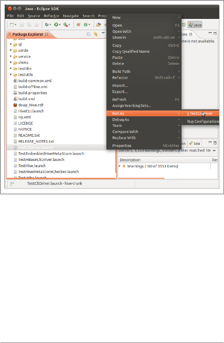
<dependency>
<groupId>org.apache.hive</groupId>
<artifactId>hive-service</artifactId>
<version>0.9.0</version>
</dependency>
The pom.xml file for hive_test, which we discuss next, provides a complete example
of the transitive dependencies for Hive v0.9.0. You can find that file at https://github
.com/edwardcapriolo/hive_test/blob/master/pom.xml.
Unit Testing in Hive with hive_test
The optimal way to write applications to work with Hive is to access Hive with Thrift
through the HiveService. However, the Thrift service was traditionally difficult to bring
up in an embedded environment due to Hive’s many JAR dependencies and the met-
astore component.
Figure 12-1. Starting the Hive Command CLI Driver from within Eclipse
Unit Testing in Hive with hive_test | 159

Hive_test fetches all the Hive dependencies from Maven, sets up the metastore and
Thrift service locally, and provides test classes to make unit testing easier. Also, because
it is very lightweight and unit tests run quickly, this is in contrast to the elaborate test
targets inside Hive, which have to rebuild the entire project to execute any unit test.
Hive_test is ideal for testing code such as UDFs, input formats, SerDes, or any com-
ponent that only adds a pluggable feature for the language. It is not useful for internal
Hive development because all the Hive components are pulled from Maven and are
external to the project.
In your Maven project, create a pom.xml and include hive_test as a dependency, as
shown here:
<dependency>
<groupId>com.jointhegrid</groupId>
<artifactId>hive_test</artifactId>
<version>3.0.1-SNAPSHOT</version>
</dependency>
Then create a version of hive-site.xml:
$ cp $HIVE_HOME/conf/* src/test/resources/
$ vi src/test/resources/hive-site.xml
Unlike a normal hive-site.xml, this version should not save any data to a
permanent place. This is because unit tests are not supposed to create or preserve any
permanent state. javax.jdo.option.ConnectionURL is set to use a feature in Derby that
only stores the database in main memory. The warehouse directory hive
.metastore.warehouse.dir is set to a location inside /tmp that will be deleted on each
run of the unit test:
<configuration>
<property>
<name>javax.jdo.option.ConnectionURL</name>
<value>jdbc:derby:memory:metastore_db;create=true</value>
<description>JDBC connect string for a JDBC metastore</description>
</property>
<property>
<name>hive.metastore.warehouse.dir</name>
<value>/tmp/warehouse</value>
<description>location of default database for the warehouse</description>
</property>
</configuration>
Hive_test provides several classes that extend JUnit test cases. HiveTestService set up
the environment, cleared out the warehouse directory, and launched a metastore and
HiveService in-process. This is typically the component to extend for testing. However,
other components, such as HiveTestEmbedded are also available:
package com.jointhegrid.hive_test;
160 | Chapter 12: Developing

import java.io.BufferedWriter;
import java.io.IOException;
import java.io.OutputStreamWriter;
import org.apache.hadoop.fs.FSDataOutputStream;
import org.apache.hadoop.fs.Path;
/* Extending HiveTestService creates and initializes
the metastore and thrift service in an embedded mode */
public class ServiceHiveTest extends HiveTestService {
public ServiceHiveTest() throws IOException {
super();
}
public void testExecute() throws Exception {
/* Use the Hadoop filesystem API to create a
data file */
Path p = new Path(this.ROOT_DIR, "afile");
FSDataOutputStream o = this.getFileSystem().create(p);
BufferedWriter bw = new BufferedWriter(new OutputStreamWriter(o));
bw.write("1\n");
bw.write("2\n");
bw.close();
/* ServiceHive is a component that connections
to an embedded or network HiveService based
on the constructor used */
ServiceHive sh = new ServiceHive();
/* We can now interact through the HiveService
and assert on results */
sh.client.execute("create table atest (num int)");
sh.client.execute("load data local inpath '"
+ p.toString() + "' into table atest");
sh.client.execute("select count(1) as cnt from atest");
String row = sh.client.fetchOne();
assertEquals("2", row);
sh.client.execute("drop table atest");
}
}
The New Plugin Developer Kit
Hive v0.8.0 introduced a Plugin Developer Kit (PDK). Its intent is to allow developers
to build and test plug-ins without the Hive source. Only Hive binary code is required.
The PDK is relatively new and has some subtle bugs of its own that can make it difficult
to use. If you want to try using the PDK anyway, consult the wiki page, https://cwiki
.apache.org/Hive/plugindeveloperkit.html, but note that this page has a few errors, at
least at the time of this writing.
The New Plugin Developer Kit | 161

CHAPTER 13
Functions
User-Defined Functions (UDFs) are a powerful feature that allow users to extend
HiveQL. As we’ll see, you implement them in Java and once you add them to your
session (interactive or driven by a script), they work just like built-in functions, even
the online help. Hive has several types of user-defined functions, each of which per-
forms a particular “class” of transformations on input data.
In an ETL workload, a process might have several processing steps. The Hive language
has multiple ways to pipeline the output from one step to the next and produce multiple
outputs during a single query. Users also have the ability to create their own functions
for custom processing. Without this feature a process might have to include a custom
MapReduce step or move the data into another system to apply the changes. Intercon-
necting systems add complexity and increase the chance of misconfigurations or other
errors. Moving data between systems is time consuming when dealing with gigabyte-
or terabyte-sized data sets. In contrast, UDFs run in the same processes as the tasks for
your Hive queries, so they work efficiently and eliminate the complexity of integration
with other systems. This chapter covers best practices associated with creating and
using UDFs.
Discovering and Describing Functions
Before writing custom UDFs, let’s familiarize ourselves with the ones that are already
part of Hive. Note that it’s common in the Hive community to use “UDF” to refer to
any function, user-defined or built-in.
The SHOW FUNCTIONS command lists the functions currently loaded in the Hive session,
both built-in and any user-defined functions that have been loaded using the techniques
we will discuss shortly:
hive> SHOW FUNCTIONS;
abs
acos
and
array
163

array_contains
...
Functions usually have their own documentation. Use DESCRIBE FUNCTION to display a
short description:
hive> DESCRIBE FUNCTION concat;
concat(str1, str2, ... strN) - returns the concatenation of str1, str2, ... strN
Functions may also contain extended documentation that can be accessed by adding
the EXTENDED keyword:
hive> DESCRIBE FUNCTION EXTENDED concat;
concat(str1, str2, ... strN) - returns the concatenation of str1, str2, ... strN
Returns NULL if any argument is NULL.
Example:
> SELECT concat('abc', 'def') FROM src LIMIT 1;
'abcdef'
Calling Functions
To use a function, simply call it by name in a query, passing in any required arguments.
Some functions take a specific number of arguments and argument types, while other
functions accept a variable number of arguments with variable types. Just like key-
words, the case of function names is ignored:
SELECT concat(column1,column2) AS x FROM table;
Standard Functions
The term user-defined function (UDF) is also used in a narrower sense to refer to any
function that takes a row argument or one or more columns from a row and returns a
single value. Most functions fall into this category.
Examples include many of the mathematical functions, like round() and floor(), for
converting DOUBLES to BIGINTS, and abs(), for taking the absolute value of a number.
Other examples include string manipulation functions, like ucase(), which converts
the string to upper case; reverse(), which reverses a string; and concat(), which joins
multiple input strings into one output string.
Note that these UDFs can return a complex object, such as an array, map, or struct.
Aggregate Functions
Another type of function is an aggregate function. All aggregate functions, user-defined
and built-in, are referred to generically as user-defined aggregate functions (UDAFs).
An aggregate function takes one or more columns from zero to many rows and returns
a single result. Examples include the math functions: sum(), which returns a sum of all
164 | Chapter 13: Functions

inputs; avg(), which computes the average of the values; min() and max(), which return
the lowest and highest values, respectively:
hive> SELECT avg(price_close)
> FROM stocks
> WHERE exchange = 'NASDAQ' AND symbol = 'AAPL';
Aggregate methods are often combined with GROUP BY clauses. We saw this example in
“GROUP BY Clauses” on page 97:
hive> SELECT year(ymd), avg(price_close) FROM stocks
> WHERE exchange = 'NASDAQ' AND symbol = 'AAPL'
> GROUP BY year(ymd);
1984 25.578625440597534
1985 20.193676221040867
1986 32.46102808021274
...
Table 6-3 in Chapter 6 lists the built-in aggregate functions in HiveQL.
Table Generating Functions
A third type of function supported by Hive is a table generating function. As for the
other function kinds, all table generating functions, user-defined and built-in, are often
referred to generically as user-defined table generating functions (UDTFs).
Table generating functions take zero or more inputs and produce multiple columns or
rows of output. The array function takes a list of arguments and returns the list as a
single array type. Suppose we start with this query using an array:
hive> SELECT array(1,2,3) FROM dual;
[1,2,3]
The explode() function is a UDTF that takes an array of input and iterates through the
list, returning each element from the list in a separate row.
hive> SELECT explode(array(1,2,3)) AS element FROM src;
1
2
3
However, Hive only allows table generating functions to be used in limited ways. For
example, we can’t project out any other columns from the table, a significant limitation.
Here is a query we would like to write with the employees table we have used before.
We want to list each manager-subordinate pair.
Example 13-1. Invalid use of explode
hive> SELECT name, explode(subordinates) FROM employees;
FAILED: Error in semantic analysis: UDTF's are not supported outside
the SELECT clause, nor nested in expressions
However, Hive offers a LATERAL VIEW feature to allow this kind of query:
Table Generating Functions | 165

hive> SELECT name, sub
> FROM employees
> LATERAL VIEW explode(subordinates) subView AS sub;
John Doe Mary Smith
John Doe Todd Jones
Mary Smith Bill King
Note that there are no output rows for employees who aren’t managers (i.e., who have
no subordinates), namely Bill King and Todd Jones. Hence, explode outputs zero to
many new records.
The LATERAL VIEW wraps the output of the explode call. A view alias and column alias
are required, subView and sub, respectively, in this case.
The list of built-in, table generating functions can be found in Table 6-4 in Chapter 6.
A UDF for Finding a Zodiac Sign from a Day
Let’s tackle writing our own UDF. Imagine we have a table with each user’s birth date
stored as a column of a table. With that information, we would like to determine the
user’s Zodiac sign. This process can be implemented with a standard function (UDF
in the most restrictive sense). Specifically, we assume we have a discrete input either as
a date formatted as a string or as a month and a day. The function must return a discrete
single column of output.
Here is a sample data set, which we’ll put in a file called littlebigdata.txt in our home
directory:
edward capriolo,edward@media6degrees.com,2-12-1981,209.191.139.200,M,10
bob,bob@test.net,10-10-2004,10.10.10.1,M,50
sara connor,sara@sky.net,4-5-1974,64.64.5.1,F,2
Load this data set into a table called littlebigdata:
hive > CREATE TABLE IF NOT EXISTS littlebigdata(
> name STRING,
> email STRING,
> bday STRING,
> ip STRING,
> gender STRING,
> anum INT)
> ROW FORMAT DELIMITED FIELDS TERMINATED BY ',';
hive> LOAD DATA LOCAL INPATH '${env:HOME}/littlebigdata.txt'
> INTO TABLE littlebigdata;
The input for the function will be a date and the output will be a string representing
the user’s Zodiac sign.
Here is a Java implementation of the UDF we need:
package org.apache.hadoop.hive.contrib.udf.example;
import java.util.Date;
166 | Chapter 13: Functions

import java.text.SimpleDateFormat;
import org.apache.hadoop.hive.ql.exec.UDF;
@Description(name = "zodiac",
value = "_FUNC_(date) - from the input date string "+
"or separate month and day arguments, returns the sign of the Zodiac.",
extended = "Example:\n"
+ " > SELECT _FUNC_(date_string) FROM src;\n"
+ " > SELECT _FUNC_(month, day) FROM src;")
public class UDFZodiacSign extends UDF{
private SimpleDateFormat df;
public UDFZodiacSign(){
df = new SimpleDateFormat("MM-dd-yyyy");
}
public String evaluate( Date bday ){
return this.evaluate( bday.getMonth(), bday.getDay() );
}
public String evaluate(String bday){
Date date = null;
try {
date = df.parse(bday);
} catch (Exception ex) {
return null;
}
return this.evaluate( date.getMonth()+1, date.getDay() );
}
public String evaluate( Integer month, Integer day ){
if (month==1) {
if (day < 20 ){
return "Capricorn";
} else {
return "Aquarius";
}
}
if (month==2){
if (day < 19 ){
return "Aquarius";
} else {
return "Pisces";
}
}
/* ...other months here */
return null;
}
}
To write a UDF, start by extending the UDF class and implements and the evaluate()
function. During query processing, an instance of the class is instantiated for each usage
of the function in a query. The evaluate() is called for each input row. The result of
A UDF for Finding a Zodiac Sign from a Day | 167

evaluate() is returned to Hive. It is legal to overload the evaluate method. Hive will
pick the method that matches in a similar way to Java method overloading.
The @Description(...) is an optional Java annotation. This is how function documen-
tation is defined and you should use these annotations to document your own UDFs.
When a user invokes DESCRIBE FUNCTION ..., the _FUNC_ strings will be replaced with
the function name the user picks when defining a “temporary” function, as discussed
below.
The arguments and return types of the UDF’s evaluate() function can
only be types that Hive can serialize. For example, if you are working
with whole numbers, a UDF can take as input a primitive int, an Inte
ger wrapper object, or an IntWritable, which is the Hadoop wrapper
for integers. You do not have to worry specifically about what the caller
is sending because Hive will convert the types for you if they do not
match. Remember that null is valid for any type in Hive, but in Java
primitives are not objects and cannot be null.
To use the UDF inside Hive, compile the Java code and package the UDF bytecode
class file into a JAR file. Then, in your Hive session, add the JAR to the classpath and
use a CREATE FUNCTION statement to define a function that uses the Java class:
hive> ADD JAR /full/path/to/zodiac.jar;
hive> CREATE TEMPORARY FUNCTION zodiac
> AS 'org.apache.hadoop.hive.contrib.udf.example.UDFZodiacSign';
Note that quotes are not required around the JAR file path and currently it needs to be
a full path to the file on a local filesystem. Hive not only adds this JAR to the classpath,
it puts the JAR file in the distributed cache so it’s available around the cluster.
Now the Zodiac UDF can be used like any other function. Notice the word TEMPO
RARY found inside the CREATE FUNCTION statement. Functions declared will only be avail-
able in the current session. You will have to add the JAR and create the function in each
session. However, if you use the same JAR files and functions frequently, you can add
these statements to your $HOME/.hiverc file:
hive> DESCRIBE FUNCTION zodiac;
zodiac(date) - from the input date string or separate month and day
arguments, returns the sign of the Zodiac.
hive> DESCRIBE FUNCTION EXTENDED zodiac;
zodiac(date) - from the input date string or separate month and day
arguments, returns the sign of the Zodiac.
Example:
> SELECT zodiac(date_string) FROM src;
> SELECT zodiac(month, day) FROM src;
hive> SELECT name, bday, zodiac(bday) FROM littlebigdata;
edward capriolo 2-12-1981 Aquarius
168 | Chapter 13: Functions

bob 10-10-2004 Libra
sara connor 4-5-1974 Aries
To recap, our UDF allows us to do custom transformations inside the Hive language.
Hive can now convert the user’s birthday to the corresponding Zodiac sign while it is
doing any other aggregations and transformations.
If we’re finished with the function, we can drop it:
hive> DROP TEMPORARY FUNCTION IF EXISTS zodiac;
As usual, the IF EXISTS is optional. It suppresses errors if the function doesn’t exist.
UDF Versus GenericUDF
In our Zodiac example we extended the UDF class. Hive offers a counterpart called
GenericUDF. GenericUDF is a more complex abstraction, but it offers support for better
null handling and makes it possible to handle some types of operations programmati-
cally that a standard UDF cannot support. An example of a generic UDF is the Hive
CASE ... WHEN statement, which has complex logic depending on the arguments to the
statement. We will demonstrate how to use the GenericUDF class to write a user-defined
function, called nvl(), which returns a default value if null is passed in.
The nvl() function takes two arguments. If the first argument is non-null, it is returned.
If the first argument is null, the second argument is returned. The GenericUDF frame-
work is a good fit for this problem. A standard UDF could be used as a solution but it
would be cumbersome because it requires overloading the evaluate method to handle
many different input types. GenericUDF will detect the type of input to the function
programmatically and provide an appropriate response.
We begin with the usual laundry list of import statements:
package org.apache.hadoop.hive.ql.udf.generic;
import org.apache.hadoop.hive.ql.exec.Description;
import org.apache.hadoop.hive.ql.exec.UDFArgumentException;
import org.apache.hadoop.hive.ql.exec.UDFArgumentLengthException;
import org.apache.hadoop.hive.ql.exec.UDFArgumentTypeException;
import org.apache.hadoop.hive.ql.metadata.HiveException;
import org.apache.hadoop.hive.ql.udf.generic.GenericUDF;
import org.apache.hadoop.hive.ql.udf.generic.GenericUDFUtils;
import org.apache.hadoop.hive.serde2.objectinspector.ObjectInspector;
Next, we use the @Description annotation to document the UDF:
@Description(name = "nvl",
value = "_FUNC_(value,default_value) - Returns default value if value"
+" is null else returns value",
extended = "Example:\n"
+ " > SELECT _FUNC_(null,'bla') FROM src LIMIT 1;\n")
UDF Versus GenericUDF | 169

Now the class extends GenericUDF, a requirement to exploit the generic handling we
want.
The initialize() method is called and passed an ObjectInspector for each argument.
The goal of this method is to determine the return type from the arguments. The user
can also throw an Exception to signal that bad types are being sent to the method. The
returnOIResolver is a built-in class that determines the return type by finding the type
of non-null variables and using that type:
public class GenericUDFNvl extends GenericUDF {
private GenericUDFUtils.ReturnObjectInspectorResolver returnOIResolver;
private ObjectInspector[] argumentOIs;
@Override
public ObjectInspector initialize(ObjectInspector[] arguments)
throws UDFArgumentException {
argumentOIs = arguments;
if (arguments.length != 2) {
throw new UDFArgumentLengthException(
"The operator 'NVL' accepts 2 arguments.");
}
returnOIResolver = new GenericUDFUtils.ReturnObjectInspectorResolver(true);
if (!(returnOIResolver.update(arguments[0]) && returnOIResolver
.update(arguments[1]))) {
throw new UDFArgumentTypeException(2,
"The 1st and 2nd args of function NLV should have the same type, "
+ "but they are different: \"" + arguments[0].getTypeName()
+ "\" and \"" + arguments[1].getTypeName() + "\"");
}
return returnOIResolver.get();
}
...
The evaluate method has access to the values passed to the method stored in an array
of DeferredObject values. The returnOIResolver created in the initialize method is
used to get values from the DeferredObjects. In this case, the function returns the first
non-null value:
...
@Override
public Object evaluate(DeferredObject[] arguments) throws HiveException {
Object retVal = returnOIResolver.convertIfNecessary(arguments[0].get(),
argumentOIs[0]);
if (retVal == null ){
retVal = returnOIResolver.convertIfNecessary(arguments[1].get(),
argumentOIs[1]);
}
return retVal;
}
...
The final method to override is getDisplayString(), which is used inside the Hadoop
tasks to display debugging information when the function is being used:
170 | Chapter 13: Functions

...
@Override
public String getDisplayString(String[] children) {
StringBuilder sb = new StringBuilder();
sb.append("if ");
sb.append(children[0]);
sb.append(" is null ");
sb.append("returns");
sb.append(children[1]);
return sb.toString() ;
}
}
To test the generic nature of the UDF, it is called several times, each time passing values
of different types, as shown the following example:
hive> ADD JAR /path/to/jar.jar;
hive> CREATE TEMPORARY FUNCTION nvl
> AS 'org.apache.hadoop.hive.ql.udf.generic.GenericUDFNvl';
hive> SELECT nvl( 1 , 2 ) AS COL1,
> nvl( NULL, 5 ) AS COL2,
> nvl( NULL, "STUFF" ) AS COL3
> FROM src LIMIT 1;
1 5 STUFF
Permanent Functions
Until this point we have bundled our code into JAR files, then used ADD JAR and CREATE
TEMPORARY FUNCTION to make use of them.
Your function may also be added permanently to Hive, however this requires a small
modification to a Hive Java file and then rebuilding Hive.
Inside the Hive source code, a one-line change is required to the FunctionRegistry class
found at ql/src/java/org/apache/hadoop/hive/ql/exec/FunctionRegistry.java. Then you
rebuild Hive following the instructions that come with the source distribution.
While it is recommended that you redeploy the entire new build, only the hive-exec-
*.jar, where \* is the version number, needs to be replaced.
Here is an example change to FunctionRegistry where the new nvl() function is added
to Hive’s list of built-in functions:
...
registerUDF("parse_url", UDFParseUrl.class, false);
registerGenericUDF("nvl", GenericUDFNvl.class);
registerGenericUDF("split", GenericUDFSplit.class);
...
Permanent Functions | 171

User-Defined Aggregate Functions
Users are able to define aggregate functions, too. However, the interface is more com-
plex to implement. Aggregate functions are processed in several phases. Depending on
the transformation the UDAF performs, the types returned by each phase could be
different. For example, a sum() UDAF could accept primitive integer input, create in-
teger PARTIAL data, and produce a final integer result. However, an aggregate like
median() could take primitive integer input, have an intermediate list of integers as
PARTIAL data, and then produce a final integer as the result.
For an example of a generic user-defined aggregate function, see the source code for
GenericUDAFAverage available at http://svn.apache.org/repos/asf/hive/branches/branch-0
.8/ql/src/java/org/apache/hadoop/hive/ql/udf/generic/GenericUDAFAverage.java.
Aggregations execute inside the context of a map or reduce task, which
is a Java process with memory limitations. Therefore, storing large
structures inside an aggregate may exceed available heap space. The
min() UDAF only requires a single element be stored in memory for
comparison. The collectset() UDAF uses a set internally to de-
duplicate data in order to limit memory usage. percentile_approx()
uses approximations to achieve a near correct result while limiting
memory usage. It is important to keep memory usage in mind when
writing a UDAF. You can increase your available memory to some extent
by adjusting mapred.child.java.opts, but that solution does not scale:
<property>
<name>mapred.child.java.opts</name>
<value>-Xmx200m</value>
</property>
Creating a COLLECT UDAF to Emulate GROUP_CONCAT
MySQL has a useful function known as GROUP_CONCAT, which combines all the
elements of a group into a single string using a user-specified delimiter. Below is an
example MySQL query that shows how to use its version of this function:
mysql > CREATE TABLE people (
name STRING,
friendname STRING );
mysql > SELECT * FROM people;
bob sara
bob john
bob ted
john sara
ted bob
ted sara
mysql > SELECT name, GROUP_CONCAT(friendname SEPARATOR ',')
FROM people
172 | Chapter 13: Functions
Downloa d f r o m W o w ! e B o o k < w w w.woweb o o k . c o m >

GROUP BY name;
bob sara,john,ted
john sara
ted bob,sara
We can do the same transformation in Hive without the need for additional grammar
in the language. First, we need an aggregate function that builds a list of all input to
the aggregate. Hive already has a UDAF called collect_set that adds all input into a
java.util.Set collection. Sets automatically de-duplicate entries on insertion, which
is undesirable for GROUP CONCAT. To build collect, we will take the code in col
lect_set and replace instances of Set with instances of ArrayList. This will stop the
de-duplication. The result of the aggregate will be a single array of all values.
It is important to remember that the computation of your aggregation must be arbi-
trarily divisible over the data. Think of it as writing a divide-and-conquer algorithm
where the partitioning of the data is completely out of your control and handled by
Hive. More formally, given any subset of the input rows, you should be able to compute
a partial result, and also be able to merge any pair of partial results into another partial
result.
The following code is available on Github. All the input to the aggregation must be
primitive types. Rather than returning an ObjectInspector, like GenericUDFs, aggregates
return a subclass of GenericUDAFEvaluator:
@Description(name = "collect", value = "_FUNC_(x) - Returns a list of objects. "+
"CAUTION will easily OOM on large data sets" )
public class GenericUDAFCollect extends AbstractGenericUDAFResolver {
static final Log LOG = LogFactory.getLog(GenericUDAFCollect.class.getName());
public GenericUDAFCollect() {
}
@Override
public GenericUDAFEvaluator getEvaluator(TypeInfo[] parameters)
throws SemanticException {
if (parameters.length != 1) {
throw new UDFArgumentTypeException(parameters.length - 1,
"Exactly one argument is expected.");
}
if (parameters[0].getCategory() != ObjectInspector.Category.PRIMITIVE) {
throw new UDFArgumentTypeException(0,
"Only primitive type arguments are accepted but "
+ parameters[0].getTypeName() + " was passed as parameter 1.");
}
return new GenericUDAFMkListEvaluator();
}
}
Table 13-1 describes the methods that are part of the base class.
User-Defined Aggregate Functions | 173

Table 13-1. Methods in AbstractGenericUDAFResolver
Method Description
init Called by Hive to initialize an instance of the UDAF evaluator
class.
getNewAggregationBuffer Return an object that will be used to store temporary aggre-
gation results.
iterate Process a new row of data into the aggregation buffer.
terminatePartial Return the contents of the current aggregation in a persistable
way. Here, persistable means the return value can only be built
up in terms of Java primitives, arrays, primitive wrappers
(e.g., Double), Hadoop Writables, Lists, and Maps. Do NOT
use your own classes (even if they implement java.io
.Serializable).
merge Merge a partial aggregation returned by
terminatePartial into the current aggregation.
terminate Return the final result of the aggregation to Hive.
In the init method, the object inspectors for the result type are set, after determining
what mode the evaluator is in.
The iterate() and terminatePartial() methods are used on the map side, while ter
minate() and merge() are used on the reduce side to produce the final result. In all cases
the merges are building larger lists:
public static class GenericUDAFMkListEvaluator extends GenericUDAFEvaluator {
private PrimitiveObjectInspector inputOI;
private StandardListObjectInspector loi;
private StandardListObjectInspector internalMergeOI;
@Override
public ObjectInspector init(Mode m, ObjectInspector[] parameters)
throws HiveException {
super.init(m, parameters);
if (m == Mode.PARTIAL1) {
inputOI = (PrimitiveObjectInspector) parameters[0];
return ObjectInspectorFactory
.getStandardListObjectInspector(
(PrimitiveObjectInspector) ObjectInspectorUtils
.getStandardObjectInspector(inputOI));
} else {
if (!(parameters[0] instanceof StandardListObjectInspector)) {
inputOI = (PrimitiveObjectInspector) ObjectInspectorUtils
.getStandardObjectInspector(parameters[0]);
return (StandardListObjectInspector) ObjectInspectorFactory
.getStandardListObjectInspector(inputOI);
} else {
internalMergeOI = (StandardListObjectInspector) parameters[0];
inputOI = (PrimitiveObjectInspector)
internalMergeOI.getListElementObjectInspector();
174 | Chapter 13: Functions

loi = (StandardListObjectInspector) ObjectInspectorUtils
.getStandardObjectInspector(internalMergeOI);
return loi;
}
}
}
...
The remaining methods and class definition define MkArrayAggregationBuffer as well
as top-level methods that modify the contents of the buffer:
You may have noticed that Hive tends to avoid allocating objects with
new whenever possible. Hadoop and Hive use this pattern to create fewer
temporary objects and thus less work for the JVM’s Garbage Collec
tion algorithms. Keep this in mind when writing UDFs, because refer-
ences are typically reused. Assuming immutable objects will lead to
bugs!
...
static class MkArrayAggregationBuffer implements AggregationBuffer {
List<Object> container;
}
@Override
public void reset(AggregationBuffer agg) throws HiveException {
((MkArrayAggregationBuffer) agg).container =
new ArrayList<Object>();
}
@Override
public AggregationBuffer getNewAggregationBuffer()
throws HiveException {
MkArrayAggregationBuffer ret = new MkArrayAggregationBuffer();
reset(ret);
return ret;
}
// Mapside
@Override
public void iterate(AggregationBuffer agg, Object[] parameters)
throws HiveException {
assert (parameters.length == 1);
Object p = parameters[0];
if (p != null) {
MkArrayAggregationBuffer myagg = (MkArrayAggregationBuffer) agg;
putIntoList(p, myagg);
}
}
// Mapside
@Override
public Object terminatePartial(AggregationBuffer agg)
User-Defined Aggregate Functions | 175

throws HiveException {
MkArrayAggregationBuffer myagg = (MkArrayAggregationBuffer) agg;
ArrayList<Object> ret = new ArrayList<Object>(myagg.container.size());
ret.addAll(myagg.container);
return ret;
}
@Override
public void merge(AggregationBuffer agg, Object partial)
throws HiveException {
MkArrayAggregationBuffer myagg = (MkArrayAggregationBuffer) agg;
ArrayList<Object> partialResult =
(ArrayList<Object>) internalMergeOI.getList(partial);
for(Object i : partialResult) {
putIntoList(i, myagg);
}
}
@Override
public Object terminate(AggregationBuffer agg) throws HiveException {
MkArrayAggregationBuffer myagg = (MkArrayAggregationBuffer) agg;
ArrayList<Object> ret = new ArrayList<Object>(myagg.container.size());
ret.addAll(myagg.container);
return ret;
}
private void putIntoList(Object p, MkArrayAggregationBuffer myagg) {
Object pCopy =
ObjectInspectorUtils.copyToStandardObject(p,this.inputOI);
myagg.container.add(pCopy);
}
}
Using collect will return a single row with a single array of all of the aggregated values:
hive> dfs -cat $HOME/afile.txt;
twelve 12
twelve 1
eleven 11
eleven 10
hive> CREATE TABLE collecttest (str STRING, countVal INT)
> ROW FORMAT DELIMITED FIELDS TERMINATED BY '09' LINES TERMINATED BY '10';
hive> LOAD DATA LOCAL INPATH '${env:HOME}/afile.txt' INTO TABLE collecttest;
hive> SELECT collect(str) FROM collecttest;
[twelve,twelve,eleven,eleven]
The concat_ws() takes a delimiter as its first argument. The remaining arguments can
be string types or arrays of strings. The returned result contains the argument joined
together by the delimiter. Hence, we have converted the array into a single comma-
separated string:
hive> SELECT concat_ws( ',' , collect(str)) FROM collecttest;
twelve,twleve,eleven,eleven
176 | Chapter 13: Functions

GROUP_CONCAT can be done by combining GROUP BY, COLLECT and concat_ws() as shown
here:
hive> SELECT str, concat_ws( ',' , collect(cast(countVal AS STRING)))
> FROM collecttest GROUP BY str;
eleven 11,10
twelve 12,1
User-Defined Table Generating Functions
While UDFs can be used be return arrays or structures, they cannot return multiple
columns or multiple rows. User-Defined Table Generating Functions, or UDTFs, ad-
dress this need by providing a programmatic interface to return multiple columns and
even multiple rows.
UDTFs that Produce Multiple Rows
We have already used the explode method in several examples. Explode takes an array
as input and outputs one row for each element in the array. An alternative way to do
this would have the UDTF generate the rows based on some input. We will demonstrate
this with a UDTF that works like a for loop. The function receives user inputs of the
start and stop values and then outputs N rows:
hive> SELECT forx(1,5) AS i FROM collecttest;
1
2
3
4
5
Our class extends the GenericUDTF interface. We declare three integer variables for the
start, end, and increment. The forwardObj array will be used to return result rows:
package com.jointhegrid.udf.collect;
import java.util.ArrayList;
import org.apache.hadoop.hive.ql.exec.UDFArgumentException;
import org.apache.hadoop.hive.ql.metadata.HiveException;
import org.apache.hadoop.hive.ql.udf.generic.GenericUDFUtils.*;
import org.apache.hadoop.hive.ql.udf.generic.GenericUDTF;
import org.apache.hadoop.hive.serde2.objectinspector.*;
import org.apache.hadoop.hive.serde2.objectinspector.primitive.*;
import org.apache.hadoop.io.IntWritable;
public class GenericUDTFFor extends GenericUDTF {
IntWritable start;
IntWritable end;
IntWritable inc;
Object[] forwardObj = null;
...
User-Defined Table Generating Functions | 177

Because the arguments to this function are constant, the value can be determined in
the initialize method. Nonconstant values are typically not available until the evaluate
method. The third argument for increment is optional, as it defaults to 1:
...
@Override
public StructObjectInspector initialize(ObjectInspector[] args)
throws UDFArgumentException {
start=((WritableConstantIntObjectInspector) args[0])
.getWritableConstantValue();
end=((WritableConstantIntObjectInspector) args[1])
.getWritableConstantValue();
if (args.length == 3) {
inc =((WritableConstantIntObjectInspector) args[2])
.getWritableConstantValue();
} else {
inc = new IntWritable(1);
}
...
This function returns only a single column and its type is always an integer. We need
to give it a name, but the user can always override this later:
...
this.forwardObj = new Object[1];
ArrayList<String> fieldNames = new ArrayList<String>();
ArrayList<ObjectInspector> fieldOIs = new ArrayList<ObjectInspector>();
fieldNames.add("col0");
fieldOIs.add(
PrimitiveObjectInspectorFactory.getPrimitiveJavaObjectInspector(
PrimitiveCategory.INT));
return ObjectInspectorFactory.getStandardStructObjectInspector(
fieldNames, fieldOIs);
}
...
The process method is where the interesting work happens. Notice that the return type
is void. This is because UDTF can forward zero or more rows, unlike a UDF, which
has a single return. In this case the call to the forward method is nested inside a for
loop, which causes it to forward a row for each iteration:
...
@Override
public void process(Object[] args)
throws HiveException, UDFArgumentException {
for (int i = start.get(); i < end.get(); i = i + inc.get()) {
this.forwardObj[0] = new Integer(i);
forward(forwardObj);
}
}
@Override
178 | Chapter 13: Functions

public void close() throws HiveException {
}
}
UDTFs that Produce a Single Row with Multiple Columns
An example of a UDTF that returns multiple columns but only one row is the
parse_url_tuple function, which is a built-in Hive function. It takes as input a param-
eter that is a URL and one or more constants that specify the parts of the URL the user
wants returned:
hive> SELECT parse_url_tuple(weblogs.url, 'HOST', 'PATH')
> AS (host, path) FROM weblogs;
google.com /index.html
hotmail.com /a/links.html
The benefit of this type of UDFT is the URL only needs to be parsed once, then returns
multiple columns—a clear performance win. The alternative, using UDFs, involves
writing several UDFs to extract specific parts of the URL. Using UDFs requires writing
more code as well as more processing time because the URL is parsed multiple times.
For example, something like the following:
SELECT PARSE_HOST(a.url) as host, PARSE_PORT(url) FROM weblogs;
UDTFs that Simulate Complex Types
A UDTF can be used as a technique for adding more complex types to Hive. For ex-
ample, a complex type can be serialized as an encoded string and a UDTF will deseri-
alize the complex type when needed. Suppose we have a Java class named Book. Hive
cannot work with this datatype directly, however a Book could be encoded to and
decoded from a string format:
public class Book {
public Book () { }
public String isbn;
public String title;
public String [] authors;
/* note: this system will not work if your table is
using '|' or ',' as the field delimiter! */
public void fromString(String parts){
String [] part = part.split("\|");
isbn = Integer.parseInt( part[0] );
title = part[1] ;
authors = part[2].split(",");
}
public String toString(){
return isbn+"\t"+title+"\t"+StringUtils.join(authors, ",");
}
}
User-Defined Table Generating Functions | 179

Imagine we have a flat text file with books in this format. For now lets assume we could
not use a delimited SerDe to split on | and ,:
hive> SELECT * FROM books;
5555555|Programming Hive|Edward,Dean,Jason
In the pipe-delimited raw form it is possible to do some parsing of the data:
hive> SELECT cast(split(book_info,"\|")[0] AS INTEGER) AS isbn FROM books
> WHERE split(book_info,"\|")[1] = "Programming Hive";
5555555
This HiveQL works correctly, however it could be made easier for the end user. For
example, writing this type of query may require consulting documentation regarding
which fields and types are used, remembering casting conversion rules, and so forth.
By contrast, a UDTF makes this HiveQL simpler and more readable. In the following
example, the parse_book() UDTF is introduced:
hive> FROM (
> parse_book(book_info) AS (isbn, title, authors) FROM Book ) a
> SELECT a.isbn
> WHERE a.title="Programming Hive"
> AND array_contains (authors, 'Edward');
5555555
The function parse_book() allows Hive to return multiple columns of different types
representing the fields of a book:
package com.jointhegrid.udf.collect;
import java.util.ArrayList;
import org.apache.hadoop.hive.ql.exec.UDFArgumentException;
import org.apache.hadoop.hive.ql.metadata.HiveException;
import org.apache.hadoop.hive.ql.udf.generic.GenericUDTF;
import org.apache.hadoop.hive.serde2.objectinspector.ObjectInspector;
import org.apache.hadoop.hive.serde2.objectinspector.ObjectInspectorFactory;
import org.apache.hadoop.hive.serde2.objectinspector.PrimitiveObjectInspector
.PrimitiveCategory;
import org.apache.hadoop.hive.serde2.objectinspector.StructObjectInspector;
import org.apache.hadoop.hive.serde2.objectinspector.primitive
.PrimitiveObjectInspectorFactory;
import org.apache.hadoop.hive.serde2.objectinspector.primitive
.WritableConstantStringObjectInspector;
import org.apache.hadoop.hive.serde2.objectinspector.primitive
.WritableStringObjectInspector;
import org.apache.hadoop.io.Text;
public class UDTFBook extends GenericUDTF{
private Text sent;
Object[] forwardObj = null;
...
180 | Chapter 13: Functions

The function will return three properties and ISBN as an integer, a title as a string, and
authors as an array of strings. Notice that we can return nested types with all UDFs,
for example we can return an array of array of strings:
...
@Override
public StructObjectInspector initialize(ObjectInspector[] args)
throws UDFArgumentException {
ArrayList<String> fieldNames = new ArrayList<String>();
ArrayList<ObjectInspector> fieldOIs = new ArrayList<ObjectInspector>();
fieldNames.add("isbn");
fieldOIs.add(PrimitiveObjectInspectorFactory.getPrimitiveJavaObjectInspector(
PrimitiveCategory.INT));
fieldNames.add("title");
fieldOIs.add(PrimitiveObjectInspectorFactory.getPrimitiveJavaObjectInspector(
PrimitiveCategory.STRING));
fieldNames.add("authors");
fieldOIs.add( ObjectInspectorFactory.getStandardListObjectInspector(
PrimitiveObjectInspectorFactory.getPrimitiveJavaObjectInspector(
PrimitiveCategory.STRING)
)
);
forwardObj= new Object[3];
return ObjectInspectorFactory.getStandardStructObjectInspector(
fieldNames, fieldOIs);
}
...
The process method only returns a single row. However, each element in the object
array will be bound to a specific variable:
...
@Override
public void process(Object[] os) throws HiveException {
sent = new Text(((StringObjectInspector)args[0])
.getPrimitiveJavaObject(os[0]));
String parts = new String(this.sent.getBytes());
String [] part = parts.split("\\|");
forwardObj[0]=Integer.parseInt( part[0] );
forwardObj[1]=part[1] ;
forwardObj[2]=part[2].split(",");
this.forward(forwardObj);
}
@Override
public void close() throws HiveException {
}
}
User-Defined Table Generating Functions | 181

We have followed the call to the book UDTF with AS, which allows the result columns
to be named by the user. They can then be used in other parts of the query without
having to parse information from the book again:
client.execute(
"create temporary function book as 'com.jointhegrid.udf.collect.UDTFBook'");
client.execute("create table booktest (str string) ");
client.execute(
"load data local inpath '" + p.toString() + "' into table booktest");
client.execute("select book(str) AS (book, title, authors) from booktest");
[555 Programming Hive "Dean","Jason","Edward"]
Accessing the Distributed Cache from a UDF
UDFs may access files inside the distributed cache, the local filesystem, or even the
distributed filesystem. This access should be used cautiously as the overhead is
significant.
A common usage of Hive is the analyzing of web logs. A popular operation is deter-
mining the geolocation of web traffic based on the IP address. Maxmind makes a GeoIP
database available and a Java API to search this database. By wrapping a UDF around
this API, location information may be looked up about an IP address from within a
Hive query.
The GeoIP API uses a small data file. This is ideal for showing the functionality of
accessing a distributed cache file from a UDF. The complete code for this example is
found at https://github.com/edwardcapriolo/hive-geoip/.
ADD FILE is used to cache the necessary data files with Hive. ADD JAR is used to add the
required Java JAR files to the cache and the classpath. Finally, the temporary function
must be defined as the final step before performing queries:
hive> ADD FILE GeoIP.dat;
hive> ADD JAR geo-ip-java.jar;
hive> ADD JAR hive-udf-geo-ip-jtg.jar;
hive> CREATE TEMPORARY FUNCTION geoip
> AS 'com.jointhegrid.hive.udf.GenericUDFGeoIP';
hive> SELECT ip, geoip(source_ip, 'COUNTRY_NAME', './GeoIP.dat') FROM weblogs;
209.191.139.200 United States
10.10.0.1 Unknown
The two examples returned include an IP address in the United States and a private IP
address that has no fixed address.
The geoip() function takes three arguments: the IP address in either string or long
format, a string that must match one of the constants COUNTRY_NAME or DMA_CODE, and a
final argument that is the name of the data file that has already been placed in the
distributed cache.
182 | Chapter 13: Functions

The first call to the UDF (which triggers the first call to the evaluate Java function in
the implementation) will instantiate a LookupService object that uses the file located in
the distributed cache. The lookup service is saved in a reference so it only needs to be
initialized once in the lifetime of a map or reduce task that initializes it. Note that the
LookupService has its own internal caching, LookupService.GEOIP\_MEMORY_CACHE, so
that optimization should avoid frequent disk access when looking up IPs.
Here is the source code for evaluate():
@Override
public Object evaluate(DeferredObject[] arguments) throws HiveException {
if (argumentOIs[0] instanceof LongObjectInspector) {
this.ipLong = ((LongObjectInspector)argumentOIs[0]).get(arguments[0].get());
} else {
this.ipString = ((StringObjectInspector)argumentOIs[0])
.getPrimitiveJavaObject(arguments[0].get());
}
this.property = ((StringObjectInspector)argumentOIs[1])
.getPrimitiveJavaObject(arguments[1].get());
if (this.property != null) {
this.property = this.property.toUpperCase();
}
if (ls ==null){
if (argumentOIs.length == 3){
this.database = ((StringObjectInspector)argumentOIs[1])
.getPrimitiveJavaObject(arguments[2].get());
File f = new File(database);
if (!f.exists())
throw new HiveException(database+" does not exist");
try {
ls = new LookupService ( f , LookupService.GEOIP_MEMORY_CACHE );
} catch (IOException ex){
throw new HiveException (ex);
}
}
}
...
An if statement in evaluate determines which data the method should return. In our
example, the country name is requested:
...
if (COUNTRY_PROPERTIES.contains(this.property)) {
Country country = ipString != null ?
ls.getCountry(ipString) : ls.getCountry(ipLong);
if (country == null) {
return null;
} else if (this.property.equals(COUNTRY_NAME)) {
return country.getName();
} else if (this.property.equals(COUNTRY_CODE)) {
return country.getCode();
}
assert(false);
} else if (LOCATION_PROPERTIES.contains(this.property)) {
...
Accessing the Distributed Cache from a UDF | 183

}
}
Annotations for Use with Functions
In this chapter we mentioned the Description annotation and how it is used to provide
documentation for Hive methods at runtime. Other annotations exist for UDFs that
can make functions easier to use and even increase the performance of some Hive
queries:
public @interface UDFType {
boolean deterministic() default true;
boolean stateful() default false;
boolean distinctLike() default false;
}
Deterministic
By default, deterministic is automatically turned on for most queries because they are
inherently deterministic by nature. An exception is the function rand().
If a UDF is not deterministic, it is not included in the partition pruner.
An example of a nondeterministic query using rand() is the following:
SELECT * FROM t WHERE rand() < 0.01;
If rand() were deterministic, the result would only be calculated a single time in the
computation state. Because a query with rand() is nondeterministic, the result of
rand() is recomputed for each row.
Stateful
Almost all the UDFs are stateful by default; a UDF that is not stateful is rand() because
it returns a different value for each invocation. The Stateful annotation may be used
under the following conditions:
• A stateful UDF can only be used in the SELECT list, not in other clauses such as
WHERE/ON/ORDER/GROUP.
• When a stateful UDF is present in a query, the implication is the SELECT will be
treated similarly to TRANSFORM (i.e., a DISTRIBUTE/CLUSTER/SORT clause), then run
inside the corresponding reducer to ensure the results are as expected.
• If stateful is set to true, the UDF should also be treated as nondeterministic (even
if the deterministic annotation explicitly returns true).
See https://issues.apache.org/jira/browse/HIVE-1994 for more details.
184 | Chapter 13: Functions

DistinctLike
Used for cases where the function behaves like DISTINCT even when applied to a non-
distinct column of values. Examples include min and max functions that return a distinct
value even though the underlying numeric data can have repeating values.
Macros
Macros provide the ability to define functions in HiveQL that call other functions and
operators. When appropriate for the particular situation, macros are a convenient
alternative to writing UDFs in Java or using Hive streaming, because they require no
external code or scripts.
To define a macro, use the CREATE TEMPORARY MACRO syntax. Here is an example that
creates a SIGMOID function calculator:
hive> CREATE TEMPORARY MACRO SIGMOID (x DOUBLE) 1.0 / (1.0 + EXP(-x));
hive> SELECT SIGMOID(2) FROM src LIMIT 1;
Macros | 185

CHAPTER 14
Streaming
Hive works by leveraging and extending the components of Hadoop, common
abstractions such as InputFormat, OutputFormat, Mapper, and Reducer, plus its own
abstractions, like SerializerDeserializer (SerDe), User-Defined Functions (UDFs),
and StorageHandlers.
These components are all Java components, but Hive hides the complexity of imple-
menting and using these components by letting the user work with SQL abstractions,
rather than Java code.
Streaming offers an alternative way to transform data. During a streaming job, the Ha-
doop Streaming API opens an I/O pipe to an external process. Data is then passed to
the process, which operates on the data it reads from the standard input and writes the
results out through the standard output, and back to the Streaming API job. While Hive
does not leverage the Hadoop streaming API directly, it works in a very similar way.
This pipeline computing model is familiar to users of Unix operating systems and their
descendants, like Linux and Mac OS X.
Streaming is usually less efficient than coding the comparable UDFs or
InputFormat objects. Serializing and deserializing data to pass it in and
out of the pipe is relatively inefficient. It is also harder to debug the whole
program in a unified manner. However, it is useful for fast prototyping
and for leveraging existing code that is not written in Java. For Hive
users who don’t want to write Java code, it can be a very effective
approach.
Hive provides several clauses to use streaming: MAP(), REDUCE(), and TRANSFORM(). An
important point to note is that MAP() does not actually force streaming during the map
phase nor does reduce force streaming to happen in the reduce phase. For this reason,
the functionally equivalent yet more generic TRANSFORM() clause is suggested to avoid
misleading the reader of the query.
187

For our streaming examples we will use a small table named a, with columns named
col1 and col2, both of type INT, and two rows:
hive> CREATE TABLE a (col1 INT, col2 INT)
> ROW FORMAT DELIMITED FIELDS TERMINATED BY '\t';
hive> SELECT * FROM a;
4 5
3 2
hive> DESCRIBE a;
a int
b int
Identity Transformation
The most basic streaming job is an identity operation. The /bin/cat command echoes
the data sent to it and meets the requirements. In this example, /bin/cat is assumed to
be installed on all TaskTracker nodes. Any Linux system should have it! Later, we will
show how Hive can “ship” applications with the job when they aren’t already installed
around the cluster:
hive> SELECT TRANSFORM (a, b)
> USING '/bin/cat' AS newA, newB
> FROM default.a;
4 5
3 2
Changing Types
The return columns from TRANSFORM are typed as strings, by default. There is an alter-
native syntax that casts the results to different types.
hive> SELECT TRANSFORM (col1, col2)
> USING '/bin/cat' AS (newA INT , newB DOUBLE) FROM a;
4 5.0
3 2.0
Projecting Transformation
The cut command can be used with streaming to extract or project specific fields. In
other words, this behaves like the SELECT statement:
hive> SELECT TRANSFORM (a, b)
> USING '/bin/cut -f1'
> AS newA, newB FROM a;
4 NULL
3 NULL
188 | Chapter 14: Streaming

Note that the query attempts to read more columns than are actually returned from the
external process, so newB is always NULL. By default, TRANSFORM assumes two columns
but there can be any number of them:
hive> SELECT TRANSFORM (a, b)
> USING '/bin/cut -f1'
> AS newA FROM a;
4
3
Manipulative Transformations
The /bin/sed program (or /usr/bin/sed on Mac OS X systems) is a stream editor. It
takes the input stream, edits it according to the user’s specification, and then writes the
results to the output stream. The example below replaces the string 4 with the string 10:
hive> SELECT TRANSFORM (a, b)
> USING '/bin/sed s/4/10/'
> AS newA, newB FROM a;
10 5
3 2
Using the Distributed Cache
All of the streaming examples thus far have used applications such as cat and sed that
are core parts of Unix operating systems and their derivatives. When a query requires
files that are not already installed on every TaskTracker, users can use the distributed
cache to transmit data or program files across the cluster that will be cleaned up when
the job is complete.
This is helpful, because installing (and sometimes removing) lots of little components
across large clusters can be a burden. Also, the cache keeps one job’s cached files sep-
arate from those files belonging to other jobs.
The following example is a bash shell script that converts degrees in Celsius to degrees
in Fahrenheit:
while read LINE
do
res=$(echo "scale=2;((9/5) * $LINE) + 32" | bc)
echo $res
done
To test this script, launch it locally. It will not prompt for input. Type 100 and then
strike Enter. The process prints 212.00 to the standard output. Then enter another
number and the program returns another result. You can continue entering numbers
or use Control-D to end the input.
Using the Distributed Cache | 189
Downloa d f r o m W o w ! e B o o k < w w w.woweb o o k . c o m >

#!/bin/bash
$ sh ctof.sh
100
212.00
0
32.00
^D
Hive’s ADD FILE feature adds files to the distributed cache. The added file is put in the
current working directory of each task. This allows the transform task to use the script
without needing to know where to find it:
hive> ADD FILE ${env:HOME}/prog_hive/ctof.sh;
Added resource: /home/edward/prog_hive/ctof.sh
hive> SELECT TRANSFORM(col1) USING 'ctof.sh' AS convert FROM a;
39.20
37.40
Producing Multiple Rows from a Single Row
The examples shown thus far have taken one row of input and produced one row of
output. Streaming can be used to produce multiple rows of output for each input row.
This functionality produces output similar to the EXPLODE() UDF and the LATERAL
VIEW syntax1.
Given an input file $HOME/kv_data.txt that looks like:
k1=v1,k2=v2
k4=v4,k5=v5,k6=v6
k7=v7,k7=v7,k3=v7
We would like the data in a tabular form. This will allow the rows to be processed by
familiar HiveQL operators:
k1 v1
k2 v2
k4 k4
Create this Perl script and save it as $HOME/split_kv.pl:
#!/usr/bin/perl
while (<STDIN>) {
my $line = $_;
chomp($line);
my @kvs = split(/,/, $line);
foreach my $p (@kvs) {
my @kv = split(/=/, $p);
print $kv[0] . "\t" . $kv[1] . "\n";
}
}
1. The source code and concept for this example comes from Larry Ogrodnek, “Custom Map Scripts and
Hive”, Bizo development (blog), July 14, 2009.
190 | Chapter 14: Streaming

Create a kv_data table. The entire table is defined as a single string column. The row
format does not need to be configured because the streaming script will do all the
tokenization of the fields:
hive> CREATE TABLE kv_data ( line STRING );
hive> LOAD DATA LOCAL INPATH '${env:HOME}/kv_data.txt' INTO TABLE kv_data;
Use the transform script on the source table. The ragged, multiple-entry-per-row format
is converted into a two-column result set of key-value pairs:
hive> SELECT TRANSFORM (line)
> USING 'perl split_kv.pl'
> AS (key, value) FROM kv_data;
k1 v1
k2 v2
k4 v4
k5 v5
k6 v6
k7 v7
k7 v7
k3 v7
Calculating Aggregates with Streaming
Streaming can also be used to do aggregating operations like Hive’s built-in SUM func-
tion. This is possible because streaming processes can return zero or more rows of
output for every given input.
To accomplish aggregation in an external application, declare an accumulator before
the loop that reads from the input stream and output the sum after the completion of
the input:
#!/usr/bin/perl
my $sum=0;
while (<STDIN>) {
my $line = $_;
chomp($line);
$sum=${sum}+${line};
}
print $sum;
Create a table and populate it with integer data, one integer per line, for testing:
hive> CREATE TABLE sum (number INT);
hive> LOAD DATA LOCAL INPATH '${env:HOME}/data_to_sum.txt' INTO TABLE sum;
Calculating Aggregates with Streaming | 191

hive> SELECT * FROM sum;
5
5
4
Add the streaming program to the distributed cache and use it in a TRANSFORM query.
The process returns a single row, which is the sum of the input:
hive> ADD FILE ${env:HOME}/aggregate.pl;
Added resource: /home/edward/aggregate.pl
hive> SELECT TRANSFORM (number)
> USING 'perl aggregate.pl' AS total FROM sum;
14
Unfortunately, it is not possible to do multiple TRANSFORMs in a single query like the
UDAF SUM() can do. For example:
hive> SELECT sum(number) AS one, sum(number) AS two FROM sum;
14 14
Also, without using CLUSTER BY or DISTRIBUTE BY for the intermediate data, this job may
run single, very long map and reduce tasks. While not all operations can be done in
parallel, many can. The next section discusses how to do streaming in parallel, when
possible.
CLUSTER BY, DISTRIBUTE BY, SORT BY
Hive offers syntax to control how data is distributed and sorted. These features can be
used on most queries, but are particularly useful when doing streaming processes. For
example, data for the same key may need to be sent to the same processing node, or
data may need to be sorted by a specific column, or by a function. Hive provides several
ways to control this behavior.
The first way to control this behavior is the CLUSTER BY clause, which ensures like data
is routed to the same reduce task and sorted.
To demonstrate the use of CLUSTER BY, let’s see a nontrivial example: another way to
perform the Word Count algorithm that we introduced in Chapter 1. Now, we will use
the TRANSFORM feature and two Python scripts, one to tokenize lines of text into words,
and the second to accept a stream of word occurrences and an intermediate count of
the words (mostly the number “1”) and then sum up the counts for each word.
Here is the first Python script that tokenizes lines of text on whitespace (which doesn’t
properly handle punctuation, etc.):
192 | Chapter 14: Streaming

import sys
for line in sys.stdin:
words = line.strip().split()
for word in words:
print "%s\t1" % (word.lower())
Without explaining all the Python syntax, this script imports common functions from
a sys module, then it loops over each line on the “standard input,” stdin, splits each
line on whitespace into a collection of words, then iterates over the word and writes
each word, followed by a tab, \t, and the “count” of one.2
Before we show the second Python script, let’s discuss the data that’s passed to it. We’ll
use CLUSTER BY for the words output from the first Python script in our TRANSFORM Hive
query. This will have the effect of causing all occurrences of the word\t1 “pairs” for a
give, word to be grouped together, one pair per line:
word1 1
word1 1
word1 1
word2 1
word3 1
word3 1
...
Hence, the second Python script will be more complex, because it needs to cache the
word it’s currently processing and the count of occurrences seen so far. When the word
changes, the script must output the count for the previous word and reset its caches.
So, here it is:
import sys
(last_key, last_count) = (None, 0)
for line in sys.stdin:
(key, count) = line.strip().split("\t")
if last_key and last_key != key:
print "%s\t%d" % (last_key, last_count)
(last_key, last_count) = (key, int(count))
else:
last_key = key
last_count += int(count)
if last_key:
print "%s\t%d" % (last_key, last_count)
We’ll assume that both Python scripts are in your home directory.
Finally, here is the Hive query that glues it all together. We’ll start by repeating a CREATE
TABLE statement for an input table of lines of text, one that we used in Chapter 1. Any
text file could serve as the data for this table. Next we’ll show the TABLE for the output
2. This is the most naive approach. We could cache the counts of words seen and then write the final count.
That would be faster, by minimizing I/O overhead, but it would also be more complex to implement.
CLUSTER BY, DISTRIBUTE BY, SORT BY | 193

of word count. It will have two columns, the word and count, and data will be tab-
delimited. Finally, we show the TRANSFORM query that glues it all together:
hive> CREATE TABLE docs (line STRING);
hive> CREATE TABLE word_count (word STRING, count INT)
> ROW FORMAT DELIMITED FIELDS TERMINATED BY '\t';
hive> FROM (
> FROM docs
> SELECT TRANSFORM (line) USING '${env:HOME}/mapper.py'
> AS word, count
> CLUSTER BY word) wc
> INSERT OVERWRITE TABLE word_count
> SELECT TRANSFORM (wc.word, wc.count) USING '${env:HOME}/reducer.py'
> AS word, count;
The USING clauses specify an absolute path to the Python scripts.
A more flexible alternative to CLUSTER BY is to use DISTRIBUTE BY and SORT BY. This is
used in the general case when you wish to partition the data by one column and sort it
by another. In fact, CLUSTER BY word is equivalent to DISTRIBUTE BY word SORT BY word
ASC.
The following version of the TRANSFORM query outputs the word count results in reverse
order:
FROM (
FROM docs
SELECT TRANSFORM (line) USING '/.../mapper.py'
AS word, count
DISTRIBUTE BY word SORT BY word DESC) wc
INSERT OVERWRITE TABLE word_count
SELECT TRANSFORM (wc.word, wc.count) USING '/.../reducer.py'
AS word, count;
Using either CLUSTER BY or DISTRIBUTE BY with SORT BY is important. Without these
directives, Hive may not be able to parallelize the job properly. All the data might be
sent to a single reducer, which would extend the job processing time.
GenericMR Tools for Streaming to Java
Typically, streaming is used to integrate non-Java code into Hive. Streaming works with
applications written in essentially any language, as we saw. It is possible to use Java for
streaming, and Hive includes a GenericMR API that attempts to give the feel of the
Hadoop MapReduce API to streaming:
FROM (
FROM src
MAP value, key
USING 'java -cp hive-contrib-0.9.0.jar
org.apache.hadoop.hive.contrib.mr.example.IdentityMapper'
AS k, v
194 | Chapter 14: Streaming

CLUSTER BY k) map_output
REDUCE k, v
USING 'java -cp hive-contrib-0.9.0.jar
org.apache.hadoop.hive.contrib.mr.example.WordCountReduce'
AS k, v;
To understand how the IdentityMapper is written, we can take a look at the interfaces
GenericMR provides. The Mapper interface is implemented to build custom Mapper
implementations. It provides a map method where the column data is sent as a string
array, String []:
package org.apache.hadoop.hive.contrib.mr;
public interface Mapper {
void map(String[] record, Output output) throws Exception;
}
The IdentityMapper makes no changes to the input data and passes it to the collector.
This is functionally equivalent to the identity streaming done with /bin/cat earlier in
the chapter:
package org.apache.hadoop.hive.contrib.mr.example;
import org.apache.hadoop.hive.contrib.mr.GenericMR;
import org.apache.hadoop.hive.contrib.mr.Mapper;
import org.apache.hadoop.hive.contrib.mr.Output;
public final class IdentityMapper {
public static void main(final String[] args) throws Exception {
new GenericMR().map(System.in, System.out, new Mapper() {
@Override
public void map(final String[] record, final Output output) throws Exception {
output.collect(record);
}
});
}
private IdentityMapper() {
}
}
The Reducer interface provides the first column as a String, and the remaining columns
are available through the record Iterator. Each iteration returns a pair of Strings,
where the 0th element is the key repeated and the next element is the value. The output
object is the same one used to emit results:
package org.apache.hadoop.hive.contrib.mr;
import java.util.Iterator;
public interface Reducer {
void reduce(String key, Iterator<String[]> records, Output output)
throws Exception;
}
GenericMR Tools for Streaming to Java | 195

WordCountReduce has an accumulator that is added by each element taken from the
records Iterator. When all the records have been counted, a single two-element array
of the key and the count is emitted:
package org.apache.hadoop.hive.contrib.mr.example;
import java.util.Iterator;
import org.apache.hadoop.hive.contrib.mr.GenericMR;
import org.apache.hadoop.hive.contrib.mr.Output;
import org.apache.hadoop.hive.contrib.mr.Reducer;
public final class WordCountReduce {
private WordCountReduce() {
}
public static void main(final String[] args) throws Exception {
new GenericMR().reduce(System.in, System.out, new Reducer() {
public void reduce(String key, Iterator<String[]> records, Output output)
throws Exception {
int count = 0;
while (records.hasNext()) {
// note we use col[1] -- the key is provided again as col[0]
count += Integer.parseInt(records.next()[1]);
}
output.collect(new String[] {key, String.valueOf(count)});
}
});
}
}
Calculating Cogroups
It’s common in MapReduce applications to join together records from multiple data
sets and then stream them through a final TRANSFORM step. Using UNION ALL and CLUSTER
BY, we can perform this generalization of a GROUP BY operation
Pig provides a native COGROUP BY operation.
Suppose we have several sources of logfiles, with similar schema, that we wish to bring
together and analyze with a reduce_script:
196 | Chapter 14: Streaming

FROM (
FROM (
FROM order_log ol
-- User Id, order Id, and timestamp:
SELECT ol.userid AS uid, ol.orderid AS id, av.ts AS ts
UNION ALL
FROM clicks_log cl
SELECT cl.userid AS uid, cl.id AS id, ac.ts AS ts
) union_msgs
SELECT union_msgs.uid, union_msgs.id, union_msgs.ts
CLUSTER BY union_msgs.uid, union_msgs.ts) map
INSERT OVERWRITE TABLE log_analysis
SELECT TRANSFORM(map.uid, map.id, map.ts) USING 'reduce_script'
AS (uid, id, ...);
Calculating Cogroups | 197

CHAPTER 15
Customizing Hive File and
Record Formats
Hive functionality can be customized in several ways. First, there are the variables and
properties that we discussed in “Variables and Properties” on page 31. Second, you
may extend Hive using custom UDFs, or user-defined functions, which was discussed
in Chapter 13. Finally, you can customize the file and record formats, which we discuss
now.
File Versus Record Formats
Hive draws a clear distinction between the file format, how records are encoded in a
file, the record format, and how the stream of bytes for a given record are encoded in
the record.
In this book we have been using text files, with the default STORED AS TEXTFILE in CREATE
TABLE statements (see “Text File Encoding of Data Values” on page 45), where each
line in the file is a record. Most of the time those records have used the default sepa-
rators, with occasional examples of data that use commas or tabs as field separators.
However, a text file could contain JSON or XML “documents.”
For Hive, the file format choice is orthogonal to the record format. We’ll first discuss
options for file formats, then we’ll discuss different record formats and how to use them
in Hive.
Demystifying CREATE TABLE Statements
Throughout the book we have shown examples of creating tables. You may have no-
ticed that CREATE TABLE has a variety of syntax. Examples of this syntax are STORED AS
SEQUENCEFILE, ROW FORMAT DELIMITED , SERDE, INPUTFORMAT, OUTPUTFORMAT. This chapter
will cover much of this syntax and give examples, but as a preface note that some syntax
199

is sugar for other syntax, that is, syntax used to make concepts easier (sweeter) to
understand. For example, specifying STORED AS SEQUENCEFILE is an alternative to spec-
ifying an INPUTFORMAT of org.apache.hadoop.mapred.SequenceFileInputFormat and an
OUTPUTFORMAT of org.apache.hadoop.hive.ql.io.HiveSequenceFileOutputFormat.
Let’s create some tables and use DESCRIBE TABLE EXTENDED to peel away the sugar and
expose the internals. First, we will create and then describe a simple table (we have
formatted the output here, as Hive otherwise would not have indented the output):
hive> create table text (x int) ;
hive> describe extended text;
OK
x int
Detailed Table Information
Table(tableName:text, dbName:default, owner:edward, createTime:1337814583,
lastAccessTime:0, retention:0,
sd:StorageDescriptor(
cols:[FieldSchema(name:x, type:int, comment:null)],
location:file:/user/hive/warehouse/text,
inputFormat:org.apache.hadoop.mapred.TextInputFormat,
outputFormat:org.apache.hadoop.hive.ql.io.HiveIgnoreKeyTextOutputFormat,
compressed:false,
numBuckets:-1,
serdeInfo:SerDeInfo(
name:null,
serializationLib:org.apache.hadoop.hive.serde2.lazy.LazySimpleSerDe,
parameters:{serialization.format=1}
),
bucketCols:[], sortCols:[], parameters:{}), partitionKeys:[],
parameters:{transient_lastDdlTime=1337814583},
viewOriginalText:null, viewExpandedText:null, tableType:MANAGED_TABLE
)
Now let’s create a table using STORED AS SEQUENCEFILE for comparison:
hive> CREATE TABLE seq (x int) STORED AS SEQUENCEFILE;
hive> DESCRIBE EXTENDED seq;
OK
x int
Detailed Table Information
Table(tableName:seq, dbName:default, owner:edward, createTime:1337814571,
lastAccessTime:0, retention:0,
sd:StorageDescriptor(
cols:[FieldSchema(name:x, type:int, comment:null)],
location:file:/user/hive/warehouse/seq,
inputFormat:org.apache.hadoop.mapred.SequenceFileInputFormat,
outputFormat:org.apache.hadoop.hive.ql.io.HiveSequenceFileOutputFormat,
compressed:false, numBuckets:-1,
serdeInfo:SerDeInfo(
name:null,
serializationLib:org.apache.hadoop.hive.serde2.lazy.LazySimpleSerDe,
parameters:{serialization.format=1}
),
200 | Chapter 15: Customizing Hive File and Record Formats

bucketCols:[], sortCols:[], parameters:{}), partitionKeys:[],
parameters:{transient_lastDdlTime=1337814571},
viewOriginalText:null, viewExpandedText:null, tableType:MANAGED_TABLE
)
Time taken: 0.107 seconds
Unless you have been blinded by Hive’s awesomeness, you would have picked up on
the difference between these two tables. That STORED AS SEQUENCEFILE has changed the
InputFormat and the OutputFormat:
inputFormat:org.apache.hadoop.mapred.TextInputFormat,
outputFormat:org.apache.hadoop.hive.ql.io.HiveIgnoreKeyTextOutputFormat,
inputFormat:org.apache.hadoop.mapred.SequenceFileInputFormat,
outputFormat:org.apache.hadoop.hive.ql.io.HiveSequenceFileOutputFormat,
Hive uses the InputFormat when reading data from the table, and it uses the OutputFor
mat when writing data to the table.
InputFormat reads key-value pairs from files; Hive currently ignores the
key and works only with the data found in the value by default. The
reason for this is that the key, which comes from TextInputFormat, is a
long integer that represents the byte offset in the block (which is not
user data).
The rest of the chapter describes other aspects of the table metadata.
File Formats
We discussed in “Text File Encoding of Data Values” on page 45 that the simplest data
format to use is the text format, with whatever delimiters you prefer. It is also the default
format, equivalent to creating a table with the clause STORED AS TEXTFILE.
The text file format is convenient for sharing data with other tools, such as Pig, Unix
text tools like grep, sed, and awk, etc. It’s also convenient for viewing or editing files
manually. However, the text format is not space efficient compared to binary formats.
We can use compression, as we discussed in Chapter 11, but we can also gain more
efficient usage of disk space and better disk I/O performance by using binary file
formats.
SequenceFile
The first alternative is the SequenceFile format, which we can specify using the STORED
AS SEQUENCEFILE clause during table creation.
Sequence files are flat files consisting of binary key-value pairs. When Hive converts
queries to MapReduce jobs, it decides on the appropriate key-value pairs to use for a
given record.
File Formats | 201

The sequence file is a standard format supported by Hadoop itself, so it is an acceptable
choice when sharing files between Hive and other Hadoop-related tools. It’s less suit-
able for use with tools outside the Hadoop ecosystem. As we discussed in Chap-
ter 11, sequence files can be compressed at the block and record level, which is very
useful for optimizing disk space utilization and I/O, while still supporting the ability
to split files on block boundaries for parallel processing.
Another efficient binary format that is supported natively by Hive is RCFile.
RCFile
Most Hadoop and Hive storage is row oriented, which is efficient in most cases. The
efficiency can be attributed to several factors: most tables have a smaller number
(1−20) of columns. Compression on blocks of a file is efficient for dealing with repeating
data, and many processing and debugging tools (more, head, awk) work well with row-
oriented data.
Not all tools and data stores take a row-oriented approach; column-oriented organi-
zation is a good storage option for certain types of data and applications. For example,
if a given table has hundreds of columns but most queries use only a few of the columns,
it is wasteful to scan entire rows then discard most of the data. However, if the data is
stored by column instead of by row, then only the data for the desired columns has to
be read, improving performance.
It also turns out that compression on columns is typically very efficient, especially
when the column has low cardinality (only a few distinct entries). Also, some column-
oriented stores do not physically need to store null columns.
Hive’s RCFile is designed for these scenarios.
While books like Programming Hive are invaluable sources of information, sometimes
the best place to find information is inside the source code itself. A good description
of how Hive’s column storage known as RCFile works is found in the source code:
cd hive-trunk
find . -name "RCFile*"
vi ./ql/src/java/org/apache/hadoop/hive/ql/io/RCFile.java
* <p>
* RCFile stores columns of a table in a record columnar way. It first
* partitions rows horizontally into row splits. and then it vertically
* partitions each row split in a columnar way. RCFile first stores the meta
* data of a row split, as the key part of a record, and all the data of a row
* split as the value part.
* </p>
A powerful aspect of Hive is that converting data between different formats is simple.
Storage information is stored in the tables metadata. When a query SELECTs from one
table and INSERTs into another, Hive uses the metadata about the tables and handles
the conversion automatically. This makes for easy evaluation of the different options
without writing one-off programs to convert data between the different formats.
202 | Chapter 15: Customizing Hive File and Record Formats

Creating a table using the ColumnarSerDe, RCFileInputFormat, and RCFileOutputFormat:
hive> select * from a;
OK
4 5
3 2
Time taken: 0.336 seconds
hive> create table columnTable (key int , value int)
> ROW FORMAT SERDE
> 'org.apache.hadoop.hive.serde2.columnar.ColumnarSerDe'
> STORED AS
> INPUTFORMAT 'org.apache.hadoop.hive.ql.io.RCFileInputFormat'
> OUTPUTFORMAT 'org.apache.hadoop.hive.ql.io.RCFileOutputFormat';
hive> FROM a INSERT OVERWRITE TABLE columnTable SELECT a.col1, a.col2;
RCFile’s cannot be opened with the tools that open typical sequence files. However,
Hive provides an rcfilecat tool to display the contents of RCFiles:
$ bin/hadoop dfs -text /user/hive/warehouse/columntable/000000_0
text: java.io.IOException: WritableName can't load class:
org.apache.hadoop.hive.ql.io.RCFile$KeyBuffer
$ bin/hive --service rcfilecat /user/hive/warehouse/columntable/000000_0
4 5
3 2
Example of a Custom Input Format: DualInputFormat
Many databases allow users to SELECT without FROM. This can be used to perform simple
calculations, such as SELECT 1+2. If Hive did not allow this type of query, then a user
would instead select from an existing table and limit the results to a single row. Or the
user may create a table with a single row. Some databases provide a table named
dual, which is a single row table to be used in this manner.
By default, a standard Hive table uses the TextInputFormat. The TextInputFormat cal-
culates zero or more splits for the input. Splits are opened by the framework and a
RecordReader is used to read the data. Each row of text becomes an input record. To
create an input format that works with a dual table, we need to create an input format
that returns one split with one row, regardless of the input path specified.1
In the example below, DualInputFormat returns a single split:
public class DualInputFormat implements InputFormat{
public InputSplit[] getSplits(JobConf jc, int i) throws IOException {
InputSplit [] splits = new DualInputSplit[1];
splits[0]= new DualInputSplit();
return splits;
}
public RecordReader<Text,Text> getRecordReader(InputSplit split, JobConf jc,
Reporter rprtr) throws IOException {
1. The source code for the DualInputFormat is available at: https://github.com/edwardcapriolo/
DualInputFormat.
File Formats | 203

return new DualRecordReader(jc, split);
}
}
In the example below the split is a single row. There is nothing to serialize or deserialize:
public class DualInputSplit implements InputSplit {
public long getLength() throws IOException {
return 1;
}
public String[] getLocations() throws IOException {
return new String [] { "localhost" };
}
public void write(DataOutput d) throws IOException {
}
public void readFields(DataInput di) throws IOException {
}
}
The DualRecordReader has a Boolean variable hasNext. After the first invocation of
next(), its value is set to false. Thus, this record reader returns a single row and then
is finished with virtual input:
public class DualRecordReader implements RecordReader<Text,Text>{
boolean hasNext=true;
public DualRecordReader(JobConf jc, InputSplit s) {
}
public DualRecordReader(){
}
public long getPos() throws IOException {
return 0;
}
public void close() throws IOException {
}
public float getProgress() throws IOException {
if (hasNext)
return 0.0f;
else
return 1.0f;
}
public Text createKey() {
return new Text("");
}
public Text createValue() {
return new Text("");
}
public boolean next(Text k, Text v) throws IOException {
if (hasNext){
hasNext=false;
return true;
} else {
return hasNext;
}
}
}
204 | Chapter 15: Customizing Hive File and Record Formats
Downloa d f r o m W o w ! e B o o k < w w w.woweb o o k . c o m >

We can create a table using our DualInputFormat and the default HiveIgnoreKeyTextOut
putFormat. Selecting from the table confirms that it returns a single empty row. Input
Formats should be placed inside the Hadoop lib directory or preferably inside the Hive
auxlib directory.
client.execute("add jar dual.jar");
client.execute("create table dual (fake string) "+
"STORED AS INPUTFORMAT 'com.m6d.dualinputformat.DualInputFormat'"+
"OUTPUTFORMAT 'org.apache.hadoop.hive.ql.io.HiveIgnoreKeyTextOutputFormat'");
client.execute("select count(1) as cnt from dual");
String row = client.fetchOne();
assertEquals("1", row);
client.execute("select * from dual");
row = client.fetchOne();
assertEquals( "", row);
Record Formats: SerDes
SerDe is short for serializer/deserializer. A SerDe encapsulates the logic for converting
the unstructured bytes in a record, which is stored as part of a file, into a record that
Hive can use. SerDes are implemented using Java. Hive comes with several built-in
SerDes and many other third-party SerDes are available.
Internally, the Hive engine uses the defined InputFormat to read a record of data. That
record is then passed to the SerDe.deserialize() method.
A lazy SerDe does not fully materialize an object until individual attributes are
necessary.
The following example uses a RegexSerDe to parse a standard formatted Apache web
log. The RegexSerDe is included as a standard feature as a part of the Hive distribution:
CREATE TABLE serde_regex(
host STRING,
identity STRING,
user STRING,
time STRING,
request STRING,
status STRING,
size STRING,
referer STRING,
agent STRING)
ROW FORMAT SERDE 'org.apache.hadoop.hive.contrib.serde2.RegexSerDe'
WITH SERDEPROPERTIES (
"input.regex" = "([^ ]*) ([^ ]*) ([^ ]*) (-|\\[[^\\]]*\\])
([^ \"]*|\"[^\"]*\") (-|[0-9]*) (-|[0-9]*)(?: ([^ \"]*|\"[^\"]*\")
([^ \"]*|\"[^\"]*\"))?",
"output.format.string" = "%1$s %2$s %3$s %4$s %5$s %6$s %7$s %8$s %9$s"
)
STORED AS TEXTFILE;
Now we can load data and write queries:
Record Formats: SerDes | 205

hive> LOAD DATA LOCAL INPATH "../data/files/apache.access.log" INTO TABLE serde_regex;
hive> LOAD DATA LOCAL INPATH "../data/files/apache.access.2.log" INTO TABLE serde_regex;
hive> SELECT * FROM serde_regex ORDER BY time;
(The long regular expression was wrapped to fit.)
CSV and TSV SerDes
What about CSV (comma-separated values) and TSV (tab-separated values) files? Of
course, for simple data such as numerical data, you can just use the default test file
format and specify the field delimiter, as we saw previously. However, this simplistic
approach doesn’t handle strings with embedded commas or tabs, nor does it handle
other common conventions, like whether or not to quote all or no strings, or the op-
tional presence of a “column header” row as the first line in each file.
First, it’s generally safer to remove the column header row, if present. Then one of
several third-party SerDes are available for properly parsing CSV or TSV files. For CSV
files, consider CSVSerde:
ADD JAR /path/to/csv-serde.jar;
CREATE TABLE stocks(ymd STRING, ...)
ROW FORMAT SERDE 'com.bizo.hive.serde.csv.CSVSerde'
STORED AS TEXTFILE
...;
While TSV support should be similar, there are no comparable third-party TSV SerDes
available at the time of this writing.
ObjectInspector
Underneath the covers, Hive uses what is known as an ObjectInspector to transform
raw records into objects that Hive can access.
Think Big Hive Reflection ObjectInspector
Think Big Analytics has created an ObjectInspector based on Java reflection called
BeansStructObjectInspector. Using the JavaBeans model for introspection, any
“property” on objects that are exposed through get methods or as public member
variables may be referenced in queries.
An example of how to use the BeansStructObjectInspector is as follows:
public class SampleDeserializer implements Deserializer {
@Override
public ObjectInspector getObjectInspector() throws SerDeException {
return BeansStructObjectInspector.getBeansObjectInspector(YourObject.class);
206 | Chapter 15: Customizing Hive File and Record Formats

}
}
XML UDF
XML is inherently unstructured, which makes Hive a powerful database platform for
XML. One of the reasons Hadoop is ideal as an XML database platform is the com-
plexity and resource consumption to parse and process potentially large XML docu-
ments. Because Hadoop parallelizes processing of XML documents, Hive becomes a
perfect tool for accelerating XML-related data solutions. Additionally, HiveQL natively
enables access to XML’s nested elements and values, then goes further by allowing joins
on any of the nested fields, values, and attributes.
XPath (XML Path Language) is a global standard created by the W3C for addressing
parts of an XML document. Using XPath as an expressive XML query language, Hive
becomes extremely useful for extracting data from XML documents and into the Hive
subsystem.
XPath models an XML document as a tree of nodes. Basic facilities are provided for
access to primitive types, such as string, numeric, and Boolean types.
While commercial solutions such as Oracle XML DB and MarkLogic provide native
XML database solutions, open source Hive leverages the advantages provided by the
parallel petabyte processing of the Hadoop infrastructure to enable widely effective
XML database vivification.
XPath-Related Functions
Hive contains a number of XPath-related UDFs since the 0.6.0 release (Table 15-1).
Table 15-1. XPath UDFs
Name Description
xpath Returns a Hive array of strings
xpath_string Returns a string
xpath_boolean Returns a Boolean
xpath_short Returns a short integer
xpath_int Returns an integer
xpath_long Returns a long integer
xpath_float Returns a floating-point number
xpath_double, xpath_number Returns a double-precision floating-point number
Here are some examples where these functions are run on string literals:
XPath-Related Functions | 207

hive> SELECT xpath(\'<a><b id="foo">b1</b><b id="bar">b2</b></a>\',\'//@id\')
> FROM src LIMIT 1;
[foo","bar]
hive> SELECT xpath (\'<a><b class="bb">b1</b><b>b2</b><b>b3</b><c class="bb">c1</c>
<c>c2</c></a>\', \'a/*[@class="bb"]/text()\')
> FROM src LIMIT 1;
[b1","c1]
(The long XML string was wrapped for space.)
hive> SELECT xpath_double (\'<a><b>2</b><c>4</c></a>\', \'a/b + a/c\')
> FROM src LIMIT 1;
6.0
JSON SerDe
What if you want to query JSON (JavaScript Object Notation) data with Hive? If each
JSON “document” is on a separate line, you can use TEXTFILE as the input and output
format, then use a JSON SerDe to parse each JSON document as a record.
There is a third-party JSON SerDe that started as a Google “Summer of Code”
project and was subsequently cloned and forked by other contributors. Think Big An-
alytics created its own fork and added an enhancement we’ll go over in the discussion
that follows.
In the following example, this SerDe is used to extract a few fields from JSON data for
a fictitious messaging system. Not all the available fields are exposed. Those that are
exposed become available as columns in the table:
CREATE EXTERNAL TABLE messages (
msg_id BIGINT,
tstamp STRING,
text STRING,
user_id BIGINT,
user_name STRING
)
ROW FORMAT SERDE "org.apache.hadoop.hive.contrib.serde2.JsonSerde"
WITH SERDEPROPERTIES (
"msg_id"="$.id",
"tstamp"="$.created_at",
"text"="$.text",
"user_id"="$.user.id",
"user_name"="$.user.name"
)
LOCATION '/data/messages';
The WITH SERDEPROPERTIES is a Hive feature that allows the user to define properties
that will be passed to the SerDe. The SerDe interprets those properties as it sees fit.
Hive doesn’t know or care what they mean.
In this case, the properties are used to map fields in the JSON documents to columns
in the table. A string like $.user.id means to take each record, represented by $, find
208 | Chapter 15: Customizing Hive File and Record Formats

the user key, which is assumed to be a JSON map in this case, and finally extract the
value for the id key inside the user. This value for the id is used as the value for the
user_id column.
Once defined, the user runs queries as always, blissfully unaware that the queries are
actually getting data from JSON!
Avro Hive SerDe
Avro is a serialization systemit’s main feature is an evolvable schema-driven binary data
format. Initially, Avro’s goals appeared to be in conflict with Hive since both wish to
provide schema or metadata information. However Hive and the Hive metastore have
pluggable design and can defer to the Avro support to infer the schema.
The Hive Avro SerDe system was created by LinkedIn and has the following features:
• Infers the schema of the Hive table from the Avro schema
• Reads all Avro files within a table against a specified schema, taking advantage of
Avro’s backwards compatibility
• Supports arbitrarily nested schemas
• Translates all Avro data types into equivalent Hive types. Most types map exactly,
but some Avro types do not exist in Hive and are automatically converted by Hive
with Avro
• Understands compressed Avro files
• Transparently converts the Avro idiom of handling nullable types as Union[T,
null] into just T and returns null when appropriate
• Writes any Hive table to Avro files
Defining Avro Schema Using Table Properties
Create an Avro table by specifying the AvroSerDe, AvroContainerInputFormat, and Avro
ContainerOutputFormat. Avro has its own schema definition language. This schema
definition language can be stored in the table properties as a string literal using the
property avro.schema.literal. The schema specifies three columns: number as int,
firstname as string, and lastname as string.
CREATE TABLE doctors
ROW FORMAT
SERDE 'org.apache.hadoop.hive.serde2.avro.AvroSerDe'
STORED AS
INPUTFORMAT 'org.apache.hadoop.hive.ql.io.avro.AvroContainerInputFormat'
OUTPUTFORMAT 'org.apache.hadoop.hive.ql.io.avro.AvroContainerOutputFormat'
TBLPROPERTIES ('avro.schema.literal'='{
"namespace": "testing.hive.avro.serde",
"name": "doctors",
"type": "record",
Avro Hive SerDe | 209

"fields": [
{
"name":"number",
"type":"int",
"doc":"Order of playing the role"
},
{
"name":"first_name",
"type":"string",
"doc":"first name of actor playing role"
},
{
"name":"last_name",
"type":"string",
"doc":"last name of actor playing role"
}
]
}');
When the DESCRIBE command is run, Hive shows the name and types of the columns.
In the output below you will notice that the third column of output states from deser
ializer. This shows that the SerDe itself returned the information from the column
rather than static values stored in the metastore:
hive> DESCRIBE doctors;
number int from deserializer
first_name string from deserializer
last_name string from deserializer
Defining a Schema from a URI
It is also possible to provide the schema as a URI. This can be a path to a file in HDFS
or a URL to an HTTP server. To do this, specify avro.schema.url in table properties
and do not specify avro.schema.literal.
The schema can be a file in HDFS:
TBLPROPERTIES ('avro.schema.url'='hdfs://hadoop:9020/path/to.schema')
The schema can also be stored on an HTTP server:
TBLPROPERTIES ('avro.schema.url'='http://site.com/path/to.schema')
Evolving Schema
Over time fields may be added or deprecated from data sets. Avro is designed with this
in mind. An evolving schema is one that changes over time. Avro allows fields to be
null. It also allows for default values to be returned if the column is not defined in the
data file.
For example, if the Avro schema is changed and a field added, the default field supplies
a value if the column is not found:
210 | Chapter 15: Customizing Hive File and Record Formats

{
"name":"extra_field",
"type":"string",
"doc:":"an extra field not in the original file",
"default":"fishfingers and custard"
}
Binary Output
There are several kinds of binary output. We have already seen compression of files,
sequence files (compressed or not), and related file types.
Sometimes, it’s also useful to read and write streams of bytes. For example, you may
have tools that expect a stream of bytes, without field separators of any kind, and you
either use Hive to generate suitable files for those tools or you want to query such files
with Hive. You may also want the benefits of storing numbers in compact binary forms
instead of strings like “5034223,” which consume more space. A common example is
to query the output of the tcpdump command to analyze network behavior.
The following table expects its own files to be in text format, but it writes query results
as binary streams:
CREATE TABLE binary_table (num1 INT, num2 INT)
ROW FORMAT SERDE 'org.apache.hadoop.hive.serde2.lazy.LazySimpleSerDe'
WITH SERDEPROPERTIES ('serialization.last.column.takes.rest'='true')
STORED AS
INPUTFORMAT 'org.apache.hadoop.mapred.TextInputFormat'
OUTPUTFORMAT 'org.apache.hadoop.hive.ql.io.HiveBinaryOutputFormat';
Here’s a SELECT TRANSFORM query that reads binary data from a src table, streams it
through the shell cat command and overwrites the contents of a destination1 table:
INSERT OVERWRITE TABLE destination1
SELECT TRANSFORM(*)
USING 'cat' AS mydata STRING
ROW FORMAT SERDE 'org.apache.hadoop.hive.serde2.lazy.LazySimpleSerDe'
WITH SERDEPROPERTIES ('serialization.last.column.takes.rest'='true')
RECORDREADER 'org.apache.hadoop.hive.ql.exec.BinaryRecordReader'
FROM src;
Binary Output | 211

CHAPTER 16
Hive Thrift Service
Hive has an optional component known as HiveServer or HiveThrift that allows access
to Hive over a single port. Thrift is a software framework for scalable cross-language
services development. See http://thrift.apache.org/ for more details. Thrift allows clients
using languages including Java, C++, Ruby, and many others, to programmatically
access Hive remotely.
The CLI is the most common way to access Hive. However, the design of the CLI can
make it difficult to use programmatically. The CLI is a fat client; it requires a local copy
of all the Hive components and configuration as well as a copy of a Hadoop client and
its configuration. Additionally, it works as an HDFS client, a MapReduce client, and a
JDBC client (to access the metastore). Even with the proper client installation, having
all of the correct network access can be difficult, especially across subnets or
datacenters.
Starting the Thrift Server
To Get started with the HiveServer, start it in the background using the service knob
for hive:
$ cd $HIVE_HOME
$ bin/hive --service hiveserver &
Starting Hive Thrift Server
A quick way to ensure the HiveServer is running is to use the netstat command to
determine if port 10,000 is open and listening for connections:
$ netstat -nl | grep 10000
tcp 0 0 :::10000 :::* LISTEN
(Some whitespace removed.) As mentioned, the HiveService uses Thrift. Thrift provides
an interface language. With the interface, the Thrift compiler generates code that cre-
ates network RPC clients for many languages. Because Hive is written in Java, and Java
bytecode is cross-platform, the clients for the Thrift server are included in the Hive
213

release. One way to use these clients is by starting a Java project with an IDE and
including these libraries or fetching them through Maven.
Setting Up Groovy to Connect to HiveService
For this example we will use Groovy. Groovy is an agile and dynamic language for the
Java Virtual Machine. Groovy is ideal for prototyping because it integrates with Java
and provides a read-eval-print-loop (REPL) for writing code on the fly:
$ curl -o http://dist.groovy.codehaus.org/distributions/groovy-binary-1.8.6.zip
$ unzip groovy-binary-1.8.6.zip
Next, add all Hive JARs to Groovy’s classpath by editing the groovy-starter.conf.
This will allow Groovy to communicate with Hive without having to manually load
JAR files each session:
# load required libraries
load !{groovy.home}/lib/*.jar
# load user specific libraries
load !{user.home}/.groovy/lib/*.jar
# tools.jar for ant tasks
load ${tools.jar}
load /home/edward/hadoop/hadoop-0.20.2_local/*.jar
load /home/edward/hadoop/hadoop-0.20.2_local/lib/*.jar
load /home/edward/hive-0.9.0/lib/*.jar
Groovy has an @grab annotation that can fetch JAR files from Maven
web repositories, but currently some packaging issues with Hive prevent
this from working correctly.
Groovy provides a shell found inside the distribution at bin/groovysh. Groovysh provides
a REPL for interactive programming. Groovy code is similar to Java code, although it
does have other forms including closures. For the most part, you can write Groovy as
you would write Java.
Connecting to HiveServer
From the REPL, import Hive- and Thrift-related classes. These classes are used to con-
nect to Hive and create an instance of HiveClient. HiveClient has the methods users
will typically use to interact with Hive:
$ $HOME/groovy/groovy-1.8.0/bin/groovysh
Groovy Shell (1.8.0, JVM: 1.6.0_23)
Type 'help' or '\h' for help.
groovy:000> import org.apache.hadoop.hive.service.*;
214 | Chapter 16: Hive Thrift Service

groovy:000> import org.apache.thrift.protocol.*;
groovy:000> import org.apache.thrift.transport.*;
groovy:000> transport = new TSocket("localhost" , 10000);
groovy:000> protocol = new TBinaryProtocol(transport);
groovy:000> client = new HiveClient(protocol);
groovy:000> transport.open();
groovy:000> client.execute("show tables");
Getting Cluster Status
The getClusterStatus method retrieves information from the Hadoop JobTracker. This
can be used to collect performance metrics and can also be used to wait for a lull to
launch a job:
groovy:000> client.getClusterStatus()
===> HiveClusterStatus(taskTrackers:50, mapTasks:52, reduceTasks:40,
maxMapTasks:480, maxReduceTasks:240, state:RUNNING)
Result Set Schema
After executing a query, you can get the schema of the result set using the get
Schema() method. If you call this method before a query, it may return a null schema:
groovy:000> client.getSchema()
===> Schema(fieldSchemas:null, properties:null)
groovy:000> client.execute("show tables");
===> null
groovy:000> client.getSchema()
===> Schema(fieldSchemas:[FieldSchema(name:tab_name, type:string,
comment:from deserializer)], properties:null)
Fetching Results
After a query is run, you can fetch results with the fetchOne() method. Retrieving large
result sets with the Thrift interface is not suggested. However, it does offer several
methods to retrieve data using a one-way cursor. The fetchOne() method retrieves an
entire row:
groovy:000> client.fetchOne()
===> cookjar_small
Instead of retrieving rows one at a time, the entire result set can be retrieved as a string
array using the fetchAll() method:
groovy:000> client.fetchAll()
===> [macetest, missing_final, one, time_to_serve, two]
Also available is fetchN, which fetches N rows at a time.
Fetching Results | 215

Retrieving Query Plan
After a query is started, the getQueryPlan() method is used to retrieve status information
about the query. The information includes information on counters and the state of
the job:
groovy:000> client.execute("SELECT * FROM time_to_serve");
===> null
groovy:000> client.getQueryPlan()
===> QueryPlan(queries:[Query(queryId:hadoop_20120218180808_...-aedf367ea2f3,
queryType:null, queryAttributes:{queryString=SELECT * FROM time_to_serve},
queryCounters:null, stageGraph:Graph(nodeType:STAGE, roots:null,
adjacencyList:null), stageList:null, done:true, started:true)],
done:false, started:false)
(A long number was elided.)
Metastore Methods
The Hive service also connects to the Hive metastore via Thrift. Generally, users should
not call metastore methods that modify directly and should only interact with Hive via
the HiveQL language. Users should utilize the read-only methods that
provide meta-information about tables. For example, the get_partition_names
(String,String,short) method can be used to determine which partitions are available
to a query:
groovy:000> client.get_partition_names("default", "fracture_act", (short)0)
[ hit_date=20120218/mid=001839,hit_date=20120218/mid=001842,
hit_date=20120218/mid=001846 ]
It is important to remember that while the metastore API is relatively stable in terms
of changes, the methods inside, including their signatures and purpose, can change
between releases. Hive tries to maintain compatibility in the HiveQL language, which
masks changes at these levels.
Example Table Checker
The ability to access the metastore programmatically provides the capacity to monitor
and enforce conditions across your deployment. For example, a check can be written
to ensure that all tables use compression, or that tables with names that start with zz
should not exist longer than 10 days. These small “Hive-lets” can be written quickly
and executed remotely, if necessary.
Finding tables not marked as external
By default, managed tables store their data inside the warehouse directory, which is /
user/hive/warehouse by default. Usually, external tables do not use this directory, but
there is nothing that prevents you from putting them there. Enforcing a rule that
216 | Chapter 16: Hive Thrift Service

managed tables should only be inside the warehouse directory will keep the environ-
ment sane.
In the following application, the outer loop iterates through the list returned
from get_all_databases(). The inner loop iterates through the list returned
from get_all_tables(database). The Table object returned from get_table(data
base,table) has all the information about the table in the metastore. We determine the
location of the table and check that the type matches the string MANAGED_TABLE. External
tables have a type EXTERNAL. A list of “bad” table names is returned:
public List<String> check(){
List<String> bad = new ArrayList<String>();
for (String database: client.get_all_databases() ){
for (String table: client.get_all_tables(database) ){
try {
Table t = client.get_table(database,table);
URI u = new URI(t.getSd().getLocation());
if (t.getTableType().equals("MANAGED_TABLE") &&
! u.getPath().contains("/user/hive/warehouse") ){
System.out.println(t.getTableName()
+ " is a non external table mounted inside /user/hive/warehouse" );
bad.add(t.getTableName());
}
} catch (Exception ex){
System.err.println("Had exception but will continue " +ex);
}
}
}
return bad;
}
Administrating HiveServer
The Hive CLI creates local artifacts like the .hivehistory file along with entries in /tmp
and hadoop.tmp.dir. Because the HiveService becomes the place where Hadoop jobs
launch from, there are some considerations when deploying it.
Productionizing HiveService
HiveService is a good alternative to having the entire Hive client install local to the
machine that launches the job. Using it in production does bring up some added issues
that need to be addressed. The work that used to be done on the client machine, in
planning and managing the tasks, now happens on the server. If you are launching
many clients simultaneously, this could cause too much load for a single HiveService.
A simple solution is to use a TCP load balancer or proxy to alternate connections be-
tween a pool of backend servers.
Administrating HiveServer | 217

There are several ways to do TCP load balancing and you should consult your network
administrator for the best solution. We suggest a simple solution that uses the hap
roxy tool to balance connections between backend ThriftServers.
First, inventory your physical ThriftServers and document the virtual server that will
be your proxy (Tables 16-1 and 16-2).
Table 16-1. Physical server inventory
Short name Hostname and port
HiveService1 hiveservice1.example.pvt:10000
HiveService2 hiveservice2.example.pvt:10000
Table 16-2. Proxy Configuration
Hostname IP
hiveprimary.example.pvt 10.10.10.100
Install ha-proxy (HAP). Depending on your operating system and distribution these
steps may be different. Example assumes a RHEL/CENTOS distribution:
$sudo yum install haproxy
Use the inventory prepared above to build the configuration file:
$ more /etc/haproxy/haproxy.cfg
listen hiveprimary 10.10.10.100:10000
balance leastconn
mode tcp
server hivethrift1 hiveservice1.example.pvt:10000 check
server hivethrift2 hiveservice1.example.pvt:10000 check
Start HAP via the system init script. After you have confirmed it is working, add it to
the default system start-up with chkconfig:
$ sudo /etc/init.d/haproxy start
$ sudo chkconfig haproxy on
Cleanup
Hive offers the configuration variable hive.start.cleanup.scratchdir, which is set to
false. Setting it to true will cause the service to clean up its scratch directory on restart:
<property>
<name>hive.start.cleanup.scratchdir</name>
<value>true</value>
<description>To clean up the Hive scratchdir while
starting the Hive server</description>
</property>
218 | Chapter 16: Hive Thrift Service

Hive ThriftMetastore
Typically, a Hive session connects directly to a JDBC database, which it uses as a met-
astore. Hive provides an optional component known as the ThriftMetastore. In this
setup, the Hive client connects to the ThriftMetastore, which in turn communicates to
the JDBC Metastore. Most deployments will not require this component. It is useful
for deployments that have non-Java clients that need access to information in the met-
astore. Using the metastore will require two separate configurations.
ThriftMetastore Configuration
The ThriftMetastore should be set up to communicate with the actual metastore using
JDBC. Then start up the metastore in the following manner:
$ cd ~
$ bin/hive --service metastore &
[1] 17096
Starting Hive Metastore Server
Confirm the metastore is running using the netstat command:
$ netstat -an | grep 9083
tcp 0 0 :::9083 :::* LISTEN
Client Configuration
Clients like the CLI should communicate with the metastore directory:
<property>
<name>hive.metastore.local</name>
<value>false</value>
<description>controls whether to connect to remove metastore server
or open a new metastore server in Hive Client JVM</description>
</property>
<property>
<name>hive.metastore.uris</name>
<value>thrift://metastore_server:9083</value>
<description>controls whether to connect to remove metastore server
or open a new metastore server in Hive Client JVM</description>
</property>
This change should be seamless from the user experience. Although, there are some
nuances with Hadoop Security and the metastore having to do work as the user.
Hive ThriftMetastore | 219

CHAPTER 17
Storage Handlers and NoSQL
Storage Handlers are a combination of InputFormat, OutputFormat, SerDe, and specific
code that Hive uses to treat an external entity as a standard Hive table. This allows the
user to issue queries seamlessly whether the table represents a text file stored in Hadoop
or a column family stored in a NoSQL database such as Apache HBase, Apache Cas-
sandra, and Amazon DynamoDB. Storage handlers are not only limited to NoSQL da-
tabases, a storage handler could be designed for many different kinds of data stores.
A specific storage handler may only implement some of the capabilities.
For example, a given storage handler may allow read-only access or im-
pose some other restriction.
Storage handlers offer a streamlined system for ETL. For example, a Hive query could
be run that selects a data table that is backed by sequence files, however it could output
Storage Handler Background
Hadoop has an abstraction known as InputFormat that allows data from different sour-
ces and formats to be used as input for a job. The TextInputFormat is a concrete im-
plementation of InputFormat. It works by providing Hadoop with information on how
to split a given path into multiple tasks, and it provides a RecordReader that provides
methods for reading data from each split.
Hadoop also has an abstraction known as OutputFormat, which takes the output from
a job and outputs it to an entity. The TextOutputFormat is a concrete implementation
of OutputFormat. It works by persisting output to a file which could be stored on HDFS
or locally.
Input and output that represent physical files are common in Hadoop, however Input
Format and OutputFormat abstractions can be used to load and persist data from other
221

sources including relational databases, NoSQL stores like Cassandra or HBase, or any-
thing that InputFormat or OutputFormat can be designed around!
In the HiveQL chapter, we demonstrated the Word Count example written in Java
Code, and then demonstrated an equivalent solution written in Hive. Hive’s abstrac-
tions such as tables, types, row format, and other metadata are used by Hive to under-
stand the source data. Once Hive understands the source data, the query engine can
process the data using familiar HiveQL operators.
Many NoSQL databases have implemented Hive connectors using custom adapters.
HiveStorageHandler
HiveStorageHandler is the primary interface Hive uses to connect with NoSQL stores
such as HBase, Cassandra, and others. An examination of the interface shows that a
custom InputFormat, OutputFormat, and SerDe must be defined. The storage handler
enables both reading from and writing to the underlying storage subsystem. This trans-
lates into writing SELECT queries against the data system, as well as writing into the data
system for actions such as reports.
When executing Hive queries over NoSQL databases, the performance is less than
normal Hive and MapReduce jobs on HDFS due to the overhead of the NoSQL system.
Some of the reasons include the socket connection to the server and the merging of
multiple underlying files, whereas typical access from HDFS is completely sequential
I/O. Sequential I/O is very fast on modern hard drives.
A common technique for combining NoSQL databases with Hadoop in an overall sys-
tem architecture is to use the NoSQL database cluster for real-time work, and utilize
the Hadoop cluster for batch-oriented work. If the NoSQL system is the master data
store, and that data needs to be queried on using batch jobs with Hadoop, bulk ex-
porting is an efficient way to convert the NoSQL data into HDFS files. Once the HDFS
files are created via an export, batch Hadoop jobs may be executed with a maximum
efficiency.
HBase
The following creates a Hive table and an HBase table using HiveQL:
CREATE TABLE hbase_stocks(key INT, name STRING, price FLOAT)
STORED BY 'org.apache.hadoop.hive.hbase.HBaseStorageHandler'
WITH SERDEPROPERTIES ("hbase.columns.mapping" = ":key,stock:val")
TBLPROPERTIES ("hbase.table.name" = "stocks");
To create a Hive table that points to an existing HBase table, the CREATE EXTERNAL
TABLE HiveQL statement must be used:
CREATE EXTERNAL TABLE hbase_stocks(key INT, name STRING, price FLOAT)
STORED BY 'org.apache.hadoop.hive.hbase.HBaseStorageHandler'
222 | Chapter 17: Storage Handlers and NoSQL
Downloa d f r o m W o w ! e B o o k < w w w.woweb o o k . c o m >

WITH SERDEPROPERTIES ("hbase.columns.mapping" = "cf1:val")
TBLPROPERTIES("hbase.table.name" = "stocks");
Instead of scanning the entire HBase table for a given Hive query, filter pushdowns will
constrain the row data returned to Hive.
Examples of the types of predicates that are converted into pushdowns are:
• key < 20
• key = 20
• key < 20 and key > 10
Any other more complex types of predicates will be ignored and not utilize the push-
down feature.
The following is an example of creating a simple table and a query that will use the
filter pushdown feature. Note the pushdown is always on the HBase key, and not the
column values of a column family:
CREATE TABLE hbase_pushdown(key int, value string)
STORED BY 'org.apache.hadoop.hive.hbase.HBaseStorageHandler'
WITH SERDEPROPERTIES ("hbase.columns.mapping" = ":key,cf:string");
SELECT * FROM hbase_pushdown WHERE key = 90;
The following query will not result in a pushdown because it contains an OR on the
predicate:
SELECT * FROM hbase_pushdown
WHERE key <= '80' OR key >= '100';
Hive with HBase supports joins on HBase tables to HBase tables, and HBase tables to
non-HBase tables.
By default, pushdowns are turned on, however they may be turned off with the
following:
set hive.optimize.ppd.storage=false;
It is important to note when inserting data into HBase from Hive that HBase requires
unique keys, whereas Hive has no such constraint.
A few notes on column mapping Hive for HBase:
• There is no way to access the HBase row timestamp, and only the latest version of
a row is returned
• The HBase key must be defined explicitly
HBase | 223

Cassandra
Cassandra has implemented the HiveStorageHandler interface in a similar way to that
of HBase. The implementation was originally performed by Datastax on the Brisk
project.
The model is fairly straightforward, a Cassandra column family maps to a Hive table.
In turn, Cassandra column names map directly to Hive column names.
Static Column Mapping
Static column mapping is useful when the user has specific columns inside Cassandra
which they wish to map to Hive columns. The following is an example of creating an
external Hive table that maps to an existing Cassandra keyspace and column family:
CREATE EXTERNAL TABLE Weblog(useragent string, ipaddress string, timestamp string)
STORED BY 'org.apache.hadoop.hive.cassandra.CassandraStorageHandler'
WITH SERDEPROPERTIES (
"cassandra.columns.mapping" = ":key,user_agent,ip_address,time_stamp")
TBLPROPERTIES (
"cassandra.range.size" = "200",
"cassandra.slice.predicate.size" = "150" );
Transposed Column Mapping for Dynamic Columns
Some use cases of Cassandra use dynamic columns. This use case is where a given
column family does not have fixed, named columns, but rather the columns of a row
key represent some piece of data. This is often used in time series data where the column
name represents a time and the column value represents the value at that time. This is
also useful if the column names are not known or you wish to retrieve all of them:
CREATE EXTERNAL TABLE Weblog(useragent string, ipaddress string, timestamp string)
STORED BY 'org.apache.hadoop.hive.cassandra.CassandraStorageHandler'
WITH SERDEPROPERTIES (
"cassandra.columns.mapping" = ":key,:column,:value");
Cassandra SerDe Properties
The following properties in Table 17-1 can be declared in a WITH SERDEPROPERTIES
clause:
Table 17-1. Cassandra SerDe storage handler properties
Name Description
cassandra.columns.mapping Mapping of Hive to Cassandra columns
cassandra.cf.name Column family name in Cassandra
cassandra.host IP of a Cassandra node to connect to
cassandra.port Cassandra RPC port: default 9160
224 | Chapter 17: Storage Handlers and NoSQL

Name Description
cassandra.partitioner Partitioner: default RandomPartitioner
The following properties in Table 17-2 can be declared in a TBLPROPERTIES clause:
Table 17-2. Cassandra table properties
Name Description
cassandra.ks.name Cassandra keyspace name
cassandra.ks.repfactor Cassandra replication factor: default 1
cassandra.ks.strategy Replication strategy: default SimpleStrategy
cassandra.input.split.size MapReduce split size: default 64 * 1024
cassandra.range.size MapReduce range batch size: default 1000
cassandra.slice.predicate.size MapReduce slice predicate size: default 1000
DynamoDB
Amazon’s Dynamo was one of the first NoSQL databases. Its design influenced many
other databases, including Cassandra and HBase. Despite its influence, Dynamo was
restricted to internal use by Amazon until recently. Amazon released another database
influenced by the original Dynamo called DynamoDB.
DynamoDB is in the family of key-value databases. In DynamoDB, tables are a collec-
tion of items and they are required to have a primary key. An item consists of a key and
an arbitrary number of attributes. The set of attributes can vary from item to item.
You can query a table with Hive and you can move data to and from S3. Here is another
example of a Hive table for stocks that is backed by a DynamoDB table:
CREATE EXTERNAL TABLE dynamo_stocks(
key INT, symbol STRING,
ymd STRING, price FLOAT)
STORED BY
'org.apache.hadoop.hive.dynamodb.DynamoDBStorageHandler'
TBLPROPERTIES (
"dynamodb.table.name" = "Stocks",
"dynamodb.column.mapping" =
"key:Key,symbol:Symbol,
ymd:YMD,price_close:Close");
See http://aws.amazon.com/dynamodb/ for more information about DynamoDB.
DynamoDB | 225

CHAPTER 18
Security
To understand Hive security, we have to backtrack and understand Hadoop security
and the history of Hadoop. Hadoop started out as a subproject of Apache Nutch. At
that time and through its early formative years, features were prioritized over security.
Security is more complex in a distributed system because multiple components across
different machines need to communicate with each other.
Unsecured Hadoop like the versions before the v0.20.205 release derived the username
by forking a call to the whoami program. Users are free to change this parameter by
setting the hadoop.job.ugi property for FSShell (filesystem) commands. Map and re-
duce tasks all run under the same system user (usually hadoop or mapred) on Task-
Tracker nodes. Also, Hadoop components are typically listening on ports with high
numbers. They are also typically launched by nonprivileged users (i.e., users other than
root).
The recent efforts to secure Hadoop involved several changes, primarily the incorpo-
ration of Kerberos authorization support, but also other changes to close vulnerabilities.
Kerberos allows mutual authentication between client and server. A client’s request for
a ticket is passed along with a request. Tasks on the TaskTracker are run as the user
who launched the job. Users are no longer able to impersonate other users by setting
the hadoop.job.ugi property. For this to work, all Hadoop components must use Ker-
beros security from end to end.
Hive was created before any of this Kerberos support was added to Hadoop, and Hive
is not yet fully compliant with the Hadoop security changes. For example, the connec-
tion to the Hive metastore may use a direct connection to a JDBC database or it may
go through Thrift, which will have to take actions on behalf of the user. Components
like the Thrift-based HiveService also have to impersonate other users. The file own-
ership model of Hadoop, where one owner and group own a file, is different than the
model many databases have implemented where access is granted and revoked on a
table in a row- or column-based manner.
227

This chapter attempts to highlight components of Hive that operate differently between
secure and nonsecure Hadoop. For more information on Hadoop security, consult
Hadoop: The Definitive Guide by Tom White (O’Reilly).
Security support in Hadoop is still relatively new and evolving. Some
parts of Hive are not yet compliant with Hadoop security support. The
discussion in this section summarizes the current state of Hive security,
but it is not meant to be definitive.
For more information on Hive security, consult the Security wiki page https://cwiki
.apache.org/confluence/display/Hive/Security. Also, more than in any other chapter in
this book, we’ll occasionally refer you to Hive JIRA entries for more information.
Integration with Hadoop Security
Hive v0.7.0 added integration with Hadoop security,1 meaning, for example, that when
Hive sends MapReduce jobs to the JobTracker in a secure cluster, it will use the proper
authentication procedures. User privileges can be granted and revoked, as we’ll discuss
below.
There are still several known security gaps involving Thrift and other components, as
listed on the security wiki page.
Authentication with Hive
When files and directories are owned by different users, the permissions set on the files
become important. The HDFS permissions system is very similar to the Unix model,
where there are three entities: user, group, and others. Also, there are three permissions:
read, write, and execute. Hive has a configuration variable hive.files.umask.value that
defines a umask value used to set the default permissions of newly created files, by
masking bits:
<property>
<name>hive.files.umask.value</name>
<value>0002</value>
<description>The dfs.umask value for the hive created folders</description>
</property>
Also, when the property hive.metastore.authorization.storage.checks is true, Hive
prevents a user from dropping a table when the user does not have permission to delete
the underlying files that back the table. The default value for this property is false, but
it should be set to true:
1. See https://issues.apache.org/jira/browse/HIVE-1264.
228 | Chapter 18: Security

<property>
<name>hive.metastore.authorization.storage.checks</name>
<value>true</value>
<description>Should the metastore do authorization checks against
the underlying storage for operations like drop-partition (disallow
the drop-partition if the user in question doesn't have permissions
to delete the corresponding directory on the storage).</description>
</property>
When running in secure mode, the Hive metastore will make a best-effort attempt to
set hive.metastore.execute.setugi to true:
<property>
<name>hive.metastore.execute.setugi</name>
<value>false</value>
<description>In unsecure mode, setting this property to true will
cause the metastore to execute DFS operations using the client's
reported user and group permissions. Note that this property must
be set on both the client and server sides. Further note that its
best effort. If client sets it to true and server sets it to false,
client setting will be ignored.</description>
</property>
More details can be found at https://issues.apache.org/jira/browse/HIVE-842, “Authen-
tication Infrastructure for Hive.”
Authorization in Hive
Hive v0.7.0 also added support for specifying authorization settings through HiveQL.2
By default, the authorization component is set to false. This needs to be set to true to
enable authentication:
<property>
<name>hive.security.authorization.enabled</name>
<value>true</value>
<description>Enable or disable the hive client authorization</description>
</property>
<property>
<name>hive.security.authorization.createtable.owner.grants</name>
<value>ALL</value>
<description>The privileges automatically granted to the owner whenever
a table gets created.An example like "select,drop" will grant select
and drop privilege to the owner of the table</description>
</property>
By default, hive.security.authorization.createtable.owner.grants is set to null, dis-
abling user access to her own tables. So, we also gave table creators subsequent access
to their tables!
2. See https://issues.apache.org/jira/browse/HIVE-78, “Authorization infrastructure for Hive,” and a draft
description of this feature at https://cwiki.apache.org/Hive/languagemanual-auth.html.
Authorization in Hive | 229

Currently it is possible for users to use the set command to disable
authentication by setting this property to false.
Users, Groups, and Roles
Privileges are granted or revoked to a user, a group, or a role. We will walk through
granting privileges to each of these entities:
hive> set hive.security.authorization.enabled=true;
hive> CREATE TABLE authorization_test (key int, value string);
Authorization failed:No privilege 'Create' found for outputs { database:default}.
Use show grant to get more details.
Already we can see that our user does not have the privilege to create tables in the
default database. Privileges can be assigned to several entities. The first entity is a user:
the user in Hive is your system user. We can determine the user and then grant that
user permission to create tables in the default database:
hive> set system:user.name;
system:user.name=edward
hive> GRANT CREATE ON DATABASE default TO USER edward;
hive> CREATE TABLE authorization_test (key INT, value STRING);
We can confirm our privileges using SHOW GRANT:
hive> SHOW GRANT USER edward ON DATABASE default;
database default
principalName edward
principalType USER
privilege Create
grantTime Mon Mar 19 09:18:10 EDT 2012
grantor edward
Granting permissions on a per-user basis becomes an administrative burden quickly
with many users and many tables. A better option is to grant permissions based on
groups. A group in Hive is equivalent to the user’s primary POSIX group:
hive> CREATE TABLE authorization_test_group(a int,b int);
hive> SELECT * FROM authorization_test_group;
Authorization failed:No privilege 'Select' found for inputs
{ database:default, table:authorization_test_group, columnName:a}.
Use show grant to get more details.
hive> GRANT SELECT on table authorization_test_group to group edward;
hive> SELECT * FROM authorization_test_group;
OK
Time taken: 0.119 seconds
230 | Chapter 18: Security

When user and group permissions are not flexible enough, roles can be used. Users
are placed into roles and then roles can be granted privileges. Roles are very flexible,
because unlike groups that are controlled externally by the system, roles are controlled
from inside Hive:
hive> CREATE TABLE authentication_test_role (a int , b int);
hive> SELECT * FROM authentication_test_role;
Authorization failed:No privilege 'Select' found for inputs
{ database:default, table:authentication_test_role, columnName:a}.
Use show grant to get more details.
hive> CREATE ROLE users_who_can_select_authentication_test_role;
hive> GRANT ROLE users_who_can_select_authentication_test_role TO USER edward;
hive> GRANT SELECT ON TABLE authentication_test_role
> TO ROLE users_who_can_select_authentication_test_role;
hive> SELECT * FROM authentication_test_role;
OK
Time taken: 0.103 seconds
Privileges to Grant and Revoke
Table 18-1 lists the available privileges that can be configured.
Table 18-1. Privileges
Name Description
ALL All the privileges applied at once.
ALTER The ability to alter tables.
CREATE The ability to create tables.
DROP The ability to remove tables or partitions inside of tables.
INDEX The ability to create an index on a table (NOTE: not currently
implemented).
LOCK The ability to lock and unlock tables when concurrency is
enabled.
SELECT The ability to query a table or partition.
SHOW_DATABASE The ability to view the available databases.
UPDATE The ability to load or insert table into table or partition.
Here is an example session that illustrates the use of CREATE privileges:
hive> SET hive.security.authorization.enabled=true;
hive> CREATE DATABASE edsstuff;
Authorization in Hive | 231

hive> USE edsstuff;
hive> CREATE TABLE a (id INT);
Authorization failed:No privilege 'Create' found for outputs
{ database:edsstuff}. Use show grant to get more details.
hive> GRANT CREATE ON DATABASE edsstuff TO USER edward;
hive> CREATE TABLE a (id INT);
hive> CREATE EXTERNAL TABLE ab (id INT);
Similarly, we can grant ALTER privileges:
hive> ALTER TABLE a REPLACE COLUMNS (a int , b int);
Authorization failed:No privilege 'Alter' found for inputs
{ database:edsstuff, table:a}. Use show grant to get more details.
hive> GRANT ALTER ON TABLE a TO USER edward;
hive> ALTER TABLE a REPLACE COLUMNS (a int , b int);
Note that altering a table to add a partition does not require ALTER privileges:
hive> ALTER TABLE a_part_table ADD PARTITION (b=5);
UPDATE privileges are required to load data into a table:
hive> LOAD DATA INPATH '${env:HIVE_HOME}/NOTICE'
> INTO TABLE a_part_table PARTITION (b=5);
Authorization failed:No privilege 'Update' found for outputs
{ database:edsstuff, table:a_part_table}. Use show grant to get more details.
hive> GRANT UPDATE ON TABLE a_part_table TO USER edward;
hive> LOAD DATA INPATH '${env:HIVE_HOME}/NOTICE'
> INTO TABLE a_part_table PARTITION (b=5);
Loading data to table edsstuff.a_part_table partition (b=5)
Dropping a table or partition requires DROP privileges:
hive> ALTER TABLE a_part_table DROP PARTITION (b=5);
Authorization failed:No privilege 'Drop' found for inputs
{ database:edsstuff, table:a_part_table}. Use show grant to get more details.
Querying from a table or partition requires SELECT privileges:
hive> SELECT id FROM a_part_table;
Authorization failed:No privilege 'Select' found for inputs
{ database:edsstuff, table:a_part_table, columnName:id}. Use show
grant to get more details.
hive> GRANT SELECT ON TABLE a_part_table TO USER edward;
hive> SELECT id FROM a_part_table;
232 | Chapter 18: Security

The syntax GRANT SELECT(COLUMN) is currently accepted but does
nothing.
You can also grant all privileges:
hive> GRANT ALL ON TABLE a_part_table TO USER edward;
Partition-Level Privileges
It is very common for Hive tables to be partitioned. By default, privileges are granted
on the table level. However, privileges can be granted on a per-partition basis. To do
this, set the table property PARTITION_LEVEL_PRIVILEGE to TRUE:
hive> CREATE TABLE authorize_part (key INT, value STRING)
> PARTITIONED BY (ds STRING);
hive> ALTER TABLE authorization_part
> SET TBLPROPERTIES ("PARTITION_LEVEL_PRIVILEGE"="TRUE");
Authorization failed:No privilege 'Alter' found for inputs
{database:default, table:authorization_part}.
Use show grant to get more details.
hive> GRANT ALTER ON table authorization_part to user edward;
hive> ALTER TABLE authorization_part
> SET TBLPROPERTIES ("PARTITION_LEVEL_PRIVILEGE"="TRUE");
hive> GRANT SELECT ON TABLE authorization_part TO USER edward;
hive> ALTER TABLE authorization_part ADD PARTITION (ds='3');
hive> ALTER TABLE authorization_part ADD PARTITION (ds='4');
hive> SELECT * FROM authorization_part WHERE ds='3';
hive> REVOKE SELECT ON TABLE authorization_part partition (ds='3') FROM USER edward;
hive> SELECT * FROM authorization_part WHERE ds='3';
Authorization failed:No privilege 'Select' found for inputs
{ database:default, table:authorization_part, partitionName:ds=3, columnName:key}.
Use show grant to get more details.
hive> SELECT * FROM authorization_part WHERE ds='4';
OK
Time taken: 0.146 seconds
Automatic Grants
Regular users will want to create tables and not bother with granting privileges to
themselves to perform subsequent queries, etc. Earlier, we showed that you might want
to grant ALL privileges, by default, but you can narrow the allowed privileges instead.
Authorization in Hive | 233

The property hive.security.authorization.createtable.owner.grants determines the
automatically granted privileges for a table given to the user who created it. In the
following example, rather than granting ALL privileges, the users are automatically
granted SELECT and DROP privileges for their own tables:
<property>
<name>hive.security.authorization.createtable.owner.grants</name>
<value>select,drop</value>
</property>
Similarly, specific users can be granted automatic privileges on tables as they are
created. The variable hive.security.authorization.createtable.user.grants controls
this behavior. The following example shows how a Hive administrator admin1 and user
edward are granted privileges to read every table, while user1 can only create tables:
<property>
<name>hive.security.authorization.createtable.user.grants</name>
<value>admin1,edward:select;user1:create</value>
</property>
Similar properties exist to automatically grant privileges to groups and roles. The names
of the properties are hive.security.authorization.createtable.group.grants for
groups and hive.security.authorization.createtable.role.grants for roles. The val-
ues of the properties follow the same format just shown.
234 | Chapter 18: Security

CHAPTER 19
Locking
While HiveQL is an SQL dialect, Hive lacks the traditional support for locking on a
column, row, or query, as typically used with update or insert queries. Files in Hadoop
are traditionally write-once (although Hadoop does support limited append seman-
tics). Because of the write-once nature and the streaming style of MapReduce, access
to fine-grained locking is unnecessary.
However, since Hadoop and Hive are multi-user systems, locking and coordination are
valuable in some situations. For example, if one user wishes to lock a table, because an
INSERT OVERWRITE query is changing its content, and a second user attempts to issue a
query against the table at the same time, the query could fail or yield invalid results.
Hive can be thought of as a fat client, in the sense that each Hive CLI, Thrift server, or
web interface instance is completely independent of the other instances. Because of this
independence, locking must be coordinated by a separate system.
Locking Support in Hive with Zookeeper
Hive includes a locking feature that uses Apache Zookeeper for locking. Zookeeper
implements highly reliable distributed coordination. Other than some additional setup
and configuration steps, Zookeeper is invisible to Hive users.
To set up Zookeeper, designate one or more servers to run its server processes. Three
Zookeeper nodes is a typical minimum size, to provide a quorum and to provide suf-
ficient redundancy.
For our next example, we will use three nodes: zk1.site.pvt, zk2.site.pvt, and
zk3.site.pvt.
Download and extract a Zookeeper release. In the following commands, we will install
Zookeeper in the /opt directory, requiring sudo access (a later version of Zookeeper, if
any, will probably work fine, too):
$ cd /opt
$ sudo curl -o http://www.ecoficial.com/am/zookeeper/stable/zookeeper-3.3.3.tar.gz
235

$ sudo tar -xf zookeeper-3.3.3.tar.gz
$ sudo ln -s zookeeper-3.3.3 zookeeper
Make a directory for Zookeeper to store its data:
$ sudo mkdir /var/zookeeper
Create the Zookeeper configuration file /opt/zookeeper/conf/zoo.cfg with the following
contents, edited as appropriate for your installation:
tickTime=2000
dataDir=/var/zookeeper
clientPort=2181
initLimit=5
syncLimit=2
server.1=zk1.site.pvt:2888:3888
server.2=zk2.site.pvt:2888:3888
server.3=zk3.site.pvt:2888:3888
On each server, create a myid file and ensure the contents of the file matches the ID
from the configuration. For example, for the file on the zk1.site.pvt node, you could
use the following command to create the file:
$ sudo echo 1 > /var/zookeeper/myid
Finally, start Zookeeper:
$ sudo /opt/zookeeper/bin/zkServer.sh start
We are starting the process as root, which is generally not recommended
for most processes. You could use any standard techniques to run this
file as a different user.
Once the Zookeeper nodes are in communication with each other, it will be possible
to create data on one Zookeeper node and read it from the other. For example, run this
session on one node:
$ /opt/zookeeper/bin/zkCli.sh -server zk1.site.pvt:2181
[zk: zk1.site.pvt:2181(CONNECTED) 3] ls /
[zookeeper]
[zk: zk1.site.pvt:2181(CONNECTED) 4] create /zk_test my_data
Created /zk_test
Then, run this session on a different node or a different terminal window on the first
node:
$ /opt/zookeeper/bin/zkCli.sh -server zk1.site.pvt:2181
[zk: zk1.site.pvt:2181(CONNECTED) 0] ls /
[zookeeper, zk_test]
[zk: zk1.site.pvt:2181(CONNECTED) 1]
Whew! Okay, the hard part is over. Now we need to configure Hive so it can use these
Zookeeper nodes to enable the concurrency support.
236 | Chapter 19: Locking

In the $HIVE_HOME/hive-site.xml file, set the following properties:
<property>
<name>hive.zookeeper.quorum</name>
<value>zk1.site.pvt,zk1.site.pvt,zk1.site.pvt</value>
<description>The list of zookeeper servers to talk to.
This is only needed for read/write locks.</description>
</property>
<property>
<name>hive.support.concurrency</name>
<value>true</value>
<description>Whether Hive supports concurrency or not.
A Zookeeper instance must be up and running for the default
Hive lock manager to support read-write locks.</description>
</property>
With these settings configured, Hive automatically starts acquiring locks for certain
queries. You can see all current locks with the SHOW LOCKS command:
hive> SHOW LOCKS;
default@people_20111230 SHARED
default@places SHARED
default@places@hit_date=20111230 SHARED
...
The following more focused queries are also supported, where the ellipsis would
be replaced with an appropriate partition specification, assuming that places is
partitioned:
hive> SHOW LOCKS places EXTENDED;
default@places SHARED
...
hive> SHOW LOCKS places PARTITION (...);
default@places SHARED
...
hive> SHOW LOCKS places PARTITION (...) EXTENDED;
default@places SHARED
...
There are two types of locks provided by Hive, and they are enabled automatically when
the concurrency feature is enabled. A shared lock is acquired when a table is read.
Multiple, concurrent shared locks are allowed.
An exclusive lock is required for all other operations that modify the table in some way.
They not only freeze out other table-mutating operations, they also prevent queries by
other processes.
When the table is partitioned, acquiring an exclusive lock on a partition causes a shared
lock to be acquired on the table itself to prevent incompatible concurrent changes from
occurring, such as attempting to drop the table while a partition is being modified. Of
course, an exclusive lock on the table globally affects all partitions.
Locking Support in Hive with Zookeeper | 237

Explicit, Exclusive Locks
You can also manage locks explicitly. For example, suppose one Hive session creates
an exclusive lock on table people:
hive> LOCK TABLE people EXCLUSIVE;
Here is another Hive session attempt to query the locked table:
hive> SELECT COUNT(*) FROM people;
conflicting lock present for default@people mode SHARED
FAILED: Error in acquiring locks: locks on the underlying objects
cannot be acquired. retry after some time
The table can be unlocked using the UNLOCK TABLE statement, after which queries from
other sessions will work again:
hive> UNLOCK TABLE people;
238 | Chapter 19: Locking

CHAPTER 20
Hive Integration with Oozie
Apache Oozie is a workload scheduler for Hadoop: http://incubator.apache.org/oozie/.
You may have noticed Hive has its own internal workflow system. Hive converts a
query into one or more stages, such as a map reduce stage or a move task stage. If a stage
fails, Hive cleans up the process and reports the errors. If a stage succeeds, Hive executes
subsequent stages until the entire job is done. Also, multiple Hive statements can be
placed inside an HQL file and Hive will execute each query in sequence until the file is
completely processed.
Hive’s system of workflow management is excellent for single jobs or jobs that run one
after the next. Some workflows need more than this. For example, a user may want to
have a process in which step one is a custom MapReduce job, step two uses the output
of step one and processes it using Hive, and finally step three uses distcp to copy the
output from step 2 to a remote cluster. These kinds of workflows are candidates for
management as Oozie Workflows.
Oozie Workflow jobs are Directed Acyclical Graphs (DAGs) of actions. Oozie Coor-
dinator jobs are recurrent Oozie Workflow jobs triggered by time (frequency) and data
availability. An important feature of Oozie is that the state of the workflow is detached
from the client who launches the job. This detached (fire and forget) job launching is
useful; normally a Hive job is attached to the console that submitted it. If that console
dies, the job is half complete.
Oozie Actions
Oozie has several prebuilt actions. Some are listed below with their description:
MapReduce
The user supplies the MapperClass, the ReducerClass, and sets conf variables
Shell
A shell command with arguments is run as an action
239

Java action
A Java class with a main method is launched with optional arguments
Pig
A Pig script is run
Hive
A Hive HQL query is run
DistCp
Run a distcp command to copy data to or from another HDFS cluster
Hive Thrift Service Action
The built-in Hive action works well but it has some drawbacks. It uses Hive as a fat
client. Most of the Hive distributions, including JARs and configuration files, need to
be copied into the workflow directory. When Oozie launches an action, it will launch
from a random TaskTracker node. There may be a problem reaching the metastore if
you have your metastore setup to only allow access from specific hosts. Since Hive can
leave artifacts like the hive-history file or some /tmp entries if a job fails, make sure to
clean up across your pool of TaskTrackers.
The fat-client challenges of Hive have been solved (mostly) by using Hive Thrift Service
(see Chapter 16). The HiveServiceBAction (Hive Service “plan B” Action) leverages the
Hive Thrift Service to launch jobs. This has the benefits of funneling all the Hive op-
erations to a predefined set of nodes running Hive service:
$ cd ~
$ git clone git://github.com/edwardcapriolo/hive_test.git
$ cd hive_test
$ mvn wagon:download-single
$ mvn exec:exec
$ mvn install
$ cd ~
$ git clone git://github.com/edwardcapriolo/m6d_oozie.git
$ mvn install
A Two-Query Workflow
A workflow is created by setting up a specific directory hierarchy with required JAR
files, a job.properties file and a workflow.xml file. This hierarchy has to be stored in
HDFS, but it is best to assemble the folder locally and then copy it to HDFS:
$ mkdir myapp
$ mkdir myapp/lib
$ cp $HIVE_HOME/lib/*.jar myapp/lib/
$ cp m6d_oozie-1.0.0.jar myapp/lib/
$ cp hive_test-4.0.0.jar myapp/lib/
240 | Chapter 20: Hive Integration with Oozie

The job.properties sets the name of the filesystem and the JobTracker. Also, additional
properties can be set here to be used as Hadoop Job Configuration properties:
The job.properties file:
nameNode=hdfs://rs01.hadoop.pvt:34310
jobTracker=rjt.hadoop.pvt:34311
queueName=default
oozie.libpath=/user/root/oozie/test/lib
oozie.wf.application.path=${nameNode}/user/root/oozie/test/main
The workflow.xml is the file where actions are defined:
<workflow-app xmlns="uri:oozie:workflow:0.2" name="java-main-wf">
<start to="create-node"/>
<!--The create-node actual defines a table if it does not
already exist-->
<action name="create-node">
<java>
<job-tracker>${jobTracker}</job-tracker>
<name-node>${nameNode}</name-node>
<configuration>
<property>
<name>mapred.job.queue.name</name>
<value>${queueName}</value>
</property>
</configuration>
<main-class>com.m6d.oozie.HiveServiceBAction</main-class>
<arg>rhiveservice.hadoop.pvt</arg>
<arg>10000</arg>
<arg>CREATE TABLE IF NOT EXISTS zz_zz_abc (a int, b int)</arg>
</java>
<!-- on success proceded to query_node action -->
<ok to="query_node"/>
<!-- on fail end the job unsuccessfully-->
<error to="fail"/>
</action>
<!-- populate the contents of the table with an
insert overwrite query -->
<action name="query_node">
<java>
<job-tracker>${jobTracker}</job-tracker>
<name-node>${nameNode}</name-node>
<configuration>
<property>
<name>mapred.job.queue.name</name>
<value>${queueName}</value>
</property>
</configuration>
<main-class>com.m6d.oozie.HiveServiceBAction</main-class>
<arg>rhiveservice.hadoop.pvt</arg>
<arg>10000</arg>
<arg>INSERT OVERWRITE TABLE zz_zz_abc SELECT dma_code,site_id
FROM BCO WHERE dt=20120426 AND offer=4159 LIMIT 10</arg>
</java>
A Two-Query Workflow | 241
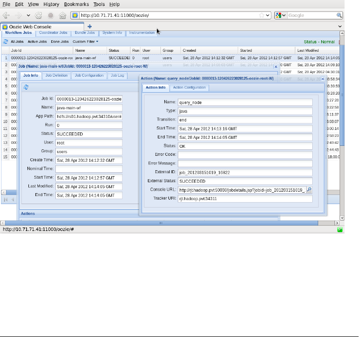
<ok to="end"/>
<error to="fail"/>
</action>
<kill name="fail">
<message>Java failed, error message
[${wf:errorMessage(wf:lastErrorNode())}]</message>
</kill>
<end name="end"/>
</workflow-app>
Oozie Web Console
The Oozie web console is helpful for troubleshooting jobs. Oozie launches each action
inside a map task and captures all the input and output. Oozie does a good job pre-
senting this information as well as providing links to job status pages found on the
Hadoop JobTracker web console.
Here is a screenshot of the Oozie web console.
Variables in Workflows
A workflow based on completely static queries is useful but not overly practical. Most
of the use cases for Oozie run a series of processes against files for today or this week.
242 | Chapter 20: Hive Integration with Oozie
Downloa d f r o m W o w ! e B o o k < w w w.woweb o o k . c o m >

In the previous workflow, you may have noticed the KILL tag and the interpolated
variable inside of it:
<kill name="fail">
<message>Java failed, error message
[${wf:errorMessage(wf:lastErrorNode())}]</message>
</kill>
Oozie provides an ETL to access variables. Key-value pairs defined in job.properties can
be referenced this way.
Capturing Output
Oozie also has a tag <captureOutput/> that can be placed inside an action. Output
captured can be emailed with an error or sent to another process. Oozie sets a Java
property in each action that can be used as a filename to write output to. The code
below shows how this property is accessed:
private static final String
OOZIE_ACTION_OUTPUT_PROPERTIES = "oozie.action.output.properties";
public static void main(String args[]) throws Exception {
String oozieProp = System.getProperty(OOZIE_ACTION_OUTPUT_PROPERTIES);
}
Your application can output data to that location.
Capturing Output to Variables
We have discussed both capturing output and Oozie variables; using them together
provides what you need for daily workflows.
Looking at our previous example, we see that we are selecting data from a hardcoded
day FROM BCO WHERE dt=20120426. We would like to run this workflow every day so we
need to substitute the hardcoded dt=20120426 with a date:
<action name="create_table">
<java>
<job-tracker>${jobTracker}</job-tracker>
<name-node>${nameNode}</name-node>
<configuration>
<property>
<name>mapred.job.queue.name</name>
<value>${queueName}</value>
</property>
</configuration>
<main-class>test.RunShellProp</main-class>
<arg>/bin/date</arg>
<arg>+x=%Y%m%d</arg>
<capture-output />
</java>
<ok to="run_query"/>
Capturing Output to Variables | 243

<error to="fail"/>
</action>
This will produce output like:
$ date +x=%Y%m%d
x=20120522
You can then access this output later in the process:
<arg>You said ${wf:actionData('create_table')['x']}</arg>
There are many more things you can do with Oozie, including integrating Hive jobs
with jobs implemented with other tools, such as Pig, Java MapReduce, etc. See the
Oozie website for more details.
244 | Chapter 20: Hive Integration with Oozie

CHAPTER 21
Hive and Amazon Web Services (AWS)
—Mark Grover
One of the services that Amazon provides as a part of Amazon Web Services (AWS) is
Elastic MapReduce (EMR). With EMR comes the ability to spin up a cluster of nodes
on demand. These clusters come with Hadoop and Hive installed and configured. (You
can also configure the clusters with Pig and other tools.) You can then run your Hive
queries and terminate the cluster when you are done, only paying for the time you used
the cluster. This section describes how to use Elastic MapReduce, some best practices,
and wraps up with pros and cons of using EMR versus other options.
You may wish to refer to the online AWS documentation available at http://aws.amazon
.com/elasticmapreduce/ while reading this chapter. This chapter won’t cover all the
details of using Amazon EMR with Hive. It is designed to provide an overview and
discuss some practical details.
Why Elastic MapReduce?
Small teams and start-ups often don’t have the resources to set up their own cluster.
An in-house cluster is a fixed cost of initial investment. It requires effort to set up and
servers and switches as well as maintaining a Hadoop and Hive installation.
On the other hand, Elastic MapReduce comes with a variable cost, plus the installation
and maintenance is Amazon’s responsibility. This is a huge benefit for teams that can’t
or don’t want to invest in their own clusters, and even for larger teams that need a test
bed to try out new tools and ideas without affecting their production clusters.
Instances
An Amazon cluster is comprised of one or more instances. Instances come in various
sizes, with different RAM, compute power, disk drive, platform, and I/O performance.
It can be hard to determine what size would work the best for your use case. With EMR,
245

it’s easy to start with small instance sizes, monitor performance with tools like Ganglia,
and then experiment with different instance sizes to find the best balance of cost versus
performance.
Before You Start
Before using Amazon EMR, you need to set up an Amazon Web Services (AWS) ac-
count. The Amazon EMR Getting Started Guide provides instructions on how to sign
up for an AWS account.
You will also need to create an Amazon S3 bucket for storing your input data and
retrieving the output results of your Hive processing.
When you set up your AWS account, make sure that all your Amazon EC2 instances,
key pairs, security groups, and EMR jobflows are located in the same region to avoid
cross-region transfer costs. Try to locate your Amazon S3 buckets and EMR jobflows
in the same availability zone for better performance.
Although Amazon EMR supports several versions of Hadoop and Hive, only some
combinations of versions of Hadoop and Hive are supported. See the Amazon EMR
documentation to find out the supported version combinations of Hadoop and Hive.
Managing Your EMR Hive Cluster
Amazon provides multiple ways to bring up, terminate, and modify a Hive cluster.
Currently, there are three ways you can manage your EMR Hive cluster:
EMR AWS Management Console (web-based frontend)
This is the easiest way to bring up a cluster and requires no setup. However, as you
start to scale, it is best to move to one of the other methods.
EMR Command-Line Interface
This allows users to manage a cluster using a simple Ruby-based CLI, named
elastic-mapreduce. The Amazon EMR online documentation describes how to
install and use this CLI.
EMR API
This allows users to manage an EMR cluster by using a language-specific SDK to
call EMR APIs. Details on downloading and using the SDK are available in the
Amazon EMR documentation. SDKs are available for Android, iOS, Java, PHP,
Python, Ruby, Windows, and .NET. A drawback of an SDK is that sometimes
particular SDK wrapper implementations lag behind the latest version of the
AWS API.
It is common to use more than one way to manage Hive clusters.
246 | Chapter 21: Hive and Amazon Web Services (AWS)

Here is an example that uses the Ruby elastic-mapreduce CLI to start up a single-node
Amazon EMR cluster with Hive configured. It also sets up the cluster for interactive
use, rather than for running a job and exiting. This cluster would be ideal for learning
Hive:
elastic-mapreduce --create --alive --name "Test Hive" --hive-interactive
If you also want Pig available, add the --pig-interface option.
Next you would log in to this cluster as described in the Amazon EMR documentation.
Thrift Server on EMR Hive
Typically, the Hive Thrift server (see Chapter 16) listens for connections on port 10000.
However, in the Amazon Hive installation, this port number depends on the version
of Hive being used. This change was implemented in order to allow users to install and
support concurrent versions of Hive. Consequently, Hive v0.5.X operates on port
10000, Hive v0.7.X on 10001, and Hive v0.7.1 on 10002. These port numbers are
expected to change as newer versions of Hive get ported to Amazon EMR.
Instance Groups on EMR
Each Amazon cluster has one or more nodes. Each of these nodes can fit into one of
the following three instance groups:
Master Instance Group
This instance group contains exactly one node, which is called the master node.
The master node performs the same duties as the conventional Hadoop master
node. It runs the namenode and jobtracker daemons, but it also has Hive installed
on it. In addition, it has a MySQL server installed, which is configured to serve as
the metastore for the EMR Hive installation. (The embedded Derby metastore that
is used as the default metastore in Apache Hive installations is not used.) There is
also an instance controller that runs on the master node. It is responsible for
launching and managing other instances from the other two instance groups. Note
that this instance controller also uses the MySQL server on the master node. If the
MySQL server becomes unavailable, the instance controller will be unable to
launch and manage instances.
Core Instance Group
The nodes in the core instance group have the same function as Hadoop slave nodes
that run both the datanode and tasktracker daemons. These nodes are used for
MapReduce jobs and for the ephemeral storage on these nodes that is used for
HDFS. Once a cluster has been started, the number of nodes in this instance group
can only be increased but not decreased. It is important to note that ephemeral
storage will be lost if the cluster is terminated.
Instance Groups on EMR | 247

Task Instance Group
This is an optional instance group. The nodes in this group also function as Hadoop
slave nodes. However, they only run the tasktracker processes. Hence, these nodes
are used for MapReduce tasks, but not for storing HDFS blocks. Once the cluster
has been started, the number of nodes in the task instance group can be increased
or decreased.
The task instance group is convenient when you want to increase cluster capacity during
hours of peak demand and bring it back to normal afterwards. It is also useful when
using spot instances (discussed below) for lower costs without risking the loss of data
when a node gets removed from the cluster.
If you are running a cluster with just a single node, the node would be a master node
and a core node at the same time.
Configuring Your EMR Cluster
You will often want to deploy your own configuration files when launching an EMR
cluster. The most common files to customize are hive-site.xml, .hiverc, hadoop-env.sh.
Amazon provides a way to override these configuration files.
Deploying hive-site.xml
For overriding hive-site.xml, upload your custom hive-site.xml to S3. Let’s assume it
has been uploaded to s3n://example.hive.oreilly.com/tables/hive_site.xml.
It is recommended to use the newer s3n “scheme” for accessing S3,
which has better performance than the original s3 scheme.
If you are starting you cluster via the elastic-mapreduce Ruby client, use a command
like the following to spin up your cluster with your custom hive-site.xml:
elastic-mapreduce --create --alive --name "Test Hive" --hive-interactive \
--hive-site=s3n://example.hive.oreilly.com/conf/hive_site.xml
If you are using the SDK to spin up a cluster, use the appropriate method to override
the hive-site.xml file. After the bootstrap actions, you would need two config steps, one
for installing Hive and another for deploying hive-site.xml. The first step of installing
Hive is to call --install-hive along with --hive-versions flag followed by a comma-
separated list of Hive versions you would like to install on your EMR cluster.
The second step of installing Hive site configuration calls --install-hive-site with
an additional parameter like --hive-site=s3n://example.hive.oreilly.com/tables/
hive_site.xml pointing to the location of the hive-site.xml file to use.
248 | Chapter 21: Hive and Amazon Web Services (AWS)

Deploying a .hiverc Script
For .hiverc, you must first upload to S3 the file you want to install. Then you can either
use a config step or a bootstrap action to deploy the file to your cluster.
Note that .hiverc can be placed in the user’s home directory or in the bin directory of
the Hive installation.
Deploying .hiverc using a config step
At the time of this writing, the functionality to override the .hiverc file is not available
in the Amazon-provided Ruby script, named hive-script, which is available at s3n://
us-east-1.elasticmapreduce/libs/hive/hive-script.
Consequently, .hiverc cannot be installed as easily as hive-site.xml. However, it is fairly
straightforward to extend the Amazon-provided hive-script to enable installation
of .hiverc, if you are comfortable modifying Ruby code. After implementing this change
to hive-script, upload it to S3 and use that version instead of the original Amazon
version. Have your modified script install .hiverc to the user’s home directory or to the
bin directory of the Hive installation.
Deploying a .hiverc using a bootstrap action
Alternatively, you can create a custom bootstrap script that transfers .hiverc from S3 to
the user’s home directory or Hive’s bin directory of the master node. In this script, you
should first configure s3cmd on the cluster with your S3 access key so you can use it to
download the .hiverc file from S3. Then, simply use a command such as the following
to download the file from S3 and deploy it in the home directory:
s3cmd get s3n://example.hive.oreilly.com/conf/.hiverc ~/.hiverc
Then use a bootstrap action to call this script during the cluster creation process, just
like you would any other bootstrap action.
Setting Up a Memory-Intensive Configuration
If you are running a memory-intensive job, Amazon provides some predefined boot-
strap actions that can be used to fine tune the Hadoop configuration parameters. For
example, to use the memory-intensive bootstrap action when spinning up your cluster,
use the following flag in your elastic-mapreduce --create command (wrapped for
space):
--bootstrap-action
s3n://elasticmapreduce/bootstrap-actions/configurations/latest/memory-intensive
Configuring Your EMR Cluster | 249

Persistence and the Metastore on EMR
An EMR cluster comes with a MySQL server installed on the master node of the cluster.
By default, EMR Hive uses this MySQL server as its metastore. However, all data stored
on the cluster nodes are deleted once you terminate your cluster. This includes the data
stored on the master node metastore, as well! This is usually unacceptable because you
would like to retain your table schemas, etc., in a persistent metastore.
You can use one of the following methods to work around this limitation:
Use a persistent metastore external to your EMR cluster
The details on how to configure your Hive installation to use an external metastore
are in “Metastore Using JDBC” on page 28. You can use the Amazon RDS (Rela-
tional Data Service), which is based on MySQL, or another, in-house database
server as a metastore. This is the best choice if you want to use the same metastore
for multiple EMR clusters or the same EMR cluster running more than one version
of Hive.
Leverage a start-up script
If you don’t intend to use an external database server for your metastore, you can
still use the master node metastore in conjunction with your start-up script. You
can place your create table statements in startup.q, as follows:
CREATE EXTERNAL TABLE IF NOT EXISTS emr_table(id INT, value STRING)
PARTITIONED BY (dt STRING)
LOCATION 's3n://example.hive.oreilly.com/tables/emr_table';
It is important to include the IF NOT EXISTS clause in your create statement to
ensure that the script doesn’t try to re-create the table on the master node metastore
if it was previously created by a prior invocation of startup.q.
At this point, we have our table definitions in the master node metastore but we
haven’t yet imported the partitioning metadata. To do so, include a line like the
following in your startup.q file after the create table statement:
ALTER TABLE emr_table RECOVER PARTITIONS;
This will populate all the partitioning related metadata in the metastore. Instead
of your custom start-up script, you could use .hiverc, which will be sourced auto-
matically when Hive CLI starts up. (We’ll discuss this feature again in “EMR Versus
EC2 and Apache Hive” on page 254).
The benefit of using .hiverc is that it provides automatic invocation. The disad-
vantage is that it gets executed on every invocation of the Hive CLI, which leads
to unnecessary overhead on subsequent invocations.
250 | Chapter 21: Hive and Amazon Web Services (AWS)

The advantage of using your custom start-up script is that you can more strictly
control when it gets executed in the lifecycle of your workflow. However, you will
have to manage this invocation yourself. In any case, a side benefit of using a file
to store Hive queries for initialization is that you can track the changes to your
DDL via version control.
As your meta information gets larger with more tables and more
partitions, the start-up time using this system will take longer and
longer. This solution is not suggested if you have more than a few
tables or partitions.
MySQL dump on S3
Another, albeit cumbersome, alternative is to back up your metastore before you
terminate the cluster and restore it at the beginning of the next workflow. S3 is a
good place to persist the backup while the cluster is not in use.
Note that this metastore is not shared amongst different versions of Hive running on
your EMR cluster. Suppose you spin up a cluster with both Hive v0.5 and v0.7.1 in-
stalled. When you create a table using Hive v0.5, you won’t be able to access this table
using Hive v0.7.1. If you would like to share the metadata between different Hive ver-
sions, you will have to use an external persistent metastore.
HDFS and S3 on EMR Cluster
HDFS and S3 have their own distinct roles in an EMR cluster. All the data stored on
the cluster nodes is deleted once the cluster is terminated. Since HDFS is formed by
ephemeral storage of the nodes in the core instance group, the data stored on HDFS is
lost after cluster termination.
S3, on the other hand, provides a persistent storage for data associated with the EMR
cluster. Therefore, the input data to the cluster should be stored on S3 and the final
results obtained from Hive processing should be persisted to S3, as well.
However, S3 is an expensive storage alternative to HDFS. Therefore, intermediate re-
sults of processing should be stored in HDFS, with only the final results saved to S3
that need to persist.
Please note that as a side effect of using S3 as a source for input data, you lose the
Hadoop data locality optimization, which may be significant. If this optimization is
crucial for your analysis, you should consider importing “hot” data from S3 onto HDFS
before processing it. This initial overhead will allow you to make use of Hadoop’s data
locality optimization in your subsequent processing.
HDFS and S3 on EMR Cluster | 251

Putting Resources, Configs, and Bootstrap Scripts on S3
You should upload all your bootstrap scripts, configuration scripts (e.g., hive-
site.xml and .hiverc), resources (e.g., files that need to go in the distributed cache, UDF
or streaming JARs), etc., onto S3. Since EMR Hive and Hadoop installations natively
understand S3 paths, it is straightforward to work with these files in subsequent Ha-
doop jobs.
For example, you can add the following lines in .hiverc without any errors:
ADD FILE s3n://example.hive.oreilly.com/files/my_file.txt;
ADD JAR s3n://example.hive.oreilly.com/jars/udfs.jar;
CREATE TEMPORARY FUNCTION my_count AS 'com.oreilly.hive.example.MyCount';
Logs on S3
Amazon EMR saves the log files to the S3 location pointed to by the log-uri field. These
include logs from bootstrap actions of the cluster and the logs from running daemon
processes on the various cluster nodes. The log-uri field can be set in the creden-
tials.json file found in the installation directory of the elastic-mapreduce Ruby client.
It can also be specified or overridden explicitly when spinning up the cluster using
elastic-mapreduce by using the --log-uri flag. However, if this field is not set, those
logs will not be available on S3.
If your workflow is configured to terminate if your job encounters an error, any logs
on the cluster will be lost after the cluster termination. If your log-uri field is set, these
logs will be available at the specified location on S3 even after the cluster has been
terminated. They can be an essential aid in debugging the issues that caused the failure.
However, if you store logs on S3, remember to purge unwanted logs on a frequent basis
to save yourself from unnecessary storage costs!
Spot Instances
Spot instances allows users to bid on unused Amazon capacity to get instances at
cheaper rates compared to on-demand prices. Amazon’s online documentation de-
scribes them in more detail.
Depending on your use case, you might want instances in all three instance groups to
be spot instances. In this case, your entire cluster could terminate at any stage during
the workflow, resulting in a loss of intermediate data. If it’s “cheap” to repeat the
calculation, this might not be a serious issue. An alternative is to persist intermediate
data periodically to S3, as long as your jobs can start again from those snapshots.
Another option is to only include the nodes in the task instance group as spot nodes.
If these spot nodes get taken out of the cluster because of unavailability or because the
spot prices increased, the workflow will continue with the master and core nodes, but
252 | Chapter 21: Hive and Amazon Web Services (AWS)

with no data loss. When spot nodes get added to the cluster again, MapReduce tasks
can be delegated to them, speeding up the workflow.
Using the elastic-mapreduce Ruby client, spot instances can be ordered by using the
--bid-price option along with a bid price. The following example shows a command
to create a cluster with one master node, two core nodes and two spot nodes (in the
task instance group) with a bid price of 10 cents:
elastic-mapreduce --create --alive --hive-interactive \
--name "Test Spot Instances" \
--instance-group master --instance-type m1.large \
--instance-count 1 --instance-group core \
--instance-type m1.small --instance-count 2 --instance-group task \
--instance-type m1.small --instance-count 2 --bid-price 0.10
If you are spinning up a similar cluster using the Java SDK, use the following Instance
GroupConfig variables for master, core, and task instance groups:
InstanceGroupConfig masterConfig = new InstanceGroupConfig()
.withInstanceCount(1)
.withInstanceRole("MASTER")
.withInstanceType("m1.large");
InstanceGroupConfig coreConfig = new InstanceGroupConfig()
.withInstanceCount(2)
.withInstanceRole("CORE")
.withInstanceType("m1.small");
InstanceGroupConfig taskConfig = new InstanceGroupConfig()
.withInstanceCount(2)
.withInstanceRole("TASK")
.withInstanceType("m1.small")
.withMarket("SPOT")
.withBidPrice("0.05");
If a map or reduce task fails, Hadoop will have to start them from the
beginning. If the same task fails four times (configurable by setting the
MapReduce properties mapred.map.max.attempts for map tasks and
mapred.reduce.max.attempts for reduce tasks), the entire job will fail. If
you rely on too many spot instances, your job times may be unpredict-
able or fail entirely by TaskTrackers getting removed from the cluster.
Security Groups
The Hadoop JobTracker and NameNode User Interfaces are accessible on port 9100
and 9101 respectively in the EMRmaster node. You can use ssh tunneling or a dynamic
SOCKS proxy to view them.
In order to be able to view these from a browser on your client machine (outside of the
Amazon network), you need to modify the Elastic MapReduce master security group
via your AWS Web Console. Add a new custom TCP rule to allow inbound connections
from your client machine’s IP address on ports 9100 and 9101.
Security Groups | 253

EMR Versus EC2 and Apache Hive
An elastic alternative to EMR is to bring up several Amazon EC2 nodes and install
Hadoop and Hive on a custom Amazon Machine Image (AMI). This approach gives
you more control over the version and configuration of Hive and Hadoop. For example,
you can experiment with new releases of tools before they are made available through
EMR.
The drawback of this approach is that customizations available through EMR may not
be available in the Apache Hive release. As an example, the S3 filesystem is not fully
supported on Apache Hive [see JIRA HIVE-2318]. There is also an optimization for
reducing start-up time for Amazon S3 queries, which is only available in EMR Hive.
This optimization is enabled by adding the following snippet in your hive-site.xml:
<property>
<name>hive.optimize.s3.query</name>
<value>true</value>
<description> Improves Hive query performance for Amazon S3 queries
by reducing their start up time </description>
</property>
Alternatively, you can run the following command on your Hive CLI:
set hive.optimize.s3.query=true;
Another example is a command that allows the user to recover partitions if they exist
in the correct directory structure on HDFS or S3. This is convenient when an external
process is populating the contents of the Hive table in appropriate partitions. In order
to track these partitions in the metastore, one could run the following command, where
emr_table is the name of the table:
ALTER TABLE emr_table RECOVER PARTITIONS;
Here is the statement that creates the table, for your reference:
CREATE EXTERNAL TABLE emr_table(id INT, value STRING)
PARTITIONED BY (dt STRING)
LOCATION 's3n://example.hive.oreilly.com/tables/emr_table';
Wrapping Up
Amazon EMR provides an elastic, scalable, easy-to-set-up way to bring up a cluster
with Hadoop and Hive ready to run queries as soon as it boots. It works well with data
stored on S3. While much of the configuration is done for you, it is flexible enough to
allow users to have their own custom configurations.
254 | Chapter 21: Hive and Amazon Web Services (AWS)

CHAPTER 22
HCatalog
—Alan Gates
Introduction
Using Hive for data processing on Hadoop has several nice features beyond the ability
to use an SQL-like language. It’s ability to store metadata means that users do not need
to remember the schema of the data. It also means they do not need to know where the
data is stored, or what format it is stored in. This decouples data producers, data con-
sumers, and data administrators. Data producers can add a new column to the data
without breaking their consumers’ data-reading applications. Administrators can re-
locate data to change the format it is stored in without requiring changes on the part
of the producers or consumers.
The majority of heavy Hadoop users do not use a single tool for data production and
consumption. Often, users will begin with a single tool: Hive, Pig, MapReduce, or
another tool. As their use of Hadoop deepens they will discover that the tool they chose
is not optimal for the new tasks they are taking on. Users who start with analytics
queries with Hive discover they would like to use Pig for ETL processing or constructing
their data models. Users who start with Pig discover they would like to use Hive for
analytics type queries.
While tools such as Pig and MapReduce do not require metadata, they can benefit from
it when it is present. Sharing a metadata store also enables users across tools to share
data more easily. A workflow where data is loaded and normalized using MapReduce
or Pig and then analyzed via Hive is very common. When all these tools share one
metastore, users of each tool have immediate access to data created with another tool.
No loading or transfer steps are required.
HCatalog exists to fulfill these requirements. It makes the Hive metastore available to
users of other tools on Hadoop. It provides connectors for MapReduce and Pig so that
users of those tools can read data from and write data to Hive’s warehouse. It has a
255

command-line tool for users who do not use Hive to operate on the metastore with
Hive DDL statements. It also provides a notification service so that workflow tools,
such as Oozie, can be notified when new data becomes available in the warehouse.
HCatalog is a separate Apache project from Hive, and is part of the Apache Incubator.
The Incubator is where most Apache projects start. It helps those involved with the
project build a community around the project and learn the way Apache software is
developed. As of this writing, the most recent version is HCatalog 0.4.0-incubating.
This version works with Hive 0.9, Hadoop 1.0, and Pig 0.9.2.
MapReduce
Reading Data
MapReduce uses a Java class InputFormat to read input data. Most frequently, these
classes read data directly from HDFS. InputFormat implementations also exist to read
data from HBase, Cassandra, and other data sources. The task of the InputFormat is
twofold. First, it determines how data is split into sections so that it can be processed
in parallel by MapReduce’s map tasks. Second, it provides a RecordReader, a class that
MapReduce uses to read records from its input source and convert them to keys and
values for the map task to operate on.
HCatalog provides HCatInputFormat to enable MapReduce users to read data stored in
Hive’s data warehouse. It allows users to read only the partitions of tables and columns
that they need. And it provides the records in a convenient list format so that users do
not need to parse them.
HCatInputFormat implements the Hadoop 0.20 API, org.apache.hadoop
.mapreduce, not the Hadoop 0.18 org.apache.hadoop.mapred API. This
is because it requires some features added in the MapReduce (0.20) API.
This means that a MapReduce user will need to use this interface to
interact with HCatalog. However, Hive requires that the underlying
InputFormat used to read data from disk be a mapred implementation.
So if you have data formats you are currently using with a MapReduce
InputFormat, you can use it with HCatalog. InputFormat is a class in the
mapreduce API and an interface in the mapred API, hence it was referred
to as a class above.
When initializing HCatInputFormat, the first thing to do is specify the table to be read.
This is done by creating an InputJobInfo class and specifying the database, table, and
partition filter to use.
256 | Chapter 22: HCatalog

InputJobInfo.java
/**
* Initializes a new InputJobInfo
* for reading data from a table.
* @param databaseName the db name
* @param tableName the table name
* @param filter the partition filter
*/
public static InputJobInfo create(String databaseName,
String tableName,
String filter) {
...
}
databaseName name indicates the Hive database (or schema) the table is in. If this is null
then the default database will be used. The tableName is the table that will be read. This
must be non-null and refer to a valid table in Hive. filter indicates which partitions
the user wishes to read. If it is left null then the entire table will be read. Care should
be used here, as reading all the partitions of a large table can result in scanning a large
volume of data.
Filters are specified as an SQL-like where clause. They should reference only partition
columns of the data. For example, if the table to be read is partitioned on a column
called datestamp, the filter might look like datestamp = "2012-05-26". Filters can contain
=, >, >=, <, <=, and, and or as operators.
There is a bug in the ORM mapping layer used by Hive v0.9.0 and earlier that causes
filter clauses with >, >=, <, or <= to fail.
To resolve this bug, you can apply the patch HIVE-2084.D2397.1.patch
from https://issues.apache.org/jira/browse/HIVE-2084 and rebuild your
version of Hive. This does carry some risks, depending on how you
deploy Hive. See the discussion on the JIRA entry.
This InputJobInfo instance is then passed to HCatInputFormat via the method setIn
put along with the instance of Job being used to configure the MapReduce job:
Job job = new Job(conf, "Example");
InputJobInfo inputInfo = InputJobInfo.create(dbName, inputTableName, filter));
HCatInputFormat.setInput(job, inputInfo);
The map task will need to specify HCatRecord as a value type. The key type is not im-
portant, as HCatalog does not provide keys to the map task. For example, a map task
that reads data via HCatalog might look like:
public static class Map extends
Mapper<WritableComparable, HCatRecord, Text, Text> {
@Override
protected void map(
MapReduce | 257

WritableComparable key,
HCatRecord value,
org.apache.hadoop.mapreduce.Mapper<WritableComparable,
HCatRecord, Text, HCatRecord>.Context context) {
...
}
}
HCatRecord is the class that HCatalog provides for interacting with records. It presents
a simple get and set interface. Records can be requested by position or by name. When
requesting columns by name, the schema must be provided, as each individual HCatRe
cord does not keep a reference to the schema. The schema can be obtained by calling
HCatInputFormat.getOutputSchema(). Since Java does not support overloading of func-
tions by return type, different instances of get and set are provided for each data type.
These methods use the object versions of types rather than scalar versions (that is
java.lang.Integer rather than int). This allows them to express null as a value. There
are also implementations of get and set that work with Java Objects:
// get the first column, as an Object and cast it to a Long
Long cnt = record.get(0);
// get the column named "cnt" as a Long
Long cnt = record.get("cnt", schema);
// set the column named "user" to the string "fred"
record.setString("user", schema, "fred");
Often a program will not want to read all of the columns in an input. In this case it
makes sense to trim out the extra columns as quickly as possible. This is particularly
true in columnar formats like RCFile, where trimming columns early means reading
less data from disk. This can be achieved by passing a schema that describes the desired
columns. This must be done during job configuration time. The following example will
configure the user’s job to read only two columns named user and url:
HCatSchema baseSchema = HCatBaseInputFormat.getOutputSchema(context);
List<HCatFieldSchema> fields = new List<HCatFieldSchema>(2);
fields.add(baseSchema.get("user"));
fields.add(baseSchema.get("url"));
HCatBaseInputFormat.setOutputSchema(job, new HCatSchema(fields));
Writing Data
Similar to reading data, when writing data, the database and table to be written to need
to be specified. If the data is being written to a partitioned table and only one partition
is being written, then the partition to be written needs to be specified as well:
/**
* Initializes a new OutputJobInfo instance for writing data from a table.
* @param databaseName the db name
* @param tableName the table name
* @param partitionValues The partition values to publish to, can be null or empty Map
*/
258 | Chapter 22: HCatalog

public static OutputJobInfo create(String databaseName,
String tableName,
Map<String, String> partitionValues) {
...
}
The databaseName name indicates the Hive database (or schema) the table is in. If this
is null then the default database will be used. The tableName is the table that will be
written to. This must be non-null and refer to a valid table in Hive. partitionValues
indicates which partition the user wishes to create. If only one partition is to be written,
the map must uniquely identify a partition. For example, if the table is partitioned by
two columns, entries for both columns must be in the map. When working with tables
that are not partitioned, this field can be left null. When the partition is explicitly
specified in this manner, the partition column need not be present in the data. If it is,
it will be removed by HCatalog before writing the data to the Hive warehouse, as Hive
does not store partition columns with the data.
It is possible to write to more than one partition at a time. This is referred to as dynamic
partitioning, because the records are partitioned dynamically at runtime. For dynamic
partitioning to be used, the values of the partition column(s) must be present in the
data. For example, if a table is partitioned by a column “datestamp,” that column must
appear in the data collected in the reducer. This is because HCatalog will read the
partition column(s) to determine which partition to write the data to. As part of writing
the data, the partition column(s) will be removed.
Once an OutputJobInfo has been created, it is then passed to HCatOutputFormat via the
static method setOutput:
OutputJobInfo outputInfo = OutputJobInfo.create(dbName, outputTableName, null));
HCatOutputFormat.setOutput(job, outputInfo);
When writing with HCatOutputFormat, the output key type is not important. The value
must be HCatRecord. Records can be written from the reducer, or in map only jobs from
the map task.
Putting all this together in an example, the following code will read a partition with a
datestamp of 20120531 from the table rawevents, count the number of events for each
user, and write the result to a table cntd:
public class MRExample extends Configured implements Tool {
public static class Map extends
Mapper<WritableComparable, HCatRecord, Text, LongWritable> {
protected void map(WritableComparable key,
HCatRecord value,
Mapper<WritableComparable, HCatRecord,
Text, LongWritable>.Context context)
throws IOException, InterruptedException {
// Get our schema from the Job object.
HCatSchema schema = HCatBaseInputFormat.getOutputSchema(context);
MapReduce | 259
Downloa d f r o m W o w ! e B o o k < w w w.woweb o o k . c o m >

// Read the user field
String user = value.get("user", schema);
context.write(new Text(user), new LongWritable(1));
}
}
public static class Reduce extends Reducer<Text, LongWritable,
WritableComparable, HCatRecord> {
protected void reduce(Text key, Iterable<LongWritable> values,
Reducer<Text, LongWritable,
WritableComparable, HCatRecord>.Context context)
throws IOException ,InterruptedException {
List<HCatFieldSchema> columns = new ArrayList<HCatFieldSchema>(2);
columns.add(new HCatFieldSchema("user", HCatFieldSchema.Type.STRING, ""));
columns.add(new HCatFieldSchema("cnt", HCatFieldSchema.Type.BIGINT, ""));
HCatSchema schema = new HCatSchema(columns);
long sum = 0;
Iterator<IntWritable> iter = values.iterator();
while (iter.hasNext()) sum += iter.next().getLong();
HCatRecord output = new DefaultHCatRecord(2);
record.set("user", schema, key.toString());
record.setLong("cnt", schema, sum);
context.write(null, record);
}
}
public int run(String[] args) throws Exception {
Job job = new Job(conf, "Example");
// Read the "rawevents" table, partition "20120531", in the default
// database
HCatInputFormat.setInput(job, InputJobInfo.create(null, "rawevents",
"datestamp='20120531'"));
job.setInputFormatClass(HCatInputFormat.class);
job.setJarByClass(MRExample.class);
job.setMapperClass(Map.class);
job.setReducerClass(Reduce.class);
job.setMapOutputKeyClass(Text.class);
job.setMapOutputValueClass(LongWritable.class);
job.setOutputKeyClass(WritableComparable.class);
job.setOutputValueClass(DefaultHCatRecord.class);
// Write into "cntd" table, partition "20120531", in the default database
HCatOutputFormat.setOutput(job
OutputJobInfo.create(null, "cntd", "ds=20120531"));
job.setOutputFormatClass(HCatOutputFormat.class);
return (job.waitForCompletion(true) ? 0 : 1);
}
public static void main(String[] args) throws Exception {
int exitCode = ToolRunner.run(new MRExample(), args);
System.exit(exitCode);
}
}
260 | Chapter 22: HCatalog

Command Line
Since HCatalog utilizes Hive’s metastore, Hive users do not need an additional tool to
interact with it. They can use the Hive command-line tool as before. However, for
HCatalog users that are not also Hive users, a command-line tool hcat is provided. This
tool is very similar to Hive’s command line. The biggest difference is that it only accepts
commands that do not result in a MapReduce job being spawned. This means that the
vast majority of DDL (Data Definition Language, or operations that define the data,
such as creating tables) are supported:
$ /usr/bin/hcat -e "create table rawevents (user string, url string);"
The command line supports the following options:
Option Explanation Example
-e Execute DDL provided on the command
line hcat -e “show tables;”
-f Execute DDL provided in a script file hcat -f setup.sql
-g See the security section below
-p See the security section below
-D Port for the Cassandra server hcat -Dlog.level=INFO
-h Port for the Cassandra server hcat -h
The SQL operations that HCatalog’s command line does not support are:
•SELECT
•CREATE TABLE AS SELECT
•INSERT
•LOAD
•ALTER INDEX REBUILD
•ALTER TABLE CONCATENATE
•ALTER TABLE ARCHIVE
•ANALYZE TABLE
•EXPORT TABLE
•IMPORT TABLE
Security Model
HCatalog does not make use of Hive’s authorization model. However, user authenti-
cation in HCatalog is identical to Hive. Hive attempts to replicate traditional database
authorization models. However, this has some limitations in the Hadoop ecosystem.
Security Model | 261

Since it is possible to go directly to the filesystem and access the underlying data, au-
thorization in Hive is limited. This can be resolved by having all files and directories
that contain Hive’s data be owned by the user running Hive jobs. This way other users
can be prevented from reading or writing data, except through Hive. However, this has
the side effect that all UDFs in Hive will then run as a super user, since they will be
running in the Hive process. Consequently, they will have read and write access to all
files in the warehouse.
The only way around this in the short term is to declare UDFs to be a privileged oper-
ation and only allow those with proper access to create UDFs, though there is no
mechanism to enforce this currently. This may be acceptable in the Hive context, but
in Pig and MapReduce where user-generated code is the rule rather than the exception,
this is clearly not acceptable.
To resolve these issues, HCatalog instead delegates authorization to the storage layer.
In the case of data stored in HDFS, this means that HCatalog looks at the directories
and files containing data to see if a user has access to the data. If so, he will be given
identical access to the metadata. For example, if a user has permission to write to a
directory that contains a table’s partitions, she will also have permission to write to
that table.
This has the advantage that it is truly secure. It is not possible to subvert the system by
changing abstraction levels. The disadvantage is that the security model supported by
HDFS is much poorer than is traditional for databases. In particular, features such as
column-level permissions are not possible. Also, users can only be given permission to
a table by being added to a filesystem group that owns that file.
Architecture
As explained above, HCatalog presents itself to MapReduce and Pig using their stan-
dard input and output mechanisms. HCatLoader and HCatStorer are fairly simple since
they sit atop HCatInputFormat and HCatOutputFormat, respectively. These two
MapReduce classes do a fair amount of work to integrate MapReduce with Hive’s
metastore.
Figure 22-1 shows the HCatalog architecture.
HCatInputFormat communicates with Hive’s metastore to obtain information about the
table and partition(s) to be read. This includes finding the table schema as well as
schema for each partition. For each partition it must also determine the actual Input
Format and SerDe to use to read the partition. When HCatInputFormat.getSplits is
called, it instantiates an instance of the InputFormat for each partition and calls
getSplits on that InputFormat. These are then collected together and the splits from
all the partitions returned as the list of InputSplits.
262 | Chapter 22: HCatalog
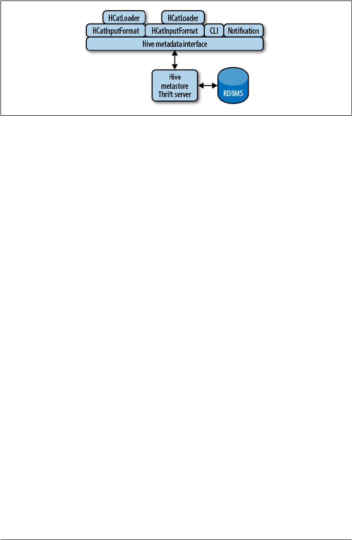
Similarly, the RecordReaders from each underlying InputFormat are used to decode the
partitions. The HCatRecordReader then converts the values from the underlying Record
Reader to HCatRecords via the SerDe associated with the partition. This includes padding
each partition with any missing columns. That is, when the table schema contains
columns that the partition schema does not, columns with null values must be added
to the HCatRecord. Also, if the user has indicated that only certain columns are needed,
then the extra columns are trimmed out at this point.
HCatOutputFormat also communicates with the Hive metastore to determine the proper
file format and schema for writing. Since HCatalog only supports writing data in the
format currently specified for the table, there is no need to open different OutputFor
mats per partition. The underlying OutputFormat is wrapped by HCatOutputFormat. A
RecordWriter is then created per partition that wraps the underlying RecordWriter,
while the indicated SerDe is used to write data into these new records. When all of the
partitions have been written, HCatalog uses an OutputCommitter to commit the data to
the metastore.
Figure 22-1. HCatalog architecture diagram
Architecture | 263

CHAPTER 23
Case Studies
Hive is in use at a multitude of companies and organizations around the world. This
case studies chapter details interesting and unique use cases, the problems that were
present, and how those issues were solved using Hive as a unique data warehousing
tool for petabytes of data.
m6d.com (Media6Degrees)
Data Science at M6D Using Hive and R
by Ori Stitelman
In this case study we examine one of many approaches our data science team, here at
m6d, takes toward synthesizing the immense amount of data that we are able to extract
using Hive. m6d is a display advertising prospecting company. Our role is to create
machine learning algorithms that are specifically tailored toward finding the best new
prospects for an advertising campaign. These algorithms are layered on top of a delivery
engine that is tied directly into a myriad of real time bidding exchanges that provide a
means to purchase locations on websites to display banner advertisements on behalf
of our clients. The m6d display advertising engine is involved in billions of auctions a
day and tens of millions of advertisements daily. Naturally, such a system produces an
immense amount of data. A large portion of the records that are generated by our
company’s display advertising delivery system are housed in m6d’s Hadoop cluster
and, as a result, Hive is the primary tool our data science team uses to interact with the
these logs.
Hive gives our data science team a way to extract and manipulate large amounts of
data. In fact, it allows us to extract samples and summarize data that prior to using
Hive could not be analyzed as efficiently, or at all, because of the immense size. Despite
the fact that Hive allows us access to huge amounts of data at rates many times faster
than before, it does not change the fact that most of the tools that we were previously
familiar with as data scientists are not always able to analyze data samples of the size
265

we can now produce. In summary, Hive provides us a great tool to extract huge amounts
of data; however, the toolbox of data science, or statistical learning, methods that we
as data scientists are used to using cannot easily accommodate the new larger data sets
without substantial changes.
Many different software packages have been developed or are under development for
both supervised and unsupervised learning on large data sets. Some of these software
packages are stand alone software implementations, such as Vowpal Wabbit and BBR,
while others are implementations within a larger infrastructure such as Mahout for
Hadoop or the multitude of “large data” packages for R. A portion of these algorithms
take advantage of parallel programing approaches while others rely on different meth-
ods to achieve scalability.
The primary tool for statistical learning for several of the data scientists in our team is
R. It provides a large array of packages that are able to perform many statistical learning
methods. More importantly, we have a lot of experience with it, know how its packages
perform, understand their features, and are very familiar with its documentation. How-
ever, one major drawback of R is that by default it loads the entire data set into memory.
This is a major limitation considering that the majority of the data sets that we extract
from Hive and are able to analyze today are much larger than what can fit in memory.
Moreover, once the data in R is larger than what is able to fit in memory, the system
will start swapping, which leads to the system thrashing and massive decreases in pro-
cessing speed.1
In no way are we advocating ignoring the new tools that are available. Obviously, it is
important to take advantage of the best of these scalable technologies, but only so much
time can be spent investigating and testing new technology. So now we are left with a
choice of either using the new tools that are available for large data sets or downsam-
pling our data to fit into the tools that we are more familiar with. If we decide to use
the new tools, we can gain signal by letting our data learn off of more data, and as a
result the variance in our estimates will decrease. This is particularly appealing in sit-
uations where the outcome is very rare. However, learning these new tools takes time
and there is an opportunity cost of using that time to learn new tools rather than an-
swering other questions that have particular value to the company.
Alternatively, we can downsample the data to obtain something that can fit in the old
tools we have at our disposal, but must deal with a loss of signal and increased variance
in our estimates. However, this allows us to deal with tools with which we are familiar
and the features that they provide. Thus, we are able to retain the functionality of our
current toolbox at the price of losing some signal. However, these are not the only two
possible approaches. In this case study, we highlight a way that we can both retain the
functionality of the current toolbox as well as gain signal, or decrease variance, by using
a larger sample, or all, of the data available to us.
1. http://www.r-bloggers.com/taking-r-to-the-limit-large-datasets-predictive-modeling-with-pmml-and
-adapa/
266 | Chapter 23: Case Studies
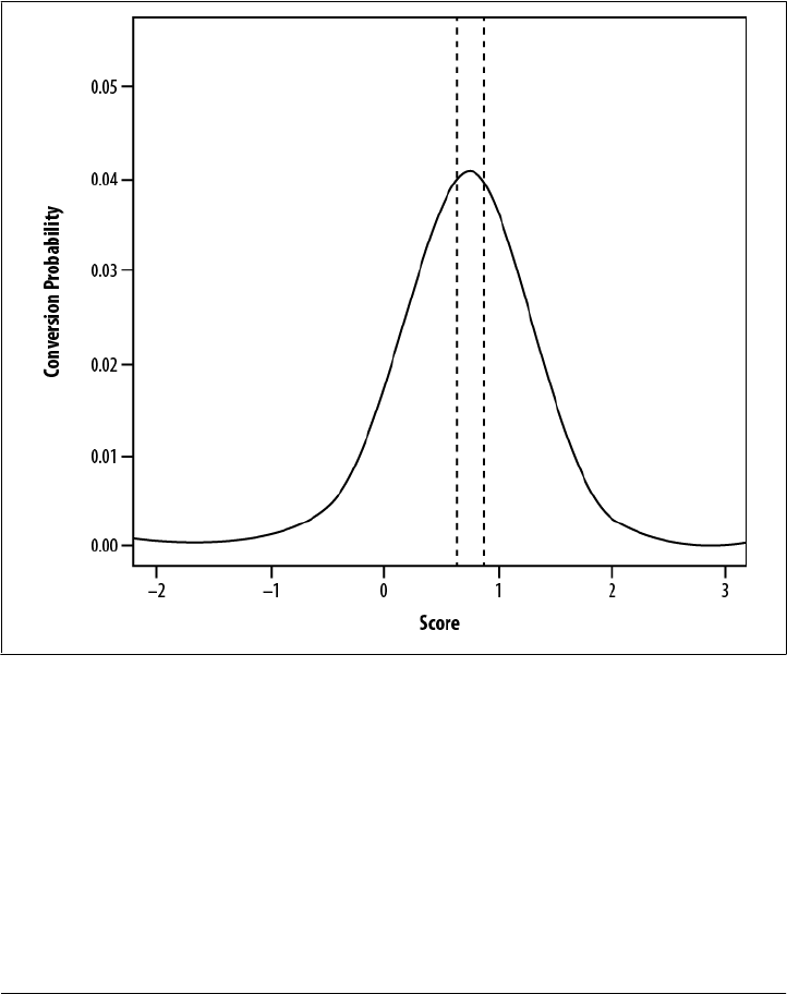
Figure 23-1 shows the probability of converting versus the score from an algorithm
designed to rank prospects for an advertising campaign. Higher scores should indicate
a higher probability of conversion. This plot clearly shows that the top individuals are
converting at a lower rate than some of the lower scoring browsers. That is, browsers
with scores greater than 1 convert at a lower rate than individuals with scores between
0.5 and 1.0. Considering that some campaigns only target a very small percentage of
the overall population, it is important the best prospects are among the top scorers.
Figure 23-1. Probability of conversion versus score
The line that expresses the relationship between the score and the conversion proba-
bility seen in Figure 23-1 is generated using a generalized additive model (GAM) in the
statistical programming package R.2 The details about GAMs will not be presented
here. For the purpose of this case study it can be thought of as a black box that produces
for each score a prediction of the conversion rate. The browsers can then be re-ranked
2. For more details on the use of generalized additive models (GAM), see Hastie et al. 2001. The R package
used to implement the GAM for the purpose of the analysis presented here is the mgcv package available
at http://cran.r-project.org/.
m6d.com (Media6Degrees) | 267

based on the predicted conversion rate; thus, the predicted conversion rate becomes
the new score.
The new ranking can be generated in the following way. First, extract the scores for
each individual browser and then follow them for some designated period of time, say
five days, and record if they took the desired action, and thus converted. Consider a
Hive table called scoretable that has the following information and is partitioned on
date and subpartitioned by offer.
Name Type Description
score double The score is the score generated by the
initial algorithm that does not neces-
sarily rank order appropriately.
convert int The variable convert is a binary variable
that is equal to one if the individual
browser takes the desired action in the
following five days and equal to zero if
not.
date int The day that the browser was given the
particular score.
offer int An ID of an offer.
The following query can then be used to extract a set of data from scoretable for use in
R to estimate the GAM line that predicts conversion for different levels of score like in
the preceding table:
SELECT score,convert
FROM scoretable
WHERE date >= (…) AND date <= (…)
AND offer = (…);
1.2347 0
3.2322 1
0.0013 0
0.3441 0
This data is then loaded into R and the following code is used to create the predicted
conversion probability versus score, as in the preceding table:
library(mgcv)
g1=gam(convert~s(score),family=binomial,data=[data frame name])
The issue with this approach is that it only can be used for a limited number of days of
data because the data set gets too large and R begins thrashing for any more than three
days of data. Moreover, it takes approximately 10 minutes of time for each campaign
to do this for about three days of data. So, running this analysis for about 300 campaigns
for a single scoring method took about 50 hours for three days of data.
By simply extracting the data from Hive in a slightly different way and making use of
the feature of the gam function in mgcv that allows for frequency weights, the same
268 | Chapter 23: Case Studies

analysis may be done using more data, and thus gaining more signal, at a much faster
rate. This is done by selecting the data from Hive by rounding the score to the nearest
hundredth and getting frequency weights for each rounded score, convert combination
by using a GROUP BY query. This is a very common approach for dealing with large data
sets and in the case of these scores there should be no loss of signal due to rounding
because there is no reason to believe that individuals with scores that differ by less than
0.001 are any different from each other. The following query would select such a data
set:
SELECT round(score,2) as score,convert,count(1) AS freq
FROM scoretable
WHERE date >= [start.date] and date <= [end.date] and offer = [chosen.offer]
GROUP BY round(score,2),convert;
1.23 0 500
3.23 1 22
0.00 0 127
0.34 0 36
The resulting data set is significantly smaller than the original approach presented that
does not use frequency weights. In fact, the initial data set for each offer consisted of
millions of records, and this new data set consists of approximately 6,500 rows per
offer. The new data is then loaded into R and the following code may be used to generate
the new GAM results:
library(mgcv)
g2=gam(convert~s(score),family=binomial,weights=freq,
data=[frequency weight data frame name])
(We wrapped the line.)
The previously presented approach took 10 minutes per offer to create the GAM for
only three days of data, compared to the frequency-weighted approach which was able
to create the GAM based on seven days of data in approximately 10 seconds. Thus, by
using frequency weights, the analysis for the 300 campaigns was able to be done in 50
minutes compared to 50 hours using the originally presented approach. This increase
in speed was also realized while using more than twice the amount of data resulting in
more precise estimates of the predicted conversion probabilities. In summary, the fre-
quency weights allowed for a more precise estimate of the GAM in significantly less
time.
In the presented case study, we showed how by rounding the continuous variables and
grouping like variables with frequency weights, we were both able to get more precise
estimates by using more data and fewer computational resources, resulting in quicker
estimates. The example shown was for a model with a single feature, score. In general,
this is an approach that will work well for a low number of features or a larger number
of sparse features. The above approach may be extended to higher dimensional prob-
lems as well using some other small tricks. One way this can be done for a larger number
of variables is by bucketing the variables, or features, into binary variables and then
using GROUP BY queries and frequency weights for those features. However, as the
m6d.com (Media6Degrees) | 269

number of features increases, and those features are not sparse, there is little value
gained by such an approach and other alternative methods must be explored, or soft-
ware designed for larger data sets must be embraced.
M6D UDF Pseudorank
by David Ha and Rumit Patel
Sorting data and identifying the top N elements is straightforward. You order the whole
data set by some criteria and limit the result set to N. But there are times when you
need to group like elements together and find the top N elements within that group
only. For example, identifying the top 10 requested songs for each recording artist or
the top 100 best-selling items per product category and country. Several database plat-
forms define a rank() function that can support these scenarios, but until Hive provides
an implementation, we can create a user-defined function to produce the results we
want. We will call this function p_rank() for psuedorank, leaving the name rank() for
the Hive implementation.
Say we have the following product sales data and we want to see the top three items
per category and country:
Category Country Product Sales
movies us chewblanca 100
movies us war stars iv 150
movies us war stars iii 200
movies us star wreck 300
movies gb titanus 100
movies gb spiderella 150
movies gb war stars iii 200
movies gb war stars iv 300
office us red pens 30
office us blue pens 50
office us black pens 60
office us pencils 70
office gb rulers 30
office gb blue pens 40
office gb black pens 50
office gb binder clips 60
In most SQL systems:
270 | Chapter 23: Case Studies

SELECT
category,country,product,sales,rank
FROM (
SELECT
category,country,product, sales,
rank() over (PARTITION BY category, country ORDER BY sales DESC) rank
FROM p_rank_demo) t
WHERE rank <= 3
To achieve the same result using HiveQL, the first step is partitioning the data into
groups, which we can achieve using the DISTRIBUTE BY clause. We must ensure that all
rows with the same category and country are sent to the same reducer:
DISTRIBUTE BY
category,
country
The next step is ordering the data in each group by descending sales using the SORT
BY clause. While ORDER BY effects a total ordering across all data, SORT BY affects the
ordering of data on a specific reducer. You must repeat the partition columns named
in the DISTRIBUTE BY clause:
SORT BY
category,
country,
sales DESC
Putting everything together, we have:
ADD JAR p-rank-demo.jar;
CREATE TEMPORARY FUNCTION p_rank AS 'demo.PsuedoRank';
SELECT
category,country,product,sales,rank
FROM (
SELECT
category,country,product,sales,
p_rank(category, country) rank
FROM (
SELECT
category,country,product,
sales
FROM p_rank_demo
DISTRIBUTE BY
category,country
SORT BY
category,country,sales desc) t1) t2
WHERE rank <= 3
The subquery t1 organizes the data so that all data belonging to the same category and
country are sorted by descending sales count. The next query t2 then uses p_rank() to
assign a rank to each row within the group. The outermost query filters the rank to be
in the top three:
m6d.com (Media6Degrees) | 271

Category Country Product Sales Rank
movies gb war stars iv 300 1
movies gb war stars iii 200 2
movies gb spiderella 150 3
movies us star wreck 300 1
movies us war stars iii 200 2
movies us war stars iv 150 3
office gb binder clips 60 1
office gb black pens 50 2
office gb blue pens 40 3
office us pencils 70 1
office us black pens 60 2
office us blue pens 50 3
p_rank() is implemented as a generic UDF whose parameters are all the identifying
attributes of the group, which, in this case, are category and country. The function
remembers the previous arguments, and so long as the successive arguments match, it
increments and returns the rank. Whenever the arguments do not match, the function
resets the rank back to 1 and starts over.
This is just one simple example of how p_rank() can be used. You can also find the
10th to 15th bestsellers by category and country. Or, if you precalculate the counts of
products in each category and country, you can use p_rank() to calculate percentiles
using a join. For example, if there were 1,000 products in the “movies” and “us” group,
the 50th, 70th, and 95th quantiles would have rank 500, 700, and 950, respectively.
Please know that p_rank() is not a direct substitute for rank() because there will be
differences in some circumstances. rank() returns the same value when there are ties,
but p_rank() will keep incrementing, so plan accordingly and test with your data.
Lastly, here is the implementation. It is public domain so feel free to use, improve, and
modify it to suit your needs:
package demo;
import org.apache.hadoop.hive.ql.exec.UDFArgumentException;
import org.apache.hadoop.hive.ql.metadata.HiveException;
import org.apache.hadoop.hive.ql.udf.generic.GenericUDF;
import org.apache.hadoop.hive.serde2.objectinspector.ObjectInspector;
import org.apache.hadoop.hive.serde2.objectinspector.primitive.
PrimitiveObjectInspectorFactory;
public class PsuedoRank extends GenericUDF {
/**
* The rank within the group. Resets whenever the group changes.
*/
272 | Chapter 23: Case Studies

private long rank;
/**
* Key of the group that we are ranking. Use the string form
* of the objects since deferred object and equals do not work
* as expected even for equivalent values.
*/
private String[] groupKey;
@Override
public ObjectInspector initialize(ObjectInspector[] oi)
throws UDFArgumentException {
return PrimitiveObjectInspectorFactory.javaLongObjectInspector;
}
@Override
public Object evaluate(DeferredObject[] currentKey) throws HiveException {
if (!sameAsPreviousKey(currentKey)) {
rank = 1;
}
return new Long(rank++);
}
/**
* Returns true if the current key and the previous keys are the same.
* If the keys are not the same, then sets {@link #groupKey} to the
* current key.
*/
private boolean sameAsPreviousKey(DeferredObject[] currentKey)
throws HiveException {
if (null == currentKey && null == groupKey) {
return true;
}
String[] previousKey = groupKey;
copy(currentKey);
if (null == groupKey && null != previousKey) {
return false;
}
if (null != groupKey && null == previousKey) {
return false;
}
if (groupKey.length != previousKey.length) {
return false;
}
for (int index = 0; index < previousKey.length; index++) {
if (!groupKey[index].equals(previousKey[index])) {
return false;
}
}
return true;
}
/**
* Copies the given key to {@link #groupKey} for future
* comparisons.
m6d.com (Media6Degrees) | 273

*/
private void copy(DeferredObject[] currentKey)
throws HiveException {
if (null == currentKey) {
groupKey = null;
} else {
groupKey = new String[currentKey.length];
for (int index = 0; index < currentKey.length; index++) {
groupKey[index] = String.valueOf(currentKey[index].get());
}
}
}
@Override
public String getDisplayString(String[] children) {
StringBuilder sb = new StringBuilder();
sb.append("PsuedoRank (");
for (int i = 0; i < children.length; i++) {
if (i > 0) {
sb.append(", ");
}
sb.append(children[i]);
}
sb.append(")");
return sb.toString();
}
}
M6D Managing Hive Data Across Multiple MapReduce Clusters
Although Hadoop clusters are designed to scale from 10 to 10,000 nodes, sometimes
deployment-specific requirements involve running more than one filesystem or Job-
Tracker. At M6D, we have such requirements, for example we have hourly and daily
process reports using Hadoop and Hive that are business critical and must complete
in a timely manner. However our systems also support data science and sales engineers
that periodically run ad hoc reporting. While using the fair share scheduler and capacity
scheduler meets many of our requirements, we need more isolation than schedulers
can provide. Also, because HDFS has no snapshot or incremental backup type features,
we require a solution that will prevent an accidental delete or drop table operations
from destroying data.
Our solution is to run two distinct Hadoop deployments. Data can have a replication
factor of two or three on the primary deployment and additionally be replicated to a
second deployment. This decision allows us to have guaranteed resources dedicated to
our time-sensitive production process as well as our ad hoc users. Additionally, we
protected against any accidental drop tables or data deletes. This design does incur
some overhead in having to administer two deployments and setup and administer the
replication processes, but this overhead is justified in our case.
274 | Chapter 23: Case Studies
Downloa d f r o m W o w ! e B o o k < w w w.woweb o o k . c o m >

Our two deployments are known as production and research. They each have their own
dedicated Data Nodes and Task Trackers. Each NameNode and JobTracker is a failover
setup using DRBD and Linux-HA. Both deployments are on the same switching net-
work (Tables 23-1 and 23-2).
Table 23-1. Production
NameNode hdfs.hadoop.pvt:54310
JobTracker jt.hadoop.pvt:54311
Table 23-2. Research
NameNode rs01.hadoop.pvt:34310
JobTracker rjt.hadoop.pvt:34311
Cross deployment queries with Hive
A given table zz_mid_set exists on Production and we wish to be able to query it from
Research without having to transfer the data between clusters using distcp. Generally,
we try to avoid this because it breaks our isolation design but it is nice to know that
this can be done.
Use the describe extended command to determine the columns of a table as well as its
location:
hive> set fs.default.name;
fs.default.name=hdfs://hdfs.hadoop.pvt:54310
hive> set mapred.job.tracker;
mapred.job.tracker=jt.hadoop.pvt:54311
hive> describe extended zz_mid_set;
OK
adv_spend_id int
transaction_id bigint
time string
client_id bigint
visit_info string
event_type tinyint
level int
location:hdfs://hdfs.hadoop.pvt:54310/user/hive/warehouse/zz_mid_set
Time taken: 0.063 seconds
hive> select count(1) from zz_mid_set;
1795928
On the second cluster, craft a second CREATE TABLE statement with the same columns.
Create the second table as EXTERNAL, in this way if the table is dropped on the second
cluster the files are not deleted on the first cluster. Notice that for the location we
specified a full URI. In fact, when you specify a location as a relative URI, Hive stores
it as a full URI:
m6d.com (Media6Degrees) | 275

hive> set fs.default.name;
fs.default.name=hdfs://rs01.hadoop.pvt:34310
hive> set mapred.job.tracker;
mapred.job.tracker=rjt.hadoop.pvt:34311
hive> CREATE TABLE EXTERNAL table_in_another_cluster
( adv_spend_id int, transaction_id bigint, time string, client_id bigint,
visit_info string, event_type tinyint, level int)
LOCATION 'hdfs://hdfs.hadoop.pvt:54310/user/hive/warehouse/zz_mid_set';
hive> select count(*) FROM table_in_another_cluster;
1795928
It is important to note that this cross-deployment access works because both clusters
have network access to each other. The TaskTrackers of the deployment we submit the
job to will have to be able to access the NameNode and DataNodes of the other de-
ployment. Hadoop was designed to move processing closer to data. This is done by
scheduling tasks to run on nodes where the data is located. In this scenario TaskTrack-
ers connect to another cluster’s DataNodes. Which means a general performance de-
crease and network usage increase.
Replicating Hive data between deployments
Replicating Hadoop and Hive data is easier than replicating a traditional database.
Unlike a database running multiple transactions that change the underlying data fre-
quently, Hadoop and Hive data is typically “write once.” Adding new partitions does
not change the existing ones, and typically new partitions are added on time-based
intervals.
Early iterations of replication systems were standalone systems that used distcp and
generated Hive statements to add partitions on an interval. When we wanted to repli-
cate a new table, we could copy an existing program and make changes for different
tables and partitions. Over time we worked out a system that could do this in a more
automated manner without having to design a new process for each table to replicate.
The process that creates the partition also creates an empty HDFS file named:
/replication/default.fracture_act/hit_date=20110304,mid=3000
The replication daemon constantly scans the replication hierarchy. If it finds a file, it
looks up the table and partition in Hive’s metadata. It then uses the results to replicate
the partition. On a successful replication the file is then deleted.
Below is the main loop of the program. First, we do some checking to make sure the
table is defined in the source and destination metastores:
public void run(){
while (goOn){
Path base = new Path(pathToConsume);
FileStatus [] children = srcFs.listStatus(base);
for (FileStatus child: children){
try {
openHiveService();
String db = child.getPath().getName().split("\\.")[0];
276 | Chapter 23: Case Studies

String hiveTable = child.getPath().getName().split("\\.")[1];
Table table = srcHive.client.get_table(db, hiveTable);
if (table == null){
throw new RuntimeException(db+" "+hiveTable+
" not found in source metastore");
}
Table tableR = destHive.client.get_table(db,hiveTable);
if (tableR == null){
throw new RuntimeException(db+" "+hiveTable+
" not found in dest metastore");
}
Using the database and table name we can look up the location information inside the
metastore. We then do a sanity check to ensure the information does not already exist:
URI localTable = new URI(tableR.getSd().getLocation());
FileStatus [] partitions = srcFs.listStatus(child.getPath());
for (FileStatus partition : partitions){
try {
String replaced = partition.getPath().getName()
.replace(",", "/").replace("'","");
Partition p = srcHive.client.get_partition_by_name(
db, hiveTable, replaced);
URI partUri = new URI(p.getSd().getLocation());
String path = partUri.getPath();
DistCp distCp = new DistCp(destConf.conf);
String thdfile = "/tmp/replicator_distcp";
Path tmpPath = new Path(thdfile);
destFs.delete(tmpPath,true);
if (destFs.exists( new Path(localTable.getScheme()+
"://"+localTable.getHost()+":"+localTable.getPort()+path) ) ){
throw new RuntimeException("Target path already exists "
+localTable.getScheme()+"://"+localTable.getHost()+
":"+localTable.getPort()+path );
}
Hadoop DistCP is not necessarily made to be run programmatically. However, we can
pass a string array identical to command-line arguments to its main function. After, we
check to confirm the returned result was a 0:
String [] dargs = new String [4];
dargs[0]="-log";
dargs[1]=localTable.getScheme()+"://"+localTable.getHost()+":"+
localTable.getPort()+thdfile;
dargs[2]=p.getSd().getLocation();
dargs[3]=localTable.getScheme()+"://"+localTable.getHost()+":"+
localTable.getPort()+path;
int result =ToolRunner.run(distCp,dargs);
if (result != 0){
throw new RuntimeException("DistCP failed "+ dargs[2] +" "+dargs[3]);
}
Finally, we re-create the ALTER TABLE statement that adds the partition:
String HQL = "ALTER TABLE "+hiveTable+
" ADD PARTITION ("+partition.getPath().getName()
m6d.com (Media6Degrees) | 277

+") LOCATION '"+path+"'";
destHive.client.execute("SET hive.support.concurrency=false");
destHive.client.execute("USE "+db);
destHive.client.execute(HQL);
String [] results=destHive.client.fetchAll();
srcFs.delete(partition.getPath(),true);
} catch (Exception ex){
ex.printStackTrace();
}
} // for each partition
} catch (Exception ex) {
//error(ex);
ex.printStackTrace();
}
} // for each table
closeHiveService();
Thread.sleep(60L*1000L);
} // end run loop
} // end run
Outbrain
by David Funk
Outbrain is the leading content-discovery platform.
In-Site Referrer Identification
Sometimes, when you’re trying to aggregate your traffic, it can be tricky to tell where
it’s actually coming from, especially for traffic coming from elsewhere in your site. If
you have a site with a lot of URLs with different structures, you can’t simply check that
the referrer URLs match the landing page.
Cleaning up the URLs
What we want is to correctly group each referrer as either In-site, Direct, or Other. If
it’s Other, we’ll just keep the actual URL. That way you can tell your internal traffic
apart from Google searches to your site, and so on and so forth. If the referrer is blank
or null, we’ll label it as Direct.
From here on out, we’ll assume that all our URLs are already parsed down to the host
or domain, whatever level of granularity you’re aiming for. Personally, I like using the
domain because it’s a little simpler. That said, Hive only has a host function, but not
domain.
If you just have the raw URLs, there are a couple of options. The host, as given below,
gives the full host, like news.google.com or www.google.com, whereas the domain would
truncate it down to the lowest logical level, like google.com or google.co.uk.
Host = PARSE_URL(my_url, ‘HOST’’)
278 | Chapter 23: Case Studies

Or you could just use a UDF for it. Whatever, I don’t care. The important thing is that
we’re going to be using these to look for matches, so just make your choice based on
your own criteria.
Determining referrer type
So, back to the example. We have, let’s say, three sites: mysite1.com, mysite2.com, and
mysite3.com. Now, we can convert each pageview’s URL to the appropriate class. Let’s
imagine a table called referrer_identification:
ri_page_url STRING
ri_referrer_url STRING
Now, we can easily add in the referrer type with a query:
SELECT ri_page_url, ri_referrer_url,
CASE
WHEN ri_referrer_url is NULL or ri_referrer_url = ‘’ THEN ‘DIRECT’
WHEN ri_referrer_url is in (‘mysite1.com’,’mysite2.com’,’mysite3.com’) THEN ‘INSITE’
ELSE ri_referrer_url
END as ri_referrer_url_classed
FROM
referrer_identification;
Multiple URLs
This is all pretty simple. But what if we’re an ad network? What if we have hundreds
of sites? What if each of the sites could have any number of URL structures?
If that’s the case, we probably also have a table that has each URL, as well as what site
it belongs to. Let’s call it site_url, with a schema like:
su_site_id INT
su_url STRING
Let’s also add one more field to our earlier table, referrer_identification:
ri_site_id INT
Now we’re in business. What we want to do is go through each referrer URL and see
if it matches with anything of the same site ID. If anything matches, it’s an In-site
referrer. Otherwise, it’s something else. So, let’s query for that:
SELECT
c.c_page_url as ri_page_url,
c.c_site_id as ri_site_id,
CASE
WHEN c.c_referrer_url is NULL or c.c_referrer_url = ‘’ THEN ‘DIRECT’
WHEN c.c_insite_referrer_flags > 0 THEN ‘INSITE’
ELSE c.c_referrer_url
END as ri_referrer_url_classed
FROM
(SELECT
a.a_page_url as c_page_url,
a.a_referrer_url as c_referrer_url,
Outbrain | 279

a.a_site_id as c_site_id,
SUM(IF(b.b_url <> ‘’, 1, 0)) as c_insite_referrer_flags
FROM
(SELECT
ri_page_url as a_page_url,
ri_referrer_url as a_referrer_url,
ri_site_id as a_site_id
FROM
referrer_identification
) a
LEFT OUTER JOIN
(SELECT
su_site_id as b_site_id,
su_url as b_url
FROM
site_url
) b
ON
a.a_site_id = b.b_site_id and
a.a_referrer_url = b.b_url
) c
A few small notes about this. We use the outer join in this case, because we expect there
to be some external referrers that won’t match, and this will let them through. Then,
we just catch any cases that did match, and if there were any, we know they came from
somewhere in the site.
Counting Uniques
Let’s say you want to calculate the number of unique visitors you have to your site/
network/whatever. We’ll use a ridiculously simple schema for our hypothetical table,
daily_users:
du_user_id STRING
du_date STRING
However, if you have too many users and not enough machines in your cluster, it might
begin to have trouble counting users over a month:
SELECT
COUNT(DISTINCT du_user_id)
FROM
daily_users
WHERE
du_date >= ‘2012-03-01’ and
du_date <= ‘2012-03-31’
In all likelihood, your cluster is probably able to make it through the map phase without
too much problems, but starts having issues around the reduce phase. The problem is
that it’s able to access all the records but it can’t count them all at once. Of course, you
can’t count them day by day, either, because there might be some redundancies.
280 | Chapter 23: Case Studies

Why this is a problem
Counting uniques is O(n), where n is the number of records, but it has a high constant
factor. We could maybe come up with some clever way to cut that down a little bit,
but it’s much easier to cut down your n. While it’s never good to have a high O(n),
most of the real problems happen further along. If you have something that takes
n1.1 time to run, who cares if you only have n=2 versus n=1. It’s slower, sure, but
nowhere near the difference between n=1 and n=100.
So, if each day has m entries, and an average of x redundancies, our first query would
have n= 31*m. We can reduce this to n=31*(m–x) by building a temp table to save
deduped versions for each day.
Load a temp table
First, create the temp table:
CREATE TABLE daily_users_deduped (dud_user_id STRING)
PARTITIONED BY (dud_date STRING)
ROW FORMAT DELIMITED
FIELDS TERMINATED BY ‘\t’;
Then we write a template version of a query to run over each day, and update it to our
temp table. I like to refer to these as “metajobs,” so let’s call this mj_01.sql:
INSERT OVERWRITE TABLE daily_users_deduped
PARTITION (dud_date = ‘:date:’)
SELECT DISTINCT
du_user_id
FROM
daily_users
WHERE
du_date = ‘:date:’
Next, we write a script that marks this file up, runs it, and repeats it for every date in a
range. For this, we have three functions, modify_temp_file, which replaces a variable
name with fire_query, which basically runs hive –f on a file, and then a function to
delete the file:
start_date = ‘2012-03-01’
end_date = ‘2012-03-31’
for date in date_range(start_date, end_date):
femp_file = modify_temp_file(‘mj_01.sql’,{‘:date:’:my_date})
fire_query(temp_file)
delete(temp_file)
Querying the temp table
Run the script, and you’ve got a table with a n=31*(m-x). Now, you can query the
deduped table without as big a reduce step to get through.
Outbrain | 281

SELECT
COUNT(DISTINCT (dud_uuid)
FROM
daily_users_deduped
If that’s not enough, you can then dedupe sets of dates, maybe two at a time, whatever
the interval that works for you. If you still have trouble, you could hash your user IDs
into different classes, maybe based on the first character, to shrink n even further.
The basic idea remains, if you limit the size of your n, a high O(n) isn’t as big of a deal.
Sessionization
For analyzing web traffic, we often want to be able to measure engagement based on
various criteria. One way is to break up user behavior into sessions, chunks of activity
that represent a single “use.” A user might come to your site several times a day, a few
days a month, but each visit is certainly not the same.
So, what is a session? One definition is a string of activity, not separated by more than
30 minutes. That is, if you go to your first page, wait five minutes, go to the second
page, it’s the same session. Wait 30 minutes exactly until the third page, still the same
session. Wait 31 minutes until that fourth page, and the session will be broken; rather
than the fourth pageview, it would be the first page of the second session.
Once we’ve got these broken out, we can look at properties of the session to see what
happened. The ubiquitous case is to compare referrers to your page by session length.
So, we might want to find out if Google or Facebook give better engagement on your
site, which we might measure by session length.
At first glance, this seems perfect for an iterative process. For each pageview, keep
counting backwards until you find the page that was first. But Hive isn’t iterative.
You can, however, figure it out. I like to break this into four phases.
1. Identify which pageviews are the session starters, or “origin” pages.
2. For every pageview, bucket it in with the correct origin page.
3. Aggregate all the pageviews for each origin page.
4. Label each origin page, then calculate engagement for each session.
This leaves a table where each row represents a full session, which you can then query
for whatever you want to find out.
Setting it up
Let’s define our table, session_test:
st_user_id STRING
st_pageview_id STRING
st_page_url STRING
282 | Chapter 23: Case Studies

st_referrer_url STRING
st_timestamp DOUBLE
Most of this is pretty straightforward, though I will mention that st_pageview_id is
basically a unique ID to represent each transaction, in this case a pageview. Otherwise,
it could be confusing if you happened to have multiple views of the same page. For the
purposes of this example, the timestamp will be in terms of seconds.
Finding origin pageviews
All right, let’s start with step one (shocking!). How do we find which pageviews are the
session starters? Well, if we assume any break of more than 30 minutes implies a new
session, than any session starter can’t have any activity that precedes it by 30 minutes
or less. This is a great case for conditional sums. What we want to do is count up how
many times, for each pageview. Then, anything with a count of zero must be an origin
case.
In order to do this, we need to compare every pageview that could precede it. This is a
pretty expensive move, as it requires performing a cross-product. To prevent this from
blowing up to unmanageable size, we should group everything on criteria that limits it
as much as possible. In this case, it’s just the user ID, but if you have a large network
of independent sites, you might also want to group based on each source, as well:
CREATE TABLE sessionization_step_one_origins AS
SELECT
c.c_user_id as ssoo_user_id,
c.c_pageview_id as ssoo_pageview_id,
c.c_timestamp as ssoo_timestamp
FROM
(SELECT
a.a_user_id as c_user_id,
a.a_pageview_id as c_pageview_id,
a.a_timestamp as c.c_timestamp,
SUM(IF(a.a_timestamp + 1800 >= b.b_timestamp AND
a.a_timestamp < b.b_timestamp,1,0)) AS c_nonorigin_flags
FROM
(SELECT
st_user_id as a_user_id,
st_pageview_id as a_pageview_id,
st_timestamp as a_timestamp
FROM
session_test
) a
JOIN
(SELECT
st_user_id as b_user_id,
st_timestamp as b_timestamp
FROM
session_test
) b
ON
Outbrain | 283

a.a_user_id = b.b_user_id
GROUP BY
a.a_user_id,
a.a_pageview_id,
a.a_timestamp
) c
WHERE
c.c_nonorigin_flags
That’s a bit much, isn’t it? The important part is to count the flags that are not of a
session origin, which is where we define c_nonorigin_flags. Basically, counting up how
many reasons why it isn’t the session starter. Aka, this line:
SUM(IF(a.a_timestamp + 1800 >= b.b_timestamp AND
a.a_timestamp < b.b_timestamp,1,0)) as c_nonorigin_flags
Let’s break this up, part by part. First, everything is in terms of subquery a. We only
use b to qualify those candidates. So, the first part, the a.a_timestamp + 1800 >=
b.b_timestamp, is just asking if the candidate timestamp is no more than 30 minutes
prior to the qualifying timestamp. The second part, a.a_timestamp < b.b_timestamp
adds a check to make sure that it is earlier, otherwise every timestamp that occurred
later than it’s qualifier would trigger a false positive. Plus, since this is a cross-product,
it prevents a false positive by using the candidate as its own qualifier.
Now, we’re left with a table, sessionization_step_one_origins, with a schema of:
ssoo_user_id STRING
ssoo_pageview_id STRING
ssoo_timestamp DOUBLE
Bucketing PVs to origins
Which is probably a good reason to start on step two, finding which pageview belongs
to which origin. It’s pretty simple to do this, every pageview’s origin must be the one
immediately prior to it. For this, we take another big join to check for the minimum
difference between a pageview’s timestamp and all the potential origin pageviews:
CREATE TABLE sessionization_step_two_origin_identification AS
SELECT
c.c_user_id as sstoi_user_id,
c.c_pageview_id as sstoi_pageview_id,
d.d_pageview_id as sstoi_origin_pageview_id
FROM
(SELECT
a.a_user_id as c_user_id,
a.a_pageview_id as c_pageview_id,
MAX(IF(a.a_timestamp >= b.b_timestamp, b.b_timestamp, NULL)) as c_origin_timestamp
FROM
(SELECT
st_user_id as a_user_id,
st_pageview_id as a_pageview_id,
st_timestamp as a_timestamp
FROM
284 | Chapter 23: Case Studies

session_test
) a
JOIN
(SELECT
ssoo_user_id as b_user_id,
ssoo_timestamp as b_timestamp
FROM
sessionization_step_one_origins
) b
ON
a.a_user_id = b.b_user_id
GROUP BY
a.a_user_id,
a.a_pageview_id
) c
JOIN
(SELECT
ssoo_usr_id as d_user_id,
ssoo_pageview_id as d_pageview_id,
ssoo_timestamp as d_timestamp
FROM
sessionization_step_one_origins
) d
ON
c.c_user_id = d.d_user_id and
c.c_origin_timestamp = d.d_timestamp
There’s a lot to mention here. First, let’s look at this line:
MAX(IF(a.a_timestamp >= b.b_timestamp, b.b_timestamp, NULL)) as c_origin_timestamp
Again, we use the idea of qualifiers and candidates, in this case b are the candidates for
every qualifier a. An origin candidate can’t come later than the pageview, so for every
case like that, we want to find the absolute latest origin that meets that criteria. The
null is irrelevant, because we are guaranteed to have a minimum, because there is always
at least one possible origin (even if it’s itself). This doesn’t give us the origin, but it gives
us the timestamp, which we can use as a fingerprint for what the origin should be.
From here, it’s just a matter of matching up this timestamp with all the other potential
origins, and we know which origin each pageview belongs to. We’re left with the table
sessionization_step_two_origin_identification, with the following schema:
sstoi_user_id STRING
sstoi_pageview_id STRING
sstoi_origin_pageview_id STRING
It’s worth mentioning that this isn’t the only way to identify the origin pageviews. You
could do it based on the referrer, labeling any external referrer, homepage URL, or
blank referrer (indicating direct traffic) as a session origin. You could base it on an
action, only measuring activity after a click. There are plenty of options, but the im-
portant thing is simply to identify what the session origins are.
Outbrain | 285

Aggregating on origins
At this point, it’s all pretty easy. Step three, where we aggregate on origins, is really,
really simple. For each origin, count up how many pageviews match to it:
CREATE TABLE sessionization_step_three_origin_aggregation AS
SELECT
a.a_user_id as sstoa_user_id,
a.a_origin_pageview_id as sstoa_origin_pageview_id,
COUNT(1) as sstoa_pageview_count
FROM
(SELECT
ssoo_user_id as a_user_id
ssoo_pageview_id as a_origin_pageview_id
FROM
sessionization_step_one_origins
) a
JOIN
(SELECT
sstoi_user_id as b_user_id,
sstoi_origin_pageview_id as b_origin_pageview_id
FROM
sessionization_step_two_origin_identification
) b
ON
a.a_user_id = b.b_user_id and
a.a_origin_pageview_id = b.b_origin_pageview_id
GROUP BY
a.a_user_id,
a.a_origin_pageview_id
Aggregating on origin type
Now, this last step we could have avoided by keeping all the qualitative info about a
pageview, particularly the origins, in one of the earlier steps. However, if you have a
lot of details you want to pay attention to, it can sometimes be easier to add it in at the
end. Which is step four:
CREATE TABLE sessionization_step_four_qualitative_labeling
SELECT
a.a_user_id as ssfql_user_id,
a.a_origin_pageview_id as ssfql_origin_pageview_id,
b.b_timestamp as ssfql_timestamp,
b.b_page_url as ssfql_page_url,
b.b_referrer_url as ssfql_referrer_url,
a.a_pageview_count as ssqfl_pageview_count
(SELECT
sstoa_user_id as a_user_id,
sstoa_origin_pageview_id as a_origin_pageview_id,
sstoa_pageview_count as a_pageview_count
FROM
sessionization_step_three_origin_aggregation
) a
286 | Chapter 23: Case Studies

JOIN
(SELECT
st_user_id as b_user_id,
st_pageview_id as b_pageview_id,
st_page_url as b_page_url,
st_referrer_url as b_referrer_url,
st_timestamp as b_timestamp
FROM
session_test
) b
ON
a.a_user_id = b.b_user_id and
a.a_origin_pageview_id = b.b_pageview_id
Measure engagement
Now, with our final table, we can do whatever we want. Let’s say we want to check the
number of sessions, average pageviews per session, weighted average pageviews per
session, and the max or min. We could pick whatever criteria we want, or none at all,
but in this case, let’s do it by referrer URL so we can find out the answer to which traffic
source gives the best engagement. And, just for kicks, let’s also check who gives us the
most unique users:
SELECT
PARSE_URL(ssfql_referrer_url, ‘HOST’) as referrer_host,
COUNT(1) as session_count,
AVG(ssfql_pageview_count) as avg_pvs_per_session,
SUM(ssfq_pageview_count)/COUNT(1) as weighted_avg_pvs_per_session,
MAX(ssfql_pageview_count) as max_pvs_per_session,
MIN(ssfql_pageview_count) as min_pvs_per_session,
COUNT(DISTINCT ssfql_usr_id) as unique_users
FROM
sessionization_step_three_origin_aggregation
GROUP BY
PARSE_URL(ssfql_referrer_url, ‘HOST’) as referrer_host
And there we have it. We could check which page URL gives the best engagement,
figure out who the power users are, whatever. Once we’ve got it all in a temp table,
especially with a more complete set of qualitative attributes, we can answer all sorts of
questions about user engagement.
NASA’s Jet Propulsion Laboratory
The Regional Climate Model Evaluation System
by Chris A. Mattmann, Paul Zimdars, Cameron Goodale, Andrew F. Hart, Jinwon Kim,
Duane Waliser, Peter Lean
Since 2009, our team at NASA’s Jet Propulsion Laboratory (JPL) has actively led the
development of a Regional Climate Model Evaluation System (RCMES). The system,
NASA’s Jet Propulsion Laboratory | 287

originally funded under the American Recovery and Reinvestment Act (ARRA) has the
following goals:
• Facilitate the evaluation and analysis of regional climate model simulation outputs
via the availability of the reference data sets of quality-controlled observations and
assimilations especially from spaceborne sensors, an efficient database structure,
a collection of computational tools for calculating the metrics for model evaluation
metrics and diagnostics, and relocatable and friendly user interfaces.
• Easily bring together a number of complex, and heterogeneous software tools and
capability for data access, representation, regridding, reformatting, and visualiza-
tion so that the end product such as a bias plot can be easily delivered to the end
user.
• Support regional assessments of climate variability, and impacts, needed to inform
decision makers (e.g., local governments, agriculture, state government, hydrolo-
gists) so that they can make critical decisions with large financial and societal
impact.
• Overcome data format and metadata heterogeneity (e.g., NetCDF3/4, CF meta-
data conventions, HDF4/5, HDF-EOS metadata conventions).
• Deal with spatial and temporal differences, (e.g., line up the data alongside a
180/80 lat-lon grid—such as converting from, for example, a 360/360 lat-lon grid
—and making sure data, that may be originally daily, is properly comparable with
monthly data.
• Elastically scaling up, performing a regional study that requires specific remote
sensing data, and climate model output data, performing a series of analyses, and
then destroying that particular instance of the system. In other words, supporting
transient analyses, and rapid construction/deconstruction of RCMES instances.
Figure 23-2 shows the architecture and data flow of the Regional Climate Model Eval-
uation System
In support of these goals, we have constructed a multifaceted system shown in Fig-
ure 23-2. Reading the diagram from left to right, available reference data sets from
observations and assimilations, especially from satellite-based remote sensing, enters
the system according to the desired climate parameters useful for climate model eval-
uation. Those parameters are stored in various mission data sets, and those data sets
are housed in several external repositories, eventually fed into the database component
(RCMED: Regional Climate Model Evaluation Database) of RCMES.
As an example, AIRS is NASA’s Atmospheric Infrared Sounder and provides parame-
ters including surface air temperature, temperature, and geopotential; MODIS is
NASA’s Moderate Imaging Spectroradiometer and provides parameters including
cloud fraction; and TRMM is NASA’s Tropical Rainfall Measurement Mission and
provides parameters including monthly precipitation. This information is summarized
288 | Chapter 23: Case Studies
Downloa d f r o m W o w ! e B o o k < w w w.woweb o o k . c o m >
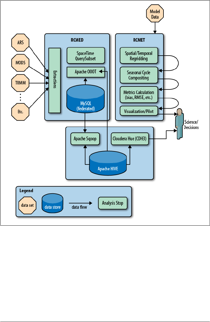
in our RCMES system website parameter table, http://rcmes.jpl.nasa.gov/rcmed/param
eters/, and shown in Figure 23-3.
Data sets are loaded into the RCMED using the Apache OODT extractor framework
and the desired parameters, their values, spatial and temporal constraints (and
optionally height) are loaded and potentially transformed (e.g., normalized, put on
same coordinate system, converted from unit values) into a MySQL database. The data
loaded into that MySQL database, RCMED, is exposed to external clients via a Space/
Time query and subsetting web service; the description of which is a topic of a separate
Figure 23-2. JPL Architecture Diagram.
NASA’s Jet Propulsion Laboratory | 289
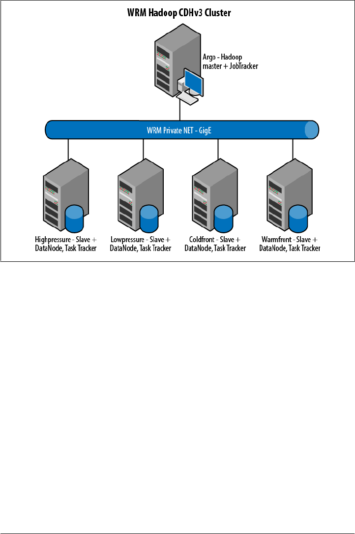
study. For all intents and purposes, it provides the same capabilities that the OPeNDAP
technology does.
The right side of the diagram shows the Regional Climate Model Evaluation Toolkit
(RCMET). It provides users with the ability to take in the reference data from RCMED
and climate model output data produced elsewhere and to re-grid these datasets in
order to match them spatially and temporally in preparation for the comparison of the
reference and model data for the evaluation of model output against the user-selected
reference data. At that point, the system allows for seasonal cycle compositing (e.g., all
Januaries, or all summer months for N years), and for preparing the data for eventual
metrics calculation, that is, comparison of the values of the model output against the
remote sensing data observation parameters and their values. The system supports
several metrics, such as bias computation, Root Mean Squared Error (RMSE), and the
generation of relevant visualizations, including traditional plots and Taylor diagrams
for science use/decision making.
Our Experience: Why Hive?
So, where does Hive come in to play? After loading 6 billion rows of (latitude, longitude,
time, data point value, height) tuples into MySQL, the system fell down and
Figure 23-3. JPL Physical Architecture Diagram
290 | Chapter 23: Case Studies

experienced data loss. This is probably due in part to our naïve strategy of storing all
of the data points in a single table. Over time, we evolved this strategy to break tables
down by dataset and by parameter, which helped but added needless overhead that we
didn’t want to spend cycles engineering around.
Instead, we decided to experiment with the Apache Hive technology. We installed Hive
0.5+20 using CDHv3 and Apache Hadoop (0.20.2+320). CDHv3 came with a number
of other relevant tools including Sqoop, and Hue, which we leveraged in our architec-
ture, shown in the bottom portion of Figure 23-3.
We used Apache Sqoop to dump out the data into Hive, and then wrote an Apache
OODT wrapper that queried Hive for the data by Space/Time and provided it back to
the RCMET and other users (shown in the middle portion of Figure 23-2). The full
architecture for the RCMES cluster is shown in Figure 23-3. We had five machines,
including a master/slave configuration as shown in the diagram, connected by a private
network running GigE.
Some Challenges and How We Overcame Them
During the migration of data from MySQL to Hive, we experienced slow response times
while doing simple tasks such as a count DB query (e.g., hive> select count(data
point_id) from dataPoint;). We initially loaded up around 2.5 billion data points in
a single table and noticed that on our machine configuration, Hive took approximately
5–6 minutes to do a count of these 2.5 billion records (15–17 minutes for the full 6.8
billion records). The reduce portion was fast (we were experiencing a single reduce
phase since we were using a count * benchmark) but the map stage took the remainder
of the time (~95%). Our system at the time consisted of six (4 x quad-core) systems
with approximately 24 GB of RAM each (all of the machines shown in Figure 23-3,
plus another “borrowed machine” of similar class from another cluster).
We attempted to add more nodes, increase map tasktrackers (many different #s),
change DFS block size (32 M, 64 M, 128 MB, 256 M), leverage LZO compression, and
alter many other configuration variables (io.sort.factor, io.sort.mb) without much
success in lowering the time to complete the count. We did notice a high I/O wait on
the nodes no matter how many task trackers we ran. The size of the database was
approximately ~200GB and with MySQL it took a few seconds to do both the 2.5
billion and 6.7 billion count.
Members of the Hive community jumped in and provided us with insight, ranging from
mentioning that HDFS read speed is about 60 MB/sec comparing to about 1 GB/sec
on local disk, depending of course on network speed, and namenode workload. The
numbers suggested by the community member suggested that we needed roughly 16
mappers in the Hadoop job to match with the I/O performance of a local non-Hadoop
task. In addition, Hive community members suggested that we increase the number of
mappers (increase parallelism) by reducing the split size (input size) for each mapper,
noting we should examine the following parameters: mapred.min.split.size,
NASA’s Jet Propulsion Laboratory | 291

mapred.max.split.size, mapred.min.split.size.per.rack, and mapred.min.split.size
.per.node, and suggesting that the parameters should be set to a value of 64 MB. Finally,
the community suggested that we look at a benchmark that only counts rows by using
count(1) instead of count (datapoint_id), as the latter is faster since no column refer-
ence means no decompression and deserialization, e.g., if you store your table in RCFile
format.
Based on the above feedback, we were able to tune our Hive cluster for RCMES to
respond to a count query benchmark, and to a space/time query from RCMET for
billions of rows in under 15 seconds, using the above-mentioned resources, making
Hive a viable and great choice for our system architecture.
Conclusion
We have described our use of Apache Hive in the JPL Regional Climate Model Evalu-
ation System. We leveraged Hive during a case study wherein we wanted to explore
cloud-based technology alternatives to MySQL, and configuration requirements
needed to make it scale to the level of tens of billions of rows, and to elastically destroy
and re-create the data stored within.
Hive did a great job of meeting our system needs and we are actively looking for more
ways to closely integrate it into the RCMES system.
Photobucket
Photobucket is the largest dedicated photo-hosting service on the Internet. Started in
2003 by Alex Welch and Darren Crystal, Photobucket quickly became one of the most
popular sites on the Internet and attracted over one hundred million users and billions
of stored and shared media. User and system data is spread across hundreds of MySQL
instances, thousands of web servers, and petabytes of filesystem.
Big Data at Photobucket
Prior to 2008, Photobucket didn’t have a dedicated analytics system in-house. Ques-
tions from the business users were run across hundreds of MySQL instances and the
results aggregated manually in Excel.
In 2008, Photobucket embarked on implementing its first data warehouse dedicated
to answering the increasingly complex data questions being asked by a fast-growing
company.
The first iteration of the data warehouse was built using an open source system with a
Java SQL optimizer and a set of underlying PostGreSQL databases. The previous system
worked well into 2009, but the shortcomings in the architecture became quickly evi-
dent. Working data sets quickly became larger than the available memory; coupled
292 | Chapter 23: Case Studies

with the difficulty in repartitioning the data across the PostGreSQL nodes forced us to
scale up when we really wanted to scale out.
In 2009, we started to investigate systems that would allow us to scale out, as the
amount of data continued to grow and still meet our SLA with the business users.
Hadoop quickly became the favorite for consuming and analyzing the terabytes of data
generated daily by the system, but the difficulty of writing MapReduce programs for
simple ad hoc questions became a negative factor for full implementation. Thankfully,
Facebook open sourced Hive a few weeks later and the barriers to efficiently answering
ad hoc business questions were quickly smashed.
Hive demonstrates many advantages over the previous warehouse implementation.
Here are a few examples of why we chose Hadoop and Hive:
1. Ability to handle structured and unstructured data
2. Real-time streaming of data into HDFS from Flume, Scribe, or MountableHDFS
3. Extend functionality through UDFs
4. A well-documented, SQL-like interface specifically built for OLAP versus OLTP
What Hardware Do We Use for Hive?
Dell R410, 4 × 2 TB drives with 24 GB RAM for the data nodes, and Dell R610, 2 × 146
GB (RAID 10) drives with 24 GB RAM for the management hardware.
What’s in Hive?
The primary goal of Hive at Photobucket is to provide answers about business func-
tions, system performance, and user activity. To meet these needs, we store nightly
dumps of MySQL data sets from across hundreds of servers, terabytes of logfiles from
web servers and custom log formats ingested through Flume. This data helps support
many groups throughout the company, such as executive management, advertising,
customer support, product development, and operations just to name a few. For his-
torical data, we keep the partition of all data created on the first day of the month for
MySQL data and 30+ days of log files. Photobucket uses a custom ETL framework for
migrating MySQL data into Hive. Log file data is streamed into HDFS using Flume and
picked up by scheduled Hive processes.
Who Does It Support?
Executive management relies on Hadoop to provide reports surrounding the general
health of the business. Hive allows us to parse structured database data and unstruc-
tured click stream data and distill the data into a format requested by the business
stakeholder.
Photobucket | 293

Advertising operations uses Hive to sift through historical data for forecast and define
quotas for ad targeting.
Product development is far and away the group generating the largest number of ad
hoc queries. As with any user base, segments change and evolve over time. Hive is
important because it allows us to run A/B tests across current and historical data to
gauge relevancy of new products in a quickly changing user environment.
Providing our users with a best-in-class system is the most important goal at Photo-
bucket. From an operations perspective, Hive is used to generate rollup data partitioned
across multiple dimensions. Knowing the most popular media, users, and referring
domains is important for many levels across the company. Controlling expenses is
important to any organization. A single user can quickly consume large amounts of
system resources, significantly increasing monthly expenditures. Hive is used to iden-
tify and analyze rogue users; to determine which ones are within our Terms of Service
and which are not. Operations also uses Hive to run A/B tests defining new hardware
requirements and generating ROI calculations. Hive’s ability to abstract users from
underlying MapReduce code means questions can be answered in hours or days instead
of weeks.
SimpleReach
by Eric Lubow
At SimpleReach, we use Cassandra to store our raw data from all of our social network
polling. The format of the row key is an account ID (which is a MongoDB ObjectId)
and a content item ID (witha MD5 hash of the URL of the content item being tracked)
separated by an underscore which we split on to provide that data in the result set. The
columns in the row are composite columns that look like the ones below:
4e87f81ca782f3404200000a_8c825814de0ac34bb9103e2193a5b824
=> (column=meta:published-at, value=1330979750000, timestamp=1338919372934628)
=> (column=hour:1338876000000_digg-diggs, value=84, timestamp=1338879756209142)
=> (column=hour:1338865200000_googleplus-total, value=12, timestamp=1338869007737888)
In order for us to be able to query on composite columns, we need to know the hex
value of the column name. In our case, we want to know the hex value of the column
name (meta:'published-at').
The hex equivalent is below: 00046D65746100000C7075626C69736865642D617400 =
meta:published-at
Once the column name is converted to hexadecimal format, Hive queries are run
against it. The first part of the query is the LEFT SEMI JOIN, which is used to mimic a
SQL subselect. All the references to SUBSTR and INSTR are to handle the case of composite
columns. Since it is known in advance that characters 10–23 of the “hour:*” columns
(i.e., SUBSTR(r.column_name,10,13)) is a timestamp and therefore we can crop it out and
use it in the returned data or for matching. The INSTR is used to match column names
294 | Chapter 23: Case Studies

and ensure the result set always has the same columns in the same place in the output.
The SUBSTR is used for matching as part of the Ruby function. The SUBSTR returns a
timestamp (long) in milliseconds since epoch and the start_date and end_date are also
a timestamp in milliseconds since epoch. This means that the passed in values can be
matched to a part of the column name.
The goal of this query is to export our data from Cassandra into a CSV file to give
aggregated data dumps to our publishers. It is done via a Resque (offline) job that is
kicked off through our Rails stack. Having a full CSV file means that all columns in the
header must be accounted for in the Hive query (meaning that zeros need to be put to
fill places where there is no data). We do that by pivoting our wide rows into fixed
column tables using the CASE statement.
Here is the HiveQL for the CSV file:
SELECT CAST(SUBSTR(r.column_name, 10, 13) AS BIGINT) AS epoch,
SPLIT(r.row_key, '_')[0] AS account_id,
SPLIT(r.row_key, '_')[1] AS id,
SUM(CAST(CASE WHEN INSTR(r.column_name, 'pageviews-total') > 0
THEN r.value ELSE '0' END AS INT)) AS pageviews,
SUM(CAST(CASE WHEN INSTR(r.column_name, 'digg-digg') > 0
THEN r.value ELSE '0' END AS INT)) AS digg,
SUM(CAST(CASE WHEN INSTR(r.column_name, 'digg-referrer') > 0
THEN r.value ELSE '0' END AS INT)) AS digg_ref,
SUM(CAST(CASE WHEN INSTR(r.column_name, 'delicious-total') > 0
THEN r.value ELSE '0' END AS INT)) AS delicious,
SUM(CAST(CASE WHEN INSTR(r.column_name, 'delicious-referrer') > 0
THEN r.value ELSE '0' END AS INT)) AS delicious_ref,
SUM(CAST(CASE WHEN INSTR(r.column_name, 'googleplus-total') > 0
THEN r.value ELSE '0' END AS INT)) AS google_plus,
SUM(CAST(CASE WHEN INSTR(r.column_name, 'googleplus-referrer') > 0
THEN r.value ELSE '0' END AS INT)) AS google_plus_ref,
SUM(CAST(CASE WHEN INSTR(r.column_name, 'facebook-total') > 0
THEN r.value ELSE '0' END AS INT)) AS fb_total,
SUM(CAST(CASE WHEN INSTR(r.column_name, 'facebook-referrer') > 0
THEN r.value ELSE '0' END AS INT)) AS fb_ref,
SUM(CAST(CASE WHEN INSTR(r.column_name, 'twitter-tweet') > 0
THEN r.value ELSE '0' END AS INT)) AS tweets,
SUM(CAST(CASE WHEN INSTR(r.column_name, 'twitter-referrer') > 0
THEN r.value ELSE '0' END AS INT)) AS twitter_ref,
SUM(CAST(CASE WHEN INSTR(r.column_name, 'linkedin-share') > 0
THEN r.value ELSE '0' END AS INT)) AS linkedin,
SUM(CAST(CASE WHEN INSTR(r.column_name, 'linkedin-referrer') > 0
THEN r.value ELSE '0' END AS INT)) AS linkedin_ref,
SUM(CAST(CASE WHEN INSTR(r.column_name, 'stumbleupon-total') > 0
THEN r.value ELSE '0' END AS INT)) AS stumble_total,
SUM(CAST(CASE WHEN INSTR(r.column_name, 'stumbleupon-referrer') > 0
THEN r.value ELSE '0' END AS INT)) AS stumble_ref,
SUM(CAST(CASE WHEN INSTR(r.column_name, 'social-actions') > 0
THEN r.value ELSE '0' END AS INT)) AS social_actions,
SUM(CAST(CASE WHEN INSTR(r.column_name, 'referrer-social') > 0
THEN r.value ELSE '0' END AS INT)) AS social_ref,
MAX(CAST(CASE WHEN INSTR(r.column_name, 'score-realtime') > 0
SimpleReach | 295

THEN r.value ELSE '0.0' END AS DOUBLE)) AS score_rt
FROM content_social_delta r
LEFT SEMI JOIN (SELECT row_key
FROM content
WHERE HEX(column_name) = '00046D65746100000C7075626C69736865642D617400'
AND CAST(value AS BIGINT) >= #{start_date}
AND CAST(value AS BIGINT) <= #{end_date}
) c ON c.row_key = SPLIT(r.row_key, '_')[1]
WHERE INSTR(r.column_name, 'hour') > 0
AND CAST(SUBSTR(r.column_name, 10, 13) AS BIGINT) >= #{start_date}
AND CAST(SUBSTR(r.column_name, 10, 13) AS BIGINT) <= #{end_date}
GROUP BY CAST(SUBSTR(r.column_name, 10, 13) AS BIGINT),
SPLIT(r.row_key, '_')[0],
SPLIT(r.row_key, '_')[1]
The output of the query is a comma-separated value (CSV) file, an example of which
is below (wrapped for length with a blank line between each record for clarity):
epoch,account_id,id,pageviews,digg,digg_ref,delicious,delicious_ref,
google_plus,google_plus_ref,fb_total,fb_ref,tweets,twitter_ref,
linkedin,linkedin_ref,stumble_total,stumble_ref,social_actions,social_ref,score_rt
1337212800000,4eb331eea782f32acc000002,eaff81bd10a527f589f45c186662230e,
39,0,0,0,0,0,0,0,2,0,20,0,0,0,0,0,22,0
1337212800000,4f63ae61a782f327ce000007,940fd3e9d794b80012d3c7913b837dff,
101,0,0,0,0,0,0,44,63,11,16,0,0,0,0,55,79,69.64308064
1337212800000,4f6baedda782f325f4000010,e70f7d432ad252be439bc9cf1925ad7c,
260,0,0,0,0,0,0,8,25,15,34,0,0,0,0,23,59,57.23718477
1337216400000,4eb331eea782f32acc000002,eaff81bd10a527f589f45c186662230e,
280,0,0,0,0,0,0,37,162,23,15,0,0,0,2,56,179,72.45877173
1337216400000,4ebd76f7a782f30c9b000014,fb8935034e7d365e88dd5be1ed44b6dd,
11,0,0,0,0,0,0,0,1,1,4,0,0,0,0,0,5,29.74849901
Experiences and Needs from the Customer Trenches
A Karmasphere Perspective
By Nanda Vijaydev
Introduction
For over 18 months, Karmasphere has been engaged with a fast-growing number of
companies who adopted Hadoop and immediately gravitated towards Hive as the op-
timal way for teams of analysts and business users to use existing SQL skills with the
Hadoop environment. The first part of this chapter provides use case techniques that
we’ve seen used repeatedly in customer environments to advance Hive-based analytics.
296 | Chapter 23: Case Studies

The use case examples we cover are:
• Optimal data formatting for Hive
• Partitions and performance
• Text analytics with Hive functions including Regex, Explode and Ngram
As companies we’ve worked with plan for and move into production use of Hive, they
look for incremental capabilities that make Hive-based access to Hadoop even easier
to use, more productive, more powerful, and available to more people in their organi-
zation. When they wire Hadoop and Hive into their existing data architectures, they
also want to enable results from Hive queries to be systematized, shared and integrated
with other data stores, spreadsheets, BI tools, and reporting systems.
In particular, companies have asked for:
• Easier ways to ingest data, detect raw formats, and create metadata
• Work collaboratively in an integrated, multi-user environment
• Explore and analyze data iteratively
• Preserved and reusable paths to insight
• Finer-grain control over data, table, and column security, and compartmentalized
access to different lines of business
• Business user access to analytics without requiring SQL skills
• Scheduling of queries for automated result generation and export to non-Hadoop
data stores
• Integration with Microsoft Excel, Tableau, Spotfire, and other spreadsheet, re-
porting systems, dashboards, and BI tools
• Ability to manage Hive-based assets including queries, results, visualizations, and
standard Hive components such as UDFs and SerDes
Use Case Examples from the Customer Trenches
Customer trenches #1: Optimal data formatting for Hive
One recurring question from many Hive users revolves around the format of their data
and how to make that available in Hive.
Many data formats are supported out-of-the-box in Hive but some custom proprietary
formats are not. And some formats that are supported raise questions for Hive users
about how to extract individual components from within a row of data. Sometimes,
writing a standard Hive SerDe that supports a custom data format is the optimal ap-
proach. In other cases, using existing Hive delimiters and exploiting Hive UDFs is the
most convenient solution. One representative case we worked on was with a company
using Hadoop and Hive to provide personalization services from the analysis of mul-
tiple input data streams. They were receiving logfiles from one of their data providers
Experiences and Needs from the Customer Trenches | 297

in a format that could not easily be split into columns. They were trying to figure out
a way to parse the data and run queries without writing a custom SerDe.
The data had top header level information and multiple detailed information. The de-
tailed section was a JSON nested within the top level object, similar to the data set
below:
{ "top" : [
{"table":"user",
"data":{
"name":"John Doe","userid":"2036586","age":"74","code":"297994","status":1}},
{"table":"user",
"data":{
"name":"Mary Ann","userid":"14294734","age":"64","code":"142798","status":1}},
{"table":"user",
"data":{
"name":"Carl Smith","userid":"13998600","age":"36","code":"32866","status":1}},
{"table":"user",
"data":{
"name":"Anil Kumar":"2614012","age":"69","code":"208672","status":1}},
{"table":"user",
"data":{
"name":"Kim Lee","userid":"10471190","age":"53","code":"79365","status":1}}
]}
After talking with the customer, we realized they were interested in splitting individual
columns of the detailed information that was tagged with “data” identifier in the above
sample.
To help them proceed, we used existing Hive function get_json_object as shown
below:
First step is to create a table using the sample data:
CREATE TABLE user (line string)
ROW FORMAT DELIMITED FIELDS TERMINATED BY '\n'
STORED AS TEXTFILE
LOCATION ‘hdfs://hostname/user/uname/tablefolder/’
Then using Hive functions such as get_json_object, we could get to the nested JSON
element and parse it using UDFs:
SELECT get_json_object(col0, '$.name') as name, get_json_object(col0, '$.userid') as uid,
get_json_object(col0, '$.age') as age, get_json_object(col0, '$.code') as code,
get_json_object(col0, '$.status') as status
FROM
(SELECT get_json_object(user.line, '$.data') as col0
FROM user
WHERE get_json_object(user.line, '$.data') is not null) temp;
Query details include:
• Extract the nested JSON object identified by data in the inner query as col0.
• Then the JSON object is split into appropriate columns using their names in the
name value pair.
298 | Chapter 23: Case Studies

The results of the query are given below, with header information saved, as a CSV file:
"name","uid","age","code","status"
"John Doe","2036586","74","297994","1"
"Mary Ann","14294734","64","142798","1"
"Carl Smith","13998600","36","32866","1"
"Kim Lee","10471190","53","79365","1"
Customer trenches #2: Partitions and performance
Using partitions with data being streamed or regularly added to Hadoop is a use case
we see repeatedly, and a powerful and valuable way of harnessing Hadoop and Hive
to analyze various kinds of rapidly additive data sets. Web, application, product, and
sensor logs are just some of the types of data that Hive users often want to perform ad
hoc, repeated, and scheduled queries on.
Hive partitions, when set up correctly, allow users to query data only in specific parti-
tions and hence improves performance significantly. To set up partitions for a table,
files should be located in directories as given in this example:
hdfs://user/uname/folder/"yr"=2012/"mon"=01/"day"=01/file1, file2, file3
/"yr"=2012/"mon"=01/"day"=02/file4, file5
…......
/"yr"=2012/"mon"=05/"day"=30/file100, file101
With the above structure, tables can be set up with partition by year, month, and day.
Queries can use yr, mon, and day as columns and restrict the data accessed to specific
values during query time. If you notice the folder names, partitioned folders have iden-
tifiers such as yr= , mon=, and day=.
Working with one high tech company, we discovered that their folders did not have
this explicit partition naming and they couldn’t change their existing directory struc-
ture. But they still wanted to benefit from having partitions. Their sample directory
structure is given below:
hdfs://user/uname/folder/2012/01/01/file1, file2, file3
/2012/01/02/file4, file5
…….
/2012/05/30/file100, file101
In this case, we can still add partitions by explicitly adding the location of the absolute
path to the table using ALTER TABLE statements. A simple external script can read the
directory and add the literal yr=, mon=, day= to an ALTER TABLE statement and provide
the value of the folder (yr=2012, mon=01,...) to ALTER TABLE statements. The output
of the script is a set of Hive SQL statements generated using the existing directory
structure and captured into a simple text file.
ALTER TABLE tablename
ADD PARTITION (yr=2012, mon=01, day=01) location '/user/uname/folder/2012/01/01/';
ALTER TABLE tablename
ADD PARTITION (yr=2012, mon=01, day=02) location '/user/uname/folder/2012/01/02/';
Experiences and Needs from the Customer Trenches | 299

...
ALTER TABLE tablename
ADD PARTITION (yr=2012, mon=05, day=30) location '/user/uname/folder/2012/05/30/';
When these statements are executed in Hive, the data in the specified directories au-
tomatically become available under defined logical partitions created using ALTER
TABLE statements.
You should make sure that your table is created with PARTITIONED BY
columns for year, month, and day.
Customer trenches #3: Text analytics with Regex, Lateral View Explode, Ngram, and other UDFs
Many companies we work with have text analytics use cases which vary from simple
to complex. Understanding and using Hive regex functions, n-gram functions and other
string functions can address a number of those use cases.
One large manufacturing customer we worked with had lot of machine-generated
compressed text data being ingested into Hadoop. The format of this data was:
1. Multiple rows of data in each file and a number of such files in time-partitioned
buckets.
2. Within each row there were a number of segments separated by /r/n (carriage
return and line feed).
3. Each segment was in the form of a “name: value” pair.
The use case requirement was to:
1. Read each row and separate individual segments as name-value pairs.
2. Zero in on specific segments and look for word counts and word patterns for an-
alyzing keywords and specific messages.
The sample below illustrates this customer’s data (text elided for space):
name:Mercury\r\ndescription:Mercury is the god of commerce, ...\r\ntype:Rocky planet
name:Venus\r\ndescription:Venus is the goddess of love...\r\ntype:Rocky planet
name:Earch\r\ndescription:Earth is the only planet ...\r\ntype:Rocky planet
name:Mars\r\ndescription: Mars is the god of War...\r\ntype:Rocky planet
name:Jupiter\r\ndescription:Jupiter is the King of the Gods...\r\ntype:Gas planet
name:Saturn\r\ndescription:Saturn is the god of agriculture...\r\ntype:Gas planet
name:Uranus\r\ndescription:Uranus is the God of the Heavens...\r\ntype:Gas planet
name:Neptune\r\ndescription:Neptune was the god of the Sea...\r\ntype:Gas planet
The data contains:
1. Planet names and their description with type.
2. Each row of data is separated by a delimiter.
300 | Chapter 23: Case Studies

3. Within each row there are three subsections, including “name,” “description,” and
“type” separated by /r/n.
4. Description is a large text.
First step is to create the initial table with this sample data:
CREATE TABLE planets (col0 string)
ROW FORMAT DELIMITED FIELDS TERMINATED BY '\n'
STORED AS TEXTFILE
LOCATION 'hdfs://hostname/user/uname/planets/'
In the following, we run a series of queries, starting with a simple query and adding
functions as we iterate. Note that the requirement can be met with queries written in
several different ways. The purpose of the queries shown below is to demonstrate some
of the key capabilities in Hive around text parsing.
First, we use a split function to separate each section of data into an array of individual
elements:
SELECT split(col0, '(\\\\r\\\\n)') AS splits FROM planets;
Next, we explode the splits (array) into individual lines using the LATERAL VIEW
EXPLODE function. Results of this query will have name-value pairs separated into indi-
vidual rows. We select only those rows that start with description. The function
LTRIM is also used to remove left spaces.
SELECT ltrim(splits) AS pairs FROM planets
LATERAL VIEW EXPLODE(split(col0, '(\\\\r\\\\n)')) col0 AS splits
WHERE ltrim(splits) LIKE 'desc%'
Now we separate the description line into name-value pair and select only the value
data. This can be done in different ways. We use split by : and choose the value pa-
rameter:
SELECT (split(pairs, ':'))[1] AS txtval FROM (
SELECT ltrim(splits) AS pairs FROM planets
LATERAL VIEW EXPLODE(split(col0, '(\\\\r\\\\n)')) col0 AS splits
WHERE ltrim(splits) LIKE 'desc%')tmp1;
Notice the use of temporary identifiers tmp1 for the inner query. This is required when
you use the output of a subquery as the input to outer query. At the end of step three,
we have the value of the description segment within each row.
In the next step, we use ngrams to show the top 10 bigrams (2-gram) words from the
description of planets. You could also use functions such as context_ngram,
find_in_set, regex_replace, and others to perform various text-based analyses:
SELECT ngrams(sentences(lower(txtval)), 2, 10) AS bigrams FROM (
SELECT (split(pairs, ':'))[1] AS txtval FROM (
SELECT ltrim(splits) AS pairs FROM planets
LATERAL VIEW EXPLODE(split(col0, '(\\\\r\\\\n)')) col0 AS splits
WHERE ltrim(splits) LIKE 'desc%') tmp1) tmp2;
Experiences and Needs from the Customer Trenches | 301
Downloa d f r o m W o w ! e B o o k < w w w.woweb o o k . c o m >

Notice that we have used functions such as lower to convert to lowercase and sentences
to tokenize each word in the text.
For additional information about the text analytics capabilities of Hive, see the func-
tions listed in Chapter 3.
Hive adoption continues to grow,
as outlined by the use cases defined above. Companies across different industry seg-
ments and various sizes have benefited immensely by leveraging Hive in their Hadoop
environments. A strong and active community of contributors and significant invest-
ments in Hive R&D efforts by leading Hadoop vendors ensures that Hive, already the
SQL-based standard for Hadoop, will become the SQL-based standard within organ-
izations that are leveraging Hadoop for Big Data analysis.
As companies invest significant resources and time in understanding and building Hive
resources, in many cases we find they look for additional capabilities that enable them
to build on their initial use of Hive and extend its reach faster and more broadly within
their organizations. From working with these customers looking to take Hive to the
next level, a common set of requirements have emerged.
These requirements include:
Collaborative multiuser environments
Hadoop enables new classes of analysis that were prohibitive computationally and
economically with traditional RDBMS technologies. Hadoop empowers organizations
to break down the data and people silos, performing analysis on every byte of data they
can get their hands on, doing this all in a way that enables them to share their queries,
results, and insights with other individuals, teams, and systems in the organization.
This model implies that users with deep understanding of these different data sets need
to collaborate in discovery, in the sharing of insights, and the availability of all Hive-
based analytic assets across the organization.
Productivity enhancements
The current implementation of Hive offers a serial batch environment on Hadoop to
run queries. This implies that once a user submits a query for job execution to the
Hadoop cluster, they have to wait for the query to complete execution before they can
execute another query against the cluster. This can limit user productivity.
One major reason for companies adopting Hive is that it enables their SQL-skilled data
professionals to move faster and more easily to working with Hadoop. These users are
usually familiar with graphical SQL editors in tools and BI products. They are looking
for similar productivity enhancements like syntax highlighting and code completion.
Managing Hive assets
A recent McKinsey report predicted significant shortage of skilled workers to enable
organizations to profit from their data. Technologies like Hive promise to help bridge
Apache Hive in production: Incremental needs and capabilities.
302 | Chapter 23: Case Studies

that skills shortage by allowing people with an SQL skillset to perform analysis on
Hadoop. However, organizations are realizing that just having Hive available to their
users is not enough. They need to be able to manage Hive assets like queries (history
and versions), UDFs, SerDes for later share and reuse. Organizations would like to
build this living knowledge repository of Hive assets that is easily searchable by users.
Extending Hive for advanced analytics
Many companies are looking to re-create analysis they perform in the traditional
RDBMS world in Hadoop. While not all capabilities in the SQL environment easily
translate into Hive functions, due to inherent limitations of how data is stored, there
are some advanced analytics functions like RANKING, etc., that are Hadoop-able. In ad-
dition, organizations have spent tremendous resources and time in building analytical
models using traditional tools like SAS and SPSS and would like the ability to score
these models on Hadoop via Hive queries.
Extending Hive beyond the SQL skill set
As Hadoop is gaining momentum in organizations and becoming a key fabric of data
processing and analytics within IT infrastructure, it is gaining popularity amongst users
with different skill sets and capabilities. While Hive is easily adopted by users with SQL
skill sets, other less SQL savvy users are also looking for drag-and-drop capabilities like
those available in traditional BI tools to perform analysis on Hadoop using Hive. The
ability to support interactive forms on top of Hive, where a user is prompted to provide
column values via simple web-based forms is an often-asked for capability.
Data exploration capabilities
Traditional database technologies provide data exploration capabilities; for example,
a user can view min, max values for an integer column. In addition, users can also view
visualizations of these columns to understand the data distribution before they perform
analysis on the data. As Hadoop stores hundreds of terabytes of data, and often peta-
bytes, similar capabilities are being requested by customers for specific use cases.
Schedule and operationalize Hive queries
As companies find insights using Hive on Hadoop, they are also looking to operation-
alize these insights and schedule them to run on a regular interval. While open source
alternatives are currently available, these sometimes fall short when companies also
want to manage the output of Hive queries; for example, moving result sets into a
traditional RDBMS system or BI stack. To manage certain use cases, companies often
have to manually string together various different open source tools or rely on poor
performing JDBC connectors.
Karmasphere is a software company, based in Silicon Valley Califor-
nia, focused exclusively on bringing native Hadoop Big Data Analytics capabilities to
teams of analysts and business users. Their flagship product, Karmasphere 2.0, is based
on Apache Hive, extending it in a multi-user graphical workspace to enable:
About Karmasphere.
Experiences and Needs from the Customer Trenches | 303
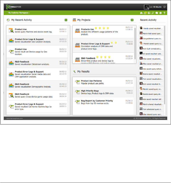
• Reuse of standard Hive-based tables, SerDes and UDFs
• Social, project-based big data analytics for teams of analysts and business users
• Easy data ingestion to the cluster
• Heuristic-based recognition and table creation of many popular data formats
• Visual and iterative data exploration and analysis
• Graphical exploration of all Hive-based analytic assets
• Sharing and scheduling of queries, results and visualizations
• Easy integration with traditional spreadsheets, reporting, dashboard, and BI tools
Figure 23-4 shows a screenshot of Karmasphere 2.0’s Hive-based Big Data Analytics
Environment.
Figure 23-4. Screenshot of Karmasphere 2.0
Hive features survey
We’d like to get feedback on the importance of these needs and share them back with
the growing Hive community. If you are interested in seeing what others think and
would like to participate, please visit:
http://karmasphere.com/hive-features-survey.html
304 | Chapter 23: Case Studies

Glossary
Amazon Elastic MapReduce
Amazon’s EMR is a hosted Hadoop service
on top of Amazon EC2 (Elastic Compute
Cloud).
Avro
Avro is a new serialization format developed
to address some of the common problems
associated with evolving other serialization
formats. Some of the benefits are: rich data
structures, fast binary format, support for
remote procedure calls, and built-in schema
evolution.
Bash
The “Bourne-Again Shell” that is the default
interactive command shell for Linux and
Mac OS X systems.
S3 Bucket
The term for the top-level container you
own and manage when using S3. A user may
have many buckets, analogous to the root of
a physical hard drive.
Command-Line Interface
The command-line interface (CLI) can run
“scripts” of Hive statements or all the user
to enter statements interactively.
Data Warehouse
A repository of structured data suitable for
analysis for reports, trends, etc. Warehouses
are batch mode or offline, as opposed to
providing real-time responsiveness for on-
line activity, like ecommerce.
Derby
A lightweight SQL database that can be em-
bedded in Java applications. It runs in the
same process and saves its data to local files.
It is used as the default SQL data store for
Hive’s metastore. See http://db.apache.org/
derby/ for more information.
Dynamic Partitions
A HiveQL extension to SQL that allows you
to insert query results into table partitions
where you leave one or more partition col-
umn values unspecified and they are deter-
mined dynamically from the query results
themselves. This technique is convenient for
partitioning a query result into a potentially
large number of partitions in a new table,
without having to write a separate query for
each partition column value.
Ephemeral Storage
In the nodes for a virtual Amazon EC2 clus-
ter, the on-node disk storage is called
ephemeral because it will vanish when the
cluster is shut down, in contrast to a physi-
cal cluster that is shut down. Hence, when
using an EC2 cluster, such as an Amazon
Elastic MapReduce cluster, it is important to
back up important data to S3.
ExternalTable
A table using a storage location and contents
that are outside of Hive’s control. It is con-
venient for sharing data with other tools, but
it is up to other processes to manage the life
cycle of the data. That is, when an external
table is created, Hive does not create the
305

external directory (or directories for parti-
tioned tables), nor are the directory and data
files deleted when an external table is
dropped.
Hadoop Distributed File System
(HDFS) A distributed, resilient file system
for data storage that is optimized for scan-
ning large contiguous blocks of data on hard
disks. Distribution across a cluster provides
horizontal scaling of data storage. Blocks of
HDFS files are replicated across the cluster
(by default, three times) to prevent data loss
when hard drives or whole servers fail.
HBase
The NoSQL database that uses HDFS for
durable storage of table data. HBase is a col-
umn-oriented, key-value store designed to
provide traditional responsiveness for quer-
ies and row-level updates and insertions.
Column oriented means that the data storage
is organized on disk by groups of columns,
called column families, rather than by row.
This feature promotes fast queries for sub-
sets of columns. Key-value means that rows
are stored and fetched by a unique key and
the value is the entire row. HBase does not
provide an SQL dialect, but Hive can be
used to query HBase tables.
Hive
A data warehouse tool that provides table
abstractions on top of data resident in
HDFS, HBase tables, and other stores. The
Hive Query Language is a dialect of the
Structured Query Language.
Hive Query Language
Hive’s own dialect of the Structured Query
Language (SQL). Abbreviated HiveQL or
HQL.
Input Format
The input format determines how input
streams, usually from files, are split into re-
cords. A SerDe handles parsing the record
into columns. A custom input format can be
specified when creating a table using the
INPUTFORMAT clause. The input format for the
default STORED AS TEXTFILE specification is
implemented by the Java object named
org.apache.hadoop.mapreduce.lib.input.
TextInputFormat. See also Output Format.
JDBC
The Java Database Connection API pro-
vides access to SQL systems, including Hive,
from Java code.
Job
In the Hadoop context, a job is a self-con-
tained workflow submitted to MapReduce.
It encompasses all the work required to per-
form a complete calculation, from reading
input to generating output. The MapRe-
duce JobTracker will decompose the job into
one or more tasks for distribution and exe-
cution around the cluster.
JobTracker
The top-level controller of all jobs using
Hadoop’s MapReduce. The JobTracker ac-
cepts job submissions, determines what
tasks to run and where to run them, moni-
tors their execution, restarts failed tasks as
needed, and provides a web console for
monitoring job and task execution, viewing
logs, etc.
Job Flow
A term used in Amazon Elastic MapReduce
(EMR) for the sequence of jobs executed on
a temporary EMR cluster to accomplish a
particular goal.
JSON
JSON (JavaScript Object Notation) is a
lightweight data serialization format used
commonly in web-based applications.
Map
The mapping phase of a MapReduce process
where an input set of key-value pairs are
converted into a new set of key-value pairs.
For each input key-value pair, there can be
zero-to-many output key-value pairs. The
input and output keys and the input and
output values can be completely different.
MapR
A commercial distribution of Hadoop that
replaces HDFS with the MapR File System
Hadoop Distributed File System
306 | Glossary

(MapR-FS), a high-performance, dis-
tributed file system.
MapReduce
A computation paradigm invented at
Google and based loosely on the common
data operations of mapping a collection of
data elements from one form to another (the
map phase) and reducing a collection to a
single value or a smaller collection (the
reduce phase). MapReduce is designed to
scale computation horizontally by decom-
posing map and reduce steps into tasks and
distributing those tasks across a cluster. The
MapReduce runtime provided by Hadoop
handles decomposition of a job into tasks,
distribution around the cluster, movement
of a particular task to the machine that holds
the data for the task, movement of data to
tasks (as needed), and automated re-
execution of failed tasks and other error
recovery and logging services.
Metastore
The service that maintains “metadata” in-
formation, such as table schemas. Hive re-
quires this service to be running. By default,
it uses a built-in Derby SQL server, which
provides limited, single-process SQL sup-
port. Production systems must use a full-
service relational database, such as MySQL.
NoSQL
An umbrella term for data stores that don’t
support the relational model for data man-
agement, dialects of the structured query
language, and features like transactional up-
dates. These data stores trade off these fea-
tures in order to provide more cost-effective
scalability, higher availability, etc.
ODBC
The Open Database Connection API pro-
vides access to SQL systems, including Hive,
from other applications. Java applications
typically use the JDBC API, instead.
Output Format
The output format determines how records
are written to output streams, usually to
files. A SerDe handles serialization of each
record into an appropriate byte stream. A
custom output format can be specified when
creating a table using the OUTPUTFORMAT
clause. The output format for the default
STORED AS TEXTFILE specification is im-
plemented by the Java object named org
.apache.hadoop.hive.ql.io.HiveIgnoreKey
TextOutputFormat. See also Input Format.
Partition
A subset of a table’s data set where one col-
umn has the same value for all records in the
subset. In Hive, as in most databases that
support partitioning, each partition is
stored in a physically separate location—in
Hive’s case, in a subdirectory of the root di-
rectory for the table. Partitions have several
advantages. The column value correspond-
ing to a partition doesn’t have to be repeated
in every record in the partition, saving space,
and queries with WHERE clauses that restrict
the result set to specific values for the parti-
tion columns can perform more quickly, be-
cause they avoid scanning the directories of
nonmatching partition values. See also dy-
namic partitions.
Reduce
The reduction phase of a MapReduce pro-
cess where the key-value pairs from the
map phase are processed. A crucial feature
of MapReduce is that all the key-value pairs
from all the map tasks that have the same
key will be sent together to the same reduce
task, so that the collection of values can be
“reduced” as appropriate. For example, a
collection of integers might be added or
averaged together, a collection of strings
might have all duplicates removed, etc.
Relational Model
The most common model for database man-
agement systems, it is based on a logical
model of data organization and manipula-
tion. A declarative specification of the data
structure and how it should be manipulated
is supplied by the user, most typically using
the Structured Query Language. The imple-
mentation translates these declarations into
Relational Model
Glossary | 307

procedures for storing, retrieving, and ma-
nipulating the data.
S3
The distributed file system for Amazon Web
Services. It can be used with or instead of
HDFS when running MapReduce jobs.
SerDe
The Serializer/Deserializer or SerDe for
short is used to parse the bytes of a record
into columns or fields, the deserialization
process. It is also used to create those record
bytes (i.e., serialization). In contrast, the In-
put Format is used to split an input stream
into records and the Output Format is used
to write records to an output stream. A
SerDe can be specified when a Hive table is
created. The default SerDe supports the
field and collection separators discussed in
“Text File Encoding of Data Val-
ues” on page 45, as well as various opti-
mizations such as a lazy parsing.
Structured Query Language
A language that implements the relational
model for querying and manipulating data.
Abbreviated SQL. While there is an ANSI
standard for SQL that has undergone peri-
odic revisions, all SQL dialects in wide-
spread use add their own custom extensions
and variations.
Task
In the MapReduce context, a task is the
smallest unit of work performed on a single
cluster node, as part of an overall job. By de-
fault each task involves a separate JVM pro-
cess. Each map and reduce invocation will
have its own task.
Thrift
An RPC system invented by Facebook and
integrated into Hive. Remote processes can
send Hive statements to Hive through
Thrift.
User-Defined Aggregate Functions
User-defined functions that take multiple
rows (or columns from multiple rows) and
return a single “aggregation” of the data,
such as a count of the rows, a sum or average
of number values, etc. The term is abbrevi-
ated UDAF. See also user-defined functions
and user-defined table generating functions.
User-Defined Functions
Functions implemented by users of Hive to
extend their behavior. Sometimes the term
is used generically to include built-in func-
tions and sometimes the term is used for the
specific case of functions that work on a sin-
gle row (or columns in a row) and return a
single value, (i.e., which don’t change the
number of records). Abbreviated UDF. See
also user-defined aggregate functions and
user-defined table generating functions.
User-Defined Table Generating Functions
User-defined functions that take a column
from a single record and expand it into mul-
tiple rows. Examples include the explode
function that converts an array into rows of
single fields and, for Hive v0.8.0 and later,
converts a map into rows of key and value
fields. Abbreviated UDTF. See also user-
defined functions and user-defined aggregate
functions.
S3
308 | Glossary

APPENDIX
References
Amazon Web Services, http://aws.amazon.com/.
Amazon DynamoDB, http://aws.amazon.com/dynamodb/.
Amazon Elastic MapReduce (Amazon EMR), http://aws.amazon.com/elasticmapreduce/.
Amazon Simple Storage Service (S3), http://aws.amazon.com/s3.
Cassandra Database, http://cassandra.apache.org/.
Apache HBase, http://hbase.apache.org/.
Apache Hive, http://hive.apache.org/.
Apache Hive Wiki: https://cwiki.apache.org/Hive/.
Apache Oozie, http://incubator.apache.org/oozie/.
Apache Pig, http://pig.apache.org/.
Apache Zookeeper, http://zookeeper.apache.org/.
Cascading, http://cascading.org.
Data processing on Hadoop without the hassle, https://github.com/nathanmarz/cascalog.
Easy, efficient MapReduce pipelines in Java and Scala, https://github.com/cloudera/
crunch.
Datalog, http://en.wikipedia.org/wiki/Datalog.
C.J. Date, The Relational Database Dictionary, O’Reilly Media, 2006, ISBN
978-0-596-52798-3.
Jeffrey Dean and Sanjay Ghemawat, MapReduce: simplified data processing on large
clusters, Proceeding OSDI ’04 Proceedings of the 6th conference on Symposium on
Operating Systems Design and Implementation - Volume 6, 2004.
Apache Derby, http://db.apache.org/derby/.
309

Jeffrey E.F. Friedl, Mastering Regular Expressions, 3rd Edition, O’Reilly Media, 2006,
ISBN 978-0-596-52812-6.
Alan Gates, Programming Pig, O’Reilly Media, 2011, ISBN 978-1-449-30264-1.
Lars George, HBase: The Definitive Guide, O’Reilly Media, 2011, ISBN
978-1-449-39610-7.
Sanjay Ghemawat, Howard Gobioff, and Shun-Tak Leung, The Google file system,
SOSP ’03 Proceedings of the nineteenth ACM symposium on Operating systems prin-
ciples, 2003.
Jan Goyvaerts and Steven Levithan, Regular Expressions Cookbook, 2nd Edition,
O’Reilly Media, 2009, ISBN 978-1-449-31943-4.
Eben Hewitt, Cassandra: The Definitive Guide, O’Reilly Media, 2010, ISBN
978-1-449-39041-9.
Ashish Thusoo, et al, Hive - a petabyte scale data warehouse using Hadoop, 2010 IEEE
26th International Conference on Data Engineering (ICDE).
JDK 1.6 java.util.regex.Pattern Javadoc, http://docs.oracle.com/javase/6/docs/api/java/
util/regex/Pattern.html.
The Java Tutorials, Lesson: Regular Expressions, http://docs.oracle.com/javase/tutorial/
essential/regex/.
JSON, http://json.org/.
Apache Kafka: A high-throughput, distributed messaging system, http://incubator.apache
.org/kafka/index.html.
Kerberos: The Network Authentication Protocol, http://web.mit.edu/kerberos.
MapR, the Next Generation Distribution for Apache Hadoop, http://mapr.com.
MarkLogic, http://www.marklogic.com/.
Wolfram Mathematica, http://www.wolfram.com/mathematica/.
Matlab: The Language of Technical Computing, http://www.mathworks.com/products/
matlab/index.html.
GNU Octave, http://www.gnu.org/software/octave/.
Oracle XML DB, http://www.oracle.com/technetwork/database/features/xmldb/index
.html.
The R Project for Statistical Computing, http://r-project.org/.
A Scala API for Cascading, https://github.com/twitter/scalding.
SciPy: Scientific Tools for Python, http://scipy.org.
Shark (Hive on Spark), http://shark.cs.berkeley.edu/.
310 | Appendix: References

Spark: Lightning-Fast Cluster Computing, http://www.spark-project.org/.
Storm: Distributed and fault-tolerant realtime computation: stream processing, continu-
ous computation, distributed RPC, and more, https://github.com/nathanmarz/storm.
Tony Stubblebine, Regular Expression Pocket Reference, O’Reilly Media, 2003, ISBN
978-0-596-00415-6.
Dean Wampler, Functional Programming for Java Developers, O’Reilly Media, 2011,
ISBN 978-1-449-31103-2.
Dean Wampler and Alex Payne, Programming Scala, O’Reilly Media, 2009, ISBN
978-0-596-15595-7.
Tom White, Hadoop: The Definitive Guide, 3nd Edition, O’Reilly Media, 2012, ISBN
978-1-449-31152-0.
XPath Specification, http://www.w3.org/TR/xpath/.
References | 311

Index
Symbols
" (single quotes)
regular expressions using, 55
*.domain.pvt, 27
.hiverc script, deploying, 249
; (semicolon)
at end of lines in Hive queries, 36
separating multiple queries, 34
A
^A (“Control” A) delimiters, 45, 47
AbstractGenericUDAFResolver, methods in,
174
ADD PARTITION clauses, ALTER TABLE ...,
63
aggregate functions, 85–87, 164–176
aggregate functions, UDF, 172–177
aggregates, calculating with streaming, 191–
192
algorithms (case study), creating machine
learning, 265–270
ALTER DATABASE command, 52
ALTER INDEX clauses, 118–119
ALTER TABLE ... ADD PARTITION clause,
63
ALTER TABLE ... ARCHIVE PARTITION
clause, 70
ALTER TABLE ... TOUCH clause, in triggering
execution hooks, 69
ALTER TABLE statements
adding, modifying, and dropping partitions,
66
altering storage properties, 68
changing schemas with, 53, 66
columns
adding, 68
changing, 67
deleting or replacing, 68
renaming tables, 66
table properties, altering, 68
Amazon Web Services (AWS)
DynamoDB, 225
Elastic MapReduce (EMR), 251
about, 245–246, 305
clusters, 246–248
logs on S3, 252
persistence and metastore on, 250–251
security groups for, 253
Thrift Server on, 247
vs. EC2 and Hive, 254
S3 system for
about, 308
accessing, 248
deploying .hiverc script to, 249
EMR logs on, 252
moving data to, 62
MySQL dump on, 251
putting resources on, 252
role on EMR cluster, 251
support for, 62
spot instances, 252–253
annotations, for use with functions, 184
ANSI SQL standard, 2, 49
Apache
Cassandra, 2, 224–225
DynamoDB, 2
Hadoop (see Hadoop)
HBase, 2, 8–9, 222–224
Hive (see Hive)
We’d like to hear your suggestions for improving our indexes. Send email to index@oreilly.com.
313
Downloa d f r o m W o w ! e B o o k < w w w.woweb o o k . c o m >

Incubator, 256
Oozie, 239–244
Zookeeper, 235–237
architecture, HCatalog, 262–263
arithmetic operators, 82
ARRAY
data types, 43, 114
return types for functions, 90
return types on aggregate functions, 86
ARRAY[ ... ], 80–81
atomic rebuilds, 119
authorization, in Hive, 229–234
autocomplete, in Hive CLI, 37
--auxpath option, for Hive services, 30
Avro ContainerOutputFormat, 209
AVRO Hive SerDe, 209
Avro Hive SerDe, 305
Avro schema, 209
B
^B delimiters, 45, 47
backup, metastore information, 28
bash shell, 305
bash shell commands, running without Hive
CLI, 37–38
Big Data systems, 44
Big Table, Google’s, 8
BIGINT data types
about, 41
as return type for aggregate functions, 85
as return type for mathematical functions,
83
/bin/sed program, as stream editor, 189
BINARY (v0.8.0+) data types
about, 42
casting, 109
Binary Output, 211
bitmap indexes, 118
BLOCK compression, in sequence files, 149
block sampling, of data, 111
BOOLEAN data types
about, 41
as return type for functions, 88, 90
bucket, S3, 305
bucketing
table data storage, 125–127
tables, input pruning for, 111–112
building Hive from source, 156
built-in functions vs. UDFs, 163
(see also functions)
C
^C delimiters, 45, 47
Cartesian product JOINs, 105
Cascading, alternative higher-level library for,
9
Cascalog, alternative higher-level library for, 9
CASE ... WHEN ... THEN clauses, 91–92, 91–
92
Cassandra, 2, 224–225, 294–296
cast() function, 109
-cat command, 21
character arrays (strings), in Hive, 42
cleanup scratch directory (HiveServer), 218
CLI (Command-Line Interface), Hive
about, 22, 305
autocomplete, 37
comments, in Hive scripts, 38
executing Hive queries from files, 35–36
for Hive services, 30
hadoop dfs commands within, 38
hive command in, 29
Hive web interface (HWI), 7
.hiverc file, 36
options, 31
pasting comments into, 38
prompt, 23
running bash shell commands without, 37–
38
running queries and exiting Hive, 34–35
scrolling through command history, 37
variables and properties, 31–34
Cloudera, Inc., virtual machines for VMWare,
16
CLUSTER BY clause
about, 108–109
in altering storage properties, 69
in streaming processes, 192–194
clusters
EMR, 246–248, 251
managing Hive data across multiple
MapReduce (case study), 274–
278
codecs
choosing, 146–147
DefaultCodec, 147
determining installed
SUB2 TEXT, 145
314 | Index

enabling intermediate compression, 147–
148
GZip compression, 148
SnappyCodec, 147
cogroups, calculating, 196
column headers, in Hive queries, 38–39
columnar tables, 128
columns
adding comments to, 53
adding to table, 127
aliases in queries for, 91
bug in using count(DISTINCT col) in with
partitioned, 86
changing, 67
computing with values from, 81–82
dynamic, transposed mapping for, 224
partition keys and, 59
specifying in queries with regular
expressions, 81
static mapping in Cassandra, 224
tuning using virtual, 142–143
Comma-Separated Values (CSVs)
as delimiters, 45, 48
SerDes, 206
command history, scrolling through Hive CLI,
37
command line tool, HCatalog, 261
Command-Line Interface (CLI) (see CLI
(Command-Line Interface), Hive)
comments, adding to columns, 53
comments, in Hive scripts, 38
compression of data
about, 128–129, 145
codecs
choosing, 146–147
determining installed, 145
enabling intermediate, 147–148
final output, 148
in action, 149–152
sequence file format, 148–149
--config directory option, for Hive services, 30
Core Instance Group, EMR, 247
count(DISTINCT col), bug in using in with
partitioned, 86
counting uniques (case study), 280–282
CREATE INDEX command, 118
CREATE TABLE statements
about, 53–56
demystifying, 199–201
CREATE VIEW command, 113, 115
Crunch, alternative higher-level library for, 9
CSVs (Comma-Separated Values)
as delimiters, 45, 48
SerDes, 206
customer experiences and needs, from
Karmasphere perspective (case
study), 296–304
cut command, 188–189
Cutting, Doug, 3
D
data
bucketing data storage on tables, 125–127
compression
about, 128–129, 145
choosing codec, 146–147
determining installed codecs, 145
enabling intermediate, 147–148
final output, 148
in action, 149–152
sequence file format, 148–149
denormalizing, 123
exporting, 76–77
inserting data into tables, 73–74
loading, 71–73, 75
making multiple passes over, 124
moving to S3 system, 62
partitioning, 59
queries (see queries, Hive)
queries that sample, 110–112
ranking by grouping like elements (case
study), 270–274
serializing and deserializing, 187
unique keys and normalizing, 123–124
using streaming for distributing and sorting
of, 192–194
views restricting data based on conditions,
114
data flow language, 8
data processing, using Hive on Hadoop for,
255
Data Science at M6D using Hive and R (case
study), 265–270
data types
changing using TRANSFORM(), 188
collection, 43–44
Hive handling wrong, 48
primitive, 41–43
Index | 315

data warehouse, 305
data warehouse applications, Hive databases
in, 2
databases, in HiveQL
about, 49–52
altering, 52
altering storage properties, 68
columns
adding, 68, 127
adding comments to, 53
bug in using count(DISTINCT col) in
with partitioned, 86
changing, 68
computing with values from, 81–82
deleting or replacing, 68
partition keys and, 59
specifying in queries with regular
expressions, 81
compression of data
about, 128–129, 145
choosing codec, 146–147
determining installed codecs, 145
enabling intermediate, 147–148
final output, 148
in action, 149–152
sequence file format, 148–149
creating directories for, 50, 54
indexing, 117–120
schema design, 121–129
setting property to print current, 52
table properties, altering, 68
table storage formats, customizing, 63–65
tables
adding, modifying, and dropping
partitions, 66
bucketing data storage on, 125–127
changing schemas, 53, 66
columnar, 128
copying schema, 54
creating, 53–56
creating and loading data, 75
creating in HBASE, 222–224
indexing, 117–120
input pruning for bucket, 111–112
JOINs, 98–105, 134
listing, 54–55
location of stored, 50
managed (see managed tables)
normalization and unique keys, 123–
124
partition tuning, 140–141
partitioning, 58–63, 74–75, 122–125
renaming, 66
schema design, 121–129
UNION ALL, 112
views and map type for dynamic, 114–
115
default database, directory of, 50
default record delimiters, 45
DefaultCodec, 147
--define key=value option, --hivevar key=value
option and, 31
delimiters (separators)
default field, 42
default record, 45
using, 42
using default, 47
denormalizing data, 123
Derby database, 305
Derby SQL server, Hive using, 22
Derby store, single node in pseudodistributed
mode using, 28
DESCRIBE command, 209
DESCRIBE DATABASE command, 50
DESCRIBE DATABASE EXTENDED
command, 51
DESCRIBE EXTENDED
command, 55, 60
log_messages, 63
table command, 65
DESCRIBE FUNCTION command, 164
DESCRIBE TABLE EXTENDED clause, 200
deserializing and serializing data, 187
Detailed Table Information, 55
deterministic annotations, 184
developing in Hive, 155–161
dfs -ls command, 20
directories
authentication of, 228–229
creating for databases, 50, 54
DISTINCT expressions, in aggregate functions,
86–87
DistinctLike annotations, 185
DISTRIBUTE BY clauses
GROUP BY clause and, 108
in streaming processes, 192, 194
with SORT BY clauses, 107–108
316 | Index

distributed cache
accessing from UDF, 182–184
using, 189–190
distributed data processing tools, not using
MapReduce, 10
distributed filesystems, 4
distributed mode
for Hadoop, 19
Hadoop in, 26–27
DNS names, 27, 51
Domain Specific Languages (DSLs), 9
*.domain.pvt, 27
DOUBLE data types, 43
about, 42
as return type for aggregate functions, 85–
86
as return type for mathematical functions,
83–85
DROP INDEX command, 119
DROP TABLE command, 66
DROP VIEW command, 116
dropping tables, 66
DSLs (Domain Specific Languages), 9
DualInputFormat, as custom input format,
203–205
dynamic partitions
about, 305
properties of, 75
tuning, 140–141
dynamic tables, views and map type for, 114–
115
DynamoDB, 2, 225
E
EC2 (Elastic Compute Cloud), 2
Eclipse, open source IDE
setting up, 158
starting Hive Command CLI Driver from
within, 159
Elastic MapReduce (EMR), 254
about, 245–246
clusters, 246–248, 251
logs on S3, 252
persistence and metastore on, 250–251
security groups for, 253
Thrift Server on, 247
vs. EC2 and Hive, 254
elastic-mapreduce Ruby client, for spot
instances, 253
Emacs text editor, 45
EMR (Elastic MapReduce), Amazon
about, 305
EMR API, 246
EMR AWS Management Console (Web-based
front-end), 246
EMR Command-Line Interface, 246
EMR Master node, Jobtracker and NameNode
User Interfaces accessible on, 253
env namespace option, for Hive CLI, 32, 34
Ephemeral Storage, 305
ETL (Extract, Transform, and Load) processes
partitioning tables and, 124–125
Pig as part of, 8, 255
User-Defined Functions in, 163
event stream processing, 10
exclusive and explicit locks, 238
execution hooks, 69
EXPLAIN clauses, tuning using, 131–134
EXPLAIN EXTENDED clauses, tuning using,
134
exporting data, 76–77
external tables
about, 56–57
partitioned, 61–63
ExternalTable, 305
F
fetchOne() method, 215
field delimiters, 45
file formats
about, 201
custom input, 203–205
HAR (Hadoop ARchive), 152–154
RCFILE format, 202
sequence, 148–149
SEQUENCEFILE, 201–202
text file encoding of data values, 45–48
vs. record formats, 199
files, authentication of, 228–229
filesystem, metadata in NameNode for, 122
final output compression, 148
FLOAT data types, 43
about, 41
as return type for mathematical functions,
84
gotchas with floating point comparisons,
94–96
Index | 317

Friedl, Jeffrey E.F., Mastering Regular
Expressions, 3rd Edition, 97
FROM clause, 79
full-outer JOINs, 104
functions
aggregate, 85–87, 164–176, 171, 172–177
annotations, for use with, 184
casting, 109
deterministic, 184
mathematical, 83–85
other built-in, 88–90
stateful, 184
table generating, 87–88, 165–166
User-Defined Functions (UDFs), 163
(see also User-Defined Functions
(UDFs))
XPath (XML Path Language), 207–208
G
Gates, Alan, Programming Pig, 8
Generalized Additive Models (GAM), 267
GenericMR Tools, for streaming to Java, 194–
196
GenericUDAs, 172–177
GenericUDFs vs. UDFs, 169–171
George, Lars, HBase: The Definitive Guide, 9
getClusterStatus method, 215
getQueryPlan() method, 216
getSchema() method, 215
Google Big Table, 8
Google File System, 3
Google Summer of Code project, JSON SerDe
and, 208
Goyvaerts, Jan, Regular Expression Pocket
Reference, 97
graphical interfaces, for interacting with Hive,
6
Groovy, setting up to connect to HiveService,
214
GROUP BY clause
about, 97
DISTRIBUTE BY clauses and, 108
HAVING clause and, 97
groups, granting and revoking privileges for
individual, 230–233
GZip compression, 148
H
Hadoop
about, 1
alternative higher-level libraries for, 9–10
alternatives to Hive for, 8–9
compression of data
about, 145
DefaultCodec, 147
SnappyCodec, 147
configuring, 24–29
HAR file format, 152–154
Hive in, 6–8
InputFormat API, 145
installing, 18–19
installing Java for, 16–18
JVM reuse as running parameter, 139–140
launching components of MapReduce for,
20–21
operating systems for, 15
runtime modes for, 19
speculative execution in, 141–142
testing installation of, 20
using Hive for data processing, 255
hadoop dfs commands, defining alias for, 20
Hadoop Distributed File System (HDFS)
about, 1, 4, 306
HBase and, 9
master node of, 51
NameNode and, 7
role on EMR cluster, 251
Sort and Shuffle phase in, 5
Hadoop Java API, implementing algorithms
using, 6
Hadoop JobTracker
getting cluster status from, 215
Hadoop security, 227
Hadoop Streaming API, 187
Hadoop: The Definitive Guide (White), 12, 24
HADOOP_HOME, Hive using, 21
HAR (Hadoop ARchive), 152–154
HAVING clause, 97
HBase, 2, 8–9, 222–224, 306
HBase: The Definitive Guide (George), 9
hcat (command line tool), options supported
by, 261
HCatalog
about, 255–256
architecture, 262–263
command line tool, 261
318 | Index

reading data in MapReduce and, 256–258
writing data in MapReduce and, 258–260
HCatInputFormat
HCatLoader atop, 262–263
reading data in MapReduce and, 256–258
HCatOutputFormat
HCatStorer atop, 262–263
writing data in MapReduce and, 258–260
HDFS (Hadoop Distributed File System)
about, 1, 4, 306
HBase and, 9
master node of, 51
NameNode and, 7
role on EMR cluster, 251
Sort and Shuffle phase in, 5
“Hello World” program, Word Count
algorithm as, 4–5
Hive
about, 306
alternatives to, 1, 8–9
core of binary distribution, 22–23
in Hadoop, 6–8
installing, 21–22
JDK for, 16–17
keys in, 44, 117–120
keywords, 24
limitations of, 2
list of built-in properties, 34
list of US states and territories used to query
in, 59
machine learning algorithms (case study),
using R in creating, 265–270
metastore requirement and Hadoop, 28–29
modules, 7
queries (see queries, Hive)
security, 227–234
starting, 23–24
strict mode, 137
using HADOOP_HOME, 21
Hive and EC2 vs. EMR, 254
Hive CLI (Command-Line Interface)
about, 22, 305
autocomplete, 37
comments, in Hive scripts, 38
executing Hive queries from files, 35–36
for Hive services, 30
hadoop dfs commands within, 38
hive command in, 29
Hive web interface (HWI), 7
.hiverc file, 36
options, 31
pasting comments into, 38
prompt, 23
running bash shell commands without, 37–
38
running queries and exiting Hive, 34–35
scrolling through command history, 37
variables and properties, 31–34
hive command, 29
Hive Command CLI Driver, starting from
within Eclipse, 159
Hive Thrift Service Action, 240
Hive Web Interface (HWI)
about, 23
as CLI, 7
Hive Wiki link, 3
Hive, in data warehouse applications, 2
hive-site.xml, deploying, 248
hiveconf namespace option, for Hive CLI, 32,
33–35
HiveQL (Hive Query Language)
about, 1, 306
altering storage properties, 68
columns
adding, 68, 127
adding comments to, 53
bug in using count(DISTINCT col) in
with partitioned, 86
changing, 67
computing with values from, 81–82
deleting or replacing, 68
partition keys and, 59
specifying in queries with regular
expressions, 81
databases, 54
about, 49–52
altering, 52
creating directories for, 50
Java vs., 10
queries (see queries, Hive)
SQL and, 2
table properties, altering, 68
table storage formats, customizing, 63–65
tables
adding, modifying, and dropping
partitions, 66
bucketing data storage on, 125–127
changing schemas, 53, 66
Index | 319

columnar, 128
copying schema, 54
creating, 53–56
creating and loading data, 75
creating in HBASE, 222–224
indexing, 117–120
input pruning for bucket, 111–112
JOINs, 98–105, 134
listing, 54–55
location of stored, 50
managed (see managed tables)
normalization and unique keys, 123–
124
partition tuning, 140–141
partitioning, 58–63, 74–75, 122–125
renaming, 65
schema design, 121–129
UNION ALL, 112
views and map type for dynamic, 114–
115
views, 113–116
.hiverc file, 36
HiveServer (HiveThrift)
about, 213
administering, 217–218
connecting to, 214–215
connecting to metastore, 216–217
fetching results, 215
getting cluster status, 215
getting schema of results, 215
on EMR Hive, 247
retrieving query plan, 216
setting up Groovy to connect to HiveService,
214
setting up ThriftMetastore, 219
starting, 213
hiveserver option, for Hive services, 30
HiveService, productionizing, 217–218
HiveService, setting up Groovy to connect to,
214
HiveStorageHandler, 222
--hivevar key=value option, --define key=value
option and, 31
hivevar namespace option, for Hive CLI, 32
hive_test, testing with, 159–161
Hortonworks, Inc., virtual machines for
VMWare, 16
Hue, graphical interface for interacting with
Hive, 6
HWI (Hive Web Interface)
about, 23
as CLI, 7
hwi option, for Hive services, 30
I
IDE (Integrated Development Environment),
setting up Eclipse open source, 158
identity transformation, using streaming, 188
IF EXISTS clause
in ALTER TABLE statements, 67
in dropping tables, 66
IF NOT EXISTS clause
in ALTER TABLE statements, 66
to CREATE TABLE statement, 53
implementation infrastructure, 4
IN ... EXISTS clauses, 104
IN database_name clause, and regular
expression, 55
Incubator, Apache, 256
indexes, Hive HQL, 117–120
tuning, 140
inner JOINs, 98–100
input
formats, 64, 203–205, 306
structure in MapReduce, 4–5
InputFormat
objects,coding, vs., streaming, 187
InputFormat API, Hadoop, 145
INPUTFORMAT clauses, 200
InputFormat clauses, 256
InputFormats, reading key-value pairs, 201
INSERT statement, in loading data into tables
using, 73
instance groups, on EMR, 247–248
INT data types, 41
as return type for functions, 88, 89, 90
as return type for mathematical functions,
84
internal tables, 56
INTO ... BUCKETS clause, in altering storage
properties, 69
INTO keyword, with INSERT statement, 73
J
JAR option, for Hive services, 30
Java
data types implemented in, 42
320 | Index

dotted name syntax in, 64
GenericMR Tools for streaming to, 194–
196
installing for Hadoop, 16–18
Java debugger, connecting to Hive, 156
Java MapReduce API, 10
Java MapReduce programs, 7
Java Virtual Machine (JVM) libraries, 9–10
Java vs. Hive, 10–13
JDBC (Java Database Connection API)
about, 306
compliant databases for using metastore,
28
JDK (Java Development Kit), for Hive, 16–17
job, 306
Job Flow, 306
JobTracker
about, 306
Hive communicating with, 7
in distributed mode, 26
security groups for, 253
JOINs
optimizing, 134
types of, 98–105, 134
JRE (Java Runtime Environment), for Hadoop,
16–17
JSON (JavaScript Object Notation)
about, 306
maps and structs in, 46
output from SELECT clause, 80
SerDe, 208–209
JUnit tests, 156, 160
JVM (Java Virtual Machine) libraries, 9–10
K
Kafka system, 10
Karmasphere perspective (case study), on
customer experiences and needs,
296–304
Karmasphere, graphical interface for
interacting with Hive, 6
key-value pairs
as structure for input and output in
MapReduce, 4–5
InputFormats reading, 201
keys, in Hive, 44, 117–120
keystrokes
for Hive CLI navigation, 37
tab key, for autocomplete, 37
L
last_modified_by table property, 56
last_modified_time table property, 56
left semi-JOINs, 104–105
left-outer JOINs, 101
LIKE predicate operator, 94, 96–97
LIMIT clause, 91, 134
LINES TERMINATED BY clause, 47
Linux
installing Hadoop on, 18–19
installing Java on, 17
load balancing, TCP, 218
LOAD DATA LOCAL statement, 72
local mode
confguration of Hadoop, 24–26
for Hadoop, 19
tuning using, 135
LOCATION clause, 54
locking, 235–238
Log4J Properties, changing, 155
M
Mac OSX, installing Java on, 17–18
machine learning algorithms (case study),
creating, 265–270
macros, in UDFs, 185
MAIN HEADING, 210
managed tables
about, 56
dropping, 66
partitioned, 58–60
managed tables, loading data into, 71–73
Managing Hive data across multiple map
reduce clusters (case study), m6d,
274–278
MAP data types
as return type for functions, 90
in Hive, 43, 46, 114
MAP(), streaming using, 187
Map, in MapReduce process, 306
map-side JOINs, 105–106
Mapper process, Word Count algorithm as
“Hello World” program for, 4
mappers and reducers, tuning by reducing
mappers and reducers, 138–139
MapR, 306
MapR, Inc., virtual machines for VMWare, 16
MapReduce
Index | 321
Downloa d f r o m W o w ! e B o o k < w w w.woweb o o k . c o m >

about, 3–6, 307
clusters, managing Hive data across
multiple (case study), 274–278
distributed data processing tools not using,
10
Hadoop and, 1
“Hello World” program for, 4–5
in running queries, 92
jobs for pairs of JOINs, 100
launching components in Hadoop for, 20–
21
metadata and, 255
multigroup into single job, 142
reading data in, 256–258
structure for input and output in, 4–5
writing data in, 258–260
Master Instance Group, EMR, 247
master node, of HDFS, 51
master security group, EMR modifying, 253
Mastering Regular Expressions, 3rd Edition
(Friedl), 97
Mathematica system, 10
mathematical functions, 83–85
Matlab system, 10
Maven project, Hive in, 158–159, 160
metadata
changing in database, 52
NameNode keeping filesystem, 122
Pig and MapReduce using, 255
metastore
about, 22, 307
backup information from, 28
connecting to metastore via HiveThrift,
216–217
database configuration, 28–29
on EMR, 250–251
option for Hive services, 30
setting up ThriftMetastore, 219
using JDBC, 28–29
MetaStore API, 216–217
methods, in AbstractGenericUDAFResolver,
174
MySQL
dump on S3, 251
server with EMR, 250
MySQL dialect vs. HiveQL, 49
MySQL, configuration for Hadoop
environment, 28
N
\n delimiters, 45
N rows return type, for table generating
functions, 87–88
NameNode
as HDFS master, 26
HDFS and, 7
metadata for filesystem in, 122
NameNode User Interfaces, security groups for,
253
namespace options, for variables and properties
of Hive CLI, 32
NASA’s Jet Propulsion Laboratory (case study),
287–292
nested SELECT statements, 91, 101–103
NONE compression, in sequence files, 149
normalizing data, unique keys and, 123–124
NoSQL, 307
about, 2
connecting using HiveStorageHandler to,
222
O
ObjectInspector, 206
Octave system, 10
ODBC (Open Database Connection), 307
OLAP (Online Analytic Processing), Hive
databases and, 2
OLTP (Online Transaction Processing), Hive
databases and, 2
Oozie, Apache, 239–244
operating systems for Hadoop, 15
operators
arithmetic, 82
predicate, 93–94
ORDER BY clauses, 107
Outbrain (case studies), 278–287
outer JOINs, 101–103
full, 104
gotcha in, 101–103
right, 103
output
capturing with Oozie, 243
compression , final, 148
format, 307
formats, 64
from SELECT clause, 80
structure in MapReduce, 4–5
322 | Index

output and input structure, in MapReduce, 4–
5
OUTPUTFORMAT clauses, 65, 200
OVERWRITE keyword
in loading data into managed tables, 72
with INSERT statement, 73
P
parallel execution, for tuning queries, 135
PARTITION clause, 60
in ALTER TABLE ... TOUCH clause, 69
in altering storage properties, 69
in loading data into managed tables, 71
partition keys
columns and, 59
showing, 60
partition-level privileges, 233
partitioned
external tables, 61–63
managed tables, 58–60
partitions
about, 307
archiving, 152–154
bug in using count(DISTINCT col) in
columns with, 86
dynamic and static, 74–75
dynamic partition
tuning, 140–141
dynamic partition properties, 75
schema design and, 122–123
PDK (Plugin Developer Kit), 161
permanent functions, UDFs as, 171
persistence, on EMR, 250–251
Photobucket (case study), 292–294
Pig, 8, 255
Plugin Developer Kit (PDK), 161
pom.xml file, for hive_test, 159, 160
PostHooks utility, 158
predicate operators
about, 93–94
LIKE, 94, 96–97
RLIKE, 94, 96–97
PreHooks utility, 158
primary keys, normalization and, 123–124
primitive data types, 41–43, 109
privileges
granting and revoking, 231–234
list of, 231
Programming Pig (Gates), 8
project specific fields, extracting, 188–189
property and variables, Hive CLI, 31–34
property names, trick for finding, 35
pseudodistributed mode
Hadoop in, 27–28
metastore in single node in, 28
pseudodistributed mode for Hadoop, running
in, 19
Python scripts, using CLUSTER BY clause,
192–194
Q
.q files, testing from, 156–158
Qubole, graphical interface for interacting with
Hive, 6
queries, Hive HQL
aggregate functions, 85–87
Cartesian product, 105
CASE ... WHEN ... THEN clauses, 91–92
casting, 109
CLUSTER BY clause, 108–109
column aliases, 91
column headers in, 38–39
DISTRIBUTE BY clauses, 107–108
executing from files, 35–36
GROUP BY clauses, 97
HAVING clause, 97
JOINs
types of, 98–105
joins
optimizing, 134
LIMIT clause, 91
making small data sets run faster, 19
MapReduce in running, 92
mathematical functions, 83–85
nested SELECT statements, 91, 101–103
ORDER BY clauses, 107
sampling data using, 110–112
SELECT ... FROM clauses, 73–74
about, 79–81
computing with values from columns,
81–82
specify columns in with, 81
semicolon (;) at end of lines in, 36
separating multiple queries, 36
SORT BY clauses, 107–108
SUB1 TEXT, 82
table generating functions, 87–88
testing from .q files, 156–158
Index | 323

tuning
by optimizing JOINs, 134
by reducing mappers and reducers, 138–
139
EXPLAIN clauses for, 131–134
EXPLAIN EXTENDED clauses for, 134
LIMIT clause in, 134
using parallel execution, 135
using strict mode, 137
UNION ALL, 112
using src (“source”) in, 35–36
views reducing complexity of, 113
WHERE clause, 92
about, 92–93
gotchas with floating point comparisons,
94–96
join statements and, 103
LIKE predicate operator, 94, 96–97
predicate operators, 93–94
RLIKE predicate operator, 94, 96–97
R
R language, 10
R language(case study), machine learning
algorithms, 265–270
ranking data by grouping like elements (case
study), 270–274
RCFILE format, 64, 202–203
rcfilecat option, for Hive services, 30
RECORD compression, in sequence files, 149
record formats, 205–210, 205
(see also SerDe (Serializer Deserializer))
vs. file formats, 199
record parsing, 64
record-level updates, 2
Reduce Operator Tree, 133, 134
REDUCE(), streaming using, 187
Reduce, in MapReduce process, 307
reducers
and mappers, tuning by reducing, 138–139
in MapReduce process, 4
Regional Climate Model Evaluation System
(RCMES) (case study), 287–292
regular expression features, support for, 55
Regular Expression Pocket Reference
(Goyvaerts and Stubblebine), 97
regular expressions
specifying columns in queries with, 81
using single quotes ("), 55
relational databases, collection data types and,
43
relational model, 307
renaming tables, 66
replicating, metastore information, 28
right-outer JOINs, 103
RLIKE predicate operator, 94, 96–97
roles, granting and revoking privileges
for individual, 230–233
ROW FORMAT DELIMITED clauses, 47
ROW FORMAT SERDE clauses, 65
runtime modes, for Hadoop, 19
S
S3 bucket, 305
S3 system for AWS
about, 308
accessing, 248
deploying .hiverc script to, 249
EMR logs on, 252
moving data to, 62
MySQL dump on, 251
putting resources on, 252
role on EMR cluster, 251
support for, 62
s3n “scheme,” for accessing S3, 248
Safari Books Online, xiv–xv
sampling data, using queries, 110–112
schema
Avro, 209
changing with ALTER TABLE statements,
53, 66
copying, 54
defining from URI, 210
design, 121–129
using getSchema() method, 215
schema on write vs. schema on read, 48
SciPy, NumPy system, 10
security
groups, EMR, 253
Hive, 227–234
model for HCatalog, 261–262
SELECT ... FROM clauses
about, 79–81
computing with values from columns, 81–
82
specify columns in with, 81
SELECT ... WHERE clauses, 73–74
SELECT clause, 79
324 | Index

SELECT statements, nested, 91, 101–103
semicolon (;)
at end of lines in Hive queries, 36
separating queries, 34
sequence file format, 148–149
SEQUENCEFILE format, 64, 149, 201–202
SerDe (Serializer Deserializer)
about, 205, 308
AVRO Hive, 209
Avro Hive, 305
Cassandra SerDe Storage Handler
properties, 224
columnar, 128
CSVs (Comma-Separated Values), 206
extraction of data from input with, 127
JSON, 208–209
record parsing by, 64–65, 127
TSV (Tab-Separated Values), 206
using SERDEPROPERTIES, 69
serializing and deserializing data, 187
Service List, for hive command, 30
sessionization (case study), 282–287
SET command
Hive CLI variables using, 32–33
to disable authentication, 230
shell execution, running bash shell commands
without Hive CLI, 37–38
shell “pipes,” bash shell commands, 37–38
SHOW FORMATTED INDEX command,
119
SHOW FUNCTIONS command, 163
SHOW PARTITIONS command, 60, 62–63
SHOW TABLES command, 52, 54
SHOW TBLPROPERTIES table_name
command, 54
Shuffle and Sort phase, in HDFS, 5
SimpleReach (case study), using Cassandra to
store social network polling at, 294–
296
single MapReduce job, multigroup by, 142
Single Point of Failure (SPOF), metastore
information as, 28
SMALLINT data types, 41
SnappyCodec, 147
social network polling (case study), using
Cassandra to store, 294–296
Sort and Shuffle phase, in HDFS, 5
SORT BY clauses
DISTRIBUTE BY clauses with, 107–108
in streaming processes, 192, 194
ORDER BY clauses and, 107
SORTED BY clauses, in altering storage
properties, 69
Spark system, 10
splittable files, 148–149
SPOF (Single Point of Failure), metastore
information as, 28
spot instances, 252–253
SQL (Structured Query Language)
about, 308
HiveQL and, 1
src (“source”), using in queries, 35–36
STAGE PLANS command, Hive job consisting
of, 132–133
standard functions, 164
stateful annotations, 184
static column mapping, in Cassandra, 224
Storage Handlers, 221–225
storage properties, altering, 68
STORED AS INPUTFORMAT ...
OUTPUTFORMAT clause, 65
STORED AS SEQUENCEFILE clause, 149,
200
STORED AS TEXTFILE clause, 47, 63–64
Storm system, 10
streaming
about, 187–188
calculating
aggregates with streaming, 191–192
cogroups, 196
changing data types, 188
distributing and sorting of data, 192–194
editor for manipulating transformations,
189
extracting project specific fields, 188–189
identity transformation using, 188
producing multiple rows from single row,
189–190
to Java using GenericMR Tools, 194–196
using distributed cache, 189–190
strict mode, 137
STRING data types
about, 42
as return type for functions, 88–90
as return type for mathematical functions,
83
STRUCT data types
in Hive, 43, 46, 114
Index | 325

in JSON, 46
Structured Query Language (SQL), 308
HiveQL and, 1
Stubblebine, Tony, Regular Expression Pocket
Reference, 97
sudo (“super user do something”), running in
Linux, 17
system namespace option, for Hive CLI, 32
T
tab key, for autocomplete, 37
Tab-Separated Values (TSV) SerDes, 206
Tab-separated Values (TSVs), as delimiters, 45,
48
Table Generating Functions (UDTFs), User-
Defined, 87–88, 165–166, 177–182,
308
table storage formats
customizing, 63–65
STORED AS TEXTFILE clause, 47, 64
tables
altering
changing schemas, 53, 66
properties of, 68
renaming, 66
bucketing data storage on, 125–127
columnar, 128
columns in
adding, 68, 127
adding comments to, 53
bug in using count(DISTINCT col) in
with partitioned, 86
changing, 67
computing with values from, 81–82
deleting or replacing, 68
partition keys and, 59
specifying in queries with regular
expressions, 81
copying schema, 54
creating, 53–56
creating and loading data, 75
creating in HBASE, 222–224
dropping, 66
external
about, 56–57
partitioned, 61–63
indexing, 117–120
input pruning for bucket, 111–112
JOINs
optimizing, 134
types of, 98–105
listing, 54–55
location of stored, 50, 54
managed
about, 56
loading data into, 71–73
partitioned, 58–60
normalization and unique keys, 123–124
partitioned, 58–63, 74–75, 122–125
partitions in
adding, modifying, and dropping, 66
tuning dynamic, 140–141
schema design, 121–129
Table-by-day pattern, 121–122
tables
views and map type for dynamic, 114–
115
UNION ALL, 112
views and map type for dynamic, 114–115
Task Instance Group, EMR, 248
Task, in MapReduce context, 308
TaskTrackers, 141, 240, 253
TBLPROPERTIES, adding additional
documentation in key-value format,
53
TCP load balancing, 218
test cases, running Hive, 156–158
testing, with hive_test, 159–161
text editor, Emacs, 45
text files, encoding of data values, 45–48
TEXTFILE clause
implication of, 64
STORED AS, 47
Think Big Analytics
JSON SerDe and, 208
ObjectInspector, 206
Think Big Analytics, Inc., virtual machines for
VMWare, 16
Thrift Server (HiveServer)
about, 213
administering, 217–218
connecting to, 214–215
connecting to metastore, 216–217
fetching results, 215
getting cluster status, 215
getting schema of results, 215
on EMR Hive, 247
retrieving query plan, 216
326 | Index

setting up Groovy to connect to HiveService,
214
setting up ThriftMetastore, 219
starting, 213
Thrift Service Action, Hive, 240
Thrift service component, 22, 308
ThriftMetastore, Hive, setting up, 219
time-range partitioning, 122
TIMESTAMP (v0.8.0+) data types, 42
TINYINT data types, 41
TRANSFORM()
changing data types, 188
doing multiple transformations, 192
in producing multiple rows from single row,
191
streaming using, 187
using with CLUSTER BY clause, 192–194
TSV (Tab-Separated Values) SerDes, 206
tuning
dynamic partition, 140–141
indexes, 140
multigroup MapReduce into single job,
142
optimizing JOINs, 134
queries
by reducing mappers and reducers, 138–
139
EXPLAIN clauses for, 131–134
EXPLAIN EXTENDED clauses for, 134
LIMIT clause in, 134
using parallel execution, 135
using strict mode, 137
using JVM reuse, 139–140
using local mode, 135
using speculative execution, 141–142
using virtual columns, 142–143
tuple return type, for table generating
functions, 87
U
UDAFs (User-Defined Aggregate Functions),
172–177, 185, 308
UDF Pseudo Rank (case study), M6d, 270–
274
UDFs (User-Defined Functions) (see User-
Defined Functions (UDFs))
UDTFs (User-Defined Table Generating
Functions), 87–88, 165–166, 177–
182, 308
UNION ALL, 112
unique keys, normalization and, 123–124
URI, defining schema from, 210
URLs (case study, identifying, 278–280
USE command, 52
User-Defined Aggregate Functions (UDAFs),
164–176, 171, 172–177, 172–177,
185, 308
User-Defined Functions (UDFs)
about, 163, 308
accessing distributed cache from, 182–184
aggregate functions, user-defined, 164–176,
171, 172–177
annotations for use with, 184
as standard functions, 164
calling, 164
describing, 164
discovering, 163
table generating functions, 87–88, 165–166,
177–182
vs. built-in functions, 163
writing example of, 166–169
XML UDF, 207
User-Defined Functions (UDFs), vs.
GenericUDFs, 169–171
User-Defined Table Generating Functions
(UDTFs), 87–88, 165–166, 177–182,
308
users, granting and revoking privileges for
individual, 230–233
/usr/bin/sed program, as stream editor, 189
V
value of type, as return type for functions, 89
variables
and properties, Hive CLI, 31–34
capturing with Oozie output to, 243–244
in Oozie workflows, 242–243
views, 113–116
virtual columns, tuning using, 142–143
Virtual Machine (VM), installing
preconfigured, 15–16
VirtualBox, 15
VMWare, 15
W
web console, Oozie, 242
web traffic (case study), analyzing, 282–287
Index | 327
Downloa d f r o m W o w ! e B o o k < w w w.woweb o o k . c o m >

WHERE clause
about, 92–93
gotchas with floating point comparisons,
94–96
join statements and, 103
LIKE predicate operator, 94, 96–97
predicate operators, 93–94
RLIKE predicate operator, 94, 96–97
White, Tom, Hadoop: The Definitive Guide,
12
White, Tom, “Hadoop: The Definitive Guide”,
24
Windows
installing Java on, 16–17
running Hadoop within, 15
WITH DEFERRED REBUILD clauses, 118
WITH SERDEPROPERTIES, 208
Word Count algorithm
as “Hello World” program for MapReduce,
4–5
using Hadoop command to launch, 20–21
using HiveQL, 10
using Java MapReduce API, 10–12
workflow, creating two-query, 242
X
XML UDF, 207
XPath (XML Path Language)
about, 207
functions, 207–208
Z
Zookeeper, 235–237
328 | Index

About the Authors
Edward Capriolo is currently System Administrator at Media6degrees, where he helps
design and maintain distributed data storage systems for the Internet advertising
industry.
Edward is a member of the Apache Software Foundation and a committer for the
Hadoop-Hive project. He has experience as a developer, as well as a Linux and network
administrator, and enjoys the rich world of open source software.
Dean Wampler is a Principal Consultant at Think Big Analytics, where he specializes
in “Big Data” problems and tools like Hadoop and Machine Learning. Besides Big Data,
he specializes in Scala, the JVM ecosystem, JavaScript, Ruby, functional and object-
oriented programming, and Agile methods. Dean is a frequent speaker at industry and
academic conferences on these topics. He has a Ph.D. in Physics from the University
of Washington.
Jason Rutherglen is a software architect at Think Big Analytics and specializes in Big
Data, Hadoop, search, and security.
Colophon
The animal on the cover of Programming Hive is a European hornet (Vespa cabro) and
its hive. The European hornet is the only hornet in North America, introduced to the
continent when European settlers migrated to the Americas. This hornet can be found
throughout Europe and much of Asia, adapting its hive-building techniques to different
climates when necessary.
The hornet is a social insect, related to bees and ants. The hornet’s hive consists of one
queen, a few male hornets (drones), and a large quantity of sterile female workers. The
chief purpose of drones is to reproduce with the hornet queen, and they die soon after.
It is the female workers who are responsible for building the hive, carrying food, and
tending to the hornet queen’s eggs.
The hornet’s nest itself is the consistency of paper, since it is constructed out of wood
pulp in several layers of hexagonal cells. The end result is a pear-shaped nest attached
to its shelter by a short stem. In colder areas, hornets will abandon the nest in the winter
and take refuge in hollow logs or trees, or even human houses, where the queen and
her eggs will stay until the warmer weather returns. The eggs form the start of a new
colony, and the hive can be constructed once again.
The cover image is from Johnson’s Natural History. The cover font is Adobe ITC Ga-
ramond. The text font is Linotype Birka; the heading font is Adobe Myriad Condensed;
and the code font is LucasFont’s TheSansMonoCondensed.
