Learning Processing: A Beginner's Guide To Programming Images, Animation, And Interaction (Morgan Kaufmann Series In Computer Gr Processing Beginners Images Animation Daniel Shiffman
Learning_Processing_-_A_Beginners_Guide_to_Programming_Images_Animation_and_Interaction_--_Daniel_Shiffman
User Manual:
Open the PDF directly: View PDF ![]() .
.
Page Count: 472 [warning: Documents this large are best viewed by clicking the View PDF Link!]
- Front Cover
- Learning Processing
- Copyright Page
- Contents
- Acknowledgments
- Introduction
- Lesson 1: The Beginning
- Lesson 2: Everything You Need to Know
- Lesson 3: Organization
- Lesson 4: More of the Same
- Lesson 5: Putting It All Together
- Lesson 6: The World Revolves Around You
- Lesson 7: Pixels Under a Microscope
- Chapter 15: Images
- 15.1 Getting Started with Images
- 15.2 Animation with an Image
- 15.3 My Very First Image Processing Filter
- 15.4 An Array of Images
- 15.5 Pixels, Pixels, and More Pixels
- 15.6 Intro to Image Processing
- 15.7 Our Second Image Processing Filter, Making Our Own Tint()
- 15.8 Writing to Another PImage Object's Pixels
- 15.9 Level II: Pixel Group Processing
- 15.10 Creative Visualization
- Chapter 16: Video
- Lesson Seven Project
- Chapter 15: Images
- Lesson 8: The Outside World
- Chapter 17: Text
- Chapter 18: Data Input
- Chapter 19: Data Streams
- 19.1 Synchronous vs. Asynchronous
- 19.2 Creating a Server
- 19.3 Creating a Client
- 19.4 Broadcasting
- 19.5 Multi-User Communication, Part 1: The Server
- 19.6 Multi-User Communication, Part 2: The Client
- 19.7 Multi-User Communication, Part 3: All Together Now
- 19.8 Serial Communication
- 19.9 Serial communication with handshaking
- 19.10 Serial Communication with Strings
- Lesson Eight Project
- Lesson 9: Making Noise
- Lesson 10: Beyond Processing
- Appendix: Common Errors
- Index
Learning Processing
A Beginner’s Guide to Programming Images,
Animation, and Interaction
The Morgan Kaufmann Series
in Computer Graphics
Learning Processing
D S
Digital Modeling of Material Appearance
J D, H R, and
F S
Mobile 3D Graphics with OpenGL ES
and M3G
K P, T A, V
M, K R, and J
V
Visualization in Medicine
B P and D B
Geometric Algebra for Computer Science: As
Object-oriented Approach to Geometry
L D, D F, and
S M
Point-Based Graphics
M G and H
P , E
High Dynamic Range Imaging: Data
Acquisition, Manipulation, and Display
E R, G W, S
P, and P D
Complete Maya Programming Volume II:
An In-depth Guide to 3D Fundamentals,
Geometry, and Modeling
D A. D. G
MEL Scripting for Maya Animators,
Second Edition
M R. W and C K
Advanced Graphics Programming Using
OpenGL
T McR and D B
Digital Geometry Geometric Methods for
Digital Picture Analysis
R K and A
R
Digital Video and HDTV Algorithms and
Interfaces
C P
Real-Time Shader Programming
R F
Complete Maya Programming: An Extensive
Guide to MEL and the C API
D A. D. G
Texturing & Modeling: A Procedural
Approach, ird Edition
D S. E, F. K M,
D P, K P, and
S W
Geometric Tools for Computer Graphics
P S and D H.
E
Understanding Virtual Reality: Interface,
Application, and Design
W B. S and A R.
C
Jim Blinn’s Corner: Notation, Notation,
Notation
J B
Level of Detail for 3D Graphics
D L, M R,
J D. C, A
V, B W, and
R H
Pyramid Algorithms: A Dynamic
Programming Approach to Curves and
Surfaces for Geometric Modeling
R G
Non-Photorealistic Computer Graphics:
Modeling, Rendering, and Animation
T S and S
S
Curves and Surfaces for CAGD: A Practical
Guid e, Fifth Edition
G F
Subdivision Methods for Geometric Design:
A Constructive Approach
J W and H W
Computer Animation: Algorithms and
Techniques
R P
e Computer Animator’s Technical
Handbook
L P and J R
Advanced RenderMan: Creating CGI for
Motion Pictures
A A. A and L G
Curves and Surfaces in Geometric
Modeling: eory and Algorithms
J G
Andrew Glassner’s Notebook: Recreational
Computer Graphics
A S. G
Warping and Morphing of Graphical Objects
J G, L D, B
C, and L V
Jim Blinn’s Corner: Dirty Pixels
J B
Rendering with Radiance: e Art and
Science of Lighting Visualization
G W L and R
S
Introduction to Implicit Surfaces
E by J B
Jim Blinn’s Corner: A Trip Down the
Graphics Pipeline
J B
Interactive Curves and Surfaces: A
Multimedia Tutorial on CAGD
A R and
P C
Wavelets for Computer Graphics: eory
and Applications
E J. S , T D. D R ,
and D H. S
Principles of Digital Image Synthesis
A S. G
Radiosity & Global Illumination
F X. S and C P
Knotty: A B-Spline Visualization Program
J Y
User Interface Management Systems:
Models and Algorithms
D R. O , Jr.
Making em Move: Mechanics, Control,
and Animation of Articulated Figures
E by N I. B , B
A. B , and D Z
Geometric and Solid Modeling: An
Introduction
C M. H
An Introduction to Splines for Use in
Computer Graphics and Geometric Modeling
R H. B , J C. B ,
and B A. B

Learning
Processing
A Beginner’s Guide to
Programming Images,
Animation, and Interaction
Daniel Shiffman
AMSTERDAM • BOSTON • HEIDELBERG • LONDON
NEW YORK • OXFORD • PARIS • SAN DIEGO
SAN FRANCISCO • SINGAPORE • SYDNEY • TOKYO
Morgan Kaufmann Publishers is an imprint of Elsevier

Morgan Kaufmann Publishers is an imprint of Elsevier
30 Corporate Drive, Suite 400, Burlington, MA 01803, USA
Copyright © 2008, Elsevier Inc. All rights reserved.
Designations used by companies to distinguish their products are often claimed as trademarks or registered
trademarks. In all instances in which Morgan Kaufmann Publishers is aware of a claim, the product names appear
in initial capital or all capital letters. All trademarks that appear or are otherwise referred to in this work belong to
their respective owners. Neither Morgan Kaufmann Publishers nor the authors and other contributors of this
work have any relationship or affi liation with such trademark owners nor do such trademark owners confi rm,
endorse, or approve the contents of this work. Readers, however, should contact the appropriate companies for
more information regarding trademarks and any related registrations.
No part of this publication may be reproduced, stored in a retrieval system, or transmitted in any form or by
any means—electronic, mechanical, photocopying, scanning, or otherwise—without prior written permission
of the publisher.
Permissions may be sought directly from Elsevier’s Science & Technology Rights Department in Oxford, UK:
phone: ( 44) 1865 843830, fax: ( 44) 1865 853333, E-mail: permissions@elsevier.com. You may also
complete your request online via the Elsevier homepage ( http://www.elsevier.com ) by selecting “ Support & Contact ”
then “ Copyright and Permission ” and then “ Obtaining Permissions. ”
Library of Congress Cataloging-in-Publication Data
Application submitted.
ISBN: 978-0-12-373602-4
For information on all Morgan Kaufmann publications, visit our
Web site at www.mkp.com or www.books.elsevier.com
Typset by Charon Tec Ltd., A Macmillan Company (www.macmillansolutions.com).
Printed in the United States of America.
08 09 10 11 12 5 4 3 2 1
Contents
Acknowledgments vii
Introduction ix
Lesson 1: The Beginning 1
Chapter 1: Pixels 3
Chapter 2: Processing 17
Chapter 3: Interaction 31
Lesson 2: Everything You Need to Know 43
Chapter 4: Variables 45
Chapter 5: Conditionals 59
Chapter 6: Loops 81
Lesson 3: Organization 99
Chapter 7: Functions 101
Chapter 8: Objects 121
Lesson 4: More of the Same 139
Chapter 9: Arrays 141
Lesson 5: Putting It All Together 163
Chapter 10: Algorithms 165
Chapter 11: Debugging 191
Chapter 12: Libraries 195
Lesson 6: The World Revolves Around You 199
Chapter 13: Mathematics 201
Chapter 14: Translation and Rotation (in 3D!) 227
Lesson 7: Pixels Under a Microscope 253
Chapter 15: Images 255
Chapter 16: Video 275
Lesson 8: The Outside World 303
Chapter 17: Text 305
Chapter 18: Data Input 325
Chapter 19: Data Streams 357
Lesson 9: Making Noise 379
Chapter 20: Sound 381
Chapter 21: Exporting 397
Lesson 10: Beyond Processing 407
Chapter 22: Advanced Object-Oriented Programming 409
Chapter 23: Java 423
Appendix: Common Errors 439
Index 447
This page intentionally left blank
Acknowledgments
In the fall of 2001, I wandered into the Interactive Telecommunications Program in the Tisch School of
the Arts at New York University having not written a line of code since some early 80’s experiments in
BASIC on an Apple II . ere, in a fi rst semester course entitled Introduction to Computational Media,
I discovered programming. Without the inspiration and support of ITP, my home since 2001, this book
would have never been written.
Red Burns, the department’s chair and founder, has supported and encouraged me in my work for the
last seven years. Dan O’Sullivan has been my teaching mentor and was the fi rst to suggest that I try a
course in Processing at ITP, giving me a reason to start putting together programming tutorials. Shawn
Van Every sat next to me in the offi ce throughout the majority of the writing of this book, providing
helpful suggestions, code, and a great deal of moral support along the way. Tom Igoe’s work with physical
computing provided inspiration for this book, and he was particularly helpful as a resource while putting
together examples on network and serial communication. And it was Clay Shirky who I can thank for
one day stopping me in the hall to tell me I should write a book in the fi rst place. Clay also provided a
great deal of feedback on early drafts.
All of my fellow computational media teachers at ITP have provided helpful suggestions and feedback
along the way: Danny Rozin (the inspiration behind Chapters 15 and 16), Amit Pitaru (who helped in
particular with the chapter on sound), Nancy Lewis, James Tu, Mark Napier, Chris Kairalla, and Luke
Dubois. ITP faculty members Marianne Petit, Nancy Hechinger, and Jean-Marc Gauthier have provided
inspiration and support throughout the writing of this book. e rest of the faculty and staff at ITP have
also made this possible: George Agudow, Edward Gordon, Midori Yasuda, Megan Demarest, Robert
Ryan, John Duane, Marlon Evans, and Tony Tseng.
e students of ITP, too numerous to mention, have been an amazing source of feedback throughout
this process, having used much of the material in this book in trial runs for various courses. I have stacks
of pages with notes scrawled along the margins as well as a vast archive of e-mails with corrections,
comments, and generous words of encouragement.
I am also indebted to the energetic and supportive community of Processing programmers and artists. I’d
probably be out of a job if it weren’t for Casey Reas and Benjamin Fry who created Processing . I’ve learned
half of what I know simply from reading through the Processing source code; the elegant simplicity of the
Processing language, web site, and IDE has made programming accessible and fun for all of my students.
I’ve received advice, suggestions, and comments from many Processing programmers including Tom
Carden, Marius Watz, Karsten Schmidt, Robert Hodgin, Ariel Malka, Burak Arikan, and Ira Greenberg.
e following teachers were also helpful test driving early versions of the book in their courses: Hector
Rodriguez, Keith Lam, Liubo Borissov, Rick Giles, Amit Pitaru, David Maccarella, Jeff Gray, and
Toshitaka Amaoka.
Peter Kirn and Douglas Edric Stanley provided extraordinarily detailed comments and feedback during
the technical review process and the book is a great deal better than it would have been without their
eff orts. Demetrie Tyler did a tremendous job working on the visual design of the cover and interior of this
book, making me look much cooler than I am. And a thanks to David Hindman, who worked on helping
me organize the screenshots and diagrams.
I’d also like to thank everyone at Morgan Kaufmann/Elsevier who worked on producing the book:
Gregory Chalson, Tiff any Gasbarrini, Jeff Freeland, Danielle Monroe, Matthew Cater, Michele Cronin,
Denise Penrose, and Mary James.
Finally, and most important, I’d like to thank my wife, Aliki Caloyeras, who graciously stayed awake
whenever I needed to talk through the content of this book (and even when I felt the need to practice
material for class) my parents, Doris and Bernard Shiff man; and my brother, Jonathan Shiff man, who all
helped edit some of the very fi rst pages of this book, even while on vacation.
viii Acknowledgments

Introduction
What is this book?
is book tells a story. It is a story of liberation, of taking the fi rst steps toward understanding the
foundations of computing, writing your own code, and creating your own media without the bonds of
existing software tools. is story is not reserved for computer scientists and engineers. is story is
for you.
Who is this book for?
is book is for the beginner. If you have never written a line of code in your life, you are in the right
place. No assumptions are made, and the fundamentals of programming are covered slowly, one by one,
in the fi rst nine chapters of this book. You do not need any background knowledge besides the basics of
operating a computer—turning it on, browsing the web, launching an application, that sort of thing.
Because this book uses Processing (more on Processing in a moment) , it is especially good for someone
studying or working in a visual fi eld, such as graphic design, painting, sculpture, architecture, fi lm, video,
illustration, web design, and so on. If you are in one of these fi elds (at least one that involves using a
computer), you are probably well versed in a particular software package, possibly more than one, such as
Photoshop, Illustrator, AutoCAD, Maya, After Eff ects, and so on. e point of this book is to release you,
at least in part, from the confi nes of existing tools. What can you make, what can you design if, instead of
using someone else’s tools, you write your own? If this question interests you, you are in the right place.
If you have some programming experience, but are interested in learning about Processing , this book could
also be useful. e early chapters will provide you with a quick refresher (and solid foundation) for the
more advanced topics found in the second half of the book.
What is Processing ?
Let’s say you are taking Computer Science 101, perhaps taught with the Java programming language.
Here is the output of the fi rst example program demonstrated in class:
xIntroduction
Traditionally, programmers are taught the basics via command line output:
1. TEXT IN → You write your code as text.
2. TEXT OUT → Your code produces text output on the command line.
3. TEXT INTERACTION → e user can enter text on the command line to interact with the program.
e output “ Hello, World! ” of this example program is an old joke, a programmer’s convention where the text
output of the fi rst program you learn to write in any given language says “ Hello, World! ” It fi rst appeared in a
1974 Bell Laboratories memorandum by Brian Kernighan entitled “ Programming in C: A Tutorial. ”
e strength of learning with Processing is its emphasis on a more intuitive and visually responsive
environment, one that is more conducive to artists and designers learning programming.
1. TEXT IN → You write your code as text.
2. VISUALS OUT → Your code produces visuals in a window.
3. MOUSE INTERACTION → e user can interact with those visuals via the mouse (and more as
we will see in this book!).
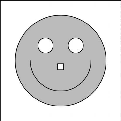
Processing ’s “ Hello, World! ” might look something like this:
Hello, Shapes!
ough quite friendly looking, it is nothing spectacular (both of these fi rst programs leave out #3:
interaction), but neither is “ Hello, World! ” However, the focus, learning through immediate visual
feedback, is quite diff erent.
Processing is not the fi rst language to follow this paradigm. In 1967, the Logo programming language was
developed by Daniel G. Bobrow, Wally Feurzeig, and Seymour Papert. With Logo, a programmer writes
instructions to direct a turtle around the screen, producing shapes and designs. John Maeda’s Design By
Numbers (1999) introduced computation to visual designers and artists with a simple, easy to use syntax.
Introduction xi
While both of these languages are wonderful for their simplicity and innovation, their capabilities are
limited.
Processing , a direct descendent of Logo and Design by Numbers , was born in 2001 in the “ Aesthetics and
Computation ” research group at the Massachusetts Institute of Technology Media Lab. It is an open
source initiative by Casey Reas and Benjamin Fry, who developed Processing as graduate students studying
with John Maeda.
“Processing is an open source programming language and environment for people who want to program
images, animation, and sound. It is used by students, artists, designers, architects, researchers, and hobbyists for
learning, prototyping, and production. It is created to teach fundamentals of computer programming within a
visual context and to serve as a software sketchbook and professional production tool. Processing is developed by
artists and designers as an alternative to proprietary software tools in the same domain.”
— www.processing.org
To sum up, Processing is awesome. First of all, it is free. It doesn’t cost a dime. Secondly, because Processing is
built on top of the Java programming language (this is explored further in the last chapter of this book), it is
a fully functional language without some of the limitations of Logo or Design by Numbers . ere is very little
you can’t do with Processing . Finally, Processing is open source. For the most part, this will not be a crucial
detail of the story of this book. Nevertheless, as you move beyond the beginning stages, this philosophical
principle will prove invaluable. It is the reason that such an amazing community of developers, teachers,
and artists come together to share work, contribute ideas, and expand the features of Processing .
A quick surf-through of the processing.org Web site reveals this vibrant and creative community. ere,
code is shared in an open exchange of ideas and artwork among beginners and experts alike. While the
site contains a complete reference as well as a plethora of examples to get you started, it does not have a
step-by-step tutorial for the true beginner. is book is designed to give you a jump start on joining and
contributing to this community by methodically walking you through the fundamentals of programming
as well as exploring some advanced topics.
It is important to realize that, although without Processing this book might not exist, this book is not a
Processing book per se. e intention here is to teach you programming. We are choosing to use Processing
as our learning environment, but the focus is on the core computational concepts, which will carry you
forward in your digital life as you explore other languages and environments.
But shouldn’t I be Learning __________ ?
You know you want to. Fill in that blank. You heard that the next big thing is that programming language
and environment Flibideefl obidee. Sure it sounds made up, but that friend of yours will not stop talking
about how awesome it is. How it makes everything soooo easy. How what used to take you a whole day
to program can be done in fi ve minutes. And it works on a Mac. And a PC! And a toaster oven! And you
can program your pets to speak with it. In Japanese!
Here’s the thing. at magical language that solves all your problems does not exist. No language is
perfect, and Processing comes with its fair share of limitations and fl aws. Processing , however, is an excellent
place to start (and stay). is book teaches you the fundamentals of programming so that you can apply
them throughout your life, whether you use Processing , Java, Actionscript, C, PHP, or some other language.
xii Introduction
It is true that for some projects, other languages and environments can be better. But Processing is really
darn good for a lot of stuff , especially media-related and screen-based work. A common misconception is
that Processing is just for fi ddling around; this is not the case. People (myself included) are out there using
Processing from day number 1 to day number 365 of their project. It is used for web applications, art projects
in museums and galleries, and exhibits and installations in public spaces. Most recently, I used Processing to
develop a real-time graphics video wall system ( http://www.mostpixelsever.com ) that can display content on a
120 by 12 foot (yes, feet!) video wall in the lobby of InterActive Corps ’ New York City headquarters.
Not only is Processing great for actually doing stuff , but for learning, there really isn’t much out there
better. It is free and open source. It is simple. It is visual. It is fun. It is object-oriented (we will get to this
later.) And it does actually work on Macs, PCs, and Linux machines (no talking dogs though, sorry).
So I would suggest to you that you stop worrying about what it is you should be using and focus on
learning the fundamentals with Processing . at knowledge will take you above and beyond this book to
any language you want to tackle.
Write in this book!
Let’s say you are a novelist. Or a screenwriter. Is the only time you spend writing the time spent sitting
and typing at a computer? Or (gasp) a typewriter? Most likely, this is not the case. Perhaps ideas swirl in
your mind as you lie in bed at night. Or maybe you like to sit on a bench in the park, feed the pigeons,
and play out dialogue in your head. And one late night, at the local pub, you fi nd yourself scrawling out a
brilliant plot twist on a napkin.
Well, writing software, programming, and creating code is no diff erent. It is really easy to forget this since
the work itself is so inherently tied to the computer. But you must fi nd time to let your mind wander,
think about logic, and brainstorm ideas away from the chair, the desk, and the computer. Personally, I do
all my best programming while jogging.
Sure, the actual typing on the computer part is pretty important. I mean, you will not end up with a life-
changing, working application just by laying out by the pool. But thinking you always need to be hunched
over the glare of an LCD screen will not be enough.
Writing all over this book is a step in the right direction, ensuring you will practice thinking through
code away from the keyboard. I have included many exercises in the book that incorporate a “ fi ll in
the blanks ” approach. (All of these fi ll in the blanks exercises have answers on the book’s Web site,
http://www.learningprocessing.com, so you can check your work.) Use these pages! When an idea
inspires you, make a note and write it down. ink of the book as a workbook and sketchbook for your
computational ideas. (You can of course use your own sketchbook, too.)
I would suggest you spend half your time reading this book away from the computer and the other half,
side by side with your machine, experimenting with example code along the way.
How should I read this book?
It is best to read this book in order. Chapter 1, Chapter 2, Chapter 3, and so on. You can get a bit more
relaxed about this after the end of Chapter 9 but in the beginning it is pretty important.

Introduction xiii
e book is designed to teach you programming in a linear fashion. A more advanced text might operate
more like a reference where you read bits and pieces here and there, moving back and forth throughout
the book. But here, the fi rst half of the book is dedicated to making one example, and building the
features of that example one step at a time (more on this in a moment). In addition, the fundamental
elements of computer programming are presented in a particular order, one that comes from several years
of trial and error with a group of patient and wonderful students in New York University’s Interactive
Telecommunications Program ( “ ITP ” ) at the Tisch School of the Arts ( http://itp.nyu.edu ).
e chapters of the book (23 total) are grouped into lessons (10 total). e fi rst nine chapters introduce
computer graphics, and cover the fundamental principles behind computer programming. Chapters 10
through 12 take a break from learning new material to examine how larger projects are developed with
an incremental approach. Chapters 13 through 23 expand on the basics and off er a selection of more
advanced topics ranging from 3D, to incorporating live video, to data visualization.
e “ Lessons ” are off ered as a means of dividing the book into digestible chunks. e end of a lesson marks
a spot at which I suggest you take a break from reading and attempt to incorporate that lesson’s chapters
into a project. Suggestions for these projects are off ered (but they are really just that: suggestions).
Is this a textbook?
is book is designed to be used either as a textbook for an introductory level programming course or for
self-instruction.
I should mention that the structure of this book comes directly out of the course “ Introduction to
Computational Media ” at ITP. Without the help my fellow teachers of this class (Dan O’Sullivan, Danny
Rozin, Chris Kairalla, Shawn Van Every, Nancy Lewis, Mark Napier, and James Tu) and hundreds of
students (I wish I could name them all here), I don’t think this book would even exist.
To be honest, though, I am including a bit more material than can be taught in a beginner level one
semester course. Out of the 23 chapters, I probably cover about 18 of them in detail in my class (but make
reference to everything in the book at some point). Nevertheless, whether or not you are reading the book
for a course or learning on your own, it is reasonable that you could consume the book in a period of a
few months. Sure, you can read it faster than that, but in terms of actually writing code and developing
projects that incorporate all the material here, you will need a fairly signifi cant amount of time. As
tempting as it is to call this book “ Learn to Program with 10 Lessons in 10 Days! ” it is just not realistic.
Here is an example of how the material could play out in a 14 week semester course.
Week 1 Lesson 1: Chapters 1–3
Week 2 Lesson 2: Chapters 4–6
Week 3 Lesson 3: Chapters 7–8
Week 4 Lesson 4: Chapter 9
Week 5 Lesson 5: Chapter 10–11
Week 6 Midterm! (Also, continue Lesson 5: Chapter 12)

xiv Introduction
Will this be on the test?
A book will only take you so far. e real key is practice, practice, practice. Pretend you are 10 years old
and taking violin lessons. Your teacher would tell you to practice every day. And that would seem perfectly
reasonable to you. Do the exercises in this book. Practice every day if you can.
Sometimes when you are learning, it can be diffi cult to come up with your own ideas. ese exercises are
there so that you do not have to. However, if you have an idea for something you want to develop, you
should feel free to twist and tweak the exercises to fi t with what you are doing.
A lot of the exercises are tiny little drills that can be answered in a few minutes. Some are a bit harder
and might require up to an hour. Along the way, however, it is good to stop and work on a project that
takes longer, a few hours, a day, or a week. As I just mentioned, this is what the “ lesson ” structure is for.
I suggest that in between each lesson, you take a break from reading and work on making something in
Processing . A page with project suggestions is provided for each lesson.
All of the answers to all of the exercises can be found on this book’s web site. Speaking of which …
Do you have a web site?
e Web site for this book is: http://www.learningprocessing.com
ere you will fi nd the following things:
• Answers to all exercises in the book.
• Downloadable versions of all code in the book.
• Online versions of the examples (that can be put online) in the book.
• Corrections of any errors in the book.
• Additional tips and tutorials beyond material in the book.
• Questions and comments page.
Since many of the examples in this book use color and are animated, the black and white, static
screenshots provided in the pages here will not give you the whole picture. As you are reading, you can
refer to the web site to view the examples running in your browser as well as download them to run
locally on your computer.
Week 7 Lesson 6: Chapter 13–14
Week 8 Lesson 7: Chapter 15–16
Week 9 Lesson 8: Chapters 17–19
Week 10 Lesson 9: Chapters 20–21
Week 11 Lesson 10: Chapters 22–23
Week 12 Final Project Workshop
Week 13 Final Project Workshop
Week 14 Final Project Presentations
Introduction xv
is book’s web site is not a substitute for the amazing resource that is the offi cial Processing web site:
http://www.processing.org . ere, you will fi nd the Processing reference, many more examples, and a lively
forum.
Take It One Step at a Time
e Philosophy of Incremental Development
ere is one more thing we should discuss before we embark on this journey together. It is an important
driving force behind the way I learned to program and will contribute greatly to the style of this book.
As coined by a former professor of mine, it is called the “ philosophy of incremental development. ” Or
perhaps, more simply, the “ one-step-at-a-time approach. ”
Whether you are a total novice or a coder with years of experience, with any programming project, it is
crucial not to fall into the trap of trying to do too much all at once. Your dream might be to create the
uber- Processing program that, say, uses Perlin noise to procedurally generate textures for 3D vertex shapes
that evolve via the artifi cial intelligence of a neural network that crawls the web mining for today’s news
stories, displaying the text of these stories onscreen in colors taken from a live video feed of a viewer in
front of the screen who can control the interface with live microphone input by singing.
ere is nothing wrong with having grand visions, but the most important favor you can do for yourself
is to learn how to break those visions into small parts and attack each piece slowly, one at a time. e
previous example is a bit silly; nevertheless, if you were to sit down and attempt to program its features all
at once, I am pretty sure you would end up using a cold compress to treat your pounding headache.
To demonstrate, let’s simplify and say that you aspire to program the game Space Invaders (see: http://
en.wikipedia.org/wiki/Space_Invaders ). While this is not explicitly a game programming book, the skills to
accomplish this goal will be found here. Following our newfound philosophy, however, we know we need
to develop one step at a time, breaking down the problem of programming Space Invaders into small
parts. Here is a quick attempt:
1. Program the spaceship.
2. Program the invaders.
3. Program the scoring system.
Great, we divided our program into three steps! Nevertheless, we are not at all fi nished. e key is to
divide the problem into the smallest pieces possible, to the point of absurdity, if necessary. You will learn
to scale back into larger chunks when the time comes, but for now, the pieces should be so small that
they seem ridiculously oversimplifi ed. After all, if the idea of developing a complex game such as Space
Invaders seems overwhelming, this feeling will go away if you leave yourself with a list of steps to follow,
each one simple and easy.
With that in mind, let’s try a little harder, breaking Step 1 from above down into smaller parts. e idea
here is that you would write six programs, the fi rst being the simplest: display a triangle . With each step,
we add a small improvement: move the triangle. As the program gets more and more advanced, eventually
we will be fi nished.

xvi Introduction
1.1 Draw a triangle onscreen. e triangle will be our spaceship.
1.2 Position the triangle at the bottom of the screen.
1.3 Position the triangle slightly to the right of where it was before.
1.4 Animate the triangle so that it moves from position left to right.
1.5 Animate the triangle from left to right only when the right-arrow key is pressed.
1.6 Animate the triangle right to left when the left-arrow key is pressed.
Of course, this is only a small fraction of all of the steps we need for a full Space Invaders game, but
it demonstrates a vital way of thinking. e benefi ts of this approach are not simply that it makes
programming easier (which it does), but that it also makes “ debugging ” easier.
Debugging
1 refers to the process of fi nding defects in a computer program and fi xing them so that the
program behaves properly. You have probably heard about bugs in, say, the Windows operating system:
miniscule, arcane errors deep in the code. For us, a bug is a much simpler concept: a mistake. Each time
you try to program something, it is very likely that something will not work as you expected, if at all. So
if you start out trying to program everything all at once, it will be very hard to fi nd these bugs. e one-
step-at-a-time methodology, however, allows you to tackle these mistakes one at a time, squishing the
bugs.
In addition, incremental development lends itself really well to object-oriented programming , a core
principle of this book. Objects, which will be introduced in Lesson 3, Chapter 8, will help us to develop
projects in modular pieces as well as provide an excellent means for organizing (and sharing) code.
Reusability will also be key. For example, if you have programmed a spaceship for Space Invaders and
want to start working on asteroids, you can grab the parts you need (i.e., the moving spaceship code), and
develop the new pieces around them.
Algorithms
When all is said and done, computer programming is all about writing algorithms . An algorithm is
a sequential list of instructions that solves a particular problem. And the philosophy of incremental
development (which is essentially an algorithm for you, the human being, to follow) is designed to make
it easier for you to write an algorithm that implements your idea.
As an exercise, before you get to Chapter 1, try writing an algorithm for something you do on a daily
basis, such as brushing your teeth. Make sure the instructions seem comically simple (as in “ Move the
toothbrush one centimeter to the left ” ).
Imagine that you had to provide instructions on how to accomplish this task to someone entirely
unfamiliar with toothbrushes, toothpaste, and teeth. at is how it is to write a program. A computer is
nothing more than a machine that is brilliant at following precise instructions, but knows nothing about
the world at large. And this is where we begin our journey, our story, our new life as a programmer. We
begin with learning how to talk to our friend, the computer.
1 e term “ debugging ” comes from the apocryphal story of a moth getting stuck in the relay circuits of one of computer scientist
Grace Murray Hopper’s computers.

Introduction xvii
Some suggestions:
• Do you do different things based on conditions? How might you use the words
“ if ” or “ otherwise ” in your instructions? (For example: if the water is too cold,
increase the warm water. Otherwise, increase cold water.)
• Use the word “ repeat ” in your instructions. For example: Move the brush up
and down. Repeat 5 times.
Also, note that we are starting with Step # 0. In programming, we often like to count
starting from 0 so it is good for us to get used to this idea right off the bat!
How to brush your teeth by ___________________________________________
Step 0. ___________________________________________________________
Step 1. ___________________________________________________________
Step 2. ___________________________________________________________
Step 3. ___________________________________________________________
Step 4. ___________________________________________________________
Step 5. ___________________________________________________________
Step 6. ___________________________________________________________
Step 7. ___________________________________________________________
Step 8. ___________________________________________________________
Step 9. ___________________________________________________________
Introductory Exercise: Write instructions for brushing your teeth.
This page intentionally left blank

Lesson One
The Beginning
1 Pixels
2 Processing
3 Interaction
This page intentionally left blank
Pixels 3
1 Pixels
“ A journey of a thousand miles begins with a single step. ”
—Lao-tzu
In this chapter:
– Specifying pixel coordinates.
– Basic shapes: point, line, rectangle, ellipse.
– Color: grayscale, “ RGB. ”
– Color transparency.
Note that we are not doing any programming yet in this chapter! We are just dipping our feet in the water and
getting comfortable with the idea of creating onscreen graphics with text-based commands, that is, “ code ” !
1.1 Graph Paper
is book will teach you how to program in the context of computational media, and it will use the
development environment Processing ( http://www.processing.org ) as the basis for all discussion and
examples. But before any of this becomes relevant or interesting, we must fi rst channel our eighth grade
selves, pull out a piece of graph paper, and draw a line. e shortest distance between two points is a good
old fashioned line, and this is where we begin, with two points on that graph paper.
0
0
1
2
3
4
5
Point B (4,5)
Point A
(1,0)
x-axis
y-axis
1234
fi g. 1.1
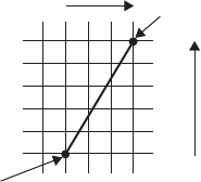
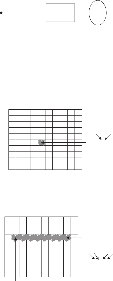
Figure 1.1 shows a line between point A (1,0) and point B (4,5). If you wanted to direct a friend of yours
to draw that same line, you would give them a shout and say “ draw a line from the point one-zero to
the point four-fi ve, please. ” Well, for the moment, imagine your friend was a computer and you wanted
to instruct this digital pal to display that same line on its screen. e same command applies (only this
time you can skip the pleasantries and you will be required to employ a precise formatting). Here, the
instruction will look like this:
line(1,0,4,5);
Congratulations, you have written your fi rst line of computer code! We will get to the precise formatting
of the above later, but for now, even without knowing too much, it should make a fair amount of sense.
We are providing a command (which we will refer to as a “ function ” ) for the machine to follow entitled
“ line. ” In addition, we are specifying some arguments for how that line should be drawn, from point
4Learning Processing
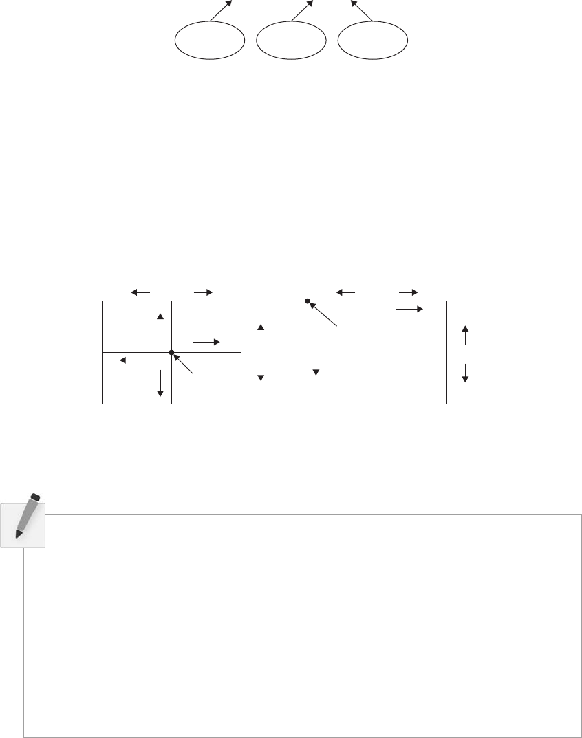
A (0,1) to point B (4,5). If you think of that line of code as a sentence, the function is a verb and the
arguments are the objects of the sentence. e code sentence also ends with a semicolon instead of a period.
Verb Object Object
Draw a line from 0,1 to 4,5
fi g. 1.2
(0,0)
(0,0)
y-axis y-axis
x-axis x-axis
Eighth grade Computer
fi g. 1.3
e key here is to realize that the computer screen is nothing more than a fancier piece of graph paper.
Each pixel of the screen is a coordinate—two numbers, an “ x ” (horizontal) and a “ y ” (vertical)—that
determine the location of a point in space. And it is our job to specify what shapes and colors should
appear at these pixel coordinates.
Nevertheless, there is a catch here. e graph paper from eighth grade ( “ Cartesian coordinate system ” )
placed (0,0) in the center with the y-axis pointing up and the x-axis pointing to the right (in the positive
direction, negative down and to the left). e coordinate system for pixels in a computer window,
however, is reversed along the y -axis. (0,0) can be found at the top left with the positive direction to the
right horizontally and down vertically. See Figure 1.3 .
Exercise 1-1: Looking at how we wrote the instruction for line “ line(1,0,4,5); ” how would
you guess you would write an instruction to draw a rectangle? A circle? A triangle? Write
out the instructions in English and then translate it into “ code. ”
English: ________________________________________________________________ _
Code: ______________________________________________________ ___________
English: ______________________________________________________ ___________
Code: ______________________________________________________ ___________
English: ______________________________________________________ ___________
Code: ______________________________________________________ ___________
Come back later and see how your guesses matched up with how Processing actually works.
Pixels 5
1.2 Simple Shapes
e vast majority of the programming examples in this book will be visual in nature. You may ultimately
learn to develop interactive games, algorithmic art pieces, animated logo designs, and (insert your own
category here) with Processing , but at its core, each visual program will involve setting pixels. e simplest
way to get started in understanding how this works is to learn to draw primitive shapes. is is not unlike
how we learn to draw in elementary school, only here we do so with code instead of crayons.
Let’s start with the four primitive shapes shown in Figure 1.4 .
Point Line Rectangle Ellipse
fi g. 1.4
0
01234
x-axis
y
-axis
56789
1
2
3
4
Point (4,5);
x
5
6
7
8
9
y
fi g. 1.5
For each shape, we will ask ourselves what information is required to specify the location and size (and
later color) of that shape and learn how Processing expects to receive that information. In each of the
diagrams below ( Figures 1.5 through 1.11), assume a window with a width of 10 pixels and height of
10 pixels. is isn’t particularly realistic since when we really start coding we will most likely work with
much larger windows (10 10 pixels is barely a few millimeters of screen space). Nevertheless for
demonstration purposes, it is nice to work with smaller numbers in order to present the pixels as they
might appear on graph paper (for now) to better illustrate the inner workings of each line of code.
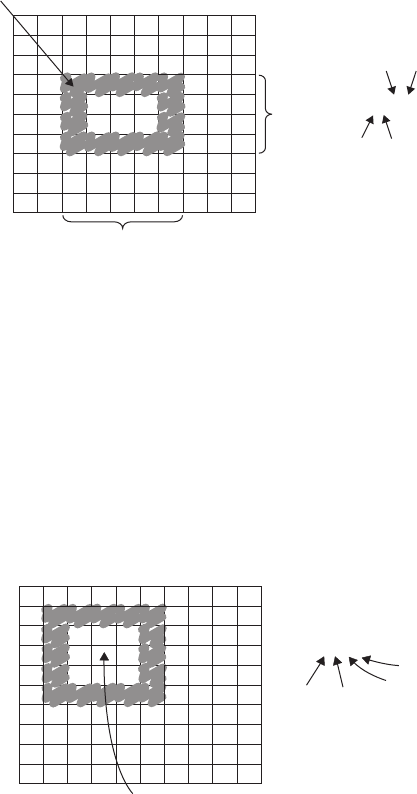
A point is the easiest of the shapes and a good place to start. To draw a point, we only need an x and y
coordinate as shown in Figure 1.5 . A line isn’t terribly diffi cult either. A line requires two points, as shown
in Figure 1.6 .
fi g. 1.6
0
01234
x-axis
y-axis
56789
1
2
3
4
Point B (8,3)
line (1,3,8,3);
5
6
7
8
9
Point A (1,3)
y
x
Point A yx
Point B
6Learning Processing
0
01234
x-axis
y
-axis
56789
1
2
3
4
rectMode (CENTER);
rect (3,3,5,5);
5
6
7
8
9
center
(3,3)
center
x
center
y
width
height
fi g. 1.8
0
01234
x-axis
y-axis
56789
1
2
3
4 rect (2,3,5,4);
top left
x
Top left
top left
y
width
width
height
height
5
6
7
8
9
fi g. 1.7
Finally, we can also draw a rectangle with two points (the top left corner and the bottom right corner).
e mode here is “ CORNERS ” (see Figure 1.9) .
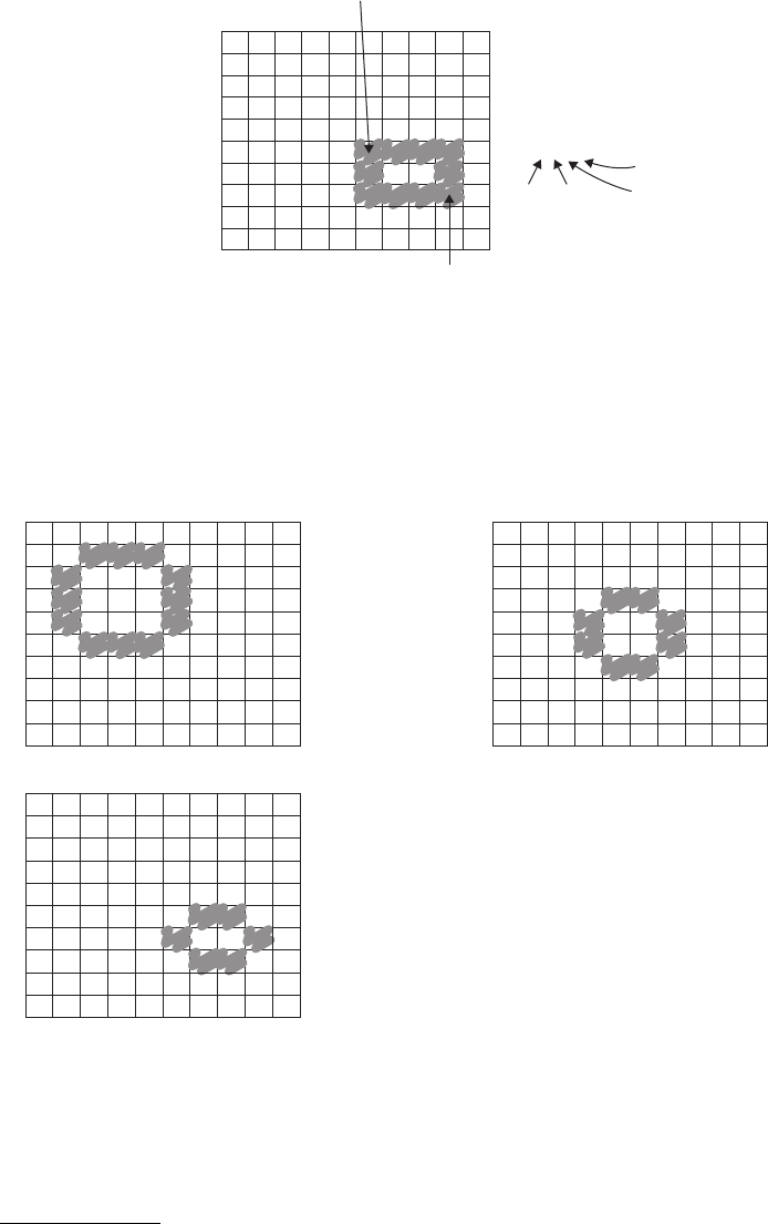
Once we arrive at drawing a rectangle, things become a bit more complicated. In Processing , a rectangle is
specifi ed by the coordinate for the top left corner of the rectangle, as well as its width and height
(see Figure 1.7 ).
However, a second way to draw a rectangle involves specifying the centerpoint, along with width
and height as shown in Figure 1.8 . If we prefer this method, we fi rst indicate that we want to use the
“ CENTER ” mode before the instruction for the rectangle itself. Note that Processing is case-sensitive.
Incidentally, the default mode is “ CORNER, ” which is how we began as illustrated in Figure 1.7 .
Pixels 7
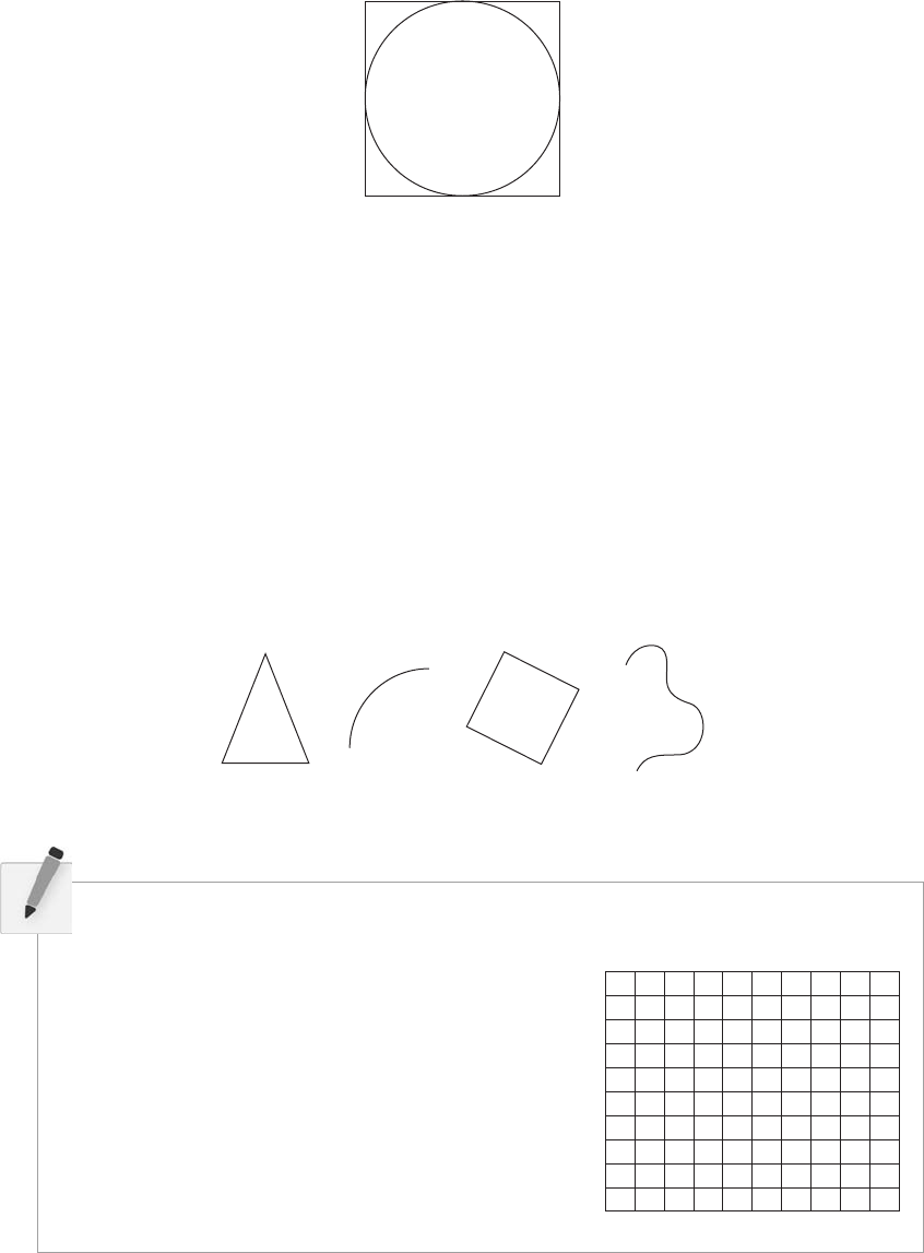
Once we have become comfortable with the concept of drawing a rectangle, an ellipse is a snap. In fact, it
is identical to rect( ) with the diff erence being that an ellipse is drawn where the bounding box
1 (as shown
in Figure 1.11 ) of the rectangle would be. e default mode for ellipse( ) is “ CENTER ” , rather than
“ CORNER ” as with rect( ) . See Figure 1.10 .
0
0123456789
1
2
3
4
5
6
7
8
9
bottom right (8,7)
rectMode (CORNERS)
rect (5,5,8,7);
top left (5,5)
top left
xbottom right x
bottom right y
top left
y
fi g. 1.9
1 A bounding box of a shape in computer graphics is the smallest rectangle that includes all the pixels of that shape. For example, the
bounding box of a circle is shown in Figure 1.11 .
0
0123456789
1
2
3
4ellipseMode (CENTER);
ellipse (3,3,5,5);
5
6
7
8
9
ellipseMode (CORNER);
ellipse (3,3,4,4);
0
0123456789
1
2
3
4
5
6
7
8
9
ellipseMode (CORNERS);
ellipse (5,5,8,7);
0
0123456789
1
2
3
4
5
6
7
8
9
fi g. 1.10
It is important to acknowledge that in Figure 1.10 , the ellipses do not look particularly circular. Processing
has a built-in methodology for selecting which pixels should be used to create a circular shape. Zoomed
in like this, we get a bunch of squares in a circle-like pattern, but zoomed out on a computer screen,
we get a nice round ellipse. Later, we will see that Processing gives us the power to develop our own
8Learning Processing
Triangle Arc Quad Curve
fi g. 1.12
algorithms for coloring in individual pixels (in fact, we can already imagine how we might do this using
“ point ” over and over again), but for now, we are content with allowing the “ ellipse ” statement to do the
hard work.
Certainly, point, line, ellipse, and rectangle are not the only shapes available in the Processing library
of functions. In Chapter 2, we will see how the Processing reference provides us with a full list of
available drawing functions along with documentation of the required arguments, sample syntax, and
imagery. For now, as an exercise, you might try to imagine what arguments are required for some other
shapes (Figure 1.12):
triangle( )
arc( )
quad( )
curve( )
0
01234
x-axis
y-axis
56789
1
2
3
4
5
6
7
8
9
line(0,0,9,6);
point(0,2);
point(0,4);
rectMode(CORNER);
rect(5,0,4,3);
ellipseMode(CENTER);
ellipse(3,7,4,4);
Exercise 1-2: Using the blank graph below, draw the primitive shapes specifi ed by the code.
Circle’s bounding box
fi g. 1.11
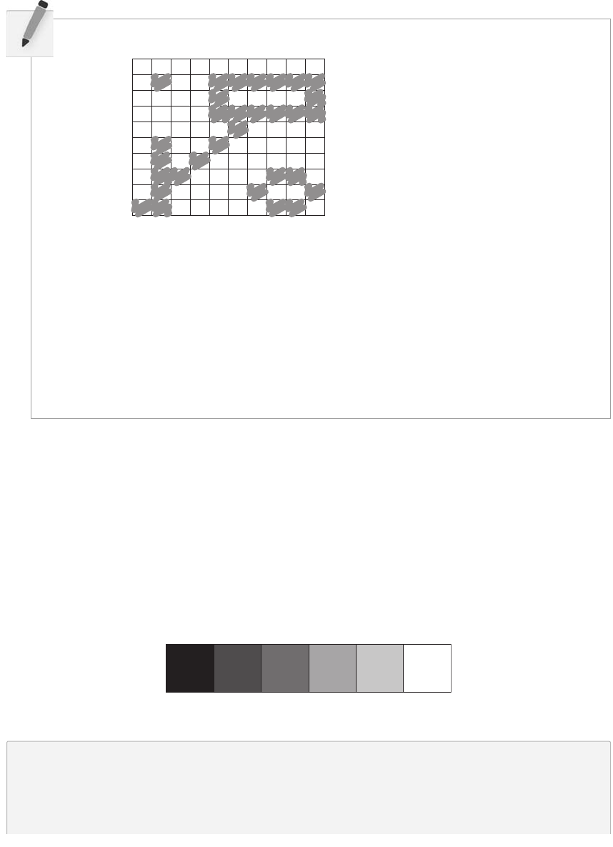
Pixels 9
Exercise 1-3: Reverse engineer a list of primitive shape drawing instructions for the diagram below.
0
01234
Note: There is more than one correct answer!
56789
1
2
3
4
5
6
7
8
9
__________________________________________________________________
__________________________________________________________________
__________________________________________________________________
__________________________________________________________________
__________________________________________________________________
1.3 Grayscale Color
As we learned in Section 1.2, the primary building block for placing shapes onscreen is a pixel
coordinate. You politely instructed the computer to draw a shape at a specifi c location with a specifi c size.
Nevertheless, a fundamental element was missing—color.
In the digital world, precision is required. Saying “ Hey, can you make that circle bluish-green? ” will
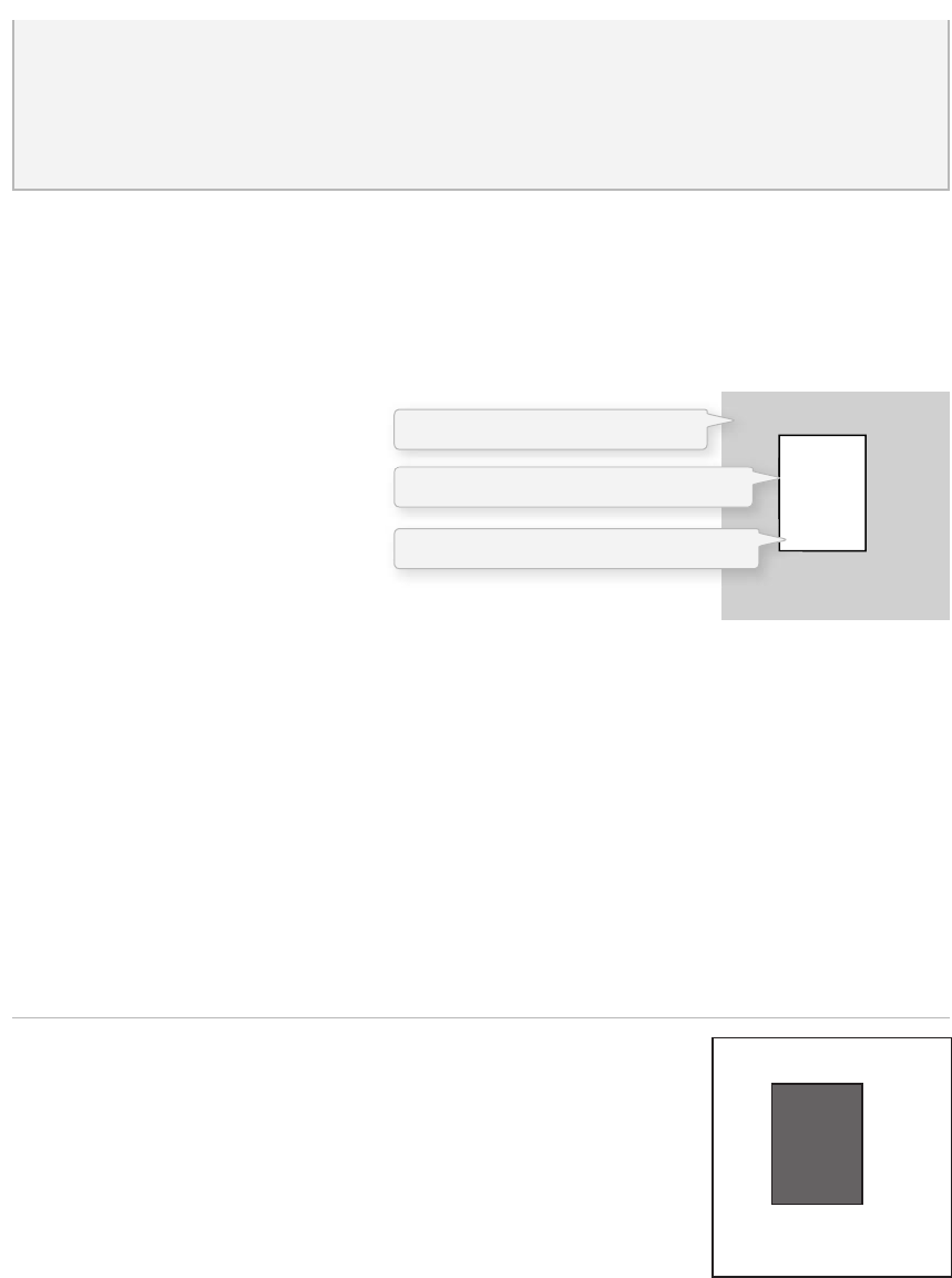
not do. erefore, color is defi ned with a range of numbers. Let’s start with the simplest case: black and
white or grayscale . In grayscale terms, we have the following: 0 means black, 255 means white. In between,
every other number—50, 87, 162, 209, and so on—is a shade of gray ranging from black to white. See
Figure 1.13 .
0 50 87 162 209 255
fi g. 1.13
Does 0–255 seem arbitary to you?
Color for a given shape needs to be stored in the computer’s memory. is memory is just a long
sequence of 0’s and 1’s (a whole bunch of on or off switches.) Each one of these switches is a
10 Learning Processing
By adding the stroke( ) and fi ll( ) functions before the shape is drawn, we can set the color. It is much like
instructing your friend to use a specifi c pen to draw on the graph paper. You would have to tell your
friend before he or she starting drawing, not after.
ere is also the function background( ) , which sets a background color for the window where shapes will
be rendered.
Example 1-1: Stroke and fi ll
background(255);
stroke(0);
fill(150);
rect(50,50,75,100);
stroke( ) or fi ll( ) can be eliminated with the noStroke( ) or noFill( ) functions.
Our instinct might be to say “ stroke(0) ” for no outline, however, it is
important to remember that 0 is not “ nothing ” , but rather denotes the color
black. Also, remember not to eliminate both—with noStroke( ) and noFill( ) ,
nothing will appear!
Understanding how this range works, we can now move to setting specifi c grayscale colors for the shapes
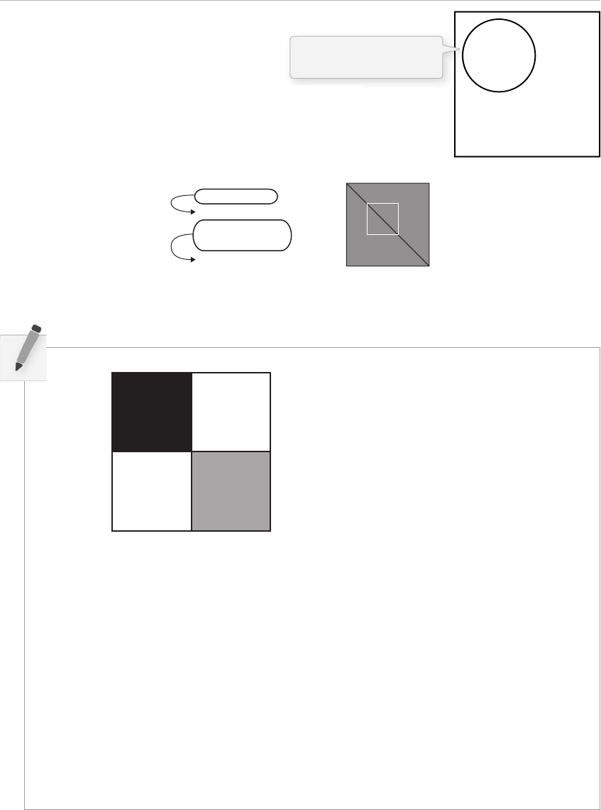
we drew in Section 1.2. In Processing , every shape has a stroke( ) or a fi ll( ) or both. e stroke( ) is the
outline of the shape, and the fi ll( ) is the interior of that shape. Lines and points can only have stroke( ) , for
obvious reasons.
If we forget to specify a color,
Processing will use black (0) for the
stroke( ) and white (255) for the
fi ll( ) by default. Note that we are
now using more realistic numbers
for the pixel locations, assuming a
larger window of size 200 200
pixels. See Figure 1.14.
rect(50,40,75,100);
fi g. 1.14
fi g. 1.15
bit , eight of them together is a byte . Imagine if we had eight bits (one byte) in sequence—how
many ways can we confi gure these switches? e answer is (and doing a little research into binary
numbers will prove this point) 256 possibilities, or a range of numbers between 0 and 255. We will
use eight bit color for our grayscale range and 24 bit for full color (eight bits for each of the red,
green, and blue color components; see Section 1.4).
The outline of the rectangle is black
The interior of the rectangle is white
The background color is gray.
Pixels 11
background(150);
stroke(0);
line(0,0,100,100);
stroke(255);
noFill();
rect(25,25,50,50);
fi g. 1.17
Example 1-2: noFill ( )
background(255);
stroke(0);
noFill();
ellipse(60,60,100,100);
If we draw two shapes at one time, Processing will always use the
most recently specifi ed stroke( ) and fi ll( ) , reading the code from top to
bottom. See Figure 1.17 .
fi g. 1.16
Exercise 1-4: Try to guess what the instructions would be for the following screenshot.
__________________________________________________________________
__________________________________________________________________
__________________________________________________________________
__________________________________________________________________
__________________________________________________________________
__________________________________________________________________
__________________________________________________________________
__________________________________________________________________
nofi ll( ) leaves the shape
with only an outline

12 Learning Processing
1.4 RGB Color
A nostalgic look back at graph paper helped us learn the fundamentals for pixel locations and size.
Now that it is time to study the basics of digital color, we search for another childhood memory to get
us started. Remember fi nger painting? By mixing three “ primary ” colors, any color could be generated.
Swirling all colors together resulted in a muddy brown. e more paint you added, the darker it got.
Digital colors are also constructed by mixing three primary colors, but it works diff erently from paint.
First, the primaries are diff erent: red, green, and blue (i.e., “ RGB ” color). And with color on the screen,
you are mixing light, not paint, so the mixing rules are diff erent as well.
• Red green yellow
• Red blue purple
• Green blue cyan (blue-green)
• Red green blue white
• No colors black
is assumes that the colors are all as bright as possible, but of course, you have a range of color available, so
some red plus some green plus some blue equals gray, and a bit of red plus a bit of blue equals dark purple.
While this may take some getting used to, the more you program and experiment with RGB color, the more
it will become instinctive, much like swirling colors with your fi ngers. And of course you can’t say “ Mix
some red with a bit of blue, ” you have to provide an exact amount. As with grayscale, the individual color
elements are expressed as ranges from 0 (none of that color) to 255 (as much as possible), and they are listed
in the order R, G, and B. You will get the hang of RGB color mixing through experimentation, but next we
will cover some code using some common colors.
Note that this book will only show you black and white versions of each Processing
sketch, but everything
is documented online in full color at http://www.learningprocessing.com with RGB color diagrams found
specifi cally at: http://learningprocessing.com/color .
Example 1-3: RGB color
background(255);
noStroke();
fill(255,0,0);
ellipse(20,20,16,16);
fill(127,0,0);
ellipse(40,20,16,16);
fill(255,200,200);
ellipse(60,20,16,16);
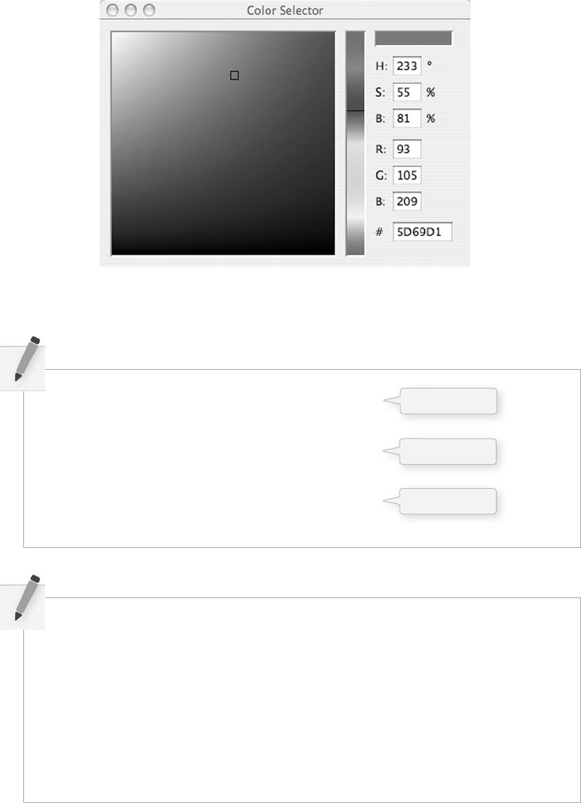
Processing also has a color selector to aid in choosing colors. Access this via TOOLS (from the
menu bar) → COLOR SELECTOR. See Figure 1.19 .
fi g. 1.18
Bright red
Dark red
Pink (pale red).
Pixels 13
fi g. 1.19
fill(0,100,0); ______________________________________
fill(100); ______________________________________
stroke(0,0,200); ______________________________________
stroke(225); ______________________________________
stroke(255,255,0); ______________________________________
stroke(0,255,255); ______________________________________
stroke(200,50,50); ______________________________________
Exercise 1-6: What color will each of the following lines of code generate?
Exercise 1-5: Complete the following program. Guess what RGB values to use (you will be
able to check your results in Processing after reading the next chapter). You could also use the
color selector, shown in Figure 1.19 .
fill(________,________,________);
ellipse(20,40,16,16);
fill(________,________,________);
ellipse(40,40,16,16);
fill(________,________,________);
ellipse(60,40,16,16);
Bright blue
Dark purple
Yellow
14 Learning Processing
1.5 Color Transparency
In addition to the red, green, and blue components of each color, there is an additional optional fourth
component, referred to as the color’s “ alpha. ” Alpha means transparency and is particularly useful when
you want to draw elements that appear partially see-through on top of one another. e alpha values for
an image are sometimes referred to collectively as the “ alpha channel ” of an image.
It is important to realize that pixels are not literally transparent, this is simply a convenient illusion that
is accomplished by blending colors. Behind the scenes, Processing takes the color numbers and adds a
percentage of one to a percentage of another, creating the optical perception of blending. (If you are
interested in programming “ rose-colored ” glasses, this is where you would begin.)
Alpha values also range from 0 to 255, with 0 being completely transparent (i.e., 0% opaque) and 255
completely opaque (i.e., 100% opaque). Example 1-4 shows a code example that is displayed in
Figure 1.20 .
Example 1-4: Alpha transparency
background(0);
noStroke( );
fill(0,0,255);
rect(0,0,100,200);
fill(255,0,0,255);
rect(0,0,200,40);
fill(255,0,0,191);
rect(0,50,200,40);
fill(255,0,0,127);
rect(0,100,200,40);
fill(255,0,0,63);
rect(0,150,200,40);
1.6 Custom Color Ranges
RGB color with ranges of 0 to 255 is not the only way you can handle color in Processing . Behind
the scenes in the computer’s memory, color is always talked about as a series of 24 bits (or 32 in
the case of colors with an alpha). However, Processing will let us think about color any way we like,
and translate our values into numbers the computer understands. For example, you might prefer to
think of color as ranging from 0 to 100 (like a percentage). You can do this by specifying a custom
colorMode( ) .
fi g. 1.20
No fourth argument means 100% opacity.
255 means 100% opacity.
75% opacity
50% opacity
25% opacity
Pixels 15
colorMode(RGB,100);
e above function says: “ OK, we want to think about color in terms of red, green, and blue. e range of
RGB values will be from 0 to 100. ”
Although it is rarely convenient to do so, you can also have diff erent ranges for each color component:
colorMode(RGB,100,500,10,255);
Now we are saying “ Red values go from 0 to 100, green from 0 to 500, blue from 0 to 10, and alpha from
0 to 255. ”
Finally, while you will likely only need RGB color for all of your programming needs, you can also specify
colors in the HSB (hue, saturation, and brightness) mode. Without getting into too much detail, HSB
color works as follows:
• Hue —The color type, ranges from 0 to 360 by default (think of 360° on a color “ wheel ” ).
• Saturation —The vibrancy of the color, 0 to 100 by default.
• Brightness —The, well, brightness of the color, 0 to 100 by default.
________________________________________
________________________________________
________________________________________
________________________________________
________________________________________
________________________________________
________________________________________
________________________________________
________________________________________
Exercise 1-7: Design a creature using simple shapes and colors. Draw the creature by hand
using only points, lines, rectangles, and ellipses. en attempt to write the code for the
creature, using the Processing commands covered in this chapter: point( ), lines( ), rect( ),
ellipse( ), stroke( ) , and fi ll( ) . In the next chapter, you will have a chance to test your results
by running your code in Processing.
With colorMode( ) you can set your own color range.
16 Learning Processing
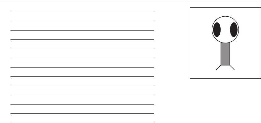
Example 1-5 shows my version of Zoog, with the outputs shown in Figure 1.21 .
Example 1-5: Zoog
ellipseMode(CENTER);
rectMode(CENTER);
stroke(0);
fi ll(150);
rect(100,100,20,100);
fi ll(255);
ellipse(100,70,60,60);
fi ll(0);
ellipse(81,70,16,32);
ellipse(119,70,16,32);
stroke(0);
line(90,150,80,160);
line(110,150,120,160);
e sample answer is my Processing -born being, named Zoog. Over the course of the fi rst nine chapters
of this book, we will follow the course of Zoog’s childhood. e fundamentals of programming will be
demonstrated as Zoog grows up. We will fi rst learn to display Zoog, then to make an interactive Zoog
and animated Zoog, and fi nally to duplicate Zoog in a world of many Zoogs.
I suggest you design your own “ thing ” (note that there is no need to limit yourself to a humanoid or
creature-like form; any programmatic pattern will do) and recreate all of the examples throughout
the fi rst nine chapters with your own design. Most likely, this will require you to only change a small
portion (the shape rendering part) of each example. is process, however, should help solidify your
understanding of the basic elements required for computer programs—Variables, Conditionals, Loops,
Functions, Objects, and Arrays—and prepare you for when Zoog matures, leaves the nest, and ventures
off into the more advanced topics from Chapter 10 on in this book.
fi g. 1.21
Processing 17
2 Processing
“ Computers in the future may weigh no more than 1.5 tons. ”
—Popular Mechanics, 1949
“ Take me to your leader. ”
—Zoog, 2008
In this chapter:
– Downloading and installing Processing .
– Menu options.
– A Processing “ sketchbook. ”
– Writing code.
– Errors.
– The Processing reference.
– The “ Play ” button.
– Your fi rst sketch.
– Publishing your sketch to the web.
2.1 Processing to the Rescue
Now that we conquered the world of primitive shapes and RGB color, we are ready to implement this
knowledge in a real world programming scenario. Happily for us, the environment we are going to use is
Processing , free and open source software developed by Ben Fry and Casey Reas at the MIT Media Lab
in 2001. (See this book’s introduction for more about Processing ’s history.)
Processing ’s core library of functions for drawing graphics to the screen will provide for immediate visual
feedback and clues as to what the code is doing. And since its programming language employs all the
same principles, structures, and concepts of other languages (specifi cally Java), everything you learn with
Processing is real programming. It is not some pretend language to help you get started; it has all the
fundamentals and core concepts that all languages have.
After reading this book and learning to program, you might continue to use Processing in your academic
or professional life as a prototyping or production tool. You might also take the knowledge acquired
here and apply it to learning other languages and authoring environments. You may, in fact, discover
that programming is not your cup of tea; nonetheless, learning the basics will help you become a better-
informed technology citizen as you work on collaborative projects with other designers and programmers.
It may seem like overkill to emphasize the why with respect to Processing . After all, the focus of this
book is primarily on learning the fundamentals of computer programming in the context of computer
graphics and design. It is, however, important to take some time to ponder the reasons behind selecting
a programming language for a book, a class, a homework assignment, a web application, a software suite,
and so forth. After all, now that you are going to start calling yourself a computer programmer at cocktail
parties, this question will come up over and over again. I need programming in order to accomplish
project X , what language and environment should I use?
I say, without a shadow of doubt, that for you, the beginner, the answer is Processing . Its simplicity is ideal
for a beginner. At the end of this chapter, you will be up and running with your fi rst computational design
and ready to learn the fundamental concepts of programming. But simplicity is not where Processing
18 Learning Processing
ends. A trip through the Processing online exhibition ( http://processing.org/exhibition/ ) will uncover a
wide variety of beautiful and innovative projects developed entirely with Processing . By the end of this
book, you will have all the tools and knowledge you need to take your ideas and turn them into real
world software projects like those found in the exhibition. Processing is great both for learning and for
producing, there are very few other environments and languages you can say that about.
2.2 How do I get Processing?
For the most part, this book will assume that you have a basic working knowledge of how to operate
your personal computer. e good news, of course, is that Processing is available for free download. Head
to http://www.processing.org/ and visit the download page. If you are a Windows user, you will see two
options: “ Windows (standard) ” and “ Windows (expert). ” Since you are reading this book, it is quite
likely you are a beginner, in which case you will want the standard version. e expert version is for those
who have already installed Java themselves. For Mac OS X, there is only one download option. ere is
also a Linux version available. Operating systems and programs change, of course, so if this paragraph is
obsolete or out of date, visit the download page on the site for information regarding what you need.
e Processing software will arrive as a compressed fi le. Choose a nice directory to store the application
(usually “ c:\Program Files\ ” on Windows and in “ Applications ” on Mac), extract the fi les there, locate the
“ Processing ” executable, and run it.
Exercise 2-1: Download and install Processing.
2.3 The Processing Application
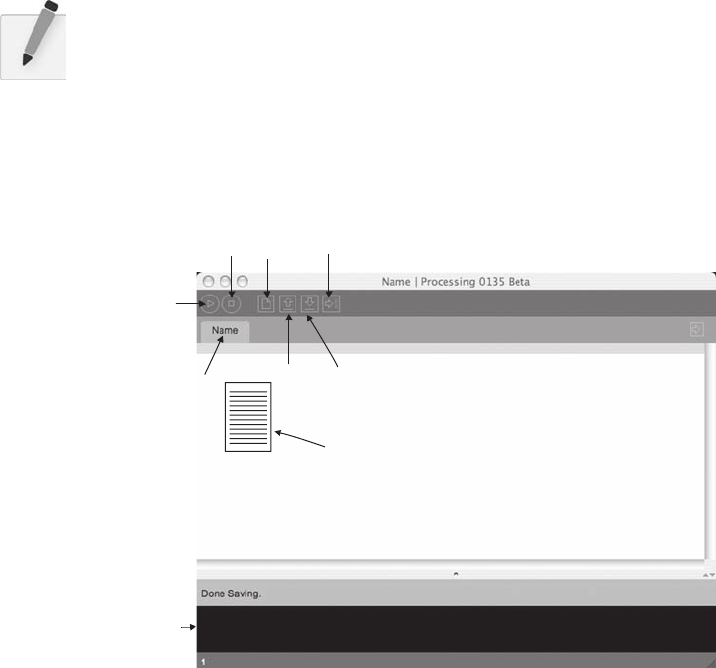
e Processing development environment is a simplifi ed environment for writing computer code, and is just
about as straightforward to use as simple text editing software (such as TextEdit or Notepad) combined
with a media player. Each sketch ( Processing programs are referred to as “ sketches ” ) has a fi lename, a place
where you can type code, and some buttons for saving, opening, and running sketches. See Figure 2.1 .
Stop New Export
Save
Open
Type code here
Sketch
name
Message
window
Run
fi g. 2.1
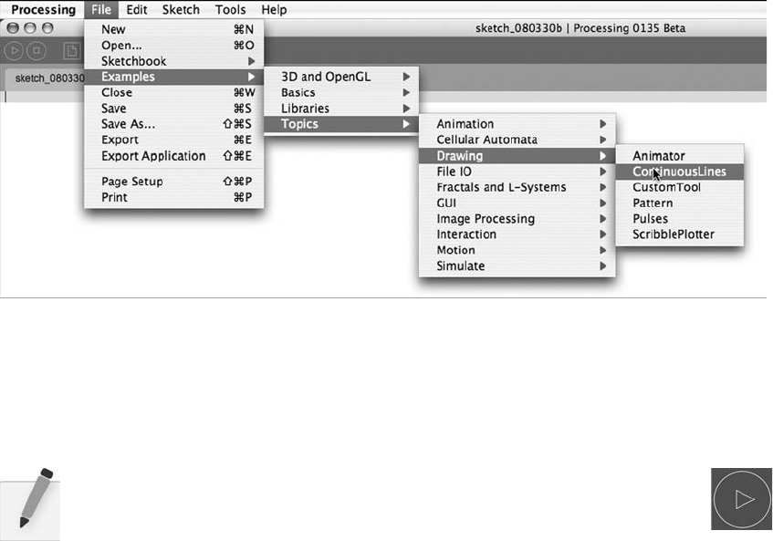
Once you have opened the example, click the “ run ” button as indicated in Figure 2.3 . If a new window
pops open running the example, you are all set! If this does not occur, visit the online FAQ “ Processing
won’t start! ” for possible solutions. e page can be found at this direct link: http://www.processing.org/faq/
bugs.html#wontstart .
Exercise 2-2: Open a sketch from the Processing examples and run it.
Processing programs can also be viewed full-screen (known as “ present mode ” in Processing ). is
is available through the menu option: Sketch → Present (or by shift-clicking the run button). Present will
not resize your screen resolution. If you want the sketch to cover your entire screen, you must use your
screen dimensions in size( ) .
2.4 The Sketchbook
Processing programs are informally referred to as sketches , in the spirit of quick graphics prototyping, and
we will employ this term throughout the course of this book. e folder where you store your sketches
is called your “sketchbook.” Technically speaking, when you run a sketch in processing , it runs as a local
application on your computer. As we will see both in this Chapter and in Chapter 18, Processing also
allows you to export your sketches as web applets (mini-programs that run embedded in a browser) or as
platform-specifi c stand-alone applications (that could, for example, be made available for download).
Once you have confi rmed that the Processing examples work, you are ready to start creating your own
sketches. Clicking the “ new ” button will generate a blank new sketch named by date. It is a good idea to
“ Save as ” and create your own sketch name. (Note: Processing does not allow spaces or hyphens, and your
sketch name cannot start with a number.)
fi g. 2.2
To make sure everything is working, it is a good idea to try running one of the Processing examples. Go
to FILE → EXAMPLES → (pick an example, suggested: Topics → Drawing → ContinuousLines) as
shown in Figure 2.2 .
fi g. 2.3
Processing 19
20 Learning Processing
When you fi rst ran Processing , a default “ Processing ” directory was created to store all sketches in the
“ My Documents ” folder on Windows and in “ Documents ” on OS X. Although you can select any
directory on your hard drive, this folder is the default. It is a pretty good folder to use, but it can be
changed by opening the Processing preferences (which are available under the FILE menu).
Each Processing sketch consists of a folder (with the same name as your sketch) and a fi le with the
extension “ pde. ” If your Processing sketch is named MyFirstProgram , then you will have a folder named
MyFirstProgram with a fi le MyFirstProgram.pde inside. e “ pde ” fi le is a plain text fi le that contains the
source code. (Later we will see that Processing sketches can have multiple pde’s, but for now one will do.)
Some sketches will also contain a folder called “ data ” where media elements used in the program, such as
image fi les, sound clips, and so on, are stored.
Exercise 2-3: Type some instructions from Chapter 1 into a blank sketch. Note how certain
words are colored. Run the sketch. Does it do what you thought it would?
2.5 Coding in Processing
It is fi nally time to start writing some code, using the elements discussed in Chapter 1. Let’s go over some
basic syntax rules. ere are three kinds of statements we can write:
• Function calls
• Assignment operations
• Control structures
For now, every line of code will be a function call. See Figure 2.4 . We will explore the other two categories
in future chapters. Functions have a name, followed by a set of arguments enclosed in parentheses.
Recalling Chapter 1, we used functions to describe how to draw shapes (we just called them “ commands ”
or “ instructions ” ). inking of a function call as a natural language sentence, the function name is the verb
( “ draw ” ) and the arguments are the objects ( “ point 0,0 ” ) of the sentence. Each function call must always
end with a semicolon. See Figure 2.5 .
Ends with
semi-colon
Arguments in
parentheses
Function
name
Line (0,0,200,200);
fi g. 2.4
We have learned several functions already, including background( ), stroke( ), fi ll( ), noFill ( ), noStroke( ),
point( ), line( ), rect( ), ellipse( ), rectMode( ), and ellipseMode( ) . Processing will execute a sequence of
functions one by one and fi nish by displaying the drawn result in a window. We forgot to learn one
very important function in Chapter 1, however— size( ). size( ) specifi es the dimensions of the window
you want to create and takes two arguments, width and height. e size( ) function should always
be fi rst.
size(320,240); Opens a window of width 320 and height 240.
ere are a few additional items to note.
• The Processing text editor will color known words (sometimes referred to as “ reserved ” words or
“ keywords ” ). These words, for example, are the drawing functions available in the Processing library,
“ built-in ” variables (we will look closely at the concept of variables in Chapter 3) and constants, as
well as certain words that are inherited from the Java programming language.
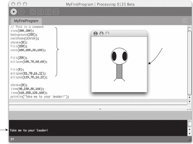
• Sometimes, it is useful to display text information in the Processing message window (located at the
bottom). This is accomplished using the println( ) function. println( ) takes one argument, a String
of characters enclosed in quotes (more about Strings in Chapter 14). When the program runs,
Processing displays that String in the message window (as in Figure 2.5 ) and in this case the String
is “ Take me to your leader! ” This ability to print to the message window comes in handy when
attempting to debug the values of variables (see Chapter 12, Debugging).
• The number in the bottom left corner indicates what line number in the code is selected.
• You can write “ comments ” in your code. Comments are lines of text that Processing ignores when
the program runs. You should use them as reminders of what the code means, a bug you intend to
fix, or a to do list of items to be inserted, and so on. Comments on a single line are created with two
forward slashes, // . Comments over multiple lines are marked by /* followed by the comments and
ending with */ .
Let’s write a fi rst example ( see Figure 2.5 ).
Output
window
Code
Print
messages
fi g. 2.5
Processing 21

22 Learning Processing
// is is a comment on one line
/* is is a comment that
spans several lines
of code */
A quick word about comments. You should get in the habit right now of writing comments in your
code. Even though our sketches will be very simple and short at fi rst, you should put comments in for
everything. Code is very hard to read and understand without comments. You do not need to have a
comment for every line of code, but the more you include, the easier a time you will have revising and
reusing your code later. Comments also force you to understand how code works as you are programming.
If you do not know what you are doing, how can you write a comment about it?
Comments will not always be included in the text here. is is because I fi nd that, unlike in an actual
program, code comments are hard to read in a book. Instead, this book will often use code “ hints ” for
additional insight and explanations. If you look at the book’s examples on the web site, though, comments
will always be included. So, I can’t emphasize it enough, write comments!
// A comment about this code
line(0,0,100,100);
Exercise 2-4: Create a blank sketch. Take your code from the end of Chapter 1 and type it in
the Processing window. Add comments to describe what the code is doing. Add a println( )
statement to display text in the message window. Save the sketch. Press the “ run ” button. Does it
work or do you get an error?
2.6 Errors
e previous example only works because we did not make any errors or typos. Over the course of a
programmer’s life, this is quite a rare occurrence. Most of the time, our fi rst push of the play button will
not be met with success. Let’s examine what happens when we make a mistake in our code in Figure 2.6 .
Figure 2.6 shows what happens when you have a typo— “ elipse ” instead of “ ellipse ” on line 9. If there is
an error in the code when the play button is pressed, Processing will not open the sketch window, and will
instead display the error message. is particular message is fairly friendly, telling us that we probably
meant to type “ ellipse. ” Not all Processing error messages are so easy to understand, and we will continue
to look at other errors throughout the course of this book. An Appendix on common errors in Processing
is also included at the end of the book.
A hint about this code!
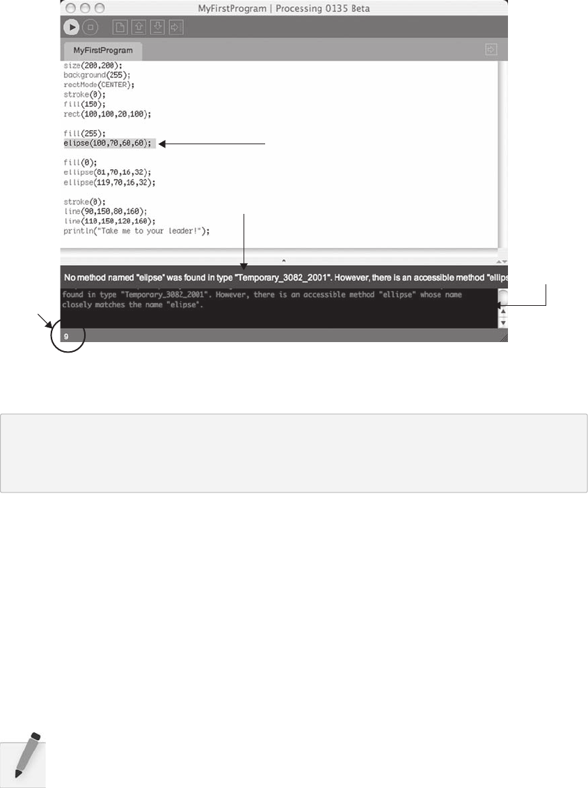
Processing 23
Line 9 highlighted
Line 9
Error message
Error message
again!
fi g. 2.6
Processing is case sensitive!
If you type Ellipse instead of ellipse , that will also be considered an error.
In this instance, there was only one error. If multiple errors occur, Processing will only alert you to the fi rst
one it fi nds (and presumably, once that error is corrected, the next error will be displayed at run time).
is is somewhat of an unfortunate limitation, as it is often useful to have access to an entire list of errors
when fi xing a program. is is simply one of the trade-off s we get in a simplifi ed environment such as
Processing. Our life is made simpler by only having to look at one error at a time, nevertheless we do not
have access to a complete list.
is fact only further emphasizes the importance of incremental development discussed in the
book’s introduction. If we only implement one feature at a time, we can only make one mistake at
a time.
Exercise 2-5: Try to make some errors happen on purpose. Are the error messages what you
expect?

24 Learning Processing
size(200,200); _______________________________________
background(); _______________________________________
stroke 255; ______________________________________ _
fill(150) ______________________________ _________
rectMode(center); _______________________________________
rect(100,100,50); _______________________________________
Exercise 2-6: Fix the errors in the following code.
2.7 The Processing Reference
e functions we have demonstrated— ellipse( ), line( ), stroke( ) , and so on—are all part of Processing’s
library. How do we know that “ ellipse ” isn’t spelled “ elipse ” , or that rect( ) takes four arguments (an
“ x coordinate, ” a “ y coordinate, ” a “ width, ” and a “ height ” )? A lot of these details are intuitive, and this
speaks to the strength of Processing as a beginner’s programming language. Nevertheless, the only way
to know for sure is by reading the online reference. While we will cover many of the elements from the
reference throughout this book, it is by no means a substitute for the reference and both will be required
for you to learn Processing .
e reference for Processing can be found online at the offi cial web site ( http://www.processing.org ) under
the “ reference ” link. ere, you can browse all of the available functions by category or alphabetically.
If you were to visit the page for rect( ) , for example, you would fi nd the explanation shown in
Figure 2.7 .
As you can see, the reference page off ers full documentation for the function rect( ) , including:
• Name —The name of the function.
• Examples —Example code (and visual result, if applicable).
• Description —A friendly description of what the function does.
• Syntax —Exact syntax of how to write the function.
• Parameters —These are the elements that go inside the parentheses. It tells you what kind of data
you put in (a number, character, etc.) and what that element stands for. (This will become clearer as
we explore more in future chapters.) These are also sometimes referred to as “ arguments. ”
• Returns —Sometimes a function sends something back to you when you call it (e.g., instead of
asking a function to perform a task such as draw a circle, you could ask a function to add two
numbers and return the answer to you). Again, this will become more clear later.
• Usage —Certain functions will be available for Processing applets that you publish online ( “ Web ” )
and some will only be available as you run Processing locally on your machine ( “ Application ” ).
• Related Methods —A list of functions often called in connection with the current function. Note
that “ functions ” in Java are often referred to as “ methods. ” More on this in Chapter 6.
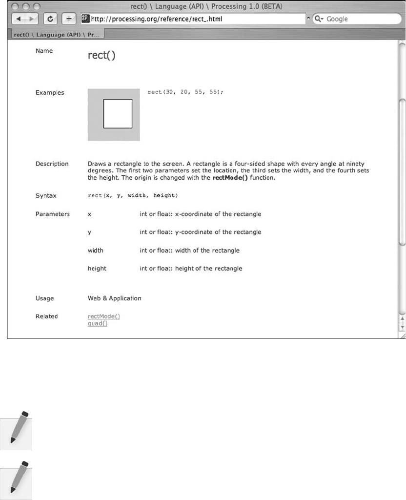
Processing 25
Processing also has a very handy “ fi nd in reference ” option. Double-click on any keyword to select it and
go to to HELP → FIND IN REFERENCE (or select the keyword and hit SHIFT CNTRL F).
Exercise 2-7: Using the Processing reference, try implementing two functions that we have
not yet covered in this book. Stay within the “ Shape ” and “ Color (setting) ” categories.
Exercise 2-8: Using the reference, fi nd a function that allows you to alter the thickness of a
line. What arguments does the function take? Write example code that draws a line one pixel
wide, then fi ve pixels wide, then 10 pixels wide.
2.8 The “ Play ” Button
One of the nice qualities of Processing is that all one has to do to run a program is press the “ play ” button.
It is a nice metaphor and the assumption is that we are comfortable with the idea of playing animations,
fi g. 2.7
26 Learning Processing
movies, music, and other forms of media. Processing programs output media in the form of real-time
computer graphics, so why not just play them too?
Nevertheless, it is important to take a moment and consider the fact that what we are doing here is not
the same as what happens on an iPod or TiVo. Processing programs start out as text, they are translated
into machine code, and then executed to run. All of these steps happen in sequence when the play button
is pressed. Let’s examine these steps one by one, relaxed in the knowledge that Processing handles the hard
work for us.
Step 1. Translate to Java. Processing is really Java (this will become more evident in a detailed
discussion in Chapter 23). In order for your code to run on your machine, it must fi rst be
translated to Java code.
Step 2. Compile into Java byte code. e Java code created in Step 1 is just another text fi le (with
the .java extension instead of .pde). In order for the computer to understand it, it needs to
be translated into machine language. is translation process is known as compilation. If you
were programming in a diff erent language, such as C, the code would compile directly into
machine language specifi c to your operating system. In the case of Java, the code is compiled
into a special machine language known as Java byte code. It can run on diff erent platforms
(Mac, Windows, cellphones, PDAs, etc.) as long as the machine is running a “ Java Virtual
Machine. ” Although this extra layer can sometimes cause programs to run a bit slower than
they might otherwise, being cross-platform is a great feature of Java. For more on how this
works, visit http://java.sun.com or consider picking up a book on Java programming (after
you have fi nished with this one).
Step 3. Execution. e compiled program ends up in a JAR fi le. A JAR is a Java archive fi le
that contains compiled Java programs ( “ classes ” ), images, fonts, and other data fi les.
e JAR fi le is executed by the Java Virtual Machine and is what causes the display
window to appear.
2.9 Your First Sketch
Now that we have downloaded and installed Processing , understand the basic menu and interface
elements, and have gotten familiar with the online reference, we are ready to start coding. As I
briefl y mentioned in Chapter 1, the fi rst half of this book will follow one example that illustrates the
foundational elements of programming: variables, arrays, conditionals, loops, functions, and objects . Other
examples will be included along the way, but following just one will reveal how the basic elements behind
computer programming build on each other.
e example will follow the story of our new friend Zoog, beginning with a static rendering with simple
shapes. Zoog’s development will include mouse interaction, motion, and cloning into a population of
many Zoogs. While you are by no means required to complete every exercise of this book with your own
alien form, I do suggest that you start with a design and after each chapter, expand the functionality of
that design with the programming concepts that are explored. If you are at a loss for an idea, then just
draw your own little alien, name it Gooz, and get programming! See Figure 2.8 .
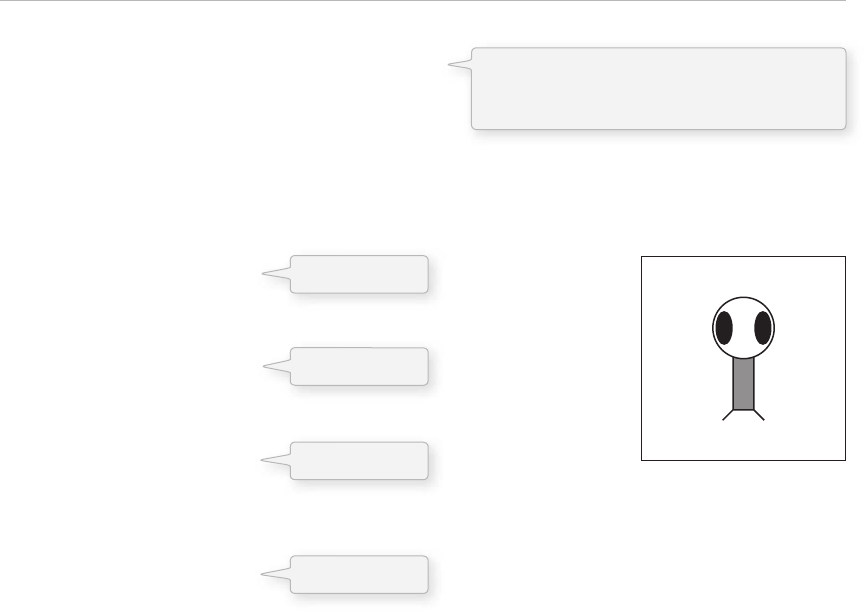
Processing 27
Example 2-1: Zoog again
size(200,200); // Set the size of the window
background(255); // Draw a black background
smooth();
// Set ellipses and rects to CENTER mode
ellipseMode(CENTER);
rectMode(CENTER);
// Draw Zoog’s body
stroke(0);
fill(150);
rect(100,100,20,100);
// Draw Zoog’s head
fill(255);
ellipse(100,70,60,60);
// Draw Zoog’s eyes
fill(0);
ellipse(81,70,16,32);
ellipse(119,70,16,32);
// Draw Zoog’s legs
stroke(0);
line(90,150,80,160);
line(110,150,120,160);
Let’s pretend, just for a moment, that you fi nd this Zoog design to be so astonishingly gorgeous that you
just cannot wait to see it displayed on your computer screen. (Yes, I am aware this may require a fairly
signifi cant suspension of disbelief.) To run any and all code examples found in this book, you have two
choices:
• Retype the code manually.
• Visit the book’s web site ( http://www.learningprocessing.com ), find the example by its number, and
copy/paste (or download) the code.
Certainly option #2 is the easier and less time-consuming one and I recommend you use the site as a
resource for seeing sketches running in real-time and grabbing code examples. Nonetheless, as you start
learning, there is real value in typing the code yourself. Your brain will sponge up the syntax and logic
as you type and you will learn a great deal by making mistakes along the way. Not to mention simply
running the sketch after entering each new line of code will eliminate any mystery as to how the sketch
works.
You will know best when you are ready for copy /paste. Keep track of your progress and if you start
running a lot of examples without feeling comfortable with how they work, try going back to manual
typing.
fi g. 2.8
Zoog’s body.
Zoog’s head.
Zoog’s eyes.
Zoog’s legs.
The function smooth() enables “anti-aliasing”
which smooths the edges of the shapes.
no smooth() disables anti-aliasing.
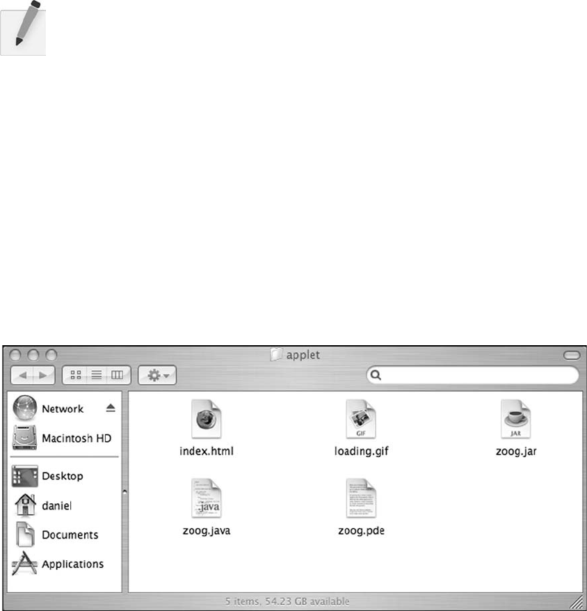
28 Learning Processing
Exercise 2-9: Using what you designed in Chapter 1, implement your own screen drawing,
using only 2D primitive shapes— arc( ) , curve( ) , ellipse( ) , line( ) , point( ) , quad( ) , rect( ) ,
triangle( ) —and basic color functions— background( ) , colorMode( ) , fi ll( ) , noFill( ) ,
noStroke( ) , and stroke( ) . Remember to use size( ) to specify the dimensions of your window.
Suggestion: Play the sketch after typing each new line of code. Correct any errors or typos
along the way.
2.10 Publishing Your Program
After you have completed a Processing sketch, you can publish it to the web as a Java applet. is will
become more exciting once we are making interactive, animated applets, but it is good to practice with a
simple example. Once you have fi nished Exercise 2-9 and determined that your sketch works, select
FILE → EXPORT.
Note that if you have errors in your program, it will not export properly, so always test by running fi rst!
A new directory named “ applet ” will be created in the sketch folder and displayed, as shown in Figure 2.9 .
fi g. 2.9
You now have the necessary fi les for publishing your applet to the web.
• index.html —The HTML source for a page that displays the applet.
• loading.gif —An image to be displayed while the user loads the applet ( Processing will supply a
default one, but you can create your own).
• zoog.jar —The compiled applet itself.
• zoog.java —The translated Java source code (looks like your Processing code, but has a few extra
things that Java requires. See Chapter 20 for details.)
• zoog.pde —Your Processing source.
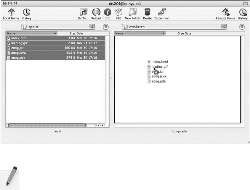
Processing 29
To see the applet working, double-click the “ index.html ” fi le which should launch a page in your default
web browser. See Figure 2.10 . To get the applet online, you will need web server space and FTP software
(or you can also use a Processing sketch sharing site such as http://www.openprocessing.org ). You can fi nd
some tips for getting started at this book’s web site.
fi g. 2.10
Exercise 2-10: Export your sketch as an applet. View the sketch in the browser (either locally
or by uploading). 00002 00002
This page intentionally left blank
Interaction 31
3 Interaction
“ Always remember that this whole thing was started with a dream and a mouse. ”
—Walt Disney
“ e quality of the imagination is to fl ow and not to freeze. ”
—Ralph Waldo Emerson
In this chapter:
– The “ fl ow ” of a program.
– The meaning behind setup( ) and draw( ) .
– Mouse interaction.
– Your fi rst “ dynamic ” Processing program.
– Handling events, such as mouse clicks and key presses.
3.1 Go with the fl ow.
If you have ever played a computer game, interacted with a digital art installation, or watched a
screensaver at three in the morning, you have probably given very little thought to the fact that the
software that runs these experiences happens over a period of time . e game starts, you save princess
so-and-so from the evil lord who-zee-ma-whats-it, achieve a high score, and the game ends.
What I want to focus on in this chapter is that very “ fl ow ” over time. A game begins with a set of initial
conditions: you name your character, you start with a score of zero, and you start on level one. Let’s think
of this part as the program’s SETUP . After these conditions are initialized, you begin to play the game.
At every instant, the computer checks what you are doing with the mouse, calculates all the appropriate
behaviors for the game characters, and updates the screen to render all the game graphics. is cycle of
calculating and drawing happens over and over again, ideally 30 or more times per second for a smooth
animation. Let’s think of this part as the program’s DRAW .
is concept is crucial to our ability to move beyond static designs (as in Chapter 2) with
Processing .
Step 1. Set starting conditions for the program one time.
Step 2. Do something over and over and over and over (and over … ) again until the program
quits.
Consider how you might go about running a race.
Step 1. Put on your sneakers and stretch. Just do this once, OK?
Step 2. Put your right foot forward, then your left foot. Repeat this over and over as fast as
you can.
Step 3. After 26 miles, quit.

32 Learning Processing
What is a block of code?
A block of code is any code enclosed within curly brackets.
{
A block of code
}
Blocks of code can be nested within each other, too.
{
A block of code
{
A block inside a block of code
}
}
is is an important construct as it allows us to separate and manage our code as individual pieces
of a larger puzzle. A programming convention is to indent the lines of code within each block to
make the code more readable. Processing will do this for you via the Auto-Format option (Tools →
Auto-Format).
Blocks of code will reveal themselves to be crucial in developing more complex logic, in terms of
variables , conditionals , iteration , objects , and functions , as discussed in future chapters. For now, we
only need to look at two simple blocks: setup( ) and draw( ) .
3.2 Our Good Friends, setup( ) and draw( )
Now that we are good and exhausted from running marathons in order to better learn programming,
we can take this newfound knowledge and apply it to our fi rst “ dynamic ” Processing sketch. Unlike
Chapter 2’s static examples, this program will draw to the screen continuously (i.e., until the user
quits). is is accomplished by writing two “ blocks of code ” setup( ) and draw( ) . Technically
speaking setup( ) and draw( ) are functions. We will get into a longer discussion of writing
our own functions in a later chapter; for now, we understand them to be two sections where we
write code.
Exercise 3-1: In English, write out the “ fl ow ” for a simple computer game, such as Pong.
If you are not familiar with Pong, visit: http://en.wikipedia.org/wiki/Pong .
_______________________________________________________________
_______________________________________________________________
_______________________________________________________________
_______________________________________________________________
Interaction 33
Let’s look at what will surely be strange-looking syntax for setup( ) and draw( ) . See Figure 3.1 .
void setup() {
// Initialization code goes here
}
void draw() {
// Code that runs forever goes here
}
What’s this? What are these for?
Curly brackets open and close a block of code.
fi g. 3.1
void setup() {
// Step 1a
// Step 1b
// Step 1c
}
void draw() {
// Step 2a
// Step 2b
}
Do once!
Skip to draw.
Loop over and over!
fi g. 3.2
Admittedly, there is a lot of stuff in Figure 3.1 that we are not entirely ready to learn about. We have
covered that the curly brackets indicate the beginning and end of a “ block of code, ” but why are there
parentheses after “ setup ” and “ draw ” ? Oh, and, my goodness, what is this “ void ” all about? It makes me
feel sad inside! For now, we have to decide to feel comfortable with not knowing everything all at once,
and that these important pieces of syntax will start to make sense in future chapters as more concepts
are revealed.
For now, the key is to focus on how Figure 3.1 ’s structures control the fl ow of our program. is is shown
in Figure 3.2 .
How does it work? When we run the program, it will follow our instructions precisely, executing the steps
in setup( ) fi rst, and then move on to the steps in draw( ) . e order ends up being something like:
1a, 1b, 1c, 2a, 2b, 2a, 2b, 2a, 2b, 2a, 2b, 2a, 2b, 2a, 2b …
Now, we can rewrite the Zoog example as a dynamic sketch. See Example 3–1 .

34 Learning Processing
Example 3-1: Zoog as dynamic sketch
void setup() {
// Set the size of the window
size(200,200);
}
void draw() {
// Draw a white background
background(255);
// Set CENTER mode
ellipseMode(CENTER);
rectMode(CENTER);
// Draw Zoog's body
stroke(0);
fill(150);
rect(100,100,20,100);
// Draw Zoog's head
stroke(0);
fill(255);
ellipse(100,70,60,60);
// Draw Zoog's eyes
fill(0);
ellipse(81,70,16,32);
ellipse(119,70,16,32);
// Draw Zoog's legs
stroke(0);
line(90,150,80,160);
line(110,150,120,160);
}
Take the code from Example 3-1 and run it in Processing. Strange, right? You will notice that nothing in the
window changes. is looks identical to a static sketch! What is going on? All this discussion for nothing?
Well, if we examine the code, we will notice that nothing in the draw( ) function varies . Each time
through the loop, the program cycles through the code and executes the identical instructions. So, yes,
the program is running over time redrawing the window, but it looks static to us since it draws the same
thing each time!
Exercise 3-2: Redo the drawing you created at the end of Chapter 2 as a dynamic program.
Even though it will look the same, feel good about your accomplishment!
setup() runs fi rst one time. size() should always be
fi rst line of setup() since Processing will not be able
to do anything before the window size if specifi ed.
draw() loops continuously until you close the sketch
window.
fi g. 3.3
Interaction 35
3.3 Variation with the Mouse
Consider this. What if, instead of typing a number into one of the drawing functions, you could type “ the
mouse’s X location ” or “ the mouse’s Y location. ”
line(the mouse's X location, the mouse's Y location, 100, 100);
In fact, you can, only instead of the more descriptive language, you must use the keywords mouseX and
mouseY , indicating the horizontal or vertical position of the mouse cursor.
Example 3-2: mouseX and mouseY
void setup() {
size(200,200);
}
void draw() {
background(255);
// Body
stroke(0);
fill(175);
rectMode(CENTER);
rect(mouseX,mouseY,50,50);
}
fi g. 3.4
An Invisible Line of Code
If you are following the logic of setup( ) and draw( ) closely, you might arrive at an interesting question:
When does Processing actually display the shapes in the window? When do the new pixels appear?
_____________________________________________________
_____________________________________________________
_____________________________________________________
_____________________________________________________
_____________________________________________________
Exercise 3-3: Explain why we see a trail of rectangles if we move background( ) to setup( ) ,
leaving it out of draw( ) .
Try moving background()
to setup() and see the
difference! (Exercise 3–3)
mouseX is a keyword that the sketch replaces with
the horizontal position of the mouse.
mouseY is a keyword that the sketch replaces with
the vertical position of the mouse.

36 Learning Processing
We could push this idea a bit further and create an example where a more complex pattern (multiple
shapes and colors) is controlled by mouseX and mouseY position. For example, we can rewrite
Zoog to follow the mouse. Note that Zoog’s body is located at the exact location of the mouse ( mouseX,
mouseY ), however, other parts of Zoog’s body are drawn relative to the mouse. Zoog’s head, for example,
is located at ( mouseX, mouseY-30 ). e following example only moves Zoog’s body and head, as shown in
Figure 3.5 .
Example 3-3: Zoog as dynamic sketch with variation
void setup() {
size(200,200); // Set the size of the window
smooth();
}
void draw() {
background(255); // Draw a white background
// Set ellipses and rects to CENTER mode
ellipseMode(CENTER);
rectMode(CENTER);
// Draw Zoog's body
stroke(0);
fill(175);
rect(mouseX,mouseY,20,100);
// Draw Zoog's head
stroke(0);
fill(255);
ellipse(mouseX,mouseY-30,60,60);
On fi rst glance, one might assume the display is updated for every line of code that includes a
drawing function. If this were the case, however, we would see the shapes appear onscreen one at
a time. is would happen so fast that we would hardly notice each shape appearing individually.
However, when the window is erased every time background( ) is called, a somewhat unfortunate
and unpleasant result would occur: fl icker.
Processing solves this problem by updating the window only at the end of every cycle through
draw( ) . It is as if there were an invisible line of code that renders the window at the end of the
draw( ) function.
void draw() {
// All of your code
// Update Display Window -- invisible line of code we don’t see
}
is process is known as double-buff ering and, in a lower-level environment, you may fi nd that
you have to implement it yourself. Again, we take the time to thank Processing for making our
introduction to programming friendlier and simpler by taking care of this for us.
fi g. 3.5
Zoog’s head is drawn above the body
at the location (mouseX, mouseY-30).
Zoog’s body is drawn at the location
(mouseX, mouseY).
Interaction 37
// Draw Zoog's eyes
fill(0);
ellipse(81,70,16,32);
ellipse(119,70,16,32);
// Draw Zoog's legs
stroke(0);
line(90,150,80,160);
line(110,150,120,160);
}
Exercise 3-4: Complete Zoog so that the rest of its body moves with the mouse.
mouseX 20
mouseY 50
1st time
through draw()
100 100 window
20 75
25
5
0
50
90
2nd time
through draw()
3rd time
through draw()
pmouseX 20
pmouseY 50
mouseX 75
mouseY 25
pmouseX 20
pmouseY 50
mouseX 50
mouseY 90
fi g. 3.6
In addition to mouseX and mouseY , you can also use pmouseX and pmouseY . ese two keywords stand
for the “ previous ” mouse X and mouse Y locations, that is, where the mouse was the last time we cycled
through draw( ) . is allows for some interesting interaction possibilities. For example, let’s consider what
happens if we draw a line from the previous mouse location to the current mouse location, as illustrated
in the diagram in Figure 3.6 .
// Draw Zoog's eyes
fill(0);
ellipse(_______,_______ ,16,32);
ellipse(_______,_______ ,16,32);
// Draw Zoog's legs
stroke(0);
line(_______,_______,_______,_______);
line(_______,_______,_______,_______);
Exercise 3-5: Recode your design so that shapes respond to the mouse (by varying color and
location).
38 Learning Processing
• The absolute value of –2 is 2.
• The absolute value of 2 is 2.
In Processing, we can get the absolute value of the number by placing it inside the abs( ) function,
that is,
• abs( 5) → 5
e speed at which the mouse is moving is therefore:
• abs( mouseX - pmouseX )
Update Exercise 3-7 so that the faster the user moves the mouse,
the wider the drawn line. Hint: look up strokeWeight( ) in the
Processing reference.
stroke(255);
_____________________________ (______________);
line(pmouse
X
,pmouse
Y
,mouse
X
,mouse
Y
);
Example 3-4: Drawing a continuous line
void setup() {
size(200,200);
background(255);
smooth();
}
void draw() {
stroke(0);
line(pmouse X ,pmouse Y ,mouse X ,mouse Y );
}
Exercise 3-6: Fill in the blank in Figure 3.6 .
fi g. 3.7
By connecting the previous mouse location to the current mouse location with a line each time through
draw( ) , we are able to render a continuous line that follows the mouse. See Figure 3.7 .
Exercise 3-7: e formula for calculating the speed of the mouse’s horizontal motion is the
absolute value of the diff erence between mouseX and pmouseX . e absolute value of a
number is defi ned as that number without its sign:
Draw a line from previous mouse
location to current mouse location.
Interaction 39
3.4 Mouse Clicks and Key Presses
We are well on our way to creating dynamic, interactive Processing sketches through the use the setup( )
and draw( ) framework and the mouseX and mouseY keywords. A crucial form of interaction, however, is
missing—clicking the mouse!
In order to learn how to have something happen when the mouse is clicked, we need to return to the
fl ow of our program. We know setup( ) happens once and draw( ) loops forever. When does a mouse
click occur? Mouse presses (and key presses) as considered events in Processing . If we want something
to happen (such as “ the background color changes to red ” ) when the mouse is clicked, we need to add a
third block of code to handle this event.
is event “ function ” will tell the program what code to execute when an event occurs. As with setup( ) ,
the code will occur once and only once. at is, once and only once for each occurrence of the event. An
event, such as a mouse click, can happen multiple times of course!
ese are the two new functions we need:
• mousePressed( ) —Handles mouse clicks.
• keyPressed( ) —Handles key presses.
e following example uses both event functions, adding squares whenever the mouse is pressed and
clearing the background whenever a key is pressed.
Example 3-5: mousePressed( ) and keyPressed( )
void setup() {
size(200,200);
background(255);
}
void draw() {
}
void mousePressed() {
stroke(0);
fill(175);
rectMode(CENTER);
rect(mouseX,mouseY,16,16);
}
void keyPressed() {
background(255);
}
In Example 3-5, we have four functions that describe the program’s fl ow. e program starts in setup( ) where
the size and background are initialized. It continues into draw( ) , looping endlessly. Since draw( ) contains
no code, the window will remain blank. However, we have added two new functions: mousePressed( ) and
fi g. 3.8
Nothing happens in draw() in this example!
Whenever a user clicks the mouse the code
written inside mousePressed() is executed.
Whenever a user presses a key the code
written inside keyPressed() is executed.

keyPressed( ) . e code inside these functions sits and waits. When the user clicks the mouse (or presses a
key), it springs into action, executing the enclosed block of instructions once and only once.
Exercise 3-8: Add “ background(255); ” to the draw( ) function. Why does the program stop
working?
We are now ready to bring all of these elements together for Zoog.
• Zoog’s entire body will follow the mouse.
• Zoog’s eye color will be determined by mouse location.
• Zoog’s legs will be drawn from the previous mouse location to the current mouse location.
• When the mouse is clicked, a message will be displayed in the message window: “ Take me to your
leader! ”
Note the addition in Example 3–6 of the function frameRate( ). frameRate( ) , which requires an integer
between 1 and 60, enforces the speed at which Processing will cycle through draw( ). frameRate (30) ,
for example, means 30 frames per second, a traditional speed for computer animation. If you do not
include frameRate( ) , Processing will attempt to run the sketch at 60 frames per second. Since computers
run at diff erent speeds, frameRate( ) is used to make sure that your sketch is consistent across multiple
computers.
is frame rate is just a maximum, however. If your sketch has to draw one million rectangles, it may take
a long time to fi nish the draw cycle and run at a slower speed.
Example 3-6: Interactive Zoog
void setup() {
// Set the size of the window
size(200,200);
smooth();
frameRate(30) ;
}
void draw() {
// Draw a black background
background(255);
// Set ellipses and rects to CENTER mode
ellipseMode(CENTER);
rectMode(CENTER);
// Draw Zoog's body
stroke(0);
fill(175);
rect(mouseX,mouseY,20,100);
// Draw Zoog's head
stroke(0);
fill(255);
ellipse(mouse X ,mouse Y -30,60,60);
fi g. 3.9
The frame rate is set to
30 frames per second.
40 Learning Processing
Interaction 41
// Draw Zoog's eyes
fill(mo useX,0,mouseY);
ellipse(mouse X-19,mouseY-30,16,32);
ellipse(mouse X + 19,mouse Y-30,16,32);
// Draw Zoog's legs
stroke(0);
line(mouse X-10,mouseY + 50,pmouse X-10,pmouseY + 60);
line(mouse X + 10,mouse Y + 50,pmouse X + 10,pmouse Y + 60);
}
void mousePressed() {
println( "Take me to your leader! ");
}
The legs are drawn according to
the mouse location and the previous
mouse location.
The eye color is determined by the mouse location.

Lesson One Project
(You may have completed much of this project already via the exercises in Chapters 1–3.
is project brings all of the elements together. You could either start from scratch with a
new design or use elements from the exercises.)
Step 1. Design a static screen drawing using RGB color and primitive shapes.
Step 2. Make the static screen drawing dynamic by having it interact with the
mouse. is might include shapes following the mouse, changing their
size according to the mouse, changing their color according to the mouse,
and so on.
Use the space provided below to sketch designs, notes, and pseudocode for your
project.
42 Learning Processing

Lesson Two
Everything You Need to Know
4 Variables
5 Conditionals
6 Loops
This page intentionally left blank

Variables 45
4 Variables
“ All of the books in the world contain no more information than is broadcast as video in a single large
American city in a single year. Not all bits have equal value. ”
—Carl Sagan
“ Believing oneself to be perfect is often the sign of a delusional mind. ”
—Lieutenant Commander Data
In this chapter:
– Variables: What are they?
– Declaring and initializing variables.
– Common uses for variables.
– Variables you get “ for free ” in Processing (AKA “ built-in ” variables).
– Using random values for variables.
4.1 What is a Variable?
I admit it. When I teach programming, I launch into a diatribe of analogies in an attempt to explain the
concept of a variable in an intuitive manner. On any given day, I might say “ A variable is like a bucket. ”
You put something in the bucket, carry it around with you, and retrieve it whenever you feel inspired.
“ A variable is like a storage locker. ” Deposit some information in the locker where it can live safely,
readily available at a moment’s notice. “ A variable is a lovely, yellow post-it note, on which is written
the message: I am a variable. Write your information on me. ”
6
Variable
bucket
Variable
locker
Variable
post-it
93
fi g. 4.1
I could go on. But I won’t. I think you get the idea. And I am not entirely sure we really need an analogy
since the concept itself is rather simple. Here’s the deal.
e computer has memory. Why do we call it memory? Because it is what the computer uses to remember
stuff it needs.
Technically speaking, a variable is a named pointer to a location in the computer’s memory ( “ memory
address ” ) where data is stored. Since computers only process information one instruction at a time, a
variable allows a programmer to save information from one point in the program and refer back to it at a
later time. For a Processing programmer, this is incredibly useful; variables can keep track of information
related to shapes: color, size, location. Variables are exactly what you need to make a triangle change from
blue to purple, a circle fl y across the screen, and a rectangle shrink into oblivion.

46 Learning Processing
Out of all the available analogies, I tend to prefer the piece of paper approach: graph paper .
Imagine that the computer’s memory is a sheet of graph paper and each cell on the graph paper has an
address. With pixels, we learned how to refer to those cells by column and row numbers. Wouldn’t it be
nice if we could name those cells? With variables, we can.
Let’s name one “ Billy’s Score ” (we will see why we are calling it that in the next section) and give it the
value 100. at way, whenever we want to use Billy’s score in a program, we do not have to remember the
value 100. It is there in memory and we can ask for it by name. See Figure 4.2 .
Billy’s score
100
fi g 4.2
Jane’s Score
5
30
53
65
87
101
10
25
47
68
91
98
Billy’s Score
fi g. 4.3
e power of a variable does not simply rest with the ability to remember a value. e whole point of a
variable is that those values vary , and more interesting situations arise as we periodically alter that value.
Consider a game of Scrabble between Billy and Jane. To keep track of the score, Jane takes out paper and
pencil, and scrawls down two column names: “ Billy’s Score ” and “ Jane’s Score. ” As the two play, a running
tally is kept of each player’s points below the headings. If we imagine this game to be virtual Scrabble
programmed on a computer, we suddenly can see the concept of a variable that varies emerge. at piece
of paper is the computer’s memory and on that paper, information is written— “ Billy’s Score ” and
“ Jane’s Score ” are variables, locations in memory where each player’s total points are stored and that
change over time. See Figure 4.3 .
In our Scrabble example, the variable has two elements—a name (e.g., “ Jane’s Score ” ) and a value
(e.g., 101). In Processing , variables can hold diff erent kinds of values and we are required to explicitly
defi ne the type of value before we can use a given variable.
Variables 47
In Figure 4.4 , we have a variable named “ count ” of type “ int, ” which stands for integer. Other possible
data types are listed below.
4.2 Variable Declaration and Initialization
Variables can hold primitive values or references to objects and arrays . For now, we are just going to worry
about primitives—we will get to objects and arrays in a later chapter. Primitive values are the building
blocks of data on the computer and typically involve a singular piece of information, like a number or
character.
Variables are declared by fi rst stating the type, followed by the name. Variable names must be one word
(no spaces) and must start with a letter (they can include numbers, but cannot start with a number). ey
cannot include any punctuation or special characters, with the exception of the underscore: “ _ ” .
A type is the kind of data stored in that variable. is could be a whole number, a decimal number, or a
character. Here are data types you will commonly use:
• Whole numbers, such as 0, 1, 2, 3, 1, 2, and so on are stored as “ integers ” and the type keyword
for integer is “ int ” .
• Decimal numbers, such as 3.14159, 2.5, and –9.95 are typically stored as “ floating point values ” and
the type keyword for floating point is “ float ” .
• Characters, such as the letters ‘ a ’ , ‘ b ’ , ‘ c ’ , and so on are stored in variables of type “ char ” and are
declared as a letter enclosed in single quotes, that is, ‘ a ’ . Characters are useful when determining
what letter on the keyboard has been pressed, and for other uses involving Strings of text (see
Chapter 17) .
int count
nametype
;
fi g. 4.4
Exercise 4-1: Consider the game Pong. What variables would you need to program the
game? (If you are not familiar with Pong, see http://en.wikipedia.org/wiki/Pong ).

48 Learning Processing
D o n’ t F o r g e t
• Variables must have a type. Why? is is how the computer knows exactly how much memory
should be allocated to store that variable’s data.
• Variables must have a name.
All Primitive Types
• boolean : true or false
• char : a character, ‘ a ’ ,‘b ’ ,‘c ’ , etc.
• byte : a small number, –128 to 127
• short : a larger number, –32768 to 32767
• int : a big number, –2147483648 to 2147483647
• long : a really huge number
• fl oat : a decimal number , such as 3.14159
• double : a decimal number with a lot more decimal places (only necessary for advanced programs
requiring mathematical precision).
What’s in a name?
Tips for choosing good variable names
• Avoid using words that appear elsewhere in the Processing language. In other words, do not call
your variable mouseX , there already is one!
• Use names that mean something. is may seem obvious, but it is an important point. For
example, if you are using a variable to keep track of score, call it “ score ” and not, say, “ cat. ”
• Start your variable with a lowercase letter and join together words with capitals. Words that start
with capitals are reserved for classes (Chapter 8). For example: “ frogColor ” is good, “ Frogcolor ”
is not. this canTake some gettingUsedTo but it will comeNaturally soonEnough.
Once a variable is declared, we can then assign it a value by setting it equal to something. In most cases,
if we forget to initialize a variable, Processing will give it a default value, such as 0 for integers, 0.0 for
fl oating points, and so on. However, it is good to get into the habit of always initializing variables in order
to avoid confusion.
int count;
count = 50;
To be more concise, we can combine the above two statements into one.
int count = 50; Declare and initialize a variable in one lines of code.
Declare and initialize a variable in two lines of code.
Variables 49
A variable can also be initialized by another variable ( x equals y ), or by evaluating a mathematical
expression ( x equals y plus z , etc.). Here are some examples:
Example 4-1: Variable declaration and initialization examples
int count = 0; // Declare an int named count, assigned the value 0
char letter = ' a'; // Declare a char named letter, assigned the value 'a'
double d = 132.32; // Declare a double named d, assigned the value 132.32
boolean happy = false; // Declare a boolean named happy, assigned the value false
float x = 4.0; // Declare a float named x, assigned the value 4.0
float y; // Declare a float named y (no assignment)
y = x + 5.2; // Assign the value of x plus 5.2 to the previously declared y
float z = x *y + 15.0; // Declare a variable named z, assign it the value which
// is x times y plus 15.0.
____________________________________________________________
____________________________________________________________
____________________________________________________________
____________________________________________________________
____________________________________________________________
____________________________________________________________
Exercise 4-2: Write out variable declaration and initialization for the game Pong.
4.3 Using a Variable
ough it may initially seem more complicated to have words standing in for numbers, variables make
our lives easier and more interesting.
Let’s take a simple example of a program that draws a circle onscreen.
void setup() {
size(200,200);
}
void draw() {
background(255);
stroke(0);
fill(175);
ellipse(100,100,50,50);
}
In a moment, we’ll add variables
at the top here.
50 Learning Processing
Rule of umb: When to Use a Variable
ere are no hard and fast rules in terms of when to use a variable. However, if you fi nd yourself
hard-coding in a bunch of numbers as you program, take a few minutes, review your code, and
change these values to variables.
Some programmers say that if a number appears three or more times, it should be a variable.
Personally, I would say if a number appears once, use a variable. Always use variables!
Example 4-2: Using variables
int circleX = 100;
int circleY = 100;
void setup() {
size(200,200);
}
void draw() {
background(100);
stroke(255);
fill(0);
ellipse(circleX,circleY,50,50);
}
Running this code, we achieve the same result as in the fi rst example: a circle appears in the middle of
the screen. Nevertheless, we should open our hearts and remind ourselves that a variable is not simply a
placeholder for one constant value. We call it a variable because it varies . To change its value, we write an
assignment operation , which assigns a new value.
Up until now, every single line of code we wrote called a function: line( ), ellipse( ) , stroke( ) , etc .
Variables introduce assignment operations to the mix. Here is what one looks like (it is the same as
how we initialize a variable, only the variable does not need to be declared).
variable name expression
Declare and initialize two integer
variables at the top of the code.
Use the variables to specify
the location of an ellipse.
In Chapter 3, we learned how to take this simple example one step further, changing the location of a
shape to mouseX, mouseY in order to assign its location according to the mouse.
ellipse(mouse X ,mouse Y ,50,50);
Can you see where this is going? mouseX and mouseY are named references to the horizonal and vertical
location of the mouse. ey are variables! However, because they are built into the Processing environment
(note how they are colored red when you type them in your code), they can be used without being
declared. Built-in variables (AKA “ System ” variables) are discussed further in the next section.
What we want to do now is create our own variables by following the syntax for declaring and initializing
outlined above, placing the variables at the top of our code. You can declare variables elsewhere in your
code and we will get into this later. For now to avoid any confusion, all variables should be at the top.
Variables 51
x = 5;
x = a + b;
x = y - 10 * 20;
x = x * 5;
A common example is incrementation. In the above code, circle X starts with a value of 100. If we
want to increment circleX by one, we say circleX equals itself plus one. In code, this amounts to
“ circle X circle X 1; ” .
Let’s try adding that to our program (and let’s start circleX with the value of 0).
Example 4-3: Varying variables
int circle X = 0;
int circleY = 100;
void setup() {
size(200,200);
}
void draw() {
background(255);
stroke(0);
fill(175);
ellipse(circleX,circleY,50,50);
circleX = circleX + 1;
}
What happens? If you run Example 4-3 in Processing , you will notice that the circle moves from left
to right. Remember, draw( ) loops over and over again, all the while retaining the value of circleX in
memory. Let’s pretend we are the computer for a moment. ( is may seem overly simple and obvious, but
it is key to our understanding of the principles of programming motion.)
An assignment operation that increments
the value of circleX by 1.
fi g. 4.5
1. Remember circle
circleX
0 and circle
circleY
100
2. Run setup()
setup()
. Open a window 200 200
3. Run draw().
draw().
• Draw circle at (circle
(circleX
, circle
circleY)
→ (0,100)
• Add one to circle
circleX
circle
circleX
0 1 1
4. Run draw()
draw()
• Draw circle at (circle
(circleX
, circle
circleY)
→ (1,100)
• Add one to circle
circleX
circle
circleX
1 1 2
5. Run draw(
draw()
• Draw circle at (circle
(circleX
, circle
circleY)
→ (2,100)
• Add one to circle
circleX
circle
circleX
2 1 3
6. And so on and so forth!
Examples of assigning a new value to a variables.
Practicing how to follow the code step-by-step will lead you to the questions you need to ask before
writing your own sketches. Be one with the computer.

52 Learning Processing
4.4 Many Variables
Let’s take the example one step further and use variables for every piece of information we can think of.
We will also use fl oating point values to demonstrate greater precision in adjusting variable values.
Example 4-4: Many variables
float circleX = 0;
float circleY = 0;
float circleW = 50;
float circleH = 100;
float circleStroke = 255;
float circleFill = 0;
float backgroundColor = 255;
float change = 0.5;
// Your basic setup
void setup() {
size(200,200);
smooth();
}
Exercise 4-3: Change Example 4-3 so that instead of the circle moving from left to right, the
circle grows in size. What would you change to have the circle follow the mouse as it grows?
How could you vary the speed at which the circle grows?
int circleSize = 0;
int circleX = 100;
int circleY = 100;
void setup() {
size(200,200);
}
void draw() {
background(0);
stroke(255);
fill(175);
_____________________________________
_____________________________________
}
We’ve got eight variables now!
All of type fl oat.
• What data do you and the computer need to remember for your sketch?
• How do you and the computer use that data to draw shapes on the screen?
• How do you and the computer alter that data to make your sketch interactive and animated?
fi g. 4.6
Variables 53
void draw() {
// Draw the background and the ellipse
background(backgroundColor);
stroke(circleStroke);
fill(circleFill);
ellipse(circleX,circleY,circleW,circleH);
// Change the values of all variables
circleX = circleX + change;
circleY = circleY + change;
circleW = circleW + change;
circleH = circleH - change;
circleStroke = circleStroke - change;
circleFill = circleFill + change;
}
Variables are used for everything:
background, stroke, fi ll, location, and size.
The variable change is used to increment
and decrement the other variables.
Step 1 : Write code that draws the following screenshots with hard-coded values. (Feel free
to use colors instead of grayscale.)
Step 2 : Replace all of the hard-coded numbers with variables.
Step 3 : Write assignment operations in draw( ) that change the value of the variables.
For example, “ variable1 variable1 2; ” . Try diff erent expressions and see
what happens!
Exercise 4-4
4.5 System Variables
As we saw with mouseX and mouseY , Processing has a set of convenient system variables freely available.
ese are commonly needed pieces of data associated with all sketches (such as the width of the window,
the key pressed on the keyboard, etc.). When naming your own variables, it is best to avoid system
variable names, however, if you inadvertently use one, your variable will become primary and override the
system one. Here is a list of commonly used system variables (there are more, which you can fi nd in the
Processing reference).
• width —Width (in pixels) of sketch window.
• height —Height (in pixels) of sketch window.
• frameCount —Number of frames processed.
54 Learning Processing
• frameRate —Rate that frames are processed (per second).
• screen.width —Width (in pixels) of entire screen.
• screen.height —Height (in pixels) of entire screen.
• key —Most recent key pressed on the keyboard.
• keyCode —Numeric code for key pressed on keyboard.
• keyPressed —True or false? Is a key pressed?
• mousePressed —True or false? Is the mouse pressed?
• mouseButton —Which button is pressed? Left, right, or center?
Following is an example that makes use of some of the above variables; we are not ready to use them all
yet, as we will need some more advanced concepts to make use of many features.
Example 4-5: Using system variables
void setup() {
size(200,200);
frameRate(30);
}
void draw() {
background(100);
stroke(255);
fill(frameCount/2);
rectMode(CENTER);
rect(width/2,height/2,mouseX + 10,mouseY + 10);
}
void keyPressed() {
println(key);
}
The rectangle will always be in the
middle of the window if it is located at
(width/2, height/2).
Exercise 4-5: Using width and height, recreate the following screenshot. Here’s the catch: the
shapes must resize themselves relative to the window size. (In other words, no matter what
you specify for size( ) , the result should look identical.)
frameCount is used to color a rectangle.
Variables 55
4.6 Random: Variety is the spice of life.
So, you may have noticed that the examples in this book so far are a bit, say, humdrum. A circle here.
A square here. A grayish color. Another grayish color.
ere is a method to the madness (or lack of madness in this case). It all goes back to the driving
principle behind this book: incremental development . It is much easier to learn the fundamentals by
looking at the individual pieces, programs that do one and only one thing. We can then begin to add
functionality on top, step by step.
Nevertheless, we have waited patiently through four chapters and we have arrived at the time where we
can begin to have a bit of fun. And this fun will be demonstrated via the use of the function random( ) .
Consider, for a moment, Example 4-6, whose output is shown in Figure 4.7 .
Example 4-6: Ellipse with variables
float r = 100;
float g = 150;
float b = 200;
float a = 200;
float diam = 20;
float x = 100;
float y = 100;
void setup() {
size(200,200);
background(255);
smooth();
}
void draw() {
// Use those variables to draw an ellipse
stroke(0);
fill(r,g,b,a);
ellipse(x,y,diam,diam);
}
ere it is, our dreary circle. Sure, we can adjust variable values and move the circle, grow its size, change
its color, and so on. However, what if every time through draw( ) , we could make a new circle, one with a
random size, color, and position? e random( ) function allows us to do exactly that.
random( ) is a special kind of function, it is a function that returns a value. We have encountered this
before. In Exercise 3-7 we used the function abs( ) to calculate the absolute value of a number. e idea
of a function that calculates a value and returns it will be explored fully in Chapter 7, but we are going to
take some time to introduce the idea now and let it sink in a bit.
Unlike most of the functions we are comfortable with (e.g., line( ), ellipse( ), and rect( ) ), random( ) does not
draw or color a shape on the screen. Instead, random( ) answers a question; it returns that answer to us.
Here is a bit of dialogue. Feel free to rehearse it with your friends.
fi g. 4.7
Declare and initialize
your variables
Use those variables! (Remember, the fourth
argument for a color is transparency).

56 Learning Processing
M e : Hey random, what’s going on? Hope you’re well. Listen, I was wondering, could you give me
a random number between 1 and 100?
Random : Like, no problem. How about the number 63?
M e : at’s awesome, really great, thank you. OK, I’m off . Gotta draw a rectangle 63 pixels wide, OK?
Now, how would this sequence look in our slightly more formal, Processing environment? e code below
the part of “ me ” is played by the variable “ w ” .
float w = random(1,100);
rect(100,100,w,50);
e random( ) function requires two arguments and returns a random fl oating point number ranging
from the fi rst argument to the second. e second argument must be larger than the fi rst for it to work
properly. e function random( ) also works with one argument by assuming a range between zero and
that argument.
In addition, random( ) only returns fl oating point numbers. is is why we declared “ w ” above as a fl oat.
However, if you want a random integer, you can convert the result of the random function to an int .
int w = int(random(1,100));
rect(100,100,w,50);
Notice the use of nested parentheses. is is a nice concept to get used to as it will be quite convenient to
call functions inside of functions as we go. e random( ) function returns a fl oat, which is then passed to
the int( ) function that converts it to an integer. If we wanted to go nuts nesting functions, we could even
condense the above code into one line:
rect(100,100,int(random(1,100)),50);
Incidentally, the process of converting one data type to another is referred to as “ casting. ” In Java (which
Processing is based on) casting a fl oat to an integer can also be written this way:
int w = (int) random(1,100);
OK, we are now ready to experiment with random( ) . Example 4-7 shows what happens if we take every
variable associated with drawing the ellipse (fi ll, location, size) and assign it to a random number each
cycle through draw( ) . e output is shown in Figure 4.8 .
A random fl oat between 1 and 100.
A random integer between 1 and 100.
The result of random (1,100) is a fl oat. It can
be converted to an integer by “casting.”
Variables 57
Example 4-7: Filling variables with random values
float r;
float g;
float b;
float a;
float diam;
float x;
float y;
void setup() {
size(200,200);
background(0);
smooth();
}
void draw() {
// Fill all variables with random values
r = random(255);
g = random(255);
b = random(255);
a = random(255);
diam = random(20);
x = random(width);
y = random(height);
// Use values to draw an ellipse
noStroke();
fill(r,g,b,a);
ellipse(x,y,diam,diam);
}
4.7 Variable Zoog
We are now ready to revisit Zoog, our alien friend, who was happily following the mouse around the
screen when we last checked in. Here, we will add two pieces of functionality to Zoog.
• New feature #1 —Zoog will rise from below the screen and fly off into space (above the screen).
• New feature #2 —Zoog’s eyes will be colored randomly as Zoog moves.
Feature #1 is solved by simply taking the previous program that used mouseX and mouseY and
substituting our own variables in their place.
Feature #2 is implemented by creating three additional variables eyeRed, eyeGreen, and eyeBlue that will
be used for the fi ll( ) function before displaying the eye ellipses.
Example 4-8: Variable Zoog
float zoogX;
float zoogY;
float eyeR;
float eyeG;
float eyeB;
void setup() {
size(200,200);
fi g. 4.8
Each time through draw(), new random
numbers are picked for a new ellipse.
fi g. 4.9
Declaring variables. zoogX and zoogY are for
feature #1. eyeR, eyeG, eyeB are for feature #2.
58 Learning Processing
zoogX = width/2; // Zoog always starts in the middle
zoogY = height + 100; // Zoog starts below the screen
smooth();
}
void draw() {
background(255);
// Set ellipses and rects to CENTER mode
ellipseMode(CENTER);
rectMode(CENTER);
// Draw Zoog's body
stroke(0);
fill(150);
rect(zoogX,zoogY,20,100);
// Draw Zoog's head
stroke(0);
fill(255);
ellipse(zoogX,zoogY - 30,60,60);
// Draw Zoog's eyes
eyeR = random(255);
eyeG
= random(255);
eyeB = random(255);
fill(eyeR,eyeG,eyeB);
ellipse(zoogX - 19,zoogY - 30,16,32);
ellipse(zoogX + 19,zoogY - 30,16,32);
// Draw Zoog's legs
stroke(150);
line(zoogX - 10,zoogY + 50,zoogX - 10,height);
line(zoogX + 10,zoogY + 50,zoogX + 10,height);
// Zoog moves up
zoogY = zoogY - 1;
}
Exercise 4-7: Using variables and the random( ) function, revise your design from the
Lesson One Project to move around the screen, change color, size, location, and so on.
Feature #1. zoogX and zoogY are initialized based on
the size of the window. Note we cannot initialize these
variables before the size () function is called since we
are using the built-in variables width and height.
Feature #1. zoogX and zoogY are
used for the shape locations.
Feature #2. eyeR, eyeG, and eye B
are given random values and used
in the fi ll() function.
Feature #1. zoogY is decreased by one so
that zoog moves upward on the screen.
Exercise 4-6: Revise Example 4-8 so that Zoog shakes left and right as Zoog moves
upward. Hint: this requires the use of random( ) in combination with zoogX.
zoogX = _____________________________;

Conditionals 59
5 Conditionals
“ at language is an instrument of human reason, and not merely a medium for the expression of thought, is
a truth generally admitted. ”
—George Boole
“ e way I feel about music is that there is no right and wrong. Only true and false. ”
—Fiona Apple
In this chapter:
– Boolean expressions.
– Conditional statements: How a program produces different results based on varying circumstances.
– If, Else If, Else .
5.1 Boolean Expressions
What’s your favorite kind of test? Essay format? Multiple choice? In the world of computer
programming, we only take one kind of test: a boolean test—true or false. A boolean expression (named for
mathematician George Boole) is an expression that evaluates to either true or false. Let’s look at some
common language examples:
• I am hungry. → true
• I am afraid of computer programming. → false
• This book is a hilarious read. → false
In the formal logic of computer science, we test relationships between numbers.
• 15 is greater than 20 → false
• 5 equals 5 → true
• 32 is less than or equal to 33 → true
In this chapter, we will learn how to use a variable in a boolean expression, allowing our sketch to take
diff erent paths depending on the current value stored in the variable.
• x 20 → depends on current value of x
• y 5 → depends on current value of y
• z 33 →
depends on current value of z
e following operators can be used in a boolean expression.
Relational Operators
greater than less than or equal to
less than equality
greater than or equal to ! inequality
60 Learning Processing
5.2 Conditionals: If, Else, Else If
Boolean expressions (often referred to as “ conditionals ” ) operate within the sketch as questions. Is 15
greater than 20? If the answer is yes (i.e., true), we can choose to execute certain instructions (such as
draw a rectangle); if the answer is no (i.e., false), those instructions are ignored. is introduces the idea of
branching; depending on various conditions, the program can follow diff erent paths.
In the physical world, this might amount to instructions like so:
If I am hungry then eat some food, otherwise if I am thirsty, drink some water, otherwise, take a nap .
In Processing , we might have something more like:
If the mouse is on the left side of the screen, draw a rectangle on the left side of the screen .
Or, more formally, with the output shown in Figure 5.1 ,
if (mouseX < width/2) {
fill(255);
rect(0,0,width/2,height);
}
e boolean expression and resulting instructions in the above source code is
contained within a block of code with the following syntax and structure:
if (boolean expression) {
// code to execute if boolean expression is true
}
e structure can be expanded with the keyword else to include code that is executed if the boolean
expression is false. is is the equivalent of “ otherwise, do such and such. ”
if (boolean expression) {
// code to execute if boolean expression is true
} else {
// code to execute if boolean expression is false
}
For example, we could say the following, with the output shown in Figure 5.2 .
If the mouse is on the left side of the screen, draw a white background,
otherwise draw a black background .
if (mouseX < width/2) {
background(255);
} else {
background(0);
}
fi g. 5.1
fi g. 5.2
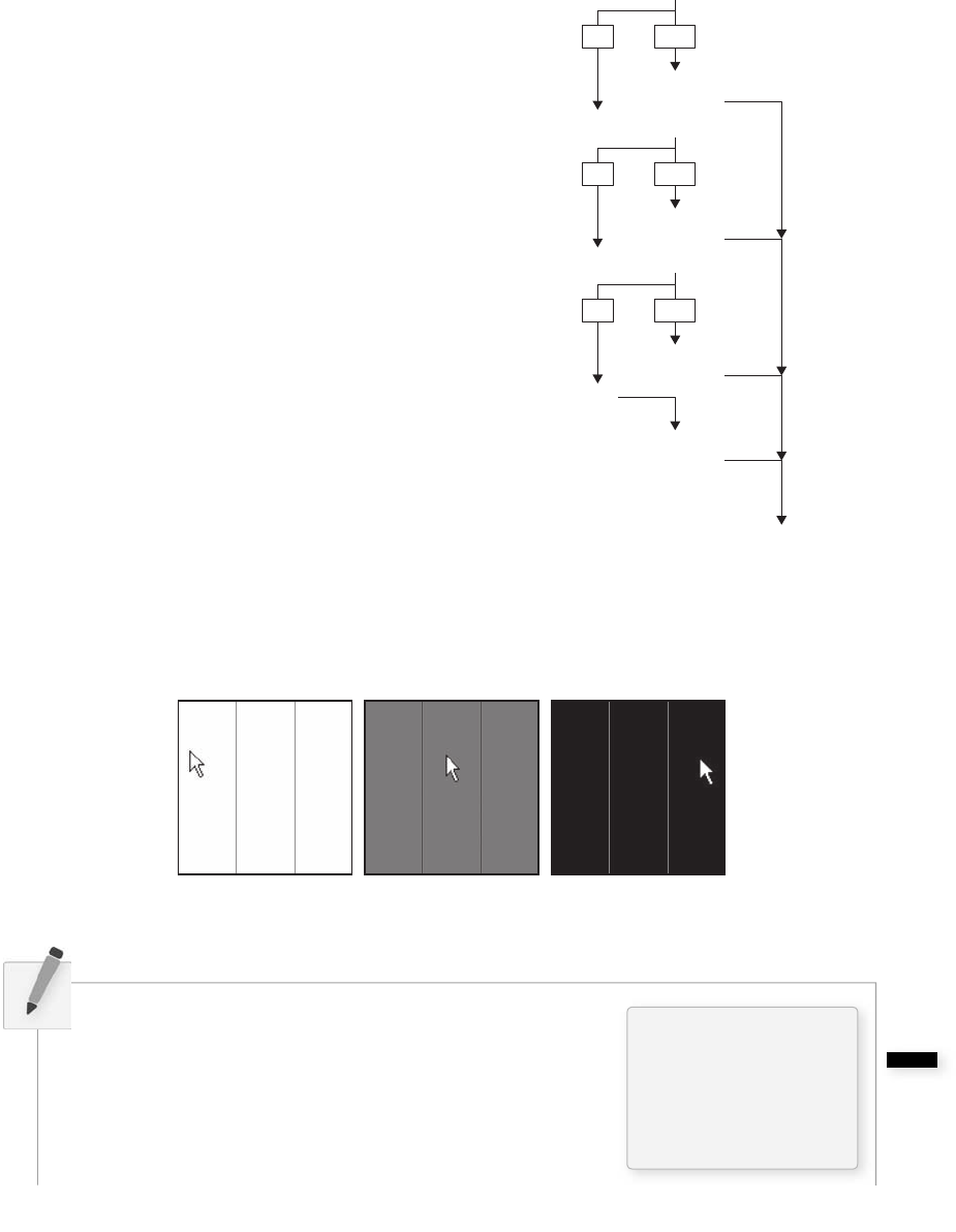
Conditionals 61
Finally, for testing multiple conditions, we can employ an “ else if. ”
When an else if is used, the conditional statements are evaluated
in the order presented. As soon as one boolean expression is found
to be true, the corresponding code is executed and the remaining
boolean expressions are ignored. See Figure 5.3 .
if (boolean expression #1) {
// code to execute if boolean expression #1 is true
} else if (boolean expression #2) {
// code to execute if boolean expression #2 is true
} else if (boolean expression #n) {
// code to execute if boolean expression #n is true
} else {
// code to execute if none of the above
// boolean expressions are true
}
Taking our simple mouse example a step further, we could say the
following, with results shown in Figure 5.4 .
If the mouse is on the left third of the window, draw a white
background, if it is in the middle third, draw a gray background,
otherwise, draw a black background.
if (mouseX < width/3) {
background(255);
} else if (mouseX < 2*width/3) {
background(127);
} else {
background(0);
}
if (A is true)
else if (B is true)
Do this.
And this.
else if (C is true)
else
Do this.
And this.
Now on to something else....
No Yes
Do this.
And this.
No Yes
Do this.
And this.
No Yes
fi g. 5.3
fi g. 5.4
float grade = random(0,100);
if (_______) {
println( "Assign letter grade A. ");
} else if (________) {
println (________);
Exercise 5-1: Consider a grading system where numbers are turned into letters. Fill in the
blanks in the following code to complete the boolean expression.
In one conditional
statement, you can only
ever have one if and one
else . However, you can
have as many else if ’s as
you like!

62 Pixels, Patterns, and Processing
} else if (________) {
println(________);
} else if (________) {
println(________);
} else {
println(________);
}
Exercise 5-2: Examine the following code samples and determine what will appear in
the message window. Write down your answer and then execute the code in Processing
to compare.
Problem #1: Determine if a number is between 0 and 25, 26 and 50, or greater than 50.
int x = 75;
if (x > 50) {
println(x + " is greater than
50! " );
} else if (x > 25) {
println(x + " is greater than
25! " );
} else {
println(x + " is 25 or
less! " );
}
int x = 75;
if(x > 25) {
println(x + " is greater
than 25! " );
} else if (x > 50) {
println(x + " is greater
than 50! " );
} else {
println(x + " is 25 or
less!
" );
}
OUTPUT:____________________ OUTPUT:____________________
Although the syntax is correct, what is problematic about the code in column two above?

Conditionals 63
It is worth pointing out that in Exercise 5-2 when we test for equality we must use two equal signs. is is
because, when programming, asking if something is equal is diff erent from assigning a value to a variable.
if (x = = y) {
x = y;
5.3 Conditionals in a Sketch
Let’s look at a very simple example of a program that performs diff erent tasks based on the result of
certain conditions. Our pseudocode is below.
Step 1. Create variables to hold on to red, green, and blue color components. Call them r , g , and b .
Step 2. Continuously draw the background based on those colors.
Step 3. If the mouse is on the right-hand side of the screen, increment the value of r , if it is on the
left-hand side decrement the value of r .
Step 4. Constrain the value r to be within 0 and 255.
is pseudocode is implemented in Processing in Example 5-1.
Problem #2: If a number is 5, change it to 6. If a number is 6, change it to fi ve.
int x = 5;
println("x is now: " + x);
if (x = = 5) {
x = 6;
}
if (x = = 6) {
x = 5;
}
println( "x is now: " + x );
int x = 5;
println("x is now: " + x);
if (x = = 5) {
x = 6;
} else if (x = = 6) {
x = 5;
}
println( "x is now: " + x);
OUTPUT:____________________ OUTPUT:____________________
Although the syntax is correct, what is problematic about the code in column one above?
“Is x equal to y?” Use double equals!
“Set x equal to y.” Use single equals!
64 Learning Processing
Example 5-1: Conditionals
float r = 150;
float g = 0;
float b = 0;
void setup() {
size(200,200);
}
void draw() {
background(r,g,b);
stroke(255);
line(width/2,0,width/2,height);
if(mouseX > width/2) {
r = r + 1;
} else {
r = r - 1;
}
if (r > 255) {
r = 255;
} else if (r < 0) {
r = 0;
}
}
Constraining the value of a variable, as in Step 4, is a common problem. Here, we do not want color
values to increase to unreasonable extremes. In other examples, we might want to constrain the size or
location of a shape so that it does not get too big or too small, or wander off the screen.
While using if statements is a perfectly valid solution to the constrain problem, Processing does off er a
function entitled constrain( ) that will get us the same result in one line of code.
if (r > 255) {
r = 255;
} else if (r < 0) {
r = 0;
}
r = constrain(r,0,255);
constrain( ) takes three arguments: the value we intend to constrain, the minimum limit, and the
maximum limit. e function returns the “ constrained ” value and is assigned back to the variable r.
(Remember what it means for a function to return a value? See our discussion of random( ) . )
fi g. 5.5
3. “If the mouse is on the right side of
the screen” is equivalent to “if mouseX
is greater than width divided by 2.”
4. If r is greater than 255, set it to 255.
If r is less than 0, set it to 0.
1. Variables.
Constrain with the constrain( ) function.
Constrain with an “if” statement.
2. Draw stuff.
Conditionals 65
Getting into the habit of constraining values is a great way to avoid errors; no matter how sure you are
that your variables will stay within a given range, there are no guarantees other than constrain( ) itself.
And someday, as you work on larger software projects with multiple programmers, functions such as
constrain( ) can ensure that sections of code work well together. Handling errors before they happen in
code is emblematic of good style.
Let’s make our fi rst example a bit more advanced and change all three color components according to
the mouse location and click state. Note the use of constrain( ) for all three variables. e system variable
mousePressed is true or false depending on whether the user is holding down the mouse button.
Example 5-2: More conditionals
float r = 0;
float b = 0;
float g = 0;
void setup() {
size(200,200);
}
void draw() {
background(r,g,b);
stroke(0);
line(width/2,0,width/2,height);
line(0,height/2,width,height/2);
if(mouseX > width/2) {
r = r + 1;
} else {
r = r - 1;
}
if (mouseY > height/2) {
b = b + 1;
} else {
b = b - 1;
}
if (mousePressed) {
g = g + 1;
} else {
g = g - 1;
}
r = constrain(r,0,255);
g = constrain(g,0,255);
b = constrain(b,0,255);
}
fi g. 5.6
Three variables for the background color.
Color the background and draw lines to
divide the window into quadrants.
If the mouse is on the right-hand side of
the window, increase red. Otherwise, it is
on the left-hand side and decrease red.
If the mouse is on the bottom of the
window, increase blue. Otherwise, it
is on the top and decrease blue.
If the mouse is pressed (using the system
variable mousePressed) increase green.
Constrain all color values to between
0 and 255.

66 Learning Processing
Exercise 5-3: Move a rectangle across a window by incrementing a variable. Start the shape
at x coordinate 0 and use an if statement to have it stop at coordinate 100. Rewrite the
sketch to use constrain( ) instead of the if statement. Fill in the missing code.
// Rectangle starts at location x
float x = 0;
void setup() {
size(200,200);
}
void draw() {
background(255);
// Display object
fill(0);
rect(x,100,20,20);
// Increment x
x = x + 1;
______________________________________________
______________________________________________
______________________________________________
}
5.4 Logical Operators
We have conquered the simple if statement:
If my temperature is greater than 98.6, then take me to see the doctor .
Sometimes, however, simply performing a task based on one condition is not enough. For example:
If my temperature is greater than 98.6 OR I have a rash on my arm, take me to see the doctor .
If I am stung by a bee AND I am allergic to bees, take me to see the doctor .
We will commonly want to do the same thing in programming from time to time.
If the mouse is on the right side of the screen AND the mouse is on the bottom of the screen, draw a rectangle
in the bottom right corner .
Conditionals 67
Our fi rst instinct might be to write the above code using a nested if statement, like so:
if (mouseX > width/2) {
if (mouseY > height/2) {
fill(255);
rect(width/2,height/2,width/2,height/2);
}
}
In other words, we would have to bypass two if statements before we can
reach the code we want to execute. is works, yes, but can be accomplished
in a simpler way using what we will call a “ logical and, ” written as two
ampersands ( “ & & ” ). A single ampersand ( “ & ” ) means something else
1 in
Processing so make sure you include two!
1
“ & ” or “ | ” are reserved for bitwise operations in Processing. A bitwise operation compares each bit (0 or 1) of the binary
representations of two numbers. It is used in rare circumstances where you require low-level access to bits.
|| (logical OR)
& & (logical AND)
! (logical NOT)
A “ logical or ” is two vertical bars (AKA two “ pipes ” ) “ || ” . If you can’t fi nd the pipe, it is typically on the
keyboard as shift-backslash.
if (mouseX > width/2 & & mouseY > height/2) {
fill(255);
rect(width/2,height/2,width/2,height/2);
}
In addition to & & and ||, we also have access to the logical operator “ not, ” written as an exclamation
point: !
If my temperature is NOT greater than 98.6, I won’t call in sick to work.
If I am stung by a bee AND I am NOT allergic to bees, do not worry!
A Processing example is:
If the mouse is NOT pressed, draw a circle, otherwise draw a square .
if (!mousePressed) {
ellipse(width/2,height/2,100,100);
} else {
rect(width/2,height/2,100,100);
}
Notice this example could also be written omitting the not , saying:
If the mouse is pressed, draw a square, otherwise draw a circle .
! means not. “mousePressed” is a boolean
variable that acts as its own boolean expression.
Its value is either true or false (depending on
whether or not the mouse is currently pressed).
Boolean variables will be explored in greater
detail in Section 5.6.
If the mouse is on the right side and on
the bottom.
68 Learning Processing
Exercise 5-4: Are the following boolean expressions true or false? Assume variables
x 5 and y 6 .
!(x > 6) _______ ______________________________
(x = = 6& & x = = 5)_____________________________________
(x = = 6 || x = = 5)_____________________________________
(x > -1 & & y < 10)_______ _______________________________
Although the syntax is correct, what is fl awed about the following boolean expression?
(x > 10 & & x < 5) ________________________________
E x e rcise 5-5: Write a program that implements a simple rollover. In other words, if the
mouse is over a rectangle, the rectangle changes color. Here is some code to get you started.
int x = 50;
int y = 50;
int w = 100;
int h = 75;
void setup() {
size(200,200);
}
void draw() {
background(0);
stroke(255);
if (_______ & & _______ & & _______ & & _______) {
_______
} _______ {
_______
}
rect(x,y,w,h);
}
Conditionals 69
5.5 Multiple Rollovers
Let’s solve a simple problem together, a slightly more advanced version of Exercise 5-5. Consider the
four screenshots shown in Figure 5.7 from one single sketch. A white square is displayed in one of four
quadrants, according to the mouse location.
fi g. 5.7
Let’s fi rst write the logic of our program in pseudocode (i.e., English).
Setup:
1 . Set up a window of 200 200 pixels .
D r a w :
1. Draw a white background.
2 . Draw horizontal and vertical lines to divide the window in four quadrants .
3. If the mouse is in the top left corner, draw a black rectangle in the top left corner.
4. If the mouse is in the top right corner, draw a black rectangle in the top right corner.
5. If the mouse is in the bottom left corner, draw a black rectangle in the bottom left corner.
6. If the mouse is in the bottom right corner, draw a black rectangle in the bottom right corner.
For instructions 3 through 6, we have to ask ourselves the question: “ How do we know if the mouse is
in a given corner? ” To accomplish this, we need to develop a more specifi c if statement. For example,
we would say: “ If the mouse X location is greater than 100 pixels and the mouse Y location is greater
than 100 pixels, draw a black rectangle in the bottom right corner. As an exercise, you may want to try
writing this program yourself based on the above pseudocode. e answer, for your reference, is given in
Example 5-3.
Example 5-3: Rollovers
void setup() {
size(200,200);
}
void draw() {
background(255);
stroke(0);
line(100,0,100,200);
line(0,100,200,100);

70 Learning Processing
// Fill a black color
noStroke();
fill(0);
if (mouseX < 100 & & mouseY < 100) {
rect(0,0,100,100);
} else if (mouseX > 100 & & mouseY < 100) {
rect(100,0,100,100);
} else if (mouseX < 100 & & mouseY > 100) {
rect(0,100,100,100);
} else if (mouseX > 100 & & mouseY > 100) {
rect(100,100,100,100);
}
}
Depending on the mouse location,
a different rectangle is displayed.
5.6 Boolean Variables
e natural next step up from programming a rollover is a button. After all, a button is just a rollover that
responds when clicked. Now, it may feel ever so slightly disappointing to be programming rollovers and
buttons. Perhaps you are thinking: “ Can’t I just select ‘ Add Button ’ from the menu or something? ” For us,
right now, the answer is no. Yes, we are going to eventually learn how to use code from a library (and you
might use a library to make buttons in your sketches more easily), but there is a lot of value in learning
how to program GUI (graphical user interface) elements from scratch.
For one, practicing programming buttons, rollovers, and sliders is an excellent way to learn the basics of
variables and conditionals. And two, using the same old buttons and rollovers that every program has is
not terribly exciting. If you care about and are interested in developing new interfaces, understanding how
to build an interface from scratch is a skill you will need.
OK, with that out of the way, we are going to look at how we use a boolean variable to program a button.
A boolean variable (or a variable of type boolean) is a variable that can only be true or false. ink of it
as a switch. It is either on or off . Press the button, turn the switch on. Press the button again, turn it off .
We just used a boolean variable in Example 5-2: the built-in variable mousePressed . mousePressed is true
when the mouse is pressed and false when the mouse is not.
And so our button example will include one boolean variable with a starting value of false (the assumption
being that the button starts in the off state).
boolean button = false;
In the case of a rollover, any time the mouse hovered over the rectangle, it turned white. Our sketch will
turn the background white when the button is pressed and black when it is not.
if (button) {
background(255);
} else {
background(0);
}
Exercise 5-6: Rewrite Example 5-3 so that the squares fade from white to black when the
mouse leaves their area. Hint: you need four variables, one for each rectangle’s color.
A boolean variables is either true of false.
If the value of button is true, the
background is white. If it is false, black.

Conditionals 71
We can then check to see if the mouse location is inside the rectangle and if the mouse is pressed, setting
the value of button to true or false accordingly. Here is the full example:
Example 5-4: Hold down the button
boolean button = false;
int x = 50;
int y = 50;
int w = 100;
int h = 75;
void setup() {
size(200,200);
}
void draw() {
if (mouseX > x & & mouseX < x + w & & mouseY > y & & mouseY < y + h & & mousePressed) {
button = true;
} else {
button = false;
}
if (button) {
background(255);
stroke(0);
} else {
background(0);
stroke(255);
}
fill(175);
rect(x,y,w,h);
}
is example simulates a button connected to a light that is only on when the button is pressed. As soon
as you let go, the light goes off . While this might be a perfectly appropriate form of interaction for some
instances, it is not what we are really going for in this section. What we want is a button that operates like
a switch; when you fl ip the switch (press the button), if the light is off , it turns on. If it is on, it turns off .
For this to work properly, we must check to see if the mouse is located inside the rectangle inside
mousePressed( ) rather than as above in draw( ) . By defi nition, when the user clicks the mouse, the code
inside mousePressed( ) is executed once and only once (see Section 3.4). When the mouse is clicked, we
want the switch to turn on or off (once and only once).
We now need to write some code that “ toggles ” the switch, changes its state from on to off , or off to on.
is code will go inside mousePressed( ) .
If the variable “ button ” equals true, we should set it to false. If it is false, we should set it to true.
The button is pressed if (mouseX, mouseY) is
inside the rectangle and mousePressed is true.
72 Learning Processing
if (button) {
button = false;
} else {
button = true;
}
ere is a simpler way to go which is the following:
button = !button;
Here, the value of button is set to “ not ” itself. In other words, if the button is true then we set set it to not
true (false). If it is false then we set it to not false (true). Armed with this odd but eff ective line of code, we
are ready to look at the button in action in Example 5-5.
Example 5-5: Button as switch
boolean button = false;
int x = 50;
int y = 50;
int w = 100;
int h = 75;
void setup() {
size(200,200);
}
void draw() {
if (button) {
background(255);
stroke(0);
} else {
background(0);
stroke(255);
}
fill(175);
rect(x,y,w,h);
}
void mousePressed() {
if (mouseX > x & & mouseX < x + w & & mouseY > y & & mouseY < y + h){
button = !button;
}
}
The explicit way to toggle a boolean variable.
If the value of button is true, set it equal to
false. Otherwise, it must be false, so set it
equal to true.
Not true is false. Not false is true!
fi g. 5.8
When the mouse is pressed, the state of the button is toggled. Try moving
this code to draw( ) like in the rollover example. (See Exercise 5–7.)
if (mouseX > x && mouseX < x+w && mouseY > y && mouseY < y+h &&
mousePressed){
button = !button;
}
Exercise 5-7: Why doesn’t the following code work properly when it is moved to draw( )?

Conditionals 73
Exercise 5-8: Example 4-3 in the previous chapter moved a circle across the window.
Change the sketch so that the circle only starts moving once the mouse has been pressed. Use a
boolean variable.
boolean __________ = _________;
int circleX = 0;
int circleY = 100;
void setup() {
size(200,200);
}
void draw() {
background(100);
stroke(255);
fill(0);
ellipse(circleX,circleY,50,50);
____________________________________
____________________________________
____________________________________
}
void mousePressed() {
____________________________________
}
5.7 A Bouncing Ball
It is time again to return to our friend Zoog. Let’s review what we have done so far. First, we learned
to draw Zoog with shape functions available from the Processing reference. Afterward, we realized we
could use variables instead of hard-coded values. Having these variables allowed us move Zoog. If Zoog’s
location is X , draw it at X , then at X 1, then at X 2, and so on.
It was an exciting, yet sad moment. e pleasure we experienced from discovering the motion was quickly
replaced by the lonely feeling of watching Zoog leave the screen. Fortunately, conditional statements are
here to save the day, allowing us to ask the question: Has Zoog reached the edge of the screen? If so, turn Zoog
around!
To simplify things, let’s start with a simple circle instead of Zoog’s entire pattern.
Write a program where Zoog (a simple circle) moves across the screen horizontally from left to right.
When it reaches the right edge it reverses direction.

74 Learning Processing
From the previous chapter on variables, we know we need global variables to keep track of Zoog’s
location.
int x = 0;
Is this enough? No. In our previous example Zoog always moved one pixel.
x = x + 1;
is tells Zoog to move to the right. But what if we want it to move to the left? Easy, right?
x = x - 1;
In other words, sometimes Zoog moves with a speed of “ 1 ” and sometimes “ 1. ” e speed of Zoog varies .
Yes, bells are ringing. In order to switch the direction of Zoog’s speed, we need another variable : speed.
int x = 0;
int speed = l;
Now that we have our variables, we can move on to the rest of the code. Assuming setup( ) sets the size
of the window, we can go directly to examining the steps required inside of draw( ) . We can also refer to
Zoog as a ball in this instance since we are just going to draw a circle.
background(0);
stroke(255);
fill(100);
ellipse(x,100,32,32);
Elementary stuff . Now, in order for the ball to move, the value of its x location should change each cycle
through draw( ) .
x = x + speed;
If we ran the program now, the circle would start on the left side of the window, move toward the right,
and continue off the edge of the screen—this is the result we achieved in Chapter 4. In order for it to turn
around, we need a conditional statement.
If the ball goes off the edge, turn the ball around .
Or more formally . . .
If x is greater than width, reverse speed.
if (x > width) {
speed = speed * -1;
}
A variable for Zoog’s speed. When speed
is positive Zoog moves to the right, when
speed is negative Zoog moves to the left.
For simplicity, Zoog is just a circle.
Multiplying by 1 reverses the speed.

Conditionals 75
Running the sketch, we now have a circle that turns around when it reaches the right-most edge, but runs
off the left-most edge of the screen. We’ll need to revise the conditional slightly.
If the ball goes off either the right or left edge, turn the ball around.
Or more formally . . .
If x is greater than width or if x is less than zero, reverse speed .
if ((x > width) || (x < 0)) {
speed = speed * -1;
}
Example 5-6 puts it all together.
Example 5-6: Bouncing ball
int x = 0;
int speed = 1;
void setup() {
size(200,200);
smooth();
}
void draw() {
background(255);
x = x + speed;
if ((x > width) || (x < 0)) {
speed = speed * -1;
}
// Display circle at x location
stroke(0);
fill(175);
ellipse(x,100,32,32);
}
Reversing the Polarity of a Number
When we want to reverse the polarity of a number, we mean that we want a positive number to
become negative and a negative number to become positive. is is achieved by multiplying by –1.
Remind yourself of the following:
• -5 * -1 = 5
• -5 * -1 = -5
• -1 * 1 = -1
• -1 * -1 = 1
Remember, 储 means “or”.
Add the current speed to the x location.
If the object reaches either edge,
multiply speed by 1 to turn it around.
76 Learning Processing
Exercise 5-9: Rewrite Example 5-6 so that the ball not only moves horizontally, but
vertically as well. Can you implement additional features, such as changing the size or color
of the ball based on certain conditions? Can you make the ball speed up or slow down in
addition to changing direction?
e “ bouncing ball ” logic of incrementing and decrementing a variable can be applied in many ways
beyond the motion of shapes onscreen. For example, just as a square moves from left to right, a color
can go from less red to more red. Example 5-7 takes the same bouncing ball algorithm and applies it to
changing color .
Example 5-7: “ Bouncing ” color
float c1 = 0;
float c2 = 255;
float c1dir = 0.1;
float c2dir = -0.1;
void setup() {
size(200,200);
}
void draw() {
noStroke();
// Draw rectangle on left
fill(c1,0,c2);
rect(0,0,100,200);
// Draw rectangle on right
fill(c2,0,c1);
rect(100,0,100,200);
// Adjust color values
c1 = c1 + c1dir;
c2 = c2 + c2dir;
// Reverse direction of color change
if (c1 < 0 || c1 > 255) {
c1dir * = -1;
}
if (c2 < 0 || c2 > 255) {
c2dir * = -1;
}
}
Having the conditional statement in our collection of programming tools allows for more complex
motion. For example, consider a rectangle that follows the edges of a window.
fi g. 5.9
Two variables for color.
Start by incrementing c1.
Start by decrementing c2.
Instead of reaching the edge of a window, these
variables reach the “edge” of color: 0 for no color
and 255 for full color. When this happens, just like
with the bouncing ball, the direction is reversed.
Conditionals 77
One way to solve this problem is to think of the rectangle’s motion as having four possible states,
numbered 0 through 3. See Figure 5.10 .
• State #0: left to right.
• State #1: top to bottom.
• State #2: right to left.
• State #3: bottom to top.
We can use a variable to keep track of the state number and adjust
the x , y coordinate of the rectangle according to the state. For example:
“ If the state is 2, x equals x minus 1. ”
Once the rectangle reaches the endpoint for that state, we can change the state variable. “ If the state is 2:
(a) x equals x minus 1. (b) if x less than zero, the state equals 3. ”
e following example implements this logic .
Example 5-8: Square following edge, uses a “ state ” variable
int x = 0; // x location of square
int y = 0; // y location of square
int speed = 5; // speed of square
int state = 0;
void setup() {
size(200,200);
}
void draw() {
background(100);
// Display the square
noStroke();
fill(255);
rect(x,y,10,10);
if (state = = 0) {
x = x + speed;
if (x > width-10) {
x = width-10;
state = 1;
}
} else if (state = = 1) {
y = y + speed;
if (y > height-10) {
y = height-10;
state = 2;
}
fi g. 5.11
fi g. 5.10
A variable to keep track of the square’s
“state.” Depending on the value of its state,
it will either move right, down, left, or up.
If, while the state is 0, it reaches the right
side of the window, change the state to 1.
Repeat this same logic for all states!
If the state is 0, move to the right.

} else if (state = = 2) {
x = x - speed;
if (x < 0) {
x = 0;
state = 3;
}
} else if (state = = 3) {
y = y - speed;
if (y < 0) {
y = 0;
state = 0;
}
}
}
5.8 Physics 101
For me, one of the happiest moments of my programming life was the moment I realized I could code
gravity. And in fact, armed with variables and conditionals, you are now ready for this moment.
e bouncing ball sketch taught us that an object moves by altering its location according to speed.
location location speed
Gravity is a force of attraction between all masses. When you drop a pen, the force of gravity from the
earth (which is overwhelmingly larger than the pen) causes the pen to accelerate toward the ground.
What we must add to our bouncing ball is the concept of “ acceleration ” (which is caused by gravity, but
could be caused by any number of forces). Acceleration increases (or decreases) speed. In other words,
acceleration is the rate of change of speed. And speed is the rate of change of location. So we just need
another line of code:
speed speed acceleration
And now we have a simple gravity simulation.
Example 5-9: Simple gravity
float x = 100; // x location of square
float y = 0; // y location of square
float speed = 0; // speed of square
float gravity = 0.1;
void setup() {
size(200,200);
}
void draw() {
background(255);
fi g. 5.12
A new variable, for gravity (i.e.,
acceleration). We use a relatively
small number (0.1) because this
acceleration accumulates over
time, increasing the speed. Try
changing this number to 2.0 and see
what happens.
78 Learning Processing

Conditionals 79
// Display the square
fill(0);
noStroke();
rectMode(CENTER);
rect(x,y,10 , 10);
y = y + speed;
speed = speed + gravity;
// If square reaches the bottom
// Reverse speed
if (y > height) {
speed = speed * -0.95;
}
}
Exercise 5-10: Continue with your design and add some of the functionality demonstrated
in this chapter. Some options:
• Make parts of your design rollovers that change color when the mouse is over
certain areas.
• Move it around the screen. Can you make it bounce off all edges of the window?
• Fade colors in and out.
Add gravity to speed.
Here is a simple version with Zoog.
Example 5-10: Zoog and conditionals
float x = 100;
float y = 100;
float w = 60;
float h = 60;
float eyeSize = 16;
float xspeed = 3;
float yspeed = 1;
void setup() {
size(200,200);
smooth();
}
void draw() {
// Change the location of Zoog by speed
x = x + xspeed;
y = y + yspeed;
Multiplying by 0.95 instead of 1 slows the square down
each time it bounces (by decreasing speed). This is known
as a “dampening” effect and is a more realistic simulation
of the real world (without it, a ball would bounce forever).
Zoog has variables for speed in the horizontal and vertical direction.
Add speed to location.

if ((x > width) 储 (x < 0)) {
xspeed = xspeed * -1;
}
if ((y > height) 储 (y < 0)) {
yspeed = yspeed * -1;
}
background(0);
ellipseMode(CENTER);
rectMode(CENTER);
noStroke();
// Draw Zoog's body
fill(150);
rect(x,y,w/6,h*2);
// Draw Zoog's head
fill(255);
ellipse(x,y-h/2,w,h);
// Draw Zoog's eyes
fill(0);
ellipse(x-w/3,y-h/2,eyeSize,eyeSize*2);
ellipse(x + w/3,y-h/2,eyeSize,eyeSize*2);
// Draw Zoog's legs
stroke(150);
line(x-w/12,y + h,x-w/4,y + h +
10);
line(x + w/12,y + h,x + w/4,y + h + 10);
}
An IF statements with a logical OR determines if Zoog has
reached either the right or left edges of the screen. When this is
true, we multiply the speed by 1, reversing Zoog’s direction!
Identical logic is applied to the y direction as well.
80 Learning Processing

Loops 81
6 Loops
“ Repetition is the reality and the seriousness of life. ”
—Soren Kierkegaard
“ What’s the key to comedy? Repetition. What’s the key to comedy? Repetition. ”
—Anonymous
In this chapter:
– The concept of iteration.
– Two types of loops: “ while, ” and “ for. ” When do we use them?
– Iteration in the context of computer graphics.
6.1 What is iteration? I mean, what is iteration? Seriously, what is iteration?
Iteration is the generative process of repeating a set of rules or steps over and over again. It is a
fundamental concept in computer programming and we will soon come to discover that it makes our lives
as coders quite delightful. Let’s begin.
For the moment, think about legs. Lots and lots of legs on our little Zoog. If we had only read Chapter 1
of this book, we would probably write some code as in Example 6-1 .
Example 6-1: Many lines
size(200,200);
background(255);
// Legs
stroke(0);
line(50,60,50,80);
line(60,60,60,80);
line(70,60,70,80);
line(80,60,80,80);
line(90,60,90,80);
line(100,60,100,80);
line(110,60,110,80);
line(120,60,120,80);
line(130,60,130,80);
line(140,60,140,80);
line(150,60,150,80);
In the above example, legs are drawn from x = 50 pixels all the way to x 150 pixels, with one leg every
10 pixels. Sure, the code accomplishes this, however, having learned variables in Chapter 4, we can make
some substantial improvements and eliminate the hard-coded values.
First, we set up variables for each parameter of our system: the legs ’ x , y locations, length, and the spacing
between the legs. Note that for each leg drawn, only the x value changes. All other variables stay the same
(but they could change if we wanted them to!).
fi g. 6.1

82 Learning processing
Example 6-2: Many lines with variables
size(200,200);
background(0);
// Legs
stroke(255);
int y = 80; // Vertical location of each line
int x = 50; // Initial horizontal location for first line
int spacing = 10; // How far apart is each line
int len = 20; // Length of each line
line(x,y,x,y + len);
x = x + spacing;
line(x,y,x,y + len);
x = x + spacing;
line(x,y,x,y + len);
x = x + spacing;
line(x,y,x,y + len);
x = x + spacing;
line(x,y,x,y + len);
x = x + spacing;
line(x,y,x,y + len);
x = x + spacing;
line(x,y,x,y + len);
x = x + spacing;
line(x,y,x,y + len);
x = x + spacing;
line(x,y,x,y + len);
x = x + spacing;
line(x,y,x,y + len);
x = x + spacing;
line(x,y,x,y + len);
Not too bad, I suppose. Strangely enough, although this is technically more effi cient (we could adjust the
spacing variable, for example, by changing only one line of code), we have taken a step backward, having
produced twice as much code! And what if we wanted to draw 100 legs? For every leg, we need two lines
of code. at’s 200 lines of code for 100 legs! To avoid this dire, carpal-tunnel inducing problem, we want
to be able to say something like:
Draw one line one hundred times.
Aha, only one line of code!
Obviously, we are not the fi rst programmers to reach this dilemma and it is easily solved with the
very commonly used control structure —the loop . A loop structure is similar in syntax to a conditional
Draw the fi rst leg.
Add spacing so the next leg
appears 10 pixels to the right.
Continue this process for
each leg, repeating it over
and over.
Loops 83
(see Chapter 5). However, instead of asking a yes or no question to determine whether a block of code
should be executed one time, our code will ask a yes or no question to determine how many times the
block of code should be repeated . is is known as iteration.
6.2 “ WHILE ” Loop, the Only Loop You Really Need
ere are three types of loops, the while loop, the do-while loop, and the for loop. To get started, we are
going to focus on the while loop for a little while (sorry, couldn’t resist). For one thing, the only loop you
really need is while . e for loop, as we will see, is simply a convenient alternative, a great shorthand for
simple counting operations. Do-while , however, is rarely used (not one example in this book requires it)
and so we will ignore it.
Just as with conditional ( if / else ) structures, a while loop employs a boolean test condition. If the test
evaluates to true, the instructions enclosed in curly brackets are executed; if it is false, we continue on to
the next line of code. e diff erence here is that the instructions inside the while block continue to be
executed over and over again until the test condition becomes false. See Figure 6.2 .
Let’s take the code from the legs problem. Assuming the following variables . . .
int y = 80; // Vertical location of each line
int x = 50; // Initial horizontal location for first line
int spacing = 10; // How far apart is each line
int len = 20; // Length of each line
… we had to manually repeat the following code:
stroke(255);
line(x,y,x,y + len); // Draw the first leg
x = x + spacing; // Add "spacing " to x
line(x,y,x,y + len); // The next leg is 10 pixels to the right
x = x + spacing; // Add "spacing" to x
line(x,y,x,y + len); // The next leg is 10 pixels to the right
x = x + spacing; // Add ''spacing” to x
line(x,y,x,y + len); // The next leg is 10 pixels to the right
// etc. etc. repeating with new legs
WHILE (BOOLEAN TEST)
A. DO THIS
B. DO THIS
IS FALSEIS TRUE
REPEAT
fi g. 6.2
84 Learning processing
Now, with the knowledge of the existence of while loops, we can rewrite the code as in Example 6-3,
adding a variable that tells us when to stop looping, that is, at what pixel the legs stop.
Example 6-3: While loop
int endLegs = 150;
stroke(0);
while (x < = endLegs) {
line (x,y,x,y + len);
x = x + spacing;
}
Instead of writing “ line(x,y,x,y + len); ” many times as we did at fi rst, we now write it only once inside of the
while loop , saying “ as long as x is less than 150, draw a line at x , all the while incrementing x . ” And so
what took 21 lines of code before, now only takes four!
In addition, we can change the spacing variable to generate more legs. e results are shown in Figure 6.4 .
int spacing = 4;
while (x < = endLegs) {
line (x,y,x,y + len); // Draw EACH leg
x = x + spacing;
}
Let’s look at one more example, this time using rectangles instead of
lines, as shown in Figure 6.5 , and ask three key questions.
1. What is the initial condition for your loop? Here, since the fi rst rectangle is at y location 10, we want
to start our loop with y 10.
int y = 10;
2. When should your loop stop? Since we want to display rectangles all the way to the bottom of the
window, the loop should stop when y is greater than height. In other words, we want the loop to keep
going as long as y is less than height.
fi g. 6.3
fi g. 6.4
fi g. 6.5
Draw each leg inside
awhile loop.
A variable to mark
where the legs end.
A smaller spacing
value results in legs
closer together.
Loops 85
while (y < 100) {
// Loop!
}
3. What is your loop operation? In this case, each time through the loop, we want to draw a new
rectangle below the previous one. We can accomplish this by calling the rect( ) function and
incrementing y by 20.
rect(100,y,100,10);
y = y + 20;
Putting it all together:
int y = 10;
while (y < height) {
rect(100,y,100,10);
y = y + 20;
}
Initial condition.
The loop continues while the boolean expression is true.
Therefore, the loop stops when the boolean expression is false.
We increment y each time through the loop, drawing rectangle
after rectangle until y is no longer less than height.
size(200,200);
background(255);
int y = 0;
while (________) {
stroke(0);
line(_______,_______,_______,_______);
y = ________ ;
}
size(200,200);
background(255);
float w = ________ ;
while (________) {
stroke(0);
fill(________);
ellipse(_______,_______,_______,_______);
__________20;
}
Exercise 6-1: Fill in the blanks in the code to recreate the following screenshots.
86 Learning processing
Examining the “ legs ” in Example 6-3, we can see that as soon as x is greater than 150, the loop stops.
And this always happens because x increments by “ spacing ” , which is always a positive number. is is not
an accident; whenever we embark on programming with a loop structure, we must make sure that the exit
condition for the loop will eventually be met!
Processing will not give you an error should your exit condition never occur. e result is Sisyphean, as
your loop rolls the boulder up the hill over and over and over again to infi nity.
Example 6-4: Infi nite loop. Don’t do this!
int x = 0;
while (x < 10) {
println(x);
x = x – 1;
}
For kicks, try running the above code (make sure you have saved all your work and are not running some
other mission-critical software on your computer). You will quickly see that Processing hangs. e only
way out of this predicament is probably to force-quit Processing . Infi nite loops are not often as obvious as
in Example 6-4. Here is another fl awed program that will sometimes result in an infi nite loop crash.
Example 6-5: Another infi nite loop. Don’t do this!
int y = 80; // Vertical location of each line
int x = 0; // Horizontal location of first line
int spacing = 10; // How far apart is each line
int len = 20; // Length of each line
int endLegs = 150; // Where should the lines stop?
void setup() {
size(200,200);
}
void draw() {
background(0);
stroke(255);
x = 0;
spacing = mouseX / 2;
6.3 “ Exit ” Conditions
Loops, as you are probably starting to realize, are quite handy. Nevertheless, there is a dark, seedy
underbelly in the world of loops, where nasty things known as infi nite loops live. See Figure 6.6 .
WHILE (ALWAYS TRUE)
BAD!!
DO THIS FOREVER AND EVER...
fi g. 6.6
The spacing variable, which sets the distance
in between each line, is assigned a value
equal to mouseX divided by two.
Decrementing x results in an infi nite loop here because
the value of x will never be 10 or greater. Be careful!

Loops 87
while (x < = endLegs) {
line(x,y,x,y + len);
x = x + spacing;
}
}
Will an infi nite loop occur? We know we will be stuck looping forever if x never is greater than 150. And
since x increments by spacing, if spacing is zero (or a negative number) x will always remain the same
value (or go down in value.)
Recalling the constrain( ) function described in Chapter 4, we can guarantee no infi nite loop by
constraining the value of spacing to a positive range of numbers:
int spacing = constrain(mouseX/2, 1, 100);
Since spacing is directly linked with the necessary exit condition, we enforce a specifi c range of values to
make sure no infi nite loop is ever reached. In other words, in pseudocode we are saying: “ Draw a series of
lines spaced out by N pixels where N can never be less than 1! ”
is is also a useful example because it reveals an interesting fact about mouseX . You might be tempted to
try putting mouseX directly in the incrementation expression as follows:
while (x < = endLegs) {
line(x,y,x,y + len);
x = x + mouseX / 2;
}
Wouldn’t this solve the problem, since even if the loop gets stuck as soon as the user moves the mouse
to a horizontal location greater than zero, the exit condition would be met? It is a nice thought, but one
that is sadly quite fl awed. mouseX and mouseY are updated with new values at the beginning of each
cycle through draw( ) . So even if the user moves the mouse to X location 50 from location 0, mouseX will
never know this new value because it will be stuck in its infi nite loop and not able to get to the next cycle
through draw( ) .
6.4 “ FOR ” Loop
A certain style of while loop where one value is incremented repeatedly (demonstrated in Section 6.2)
is particularly common. is will become even more evident once we look at arrays in Chapter 9. e
for loop is a nifty shortcut for commonly occurring while loops. Before we get into the details, let’s talk
through some common loops you might write in Processing and how they are written as a for loop.
Start at 0 and count up to 9. for (int i = 0; i < 10; i = i + 1)
Start at 0 and count up to 100 by 10. for (int i = 0; i < 101; i = i + 10)
Start at 100 and count down to 0 by 5. for (int i = 100; i > = 0; i = i – 5)
Exit Condition — when x is greater than endlegs.
Incrementation of x.x always increases by
the value of spacing. What is the range of
possible value for spacing?
Using constrain() to ensure
the exit condition is met.
Placing mouseX inside the loop is not
a solution to the infi nite loop problem.
88 Learning processing
Looking at the above examples, we can see that a for loop consists of three parts:
• Initialization —Here, a variable is declared and initialized for use within the body of the loop. This
variable is most often used inside the loop as a counter.
• Boolean Test —This is exactly the same as the boolean tests found in conditional statements and
while loops. It can be any expression that evaluates to true or false.
• Iteration Expression —The last element is an instruction that you want to happen with each loop
cycle. Note that the instruction is executed at the end of each cycle through the loop. (You can have
multiple iteration expressions, as well as variable initializations, but for the sake of simplicity we will
not worry about this now.)
START
WITH THIS
RUN THE CODE
DO THIS
RETURN TO #2
for (int i = 0; i < 10; i+ +) {
#4 & #5 ARE “INVISIBLE”
}
TEST THIS
IF FALSE EXIT
1
3
4
5
2
fi g. 6.7
Increment/Decrement Operators
e shortcut for adding or subtracting one from a variable is as follows:
x
++; is equivalent to:
x
x
1; meaning: “ increment
x
by 1 ” or
“ add 1 to the current value of
x
”
x
; is equivalent to:
x
x
1;
We also have:
x
2; same as
x
x
2;
x
* 3; same as
x
x
* 3;
and so on.
In English, the above code means: repeat this code 10 times. Or to put it even more simply: count from
zero to nine!
To the machine, it means the following:
• Declare a variable i,
and set its initial value to 0.
• While i is less than 10, repeat this code.
• At the end of each iteration, add one to i .
Afor loop can have its own variable just for the
purpose of counting. A variable not declared at
the top of the code is called a local variable.
We will explain and defi ne it shortly.
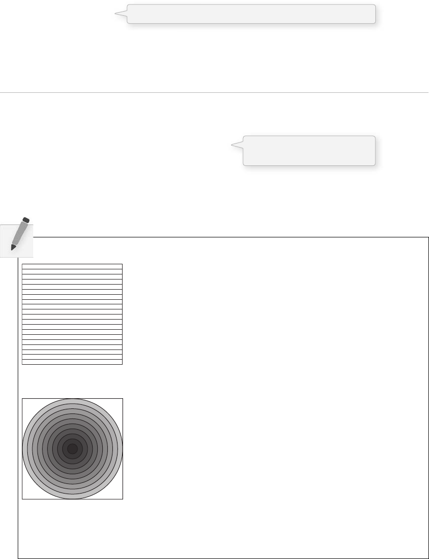
Loops 89
e same exact loop can be programmed with the while format:
int i = 0;
while (i < 10) {
i + + ;
//lines of code to execute here
}
Rewriting the leg drawing code to use a for statement looks like this:
Example 6-6: Legs with a for loop
int y = 80; // Vertical location of each line
int spacing = 10; // How far apart is each line
int len = 20; // Length of each line
for (int x = 50; x < = 150; x + = spacing) {
line(x,y,x,y + len);
}
Translation of the legs while
loop to a for loop.
Exercise 6-2: Rewrite Exercise 6-1 using a for loop.
size(200,200);
background(255);
for (int y =________;________;________) {
stroke(0);
line(________,________,________,________);
}
size(200,200);
background(255);
for (________;________;________– 20) {
stroke(0);
fill(________);
ellipse(________,________,________,
________);
ellipse(________,________,________,
________);
}
This is the translation of the for loop, using a while loop.
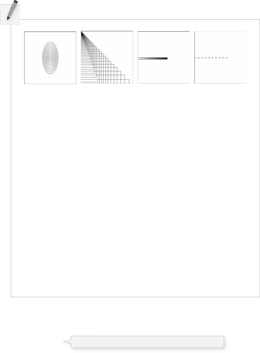
90 Learning processing
Exercise 6-3: Following are some additional examples of loops. Match the appropriate
screenshot with the loop structure. Each example assumes the same four lines of initial code.
ABCD
size(300,300); // Just setting up the size
background(255); // Black background
stroke(0); // Shapes have white lines
noFill(); // Shapes are not filled in
________ for (int i 0; i 10; i ) {
rect(i*20,height/2, 5, 5);
}
________ int i 0;
while (i 10) {
ellipse(width/2,height/2, i*10, i*20);
i;
}
________ for (float i 1.0; i width; i * 1.1) {
rect(0,i,i,i*2);
}
________ int x 0;
for (int c 255; c 0; c – 15) {
fill(c);
rect(x,height/2,10,10);
x x 10;
}
6.5 Local vs. Global Variables (AKA “ Variable Scope ” )
Up until this moment, any time that we have used a variable, we have declared it at the top of our
program above setup( ) .
int x = 0;
void setup() {
}
We have always declared our variables at the top of our code.

Loops 91
is was a nice simplifi cation and allowed us to focus on the fundamentals of declaring, initializing, and
using variables. Variables, however, can be declared anywhere within a program and we will now look at
what it means to declare a variable somewhere other than the top and how we might go about choosing
the right location for declaring a variable.
Imagine, for a moment, that a computer program is running your life. And in this life, variables are
pieces of data written on post-its that you need to remember. One post-it might have the address of a
restaurant for lunch. You write it down in the morning and throw it away after enjoying a nice turkey
burger. But another post-it might contain crucial information (such as a bank account number), and you
save it in a safe place for years on end. is is the concept of scope . Some variables exist (i.e., are accessible)
throughout the entire course of a program’s life— global variables —and some live temporarily, only for the
brief moment when their value is required for an instruction or calculation— local variables .
In Processing , global variables are declared at the top of the program, outside of both setup( ) and draw( ) .
ese variables can be used in any line of code anywhere in the program. is is the easiest way to use a
variable since you do not have to remember when you can and cannot use that variable. You can always
use that variable (and this is why we started with global variables only).
Local variables are variables declared within a block of code. So far, we have seen many diff erent examples
of blocks of code: setup( ) , draw( ) , mousePressed( ) , and keyPressed( ) , if statements, and while and for loops.
A local variable declared within a block of code is only available for use inside that specifi c block of code where it was
declared. If you try to access a local variable outside of the block where it was declared, you will get this error:
“ No accessible fi eld named “ variableName ” was found”
is is the same exact error you would get if you did not bother to declare the variable “ variableName ” at
all. Processing does not know what it is because no variable with that name exists within the block of code
you happen to be in.
Here is an example where a local variable is used inside of draw( ) for the purpose of executing a while loop.
Example 6-7: Local variable
void setup() {
size(200,200);
}
void draw() {
background(0);
int x = 0;
while (x < width) {
stroke(255);
line(x,0,x,height);
x + = 5;
}
}
X is not available! It is local to the draw() block
of code.
void mousePressed() {
println( "The mouse was pressed! ");
}
X is not available! It is local to the draw( ) block
of code.
Xis available! Since it is declared within the
draw() block of code, it is available here.
Notice, however, that it is not available inside
draw() above where it is declared. Also, it
is available inside the while block of code
because while is inside of draw ().
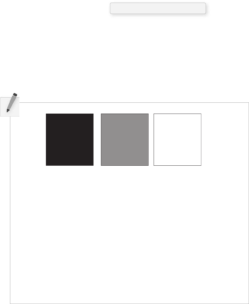
92 Learning processing
//SKETCH #1: Global //SKETCH #2: Local
" count "" count "
int count = 0; void setup() {
size(200,200);
void setup() { }
size(200,200);
} void draw() {
int count 0;
void draw() { count count 1;
count = count + 1; background(count);
background(count); }
}
________ ________
C
Why bother? Couldn’t we just have declared x as a global variable? While this is true, since we are only
using x within the draw( ) function, it is wasteful to have it as a global variable. It is more effi cient and
ultimately less confusing when programming to declare variables only within the scope of where they are
necessary. Certainly, many variables need to be global, but this is not the case here.
A for loop off ers up a spot for a local variable within the “ initialization ” part:
for (int i = 0; i < 100; i + = 10) {
stroke(255);
fill(i);
rect(i,0,10,height);
}
It is not required to use a local variable in the for loop, however, it is usually convenient to do so.
It is theoretically possible to declare a local variable with the same name as a global variable. In this case,
the program will use the local variable within the current scope and the global variable outside of that
scope. As a general rule, it is better to never declare multiple variables with the same name in order to
avoid this type of confusion.
iis only available inside the for loop.
Exercise 6-4: Predict the results of the following two programs. Test your theory by running them.
A B

Loops 93
6.6 Loop Inside the Main Loop
e distinction between local and global variables moves us one step further toward successfully integrating
a loop structure into Zoog. Before we fi nish this chapter, I want to take a look at one of the most common
points of confusion that comes with writing your fi rst loop in the context of a “ dynamic ” Processing sketch.
Consider the following loop (which happens to be the answer to
Exercise 6-2) . e outcome of the loop is shown in Figure 6.8 .
for (int y = 0; y < height; y + = 10) {
stroke(0);
line(0,y,width,y);
}
Let’s say we want to take the above loop and display each line one at a
time so that we see the lines appear animated from top to bottom. Our
fi rst thought might be to take the above loop and bring it into a dynamic
Processing sketch with setup( ) and draw( ) .
void setup() {
size(200,200);
}
void draw() {
background(255);
for (int y = 0; y < height; y + = 10) {
stroke(0);
line(0,y,width,y);
}
}
If we read the code, it seems to make sense that we would see each line appear one at a time. “ Set up a
window of size 200 by 200 pixels. Draw a black background. Draw a line at y equals 0. Draw a line at y
equals 10. Draw a line at y equals 20. ”
Referring back to Chapter 2, however, we recall that Processing does not actually update the display
window until the end of draw( ) is reached. is is crucial to remember when using while and for loops.
ese loops serve the purpose of repeating something in the context of one cycle through draw( ) . ey are
a loop inside of the sketch’s main loop, draw( ) .
Displaying the lines one at a time is something we can do with a global variable in combination with the
very looping nature of draw( ) itself
Example 6-8: Lines one at a time
int y = 0 ;
void setup() {
size(200,200);
background(0);
frameRate(5);
}
fi g. 6.8
No for loop here. Instead, a global variable.
Slowing down the frame rate so we can
easily see the effect.
94 Learning processing
void draw() {
// Draw a line
stroke(255);
line(0,y,width,y);
// Increment y
y + = 10;
}
e logic of this sketch is identical to Example 4 - 3 , our fi rst motion sketch with variables. Instead of
moving a circle across the window horizontally, we are moving a line vertically (but not clearing the
background for each frame).
Only one line is drawn each time through draw( ).
Using a loop inside draw( ) also opens up the possibility of interactivity. Example 6-9 displays a series of
rectangles (from left to right), each one colored with a brightness according to its distance from the mouse.
Example 6-9: Simple while loop with interactivity
void setup() {
size(255,255);
background(0);
}
void draw() {
background(0);
// Start with i as 0
int i = 0;
// While i is less than the width of the window
while (i < width) {
noStroke(); fi g. 6.9
int endY;
void setup() {
size(200,200);
frameRate(5);
endY = ________;
}
void draw() {
background(0);
for (int y = ________; ________; ________) {
stroke(255);
line(0,y,width,y);
}
________;
}
Exercise 6-5: It is possible to achieve the eff ect of rendering one line at a time using a for
loop. See if you can fi gure out how this is done. Part of the code is below.
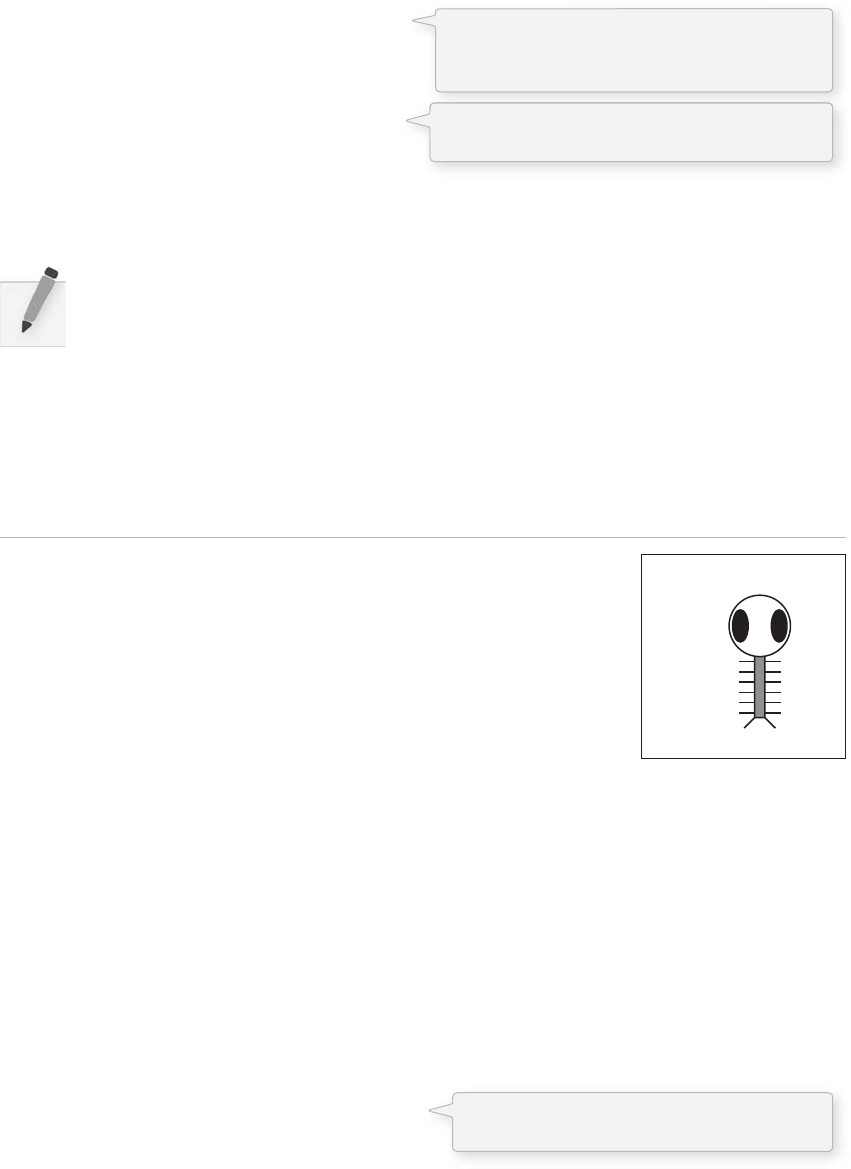
Loops 95
float distance = abs(mouseX – i);
fill(distance);
rect(i,0,10,height);
// Increase i by 10
i + = 10;
}
}
Exercise 6-6: Rewrite Example 6-9 using a for loop.
6.7 Zoog grows arms.
We last left Zoog bouncing back and forth in our Processing window. is new version of Zoog comes with
one small change. Example 6-10 uses a for loop to add a series of lines to Zoog’s body, resembling arms.
Example 6-10: Zoog with arms
int x = 100;
int y = 100;
int w = 60;
int h = 60;
int eyeSize = 16;
int speed = 1;
void setup() {
size(200,200);
smooth();
}
void draw() {
// Change the x location of Zoog by speed
x = x + speed;
// If we've reached an edge, reverse speed (i.e. multiply it by –1)
//(Note if speed is a + number, square moves to the right,– to the left)
if ((x width)储(x < 0)) {
speed = speed * –1;
}
background(255); // Draw a white background
// Set ellipses and rects to CENTER mode
ellipseMode(CENTER);
rectMode(CENTER);
// Draw Zoog's arms with a for loop
for (int i = y + 5; i < y + h; i + = 10) {
stroke(0);
line(x–w/3,i,x + w/3,i);
}
That distance is used to fi ll the color of a
rectangle at horizontal location i.
fi g. 6.10
Arms are incorporated into Zoog’s design with
afor loop drawing a series if lines.
The distance between the current rectangle and
the mouse is equal to the absolute value of the
difference between i and mouseX.
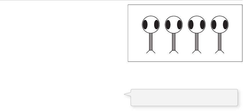
96 Learning processing
// Draw Zoog's body
stroke(0);
fill(175);
rect(x,y,w/6,h*2);
// Draw Zoog's head
fill(255);
ellipse(x,y–h/2,w,h);
// Draw Zoog's eyes
fill(0);
ellipse(x–w/3,y–h/2,eyeSize,eyeSize*2);
ellipse(x + w/3,y–h/2,eyeSize,eyeSize*2);
// Draw Zoog's legs
stroke(0);
line(x–w/12,y + h,x–w/4,y + h + 10);
line(x + w/12,y + h,x + w/4,y + h + 10);
}
We can also use a loop to draw multiple instances of Zoog by placing the code for Zoog’s body inside of a
for loop. See Example 6–11 .
Example 6-11: Multiple Zoogs
int w = 60;
int h = 60;
int eyeSize = 16;
void setup() {
size(400,200);
smooth();
}
void draw() {
background(255);
ellipseMode(CENTER);
rectMode(CENTER);
int y = height/2;
// Multiple versions of Zoog
for (int x = 80; x < width; x + = 80) {
// Draw Zoog's body
stroke(0);
fill(175);
rect(x,y,w/6,h*2);
// Draw Zoog's head
fill(255);
ellipse(x,y–h/2,w,h);
// Draw Zoog's eyes
fill(0);
ellipse(x–w/3,y–h/2,eyeSize,eyeSize*2);
ellipse(x + w/3,y–h/2,eyeSize,eyeSize*2);
fi g. 6.11
The variable x is now included in a for loop,
in order to iterate and display multiple Zoogs!
Loops 97
// Draw Zoog's legs
stroke(0);
line(x–w/12,y + h,x–w/4,y + h +10);
line(x + w/12,y + h,x + w/4,y + h +10); }
}
Exercise 6-7: Add something to your design using a for or while loop. Is there anything you
already have which could be made more effi cient with a loop?
Exercise 6-8: Create a grid of squares (each colored randomly) using a for loop. (Hint: You
will need two for loops!) Recode the same pattern using a “ while ” loop instead of “ for. ”

98 Learning processing
Lesson Two Project
Step 1. Take your Lesson One design and rewrite it with variables instead of
hard-coded values. Consider using a for loop in the creation of your
design.
Step 2. Write a series of assignment operations that alter the values of those
variables and make the design dynamic. You might also use system
variables, such as width , height, mouseX , and mouseY .
Step 3. Using conditional statements, alter the behavior of your design based on
certain conditions. What happens if it touches the edge of the screen, or
if it grows to a certain size? What happens if you move the mouse over
elements in your design?
Use the space provided below to sketch designs, notes, and pseudocode for your
project.

Lesson Three
Organization
7 Functions
8 Objects
This page intentionally left blank

Functions 101
7 Functions
“ When it’s all mixed up, better break it down. ”
—Tears for Fears
In this chapter:
– Modularity.
– Declaring and defi ning a function.
– Calling a function.
– Parameter passing.
– Returning a value.
– Reusability.
7.1 Break It Down
e examples provided in Chapters 1 through 6 are short. We probably have not looked at a sketch with
more than 100 lines of code. ese programs are the equivalent of writing the opening paragraph of this
chapter, as opposed to the whole chapter itself.
Processing is great because we can make interesting visual sketches with small amounts of code. But as
we move forward to looking at more complex projects, such as network applications or image processing
programs, we will start to have hundreds of lines of code. We will be writing essays, not paragraphs. And
these large amounts of code can prove to be unwieldy inside of our two main blocks— setup( ) and draw( ).
Functions are a means of taking the parts of our program and separating them out into modular pieces,
making our code easier to read, as well as to revise. Let’s consider the video game Space Invaders. Our steps
for draw( ) might look something like:
• Erase background.
• Draw spaceship.
• Draw enemies.
• Move spaceship according to user keyboard interaction.
• Move enemies.
What ’ s in a name?
Functions are often called other things, such as “Procedures” or “Methods” or “Subroutines.” In
some programming languages, there is a distinction between a procedure (performs a task) and a
function (calculates a value). In this chapter, I am choosing to use the term function for simplicity’s
sake. Nevertheless, the technical term in the Java programming language is “method” (related to
Java’s object-oriented design) and once we get into objects in Chapter 8, we will use the term
“method” to describe functions inside of objects.

102 Learning Processing
Before this chapter on functions, we would have translated the above pseudocode into actual code, and
placed it inside draw( ) . Functions, however, will let us approach the problem as follows:
void draw() {
background(0);
drawSpaceShip();
drawEnemies();
moveShip();
moveEnemies();
}
e above demonstrates how functions will make our lives easier with clear and easy to manage code.
Nevertheless, we are missing an important piece: the function defi nitions. Calling a function is old hat.
We do this all the time when we write line( ) , rect( ) , fi ll( ) , and so on. Defi ning a new “ made-up ” function
is going to be hard work.
Before we launch into the details, let’s refl ect on why writing our own functions is so important:
• Modularity —Functions break down a larger program into smaller parts, making code more
manageable and readable. Once we have figured out how to draw a spaceship, for example, we can
take that chunk of spaceship drawing code, store it away in a function, and call upon that function
whenever necessary (without having to worry about the details of the operation itself ).
• Reusability —Functions allow us to reuse code without having to retype it. What if we want to
make a two player Space Invaders game with two spaceships? We can reuse the drawSpaceShip( )
function by calling it multiple times without having to repeat code over and over.
In this chapter, we will look at some of our previous programs, written without functions, and demonstrate
the power of modularity and reusability by incorporating functions. In addition, we will further emphasize
the distinctions between local and global variables, as functions are independent blocks of code that will
require the use of local variables. Finally, we will continue to follow Zoog’s story with functions.
We are calling functions we made up inside of draw()!
Exercise 7-1: Write your answers below.
What functions might you write for
your Lesson Two Project?
What functions might you write in order
to program the game Pong?

Functions 103
7.2 “ User Defi ned ” Functions
In Processing , we have been using functions all along. When we say “ line(0,0,200,200); ” we are calling the
function line( ) , a built-in function of the Processing environment. e ability to draw a line by calling the
function line( ) does not magically exist. Someone, somewhere defi ned (i.e., wrote the underlying code
for) how Processing should display a line. One of Processing ’s strengths is its library of available functions,
which we have started to explore throughout the fi rst six chapters of this book. Now it is time to move
beyond the built-in functions of Processing and write our own user-defi ned ( AKA “ made-up ” ) functions .
7.3 Defi ning a Function
A function defi nition (sometimes referred to as a “ declaration ” ) has three parts:
• Return type.
• Function name.
• Arguments.
It looks like this:
returnType functionName (arguments ) {
// Code body of function
}
Deja vu?
Remember when in Chapter 3 we introduced the functions setup( ) and draw( )? Notice that they
follow the same format we are learning now.
setup( ) and draw( ) are functions we defi ne and are called automatically by Processing in order to
run the sketch. All other functions we write have to be called by us.
For now, let’s focus solely on the functionName and code body, ignoring “ returnType ” and “ arguments ” .
Here is a simple example:
Example 7-1: Defi ning a function
void drawBlackCircle() {
fill(0);
ellipse(50,50,20,20);
}
is is a simple function that performs one basic task: drawing an ellipse colored black at coordinate
(50,50). Its name— drawBlackCircle( ) —is arbitrary (we made it up) and its code body consists of two

104 Learning Processing
void setup() {
size(200,200);
}
void draw() {
background(0);
______________________________________________________
}
___________________ _________________ ________________ {
______________________________________________________
______________________________________________________
______________________________________________________
______________________________________________________
__________________
Exercise 7-2: Write a function that displays Zoog (or your own design). Call that function
from within draw( ) .
instructions (we can have as much or as little code as we choose). It is also important to remind ourselves
that this is only the defi nition of the function. e code will never happen unless the function is actually
called from a part of the program that is being executed. is is accomplished by referencing the function
name, that is, calling a function, as shown in Example 7-2.
Example 7-2: Calling a function
void draw() {
background(255);
drawBlackCircle();
}
7.4 Simple Modularity
Let’s examine the bouncing ball example from Chapter 5 and rewrite it using functions, illustrating
one technique for breaking a program down into modular parts. Example 5-6 is reprinted here for your
convenience.
Functions 105
Example 5-6: Bouncing ball
// Declare global variables
int x = 0;
int speed = 1;
void setup() {
size(200,200);
smooth();
}
void draw() {
background(255);
// Change x by speed
x = x + speed;
// If we’ve reached an edge, reverse speed
if ((x > width) || (x < 0)) {
speed = speed * –1;
}
// Display circle at x location
stroke(0);
fill(175);
ellipse(x,100,32,32);
Move the ball!
Bounce the ball!
Display the ball!
}
Once we have determined how we want to divide the code up into functions, we can take the pieces out
of draw( ) and insert them into function defi nitions, calling those functions inside draw( ) . Functions
typically are written below draw( ) .
Example 7-3: Bouncing ball with functions
// Declare all global variables (stays the same)
int x = 0;
int speed = 1;
// Setup does not change
void setup() {
size(200,200);
smooth();
}
void draw() {
background(255);
move();
bounce();
display();
}
Instead of writing out all the code about the
ball is draw(), we simply call three functions.
How do we know the names of these
functions? We made them up!

106 Learning Processing
// A function to move the ball
void move() {
// Change the x location by speed
x = x + speed;
}
// A function to bounce the ball
void bounce() {
// If we’ve reached an edge, reverse speed
if ((x > width) || (x < 0)) {
speed = speed * - 1;
}
}
// A function to display the ball
void display() {
stroke(0);
fill(175);
ellipse(x,100,32,32);
}
Note how simple draw( ) has become. e code is reduced to function calls ; the detail for how variables
change and shapes are displayed is left for the function defi nitions. One of the main benefi ts here is
the programmer’s sanity. If you wrote this program right before leaving on a two-week vacation in the
Caribbean, upon returning with a nice tan, you would be greeted by well-organized, readable code. To
change how the ball is rendered, you only need to make edits to the display( ) function, without having
to search through long passages of code or worrying about the rest of the program. For example, try
replacing display( ) with the following:
void display() {
background(255);
rectMode(CENTER);
noFill();
stroke(0);
rect(x,y,32,32);
fi ll(255);
rect(x - 4,y - 4,4,4);
rect(x + 4,y - 4,4,4);
line(x - 4,y + 4,x + 4,y + 4);
}
Another benefi t of using functions is greater ease in debugging. Suppose, for a moment, that our
bouncing ball function was not behaving appropriately. In order to fi nd the problem, we now
have the option of turning on and off parts of the program. For example, we might simply run the
program with display( ) only, by commenting out move( ) and bounce( ) :
void draw() {
background(0);
// move();
// bounce();
display();
}
e function defi nitions for move( ) and bounce( ) still exist, only now the functions are not being
called. By adding function calls one by one and executing the sketch each time, we can more easily
deduce the location of the problematic code.
Where should functions be
placed?
You can defi ne your
functions anywhere in the
code outside of setup() and
draw().
However, the convention
is to place your function
defi nitions below draw().
If you want to change the appearance of the
shape, the display() function can be rewritten
leaving all the other features of the sketch intact.
Functions can be commented out to determine if
they are causing a bug or not.

Functions 107
_______________________________________________________________
_______________________________________________________________
_______________________________________________________________
_______________________________________________________________
_______________________________________________________________
Exercise 7-3: Take any Processing program you have written and modularize it using
functions, as above. Use the following space to make a list of functions you need to write.
7.5 Arguments
Just a few pages ago we said “ Let’s ignore ReturnType and Arguments . ” We did this in order to ease into
functions by sticking with the basics. However, functions possess greater powers than simply breaking a
program into parts. One of the keys to unlocking these powers is the concept of arguments (AKA “ parameters ” ).
Arguments are values that are “ passed ” into a function. You can think of them as conditions under which
the function should operate. Instead of merely saying “ Move, ” a function might say “ Move N number of
steps, ” where “ N ” is the argument.
When we display an ellipse in Processing , we are required to specify details about that ellipse. We can’t just
say draw an ellipse, we have to say draw an ellipse at this location and with this size . ese are the ellipse( )
function’s arguments and we encountered this in Chapter 1 when we learned to call functions for the fi rst
time.
Let’s rewrite drawBlackCircle( ) to include an argument:
void drawBlackCircle(int diameter) {
fill(0);
ellipse(50,50, diameter, diameter);
}
An argument is simply a variable declaration inside the parentheses in the function defi nition.
is variable is a local variable (Remember our discussion in Chapter 6?) to be used in that function
(and only in that function). e white circle will be sized according to the value placed in parentheses.
drawBlackCircle(16); // Draw the circle with a diameter of 16
drawBlackCircle(32); // Draw the circle with a diameter of 32
Looking at the bouncing ball example, we could rewrite the move( ) function to include an argument:
void move(int speedFactor) {
x = x + (speed * speedFactor);
}
“diameter” is an arguments to
the function drawBlackCircle().
The argument “speedFactor”
affects how fast the circle moves.
108 Learning Processing
In order to move the ball twice as fast:
move(2);
Or by a factor of 5:
move(5);
We could also pass another variable or the result of a mathematical expression (such as mouseX divided by 10)
into the function. For example:
move(mouseX/10);
Arguments pave the way for more fl exible, and therefore reusable, functions. To demonstrate this, we will
look at code for drawing a collection of shapes and examine how functions allow us to draw multiple
versions of the pattern without retyping the same code over and over.
Leaving Zoog until a bit later, consider the following pattern resembling a car (viewed from above as
shown in Figure 7.1 ):
size(200,200);
background(255);
int x = 100; // x location
int y = 100; // y location
int thesize = 64; // size
int offset = thesize/4; // position of wheels relative to car
// draw main car body (i.e. a rect)
rectMode(CENTER);
stroke(0);
fill(175);
rect(x,y,thesize,thesize/2);
// draw four wheels relative to center
fill(0);
rect(x – offset,y – offset,offset,offset/2);
rect(x + offset,y – offset,offset,offset/2);
rect(x – offset,y + offset,offset,offset/2);
rect(x + offset,y + offset,offset,offset/2);
To draw a second car, we repeat the above code with diff erent values, as shown in Figure 7.2 .
x = 50; // x location
y = 50; // y location
thesize = 24; // size
offset = thesize/4; // position of wheels relative to car
// draw main car body (i.e. a rect)
rectMode(CENTER);
stroke(0);
fill(175);
rect(x,y,thesize,thesize/2);
// draw four wheels relative to center
fill(0);
rect(x - offset,y - offset,offset,offset/2);
rect(x + offset,y - offset,offset,offset/2);
rect(x - offset,y + offset,offset,offset/2);
rect(x + offset,y+offset,offset,offset/2);
fi g. 7.2
fi g. 7.1
The car shape is fi ve rectangles,
one large rectangle in the center
and four wheels on the outside.
Every single line of code is
repeated to draw the second car.
Functions 109
It should be fairly apparent where this is going. After all, we are doing the same thing twice, why bother
repeating all that code? To escape this repetition, we can move the code into a function that displays the
car according to several arguments (position, size, and color).
void drawcar(int x, int y, int thesize, color c) {
// Using a local variable "offset"
int offset = thesize/4;
// Draw main car body
rectMode(CENTER);
stroke(200);
fill(c);
rect(x,y,thesize,thesize/2);
// Draw four wheels relative to center
fill(200);
rect(x - offset,y - offset,offset,offset/2);
rect(x + offset,y - offset,offset,offset/2);
rect(x - offset,y + offset,offset,offset/2);
rect(x + offset,y + offset,offset,offset/2);
}
In the draw( ) function, we then call the drawCar( ) function three times, passing
four parameters each time. See the output in Figure 7.3 .
void setup() {
size(200,200);
}
void draw() {
background(0);
drawCar(100,100,64,color(200,200,0));
drawCar(50,75,32,color(0,200,100));
drawCar(80,175,40,color(200,0,0));
}
Technically speaking, arguments are the variables that live inside the parentheses in the function
defi nition, that is, “ void drawCar(int x, int y, int thesize, color c) . ” Parameters are the values passed into
the function when it is called, that is, “ drawCar(80,175,40,color (100,0,100)); ” . e semantic diff erence
between arguments and parameters is rather trivial and we should not be terribly concerned if we confuse
the use of the two words from time to time.
e concept to focus on is this ability to pass parameters. We will not be able to advance our
programming knowledge unless we are comfortable with this technique.
Let’s go with the word pass . Imagine a lovely, sunny day and you are playing catch with a friend in
the park. You have the ball. You (the main program) call the function (your friend) and pass the ball
fi g. 7.3
drawCar(80,175,40,color(100,0,100));
passing
parameters
void drawCar(int x, int y, int thesize, color C) {
// CODE BODY
}
fi g. 7.4
This code is the function defi nition.
The function drawCar( ) draws a car
shape based on four arguments:
horizontal location, vertical location,
size, and color.
Local variables can be declared and
used in a function!
This code calls the function three
times, with the exact number of
parameters in the right order.

110 Learning Processing
(the argument). Your friend (the function) now has the ball (the argument) and can use it however he or
she pleases (the code itself inside the function) See Figure 7.4.
Important ings to Remember about Passing Parameters
• You must pass the same number of parameters as defined in the function.
• When a parameter is passed, it must be of the same type as declared within the arguments
in the function definition. An integer must be passed into an integer, a floating point into a
floating point, and so on.
• The value you pass as a parameter to a function can be a literal value (20, 5, 4.3, etc.), a
variable (x, y, etc.), or the result of an expression (8 3, 4 * x/2, random(0,10), etc.)
• Arguments act as local variables to a function and are only accessible within that function.
void sum(int a, int b, int c) {
int total = a + b + c;
println(total);
}
Looking at the function defi nition above, write the code that calls the function.
________________________________________________________________
Exercise 7-4: e following function takes three numbers, adds them together, and prints the
sum to the message window.
Exercise 7-5: OK, here is the opposite problem. Here is a line of code that assumes a function
that takes two numbers, multiplies them together, and prints the result to a message window.
Write the function defi nition that goes with this function call.
multiply(5.2,9.0);
________________________________________________________________
________________________________________________________________
________________________________________________________________
________________________________________________________________

Functions 111
int globalX = 0;
int globalY = 100;
int speed = 1;
void setup() {
size(200,200);
smooth();
}
void draw() {
background(0);
_______________________________________________________________
_______________________________________________________________
_______________________________________________________________
}
void move() {
// Change the x location by speed
globalX = globalX + speed;
}
void bounce() {
if ((globalX > width) || (globalX < 0)) {
speed = speed * –1;
}
}
void drawCar(int x, int y, int thesize, color c) {
int offset = thesize / 4;
rectMode(CENTER);
stroke(200);
fill(c);
rect(x,y,thesize,thesize/2);
fill(200);
Exercise 7-6: Here is the bouncing ball from Example 5-6 combined with the drawCar( )
function. Fill in the blanks so that you now have a bouncing car with parameter passing! (Note
that the global variables are now named globalX and globalY to avoid confusion with the local
variables x and y in drawCar( ) ).

112 Learning Processing
rect(x - offset,y - offset,offset,offset/2);
rect(x + offset,y - offset,offset,offset/2);
rect(x - offset,y + offset,offset,offset/2);
rect(x + offset,y + offset,offset,offset/2);
}
7.6 Passing a Copy
ere is a slight problem with the “ playing catch ” analogy. What I really should have said is the following.
Before tossing the ball (the argument), you make a copy of it (a second ball), and pass it to the receiver
(the function).
Whenever you pass a primitive value (integer, fl oat, char, etc.) to a function, you do not actually pass the
value itself, but a copy of that variable. is may seem like a trivial distinction when passing a hard-coded
number, but it is not so trivial when passing a variable.
e following code has a function entitled randomizer( ) that receives one argument (a fl oating point
number) and adds a random number between – 2 and 2 to it. Here is the pseudocode.
• num is the number 10.
• num is displayed: 10
• A copy of num is passed into the argument newnum in the function randomizer( ) .
• In the function randomizer( ) :
– a random number is added to newnum .
– newnum is displayed: 10.34232
• num is displayed again: Still 10! A copy was sent into newnum so num has not changed.
And here is the code:
void setup() {
float num = 10;
println( " The number is: " + num);
randomizer(num);
println( " The number is: " + num);
}
void randomizer(float newnum) {
newnum = newnum + random( – 2,2);
println( " The new number is: " + newnum);
}
Even though the variable num was passed into the variable newnum, which then quickly changed values,
the original value of the variable num was not aff ected because a copy was made.
I like to refer to this process as “ pass by copy, ” however, it is more commonly referred to as “ pass by value. ”
is holds true for all primitive data types (the only kinds we know about so far: integer, fl oat, etc.), but
will not be the case when we learn about objects in the next chapter.
Functions 113
void setup() {
println( "a");
function1();
println( "b");
}
void draw() {
println( "c");
function2();
println( "d");
function1();
noLoop();
}
void function1() {
println( "e");
println( "f");
}
void function2() {
println( "g");
function1();
println( "h");
}
is example also gives us a nice opportunity to review the fl ow of a program when using a function.
Notice how the code is executed in the order that the lines are written, but when a function is called, the
code leaves its current line, executes the lines inside of the function, and then comes back to where it left
off . Here is a description of the above example’s fl ow:
1. Set num equal to 10.
2. Print the value of num.
3. Call the function randomizer.
a. Set newnum equal to newnum plus a random number.
b. Print the value of newnum.
4. Print the value of num.
Exercise 7-7: Predict the output of this program by writing out what would appear in the
message window.
New! noLoop() is a built-in
function in Processing that
stops draw() from looping.
In this case, we can use it
to ensure that draw() only
executes one time. We
could restart it at some
other point in the code by
calling the function loop().
It is perfectly reasonable
to call a function from
within a function. In fact,
we do this all the time
whenever we call any
function from inside of
setup() or draw().
Output:

114 Learning Processing
7.7 Return Type
So far we have seen how functions can separate a sketch into smaller parts, as well as incorporate
arguments to make it reusable. ere is one piece missing still, however, from this discussion and it is the
answer to the question you have been wondering all along: “ What does void mean? ”
As a reminder, let’s examine the structure of a function defi nition again:
ReturnType FunctionName ( Arguments ) {
//code body of function
}
OK, now let’s look at one of our functions:
// A function to move the ball
void move(int speedFactor) {
// Change the x location of organism by speed multiplied by speedFactor
x = x + (speed * speedFactor);
}
“ move ” is the FunctionName , “ speedFactor ” is an Argument to the function and “ void ” is the
ReturnType . All the functions we have defi ned so far did not have a return type; this is precisely what
“ void ” means: no return type. But what is a return type and when might we need one?
Let’s recall for a moment the random( ) function we examined in Chapter 4. We asked the function for a
random number between 0 and some value, and random( ) graciously heeded our request and gave us back
a random value within the appropriate range. e random( ) function returned a value. What type of a
value? A fl oating point number. In the case of random( ) , therefore, its return type is a fl oat .
e return type is the data type that the function returns. In the case of random( ) , we did not specify the
return type, however, the creators of Processing did, and it is documented on the reference page for random( ).
Each time the random( ) function is called, it returns an unexpected value within the specifi ed range. If one
parameter is passed to the function it will return a fl oat between zero and the value of the parameter. e
function call random(5) returns values between 0 and 5. If two parameters are passed, it will return a fl oat
with a value between the parameters. e function call random(–5, 10.2) returns values between –5
and 10.2.
—From http://www.processing.org/reference/random.html
If we want to write our own function that returns a value, we have to specify the type in the function
defi nition. Let’s create a trivially simple example:
int sum(int a, int b, int c) {
int total = a + b + c;
return total;
}
Instead of writing void as the return type as we have in previous examples, we now write int . is specifi es
that the function must return a value of type integer. In order for a function to return a value, a return
statement is required. A return statement looks like this:
return valueToReturn;
This function, which adds three numbers
together, has a return type — int.
A return statement is required! A function with a return
type must always return a value of that type.
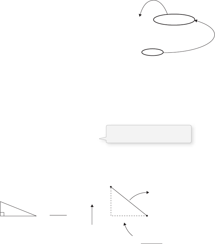
Functions 115
If we did not include a return statement, Processing would give us an error:
e method “ int sum(int a, int b, int c); ” must contain a return statement with an expression compatible
with type “ int. ”
As soon as the return statement is executed, the program exits the function and sends the returned value
back to the location in the code where the function was called. at value can be used in an assignment
operation (to give another variable a value) or in any appropriate expression. See the illustration in
Figure 7.5 . Here are some examples:
int x = sum(5,6,8);
int y = sum(8,9,10) * 2;
int z = sum(x,y,40);
line(100,100,110,sum(x,y,z));
I hate to bring up playing catch in the park again, but you
can think of it as follows. You ( the main program ) throw a
ball to your friend ( a function ). After your friend catches
that ball, he or she thinks for a moment, puts a number
inside the ball ( the return value ) and passes it back to you.
Functions that return values are traditionally used to perform complex calculations that may need to be
performed multiple times throughout the course of the program. One example is calculating the distance
between two points: ( x 1, y 1) and ( x 2, y 2). e distance between pixels is a very useful piece of information in
interactive applications. Processing , in fact, has a built-in distance function that we can use. It is called dist( ) .
float d = dist(100, 100, mouseX, mouseY);
is line of code calculates the distance between the mouse location and the point (100,100). For the
moment, let’s pretend Processing did not include this function in its library. Without it, we would have to
calculate the distance manually, using the Pythagorean eorem, as shown in Figure 7.6 .
a2b2c2
ac
bc√a2b2mouseX
mouseX
100
mouseY
mouseY
100
distance
(100,100)
(mouseX
mouseX
,mouseY
mouseY
)
dx
dy
distance √dx2dy2
sqrt (dx*dx dy*dy);
fi g. 7.6
int answer = sum(5,10,32);
int sum(int a, int b, int c) {
int total = a + b + c;
return total;
}
t
o
t
a
l
i
s
r
e
t
u
r
n
e
d
t
o
h
e
r
e
fi g. 7.5
Calculating the distance between
(100,100) and (mouseX,mouseY).
float dx = mouseX – 100;
float dy = mouseY – 100;
float d = sqrt(dx*dx + dy*dy);
If we wanted to perform this calculation many times over the course of a program, it would be easier to
move it into a function that returns the value d .
float distance(float x1, float y1, float x2, float y2) {
float dx = x1 – x2;
float dy = y1 – y2;
float d = sqrt(dx*dx + dy*dy);
return d;
}
Note the use of the return type fl oat. Again, we do not have to write this function because Processing
supplies it for us. But since we did, we can now look at an example that makes use of this function.
Example 7-4: Using a function that returns a value, distance
void setup() {
size(200,200);
}
void draw() {
background(0);
stroke(0);
// Top left square
fill(distance(0,0,mouseX,mouseY));
rect(0,0,width/2 – 1,height/2 – 1);
// Top right square
fill(distance(width,0,mouseX,mouseY));
rect(width/2,0,width/2 – 1,height/2 – 1);
// Bottom left square
fill(distance(0,height,mouseX,mouseY));
rect(0,height/2,width/2 – 1,height/2 – 1);
// Bottom right square
fill(distance(width,height,mouseX,mouseY));
rect(width/2,height/2,width/2 – 1,height/2 – 1);
}
float distance(float x1, float y1, float x2, float y2)
{
float dx = x1 – x2;
float dy = y1 – y2;
float d = sqrt(dx*dx + dy*dy);
return d;
}
fi g. 7.7
Our version of Processing’s
dist() function.
Our distance function
is used to calculate a
brightness value for
each quadrant. We could
use the built-in function
dist() instead, but we are
learning how to write our
own functions.
116 Learning Processing
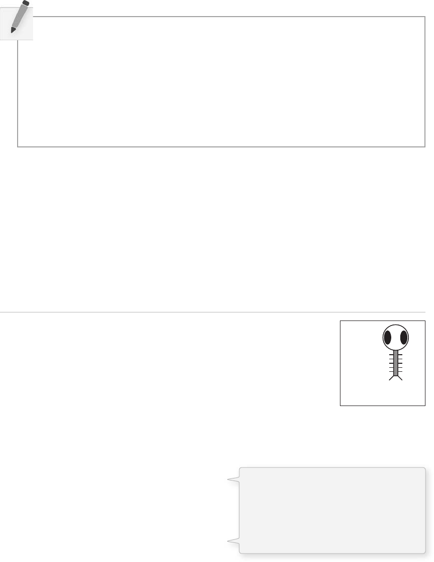
Functions 117
7.8 Zoog Reorganization
Zoog is now ready for a fairly major overhaul.
• Reorganize Zoog with two functions: drawZoog( ) and jiggleZoog( ) . Just for variety, we are going to
have Zoog jiggle (move randomly in both the x and y directions) instead of bouncing back and forth.
• Incorporate arguments so that Zoog’s jiggliness is determined by the mouseX position and Zoog’s
eye color is determined by Zoog’s distance to the mouse.
Example 7-5: Zoog with functions
float x = 100;
float y = 100;
float w = 60;
float h = 60;
float eyeSize = 16;
void setup() {
size(200,200);
smooth();
}
void draw() {
background(255); // Draw a black background
// mouseX position determines speed factor for moveZoog function
// float factor = constrain(mouseX/10,0,5);
jiggleZoog(factor);
// pass in a color to drawZoog
// function for eye's color
float d = dist(x,y,mouseX,mouseY);
color c = color(d);
drawZoog(c);
}
fi g. 7.8
Exercise 7-8: Write a function that takes one argument—F for Fahrenheit—and computes
the result of the following equation (converting the temperature to Celsius).
C (F 32) * (5/9)
______ tempConverter(float ________) {
______ _______ = _______________
______________________________
}
The code for changing the variables
associated with Zoog and displaying Zoog is
moved outside of draw() and into functions
called here. The functions are given
arguments, such as “Jiggle Zoog by the
following factor” and “draw Zoog with the
following eye color.”

void jiggleZoog(float speed) {
// Change the x and y location of Zoog randomly
x = x + random( - 1,1)*speed;
y = y + random( - 1,1)*speed;
// Constrain Zoog to window
x = constrain(x,0,width);
y = constrain(y,0,height);
}
void drawZoog(color eyeColor) {
// Set ellipses and rects to CENTER mode
ellipseMode(CENTER);
rectMode(CENTER);
// Draw Zoog's arms with a for loop
for (float i = y - h/3; i < y + h/2; i + = 10) {
stroke(0);
line(x - w/4,i,x + w/4,i);
}
// Draw Zoog's body
stroke(0);
fill(175);
rect(x,y,w/6,h);
// Draw Zoog's head
stroke(0);
fill(255);
ellipse(x,y - h,w,h);
// Draw Zoog's eyes
fill(eyeColor);
ellipse(x - w/3,y - h,eyeSize,eyeSize*2);
ellipse(x + w/3,y - h,eyeSize,eyeSize*2);
// Draw Zoog's legs
stroke(0);
line(x - w/12,y + h/2,x - w/4,y + h/2 + 10);
line(x + w/12,y + h/2,x + w/4,y + h/2 + 10);
}
Exercise 7-9: Following is a version of Example 6-11 ( “ multiple Zoogs ” ) that calls a function to draw
Zoog. Write the function defi nition that completes this sketch. Feel free to redesign Zoog in the process.
void setup() {
size(400,200); // Set the size of the window
smooth(); // Enables Anti-Aliasing (smooth edges on
shapes)
}
118 Learning Processing

Functions 119
void draw() {
background(0); // Draw a black background
int y = height/2;
// Multiple versions of Zoog are displayed by using a for loop
for (int x = 80; x < width; x + = 80) {
drawZoog(x,100,60,60,16);
}
}
_____________________________________________________________________
_____________________________________________________________________
_____________________________________________________________________
_____________________________________________________________________
_____________________________________________________________________
_____________________________________________________________________
_____________________________________________________________________
_____________________________________________________________________
Exercise 7-10: Rewrite your Lesson Two Project using functions. Still 10! A copy was sent into
newnum so num has not changed.
This page intentionally left blank
Objects 121
8 Objects
“ No object is so beautiful that, under certain conditions, it will not look ugly. ”
—Oscar Wilde
In this chapter:
– Data and functionality, together at last.
– What is an object?
– What is a class?
– Writing your own classes.
– Creating your own objects .
– Processing “ tabs. ”
8.1 I’m down with OOP.
Before we begin examining the details of how object-oriented programming (OOP) works in Processing ,
let’s embark on a short conceptual discussion of “ objects ” themselves. It is important to understand that
we are not introducing any new programming fundamentals: objects use everything we have already
learned: variables, conditional statements, loops, functions, and so on. What is entirely new, however, is a
way of thinking, a way of structuring and organizing everything we have already learned.
Imagine you were not programming in Processing , but were instead writing out a program for your day, a
list of instructions, if you will. It might start out something like:
• Wake up.
• Drink coffee (or tea).
• Eat breakfast: cereal, blueberries, and soy milk.
• Ride the subway.
What is involved here? Specifi cally, what things are involved? First, although it may not be immediately
apparent from how we wrote the above instructions, the main thing is you , a human being, a person. You
exhibit certain properties. You look a certain way; perhaps you have brown hair, wear glasses, and appear
slightly nerdy. You also have the ability to do stuff , such as wake up (presumably you can also sleep), eat,
or ride the subway. An object is just like you, a thing that has properties and can do stuff .
So how does this relate to programming? e properties of an object are variables; and the stuff an object
can do are functions. Object-oriented programming is the marriage of everything we have learned in
Chapters 1 through 7, data and functionality, all rolled into one thing .
Let’s map out the data and functions for a very simple human object:
Human data
• Height.
• Weight.
• Gender .

122 Learning Processing
8.2 Using an Object
Before we look at the actual writing of a class itself, let’s briefl y look at how using objects in our main
program (i.e., setup( ) and draw( ) ) makes the world a better place.
Returning to the car example from Chapter 7, you may recall that the pseudocode for the sketch looked
something like this:
Data (Global Variables):
Car color.
Car x location.
Car y location.
Car x speed.
• Eye color.
• Hair color.
Human functions
• Sleep .
• Wake up.
• Eat .
• Ride some form of transportation .
Now, before we get too much further, we need to embark on a brief metaphysical digression. e
above structure is not a human being itself; it simply describes the idea, or the concept, behind a
human being. It describes what it is to be human. To be human is to have height, hair, to sleep, to
eat, and so on. is is a crucial distinction for programming objects. is human being template is
known as a class . A class is diff erent from an object . You are an object. I am an object. at guy on the
subway is an object. Albert Einstein is an object. We are all people, real world instances of the idea of a
human being.
ink of a cookie cutter. A cookie cutter makes cookies, but it is not a cookie itself. e cookie cutter is
the class , the cookies are the objects .
Exercise 8-1: Consider a car as an object. What data would a car have? What functions
would it have?
Car data Car functions
_________________________________ _________________________________
_________________________________ _________________________________
_________________________________ _________________________________
_________________________________ _________________________________
_________________________________ _________________________________

Objects 123
Setup:
Initialize car color.
Initialize car location to starting point.
Initialize car speed.
Draw:
Fill background.
Display car at location with color.
Increment car’s location by speed.
In Chapter 7, we defi ned global variables at the top of the program, initialized them in setup( ) , and called
functions to move and display the car in draw( ) .
Object-oriented programming allows us to take all of the variables and functions out of the main
program and store them inside a car object. A car object will know about its data— color , location , speed .
at is part one. Part two of the car object is the stuff it can do, the methods (functions inside an object).
e car can move and it can be displayed .
Using object-oriented design, the pseudocode improves to look something like this:
Data (Global Variables):
Car object.
Setup:
Initialize car object.
Draw:
Fill background.
Display car object.
Move car object.
Notice we removed all of the global variables from the fi rst example. Instead of having separate variables for
car color, car location, and car speed, we now have only one variable, a Car variable! And instead of initializing
those three variables, we initialize one thing, the Car object. Where did those variables go? ey still exist, only
now they live inside of the Car object (and will be defi ned in the Car class, which we will get to in a moment).
Moving beyond pseudocode, the actual body of the sketch might look like:
Car myCar;
void setup() {
myCar = new Car();
}
void draw() {
background(0);
myCar.move();
myCar.display();
}
We are going to get into the details regarding the previous code in a moment, but before we do so, let’s
take a look at how the Car class itself is written.
An object in Processing.
124 Learning Processing
8.3 Writing the Cookie Cutter
e simple Car example above demonstrates how the use of object in Processing makes for clean, readable
code. e hard work goes into writing the object template, that is the class itself. When you are fi rst
learning about object-oriented programming, it is often a useful exercise to take a program written
without objects and, not changing the functionality at all, rewrite it using objects. We will do exactly this
with the car example from Chapter 7, recreating exactly the same look and behavior in an object-oriented
manner. And at the end of the chapter, we will remake Zoog as an object.
All classes must include four elements: name , data , constructor , and methods . (Technically, the only actual required
element is the class name, but the point of doing object-oriented programming is to include all of these.)
Here is how we can take the elements from a simple non-object-oriented sketch (a simplifi ed version of
the solution to Exercise 7-6) and place them into a Car class, from which we will then be able to make
Car objects.
}
color c;
int xpos;
int ypos;
int xspeed;
void display () {
rectMode(CENTER);
fill(c);
rect
(xpos,ypos,20,10);
}
void drive () {
xpos = xpos + xspeed;
if (xpos > width) {
xpos = 0;
}
}
void draw() {
background(0);
display();
drive();
}
color c;
float xpos;
float ypos;
float xspeed;
class Car {
Car() {
c = color(255);
xpos = width/2;
ypos = height/2;
xspeed = 1;
}
void display() {
rectMode(CENTER);
fill(c);
rect(xpos,ypos,20,10);
}
void drive() {
xpos = xpos + xspeed;
if (xpos > width){
xpos = 0;
}
}
void setup() {
size(200,200);
c = color(255);
xpos = width/2;
ypos = height/2;
xspeed = 1;
}
The class name
Data
Constructor
Functionality
// Simple non OOP Car
Objects 125
• The Class Name—The name is specified by “ class WhateverNameYouChoose ” . We then enclose
all of the code for the class inside curly brackets after the name declaration. Class names are
traditionally capitalized (to distinguish them from variable names, which traditionally are lowercase).
• Data—The data for a class is a collection of variables. These variables are often referred to as instance
variables since each instance of an object contains this set of variables.
• A Constructor—The constructor is a special function inside of a class that creates the instance
of the object itself. It is where you give the instructions on how to set up the object. It is just like
Processing ’s setup( ) function, only here it is used to create an individual object within the sketch,
whenever a new object is created from this class . It always has the same name as the class and is
called by invoking the new operator: “ Car myCar ⴝ new Car( ); ” .
• Functionality—We can add functionality to our object by writing methods. These are done in the
same way as described in Chapter 7, with a return type, name, arguments, and a body of code.
is code for a class exists as its own block and can be placed anywhere outside of setup( ) and draw( ) .
A Class Is a New Block of Code!
void setup() {
}
void draw() {
}
class Car {
}
Exercise 8-2: Fill in the blanks in the following Human class defi nition. Include a function
called sleep( ) or make up your own function. Follow the syntax of the Car example. ( ere are
no right or wrong answers in terms of the actual code itself; it is the structure that is important.)
________ ________ {
color hairColor;
float height;
________() {
________________________
________________ ________
}
________________________ {
________________________
________________________
}
}

126 Learning Processing
8.4 Using an Object: The Details
In Section 8.2, we took a quick peek at how an object can greatly simplify the main parts of a Processing
sketch ( setup( ) and draw( ) ).
Car myCar;
void setup() {
myCar = new Car();
}
void draw() {
background(0);
myCar.move();
myCar.display();
}
Let’s look at the details behind the above three steps outlining how to use an object in your sketch.
Step 1. Declaring an object variable.
If you fl ip back to Chapter 4, you may recall that a variable is declared by specifying a type and a name .
// Variable Declaration
int var; // type name
e above is an example of a variable that holds onto a primitive , in this case an integer. As we learned
in Chapter 4, primitive data types are singular pieces of information: an integer, a fl oat, a character.
Declaring a variable that holds onto an object is quite similar. e diff erence is that here the type is the
class name, something we will make up, in this case “ Car. ” Objects, incidentally, are not primitives and
are considered complex data types. ( is is because they store multiple pieces of information: data and
functionality. Primitives only store data.)
Step 2. Initializing an object.
Again, you may recall from Chapter 4 that in order to initialize a variable (i.e., give it a starting value), we
use an assignment operation—variable equals something.
// Variable Initialization
var = 10; // var equals 10
Initializing an object is a bit more complex. Instead of simply assigning it a primitive value, like an integer
or fl oating point number, we have to construct the object. An object is made with the new operator.
// Object Initialization
myCar = new Car();
In the above example, “ myCar ” is the object variable name and “ ” indicates we are setting it equal
to something, that something being a new instance of a Car object. What we are really doing here is
initializing a Car object. When you initialize a primitive variable, such as an integer, you just set it equal
to a number. But an object may contain multiple pieces of data. Recalling the Car class from the previous
section, we see that this line of code calls the constructor , a special function named Car( ) that initializes all
of the object’s variables and makes sure the Car object is ready to go.
Step 1. Declare an object.
Step 2. Initialize object.
Step 3. Call methods on the object.
The new operator is used to make a new object.

Objects 127
One other thing; with the primitive integer “ var, ” if you had forgotten to initialize it (set it equal to 10),
Processing would have assigned it a default value, zero. An object (such as “ myCar ” ), however, has no
default value. If you forget to initialize an object, Processing will give it the value null. null means nothing .
Not zero. Not negative one. Utter nothingness. Emptiness. If you encounter an error in the message
window that says “ NullPointerException ” (and this is a pretty common error), that error is most likely
caused by having forgotten to initialize an object. (See the Appendix for more details.)
Step 3. Using an object
Once we have successfully declared and initialized an object variable, we can use it. Using an object involves
calling functions that are built into that object. A human object can eat, a car can drive, a dog can bark.
Functions that are inside of an object are technically referred to as “ methods ” in Java so we can begin to use this
nomenclature (see Section 7.1). Calling a method inside of an object is accomplished via dot syntax:
variableName.objectMethod(Method Arguments);
In the case of the car, none of the available functions has an argument so it looks like:
myCar.draw();
myCar.display();
8.5 Putting It Together with a Tab
Now that we have learned how to defi ne a class and use an object born from that class, we can take the
code from Sections 8.2 and 8.3 and put them together in one program.
Example 8-1: A Car class and a Car object
Car myCar;
void setup() {
size(200,200);
// Initialize Car object
myCar = new Car();
}
void draw() {
background(0);
// Operate Car object.
myCar.move();
myCar.display();
}
Exercise 8-3: Assume the existence of a Human class. You want to write the code to declare a
Human object as well as call the function sleep( ) on that human object. Write out the code below:
Declare and initialize the Human object: ________________________________
Call the sleep( ) function: ________________________________
Initialize car object in setup() by calling constructor.
Operate the car object in draw( )by calling object
methods using the dots syntax.
Declare car object as a globle variable.
Functions are called with the “dot syntax”.

128 Learning Processing
class Car {
color c;
float xpos;
float ypos;
float xspeed;
Car() {
c = color(255);
xpos = width/2;
ypos = height/2;
xspeed = 1;
}
void display() {
// The car is just a square
rectMode(CENTER);
fill(c);
rect(xpos,ypos,20,10);
}
void move() {
xpos = xpos + xspeed;
if (xpos > width) {
xpos = 0;
}
}
}
You will notice that the code block that contains the Car class is placed below the main body of the
program (under draw( ) ). is spot is identical to where we placed user-defi ned functions in Chapter 7.
Technically speaking, the order does not matter, as long as the blocks of code (contained within curly
brackets) remain intact. e Car class could go above setup( ) or it could even go between setup( ) and
draw( ) . ough any placement is technically correct, when programming, it is nice to place things where
they make the most logical sense to our human brains, the bottom of the code being a good starting
point. Nevertheless, Processing off ers a useful means for separating blocks of code from each other
through the use of tabs.
In your Processing window, look for the arrow inside a square in the top right-hand corner . If you click
that button, you will see that it off ers the “ New Tab ” option shown in Figure 8.1 .
Upon selecting “ New Tab, ” you will be prompted to type in a name for the new tab, as shown in Figure 8.2 .
Although you can pick any name you like, it is probably a good idea to name the tab after the class you
intend to put there. You can then type the main body of code on one tab (entitled “ objectExample ” in
Figure 8.2 ) and type the code for your class in another (entitled “ Car ” ).
Toggling between the tabs is simple, just click on the tab name itself, as shown in Figure 8.3 . Also, it
should be noted that when a new tab is created, a new .pde fi le is created inside the sketch folder, as
shown in Figure 8.4 . e program has both an objectExample.pde fi le and Car.pde fi le.
Variables.
A constructor.
Function.
Defi ne a class below the rest of the program.
Function.
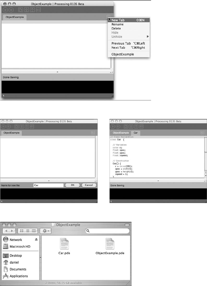
Objects 129
fi g. 8.1
fi g. 8.3 fi g. 8.2
fi g. 8.4

130 Learning Processing
Exercise 8-4: Create a sketch with multiple tabs. Try to get the Car example to run without
any errors.
8.6 Constructor Arguments
In the previous examples, the car object was initialized using the new operator followed by the constructor
for the class.
Car myCar = new Car();
is was a useful simplifi cation while we learned the basics of OOP. Nonetheless, there is a rather serious
problem with the above code. What if we wanted to write a program with two car objects?
// Creating two car objects
Car myCar1 = new Car();
Car myCar2 = new Car();
is accomplishes our goal; the code will produce two car objects, one stored in the variable myCar1 and
one in myCar2. However, if you study the Car class, you will notice that these two cars will be identical:
each one will be colored white, start in the middle of the screen, and have a speed of 1. In English, the
above reads:
Make a new car.
We want to instead say:
Make a new red car, at location (0,10) with a speed of 1.
So that we could also say:
Make a new blue car, at location (0,100) with a speed of 2.
We can do this by placing arguments inside of the constructor method.
Car myCar = new Car(color(255,0,0),0,100,2);
e constructor must be rewritten to incorporate these arguments:
Car(color tempC, float tempXpos, float tempYpos, float tempXspeed) {
c = tempC;
xpos = tempXpos;
ypos = tempYpos;
xspeed = tempXspeed;
}
In my experience, the use of constructor arguments to initialize object variables can be somewhat
bewildering. Please do not blame yourself. e code is strange-looking and can seem awfully redundant:
“ For every single variable I want to initialize in the constructor, I have to duplicate it with a temporary
argument to that constructor? ”
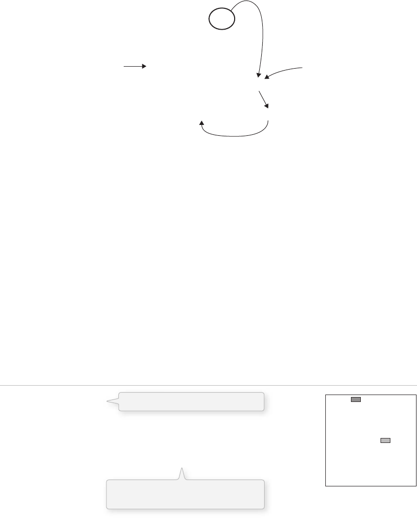
Objects 131
Arguments are local variables used inside the body of a function that get fi lled with values when the
function is called. In the examples, they have one purpose only , to initialize the variables inside of an
object. ese are the variables that count, the car’s actual car, the car’s actual x location, and so on. e
constructor’s arguments are just temporary , and exist solely to pass a value from where the object is made
into the object itself.
is allows us to make a variety of objects using the same constructor. You might also just write the
word temp in your argument names to remind you of what is going on (c vs. tempC). You will also see
programmers use an underscore (c vs. c_) in many examples. You can name these whatever you want, of
course. However, it is advisable to choose a name that makes sense to you, and also to stay consistent.
We can now take a look at the same program with multiple object instances, each with unique properties.
Example 8-2: Two Car objects
Car myCar1;
Car myCar2;
void setup() {
size(200,200);
myCar1 = new Car(color(255,0,0),0,100,2);
myCar2 = new Car(color(0,0,255),0,10,1);
}
void draw() {
background(255);
Nevertheless, this is quite an important skill to learn, and, ultimately, is one of the things that makes
object-oriented programming powerful. But for now, it may feel painful. Let’s briefl y revisit parameter
passing again to understand how it works in this context. See Figure 8.5 .
Frog f;
void setup () {
f = new Frog (100);
}
class Frog {
int tongueLength;
Frog (int tempTongueLength) {
tongueLength = tempTongueLength;
}
}
Parameter Passing:
100 goes into
tempTongueLength
Temporary local
variable
tempTongueLength is used to
assign a value to tongueLength.
Therefore tongueLength = 100
Translation: Make a new frog with a tongue length of 100.
Instance variable:
This is the
variable we care
about, the one that
stores the frog’s
t
ongue length!
fi g. 8.5
Two objects!
Parameters go inside the parentheses
when the object is constructed.
fi g. 8.6

132 Learning Processing
myCar1.move();
myCar1.display();
myCar2.move();
myCar2.display();
}
class Car {
color c;
float xpos;
float ypos;
float xspeed;
Car(color tempC, float tempXpos, float tempYpos, float tempXspeed) {
c = tempC;
xpos = tempXpos;
ypos = tempYpos;
xspeed = tempXspeed;
}
void display() {
stroke(0);
fill(c);
rectMode(CENTER);
rect(xpos,ypos,20,10);
}
void move() {
xpos = xpos + xspeed;
if (xpos > width) {
xpos = 0;
}
}
}
Even though there are multiple objects, we
still only need one class. No matter how many
cookies we make, only one cookie cutter is
needed.Isn’t object-oriented programming swell?
The Constructor is defi ned with arguments.
Exercise 8-5: Rewrite the gravity example from Chapter 5 using objects with a Ball class.
Include two instances of a Ball object. e original example is included here for your reference
with a framework to help you get started.
_______ _______;
Ball ball2;
float grav = 0.1;
void setup() {
size(200,200);
ball1 = new _______(50,0,16);
_________________(100,50,32);
}

Objects 133
void draw() {
background(100);
ball1.display();
__________________________
__________________________
__________________________
}
_______________ {
float x;
__________________
float speed;
float w;
______(______,______,______) {
x = ______;
___________
___________
speed = 0;
}
void ___________() {
_____________________________
_____________________________
_____________________________
}
______________________________
______________________________
______________________________
______________________________
______________________________
______________________________
}
// Simple gravity
float x = 100; // x
location
float y = 0; // y
location
float speed = 0; // speed
float gravity = 0.1;// gravity
void setup() {
size(200,200);
}
void draw() {
background(100);
// display the square
fill(255);
noStroke();
rectMode(CENTER);
rect(x,y,10,10);
// Add speed to y location
y = y + speed;
// Add gravity to speed
speed = speed + gravity;
// If square reaches the bottom
// Reverse speed
if (y > height) {
speed = speed * -0.95;
}
}
134 Learning Processing
8.7 Objects are data types too !
is is our fi rst experience with object-oriented programming, so we want to take it easy. e examples
in this chapter all use just one class and make, at most, two or three objects from that class. Nevertheless,
there are no actual limitations. A Processing sketch can include as many classes as you feel like writing.
If you were programming the Space Invaders game, for example, you might create a Spaceship class, an
Enemy class, and a Bullet class, using an object for each entity in your game.
In addition, although not primitive , classes are data types just like integers and fl oats. And since classes
are made up of data, an object can therefore contain other objects! For example, let’s assume you had just
fi nished programming a Fork and Spoon class. Moving on to a PlaceSetting class, you would likely include
variables for both a Fork object and a Spoon object inside that class itself. is is perfectly reasonable and
quite common in object-oriented programming.
class PlaceSetting {
Fork fork;
Spoon spoon;
PlaceSetting() {
fork = new Fork();
spoon = new Spoon();
}
}
Objects, just like any data type, can also be passed in as arguments to a function. In the Space Invaders
game example, if the spaceship shoots the bullet at the enemy, we would probably want to write a
function inside the Enemy class to determine if the Enemy had been hit by the bullet.
void hit(Bullet b) {
// Code to determine if
// the bullet struck the enemy
}
In Chapter 7, we showed how when a primitive value (integer, fl oat, etc.) is passed in a function, a copy
is made. With objects, this is not the case, and the result is a bit more intuitive. If changes are made
to an object after it is passed into a function, those changes will aff ect that object used anywhere else
throughout the sketch. is is known as pass by reference since instead of a copy, a reference to the actual
object itself is passed into the function.
As we move forward through this book and our examples become more advanced, we will begin to
see examples that use multiple objects, pass objects into functions, and more. e next chapter, in fact,
focuses on how to make lists of objects. And Chapter 10 walks through the development of a project that
includes multiple classes. For now, as we close out the chapter with Zoog, we will stick with just one class.
8.8 Object-Oriented Zoog
Invariably, the question comes up: “ When should I use object-oriented programming? ” For me, the
answer is always. Objects allow you to organize the concepts inside of a software application into
A class can include other objects among its variables.
A function can have an object as its argument.

Objects 135
modular, reusable packages. You will see this again and again throughout the course of this book.
However, it is not always convenient or necessary to start out every project using object-orientation,
especially while you are learning. Processing makes it easy to quickly “ sketch ” out visual ideas with non
object-oriented code.
For any Processing project you want to make, my advice is to take a step-by-step approach. You do not
need to start out writing classes for everything you want to try to do. Sketch out your idea fi rst by
writing code in setup( ) and draw( ) . Nail down the logic of what you want to do as well as how you
want it to look. As your project begins to grow, take the time to reorganize your code, perhaps fi rst with
functions, then with objects. It is perfectly acceptable to dedicate a signifi cant chunk of your time to this
reorganization process (often referred to as refactoring ) without making any changes to the end result, that
is, what your sketch looks like and does on screen.
is is exactly what we have been doing with cosmonaut Zoog from Chapter 1 until now. We sketched
out Zoog’s look and experimented with some motion behaviors. Now that we have something, we can
take the time to refactor by making Zoog into an object. is process will give us a leg up in programming
Zoog’s future life in more complex sketches.
And so it is time to take the plunge and make a Zoog class. Our little Zoog is almost all grown up. e
following example is virtually identical to Example 7-5 (Zoog with functions) with one major diff erence.
All of the variables and all of the functions from Example 7-5 are now incorporated into the Zoog class
with setup( ) and draw( ) containing barely any code.
Example 8-3
Zoog zoog;
void setup() {
size(200,200);
smooth();
zoog = new Zoog(100,125,60,60,16);
}
void draw() {
background(255);
// mouseX position determines speed factor
float factor = constrain(mouseX/10,0,5);
zoog.jiggle(factor);
zoog.display();
}
class Zoog {
// Zoog's variables
float x,y,w,h,eyeSize;
// Zoog constructor
Zoog(float tempX, float tempY, float tempW, float tempH, float tempEyeSize) {
x = tempX;
y = tempY;
w = tempW;
h = tempH;
eyeSize = tempEyeSize;
}
Zoog is an object!
Zoog is given initial properties via the constructor.
Zoog can do stuff with functions!
Everything about Zoog is contained in this one class.
Zoog has properties (location, with , height, eye size)
and Zoog has abilities (jiggle, display).
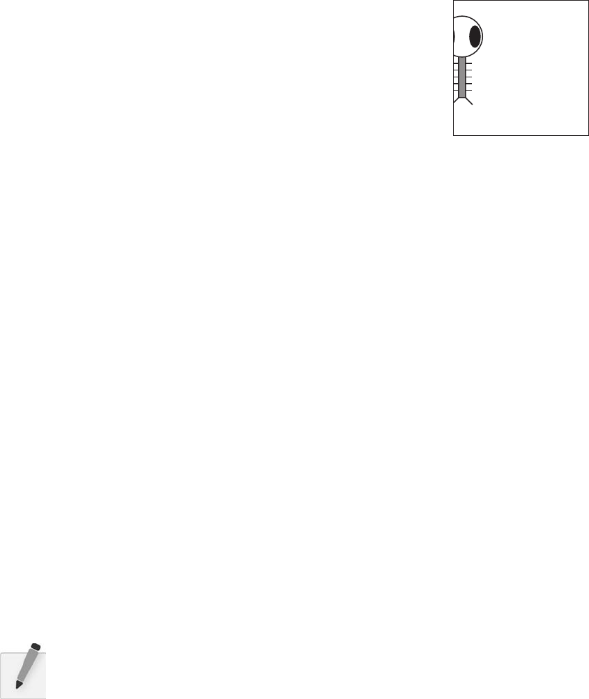
136 Learning Processing
// Move Zoog
void jiggle(float speed) {
// Change the location of Zoog randomly
x = x + random(-1,1)*speed;
y = y + random(-1,1)*speed;
// Constrain Zoog to window
x = constrain(x,0,width);
y = constrain(y,0,height);
}
// Display Zoog
void display() {
// Set ellipses and rects to CENTER mode
ellipseMode(CENTER);
rectMode(CENTER);
// Draw Zoog's arms with a for loop
for (float i = y - h/3; i < y + h/2; i + = 10) {
stroke(0);
line(x-w/4,i,x + w/4,i);
}
// Draw Zoog's body
stroke(0);
fill(175);
rect(x,y,w/6,h);
// Draw Zoog's head
stroke(0);
fill(255);
ellipse(x,y-h,w,h);
// Draw Zoog's eyes
fill(0);
ellipse(x-w/3,y-h,eyeSize,eyeSize*2);
ellipse(x + w/3,y – h,eyeSize,eyeSize*2);
// Draw Zoog's legs
stroke(0);
line(x – w/12,y + h/2,x – w/4,y + h/2 + 10);
line(x + w/12,y + h/2,x + w/4,y + h/2 + 10);
}
}
Exercise 8-6: Rewrite Example 8-3 to include two Zoogs. Can you vary their appearance?
Behavior? Consider adding color as a Zoog variable.
fi g. 8.7

Objects 137
Lesson Three Project
Step 1. Take your Lesson Two Project and reorganize the code using functions.
Step 2. Reorganize the code one step further using a class and an object variable.
Step 3. Add arguments to the Constructor of your class and try making two or three
objects with diff erent variables.
Use the space provided below to sketch designs, notes, and pseudocode for your
project.
This page intentionally left blank

Lesson Four
More of the Same
9 Arrays
This page intentionally left blank
Arrays 141
9 Arrays
“ I might repeat to myself slowly and soothingly, a list of quotations beautiful
from minds profound—if I can remember any of the damn things. ”
— Dorothy Parker
In this chapter:
– What is an array?
– Declaring an array.
– Initialization.
– Array operations—using the “ for ” loop with an array.
– Arrays of objects.
9.1 Arrays, why do we care?
Let’s take a moment to revisit the car example from the previous chapter on object-oriented
programming. You may remember we spent a great deal of eff ort on developing a program that contained
multiple instances of a class, that is, two objects.
Car myCar1;
Car myCar2;
is was indeed an exciting moment in the development of our lives as computer programmers. It is
likely you are contemplating a somewhat obvious question. How could I take this further and write a
program with 100 car objects? With some clever copying and pasting, you might write a program with
the following beginning:
Car myCar1
Car myCar2
Car myCar3
Car myCar4
Car myCar5
Car myCar6
Car myCar7
Car myCar8
Car myCar9
Car myCar10
Car myCar11
Car myCar12
Car myCar13
Car myCar14
Car myCar15
Car myCar16
Car myCar17
Car myCar18
Car myCar19
Car myCar20
Car myCar21
142 Learning Processing
Car myCar22
Car myCar23
Car myCar24
Car myCar25
Car myCar26
Car myCar27
Car myCar28
Car myCar29
Car myCar30
Car myCar31
Car myCar32
Car myCar33
Car myCar34
Car myCar35
Car myCar36
Car myCar37
Car myCar38
Car myCar39
Car myCar40
Car myCar41
Car myCar42
Car myCar43
Car myCar44
Car myCar45
Car myCar46
Car myCar47
Car myCar48
Car myCar49
Car myCar50
Car myCar51
Car myCar52
Car myCar53
Car myCar54
Car myCar55
Car myCar56
Car myCar57
Car myCar58
Car myCar59
Car myCar60
Car myCar61
Car myCar62
Car myCar63
Car myCar64
Car myCar65
Car myCar66
Car myCar67
Car myCar68
Car myCar69
Car myCar70
Car myCar71
Car myCar72
Car myCar73
Car myCar74
Car myCar75
Car myCar76
Car myCar77
Car myCar78
Car myCar79

Arrays 143
Car myCar80
Car myCar81
Car myCar82
Car myCar83
Car myCar84
Car myCar85
Car myCar86
Car myCar87
Car myCar88
Car myCar89
Car myCar90
Car myCar91
Car myCar92
Car myCar93
Car myCar94
Car myCar95
Car myCar96
Car myCar97
Car myCar98
Car myCar99
Car myCar100
If you really want to give yourself a headache, try completing the rest of the program modeled after the
above start. It will not be a pleasant endeavor. I am certainly not about to leave you any workbook space
in this book to practice.
An array will allow us to take these 100 lines of code and put them into one line. Instead of having
100 variables, an array is one thing that contains a list of variables.
Any time a program requires multiple instances of similar data, it might be time to use an array. For
example, an array can be used to store the scores of four players in a game, a selection of 10 colors in a
design program, or a list of fi sh objects in an aquarium simulation.
_______________________________________________________________
_______________________________________________________________
_______________________________________________________________
_______________________________________________________________
_______________________________________________________________
Exercise 9-1: Looking at all of the sketches you have created so far, do any merit the use of an
array? Why?
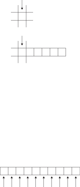
144 Learning Processing
9.2 What is an array?
From Chapter 4, you may recall that a variable is a named pointer to a location in memory where data is
stored. In other words, variables allow programs to keep track of information over a period of time. An
array is exactly the same, only instead of pointing to one singular piece of information, an array points to
multiple pieces. See Figure 9.1 .
You can think of an array as a list of variables. A list, it should be noted, is useful for two important
reasons. Number one, the list keeps track of the elements in the list themselves. Number two, the list
keeps track of the order of those elements (which element is the fi rst in the list, the second, the third,
etc.). is is a crucial point since in many programs, the order of information is just as important as the
information itself.
In an array, each element of the list has a unique index, an integer value that designates its position in the
list (element #1, element #2, etc.). In all cases, the name of the array refers to the list as a whole, while
each element is accessed via its position.
Notice how in Figure 9.2 , the indices range from 0 to 9. e array has a total of 10 elements, but the fi rst
element number is 0 and the last element is 9. We might be tempted to stomp our feet and complain:
“ Hey, why aren’t the elements numbered from 1 to 10? Wouldn’t that be easier? ”
7
Variable
4 8 15 16 23 42
Array
fi g. 9.1
0
Array index values
1 2 3 4 5 6 7 8 9
fi g. 9.2
While at fi rst, it might intuitively seem like we should start counting at one (and some programming
languages do), we start at zero because technically the fi rst element of the array is located at the start of
the array, a distance of zero from the beginning. Numbering the elements starting at 0 also makes many
array operations (the process of executing a line of code for every element of the list) a great deal more
convenient. As we continue through several examples, you will begin to believe in the power of counting
from zero.
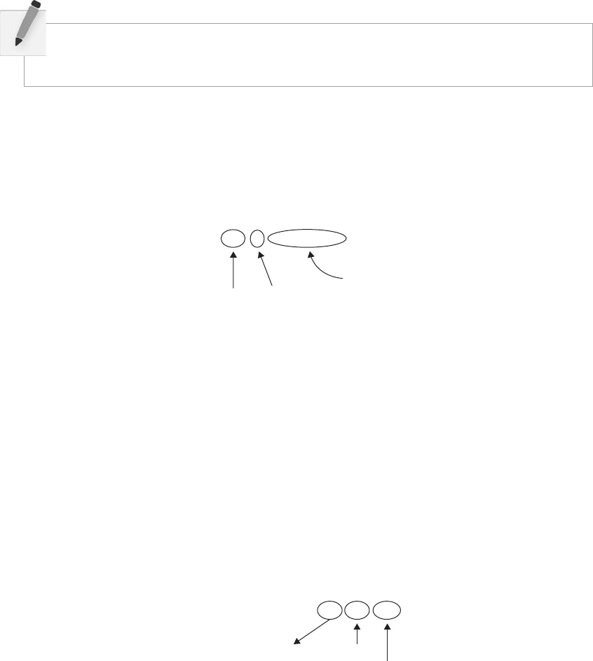
Arrays 145
int[] arrayOfInts = new int [42];
The "new" operator
means we're making a
"new" array.
Array declaration and creation
Type
Size of
array
fi g. 9.4
int [] arrayOfInts;
Type
Name
Indicates
array
fi g. 9.3
9.3 Declaring and Creating an Array
In Chapter 4, we learned that all variables must have a name and a data type. Arrays are no diff erent.
e declaration statement, however, does look diff erent. We denote the use of an array by placing empty
square brackets ( “ [] ” ) after the type declaration. Let’s start with an array of primitive values, for example,
integers. (We can have arrays of any data type, and we will soon see how we can make an array of
objects.) See Figure 9.3 .
e declaration in Figure 9.3 indicates that “ arrayOf Ints ” will store a list of integers. e array name
“ arrayOfInts ” can be absolutely anything you want it to be (we only include the word “ array ” here to
illustrate what we are learning).
One fundamental property of arrays, however, is that they are of fi xed size. Once we defi ne the size for an
array, it can never change. A list of 10 integers can never go to 11 . But where in the above code is the size
of the array defi ned? It is not. e code simply declares the array; we must also make sure we create the
actual instance of the array with a specifi ed size.
To do this, we use the new operator, in a similar manner as we did in calling the constructor of an object.
In the object’s case, we are saying “ Make a new Car ” or “ Make a new Zoog. ” With an array, we are saying
“ Make a new array of integers, ” or “ Make a new array of Car objects, ” and so on. See array declaration in
Figure 9.4 .
e array declaration in Figure 9.4 allows us to specify the array size: how many elements we want the
array to hold (or, technically, how much memory in the computer we are asking for to store our beloved
data). We write this statement as follows: the new operator, followed by the data type, followed by the
size of the array enclosed in brackets. is size must be an integer. It can be a hard-coded number, a
variable (of type integer), or an expression that evaluates to an integer (like 2 2).
Exercise 9-2: If you have an array with 1,000 elements, what is the range of index values
for that array?
Answer: _______ through _______
146 Learning Processing
Example 9-1: Additional array declaration and creation examples
float[] scores = new float[4]; // A list of 4 floating point numbers
Human[] people = new Human[100]; // A list of 100 Human objects
int num = 50;
Car[] cars = new Car[num]; // Using a variable to specify size
Spaceship[] ships = new Shapeship[num*2 + 3]; // Using an expression to
specify size
Exercise 9-3: Write the declaration statements for the following arrays:
30 integers
100 fl oating point numbers
56 Zoog objects
Exercise 9-4: Which of the following array declarations are valid and which are invalid
(and why)?
int[] numbers = new int[10];
float[] numbers = new float[5 + 6];
int num = 5;
float[] numbers = new int[num];
float num = 5.2;
Car[] cars = new Car[num];
int num = (5 * 6)/2;
float[] numbers = new
float[num = 5];
int num = 5;
Zoog[] zoogs = new Zoog[num * 10];
ings are looking up. Not only did we successfully declare the existence of an array, but we have given
it a size and allocated physical memory for the stored data. A major piece is missing, however: the data
stored in the array itself !
Arrays 147
9.4 Initializing an Array
One way to fi ll an array is to hard-code the values stored in each spot of the array.
Example 9-2: Initializing the elements of an array one at a time
int[] stuff = new int[3];
stuff [0] = 8; // The first element of the array equals 8
stuff [1] = 3; // The second element of the array equals 3
stuff [2] = 1; // The third element of the array equals 1
As you can see, we refer to each element of the array individually by specifying an index, starting at 0.
e syntax for this is the name of the array, followed by the index value enclosed in brackets.
arrayName[INDEX]
A second option for initializing an array is to manually type out a list of values enclosed in curly braces
and separated by commas.
Example 9-3: Initializing the elements of an array all at once
int[] arrayOfInts = { 1, 5, 8, 9, 4, 5 };
float[] floatArray = { 1.2, 3.5, 2.0, 3.4123, 9.9 };
Both of these approaches are not commonly used and you will not see them in most of the examples
throughout the book. In fact, neither initialization method has really solved the problem posed at the
beginning of the chapter. Imagine initializing each element individually with a list of 100 or (gasp)
1,000 or (gasp gasp!) 1,000,000 elements.
e solution to all of our woes involves a means for iterating through the elements of the array. Ding ding
ding. Hopefully a loud bell is ringing in your head. Loops! (If you are lost, revisit Chapter 6.)
Exercise 9-5: Declare an array of three Zoog objects. Initialize each spot in the array with a
Zoog object via its index.
Zoog__ zoogs = new _______ [_______ ];
_______[_______ ] = _______ _______(100, 100, 50, 60, 16);
_______[_______ ] = _______ _______(________________);
_______[_______ ] = _______ _______(________________);

148 Learning Processing
9.5 Array Operations
Consider, for a moment, the following problem:
(A) Create an array of 1,000 fl oating point numbers. (B) Initialize every element of that array with a
random number between 0 and 10.
Part A we already know how to do.
float[] values = new float[1000];
What we want to avoid is having to do this for Part B:
values[0] = random(0,10);
values[1] = random(0,10);
values[2] = random(0,10);
values[3] = random(0,10);
values[4] = random(0,10);
values[5] = random(0,10);
etc. etc.
Let’s describe in English what we want to program:
For every number n from 0 to 99, initialize the n th element stored in array as a random value
between 0 and 10. Translating into code, we have:
int n = 0;
values[n] = random(0,10);
values[n + 1] = random(0,10);
values[n + 2] = random(0,10);
values[n + 3] = random(0,10);
values[n + 4] = random(0,10);
values[n + 5] = random(0,10);
Unfortunately, the situation has not improved. We have, nonetheless, taken a big leap forward. By using
a variable (n) to describe an index in the array, we can now employ a while loop to initialize every n
element.
Example 9-4: Using a while loop to initialize all elements of an array
int n = 0;
while (n < 1000) {
values[n] = random(0,10);
n = n + 1;
}
A for loop allows us to be even more concise, as Example 9-5 shows.

Arrays 149
Example 9-5: Using a for loop to initialize all elements of an array
for (int n = 0; n < 1000; n + + ){
values[n] = random(0,10);
}
What was once 1,000 lines of code is now three!
We can exploit the same technique for any type of array operation we might like to do beyond simply
initializing the elements. For example, we could take the array and double the value of each element
(we will use i from now on instead of n as it is more commonly used by programmers).
Example 9-6: An array operation
for (int i = 0; i < 1000; i + + ){
values[i] = values[i] * 2;
}
ere is one problem with Example 9-6: the use of the hard-coded value 1,000. Striving to be better
programmers, we should always question the existence of a hard-coded number. In this case, what if
we wanted to change the array to have 2,000 elements? If our program was very long with many array
operations, we would have to make this change everywhere throughout our code. Fortunately for us,
Processing gives us a nice means for accessing the size of an array dynamically, using the dot syntax we
learned for objects in Chapter 8. length is a property of every array and we can access it by saying:
arrayName dot length
Let’s use length while clearing an array. is will involve resetting every value to 0.
Example 9-7: An array operation using dot length
for (int i = 0; i < values.length; i + + ){
values[i] = 0;
}
Exercise 9-6: Assuming an array of 10 integers, that is,
int[] nums = { 5,4,2,7,6,8,5,2,8,14};
write code to perform the following array operations (Note that the number of clues vary,
just because a [____] is not explicitly written in does not mean there should not be brackets).
Square each number for (int i ___; i < _____; i + + ){
(i.e., multiply each ____[i] = ______*_____;
by itself ) }
150 Learning Processing
9.6 Simple Array Example: The Snake
A seemingly trivial task, programming a trail following the mouse, is not as easy as it might initially
appear. e solution requires an array, which will serve to store the history of mouse locations. We will use
two arrays, one to store horizontal mouse locations, and one for vertical. Let’s say, arbitrarily, that we want
to store the last 50 mouse locations.
First, we declare the two arrays.
int[] xpos = new int[50];
int[] ypos = new int[50];
Second, in setup( ) , we must initialize the arrays. Since at the start of the program there has not been any
mouse movement, we will just fi ll the arrays with 0’s.
for (int i = 0; i < xpos.length; i + + ){
xpos[i] = 0;
ypos[i] = 0;
}
Each time through the main draw( ) loop, we want to update the array with the current mouse location.
Let’s choose to put the current mouse location in the last spot of the array. e length of the array is 50,
meaning index values range from 0–49. e the last spot is index 49, or the length of the array minus one.
xpos[xpos.length–l] = mouseX;
ypos[ypos.length–1] = mouseY;
Add a random
number between
zero and 10 to each
number.
_________________________________
_____ + = int(________);
__
Add to each number
the number that
follows in the array.
Skip the last value
in the array.
for (int i = 0; i < _____; i + + ){
_____ + = ______ [____];
}
Calculate the sum of
all the numbers.
_____ ________ = ____;
for (int i = 0; i < nums.length; i + + )
{
______ + = ________;
}
The last spot in an array is length minus one.

Arrays 151
Now comes the hard part. We want to keep only the last 50 mouse locations. By storing the current
mouse location at the end of the array, we are overwriting what was previously stored there. If the mouse
is at (10,10) during one frame and (15,15) during another, we want to put (10,10) in the second to last
spot and (15,15) in the last spot. e solution is to shift all of the elements of the array down one spot
before updating the current location. is is shown in Figure 9.5 .
1 moves
into 0
Spot 0
is overwritten New value goes
into 3
New value
2 moves
into 1 3 moves
into 2
542913
13 8429
fi g. 9.5
Element index 49 moves into spot 48, 48 moves into spot 47, 47 into 46, and so on. We can do this by
looping through the array and setting each element index i to the value of element i plus one. Note we
must stop at the second to last value since for element 49 there is no element 50 (49 plus 1). In other
words, instead of having an exit condition
i xpos.length;
we must instead say:
i xpos.length – 1;
e full code for performing this array shift is as follows:
for (int i = 0; i < xpos.length–1; i + + ) {
xpos[i] = xpos[i + 1 ];
ypos[i] = ypos[i + 1 ];
}
Finally, we can use the history of mouse locations to draw a series of circles. For each element of the xpos
array and ypos array, draw an ellipse at the corresponding values stored in the array.
for (int i = 0; i < xpos.length; i + + ){
noStroke();
fill(255);
ellipse(xpos[i],ypos[i],32,32);
}
Making this a bit fancier, we might choose to link the brightness of the circle as well as the size of the
circle to the location in the array, that is, the earlier (and therefore older) values will be bright and small
and the later (newer) values will be darker and bigger. is is accomplished by using the counting variable
i to evaluate color and size.
152 Learning Processing
for (int i = 0; i < xpos.length; i + + ){
noStroke();
fill(255 – i*5);
ellipse(xpos[i],ypos[i],i,i);
}
Putting all of the code together, we have the following example, with the output shown in Figure 9.6 .
Example 9-8: A snake following the mouse
// x and y positions
int[] xpos = new int[50];
int[] ypos = new int[50];
void setup() {
size(200,200);
smooth();
// Initialize
for (int i = 0; i < + + )
xpos[i] = 0;
ypos[i] = 0;
}
}
void draw() {
background(255);
// Shift array values
for (int i = 0; i < xpos.length-1; i + + ) {
xpos [i] = xpos[i + 1];
ypos[i] = ypos[i + 1];
}
// New location
xpos[xpos.length–1] = mouseX;
ypos[ypos.length–1] = mouseY;
// Draw everything
for (int i = 0; i < xpos.length; i + + ){
noStroke();
fill(255-i*5);
ellipse(xpos[i],ypos[i],i,i);
}
}
fi g. 9.6
Declare two arrays with 50 elemets.
Initialize all elements of each array to zero.
Shift all elements down one spot.
xpos[0] = xpos[1], xpos[1] = xpos = [2], and so on.
Stop at the second to last element.
Update the last spot in the array with the
mouse location.
Draw an ellipse for each element in the arrays.
Color and size are tied to the loop’s counter: i.
xpos.length; i

Arrays 153
Exercise 9-7: Rewrite the snake example in an object-oriented fashion with a Snake class.
Can you make snakes with slightly diff erent looks (diff erent shapes, colors, sizes)? (For an
advanced problem, create a Point class that stores an x and y coordinate as part of the sketch.
Each snake object will have an array of Point objects, instead of two separate arrays of x and
y values. is involves arrays of objects, covered in the next section.)
9.7 Arrays of Objects
I know, I know. I still have not fully answered the question. How can we write a program with 100 car
objects?
One of the nicest features of combining object-oriented programming with arrays is the simplicity of
transitioning a program from one object to 10 objects to 10,000 objects. In fact, if we have been careful,
we will not have to change the Car class whatsoever. A class does not care how many objects are made
from it. So, assuming we keep the identical Car class code, let’s look at how we expand the main program
to use an array of objects instead of just one.
Let’s revisit the main program for one Car object.
Car myCar;
void setup() {
myCar = new Car(color(255,0,0),0,100,2);
}
void draw() {
background(255);
myCar.move();
myCar.display();
}
ere are three steps in the above code and we need to alter each one to account for an array.
BEFORE AFTER
Declare the Car
Car myCar;
Declare the Car Array
Car[] cars = new Car[100];
Initialize the Car
myCar = new Car(color(255),0,100,2);
Initialize each element of the Car Array
for (int i = 0; i < cars.length; i + + ) {
cars[i] = new Car(color(i*2),0,i*2,i);
}
Run the Car by Calling Methods
myCar.move();
myCar.display();
Run each element of the Car Array
for (int i = 0; i < cars.length; i + + ) {
cars[i].move();
cars[i].display();
}
154 Learning Processing
is leaves us with Example 9–9 . Note how changing the number of cars present in the program requires
only altering the array defi nition. Nothing else anywhere has to change!
Example 9-9: An array of Car objects
Car[] cars = new Car[100] ;
void setup() {
size(200,200);
smooth();
for (int i = 0; i < cars.length; i + + ){
cars[i] = new Car(color(i*2),0,i*2,i/20.0);
}
}
void draw() {
background(255);
for (int i = 0; i < cars.length; i + + ){
cars[i].move();
cars[i].display();
}
}
class Car {
color c;
float xpos;
float ypos;
float xspeed;
Car(color c_, float xpos_, float ypos_, float xspeed_) {
c = c_;
xpos = xpos_;
ypos = ypos_;
xspeed = xspeed_;
}
void display() {
rectMode(CENTER);
stroke(0);
fill(c);
rect(xpos,ypos,20,10);
}
void move() {
xpos = xpos + xspeed;
if (xpos > width) {
xpos = 0;
}
}
}
fi g. 9.7
An array of 100 Car objects!
The Car class does not change
whether we are making one
car, 100 cars or 1,000 cars!
Initialize each Car using a for loop.
Run each Car using a for loop.
Arrays 155
9.8 Interactive Objects
When we fi rst learned about variables (Chapter 4) and conditionals (Chapter 5), we programmed a
simple rollover eff ect. A rectangle appears in the window and is one color when the mouse is on top and
another color when the mouse is not. e following is an example that takes this simple idea and puts it
into a “ Stripe ” object. Even though there are 10 stripes, each one individually responds to the mouse by
having its own rollover( ) function.
void rollover(int mx, int my) {
if (mx > x & & mx < x + w) {
mouse = true;
} else {
mouse = false;
}
}
is function checks to see if a point ( mx , my ) is contained within the vertical stripe. Is it greater than
the left edge and less than the right edge? If so, a boolean variable “ mouse ” is set to true. When designing
your classes, it is often convenient to use a boolean variable to keep track of properties of an object that
resemble a switch. For example, a Car object could be running or not running. Zoog could be happy or
not happy.
is boolean variable is used in a conditional statement inside of the Stripe object’s display( ) function to
determine the Stripe’s color.
void display() {
if (mouse) {
fill(255);
} else {
fill(255,100);
}
noStroke();
rect(x,0,w,height);
}
When we call the rollover( ) function on that object, we can then pass in mouseX and mouseY as
arguments.
stripes[i].rollover(mouseX,mouseY);
Even though we could have accessed mouseX and mouseY directly inside of the rollover ( ) function, it is
better to use arguments. is allows for greater fl exibility. e Stripe object can check and determine if
any x , y coordinate is contained within its rectangle. Perhaps later, we will want the Stripe to turn white
when another object, rather than the mouse, is over it.
Here is the full “ interactive stripes ” example.
156 Learning Processing
Example 9-10: Interactive stripes
// An array of stripes
Stripe[] stripes = new Stripe[10];
void setup() {
size(200,200);
// Initialize all " stripes "
for (int i = 0; i < stripes.length; i + + ) {
stripes[i] = new Stripe();
}
}
void draw() {
background(100);
// Move and display all " stripes "
for (int i = 0; i < stripes.length; i + + ) {
// Check if mouse is over the Stripe
stripes[i].rollover(mouseX,mouseY);
stripes[i].move();
stripes[i].display();
}
}
class Stripe {
float x; // horizontal location of stripe
float speed; // speed of stripe
float w; // width of stripe
boolean mouse; // state of stripe (mouse is over or not?)
Stripe() {
x = 0; // All stripes start at 0
speed = random(1); // All stripes have a random positive speed
w = random(10,30);
mouse = false;
}
// Draw stripe
void display() {
if (mouse) {
fill(255);
} else {
fill(255,100);
}
noStroke();
rect(x,0,w,height);
}
// Move stripe
void move() {
x + = speed;
if (x > width + 20) x = – 20;
}
fi g. 9.8
Passing the mouse coordinates
into an object.
A boolean variable
keeps track of the
object’s state.
Boolean variable determines
Stripe color.

Arrays 157
// Check if point is inside of Stripe
void rollover(int mx, int my) {
// Left edge is x, Right edge is x + w
if (mx > x & & mx < x + w) {
mouse = true;
} else {
mouse = false;
}
}
}
Check to see if point (mx,my) is
inside the Stripe.
Exercise 9-8: Write a Button class (see Example 5-5 for a non-object-oriented button). e button
class should register when a mouse is pressed over the button and change color. Create button objects
of diff erent sizes and locations using an array. Before writing the main program, sketch out the
Button class. Assume the button is off when it fi rst appears. Here is a code framework:
class Button {
float x;
float y;
float w;
float h;
boolean on;
Button(float tempX, float tempY, float tempW, float tempH) {
x = tempX;
y = tempY;
w = tempW;
h = tempH;
on = __________;
}
_____________________________________________________________________
_____________________________________________________________________
_____________________________________________________________________
_____________________________________________________________________
_____________________________________________________________________
_____________________________________________________________________
_____________________________________________________________________
_____________________________________________________________________
158 Learning Processing
9.9 Processing’s Array Functions
OK, so I have a confession to make. I lied. Well, sort of. See, earlier in this chapter, I made a very big
point of emphasizing that once you set the size of an array, you can never change that size. Once you have
made 10 Button objects, you can’t make an 11th.
And I stand by those statements. Technically speaking, when you allocate 10 spots in an array, you have
told Processing exactly how much space in memory you intend to use. You can’t expect that block of
memory to happen to have more space next to it so that you can expand the size of your array.
However, there is no reason why you couldn’t just make a new array (one that has 11 spots in it), copy the
fi rst 10 from your original array, and pop a new Button object in the last spot. Processing , in fact, off ers
a set of array functions that manipulate the size of an array by managing this process for you. ey are:
shorten( ), concat( ), subset( ), append( ), splice( ), and expand( ) . In addition, there are functions for changing
the order in an array, such as sort( ) and reverse( ) .
Details about all of these functions can be found in the reference. Let’s look at one example that uses
append( ) to expand the size of an array. is example (which includes an answer to Exercise 8-5) starts
with an array of one object. Each time the mouse is pressed, a new object is created and appended to the
end of the original array .
Example 9-11: Resizing an array using append()
Ball[] balls = new Ball[1];
float gravity = 0.1;
void setup() {
size(200,200);
smooth();
frameRate(30);
// Initialize ball index 0
balls[0] = new Ball(50,0,16);
}
void draw() {
background(100);
// Update and display all balls
for (int i = 0; i < balls.length; i + + ) {
fi g. 9.9
_____________________________________________________________________
_____________________________________________________________________
_____________________________________________________________________
_____________________________________________________________________
_____________________________________________________________________
}
We start with an array
with just one element.
Whatever the length of
that array, update and
display all of the objects.
Arrays 159
balls[i].gravity();
balls[i].move();
balls[i].display();
}
}
void mousePressed() {
// A new ball object
Ball b = new Ball(mouseX,mouseY,10);
// Append to array
balls = (Ball[]) append(balls,b);
}
class Ball {
float x;
float y;
float speed;
float w;
x = tempX;
y = tempY;
w = tempW;
speed = 0;
}
void gravity() {
// Add gravity to speed
speed = speed + gravity;
}
void move() {
// Add speed to y location
y = y + speed;
// If square reaches the bottom
// Reverse speed
if (y > height) {
speed = speed * –0.95;
y = height;
}
}
void display() {
// Display the circle
fill(255);
noStroke();
ellipse(x,y,w,w);
}
}
Another means of having a resizable array is through the use of a special object known as an ArrayList ,
which will be covered in Chapter 23.
Make a new object at the mouse location.
Here, the function, append() adds an element to the
end of the array. append() takes two arguments.
The fi rst is the array you want to append to, and the
second is the thing you want to append.
You have to reassign the result of the append()
function to the original array. In addition, the append()
function requires that you explicitly state the type of
data in the array again by putting the array data type
in parentheses: “(Ball[])”. This is known as casting.
Ball(float tempX, float tempY, float tempW) {
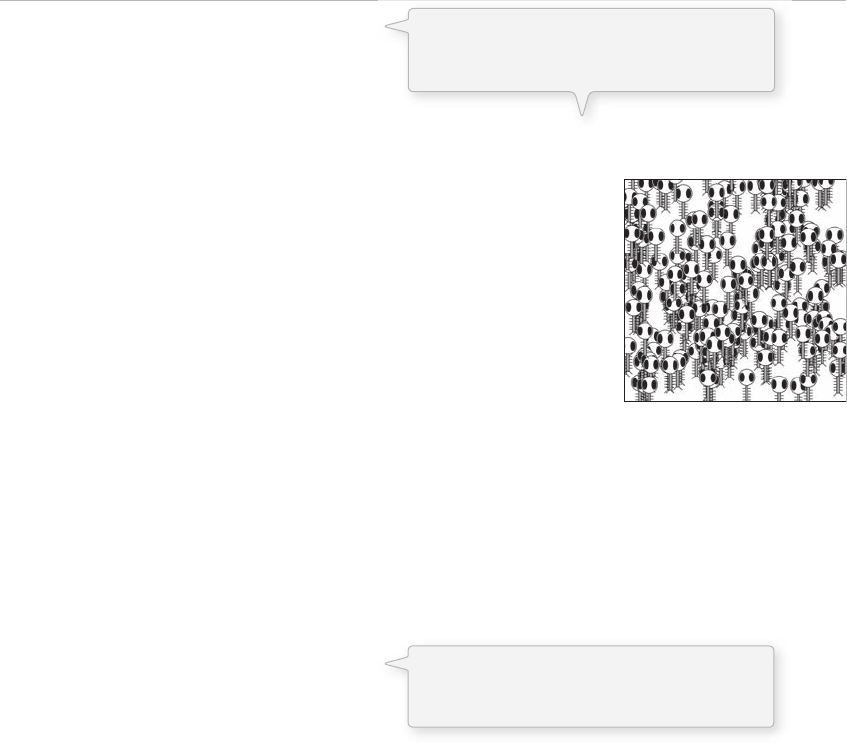
9.10 One Thousand and One Zoogs
It is time to complete Zoog’s journey and look at how we move from one Zoog object to many. In the
same way that we generated the Car array or Stripe array example, we can simply copy the exact Zoog
class created in Example 8-3 and implement an array .
Example 9-12: 200 Zoog objects in an array
Zoog[] zoogies = new Zoog[200];
void setup() {
size(400,400);
smooth();
for (int i = 0; i < zoogies.length; i + + ) {
zoogies[i] = new Zoog(random(width),random(height),30,30,8);
}
}
void draw() {
background(255); // Draw a black background
for (int i = 0; i < zoogies.length; i + + ) {
zoogies[i].display();
zoogies[i].jiggle();
}
}
class Zoog {
// Zoog's variables
float x,y,w,h,eyeSize;
// Zoog constructor
Zoog(float tempX, float tempY, float tempW, float tempH, float tempEyeSize) {
x = tempX;
y = tempY;
w = tempW;
h = tempH;
eyeSize = tempEyeSize;
}
// Move Zoog
void jiggle() {
// Change the location
x = x + random(–1,1);
y = y + random(–1,1);
// Constrain Zoog to window
x = constrain(x,0,width);
y = constrain(y,0,height);
}
// Display Zoog
void display() {
// Set ellipses and rects to CENTER mode
ellipseMode(CENTER);
rectMode(CENTER);
fi g. 9.10
The only difference between this example
and the previous chapter (Example 8-3) is
the use of an array for multiple Zoog objects.
For simplicity we have also removed the
“speed” argument from the jiggle() function.
Try adding it back in as an exercise.
160 Learning Processing
Arrays 161
// Draw Zoog's arms with a for loop
for (float i = y-h/3; i < y + h/2; i + = 10) {
stroke(0);
line(x–w/4,i,x + w/4,i);
}
// Draw Zoog's body
stroke(0);
fill(175);
rect(x,y,w/6,h);
// Draw Zoog's head
stroke(0);
fill(255);
ellipse(x,y-h,w,h);
// Draw Zoog's eyes
fill(0);
ellipse(x–w/3,y–h,eyeSize,eyeSize*2);
ellipse(x + w/3,y–h,eyeSize,eyeSize*2);
// Draw Zoog's legs
stroke(0);
line(x–w/12,y + h/2,x-w/4,y + h/2 + 10);
line(x + w/12,y + h/2,x + w/4,y + h/2 +
10);
}
}

Lesson Four Project
Step 1. Take the Class you made in Lesson ree and make an array of objects
from that class.
Step 2. Can you make the objects react to the mouse? Try using the dist( )
function to determine the object’s proximity to the mouse. For example,
could you make each object jiggle more the closer it is to the mouse?
How many objects can you make before the sketch runs too slow?
Use the space provided below to sketch designs, notes, and pseudocode for your
project.
162 Learning Processing

Lesson Five
Putting It All Together
10 Algorithms
11 Debugging
12 Libraries
This page intentionally left blank
Algorithms 165
10 Algorithms
“ Lather. Rinse. Repeat. ”
— Unknown
10.1 Where have we been? Where are we going?
Our friend Zoog had a nice run. Zoog taught us the basics of the shape drawing libraries in Processing.
From there, Zoog advanced to interacting with the mouse, to moving autonomously via variables,
changing direction with conditionals, expanding its body with a loop, organizing its code with functions,
encapsulating its data and functionality into an object, and fi nally duplicating itself with an array. It is a
good story, and one that treated us well. Nonetheless, it is highly unlikely that all of the programming
projects you intend to do after reading this book will involve a collection of alien creatures jiggling
around the screen (if they do, you are one lucky programmer!). What we need to do is pause for a
moment and consider what we have learned and how it can apply to what you want to do. What is your
idea and how can variables, conditionals, loops, functions, objects, and arrays help you?
In earlier chapters we focused on straightforward “ one feature ” programming examples. Zoog would
jiggle and only jiggle. Zoog didn’t suddenly start hopping. And Zoog was usually all alone, never
interacting with other alien creatures along the way. Certainly, we could have taken these early examples
further, but it was important at the time to stick with basic functionality so that we could really learn the
fundamentals.
In the real world, software projects usually involve many moving parts. is chapter aims to demonstrate
how a larger project is created out of many smaller “ one feature ” programs like the ones we are starting
to feel comfortable making. You, the programmer, will start with an overall vision, but must learn how to
break it down into individual parts to successfully execute that vision.
We will start with an idea. Ideally, we would pick a sample “ idea ” that could set the basis for any project
you want to create after reading this book. Sadly, there is no such thing. Programming your own software
is terrifi cally exciting because of the immeasurable array of possibilities for creation. Ultimately, you will
have to make your own way. However, just as we picked a simple creature for learning the fundamentals,
knowing we will not really be programming creatures all of our lives, we can attempt to make a generic
choice, one that will hopefully serve for learning about the process of developing larger projects.
Our choice will be a simple game with interactivity, multiple objects, and a goal. e focus will not be
on good game design, but rather on good software design. How do you go from thought to code? How
do you implement your own algorithm to realize your ideas? We will see how a larger project divides
into four mini-projects and attack them one by one, ultimately bringing all parts together to execute the
original idea.
We will continue to emphasize object-oriented programming, and each one of these parts will be
developed using a class. e payoff will be seeing how easy it then is to create the fi nal program by

166 Learning Processing
bringing the self-contained, fully functional classes together. Before we get to the idea and its parts, let’s
review the concept of an algorithm which we’ll need for steps 2a and 2b.
Our Process
1. Idea —Start with an idea.
2. Parts —Break the idea down into smaller parts.
a. Algorithm Pseudocode —For each part, work out the algorithm for that part in pseudocode.
b . Algorithm Code —Implement that algorithm with code.
c. Objects —Take the data and functionality associated with that algorithm and build it into a
class.
3. Integration —Take all the classes from Step 2 and integrate them into one larger algorithm.
10.2 Algorithm: Dance to the beat of your own drum.
An algorithm is a procedure or formula for solving a problem. In computer programming, an algorithm is
the sequence of steps required to perform a task. Every single example we have created so far in this book
involved an algorithm.
An algorithm is not too far off from a recipe.
1. Preheat oven to 400°F.
2. Place four boneless chicken breasts in a baking dish.
3. Spread mustard evenly over chicken.
4. Bake at 400°F for 30 min.
e above is a nice algorithm for cooking mustard chicken. Clearly we are not going to write a Processing
program to cook chicken. Nevertheless, if we did, the above pseudocode might turn into the following code.
preheatOven(400);
placeChicken(4, " baking dish "167 );
spreadMustard();
bake(400,30);
An example that uses an algorithm to solve a math problem is more relevant to our pursuits. Let’s
describe an algorithm to evaluate the sum of a sequence of numbers 1 through N .
SUM( N ) 1 2 3 … N
where N is any given whole number greater than zero.
1. Set SUM 0 and a counter I 1
2. Repeat the following steps while I is less than or equal to N .
a. Calculate SUM I and save the result in SUM.
b. Increase the value of I by 1.
3. e solution is now the number saved in SUM.

Algorithms 167
Translating the preceding algorithm into code, we have:
int sum = 0;
int n = 10;
int i = 0;
while (i < = n) {
sum = sum + i;
i + + ;
}
print ln(sum);
Traditionally, programming is thought of as the process of (1) developing an idea, (2) working out an
algorithm to implement that idea, and (3) writing out the code to implement that algorithm. is is what
we have accomplished in both the chicken and summation examples. Some ideas, however, are too large
to be fi nished in one fell swoop. And so we are going to revise these three steps and say programming is
the process of (1) developing an idea, (2) breaking that idea into smaller manageable parts, (3) working
out the algorithm for each part, (4) writing the code for each part, (5) working out the algorithm for all
the parts together, and (6) integrating the code for all of the parts together.
is does not mean to say one shouldn’t experiment along the way, even altering the original idea
completely. And certainly, once the code is fi nished, there will almost always remain work to do in terms
of cleaning up code, bug fi xes, and additional features. It is this thinking process, however, that should
guide you from idea to code. If you practice developing your projects with this strategy, creating code that
implements your ideas will hopefully feel less daunting.
10.3 From Idea to Parts
To practice our development strategy, we will begin with the idea, a very simple game. Before we can get
anywhere, we should describe the game in paragraph form.
Rain Game
e object of this game is to catch raindrops before they hit the ground. Every so often (depending
on the level of diffi culty), a new drop falls from the top of the screen at a random horizontal
location with a random vertical speed. e player must catch the raindrops with the mouse with
the goal of not letting any raindrops reach the bottom of the screen.
Step 1. Set sum equal to 0 and counter i 0.
Step 2. Repeat while in.
Step 2a. Increment sum.
Step 2b. Increment i.
Step 3. The solution is in sum. Print sum!
Exercise 10.1: Write out an idea for a project you want to create. Keep it simple, just not too
simple. A few elements, a few behaviors will do.

168 Learning Processing
Now let’s see if we can take the “ Rain Game ” idea and break it down into smaller parts. How do we
do this? For one, we can start by thinking of the elements in the game: the raindrops and the catcher.
Secondly, we should think about these elements ’ behaviors. For example, we will need a timing
mechanism so that the drops fall “ every so often ”. We will also need to determine when a raindrop is
“ caught. ” Let’s organize these parts more formally.
Part 1. Develop a program with a circle controlled by the mouse. is circle will be the user-
controlled “ rain catcher. ”
Part 2. Write a program to test if two circles intersect. is will be used to determine if the rain
catcher has caught a raindrop.
Part 3. Write a timer program that executes a function every N seconds.
Part 4. Write a program with circles falling from the top of the screen to the bottom. ese will be
the raindrops.
Parts 1 through 3 are simple and each can be completed in one fell swoop. However, with Part 4,
even though it represents one piece of the larger project, it is complex enough that we will need to
complete this exact exercise by breaking it down into smaller steps and building it back up.
Exercise 10-2: Take your idea from Exercise 10-1 and write out the individual parts. Try to
make the parts as simple as possible (almost to the point that it seems absurd). If the parts are
too complex, break them down even further.
Sections 10.4 to 10.7 will follow the process of Steps 2a, 2b, and 2c (see breakout box on p. 166) for each
individual part. For each part, we will fi rst work out the algorithm in pseudocode, then in actual code,
and fi nish with an object-oriented version. If we do our job correctly, all of the functionality needed will
be built into a class which can then be easily copied into the fi nal project itself when we get to Step 3
(integration of all parts).
10.4 Part 1: The Catcher
is is the simplest part to construct and requires little beyond what we learned in Chapter 3. Having
pseudocode that is only two lines long is a good sign, indicating that this step is small enough to handle
and does not need to be made into even smaller parts .
Pseudocode:
• Erase background.
• Draw an ellipse at the mouse location.
Translating it into code is easy:
void setup() {
size(400,400);
smooth();
}

Algorithms 169
void draw() {
background(255);
stroke(0);
fill(175);
ellipse(mouseX,mouseY,64,64);
}
is is good step, but we are not done. As stated, our goal is to develop the rain catcher program in an
object-oriented manner. When we take this code and incorporate it into the fi nal program, we will want
to have it separated out into a class so that we can make a “ catcher ” object. Our pseudocode would be
revised to look like the following.
Setup:
• Initialize catcher object.
D r a w :
• Erase background.
• Set catcher location to mouse location.
• Display catcher.
Example 10-1 shows the code rewritten assuming a Catcher object.
Example 10-1: Catcher
Catcher catcher;
void setup() {
size(400,400);
catcher = new Catcher(32);
smooth();
}
void draw() {
background(255);
catcher.setLocation(mouseX,mouseY);
catcher.display();
}
e Catcher class itself is rather simple, with variables for location and size, and two functions, one to set
the location and one to display.
class Catcher {
float r; // radius
float x,y; // location
Catcher(float tempR) {
r = tempR;
x = 0;
y = 0;
}
fi g. 10.1
170 Learning Processing
void setLocation(float tempX, float tempY) {
x = tempX;
y = tempY;
}
void display() {
stroke(0);
fill(175);
ellipse(x,y,r*2,r*2);
}
}
10.5 Part 2: Intersection
Part 2 of our list requires us to determine when the catcher and a raindrop intersect. Intersection
functionality is what we want to focus on developing in this step. We will start with a simple bouncing
ball class (which we saw in Example 5-6) and work out how to determine when two bouncing circles
intersect. During the “ integration ” process, this intersect( ) function will be incorporated into the Catcher
class to catch raindrops.
Here is our algorithm for this intersection part.
Setup:
• Create two ball objects.
D r a w :
• Move balls.
• If ball #1 intersects ball #2, change color of both balls to white. Otherwise, leave color gray.
• Display balls.
Certainly the hard work here is the intersection test, which we will get to in a moment. First, here is what
we need for a simple bouncing “ Ball ” class without an intersection test.
Data:
• X and Y location.
• Radius.
• Speed in X and Y directions.
Functions:
• Constructor.
– Set radius based on argument
– Pick random location.
– Pick random speed.
• Move.
– Increment X by speed in X
direction.
– Increment Y by speed in Y direction.
– If Ball hits any edge, reverse direction.
• Display.
– Draw a circle at X and Y location.
We are now ready to translate this into code.

Algorithms 171
Example 10-2: Bouncing ball class
class Ball {
float r; // radius
float x,y; // location
float xspeed,yspeed; // speed
// Constructor
Ball(float tempR) {
r = tempR;
x = random(width);
y = random(height);
xspeed = random( -5,5);
yspeed = random( -5,5);
}
void move() {
x + = xspeed; // Increment x
y + = yspeed; // Increment y
// Check horizontal edges
if (x > width | | x < 0) {
xspeed * = - 1;
}
//Check vertical edges
if (y > height | | y < 0) {
yspeed * = – 1;
}
}
// Draw the ball
void display() {
stroke(255);
fill(100,50);
ellipse(x,y,r*2,r*2);
}
}
From here, it is pretty easy to create a sketch with two ball objects. Ultimately, in the fi nal sketch, we’ll
need an array for many raindrops, but for now, two ball variables will be simpler.
Example 10-2 Catcher (Cont.): Two ball objects
// Two ball variables
Ball ball1;
Ball ball2;
void setup() {
size(400,400);
smooth();
// Initialize balls
ball1 = new Ball(64);
ball2 = new Ball(32);
}
void draw() {
background(0); fi g. 10.2

172 Learning Processing
// Move and display balls
ball1.move();
ball2.move();
ball1.display();
ball2.display();
}
Now that we have set up our system for having two circles moving around the screen, we need to develop
an algorithm for determining if the circles intersect. In Processing , we know we can calculate the distance
between two points using the dist( ) function (see Chapter 7). We also have access to the radius of each
circle (the variable r inside each object). e diagram in Figure 10.3 shows how we can compare the
distance between the circles and the sum of the radii to determine if the circles overlap.
R
1
R
2
DIST
DIST > (R1 + R2)
NOT INTERSECTING
DIST < (R1 + R2)
INTERSECTING
R
1
R2
DIST
fi g. 10.3
OK, so assuming the following:
• x
1, y
1: coordinates of circle one
• x
2, y
2: coordinates of circle two
• r
1: radius of circle one
• r
2: radius of circle two
We have the statement:
If the distance between (x1,y1) and (x2,y2) is less than the sum of r1 and r2, circle one intersects
circle two.
Our job now is to write a function that returns true or false based on the above statement.
// A function that returns true or false based on whether two circles intersect
// If distance is less than the sum of radii the circles touch
boolean intersect(float x1, float y1, float x2, float y2, float r1, float r2) {
float distance = dist(x1,y2,x2,y2); // Calculate distance
if (distance < r1 + r2) { // Compare distance to r1 + r2
return true;
} else {
return false;
}
}
Algorithms 173
Now that the function is complete, we can test it with data from ball1 and ball2.
boolean intersecting = intersect(ball1.x,ball1.y,ball2.x,ball2.y,ball1.r,ball2.r);
if (intersecting) {
println( "The circles are intersecting! ");
}
e above code is somewhat awkward and it will be useful to take the function one step further,
incorporating it into the ball class itself. Let’s fi rst look at the entire main program as it stands.
// Two ball variables
Ball ball1;
Ball ball2;
void setup() {
size(400,400);
framerate(30);
smooth();
// Initialize balls
ball1 = new Ball(64);
ball2 = new Ball(32);
}
void draw() {
background(0);
// Move and display balls
ball1.move();
ball2.move();
ball1.display();
ball2.display();
boolean intersecting = intersect(ball1.x,ball1.y,ball2.x,ball2.y,ball1.r,ball2.r);
if (intersecting) {
println( “The circles are intersecting! ”);
}
}
// A function that returns true or false based on whether two circles intersect
// If distance is less than the sum of radii the circles touch
boolean intersect(float x1, float y1, float x2, float y2, float r1, float r2) {
float distance = dist(x1,y2,x2,y2); // Calculate distance
if (distance < r1 + r2) { // Compare distance to r1 + r2
return true;
} else {
return false;
}
}
Since we have programmed the balls in an object-oriented fashion, it is not terribly logical to suddenly
have an intersect( ) function that lives outside of the ball class. A ball object should know how to test if it
is intersecting another ball object. Our code can be improved by incorporating the intersect logic into the
class itself, saying “ ball1.intersect (ball2); ” or, does Ball 1 intersect Ball 2?
void draw() {
background(0);
// Move and display balls
ball1.move();
ball2.move();
ball1.display();
ball2.display();
174 Learning Processing
boolean intersecting = ball1.intersect(ball2);
if (intersecting) {
println( " The circles are intersecting! " );
}
}
Following this model and the algorithm for testing intersection, here is a function for inside the ball class
itself. Notice how the function makes use of both its own location ( x and y ) as well as the other ball’s
location ( b.x and b.y ).
// A function that returns true or false based on whether two Ball objects intersect
// If distance is less than the sum of radii the circles touch
boolean intersect(Ball b) {
float distance = dist(x,y,b.x,b.y); // Calculate distance
if (distance < r + b.r) { // Compare distance to sum of radii
return true;
} else {
return false;
}
}
Putting it all together, we have the code in Example 10-3 .
Example 10-3: Bouncing ball with intersection
// Two ball variables
Ball ball1;
Ball ball2;
void setup() {
size(400,400);
smooth();
// Initialize balls
ball1 = new Ball(64);
ball2 = new Ball(32);
}
void draw() {
background(255);
// Move and display balls
ball1.move();
ball2.move();
if (ball1.intersect(ball2)) {
ball1.highlight();
ball2.highlight();
}
ball1.display();
ball2.display();
}
class Ball {
float r; // radius
float x,y;
float xspeed,yspeed;
color c = color(100,50);
fi g. 10.4
Assumes a function intersect() inside
the Ball class that returns true or false.
New! An object can have a function that takes
another object as an argument. This is one
way to have objects communicate. In this case
they are checking to see if they intersect.
Algorithms 175
// Constructor
Ball(float tempR) {
r = tempR;
x = random(width);
y = random(height);
xspeed = random( –5,5);
yspeed = random( –5,5);
}
void move() {
x + = xspeed; // Increment x
y + = yspeed; // Increment y
// Check horizontal edges
if (x > width | | x < 0) {
xspeed * = – 1;
}
// Check vertical edges
if (y > height | | y < 0) {
yspeed * = – 1;
}
}
void highlight() {
c = color(0,150);
}
// Draw the ball
void display() {
stroke(0);
fill(c);
ellipse(x,y,r*2,r*2);
c = color(100,50);
}
// A function that returns true or false based on whether two circles intersect
// If distance is less than the sum of radii the circles touch
boolean intersect(Ball b) {
float distance = dist(x,y,b.x,b.y); // Calculate distance
if (distance < r + b.r) { // Compare distance to
sum of radii
return true;
} else {
return false;
}
}
}
10.6 Part 3: The Timer
Our next task is to develop a timer that executes a function every N seconds. Again, we will do this in two
steps, fi rst just using the main body of a program and second, taking the logic and putting it into a Timer
class. Processing has the functions hour( ), second( ), minute( ), month( ), day( ), and year( ) to deal with time.
We could conceivably use the second( ) function to determine how much time has passed. However, this is
not terribly convenient, since second( ) rolls over from 60 to 0 at the end of every minute.
Whenever the balls are touching, this highlight()
function is called and the color is darkened.
After the ball is displayed, the color is reset back
to a darker gray.
Objects can
be passed into
functions as
arguments too!

176 Learning Processing
For creating a timer, the function millis( ) is best. First of all, millis( ) , which returns the number of
milliseconds since a sketch started, allows for a great deal more precision. One millisecond is one one-
thousandth of a second (1,000 ms 1 s). Secondly, millis( ) never rolls back to zero, so asking for the
milliseconds at one moment and subtracting it from the milliseconds at a later moment will always result
in the amount of time passed.
Let’s say we want an applet to change the background color to red 5 seconds after it started. Five seconds
is 5,000 ms, so it is as easy as checking if the result of the millis( ) function is greater than 5,000.
if (millis() > 5000) {
background(255,0,0);
}
Making the problem a bit more complicated, we can expand the program to change the background to a
new random color every 5 seconds.
Setup:
• Save the time at startup (note this should always be zero, but it is useful to save it in a variable
anyway). Call this “ savedTime ” .
D r a w :
• Calculate the time passed as the current time (i.e., millis( ) ) minus savedTime. Save this as
“ passedTime ” .
• If passedTime is greater than 5,000, fill a new random background and reset savedTime to the current
time . This step will restart the timer.
Example 10-4 translates this into code.
Example 10-4: Implementing a timer
int savedTime;
int totalTime = 5000;
void setup() {
size(200,200);
background(0);
savedTime = millis();
}
void draw() {
// Calculate how much time has passed
int passedTime = millis() - savedTime;
// Has five seconds passed?
if (passedTime > totalTime) {
println( " 5 seconds have passed! " );
background(random(255)); // Color a new background
savedTime = millis(); // Save the current time to restart the timer!
}
}
Algorithms 177
With the above logic worked out, we can now move the timer into a class. Let’s think about what data is
involved in the timer. A timer must know the time at which it started ( savedTime) and how long it needs
to run ( totalTime ).
Data:
• savedTime
• totalTime
e timer must also be able to start as well as check and see if it is fi nished .
Functions:
• start( )
• isFinished( ) —returns true or false
Taking the code from the non-object-oriented example and building it out with the above structure, we
have the code shown in Example 10-5.
Example 10-5: Object-oriented timer
Timer timer;
void setup() {
size(200,200);
background(0);
timer = new Timer(5000);
timer.start();
}
void draw() {
if (timer.isFinished()) {
background(random(255));
timer.start();
}
}
class Timer {
int savedTime; // When Timer started
int totalTime; // How long Timer should last
Timer(int tempTotalTime) {
totalTime = tempTotalTime;
}
// Starting the timer
void start() {
savedTime = millis();
}
boolean isFinished() {
// Check how much time has passed
int passedTime = millis()- savedTime;
if (passedTime > totalTime) {
return true;
} else {
return false;
}
}
}
When the timer starts it stores the current time in
milliseconds.
The function isFinished() returns
true if 5,000 ms have passed. The
work of the timer is farmed out to
this method.

178 Learning Processing
10.7 Part 4: Raindrops
We are almost there. We have created a catcher, we know how to test for intersection, and we have
completed the timer object. e fi nal piece of the puzzle is the raindrops themselves. Ultimately, we want
an array of Raindrop objects falling from the top of the window to the bottom. Since this step involves
creating an array of objects that move, it is useful to approach this fourth part as a series of even smaller
steps, subparts of Part 4, thinking again of the individual elements and behaviors we will need.
Part 4 Subparts:
Part 4.1. A single moving raindrop.
Part 4.2. An array of raindrop objects.
Part 4.3. Flexible number of raindrops (appearing one at a time).
Part 4.4. Fancier raindrop appearance.
Part 4.1, creating the motion of a raindrop (a simple circle for now) is easy—Chapter 3 easy.
• Increment raindrop y value.
• Display raindrop.
Translating into code we have Part 4.1—A single moving raindrop , shown in Example 10-6.
Example 10-6: Simple raindrop behavior
float x,y; // Variables for drop location
void setup() {
size(400,400);
background(0);
x = width/2;
y = 0;
}
void draw() {
background(255);
// Display the drop
fill(50,100,150);
noStroke();
ellipse(x,y,16,16);
// Move the drop
y + + ;
}
Again, however, we need to go a step further and make a Drop class—after all we will ultimately want an array
of drops. In making the class, we can add a few more variables, such as speed and size, as well as a function to
test if the raindrop reaches the bottom of the screen, which will be useful later for scoring the game.
class Drop {
float x,y; // Variables for location of raindrop
float speed; // Speed of raindrop
color c;
float r; // Radius of raindrop
A raindrop object has a location,
speed, color, and size.
Algorithms 179
Drop() {
r = 8; // All raindrops are the same size
x = random(width); // Start with a random x location
y = -r*4; // Start a little above the window
speed = random(1,5); // Pick a random speed
c = color(50,100,150); // Color
}
//Move the raindrop down
void move() {
y + = speed; // Increment by speed
}
// Check if it hits the bottom
boolean reachedBottom() {
// If we go a little past the bottom
if (y > height + r*4) {
return true;
} else {
return false;
}
}
// Display the raindrop
void display() {
// Display the drop
fill(50,100,150);
noStroke();
ellipse(x,y,r*2,r*2);
}
}
Before we move on to Part 4.3, the array of drops, we should make sure that a singular Drop object functions
properly. As an exercise, complete the code in Exercise 10-3 that would test a single drop object.
Incrementing y is now in the move() function.
In addition, we have a function that determines
if the drop leaves the window.
Exercise 10-3: Fill in the blanks below completing the “ test Drop ” sketch.
Drop drop;
void setup() {
size(200,200);
_________________________________;
}
void draw() {
background(255);
drop. _________________;
_____________________________;
}

180 Learning Processing
Now that this is complete, the next step is to go from one drop to an array of drops— Part 4.2 . is is
exactly the technique we perfected in Chapter 9.
// An array of drops
Drop[] drops = new Drop[50];
void setup() {
size(400,400);
smooth();
// Initialize all drops
for (int i = 0; i < drops.length; i + + ) {
drops[i] = new Drop();
}
}
void draw() {
background(255);
// Move and display all drops
for (int i = 0; i < drops.length; i + + ) {
drops[i].move();
drops[i].display();
}
}
e problem with the above code is that the raindrops appear all at once. According to the specifi cations
we made for our game, we want to have the raindrops appear one at a time, every N seconds—we are
now at Part 4.3—Flexible number of raindrops (appearing one at a time) . We can skip worrying about the
timer for now and just have one new raindrop appear every frame. We should also make our array much
larger, allowing for many more raindrops.
To make this work, we need a new variable to keep track of the total number of drops— “ totalDrops ” .
Most array examples involve walking through the entire array in order to deal with the entire list. Now,
we want to access a portion of the list, the number stored in totalDrops. Let’s write some pseudocode to
describe this process:
Setup:
• Create an array of drops with 1,000 spaces in it.
• Set totalDrops
= 0.
D r a w :
• Create a new drop in the array (at the location totalDrops). Since totalDrops starts at 0, we will first
create a new raindrop in the first spot of the array.
• Increment totalDrops (so that the next time we arrive here, we will create a drop in the next spot in
the array).
• If totalDrops exceeds the array size, reset it to zero and start over.
• Move and display all available drops (i.e., totalDrops).
Example 10-7 translates the above pseudocode into code.
Instead of one Drop object, an array of 50.
Using a loop to initialize all drops.
Move and display all drops.
Algorithms 181
Example 10-7: Drops one at a time
// An array of drops
Drop[] drops = new Drop[1000];
int totalDrops = 0;
void setup() {
size(400,400);
smooth();
background(0);
}
void draw() {
background(255);
// Initialize one drop
drops[totalDrops] = new Drop();
// Increment totalDrops
totalDrops + + ;
// If we hit the end of the array
if (totalDrops > = drops.length) {
totalDrops = 0; //Start over
}
// Move and display drops
for (int i = 0; i < totalDrops; i + + ){
drops[i].move();
drops[i].display();
}
}
We have taken the time to fi gure out how we want the raindrop to move, created a class that exhibits that
behavior, and made an array of objects from that class. All along, however, we have just been using a circle
to display the drop. e advantage to this is that we were able to delay worrying about the drawing code
and focus on the motion behaviors and organization of data and functions. Now we can focus on how the
drops look— Part 4.4—Finalize raindrop appearance.
One way to create a more “ drop-like ” look is to draw a sequence of circles in the vertical direction,
starting small, and getting larger as they move down.
Example 10-8: Fancier looking raindrop
background(255);
for (int i = 2; i < 8; i + + ){
noStroke();
fill(0);
ellipse(width/2,height/2 + i*4,i*2,i*2);
}
We can incorporate this algorithm in the raindrop class from Example 10-7,
using x and y for the start of the ellipse locations, and the raindrop radius
as the maximum value for i in the for loop. e output is shown in
Figure 10.7 .
fi g. 10.5
fi g. 10.6
New variable to keep track of total
number of drops we want to use!
New! We no longer move and display all
drops, but rather only the “totalDrops”
that are currently present in the game.
182 Learning Processing
// Display the raindrop
void display() {
// Display the drop
noStroke();
fill(c);
for (int i = 2; i < r; i + + ) {
ellipse(x,y + i*4,i*2,i*2);
}
}
10.8 Integration: Puttin ’ on the Ritz
It is time. Now that we have developed the individual pieces and confi rmed that each one works properly,
we can assemble them together in one program. e fi rst step is to create a new Processing sketch that has
four tabs, one for each of our classes and one main program, as shown in Figure 10.8 .
fi g. 10.8
e fi rst step is to copy and paste the code for each class into each tab. Individually, they will not need to
change, so there is no need for us to revisit the code. What we do need to revisit is the main program—
what goes in setup( ) and draw( ) . Referring back to the original game description and knowing how the
pieces were assembled, we can write the pseudocode algorithm for the entire game.
Setup:
• Create Catcher object.
• Create array of drops.
• Set totalDrops equal to 0.
• Create Timer object.
• Start timer.
D r a w :
• Set Catcher location to mouse location.
• Display Catcher.
• Move all available Drops.
• Display all available Drops.
• If the Catcher intersects any Drop.
– Remove Drop from screen.
• If the timer is finished:
– Increase the number of drops.
– Restart timer.
fi g. 10.7

Algorithms 183
Notice how every single step in the above program has already been worked out previously in the chapter
with one exception: “ Remove Drop from screen. ” is is rather common. Even with breaking the idea
down into parts and working them out one at a time, little bits can be missed. Fortunately, this piece of
functionality is simple enough and with some ingenuity, we will see how we can slip it in during assembly.
One way to approach assembling the above algorithm is to start by combining all of the elements into
one sketch and not worrying about how they interact. In other words, everything but having the timer
trigger the drops and testing for intersection. To get this going, all we need to do is copy/paste from each
part’s global variables, setup( ) and draw( ) !
Here are the global variables: a Catcher object, an array of Drop objects, a Timer object, and an integer to
store the total number of drops.
Catcher catcher; // One catcher object
Timer timer; // One timer object
Drop[] drops; // An array of drop objects
int totalDrops = 0; // totalDrops
In setup( ) , the variables are initialized. Note, however, we can skip initializing the individual drops in the
array since they will be created one at a time. We will also need to call the timer’s start( ) function.
void setup() {
size(400,400);
catcher = new Catcher(32); // Create the catcher with a radius of 32
drops = new Drop[1000]; // Create 1000 spots in the array
timer = new Timer(2000); // Create a timer that goes off every 2 seconds
timer.start(); // Starting the timer
}
In draw( ) , the objects call their methods. Again, we are just taking the code from each part we did
separately earlier in this chapter and pasting in sequence.
Example 10-9: Using all the objects in one sketch
Catcher catcher; // One catcher object
Timer timer; // One timer object
Drop[] drops; // An array of drop objects
int totalDrops = 0; // totalDrops
void setup() {
size(400,400);
smooth();
catcher = new Catcher(32); // Create the catcher with a radius of 32
drops = new Drop[1000]; // Create 1000 spots in the array
timer = new Timer(2000); // Create a timer that goes off every 2 seconds
timer.start(); // Starting the timer
}
184 Learning Processing
e next step is to take these concepts we have developed and have them work together. For example,
we should only create a new raindrop whenever two seconds have passed (as indicated by the timer’s
isFinished( ) function).
// Check the timer
if (timer.isFinished()) {
// Deal with raindrops
// Initialize one drop
drops[totalDrops] = new Drop();
// Increment totalDrops
totalDrops + + ;
// If we hit the end of the array
if (totalDrops > = drops.length) {
totalDrops = 0; // Start over
}
timer.start();
}
We also need to fi nd out when the Catcher object intersects a Drop. In Section 10.5, we tested for
intersection by calling the intersect( ) function we wrote inside the Ball class.
void draw() {
background(255);
catcher.setLocation(mouseX,mouseY); // Set catcher location
catcher.display(); // Display the catcher From Part 1.
The Catcher!
// Check the timer
if (timer.isFinished()) {
println( " 2 seconds have passed! " );
timer.start();
}
From Part 3.
The Timer!
// Deal with raindrops
// Initialize one drop
drops[totalDrops] = new Drop();
//Increment totalDrops
totalDrops + + ;
// If we hit the end of the array
if (totalDrops > = drops.length) {
totalDrops = 0; // Start over
}
// Move and display all drops
for (int i = 0; i < totalDrops; i + + ){
drops[i].move();
drops[i].display();
}
From Part 4.
The Raindrops!
Objects working together! Here when
the timer “is fi nished,” a Drop object is
added (by incrementing “totalDrops”).
}

Algorithms 185
boolean intersecting = ball1.intersect(ball2);
if (intersecting) {
println( "The circles are intersecting! ");
}
We can do the same thing here, calling an intersect( ) function in the Catcher class and passing
through every raindrop in the system. Instead of printing out a message, we will actually want to
aff ect the raindrop itself, telling it to disappear, perhaps. is code assumes that the caught( ) function
will do the job.
// Move and display all drops
for (int i = 0; i < totalDrops; i + + ){
drops[i].move();
drops[i].display();
if (catcher.intersect(drops[i])) {
drops[i].caught();
}
}
Our Catcher object did not originally contain the function intersect( ) , nor did Drop include caught( ) .
So these are some new functions we will need to write as part of the integration process.
intersect( ) is easy to incorporate since we solved the problem already in Section 10.5 and can literally copy
it into the Catcher class (changing the argument from a Ball object to a Drop object).
// A function that returns true or false based if the catcher intersects a raindrop
boolean intersect(Drop d) {
// Calculate distance
float distance = dist(x,y,d.x,d.y);
// Compare distance to sum of radii
if (distance < r + d.r) {
return true;
} else {
return false;
}
}
When the drop is caught, we will set its location to somewhere off screen (so that it can’t be seen, the
equivalent of “ disappearing ” ) and stop it from moving by setting its speed equal to 0. Although we did
not work out this functionality in advance of the integration process, it is simple enough to throw in right
now.
// If the drop is caught
void caught() {
speed = 0; // Stop it from moving by setting speed equal to zero
y = – 1000; // Set the location to somewhere way off-screen
}
And we are fi nished! For reference, Example 10-10 is the entire sketch. e timer is altered to execute
every 300 ms, making the game ever so slightly more diffi cult .
Objects working together! Here, the Catcher
object checks to see if it intersects any Drop
object in the drops array.
In addition to calling functions, we can
access variables inside of an object using
the dot syntax.

186 Learning Processing
Example 10-10: The raindrop catching game
Catcher catcher; // One catcher object
Timer timer; // One timer object
Drop[] drops; // An array of drop objects
int totalDrops = 0; // totalDrops
void setup() {
size(400,400);
smooth();
catcher = new Catcher(32); // Create the catcher with a radius of 32
drops = new Drop[1000]; // Create 1000 spots in the array
timer = new Timer(300); // Create a timer that goes off every 2 seconds
timer.start(); // Starting the timer
}
void draw() {
background(255);
catcher.setLocation(mouseX,mouseY); // Set catcher location
catcher.display(); // Display the catcher
// Check the timer
if (timer.isFinished()) {
// Deal with raindrops
// Initialize one drop
drops[totalDrops] = new Drop();
// Increment totalDrops
totalDrops + + ;
// If we hit the end of the array
if (totalDrops > = drops.length) {
totalDrops = 0; // Start over
}
timer.start();
}
// Move and display all drops
for (int i = 0; i < totalDrops; i + + ){
drops[i].move();
drops[i].display();
if (catcher.intersect(drops[i])) {
drops[i].caught();
}
}
}
class Catcher {
float r; // radius
color col; // color
float x,y; // location
Catcher(float tempR) {
r = tempR;
col = color(50,10,10,150);
x = 0;
y = 0;
}
fi g. 10.9
Algorithms 187
void setLocation(float tempX, float tempY) {
x = tempX;
y = tempY;
}
void display() {
stroke(0);
fill(col);
ellipse(x,y,r*2,r*2);
}
// A function that returns true or false based if the catcher intersects a raindrop
boolean intersect(Drop d) {
float distance = dist(x,y,d.x,d.y); // Calculate distance
if (distance < r + d.r) { // Compare distance to sum of radii
return true;
} else {
return false;
}
}
}
class Drop {
float x,y; // Variables for location of raindrop
float speed; // Speed of raindrop
color c;
float r; // Radius of raindrop
Drop() {
r = 8; // All raindrops are the same size
x = random(width); // Start with a random x location
y = -r*4; // Start a little above the window
speed = random(1,5); // Pick a random speed
c = color(50,100,150); // Color
}
// Move the raindrop down
void move() {
y + = speed; // Increment by speed
}
// Check if it hits the bottom
boolean reachedBottom() {
if (y > height + r*4) { // If we go a little beyond the bottom
return true;
} else {
return false;
}
}
// Display the raindrop
void display() {
// Display the drop
fill(c);

noStroke();
for (int i = 2; i < r; i + + ) {
ellipse(x,y + i*4,i*2,i*2);
}
}
// If the drop is caught
void caught() {
speed = 0; // Stop it from moving by setting speed equal to zero
// Set the location to somewhere way off-screen
y = – 1000;
}
}
class Timer {
int savedTime; // When Timer started
int totalTime; // How long Timer should last
Timer(int tempTotalTime) {
totalTime = tempTotalTime;
}
// Starting the timer
void start() {
savedTime = millis();
}
boolean isFinished() {
// Check out much time has passed
int passedTime = millis()- savedTime;
if (passedTime > totalTime) {
return true;
} else {
return false;
}
}
}
Exercise 10-4: Implement a scoring system for the game. Start the player off with 10 points.
For every raindrop that reaches the bottom, decrease the score by 1. If all 1,000 raindrops
fall without the score getting to zero, a new level begins and the raindrops appear faster. If
10 raindrops reach the bottom during any level, the player loses. Show the score onscreen as
a rectangle that decreases in size. Do not try to implement all of these features at once. Do
them one step at a time!
10.9 Getting Ready for Act II
e point of this chapter is not to learn how to program a game of catching falling raindrops, rather it
is to develop an approach to problem solving—taking an idea, breaking it down into parts, developing
pseudocode for those parts, and implementing them one very small step at a time.
188 Learning Processing
Algorithms 189
It is important to remember that getting used to this process takes time and it takes practice. Everyone
struggles through it when fi rst learning to program.
Before we embark on the rest of this book, let’s take a moment to consider what we have learned
and where we are headed. In these 10 chapters, we have focused entirely on the fundamentals of
programming.
• Data—in the form of variables and arrays.
• Control Flow—in the form of conditional statements and loops.
• Organization—in the form of functions and objects.
ese concepts are not unique to Processing and will carry you through to any and all programming
languages and environments, such as C , Actionscript (as in Flash), and server-side programming
languages such as PHP. e syntax may change, but the fundamental concepts will not.
Starting with Chapter 13 the book will focus on some advanced concepts available in Processing , such as
three-dimensional translation and rotation, image processing and video capture, networking, and sound.
Although these concepts are certainly not unique to Processing , the details of their implementation will be
more specifi c to the environment we have chosen.
Before we move on to these advanced topics we will take a quick look at basic strategies for fi xing errors
in your code (Chapter 11: Debugging) as well as how to use Processing libraries (Chapter 12). Many of
these advanced topics require importing libraries that come with Processing as well as libraries made for
this book or by third parties. One of the strengths of Processing is its ability to be easily extended with
libraries. We will see some hints of how to create your own libraries in the fi nal chapter of this book.
Onward, ho!

Lesson Five Project
Step 1. Develop an idea for a project that can be created with Processing using
simple shape drawing and the fundamentals of programming. If you feel
stuck, try making a game such as Pong or Tic-Tac-Toe.
Step 2. Follow the strategy outlined in this chapter and break the idea down
into smaller parts, implementing the algorithm for each one individually.
Make sure to use object-oriented programming for each part.
Step 3. Bring the smaller parts together in one program. Did you forget any
elements or features?
Use the space provided below to sketch designs, notes, and pseudocode for your
project.
190 Learning Processing
Debugging 191
11 Debugging
“ e diff erence between the right word and the almost right word
is the diff erence between lightning and a lightning bug. ”
—Mark Twain
“ L’appétit vient en mangeant. ”
— e French
Bugs happen.
Five minutes ago, your code was working perfectly and you swear, all you did was change the color of
some object! But now, when the spaceship hits the asteroid, it doesn’t spin any more. But it was totally
spinning fi ve minutes ago! And your friend agrees: “ Yeah, I saw it spin. at was cool. ” e rotate( )
function is there. What happened? It should work. is makes no sense at all! e computer is probably
broken. Yeah. Yeah . It is defi nitely the computer’s fault.
No matter how much time you spend studying computer science, reading programming books, or playing
audio recordings of code while you sleep hoping it will soak in that way, there is just no way to avoid
getting stuck on a bug.
It can be really frustrating.
A bug is any defect in a program. Sometimes it is obvious that you have a bug; your sketch will quit (or
not run at all) and display an error in the message console. ese types of bugs can be caused by simple
typos, variables that were never initialized, looking for an element in an array that doesn’t exist, and so on.
For some additional clues on “ error ” bugs, take a look at the Appendix on errors at the end of this book.
Bugs can also be more sinister and mysterious. If your Processing sketch does not function the way you
intended it to, you have a bug. In this case, your sketch might run without producing any errors in the
message console. Finding this type of bug is more diffi cult since it will not necessarily be as obvious
where to start looking in the code.
In this chapter, we will discuss a few basic strategies for fi xing bugs ( “ debugging ” ) with Processing .
11.1 Tip #1: Take a break.
Seriously. Go away from your computer. Sleep. Go jogging. Eat an orange. Play scrabble. Do something
other than working on your code. I can’t tell you how many times I have stared at my code for hours
unable to fi x it, only to wake up the next morning and solve the problem in fi ve minutes .
11.2 Tip #2: Get another human being involved.
Talk through the problem with a friend. e process of showing your code to another programmer (or
nonprogrammer, even) and walking through the logic out loud will often reveal the bug. In many cases, it
is something obvious that you did not see because you know your code so well. e process of explaining
it to someone else, however, forces you to go through the code more slowly. If you do not have a friend
nearby, you can also do this out loud to yourself. Yes, you will look silly, but it helps.
192 Learning Processing
11.3 Tip #3: Simplify
Simplify. Simplify! SIMPLIFY!
In Chapter 10, we focused on the process of incremental development. e more you develop your
projects step-by-step, in small, easy to manage pieces, the fewer errors and bugs you will end up having.
Of course, there is no way to avoid problems completely, so when they do occur, the philosophy of
incremental development can also be applied to debugging. Instead of building the code up piece by
piece, debugging involves taking the code apart piece by piece.
One way to accomplish this is to comment out large chunks of code in order to isolate a particular
section. Following is the main tab of an example sketch. e sketch has an array of Snake objects,
a Button object, and an Apple object. ( e code for the classes is not included.) Let’s assume that
everything about the sketch is working properly, except that the Apple is invisible. To debug the problem,
everything is commented out except for the few lines of code that deal directly with initializing and
displaying the Apple object.
// Snake[] snakes = new Snake[100];
// Button button;
Apple apple;
void setup() {
size(200,200);
apple = new Apple();
/*for (int i = 0; i < snakes.length; i ++ ) {
snakes[i] = new Snake();
}
button = new Button(10,10,100,50);
smooth();*/
}
void draw() {
background(0);
apple.display();
// apple.move();
}
/*void mousePressed() {
button.click(mouseX,mouseY);
} */
/*for (int i = 0; i < snakes. length; i + + ) {
snakes[i].display();
snakes[i].slither();
snakes[i].eat(apple);
}
if (button.pressed()) {
applet.restart();
} */
Large blocks of code can be
commented out between /*and*/
/*All of this is
commented out */
Only the code that makes the
Apple object and displays the
object is left uncommented. This
way, we can be sure that none of
the other code is the cause of the
issue.

Debugging 193
Once all the code is commented out, there are two possible outcomes. Either the apple still does not
appear or it does. In the former, the issue is most defi nitely caused by the apple itself, and the next step
would be to investigate the insides of the display( ) function and look for a mistake.
If the apple does appear, then the problem is caused by one of the other lines of code. Perhaps the
move( ) function sends the apple off screen so that we do not see it. Or maybe the Snake objects
cover it up by accident. To fi gure this out, I would recommend putting back lines of code, one at a time.
Each time you add back in a line of code, run the sketch and see if the apple disappears. As soon as it
does, you have found the culprit and can root out the cause. Having an object-oriented sketch as above
(with many classes) can really help the debugging process. Another tactic you can try is to create a new
sketch and just use one of the classes, testing its basic features. In other words, do not worry about fi xing
your entire program just yet. First, create a new sketch that only does one thing with the relevant class
(or classes) and reproduce the error. Let’s say that, instead of the apple, the snakes are not behaving
properly. To simplify and fi nd the bug, we could create a sketch that just uses one snake (instead of an
array) without the apple or the button. Without the bells and whistles, the code will be much easier to
deal with.
Snake snake;
void setup() {
size(200,200);
snake = new Snake();
}
void draw() {
background(0);
snakes.display();
snakes.slither();
//snakes.eat(apple);
}
Although we have not yet looked at examples that involve external devices (we will in many of the
chapters that follow), simplifying your sketch can also involve turning off connections to these devices,
such as a camera, microphone, or network connection and replacing them with “ dummy ” information.
For example, it is much easier to fi nd an image analysis problem if you just load a JPG, rather than use
a live video source. Or load a local text fi le instead of connecting to a URL XML feed. If the problem
goes away, you can then say defi nitively: “ Aha, the web server is probably down ” or “ My camera must be
broken. ” If it does not, then you can dive into your code knowing the problem is there. If you are worried
about worsening the problem by taking out sections of code, just make a copy of your sketch fi rst before
you begin removing features.
11.4 Tip #4: println( ) is your friend.
Using the message window to display the values of variables can be really helpful. If an object is
completely missing on the screen and you want to know why, you can print out the values of its location
variables. It might look something like this:
println( "x: " + thing.x + " y: " + thing.y);
Since this version does not include an Apple object,
we cannot use this line of code. As part of the
debugging process, however, we might incrementally
add back in the apple and uncomment this line.
194 Learning Processing
Let’s say the result is:
x: 9000000 y: – 900000
x: 9000116 y: – 901843
x: 9000184 y: – 902235
x: 9000299 y: – 903720
x: 9000682 y: – 904903
It is pretty obvious that these values are not reasonable pixel coordinates. So something would be off in
the way the object is calculating its ( x , y ) location. However, if the values were perfectly reasonable, then
you would move on. Maybe the color is the problem?
println( " brightness: " + brightness(thing.col) + " alpha: " + alpha(thing.col));
Resulting in:
brightness: 150.0 alpha: 0.0
Well, if the alpha value of the object’s color is zero, that would explain why you can’t see it! We should
take a moment here to remember Tip #3: Simplify. is process of printing variable values will be much
more eff ective if we are doing it in a sketch that only deals with the ing object. is way, we can be sure
that it is not another class which is, say, drawing over the top of the ing by accident.
You may have also noticed that the above print statements concatenate actual text with the variables.
(See Chapter 17 for more on concatenation.) It is generally a good idea to do this. e following line of
code only prints the value of x , with no explanation.
println(x);
is can be confusing to follow in the message window, especially if you are printing diff erent values in
diff erent parts of the code. How do you know what is x and what is y ? If you include your own notes in
println( ) , there can’t be any confusion:
println( " The x value of the thing I’m looking for is: " + x);
In addition, println( ) can be used to indicate whether or not a certain part of the code has been reached.
For example, what if in our “ bouncing ball ” example, the ball never bounces off of the right-hand side of
the window? e problem could be (a) you are not properly determining when it hits the edge, or (b) you
are doing the wrong thing when it hits the edge. To know if your code correctly detects when it hits the
edge, you could write:
if (x > width) {
println( " X is greater than width. This code is happening now! " );
xspeed * = – 1;
}
If you run the sketch and never see the message printed, then something is probably fl awed with your
boolean expression.
Admittedly, println( ) is not a perfect debugging tool. It can be hard to track multiple pieces of
information with the message window. It can also slow your sketch down rather signifi cantly (depending
on how much printing you are doing). More advanced development environments usually off er
debugging tools which allow you to track specifi c variables, pause the program, advance line by line in
the code, and so on. is is one of the trade-off s we get using Processing . It is much simpler to use, but
it does not have all of the advanced features. Still, in terms of debugging, some sleep, a little common
sense, and println( ) can get you pretty far.
Libraries 195
12 Libraries
“ If truth is beauty, how come no one has their hair done in the library? ”
—Lily Tomlin
Many of the chapters that follow require the use of Processing libraries. is chapter will cover how to
download, install, and use these libraries. I recommend that you read the chapter for a basic sense of
libraries now (we will start talking about them immediately in Chapter 14: Translation and Rotation)
and, if necessary, refer back to it when you suddenly fi nd yourself downloading one (which fi rst occurs in
Chapter 15: Video).
12.1 Libraries
Whenever we call a Processing function, such as line( ) , background( ) , stroke( ) , and so on, we are calling a
function that we learned about from the Processing reference page (or perhaps even from this book!). at
reference page is a list of all the available functions in the core Processing library . In computer science, a
library refers to a collection of “ helper ” code. A library might consist of functions, variables, and objects.
e bulk of things we do are made possible by the core Processing library.
In most programming languages, you are required to specify which libraries you intend to use at the top
of your code. is tells the compiler (see Chapter 2) where to look things up in order to translate your
source code into machine code. If you were to investigate the fi les inside of your Processing application
directory, you would fi nd a fi le named core.jar inside of the folder lib . at jar fi le contains the compiled
code for just about everything we do in Processing . Since it is used in every program, Processing just
assumes that it should be imported and does not require that you explicitly write an import statement.
However, if this were not the case, you would have the following line of code at the top of every single
sketch:
import processing.core.*;
“ Import ” indicates we are going to make use of a library, and the library we are going to use is “ processing.
core. ” e “ .* ” is a wildcard, meaning we would like access to everything in the library. e naming of the
library using the dot syntax (processing dot core) has to do with how collections of classes are organized
into “ packages ” in the Java programming language. As you get more comfortable with Processing and
programming, this is likely a topic you will want to investigate further. For now, all we need to know is
that “ processing.core ” is the name of the library.
While the core library covers all the basics, for other more advanced functionality, you will have to import
specifi c libraries that are not assumed . Our fi rst encounter with this will come in Chapter 14, where in
order to make use of the OpenGL renderer, the OpenGL library will be required:
import processing.opengl.*;
196 Learning Processing
Many of the chapters that follow will require the explicit use of external Processing libraries, such as video,
networking, serial, and so on. Documentation for these libraries can be found on the Processing web site
at http://www.processing.org/reference/libraries/ . ere, you will fi nd a list of libraries that come with
Processing , as well as links to third party libraries available for download on the web.
12.2 Built-in Libraries
Using a built-in library is easy because there is no installation required. ese libraries come with your
Processing application. e list of built-in libraries (full list available at above URL) is not terribly long
and all but a few are covered in this book as listed below.
• Video —For capturing images from a camera, playing movie files, and recording movie files. Covered
in Chapters 16 and 21.
• Serial —For sending data between Processing and an external device via serial communication.
Covered in Chapter 19.
• OpenGL —For rendering a sketch with graphics acceleration. Covered in Chapter 14.
• Network —For creating client and server sketches that can communicate across the internet.
Covered in Chapter 19.
• PDF —For creating high resolution PDFs of graphics generated in Processing . Covered in Chapter 21.
• XML —For importing data from XML documents. Covered in Chapter 18.
Examples specifi cally tailored toward using the above libraries are found in the chapters listed. e
Processing web site also has superb documentation for these libraries (found on the “ libraries ” page). e only
generic knowledge you need regarding Processing built-in libraries is that you must include the appropriate
import statement at the top of your program. is statement will automatically be added to the sketch if you
select SKETCH → IMPORT LIBRARY. Or, you can simply type the code in manually (using the import
library menu option does not do anything other than just add the text for the import statement).
import processing.video.*;
import processing.serial.*;
import processing.opengl.*;
import processing.net.*;
import processing.pdf.*;
import processing.xml.*;
12.3 Contributed Libraries
e world of third party (also known as “ contributed ” ) libraries for Processing resembles the wild west.
As of the writing of this book, there are 47 contributed libraries, with capabilities ranging from sound
generation and analysis, to packet sniffi ng, to physics simulations, to GUI controls. Several of these
contributed libraries will be demonstrated over the course of the remainder of this book. Here, we will
take a look at the process of downloading and installing a contributed library.
e fi rst thing you need to do is fi gure out where you installed Processing . On a Mac, the application
is most likely found in the “ Applications ” directory, on a PC, “ Program Files. ” We will make this
assumption, but have no fear if you installed it somewhere else ( Processing can be installed in any directory
and will work just fi ne), just replace the path listed below with your own fi le path!
Once you have determined where you installed Processing , take a look inside the Processing folder. See
Figure 12.1 .
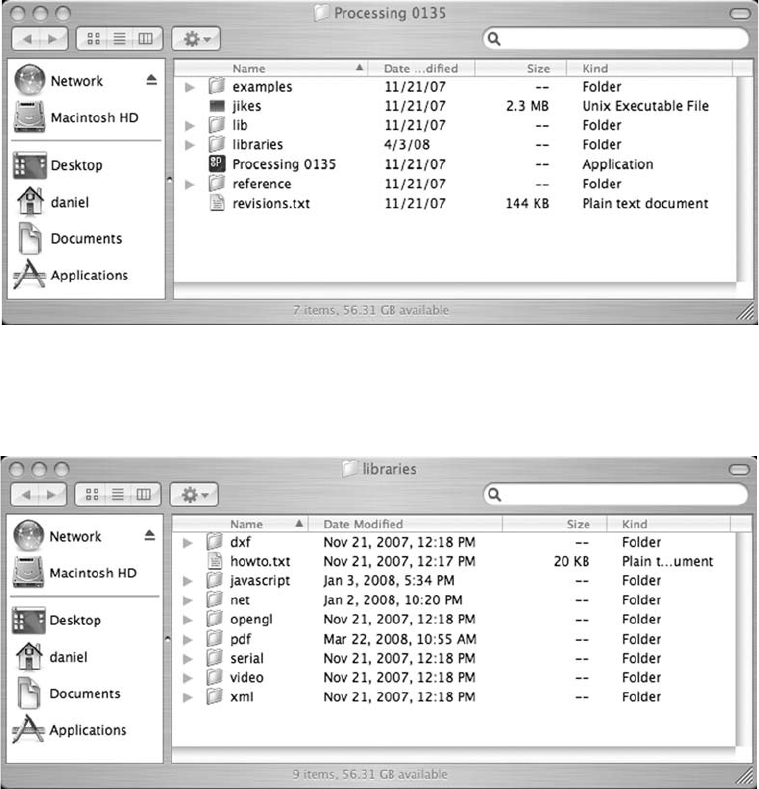
Libraries 197
fi g. 12.1
fi g. 12.2
/Applications/Processing 0135/
or
c:/Program Files/Processing 0135/
e libraries directory is where you will install contributed libraries.
e fi rst use of a third party library can be found in Chapter 18 of this book. e “ simpleML ” library,
designed to make HTML and XML data retrieval simple, is available for download at the book’s web
site, http://www.learningprocessing.com/libraries . If you want to get a jump start on Chapter 18, download
the fi le simpleML.zip and follow the instructions below, and illustrated in Figure 12.3 . e process for
installing other contributed libraries will be identical, with the exception of fi lenames.
Step 1. Extract the ZIP fi le. is can usually be accomplished by double-clicking the fi le or with any
decompression application, such as Winzip on a PC.
Inside the libraries directory, you will fi nd folders for each of the built-in libraries, along with a “ howto.txt ”
fi le that provides tips and instructions related to making your own library (a topic beyond the scope of
this book). See Figure 12.2 .
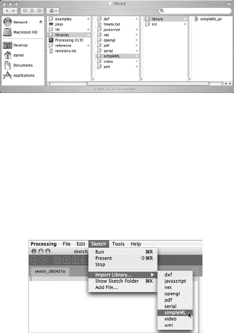
198 Learning Processing
fi g. 12.4
fi g. 12.3
Step 2. Copy the extracted fi les to the Processing libraries folder. Most libraries you download will
automatically unpack with the right directory structure. e full directory structure should
look like this:
/Processing 0135/libraries/simpleML/library/simpleML.jar
More generically:
/Processing 0135/libraries/libraryName/library/libraryName.jar
Some libraries may include additional fi les in the “ library ” folder, as well as the source code
(which is commonly stored one directory up, in the “ libraryName ” folder). If the library does not
automatically unpack itself with the above directory structure, you can manually create these folders
(using the fi nder or explorer) and place the libraryName.jar fi le in the appropriate location yourself.
Step 3. Restart Processing. If Processing was running while you performed Step 2, you will need to
quit Processing and restart it in order for the library to be recognized. Once you have restarted,
if everything has gone according to plan, the library will appear under the “ Sketch → Import
Library ” option shown in Figure 12.4 .
e newly installed library will now appear in the list! What to do once you have installed the library
really depends on which library you have installed. Examples that make use in code of a contributed
library can be found in Chapter 18 (simpleML, Yahoo API) and Chapter 20 (Sonia, Minim).
Lesson Six
The World Revolves Around You
13 Mathematics
14 Translation and Rotation (in 3D!)
This page intentionally left blank
Mathematics 201
13 Mathematics
“ If people do not believe that mathematics is simple, it is only because they do not realize how complicated
life is. ”
—John von Neumann
“ If you were cosine squared, I’d be sine squared, because together we’d be one. ”
—Anonymous
In this chapter:
– Probability.
– Perlin noise.
– Trigonometry.
– Recursion.
Here we are. e fundamentals are fi nished and we are going to start looking at some more sophisticated
topics in Processing . You may fi nd there is less of a story to follow from chapter to chapter. Nonetheless,
although the concepts do not necessarily build on each other as fl uidly as they did previously, the chapters
are ordered with a step-by-step learning approach in mind.
Everything we do from here on out will still employ the same fl ow structure of setup( ) and draw( ) . We
will continue to use functions from the Processing library and algorithms made of conditional statements
and loops, and organize sketches with an object-oriented approach in mind. At this point, however, the
descriptions will assume a knowledge of these essential topics and I encourage you to return to earlier
chapters to review as needed.
13.1 Mathematics and Programming
Did you ever start to feel the sweat beading on your forehead the moment your teacher called you up to
the board to write out the solution to the latest algebra assignment? Does the mere mention of the word
“ calculus ” cause a trembling sensation in your extremities?
Relax, there is no need to be afraid. ere is nothing to fear, but the fear of mathematics itself. Perhaps at
the beginning of reading this book, you feared computer programming. I certainly hope that, by now, any
terrifi ed sensations associated with code have been replaced with feelings of serenity. is chapter aims to
take a relaxed and friendly approach to a few useful topics from mathematics that will help us along the
journey of developing Processing sketches.
You know, we have been using math all along.
For example, we have likely had an algebraic expression on almost every single page since learning variables.
x = x + 1;
202 Learning Processing
And most recently, in Chapter 10, we tested intersection using the Pythagorean eorem.
float d = dist(x1,x2,y1,y2);
ese are just a few examples we have seen so far and as you get more and more advanced, you may even
fi nd yourself online, late at night, googling “ Sinusoidal Spiral Inverse Curve. ” For now, we will start with a
selection of useful mathematical topics.
13.2 Modulus
We begin with a discussion of the modulo operator , written as a percent sign, in Processing. Modulus is a
very simple concept (one that you learned without referring to it by name when you fi rst studied division)
that is incredibly useful for keeping a number within a certain boundary (a shape on the screen, an index
value within the range of an array, etc.) e modulo operator calculates the remainder when one number
is divided by another. It works with both integers and fl oats.
20 divided by 6 equals 3 remainder 2. (In other words: 6*3 ⴙ 2 ⴝ 1 8 ⴙ 2 ⴝ 20.)
therefore:
20 modulo 6 equals 2 or 20 % 6 ⴝ 2
Here are a few more, with some blanks for you to fi ll in.
17 divided by 4 equals 4 remainder 1 17 % 4 1
3 divided by 5 equals 0 remainder 3 3 % 5 3
10 divided by 3.75 equals 2 remainder 2.5 10.0 % 3.75 2.5
100 divided by 50 equals ___________ remainder ______ _________ 100 % 40 ____________
9.25 divided by 0.5 equals ___________ remainder _______________ 9.25 % 0.5 ______ _____
You will notice that if A B % C , A can never be larger than C . e remainder can never be larger than
the divisor.
0 % 3 0
1 % 3 1
2 % 3 2
3 % 3 0
4 % 3 1
etc .

Mathematics 203
erefore, modulo can be used whenever you need to cycle a counter variable back to zero. e following
lines of code:
x = x + 1;
if (x > = limit) {
x = 0;
}
can be replaced by:
x = (x + 1) % limit;
is is very useful if you want to count through the elements of an array one at a time, always returning to
0 when you get to the length of the array.
Example 13-1: Modulo
// 4 random numbers
float[] randoms = new float[4];
int index = 0; // Which number are we using
void setup() {
size(200,200);
// Fill array with random values
for (int i = 0; i < randoms.length; i + + ){
randoms[i] = random(0,256);
}
frameRate(1);
}
void draw() {
// Every frame we access one element of the array
background(randoms[index]);
// And then go on to the next one
index = (index + 1) % randoms.length;
}
13.3 Random Numbers
In Chapter 4, we were introduced to the random( ) function, which allowed us to randomly fi ll variables.
Processing’s random number generator produces what is known as a “ uniform ” distribution of numbers. For
example, if we ask for a random number between 0 and 9, 0 will come up 10% of the time, 1 will come
up 10% of the time, 2 will come up 10% of the time, and so on. We could write a simple sketch using an
array to prove this fact. See Example 13-2 .
Pseudo-Random Numbers
e random numbers we get from the random( ) function are not truly random and are known as
“ pseudo-random. ” ey are the result of a mathematical function that simulates randomness. is
function would yield a pattern over time, but that time period is so long that for us, it is just as
good as pure randomness!
Using the modulo operator
to cycle a counter back to 0.

204 Learning Processing
Example 13-2: Random number distribution
// An array to keep track of how often random numbers are picked.
float[] randomCounts;
void setup() {
size(200,200);
randomCounts = new float[20];
}
void draw() {
background(255);
// Pick a random number and increase the count
int index = int(random(randomCounts.length));
randomCounts[index] + + ;
// Draw a rectangle to graph results
stroke(0);
fill(175);
for (int x = 0; x < randomCounts.length; x + + ) {
rect(x*10,0,9,randomCounts[x]);
}
}
With a few tricks, we can change the way we use random( ) to produce a nonuniform distribution of
random numbers and generate probabilities for certain events to occur. For example, what if we wanted
to create a sketch where the background color had a 10% chance of being green and a 90% chance of
being blue?
13.4 Probability Review
Let’s review the basic principles of probability, fi rst looking at single event probability, that is, the
likelihood of something to occur.
Given a system with a certain number of possible outcomes, the probability of any given event occurring
is the number of outcomes which qualify as that event divided by total number of possible outcomes. e
simplest example is a coin toss. ere are a total of two possible outcomes (heads or tails). ere is only
one way to fl ip heads, therefore the probability of heads is one divided by two, that is, 1/2 or 50%.
Consider a deck of 52 cards. e probability of drawing an ace from that deck is:
number of aces/number of cards ⴝ 4/52 ⴝ 0.077 ⴝ ⬃ 8%
e probability of drawing a diamond is:
number of diamonds/number of cards ⴝ 13/52 ⴝ 0.25 ⴝ 2 5 %
We can also calculate the probability of multiple events occurring in sequence as the product of the
individual probabilities of each event.
fi g. 13.1

Mathematics 205
e probability of a coin fl ipping up heads three times in a row is:
(1/2) * (1/2) * (1/2) ⴝ 1/8 (or 0.125).
In other words, a coin will land heads three times in a row one out of eight times (with each “ time ” being
three tosses).
13.5 Event Probability in Code
ere are few diff erent techniques for using the random( ) function with probability in code. For example,
if we fi ll an array with a selection of numbers (some repeated), we can randomly pick from that array and
generate events based on what we select.
int[] stuff = new int[5];
stuff[0] = 1;
stuff[1] = 1;
stuff[2] = 2;
stuff[3] = 3;
stuff[4] = 3;
int index = int(random(stuff.length));
if (stuff[index] == 1) {
// do something
}
If you run this code, there will be a 40% chance of selecting the value 1, a 20% chance of selecting the
value 2, and a 40% chance of selecting the value 3.
Another strategy is to ask for a random number (for simplicity, we consider random fl oating point values
between 0 and 1) and only allow the event to happen if the random number we pick is within a certain
range. For example:
float prob = 0.10; // A probability of 10%
float r = random(l); // A random floating point value between 0 and 1
if (r < prob) { // If our random is less than .1
/*INSTIGATE THE EVENT HERE*/
}
is same technique can also be applied to multiple outcomes.
Outcome A — 60% | Outcome B — 10% | Outcome C — 30%
______________________________________
Exercise 13-1: What is the probability of drawing two aces in a row from the deck of cards?
This code will only be executed 10% of
the time.
Picking a random element from an array.
206 Learning Processing
To implement this in code, we pick one random fl oat and check where it falls.
• Between 0.00 and 0.60 (10%) → outcome A.
• Between 0.60 and 0.70 (60%) → outcome B.
• Between 0.70 and 1.00 (30%) → outcome C .
Example 13-3 draws a circle with a three diff erent colors, each with the above probability (red: 60%,
green: 10%, blue: 30%). is example is displayed in Figure 13.2 .
Example 13-3: Probabilities
void setup() {
size(200,200);
background(255);
smooth();
noStroke();
}
void draw() {
// Probabilities for 3 different cases
// These need to add up to 100%!
float red_prob = 0.60; // 60% chance of red color
float green_prob = 0.10; // 10% chance of green color
float blue_prob = 0.30; // 30% chance of blue color
float num = random(1); // pick a random number between 0 and 1
// If random number is less than .6
if (num < red_prob) {
fill(255,53,2,150);
// If random number is between .6 and .7
} else if (num < green_prob + red_prob) {
fill(156,255,28,150);
// All other cases (i.e. between .7 and 1.0)
} else {
fill(10,52,178,150);
}
ellipse(random(width),random(height),64,64);
}
fi g. 13.2
float y = 100;
void setup() {
size(200,200);
smooth();
}
Exercise 13-2: Fill in the blanks in the following code so that the circle has a 10% chance of
moving up, a 20% chance of moving down, and a 70% chance of doing nothing.
Mathematics 207
13.6 Perlin Noise
One of the qualities of a good random number generator is that the numbers produced appear to have no
relationship. If they exhibit no discernible pattern, they are considered random .
In programming behaviors that have an organic, almost lifelife quality, a little bit of randomness is a good
thing. However, we do not want too much randomness. is is the approach taken by Ken Perlin, who
developed a function in the early 1980’s entitled “ Perlin noise ” that produces a naturally ordered (i.e.,
“ smooth ” ) sequence of pseudo-random numbers. It was originally designed to create procedural textures,
for which Ken Perlin won an Academy Award for Technical Achievement. Perlin noise can be used to
generate a variety of interesting eff ects including clouds, landscapes, marble textures, and so on.
Figure 13.3 shows two graphs,—a graph of Perlin noise over time (the x -axis represents time; note how
the curve is smooth) compared to a graph of pure random numbers over time. (Visit this book’s web site
for the code that generated these graphs.)
Perlin Noise Random
fi g. 13.3
void draw() {
background(0);
float r = random(1);
____________________________________________________
____________________________________________________
____________________________________________________
____________________________________________________
____________________________________________________
____________________________________________________
ellipse(width/2,y,16,16);
}

208 Learning Processing
Processing has a built-in implementation of the Perlin noise algorithm with the function noise( ) . e
noise( ) function takes one, two, or three arguments (referring to the “ space ” in which noise is computed:
one, two, or three dimensions). is chapter will look at one-dimensional noise only. Visit the Processing
web site for further information about two-dimensional and three-dimensional noise.
One-dimensional Perlin noise produces as a linear sequence of values over time. For example:
0.364, 0.363, 0.363, 0.364, 0.365
Note how the numbers move up or down randomly, but stay close to the value of their predecessor. Now,
in order to get these numbers out of Processing , we have to do two things: (1) call the function noise( ) , and
(2) pass in as an argument the current “ time. ” We would typically start at time t 0 and therefore call the
function like so: “ noise(t); ”
float t = 0.0;
float noisevalue = noise(t); // Noise at time 0
We can also take the above code and run it looping in draw( ) .
float t = 0.0;
void draw() {
float noisevalue = noise(t);
println(noisevalue);
}
e above code results in the same value printed over and over. is is because we are asking for the
result of the noise( ) function at the same point in “ time ” —0.0—over and over. If we increment the “ time ”
variable t, however, we will get a diff erent result.
float t = 0.0;
void draw() {
float noisevalue = noise(t);
println(noisevalue);
t + = 0.01;
}
Noise Detail
If you visit the Processing.org noise reference, you will fi nd that noise is calculated over several
“ octaves. ” You can change the number of octaves and their relative importance by calling
the noiseDetail( ) function. is, in turn, can change how the noise function behaves.
See http://processing.org/reference/noiseDetail_.html.
You can read more about how noise works from Ken Perlin himself:
http://www.noisemachine.com/talk1/.
Time moves forward!
Output:
0.28515625
0.28515625
0.28515625
0.28515625
Output:
0.12609221
0.12697512
0.12972163
0.13423012
0.1403218
Mathematics 209
How quickly we increment t also aff ects the smoothness of the noise. Try running the code several times,
incrementing t by 0.01, 0.02, 0.05, 0.1, 0.0001, and so on.
By now, you may have noticed that noise( ) always returns a fl oating point value between 0 and 1. is
detail cannot be overlooked, as it aff ects how we use Perlin noise in a Processing sketch. Example 13-4
assigns the result of the noise( ) function to the size of a circle. e noise value is scaled by multiplying
by the width of the window. If the width is 200, and the range of noise( ) is between 0.0 and 1.0, the
range of noise( ) multiplied by the width is 0.0 to 200.0. is is illustrated by the table below and by
Example 13-4 .
Noise Value Multiplied by Equals
0 200 0
0.12 200 24
0.57 200 114
0.89 200 178
1 200 200
Example 13-4: Perlin noise
float time = 0.0;
float increment = 0.01;
void setup() {
size(200,200);
smooth(); {
void draw() {
background(255);
float n = noise(time)*width;
// With each cycle, increment the "time"
time + = increment;
// Draw the ellipse with size determined by Perlin noise
fill(0);
ellipse(width/2,height/2,n,n);
}
fi g. 13.4
Get a noise value at “time” and scale
it according to the window’s width.
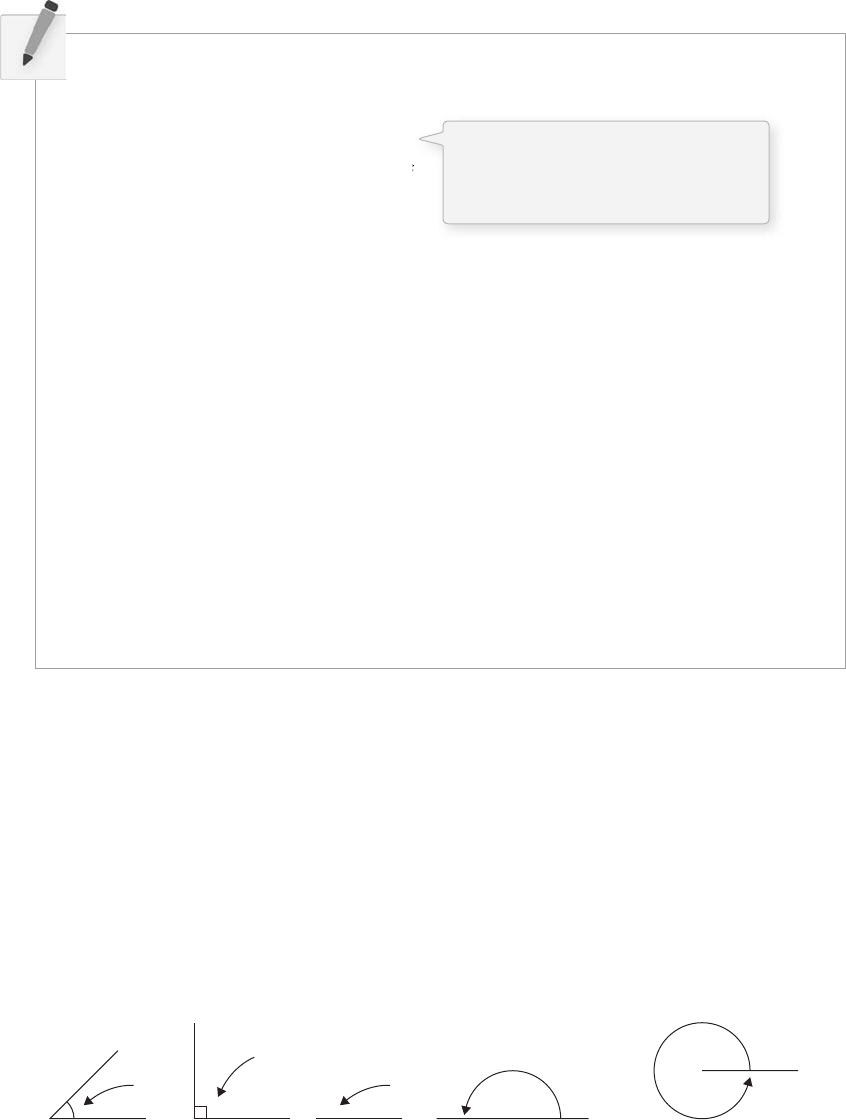
210 Learning Processing
90°
0°45 °
180°360°
fi g. 13.5
// Noise " time " variables
float xtime = 0.0;
float ytime = 100.0;
float increment = 0.01;
void setup() {
size(200,200);
smooth();
}
void draw() {
background(0);
float x = ____________________________________;
float y = ____________________________________;
____________________________________;
____________________________________;
// Draw the ellipse with size determined by Perlin noise
fill(200);
ellipse(__________,__________,__________,__________);
}
Exercise 13-3: Complete the following code which uses Perlin noise to set the location of
a circle. Run the code. Does the circle appear to be moving “ naturally ” ?
13.7 Angles
Some of the examples in this book will require a basic understanding of how angles are defi ned in
Processing. In Chapter 14 , for example, we will need to know about angles in order to feel comfortable
using the rotate( ) function to rotate and spin objects.
In order to get ready for these upcoming examples, we need to learn about radians and degrees . It is likely
you are familiar with the concept of an angle in degrees. A full rotation goes from zero to 360
° . An angle
of 90
° (a right angle) is one-fourth of 360
° , shown in Figure 13.5 as two perpendicular lines.
In this sketch, we want to use noise for
two different values. So that the output
of the noise function is not identical,
we start at two different points in time.
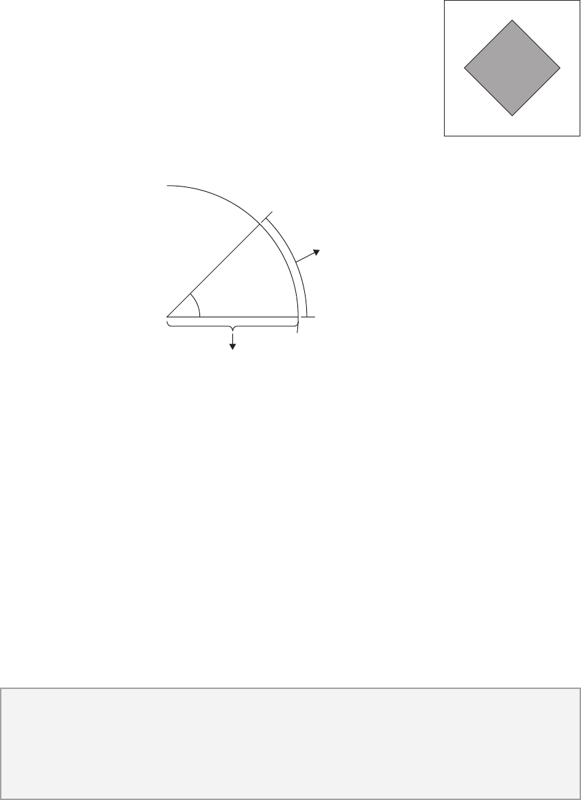
Mathematics 211
It is fairly intuitive for us to think angles in terms of degrees. For
example, the rectangle in Figure 13.6 is rotated 45 ° around its center.
Processing , however, requires angles to be specifi ed in radians . A radian is a
unit of measurement for angles defi ned by the ratio of the length of the arc
of a circle to the radius of that circle. One radian is the angle at which that
ratio equals one (see Figure 13.7 ). An angle of 180° PI radians. An angle
of 360 ° 2*PI radians, and 90 ° PI/2 radians, and so on.
fi g. 13.6
arc length radius
radius
angle 1 radian
fi g. 13.7
PI, What Is It?
e mathematical constant PI (or π ) is a real number defi ned as the ratio of a circle’s circumference
(the distance around the perimeter) to its diameter (a straight line that passes through the circle
center). It is equal to approximately 3.14159.
e formula to convert from degrees to radians is:
Radians 2 * PI * (degrees/360)
Fortunately for us, if we prefer to think in degrees but code with radians, Processing makes this easy. e
radians( ) function will automatically convert values from degrees to radians. In addition, the constants PI
and TWO_PI are available for convenient access to these commonly used numbers (equivalent to 180 °
and 360 ° , respectively). e following code, for example, will rotate shapes by 60 ° (rotation will be fully
explored in the next chapter).
float angle = radians(60);
rotate(angle);
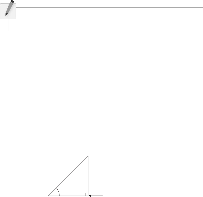
212 Learning Processing
angle
adjacent
opposite
right angle 90°π/2 radians
hypotenuse
fi g. 13.8
13.8 Trigonometry
Sohcahtoa. Strangely enough, this seemingly nonsense word, sohcahtoa , is the foundation for a lot of
computer graphics work. Any time you need to calculate an angle, determine the distance between
points, deal with circles, arcs, lines, and so on, you will fi nd that a basic understanding of trigonometry is
essential.
Trigonometry is the study of the relationships between the sides and angles of triangles and sohcahtoa
is a mnemonic device for remembering the defi nitions of the trigonometric functions, sine, cosine, and
tangent. See Figure 13.8 .
• soh : sine opposite/hypotenuse
• cah : cosine adjacent/hypotenuse
• toa : tangent opposite/adjacent
Degrees: _____________________ Radians: _____________________
Exercise 13-4: A dancer spins around two full rotations. How many degrees did the dancer
rotate? How many radians?
Any time we display a shape in Processing , we have to specify a pixel location, given as x and y coordinates.
ese coordinates are known as Cartesian coordinates, named for the French mathematician René
Descartes who developed the ideas behind Cartesian space.
Another useful coordinate system, known as polar coordinates , describes a point in space as an angle of
rotation around the origin and a radius from the origin. We can’t use polar coordinates as arguments to
a function in Processing . However, the trigonometric formulas allow us to convert those coordinates
to Cartesian, which can then be used to draw a shape. See Figure 13.9 .
Mathematics 213
θ
r
ysin(θ) = y/r
cos(θ) = x/r
x
y-axis
Polar coordinate (r,θ)
Cartesian coordinate (x,y)
x-axis
fi g. 13.9
sine(theta) y/r → y r * sine(theta)
cosine(theta) x/r → x r * cosine(theta)
For example, if r is 75 and theta is 45 ° (or PI/4 radians), we can calculate x and y as follows. e functions
for sine and cosine in Processing are sin( ) and cos( ) , respectively. ey each take one argument, a fl oating
point angle measured in radians.
float r = 75;
float theta = PI / 4; // We could also say: float theta = radians(45);
float x = r * cos(theta);
float y = r * sin(theta);
is type of conversion can be useful in certain applications. For example, how would you move a shape
along a circular path using Cartesian coordinates? It would be tough. Using polar coordinates, however,
this task is easy. Simply increment the angle!
Here is how it is done with global variables r and theta .
Example 13-5: Polar to Cartesian
// A Polar coordinate
float r = 75;
float theta = 0;
void setup() {
size(200,200);
background(255);
smooth();
}
void draw() {
// Polar to Cartesian conversion
float x = r * cos(theta);
float y = r * sin(theta);
fi g. 13.10
The Greek letter θ (theta) is often
used as a symbol for an angle.
Polar coordinates
(r, theta) are
converted to
Cartesian (x,y)
for use in the
ellipse() function.
214 Learning Processing
4
2
2
4
0
01π1π2π
x
y
fi g. 13.11
13.9 Oscillation
Trigonometric functions can be used for more than geometric calculations associated with right triangles.
Let’s take a look at Figure 13.11, a graph of the sine function where y sin( x ).
Exercise 13-5: Using Example 13-5, draw a spiral path. Start in the center and move
outward. Note that this can be done by changing only one line of code and adding one line
of code!
// Draw an ellipse at x,y
noStroke();
fill(0);
ellipse(x + width/2, y + height/2, 16, 16); // Adjust for center of window
// Increment the angle
theta + = 0.01;
}
You will notice that the output of sine is a smooth curve alternating between –1 and 1 . is type of
behavior is known as oscillation , a periodic movement between two points. A swinging pendulum, for
example, oscillates.
We can simulate oscillation in a Processing sketch by assigning the output of the sine function to an
object’s location. is is similar to how we used noise( ) to control the size of a circle (see Example 13-4),
only with sin( ) controlling a location. Note that while noise( ) produces a number between 0 and 1.0, sin( )
outputs a range between –1 and 1. Example 13-6 shows the code for an oscillating pendulum .
Mathematics 215
class Oscillator {
float xtheta;
float ytheta;
___________________________________________
Oscillator() {
xtheta = 0;
ytheta = 0;
__________________________________________
}
void oscillate() {
__________________________________________
__________________________________________
}
void display() {
float x = ____________________________________________
float y = ____________________________________________
ellipse(x,y,16,16);
}
}
Example 13-6: Oscillation
float theta = 0.0;
void setup() {
size(200,200);
smooth();
}
void draw() {
background(255);
// Get the result of the sine function
// Scale so that values oscillate between 0 and width
float x = (sin(theta) + 1) * width/2;
// With each cycle, increment theta
theta + = 0.05;
// Draw the ellipse at the value produced by sine
fill(0);
stroke(0);
line(width/2,0,x,height/2);
ellipse(x,height/2,16,16);
}
fi g. 13.12
Exercise 13-6: Encapsulate the above functionality into an Oscillator object. Create an array
of Oscillators, each moving at diff erent rates along the x and y axes. Here is some code for the
Oscillator class to help you get started.
The output of the sin() function
oscillates smoothly between 1
and 1. By adding 1 we get values
between 0 and 2. By multiplying
by 100, we get values between 0
and 200 which can be used as the
ellipse’s x location.
216 Learning Processing
Exercise 13-7: Use the sine function to create a “ breathing ” shape, that is, one whose size oscillates.
We can also produce some interesting results by drawing a sequence of shapes along the path of the sine
function. See Example 13–7 .
Example 13-7: Wave
// Starting angle
float theta = 0.0;
void setup() {
size(200,200);
smooth();
}
void draw() {
background(255);
// Increment theta (try different values for " angular velocity " here)
theta + = 0.02;
noStroke();
fill(0);
float x = theta;
// A simple way to draw the wave with an ellipse at each location
for (int i = 0; i < = 20; i + + ) {
// Calculate y value based off of sine function
float y = sin(x)*height/2;
// Draw an ellipse
ellipse(i*10,y + height/2,16,16);
// Move along x-axis
x + = 0.2;
}
}
Exercise 13-8: Rewrite the above example to use the noise( ) function instead of sin( ) .
13.10 Recursion
fi g. 13.14 The Mandelbrot set:
http://processing.org/learning/topics/mandelbrot.html
fi g. 13.13
Afor loop is used to draw all the points along a sine
wave (scaled to the pixel dimension of the window).
Mathematics 217
In 1975, Benoit Mandelbrot coined the term fractal to describe self-similar shapes found in nature.
Much of the stuff we encounter in our physical world can be described by idealized geometrical forms—a
postcard has a rectangular shape, a ping-pong ball is spherical, and so on. However, many naturally
occurring structures cannot be described by such simple means. Some examples are snowfl akes, trees,
coastlines, and mountains. Fractals provide a geometry for describing and simulating these types of
self-similar shapes (by “ self-similar ” we mean no matter how “ zoomed out ” or “ zoomed in, ” the shape
ultimately appears the same). One process for generating these shapes is known as recursion.
We know that a function can call another function. We do this whenever we call any function inside
of the draw( ) function. But can a function call itself? Can draw( ) call draw( ) ? In fact, it can (although
calling draw( ) from within draw( ) is a terrible example, since it would result in an infi nite loop).
Functions that call themselves are recursive and are appropriate for solving diff erent types of problems.
is occurs in mathematical calculations; the most common example of this is “ factorial. ”
e factorial of any number n , usually written as n !, is defi ned as:
n ! n * n – 1 * . . . . * 3 * 2 * 1
0! 1
We could write a function to calculate factorial using a for loop in Processing :
int factorial(int n) {
int f = 1;
for (int i = 0; i < n; i + + ){
f = f * (i + 1);
}
return f;
}
If you look closely at how factorial works, however, you will notice something interesting. Let’s examine
4! and 3!
4! 4 * 3 * 2 * 1
3! 3 * 2 * 1
therefore. . . 4! 4 * 3!
We can describe this in more general terms. For any positive integer n :
n ! n * ( n – 1)!
1! 1
Written in English:
e factorial of N is defi ned as N times the factorial of N – 1.
218 Learning Processing
e same principle can be applied to graphics with interesting results. Take a look at the following
recursive function. e results are shown in Figure 13.16 .
void drawCircle(int x, int y, float radius) {
ellipse(x, y, radius, radius);
if(radius > 2) {
radius * = 0.75f;
drawCircle(x, y, radius);
}
}
What does drawCircle( ) do? It draws an ellipse based on a set of parameters received as arguments, and
then calls itself with the same parameters (adjusting them slightly). e result is a series of circles each
drawn inside the previous circle.
Notice that the above function only recursively calls itself if the radius is greater than two. is is a crucial
point. All recursive functions must have an exit condition! is is identical to iteration. In Chapter 6, we
learned that all for and while loops must include a boolean test that eventually evaluates to false, thus
exiting the loop. Without one, the program would crash, caught inside an infi nite loop. e same can be
e defi nition of factorial includes factorial ?! It is kind of like saying “ tired ” is defi ned as “ the feeling you
get when you are tired. ” is concept of self-reference in functions is known as recursion . And we can use
recursion to write a function for factorial that calls itself.
int factorial(int n) {
if (n == 1) {
return 1;
} else {
return n * factorial(n-1);
}
}
Crazy, I know. But it works. Figure 13.15 walks through the steps that happen when factorial(4) is called.
becomes 24
f
actorial(4)
return 4 * factorial(3)
return 3 * factorial(2)
return 2 * factorial(1)
return
1
becomes 6
becomes 2
becomes 1
fi g. 13.15
fi g. 13.16
Mathematics 219
said about recursion. If a recursive function calls itself forever and ever, you will most likely be treated to a
nice frozen screen.
e preceding circles example is rather trivial, since it could easily be achieved through simple iteration.
However, in more complex scenarios where a method calls itself more than once, recursion becomes
wonderfully elegant.
Let’s revise drawCircle( ) to be a bit more complex. For every circle displayed, draw a circle half its size to
the left and right of that circle. See Example 13–8 .
Example 13-8: Recursion
void setup() {
size(200,200);
smooth();
}
void draw() {
background(255);
stroke(0);
noFill();
drawCircle(width/2,height/2,100);
}
void drawCircle(float x, float y, float radius) {
ellipse(x, y, radius, radius);
if(radius > 2) {
drawCircle(x + radius/2, y, radius/2);
drawCircle(x – radius/2, y, radius/2);
}
}
With a teeny bit more code, we could add a circle above and below. is result is shown in Figure 13.18 .
void drawCircle(float x, float y, float radius) {
ellipse(x, y, radius, radius);
if(radius > 8) {
drawCircle(x + radius/2, y, radius/2);
drawCircle(x – radius/2, y, radius/2);
drawCircle(x, y + radius/2, radius/2);
drawCircle(x, y – radius/2, radius/2);
}
}
Just try recreating this sketch with iteration instead of recursion! I dare you!
fi g. 13.17
fi g. 13.18
drawCircle() calls itself twice, creating a
branching effect. For every circle, a smaller
circle is drawn to the left and right.
220 Learning Processing
Exercise 13-9: Complete the code which generates the following pattern (Note: the solution
uses lines, although it would also be possible to create the image using rotated rectangles,
which we will learn how to do in Chapter 14).
13.11 Two-Dimensional Arrays
In Chapter 9, we learned that an array keeps track of multiple pieces of information in linear order, a
one-dimensional list. However, the data associated with certain systems (a digital image, a board game,
etc.) lives in two dimensions. To visualize this data, we need a multi-dimensional data structure, that is,
a multi-dimensional array.
void setup() {
size(400,200);
}
void draw() {
background(255);
stroke(0);
branch(width/2,height,100);
}
void branch(float x, float y, float h) {
________________________________________;
________________________________________;
if (__________________) {
________________________________________;
________________________________________;
}
}
Mathematics 221
A two-dimensional array is really nothing more than an array of arrays (a three-dimensional array is an
array of arrays of arrays). ink of your dinner. You could have a one-dimensional list of everything you eat:
(lettuce, tomatoes, salad dressing, steak, mashed potatoes, string beans, cake, ice cream, coff ee)
Or you could have a two-dimensional list of three courses, each containing three things you eat:
(lettuce, tomatoes, salad dressing) and (steak, mashed potatoes, string beans) and (cake, ice cream, coff ee)
In the case of an array, our old-fashioned one-dimensional array looks like this:
int[] myArray = { 0,1,2,3};
And a two-dimensional array looks like this:
int[][] myArray = { { 0,1,2,3},{3,2,1,0},{3,5,6,1},{3,8,3,4} } ;
For our purposes, it is better to think of the two-dimensional array as a matrix. A matrix can be thought
of as a grid of numbers, arranged in rows and columns, kind of like a bingo board. We might write the
two-dimensional array out as follows to illustrate this point:
int[][] myArray = { {0, 1, 2, 3 },
{ 3, 2, 1, 0 },
{ 3, 5, 6, 1 },
{ 3, 8, 3, 4 } };
We can use this type of data structure to encode information about an image.
For example, the grayscale image in Figure 13.19 could be represented by the
following array:
int[][] myArray = { {236, 189, 189, 0},
{ 236, 80, 189, 189 },
{ 236, 0, 189, 80},
{ 236, 189, 189, 80} };
To walk through every element of a one-dimensional array, we use a for loop, that is :
int[] myArray = new int[10];
for (int i = 0; i < myArray.length; i + + ){
myArray[i] = 0;
}
For a two-dimensional array, in order to reference every element, we must use two nested loops. is gives
us a counter variable for every column and every row in the matrix. See Figure 13.20 .
int cols = 10;
int rows = 10;
int[][] myArray = new int[cols][rows];
fi g. 13.19
222 Learning Processing
for (int i = 0; i < cols; i + + ) {
for (int j = 0; j < rows; j + + ) {
myArray[i][j] = 0;
}
}
For example, we might write a program using a two-dimensional array to draw a grayscale image as in
Example 13–9 .
Example 13-9: Two-dimensional array
// Set up dimensions
size(200,200);
int cols = width;
int rows = height;
// Declare 2D array
int[][] myArray = new int[cols][rows];
// Initialize 2D array values
for (int i = 0; i < cols; i + + ) {
for (int j = 0; j < rows; j + + ) {
myArray[i][j] = int(random(255));
}
}
// Draw points
for (int i = 0; i < cols; i + + ) {
for (int j = 0; j < rows; j + + ) {
stroke(myArray[i][j]);
point(i,j);
}
}
A two-dimensional array can also be used to store objects, which is especially convenient for
programming sketches that involve some sort of “ grid ” or “ board. ” Example 13-10 displays a grid of Cell
objects stored in a two-dimensional array. Each cell is a rectangle whose brightness oscillates from 0–255
with a sine function .
fi g. 13.21
columns
rows
for every column i
&
for every row j
0123456789
0
1
2
3
4
5
6
7
8
9
fi g. 13.20
Two nested loops allow us to visit
every spot in a two-dimensional array.
For every column i, visit every row j.
Example 13-10: Two-dimensional array of objects
// 2D Array of objects
Cell[][] grid;
// Number of columns and rows in the grid
int cols = 10;
int rows = 10;
void setup() {
size(200,200);
grid = new Cell[cols][rows];
for (int i = 0; i < cols; i + + ){
for (int j = 0; j < rows; j + + ){
// Initialize each object
grid[i][j] = new Cell(i*20,j*20,20,20,i + j);
}
}
}
void draw() {
background(0);
for (int i = 0; i < cols; i + + ){
for (int j = 0; j < rows; j + + ){
// Oscillate and display each object
grid[i][j].oscillate();
grid[i][j].display();
}
}
}
// A Cell object
class Cell {
float x,y; // x,y location
float w,h; // width and height
float angle; // angle for oscillating brightness
// Cell Constructor
Cell(float tempX, float tempY, float tempW, float tempH, float tempAngle) {
x = tempX;
y = tempY;
w = tempW;
h = tempH;
angle = tempAngle;
}
// Oscillation means increase angle
void oscillate() {
angle + = 0.02;
}
void display() {
stroke(255);
// Color calculated using sine wave
fill(127 + 127*sin(angle));
rect(x,y,w,h);
}
}
fi g. 13.22
A two-dimensional array can
be used to store objects.
The counter variables i and j are also
the column and row numbers, and are
used as arguments to the constructor
for each object in the grid.
A cell object knows about its location
in the grid as well as its size with the
variables x, y, w, h.
Mathematics 223

Exercise 13-10: Develop the beginnings of a Tic-Tac-Toe game. Create a Cell object that
can exist in one of two states: O or nothing. When you click on the cell, its state changes from
nothing to “ O ” . Here is a framework to get you started.
Cell[][] board;
int cols = 3;
int rows = 3;
void setup() {
// FILL IN
}
void draw() {
background(0);
for (int i = 0; i < cols; i + + ){
for (int j = 0; j < rows; j + + ){
board[i][j].display();
}
}
}
void mousePressed() {
// FILL IN
}
// A Cell object
class Cell {
float x,y;
float w,h;
int state;
// Cell Constructor
Cell(float tempX, float tempY, float tempW, float tempH) {
// FILL IN
}
void click(int mx, int my) {
// FILL IN
}
224 Learning Processing

Exercise 13-11: If you are feeling saucy, go ahead and complete the Tic-Tac-Toe game
adding X and alternating player turns with mouse clicks.
void display() {
// FILL IN
}
}
Mathematics 225
This page intentionally left blank

Translation and Rotation (in 3D!) 227
14 Translation and Rotation (in 3D!)
“ What is the Matrix? ”
— Neo
In this chapter:
– 2D and 3D translation.
– Using P3D and OPENGL.
– Vertex shapes.
– 2D and 3D rotation.
– Saving the transformation state in the stack: pushMatrix() and popMatrix() .
14.1 The Z-Axis
As we have seen throughout this book, pixels in a two-dimensional window are described using Cartesian
coordinates: an X (horizontal) and a Y (vertical) point. is concept dates all the way back to Chapter 1,
when we began thinking of the screen as a digital piece of graph paper.
In three-dimensional space (such as the actual, real-world space where you are reading this book), a
third axis (commonly referred to as the Z -axis) refers to the depth of any given point. In a Processing
sketch’s window, a coordinate along this Z -axis indicates how far in front or behind the window a pixel
lives. Scratching your head is a perfectly reasonable response here. After all, a computer window is only
two dimensional. ere are no pixels fl oating in the air in front of or behind your LCD monitor! In this
chapter, we will examine how using the theoretical Z -axis will create the illusion of three-dimensional
space in your Processing window.
We can, in fact, create a three-dimensional illusion with what we have learned so far. For example, if you
were to draw a rectangle in the middle of the window and slowly increase its width and height, it might
appear as if it is moving toward you. See Example 14-1.
Example 14-1: A growing rectangle, or a rectangle moving toward you?
float r = 8;
void setup() {
size(200,200);
}
void draw() {
background(255);
// Display a rectangle in the middle of the screen
stroke(0);
fill(175);
rectMode(CENTER);
rect(width/2,height/2,r,r);
// Increase the rectangle size
r + + ;
}
fi g. 14.1
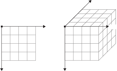
228 Learning Processing
Is this rectangle fl ying off of the computer screen about to bump into your nose? Technically, this is
of course not the case. It is simply a rectangle growing in size. But we have created the illusion of the
rectangle moving toward you.
Fortunately for us, if we choose to use 3D coordinates, Processing will create the illusion for us. While the
idea of a third dimension on a fl at computer monitor may seem imaginary, it is quite real for Processing.
Processing knows about perspective, and selects the appropriate two-dimensional pixels in order to create
the three-dimensional eff ect. We should recognize, however, that as soon as we enter the world of 3D
pixel coordinates, a certain amount of control must be relinquished to the Processing renderer. You can no
longer control exact pixel locations as you might with 2D shapes, because XY locations will be adjusted to
account for 3D perspective.
In order to specify points in three dimensions, the coordinates are specifi ed in the order you would expect:
x , y , z . Cartesian 3D systems can be described as “ left-handed ” or “ right-handed. ” If you use your right
hand to point your index fi nger in the positive y direction (up) and your thumb in the positive x direction
(to the right), the rest of your fi ngers will point toward the positive z direction. It is left-handed if you use
your left hand and do the same. In Processing, the system is left-handed, as shown in Figure 14.2 .
–Z
+X
+Y+Y
(0,0) (0,0) +X
fi g. 14.2
Our fi rst goal is to rewrite Example 14-1 using the 3D capabilities of Processing. Assume the following
variables:
int x = width/2;
int y = height/2;
int z = 0;
int r = 10;
In order to specify the location for a rectangle, the rect( ) function takes four arguments: an x location,
a y location, a width, and a height.
rect(x,y,w,h);
Translation and Rotation (in 3D!) 229
Our fi rst instinct might be to add another argument to the rect( ) function.
rect(x,y, z ,w,h);
e Processing reference page for rect( ) , however, does not allow for this possibility. In order to specify 3D
coordinates for shapes in the Processing world, we must learn to use a new function, called translate( ) .
e translate( ) function is not exclusive to 3D sketches, so let’s return to two dimensions to see how it
works.
e function translate( ) moves the origin point—(0,0)—relative to its previous state. We know that when
a sketch fi rst starts, the origin point lives on the top left of the window. If we were to call the function
translate( ) with the arguments (50,50), the result would be as shown in Figure 14.3 .
Before
(100,100)
(50,50)(0,0)
After
(-50,-50) (0,0)
⇒ translate (50,50)⇒
(50,50)
fi g. 14.3
Where is the origin?
e “ origin ” in a Processing sketch is the point (0,0) in two dimensions or (0,0,0) in three
dimensions. It is always at the top left corner of the window unless you move it using translate( ) .
You can think of it as moving a pen around the screen, where the pen indicates the origin point.
In addition, the origin always resets itself back to the top left corner at the beginning of draw( ) . Any calls
to translate( ) only apply to the current cycle through the draw( ) loop. See Example 14-2.
Incorrect! We cannot use an (x,y,z) coordinate in Processing’s
shape functions such as rect(),ellipse(),line(), and so on.
Other functions in Processing can take three arguments for
x,y,z and we will see this later in the chapter.

230 Learning Processing
Example 14-2: Multiple translations
void setup() {
size(200,200);
smooth();
}
void draw() {
background(255);
stroke(0);
fill(175);
// Grab mouse coordinates, constrained to window
int mx = constrain(mouseX,0,width);
int my = constrain(mouseY,0,height);
// Translate to the mouse location
translate(mx,my);
ellipse(0,0,8,8);
// Translate 100 pixels to the right
translate(100,0);
ellipse(0,0,8,8);
// Translate 100 pixels down
translate(0,100);
ellipse(0,0,8,8);
// Translate 100 pixels left
translate(–100,0);
ellipse(0,0,8,8);
}
Now that we understand how translate( ) works, we can return to the original problem of specifying 3D
coordinates. translate( ) , unlike rect( ), ellipse( ) , and other shape functions, can accept a third argument for
a Z coordinate.
// Translation along the z-axis
translate(0,0,50);
rectMode(CENTER);
rect(100,100,8,8);
e above code translates 50 units along the Z -axis, and then draws a rectangle at (100,100). While the
above is technically correct, when using translate( ) , it is a good habit to specify the ( x , y ) location as part
of the translation, that is:
// Translation along the z-axis II
translate(100,100,50);
rectMode(CENTER);
rect(0,0,8,8);
Finally, we can use a variable for the Z location and animate the shape moving toward us.
fi g. 14.4
When using translate(), the rectangle’s location
is (0,0) since translate() moved us to the location
for the rectangle.
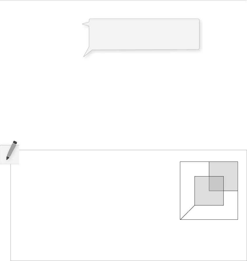
Translation and Rotation (in 3D!) 231
Example 14-3: A rectangle moving along the z-axis
float z = 0; // a variable for the Z (depth) coordinate
void setup() {
size(200,200,P3D);
}
void draw() {
background(0);
stroke(255);
fill(100);
// Translate to a point before displaying a shape there
translate(width/2,height/2,z);
rectMode(CENTER);
rect(0,0,8,8);
z + + ; // Increment Z (i.e. move the shape toward the viewer)
}
Although the result does not look diff erent from Example 14-1, it is quite diff erent conceptually as we have
opened the door to creating a variety of three-dimensional eff ects on the screen with Processing’s 3D engine.
size(200,200);
background(0);
stroke(255);
fill(255,100);
translate(_______,_______);
rect(0,0,100,100);
translate(_______,_______);
rect(0,0,100,100);
translate(_______,_______);
line(0,0,-50,50);
Exercise 14-1: Fill in the appropriate translate( ) functions to create this pattern. Once you are
fi nished, try adding a third argument to translate( ) to move the pattern into three dimensions.
When using (x,y,z) coordinates, we must tell
Processing we want a 3D sketch. This is done
by adding a third argument “P3D” to the size()
function. See Section 14.2 for more details.
e translate( ) function is particularly useful when you are drawing a collection of shapes relative to a
given centerpoint. Harking back to a Zoog from the fi rst 10 chapters of this book, we saw code like this:
void display() {
// Draw Zoog's body
fill(150);
rect( x,y ,w/6,h*2);
// Draw Zoog's head
fill(255);
ellipse( x,y-h/2 ,w,h);
}

232 Learning Processing
e display( ) function above draws all of Zoog’s parts (body and head, etc.) relative to Zoog’s x , y location.
It requires that x and y be used in both rect( ) and ellipse( ). translate( ) allows us to simply set Processing’s
origin (0,0) at Zoog’s ( x , y ) location and therefore draw the shapes relative to (0,0).
void display() {
// Move origin (0,0) to (x,y)
translate(x,y);
// Draw Zoog's body
fill(150);
rect( 0,0 ,w/6,h*2);
// Draw Zoog's head
fill(255);
ellipse(0,-h/2,w,h);
}
14.2 P3D vs. OPENGL
If you look closely at Example 14-3, you will notice that we have added a third argument to the size( )
function. Traditionally, size( ) has served one purpose: to specify the width and height of our Processing
window. e size( ) function, however, also accepts a third parameter indicating a drawing mode.
e mode tells Processing what to do behind the scenes when rendering the display window. e default
mode (when none is specifi ed) is “ JAVA2D, ” which employs existing Java 2D libraries to draw shapes, set
colors, and so on. We do not have to worry about how this works. e creators of Processing took care of
the details.
If we want to employ 3D translation (or rotation as we will see later in this chapter), the JAVA2D mode
will no longer suffi ce. Running the example in the default mode results in the following error:
“ translate(x, y, z) can only be used with OPENGL or P3D, use translate(x, y) instead. ”
Instead of switching to translate(x,y) , we want to select a diff erent mode. ere are two options:
• P3D —P3D is a 3D renderer developed by the creators of Processing . It should also be noted that
anti-aliasing (enabled with the smooth( ) function) is not available with P3D.
• OPENGL —OPENGL is a 3D renderer that employs hardware acceleration. If you have an
OpenGL compatible graphics card installed on your computer (which is pretty much every
computer), you can use this mode. Although at the time of the writing of this book, there are still
a few, minor kinks to be worked out with this mode (you may find things look slightly different
between P3D and OPENGL), it may prove exceptionally useful in terms of speed. If you are
planning to display large numbers of shapes onscreen in a high-resolution window, this mode will
likely have the best performance.
To specify a mode, add a third argument in all caps to the size( ) function.
size(200,200); // using the default JAVA2D mode
size(200,200,P3D); // using P3D
size(200,200,OPENGL); // using OPENGL
translate() can be used to draw a collection
of shapes relative to a given point.

Translation and Rotation (in 3D!) 233
14.3 Vertex Shapes
Up until now, our ability to draw to the screen has been limited to a small list of primitive two-
dimensional shapes: rectangles, ellipses, triangles, lines, and points. For some projects, however, creating
your own custom shapes is desirable. is can be done through the use of the functions beginShape( ) ,
endShape( ) , and vertex( ) .
Consider a rectangle. A rectangle in Processing is defi ned as a reference point, as well as a width and height.
rect(50,50,100,100);
But we could also consider a rectangle to be a polygon (a closed shape bounded by line segments)
made up of four points. e points of a polygon are called vertices (plural) or vertex (singular). e
following code draws exactly the same shape as the rect( ) function by setting the vertices of the rectangle
individually. See Figure 14.5 .
beginShape();
vertex(50,50);
vertex(150,50);
vertex(150,150);
vertex(50,150);
endShape(CLOSE);
beginShape( ) indicates that we are going to create a custom shape made up of some
number of vertex points: a single polygon. vertex( ) specifi es the points for each vertex in
the polygon and endShape( ) indicates that we are fi nished adding vertices. e argument “ CLOSE ” inside
of endShape(CLOSE) declares that the shape should be closed, that is, that the last vertex point should
connect to the fi rst.
e nice thing about using a custom shape over a simple rectangle is fl exibility. For example, the sides are
not required to be perpendicular. See Figure 14.6 .
stroke(0);
fill(175);
beginShape();
vertex(50,50);
vertex(150,25);
vertex(150,175);
vertex(25,150);
endShape(CLOSE);
When using the OPENGL mode, you must also import the OPENGL library.
is can be done by selecting the SKETCH ➝ IMPORT LIBRARY menu option or by manually
adding the following line of code to the top of your sketch (see Chapter 12 for a detailed explanation
on libraries):
import processing.opengl.*;
fi g. 14.5
Exercise 14-2: Run any Processing sketch in P3D, then switch to OPENGL. Notice any
diff erence?
fi g. 14.6

234 Learning Processing
We also have the option of creating more than one shape, for example, in a loop, as shown in Figure 14.7 .
stroke(0);
for (int i = 0; i < 10; i + + ) {
beginShape();
fill(175);
vertex(i*20,10-i);
vertex(i*20 + 15,10 + i);
vertex(i*20 + 15,180 + i);
vertex(i*20,180-i);
endShape(CLOSE);
}
You can also add an argument to beginShape( ) specifying exactly what type of shape you want to
make. is is particularly useful if you want to make more than one polygon. For example, if you
create six vertex points, there is no way for Processing to know that you really want to draw two
triangles (as opposed to one hexagon) unless you say beginShape(TRIANGLES) . If you do not want
to make a polygon at all, but want to draw points or lines, you can by saying beginShape(POINTS) or
beginShape(LINES) . See Figure 14.8 .
stroke(0);
beginShape(LINES);
for (int i = 10; i < width; i + = 20) {
vertex(i,10);
vertex(i,height–10);
}
endShape();
Note that LINES is meant for drawing a series of individual lines, not a continous loop. For a continuous
loop, do not use any argument. Instead, simply specify all the vertex points you need and include noFill( ) .
See Figure 14.9 .
noFill();
stroke(0);
beginShape();
for (int i = 10; i < width; i + = 20) {
vertex(i,10);
vertex(i,height–10);
}
endShape();
e full list of possible arguments for beginShape( ) is available in the Processing reference
http://processing.org/reference/beginShape_.html
POINTS, LINES, TRIANGLES, TRIANGLE_FAN, TRIANGLE_STRIP, QUADS,
QUAD_STRIP
fi g. 14.8
fi g. 14.9
fi g. 14.7
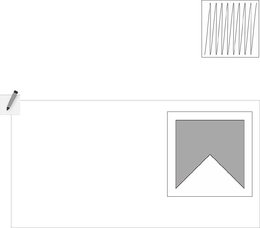
Translation and Rotation (in 3D!) 235
In addition, vertex( ) can be replaced with curveVertex( ) to join the points with curves instead of straight
lines. With curveVertex( ) , note how the fi rst and last points are not displayed. is is because they are
required to defi ne the curvature of the line as it begins at the second point and ends at the second to last
point. See Figure 14.10 .
noFill();
stroke(0);
beginShape();
for (int i = 10; i < width; i + = 20) {
curveVertex(i,10);
curveVertex(i,height-10);
}
endShape(); fi g. 14.10
14.4 Custom 3D Shapes
ree-dimensional shapes can be created using beginShape( ) , endShape( ) , and vertex( ) by placing
multiple polygons side by side in the proper confi guration. Let’s say we want to draw a four-sided
pyramid made up of four triangles, all connected to one point (the apex) and a fl at plane (the base). If
your shape is simple enough, you might be able to get by with just writing out the code. In most cases,
however, it is best to start sketching it out with pencil and paper to determine the location of all the
vertices. One example for our pyramid is shown in Figure 14.11 .
Example 14-4 takes the vertices from Figure 14.11 and puts them in a function that allows us to draw the
pyramid with any size. (As an exercise, try making the pyramid into an object.)
size(200,200);
background(255);
stroke(0);
fill(175);
beginShape();
vertex(20, 20);
vertex(_______,_______);
vertex(_______,_______);
vertex(_______,_______);
vertex(_______,_______);
endShape(_______);
Exercise 14-3: Complete the vertices for the shape pictured.
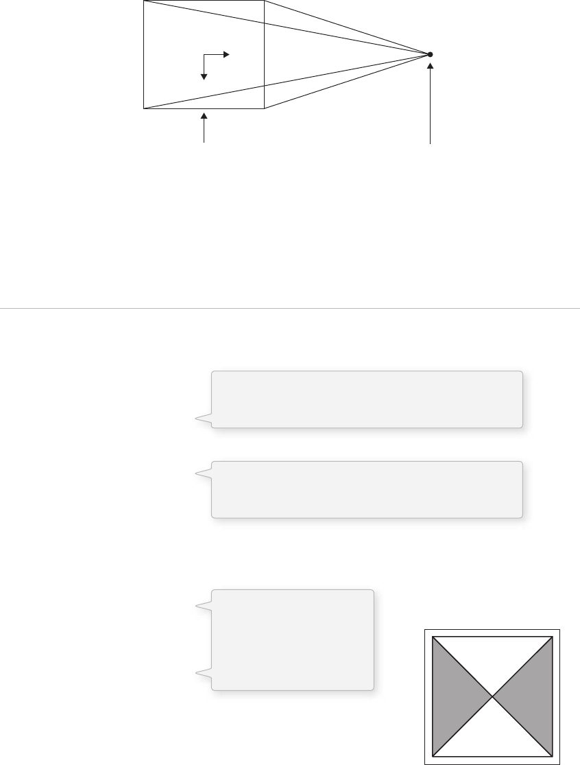
236 Learning Processing
Example 14-4: Pyramid using beginShape(TRIANGLES)
void setup() {
size(200,200,P3D);
}
void draw() {
background(255);
translate(100,100,0);
drawPyramid(150);
}
void drawPyramid(int t) {
stroke(0);
// this pyramid has 4 sides, each drawn as a separate triangle
// each side has 3 vertices, making up a triangle shape
// the parameter " t " determines the size of the pyramid
beginShape(TRIANGLES);
fill(255,150);
vertex(–t,–t,–t);
vertex( t,-t,–t);
vertex( 0, 0, t);
fill(150,150);
vertex( t,–t,–t);
vertex( t, t,–t);
vertex( 0, 0, t);
fill(255,150);
vertex( t, t,–t);
vertex(–t, t,–t);
vertex( 0, 0, t); fi g. 14.12
fi g. 14.11
(0,0,10)
(10,10,10)(10,10,10)
(10,10,10)
BASE
at
z = 10
APEX
at
z = 10
Connected to
(10,10,10)
x
y
vertex(–10,–10,–10); vertex(10,–10,–10); vertex( 10,10,–10); vertex( –10, 10,–10);
vertex( 10,–10,–10); vertex(10, 10,–10); vertex(–10,10,–10); vertex(–10,–10,–10);
vertex( 0, 0, 10); vertex( 0, 0, 10); vertex( 0, 0, 10); vertex( 0, 0, 10);
Since the pyramid’s vertices are drawn relative to
a centerpoint, we must call translate() to place the
pyramid properly in the window.
The function sets the vertices for the pyramid around
the centerpoint at a fl exible distance, depending on the
number passed in as an argument.
Note that each polygon
can have its own color.

Translation and Rotation (in 3D!) 237
fill(150,150);
vertex(–t, t,–t);
vertex(–t,–t,–t);
vertex( 0, 0, t);
endShape();
}
Exercise 14-4: Create a pyramid with only three sides. Include the base (for a total of four
triangles). Use the space below to sketch out the vertex locations as in Figure 14.11 .
Exercise 14-5: Create a three-dimensional cube using eight quads— beginShape(QUADS) .
(Note that a simpler way to make a cube in Processing is with the box( ) function.)
14.5 Simple Rotation
ere is nothing particularly three dimensional about the visual result of the pyramid example. e image
looks more like a fl at rectangle with two lines connected diagonally from end to end. Again, we have
to remind ourselves that we are only creating a three-dimensional illusion , and it is not a particularly
eff ective one without animating the pyramid structure within the virtual space. One way for us to
demonstrate the diff erence would be to rotate the pyramid. So let’s learn about rotation.
For us, in our physical world, rotation is a pretty simple and intuitive concept. Grab a baton, twirl it, and
you have a sense of what it means to rotate an object.
Programming rotation, unfortunately, is not so simple. All sorts of questions come up. Around what axis
should you rotate? At what angle? Around what origin point? Processing off ers several functions related to
rotation, which we will explore slowly, step by step. Our goal will be to program a solar system simulation
with multiple planets rotating around a star at diff erent rates (as well as to rotate our pyramid in order to
better experience its three dimensionality).
But fi rst, let’s try something simple and attempt to rotate one rectangle around its center. We should be
able to get rotation going with the following three principles:
1. Shapes are rotated in Processing with the rotate( ) function.
2. e rotate( ) function takes one argument, an angle measured in radians.
3. rotate( ) will rotate the shape in the clockwise direction (to the right) .
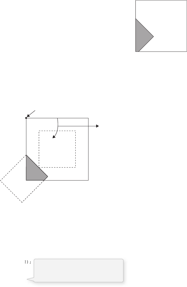
238 Learning Processing
OK, armed with this knowledge, we should be able to just call the rotate( ) function and pass in an angle.
Say, 45° (or PI/4 radians) in Processing . Here is our fi rst (albeit fl awed) attempt, with the output shown in
Figure 14.13 .
rotate(radians(45));
rectMode(CENTER);
rect(width/2,height/2,100,100);
Shoot. What went wrong? e rectangle looks rotated, but it is in the wrong place!
e single most important fact to remember about rotation in Processing is that
shapes always rotate around the point of origin . Where is the point of origin in this example? e top left
corner! e origin has not been translated. e rectangle therefore will not spin around its own center.
Instead, it rotates around the top left corner. See Figure 14.14 .
fi g. 14.13
origin
rectangle rotating around
top left origin
45° rotation
from origin
fi g. 14.14
Sure, there may come a day when all you want to do is rotate shapes around the top left corner, but until
that day comes, you will always need to fi rst move the origin to the proper location before rotating, and
then display the rectangle. translate( ) to the rescue!
translate(width/2,height/2);
rotate(radians(45));
rectMode(CENTER);
rect(0,0,100,100);
We can expand the above code using the mouseX location to calculate an angle of rotation and thus animate
the rectangle, allowing it to spin. See Example 14-5 .
Because we translated in order to
rotate, the rectangle now lives at the
point (0,0).
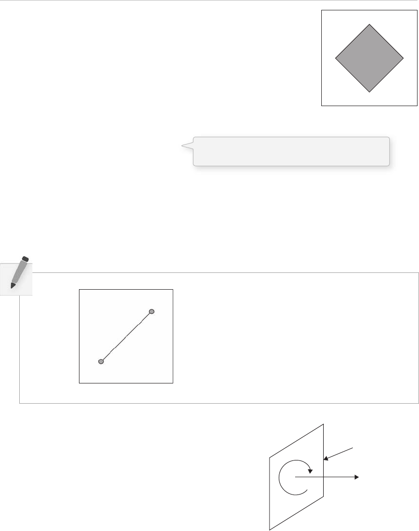
Translation and Rotation (in 3D!) 239
Example 14-5: Rectangle rotating around center
void setup() {
size(200,200);
}
void draw() {
background(255);
stroke(0);
fill(175);
// Translate origin to center
translate(width/2,height/2);
// theta is a common name of a variable to store an angle
float theta = PI*mouseX / width;
// Rotate by the angle theta
rotate(theta);
// Display rectangle with CENTER mode
rectMode(CENTER);
rect(0,0,100,100);
}
fi g. 14.15
The angle ranges from 0 to PI, based on the ratio
of mouseX location to the sketch’s width.
Exercise 14-6: Create a line that spins around its center (like twirling a baton). Draw a
circle at both endpoints.
fi g. 14.16
Z-axis
Processing window
14.6 Rotation Around Different Axes
Now that we have basic rotation out of the way, we can begin
to ask the next important rotation question:
Around what axis do we want to rotate?
In the previous section, our square rotated around the Z -axis.
is is the default axis for two-dimensional rotation. See
Figure 14.16 .
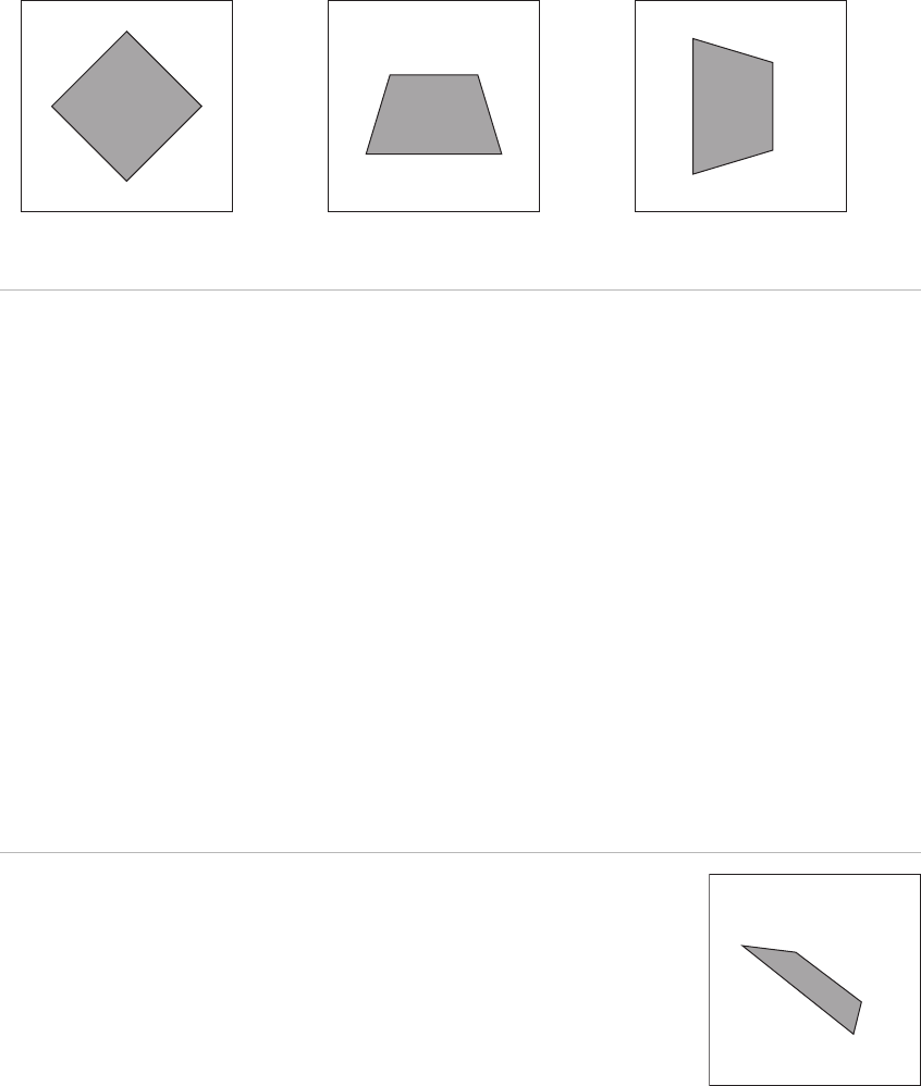
240 Learning Processing
e rotate functions can also be used in combination. e results of Example 14-9 are shown in Figure 14.20 .
Example 14-9: Rotate around more than one axis
void setup() {
size(200,200,P3D);
}
void draw() {
background(255);
stroke(0);
fill(175);
translate(width/2,height/2);
rotateX(PI*mouseY/height);
rotateY(PI*mouseX/width);
rectMode(CENTER);
rect(0,0,100,100);
}
Processing will also allow for rotation around the x or y -axis with the functions rotateX( ) and rotateY( ) ,
which each require P3D or OPENGL mode. e function rotateZ( ) also exists and is the equivalent of
rotate( ). See Examples 14-6, 14-7 and 14-8.
fi g. 14.20
Example 14-6: rotateZ Example 14-7: rotateX Example 14-8: rotateY
float theta = 0.0;
void setup() {
size(200,200,P3D);
}
void draw() {
background(255);
stroke(0);
fill(175);
translate(width/2,
height/2);
rotateZ(theta);
rectMode(CENTER);
rect(0,0,100,100);
theta + = 0.02;
}
float theta = 0.0;
void setup() {
size(200,200,P3D);
}
void draw() {
background(255);
stroke(0);
fill(175);
translate(width/2,
height/2);
rotateX(theta);
rectMode(CENTER);
rect(0,0,100,100);
theta + = 0.02;
}
float theta = 0.0;
void setup() {
size(200,200,P3D);
}
void draw() {
background(255);
stroke(0);
fill(175);
translate(width/2,
height/2);
rotateY(theta);
rectMode(CENTER);
rect(0,0,100,100);
theta + = 0.02;
}
fi g. 14.17 fi g. 14.19 fi g. 14.18

Translation and Rotation (in 3D!) 241
Returning to the pyramid example, we will see how rotating makes the three-dimensional quality of
the shape more apparent. e example is also expanded to include a second pyramid that is off set from
the fi rst pyramid using translate. Note, however, that it rotates around the same origin point as the fi rst
pyramid (since rotateX( ) and rotateY( ) are called before the second translate( ) ).
Example 14-10: Pyramid
float theta = 0.0;
void setup() {
size(200,200,P3D);
}
void draw() {
background(144);
theta + = 0.01;
translate(100,100,0);
rotateX(theta);
rotateY(theta);
drawPyramid(50);
// translate the scene again
translate(50,50,20);
// call the pyramid drawing function
drawPyramid(10);
}
void drawPyramid(int t) {
stroke(0);
// this pyramid has 4 sides, each drawn as a separate triangle
// each side has 3 vertices, making up a triangle shape
// the parameter "t" determines the size of the pyramid
fill(150,0,0,127);
beginShape(TRIANGLES);
vertex(–t,–t,–t);
vertex( t,–t,–t);
vertex( 0, 0, t);
fill(0,150,0,127);
vertex( t,–t,–t);
vertex( t, t,–t);
vertex( 0, 0, t);
fill(0,0,150,127);
vertex( t, t,–t);
vertex(–t, t,–t);
vertex( 0, 0, t);
fill(150,0,150,127);
vertex(–t, t,–t);
vertex(–t,–t,–t);
vertex( 0, 0, t);
endShape();
}
fi g. 14.21
242 Learning Processing
Exercise 14-7: Rotate the 3D cube you made in Exercise 14-5. Can you rotate it around the
corner or center? You can also use the Processing function box( ) to make the cube.
Exercise 14-8: Make a Pyramid class.
14.7 Scale
In addition to translate( ) and rotate( ) , there is one more function, scale( ) , that aff ects the way shapes
are oriented and drawn onscreen. scale( ) increases or decreases the size of objects onscreen. Just as with
rotate( ) , the scaling eff ect is performed relative to the origin’s location.
scale( ) takes a fl oating point value, a percentage at which to scale: 1.0 is 100%. For example, scale(0.5)
draws an object at 50% of its size and scale(3.0) increases the object’s size to 300%.
Following is a re-creation of Example 14-1 (the growing square) using scale( ) .
Example 14-11: A growing rectangle, using scale()
float r = 0.0;
void setup() {
size(200,200);
}
void draw() {
background(0);
// Translate to center of window
translate(width/2,height/2);
// Scale any shapes according to value of r
scale(r);
// Display a rectangle in the middle of the screen
stroke(255);
fill(100);
rectMode(CENTER);
rect(0,0,10,10);
// Increase the scale variable
r + = 0.02;
}
scale( ) can also take two arguments (for scaling along the x and y -axes with diff erent values) or three
arguments (for the x -, y -, and z -axes).
14.8 The Matrix: Pushing and Popping
What is the matrix?
In order to keep track of rotations and translations and how to display the shapes according to diff erent
transformations, Processing (and just about any computer graphics software) uses a matrix.
fi g. 14.22
scale() increases the dimensions
of an object relative to the origin
by a percentage (1.0 100%).
Notice how in this example the
scaling effect causes the outline
of the shape to become thicker.

Translation and Rotation (in 3D!) 243
is concept is best illustrated with an example. Let’s give ourselves an assignment: Create a Processing
sketch where two rectangles rotate at diff erent speeds in diff erent directions around their respective
centerpoints.
As we start developing this example, we will see where the problems arise and how we will need to
implement the functions pushMatrix( ) and popMatrix( ) .
Starting with essentially the same code from Section 14.4, we can rotate a square around the Z -axis in
the top left corner of the window. See Example 14-12.
Example 14-12: Rotating one square
float theta1 = 0;
void setup() {
size(200,200,P3D);
}
void draw() {
background (255);
stroke(0);
fill(175);
rectMode(CENTER);
translate(50,50);
rotateZ(theta1);
rect(0,0,60,60);
theta1 + = 0.02;
}
How matrix transformations work is beyond the scope of this book; however, it is useful to simply know
that the information related to the coordinate system is stored in what is known as a transformation
matrix. When a translation or rotation is applied, the transformation matrix changes. From time to time,
it is useful to save the current state of the matrix to be restored later. is will ultimately allow us to move
and rotate individual shapes without them aff ecting others.
fi g. 14.23
What is the matrix?
A matrix is a table of numbers with rows and columns. In Processing , a transformation matrix is used
to describe the window orientation —is it translated or rotated? You can view the current matrix at
any time by calling the function printMatrix( ) . is is what the matrix looks like in its “ normal ”
state, with no calls to translate( ) or rotate( ) .
1.0000 0.0000 0.0000
0.0000 1.0000 0.0000
244 Learning Processing
Making some minor adjustments, we now implement a rotating square in the bottom right-hand corner .
Example 14-13: Rotating another square
float theta2 = 0;
void setup() {
size(200,200,P3D);
}
void draw() {
background (255);
stroke(0);
fill(175);
rectMode(CENTER);
translate(150,150);
rotateY(theta2);
rect(0,0,60,60);
theta2 + = 0.02;
}
Without careful consideration, we might think to simply combine the two programs. e setup( ) function
would stay the same, we would incorporate two globals, theta1 and theta2, and call the appropriate
translation and rotation for each rectangle. We would also adjust translation for the second square from
translate(150,150) to translate(100,100) , since we have already translated to (50,50) with the fi rst square .
float theta1 = 0;
float theta2 = 0;
void setup() {
size(200,200,P3D);
}
void draw() {
background(255);
stroke(0);
fill(175);
rectMode(CENTER);
translate(50,50);
rotateZ(theta1);
rect(0,0,60,60);
theta1 + = 0.02;
translate(100,100);
rotateY(theta2);
rect(0,0,60,60);
theta2 + = 0.02;
}
fi g. 14.24
fi g. 14.25
This fi rst call to rotateZ() affects
all shapes drawn afterward. Both
squares rotate around the center
of the fi rst square.
Translation and Rotation (in 3D!) 245
Running this example will quickly reveal a problem. e fi rst (top left) square rotates around its center .
However, while the second square does rotate around its center, it also rotates around the fi rst square!
Remember, all calls to translate and rotate are relative to the coordinate system’s previous state. We need a
way to restore the matrix to its original state so that individual shapes can act independently.
Saving and restoring the rotation/translation state is accomplished with the functions pushMatrix( ) and
popMatrix( ) . To get started, let’s think of them as saveMatrix( ) and restoreMatrix( ) . (Note there are no
such functions.) Push save. Pop restore.
For each square to rotate on its own, we can write the following algorithm (with the new parts bolded).
1. Save the current transformation matrix. is is where we started, with (0,0) in the top left corner of
the window and no rotation.
2. Translate and rotate the fi rst rectangle.
3. Display the fi rst rectangle.
4. Restore matrix from Step 1 so that it isn’t aff ected by Steps 2 and 3!
5. Translate and rotate the second rectangle.
6. Display the second rectangle.
Rewriting our code in Example 14-14 gives the correct result as shown in Figure 14.26 .
Example 14-14: Rotating both squares
float theta1 = 0;
float theta2 = 0;
void setup() {
size(200,200,P3D);
}
void draw() {
background(255);
stroke(0);
fill(175);
rectMode(CENTER);
pushMatrix();
translate(50,50);
rotateZ(theta1);
rect(0,0,60,60);
popMatrix();
pushMatrix();
translate(150,150);
rotateY(theta2);
rect(0,0,60,60);
popMatrix();
theta1 + = 0.02;
theta2 + = 0.02;
}
fi g. 14.26
1
2
4
5
6
3
246 Learning Processing
Although technically not required, it is a good habit to place pushMatrix( ) and popMatrix( ) around
the second rectangle as well (in case we were to add more to this code). A nice rule of thumb when
starting is to use pushMatrix( ) and popMatrix( ) before and after translation and rotation for all shapes
so that they can be treated as individual entities. In fact, this example should really be object oriented,
with every object making its own calls to pushMatrix( ), translate( ), rotate( ) , and popMatrix( ) .
See Example 14-5 .
Example 14-15: Rotating many things using objects
// An array of Rotater objects
Rotater[] rotaters;
void setup() {
size(200,200);
rotaters = new Rotater[20];
// Rotaters are made randomly
for (int i = 0; i < rotaters.length; i + + ) {
rotaters[i] = new Rotater(random(width),random(height),random(–0.1,0.1),random(48));
}
}
void draw() {
background(255);
// All Rotaters spin and are displayed
for (int i = 0; i < rotaters.length; i + + ) {
rotaters[i].spin();
rotaters[i].display();
}
}
// A Rotater class
class Rotater {
float x,y; // x,y location
float theta; // angle of rotation
float speed; // speed of rotation
float w; // size of rectangle
Rotater(float tempX, float tempY, float tempSpeed, float tempW) {
x = tempX;
y = tempY;
theta = 0; // Angle is always initialized to 0
speed = tempSpeed;
w = tempW;
}
// Increment angle
void spin() {
theta + = speed;
}
// Display rectangle
void display() {
rectMode(CENTER);
stroke(0);
fi g. 14.27
Translation and Rotation (in 3D!) 247
fill(0,100);
// Note the use of pushMatrix()
// and popMatrix() inside the object's
// display method!
pushMatrix();
translate(x,y);
rotate(theta);
rect(0,0,w,w);
popMatrix();
}
}
Interesting results can also be produced from nesting multiple calls to pushMatrix( ) and popMatrix( ).
ere must always be an equal amount of calls to both pushMatrix( ) and popMatrix( ), but they do not
always have to come one right after the other.
To understand how this works, let’s take a closer look at the meaning of “ push ” and “ pop. ” “ Push ” and
“ pop ” refer to a concept in computer science known as a stack. Knowledge of how a stack works will help
you use pushMatrix( ) and popMatrix( ) properly.
A stack is exactly that: a stack. Consider an English teacher getting settled in for a night of grading
papers stored in a pile on a desk, a stack of papers. e teacher piles them up one by one and reads them
in reverse order of the pile. e fi rst paper placed on the stack is the last one read. e last paper added
is the fi rst one read. Note this is the exact opposite of a queue. If you are waiting in line to buy tickets
to a movie, the fi rst person in line is the fi rst person to get to buy tickets, the last person is the last. See
Figure 14.28 .
INBOX
STACK
First one
out
First one
in
QUEUE
First one in & out
Tickets
fi g. 14.28
Pushing refers to the process of putting something in the stack, popping to taking something out. is
is why you must always have an equal number of pushMatrix( ) and popMatrix( ) calls. You can’t pop
something if it does not exist! (If you have an incorrect number of pushes and pops, Processing will say:
“ Too many calls to popMatrix() (and not enough to pushMatrix). ”
Using the rotating squares program as a foundation, we can see how nesting pushMatrix( ) and
popMatrix( ) is useful. e following sketch has one circle in the center (let’s call it the sun) with another
circle rotating it (let’s call it earth) and another two rotating around it (let’s call them moon #1 and
moon #2).
pushMatrix() and popMatrix() are called
inside the class’ display() method. This
way, every Rotater object is rendered
with its own independent translation
and rotation!
248 Learning Processing
Example 14-16: Simple solar system
// Angle of rotation around sun and planets
float theta = 0;
void setup() {
size(200,200);
smooth();
}
void draw() {
background(255);
stroke(0);
// Translate to center of window
// to draw the sun.
translate(width/2,height/2);
fill(255,200,50);
ellipse(0,0,20,20);
// The earth rotates around the sun
pushMatrix();
rotate(theta);
translate(50,0);
fill(50,200,255);
ellipse(0,0,10,10);
// Moon #1 rotates around the earth
pushMatrix();
rotate(–theta*4);
translate(15,0);
fill(50,255,200);
ellipse(0,0,6,6);
popMatrix();
// Moon #2 also rotates around the earth
pushMatrix();
rotate(theta*2);
translate(25,0);
fill(50,255,200);
ellipse(0,0,6,6);
popMatrix();
popMatrix();
theta + = 0.01;
}
pushMatrix( ) and popMatrix( ) can also be nested inside for or while loops with rather unique and
interesting results. e following example is a bit of a brainteaser, but I encourage you to play around
with it .
fi g. 14.29
pushMatrix() is called to save the transformation
state before drawing moon #1. This way we can
pop and return to earth before drawing moon #2.
Both moons rotate around the earth (which itself
is rotating around the sun).
Translation and Rotation (in 3D!) 249
Example 14-17: Nested push and pop
// Global angle for rotation
float theta = 0;
void setup() {
size(200, 200);
smooth();
}
void draw() {
background(100);
stroke(255);
// Translate to center of window
translate(width/2,height/2);
// Loop from 0 to 360 degrees (2*PI radians)
for(float i = 0; i < TWO_PI; i + = 0.2) {
// Push, rotate and draw a line!
pushMatrix();
rotate(theta + i);
line(0,0,100,0);
// Loop from 0 to 360 degrees (2*PI radians)
for(float j = 0; j < TWO_PI; j + = 0.5) {
// Push, translate, rotate and draw a line!
pushMatrix();
translate(100,0);
rotate(–theta–j);
line(0,0,50,0);
// We're done with the inside loop, pop!
popMatrix();
}
// We're done with the outside loop, pop!
popMatrix();
}
endShape();
// Increment theta
theta + = 0.01;
}
Exercise 14-9: Take either your pyramid or your cube shape and make it into a class. Have
each object make its own call to pushMatrix( ) and popMatrix( ) . Can you make an array
of objects all rotating independently in 3D?
14.9 A Processing Solar System
Using all the translation, rotation, pushing, and popping techniques in this chapter, we are ready to build
a Processing solar system. is example will be an updated version of Example 14-16 in the previous
section (without any moons), with two major changes:
• Every planet will be an object, a member of a Planet class.
• An array of planets will orbit the sun.
fi g. 14.30
The transformation state is saved
at the beginning of each cycle
through the for loop and restored
at the end. Try commenting out
these lines to see the difference!
250 Learning Processing
Example 14-18: Object-oriented solar system
// An array of 8 planet objects
Planet[] planets = new Planet[8];
void setup() {
size(200,200);
smooth();
// The planet objects are initialized using the counter variable
for (int i = 0; i < planets.length; i + + ) {
planets[i] = new Planet(20 + i*10,i + 8);
}
}
void draw() {
background(255);
// Drawing the Sun
pushMatrix();
translate(width/2,height/2);
stroke(0);
fill(255);
ellipse(0,0,20,20);
// Drawing all Planets
for (int i = 0; i < planets.length; i + + ) {
planets[i].update();
planets[i].display();
}
popMatrix();
}
class Planet {
float theta; // Rotation around sun
float diameter; // Size of planet
float distance; // Distance from sun
float orbitspeed; // Orbit speed
Planet(float distance_, float diameter_) {
distance = distance_;
diameter = diameter_;
theta = 0;
orbitspeed = random(0.01,0.03);
}
void update() {
// Increment the angle to rotate
theta + = orbitspeed;
}
void display() {
pushMatrix();
rotate(theta); // rotate orbit
translate(distance,0); // translate out distance
fi g. 14.31
Each planet object keeps track
of its own angle of rotation.
Before rotation and translation,
the state of the matrix is saved
with pushMatrix().
Translation and Rotation (in 3D!) 251
stroke(0);
fill(175);
ellipse(0,0,diameter,diameter);
// Afer we are done, restore matrix!
popMatrix();
}
}
Exercise 14-10: How would you add moons to the planets? Hint: Write a Moon class that
is virtually identical to the Planet. en, incorporate a Moon variable into the Planet class.
(In Chapter 22, we will see how this could be made more effi cient with advanced OOP
techniques.)
Exercise 14-11: Extend the solar system example into three dimensions. Try using sphere( )
or box( ) instead of ellipse( ) . Note sphere( ) takes one argument, the sphere’s radius. box( ) can
take one argument (size, in the case of a cube) or three arguments (width, height, and depth.)
Once the planet is drawn, the matrix
is restored with popMatrix() so that
the next planet is not affected.

252 Learning Processing
Lesson Six Project
Create a virtual ecosystem. Make a class for each “ creature ” in your world. Using
the techniques from Chapters 13 and 14, attempt to infuse your creatures with
personality. Some possibilities:
• Use Perlin noise to control the movements of creatures.
• Make the creatures look like they are breathing with oscillation.
• Design the creatures using recursion.
• Design the custom polygons using beginShape( ) .
• Use rotation in the creatures ’ behaviors.
Use the space provided below to sketch designs, notes, and pseudocode for your
project.

Lesson Seven
Pixels Under a Microscope
15 Images
16 Video
This page intentionally left blank

Images 255
15 Images
“ Politics will eventually be replaced by imagery. e politician will be only too happy to abdicate in favor
of his image, because the image will be much more powerful than he could ever be. ”
—Marshall McLuhan
“ When it comes to pixels, I think I’ve had my fi ll. ere are enough pixels in my fi ngers and brains that
I probably need a few decades to digest all of them. ”
—John Maeda
In this chapter:
– The PImage class.
– Displaying images.
– Changing image color.
– The pixels of an image.
– Simple image processing.
– Interactive image processing.
A digital image is nothing more than data—numbers indicating variations of red, green, and blue at
a particular location on a grid of pixels. Most of the time, we view these pixels as miniature rectangles
sandwiched together on a computer screen. With a little creative thinking and some lower level
manipulation of pixels with code, however, we can display that information in a myriad of ways. is
chapter is dedicated to breaking out of simple shape drawing in Processing and using images (and their
pixels) as the building blocks of Processing graphics.
15.1 Getting Started with Images
By now, we are quite comfortable with the idea of data types. We specify them often—a fl oat variable
called speed , an int named x , perhaps even a char entitled letterGrade . ese are all primitive data types,
bits sitting in the computer’s memory ready for our use. ough perhaps a bit trickier, we are also
beginning to feel at ease with objects, complex data types that store multiple pieces of data (along with
functionality)—our Zoog class, for example, included fl oating point variables for location, size, and
speed as well as methods to move, display itself, and so on. Zoog,
of course, is a user-defi ned class; we brought Zoog into this
programming world, defi ning what it means to be a Zoog, and
defi ning the data and functions associated with a Zoog object.
In addition to user-defi ned objects, Processing has a bunch of
handy classes all ready to go without us writing any code. (Later,
in Chapter 23, we will fi nd out that we also have access to a vast
library of Java classes.) e fi rst Processing- defi ned class we will
examine is PImage, a class for loading and displaying an image such
as the one shown in Figure 15.1 . fi g. 15.1
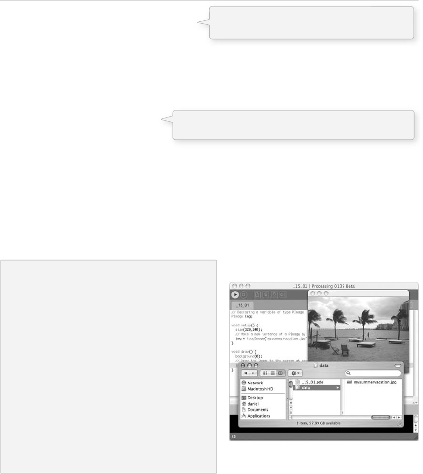
256 Learning Processing
Example 15-1: “ Hello World ” images
// Declaring a variable of type PImage
PImage img;
void setup() {
size(320,240);
// Make a new instance of a PImage by loading an image file
img = loadImage( " mysummervacation.jpg " );
}
void draw() {
background(0);
image(img,0,0);
}
Using an instance of a PImage object is no diff erent than using a user-defi ned class. First, a variable of
type PImage , named “ img, ” is declared. Second, a new instance of a PImage object is created via the
loadImage( ) method. loadImage( ) takes one argument, a String ( Strings are explored in greater detail in
Chapter 17) indicating a fi le name, and loads the that fi le into memory. loadImage( ) looks for image fi les
stored in your Processing sketch’s data folder.
e Data Folder: How do I get there?
Images can be added to the data folder
automatically via:
Sketch → Add File…
or manually:
Sketch → Show Sketch Folder
is will open up the sketch folder as shown in
Figure 15.2. If there is no data directory, create
one. Otherwise, place your image fi les inside.
Processing accepts the following fi le formats for
images: GIF, JPG, TGA, and PNG. fi g. 15.2
In Example 15-1, it may seem a bit peculiar that we never called a “ constructor ” to instantiate the PImage
object, saying “ new PImage( ) ” . After all, in all the object-related examples to date, a constructor is a must
for producing an object instance.
Spaceship ss = new Spaceship();
Flower flr = new Flower(25);
Declaring a variable of type PImage, a class
available to us from the Processing core library.
The image() function displays the image at a location—in
this case the point (0,0).

Images 257
And yet:
PImage img = loadImage( "file.jpg");
In fact, the loadImage( ) function performs the work of a constructor, returning a brand new instance of
a PImage object generated from the specifi ed fi lename. We can think of it as the PImage constructor for
loading images from a fi le. For creating a blank image, the createImage( ) function is used.
// Create a blank image, 200 X 200 pixels with RGB color
PImage img = createImage(200,200,RGB);
We should also note that the process of loading the image from the hard drive into memory is a slow one,
and we should make sure our program only has to do it once, in setup( ) . Loading images in draw( ) may
result in slow performance, as well as “ Out of Memory ” errors.
Once the image is loaded, it is displayed with the image( ) function. e image( ) function must include
three arguments—the image to be displayed, the x location, and the y location. Optionally, two arguments
can be added to resize the image to a certain width and height.
image(img,10,20,90,60);
Exercise 15-1: Load and display an image. Control the image’s width and height with
the mouse.
15.2 Animation with an Image
From here, it is easy to see how you can use images to further develop examples from previous chapters.
Example 15-2: Image “ sprite ”
PImage head; // A variable for the image file
float x,y; // Variables for image location
float rot; // A variable for image rotation
void setup() {
size(200,200);
// load image, initialize variables
head = loadImage( "face.jpg");
x = 0.0f;
y = width/2.0f;
rot = 0.0f;
}
void draw() {
background(255);
// Translate and rotate
translate(x,y);
rotate(rot);
image(head,0,0); // Draw image
fi g. 15.3
Images can be animated just like regular shapes
using variables, translate(), rotate(), and so on.

258 Learning Processing
class Head {
________ // A variable for the image file
________ // Variables for image location
________ // A variable for image rotation
Head(String filename, ________, ________) {
// Load image, initialize variables
________ = loadImage(________);
__________________________________
__________________________________
__________________________________
}
void display() {
__________________________________
__________________________________
__________________________________
}
void move() {
__________________________________
__________________________________
__________________________________
__________________________________
__________________________________
__________________________________
}
}
// Adjust variables to create animation
x + = 1.0;
rot + = 0.01;
if (x > width) {
x = 0;
}
}
Exercise 15-2: Rewrite this example in an object-oriented fashion where the data for the
image, location, size, rotation, and so on is contained in a class. Can you have the class swap
images when it hits the edge of the screen?
String is also a class
we get for free and
will be explored
further in Chapter 17.
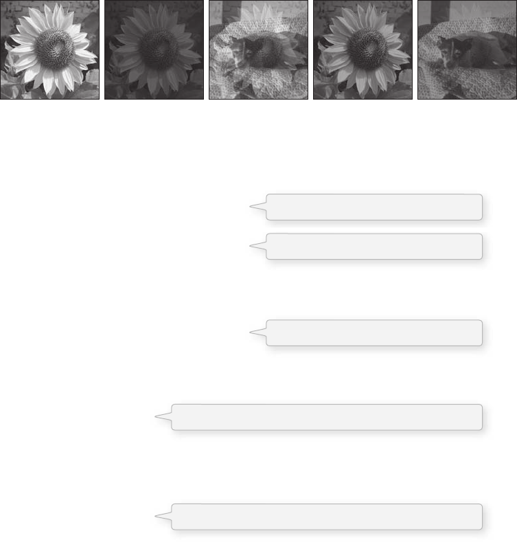
Images 259
If tint( ) receives one argument, only the brightness of the image is aff ected.
tint(255);
image(sunflower,0,0);
tint(100);
image(sunflower,0,0);
A second argument will change the image’s alpha transparency.
tint(255,127);
image(sunflower,0,0);
ree arguments aff ect the brightness of the red, green, and blue components of each color.
tint(0,200,255)
image(sunflower,0,0);
Finally, adding a fourth argument to the method manipulates the alpha (same as with two arguments).
Incidentally, the range of values for tint( ) can be specifi ed with colorMode( ) (see Chapter 1).
tint(255,0,0,100);
image(sunflower,0,0);
ABCDE
fi g. 15.4
15.3 My Very First Image Processing Filter
Every now and then, when displaying an image, we choose to alter its appearance. Perhaps we would like
the image to appear darker, transparent, bluish, and so on. is type of simple image fi ltering is achieved
with Processing ’ s tint( ) function. tint( ) is essentially the image equivalent of shape’s fi ll( ) , setting the color
and alpha transparency for displaying an image on screen. An image, nevertheless, is not usually all one
color. e arguments for tint( ) simply specify how much of a given color to use for every pixel of that
image, as well as how transparent those pixels should appear.
For the following examples, we will assume that two images (a sunfl ower and a dog) have been loaded
and the dog is displayed as the background (which will allow us to demonstrate transparency). See Figure
15.4 . For color versions of these images visit: http://www.learningprocessing.com )
PImage sunflower = loadImage( "sunflower.jpg");
PImage dog = loadImage( "dog.jpg");
background(dog);
A The image retains its original state.
B The image appears darker.
C The image is at 50% opacity.
D None of it is red, most of it is green, and all of it is blue.
E The image is tinted red and transparent.

260 Learning Processing
Exercise 15-3: Display an image using tint( ) . Use the mouse location to control the amount
of red, green, and blue tint. Also try using the distance of the mouse from the corners or center.
Exercise 15-4: Using tint( ) , create a montage of blended images. What happens when you
layer a large number of images, each with diff erent alpha transparency, on top of each other?
Can you make it interactive so that diff erent images fade in and out?
15.4 An Array of Images
One image is nice, a good place to start. It will not be long, however, until the temptation of using many
images takes over. Yes, we could keep track of multiple images with multiple variables, but here is a
magnifi cent opportunity to rediscover the power of the array. Let’s assume we have fi ve images and want
to display a new background image each time the user clicks the mouse.
First, we set up an array of images, as a global variable.
// Image Array
PImage[] images = new PImage[5];
Second, we load each image fi le into the appropriate location in the array. is happens in setup( ) .
// Loading Images into an Array
images[0] = loadImage( " cat.jpg " );
images[1] = loadImage( " mouse.jpg " );
images[2] = loadImage( " dog.jpg " );
images[3] = loadImage( " kangaroo.jpg " );
images[4] = loadImage( " porcupine.jpg " );
Of course, this is somewhat awkward. Loading each image individually is not terribly elegant. With fi ve
images, sure, it is manageable, but imagine writing the above code with 100 images. One solution is to
store the fi lenames in a String array and use a for statement to initialize all the array elements.
// Loading Images into an Array from an array of fi lenames
String[] fi lenames = { "cat.jpg " , " mouse.jpg" , " dog.jpg " , " kangaroo.jpg " , " porcupine.jpg " );
for (int i = 0; i < fi lenames.length; i + + ) {
images[i] = loadImage(fi lenames[i]);
}
Concatenation: A New Kind of Addition
Usually, a plus sign () means, add. 2 2 4, right?
With text (as stored in a String, enclosed in quotes), means concatenate, that is, join two Strings
together.
“Happy” “ Trails” “Happy Trails”
“2” “2” “22”
See more about Strings in Chapter 17.
Images 261
Even better, if we just took a little time out of our hectic schedules to plan ahead, numbering the image
fi les ( “ animal1.jpg ” , “ animal2.jpg ” , “ animal3.jpg ” , etc.), we can really simplify the code:
// Loading images with numbered files
for (int i = 0; i < images.length; i + + ){
images[i] = loadImage( "animal" + i + ".jpg");
}
Once the images are loaded, it’s on to draw( ) . ere, we choose to display one particular image, picking
from the array by referencing an index ( “ 0 ” below).
image(images[0],0,0);
Of course, hard-coding the index value is foolish. We need a variable in order to dynamically display a
diff erent image at any given moment in time.
image(images[imageindex],0,0);
e “ imageindex ” variable should be declared as a global variable (of type integer). Its value can be
changed throughout the course of the program. e full version is shown in Example 15-3.
Example 15-3: Swapping images
int maxImages = 10; // Total # of images
int imageIndex = 0; // Initial image to be displayed is the first
PImage[] images = new PImage[maxImages]; // The image array
void setup() {
size(200,200);
// Loading the images into the array
// Don't forget to put the JPG files in the data folder!
for (int i = 0; i < images.length; i + + ){
images[i] = loadImage( "animal" + i + ".jpg");
}
}
void draw() {
image(images[imageIndex],0,0); // Displaying one image
}
void mousePressed() {
// A new image is picked randomly when the mouse is clicked
// Note the index to the array must be an integer!
imageIndex = int(random(images.length));
}
To play the images in sequence as an animation, follow Example 15-4.
Example 15-4: Image sequence
void draw() {
background(0);
image(images[imageIndex],0,0);
// increment image index by one each cycle
// use modulo "%" to return to 0 once the size
//of the array is reached
imageIndex = (imageIndex + 1) % images.length;
}
Displaying one image
from the array.
Declaring an array of
images.
Loading an array of
images.
Picking a new image
to display by changing
the index variable!
Remember modulus? The % sign?
It allows us to cycle a counter back
to 0. See Chapter 13 for a review.
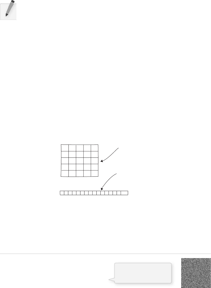
262 Learning Processing
Take the following example. is sketch sets each pixel in a window to a random grayscale value. e
pixels array is just like an other array, the only diff erence is that we do not have to declare it since it is a
Processing built-in variable.
Example 15-5: Setting pixels
size(200,200);
// Before we deal with pixels
loadPixels();
// Loop through every pixel
for (int i = 0; i < pixels.length; i + + ) {
// Pick a random number, 0 to 255
float rand = random(255);
Exercise 15-5: Create multiple instances of an image sequence onscreen. Have them start
at diff erent times within the sequence so that they are out of sync. Hint: Use object-oriented
programming to place the image sequence in a class.
15.5 Pixels, Pixels, and More Pixels
If you have been diligently reading this book in precisely the prescribed order, you will notice that so
far, the only off ered means for drawing to the screen is through a function call. “ Draw a line between
these points ” or “ Fill an ellipse with red ” or “ load this JPG image and place it on the screen here. ” But
somewhere, somehow, someone had to write code that translates these function calls into setting the
individual pixels on the screen to refl ect the requested shape. A line does not appear because we say line( ) ,
it appears because we color all the pixels along a linear path between two points. Fortunately, we do not
have to manage this lower-level-pixel-setting on a day-to-day basis. We have the developers of Processing
(and Java) to thank for the many drawing functions that take care of this business.
Nevertheless, from time to time, we do want to break out of our mundane shape drawing existence and
deal with the pixels on the screen directly. Processing provides this functionality via the pixels array.
We are familiar with the idea of each pixel on the screen having an X and Y position in a two-
dimensional window. However, the array pixels has only one dimension, storing color values in linear
sequence. See Figure 15.5 .
01234How the pixels look
How the pixels
are stored.
56789
10 11 12 13 14
15 16 17 18 19
20 21 22 23 24
0123456789...
fi g. 15.5
fi g. 15.6
We can get the length of
the pixels array just like
with any array.
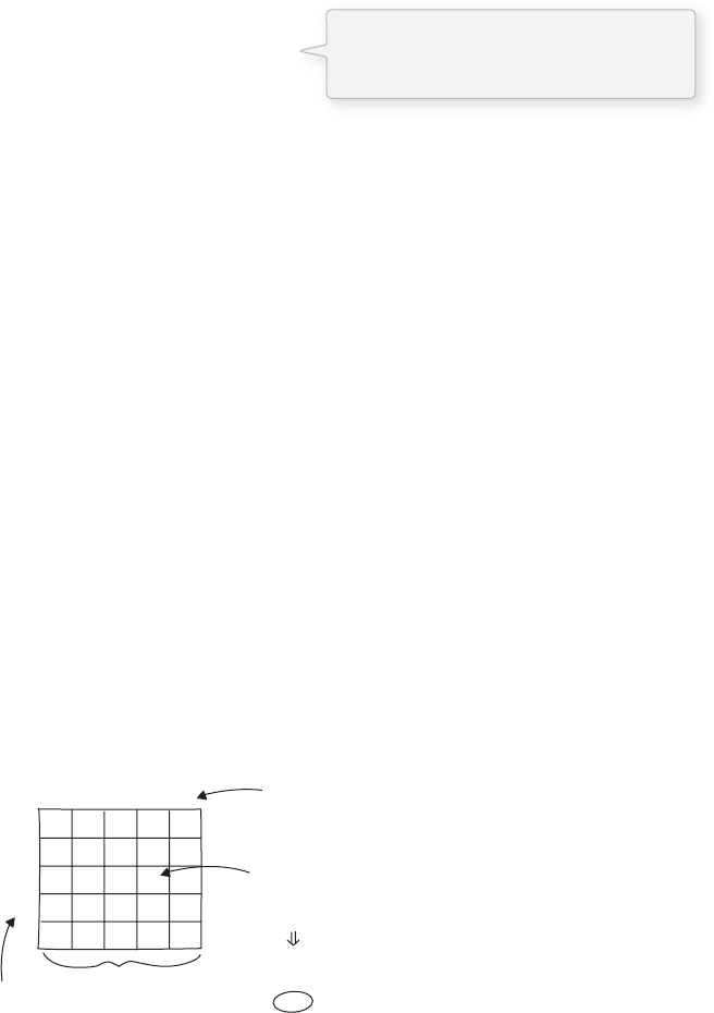
Images 263
is may remind you of two-dimensional arrays in Chapter 13. In fact, we will need to use the same
nested for loop technique. e diff erence is that, although we want to use for loops to think about the
pixels in two dimensions, when we go to actually access the pixels, they live in a one-dimensional array,
and we have to apply the formula from Figure 15.7 .
Let’s look at how it is done, completing the even/odd column problem. See Figure 15.8 .
// Create a grayscale color based on random number
color c = color(rand);
// Set pixel at that location to random color
pixels[i] = c;
}
// When we are finished dealing with pixels
updatePixels();
First, we should point out something important in the above example. Whenever you are accessing the pixels of
a Processing window, you must alert Processing to this activity. is is accomplished with two functions:
• loadPixels( ) —This function is called before you access the pixel array, saying “ load the pixels, I would
like to speak with them! ”
• updatePixels( ) —This function is called after you finish with the pixel array, saying “ Go ahead and
update the pixels, I’m all done! ”
In Example 15-5, because the colors are set randomly, we did not have to worry about where the pixels
are onscreen as we access them, since we are simply setting all the pixels with no regard to their relative
location. However, in many image processing applications, the XY location of the pixels themselves is
crucial information. A simple example of this might be, set every even column of pixels to white and
every odd to black. How could you do this with a one-dimensional pixel array? How do you know what
column or row any given pixel is in?
When programming with pixels, we need to be able to think of every pixel as living in a two-dimensional
world, but continue to access the data in one dimension (since that is how it is made available to us). We
can do this via the following formula:
1 . Assume a window or image with a given WIDTH and HEIGHT.
2 . We then know the pixel array has a total number of elements equaling WIDTH * HEIGHT.
3 . For any given X , Y point in the window, the location in our one-dimensional pixel array is:
LOCATION X Y * WIDTH
01234
01234Columns
56789
10 11 12 13 14
15 16 17 18 19
20 21 22 23 24
0
1
2
3
4
Pixel 13 is in Column 3, row 2.
width = 5
x + y * width
3 + 2 * 5
3 + 10
13
rows
fi g. 15.7
We can access individual elements of
the pixels array via an index, just like
with any other array.
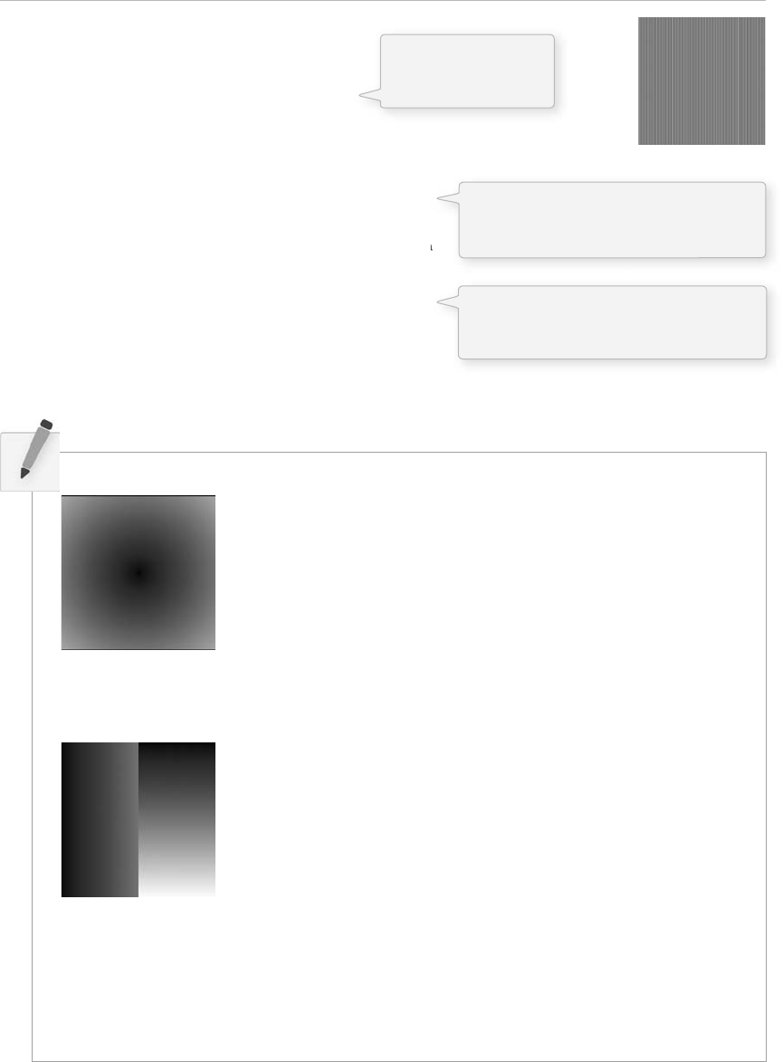
264 Learning Processing
Exercise 15-6: Complete the code to match the corresponding screenshots.
Example 15-6: Setting pixels according to their 2D location
size(200,200);
loadPixels();
// Loop through every pixel column
for (int x = 0; x < width; x + + ) {
// Loop through every pixel row
for (int y = 0; y < height; y + + ) {
// Use the formula to find the 1D location
int loc = x + y * width;
if (x % 2 = = 0) { // If we are an even column
pixels[loc] = color(255);
} else { // If we are an odd column
pixels[loc] = color(0);
}
}
}
updatePixels();
fi g. 15.8
The location in the pixel array is
calculated via our formula: 1D pixel
location xy * width
size(255,255);
___________________;
for (int x = 0; x < width; x + + ){
for (int y = 0; y < height; y + + ){
int loc = ___________________;
float distance = ___________________);
pixels[loc] = ___________________;
}
}
___________________;
size(255,255);
___________________;
for (int x = 0; x < width; x + + ){
for (int y = 0; y < height; y + + ){
___________________;
if (___________________) {
___________________;
} else {
___________________;
}
}
}
___________________;
Two loops allow us to
visit every column (x)
and every row (y).
We use the column number (x) to
determine whether the color should be
black or white.
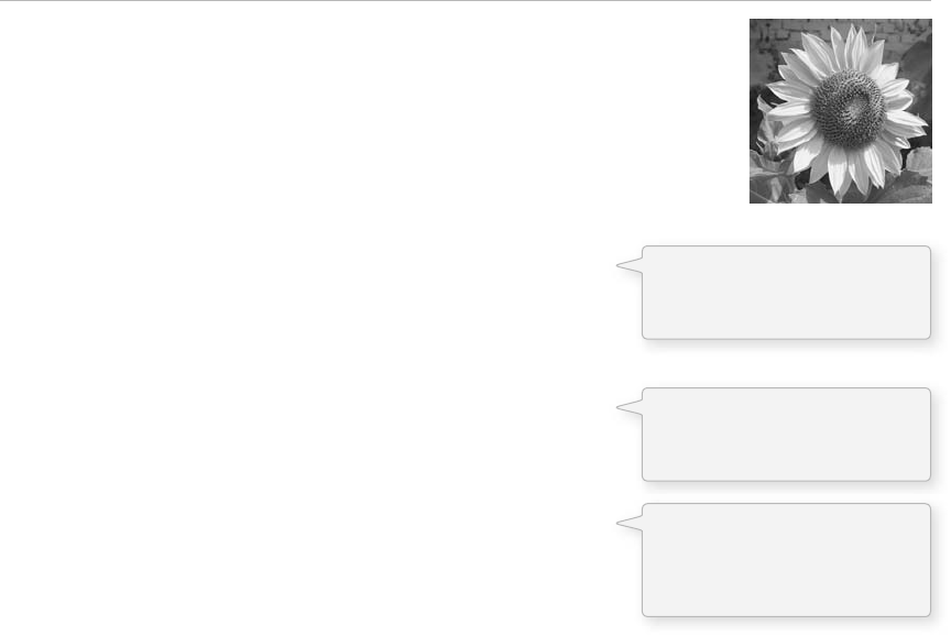
Images 265
15.6 Intro to Image Processing
e previous section looked at examples that set pixel values according to an arbitrary calculation. We will
now look at how we might set pixels according to those found in an existing PImage object. Here is some
pseudocode.
1. Load the image fi le into a PImage object.
2. For each pixel in the PImage, retrieve the pixel’s color and set the display pixel to that color.
e PImage class includes some useful fi elds that store data related to the image—width, height, and
pixels. Just as with our user-defi ned classes, we can access these fi elds via the dot syntax.
PImage img = createImage(320,240,RGB); // Make a PImage object
println(img.width); // Yields 320
println(img.height); // Yields 240
img.pixels[0] = color(255,0,0); // Sets the first pixel of the image to red
Access to these fi elds allows us to loop through all the pixels of an image and display them onscreen.
Example 15-7: Displaying the pixels of an image
PImage img;
void setup() {
size(200,200);
img = loadImage( "sunflower.jpg");
}
void draw() {
loadPixels();
// Since we are going to access the image's pixels too
img.loadPixels();
for (int y = 0; y < height; y + + ){
for (int x = 0; x < width; x + + ){
int loc = x + y*width;
// Image Processing Algorithm would go here
float r = red (img.pixels [loc]);
float g = green(img.pixels[loc]);
float b = blue (imq.pixels[loc];
// Image Processing would go here
// Set the display pixel to the image pixel
pixels[loc] = color(r,g,b);
}
}
updatePixels();
}
Now, we could certainly come up with simplifi cations in order to merely display the image (e.g., the
nested loop is not required, not to mention that using the image( ) function would allow us to skip all this
fi g. 15.9
We must also call loadPixels()
on the PImage since we are
going to read its pixels.
The functions red(), green(),
and blue() pull out the three
color components from a pixel.
If we were to change the RGB
values, we would do it here,
before setting the pixel in the
display window.
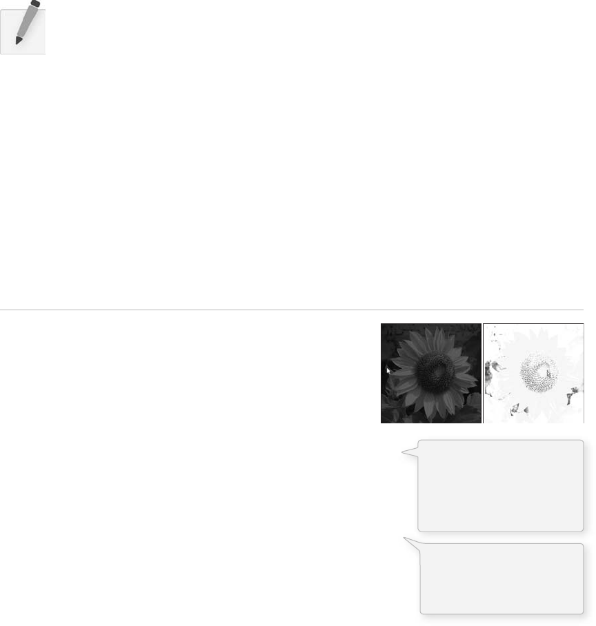
266 Learning Processing
pixel work entirely). However, Example 15-7 provides a basic framework for getting the red, green, and
blue values for each pixel based on its spatial orientation ( XY location); ultimately, this will allow us to
develop more advanced image processing algorithms.
Before we move on, I should stress that this example works because the display area has the same
dimensions as the source image. If this were not the case, you would simply need to have two pixel
location calculations, one for the source image and one for the display area.
int imageLoc = x + y*img.width;
int displayLoc = x + y*width;
Exercise 15-7: Using Example 15-7, change the values of r, g, and b before displaying them.
15.7 Our Second Image Processing Filter, Making Our Own Tint( )
Just a few paragraphs ago, we were enjoying a relaxing coding session, colorizing images and adding alpha
transparency with the friendly tint( ) method. For basic fi ltering, this method did the trick. e pixel
by pixel method, however, will allow us to develop custom algorithms for mathematically altering the
colors of an image. Consider brightness—brighter colors have higher values for their red, green, and blue
components. It follows naturally that we can alter the brightness of an image by increasing or decreasing
the color components of each pixel. In the next example, we dynamically increase or decrease those values
based on the mouse’s horizontal location. (Note that the next two examples include only the image
processing loop itself, the rest of the code is assumed.)
Example 15-8: Adjusting image brightness
for (int x = 0; x < img.width; x + + ){
for (int y = 0; y < img.height; y + + ){
// Calculate the 1D pixel location
int loc = x + y*img.width;
// Get the R,G,B values from image
float r = red (img.pixels[loc]);
float g = green (img.pixels[loc]);
float b = blue (img.pixels[loc]);
// Change brightness according to the mouse here
float adjustBrightness = ((float) mouseX / width) * 8.0;
r * = adjustBrightness;
g * = adjustBrightness;
b * = adjustBrightness;
// Constrain RGB to between 0-255
r = constrain(r,0,255);
g = constrain(g,0,255);
b = constrain(b,0,255);
// Make a new color and set pixel in the window
color c = color(r,g,b);
pixels[loc] = c;
}
}
fi g. 15.10
We calculate a multiplier
ranging from 0.0 to 8.0
based on mouseX position.
That multiplier changes the
RGB value of each pixel.
The RGB values are
constrained between 0 and
255 before being set as a
new color.
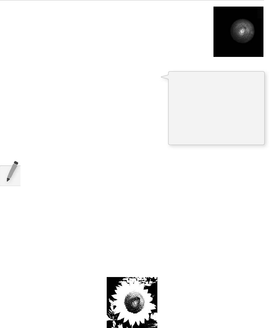
Images 267
Since we are altering the image on a per pixel basis, all pixels need not be treated equally. For example, we
can alter the brightness of each pixel according to its distance from the mouse.
Example 15-9: Adjusting image brightness based on pixel location
for (int x = 0; x < img.width; x + + ){
for (int y = 0; y < img.height; y + + ){
// Calculate the 1D pixel location
int loc = x + y*img.width;
// Get the R,G,B values from image
float r = red (img.pixels[loc]);
float g = green (img.pixels[loc]);
float b = blue (img.pixels[loc]);
// Calculate an amount to change brightness
// based on proximity to the mouse
float distance = dist(x,y,mouseX,mouseY);
float adjustBrightness = (50-distance)/50;
r * = adjustBrightness;
g * = adjustBrightness;
b * = adjustBrightness;
// Constrain RGB to between 0-255
r = constrain(r,0,255);
g = constrain(g,0,255);
b = constrain(b,o,255);
// Make a new color and set pixel in the window
color c = color(r,g,b);
pixels[loc] = c;
}
}
Exercise 15-8: Adjust the brightness of the red, green, and blue color components separately
according to mouse interaction. For example, let mouseX control red, mouseY green, distance
blue, and so on.
15.8 Writing to Another PImage Object’s Pixels
All of our image processing examples have read every pixel from a source image and written a new pixel
to the Processing window directly. However, it is often more convenient to write the new pixels to a
destination image (that you then display using the image( ) function). We will demonstrate this technique
while looking at another simple pixel operation: threshold .
A threshold fi lter displays each pixel of an image in only one of two states, black or white. at state is set
according to a particular threshold value. If the pixel’s brightness is greater than the threshold, we color the pixel
white, less than, black. Example 15-10 uses an arbitrary threshold of 100 .
fi g. 15.11
fi g. 15.12
The closer the pixel is to the mouse, the
lower the value of “distance” is. We want
closer pixels to be brighter, however, so we
invert the value with the formula:
adjustBrightness (50-distance)/50
Pixels with a distance of 50 (or greater)
have a brightness of 0.0 (or negative which
is equivalent to 0 here) and pixels with a
distance of 0 have a brightness of 1.0.
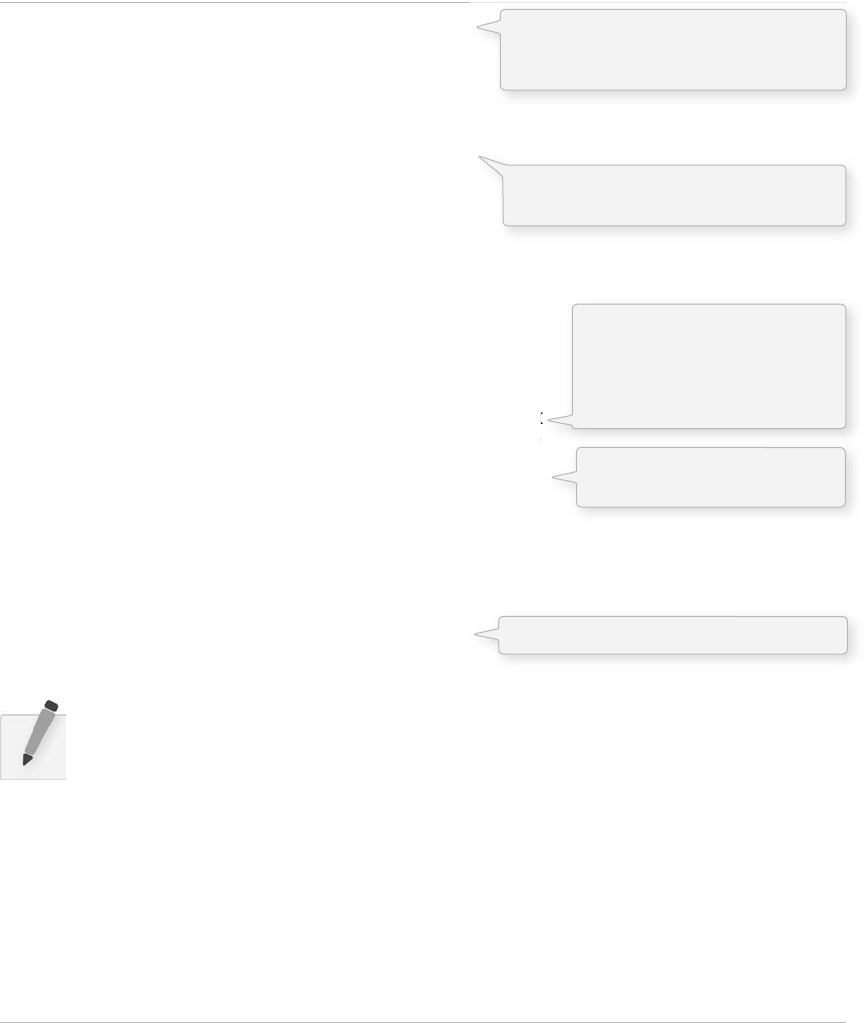
268 Learning Processing
Example 15-10: Brightness threshold
PImage source; // Source image
PImage destination; // Destination image
void setup() {
size(200,200);
source = loadImage( " sunflower.jpg " );
destination =
}
void draw() {
float threshold = 127;
// We are going to look at both image's pixels
source.loadPixels();
destination.loadPixels();
for (int x = 0; x < source.width; x + + ) {
for (int y = 0; y < source.height; y + + ) {
int loc = x + y*source.width;
// Test the brightness against the threshold
if (brightness(source.pixels[loc]) > threshold){
destination.pixels[loc] = color(255); // White
} else {
destination.pixels[loc] = color(0); // Black
}
}
}
// We changed the pixels in destination
destination.updatePixels();
// Display the destination
image(destination,0,0);
}
Exercise 15-9: Tie the threshold to mouse location.
is particular functionality is available without per pixel processing as part of Processing ’ s fi lter( )
function. Understanding the lower level code, however, is crucial if you want to implement your own
image processing algorithms, not available with fi lter( ) .
If all you want to do is threshold, Example 15-11 is much simpler.
Example 15-11: Brightness threshold with fi lter
// Draw the image
image(img,0,0);
// Filter the window with a threshold effect
// 0.5 means threshold is 50% brightness
filter(THRESHOLD,0.5);
We need two images, a source (original
fi le) and destination (to be displayed)
image.
The destination image is created as a
blank image the same size as the source.
Writing to the destination
image’s pixels.
brightness( ) returns a value
between 0 and 255, the overall
brightness of the pixel’s color. If
it is more than 100, make it white,
less than 100, make it black.
We have to display the destination image!
createImage(source.width, source.height, RGB);

Images 269
15.9 Level II: Pixel Group Processing
In previous examples, we have seen a one-to-one relationship between source pixels and destination
pixels. To increase an image’s brightness, we take one pixel from the source image, increase the RGB
values, and display one pixel in the output window. In order to perform more advanced image processing
functions, however, we must move beyond the one-to-one pixel paradigm into pixel group processing .
Let’s start by creating a new pixel out of two pixels from a source image—a pixel and its neighbor to the left.
If we know the pixel is located at ( x , y ):
int loc = x + y*img.width;
color pix = img.pixels[loc];
Then its left neighbor is located at ( x 1, y ):
int leftLoc = (x-1) + y*img.width;
color leftPix = img.pixels[leftLoc];
We could then make a new color out of the difference between the pixel and its neighbor to the left.
float diff = abs(brightness(pix) - brightness(leftPix));
pixels[loc] = color(diff);
Example 15-12 shows the full algorithm, with the results shown in Figure 15.13 .
Example 15-12: Pixel neighbor differences (edges)
// Since we are looking at left neighbors
// We skip the first column
for (int x = 1; x < width; x + + ){
for (int y = 0; y < height; y + + ){
// Pixel location and color
int loc = x + y*img.width;
color pix = img.pixels[loc];
// Pixel to the left location and color
int leftLoc = (x –1) + y*img.width;
color leftPix = img.pixels[leftLoc];
fi g. 15.13
More on fi lter( ):
fi lter(mode);
fi lter(mode,level);
e fi lter( ) function off ers a set of prepackaged fi lters for the display window. It is not necessary
to use a PImage, the fi lter will alter the look of whatever is drawn in the window at the time it is
executed. Other available modes besides THRESHOLD are GRAY, INVERT, POSTERIZE,
BLUR, OPAQUE, ERODE, and DILATE. See the Processing reference
( http://processing.org/reference/fi lter_.html ) for examples of each.
Reading the pixel to the left.
270 Learning Processing
ese image processing algorithms are often referred to as a “ spatial convolution. ” e process uses a
weighted average of an input pixel and its neighbors to calculate an output pixel. In other words, that new
pixel is a function of an area of pixels. Neighboring areas of diff erent sizes can be employed, such as a
3 3 matrix, 5 5, and so on.
Diff erent combinations of weights for each pixel result in various eff ects. For example, we “ sharpen ”
an image by subtracting the neighboring pixel values and increasing the centerpoint pixel. A blur is
achieved by taking the average of all neighboring pixels. (Note that the values in the convolution matrix
add up to 1.)
For example,
Sharpen:
– 1 – 1 – 1
– 1 9 – 1
– 1 – 1 – 1
Blur:
1/9 1/9 1/9
1/9 1/9 1/9
1/9 1/9 1/9
// New color is difference between pixel and left neighbor
float diff = abs(brightness(pix) - brightness(leftPix));
pixels[loc] = color(diff);
}
}
Example 15-12 is a simple vertical edge detection algorithm. When pixels diff er greatly from their
neighbors, they are most likely “ edge ” pixels. For example, think of a picture of a white piece of paper
on a black tabletop. e edges of that paper are where the colors are most diff erent, where white
meets black.
In Example 15-12, we look at two pixels to fi nd edges. More sophisticated algorithms, however, usually
involve looking at many more neighboring pixels. After all, each pixel has eight immediate neighbors: top
left, top, top right, right, bottom right, bottom, bottom left, and left. See Figure 15.14 .
its neighbor
(x+ 1, y+ 1)
its neighbor
(x 1, y)
a pixel
at
x,y
A pixel and its Friendly Neighbors
fi g. 15.14
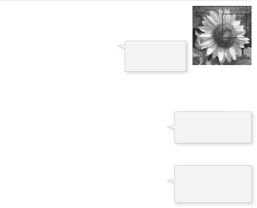
Images 271
Example 15-13 performs a convolution using a 2D array (see Chapter 13 for a review of 2D arrays) to
store the pixel weights of a 3 3 matrix. is example is probably the most advanced example we have
encountered in this book so far, since it involves so many elements (nested loops, 2D arrays, PImage
pixels, etc.).
Example 15-13: Sharpen with convolution
PImage img;
int w = 80;
// It's possible to perform a convolution
// the image with different matrices
float[][] matrix = { { – 1, – 1, – 1 },
{ – 1, 9, –1 },
{ – 1, – 1, –1 } ;
void setup() {
size(200,200);
img = loadImage( "sunflower.jpg");
}
void draw() {
// We're only going to process a portion of the image
// so let's set the whole image as the background first
image(img,0,0);
// Where is the small rectangle we will process
int xstart = constrain(mouseX-w/2,0,img.width);
int ystart = constrain(mouseY-w/2,0,img.height);
int xend = constrain(mouseX +
w/2,0,img.width);
int yend = constrain(mouseY + w/2,0,img.height);
int matrixsize = 3;
loadPixels();
// Begin our loop for every pixel
for (int x = xstart; x < xend; x + + ){
for (int y = ystart; y < yend; y + + ){
color c = convolution(x,y,matrix,matrixsize,img);
int loc = x + y*img.width;
pixels[loc] = c;
}
}
updatePixels();
stroke(0);
noFill();
rect(xstart,ystart,w,w);
}
color convolution(int x, int y, float[][] matrix, int matrixsize, PImage img) {
float rtotal = 0.0;
float gtotal = 0.0;
float btotal = 0.0;
int offset = matrixsize / 2;
// Loop through convolution matrix
for (int i = 0; i < matrixsize; i + + ){
for (int j = 0; j < matrixsize; j + + ) {
// What pixel are we testing
fi g. 15.15
The convolution matrix
for a “sharpen” effect
stored as a 3 3 two-
dimensional array.
In this example we are only
processing a section of the
image—an 80 80 rectangle
around the mouse location.
Each pixel location (x,y) gets
passed into a function called
convolution( ) which returns
a new color value to be
displayed.
}
272 Learning Processing
int xloc = x + i-offset;
int yloc = y + j-offset;
int loc = xloc + img.width*yloc;
// Make sure we haven't walked off the edge of the pixel array
loc = constrain(loc,0,img.pixels.length-1);
// Calculate the convolution
rtotal += (red(img.pixels[loc]) * matrix[i][j]);
gtotal += (green(img.pixels[loc]) * matrix[i][j]);
btotal += (blue(img.pixels[loc]) * matrix[i][j]);
}
}
// Make sure RGB is within range
rtotal = constrain(rtotal,0,255);
gtotal = constrain(gtotal,0,255);
btotal = constrain(btotal,0,255);
// Return the resulting color
return color(rtotal,gtotal,btotal);
}
}
Exercise 15-10: Try diff erent values for the convolution matrix.
Exercise 15-11: Using the framework established by our image processing examples, create
a fi lter that takes two images as input and generates one output image. In other words, each
pixel displayed should be a function of the color values from two pixels, one from one image
and one from another. For example, can you write the code to blend two images together
(without using tint( ) )?
15.10 Creative Visualization
You may be thinking: “ Gosh, this is all very interesting, but seriously, when I want to blur an image or
change its brightness, do I really need to write code? I mean, can’t I use Photoshop? ” Indeed, what we have
achieved here is merely an introductory understanding of what highly skilled programmers at Adobe do. e
power of Processing, however, is the potential for real-time, interactive graphics applications. ere is no need
for us to live within the confi nes of “ pixel point ” and “ pixel group ” processing.
Following are two examples of algorithms for drawing Processing shapes. Instead of coloring the shapes
randomly or with hard-coded values as we have in the past, we select colors from the pixels of a PImage
object. e image itself is never displayed; rather, it serves as a database of information that we can exploit
for our own creative pursuits.
In this fi rst example, for every cycle through draw( ) , we fi ll one ellipse at a random location onscreen
with a color taken from its corresponding location in the source image. e result is a “ pointillist-like ”
eff ect. See Figure 15.16 .
It is often good when looking at
neighboring pixels to make sure
we have not gone off the edge
of the pixel array by accident.
We sum all the neighboring pixels multiplied by
the values in the convolution matrix.
After the sums are constrained within a range of
0–255, a new color is made and returned.
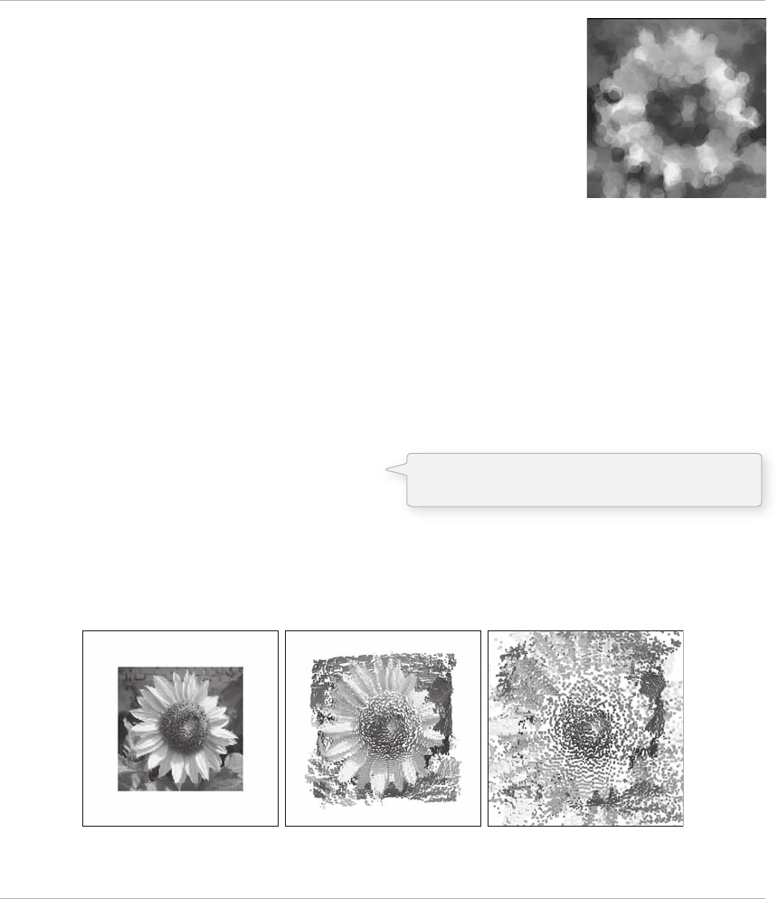
Images 273
Example 15-14: “ Pointillism ”
PImage img;
int pointillize = 16;
void setup() {
size(200,200);
img = loadImage( "sunflower.jpg");
background(0);
smooth();
}
void draw() {
// Pick a random point
int x = int(random(img.width));
int y = int(random(img.height));
int loc = x + y*img.width;
// Look up the RGB color in the source image
loadPixels();
float r = red(img.pixels[loc]);
float g = green(img.pixels[loc]);
float b = blue(img.pixels[loc]);
noStroke();
// Draw an ellipse at that location with that color
fill(r,g,b,100);
ellipse(x,y,pointillize,pointillize);
}
In this next example, we take the data from a two-dimensional image and, using the 3D translation
techniques described in Chapter 14, render a rectangle for each pixel in three-dimensional space. e
z location is determined by the brightness of the color. Brighter colors appear closer to the viewer and
darker ones further away.
fi g. 15.17
fi g. 15.16
Example 15-15: 2D image mapped to 3D
PImage img; // The source image
int cellsize = 2; // Dimensions of each cell in the grid
int cols, rows; // Number of columns and rows in our system
void setup() {
size(200,200,P3D);
Back to shapes! Instead of setting a pixel, we
use the color from a pixel to draw a circle.
274 Learning Processing
img = loadImage( " sunflower.jpg " ); // Load the image
cols = width/cellsize; // Calculate # of columns
rows = height/cellsize; // Calculate # of rows
}
void draw() {
background(0);
loadPixels();
// Begin loop for columns
for (int i = 0; i < cols; i + + ) {
// Begin loop for rows
for (int j = 0; j < rows; j + + ) {
int x = i*cellsize + cellsize/2; // x position
int y = j*cellsize + cellsize/2; // y position
int loc = x + y*width; // Pixel array location
color c = img.pixels[loc]; // Grab the color
// Calculate a z position as a function of mouseX and pixel brightness
float z = (mouseX/(float)width) * brightness(img.pixels[loc])- 100.0;
// Translate to the location, set fill and stroke, and draw the rect
pushMatrix();
translate(x,y,z);
fill(c);
noStroke();
rectMode(CENTER);
rect(0,0,cellsize,cellsize);
popMatrix();
}
}
}
Exercise 15-12: Create a sketch that uses shapes to display a pattern that covers an entire
window. Load an image and color the shapes according to the pixels of that image.
e following image, for example, uses triangles.
Az value for 3D translation is calculated as a function
of the pixel’s brightness as well as mouse location.
Video 275
16 Video
“ I have no memory. It’s like looking in a mirror and seeing nothing but mirror. ”
—Alfred Hitchcock
In this chapter:
– Displaying live video.
– Displaying recorded video.
– Creating a software mirror.
– How to use a video camera as a sensor.
16.1 Before Processing
Now that we have explored static images in Processing , we are ready to move on to moving images,
specifi cally from a live camera (and later, from a recorded movie). Using a digital video camera connected
to a PC or Mac requires a few simple steps before any code can be written.
On a Mac:
• Attach a camera to your computer.
• Make sure any necessary software and drivers for the camera are installed.
• Test the camera in another program, such as iChat, to make sure it is working.
On a PC:
• Attach a camera to your computer.
• Make sure any necessary software and drivers for the camera are installed.
• Test the camera. (Use whatever software that came with your camera that allows you to view the
video stream.)
• Install QuickTime (version 7 or higher). If you are using a previous version of QuickTime, you must
make sure you choose “ custom ” installation and select “ QuickTime for Java. ”
• You will also need to install a vdig (video digitizer) that allows QuickTime applications (what we
are creating) to capture video in Windows. The vdig situation is in flux so I recommend you check
this book’s web site for updates. Although no longer being developed, a free vdig is available at
this site: http://eden.net.nz/7/20071008/ . You can also consider using Abstract Plane’s vdig
( http://www.abstractplane.com.au/products/vdig.jsp ), which costs a small fee, but has more advanced
features.
Admittedly, the process is a bit less complicated on a Mac. is is because Processing uses the
QuickTime libraries in Java to handle video. On Apple computers, QuickTime comes preinstalled
(although sometimes software updates can cause issues), whereas on Windows, we have to make sure we
have taken the steps to install and properly confi gure QuickTime. At the end of this chapter, we will see

276 Learning Processing
that there are few third party libraries available in Processing that do not require QuickTime for video
capture on Windows.
Exercise 16-1: Hook a camera up to your computer. Does it work in another program (not
Processing)? If you are on a PC, install a vdig and test.
16.2 Live Video 101
Once you have made sure you have a working camera connected to your machine, you can start
writing Processing code to capture and display the image. We begin by walking through the basic
steps of importing the video library and using the Capture class to display live video.
Step 1. Import the Processing video library.
If you skipped Chapter 12 on Processing libraries, you might want to go back and review the details.
ere is not much to it here, however, since the video library comes with the Processing application.
All you need to do is import the library. is is done by selecting the menu option Sketch → Import
Library → video, or by typing the following line of code (which should go at the very top of your
sketch):
import processing.video.*;
Using the “ Import Library ” menu option does nothing other than automatically insert that line into your
code, so manual typing is entirely equivalent.
Step 2. Declare a Capture object
We learned in Chapter 12 how to create objects from classes built into the Processing language. For
example, we made PImage objects from the Processing PImage class. PImage, it should be noted, is part of
the processing.core library and, therefore, no import statement was required. e processing.video library has
two useful classes inside of it—Capture, for live video, and Movie, for recorded video. We will start with
declaring a Capture object.
Capture video;
Step 3. Initialize the Capture object.
e Capture object “ video ” is just like any other object. As we learned in Chapter 8, to construct an object,
we use the new operator followed by the constructor. With a Capture object, this code typically appears
in setup( ) , assuming you want to start capturing video when the sketch begins.
video = new Capture();
Video 277
e above line of code is missing the appropriate arguments for the constructor. Remember, this is not
a class we wrote ourselves so there is no way for us to know what is required between the parentheses
without consulting the reference. e online reference for the Capture constructor can be found on the
Processing web site at:
http://www.processing.org/reference/libraries/video/Capture.html
e reference will show there are several ways to call the constructor (see overloading in Chapter 23 about
multiple constructors). A typical way to call the Capture constructor is with four arguments:
void setup() {
video = new Capture(this,320,240,30);
}
Let’s walk through the arguments used in the Capture constructor.
• this —If you are confused by what this means, you are not alone. We have never seen a reference
to this in any of the examples in this book so far. Technically speaking, this refers to the instance
of a class in which the word this appears. Unfortunately, such a definition is likely to induce head
spinning. A nicer way to think of it is as a self-referential statement. After all, what if you needed to
refer to your Processing program within your own code? You might try to say “ me ” or “ I. ” Well, these
words are not available in Java, so instead we say “ this. ” The reason we pass “ this ” into the Capture
object is we are telling it: “ Hey listen, I want to do video capture and when the camera has a new
image I want you to alert this applet. ”
• 320 —Fortunately for us, the first argument, this , is the only confusing one. 320 refers to the width of
the video captured by the camera.
• 240 —The height of the video.
• 30 —The desired framerate captured, in frames per second (fps). What framerate you choose
really depends on what you are doing. If you only intend to capture an image from the camera
every so often when the user clicks the mouse, for example, you would not need a high framerate
and could bring that number down. However, if you want to display full motion video onscreen,
then 30 is a good bet. This, of course, is simply your desired framerate. If your computer is too
slow or you request a very high resolution image from the camera, the result might be a slower
framerate.
Step 4. Read the image from the camera.
ere are two strategies for reading frames from the camera. We will briefl y look at both and somewhat
arbitrarily choose one for the remainder of the examples in this chapter. Both strategies, however, operate
under the same fundamental principle: we only want to read an image from the camera when a new frame is
available to be read .
In order to check if an image is available, we use the function available( ) , which returns true or false
depending on whether something is there. If it is there, the function read( ) is called and the frame from
the camera is read into memory. We do this over and over again in the draw( ) loop, always checking to
see if a new image is free for us to read.
278 Learning Processing
void draw() {
if (video.available()) {
video.read();
}
}
e second strategy, the “ event ” approach, requires a function that executes any time a certain event,
in this case a camera event, occurs. If you recall from Chapter 3, the function mousePressed( ) is
executed whenever the mouse is pressed. With video, we have the option to implement the function
captureEvent( ) , which is invoked any time a capture event occurs, that is, a new frame is available from
the camera. ese event functions ( mousePressed( ), keyPressed( ), captureEvent( ) , etc.) are sometimes
referred to as a “ callback. ” And as a brief aside, if you are following closely, this is where this fi ts in. e
Capture object, “ video, ” knows to notify this applet by invoking captureEvent( ) because we passed it a
reference to ourselves when creating “ video. ”
captureEvent( ) is a function and therefore needs to live in its own block, outside of setup( ) and draw( ) .
void captureEvent(Capture video) {
video.read();
}
To summarize, we want to call the function read( ) whenever there is something for us to read and we can
do so by either checking manually using available( ) within draw( ) or allowing a callback to handle it
for us— captureEvent( ) . Many other libraries that we will explore in later chapters (such as network and
serial) will work exactly the same way.
Step 5. Display the video image.
is is, without a doubt, the easiest part. We can think of a Capture object as a PImage that changes over
time and, in fact, a Capture object can be utilized in an identical manner as a PImage object.
image(video,0,0);
All of this is put together in Example 16-1 .
Example 16-1: Display video
// Step 1. Import the video library
import processing.video.*;
// Step 2. Declare a Capture object
Capture video;
void setup() {
size(320,240);
// Step 3. Initialize Capture object via Constructor
// video is 320 x 240, @15 fps
video = new Capture(this,320,240,15);
} fi g. 16.1
Step 1. Import the video library!
Step 2. Declare a Capture object!
Step 3. Initialize Capture object! This starts the capturing process.

Video 279
void draw() {
// Check to see if a new frame is available
if (video.available()) {
// If so, read it.
video.read();
}
// Display the video image
image(video,0,0);
}
Again, anything we can do with a PImage (resize, tint, move, etc.) we can do with a Capture object.
As long as we read( ) from that object, the video image will update as we manipulate it. See
Example 16-2 .
Example 16-2: Manipulate video image
// Step 1. Import the video library
import processing.video.*;
Capture video;
void setup() {
size(320,240);
video = new Capture(this,320,240,15);
}
void draw() {
if (video.available()) {
video.read();
}
// Tinting using mouse location
tint(mouseX,mouseY,255);
// Width and height according to mouse
image(video,0,0,mouseX,mouseY);
}
Every single image example from Chapter 15 can be recreated with video. Following is the “ adjusting
brightness ” example (15-19) with a video image .
Example 16-3: Adjust video brightness
// Step 1. Import the video library
import processing.video.*;
// Step 2. Declare a Capture object
Capture video;
void setup() {
size(320,240);
// Step 3. Initialize Capture object via Constructor
video = new Capture(this,320,240,15); // video is 320 x 240, @15 fps
background(0);
}
fi g. 16.2
Step 4. Read the image from the camera.
Step 5. Display the image.
A video image can also be tinted
and resized just as with a PImage.
280 Learning Processing
void draw() {
// Check to see if a new frame is available
if (video.available()) {
// If so, read it.
video.read();
}
loadPixels();
video.loadPixels();
for (int x = 0; x video.width; x + + ){
for (int y = 0; y video.height; y + + ) {
// calculate the 1D location from a 2D grid
int loc = x + y*video.width;
// get the R,G,B values from image
float r,g,b;
r = red (video.pixels[loc]);
g = green (video.pixels[loc]);
b = blue (video.pixels[loc]);
// calculate an amount to change brightness based on proximity to the mouse
float maxdist = 100;// dist(0,0,width,height);
float d = dist(x,y,mouseX,mouseY);
float adjustbrightness = (maxdist-d)/maxdist;
r * = adjustbrightness;
g * = adjustbrightness;
b * = adjustbrightness;
// constrain RGB to make sure they are within 0-255 color range
r = constrain(r,0,255);
g = constrain(g,0,255);
b = constrain(b,0,255);
// make a new color and set pixel in the window
color c = color(r,g,b);
pixels[loc] = c;
}
}
updatePixels();
}
fi g. 16.3
Exercise 16-2: Recreate Example 15-14 (pointillism) to work with live video.
Video 281
16.3 Recorded Video
Displaying recorded video follows much of the same structure as live video. Processing ’s video library
only accepts movies in QuickTime format. If your video fi le is a diff erent format, you will either have to
convert it or investigate using a third party library. Note that playing a recorded movie on Windows does
not require a vdig.
Step 1. Instead of a Capture object, declare a Movie object.
Movie movie;
Step 2. Initialize Movie object.
movie = new Movie(this, "testmovie.mov");
e only necessary arguments are this and the movie’s fi lename enclosed in quotes. e movie fi le should
be stored in the sketch’s data directory.
Step 3. Start movie playing.
Here, there are two options, play( ) , which plays the movie once, or loop( ) , which loops it continuously.
movie.loop();
Step 4. Read frame from movie.
Again, this is identical to capture. We can either check to see if a new frame is available, or use a callback
function.
void draw() {
if (movie.available()) {
movie.read();
}
}
Or:
void movieEvent(Movie movie) {
movie.read();
}
Step 5. Display the movie.
image(movie,0,0);
Example 16-4 shows the program all put together.

282 Learning Processing
Example 16-4: Display QuickTime movie
import processing.video.*;
Movie movie; // Step 1. Declare Movie object
void setup() {
size(200,200);
// Step 2. Initialize Movie object
movie = new Movie(this, "testmovie.mov"); // Movie file should be in data folder
// Step 3. Start movie playing
movie.loop();
}
// Step 4. Read new frames from movie
void movieEvent(Movie movie) {
movie.read();
}
void draw() {
// Step 5. Display movie.
image(movie,0,0);
}
Although Processing is by no means the most sophisticated environment for dealing with displaying
and manipulating recorded video (and it should be noted that performance with large video fi les will
tend to be fairly sluggish), there are some more advanced features available in the video library. ere
are functions for obtaining the duration (length measured in seconds) of a video, for speeding it up and
slowing it down, and for jumping to a specifi c point in the video (among others).
Following is an example that makes use of the jump( ) (jump to a specifi c point in the video) and
duration( ) (returns the length of movie) functions.
Example 16-5: Scrubbing forward and backward in movie
// If mouseX is 0, go to beginning
// If mouseX is width, go to end
// And everything else scrub in between
import processing.video.*;
Movie movie;
void setup() {
size(200,200);
background(0);
movie = new Movie(this, "testmovie.mov");
}
void draw() {
// Ratio of mouse X over width
float ratio = mouseX / (float) width;
// Jump to place in movie based on duration
movie.jump(ratio*movie.duration());
movie.read(); // read frame
image(movie,0,0); // display frame
}
The jump( ) function allows you to jump immediately
to a point of time within the video. duration( )
returns the total length of the movie in seconds.

Video 283
Exercise 16-3: Using the speed( ) method in the Movie class, write a program where the
user can control the playback speed of a movie with the mouse. Note speed( ) takes one
argument and multiplies the movie playback rate by that value. Multiplying by 0.5 will
cause the movie to play half as fast, by 2, twice as fast, by 2, twice as fast in reverse,
and so on.
16.4 Software Mirrors
With small video cameras attached to more and more personal computers, developing software that
manipulates an image in real-time is becoming increasingly popular. ese types of applications are
sometimes referred to as “ mirrors, ” as they provide a digital refl ection of a viewer’s image. Processing ’s
extensive library of functions for graphics and its ability to capture from a camera in real-time make it an
excellent environment for prototyping and experimenting with software mirrors.
As we saw earlier in this chapter, we can apply basic image processing techniques to video images, reading
and replacing the pixels one by one. Taking this idea one step further, we can read the pixels and apply the
colors to shapes drawn onscreen.
We will begin with an example that captures a video at 80 60 pixels and renders it on a 640 480
window. For each pixel in the video, we will draw a rectangle 8 pixels wide and 8 pixels tall.
Let’s fi rst just write the program that displays the grid of rectangles. See Figure 16.4 .
fi g. 16.4
284 Learning Processing
Example 16-6: Drawing a grid of 8 8 squares
// Size of each cell in the grid, ratio of window size to video size
int videoScale = 8;
// Number of columns and rows in our system
int cols, rows;
void setup() {
size(640,480);
// Initialize columns and rows
cols = width/videoScale;
rows = height/videoScale;
}
void draw() {
// Begin loop for columns
for (int i = 0; i cols; i + + ) {
// Begin loop for rows
for (int j = 0; j rows; j + + ) {
// Scaling up to draw a rectangle at (x,y)
int x = i*videoScale;
int y = j*videoScale;
fill(255);
stroke(0);
rect(x,y,videoScale,videoScale);
}
}
}
Knowing that we want to have squares 8 pixels wide by 8 pixels high, we can calculate the number of
columns as the width divided by eight and the number of rows as the height divided by eight.
• 640/8 80 columns
• 480/8 60 rows
We can now capture a video image that is 80 60. is is useful because capturing a 640 480 video
from a camera can be slow compared to 80 60. We will only want to capture the color information at
the resolution required for our sketch.
fi g. 16.5
The videoScale variable tells us
the ratio of the window’s pixel size
to the grid’s size.
80 * 8 640
60 * 8 480
For every column and row, a
rectangle is drawn at an (x,y)
location scaled and sized by
videoScale.

Video 285
For every square at column i and row j , we look up the color at pixel ( i , j ) in the video image and color it
accordingly. See Example 16-7 (new parts in bold).
Example 16-7: Video pixelation
// Size of each cell in the grid, ratio of window size to video size
int videoScale = 8;
// Number of columns and rows in our system
int cols, rows;
// Variable to hold onto Capture object
Capture video;
void setup() {
size(640,480);
// Initialize columns and rows
cols = width/videoScale;
rows = height/videoScale;
background(0);
video = new Capture(this,cols,rows,30);
}
void draw() {
// Read image from the camera
if (video.available()) {
video.read();
}
video.loadPixels();
// Begin loop for columns
for (int i = 0; i cols; i + + ){
// Begin loop for rows
for (int j = 0; j rows; j + + ){
// Where are we, pixel-wise?
int x = i*videoScale;
int y = j*videoScale;
// Looking up the appropriate color in the pixel array
color c = video.pixels[i + j*video.width];
fill(c);
stroke(0);
rect(x,y,videoScale,videoScale);
}
}
}
As you can see, expanding the simple grid system to include colors from video only requires a few
additions. We have to declare and initialize the Capture object, read from it, and pull colors from the
pixel array.
Less literal mappings of pixel colors to shapes in the grid can also be applied. In the following example,
only the colors black and white are used. Squares are larger where brighter pixels in the video appear, and
smaller for darker pixels. See Figure 16.6 .
The color for each square is pulled
from the Capture object’s pixel array.
286 Learning Processing
Example 16-8: Brightness mirror
// Each pixel from the video source is drawn as a
// rectangle with size based on brightness.
import processing.video.*;
// Size of each cell in the grid
int videoScale = 10;
// Number of columns and rows in our system
int cols, rows;
// Variable for capture device
Capture video;
void setup() {
size(640,480);
// Initialize columns and rows
cols = width/videoScale;
rows = height/videoScale;
smooth();
// Construct the Capture object
video = new Capture(this,cols,rows,15);
}
void draw() {
if (video.available()) {
video.read();
}
background(0);
video.loadPixels();
// Begin loop for columns
for (int i = 0; i cols; i + + ) {
// Begin loop for rows
for (int j = 0; j rows; j + + ) {
// Where are we, pixel-wise?
int x = i*videoScale;
int y = j*videoScale;
// Reversing x to mirror the image
int loc = (video.width – i – 1) + j*video.width;
fi g. 16.6
In order to mirror the image, the column
is reversed with the following formula:
mirrored column width – column – 1
Video 287
// Each rect is colored white with a size determined by brightness
color c = video.pixels[loc];
float sz = (brightness(c)/255.0)*videoScale;
rectMode(CENTER);
fill(255);
noStroke();
rect(x + videoScale/2,y + videoScale/2,sz,sz);
}
}
}
It is often useful to think of developing software mirrors in two steps. is will also help you think
beyond the more obvious mapping of pixels to shapes on a grid.
Step 1. Develop an interesting pattern that covers an entire window.
Step 2. Use a video’s pixels as a look-up table for coloring that pattern.
For example, say for Step 1, we write a program that scribbles a random line around the window. Here is
our algorithm, written in pseudocode .
• Start with x and y as coordinates at the center of the screen.
• Repeat forever the following:
— Pick a new x and y (staying within the edges).
— Draw a line from the old ( x , y ) to the new ( x , y ).
— Save the new ( x , y ).
Example 16-9: The scribbler
// Two global variables
float x;
float y;
void setup() {
size(320,240);
smooth();
background(255);
// Start x and y in the center
x = width/2;
y = height/2;
}
void draw() {
// Pick a new x and y
float newx = constrain(x + random( –20,20),0,width);
float newy = constrain(y + random( –20,20),0,height);
// Draw a line from x,y to the newx,newy
stroke(0);
strokeWeight(4);
line(x,y,newx,newy);
x = newx;
y = newy;
}
A rectangle size is calculated as a
function of the pixel’s brightness. A
bright pixel is a large rectangle, and
a dark pixel is a small one.
fi g. 16.7
A new x,y location is picked as
the current (x,y) plus or minus
a random value. The new
location is constrained within
the window’s pixels.
We save the new location in (x,y) in
order to start the process over again.
// Save newx, newy in x,y
288 Learning Processing
Now that we have fi nished our pattern generating sketch, we can change stroke( ) to set a color according
to the video image. Note again the new lines of code added in bold in Example 16-10.
Example 16-10: The scribbler mirror
import processing.video.*;
// Two global variables
float x;
float y;
// Variable to hold onto Capture object
Capture video;
void setup() {
size(320,240);
smooth();
// framerate(30);
background(0);
// Start x and y in the center
x = width/2;
y = height/2;
// Start the capture process
video = new Capture(this,width,height,15);
}
void draw() {
// Read image from the camera
if (video.available()) {
video.read();
}
video.loadPixels();
// Pick a new x and y
float newx = constrain(x + random( 20,20),0,width-1);
float newy = constrain(y + random( 20,20),0,height-1);
// Find the midpoint of the line
int midx = int((newx + x) / 2);
int midy = int((newy + y) / 2);
// Pick the color from the video, reversing x
color c = video.pixels[(width-1-midx) + midy*video.width];
// Draw a line from x,y to the newx,newy
stroke(c);
strokeWeight(4);
line(x,y,newx,newy);
// Save newx, newy in x,y
x = newx;
y = newy;
}
Exercise 16-4: Create your own software mirror using the methodology from Examples
16-9 and 16-1 0. Create your system without the video fi rst and then incorporate using the
video to determine colors, behaviors, and so on.
fi g. 16.8
If the window were larger (say 800
600), we might want to introduce a
videoScale variable so that we do not
have to capture such a large image.
The color for the
scribbler is pulled
from a pixel in the
video image.
Video 289
16.5 Video as Sensor, Computer Vision
Every example in this chapter has treated the video camera as a data source data for digital imagery
displayed onscreen. is section will provide a simple introduction to things you can do with a video
camera when you do not display the image, that is, “ computer vision. ” Computer vision is a scientifi c
fi eld of research dedicated to machines that see , using the camera as a sensor.
In order to better understand the inner workings of computer vision algorithms, we will write all of the
code ourselves on a pixel by pixel level. However, to explore these topics further, you might consider
downloading some of the third party computer vision libraries that are available for Processing. Many of
these libraries have advanced features beyond what will be covered in this chapter. A brief overview of the
libraries will be off ered at the end of this section.
Let’s begin with a simple example.
e video camera is our friend because it provides a ton of information. A 320 240 image is 76,800
pixels! What if we were to boil down all of those pixels into one number: the overall brightness of a
room? is could be accomplished with a one dollar light sensor (or “ photocell ” ), but as an exercise we
will make our webcam do it.
We have seen in other examples that the brightness value of an individual pixel can be retrieved with the
brightness( ) function, which returns a fl oating point number between 0 and 255. e following line of
code retrieves the brightness for the fi rst pixel in the video image.
float brightness = brightness(video.pixels[0]);
We can then compute the overall (i.e., average) brightness by adding up all the brightness values and
dividing by the total number of pixels.
video.loadPixels();
// Start with a total of 0
float totalBrightness = 0;
// Sum the brightness of each pixel
for (int i = 0; i < video.pixels.length; i + + ){
color c = video.pixels[i];
totalBrightness + = brightness(c);
}
// Compute the average
float averageBrightness =
// Display the background as average brightness
background(averageBrightness);
Before you start to cheer too vigorously from this accomplishment, while this example is an excellent
demonstration of an algorithm that analyzes data provided by a video source, it does not begin to harness
the power of what one can “ see ” with a video camera. After all, a video image is not just a collection of
colors, but it is a collection of spatially oriented colors. By developing algorithms that search through the
pixels and recognize patterns, we can start to develop more advanced computer vision applications.
Sum all brightness values.
Average brightness total
brightness / total pixels
totalBrightness / video.pixels.length;

290 Learning Processing
Tracking the brightest color is a good fi rst step. Imagine a dark room with a single moving light source.
With the techniques we will learn, that light source could replace the mouse as a form of interaction.
Yes, you are on your way to playing Pong with a fl ashlight.
First, we will examine how to search through an image and fi nd the x , y location of the brightest pixel.
e strategy we will employ is to loop through all the pixels, looking for the “ world record ” brightest pixel
(using the brightness( ) function). Initially, the world record will be held by the fi rst pixel. As other pixels
beat that record, they will become the world record holder. At the end of the loop, whichever pixel is the
current record holder gets the “ Brightest Pixel of the Image ” award.
Here is the code:
// The record is 0 when we fi rst start
float worldRecord = 0.0;
// Which pixel will win the prize?
int xRecordHolder = 0;
int yRecordHolder = 0;
for (int x = 0; x < video.width; x + + ){
for (int y = 0; y < video.height; y + + ) {
// What is current brightness
int loc = x + y*video.width;
float currentBrightness = brightness(video.pixels[loc]);
if (currentBrightness > worldRecord) {
// Set a new record
worldRecord = currentBrightness;
// This pixel holds the record!
xRecordHolder = x;
yRecordHolder = y;
}
}
}
A natural extension of this example would be to track a specifi c color, rather than simply the brightest.
For example, we could look for the most “ red ” or the most “ blue ” in a video image. In order to perform
this type of analysis, we will need to develop a methodology for comparing colors. Let’s create two colors,
c 1 and c 2.
color c1 = color(255,100,50);
color c2 = color(150,255,0);
Colors can only be compared in terms of their red, green, and blue components, so we must fi rst separate
out these values.
float r1 = red(c1);
float g1 = green(c1);
float b1 = blue(c1);
float r2 = red(c2);
float g2 = green(c2);
float b2 = blue(c2);
When we fi nd the new brightest pixel, we must save the (x,y)
location of that pixel in the array so that we can access it later.
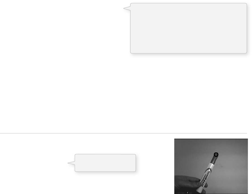
Video 291
Now, we are ready to compare the colors. One strategy is to take the sum of the absolute value
of the diff erences. at is a mouthful, but it is really fairly simple. Take r 1 minus r 2. Since we
only care about the magnitude of the diff erence, not whether it is positive or negative, take the
absolute value (the positive version of the number). Do this for green and blue and add them all
together.
float diff = abs(r1-r2) + abs(g1-g2) + abs(b1-b2);
While this is perfectly adequate (and a fast calculation at that), a more accurate way to compute the
diff erence between colors is to take the “ distance ” between colors. OK, so you may be thinking: “ Um,
seriously? How can a color be far away or close to another color? ” Well, we know the distance between
two points is calculated via the Pythagorean eorem. We can think of color as a point in three-
dimensional space, only instead of x , y , and z , we have r , g , and b . If two colors are near each other in this
color space, they are similar; if they are far, they are diff erent.
float diff = dist(r1,g1,b1,r2,g2,b2);
Looking for the “ most red ” pixel in an image, for
example, is therefore looking for the color “ closest ”
to red—(255,0,0).
By adjusting the brightness tracking code to look for the closest pixel to any given color (rather than the
brightest), we can put together a color tracking sketch. In the following example, the user can click the
mouse on a color in the image to be tracked. A black circle will appear at the location that most closely
matches that color. See Figure 16.9 .
Example 16-11: Simple color tracking
import processing.video.*;
// Variable for capture device
Capture video;
color trackColor;
void setup() {
size(320,240);
video = new Capture(this,width,height,15);
// Start off tracking for red
trackColor = color(255,0,0);
smooth();
}
Although more accurate, because the dist( )
function involves a square root in its calculation, it
is slower than the absolute value of the difference
method. One way around this is to write your own
color distance function without the square root.
colorDistance (r1r 2)*(r1r2) (g1g2)*
(g1g2) (b1b2)*(b1b2)
fi g. 16.9
A variable for the color
we are searching for.
292 Learning Processing
void draw() {
// Capture and display the video
if (video.available()) {
video.read();
}
video.loadPixels();
image(video,0,0);
// Closest record, we start with a high number
float worldRecord = 500;
// XY coordinate of closest color
int closestX = 0;
int closestY = 0;
// Begin loop to walk through every pixel
for (int x = 0; x < video.width; x + + ){
for (int y = 0; y < video.height; y + + ) {
int loc = x + y*video.width;
// What is current color
color currentColor = video.pixels[loc];
float r1 = red(currentColor);
float g1 = green(currentColor);
float b1 = blue(currentColor);
float r2 = red(trackColor);
float g2 = green(trackColor);
float b2 = blue(trackColor);
// Using euclidean distance to compare colors
float d = dist(r1,g1,b1,r2,g2,b2);
// If current color is more similar to tracked color than
// closest color, save current location and current difference
if (d worldRecord) {
worldRecord = d;
closestX = x;
closestY = y;
}
}
}
if (worldRecord < 10) {
// Draw a circle at the tracked pixel
fill(trackColor);
strokeWeight(4.0);
stroke(0);
ellipse(closestX,closestY,16,16);
}
}
void mousePressed() {
// Save color where the mouse is clicked in trackColor variable
int loc = mouseX + mouseY*video.width;
trackColor = video.pixels[loc];
}
Before we begin searching, the “world
record” for closest color is set to a high
number that is easy for the fi rst pixel to beat.
We are using the dist( ) function
to compare the current color with
the color we are tracking.
We only consider the color found if its color
distance is less than 10. This threshold of 10
is arbitrary and you can adjust this number
depending on how accurate you require
the tracking to be.
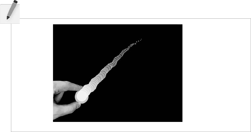
Video 293
Exercise 16-5: Take any Processing sketch you previously created that involves mouse
interaction and replace the mouse with color tracking. Create an environment for the
camera that is simple and high contrast. For example, point the camera at a black tabletop
with a small white object. Control your sketch with the object’s, location. e picture shown
illustrates the example that controls the “ snake ” (Example 9-9) with a tracked bottlecap.
16.6 Background Removal
e distance comparison for color proves useful in other computer vision algorithms as well, such as
background removal. Let’s say you wanted to show a video of you dancing the hula, only you did not want
to be dancing in your offi ce where you happen to be, but at the beach with waves crashing behind you.
Background removal is a technique that allows you to remove the background of an image (your offi ce)
and replace it with any pixels you like (the beach), while leaving the foreground (you dancing) intact.
Here is our algorithm.
• Memorize a background image.
• Check every pixel in the current video frame. If it is very different from the corresponding pixel
in the background image, it is a foreground pixel. If not, it is a background pixel. Display only
foreground pixels.
To demonstrate the above algorithm, we will perform a reverse green screen. e sketch will remove the
background from an image and replace it with green pixels.
Step one is “ memorizing ” the background. e background is essentially a snapshot from the video. Since
the video image changes over time, we must save a copy of a frame of video in a separate PImage object.
PImage backgroundImage;
void setup() {
backgroundImage = createImage(video.width,video.height,RGB);
}

294 Learning Processing
When backgroundImage is created, it is a blank image, with the same dimensions as the video. It is not
particularly useful in this form, so we need to copy an image from the camera into the background image
when we want to memorize the background. Let’s do this when the mouse is pressed.
void mousePressed() {
// Copying the current frame of video into the backgroundImage object
// Note copy takes 5 arguments:
// The source image
// x,y,width, and height of region to be copied from the source
// x,y,width, and height of copy destination
backgroundImage.updatePixels();
}
Once we have the background image saved, we can loop through all the pixels in the current frame and
compare them to the background using the distance calculation. For any given pixel ( x , y ), we use the
following code:
int loc = x + y*video.width; // Step 1, what is the 1D pixel location
color fgColor = video.pixels[loc]; // Step 2, what is the foreground color
color bgColor = backgroundImage.pixels[loc]; // Step 3, what is the background color
// Step 4, compare the foreground and background color
float r1 = red(fgColor); float g1 = green(fgColor); float b1 = blue(fgColor);
float r2 = red(bgColor); float g2 = green(bgColor); float b2 = blue(bgColor);
float diff = dist(r1,g1,b1,r2,g2,b2);
// Step 5, Is the foreground color different from the background color
if (diff > threshold) {
// If so, display the foreground color
pixels[loc] = fgColor;
} else {
// If not, display green
pixels[loc] = color(0,255,0);
}
e above code assumes a variable named “ threshold. ” e lower the threshold, the easier it is for a pixel
to be in the foreground. It does not have to be very diff erent from the background pixel. Here is the full
example with threshold as a global variable.
Example 16-12: Simple background removal
// Click the mouse to memorize a current background image
import processing.video.*;
// Variable for capture device
Capture video;
// Saved background
PImage backgroundImage;
// How different must a pixel be to be a foreground pixel
float threshold = 20; fi g. 16.10
copy( ) allows you to copy pixels from one
image to another. Note that updatePixels( )
should be called after new pixels are copied!
backgroundImage.copy(video,0,0,video.width,video.height,0,0,video.width,video.height);

Video 295
void setup() {
size(320,240);
video = new Capture(this, width, height, 30);
// Create an empty image the same size as the video
backgroundImage = createImage(video.width,video.height,RGB);
}
void draw() {
// Capture video
if (video.available()) {
video.read();
}
loadPixels();
video.loadPixels();
backgroundImage.loadPixels();
// Draw the video image on the background
image(video,0,0);
// Begin loop to walk through every pixel
for (int x = 0; x < video.width; x + + ){
for (int y = 0; y < video.height; y + + ) {
int loc = x + y*video.width; // Step 1, what is the 1D pixel location
color fgColor = video.pixels[loc]; // Step 2, what is the foreground color
// Step 3, what is the background color
color bgColor = backgroundImage.pixels[loc];
// Step 4, compare the foreground and background color
float r1 = red(fgColor);
float g1 = green(fgColor);
float b1 = blue(fgColor);
float r2 = red(bgColor);
float g2 = green(bgColor);
float b2 = blue(bgColor);
float diff = dist(r1,g1,b1,r2,g2,b2);
// Step 5, Is the foreground color different from the background color
if (diff > threshold) {
// If so, display the foreground color
pixels[loc] = fgColor;
} else {
// If not, display green
pixels[loc] = color(0,255,0);
}
}
}
updatePixels();
}
void mousePressed() {
// Copying the current frame of video into the backgroundImage object
// Note copy takes 5 arguments:
// The source image
// x,y,width, and height of region to be copied from the source
// x,y,width, and height of copy destination
backgroundImage.copy(video,0,0,video.width,video.height,0,0,video.width,video.
height);
backgroundImage.updatePixels();
}
We are looking at the video’s pixels,
the memorized backgroundImage’s
pixels, as well as accessing the display
pixels. So we must loadPixels() for all!
We could choose to replace the
background pixels with something
other than the color green!

296 Learning Processing
When you ultimately get to running this example, step out of the frame, click the mouse to memorize
the background without you in it, and then step back into the frame; you will see the result as seen in
Figure 16.10.
If this sketch does not seem to work for you at all, check and see what “ automatic ” features are
enabled on your camera. For example, if your camera is set to automatically adjust brightness or
white balance, you have a problem. Even though the background image is memorized, once the
entire image becomes brighter or changes hue, this sketch will think all the pixels have changed
and are therefore part of the foreground! For best results, disable all automatic features on your
camera.
Exercise 16-6: Instead of replacing the background with green pixels, replace it with another
image. What values work well for threshold and what values do not work at all? Try
controlling the threshold variable with the mouse.
16.7 Motion Detection
Today is a happy day. Why? Because all of the work we did to learn how to remove the background
from a video gets us motion detection for free. In the background removal example, we examined each
pixel’s relationship to a stored background image. Motion in a video image occurs when a pixel color
diff ers greatly from what it used to be one frame earlier. In other words, motion detection is exactly the
same algorithm, only instead of saving a background image once, we save the previous frame of video
constantly!
e following example is identical to the background removal example with only one important change—
the previous frame of video is always saved whenever a new frame is available.
// Capture video
if (video.available()) {
// Save previous frame for motion detection!!
prevFrame.copy(video,0,0,video.width,video.height,0,0,video.width,video.height);
video.read();
}
( e colors displayed are also changed to black and white and some of the variable names are diff erent,
but these are trivial changes.)
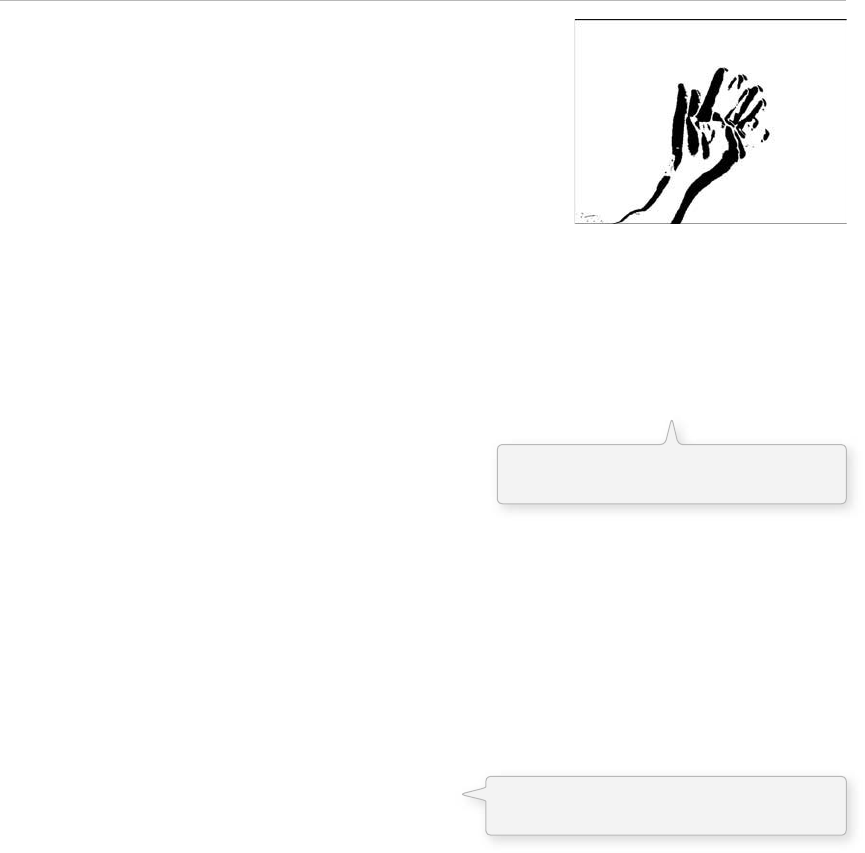
Video 297
Example 16-13: Simple motion detection
import processing.video.*;
// Variable for capture device
Capture video;
// Previous Frame
PImage prevFrame;
// How different must a pixel be to be a "motion" pixel
float threshold = 50;
void setup() {
size(320,240);
video = new Capture(this, width, height, 30);
// Create an empty image the same size as the video
prevFrame = createImage(video.width,video.height,RGB);
}
void draw() {
// Capture video
if (video.available()) {
// Save previous frame for motion detection!!
prevFrame.copy(video,0,0,video.width,video.height,0,0,video.width,video.height);
prevFrame.updatePixels();
video.read();
}
loadPixels();
video.loadPixels();
prevFrame.loadPixels();
// Begin loop to walk through every pixel
for (int x = 0; x < video.width; x + + ){
for (int y = 0; y < video.height; y + + ){
int loc = x + y*video.width; // Step 1, what is the 1D pixel location
color current = video.pixels[loc]; // Step 2, what is the current color
color previous = prevFrame.pixels[loc]; // Step 3, what is the previous color
// Step 4, compare colors (previous vs. current)
float r1 = red(current); float g1 = green(current); float b1 = blue(current);
float r2 = red(previous); float g2 = green(previous); float b2 = blue(previous);
float diff = dist(r1,g1,b1,r2,g2,b2);
// Step 5, How different are the colors?
if (diff > threshold) {
// If motion, display black
pixels[loc] = color(0);
} else {
// If not, display white
pixels[loc] = color(255);
}
}
}
updatePixels();
}
What if we want to just know the “ overall ” motion in a room? At the start of section 16.5 , we calculated
the average brightness of an image by taking the sum of each pixel’s brightness and dividing it by the total
number of pixels.
fi g. 16.11
Before we read the new frame, we always
save the previous frame for comparison!
If the color at that pixel has changed, then
there is “motion” at that pixel.

298 Learning Processing
Average Brightness
=
Total Brightness / Total Number of Pixels
We can calculate the average motion the same way:
Average Motion
=
Total Motion / Total Number of Pixels
e following example displays a circle that changes color and size based on the average amount of
motion. Note again that you do not need to display the video in order to analyze it!
Example 16-14: Overall motion
import processing.video.*;
// Variable for capture device
Capture video;
// Previous Frame
PImage prevFrame;
// How different must a pixel be to be a "motion" pixel
float threshold = 50;
void setup() {
size(320,240);
// Using the default capture device
video = new Capture(this, width, height, 15);
// Create an empty image the same size as the video
prevFrame = createImage(video.width,video.height,RGB);
}
void draw() {
background(0);
// If you want to display the videoY
// You don't need to display it to analyze it!
image(video,0,0);
// Capture video
if (video.available()) {
// Save previous frame for motion detection!!
prevFrame.copy(video,0,0,video.width,video.height,0,0,video.width,video.height);
prevFrame.updatePixels();
video.read();
}
loadPixels();
video.loadPixels();
prevFrame.loadPixels();
// Begin loop to walk through every pixel
// Start with a total of 0
float totalMotion = 0;
// Sum the brightness of each pixel
for (int i = 0; i < video.pixels.length; i + + ) {
color current = video.pixels[i];
// Step 2, what is the current color
color previous = prevFrame.pixels[i];
// Step 3, what is the previous color

Video 299
// Step 4, compare colors (previous vs. current)
float r1 = red(current); float g1 = green(current);
float b1 = blue(current);
float r2 = red(previous); float g2 =
float b2 = blue(previous);
float diff = dist(r1,g1,b1,r2,g2,b2);
totalMotion + = diff;
}
float avgMotion = totalMotion / video.pixels.length;
// Draw a circle based on average motion
smooth();
noStroke();
fill(100 + avgMotion*3,100,100);
float r = avgMotion*2;
ellipse(width/2,height/2,r,r);
}
Exercise 16-7: Create a sketch that looks for the average location of motion. Can you have an
ellipse follow your waving hand?
16.8 Computer Vision Libraries
ere are several computer vision libraries already available for Processing (and there will inevitably be
more). e nice thing about writing your own computer vision code is that you can control the vision
algorithm at the lowest level, performing an analysis that conforms precisely to your needs. e benefi t
to using a third party library is that since there has been a great deal of research in solving common
computer vision problems (detecting edges, blobs, motion, tracking color, etc.), you do not need to do all
of the hard work yourself ! Here is a brief overview of three libraries currently available.
JMyron (WebCamXtra) by Josh Nimoy et al.
http://webcamxtra.sourceforge.net/
One advantage of using JMyron is its freedom from needing a vdig on Windows. It also includes many
built-in functions to perform some of the tasks explained in this chapter: motion detection and color
tracking. It will also search for groups of similar pixels (known as blobs or globs).
LibCV by Karsten Schmidt
http://toxi.co.uk/p5/libcv/
Much like JMyron, LibCV does not require QuickTime or WinVDIG for Windows machines. Instead
of using native code, however, it uses the Java Media Framework (JMF) to connect to and capture images
from a digital video camera. LibCV also includes functions not available in some of the other computer
vision libraries, such as “ background learning, background subtraction, diff erence images, and keystoning
(perspective correction). ”
totalMotion is the sum of all color differences.
Motion for an individual pixel is the difference
between the previous color and current color.
averageMotion is total motion
divided by the number of pixels
analyzed.
green(previous);
300 Learning Processing
BlobDetection by Julien “v3ga” Gachadoat
http://www.v3ga.net/processing/BlobDetection/
is library, as made obvious by its name, is specifi cally designed for detecting blobs in an image. Blobs
are defi ned as areas of pixels whose brightness is above or below a certain threshold. e library takes any
image as input and returns an array of Blob objects, each of which can tell you about its edge points and
bounding box.
16.9 The Sandbox
Up until now, every single sketch we have created in this book could be published online. Perhaps you
have already got a web site full of your Processing work. Once we start working with a video camera,
however, we run into a problem. ere are certain security restrictions with web applets and this is
something we will see here and there throughout the rest of the book. A web applet, for example, cannot
connect to a video camera on a user’s computer. For the most part, applets are not allowed to connect to
any local devices.
It makes sense that there are security requirements. If there weren’t, a programmer could make an applet
that connects to your hard drive and deletes all your fi les, send an e-mail out to all of his or her friends
and say: “ Check out this really cool link! ” Applications do not have security requirements. After all, you
can go and download applications that erase and reformat hard drives. But downloading and installing an
application is diff erent from just popping on a URL and loading an applet. ere is an assumed level of
trust with applications.
Incidentally, whether or not a feature of Processing will work in a web applet is listed on every single
reference page under “ Usage. ” If it says “ Web ” it can be used in a web applet.
If you must publish a camera connecting a Processing sketch online, there are ways around this and I will
off er some tips and suggestions on this book’s website: http://www.learningprocssing.com/sandbox/ .

Video 301
Lesson Seven Project
Develop a software mirror that incorporates computer vision techniques. Follow
these steps.
Step 1. Design a pattern with no color. is could be a static pattern (such
as a mosaic) or a moving one (such as the “scribbler” example) or a
combination.
Step 2. Color that pattern according to a JPG image.
Step 3. Replace the JPG with images from a live camera (or recorded
QuickTime).
Step 4. Using computer vision techniques, alter the behavior of the patterns’
elements according to the properties of the image. For example, perhaps
brighter pixels cause shapes to spin or pixels that change a lot cause
shapes to fl y off the screen, and so on.
Use the space provided below to sketch designs, notes, and pseudocode for your
project.
This page intentionally left blank
Lesson Eight
The Outside World
17 Text
18 Data Input
19 Data Streams
This page intentionally left blank
Text 305
17 Text
“ I could entertain future historians by saying I think all this superstring stuff is crazy. ”
—Richard Feynman
In this chapter:
– Storing text in a String object.
– Basic String functionality.
– Creating and loading fonts.
– Displaying text.
17.1 Where do Strings come from?
In Chapter 15, we explored a new object data type built into the Processing environment for dealing with
images—PImage. In this chapter, we will introduce another new data type, another class we get for free
with Processing , called String .
e String class is not a completely new concept. We have dealt with Strings before whenever we have
printed some text to the message window or loaded an image from a fi le.
println( "printing some text to the message window! "); // Printing a String
PImage img = loadImage("filename.jpg"); // Using a String for a file name
Nevertheless, although we have used a String here and there, we have yet to explore them fully and
unleash their potential. In order to understand the origins of the String , let’s remind ourselves where
classes come from. We know we can create our own classes (Zoog, Car, etc.). We can use classes built
into the Processing environment, such as PImage. And fi nally, in the last chapter we learned that we could
import additional Processing libraries to use certain classes such as Capture or Movie.
Nevertheless, these classes come from our lives in the Processing bubble. We have yet to venture out into
the great unknown, the world of thousands upon thousands of available Java classes. Before we leap over
the Java API cliff (which we will do in Chapter 23), it is useful to just peek over the edge and explore one
of the most basic and fundamental Java classes out there, the String class, which we will use to store and
manipulate text.
Where do we fi nd documentation for the String class?
In order to learn the details about built-in variables, functions, and classes, the Processing reference has
always been our guide. Although technically a Java class, because the String class is so commonly used,
Processing includes documentation in its reference. In addition, no import statement is required.
http://www.processing.org/reference/String.html

306 Learning Processing
is page only covers a few of the available methods of the String class. e full documentation can be
found at Sun’s Java site:
http://java.sun.com/j2se/1.4.2/docs/api/java/lang/String.html
(Also note the URL for the entire Java API: http://java.sun.com/j2se/1.4.2/docs/api).
We are not going to cover how to use the Java documentation just yet (see Chapter 23 for more), but you
can whet your appetite by just visiting and perusing the above links.
17.2 What is a String ?
A String , at its core, is really just a fancy way of storing an array of characters—if we did not have the
String class, we would probably have to write some code like this:
char[] sometext = { ' H ', ' e ' , ' l ' , ' l' , ' o ' , ' ' ,' W ' , ' o ' , ' r ' ,' l ' , ' d ' } ;
Clearly, this would be a royal pain in the Processing behind. It is much simpler to do the following and
make a String object:
String sometext = " How do I make a String? Type characters between quotes! " ;
It appears from the above that a String is nothing more than a list of characters in between quotes.
Nevertheless, this is only the data of a String . We must remember that a String is an object with
methods (which you can fi nd on the reference page). is is the same as how a PImage object
stored the data associated with an image as well as had functionality in the form of methods: copy( ) ,
loadPixels( ) , and so on. We will look more closely at String methods in Chapter 18. However, here are a
few examples.
e method charAt( ) returns the individual character in the String at a given index. Strings are just like
arrays in that the fi rst character is index #0!
Another useful method is length( ) . is is easy to confuse with the length property of an array. However,
when we ask for the length of a String object, we must use the parentheses since we are calling a function
called length( ) rather than accessing a property called length.
String message = " This String is 34 characters long. " ;
println(message.length());
String message = " a bunch of text here. " ;
char c = message.charAt(3);
println(c);
________
Exercise 17-1: What is the result of the following code?

Text 307
Exercise 17-2: Loop through and print every character of a String one at a time.
String message = " a bunch of text here. ";
for (int i = 0; i < _____________ ); i + + ){
char c = ________________ ;
println(c);
}
We can also change a String to all uppercase (or lowercase) using the toUpperCase( ) method.
String uppercase = message.toUpperCase() ;
println(uppercase);
You might notice something a bit odd here. Why didn’t we simply say “ message.toUpperCase( ) ” and then
print the “ message ” variable? Instead, we assigned the result of “ message.toUpperCase( ) ” to a new variable
with a diff erent name— “ uppercase ” .
is is because a String is a special kind of object. It is immutable . An immutable object is one whose data
can never be changed. Once we create a String , it stays the same for life. Any time we want to change the
String , we have to create a new one. So in the case of converting to uppercase, the method toUpperCase( )
returns a copy of the String object with all caps.
e last method we will cover in this chapter is equals( ) . You might fi rst think to compare Strings using
the “ = = ” operator.
String one = " hello";
String two = " hello";
println(one = = two);
Technically speaking, when “ ” is used with objects, it compares the memory addresses for each object.
Even though each string contains the same data— “ hello ” —if they are diff erent object instances, then
“ ” could result in a false comparison. e equals( ) function ensures that we are checking to see if two
String objects contain the exact same sequence of characters, regardless of where that data is stored in the
computer’s memory.
String one = " hello";
String two = " hello";
println(one.equals(two));
Although both of the above methods return the correct result, it is safer to use equals( ) . Depending on
how String objects are created in a sketch, “ ” will not always work.

308 Learning Processing
One other feature of String objects is concatenation, joining two Strings together. Strings are joined with
the “ ” operator. e plus operator ( ), of course, usually means add in the case of numbers. When used
with Strings , it means join .
String helloworld = " Hello " + " World " ;
Variables can also be brought into a String using concatenation.
int x = 10;
String message = " The value of x is: " + x;
We saw a good example of this in Chapter 15 when loading an array of images with numbered fi lenames.
Exercise 17-3: Find the duplicates in the following array of Strings.
String words = { "I","love " , " coffee " , " I " , " love " , " tea " } ;
for (int i = 0; i < _______________; i + + ){
for (int j = __; j < _______________; j + + ){
if (___________________) {
println(____________ + " is a duplicate. " );
}
}
}
at rectangle is 10 pixels wide, 12 pixels tall and sitting right at (100,100).
float w = 10;
float h = 12;
float x = 100;
float y = 100;
String message = ____________________________________;
println(message);
Exercise 17-4: Concatenate a String from the variables given that outputs the following
message.
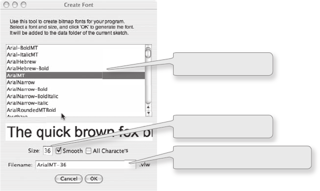
Text 309
17.3 Displaying Text
We will continue to explore the functions available as part of the String class in Chapter 18, which
focuses on analyzing and manipulating Strings . What we have learned so far about Strings is enough to
get us to the focus of this chapter: rendering text .
e easiest way to display a String is to print it in the message window. is is likely something you have
been doing here and there while debugging. For example, if you needed to know the horizontal mouse
location, you would write:
println(mouseX);
Or if you needed to determine that a certain part of the code was executed, you might print out a
descriptive message.
println( "We got here and we're printing out the mouse location!!! ");
While this is valuable for debugging, it is not going to help our goal of displaying text for a user. To place
text on screen, we have to follow a series of simple steps.
1. Choose a font by selecting “ Tools ” → “ Create Font. ” is will create and place the font fi le in your
data directory. Make note of the font fi lename for Step 3. Processing uses a special font format, “ vlw, ”
that uses images to display each letter. Because of this, you should create the font at the size you
intend to display. See Figure 17.1 .
Select a font.
Select a size.
Make note of the font filename.
fi g. 17.1
2. Declare an object of type PFont.
PFont f;
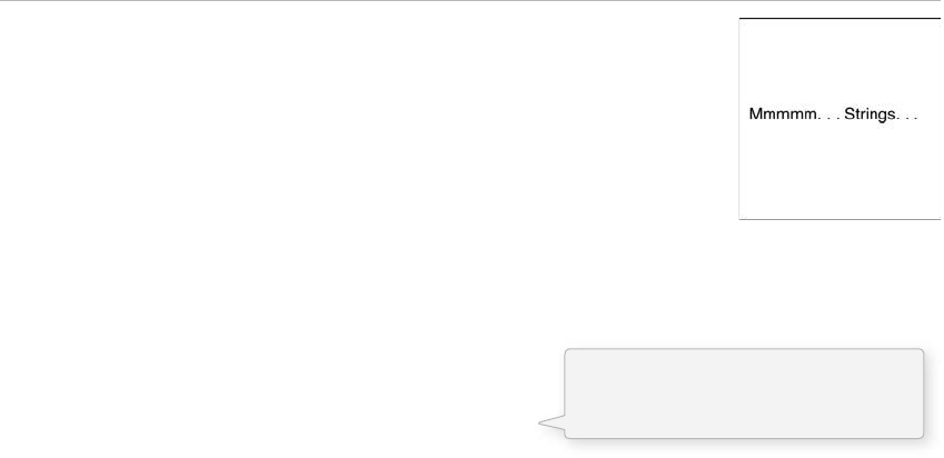
310 Learning Processing
3. Load the font by referencing the font fi le name in the function loadFont( ). is should be done
only once, usually in setup( ) . Just as with loading an image, the process of loading a font into memory
is slow and would seriously aff ect the sketch’s performance if placed inside draw( ) .
f = loadFont( " ArialMT-16.vlw " );
4. Specify the font using textFont( ). textFont( ) takes one or two arguments, the font variable and
the font size, which is optional. If you do not include the font size, the font will be displayed at the
size originally loaded. Specifying a font size that is diff erent from the font size loaded can result in
pixelated or poor quality text.
textFont(f,36);
5. Specify a color using fi ll( ) .
fill(0);
6. Call the text( ) function to display text. ( is function is just like shape or image drawing, it takes
three arguments—the text to be displayed, and the x and y coordinate to display that text.)
text( "Mmmmm... Strings... " ,10,100);
All the steps together are shown in Example 17-1 .
Example 17-1: Simple displaying text
PFont f; // STEP 2 Declare PFont variable
void setup() {
size(200,200);
f = loadFont( " ArialMT-16.vlw " ); // STEP 3 Load Font
}
void draw() {
background(255);
textFont(f,16); // STEP 4 Specify font to be used
fill(0); // STEP 5 Specify font color
text ( " Mmmmm... Strings ... " ,10,100); // STEP 6 Display Text
}
Fonts can also be created using the function createFont( ).
myFont = createFont( " Georgia " , 24, true);
createFont( ) allows you to use a font that may be installed on your local machine, but not available as
part of Processing ’s font options. In addition, createFont( ) allows the font to be scaled to any size
without it looking pixelated or smushed. For more about createFont( ) , visit the Processing reference:
http://processing.org/reference/createFont_.html . You can see all the available fonts with “ PFont.list( ) . ”
fi g. 17.2
The arguments to createFont() are font
name, font size, and a boolean that
enables smoothing (anti-aliasing).
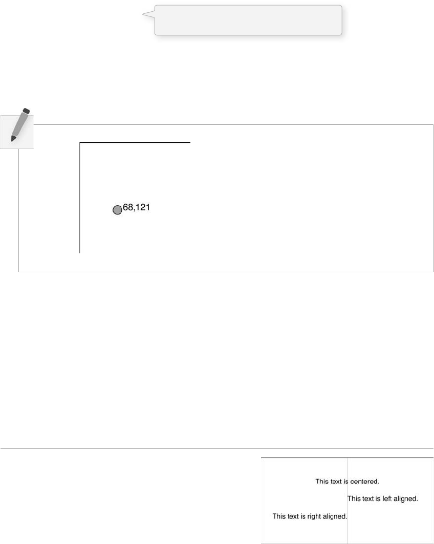
Text 311
println(PFont.list());
For demonstration purposes, createFont( ) will be used for all examples, rather than loadFont( ) .
17.4 Text Animation
Now that we understand the steps required to display text, we can apply other concepts from this book to
animate text in real-time.
To get started, let’s look at two more useful Processing functions related to displaying text:
textAlign( ) —specifi es RIGHT, LEFT, or CENTER alignment for text .
Example 17-2: Text align
PFont f;
void setup() {
size(400,200);
f = createFont( "Arial",16,true);
}
void draw() {
background(255);
stroke(175);
line(width/2,0,width/2,height);
textFont(f);
fill(0);
fi g. 17.3
Print all fonts available to createFont() to the
message window.
Exercise 17-5: Take the bouncing ball example from Chapter 5. Display the X and Y
coordinates as text next to the ball.

312 Learning Processing
textAlign(CENTER);
text( " This text is centered. " ,width/2,60);
textAlign (LEFT) ;
text( " This text is left aligned. " ,width/2,100);
textAlign(RIGHT);
text( " This text is right aligned. " ,width/2,140);
}
textWidth( ) —Calculates and returns the width of any character or text string.
Let’s say we want to create a news ticker, where text scrolls across the bottom of the screen from left
to right . When the news headline leaves the window, it reappears on the right-hand side and scrolls
again. If we know the x location of the beginning of the text and we know the width of that text, we can
determine when it is no longer in view (see Figure 17.4). textWidth( ) gives us that width.
To start, we declare headline, font, and x location variables, initializing them in setup( ) .
// A headline
String headline = " New study shows computer programming lowers cholesterol. " ;
PFont f; // Global font variable
float x; // Horizontal location of headline
void setup() {
f = createFont( " Arial " ,16,true); // Loading font
x = width; // Initializing headline off-screen to the right
}
e draw( ) function is similar to our bouncing ball example in Chapter 5. First, we display the text at the
appropriate location.
// Display headline at x location
textFont(f,16);
textAlign(LEFT);
text(headline,x,180);
We change x by a speed value (in this case a negative number so that the text moves to the left.)
// Decrement x
x = x – 3;
Now comes the more diffi cult part. It was easy to test when a circle reached the left side of the screen. We
would simply ask: is x less than 0? With the text, however, since it is left-aligned, when x equals zero, it
is still viewable on screen. Instead, the text will be invisible when x is less than 0 minus the width of the
text (see Figure 17.4 ). When that is the case, we reset x back to the right-hand side of the window, that
is, width .
textAlign() sets the alignment
for displaying text. It takes one
argument: CENTER, LEFT, or RIGHT.
Text 313
float w = textWidth(headline) ;
if (x < -w) {
x = width;
}
Example 17-3 is a full example that displays a diff erent headline each time the previous headline leaves
the screen. e headlines are stored in a String array .
Example 17-3: Scrolling headlines
// An array of news headlines
String[] headlines = {
" Processing downloads break downloading record. ",
" New study shows computer programming lowers cholesterol. ",
} ;
PFont f; // Global font variable
float x; // Horizontal location
int index = 0;
void setup() {
size(400,200);
f = createFont( "Arial",16,true);
// Initialize headline offscreen
x = width;
}
void draw() {
background(255);
fill (0);
// Display headline at x location
textFont(f,16);
textAlign (LEFT );
text(headlines[index],x,180);
// Decrement x
x = x – 3;
// If x is less than the negative width,
// then it is off the screen
float w = textWidth(headlines[index]);
if (x < -w) {
x = width;
index = (index + 1) % headlines.length;
}
}
X = 0
X = 50
Some text
Some text
width = 100 pixels
still on screen!
X = 100
Some text
all the way off screen!
fi g. 17.4
fi g. 17.5
If x is less than the negative width, then it is
completely off the screen
A specifi c String from the array is
displayed according to the value of the
“index” variable.
textWidth() is used to calculate the width
of the current String.
“index“ is incremented when the current
String has left the screen in order to
display a new String.
Multiple Strings are
stored in an array.
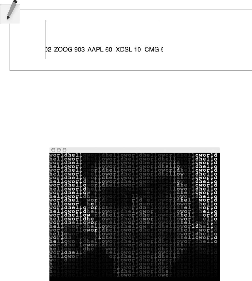
314 Learning Processing
fi g. 17.6
In addition to textAlign( ) and textWidth( ), Processing also off ers the functions textLeading( ), textMode( ) ,
and textSize( ) for additional display functionality. ese functions are not necessary for the examples
covered in this chapter, but you can explore them on your own in the Processing reference.
Exercise 17-6: Create a stock ticker that loops over and over. As the last stock enters the
window, the fi rst stock appears immediately to its right.
17.5 Text Mosaic
Combining what we learned in Chapters 15 and 16 about the pixel array, we can use the pixels of an
image to create a mosaic of characters. is is an extension of the video mirror code in Chapter 16. (Note
that in Example 17-4, new text-related code is in bold.) See Figure 17.6 .
Text 315
Example 17-4: Text mirror
import processing.video.*;
// Size of each cell in the grid, ratio of window size to video size
int videoScale = 14;
// Number of columns and rows in our system
int cols, rows;
// Variable to hold onto capture object
capture video;
// A String and Font
String chars = " helloworld" ;
PFont f;
void setup() {
size(640,480);
//set up columns and rows
cols = width/videoScale;
rows = height/videoScale;
video = new Capture(this,cols,rows,15);
// Load the font
f = loadFont (" Courier-Bold-20.vlw ");
}
void draw() {
background(0);
// Read image from the camera
if (video.available()) {
video.read();
}
video.loadPixels();
// Use a variable to count through chars in String
int charcount = 0;
// Begin loop for rows
for (int j = 0; j < rows; j + + ){
// Begin loop for columns
for (int i = 0; i < cols; i + + ){
// Where are we, pixel-wise?
int x = i*videoScale;
int y = j*videoScale;
color c = video.pixels[i + j*video.width];
// Instead of a rectangle
textFont(f);
fill(c);
text(chars.charAt(charcount),x,y);
// Go on to the next character
charcount = (charcount + 1) % chars.length();
}
}
}
The source text used in the mosaic
pattern. A longer String might
produce more interesting results.
Using a “fi xed-width” font. In most fonts,
individual characters have different
widths. In a fi xed-width font, all characters
have the same width. This is useful here
since we intend to display the letters one
at a time spaced out evenly. See Section
17.7 for how to display text character by
character with a nonfi xed width font.
One character from the
source text is displayed
colored accordingly to the
pixel location. A counter
variable—“charcount”—is
used to walk through
the source String one
character at a time.
// Looking up the appropriate color in the pixel array
// Displaying an individual character from the String
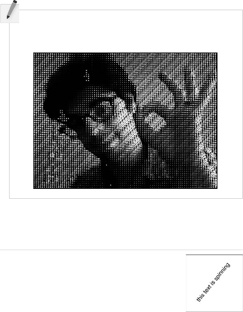
316 Learning Processing
Exercise 17-7: Create a video text mosaic where each letter is colored white, but the size of
each letter is determined by a pixel’s brightness. e brighter the pixel, the bigger it is. Here is
a little bit of code from the inside of the pixel loop (with some blank spots) to get you started.
17.6 Rotating Text
Translation and rotation (as seen in Chapter 14) can also be applied to text. For example, to rotate text
around its center, translate to an origin point and use textAlign(CENTER) before displaying the text.
Example 17-5: Rotating text
PFont f;
String message = " this text is spinning " ;
float theta;
void setup() {
size(200,200);
f = createFont( " Arial " ,20,true);
}
void draw() {
background(255);
fill (0);
float b = brightness(video.pixels[i + j*video.width]);
float fontSize = _____ * (_____ / _____);
textSize(fontSize);
fi g. 17.7
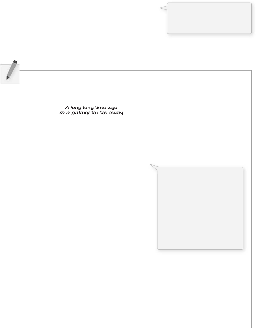
Text 317
textFont(f); // Set the font
translate(width/2,height/2); // Translate to the center
rotate(theta); // Rotate by theta
textAlign( CENTER) ;
text(message,0,0);
theta + = 0.05; // Increase rotation
}
String info = " A long long time ago\nIn a galaxy far far away ";
PFont f;
float y = 0;
void setup() {
size(400,200,P3D);
f = createFont( "Arial",20*4,true);
}
void draw() {
background(255);
fill(0);
translate(__________,__________);
__________ (__________);
textFont(f);
textAlign(CENTER);
text(info, __________,__________);
y--;
}
Exercise 17-8: Display text that is centered and rotated to appear fl at. Have the text scroll
off into the distance.
The text is center aligned and
displayed at (0,0) after translating
and rotating. See Chapter 14 or a
review of translation and rotation.
“\” means “new line.” In Java,
invisible characters can be
incorporated into a String with an
“escape sequence”—a backward
slash “\” followed by a character.
Here are a few more.
\n—new line
\r—carriage return
\t—tab
\’—single quote
\”—double quote
\\—backward slash
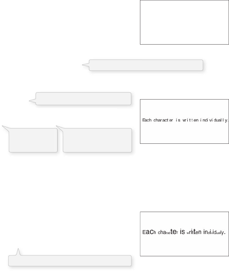
318 Learning Processing
17.7 Display text character by character.
In certain graphics applications, displaying text with each character rendered individually is required. For
example, if each character needs to move independently, then simply saying text( “ a bunch of letters ” ,0,0)
will not do.
e solution is to loop through a String , displaying each character one at a time.
Let’s start by looking at an example that displays the text all at once. See Figure 17.8 .
PFont f;
String message = " Each character is not
written individually." ;
void setup() {
size(400,200);
f = createFont( " Arial " ,20,true);
}
void draw() {
background(255);
fill(0);
textFont(f);
text(message,10,height/2);
}
We rewrite the code to display each character in a loop, using the charAt( ) function. See Figure 17.9 .
int x = 10;
for (int i = 0; i < message.length(); i + + ) {
text(message.charAt(i) ,x, height/2);
x + = 10;
}
Calling the text( ) function for each character will allow us more fl exibility in future examples (for
coloring, sizing, and placing characters within one String individually). is example has a pretty
major fl aw, however. Here, the x location is increased by 10 pixels for each character. Although this
is approximately correct, because each character is not exactly 10 pixels wide, the spacing is off . e
proper spacing can be achieved using the textWidth( ) function as demonstrated in the following code.
Note how this example achieves the proper spacing even with each character being a random size!
See Figure 17.10 .
int x = 10;
for (int i = 0; i < message.length(); i + + ) {
textSize(random(12,36));
text(message.charAt(i)
,x, height/2);
x + = textWidth(message.charAt(i));
}
Each character is not written individually.
fi g. 17.8
fi g. 17.9 (Note how the spacing is incorrect.)
fi g. 17.10 (Note how the spacing is correct even
with differently sized characters!)
The fi rst character is at pixel 10.
All characters are
spaced 10 pixels
apart.
Each character is displayed
one at a time with the
charAt() function.
textWidth() spaces the characters out properly.
Displaying a block of text all at once using text().
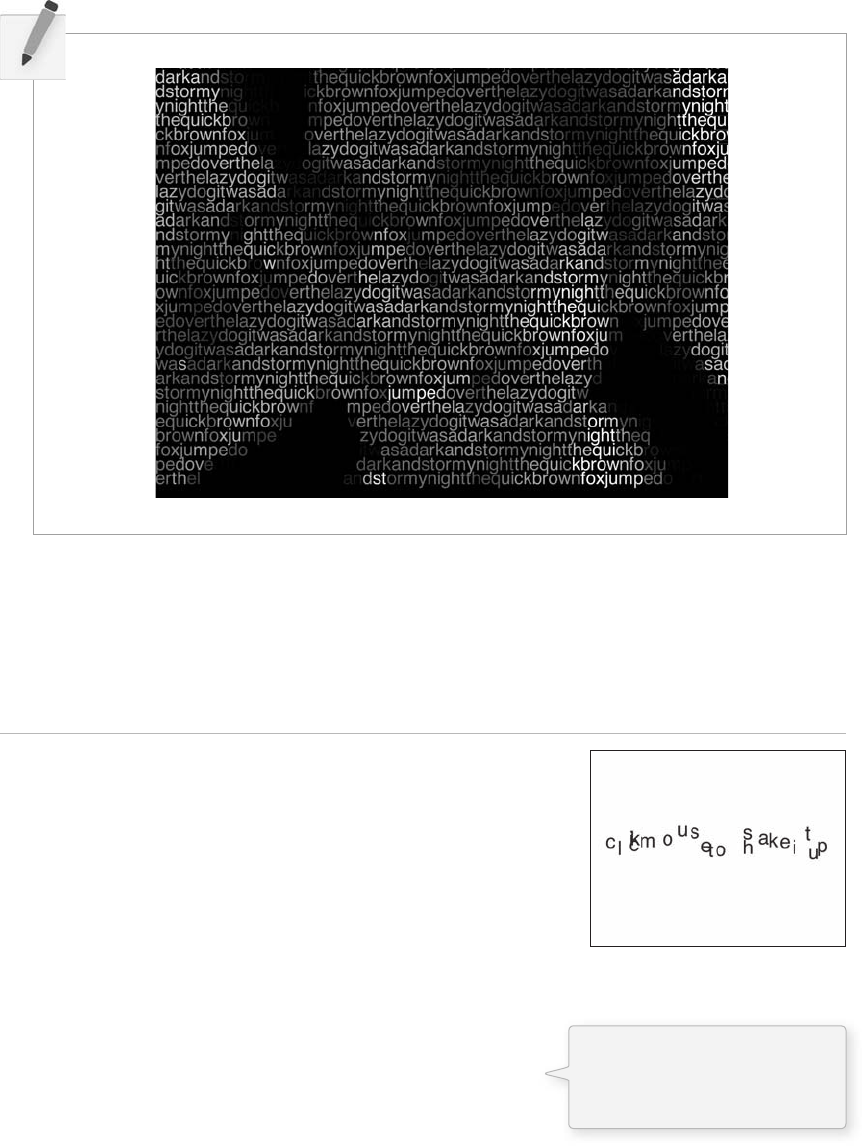
Text 319
Exercise 17-9: Using textWidth( ) , redo Example 17-4 (the text “ mirror ” ) to use a non-
fi xed-width font with proper character spacing. e following image uses Arial.
is “ letter by letter ” methodology can also be applied to a sketch where characters from a String move
independently of one another. e following example uses object-oriented design to make each character
from the original String a Letter object, allowing it to both be displayed in its proper location as well as
move about the screen individually.
Example 17-6: Text breaking up
PFont f;
String message = " click mouse to shake it up ";
// An array of Letter objects
Letter[] letters;
void setup() {
size(260,200);
// Load the font
f = createFont( "Arial",20,true);
textFont(f);
// Create the array the same size as the String
letters = new Letter[message.length()];
// Initialize Letters at the correct x location
int x = 16;
for (int i = 0; i < message.length(); i + + ){
letters[i] = new Letter(x,100,message.charAt(i));
x + = textwidth(message.charAt(i));
}
}
fi g. 17.11
Letter objects are initialized with
their location within the String
as well as what character they
should display.

320 Learning Processing
void draw() {
background(255);
for (int i = 0; i < letters.length; i + + ) {
// Display all letters
letters[i].display();
// If the mouse is pressed the letters shake
// If not, they return to their original location
if (mousePressed) {
letters[i].shake();
} else {
letters[i].home();
}
}
}
// A class to describe a single Letter
class Letter {
char letter;
// The object knows its original " home " location
float homex,homey;
// As well as its current location
float x,y;
Letter (float x_, float y_, char letter_) {
homex = x = x_;
homey = y = y_;
letter = letter_;
}
// Display the letter
void display() {
fill(0);
textAlign(LEFT);
text(letter,x,y);
}
// Move the letter randomly
void shake() {
x + = random(-2,2);
y + = random(-2,2);
}
// Return the letter home
void home() {
x = homex;
y = homey;
}
}
e character by character method also allows us to display text along a curve. Before we move on to
letters, let’s fi rst look at how we would draw a series of boxes along a curve. is example makes heavy use
of the trigonometric functions covered in Chapter 13 .
At any point, the current location can
be set back to the home location by
calling the home() function.
The object knows about its original
“home” location within the String of
text, as well as its current (x,y) location
should it move around the screen.
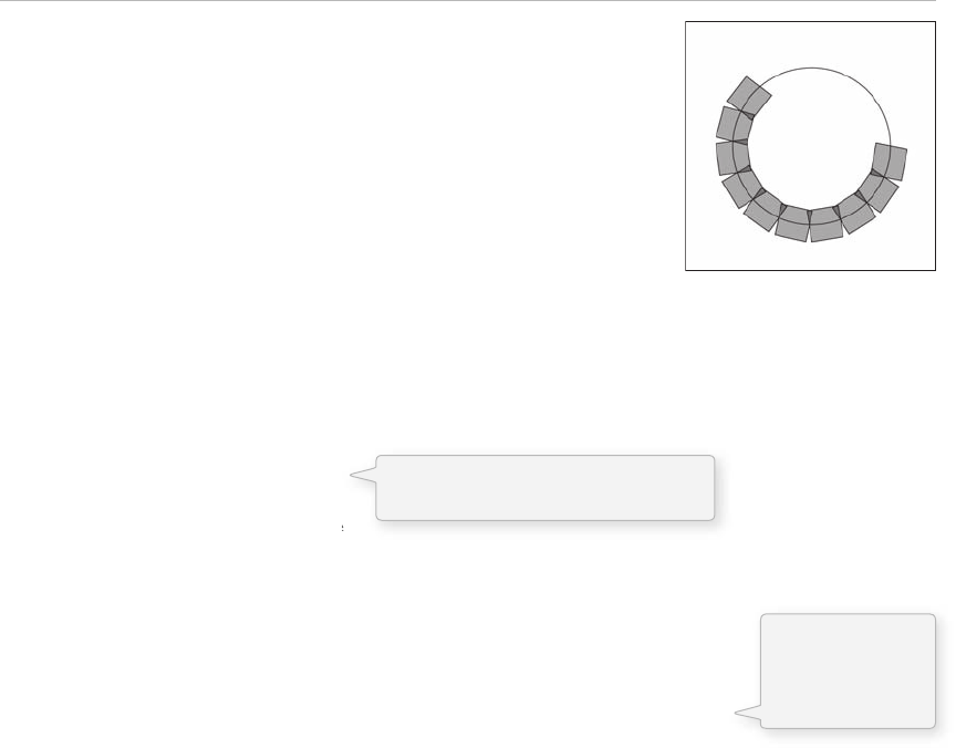
Text 321
Example 17-7: Boxes along a curve
PFont f;
// The radius of a circle
float r = 100;
// The width and height of the boxes
float w = 40;
float h = 40;
void setup() {
size(320,320);
smooth();
}
void draw() {
background(255);
// Start in the center and draw the circle
translate(width /2, height / 2);
noFill();
stroke(0);
ellipse(0, 0, r*2, r*2);
// 10 boxes along the curve
int totalBoxes = 10;
// We must keep track of our position along the curve
float arclength = 0;
// For every box
for (int i = 0; i < totalBoxes; i + + ){
// Each box is centered so we move half the width
arclength + = w/2;
// Angle in radians is the arclength divided by the radius
float theta = arclength /r;
pushMatrix();
// Polar to cartesian coordinate conversion
translate(r*cos(theta)
, r*sin(theta));
// Rotate the box
rotate(theta);
// Display the box
fill(0 , 100);
rectMode(CENTER);
rect(0
, 0 , w,h);
popMatrix();
// Move halfway again
arclength + = w/2;
}
}
Even if you fi nd the mathematics of this example to be diffi cult, Figure 17.12 should reveal the next step.
What we need to do is replace each box with a character from a String that fi ts inside the box. And since
characters do not all have the same width, instead of using a variable “ w ” that stays constant, each box will
have a variable width along the curve according to the textWidth( ) function.
fi g. 17.12
Our curve is a circle with radius r in
the center of the window.
We move along
the curve
according to the
width of the box.
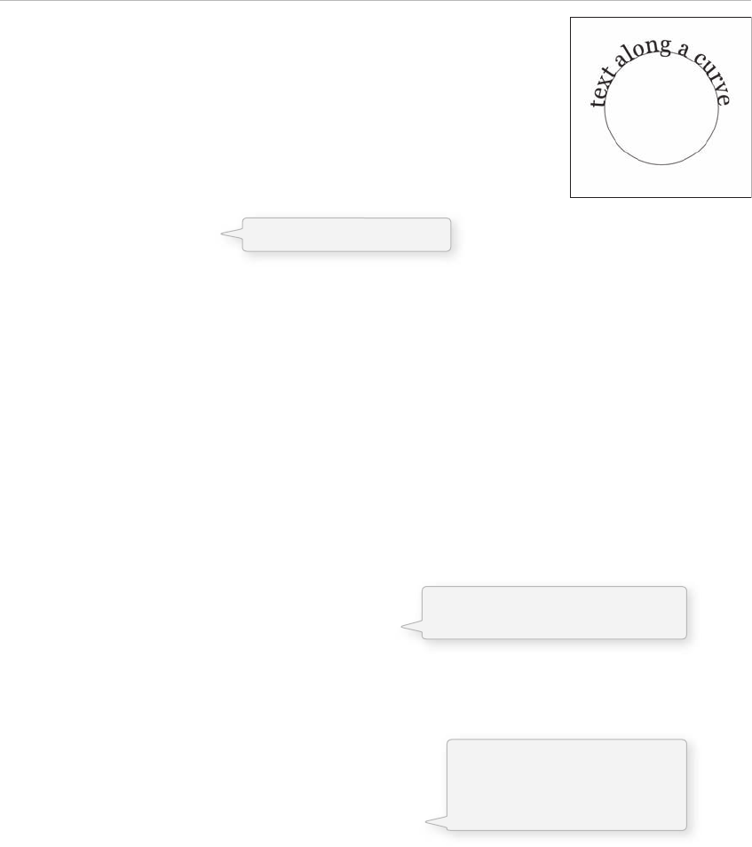
322 Learning Processing
Example 17-8: Characters along a curve
// The message to be displayed
String message = " text along a curve " ;
PFont f;
// The radius of a circle
float r = 100;
void setup() {
size(320,320);
f = createFont( " Georgia ",40,true);
textFont(f);
textAlign(CENTER);
smooth();
}
void draw() {
background(255);
// Start in the center and draw the circle
translate(width / 2, height / 2);
noFill();
stroke(0);
ellipse(0, 0, r*2, r*2);
// We must keep track of our position along the curve
float arclength = 0;
// For every box
for (int i = 0; i < message.length(); i + + ) {
// The character and its width
char currentChar = message.charAt(i);
float w = textWidth(currentChar);
// Each box is centered so we move half the width
arclength + = w/2;
// Angle in radians is the arclength divided by the radius
// Starting on the left side of the circle by adding PI
float theta = PI + arclength / r;
pushMatrix();
// Polar to cartesian coordinate conversion
translate(r*cos(theta), r*sin(theta));
// Rotate the box
rotate(theta + PI/2); // rotation is offset by 90 degrees
// Display the character
fill(0);
text(currentChar,0,0);
popMatrix();
// Move halfway again
arclength + = w/2;
}
}
fi g. 17.13
The text must be centered!
Instead of a constant width, we
check the width of each character.
Polar to Cartesian conversion
allows us to fi nd the point along
the curve. See Chapter 13 for a
review of this concept.
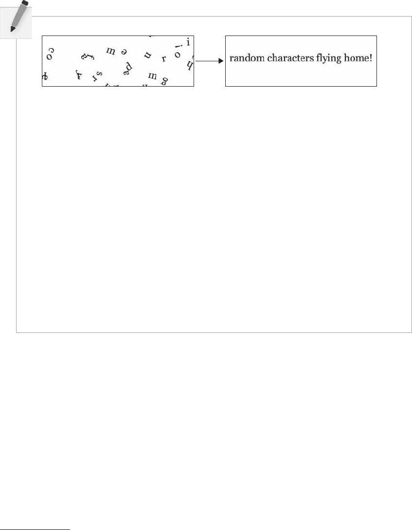
Text 323
Exercise 17-10: Create a sketch that starts with characters randomly scattered (and rotated).
Have them slowly move back toward their “ home ” location. Use an object-oriented approach
as seen in Example 17-6. 1
One way to solve this is to use interpolation. Interpolation refers to the process of
calculating values in between two given pieces of data. In this exercise, we want to know
the in-between x locations (and y locations) from the random starting point to the target
location in the String . One interpolation method is to simply take the average. ink of it
as walking to a wall by always taking a step halfway.
x = (x + targetX) /2;
y = (y + targetY) /2;
Another possibility is to simply go 10% of the way there.
x = 0.9*x + 0.l*targetX;
y = 0.9*y + 0.l*targetY;
Processing ’s lerp( ) function will do interpolation for you. Visit the reference page for more
information: http://processing.org/reference/lerp_.html.
Consider making your sketch interactive. Can you push the letters around using the mouse?
1 e origins of this exercise can be traced back to John Maeda’s 1995 work: Flying Letters .
This page intentionally left blank

Data Input 325
18 Data Input
“ A million monkeys were given a million typewriters. It’s called the Internet. ”
—Simon Munnery
In this chapter:
– Manipulating Strings.
– Reading and writing text fi les.
– HTTP requests, parsing HTML.
– XML, RSS feeds.
– The Yahoo search API.
– The applet sandbox.
is chapter will move beyond displaying text and examine how to use String objects as the basis for
reading and writing data. We will start by learning more sophisticated methods for manipulating Strings ,
searching in them, chopping them up, and joining them together. Afterward, we will see how these skills
allow us to use input from data sources, such as text fi les, web pages, XML feeds, and third party APIs,
and take a step into the world of data visualization.
18.1 Manipulating Strings
In Chapter 17, we touched on a few of the basic functions available in the Java String class, such as
charAt( ) , toUpperCase( ) , equals( ) , and length( ) . ese functions are documented on the Processing
reference page for Strings. Nevertheless, in order to perform some more advanced data parsing
techniques, we will need to explore some additional String manipulation functions documented in the
Java API (more about the Java API to come in Chapter 23).
http://java.sun.com/j2se/1.4.2/docs/api/java/lang/String.html
Let’s take a closer look at the following two String functions: indexOf( ) and substring( ) .
indexOf( ) locates a sequence of characters within a String . It takes one argument, a search String , and
returns a numeric value that corresponds to the fi rst occurrence of the search String inside of the String
being searched.
String search = " def";
String toBeSearched = " abcdefghi";
int index = toBeSearched.indexOf(search);
Strings are just like arrays, in that the fi rst character is index number zero and the last character is the
length of the String minus one.
The value of index
in this example is 3.

326 Learning Processing
Exercise 18-1: Predict the result of the code below.
String sentence = " The quick brown fox jumps over the lazy dog. " ;
println(sentence.indexOf( " quick " )); ________
println(sentence.indexOf( " fo " )); ________
println(sentence.indexOf( " The " )); ________
println(sentence.indexOf( " blah blah " )); ________
Exercise 18-2: Fill in the blanks to get the substring “ fox jumps over the lazy dog ” (without
the period).
String sentence = " The quick brown fox jumps over the lazy dog. " ;
int foxIndex = sentence.indexOf(________);
int periodIndex = sentence.indexOf( " . " );
String sub = ________ ·________(________,________);
18.2 Splitting and Joining
In Chapter 17, we saw how Strings can be joined together (referred to as “ concatenation ” ) using the “ ”
operator. Let’s review with an example that uses concatenation to get user input from a keyboard .
If you are stuck on the last line of Exercise 18-1, it is because there is no way for you to know the answer
without consulting the Java reference (or making an educated guess). If the search String cannot be found,
indexOf( ) returns 1. is is a good choice because “ 1 ” is not a legitimate index value in the String
itself, and therefore can indicate “ not found. ” ere are no negative indices in a String of characters or in an
array.
After fi nding a search phrase within a String , we might want to separate out part of the String , saving
it in a diff erent variable. A part of a String is known as s ubstring and substrings are made with the
substring( ) function which takes two arguments, a start index and an end index. substring( ) returns the
substring in between the two indices.
String alphabet = " abcdefghi " ;
String sub = alphabet.substring(3,6);
Note that the substring begins at the specifi ed start index (the fi rst argument) and extends to the character
at end index (the second argument) minus one . I know. I know. Wouldn’t it have been easier to just take the
substring from the start index all the way to the end index? While this might initially seem true, it is actually
quite convenient to stop at end index minus one. For example, if you ever want to make a substring that
extends to the end of a String , you can simply go all the way to thestring.length( ) . In addition, with end index
minus one marking the end, the length of the substring is easily calculated as end index minus begin index .
The String sub is now “def”.
Data Input 327
Example 18-1: User input
PFont f;
// Variable to store text currently being typed
String typing = " " ;
// Variable to store saved text when return is hit
String saved = " " ;
void setup() {
size(300,200);
f = createFont( "Arial",16,true);
}
void draw() {
background(255);
int indent = 25;
// Set the font and fill for text
textFont(f);
fill(0);
// Display everything
text("Click in this applet and type. \nHit return to save what you typed. ",indent,40);
text(typing,indent,90);
text(saved,indent,130);
}
void keyPressed() {
// If the return key is pressed, save the String and clear it
if (key = = '\n') {
saved = typing;
typing = " " ;
// Otherwise, concatenate the String
} else {
typing = typing + key;
}
}
Exercise 18-3: Create a sketch that chats with the user. For example, if a user enters “ cats ” the
sketch might reply “ How do cats make you feel? ”
Processing has two additional functions that make joining Strings (or the reverse, splitting them up) easy.
In sketches that involve parsing data from a fi le or the web, we will often get that data in the form of an
array of Strings or as one long String . Depending on what we want to accomplish, it is useful to know
how to switch between these two modes of storage. is is where these two new functions, split( ) and
join( ) , will come in handy.
“ one long string or array of strings ” ← → { “ one ” , “ long ” , “ string ” , “ or ” , “ array ” , “ of ” , “ strings ” }
Let’s take a look at the split( ) function. split( ) separates a longer String into an array of Strings , based on
a split character known as the delimiter. It takes two arguments, the String to be split and the delimiter.
( e delimiter can be a single character or a String .)
fi g. 18.1
For keyboard input, we use two
variables. One will store the text as
it is being typed. Another will keep
a copy of the typed text once the
Enter key is pressed.
AString can be cleared by setting it equal to ““.
Each character typed by the user is added to the
end of the String variable.
328 Learning Processing
// Splitting a String based on spaces
String spaceswords = " The quick brown fox jumps over the lazy dog. " ;
String[] list = split(spaceswords, " " );
for (int i = 0; i < list.length; i + + ){
println(list[i] + " " + i);
}
Here is an example using a comma as the delimiter.
// Splitting a String based on commas
String commaswords = " The,quick,brown,fox,jumps,over,the,lazy,dog. " ;
String[] list = split(commaswords, ‘ , ’ );
for (int i = 0; i < list.length; i + + ){
println(list[i] + " " + i);
}
If you want to use more than one delimiter to split up a text, you must use the Processing function
splitTokens( ). splitTokens( ) works identically is split( ) with one exception: any character that appears in
the String qualifi es as a delimiter.
// Splitting a String based on multiple delimiters
String stuff = " hats & apples, cars + " ;
String[] list = splitTokens(stuff, " & , + . " );
for (int i = 0; i < list.length; i + + ){
println(list[i] + " " + i);
}
If we are splitting numbers in a String, the resulting array can be converted into an integer array with
Processing ’s int( ) function.
// Calculate sum of a list of numbers in a String
String numbers = " 8,67,5,309 " ;
// Converting the String array to an int array
int[] list = int(split(numbers, ' , ' ));
int sum = 0;
for (int i = 0; i < list.length; i + + ){
sum = sum + list[i];
}
println(sum);
Exercise 18-4: Fill in what the above code will print in the Processing message window:
hats_______________
__________________
__________________
__________________
__________________
This period is not set as a delimeter and
therefore will be included in the last
String in the array: “dog.”
The period is set as a delimiter and therefore will
not be included in the last String in the array: “dog”.
Numbers in a String are not numbers
and cannot be used in mathematical
operations unless we convert them fi rst.
phones % elephants dog.

Data Input 329
e reverse of split( ) is join( ). join( ) takes an array of Strings and joins them together into one long String.
e join( ) function also takes two arguments, the array to be joined and a separator . e separator can
either be a single character or a String of characters.
Consider the following array:
String[] lines = { " It", "was", "a", "dark", " and" , "stormy", "night." } ;
Using the operator along with a for loop, we can join a String together as follows:
// Manual Concatenation
String onelongstring = " " ;
for (int i = 0; i < lines.length; i + + ){
onelongstring = onelongstring + lines[i] + " ";
}
e join( ) function, however, allows us to bypass this process, achieving the same result in only one line
of code.
// Using Processing’s join()
String onelongstring = join(lines, " ");
18.3 Reading and Writing Text Files
Data can come from many diff erent places: web sites, news feeds, databases, and so on. When developing
an application that involves a data source, such as a data visualization, it is important to separate out the
logic for what the program will ultimately do with the data from the retrieval of the data itself.
In fact, while working out the visuals, it is especially useful to develop with “ dummy ” or “ fake ” data. In
keeping with our one-step-at-a-time mantra, once the meat of the program is completed with dummy
data, you can then focus solely on how to retrieve the actual data from the real source.
Exercise 18-5: Split the following String into an array of fl oating point numbers and
calculate the average.
String floats = " 5023.23:52.3:10.4:5.9, 901.3---2.3 ";
float[] numbers = ________(________(________, "________"));
float total = 0;
for (int i = 0; i < numbers.length; i + + ){
________ += ________;
}
float avg = ____________________;
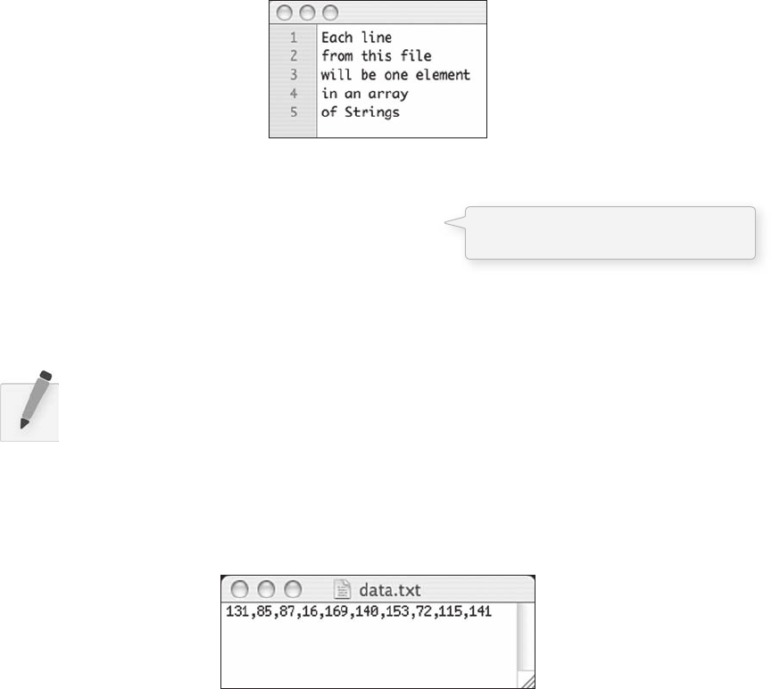
330 Learning Processing
We are going to follow this model in this section, working with the simplest means of data retrieval:
reading from a text fi le. Text fi les can be used as a very simple database (we could store settings for a
program, a list of high scores, numbers for a graph, etc.) or to simulate a more complex data source.
In order to create a text fi le, you can use any simple text editor. Windows Notepad or Mac OS X
TextEdit will do, just make sure you format the fi le as “ plain text. ” It is also advisable to name the text
fi les with the “ .txt ” extension, just to avoid any confusion. And just as with image fi les in Chapter 15,
these text fi les should be placed in the sketch’s “ data ” directory in order for them to be recognized by the
Processing sketch.
Once the text fi le is in place, Processing ’s loadStrings( ) function is used to read the content of the fi le into
a String array. e individual lines of text in the fi le (see Figure 18.2) each become an individual element
in the array.
String[] lines = loadStrings(" file.txt " );
println( " there are " + lines.length + " lines "
for (int i = 0; i < lines.length; i + + ){
println(lines[i]);
}
To run the code, create a text fi le called “ fi le.txt ” , type a bunch of lines in that fi le, and place it in your
sketch’s data directory.
Exercise 18-6: Rewrite Example 17-3 so that it loads the headlines from a text fi le.
Text from a data fi le can be used to generate a simple visualization. In Example 18-2, loads data fi le
shown in Figure 18.3 . e results of visualizing this data are shown in Figure 18.4 .
fi g. 18.3 Contents of “Data.txt”
fi g 18.2
This code will print all the lines from the
source text fi le. Shown in Figure 18.2.
);
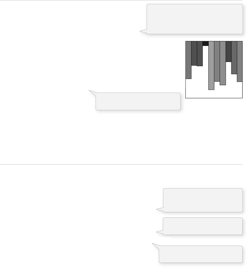
Data Input 331
Example 18-2: Graphing comma separated numbers from a text fi le
int[] data;
void setup() {
size(200,200);
// Load text file as a String
String[] stuff = loadStrings( "data.txt");
// Convert string into an array of integers
// using ',' as a delimiter
data = int(split(stuff[0], ','));
}
void draw() {
background(255);
stroke(0);
for (int i = 0; i < data.length; i + + ){
fill(data[i]);
rect(i*20,0,20,data[i]);
}
noLoop();
}
We can also use the contents of a text fi le to initialize objects by passing the data from the text fi le into
an object constructor. In Example 18-3, the text fi le has 10 lines, each line representing one instance of an
object with the values for that object’s variables separated by commas. See Figure 18.5 .
Example 18-3: Creating objects from a text fi le
Bubble[] bubbles;
void setup() {
size(200,200);
smooth();
// Load text file as an array of String
String[] data = loadStrings( "data.txt");
bubbles = new Bubble[data.length];
for (int i = 0; i < bubbles.length; i + + ){
float[] values = float(split(data[i], ","));
bubbles[i] = new Bubble(values[0],values[1],values[2]);
}
}
void draw() {
background(100);
// Display and move all bubbles
for (int i = 0; i < bubbles.length; i + + ){
bubbles[i].display();
bubbles[i].drift();
}
}
// A Class to describe a "Bubble"
class Bubble {
float x,y;
float diameter;
fi g. 18.4
The text from the fi le is loaded into
an array. This array has one element
because the fi le only has one line. That
element is then split into an array of ints.
The array of ints is used to set the
color and height of each rectangle.
The size of the array of Bubble
objects is determined by the total
number of lines in the text fi le.
Each line is split into an array of
fl oating point numbers.
The values in the array are passed
into the Bubble class constructor.
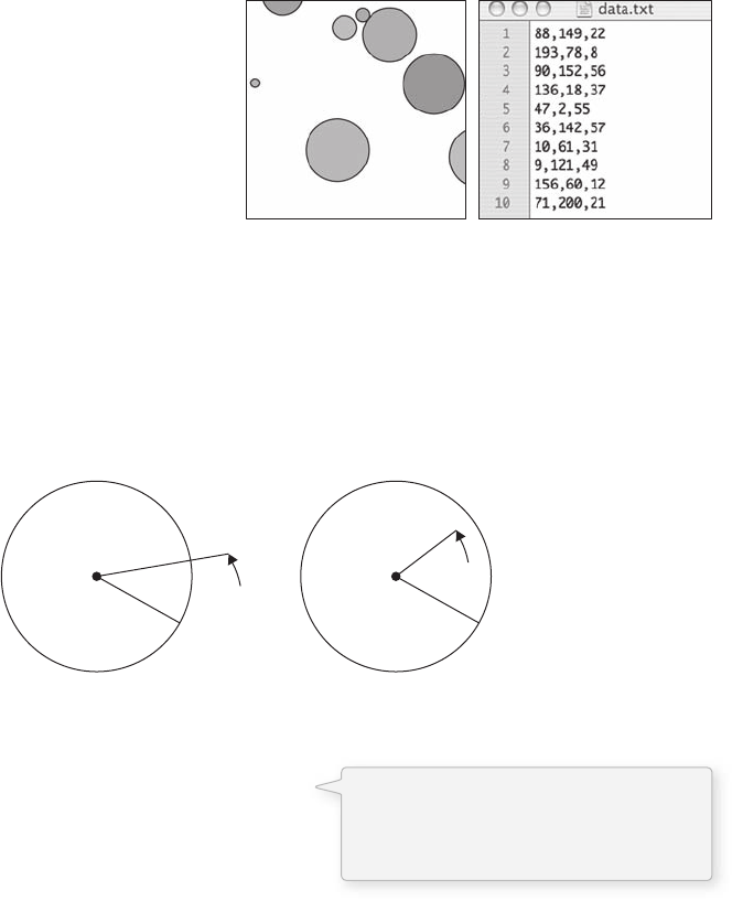
332 Learning Processing
float speed;
float r,g;
// The constructor initializes color and size
// Location is filled randomly
Bubble(float r_, float g_, float diameter_) {
x = random(width);
y = height;
r = r_;
g = g_;
diameter = diameter_;
}
// Display the Bubble
void display() {
stroke(255);
fill(r,g,255,150);
ellipse(x,y,diameter,diameter);
}
// Move the bubble
void drift() {
y + = random(–3,–0.1);
x + = random(–1,1);
if (y < -diameter*2) {
y = height + diameter*2;
}
}
}
Now that we are comfortable with the idea of loading information from a text fi le to initialize Processing
sketches, we are ready to ask the following question: What if we want to save information so that it can
be loaded the next time a program is run? For example, let’s say we want to revise Example 18-3 so that
the bubbles change on a mouse rollover. (We have worked on rollovers with a rectangle before in Exercise
5-5, and Example 9-11 but this rollover example will use a circle.) See Figure 18.6 .
dist
r
r
dist
dist > r
No Rollover
dist < r
Rollover
fi g. 18.6
fi g. 18.5
boolean rollover(int mx, int my) {
if (dist(mx,my,x,y) < diameter/2) {
return true;
} else {
return false;
}
}
The rollover() function in the Bubble
class returns a boolean value (true
or false) depending on whether the
arguments (mx,my) are inside the circle.
Data Input 333
e rollover( ) function checks to see if the distance between a given point ( mx , my ) and the bubble’s
location ( x , y ) is less than the radius of the circle; the radius is defi ned as the diameter divided by two (see
Figure 18.6 ). If this is true, then that point ( mx , my ) must be inside the circle. Calling this function using
the mouse location as the arguments allows us to test whether the mouse is, in fact, rolling over any of the
bubbles.
for (int i = 0; i < bubbles.length; i + + ){
bubbles[i].display();
bubbles[i].drift();
if (bubbles[i].rollover(mouseX,mouseY)) {
bubbles[i].change();
}
}
Once we implement the change( ) function to adjust the Bubble’s variables, we can save the new
information in a text fi le with Processing ’s saveStrings( ) function. saveStrings( ) is essentially the opposite
of loadStrings( ) , receiving a fi lename and a String array and saving that array to the fi le.
String[] stuff = { " Each String ", "will be saved ", "on a ", "separate line " } ;
saveStrings( "data.txt", stuff);
fi g. 18.7
saveStrings( ) , however, does not store the text fi le in the data folder, but rather places it in the local
sketch directory. If we want the fi le to be written to the data directory, we must specify the path. Also, if
the fi le already exists, it will be overwritten.
Knowing this, we can concoct a saveData( ) function for the Bubbles sketch that rewrites “ data.txt ” with
the properties from the objects in their current state. In this example, we will save the new data whenever
the mouse is pressed.
void saveData() {
String[] data = new String[bubbles.length];
for (int i = 0; i < bubbles.length; i + + ){
data[i] = bubbles[i].r + " ," + bubbles[i].g + " ," + bubbles[i].diameter;
}
saveStrings( "data/data.txt",data);
}
void mousePressed() {
saveData();
}
Since the original data fi le is overwritten, whenever you run the sketch again, the new values are loaded.
Here is the entire example for reference. Figure 18-18 shows the new data fi le after saveStrings( ):
We fi rst create an array of Strings
with a size equal to the total number
of Bubble objects.
Each element of the String array is
made by concatenating the values
of each Bubble object’s variables.
This code will create the
text fi le in Figure 18.7.
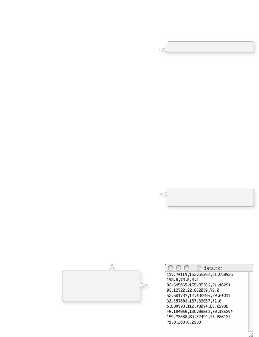
334 Learning Processing
Example 18-4: Loading and saving data to text fi le
// An array of Bubble objects
Bubble[] bubbles;
void setup() {
size(200,200);
smooth();
// Load text file as a string
String[] data = loadStrings(" data.txt " );
// Make as many objects as lines in the text file
bubbles = new Bubble[data.length];
// Convert values to floats and pass into Bubble constructor
for (int i = 0; i < bubbles.length; i + + ) {
float[] values = float(split(data[i], " , " ));
bubbles[i]
= new Bubble(values[0],values[1],values[2]);
}
}
void draw() {
background(255);
// Display and move all bubbles
for (int i
= 0; i < bubbles.length; i + +){
bubbles[i].display();
bubbles[i].drift();
// Change bubbles if mouse rolls over
if (bubbles[i].rollover(mouseX,mouseY)) {
bubbles[i].change();
}
}
}
// Save new Bubble data when mouse is Pressed
void mousePressed() {
saveData();
}
void saveData() {
// For each Bubble make one String to be saved
String[] data
= new String[bubbles.length];
for (int i
= 0; i < bubbles.length; i + +){
// Concatenate bubble variables
data[i]
= bubbles[i].r + " , " + bubbles[i].g + " , " + bubbles[i].diameter;
}
// Save to File
saveStrings( " data/data.txt ",data);
}
// A Bubble class
class Bubble {
float x,y;
float diameter;
float speed;
float r,g;
Bubble(float r_,float g_, float diameter_) {
x
= random(width);
y
= height;
r
= r_;
g
= g_;
fi g 18.8 The new data fi le after save strings ( )
Bubble data is loaded in setup().
Bubble data is saved in
mousePressed().
The same fi le is overwritten by
adding the “data” folder path
to saveStrings() as shown in
Figure 18.8.

Data Input 335
diameter = diameter_;
}
// True or False if point is inside circle
boolean rollover(int mx, int my) {
if (dist(mx,my,x,y)
< diameter/2) {
return true;
} else {
return false;
}
}
// Change Bubble variables
void change() {
r
= constrain(r + random(–10,10),0,255);
g
= constrain(g + random(–10,10),0,255);
diameter
= constrain(diameter + random(–2,4),4,72);
}
// Display Bubble
void display() {
stroke(0);
fill(r,g,255,150);
ellipse(x,y,diameter,diameter);
}
// Bubble drifts upwards
void drift() {
y + = random(–3,–0.1);
x + = random(–1,1);
if (y < -diameter*2) {
y = height + diameter*2;
}
}
}
18.4 Text Parsing
Now that we are comfortable with how loadStrings( ) works for text fi les stored locally, we can start to
examine what we might do with textual data we retrieve from other sources such as a URL.
String[] lines = loadStrings( " http://www.yahoo.com " );
Exercise 18-7: Create a sketch that visualizes the following data. Feel free to add to and
change the text.

336 Learning Processing
When you send a URL path into loadStrings( ) , you get back the raw HTML ( “ Hypertext Markup
Language ” ) source of the requested web page. It is the same stuff that appears upon selecting “ View
Source ” from a browser’s menu options. You do not need to be an HTML expert to follow this section,
but if you are not familiar at all with HTML, you might read http://en.wikipedia.org/wiki/HTML .
Unlike with the comma-delimited data from a text fi le that was specially formatted for use in a Processing
sketch, it is not practical to have the resulting raw HTML stored in an array of Strings (each element
representing one line from the source). Converting the array into one long String can make things a bit
simpler. As we saw earlier in the chapter, this can be achieved using join( ) .
String onelongstring = join(lines, " " );
When pulling raw HTML from a web page, it is likely you do not want all of the source, but just a small
piece of it. Perhaps you are looking for weather information, a stock quote, or a news headline. We can
take advantage of the String manipulation functions we learned— indexOf( ) , substring( ) , and length( ) —
to fi nd pieces of data within a large block of text. We saw an early example of this in Exercise 18-2 . Take,
for example, the following String:
String stuff = " Number of apples:62. Boy, do I like apples or what! " ;
Let’s say we want to pull out the number of apples from the above text. Our algorithm would be as
follows:
1. Find the end of the substring “ apples: ”. Call it start.
2. Find the fi rst period after “ apples: ” . Call it end.
3. Make a substring of the characters between start and end.
4. Convert the String to a number (if we want to use it as such).
In code, this look’s like:
int start = stuff.indexOf( " apples: " ) + 8; // STEP 1
int end = stuff.indexOf( " . " ,start); // STEP 2
String apples = stuff.Substring(start,end); // STEP 3
int apple_no = int(apples); // STEP 4
e above code will do the trick, but we should be a bit more careful to make sure we do not run into
any errors if we do not fi nd the substrings . We can add some error checking and generalize the code into a
function:
// A function that returns a substring between two substrings
String giveMeTextBetween(String s, String startTag, String endTag) {
String found = " " ;
// Find the index of the beginning tag
int startIndex = s.indexOf(startTag);
// If we don’t find anything
if (startIndex = = –1) return " " ;
// Move to the end of the beginning tag
startIndex + = startTag.length();
The “end” of a String
can be found by
searching for the index
of that String and
adding the length to that
index (in this case 8).
A function to return a String found
between two Strings. If beginning
or end “tag” is not found, the
function returns an empty String.
Data Input 337
// Find the index of the end tag
int endIndex = s.indexOf(endTag, startIndex);
// If we don’t find the end tag,
if (endIndex = = –1) return " " ;
// Return the text in between
return s.substring(startIndex,endIndex);
}
With this technique, we are ready to connect to a web site from within Processing and grab data to
use in our sketches. For example, we could read the HTML source from http://www.nytimes.com and
look for today’s headlines, search http://fi nance.yahoo.com for stock quotes, count how many times the
word “ Flickr ” appears on your favorite blog, and so on. HTML, however, is an ugly, scary place with
inconsistently formatted pages that are diffi cult to reverse engineer and parse eff ectively. Not to mention
the fact that companies change the source code of web pages rather often, so any example that I might
make while I am writing this paragraph might break by the time you read this paragrap.
For grabbing data from the web, an XML (Extensible Markup Language) feed will prove to be more
reliable and easier to parse. Unlike HTML (which is designed to make content viewable by a human’s
eyes) XML is designed to make content viewable by a computer and facilitate the sharing of data across
diff erent systems. We will get into how XML works more in Section 18.17 . For now, let’s examine how we
might grab the weather for any given zip code from Yahoo’s XML weather feed. Information about all of
Yahoo’s XML feeds can be found here: http://developer.yahoo.com/rss/ . e weather XML feed is here:
http://xml.weather.yahoo.com/forecastrss?p 10025
One way to grab the data from a weather feed is to use the Processing XML library (which facilitates
reading from an XML document). However, in order to demonstrate String parsing on a lower level,
as an exercise, we will use our loadStrings( ) scraping techniques and search for bits of information
embedded in the XML source manually. Admittedly, this is somewhat of a silly pursuit since XML is
designed to be parsed without having to resort to this methodology. For comparison, we will look at this
sample example using two diff erent XML libraries in Sections 18.7 and 18.8.
Looking in the XML source from the above URL, we can see that the temperature today (which happens
to be August 1, 2007 at the time of this writing) is 88ⴰF— temp “ 88 ” .
< yweather:condition text = " Fair" code = " 34" temp = " 88" date = " Wed, 01 Aug 2007
3:51 pm EDT "/
e temperature is variable but the XML format is not, and therefore we can deduce that the start tag for
our search should be:
temp"
and the end tag:
"
(i.e., the fi rst quote after the start tag).
Knowing the start and end tags, we can use giveMeTextBetween( ) to pull out the temperature.
IndexOf() can also take a second
argument, an integer. That second
argument means: Find the fi rst
occurrence of the search String
after this specifi ed index. We use
it here to ensure that end index
follows start index.
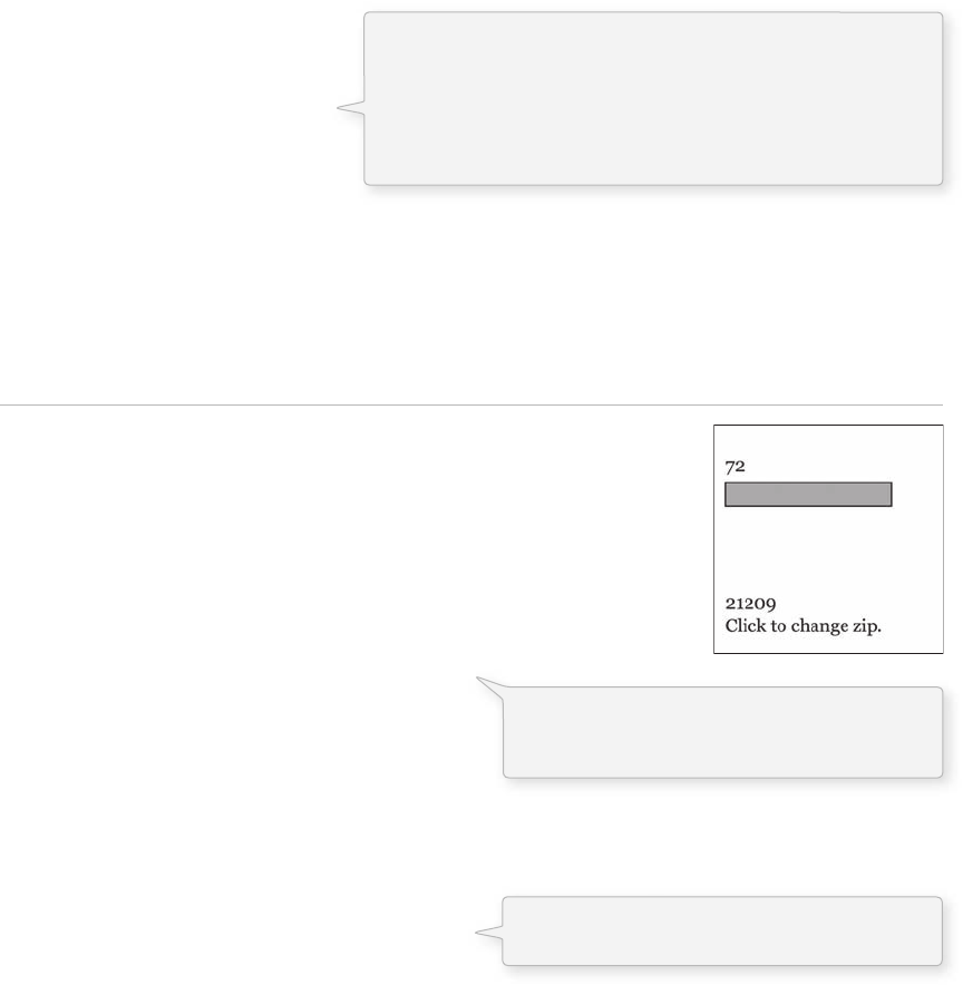
338 Learning Processing
String url = " http://xml.weather.yahoo.com/forecastrss?p = 10003 " ;
String[] lines = loadStrings(url);
// Get rid of the array in order to search
// the whole page
String xml = join(lines, " " );
// Searching for temperature
String tag1 = " temp = \ " " ;
String tag2 = " \ " " ;
temp = int(giveMeTextBetween
(xml,tag1,tag2));
println(temp);
Example 18-5 retrieves the temperature from Yahoo’s weather XML feed and displays it onscreen. e
example also uses object-oriented programming, putting all of the String parsing functionality into a
WeatherGrabber class.
Example 18-5: Parsing Yahoo’s XML weather feed manually
PFont f;
String[] zips = { " 10003 ", " 21209 ", " 90210 " } ;
int counter = 0;
// The WeatherGrabber object does the work for us!
WeatherGrabber wg;
void setup() {
size(200,200);
// Make a WeatherGrabber object
wg = new WeatherGrabber(zips[counter]);
// Tell it to request the weather
wg.requestWeather();
f = createFont( " Georgia " ,16,true);
}
void draw() {
background(255);
textFont(f);
fill(0);
// Get the values to display
String weather = wg.getWeather();
int temp = wg.getTemp();
// Display all the stuff we want to display
text(zips[counter],10,160);
text(weather,10,90);
text(temp,10,40);
text(" Click to change zip. " ,10,180);
// Draw a little thermometer based on the temperature
stroke(0);
fill(175);
rect(10,50,temp*2,20);
}
fi g. 18.9
A quote in Java marks the beginning or end of a String. So how
do we include an actual quote in a String?
The answer is via an “escape” sequence. (We encountered this
in Exercise 17-8.) A quote can be included in a String using a
backward slash, followed by a quote. For example:
String q = "This String has a quote \"in it";
The WeatherGrabber object is initialized with
a zip code. The XML data is loaded and parsed
upon calling the requestWeather() function.
The weather and temperature information is
pulled from the WeatherGrabber object.

Data Input 339
void mousePressed() {
// Increment the counter and get the weather at the next zip code
counter = (counter + 1) % zips.length;
wg.setZip(zips[counter]);
wg.requestWeather();
}
// A WeatherGrabber class
class WeatherGrabber {
int temperature = 0;
String weather = " " ;
String zip;
WeatherGrabber(String tempZip) {
zip = tempZip;
}
// Set a new Zip code
void setZip(String tempZip) {
zip = tempZip;
}
// Get the temperature
int getTemp() {
return temperature;
}
// Get the weather
String getWeather() {
return weather;
}
// Make the actual XML request
void requestWeather() {
// Get all the HTML/XML source code into an array of strings
// (each line is one element in the array)
String url = " http://xml.weather.yahoo.com/forecastrss?p = " + zip ;
String[] lines = loadStrings(url);
String xml = join(lines, " " ); // Turn array into one long String
// Searching for weather condition
String lookfor = " < yweather:condition text = \ " " ;
String end = " \ " " ;
weather = giveMeTextBetween (xml,lookfor,end);
// Searching for temperature
lookfor = " temp = \ " " ;
temperature = int(giveMeTextBetween (xml,lookfor,end));
}
// A function that returns a substring between two substrings
String giveMeTextBetween(String s, String before, String after) {
String found = " " ;
int start = s.indexOf(before); // Find the index of the beginning tag
if (start = = – 1) return " " ; // If we don’t find anything, send back a blank
// String
start + = before.length(); // Move to the end of the beginning tag
int end = s.indexOf(after,start); // Find the index of the end tag
if (end == –1) return ""; // If we don’t find the end tag, send back a blank String
return s.substring(start,end); // Return the text in between
}
}
The data is requested again with a new zip
code every time the mouse is pressed.

340 Learning Processing
Exercise 18-8: Expand Example 18-5 to also search for the next day’s high and low temperature.
Exercise 18-9: Take a look at Yahoo’s “ Word of the Day ” XML feed available at this URL:
http://xml.education.yahoo.com/rss/wotd/ . Use the manual parsing techniques to pull out the
Word of the Day from the feed.
18.5 Text Analysis
Loading text from a URL need not only be an exercise in parsing out small bits of information. It is
possible with Processing to analyze large amounts of text found on the web from news feeds, articles, and
speeches, to entire books. A nice source is Project Gutenberg ( http://www.gutenberg.org/ ) —which makes
available thousands of public domain texts. Algorithms for analyzing text merits an entire book itself, but
we will look at one simple beginner example here.
Example 18-6 retrieves the entire text of Shakespeare’s play King Lear , and uses split Tokens ( ) to make
an array of all the words in the play. e sketch then displays the words one by one, along with a count of
how many times the word appears in the text.
Example 18-6: Analyzing King Lear
PFont f; // A variable to hold onto a font
String[] kinglear; // The array to hold all of the text
int counter = 0; // Where are we in the text
// We will use spaces and punctuation as delimiters
String delimiters = " ,.?!;: " ;
void setup() {
size(200,200);
// Load the font
f = loadFont( " Georgia-Bold-16.vlw " );
// Load King Lear into an array of strings
String url = " http://www.gutenberg.org/dirs/etext97/1ws3310.txt " ;
String[] rawtext = loadStrings(url);
// Join the big array together as one long string
String everything = join(rawtext, " " );
// Split the array into words using any delimiter
kinglear = splitTokens(everything,delimiters);
frameRate(5);
}
void draw() {
background(255);
// Pick one word from King Lear
String theword = kinglear[counter];
// Count how many times that word appears in King Lear
int total = 0;
Any punctuation is used as a delimiter.
All the lines in King Lear are
fi rst joined as one big String
and then split up into an array of
individual words. Note the use
of splitTokens() since we are
using spaces and punctuation
marks all as delimiters.
This loop counts the
number of occurrences
of the current word being
displayed.
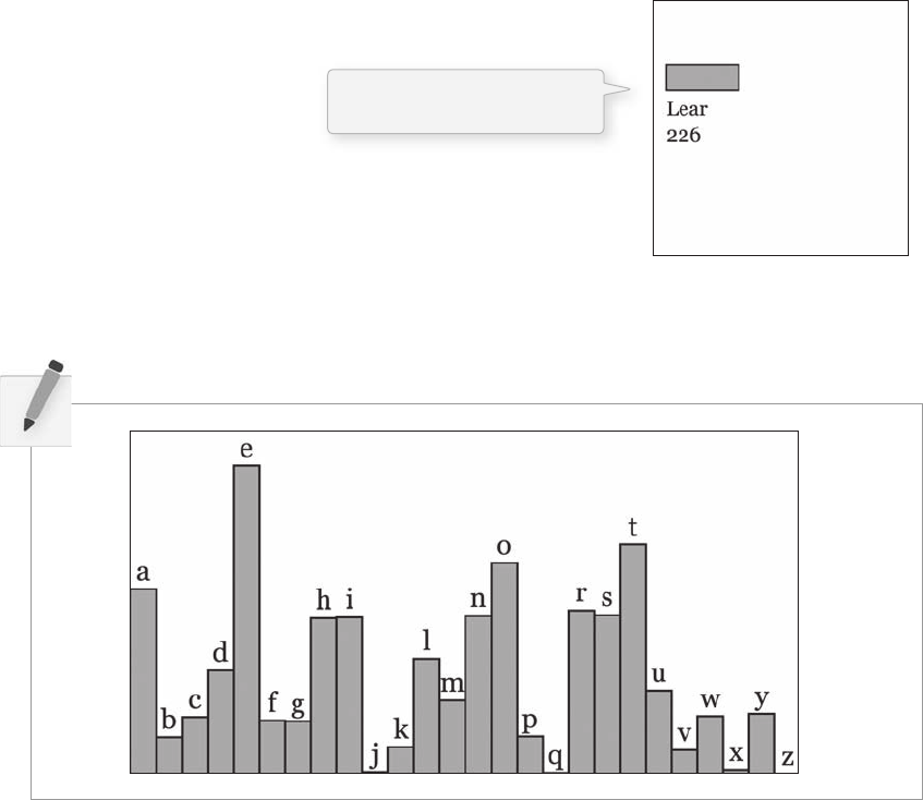
Data Input 341
for (int i = 0; i < kinglear.length; i + + ){
if (theword.equals(kinglear[i])) {
total + + ;
}
}
// Display the text and total times the word appears
textFont(f);
fill(0);
text(theword,10,90);
text(total,10,110);
stroke(0);
fill(175);
rect(10,50,total/4,20);
// Move onto the next word
counter = (counter + 1) % kinglear.length;
} fi g. 18.10
Exercise 18-10: Count the number of times each letter of the alphabet appears in King Lear
Visualize those counts. Here is one possibility (you should be more creative). Note this sketch
will require the use of the charAt( ) function.
18.6 Asynchronous Requests
As we have seen, the loadStrings( ) function can be used for retrieving raw data from web pages.
Nonetheless, unless your sketch only needs to load the data once during setup( ) , you may have a problem.
For example, consider a sketch that grabs the price of AAPL stock from an XML feed every 5 min.
Each time loadStrings( ) is called, the sketch will pause while waiting to receive the data. Any animation
will stutter. is is because loadStrings( ) is a “ blocking ” function, in other words, the sketch will sit and
wait at that line of code until loadStrings( ) completes its task. With a local text fi le, this is extremely fast.
Nonetheless, a request for a web page (known as an “ HTTP request ” ) is asynchronous , meaning the web
server can take its time getting back to you with the data requested. Who knows how long loadStrings( )
will take? No one, you are at the mercy of the server!
e simpleML library (available for download at this book’s web site: http://www.learniningprocessing.
com/simpleML/ ) gets around this problem by executing these HTTP requests to web servers in parallel
The word “Lear” appears 226
times in the text of King Lear.

342 Learning Processing
without pausing your Processing sketch, allowing the sketch to multitask and continue animating while
the data retrieval is in process.
e library functions in a similar manner to the Processing video library, which we became familiar with in
Chapter 16. To retrieve a web page, you must create an instance of an HTMLRequest object, passing in a
reference to the the sketch itself ( this ) and the URL you want to request.
HTMLRequest req = new HTMLRequest(this, " http://www.yahoo.com " );
e request will not begin, however, until you call makeRequest( ).
req.makeRequest();
Finally, to receive the data, you must write a function called netEvent( ) . is function will be invoked the
instant the request is fi nished and data is available.
is function is another example of a callback function, the same as captureEvent( ) (see Chapter 16) or
mousePressed( ) . In this case, instead of an event being triggered when the user clicks the mouse or an
image from the camera is available, the event is triggered when the HTML request fi nishes (or XML as
we will see in a moment).
e HTML source of the web page is returned as a String via the function readRawSource( ) .
void netEvent(HTMLRequest ml) {
String html = ml.readRawSource();
println(html);
}
Example 18-7 retrieves Yahoo’s homepage every ten seconds using the simpleML library. e
visualization here is arbitrary (lines are colored according to the characters in Yahoo’s HTML source);
however, what is important is to notice how the animation never pauses while waiting for the data to
arrive .
Example 18-7: Loading a URL with simpleML
import simpleML.*;
// A Request object, from the library
HTMLRequest htmlRequest;
Timer timer = new Timer(5000);
String html = " " ; // String to hold data from request
int counter = 0; // Counter to animate rectangle across window
int back = 255; // Background brightness
void setup() {
size(200,200);
Data Input 343
// Create and make an asynchronous request
htmlRequest = new HTMLRequest(this, " http://www.yahoo.com " );
htmlRequest.makeRequest();
timer.start();
background(0);
}
void draw() {
background(back);
// Every 5 seconds, make a new request
if (timer.isFinished()) {
htmlRequest.makeRequest();
println( "Making request! ");
timer.start();
}
// Draw some lines with colors based on characters from data retrieved
for (int i = 0; i < width; i + + ){
if (i < html.length()) {
int c = html.charAt(i);
stroke(c,150);
line(i,0,i,height);
}
}
// Animate rectangle and dim rectangle
fill(255);
noStroke();
rect(counter,0,10,height);
counter = (counter + 1) % width;
back = constrain(back – 1,0,255);
}
// When a request is finished
void netEvent(HTMLRequest ml) {
html = ml.readRawSource(); // Read the raw data
back = 255; // Reset background
println( "Request completed! "); // Print message
}
// Timer Class from Chapter 10
class Timer {
int savedTime;
boolean running = false;
int totalTime;
Timer(int tempTotalTime) {
totalTime = tempTotalTime;
}
void start() {
running = true;
savedTime = millis();
}
boolean isFinished() {
int passedTime = millis() – savedTime;
if (running & & passedTime > totalTime) {
running = false;
fi g. 18.11
An HTML Request object to request
the source from a URL.
A request is made every 5 s. The data is not
received here, however, this is only the request.
The data is received in the netEvent() function
which is automatically called whenever data
is ready.
344 Learning Processing
return true;
} else {
return false;
}
}
}
18.7 Beginner XML
e examples in Section 18.4 demonstrated the process of manually searching through text for individual
pieces of data. Admittedly, manually parsing the raw XML data from http://xml.weather.yahoo.com/
forecastrss?p 10003 was not the most effi cient strategy. Yes, if you need information from an oddly
formed HTML page, these manual techniques are required. However, because XML is designed to
facilitate the sharing of data across diff erent systems, it can be parsed without manual searching, using an
XML parsing library.
XML organizes information in a tree structure. Let’s imagine a list of students. Each student has an id
number, name, address, e-mail, and telephone number. Each student’s address has a city, state, and zip
code. An XML tree for this dataset might look like Figure 18.12 .
Student Student Student Student
id name phone e-mail address
street city state zip
Students
fi g. 18.12
e XML source itself (with two students listed) is:
?xml version = " 1.0 " encoding = " UTF-8 " ?
students
student
id 001 /id
name Daniel Shiffman /name
phone 555-555-5555 /phone
email daniel@shiffman.net /email
address
street 123 Processing Way /street
city Loops /city
state New York /state
zip 01234 /zip
/address
/student
Data Input 345
student
id 002 /id
name Zoog /name
phone 555-555-5555 /phone
email zoog@planetzoron.uni /email
address
street 45.3 Nebula 5 /street
city Boolean City /city
state Booles /state
zip 12358 /zip
/address
/student
/students
Note the similarities to object-oriented programming. We could think of the XML tree in the following
terms. e XML document represents an array of student objects. Each student object has multiple pieces
of information, an id, a name, a phone number, an e-mail address, and a mailing address. e mailing
address is also an object that also has multiple pieces of data, such as street, city, state, and zip.
?xml version = "1.0"?
________
bubble
________ 40 /________
________ 100 /________
________ 255 /green
________
/bubbles
Exercise 18-11: Revisit the “ Bubble ” Example 18-3. Design an XML tree structure for
Bubble objects. Diagram the tree and write out the XML source. (Use the empty diagram
and fi ll in the blanks below.)
Returning to the weather example, we can now make some sense of Yahoo’s XML data with the tree
structure terms of a tree. Here is the raw XML source. (Note I have edited it for simplifi cation purposes.)
346 Learning Processing
?xml version = " 1.0 " encoding = " UTF-8 " standalone = " yes " ?
rss version = " 2.0 " xmlns:yweather = " http://xml.weather.yahoo.com/ns/rss/1.0 "
channel
item
title Conditions for New York, NY at 3:51 pm EST /title
geo:lat 40.67 /geo:lat
geo:long -73.94 /geo:long
link http://xml.weather.yahoo.com/forecast/USNY0996_f.html /link
pubDate Mon, 20 Feb 2006 3:51 pm EST /pubDate
yweather:condition text = " Fair " code = " 34 " temp =
" 35 " date = " Mon, 20 Feb 2006
3:51 pm EST " /
yweather:forecast day = " Mon " date = " 20 Feb 2006 " low = " 25 " high = " 37 "
text = " Clear " code = " 31 " /
/item
/channel
/rss
e data is mapped in the tree stucture shown in Figure 18.13 .
RSS
Channel
item
title geo:lat geo:long link pub Date y weather:
condition y weather:
forecast
fi g. 18.13
You may be wondering what the top level “ RSS ” is all about. Yahoo’s XML weather data is provided
in RSS format. RSS stands for “ Really Simple Syndication ” and is a standardized XML format for
syndicating web content (such as news articles, etc.). You can read more about RSS on wikipedia:
http://en.wikipedia.org/wiki/RSS .
Now that we have a handle on the tree structure, we should look at the specifi cs inside that structure.
With the exception of the fi rst line (which simply indicates that this page is XML formatted), this XML
document contains a nested list of elements , each with a start tag, that is, channel , and an end tag,
that is, /channel . Some of these elements have content between the tags:
title Conditions for New York, NY at 3:51 pm EST /title
and some have attributes (formatted by Attribute Name equals Attribute Value in quotes ):
yweather:forecast day = " Mon " date = " 20 Feb 2006 " low = " 25 " high = " 37 " text = " Clear "
code = " 31 " /
ere are several XML Parsing libraries available for Processing and we will explore two in this chapter.
e fi rst, designed for this book, is the simplest (but has the fewest features): the simpleML library.
simpleML can perform the following three tasks:
• Retrieve the text from one XML element as a String .
• Retrieve the text from one attribute of an XML element as a String .
• Retrieve the text from many XML elements (with the same tag) as an array of Strings .

Data Input 347
Requests for XML data are made via an XMLRequest object.
XMLRequest req = new XMLRequest(this, " http://xml.weather.yahoo.
com/forecastrss?p = 10003 " );
Again, the request will not begin until you call makeRequest( ) .
req.makeRequest();
Just as with the HTML request, to receive the data from the XML request, you must implement
netEvent( ) , this time with an XMLRequest object as its argument.
e function getElementText( ) returns the content from a single XML element (the name of that
element must be passed into the function). For an attribute, use getElementAttributeText( ) with the name
of the element, followed by the name of the attribute.
For example, with the following XML data:
geo:lat 40.67 /geo:lat
yweather:forecast day = " Mon" date = " 20 Feb 2006 " low = " 25" high = " 37"
text =" Clear " code =" 31 "/
e code to grab data is:
void netEvent(XMLRequest ml) {
// Getting the text of one Element
String lat = ml.getElementText( "geo:lat");
// Getting the text of one Attribute from one Element
String temperature = ml.getElementAttributeText( "yweather:forecast","high");
println( "Latitude is: " + lat);
println( "The high temperature is:
" + temperature);
}
e method getElementArray( ) can also be called to retrieve
XML elements that appear multiple times. It returns an array
of Strings , one String for every element in the XML document.
e following example grabs all of the headlines from Yahoo’s
Top Stories XML Feed.
Example 18-8: Loading XML with simpleML
import simpleML.*;
XMLRequest xmlRequest;
void setup() {
size(200,200);
The content of an XML element is
retreived by passing in the element
name (in this case “geo:lat”) to the
getElementText() function.
The content of an XML element’s
attribute is retrieved by passing
in the element name (in this case
“yweather:forecast”) as well as the
attribute name (in this case “high”)
to the getElementAttrributeText()
function.
348 Learning Processing
// Creating and starting the request
xmlRequest = new XMLRequest(this, " http://rss.news.yahoo.com/rss/topstories " );
xmlRequest.makeRequest();
}
void draw() {
noLoop();// Nothing to see here
}
// When the request is complete
void netEvent(XMLRequest ml) {
// Retrieving an array of all XML elements inside " title* " tags
String[] headlines = ml.getElementArray( " title " );
for (int i = 0; i headlines.length; i + + ) {
println(headlines[i]);
}
}
Exercise 18-12: Visualize the Yahoo weather data using simpleML. Following is part of the
code to get you started. is is the XML in case you forgot: < yweather:condition
text = “ Fair ” code = “ 34 ” temp = “ 35 ” date = “Mon, 20 Feb 2006
3:51 pm EST ” /
import simpleML.*;
// Variables for temperature and weather
int temperature = 0;
String weather = " " ;
void setup() {
// FILL THIS IN HOWEVER YOU LIKE!
}
void draw() {
// FILL THIS IN HOWEVER YOU LIKE!
}
// Function that makes the weather request with a Zip Code
void getWeather(String zip) {
String url = " http://xml.weather.yahoo.com/
forecastrss?p = " + zip ;
XMLRequest req = new XMLRequest(this,url);
req.makeRequest();
}
void netEvent(XMLRequest ml) {
// Get the specifi c XML content we want
temperature = int(ml.__________( " _________ " , "
_________ " ));
weather = ml.___________( " __________ " , " __________ " );
}
An array of XML elements can be retrieved
using getElementArray. This only works for
elements with the same name that appear
multiple times in the XML document.

Data Input 349
18.8 Using the Processing XML Library
e functionality of the simpleML library, though easy to use, is quite limited. If you want to create your
own XML documents, or parse multiple elements of a document with a custom algorithm, you are out of
luck. For more sophisticated XML functionality, there are two options. e fi rst, more advanced option is
proXML ( http://www.texone.org/proxml/ ) created by Christian Riekoff . While the learning curve is a bit
steeper, you have direct access to the XML tree structure and can read and write XML documents.
e second option, which we will explore in this chapter, is Processing ’s built-in XML library.
import processing.xml.*;
Once the library is imported, the fi rst step is to create an XMLElement object. is object will load the
data from XML documents (stored locally or on the web). e constructor requires two arguments, “ this ”
and the fi lename or URL path for the XML document.
String url = " xmldocument.xml";
XMLElement xml = new XMLElement(this,url);
Unlike simpleML, this XML library pauses the sketch and waits for the document to load. For an
asynchronous approach to XML parsing, you will need to use proXML.
An XMLElement object represents one element of an XML tree. When a document is fi rst loaded, that
element object is always the root element. simpleML did the work of traversing the tree and fi nding the
right information for us. With the Processing XML library, we have to do this work ourselves. Although
this is more complex, we have more control over how we search and what we search for.
Referring back to Figure 18.13 , we can fi nd the temperature via the following path:
1. e root element of the tree is “ RSS. ”
2. “ RSS ” has a child element named “ Channel. ”
3. e 13th child of “ Channel ” is “ item. ” ( e diagram is simplifi ed to show only one child of channel.)
4. e sixth child of “ item ” is “ yweather:condition. ”
5. e temperature is stored in “ yweather:condition ” as the attribute “ temp. ”
e children of an element are accessed with an index (starting at zero, same as an array) passed into the
getChild( ) function. e content of an element is retrieved with getContent( ) and attributes are read as
either numbers— getIntAttribute( ), getFloatAttribute( ) —or text— getStringAttribute( ) .
// Accessing the first child element of the root element
XMLElement channel = xml.getChild(0);
Following steps 1 through 5 outlined above through the XML tree, we have:
XMLElement xml = new XMLElement(this, url);
XMLElement channel = xml.getChild(0);
XMLElement item = channel.getChild(12);
XMLElement condition = item.getChild(5);
temp = condition.getIntAttribute( "temp");
The 13th child of an element is index #12.

350 Learning Processing
Other useful functions that can call XMLElement objects are:
• getChildCount( ) —returns the total number of children of an XMLElement.
• getChildren( ) —returns all of the children as an array of XMLElements.
In Example 18-3 , we used a series of comma separated values in a text fi le to store information related to
Bubble objects. An XML document can also be used in the same manner. Here is a possible solution to
Exercise 18-11, an XML tree of Bubble objects. (Note that this solution uses element attributes for red
and green colors; this was not the format provided in Exercise 18-11 since we had not yet learned about
attributes.)
?xml version = " 1.0 " ?
bubbles
bubble
diameter 40 /diameter
color red = " 75 " green = " 255 " /
/bubble
bubble
diameter 20 /diameter
color red = " 255 " green = " 75" /
/bubble
bubble
diameter
80 /diameter
color red = " 100 " green = " 150 " /
/bubble
/bubbles
We can use getChildren( ) to receive the array of “ Bubble ” elements and make a Bubble object from each
one. Here is the example (which uses the identical Bubble class from earlier). e new elements are in bold.
Example 18-9: Using Processing’s XML library
import processing.xml.*;
// An array of Bubble objects
Bubble[] bubbles;
void setup() {
size(200,200);
smooth();
// Load an XML document
XMLElement xml = new XMLElement(this, " bubbles.xml " );
// Get the total number of bubbles
int totalBubbles = xml.getChildCount();
// Make an array the same size
bubbles = new Bubble[totalBubbles];
// Get all the child elements
XMLElement[] children = xml.getChildren();
for (int i = 0; i < children.length; i + + ) {
// The diameter is child 0
The root element is “bubbles”, which has
three children.
Each child “bubble” has two children,
“diameter” and “color.” The “color” element
has two attributes, “red” and “green”.
Getting the total number of Bubble objects
with getChildCount().

Data Input 351
XMLElement diameterElement = children[i].getChild(0);
int diameter = int(diameterElement.getContent());
// Color is child 1
XMLElement colorElement = children[i].getChild(1);
int r = colorElement.getIntAttribute( "red");
int g = colorElement.getIntAttribute( "green");
// Make a new Bubble object with values from XML document
bubbles[i] = new Bubble(r,g,diameter);
}
}
void draw() {
background(100);
// Display and move all bubbles
for (int i = 0; i bubbles.length; i + + ){
bubbles[i].display();
bubbles[i].drift();
}
}
Exercise 18-13: Use the following XML document to initialize an array of objects. Design
the objects to use all of the values in each XML element. (Feel free to rewrite the XML
document to include more or less data.) If you do not want to retype the XML, it is available
at this book’s web site.
The diameter is the content of the
fi rst element while red and green
are attributes of the second.
?xml version = "1.0"?
blobs
blob
location x = "99" y = " 192"/
speed x = " 0.88238335 " y = " 2.2704291"/
size w = "38" h = " 10"/
/blob
blob
location x = "97" y =
"14" /
speed x =
" 2.8775783 " y = " 2.9483867 "/
size w =
"81" h = "43" /
/blob
blob
location x =
" 159 " y = " 193 " /
speed x =
" -1.2341062 " y = " 0.44016743 " /
size w =
"19" h = "95" /
/blob
blob

352 Learning Processing
18.9 The Yahoo API
Loading HTML and XML documents is convenient for pulling information from the web, however,
for more sophisticated applications, many sites off er an API. An API (Application Programming
Interface) is an interface through which one application can access the services of another. ere are
many APIs that can be used with Processing and you might look through the “ Data / Protocols ”
section of the Processing libraries web page ( http:/processing.org/reference/libraries/index.html ) for some
ideas.
In this section, we will look at an example that performs a web search, using the Yahoo API.
Although you can access the Yahoo API directly, I have created a Processing library that makes it a bit
simpler (as well as allowing the search to be performed asynchronously and not cause the sketch
to pause). You will need to download both my Processing library, as well as the Yahoo API fi les (these
are known as an SDK: “ Software Development Kit ” ). Instructions for this can be found at the library
page:
http://www.learningprocessing.com/libraries/yahoo/
Once you have downloaded the fi les, you must fi rst get a Yahoo API key. In many cases, companies will
require that you register and get a key before having access to their API. at way, they can track your
usage and make sure you are not up to anything nefarious. It is a small price to pay for free programmatic
access to Yahoo’s features. You can register for the ID here:
https://developer.yahoo.com/wsregapp/index.php
Once you have the key, you are ready to go. e library works in a similar fashion to simpleML. You
make a YahooSearch object and call the search( ) function. When the search is completed, it will arrive
in an event callback: searchEvent( ) . ere, you can ask for information about the search results, such as
URLs, titles, or summaries (all available as String arrays).
location x = " 102 " y = "53" /
speed x = "0.8000488" y = " -2.2791147 " /
size w = "25" h = " 95 " /
/blob
blob
location x = "152 " y = " 181 " /
speed x = "1.9928784 " y = " -2.9540048 "/
size w = "74" h = " 19 " /
/blob
/blobs

Data Input 353
Example 18-10: A Yahoo search
import pyahoo.*;
YahooSearch yahoo;
void setup() {
size(400,400);
// Make a search object, pass in your key
yahoo = new YahooSearch(this, "YOUR API KEY HERE ");
}
void mousePressed() {
yahoo.search( "processing.org");
}
void draw() {
noLoop();
}
// When the search is complete
void searchEvent(YahooSearch yahoo) {
// Get Titles and URLs
String[] titles = yahoo.getTitles();
String[] urls = yahoo.getUrls();
for (int i = 0; i titles.length; i + + ){
println( "___________");
println(titles[i]);
println(urls[i]);
}
}
e library can be used to perform a simple visualization. e following example searches for fi ve names
and draws a circle for each one (with a size tied to the total number of results available).
Example 18-11: Yahoo search visualization
import pyahoo.*;
YahooSearch yahoo;
PFont f;
// The names to search, an array of "Bubble" objects
String[] names = { " Aliki","Cleopatra","Penelope","Daniel","Peter" } ;
Bubble[] bubbles = new Bubble[names.length];
int searchCount = 0;
void setup() {
size(500,300);
yahoo = new YahooSearch(this, "YOUR APPI HERE ");
f = loadFont( "Georgia-20.vlw");
textFont(f);
smooth();
// Search for all names
for (int i = 0; i names.length; i + + ){
yahoo.search(names[i]);
}
}
Create a YahooSearch object. You have to
pass in the API key given to you by Yahoo.
Search for a String. By default you will get
back 10 results. If you want more (or less),
you can request a specifi c number by saying:
yahoo.search("processing.
org", 30);
Search results arrive as an array of Strings.
You can also get the summaries with
getSummaries().
The search() function is called for each
name in the array.
354 Learning Processing
void draw() {
background(255);
// Show all bubbles
for (int i = 0; i searchCount; i + + ){
bubbles[i].display();
}
}
// Searches come in one at a time
void searchEvent(YahooSearch yahoo) {
// Total # of results for each search
int total = yahoo.getTotalResultsAvailable();
// Scale down the number so that it can be viewable
float r = sqrt(total)/75;
// Make a new bubble object
Bubble b = new Bubble(yahoo.getSearchString(), r,50 + searchCount*100,height/2);
bubbles[searchCount] = b;
searchCount + + ;
}
// Simple " Bubble " class to represent each search
class Bubble {
String search;
float x,y,r;
Bubble(String search_, float r_, float x_, float y_) {
search = search_;
r = r_;
x = x_;
y = y_;
}
void display() {
stroke(0);
fill(0,50);
ellipse(x, y, r, r);
textAlign(CENTER);
fill(0);
text(search,x,y);
}
}
18.10 Sandbox
When running your program locally from within the Processing development environment, you are free
to reach out across ports and networks. However, when running your program as an applet within a web
browser, there are certain security requirements, just as we noticed with connecting to a video camera in
Chapter 16.
Requesting a URL on the same domain is allowed. For example, if your applet is stored on your web site:
http://www.myrockindomain.com you are in the clear with:
// Will work in the browser
String[] lines = loadStrings( " http://www.myrockindomain.com/data.html " );
fi g. 18.14
getTotalResultsAvailable() returns
the total number of web pages
that Yahoo found containing the
search phrase. These numbers
can be quite large so they are
scaled down before being used as
an ellipse size.
The search data is used to make a
Bubble object for the visualization.
Data Input 355
However, if you request a URL on a diff erent domain, you are out of luck.
// Will not work in the browser
String[] lines = loadStrings( " http://www.yourkookoodomain.com " );
A solution for this problem is to create a proxy script that lives on the server with your applet, connects to
an external URL and passes that information back to the applet—in essence, you are tricking your applet
into thinking it is retrieving only local information.
Another solution is to “ sign ” your applet. Signing an applet is the process of saying “ Hello, my name is
Daniel Shiff man and I made this applet. If you trust me say ‘ yes ’ to let this applet access resources it might
not normally be allowed to access. ”
Again, if you are just developing sketches locally on your computer in the Processing development
environment you will not have an issue. If you need to get your applet working on a web server
and need to make requests to pages not on that server, please visit this book’s web site
( http://www.learningprocessing.com/sandbox/ ) for an example PHP proxy script as well as tips on how
to sign your applets.
This page intentionally left blank
Data Streams 357
19 Data Streams
“ I’m mad as hell and I’m not going to take this anymore! ”
—Howard Beale, Network
In this chapter:
– Sockets.
– Servers.
– Clients.
– Multi-user processing.
– Serial input.
19.1 Synchronous vs. Asynchronous
In Chapter 18, we looked at how we can request the raw source of a URL using loadStrings( ), the
simpleML library, or the XML library. You make the request, sit back, and await the results. You may have
noticed that this process does not happen instantaneously. Sometimes the program may pause for seconds
(or even minutes) while a web page or XML document loads. is is due to the length of time required for
what Processing performs behind the scenes—an HTTP request. HTTP stands for “ Hypertext Transfer
Protocol, ” a request/response protocol for the transfer of information on the world wide web.
Let’s consider, for a moment, what we mean by “ request/response. ” Perhaps you wake up one morning
and think to yourself that a vacation, say in Tuscany, is in order. You turn on your computer, launch a web
browser, type www.google.com in the address bar, and enter “ romantic getaway Tuscany villa ” . You, the
client , made a request, and it is the job of google, the server , to provide a response.
The Client :
Just to introduce myself, I'm Firefox, the web browser, and I have a
request
. I was
wondering if you might be so kind as to send me your web page about vacation villas in
Tuscany?
[Dramatic Pause]
The Server:
Sure, no problem, here is my
response
. It's really just a whole lot of bytes, but if you
read it as html you'll see it's a nicely formatted page about Tuscany vacation rentals.
Enjoy! Oh, can you let me know that you received it ok?
The Client:
Got it, thanks!
[The Client and the Server shake hands.]
e above process is known as an asynchronous request and response, bi-directional communication
between a server and a client where the server responds at its leisure. e connection is established
temporarily in order to transfer the web page after which it is promptly closed.
In terms of sending information along the world wide web, this methodology is perfectly adequate.
Nevertheless, imagine if you were to use asynchronous communication in a multiplayer game. It would
358 Learning Processing
be a disaster. Having to open and close the connection every time one player sends a message to another
would result in huge delays and lag between movements. For multiuser applications in Processing where
we need near real-time communication, a diff erent type of connection is used, a synchronous one known as
a socket connection. Synchronous communication is also necessary for live performance applications that
need real-time interaction between elements. See Figure 19.1 .
fi g. 19.1
SERVER
response
response
response
response
request
request
request
request
Client
Client
Client
Client
Asynchronous Request
(e.g., asking for a web page)
SERVER
Client
Continuous
Socket,
bi = 2 directional
Socket Connection
(e.g., chat)
A network socket connection is a continuous connection between two programs across a network. Sockets
are used for multi-user applications, such as games, instant messenger, and chat (among other things).
ey consist of an IP address—the numeric address of a machine on the network—and a port number—
a number used to route information from one program to another.
We can use sockets in Processing to write programs that can communicate with each other in real-time.
To do this, we will use the built-in net library ( processing.net ) to create servers and clients connecting via
sockets.
19.2 Creating a Server
In order to create a server, we need to choose a port number. Any client that wants to connect to the
server will need to know this number. Port numbers range from 0 to 65,536 and any number is fair game,
however, ports 0 through 1,024 are usually reserved for common services, so it is best to avoid those. If
you are unsure, a google search will turn up information on whether the port is likely used by another
application. For our purposes, we will use the port 5,204 (this is the same port used in the Processing net
library reference that you would fi nd at processing.org ).
To create a server, we must fi rst import the library and create an instance of a Server object.

Data Streams 359
import processing.net.* ;
Server server;
e server is initialized via the constructor, which takes two arguments: “ this ” (a reference to this applet as
explained in Chapter 16) and an integer value for a port number.
server = new Server(this, 5204);
e Server starts and waits for connections as soon as it is created. It can be closed at any time by calling
the stop( ) function.
server.stop();
You may recall from our discussion of video capturing in Chapter 16 that we used a callback function
(captureEvent( )) to handle a new frame of video available from the camera. We can fi nd out if a new
client has connected to our server with the same technique, using the callback function serverEvent( ).
serverEvent( ) requires two arguments, a server (the one generating the event) and a client (that has
connected). We might use this function, for example, to retrieve the IP address of the connected client.
// The serverEvent function is called whenever
// A new client connects
void serverEvent(Server server, Client client) {
println( "A new client has connected: " + client.ip());
}
When a client sends a message (after having connected), a serverEvent( ) is not generated. Instead, we
must use the available( ) function to determine if there is a new message from any client available to be
read. If there is, a reference to the client broadcasting the method is returned and we can read the content
using the readString( ) method. If nothing is available, the function will return the value null, meaning no
value (or no client object exists).
void draw() {
// If a client is available, we will find out
// If there is no client, it will be "null"
Client someClient = server.available();
// We should only proceed if the client is not null
if (someClient! = null) {
println( "Client says: " + SomeClient.readString());
}
}
e function readString( ) is useful in applications where text information is sent across the network. If
the data should be treated diff erently, for instance, as a number (as we will see in future examples), other
read( ) methods can be called.
A server can also send messages out to clients, and this is done with the write( ) method.
server.write( "Great, thanks for the message!\n ");
Depending on what you are doing, it is often a good idea to send a newline character at the end of your
messages. e escape sequence for adding a newline character to a String is ‘ \n ’ (for a reminder about
escape characters see Chapter 18).
Server events occur only
when a new client connects.
360 Learning Processing
Putting all of the above together, we can write a simple chat server. is server replies to any message it
receives with the phrase “ How does ‘ that ’ make you feel? ” See Example 19-1, Figure 19.2 .
Example 19-1: Simple therapy server
// Import the net libraries
import processing.net.*;
// Declare a server
Server server;
// Used to indicate a new message has arrived
float newMessageColor = 255;
PFont f;
String incomingMessage = " " ;
void setup() {
size(400,200);
// Create the Server on port 5204
server = new Server(this, 5204);
f = createFont( " Arial " ,16,true);
}
void draw() {
background(newMessageColor);
// newMessageColor fades to white over time
newMessageColor = constrain(newMessageColor + 0.3,0,255);
textFont(f);
textAlign(CENTER);
fill(255);
text(incomingMessage,width/2,height/2);
// If a client is available, we will find out
// If there is no client, it will be " null "
Client client = server.available();
// We should only proceed if the client is not null
if (client! = null) {
// Receive the message
incomingMessage = client.readString();
incomingMessage = incomingMessage.trim();
// Print to Processing message window
println( " Client says: " + incomingMessage);
// Write message back out (note this goes to ALL clients)
server.write( " How does " + incomingMessage + " make you feel?\n "
);
// Reset newMessageColor to black
newMessageColor = 0;
}
}
// The serverEvent function is called whenever a new client connects.
void serverEvent(Server server, Client client) {
incomingMessage = " A new client has connected: " + client.ip();
println(incomingMessage);
// Reset newMessageColor to black
newMessageColor = 0;
}
This sketch runs a Server on port 5204.
The most recent incoming message
is displayed in the window.
The message is read using
readString(). The trim()
function is used to remove
the extra line break that
comes in with the message.
A reply is sent using write().
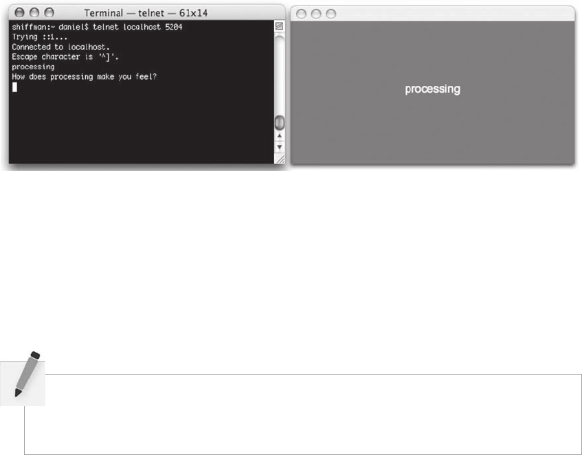
Data Streams 361
Once the server is running, we can create a client that connects to the server. Ultimately, we will look at
an example where we write both the server and client in Processing . However, just to demonstrate that
the server is in fact working, we can connect to it using any telnet client application. Telnet is a standard
protocol for remote connections and all machines generally come with built-in telnet abilities. On a Mac,
launch terminal, on Windows, go to the command prompt. I also recommend using PuTTY, a free telnet
client: http://www.chiark.greenend.org.uk/~sgtatham/putty/ .
Since we are connecting to the server from the same machine that the server is running on, the address
we telnet to is localhost , meaning the local computer, port 5,204. We could also use the address 127.0.0.1 .
is is a special address reserved for programs on a computer to speak to each other locally (i.e., on the
same machine) and is the equivalent of localhost . If we were connecting from a diff erent computer, we
would have to know the network IP address of the machine running the server.
fi g. 19.2
Telnet clients traditionally send messages to the server when the user types enter. e carriage return and
line feed are included in the message and therefore when the server sends back the reply, you will notice
that “ How does processing ” and “ make you feel ” appear on separate lines.
Exercise 19-1: Using String manipulation techniques from Chapter 15, fi x Example 19-1
so that if the client sends newline characters, the server removes them before replying back to
the client. You will want to alter the “ incomingMessage ” variable.
incomingMessage = client.readString();
incomingMessage = incomingMessage. ______ (______, ______);
19.3 Creating a Client
Once we have written a server and tested it with telnet, we can then develop our own client in Processing.
We start off the same way we did with a server, importing the net library and declaring an instance of a
Client object.

362 Learning Processing
import processing.net.*;
Client client;
e client constructor requires three arguments— “ this ” , referring again to this PApplet , the IP address we
want to connect to (as a String), and the port number (as an integer).
client = new Client(this, " 127.0.0.1 " , 5204);
If the server is running on a diff erent computer than the client, you will need to know the IP address of
that server computer. In addition, if there is no server running at the specifi ed IP and port, the Processing
sketch will give the error message: “ java.net.ConnectException: Connection refused ” meaning either the
server rejected the client or that there is no server.
Sending to the server is easy using the write( ) function.
client.write( " Hello! " );
Reading messages from the server is done with the read( ) function. e read( ) method, however, reads
from the server one byte at a time. To read the entire message as a String, readString( ) is used.
Before we can even contemplate reading from the server, we must be sure there is something to read. is
check happens with available( ). available( ) returns the number of bytes that are waiting to be read. We can
determine if there is anything waiting to be read by asking if the number of bytes is greater than zero.
if (client.available() > 0) {
String message = client.readString();
}
Using the code from Example 18-1 , (keyboard input), we can create a Processing client that connects and
communicates with our server, sending messages entered by the user. See Example 19-2.
Example 19-2: Simple therapy client
// Import the net libraries
import processing.net.*;
// Declare a client
Client client;
// Used to indicate a new message
float newMessageColor = 0;
// A String to hold whatever the server says
String messageFromServer = " " ;
// A String to hold what the user types
String typing = " " ;
PFont f;
void setup() {
size(400,200);
// Create the Client
client = new Client(this, " 127.0.0.1 " , 5204);
f = createFont( " Arial " ,16,true);
}
Type text and hit return to send to server.
How does processing make you feel?
fi g. 19.3
Connect to server at 127.0.0.1
(localhost), port 5204
Data Streams 363
void draw() {
background(255);
// Display message from server
fill(newMessageColor);
textFont(f);
textAlign(CENTER);
text(messageFromServer,width/2,140);
// Fade message from server to white
newMessageColor = constrain(newMessageColor + 1,0,255);
// Display Instructions
fill(0);
text( "Type text and hit return to send to server. ",width/2,60);
// Display text typed by user
fill(0);
text(typing,width/2,80);
// If there is information available to read
if (client.available() > 0) {
// Read it as a String
messageFromServer = client.readString();
// Set brightness to 0
newMessageColor = 0;
}
}
// Simple user keyboard input
void keyPressed() {
// If the return key is pressed, save the String and clear it
if (key == '\n') {
// When the user hits enter, write the sentence out to the Server
client.write(typing);
typing = " " ;
} else {
typing = typing + key;
}
}
Exercise 19-2: Create a client and server that talk to each other. Have the client send
messages typed by the user and the server respond autonomously. For example, you could use
String parsing techniques to reverse the words sent by the client. Client: “ How are you? ”
Server: “ You are how? ”
19.4 Broadcasting
Now that we understand the basics of how clients and servers work, we can examine more practical uses
of networked communication. In the therapist client/server examples, we treated the data sent across the
network as a String, but this may not always be the case. In this section, we will look at writing a server
that broadcasts numeric data to clients.
How is this useful? What if you wanted to continuously broadcast the temperature outside your house or
a stock quote or the amount of motion seen by a camera? You could set up a single computer running a
The new message fades
to white by increasing
the brightness.
We know there is a message from
the Server when there are greater
than zero bytes available.
When the user hits enter, the
String typed is sent to the Server.
364 Learning Processing
Processing server to process and broadcast that information. Client sketches from anywhere in the world
could connect to this machine to receive the information.
To demonstrate the framework for such a program, we will write a server that broadcasts a number
between 0 and 255 (we can only send one byte at time). We will then look at clients that retrieve the data
and interpret it in their own way.
Here is the server, which increments a number randomly and broadcasts it .
Example 19-3: Server broadcasting a number (0–255)
// Import the net libraries
import processing.net.*;
// Declare a server
Server server;
PFont f;
int data = 0;
void setup() {
size(200,200);
// Create the Server on port 5204
server = new Server(this, 5204);
f = createFont( " Arial " ,20,true);
}
void draw() {
background(255);
// Display data
textFont(f);
textAlign(CENTER);
fill(0);
text(data,width/2,height/2);
// Broadcast data
server.write(data);
// Arbitrarily changing the value of data randomly
data
= (data + int(random( – 2,4))) % 256;
}
// The serverEvent function is called whenever a new client connects.
void serverEvent(Server server, Client client) {
println( " A new client has connected: " + client.ip());
}
Next, we will write a client that receives the number from the server and uses it to fi ll a variable. e
example is written with the assumption that the server and the client are running on the same computer
(you can open both examples and run them together in Processing), but in a real world scenario this would
likely not be the case. If you choose to run the server and clients on diff erent computers, the machines
178
fi g. 19.4
The number is continuously sent
to all clients because write() is
called every cycle through draw().
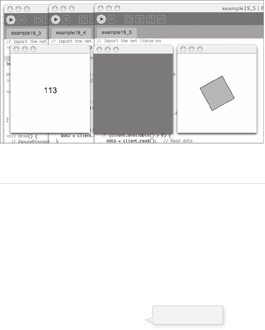
Data Streams 365
must be networked locally (via a router or hub, ethernet or wifi ) or on the internet. e IP address can be
found in the network settings of your machine.
fi g. 19.5 Examples 19-3, 19-4, and 19-5 all running together
Example 19-4: Client reading values as background color
// Import the net libraries
import processing.net.*;
// Declare a client
Client client;
// The data we will read from the server
int data;
void setup() {
size(200,200);
// Create the Client
client = new Client(this, "127.0.0.1", 5204);
}
void draw() {
if (client.available() > 0) {
data = client.read(); // Read data
}
background(data);
}
The incoming data is used
to color the background.

366 Learning Processing
Example 19-5: Client reading values as rotation value
// Import the net libraries
import processing.net.*;
// Declare a client
Client client;
// The data we will read from the server
int data;
void setup() {
size(200,200);
smooth();
// Create the Client
client = new Client(this, " 127.0.0.1 " , 5204);
}
void draw() {
if (client.available() > 0) {
data = client.read(); // Read data
}
background(255);
stroke(0);
fill(175);
translate(width/2,height/2);
float theta = (data/255.0) *
rotate(theta);
rectMode(CENTER);
rect(0,0,64,64);
}
Exercise 19-3: Write a client that uses the number broadcast from the server to control the
location of a shape.
19.5 Multi-User Communication, Part 1: The Server
e broadcast example demonstrates one-way communication where a server broadcasts a message and
many clients receive that message. e broadcast model, however, does not allow a client to turn around
and send a reply back to the server. In this section, we will cover how to create a sketch that involves
communication between multiple clients facilitated by a server.
Let’s explore how a chat room works. Five clients (you and four friends) connect to a server. One client
types a message: “ Hey everyone! ” at message is sent to the server, which relays it back to all fi ve clients.
Most multi-user applications function in a similar fashion. A multiplayer online game, for example,
would likely have clients sending information related to their whereabouts and actions to a server that
broadcasts that data back to all other clients playing the game.
A multi-user application can be developed in Processing using the network library. To demonstrate, we
will create a networked, shared whiteboard. As a client drags its mouse around the screen, the sketch
The incoming data is
used to rotate a square.
TWO_PI;

Data Streams 367
will send X , Y coordinates to the server that passes them back to any other connected clients. Everyone
connected will be able to see the drawing actions of everyone else.
In addition to learning how to communicate between multiple clients, this example will explore how to
send multiple values. How can a client send two values (an X and a Y coordinate) and have the server
know which one is which?
e fi rst step toward a solution involves developing a protocol for communication between the clients. In
what format is the information sent and how is that information received and interpreted? Luckily for
us, the time we spent learning how to create, manage, and parse String objects in Chapters 17 and 18 will
provide all the tools we need.
Assume a client wants to send the mouse location: mouseX ⴝ 150 and mouseY ⴝ 125. We need to format
that information as a String in a way that is convenient to decipher. One possibility is as follows:
“ e fi rst number before the comma is the X location, the second number after the comma is 125. Our
data ends where an asterisk (*) appears. ”
In code, it would appear as follows:
String dataToSend = " 100,125*";
or, more generally:
String dataToSend = mouseX + " ," + mouseY + " *";
Here, we have developed a protocol for sending and receiving data. e integer values for mouseX and
mouseY are encoded as a String during sending (number, followed by comma, followed by number,
followed by asterisk). ey will have to be decoded upon receipt and we will get to that later. I should also
point out that most examples will typically use a newline or carriage return to mark the end of a message
(as we saw in the fi rst section of this chapter). We use an asterisk here for two reasons: (1) an asterisk is
plainly visible when displayed whereas newline is not (especially in the context of a book) and (2) using
an asterisk demonstrates that you can design and implement any messaging protocol you so choose as
long as it matches up in the client and server code.
What is really sent?
Data sent across a network is sent as a sequential list of individual bytes. Recalling the discussion
of data types in Chapter 4, a byte is an 8-bit number, that is, a number made up of eight 0’s and 1’s
or a value between 0 and 255.

368 Learning Processing
We are now ready to create a server to receive the messages from the client. It will be the client’s job to
format those messages with our protocol. e job of the server remains simple: (1) receive the data and
(2) relay the data. is is similar to the approach we took in Section 19.2.
Step 1 . Receiving data.
Client client = server.available();
if (client ! = null) {
incomingMessage = client. readStringUntil( ' * ' );
}
What is new in this example is the function readStringUntil( ) . e readStringUntil( ) function takes
one argument, a character. at character is used to mark the end of the incoming data. We are simply
following the protocol established during sending. We are able to do this because we are designing both
the server and the client.
Once that data is read, we are ready to add:
Step 2. Relaying data back out to clients.
Client client = server.available();
if (client ! = null) {
incomingMessage = client.readStringUntil( ' * ' );
server.write(incomingMessage);
}
Let’s assume we want to send the number 42. We have two options:
client.write(42); // sending the byte 42
In the line above, we are really sending the actual byte 42.
client.write( " 42 " ); // sending the String " 42 "
In the line above, we are sending a String . at String is made up of two characters, a ‘ 4 ’ and a ‘ 2 ’ .
We are sending two bytes! ose bytes are determined via the ASCII (American Standard Code
for Information Interchange) code, a standardized means for encoding characters. e character ‘ A ’
is byte 65, the character ‘ B ’ 66, and so on. e character ‘ 4 ’ is byte 52 and ‘ 2 ’ is 50.
When we read the data, it is up to us to know whether we want to interpret the bytes coming in
as literal numeric values or as ASCII codes for characters. We accomplish this by choosing the
appropriate read( ) function.
int val ⴝ client.read(); // matches up with client.write(42);
String s ⴝ client.readString(); // matches up with client.write( " 42 " );
int num ⴝ int(s); // convert the String that is read into a number
Because we designed our own
protocol and are not using
newline/carriage return to mark
the end of our message, we must
use readStringUntil() instead of
readString().
Writing the message back out to
all clients.

Data Streams 369
Here is the full Server with some bells and whistles. A message is displayed onscreen when new clients
connect as well as when the server receives data.
Example 19-6: Multi-user server
// Import the net libraries
import processing.net.*;
// Declare a server
Server server;
PFont f;
String incomingMessage = " " ;
void setup() {
size(400,200);
// Create the Server on port 5204
server = new Server(this, 5204);
f = createFont( "Arial",20,true);
}
void draw() {
background(255);
// Display rectangle with new message color
fill(0);
textFont(f);
textAlign(CENTER);
text(incomingMessage,width/2,height/2);
// If a client is available, we will find out
// If there is no client, it will be "null"
Client client = server.available();
// We should only proceed if the client is not null
if (client ! = null) {
// Receive the message
incomingMessage = client.readStringUntil( '*');
// Print to Processing message window
println( "Client says: " + incomingMessage);
// Write message back out (note this goes to ALL clients)
server.write(incomingMessage);
}
}
// The serverEvent function is called whenever a new client connects.
void serverEvent(Server server, Client client) {
incomingMessage = " A new client has connected: " + client.ip();
println(incomingMessage);
}
19.6 Multi-User Communication, Part 2: The Client
e client’s job is three-fold:
1. Send mouseX and mouseY coordinates to server.
2. Retrieve messages from server.
3. Display ellipses in the window based on server messages.
All messages received from
one client are immediately
relayed back out to all
clients with write().

370 Learning Processing
For Step 1, we need to adhere to the protocol we established for sending:
mouseX comma mouseY asterisk
String out = mouseX + " , " + mouseY + " * " ;
client.write(out);
e question remains: when is the appropriate time to send that information? We could choose to insert
those two lines of code into the main draw( ) loop, sending mouse coordinates every frame. In the case
of a whiteboard client, however, we only need to send the coordinates when the user drags the mouse
around the window.
e mouseDragged( ) function is an event handling function similar to mousePressed( ) . Instead of being
called when a user clicks the mouse, it is called whenever a dragging event occurs, that is, the mouse
button is pressed and the mouse is moving. Note the function is called continuously as a user drags the
mouse. is is where we choose to do our sending.
void mouseDragged() {
String out = mouseX + " , " + mouseY + " * " ;
// Send the String to the server
client.write(out);
// Print a message indicating we have sent data
println( " Sending: " + out);
}
Step 2, retrieving messages from the server, works much like the therapy client and broadcast client
examples. e only diff erence is the use of readStringUntil( ) , which follows the “ number-comma-
number-asterisk ” protocol.
if (client.available() > 0) {
// Read message as a String, all messages end with an asterisk
String in = client.readStringUntil( ' * ' );
//
Print message received
println( " Receiving: " + in);
}
Once the data is placed into a String object, it can be interpreted with parsing techniques from Chapter 18.
First, the String is split into an array of Strings using the comma (or asterisk) as the delimiter.
String[] splitUp = split(in, " ,* " );
e String array is then converted into an array of integers (length: 2).
int[] vals = int(splitUp);
And those integers are used to display an ellipse.
fill(255,100);
noStroke();
ellipse(vals[0],vals[1],16,16);
Put the String together with our
protocol:
mouseX comma mouseY asterisk.

Data Streams 371
Here is the entire client sketch:
Example 19-7: Client for multi-user whiteboard
// Import the net libraries
import processing.net.*;
// Declare a client
Client client;
void setup() {
size(200,200);
// Create the Client
client = new Client(this, "127.0.0.1", 5204);
background(255);
smooth();
}
void draw() {
// If there is information available to read from the Server
if (client.available() > 0) {
// Read message as a String, all messages end with an asterisk
String in = client.readStringUntil( '*');
// Print message received
println( "Receiving: " + in);
// Split up the String into an array of integers
int[] vals = int(splitTokens(in, ",*"));
// Render an ellipse based on those values
fill(0,100);
noStroke();
ellipse(vals[0],vals[1],16,16);
}
}
// Send data whenever the user drags the mouse
void mouseDragged() {
// Put the String together with our protocol: mouseX comma mouseY asterisk
String out = mouseX + " ," + mouseY + " *";
// Send the String to the server
client.write(out);
// Print a message indicating we have sent data
println("Sending: " + out);
}
19.7 Multi-User Communication, Part 3: All Together Now
When running a multi-user application, the order in which the elements are launched is important. e
client sketches will fail unless the server sketch is already running.
You should fi rst (a) identify the IP address of the server, (b) choose a port and add it to the server’s code,
and (c) run the server.
Afterward, you can launch the clients with the correct IP address and port.
The client reads messages from
the Server and parses them with
splitTokens() according to our
protocol.
A message is sent whenever the
mouse is dragged. Note that a client
will receive its own messages!
Nothing is drawn here!
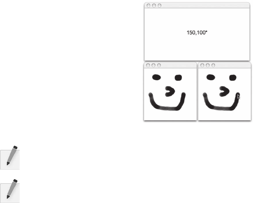
372 Learning Processing
If you are working on a multi-user project, you most
likely want to run the servers and clients on separate
computers. After all, this is the point of creating multi-
user applications in the fi rst place. However, for testing
and development purposes, it is often convenient to run
all the elements from one computer. In this case, the
server IP address will be “ localhost ” or 127.0.0.1 (note
this is the IP address used in this chapter’s examples).
As will be covered in Section 21.3, Processing ’s “ export to
application ” feature will allow you to export a stand-alone
application for your server, which you can then run in the
background while you develop your client in Processing .
Details as to how “ export to application ” works can be
found in Chapter 18. You can also run multiple copies
of a stand-alone application to simulate an environment
with more than one client. Figure 19.6 shows the server
running with two client instances.
Exercise 19-4: Expand the whiteboard to allow for color. Each client should send a red,
green, and blue value in addition to the XY location. You will not need to make any changes
to the server for this to work.
Exercise 19-5: Create a two-player game of Pong played over the network. is is a complex
assignment, so build it up slowly. For instance, you should get Pong to work fi rst without
networking (if you are stuck, an example is provided at the book’s web site). You will also
need to make changes to the server; specifi cally, the server will need to assign the players a
paddle as they connect (left or right).
19.8 Serial Communication
A nice reward for learning the ins and outs of networked communication is that it makes serial
communication in Processing a breeze. Serial communication involves reading bytes from the computer’s
serial port. ese bytes might come from a piece of hardware you purchase (a serial joystick, for example)
or one that you design yourself by building a circuit and programming a microcontroller.
is book does not cover the external hardware side of serial communication. However, if you are
interested in learning more about physical computing, I recommend the book Physical Computing: Sensing
and Controlling the Physical World with Computers (Course Technology PTR) by Dan O’Sullivan and Tom
Igoe as well as Making ings Talk: Practical Methods for Connecting Physical Objects (Make Books) by Tom
Igoe. e Arduino ( http://www.arduino.cc/ ) and Wiring ( http://wiring.org.co/ ) web sites are also excellent
resources. Wiring and Arduino are two open-source physical computing platforms developed at the
Interaction Design Institute Ivrea with a programming language modeled after Processing . I will provide
some accompanying Arduino code for your reference, but the material in this book will only cover what
to do once the data has already arrived in Processing .
fi g. 19.6 Examples 19-6 and 19-7 running together
Data Streams 373
Serial communication refers to the process of sending data in sequence, one byte at a time. is is how
data was sent over the network in our client/server examples. e Processing serial library is designed for
serial communication into the computer from a local device, most likely via a USB (Universal Serial Bus)
port. e term “ serial ” refers to the serial port, designed to interface with modems, that is rarely found on
newer computers.
e process of reading data from a serial port is virtually identical to that found in the networked client/
server examples, with a few exceptions. First, instead of importing the network library, we import the
serial library and create a Serial object.
import processing.serial.*;
Serial port = new Serial(this, "COM1", 9600);
e Serial constructor takes three arguments. e fi rst one is always “ this, ” referring to this applet (see
Chapter 16). Argument 2 is a String representing the communications port being used. Computers label
ports with a name. On a PC, these will likely be “ COM1, ” “ COM2, ” “ COM3, ” and so on. On UNIX-
based computers (such as MAC OS X), they will be labeled “ /dev/tty.something ” where “ something ”
represents a terminal device. If you are using a USB device, you will probably need to install USB drivers
before a working port will be available. Instructions for how to get this working with Arduino can be
found at the Arduino guide: http://www.arduino.cc/en/Guide/HomePage .
You can also print out a list of available ports using the Serial library’s list( ) function, which returns an
array of String objects.
String[] portList = Serial.list();
println(portList);
If the port you want to use is the fi rst one in the list, for example, your call to the constructor would look like:
String[] portList = Serial.list();
Serial port = new Serial(this, portList[0], 9600);
e third argument is the rate at which the data is transmitted serially, typically 9,600 baud.
Bytes are sent out via the serial port using the write( ) function. e following data types can be sent: byte,
char, int, byte array, and String . Remember, if you are sending a String , the actual data sent are raw ASCII
byte values of each character.
port.write(65); // Sending the byte 65
Data can be read with the same functions found in clients and servers: read( ) , readString( ) , and
readStringUntil( ) . A callback function, serialEvent( ) , is triggered whenever a serial event occurs, that is,
whenever there is data available to be read.
void serialEvent(Serial port) {
int input = port.read();
println( "Raw Input: " + input);
}
374 Learning Processing
e read( ) function will return a 1 if there is nothing available to read, however, assuming you are
writing the code inside serialEvent( ) , there will always be available data.
Following is an example that reads data from the serial port and uses it to color the sketch’s background.
Example 19-8: Reading from serial port
import processing.serial.*;
int val = 0; // To store data from serial port, used to color background
Serial port; // The serial port object
void setup() {
size(200,200);
// In case you want to see the list of available ports
// println(Serial.list());
// Using the first available port (might be different on your computer)
port = new Serial(this, Serial.list()[0], 9600);
}
void draw() {
// Set the background
background(val);
}
// Called whenever there is something available to read
void serialEvent(Serial port) {
// Read the data
val = port.read();
// For debugging
// println( " Raw Input: " + input);
}
For reference, if you are using Arduino, here is some corresponding code:
int val;
void setup() {
beginSerial(9600);
pinMode(3, INPUT);
}
void loop() {
val = analogRead(0);
Serial.print(val,BYTE);
}
19.9 Serial communication with handshaking
It is often advantageous to add a handshaking component to serial communication code. If a hardware
device sends bytes faster than a Processing sketch can read, for example, there can sometimes be a logjam
This is not Processing code! It is Arduino
code. For more about Arduino, visit:
http://www.arduino.cc/.
The serial data is used to
color the background.
Data from the Serial port is read in
serialEvent() using the read() function
and assigned to the global variable “val.”
Initializing the Serial object
with the fi rst port in the list.

Data Streams 375
of information, causing the sketch to lag. e sensor values may arrive late, making the interaction
confusing or misleading to the user. e process of sending information only when requested, known as
“ handshaking, ” alleviates this lag.
When the sketch starts up, it will send a byte to the hardware device asking for data.
Example 19-9: Handshaking
void setup() {
size(200,200);
// In case you want to see the list of available ports
// println(Serial.list());
// Using the first available port (might be different on your computer)
port = new Serial(this, Serial.list()[0], 9600);
// Request values from the hardware device
port.write(65);
}
After the sketch fi nishes processing a byte inside of serialEvent( ) , it asks again for a new value.
// Called whenever there is something available to read
void serialEvent(Serial port) {
// Read the data
val = port.read();
// For debugging
// println( "Raw Input: " +
// Request a new value
port.write(65);
}
As long as the hardware device is designed to only send the sensor values when requested, any possible lag
will be eliminated. Here is the revised Arduino code. is example does not care what the request byte is,
only that there is a byte request. A more advanced version might have diff erent replies for diff erent requests.
int val;
void setup() {
beginSerial(9600);
pinMode(3, INPUT);
}
void loop() {
// Only send out if something has come in
if (Serial.available() > 0) {
Serial.read();
val = analogRead(0);
Serial.print(val,BYTE);
}
}
The byte 65 tells the serial device
that we want to receive data.
After we receive a byte, we
reply asking for the next one.
This is not Processing code! It
is Arduino code. For more about
Arduino, visit: http://www.arduino.cc/.
input);

376 Learning Processing
19.10 Serial Communication with Strings
In cases where you need to retrieve multiple values from the serial port (or numbers greater than 255),
the readStringUntil( ) function is handy. For example, let’s assume you want to read from three sensors,
using the values for the red, green, and blue components of your sketch’s background color. Here, we will
use the same protocol designed in the multi-user whiteboard example. We will ask the hardware device
(where the sensors live) to send the data as follows:
Sensor Value 1 COMMA Sensor Value 2 COMMA Sensor Value 3 ASTERISK
For example:
104,5,76*
Example 19-10: Serial communication with Strings
import processing.serial.*;
int r,g,b; // Used to color background
Serial port; // The serial port object
void setup() {
size(200,200);
// In case you want to see the list of available ports
// println(Serial.list());
// Using the first available port (might be different on your computer)
port = new Serial(this, Serial.list()[0], 9600);
// Request values right off the bat
port.write(65);
}
void draw() {
// Set the background
background(r,g,b);
}
// Called whenever there is something available to read
void serialEvent(Serial port) {
// Read the data
String input = port.readStringUntil( ' * ' );
if (input ! = null) {
// Print message received
println( " Receiving: " + input);
// Split up the String into an array of integers
int[] vals = int(splitTokens(input, " ,* " ));
// Fill r,g,b variables
r = vals[0];
g = vals[1];
b = vals[2];
}
// When finished ask for values again
port.write(65);
}
Data from the Serial port is read in
serialEvent() using the readStringUntil()
function with ‘*’ as the end character.
The data is split into an array of
Strings with a comma or asterisk
as a delimiter and converted into
an array of integers.
Three global variables are
fi lled using the input data.

Data Streams 377
Corresponding Arduino code:
int sensor1 = 0;
int sensor2 = 0;
int sensor3 = 0;
void setup()
{
beginSerial(9600);
pinMode(3, INPUT);
}
void loop()
{
if (Serial.available() > 0) { //only send if you have hear back
Serial.read();
sensor1 = analogRead(0);
sensor2 = analogRead(1);
sensor3 = analogRead(2);
// Send the integer out as a String using "DEC"
Serial.print(sensor1,DEC);
// Send a comma -- ASCII code 44
Serial.print( ",", BYTE);
Serial.print(sensor2,DEC);
Serial.print( ",", BYTE);
Serial.print(sensor3,DEC);
// Send an asterisk -- ASCII code 42
Serial.print( "*", BYTE);
}
}
Exercise 19-6: If you have an Arduino board, build your own interface to control a
Processing sketch you have already made. (Before you attempt this, you should make sure
you can successfully run the simple examples provided in this chapter.)
This is not Processing code! It
is Arduino code. For more about
Arduino, visit: http://www.arduino.cc/.

378 Learning Processing
Lesson Eight Project
Create a data visualization by loading external information (a local fi le, web
page, XML feed, server or serial connection) into Processing .
Make sure you build up the project incrementally. For example, try designing
the visualization fi rst without any real data (use random numbers or hard-coded
values). If you are loading data from the web, consider using a local fi le while
you are developing the project. Do not be afraid to fake the data, waiting until
you are fi nished with aspects of the design before connecting the real data.
Experiment with levels of abstraction. Try displaying information literally
onscreen by writing text. Build an abstract system where the input data aff ects
the behaviors of objects (you might even use your “ ecosystem ” from the Lesson
Six Project).
Use the space provided below to sketch designs, notes, and pseudocode for your
project.

Lesson Nine
Making Noise
20 Sound
21 Exporting
This page intentionally left blank
Sound 381
20 Sound
“ Check. Check. Check 1. Sibilance. Sibilance. Check. Check. Check 2. Sibilance. Sibilance. ”
—Barry the Roadie
In this chapter:
– Libraries for Sound.
– Simple sound playback.
– Playback with adjusting volume, pitch, and pan.
– Microphone as sound sensor.
Processing does not have built-in support for sound. Not that there is anything wrong with sound. Not
that Processing has a personal grudge against sound. ere is just no built-in sound. As we discussed
in the introduction to this book, Processing is a programming language and development environment,
rooted in Java, designed for learning to program in a visual context . So, if you want to develop large-scale
interactive applications primarily focused on sound, you should really ask yourself: “ Is Processing the
right programming environment for me? ” is chapter will help answer that question as we explore the
possibilities and limitations of working with sound in Processing .
Incorporating sound into Processing sketches can be accomplished a number of diff erent ways. Because
Processing does not support sound in its core library, many Processing developers choose to incorporate
sound via a third party application geared toward sound, such as PureData ( http://www.puredata.org/ )
or Max/MSP ( http://www.cycling74.com/ ). Processing can communicate with these applications via OSC
( “ open sound control ” ) a protocol for network communication between computers and multimedia
devices. is can be accomplished in Processing by using the network library (see the previous chapter) or
with the oscP5 library, by Andreas Schlegel ( http://www.sojamo.de/libraries/oscP5 )
Visiting the Processing web site will also reveal a list of contributed libraries for using sound directly in
Processing : playing sound samples, analyzing sound input from a microphone, synthesizing sound, and
sending and receiving midi information. is chapter will focus on two of these elements: sound playback
and sound input . For playback of sound eff ects we will look at the Sonia library (by Amit Pitaru) and the
Minim library (by Damien Di Fede). Sound input will be demonstrated with Sonia .
ese sound libraries are available at the following URLs:
Sonia: http://sonia.pitaru.com/
Minim: http://code.compartmental.net/tools/minim/
For a review on how to install third party libraries, visit Chapter 12 . You will also want to visit
http://www.learning processing.com to download the sample sound fi les used in these examples.
20.1 Really Simple Sound
Before we look at the libraries, however, there is one simple (but extremely limited) way to play a sound
fi le in a Processing sketch without installing a third party library. is is through the use of the Movie class
which we learned in Chapter 16. e Movie class is designed to play QuickTime movies, but can also be
382 Learning Processing
used to play a WA V or AIFF fi le. WA V is an audio fi le format that stands for “ Waveform audio format ”
and is the standard format for PCs. AIFF stands for “ Audio Interchange File Format ” and is commonly
used on Macintosh computers.
All of the functions we looked at in Chapter 16 are available for a sound fi le. e main diff erence, of
course, is that we cannot use image( ) to display the Movie object since there is no image.
Example 20-1: Simple sound with video library
import processing.video.*;
Movie movie;
void setup() {
size(200, 200);
movie = new Movie (this, " dingdong.wav " );
}
void draw() {
background(0);
noLoop();
}
void mousePressed() {
movie.stop();
movie.play();
}
Exercise 20-1: Using the bouncing ball sketch from Example 5–6, play a sound eff ect every
time the ball bounces off a window’s edge.
20.2 Getting Started with Sonia and Minim
e Movie class will do for playing simple sound eff ects, but for more sophisticated playback
functionality, we will need to look at libraries designed for use with sound. We will start with Sonia
( http://sonia.pitaru.com/ ). First things fi rst, as with any contributed library, you fi rst need the import
statement at the top of your code.
import pitaru.sonia_v2_9.*;
Sonia is an interface to a Java sound library, entitled Jsyn by Phil Burk. In order for it to work, Sonia has
to communicate with the audio playback and input hardware on your computer. is communication is
achieved via Jsyn. Before any sounds can be played, therefore, that link needs to be established, that is, the
sound engine needs to be started. is is done with the following line of code, which you would place in
setup( ) .
Construct a Movie object with a WAV
(or AIFF) fi le.
The sound is played whenever the mouse is
pressed. Including the function stop() before
play() ensures that the sound fi le will play
from the beginning.
Sound 383
void setup() {
Sonia.start(this);
}
Now, it would be rather irresponsible of us to make this connection to the sound hardware, but never
bother to close it down when we are fi nished. By now, the fl ow of a Processing sketch is all too familiar,
start with setup( ) , loop with draw( ) , and stop whenever you quit the sketch. e thing is, we want to
terminate the sound engine during that last step, when the sketch quits. Fortunately, there is an extra
hidden function we can implement entitled stop( ) that does precisely that. When a sketch quits, any
last minute instructions can be executed inside the stop( ) function. is is where we will shut down the
Sonia engine.
void stop() {
Sonia.stop();
super.stop();
}
Sonia.stop( ) is the call to stop Sonia. ere is also, however, the line super.stop( ) . e meaning of “ super ”
will be explored further in Chapter 22. For now, we can understand that line of code as saying “ Oh,
whatever else you would normally do in stop( ) , do that stuff , too . ”
All of the above applies to Minim as well. Here is the corresponding code:
import ddf.minim.*;
void setup() {
size(200, 200);
Minim.start(this);
}
void stop() {
super.stop();
}
20.3 Basic Sound Playback
Once this call to the library has been made, you have the whole world (of sound) in your hands. We
will start by demonstrating how to play sound fi les. Before a sound can be played, it must be loaded into
memory, much in the same way we loaded image fi les before displaying them. With Sonia , a Sample
object is used to store a reference to a sound sample.
Sample dingdong;
e object is initialized by passing the sound fi lename to the constructor.
dingdong = new Sample( "dingdong.wav");
Start the Minim sound engine!
With Minim, sounds will be closed
individually here. We will see this
in a moment.
The fi le “dingdong.wav” should be placed in
the data directory.

384 Learning Processing
Just as with images, loading the sound fi le from the hard drive is a slow process so the previous line of
code should be placed in setup( ) so as to not hamper the speed of draw( ) .
e type of sound fi le compatible with Sonia is somewhat limited. Only sounds that are formatted as WA V
or AIFF fi les (16-bit mono or stereo) are allowed. If you want to use a sound fi le that is not stored in a
compatible format, you could download a free audio editor, such as Audacity ( http://audacity.sourceforge.net/ )
and convert the fi le. Most audio fi les can be saved raw or with compression. Sonia only works with raw fi les.
However, in the next section, we will demonstrate how compressed (MP3) fi les can be played with the
ESS library.
Once the sound is loaded, playing is easy.
dingdong.play();
e following example plays a doorbell sound whenever the mouse is clicked on the graphical doorbell.
is Doorbell class implements simple button functionality (rollover and click) and just happens to
be a solution for Exercise 9–8 . e code for the new concepts (related to sound playback) is shown in
bold type .
Example 20-2: Doorbell with Sonia
// Import the Sonia library
import pitaru.sonia_v2_9.*;
// A sample object (for a sound)
Sample dingdong;
// A doorbell object (that will trigger the sound)
Doorbell doorbell;
void setup() {
size(200,200);
Sonia.start(this); // Start Sonia engine.
// Create a new sample object.
dingdong = new Sample( " dingdong.wav " );
// Create a new doorbell
doorbell = new Doorbell(150,100,32);
smooth();
}
void draw() {
background(255);
// Show the doorbell
doorbell.display(mouseX,mouseY);
}
fi g. 20.1
The play() function plays the sound sample once.
Sound 385
void mousePressed() {
// If the user clicks on the doorbell, play the sound!
if (doorbell.contains(mouseX,mouseY)) {
dingdong.play();
}
}
// Close the sound engine
public void stop() {
Sonia.stop();
super.stop();
}
// A Class to describe a "doorbell" (really a button)
class Doorbell {
// Location and size
float x;
float y;
float r;
// Create the doorbell
Doorbell (float x_, float y_, float r_) {
x = x_;
y = y_;
r =
r_;
}
// Is a point inside the doorbell (used for mouse rollover, etc.)
boolean contains(float mx, float my) {
if (dist(mx,my,x,y) < r) {
return true;
} else {
return false;
}
}
// Show the doorbell (hardcoded colors, could be improved)
void display(float mx, float my) {
if (contains(mx,my)) {
fill(100);
} else {
fill(175);
}
stroke(0);
ellipse(x,y,r,r);
}
}

386 Learning Processing
// A Class to describe a " doorbell " (really a button)
class Doorbell {
// Location and size
float x;
float y;
float r;
// A sample object (for a sound)
_________ ____________;
// Create the doorbell
Doorbell (float x_, float y_, float r_, _______ filename) {
x = x_;
y = y_;
r = r_;
_________ = new _________(_____________);
}
void ring() {
____________________;
}
boolean contains(float mx, float my) {
// same as original
}
void display(float mx, float my) {
// same as original
}
}
Exercise 20-2: Rewrite the Doorbell class to include a reference to the Sonia sample. is
will allow you to easily make multiple Doorbell objects that each play a diff erent sound.
Here is some code to get you started.
If you run the Doorbell example and click on the doorbell many times in rapid succession, you will notice
that the sound restarts every time you click. It is not given a chance to fi rst fi nish playing. While this
is not much of an issue for this straightforward example, stopping a sound from restarting can be very
important in other, more complex, sound sketches. e simplest way to achieve such a result is to always

Sound 387
check and see if a sound is playing before you call the play( ) function. Sonia has a nice function called
isPlaying( ) which does exactly this, returning true or false. We want to play the sound if it is not already
playing, that is,
if (!dingdong.isPlaying()) {
dingdong.play();
}
Exercise 20-3: Expand the Doorbell class to animate (perhaps moving its location and
changing its size randomly) only while its sound is playing. Create an array of fi ve Doorbell
objects. Here is part of a function to add to the Doorbell class:
void jiggle() {
if (_________________)) {
x += ____________;
y += ____________;
_________________;
}
}
With Minim instead of Sonia, very little changes. Instead of a Sample object, we have an AudioPlayer
object. e following example includes the solutions for Exercises 20-2 and 20-3 (but uses the Minim
code, rather than Sonia). It does not implement an array, however.
Example 20-3: Doorbell with Minim
import ddf.minim.*;
// A doorbell object (that will trigger the sound)
Doorbell doorbell;
void setup() {
size(200,200);
// start up Minim
Minim.start(this);
// Create a new doorbell
doorbell = new Doorbell(150,100,32, "dingdong.wav");
smooth();
}
Remember, “!” means not!
388 Learning Processing
void draw() {
background(100,100,126);
// Show the doorbell
doorbell.display(mouseX,mouseY);
doorbell.jiggle();
}
void mousePressed() {
// If the user clicks on the doorbell, play the sound!
if (doorbell.contains(mouseX,mouseY)) {
doorbell.ring();
}
}
// Close the sound files
public void stop() {
doorbell.close();
super.stop();
}
class Doorbell {
// Location and size
float x;
float y;
float r;
// An AudioPlayer object
AudioPlayer dingdong;
// Create the doorbell
Doorbell (float x_, float y_, float r_, String filename) {
x = x_;
y = y_;
r = r_;
// load " dingdong.wav " into a new AudioPlayer
dingdong = Minim.loadFile(filename);
}
// If the " doorbell " is ringing, the shape jiggles
void jiggle() {
if (dingdong.isPlaying()) {
x + = random( – 1,1);
y + = random( – 1,1);
r = constrain(r + random( – 2,2),10,100);
}
}
// The doorbell rings!
void ring() {
if (!dingdong.isPlaying()) {
dingdong.rewind();
dingdong.play();
}
}
The doorbell object must close its sound.
An AudioPlayer object is used to store
the sound.
The doorbell only jiggles if the
sound is playing.
The ring() function plays the
sound, as long as it is not
already playing. rewind()
ensures the sound starts from
the beginning.

Sound 389
// Is a point inside the doorbell (used for mouse rollover, etc.)
boolean contains(float mx, float my) {
if (dist(mx,my,x,y) < r) {
return true;
} else {
return false;
}
}
// Show the doorbell (hardcoded colors, could be improved)
void display(float mx, float my) {
if (contains(mx,my)) {
fill( 126,114,100);
} else {
fill(119,152,202);
}
stroke(202,175,142);
ellipse(x,y,r,r);
}
void close() {
dingdong.close();
}
}
One of the advantages of using Minim over Sonia is that Minim supports MP3 fi les. MP3 (or “ MPEG-1
Audio Layer 3 ” ) fi les are compressed and therefore take up much less hard drive space than raw WAV or
AIFF sound fi les.
AudioPlayer dingdong = Minim.loadFile( "dingdong.mp3");
20.4 A Bit Fancier Sound Playback
During playback, a sound sample can be manipulated in real time. Volume, pitch, and pan can all be
controlled using Sonia and Minim .
Let’s start with volume in Sonia . A Sample object’s volume can be set with the setVolume( ) function,
which takes a fl oating point value between 0.0 and 1.0 (0.0 being silent, 1.0 being the loudest). e
following snippet assumes a sample named “ tone ” and sets the volume based on mouseX position (by
normalizing it to a range between 0 and 1).
float ratio = (float) mouseX /width;
tone.setVolume(ratio);
Pan works the same way, only the range is between 1.0 (for left) and 1.0 (for right).
float ratio = (float) mouseX /width;
tone.setPan(ratio*2 – 1);
e pitch is altered by changing the rate of playback (i.e., faster playback is higher pitch, slower
playback is lower pitch) using setRate( ) . You can set the sample playback rate to anything you like, a
The doorbell has a close() function
to close the AudioPlayer object.
Volume ranges from 0.0 to 1.0.
Pan ranges from –1.0 to 1.0.
390 Learning Processing
fairly comprehensive range is from 0 (where you would not hear it at all) to 88,200 (a relatively fast
playback rate).
float ratio = (float) mouseX / width;
tone.setRate(ratio*88200);
e following example adjusts the volume and pitch of a sound according to mouse movements. Note the
use of repeat( ) instead of play( ) , which loops the sound over and over rather than playing it one time .
Example 20-4: Manipulating sound (with Sonia)
// Import the Sonia library
import pitaru.sonia_v2_9.*;
// A Sample object (for a sound)
Sample tone;
void setup() {
size(200,200);
Sonia.start(this); // Start Sonia engine.
// Create a new sample object.
tone = new Sample( " tone.wav " );
// Loop the sound forever
// (well, at least until stop() is called)
tone.repeat();
smooth();
}
void draw() {
if (tone.isPlaying()) {
background(255);
} else {
background(100);
}
// Set the volume to a range between 0 and 1.0
float ratio = (float) mouseX /
width;
tone.setVolume(ratio);
// Set the rate to a range between 0 and 88,200
// Changing the rate alters the pitch
ratio = (float) mouseY / height;
tone.setRate(ratio*88200);
// Draw some rectangles to show what is going on
stroke(0);
fill(175);
rect(0,160,mouseX,20);
stroke(0);
fill(175);
rect(160,0,20,mouseY);
}
fi g. 20.2
A reasonable range for rate (i.e., pitch)
is between 0 and 88,200.
The volume is set according
to the mouseX position.
The rate is set according to
the mouseY position.

Sound 391
// Pressing the mouse stops and starts the sound
void mousePressed() {
if (tone.isPlaying()) {
tone.stop();
} else {
tone.repeat();
}
}
// Close the sound engine
public void stop() {
Sonia.stop();
super.stop();
}
Exercise 20-4: In Example 20-4, fl ip the Y-axis so that the lower sound plays when the
mouse is down rather than up.
An AudioPlayer object can also be manipulated with Minim using the functions: setVolume( ) ,
setPan( ) , and addEff ect( ) , among others documented on the Minim site ( http://code.compartmental.
net/tools/minim/ ).
20.5 Live input
In Chapter 16, we looked at how serial communication allows a Processing sketch to respond to input
from an external hardware device connected to a sensor. Reading input from a microphone is a similar
pursuit. In essence, the microphone acts as a sensor. Not only can a microphone record sound, but it can
determine if the sound is loud, quiet, high-pitched, low-pitched, and so on. For example, a Processing
sketch could determine if it is living in a crowded room based on sound levels, or whether it is listening
to a soprano or bass singer based on pitch levels. is section will cover how to retrieve and use sound
volume data using the Sonia library. For analyzing sound pitch levels from a microphone, visit the Sonia
web site ( http://sonia.pitaru.com ) for further examples.
e previous sections used a Sample object to play a sound. Sound input from a microphone is retrieved
with a LiveInput object. ere is a somewhat odd distinction here in the way we will use these two
classes that we have yet to encounter over the course of this book.
Consider a scenario where we have three sound fi les. We would create three Sample objects.
Sample sample1 = new Sample( "file1.wav");
Sample sample2 = new Sample( "file2.wav");
Sample sample3 = new Sample( "file3.wav");
Technically speaking, we have made three instances of Sample objects, born via the Sample class. If we
want to play a sound, we have to refer to a specifi c Sample object.
sample1.play();
The sound can be stopped
with the function stop().
392 Learning Processing
With LiveInput , however, we are not going to make any object instances . Since the Sonia library only
allows one input source,
1 there is no reason to refer to a specifi c LiveInput object. Instead, when listening
to the microphone, we refer to the LiveInput class as a whole:
LiveInput.start(); // Start LiveInput
Functions that we call from the class name itself (rather than from a specifi c object instance) are known
as static functions. We can’t create static functions ourselves in Processing so it is not something we need
to worry about too much. However, since they are part of Java, we will encounter them from time to time
when using contributed libraries. LiveInput is an example of a class with static functions for retrieving
the sound and pitch levels from a microphone.
Let’s begin by building a very simple example that ties the size of a circle to the sound level of the
microphone.
Step #1 is exactly what we just did, start the process of listening to the computer’s microphone.
LiveInput.start(); // Start LiveInput
Step #2 is reading the volume level from the microphone itself . We can do this two ways. Because the
microphone listens in stereo, we can read the volume level from the right or left channel with getLevel( ) :
float rightLevel = LiveInput.getLevel(Sonia.RIGHT);
float leftLevel = LiveInput.getLevel(Sonia.LEFT);
We can also simply listen to both channels.
float level = LiveInput.getLevel();
e level returned will always range between 0.0 and 1.0.
Putting it all together, and tying the sound level to the size of an ellipse, we have:
Example 20-5: Live Input with Sonia
// Import the Sonia library
import pitaru.sonia_v2_9.*;
void setup() {
size(200,200);
Sonia.start(this);
// Start listening to the microphone
LiveInput.start();
smooth();
}
1Sonia’s Live Input will listen to whatever audio source is set up as the “sound input” device on your computer. You could use a
built-in microphone, a line-in from another audio source, or even potentially the CD player on your computer. A Sample object can
also be treated as live input by using the function: connectLiveInput( ).
We can specify whether we
want to listen to the RIGHT or
LEFT channel’s volume.
All functions for
sound input are static,
meaning they are called
from the class name
itself, LiveInput, rather
than an object instance.
With no argument, getLevel()
returns the volume of both
RIGHT and LEFT combined.

Sound 393
20.6 Sound Thresholding
A common sound interaction is triggering an event when a sound is made. Consider “ the clapper. ” Clap,
the lights go on. Clap again, the lights go off . A clap can be thought of as a very loud and short sound.
To program “ the clapper ” in Processing, we will need to listen for volume and instigate an event when the
volume is high.
In the case of clapping, we might decide that when the overall volume is greater than 0.5, the user is
clapping (this is not a scientifi c measurement, but is good enough for this example). is value of 0.5
is known as the threshold. Above the threshold, events are triggered, below, they are not.
float vol = LiveInput.getLevel();
if (vol > 0.5) {
// DO SOMETHING WHEN THE VOLUME IS GREATER THAN ONE!
}
Example 20-6 draws rectangles in the window whenever the overall volume level is greater than 0.5. e
volume level is also displayed on the left-hand side as a bar.
Example 20-6: Sound threshold with Sonia
// Import the Sonia library
import pitaru.sonia_v2_9.*;
void setup() {
size(200,200);
Sonia.start(this); // Start Sonia engine.
LiveInput.start(); // Start listening to the microphone
smooth();
background(255);
}
void draw() {
background(255,120,0);
// Get the overall volume (between 0 and 1.0)
float level = LiveInput.getLevel();
fill(200);
stroke(50);
// Draw an ellipse with size based on volume
ellipse(width/2,height/2,level*200,level*200);
}
// Close the sound engine
public void stop() {
Sonia.stop();
super.stop();
}
Exercise 20-5: Rewrite Example 20-5 with left and right volume levels mapped to
diff erent circles.
The variable that stores the
volume (“level”) is used as
the size of an ellipse.
fi g. 20.3
void draw() {
// Get the overall volume (between 0 and 1.0)
float vol = LiveInput.getLevel();
// If the volume is greater than 0.5, draw a rectangle
if (vol > 0.5) {
stroke(0);
fill(0,100);
rect(random(width),random(height),vol*20,vol*20);
}
// Graph the overall volume
// First draw a background strip
fill(175);
rect(0,0,20,height);
// Then draw a rectangle size according to volume
fill(0);
rect(0,height-vol*height/2,20,vol*height/2);
}
// Close the sound engine
public void stop() {
Sonia.stop();
super.stop();
}
is application works fairly well, but does not truly emulate the clapper. Notice how each clap results in
several rectangles drawn to the window. is is because the sound, although seemingly instantaneous to
our human ears, occurs over a period of time. It may be a very short period of time, but it is enough to
sustain a volume level over 0.5 for several cycles through draw( ) .
In order to have a clap trigger an event one and only one time, we need to rethink the logic of our
program. In plain English, this is what we are trying to achieve:
• If the sound level is above 0.5, then you are clapping and trigger the event. However, do not trigger the
event if you just did a moment ago!
e key here is how we defi ne “ a moment ago. ” One solution would be to implement a timer, that is, only
trigger the event once and then wait one second before you are allowed to trigger the event again. is is
a perfectly OK solution. Nonetheless, with sound, a timer is totally unnecessary since the sound itself will
tell us when we are fi nished clapping!
• If the sound level is less than 0.25, then it is quiet and we have finished clapping.
OK, with these two pieces of logic, we are ready to program this “ double-thresholded ” algorithm. ere
are two thresholds, one to determine if we have started clapping, and one to determine if we have
fi nished. We will need a boolean variable to tell us whether we are currently clapping or not.
Assume clapping false to start.
• If the sound level is above 0.5 and we are not already clapping, trigger the event and set clapping t r u e .
• If we are clapping and the sound level is less than 0.25, then it is quiet and set clapping false.
394 Learning Processing
If the volume is greater than 0.5
a rectangle is drawn at a random
location in the window. The louder
the volume, the larger the rectangle.
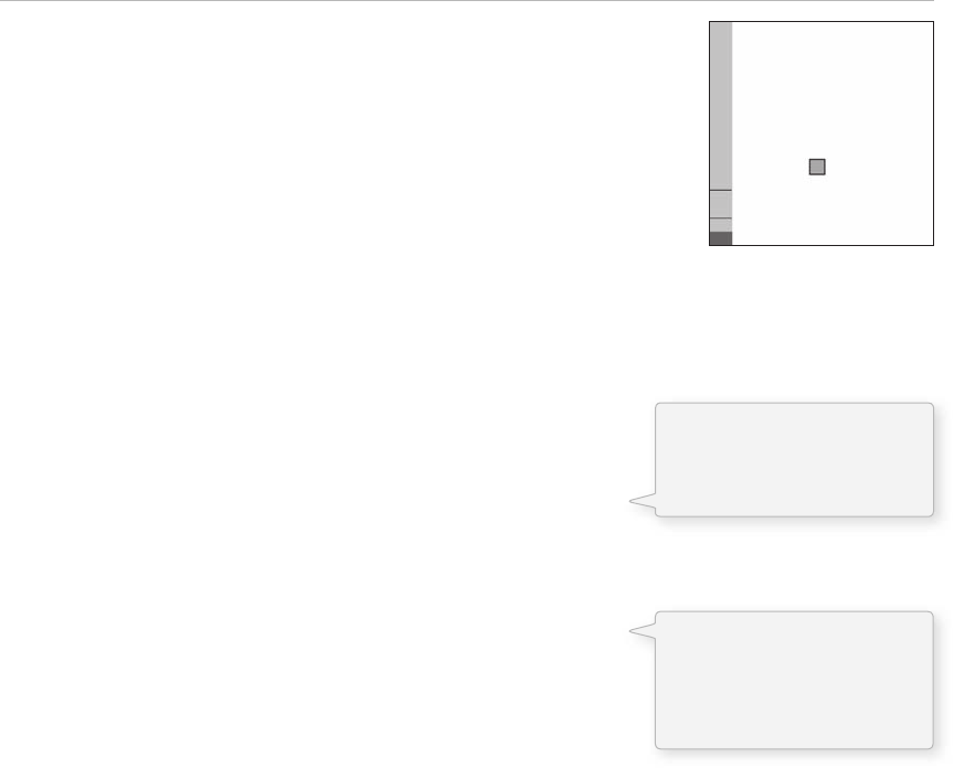
Sound 395
In code, this translates to:
// If the volume is greater than one and we are not clapping, draw a rectangle
if (vol > 0.5 & & !clapping) {
// Trigger event!
clapping = true; // We are now clapping!
} else if (clapping & & vol < 0.25) { // If we are finished clapping
clapping = false;
}
Here is the full example where one and only one rectangle appears per clap.
Example 20-7: Sound events (double threshold) with Sonia
// Import the Sonia library
import pitaru.sonia_v2_9.*;
float clapLevel = 0.5; // How loud is a clap
float threshold = 0.25; // How quiet is silence
boolean clapping = false;
void setup() {
size(200,200);
Sonia.start(this); // Start Sonia engine.
LiveInput.start(); // Start listening to the microphone
smooth();
background(255);
}
void draw() {
// Get the overall volume (between 0 and 2.0)
float vol = LiveInput.getLevel();
// If the volume is greater than 0.5 and
// we are not clapping, draw a rectangle
if (vol > clapLevel & & !clapping) {
stroke(0);
fill(0,100);
rect(random(width),random(height),vol*20,vol*20);
clapping = true; // We are now clapping!
// If we are finished clapping
} else if (clapping & & vol < threshold) {
clapping = false;
}
// Graph the overall volume
// First draw a background strip
noStroke();
fill(200);
rect(0,0,20,height);
// Then draw a rectangle size according to volume
fill(100);
rect(0,height-vol*height/2,20,vol*height/2);
fi g. 20.4
If the volume is greater
than 1.0, and we were not
previously clapping, then we
are clapping!
Otherwise, if we were just
clapping and the volume
level has gone down below
0.25, then we are no longer
clapping!

// Draw lines at the threshold levels
stroke(0);
line(0,height-clapLevel*height/2,19,height-clapLevel*height/2 );
line(0,height-threshold*height/2,19,height-threshold*height/2 );
}
// Close the sound engine
public void stop() {
Sonia.stop();
super.stop();
}
Exercise 20-6: Trigger the event from Example 20-7 after a sequence of two claps. Here is
some code to get you started that assumes the existence of a variable named “ clapCount ” .
if (vol > c lapLevel & & !clapping) {
clapCount___;
if (_______________) {
________________;
________________;
________________;
}
_________________;
} else if (clapping & & vol < 0.5) {
clapping = false;
}
Exercise 20-7: Create a simple game that is controlled with volume. Suggestion: First make
the game work with the mouse, then replace the mouse with live input. Some examples are
Pong, where the paddle’s position is tied to volume, or Duck Hunt, where a bullet is shot
whenever the user claps.
396 Learning Processing
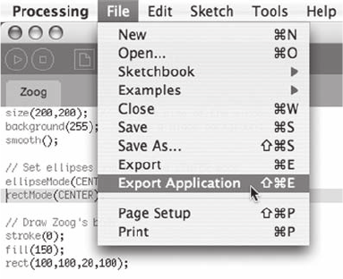
Exporting 397
21 Exporting
“ Wait a minute. I thought that Art wanted to give up the exporting. ”
—Seinfeld
In this chapter:
– Web applets.
– Stand-alone applications.
– High resolution PDFs.
– Images and image sequences.
– QuickTime movies.
We have focused our energy in this book on learning to program. Nevertheless, eventually our code babies
will grow up and want to fi nd their way out in the world. is chapter is dedicated to a discussion of the
various publishing options available to Processing sketches.
21.1 Web Applets
Processing sketches can be exported as Java applets to run on the web. How this works is covered in
Chapter 2. We have seen, however, that because of security restrictions, applets cannot perform certain
tasks, such as connect to a remote server or access a serial port, web camera, or other hardware device.
If you have a sketch that you must publish online, but uses a feature that is restricted, there are some
solutions. One possibility (as mentioned in Chapter 16) is to sign your applet. Some tips on how to do
this are available at this book’s web site ( http://www.learningprocessing.com/sandbox ).
21.2 Stand-Alone Applications
A great feature of Processing is that sketches can
be published as stand-alone applications, meaning
double-clickable programs that can run without the
Processing development environment being installed.
If you are creating a program for an installation or
kiosk environment, this feature will allow you to
create applications that easily can be launched when
a machine boots up. Export Application is also useful
if you need to run multiple copies of a sketch at the
same time (such as in the case of the client/server
examples in Chapter 19) . None of the applet security
restrictions apply to applications.
To export as an application, go to:
FILE → EXPORT APPLICATION (see Figure 21.1 )
You will then notice that three new folders appear as shown in Figure 21.2 .
fi g. 21.1
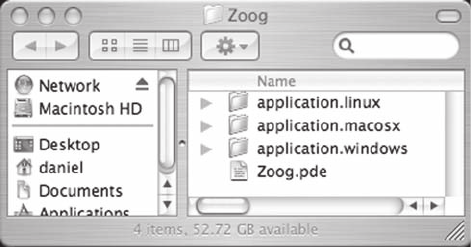
398 Learning Processing
Processing auto-creates applications for three operating systems, Mac OS X, Windows, and Linux. If you
Export Application from a Windows computer, the Mac application will not work properly (instructions
for fi xing this issue are included in a readme.txt fi le that appears). To avoid this, simply Export
Application on a Mac.
e folder will contain all the fi les you need:
• sketchName.exe (or named simply sketchName on Mac and Linux). This file is the double-clickable
application.
• “ source ” directory . The application folder will include a directory containing the source files for your
program. This folder is not required to run the application.
• “ lib ” . This folder only appears for Windows and Linux and contains required library files. It will always
contain core.jar , the core processing library, as well as any others you import. On Mac OS X, the library
files are visible by control-clicking the application file and selecting “ Show Package Contents. ”
e user of your application will need Java installed on his or her computer in order for the application
to run properly. On a Mac, Java comes preinstalled with the operating system, so you should not have
any issues as long as the end user has not messed with their Java installation. On Windows, if this is
a concern, you can include Java with the application by copying the “ Java ” folder from the Processing
directory to the application folder (and you must be on a PC to do this).
ere are a few tricks related to the Export Application feature. For example, if you want to have your own
text in the title bar, you can add the following code to setup( ) .
frame.setTitle( " My super-awesome application! " );
In addition, although exported applications run in windowed mode (as opposed to “ present ” mode),
you can set applications to run full screen by adding some code. Understanding the code requires some
advanced knowledge of Java and the inner workings of Processing sketches.
Some clues to this will be revealed in Chapter 23 , but for now this code is off ered simply to be copied:
static public void main(String args[]) {
PApplet.main(new String[] { " --present " , " SketchName " } );
}
fi g. 21.2

Exporting 399
is code can be inserted anywhere as its own block (above setup( ) is a good place for it). e
“ SketchName ” must match the name of your Processing sketch.
Exercise 21-1: Export a stand-alone application for any Processing sketch you have made
or any example in this book.
21.3 High-Resolution PDFs
We have been using Processing primarily as a means for creating graphics programs that run on a
computer screen. In fact, if you recall Chapter 3, we spent a great deal of time learning about how the
fl ow of a program works over time. Nevertheless, now is a good time to return to the idea of a static
program, one whose sole purpose is to create a static image. e Processing PDF library allows us to take
these static sketches and create high-resolution images for print. (In fact, almost all of the images in this
book were produced with this method.)
Following are the required steps for using the PDF library.
Step 1. Import the library.
import processing.pdf.*;
Step 2. In setup( ) , use the size( ) function with “ PDF ” mode and a String fi lename argument.
size(400, 400, PDF, "filename.pdf");
Step 3. In draw( ) , do your magic!
background(255);
fill(175);
stroke(0);
ellipse(width/2,height/2,160,160);
Step 4. Call the function “ exit( ) ” . is is very important. Calling exit( ) causes the PDF to fi nish
rendering. Without it, the fi le will not open properly.
exit(); // Required!
Here is how the program looks all together:
Example 21-1: Basic PDF
// Import the library
import processing.pdf.*;
// Using "PDF" mode, 4th argument is the name of the file
size(400, 400, PDF, "filename.pdf");

400 Learning Processing
// Draw some stuff!
background(255);
fill(175);
stroke(0);
ellipse(width/2,height/2,160,160);
// Very important, required for the PDF to render properly
exit();
If you run this example, you will notice that no window appears. Once you have set the Processing
rendering mode to PDF, the sketch window will no longer appear. is is because one often uses PDF
mode to create extremely high-resolution, complex images that cannot easily be displayed onscreen.
However, it is possible to see the Processing sketch window while rendering a PDF using the functions
beginRecord( ) and endRecord( ) . is runs slower than the fi rst example, but allows you to see what is
being saved.
Example 21-2: PDF using beginRecord( )
import processing.pdf.*;
void setup() {
size(400, 400);
beginRecord(PDF, " filename.pdf " );
}
void draw() {
// Draw some stuff!
smooth();
background(100);
fill(0);
stroke(255);
ellipse(width/2,height/2,160,160);
endRecord();
noLoop();
}
endRecord( ) does not have to be called on the fi rst frame rendered, and therefore this mode can be used
to generate a PDF compiled from multiple cycles through draw( ) . e following example takes the
“ Scribbler ” program from Chapter 16 and renders the result to a PDF. Here the colors are not taken from
a video stream, but are picked based on a counter variable. See Figure 21.3 for a sample output.
Example 21-3: Multiple frames into one PDF
import processing.pdf.*;
float x 0;
float y 0;
beginRecord( ) starts the process.
The fi rst argument should read PDF
and the second is the fi lename.
endRecord( ) is called to fi nish
the PDF.
There’s no reason to loop any more
since the PDF is fi nished.
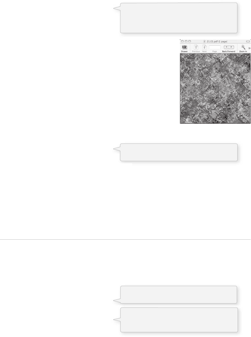
Exporting 401
void setup() {
size(400, 400);
beginRecord(PDF, "scribbler.pdf");
background(255);
}
void draw() {
// Pick a new x and y
float newx = constrain(x + random( -20,20),0,width);
float newy = constrain(y + random( -20,20),0,height);
// Draw a line from x,y to the newx,newy
stroke(frameCount%255,frameCount*3%255,
frameCount*11%255,100);
strokeWeight(4);
line(x,y,newx,newy);
// Save newx, newy in x,y
x newx;
y newy;
}
// When the mouse is pressed, we finish the PDF
void mousePressed() {
endRecord();
// We can tell Processing to open the PDF
open(sketchPath( "scribbler.pdf"));
noLoop();
}
If you are rendering 3D shapes (in P3D mode or OPENGL), you will want to use beginRaw( )
and endRaw( ) instead of beginRecord( ) and endRecord( ) . is example also uses a boolean variable
( “ recordPDF ” ) .
Example 21-4: PDF and openGL
// Using OPENGL
import processing.opengl.*;
import processing.pdf.*;
// Cube rotation
float yTheta = 0.0;
float xTheta = 0.0;
// To trigger recording the PDF
boolean recordPDF = false;
void setup() {
size(400, 400, OPENGL);
smooth();
}
fi g. 21.3
background( ) should be in setup( ). If
background( ) is placed in draw( ) the PDF
would accumulate a lot of graphics elements
only to erase them over and over again.
In this example, the user chooses when to fi nish
rendering the PDF by clicking the mouse.
A boolean variable that when set to true causes
a PDF to be made.
OPENGL or P3D mode requires the use
of beginRaw( ) and endRaw( ) instead of
beginRecord( ) and endRecord( ).
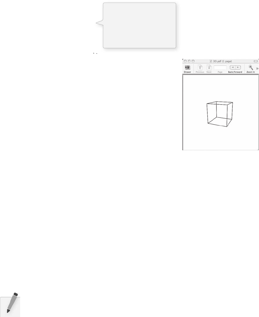
402 Learning Processing
void draw() {
// Begin making the PDF
if (recordPDF) {
beginRaw(PDF, " 3D.pdf " );
}
background(255);
stroke(0);
noFill();
translate(width/2,height/2);
rotateX(xTheta);
rotateY(yTheta);
box(100);
xTheta + = 0.02;
yTheta + = 0.03;
// End making the PDF
if (recordPDF) {
endRaw();
recordPDF = false;
}
}
// Make the PDF when the mouse is pressed
void mousePressed() {
recordPDF = true;
}
Two important notes about the PDF library.
• Images —If you are displaying images in the PDF, these will not necessarily look good after export.
A 320 240 pixel image is still a 320 240 pixel image whether rendered into a high-resolution
PDF or not.
• Text —If you are displaying text in the PDF, you will have to have the font installed in order to view
the PDF properly. One way around this is to include “ textMode(SHAPE); ” after size( ) . This will
render the text as a shape to the PDF and not require the font installed.
For full documentation of the PDF library, visit the Processing reference page at http://processing.org/
reference/libraries/pdf/index.html . While the PDF library will take care of many of your needs related
to high-resolution generation, there are two other contributed libraries that might be of interest. One
is proSVG by Christian Riekoff for exporting fi les in the SVG ( “ Scalable Vector Graphics ” ) format:
http://www.texone.org/prosvg/ . Another is SimplePostScript by Marius Watz for writing vector fi les in the
PostScript format: http://processing.unlekker.net/SimplePostscript/ .
Exercise 21-2: Create a PDF from any Processing sketch you have made or any example
in this book.
21.4 Images/ saveFrame( )
High-resolution PDFs are useful for printing; however, you can also save the contents of the Processing
window as an image fi le (with the same resolution as the pixel size of the window itself). is is
accomplished with save( ) or saveFrame( ) .
fi g. 21.4
If you include “####”
in the fi lename—
“3D-####.pdf”—separate,
numbered PDFs will be
made for each frame that
is rendered.
Exporting 403
save( ) takes one argument, the fi lename for the image you want to save. save( ) will generate image fi les
with the following formats: JPG, TIF, TGA, or PNG, indicated by the fi le extension you include in the
fi lename. If no extension is included, Processing will default to the TIF format.
background(255,0,0);
save( "file.jpg");
If you call save( ) multiple times with the same fi lename, it will overwrite the previous image. However,
if you want to save a sequence of images, the saveFrame( ) function will auto-number the fi les. Processing
will look for the String “ #### ” in the fi lename and replace it with a numbered sequence of images. See
Figure 21.5 .
fi g. 21.5
void draw() {
background(random(255));
saveFrame( "file####.jpg");
}
is technique is commonly used to import a numbered sequence of images into video or animation software.
21.5 MovieMaker
e image sequence that resulted from saveFrame( ) can be made into a movie fi le, using QuickTime Pro,
iMovie, or any number of video software packages.
For longer movies, however, having a directory full of thousands of images can prove to be a bit unwieldy. Using
the MovieMaker class makes this process easier by writing the frames directly to a movie fi le. I originally
developed MovieMaker as a contributed library, but it is now available in Processing’s video library itself.
import processing.video.*;
A MovieMaker object requires the following arguments (in order):
• this —Refers to the sketch that the movie will be associated with.
• width —An integer, typically the same width as the sketch.
404 Learning Processing
• height —An integer, typically the same height as the sketch.
• filename —A String for the movie’s file name.
• framerate —A frame rate for the movie, typically 30.
• type —What compression format should the movie use.
• quality —The compression quality for the movie.
An example of the constructor is as follows:
mm = new MovieMaker(this, width, height, " test.mov " , 30, MovieMaker.H263,
MovieMaker.HIGH);
e library off ers many options for compression codecs. e term codec originally comes from the term
“ coder-decoder, ” referring to a hardware device that converts analog video to digital. Here, however,
codec refers to a “ compressor-decompressor, ” software that coverts video between its raw, uncompressed
form (for viewing) and its compressed form (for storage). e following are the codecs available with the
MovieMaker library (check the reference page for any updates to this list: http://processing.org/reference/
libraries/video/MovieMaker.html ) .
ANIMATION, BASE, BMP, CINEPAK, COMPONENT, CMYK, GIF, GRAPHICS, JPEG,
MS_VIDEO, MOTION_JPEG_A, MOTION_JPEG_B, RAW, SORENSON, VIDEO, H261,
H263, H264
Selecting a codec will aff ect the size of the movie fi le as well as the quality. RAW , for example, will store
the video in its raw uncompressed (and therefore highest quality) form, but will result in an enormous
video fi le. You can read more about the various codecs at Apple’s QuickTime site.
• QuickTime: http://www.apple.com/quicktime/ .
• QuickTime Developer: http://developer.apple.com/quicktime/ .
Once you have selected a codec, you must then specify a codec quality, ranging from worst to lossless.
WORST, LOW, MEDIUM, HIGH, BEST, LOSSLESS
After the MovieMaker object is constructed, frames can be added one at a time to the movie by calling
the addFrame( ) function.
void draw() {
// Some cool stuff that you are drawing!
mm.addFrame();
}
Finally, in order for the movie fi le to play properly it has to be “ fi nished ” with the fi nishMovie( ) function.
If you quit the Processing sketch before this function is called, the movie fi le will not be recognized by
QuickTime! One solution is to fi nish the movie on a mouse click. However, if you are using mouse
presses already in your applet, you might want to consider other options, such as fi nishing on a key press
or after a timer has run out.
public void mousePressed() {
mm.finishMovie();
}
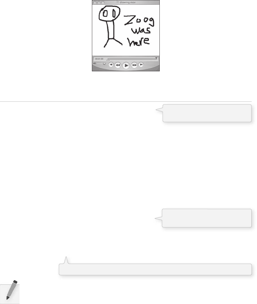
Exporting 405
Example 21-5 records a movie of a mouse drawing on the screen. e movie is fi nished when the space
bar is pressed.
fi g. 21.6 Output of Example 21-5
Example 21-5: Making a QuickTime movie
import processing.video.*;
MovieMaker mm; // Declare MovieMaker object
void setup() {
size(320, 240);
// Create MovieMaker object with size, filename,
// framerate, compression codec and quality
mm = new MovieMaker(this, width, height, "drawing.mov", 30, MovieMaker.H263,
MovieMaker.HIGH);
background(255);
}
void draw() {
stroke(0);
strokeWeight(4);
if (mousePressed) {
line(pmouseX, pmouseY, mouseX, mouseY);
}
mm.addFrame(); // Add window's pixels to movie
}
void keyPressed() {
if (key = = ''){
println( "finishing movie ");
mm.finish(); // Finish the movie if space bar is pressed!
}
}
Exercise 21-3: Create a movie from any Processing sketch you have made or any example
in this book.
The MovieMaker class is part of
Processing’s video library.
A new frame is added to the movie
every cycle through draw( ).
Do not forget to fi nish the movie! Otherwise, it will not play properly.

406 Learning Processing
Lesson Nine Project
Choose one or both!
1. Incorporate sound into a Processing sketch, either by adding sound eff ects
or by controlling the sketch with live input.
2 . Use Processing to generate an output other than real-time graphics. Make a
print (using PDF). Make a video (using MovieMaker), and so on.
Use the space provided below to sketch designs, notes, and pseudocode for your
project.

Lesson Ten
Beyond Processing
22 Advanced Object-Oriented Programming
23 Java
This page intentionally left blank
Advanced Object-Oriented Programming 409
22 Advanced Object-Oriented
Programming
“ Do you ever think about things that you do think about? ”
—Henry Drummond, Inherit the Wind
In this chapter:
– Encapsulation.
– Inheritance.
– Polymorphism.
– Overloading.
In Chapter 8, we introduced object-oriented programming ( “ OOP ” ). e driving principle of the chapter
was the pairing of data and functionality into one single idea, a class . A class is a template and from
that template we made instances of objects and stored them in variables and arrays. Although we learned
how to write classes and make objects, we did not delve very deeply into the core principles of OOP
and explore its advanced features. Now that we are nearing the end of the book (and about to leap into
the world of Java in the next chapter), it is a good time to refl ect on the past and take steps toward the
future.
Object-oriented programming in Processing and Java is defi ned by three fundamental concepts:
encapsulation , inheritance , and polymorphism . We are familiar with encapsulation already; we just have not
formalized our understanding of the concept and used the terminology. Inheritance and polymorphism
are completely new concepts we will cover in this chapter. (At the end of this chapter, we will also take
a quick look at method overloading , which allows objects to have more than one way of calling the
constructor.)
22.1 Encapsulation
To understand encapsulation , let’s return to the example of a Car class. And let’s take that example out into
the world and think about a real-life Car object, operated by a real-life driver: you . It is a nice summer day
and you are tired of programming and opt to head to the beach for the weekend. Traffi c permitting, you
are hoping for a nice drive where you will turn the steering wheel a bunch of times, press on the gas and
brakes, and fi ddle with dial on the radio.
is car that you are driving is encapsulated . All you have to do to drive is operate the functions: steer( ) ,
gas( ) , brake( ) , and radio( ) . Do you know what is under the hood? How the catalytic converter connects to
the engine or how the engine connects to the intercooler? What valves and wires and gears and belts do
what? Sure, if you are an experienced auto mechanic you might be able to answer these questions, but the
point is you don’t have to in order to drive the car. is is encapsulation .
Encapsulation is defi ned as hiding the inner workings of an object from the user of that object.
410 Learning Processing
In terms of object-oriented programming, the “ inner workings ” of an object are the data (variables
of that object) and functions. e “ user ” of the object is you, the programmer, who is making object
instances and using them throughout your code.
Now, why is this a good idea? Chapter 8 (and all of the OOP examples throughout the book)
emphasized the principles of modularity and reusability. Meaning, if you already fi gured out how to
program a Car, why do it over and over again each time you have to make a Car? Just organize it all
into the Car class, and you have saved yourself a lot of headaches.
Encapsulation goes a step further. OOP does not just help you organize your code, it protects you from
making mistakes . If you do not mess with the wiring of the car while you are driving it, you are less
likely to break the car. Of course, sometimes a car breaks down and you need to fi x it, but this requires
opening the hood and looking at the code inside the class itself.
Take the following example. Let’s say you are writing a BankAccount class which has a fl oating point
variable for the bank account balance .
BankAccount account = new BankAccount(1000);
You will want to encapsulate that balance and keep it hidden. Why? Let’s say you need to withdraw money
from that account. So you subtract $100 from that account.
account.balance = account.balance – 100.
But what if there is a fee to withdraw money? Say, $1.25? We are going to get fi red from our bank
programming job pretty quickly, having left this detail out. With encapsulation, we would keep our
job, having written the following code instead.
account.withdraw(100);
If the withdraw( ) function is written correctly, we will never forget the fee, since it will happen every
single time the method is called.
void withdraw(float amount) {
float fee = 1.25;
account – = (amount + fee);
}
Another benefi t of this strategy is that if the bank decides to raise the fee to $1.50, it can simply adjust
the fee variable inside the BankAccount class and everything will keep working!
Technically speaking, in order to follow the principles of encapsulation, variables inside of a class
should never be accessed directly and can only be retrieved with a method. is is why you will often
see programmers use a lot of functions known as getters and setters , functions that retrieve or change
the value of variables. Here is an example of a Point class with two variables ( x and y ) that are accessed
with getters and setters.
A bank account object with a
starting balance of $1,000.
Withdrawing $100 by accessing
the balance variable directly.
Withdrawing $100 by
calling a method!
This function ensures that a
fee is also deducted whenever
the money is withdrawn.
Advanced Object-Oriented Programming 411
class Point {
float x,y;
Point(float tempX, float tempY) {
x = tempX;
y = tempY;
}
// Getters
float getX() {
return x;
}
float getY() {
return y;
}
// Setters
float setX(float val) {
x = val;
}
float setY(float val) {
if (val > height) val = height;
y = val;
}
}
If we wanted to make a point and increment the y value, we would have to do it this way:
p.setY(p.getY() + 1);
Java actually allows us to mark a variable as “ private ” to make it illegal to access it directly (in other words,
if you try to, the program will not even run).
class Point {
private float x;
private float y;
}
While encapsulation is a core principle of object-oriented programming and is very important when
designing large-scale applications programmed by a team of developers, sticking to the letter of the law
(as with incrementing the y value of the Point object above) is often rather inconvenient and almost silly
for a simple Processing sketch. So, it is not the end of the world if you make a Point class and access the x
and y variables directly. We have done this several times in the examples found in this book.
However, understanding the principle of encapsulation should be a driving force in how you design your
objects and manage your code. Any time you start to expose the inner workings of an object outside of
the class itself, you should ask yourself: Is this necessary? Could this code go inside a function inside the
class? In the end, you will be a happier programmer and keep that job at the bank.
The variables x and y are accessed
with getter and setter functions.
Getters and setters allow us to protect
the value of variables. For example,
here the value of y can never be set to
greater than the sketch’s height.
Instead of:
p.y = p.y + 1;
Although rarely seen in Processing
examples, variables can be set as
private, meaning only accessible
inside the class itself. By default all
variables and functions in Processing
are “public.”

412 Learning Processing
22.2 Inheritance
Inheritance , the second in our list of three fundamental object-oriented programming concepts, allows us
to create new classes that are based on existing classes.
Let’s take a look at the world of animals: dogs, cats, monkeys, pandas, wombats, and sea nettles.
Arbitrarily, let’s begin by programming a Dog class. A Dog object will have an age variable (an integer), as
well as eat( ), sleep( ), and bark( ) functions.
class Dog {
int age;
Dog() {
age = 0;
}
void eat() {
// eating code goes here
}
void sleep() {
// sleeping code goes here
}
void bark() {
println( " WOOF! " );
}
}
Finished with dogs, we can now move on to cats.
class Cat {
int age;
Cat() {
age = 0;
}
void eat() {
// eating code goes here
}
void sleep() {
// sleeping code goes here
}
void meow() {
println( " MEOW! " );
}
}
Sadly, as we move onto fi sh, horses, koala bears, and lemurs, this process will become rather tedious as
we rewrite the same code over and over again. What if, instead, we could develop a generic Animal
Notice how dogs and cats have the same
variables (age) and functions (eat, sleep).
However, they also have a unique function
for barking or meowing.
Advanced Object-Oriented Programming 413
class to describe any type of animal? After all, all animals eat and sleep. We could then say the
following:
• A dog is an animal and has all the properties of animals and can do all the things animals can do.
In addition, a dog can bark.
• A cat is an animal and has all the properties of animals and can do all the things animals can do.
In addition, a cat can meow.
Inheritance allows us to program just this. With inheritance , classes can inherit properties (variables) and
functionality (methods) from other classes. e Dog class is a child (AKA a subclass ) of the Animal class.
Children inherit all variables and functions automatically from their parent (AKA superclass ). Children
can also include additional variables and functions not found in the parent. Inheritance follows a tree-
structure (much like a phylogenetic “ tree of life ” ). Dogs can inherit from Canines which inherit from
Mammals which inherit from Animals, and so on. See Figure 22.1 .
Animal
ReptileMammal
Cat dog lizard Crocodile
fi g. 22.1
Here is how the syntax works with inheritance.
class Animal {
int age;
Animal() {
age = 0;
}
void eat() {
// eating code goes here
}
void sleep() {
// sleeping code goes here
}
}
class Dog extends Animal {
Dog() {
super();
}
void bark() {
println( "WOOF!");
}
}
The Animal class is the parent (or super) class.
The Dog class is the child (or sub) class. This
is indicated with the code "extends Animal "
The variable age and the functions eat() and
sleep() are inherited by Dog and Cat.

414 Learning Processing
class Cat extends Animal {
Cat() {
super();
}
void bark() {
println( " MEOW! " );
}
}
e following new terms have been introduced:
• extends —This keyword is used to indicate a parent class for the class being defined. Note that classes
can only extend one class. However, classes can extend classes that extend other classes, that is, Dog
extends Animal, Terrier extends Dog. Everything is inherited all the way down the line.
• super( ) —Super calls the constructor in the parent class. In other words, whatever you do in the
parent constructor, do so in the child constructor as well. This is not required, but is fairly common
(assuming you want child objects to be created in the same manner as their parents). Other code can
be written into the constructor in addition to super( ) .
A subclass can be expanded to include additional functions and properties beyond what is contained in
the superclass. For example, let’s assume that a Dog object has a hair color variable in addition to age,
which is set randomly in the constructor. e class would now look like so:
class Dog extends Animal {
color haircolor;
Dog() {
super();
haircolor = color(random(255));
}
void bark() {
println( " WOOF! " );
}
}
Note how the parent constructor is called via super( ) , setting the age to 0, but the haircolor is set inside
the Dog constructor itself. Suppose a Dog object eats diff erently than a generic Animal. Parent functions
can be overridden by rewriting the function inside the subclass.
class Dog extends Animal {
color haircolor;
Dog() {
super();
haircolor = color(random(255));
}
void eat() {
// Code for how a dog specifically eats
}
void bark() {
println( " WOOF! " );
}
}
A child class can introduce new
variables not included in the parent.
A child can override a parent
function if necessary.
Since bark() is not part of the parent class,
we have to defi ne it in the child class.
super() means execute code found in the
parent class.
Advanced Object-Oriented Programming 415
But what if a Dog should eat the same way an Animal does, but with some additional functionality?
A subclass can both run the code from a parent class and incorporate some custom code.
class Dog extends Animal {
color haircolor;
Dog() {
super();
haircolor = color(random(255));
}
void eat() {
// Call eat() from Animal
super.eat();
// Add some additional code
// for how a dog specifically eats
println( "Yum!!!");
}
void bark() {
println( "WOOF!");
}
}
22.3 An Inheritance Example: SHAPES
Now that we have had an introduction to the theory of inheritance and its syntax, we can develop a
working example in Processing .
A typical example of inheritance involves shapes. Although a bit of a cliche, it is useful because of its
simplicity. We will create a generic “ Shape ” class where all Shape objects have an x , y location as well as a
size, and a function for display. Shapes move around the screen by “ jiggling ” randomly.
Exercise 22-1: Continuing with the Car example from our discussion of encapsulation, how
would you design a system of classes for vehicles (that is, cars, trucks, buses, and motorcycles)?
What variables and functions would you include in a parent class? And what would be
added or overridden in the child classes? What if you wanted to include planes, trains, and
boats in this example as well? Diagram it, modeled after Figure 22.1 .
A child can execute a function from the
parent while adding its own code as well.

416 Learning Processing
class Shape {
float x;
float y;
float r;
Shape(float x_, float y_, float r_) {
x = x_;
y = y_;
r = r_;
}
void jiggle() {
x + = random(–1,1);
y + = random(–1,1);
}
void display() {
point(x,y);
}
}
Next, we create a subclass from Shape (let’s call it “ Square ” ). It will inherit all the instance variables and
methods from Shape. We write a new constructor with the name “ Square ” and execute the code from the
parent class by calling super( ) .
class Square extends Shape {
// we could add variables for only Square here if we so desire
Square(float x_, float y_, float r_) {
super(x_,y_,r_);
}
// Inherits jiggle() from parent
// Add a display method
void display() {
rectMode(CENTER);
fill(175);
stroke(0);
rect(x,y,r,r);
}
}
Notice that if we call the parent constructor with super( ) , we must have to include the required
arguments. Also, because we want to display the square onscreen, we override display( ) . Even though
we want the square to jiggle, we do not need to write the jiggle( ) function since it is inherited.
What if we want a subclass of Shape to include additional functionality? Following is an example of a
Circle class that, in addition to extending Shape, contains an instance variable to keep track of color.
(Note this is purely to demonstrate this feature of inheritance, it would be more logical to place a color
variable in the parent Shape class.) It also expands the jiggle( ) function to adjust size and incorporates a
new function to change color.
A generic shape does not really
know how to be displayed. This will
be overridden in the child classes.
If the parent constructor takes
arguments then super() needs to
pass in those arguments.
Aha, the square overrides its
parent for display.
Variables are inherited from the parent.
Advanced Object-Oriented Programming 417
class Circle extends Shape {
// inherits all instance variables from parent + adding one
color c;
Circle(float x_, float y_, float r_, color c_) {
super(x_,y_,r_); // call the parent constructor
c = c_; // also deal with this new instance variable
}
// call the parent jiggle, but do some more stuff too
void jiggle() {
super.jiggle();
r + = random(-1,1);
r = constrain(r,0,100);
}
void changeColor() {
c = color(random(255));
}
void display() {
ellipseMode(CENTER);
fill(c);
stroke(0);
ellipse(x,y,r,r);
}
}
To demonstrate that inheritance is working, here is a program that makes one Square object and one
Circle object. e Shape, Square, and Circle classes are not included again, but are identical to the ones
above. See Example 22-1 .
Example 22-1: Inheritance
// Object oriented programming allows us to define classes in terms of other classes.
// A class can be a subclass (aka "child") of a super class (aka "parent").
// This is a simple example demonstrating this concept, known as "inheritance."
Square s;
Circle c;
void setup() {
size(200,200);
smooth();
// A square and circle
s = new Square(75,75,10);
c = new Circle(125,125,20,color(175));
}
void draw() {
background(255);
c.jiggle();
s.jiggle();
c.display();
s.display();
}
fi g. 22.2
The Circle jiggles its size as well as its x,y
location.
The changeColor() function is unique to
circles.
This sketch includes one Circle object and
one Square object. No Shape object is
made. The Shape class just functions as
part of our inheritance tree!
418 Learning Processing
Exercise 22-2: Write a Line class that extends Shape and has variables for the two points of
the line. When the line jiggles, move both points. You will not need “ r ” for anything in the
line class (but what could you use it for?).
class Line _______ {
float x2,y2;
Line(_______,_______,_______,_______) {
super(_________________);
x2 = _______;
y2 = _______;
}
void jiggle() {
______________________
______________________
______________________
}
void display() {
stroke(255);
line(______________________);
}
}
Exercise 22-3: Do any of the sketches you have created merit the use of inheritance? Try to
fi nd one and revise it.
22.4 Polymorphism
Armed with the concepts of inheritance, we can program a diverse animal kingdom with arrays of dogs,
cats, turtles, and kiwis frolicking about.
Dog[] dogs = new Dog[100];
Cat[] cats = new Cat[101];
Turtle[] turtles = new Turtle[23];
Kiwi[] kiwis = new Kiwi[6];
100 dogs. 101 cats. 23 turtles. 6 kiwis.
Advanced Object-Oriented Programming 419
for (int i = 0; i < dogs.length; i + + ){
dogs[i] = new Dog();
}
for (int i = 0; i < cats.length; i + + ){
cats[i] = new Cat();
}
for (int i = 0; i < turtles.length; i + + ){
turtle[i] = new Turtle();
}
for (int i = 0; i < kiwis.length; i + + ){
kiwis[i] = new Kiwi();
}
As the day begins, the animals are all pretty hungry and are looking to eat. So it is off to looping time.
for (int i = 0; i < dogs.length; i + + ){
dogs[i].eat();
}
for (int i = 0; i < cats.length; i + + ){
cats[i].eat();
}
for (int i = 0; i < turtles.length; i + + ){
turtles[i].eat();
}
for (int i = 0; i < kiwis.length; i + + ){
kiwis[i].eat();
}
is works great, but as our world expands to include many more animal species, we are going to get
stuck writing a lot of individual loops. Isn’t this unnecessary? After all, the creatures are all animals, and
they all like to eat. Why not just have one array of Animal objects and fi ll it with all diff erent kinds of
Animals?
Animal[] kingdom = new Animal[1000];
for (int i = 0; i < kingdom.length; i + + ){
if (i < 100) kingdom[i] = new Dog();
else if (i < 400) kingdom[i] = new Cat();
else if (i < 900) kingdom[i] = new Turtle();
else kingdom[i] = new Kiwi();
}
for (int i = 0; i < kingdom.length; i + + ){
kingdom[i].eat();
}
e ability to treat a Dog object as either a member of the Dog class or the Animal class (its parent) is
known as Polymorphism , the third tenet of object-oriented programming.
Polymorphism (from the Greek, polymorphos, meaning many forms) refers to the treatment of a single
object instance in multiple forms. A Dog is certainly a Dog, but since Dog extends Animal, it can also be
considered an Animal. In code, we can refer to it both ways.
Dog rover = new Dog();
Animal spot = new Dog();
Because the arrays are different sizes,
we need a separate loop for each array.
The array is of type Animal, but the
elements we put in the array are
Dogs, Cats, Turtles, and Kiwis.
When it is time for all the Animals to
eat, we can just loop through that one
big array.
Normally, the type on the left must match the type on the
right. With polymorphism, it is OK as long as the type on
the right is a child of the type on the left.

Although the second line of code might initially seem to violate syntax rules, both ways of declaring a
Dog object are legal. Even though we declare spot as an Animal, we are really making a Dog object and
storing it in the spot variable. And we can safely call all of the Animal methods on spot because the rules
of inheritance dictate that a Dog can do anything an Animal can.
What if the Dog class, however, overrides the eat( ) function in the Animal class? Even if spot is declared
as an Animal, Java will determine that its true identity is that of a Dog and run the appropriate version of
the eat( ) function.
is is particularly useful when we have an array.
Let’s rewrite the Shape example from the previous section to include many Circle objects and many
Square objects.
// Many Squares and many Circles
Square[] s = new Square[10];
Circle[] c = new Circle[20];
void setup() {
size(200,200);
smooth();
// Initialize the arrays
for (int i = 0; i < s.length; i + + ) {
s[i] = new Square(100,100,10);
}
for (int i = 0; i < c.length; i + + ) {
c[i] = new Circle(100,100,10,color(random(255),100));
}
}
void draw() {
background(100);
// Jiggle and display all squares
for (int i = 0; i < s.length; i + + ) {
s[i].jiggle();
s[i].display();
}
// Jiggle and display all circles
for (int i = 0; i < c.length; i + + ) {
c[i].jiggle();
c[i].display();
}
}
Polymorphism allows us to simplify the above by just making one array of Shape objects that contains
both Circle objects and Square objects. We do not have to worry about which are which, this will all be
taken care of for us! (Also, note that the code for the classes has not changed, so we are not including it
here.) See Example 22.2 .
The old "non-polymorphism"
way with multiple arrays.
420 Learning Processing
Advanced Object-Oriented Programming 421
Example 22-2: Polymorphism
// One array of Shapes
Shape[] shapes = new Shape[30];
void setup() {
size(200,200);
smooth();
for (int i = 0; i < shapes.length; i + + ){
int r = int(random(2));
// randomly put either circles or squares in our array
if (r = = 0) {
shapes[i] = new Circle(100,100,10,color(random(255),100));
} else {
shapes[i] = new Square(100,100,10);
}
}
}
void draw() {
background(100);
// Jiggle and display all shapes
for (int i
= 0; i < shapes.length; i + + ){
shapes[i].jiggle();
shapes[i].display();
}
}
fi g. 22.3
22.5 Overloading
In Chapter 16, we learned how to create a Capture object in order to read live images from a video
camera. If you looked at the Processing reference page ( http://www.processing.org/reference/libraries/video/
Capture.html ), you may have noticed that the Capture constructor can be called with three, four, or fi ve
arguments:
Capture(parent, width, height)
Capture(parent, width, height, fps)
Capture(parent, width, height, name)
Capture(parent, width, height, name, fps)
Functions that can take varying numbers of arguments are actually something we saw all the way back
in Chapter 1! fi ll( ) , for example, can be called with one number (for grayscale), three (for RGB color), or
four (to include alpha transparency).
Exercise 22-4: Add the Line class you created in Exercise 22-2 to Example 22-2. Randomly
put circles, squares, and lines in the array. Notice how you barely have to change any code
(you should only have to edit setup( ) above).
Exercise 22-5: Implement polymorphism in the sketch you made for Exercise 22-3.
The new polymorphism way with
one array that has different types
of objects that extend Shape.
422 Learning Processing
fill(255);
fill(255,0,255);
fill(0,0,255,150);
e ability to defi ne functions with the same name (but diff erent arguments) is known as overloading .
With fi ll( ) , for example, Processing does not get confused about which defi nition of fi ll( ) to look up, it
simply fi nds the one where the arguments match. A function’s name in combination with its arguments
is known as the function’s signature —it is what makes that function defi nition unique. Let’s look at an
example that demonstrates how overloading can be useful.
Let’s say you have a Fish class. Each Fish object has a location: x and y .
class Fish {
float x;
float y;
What if, when you make a Fish object, you sometimes want to make one with a random location and
sometimes with a specifi c location. To make this possible, we could write two diff erent constructors:
Fish() {
x = random(0,width);
y = random(0,height);
}
Fish(float tempX, float tempY) {
x = tempX;
y = tempY;
}
}
When you create a Fish object in the main program, you can do so with either constructor:
Fish fish1 = new Fish();
Fish fish2 = new Fish(100,200);
Overloading allows us to defi ne two
constructors for the same object
(as long as these constructors take
different arguments).
If two constructors are defi ned,
an object can be initialized using
either one.
Java 423
23 Java
“ I l o v e c o ff ee, I love tea, I love the Java Jive and it loves me. ”
—Ben Oakland and Milton Drake
In this chapter:
– Processing is really Java.
– If we did not have Processing what would our code look like?
– Exploring the Java API.
– Some useful examples: ArrayList, and Rectangle.
– Exception (error) handling—try and catch.
– Beyond Processing ?
23.1 Revealing the Wizard
Perhaps, all along while reading this book, you have been thinking: “ Gosh, this is so awesome. I love
programming. I am so glad I am learning Processing . I can’t wait to go on and learn Java! ” e funny thing
is, you do not really need to learn Java. Pulling back the curtain of Processing , what we will discover is that
we have been learning Java all along. For example, in Java, you:
• Declare, initialize, and use variables the same way.
• Declare, initialize, and use arrays the same way.
• Employ conditional and loop statements the same way.
• Define and call functions the same way.
• Create classes the same way.
• Instantiate objects the same way.
Processing , of course, gives us some extra stuff for free (and simplifi es some stuff here and there) and this
is why it is a great tool for learning and for developing interactive graphics projects. Here is a list of some
of what Processing off ers that is not as easily available with just plain Java.
• A set of functions for drawing shapes.
• A set of functions for loading and displaying text, images, and video.
• A set of functions for 3D transformations.
• A set of functions for mouse and keyboard interaction.
• A simple development environment to write your code.
• A friendly online community of artists, designers, and programmers!
23.2 If we did not have Processing , what would our code look like?
In Chapter 2, we discussed the compilation and execution process—this is what happens when you
press the play button and turn your code into a window with graphics. Step 1 of this process involves
“ translating ” your Processing code into Java. In fact, when you export to applet, this same process
occurs and you will notice that along with the fi le “ Sketchname.pde, ” a new fi le will appear named

424 Learning Processing
“ SketchName.java. ” is is your “ translated ” code, only translation is somewhat of a misnomer since very
little changes. Let’s look at an example:
// Randomly Growing Square
float w = 30.0; // Variable to keep track of size of rect
void setup() {
size(200, 200);
}
void draw() {
background(100);
rectMode(CENTER);
fill(255);
noStroke();
rect(mouseX,mouseY,w,w); // Draw a rect at mouse location
w + = random( – 1,1); // Randomly adjust size variable
}
Exporting the sketch, we can open up the Java fi le and look at the Java source.
// Randomly Growing Square with Java Stuff
import processing.core.*;
import java.applet.*;
import java.awt.*;
import java.awt.image.*;
import java.awt.event.*;
import java.io.*;
import java.net.*;
import java.text.*;
import java.util.*;
import java.util.zip.*;
float w = 30.0f; // Variable to keep track of size of rect
public void setup() {
size(200, 200);
}
public void draw() {
background(100);
rectMode(CENTER);
fill(255);
noStroke();
rect(mouseX,mouseY,w,w); // draw a rect at mouse location
w + = random( – 1,1); // randomly adjust size variable
}
}
It is clear that little has changed, rather, some code has been added before and after the usual setup( ) and
draw( ) stuff .
• Import Statements —At the top, there are a set of import statements allowing access to certain
libraries. We have seen this before when using Processing libraries. If we were using regular Java
What we are used to seeing, our
regular old Processing code.
The translated Java code has
some new stuff at the top, but
everything else stays the same.
public class JavaExample extends PApplet {
Java 425
instead of Processing , specifying all libraries would always be required. Processing , however, assumes a
base set of libraries from Java (e.g., java.applet.*) and from Processing (e.g., processing.core.* ) which is
why we do not see these in every sketch.
• public —In Java, variables, functions, and classes can be “ public ” or “ private. ” This designation
indicates what level of access should be granted to a particular piece of code. It is not something
we have to worry much about in the simpler Processing environment, but it becomes an important
consideration when moving on to larger Java programs. As an individual programmer, you are
most often granting or denying access to yourself, as a means for protecting against errors. We
encountered some examples of this in Chapter 22’s discussion about encapsulation.
• class JavaExample —Sound somewhat familiar? Java, it turns out, is a true object-oriented language.
There is nothing written in Java that is not part of a class! We are used to the idea of the Zoog class,
Car class, PImage class, and so on, but it is important to note that the sketch as a whole is a class,
too! Processing fills this stuff in for us so we do not have to worry about classes when we are first
learning to program.
• extends PApplet —Well, after reading Chapter 22, we should be quite comfortable with what this
means. This is just another example of inheritance. Here, the class JavaExample is a child of the class
PApplet (or, equivalently, PApplet is the parent of JavaExample). PApplet is a class developed by
the creators of Processing and by extending it, our sketch has access to all of the Processing goodies—
setup( ), draw( ) , mouseX , mouseY , and so on. This little bit of code is the secret behind how almost
everything works in a Processing sketch.
Processing has served us so well because it eliminates the need to worry about the above four elements, all
the while providing access to the benefi ts of the Java programming language. e rest of this chapter will
show how we can begin to make use of access to the full Java API. (We briefl y began this journey when
we worked with String parsing in Chapters 17 and 18.)
23.3 Exploring the Java API
e Processing reference quickly became our best friend forever while learning to program. e Java API
will start off more as an acquaintance we bump into from time to time. at acquaintance might turn into
a really excellent friend someday, but for now, small doses will be just fi ne.
We can explore the full Java documentation by visiting:
http://java.sun.com/
ere, we can click over to API specifi cations:
http://java.sun.com/reference/api/index.html
and fi nd a selection of versions of Java. On a Mac, Processing will run with the selected version of Java
(run Java Preferences, found, e.g., in: /Applications/Utilities/Java/J2SE 5.0/). On a PC, the Processing
“ standard ” download comes with Java version 1.4.2 (the Windows expert version allows you to install
your own version of Java). Versions of Java will change in the future with updated info at processing.org.
In any case, while there are diff erences between the version of Java, for what we are doing, they will not
be terribly relevant, and we can look at the API for J2SE 1.4.2 for pretty much whatever we want to do.
See Figure 23.1 .
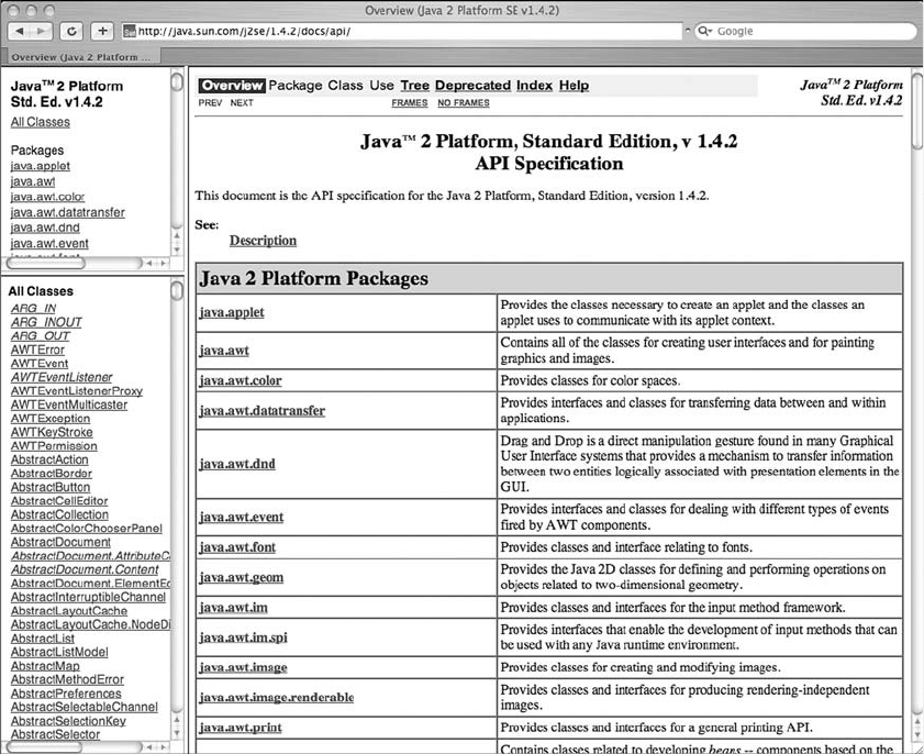
426 Learning Processing
fi g. 23.1 http://java.sun.com/j2se/1.4.2/docs/api/
And so, very quickly, you will fi nd yourself completely lost. And that is OK. e Java API is huge.
Humongous. It is not really meant to be read or even perused . It is really pure reference, for looking up
specifi c classes that you know you need to look up.
For example, you might be working on a program that requires sophisticated random number
generation beyond what random( ) can do, and you overheard a conversation about the class “ Random ”
and thought “ Hey, maybe I should check that out! ” e reference page for a specifi c class can be
found by scrolling down the “ All Classes ” list or else by selecting the right package (in this case the
package java.util). A package, much like a library, is a collection of classes (the API organizes
them by topic). e easiest way to fi nd a class, though, is to just type the name of the class and Java
(i.e., “ Java Random ” ) into google. e documentation page is just about always the fi rst result.
See Figure 23.2 .
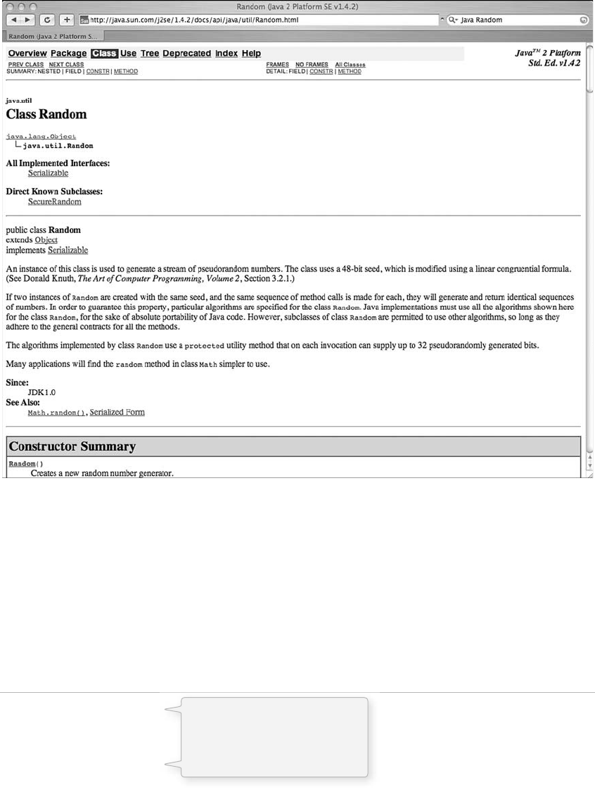
Java 427
Just as with the Processing reference, the Java page includes an explanation of what the class does, the
Constructors for creating an object instance, and available fi elds (variables) and methods (functions). Since
Random is part of the java.util package (which Processing imports by assumption), we do not need to
explicitly write an import statement to use it.
Here is some code that makes a Random object and calls the function nextBoolean( ) on it to get a
random true or false.
Example 23-1: Using java.util.Random instead of random()
Random r;
void setup() {
size(200,200);
r = new Random();
}
fi g. 23.2
Declaring a Random object and
calling the constructor as found
at http://java.sun.com/j2se/1.4.2/
docs/api/java/util/Random.html

428 Learning Processing
void draw() {
boolean trueorfalse = r.nextBoolean();
if (trueorfalse) {
background(0);
} else {
background(255);
}
}
Exercise 23-1: Visit the Java reference page for Random and use it to get a random integer
between 0 and 9. http://java.sun.com/j2se/1.4.2/docs/api/java/util/Random.html .
23.4 Other Useful Java Classes: ArrayList
In Chapter 6, we learned how to use an array to keep track of ordered lists of information. We created
an array of N objects and used a “ for ” loop to access each element in the array. e size of that array was
fi xed—we were limited to having N and only N elements.
ere are alternatives. One option is to use a very large array and use a variable to track how much of the
array to use at any given time (see Chapter 10’s rain catcher example). Processing also off ers expand( ) ,
contract( ), subset( ) , splice( ) and other methods for resizing arrays. It would be great, however, to have a
class that implements a fl exibly sized array, allowing items to be added or removed from the beginning,
middle, and end of that array.
is is exactly what the Java class ArrayList, found in the java.util package, does.
e reference page is here: http://java.sun.com/j2se/1.4.2/docs/api/java/util/ArrayList.html .
Using an ArrayList is conceptually similar to a standard array, but the syntax is diff erent. Here is some
code (that assumes the existence of a class “ Particle ” ) demonstrating identical results, fi rst with an array,
and second with an ArrayList. All of the methods used in this example are documented on the JavaDoc
reference page.
// THE STANDARD ARRAY WAY
int MAX = 10;
//declaring the array
Particle[] parray = new Particle[MAX];
// Initialize the array in setup
void setup() {
for (int i = 0; i < parray.length; i + + ) {
parray[i] = new Particle();
}
}
// Loop through the array to call methods in draw
void draw() {
for (int i = 0; i < parray.length; i + + ) {
Calling a function found at http://java.sun.com/
j2se/1.4.2/docs/api/java/util/Random.html
The Standard Array Way
This is what we have been
doing all along, accessing
elements of the array via
an index and brackets—[].
Java 429
Particle p = parray[i];
p.run();
p.display();
}
}
// THE NEWFANGLED ARRAYLIST WAY
int MAX = 10;
// Declaring and creating the ArrayList instance
ArrayList plist = new ArrayList();
void setup() {
for (int i = 0; i < MAX; i + + ){
plist.add(new Particle());
}
}
void draw() {
for (int i = 0; i < plist.size(); i + + ){
Particle p = (Particle) plist.get(i);
p.run();
p.display();
}
}
In this last “ for ” loop, we have to cast the object as we get it out of the ArrayList. An ArrayList does not
keep track of the type of objects stored inside—even though it may seem redundant, it is our job to remind
the program by placing the class type (i.e., Particle) in parentheses. is process is known as casting .
Of course, the above example is somewhat silly, because it does not take advantage of the ArrayList’s
resizability, using a fi xed size of 10. Following is a better example that adds one new Particle to the
ArrayList with each cycle through draw( ) . We also make sure the ArrayList never gets larger than 100
particles. See Figure 23.3 .
The New ArrayList Way
Elements of an ArrayList are added and accessed
with functions (rather than brackets)—add() and
get(). All of these functions are documented in the
Java reference: http://java.sun.com/j2se/1.4.2/docs/
api/java/util/ArrayList.html.
The term “particle system” was coined in 1983 by William T. Reeves as he developed the “Genesis”
effect for the end of the movie, Star Trek II: The Wrath of Khan.
A particle system is typically a collection of independent objects, usually represented by a simple shape
or dot. It can be used to model types of natural phenomena, such as explosions, fi re, smoke, sparks,
waterfalls, clouds, fog, petals, grass, bubbles, and so on.
Example 23-2: Simple particle system with ArrayList
ArrayList particles;
void setup() {
size(200,200);
particles = new ArrayList();
smooth();
}
An object is added to an ArrayList with add().
The size of the ArrayList is returned by size().
An object is accessed from the ArrayList with get(). You must “cast”
whatever comes out of the ArrayList with a type, that is (Particle).
Casting is discussed in Chapter 4.
fi g. 23.3
430 Learning Processing
void draw() {
particles.add(new Particle());
background(255);
// Iterate through our ArrayList and get each Particle
for (int i = 0; i < particles.size(); i + + ) {
Particle p = (Particle) particles.get(i);
p.run();
p.gravity();
p.display();
}
// Remove the first particle when the list gets over 100.
if (particles.size() > 100) {
particles.remove(0);
}
}
// A simple Particle class
class Particle {
float x;
float y;
float xspeed;
float yspeed;
Particle() {
x = mouseX;
y = mouseY;
xspeed = random(–1,1);
yspeed = random(–2,0); }
void run() {
x = x + xspeed;
y = y + yspeed;
}
void gravity() {
yspeed + = 0.1;
}
void display() {
stroke(0);
fill(0,75);
ellipse(x,y,10,10);
}
}
A new Particle object is added to the
ArrayList every cycle through draw().
The ArrayList keeps track of how many
elements it is storing and we iterate
through them all.
If the ArrayList has more than 100 elements
in it, we delete the fi rst element, using
remove().
Java 431
Particle
AParticle
BParticle
CParticle
DParticle
E
C is removed....
ArrayList particles
012
size = 5 size = 4
34
Particle
AParticle
BParticle
DParticle
E
0123
fi g. 23.4
Hint: Add a function that returns a boolean in the Particle class.
_______ finished() {
if (_______) {
return _______;
} else {
return false;
}
}
Hint: In order for this to work properly, you must iterate through elements of the ArrayList
backward! Why? Because when an element is removed, all subsequent elements are shifted to the
left (see Figure 23.4 ).
for (int i = _______; i _______; i_______) {
Particle p = (Particle) particles.get(i);
p.run();
p.gravity();
p.render();
if (_______) {
_______;
}
}
Exercise 23-2 : Rewrite Example 23-2 so that particles are removed from the list whenever
they leave the window (i.e., their y location is greater than height).
432 Learning Processing
23.5 Other Useful Java Classes: Rectangle
e second helpful Java class we will examine is the Rectangle class:
http://java.sun.com/j2se/1.4.2/docs/api/java/awt/Rectangle.html .
A Java Rectangle specifi es an area in a coordinate space that is enclosed by the Rectangle object’s top-left point
( x , y ), its width, and its height. Sound familiar? Of course, the Processing function rect( ) draws a rectangle with
precisely the same parameters. e Rectangle class encapsulates the idea of a rectangle into an object.
A Java Rectangle has useful methods, for instance, contains( ). contains( ) off ers a simple way of checking if
a point or rectangle is located inside that rectangle, by receiving an x and y coordinate and returning true
or false, based on whether the point is inside the rectangle or not.
Here is a simple rollover implemented with a Rectangle object and contains( ) . See Example 23.3 .
Example 23-3: Using a java.awt.Rectangle object
Rectangle rect1, rect2;
void setup() {
size(200,200);
rect1 = new Rectangle(25,25,50,50);
rect2 = new Rectangle(125,75,50,75);
}
void draw() {
background(255);
stroke(0);
if (rect1.contains(mouseX,mouseY)) {
fill(200);
} else {
fill(100);
}
rect(rect1.x, rect1.y, rect1.width,rect1.height);
// Repeat for the second Rectangle
// (of course, we could use an array or ArrayList here!)
if (rect2.contains(mouseX,mouseY)) {
fill(200);
} else {
fill(100);
}
rect(rect2.x, rect2.y, rect2.width,rect2.height);
}
Let’s have some fun and combine the ArrayList “ particle ” example with the Rectangle “ rollover. ” In
Example 23-4, particles are made every frame and pulled down by gravity toward the bottom of the
window. If they run into a rectangle, however, they are caught. e particles are stored in an ArrayList
and a Rectangle object determines if they have been caught or not. ( is example contains answers to
Exercise 23-2.)
fi g. 23.5
This sketch uses two
Rectangle objects.
The arguments for
the constructor
(x,y,width,height) are
documented in the Java
reference: http://java.sun.
com/j2se/1.4.2/docs/api/
java/awt/Rectangle.html.
A Rectangle object only
knows about the variables
associated with a rectangle.
It cannot display one. So
we use Processing’s rect()
function in combination with
the Rectangle’s data.
The contains() function is used to determine
if the mouse is located inside the rectangle.
Java 433
Example 23-4: Super fancy ArrayList and rectangle particle system
// Declaring a global variable of type ArrayList
ArrayList particles;
// A "Rectangle" will suck up particles
Rectangle blackhole;
void setup() {
size(200,200);
blackhole = new Rectangle(50,150,100,25);
particles = new ArrayList();
smooth();
}
void draw() {
background(255);
// Displaying the Rectangle
stroke(0);
fill(175);
rect(blackhole.x, blackhole.y, blackhole.width,blackhole.height);
// Add a new particle at mouse location
particles.add(new Particle(mouseX,mouseY));
// Loop through all Particles
for (int i = particles.size() – 1; i > = 0; i – – ){
Particle p = (Particle) particles.get(i);
p.run();
p.gravity();
p.display();
if (blackhole.contains(p.x,p.y)) {
p.stop();
}
if (p.finished()) {
particles.remove(i);
}
}
}
// A simple Particle Class
class Particle {
float x;
float y;
float xspeed;
float yspeed;
float life;
// Make the Particle
Particle(float tempX, float tempY) {
x = tempX;
y = tempY;
xspeed = random(–1,1);
yspeed = random(–2,0);
life = 255;
}
fi g. 23.6
If the Rectangle contains the location of the
Particle, stop the Particle from moving.

434 Learning Processing
// Move
void run() {
x = x + xspeed;
y = y + yspeed;
}
// Fall down
void gravity() {
yspeed + = 0.1;
}
// Stop moving
void stop() {
xspeed = 0;
yspeed = 0;
}
// Ready for deletion
boolean finished() {
life – = 2.0;
if (life < 0) return true;
else return false;
}
// Show
void display() {
stroke(0);
fill(0,life);
ellipse(x,y,10,10);
}
}
Exercise 23-3: Write a Button class that includes a Rectangle object to determine if the
mouse has clicked inside the button’s area. ( is is an extension of Exercise 9-8 .)
23.6 Exception (Error) Handling
In addition to a very large library of useful classes, the Java programming language includes some features
beyond what we have covered while learning Processing . We will explore one of those features now:
exception handling .
Programming mistakes happen. We have all seen them.
java.lang.ArrayIndexOutOfBoundsException
java.io.IOException: openStream() could not open file.jpg
java.lang.NullPointerException
The Particle has a “life” variable which
decreases. When it reaches 0 the Particle
can be removed from the ArrayList.
Java 435
It is sad when these errors occur. Really, it is. e error message prints out and the program sputters to a
halt, never to continue running again. Perhaps you have developed some techniques for protecting against
these error messages. For example:
if (index < somearray.length) {
somearray[index] = random(0,100);
}
e above is a form of “ error checking. ” e code uses a conditional to check that the index is valid
before an element at that index is accessed. e above code is quite conscientious and we should all aspire
to be so careful.
Not all situations are as simple to avoid, however, and this is where exception handling comes into play.
Exception handling refers to the process of handling exceptions , out of the ordinary events (i.e., errors)
that occur during the execution of a program.
e code structure for exception handling in Java is known as try catch . In other words, “ Try to run some
code. If you run into a problem, however, catch the error and run some other code. ” If an error is caught
using try catch, the program is allowed to continue. Let’s look at how we might rewrite the array index
error checking code try catch style.
try {
somearray[index] = 200;
} catch (Exception e) {
println( "Hey, that’s not a valid index! ");
}
e above code catches any possible exception that might occur. e type of error caught is the generic
Exception. However, if you want to execute certain code based on a specifi c exception, you can, as the
following code demonstrates.
try {
somearray[index] = 200;
} catch (ArrayIndexOutOfBoundsException e) {
println ( "Hey, that’s not a valid index! ");
} catch (NullPointerException e) {
println( "I think you forgot to create the array! ");
} catch (Exception e) {
println( "Hmmm, I dunno, something weird happened! ");
e.printStackTrace();
}
e above code, nevertheless, does nothing more than print out custom error messages. ere are
situations where we want more than just an explanation. For example, take the examples from Chapter 18
where we loaded data from a URL path. What if our sketch had failed to connect to the URL? It would
have crashed and quit. With exception handling, we can catch that error and fi ll the array with Strings
manually so that the sketch can continue running.
The code that might produce an error
goes within the “try” section. The
code that should happen if an error
occurs goes in the “catch” section.
Different “catch” sections
catch different types of
exceptions. In addition, each
exception is an object and
can therefore have methods
called on it. For example:
e.printStackTrace();
displays more detailed
information about the
exception.
436 Learning Processing
String[] lines;
String url = " http://wwww.rockinurl.com " ;
try {
lines = loadStrings(url);
} catch (Exception e) {
lines = new String[3];
lines[0] = " I could not connect to " + url + " !!! " ;
lines[1] = " But here is some stuff to work with " ;
lines[2] = " anyway. " ;
}
println(lines);
23.7 Java Outside of Processing
Here we are, the very last section of this book. You can can take a break now if you want. Maybe go
outside and have a walk. A little jog around the block even. It will be good for you.
OK, back now? Great, let’s go on.
As we close out this chapter and the book, we will cover one fi nal topic: what to do if and when you
decide you want to start coding outside of Processing .
But why would I ever want to do this?
One instance that would merit another programming environment is in the case of making an application
that does not involve any graphics! Perhaps you need to write a program that takes all of your fi nancial
info from spreadsheets and logs it in a database. Or a chat server that runs in the background on your
computer. While both of these could be written in the Processing environment, they do not necessarily
need any of the features of Processing to run.
In the case of developing larger and larger projects that involve many classes, the Processing environment
can become a bit diffi cult to use. For example, what if your project involves, say, 20 classes. Creating a
Processing sketch with 20 tabs (and what if it were 40? or 100?) can be hard to manage, let alone fi t on
the screen. In this case, a development environment designed for large-scale Java projects would be better.
Since Processing is Java, you can still use all of the functions available in Processing in other development
environments by importing the core libraries.
So, what do you do? First, I would say do not rush. Enjoy Processing and take the time to feel comfortable
with your own coding process and style before getting yourself wrapped up in the myriad of issues and
questions that come along with programming in Java.
If you feel ready, a good fi rst step is to just take some time browsing the Java web site:
http://java.sun.com/
Start with one of the tutorials:
http://java.sun.com/docs/books/tutorial/
If a problem occurs connecting
to the URL, we will just fi ll the
array with dummy text so that
the sketch can still run.
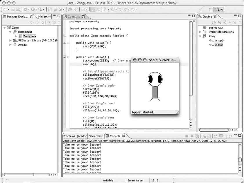
Java 437
e tutorials will cover the same material found in this book, but from a pure Java perspective.
e next step would be to just try compiling and running a “ Hello World ” Java program.
public class HelloWorld {
public static void main(String[] args) {
System.out.println( "Hello World. I miss you Processing. ");
}
}
e Java site has tutorials which explain all the elements in a Hello World program, as well as provide
instructions on how to compile and run it on the “ command line. ”
http://java.sun.com/docs/books/tutorial/getStarted/index.html
Finally, if you are feeling ambitious, go and download Eclipse:
http://www.eclipse.org/
fi g. 23.7 A Processing sketch in Eclipse
438 Learning Processing
Eclipse is a development environment for Java with many advanced features. Some of those features will
give you a headache and some will make you wonder how you ever programmed without Eclipse. Just
remember, when you started with Processing in Chapter 2, you were probably up and running with your
fi rst sketch in less than fi ve minutes. With something like Eclipse , you could need a much longer time to
get started. See Figure 23.7 .
Visit this book’s web site for links and tutorials about how to run a Processing sketch within the Eclipse
environment.
anks for reading. Feedback is encouraged and appreciated, so come on down to http://www.
learningprocessing.com and sound off !

Appendix 439
Appendix: Common Errors
is appendix off ers a brief overview of common errors that occur in Processing , what those errors mean
and why they occur. e language of error messages can often be cryptic and confusing, mostly due to
their origins in the Java programming language.
For these error messages, we will use the following conventions:
Variables in the error messages will be named “ myVar ” .
Arrays in the error messages will be named “ myArray ” .
If the error is specifi cally related to an object variable, the variable will be named “ myObject ” .
If the error is related to a class, the class will be named “ ing ” .
If the error is related to a function, the function will be named “ function ” .
ERROR PAGE NO.
unexpected token: _____ 440
Found one too many { characters without a } to match it. 440
No accessible fi eld named “ myVar ” was found in type “ Temporary_####_#### ” 441
e variable “ myVar ” may be accessed here before having been defi nitely assigned a
value.
442
java.lang.NullPointerException 442
Type “ ing ” was not found. 444
Perhaps you wanted the overloaded version “ type function (type $1, type $2, … ); ”
instead?
445
No method named “ fnction ” was found in type “ Temporary_####_#### ” . However,
there is an accessible method “ function ” whose name closely matches the name
“ fnction ” .
445
No accessible method with signature “ function (type, type, … ) ” was found in type
“ Temporary_3018_2848 ” .
445
java.lang.ArrayIndexOutOfBoundsException 446
Error:
unexpected token: something
Translation:
I’m expecting a piece of code here that you forgot, most likely some punctuation, like a semicolon,
parenthesis, curly bracket, and so on.
is error is pretty much always caused by a typo. Unfortunately, the line of code that the error points to
can be misleading. e “ something ” is sometimes correct and the actual error is caused by line before or
after. Any time you forget or include an improper comma, semicolon, quote, parenthesis, bracket, and so
on, you will get this error. Here are some examples:
ERROR CORRECTED
void setup() {
for (int i = 0; i < 10; i + + ) {
if (i > 5) {
line(0,i,i,0);
println( " " );
}
}
void setup() {
for (int i = 0; i < 10; i + + ) {
if (i > 5) {
line(0,i,i,0);
println( " i is greater than 5 " );
}
}
}
Error:
Found one too many { characters without a } to match it.
Translation:
You forgot to close a block of code, such as an if statement, a loop, a function, a class, and so on.
Any time you have an open curly bracket in your code ( “ { ” ), you must have a matching close curly bracket
( “ } ” ). And since blocks of code are often nested inside each other, it is easy to forget one by accident,
resulting in this error.
440 Learning Processing
ERROR CORRECTED
int val = 5 int val = 5;
if (x < 5 {
ellipse(0,0,10,10);
}
if (x < 5) {
ellipse (0,0,10,10);
}
for (int i = 0, i < 5,i + + ) {
println(i);
}
for (int i = 0; i < 5; i + +)
println(i);{
Missing semicolon.
Missing close parenthesis.
For loop should be separated
by semicolons, not commans.
Missing a close curly bracket!
i is greater than 5

Appendix 441
Error:
No accessible fi eld named “ myVar ” was found in type “ Temporary_7665_1082 ”
Translation:
I do not know about the variable “ myVar. ” It is not declared anywhere I can see.
is error will happen if you do not declare a variable. Remember, you can’t use a variable until you have
said what type it should be. You will get the error if you write:
myVar = 10;
instead of:
int myVar = 10;
Of course, you should only declare the variable once, otherwise you can run into trouble. So this is
perfectly OK:
int myVar = 10;
myVar = 20;
is error can also occur if you try to use a local variable outside of the block of code where it was
declared. For example:
if (mousePressed) {
int myVar = 10;
}
ellipse(myVar,10,10,10);
Here is a corrected version:
int myVar = 0;
if (mousePressed) {
myVar = 10;
}
ellipse(myVar,10,10,10);
Or if you have declared a variable in setup( ) , but try to use it in draw( ) .
void setup() {
int myVar = 10;
}
void draw() {
ellipse(myVar,10,10,10);
}
Corrected:
int myVar = 0;
void setup() {
myVar
= 10;
}
ERROR! myVar is local to the if statement so
it cannot be accessed here.
OK! The variable was declared.
OK! The variable is declared outside of the
if statement.
ERROR! myVar is local to the setup() so it
cannot be accessed here.

442 Learning Processing
void draw() {
ellipse(myVar,10,10,10);
}
e same error will occur if you use an array in any of the above scenarios.
myArray[0] = 10;
Error:
e variable “ myVar ” may be accessed here before having been defi nitely assigned a value.
Translation:
You declared the variable “ myVar ” , but you did not initialize it. You should give it a value fi rst.
is is a pretty simple error to fi x. Most likely, you just forgot to give your variable its default starting
value. is error only occurs for local variables (with global variables Processing will either not care, and
assume the value is zero, or else throw a NullPointerException ).
int myVar;
line(0, myVar,0,0);
int myVar = 10;
line(0, myVar,0,0);
is error can also occur if you try to use an array before allocating its size properly.
int[] myArray;
myArray[0] = 10;
int[] myArray = new int[3];
myArray[0] = 10;
Error:
java.lang.NullPointerException
Translation:
I have encountered a variable whose value is null. I can’t work with this.
e NullPointerException error can be one of the most diffi cult errors to fi x. It is most commonly caused by
forgetting to initialize an object. As mentioned in Chapter 8, when you declare a variable that is an object,
it is fi rst given the value of null , meaning nothing. ( is does not apply to primitives, such as integers and
fl oats.) If you attempt to then use that variable without having initialized it (by calling the Constructor),
this error will occur. Here are a few examples (that assume the existence of a class called “ ing ” ).
Thing thing;
void setup() {
}
ERROR! No array was declared.
OK! The variable is global.
ERROR! myVar does not have a value.
OK! myVar equals ten.
ERROR! myArray was not created properly.
OK! myArray is an array of three integers.
Appendix 443
void draw() {
thing.display();
}
Corrected:
Thing thing;
void setup() {
thing = new Thing();
}
void draw() {
thing.display();
}
Sometimes, the same error can occur if you do initialize the object, but as a local variable by accident.
Thing thing;
void setup() {
Thing thing = new Thing();
}
void draw() {
thing.display();
}
e same goes for an array as well. If you forget to initialize the elements, you will get this error.
Thing[] things = new Thing[10];
for (int i = 0; i < things.length; i ++ ) {
things[i].display();
}
Corrected:
Thing[] things = new Thing[10];
for (int i = 0; i < things.length; i ++ ) {
things[i] = new Thing();
}
for (int i = 0; i < things.length; i ++ ) {
things[i].display();
}
Finally, if you forget to allocate space for an array, you can also end up with this error.
int[] myArray;
void setup() {
myArray[0]
= 5;
}
ERROR! “thing” was never initialized and
therefore has the value null.
OK! “thing” is not null because it was initialized
with the constructor.
ERROR! This line of code declares and initializes
a different “thing” variable (even though it has
the same name). It is a local variable for only
setup(). The global “thing” is still null!
ERROR! All the elements on the array are null!
OK! The fi rst loop initialized the elements of the array.
ERROR! myArray is null because you never
created it and gave it a size.

444 Learning Processing
Corrected:
int[] myArray = new int[3];
void setup() {
myArray[0] = 5;
}
Error:
Type “ ing ” was not found.
Translation:
You are trying to declare a variable of type ing, but I do not know what a ing is.
is error occurs because you either (a) forgot to defi ne a class called “ ing ” or (b) made a typo in the
variable type.
A typo is pretty common:
intt myVar = 10;
Or maybe you want to create an object of type ing, but forgot to defi ne the thing class.
Thing myThing = new Thing();
is will work, of course, if you write:
void setup() {
Thing myThing = new Thing();
}
class Thing {
Thing() {
}
}
Finally, the error will also occur if you try to use an object from a library, but forget to import the library.
void setup() {
Capture video = new Capture(this,320,240,30);
}
Corrected:
import processing.video.*;
void setup() {
Capture video
= new Capture(this,320,240,30);
}
OK! myArray is an array of three integers.
ERROR! You probably meant to type “int” not “intt.”
ERROR! If you did not defi ne a class called “Thing.”
OK! You did declare a class called “Thing.”
ERROR! You forgot to import
the video library.
OK! You imported the library.

Appendix 445
Error:
Perhaps you wanted the overloaded version “ type function (type $1, type $2, … ); ” instead?
Translation:
You are calling a function incorrectly, but I think I know what you mean to say. Did you want call
this function with these arguments?
is error occurs most often when you call a function with the incorrect number of arguments. For
example, to draw an ellipse, you need an x location, y location, width, and height. But if you write:
ellipse(100,100,50);
You will get the error: “ Perhaps you wanted the overloaded version ‘void ellipse(fl oat $1, fl oat $2, fl oat $3,
fl oat $4);’ instead? ” e error lists the function defi nition for you, indicating you need four arguments, all of
fl oating point. e same error will also occur if you have the right number of arguments, but the wrong type.
ellipse(100,100,50, "Wrong Type of Argument ");
Error:
No method named “ fnction ” was found in type “ Temporar y_9938_7597 ” . However, there is an
accessible method “ function ” whose name closely matches the name “ fnction ” .
Translation:
You are calling a function I have never heard of, however, I think I know what you want to say
since there is a function I have heard of that is really similar.
is is a similar error and pretty much only happens when you make a typo in a function’s name.
elipse(100,100,50,50);
Error:
No accessible method with signature “ function (type, type, … ) ” was found in type
“ Temporary_3018_2848 ” .
Translation:
You are calling a function that I have never heard of. I have no idea what you are talking about!
is error occurs if you call a function that just plain does not exist, and Processing can’t make any guess as
to what you meant to say.
functionCompletelyMadeUp(200);
ERROR! ellipse() requires four arguments.
ERROR! ellipse() can not take a String!
ERROR! You have the right number of arguments,
but you spelled “ellipse” incorrectly.
ERROR! Unless you have defi ned this function,
Processing has no way of knowing what it is.

446 Learning Processing
Same goes for a function that is called on an object.
Capture video = new Capture(this,320,240,30);
video.turnPurple();
Error:
java.lang.ArrayIndexOutOfBoundsException: ##
Translation:
You tried to access an element of an array that does not exist.
is error will happen when the index value of any array is invalid. For example, if your array is of length
10, the only valid indices are zero through nine. Anything less than zero or greater than nine will produce
this error.
int[] myArray = new int[10];
myArray[-1] = 0
myArray[0] = 0;
myArray[5] = 0;
myArray[10] = 0;
myArray[20] = 0;
is error can be a bit harder to debug when you are using a variable for the index.
int[] myArray = new int[100];
myArray[mouseX] = 0;
int index =
myArray[index] = 0;
A loop can also be the source of the problem.
for (int i = 0; i < 200; i + +
myArray[i] = 0;
}
for (int i = 0; i < myArray.length; i + + ) {
myArray[i]
= 0;
}
for (int i = 0; i < 200; i + + )
if (i
< myArray.length) {
myArray[i] = 0;
}
}
ERROR! There is no function called turnPurple() in the
Capture class.
ERROR! –1 is not a valid index.
OK! 0 and 5 are valid indices.
ERROR! 10 is not a valid index.
ERROR! 20 is not a valid index.
ERROR! mouseX could be bigger than 99.
OK! mouseX is constrained between 0 and 99 fi rst.
ERROR! i loops past 99.
OK! If your loop really needs to go to 200, then you could build
in an if statement inside the loop.
OK! Using the length property of the array as the exit condition for the loop.
{
) {
constrain(mouseX,0,myArray.length-1);
Index 447
Index
AIFF (Audio Interchange File Format) 380 , 382
Algorithms 165
Act II, getting ready for 188–9
catcher, 168–70
from ideas to parts 167–8
intersection 170–5
project 189
puttin ’ on the Ritz 182–8
raindrops 178–82
timer 176–8
Alpha transparency 14
Angles 210–11
Animation:
with image 255–6
of text 309–12
API (Application Programming Interface) 349
Append( ) function 157 , 158
Apple Computers 273
Applets 20
Arc( )
8 , 9
Arduino web sites 369
Arguments 25 , 108–13
ArrayList 426–9
ArrayOfInts 145
Arrays 141
concepts 144–5
declaration and creation of 145–6
of images 258–9
initialization 146–7
interactive objects 154–7
of objects 152–4
operations 144 , 147–9
processing’s array functions 157–9
snake 150–2
Zoogs in 159–60
ASCII (American Standard Code for Information
Interchange) code 364 , 370
Asterisk 363
Asynchronous requests
339–42
vs. synchronous requests 353–4
Audacity 382
Available( ) function 275 , 355
Background removal 292–4
Background( ) function 11 , 36 , 195
BeginRecord( ) function 398
BeginShape( ) function 231 , 233
Bit 10
BlobDetection 298
Blobs 298
Block of code 32
Boolean expressions 61
Boolean variables 71–4
Bouncing ball 74–8
Box( ) function 235
Brightness mirror 284–6
Brightness( ) function 288
Broadcasting 360–2
Bubble class constructor 329
Bug 191
Built-in libraries 196
Byte 10
Callback function 276 , 340
Capture constructor 275
Capture object 274–5
CaptureEvent( ) function 276 , 340 , 355
Cartesian coordinates 212
Casting 57 , 427
Catcher 168–70
Caught( ) function 185
“ CENTER ” mode 6 , 7
Change( ) function 331
Characters 47
CharAt( ) function 304 , 316 , 323
Charcount 313
Clapper 390
Class 122 , 407
Class JavaExample 423
Class name 125
Client:
creation 358–9
multi-user communication 366–7
Codec 402
Coding, in processing 20–3
Color selector 13
Color transparency 14–15
ColorMode( ) function 15 , 257
Compilation 26
Computer vision 287–91
libraries 297–8
Concat( ) function 157
448 Index
Concatenation 258 , 306 , 324
Conditionals:
boolean expressions 61
boolean variables 71–4
bouncing ball 74–8
description 65–7
if, else, else if 62–4
logical operators 67–9
multiple rollovers 69–70
physics 101 , 79–81
Constrain( ) function 65 , 66 , 89
Constructor 125
arguments 131–4
Contains( ) function 429 , 430
Contributed libraries 196–8
Control structure 84
Convolution( ) function 269
Copy( ) 292
, 304
“ CORNER ” mode 6 , 7
Cos( ) function 213
Cosine 212 , 213
CreateFont( ) function 308
CreateImage( ) function 255
Curve vertex 233
Curve( ) 8 , 9
Custom color ranges 15–16
Dampening eff ect 80
Data 125
types 47
Data input 323
asynchronous requests 339–42
sandbox 352
splitting and joining 324–7
string manipulation 323–4
text analysis
338–9
text fi les, reading and writing
327–33
text parsing 333–8
XML 342–6
XML library, processing 346–9
Yahoo API 349–52
Data streams 353
broadcasting 360–2
client creation 358–9
multi-user communication 362
client 366–7
server 362–5
server and client 368
serial communication 368–71
with handshaking 371–2
with strings 372–4
server creation 354–7
synchronous vs. asynchronous request 353–4
Debugging 191
human being, involvement of
191
println( ) 193–4
simplify
192–3
taking a break 191
Decimal numbers 47
Delimiter 325
Descartes, René 212
Display( ) function 107 , 108 , 155 , 193 , 230 , 245
Displaying text 306–9 , 315–21
Dist( ) function 116 , 117 , 172
Do-while loop 85
Doorbell 382
with Minim 385–6
with Sonia 382–4
Dot syntax 195 , 127
Double-buff ering process 36
Double-threshold algorithm 391
Draw( ) function 32–4 , 36 , 37 ,
38 , 72 , 75 , 90 , 93 , 94 , 96 ,
103 , 105 , 107 , 110 , 114 , 123 , 179 , 183 , 227 , 255 ,
307 , 310
Draw( ) loop 51 , 150 , 275
DrawBlackCircle( ) function 105 , 109
DrawCircle( ) 218
DrawSpaceShip( ) function 104
DrawZoog( ) function 118
Duration( ) function 281
Eclipse
434 , 435
Ellipse 5
with variables 55
Ellipse( ) function 24 , 109 ,
227 , 230
Encapsulation 407–40
EndRaw( ) function 399
EndRecord( ) function 398 , 399
EndShape( ) function 231 , 233
Equals( ) function 305 , 323
Error 23–4
exception handling, in Java 432–3
messages 437–44
Exit conditions 88–90
Expand( ) function 157
Export Application 395–6
Exporting 395
high-resolution PDFs 397–400
images/saveFrame( ) 400–1
MovieMaker 401–3
stand-alone applications 395–7
web applets 395
Extends PApplet 423
Factorial 217
Fil( ) function 104
Index 449
Fill( ) function 10 , 11 , 256 , 308
Filter( ) function 266
FinishMovies( ) function 402
Flow 31–2
“ For ” loop 90–3
Fractals 217
FrameRate( ) function 40
Functionality, of objects 125
Functions 103
arguments 108–13
defi nition 105–6
passing a copy 113–14
return type 114–17
simple modularity 106–8
splitting of 103–4
user defi ned 104
Zoog reorganization 118–19
Function’s signature 419
GetChild( ) function 347
GetChildCount( ) function 347 , 348
GetChildren( ) function 347
GetContent( ) 347
GetElementArray 346
GetElementAttributeText( ) 345
GetElementText( ) function 345
GetFloatAttribute( ) 347
GetIntAttribute( ) 347
GetStringAttribute( ) 347
GetSummaries( ) 350
Getters 408
GetTotalResultsAvailable( ) 351
Global variable 93–5
Globs see Blobs
Good friends 32–4
Graph paper 3–4
Graphical user interface (GUI) 71
Grayscale color 10–12
Grayscale image
221 , 222
Handshaking, serial communication with 371–2
High-resolution PDFs 397–400
Highlight( ) function 175
Home( ) function 318
HTML 333 , 335
HTMLRequest object 340 , 341
Hypertext Transfer Protocol (HTTP) 353
If, else, else if conditionals 62–4
Image( ) function 254 , 255 , 263
Imageindex 259
Images 253
adjusting brightness 264–5
animation with 255–6
array of 258–9
creative visualization 270–2
getting started 253–5
group processing 267–70
image fi ltering
256–7
pixels 260
displaying of 263
PImage object 265–6
setting of 260 , 261–2
processing of 262–4
sequence 259
swapping of 259
tint( ) 264–5
Images/saveFrame( ) 400–1
Immutable object 305
Import statements 195 , 422–3
Increment/decrement operators 91
Index variable 311
IndexOf( ) function 323 , 334
Infi nite loops 88 , 89
Inheritance 410–13
Int( ) function 57
Integration
83–5
defi nition 85
Interaction 31
fl ow 31–2
good friends 32–4
mouse, variation with 34–8
mouse clicks and key presses 38–40
Interactive strips 155–6
Interactive Zoog 40
Intersect( ) function 170 , 174 , 184 , 185
Invisible Line of Code 35–6
IsFinished( ) function 178
IsPlaying( ) function 384
JAR fi le 26
Java 421
API, exploring 423–6
code, translation 421–3
coding outside of processing 433–5
exception (error) handling 432–3
Java classes 426
ArrayList 426–9
Rectangle 429–32
wizard, revealing 421
Java 2D 230
Java byte code 26
Java Virtual Machine 26
Jiggle( ) function 414
JiggleZoog( ) function 118
JMyron 298
450 Index
Join( ) function 325 , 326 , 327
Jump( ) function 281
Key presses 38–40
KeyPressed( ) function 39 , 93
Keywords see Reserved words
Length, of array 149
Length( ) function 304 , 323 , 334
Lerp( ) function 321
Lib 396
LibCV 298
Libraries:
built-in libraries 196
contributed libraries 196–8
defi nition 195
Line( ) function 24 , 104 , 195 , 227 , 260
Live video 101 , 274
LiveInput 388–90
LoadFont( ) function 307
LoadImage( ) function 254 , 255
LoadPixels( ) function 261 , 263 , 304
LoadStrings( ) function 327 , 339
Local variable 93–5
“ Logical and ” 68
Logical operators 67–9
“ Logical or ” 68
Loop( ) function 114 , 279–80
Loops 83
exit conditions 88–90
“ for ” loop 90–3
global variable 93–5
iteration 83–5
local variable
93–5
loop inside the main loop 95–7
“ while ” loop 85–8
Zoog grows arms 97–9
MakeRequest( ) 345
Mandelbrot set 216
Mathematics 201
angles 210–11
event probability, in code 205–7
modulus 202–3
oscillation 214–16
Perlin noise 207–10
probability review 204–5
and programming 201–2
random numbers 203–4
recursion 216–20
trigonometry 212–14
two-dimensional arrays 220–4
Matrix, defi nition of 241
Methods see Functions
Microphone, as sound sensor
388
Millis( ) function 176
Minim library 379 , 381
Mirrors 281
Modulo operator 202–3
Mosaic 312–14
Motion detection 294–7
Mouse, variation with 34–8
Mouse clicks 38–40
MouseDragged( ) function 366
MousePressed( ) function 39 , 66 , 67 , 68 , 72 , 93 , 340
Move( ) function 109 , 179 , 193
Movie object 279–81
MovieMaker
401–3
MP3 fi les 386
Multiple rollovers 69–70
Multi-user communication 362
client 366–7
server 362–5
server and client 368
MyVar, error messages of 438–9
NetEvent( ) function 340 , 341 , 345
New PImage( ) 254
Newline character 355–6
NewTab option 128 , 129
NoFill( ) function 11 , 232
Noise( ) function 208
NoLoop( ) function 114
NoSmooth( ) function 27
NoStroke( ) function 11
NullPointerException error 127 , 440–1
Object-oriented programming (OOP)
121 , 407
encapsulation 407–9
inheritance 410–13
overloading 419
polymorphism 416–18
shapes 413–16
Object-oriented Zoog 135–7
Objects 122
arrays of 152–4
constructor arguments 131–4
cookie cutter, writing 124–5
data types 135
object-oriented Zoog 135–7
with OOP 121–2
usage 122–4
details 125–7
with tab 127–31
Index 451
One-dimensional Perlin noise 208
OPENGL 230–1
Origin, defi nition of 227
OSC (open sound control) 379
Oscillation 214–16
Overloading 419
P3D 230–1
PApplet 423
Particle system 427
Pass by reference 135
Pass by value 113
Passing parameters 111
Pde fi le 20 , 128 , 131
Perlin noise 207–10
PFont.list( ) 308
Physics 101 , 79–81
PI, defi nition of 211
Pixel point 270
Pixels
3 , 260–2
color transparency 14–15
custom color ranges 15–16
graph paper 3–4
grayscale color 10–12
PImage object 265–6
pixel group processing 267–70
RGB color 12–14
simple shapes 5–9
Play( ) function 279 , 380 , 384 , 387
Pointillism 270–1
Polar coordinates 212
to Cartesian 213
Polymorphism 416–18
PopMatrix( ) function 241 , 243 , 244 , 245 , 246 , 249
Port numbers 354
Present mode 19
Primitive data types 113 , 253
Primitive shapes 5
Primitive values 47
Println 193–4
Println( ) function 22
PrintMatrix( ) function 241
Probability review 204–5
event probability, in code 205–7
Procedures see Functions
Processing fi lter 256–7
Processing graphics 253
Processing library 350
Processing software 17
application of 18–20
coding 20–3 , 26–8
errors 23–4
play button 26
publishing, as Java applet 28–9
reference
24–6
sketchbook 20
ProSVG 400
Pseudocode 168
Pseudo-random numbers 203
Public/private classes, in Java 423
Publishing, as Java applet 28–9
Pushing and popping, matrix 240–7
PushMatrix( ) function 241 , 243 , 244 , 245 , 246 , 248
Puttin ’ on the Ritz 182–8
Quad( ) 8 , 9
QuickTime libraries 273
QuickTime movies 401–3
Radians, defi nition of 210–11
Radians( ) function 211
Raindrops 178–82
Random numbers 203–4
distribution
204
Random( ) function 55 , 56 , 57 , 66 , 115 , 203
Randomizer( ) function 113
Read( ) function 275
ReadRawSource( ) function 340
ReadString( ) function 355
ReadStringUntil( ) function 364
Really Simple Syndication (RSS) 344
Recorded video 279–81
Rect( ) function 24 , 87 , 104 , 227 , 230 , 429
Rectangle class 429–32
Recursion 216–20
Reference, in processing 24–6
RequestWeather( ) function 336
Reserved words 22
RestoreMatrix( ) 243
Return statement
115
Return type 114–17
Reverse( ) function 157
RGB color 12–14
Rollover( ) function 154 , 330
Rotate( ) function 210 , 235 , 236 , 238 , 256
RotateZ( ) function 242 , 244
Rotation, around axes 237–40
Sandbox 298 , 352
SaveData( ) function 331
SaveFrame( ) 400–1
SaveMatrix( ) 243
SaveString( ) function 331 , 332
Scale 240
452 Index
Scribbler mirror 286–7
Search( ) function 350 , 351
SearchEvent( ) 350
Serial communication 368
with handshaking 371–2
with strings 372–4
SerialEvent( ) function 370
Server:
creation 354–7
for multi-user communication 362–5
ServerEvent( ) function 355
SetRate( ) function 387
Setters 408
Setup( ) functions 32–4 , 38 , 75 , 93 , 103 , 105 , 123 , 150 ,
182 , 183 , 242 , 255 , 307
SetVolume( ) function
386
Shapes
413–16
Shorten( ) function 157
Simple background removal 293–4
Simple color tracking 290–1
Simple modularity 106–8
Simple rotation 235–7
Simple shapes 5–9
SimpleML library 197 , 339 , 340–2
SimplePostScript 400
Sin( ) function 213
Sine 212 , 213 , 216
Size( ) function 21 , 229 , 230 , 231
Sketchbook 20
Sketches 18 , 20
SketchName.exe 396
Smooth( ) function 27
Socket connection 354
Software mirrors
281–7
Sohcahtoa 212
Solar system, processing 247
object-oriented 248–9
Sonia library 379 , 380–1
Sonia.stop( ) function 381
Sort( ) function 157
Sound 379
libraries for 380–1
LiveInput 388–90
playback 381–6
volume, pitch, and pan control 386–8
thresholding 390–3
Sound events, with Sonia 392–3
Source directory 396
Spatial convolution 268
Splice( ) function 157
Split( ) function 325
, 326
Stand-alone applications 395–7
Start( ) function
183
State variable 78
Static functions 389
Strings 303–6
manipulation 323–4
serial communication with 372–4
Stripe object 154–5
Stroke( ) function 10 , 11 , 24 , 195
Subroutines see Functions
Subset( ) function 157
Substring( ) function 323 , 324 , 334
Super( ) 412 , 414
SVG (Scalable Vector Graphics) 400
Synchronous vs. asynchronous requests 353–4
System variables
54–5
Tangent 212
Telnet client 357
Text 303
analysis 338–9
animation 309–12
character by character, displaying 315–21
displaying 306–9
mosaic 312–14
parsing 333–8
rotating 314–15
strings 303–6
Text fi les, reading and writing of 327–33
creating objects 329
loading and saving data 331–3
Text( ) function 316
TextAlign( ) function 309
TextFont( ) function 308
TextLeading( ) function 311
TextMode( ) function 311
TextSize( ) function 311
TextWidth( ) 310 , 311 , 316
estring.length( ) 324
“ ing ” class, error messages of 442
ird party library 197
reshold fi lter 265
Timer 176–8
Tint( ) function 256 , 257 , 264–5
ToUpperCase( ) function 323
Transformation matrix 241
Translate( ) function 227 , 228 , 229 , 230 , 236 , 244 , 256
Translation and rotation, in3D 225
custom 3D shapes 233–5
diff erent axes, of rotation
237–40
OPENGL 230–1
P3D 230–1
pushing and popping 240–7
scale 240
simple rotation
235–7
Index 453
solar system, processing 247–9
vertex shapes 231–3
z-axis 225–30
Triangle( ) 8 , 9
Trigonometry 212–14
Trim( ) function 356
Try catch 432
Two-dimensional arrays 220–4
of objects 223–4
Type, defi nition of 47
UpdatePixels( ) function 261 , 292
UpperCase( ) method 305
USB (Universal Serial Bus) 369
User defi ned functions 104
Variable names, tips for 48–9
Variable scope 93–5
Variable Zoog 57–9
Variables 45
declaration and initialization 47–9
many variables 52–3
system variables 54–5
usage 49–52
variable Zoog 57–9
variety, spice of life 55–7
Variety, spice of life 55–7
Vertex( ) function 231 , 233
Vertex shapes 231–3
Video 273
before processing 273
background removal 292–4
computer vision 287–91
libraries 297–8
image manipulation 277–8
live video 101 , 274–8
motion detection 294–7
pixelation 283–4
recorded video 279–81
sandbox 298
as sensor
287–91
software mirrors 281–7
Visualization 270–2
Volume, pitch, and pan control 386–8
WAV (Waveform audio format) 380
Web applets 395
“ While ” loop 85–8
Whole numbers 47
Wiring web sites 369
Withdraw( ) function 408
XML 335 , 342–6
XML library, processing 346–9
XMLElement object 347
XMLRequest( ) 345
Yahoo API 349–52
Z-axis, in 3D space 225–30
Zoog 16 , 97–9
in arrays 159–60
as dynamic sketch 34
with variation 36
OOP 135–7
reorganization 118–19