MYSTRAN Users Manual
User Manual:
Open the PDF directly: View PDF ![]() .
.
Page Count: 283 [warning: Documents this large are best viewed by clicking the View PDF Link!]
- Users Reference Manual
- Table of Contents
- 1 Introduction
- 2 General description of input data
- 3 The finite element model
- 3.1 Grid points
- 3.2 Elements
- 3.3 Applied loads
- 3.3.1 Forces and moments directly applied to grids
- 3.3.2 Pressure loads on plate elements
- 3.3.3 Gravity loads
- 3.3.4 Equivalent loads due to thermal expansion
- 3.3.5 Equivalent loads due to enforced displacements
- 3.3.6 Loads due to rigid body rotation about a specified grid (RFORCE)
- 3.3.7 LOAD Bulk Data entry – combining loads
- 3.4 Constraints
- 3.5 Mass
- 3.6 Displacement set notation
- 4 MYSTRAN solution types
- 5 References
- 6. Detailed description of input data
- 6.1 File Management
- 6.2 Executive Control
- 6.3 Case Control
- 6.3.1 Detailed Description of Case Control Entries
- 6.3.1.1 BEGIN BULK
- 6.3.1.2 ACCELERATION
- 6.3.1.3 DISPLACEMENT
- 6.3.1.4 ECHO
- 6.3.1.5 ELDATA
- 6.3.1.7 ENFORCED
- 6.3.1.8 ELSTRAIN
- 6.3.1.9 ELSTRESS
- 6.3.1.10 FORCE
- 6.3.1.11 GPFORCES
- 6.3.1.12 LABEL
- 6.3.1.13 LOAD
- 6.3.1.14 MEFFMASS
- 6.3.1.15 METHOD
- 6.3.1.16 MPC
- 6.3.1.17 MPCFORCES
- 6.3.1.18 MPFACTOR
- 6.3.1.19 OLOAD
- 6.3.1.20 SET
- 6.3.1.21 SPC
- 6.3.1.22 SPCFORCES
- 6.3.1.23 STRAIN
- 6.3.1.24 STRESS
- 6.3.1.25 SUBCASE
- 6.3.1.26 SUBTITLE
- 6.3.1.27 TEMPERATURE
- 6.3.1.28 TITLE
- 6.3.1.29 VECTOR
- 6.3.1 Detailed Description of Case Control Entries
- 6.4 Bulk Data
- 6.4.1 Detailed Description of Bulk Data Entries
- 6.4.1.1 ASET
- 6.4.1.2 ASET1
- 6.4.1.3 BAROR
- 6.4.1.4 CBAR
- 6.4.1.5 CBUSH
- 6.4.1.6 CELAS1
- 6.4.1.7 CELAS2
- 6.4.1.8 CELAS3
- 6.4.1.9 CELAS4
- 6.4.1.10 CHEXA
- 6.4.1.11 CMASS1
- 6.4.1.12 CMASS2
- 6.4.1.13 CMASS3
- 6.4.1.14 CMASS4
- 6.4.1.15 CONM2
- 6.4.1.16 CONROD
- 6.4.1.17 CORD1C
- 6.4.1.18 CORD1R
- 6.4.1.19 CORD1S
- 6.4.1.20 CORD2C
- 6.4.1.21 CORD2R
- 6.4.1.22 CORD2S
- 6.4.1.23 CPENTA
- 6.4.1.24 CQUAD4
- 6.4.1.25 CQUAD4K
- 6.4.1.26 CROD
- 6.4.1.27 CSHEAR
- 6.4.1.28 CTETRA
- 6.4.1.29 CTRIA3
- 6.4.1.30 CTRIA3K
- 6.4.1.31 CUSERIN
- 6.4.1.32 DEBUG
- 6.4.1.33 EIGR
- 6.4.1.34 EIGRL
- 6.4.1.35 FORCE
- 6.4.1.36 GRAV
- 6.4.1.37 GRDSET
- 6.4.1.38 GRID
- 6.4.1.39 LOAD
- 6.4.1.40 MAT1
- 6.4.1.41 MAT2
- 6.4.1.42 MAT8
- 6.4.1.43 MAT9
- 6.4.1.44 MOMENT
- 6.4.1.45 MPC
- 6.4.1.46 MPCADD
- 6.4.1.47 OMIT
- 6.4.1.48 OMIT1
- 6.4.1.49 PARAM
- 6.4.1.50 PARVEC
- 6.4.1.51 PARVEC1
- 6.4.1.52 PBAR
- 6.4.1.53 PBARL
- 6.4.1.54 PBUSH
- 6.4.1.55 PCOMP
- 6.4.1.56 PCOMP1
- 6.4.1.57 PELAS
- 6.4.1.58 PLOAD2
- 6.4.1.59 PLOAD4
- 6.4.1.60 PLOTEL
- 6.4.1.61 PROD
- 6.4.1.62 PSHEAR
- 6.4.1.63 PSHELL
- 6.4.1.64 PSOLID
- 6.4.1.65 PUSERIN
- 6.4.1.66 RBE2
- 6.4.1.67 RBE3
- 6.4.1.68 RFORCE
- 6.4.1.69 RSPLINE
- 6.4.1.70 SEQGP
- 6.4.1.71 SLOAD
- 6.4.1.72 SPC
- 6.4.1.73 SPC1
- 6.4.1.74 SPCADD
- 6.4.1.75 SPOINT
- 6.4.1.76 SUPORT
- 6.4.1.77 TEMP
- 6.4.1.78 TEMPD
- 6.4.1.79 TEMPP1
- 6.4.1.80 TEMPRB
- 6.4.1.81 USET
- 6.4.1.82 USET1
- 6.4.1 Detailed Description of Bulk Data Entries
- 7 Appendix A: MYSTRAN Sample Problem
- 8 Appendix B: Equations for the reduction of the G-set to the A-set and solution for displacements and constraint forces
- 9 Appendix C: Equations for element stress recovery
- 10 Appendix D: Craig-Bampton Model Generation
- 10.1 Craig-Bampton Equations of Motion for Substructures
- 10.2 Development of Displ Output Transformation Matrices (Displ OTM’s)
- 10.3 Development of Load Output Transformation Matrices (Load OTM’s)
- 10.4 Development of Acceleration Output Transfer Matrices (Accel OTM)
- 10.5 Correspondence between matrix names and CB Equation Variables
- 10.6 Craig-Bampton model generation example problem
- 11. Appendix E: Derivation of the RBE3 element constraint equations
- 11. Appendix E: Derivation of the RBE3 element constraint equations

Users Reference Manual
For the
MYSTRAN General Purpose Finite Element
Structural Analysis Computer Program
(Nov 2011)

Table of Contents
1 INTRODUCTION 1
2 GENERAL DESCRIPTION OF INPUT DATA 5
3 THE FINITE ELEMENT MODEL 6
3.1 Grid points 6
3.1.1 Grid point and coordinate system definition 6
3.1.2 Grid point sequencing 7
3.1.2.1 Automatic grid point sequencing 7
3.1.2.2 Manual grid point sequencing 7
3.2 Elements 8
3.2.1 Element connection, property, and material definition 8
3.2.2 Elastic elements 9
3.2.2.1 Scalar spring 9
3.2.2.2 Rod element 9
3.2.2.3 Bar element 10
3.2.2.4 Plate elements 11
3.2.2.5 Solid elements 13
3.2.3 Rigid elements 13
3.2.3.1 RBE2 rigid element 13
3.2.4 RBE3 element 14
3.2.5 RSPLINE element 14
3.3 Applied loads 15
3.3.1 Forces and moments directly applied to grids 15
3.3.2 Pressure loads on plate elements 15
3.3.3 Gravity loads 16
3.3.4 Equivalent loads due to thermal expansion 16
3.3.5 Equivalent loads due to enforced displacements 16
3.3.6 Loads due to rigid body rotation about a specified grid (RFORCE) 17
3.3.7 LOAD Bulk Data entry – combining loads 17
3.4 Constraints 17
3.4.1 Single point constraints 17
3.4.1.1 AUTOSPC feature…………………………………………………………………….18
3.4.2 Multi point constraints 19
3.4.3 Boundary degrees of freedom in Craig-Bampton analyses 19
3.5 Mass 19
3.5.1 Mass density on material entries 19
3.5.2 Mass per unit length or area of finite elements 20
3.5.3 Concentrated masses at grids 19
3.5.4 Model total mass 20
3.5.5 Mass units 21
3.6 Displacement set notation 21
ii

4
MYSTRAN SOLUTION TYPES 24
4.1 Statics 24
4.2 Eigenvalues 24
4.3 Craig-Bampton model generation 24
Figures 26
5 REFERENCES 33
6 DETAILED DESCRIPTION OF INPUT DATA 34
6.1 File Management 34
6.2 Executive Control 34
6.2.1 IN4 Exec Control command 35
6.2.2 OUTPUT4 Exec Control command 35
6.3 Case Control 40
6.3.1 Detailed Description of Case Control Entries 41
6.3.1.1 BEGIN BULK 42
6.3.1.2 ACCELERATION 43
6.3.1.3 DISPLACEMENT 44
6.3.1.4 ECHO 45
6.3.1.5 ELDATA 46
6.3.1.6 ELFORCE 48
6.3.1.7 ENFORCED 49
6.3.1.8 ELSTRAIN 50
6.3.1.9 ELSTRESS 51
6.3.1.10 FORCE 52
6.3.1.11 GPFORCES 53
6.3.1.12 LABEL 54
6.3.1.13 LOAD 55
6.3.1.14 MEFFMASS 56
6.3.1.15 METHOD 57
6.3.1.16 MPC 58
6.3.1.17 MPCFORCES 59
6.3.1.18 MPFACTOR 60
6.3.1.19 OLOAD 61
6.3.1.20 SET 62
6.3.1.21 SPC 63
6.3.1.22 SPCFORCES 64
6.3.1.23 STRAIN 65
6.3.1.24 STRESS 66
6.3.1.25 SUBCASE 67
6.3.1.26 SUBTITLE 68
6.3.1.27 TEMPERATURE 69
6.3.1.28 TITLE 70
6.3.1.29 VECTOR 71
6.4 Bulk Data 72
6.4.1 Detailed Description of Bulk Data Entries 81
6.4.1.1 ASET 82
iii

6.4.1.2
ASET1 83
6.4.1.3 BAROR…. 84
6.4.1.4 CBAR 85
6.4.1.5 CBUSH 87
6.4.1.6 CELAS1 89
6.4.1.7 CELAS2 90
6.4.1.8 CELAS3 91
6.4.1.9 CELAS4 92
6.4.1.10 CHEXA 93
6.4.1.11 CMASS1 94
6.4.1.12 CMASS2 95
6.4.1.13 CMASS3 96
6.4.1.14 CMASS4 97
6.4.1.15 CONM2 98
6.4.1.16 CONROD 99
6.4.1.17 CORD1C 100
6.4.1.18 CORD1R 101
6.4.1.19 CORD1S 102
6.4.1.20 CORD2C 103
6.4.1.21 CORD2R 104
6.4.1.22 CORD2S 105
6.4.1.23 CPENTA 106
6.4.1.24 CQUAD4 107
6.4.1.25 CQUAD4K 108
6.4.1.26 CROD 109
6.4.1.27 CSHEAR 110
6.4.1.28 CTETRA 111
6.4.1.29 CTRIA3 112
6.4.1.30 CTRIA3K 113
6.4.1.31 CUSERIN 114
6.4.1.32 DEBUG 116
6.4.1.33 EIGR 121
6.4.1.34 EIGRL 123
6.4.1.35 FORCE 124
6.4.1.36 GRAV 125
6.4.1.37 GRDSET 126
6.4.1.38 GRID 127
6.4.1.39 LOAD 128
6.4.1.40 MAT1 129
6.4.1.41 MAT2 131
6.4.1.42 MAT8 133
6.4.1.43 MAT9 135
6.4.1.44 MOMENT 136
6.4.1.45 MPC 137
6.4.1.46 MPCADD 138
6.4.1.47 OMIT 139
6.4.1.48 OMIT1 140
6.4.1.49 PARAM 141
6.4.1.50 PARVEC 149
6.4.1.51 PARVEC1 150
6.4.1.52 PBAR 151
6.4.1.53 PBARL 153
6.4.1.54 PBUSH 157
6.4.1.55 PCOMP 159
6.4.1.56 PCOMP1 160
6.4.1.57 PELAS 161
iv

6
.4.1.58 PLOAD2 162
6.4.1.59 PLOAD4 163
6.4.1.60 PLOTEL 165
6.4.1.61 PROD 166
6.4.1.62 PSHEAR 167
6.4.1.63 PSHELL 168
6.4.1.64 PSOLID 170
6.4.1.65 PUSERIN 172
6.4.1.66 RBE2 173
6.4.1.67 RBE3 174
6.4.1.68 RFORCE. 175
6.4.1.69 RSPLINE 177
6.4.1.70 SEQGP 178
6.4.1.71 SLOAD 179
6.4.1.72 SPC 180
6.4.1.73 SPC1 181
6.4.1.74 SPCADD 182
6.4.1.75 SPOINT 183
6.4.1.76 SUPORT 184
6.4.1.49 PARAM 185
6.4.1.78 TEMPD 186
6.4.1.79 TEMPP1 187
6.4.1.80 TEMPRB 189
6.4.1.81 USET 191
6.4.1.82 USET1 192
7 APPENDIX A: MYSTRAN SAMPLE PROBLEM NO. 1 193
8 APPENDIX B: EQUATIONS FOR REDUCTION OF THE G-SET TO THE A-SET 210
8.1 Introduction 211
8.2 Reduction of the G-set to the N-set 211
8.3 Reduction of the N-set to the F-set 213
8.4 Reduction of the F-set to the A-set 214
8.5 Reduction of the A-set to the L-set 216
8.6 Solution for constraint forces 216
9 APPENDIX C: EQUATIONS FOR ELEMENT STRESS RECOVERY MATRICES 220
9.1 General discussion 221
9.2 Rod element 221
9.3 Bar element 222
v

9
.4 Plate elements 224
9.4.1 Membrane stresses 224
9.4.2 Bending stresses 225
9.4.3 Combined membrane and bending stresses 225
9.4.4 Transverse shear stresses 225
10 APPENDIX D: CRAIG-BAMPTON MODEL GENERATION 227
10.1 Craig-Bampton equations of motion for substructures 228
10.2 Development of displacement output transformation matrices 233
10.3 Development of load output transformation matrices 236
10.3.1 LTM terms for substructure interface forces 236
10.3.2 LTM terms for net c.g. loads 236
10.3.3 LTM terms for element forces and stresses 238
10.3.4 LTM terms for grid point forces due to MPC’s 238
10.4 Development of acceleration output transformation matrices 241
10.5 Correspondence between matrix names and CB Equation Variables 242
10.6 Craig-Bampton model generation example problem 244
10.6.1 CB-EXAMPLE-12b.F06 245
10.6.2 OUTPUT4 matrices written to CB-EXAMPLE-12-b.OP1 and OP2 246
10.6.3 Displ, Elem force/stress OTM’s written to CB-EXAMPLE-12-b.OP8 and OP9 246
11 APPENDIX E: DERIVATION OF RBE3 CONSTRAINT EQUATIONS 265
11.1 Introduction 266
11.2 Equations for translational force components
268
11.4 Summary of equations for the RBE3
275
vi

List of Figures
Figure 3 1: Rectangular, Cylindrical and Spherical Coordinate Systems 26
Figure 3 2: Rod Element Geometry, Coordinate System and Forces 27
Figure 3 3: Bar Element Geometry and Coordinate System 28
Figure 3 4: Bar Element Forces 29
Figure 3 5: Plate Element Geometry and Coordinate Systems 30
Figure 3 6: Plate Element Force Resultants 31
Figure 3 7: Example of MYSTRAN Development of Equations for a Rigid Element 32
vii

viii
List of Tables
Table 6-1: Matrices that can be written to OUTPUT4 files 36

1 Introduction
MYSTRAN is a general purpose finite element analysis computer program for structures that can be
modeled as linear (i.e. displacements, forces and stresses proportional to applied load). MYSTRAN is an
acronym for “My Structural Analysis”, to indicate it’s usefulness in solving a wide variety of finite element
analysis problems on a personal computer (although there is no reason that it could not be used on
mainframe computers as well). For anyone familiar with the popular NASTRAN computer program
developed by NASA (National Aeronautics and Space Administration) in the 1970’s and popularized in
several commercial versions since, the input to MYSTRAN will look quite familiar. Indeed, many
structural analyses modeled for execution in NASTRAN will execute in MYSTRAN with little, or no,
modification. MYSTRAN, however, is not NASTRAN. All of the finite element processing to obtain the
global stiffness matrix (including the finite element matrix generation routines themselves), the reduction
of the stiffness matrix to the solution set, as well as all of the input/output routines are written in
independent, modern, Fortran 90/95 code. The major solution algorithms (e.g., triangular decomposition
of matrices and forward/backward substitution to obtain solutions of linear equations) as well as the
Givens method of eigenvalue extraction, however, were obtained from the popular LAPACK code,
Reference 1, available to the general public on the World Wide Web. The code for the Lanczos method
of eigenvalue extraction, Reference 2, was obtained from the ARPACK library, also available to the
general public on the World Wide Web. The code for the grid point sequencing algorithm (used to insure
a minimum bandwidth for the stiffness matrix) was obtained from the author of Reference 3.
Besides the LAPACK linear equation solver, there is an optional sparse matrix solver from the Intel Math
kernel Library (MKL) that is necessary for extremely large problems (hundreds of thousands of degrees of
freedom). In addition, there is another solver that uses sparse matrix technology and is described in
Reference 13. The choice of solver (LAPACK, Intel MKL or Yale) is chosen by the user via parameter
SOLLIB in the MYSTRAN input data section.
There is no inherent limitation to problem size, or number of degrees of freedom, for the version of
MYSTRAN distributed with an ”Unlock” key. Rather, the users’ personal computer memory (RAM and
disk) limitations will dictate what size problems can be effectively solved using MYSTRAN on their
computer.
Major features of the program are:
NASTRAN style input. NASTRAN model files will run in MYSTRAN with little or no
modification for static and eigenvalue analyses
3D structures with arbitrary geometry.
Linear static analysis.
Eigenvalue analysis via Lanczos, Givens and modified Givens methods. In addition, for the
fundamental mode there is also an Inverse Power method.
Optional calculation of modal mass and/or modal participation factors (Reference 8)
Craig-Bampton model generation.
Interface to the popular FEMAP pre/post processor program.
Grid points (3 translations and 3 rotations per grid) that define the finite element model mesh:
1

Locations can be defined in rectangular, cylindrical or spherical coordinate systems
that can be different for each grid
Global stiffness matrix can be formulated in rectangular, cylindrical or spherical
coordinate systems that can be different for each grid
Scalar points (SPOINT’) that have no defined geometry (one degree of freedom)
A finite element library consisting of the following elastic and rigid elements.
Elastic Elements (1, 2 and 3D):
1D and scalar elements.
BAR element with two grids and stiffness for up to six degrees of freedom
per grid (axial, two planes of bending, torsion) for beams that have their
shear center and elastic axis coincident
BUSH element (spring connecting two grids)
ELAS1,2,3,4 elements (scalar spring connecting two degrees of freedom)
ROD element (axial load and torsion element connected to two grid points)
Triangular and quadrilateral plate elements for thick (Mindlin plate theory) and thin
(Kirchoff plate theory) plates. The plates can include membrane and/or bending
stiffness and can be either single or multi ply composite elements:
QUAD4 quadrilateral plate element with plate membrane and bending
stiffness, as well as transverse shear flexibility, based on Mindlin thick plate
theory (References 5 and 9). This is essentially a flat element, however
small distortion out of plane is accommodated. Version 2.06 of MYSTRAN
introduced the QUAD4 element described in Reference 9 to correct the
deficiency in the prior QUAD4 that had diminished accuracy for elements that
were not rectangular
TRIA3 flat triangular plate element with plate membrane and bending
stiffness, as well as transverse shear flexibility, based on Mindlin thick plate
theory (Reference 4)
QUAD4K quadrilateral plate element with plate membrane and bending
stiffness based on Kirchoff thin plate theory (Reference 7). This is essentially
a flat element, however small distortion out of plane is accommodated.
TRIA3K flat triangular plate element with plate membrane and bending
stiffness based on Kirchoff thin plate theory (Reference 6)
SHEAR element that carries in-plane shear stresses
3D solid elements
TETRA 4 and 10 node solid elements. See Reference 10
2
PENTA 6 and 15 node elements with selective substitution reduction for
shear (if desired). See Reference 10
HEXA 8 and 20 node elements with selective substitution reduction for shear
(if desired). See Reference 10
R-elements:
RBE2 rigid element specifying a relationship for one or more degrees of
freedom (DOF's) of one or more grids being rigidly dependent on the DOF's
of another grid.
RBE3 element for distributing loads or mass from one grid to other grids.
RSPLINE element for interpolating displacements between elements
User defined elements:
CUSERIN element where the user inputs the stiffness and mass matrices
and specifies the connection of the element to defined grids and scalar points
Single point constraints (SPC’s) wherein some degrees of freedom are grounded (e.g. for
specifying boundary conditions).
Other SPC’s wherein specified degrees of freedom have a specified motion (enforced
displacements).
Multi point constraints (MPC’s), wherein specified degrees of freedom are linearly dependent
on other degrees of freedom.
Loads on the finite element model via:
Forces and/or moments applied directly to grid points
Pressure loading on plate element surfaces
Gravity loads on the whole model (in conjunction with mass defined by the user)
Equivalent loads due to thermal expansion
Equivalent loads due to enforced displacements
Inertia Loads due to rigid body angular velocity and acceleration about some
specified grid (RFORCE)
Loads on scalar SPOINT’s (via SLOAD)
Linear isotropic, orthotropic and anisotropic material properties.
Mass defined via:
Density on material entries
Mass per unit length, or per unit area, for finite elements
3
Concentrated masses at grids (CONM2) with possible offsets and moments of inertia.
Scalar masses (CMASS1,2,3,4)
Multiple subcases to allow for solution for more than one loading condition in one execution.
Output of
Displacements (six degrees of freedom per grid) for any defined set of grids desired
Applied loads for any defined set of grids
Single point forces of constraint for any defined set of grids
Multi point forces of constraint for any defined set of grids (includes forces of
constraint due to MPC’s as well as rigid elements)
Grid point force balance for any defined set of grids
Element engineering and/or nodal forces for any defined set of elements
Element stresses for any defined set of elements
Element strains for 2D and 3D elements (including ply strains in composite elements)
Effective modal mass and/or modal participation factors in eigenvalue analyses
Output transformation matrices (OTM's) in Craig-Bampton analyses for displacement,
acceleration, force, and stress quantities
Interface to FEMAP post processing program for display of model and results (see Bulk Data
entry PARAM with parameter name POST)
Guyan reduction to statically reduce the stiffness and mass matrices. This is needed if the
Givens method of eigenvalue analyses is used to remove degrees of freedom that have no
mass (however, LANCZOS is the preferred method of eigenvalue extraction)
Limited CHKPNT/RESTART feature that allows a previous job to be restarted to obtain new
or different outputs (displacements, etc). The finite element model and solution (SOL in Exec
Control) must remain the same.
General:
AUTOSPC (automatic SPC generation based on used control)
Stiffness matrix equilibrium checks on request (Bulk Data PARAM entry EQCHECK)
Automatic grid point resequencing to reduce matrix bandwidth (Bulk Data PARAM
entry GRIDSEQ with value BANDIT – default).
4

2 General description of input data
A general description of MYSTRAN input data (referred to as a data section) is given in this section. A
more detailed description of each of the three parts of the data section will be given in Section 5.
Appendix A contains a sample MYSTRAN input and may be of help when reviewing this section.
The MYSTRAN data section consists of three distinct parts:
The Executive Control section
The Case Control section
The Bulk Data section
The Executive Control section is an overall identification of the job and the solution type to be performed
(e.g. statics, eigenvalues). It usually consists of a very few entries1. It begins with an ID entry and ends
with a mandatory CEND entry. All Executive Control section entries are described in Section 5.1.
The Case Control section defines the job title that is printed out with the output, the loading for each of the
different subcases, the constraint boundary conditions and the sets that define the grids and elements for
displacement, load and stress output. The Case Control section begins with the entry following the
Executive Control CEND entry and ends with the mandatory BEGIN BULK entry. The only requirement
on the order of entries in the Case Control section is that the order makes sense when there are multiple
subcases. The details of each of the Case Control section entries are given in Section 5.2
The Bulk Data section defines the finite element model in detail. It begins with the entry immediately
following the BEGIN BULK entry and ends with the mandatory ENDDATA entry. Grid points form the
“mesh” of the finite element model and are defined with their locations (in any of several coordinate
systems). The elements that make up the finite element model are defined by the grid points to which
they are connected, by their physical properties and by their material properties. Loads and boundary
conditions are also defined in the Bulk Data section. In the case of eigenvalue analysis, the eigenvalue
extraction method is also defined here.
All physical Bulk Data entries are broken down into 10 fields of 8 columns each with field 1 being a
mnemonic that defines the type of entry (e.g. GRID for a grid point definition, PBAR for a bar element
property definition, etc.). Since 10 fields may not be enough for some of the entries, provision is made to
include “continuation” entries. For example, the PBAR Bulk Data entry that defines geometric properties
for a bar element has three physical entries necessary to define all of the properties. These three
physical entries comprise the one logical PBAR entry. This is explained in detail in the description of Bulk
Data entries in Section 5.3. Suffice it to say here that a logical Bulk data entry in MYSTRAN may consist
of several physical entries with the initial entry being called the “parent” entry and subsequent
continuation entries (if necessary) called “child” entries. Since all logical Bulk Data entries have a
mnemonic that defines which type of input it describes, there is no requirement on the order of logical
entries in the Bulk Data section. Physical entries that make up a given logical entry must, however, be in
order and grouped together.
1 “entry” is used to mean a single line of entry in the data section. It is a holdover from the familiar 80
column punched entries used to enter data into computers long ago. The MYSTRAN data section does
consist of lines of entry that can contain data in columns 1 through, possibly, column 80 (each denoted as
a physical entry). A logical entry can, in some instances, consist of more than one physical entry.
5
3 The finite element model
The finite element model is specified by defining:
Grid points that locate the frame to which elements are connected
Finite elements (connection, property and material definitions)
Applied loads
Constraints
Mass at grid points and or of elements
The following sub-sections discuss each of these.
3.1 Grid points
3.1.1 Grid point and coordinate system definition
Grid points are defined on GRID Bulk Data section entries. The GRID entry gives the grid point number
and the coordinates of the grid point in any of several types of coordinate systems. The grid point
numbers can be any arbitrary integers containing from 1 to 8 digits as long as the numbers are unique
among all grids. The GRID entry can also be used to specify constraint information. A “basic” coordinate
system is implicitly defined and is rectangular. Grid coordinates are either defined in the basic system or
in other rectangular, cylindrical or spherical coordinate systems whose location can be traced back to the
basic system. If coordinate systems other than the implicitly defined basic system are used, their
locations are defined using the CORD2R, CORD2C and CORD2S Bulk Data entries (for rectangular,
cylindrical and spherical coordinate systems). These entries give the location of three points in some
other coordinate system that is previously defined. This is cascaded until the last coordinate system is
defined relative to the basic system.
In addition to locating grid points, the GRID entry references another coordinate system, known as the
global coordinate system for that grid point. This global coordinate system is the system in which the
overall (global) stiffness matrix is generated for each grid and in which constraints are applied and
solution for displacements is obtained. Again, the basic system is the default for the global system at any
grid but can be overridden on the GRID entry for the grid in question. It is important to realize that when
reference is made to the “global” coordinate system, what is really meant is a collection of coordinate
systems that may be different for each grid point. Alternatively, the global coordinate system for a grid
point is also referred to as its displacement coordinate system.
Each grid point has six degrees of freedom: translations along three orthogonal axes and the orthogonal
rotations about these three axes. The six degrees of freedom will be collectively referred to as the
displacements of the grid point in question and are denoted as:
gggggg
123123
u,u,u, , ,
3-1
where g designates a grid point. In the case of a rectangular displacement coordinate system for a grid
point, the three orthogonal translations are positive along axes that are at the grid and parallel to the three
coordinate axes directions defined by a CORD2R entry. The three rotations are positive for right hand
rule rotation (in radians) about these three axes. For a cylindrical displacement coordinate system for a
6

grid point, the translations are along the radial, tangential and axial directions at the grid and the rotations
are again positive for right hand rule rotation about these three axes. For a spherical displacement
coordinate system the three translations are in the radial, meridional and azimuthal directions with the
rotations about these axes. Figure 3-1 shows these three coordinate systems.
The GRID entry also has a field that can be used to denote constraints that are for zero displacement for
any of the six degrees of freedom for that grid point. These constraints are known as permanent single
point constraints (or PSPC’s).
3.1.2 Grid point sequencing
It is important to include provision for internally rearranging the order of the grids in order to obtain a
global stiffness matrix that has a minimal bandwidth. The CPU time to perform linear equation solutions
is directly dependent on the stiffness matrix bandwidth. In addition, several matrices have to be put into
“banded” form for the LAPACK algorithms used in MYSTRAN. Thus, bandwidth is extremely important in
determining the disk storage requirements for those matrices.
The sequencing method used in any execution of MYSTRAN is controlled via the Bulk Data PARAM
GRIDSEQ entry. The user has several options for specifying sequencing that are basically manual or
automatic, as explained below.
3.1.2.1 Automatic grid point sequencing
Automatic grid point sequencing to achieve a minimal stiffness matrix bandwidth is accomplished using
an algorithm called BANDIT which is described in Reference 3. The code for accomplishing this was
obtained from that author and is imbedded in MYSTRAN. BANDIT, when originally written, was a stand-
alone program that generated SEQGP Bulk Data entries (see section on the Bulk Data section) which
defined the sequence order for each grid. Within MYSTRAN, BANDIT is a subroutine which generates
these SEQGP entries and MYSTRAN uses these to define the grid sequencing. BANDIT is the default
sequencing method in MYSTRAN and is equivalent to including a Bulk Data PARAM GRIDSEQ entry with
BANDIT specified in field 3 of the PARAM entry. When BANDIT sequencing is used, any user supplied
SEQGP Bulk Data entries are ignored and a warning message is given.
3.1.2.2 Manual grid point sequencing
In manual grid sequencing, the user supplies the Bulk Data section SEQGP entries which are used to
sequence the grids. However, only those grids which are to be re-sequenced from their initial order need
to have their sequence number specified on SEQGP entries. In order to facilitate this MYSTRAN starts
out with a predefined sequence order that can then be modified with the user supplied SEQGP entries.
The predefined sequence order can be one of two possibilities (and is defined on the PARAM GRIDSEQ
Bulk Data entry):
Grid numerical order (PARAM GRIDSEQ GRID)
Order of the grids as they appear in the Bulk Data section (PARAM GRIDSEQ INPUT)
The following beam model with seven grid points illustrates this:
201 101
301 401 501 601 701
7
Assuming that the user has the initial order set with PARAM GRIDSEQ GRID then grid 101 would be
sequenced 1st initially. However, for a minimum stiffness matrix bandwidth, it should be sequenced so
that it is 4th. Using the SEQGP entry, grid 101 can be re-sequenced to be 4th by giving it a sequence
number between where grids 401 and 501 are sequenced. Since the sequence number can be a decimal
value then grid 101’s sequence number should be a number that is greater than 4 but less than 5 (say
4.1)
3.2 Elements
3.2.1 Element connection, property, and material definition
Elastic elements are defined by their connectivity (the grids to which they attach), by their geometric
properties and, in all but the ELAS1 element, by their material properties. The mnemonic in field 1 of all
elastic element connection entries begins with a “C” followed by the element name. The mnemonic in
field 1 of a bar element connection entry, for example, is CBAR (in columns 1-4). Field 2 of a connection
entry gives the element ID, which is an arbitrary integer (although elements must have unique IDs among
the set of all elements). Field 3 of the connection entry for all one and two dimensional elements gives
the ID of an element property Bulk Data entry that is used to specify geometric properties of the element.
Following this on the element connection entry, the grid points to which the element connect are
specified. With the exception of the scalar spring element, all elements have a local element coordinate
system. This local element coordinate system is defined by the order of the grids on the element
connection entry and by, for some elements, an orientation vector that is also defined on the element
connection entry. This will be discussed in detail in each of the separate element sections below.
Element property entries define the geometric properties of the elements (e.g. cross-sectional areas,
moments of inertia of bars, thickness of plates, etc.). The mnemonic in field 1 for all property entries
begins with a “P” followed by the element name. The property entry for a bar element, for example, has
PBAR in field 1 and has, in field 2, the property ID that was referenced on the connection entry. Field 3
specifies an ID of a material Bulk Data entry. The remaining fields define the geometric properties of the
bar element and can take up to three physical entries for the complete description. For example, the
PBAR entry has the following properties:
Cross-sectional area
Moments of inertia and product of inertia
Torsional constant
Mass per unit length
Up to four locations, on the cross-section, where stresses are to be calculated
Area factors for shear flexibility
Material properties are specified on the MAT1 Bulk Data entry for linear isotropic materials and on the
MAT8 entry for linear orthotropic materials (plate elements only). Field 2 contains the material ID and the
remaining fields contain material constants (such as Young’s modulus, Poisson’s ratio, mass density,
thermal expansion coefficients, etc.).
The reason for the connection entries pointing to property entries which, in turn, point to material entries
is the following: every element must have a connection entry but many of them may be for elements that
have the same physical properties and there may be even fewer material entries needed. Also, in this
8
manner, it is not required that the entries in the Bulk Data section be in any specific order with the
exception that, for continuation entries, the child entries must follow the parent entry in order.
3.2.2 Elastic elements
3.2.2.1 Scalar spring (ELAS and BUSH elements)
The ELAS1 scalar spring element connects between two degrees of freedom. The CELAS1 Bulk Data
entry defines the connection information, which consists of a pair of grid points and the displacement
components at those grid points that the spring is to be connected between. In addition, the CELAS1
entry references a PELAS property entry that will define the spring rate, K, and a stress recovery
coefficient, S, such that S times the elongation of the spring gives the stress that is output for the element.
No material entry is needed for the CELAS1 element.
Care must be taken when using scalar spring elements that rigid body motion of the model is not
constrained. For example, if the spring is connected between two non-coincident grids then rigid body
motion of the model may be constrained if the degrees of freedom that the spring is connected to are not
along a line between the grids.
Output for a spring element can include any, or all, of the following:
Element nodal forces:
Output in either global or basic coordinates at all grids for selected elements
Element stress (positive for positive engineering forces):
Stress calculated as the spring stress recovery coefficient (specified on the PELAS
Bulk Data entry) times the spring elongation.
The BUSH element is a spring connecting two grid points. It can have up to 6 stiffness values (one for
each displacement degree of freedom). The element connection can take into consideration that the two
grid points are not coincident. It is a better choice for a scalar spring than the ELAS elements if the grids
are not coincident. The BUSH can have the following element outputs:
Element nodal forces:
Output in either global or basic coordinates at all grids for selected elements
Element engineering forces:
Element stress (positive for positive engineering forces):
Stress calculated as the spring stress recovery coefficient (specified on the PELAS
Bulk Data entry) times the spring elongation.
9
3.2.2.2 Rod element
The rod is a one-dimensional element that is connected between two grid points (G1 and G2) and which
has stiffness for axial and torsional motion. The CROD entry specifies the element connection for the rod
and the PROD entry defines the area, torsional constant, torsional stress recovery coefficient and mass
per unit length for the rod. The local element coordinate system only requires the definition of one axis;
namely along the axis from grid point G1 through grid point G2 as shown in Figure 3-2.
Output for a rod element can include any, or all, of the following:
Element engineering forces:
Axial force (positive is tension)
Torsion (positive as shown on Figure 3-2)
Element nodal forces:
Output in either local, global, or basic coordinates at all grids for selected elements
Element stresses (positive for positive engineering forces):
Axial stress and margin of safety
Torsional stress and margin of safety
3.2.2.3 Bar element
The bar element is a simple beam that has its shear center coincident with its neutral axis. It is defined
using the CBAR connection entry and the PBAR property entry. It can carry bending and shear in two
planes, axial force and torque. Shear flexibility can also be included. Figures 3-3 and 3-4 show the
element coordinate system and element engineering forces.
The ends of the bar element can be offset from the grids G1 and G2 as indicated on Figure 3-3. This is a
rigid offset and can have components in up to three orthogonal directions. The components of the offset
vectors are specified on the CBAR entry in the global coordinate systems of grids G1 and G2,
respectively.
The v vector in Figure 3-3 is used to determine Plane 1 and Plane 2 of the bar as indicated in the figure.
This is necessary so that the moments of inertia (I1, I2, I12) on the PBAR entry can be interpreted
correctly. The v vector is specified on the CBAR entry as either three components of a vector measured
from end “a” in the global coordinate system of grid G1, or by a grid point, G0, along the v vector (which,
together with end “a”, defines v). The moment of inertia, I1, on the PBAR entry is the moment of inertia
about the element ze axis. Moment of inertia, I2, on the PBAR entry is about the element ye axis. Planes
1 and 2 need not be principal planes. If they are not, then the product of inertia, I12, must be specified on
the PBAR entry.
The bar can be disconnected from a grid point in any of the six degrees of freedom, resulting in the
corresponding force(s) in the bar being zero. This is referred to as a “pin flag” feature for the bar. Either
end of the bar can be pin flagged. However, the pin flags specified cannot result in the bar being
completely disconnected from the grid mesh in any rigid body degree of freedom. For example, degree of
freedom 1 (axial) cannot be pin flagged at both ends. This would result in the bar being disconnected
from the grid mesh along its xe axis.
10
The following output is available for the bar element:
Element engineering forces:
Axial force
Torque
Bending moments at both ends in each of the two planes
Shear in the two planes
Element nodal forces
Output in either local, global, or basic coordinates at all grids for selected elements
Element stresses (positive for positive engineering forces):
Stresses due to bending in the two planes at up to four points defined by the user on
the PBAR entry
Stress due to axial force
Maximum, and minimum, combined bending and axial stress at each end of the bar
Margins of safety for tension and compression stresses, flagged when they are less
than zero
Torsional stress (if SCOEFF is input on the Bulk data PBAR entry)
Maximums and minimums are determined from the stress due to axial force and the bending stresses at
the four points, at each end, if the user specified those points on the PBAR entry. Otherwise the
maximums and minimums are based on the stress due to axial force.
3.2.2.4 Plate elements
MYSTRAN provides for both triangular and quadrilateral plate elements that include membrane and/or
bending stiffness, several of which may be used to model thick plates consistent with Mindlin plate theory.
All of the plate element formulations have constant thickness. The separate connection entries available
for this modeling are given below (in all cases the mid-plane of the plate can be offset from the grids) :
Combination Membrane-Bending Elements:
CTRIA3: triangular element for modeling thick plates and shells
CTRIA3K: triangular element for modeling thin plates and shells
CQUAD4: quadrilateral element for modeling thick plates and shells
CQUAD4K: quadrilateral element for modeling thin plates and shells
In-plane shear element Elements:
11

CSHEAR: quadrilateral element for modeling thin shear plates
The property entry used for the combination membrane-bending elements is either the PSHELL or
PCOMP/PCOMP1 entry. The SHEAR element properties are specified via the PSHELL entry. The
PSHELL entry has provision for specifying membrane, bending and transverse shear properties
(CTRIA3K, CQUAD4K do not have transverse shear flexibility). As with other property entries, the
PSHELL entry has the property ID in field 2 and up to three material IDs (fields 3, 5 and 7); one each for
membrane, bending and transverse shear. In addition, the membrane, bending and transverse shear
properties themselves are input (fields 4, 6 and 8). A mass per unit area can also be input (field 9). The
membrane, bending and transverse shear properties and material IDs are discussed in detail below.
PSHELL Property Values and Material IDs:
Membrane
Field 3 specifies MID1, the ID of a material entry for the membrane portion of
the plate. If this field is left blank, no membrane stiffness will be computed.
Field 4 specifies TM, the membrane thickness. This is required, even if the
MID1 field is left blank, since it is used in the computation of bending and
transverse shear properties.
Bending
Field 5 specifies MID2, the ID of a material entry for the bending portion of
the plate. If this field is left blank, no bending stiffness or transverse shear
flexibility will be computed.
Field 6 specifies 12(I/TM**3), a normalized bending property where I is the
moment of inertia per unit width of the plate and TM is the membrane
thickness discussed above. This normalized bending property has a default
value of 1.0. If field 6 is left blank, it signifies a homogeneous plate.
Transverse Shear
Field 7 specifies MID3, the ID of a material entry for the transverse shear
portion of the plate. If this field is left blank, no transverse shear flexibility will
be calculated. Only the CTRIA3 and CQUAD4 thick plate elements have the
capability for transverse shear flexibility.
Field 8 specifies TS/TM, the ratio of shear to membrane thickness. This has
a default value of 5/6 = 0.833333, if field 8 is left blank. This is an historic
value that is based on the shear stress distribution in a solid cross-section
beam. A more realistic value for plates is based on Mindlin plate theory and
is 2
12
(or 0.822467), which is only a few percent different than the historic
value. The default value for all PSHELL property entries can be reset on the
Bulk Data entry PARAM (with name TSTM_DEF in field 2 and the new value
in field 3).
The PCOMP or PCOMP1 property entry is for defining the plies, or lamina, of composite elements
(laminates). Each ply can have a distinct material property that can be isotropic, orthotropic or
anisotropic. The assumption is made that each ply, is in a state of plane stress, the bonding material
between the plies is perfect, and two dimensional plate theory can be used for the laminate.
12
Figure 3-5 shows the triangular and quadrilateral element coordinate systems. Figure 3-6 shows the
convention for plate force resultants which are the basis for calculating element stresses. These are
standard definitions of plate force resultants that can be found in texts on the theory of plates and shells.
The quadrilateral elements can accommodate some out of plane warping, but they are generally intended
for use as flat elements. When the quadrilateral element has out of plane distortion, the xe – ye plane for
the element (as shown in Figure 3-5) is the mean plane between the grids. Instead of allowing significant
warp of quadrilateral elements, triangular elements should be used.
Output for the plate elements includes:
Element engineering forces:
Membrane force resultants (force/length) as shown on Figure 3-6
Bending moment resultants (moment/length) as shown on Figure 3-6
Transverse shear force resultants (force/length) for the QUAD4 and TRIA3 as shown
on Figure 3-6
Element nodal forces
Output in either global or basic coordinates at all grids for selected elements
In plane element stresses at fiber distances Z1 and Z2 (on the PSHELL entry, with +/-TM/2
as default) that are derived from the above force and moment resultants
Normal stress in the xe direction
Normal stress in the ye direction
In-plane shear stress
Major and minor principal stress and the associated angle
Max in-plane shear stress
von Mises or max shear stress
Transverse shear stresses (for the QUAD4 and TRIA3)
For the QUAD4 stresses can be output at the element center as well as at the corner nodes of the
element. The TRIA3 element has constant stress so only one output per element is provided.
3.2.2.5 3D Solid elements
MYSTRAN has hexahedra, pentahedra and tetrahedra elements for modeling of 3D structures. The
CHEXA hex element comes in 8 node and 20 node versions. The CPENTA element comes in 6 node
and 15 node versions. The CTETRA is available in 4 node and 10 node versions. Properties for these
solid elements are specified on the PSOLID Bulk Data entry, with several choices for integration order
and integration scheme. Material properties are specified on the MAT1 entry. Outputs for the solid
elements are in the form of stresses at the element center and can include von Mises and max shear
results.
13
3.2.3 Rigid elements
In addition to the elastic elements discussed above, MYSTRAN also has a capability for specifying a rigid
relationship among specified degrees of freedom. These elements are suited for situations where a
portion of a model is so much stiffer than the remainder that it could cause ill conditioning of the stiffness
matrix if it were modeled with elastic elements. When rigid elements are used, selected degrees of
freedom are eliminated from the solution set using equations (automatically generated in MYSTRAN) that
represent rigid body notion of the “dependent” degrees of freedom based on rigid motion of a selected set
of “independent” degrees of freedom. Specification of rigid elements in MYSTRAN is accomplished with
Bulk Data entries similar to elastic element connection entries (however, no property ID is needed). Field
1 of the rigid element connection entry, like elastic elements, has a mnemonic describing the rigid
element type
Care must be taken when using rigid elements in thermal distortion analyses. The rigid elements do not
expand with temperature and can otherwise constrain a model that the user expects to expand in a stress
free manner.
3.2.3.1 RBE2 rigid element
The RBE2 element specifies that the motion of a set of grid points (all having the same set of dependent
degree of freedom numbers) are dependent on the six degrees of freedom at another grid point.
An example of the equations developed by MYSTRAN to eliminate the dependent degrees of freedom is
shown in Figure 3-7 (for a simple one-dimensional problem). In this example, degrees of freedom 1, 2
and 6 at grid 103 will be eliminated from the solution set of degrees of freedom using the equations
shown. The user does not have to input these equations; only the Bulk Data RBE2 field entries.
3.2.4 RBE3 element
The RBE3 element is not a rigid element but is used to distribute loads and mass from some central grid
point to other grids in the model. It is defined by a dependent, central, point at which the load or mass is
defined along with grids to which the load or mass are to be distributed along with weighting factors at
these distributed grids. The dependent point on the RBE3 should never be connected to other elastic
elements in the model to avoid stiffening of the structure by the RBE3 element. Appendix E gives a
mathematical derivation of the RBE3 equations which reduce the dependent grid point out of the model
equations of motion.
3.2.5 RSPLINE element
The RSPLINE element is generally used to model transitions from a coarse to a fine mesh. In
MYSTRAN, the RSPLINE element connects to 2 independent end points. Displacements along and
perpendicular to the line between the end points is interpolated using the 6 displacements of the end
points as follows:
Displacenents along the line and rotations about the line are linear
Displacements perpendicular to the line are cubic
Rotations normal to the line are quadratic
14
3.3 Applied loads
MYSTRAN provides several methods of specifying applied loads:
Forces and/or moments applied directly to grids
Pressure loading on plate elements
Gravity loads
Equivalent loads due to thermal expansion
Equivalent loads due to enforced displacements
Loads on scalar points (SLOAD)
All of the Bulk Data entries defining these loads have a set ID which is used to control whether they are
used in a particular subcase. Thus, the user is free to include load entries in the Bulk Data that may not
be used in a particular execution of the program (that might be used in a subsequent run, for example).
3.3.1 Forces and moments directly applied to grids
Bulk Data entries FORCE and MOMENT are used to define forces and/or moments applied directly to a
grid point. Both of these entries have, in field 2, a set ID.
Field 3 of both the FORCE and MOMENT entry specifies the grid point where the load is to be applied.
Field 5 specifies an overall scale factor and fields 6 – 8 specify the vector components of the load. The
load applied in a component direction is the product of the overall scale factor times the vector
component in that direction. The vector components are in a coordinate system whose ID is specified in
field 4.
FORCE and MOMENT entries to be used in a particular subcase must be requested in Case Control with
a LOAD = SID Case Control entry. The SID is either the set ID from the FORCE and/or MOMENT entries
or is the set ID of a Bulk Data LOAD entry (see below) that has the FORCE and/or MOMENT set IDs
specified.
3.3.2 Pressure loads on plate elements
Pressure loads normal to the surface of plate elements can be specified on PLOAD2 and PLOAD4 Bulk
Data entries. As with the grid point load entries discussed above, the PLOAD entries have a set ID in
field 2 that must be referenced (directly or indirectly) in Case Control in order to be used for a particular
subcase. The pressure value is specified in field 3. The remainder of the entry presents two options for
specifying what plate elements are to have this pressure value. One option is to list the element IDs
using in fields 4 through 9 of the parent entry and, if necessary, fields 2 through 9 of continuation entries.
The other option allows the elements to be specified using a THRU option, in which case any element
whose ID is in the range of EID1 (field 4) through EID2 (field 6) will receive the pressure value in field 3.
Pressure loads are requested in Case Control the same as was described for the FORCE and MOMENT
entries (either directly or by use of the LOAD Bulk Data entry).
15
3.3.3 Gravity loads
Gravity loads for the model are specified using the GRAV Bulk Data entry. The GRAV entry specifies an
acceleration vector that, in conjunction with the mass at the grid points (discussed later), allows
MYSTRAN to calculate static forces at all of the grid points due to the specified acceleration using the
inertia properties of the model (grid point masses, etc., discussed later). As with other loads, the GRAV
entry has a set ID in field 2. Fields 4 through 7 specify the magnitude and vector components of the
acceleration in a coordinate system whose ID is given in field 3. The magnitude and/or vector
components must be given in units consistent with model mass, discussed in a later section.
Gravity loads are requested in Case Control the same as was described for the FORCE and MOMENT
entries (either directly or by use of the LOAD Bulk Data entry).
3.3.4 Equivalent loads due to thermal expansion
The equivalent loads due to thermal expansion are calculated automatically in MYSTRAN based on grid
and/or element temperature data supplied by the user on a variety of Bulk Data entries, listed below, all of
which have a set ID in field 2 of the entry:
Grid temperature definition Bulk Data entries:
TEMPD specifies a default temperature for all grids
TEMP specifies a temperature for grids listed on this entry. These temperatures
override any default values on TEMPD entries.
Element temperature Bulk Data entries:
TEMPRB specifies average element temperatures for ROD and BAR elements as
well as temperature gradients through the depth for BAR elements
TEMPP1 specifies average element temperatures and gradients through the
thickness for plate elements
When a temperature load is to be used, all of the elements in the model must have a temperature
defined. This may be done either indirectly using a TEMPD or TEMP entry that defines the temperatures
of the grids to which the element connects, or directly by specification on a TEMPRB or TEMPP1 element
temperature entry. Thermal expansion coefficients and reference temperatures, needed in the calculation
of equivalent loads due to thermal expansion, must be specified on material Bulk Data entries.
The user must request temperatures in Case Control with the Case Control entry TEMP = SID where SID
is the set ID on the above Bulk Data temperature entries which define the temperatures for the model.
3.3.5 Equivalent loads due to enforced displacements
If the user knows, a priori, the displacement (translation or rotation) of some degrees of freedom,
MYSTRAN handles this by what is referred to as “enforced displacements”. The user specifies the known
displacement on a Bulk Data SPC entry (in the global directions for the grid) and MYSTRAN uses this as
a constraint. The Bulk Data SPC entries’ set ID must be selected in Case Control with the Case Control
entry SPC = SID, where SID is the set ID of the Bulk Data SPC entries defining the enforced
displacements.
16
The program calculates loads necessary to enforce this constraint and applies them to the structure in
combination with all other loads specified. When forces of constraint are calculated in the program, the
forces listed (in the output, if Case Control entry SPCFORCES is included) are those necessary to make
the degrees of freedom displace the amounts that were specified as enforced displacements.
3.3.6 Loads due to rigid body rotation about a specified grid (RFORCE)
The finite element model can have loads calculated due to a rigid body angular velocity and/or angular
acceleration. The loads are calculated as if the body were rotating when, in actuality, it is fixed. The
equivalent loads due to this angular velocity and acceleration are applied to the fixed body. In this
fashion, situations such as rotating turbines with centripetal forces can be simulated. This force is
calculated via the Bulk data entry RFORCE.
3.3.7 LOAD Bulk Data entry – combining loads
Loads defined via the FORCE, MOMENT, GRAV and PLOAD2 entries that have different set IDs can be
combined into one set for use in a subcase using the LOAD Bulk Data entry (not to be confused with the
LOAD Case Control entry). The LOAD Bulk Data entry has a set ID in field 2. The following fields
(including possible continuation entries) specify which of the individual load sets to use. This is specified
as pairs of set IDs (of FORCE, MOMENT, GRAV or PLOAD2 loads) and scale factors for each of the
separate loads. In addition, an overall scale factor for the combination of the loads on the LOAD Bulk
Data entry is defined in field 3.
3.4 Constraints
3.4.1 Single point constraints
Single point constraints (SPC’s) are needed for the following reasons:
To specify boundary conditions where the model is to be grounded. These constraints will
result in those degrees of freedom being zero and will also result in, generally, non-zero
forces of constraint at the specified degrees of freedom.
To remove singularities in the model. The global stiffness matrix is built on the basis of six
degrees of freedom (3 translations and 3 rotations) per grid point which, for some models,
means that some degrees of freedom may not have any stiffness. For example, a 2D model
of a plate for bending and membrane action would have, at most, five degrees of freedom per
grid since the plate elements have no stiffness for rotation about the normal to the plate.
Thus, this plate model will have a singular global stiffness matrix for the degrees of freedom
representing rotation about the normal to the plate. The user has a choice of identifying
these explicitly or by having MYSTRAN constrain degrees of freedom that are singular
through the use of an AUTOSPC feature (see Bulk Data PARAM entry for parameter
AUTOSPC). In either event, these degrees of freedom are constrained to zero prior to
solving for the displacements. If there is no stiffness for these degrees of freedom, the
forces of constraint for them will be zero
To specify enforced displacements at degrees of freedom where the user knows, a priori, the
nonzero value of those displacements.
For the user defined SPC’s the constraints are specified on SPC or SPC1 Bulk Data entries (or as
“permanent” single point constraints in field 8 of the GRID Bulk Data entry). Both the SPC and SPC1
entries have a set ID in field 2. In addition, there is a SPCADD Bulk Data entry that can be used to
combine requests made by the SPC and/or the SPC1 entries. The constraints specified on the SPC,
17
SPC1 or SPCADD entries must be selected in Case Control with the SPC = SID Case Control entry,
where SID is the set ID of either a SPCADD or of one or more SPC and/or SPC1 Bulk Data entries.
The SPC Bulk Data entry must be used for nonzero enforced displacements. Either the SPC or SPC1
entry (two different methods of specifying zero constraints of selected degrees of freedom) can be used
for the other types of SPC’s.
There can be only one SPC request in Case Control for any one MYSTRAN execution.
3.4.1.1 AUTOSPC Feature
The AUTOSPC feature mentioned above is done automatically in MYSTRAN unless the user includes a
Bulk data PARAM AUTOSPC entry with an N in field 3 to request that MYSTRAN do not perform an
AUTOSPC calculation. The explanation of the AUTOSPC feature that follows assumes the user is
familiar with the displacement set notation defined in Section 3.6.
In order to identify singular degrees of freedom when the G-set singularity processor is run, MYSTRAN
uses a comparison of stiffness terms to a small number and constrains the degree of freedom if this
criterion is met. The specific procedure is explained below:
For each grid of the G-set stiffness matrix, the two 3x3 stiffness matrices (one for translation
and one for rotation) are obtained for one grid.
The three eigenvalues and eigenvectors of the two 3x3 matrix are determined.
The ratio of each of the three eigenvalues to the eigenvalue that is the max among the three
is determined. A comparison of the ratio to AUTOSPC_RAT (see PARAM AUTOSPC Bulk
Data entry field 4) is made.
If the ratio is less than the criteria, one degree of freedom will be constrained. The degree of
freedom that is constrained is the one whose eigenvector absolute value is largest (using the
eigenvector corresponding to the eigenvalue for that ratio).
If the eigenvalues of the 3x3 matrices are exactly zero, then no forces of constraint will result from the
AUTOSPC’s. There are instances in problems with near singularities in which the eigenvalue ratios are
not exactly zero and in those cases some small force of constraint will result. These should be generally
negligible, but the user should always request output of the forces of constraint, especially when using the
AUTOSPC feature. An example of a case where these small ratios can be nonzero is in the case of
modeling a curved surface with only plate elements. If the user makes several models and continually
refines the mesh, then at some point two contiguous elements will become nearly parallel. At this point
there will be negligible stiffness at a common node for rotation about the normal to the plate. When this
stiffness gets small enough, MYSTRAN will constrain it if the AUTOSPC feature is turned on.
Through this procedure, the AUTOSPC feature can identify many, but perhaps not all, singular degrees of
freedom. In the case where the model has either rigid elements or multi-point constraints (MPC’s) a
situation can arise where the G-set stiffness matrix is singular. When the G-set singularity processor is
called for each grid, any grid that is specified as independent on an MPC or rigid element is skipped. This
is done since these grids may not have any stiffness (they may have no elastic element connected to all
six grid components) in the G-set stiffness matrix but may get stiffness when the MPC and rigid element
degrees of freedom are eliminated. Thus they must be ignored until after the reduction from the G-set to
the N-set. After this reduction, the N-set stiffness matrix will be scanned (if AUTOSPC_NSET on the
PARAM AUTOSPC entry is equal to 1) to see if any rows are null. There may be null rows if some of the
independent degrees of freedom on MPC’s and rigid elements do not have stiffness at this point. If any
rows are null, the degrees of freedom corresponding to these rows are AUTOSPC’d also.
18
AUTOSPC_NSET can also be set to 2 or 3 also. If equal to 2, then MYSTRAN will remove any N-set
degrees of freedom whose diagonal stiffness ratio (to max diagonal stiffness) is less than
AUTOSPC_RAT. If it is equal to 3, then both actions for AUTOSPC_NSET = 1 and 2 are applied. In
general AUTOSPC_NSET = 1 (default) is recommended.
3.4.2 Multi point constraints
Multi point constraints (MPC’s) may be needed for the following reason:
To specify linear dependence of some degrees of freedom on other degrees of freedom. The
equation relating the linear dependence is specified on MPC Bulk Data entries. Rigid
elements are really automated multi point constraints that represent rigid motion of an
“element” and are a subset of the more general MPC relationship. MPC’s are a more general
way of specifying linear dependence of some degrees of freedom on other degrees of
freedom.
There can be only one MPC request in Case Control for any one MYSTRAN execution.
3.4.3 Boundary degrees of freedom in Craig-Bampton analyses (SUPORT)
This feature is primarily included for Craig-Bampton (CB) model generation. It provides a set of degrees
of freedom (DOF’s) that are to be boundary DOF’s used in calculating modal properties of a substructure.
Reference 11 and Appendix D describe the Craig-Bampton method as it is currently implemented in
MYSTRAN. The boundary DOF’s are identified on Bulk Data SUPORT entries and define the R-set of
degrees of freedom (see later discussion on displacement set notation). For CB analyses the modal
properties of the substructure are determined with fixed boundaries so that the R-set is constrained to
zero for the purposes of calculating modal properties of the substructure. The SUPORT feature is not
intended for use in any of the other MYSTRAN solutions (e.g. statics, eigenvalues). If the SUPORT
feature is used in any solution method other than Craig-Bampton, the result is the same as if the
SUPORT DOF’s were identified as constrained to zero motion on SPC or SPC1 Bulk Data entries.
3.5 Mass
Mass for the finite element model can be specified in several ways:
Mass density for finite elements (specified on property Bulk Data material entries)
Mass per unit length, or per unit area, for finite elements (specified on element property Bulk
Data entries)
Concentrated masses at grids (using CONM2 Bulk Data entry) with possible offsets and
moments of inertia.
Any of the above can be used in combination, or separately, in defining the mass for any finite element
(or grid point in the case of CONM2’s) in the model.
3.5.1 Mass density on material entries
The MAT1 Bulk data entry used to define material properties, discussed earlier, has a field to specify the
mass density of the material. This mass density, together with the volume of each finite element, can be
19
used by MYSTRAN to calculate a mass for each element. For example, plate elements have a surface
area defined by the grid locations of the three or four grids that the plate element is connected to. The
plate element thickness (membrane thickness on the property entry PSHELL) along with the surface area
defines a volume for the element. The mass density on the MAT1 entry times this volume defines the
mass for this element. Similarly, a beam element (BAR) has a length defined by the two grids that the
element connects to and has a cross-sectional area specified on the PBAR entry. The element volume is
calculated from this area and length.
3.5.2 Mass per unit length or area of finite elements
Mass can also be defined using data entered on the element property Bulk Data entries. The PBAR
entry, for example, has a provision for specifying mass per unit length of the bar. The plate element
property entries have a field in which a mass per unit area can be defined. These can be used in
conjunction with the other two methods of defining mass, or can be used independently to completely
define the mass for an element.
3.5.3 Concentrated masses at grids
Concentrated masses can be placed directly at grid points using the CONM2 Bulk Data entry. This entry
provides the user with the option of specifying a mass value with possible offsets from the grid point and
mass moments of inertia, including products of inertia. The offsets and inertia’s can be specified in a
coordinate system referenced on the CONM2 entry. Use of the CONM2 presents a convenient method
for including “rigid masses” at grid points. The CONM2 entry has an “element” ID in field 2, the ID for the
grid to which the mass is attached in field 3, the coordinate system in which the mass properties are
specified in field 4 and the mass value in field 5. The remainder of the logical entry (which can span two
physical entries) is used to specify possible offsets and moments and products of inertia. The offsets are
the relative coordinates of the c.g of the mass with respect to the grid and are specified in the coordinate
system whose ID is in field 3. The inertia values are the moments and products of inertia of the mass
about it’s own c.g., also with respect to the coordinate system specified in field 3. Moments of inertia
about any of the three axes of this coordinate system can be specified. There are, possibly, six products
of inertia but only the three independent ones need be specified. The offsets and inertia values are
optional.
A 6 x 6 symmetric mass matrix, M, (at the c.g. of the mass) is created by MYSTRAN as given by:
3-2
32
31
21
11 12 13
22 23
33
m 0 0 0 md md
m0md 0 md
0mmdmd0
MIII
SYM I I
I
In the above, m denotes the mass value on the CONM2 entry and d1, d2 and d3 denote the offsets of m
from the grid and Iij are the six independent moments and products of inertia. The 1,2 and 3 subscripts
refer to the 3 axes of the coordinate system whose ID is in field 4 of the CONM2 entry.
3.5.4 Model total mass
MYSTRAN can calculate the rigid body mass properties (total mass, overall c.g. and moments of inertia)
of the finite element model if the user desires. The calculation is done in the basic coordinate system and
can be done relative to any user specified grid point. The Bulk Data entry PARAM with a parameter
name of GRDPNT in field 2 is used to request output of the rigid body mass properties of the model. If
20

field 3 of this PARAM entry contains a grid point ID, the calculation will give the mass properties relative
to that grid point. If field 3 is blank (or zero), the calculation will be done relative to the origin of the basic
coordinate system.
3.5.5 Mass units
All units of mass input in the Bulk data must be consistent. However, the user can input these in terms of
mass or weight. If weight units are used, the finite element mass matrix must be converted back to mass
units prior to performing eigenvalue analyses. This is accomplished using the Bulk Data PARAM entry
with a parameter name of WTMASS in field 2. The value of the WTMASS parameter is used to multiply
the mass matrix prior to eigenvalue analyses. Thus, if the user has input weight units instead of mass
units a WTMASS value of 1.0/gravity (e.g. 1.0/386 if gravity is 386 in/sec2) must be used. The units of the
output for the rigid body mass properties of the whole model (discussed above) are the same as the input
units (mass or weight).
If the user has specified a gravity loading (see section on Applied Loads) the units of the acceleration on
the GRAV entry must also be consistent with the units of mass. For example, if mass units are used then
the GRAV entry should specify the gravity loading in acceleration units. However, if weight units are used
the gravity loading should be specified in terms of g’s.
3.6 Displacement set notation
As was mentioned in an earlier section, MYSTRAN originally constructs stiffness and mass matrices for
the model based on all grid points having six degrees of freedom. These matrices are referred to as the
G-set matrices such that if there are n grid points, the original stiffness and mass matrices will have 6n
rows and columns (i.e., the G-set consists of 6n degrees of freedom). The stiffness matrix for these G-set
degrees of freedom must, therefore, be singular since no constraints of any kind will have been imposed
on it; either through specification of boundary constraints or through rigid elements (which cause
constraints as well). In order to reduce this matrix to the independent degrees of freedom, MYSTRAN
partitions and reduces the G-set to the independent degrees of freedom, denoted as the L-set. This
section describes the various sets as MYSTRAN reduces from the G-set to the L-set.
The G set is initially constructed in a degree of freedom (DOF) order that is discussed in the section on
Grid point sequencing. The G-set is then partitioned into two sets; one of which consists of all degrees of
freedom denoted as dependent on rigid elements or multi-point constraints (M-set) plus all others
(denoted as the N-set). In displacement set notation, then:
N
GM
U
UU
3-3
The M-set degrees of freedom are eliminated using the multi point constraint equations as well as
equations developed in MYSTRAN based on the rigid element geometry and the dependent degrees of
freedom in the N-set. Following this reduction, the stiffness and mass matrices are in terms of the N-set
degrees of freedom. This N-set is further partitioned into two sets; those that are constrained via single
point constraints (denoted as the S-set) plus all other degrees of freedom from the N-set (denoted as the
F-set). The displacement set notation for this is:
F
NS
U
UU
3-4
21
The S-set degrees of freedom are eliminated using the single point constraints (both zero constraints and
enforced displacements). Following this reduction, the stiffness and mass matrices are in terms of the F-
set degrees of freedom. At this point, the F-set may well be an independent set of degrees of freedom.
However, MYSTRAN allows for a further reduction of the F-set based on Guyan reduction (static
condensation). A Guyan reduction is necessary, for real eigenvalue analysis by the Givens method, if
there are any zeros on the diagonal of the mass matrix. Zero diagonal terms would occur, for example, if
the mass matrix had mass terms only for the translation degrees of freedom and not for the rotation
degrees of freedom. Other situations could also result in zero diagonal terms in the mass matrix. The
degrees of freedom to be eliminated by static condensation are denoted as the O-set. The O-set is
defined using the Bulk Data entry OMIT or OMIT1 (or alternately via the ASET or ASET1 entry). In
general, there is no reason to specify an O-set for static analysis. At any rate, the F-set is partitioned into
these 0-set degrees of freedom plus all remaining degrees of freedom in the F-set (denoted as the A-set).
The displacement set notation for this is:
A
FO
U
UU
3-5
The O-set degrees of freedom are eliminated via Guyan reduction (static condensation). Following this
reduction, the stiffness and mass matrices are in terms of the A-set degrees of freedom. In the static and
eigenvalue analysis solutions, the A-set is the final, independent, set of degrees of freedom. However,
for Craig-Bampton (CB) model generation the A-set is comprised of the L and R-sets. The displacement
set notation for this is:
L
AR
U
UU
3-6
The R-set are the degrees of freedom at the boundary of the substructure where it connects to other
substructures. The R-set is defined by the user via the SUPORT Bulk Data entry. In CB analysis, the R-
set are constrained to zero for the purposes of calculating the fixed interface modal properties of the
substructure and the R-set is used in determining the boundary stiffness and mass. As shown in
Reference 11, these matrices provide the overall properties of the substructure in terms of modal and
boundary degrees of freedom which are typically a much smaller subset of the physical degrees of
freedom in the R and L-sets combined.
Following elimination of the R-set degrees of freedom, MYSTRAN is set to solve for the displacements of
the L-set.
If there is no R-set defined by the user, then the L-set is equivalent to the A-set. If there is no O-set
defined by the user, then the A-set is equivalent to the F-set. If there is no S-set, the F-set is equivalent
to the N-set (although the stiffness matrix for this would be singular since no boundary constraints would
exist). If there is no M-set then the N-set is equivalent to the G-set.
The mutually exclusive sets are the M-set, the S-set, the O-set and the R-set and the L-set. The G-set
consists of all of these.
Appendix B has a complete mathematical discussion on the details of how the G-set is reduced to the A-
set
22
When the degree of freedom (DOF) tables are printed out (if requested by the user through the PARAM
PRTSET and PARAM PRTDOF Bulk Data entries), the S-set is broken down into the several sub-sets.
Below is a summary of all of the columns of the DOF table:
G: All DOF’s in the model
M: All DOF's multi-point constrained
N: G – M ( or F + S)
SA: DOF’s SPC’d when AUTOSPC = Y
SB: DOF’s SPC’d to zero via Bulk Data SPC, SPC1 Bulk Data entries (requested in CaseControl)
SE: DOF’s SPC’d to nonzero values (enforced displacements) (requested in Case Control)
SG: DOF’s SPC’d to zero values that are identified in field 8 of the Bulk data GRID entry
SZ: SA + SB + SG (all zero value SPC’s)
S: All DOF’s single-point constrained (S = SA + SB + SG + SE)
F: N – S ( or A + O)
O: All DOF’s statically omitted
A: F – O (or L + R)
R: All DOF's defined via Bulk Data SUPORT entries
L: A – R
23
4 MYSTRAN solution types
MYSTRAN currently has 3 solution types: SOL = 1 for statics, SOL = 3 for eigenvaluse and SOL = 31 for
Craig-Bampton (CB) model generation. The first two of these are very similar to the static and eigenvalue
solution types in NASTRAN and will not be elaborated upon. The third, CB model generation is a new
analysis type and is discussed in more detail
4.1 Statics
SOL 1 or, alternately, SOL STATICS is for static solution of a model with constant loads. It is the same
as statics for NASTRAN and uses all of the features described above for model description, load
definition, etc. Output for displacements, applied loads, constraint forces, grid point force balance,
element forces and stresses are available. In addition output of matrices and debug information is
available
4.2 Eigenvalues
SOL 3 or, alternately, SOL MODES, or SOL MODAL or SOL NORMAL MODES is for eigenvalue
analyses of a model. It is the same as the eigenvalue analysis type of solution in NASTRAN. All of the
model features in statics (with a few exceptions such as loads and enforced displacements) are available.
Besides the eigenvalues themselves, output for displacements, constraint forces, element forces and
stresses are available. Also, output of modal participation factors and modal effective mass is available.
In addition output of matrices and debug information is available
4.3 Craig-Bampton model generation
SOL 31 or SOL GEN CB MODEL is for Craig-Bampton (CB) model generation and is a new feature in
MYSTRAN that is not a direct solution type available in NASTRAN. It involves reduction of a large model,
originally in terms of physical degrees of freedom (DOF’s) at all grid locations, to one in which the DOF’s
are a smaller subset using modal DOF’s for fixed base modes to describe the vibration characteristics of
the model and physical DOF’s for the boundaries between substructures. Appendix D gives a detailed
description of CB analyses including references to the original work by those that pioneered the technique
and also includes an example problem. Using NASTRAN to get CB models is a more cumbersome
technique than the direct one in MYSTRAN in that it employs a rather complicated (and in some areas
arcane) DMAP (or Direct Matrix Abstraction Programming) program.
Sometimes called dynamic substructure analysis, CB analysis is often used in cases where a very large
model is broken into smaller pieces each of which is generally a defined substructure. An example would
be a spacecraft with several scientific instrument and appendages. Each of these individual pieces may
come from different analytical groups and may be needed in a combined analysis. Each of the groups
developing models of their substructure would deliver an analytical CB model of their hardware and the
systems contractor would assemble these for a combined structural dynamic analysis.
The input to a SOL 31 CB model generation analysis for a single substructure is the same as that for a
standard eigenvalue analysis with a few additions. The biggest difference is in defining the boundary
DOF’s for the substructure where it connects to other substructures. The boundaries are defined using
Bulk Data SUPORT entries which key MYSTRAN to put these DOF’s into the R-set. The fixed base
modes of the substructure are those for which the R-set is constrained to zero. However, the model
delivered to the system contractor for integration cannot be grounded at these DOF’s since they will be
24
active in the combined analysis. Thus, the CB solution takes into account that these boundary DOF’s are
free in the matrices that define the CB model even though they were temporarily grounded to obtain the
fixed mode properties of the substructure. It should be mentioned that the boundary DOF’s defined via
the SUPORT Bulk Data entry must be the only DOF’s constrained to zero motion except for those
removed to avoid singularities.
The output from the CB analysis of a single substructure is quite different than those from a normal
eigenvalue analysis except that the fixed base modal frequencies and mode shapes can be output and
are the same as those that would result from a SOL 3 eigenvalue analysis with the R-set constrained to
zero motion. The rest of the available outputs are generally for Output Transformation Matrices (OTM’s)
and other CB model matrices needed by the systems contractor in performing the combined analysis.
Appendix D discusses all of the available OTM’s from a SOL 31 CB model generation analysis. However,
the following is a general idea of how to obtain CB model data from MYSTRAN:
For any of the matrices listed in Table 9.5 of Appendix B (including Net C.G. loads and Interface
Force LTM) use the OUTPUT4 entry in Executive Control. Theses are written to disk files with the
names filename.ext where ext (file extension) is OPi with i=1,2,3,4,5,6,7 as defined by the user in
the OUTPUT4 command.
For displacement, acceleration, element force, element stress, MPC forces, use normal Case
Control requests (including defining sets of grids/elements for output). These OTM’s are output in
the normal F06 output file and also onto disk files with the extension OP8 (for grid related OTM’s)
and extension OP9 (for element related OTM’s. Text files (extensions OT8 and OT9) have
explanations of the rows of the OTM’s written to the OP8 and OP9 files.
In addition to creating CB models, MYSTRAN can synthesize CB models, along with an optional finite
element model, into a systems model for eigenvalue analyses. This feature is demonstrated in
25
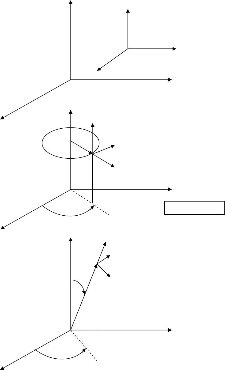
Figures
Figure 4-1: Rectangular, Cylindrical and Spherical Coordinate Systems
Z
g
3
u (Z direction)
G.P. g
g
2
u (Y direction)
g
1
u (X direction)
Rectangular
Y
Z
X
(G.P. = Grid Point)
Cylindrical
G.P. g
g
3
u (z direction)
rg
2
u(direction)
g
1
u (r direction)
Y
X Z
Spherical
r
G.P. g
g
1
u (r direction)
g
3
u(direction)
g
2
u(direction)
Y
26
X
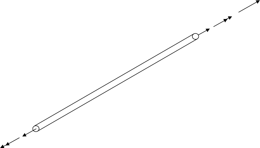
Figure 4-2: Rod Element Geometry, Coordinate System and Forces
xe
a
F
G1
G2 t
M
a
F
t
M
a
t
e
F Axial Load
M Torque
x Rod axis (positive from grid G1 through grid G2)
27
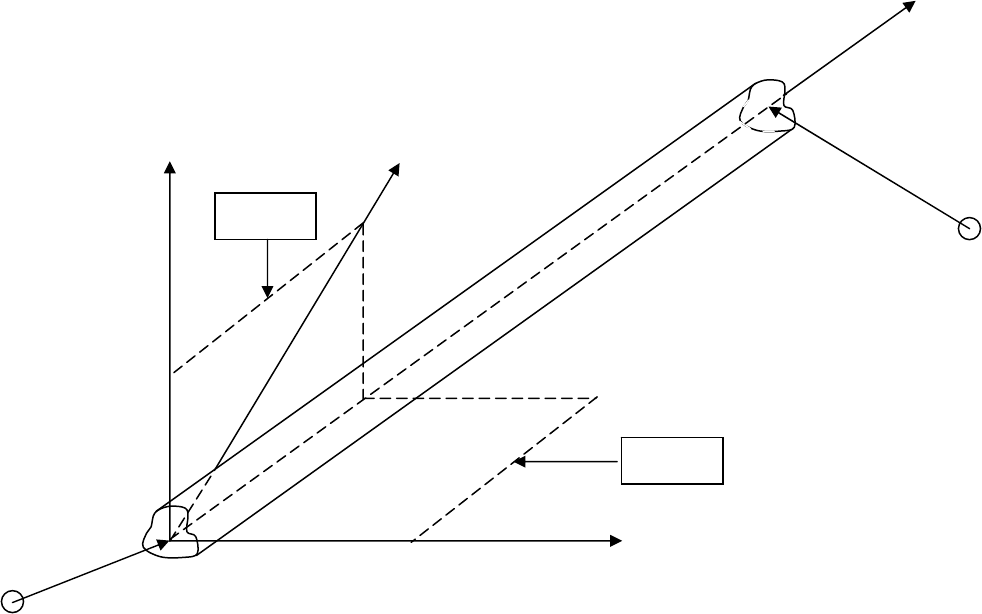
Figure 4-3: Bar Element Geometry and Coordinate System
Neutral axis of the bar (positive direction goes from end a toward end b)
Vector specified on the CBAR card that is used in defining Plane 1.
Axis in the plane defined by and the vector cro
e
ee
x
v
zx
ss product
Axis in the direction of the vector cross product
Vector from grid G1 on the CBAR card to end a of the bar (the offset at end a)
Vector from grid G2 on the CBAR card to
e
eee
a
b
xv
yz
w
w
end b of the bar (the offset at end b)
x
Plane 1
Bar end b
v
G1
G2
Plane 2
wb
ze
ye
xe
Plane 1 is x
Plane 2 is x
ee
ee
y
z
,
,
waBar end a
28
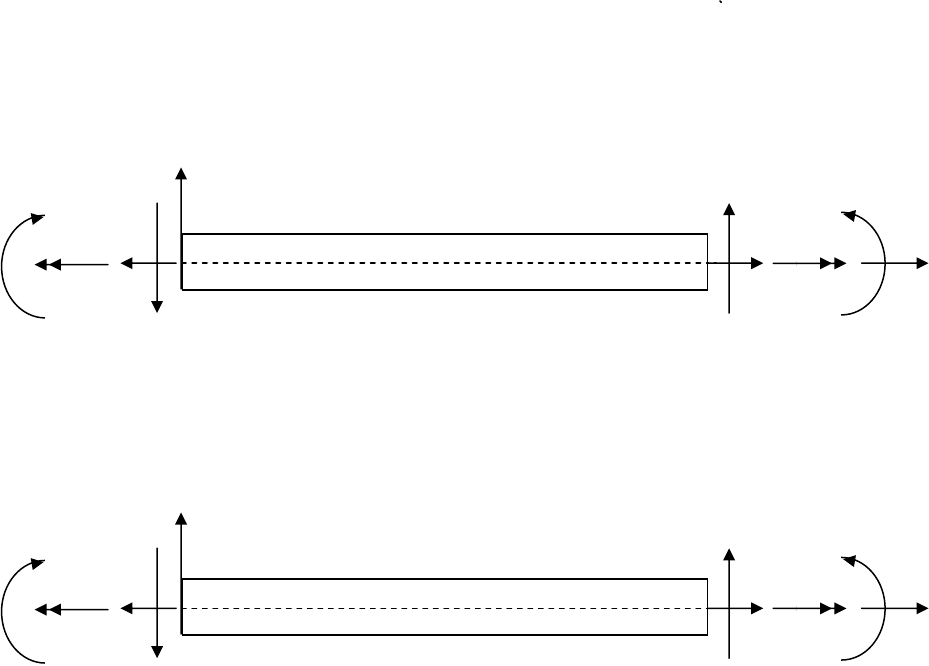
Figure 4-4: Bar Element Forces
t
1
2
1a
1b
2a
2b
P Axial Load
MTorque
V Shear in Plane 1
V Shear in Plane 2
M Bending Moment in Plane 1at end a
M Bending Moment in Plane 1at end b
M Bending Moment in Plane 2 at end a
M Bending Moment in Plane 2 at end b
P
P
t
Mt
M
Ma2
V2
V2
xe
ze
Plane 2
Mb2
a b
P
P
t
M
Ma1 Mb1
V1
V1
xe
ye
t
M
b
a
Plane 1
29
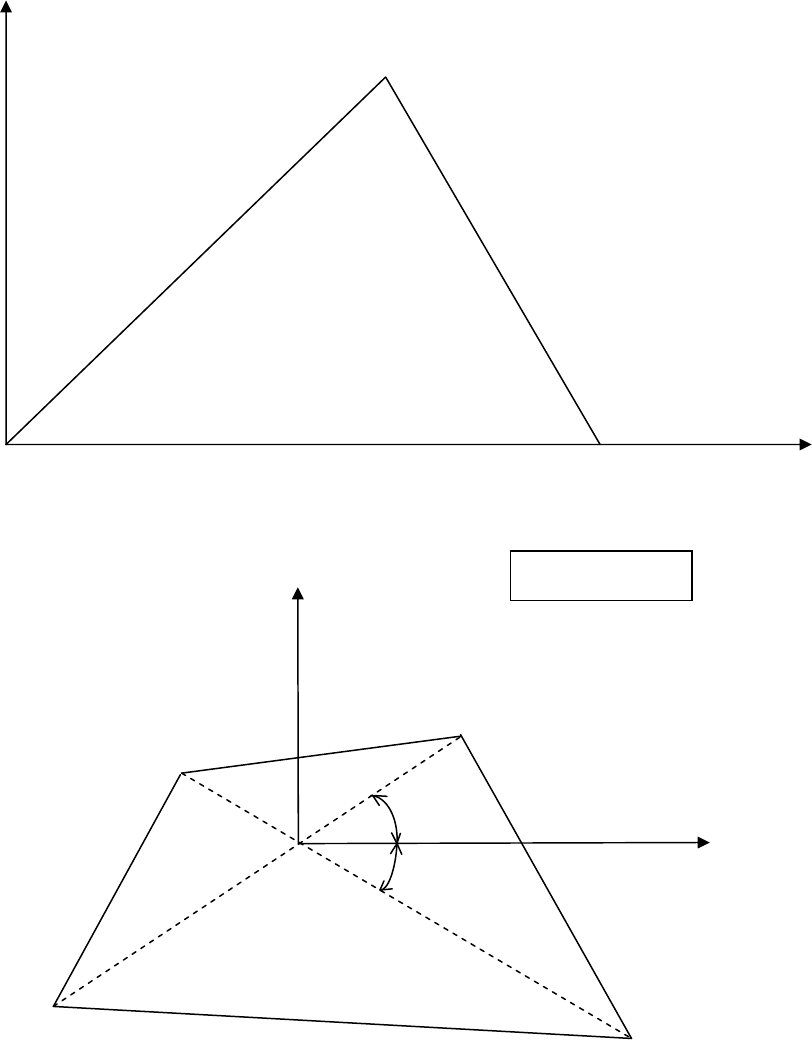
Figure 4-5: Plate Element Geometry and Coordinate Systems
ye
G3
Triangular Plate Element
xe
G1 G2
Gi is a grid point
ye
xe
G3
G4
Quadrilateral Plate Element
G1 G2
30
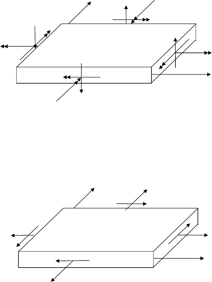
Figure 4-6: Plate Element Force Resultants
Vx
Vx
Vy
Vy
Mxx
Mxx
Myy
Myy
Mxy
Mxy
Mxy
Mxy
xe
ye
Plate Bending Moment and Transverse Shear Force Resultants
xe
ye
Nx
Nx
Ny
Ny
Nxy Nxy
Nxy
Nxy
Plate Membrane Force Resultants
31
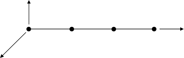
Figure 4-7: Example of MYSTRAN Development of Equations for a Rigid Element
104101 102 103
X ( global degree of
freedom numbers 1, 4)
Y (global degree of freedom
numbers 2, 5)
Z (global degree of
freedom numbers 3, 6)
12 13 14
Grid ID's are: 101 - 106
Element ID's are: 12 - 14 (12 and 14 elastic and 13 rigid)
Global displacement system is the X, Y, Z basic system shown
Define:
displ of grid i in the X direction, rotation of grid i about X axis
displ of grid i in the Y direction, rotation of grid i about Y axis
displ of grid i in the Z direction, rotation of grid i about Z axis
X coordinate of grid i
Assume that rigid element 13 is rigid only in the X - Y plane.
Take grid 103, degrees of freedom 1,2,6 as dependent. Use grid 102 as independent.
The linear equations that specify the dependence of grid 103 on grid 102 in the X - Y plane are:
u
v
w
X
uu
vv XX
ix
iy
iz
i
z
zz
i
i
i
103 102
103 102 103 102 102
103 102
()
32

33
5 References
1. LAPACK Users’ Guide, 3rd edition, SIAM, 1999 (see website at http://www.netlib.org/lapack)
2. ARPACK Users’ Guide, 3rd edition, SIAM, 1998 (see website at
http://www.caam.rice.edu/software/ARPACK/)
3. Everstine, G. C., “Recent improvements to Bandit”, NASTRAN: Users’ Experiences, Volume NASA
TM X-3278 pages 511-521, Washington, DC, 1975. National Aeronautics and Space Administration.
4. Tessler, A. and Hughes, T.J.R., “A three-node Mindlin plate element with improved transverse shear”,
Computer Methods In Applied Mechanics And Engineering 50 (1985) 71-101
5. Tessler, A. and Hughes, T.J.R., “An improved treatment of transverse shear in the Mindlin-type four-
node quadrilateral element”, Computer Methods In Applied Mechanics And Engineering 39 (1983)
311-335
6. Batoz, J., “An explicit formulation for an efficient triangular plate-bending element”, International
Journal For Numerical Methods In Engineering, Vol. 18 (1982), 1077-1089
7. Batoz, J. and Tahar, M.B., “Evaluation of a new quadrilateral thin plate”, International Journal For
Numerical Methods In Engineering, Vol. 18 (1982), 1655-1677
8. Case, William R., “A NASTRAN DMAP procedure for calculation of base excitation modal
participation factors”, 11th NASTRAN User’s Colloquium, May 5-6, 1983
9. Liu,, J, Riggs, H.R. and Tessler, A. , “A four-node, shear-deformable shell element developed via
explicit Kirchoff constraints”, International Journal For Numerical Methods In Engineering, Vol. 2000,
49, pp 1065-1086
10. MacNeal, Richard H., “Finite Elements. Their Design and Performance”, Marcel Dekker, 1993
11. Case, William R., DMAP for generating Craig-Bampton Models, notes from a course given at the
Goddard Space Flight Center (contact author for copy of paper)
12. MYSTRAN-Demo-Problem-Manual (contained in the MYSTRAN setup file downloaded from
www.MYSTRAN.com along with this manual.
13. S. C. Eisenstat, M. C. Gursky, M. H. Schultz and A. H. Sherman. “Yale Sparse Package. The
Symmetric Codes,” Yale University of Computer Science Research Report #112
6. Detailed description of input data
The input entries for the Executive Control, Case Control and Bulk Data Sections are described in detail
in the next three sections. In all of the sections, an entry with a $ sign in column 1 is considered as a
comment and is ignored. In addition, any blank entry is ignored. All other entries must be in upper case.
Appendix A contains a sample problem input/output.
6.1 File Management
As mentioned earlier, the input data file consists of 3 sections: Executive Control, Case Control and Bulk
Data. In order to make the most efficient use of resources, each of these can contain requests to include
some defined file to be part (or all) of that portion of the input data file. This is accomplished through the
use of an INCLUDE entry whose format is:
INCLUDE ‘filename’
Where filename is the name of a file to include at the location where the INCLUDE entry exists. The
INCLUDE entries can be used in any or all of the 3 sections of the input data file. In addition, multiple
INCLUDE entries in any section are permitted. The quotes around filename are recommended but not
required.
6.2 Executive Control
The Executive Control Section consists of only a few entries. Most are free field; that is they can begin in
any column and the parts of an entry may be separated by any amount of columns within the confines of
the 80 column physical entry. In addition, the fields of an entry may be delimited by tabs, as well as a
white space. Some of the entries are required and some are not required but are recognized. Other
entries are ignored with a warning message printed in the output. Any requirements on the order of the
entries in the Executive Control Section are noted.
With the CHKPNT/RESTART feature, users may restart a previously run job to get additional outputs. In
a restart the Bulk Data must remain the same except for a few PARAM and DEBUG entries. Case
Control requests for additional displacements, element forces, stresses, etc will be processed.
34

Executive Control Entries required and/or recognized by MYSTRAN
Entry Required
(Y/N) Format Description
ID N Free Field If input, it is generally the first entry in the Exec Control Section.
IN4 N Defines a file containing element stiffness, mass and other data for
a CUSERIN element
APP N Free Field An entry of APP DISP is common if this entry is included
CHKPNT Y/N Free Field Required if the user expects to restart the current job, at a later
date, to obtain additional outputs
DEBUG N Fields of 8
chars like
Bulk Data
These are the same as the Bulk Data DEBUG entries and are
allowed here since some DEBUG values need to be used prior to
reading the Bulk Data
OUTPUT4 N Free Field Requests for CB matrices to be written to unformatted files in the
same format as NASTRAN uses. An example is shown below
along with the allowable matrices that can be output
PARTN N Free Field Requests to partition a previously defined OUTPUT4 matrix
RESTART Y/N Free Field Required only if the current job is a restart of an earlier job in
which the CHKPNT entry was present. The file name (w/ ext) of
the CHKPNT’d original run must follow the command RESTART
SOL Y Free Field SOL entry must have a value that designates what kind of problem
this is:
(1) SOL 1 or SOL STATICS designates the job as a statics
problem
(2) SOL 3 or SOL = MODAL or SOL MODES or SOL NORMAL
MODES for eigenvalues
(3) SOL 31 or SOL GEN CB MODEL for Craig-Bampton (CB)
model generation
TIME N Free Field TIME n, where n is the job estimated time in minutes, is a typical
input
CEND Y Free Field The CEND entry has no other input required. It must be the last
entry in the Exec Control Section
6.2.1 IN4 Exec Control command
The Exec Control command IN4 specifies binary files (NASTRAN INPUTT4 format) which contain the
element matrices needed for CUSERIN Bulk Data element definition. The IN4 command has the
following format:
IN4 i filename
Where i is the ID of the file and is what must appear in field 3 of the Bulk Data PUSERIN property entry
for the CUSERIN element. filename is the name of the file that contains the matrices specified on the
PUSERIN entry for the element. filename must contain the full path unless the file is in the current path
where the program is being executed. An example is:
IN4 100 cb1_example1.OP1
35
6.2.2 OUTPUT4 and PARTN Exec Control commands
MYSTRAN allows output of selected matrices to binary files in the OUTPUT4 format that is the same as
that currently used by NASTRAN. The form of the OUTPUT4 command is:
OUTPUT4 MAT1,MAT2,MAT3,MAT4,MAT5//ITAPE/IUNIT $
From 1 to 5 matrices can be output per OUTPUT4 command. All 4 commas must be present even if
fewer than 5 matrices are requested. The // followed by ITAPE value (must be 0 to -3 but is currently not
used) must also be present. The final / followed by a file unit number (can be 21-27) is also required. A
trailing $ can exist but is not required. If present, it signifies the end of data read for the OUTPUT4
command.
These OUTPUT4 matrices can be partitioned, in some cases, using an Exec Control PARTN command.
The resulting partitioned matrix will be the one output to the OUTPUT4 binary file. The partitioning
vectors that define which columns and rows to partition from the original OUTPUT4 matrix are defined on
Bulk Data PARVEC and PARVEC1 entries. These Bulk Data partitioning vector entries give the grid and
component pairs of the columns and rows to partition. As such, the partitioning can only be done on
OUTPUT4 matrices that have columns and/or rows that are part of a normal displacement set (the G-set,
M-set, etc.). See section 3.6, “Displacement set notation”, for a definition of all of the displacement sets.
The general form for the PARTN command for MYSTRAN is:
PARTN MAT, CP, RP / $
where MAT is an OUTPUT4 matrix previously requested for OUTPUT4 output and CP and RP are
column and row partitioning vectors defined in the Bulk data using PARVEC and/or PARVEC1 Bulk Data
entries.
If the input file for a MYSTRAN run is filename.DAT, the binary OUTPUT4 file names are filename.OPi
where i=1,7 (corresponding to units 21-27 used as values for UNIT in the OUTPUT4 command). The
format in which these files are written is the same as that for the NASTRAN OUTPUT4 matrices.
The table on the following page shows the matrices that are currently eligible for OUTPUT4 output. Note
that there is a correspondence between MYSTRAN and NASTRAN matrix names. The OUTPUT4
commands can use either name as desired by the user. All matrix names must be no more than16
characters long. An example of the use of the Exec Control commands OUTPUT4 and PARTN is given
following the table.
36

Table 6-1
Matrices that can be written to OUTPUT4 files
(and the correspondence between MYSTRAN matrix names, NASTRAN names
and CB Equation Variables)
MYSTRAN
Matrix Name
(OUTPUT4
matrices)
NASTRAN
DMAP
Name
CB equation variable in Appendix D
(where applicable) Matrix size1 Partition
rows
and/or
cols
1 CG_LTM
6r 6N
LTM11 LTM12 0 6x(2R+N)
2 DLR DM LR
D LxR rows and
cols
3 EIGEN_VAL LAMA 2
NN
NxN
4 EIGEN_VEC PHIG GN LN
, ( with rows expanded to G-set) GxN rows
5 GEN_MASS MI NN
m Nx1 vector of
diag. terms
6 IF_LTM
RR RN RR
LTM21 LTM22 LTM23 Rx(2R+N) rows
7 KAA KAA AA
K AxA rows and
cols
8 KGG KGG GG
K GxG rows and
cols
9 KLL KLL LL
K LxL rows and
cols
10 KRL KLR(t) LR
K LxR rows and
cols
11 KRR KRR RR
K RxR rows and
cols
12 KRRcb KBB T
RR RR LR LR
kKKD RxR rows and
cols
13 KXX KRRGN XX
K (R+N)x(R+N)
14 LTM LTM CG_LTM and IF_LTM merged (6+R)x(2R+N)
15 MCG RBMCG cg
m 6x6
16 MEFFMASS Modal effective mass Nx6
17 MPFACTOR Modal participation factors Nx6 or NxR
18 MAA AA
M AxA rows and
cols
19 MGG GG
M GxG rows and
cols
20 MLL MLL LL
M LxL rows and
cols
21 MRL MRL RL
M RxL rows and
cols
22 MRN T
RN NR
mm RxN rows
23 MRR MRR RR
M RxR rows and
cols
37

Table 6-1 (con’t)
MYSTRAN
Matrix
Name
(OUTPUT4
matrices)
NASTRAN
DMAP
Name
CB equation variable in Appendix D
(where applicable) Matrix size1 Partition
rows
and/or
cols
24 MRRcb MBB TTTT
RR RR LR LR LR LR LR LL LR
mMMD(MD)DMD RxR rows and
cols
25 MXX MRRGN
T
RR NR
XX
NR NN
mm
Mmm
(R+N)x(R+N)
26 PA (A-set static reduced loads - only used in statics) Rows
27 PG (G-set static loads - only used in statics) Rows
28 PL (L-set static reduced loads - only used in statics) rows
29 PHIXG PHIXG AX AX
, ( with rows expanded to G-set) Gx(R+N) rows
30 PHIZG The G-set displacement transformation matrix is
written out in the F06 file under
“C B D I S P L A C E M E N T O T M” Gx(2R+N) rows
31 RBM0 Rigid body mass matrix relative to the basic origin 6x6
32 TR6_0 RBR R6
T: rigid body displacement matrix for R-set
relative to the model basic coordinate system Rx6 rows
33 TR6_CG RBRCG R6
T: rigid body displacement matrix for R-set
relative to the model CG Rx6 rows
Note: (t) indicates matrix transposition
1 Matrix size given in rows x columns where R means the size of the R-set, L is the size of the L-set, A is
the size of the A-set, G is the size of the G-set and N is the number of eigenvectors. See section 3.6 for
definition of the complete displacement set notation
38

Example of OUTPUT4 request in Exec Control
Format:
OUTPUT4 MAT1, MAT2, MAT3, MAT4, MAT5 // ITAPE / IUNIT $
Example:
OUTPUT4 PHIZG, KRRcb,,, // -1 / 22 $
a) The OUTPUT4 entry is free-field (except that there can be no blank characters in any of the
names, including OUTPUT4).
b) MATi can be any of the matrix names in the OUTPUT4 table above. There can be 1 to 5 matrices
in any OUTPUT4 request but all 4 commas must be present.. If there is a name for the matrix in
the column “NASTRAN DMAP Name”, that name can be used in place of the MYSTRAN Matrix
Name for OUTPUT4 purposes
c) ITAPE (using NASTRAN notation) should be: -3ITAPE0
(but is currently not used in
MYSTRAN),
d) IUNIT must be: . Any number of the OUTPUT4 matrices can be sent to one
IUNIT and more than one IUNIT can be used in one Exec Control section,
21 IUNIT 28
e) The / characters must be present,
f) Anything after the $ character (if present) is ignored.
Example of PARTN request in Exec Control
Format:
PARTN MAT, CP, RP/ $
CP is the column partitioning vector and RP is the row partitioning vector
Example:
OUTPUT4 PHIZG,, RVEC1 / $
a) The PARTN entry is free-field (except that there can be no blank characters in any of the names,
including PARTN).
b) MAT is the name of the matrix to partition (with restrictions noted in Table 6-1 regarding whether
rows and or column of this matrix are available for partitioning).
c) RP (RVEC1 in the example) is the row partition vector which must be specified using either the
PARVEC or PARVEC1 Bulk Data entry.
d) The PARTN entry must have 2 and only 2 commas. Note that in the example above that CP is
not specified (since PHIZG is only available for row partitioning) but the 2nd comma is present.
e) The PARTN entry for MAT must follow (but not necessarily immediately) the mandatory
OUTPUT4 request for it.
39

6.3 Case Control
The Case Control Section performs several functions outlined below. The entries for each of the major
purposes are enumerated below. A detailed explanation of each is contained in the following section. A
BEGIN BULK entry is considered as the last, and mandatory, entry in the Case Control Section. In
addition, the fields of an entry may be delimited by tabs, as well as a white space.
The following entries specify the titles that will be printed in the output file, none of which are
required:
TITLE Specifies a line of text to be printed in the output file
SUBTITLE Specifies a 2nd line of text to be printed in the output file
LABEL Specifies a 3rd line of text to be printed in the output file
The following entries select items from the Bulk data to be used in the current job (loads,
constraints, temperature sets, eigenvalue extraction ID):
ENFORCED Specifies a file containing all grid displacements (all translations and
rotations for all grids). With this command, users can run cases in which
all displacements are known (as for example from test data) and can
request any outputs based on these displacements.
LOAD Selects FORCE, MOMENT, GRAV, PLOAD2, PLOAD4, RFORCE and
LOAD sets from the Bulk Data Section that define loads for a statics
solution.
METH Selects an eigenvalue extraction set from the Bulk Data for a eigenvalue
solution.
SPC Selects SPC, SPC1 from the Bulk Data Section that define single point
constraints (including enforced displacements) for the current job.
MPC Selects MPC entries from the Bulk Data Section that define multi-point
constraints for the current job.
TEMP Selects TEMP, TEMPD and TEMPP1 sets from the Bulk Data Section
that define temperature loads for a statics solution.
The following entries define output requests:
ACCEL Requests output of accelerations.
DISPL Requests output of displacements.
ECHO Requests form of the input file echoed to the output file.
ELDATA Requests element matrix generation output to the BUG file2.
ELFORCE Requests output of element engineering and/or node forces.
2 The various files (output and scratch) generated by MYSTRAN are described in a later section. BUG is
the extension of one of those files.
40
GPFORCE Requests output of grid point force balance showing all of the forces
acting on a grid point and checking equilibrium of those forces.
MEFFMASS Requests output of modal effective masses in eigenvalue analyses.
MPCFORCE Requests output of multi point forces of constraint (due to MPC’s as well
as rigid elements).
MPFACTOR Requests output of modal participation factors in eigenvalue analyses.
OLOAD Requests output of applied loads.
SET Specifies sets that define grid points and elements for which output is
desired.
SPCFORCE Requests output of single point forces of constraint.
STRESS Requests output of element stresses.
STRAIN Requests output of element strains for shell and solid elements
The following entry defines subcases for which solutions will be calculated in static analyses
(SOL 1):
SUBCASE A entry that indicates that the following entries (until another SUBCASE
entry is encountered) define the conditions for one solution in the current
job. A separate subcase must be used for each loading condition for
which a solution is desired.
6.3.1 Detailed Description of Case Control Entries
The following pages give the details for each of the Case Control Section entries listed above. The
format of each is free field with the following conventions:
Upper case letters must be entered as shown.
Lower case letters indicate that a substitution must be made.
Parentheses shown must be entered.
Braces { } indicate that a choice, from the items listed, must be made.
Brackets [ ] indicate that the terms enclosed may be omitted, if desired. Braces within
brackets indicate that if terms within the brackets are input a choice must be made of the
portion within the braces.
Underlined values are the default values.
In addition, some of the entries have an acceptable abbreviation of the entry name. For example, the
entry requesting displacement output can be DISPLACEMENT or at least the first four letters of the
name. This is noted in the detailed description with brackets. Thus DISP[LACEMENT] indicates the
acceptable forms of this Case Control entry.
41

BEGIN BULK
6.3.1.1 BEGIN BULK
Description:
Indicates the end of the Case Control section
Format:
BEGIN BULK
42

ACCELERATION
6.3.1.2 ACCELERATION
Description:
Requests output of grid point accelerations in the global coordinate system for selected grids. For Craig-
Bampton model generation, the output is of the columns of the acceleration transfer matrix (ATM).
Format:
ALL
ACCE[LERATION] = n
NONE
Examples:
ACCELERATION = ALL (requests output of accelerations for all grid points)
ACCE = 45 (requests output of accelerations for grid points included in Case Control entry SET 45)
Options:
Option Meaning
ALL Accelerations for all grid points in the model will be output.
n ID of a SET Case Control entry previously defined. Accelerations for the grid points
defined by SET n will be output. Integer > 0, no default value.
NONE No accelerations will be output.
Remarks:
1. NONE is used to override an overall output request made above the SUBCASE level.
43

DISPLACEMENT
6.3.1.3 DISPLACEMENT
Description:
Requests output of grid point displacements in the global coordinate system for selected grids. For
eigenvalue analyses, the output is of eigenvectors.
Format:
ALL
DISP[LACEMENT] = n
NONE
Examples:
DISPLACEMENT = ALL (requests output of displacements for all grid points)
DISP = 45 (requests output of displacements for grid points included in Case Control entry SET 45)
Options:
Option Meaning
ALL Displacements for all grid points in the model will be output.
n ID of a SET Case Control entry previously defined. Displacements for the grid points
defined by SET n will be output. Integer > 0, no default value.
NONE No displacements will be output.
Remarks:
1. NONE is used to override an overall output request made above the SUBCASE level.
44

ECHO
6.3.1.4 ECHO
Description:
Requests that the input data file be echoed in the output file
Format:
NONE
ECHO= UNSORT
Examples:
ECHO = NONE
Options:
Option Meaning
NONE No echo of the input data file will be in the output file.
UNSORT The echo of the data file in the output will be in the same entry order that the input data
file is in.
45

ELDATA
6.3.1.5 ELDATA
Description:
Requests output of element data from the element matrix generation subroutines for selected elements.
The data is written to files separate from the standard output file. Description of the data items that can
be output is given in the table below. The output files that the data is written to are described in the
MYSTRAN Installation and Run Manual.
Format:
,PRINT ALL
ELDA[TA] (m ,PUNCH ) = n
,BOTH NONE
Examples:
ELDATA(1,BOTH) = 2 (print and punch output of elem data item 1 for elems in SET 2).
ELDATA(3) = 3 (print output of elem data item 3 for elems included in SET 3).
ELDATA(2,PUNCH) = ALL (punch output of elem data item 2 for all elems).
Options:
Option Meaning
m Defines which element data items are to be output (see table below)
ALL Data items m for all elements will be output.
n ID of a SET Case Control entry previously defined. Element data for item m defined by
SET n will be output. Integer > 0, no default value.
NONE No element data items will be output.
Remarks:
1. NONE is used to override an overall output request made above the SUBCASE level.
2. See table below for a description of the data items that can be output
46

Element Data Items Output for ELDATA Case Control Entry
m
Data Item(s) Output
Printed
to
Text
File
With
Extension
Written
To
Unformatted
File
With
Extension
0 Actual and internal grid points and basic coordinates.
Array of element property data.
Array of element material data.
Array of element temperature data.
Bar element v vector in basic coordinates.
Bar pin flag data.
Bar offsets.
TE coord transform matrix (transforms a vector from basic to local elem coords).
Actual and internal grid points and local element coordinates.
BUG
1 Element mass matrix in local element coordinates. BUG F21
2 Element thermal and pressure loads in local element coordinates. BUG F22
3 Element stiffness matrix in local element coordinates. BUG F23
4 Element stress recovery matrices in local element coordinates. BUG F24
5 Element grid point displacements and loads. The coordinate system will be the
one defined by Bulk data PARAM ELFORCEN. BUG F25
6 Data on isoparametric element shape functions and Jacobian matrices BUG
7 Isoparametric element shape functions BUG
8 Check isoparametric element strain-displ matrices for rigid body motion and
constant strain BUG
Notes:
1) The filename will be the same as the input data file but with the extension given in the table.
2) See Appendix B for a description of some of these matrices that can be output.
47

ELFORCE
6.3.1.6 ELFORCE
Description:
Requests output of nodal or engineering forces for selected elements.
Format:
ENGR ALL
ELFO[RCE] (NODE) = n
(BOTH) NONE
Examples:
ELFORCE = ALL (requests output of element engineering forces for all elements)
ELFO(NODE) = 125 (requests output of element nodal forces for elements included in SET 125)
Options:
Option Meaning
ALL Element forces for all elements in the model will be output.
n ID of a SET Case Control entry previously defined. Element forces for the elements
defined by SET n will be output. Integer > 0, no default value.
NONE No element forces will be output.
Remarks:
1. NONE is used to override an overall output request made above the SUBCASE level
2. The forces can be output in local element, basic, or global coordinates. See Bulk Data PARAM
ELFORCEN entry
48

ENFORCED
6.3.1.7 ENFORCED
Description:
Requests a run in which the displacements (all 3 translations and rotations) are specified in a file whose
name is given as part of this command. The situation in which this might be useful is one in which all grid
displacements are known from test data and the user would like to get other outputs (e.g. stresses) due to
these displacements.
Format:
ENFORCED = filename
Examples:
ENFORCED = Case1-displacements-rotations.txt
Remarks:
1. filename is a text file with NGRID+1 records (where NGRID are the number of grids in the model)
a) Record 1 is a comment line
b) Records 2 through NGRID+1 have the following in CSV format for each grid:
grid ID, T1, T2, T3, R1, R2, R3
2. An example of the ENFORCED file for 2 grids is:
Displacements and rotations for model A with 3 grids (101, 102)
101, 1.23456D-02, 2.34567D-02, 3.45678D-03, 0.00000D+00, 4.56789D-04, 3.67890D-05
102, 6.54321D-02, 7.65432D-03, 8.76543D-03, 9.87654D-05, 5.43210D-06, 0.00000D-05
3. All grids must have all 6 components specified in the file (i.e. all DOF’s must be in the S-set)
4. Any Case Control requests for SPC’s or MPC’s will result in an error
5. Any Bulk Data ASET or OMIT entries will result in an error
49

ELSTRAIN
6.3.1.8 ELSTRAIN
Description:
Requests output of strains for selected elements. See STRAIN entry for description
50

ELSTRESS
6.3.1.9 ELSTRESS
Description:
Requests output of stresses for selected elements. See STRESS entry for description
51

FORCE
6.3.1.10 FORCE
Description:
Requests element engineering and/or node forces. See ELFORCE entry.
52

GPFORCES
6.3.1.11 GPFORCES
Description:
Requests output of grid point force balance in the global coordinate system for selected grids.
Format:
A
LL
GPFO[RCES] = n
NONE
Examples:
GPFO = ALL (requests output of grid point force balance for all grid points)
GPFO = 45 (requests output of grid point force balance for grid points included in SET 45)
Options:
Option Meaning
ALL Grid point force balance for all grid points in the model will be output
n ID of a SET Case Control entry. Grid point force balance for the grid points defined by
this set will be output. Integer > 0, no default value.
NONE No grid point force balance will be output
Remarks:
1. NONE is used to override an overall output request made above the SUBCASE level.
53

LABEL
6.3.1.12 LABEL
Description:
Specifies a third text line to be printed in the output file.
Format:
LABE[L] = [optional text material up to, and including, column 80]
Remarks:
1. This line of text will be printed in the output file and can be different for each subcase
54

LOAD
6.3.1.13 LOAD
Description:
Indicates what applied loads (identified in the Bulk Data) are to be used for a solution.
Format:
LOAD = n
Examples:
LOAD = 98 (requests load set 98 be used)
Options:
Option Meaning
n Set ID of a load (must be the ID of at least one of the following Bulk data entries: LOAD,
FORCE, GRAV, MOMENT, PLOAD2). Integer > 0, no default value.
Remarks:
1. If the Case Control LOAD entry identifies a Bulk Data LOAD entry (load combining entry), then n must
not appear as a set ID on any of the Bulk Data FORCE, GRAV, MOMENT or PLOAD2 entries that
are in the input data file.
2. The Case Control LOAD entry must be present if a static loading is desired in a solution.
55

MEFFMASS
6.3.1.14 MEFFMASS
Description:
Requests calculation and output of modal effective masses in an eigenvalue solution.
Format:
MEFFMASS
Remarks:
1. This entry may appear in the Case Control section for eigenvalue extraction solutions.
2. See Bulk Data PARAM MEFMLOC for the reference point to use in calculating effective masses
in Craig-Bampton (SOL 31) analyses
56

METHOD
6.3.1.15 METHOD
Description:
Indicates what eigenvalue extraction method (identified in the Bulk Data on an EIGR or EIGRL entry) is to
be used for an eigenvalue solution.
Format:
METH[OD] = n
Examples:
METHOD = 18 (requests that eigenvalue extraction method 18 be used)
Options:
Option Meaning
n Set ID of a Bulk data EIGR entry. Integer > 0, no default value.
Remarks:
1. This entry must appear in the Case Control section for all eigenvalue extraction solutions.
57

MPC
6.3.1.16 MPC
Description:
Indicates what multipoint constraints (identified in the Bulk Data) are to be used for a solution.
Format:
MPC = n
Examples:
MPC = 47 (requests multi point constraint set 47, defined in Bulk Data, be used)
Options:
Option Meaning
n Set ID of an MPC and/or MPCADD Bulk data entry. Integer > 0, no default value.
Remarks:
1. There can be only one Case Control MPC entry per solution. It should appear in the Case Control
section above any SUBCASE definitions.
58

MPCFORCES
6.3.1.17 MPCFORCES
Description:
Requests output of multi point constraint forces in the global coordinate system for selected grids. Multi
point constraint forces consist of forces due to directly defined MPC’s and also due to rigid elements
(which are automated, internally in MYSTRAN, as MPC’s)
Format:
A
LL
MPCF[ORCES] = n
NONE
Examples:
MPCF = ALL (requests output of multi point constraint forces for all grid points)
MPCF = 45 (requests output of multi point constraint forces for grid points included in SET 45)
Options:
Option Meaning
ALL Multi point constraint forces for all grid points in the model will be output
n ID of a SET Case Control entry. Multi point constraint forces for the grid points defined by
this set will be output. Integer > 0, no default value.
NONE No Multi point constraint forces will be output
Remarks:
1. NONE is used to override an overall output request made above the SUBCASE level.
59

MPFACTOR
6.3.1.18 MPFACTOR
Description:
Requests calculation and output of modal participation factors in an eigenvalue solution.
Format:
MPFACTOR
Remarks:
1. This entry may appear in the Case Control section for eigenvalue extraction solutions.
60

OLOAD
6.3.1.19 OLOAD
Description:
Requests output of applied loads in the global coordinate system for selected grids.
Format:
A
LL
OLOA[D] = n
NONE
Examples:
OLOAD = ALL (requests output of applied loads for all grid points)
OLOAD = 45 (requests output of applied loads for grid points included in SET 45)
Options:
Option Meaning
ALL Applied loads for all grid points in the model will be output
n ID of a SET Case Control entry previously defined. Applied loads for the grid points
defined by this set will be output. Integer > 0, no default value.
NONE No applied loads will be output
Remarks:
1. NONE is used to override an overall output request made above the SUBCASE level.
61

SET
6.3.1.20 SET
Description:
Defines sets of grid points or elements for which output is desired.
Format:
SET n = {i i i , i THRU i , EXCEPT i i i THRU i ]}
123
[, , , ,
4 5 678 9
Examples:
SET 39 = 2998
SET 57 = 101 THRU 298
SET 12 = 301, 305, 491 THRU 672 EXCEPT 501
Options:
Option Meaning
n Set ID number. Integer > 0, no default.
i1, i2, i3, etc. Individual grid point or element numbers.
i4 THRU i5 Inclusive group of grid or element numbers.
EXCEPT Grid or element numbers following EXCEPT (but before next THRU) will be excluded from
the previous THRU group.
Remarks:
1. Any number of SETs can be defined as long as the ID numbers are unique integers. The SET logical
entry can consist of multiple physical entries, each of 80 columns max. If a SET definition requires
more than one physical entry each entry (except the last) must end with a “,”
2. Ranges in THRU statements must be increasing (that is, i4 must be less than i5 in the above
example). It is acceptable that some grid or element numbers in the THRU range do not exist.
However, all grids or elements that are in the THRU range will be included in the SET.
3. Whether the set indicates grids or elements is dependent on the context in which the SET is used. If
DISP = 39 output is requested, then the integers in SET 39 will be interpreted as grid point numbers.
If ELFORCE = 39 output is requested, then the integers in SET 39 will be interpreted as element
numbers.
62

SPC
6.3.1.21 SPC
Description:
Indicates what single point constraints (identified in the Bulk Data) are to be used for a solution.
Format:
SPC = n
Examples:
SPC = 74 (requests single point constraint set 74 be used)
Options:
Option Meaning
n Set ID of at least one SPC, SPC1 and/or SPCADD Bulk data entries. Integer > 0, no
default value.
Remarks:
1. There can be only one Case Control SPC entry per solution. It should appear in the Case Control
section above any SUBCASE definitions.
63

SPCFORCES
6.3.1.22 SPCFORCES
Description:
Requests output of single point constraint (SPC) forces in the global coordinate system for selected grids.
Format:
A
LL
SPCF[ORCES] = n
NONE
Examples:
SPCF = ALL (requests output of SPC forces for all grid points)
SPCFORCES = 45 (requests output of SPC forces for grid points included in SET 45)
Options:
Option Meaning
ALL SPC forces for all grid points in the model will be output.
n ID of a SET Case Control entry previously defined. SPC forces for the grid points defined
by this set will be output. Integer > 0, no default value.
NONE No SPC forces will be output.
Remarks:
1, NONE is used to override an overall output request made above the SUBCASE level
64

STRAIN
6.3.1.23 STRAIN
Description:
Requests output of stresses for selected elements.
Format:
A
LL
VONMISES CENTER
STRA IN = n
MAXS or SHEAR CORNER NONE
Examples:
Options:
Option Meaning
VONMISES Requests von Miises strain (default)
MAXS or
SHEAR Requests maximum shear strain for shell elements and octrahedral strain for solid
elements
CENTER Requests strains at the center of shell and solid elements (default)
CORNER Requests strains at the element corners for the QUAD4 and QUAD4K elements, in
addition to strains at the element center
ALL Strains for all elements in the model will be output.
n ID of a SET Case Control entry previously defined. Strains for the elements defined by
SET n will be output. Integer > 0, no default value.
NONE No displacements will be output.
Remarks:
1. NONE is used to override an overall output request made above the SUBCASE level
2. ELSTRAIN is an alternate form of this Case Control command
3. The options VONMISES, MASS (or SHEAR), CENTER and CORNER will apply for all subcases
65

STRESS
6.3.1.24 STRESS
Description:
Requests output of stresses for selected elements.
Format:
A
LL
VONMISES CENTER
STRE SS = n
MAXS or SHEAR CORNER NONE
Examples:
Options:
Option Meaning
VONMISES Requests von Miises stress (default)
MAXS or
SHEAR Requests maximum shear stress for shell elements and octrahedral stress for solid
elements
CENTER Requests stresses at the center of shell and solid elements (default)
CORNER Requests stresses at the element corners for the QUAD4 and QUAD4K elements, in
addition to stresses at the element center
ALL Stresses for all elements in the model will be output.
n ID of a SET Case Control entry previously defined. Stresses for the elements defined by
SET n will be output. Integer > 0, no default value.
NONE No displacements will be output.
Remarks:
1. NONE is used to override an overall output request made above the SUBCASE level
2. ELSTRESS is an alternate form of this Case Control command
3. The options VONMISES, MASS (or SHEAR), CENTER and CORNER will apply for all subcases
66

SUBCASE
6.3.1.25 SUBCASE
Description:
Beginning of the portion of the Case Control section that defines the options to be used in one subcase.
Multiple subcases must be used when solution with separate static loads in one run is desired.
Format:
SUBC[ASE] = n
Examples:
SUBCASE = 361
Options:
Option Meaning
n Set ID of a subcase. Integer > 0, no default value.
Remarks:
1. There can be multiple subcases and there is no restriction on the integer numbers used for subcase
IDs
2. All Case Control entries following a SUBCASE entry (up to the next SUBCASE Case Control entry)
identify the conditions for solution (loads and output) for this subcase. Case Control entries “above”
the SUBCASE level will be used for all subcases unless specifically overridden in the subcase
definition.
67

SUBTITLE
6.3.1.26 SUBTITLE
Description:
Specifies a second text line to be printed in the output file.
Format:
SUBT[ITLE] = [optional text material up to, and including, column 80]
Remarks:
1. This line of text will be printed in the output file and can be different for each subcase.
68

TEMPERATURE
6.3.1.27 TEMPERATURE
Description:
Indicates temperature distributions (identified in the Bulk Data) that are to be used for a statics solution.
Format:
TEMP[ERATURE] = n
Examples:
TEMP = 174 (requests temperature set 174 be used)
TEMPERATURE = 13 (requests temperature set 13 be used)
Options:
Option Meaning
n Set ID of Bulk Data TEMP, TEMPD, TEMPRB and/or TEMPP1 cards. Integer > 0, no
default value.
Remarks:
1. Thermal loads can be used in combination with other static loads in any subcase but must be
selected in Case Control with the TEMPERATURE = n card.
69

TITLE
6.3.1.28 TITLE
Description:
Specifies a text line to be printed in the output file.
Format:
TITLE = [optional text material up to, and including, column 80]
Remarks:
1. This line of text will be printed in the output file and can be different for each subcase
70

VECTOR
6.3.1.29 VECTOR
Description:
Requests eigenvector output. See DISPLACEMENT entry.
71

6.4 Bulk Data
The major function of the Bulk Data Section is to define the finite element model and the loading and
constraints. In the case of loading and constraints, the Bulk Data entries have a set ID which must be
chosen in Case Control for the particular load or constraint to be applied.
The entries for each of the major purposes are enumerated below. A detailed explanation of each is
contained in the following section. An ENDDATA entry is considered as the last, and mandatory, entry in
the Bulk data Section.
Geometry/scalar point definition
GRID Defines grid point ID and location, coordinate systems for the grid
location and for the global coordinate system, and permanent single
point constraints.
GRDSET Defines default values for coordinate systems and permanent SPC’s for
GRID entries whose corresponding fields are blank.
SPOINT Defines a scalar point to which elastic and mass elements may be
attached.
Grid point sequencing
SEQGP Used to define the internal sequence order for grid points so as to obtain
a banded stiffness matrix. If not input, then the grid order is set to, either:
grid numerical order (default) or grid input order (using PARAM
SEQUENCE)
Coordinate system definition (i = 1 or 2)
CORDiR Defines a rectangular coordinate system.
CORDiC Defines a cylindrical coordinate system.
CORDiS Defines a spherical coordinate system.
Element connection definition
Scalar and bushing elastic elements
CBUSH Spring element with geometry definition
CELAS1 Defines a spring element ID, property ID and the grid/degrees of freedom
to which the spring element is connected.
CELAS2 Defines a spring element ID, stiffness and the grid/degrees of freedom to
which the spring element is connected.
CELAS3 Defines a spring element ID, property ID and the scalar points to which
the spring element is connected.
72

CELAS4 Defines a spring element ID, stiffness and the scalar points to which the
spring element is connected.
1D elastic elements
CBAR Defines a bar (axial load, bending, torsion) element ID, property ID and
the grid connections and v vector (which, together with the bar axis,
defines the orientation of the bar cross-section in the model).
BAROR Defines default values of property ID and v vector for the CBAR entry.
CROD, Defines a rod (axial load and torsion) element ID, property ID and the
grid connections. The bar element can be used to describe 1D element
extension, as well.
CONROD Alternate form of CROD
2D elastic elements
CQUAD4K Defines a thin quadrilateral plate (membrane, bending, twist) element ID,
property ID and the grid points to which the quad element is connected.
CQUAD4 Defines a thick quadrilateral plate (membrane, bending, twist) element
ID, property ID and the grid points to which the quad element is
connected.
CTRIA3K Defines a thin triangular plate (membrane, bending, twist) element ID,
property ID and the grid points to which the triangular element is
connected.
CTRIA3 Defines a thick triangular plate (membrane, bending, twist) element ID,
property ID and the grid points to which the triangular element is
connected.
CSHEAR Defines a thin quadrilateral element that carries only in-plane shear
3D elastic elements
CHEXA Defines a hexahedron element with either 8 or 20 nodes.
CPENTA Defines a pentahedron element with either 6 or 15 nodes.
CTETRA Defines a tetrahedron element with either 4 or 10 nodes.
73

R- elements
The R-elements (currently RBE2 and RBE3) are used to generate internal multi-point
constraint equations (MPC’s) that define a dependence of some degrees of freedom of
the model with respect to the other degrees of freedom in the model.
RBE2 Defines a rigid portion of the finite element model by specifying an
element ID plus a number of dependent grid points that will behave in a
rigid fashion relative to the six components of motion at a specified
independent grid point. The degrees of freedom for the dependent grids
are also specified. In its most simplistic form, the RBE2 can be used to
define, for instance, a rigid 1-D bar or a rigid 2-D element.
RBE3 Defines one dependent grid point (and the dependent degrees of
freedom at that grid point) and one or more grids (and their degrees of
freedom) that the dependent degrees of freedom depend on. The most
common use of this element is to distribute loads or mass specified at
the dependent grid to ones at the independent grid. This is very different
than the RBE3 which is a rigid element. In general, the dependent grid
on the RBE3 should not be connected via elastic or rigid elements to the
rest of the structure except via the RBE3 element on which it is defined.
There is also a provision for specifying weighting factors at the
independent grids (which in many cases are just 1.0).
RSPLINE Constraint element that defines interpolations of displacements between
it’s 2 ends. Displacements and rotations avout a line between the 2 ends
are interpolated linearly. Displacements perpendicular to the line are
interpolated cubically. Rotations perpendicular to the line are
interpolated quadrically.
Scalar mass elements
CMASS1 Defines a mass element ID, property ID and the grid/degrees of freedom
to which the mass element is connected.
CMASS2 Defines a mass element ID, stiffness and the grid/degrees of freedom to
which the mass element is connected.
CMASS3 Defines a mass element ID, property ID and the scalar points to which
the mass element is connected.
CMASS4 Defines a mass element ID, stiffness and the scalar points to which the
mass element is connected.
User defined elements
CUSERIN Elements whose elastic properties will be defined via stiffness and mass
matrices on disk files. The CUSERIN entry defines the degrees of
freedom that the element is connected to. These elements are used in
substructure analyses (primarily Craig-Bampton dynamic analyses).
74

Element property definition
Scalar elastic element
PELAS Defines a spring element property ID and the stiffness, damping and
stress recovery values for a ELAS1 scalar spring element
PBUSH Defines the elastic properties of a CBUSH element
1D elastic elements
PBAR, PBARL Defines a bar property ID and material ID and the bar properties,
including: cross-sectional area, area moments, and cross-products, of
inertia, torsional constant, mass per unit length, stress recovery locations
on the cross-section and area factors for shear flexibility.
PROD Defines a rod property ID and material ID and the rod properties,
including: cross-sectional area, torsional constant, torsion stress
recovery coefficient and mass per unit length
2D elastic elements
PSHEAR Defines the elastic properties of a CSHEAR element
PSHELL Defines a 2D plate element property ID and material IDs and the plate
properties, including: thickness, .bending moment of inertia ratio, shear
thickness ratio, fiber distances for stress calculation, mass per unit
length.
PCOMP, 1 Defines the properties of a 2D composite plate element with n plies.
3D elastic elements
PSOLID Defines a 3D solid element property ID and material ID and integration
parameters.
User elements
PUSERIN Defines information needed to locate the matrices (specified on disk
files) for CUSERIN elements.
Element material definition
MAT1 Defines a material ID and the material properties, including: Young’s
modulus, shear modulus, Poisson’s ratio, material mass density, thermal
expansion coefficient, reference temperature, and a damping coefficient.
75
MAT2 Defines a 2D anisotropic material.
MAT8 Defines an orthotropic material.
MAT9 Defines an anisotropic material.
PMASS Defines scalar mass for elements defined on CMASS2,4 entries.
Grid point mass
CONM2 Defines a concentrated mass at a grid point, including: mass ID, grid
where mass is located, the mass value, the offsets from the grid to the
mass center of gravity (c.g.), the six independent moments and products
of inertia of the mass about its c.g., and the coordinate system in which
the offsets and moments of inertia are specified.
Applied loads
FORCE Defines a concentrated force at a grid point, including: load ID, grid ID at
which the force acts, coordinate system in which the force is specified,
and the magnitude and direction of the force.
MOMENT Defines a concentrated moment at a grid point, including: load ID, grid ID
at which the moment acts, coordinate system in which the moment is
specified, and the magnitude and direction of the moment.
GRAV Defines an acceleration vector for the finite element model, including:
load ID, coordinate system in which the acceleration vector is specified,
and magnitude and direction of the acceleration vector. MYSTRAN
creates a static load that is applied to a model to simulate a gravity type
of loading but with rigid body motion restrained.
PLOAD2 Defines a pressure load for 2D elements, including: load ID, pressure
magnitude, and element IDs for the elements that are to have the
pressure load.
PLOAD4 Defines a pressure load for 2D elements, including: load ID, pressure
magnitudes at up to 4 grids, and element IDs for the elements that are to
have the pressure load.
LOAD Defines a static load for the finite element model that is a linear
combination of loads that are defined on FORCE, MOMENT, GRAV and
PLOAD2 entries, including: ID of this load combination, a scale factor to
be applied to all loads being combined, and load set IDs and magnitudes
of the various load sets being combined.
RFORCE Defines an angular velocity and optional angular acceleration of the finite
element model about some defined grid point and in some defined
coordinate system.
SLOAD Defines a.
76
Thermal loads (all are used by MYSTRAN to calculate loads on the model)
TEMPD Defines an overall constant temperature for the finite element model
including: temperature set ID and the temperature value.
TEMP Defines a temperature for a grid point including: temperature set ID, the
grid ID, and the temperature value
TEMPRB Defines a temperature field for the bar element including: temperature
set ID, the average temperature of the cross-section at the two bar ends,
the two temperature gradients through the bar cross-section at each of
the two ends.
TEMPP1 Defines a temperature field for 2D elements including: temperature set
ID, the average temperature of the element at its mid-plane, the
temperature gradient through the element.
Single point constraints (SPC)
SPC Defines a constraint for a single degree of freedom including: SPC set
ID, the grid and degree of freedom component number, and the
constraint value. If the constraint value is nonzero (that is, an enforced
displacement), MYSTRAN calculates equivalent grid forces and applies
them to the model.
SPC1 Defines degrees of freedom where displacement is zero. The definition
Includes: the SPC set ID, the degree of freedom component number and
the grids that are to be constrained.
SPCADD Defines an SPC as a union of SPC’s defined via SPC and/or SPC1 Bulk
data entries.
Multi point constraints (MPC)
MPC Defines a dependence of one degree of frrrdom on one or more other
degrees of freedom.
MPCADD Defines an MPC as a union of MPC’s defined via MPC Bulk data entries.
Boundary degrees of freedom for Craig-Bampton (CB) analyses
SUPORT Defines degrees of freedom at the boundary of a CB model.
Analysis degrees of freedom (only needed when Guyan reduction is employed)
ASET Defines degrees of freedom that are to be included in the A-set by
specifying pairs of component/grid IDs
ASET1 Defines degrees of freedom that are to be included in the A-set by
specifying a component number and a list of grid IDs
OMIT Defines degrees of freedom that are to be included in the O-set by
specifying pairs of component/grid IDs
OMIT1 Defines degrees of freedom that are to be included in the O-set by
specifying a component number and a list of grid IDs
77

Eigenvalue extraction
EIGR Defines the data needed during eigenvalue extraction by the Givens
(GIV), modified Givens( MGIV) or Inverse Power (INV) method,
including: eigenvalue extraction set ID, extraction method, frequency
range to search, number of estimated and desired eigenvalues, the
eigenvector orthogonality criteria, and method of eigenvector
renormalization.
EIGRL Defines the data needed during eigenvalue extraction by the Lanczos
method, including: eigenvalue extraction set ID, desired eigenvalues,
and method of eigenvector renormalization. Either ARPACK or TRLan
(Thick Restart Lanczos) can be requested. Use of TRLan requires
converting the eigenproblem from generalized format to standard which
can be quite time and resource consuming. On the other hand,
ARPACK K and M matrices must be stored in banded form which can
require a considerable amount of memory.
Partitioning vectors (used in conjunction with the OUTPUT4 and PARTN Exec Control entries)
PARVEC The format for this entry is similar to the Bulk Data SPC entry and gives
the grid/component pairs of the degrees of freedom (in any of the
allowable displacement sets3) that define the rows or columns to be
partitioned from the OUTPUT4 matrix.
PARVEC1 The format for this entry is similar to the Bulk Data SPC1 entry and gives
the same information as for the PARVEC entry, only in a different format
Degree of freedom set definition (requests output in a row format of a displacement set)
USET The format for this entry is similar to the Bulk Data SPC entry and
requests a tabular output of selected grid/component pairs, in internal
sort, that are members of a named displacement set (e.g. the A-set).
USET1 The format for this entry is similar to the Bulk Data SPC1 entry and gives
the same information as for the USET entry, only in a different format.
PARVEC The format for this entry is the same as that for the Bulk Data SPC entry PARAM
Field 2 identifies the parameter name and subsequent fields define the Parameters (used
to control solution options during execution)
PARAM Field 2 identifies the parameter name and subsequent fields define the
parts of the parameter either as character, integer or real data.
Debug (used to control debug options during execution)
DEBUG The word DEBUG must be in field 1. The DEBUG number (I) goes in
field 2 and the value of DEBUG(I) goes in field 3.
Plot elements (only for compatibility with NASTRAN input data files)
PLOTEL
3 see section 3.6 for a definition of displacement sets
78

A Bulk Data physical entry contains 80 columns of data in up to 10 fields of 8 columns each. As
discussed in an earlier section, some Bulk data entries require more than the 10 fields in order to specify
all of its data. Thus, a logical entry exists to describe all of the data required for one Bulk data entry. This
logical entry can consist of more than one physical entry with the initial entry of 10 fields being called the
“parent” and subsequent continuation entries called “child” entries. Whenever a logical entry requires
continuation entries, or is capable of having continuation entries, this is noted.
Each of the Bulk Data entries is described with:
Name of the entry and a brief sentence describing its function.
Format of the entry with names of the data items that go in each of the (up to) 10 fields.
Numerical example(s).
Description of each fields’ contents, data type (i.e. character, integer, real) and default values.
Remarks regarding the entry.
An example of the format section for the PBAR Bulk Data entry is shown below with some explanation of
the format. The data can be entered in the traditional way as shown with 10 fields of 8 columns each.
Alternatively, the 10 fields can be separated by either commas (referred to as comma separated values,
or CSV) or tabs (TSV)
Format (small field entry with 8 columns for each of the 10 fields):
1 2 3 4 5 6 7 8 9 10
PBAR PID MID A I1 I2 J MPL +CONT1
+CONT1 Y1 Z1 Y2 Z2 Y3 Z3 Y4 Z4 +CONT2
+CONT2 K1 K2 I12
The format section for the PBAR has four rows of text. Note the following:
Row 1 of the format section (for all Bulk Data entry descriptions) is only to show the field number
of the Bulk Data entry and is not part of the input for the Bulk Data entry. Each of the 10 fields is
8 columns wide.
Row 2 is the “parent” entry for the entry illustrated here (PBAR) and is always required.
The entry in field 1 is the name of the Bulk Data entry and must be entered exactly as
shown, starting in column 1 of field 1.
Fields 2-9 in general (2-8 in the PBAR above), show names of the data items (in row 1)
for the Bulk Data entry (e.g. PID is the property ID for this PBAR). The data names are to
be replaced by actual data that can be placed anywhere in the field. The data for a
specific field might call for a character or integer or real value and this requirement is
noted for each field. The entry in field 10 is only required if there is a continuation entry.
If no continuation entry will be used, field 10 could contain comments.
79

If continuation entries are required or optional for the parent entry, they will be shown in rows 3
and on as in the example above.
The entry in field 1 of a continuation must be the same as that in field 10 of the previous
continuation (or parent, in the case of the first continuation).
The entry in fields 2-9, like those on the parent are to contain data that can be placed
anywhere in the field.
The entry in field 10 is only required if there is to be another continuation entry to follow.
Continuation entries must contain a “+” sign in column 1 of field 10 of one entry and field
1 of the following entry and be the same otherwise. They do not have to be as shown in
the example above (e.g. +CONT1 in field 10 of the parent and in field 1 of the first
continuation entry)
Shaded fields (like field 9 of the parent entry, above, and fields 5-9 of the second continuation
entry), must be left blank.
Data can be character, integer or real but must be of the type specified and with the following
conventions:
Character data can be alphanumeric but must begin with an alpha character. No
quotation marks are to be included. Character data that can go in fields 2-9 are always
spelled out as to what the options are and must be entered exactly as shown (except that
they may be placed anywhere in the field).
Integer data must contain no decimal point or imbedded blanks.
Real data must contain a decimal point and no imbedded blanks. Some examples of
valid real entries are:
1.234567
2.57E-4 or 2.57-4 (i.e. 2.57x10⁻⁴)
Each of the Bulk Data entries are described in detail on the following pages
There is also a large field Bulk data entry capability where data fields 2 through 9 of a Bulk Data entry can
be 16 characters long, instead of just 8 characters. This is done in order to allow more precision in the
input for real data fields. Recall that each small field physical entry has 10 fields of 8 characters each. In
the large field entry, there are 2 physical entries required to specify all of the data from a small field entry.
The following shows the correspondence between small and large field entries:
Small field PBAR parent entry (1 physical entry for the 10 fields of data):
1 2 3 4 5 6 7 8 9 10
PBAR PID MID A I1 I2 J MPL +CONT1
80

Format (large field entry with 16 columns for each of fields 2 through 9):
Large field PBAR parent entry (2 physical entries needed to specify the 10 fields of data)
1 2 3 4 5 link
PBAR* PID MID A I1 *
link 6 7 8 9 10
* I2 J MPL
Note that an * is used after PBAR to indicate that this is a large field entry. In addition, in order to link the
2 halves of the physical entry, an * is placed in column 73 of the 1st part of the entry and in column 1 of
the 2nd part of the entry. Fields 1 and 10, as well as the last field of the 1st part and the 1st field of the 2nd
part, are 8 columns each. Fields 2 through 9 are 16 columns each.
6.4.1 Detailed Description of Bulk Data Entries
The following sections describe the input required for each of the different Bulk Data entries.
81

ASET
6.4.1.1 ASET
Description:
Define degrees of freedom to go into the analysis set (A-set)
Format:
ASET G1 C1 G2 C2 G3 C3 G4 C4
Example:
ASET 19 1 28 2345 37 124 46 134
Data Description:
Field Contents Type Default
Gi ID numbers of grids Integer > 0 None
Ci Displacement component numbers Integers 1-6 None
Remarks:
1. The degrees of freedom defined by grids Gi, components Ci will be placed in the mutually exclusive
A-set. These degrees of freedom cannot have been defined to be in any other mutually exclusive set
(i.e.. M, S or O-sets).
2. If there are no ASET (or ASET1) and no OMIT (or OMIT1) entries, all degrees of freedom not in the M
or S-set will be placed in the A-set
3. If ASET (or ASET1) entries are present in the input data file, then all degrees of freedom not specified
on these entries and also not in the M or S-sets will be placed in the O-set.
4. If both ASET (or ASET1) and OMIT (or OMIT1) are present, then all degrees of freedom not in the M
and S-sets must be explicitly defined on these ASET (or ASET1) and OMIT (or OMIT1) entries.
5. Up to four pairs of Gi, Ci can be specified on one ASET entry. For more pairs, use additional ASET
entries (i.e. there is no continuation entry for ASET).
82
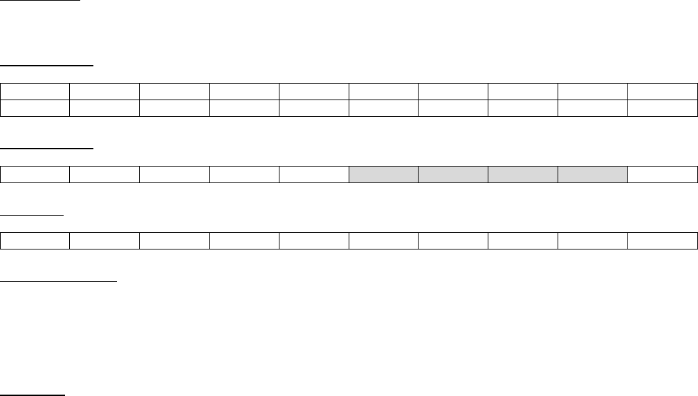
ASET1
6.4.1.2 ASET1
Description:
Define degrees of freedom to go into the analysis set (A-set)
Format No. 1:
ASET1 C G1 G2 G4 G4 G5 G6 G7 +Q001
+Q001 G8 G9 (etc)
Format No. 2:
ASET1 C G1 THRU G2
Example:
ASET1 135 17934 THRU 19012
Data Description:
Field Contents Type Default
Gi ID numbers of grids. G2 > G1 Integer > 0 None
C Displacement component numbers Integers 1-6 None
Remarks:
1. In Format No. 2, any grid whose ID is in the range G1 through G2 will have component C defined in
the A-set.
2. The degrees of freedom defined by grids GI, components Ci will be placed in the mutually exclusive
A-set. These degrees of freedom cannot have been defined to be in any other mutually exclusive set
(i.e.. M, S or O-sets).
3. If there are no ASET (or ASET1) and no OMIT (or OMIT1) entries, all degrees of freedom not in the
M or S-set will be placed in the A-set
4. If ASET (or ASET1) entries are present in the input data file, then all degrees of freedom not specified
on these entries and also not in the M or S-sets will be placed in the O-set.
5. If both ASET (or ASET1) and OMIT (or OMIT1) are present, then all degrees of freedom not in the M
and S sets must be explicitly defined on these ASET (or ASET1) and OMIT (or OMIT1) entries.
6. Up to four pairs of Gi, Ci can be specified on one ASET entry. For more pairs, use additional ASET
entries (i.e. there is no continuation entry for ASET).
83

BAROR
6.4.1.3 BAROR
Description:
Define default values for the CBAR entry.
Format No.1:
BAROR PID V1 V2 V3
Format No.2:
BAROR PID G0
Examples:
BAROR 57 1.3 3.5 0.7
BAROR 57 1563
Data Description:
Field Contents Type Default
PID ID number of a PBAR Bulk data entry Integer > 0
or blank None
G0 ID of a grid used to define the orientation v vector Integer > 0
or blank None
Vi The three components of the orientation v vector specified in the
global coordinate system for grid G1 on the CBAR entry. Real or blank None
Remarks:
1. Only one BAROR entry is allowed in the input data file. Any data entered on a BAROR entry will be
used unless overridden on a CBAR entry. If format 1 is used, all three components of the v vector
must be entered.
2. The orientation v vector can be specified using either a grid point (G0) or the components Vi. Either
one of these, in conjunction with the grid G1 on the CBAR entry, defines the orientation vector.
3. See CBAR entry for remarks concerning the v vector.
84

CBAR
6.4.1.4 CBAR
Description:
1D bar element for axial load, bending and torsion
Format No. 1:
1 2 3 4 5 6 7 8 9 10
CBAR EID PID G1 G2 G0 +CONT
+CONT P1 P2 W11 W12 W13 W21 W22 W23
Format No. 2:
CBAR EID PID GA GB V1 V2 V3 +CONT
+CONT P1 P2 W11 W12 W13 W21 W22 W23
Examples:
CBAR 98 43 1234 56 78 +BAR98
+BAR98 456 13 0.0 0.2 0.3 0.1 0.05 0.10
CBAR 98 43 1234 56 0.5 1.5 3.2
Data Description:
Field Contents Type Default
EID Element ID number Integer > 0 None
PID ID number of a PBAR Bulk data entry Integer > 0 EID
G1, G2 ID numbers of the grids to which the element is attached Integer > 0 None
G0 ID of a grid used to define the orientation v vector Integer > 0 None
Vi Components of the orientation v vector Real None
P1, P2 Pin flags for bar ends 1 and 2 respectively Integers 1-6 None
W1j Components of the bar offset from grid G1 Real None
W2j Components of the bar offset from grid G2 Real None
Remarks:
1. No other element in the model may have the same element ID
2. The v vector is a vector from either: (a) grid G1 to grid G0, or (b) from grid G1 in the direction of the
vector defined by V1, V2, V3. These components are measured in the global coordinate system of
grid G1 (see GRID entry for definition of the global coordinate system for a grid). If format 1 is used,
all three components of the v vector must be entered.
85
3. The local x axis of the element is a vector from G1 through G2 (see Figure 4-3)
4. The x axis and the v vector define a plane. On the PBAR entry, I1 is the bending moment of inertia in
this plane.
86
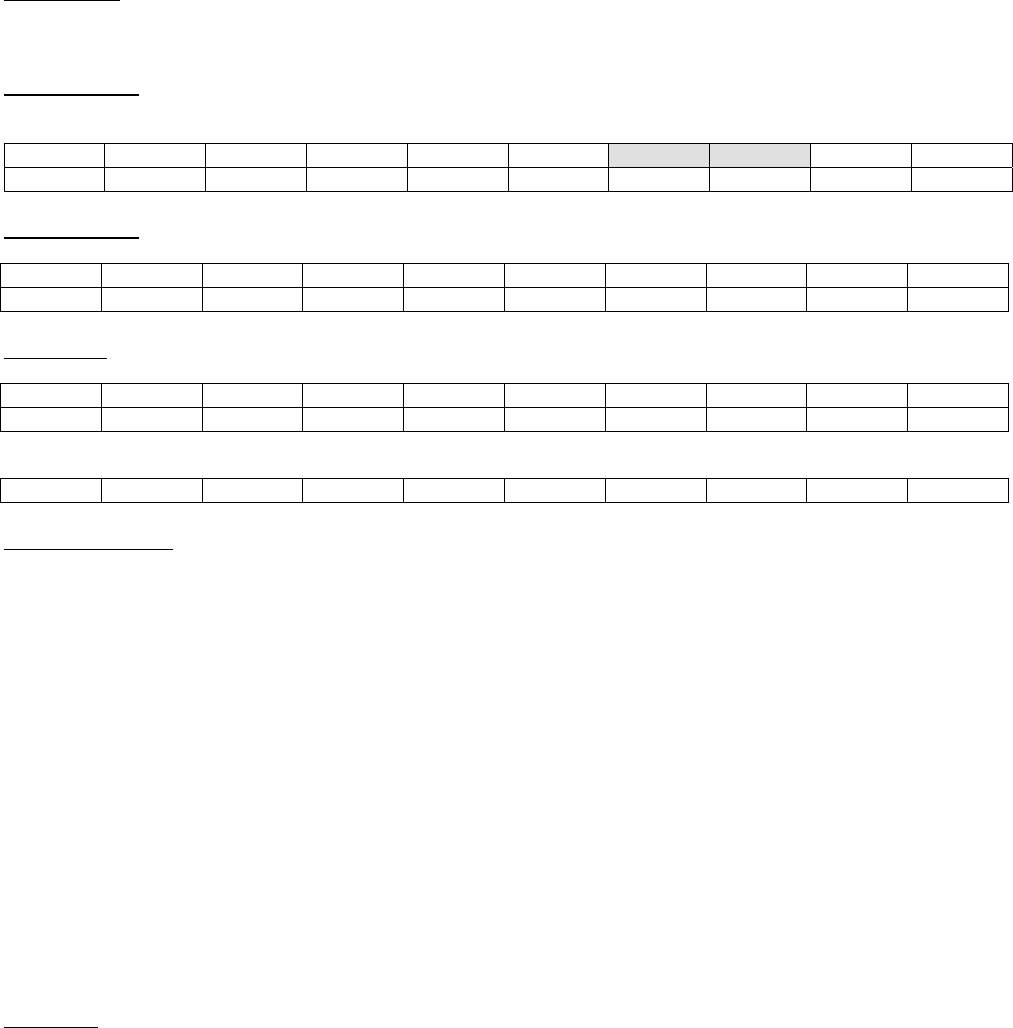
CBUSH
6.4.1.5 CBUSH
Description:
Spring element
Format No. 1:
1 2 3 4 5 6 7 8 9 10
CBUSH EID PID G1 G2 G0 CID +CONT
+CONT S OCID S1 S2 S3
Format No. 2:
CBUSH EID PID GA GB V1 V2 V3 CID +CONT
+CONT S OCID S1 S2 S3
Examples:
CBUSH 98 43 1234 56 78 +BAR98
+BAR98 456 13 0.0 0.2 0.3
CBAR 98 43 1234 56 0.5 1.5 3.2
Data Description:
Field Contents Type Default
EID Element ID number Integer > 0 None
PID ID number of a PBAR Bulk data entry Integer > 0 EID
G1, G2 ID numbers of the grids to which the element is attached Integer > 0 None
G0 ID of a grid used to define the orientation v vector Integer > 0 None
Vi Components of the orientation v vector Real None
CID Element coordinate system identification (0 is basic system) If blank,
the element system is defined by G0 or Vi Integer >= 0
or blank None
S Location of spring 0.< Real < 1. 0.5
OCID ID of coordinate system used in defining the offstes. OCID = -1
indicates that the offsets are specified in the element coordinate
system
Integer >= -1 -1
Si Components of spring offset Real 0.
Remarks:
1. No other element in the model may have the same element ID
87
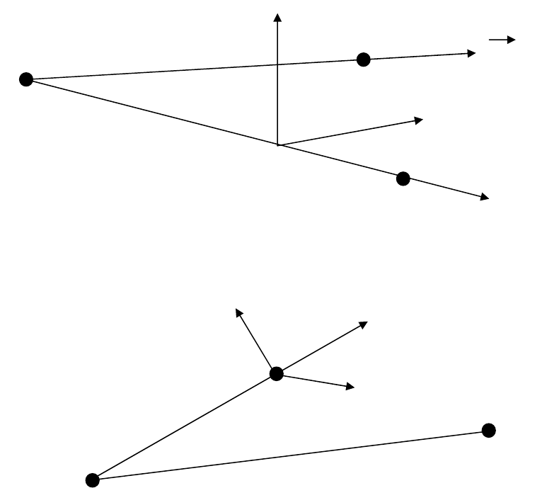
2. If CID >= 0 the element x axis is along the x axis of coordinate system CID, etc.
3. A V vector must be specified. That is, fields 6-9 cannot all br blank
4. GB cannot be blank
5. The following pertains to OCID:
(a) OCID = -1 (or blank) means S is used and Si are ignored
(b) OCID >= 0 menas S is ignored and Si are used
Ze
V
G0
G1 Ye
G2
Figure 1: BUSH element Xe
Ze
Ye
Xe
(S1,S2,S3)
G2
Figure 2: Offsets Si
G1
88

CELAS1
6.4.1.6 CELAS1
Description:
Scalar spring element connected to 2 grid points (GRID’s) with reference to a PELAS entry to define the
real values for the element
Format:
1 2 3 4 5 6 7 8 9 10
CELAS1 EID PID G1 C1 G2 C2
Example:
CELAS1 789 32 3731 5 67 5
Data Description:
Field Contents Type Default
EID Unique element identification (ID) number Integer > 0 None
PID ID number of a PROD Bulk data entry Integer > 0 EID
Gi ID numbers of the grids to which the element is attached Integer > 0 None
Ci Component number (1-6) of the degree of freedom, at Gi, to which the
spring element is connected Integer 1-6 None
Remarks:
1. No other element in the model may have the same element ID
2. The degrees of freedom specified by Gi/Ci must be global degrees of freedom
3. Care must be exercised that rigid body motion of the model is not restrained when using scalar
springs For example, connecting a scalar spring between two translational degrees of freedom that
are not colinear may restrain rigid body motion and give erroneous results
89
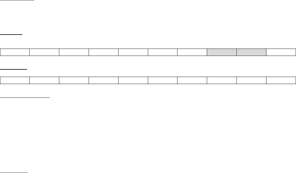
CELAS2
6.4.1.7 CELAS2
Description:
Scalar spring element connected to 2 grid points (GRID’s) with the element stiffness defined
Format:
1 2 3 4 5 6 7 8 9 10
CELAS2 EID K G1 C1 G2 C2
Example:
CELAS2 789 1.234+06 3731 5 67 5
Data Description:
Field Contents Type Default
EID Unique element identification (ID) number Integer > 0 None
K Stiffness value Real 0.
Gi ID numbers of the grids to which the element is attached Integer > 0 None
Ci Component number (1-6) of the degree of freedom, at Gi, to which the
spring element is connected Integer 1-6 None
Remarks:
1. No other element in the model may have the same element ID
2. The degrees of freedom specified by Gi/Ci must be global degrees of freedom
3. Care must be exercised that rigid body motion of the model is not restrained when using scalar
springs For example, connecting a scalar spring between two translational degrees of freedom that
are not colinear may restrain rigid body motion and give erroneous results
90
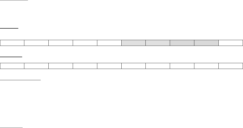
CELAS3
6.4.1.8 CELAS3
Description:
Scalar spring element connected to 2 scalar points (SPOINT’s) with reference to a PELAS entry to define
the real values for the element
Format:
1 2 3 4 5 6 7 8 9 10
CELAS3 EID PID S1 S2
Example:
CELAS3 789 32 3731 5
Data Description:
Field Contents Type Default
EID Unique element identification (ID) number Integer > 0 None
PID ID number of a PROD Bulk data entry Integer > 0 EID
Si ID numbers of the SPOINT’s to which the element is attached Integer > 0 None
Remarks:
1. No other element in the model may have the same element ID
2. The degrees of freedom specified by Si must be global degrees of freedom
3. Care must be exercised that rigid body motion of the model is not restrained when using scalar
springs For example, connecting a scalar spring between two translational degrees of freedom that
are not colinear may restrain rigid body motion and give erroneous results
91
CELAS4
6.4.1.9 CELAS4
Description:
Scalar spring element connected to 2 scalar points (SPOINT’s) with the element stiffness defined
Format:
1 2 3 4 5 6 7 8 9 10
CELAS4 EID K S1 S2
Example:
CELAS4 789 32 3731 5
Data Description:
Field Contents Type Default
EID Unique element identification (ID) number Integer > 0 None
K Stiffness value Real 0.
Si ID numbers of the SPOINT’s to which the element is attached Integer > 0 None
Remarks:
1. No other element in the model may have the same element ID
2. The degrees of freedom specified by Si must be global degrees of freedom
3. Care must be exercised that rigid body motion of the model is not restrained when using scalar
springs For example, connecting a scalar spring between two translational degrees of freedom that
are not colinear may restrain rigid body motion and give erroneous results
92
CHEXA
6.4.1.10 CHEXA
Description:
3D solid tetrahedron element
Format No. 1:
1 2 3 4 5 6 7 8 9 10
CHEXA EID PID G1 G2 G3 G4 G5 G6 +CH1
+CH1 G7 G8 G9 G10 G11 G12 G13 G14 +CH2
+CH2 G15 G16 G17 G18 G19 G20
Example:
CHEXA 98 43 101 123 254 12 621 8945 +CH1
+CH1 43 998
Data Description:
Field Contents Type Default
EID Unique element identification (ID) number Integer > 0 None
PID ID number of a PSOLID Bulk data entry Integer > 0 None
G1-G20 ID numbers of the grids to which the element is attached. Specify G1-
G8 for a 4 node HEXA and all 20 for a 20 node HEXA Integer > 0 None
Remarks:
1. No other element in the model may have the same element ID
2. The first continuation entry is required. The second is only needed for the 20 node element
93

CMASS1
6.4.1.11 CMASS1
Description:
Scalar mass element connected to 2 grid points (GRID’s) with reference to a PMASS entry to define the
real values for the element
Format:
1 2 3 4 5 6 7 8 9 10
CMASS1 EID PID G1 C1
Example:
CMASS1 789 32 3731 5
Data Description:
Field Contents Type Default
EID Unique element identification (ID) number Integer > 0 None
PID ID number of a PMASS Bulk data entry Integer > 0 EID
G1 ID number of the grid to which the element is attached Integer > 0 None
C Component number (1-6) of the degree of freedom, at G1, to which
the mass element is connected Integer 1-6 None
Remarks:
1. No other element in the model may have the same element ID
2. The degrees of freedom specified by Gi/Ci must be global degrees of freedom.
3. For MYSTRAN, the mass can only be connected to 1 grid (not 2 as is allowed in NASTRAN)
94

CMASS2
6.4.1.12 CMASS2
Description:
Scalar mass element connected to 2 grid points (GRID’s) with the element stiffness defined
Format:
1 2 3 4 5 6 7 8 9 10
CMASS2 EID K G1 C1
Example:
CMASS2 789 1.234+06 3731 5
Data Description:
Field Contents Type Default
EID Unique element identification (ID) number Integer > 0 None
K Stiffness value Real 0.
Gi ID numbers of the grids to which the element is attached Integer > 0 None
Ci Component number (1-6) of the degree of freedom, at Gi, to which the
mass element is connected Integer 1-6 None
Remarks:
1. No other element in the model may have the same element ID
2. The degrees of freedom specified by Gi/Ci must be global degrees of freedom.
3. For MYSTRAN, the mass can only be connected to 1 grid (not 2 as is allowed in NASTRAN)
95
CMASS3
6.4.1.13 CMASS3
Description:
Scalar mass element connected to 2 scalar points (SPOINT’s) with reference to a PMASS entry to define
the real values for the element
Format:
1 2 3 4 5 6 7 8 9 10
CMASS3 EID PID S1
Example:
CMASS3 789 32 3731 5
Data Description:
Field Contents Type Default
EID Unique element identification (ID) number Integer > 0 None
PID ID number of a PMASS Bulk data entry Integer > 0 EID
Si ID numbers of the SPOINT’s to which the element is attached Integer > 0 None
Remarks:
1. No other element in the model may have the same element ID
2. The degrees of freedom specified by Si must be global degrees of freedom.
3. For MYSTRAN, the mass can only be connected to 1 scalar point (not 2 as is allowed in NASTRAN)
96
CMASS4
6.4.1.14 CMASS4
Description:
Scalar mass element connected to 2 scalar points (SPOINT’s) with the element stiffness defined
Format:
1 2 3 4 5 6 7 8 9 10
CMASS4 EID K S1
Example:
CMASS4 789 32 3731 5
Data Description:
Field Contents Type Default
EID Unique element identification (ID) number Integer > 0 None
K Stiffness value Real 0.
Si ID numbers of the SPOINT’s to which the element is attached Integer > 0 None
Remarks:
1. No other element in the model may have the same element ID
2. The degrees of freedom specified by Si must be global degrees of freedom.
3. For MYSTRAN, the mass can only be connected to 1 scalar point (not 2 as is allowed in NASTRAN)
97
CONM2
6.4.1.15 CONM2
Description:
Concentrated mass at a grid point
Format:
1 2 3 4 5 6 7 8 9 10
CONM2 EID G CID M X1 X2 X3 +CONT
+CONT I11 I21 I22 I31 I32 I33
Example:
CONM2 98 354 29 0.5 0.3 1.2 0.65 +1002
+1002 123. -45. 321. 12. -43. 567.
Data Description:
Field Contents Type Default
EID Element identification (ID) number Integer > 0 None
G ID number of the grid to which the mass is attached Integer > 0 None
CID ID number of a coordinate system defined on a CORD2C, CORD2R or
CORD2S Bulk Data entry Integer > 0 0
M Mass value Real 0.
Xi Offset distances from grid G to the center of gravity of M in coordinate
system CID Real 0.
Iij The 6 independent moments of inertia of M about its center of gravity
measured in coordinate system CID. Real 0.
Remarks:
1. EID must be unique among all CONM2 entries
2. The continuation entry is optional.
3. The moments of inertia I11, I22 and I33 (if entered) must be > 0.
4. A blank entry for CID implies the basic coordinate system.
98

CONROD
6.4.1.16 CONROD
Description:
1D elastic rod element for axial load and torsion with properties
Format:
1 2 3 4 5 6 7 8 9 10
CROD EID PID G1 G2 A J C NSM
Example:
CROD 98 43 1234 56
Data Description:
Field Contents Type Default
EID Unique element identification (ID) number Integer > 0 None
PID ID number of a PROD Bulk data entry Integer > 0 EID
G1, G2 ID numbers of the grids to which the element is attached Integer > 0 None
A Bar cross-sectional area Real 0.
J Torsional constant Real 0.
C Torsional stress recovery coefficient Real 0.
MPL Mass per unit length Real 0.
Remarks:
1. No other element in the model may have the same element ID
2. The local xe axis of the element is a vector from G1 through G2 (see Figure 4-2)
99

CORD1C
6.4.1.17 CORD1C
Description:
Cylindrical coordinate system definition defined via 3 grid points. Two separate coordinate systems may
be defined on one physical CORD1C entry.
Format:
1 2 3 4 5 6 7 8 9 10
CORD1C CIDA G1A G2A G3A CIDB G1A G2A G3A
Example:
CORD1C
Data Description:
Field Contents Type Default
CID Coordinate system ID number Integer > 0 None
G1A, G1B ID’s of grid points at the origin of systems A, B respectively Integer > 0 None
G2A, G2B ID’s of grid points along the z axis of systems A, B respectively Integer > 0 None
G1C, G2C ID’s of grid points in the x-z plane of systems A, B respectively Integer > 0 None
Remarks:
1. See Figure 4-1 for the cylindrical coordinate system notation and the “defining” rectangular system
2. CIDA, CIDB must be unique over all coordinate systems defined in the model.
3. One or 2 coordinate systems may be defined on a single CORD1S entry.
4. The grid points on this entry must be defined in a system that does not involve the system being
defined.
5. See Figure 4-1 for a definition of the various coordinate systems and the directions of the
displacements in those systems.
6. The location of a grid point using this coordinate system is defined by the r, , z coordinates of a
cylindrical coordinate system (see Figure 4-1).
θ
100
CORD1R
6.4.1.18 CORD1R
Description:
Rectangular coordinate system definition defined via 3 grid points. Two separate coordinate systems
may be defined on one physical CORD1C entry.
Format:
1 2 3 4 5 6 7 8 9 10
CORD1C CIDA G1A G2A G3A CIDB G1A G2A G3A
Example:
CORD1C
Data Description:
Field Contents Type Default
CID Coordinate system ID number Integer > 0 None
G1A, G1B ID’s of grid points at the origin of systems A, B respectively Integer > 0 None
G2A, G2B ID’s of grid points along the z axis of systems A, B respectively Integer > 0 None
G1C, G2C ID’s of grid points in the x-z plane of systems A, B respectively Integer > 0 None
Remarks:
1. See Figure 4-1 for the cylindrical coordinate system notation and the “defining” rectangular system
2. CIDA, CIDB must be unique over all coordinate systems defined in the model.
3. One or 2 coordinate systems may be defined on a single CORD1S entry.
4. The grid points on this entry must be defined in a system that does not involve the system being
defined.
5. See Figure 4-1 for a definition of the various coordinate systems and the directions of the
displacements in those systems.
6. The location of a grid point using this coordinate system is defined by the x, y, z coordinates of a
rectangular coordinate system (see Figure 4-1).
101

CORD1S
6.4.1.19 CORD1S
Description:
Spherical coordinate system definition defined via 3 grid points. Two separate coordinate systems may
be defined on one physical CORD1C entry.
Format:
1 2 3 4 5 6 7 8 9 10
CORD1C CIDA G1A G2A G3A CIDB G1A G2A G3A
Example:
CORD1C
Data Description:
Field Contents Type Default
CID Coordinate system ID number Integer > 0 None
G1A, G1B ID’s of grid points at the origin of systems A, B respectively Integer > 0 None
G2A, G2B ID’s of grid points along the z axis of systems A, B respectively Integer > 0 None
G1C, G2C ID’s of grid points in the x-z plane of systems A, B respectively Integer > 0 None
Remarks:
1. See Figure 4-1 for the cylindrical coordinate system notation and the “defining” rectangular system
2. CIDA, CIDB must be unique over all coordinate systems defined in the model.
3. One or 2 coordinate systems may be defined on a single CORD1S entry.
4. The grid points on this entry must be defined in a system that does not involve the system being
defined.
5. See Figure 4-1 for a definition of the various coordinate systems and the directions of the
displacements in those systems.
6. The location of a grid point using this coordinate system is defined by the r, θ,
coordinates of a
spherical coordinate system (see Figure 4-1).
102

CORD2C
6.4.1.20 CORD2C
Description:
Cylindrical coordinate system definition
Format:
1 2 3 4 5 6 7 8 9 10
CORD2R CID RID A1 A2 A3 B1 B2 B3 +CONT
+CONT C1 C2 C3
Example:
CORD2R 26 41 4.6 1.9 13.89 5.76 11.3 2.7 +01A
+01A 4.9 26.2 3.4
Data Description:
Field Contents Type Default
CID Coordinate system ID number Integer > 0 None
RID ID number of the reference coordinate system in which the points Ai, Bi,
Ci are specified Integer >= 0
or blank 0
Ai Coordinates of the origin of CID (specified in RID coordinate system) Real None
Bi Coordinates of a point on the z axis of the defining rectangular system
of CID (specified in RID coordinate system) Real None
Ci Coordinates of a point in the x-z plane of the defining rectangular
system of CID (specified in RID coordinate system) Real None
Remarks:
1. See Figure 4-1 for the rectangular coordinate system notation and the “defining” rectangular system.
2. CID must be unique over all coordinate systems defined in the model.
3. The continuation entry is required.
4. RID = 0 or blank means that the reference coordinate system is the basic coordinate system.
5. CID must be able to be traced, through a chain of coordinate references, back th the basic system.
For example, in the example above CID 26 is defined using system 46. Coordinate system 46 can be
defined using some other coordinate system, and so on, until the final RID is 0 (basic).
6. The basic system need not be defined explicitly. Its axes are implied from the model (grid point
coordinates on GRID entries and coordinate system definitions of all other systems)
103
CORD2R
6.4.1.21 CORD2R
Description:
Rectangular coordinate system definition
Format:
1 2 3 4 5 6 7 8 9 10
CORD2R CID RID A1 A2 A3 B1 B2 B3 +CONT
+CONT C1 C2 C3
Example:
CORD2R 26 41 4.6 1.9 13.89 5.76 11.3 2.7 +01A
+01A 4.9 26.2 3.4
Data Description:
Field Contents Type Default
CID Coordinate system ID number Integer > 0 None
RID ID number of the reference coordinate system in which the points Ai, Bi,
Ci are specified Integer >= 0
or blank 0
Ai Coordinates of the origin of CID (specified in RID coordinate system) Real None
Bi Coordinates of a point on the z axis of the defining rectangular system
of CID (specified in RID coordinate system) Real None
Ci Coordinates of a point in the x-z plane of the defining rectangular
system of CID (specified in RID coordinate system) Real None
Remarks:
1. See Figure 4-1 for the rectangular coordinate system notation and the “defining” rectangular system.
2. CID must be unique over all coordinate systems defined in the model.
3. The continuation entry is required.
4. RID = 0 or blank means that the reference coordinate system is the basic coordinate system.
5. CID must be able to be traced, through a chain of coordinate references, back th the basic system.
For example, in the example above CID 26 is defined using system 46. Coordinate system 46 can be
defined using some other coordinate system, and so on, until the final RID is 0 (basic).
6. The basic system need not be defined explicitly. Its axes are implied from the model (grid point
coordinates on GRID entries and coordinate system definitions of all other systems).
104

CORD2S
6.4.1.22 CORD2S
Description:
Spherical coordinate system definition
Format:
1 2 3 4 5 6 7 8 9 10
CORD2S CID RID A1 A2 A3 B1 B2 B3 +CONT
+CONT C1 C2 C3
Example:
CORD2S 26 41 4.6 1.9 13.89 5.76 11.3 2.7 +01A
+01A 4.9 26.2 3.4
Data Description:
Field Contents Type Default
CID Coordinate system ID number Integer > 0 None
RID ID number of the reference coordinate system in which the points Ai, Bi,
Ci are specified Integer >= 0
or blank 0
Ai Coordinates of the origin of CID (specified in RID coordinate system) Real None
Bi Coordinates of a point on the z axis of the defining rectangular system
of CID (specified in RID coordinate system) Real None
Ci Coordinates of a point in the x-z plane of the defining rectangular
system of CID (specified in RID coordinate system) Real None
Remarks:
1. See Figure 4-1 for the rectangular coordinate system notation and the “defining” rectangular system.
2. CID must be unique over all coordinate systems defined in the model.
3. The continuation entry is required.
4. RID = 0 or blank means that the reference coordinate system is the basic coordinate system.
5. CID must be able to be traced, through a chain of coordinate references, back th the basic system.
For example, in the example above CID 26 is defined using system 46. Coordinate system 46 can be
defined using some other coordinate system, and so on, until the final RID is 0 (basic).
6. The basic system need not be defined explicitly. Its axes are implied from the model (grid point
coordinates on GRID entries and coordinate system definitions of all other systems).
105
CPENTA
6.4.1.23 CPENTA
Description:
3D solid pentahedron element
Format No. 1:
1 2 3 4 5 6 7 8 9 10
CPENTA EID PID G1 G2 G3 G4 G5 G6 +CP1
+CP1 G7 G8 G9 G10 G11 G12 G13 G14 +CP2
+CP2 G15
Example:
CPENTA 98 43 101 123 254 12 1002 98
Data Description:
Field Contents Type Default
EID Unique element identification (ID) number Integer > 0 None
PID ID number of a PSOLID Bulk data entry Integer > 0 None
G1-G15 ID numbers of the grids to which the element is attached. Specify G1-
G6 for a 6 node PENTA and all 15 for a 15 node PENTA Integer > 0 None
Remarks:
1. No other element in the model may have the same element ID
2. Continuation entries are only needed for the 15 node element
106

CQUAD4
6.4.1.24 CQUAD4
Description:
Thick quadrilateral plate element. This element has membrane and bending stiffness and can
include flexibility for transverse shear deformations.
Format:
1 2 3 4 5 6 7 8 9 10
CQUAD4 EID PID G1 G2 G3 G4
THETA ZOFFS
Example:
CQUAD4 68 123 935 67 1357 2
Data Description:
Field Contents Type Default
EID Unique element identification (ID) number Integer > 0 None
PID ID number of a PSHELL Bulk data entry Integer > 0 EID
Gi ID numbers of the grids to which the element is attached Integer > 0 None
THETA Material property orientation angle in degtees measured from axis
connectiong grids 1 and 2 Real 0.
ZOFFS Offset of the grid plane to element reference plane Real 0.
Remarks:
1. No other element in the model may have the same element ID
2. The grids must be numbered in a clockwise or counter clockwise direction around the quadrilateral
element.
3. The local ze axis of the element is in the direction of the cross-product of the diagonal from G1 to G3
with the diagonal from G2 to G4. If the element is rectangular, the local xe axis is the projection of the
vector from G1 to G2 onto the mean plane. If not rectangular, this is rotated to split the angle
between the diagonals. The local ye axis is in the direction of ze cross xe. See Figure 4-5
107
CQUAD4K
6.4.1.25 CQUAD4K
Description:
Thin quadrilateral plate element . This element has membrane and bending stiffness but does not
include flexibility for transverse shear deformations.
Format:
1 2 3 4 5 6 7 8 9 10
CQUAD4K EID PID G1 G2 G3 G4
Example:
CQUAD4K 68 123 935 67 1357 2
Data Description:
Field Contents Type Default
EID Unique element identification (ID) number Integer > 0 None
PID ID number of a PSHELL Bulk data entry Integer > 0 EID
Gi ID numbers of the grids to which the element is attached Integer > 0 None
Remarks:
1. No other element in the model may have the same element ID
2. The grids must be numbered in a clockwise or counter clockwise direction around the quadrilateral
element.
3. The local ze axis of the element is in the direction of the cross-product of the diagonal from G1 to G3
with the diagonal from G2 to G4. If the element is rectangular, the local xe axis is the projection of the
vector from G1 to G2 onto the mean plane. If not rectangular, this is rotated to split the angle
between the diagonals. The local ye axis is in the direction of ze cross xe. See Figure 4-5
108

CROD
6.4.1.26 CROD
Description:
1D elastic rod element for axial load and torsion
Format:
1 2 3 4 5 6 7 8 9 10
CROD EID PID G1 G2
Example:
CROD 98 43 1234 56
Data Description:
Field Contents Type Default
EID Unique element identification (ID) number Integer > 0 None
PID ID number of a PROD Bulk data entry Integer > 0 EID
G1, G2 ID numbers of the grids to which the element is attached Integer > 0 None
Remarks:
1. No other element in the model may have the same element ID
2. The local xe axis of the element is a vector from G1 through G2 (see Figure 4-2)
109

CSHEAR
6.4.1.27 CSHEAR
Description:
Defines a quadrilateral shell element that carries only in-plane shear
Format:
1 2 3 4 5 6 7 8 9 10
CSHEAR EID PID G1 G2 G3 G4
Example:
CSHEAR 98 43 978 564 94 465
Data Description:
Field Contents Type Default
EID Unique element identification (ID) number Integer > 0 None
PID ID number of a PROD Bulk data entry Integer > 0 EID
Gi ID numbers of the grids to which the element is attached Integer > 0 None
Remarks:
1. No other element in the model may have the same element ID
2. The local xe axis of the element is defined the same as for the QUAD4 element
110
CTETRA
6.4.1.28 CTETRA
Description:
3D solid tetrahedron element
Format No. 1:
1 2 3 4 5 6 7 8 9 10
CTETRA EID PID G1 G2 G3 G4 G5 G6 +CT1
+CT1 G7 G8 G9 G10
Example:
CTETRA 98 43 101 123 254 12
Data Description:
Field Contents Type Default
EID Unique element identification (ID) number Integer > 0 None
PID ID number of a PSOLID Bulk data entry Integer > 0 None
G1-G10 ID numbers of the grids to which the element is attached. Specify G1-
G4 for a 4 node TETRA and all 10 for a 10 node TETRA Integer > 0 None
Remarks:
1. No other element in the model may have the same element ID
2. Continuation entries are only needed for the 15 node element
111
CTRIA3
6.4.1.29 CTRIA3
Description:
Thick triangular plate element . This element has membrane and bending stiffness and can
include flexibility for transverse shear deformations
Format:
1 2 3 4 5 6 7 8 9 10
CTRIA3 EID PID G1 G2 G3
THETA ZOFFS
Example:
CTRIA3 68 123 935 67 1357
Data Description:
Field Contents Type Default
EID Unique element identification (ID) number Integer > 0 None
PID ID number of a PSHELL Bulk data entry Integer > 0 EID
Gi ID numbers of the grids to which the element is attached Integer > 0 None
THETA Material property orientation angle in degtees measured from axis
connectiong grids 1 and 2 Real 0.
ZOFFS Offset of the grid plane to element reference plane Real 0.
Remarks:
1. No other element in the model may have the same element ID
2. The local xe axis of the element is in the direction from G1 to G2. The local ze axis is in the direction
of the cross product of the vector from G1 to G2 with the vector from G1 to G3. The local ye axis is in
the direction of ze cross xe. See Figure 4-5.
112
CTRIA3K
6.4.1.30 CTRIA3K
Description:
Thin triangular plate element . This element has membrane and bending stiffness but does not
include flexibility for transverse shear deformations.
Format:
1 2 3 4 5 6 7 8 9 10
CTRIA3K EID PID G1 G2 G3
Example:
CTRIA3K 68 123 935 67 1357
Data Description:
Field Contents Type Default
EID Element identification (ID) number Integer > 0 None
PID ID number of a PSHELL Bulk data entry Integer > 0 EID
Gi ID numbers of the grids to which the element is attached Integer > 0 None
Remarks:
1. No other element in the model may have the same element ID
2. The local xe axis of the element is in the direction from G1 to G2. The local ze axis is in the direction
of the cross product of the vector from G1 to G2 with the vector from G1 to G3. The local ye axis is in
the direction of ze cross xe. See Figure 4-5.
113
CUSERIN
6.4.1.31 CUSERIN
Description:
User defined element for which the user will supply the mass and stiffness matrices via NASTRAN
formatted INPUTT4 files.
Format 1:
1 2 3 4 5 6 7 8 9 10
CUSERIN EID PID NG NS CID0 +CU01
+CU01 G1 C1 G2 C2 etc +CU11
+CU11 S1 S2 S3 etc
Format 2:
1 2 3 4 5 6 7 8 9 10
CUSERIN EID PID NG NS CID0 +CU01
+CU01 G1 C1 G2 C2 etc +CU11
+CU11 S1 THRU S2
Example:
CUSERIN 32 123 3 8 198 +CU01
+CU01 201 123 202 13 203 3 +CU02
+CU02 20001 THRU 20008
Data Description:
Field Contents Type Default
EID Element identification (ID) number Integer > 0 None
PID ID number of a PUSERIN Bulk Data entry Integer > 0 EID
NG Number of grid points (GRID’s) that the element is attached to Integer >= 0 0
NS Number of scalar points (SPOINT’s) that the element is attached to Integer >= 0 0
CID0 ID of the coordinate system that defines the basic coord system of this
element relative to the basic coord system of the overall model Integer >= 0 0
Gi, Ci NG grid/component numbers for the grids and components that the
element connects to (Ci have to be integers 1,2,3,4,5 and/or 6) Integer > 0 None
Si NS scalar points (Bulk Data SPOINT) that the element connects to Integer > 0 None
Remarks:
1. No other element in the model may have the same element ID
2. An example of how this element is used is in Craig-Bampton analyses where a system model is made
up of one or more substructures (generated in CB model generation solution sequence, SOL 31).
114
Each CB model’s connection information is described by a CUSERIN element. The PUSERIN Bulk
Data entry is required.
115

DEBUG
6.4.1.32 DEBUG
Description:
Define debug parameters
Format:
1 2 3 4 5 6 7 8 9 10
DEBUG i VALUE
Example:
DEBUG 31 1
Data Description:
Field Contents Type Default
i Debug number (index in DEBUG array) 0 < Integer < 100 None
VALUE The value for DEBUG(i) Integer 0
Remarks:
1. No other element in the model may have the same element ID
2. See table below for actions taken based on the various debug values. Unless otherwise stated,
DEBUG(i) = 0 is the default and, for the “print” parameters, no printing is done.
116

Action Taken For DEBUG(I) Values
I DEBUG(I)
A
ction (NOTE: default values are zero)
1 1 Print KIND parameters defined in module PENTIUM_II_KIND to F06 file
2 1 Print constants (parameters) defined in module CONSTANTS_1
3 1 Print machine parameters as determined by LAPACK function DLAMCH
4 1 Do not use BMEAN when calculating membrane quad element stiffness for warped elements
5 1 Print Gauss quadrature abscissas and weight s for plate elements
6 1
2 Print some quad elem data to BUG file (over and above what is printed with Case Control ELDATA)
Print some hexa elem data to BUG file (over and above what is printed with Case Control ELDATA)
7 1 Print arrays ESORT1, ESORT2, EPNT, ETYPE in subr ELESORT before/after sorting elems
8 1
2
3
Print grid temperature data in subr TEMPERATURE_DATA_PROC
Print elem temperature data in subr TEMPERATURE_DATA_PROC
Print both grid and elem temperature data in subr TEMPERATURE_DATA_PROC
9 > 0 Prints debug info on BAR pin flag processing
10
11 or 33
12 or 32
13 or 33
21 or 33
22 or 32
Print data on algorithm to create STF stiffness arrays in subr ESP
Print detailed data on algorithm to create STF arrays in subr SPARSE
Print template of nonzero terms in KGG if PARAM SETLKTK = 1 or 2
Print data on algorithm to create EMS mass arrays in subr ESP
Print detailed data on algorithm to create EMS mass arrays in subr SPARSE
11 1
2
3
Print individual 6x6 rigid body. displacement matrices in basic and global coordinates for each grid
Print NGRID by 6 rigid body displacement matrix in global coordinates for the model
Print both
12 1 Use area shear factors in computing BAR stiffness matrix regardless of I12 value
13 1 Print grid sequence tables in subr SEQ
14 1 Print matrices generated in the rigid element generation subr's
15 1 Print concentrated mass data in subr CONM2_PROC_1
16 1 Use static equivalent instead of work equivalent pressure loads for the QUAD4, TRIA3
17 > 0
> 1 Print some info in subr KGG_SINGULARITY_PROC for grids that have AUTOSPC'd components
Do above for all grids (not just ones that have AUTOSPC's)
18 > 0 Print diagnostics in subr QMEM1 regarding checks on the BMEAN matrix satisfying R.B. motion
19 1 Print debug output from subr STOKEN
20 0
1 Use simple solution for GMN if RMM is diagonal.
Bypass the simple solution for GMN if RMM is diagonal and use subr SOLVE_GMN instead
21 0
1 Use MATMULT_SFF to multiply stiffness matrix times rigid body displs in STIFF_MAT_EQUIL_CHK
Use LAPACK subroutine DSBMV
22 1 Print RBMAT in subr STIFF_MAT_EQUIL_CHK
23 > 0 Do equilibrium checks on stiffness matrix even though model has SPOINT's
24 1 or 3
2 or 3 Print KFSe matrix in subr REDUCE_KNN_TO_KFF
Print KSSe matrix in subr REDUCE_KNN_TO_KFF
25 1 or 3
2 or 3 Print PFYS matrix in subr REDUCE_N_FS
Print QSYS matrix in subr REDUCE_N_FS
26 1 Print YS matrix (S-set enforcorced displs) in LINK2 (LAPACK)
31 1 Print KLL stiff matrix in LINK3-LAPACK
32 1 Print PL load matrix in LINK3-LAPACK
33 1 Print UL displacement matrix before refining sulotion in LINK3_LAPACK
34 1 or 3
2 or 3 Print ABAND matrix (KLL in band form) before equilibrating it in LINK3 (LAPACK
Print ABAND matrix after equilibrating it in LINK3 (LAPACK)
35 1 Print ABAND’s decomp matrix (KLL triangular factor) in LINK3 (LAPACK)
36 1 Print grid 6x6 mass for every grid in LINK2
117

I DEBUG(I)
A
ction (NOTE: default values are zero)
40
1 or 3
2 or 3
1
1
Print banded stiffness matrix ABAND in subr EIG_GIV_MGIV
Print banded mass matrix ABAND in subr EIG_GIV_MGIV
print RFAC = KLL - sigma*MLL in subr EIG_INV
print RFAC = KLL - sigma*MLL in subr EIG_LANCZOS
41 1 Print KLL stiffness matrix in LINK4
42 1 Print MLL stiffness matrix in LINK4
43 1 Print eigenvectors in LINK4 (normally not printed until LINK9)
46 1 Print debug info for Inverse Power eigenvalue extraction
47 1 Print eigenvalue estimates at each iteration in Lanczos
48 1 Do not calculate off-diag terms in generalized mass matrix
49 1 Print diagnostics in ARPACK subroutine DSBAND
55 1
2
3
Print PHIXG in full format in EXPAND_PHIXA_TO_PHIXG
Print PHIZG in full format in LINK5
Do both
118

I DEBUG(I) Action (NOTE: default values are zero)
80 > 0 Print LAPACK_S scale factors, in subr EQUILIBRATE, used to equilibrate the stiffness matrices
81 1
2
3
Print data on how subr MATADD_SSS_NTERM determines no. terms to allocate for matrix add
Print data on progress of matrix add in subr MATADD_SSS
Print data from both subroutines
82 1 Print data on progress of matrix multiply in subr MATMULT_SFF
83 1
2
3
Print data on how subr MATMULT_SFS_NTERM determines no. terms to allocate for matrix multiply
Print data on progress of matrix multiply in subr MATMULT_SFS
Print data from both subroutines
84 1
2
3
Print data on how subr MATMULT_SSS_NTERM determines no. terms to allocate for matrix multiply
Print data on progress of matrix multiply in subr MATMULT_SSS
Print data from both subroutines
85 1 Print data on matrix transposition in subr MATTRNSP_SS
86 1
2
3
Print data on how subr PARTITION_SS_NTERM determines no. terms to allocate for matrix partition
Print data on progress of matrix partition in subr PARTITION_SS
Print data from both subroutines
87 1
Print data on algorithm to convert sparse CRS matrix to sparse CCS in subr
SPARSE_CRS_SPARSE_CCS
88 1 Do not write separator line between grids several places(matrix diagonal output, equil check)
89 1 Write row numbers where there are zero diag terms in subroutine SPARSE_MAT_DIAG_ZEROS
91 1
Print Information on how the maximum number of requests for grid or element related outputs is
determined. This controls the allocation of memory in LINK9
92 1 Print OLOAD, SPCF, MPCF totals even if global coordinate systems for all grids are not the same
100 > 0
> 1 Check allocation status of allocatable arrays.
Also write memory allocated to all arrays to F06 file.
101 > 0
> 1 Write sparse I_MATOUT array in subroutine READ_MATRIX_1.
Call subroutine to check I_MATOUT array to make sure that terms are nondecreasing
102 > 0 Print debug info in subroutine MERGE_MAT_COLS_SSS
103 > 0 Do not use MRL (or MLR) in calc of modal participation factors and effective mass
104 > 0 Check if KRRcb is singular
105 > 0 write KLLs matrix to unformatted file
106 > 0
write info on all files in subr WRITE_ALLOC_MEM_TABLE (if 0 only write for those arrays that have
memory allocated to them
107 > 0 Write allocated memory in F04 file with 6 decimal points (3 if DEBUG(107) = 0)
108 > 0 Write EDAT table
109 > 0 Write debug info in subr ELMDIS
110 > 0 Write debug info for BUSH elem in subrs ELMDAT1, ELMGM1
111 > 0 Write some debug info on RSPLINE
112 > 0 Write THETAM (plate element material angle) and the location in subr EMG where it was calculated
113 > 0 Write PBARL entries in a special format that has 1 line per PBAR entry
114 > 0 Write debug info in subr OU4_PARTVEC_PROC
115 > 0 Write debug info in subr READ_INCLUDE_FILNAM
116 = 1 Write debug info in Yale subr SFAC
= 2 Write debug info in Yale subr NFAC
= 3 Do both
119

I DEBUG(I) Action (NOTE: default values are zero)
172 > 0 Calc PHI_SQ for the MIN4T based on area weighting of the TRIA3's. Otherwise, use simple average
173 = 1 Write some debug info in subr PARSE_CSV_STRING
= 2 Write some more detailed data
174 > 0 Print MPFACTOR, MEFFMASS values with 2 decimal places of accuracy rather than 6
175 > 0
Write debug output from subroutine SURFACE_FIT regarding the polynomial fit to obtain element
corner stresses from Gauss point stresses
176 > 0
Calculate stresses using element SEi, STEi matrices and displacements rather than from BEi matrices
and strains
177 > 0 Print BAR, ROD margins of safety whether or not they would otherwise be
178 = 1 Print info on user key if PROTECTED = 'N'
179 = 1 Print blank space at beg of lines of output for CUSERIN entries in the F06 file
180 > 0 Write debug info to F06 for USERIN elements
181 = 1 Include USERIN RB mass in subr GPWG even though user did not input 3rd matrix (RBM0) on IN4FIL
182 = 1 Print debug data in subr MGGS_MASS_MATRIX for scalar mass matrix
183 = 1 Write some debug data for generating TDOF array
184 > 0 Write L1M data to F06
185 > 0
Let eigen routines find and process all eigenval, vecs found even if NVEC > NDOFL -
NUM_MLL_DIAG_ZEROS
186 > 0 Print debug info for pressure loads on faces of solid elements
187 > 0 Write list ao the number of various elastic elements in the DAT file to the F06 file
188 > 0 Do not abort in QPLT3 if KOO is reported to be singular
189 1
2
3
Print messages in subroutine ESP for KE in local coords if element diagonal stiffness < 0
Print these messages in subroutine ESP after transformation to global
Do both
190 > 0 Do not round off FAILURE_INDEX to 0 in subr POLY_FAILURE_INDEX
191 = 0 Use temperatures at Gauss points for thermal loads in solid elements
192 > 0 Print some summary info for max abs value of GP force balance for each solution vector
193
= 1
= 2
= 3
= 4
= 5
= 6
= 9
= 100
= 999
call FILE_INQUIRE at end of LINK1
call FILE_INQUIRE at end of LINK2
call FILE_INQUIRE at end of LINK3
call FILE_INQUIRE at end of LINK4
call FILE_INQUIRE at end of LINK5
call FILE_INQUIRE at end of LINK6
call FILE_INQUIRE at end of LINK9
call FILE_INQUIRE at end of MAIN
do all of the above
194 1 or 3
2 or 3
3
skip check on CW/CCW numbering of QUAD's
2 or 3 skip check on QUAD interior angles < 180 deg
skip both
195 > 0 Print CB OTM matrices to F06 at end of LINK9
196 0
> 0 Matrix output filter SMALL = EPSIL(1)
Matrix output filter SMALL = TINY (param defined by user with default = 0.D0)
197 > 0 Print debug info in subr EC_ENTRY_OUTPUT4 which reads Exec Control OUTPUT4 entries
198 > 0 Write debug info in subroutine QPLT3 (for QUAD4 element)
199 > 0 Check matrix times its inverse = identity matrix in several subroutines
200 > 0 Write problem answers (displs, etc) to filename.ANS as well as to filename.F06 (where filename is the
name of the DAT data file submitted to MYSTRAN. This feature is generally only useful to the author
when performing checkout of test problem answers
120
EIGR
6.4.1.33 EIGR
Description:
Eigenvalue extraction data
Format:
1 2 3 4 5 6 7 8 9 10
EIGR SID METH F1 F2 NE ND CRIT +CONT
+CONT NORM G C
Examples:
EIGR 98 GIV 0.1 20. 1.E-4 +ZZ02
+ZZ02 MAX
EIGR 25 GIV 15. 20. 1.E-4 +ZZ02
+ZZ02 POINT 471 3
Data Description:
Field Contents Type Default
SID Eigenvalue extraction set number Integer > 0 None
METH Method for eigenvalue extraction: (GIV, MGIV, INV) Character None
F1, F2 Frequency range of interest Real 0.
NE Number of estimated eigenvalues in range (not used for GIV) Integer 0
ND Number of desired eigenvalues in range (not used for GIV) Integer 0
CRIT Orthogonality criteria Real 0.
NORM Method of eigenvector renormalization (POINT, MAX, MASS) Character None
G If NORM = POINT, the grid to be used in normalizing eigenvector to
1.0 Integer > 0
or blank 0
C If NORM = POINT, the component (1-6) at G to be used in normalizing
the eigenvector = 1.0 Integer 1-6
or blank 0
Remarks:
1. Givens (GIV) or Modified Givens (MGIV) methods of eigenvalue extraction are available. In addition,
an Inverse Power (INV) method is also available, but only for the fundamental mode.
2. The EIGR set ID, SID, must be selected in Case Control with the entry METHOD = SID
121
3. The three methods of eigenvector renormalization are:
MASS: eigenvectors are normalized to unit generalized mass (1.0)
MAX: eigenvectors are normalized to 1.0 for the largest term
POINT: eigenvectors are normalized such that the value at grid G, component C is 1.0
4. For the GIV method the mass matrix must be positive definite (thus the mass matrix can have no
zeros on its diagonal). For the MGIV method, the model must have the stiffness matrix positive
definite (thus modes of a model that is not restrained from rigid body motion cannot be obtained)
122
EIGRL
6.4.1.34 EIGRL
Description:
Eigenvalue extraction data for Lanczos method
Format:
1 2 3 4 5 6 7 8 9 10
EIGR SID F1 F2 N MSGLVL NCVFACL SIGMA NORM +CONT
+CONT MODE TYPE
Examples:
EIGRL 98 0. 50.
Data Description:
Field Contents Type Default
SID Eigenvalue extraction set number Integer > 0 None
F1, F2 Frequency range of interest Real 0.
N Number of desired eigenvalues Integer 0
MSGLVL Output message level (0 for none, or 1 or 2 for some messaging) Integer 0
NCVFAC Used to dimension several arrays in the Lanczos method. Must be > 1 Integer 2
SIGMA Shift eigenvalue Real -10.
NORM Method of eigenvector renormalization (MAX, MASS) Character None
Mode Lanczos mode for calculating eigenvalues Integer 2
Type Lanczos matrix type (DPB, DGB) Character DPB
Remarks:
1. The EIGRL set ID, SID, must be selected in Case Control with the entry METHOD = SID
2. Either F1 (and F2) or N must be specified. If both are specified, N will be used.
3. Mode refers to the Lanczos mode type to be used in the solution. In mode 3 the mass matrix,
Maa,must be nonsingular whereas in mode 2 the matrix aa aa
KM
must be nonsingular (where
=
SIGMA). See Bulk Data PARAM ART_MASS for use if the mass matrix is singular.
4. TYPE = DPB uses sym storage of the matrices (preferred) whereas DGB stores all nonzero terms.
5. SIGMA is the shift eigenvalue. It should generally be a small negative real number.
123
FORCE
6.4.1.35 FORCE
Description:
Static concentrated force at a grid point
Format:
1 2 3 4 5 6 7 8 9 10
FORCE SID GID CID F N1 N2 N3
Example:
FORCE 1234 567 89 1000. 1.5 2.5 3.5
Data Description:
Field Contents Type Default
SID Load set ID number Integer > 0 None
GID ID of the grid at which this concentrated force acts Integer >0 None
CID ID of the coordinate system in which the Ni are specified Integer >= 0 0
F An overall scale factor for the force Real 0.
Ni Components of a vector in the direction of the force Real 0.
Remarks:
1. The static concentrated force applied to the grid is the vector:
PFN
with Ni in fields 6-8 the components of the vector N
2. In order for this load to be used in a static analysis the load set ID must either be selected in Case
Control by LOAD = SID, or this load set ID must be referenced on a LOAD Bulk Data entry which
itself is selected in Case Control.
3. A blank entry for CID implies the basic coordinate system.
124
GRAV
6.4.1.36 GRAV
Description:
Gravity load definition
Format:
1 2 3 4 5 6 7 8 9 10
GRAV SID CID A N1 N2 N3
Example:
GRAV 975 246 386. 2. 3. 4.
Data Description:
Field Contents Type Default
SID Load set ID number Integer > 0 None
CID ID of the coordinate system in which the Ni are specified Integer >= 0 0
A Acceleration value Real 0.
Ni Components of a vector in the direction of the force Real 0.
Remarks:
1. GRAV causes a static load to be applied to the complete model that is calculated based on the
acceleration vector on the GRAV entry and the mass properties of the model.
2. The acceleration vector applied to the model is the vector:
a
A
N
with Ni in fields 5-7 the components of the vector N
3. In order for this load to be used in a static analysis the load set ID must either be selected in Case
Control by LOAD = SID, or this load set ID must be referenced on a LOAD Bulk Data entry which
itself is selected in Case Control.
4. A blank entry for CID implies the basic coordinate system.
125
GRDSET
6.4.1.37 GRDSET
Description:
Default values for the GRID entry
Format:
1 2 3 4 5 6 7 8 9 10
GRDSET CID1 CID2 PSPC
Example:
GRDSET 12 42 245
Data Description:
Field Contents Type Default
CID1 Default value for the coordinate system ID in which grids will be
located for GRID entries which have a blank in this field Integer >= 0 0
CID2 Default value for the global coordinate system for GRID entries which
have a blank in this field Integer >= 0 0
PSPC Default value for permanent single point constraints for GRID entries
which have a blank in this field Integers 1-6 0
Remarks:
1. Only one GRDSET entry is allowed in the data file. Any data entered on a GRDSET entry will be
used for the corresponding field of any GRID entry that has that field blank. Thus, if the user desires
to have CIDi be the basic system on a GRID entry, and a GRDSET entry is present with nonzero
value for CIDi, the GRID entry in question must have 0 (not blank) for CIDi.
2. See the GRID entry for remarks on the above fields of this entry.
3. A blank entry for CIDi implies the basic coordinate system.
126
GRID
6.4.1.38 GRID
Description:
Grid point definition
Format:
1 2 3 4 5 6 7 8 9 10
GRID GID CID1 X1 X2 X3 CID2 PSPC
Example:
GRID 58 12 10. 20. 30 42 245
Data Description:
Field Contents Type Default
GID Grid point ID number Integer > 0 None
CID1 ID of the coordinate system that the Xi are defined in Integer >= 0 0
Xi Coordinates of the grid defined in coordinate system CID1 Real 0.
CID2 ID of the global coordinate system for this grid point Integer >= 0 0
PSPC Permanent single point constraints at this grid point Integers 1-6 Blank
Remarks:
1. Grid IDs must be unique among all GRID entries.
2. The word “permanent” in regards to the single point constraints (SPC’s) defined on the GRID entry is
merely a designation given to SPC’s defined on GRID entries. The PSPC field does not have to be
used. Any, or all, of the zero value (i.e., not enforced displacement) single point constraints used in a
model can be specified on Bulk Data SPC or SPC1 entries or as PSPC’s on the GRID entry.
3. A blank entry for CIDi implies the basic coordinate system.
127
LOAD
6.4.1.39 LOAD
Description:
This entry combines loads defined on FORCE, MOMENT, PLOAD2, GRAV entries
Format:
1 2 3 4 5 6 7 8 9 10
LOAD SID S S1 L1 S2 L2 S3 L3 +CONT
+CONT S4 L4 (etc)
Example:
LOAD 12345 1500. 151.5 25 290.2 33 780.3 24 +L002
+L002 2450.1 12
Data Description:
Field Contents Type Default
SID Load set ID number Integer > 0 None
S An overall scale factor for the load combination Real 0.
Si Scale factor for load set Li Real 0.
Li Load set ID number for loads defined on FORCE, MOMENT,
PLOAD2, GRAV entries Integer > 0 None
Remarks:
1. The static load applied to the model is the vector:
PSSP
iL
i
i
where PLi is the load defined on the FORCE, MOMENT, PLOAD2 or GRAV that has Li load set ID.
2. In order for this load to be used in a static analysis the load set ID must be selected in Case Control
by the command LOAD = SID.
3. Any number of continuation entries may be included.
128
MAT1
6.4.1.40 MAT1
Description:
Linear isotropic material definition
Format:
1 2 3 4 5 6 7 8 9 10
MAT1 MID E G NU RHO ALPHA TREF GE +CONT
+CONT TA CA SA
Example:
MAT1 10 1.E7 0.33 0.1 2.E-5 21. +MATL01
+MATL01 10000. 20000. 15000.
Data Description:
Field Contents Type Default
MID Material ID number Integer > 0 None
E Young’s modulus Real > 0. or blank See remarks
G Shear modulus Real > 0. or blank See remarks
NU Poisson’s ratio Real > 0. or blank See remarks
RHO Material mass density Real > 0. or blank 0.
ALPHA Coefficient of thermal expansion Real > 0. or blank 0.
TREF Reference temperature Real > 0. or blank 0.
GE Damping coefficient Real > 0. or blank 0.
TA Tension allowable for the material Real > 0. or blank 0.
CA Compression allowable for the material Real > 0. or blank 0.
SA Shear allowable for the material Real > 0. or blank 0.
Remarks:
1. MID must be unique among all material property entries.
2. The continuation entry is not required.
3. The following action is taken if one or more of the fields E, G and NU are blank:
a) If one of E, G or NU is blank it will be calculated using the relationship E = 2(1 + NU)G
b) If E and NU are blank or if G and NU are blank, these two are set to 0.
c) If E and G are blank (or zero) a fatal error occurs
129
4. A warning is given if: .5 < NU < 0.
5. A warning is given if if E, G and NU are all input and do not satisfy the relationship:
E
10
2(1 NU)G
.01
130
MAT2
6.4.1.41 MAT2
Description:
Linear anisothotropic material definition for 2D plate elements
Format:
1 2 3 4 5 6 7 8 9 10
MAT2 MID G11 G12 G13 G22 G23 G33 RHO +CONT1
+CONT A1 A2 A3 TREF GE ST SC SS
Example:
MAT2 10 9.9+6 3.+6 2.+6 10.1+6 3.2+6 8.9+6 .00025 +MAT21
+MAT21 2.-5 3.-5 1.5-5 21. .001 30000. 20000. 25000
Data Description:
Field Contents Type Default
MID Material ID number Integer > 0 None
Gij Terms in the 3x3 material property matrix Real 0.
RHO Material mass density Real 0.
Ai Thermal expansion coefficients Real 0.
TREF Reference temperature Real 0.
GE Structural damping coefficient Real 0.
ST Tension stress limit Real 0.
SC Compression stress limit Real 0.
SS Shear stress limit Real 0.
Remarks:
1. MID must be unique among all material property entries.
2. The continuation entry is not required.
3. If this entry is used for the transverse shear properties (MID3 on PSHELL) then G13, G23 and G33
are ignored .
131
4. The stress strain relationship for an element using the MAT2 is:
.
11112131
21222232 ref
31323333
xz xz
11 12
yz yz
12 22
GGG
GGG (TT)
GGG
and
GG
GG
1
2
3
132

MAT8
6.4.1.42 MAT8
Description:
Linear orthotropic material definition for plate elements
Format:
1 2 3 4 5 6 7 8 9 10
MAT8 MID E1 E2 NU12 G12 G1Z G2Z RHO +CONT1
+CONT1 A1 A2 TREF Xt Yc Yt Yc S +CONT2
+CONT2 GE F12 STRN
Example:
MAT8 10 9.+6 11.+6 0.29 4.+6 3.+6 5.+6 .00258 +MATL01
+MATL01 20.-5 22.-5 21.0 +MATL02
+MATL02
Data Description:
Field Contents Type Default
MID Material ID number Integer > 0 None
E1 Elastic modulus in longitudinal direction Real > 0. 0.
E2 Elastic modulus in lateral direction Real > 0. 0.
G12 In-plane shear modulus Real >= 0. 0.
G1Z Transverse shear modulus in the 1-Z plane Real >= 0. 0.
G2Z Transverse shear modulus in the 2-Z plane Real >= 0. 0.
NU12 Poisson’s ratio Real >= 0. 0.
RHO Material mass density Real >= 0. 0.
A1 Coefficient of thermal expansion in the longitudinal direction Real >= 0. 0.
A2 Coefficient of thermal expansion in the lateral direction Real >= 0. 0.
TREF Reference temperature Real 0.
Xt Real > 0. 0.
Xc Real > 0. 0.
Yt Real > 0. 0.
Yc Real > 0. 0.
S Real > 0. 0.
GE Damping coefficient Real > 0. 0.
F12 Real > 0. 0.
STRN Compression allowable for the material Real > 0. 0.
133

Remarks:
1. MID must be unique among all material property entries.
2. The continuation entries are not required.
3. If G1Z and G2Z are zero (or blank) transverse shear flexibility is zero (infinite transverse shear
stiffness).
134
MAT9
6.4.1.43 MAT9
Description:
Linear anisotropic material definition for 3D solid elements
Format:
1 2 3 4 5 6 7 8 9 10
MAT9 MID G11 G12 G13 G14 G15 G16 G22 +CONT1
+CONT1 G23 G24 G25 G26 G33 G34 G35 G36 +CONT2
+CONT2 G44 G45 G46 G55 G56 G66 RHO A1 +CONT3
+CONT3 A2 A3 A4 A5 A6 TREF GE
Example:
MAT8 10 8.+6 4.+4 3.2+6 2.5+6 9.+6 +MATL01
+MATL01 10.+6 +MATL02
+MATL02 4.+6 5.+6 3.+6 .003 20.-5 +MATL03
+MATL03 22.-5 18.-5
Data Description:
Field Contents Type Default
MID Material ID number Integer > 0 None
Gij Elements of the 6x6 material matrix Real > 0. 0.
RHO Material mass density Real >= 0. 0.
AI Coefficients of thermal expansion Real >= 0. 0.
TREF Reference temperature Real 0.
GE Damping coefficient Real > 0. 0.
Remarks:
1. MID must be unique among all material property entries.
2. The first two continuation entries are required but the third continuation entry is not required.
3. The Gij are the transformation of strains to stresses as in:
xx
11 12 13 14 15 16
yy
22 23 24 25 26
zz
33 34 35 36
xy xy
44 45 46
55 56
yz yz
66
zx zx
GGGGGG
GGGGG
GGGG
GGG
sym G G
G
135
MOMENT
6.4.1.44 MOMENT
Description:
Static concentrated moment at a grid point
Format:
1 2 3 4 5 6 7 8 9 10
MOMENT SID GID CID M N1 N2 N3
Example:
MOMENT 1234 567 89 1000. 1.5 2.5 3.5
Data Description:
Field Contents Type Default
SID Load set ID number Integer > 0 None
GID ID of the grid at which this concentrated moment acts Integer >0 None
CID ID of the coordinate system in which the Ni are specified Integer >= 0 0
M An overall scale factor for the moment Real 0.
Ni Components of a vector in the direction of the moment Real 0.
Remarks:
1. The static concentrated moment applied to the grid is the vector:
PMN
with Ni in fields 6-8 the components of the vector N
2. In order for this load to be used in a static analysis the load set ID must either be selected in Case
Control by LOAD = SID, or this load set ID must be referenced on a LOAD Bulk Data entry which
itself is selected in Case Control.
3. A blank entry for CID implies the basic coordinate system.
136
MPC
6.4.1.45 MPC
Description:
Multi point constraints define a linear dependence of one degree of freedom (that becomes a
member of the M-set) on other degrees of freedom.
Format:
1 2 3 4 5 6 7 8 9 10
MPC SID G1 C1 D1 G2 C2 D2 +MPC1
+MPC1 G3 C3 S3 G4 C4 D4 +MPC2
+MPC2 G6 C5 D6 etc…
Example:
As an example consider the following equation relating several degrees of freedom (in global
coordinates):
623 76
101 201 y z
1.2w 4.5v 0.63 12.7 0
where w101 is the the displacement in the global z direction at grid 101, v201 is the displacement in the
global y direction at grid 201, and the remaining two terms are the rotation about the global y and z
directions at grids 623 and 76 respectively. Assuming that w101 has been chosen as the M-set degree of
freedom for this MPC equation, the input would be:
MPC 56 101 3 1.2 201 2 4.5 +M01
+M01 623 5 -.63 76 6 12.7
Data Description:
Field Contents Type Default
SID ID number of the multi point constraint set Integer > 0 None
Gi ID numbers of the grids involved in the constraint. Grid G1, componrnt
C1 is, by definition, the dependent (M-set) degree of freedom Integer > 0 None
Ci Component numbers at grids Gi involved in the MPC equation Integers 1-6 None
Di The value for coefficient D for grid Gi, component Ci Real 0.
Remarks:
1. Multi point constraint sets must be selected in Case Control with the entry MPC = SID in order for
them to be applied.
2. Degrees of freedom defined as dependent on MPC entries will be members of the M-set and cannot
be defined as being members of any other mutually exclusive set.
3. G1/C1 is the degree of freedom eliminated (M-set) due to the MPC equation and the remaining terms
in the MPC equation can be for degrees of freedom belonging to any displacement set.
137

MPCADD
6.4.1.46 MPCADD
Description:
Combine multi-point constraint sets defined on MPC entries
Format:
1 2 3 4 5 6 7 8 9 10
MPCADD SID S1 S2 S3 S4 S5 S6 S7 +CONT
+CONT S8 S9 (etc)
Example:
SPCADD 283 11 74 123 564
Data Description:
Field Contents Type Default
SID Multi-point constraint set ID number Integer > 0 None
Si Set IDs of MPC Bulk Data entries Integer > 0 None
Remarks:
1. Multi-point constraint sets must be selected in Case Control with the entry MPC = SID in order for
them to be applied.
2. All multi-point constraints specified on MPC entries whose set IDs are the Si on the MPCADD will be
applied to the model if MPC = SID is in Case Control.
138

OMIT
6.4.1.47 OMIT
Description:
Define degrees of freedom to go into the omit set (O-set)
Format:
1 2 3 4 5 6 7 8 9 10
OMIT G1 C1 G2 C2 G3 C3 G4 C4
Example:
OMIT 19 1 28 2345 37 124 46 134
Data Description:
Field Contents Type Default
Gi ID numbers of grids Integer > 0 None
Ci Displacement component numbers Integers 1-6 None
Remarks:
1. The degrees of freedom defined by grids GI, components Ci will be placed in the mutually exclusive
O-set. These degrees of freedom cannot have been defined to be in any other mutually exclusive set
(i.e.. M, S or A sets).
2. If OMIT or OMIT1 are present in the data file, then all degrees of freedom not specified on these
entries and also not in the M or S sets will be placed in the A-set. If both ASET (or ASET1) and OMIT
(or OMIT1) are present, then all degrees of freedom not in the M and S sets must be explicitly defined
on ASET (or ASET1) and OMIT (or OMIT1)
3. Up to four pairs of Gi, Si can be specified on one OMIT entry. For more pairs, use additional OMIT
entries (i.e. there is no continuation entry for OMIT).
139

OMIT1
6.4.1.48 OMIT1
Description:
Define degrees of freedom to go into the omit set (O-set)
Format No. 1:
OMIT1 C G1 G2 G4 G4 G5 G6 G7 +Q001
+Q001 G8 G9 (etc)
Format No. 2:
OMIT1 C G1 THRU G2
Example:
OMIT1 135 17934 THRU 19012
Data Description:
Field Contents Type Default
Gi ID numbers of grids. G2 > G1 Integer > 0 None
C Displacement component numbers Integers 1-6 None
Remarks:
1. In Format No. 2, all grids in the range G1 through G2 will have component C defined in the O-set.
2. The degrees of freedom defined by grids GI, components C will be placed in the mutually exclusive
O-set. These degrees of freedom cannot have been defined to be in any other mutually exclusive set
(i.e.. M, S or A sets).
3. If OMIT or OMIT1 are present in the data file, then all degrees of freedom not specified on these
entries and also not in the M or S sets will be placed in the A-set. If both ASET (or ASET1) and OMIT
(or OMIT1) are present, then all degrees of freedom not in the M and S sets must be explicitly defined
on ASET (or ASET1) and OMIT (or OMIT1)
140

PARAM
6.4.1.49 PARAM
Description:
Provide values, other than default values, for parameters that control options during execution.
Format:
1 2 3 4 5 6 7 8 9 10
PARAM NAME V1 V2 V3 V4
Example:
PARAM PRTDOF 2
Data Description:
Field Contents Type Default
NAME Parameter name Char None
Vi Values for the parts of the parameter Char, Integer or real Various
Remarks:
1. See table below for a list of the various parameters and what action is taken based on their values.
Unless otherwise stated, only value V1 is used. The parameter name always goes in field 2 and V1
always goes in field 3. When there is more than one Vi, the table explicitly states in what fields the Vi
go.
141

Parameters
Parameter
Name Data
Type Function of Parameter
NOTE: Default values of parameters are: N for Char, 0 for Int and 0.0 for real
ARP_TOL Real Default = 1x10⁻⁶
Tolerance to use in Lanczos eigenvalue extraction method for convergence
ART_KED
(for diff stiffness
– not fully
implemented)
Char Field 3: ART_KED, default = N. If Y add artificial stiff to diag of KED stiff matrix
Field 4: ART_TRAN_MASS: value for translation degrees of freedom, default 1x10⁻⁶
Field 5: ART_ROT_MASS: value for translation degrees of freedom, default 1x10⁻⁶
ART_MASS Char Field 3: ART_MASS, default = N. If Y add artificial mass to diag of MGG mass matrix
Field 4: ART_TRAN_MASS: value for translation degrees of freedom, default 1x10⁻⁶
Field 5: ART_ROT_MASS: value for translation degrees of freedom, default 1x10⁻⁶
AUTOSPC Char
Real
Int
Char
Char
Field 3: AUTOSPC value, default = Y (AUTOSPC), N turns AUTOSPC off.
Field 4: AUTOSPC_RAT, default = 1x10⁻⁶ (see Section 3.4.1.1)
Field 5: AUTOSPC_NSET, default = 1 (see Section 3.4.1.1)
Field 6: AUTOSPC_INFO, default = N. If Y then print messages about the AUTOSPC’s
Field 7: AUTOSPC_SPCF, default = N. If Y print AUTOSPC forces of constraint
BAILOUT Int Default = 1
If > 0 quit if a singularity in decomposing a matrix is detected.
If <= 0 do not quit
CBMIN3 Real Default = 2.0
CBMIN3 is the constant CB used in tuning the shear correction factor in Ref 3 for the
TRIA3 plate element. The default 2.0 is the value suggested by the author.
CBMIN4 Real Default = 3.6
CBMIN4 is the constant CB used in tuning the shear correction factor in Ref 4 for the
QUAD4 plate element (QUAD4TYP = ‘MIN4 ‘). See Ref 4
CBMIN4T Real Default = 3.6
CBMIN4T is the constant CB used in tuning the shear correction factor in Ref 4 for the
QUAD4 plate element (QUAD4TYP = ‘MIN4T’).
CHKGRDS Char Default = Y. If N do not check that all grids for all elements exist
CUSERIN Char
Int
Int
Int
Int
Char
Int
If this parameter is present, Bulk Data entries for Craig-Bampton (CB) reduced models
will be written to the F06 file as a CUSERIN element (including grids, coordinate
systems, etc)
Field 3: element ID, default = 9999999
Field 4: property ID default = 9999999
Field 5: starting index for the SPOINT’s to represent modes of the CB model, default =
1001
Field 6: IN4 file number that goes on the PUSERIN entry for this CUSERIN element,
default = 9999999
Field 7: Set-ID for the CUSERIN element (typically the “R”, or boundary, set), default is
blank field
Field 8: Format for how to write the component numbers (1 thru 6) for each grid of the
CUSERIN element. If 0, write them in compact form (e.g. 1356). If > 0 write them in
expanded form (1 3 56), default = 0
DARPACK Int Default = 2
how many extra modes to find above EIG_N2 on the EIGRL entry. These few highest
mode are not used due to difficulty with getting good GP force balance.
EIGESTL Int Defaule 5000
For eigenvalue problems by the Lanczos method, if the number of L-set DOF’s exceed
EIGESTL the method for specifying the search range will be changed from F1 to F2 to N
(see EIGRL Bulk Data entry) to avoid excessive run times (since the code to estimate
the number of eigens in the F1 to F2 range can be excessive).
EIGNORM2 Char Default = N. if 'Y' then eigenvectors will be renormalized a last time by multiplying by a
set of scale factors (1 per eigenvector) supplied in a file with the same name as the
input file and extension 'EIN' (if it exists)
142

Parameters (continued)
Parameter
Name Data
Type Function of Parameter
NOTE: Default values of parameters are: N for Char, 0 for Int and 0.0 for real
ELFORCEN Char Default = GLOBAL
If ELFORCEN = GLOBAL, and nodal forces have been requested in Case Control, they
will be output in the global coordinate system.
If ELFORCEN = BASIC, and nodal forces have been requested in Case Control, they
will be output in the basic coordinate systeml.
If ELFORCEN = LOCAL, and nodal forces have been requested in Case Control, they
will be output in the local element coordinate system.
EPSERR Char Default = Y. If N, do not calculate the NASTRAN like “epsilon error estimate”
EPSIL Real There are 3 EPSIL(i) values each of which requires a separate PAPAM EPSIL Bulk
Data entry with the index (i) in field 3 and EPSIL(i) value in field 4.
These are small numbers used in MYSTRAN for the purposes indicated below:
1) EPSIL(1) (default = 1x10-15) is used in MYSTRAN such that, in any real number
comparisons, any real number whose absolute magnitude is less than EPSIL(1) is
considered to be zero. If no PARAM EPSIL 1 entry is in the data file then this value
is reset (from the default) in LINK1 to a value based on machine precision
calculated using LAPACK BLAS function DLAMCH. If the user has a PARAM
EPSIL 1 entry, this value will be used for EPSIL(1) instead of the LAPACK machine
precision.
2) Currently not used
3) EPSIL(3) is used in the Inverse Power method of eigenvalue extraction to test
convergence of an eigenvalue. The default value (% change) is 1x10⁻⁵ %
4) EPSIL(4) is used to calculate the maximum warp for quadrilateral plate elements,
above which a warning message will be written. This maximum warp is EPSIL(2)
times the average length of the quadrilateral’s two diagonals. The default for
EPSIL(2) is 1.x10-1.
5) EPSIL(5) (default 1.x10-6) is used in BAR and ROD margin of safety calculations. If
a stress magnitude is less than EPSIL(5) a 1.x1010 margin of safety will printed out
for that stress (in other words, an infinite margin of safety)
6) EPSIL(6) (default 1.x10-15) is used in BAR margin of safety calculations
EQCHECK Int
Int
Int
Int
Int
Int
Real
Char
Field 3: Default = 0 (basic origin) or reference grid to use in calculating the rigid body
displacement matrix for the equilibrium check
Field 4: If nonzero, do equilibrium check on the G-set
Field 5: If nonzero, do equilibrium check on the N-set
Field 6: If nonzero, do equilibrium check on the F-set
Field 7: If nonzero, do equilibrium check on the A-set
Field 8: If nonzero, do equilibrium check on the L-set
The value in fields 4-8 can be:
1: print loads due to rigid body displacements
2: print strain energy due to rigid body displacements
3: print both
Field 9: EQCHK_TINY, default = 1x10⁻⁵. I Do not print grid forces smaller than this
Field 10: Default = N. If Y, normalize the grid forces on diagonal stiffness
GRDPNT Int Default = -1. If not -1 then the value is interpreted as a grid number
If GRDPNT /= 0, calculate total mass properties of the model relative to the basic
coordinate system origin or relative to the specified grid.
GRIDSEQ Char
Char
Char
Field 3: GRIDSEQ value (default = BANDIT). Other values are GRID and INPUT.
BANDIT is automatic grid sequencing. GRID is sequencing in grid ID numerical order.
INPUT is sequencing in the grid input order.
Field 4: SEQQUIT, default = N. If Y, then quit in the sequence processor if BANDIT did
not run correctly.
Field 5: SEQPRT, default = N. If Y, print SEQGP card images generated by BANDIT to
the F06 output file
143

Parameters (continued)
Parameter
Name Data
Type Function of Parameter
NOTE: Default values of parameters are: N for Char, 0 for Int and 0.0 for real
HEXAXIS Char 'SIDE12', use side 1-2 as the local elem x axis.
'SPLITD' (default), use angle that splits the 2 diags to define the elem x axis
IORQ1M Int Default = 2
Gaussian integration order for membrane direct stress terms for the QUAD4, QUAD4K
quadrilateral elements
IORQ1S Int Default = 1
Gaussian integration order for membrane shear stress terms for all quad elements
IORQ1B Int Default = 2
Gaussian integration order for bending stress terms for the QUAD4K element
IORQ2B Int Default = 2
Gaussian integration order for bending stress terms for the QUAD4 element
IORQ2T Int Default = 3
Gaussian integration order for transverse shear stress terms for the QUAD4 element
ITMAX Int Default = 5
Max number of iterations in refining the solution when parameter UREFINE = Y
KLLRAT Char Default = Y to tell whether to calc ratio of max/min KLL diagonal terms
KOORAT Char Default = Y to tell whether to calc ratio of max/min KOO diagonal terms
LANCMETH Char Procedure to use for Lanczos eigenvalue extraction (ARPACK or TRLan)
MATSPARS Char If = Y (default), use sparse matrix routines for add/multiply in all matrix operations. If N,
use full matrix add/multiply (not recommended)
MAXRATIO Real Default =1X10⁷
Max value of matrix diagonal to factor diagonal before messages are written and
BAILOUT tested for aborting run
MEFMCORD Int Default = 0. The coordinate system in which to calculate modal mass and participation
factors
MEFMLOC Char Reference location for calculating modal effective mass in Craig-Bampton (SOL 31)
analyses. This only affects the rotational modal effective masses. Field 3 can be
GRDPNT, GRID or CG:
If field 3 = GRDPNT (default): ref point is the same as the one for PARAM GRDPNT
If field 3 = CG: use the model center of gravity as the reference point
If field 3 = GRID: use the grid point number in field 4 as the reference point
Field 4: MEFMGRID (grid to use when field 3 is GRID)
MEMAFAC Int Default = 0.9. Factor to multiply the size request of memory to be allocated when
looping to find an allowable amount of memory to allocate. Used when the initial request
for memory (in subrs ESP or EMP) cannot be met and we know that the request is
conservative.
MIN4TRED Char Default = STC. Defines the method for how the 5th node of the MIN4T element is
reduced out (to get a 4 node quad element). STC (default) is static condensation. B%$
(not implemented as of Version 3.0) uses a method developed by the element author
(see Users Reference manual)
MKLFACij Char Default = INDEF. Matrix type for use in decomposing matrices in various subroutines in
MYSTRAN when PARAM SOLLIB is IntMKL’
MKLFAC21 is for use in subr REDUCE_KAA_TO_KFF
MKLFAC31 is for use in subr LINK3
MKLFAC41 is for use in subr EIG_INV_PWR
MKLFAC42 is for use in subr EIG_LANCZOS_ARPACK
MKLFAC61 is for use in subr CALC_KRRcb
MKLFAC62 is for use in subr SOLVE_DLR
MKLFAC63 is for use in subr SOLVE_PHIZL1
MKLMATST Char Default = NONSYM. Matrix structure to use when PARAM SOLLIB = IntMKL. Values
can be NONSYM or SYM
144

Parameters (continued)
Parameter
Name Data
Type Function of Parameter
NOTE: Default values of parameters are: N for Char, 0 for Int and 0.0 for real
MKLSTATS Char Default = N. If Y write stats on matrix decomposition when PARAM SOLLIB = IntMKL
MPFOUT Char (1) ‘6’ (default) indicates to output modal participation factors (MPF) relative to the 6
DOF’s at grid MEFMGRID (see PARAM MEFMLOC)
(2) ‘R’ indicates to output MPF’s for all of the R-set DOF’s individually
MXALLOCA Int Default = 10. Max number of attempts to allow when trying to allocate memory in
subroutine ALLOCATE_STF_ARRAYS
MXITERI Int Default = 50. Max number of iterations to use in the Inverse Power eigenvalue
extraction method
MXITERL Int Default = 50. Max number of iterations to use in the Lanczos eigenvalue extraction
method
OTMSKIP Int Number of lines to skip between segments of OTM text file descriptors
PBARLDEC Int Default = 5. Number of decimal digits when writing PBAR equivalents for PBARL entry
real data
PBARLSHR Char Default = Y. Include K1, K2 for PBAR equiv to PBARL BAR properties
PCHSPC1 Char
Int
Char
Field 3: PCHSPC1 value (default = N, do not punch SPC1 card images for constraints
generated by the AUTOSPC feature, use Y to punch these)
Field 4: SPC1SID value (default = 9999999, the set ID to put on the SPC1 card images)
Field 5: SPC1QUIT value (default = N, do not stop after SPC!’s are punched, or Y to
stop processing)
PCMPTSTM Real Factor to multiply composite ply thickness for effective shear thickness
PCOMPEQ Int Default = 0. Indicator to write equiv PSHELL, MAT2 to F06 for PCOMP's. If > 0, write
the equivalent PSHELL amd MAT2 Bulk Data entries for the PCOMP. If > 1 also write
the data in a format with a greater number of digits of accuracy.
POST Int If = -1 then write FEMAP neutral file for post processing of MYSTRAN outputs
PRTBASIC Int If = 1 print grid coordinates in the basic coordinate system
PRTCGLTM Int If = 1 print CB matrix for C.G. LTM loads
PRTCONN Int If = 1, print table of elements connected to each grid
PRTCORD Int If PRTCORD = 1 print coordinate system transformation data
PRTDISP Int PRTDISP(I), I=1-4 go in fields 3-6 of the PARAM PRTDISP entry that prints
displacement matrices for G, N, F, and/or A-sets:
V1 = PRTDISP(1) = 1 print UG
V2 = PRTDISP(2) = 1 or 3 print UN, 2 or 3 print UM
V3 = PRTDISP(3) = 1 or 3 print UF, 2 or 3 print US
V4 = PRTDISP(4) = 1 or 3 print UA, 2 or 3 print UO
V5 = PRTDISP(5) = 1 or 3 print UL, 2 or 3 print UR
PRTDLR Int If = 1, the DLR matrix will be printed
PRTDOF Int If PRTDOF = 1 or 3 print TDOF table, in grid point ID numerical order, which gives a list
of the degree of freedom numbers for each displacement set (size is number of degrees
of freedom x number of displacement sets)
If PRTDOF = 2 or 3 print TDOF table, in degree of freedom numerical order, which
gives a list of the degree of freedom numbers for each displacement set (size is number
of degrees of freedom x number of displacement sets)
PRTFOR Int PRTFOR(I), I=1-4 go in fields 3-6 of the PARAM PRTFOR entry that prints sparse force
matrices for G, N, F, and/or A-sets:
V1 = PRTFOR(1) = 1 print sparse PG
V2 = PRTFOR(2) = 1 or 3 print sparse PN, 2 or 3 print PM
V3 = PRTFOR(3) = 1 or 3 print sparse PF, 2 or 3 print PS
V4 = PRTFOR(4) = 1 or 3 print sparse PA, 2 or 3 print PO
V5 = PRTFOR(5) = 1 or 3 print sparse PL, 2 or 3 print PR
PRTGMN Int If PRTGMN = 1, print GMN matrix
PRTGOA Int If PRTGOA = 1, print GOA matrix
145

Parameters (continued)
Parameter
Name Data
Type Function of Parameter
NOTE: Default values of parameters are: N for Char, 0 for Int and 0.0 for real
PRTHMN Int If = 1 print HMN constraint matrix
PRTIFLTM Int If = 1 print CB matrix for Interface Forces LTM
PRTKXX Int If = 1 print CB matrix KXX
PRTMASSD Int Same as PRTMASS, except only print diagonal terms
PRTMASS Int PRTMASS(I), I=1-4 go in fields 3-6 of the PARAM PRTMASS entry that prints sparse
mass matrices for G, N, F, and/or A-sets:
V1 = PRTMASS(1) = 1 print sparse MGG
V2 = PRTMASS(2) = 1 or 3 print sparse MNN, 2 or 3 print MNM, MMM
V3 = PRTMASS(3) = 1 or 3 print sparse MFF, 2 or 3 print MFS, MSS
V4 = PRTMASS(4) = 1 or 3 print sparse MAA, 2 or 3 print MAO, MOO
V5 = PRTMASS(5) = 1 or 3 print sparse MLL, 2 or 3 print MLR, MRR
PRTMXX Int If = 1 print CB matrix MXX
PRTOU4 Int If > 0 write all OU4 (OUTPUT4) matrices to F06 file
PRTPHIXA Int If = 1 print CB matrix PHIXA
PRTPHIZL Int If = 1 print CB matrix PHIZL
PRTPSET Int If > 0 print the OUTPUT4 matrix partitioning vector sets
PRTQSYS Int If = 1 print matrix QSYS
PRTRMG Int If PRTRMG = 1 or 3, print constraint matrix RMG
If PRTRMG = 2 or 3, print partitions RMN and RMM of constraint matrix RMG
PRTSCP Int If PRTSCP = 1 print data generated in the subcase processor
PRTSTIFD Int Same as PRTSTIFF, except only print diagonal terms
PRTSTIFF Int Defaults = 0 for PRTSTIFF(I), I=1-4 which go in fields 3-6 of the PARAM PRTSTIFF
entry that prints sparse stiffness matrices for G, N, F, and/or A-sets:
V1 = PRTSTIFF(1) = 1 print sparse KGG
V2 = PRTSTIFF(2) = 1 or 3 print sparse KNN, 2 or 3 print KNM, KMM
V3 = PRTSTIFF(3) = 1 or 3 print sparse KFF, 2 or 3 print KFS, KSS
V4 = PRTSTIFF(4) = 1 or 3 print sparse KAA, 2 or 3 print KAO, KOO
V5 = PRTSTIFF(5) = 1 or 3 print sparse KLL, 2 or 3 print KLR, KRR
PRTTSET Int If PRTSET = 1 print TSET table which gives the character name of the displacement
sets that each degree of freedom belongs to (size is number of grids x 6)
PRTUO0 Int If = 1 print UO0
PRTUSET Int If > 0 print the user defined set (U1 or U2) definitions
PRTYS Int If = 1 print matrix YS
Q4SURFIT Int Default = 6. Polynomial order for the surface fit of QUAD4 stress/strain when stresses
are requested for other than corner locations
QUAD4TYP Char 'MIN4T' ! Which element to use in MYSTRAN as the QUAD4 element
'MIN4T (default)': Use Tessler's MIN4T element made up of 4 MIN3 triangles
'MIN4 ': Use Tessler's MIN4 element
QUADAXIS Char Default = ‘SIDE12’
This determines how the quad element local x axis is defined. ‘SIDE12’ means that the
axis between grids 1 and 2 of the quad define the local x axis. ‘SPLITD’ means that the
axis is defined as the direction that splits the angle between the quad diagonals
146

Parameters (continued)
Parameter
Name Data
Type Function of Parameter
NOTE: Default values of parameters are: N for Char, 0 for Int and 0.0 for real
RCONDK Char If RCONDK = Y, then LAPACK calculates the condition number of the A-set stiffness
matrix. This is required if LAPACK error bounds on the A-set displacement solution are
desired. This can require significant solution time.
RELINK3 Char ‘Y’ or ‘N’ to specify whether to rerun LINK3 and also LINK5 in a restart
SETLKTK Int
Char
Int
Field 3: SETLKTK value. Default = 0. Method to estimate number of nonzeros in G-set
stiffness matrix so array can be allocated.
(1) If SETLKTK = 0, estimate LTERM_KGG based on full element stiffness matrices
unconnected (most conservative but not time consuming).
(2) If SETLKTK = 1, estimate LTERM_KGG based on KGG bandwidth.
(3) If SETLKTK = 2, estimate LTERM_KGG based on KGG density of nonzero terms
(4) If SETLKTK = 3, estimate LTERM_KGG based on actual element stiffness matrices
unconnected.
(5) f SETLKTK = 4, estimate LTERM_KGG on value input by user in field 5 of the
PARAM SETLKT entry (PARAM USR_LTERM_KGG).
Field 4: ESP0_PAUSE value (default = N, do not pause after subr ESP0 to let user input
LTERM_KGG, or pause if = Y
Field 5: User input value of LTERM_KGG
SETLKTM Same as SETLKTK but for the G-set mass matrix. Only the values for SETLKTM = 1, 3,
4 are available
SHRFXFAC Real Default = 1x10⁶. Factor used to adjust transverse shear stiffness when user has
indicated zero shear flexibility for shell elements. The shear stiffness will be reset from
infinite (zero flexibility) to SHRFXFAC times the average of the bending stiffnesses in
the 2 planes
SKIPMKGG Char Default = N. 'Y', 'N' indicator to say whether to skip calculation of MGG, KGG in which
case MGG, KGG will be read from previously generated, and saved, files (LINK1L for
KGG, LINK1R for MGG)
SOLLIB Char Default = IntMKL. Denotes which library to use for matrix decomposition and equation
solution. Options are:
IntMKL: Intel Math Kernel Library (matrices stored in sparse form)
LAPACK (matrices stored in band form)
YaleSMP: (matrices stored in sparse form) – not fully implemented in MYSTRAN
SORT_MAX Int Default = 5
Max number of times to run algorithm when sorting arrays before fatal message.
SPARSTOR Char Default = SYM
If SYM, symmetric matrices are stored with only the terms on and above the diagonal. If
NONSYM all terms are stored. SYM requires less disk storage but NONSYM can save
significant time in sparse matrix partitioning and multiply operations.
STR_CID Int Default = -1. Indicator for the coordinate system to use ID for elem stress, strain and
emgineering force output:
-1 is local element coordinate system (default)
0 is basic coordinate system
j (any other integer) is a defined coordinate system for output
SUPINFO Char Default = Y
Indicator of whether some information messages should be suppressed in the F06
output file. N indicates to suppress, Y indicates to not suppress messages in the file.
SUPWARN Char Default = Y
Indicator of whether warning messages should be suppressed in the F06 output file.
N indicates to suppress, Y indicates to not suppress messages in the file.
THRESHK Real Default = 0.1
User defined value for the threshold in deciding whether to equilibrate the A-set stiffness
matrix in LAPACK subroutine DLAQSB. Default value 0.1, LAPACK suggests
147

Parameters (continued)
Parameter
Name Data
Type Function of Parameter
NOTE: Default values of parameters are: N for Char, 0 for Int and 0.0 for real
TINY Real Do not print matrix values whose absolute value is less than this parameter value
TRLLOHI Int For TRLan eigen extraction (default = -1) - which end of spectrum to compute:
< 0, the smallest eigenvalues
= 0. whichever converges first
> 0, the largest eigenvalues
TRLMXLAN Int For TRLan eigen extraction (default = 7) - Max num Lanczos basis vectors to be used
(If user enters a Bulk Data PARAM TRLMXLAN then internal parameter
USER_TRLMXLAN is set to ‘Y’)
TRLMXMV Int For TRLan eigen extraction (default = -2000) - Max number of matrix-vector
multiplications allowed
TRLREST Int For TRLan eigen extraction (default = 1) - Index of restarting schemes
TRLTOL Real For TRLan eigen extraction (default = 1.4901D-8) - Eigenpair is declared converged if
its residual norm is < tol*||OP||
TRLVERB Int For TRLan eigen extraction (default = 0) - Level of output data written by TRLan
TSTM_DEF Real Default = 5/6 = 0.833333
Value for TS/TM on PSHELL Bulk data entry when that field on the PSHELL is blank
USETSTR Char Requests output of the internal sequence order for displacement sets (e.g. G-set, etc).
See section 3.6 for a discussion of displacement sets. In addition to the sets in section
3.7, the user displacement sets U1 and U2 (see Bulk Data entry USET and USET1) can
also have the internal sort order output to the F06 file. As an example, to obtain a row
oriented tabular output of the internal sort order for the R-set, include the Bulk data
entry:
PARAM, USETSTR, R
USR
_
JCT Int User supplied value for JCT - used in shell sort subroutines. If USR_JCT = 0, internal
values for JCT will be used in the shell sort.
WINAMEM Real Default = 2.0 GB. Max memory Windows allows for any array. If it is exceeded, a
message is printed out and execution is aborted. This is used to avoid a failure which
aborts MYSTRAN catastrophically (due to a system fault).
WTMASS Real Default = 1.0
Multiplier for mass matrix after the model total mass is output in the Grid Point Weight
Generator (GPWG). This allows user to input mass terms as weight to get model mass
properties in weight units and then to convert back to mass units after the GPWG has
run. For example, if the model units are lb-sec2/inch for mass and inches for length and
the input data file has lb for “mass” (read weight), then 1/386, or 0.002591 would be the
value for WTMASS needed to convert the “mass” matrix from weight units to mass
units.
148

PARVEC
6.4.1.50 PARVEC
Description:
Defines a partitioning vector to be used in partitioning an OUTPUT4 matrix. See the Exec
Control statements OUTPUT4 and PARTN.
Format:
1 2 3 4 5 6 7 8 9 10
PARVEC NAME G1 C1 G2 C2 G3 C3
Example:
PARVEC COLVEC 101 3 201 2
Data Description:
Field Contents Type Default
NAME Name of a row or column partitioning vector specified in a PARTN
Exec Control command Char None
GI ID numbers of the grids that will be partitioned Integer > 0 None
C Component numbers at grids Gi that will be partitioned Integers 1-6 None
Remarks:
1. The Gi, Ci must be members of the displacement set for the matrix being partitioned. For example, if
the OUTPUT4 matrix being partitioned is the row partitioning vector grid/component values must
be members of the R-set and the column partitioning vector must be a member of the L-set.
RL
K
149
PARVEC1
6.4.1.51 PARVEC1
Description:
Defines a partitioning vector to be used in partitioning an OUTPUT4 matrix. See the Exec
Control statements OUTPUT4 and PARTN.
Format No. 1:
1 2 3 4 5 6 7 8 9 10
PARVEC1 NAME C G1 G2 G3 G4 G5 G6 +CONT
+CONT G7 G8 G9 (etc)
Format No. 2:
1 2 3 4 5 6 7 8 9 10
PARVEC1 U1 C G1 THRU G2
Examples:
PARVEC1 52 135 1001 1002 103 1004 2001 2002 +SZA
+SZA 2003 2004
PARVEC1 52 135 1001 THRU 1004
Data Description:
Field Contents Type Default
NAME Name of a row or column partitioning vector specified in a PARTN
Exec Control command Char None
Gi ID numbers of the grids that will be partitioned Integers 1-6 None
C Component numbers at grids Gi that will be partitioned Integer > 0 None
Remarks:
1. The Gi, Ci must be members of the displacement set for the matrix being partitioned. For example, if
the OUTPUT4 matrix being partitioned is the row partitioning vector grid/component values must be
members of the R-set and the column partitioning vector must be a member of the L-set.
RL
K
.
150

PBAR
6.4.1.52 PBAR
Description:
Property definition for BAR element
Format:
1 2 3 4 5 6 7 8 9 10
PBAR PID MID A I1 I2 J MPL +CONT1
+CONT1 Y1 Z1 Y2 Z2 Y3 Z3 Y4 Z4 +CONT2
+CONT2 K1 K2 I12 CT
Example:
PBAR 5 2 1.44 .144 .1 .005 0.1 +P01
+P01 0.5 0.6 -0.5 0.6 -0.5 -0.6 0.5 -0.6 +P02
+P02 .833 .833
Data Description:
Field Contents Type Default
PID Property ID number Integer > 0 None
MID Material ID number Integer > 0 None
A Bar cross-sectional area Real 0.
I1 Section moment of inertia about the element z axis Real 0.
I2 Section moment of inertia about the element y axis Real 0.
J Torsional constant Real 0.
MPL Mass per unit length Real 0.
Yi, Zi Element y, z coordinates, in the bar cross-section, of four points at
which to recover stresses Real 0.
K1, K2 Area factors for shear Real 0.
I12 Section cross-product of inertia Real 0.
CT Torsional stress recovery coefficient Real 0
Remarks:
1. PID must be unique among all PBAR, PBARL property ID’s
2. Neither continuation entry is required
3. The shear center and neutral axis of the beam coincide.
4. See Figure 4-3 for bar element axes
5. Torsional stress is CT/J times the torsion load in the CBAR
151

4. K1 and K2 are used to calculate the transverse shear flexibility of the bar. For infinite shear stiffness
(zero shear flexibility), K1 and K2 must be infinite by beam element theory. In order to implement
this, and avoid dealing with very large numerical values for K1 and K2, MYSTRAN interprets zero K1
and K2 to indicate zero transverse shear flexibility
152
PBARL
6.4.1.53 PBARL
Description:
Property definition for a CBAR element via reference to a cross-section shape (whose dimensions are
specified)
Format:
1 2 3 4 5 6 7 8 9 10
PBAR PID MID TYPE +CONT1
+CONT1 DIM1 DIM2 DIM3 DIM4 DIM5 DIM6 DIM7 DIM8 +CONT2
+CONT2 DIM9 etc NSM
Example:
PBAR 5 2 CHAN +P01
+P01 0.5 1.6 0.2 0.1
Data Description:
Field Contents Type Default
PID Property ID number Integer > 0 None
MID Material ID number Integer > 0 None
TYPE Cross section type Real 0.
DIMi Cross-section dimensions Real 0.
NSM Nonstructural mass per unit length Real 0.
Remarks:
1. PID must be unique among all PBAR, PBARL property ID’s
2. If ECHO /= NONE the equivalent PBAR entries will be printed in the F06 file
3. Allowable cross-section types are:
BAR BOX BOX1 CHAN CHAN1 CHAN2
CROSS H HAT HEXA I I1
ROD T T1 T2 TUBE Z
4. The figures on the following 3 pages show the above cross-section types along with the dimension
variables (DIMi) and the cross-section axes. The axes are centered on the cross-section shear
center. Points C, D E F are where stresses will be recovered.
153
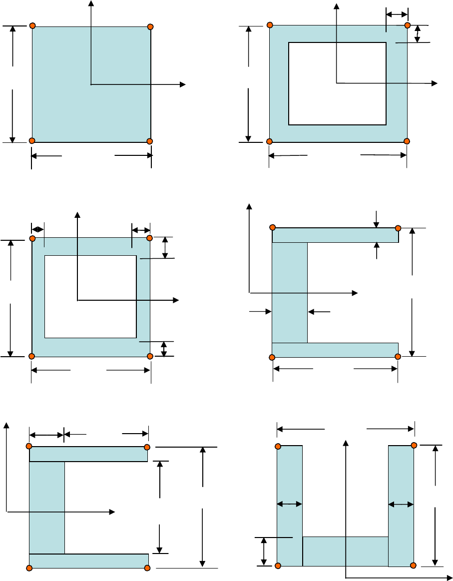
Ye
154
DIM2
Ye
Ze
TYPE = BAR
DIM1
C
D
E
F DIM3
TYPE = BOX
DIM2
DIM1
DIM4
Ze
C
F
D
E
Ze
DIM2
DIM5
DIM3
TYPE = BOX1
Ye
DIM4
DIM6
DIM1
C
D
E
F
TYPE = CHAN
DIM1
DIM2
Ze
Ye
DIM4
C
DIM3
D
E
F
Ze
Ye
DIM4
DIM3
DIM1
DIM2 DIM4
TYPE = CHAN1
C
D
E
F
DIM2
TYPE = CHAN2
Ye
Ze
DIM3
C
F
DIM1 DIM1
D
E
PBARL cross-section types – Fig 1 of 3
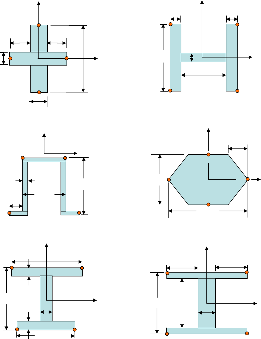
155
Ye
Ze
DIM3
DIM2
DIM4
DIM1
TYPE = HAT
C
D
E
F
Ze
Ye
DIM3
DIM2
DIM1
TYPE = HEX
C
D
E
F
Ye
Ze
Ye
Ze
0.5*DIM2
DIM3
0.5*DIM1
0.5*DIM1
DIM2
TYPE = CROSS
C
D
E
F
DIM4
DIM1
DIM3
C
D
E
F
TYPE = H
DIM4
Ze
Ye
DIM3
DIM1
DIM2
DIM6
DIM4
TYPE = I
C
D
E
F
DIM5
PBARL cross-section types – Fig 2 of 3
0.5*DIM2
Ye
Ze
0.5*DIM1
DIM3
DIM2
DIM4
C
D
E
F
0.5*DIM1
TYPE = I1
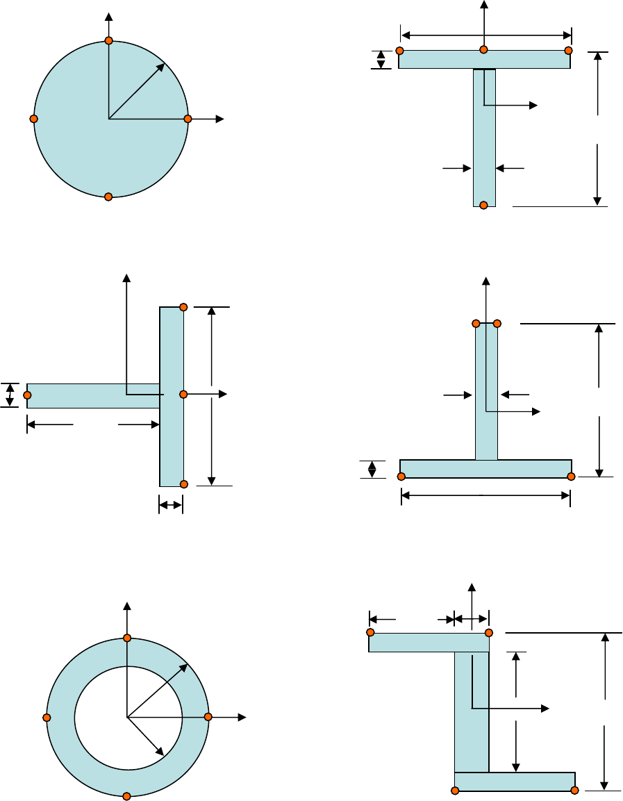
156
Ze
Ye
DIM2
DIM1
TYPE = TUBE
C
D
E
F
DIM1 DIM2
DIM3
DIM4
TYPE = Z
Ye
Ze
C
D
E
F
DIM1
DIM
DIM3
DIM4
Ye
Ze
TYPE = T1
C
D
E
F
TYPE = T2
DIM2
DIM1
Ye
DIM3
DIM4
Ze
C
D
E
F
DIM1
TYPE = ROD
Y
Ze
C
D
E
F
TYPE = T
DIM4
DIM3
DIM1
DIM2
Ye
Ze
C D
E
F
PBARL cross-section types – Fig 3 of 3

PBUSH
6.4.1.54 PBUSH
Description:
Property definition for a spring element defined by a CBUSH entry
Format:
1 2 3 4 5 6 7 8 9 10
PBUSH PID “K” K1 K2 K3 K4 K5 K6 +CONT1
+CONT1 “RCV” SA ST EA ET
Example:
PBUSH 136 K 10000. 20000. 30000. 4000. 50000. 60000. +PB1
+PB1 RCV 30. 40. .01 .02
Data Description:
Field Contents Type Default
PID Property ID number Integer > 0 None
“K” Indicates that the next 6 foelds are stiffness values Char None
Ki Stiffness values Real 0.
“RCV” Indicates that the next 4 values are stress/strain recovery
coefficients Real 0.
SA Stress recovery coefficient in the 3 translational directions
ST Stress recovery coefficient in the 3 rotational directions
EA Strain recovery coefficient in the 3 translational directions
ET Strain recovery coefficient in the 3 rotational directions
Remarks:
1. Element stresses and are calculated by multiplying element engineering forces times the RCV
coefficients
157
PCOMP
6.4.1.55 PCOMP
Description:
Property definition for a composite 2D plate/shell element made up of one or more plies
Format:
1 2 3 4 5 6 7 8 9 10
PCOMP PID Z0 NSM SB FT TREF GE LAM +CONT1
+CONT1 MID1 T1 THETA1 SOUT1 MID2 T2 THETA2 SOUT2 +CONT2
+CONT2 MID3 (etc)
Example:
PCOMP 136 -1.02 .0003 30000 TSAI 21. .002 SYM +PC1
+PC1 91 .02 30.
Data Description:
Field Contents Type Default
PID Property ID number Integer > 0 None
Z0 Distance from reference plane to bottom surface of the element Real Remark 2
NSM Non structural mass Real 0.
SB Allowable interlaminar shear stress Real 0.
FT Failure theory Char None
TREF Reference temperature Real 0.
GE Structural damping coefficient Real 0.
LAM Symmetric lamination option Char NONSYM
MIDi Ply material ID (MID1 must be specified) Integer Last one
Ti Ply thickness (T1 must be specified) Real Last one
THETAi Material angle of ply relative to element material axis Real 0.
SOUTi Not currently used in MYSTRAN
Remarks:
1. PID must be unique among all PCOMP/PSHELL property entries
2. The default for Z0 is 0.5 times the laminate thickness
3. The failure index for the interlaminar shear is the maximum transverse shear stress divided by SB
4. The allowable failure theories are FT = HILL, HOFF, TSAI or STRN
158
5. If LAM = SYM only plies on one side of the laminate are to be specified. If an odd number of plies are
desired with LAM = SYM then the center ply should have a thickness equal to one-half the actual
thickness.
6. The default for MIDi is the previous defined MID. The same holds true for Ti.
7. In order for a ply to be defined, at least one of the 4 ply fields on continuation entries must be present.
159
PCOMP1
6.4.1.56 PCOMP1
Description:
Property definition for a composite 2D plate/shell element made up of one or more plies where all plies
are the same thickness and same material
Format:
1 2 3 4 5 6 7 8 9 10
PCOMP1 PID Z0 NSM SB FT MID T LAM +CONT1
+CONT1 THETA1 THETA2 THETA3 etc
Example:
PCOMP 136 -1.02 .0003 30000 TSAI 21. .002 SYM +PC1
+PC1 91 .02 30.
Data Description:
Field Contents Type Default
PID Property ID number Integer > 0 None
Z0 Distance from reference plane to bottom surface of the element Real Remark 2
NSM Non structural mass Real 0.
SB Allowable interlaminar shear stress Real 0.
FT Failure theory Char None
MID Material ID for all plies Integer > 0 None
T Thickness for all plies Real 0.
LAM Symmetric lamination option Char NONSYM
THETAi Material angle of ply relative to element material axis Real 0.
Remarks:
1. PID must be unique among all PCOMP/PSHELL property entries
2. The default for Z0 is 0.5 times the laminate thickness
3. The failure index for the interlaminar shear is the maximum transverse shear stress divided by SB
4. The allowable failure theories are FT = HILL, HOFF, TSAI or STRN
5. If LAM = SYM only plies on one side of the laminate are to be specified. If an odd number of plies are
desired with LAM = SYM then the center ply should have a thickness equal to one-half the actual
thickness.
160
PELAS
6.4.1.57 PELAS
Description:
Stiffness definition for CELAS spring elements
Format:
1 2 3 4 5 6 7 8 9 10
PELAS PID K GE S
Example:
PELAS 63 1.55E6 .015
Data Description:
Field Contents Type Default
PID Property ID number Integer > 0 None
K Spring stiffness Real 0.
GE Damping coefficient Real 0.
S Stress recovery coefficient Real 0.
Remarks:
1. PID must be unique among all PELAS property entries
2. Stress is output for this element as S times the elongation of the spring.
161
PLOAD2
6.4.1.58 PLOAD2
Description:
Uniform pressure load for 2D bending plate elements
Format No. 1:
1 2 3 4 5 6 7 8 9 10
PLOAD2 SID P EID1 EID2 EID3 EID4 EID5 EID6
Format No. 2:
1 2 3 4 5 6 7 8 9 10
PLOAD2 SID P EID1 THRU EID2
Examples:
PLOAD2 267 .05 12 23 56 124 9789
PLOAD2 345 .167 269 THRU 9823
Data Description:
Field Contents Type Default
SID Load set ID number Integer > 0 None
P Pressure value Real 0.
EIDi ID numbers of elements that are to have this pressure as a load Integer > 0 None
Remarks:
1. A positive value of P will result in a pressure being applied in the positive direction of the local z axis
for the element (perpendicular to the elements’ average midplane)
2. If the THRU option is used EID2 must be greater than EID1. All elements whose ID’s are in the range
EID1 through EID2 will have the pressure load (if SID selected in Case Control directly or via the load
combining LOAD Bulk Data entry).
3. In order for this load to be used in a static analysis the load set ID must either be selected in Case
Control by LOAD = SID, or this load set ID must be referenced on a LOAD Bulk Data entry which
itself is selected in Case Control.
4. Up to six elements can have their pressure specified on one PLOAD2 entry in Format No 1. For more
elements, use additional PLOAD2 entries (i.e. there is no continuation entry for PLOAD2).
162
PLOAD4
6.4.1.59 PLOAD4
Description:
Pressure load on the face of 2D bending plate elements, CTRIA3, CTRIA3K, CQUAD4, CQUAD4K
Format No. 1:
1 2 3 4 5 6 7 8 9 10
PLOAD4 SID EID P1 P2 P3 P4
Format No. 2:
1 2 3 4 5 6 7 8 9 10
PLOAD4 SID EID1 P1 P2 P3 P4 THRU EID2
Examples:
PLOAD4 267 987 1.1 1.5 1.25 1.4
PLOAD4 345 101 2.4 2.25 2.1 2.0 THRU 200
Data Description:
Field Contents Type Default
SID Load set ID number Integer > 0 None
Pi Pressure value at up to 4 grid locations Real 0.
EIDi ID numbers of elements that are to have this pressure as a load Integer > 0 None
Remarks:
1. A positive value of P will result in a pressure being applied in the positive direction of the local z axis
for the element (perpendicular to the elements’ average midplane)
2. If the THRU option is used EID2 must be greater than EID1. All elements whose ID’s are in the range
EID1 through EID2 will have the pressure load (if SID selected in Case Control directly or via the load
combining LOAD Bulk Data entry).
3. In order for this load to be used in a static analysis the load set ID must either be selected in Case
Control by LOAD = SID, or this load set ID must be referenced on a LOAD Bulk Data entry which
itself is selected in Case Control.
4. If the fields for P2, P3 and/or P4 are blank that pressure is set equal to P1. P4 has no meaning for
triangular elements.
163
164

PLOTEL
6.4.1.60 PLOTEL
Description:
1 dimensional dummy element that only serves the purpose of plotting a line. It has no elastic properties
Format No. 1:
1 2 3 4 5 6 7 8 9 10
PLOTEL EID G1 G2
Example:
PLOTEL 63 1001 2365 .
Data Description:
Field Contents Type Default
EID Element ID number Integer > 0 None
Gi Grid point ID’s Integer > 0 None
Remarks:
1. EID must be unique among all element ID’s
2. This element does not result in any stiffness or mass. It’s purpose is only to plot a line between 2
grids
165
PROD
6.4.1.61 PROD
Description:
Property definition for ROD element
Format:
1 2 3 4 5 6 7 8 9 10
PROD PID MID A J C MPL
Example:
PROD 49 2 .175 .093 1.5 0.0175
Data Description:
Field Contents Type Default
PID Property ID number Integer > 0 None
MID Material ID number Integer > 0 None
A Bar cross-sectional area Real 0.
J Torsional constant Real 0.
C Torsional stress recovery coefficient Real 0.
MPL Mass per unit length Real 0.
Remarks:
1. PID must be unique among all PROD property entries
2. The torsional stress is calculated as:
t
M
CJ
where Mt is the torsional moment in the rod element.
166
PSHEAR
6.4.1.62 PSHEAR
Description:
Property definition for SHEAR element
Format:
1 2 3 4 5 6 7 8 9 10
PSHEAR PID MID T NSM
Example:
PSHEAR 49 2 .175 .093
Data Description:
Field Contents Type Default
PID Property ID number Integer > 0 None
MID Material ID number Integer > 0 None
T Shear panel thickness Real > 0. None
NSM Nonstructural mass per unit area Real 0.
Remarks:
1. PID must be unique among all PROD property entries
167
PSHELL
6.4.1.63 PSHELL
Description:
Property definition for 2D plate elements
Format:
1 2 3 4 5 6 7 8 9 10
PSHELL PID MID1 TM MID2 12I/TM**3 MID3 TS/TM MPA +CONT
+CONT Z1 Z2
Examples:
PSHELL 987 234 0.10 123 125. 45 20. .005 +ABC
+ABC 0.5 -0.5
PSHELL 78 234 0.10 234 45 +ABC
Data Description:
Field Contents Type Default
PID Property ID number Integer > 0 None
MID1 Material ID number for membrane material properties Integer > 0 or
blank None
TM Membrane thickness Real or blank 0.
MID2 Material ID number for bending material properties Integer > 0 or
blank None
12I/TM**3 Ratio of actual bending moment inertia (I) to bending inertia of a solid
plate of thickness TM Real or blank 1.0
MID3 Material ID number for transverse shear material properties Integer > 0 or
blank None
TS/TM Ratio of shear to membrane thickness Real or blank Remark 3
MPA Mass per unit area Real 0.
Z1, Z2 Distances from the neutral plane of the plate to locations where
stress is calcilated Real Remark 4
Remarks:
1. PID must be unique among all PSHELL property entries
2. Continuation entry is not required. If Z1 and Z2 are not input, then stresses are calculated at +/-TM/2.
3. Default value for TS/TM is 5/6 = 0.83333 unless a PARAM Bulk data entry with parameter name
TSTM_DEF is in the data file, in which case the TSTM_DEF value on the PARAM entry is used.
168
4. The following holds for the cases of MIDi blank:
If MID1 is blank, no membrane stiffness is calculated
If MID2 is blank, no bending or transverse shear stiffness is calculated
If MID3 is blank, no transverse shear flexibility is included (Kirchoff plate theory: plate is assumed
infinitely stiff in transverse shear) so that normals to the mid-plane remain normal after bending)
169
PSOLID
6.4.1.64 PSOLID
Description:
Property definition for 3D solid elements
Format:
1 2 3 4 5 6 7 8 9 10
PSOLID PID MID CID IN ISOP
Examples:
PSOLID 987 234 23 3 FULL
Data Description:
Field Contents Type Default
PID Property ID number Integer > 0 None
MID1 Material ID number for membrane material properties Integer > 0 or
blank None
CID Material coordinate system ID Integer or
blank 0.
IN Indicator for integration order (see table below) Integer = 2,3 2
ISOP Integration scheme (whether to use FULL or REDUCED integration Character REDUCED
Remarks:
1. See table below for values of IN and ISOP to use
170

PSOLID entries IN and ISOP for solid elements – only use ones that have comment: OK
(based on test runs by the author)
(bold, underline indicates default which can also be blank)
HEXA Integration IN ISOP Comments
2x2x2 reduced shear 2 REDUCED OK
2x2x2 standard isopar. 2 FULL or 1 (1)
3x3x3 reduced shear 3 REDUCED (1)
8 node
3x3x3 standard isopar 3 FULL or 1 (1)
2x2x2 reduced shear 2 REDUCED (2)
2x2x2 standard isopar. 2 FULL or 1 OK
3x3x3 reduced shear 3 REDUCED OK
20 node
3x3x3 standard isopar 3 FULL or 1 OK
PENTA Integration IN ISOP Comments
2x3 reduced shear 2 REDUCED OK
2x3 standard isopar. 2 FULL or 1 (1)
3x7 reduced Shear 3 REDUCED (1)
6 node
3x7 standard isopar 3 FULL or 1 (1)
2x3 reduced shear 2 REDUCED (2)
2x3 standard isopar. 2 FULL or 1 OK
3x7 reduced shear 3 REDUCED OK
15 node
3x7 standard isopar 3 FULL or 1 OK
TETRA Integration IN ISOP Comments
1 point standard isopar 2 FULL (1)
4 node 4 point standard isopar 3 FULL (1)
1 point standard isopar FULL (2)
10 node 4 point standard isopar 3 FULL OK
Notes: (1) Answers degrade for aspect ratio (AR) above AR =1
(2) Answers are nonsense
OK means answers are good
Reduced integration is used for shear strains to avoid shear locking. For HEXA 2x2x2 and PENTA 2x3
integration it uses selective substitution. For HEXA 3x3x3 reduced integration it uses 2x2x2 for shear. For
PENTA 3x7 reduced integration it uses 2x3 for shear
171

PUSERIN
6.4.1.65 PUSERIN
Description:
Property definition for CUSERIN elements
Format:
1 2 3 4 5 6 7 8 9 10
PUSERIN PID IN4_ID KNAME MNAME RBNAME PNAME
Examples:
PUSERIN 101 95 KRRGN MRRGN
Data Description:
Field Contents Type Default
PID Property ID number Integer > 0 None
IN4_ID ID of an Exec Control IN4 entry that specifies the NASTRAN
formatted INPUTT4 file containing the stiffness and mass matrices
(whose name are KNAME, MNAME)
Integer > 0 or
blank None
KNAME Name of the stiffness matrix which was written to the INPUTT4 file
when it was created. This can be up to 8 characters long Char None
MNAME Name of the mass matrix which was written to the INPUTT4 file
when it was created. This can be up to 8 characters long Char None
RBNAME Name of a 6x6 rigid body mass matrix which specifies the rigid body
mass relative to the C.G. of the CUSERIN element in its basic
coordinate system. This can be up to 8 characters long
Char None
PNAME Name of the load matrix which was written to the INPUTT4 file when
it was created. This can be up to 8 characters long. Char None
Remarks:
1. PID must be unique among all PUSERIN property entries
2. IN4_ID is required. In the example above, an Exec Control entri IN4 with ID = 234 is required
3. The matrix whose name is RBNAME is not required. However, the rigid body mass properties
(PARAM GRDPNT) for the overall model will be in error unless the element has the same basic
coordinate system as the overall model.
4. The matrix whose name is PNAME is only used for statics solutions.
172
RBE2
6.4.1.66 RBE2
Description:
Rigid element that has specified components at a number of grids dependent on the six degrees
of freedom at one other grid.
Format:
1 2 3 4 5 6 7 8 9 10
RBE2 EID GN CM GM1 GM2 GM3 GM4 GM5 +CONT
+CONT GM6 GM7 (etc)
Example:
RBE2 43 1021 346 1031 1033 1035 1041 1043 +REL01
+REL01 1045
Data Description:
Field Contents Type Default
EID Element ID number Integer > 0 None
GN ID number of the grid that will have all 6 components as the 6
independent degrees of freedom for this rigid element Integer > 0 None
CM The component numbers of the dependent degrees of freedom at grid
points GMi Integers 1-6 None
GMi The components CM at grids GMi are the dependent degrees of
freedom that will be eliminated due to this rigid element Integer > 0 None
Remarks:
1. No other element in the model may have the same element ID
2. All of the degrees of freedom defined by components CM at each of the grids GMi are made
members of the M-set and their displacements will be rigidly dependent on the six degrees of
freedom at grid GN.
3. Dependent degrees of freedom defined by RBE2 elements can not be defined as members of any
other mutually exclusive set (i.e., cannot appear on SPC, SPC1, OMIT, OMIT1, ASET or ASET1
entries, nor can they appear as dependent degrees of freedom on other rigid elements)
173
RBE3
6.4.1.67 RBE3
Description:
Element used to distribute loads or mass from one grid point (denoted as the dependent grid) to
other grids in the model. The element is defined based on the grids/components that it
connects. The resulting multi-point constraints (MPC’s) generated internally in MYSTRAN, will
eliminate the dependent degrees of freedom and will distribute any loads or mass from the
dependent grid to the remaining grids defined on the RBE3. Unlike the NASTRAN RBE3, the
MYSTRAN RBE3 does not support the “UM” option at the current time
Format:
1 2 3 4 5 6 7 8 9 10
RBE3 EID REFGRID REFC WT1 C1 G1,1 G1,2 +1
+1 G1,3 WT2 C2 G2,1 G2,2 G2,3 G2,4 WT3 +2
+2 C3 G3,1 G3,2 etc
Example:
RBE3 43 9001 123456 1.0 123 1001 1002 +R1
+R1 1003 1004
Data Description:
Field Contents Type Default
EID Element ID number Integer > 0 None
REFGRID Grid that will be the dependent (or reference) grid Integer > 0 None
REFC The component numbers of the dependent degrees of freedom at grid
point REFGRID Integers 1-6 None
WTi Weighting factors for the grids/components that follow Real None
Ci Displacement components at the following Gi,j that have weighting
factor WTi Integers 1-6 None
Gi,j Grids that REFGRID depend on Integer > 0 None
Remarks:
1. No other element in the model may have the same element ID
2. Fpr most applications only the translation displacement components (1,2,3) should be defined for the
Ci. If REFGRID and a Gi,j are coincident then rotation components (4,5,6) can be defined for Ci.
3. Dependent degrees of freedom defined by RBE3 elements can not be defined as members of any
other mutually exclusive set (i.e., cannot appear on SPC, SPC1, OMIT, OMIT1, ASET or ASET1
entries, nor can they appear as dependent degrees of freedom on other rigid elements)
174

RFORCE
6.4.1.68 RFORCE
Description:
Defines rigid body rotational velocity, and optional rotational acceleration, of the model about some
specified grid for the purpose of generating inertia forces on the finite element model.
Format:
1 2 3 4 5 6 7 8 9 10
RFORCE SID GID CID V N1 N2 N3 +RF1
+RF1 A
Example:
Data Description:
Field Contents Type Default
SID Load set ID number (must be selected in Case Control) Integer > 0 None
GID ID of the grid at which this concentrated moment acts Integer >0 None
CID ID of the coordinate system in which the Ni are specified Integer >= 0 0
V An overall scale factor for the angular velocity in revolutions per unit
time Real 0.
Ni Components of a vector in the direction of the angular velocity and
angular acceleration Real 0.
A An overall scale factor for the angular acceleration in revolutions per
unit time squared Real 0.
Remarks:
1. The force at grid i due to the angular velocity and acceleration is:
(( ) ( )
where
= grid point
6x6 mass matrix at grid i
= rigid body angular velocity of the model
= rigid body angular acceleration of the model
= distance from basic system or
i i ia ia
i
i
FM rrarr
i
M
a
r
igin to grid i
= distance from basic system origin to reference grid about which the model rotates
a
r
175
2. The load set ID (SID) is selected by the Case Control entry LOAD:
3. GID = 0 signifies that the rotation vector acts through the basic system origin.
4. CID = 0 indicates that the rotation vector is defined in the basic coordinate system
176
RSPLINE
6.4.1.69 RSPLINE
Description:
Interpolation element. A spline fit using the 2 independent end points (GI1, GI2) is applied to
the locations of the dependent points (defined by GDi/CDi) to rigidly constrain the GDi/CDi
Format:
1 2 3 4 5 6 7 8 9 10
RSPLINE EID GI1 GD1 CD1 GD2 CD2 GD3 +CONT
+CONT CD3 GD4 CD4 etc GI2
Example:
RBE2 43 1001 2001 123456 2002 123456 2003 +REL01
+REL01 123456 2004 123456 2005 123456 1002
Data Description:
Field Contents Type Default
EID Element ID number Integer > 0 None
GIi Grid numbers of the 2 independent end points Integer > 0 None
GDi Grid numbers of the dependent grtids Integers > 0 None
CDi Displacement component numbers at the GDi Integer 1-6 None
Remarks:
1. No other element in the model may have the same element ID
2. Displacements at the GDi are interpolated using the following rules applied to the line between the 2
end ponts:
Displacenents along the line and rotations about the line are linear
Displacements perpendicular to the line are cubic
Rotations normal to the line are quadratic
177

SEQGP
6.4.1.70 SEQGP
Description:
Manual re-sequencing of grids
Format:
1 2 3 4 5 6 7 8 9 10
SEQGP G1 S1 G2 S2 G3 S3 G4 S4
Example:
SEQGP 1001 1.5 1011 1. 1021 2. 1031 3.5
Data Description:
Field Contents Type Default
Gi ID number of a grid point Integer > 0 None
Si The sequence number for Gi Integer or Real > 0 None
Remarks:
1. The SEQGP entry is used to manually re-sequence grids. See the Bulk Data PARAM GRIDSEQ
entry for the starting sequence MYSTRAN uses in manual grid sequencing.
2. Either integer or real sequence numbers are allowed but all are converted to real internally. Thus, if
the user has two grids sequenced consecutively, say with integer sequence numbers 10 and 11, then
some other grid can be inserted in the sequence between the two with a real sequence number
anywhere in the range:
10. < Si < 11.
3. Up to four pairs of Gi, Si can be specified on one SEQGP entry. For more pairs, use additional
SEQGP entries (i.e. there is no continuation entry for SEQGP).
4. If automatic grid point sequencing by BANDIT, any used defined SEQGP entries are ignored.
178

SLOAD
6.4.1.71 SLOAD
Description:
Defines the existence of a scalar load on a scalar point
Format:
1 2 3 4 5 6 7 8 9 10
SLOAD SID Si FMAG
Example:
SPOINT 56 101 125.6
Data Description:
Field Contents Type Default
SID Load set ID number Integer > 0 None
Si Scalar point ID Integer > 0 None
FMAG Magnitude of the orce on scalar point Si Real 0.
Remarks:
1. In order for this load to be used in a static analysis the load set ID must either be selected in Case
Control by LOAD = SID, or this load set ID must be referenced on a LOAD Bulk Data entry which
itself is selected in Case Control.
179
SPC
6.4.1.72 SPC
Description:
Single point constraints that are defined by specifying the degree of freedom and its
displacement (either zero or some enforced nonzero value)
Format:
1 2 3 4 5 6 7 8 9 10
SPC SID G1 C1 D1 G2 C2 D2
Example:
SPC 56 101 3 1.2E-3 201 2 0.0
Data Description:
Field Contents Type Default
SID ID number of the single point constraint set Integer > 0 None
GI ID numbers of the grids that will have component number Ci
constrained Integer > 0 None
CI Component numbers at grids Gi that will be constrined Integers 1-6 None
DI The value for the displacement at grid Gi, component Ci Real 0.
Remarks:
1. Single point constraint sets must be selected in Case Control with the entry SPC = SID in order for
them to be applied.
2. Degrees of freedom defined on SPC entries will be members of the S-set and cannot be defined as
being members of any other mutually exclusive set.
2. Up to two gid/component pairs can be specified as being single point constrained on one SPC entry
(i.e. continuation entries are not allowed). Additional SPC entries can have the same SID.
3. If a Gi/Ci pair is constrained more than once (with the same SID), the last value read for Di will be
used.
4. A degree of freedom may be specified redundantly as a permanent single point constraint on a GRID
Bulk Data entry and on an SPC or SPC1 Bulk Data entry. If it is defined on the GRID entry and on an
SPC Bulk Data entry, Di must be zero on the SPC entry or a fatal error will occur.
180
SPC1
6.4.1.73 SPC1
Description:
Single point constraints that are defined by specifying the degree of freedom to be constrained
to zero displacement.
Format No. 1:
1 2 3 4 5 6 7 8 9 10
SPC1 SID C G1 G2 G3 G4 G5 G6 +CONT
+CONT G7 G8 G9 (etc)
Format No. 2:
1 2 3 4 5 6 7 8 9 10
SPC1 SID C G1 THRU G2
Examples:
SPC1 52 135 1001 1002 103 1004 2001 2002 +SZA
+SZA 2003 2004
SPC1 52 135 1001 THRU 1004
SPC1 52 135 2001 THRU 2004
Data Description:
Field Contents Type Default
SID ID number of the single point constraint set Integer > 0 None
C Component numbers at grids Gi that will be constrained Integers 1-6 None
GI ID numbers of the grids that will have component number Ci
constrained Integer > 0 None
DI The value for the displacement at grid Gi, component Ci Real 0.
Remarks:
1. Single point constraint sets must be selected in Case Control with the entry SPC = SID in order for
them to be applied.
2. Degrees of freedom defined on SPC entries will be members of the S-set and cannot be defined as
being members of any other mutually exclusive set.
3. For format 2, all grids in the model that are in the range G1 through G2 will have component C
constrained
4. A degree of freedom may be specified redundantly as a permanent single point constraint on a GRID
Bulk Data entry and on an SPC or SPC1 Bulk Data entry.
181
SPCADD
6.4.1.74 SPCADD
Description:
Combine single point constraint sets defined on SPC, SPC1 entries
Format:
1 2 3 4 5 6 7 8 9 10
SPCADD SID S1 S2 S3 S4 S5 S6 S7 +CONT
+CONT S8 S9 (etc)
Example:
SPCADD 283 11 74 123 564
Data Description:
Field Contents Type Default
SID Single point constraint set ID number Integer > 0 None
Si Set IDs of SPC and/or SPC1 Bulk Data entries Integer > 0 None
Remarks:
1. Single point constraint sets must be selected in Case Control with the entry SPC = SID in order for
them to be applied.
4. All single point constraints specified on the SPC and/or SPC1 entries whose set IDs are the Si on the
SPCADD will be applied to the model if SPC = SID is in Case Control.
182

SPOINT
6.4.1.75 SPOINT
Description:
Defines the existence of a scalar point (1 component of displacement) in the model
Format 1:
1 2 3 4 5 6 7 8 9 10
SPOINT ID1 ID2 ID3 ID4 ID5 ID6 ID7 ID8 +S01
+S01 ID9 etc
Format 2:
1 2 3 4 5 6 7 8 9 10
SPOINT ID1 THRU ID2
Example:
SPOINT 56 101 3 1.2E-3 201 2 0.0
Data Description:
Field Contents Type Default
IDi ID of an SPOINT Integer > 0 None
Remarks:
1. SPOINT ID’s must be unique among all other SPOINT’s and among all GRID’s
2. SPOINT’s are like GRID’s but have only 1 component of displacement and their outputs are scalar, not
vector, quantities. In the F06 output file, however, the output quantities are reported under the T1
headings.
183
SUPORT
6.4.1.76 SUPORT
Description:
Defines degrees of freedom that are to be in the R-set (for Craig-Bampton model generation)
Format:
1 2 3 4 5 6 7 8 9 10
SUPORT GID C GID C GID C GID C
Example:
SUPORT 4981 12 695 123 5647 456
Data Description:
Field Contents Type Default
GID ID of a grid whose components in the next field will be put into the
R-set Integer > 0 None
C Displacement component numbers (digits 1 through 6) Integer > 0 None
Remarks:
1. This Bulk Data entry is meant for use in Craig-Bampton analyses. The degrees of freedom specified
on this entry will be treated the same as Single Point Constraints (SPC’s) in all other analyses
184
TEMP
6.4.1.77 TEMP
Description:
Grid point temperature definition for purposes of calculating thermal loads on the model.
Format:
1 2 3 4 5 6 7 8 9 10
TEMP SID G1 T1 G2 T2 G3 T3
Example:
TEMP 4 1011 25. 1012 32. 1013 28.
Data Description:
Field Contents Type Default
SID ID number of the temperature set Integer > 0 None
GI ID numbers of the grids whose temperature is being defined Integer > 0 None
Ti Temperature of grid Gi Real 0.
Remarks:
1. Temperature sets must be selected in Case Control with the entry TEMP = SID in order for them to
be used in calculating thermal loads
2. Every element in the model must have its temperature defined for set SID, either explicitly through an
element temperature entry on TEMPRB, TEMPP1 Bulk Data entry or implicitly using grid
temperatures on TEMP, TEMPD Bulk Data entries. Element temperatures defined on element
TEMPRB, TEMPP1 entries take precedence over any that might be defined using grid temperatures.
If no element temperature is explicitly defined, the element temperature is taken to be the average of
the temperatures of the grids to which the element is connected.
3. Thermal loads for the model are calculated using element temperatures defined via TEMP, TEMPD,
TEMPRB, TEMPP1 Bulk data entries, the element properties and the material properties (including
coefficient of thermal expansion and reference temperature). The thermal loads calculated are based
on element temperatures that are the difference between those defined on TEMP, TEMPD, TEMPRB,
TEMPP1 and the reference temperature defined on the material entry for the element.
4. Only three grids may have their temperature defined for set SID in one TEMP entry. Additional grid
temperatures can be specified using more TEMP Bulk Data entries with the same SID.
185
TEMPD
6.4.1.78 TEMPD
Description:
Default grid point temperature definition for purposes of calculating thermal loads on the model.
Format:
1 2 3 4 5 6 7 8 9 10
TEMP SID1 T1 SID2 T2 SID3 T3 SID4 T4
Example:
TEMP 4 46.2 33 52.1
Data Description:
Field Contents Type Default
SIDi ID number of a temperature set Integer > 0 None
Ti The default temperature for grids for set SIDi Real 0.
Remarks:
1. Temperature sets must be selected in Case Control with the entry TEMP = SID in order for them to
be used in calculating thermal loads
2. All grids whose temperature is not defined on a TEMP Bulk Data entry will have the default
temperature T, if there is one defined on a TEMPD for set SID.
3. Every element in the model must have its temperature defined for set SID, either explicitly through an
element temperature entry on TEMPRB, TEMPP1 Bulk Data entry or implicitly using grid
temperatures on TEMP, TEMPD Bulk Data entries. Element temperatures defined on element
TEMPRB, TEMPP1 entries take precedence over any that might be defined using grid temperatures.
If no element temperature is explicitly defined, the element temperature is taken to be the average of
the temperatures of the grids to which the element is connected.
4. Thermal loads for the model are calculated using element temperatures defined via TEMP, TEMPD,
TEMPRB, TEMPP1 Bulk data entries, the element properties and the material properties (including
coefficient of thermal expansion and reference temperature). The thermal loads calculated are based
on element temperatures that are the difference between those defined on TEMP, TEMPD, TEMPRB,
TEMPP1 and the reference temperature defined on the material entry for the element.
5. Only four pairs of SIDi/Ti may be defined on one TEMPD entry. Additional pairs can be specified
using more TEMPD Bulk Data entries.
186
TEMPP1
6.4.1.79 TEMPP1
Description:
Defines temperatures and temperature gradients for 2D plate elements.
Format No. 1:
1 2 3 4 5 6 7 8 9 10
TEMPP1 SID EID1 TBAR TPRIME +CONT
+CONT EID2 EID3 EID4 EID5 (etc)
Format No. 2:
1 2 3 4 5 6 7 8 9 10
TEMPP1 SID EID1 TBAR TPRIME +CONT
+CONT EID2 THRU EID3 EID4 THRU EID5
Examples:
TEMPP1 13 2101 35.7 10.1 +TP1
+TP1 2679 3201 1104 32 5555
TEMPP1 13 2101 35.7 10.1 +TP1
+TP1 2304 THRU 6789 12 THRU 46
Data Description:
Field Contents Type Default
SID ID number of the temperature set Integer > 0 None
EIDi Element ID numbers Integer > 0 None
TBAR Average temperature of the element Real 0.
TPRIME Linear thermal gradient through the thickness of the element Real 0.
Remarks:
1. Any number of continuation entries can be used
2. For format number 2, the THRU ranges must have the second element ID greater than the first.
3. Temperature sets must be selected in Case Control with the entry TEMP = SID in order for them to
be used in calculating thermal loads.
4. Every element in the model must have its temperature defined for set SID, either explicitly through an
element temperature entry on TEMPRB, TEMPP1 Bulk Data entry or implicitly using grid
temperatures on TEMP, TEMPD Bulk Data entries. Element temperatures defined on element
TEMPRB, TEMPP1 entries take precedence over any that might be defined using grid temperatures.
187
If no element temperature is explicitly defined, the element temperature is taken to be the average of
the temperatures of the grids to which the element is connected.
5. Thermal loads for the model are calculated using element temperatures defined via TEMP, TEMPD,
TEMPRB, TEMPP1 Bulk data entries, the element properties and the material properties (including
coefficient of thermal expansion and reference temperature). The thermal loads calculated are based
on element temperatures that are the difference between those defined on TEMP, TEMPD, TEMPRB,
TEMPP1 and the reference temperature defined on the material entry for the element.
188
TEMPRB
6.4.1.80 TEMPRB
Description:
Defines temperatures and temperature gradients for 1D bar elements.
Format No. 1:
1 2 3 4 5 6 7 8 9 10
TEMPRB SID EID1 TA TB TP1A TP1B TP2A TP2B +CONT
+CONT EID2 EID3 EID4 EID5 (etc)
Format No. 2:
1 2 3 4 5 6 7 8 9 10
TEMPRB SID EID1 TA TB TP1A TP1B TP2A TP2B +CONT
+CONT EID2 THRU EID3 EID4 THRU EID5
Examples:
TEMPRB 13 2101 35.7 10.1 +TP1
+TP1 67 89 2 13 1 789
TEMPRB 13 2101 35.7 10.1 +TP1
+TP1 68 THRU 97 2101 THRU 4009
Data Description:
Field Contents Type Default
SID ID number of the temperature set Integer > 0 None
EIDi Element ID numbers Integer > 0 None
TA Average temperature of the element at end a Real > 0. 0.
TB Average temperature of the element at end b Real > 0. 0.
TP1A Linear temperature gradient in element y axis at end a Real 0.
TP1B Linear temperature gradient in element y axis at end b Real 0.
TP2A Linear temperature gradient in element z axis at end a Real 0.
TP2B Linear temperature gradient in element z axis at end b Real 0.
Remarks:
1. Any number of continuation entries can be used
2. For format number 2, the THRU ranges must have the second element ID greater than the first
3. Temperature sets must be selected in Case Control with the entry TEMP = SID in order for them to
be used in calculating thermal loads
189

4. Every element in the model must have its temperature defined for set SID, either explicitly through an
element temperature entry on TEMPRB, TEMPP1 Bulk Data entry or implicitly using grid
temperatures on TEMP, TEMPD Bulk Data entries. Element temperatures defined on element
TEMPRB, TEMPP1 entries take precedence over any that might be defined using grid temperatures.
If no element temperature is explicitly defined, the element temperature is taken to be the average of
the temperatures of the grids to which the element is connected.
5. Thermal loads for the model are calculated using element temperatures defined via TEMP, TEMPD,
TEMPRB, TEMPP1 Bulk data entries, the element properties and the material properties (including
coefficient of thermal expansion and reference temperature). The thermal loads calculated are based
on element temperatures that are the difference between those defined on TEMP, TEMPD, TEMPRB,
TEMPP1 and the reference temperature defined on the material entry for the element.
6. The average temperatures TA and TB at ends a and b respectively are:
a
A
b
A
1
TA= T (y,z)dA
A
1
TB= T (y,z)dA
A
where A is the cross-sectional area and Ta(y,z) and Tb(y,z) are the temperature distributions at ends a
and b respectively.
7. The linear gradients through the thickness, TP1A, TP1B, TP2A and TP2B, are:
a
A
b
A
a
A
b
A
1
TP1A= T (y,z)ydA
I1
1
TP1B= T (y,z)ydA
I1
1
TP2A= T (y,z)zdA
I2
1
TP2B= T (y,z)zdA
I2
where I1 and I2 are the bending moments of inertia for the bar (on the PBAR entry) and Ta(y,z) and
b(y,z) are the temperature distributions at ends a and b respectively. T
190
USET
6.4.1.81 USET
Description:
Defines a set of degrees of freedom that belong to a user defined set (named either “U1” or
“U2”). The purpose is for the user to get an output listing that defines the internal degree of
freedom order for the members of the set.
Format:
1 2 3 4 5 6 7 8 9 10
USET NAME G1 C1 G2 C2 G3 C3
Example:
USET U1 101 3 201 2
Data Description:
Field Contents Type Default
NAME A user defined set. The name must be either “U1” or “U2” Char None
GI ID numbers of the grids that the user wants to be members of the set Integer > 0 None
CI Component numbers at grid Gi that will be members of the set Integers 1-6 None
Remarks:
1. The Gi, Ci are defined as members of the displacement set named SNAME.
2. A row oriented tabular output showing the internal sort order of the members of the set (named
SNAME) can be output if a PARAM, USETSTR, Ui Bulk Data entry is present (I = 1 or 2).
3. In order to get a listing of the internal sort order, a Bulk Data PARAM, USETSTR, Ui (i=1 or 2) must
be included
191
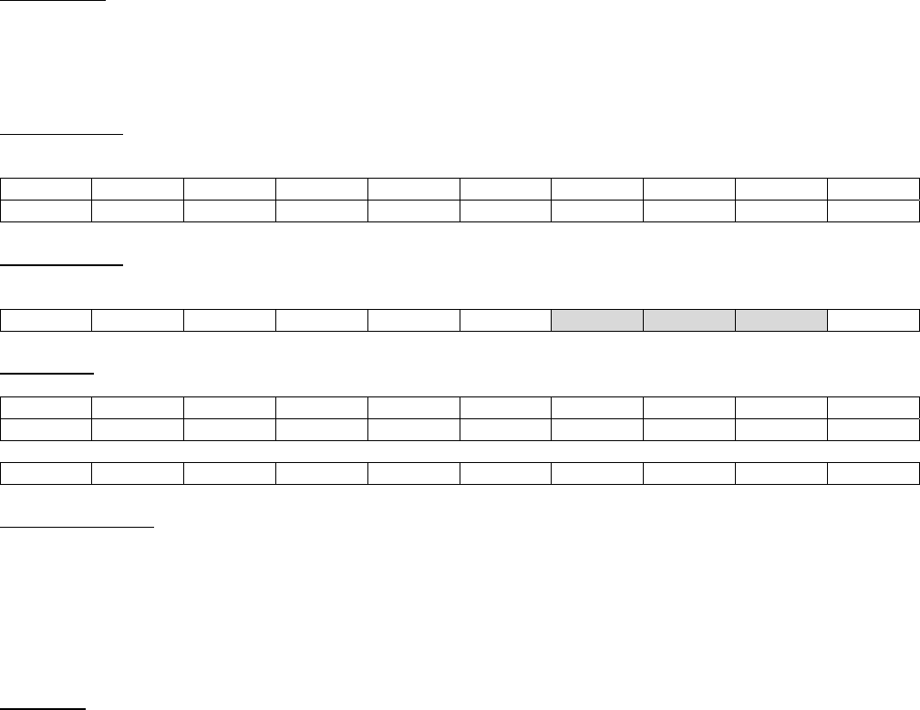
192
USET1
6.4.1.82 USET1
Description:
Defines a set of degrees of freedom that belong to a user defined set (named either “U1” or
“U2”). The purpose is for the user to get an output listing that defines the internal degree of
freedom order for the members of the set.
Format No. 1:
1 2 3 4 5 6 7 8 9 10
USET1 SNAME C G1 G2 G3 G4 G5 G6 +CONT
+CONT G7 G8 G9 (etc)
Format No. 2:
1 2 3 4 5 6 7 8 9 10
USET1 SNAME C G1 THRU G2
Examples:
USET1 U2 135 1001 1002 103 1004 2001 2002 +SZA
+SZA 2003 2004
USET1 U2 135 1001 THRU 1004
Data Description:
Field Contents Type Default
SNAME A user defined set. The name must be either “U1” or “U2” Char None
GI ID numbers of the grids that are members of the user defined set Integers 1-6 None
C Component numbers at grids Gi that are part of the user defined set Integer > 0 None
Remarks:
1. The Gi, C are defined as members of the displacement set named SNAME.
2. A row oriented tabular output showing the internal sort order of the members of the set (named
SNAME) can be output if a PARAM, USETSTR, Ui Bulk Data entry is present (I = 1 or 2).
3. In order to get a listing of the internal sort order, a Bulk Data PARAM, USETSTR, Ui (i=1 or 2) must
be included
7 Appendix A: MYSTRAN Sample Problem
193
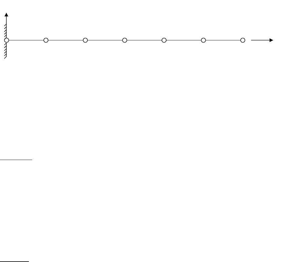
This example problem shows the input and output for a simple rod with 7 grids and 6 elements. The rod
is subjected to loads in two subcases as described below:
Z0, X13
The basic coordinate system is the X0, Y0, Z0 system shown (with X0 in the direction of Yo cross Z0). In
addition, rectangular coordinate system X13, Y13, Z13 (with X13 in the same direction as Z0) is also shown
and will be used in the input data in order to help explain the use of coordinate systems. The basic
system does not have to be defined explicitly. It is implied through the model grid coordinates and any
other coordinate systems (other than basic) which might be referenced in field 3 of the Bulk Data GRID
entry. Coordinate system 13 must be defined via a CORD2R Bulk data entry.
The grid point IDs are 101-701 and the rod element IDs are 1-6. The total length is 60 inches consisting
of 6 elements of 10 inches each. All of the rods have the same cross-sectional area of 0.6 inch2. The
material is aluminum with a Young’s modulus of 1x10⁷. The model is constrained at the left end. Several
loads are applied in two subcases.
Subcase 35 consists of a 120 lb load at grid 701
Subcase 8 consists of a 240 lb load at grid 201, a 150. Lb load at grid 301 and a 200 lb load at grid 401
Yo, Z13
6
5
4
3 2 1
701
601
501 401
301
201
101
101
201
301
401
501
601
701
P0.
P0.
P0.
PP 0.
P0.
P0.
P120.
101
201
301
401
501
601
701
P0.
P240.
P150.
PP 200.
P0.
P0.
P0.
194

The output, which includes an echo of the input data deck, is shown on the following pages. Note the
following about the OUTPUT:
The input data consists of everything from the ID entry through the ENDDATA entry, and
consists of the Executive Control, Case Control and Bulk Data Decks. Entries that begin with
a $ sign (and have anything after $ in the entry) are commentary and are ignored.
The Executive Control Deck begins with the optional ID entry, has the mandatory
SOL entry (1 for statics) and ends with the mandatory CEND entry. All Executive
Control entries are free field in that they may be anywhere within the 80 columns of
an entry.
The Case Control Deck begins with the entry following CEND (which in this case is a
TITLE Case Control entry) and ends with the mandatory BEGIN BULK entry. The
entries in between can be in any order that makes sense. That is, if there are no
subcases, the data can be in any order. When there are subcases, as is the case for
this example, the entries between one SUBCASE entry and another apply only to
that subcase. Anything “above” the subcase level pertains to all subcases, unless
overridden in a subcase. All Case Control entries are free field.
The SPC = 19 entry requests that a Bulk Data SPC (or SPC1, SPCADD) with
set ID = 19 be used in defining the single point constraints for the model.
The following three entries request various outputs (displacements, etc) with
ALL meaning that displacements for all grids (DISP = ALL), applied loads for
all grids (OLOAD = ALL) and forces of single point constraint (SPCF = ALL).
As these are “above” the subcase ;evel, they apply to all subcases (unless a
subcase requests output of the same type for a different set of grids or
elements)
Subcase 35 (the first subcase in Case Control) is defined with its own subtitle
and with LOAD = 191 requesting that a Bulk Data entry with set ID of 191
define the loads for this subcase (which requires that the load be defined on
a LOAD, FORCE, MOMENT, GRAV od PLOAD2 Bulk Data entry). In this
case, Bulk Data entry FORCE with a set ID od 191 contains the load
definition for this subcase. Element engineering force and stress output is
requested for this subcase (in addition to the requests above the subcase
level). .
Subcase 8 (the second subcase in Case Control) is defined with its own
subtitle (notice the order doesn’t matter) and requesting load set 26 in Bulk
Data to define the load. There is also another output request (for nodal
element forces) for set 98. Set 98 is defined as 2,5. Since set 98 output is
requested as element forces, the 2,5 is interpreted as the element numbers
for which nodal element forces will be output in this subcase only. If the
request had been above the subcase level (as DISP = ALL, etc) the request
would have been honored for both subcases.
The Bulk Data Deck begins with the entry immediately following BEGIN BULK and
ends with the mandatory ENDDATA entry. The logical entries in between can be in
any order with the exception that any one logical entry must be in order. Thus the
MAT1 logical entry, which has one parent entry and one continuation entry must be
entered together and in the order shown.
195
Coordinate system 13 is defined on the CORD2R Bulk Data entry with 13 as
the coordinate system ID in field 2. The reference system in field 3 is, in this
case, the basic system. It does not have to be. Coordinate system 13 could
use some other coordinate system as its reference, and so on. However, the
last system in the chain would have to have the basic system as its
reference. The nine real numbers on the remainder of the CORD2R logical
entry describe three points in coordinates of the reference (basic) system.
The first three numbers are the coordinates of the origin of coordinate system
13, which is at the origin of the basic system. The next three numbers are
the coordinates of a point on the Z13 axis, which is in the direction of the Y0.
The next three numbers (on the continuation entry) are the coordinates of a
point in the X13 – Z13 plane. Thus it is seen that this CORD2R entry
describes coordinate system 13 as seen on the figure above.
The seven grid points of the model are defined on the GRID entries. Note
that field 3 (coordinate systems for grid coordinates) is blank indicating the
basic coordinate system for grid locations for all seven grids. Field 7, the
global coordinate system for each grid is also the basic system for grids 101
through 601. Grid 701, however uses coordinate system 13 as its global
system. Field 8 of the GRID entries is for “permanent” single point
constraints. Note that 13456 are the permanent single point constraints for
grids 101 - 601. Since the rod can only take axial load and torque, only
global degrees of freedom that are for displacement along the rod, or rotation
about its axis can possibly have stiffness. Since grids 101 - 601, have the
basic system as global, degrees of freedom 1346 will be singular and must
therefore be removed via single point constraints at these grids. In addition,
since the PROD entry has zero torsional constant (field 4 of PROD is blank),
there will be no stiffness for global degree of freedom 5 at grids 101 - 601.
Thus, field 7 of the grid 101 - 601 entries have 13456 constrained. These
constraints do not have to appear on the GRID entry, they can be on SPC (or
SPC1) entries as well. Because they appear on the GRID entry these
constraints will be used regardless of whether an SPC = SID entry appears
in Case Control. Grid 701, on the other hand, uses coordinate system 13 as
its global coordinate system. Thus, by the same reasoning as above, global
degrees of freedom 12456 are taken as permanent single point constraints.
The connection entries for the rod elements are the six CROD’s whose
element IDs are indicated in field 2. Field 3 (with 16 in it) is the property ID
and points to the PROD, ID = 16) for the rod elements properties, which are
all the same in this example. Fields 4 and 5 give the grids to which the
elements are attached.
The PROD 16 entry points to a material entry (ID = 20) in field 3 and gives
the rod cross-sectional area in field 4.
The material properties are defined on the MAT1 with ID = 20. Only Young’s
modulus is needed for this example but a material density of 0.1 is also
entered in field 6.
Case Control had a request for single point constraint set. The SPC entry,
with set ID 19, specifies the remaining constraint of zero displacement in
global degree of freedom 2 at grid 101. This could have been included with
the constraints specified in field 7 of the GRID 101 entry, in which case the
SPC = 19 would not have been needed in Case Control.
196
Case Control had a request for load set 191 for subcase 35. The FORCE
Bulk Data entry with ID = 191 is the ID requested for this subcase and
defines a 120 lb load at grid 701. The coordinate system for this load
definition is coordinate system 13 (indicated by the 13 in field 4). Since the
components of the load vector are 0., 0., 1. (fields6-8) this indicates a force in
the Z13 direction which is along the axis of the rod.
Case Control also had a request for load set 26 for subcase 8. As shown
above, this loading condition has axial loads on three grid points. As such,
these could have been defined using three FORCE Bulk Data entries, all with
set ID = 26. However, the LOAD (load combining) Bulk Data entry will be
used for illustrative purposes. The LOAD entry has set ID = 26 which is the
ID requested for this subcase. It defines a load that is a linear combination of
load sets 39, 5 and 178, where the loads for sets 39, 5 and 178 are specified
on the FORCE Bulk Data entries below the LOAD 26 entry. The linear
combination on LOAD 26 is:
set 26 set 39 set 5 set178
0.
240.
150.
P2(4P3PP)
200.
0.
0.
0.
erator
alculate the total model mass properties relative to grid point 101.
The PARAM PRTDOF 1 requests printing of the degree of freedom table.
The ENDDATA signifies the end of the Bulk Data Deck.
er of the output for the sample problem is shown on the pages following the
ENDDATA
f page lists some informational messages printed out as MYSTRAN
executes.
AM
t
01 –
as its
the global system for this grid is
coordina stem 13, is in the Z direction
um material of
which the rod is made. Thus, the units for the GPWG output are lb.
The PARAM GRDPNT 101 requests that the Grid Point Weight Gen
c
The remaind
The next o
The degree of freedom table is printed as requested via the Bulk Data PAR
PRTDOF entry. It shows the degree of freedom numbers for each of the
displacement sets and is in internal degree of freedom order. Note on this listing tha
the A-set (analysis set) has six degrees of freedom and these are the axial degrees
of freedom of the rod at the “free” grids, namely 201 – 701. Note that for grids 2
601, the A-set degree of freedom is in the “2” direction. This is the global “2”
direction for these grids, which is the basic Y0 system. Note also that grid 701 h
A-set degree of freedom as “3” which, since
te sy 13
The Grid Point Weight Generator (GPWG) calculates the model total mass properties
and prints them. In this example problem, 0.1 was the “mass” density on the MAT1
Bulk data entry. This happens to be the weight density of the alumin
197
198
f pages list some informational messages printed out as
MYSTRAN executes.
eing correct with some simple hand
calc lations. Note the following:
constraint force output are for grids and all
have headings “T1”, etc, where
1 is translation in the global X direction of that grid
2 is translation in the global Y direction of that grid
3 is translation in the global Z direction of that grid
1 is rotation about the global X axis
2 is rotation about the global Y axis
R3 is rotation about the global Z axis
as
system 13 as global and has T3 displacement since T3 is in the Z13 direction
ystem for each element. See Figure 3-2 for the rod element
local axes.
displacements, that is, forces at the grids in global coordinate directions
The following couple o
The remainder of the output shows the items requested in Case Control for each
subcase. The output shows the subcase number at the beginning of each subcases’
output. The output values are easily verified as b
u
Displacement, applied load and
T
T
T
R
R
Grids 201 – 601 have T2 displacements since they use the basic system
global and T2 is in the Y0 direction. Grid 701, however, uses coordinate
Element engineering forces and stresses are output in the local element
coordinate s
Element node forces are output in the same format as grid point
199
119150503
MYSTRAN Version 2.06 Jan 19 2006 by Dr Bill Case
>> MYSTRAN BEGIN: 1/19/2006 at 15: 5: 3. 15 The input file is EXAMPLE1.DAT
>> LINK 1 BEGIN
ID ROD SAMPLE PROBLEM FOR USERS MANUAL
SOL 1
CEND
TITLE = ROD WITH AXIAL LOADS IN 2 SUBCASES
ECHO = UNSORT
SPC = 19
DISP = ALL
OLOAD = ALL
SPCF = ALL
SUBCASE 35
SUBTITLE = 120 LB LOAD ON GRID 701
ELFORCE = ALL
STRESS = ALL
LOAD = 191
SUBCASE 8
SET 98 = 2,5
LOAD = 26
ELFORCE(NODE) = 98
SUBTITLE = 240 LB ON GRID 201 + 150 LB ON GRID 301 + 200 LB ON GRID 401
BEGIN BULK
$
CORD2R 13 0 0. 0. 0. 0. 1. 0. +CORD13
+CORD13 0. 0. 1.
$
GRID 701 0. 60. 0. 13 12456
GRID 601 0. 50. 0. 13456
GRID 501 0. 40. 0. 13456
GRID 401 0. 30. 0. 13456
GRID 301 0. 20. 0. 13456
GRID 201 0. 10. 0. 13456
GRID 101 0. 0. 0. 13456
$
CROD 1 16 101 201
CROD 2 16 201 301
CROD 3 16 301 401
CROD 4 16 401 501
CROD 5 16 501 601
CROD 6 16 601 701
$
PROD 16 20 .6
$
MAT1 20 1.+7 .33 .1 1. +MAT1
*INFORMATION: MAT1 ENTRY 20 HAD FIELD FOR G BLANK. MYSTRAN CALCULATED G = 3.759398E+06
200
+MAT1 10000. 10000. 10000.
$
SPC1 19 2 101
$
FORCE 191 701 13 120. 0. 0. 1.
$
LOAD 26 2.0 4.0 39 3.0 5 1.0 178
FORCE 39 201 0 30. 0. 1. 0.
FORCE 5 301 13 25. 0. 0. 1.
FORCE 178 401 0 100. 0. 1. 0.
$
PARAM GRDPNT 101
PARAM PRTDOF 1
DEBUG 200 1
$
ENDDATA
201
*INFORMATION: SPARSE MATRICES ARE STORED IN SYM FORMAT
*INFORMATION: BANDIT WAS CALLED TO RESEQUENCE THE GRIDS AND HAS RETURNED WITH ERROR = 0
*INFORMATION: FILE EXAMPLE1.SEQ
CONTAINING THE BULK DATA SEQGP CARD IMAGES (NEEDED FOR AUTO GRID POINT SEQUENCING REQUESTED BY
THE USER VIA PARAM GRIDSEQ BANDIT ), DOES NOT EXIST
IT MAY BE THAT BANDIT FOUND THAT NO RESEQUENCING WAS NEEDED OR DUE TO ERROR IN RUNNING BANDIT.
MAKE SURE BANDIT HAS RUN SUCCESSFULLY (CHECK FILE BANDIT.OUT IN THE DIRECTORY WHERE MYSTRAN.EXE RESIDES).
*INFORMATION: SUBR AUTO_SEQ_PROC DID NOT SEQUENCE ALL OF THE 7 GRIDS. ONLY 0 GRIDS WERE SEQUENCED.
MYSTRAN WILL DEFAULT TO A SEQUENCE THAT IS IN GRID NUMERICAL ORDER
202
DEGREE OF FREEDOM TABLE SORTED ON GRID POINT (TDOF)
(Before any AUTOSPC)
EXTERNAL INTERNAL DOF NUMBER FOR DISPLACEMENT SET:
GRD-COMP GRD-COMP ---------------------------------------------------------------------------------------------------------------|
NUMBER NUMBER G M N SA SB SG SZ SE S F O A R L
101-1 1-1 1 0 1 0 0 1 1 0 1 0 0 0 0 0
-2 -2 2 0 2 0 1 0 2 0 2 0 0 0 0 0
-3 -3 3 0 3 0 0 2 3 0 3 0 0 0 0 0
-4 -4 4 0 4 0 0 3 4 0 4 0 0 0 0 0
-5 -5 5 0 5 0 0 4 5 0 5 0 0 0 0 0
-6 -6 6 0 6 0 0 5 6 0 6 0 0 0 0 0
201-1 2-1 7 0 7 0 0 6 7 0 7 0 0 0 0 0
-2 -2 8 0 8 0 0 0 0 0 0 1 0 1 0 1
-3 -3 9 0 9 0 0 7 8 0 8 0 0 0 0 0
-4 -4 10 0 10 0 0 8 9 0 9 0 0 0 0 0
-5 -5 11 0 11 0 0 9 10 0 10 0 0 0 0 0
-6 -6 12 0 12 0 0 10 11 0 11 0 0 0 0 0
301-1 3-1 13 0 13 0 0 11 12 0 12 0 0 0 0 0
-2 -2 14 0 14 0 0 0 0 0 0 2 0 2 0 2
-3 -3 15 0 15 0 0 12 13 0 13 0 0 0 0 0
-4 -4 16 0 16 0 0 13 14 0 14 0 0 0 0 0
-5 -5 17 0 17 0 0 14 15 0 15 0 0 0 0 0
-6 -6 18 0 18 0 0 15 16 0 16 0 0 0 0 0
401-1 4-1 19 0 19 0 0 16 17 0 17 0 0 0 0 0
-2 -2 20 0 20 0 0 0 0 0 0 3 0 3 0 3
-3 -3 21 0 21 0 0 17 18 0 18 0 0 0 0 0
-4 -4 22 0 22 0 0 18 19 0 19 0 0 0 0 0
-5 -5 23 0 23 0 0 19 20 0 20 0 0 0 0 0
-6 -6 24 0 24 0 0 20 21 0 21 0 0 0 0 0
501-1 5-1 25 0 25 0 0 21 22 0 22 0 0 0 0 0
-2 -2 26 0 26 0 0 0 0 0 0 4 0 4 0 4
-3 -3 27 0 27 0 0 22 23 0 23 0 0 0 0 0
-4 -4 28 0 28 0 0 23 24 0 24 0 0 0 0 0
-5 -5 29 0 29 0 0 24 25 0 25 0 0 0 0 0
-6 -6 30 0 30 0 0 25 26 0 26 0 0 0 0 0
601-1 6-1 31 0 31 0 0 26 27 0 27 0 0 0 0 0
-2 -2 32 0 32 0 0 0 0 0 0 5 0 5 0 5
-3 -3 33 0 33 0 0 27 28 0 28 0 0 0 0 0
-4 -4 34 0 34 0 0 28 29 0 29 0 0 0 0 0
-5 -5 35 0 35 0 0 29 30 0 30 0 0 0 0 0
-6 -6 36 0 36 0 0 30 31 0 31 0 0 0 0 0
701-1 7-1 37 0 37 0 0 31 32 0 32 0 0 0 0 0
-2 -2 38 0 38 0 0 32 33 0 33 0 0 0 0 0
-3 -3 39 0 39 0 0 0 0 0 0 6 0 6 0 6
-4 -4 40 0 40 0 0 33 34 0 34 0 0 0 0 0
-5 -5 41 0 41 0 0 34 35 0 35 0 0 0 0 0
-6 -6 42 0 42 0 0 35 36 0 36 0 0 0 0 0
------- ------- ------- ------- ------- ------- ------- ------- ------- ------- ------- ------- ------- -------
TOTAL NUMBER OF DOF: 42 0 42 0 1 35 36 0 36 6 0 6
203
O U T P U T F R O M G R I D P O I N T W E I G H T G E N E R A T O R
REFERENCE POINT IS GRID POINT 101
TOTAL MASS = 3.600000E+00
X Y Z
C.G. LOCATION : 0.000000E+00 3.000000E+01 0.000000E+00
(RELATIVE TO REFERENCE POINT IN BASIC COORDINATE SYSTEM)
M.O.I. MATRIX - ABOUT REFERENCE POINT IN BASIC COORDINATE SYSTEM
*** ***
* 4.380000E+03 0.000000E+00 0.000000E+00 *
* 0.000000E+00 0.000000E+00 0.000000E+00 *
* 0.000000E+00 0.000000E+00 4.380000E+03 *
*** ***
M.O.I. MATRIX - ABOUT C.G. IN BASIC COORDINATE SYSTEM
*** ***
* 1.140000E+03 0.000000E+00 0.000000E+00 *
* 0.000000E+00 0.000000E+00 0.000000E+00 *
* 0.000000E+00 0.000000E+00 1.140000E+03 *
*** ***
M.O.I. MATRIX - ABOUT C.G. IN PRINCIPAL DIRECTIONS
*** ***
* 0.000000E+00 0.000000E+00 0.000000E+00 *
* 0.000000E+00 1.140000E+03 0.000000E+00 *
* 0.000000E+00 0.000000E+00 1.140000E+03 *
*** ***
TRANSFORMATION FROM BASIC COORDINATES TO PRINCIPAL DIRECTIONS
*** ***
* 0.000000E+00 1.000000E+00 0.000000E+00 *
* 1.000000E+00 0.000000E+00 0.000000E+00 *
* 0.000000E+00 0.000000E+00 1.000000E+00 *
*** ***
204
*INFORMATION: LTERM_MGGE ESTIMATE OF THE NUMBER OF NONZEROS IN MASS MATRIX MGGE IS = 468
*INFORMATION: NUMBER OF NONZERO TERMS IN THE MGG MASS MATRIX IS = 7
*INFORMATION: NUMBER OF NONZERO TERMS IN THE MGG MASS MATRIX IS = 7
*INFORMATION: MAX NUMBER OF NONZERO TERMS IN A ROW OF THE G-SET MASS MATRIX = 1
*INFORMATION: LTERM_KGG ESTIMATE OF THE NUMBER OF NONZEROS IN STIFF MATRIX KGG IS = 468
*INFORMATION: NUMBER OF NONZERO TERMS IN THE KGG STIFFNESS MATRIX IS = 13
*INFORMATION: MAX NUMBER OF NONZERO TERMS IN A ROW OF THE G-SET STIFFNESS MATRIX = 2
*INFORMATION: NUMBER OF GRID POINTS = 7
*INFORMATION: NUMBER OF G SET DEGREES OF FREEDOM (NDOFG) = 42
>> LINK 1 END
>> LINK 2 BEGIN
*INFORMATION: BASED ON PARAMETER AUTOSPC_NSET = 1 MYSTRAN IS CHECKING KNN TO SEE IF THERE ARE NULL ROWS THAT SHOULD BE AUTOSPC'd
*INFORMATION: MYSTRAN FOUND NO N-SET DOF's THAT WERE SINGULAR AND THAT WERE NOT ALREADY MEMBERS OF THE S-SET
*INFORMATION: AUTOSPC Summary, Overall: after identification of all AUTOSPC's
AUTOSPC_RAT = 1.000000E-06
Number of DOF's identified for AUTOSPC in component 1 = 0
Number of DOF's identified for AUTOSPC in component 2 = 0
Number of DOF's identified for AUTOSPC in component 3 = 0
Number of DOF's identified for AUTOSPC in component 4 = 0
Number of DOF's identified for AUTOSPC in component 5 = 0
Number of DOF's identified for AUTOSPC in component 6 = 0
------------
Total number of DOF's identified overall = 0
*INFORMATION: NUMBER OF M SET DEGREES OF FREEDOM (NDOFM) = 0
*INFORMATION: NUMBER OF N SET DEGREES OF FREEDOM (NDOFN) = 42
*INFORMATION: NUMBER OF S SET DEGREES OF FREEDOM (NDOFS) = 36
*INFORMATION: NUMBER OF SA SET DEGREES OF FREEDOM (NDOFSA) = 0
*INFORMATION: NUMBER OF F SET DEGREES OF FREEDOM (NDOFF) = 6
*INFORMATION: NUMBER OF O SET DEGREES OF FREEDOM (NDOFO) = 0
*INFORMATION: NUMBER OF A SET DEGREES OF FREEDOM (NDOFA) = 6
*INFORMATION: NUMBER OF R SET DEGREES OF FREEDOM (NDOFR) = 0
*INFORMATION: NUMBER OF L SET DEGREES OF FREEDOM (NDOFL) = 6
205
>> LINK 2 END
>> LINK 3 BEGIN
*INFORMATION: NUMBER OF SUPERDIAGONALS IN THE UPPER TRIANGLE OF MATRIX KLL = 1
*INFORMATION: MAXIMUM DIAGONAL TERM IN MATRIX KLL = 1.200000E+06 Occurs in row/col no. 1
*INFORMATION: MINIMUM DIAGONAL TERM IN MATRIX KLL = 6.000000E+05 Occurs in row/col no. 6
*INFORMATION: RATIO OF MAX TO MIN DIAGONALS IN MATRIX KLL = 2.000000E+00
*INFORMATION: MAX RATIO OF MATRIX DIAGONAL TO FACTOR DIAGONAL FOR MATRIX KLL = 1.897367E+03 Occurs in row/col no. 6
*INFORMATION: FOR INTERNAL SUBCASE NUMBER 1 EPSILON ERROR ESTIMATE = 1.421085E-15 Based on U'*(K*U - P)/(U'*P)
*INFORMATION: FOR INTERNAL SUBCASE NUMBER 2 EPSILON ERROR ESTIMATE = 1.104361E-15 Based on U'*(K*U - P)/(U'*P)
>> LINK 3 END
>> LINK 5 BEGIN
>> LINK 5 END
>> LINK 9 BEGIN
206
SUBCASE 35
ROD WITH AXIAL LOADS IN 2 SUBCASES
120 LB LOAD ON GRID 701
D I S P L A C E M E N T S
(in global coordinate system at each grid)
GRID COORD T1 T2 T3 R1 R2 R3
SYS
101 0 0.000000E+00 0.000000E+00 0.000000E+00 0.000000E+00 0.000000E+00 0.000000E+00
201 0 0.000000E+00 2.000000E-04 0.000000E+00 0.000000E+00 0.000000E+00 0.000000E+00
301 0 0.000000E+00 4.000000E-04 0.000000E+00 0.000000E+00 0.000000E+00 0.000000E+00
401 0 0.000000E+00 6.000000E-04 0.000000E+00 0.000000E+00 0.000000E+00 0.000000E+00
501 0 0.000000E+00 8.000000E-04 0.000000E+00 0.000000E+00 0.000000E+00 0.000000E+00
601 0 0.000000E+00 1.000000E-03 0.000000E+00 0.000000E+00 0.000000E+00 0.000000E+00
701 13 0.000000E+00 0.000000E+00 1.200000E-03 0.000000E+00 0.000000E+00 0.000000E+00
------------- ------------- ------------- ------------- ------------- -------------
MAX (for output set): 0.000000E+00 1.000000E-03 1.200000E-03 0.000000E+00 0.000000E+00 0.000000E+00
MIN (for output set): 0.000000E+00 0.000000E+00 0.000000E+00 0.000000E+00 0.000000E+00 0.000000E+00
ABS (for output set): 0.000000E+00 1.000000E-03 1.200000E-03 0.000000E+00 0.000000E+00 0.000000E+00
SUBCASE 35
ROD WITH AXIAL LOADS IN 2 SUBCASES
120 LB LOAD ON GRID 701
A P P L I E D F O R C E S
(in global coordinate system at each grid)
GRID COORD T1 T2 T3 R1 R2 R3
SYS
101 0 0.000000E+00 0.000000E+00 0.000000E+00 0.000000E+00 0.000000E+00 0.000000E+00
201 0 0.000000E+00 0.000000E+00 0.000000E+00 0.000000E+00 0.000000E+00 0.000000E+00
301 0 0.000000E+00 0.000000E+00 0.000000E+00 0.000000E+00 0.000000E+00 0.000000E+00
401 0 0.000000E+00 0.000000E+00 0.000000E+00 0.000000E+00 0.000000E+00 0.000000E+00
501 0 0.000000E+00 0.000000E+00 0.000000E+00 0.000000E+00 0.000000E+00 0.000000E+00
601 0 0.000000E+00 0.000000E+00 0.000000E+00 0.000000E+00 0.000000E+00 0.000000E+00
701 13 0.000000E+00 0.000000E+00 1.200000E+02 0.000000E+00 0.000000E+00 0.000000E+00
------------- ------------- ------------- ------------- ------------- -------------
MAX (for output set): 0.000000E+00 0.000000E+00 1.200000E+02 0.000000E+00 0.000000E+00 0.000000E+00
MIN (for output set): 0.000000E+00 0.000000E+00 0.000000E+00 0.000000E+00 0.000000E+00 0.000000E+00
ABS (for output set): 0.000000E+00 0.000000E+00 1.200000E+02 0.000000E+00 0.000000E+00 0.000000E+00
------------- ------------- ------------- ------------- ------------- -------------
APPLIED FORCE TOTALS: not printed since all grids do not have the same global coordinate system
207
SUBCASE 35
ROD WITH AXIAL LOADS IN 2 SUBCASES
120 LB LOAD ON GRID 701
S P C F O R C E S
(in global coordinate system at each grid)
GRID COORD T1 T2 T3 R1 R2 R3
SYS
101 0 0.000000E+00 -1.200000E+02 0.000000E+00 0.000000E+00 0.000000E+00 0.000000E+00
201 0 0.000000E+00 0.000000E+00 0.000000E+00 0.000000E+00 0.000000E+00 0.000000E+00
301 0 0.000000E+00 0.000000E+00 0.000000E+00 0.000000E+00 0.000000E+00 0.000000E+00
401 0 0.000000E+00 0.000000E+00 0.000000E+00 0.000000E+00 0.000000E+00 0.000000E+00
501 0 0.000000E+00 0.000000E+00 0.000000E+00 0.000000E+00 0.000000E+00 0.000000E+00
601 0 0.000000E+00 0.000000E+00 0.000000E+00 0.000000E+00 0.000000E+00 0.000000E+00
701 13 0.000000E+00 0.000000E+00 0.000000E+00 0.000000E+00 0.000000E+00 0.000000E+00
------------- ------------- ------------- ------------- ------------- -------------
MAX (for output set): 0.000000E+00 0.000000E+00 0.000000E+00 0.000000E+00 0.000000E+00 0.000000E+00
MIN (for output set): 0.000000E+00 -1.200000E+02 0.000000E+00 0.000000E+00 0.000000E+00 0.000000E+00
ABS (for output set): 0.000000E+00 1.200000E+02 0.000000E+00 0.000000E+00 0.000000E+00 0.000000E+00
------------- ------------- ------------- ------------- ------------- -------------
SPC FORCE TOTALS: not printed since all grids do not have the same global coordinate system
SUBCASE 35
ROD WITH AXIAL LOADS IN 2 SUBCASES
120 LB LOAD ON GRID 701
E L E M E N T E N G I N E E R I N G F O R C E S
F O R E L E M E N T T Y P E R O D
Element Axial Torque Element Axial Torque Element Axial Torque
ID Force ID Force ID Force
1 1.200000E+02 0.000000E+00 2 1.200000E+02 0.000000E+00 3 1.200000E+02 0.000000E+00
4 1.200000E+02 0.000000E+00 5 1.200000E+02 0.000000E+00 6 1.200000E+02 0.000000E+00
SUBCASE 35
ROD WITH AXIAL LOADS IN 2 SUBCASES
120 LB LOAD ON GRID 701
E L E M E N T S T R E S S E S I N L O C A L E L E M E N T C O O R D I N A T E S Y S T E M
F O R E L E M E N T T Y P E R O D
Element Axial Safety Torsional Safety Element Axial Safety Torsional Safety
ID Stress Margin Stress Margin ID Stress Margin Stress Margin
1 2.000000E+02 4.90E+01 0.000000E+00 2 2.000000E+02 4.90E+01 0.000000E+00
3 2.000000E+02 4.90E+01 0.000000E+00 4 2.000000E+02 4.90E+01 0.000000E+00
5 2.000000E+02 4.90E+01 0.000000E+00 6 2.000000E+02 4.90E+01 0.000000E+00
208
SUBCASE 8
ROD WITH AXIAL LOADS IN 2 SUBCASES
240 LB ON GRID 201 + 150 LB ON GRID 301 + 200 LB ON GRID 401
D I S P L A C E M E N T S
(in global coordinate system at each grid)
GRID COORD T1 T2 T3 R1 R2 R3
SYS
101 0 0.000000E+00 0.000000E+00 0.000000E+00 0.000000E+00 0.000000E+00 0.000000E+00
201 0 0.000000E+00 9.833333E-04 0.000000E+00 0.000000E+00 0.000000E+00 0.000000E+00
301 0 0.000000E+00 1.566667E-03 0.000000E+00 0.000000E+00 0.000000E+00 0.000000E+00
401 0 0.000000E+00 1.900000E-03 0.000000E+00 0.000000E+00 0.000000E+00 0.000000E+00
501 0 0.000000E+00 1.900000E-03 0.000000E+00 0.000000E+00 0.000000E+00 0.000000E+00
601 0 0.000000E+00 1.900000E-03 0.000000E+00 0.000000E+00 0.000000E+00 0.000000E+00
701 13 0.000000E+00 0.000000E+00 1.900000E-03 0.000000E+00 0.000000E+00 0.000000E+00
------------- ------------- ------------- ------------- ------------- -------------
MAX (for output set): 0.000000E+00 1.900000E-03 1.900000E-03 0.000000E+00 0.000000E+00 0.000000E+00
MIN (for output set): 0.000000E+00 0.000000E+00 0.000000E+00 0.000000E+00 0.000000E+00 0.000000E+00
ABS (for output set): 0.000000E+00 1.900000E-03 1.900000E-03 0.000000E+00 0.000000E+00 0.000000E+00
SUBCASE 8
ROD WITH AXIAL LOADS IN 2 SUBCASES
240 LB ON GRID 201 + 150 LB ON GRID 301 + 200 LB ON GRID 401
A P P L I E D F O R C E S
(in global coordinate system at each grid)
GRID COORD T1 T2 T3 R1 R2 R3
SYS
101 0 0.000000E+00 0.000000E+00 0.000000E+00 0.000000E+00 0.000000E+00 0.000000E+00
201 0 0.000000E+00 2.400000E+02 0.000000E+00 0.000000E+00 0.000000E+00 0.000000E+00
301 0 0.000000E+00 1.500000E+02 0.000000E+00 0.000000E+00 0.000000E+00 0.000000E+00
401 0 0.000000E+00 2.000000E+02 0.000000E+00 0.000000E+00 0.000000E+00 0.000000E+00
501 0 0.000000E+00 0.000000E+00 0.000000E+00 0.000000E+00 0.000000E+00 0.000000E+00
601 0 0.000000E+00 0.000000E+00 0.000000E+00 0.000000E+00 0.000000E+00 0.000000E+00
701 13 0.000000E+00 0.000000E+00 0.000000E+00 0.000000E+00 0.000000E+00 0.000000E+00
------------- ------------- ------------- ------------- ------------- -------------
MAX (for output set): 0.000000E+00 2.400000E+02 0.000000E+00 0.000000E+00 0.000000E+00 0.000000E+00
MIN (for output set): 0.000000E+00 0.000000E+00 0.000000E+00 0.000000E+00 0.000000E+00 0.000000E+00
ABS (for output set): 0.000000E+00 2.400000E+02 0.000000E+00 0.000000E+00 0.000000E+00 0.000000E+00
------------- ------------- ------------- ------------- ------------- -------------
APPLIED FORCE TOTALS: not printed since all grids do not have the same global coordinate system
209
SUBCASE 8
ROD WITH AXIAL LOADS IN 2 SUBCASES
240 LB ON GRID 201 + 150 LB ON GRID 301 + 200 LB ON GRID 401
S P C F O R C E S
(in global coordinate system at each grid)
GRID COORD T1 T2 T3 R1 R2 R3
SYS
101 0 0.000000E+00 -5.900000E+02 0.000000E+00 0.000000E+00 0.000000E+00 0.000000E+00
201 0 0.000000E+00 0.000000E+00 0.000000E+00 0.000000E+00 0.000000E+00 0.000000E+00
301 0 0.000000E+00 0.000000E+00 0.000000E+00 0.000000E+00 0.000000E+00 0.000000E+00
401 0 0.000000E+00 0.000000E+00 0.000000E+00 0.000000E+00 0.000000E+00 0.000000E+00
501 0 0.000000E+00 0.000000E+00 0.000000E+00 0.000000E+00 0.000000E+00 0.000000E+00
601 0 0.000000E+00 0.000000E+00 0.000000E+00 0.000000E+00 0.000000E+00 0.000000E+00
701 13 0.000000E+00 0.000000E+00 0.000000E+00 0.000000E+00 0.000000E+00 0.000000E+00
------------- ------------- ------------- ------------- ------------- -------------
MAX (for output set): 0.000000E+00 0.000000E+00 0.000000E+00 0.000000E+00 0.000000E+00 0.000000E+00
MIN (for output set): 0.000000E+00 -5.900000E+02 0.000000E+00 0.000000E+00 0.000000E+00 0.000000E+00
ABS (for output set): 0.000000E+00 5.900000E+02 0.000000E+00 0.000000E+00 0.000000E+00 0.000000E+00
------------- ------------- ------------- ------------- ------------- -------------
SPC FORCE TOTALS: not printed since all grids do not have the same global coordinate system
SUBCASE 8
ROD WITH AXIAL LOADS IN 2 SUBCASES
240 LB ON GRID 201 + 150 LB ON GRID 301 + 200 LB ON GRID 401
E L E M N O D A L F O R C E S I N G L O B A L C O O R D S
F O R E L E M E N T T Y P E R O D
Element Grid T1 T2 T3 R1 R2 R3
ID Point
2 201 0.000000E+00 -3.500000E+02 0.000000E+00 0.000000E+00 0.000000E+00 0.000000E+00
301 0.000000E+00 3.500000E+02 0.000000E+00 0.000000E+00 0.000000E+00 0.000000E+00
5 501 0.000000E+00 -2.273737E-13 0.000000E+00 0.000000E+00 0.000000E+00 0.000000E+00
601 0.000000E+00 2.273737E-13 0.000000E+00 0.000000E+00 0.000000E+00 0.000000E+00
------------- ------------- ------------- ------------- ------------- -------------
MAX (for output set): 0.000000E+00 3.500000E+02 0.000000E+00 0.000000E+00 0.000000E+00 0.000000E+00
MIN (for output set): 0.000000E+00 -3.500000E+02 0.000000E+00 0.000000E+00 0.000000E+00 0.000000E+00
ABS (for output set): 0.000000E+00 3.500000E+02 0.000000E+00 0.000000E+00 0.000000E+00 0.000000E+00
>> LINK 9 END
>> MYSTRAN END : 1/19/2006 at 15: 5: 3.8
8 Appendix B: Equations for the reduction of the G-set to the A-
set and solution for displacements and constraint forces
210

8.1 Introduction
As discussed in Section 3.6, MYSTRAN builds the original stiffness and mass matrices based on the
G-set, which has 6 degrees of freedom per grid specified in the Bulk Data deck. The stiffness matrix
is by definition singular as, at this point, there have been no constraints imposed. There are two type
of constraints MYSTRAN allows; single point constraints and multi-point constraints as discussed
earlier in this manual. In order to apply boundary conditions that restrain the model from rigid body
motion, single point constraints must be used. Multi-point constraints (using rigid elements or Bulk
Data MPC entries) are used to express some degrees of freedom (DOF’s) of the model as being
rigidly restrained to some other DOF’s. Thus, MYSTRAN must reduce the G-set stiffness, mass, and
loads to the independent A-set DOF’s
The discussion below shows the process that MYSTRAN uses to solve for the displacements and
constraint forces by going through a systematic reduction of the G-set to the N-set then to the F-set
and finally to the L-set which represent the independent DOF’s. These equations can then be solved
for the L-set DOF’s. The other DOF displacements, as well as constraint forces, can then be
recovered. Element forces and stresses are obtained from the displacements as discussed in
Appendix C. The process in this appendix uses the displacement set notation developed in Section
3.6 which should be reviewed prior to this section. In general, the matrix notation used in this
development is such that the matrix subscripts describe the matrix size. Thus, KGG is a matrix which
has G rows and columns, RCG is a matrix that has C rows and G columns and RTCG is the transpose
of RCG and has G rows and C columns. If a matrix has only one column, it would exhibit only one
subscript, as in YS which is an S x 1 matrix of single point constraint values
8.2 Reduction of the G-set to the N-set
In terms of this G-set, the equations of motion for the structure can be written as:
T
GG G GG G G CG C
CG G C
MU KU P R q
RU Y
(8-1)
In the first of equations 8.1 MGG is the G-set mass matrix, KGG is the G-set stiffness matrix, UG are the
G-set displacements, PG are the applied loads on the G-set DOF’s and qC are the independent,
generalized, constraint forces (due to single and multi-point constraints). The second of 8.1
expresses the constraints (both single and multi-point constraints) wherein C is the number of
constraint equations, RCG is a constraint coefficient matrix and YC is a vector of constraint values. For
example, if all of the constraints were single point constraints, then all of the coefficients in any one
row of RCG would be zero except for one unity value. In addition, if all of these single point constraints
were for DOF’s that are grounded, then all of the YC values would be zero and these single point
constraints would all have the form of ui = 0.
The unknowns in 8.1 are the UG displacements and the qC generalized constraint forces and there
are G+C equations to solve for these unknowns. As will be explained later, direct solution of the qC
constraint forces will not be made.
The qC generalized forces of constraint do not necessarily have any physical meaning. Rather, the
G-set nodal forces of constraint are of interest and are expressed in terms of the qC as:
(8-2)
T
GCG
QRqC
In order to reduce 8.1 the G-set is partitioned into the N and M-sets, where the M DOF’s are to be
eliminated using the multi-point constraints (from rigid elements as well as MPC Bulk Data entries
211

defined by the user in the input data deck). The UN are the remainder of the DOF’s in the G-set.
Thus, write UG as:
N
GM
U
UU
(8-3)
The number of constraints is C which is equal to M+S (where S is the number of DOF’s in the S set).
Thus, partition qC and YC as:
S
CM
S
CM
q
qq
Y
Y0
(8-4)
0M is a column vector of M zeros. That is, only the S-set can have nonzero constraint values.
With the second of 8.4 in mind, partition the second of equations 8.1 using 8.3 as:
SN SM N S
MN MM M M
R0 U Y
RR U 0
(8-5)
The 0SM partition is an S x M matrix of zero’s. This is required by the form of the single point
constraint equations which are all of the form ui = Yi where Yi is a constant (zero or some enforced
displacement value).
Using 8.3, partition the first of equations 8.1 as:
TT
NN NM NN NM SN MN
NN
N
TT TT
MM
M
M
NM MM NM MM SM MM
MM KK RR
UU
P
Uq
P
U
MM KK 0R
S
q
N
(8-6)
The bars over the N-set mass, stiffness and loads matrices are used for convenience to distinguish
these terms from those that will result from the reduction of the G-set to the N-set. From the second
of the constraint equations in 8.5 solve for UM in terms of UN:
MMN
UGU
(8-7)
where
(8-8)
1
MN MM MN
G(RR
)
N
U
Using 8.7, equation 8.3 can be written as:
NNN
G
MMN
UI
U
UG
(8-9)
where INN is an identity matrix of size N.
Substitute 8.9 into 8.6 and premultiply the result by the transpose of the coefficient matrix in 8.9. The
result can be written as:
212

S
TTTT
NN N NN N N SN MN MN MM M
q
MU KU P R (R GR ) q
(8-10)
where:
TT
NN NN NM MN NM MN MN MM MN
TT
NN NN NM MN NM MN MN MM MN
T
NN MNM
KKKG(KG)GKG
MMMG(MG)GMG
PPGP
(8-11)
MNN , KNN and PN are the reduced N-set mass stiffness and loads. Note that PN is not the set of
applied loads on the N-set if there are applied loads on the M-set as expressed by the second of
equations 8.11 ( N
P are the applied loads on the N set).
In addition, the second term in the square brackets in 8.10 is zero by the definition of GMN in 8.8 so
that 8.10 and 8.5 can be written as:
T
NN N NN N N SN S
MU KU P Rq
(8-12)
8.3 Reduction of the N-set to the F-set
The N-set can now be partitioned into the F and S-sets where the S DOF’s are to be eliminated using
the single point constraints identified by the user in the input data deck. The F-set are the remainder
of the DOF’s in the N-set and are known as the “free” DOF’s (i.e. those that have no constraints
imposed on them). Thus, partition UN into UF and US:
F
NS
U
UU
(8-13)
Rewrite equation 8.5 in terms of the F, S and M-sets with the restriction that the single point
constraints are of the form ui = Yi where Yi is a constant (zero or some enforced displacement value),
using:
SN SF SS
MN MF MS
R0I
RRR
(8-14)
where OSF is an S x F matrix of zeros and ISS is an S size identity matrix. Equation 8.5 can be written
as:
F
SF SS SM S
S
MF MS MM M
M
U
0IO Y
U
RRR 0
U
(8-15)
Substitute 8.13 and the first of 8.14 into 8.12 and partition the mass, stiffness and load matrices into
the F and S-sets to get:
213

FF FS FF FS
FF
FS
TT
SS
S
FS SS FS SS
S
MM KK
UU
Pq
UI
P
MM KK
U
FS
S
O
(8-16)
Note that 0SF is the transpose of 0FS and is an S x F matrix of zero’s. From the first of 8.15 it is seen
that the single point constraints are of the form:
SS
U Y constants
(8-17)
where YS is a column matrix of known constant displacement values (either zero or some enforced
displacement). This agrees with the single point constraint form discussed above; that is, single point
constraints express one DOF as being equal to a constant.
Substituting 8.17 into the first of 8.16 results in the equations for the F-set displacements:
FF F FF F F
MU KU P
(8-18)
where
FFFS
PPKY S
(8-19)
At this point the F-set equations in 8.18 can be solved for since there are F unknowns and F
equations with which to solve for them. However, MYSTRAN also allows for a Guyan reduction
which, although not generally used in static analysis, may be relevant for eigenvalue analysis. In
eigenvalue analyses by the GIV method (see EIGR Bulk Data entry), the mass matrix must be
nonsingular. In a situation where the model has no mass for the rotational DOF’s, the mass matrix
would be singular. Guyan reduction to statically condense massless DOF’s will result in a
nonsingular mass matrix. Thus, if the user identifies an O set, there is a further reduction; that from
the F-set to the A-set
8.4 Reduction of the F-set to the A-set
The F-set is partitioned into the A and O-sets where the O DOF’s are to be eliminated using Guyan
reduction identified by the user either through the use of ASET/ASET1 or OMIT/OMIT1 entries in the
input data deck. The A-set are the remainder of the DOF’s in the F-set and are known as the
“analysis” DOF’s. Thus, partition UF into UA and UO:
A
FO
U
UU
(8-20)
Substitute 8.20 into 8.18 and partition the stiffness and load matrices into the A and O-sets to get:
AA AO AA AO
AA
A
TT
OO
O
AO OO AO OO
MM KK
UU
P
UP
U
MM KK
(8-21)
Guyan reduction is only exact, in general, for a statics problem. In a dynamic problem it is only exact
if there is no mass on the O-set. In order to explain the Guyan reduction, consider equation 8.21 for a
statics problem:
In a static analysis ( =0) the second of 8.21 can be used to get:
U
214

AA AO AA
TOO
AO OO
KK UP
UP
KK
(8-22)
From the 2nd of 8.22 we can solve for in terms of . We can then write:
O
UA
U
AAA
A0
OOA O
1T
OA OO AO
01
OOOO
0
UI
U
UG U
where
GKK
and
UKP
(8-23)
The first part of the first equation in 8.23 suggests the possibility of using:
AAA
A
OOA
UI
U
UG
(8-24)
Using 8.24 in 8.22 and premutiplying by the transpose of the coefficient matrix in 8.24 yields:
AA A
TT
AA AO A
AA OA AA OA
TOA O
AO OO O
AA A A
TT
AA AA AO OA AO OA MN OO OA AA AO OA OA
T
AA OAO
IU
KK P
IG IG
GU
KK P
or
KU P
where
K K K G (K G ) G K G K K G (by virtue of definition of G )
and
PPGP
(8-25)
Which is exactly what would have been found if 8.23 had been substituted into 8.22 for .
O
U
Equation 8.24 to can be used as a way to eliminate the O-set degrees of freedom for the dynamic
system of equations in 8.21. This would be an approximation unless there was no mass associated
with the O-set degrees of freedom and is the classic Guyan reduction approximation made in
dynamic analyses in which the O-set is eliminated by static condensation (i.e. using the in
equation 8.23). Using 8.24 in 8.21 yields
OA
G
AA AA A
TT
AA AO AA AO A
A
AA OA AA OA AA OA
TT
OA OA O
AO OO AO OO O
O
IIU
MM KK P
U
IG IG IG
GGU
MM KK P
U
T
(8-26)
where:
215

AA A AA A A
TT
AA AA AO OA AO OA OA OO OA
AA AA AO OA
T
AAOAO
MU KU P
where
MMMG(MG)GMG
KKKG
PPGP
(8-27)
Now, equation 8.27 can be solved for the A-set DOF displacements. The process of recovering the
displacements of the O, S and M-set displacements is accomplished by reversing the process we just
went through in the reduction. First, the O set displacements are recovered using 8.23. The
combination of the A and O-sets yields the F-set. The S-set is given by 8.17. The combination of the
F and S-sets yields the N-set. The M-set is recovered from the N-set by 8.7 and the combination of
the N and M-sets yield the complete model displacements in the G-set.
8.5 Reduction of the A-set to the L-set
The A-set is partitioned into the L and R-sets where the R DOF’s are boundary DOF’s where one
substructure attaches to another in Craig-Bampton (CB) analyses. The modal properties of the
substructure in CB analysis are fixed boundary modes so that, for the modal portion of CB, the R-set
are constrained to zero. The development of the subsequent CB equations of motion in terms of the
modal and boundary DOF’s will not be presented here. See Appendix D and reference 11 for a
complete discussion of CB analyses. For other analyses there is no R-set so that the L set is the
same as the A set for solution of the independent degrees of freedom
L
AR
U
UU
8.6 Solution for constraint forces
The constraint forces are recovered as follows. Rewrite 8.2 by partitioning QG into QF, QN and QM
and partitioning qC into qS and qM. Using the coefficient matrix in 8.15 for RCG we get, for QG:
T
FS MF
FS
T
GSSSMS
M
T
MMS MM
0R
Qq
QQ IRq
Q0R
(8-28)
As discussed earlier, the distinction between the q and Q is that the former are generalized forces of
constraint and the later are physical constraint forces on the DOF’s of the model. It is the Q
constraint forces that are of interest.
216

Rewrite 8.28 as:
T
MF
FT
GS MS
T
MMM
R
0
Qq Rq
0R
M
(8-29)
where 0F and 0M are null column matrices of size F and M.
Equation 8.29 can be written as:
(8-30)
SPC MPC
GG G
QQ Q
The first term in 8.30 represents the forces of single point constraint and the second the forces of
multi-point constraint. Comparing 8.29 and 8.30:
SPC
MPC
F
GS
M
T
MF
T
GMS
T
MM
0
Qq
0
R
QR
R
M
q
(8-31)
From the first of 8.31 it is seen that the grid point SPC constraint forces are equal to the generalized
qS forces. Using 8.17 and the second of 8.16 (keeping in mind that the derivatives of the S-set
degrees of freedom are zero due to 8.17) the qS, or QS is:
SPC SPC
F
FT
G S FF FF FS F SS S S
M
M
0
0
QQ MUKUKYP
0
0
(8-32)
Thus, there are SPC forces only on the S-set DOF’s
From the second of 8.31 and using 8.14 it is seen that the MPC forces can be written as:
MPC
T
MN
G
T
MM
R
Q
RM
q
(8-33)
From 8.7 and the second of 8.6, solve for qM :
(8-34)
TT T
M MM NM MM MN N NM MM MN N M
q R[(M MG)U (K KG)U P]
Substituting 8.34 into 8.33 yields:
(8-35)
MPC
TT TT
MN MM
G NM MM MN N NM MM MN N M
MM
RR
Q [(M M G )U (K K G )U P ]
I
217

Using 8.8 this becomes:
MPC
MPC
MPC
T
NTT
MN
G NM MM MN N NM MM MN N M
MMM
QG
Q [(M M G )U (K K G )U P ]
QI
(8-36)
This can also be written as:
MPC
MPC
MPC
MPC
MPC MPC
N
GM
MMNNmnn
T
NmnM
T
mn NM MM MN
T
MN NM MM MN
Q
QQ
with
QLUHU
QGQ
where
H(KKG)
L(MMG)
m
P
(8-37)
There are MPC forces on the N-set (which includes the F and S-sets) as well as on the M-set.
Equations 8.32 and 8.36 (or 8.37) are used to determine the constraint forces once the UG are found.
This completes the derivation of the solution for the G-set displacements and the constraint forces.
However, it is of interest to demonstrate that the constraint forces satisfy the principal of virtual work
(that is, constraint forces do no virtual work).
Let WC be the work done by the constraint forces and C
W
the virtual work done by the constraint
forces. Write as:
C
W
(8-38)
CSPCMPC
SPC
MPC
WW W 0
where
W virtaul work of the SPC single point constraint forces
and
W virtaul work of the MPC multi-point constraint forces
The virtual work of the constraint forces is equal to the constraint forces moving through a virtual
displacement, . Thus:
U
SPC
T
SPC S S
WQU
(8-39)
By virtue of 8.17:
218
219
S
SS
UY0
(8-40)
That is, the virtual displacements of the S-set are zero since YS contains specified values (zero or
some enforced displacement). Therefore:
spc
W0
(8-41)
Thus must also be zero by virtue of the first of 8.38. This virtual work of the MPC forces can
be written as a combination of the virtual work of the MPC forces on the N and M-sets as follows:
MPC
W
MPC MPC
TT
MPC N N M M
WQUQU
(8-42)
Using 8.7 this can be written as:
MPC MPC
TT
MPC N M MN N
W(QQG)U
(8-43)
using 8-41:
(8-44)
MPC MPC
TT
MPC N MN M N
W(QGQ)U 0
Since the virtual displacements of the N-set are not necessarily zero this requires that:
(8-45)
MPC MPC
T
NMNM
QGQ
This agrees with 8.36. Thus, the constraint forces developed above are consistent with the principal
of virtual work.
9 Appendix C: Equations for element stress recovery
220

9.1 General discussion
The element internal forces and stresses are recovered using the element displacements. These
displacements, along with several matrices, are used to calculate element stresses (as well as
element forces which are stress resultants).
For each element, an array called STRESS is calculated that is based on the parameters of the
particular element. This STRESS array can contain up to 9 rows and there is one of these calculated
for each subcase. Rows 1-3 are referred to as array STRESS1, rows 4-6 as STRESS2 and rows 7-9
as STRESS3. Array STRESS doesn’t necessarily contain actual stress values in all cases. It does,
however, contain the basic information needed to determine stresses throughout the element. In all
cases, array STRESS is:
1
2
3
STRESS
STRESS STRESS
STRESS
(9-1)
where STRESSi has 3 rows and is written as the sum of two terms:
ie
STRESS (SEi) U (STEi)
(9-2)
Ue are the displacements of the nodes of the element in the local element coordinate system (see
Figures 3-2 through 3-6 in the main body of this manual) and are obtained from the G-set
displacements, the solution for which is discussed in Appendix B. These G-set displacements for the
nodes of an element are transformed to the local element coordinate system to obtain Ue which has
a number of rows equal to 6n where n is the number of nodes for the element (e.g. n=4 for a
quadrilateral plate element). There is one Ue for each subcase in the solution. The SEi arrays each
have 3 rows and 6n columns and are based on the strain-displacement relationships for individual
elements. The STEi arrays contain the thermal stress effects, if there are any, and have 3 rows and
as many columns as there are thermal subcases.. That is, if the input data deck has 5 subcases and
two of these have thermal loads, then STEi will have only 2 columns while Ue will have 5 columns. If
a user outputs the SEi and STEi arrays, it is their responsibility to keep track of which subcases the
columns of STEi belong. MYSTRAN does this internally for its stress output calculations.
The following sections show what is contained in arrays STRESSi for each of the element types. In
that manner, it will be obvious how MYSTRAN uses the SEi and STEi arrays, generated internally in
MYSTRAN, to obtain stresses. If desired, they are available to be output to a text or unformatted
binary file through use of the Case Control entry ELDATA. They need not be output for the user to
obtain element stresses, however, which are available in the normal text output file through use of the
Case Control entry STRESS.
9.2 Rod element
The rod geometry and loading is shown in Figure 3-2 in the main body of this manual. It is a very
simple element and has only two stresses that can be output: the axial stress and the torsional stress.
It only uses the first 2 rows of array STRESS1 with row 1 being the axial stress and row 2 the torsional
stress. Array STRESS1 is:
axial
1
STRESS
0
(9-3)
221

As an example of what is in arrays SE1 and STE1 for a simple element, the arrays are shown below
for this rod element. More complicated elements won’t have a simple closed form for these matrices
and will not be shown.
Array SE1 for the rod element is:
E00 0 00E00 0 00
1
SE1 0 00 CG00000CG00
L000 0 00000000
(9-4)
E and G are Young’s modulus and shear modulus from the Bulk Data material entry for the element,
L is the element length and C is the torsional stress recovery coefficient from a PROD entry.
Array STE1 would have the following column for each subcase that has a thermal load:
ref
1
STE1 E (T T ) 0
0
(9-5)
and Tref are the coefficient of thermal expansion and reference temperature from the material Bulk
Data entry for the element and T is the average element temperature for the thermal subcase.
9.3 Bar element
The bar element geometry and loading is shown in Figures 3-3 and 3-4 in the main body of this
manual. For the bar element, array STRESS uses all 3 rows of STRESS1 and STRESS2. The first
row of STRESS1 contains the actual axial stress in the bar and the third row of STRESS2 contains the
actual torsional stress. The second and third rows of STRESS1 and the first two rows of STRESS2 are
not actual stress values. Rather, they are the four independent parameters needed to determine the
bending stresses at points in the bar cross-section. Thus:
axial 2a
11a 2 2b
1b
1a 2 2a 1 2 1b 2 2b 12
1a 1b
22
12 12 12 12
2a 1 1a 12 2b 1 1b 12
2a 2b
22
12 12 12 12
STRESS , STRESS
where
MI MI MI MI
,
II I II I
MI MI MI MI
,
II I II I
(9-6)
and
(9-7)
axial
1212
1a 2a 1b 2b
Axial stress at the neutral axis
Torsional stress
I , I , I the moments of inertia of the bar on the PBAR entry for this bar element
M , M , M , M = the moments in planes 1 and 2 at ends a an
d b of the bar
This can be put into the form of equation 8.2 as:
222

1e
2e
1aa 1ab 1aa
2aa 2ab 2aa
STRESS SE1 U STE1
STRESS SE2 U STE2
where
SE1 B K B K , STE1 B K AT
SE2 B K B K , STE1 B K AT
Kaa and Kab are 6x6 partitions from the 1st 6 rows of the bar element stiffness matrix and B1, B2 and
A
are matrices of element properties as shown below:
1121
212
112 121
2122 212
11 11 12 2 12 2
121 121 22 22
121 121 22 22
11
1000 0 0
A
B 0 000
0 000
0L L0
B0 L L0
C
00 0 0 0
J
10 0 0 0
LI LI L I L I
063 63
LI LI LI LI
06363
A00 0 0 0
IIII
02222
I
02
11 12 2 12 2
ref
1a
1b
2a
2b
III
222
and
avg bulk temp above material ref temp
TT
gradient through bar in plane 1 at end a
T
Tgradient through bar in plane
T
T
T
1 at end b
gradient through bar in plane 2 at end a
gradient through bar in plane 2 at end b
with the following bar properties:
223

1
2
12
2
12
12 12
1
22
12 12
12
12 2
12 12
L bar length
A cross-sectional area
I area moment of inertia in plane 1
I area moment of inertia in plane 1
I product of inertia
I
II I
I
II I
I
II I
Stresses due to bending (i.e. not including axial stress at the neutral axis) at ends a and b of the bar
element are obtained from:
a1ae2ae b1be2b
(y z), (y z
e
)
(9-8)
where are the bending
ab
, stresses at ends a and b of the bar and ee
y,z are the coordinates of
a point on the bar cross section as measured in the local element coordinate system (see Figure 3-3
in the main body of this manual). It should be noted that temperature distributions through the depth
of the bar that are higher order than linear are ignored
9.4 Plate elements
Triangular and quadrilateral plate element geometry, loading and stress conventions are shown in
Figures 3-5 and 3-6 in the main body of this manual. They can use all three of the STRESSi arrays.
9.4.1 Membrane stresses
STRESS1 contains the membrane stresses (at the plate mid-plane)
x
1y
xy z0
STRESS
(9-9)
This can be put into the form of equation 8.2 as:
(9-10)
1e
mm m ref
STRESS (SE1) U (STE1)
where
SE1 E B and STE1 E (T T )
Em is the 3x3 membrane material matrix, Bm is the element membrane strain-displacement matrix
(developed internally in MYSTRAN),
is the 3x1 vector of coefficients of thermal expansion for the
material, T is the element average bulk temperature and is the reference temperature for the
element material.
ref
T
224
9.4.2 Bending stresses
STRESS2, times a fiber distance, contains the stresses due to bending, where:
x
2y
xy
STRESS
(9-11)
This can be put into the form of equation 8.2 as:
2e
bb b
STRESS (SE2) U (STE2)
where
SE2 E B and STE2 E T
(9-12)
Eb is the 3x3 bending material matrix, Bb is the element bending strain-displacement matrix
(developed internally in MYSTRAN),
is the 3x1 vector of coefficients of thermal expansion for the
material and is the temperature gradient through the thickness of the plate element.
T
9.4.3 Combined membrane and bending stresses
The total bending and in-plane shear stresses at a fiber distance z are obtained from STRESS1 and
STRESS2 as:
(9-13)
x
y1
xy
STRESS z(STRESS )
2
9.4.4 Transverse shear stresses
The average transverse shear stresses through the thickness of the plate (for TRIA3 and QUAD4
elements only) are obtained from STRESS3:
zx
3zy
STRESS
0
(9-14)
This can be put into the form of equation 8.2 as
3
ss
STRESS SE3
where
SE3 E B
Es is the 3x3 transverse shear material matrix and Bs is the element transverse shear strain-
displacement matrix (developed internally in MYSTRAN).
225
226
The transverse shear stresses are not output in the normal output file even if stress output is
requested in Case Control. However, the transverse shear stress resultants (integrals of shear stress
through thickness) are output if there is a request in Case Control for element engineering forces
10 Appendix D: Craig-Bampton Model Generation
227

10.1 Craig-Bampton Equations of Motion for Substructures
MYSTRAN has the capability to generate Craig-Bampton (CB) models via SOL 31 (or SOL GEN CB
MODEL). This solution sequence calculates the fixed-base modes of a substructure and generates
all of the matrices needed to couple the substructure to other CB models. This appendix describes
the Craig-Bampton method and its implementation in MYSTRAN and includes an example problem to
explain the input and output for SOL 31.
Craig and Bampton1 are credited with the first unified approach to modal synthesis, or substructuring
for dynamic analysis, using fixed interface flexible modes augmented by boundary constraint modes
to describe each substructure. Their work was a simplification of earlier work by Hurty2 who first
introduced the concept for substructures with redundant boundary degrees of freedom (DOF’s).
In order to explain the Craig-Bampton (CB) method, consider a structure represented by the picture
below that is comprised of several (in this case 5) substructures connected at an arbitrary number of
points:
IV
I
II III
V
Figure 10.1 - Overall Structure Composed of Several Substructures
Each substructure is joined to one or more other substructures at some number of interface, or
boundary, DOF’s (indicated by the hatched areas in the above picture. The complete structure,
consisting of the connected substructures, may or may not be restrained from free body motion. For
any one of the substructures ( j = I, II, III, etc.) the G-set equations of motion (ignoring damping for
the moment) are:
1 Craig, R.R. and Bampton, M.C.C. “Coupling of Substructures for Dynamic Analysis”, AIAA Journal,
Vol. 6, No. 7, July 1968, pp 1313-1319
2 Hurty, W.C. “Dynamic Analysis of Structural Systems Using Component Modes”, AIAA Journal, Vol.
3, No. 4, April 1965, pp 678-685
228
10-1
jj
j
jj jj j j
GG G GG G G G
jrj
ms
GG
GG
j
A
j
jO
Gj
S
j
M
j
G
m
G
where
analysis DOF's
omitted DOF's
SPC'd DOF's
MPC'd DOF's
and
= applied loads on the G-set
constraint forces
Mu Ku P Q
QQ QQ
u
u
uu
u
P
Q
j
j
s
G
r
G
due to multi-point constraints (MPC's)
constraint forces due to single point constraints (SPC's)
interface forces at boundaries between substructures
Q
Q
In MYSTRAN nomenclature, the G-set is reduced to the A-set by the elimination of the M-set multi-
point constraints, the S-set single point constraints and the O-set omitted DOF’s (using OMIT’s or
ASET’s). The A-set DOF’s for this substructure must contain all DOF’s that will be connected to other
substructures The resulting A-set equations of motion (dropping the j superscript notation for each
substructure) are:
10-2
r
AA A AA A A A
Mu Ku P Q
where the A set matrices are mathematical reductions from the G-set (see Appendix B for details)
Partition 2 into the R-set and L-set, where, the R-set represents the boundary DOF’s in which this
substructure connects with other substructures and the L-set are all free interior DOF’s in this
substructure
TT r
RRR
RR LR RR LR R
LLL
LR LL LR LL
uuP
MM KK Q
uuP
MM KK o
10-3
Notice at this point that there remain forces of constraint only at the substructure attach points as the
L-set represents all free DOF’s for this substructure.
At this point we can introduce the transformation from the physical displacements in equation (3) to
what are known as the CB DOF’s; namely the flexible mode DOF’s and the boundary (R-set) DOF’s.
In order to show that this is not any further approximation to equation 3, consider the following
argument:
1) the DOF’s are clearly a complete set of DOF’s for the substructure in that,
once they are known, the complete g-set DOF’s for this substructure can be determined.
R
A
L
u
uu
229

2) similarly, a new set of DOF’s for the substructure,
R
X
N
u
u
10-4
are a complete set of DOF’s if
N are the generalized DOF’s for flexible modes when
R
u0
3) Thus we can take to be a linear combination of and
L
uR
uN
or:
LLRRLN
uDu N
10-5
if we insist that:
a) are shapes when
LN
R
u0 and
N are modal DOF’s. That is, the columns of
are the flexible modes,
LN
i
L
, when the boundary is fixed. The i-th column of the
modal matrix is
LN
i
L.
b) are shapes when
LR
D
N0. That is, the columns of are the L-set shapes
for unit motions of the R-set when the flexible mode DOF’s are zero.
LR
D
The are easy to understand. They are the eigenvectors resulting from solving an eigenvalue
problem from equations 3 with . This eigenvalue problem would be:
i
L
R
u0
2
LL LL L
(K M ) 0
10-6
This requires that the determinant of the coefficient matrix on the left side of equation 6 be zero:
2
LL LL 1 2 N
which yields N eigenvaluesKM0 ,,
222
0 10-7
The i-th eigenvector,, is then determined by solving the equation:
i
L
10-8
2i
LL i LL L for 1,2(K M ) 0 i , ,N
Solution of equation 8 requires that one element of
i
L be arbitrarily set (the are shapes and their
amplitude does not matter). Once equation 8 is solved, the modal matrix is:
i
L
12 N
LN l l L
10-9
The can also be explained easily. As stated above, the are shapes when the flexible mode
response is zero. We can see from equation 5 that a column of represents the displacements at
the L-set DOF’s due to motion at one of the R-set DOF’s while all other R-set DOF’s are zero (as well
LR
DLR
D
DLR
230

as all ). We can therefore solve for from equation 3 by taking all applied forces and
accelerations equal to zero and solving the statics problem:
N0LR
D
T
LR
LL
KK
KK
r
R
RR R
s
L
LR
uQ
uo
10-10
where are static displacements of the L-set. From the second row of equation 10, solve for in
terms of :
s
L
u
R
u
s
L
u
10-11
s1
LLRRLR
1
LR LL LR
or
KuDu
K
LL
uK
DK
uD
R
R
N
Thus, the CB DOF’s are contained in (equation 4) and the transformation between and is:
X
uX
uA
u
R
LLRLN
uI0u
10-12
LN
I0
where I is an R x R identity matrix. Equation 12 can be written as:
AAXX
RR
AX A X
LR L N
where
uu
u u
,u ,u
Du
10-13
X
matrix d
uu
PH
AX is the CB transformation matrix and is of A-set size. In MYSTRAN this is called matrix PHIXA.
When expanded to G-set size, PHIXA becomes matrix PHIXG:
GGX
GX ata block
expanded to G-set
PHIXG
PHIXG IXA
10-14
Note that when all flexible modes of the substructure are used in equation 13 is exact. In
practice, all modes are never used since this would defeat the purpose of making the transformation
(which is to find a smaller set of DOF’s which are nonetheless an accurate representation of the A-
set). Substituting equation 13 into equation 2 and premultiplying the result by the transpose of
X
u
AX
yields:
10-15
r
XX XX X X X
Mu Ku P Q
X
231

where:
T
TT
TLR RR LR RR NR
XX AX AA AX TLR LN
LN LR LL NR NN
TT RR
TLR RR LR
XX AX AA AX TLR LN NN
LN LR LL
TR
TLR
XAXA TL
LN
I0
ID M M m m
MM D
0MM mm
I0 k 0
ID K K
KK D0k
0KK
P
ID
PP P
0
RTT
RRLRL N LNL
N
Trr
rTr LR RR
XAXA T
LN
P,P P DP, P
ID QQ
QQ
0o0
10-16
nd:
10-17
are diagonal matrices of generalized maesses and stiffnesses, respectively.
quations 15 for the i-th substructure can be written as:
a
TTTT
RR RR LR LR LR LR LR LL LR
T
NR LN LR LL LR
T
NN LN LL LN
T
RR RR LR LR
T
NN LN LL LN
mMMD(MD)DMD
m(MMD)
mM
kKKD
kK
NN NN
km,
E
Tr
RRR R R
RR NR R
NNNNN
NR NN
uk0u P
mm Q
0k
mm 0
10-18
he off-diagonal terms in the above stiffness matrix are zero due to the definition of in equation
s
e
TLR
D
R
11. In addition, matrix kin equation 18 is null if the boundary is a determinant interface. Equation
14 and 18 are the Craig mpton equations of motion for the i-th substructure. The P are due to
applied loads on the R and L-set DOF’s (see equation 16) and the r
Qare the interface forces wher
substructures connect. Once the equations are developed for all substructures, the individual
substructures can be connected and the resulting equations solved for the combined R-set and N-set
DOF’s RN
andu for all substructures. Once this is done, the forces of inter-connection, or
substruc es, (that is, the r
Q) can be solved from the individual substructure
RR
-Ba
R
ture interface forc R
232

equations in the top row of equation 18. Equation 14 is used to obtain displacements for all G-set
DOF’s.
Each organization that is developing a substructure in CB format would deliver the above coefficient
matrices in equations 14 and 18 to the organization that is doing the combined structure analysis. In
addition, Displacement and Load Transformation Matrices (DTM’s and LTM’s) collectively known as
Output Transformation Matrices, (OTM’s), described below, are also delivered as part of the CB
model.
10.2 Development of Displ Output Transformation Matrices (Displ OTM’s)
Typically, a set of displacement output transformation matrices (displ OTM’s, or DTM’s for short), is
delivered with a Craig-Bampton model to the organization that will couple all substructures and solve
for the primary unknowns ( and ) in order that desired displacements at some of the
substructure G-set DOF’s may be obtained along with the coupled solution.
RN
andu r
R
Q
Once the combined structure has been solved for the primary variables, the original physical
DOF’s could be determined from equation 5 and then element forces and stresses could be
determined from the displacements . This is called recovery of the DOF’s and
element forces and stresses using the Modal Displacement Method (MDM). However, as is often the
case, equations 18 are solved using a severely truncated set of modes for each substructure. While
this may not compromise the accuracy of the solutions for
L
u
R
andu u
L
N
L
u
R
andu
, it could compromise the
accuracy of element forces and stresses calculated using displacements determined from equation 5
with the truncated set of modes. In order to avoid this problem, the DOF’s can be found using the
Modal Acceleration Method (MAM), described below. It should be noted that the MAM described
below ignores damping forces so that it is only useful when the damping is small (e.g. less than 10%
or so).
L
u
From the bottom row of equation 3, solve for in terms of the other variables in the equation:
L
u
10-19
11
L LL LRR LLL LL LRR LLL
1
LL LR R LL L LR R LL L
u K(MuMu)KKuKP
K(Mu Mu)Du KP
1
1
Differentiate equation 5 twice and use the result for in equation 19, to get:
L
u
R
11
LLLLRLLLRLLLLLNLRNL
R
u
uK(MMD)KM D K
u
1
L
P
10-20
The term in equation 20. can be written in a form more convenient for calculation. From
equation 8 it can be seen that:
1
LL LL LN
KM
1i
LL LL L L
2
i
1
KM
i
so that
233

2
1
2
112 N12 N 2
LL LL l l L l l L
2
N
KM
or
1
LL LL LN LN NN
KM 2
10-21
where
2
1
2
22
NN
2
N
10-22
substitute equation 21 into equation 20 to get:
R
12
LLLLRLLLRLNNNLRNLL
R
u
uK(MMD) D K
u
1
L
P
10-23
The various terms in the coefficient matrices in equation 23 are known as Displacement
Transformation Matrices (DTM’s). Equation 23 can be written as:
R
LLRLNLRN
R
u
u DTM1 DTM2 DTM3 DTM4 P
u
LLl
10-24
where
10-25
1
LR LL LR LL LT
2
LN LN NN
LR LR
1
LL LL
DTM1 K (M M D )
DTM2
DTM3 D
DTM4 K
Equations 24 and 25 represent the MAM for recovering displacements for the L-set, for the i-th
substructure, once the assembled substructure equations have been solved for the
DOF’s. Once the L-set displacements have been found, recovery of the remaining displacements in
RN
andu q
234

the G-set is accomplished through the transformation matrices used in their elimination from equation
1 (for details see Appendix B). At the G-set level, equation 24 is:
R
GGRGNGRN GLL
R
GGZZ GLL
GZ GR GN GR GZ
R
ZN Z
R
or
where
and
u
u DTM1 DTM2 DTM3 DTM4 P
u
uuDTM4P
DTM1 DTM2 DTM3 DTM
u
u , where u are the Craig-Bampton Degrees of freedom (CB_DOF's)
u
10-26
.
where each of the G-set DTM’s in equation 26 is obtained from the L-set DTM’s in equation 25
through the normal recovery operations to build back up to the G-set from the L-set. The coefficient
matrix in equation 26 that has DTM’s 1 - 3 in it is called matrix PHIZG. The table below explains the
meaning of each of the DTM’s in equation 26:
Table 10.1
i-th col of: Represents:
GR
DTM1 displ’s of G-set due to a unit accel of the i-th interface DOF (all other R, N set DOF’s zero)
GN
DTM2 displ’s of G-set due to a unit accel of the i-th flex mode DOF (all other R, N set DOF’s
zero)
GR
DTM3 displ’s of G-set due to a unit displ of the i-th interface DOF (all other R, N set DOF’s zero)
GL
DTM4 displ’s of G-set due to a unit force on the i-th L-set DOF (all other L-set forces zero)
235
10.3 Development of Load Output Transformation Matrices (Load OTM’s)
Once the G-set displacements have been found, substructure element forces and stresses, as well as
grid point forces, can be recovered and assembled into a Loads Output Transformation Matrix, or
Load OTM (more commonly referred to as LTM). There are several types of quantities one may
desire in an LTM. Equations are developed, below, for several types of LTM quantities typically used
in CB analyses.
10.3.1 LTM Terms for Substructure Interface Forces
From the top row of equation 18, the interface forces can be determined once the substructures have
been coupled and the solved. The interface forces are:
R
andu N
R
rT
RRRRNRNRRRR
R
rT
R RR NRRRNRR
R
or
Qmum kuP
u
Qmmk IP
u
RRR
10-27
where is an RxR identity matrix. Equation 27 can be written as:
RR
I
10-28
R
r r
RRRRNRRN
R
r
RRZZRRR
RZ RR RN RR RZ
RR RR
T
RN NR
RR RR
RR RR
u
Q LTM21 LTM22 LTM23 LTM24 P
u
or
QJUIP
where
J LTM21 LTM22 LTM23 LTM2
LTM21 m
LTM22 m
LTM23 k
LTM24 I
10.3.2 LTM Terms for Net cg Loads
Terms can also be included in the overall LTM that will recover what are known as “net” accelerations
at the center of gravity (cg) of the CB model. These are termed Net Load factors (NLF’s) and
represent rigid body accelerations of the cg due to the reaction (or interface) forces, . The
development below demonstrates how these are determined.
r
R
Q
236
Define:
10-29
rb
cg
R
R6
6 x 1 matrix of rigid body displacements of the cg of the substructure
r x 1 vector of rigid body displacements at the r DOF
r x 6 matrix where each column represents rigid body displacemen
u
u
T
r
cg r
ts of
the r DOF due to a unit motion in one DOF at the cg
6 x 1 vector of forces at the cg that are static equivalents of
QQ
Then:
rb
RR6
Tr
cg R6 R
and
uTu
QTQ
cg
10-30
Substitute equation 27 into 30 for :
r
R
Q
TT
cg R6 RR R NR N RR R R
QT(mum kuP)
10-31
For rigid body motion:
cg cg cg
Qmu
10-32
where is the 6 x 6 rigid body mass matrix relative to the cg and is equal to:
cg
m
10-33
T
cg R6 RR R6
mTmT
and is given in equation 17. From equations 31 through 33 we can write the cg acceleration net
load factors (NLF’s) as:
RR
m
10-34
R
11T T 1T
cg cg cg cg R6 RR NR RR N cg R6 R
R
u
umQmTmmk mTP
u
However, since the columns of are rigid body modes. Therefore:
T
R6 RR
Tk 0R6
T
10-35
R
11T T 1T
cg cg cg cg R6 RR NR N cg R6 R
R
u
umQmTmm0 mTP
u
237

which can be written as:
R
cg 6R 6N 6R N 6R R
R
1T
6R cg R6 RR
1T T
6N cg R6 NR
1T
6R cg R6
6Z 6R 6N
where
u
u LTM11 LTM12 0 LTM14 P
u
LTM11 m T m
LTM12 m T m
LTM14 m T
LTM1 LTM11 LTM12 0
10-36
10.3.3 LTM Terms for Element Forces and Stresses
In MYSTRAN, element forces and stresses are obtained from the G-set displacement vector and the
individual element stiffness matrices. Equation 26 is the G-set displacement vector:
R
GGRGNGRN GLLGZZ
R
u
u DTM1 DTM2 DTM3 DTM4 P u DTM4 P
u
GLL
Thus the columns of each of the DTM’s represents G-set displacements per unit value of one of the
variables as described in Table 10.1. Therefore, each of the DTM’s can be used as if
they were a matrix of displacements in calculating element forces and stresses to give:
RNRL
u, ,u,P
R
eeReNeRN eLL
R
e
eR
where
vector of element forces and stresses (e = number of finite elements )
matrix of element forces and stresses due to G-set displ's
u
f LTM31 LTM32 LTM33 LTM34 P
u
f
LTM31 D
GR
eN GN
eR GR
eL
matrix of element forces and stresses due to G-set displ's
matrix of element forces and stresses due to G-set displ's
matrix of element forces and stresses due
TM1
LTM32 DTM2
LTM33 DTM3
LTM34
GL
eZ eR eN eR
to G-set displ's DTM4
LTM3 LTM31 LTM32 LTM33
10-37
10.3.4 LTM Terms for Grid Point Forces due to multi-point constraints (MPC’s)
There are cases in CB analyses in which the forces due to MPC’s are of interest. As an example, if a
user wishes to determine a load in a bolt at an interface between components, it is common to model
the bolt as an MPC where two coincident grids are constrained to have the same displacements.
This section develops the equations for determining an LTM for grid point MPC forces.
238

Equation 1 for the i-th substructure (dropping the superscript-j notation):
10-38
sm
GG G GG G G G G G
Mu Ku P Q Q Q
r
r
G
As described in section 10.1 the Q constraint forces on the right side of equation 38 are the constraint
forces on the S-set SPC DOF’s, the M-set MPC DOF’s and on the R-set boundary DOF’s
respectively. Since all of the boundary DOF’s are contained in the R-set there should be no
constraint forces on the S-set. That is, all S-set DOF’s should be the result of removing singularities
and not the result of grounding the model3. With this assumption, as well as the assumption that
there are no applied loads on the M-st degrees of freedom the following equation is valid for the MPC
forces on the M-set grids:
10-39
m
GGGGGGG
QMuKuQ
We want to get 39 in a form like the other LTM’; that is, in terms of .
Z
u
From equation 26 with applied loads zero:
R
GGZZ Z N
R
u
uu,u
u
10-40
The g-set DOF vector can also be written using equation 14:
R
GGXXX
N
u
uu,u
10-41
Differentiating twice:
GGX
uu
X
This can also be written as:
X
GGX
R
u
u0
u
10-42
Partition the x DOF’s into R and N as in equation 13. This will require partitioning into sub-
matrices for the R and N also, so that equation 42 can be written as:
GX
3 This should be verified by the user by inspection of the forces of single point constraint in the output
from the analysis
239
R
GGRGN N GZ
R
GZ GR GN GX
u
u0
u
00
Z
u
where
10-43
.
Substitute equations 40 and 43 into 39 for and respectively to get:
G
uG
u
10-44
m
GGGGZZGGGZZ
QM uK uQ
r
G
R
R
We need to express the boundary constraint forces in equation 44 in terms of the vector as we did
for the inertia and stiffness terms. From 28:
Z
u
10-45
r
RRZZRR
QJuIP
The boundary forces on the R-set can be expanded from the R-set to the G-set by adding
zero rows to 45 for the M, S, O-sets (all of the G-set but the R degrees of freedom) to give
r
R
Qr
G
Q
10-46
r
GGZZGR
QJuIP
where is expanded to G-set size by addition of zero rows for M, S, O-sets and is
expanded from in the same fashion (recall is an R size identity matrix). Substituting 46 into 44
we get::
GZ
JRZ
J
RR
I
GR
I
RR
I
10-47
m
GGGGZGGGZGZZ
m
GGZZ
GZ GG GZ GG GZ GZ
or
where
Q(M K J)u
QLTM4u
LTM4 (M K J )
GZ
LTM4 is the LTM for MPC forces at grids that have no applied load
240
10.4 Development of Acceleration Output Transfer Matrices (Accel OTM)
In addition to the displacement and load output transformation matrices (DTM’s and LTM’s) it is
common to supply acceleration output transformation matrices (accel OTM’s or ATM’s for short).
From equation 10-12 and differentiating twice we obtain:
RR
LN
LR LN
where
uu
ATM
u
I0
ATM D
10-48
ATM is the acceleration transfer matrix. Notice that the “degrees of freedom” for the ATM are the
accelerations of the boundary and modal degrees of freedom whereas all of the other OTM’s have as
degrees of freedom: boundary accelerations, modal accelerations and boundary displacements.
This is due to the use of the modal acceleration method for recovery of displacements and element
forces.
241

10.5 Correspondence between matrix names and CB Equation Variables
The table below shows the correspondence between variables introduced in the above equations and
matrix data block names in the DMAP program in Section 10.5. Any of these may be output in a
MYSTRAN CB model generation analysis using the Executive Control entry OUTPUT4.
Table 10-2
Matrices that can be written to OUTPUT4 files
MYSTRAN
Matrix Name
(OUTPUT4
matrices)
NASTRAN
DMAP
Name
CB equation variable in Appendix D
(where applicable) Matrix size1 Partition
rows
and/or
cols
1 CG_LTM
6r 6N
LTM11 LTM12 0 6x(2R+N)
2 DLR DM LR
D LxR rows and
cols
3 EIGEN_VAL LAMA 2
NN
NxN
4 EIGEN_VEC PHIG GN LN
, ( with rows expanded to G-set) GxN rows
5 GEN_MASS MI NN
m Nx1 vector of
diag. terms
6 IF_LTM
RR RN RR
LTM21 LTM22 LTM23 Rx(2R+N) rows
7 KAA KAA AA
K AxA rows and
cols
8 KGG KGG GG
K GxG rows and
cols
9 KLL KLL LL
K LxL rows and
cols
10 KRL KLR(t) LR
K LxR rows and
cols
11 KRR KRR RR
K RxR rows and
cols
12 KRRcb KBB T
RR RR LR LR
kKKD RxR rows and
cols
13 KXX KRRGN XX
K (R+N)x(R+N)
14 LTM LTM CG_LTM and IF_LTM merged (6+R)x(2R+N)
15 MCG RBMCG cg
m 6x6
16 MEFFMASS Modal effective mass Nx6
17 MPFACTOR Modal participation factors Nx6 or NxR
18 MAA AA
M AxA rows and
cols
19 MGG GG
M GxG rows and
cols
20 MLL MLL LL
M LxL rows and
cols
21 MRL MRL RL
M RxL rows and
cols
22 MRN T
RN NR
mm RxN rows
23 MRR MRR RR
M RxR rows and
cols
242

Table 10-2 (con’t)
MYSTRAN
Matrix
Name
(OUTPUT4
matrices)
NASTRAN
DMAP
Name
CB equation variable in Appendix D
(where applicable) Matrix size4 Partition
rows
and/or
cols
24 MRRcb MBB TTTT
RR RR LR LR LR LR LR LL LR
mMMD(MD)DMD RxR rows and
cols
25 MXX MRRGN
T
RR NR
XX
NR NN
mm
Mmm
(R+N)x(R+N)
26 PA (A-set static reduced loads - only used in statics) Rows
27 PG (G-set static loads - only used in statics) Rows
28 PL (L-set static reduced loads - only used in statics) rows
29 PHIXG PHIXG AX AX
, ( with rows expanded to G-set) Gx(R+N) rows
30 PHIZG The G-set displacement transformation matrix is
written out in the F06 file under
“C B D I S P L A C E M E N T O T M” Gx(2R+N) rows
31 RBM0 Rigid body mass matrix relative to the basic origin 6x6
32 TR6_0 RBR R6
T: rigid body displacement matrix for R-set
relative to the model basic coordinate system Rx6 rows
33 TR6_CG RBRCG R6
T: rigid body displacement matrix for R-set
relative to the model CG Rx6 rows
Notes: a. (t) indicates matrix transposition
b. Matrix RR
mwill be singular if there are rotational DOF’s but no rotational
inertia in the R-set, in which case small rotational inertias may have to be
added at these DOF’s.
c. Matrix RR
kis null if the boundary is a determinant set of DOF’s.
d. Matrix RR
m is the rigid body mass matrix if the boundary is a determinant set
of DOF’s
4 Matrix size given in rows x columns where R means the size of the R-set, L is the size of the L-set,
A is the size of the A-set, G is the size of the G-set and N is the number of eigenvectors. See section
3.6 for definition of the complete displacement set notation
243
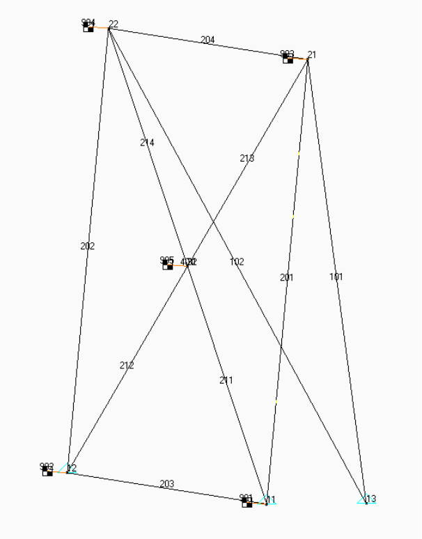
10.6 Craig-Bampton model generation example problem
The figure below shows a small example problem that is a frame made of CBAR’s that is a
substructure assumed to be attached to some other structure in DOF’s 1,2,3 at grids 11 and 13 and in
DOF’s 2,3 at grid 12. The example problem F06 file (with the input echo’d) is shown on the following
pages. This section will discuss the input and output in an effort to explain the Craig-Bampton model
generation process.
Equation 10.26 defines the Craig-Bampton degrees of freedom (CB-DOF’s) as Uz which, for this
example, consists of the 18 DOF’s:
8 boundary acceleration DOF’s,
R
u
2 modal acceleration DOF’s, N
(see EIGRL request for 2 modes to be extracted)
8 boundary displacement DOF’s, R
u
Figure 10.2 – Example CB model: CB-EXAMPLE-12b.DAT
244

Notes on section 10.6.1: CB-EXAMPLE-12b.F06
The echo of the input shows the following salient points for a CB model generation (much like a SOL
3 eigenvalue analysis in terms of input data):
Executive Control:
SOL 31 indicates CB model generation
The OUTPUT4 commands show the matrices that will be written in a format the same as
NASTRAN OUTPUT4 files. These matrix data blocks are ones that are listed on Table
10.2 as allowable OUTPUT4 matrices. Notice that several are written to unit 21 while
others are written to unit 22. As explained in section 5.1 of the MYSTRAN Users
Reference Manual, unit numbers 21 through 27 are valid for writing OUTPUT4 matrices.
Case Control:
METHOD = 1 is to be used for a normal eigenvalue analysis (same as if SOL were 3)
Outputs (ACCE, DISP, ELFORCE, STRESS) are for Output Transformation Matrices
(OTM’s) for the specified sets. These will be written to the text F06 file. In addition they
will be written to binary files (same name, CB-EXAMPLE-12b) with extension OP8 for the
element related OTM;s (ELFORCE, STRESS in this case and OP9 for the grid related
OTM’s (ACCE, DISP in this case)
Bulk Data:
Shows the model for this example (notice it has mostly CBAR’s but there is also a RBE2)
Degrees of freedom at the boundary where this substructure attaches to other
substructures are defined with the SUPORT Bulk Data entry. This is the same procedure
that is used in CB analyses by the NASTRAN DMAP (Direct Matrix Abstraction Program)
method familiar to NASTRAN CB analysts.
Eigenvalue extraction, EIGRL requesting 2 modes to be extracted
The delineated F06 output begins on the page following the input model echo and shows the
following:
Eigenvalues extracted
Messages on the matrices requested to be written to OUTPUT4 files
For the first 3 of the 18 CB_DOF’s in this example the following output (requested in Case
Control) is shown (other 15 were left out for clarity):
Displacement OTM for the requested grids (see Case Control command DISP = 102)
Element engineering force OTM (see Case Control command ELFORCE = 201)
Element stress OTM (see Case Control command STRESS = 202)
Acceleration OTM. As shown in equation 10.48 the acceleration OTM has columns for R
u
and N
but not R
u. For this example, there are 10 columns in the acceleration OTM (8
boundary acceleration DOF’s and 2 modal acceleration DOF’s)
245

246
Notes on section 10.6.2: OUTPUT4 matrices written to CB-EXAMPLE-12b.OP1 and OP2
As shown in the Executive Control section of the F06 file in section 10.6.1, there were 3 matrices
requested to be written to unit 21 and 4 to unit 22. These binary files, translated to text, are shown in
section 10.6.2. The number of actual columns for each matrix is indicated in Table 10.2 but only the
first 5 of the columns are shown here for the sake of brevity. These are several of the important CB
matrices needed to couple this CB substructure to other substructures in a combined analysis. The
binary OUTPUT4 files are written in the same format as the NASTRAN OUTPUT4 binary files.
Notes on section 10.6.3: Displ and elem force/stress OTM’s written to CB-EXAMPLE-12b.OP1, OP2
Any output requests in Case Control for grid related outputs (e.g. DISPL, ACCEL) and element
force/stress outputs (e.g. ELFORCE, STRESS) are written to the text F06 file and also written to
OUTPUT4 binary files (automatically; that is, no formal OUTPUT4 request is needed). The element
related OTM’s are always written to a file with the same filename as the F06 file but with extension
OP8. The grid related OTM’s are written to a file with extension OP9.
The first page of section 10.6.3 is a text translation of the element related OTM’s written to file
CB-EXAMPLE-12b.OP8. The values are the same as was written to the F06 file for element forces
and stresses but are also written to binary files in OUTPUT4 format to be used in analyses that
couple the CB substructures. In order to explain the contents of the binary OP8 file, a text file with
extension OT8 is also automatically written (provided any Case Control requests are included for
element forces/stresses) describing the contents of the OP8 binary file. This OT8 text file gives an
overview of the OP8 binary file and then goes on to describe each row written to the OP8 file.
The next several pages show the same type of information on the grid related OTM’s written to binary
file with extension OP9 (with text description in OT9). Again, this is the grid related outputs requested
in Case Control and also written to the F06 text file.
*
247
10.6.1 CB-EXAMPLE-12-b.F06
(delineated – some output not included here for the sake of clarity)
248
1030180330
MYSTRAN Version 3.00 Oct 20 2006 by Dr Bill Case (this TRIAL edition is SP protected)
>> MYSTRAN BEGIN : 10/30/2006 at 18: 3:30.640 The input file is CB-EXAMPLE-12-b.DAT
>> LINK 1 BEGIN
SOL 31
$
OUTPUT4 CG_LTM , IF_LTM , , , //-1/21 $
OUTPUT4 KRRGN , RBMCG , MRRGN , , RBRCG //-1/22 $
OUTPUT4 MR , , , , //-1/21 $
CEND
TITLE = TEST OF CRAIG-BAMPTON SOLUTION
SUBTI = FRAME USING CBAR's
SPC = 1
METHOD = 1
ECHO = UNSORT
$
SET 101 = 32
SET 102 = 22, 32
SET 201 = 211, 212
SET 202 = 201
$
ACCE = 101
DISP = 102
ELFORCE = 201
STRESS = 202
MEFFMASS = ALL
MPFACTOR = ALL
$
BEGIN BULK
$
EIGRL 1 2 2 DPB -1. MASS
$
EIGR 2 MGIV 1 24 +E1
+E1 MASS
GRID 11 0. 0. 0.
GRID 12 100. 0. 0.
GRID 13 50. 0. 50.
GRID 21 0. 100. 0.
GRID 22 100. 100. 0.
GRID 31 50. 50. 0.
GRID 32 50. 50. 0.
$
RBE2 401 31 123456 32
249
$
$ Frame support bars
$
CBAR 101 1 13 21 0.0 0.5 1.0 +C1
+C1 56 456
CBAR 102 1 13 22 0.0 0.5 1.0 +C2
+C2 56 456
$
$ Edge bars
$
CBAR 201 2 11 21 0.0 0.0 1.0
CBAR 202 2 12 22 0.0 0.0 1.0
CBAR 203 2 11 12 0.0 0.0 1.0
CBAR 204 2 21 22 0.0 0.0 1.0
$
$ Diag bars
$
CBAR 211 3 11 31 0.0 0.0 1.0
CBAR 212 3 12 31 0.0 0.0 1.0
CBAR 213 3 21 31 0.0 0.0 1.0
CBAR 214 3 22 31 0.0 0.0 1.0
$
PBAR 1 1 0.36 0.09 0.09 0.18
PBAR 2 1 0.10 10.0 10.0 20.0
PBAR 3 1 6.0 6.0 6.0 12.0
$
MAT1 1 10.+6 0.3 0.1
*INFORMATION: MAT1 ENTRY 1 HAD FIELD FOR G BLANK. MYSTRAN CALCULATED G = 3.846154E+06
$
CONM2 901 11 150.0 0.0 0.0 -5.0
CONM2 902 12 150.0 0.0 0.0 -5.0
CONM2 903 21 150.0 0.0 0.0 -5.0
CONM2 904 22 150.0 0.0 0.0 -5.0
CONM2 905 32 150.0 0.0 0.0 -5.0
$
SPC1 1 456 13
$
$ BOUNDARY DOF'S
$
SUPORT 11 123 12 23 13 123
$
PARAM WTMASS .002591
$
ENDDATA
250
E I G E N V A L U E A N A L Y S I S S U M M A R Y (LANCZOS Mode 2 DPB Shift eigen = -1.00E+00)
NUMBER OF EIGENVALUES EXTRACTED . . . . . . 2
LARGEST OFF-DIAGONAL GENERALIZED MASS TERM -2.7E-13 (Vecs renormed to 1.0 for gen masses)
. . . 2
MODE PAIR . . . . . . . . . .
. . . 1
NUMBER OF OFF DIAGONAL GENERALIZED MASS
TERMS FAILING CRITERION OF 1.0E-04. . . . . 0
R E A L E I G E N V A L U E S
MODE EXTRACTION EIGENVALUE RADIANS CYCLES GENERALIZED GENERALIZED
NUMBER ORDER MASS STIFFNESS
1 1 3.895211E+03 6.241163E+01 9.933119E+00 1.000000E+00 3.895211E+03
2 2 7.011163E+03 8.373269E+01 1.332647E+01 1.000000E+00 7.011163E+03
>> LINK 4 END
>> LINK 6 BEGIN
251
*INFORMATION: THE FOLLOWING 7 MATRICES WILL BE WRITTEN TO 2 OUTPUT4 FILES IN THE ORDER LISTED BELOW:
OUTPUT4 file on unit 21 has been created as: CB-EXAMPLE-12-b.OP1 and will contain the matrices:
( 1) CG_LTM : 6 rows and 18 cols This is MYSTRAN matrix CG_LTM
( 2) IF_LTM : 8 rows and 18 cols This is MYSTRAN matrix IF_LTM
( 3) MR : 8 rows and 8 cols This is MYSTRAN matrix MRRcb
OUTPUT4 file on unit 22 has been created as: CB-EXAMPLE-12-b.OP2 and will contain the matrices:
( 1) KRRGN : 10 rows and 10 cols This is MYSTRAN matrix KXX
( 2) RBMCG : 6 rows and 6 cols This is MYSTRAN matrix MCG
( 3) MRRGN : 10 rows and 10 cols This is MYSTRAN matrix MXX
( 4) RBRCG : 8 rows and 6 cols This is MYSTRAN matrix TR6
>> LINK 6 END
>> LINK 5 BEGIN
>> LINK 5 END
>> LINK 9 BEGIN

252
OUTPUT FOR CRAIG-BAMPTON DOF 1 OF 18
C B D I S P L A C E M E N T O T M
(in global coordinate system at each grid)
GRID COORD T1 T2 T3 R1 R2 R3
SYS
22 0 -1.412939E-05 1.622140E-05 8.242222E-05 5.883709E-07 -1.667433E-06 5.125151E-07
32 0 1.051041E-05 -9.465944E-06 -3.182887E-06 -1.086181E-07 -9.450720E-07 2.106009E-07
C B E L E M E N T E N G I N E E R I N G F O R C E O T M
F O R E L E M E N T T Y P E B A R
Element Bend-Moment End A Bend-Moment End B - Shear - Axial Torque
ID Plane 1 Plane 2 Plane 1 Plane 2 Plane 1 Plane 2 Force
211 2.091876E-01 7.894539E-01 1.515607E+00 -1.439344E+00 -1.847556E-02 3.151997E-02 6.266800E-01 9.672846E-03
212 -1.133151E-01 -1.008960E-02 -1.725401E+00 -6.166148E-02 2.279833E-02 7.293366E-04 -2.953611E-01 -4.720428E-03
C B E L E M E N T S T R E S S O T M I N L O C A L E L E M E N T C O O R D I N A T E S Y S T E M
F O R E L E M E N T T Y P E B A R
Element SA1 SA2 SA3 SA4 Axial SA-Max SA-Min M.S.-T
ID SB1 SB2 SB3 SB4 Stress SB-Max SB-Min M.S.-C
201 0.000000E+00 0.000000E+00 0.000000E+00 0.000000E+00 -2.748670E+00 -2.748670E+00 -2.748670E+00
0.000000E+00 0.000000E+00 0.000000E+00 0.000000E+00 -2.748670E+00 -2.748670E+00
OUTPUT FOR CRAIG-BAMPTON DOF 2 OF 18
C B D I S P L A C E M E N T O T M
(in global coordinate system at each grid)
GRID COORD T1 T2 T3 R1 R2 R3
SYS
22 0 -7.600290E-05 8.243595E-05 3.128787E-04 1.925291E-06 2.220055E-06 1.292053E-07
32 0 -5.990878E-05 6.308617E-05 3.224179E-04 3.643362E-06 4.904270E-07 3.218612E-08
C B E L E M E N T E N G I N E E R I N G F O R C E O T M
F O R E L E M E N T T Y P E B A R
Element Bend-Moment End A Bend-Moment End B - Shear - Axial Torque
ID Plane 1 Plane 2 Plane 1 Plane 2 Plane 1 Plane 2 Force
211 3.640634E+00 -2.875040E+00 -7.752079E+00 4.486528E+00 1.611173E-01 -1.041083E-01 1.906435E+00 -5.333935E-03
212 3.789705E+00 2.992877E+00 -6.061077E+00 -4.713484E+00 1.393111E-01 1.089844E-01 1.808077E+00 5.333935E-03
C B E L E M E N T S T R E S S O T M I N L O C A L E L E M E N T C O O R D I N A T E S Y S T E M
F O R E L E M E N T T Y P E B A R
Element SA1 SA2 SA3 SA4 Axial SA-Max SA-Min M.S.-T
ID SB1 SB2 SB3 SB4 Stress SB-Max SB-Min M.S.-C
201 0.000000E+00 0.000000E+00 0.000000E+00 0.000000E+00 7.582667E+00 7.582667E+00 7.582667E+00
0.000000E+00 0.000000E+00 0.000000E+00 0.000000E+00 7.582667E+00 7.582667E+00

253
OUTPUT FOR CRAIG-BAMPTON DOF 3 OF 18
C B D I S P L A C E M E N T O T M
(in global coordinate system at each grid)
GRID COORD T1 T2 T3 R1 R2 R3
SYS
22 0 3.800145E-05 -4.121798E-05 -1.564393E-04 -9.626456E-07 -1.110028E-06 -6.460267E-08
32 0 2.995439E-05 -3.154308E-05 -1.612090E-04 -1.821681E-06 -2.452135E-07 -1.609306E-08
C B E L E M E N T E N G I N E E R I N G F O R C E O T M
F O R E L E M E N T T Y P E B A R
Element Bend-Moment End A Bend-Moment End B - Shear - Axial Torque
ID Plane 1 Plane 2 Plane 1 Plane 2 Plane 1 Plane 2 Force
211 -1.820317E+00 1.437520E+00 3.876039E+00 -2.243264E+00 -8.055864E-02 5.205414E-02 -9.532175E-01 2.666968E-03
212 -1.894852E+00 -1.496438E+00 3.030538E+00 2.356742E+00 -6.965554E-02 -5.449220E-02 -9.040385E-01 -2.666968E-03
C B E L E M E N T S T R E S S O T M I N L O C A L E L E M E N T C O O R D I N A T E S Y S T E M
F O R E L E M E N T T Y P E B A R
Element SA1 SA2 SA3 SA4 Axial SA-Max SA-Min M.S.-T
ID SB1 SB2 SB3 SB4 Stress SB-Max SB-Min M.S.-C
201 0.000000E+00 0.000000E+00 0.000000E+00 0.000000E+00 -3.791334E+00 -3.791334E+00 -3.791334E+00
0.000000E+00 0.000000E+00 0.000000E+00 0.000000E+00 -3.791334E+00 -3.791334E+00
.
.
.
.
.
.
.
.
.
(output for the 4th – 18th CB DOF deleted)

254
OUTPUT FOR CRAIG-BAMPTON ACCEL OTM COL 1 OF 10
C B A C C E L E R A T I O N O T M
(in global coordinate system at each grid)
GRID COORD T1 T2 T3 R1 R2 R3
SYS
32 0 2.199853E-02 -2.028331E-02 -1.681579E-02 -3.363157E-04 8.006145E-03 5.254334E-04
OUTPUT FOR CRAIG-BAMPTON ACCEL OTM COL 2 OF 10
C B A C C E L E R A T I O N O T M
(in global coordinate system at each grid)
GRID COORD T1 T2 T3 R1 R2 R3
SYS
32 0 0.000000E+00 0.000000E+00 -1.000000E+00 -2.000000E-02 0.000000E+00 0.000000E+00
OUTPUT FOR CRAIG-BAMPTON ACCEL OTM COL 3 OF 10
C B A C C E L E R A T I O N O T M
(in global coordinate system at each grid)
GRID COORD T1 T2 T3 R1 R2 R3
SYS
32 0 0.000000E+00 0.000000E+00 5.000000E-01 1.000000E-02 0.000000E+00 0.000000E+00
.
.
.
.
.
.
.
.
.
(output for the 4th – 10th Accel OTM columns deleted)
255
M O D A L P A R T I C I P A T I O N F A C T O R S
(dimensionless, in coordinate sys 0)
MODE T1 T2 T3 R1 R2 R3
NUM
1 1.227574E-01 -1.758352E+00 8.791759E-01 1.259087E+00 6.535370E-02 -5.341716E-01
2 6.061630E-01 1.829524E-01 -9.147622E-02 -4.910542E-01 -1.366914E-01 -4.626569E-01
------------------------------------------------------------------------------------------------------------------------------------
E F F E C T I V E M O D A L M A S S E S O R W E I G H T S
(in coordinate system 0)
Units are same as units for mass input in the Bulk Data Deck
MODE T1 T2 T3 R1 R2 R3
NUM
1 6.532677E+01 4.179096E+01 4.694259E+02 3.836785E+05 3.287406E+04 3.611917E+02
2 7.948285E+00 9.016521E-01 1.363070E+01 1.674257E+00 6.082279E+05 4.781873E+05
------------- ------------- ------------- ------------- ------------- -------------
Sum all modes: 7.327506E+01 4.269261E+01 4.830566E+02 3.836801E+05 6.411019E+05 4.785485E+05
Total model mass: 9.325238E+02 9.325238E+02 9.325238E+02 4.105260E+06 4.094237E+06 8.139951E+06
Modes % of total mass*: 7.86 4.58 51.80 9.35 15.66 5.88
*If all modes are calculated the % of total mass should be 100% of the free mass (i.e. not counting mass at constrained DOF's).
Percentages are only printed for components that have finite model mass.
-----
>> LINK 9 END
>> MYSTRAN END : 10/30/2006 at 18: 3:31.562
256
10.6.2 OUTPUT4 matrices written to CB-EXAMPLE-12-b.OP1 and OP2
(OUTPUT4 matrices requested in Exec Control)

257
OUTPUT4 matrices requested in Exec Control to be written to file CB-EXAMPLE-12-b.OP1 (on unit 21)
(note: only 1st 5 columns written here for the sake of clarity)
CG_LTM NCOLS = 18 NROWS = 6 FORM = 2 PREC = 2
1 2 3 4 5
1 -6.65821789802521E-05 1.29562159612018E-17 -6.47810798060089E-18 -1.29549999999999E-03 6.47766872193621E-05 .......
2 -2.99785601343913E-05 -1.96135553418977E-04 1.04193052213477E-04 1.39356777670951E-03 -6.70858061739371E-05 .......
3 -4.35697030582909E-05 -2.59100000000000E-03 1.30775055100798E-03 1.29550000000001E-03 6.19839872966866E-04 .......
4 -3.33844454038618E-04 -2.00000000000000E-02 9.80743672854175E-03 1.00000000000000E-02 -5.07064059129018E-03 .......
5 8.13687816036514E-03 1.47885176327023E-16 -7.39425881635114E-17 -7.78457159844592E-17 -5.93156091981744E-03 .......
6 5.63393757592496E-04 8.55130582230051E-17 -4.27565291115026E-17 9.99999999999996E-03 2.81696878796245E-04 .......
IF_LTM NCOLS = 18 NROWS = 8 FORM = 2 PREC = 2
1 2 3 4 5
1 6.02957424769077E-01 7.32039059471622E-02 -3.66019529735811E-02 3.35492666170908E-02 -7.19015457719424E-02 .......
2 7.32039059471623E-02 4.25469107253153E+00 -2.12163357113457E+00 -2.21879607113459E+00 -1.10665832128050E-01 .......
3 -3.66019529735811E-02 -2.12163357113457E+00 1.07224071582968E+00 1.10939803556729E+00 5.53329160640251E-02 .......
4 3.35492666170908E-02 -2.21879607113459E+00 1.10939803556729E+00 3.26418464157067E+00 1.75366508593570E-02 .......
5 -7.19015457719424E-02 -1.10665832128050E-01 5.53329160640251E-02 1.75366508593570E-02 4.96481812094837E-01 .......
6 -6.65046890695409E-01 -7.32039059471504E-02 3.66019529735752E-02 -1.24163383728600E+00 1.32307347677584E-01 .......
7 -1.34708893096271E-01 -2.21879607113459E+00 1.10939803556729E+00 2.54146535101691E-01 3.05700710026811E-02 .......
8 6.78737140960850E-02 -1.83869738075211E-01 9.19348690376054E-02 8.11498842422746E-02 2.62006997196796E-02 .......
MR NCOLS = 8 NROWS = 8 FORM = 1 PREC = 2
1 2 3 4 5
1 6.02957424769077E-01 7.32039059471622E-02 -3.66019529735811E-02 3.35492666170908E-02 -7.19015457719424E-02 .......
2 7.32039059471623E-02 4.25469107253153E+00 -2.12163357113457E+00 -2.21879607113459E+00 -1.10665832128050E-01 .......
3 -3.66019529735811E-02 -2.12163357113457E+00 1.07224071582968E+00 1.10939803556729E+00 5.53329160640251E-02 .......
4 3.35492666170908E-02 -2.21879607113459E+00 1.10939803556729E+00 3.26418464157067E+00 1.75366508593570E-02 .......
5 -7.19015457719424E-02 -1.10665832128050E-01 5.53329160640251E-02 1.75366508593570E-02 4.96481812094837E-01 .......
6 -6.65046890695409E-01 -7.32039059471504E-02 3.66019529735752E-02 -1.24163383728600E+00 1.32307347677584E-01 .......
7 -1.34708893096271E-01 -2.21879607113459E+00 1.10939803556729E+00 2.54146535101691E-01 3.05700710026811E-02 .......
8 6.78737140960850E-02 -1.83869738075211E-01 9.19348690376054E-02 8.11498842422746E-02 2.62006997196796E-02 .......

258
OUTPUT4 matrices requested in Exec Control to be written to file CB-EXAMPLE-12-b.OP2 (on unit 22)
(note: only 1st 5 columns written here the sake of clarity)
KRRGN NCOLS = 10 NROWS = 10 FORM = 1 PREC = 2
1 2 3 4 5
1 1.19504240447136E+03 -3.63797880709171E-12 1.81898940354586E-12 1.54614099301398E-11 5.97521202235677E+02 .......
2 -5.45696821063757E-12 0.00000000000000E+00 0.00000000000000E+00 1.81898940354586E-12 0.00000000000000E+00 .......
3 2.72848410531878E-12 0.00000000000000E+00 0.00000000000000E+00 -9.09494701772928E-13 0.00000000000000E+00 .......
4 2.08011385893769E-11 0.00000000000000E+00 0.00000000000000E+00 -1.16415321826935E-10 9.43778388773353E-12 .......
5 5.97521202235677E+02 -1.13686837721616E-13 5.68434188608080E-14 -1.59161572810262E-12 2.98760601117838E+02 .......
6 -1.19504240447137E+03 0.00000000000000E+00 0.00000000000000E+00 -1.79397829924710E-10 -5.97521202235685E+02 .......
7 -2.98427949019242E-13 0.00000000000000E+00 0.00000000000000E+00 -4.31782609666698E-10 -2.76401124210679E-12 .......
8 -5.97521202235677E+02 -1.81898940354586E-12 9.09494701772928E-13 1.36424205265939E-12 -2.98760601117839E+02 .......
9 0.00000000000000E+00 0.00000000000000E+00 0.00000000000000E+00 0.00000000000000E+00 0.00000000000000E+00 .......
10 0.00000000000000E+00 0.00000000000000E+00 0.00000000000000E+00 0.00000000000000E+00 0.00000000000000E+00 .......
RBMCG NCOLS = 6 NROWS = 6 FORM = 2 PREC = 2
1 2 3 4 5
1 2.41616914133782E+00 -3.35287353436797E-14 -6.52256026967279E-15 -1.34114941374719E-13 -3.97903932025656E-13 .......
2 -3.30846461338297E-14 2.41616914133786E+00 2.33146835171283E-14 7.74491581978509E-13 2.89102075612391E-13 .......
3 -6.52256026967279E-15 2.27734497926235E-14 2.41616914133783E+00 -9.59232693276135E-14 -7.10542735760100E-14 .......
4 -1.35891298214119E-13 7.81374964731185E-13 -1.24344978758018E-13 4.56169135583651E+03 -3.86535248253495E-12 .......
5 -3.92130772297605E-13 2.88435941797616E-13 -6.75015598972095E-14 -4.09272615797818E-12 4.53313153018053E+03 .......
6 1.99662508748588E-12 4.26325641456060E-14 -3.62376795237651E-13 -1.36424205265939E-11 2.85598256559946E+01 .......
MRRGN NCOLS = 10 NROWS = 10 FORM = 1 PREC = 2
1 2 3 4 5
1 6.02957424769077E-01 7.32039059471622E-02 -3.66019529735811E-02 3.35492666170908E-02 -7.19015457719424E-02 .......
2 7.32039059471623E-02 4.25469107253153E+00 -2.12163357113457E+00 -2.21879607113459E+00 -1.10665832128050E-01 .......
3 -3.66019529735811E-02 -2.12163357113457E+00 1.07224071582968E+00 1.10939803556729E+00 5.53329160640251E-02 .......
4 3.35492666170908E-02 -2.21879607113459E+00 1.10939803556729E+00 3.26418464157067E+00 1.75366508593570E-02 .......
5 -7.19015457719424E-02 -1.10665832128050E-01 5.53329160640251E-02 1.75366508593570E-02 4.96481812094837E-01 .......
6 -6.65046890695409E-01 -7.32039059471504E-02 3.66019529735752E-02 -1.24163383728600E+00 1.32307347677584E-01 .......
7 -1.34708893096271E-01 -2.21879607113459E+00 1.10939803556729E+00 2.54146535101691E-01 3.05700710026811E-02 .......
8 6.78737140960850E-02 -1.83869738075211E-01 9.19348690376054E-02 8.11498842422746E-02 2.62006997196796E-02 .......
9 1.22757372107055E-01 -1.75835189695839E+00 8.79175948479194E-01 1.25908689725916E+00 6.53537005701318E-02 .......
10 6.06162990294928E-01 1.82952442095713E-01 -9.14762210478567E-02 -4.91054200271590E-01 -1.36691428775775E-01 .......
RBRCG NCOLS = 6 NROWS = 8 FORM = 2 PREC = 2
1 2 3 4 5
1 1.00000000000000E+00 0.00000000000000E+00 0.00000000000000E+00 0.00000000000000E+00 5.37849392786371E+01 .......
2 0.00000000000000E+00 1.00000000000000E+00 0.00000000000000E+00 -5.37849392786371E+01 0.00000000000000E+00 .......
3 0.00000000000000E+00 0.00000000000000E+00 1.00000000000000E+00 -5.00000000000000E+01 0.00000000000000E+00 .......
4 0.00000000000000E+00 1.00000000000000E+00 0.00000000000000E+00 -3.78493927863709E+00 0.00000000000000E+00 .......
5 0.00000000000000E+00 0.00000000000000E+00 1.00000000000000E+00 -5.00000000000000E+01 -5.00000000000000E+01 .......
6 1.00000000000000E+00 0.00000000000000E+00 0.00000000000000E+00 0.00000000000000E+00 3.78493927863709E+00 .......
7 0.00000000000000E+00 1.00000000000000E+00 0.00000000000000E+00 -3.78493927863709E+00 0.00000000000000E+00 .......
8 0.00000000000000E+00 0.00000000000000E+00 1.00000000000000E+00 -5.00000000000000E+01 5.00000000000000E+01 .......
259
10.6.3 Displ and Element force/stress OTM’s written to CB-EXAMPLE-12-b.OP8 and OP9
(OTM’s requested in Case Control)

260
CB-EXAMPLE-12-b.OP8 binary file of element force/stress OTM’s requested in Case Control
(note: only 1st 5 columns written here the sake of clarity)
OTM_ELFE NCOLS = 18 NROWS = 16 FORM = 2 PREC = 2
1 2 3 4 5
1 2.09187572390564E-01 3.64063384390388E+00 -1.82031692195194E+00 -1.84227921264778E+00 -9.14925412689932E-01 .......
2 7.89453912890167E-01 -2.87503976462738E+00 1.43751988231369E+00 1.92080844772306E+00 -1.26234542491864E-01 .......
3 1.51560714339846E+00 -7.75207867487571E+00 3.87603933743785E+00 3.62690741509324E+00 1.45527637571713E+00 .......
4 -1.43934432738336E+00 4.48652751792572E+00 -2.24326375896286E+00 -2.73874759882899E+00 2.35906653084923E-01 .......
5 -1.84755627546901E-02 1.61117285562758E-01 -8.05586427813792E-02 -7.73459790410093E-02 -3.35197151472623E-02 .......
6 3.15199669918811E-02 -1.04108282913086E-01 5.20541414565432E-02 6.58960735567147E-02 -5.12144990278700E-03 .......
7 6.26679968599842E-01 1.90643492900070E+00 -9.53217464500349E-01 -1.19040949990613E-01 -1.14791218537626E-01 .......
8 9.67284596743351E-03 -5.33393540270422E-03 2.66696770135211E-03 -5.34876839175438E-02 8.35971431688627E-04 .......
9 -1.13315069892136E-01 3.78970456518829E+00 -1.89485228259414E+00 -1.26147862482940E+00 -9.55864075040792E-01 .......
10 -1.00896004659258E-02 2.99287680850590E+00 -1.49643840425295E+00 -4.03697533588189E+00 -1.41398274167766E-02 .......
11 -1.72540058669802E+00 -6.06107677196644E+00 3.03053838598322E+00 2.53928832803047E+00 1.96715396237338E+00 .......
12 -6.16614847670031E-02 -4.71348398353008E+00 2.35674199176504E+00 6.82365970711492E+00 3.39064169416761E-02 .......
13 2.27983320157212E-02 1.39311085669760E-01 -6.96555428348799E-02 -5.37509617215390E-02 -4.13377175157231E-02 .......
14 7.29336582157196E-04 1.08984399486375E-01 -5.44921997431877E-02 -1.53592573737906E-01 -6.79476503928156E-04 .......
15 -2.95361107284698E-01 1.80807707871691E+00 -9.04038539358453E-01 -1.95832712226347E+00 3.00896480121837E-03 .......
16 -4.72042770150405E-03 5.33393540270377E-03 -2.66696770135189E-03 -1.12160973347287E-01 -3.69369770142806E-03 .......
OTM_STRE NCOLS = 18 NROWS = 18 FORM = 2 PREC = 2
1 2 3 4 5
1 0.00000000000000E+00 0.00000000000000E+00 0.00000000000000E+00 0.00000000000000E+00 0.00000000000000E+00 .......
2 0.00000000000000E+00 0.00000000000000E+00 0.00000000000000E+00 0.00000000000000E+00 0.00000000000000E+00 .......
3 0.00000000000000E+00 0.00000000000000E+00 0.00000000000000E+00 0.00000000000000E+00 0.00000000000000E+00 .......
4 0.00000000000000E+00 0.00000000000000E+00 0.00000000000000E+00 0.00000000000000E+00 0.00000000000000E+00 .......
5 -2.74867035744303E+00 7.58266712433821E+00 -3.79133356216910E+00 -1.07520478850513E+00 4.30045958649968E-01 .......
6 -2.74867035744303E+00 7.58266712433821E+00 -3.79133356216910E+00 -1.07520478850513E+00 4.30045958649968E-01 .......
7 -2.74867035744303E+00 7.58266712433821E+00 -3.79133356216910E+00 -1.07520478850513E+00 4.30045958649968E-01 .......
8 -1.00000000000000E+00 -1.00000000000000E+00 -1.00000000000000E+00 -1.00000000000000E+00 -1.00000000000000E+00 .......
9 0.00000000000000E+00 0.00000000000000E+00 0.00000000000000E+00 0.00000000000000E+00 0.00000000000000E+00 .......
10 0.00000000000000E+00 0.00000000000000E+00 0.00000000000000E+00 0.00000000000000E+00 0.00000000000000E+00 .......
11 0.00000000000000E+00 0.00000000000000E+00 0.00000000000000E+00 0.00000000000000E+00 0.00000000000000E+00 .......
12 0.00000000000000E+00 0.00000000000000E+00 0.00000000000000E+00 0.00000000000000E+00 0.00000000000000E+00 .......
13 0.00000000000000E+00 0.00000000000000E+00 0.00000000000000E+00 0.00000000000000E+00 0.00000000000000E+00 .......
14 -2.74867035744303E+00 7.58266712433821E+00 -3.79133356216910E+00 -1.07520478850513E+00 4.30045958649968E-01 .......
15 -2.74867035744303E+00 7.58266712433821E+00 -3.79133356216910E+00 -1.07520478850513E+00 4.30045958649968E-01 .......
16 -2.74867035744303E+00 7.58266712433821E+00 -3.79133356216910E+00 -1.07520478850513E+00 4.30045958649968E-01 .......
17 -1.00000000000000E+00 -1.00000000000000E+00 -1.00000000000000E+00 -1.00000000000000E+00 -1.00000000000000E+00 .......
18 1.00000000000000E+10 1.00000000000000E+10 1.00000000000000E+10 1.00000000000000E+10 1.00000000000000E+10 .......

261
CB-EXAMPLE-12-b.OT8 text file descriptor of rows in above binary file for element related OTM’s
This text file describes the rows of the elem related OTM matrices written to unformatted file: CB-EXAMPLE-12-b.OP8
----------------------------------------------------------------------------------------------
The description for each of the matrices has the headers:
ROW : row number in the individual OTM described
DESCRIPTION: what OTM is this
TYPE : element type
EID : element ID
Then, for the element nodal force OTM:
GRID : grid number of the element that the OTM is for
COMP : displacement component number (1,2,3 translations and 4,5,6 rotations)
and for element engineering force and element stress OTMs:
ITEM : element force or stress item (axial force, torque, etc)
The number of rows for each OTM depends on the output requests, by the user, in Case Control
The number of cols for each OTM depends on the number of support DOFs (NDOFR) and the number of eigenvecors (NVEC)where:
NDOFR = 8
NVEC = 2
This text file has descriptions for the following element related OTMs from CB-EXAMPLE-12-
b
.OP8
Element engr force OTM (matrix OTM_ELFE) with 2*NDOFR + NVEC = 18 cols
Element stress OTM (matrix OTM_STRE) with 2*NDOFR + NVEC = 18 cols
---------------------------------------------------------------------------------
Explanation of rows of 16 row by 18 col matrix OTM_ELFE
ROW DESCRIPTION TYPE EID ITEM
------- ------------------------------ -------- ------- --------------------
1 Element engineering force BAR 211 M1a: Mom Plane1 EndA
2 Element engineering force BAR 211 M1b: Mom Plane2 EndA
3 Element engineering force BAR 211 M2a: Mom Plane1 EndB
4 Element engineering force BAR 211 M2b: Mom Plane2 EndB
5 Element engineering force BAR 211 V1 : Shear Plane1
6 Element engineering force BAR 211 V2 : Shear Plane2
7 Element engineering force BAR 211 FX : Axial force
8 Element engineering force BAR 211 T : Torque
9 Element engineering force BAR 212 M1a: Mom Plane1 EndA
10 Element engineering force BAR 212 M1b: Mom Plane2 EndA
11 Element engineering force BAR 212 M2a: Mom Plane1 EndB
12 Element engineering force BAR 212 M2b: Mom Plane2 EndB
13 Element engineering force BAR 212 V1 : Shear Plane1
14 Element engineering force BAR 212 V2 : Shear Plane2
15 Element engineering force BAR 212 FX : Axial force
16 Element engineering force BAR 212 T : Torque
262
---------------------------------------------------------------------------------
Explanation of rows of 18 row by 18 col matrix OTM_STRE
ROW DESCRIPTION TYPE EID ITEM
------- ------------------------------ -------- ------- --------------------
1 Element stress BAR 201 SA1: Stress Pt1 EndA
2 Element stress BAR 201 SA2: Stress Pt2 EndA
3 Element stress BAR 201 SA3: Stress Pt3 EndA
4 Element stress BAR 201 SA4: Stress Pt4 EndA
5 Element stress BAR 201 Axial Stress
6 Element stress BAR 201 SA-Max
7 Element stress BAR 201 SA-Min
8 Element stress BAR 201 MS-Tension
9 Element stress BAR 201 Torsional Stress
10 Element stress BAR 201 SB1: Stress Pt1 EndB
11 Element stress BAR 201 SB2: Stress Pt2 EndB
12 Element stress BAR 201 SB3: Stress Pt3 EndB
13 Element stress BAR 201 SB4: Stress Pt4 EndB
14 Element stress BAR 201 Axial stress
15 Element stress BAR 201 SB-Max
16 Element stress BAR 201 SB-Min
17 Element stress BAR 201 MS-Compression
18 Element stress BAR 201 MS-Torsion

263
CB-EXAMPLE-12-b.OP9 binary file of displacement OTM’s requested in Case Control
(note: only 1st 5 columns written here the sake of clarity)
OTM_ACCE NCOLS = 10 NROWS = 6 FORM = 2 PREC = 2
1 2 3 4 5
1 2.19985250269592E-02 0.00000000000000E+00 0.00000000000000E+00 -5.00000000000004E-01 1.09992625134795E-02 .......
2 -2.02833087802606E-02 0.00000000000000E+00 0.00000000000000E+00 5.00000000000004E-01 -1.01416543901302E-02 .......
3 -1.68157865913898E-02 -1.00000000000000E+00 5.00000000000000E-01 5.00000000000005E-01 2.41592106704306E-01 .......
4 -3.36315731827796E-04 -2.00000000000000E-02 1.00000000000000E-02 1.00000000000001E-02 -5.16815786591390E-03 .......
5 8.00614495648658E-03 0.00000000000000E+00 0.00000000000000E+00 0.00000000000000E+00 -5.99692752175671E-03 .......
6 5.25433423070610E-04 0.00000000000000E+00 0.00000000000000E+00 9.99999999999992E-03 2.62716711535305E-04 .......
OTM_DISP NCOLS = 18 NROWS = 12 FORM = 2 PREC = 2
1 2 3 4 5
1 -1.41293911043985E-05 -7.60029025912968E-05 3.80014512956484E-05 1.29492635368416E-04 3.14571590643487E-06 .......
2 1.62214021120513E-05 8.24359519633505E-05 -4.12179759816752E-05 -1.30161832591346E-04 -3.52963231517632E-06 .......
3 8.24222187730972E-05 3.12878663301563E-04 -1.56439331650781E-04 -2.40634384994669E-04 -1.68993616070736E-05 .......
4 5.88370868696758E-07 1.92529119983460E-06 -9.62645599917302E-07 -2.07019101770705E-06 1.88916538580397E-07 .......
5 -1.66743323917105E-06 2.22005501168008E-06 -1.11002750584004E-06 -1.14971054599053E-06 -8.88454144573320E-08 .......
6 5.12515138397389E-07 1.29205343624621E-07 -6.46026718123106E-08 -1.07589130445167E-06 -9.61720937623318E-08 .......
7 1.05104109813473E-05 -5.99087762260462E-05 2.99543881130231E-05 6.53233961326989E-05 -1.57813540011406E-06 .......
8 -9.46594436701425E-06 6.30861677743807E-05 -3.15430838871904E-05 -6.55217977160166E-05 1.38681670255135E-06 .......
9 -3.18288681491121E-06 3.22417925611894E-04 -1.61208962805947E-04 -1.96081126486432E-04 -3.61627931263323E-05 .......
10 -1.08618067423320E-07 3.64336233382231E-06 -1.82168116691115E-06 -2.63986785628832E-06 -3.24126419085498E-08 .......
11 -9.45071958677177E-07 4.90427017653186E-07 -2.45213508826593E-07 -2.21449664764883E-07 1.36502293189118E-07 .......
12 2.10600905814006E-07 3.21861205426993E-08 -1.60930602713497E-08 -6.09852683088454E-07 -3.82285587596693E-08 .......

264
CB-EXAMPLE-12-b.OT9 text file descriptor of rows in above binary file for grid related OTM’s
This text file describes the rows of the grid related OTM matrices written to unformatted file: CB-EXAMPLE-12-
b
.OP9
----------------------------------------------------------------------------------------------
The description for each of the matrices has the headers:
ROW : row number in the individual OTM described
DESCRIPTION: what OTM is this
GRID : grid number for this row of the OTM
COMP : displacement component number (1,2,3 translations and 4,5,6 rotations)
The number of rows for each OTM depends on the output requests, by the user, in Case Control
The number of cols for each OTM depends on the number of support DOFs (NDOFR) and the number of eigenvecors (NVEC)where:
NDOFR = 8
NVEC = 2
This text file has descriptions for the following grid relatad OTMs from CB-EXAMPLE-12-b.OP9
Acceleration OTM (matrix OTM_ACCE) with NDOFR + NVEC = 10 cols
Displacement OTM (matrix OTM_DISP) with 2*NDOFR + NVEC = 18 cols
---------------------------------------------------------------------------------
Explanation of rows of 6 row by 10 col matrix OTM_ACCE
ROW DESCRIPTION GRID COMP
------- ------------------------------ ------- ----
1 Acceleration 32 1
2 Acceleration 32 2
3 Acceleration 32 3
4 Acceleration 32 4
5 Acceleration 32 5
6 Acceleration 32 6
---------------------------------------------------------------------------------
Explanation of rows of 12 row by 18 col matrix OTM_DISP
ROW DESCRIPTION GRID COMP
------- ------------------------------ ------- ----
1 Displacement 22 1
2 Displacement 22 2
3 Displacement 22 3
4 Displacement 22 4
5 Displacement 22 5
6 Displacement 22 6
7 Displacement 32 1
8 Displacement 32 2
9 Displacement 32 3
10 Displacement 32 4
11 Displacement 32 5
12 Displacement 32 6
11. Appendix E: Derivation of the RBE3 element constraint
equations
265
11.1 Introduction
The RBE3 element is used for distributing applied loads and mass from a reference point to other
points in the finite element model. The geometry and loads for a RBE3 are shown in Figure 1. Point
d in the figure is the RBE3 reference (or dependent) point and is the grid where loads will be applied
by the user. The RBE3 element will distribute these loads to other, independent, points i = 1,…,N, in
the model, where N is the total number of independent grid points defined on the RBE3 Bulk Data
entry. The RBE3 is not intended to add stiffness to the model as does a RBE2 element. As such, the
RBE3 reference point should not be a grid that is attached to other elements in the model – it should
be a stand alone grid only connected to other grids through the REB3 element definition. The
following describes the nomenclature used in this appendix in deriving the “constraint” equations used
in MYSTRAN for the RBE3 element.
Superscripts denote the location of a quantity:
“d” refers to the reference (or dependent) grid on the RBE3
“i” refers to the independent grids, the locations where the loads on point d will be distributed
xyz
xyz
xyz
xyz
X,Y,Z coordinate system axes
u , u ,u displacements in the x, y, z directions
, , rotations about the x, y, z axes
F ,F ,F forces in the x, y, z directions
M ,M ,M moments about the x, y, z axe
iii
xyz
s
d , d , d position of point i relative to the RBE3 reference point, d
For the sake of simplicity and clarity, the following derivation of the RBE3 equations is done for
conditions where the global coordinate systems of all grid points involved in the RBE3 are the same
and are rectangular. The code in the MYSTRAN program is written for general conditions where the
global system of all points may be different and non-rectangular.
266
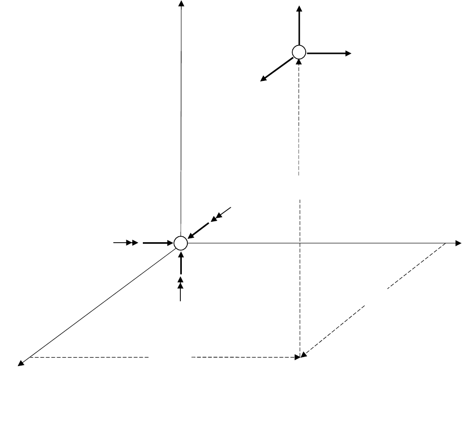
zz
Z, u ,
Point i (1 to N) is a typical point to
which loads will be transferred from
the reference point d via the RBE3
Point d is the RBE3 reference
point shown with the loads
applied. The loads will be
transferred to the points i (typical
point i shown above)
Fig 1: RBE3 geometry and loads
i
x
d
i
y
d
i
z
d
i
x
F
i
y
F
i
z
F
i
d
x
F
d
x
M
d
z
F
d
y
F
d
y
M
d
z
M
xx
X, u ,
yy
Y, u ,
d
267

11.2 Equations for translational force components
In this section 3 equations will be developed that relate the forces applied at the RBE3 reference
point to those where the loads will be distributed (points i = 1,…,N).
The sum of the forces on the points i = 1,…,N must equal the forces on the reference point d. Thus:
11-1
NN
id id i
xx yy z
i1 i1 i1
FF , FF , FF
N
d
z
The moments at reference point due to the forces at the points i are:
11-2
NNN
ii ii d ii ii d ii ii d
zy yz x xz zx y yx xy z
i1 i1 i1
(F d F d ) M , (F d F d ) M , (F d F d ) M
Write the , etc, as:
i
x
F
id id i
ii
xx yy z
TT
FF,FF,F
WW
d
i
z
T
F
W
i
11-3
where is the weighting factor (the WTi on the RBE3 Bulk Data entry) for the ith force and:
i
N
T
i1
W
11-4
Equations 3 and 4 are sufficient for equations 1. Substitute equations 3 and 4 into 2 to get the
following 3 equations:
d
dNN
y
ii
z
iy iz x
i1 i1
TT
F
Fdd
WW
d
M
11-5
dd
NN
ii
xz
iz ix y
i1 i1
TT
FF
dd
WW
d
M
11-6
dd
NN
yii
x
ix iy z
i1 i1
TT
FF
dd
WW
d
M
11-7
Define:
NN
ii
xix yiy z
i1 i1 i1
TT
11
dd,dd,d
WW
N
i
iz
T
1
d
W
11-8
Using equation 8, equations 5-7 become:
dd
zy yz x
Fd Fd M
d
11-9
268

dd
xz zz y
Fd Fd M
d
11-10
dd
yx xy z
Fd Fd M
d
11-11
The work done by the forces and moments at the reference point, d, is d
:
11-12
dd dd dd dd dd dd
dxxyyzzxxyyz
Fu Fu Fu M M M
z
z
where u, are the displacements and rotations of the reference point in the x, y, z directions.
Similarly, the work done by the forces on the points I = 1,…,N is:
11-13
N
ii ii ii
Nxxyyz
i1
(F u F u F u )
The , ec, are the displacements in the x, y and z directions at point I. Substitute equation 3 into 12
and 9, 10 and 11 into 12 and equate the work done by the two systems of forces:
i
x
u
dd dd dd d d d d d d d d d
xx yy zz z y yz x x z zz y y x xy z
N
di di di
iii
xx yy zz
i1 TTT
Fu Fu Fu (Fd Fd) (Fd Fd) (Fd Fd)
(FuFuFu)
WWW
Rearrange:
N
ddd id
i
xzyyz xx
i1 T
N
ddd id
i
yzxxz yy
i1 T
N
ddd id
i
zyxxy zz
i1 T
(u d d u )F
W
(u d d u )F
W
(u d d u )F 0
W
11-14
Since the , and are independent and, in general, not zero, equation 14 requires that:
d
x
Fd
y
Fd
z
F
N
ddd i
i
xzyyz x
i1 T
N
ddd i
i
yzxxz y
i1 T
N
ddd i
i
zyxxy z
i1 T
(u d d u ) 0
W
(u d d u ) 0
W
(u d d u ) 0
W
11-15
Equation 15 represents 3 constraint equations for the RBE3. However, there are only 3 equations and
6 unknowns. This will be resolved in the next section where we develop 3 more equations based on
the moments at the reference point.
269
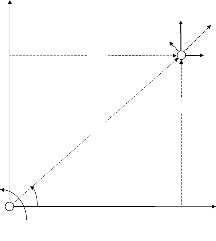
11.3 Equations for rotational moment components
In addition to the 3 equations developed in the last section there are also 3 equations that relate the
moments applied at the RBE3 reference point to those where the loads will be distributed (points i =
1,…,N).
Figure 2 shows how the forces in the y-z plane relate to the RBE3 reference point moment about the
x axis:
Z
i
yz
yz yz
ii
rφ
ii
xy
id
yy
are components of forces
expressed in an coord system
u are displacements with the y
relative displ between points i and d, etc
F,F
F,F r- .
(u u )
i
yz
rradius to point i from ref
point d in the y-z plane
dd
xx
M,
i
yz
dd
xx
are the moment and
rotation about the x axis
angle in y-z plane to point i
.
=
M,
Y
d
ii
yy
F,(u u
ii d
zz z
F,(u u )
yz yz
ii
F,u
d
y
)
yz yz
ii
rr
F,u
i
Figure 2: Relationship of moments and forces in the y-z plane
i
y
d
i
z
d
270

Using the r- components of the forces, the moments about the x axis of the forces at the i = 1,..,N
points is:
11-16
yz
N
ii d
yz x
i1
Fr M
As before, express the forces at the i points using the weighting factors, i
:
yz 2
ii
yz
i
N
ii
yz
i1
r
F
r
d
x
M
11-17
Note that if equation 17 were substituted into 16 it would be seen that 17 is a valid representation of
the tangential force components.
The work done by must equal that due to all of the
d
x
Myz
i
F
, or:
yz yz
ii dd
xx
Fu M
11-18
where is the tangential component of displacement at independent grid i in the y-z plane.
Substitute equation 17 into 18:
yz
i
u
yz
2
ii
N
yz di dd
Nx
ii
i1
yz
i1
rMu M
r
xx
or:
yz
2
n
ii i
yz
di1
xN
ii
yz
i1
ru
r
11-19
From Figure 2 it can be seen that:
yz
iidiid
zz yz yy y
ii
y
id id
z
zz yy
ii
yz yz
u(uu)cos (uu)sin
dd
(u u ) (u u )
rr
i
z
Therefore:
11-20
yz
ii i di i d i
yz z z y y y z
ru (u u)d (u u)d
Define:
22
yz
NN
iii ii
yz y z
i1 i1
TT
11
er (d
WW
2
i
d)
11-21
271

Substitute equations 20 and 21 into 19
NN
diidiiidi
xzzyyyz
i
i1 i1
Tyz
NNNN
ii d ii d ii i ii i
yz zy yz zy
i
i1 i1 i1 i1
Tyz
NN
dd iii iii
yz zy yz zy
i
i1 i1
yz T T
1(u u )d (u u )d
We
1(d)u(d)u du du
We
111
du du du du
eWW
11-22
In reference to Figures 3 and 4, define:
22
zx
22
xy
NN
iii ii
zx z x
i1 i1
TT
NN
iii ii
xy x y
i1 i1
TT
11
er (d
WW
and
11
er (d
WW
2
2
i
i
d)
d)
11-23
Then, and , by similar reasoning for
d
y
d
z
a
x
in equation 22 are:
NN
diidiiidi
yxxzzzx
i
i1 i1
Tzx
NN
dd iii ii
zx xz zx xz
i
i1 i1
zx T T
1(u u )d (u u )d
We
111
du du du du
eWW
i
11-24
and
NN
diidiiiai
zyyxxxy
i
i1 i1
Txy
NN
dd iii ii
xy yx xy yx
i
i1 i1
xy T T
1(u u )d (u u )d
We
111
du du du du
eWW
i
11-25
Thus, for the rotations:
NN
ddd iii iii
yz x z y y z z y y z
i1 i1
TT
NN
ddd iii iii
zx y z x x z z x x z
i1 i1
TT
NN
ddd iii iii
xy z y x x y y x x y
i1 i1
TT
11
edudududu
WW
11
edudu du du
WW
11
edudu du du
WW
0
0
0
11-26
Equations 15 and 26 constitute 6 equations in the 6 unknown displacements and rotations at point a.
They are summarized in matrix notation below at the end of this appendix.
272

i
zx
zx zx
ii
rφ
ii
zx id
zz
are components of forces
expressed in an coord system
u are displacements with the z
relative displ between points i and d, etc
F,F
F,F r- .
(u u )
i
zx
r
radius to point i from ref
point d in the z-x plane
dd
yy
M,
i
zx
dd
yy
are the moment and
rotation about the y axis
angle in z-x plane to point i
.
=
M,
X
Z
ii d
zz z
F,(u u )
ii d
xx x
F,(u u )
zx zx
ii
F,u
zx zx
ii
rr
F,u
i
i
z
d
i
x
d
d
Figure 3: Relationship of moments and forces in the z-x plane
273

i
zx
xy xy
ii
rφ
ii
xy
id
xx
are components of forces
expressed in an coord system
u are displacements with the x
relative displ between points i and d, etc
F,F
F,F r- .
(u u )
i
xy
r
radius to point i from ref
point a in the x-y plane
dd
zz
M,i
xy
dd
zz
are the moment and
rotation about the z axis
angle in x-y plane to point i
.
=
M,
Y
X
ii d
xx x
F,(u u )
ii d
yy y
F,(u u )
xy xy
ii
F,u
xy xy
ii
rr
F,u
i
i
x
d
i
y
d
d
Figure 4: Relationship of moments and forces in the x-y plane
274

11.4 Summary of equations for the RBE3
In general, the equations for one RBE3 can be represented in matrix notation as:
dd d dN N
RU RU 0
11-27
dd
Ris the square, d x d, matrix of coefficients for the dependent (or reference) grid denoted as
REFGRID in field 4 of the RBE3 Bulk Data entry. It can have up to d = 6 dependent components
(REFC in field 5). For all 6 components, and are:
dd
Rd
U
a
zy x
a
y
zx
a
yx z
dd d
a
x
zy yz
a
y
zx zx
a
z
yx xy
100|0d d u
u
010|d0d
001|d d0 u
R,
|
0dd|e 00
d0d|0e 0
dd 0|0 0e
U
11-28
dN
Ris a rectangular, d x N, matrix of coefficients for the N independent grids on the RBE3
1
2
dN d1 d2 dN N
T
N
U
U
.
1
RRR...R,U
.
W
.
U
11-29
A typical sub-matrix in is of size d by 3 with and . For d = 6:
ai
Rai
Ri
U
i
i
ii
x
i
di i y
ii ii
Ti
zy z
ii ii
zx
ii ii
yx
00
00
00 u
1
R
W0dd u
d0 d
dd0
,Uu
11-30
A RBE3 is processed by solving equation 27 for the dependent degrees of freedom, , in terms of
the independent degrees of freedom, .
d
U
N
U
275
