Manual

User Manual:

Open the PDF directly: View PDF .
Page Count: 20

GMXPBSA 2.1: a GROMACS tool to perform MM/PBSA and computational alanine

scanning

C. Paissonia, D. Spiliotopoulosa,b, G. Muscoa, A. Spitaleria,c,*

a Biomolecular NMR Unit, S. Raffaele Scientific Institute , via Olgettina 58, Milan 20132, Italy

b Present address: Computational Structural Biology Biochemisches Institut Universität Zürich, Winterthurerstrasse

190, CH- 8057 Zürich, Switzerland.

c Drug Discovery and Development, Istituto Italiano di Tecnologia, Via Morego 30, Genoa 16163, Italy.

* Corresponding author at: Drug Discovery and Development, Istituto Italiano di Tecnologia, Via Morego, 30, Genoa

16163, Italy. E-mail address: andrea.spitaleri@iit.it

1. Introduction

MM/PBSA is a versatile method to calculate the binding free energies of a protein–ligand complex

[1]. It incorporates the effects of thermal averaging with a force field/continuum solvent model to

post-process a series of representative snapshots from MD trajectories. MM/PBSA has been

successfully applied to compute the binding free energy of numerous protein–ligand interactions [2-

5]. The method expresses the free energy of binding as the difference between the free energy of the

complex and the free energy of the receptor plus the ligand (end-state method). This difference is

averaged over a number of trajectory snapshots [6]. Of note, the MM/PBSA approach allows for a

rapid estimation of the variation in the free energy of binding, with the caveat that generally it does

not reproduce the absolute binding free energy values. Nevertheless, it usually exhibits good

correlations with experiments, thus representing a fair compromise between efficiency and efficacy

for the calculation and comparison of binding free energy variations. The theory underlying

MM/PBSA approach has been described previously [6]. Briefly, the binding free energy of a protein

molecule to a ligand molecule in solution is defined as:

ΔGbinding = Gcomplex – (Gprotein + Gligand) (1)

A MD simulation is performed to generate a thermodynamically weighted ensemble of structures.

The free energy term is calculated as an average over the considered structures:

<G> = <EMM> + <Gsolv> – T<SMM> (2)

The energetic term EMM is defined as:

EMM = Eint + Ecoul + ELJ (3)

where Eint indicates bond, angle, and torsional angle energies, and Ecoul and ELJ denote the

intramolecular electrostatic and Lennard-Jones energies, respectively.

The solvation term Gsolv in Eq. 4 is split into polar Gpolar and nonpolar contributions, Gnonpolar:

Gsolv = Gpolar + Gnonpolar (4)

GMXPBSA 2.1 calculates Gpolar and Gnonpolar with Adaptive Poisson-Boltzmann Solver (APBS)

program [7].

The polar contribution Gpolar refers to the energy required to transfer the solute from a continuum

medium with a low dielectric constant (ε=1) to a continuum medium with the dielectric constant of

water (ε=80). Gpolar is calculated using the non linearized or linearized Poisson Boltzmann equation.

The nonpolar contribution Gnonpolar is considered proportional to the solvent accessible surface area

(SASA):

Gnonpolar = γ SASA + β (5)

where γ = 0.0227 kJ mol–1 Å–2 and β = 0 kJ mol–1 [8]. The dielectric boundary is defined using a

probe of radius 1.4 Å.

Herein, we present an updated and revised version of the tool, GMXPBSA 2.1 (Fig. 1). We have

introduced in GMXPBSA 2.1 the following improvements with respect to the previous version [11]:

 control of the input and output options;

 automatic setup and a posteriori CAS calculations;

 CAS calculations on a single residues or on a set of residues simultaneously;

 handling of multiple protein-ligands MD simulations to allow comparisons between

different ligands;

 handling of multiple protein-ligands MD simulations to allow comparisons (e.g. between

wild-type complex and non-alanine mutants);

 handling of APBS calculations on a multi core system (distributed calculations in cluster).

 possibility to use custom van der Waals radii;

 check and restart of the failed MM/PBSA calculations;

 statistical analysis of the results.

2. Program usage

2.1 GMXPBSA 2.1 calculation workflow

GMXPBSA 2.1 is a user-friendly suite of Bash/Perl scripts that efficiently streamlines the set up

procedure and the calculation of binding free energies for an ensemble of complex structures

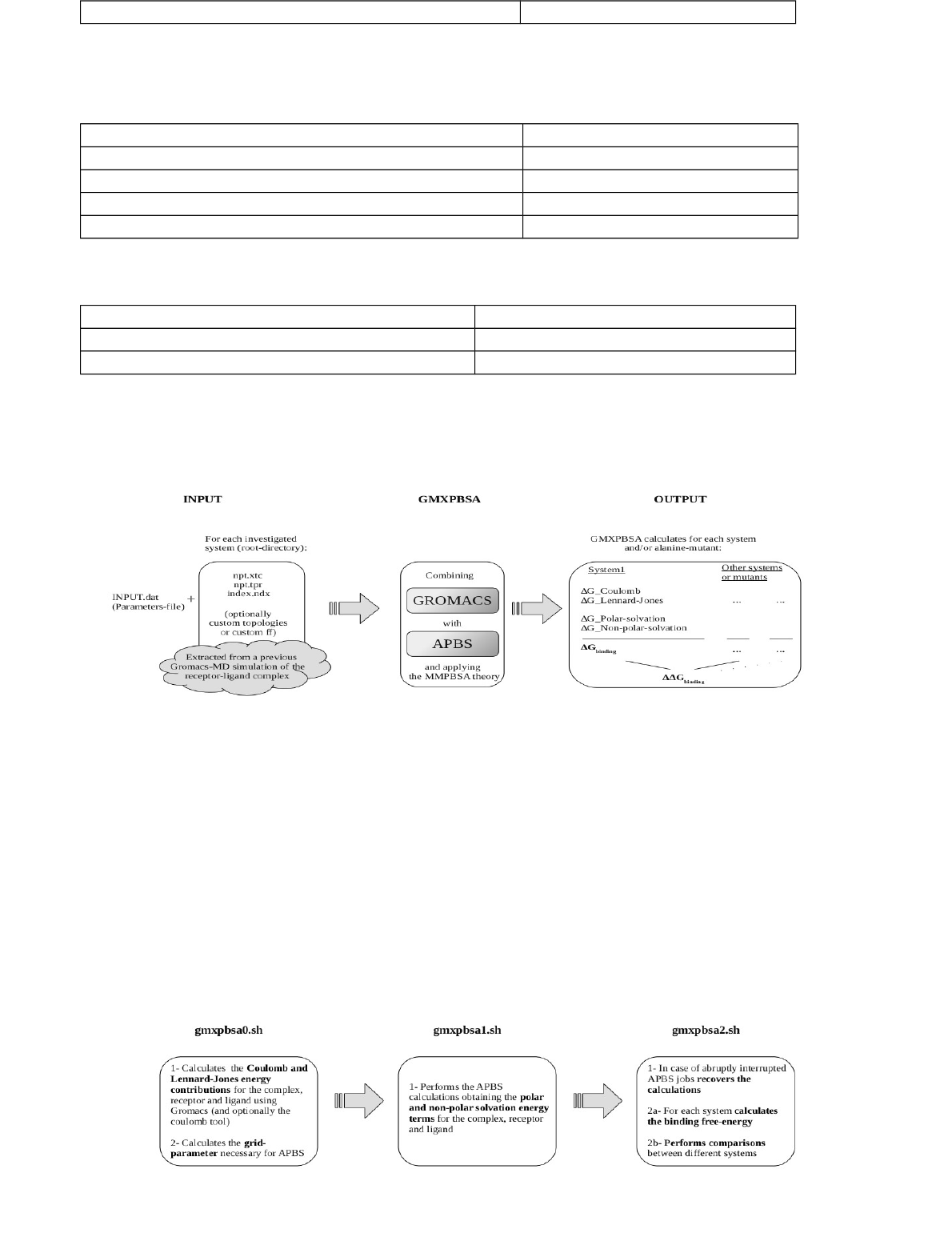
generated by GROMACS MD engine. The program workflow, (Figures 1 and 2) consists of three

different sequential steps comprising:

1. gmxpbsa0.sh:

In this step, the tool exploits the gmxpbsa0.sh script to setup the system and to perform preliminary

calculations including:

check of the required input files and directories;

extraction of the frames of the complex from the MD simulations, subsequently split in the

protein and the ligand components by the GROMACS tools;

calculation of the Coulomb energy contributions using either GROMACS tools or the

“coulomb” program available in the APBS suite, and Lennard-Jones term using

GROMACS.

If the computational alanine scanning (CAS) calculation is required, the script performs alanine

mutations on the defined residues on every single extracted frames removing the side chains atoms

of the target residues up to the beta C atom (CB atom) and then recalculating the Coulomb and the

Lennard-Jones energy contributions of the structure containing the alanine mutant. It also generates

the grid and the input to perform the APBS calculations for each frame of the simulation. The latter

task is critical, since deletion of artefacts in the MM/PBSA calculation requires an exact matching

of the grid setup between all the system components (complex, protein and ligand).

2. gmxpbsa1.sh:

In this step, the gmxpbsa1.sh script computes the solvation polar and nonpolar energy contributions

using APBS program. These calculations can be distributed on a cluster or on a multi core

workstation.

3. gmxpbsa2.sh:

In this last step, the gmxpbsa2.sh script combines for all the frames the single terms, <EMM> and

<Gsolv> respectively, in order to calculate the final binding free energy value. It also checks and tries

to fix errors and/or failures occurring in the preceding step 2 (APBS calculations). Statistical

analysis is also performed computing average and standard error (SE). The SE is calculated as

follows: SE = σ/√N, where σ is the standard deviation and N is the number of structures (MD

frames) used in the calculation. The average Coulomb and Lennard-Jones values, the polar and

nonpolar solvation terms are calculated along each trajectory. If a value differs from the average

more than two standard deviations it is considered as an outlier and the corresponding frame is

excluded from the final calculation. However, it is always possible to check for outlier frames, since

their reference-numbers are stored in the WARNING.dat file.

2.2 Installation and execution of the program

Once the source code of the program GMXPBSAtool.tar.gz has been downloaded the user should

perform the following steps:

1. extract the source code in a user defined location, e.g.. /home/myprogram/, by typing tar

zxvf GMXPBSAtool.tar.gz; set the GMXPBSAHOME environment variable in bash: export

GMXPBSAHOME=/home/myprogram/GMXPBSAtool; change the /home/myprogram to

whatever directory is appropriate for your machine; verify write permissions in the directory

tree, and execute permissions for the gmxpbsa0.sh, gmxpbsa1.sh and gmxpbsa2.sh scripts.

$GMXPBSAHOME should be also added to the PATH.

2. In order to perform MM/PBSA calculations, the user has to run the tool by typing

$GMXPBSAHOME/<script>, where <script> can be either gmxpbsa0.sh, or gmxpbsa1.sh

or gmxpbsa2.sh , according to the calculation step (see section 2.4). Each script will read the

INPUT.dat file to perform the MM/PBSA calculation. For instance, if the INPUT.dat file and

the directory containing the simulations are located in /home/mysimulations, the user will

type $GMXPBSAHOME/<script> in the aforementioned directory. See section 3 for further

details.

In order to test the correctness of GMXPBSA 2.1 installation, the tool is distributed with the

examples (with shortened trajectories) presented in Section 4 to test the correctness of the

installation.

2.3 Input files preparation

In order to perform binding free energy calculations on a ligand-receptor system (where the ligand

can be either a protein, a peptide or a small molecule), the user needs first to perform a MD

simulation using GROMACS engine 4.5 or later versions. Before starting any GMXPBSA 2.1

calculations, the user should verify the convergence of MD simulations, as lack of convergence

might strongly compromise the reliability of the MM/PBSA results, as pointed out in [11]. Along

with simulations data, the user should edit the INPUT.dat file, defining all the options on the

binding free energy calculations (see section 2.4).

For each system under investigation MM/PBSA calculations require the following input files:

1. the trajectory file describing the dynamic of the complex (name_xtc in the INPUT.dat). We

encourage the user to strip off the water from the trajectory to speed up calculations. The

possible artefacts deriving from periodic boundary condition (pbc) should be removed from

the trajectory, using the trjconv GROMACS tool (-pbc whole or -pbc nojump or -pbc res is

usually sufficient). The latter step is fundamental before carrying out the MM/PBSA

calculations in order to remove the presence of possible broken molecules. The processed

trajectory can be checked using a molecular visualizer before performing GMXPBSA

calculations.

2. the portable binary run input file (name_tpr in the INPUT.dat). This file contains the

information on mass, charges and force field parameters used in the MD simulations.

3. the index file, with mandatory name index.ndx. This file contains the groups used in the

simulations. Three groups are compulsory in order to run GMXPBSA 2.1: the complex,

containing the atoms index of the complex (union of the receptor and ligand atoms), the

receptor, containing the atoms index of the receptor, and the ligand, containing the atoms

index of the ligand. The three group index names can be chosen by the user.

The three files are placed in a directory, whose name will be referred to as root in the INPUT.dat

file. Additional files should be present in the root directory in case the MD simulation has been

carried out using either a custom GROMACS force field (e.g. including modified amino acid) or

custom topologies (i.e. ligand). See section 2.4.2 for further details (keyword use_nonstd_ff and

use_topology, respectively). When handling different trajectories, the user should create different

root-directories, one for each simulation, and define the name of these directories in the

root_multitrj variable contained in the INPUT.dat file. The tool will then automatically perform the

MM/PBSA calculations on all the systems defined in the root_multitrj directories. In order to cancel

out artefacts for each system (i.e. for each directory) an identical grid setup in the PBSA calculation

will be defined.

2.4 INPUT.dat file

The INPUT.dat is the macro file in ASCII format, through which the user can define several options

to perform binding free energy calculations. It contains 7 different sections, in which the user has to

define the mandatory keywords with the options described in the following chapters and

summarized in Table 1.

2.4.1. GENERAL

In this section the user defines the molecular system and the environment path as follows.

root: the name of the directory that contains the input files necessary to calculate the binding

free energy (trajectory, index, tpr and custom force field or topology files).

multitrj: if set to y more than one system will be analysed. If set to n only the directory

named root will be considered.

root_multitrj: this variable is considered only if multitrj is set to y. It is the list containing the

names of the directories that will be analysed (e.g if the user aims to analyse the directories

Name1, Name2 and Name3, the command should be set to: root_multitrj Name1 Name2

Name3).

run: can be either a string or an integer. For example, if the chosen option is “1” the program

will create the RUN1_root directory. In this directory GMXPBSA 2.1 will carry out all the

calculations and store the corresponding output and an input-reminders. This might be

useful when different runs with different parameters for either Molecular Mechanics (MM)

or solvation terms (PBSA) analysis are performed.

RecoverJobs: can be set to n or y. If it is set to y, during the third calculation step

GMXPBSA 2.1 will try to recover APBS failed jobs and will try to re-run them; if it is set to

n failed jobs are neglected in the final statistical analysis.

backup: can be set to n or y. If it is set to y (default), GMXPBSA 2.1 will copy the

RUN1_root in backup_RUN1_root before analysis and merging of l the energetic terms

(MM and PBSA) during the gmxpbsa2.sh step. This is useful when: i) problems arise in the

final analysis, ii) the user wants to repeat the analysis.

Cpath: the full path of the APBS “coulomb” tool. If the variable coulomb is set to coul and

no path is defined, GMXPBSA 2.1 will try to locate the binary program only if it is present

in the user's path environment.

Apath: the full path of the apbs program from the APBS suite. The user can skip this option

in case the apbs program, which is the executive PBSA solver of APBS suite, is present in

the path environment.

Gpath: the full path of the GROMACS binary tools. The user can skip this option if the

GROMACS binary tools path is present in the path environment.

2.4.2 FORCE FIELD

To calculate the Coulomb and Lennard-Jones energy contributions GMXPBSA 2.1 performs a short

energy minimization on each frame extracted from the MD simulation, that requires a GROMACS

force field. GMXPBSA 2.1 provides three options, ffield, use_nonstd_ff and use_topology.

ffield: it can be an integer representing the force field used in MD simulations (the list of

the force field can be visualized typing in the bash shell the GROMACS tool “pdb2gmx”).

The user should set the identical force field used in the MD simulations (Figure 3A). It is

possible to perform the CAS calculations. See example 1, hMdmd2-p53 complex (section

4.1).

use_nonstd_ff: it can be either n or y . If n, GMXPBSA 2.1 will use standard force field

parameters as reported in GROMACS, defined in the previous ffield keyword. If y, the

complex can be described by a modified force field in GROMACS, the user should add in

the root directory the force field files along with the trajectory, index and tpr file. The

custom force field should have the GROMACS 4.5 or later version format, with all the

parameters files placed in a directory, i.e. amber99sb.ff or oplsaa.ff. Moreover, the custom

residuetypes.dat file, which includes all the modified amino acids, should be present in the

root directory (Figure 3B). For details, please refer to the GROMACS manual. It is

possible to perform CAS calculations. See example 2, PHD-H3 complex (section 4.2).

use_topology: it can be either n or y. If n, GMXPBSA 2.1 will use either the standard force

field from the GROMACS package, defined in the previous ffield keyword, or the custom

force field placed in the root directory. If y, GMXPBSA 2.1 will perform the calculations

using the user defined custom topologies, namely receptor.itp and ligand.itp files. In this

case, the root directory should contain the topology file named topol.top (Figure 3C). This

file retrieves the receptor and ligand itp files. If use_topology is set to y, it is not possible to

perform CAS, since the modification of the topology files could lead to errors in the

modified topology. When the MM/PBSA calculations are performed on different

trajectories, each root directory should contain the proper topologies. For details see

example 3, Trypsin-Benzamidine complex, described in section 4.3.

itp_receptor: receptor topology file name. Receptors with more than one chain, require

repetition of the keyword for all the chains.

itp_ligand: ligand topology file name.

2.4.3 GROMACS

The users can define the name of the complex, receptor and ligand as defined in the index.ndx file.

They can also set different options for the Molecular Mechanics (MM) analysis in the MM/PBSA

calculation, as explained subsequently.

name_xtc: name of the trajectory file in GROMACS format.

name_tpr: name of the binary tpr file in GROMACS format.

complex: name of the complex in the index.ndx file.

receptor: name of the receptor in the index.ndx file.

ligand: name of the ligand in the index.ndx file.

multichain: Useful if in the pdbs extracted from the trajectory there are more than one

chains.The option "multichain" must be used ONLY if the string TER is not present at the

end of each chain in the comp/receptor pdb files.

protein_alone: it can be either y or n, depending on whether the user wants perform an

energetic estimation of a free protein and to study the CAS mutations. Default is n.

itp_protein: the name of the itp file of the protein in case “use_topology=y”.

skip: any integer no lower than 1. If skip is set to the integer N, a structure will be extracted

from the trajectory every N frames to be used for the subsequent analysis. In order to have

statistical reliability of the calculations, we suggest to use at least 100 frames. For instance,

in a trajectory of 1000 frames, if skip = 10, GMXPBSA 2.1 will extract 100 frames that are

equally distributed along the simulation.

min: it can be either y or n, depending on whether the user does or does not perform the

energy minimization, respectively. Energy minimization will be performed on each frame

before calculating the Coulomb/ Lennard-Jones contributions.

double_p: it can be either y or n, depending on whether double precision in energy

minimization is required, respectively.

read_vdw_radii: it can be either y or n. In case of y GMXPBSA 2.1 requires the presence of

the vdwradii.dat file (containing the Van der Waals radii) in the root directory. In this case

the “editconf” gromacs tool will use this file to generate the pqr files and will not compute

the radii based on the force field. The default option is n, however, care should be taken

when using this option, as the definition of the Van der Waals radii might influence the

MM/PBSA results.

coulomb: GMXPBSA 2.1 can calculate the coulomb energy term either using the APBS

“coulomb” tool (option coul) or using GROMACS (option gmx). By default it is set to coul.

2.4.4 APBS

The following section allows the user to define the options for the polar (PB) and nonpolar (SA)

solvation terms in MM/PBSA calculations. For details, please refer to the APBS manual

(http://www.poissonboltzmann.org/apbs/).

linearized: APBS can calculate the solvation energy by solving the linearized (option y) or

nonlinear (option n) Poisson-Boltzmann equation. By default it is set to n.

precF: can be a digit (either 0, 1, 2 or 3), which controls the size of the grid generated during

the APBS calculations (from 0 to 3 the grid spacing is decreased, resulting in more

expensive calculations ). By default it is set to 1.

temp: indicates the temperature at which the APBS calculations are performed. By default it

is set to 293 K.

bcfl: specifies the type of boundary conditions used to solve the Poisson-Boltzmann

equation. It can be either sdh, mdh or focu. By default it is set to mdh.

pdie: defines the dielectric constant of the biomolecule. This is usually a value between 2 to

20, lower values consider only electronic polarization and higher values consider additional

polarization due to intramolecular motion. By default it is set to 2.

extraspace: 5, quantity to add (A°) for each side to get fine-grid dimensions.

coarsefactor: 1.7, factor to get coarse-grid dimensions.

grid_spacing: 0.5 fine mesh spacing

sdie: 80

chgm: spl2

srfm: smol

srad: 1.4

swin: 0.3

sdens: 10.0

calcforce: no

ion_ch_pos: 1 positive ion charge in electron units

ion_rad_pos: 2.0 positive ion radius

ion_conc_pos: 0.15 positive ion concentration

ion_ch_neg: -1 negative ion charge in electron units

ion_rad_neg: 2.0 negative ion radius

ion_conc_neg: 0.15 negative ion concentration

Hsrfm: sacc srfm for non-polar calculations

Hpress : 0.00 press for non-polar calculations

Hgamma: 0.0227 gamma for non-polar calculations

Hdpos: 0.20 dpos for non-polar calculations

Hcalcforce: total calcforce for non-polar calculations

Hxgrid: 0.1xgrid for non-polar calculations

Hygrid: 0.1ygrid for non-polar calculations

Hzgrid : 0.1zgrid for non-polar calculations

2.4.5 DISTRIBUTED CALCULATIONS

The user can define the different options for calculations submission to a cluster facility. Since

energy calculations for each frame are independent, they can be easily parallelized in a distributed

fashion assigning single frames to the available processors. MM/PBSA calculations can be

performed either in a workstation exploiting one single core or multi core, or in a cluster exploiting

the PBS/TORQUE queue system. The latter option is useful for the analysis of a large amount of

frames, whereby GMXPBSA 2.1 submits to a batch queue a series of jobs carrying out MM/PBSA

calculations. The number of submitted jobs depends on the mnp keyword and on the total number of

frames (total_frames) that are analysed. GMXPBSA 2.1 calculates the number of total jobs to be

submitted according to the following rule: total_number_of_jobs = total_frames/mnp. For instance,

if the user sets mnp to20 and the trajectory contains 1000 frames, the total_number_of_jobs will be

50, whereby each job will contain 20 PBSA calculations. GMXPBSA 2.1 will then submit to the

queue these 50 jobs, monitoring the status (Running, Queue, Hold), checking the completion of

each job, and verifying the end of the calculations (jobs failed and/or successful completed). In case

of failed jobs, the program will recover them (if RecoverJobs is set to y) and resubmit to the queue

as previously described. In case of further failures, GMXPBSA 2.1 will print a warning in a log file,

and the failed frames will be excluded from the final MM/PBSA calculations. Finally, if cluster is

set to n and mnp is bigger than 1, GMXPBSA 2.1 will use the requested processors without using

the PBS system.

cluster: when the option is set to y GMXPBSA 2.1 performs calculations on a cluster in a

distributed fashion taking advantage of the PBS queue manager and divides frames across

all processors thus speeding up calculations.

Q: defines the name of the queue that is used for solvation energy calculations (this is

necessary only if cluster is set to y).

budget_name: the name of the user account in the computing facilities

walltime: the total maximum wall-clock time during which this job can run (note than 800

means seconds, 80:00 means minutes and seconds and 1:00:00 means hours, minutes and

seconds).

mnp: defines the maximum number of processors used during GMXPBSA 2.1 calculations.

We highly recommend to use numbers > 1 in workstations bearing multi core only when a

large amount of physical memory is available (at least 2Gb).

nodes: 1

mem: 5GB

When performing the calculations in a cluster with the PBS queue manager, the job are submitted

as: PBS -l select:$mnp:ncpus:$nodes:mem=$mem.

2.4.6 OUTPUT

The scripts always generate an output file in ASCII format, the user can chose an option that

generates the output file in PDF format.

pdf: generates a PDF file report as output (y or n). To set pdf to y it is necessary to have

installed LaTeX.

2.4.7 COMPUTATIONAL ALANINE SCANNING

In this section, the user can perform CAS calculations a posteriori on the trajectory. In this case, the

user should specify which residues (ligand and/or receptor) should be modified in alanine.

cas: if the y option is selected, GMXPBSA 2.1 will perform CAS

The setting for the mutation should contain the following string:

MUTATION root directory residue_number residue_name [receptor or lig] mutation_name.

The keywords receptor or lig are mandatory. GMXPBSA 2.1 automatically creates in the

RUN1_root directory a new directory for each mutation

( (root_MUTATION_mutation_name).

In the following, we present some syntax examples of the INPUT.dat file (Table 2):

a. “MUTATION PHD 9 ASP receptor ASP9ALA”, indicates that GMXPBSA 2.1 mutates the

residue ASP9 of the receptor in ALA.

b. “MUTATION PHD 8 ARG lig ARG8ALA”, indicates that GMXPBSA 2.1 mutates the

residue ARG8 of the peptide (lig) in ALA.

c. “MUTATION PHD 9 ASP receptor RES_9-11”, “MUTATION PHD 10 GLU receptor

RES_9-11”, “MUTATION PHD 11 CYZ receptor RES_9-11”, indicates that GMXPBSA

2.1 mutates the residues in the range 9-11 to ALA of the receptor.

It is possible to simultaneously apply all the above combinations in the CAS study, in this case

GMXPBSA 2.1 will create for each mutation name a directory.

3. Calculations steps of GMXPBSA 2.1

In the subsequen section we present the three calculation steps performed by GMXPBSA 2.1, a

summary of the main calculations and of the main output files generated by the scripts. Further

details are reported in the Supporting Material.

3.1 Calculations of Molecular Mechanics terms: gmxpbsa0.sh

In this first step GMXPBSA 2.1 calculates the Molecular Mechanics term (MM) of the MM/PBSA

approach, including Coulomb and Lennard-Jones terms. In order to perform the MM/PBSA

calculations, each GMXPBSA 2.1 script should read the INPUT.dat file. For instance, if the input

files (npt.xtc, npt.tpr and index.ndx and possible additional files) are placed in

/home/mysimulations/MD, the corresponding INPUT.dat file should be placed in

/home/mysimulations (working directory). The root keyword in INPUT.dat will be MD. In the

working directory (/home/mysimulations) the user will run the script:

$GMXPBSAHOME/gmxpbsa0.sh

to calculate the Coulomb and Lennard-Jones energies, the so called EMM terms. In this step

GMXPBSA 2.1 will also generate the grid needed to perform the APBS calculations in the second

workflow step. By default the grid is generated as follows (Figure 4):

fine grid: 10 Å added in each direction from the extreme coordinates of the complex;

coarse grid: 1.7 time larger than the fine grid.

The grid spacing is automatically set to an upper limit of 0.5 Å. Setting run keyword in INPUT.dat

to 1, GMXPBSA 2.1 will create RUN1_MD (RUNrun_root). At the end of the calculations, the

RUN1_MD directory will contain several output files (described in detail in the Supporting

Material). In particular, the RUNrun_root will be organized in three sub-folders:

1. STORED_FILES, containing all the files used during the Coulomb and Lennard-Jones

energy calculations;

2. APBS_CALCULATIONS, containing all the input files necessary for APBS. In this

directory, during the second step of the calculation APBS will generate also the

corresponding output;

3. SUMMARY_FILES for each analysed frame, a strun.rep file is generated, where n is the

number of generated frames (n = [Numer of total frames]/skip). These files contain all the

energy contributions (Coulomb and Lennard-Jones) of each frame.

In case of error or failure occurring in this step, GMXPBSA 2.1 will stop and will report the

possible failure causes in the STD_ERR0 file, that is present in each RUNrun_root.

3.2 Calculations of Solvation energy terms: gmxpbsa1.sh

In this step the PB and SA solvation energy terms of MM/PBSA are calculated. These contributions

are calculated typing the following command in the working directory (i.e. /home/mysimulations):

$GMXPBSAHOME/gmxpbsa1.sh

These calculations are often computationally expensive. Depending on the system size and frame

numbers they might require hours to finish; e.g. a system composed by 70 amino acids requires 5

min/frame calculation time on a single core.

The APBS calculations are performed by default at a NaCl concentration of 0.15 M and at a

temperature of 293 K, however these parameters can be easily changed by the user in the

INPUT.dat file. At the end of the calculations, the RUNrun_root directory (i.e. RUN1_MD) will

contain several output files (described in detail in the Supporting Material). The output file of each

APBS calculation will be stored in the SUMMARY_FILES folder.

3.3 Calculations of MM/PBSA binding free energy: gmxpbsa2.sh

This is the last step of the tool that combines all the energetic terms to compute the MM/PBSA

binding free energy value. To this aim it is sufficient to type in the working directory:

$GMXPBSAHOME/gmxpbsa2.sh

This script calculates the average and standard error of the MM/PBSA binding free energy values

deriving from the extracted frames. Before calculating the MM/PBSA value, the script will try to

recover failed jobs generated in the preceding step (if the variable RecoverJob is set to y). The

RUNrun_root directory will contain a series of files that are described in detail in Supporting

Material. To facilitate comparisons the file Compare_MMPBSA.dat generated in this step, contains

the average energy values plus the standard error SE (both the total energy and the single

contributions) of each system.

4 Examples

We run GMXPBSA 2.1 on three different systems in order to test its performance using different

INPUT.dat parameters. The first test was performed on cellular regulatory phosphoprotein p53 in

complex with oncoprotein Mdm2. This complex is considered as a reference system, as it has been

the first to be studied by the MM/PBSA approach [6]. This example requires to use the ffield

keyword in INPUT.dat. The second test was performed on the first PHD finger domain of

autoimmune regulator protein (AIRE) in complex with a 10 residue peptide corresponding to the N-

terminal tail of histone H3 [11]. In this example we perform MM/PBSA calculations on a system

bearing modified amino acids (use_nonstd_ff keyword in INPUT.dat). Finally, in the third example

we studied trypsin in complex with drug-like molecules (reversible competitive inhibitors

benzamidine and 1,3benzamidine [12]). In this example we used the use_topology keyword in

INPUT.dat. All the calculations have been carried out on a workstation Intel 3.30 GHz bearing 4 Gb

of RAM.

4.1. Example 1: p53 in complex with hMdm2 and CAS

We used GMXPBSA 2.1 to: i) calculate the binding free energy generated by the interaction

between p53 and hMdm2; ii) to perform CAS calculations. In this example we apply the standard

procedure, where the user gives as input files only the trajectory (xtc), the portable input binary (tpr)

and the index (ndx) files (Figure 3a). Before running GMXPBSA we performed 10ns of MD

simulation on the wild-type complex using amber99sb-ildn force field. In order to speed up the

calculations we removed the water molecules and the analysis was therefore performed on 1678

atoms. The final trajectory contained 1000 frames; in the INPUT.dat file we defined the following

parameters: ffield to 6 (amber99sb-ildn force field), skip 50 (20 frames to be considered),

linearized n, coulomb coul, mnp 1 and four alanine mutants on the 12-residue peptide of p53

defined in Table 3 (CAS calculations). The first step, gmxpbsa0.sh, required 3 minutes to extract all

the MM terms and to setup the grid for the PBSA calculation from 100 frames (20 frames for each

system, i.e. the wild type and the four alanine mutants). The second and third steps required 450

minutes and 5 seconds, respectively.

4.2 Example 2: AIRE-PHD1 in complex with histone H3 peptide and CAS

PHD fingers are Zn2+ binding domains consisting of 50–80 amino acids that form a two-stranded

antiparallel β-sheet followed by an α helix. The first PHD finger domain of AIRE recognizes the

unmodified tail of histone H3 to promote the expression of AIRE target genes [13]. We generated

10ns of trajectory of the PHD in complex with a histone peptide corresponding to the first 10

residues of histone H3 N-terminal tail (H3K4me0), using a custom oplsa force field, that was used

to define two Zn2+ coordinating residues, namely: CYM and HIZ, corresponding to an unprotonated

cysteine and a single protonated histidine, respectively. We also performed CAS calculations. We

stripped out the water molecules from the trajectory (final number of atoms: 1136). In the

INPUT.dat we defined the following parameters: use_nonstd_ff y, skip 1, linearized n, coulomb

coul, mnp 1 and two alanine mutants defined in Table 4 (CAS calculations). The PHD directory

contains the trajectory (xtc), the portable binary (tpr) and the index (ndx) files, the oplsaa.ff

directory and the residuetypes.dat file, which were used to carry out MD simulations (Figure 3b). In

this case we performed calculations on a total of 60 frames (20 frames for the wild type and 20 for

each of the mutants). The three steps required 2 minutes, 225 minutes and 2 seconds, respectively.

4.3 Example 3: Trypsin in complex with benzamidine ligands

In this example we used GMXPBSA 2.1 to compare the affinity of two ligands towards the same

receptor, to this aim we performed MM/PBSA calculations on trypsin in complex with benzamidine

and 1,3benzamidine ligands [12]. In this case, in order to carry out MD simulations followed by

MM/PBSA calculations, it was necessary to generate the topology file of the benzamidine ligands.

We exploited the Amber Antechamber program to calculate the ligand charges and the topology

parameter. Once we created the topology files for each ligand, ben.itp and ben2.itp, respectively

(see details in Supporting Material) we performed MD calculations (10ns) for each complex system.

Thereafter, we used GMXPBSA 2.1 to calculate the binding free energy of the benzamidine-trypsin

and 1,3benzamidine-trypsin complexes on the GROMACS trajectories. We stripped out of the water

molecules (final number of atoms: 3237 and 3239, respectively). We created two directories called

TRY and TRY2. In each directory we put the corresponding trajectory file (npt.xtc), portable input

binary file (npt.tpr), and index file with the complex, receptor and ligand group names (index.ndx),

and the complex, protein and ligand topologies, topol.top, trp.itp and ben.itp, in TRY1 and in TRY2

directories, respectively (Figure 3c). The main parameters in the INPUT.dat file were the following:

use_topology y, skip 100, linearized n, coulomb coul and mnp 1. Calculations were performed on a

total of 20 frames (10 frames for TRY and 10 for TRY2). The three steps required 1 minute, 80

minutes and 2 seconds, respectively. Computational alanine scanning cannot be performed in this

example since we are using the use_topology keyword.

Table 1. INPUT.dat file to run GMXPBSA 2.1

Keywords Value Note Default

root Name_of_Directory String -

run Any_Number Integer 1

multitrj “y” “n” Boolean n

root_multitrj* List of directory name String -

RecoverJobs “y” “n” Boolean y

backup “y” “n” Boolean y

Cpath Full_path String -

Apath Full_path String -

Gpath Full_path String -

use_topology “y” “n” Boolean -

itp_receptor* Name_of_topology String -

itp_ligand* Name_of_topology String -

use_nonstd_ff “y” “n” Boolean n

ffield* Number_of_ff_used_in_MD Integer -

name_xtc Name of GROMACS xtc String -

name_tpr Name of GROMACS tpr String -

complex Name_in_index_file String -

receptor Name_in_index_file String -

multichain “y” “n” Boolean n

protein_alone “y” “n” Boolean n

itp_protein Name_of_topology String -

ligand Name_in_index_file String -

skip Any_Digit Integer 1

min “y” “n” Boolean n

double_p “y” “n” Boolean n

read_vdw_radii “y” “n” Boolean n

coulomb “coul” “gmx” String gmx

linearized “y” “n” Boolean y

precF “0” “1” “2” “3” Integer 0

temp Temperature Integer 293

bcfl “sdh” “mdh” “focus” String mdh

pdie Any_Digit in [0:20] range Integer 2

coarsefactor Float 1.7

grid_spacing Float 0.5

sdie Integer 80

chgm String spl2

srfm String smol

srad Float 1.4

swin Float 0.3

sdens Float 10.0

calcforce Boolean no

ion_ch_pos Integer 1

ion_rad_pos Float 2.0

ion_conc_pos Float 0.15

ion_ch_neg Float -1

ion_rad_neg Float 2.0

ion_conc_neg Float 0.15

Hsrfm String sacc

Hpress Float 0.0

Hgamma Float 0.0227

Hdpos Float 0.2

Hcalcforce String total

Hxgrid Float 0.1

Hygrid Float 0.1

Hzgrid Float 0.1

cluster “y” “n” Boolean y

QName_of_queue String -

budget_name Name_of_budget String -

walltime Any Digit Integer -

mnp Any_Digit Integer 1

pdf “y” “n” Boolean n

cas “y” “n” Boolean n

Table 2. Example of CAS parameters as defined in INPUT.dat file

Requested mutation Name of working directory

MUTATION PHD 9 ASP receptor ASP9ALA RUN1_PHD_ASP9ALA

MUTATION PHD 8 ARG lig ARG8ALA RUN1_PHD_ARG8ALA

MUTATION PHD 9 ASP receptor RES_9-11

MUTATION PHD 10 GLU receptor RES_9-11

RUN1_PHD_RES_9-11

MUTATION PHD 11 CYZ receptor RES_9-11

Table 3. CAS parameters as defined in INPUT.dat file of Example 1

Requested mutation Name of working directory

MUTATION P53 112 PHE lig PHE19ALA RUN1_P53_PHE112ALA

MUTATION P53 115 LEU lig LEU22ALA RUN1_P53_LEU115ALA

MUTATION P53 116 TRP lig TRP23ALA RUN1_P53_TRP116ALA

MUTATION P53 119 LEU lig LEU26ALA RUN1_P53_LEU119ALA

Table 4. CAS parameters as defined in INPUT.dat file of Example 2

Requested mutation Name of working directory

MUTATION PHD 9 ASP receptor ASP9ALA RUN1_PHD_ASP9ALA

MUTATION PHD 8 ARG lig ARG8ALA RUN1_PHD_ARG8ALA

Figure 1 Workflow diagram for GMXPBSA 2.1. Diagram describing the general GMXPBSA 2.1

workflow scheme. GMXPBSA 2.1 combines the GROMACS and APBS programs in order to use

the frames extracted from the molecular dynamics simulations and to calculate the binding free

energy.

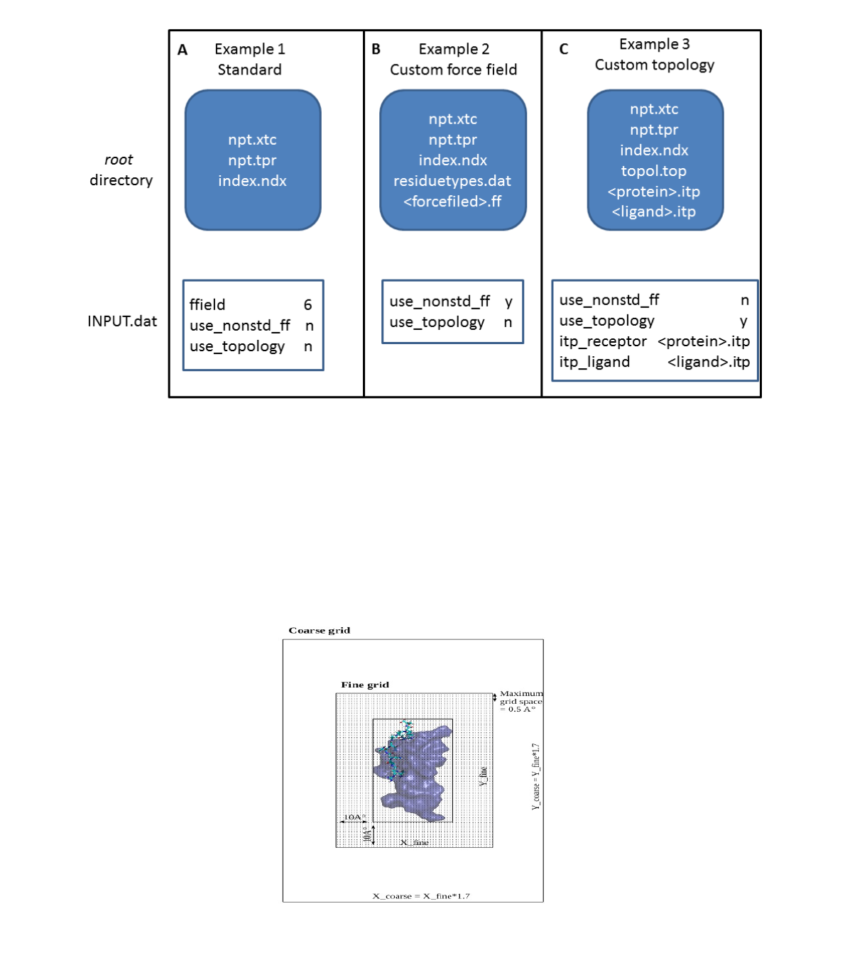
Figure 2 Schematic diagram of the three GMXPBSA 2.1 calculation steps Diagram showing the

input files used by GMXPBSA 2.1 and the output files generated during each MM/PBSA step.

Figure 3 Schematic diagram of the three GMXPBSA 2.1 examples. Diagram showing the input

files and the INPUT.dat parameters used by GMXPBSA 2.1 in each example.

Figure 4 2D-schematic representation of the grid preparation in the apbs calculation. The

protein and the ligand are shown in blue surface and licorice, respectively. The fine grid is

generated adding 10 Å in each direction from the extreme coordinates of the complex. The coarse

grid is 1.7 times larger than the fine grid. In this scheme the z-axis is omitted for clarity.

REFERENCES

[1] MR Reddy, CR Reddy, RS Rathore, MD Erion, P Aparoy, RN Reddy, et al. Free Energy

Calculations to Estimate Ligand-Binding Affinities in Structure-Based Drug Design,

Curr.Pharm.Des. (2013).

[2] MK Gilson, HX Zhou. Calculation of protein-ligand binding affinities,

Annu.Rev.Biophys.Biomol.Struct. 36 (2007) 21-42.

[3] S Huo, I Massova, PA Kollman. Computational alanine scanning of the 1:1 human growth

hormone-receptor complex, J.Comput.Chem. 23 (2002) 15-27.

[4] IS Moreira, PA Fernandes, MJ Ramos. Protein-protein docking dealing with the unknown,

J.Comput.Chem. 31 (2010) 317-342.

[5] RT Bradshaw, BH Patel, EW Tate, RJ Leatherbarrow, IR Gould. Comparing experimental

and computational alanine scanning techniques for probing a prototypical protein-protein

interaction, Protein Eng.Des.Sel. 24 (2011) 197-207.

[6] KP Massova I. Computational alanine scanning to probe protein-protein interactions: A

novel approach to evaluate binding free energies, J. Am. Chem. Soc. 121 (1999) 8133-8143.

[7] NA Baker, D Sept, S Joseph, MJ Holst, JA McCammon. Electrostatics of nanosystems:

application to microtubules and the ribosome, Proc.Natl.Acad.Sci.U.S.A. 98 (2001) 10037-

10041.

[8] SP Brown, SW Muchmore. Large-scale application of high-throughput molecular

mechanics with Poisson-Boltzmann surface area for routine physics-based scoring of protein-

ligand complexes, J.Med.Chem. 52 (2009) 3159-3165.

[9] Bill R. Miller, III, T. Dwight McGee, Jr., Jason M. Swails, Nadine Homeyer, Holger

Gohlke, and Adrian E. Roitberg. MMPBSA.py: An Efficient Program for End-State Free

Energy

Calculations, J. Chem. Theory Comput. 8 (2012) 3314-3321.

[10] S Pronk, S Pall, R Schulz, P Larsson, P Bjelkmar, R Apostolov, et al. GROMACS 4.5: a

high-throughput and highly parallel open source molecular simulation toolkit, Bioinformatics.

29 (2013) 845-854.

[11] D Spiliotopoulos, A Spitaleri, G Musco. Exploring PHD fingers and H3K4me0

interactions with molecular dynamics simulations and binding free energy calculations:

AIRE-PHD1, a comparative study, PLoS One. 7 (2012) e46902.

[12] D Jiao, J Zhang, RE Duke, G Li, MJ Schnieders, P Ren. Trypsin-ligand binding free

energies from explicit and implicit solvent simulations with polarizable potential,

J.Comput.Chem. 30 (2009) 1701-1711.

[13] J Derbinski, J Gabler, B Brors, S Tierling, S Jonnakuty, M Hergenhahn, et al.

Promiscuous gene expression in thymic epithelial cells is regulated at multiple levels,

J.Exp.Med. 202 (2005) 33-45.

[14] T Hou, J Wang, Y Li, W Wang. Assessing the performance of the MM/PBSA and

MM/GBSA methods. 1. The accuracy of binding free energy calculations based on molecular

dynamics simulations, J.Chem.Inf.Model. 51 (2011) 69-82.

[15] L Li, C Li, S Sarkar, J Zhang, S Witham, Z Zhang, et al. DelPhi: a comprehensive suite

for DelPhi software and associated resources, BMC Biophys. 5 (2012) 9-1682-5-9.

Manual

Manual

Navigation menu

Versions of this User Manual:

Views

Navigation