PAM RTM 2014 User Guide Tutorials
User Manual:
Open the PDF directly: View PDF ![]() .
.
Page Count: 464 [warning: Documents this large are best viewed by clicking the View PDF Link!]
- INTRODUCTION
- PAM-RTM USER'S GUIDE
- INTRODUCTION
- PRESENTATION OF THE USER INTERFACE
- FILE MENU
- SELECTION MENU
- GROUPS MENU
- MESH MENU
- VIEW MENU
- PROCESS PARAMETERS
- NUMERICAL PARAMETERS
- FUNCTION EDITOR
- MATERIAL PROPERTIES OF THE RESIN
- MATERIAL PROPERTIES OF THE FIBER REINFORCEMENTS
- MATERIAL PROPERTIES OF SOLIDS
- LAMINATES
- MATERIAL DATABASE
- BOUNDARY CONDITIONS
- NON-COINCIDENT INTERFACES
- SENSORS
- TRIGGER MANAGER
- CURVE VIEWER
- RUNNING THE SIMULATION FROM A COMMAND WINDOW
- TUTORIALS
- CENTRAL INJECTION
- EDGE EFFECTS – RECTANGULAR PLATE
- EDGE EFFECTS – COMPLEX SHAPE
- FIBER ORIENTATIONS
- COMPARISON 2D – 2.5D – 3D
- AIR ENTRAPMENT
- VACUUM ASSISTED RESIN INFUSION (VARI)
- LANDING GEAR
- MESH EXTRUSION
- NON-ISOTHERMAL INJECTION
- CURING OF A PLATE
- CURING OF A PART WITH AN INSERT
- THERMAL CONTACT RESISTANCE
- NON-ISOTHERMAL 3D – FIBERS ORIENTATION
- USER DEFINED FUNCTIONS
- ONE SHOT FILLING SIMULATION
- GENPORTS
- SEQUENTIAL INJECTION (TRIGGER MANAGER)
- VELOCITY OPTIMIZATION
- COMPRESSION RTM
- LOCAL PERMEABILITY FROM DRAPING RESULTS
- LOCAL PERMEABILITY FROM DRAPING RESULTS (ADVANCED)
- PAM-QUIKFORM

PAM-RTM 2014
User’s Guide & Tutorials

April 2014
GR/PART/14/01/00/A
PAM-RTM 2014
USER’S GUIDE & TUTORIALS
The documents and related know-how herein provided by ESI Group subject to
contractual conditions are to remain confidential. The CLIENT shall not disclose
the documentation and/or related know-how in whole or in part to any third party
without the prior written permission of ESI Group.
© 2014 ESI Group. All rights reserved.

PAM-RTM 2014 i USER’S GUIDE & TUTORIALS
© 2014 ESI Group (released: Apr-14)
CONTENTS
CONTENTS
INTRODUCTION 1
Presentation of Liquid Composite Molding ------------------------------------------ 1
RTM Process ------------------------------------------------------------------------------- 4
Motivation of Filling Simulations ------------------------------------------------------- 4
Modeling ------------------------------------------------------------------------------------- 4
Credits -------------------------------------------------------------------------------------- 12
PAM-RTM USER'S GUIDE 15
Introduction -------------------------------------------------------------------------------- 15
Presentation of the User Interface -------------------------------------------------- 16
Interaction with the Mouse ------------------------------------------------------------ 17
Toolbars ----------------------------------------------------------------------------------- 18
Model Explorer --------------------------------------------------------------------------- 23
Message Pane --------------------------------------------------------------------------- 24
File Menu ---------------------------------------------------------------------------------- 25
File > New --------------------------------------------------------------------------------- 25
File > Open ------------------------------------------------------------------------------- 26
File > Close ------------------------------------------------------------------------------- 27
File > Save -------------------------------------------------------------------------------- 27
File > Save As ---------------------------------------------------------------------------- 28
File > Import > Mesh -------------------------------------------------------------------- 28
File > Import > Scalar Fields ---------------------------------------------------------- 28
File > Import > Draping Results ------------------------------------------------------ 29
File > Export > Mesh ------------------------------------------------------------------- 30
File > Export > PAM-RTM Scalar Field -------------------------------------------- 30
File > Clear > Scalar Fields ----------------------------------------------------------- 30
File > Clear >Laminate ----------------------------------------------------------------- 30
File > Save Image ----------------------------------------------------------------------- 30
File > Generate AVI --------------------------------------------------------------------- 30
File > Print--------------------------------------------------------------------------------- 31
File > Print Preview --------------------------------------------------------------------- 31
File > Print Setup ------------------------------------------------------------------------ 31
Selection Menu --------------------------------------------------------------------------- 32
Selection Filter --------------------------------------------------------------------------- 32
Selection > Pick Normal Vector ------------------------------------------------------ 32
Selection > Pick Normal Vector and Zone ----------------------------------------- 33
Selection > Pick Zone ------------------------------------------------------------------ 33
Selection > Pick Boundary ------------------------------------------------------------ 34
Selection > Pick Free Edge ----------------------------------------------------------- 34
Selection > Zone ID --------------------------------------------------------------------- 35
Selection > Entity ID -------------------------------------------------------------------- 36
Selection > Bounding Box ------------------------------------------------------------- 36
Selection > Select All ------------------------------------------------------------------- 37
Selection > Unselect All (filter) ------------------------------------------------------- 37
USER’S GUIDE & TUTORIALS ii PAM-RTM 2014
(released: Apr-14) © 2014 ESI Group
CONTENTS
Selection > Unselect All (no filter) --------------------------------------------------- 37
Selection > Set Scalar Field Value -------------------------------------------------- 37
Selection > Info Summary ------------------------------------------------------------- 37
Selection > Info Detailed --------------------------------------------------------------- 37
Groups Menu ----------------------------------------------------------------------------- 38
Groups > Create ------------------------------------------------------------------------- 38
Groups > Add To ------------------------------------------------------------------------ 38
Groups > Remove From --------------------------------------------------------------- 38
Groups > Change ID -------------------------------------------------------------------- 38
Groups > Contact Interface ----------------------------------------------------------- 38
Groups > Mold/Cavity Interface ------------------------------------------------------ 39
Groups > Nodes to Faces ------------------------------------------------------------- 41
Groups > Faces to Nodes ------------------------------------------------------------- 41
Groups > Delete (Pick) ----------------------------------------------------------------- 41
Groups > Delete (ID) ------------------------------------------------------------------- 41
Groups > Info Summary --------------------------------------------------------------- 41
Groups > Info Detailed ----------------------------------------------------------------- 41
Mesh Menu -------------------------------------------------------------------------------- 42
Mesh > Remesh > Injection Point --------------------------------------------------- 42
Mesh > Remesh > Runner ------------------------------------------------------------ 43
Mesh > Orientations > K1 ------------------------------------------------------------- 45
Mesh > Orientations > Set Vectors-------------------------------------------------- 45
Mesh > Orientations > Project Vectors --------------------------------------------- 45
Mesh > Orientations > Set K from Selected Nodes ----------------------------- 45
Mesh > Orientations > Set K Orthogonal ------------------------------------------ 46
Mesh > Orientations > Align Plies --------------------------------------------------- 46
Mesh > Orientations > Reverse ------------------------------------------------------ 47
Mesh > Orientations > Project on Skin --------------------------------------------- 47
Mesh > Orientations > Interpolate --------------------------------------------------- 47
Mesh > Orientations > Map Draping Results ------------------------------------- 55
Mesh > Orientations > Compute Local Permeability on Shells --------------- 56
Mesh > Orientations > Compute Local Permeability on Solids --------------- 63
Mesh > Orientations > Compute Local Permeability from Zones ------------ 64
Mesh > Orientations > Compute Thickness from Skins ------------------------ 64
Mesh > Orientations > Clear on Selection ----------------------------------------- 65
Mesh > Orientations > Clear All ------------------------------------------------------ 66
Mesh > Transform > Set Zone ID---------------------------------------------------- 66
Mesh > Transform > Offset Zone Ids ----------------------------------------------- 67
Mesh > Transform > Extrude --------------------------------------------------------- 67
Mesh > Transform > Split Quads ---------------------------------------------------- 70
Mesh > Transform > Split Solid Elements ----------------------------------------- 71
Mesh > Transform > Scale ------------------------------------------------------------ 71
Mesh > Transform > Translate ------------------------------------------------------- 71
Mesh > Transform > Rotate ----------------------------------------------------------- 72
Mesh > Transform > Extract Shell from Solid ------------------------------------- 72
Mesh > Create > Node ----------------------------------------------------------------- 74
Mesh > Cleanup > Merge Coincident Nodes ------------------------------------- 74
Mesh > Cleanup > Reverse Normals (selection) -------------------------------- 74
Mesh > Cleanup > Align Normals (auto) ------------------------------------------- 74
Mesh > Cleanup > Delete Unreferenced Nodes --------------------------------- 74
PAM-RTM 2014 iii USER’S GUIDE & TUTORIALS
© 2014 ESI Group (released: Apr-14)
CONTENTS
Mesh > Cleanup > Delete Selected Entities -------------------------------------- 75
Mesh > Cleanup > Delete Degenerate Elements -------------------------------- 75
Mesh > Cleanup > Swap Diagonal -------------------------------------------------- 75
Mesh > Check ---------------------------------------------------------------------------- 75
Mesh > Info ------------------------------------------------------------------------------- 76
Mesh > Info Pick ------------------------------------------------------------------------- 76
View Menu --------------------------------------------------------------------------------- 77
View > Curve Viewer ------------------------------------------------------------------- 77
View > Orientations > K1 Only ------------------------------------------------------- 77
View > Orientations > K2 Only ------------------------------------------------------- 77
View > Orientations > K1 and K2 ---------------------------------------------------- 78
View > Orientations > None ----------------------------------------------------------- 78
View > Outline > Part ------------------------------------------------------------------- 78
View > Outline > Free Edges --------------------------------------------------------- 78
View > Outline > Plies ------------------------------------------------------------------ 78
View > Flow Front ----------------------------------------------------------------------- 79
View > Normal Vectors ----------------------------------------------------------------- 80
View > Zones Visibility ----------------------------------------------------------------- 80
View > Cutting Plane ------------------------------------------------------------------- 80
View > Post-Processing --------------------------------------------------------------- 82
View > Symmetry ------------------------------------------------------------------------ 84
View > Delete N Last Steps ----------------------------------------------------------- 84
View > Set Same Viewpoint ---------------------------------------------------------- 85
View > Options > Paths ---------------------------------------------------------------- 85
View > Options > Display -------------------------------------------------------------- 87
View > Options > Colors --------------------------------------------------------------- 89
View > Color Scale ---------------------------------------------------------------------- 90
View > Color Schemes ----------------------------------------------------------------- 91
View > Lights ----------------------------------------------------------------------------- 91
View > Refresh --------------------------------------------------------------------------- 91
Process Parameters -------------------------------------------------------------------- 92
RTM Simulation -------------------------------------------------------------------------- 92
VARI Simulation ------------------------------------------------------------------------- 94
Heated RTM Simulation --------------------------------------------------------------- 95
Preheating Simulation ------------------------------------------------------------------ 97
Presimulation ----------------------------------------------------------------------------- 98
Curing Simulation ----------------------------------------------------------------------- 98
Compression RTM Simulation ------------------------------------------------------- 99
PAM-QUIKFORM Simulation ------------------------------------------------------- 100
Numerical Parameters---------------------------------------------------------------- 107
RTM Simulation ------------------------------------------------------------------------ 107
VARI Simulation (standard solver only) ------------------------------------------ 115
Heated RTM Simulation ------------------------------------------------------------- 118
Preheating Simulation ---------------------------------------------------------------- 121
Curing Simulation --------------------------------------------------------------------- 123
Presimulation (standard solver only) ---------------------------------------------- 125
PAM-QUIKFORM Simulation ------------------------------------------------------- 126
Function Editor ------------------------------------------------------------------------- 130
Overview -------------------------------------------------------------------------------- 130
User Defined Functions -------------------------------------------------------------- 132

USER’S GUIDE & TUTORIALS iv PAM-RTM 2014
(released: Apr-14) © 2014 ESI Group
CONTENTS
Function Pool --------------------------------------------------------------------------- 133
Import/Export --------------------------------------------------------------------------- 134
Material Properties of the Resin --------------------------------------------------- 135
General Tab ---------------------------------------------------------------------------- 135
Thermal Tab ---------------------------------------------------------------------------- 138
Chemical Tab -------------------------------------------------------------------------- 139
Material Properties of the Fiber Reinforcements ------------------------------ 142
General Tab ---------------------------------------------------------------------------- 143
Compressibility Tab ------------------------------------------------------------------- 144
Thermal Tab ---------------------------------------------------------------------------- 146
Advanced Tab (Fabrics) ------------------------------------------------------------- 148
Draping Tab ---------------------------------------------------------------------------- 149
Material Properties of Solids -------------------------------------------------------- 150
General Tab ---------------------------------------------------------------------------- 150
Thermal Tab ---------------------------------------------------------------------------- 151
Laminates -------------------------------------------------------------------------------- 152
Material Database --------------------------------------------------------------------- 155
Creation of the Material Database ------------------------------------------------- 155
Using the Material Database ------------------------------------------------------- 156
Boundary Conditions ------------------------------------------------------------------ 160
Non-Coincident Interfaces ----------------------------------------------------------- 165
Sensors ----------------------------------------------------------------------------------- 167
Creating Sensors ---------------------------------------------------------------------- 167
Editing Sensors ------------------------------------------------------------------------ 169
Plotting sensors ------------------------------------------------------------------------ 169
Trigger Manager ----------------------------------------------------------------------- 171
Curve Viewer --------------------------------------------------------------------------- 175
Importing Curves ---------------------------------------------------------------------- 175
Settings ---------------------------------------------------------------------------------- 176
Saving Images ------------------------------------------------------------------------- 182
Running the Simulation from a Command Window -------------------------- 183
Windows --------------------------------------------------------------------------------- 183
Linux -------------------------------------------------------------------------------------- 184
TUTORIALS 187
Central Injection ------------------------------------------------------------------------ 187
Objective -------------------------------------------------------------------------------- 187
Model of the Part and Physical Parameters------------------------------------- 187
Mesh Import and Visualization of the Zones ------------------------------------ 188
Creation of Groups -------------------------------------------------------------------- 190
Simulation ------------------------------------------------------------------------------- 192
Post-Processing the Results -------------------------------------------------------- 196
Edge Effects – Rectangular Plate ------------------------------------------------- 202
Objective -------------------------------------------------------------------------------- 202
Creation of Groups and Visualization of Zones -------------------------------- 202
Simulation ------------------------------------------------------------------------------- 205
Visualization of Results -------------------------------------------------------------- 206
Edge Effects – Complex Shape ---------------------------------------------------- 208
Objective -------------------------------------------------------------------------------- 208
PAM-RTM 2014 v USER’S GUIDE & TUTORIALS
© 2014 ESI Group (released: Apr-14)
CONTENTS
Visualization of Groups and Zones ------------------------------------------------ 208
Simulation ------------------------------------------------------------------------------- 210
Fiber Orientations ---------------------------------------------------------------------- 213
Objective -------------------------------------------------------------------------------- 213
Test Part --------------------------------------------------------------------------------- 213
Fiber Orientations --------------------------------------------------------------------- 213
Visualizing the Simulation Results ------------------------------------------------ 224
Comparison 2D – 2.5D – 3D -------------------------------------------------------- 228
Introduction ----------------------------------------------------------------------------- 228
Simulation Results -------------------------------------------------------------------- 235
Special Effects in the Rib Junction ------------------------------------------------ 237
Conclusion ------------------------------------------------------------------------------ 243
Air Entrapment ------------------------------------------------------------------------- 245
Visualization of Groups and Orientations ---------------------------------------- 245
Vacuum Assisted Resin Infusion (vari) ------------------------------------------ 251
Objectives ------------------------------------------------------------------------------- 251
Mesh Modification --------------------------------------------------------------------- 251
Simulation ------------------------------------------------------------------------------- 253
Landing Gear --------------------------------------------------------------------------- 265
Introduction ----------------------------------------------------------------------------- 265
Analysis of a Landing Gear --------------------------------------------------------- 266
Analysis of Simulation Results ----------------------------------------------------- 268
Conclusion ------------------------------------------------------------------------------ 269
Mesh Extrusion ------------------------------------------------------------------------- 270
Objectives ------------------------------------------------------------------------------- 270
Mesh Extrusion ------------------------------------------------------------------------ 270
Process and Numerical Parameters ---------------------------------------------- 277
Launching the Simulation and Post-Processing ------------------------------- 279
Non-Isothermal Injection ------------------------------------------------------------- 280
Objective of the Analysis ------------------------------------------------------------ 280
Geometry Description ---------------------------------------------------------------- 280
Visualization of Groups -------------------------------------------------------------- 281
Simulation Parameters --------------------------------------------------------------- 281
Simulation Cases ---------------------------------------------------------------------- 289
Curing of a Plate ----------------------------------------------------------------------- 298
Visualization of the Mesh and Groups -------------------------------------------- 298
Simulation Parameters --------------------------------------------------------------- 299
Simulation Results -------------------------------------------------------------------- 303
Curing of a Part with an Insert ------------------------------------------------------ 305
Objectives of the Analysis ----------------------------------------------------------- 305
Visualization of Groups and Zones ------------------------------------------------ 305
Simulation Parameters --------------------------------------------------------------- 307
Curing Simulations -------------------------------------------------------------------- 311
Conclusion ------------------------------------------------------------------------------ 323
Thermal Contact Resistance ------------------------------------------------------- 324
Objectives ------------------------------------------------------------------------------- 324
Creation of Groups -------------------------------------------------------------------- 324
Simulation ------------------------------------------------------------------------------- 326
Non-Isothermal 3D – Fibers Orientation ----------------------------------------- 330
USER’S GUIDE & TUTORIALS vi PAM-RTM 2014
(released: Apr-14) © 2014 ESI Group
CONTENTS
Objective of the Analysis ------------------------------------------------------------ 330
Geometry Description ---------------------------------------------------------------- 330
Zones of the Part ---------------------------------------------------------------------- 331
Fiber Orientations --------------------------------------------------------------------- 332
Material parameters ------------------------------------------------------------------ 333
Material Assignment ------------------------------------------------------------------ 337
Simulation Stage1: Preheating ----------------------------------------------------- 338
Simulation Stage2: Heated RTM -------------------------------------------------- 342
Simulation Stage 3: Curing ---------------------------------------------------------- 345
Analysis of the Results --------------------------------------------------------------- 347
Conclusion ------------------------------------------------------------------------------ 350
User Defined Functions -------------------------------------------------------------- 351
Objectives ------------------------------------------------------------------------------- 351
Windows Procedure ------------------------------------------------------------------ 351
Linux Procedure ----------------------------------------------------------------------- 355
Setting the parameters in the PAM-RTM GUI ---------------------------------- 356
User functions for resin specific heat and effective conductivity ----------- 357
One Shot Filling Simulation --------------------------------------------------------- 361
Objectives ------------------------------------------------------------------------------- 361
Material Properties -------------------------------------------------------------------- 361
Boundary Conditions ----------------------------------------------------------------- 364
One Shot Parameters ---------------------------------------------------------------- 365
Launching the Simulation and Post-processing -------------------------------- 366
GenPorts --------------------------------------------------------------------------------- 368
Objectives ------------------------------------------------------------------------------- 368
Material Properties and Boundary Conditions ---------------------------------- 368
GenPorts Parameters ---------------------------------------------------------------- 369
Launching the Simulation and Post-processing -------------------------------- 371
Sequential Injection (Trigger Manager) ------------------------------------------ 373
Objectives ------------------------------------------------------------------------------- 373
Boundary Conditions ----------------------------------------------------------------- 373
Material definition ---------------------------------------------------------------------- 375
Sensors ---------------------------------------------------------------------------------- 376
Trigger Manager ----------------------------------------------------------------------- 376
Launching the Simulation and Post-processing -------------------------------- 379
Velocity optimization ------------------------------------------------------------------ 383
Objectives ------------------------------------------------------------------------------- 383
Process and Numerical Parameters ---------------------------------------------- 383
Material Properties -------------------------------------------------------------------- 385
Boundary Conditions ----------------------------------------------------------------- 385
Launching the Simulation and Post-processing -------------------------------- 387
Compression RTM -------------------------------------------------------------------- 394
Objective -------------------------------------------------------------------------------- 394
Geometry and Boundary Conditions ---------------------------------------------- 394
Material Characteristics -------------------------------------------------------------- 395
RTM Injection--------------------------------------------------------------------------- 396
Compression RTM Injection -------------------------------------------------------- 399
Conclusion ------------------------------------------------------------------------------ 408
Local Permeability from Draping Results ---------------------------------------- 409
Introduction ----------------------------------------------------------------------------- 409
PAM-RTM 2014 vii USER’S GUIDE & TUTORIALS
© 2014 ESI Group (released: Apr-14)
CONTENTS
Map Draping Results ----------------------------------------------------------------- 410
Local Permeability Calculation ----------------------------------------------------- 418
Filling Simulation ---------------------------------------------------------------------- 422
Local Permeability from Draping Results (Advanced) ----------------------- 426
Objectives ------------------------------------------------------------------------------- 426
Map Draping Results ----------------------------------------------------------------- 427
Local Permeability Calculation ----------------------------------------------------- 430
PAM-QUIKFORM ---------------------------------------------------------------------- 438
Objectives ------------------------------------------------------------------------------- 438
Process and Numerical Parameters ---------------------------------------------- 438
Launching the Simulation and Post-Processing ------------------------------- 443
Credits ----------------------------------------------------------------------------------- 449

PAM-RTM 2014 1 USER’S GUIDE & TUTORIALS
© 2014 ESI Group (released: Apr-14)
INTRODUCTION
Presentation of Liquid Composite Molding
INTRODUCTION
PRESENTATION OF LIQUID COMPOSITE
MOLDING
"Liquid Composite Molding" (LCM) is a generic term for a family of related processes
in composite manufacturing, in which continuous fibers used as reinforcement are first
placed in the bottom part of a mold, then a polymer matrix is injected as liquid resin
into the cavity. After curing, the part is demolded. The resin impregnation of the
preform is governed by Darcy's law, the general model describing fluid flows through
porous media. Although LCM technologies are used mainly to manufacture
composites with thermosetting resins, thermoplastic resins can also be processed under
certain conditions.
The main LCM process variants are stated below:
- Standard or closed mold RTM ("Resin Transfer Molding"): closed mold injection
of resin that can be performed also after vacuum has been made in the mold. This
latter alternative is often called "Vacuum Assisted Resin Transfer Molding" -
VARTM).
- Non isothermal RTM . The mold and/or the resin are heated to facilitate the resin
flow by decreasing resin viscosity.
- Injection-compression ("Compression Resin Transfer Molding" - CRTM). The
top part of the mold is opened slightly during resin injection in order to increase the
porosity of the reinforcement and facilitate mold filling. Transverse flow is
considered as negligible for this process.
- Vacuum Assisted Resin Infusion - VARI. The reinforcement is covered by a
flexible membrane, which is sealed and under which vacuum is done.
- Liquid Resin Infusion – LRI. Often, VARI is considered as a variant of LRI. What
distinguishes LRI is a use of a highly permeable layer; it could be a net bleeder set
over one side of the preform or an internal reinforcement layer. The resin flow is a
combination of transverse flow and surface flow; transverse flow is significant for
this process and can not be neglected. Note also that in a quite similar - and patented
- process variant called SCRIMP, a flexible membrane is also used with vacuum
together with a skin of much higher permeability on top of the reinforcement.
- Resin Film Infusion - RFI. A resin film is positioned on top of the reinforcement.
Resin flow occurs through the thickness of the part, as the resin film is heated and
compressed by a press.
- Autoclave RTM. This hybrid process variant uses an autoclave to control the
pressure on top of a flexible membrane under which resin is injected. The
USER’S GUIDE & TUTORIALS 2 PAM-RTM 2014
(released: Apr-14) © 2014 ESI Group
INTRODUCTION
Presentation of Liquid Composite Molding
membrane is semi-permeable, in the sense that it allows air to be expelled during
resin injection, but it is impermeable to resin.
PAM-RTM 2014 3 USER’S GUIDE & TUTORIALS
© 2014 ESI Group (released: Apr-14)
INTRODUCTION
Presentation of Liquid Composite Molding
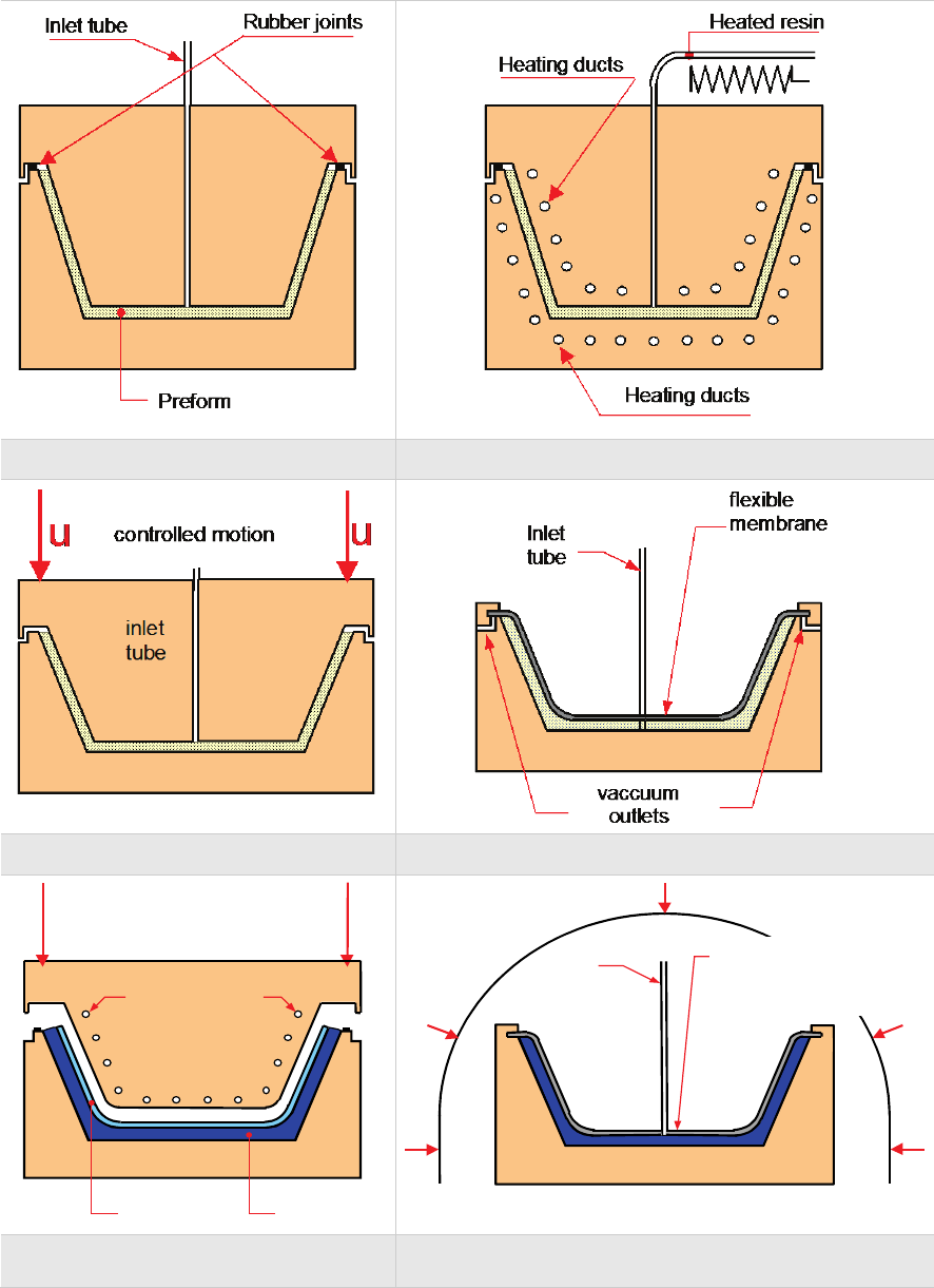
These LCM process variants are illustrated in the following figures:
closed mold RTM heated RTM
injection-compression (CRTM) Vacuum Assisted Resin Infusion (VARI)
heated
press
p
p
heating tubes
preform
resin film
autoclave
controlled
pressure
inlet
tube
flexible
semi
-permeable
membrane
Resin Film Infusion (RFI) Autoclave RTM
USER’S GUIDE & TUTORIALS 4 PAM-RTM 2014
(released: Apr-14) © 2014 ESI Group
INTRODUCTION
Presentation of Liquid Composite Molding
As there is a large number of LCM process variants currently in use or under
development, it is not possible to describe all of them, nor even the details of the ones
presented above. This information is usually part of the corporate know-how. Very
often LCM simulations must be tailored to meet the diversity of injection processes.
RTM Process
The most frequently used resins are polyester, polyurethane, phenolic and epoxy
systems. The reinforcements are made of glass, carbon or kevlar fibers. In the RTM
process, resin is injected at a relatively weak pressure, usually less than 5 bars to
prevent fiber washing by the resin flow. The injection can be performed using one or
several injection ports, injection lines or a tree of injection channels. It is necessary to
select a good configuration of injection ports and vents to avoid dry spots and minimize
filling time. This is precisely the goal of numerical simulation.
Motivation of Filling Simulations
In numerous situations, numerical simulations of mold filling can be of great help to
avoid problems such as resin rich areas, air bubbles, dry spots, zones of high porosity,
as well as the formation of cracks following cure shrinkage. Most of the time, for large
parts, and even for small parts with ribbed connections, it is advantageous to determine
by simulation the optimal positions of injection ports and vents.
Simulation software has been developed in the last few years to assist in the design of
RTM molds. It is more economic to perform simulations before construction of the
mold than to modify an existing mold. The more complex is the mold, the more costly
are mistakes in mold design. This is the reason why, even for small parts, it is useful to
perform a preliminary study by simulation.
Modeling
The numerical simulation of the RTM process implies the modeling of three categories
of physical phenomena: the resin flow through the fiber bed, the thermal analysis of
heat exchanges in the part and with the mold, and finally, the chemical reaction of the
resin.
Flow in a Porous Medium
In the RTM process, the resin flows through a fibrous reinforcement, which can be
considered as a porous medium. In this case, the flow of resin is governed by Darcy’s
law, which states that the flow rate of resin per unit area is proportional to the pressure
gradient and inversely proportional to the viscosity of the resin. The constant of
proportionality is called the permeability of the porous medium. It is independent of the
fluid, but it depends on the direction of the fibers which form the reinforcement (if the
porous medium is no isotropic). The reinforcement is initially dry and the resin must
fill the cavity. Capillary forces of attraction or repulsion act to the forehead of flow.

PAM-RTM 2014 5 USER’S GUIDE & TUTORIALS
© 2014 ESI Group (released: Apr-14)
INTRODUCTION
Presentation of Liquid Composite Molding
These forces, which depend on the surface tension of the resin and on its ability to
adhere to the surface of fibers, have the effect of either reducing or increasing the
effective pressure at the resin front. However, they are considered as sufficiently small
in front of the pressure field in RTM to be neglected by numerical models.
Darcy’s law states that the fluid velocity is proportional to the pressure gradient:
K
VP
µ
→→
= −
∇
where:
- K : permeability tensor
-
µ
: viscosity of the resin
- V : Darcy’s velocity
- P : pressure
In order to preserve the balance of resin mass, the velocity field must satisfy the
divergence condition :
.0V∇=
By combining these two equations, we get
.0
KP
µ
∇ ∇=
If Ω denotes the cavity and dΩ its boundary, boundary conditions are necessary to solve
the problem. These conditions can be of two types:
- Dirichlet conditions, or imposed pressure:
(, ,)p f xyz=
This means that the pressure is specified on part of the boundary dΩ. This is also the
case when the injection is made under vacuum; the pressure at the inlet gate is then
simply the air pressure. At the inlet gates, the pressure is equal to the value fixed by the
injection pump.
- Neumann conditions, or imposed flow rate at the inlet gates:
.Vn Q=
An alternative to RTM is Vacuum Assisted Resin Infusion (VARI), which uses flexible
covers instead. The VARI process inherits the basic principles from RTM, while
requiring vacuum in the cavity where the reinforcement has to be placed. The vacuum is
mainly intended to reduce voids formation and facilitate the transfer of the resin, which
is injected at the ambient pressure.
USER’S GUIDE & TUTORIALS 6 PAM-RTM 2014
(released: Apr-14) © 2014 ESI Group
INTRODUCTION
Presentation of Liquid Composite Molding
However, in the case of deformable media, one has to derive the governing equations
starting from the resin mass balance in order to ensure conservation. The continuity
equation, considering the resin and the fibers material as incompressible, is expressed
as:
( ) ( )
sr VdivVdiv
−=⋅
φ
Where
φ
is the porosity, Vr is the resin velocity and Vs is the solid velocity.
Finally, Darcy’s law enables to write:
[ ]
( )
dt
d
VdivPdiv s
ε
µ
==
∇
K
where
ε
represents an infinitesimal deformation of the fiber bed.
This equation is the general form of mass conservation for the consolidation problem
and is often called the unified Darcy equation.
An additional equation is introduced to follow the deformation of the cover. A quasi-
steady state is assumed to prevail at any point on the cover surface. In the present case,
the sum of the compaction pressure (Pc) and the resin pressure (Pr) has to balance the
external pressure (Pext) acting on the cover surface. This can be formulated as:
extrc
PPP =+
The knowledge of the resin pressure and the external pressure allows the user to obtain
at each time step the thickness of the cavity from the compaction law of the
reinforcement. Therefore, compaction curve plays a major role in this approach.
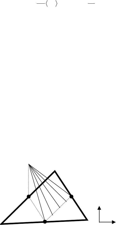
The flow is solved using a non-conforming finite element approximation. The pressure
is discontinuous along the inter-element boundaries except at the middle nodes, as
shown below for a triangular element. Contrary to conforming finite elements, the
computed Darcy flow rates remain continuous across the boundary of elements. Instead
of associating fill factors with the nodes of the mesh as in the conforming finite
element, they are based on the elements of the mesh.
1
N1
2
3
x
y

PAM-RTM 2014 7 USER’S GUIDE & TUTORIALS
© 2014 ESI Group (released: Apr-14)
INTRODUCTION
Presentation of Liquid Composite Molding
The pressure is interpolated using linear shape functions Ni as
( ) ( )
yxNPcybxayxp i
i
i,, ∑
=++=
and
( )
jiif
jiif
yxN
ijjji =
≠
=
=
∗∗
,1
,0
{
,
δ
where (
∗
∗
jj yx ,
) are the middle nodes at the element boundaries.
Permeability of the Reinforcement
The permeability characterizes the relative facility of a viscous liquid to impregnate a
porous medium. This physical property of the porous medium (cloth, fabric, fiber mat,
etc.) depends on the fiber volume fraction (degree of compaction) and on the draping of
the plies. The permeability is usually denoted by K and its unit is m2. The permeability
of reinforcements in their principal directions is determined experimentally.
Thermal Phenomena
The part lies in the cavity of the mold. It consists of fibrous reinforcements and resin,
which first fills up the mold and then becomes progressively polymerized. Heat transfer
phenomena have a strong influence on mold filling and resin curing. Indeed, the
temperature of the resin governs the reactivity of the polymerization reaction.
Temperature also has an influence on mold filling, since the viscosity of the resin
depends on temperature. Thermal simulations are therefore delicate to conduct because
of all the related phenomena. Firstly, heat is transferred by conduction between the
fibers and the resin. Secondly a convective transport of heat occurs during the filling of
the cavity by the resin. Finally, heat is produced by the exothermic chemical reaction of
resin polymerization. Some heat is also created by the viscous dissipation during the
resin flow, but to a lesser degree than the heat originating from the chemical reaction.
The temperature field is governed by the general equation:
Dt
D
hTkT
Vc
t
T
Crprrp
α
ρρ
ρ
∆−∇••
∇=∇•
+
∂
∂}{
where T denotes the temperature, t denotes the time,
ρ
is the density, Cp is the specific
heat, k is the heat conduction coefficient tensor, the subscript r designates the resin,
h∆
is the total enthalpy of the polymerization of the resin,
α
is the resin cure.
There are three kinds of temperature boundary conditions:
- Prescribed temperature boundary condition:
0
TT =

USER’S GUIDE & TUTORIALS 8 PAM-RTM 2014
(released: Apr-14) © 2014 ESI Group
INTRODUCTION
Presentation of Liquid Composite Molding
- Heat flux boundary condition:
q
n
T=
∂
∂
- Heat convection boundary condition:
)( TTh
n
T−=
∂
∂
∞
, where h is the heat
convection coefficient,
∞
T
is the environmental temperature.
This general equation permits to treat the steps of pre-heating, filling and curing.
During the filling step, it is used with effective properties:
- For non-impregnated fibers:
pffpaap
C
C
C
ρφ
φρρ
)
1
(−
+
=
fa kk
k)1
(
φ
φ
−+
=
- For impregnated fibers:
pff
pr
rp
C
CC
ρφφρ
ρ
)1
(−
+=
De kkk +=
where the subscript r stands for the resin, f for the fibers and a for the air. In general,
thermal properties of the air are neglected. The effective conductivity tensor ke of the
composite is averaged in each direction. Like the permeability tensor K, the heat
conduction coefficient tensor k reduces to a scalar for the isotropic fiber preform.
The coefficient kD represents the thermal dispersion tensor arising from hydrodynamic
dispersion. It can be evaluated as a function of Peclet number, but its influence is small
as long as the fluid velocity is weak. However starting with PAM-RTM™ 2008, it is
now possible to take into account thermal dispersion. The following paragraphs
describe how it is modeled.
Experimental results showed that dispersion depends on Prandtl and Reynolds numbers
and that Peclet number can approximate hydrodynamics and heat transfer phenomena at
the pore level. Based on this, Delaunay et al. further extended this approach and showed
experimentally that both transverse and axial dispersions can be modeled empirically
using a mixing length approach, by correcting the components of the thermal
conductivity with an expression that depends on Peclet number as follows:
( )
Pe
stattrans 1.01+=
λλ
PAM-RTM 2014 9 USER’S GUIDE & TUTORIALS
© 2014 ESI Group (released: Apr-14)
INTRODUCTION
Presentation of Liquid Composite Molding
( )
Pe
stataxial 8
.0
1+=
λ
λ
Peclet number Pe is defined here as:
a
lv
Pe
f
=
where,
f
v
the observed velocity of the flow front (m/s), connected with Darcy
velocity by the relation
φ
v
v
f
=
(
φ
denotes the porosity of the fibrous
reinforcement)
l characteristic length (m)
a thermal diffusivity (m2 /s)
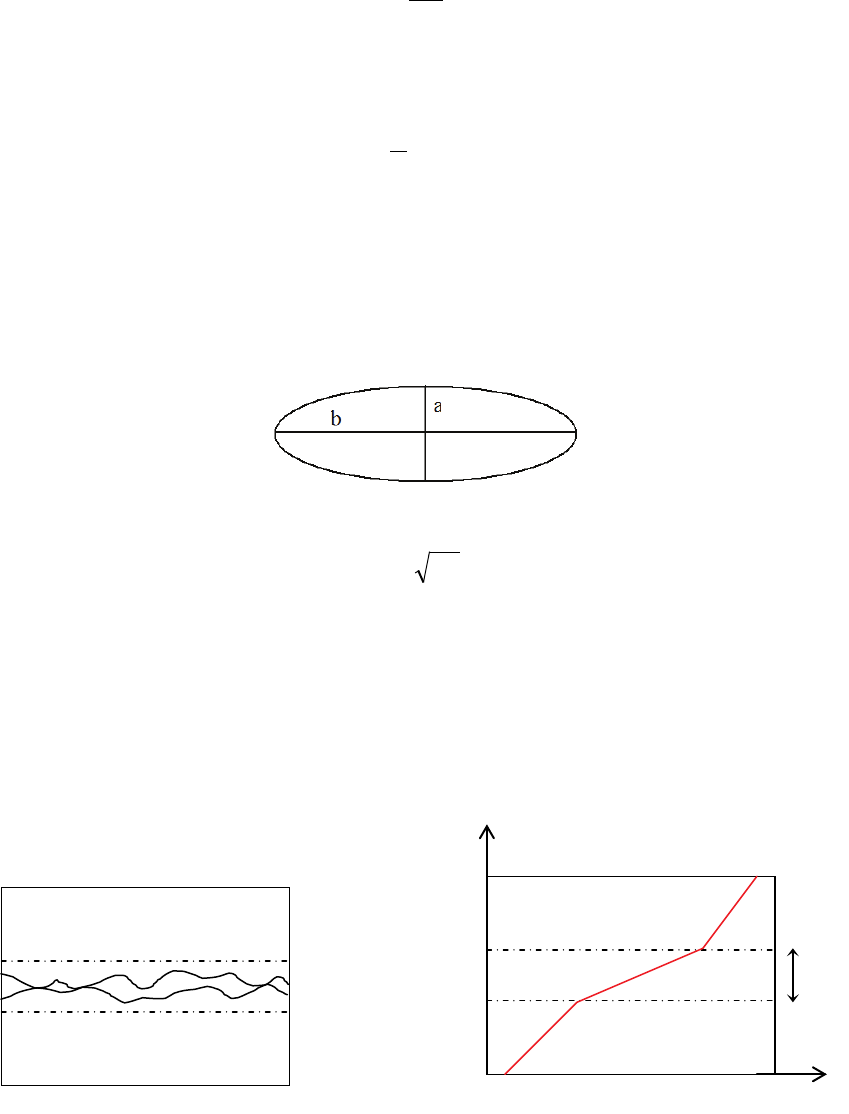
The characteristic length is referred to as the characteristic scale of the elliptical shape
of a compressed fiber tow,
In which case it is given by:
bal =
The following describes the thermal contact resistance. In a general way, when two
solids (parts of a mold, reinforcement) are in contact, because of their roughness and the
non-flatness of their surfaces, the contact is never carried out on all apparent surface.
Between the zones of contact remains an interstitial space, which is a zone with low
conductivity. The temperature field is thus considerably disturbed. The introduction of a
thermal contact resistance Rth allows to neglect the thickness of the contact zone and to
replace the abrupt variation in temperature by a true discontinuity.
Illustration of the thermal contact resistance
1st solid
2nd solid
contact zone
y
x
T1(y)
T2(y)
e

USER’S GUIDE & TUTORIALS 10 PAM-RTM 2014
(released: Apr-14) © 2014 ESI Group
INTRODUCTION
Presentation of Liquid Composite Molding
The thermal contact resistance Rth is defined by
th
R
TT
2
1
−
=
ϕ
where T1 and T2 are the
contact temperatures on the interface and ϕ the heat transfer. Its surface value is
determined by the following relation:
k
e
Rth =
(m2W-1K)
Where e is the thickness of the disturbed zone and k is often the thermal conductivity of
the air.
Thus, we can consider gaps in the mold or ribs in the reinforcement, by affecting locally
a value of thermal resistance.
The source term on the right side of the general equation of thermal phenomena
accounts for the internal heat generated by the exothermic chemical reaction in
thermoset resin system. This source term is usually assumed to be proportional to the
reaction rate
Dt
D
α
.
Viscosity of the Resin
The viscosity of the resin depends on temperature and on the degree of conversion. The
dependence on the degree of conversion is very strong, since it is usually assumed that
viscosity reaches infinity when the resin comes to gelation.
The dependence of viscosity on temperature and the degree of conversion is modeled by
a constitutive law. PAM-RTM™ offers several options to model viscosity:
- Constant viscosity.
- Viscosity function of the temperature from a predefined model
( )
)exp( TB
AT ⋅⋅
=
µ
where A and B are two user specified constants.
- Viscosity function of temperature and of resin rate of conversion from a predefined
model, where A, B and
κ
are characteristic constants of the resin:
( )
⋅+⋅=
ακαµ
T
B
AT exp,
- Viscosity
µ
= f(T,
α
) function of temperature and of the resin rate of conversion,
such as in the following frequently used model:
( )
α
αα
α
αµ
⋅+
−
⋅
⋅=
21
exp,
cc
gel
gel
b
T
T
BT
where B, Tb,
α
gel, C1 and C2 are user defined characteristic constants of the resin.

PAM-RTM 2014 11 USER’S GUIDE & TUTORIALS
© 2014 ESI Group (released: Apr-14)
INTRODUCTION
Presentation of Liquid Composite Molding
Kinetics of Resin Polymerization
The software permits to define a kinetics of polymerization of the resin from the model
of Kamal-Sourour. The general shape of the equation of Kamal-Sourour for a resin
with n components is the following:
1
n
ii
i
C
αα
=
=∑
( ) ( )
ii p
i
m
ii
i
TK
dt
d
αα
α
−⋅⋅= 1
where
dt
di
α
is the rate of reaction for the ith component in s-1, the values of Ki are
defined by the law of Arrhenius : Ki=Aiexp(-Ei/RT)
- Ai give the number of useful shocks to reactions,
- Ei are the energies of activation of the chemical reaction,
- mi and pi are exponents characterizing the sensitivity of each autocatalytic reaction,
- Ci are the weights of each reaction.
Coupling of Physical Phenomena
The following table presents a summary of the main phenomena that come into play in
the RTM process. All these phenomena are strongly coupled and PAM-RTM™ is able
to simulate them.
Category
Phenomenon
Mathematical model
Rheologic Resin flow in a porous medium
Variations of viscosity
Darcy’s law
Constitutive law
Thermal Mold: conduction, loss in surface
Part: conduction, convection,
generation of heat, superficial heat
loss
Heat equation, transfer coefficient
(convection-radiance)
Equation of convection-diffusion
with source term, model with one
temperature
Chemical Transport of chemical species,
diffusion, polymerization
Equation of convection-diffusion
with source term, kinetic model
(Kamal-Sourour)
Mechanical Mold deformation
Variation of porosity and permeability
Newton’s law
Empirical models

USER’S GUIDE & TUTORIALS 12 PAM-RTM 2014
(released: Apr-14) © 2014 ESI Group
INTRODUCTION
Credits
CREDITS
A series of software modules developed by the Chair on Composites of High
Performance (CCHP) at École Polytechnique de Montréal have been incorporated in
PAM-RTM™ 2008, 2009 and 2010:
- Optimization of the void distribution in an RTM composite part through injection
flow rate (VoidOpt module);
- Rapid RTM flow simulation (OneShot module);
- Conditional opening of injection ports and vents during resin injection
(TriggerManager module);
- Incorporation of simultaneous filling and curing simulations including the
overfilling phase and the evacuation of excess resin at the end of the filling cycle;
- Optimization using genetic algorithms of injection points locations minimizing fill
time (GenPorts module);
- Compression RTM and Articulated Compression RTM (ACRTM).

PAM-RTM 2014 13 USER’S GUIDE & TUTORIALS
© 2014 ESI Group (released: Apr-14)
INTRODUCTION
Credits
Permeability tensor of the reinforcements is the main material data required for Liquid
Composites Molding simulation. However, no normalization of the permeability
measurements exists today and significant scatters in measured permeability values
between laboratories are observed. In the first stage of an international benchmark
exercise on the experimental determination of reinforcement permeability; 11 partners,
implementing 16 different measurement techniques between them, compared in-plane
permeability data for the examples of fabrics provided by HEXCEL. A second stage of
this benchmark study is currently on-going; its purpose is to eliminate sources of scatter
and lead to a standardization of measurement methods.
Andy Long’s team especially Andreas Endruweit from Nottingham University who
participates in that benchmark partnered with ESI Group composites team is sharing
non-confidential permeability values measured these last years at the University. Few of
these reinforcement data are in the PAM-RTM installation files. A more extensive
database that is continuously improved and completed with new data is available on ESI
customer portal “MyESI” (local ESI representative must be reached for more
information).
There are currently no standards for permeability measurement to interpret the provided
data; while observed trends (e.g. for the change in permeability as a function of the fiber
volume fraction), are of general validity, application of different experimental methods
may result in quantitative differences in absolute permeability values.
The main purpose of the database is to provide a starting point to PAM-RTM users.

PAM-RTM 2014 15 USER’S GUIDE & TUTORIALS
© 2014 ESI Group (released: Apr-14)
PAM-RTM USER'S GUIDE
Introduction
PAM-RTM USER'S GUIDE
INTRODUCTION
To run a simulation with PAM-RTM™, it is necessary at least to have prepared a mesh
of the part to inject using a commercial (GEOMESH, I-DEAS, PATRAN, CATIA) or
public domain mesh generator. Whatever the mesh generator you choose, it should have
the capability to export a mesh in one of the file formats supported by PAM-RTM™:
I-DEAS Universal, PATRAN Neutral, NASTRAN or PAM-SYSTEM. Most
commercial mesh generators can export a mesh in NASTRAN format, so it shouldn’t be
a problem to work with any mesh generator.
The important point is that you work in the CAD system you like to prepare the
geometry for meshing, then you mesh in the mesh generator you like, and finally you
export the mesh (only nodes and elements, not the boundary conditions or physical
properties) in one of the formats supported by PAM-RTM™. The boundary conditions
and physical properties are later specified in PAM-RTM™.
For simulations involving resolution of Darcy’s equation (RTM, Heated RTM, VARI),
PAM-RTM™ uses non-conforming finite elements. Non-conforming finite elements
are only available on triangles and tetrahedrons. This means that the cavity has to be
meshed with 3 nodes triangles or 4 nodes tetrahedrons. For Heated RTM simulations,
the mold could be meshed with 4 nodes quads or 8 nodes bricks. For simulations that
don’t solve Darcy’s equation (preheating, curing), quads and bricks could be used to
mesh the cavity.
In general, having a finite element mesh created by I-DEAS or PATRAN is not enough
to launch a simulation with PAM-RTM™. Injection ports and vents have to be
defined. In addition, the specification of fiber orientations is not always available in the
mesh file. PAM-RTM™ has some tools to specify material orientations and to modify
the mesh for injection points and vents. Groups of nodes are created interactively in
PAM-RTM™ to be used in the specification of boundary conditions.
Once the model is completely specified (material properties, orientations, groups,
boundary conditions, etc.), the simulation parameters file (.dtf) is saved and the
simulation can be launched from the user interface or from a command window. The
latter is mostly used to run the simulation on a Unix server (see chapter Running the
Simulation from a Command Window).
When the simulation is done, the PAM-RTM™ post-processing functionalities are
used to visualize the simulation results. Alternatively, by using the appropriate output
format, simulation results can be visualized in I-DEAS or PATRAN.
USER’S GUIDE & TUTORIALS 16 PAM-RTM 2014
(released: Apr-14) © 2014 ESI Group
PAM-RTM USER'S GUIDE
Presentation of the User Interface
PRESENTATION OF THE USER INTERFACE
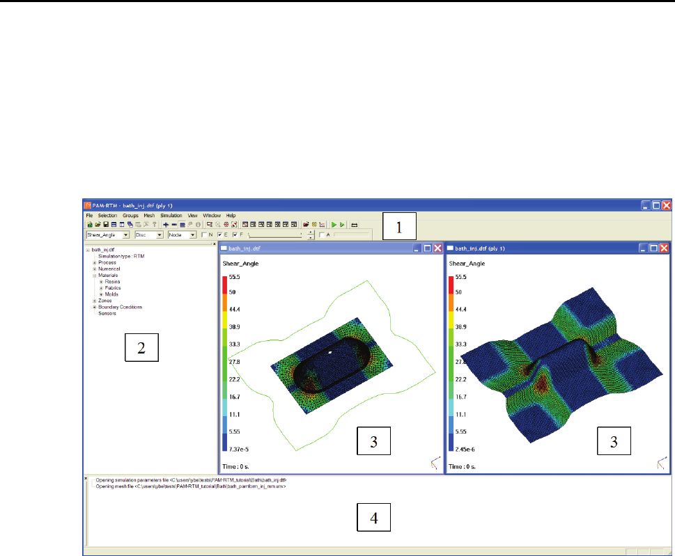
The main frame window of PAM-RTM™ is made of 4 areas:
- toolbar area [1]
- model explorer [2]
- 3D graphics windows [3]
- message pane [4]
Overview of the PAM-RTM user interface
PAM-RTM™ is a multi-document, multi-view application, which means that many
documents can be opened at the same time, and many views can be created on the same
document. This is useful, for example, to visualize the resin pressure field in one view
and the temperature field in another view. Or, as shown in the previous image, to
visualize a mesh of the part to inject in one view, and a mesh of a ply with fiber
orientations in another view.
To open a new view on the current document, use the Window->New Window command.
When many windows are opened, you can use the Window->Cascade, Window->Tile
Horizontally and Window->Tile Vertically commands to have automatic layout of the
windows.
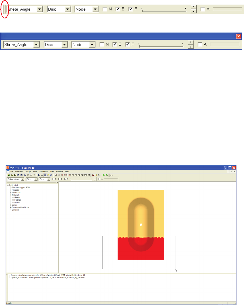
You can position toolbars in PAM-RTM toolbars any way you like. The recommended
setup of toolbars is shown in the previous picture. To move a toolbar you have to click
on the left double vertical bar, then drag the toolbar where you want, as shown in the
PAM-RTM 2014 17 USER’S GUIDE & TUTORIALS
© 2014 ESI Group (released: Apr-14)
PAM-RTM USER'S GUIDE
Presentation of the User Interface
next picture. When the toolbar is floating, there is an X box that appears in the upper
right corner of the window that allows to close it (in case you need more space or you
never use some toolbars). To recover a toolbar you closed in such a way, there is a
command in the Window menu to show or hide each of the PAM-RTM™ toolbars (ex:
Window->Display Toolbar, Window->Selection Toolbar, etc.).
Handle to move the toolbars
Floating toolbar
Interaction with the Mouse
The middle mouse button is reserved in PAM-RTM™ to dynamically control the
viewpoint:
- Middle button alone: rotate
- Ctrl + Middle button: pan
- Shift + Middle button : zoom
The left button is used for selection (picking or area). The selection filter (nodes, faces,
elements) is available in the Display toolbar.
Selection of elements by area
USER’S GUIDE & TUTORIALS 18 PAM-RTM 2014
(released: Apr-14) © 2014 ESI Group
PAM-RTM USER'S GUIDE
Presentation of the User Interface
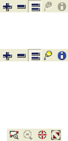
Toolbars
File Toolbar
File toolbar
This toolbar contains shortcuts to standard Windows commands (from left to right):
File->New, File->Open, File->Save, Window->Tile Horizontally, Window->Tile Vertically,
Window->Cascade, Help->About.
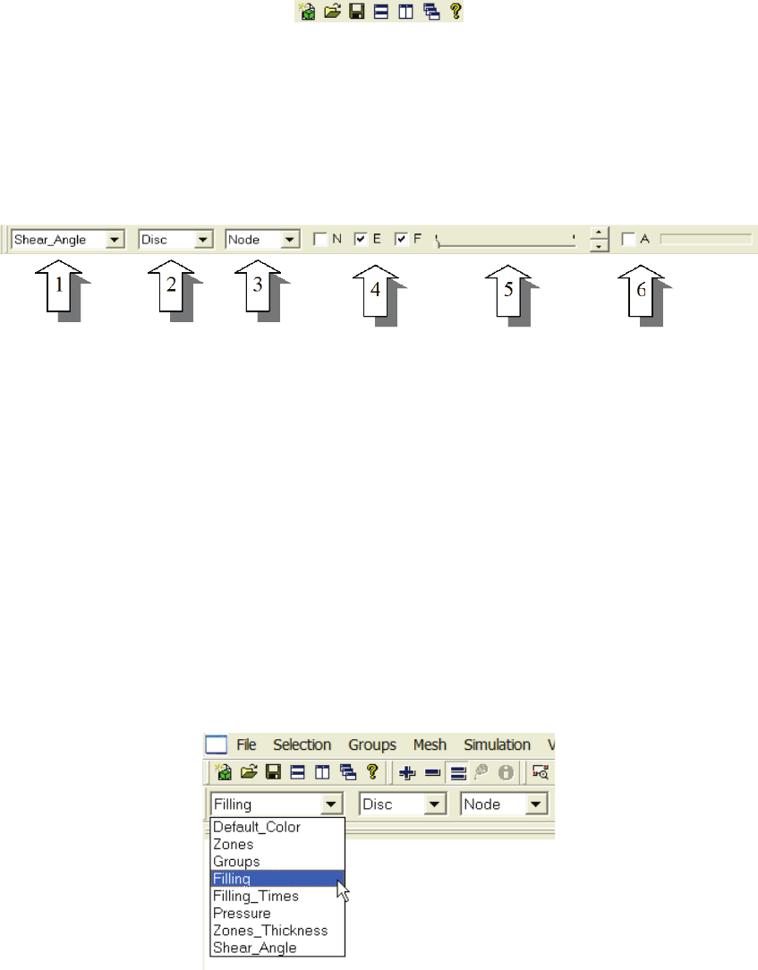
Display Toolbar
Display toolbar
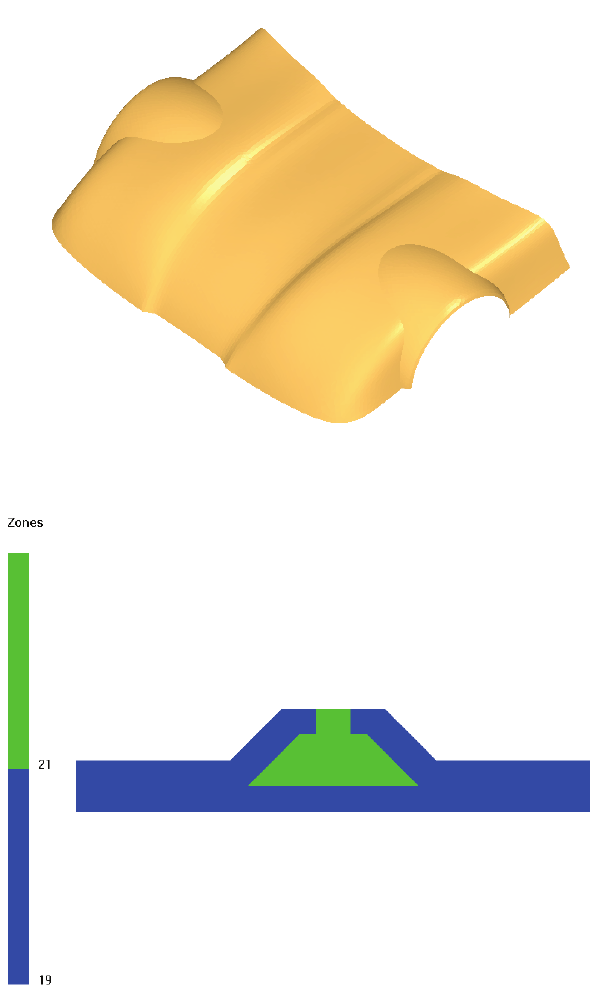
There are basically 4 display modes in PAM-RTM™ that affect the coloring of display
entities:
- Default color: in this mode, nodes, edges and faces are displayed using the default
colors specified by the user in the Color tab of the View->Options dialog box.
- Zones: element faces are colored according to their zone ID.
- Groups: if a node or face is part of a group, it is colored according to the group ID.
- Scalar Field: faces are colored based on a scalar field value (for example
temperature or pressure).
The 4 display modes are activated by selecting something in the scalar field roll-down
list of the display toolbar [1]. Depending on the context, there will be more or less
scalar fields to display. Here is an example.
Scalar field list
PAM-RTM 2014 19 USER’S GUIDE & TUTORIALS
© 2014 ESI Group (released: Apr-14)
PAM-RTM USER'S GUIDE
Presentation of the User Interface
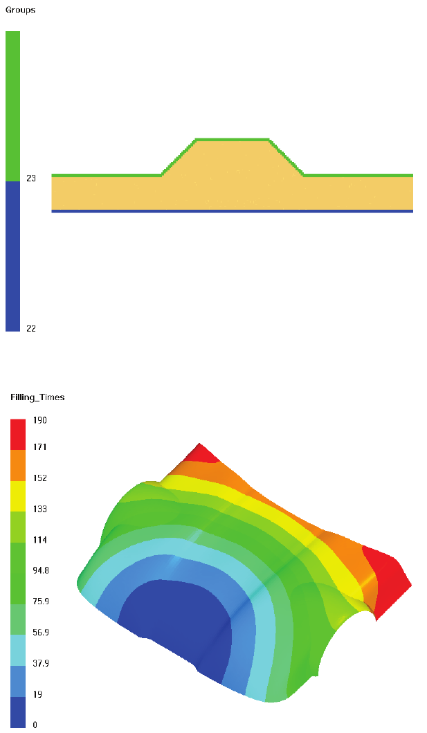
Examples of the each display mode are shown in the following figures.
Surface mesh displayed in Default Color mode
Zones display
USER’S GUIDE & TUTORIALS 20 PAM-RTM 2014
(released: Apr-14) © 2014 ESI Group
PAM-RTM USER'S GUIDE
Presentation of the User Interface
Groups display
Segmented filling scalar field display
Here is a description of the other controls available in the display toolbar.
- Plot type [2]: Disc or Iso. This parameter has an effect only when visualizing scalar
fields.
PAM-RTM 2014 21 USER’S GUIDE & TUTORIALS
© 2014 ESI Group (released: Apr-14)
PAM-RTM USER'S GUIDE
Presentation of the User Interface
· Disc is used for example to display a scalar field that was computed at the
nodes as a discontinuous fields averaged on each element.
· Iso is used to display contours of the current scalar field. Note that if the
original field was computed at elements (which is the case for instance for
the filling factor), the values will be averaged at the nodes before contours
can be generated, which can take a while depending on the mesh size and
number of steps.
- Selection filter [3]: set the selection filter to Node, Face or Element. For example,
use Node if you want to pick nodes, or Element if you want to pick elements.
- N, E, F [4]: check boxes to show or hide nodes, edges, faces.
- Time step [5]: drag this slider to visualize the current scalar field step by step.
- Animate [6]: starts/stops animation of the current scalar field. Use View->Post-
Processing for animation parameters.
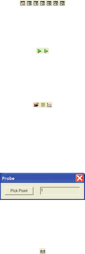
Selection Toolbar
This toolbar is used to control the behavior of the selection. For example, if the
selection filter is Node and the = button is pushed when some nodes are selected by
area, the current selection will be replaced by the new selection. When the + button is
pushed, each new selection is added to the current selection. When the – button is
pushed, the new selection is removed from the current selection set. Other buttons are
available to clear the current selection (equivalent to Selection->Unselect All (no filter)),
and to get information about the selected entities (equivalent to Selection->Info
Detailed).
Selection toolbar (current selection empty)
Selection toolbar (non-empty selection)
Camera Toolbar
Camera toolbar
From left to right:
- Corner zoom: drag the mouse to define a rectangular area to zoom in.
- Zoom out: use after a corner zoom to restore the previous state.
- Rotation center: pick a point on the mesh to set the center for rotation and zoom.
USER’S GUIDE & TUTORIALS 22 PAM-RTM 2014
(released: Apr-14) © 2014 ESI Group
PAM-RTM USER'S GUIDE
Presentation of the User Interface
- Fit: reset view so that the mesh is completely displayed, in the center of the graphics
window.
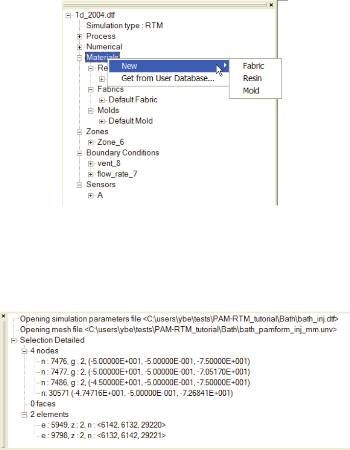
Viewpoint Toolbar
Viewpoint toolbar
Choose one of the pre-defined viewpoints (along -X axis, +X axis, etc.).
Simulation Toolbar
Simulation toolbar
Start or restart the simulation. Restart is used when simulation was stopped with a
CTRL-C and needs to be restarted.
Results Toolbar
Results toolbar
From left to right:
- Reload results: reloads all the results files that were generated for this simulation.
This is the preferred way to load results in PAM-RTM™.
- Probe: opens the Probe dialog box, allowing the user to pick an arbitrary point on
the mesh and display the value of the current scalar field for the current time step on
that point.
Probe dialog box
- Plot: allows the user to pick a point and automatically generate a plot of the scalar
field value on that point as a function of time.
Tools Toolbar
Tools toolbar

PAM-RTM 2014 23 USER’S GUIDE & TUTORIALS
© 2014 ESI Group (released: Apr-14)
PAM-RTM USER'S GUIDE
Presentation of the User Interface
There is only one tool currently available in this toolbar: the measure tool. Pushing this
button opens the Measure dialog box, allowing the user to pick two arbitrary points on
the mesh and get the distance between the points.
Measure tool
Model Explorer
The model explorer displays information about open documents in a tree structure. The
information displayed can be seen as a summary of open documents. Only the most
useful information is displayed in the tree, depending on the type of simulation.
Double-clicking an item in the tree most of the time pops up a dialog box to edit the
parameters related to the selected item. For example, double-clicking a zone opens the
Zone dialog box.
Zone dialog box
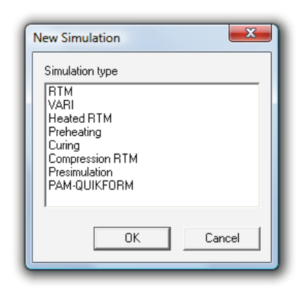
Right-clicking an item in the explorer will most probably popup a menu, depending on
the item selected. In the following picture, the user right-clicked on the Materials item.
USER’S GUIDE & TUTORIALS 24 PAM-RTM 2014
(released: Apr-14) © 2014 ESI Group
PAM-RTM USER'S GUIDE
Presentation of the User Interface
Right-click in the explorer window
Message Pane
The message pane is used to display messages to the user. A tree structure is used. For
example, the Selection->Info Detailed command prints the following.
Message pane

PAM-RTM 2014 25 USER’S GUIDE & TUTORIALS
© 2014 ESI Group (released: Apr-14)
PAM-RTM USER'S GUIDE
File Menu
FILE MENU
File > New
This is used to create a new simulation project. The supported simulation types are:
- RTM: classical isothermal closed mold RTM.
- VARI: Vacuum Assisted Resin Infusion. Isothermal injection under deformable
plastic film. The thickness and permeability change of the fiber reinforcement is
taken into account.
- Heated RTM: non-isothermal RTM. Heat exchanges between resin, fiber
reinforcement and mold is taken into account. The effect of resin polymerization on
viscosity and heat generation can also be taken into account.
- Preheating: heating of the mold and fiber reinforcement before filling. The possibly
non-uniform temperature distribution at the end of preheating can be used to
initialize Heated RTM simulation.
- Curing: post-filling resin cure. By default, assumes that the cavity is completely
filled and the initial temperature and degree of cure is uniform. Otherwise the results
of the Heated RTM simulation (filling factor, temperature, degree of cure) can be
used to initialize the curing simulation.
- Compression RTM: simulates a process in which some amount of resin is injected
first with a cavity thickness slightly higher than the targeted part thickness. This is
done in order to facilitate impregnation since the permeability is higher. Once that
amount of resin has been injected, the part is not completely filled yet. The inlet is
closed, and the remaining dry areas are filled by a flow induced by compression of
the preform. The compression direction can be normal to the part, or in a specified
direction. This simulation is based on a 2.5D modeling where only the pseudo
thickness of the shell element varies. Thus only meshes of triangles are supported.
- Presimulation: this simulation allows a first approximation of the filling time and
flow behavior without solving Darcy’s equation. That’s why it is very fast. However
it works only with constant flow rate injection.
- PAM-QUIKFORM: draping analysis of fiber reinforcements (bi-directional fabrics
and unidirectional).
USER’S GUIDE & TUTORIALS 26 PAM-RTM 2014
(released: Apr-14) © 2014 ESI Group
PAM-RTM USER'S GUIDE
File Menu
New Simulation dialog box
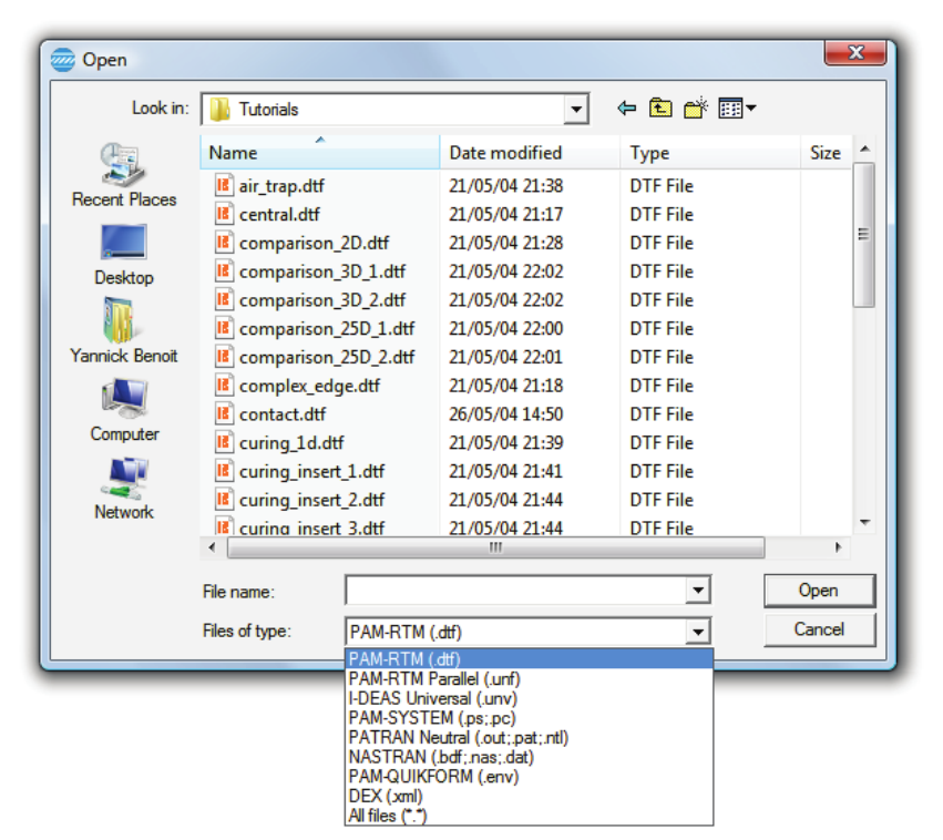
File > Open
This is used to open a project file (.dtf) or a mesh file. Most of the time this command
is used to open a .dtf file, which contains the PAM-RTM™ simulation parameters as
well as links to external files such as mesh files. It can also be used to open directly a
mesh file. In that case a default RTM simulation is automatically associated to the
opened mesh file.
The option PAM-RTM Parallel (.unf) is to be used for post-processing of results generated
by the new high performance parallel solver introduced in PAM-RTM™ 2010.
Note:
· The .unf format is intended for post-processing only. All the pre-processing
functionalities of the PAM-RTM GUI, such as creation of groups, specification
of material orientations, etc., will be non-functional if such a document is
loaded.
The supported mesh file formats are:
- PAM-SYSTEM
- I-DEAS Universal
- PATRAN Neutral
- NASTRAN Bulk
PAM-RTM 2014 27 USER’S GUIDE & TUTORIALS
© 2014 ESI Group (released: Apr-14)
PAM-RTM USER'S GUIDE
File Menu
File Open dialog box
File > Close
Closes the active document. If some modifications were done, the user is prompted to
save the file before closing.
File > Save
Saves the .dtf file (simulation parameters) and the mesh file (.unv) in the directory
where the .dtf file was opened. For example, if file c:\rtm_tests\test.dtf was
opened, when the File->Save command is used, the file c:\rtm_tests\test.dtf
will be overwritten and the associated mesh file c:\rtm_tests\test.unv will be
generated.
USER’S GUIDE & TUTORIALS 28 PAM-RTM 2014
(released: Apr-14) © 2014 ESI Group
PAM-RTM USER'S GUIDE
File Menu
File > Save As
Prompts the user to specify a new name and directory for the project. For example, if
c:\rtm_tests\test_2.dtf is chosen, the current simulation parameters will be
saved in c:\rtm_tests\test_2.dtf and an associated mesh file
c:\rtm_tests\test_2.unv will be generated.
File > Import > Mesh
This is the command to use after a File->New, to import in the current document the
mesh to use for the simulation. In some rare situations you could use this command to
load many meshes in the current document, then merge them with Mesh->Cleanup-
>Merge Coincident Nodes. See File->Open for the supported mesh file formats.
File > Import > Scalar Fields
This command is used to import scalar fields (simulation results) into the currently
active PAM-RTM™ document for post-processing. These are the available file
formats for scalar fields:
- I-DEAS Universal (extension: .unv)
- PAM-RTM Scalar Field (extension: .sf)
- PAM-RTM Filling Compact (extension: .fil)
- PAM-RTM Flow Front (extension: .front)
- Velocity Components Vx Vy Vz (I-DEAS format, extension .unv)
The PAM-RTM Filling Compact file contains the filling result of a PAM-RTM™
simulation. The size of this file is much smaller than the same scalar field saved in a
more general format like I-DEAS Universal.
The PAM-RTM Flow Front file contains the flow front position in time. This is the
“raw” flow front position (not smoothed). It is made of line segments that define the
saturated domain. The flow front position can be displayed on top of any scalar field in
PAM-RTM™. This is useful to analyze, for example, temperature results.
Since PAM-RTM™ 2008, it is possible to display a vector field on top of a scalar field.
This is generally used to display the resin velocity vector field on top of a pressure or
temperature field, for instance. However any 3 components vector field could be
displayed, as long as the 3 components are imported together with File->Import->Scalar
Fields->Velocity Components. In general the user doesn’t have to use this command, as
the velocity components are imported automatically with the Reload Results button in
the Results Toolbar, if the Save Velocity option was checked in the Numerical
Parameters.

PAM-RTM 2014 29 USER’S GUIDE & TUTORIALS
© 2014 ESI Group (released: Apr-14)
PAM-RTM USER'S GUIDE
File Menu
Note:
· The preferred way to load simulation results in PAM-RTM™ is to use the button
in the Results Toolbar.
File > Import > Draping Results
This menu is used to import draping analysis results files in the active document.
Draping results are a set of meshes that define plies geometry (one mesh for each ply).
Depending on the software that generated the laminate plies, material properties like
fiber directions and thickness can be defined on each finite element of a ply. For
example, the result of a PAM-FORM™ simulation gives the fiber orientations and
thickness on each element. However a PAM-QUIKFORM™ simulation gives only
the fiber directions, not the thickness.
These are the available interfaces to import draping results in PAM-RTM™:
- PAM-FORM
- PAM-QUIKFORM
- PATRAN Laminate Modeler
- FiberSIM XML
All these interfaces support local fiber directions specified on each element of each ply.
The PAM-FORM interface reads a PAM-FORM™ results file (extension .dsy). A
PAM-FORM™ results file normally contains many states. PAM-RTM™ assumes
that it is only the last state that is interesting in the context of RTM simulation, so it
loads in memory only the last state of the PAM-FORM™ simulation.
There are two possibilities to import PAM-QUIKFORM™ results. In case the PAM-
QUIKFORM simulation was created and run in PAM-RTM (File->New->PAM-
QUIKFORM), it is possible to import the PAM-QUIKFORM .dtf file, in which case
higher level information such as materials used in the laminate definition is available.
Otherwise it is also possible to import only the PAM-QUIKFORM generated mesh files
(.ps, PAM-SYSTEM format). In that case, the user will have to associate materials to
imported meshes by re-defining the laminate, if calculation of local permeability is
needed.
The PATRAN Laminate Modeler interface reads a .fmd file, which contains a list of
filenames that define the laminate. Each ply is a NASTRAN file with a special
definition of the PCOMP section that allows the specification of 2 fiber directions on
each element. One PCOMP section is specified for each element and each PCOMP
section refers to 2 layers of UD.
The FiberSIM interface is used to import ply data generated by the FiberSIM software,
in a special XML format.

USER’S GUIDE & TUTORIALS 30 PAM-RTM 2014
(released: Apr-14) © 2014 ESI Group
PAM-RTM USER'S GUIDE
File Menu
File > Export > Mesh
This command is used to export the current mesh in one of the supported formats:
- PAM-SYSTEM
- I-DEAS Universal
- PATRAN Neutral
File > Export > PAM-RTM Scalar Field
This is used to export the currently displayed scalar field in a PAM-RTM™ specific
file format. This is used most of the time in the context of local permeability
calculation, to export the k1.sf, k2.sf, porosity.sf and thickness.sf files
needed to initialize a calculation that takes into account local permeability.
File > Clear > Scalar Fields
Clears from memory all the scalar fields that have been imported in the current
document with the command File->Import->Scalar Fields or loaded with the button.
File > Clear >Laminate
Clears from memory all the plies meshes that have been loaded by using File->Import-
>Laminate.
File > Save Image
Saves the active 3D graphics window in one of the supported graphics file formats:
- PNG
- GIF
- TIFF
- JPEG
File > Generate AVI
Generates an animation file (.avi) from the currently visualized scalar field. The
resulting AVI file can be visualized in Windows Media Player or integrated in
PowerPoint presentations.
When the command is selected, the following dialog box pops-up, allowing the user to
specify the cycle time, which is the time to display all the frames in the AVI file. The
end delay is used to have the last frame displayed for some time. This can be useful for
presentations.
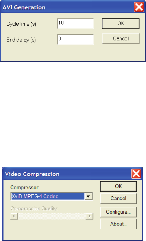
PAM-RTM 2014 31 USER’S GUIDE & TUTORIALS
© 2014 ESI Group (released: Apr-14)
PAM-RTM USER'S GUIDE
File Menu
AVI Generation
Then the user is asked to specify the name of the generated AVI file from the standard
Windows file selection dialog.
Finally another dialog box pops up to select the “codec” to compress frames in the AVI
file. This dialog box lists all the available codecs on the user machine. Since this list
depends on other software installed on the machine, it is difficult to recommend the best
codec. The Cinepak codec by Radius seems to be available on most machines and has
given good results. However it is recommended to download from the internet the XviD
MPEG-4 codec, which is open source and free. The Full Frames codec should be
avoided as it generates huge files.
Selection of codec
Note:
· Introduced in PAM-RTM™ 2008, the generated AVI can now take into account
the Proportional animation option.
File > Print
Prints the active 3D graphics window.
File > Print Preview
Gives a preview of the print command in the standard Windows print preview window.
File > Print Setup
Opens the standard Windows dialog box to configure printing.
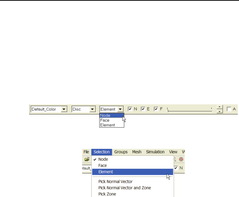
USER’S GUIDE & TUTORIALS 32 PAM-RTM 2014
(released: Apr-14) © 2014 ESI Group
PAM-RTM USER'S GUIDE
Selection Menu
SELECTION MENU
Selection Filter
There are three types of geometrical entities that can be selected in PAM-RTM™:
nodes, finite element faces, and finite elements. The selection filter is used to specify
the type of entity to select. For example, if you want to pick some elements with the
mouse, you have to set the selection filter to Element. If you want to select all the
elements in a zone specified with an ID, you have to set the selection filter to Element
before using the Selection->Zone ID command. The usual way to set the selection filter
is using the Display toolbar. The Selection->Node, Selection->Face, and Selection-
>Element commands can also be used. A check mark is shown besides the currently
active filter.
Selection filter in the Display toolbar
Selection filter in the Selection menu
Selection > Pick Normal Vector
The Pick Normal Vector command is useful to select entities on the same planar surface
(i.e. entities that have the same normal vector) in a single operation. For example, in
the following image, all the faces in red were selected in a single click, while selection
by area would have required many operations. When the Pick Normal Vector command
is used, a dialog box pops up to prompt the user for a tolerance on the angle between
two adjacent faces (angle between the 2 normal vectors). This is useful when the
surface to select is not perfectly planar.
Note that nodes, faces and elements can be selected using this approach. When the
selection filter is Nodes, all the nodes of all the faces that have the specified normal
vector are selected.
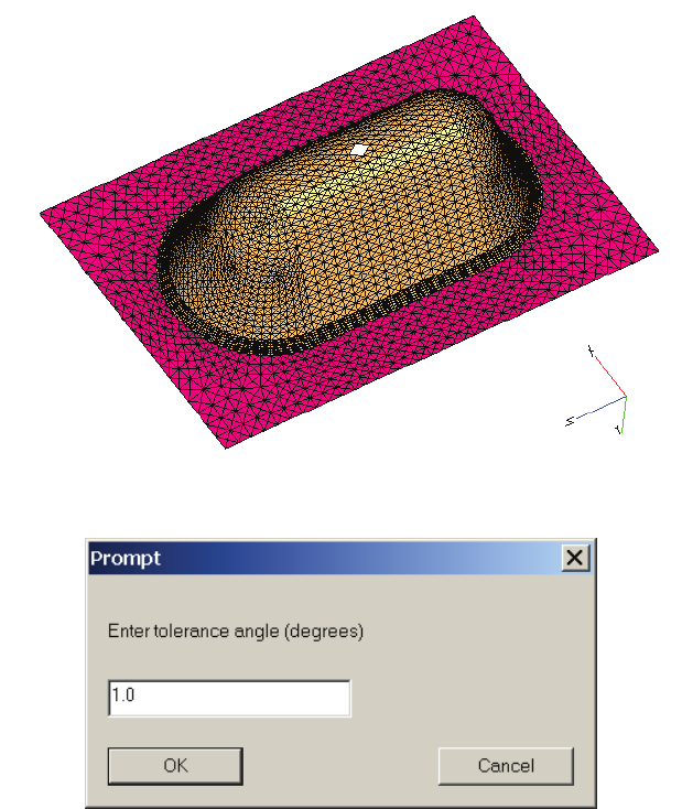
PAM-RTM 2014 33 USER’S GUIDE & TUTORIALS
© 2014 ESI Group (released: Apr-14)
PAM-RTM USER'S GUIDE
Selection Menu
Selection of faces with Pick Normal Vector
Tolerance angle for Pick Normal Vector
Selection > Pick Normal Vector and Zone
This command is basically the same as the previous one, except that it adds as a
selection filter the zone ID of the face used to define the normal vector.
Selection > Pick Zone
This command allows selection of all the nodes, all the faces or all the elements in a
zone picked by the user with the mouse. The user is first prompted to pick a face in the
zone to select. Then all the entities are selected based on the current selection filter.
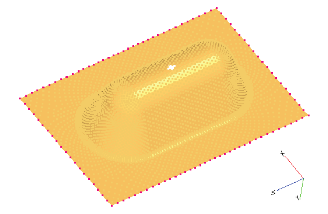
USER’S GUIDE & TUTORIALS 34 PAM-RTM 2014
(released: Apr-14) © 2014 ESI Group
PAM-RTM USER'S GUIDE
Selection Menu
Selection > Pick Boundary
This command is useful to quickly select all the nodes on a boundary. The user is first
prompted to pick the initial node that will be used in the algorithm to determine the
boundary based on the neighbor elements of this node. Currently only boundary nodes,
not elements, can be selected this way.
Selection -> Pick Boundary
Selection > Pick Free Edge
With this command, the user can select with a single click all the nodes along one side
of the part. The identification of a part’s side is done neighbor to neighbor starting from
the picked node. The user is prompted to enter a tolerance to stop the propagation when
the angle between two elements is larger than the tolerance value. Typically a tolerance
value of 30 degrees could be used, to allow selection on a curved side and stop selection
when a sharp corner is reached.
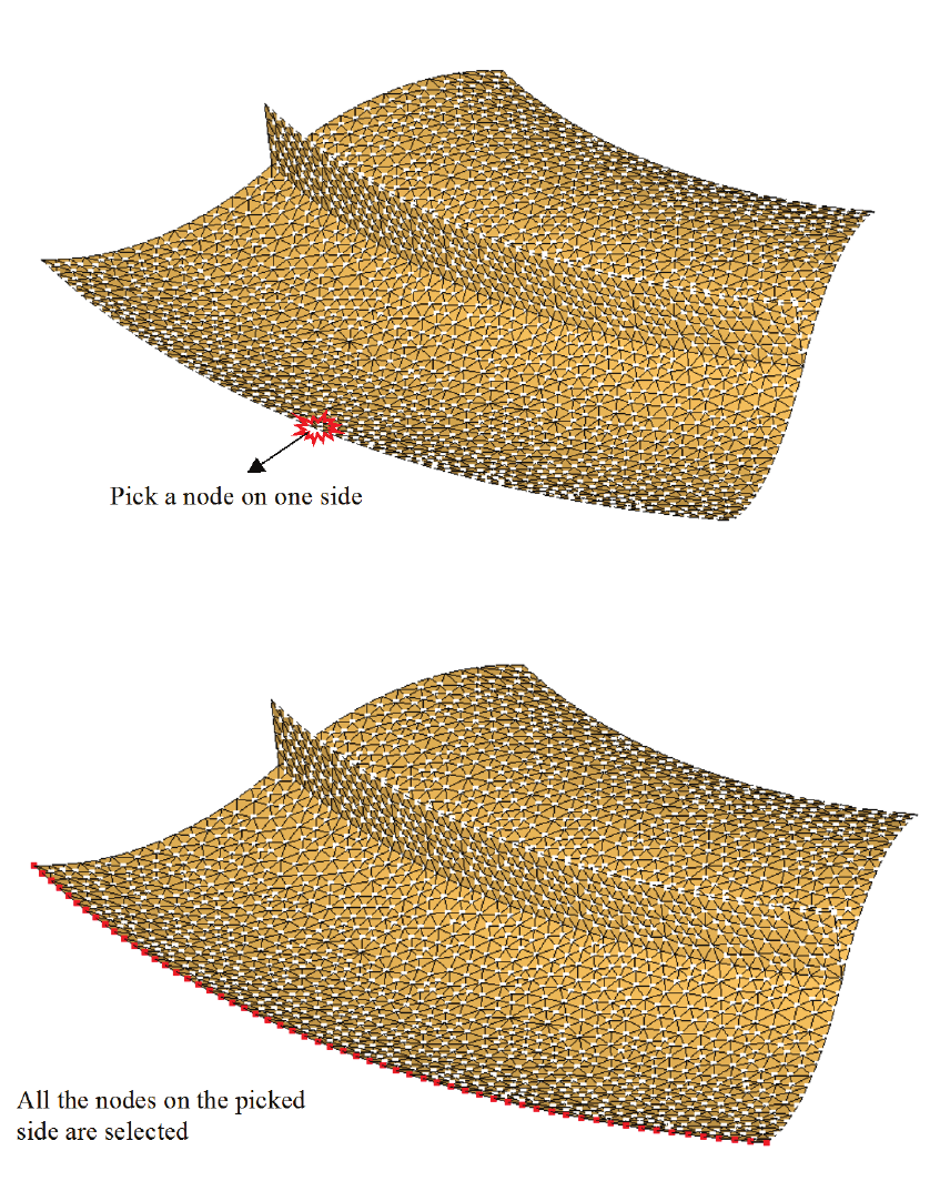
PAM-RTM 2014 35 USER’S GUIDE & TUTORIALS
© 2014 ESI Group (released: Apr-14)
PAM-RTM USER'S GUIDE
Selection Menu
Selection > Zone ID
When the zone ID of the entities to select is known, the user can type it directly in the
dialog box that pops up when the Selection -> Zone ID command is used. It is also
possible to enter two values to specify a range. In the following image, the user enters 1
and 7 to select all the elements of all the zones in the range 1 to 7.
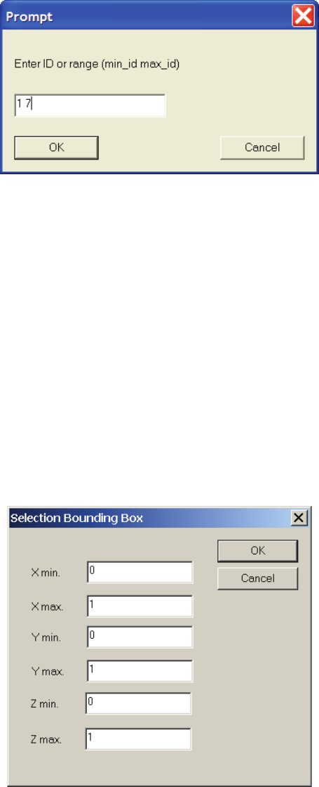
USER’S GUIDE & TUTORIALS 36 PAM-RTM 2014
(released: Apr-14) © 2014 ESI Group
PAM-RTM USER'S GUIDE
Selection Menu
Selection with zone ID
Selection > Entity ID
This command is used to select an entity based on its ID. For example, it is possible to
select the node with ID = 999 by entering this value in the selection dialog box. It is
also possible to select all the nodes with IDs in the range 0 to 999 by entering the string
“0 999” in the text field. This is the same behavior as Selection->Zone ID.
Selection > Bounding Box
This command opens a dialog box in which the user can specify the (xmin, ymin, zmin)
and (xmax, ymax, zmax) coordinates of a bounding box. All the entities that fit in this
bounding box are selected. For a face or an element, as soon as a node is inside the
bounding box, the entity is selected.
Selection with bounding box
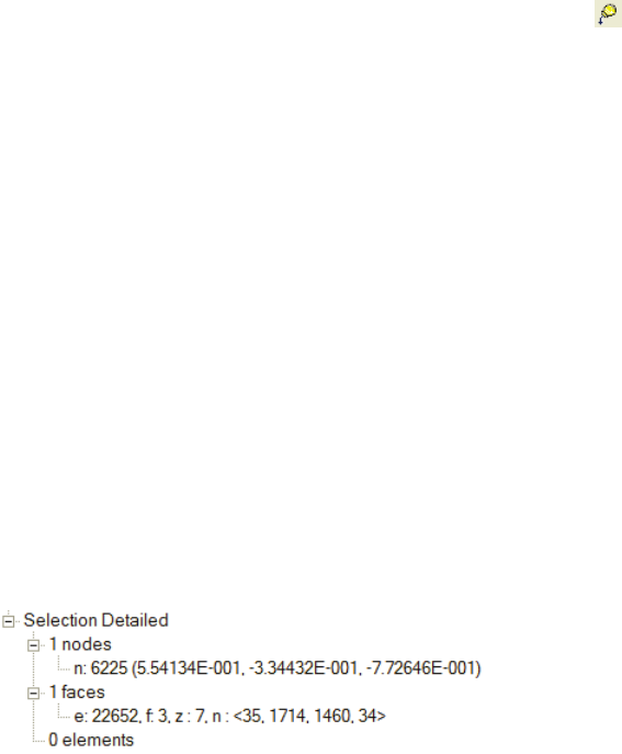
PAM-RTM 2014 37 USER’S GUIDE & TUTORIALS
© 2014 ESI Group (released: Apr-14)
PAM-RTM USER'S GUIDE
Selection Menu
Selection > Select All
Selects all the entities based on the current selection filter. For example, if the selection
filter is set to Nodes, all the nodes of the mesh are selected.
Selection > Unselect All (filter)
Unselects all the entities based on the current selection filter. For example, if the
selection filter is set to Nodes, all the nodes are unselected. If faces or elements are
selected, they stay selected.
Selection > Unselect All (no filter)
Completely clears the current selection (nodes, faces and elements) regardless of the
selection filter. You can also use the CTRL-U keyboard shortcut or this button in the
Selection toolbar to call this command.
Selection > Set Scalar Field Value
If you are currently visualizing a scalar field such as porosity or thickness, you can use
this command to modify the scalar field values on the selected nodes or elements. This
is sometimes useful to correct scalar fields after a Compute Local Permeability, when the
mapping results are not very good because of complex geometry. The corrected scalar
fields can be exported with File->Export->PAM-RTM Scalar Field.
Selection > Info Summary
Displays in the message window information about the current selection. The total
number of nodes, faces and elements is displayed.
Selection > Info Detailed
Displays in the message window the details of the current selection. The ID of each
selected entity is displayed. For example:
For selected faces, e means element ID, f means face index of the element (solid
elements only), z means zone ID, and n is the connectivity of the element. For selected
nodes, n means node ID, g is group ID (if the node is part of a group), and the (x, y, z)
coordinates of the node are displayed.

USER’S GUIDE & TUTORIALS 38 PAM-RTM 2014
(released: Apr-14) © 2014 ESI Group
PAM-RTM USER'S GUIDE
Groups Menu
GROUPS MENU
Groups of nodes or faces are created in PAM-RTM to be used as boundary conditions.
Groups > Create
Creates a new group with the currently selected entities. If nodes are currently selected,
a new group of nodes is created. If faces are selected, a new group of faces is created.
It is not possible to create a group of elements in PAM-RTM.
The ID of the new group is automatically assigned by PAM-RTM based on the largest
ID of the groups currently defined. If the largest group ID is 99, the new group will
have ID = 100. It is not possible to change the ID of a group after it has been created.
It is not possible to have nodes and faces in the same group.
Groups > Add To
This command is used to add nodes or faces to an existing group. The procedure is to
select first some nodes or faces, then call the Groups->Add To command, and finally
pick a node or face which is part of the group you want to modify.
Groups > Remove From
The procedure is to first select some nodes or faces, then call the Groups->Remove From
command. The selected entities will be removed from all the groups they belong to.
This means that if a node, for example, was part of 2 groups, it will be removed from
the 2 groups.
Groups > Change ID
This command allows modification of a group ID. It asks the user the current ID of the
group, and its new ID. If the specified new ID is already used, an error message is
displayed.
Groups > Contact Interface
This command is used to create a special group that is currently used only for thermal
contact resistance boundary condition. The elements are disconnected on the interface.
This can be verified with the command View->Outline->Free Edges. A contact interface
can only be created on the interface between two zones. The selection of nodes must be
done with care. As shown in the following image, the two end points must not be
selected. On a 3D mesh, it is recommended to work with a selection of faces.
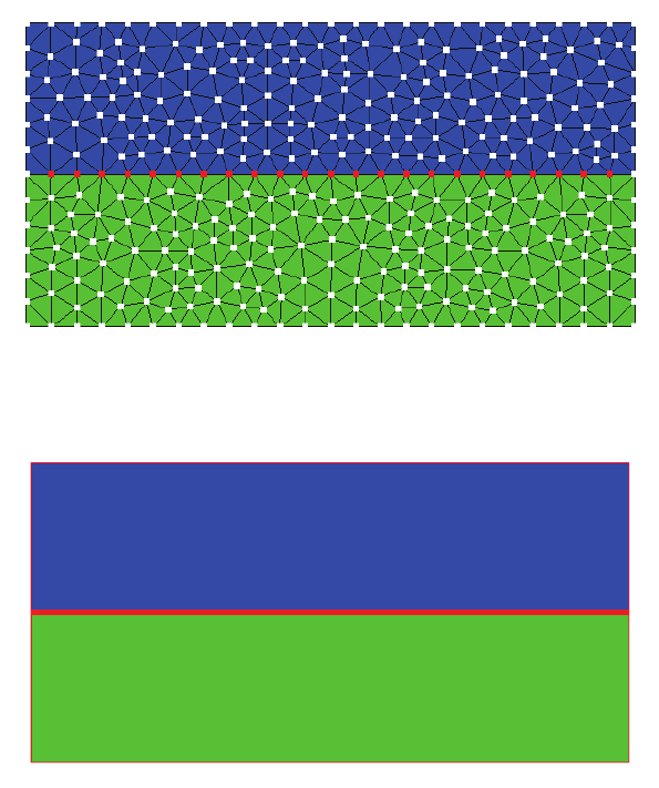
PAM-RTM 2014 39 USER’S GUIDE & TUTORIALS
© 2014 ESI Group (released: Apr-14)
PAM-RTM USER'S GUIDE
Groups Menu
Nodes selection for contact interface
Free edges after creation of contact interface
Groups > Mold/Cavity Interface
Automatically disconnects the elements on the mold/cavity interface for the whole
mesh. The material type assigned elements through zones is used. Material type solid
defines the mold area, and reinforcement the cavity area. A group of faces is
automatically created, that can be referred by a contact resistance boundary condition.
The following pictures show a cross section of a part with a metallic mold and insert.
The first picture shows the solid material area (mold + insert), the second picture shows
the reinforcement area, and the third picture shows the interface created by this
command.
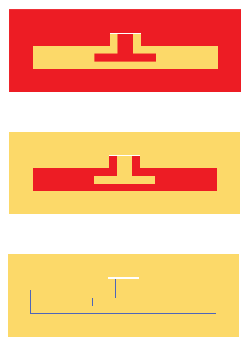
USER’S GUIDE & TUTORIALS 40 PAM-RTM 2014
(released: Apr-14) © 2014 ESI Group
PAM-RTM USER'S GUIDE
Groups Menu
Solid material area (mold + insert)
Reinforcement material area
Interface created
PAM-RTM 2014 41 USER’S GUIDE & TUTORIALS
© 2014 ESI Group (released: Apr-14)
PAM-RTM USER'S GUIDE
Groups Menu
Groups > Nodes to Faces
Convert a group of nodes to a group of faces. PAM-RTM prompts the user for the
group ID to convert. Enter –1 to convert all groups.
Groups > Faces to Nodes
Convert a group of faces (for solid elements) or edges (for shell elements) to a group of
nodes. PAM-RTM prompts the user for the group ID to convert. Enter –1 to convert all
groups. This command is useful for example when you import a mesh generated in I-
DEAS which contains groups of edges. PAM-RTM reads the group of edges from the I-
DEAS file, but these groups can’t be visualized or modified with the user interface. In
such a case, this command should be used to convert all groups of edges to nodes.
Groups > Delete (Pick)
To delete a group, the user first calls this command, then picks a node or face in the
group to delete.
Groups > Delete (ID)
Another way to delete a group is by entering its ID. Enter –1 to delete all groups.
Groups > Info Summary
Displays in the message window a short summary of the currently available groups.
The ID of the group is listed, together with the total number of nodes or faces in the
group.
Groups > Info Detailed
Lists in the message window all the node IDs and face IDs of all the groups.

USER’S GUIDE & TUTORIALS 42 PAM-RTM 2014
(released: Apr-14) © 2014 ESI Group
PAM-RTM USER'S GUIDE
Mesh Menu
MESH MENU
Commands in the Mesh menu are used to make some modifications to a mesh, but most
importantly to specify material orientations.
Mesh > Remesh > Injection Point
This command is used to create a hole in a shell mesh that can be used as an injection
point. A group is automatically created within the nodes around the hole. The following
image shows the Mesh Injection Point dialog box, together with the points that were
picked for Center (A) and Radius (B).
Creation of a hole and a group

PAM-RTM 2014 43 USER’S GUIDE & TUTORIALS
© 2014 ESI Group (released: Apr-14)
PAM-RTM USER'S GUIDE
Mesh Menu
Mesh around the hole
Mesh > Remesh > Runner
This command is used to create layers of thin elements that can be used to simulate
runners or edge effects. The remeshed areas are most of the time on the part boundary,
but they can also be internal to simulate special injection systems (for example injection
tubes placed on top of the part). A distinct zone ID is automatically assigned to the
elements in the remeshed zones.
You will most probably need the measure tool to use this command effectively.
In the following image, a runner is created on the complete boundary of a rectangular
part. To pick the full boundary, push the Boundary button, then pick any node on the
boundary. The boundary is highlighted. Then you have to specify the size of elements
along the path. The runner can be seen as a cylinder placed on top of the part. That’s
why it makes sense to talk about the runner radius. Specify the runner radius and the
number of element layers you want on the runner radius. Use the measure tool to
estimate the size of elements along the path and the runner radius. In this example the
size of elements along the path was set to 0.01 m, the runner radius is 0.02 m and the
number of layers on the radius is 2, which leads to elements with a good aspect ratio. As
shown in the resulting mesh image, the runner is not a perfect straight line. However
this should be good enough to simulate runners in PAM-RTM.
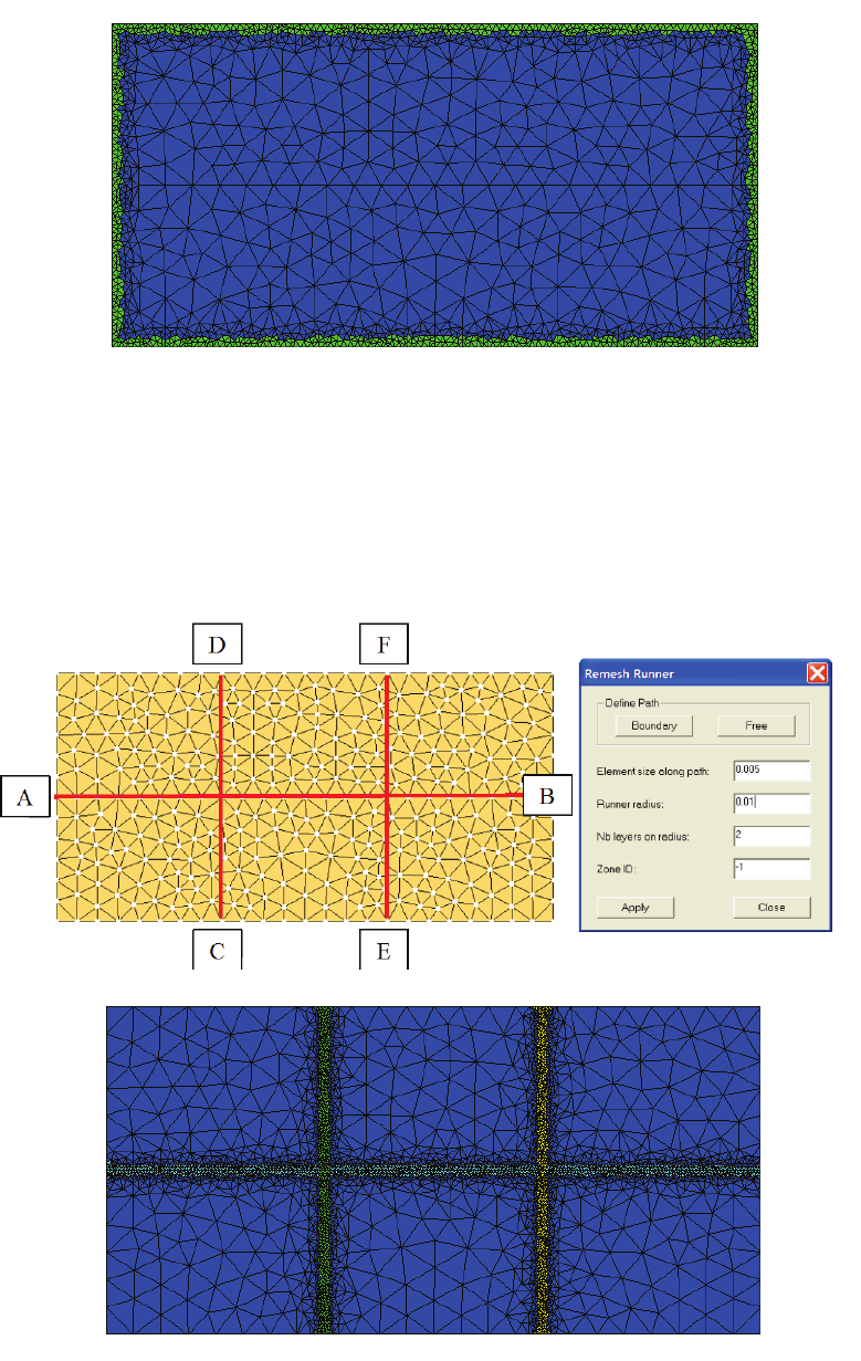
USER’S GUIDE & TUTORIALS 44 PAM-RTM 2014
(released: Apr-14) © 2014 ESI Group
PAM-RTM USER'S GUIDE
Mesh Menu
Creation of a runner on the boundary
It is also possible to create internal (not located on the boundary) free paths. Push the
Free button, and then pick a sequence of nodes or points to define the path. The
following images show how a branch like injection system can be created. First push
the Free button, then pick nodes A and B. Enter the size parameters, then push the Apply
button. Repeat the same procedure for the lines C-D and E-F.
Creation of a branch like injection system
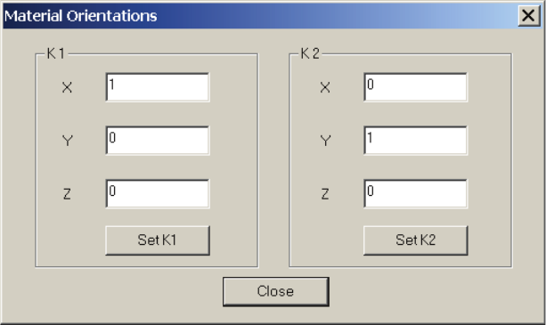
PAM-RTM 2014 45 USER’S GUIDE & TUTORIALS
© 2014 ESI Group (released: Apr-14)
PAM-RTM USER'S GUIDE
Mesh Menu
Mesh > Orientations > K1
The Mesh->Orientations->K1 and Mesh->Orientations->K2 commands are used to set the
current working direction. For example, a command like Set K Orthogonal needs to
know if the direction to make orthogonal is K1 or K2. A check mark is displayed beside
the current working direction.
Mesh > Orientations > Set Vectors
This command is used to set the direction vectors K1 and K2 by entering the 3
coordinates of vectors specified in the global coordinate system. After specifying the
coordinates of K1 or K2, push the Set K1 or Set K2 button to apply the appropriate
vector. The Set Vector command works on the currently selected faces or elements.
Mesh > Orientations > Project Vectors
This command is the same as Set Vectors except that it does an orthogonal projection of
the specified vectors on the selected elements.
Dialog box used by Set Vectors and Project Vectors
Mesh > Orientations > Set K from Selected Nodes
This command is used to specify material orientations in curved regions for which
permeability directions can be described by a simple piecewise linear curve. For
example, in the following image, K1 was specified by projecting the elements on the
curve defined by the selected nodes. The tangent vector of the curve at the point of
projection defines the K1 direction. Depending on the current working direction, K1 or
K2 will be specified.
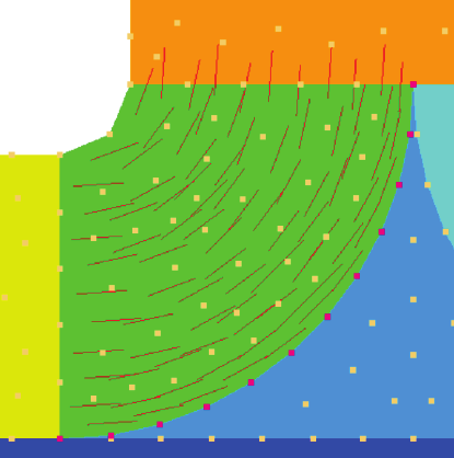
USER’S GUIDE & TUTORIALS 46 PAM-RTM 2014
(released: Apr-14) © 2014 ESI Group
PAM-RTM USER'S GUIDE
Mesh Menu
Setting material orientations in a curved region
The procedure to use this command is the following:
- Set the working direction (K1 or K2).
- Select faces or elements on which you want to specify the direction.
- Select nodes to define a piecewise linear curve. Nodes must be selected in a
consistent order. For example in the previous image, nodes could be selected from
bottom-left to top-right, or from top-right to bottom-left.
- Execute the Mesh->Orientations->Set K from Selected Nodes command.
- Verify the direction vectors with View->Orientations->K1 Only or View-
>Orientations->K2 Only.
Mesh > Orientations > Set K Orthogonal
This sets the orientation vectors in the current working direction as orthogonal to the
other direction. For example, if the current working direction is K2 and this command is
executed, the K2 direction of the selected elements will be made orthogonal to K1. Of
course, in this example, K1 must be defined first.
Mesh > Orientations > Align Plies
This command is used to make material orientations consistent in plies. For example,
after importing PAM-QUIKFORM plies, some direction vectors could be pointing in
the X+ direction while other vectors in the same ply could be pointing in the X-
direction. The goal of this command is to have all the elements in a ply oriented in the
same global direction.
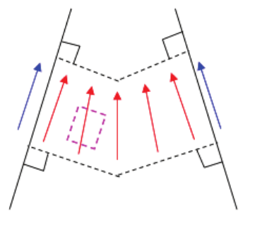
PAM-RTM 2014 47 USER’S GUIDE & TUTORIALS
© 2014 ESI Group (released: Apr-14)
PAM-RTM USER'S GUIDE
Mesh Menu
The algorithm currently implemented takes the first element of a ply and makes the
directions consistent on the ply from neighbor to neighbor. This means that there is a
risk that from ply to ply the directions could not be consistent. The user should always
check the orientations on each ply after running this command. If a problem is found on
a ply, the orientations on this ply can easily be reversed by selecting all the elements of
the ply with Selection->Select All, then by reversing the orientations with Mesh ->
Orientations->Reverse.
Mesh > Orientations > Reverse
This command reverses the current direction (K1 or K2) of the selected elements or
faces. For example, if the current working direction is K1 and the command is executed
on a set of elements with K1 pointing in the +X direction, the K1 direction will be
reversed to -X.
Mesh > Orientations > Project on Skin
This command is used to project the orientation of an imported draping result on the
mesh. It searches for each element in the mesh the closest element in the draping result
and sets the direction K1 and K2 found on the draping result element on the mesh
element.
Mesh > Orientations > Interpolate
This command works with two imported draping results, called skins. It will make an
interpolation of the directions on each skin for the mesh.
The algorithm works that way:
For each element of the mesh and each element of the skin, the coordinates of the
centers of gravity (COG) are computed. If the distance between COG is inferior to the
tolerance, it will try to project the cog on the skin element.
USER’S GUIDE & TUTORIALS 48 PAM-RTM 2014
(released: Apr-14) © 2014 ESI Group
PAM-RTM USER'S GUIDE
Mesh Menu
If no valid projection of the COG is found, the closest COG of the elements of skin
mesh will be found, and the element will be selected.
For each skin, the direction of the weft and warp projection element will be saved, and
the weft and warp direction of the element of the mesh to orient will be an interpolation
of these two directions.
The used algorithm is the following.
Search of the closest 2D skin element e
of the element E
Definition of the element e material
orientation on the element Ei:
(WrEi_inner, Wf Ei_inner, ZEi_inner)
Projection of the COG of the element E
on the medium plane of the retained
2D elements. This projection is
performed along the medium plane
Search of the 2D elements the COG of
which is close to the element E COG
from a distance lower than a value D
given by the user.
Selection of the 2D skin elements for
which the projections are inside those
2D elements.

PAM-RTM 2014 49 USER’S GUIDE & TUTORIALS
© 2014 ESI Group (released: Apr-14)
PAM-RTM USER'S GUIDE
Mesh Menu
Then the interpolation formula is
Where:
- Wr and Wf are Weft and Warp directions,
- Z normal vector,
- Ei_outer is related to the outer skin and Ei_inner is related to the inner skin.
The function is used with this dialog box where the user can define or not define if the
box is not checked:
- Path to the inner skin mesh file
- Path to the outer skin mesh file,
- Path to the output mesh in .unv format,
- Path to the log file,
- Tolerance value (mandatory),
- Path to the SAMCEF file,
- Number of the first frame in SAMCEF frame file.
Interpolation formula :
WrEi = dEi_outer / (dEi_inner + dEi_outer) × WrEi_inner + dEi_inner / (d Ei_inner +
dEi_outer) × WrEi_outer
WfEi = dEi_outer / (dEi_inner + dEi_outer) × WfEi_inner + dEi_inner / (d Ei_inner +
dEi_outer) × WfEi_outer
ZEi = WrEi Λ WfEi

USER’S GUIDE & TUTORIALS 50 PAM-RTM 2014
(released: Apr-14) © 2014 ESI Group
PAM-RTM USER'S GUIDE
Mesh Menu
If the box for the inner and outer skin are not provided the interpolation will be made
with draping results that would have been imported with the function Mesh->import-
>draping results. It will work only in the case when two draping results are already
loaded. Otherwise an error message will be displayed.
If the box for the output mesh is not checked, the mesh will not be automatically
exported. The user will have to export the mesh with Mesh->export or save the data.
If the box for the log file is not checked, no log file is written.
If the box for the SAMCEF frame file is not checked, this file is not exported.
Every path selection will be made with windows explorer dialog box.
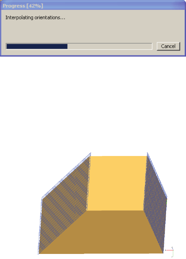
PAM-RTM 2014 51 USER’S GUIDE & TUTORIALS
© 2014 ESI Group (released: Apr-14)
PAM-RTM USER'S GUIDE
Mesh Menu
The user can follow the interpolation with a dialog box indicating the percentage made
at any time. It is possible to stop calculation at any time by clicking on Cancel in this
dialog box.
When interpolation is finished, a projection scalar field is displayed. The code for
projection scalar field is:
- 1: projection worked on both skins,
- 2: projection didn’t work on lower skin, the closest element is chosen,
- 3: projection didn’t work on upper skin,
- 4: projection didn’t work on both skins.
Below are showed one case where projection where some elements do not have a valid
projection.
Trapezium volume mesh and skins to project
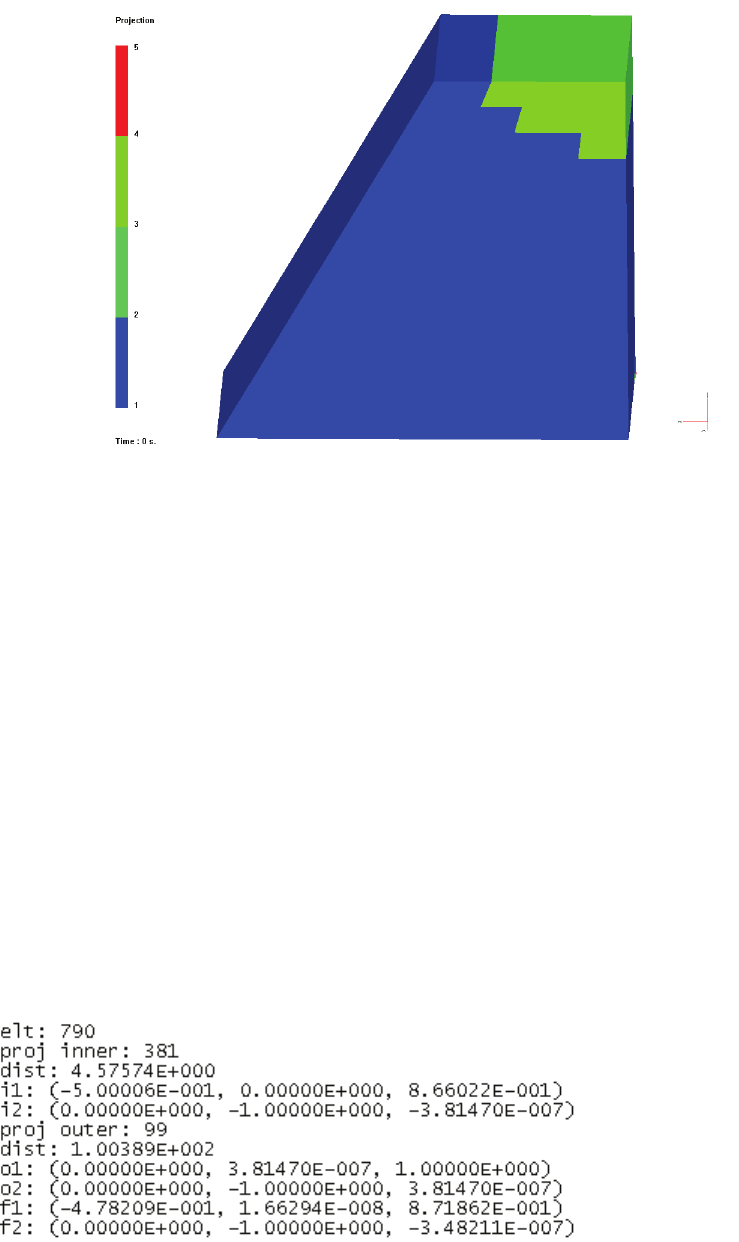
USER’S GUIDE & TUTORIALS 52 PAM-RTM 2014
(released: Apr-14) © 2014 ESI Group
PAM-RTM USER'S GUIDE
Mesh Menu
Trapezium projection results
The orientation can be displayed with the menu View->Orientation.
The .log file contains the following information:
- CPU time for the interpolation of the distance,
- Name of the exported files (.unv and .dat)
- For each element of the initial mesh:
· Number of element
· Number of the projection element on inner/outer skin or closest element id
projection didn’t work
· Distance of projection
· Weft/warp vector for inner/outer skin
· Weft/warp vector for the element.
Examples of the content of the .log file are shown below in the cases where both
projections worked and only the projection on outer skin worked.
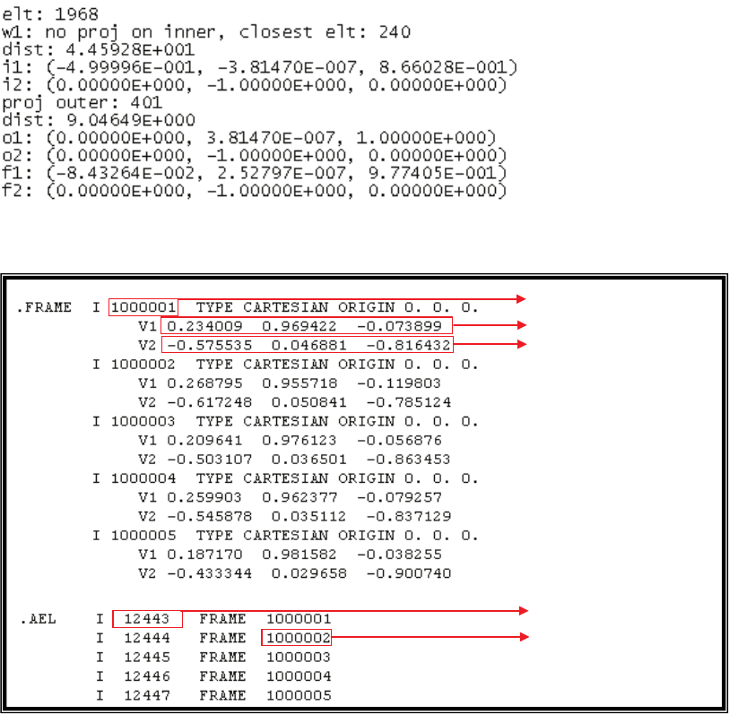
PAM-RTM 2014 53 USER’S GUIDE & TUTORIALS
© 2014 ESI Group (released: Apr-14)
PAM-RTM USER'S GUIDE
Mesh Menu
SAMCEF frame file contains for each element weft and warp vector using following
format:
Frame number
Warp interpolated vector coordinates
Weft interpolated vector coordinates
Element number
Frame number
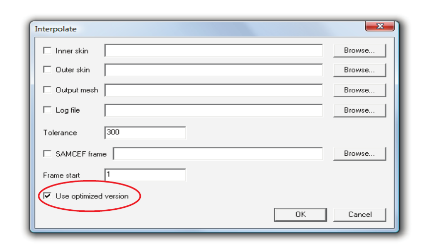
USER’S GUIDE & TUTORIALS 54 PAM-RTM 2014
(released: Apr-14) © 2014 ESI Group
PAM-RTM USER'S GUIDE
Mesh Menu
Introduced in PAM-RTM 2009 is a new optimized version of the method described
above. To enable the optimized version, simply select use optimized version. The
optimized version uses a completely different algorithm for the projection of the solid
elements on the surface meshes. This algorithm is much faster but a little less accurate,
so the non-optimized version should be used when accuracy is of primary concern
compared to CPU time. However speedups of 30 were obtained with the optimized
version, which makes it the version of choice for meshes of millions of elements. To get
the best performance from this optimized version, the size of the surface elements
should be at least 2 times smaller than the solid elements.
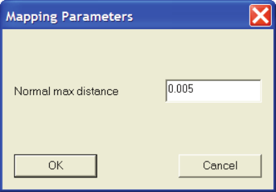
PAM-RTM 2014 55 USER’S GUIDE & TUTORIALS
© 2014 ESI Group (released: Apr-14)
PAM-RTM USER'S GUIDE
Mesh Menu
Mesh > Orientations > Map Draping Results
This command is used to project a stack of plies that have been imported with the
command File->Import->Draping Results, on the mesh used for the injection simulation
(the mesh that was loaded in PAM-RTM™ with the command File->Open or File-
>Import). This is a CPU intensive geometrical calculation that tries to match elements of
the injection mesh with elements in plies. The final goal is the calculation of the average
local permeability on the injection mesh by taking into account the local fiber
orientations in each ply.
Basically, what the algorithm does is the following:
- For each element of the injection mesh
· Calculate the center of gravity (C) of the injection mesh element.
· Define a ray R starting from C, with the direction of the normal vector of the
injection mesh element.
· For each ply mesh
Calculate the intersection of R with all the elements of the ply mesh
If an intersection is found within the normal max distance
value, record the mapping of the element of the ply mesh with
the element of the injection mesh.
This is an exhaustive search through all the elements of all the plies.
The Map Draping Results command can work on the full injection mesh, or on the
currently selected elements. If the current selection is empty, mapping is done on the
full injection mesh. Otherwise, PAM-RTM™ asks the user if he wants to do the
mapping on the selected elements only, or the full injection mesh. PAM-RTM™ then
prompts the user for the normal max distance parameter, as shown in the following
dialog box:
Mapping tolerance
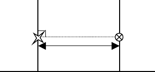
USER’S GUIDE & TUTORIALS 56 PAM-RTM 2014
(released: Apr-14) © 2014 ESI Group
PAM-RTM USER'S GUIDE
Mesh Menu
- Normal max distance. Unit: length.
d
center of gravity
Valid projection discarded because d >max normal distance
The max normal distance is used to discard elements that have a valid projection, but
the distance between the center of gravity of the injection element and the projected
point is larger than the specified tolerance. This is useful in case of ribbed parts.
When the mapping calculation is done, it is always a good idea to verify the validity of
the mapping with the Nb_Plies scalar field. This scalar field is automatically generated
by PAM-RTM™ after a Map Draping Results calculation. It shows the number of plies
covering each element of the injection mesh. For example, if you drape 4 plies that
cover completely the surface to drape, you should have Nb_Plies = 4 everywhere. If you
find that some elements have different values, it means there was a problem with the
mapping, and maybe you need to change the max normal distance.
Mesh > Orientations > Compute Local Permeability on Shells
Before we describe the options to calculate the local permeability of a sheared fabric,
some definitions are necessary.
A very important thing to understand is that when you visualize material orientations in
PAM-RTM™ with the View->Orientations->K1 or View->Orientations->K2 commands,
these orientations can have a different meaning depending on the context. For example,
when you visualize orientations on a ply imported with the PAM-FORM interface, the
orientations should be seen as fiber directions, not permeability directions. However if
you use View->Orientations->K1 on the injection mesh after a Compute Local
Permeability, the vectors you see are principal directions of the permeability tensor, not
fiber directions.
In the following text, we will refer to the direction visualized with View->Orientations-
>K1 in the context of fiber directions as f1. The f1 direction is also defined as the warp
direction for fabrics. The f2 direction is the weft direction for fabrics.
The shear angle α is defined as shown in the next figure: it is the angle between the
weft direction and the direction orthogonal to the warp.
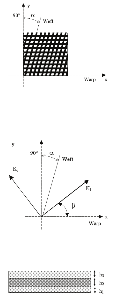
PAM-RTM 2014 57 USER’S GUIDE & TUTORIALS
© 2014 ESI Group (released: Apr-14)
PAM-RTM USER'S GUIDE
Mesh Menu
Definition of the shear angle
α
When a fabric is sheared, the principal directions of the permeability tensor change as a
function of the shear angle α. The principal permeability direction K1 is defined with an
angle β relative to the warp direction.
Rotation of the K1 direction as a function of the shear angle
α
In general, a laminate is made of many plies with different thickness and material
properties.
A typical laminate made of many layers of different thickness and permeability

USER’S GUIDE & TUTORIALS 58 PAM-RTM 2014
(released: Apr-14) © 2014 ESI Group
PAM-RTM USER'S GUIDE
Mesh Menu
The average permeability calculation takes into account the thickness of each layer:
∑
∑
=
=
=n
i
i
n
i
ii
avg
h
hk
k
1
1
Since the permeability of each layer is actually a tensor, the permeability tensor of each
layer is transformed in the referential given by the K1 and K2 directions of the first ply.
The resulting non-diagonal tensor is then diagonalized and the final principal directions
of the laminate are the eigenvectors of the non-diagonal tensor. The local permeability
values k1 and k2 are the eigenvalues.
There are two ways to use the Compute Local Permeability command. The first one
simply computes the average permeability, porosity and total thickness of a laminate
material (found in the Materials folder of the document tree), and assigns these values to
the current selection, or the whole mesh if nothing is selected. It uses the currently
defined orientations on the mesh as the zero degree referential. The other approach uses
the mapping computed by the Map Draping Results command to calculate the average
local permeability of deformed plies. In that context, a laminate material still has to be
defined by the user in order to link material properties to the imported plies. The
number of layers of this laminate must match the number of imported plies. For
example, if 4 draped plies were imported, a laminate material made of 4 layers must be
defined. This is because PAM-RTM™ needs to know the type of reinforcement and
permeability model associated to each layer.
When the Mesh->Orientations->Compute Local Permeability command is called, PAM-
RTM™ opens the following dialog box. If draped plies, such as PAM-QUIKFORM
results imported with File>Import>Draping Results, are to be used for the average
permeability calculation, the user checks the use imported plies option. Otherwise, if
that option is not checked, it means that one of the laminate materials currently defined
will be used. The laminate combo lists the available laminate materials. In case sheared
fabrics such as PAM-QUIKFORM™ results are used, it is also necessary to specify
the permeability model for sheared fabrics. Four models are currently supported and
explained below: unidirectional, isotropic woven fabric, general woven fabric, and
Demaria.
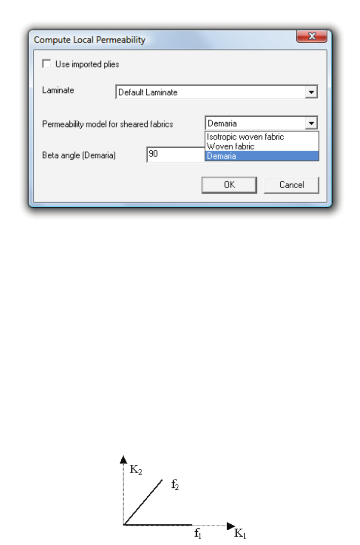
PAM-RTM 2014 59 USER’S GUIDE & TUTORIALS
© 2014 ESI Group (released: Apr-14)
PAM-RTM USER'S GUIDE
Mesh Menu
Available models to compute local permeability of fabrics
UD Model
When a layer is associated to a UD (unidirectional) reinforcement, the local K1 principal
permeability direction is automatically set in the same direction as the f1 fiber direction.
The f2 direction is completely ignored (it is a UD, so the f2 direction is meaningless),
and K2 is made orthogonal to K1.
The permeability values assigned in the K1 and K2 directions are directly the values
specified in the Reinforcement associated to each layer, without any local modification
based on shearing.
Referring to the figure Rotation of the K1 direction as a function of the shear angle
α
, the
K1 direction is given for this model by β=0.
Principal permeability K1 for unidirectional
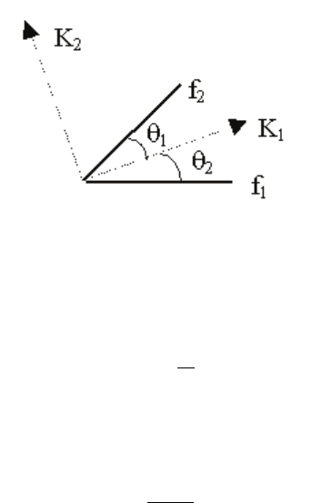
USER’S GUIDE & TUTORIALS 60 PAM-RTM 2014
(released: Apr-14) © 2014 ESI Group
PAM-RTM USER'S GUIDE
Mesh Menu
Isotropic Woven Fabric Model
With this model, which is valid only for fabrics with initially isotropic permeability
(permeability of the fabric before shearing is isotropic), the principal permeability
direction K1 is calculated as the bisector of the angle between the warp and weft (θ1 =
θ2 in the following figure).
Permeability directions calculated with the isotropic woven fabric model
Referring again to figure Rotation of the K1 direction as a function of the shear angle
α
, the
angle β for this model is given by :
2
45
α
β
−
=
The local fiber content (vf) is calculated from the shear angle (α) and the initial fiber
content of the ply, before deformation (vf0) :
α
cos
0f
f
v
v=
The local permeability values in the principal directions are then computed using the
permeability curves function of the fiber content specified in the Fabric associated to
the ply (we call these curves U1 and U2 here) and an internal model that modifies these
values as a function of the shear angle (M1 and M2) :
)(*)(
111
α
MvUk
f
=
)(*)(
222
α
MvUk
f
=
This means that to use this model, the user should ideally have access to experimental
curves giving the permeability as a function of the fiber content. These curves are
entered in the Permeability K1 and Permeability K2 fields of the fabric editor (next
figure). The initial porosity required to calculate the local fiber content is specified for
each layer of the laminate.
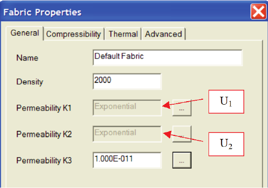
PAM-RTM 2014 61 USER’S GUIDE & TUTORIALS
© 2014 ESI Group (released: Apr-14)
PAM-RTM USER'S GUIDE
Mesh Menu
Specification of the permeability curves as a function of the fiber content in the Fabric
Properties dialog
Woven Fabric Model
This empirical model uses the functions specified in the Sheared Permeability K1, K2,
K3 and Sheared Rotation Angle (β) fields of the fabric editor. These are functions of the
shear angle and initial fiber content:
),
(
0
1f
vfk
α
=
)
,(
02 f
vf
k
α
=
),(
03 f
vfk
α
=
),( 0fvf
αβ
=
The definition of the rotation angle β is the one shown in figure Rotation of the K1
direction as a function of the shear angle
α
. It is important to note that to calculate the K1
direction with the angle β, PAM-RTM™ constructs a right handed local coordinate
system on an element of a ply with the f1 direction, the normal vector of the element,
and the direction orthogonal to f1 and the normal vector (f1o). If the user notices that K1
is not rotated in the expected direction, he should verify normal vectors in each ply with
View->Normal Vector, and then use the Mesh->Cleanup->Reverse Normals command if
necessary to reverse the normal vectors of a ply.
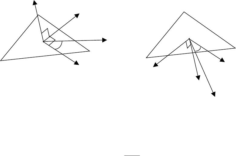
USER’S GUIDE & TUTORIALS 62 PAM-RTM 2014
(released: Apr-14) © 2014 ESI Group
PAM-RTM USER'S GUIDE
Mesh Menu
f1
n
f1o
β
K1
f1
n
f1o
β
K1
The effect of the normal vector on the K1 direction
The local fiber content (vf) is calculated from the shear angle (α) and the initial fiber
content of the ply, before deformation (vf0):
α
cos
0f
f
v
v=
As an application example of the first approach (the one that works directly on a
laminate without draping results), suppose you have a mesh already oriented and you
want to rotate the orientations by 45 degrees. You could define a single layer laminate
material, set the orientation angle of that layer to 45 degrees, run the Compute Local
Permeability command and select the one layer laminate in the laminate dropdown list.
Demaria Model
The reference for this model is:
Demaria C, Ruiz E, Trochu F. In-plane anisotropic permeability characterization of
deformed woven fabrics by unidirectional injection. Part II: Prediction model and
numerical simulations. Polymer Composites, December 2007.
This model assumes that the principal permeabilities in the two principal directions can
be expressed as follows:
( ) ( ) ( )
( )
( ) ( )
ααααα
α
geovgeo
vFFKFKK
f
f
°
=== 0
2,12,1
2,1
Only the unsheared permeabilities
( )
°
=0
2,1
α
K
are needed to use this model. The
( )
α
f
v
F
term is derived from Kozeny-Carman, and the
( )
α
geo
F
term from the
geometrical analysis of the deformation of a unit cell.
PAM-RTM 2014 63 USER’S GUIDE & TUTORIALS
© 2014 ESI Group (released: Apr-14)
PAM-RTM USER'S GUIDE
Mesh Menu
The
( )
°
=0
2,1
α
K
permeabilities are simply the Permeability K1 and Permeability K2
parameters found in the General tab of the Fabric Properties dialog.
The parameter beta angle is available in the Compute Local Permeability dialog to
specify the initial permeability angle with respect to the first fiber direction. It is
equivalent to the angle β of the woven fabric model.
This model has been validated experimentally on a woven fabric, and should be
applicable to any woven fabric.
The current implementation has an important limitation: the shear angle added to the
initial permeability angle (beta angle) must remain in the X+Y+ quadrant, i.e. the final
angle must be between zero and 90 degrees. For instance if the initial permeability
angle is 60 degrees, a maximum negative shear deformation of 30 degrees is allowed,
while a maximum positive shear deformation of 60 degrees is allowed. However it is
better to stay away from these limits. The model will work better for instance with an
initial permeability angle of 45 degrees and shear deformations in the range of +/- 30
degrees.
Mesh > Orientations > Compute Local Permeability on Solids
This command assumes that some orientations are already set on solid elements and
represent fiber directions, potentially sheared (i.e. non-orthogonal). These orientations
could have been transferred to the solid mesh with a command such as Project on Skin.
This command is then used to compute from the draped fiber directions a permeability
tensor on each solid element taking into account shearing.
If some elements are selected, the command will only compute permeability of those
elements. Otherwise it will use the whole mesh.
When the command is launched, it opens a dialog box asking which draped
permeability model to use. The options are:
- Isotropic woven fabric (bisector)
- Woven fabric
The first option is the simple bisector model, which doesn’t need any material
parameter.
The second option makes use of the “sheared” parameters of the Advanced tab of the
reinforcement dialog box. In that case, the zone ID of each element is used to get the
associated reinforcement.
There is actually a third option: if the zone refers to an unidirectional reinforcement, the
first fiber direction f1 will be kept as is and used as permeability direction K1, then K2
USER’S GUIDE & TUTORIALS 64 PAM-RTM 2014
(released: Apr-14) © 2014 ESI Group
PAM-RTM USER'S GUIDE
Mesh Menu
will be made orthogonal to K1 in the plane of f1 and f2. The permeability value is
directly the one specified on the reinforcement (in the General tab).
The local porosity is also calculated by the command.
The Use local permeability files and Use local porosity file options in the Numerical
Parameters > Local Variables tab are automatically selected.
Mesh > Orientations > Compute Local Permeability from
Zones
Starting with PAM-RTM™ 2010, it is now possible to assign laminate materials to
zones. However the PAM-RTM™ solver cannot run a flow simulation directly on the
laminate materials. Instead the solver reads the local permeability, local porosity and
local thickness files generated by the PAM-RTM™ GUI (.sf files).
First the user assigns some laminates to zones. Then he launches the Compute Local
Permeability from Zones command to generate the local permeability, local porosity and
local thickness data. These can be checked graphically by choosing the appropriate
entry in the dropdown list of the main toolbar (K1 or Plies_Thickness for instance). The
command will automatically turn on use local permeability files, use local porosity file
and use local thickness file in the Local Variables tab of the Numerical Parameters.
When the .dtf document will be saved, .sf files will be generated with names matching
the .dtf name. This means the simulation is ready to run once the .dtf has been saved.
Note that it is not mandatory to assign a laminate to every zone to use that command.
Some zones could be linked to a simple reinforcement, while others could be linked to
laminates. In a case involving race tracking for instance, the high permeability zone
could be linked to a simple reinforcement.
Mesh > Orientations > Compute Thickness from Skins
The goal of that command is to calculate the distance between a shell mesh (the
reference mesh) and the top and bottom surfaces of a solid, then generate a local
thickness field for the reference mesh. The mesh that was loaded in the PAM-RTM™
GUI with File>Open or File>Import>Mesh is the reference mesh. The command uses the
draped plies meshes currently loaded (one or two) as skin information. In case a single
draped mesh is available, the reference mesh is seen as the bottom skin of a solid, and
the draped ply is the top skin of the solid. In case 2 draped plies are available, these are
seen as the top and bottom skins of the solid, and the reference mesh is the mid-surface
of the solid.
Below is an example where only the top surface of a solid was imported as a draped ply
(File>Import>Draping Results>PAM-QUIKFORM). After running Compute Thickness
from Skins, the Mapped_Thickness field is available in the dropdown list of the main
toolbar.
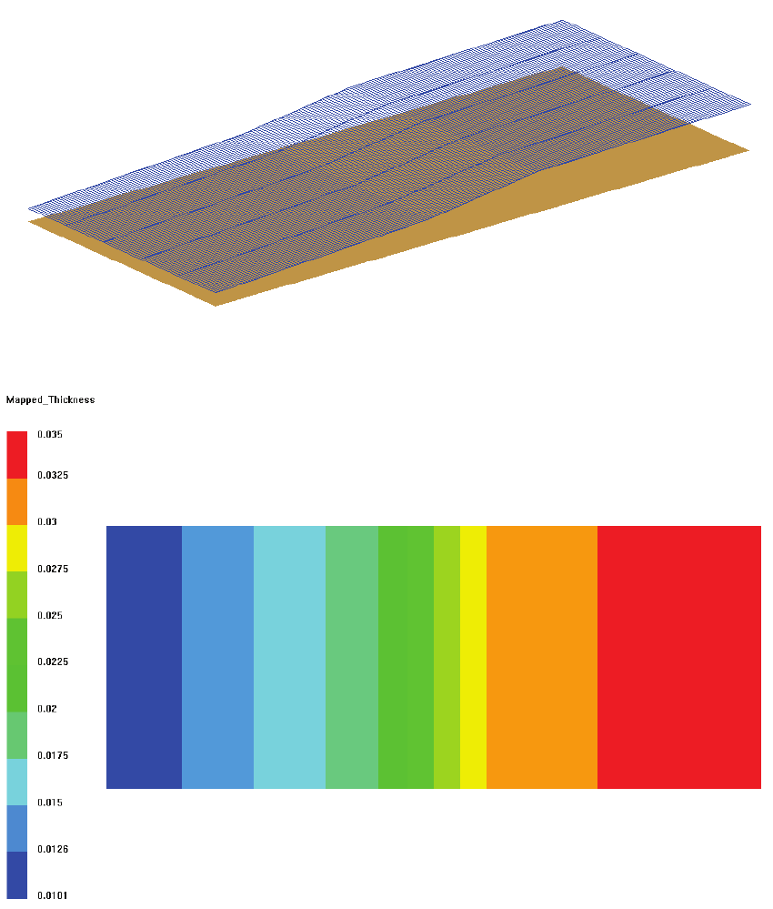
PAM-RTM 2014 65 USER’S GUIDE & TUTORIALS
© 2014 ESI Group (released: Apr-14)
PAM-RTM USER'S GUIDE
Mesh Menu
To use that thickness field in a filling calculation, the user has to export the field first
with File>Export>PAM-RTM Scalar Field. Assuming the case is called x.dtf, the exported
scalar field file would be called x_thickness.sf. Then the option use local thickness has
to be checked in the Local Variables tab of the Numerical Parameters.
Mesh > Orientations > Clear on Selection
Removes any orientation specified on the currently selected elements.

USER’S GUIDE & TUTORIALS 66 PAM-RTM 2014
(released: Apr-14) © 2014 ESI Group
PAM-RTM USER'S GUIDE
Mesh Menu
Mesh > Orientations > Clear All
Removes any orientation specified on the whole mesh.
Mesh > Transform > Set Zone ID
This command is used to assign a different zone ID to the selected elements. This can
be useful for example to create a runner (a zone with higher permeability).
Selection of elements on the edge of a part to create a runner with Set Zone ID

PAM-RTM 2014 67 USER’S GUIDE & TUTORIALS
© 2014 ESI Group (released: Apr-14)
PAM-RTM USER'S GUIDE
Mesh Menu
Assignment of zone ID 99 to the selected elements
Mesh > Transform > Offset Zone Ids
Adds a user specified value to the zone ID of each zone. For example if 10 zones are
currently defined and numbered from 1 to 10, an offset of 100 will renumber zones
from 101 to 110. This is useful in the context of local permeability calculation from
imported plies. If there is a conflict between the zone IDs of the injection mesh and the
plies IDs, the user can simply offset the zone IDs of the injection mesh.
Mesh > Transform > Extrude
This command extrudes a mesh of shell elements to a mesh of solid elements. Triangle
elements are transformed to 6-node prismatic elements, and 4-node quads are
transformed to 8-node bricks.
For simple extrusion, the user can specify the total thickness of the solid part and the
number of layers. In that case all the layers will have the same thickness. A different
zone ID is assigned to each layer so that it is easier later for the user to assign a different
material to each layer.
For more advanced extrusion, it is possible to select a laminate material, so that the
thickness of each layer of the laminate is used as the thickness of each layer of the
extruded mesh. This process is shown below. Assuming the user already created a
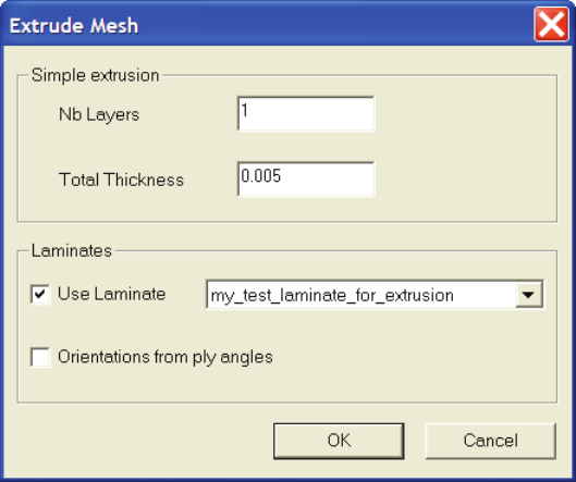
USER’S GUIDE & TUTORIALS 68 PAM-RTM 2014
(released: Apr-14) © 2014 ESI Group
PAM-RTM USER'S GUIDE
Mesh Menu
laminate material and specified the thickness of each layer, he checks the Use laminate
option and selects the laminate previously created in the dropdown list. Note that if Use
laminate is checked, the Nb Layers and Total Thickness parameters are completely
ignored. It is also possible to have the elements of the extruded mesh automatically
oriented if the orientation from ply angles option is checked. This assumes the user has
specified the angle of each ply of the laminate, and that orientations are defined on the
shell mesh. The orientations of the shell mesh correspond to zero degree ply angle. The
final orientations are obtained by rotating those orientations by each ply’s angle.
Extrude dialog box

PAM-RTM 2014 69 USER’S GUIDE & TUTORIALS
© 2014 ESI Group (released: Apr-14)
PAM-RTM USER'S GUIDE
Mesh Menu
Definition of a 4 plies laminate, to be used for mesh extrusion. Notice the thickness of the 4th
layer, much thinner.
Shell mesh to be extruded
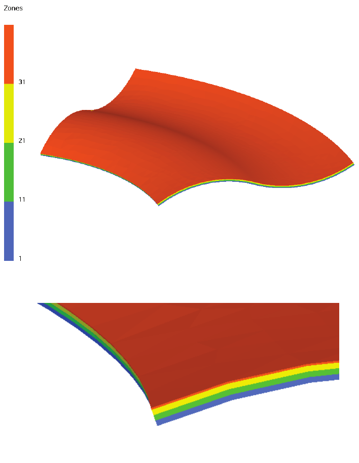
USER’S GUIDE & TUTORIALS 70 PAM-RTM 2014
(released: Apr-14) © 2014 ESI Group
PAM-RTM USER'S GUIDE
Mesh Menu
Extruded 4 layers part
Notice the top layer, much thinner. Linked to a material with a much higher permeability, it
could be used as a flow enhancing layer, for VARTM simulation for instance.
Mesh > Transform > Split Quads
Splits the 4 nodes quad elements into triangles. Each quad is split in 4 triangles, the
barycenter of the quad being used as the common node of the 4 triangles.
This command is quite useful in PAM-RTM since quads are not allowed for filling
simulations with Darcy. If the user has a mesh of quads that he would like to use for a
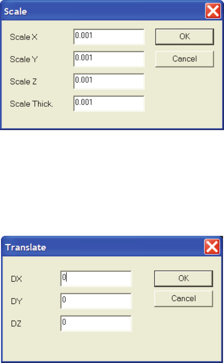
PAM-RTM 2014 71 USER’S GUIDE & TUTORIALS
© 2014 ESI Group (released: Apr-14)
PAM-RTM USER'S GUIDE
Mesh Menu
filling simulation, he can save a lot of time with this command instead of going back to
his mesh generator.
Mesh > Transform > Split Solid Elements
The goal of this command is the same as the Split Quads command : since 6-node
wedges and 8-node bricks are not allowed for PAM-RTM filling simulations with
Darcy, this command can be used to split such elements into 4-nodes tetrahedra.
Mesh > Transform > Scale
Used to apply a scale factor to the nodes of a mesh. This is useful for example to
convert a mesh in millimeters to meters, since meters are used in PAM-RTM. It is also
possible to apply a scale factor to the pseudo-thickness of a shell mesh.
Scale dialog box
Mesh > Transform > Translate
Applies a translation to all the nodes of a mesh, defined by the vector (DX, DY, DZ), in
the global coordinate system.
Translate dialog box
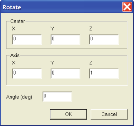
USER’S GUIDE & TUTORIALS 72 PAM-RTM 2014
(released: Apr-14) © 2014 ESI Group
PAM-RTM USER'S GUIDE
Mesh Menu
Mesh > Transform > Rotate
Rotates all the nodes of a mesh around a specified axis. The center of rotation can be
specified. The rotation angle is entered in degrees.
Rotate dialog box
Mesh > Transform > Extract Shell from Solid
Assuming some faces are selected on a solid mesh, this command generates a surface
mesh from the selected faces. The current solid mesh in the document is replaced by the
surface mesh. See images below.
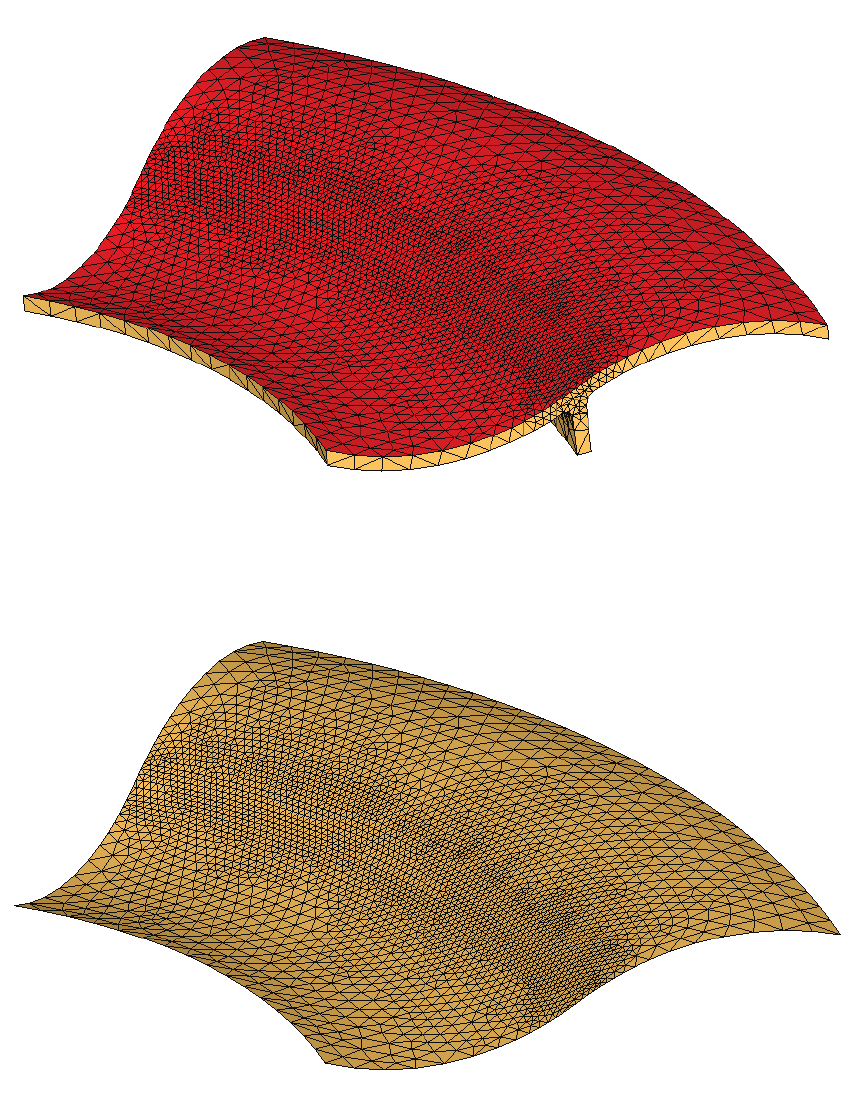
PAM-RTM 2014 73 USER’S GUIDE & TUTORIALS
© 2014 ESI Group (released: Apr-14)
PAM-RTM USER'S GUIDE
Mesh Menu
To extract a shell mesh from a solid mesh, first select some faces.
Extracted surface mesh
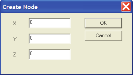
USER’S GUIDE & TUTORIALS 74 PAM-RTM 2014
(released: Apr-14) © 2014 ESI Group
PAM-RTM USER'S GUIDE
Mesh Menu
Mesh > Create > Node
Creates a new node with the specified (x, y, z) coordinates.
Create node dialog box
Mesh > Cleanup > Merge Coincident Nodes
It can sometimes happen that elements in a mesh are not connected, i.e. they have
geometrically common nodes, but these nodes are actually different entities (they are
nodes with different IDs but with the same coordinates). This problem can be fixed by
PAM-RTM. The user enters a merge tolerance, i.e. the smallest allowable distance
between 2 nodes. If 2 elements are closer than the specified distance, they will be
considered the same node, and the elements connectivity will be modified accordingly.
Mesh > Cleanup > Reverse Normals (selection)
This command updates the nodes connectivity of the selected elements so that their
normal vector points in the opposite direction.
Mesh > Cleanup > Align Normals (auto)
Automatically aligns the normal vectors based on the picked element. The picked
element is used as the starting element in an algorithm that visits all the elements of the
mesh from neighbor to neighbor, and changes nodes connectivity if needed to have the
normal vector of an element pointing in the same direction as its neighbors.
Mesh > Cleanup > Delete Unreferenced Nodes
It is possible that some nodes in a mesh are not referenced by any element. This
command is used to delete all the unreferenced nodes of the current mesh.
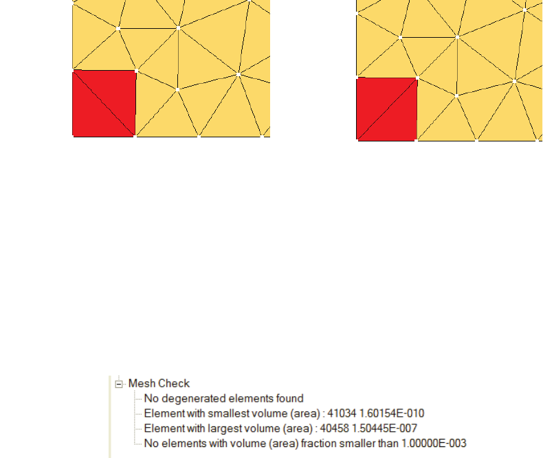
PAM-RTM 2014 75 USER’S GUIDE & TUTORIALS
© 2014 ESI Group (released: Apr-14)
PAM-RTM USER'S GUIDE
Mesh Menu
Mesh > Cleanup > Delete Selected Entities
Deletes the selected nodes or elements. If nodes are deleted, the elements referring to
these nodes will, of course, be deleted. Each time an entity is deleted, groups of nodes
and groups of faces are also updated to make sure they don’t refer to deleted entities.
Mesh > Cleanup > Delete Degenerate Elements
Deletes degenerate elements in a mesh, which are defined as elements referring more
than once to the same node.
Mesh > Cleanup > Swap Diagonal
Modifies the connectivity table of 2 adjacent elements, so that their diagonal (common
edge) is swapped.
Mesh > Check
This command tries to find problems in a mesh. First it looks for degenerated elements,
i.e. elements that have the same node ID appearing twice or more in their connectivity
table. Then it outputs some information about the smallest and largest elements in the
mesh, which can be useful for “debugging” a simulation. Finally it lists all the elements
with a volume 1000 times smaller than the largest volume. This can also help to find
problems, especially with volume meshes in which it can occur that very small elements
are generated in the center of the part.
Output of the Mesh->Check command

USER’S GUIDE & TUTORIALS 76 PAM-RTM 2014
(released: Apr-14) © 2014 ESI Group
PAM-RTM USER'S GUIDE
Mesh Menu
Mesh > Info
This command outputs some general information about a mesh, for example the number
of elements of each type, the number of nodes, the group IDs, and some geometrical
information like bounding box (min and max coordinates of a box containing all the
nodes), span (size of the part in the x, y, z directions), and the volume of the mesh.
Output of the Mesh->Info command
Mesh > Info Pick
This command opens the following dialog box, which lets the user pick nodes or
elements and get info on the picked entities.
Info Pick dialog box
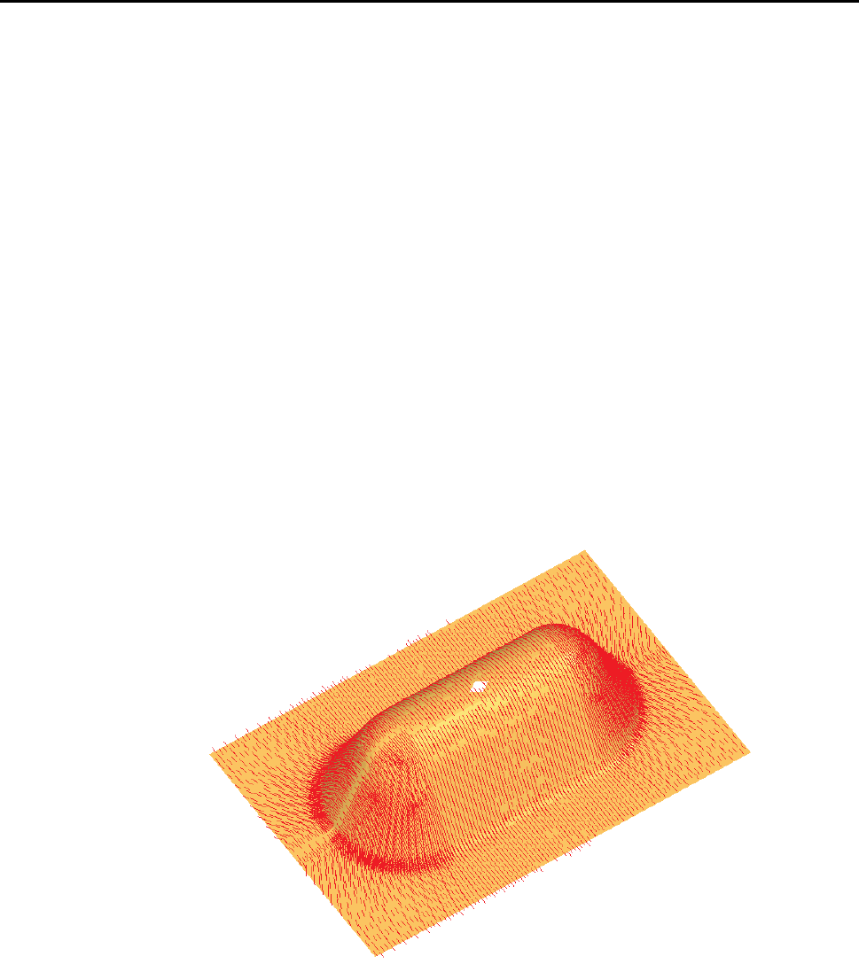
PAM-RTM 2014 77 USER’S GUIDE & TUTORIALS
© 2014 ESI Group (released: Apr-14)
PAM-RTM USER'S GUIDE
View Menu
VIEW MENU
View > Curve Viewer
Opens the curve viewer dialog box. See section Curve Viewer.
View > Orientations > K1 Only
Used to visualize vectors in the K1 direction (see next figure).
Note
· It is very important to understand the difference between the permeability
directions and the fiber directions of a reinforcement. Most of the time, when
you import a ply with File->Import->Laminate, the K1 and K2 directions are fiber
directions, not permeability directions. The fiber directions are transformed to
permeability directions with the Mesh->Orientations->Compute Local
Permeability command. The same menu is used to visualize orientation vectors.
Depending on the context, these vectors will be interpreted by the user as fiber
directions or permeability directions.
Visualization of the K1 direction (actually the f1 direction or warp direction)
View > Orientations > K2 Only
Displays the K2 direction only.
USER’S GUIDE & TUTORIALS 78 PAM-RTM 2014
(released: Apr-14) © 2014 ESI Group
PAM-RTM USER'S GUIDE
View Menu
View > Orientations > K1 and K2
Displays the K1 and K2 directions together.
View > Orientations > None
Clears the display of orientations.
View > Outline > Part
Plots the outline and the sharp edges of the mesh displayed in the current window (it
can be the injection mesh or a ply mesh). The display of sharp edges is based on the
Outline Critical Angle parameter available in the View->Options->Display dialog box.
By default, this value is 40 degrees, which means that an edge common to two neighbor
elements will be plotted if the angle between the two elements is greater than 40
degrees. A lower value would result in more line segments plotted.
View > Outline > Free Edges
This command plots free edges in a mesh of shell elements, i.e. edges that are not
shared by more than one element. This is useful to find connectivity problems in a
mesh.
View > Outline > Plies
It is possible to have the outline of all the draped plies (imported through File->Import-
>Draping Results) plotted in the same window as the injection mesh, as shown in the
next figure. This can be useful to analyze problems with Map Draping Results.
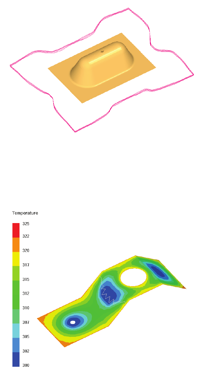
PAM-RTM 2014 79 USER’S GUIDE & TUTORIALS
© 2014 ESI Group (released: Apr-14)
PAM-RTM USER'S GUIDE
View Menu
Visualization of plies outline with the injection mesh
View > Flow Front
The flow front position can be visualized on top of any scalar field. The user must
import first the flow front file generated by the PAM-RTM™ solver (extension
.front), with File->Import->Scalar Field->PAM-RTM Flow Front.
Flow front position (white line) on top of a temperature result
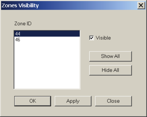
USER’S GUIDE & TUTORIALS 80 PAM-RTM 2014
(released: Apr-14) © 2014 ESI Group
PAM-RTM USER'S GUIDE
View Menu
View > Normal Vectors
This command can be used to visualize normal vectors on shell elements or the external
skin of a solid mesh.
View > Zones Visibility
Opens the following dialog box, which is used to activate or deactivate the visualization
of some zones. This can be useful to visualize results on internal zones completely
surrounded by solid elements. This situation happens for example when the cavity and
the mold are meshed with solid elements.
Zones visibility dialog box
View > Cutting Plane
Opens the Cutting Plane dialog box, used to specify the parameters of a cutting plane.
When Clipping is checked, visualization of graphics entities is disabled on one side of
the plane. When Cross Section is checked, the intersection of the plane with a solid
mesh is calculated and displayed. The plane is defined in space by entering the
coordinates of a point and the normal vector of the plane. Coordinates can be specified
exactly by the user. Otherwise, a node of the mesh can be picked with the mouse to
define the plane’s position. When the position is defined, another node can be picked to
define the normal vector.
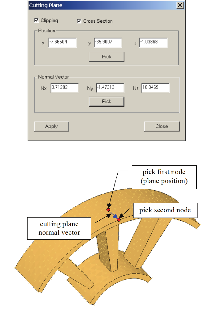
PAM-RTM 2014 81 USER’S GUIDE & TUTORIALS
© 2014 ESI Group (released: Apr-14)
PAM-RTM USER'S GUIDE
View Menu
Cutting plane dialog box
Picking of nodes to define the cutting plane
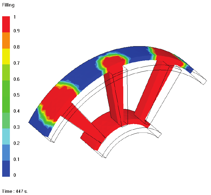
USER’S GUIDE & TUTORIALS 82 PAM-RTM 2014
(released: Apr-14) © 2014 ESI Group
PAM-RTM USER'S GUIDE
View Menu
Display of the filling factor with the cutting plane active
View > Post-Processing
This command opens the Post-Processing dialog box, used to set post-processing
parameters.
The first group of parameters is related to animation. Animation can be activated or
stopped with the On/Off check box. When Proportional is checked, each animation
frame is displayed for a time that depends on the simulated time and the Loop Time.
The loop time specifies the total time to display all the frames. It is specified in
seconds. For example, if a filling simulation generates output for times 1 s., 2 s., 5 s.,
10 s., and if the loop time is set to 10 (s), the first frame would be displayed for 1 s., the
second one for 3 s., the third one for 5 s. and the last frame is always displayed for some
fixed time on which the user doesn’t have control (2 s.). If proportional is not checked,
each frame is displayed the same time. With the same example, since there are 4 frames
to display in 10 seconds, each frame would be displayed for about 2.5 s. Note that there
is nothing that warns the user if the computer is not able to achieve this frame rate.
The second set of post-processing parameters is related to the color scale. There are
many options to control the range of the color scale :
- Auto Step: PAM-RTM™ automatically adjusts the color scale based on the min and
max values of each time step of the visualized scalar field.
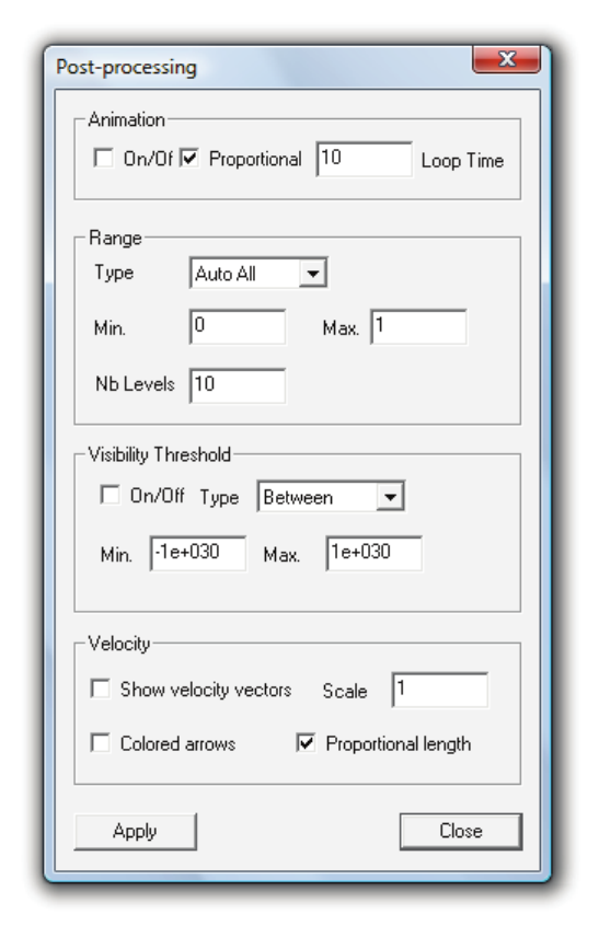
PAM-RTM 2014 83 USER’S GUIDE & TUTORIALS
© 2014 ESI Group (released: Apr-14)
PAM-RTM USER'S GUIDE
View Menu
- Auto All: the min and max values of all the time steps are used as the range of the
color scale.
- Fixed: the values specified by the user in the Min and Max fields are used.
- Min Fixed: only the value specified in the Min field is fixed, the max value is
automatically adjusted for each step.
- Max Fixed: only the value specified in the Max field is fixed, the min value is
automatically adjusted for each step.
The number of color levels in the color scale is set with Nb Levels.
Post-processing parameters
The third set of parameters concerns the visibility of faces. If On/Off is checked, it
means that some faces will be hidden. There are 4 options to control the visibility
threshold:
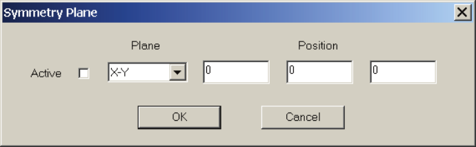
USER’S GUIDE & TUTORIALS 84 PAM-RTM 2014
(released: Apr-14) © 2014 ESI Group
PAM-RTM USER'S GUIDE
View Menu
- Under: only faces with a scalar field value lower than the value specified in the Min
field are displayed.
- Between: only faces with a scalar field value between the values specified in the Min
and Max field will be displayed.
- Not Between: only faces with a scalar field value lower than the value specified in
the Min field or greater than the value in the Max field will be displayed.
- Above: only faces with a scalar field value greater than the value specified in the
Max field will be displayed.
Finally, the Show velocity vectors check box allows velocity vectors to be displayed on
top of the currently visualized contour. For instance, it is possible to display velocity
vectors on top of a temperature contour. The Scale value can be used to apply a scale
factor to the velocity vectors, in case they are displayed too short or too long by default.
The colored arrows option allows vectors to be colored based on their norm. The
proportional length option, when active, displays arrows of size proportional to the
norm of the vectors. Since velocity vectors close to the flow front are typically very
small compared to vectors close to inlets, uncheck this option to visualize them
correctly. These two last options are only available for post-processing of parallel solver
results.
View > Symmetry
This command is useful when a simulation was run on mesh representing only half a
part for symmetry reasons. It is possible using this command to recreate the complete
mesh, to produce pictures for a report, for example.
The symmetry plane can be chosen as X-Y, Y-Z or X-Z. The position of the symmetry
plane must also be specified by entering the 3 coordinates of a point in the Position text
fields.
View->Symmetry dialog box
View > Delete N Last Steps
It sometimes happens that the last states of a filling calculation are not significant. For
instance, depending on the outlet conditions, it could happen that only a few elements
are filled in the last steps in a very long time. This command is used most of the time in
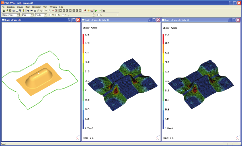
PAM-RTM 2014 85 USER’S GUIDE & TUTORIALS
© 2014 ESI Group (released: Apr-14)
PAM-RTM USER'S GUIDE
View Menu
the context of the display of an animation, or for the generation of an AVI file. It allows
exclusion of the n last steps from the animation. Of course this command doesn’t delete
anything in results files. It just prevents the last steps from being displayed.
View > Set Same Viewpoint
When many graphics windows are opened, it can be useful to set the same viewpoint
(rotation) for all the views. This command sets the same viewpoint for all views of all
open documents, based on the active view. Activate first the window that you want to
use as the reference.
Result of the Set Same Viewpoint command. The active window is the left one.
View > Options > Paths
This tab is used to set the path to the PAM-RTM™ standard solver executable
(pamrtm.exe) and the parallel solver (pamrtm_dmp.exe). The PAM-QUIKFORM solver
(quik_form.exe), MPI version used to run the parallel solver, and other executables are
also specified in this tab. Normally these paths don’t need to be changed. They are set
by the InstallShield when PAM-RTM™ is installed. However in some special
situations like a minor PAM-RTM™ update that doesn’t ship with an InstallShield, the
path could be changed manually by the user.
See section Material Database for information about the path to the material database.
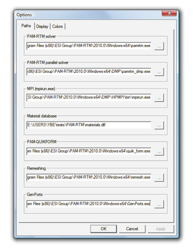
USER’S GUIDE & TUTORIALS 86 PAM-RTM 2014
(released: Apr-14) © 2014 ESI Group
PAM-RTM USER'S GUIDE
View Menu
Paths tab
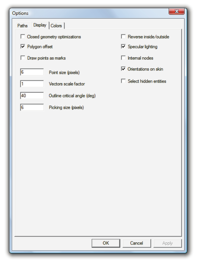
PAM-RTM 2014 87 USER’S GUIDE & TUTORIALS
© 2014 ESI Group (released: Apr-14)
PAM-RTM USER'S GUIDE
View Menu
View > Options > Display
Display tab
There are many viewing parameters that can be set through the Display tab.
- Closed geometry optimizations: when it is checked, this parameter tells PAM-
RTM™ to turn on display optimizations relevant for closed geometry (usually
USER’S GUIDE & TUTORIALS 88 PAM-RTM 2014
(released: Apr-14) © 2014 ESI Group
PAM-RTM USER'S GUIDE
View Menu
solids), such as culling (elimination at the first stage of the graphics pipeline of back
facing polygons). If the user suspects rendering problems, for example faces that
are not displayed, this optimization should be turned off.
- If Closed geometry optimizations is active, so is culling, which means that the
normal vector has an effect on the faces that will be displayed. By default, PAM-
RTM™ manages to have normal vector of the front facing polygons point in the
direction of the viewer. However if the user notices some strange “inverse effects”,
for example when rotating the mesh it seems to turn in the inverse direction, the
Reverse inside/outside parameter should be checked.
- The Polygon Offset flag is used to offset the element faces by some small distance
so that the element edges can be displayed with better quality. Some graphics cards
might not support this OpenGL feature very well, so it can be turned off if you
suspect a problem.
- Draw points as marks: by default, nodes are displayed with OpenGL points.
Problems with OpenGL points have been seen on some graphics cards. If the Draw
points as marks check box is checked, nodes will be displayed as a small x instead
of points.
- Specular Lighting: this flag is used to turn on or off specular lighting, i.e. the
lighting that makes surfaces appear shiny. By default specular lighting is on.
- By default, only nodes on the external skin of solid meshes are displayed in PAM-
RTM™. Internal nodes can be checked to visualize nodes inside solid meshes. This
can be useful to create sensors by picking internal nodes.
- The Point Size parameter controls the half size of points, in pixels.
- Vectors Scale Factor: by default, PAM-RTM™ calculates the length of vectors
such that they have a reasonable size when projected in the graphics window. If the
vectors appear too small or too large on screen, the user can apply a scale factor to
the vectors. For example, if 0.5 is specified, the vectors will be 2 times smaller.
- Outline Critical Angle: this parameter controls drawing of sharp edges. PAM-
RTM™ determines sharp edges based on the angle between 2 adjacent faces. If too
many sharp edges (false edges) are drawn, you should increase the value of this
parameter. The maximum value is 90 degrees.
- Picking Size: this parameter can be used to modify the picking sensibility. It
specifies the diameter of a circle (in pixels) around the point where the mouse
button is clicked. The default value is 6 pixels. This means that to pick a node, for
example, the user can click at most 3 pixels away from the node. If you think it’s
too difficult to pick nodes with the default settings, you should increase the value of
this parameter.
- Orientations on skin: this option concerns solid meshes only. If the option is not
checked, orientation vectors are displayed for all elements of the mesh, including
internal elements. Orientation vectors are displayed with an arrow starting at the
center of gravity of the element. If the option is checked, orientation vectors will
only be displayed for elements on the skin of the solid (external boundary), thus
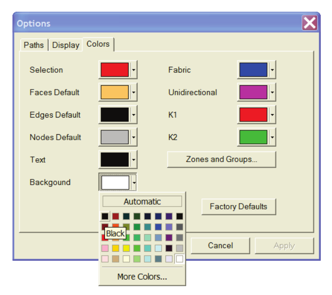
PAM-RTM 2014 89 USER’S GUIDE & TUTORIALS
© 2014 ESI Group (released: Apr-14)
PAM-RTM USER'S GUIDE
View Menu
reducing the number of vectors displayed. Also, the center of gravity of the external
face will be used as the origin for the display of orientation vectors, instead of the
center of gravity of the element, which should lead to better visualization in general.
- Select hidden entities: by default, selection using a rectangular box only selects
visible entities (nodes, faces, elements). It is sometimes useful, for instance when
working on a solid model, to select entities located inside the solid. When this
option is activated, all the entities that project inside the rectangle defined by the
user will be selected, whether they are visible or not.
View > Options > Colors
The user can change the color of many graphics entities with the Options->Color tab.
For example the default background color (white by default) can be changed by pushing
the arrow on the Background button. This pops up a color chooser with a selection of
pre-defined colors (see next figure). If the user doesn’t find the color he wants in the
pre-defined colors, he can use the More Colors button to popup the standard Windows
Color Chooser. The default color of faces, nodes, etc., can also be changed. When the
user changes one of these colors, the modified color settings are saved in the Windows
registry. It is possible to come back to the original PAM-RTM™ default values with
the Factory Defaults button.
Colors tab
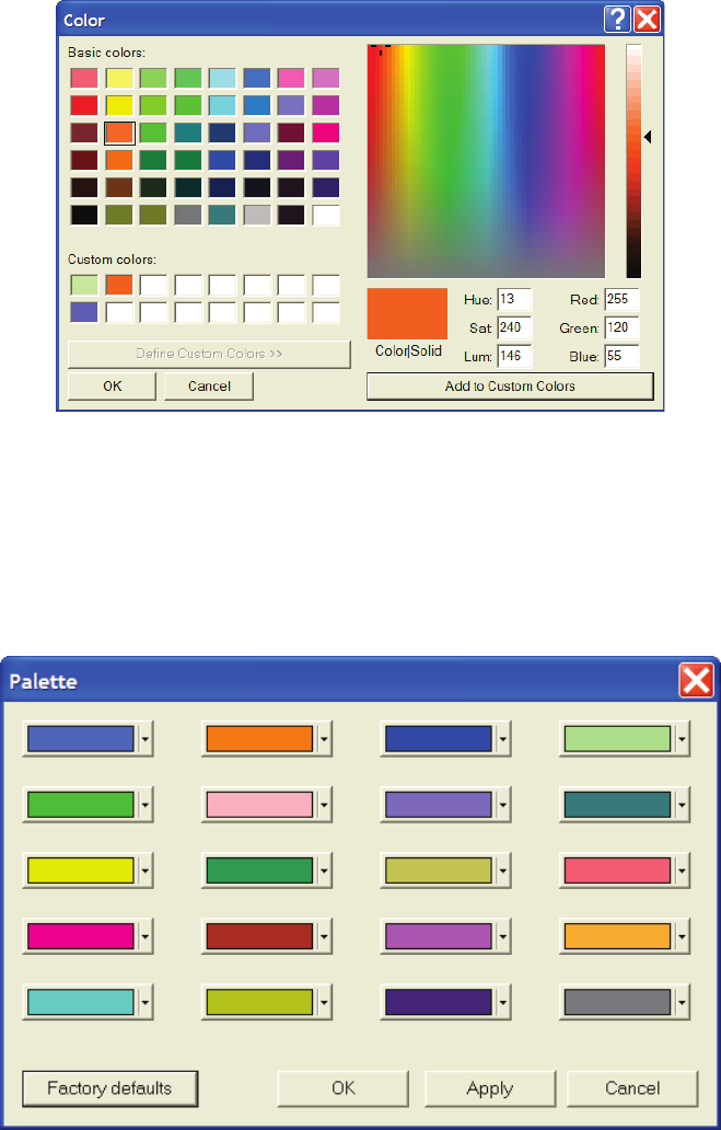
USER’S GUIDE & TUTORIALS 90 PAM-RTM 2014
(released: Apr-14) © 2014 ESI Group
PAM-RTM USER'S GUIDE
View Menu
Standard Windows color chooser
The Zones and Groups button allows the user to customize the color scale used to
display zones and groups. 20 colors are available for this color scale. If there are more
than 20 groups or zones to display, the colors are re-used. Note that it is still possible to
use the color scale that was used in version 2004 for groups and zones with View->Color
Scale->RGB.
Default color palette used to display groups and zones
View > Color Scale
Enables the user to select the color space used to interpolate colors in the color scale.
RGB, HSV and GREY color spaces are available.
PAM-RTM 2014 91 USER’S GUIDE & TUTORIALS
© 2014 ESI Group (released: Apr-14)
PAM-RTM USER'S GUIDE
View Menu
View > Color Schemes
The user can select with this menu between a Black Background or White Background
color scheme. For example, when the black background is selected, the color used for
text is automatically set to white.
View > Lights
The View->Lights menu is used to turn on or off one of the 6 predefined lights.
View > Refresh
Forces the redraw of the active window. Use CTRL-R as a shortcut.
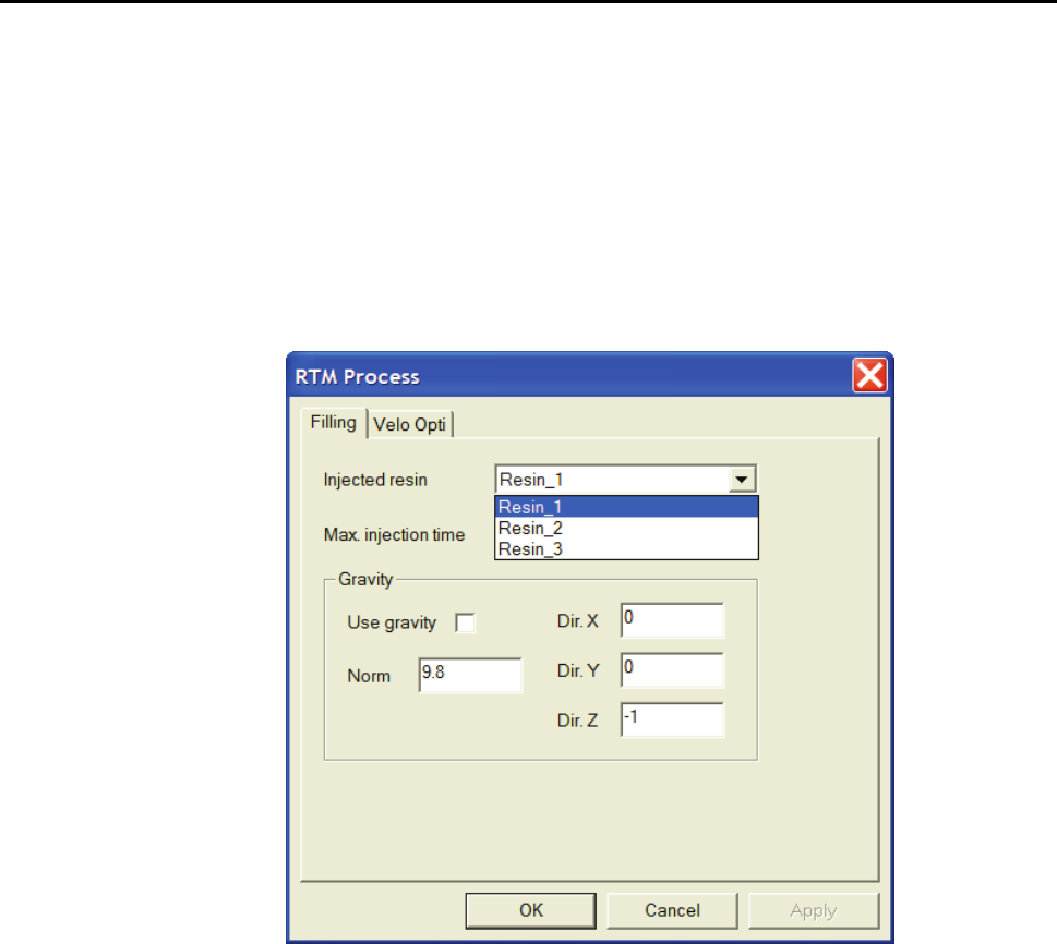
USER’S GUIDE & TUTORIALS 92 PAM-RTM 2014
(released: Apr-14) © 2014 ESI Group
PAM-RTM USER'S GUIDE
Process Parameters
PROCESS PARAMETERS
The process parameters will be presented in the following sections for each simulation
type. Many parameters are common to many simulation types, so instead of repeating
text we refer to the section where the parameter was first described.
RTM Simulation
Filling Tab
RTM process parameters
- Injected resin: drop-down list allowing the user to select the resin to be injected.
This list contains the names of all the resins currently defined in the model.
- Max injection time: the simulation will stop even if the part is not completely filled if
the maximum injection time is reached.
- Use gravity: tells PAM-RTM™ to take gravity into account when calculating the
resin pressure field.
- Gravity Norm: gravitational acceleration. Unit: m/s2.
- Dir. X, Dir. Y, Dir. Z: components of the gravity direction vector. By default gravity is
in the negative Z direction.
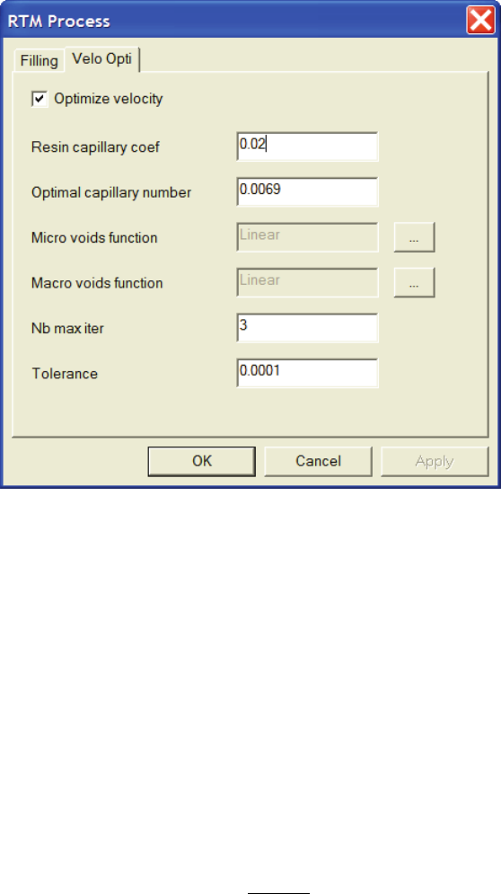
PAM-RTM 2014 93 USER’S GUIDE & TUTORIALS
© 2014 ESI Group (released: Apr-14)
PAM-RTM USER'S GUIDE
Process Parameters
Velo Opti Tab
The reference for the velocity optimization (voids minimization) functionality of PAM-
RTM™ is:
Ruiz E, Achim V, Soukane S, Trochu F, Bréard J. Optimization of injection flow rate to
minimize micro/macro-voids formation in resin transfer molded composites.
Composites Science and Technology 66 (2006) 475–486.
- Optimize velocity: tells PAM-RTM™ to adjust the injection flow rate so that the
voids percentage is minimal in the final part. Pressure controlled inlets are
converted to flow rate controlled. If this parameter is not checked and the micro and
macro voids functions are defined, PAM-RTM™ won’t optimize the velocity but
will calculate the micro and macro void values. This is useful to have an idea of the
void content that you would have at the end of the injection if you didn’t control the
flow rate.
- Resin capillary coef: the capillary number is defined as:
θγ
µ
cos
*v
Ca =
where
µ
is the fluid viscosity,
v
the superficial velocity,
γ
the surface tension, and
θ
the contact angle between the resin and the fibers. The resin capillary coef is the term
θγ
cos
.
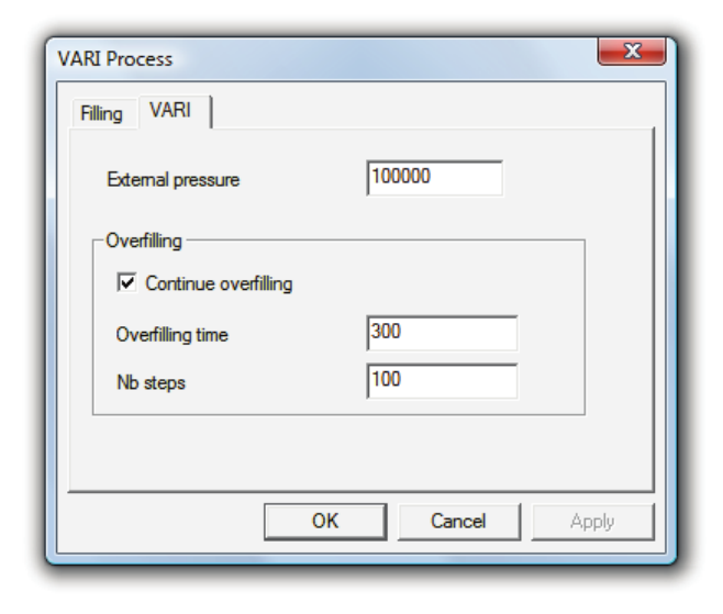
USER’S GUIDE & TUTORIALS 94 PAM-RTM 2014
(released: Apr-14) © 2014 ESI Group
PAM-RTM USER'S GUIDE
Process Parameters
- Optimal capillary number: the capillary number minimizing the void content.
- Micro voids function: the function describing the micro voids content, as un function
of the capillary number.
- Macro voids function: the function describing the macro voids content, as un
function of the capillary number.
- Nb max iter: the maximum number of Darcy’s equation resolutions done each time
step of filling to optimize the flow front velocity.
- Tolerance: the convergence error allowed in the optimization process.
Please see the tutorial Velocity Optimization for more information.
VARI Simulation
Filling Tab
See RTM Simulation.
VARI Tab
VARI Process tab
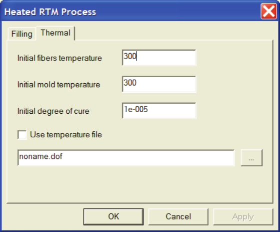
PAM-RTM 2014 95 USER’S GUIDE & TUTORIALS
© 2014 ESI Group (released: Apr-14)
PAM-RTM USER'S GUIDE
Process Parameters
- External pressure: most of the time the default atmospheric pressure (100 000 Pa) is
used, but if the infusion is done in an autoclave, a higher pressure could be
specified.
- Continue overfilling: when checked, simulation will continue even if the part is
filled. That allows the user to study the relaxation of the reinforcement after filling,
and estimate how long it takes to reach thickness equilibrium. Different scenarios
are possible. For instance the inlet could be kept on after filling is complete, or
closed with the Trigger Manager.
- Overfilling time: the duration of the post-filling phase.
- Nb steps: the number of steps to compute for the post-filling phase. A constant time
step is used, given by overfilling_time/nb_steps.
Heated RTM Simulation
Filling Tab
See RTM Simulation.
Thermal Tab
Heated RTM process parameters
- Initial fibers temperature: initial temperature applied on the fibers just before the
resin starts entering the cavity. This value is not used if Use temperature file is
checked. Unit: degree Kelvin.
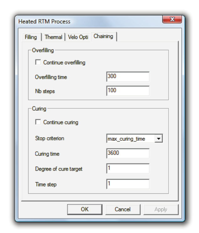
USER’S GUIDE & TUTORIALS 96 PAM-RTM 2014
(released: Apr-14) © 2014 ESI Group
PAM-RTM USER'S GUIDE
Process Parameters
- Initial mold temperature: initial temperature of the mold. This value is not used if
Use temperature file is checked. Unit: degree Kelvin.
- Initial degree of cure: degree of cure of the resin just before entering the cavity.
- Use temperature file: check this parameter if you want to initialize temperature in
the mold and fibers with a non-uniform temperature field, result of a preheating
simulation. Use the … button to browse to the file containing initial temperature.
That file is x_Thermal_p.dof with the standard solver, xt.unf with the parallel
solver, where x is the name of the preheating case.
Note:
· It is also possible to specify initial temperature per zone. However zone
temperature will be ignored if use temperature file is active.
Chaining Tab

PAM-RTM 2014 97 USER’S GUIDE & TUTORIALS
© 2014 ESI Group (released: Apr-14)
PAM-RTM USER'S GUIDE
Process Parameters
- Continue overfilling: tells PAM-RTM™ to perform overfilling, i.e. let the resin
flow out of the vents for some time after the part is completely filled. This is useful
to get a more uniform degree of cure distribution before starting the actual curing.
The overfilling stage is optional. You could chain curing directly after filling,
without overfilling.
- Overfilling time: the time allowed for the resin to flow out of the vents after filling.
Unit: seconds.
- Nb steps: the number of steps of overfilling, i.e. the number of Darcy’s resolutions
after the part is filled.
- Continue curing: check this parameter if you want PAM-RTM™ to continue with a
curing simulation after filling or overfilling.
- Stop criterion: if max_curing_time is selected, the curing simulation will run until
curing_time is reached. The min_above option will stop the simulation when all
elements have at least the degree of cure specified in degree of cure target, while the
avg_above option will stop the simulation when the average degree of cure on the
mesh is above degree of cure target.
- Curing time: the time allowed for curing when the max_curing_time option is
selected.
- Degree of cure target: the degree of cure to reach, when the min_above or
avg_above options are selected.
- Time step: the time step for the curing simulation is explicitly set by the user. Unit:
seconds.
Preheating Simulation
Preheating process parameters
- Initial fibers temperature: initial temperature of the fibers. Unit: degree Kelvin.
- Initial mold temperature: initial temperature of the mold. Unit: degree Kelvin.
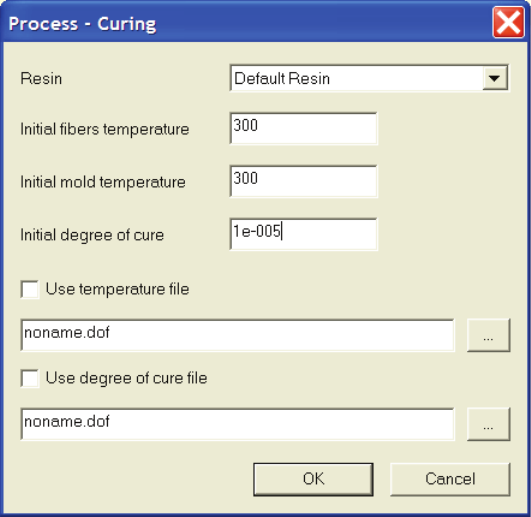
USER’S GUIDE & TUTORIALS 98 PAM-RTM 2014
(released: Apr-14) © 2014 ESI Group
PAM-RTM USER'S GUIDE
Process Parameters
Note:
· It is also possible to specify initial temperature per zone.
Presimulation
No process parameters are available for presimulation.
Curing Simulation
Curing process parameters
- Resin: if many resins are defined in your document, you have to choose which resin
to use for the curing simulation from this drop-down list.
- Initial fibers temperature: initial temperature in zones linked to fiber reinforcements.
This parameter is not used if Use temperature file is checked. Unit: degree Kelvin.
- Initial mold temperature: initial temperature in zones linked to mold material. This
parameter is not used if Use temperature file is checked. Unit: degree Kelvin.
- Initial degree of cure: initial degree of cure assigned to all the elements in the cavity.
This parameter is not used if Use degree of cure file is checked. By default, the
curing simulation assumes that the cavity is completely filled (filling factor is 1
everywhere in the cavity). The only way to take into account partially filled
elements is with the degree of cure file.
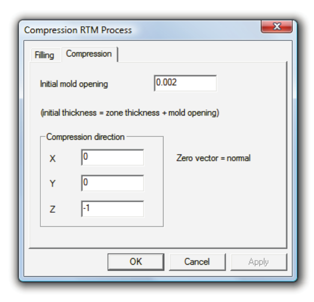
PAM-RTM 2014 99 USER’S GUIDE & TUTORIALS
© 2014 ESI Group (released: Apr-14)
PAM-RTM USER'S GUIDE
Process Parameters
- Use temperature file: check this option and browse to the x_Thermal_f.dof to
initialize temperature with a non-uniform field resulting from the Heated RTM
simulation. With the parallel solver the file to select is xt.unf.
- Use degree of cure file: check this option and browse to the x_Curing_f.dof to
initialize the degree of cure with a non-uniform field resulting from the Heated RTM
simulation. With the parallel solver the file to select is xcr.unf.
Note:
· It is also possible to specify initial temperature per zone. However zone
temperature will be ignored if use temperature file is active.
Compression RTM Simulation
Filling Tab
See RTM Simulation.
Compression Tab
CRTM process parameters
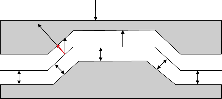
USER’S GUIDE & TUTORIALS 100 PAM-RTM 2014
(released: Apr-14) © 2014 ESI Group
PAM-RTM USER'S GUIDE
Process Parameters
- Initial mold opening: this is the thickness difference from start to end of compression
(h1 in the figure below). In case of a vertical mold displacement (compression
direction –Z), the initial mold opening corresponds to the displacement of the tool.
- Compression direction: the vector in the global coordinate system defining the
compression direction. If a zero length vector is specified, the normal vector of each
element is used as the compression direction.
Note:
· The initial mold opening doesn’t correspond to an empty gap. PAM-RTM™
modeling of CRTM assumes that the preform always fills completely the cavity.
· The final thickness of the part is specified on zones. Even though in general the
same final thickness will be specified on all the zones, it is possible to specify a
different final thickness on each zone if needed. The initial thickness is
automatically computed by PAM-RTM™ so that at the end of compression the
thickness matches the thickness of zones. This means the initial thickness could
change from element to element, depending on the element’s normal and the
compression direction. The initial thickness is hf+h2, where h2 is the projection
of h1 on the local normal vector.
PAM-QUIKFORM Simulation
There are basically two process parameters for a PAM-QUIKFORM simulation: axis
(also called draping referential) and operation. Even though axis do not appear in the
hf
hf
hf (final thickness)
hf
hf
h1 (initial mold opening)
h2
n
h1
compression direction
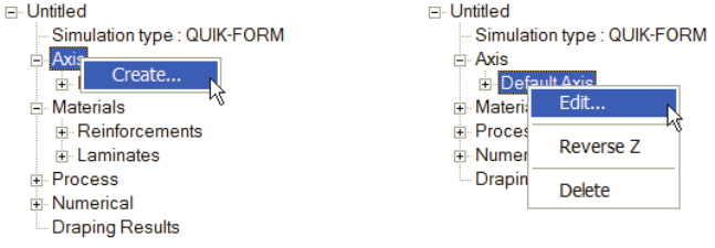
PAM-RTM 2014 101 USER’S GUIDE & TUTORIALS
© 2014 ESI Group (released: Apr-14)
PAM-RTM USER'S GUIDE
Process Parameters
process folder of the explorer, they are clearly process parameters since they are used to
specify contact point and draping direction.
Another process parameter, used only in advanced applications, is the draping curve. It
is possible to import a draping curve with the Import Curves command available in the
popup menu associated to the Process item in the explorer. See description of the curve
parameter in the PAM-QUIKFORM solver manual.
It is possible to create many axis in a PAM-QUIKFORM document. An axis is used as
a referential on which a laminate is aligned before it is draped. The origin of the
referential can be seen as the contact point, and the local X axis of the referential is the
draping direction for a zero degree layer.
A draping operation is the association of a laminate, an axis and optionally a
geometrical support (a selection of elements of the tool mesh). If the geometrical
support is not specified, it is assumed that a layer is to be draped on the complete tool
mesh. A laminate part is defined by specifying a sequence of draping operations. For
example:
- Drape laminate 1 from axis 1.
- Drape laminate 2 on axis 2.
- etc.
Axis Definition
To create an axis, right-click the axis item in the explorer and choose Create. To edit an
axis, double-click it in the explorer, or choose Edit in the axis popup menu. This opens
the Axis Definition dialog.
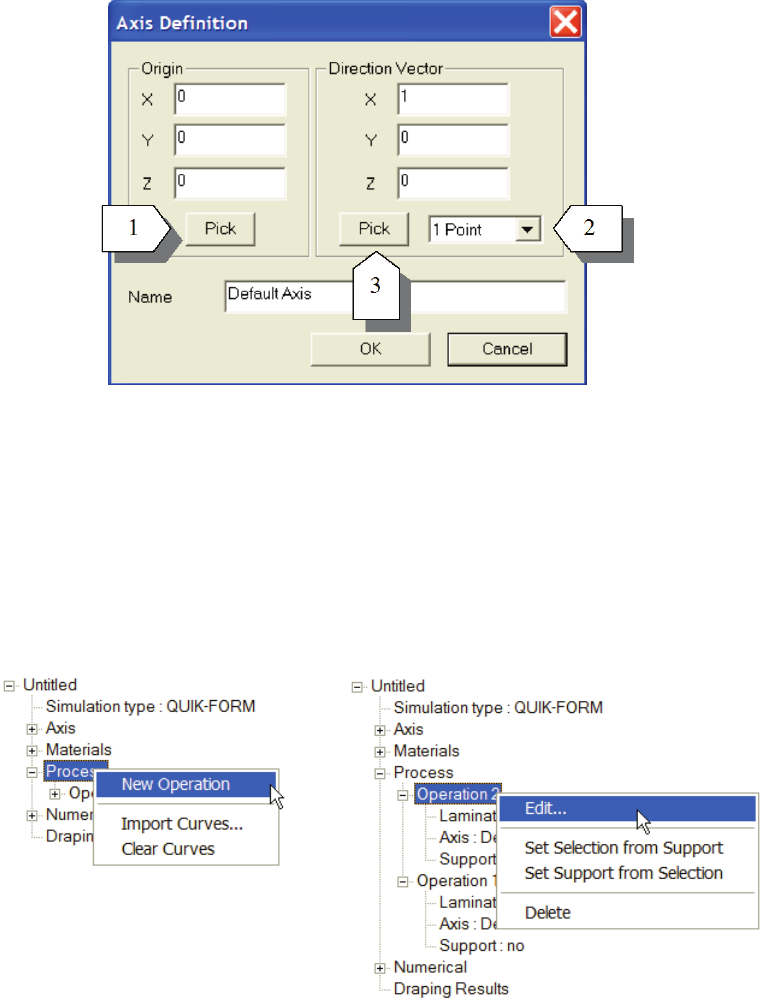
USER’S GUIDE & TUTORIALS 102 PAM-RTM 2014
(released: Apr-14) © 2014 ESI Group
PAM-RTM USER'S GUIDE
Process Parameters
The coordinates of the origin can be entered manually, or an arbitrary point can be
picked on the tool mesh with the Pick button [1]. The direction vector (local X axis of
the referential) can also be entered manually, or interactively by picking points. First
choose 1 Point or 2 Points option [2]. If 1 Point is chosen, push the Pick button [3] and
pick one point. The direction vector is then defined from the origin to the picked point.
If 2 Points is used, push the Pick button [3], then pick two points on the tool mesh. The
direction vector is then defined from the first picked point to the second.
Draping Sequence
Before the sequence of draping operations can be specified, some axis and laminates
must be defined (see chapter Laminates). To create a new operation, use the New
Operation command in the Process popup menu. To edit an operation, double-click it in
the explorer, or choose Edit in the popup menu. New operations are always added at the
end of the operation sequence. It is not possible to move an operation in the sequence
once it is created.
Editing an operation pops up the following dialog box, where the laminate to drape and
the associated axis can be selected from the list of available entities.
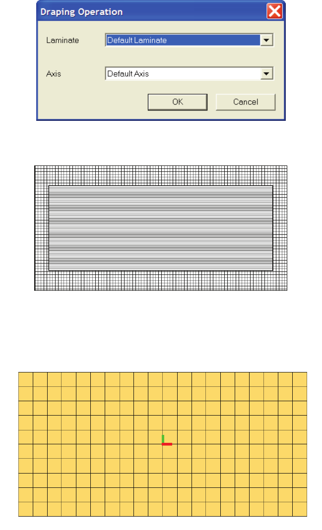
PAM-RTM 2014 103 USER’S GUIDE & TUTORIALS
© 2014 ESI Group (released: Apr-14)
PAM-RTM USER'S GUIDE
Process Parameters
Optionally, it is possible to set a geometrical support to an operation. The use of
supports will be demonstrated with the following example.
A rectangular surface is to be draped first with a layer of fabric. Then a layer of UD is
draped on top of the fabric. The UD layer doesn’t cover the surface completely.
The mesh used in this example is the following.
First we set the draping referential to the center of the part. When using supports, it is
important that the referential used in a draping operation be located on the support.
Then we create 2 laminates: one for the fabric layer, and one for the UD layer.
The next step is to create 2 operations. The first one is associated to the fabric layer, the
second one to the UD layer.
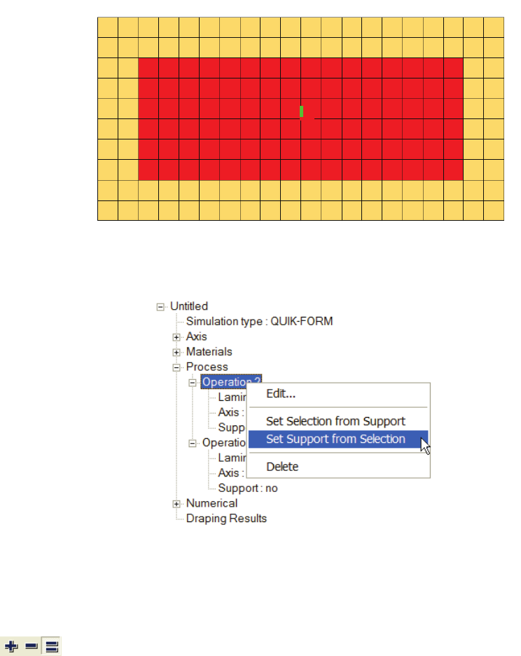
USER’S GUIDE & TUTORIALS 104 PAM-RTM 2014
(released: Apr-14) © 2014 ESI Group
PAM-RTM USER'S GUIDE
Process Parameters
Finally we set the support of the UD operation. Set the selection filter to Element then
select elements like this.
Use the Set Support From Selection command, available in the operation popup menu,
to set the support of operation 2.
To visualize later the support of an operation, use the Set Selection from Support
command.
To modify a support, first use Set Selection from Support to clear the current selection
and set it to the elements of the support, then modify selection (use these buttons
to replace, add to, or remove from selection), and finally set the support with
Set Selection from Support.
At this point the explorer looks like this.
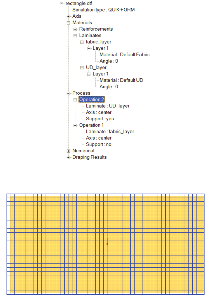
PAM-RTM 2014 105 USER’S GUIDE & TUTORIALS
© 2014 ESI Group (released: Apr-14)
PAM-RTM USER'S GUIDE
Process Parameters
Running the simulation, we get the following results. The fabric layer covers the surface
completely, while the UD layer is restricted to elements of the support.

USER’S GUIDE & TUTORIALS 106 PAM-RTM 2014
(released: Apr-14) © 2014 ESI Group
PAM-RTM USER'S GUIDE
Process Parameters

PAM-RTM 2014 107 USER’S GUIDE & TUTORIALS
© 2014 ESI Group (released: Apr-14)
PAM-RTM USER'S GUIDE
Numerical Parameters
NUMERICAL PARAMETERS
The numerical parameters will be presented in the following sections for each
simulation type. Many parameters are common to many simulation types, so instead of
repeating text we refer to the section where the parameter was first described.
RTM Simulation
Output Tab
RTM Output tab
- Save Filling Factor: tells PAM-RTM™ to generate result file for filling factor.
- Save Pressure: save pressure result file.
- Save Velocity: save resin velocity results files.
USER’S GUIDE & TUTORIALS 108 PAM-RTM 2014
(released: Apr-14) © 2014 ESI Group
PAM-RTM USER'S GUIDE
Numerical Parameters
- Save capillary numbers: saves the capillary number, micro void, macro void, total
void files. This option is useless if the micro and macro voids functions in the Velo
Opti tab of the Process Parameters are not defined.
- Save closing force: writes a 5 columns text file, giving the components of the force
vector in time, as well as norm of the force vector.
- Save viscosity: save resin viscosity. This is useful in the isothermal RTM context
for viscosity function of time.
- Output format: I-DEAS Universal is the default format used by PAM-RTM™ to
write simulation results. The new ESI Group format called ERF is also available to
perform post-processing in Visual-Viewer™ (version 5.5 or later). Visual-
Viewer™ has more advanced post-processing capabilities than the standard PAM-
RTM™ viewer.
- Sampling period: store results in output files each n time step. By default n=10,
which means that 1/10 steps will be saved. This parameter is useful to minimize the
size of results files. Other options (parallel solver only):
- seconds: saves results approximately each x seconds of simulated time
- fill %: saves results approximately each y percentage of filling
- Recover period: (standard solver only) this parameter is useful in case you need to
stop the simulation (CTRL-C) and restart it later. The default value is 500, which
means that if you need to stop the simulation, you will have 500 steps to recalculate
if you do a restart. Since a restart is considered an exceptional event, the default
value is relatively large so that the simulation doesn’t waste time writing
unnecessary files. If you expect a simulation to run many days, you should maybe
consider decreasing the recover sampling period.
Notes:
- The “save” options (save filling, save pressure, etc.) only apply to the standard
solver. The parallel solver writes systematically all the results files, regardless of
that selection.
- One exception is the “save micro/macro voids” option that must be selected in
order to have the parallel solver compute the micro and macro voids.
- The seconds and fill percentage sampling period options might not be respected,
depending on the time step. For example, with a sampling period of 4 seconds and a
time step of 5 seconds, results would be saved at t=0, t=5, t=10, instead of t=0, t=4,
t=8, etc. From the time of the last save, the specified period is added, and the first
step computed with a time greater or equal to that time generates a save. Of course
with a small time step, the actual sampling period will be closer to the specified
value.
- The parallel solver can be restarted from any time. It will actually restart from the
closest time in the results files (depends on the sampling period).
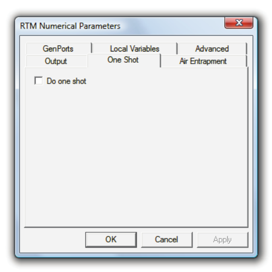
PAM-RTM 2014 109 USER’S GUIDE & TUTORIALS
© 2014 ESI Group (released: Apr-14)
PAM-RTM USER'S GUIDE
Numerical Parameters
One Shot Tab
RTM One Shot tab
- Do one shot: (standard solver only) tells PAM-RTM™ to perform a “one shot”
simulation, i.e. solve in a single step to get the last points filled. This simulation is
orders of magnitude faster than a standard filling simulation. Only pressure and flow
rate boundary conditions are taken into account. There can be many inlets specified,
but all must be of the same type (pressure or flow rare). Vents are ignored, as the
goal of this simulation is to help find the best location for vents.
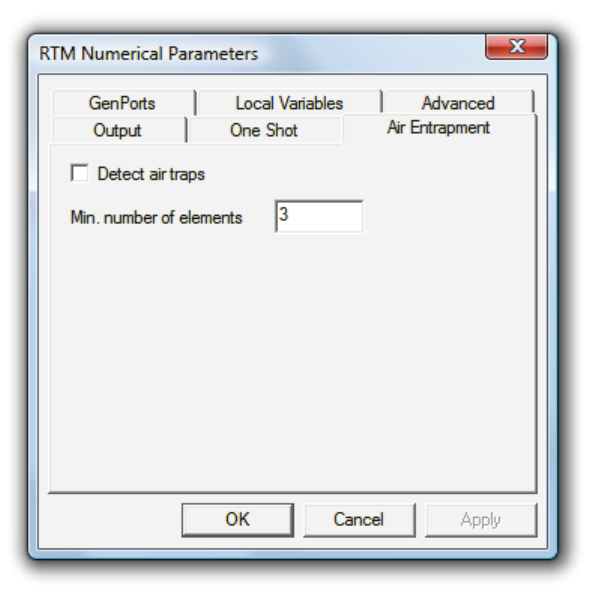
USER’S GUIDE & TUTORIALS 110 PAM-RTM 2014
(released: Apr-14) © 2014 ESI Group
PAM-RTM USER'S GUIDE
Numerical Parameters
Air Entrapment Tab
RTM Air Entrapment tab
- Detect air traps: tells PAM-RTM™ to detect air traps and take into account the
pressure inside the air trap when solving the resin pressure field. An air trap is
defined as a closed region of empty or partially filled elements not connected to an
open vent.
- Min. number of elements: this parameter is used to avoid false air traps to be
detected. The default value is 3, which means that if a small air trap of one or two
elements pops up from nowhere, it won’t be considered a real air trap and the cavity
pressure still applies in this area (no pressure calculation based on the volume of the
air trap). This doesn’t mean that an air trap can never be smaller than 3 elements.
Actually a large air trap is allowed to shrink below the min number of elements
parameter.
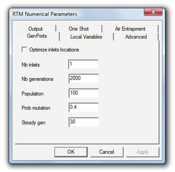
PAM-RTM 2014 111 USER’S GUIDE & TUTORIALS
© 2014 ESI Group (released: Apr-14)
PAM-RTM USER'S GUIDE
Numerical Parameters
GenPorts tab
- Optimize inlets locations: if this box is checked, the GenPorts optimization module
will be called to find the optimal injection ports locations minimizing fill time,
instead of the standard RTM filling calculation.
- Nb inlets: number of injection ports to use.
- Nb generations: number of generations to be calculated by the genetic algorithm
engine.
- Population: the number of individuals for each generation. An individual is actually
an injection configuration, which is made of the number of injection points specified
in nb inlets.
- Prob mutation: this is the probability that a major change occurs in a child with
respect to his parents. For instance if a child is normally generated on the “line”
connecting his 2 parents, a mutation could be to choose randomly a node of the
mesh instead of one of the parents.
- Steady gen: if the calculation engine doesn’t detect a significant change in the
solution for that number of successive generations, it will assume convergence has
been reached and will stop the calculation.
More information can be found in the GenPorts tutorial.
Note that GenPorts is not supported by the parallel solver.
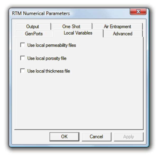
USER’S GUIDE & TUTORIALS 112 PAM-RTM 2014
(released: Apr-14) © 2014 ESI Group
PAM-RTM USER'S GUIDE
Numerical Parameters
Local Variables Tab
RTM Local Variables tab
- Use local permeability files: tells the PAM-RTM™ solver to initialize local
permeability (one permeability value for each element) from the x_k1.sf,
x_k2.sf and optionally x_k3.sf (for solid elements) that have been generated as
a result of Compute Local Permeability. For example if you do Compute Local
Permeability and save your PAM-RTM™ project as test.dtf, the files
test_k1.sf and test_k2.sf will be generated in the same directory. You have
to check Use local permeability files to initialize local permeability from these files.
Otherwise the permeability of the material associated to each zone will be used.
- Use local porosity file: tells PAM-RTM™ to use the local porosity file
(x_porosity.sf) resulting from Compute Local Permeability to initialize the
porosity of each element.
- Use local thickness file: the same principle applies to the thickness of shell elements.
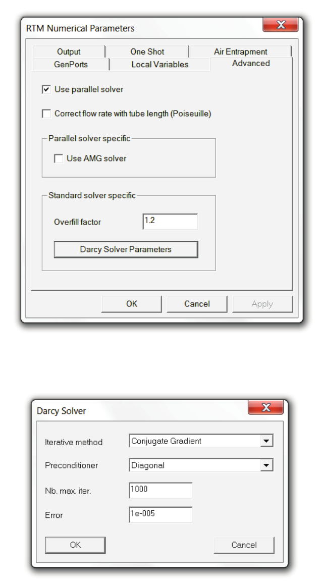
PAM-RTM 2014 113 USER’S GUIDE & TUTORIALS
© 2014 ESI Group (released: Apr-14)
PAM-RTM USER'S GUIDE
Numerical Parameters
Advanced Numerical Parameters
RTM Numerical Parameters - Advanced tab
Advanced Darcy solver parameters
USER’S GUIDE & TUTORIALS 114 PAM-RTM 2014
(released: Apr-14) © 2014 ESI Group
PAM-RTM USER'S GUIDE
Numerical Parameters
- Use parallel solver: if this box is checked, the new high performance parallel solver
introduced in PAM-RTM™ 2010 will be called instead of the standard solver.
Before the calculation is launched, a dialog box is posted, asking how many
processors are to be used. It is possible to enter 1 if the calculation is to be run on a
single processor system, such as a laptop. In that case, the calculation will still be
much faster than the standard solver, as the parallel solver uses a completely
different code architecture, highly optimized. The memory used will also be much
smaller than the standard solver. Once the calculation is done, the results have to be
loaded for post-processing with File > Open > PAM-RTM Parallel (.unf). Note that not
all the functionalities of the standard solver are currently supported by the parallel
solver. Please see the PAM-RTM™ Release Notes for the complete list of features
supported or not supported.
- Correct flow rate with tube length (Poiseuille): (parallel solver only) for pressure
driven inlets, the corresponding flow rate on each inlet is computed and compared to
the theoretical flow rate that would be obtained using Poiseuille formula (i.e. taking
into account the tube length and radius specified on the boundary condition). If the
flow rate on the inlet is found to be greater than that value, the inlet is switched to a
flow rate controlled inlet with the flow rate set as the Poiseuille value.
- Use AMG solver: (parallel solver only) new high performance multi-grid solver used
to solve Darcy’s equation. Experimental (use with care).
- Overfill factor: (standard solver only) used to speed up the filling calculation by
allowing more elements to be filled at each iteration, thus reducing the total number
of Darcy solutions needed to fill the cavity (in PAM-RTM™ most of the time is
spent solving Darcy’s equation). The idea is to allow an element to be oversaturated,
i.e. to contain more resin than it can actually contain. The excess of resin of an
element is distributed to its neighbors. The default value is 1.2, meaning that an
element can be oversaturated by 20%.
- Darcy solver parameters (standard solver only):
· Iterative method: the method used to solve the linear system Ax=b. Conjugate
gradient should be used for Darcy. Advanced users can evaluate the
performance of other supported methods:
Bi-conjugate gradient
Bi-conjugate gradient stabilized
Conjugate gradient squared
Chebyshev iteration
Generalized Minimum Residual (GMRES)
Richardson iteration
Quasi-minimal residual
Conjugate gradient 2002
Conjugate gradient 2004
Conjugate gradient 2008

PAM-RTM 2014 115 USER’S GUIDE & TUTORIALS
© 2014 ESI Group (released: Apr-14)
PAM-RTM USER'S GUIDE
Numerical Parameters
Notes:
· A new conjugate gradient implementation (conjugate gradient 2008) is
introduced in PAM- RTM™ 2008. The meaning of the conjugate gradient
option without version specification depends on the platform. For instance, on
Windows 32-bit, conjugate gradient actually means conjugate gradient 2004.
On Windows 64-bit, conjugate gradient means conjugate gradient 2008. The
2008 implementation was introduced mainly for porting reasons. Unfortunately
the 2004 implementation, which is still the fastest of all implementations, makes
use of advanced libraries which are not available on Windows 64-bit and Linux.
We recommend keeping the default generic conjugate gradient option, so that
the PAM-RTM solver automatically chooses the best implementation for a
platform.
· Preconditioner: diagonal should be used for Darcy. Other choices for advanced
users are:
Incomplete Cholesky
Incomplete LU
· Nb max iter: maximum number of iterations to solve the linear system.
· Error: The residual is defined as
ii
xAbr ∗−=
. The stopping criterion of the
iterative method is
ε
≤
2
2
b
r
i
, where
ε
is the specified error.
VARI Simulation (standard solver only)
The VARI simulation shares many of its numerical parameters with the RTM
simulation. In the following sections, we list only the VARI specific parameters. The
user should refer to the section RTM Simulation for a description of other parameters.
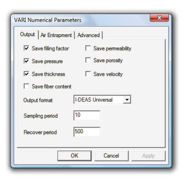
USER’S GUIDE & TUTORIALS 116 PAM-RTM 2014
(released: Apr-14) © 2014 ESI Group
PAM-RTM USER'S GUIDE
Numerical Parameters
VARI output parameters
Output Tab
Since VARI simulation involves local change of thickness, fiber content (porosity) and
permeability, these variables can be saved in results files. See RTM Simulation for other
parameters.
Air Entrapment Tab
See RTM simulation.
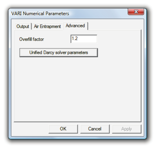
PAM-RTM 2014 117 USER’S GUIDE & TUTORIALS
© 2014 ESI Group (released: Apr-14)
PAM-RTM USER'S GUIDE
Numerical Parameters
Advanced Tab
VARI advanced numerical parameters
- Overfill factor: see RTM simulation.
- Unified Darcy solver parameters: these are specific settings to solve the unified
Darcy equation. The default settings are GMRES with ILU preconditioner.
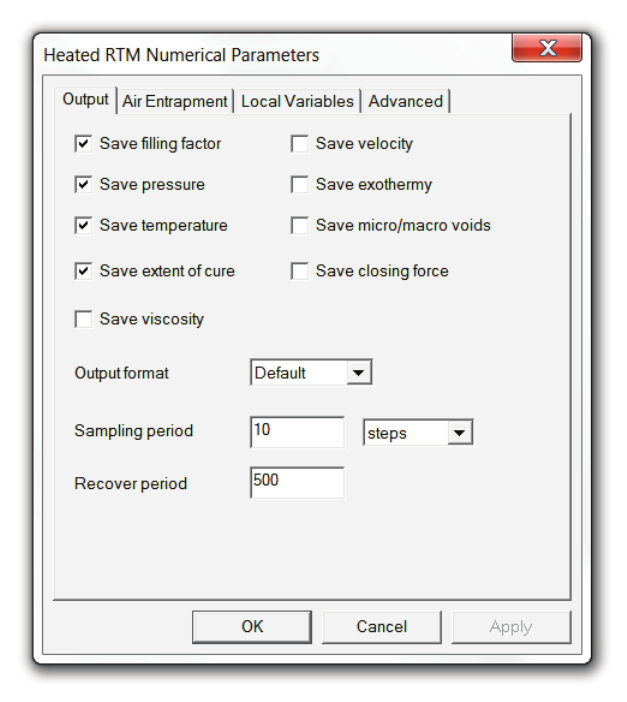
USER’S GUIDE & TUTORIALS 118 PAM-RTM 2014
(released: Apr-14) © 2014 ESI Group
PAM-RTM USER'S GUIDE
Numerical Parameters
Heated RTM Simulation
Output Tab
Heated RTM output tab
- Save filling factor, Save pressure, Save temperature, Save extent of cure, Save
exothermy, Save velocity, Save micro/macro voids, Save viscosity: (standard solver
only) check boxes to specify the variables to save in results files.
- Save closing force: writes a 5 columns text file, giving the components of the force
vector in time, as well as norm of the force vector.
- Output format: see RTM simulation.
- Sampling period: see RTM simulation.
- Recover period: see RTM simulation.
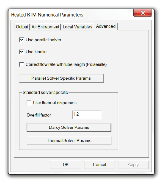
PAM-RTM 2014 119 USER’S GUIDE & TUTORIALS
© 2014 ESI Group (released: Apr-14)
PAM-RTM USER'S GUIDE
Numerical Parameters
Note:
- The exothermy output of the standard solver is replaced by the rate of reaction
(dα/dt) in the parallel solver.
Air Entrapment Tab
The air entrapment option can be used with non-isothermal filling, however the current
implementation doesn’t take into account the effect of temperature on the pressure
inside air traps. See RTM Simulation for a description of the parameters.
Local Variables Tab
See RTM simulation.
Advanced Tab
Heated RTM advanced parameters
USER’S GUIDE & TUTORIALS 120 PAM-RTM 2014
(released: Apr-14) © 2014 ESI Group
PAM-RTM USER'S GUIDE
Numerical Parameters
- Use parallel solver: see RTM simulation. Thermal analysis with the parallel solver
was introduced in PAM-RTM™ 2011.
- Use kinetic: uncheck this parameter when resin cure and its effects on viscosity and
temperature are negligible during the filling phase, to avoid solving the transport
equation for chemical species and reduce CPU time.
- Correct flow rate with tube length (Poiseuille): see RTM simulation.
- Use thermal dispersion: (standard solver only) check this parameter to have PAM-
RTM™ take into account thermal dispersion, which is basically a correction to the
thermal conductivity used in the saturated region. The corrected conductivity
depends on the resin velocity. For more details, see the description of the
characteristic length parameter, in the section on the thermal properties of the fiber
reinforcements.
- Overfill factor: see RTM simulation.
- Parallel Solver Specific Params: these parameters are only used if use parallel solver
is checked.
- Automatically generate mold/preform interface: with the parallel solver, it is
mandatory to specify a heat transfer coefficient for the mold/preform interface,
as opposed to the standard solver for which it is optional. Since it can be a lot of
work to generate that interface manually with the usual Groups>Contact
Interface command, this option is checked by default, meaning the elements will
be automatically disconnected on that interface for the whole mesh at
calculation launch. In some special situations the user might need to specify
different coefficients for different areas of the mold/preform interface. In that
case, the user has to create interfaces manually; using contact resistances (see
tutorial Thermal Contact Resistance). Be careful that the units of the contact
resistance are the reciprocal of the mold/preform interface coefficient. This
option must be unchecked if some contact resistances are to be defined manually
on the mold/preform interface. In that case it is mandatory that all the faces of
the mold/preform interface be part of a contact resistance. PAM-RTM™ won’t
create automatically the remaining interfaces if the contact resistances cover
only a subset of the mold/preform interface. Note that this doesn’t apply to
mold/mold interfaces. It is thus possible to have automatically generate
mold/preform interface checked, while contact resistances for mold/mold
interfaces are defined
- Mold/preform interface coefficient: heat transfer coefficient (conductance) used
on the whole mold/preform interface when the automatically generate
mold/preform interface option is checked. Be careful that the units (W/m2K) are
the reciprocal of a thermal resistance.
- Use AMG solver: (parallel solver only) new high performance multi-grid solver
used to solve Darcy’s equation. Experimental (use with care).
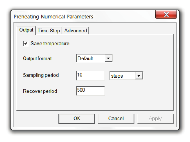
PAM-RTM 2014 121 USER’S GUIDE & TUTORIALS
© 2014 ESI Group (released: Apr-14)
PAM-RTM USER'S GUIDE
Numerical Parameters
- Darcy Solver Params: see RTM simulation. These parameters are only used by the
standard solver (i.e. if use parallel solver is unchecked).
- Thermal Solver Params: default is GMRES with ILU preconditioner. These
parameters are only used by the standard solver (i.e. if use parallel solver is
unchecked).
Preheating Simulation
Output Tab
Preheating output tab
- Save temperature: this is the only variable that can be saved for a preheating
simulation.
- Output format: see RTM simulation.
- Sampling period: see RTM simulation.
- Recover period: see RTM simulation.
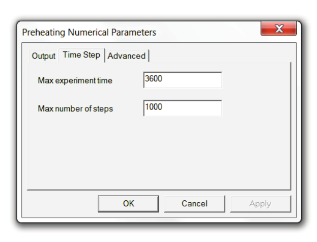
USER’S GUIDE & TUTORIALS 122 PAM-RTM 2014
(released: Apr-14) © 2014 ESI Group
PAM-RTM USER'S GUIDE
Numerical Parameters
Time Step Tab
Preheating time step tab
With the standard solver, the preheating simulation works with a constant time step
calculated as:
dt = Max experiment time/Max number of steps
- Max experiment time: the total heating time of the mold and fibers. Unit: seconds.
- Max number of steps: the number of time steps for the calculation.
The parallel solver uses an adaptive time step, meaning it changes in time to respect
convergence criteria. The dt formula above corresponds to the maximum time step.
Advanced Tab
See Heated RTM.
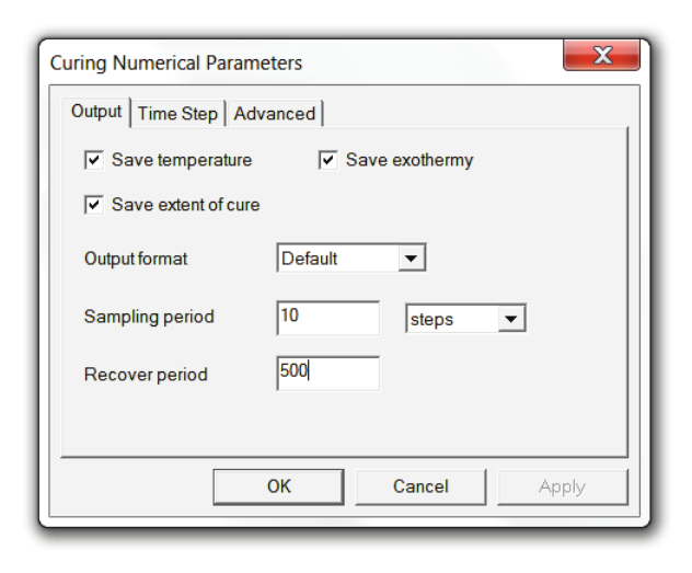
PAM-RTM 2014 123 USER’S GUIDE & TUTORIALS
© 2014 ESI Group (released: Apr-14)
PAM-RTM USER'S GUIDE
Numerical Parameters
Curing Simulation
Output Tab
Curing output tab
- Variables available for saving in results files are: temperature, extent of cure and
exothermy.
- Output format: see RTM simulation.
- Sampling period: see RTM simulation.
- Recover period: see RTM simulation.
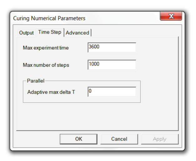
USER’S GUIDE & TUTORIALS 124 PAM-RTM 2014
(released: Apr-14) © 2014 ESI Group
PAM-RTM USER'S GUIDE
Numerical Parameters
Time Step Tab
Curing time step tab
- Max experiment time: see Preheating simulation.
- Max number of steps: see Preheating simulation.
- Adaptive max delta T: (parallel only) in order to capture the high temperature peak
typical of curing reactions, it is sometimes necessary to use this parameter to further
control the time step. It specifies the maximum absolute temperature variation
allowed on the whole domain between two steps. If the variation is higher, the time
step will be decreased (divided by two), until the condition is respected. Then the
time step will increase again as long as the condition is respected (up to the
maximum time step dt = max_experiment_time/max_number_of_steps). The default
value is zero, meaning the parameter has no effect.
Advanced Tab
See Heated RTM simulation.
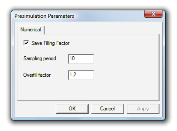
PAM-RTM 2014 125 USER’S GUIDE & TUTORIALS
© 2014 ESI Group (released: Apr-14)
PAM-RTM USER'S GUIDE
Numerical Parameters
Presimulation (standard solver only)
Presimulation numerical parameters
- Save filling factor: there is no pressure calculation involved in presimulation, so
filling factor is the only variable available for output.
- Sampling period: see RTM simulation.
- Overfill factor: see advanced numerical parameters of RTM simulation.
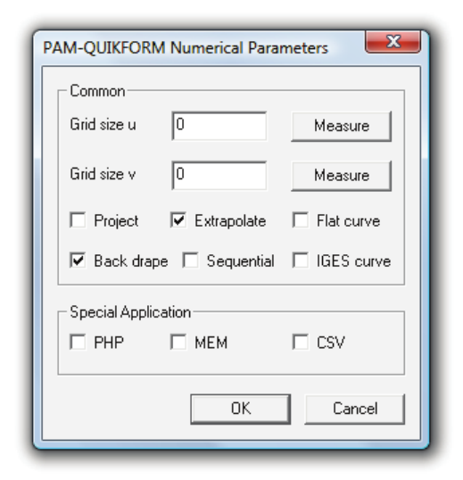
USER’S GUIDE & TUTORIALS 126 PAM-RTM 2014
(released: Apr-14) © 2014 ESI Group
PAM-RTM USER'S GUIDE
Numerical Parameters
PAM-QUIKFORM Simulation
- Grid size u: size of the elements along the local Y axis of the draping referential (see
figure below). For fabrics, grid size v is not used. Only grid size u is used for both
directions. The UD algorithm supports different sizes for u and v.
- Grid size v: size of the elements along the local X axis of the draping referential.
This value is not used for fabrics.
- Project: if this option is checked, the fiber orientations are projected by PAM-
QUIKFORM on the tool mesh, and instead of writing mesh files of the 3D draped
plies, the tool mesh is copied for each ply, with additional information for fiber
orientations. See description of the initial parameter in the PAM-QUIKFORM
solver documentation.
- Extrapolate: also called “manual draping”, this option is used by PAM-QUIKFORM
to cover a surface as much as possible by extrapolation. Without this option, draping
will cover at most a quadrangle defined by the size of the two axes first draped. See
example below.
- Back drape: activates the possibility of draping in back direction. The basic
algorithm of PAM-QUIKFORM drapes from the starting point, increasing weft and
warp directions. Due to the geometry of some parts, the basic algorithm might not
be able to cover some areas without the back drape option. See example below.
- Flat curve: if this option is active, PAM-QUIKFORM projects the boundary of the
tool on the mesh of the 3D draped ply in order to get a more accurate representation
of the 2D flat pattern.
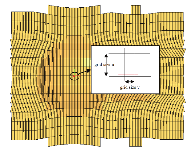
PAM-RTM 2014 127 USER’S GUIDE & TUTORIALS
© 2014 ESI Group (released: Apr-14)
PAM-RTM USER'S GUIDE
Numerical Parameters
- IGES Curve: if the flat curve option is active, the flat curve is written in IGES
format.
- Sequential: if this option is active, PAM-QUIKFORM will drape sequentially by
zones, which must be numbered sequentially from 1 to n. The origin of the draping
referential must be located in zone 1.
- PHP, MEM, CSV: special application flags. See PAM-QUIKFORM solver
documentation.
PAM-QUIKFORM grid size u and v parameters
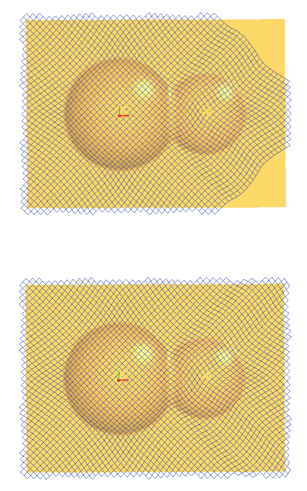
USER’S GUIDE & TUTORIALS 128 PAM-RTM 2014
(released: Apr-14) © 2014 ESI Group
PAM-RTM USER'S GUIDE
Numerical Parameters
Draping without the extrapolate option
Draping with the extrapolate option
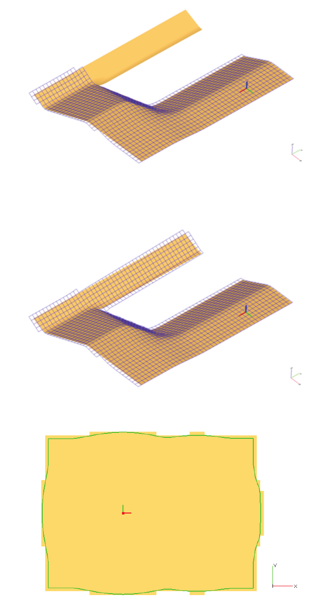
PAM-RTM 2014 129 USER’S GUIDE & TUTORIALS
© 2014 ESI Group (released: Apr-14)
PAM-RTM USER'S GUIDE
Numerical Parameters
Draping without the “back drape” option
Draping with the “back drape” option
Flat curve
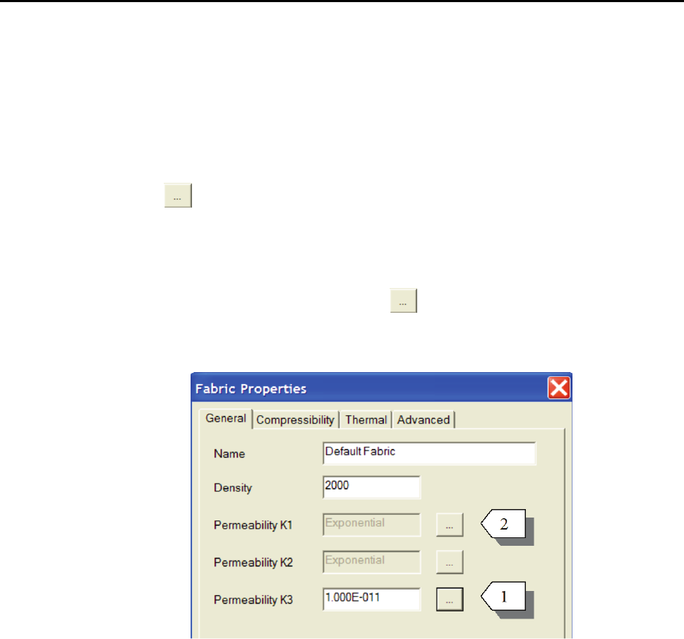
USER’S GUIDE & TUTORIALS 130 PAM-RTM 2014
(released: Apr-14) © 2014 ESI Group
PAM-RTM USER'S GUIDE
Function Editor
FUNCTION EDITOR
Many simulation parameters in PAM-RTM™ use curves or mathematical functions of
2 variables. This chapter describes the function editor, a dialog box used to edit these
mathematical functions.
Overview
This button is used in PAM-RTM™ wherever a mathematical function can be
assigned to a simulation parameter. The following image shows the General tab of the
Fabric Properties dialog. In this example, Permeability K3 [1] is a constant value, so its
value can be entered directly in the text field. Permeability K1 [2] has an exponential
curve assigned to it. The text field is used to display the type of the function, the text
field is disabled, and the user has to push the button to modify the parameters of the
exponential curve. This opens the Function Editor dialog.
General tab of the Fabric Properties

PAM-RTM 2014 131 USER’S GUIDE & TUTORIALS
© 2014 ESI Group (released: Apr-14)
PAM-RTM USER'S GUIDE
Function Editor
Function editor dialog
In this example, an exponential curve
xB
eAxf ⋅
⋅=)(
with A=2.2E-8 and B=-11.57 is
assigned to Permeability K1. The user can select other functions from the list of
predefined functions [1]. Selecting a function displays either the function parameters
such as A and B in this example, or the coordinates of the control points if the function
is defined by a set of control points (piecewise_linear or krig_e). In any case, the user
can click on a value and enter text to modify it.
A user_defined function is always available in the list of functions. The same
exponential curve as shown above could be defined with the user_defined function by
pushing the Edit User Defined button and entering the character string:
2.2E-8*exp(-11.57*x)
The curve is the same, however the evaluation of the curve costs more CPU time.
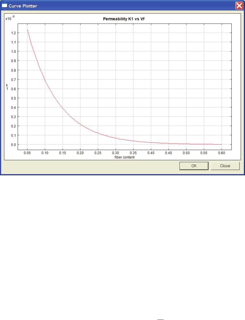
USER’S GUIDE & TUTORIALS 132 PAM-RTM 2014
(released: Apr-14) © 2014 ESI Group
PAM-RTM USER'S GUIDE
Function Editor
The curve can be visualized by pushing the View button. This opens the following Curve
Plotter.
Permeability K1 as a function of fiber content
User Defined Functions
The parser recognizes the following operators:
+, -, *, /, ^ (exponent)
as well as the following functions:
H, abs, exp, ceil, floor, log, sqrt, sin, cos, tan, asin, acos, atan, sinh, cosh, tanh.
Note that the non-standard function H is the Heavyside step function, defined as:
1
,1)(
0,0)
(
≥=
<=
xxH
xxH
As an example, the function Kinetic_01 defined as:
( )
−
⋅−⋅⋅= x
E
p
meyyAyxf 1),(
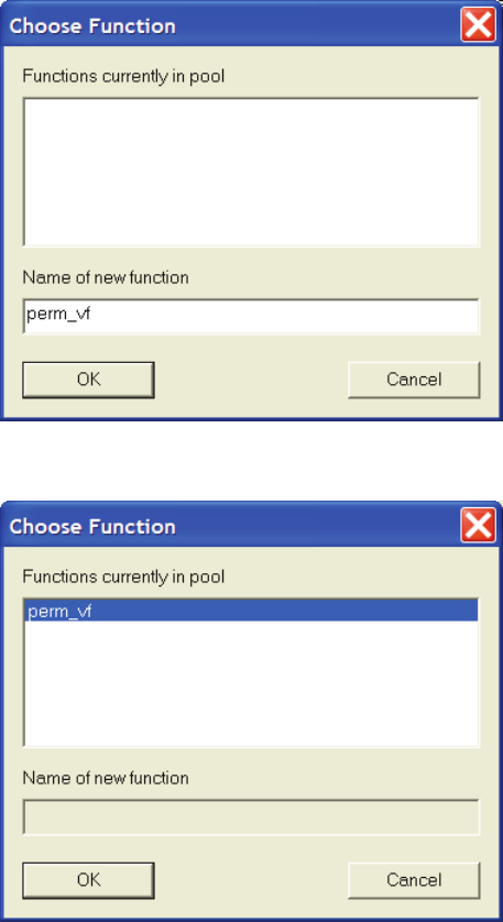
PAM-RTM 2014 133 USER’S GUIDE & TUTORIALS
© 2014 ESI Group (released: Apr-14)
PAM-RTM USER'S GUIDE
Function Editor
with A=9.17E+6, E=7304, m=0.7 and p=1.3 would be defined as a user_defined
function with the character string:
9.17E6*(y^0.7)*((1-y)^1.3)*exp(-7304/x)
Function Pool
The function pool can be seen as some kind of copy/paste functionality for
mathematical functions. This is useful when the same function is assigned to many
parameters. In that case, the user defines the function once, then push the Copy to
Function Pool button, which pops up the following dialog box. A name must be given to
the function before it is copied in the function pool. The function can be retrieved later
by its name with Get from Function Pool. Note that the function pool is shared by all
open documents and is available until PAM-RTM™ is closed.
Copy to function pool dialog
Get from function pool dialog
USER’S GUIDE & TUTORIALS 134 PAM-RTM 2014
(released: Apr-14) © 2014 ESI Group
PAM-RTM USER'S GUIDE
Function Editor
Import/Export
Depending on the context (edition of a function of 1 or 2 variables), it is possible to
import in PAM-RTM™ a 2 columns text file (curve) or a 3 columns text file (function
of 2 variables). The columns can be separated with any combination of white space, tab
or comma. If a 2 columns file is imported, a piecewise_linear curve is automatically
created. For 3 columns text files, a krig_e function is created.
The set of control points associated to piecewise linear or kriged functions can also be
exported in 2 or 3 columns text files.
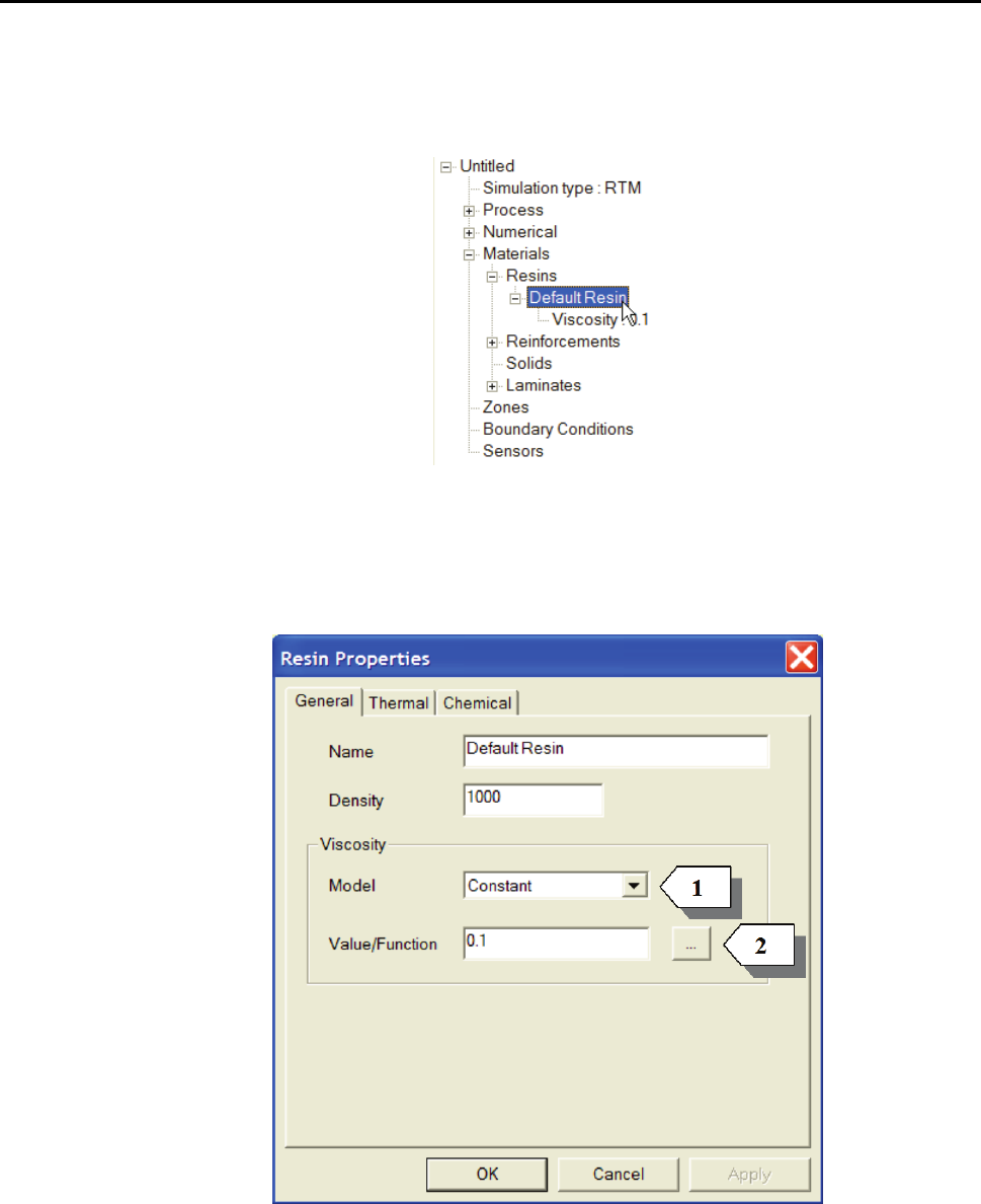
PAM-RTM 2014 135 USER’S GUIDE & TUTORIALS
© 2014 ESI Group (released: Apr-14)
PAM-RTM USER'S GUIDE
Material Properties of the Resin
MATERIAL PROPERTIES OF THE RESIN
The Resin Properties dialog box is opened by double-clicking a resin in the model
explorer.
The following dialog box is used to specify resin properties such as viscosity, chemical
reaction model, thermal conductivity and specific heat.
General Tab

USER’S GUIDE & TUTORIALS 136 PAM-RTM 2014
(released: Apr-14) © 2014 ESI Group
PAM-RTM USER'S GUIDE
Material Properties of the Resin
Name
Enter a text description to fully identify the resin. It is sometimes useful to include in
this description the validity domain of the associated viscosity and kinetics models,
such as “My resin with kinetics 350 < T < 400”.
Density
Density of the resin. Unit: kg/m3.
Viscosity
Unit: Pa.s. Several models are available:
- Constant
- Function of temperature f(temperature)
· Constant
· Exponential:
)exp()
(xBAx
f⋅⋅
=
· Piecewise linear function
· User defined
· User DLL
- Function of temperature and degree of cure f(temperature, alpha)
· Constant
· Viscosity_01 (see reference [R.1] at the end of this chapter):
⋅+⋅=
αα
C
T
B
ATf exp),(
· Viscosity_02 (Castro-Macosko [R.2]):
α
α
α
⋅
+
−
⋅
⋅
=
43
2
21
0
exp)
,(
c
c
c
c
T
c
cT
f
· Viscosity_03:
−
−
⋅⋅= 5
4
3
2
1exp)exp(),( c
c
c
T
c
cTf
α
α
· Viscosity_04:
⋅
−
−
⋅
−
⋅=
α
α
α
4
3
2
2
1
1
0
exp),(
cT
c
c
c
c
T
c
cTf
· Viscosity_05:
)...exp(),( 6
6
2
210
αααα
cccc
T
B
ATf +++++⋅=

PAM-RTM 2014 137 USER’S GUIDE & TUTORIALS
© 2014 ESI Group (released: Apr-14)
PAM-RTM USER'S GUIDE
Material Properties of the Resin
· Viscosity_06 ([R.3]):
⋅+
−
⋅=
αα
C
TT
T
hTf
m
rheo
uexp),(
· Kriged function
· User defined
· User DLL
- Function of time f(global_time)
· Constant
· Piecewise linear function
· User defined
· User DLL
- Function of time f(material_age)
· Constant
· Piecewise linear function
· User defined
· User DLL
Note:
· The user_dll type is only supported by the parallel solver. See tutorial User
defined functions.
· The time variable used for the evaluation of viscosity f(global_time) is the time
since beginning of injection. At a given time, the viscosity is uniform on the
saturated domain.
· For f(material_age), the time variable corresponds to the time since a resin
particle entered the mold. Viscosity is thus non-uniform on the saturated
domain, and higher close to the resin front.
· The f(material_age) model is only supported by the parallel solver.
· The viscosity model is selected with the Model dropdown list[1]. In case of a
constant viscosity, the value can be entered directly in the Value field. Otherwise
the user has to go through the function editor [2] to enter the coefficients of the
selected function (see section Function Editor).
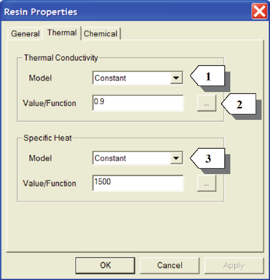
USER’S GUIDE & TUTORIALS 138 PAM-RTM 2014
(released: Apr-14) © 2014 ESI Group
PAM-RTM USER'S GUIDE
Material Properties of the Resin
Thermal Tab
Thermal Conductivity
Unit: W/m.K.
Available models are: constant, function of temperature, or function of temperature and
degree of cure [1].
Once again, in case of a constant model, the value can be entered directly in the text
field [2]. Otherwise use the … button to open the function editor.
Specific Heat
Unit: J/Kg.K.
Available models are: constant, function of temperature, or function of temperature and
degree of cure [3].
Note
· When using the parallel solver, if specific heat f(temperature, alpha) is needed,
it has to be specified with a user_dll function (i.e. C-language code written by
the user). See tutorial User Defined Functions.
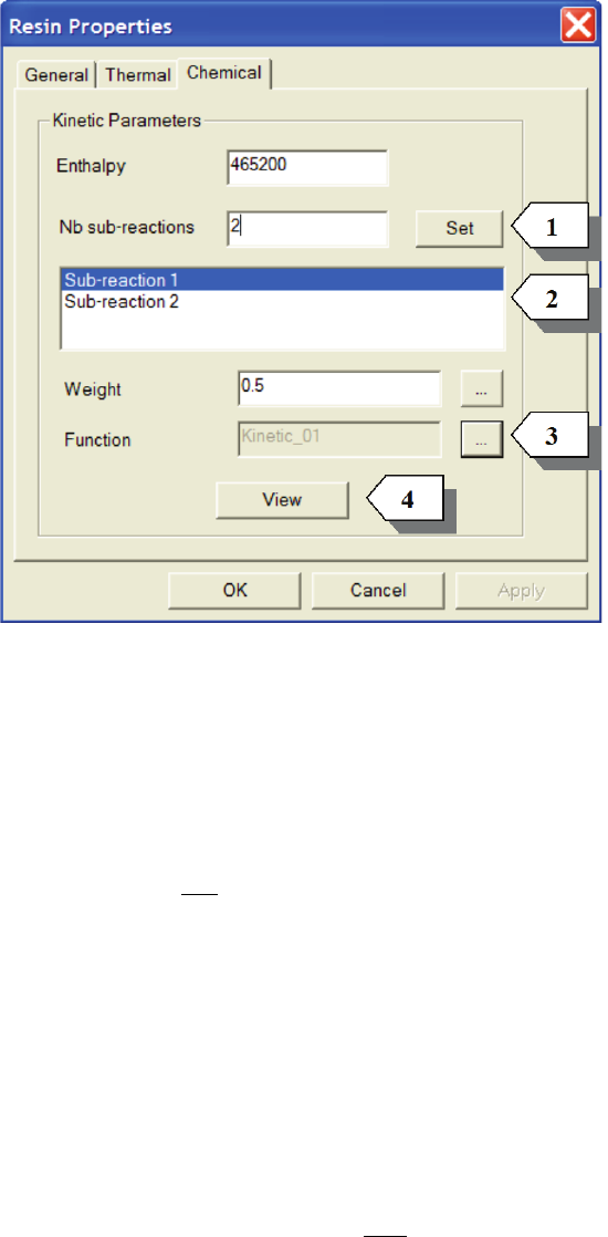
PAM-RTM 2014 139 USER’S GUIDE & TUTORIALS
© 2014 ESI Group (released: Apr-14)
PAM-RTM USER'S GUIDE
Material Properties of the Resin
Chemical Tab
Enthalpy
Unit: J/Kg.
The heat generated by the full resin polymerization per unit mass.
Reaction model
The resin kinetics model is defined as a weighted summation of sub-reactions:
( ) ( )
∑
=
⋅= n
i
ii Tftw
dt
d
1
,
α
α
The number of sub-reactions n must be specified first in the Nb sub-reactions field.
Then the user pushes the Set button [1], which actually generates the sub-reactions
listed in [2]. Select a sub-reaction, then edit the associated weight function and kinetics
function [3]. The weight is function of time, while the kinetics function is function of
temperature and degree of cure.
Available functions for kinetics are:
- Kinetic_01 (autocatalytic [R.4]):
( )
−
⋅−⋅⋅= T
E
ATf
p
m
exp1),(
αα
α
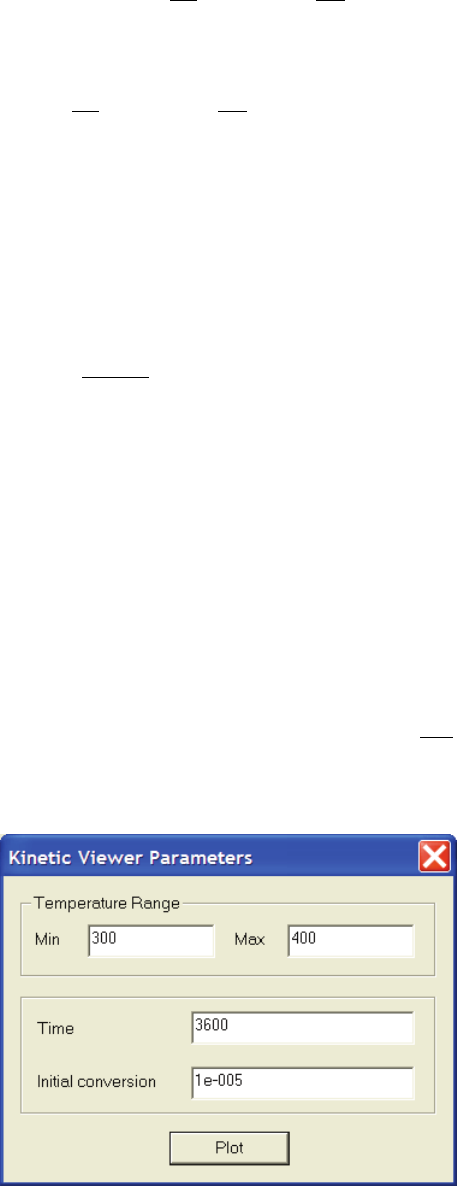
USER’S GUIDE & TUTORIALS 140 PAM-RTM 2014
(released: Apr-14) © 2014 ESI Group
PAM-RTM USER'S GUIDE
Material Properties of the Resin
- Kinetic_02 (Kamal-Sourour [R.5]):
( )
n
m
B
T
E
A
T
E
ATf
ααα
−⋅
⋅
⋅+
⋅=
2
2
1
1
expexp),(
- Kinetic_03 (modified Kamal-Sourour):
( )
( )( )
( )
Tn
Tm
TB
T
E
A
T
E
A
Tf
αα
α
−⋅
⋅
⋅+
⋅=
2
2
1
1
exp
exp)
,
(
( )
( )
( )
2
210
2
210
2
210
TnTnnTn
TmTmmTm
TbTbbTB
⋅+⋅+=
⋅+⋅+=
⋅+⋅+=
- Kinetic_04 [R.3]:
( )( )( )
[]
n
m
m
m
kin TTBramp
T
T
AT
f
αα
α
α
⋅−−⋅−−
⋅
−
−
⋅= exp1
exp)
,(
0,0)(
0,)(
<=
≥=
xxramp
xxxramp
- Kriged function: interpolation function constructed from a set of data points.
- User defined
- User DLL (parallel solver only, see tutorial User defined functions)
The View button [4] opens the Kinetic Viewer Parameters dialog, used to specify a
temperature and time range. Then pushing the Plot button plots isothermal conversion
curves, as shown below. This is actually the time integration of
dt
d
α
for different
temperatures. This viewer is useful to quickly evaluate how long it takes to fully cure
the resin at a given temperature.
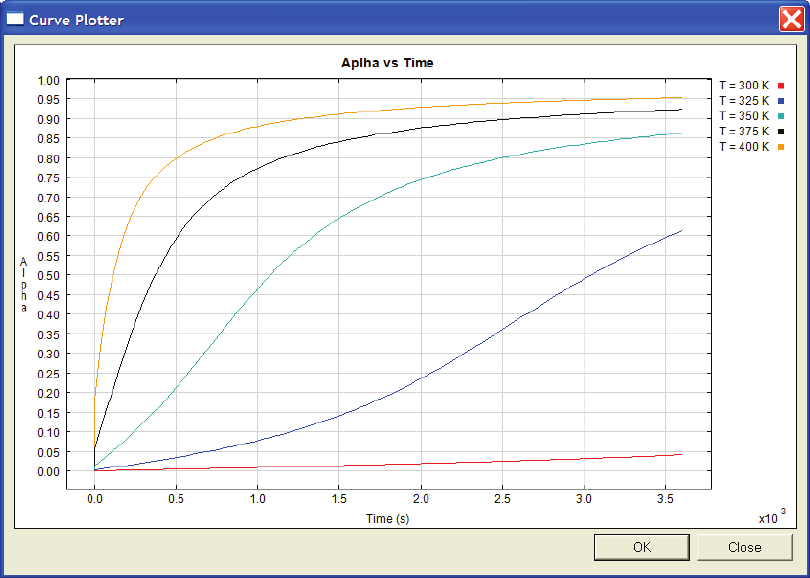
PAM-RTM 2014 141 USER’S GUIDE & TUTORIALS
© 2014 ESI Group (released: Apr-14)
PAM-RTM USER'S GUIDE
Material Properties of the Resin
Kinetic Viewer
References
[R.1] A.M. Stolin, A.G. Merzhanov, A.Y. Malkin, Polymer Engineering and Science;
1979, 19, 1074
[R.2] J.M. Castro, C.W. Macosko, Studies of mold filling and curing in the reaction
injection molding process, AIChE J., 1982, 28, 250
[R.3] M. Henne, C. Breyer, M. Niedermeier, P. Ermanni, A new kinetic and viscosity
model for liquid composite molding simulations in an industrial environment, Polymer
Composites, 2004, 25, 3
[R.4] A.M. Clayton, Epoxy Resins, Engineered Material Handbook: Composites, ASM
International, 1998
[R.5] M.R. Kamal, S. Sourour, Kinetics and thermal characterisation of thermoset cure,
Polymer Engineering and Science, January 1973, Vol. 13, No. 1

USER’S GUIDE & TUTORIALS 142 PAM-RTM 2014
(released: Apr-14) © 2014 ESI Group
PAM-RTM USER'S GUIDE
Material Properties of the Fiber Reinforcements
MATERIAL PROPERTIES OF THE FIBER
REINFORCEMENTS
Three types of fiber reinforcements can be created in PAM-RTM™: fabric,
unidirectional, and random mat. Right-click the Reinforcements item in the explorer to
create new instances of reinforcements.
To edit a fiber reinforcement, double-click it in the model explorer. The General,
Thermal and Compressibility tabs are shared by all reinforcements. An Advanced tab is
available on the fabric to specify permeability as a function of shear angle. A Draping
tab is available in the context of a PAM-QUIKFORM simulation.

PAM-RTM 2014 143 USER’S GUIDE & TUTORIALS
© 2014 ESI Group (released: Apr-14)
PAM-RTM USER'S GUIDE
Material Properties of the Fiber Reinforcements
General Tab
Name
Enter a text description to fully identify the fiber reinforcement.
Density
Unit: kg/m3
Density of the “solid” fiber material, i.e. density for 100% fiber volume fraction. For
example density of pure glass, if the reinforcement is made of glass fibers.
Permeability K1, K2, K3
Unit: m2
Permeability in the 3 principal directions of the permeability tensor, i.e. the directions in
which the tensor is diagonal. K1, K2 and K3 are the values on the principal diagonal.
The in-plane principal permeability components K1, K2 and through-thickness
permeability K3 are most of the time specified as constant values for a given fiber
volume fraction (vf). They can also be specified as functions of vf. It is important for
VARI simulation to specify permeability as a function of vf.
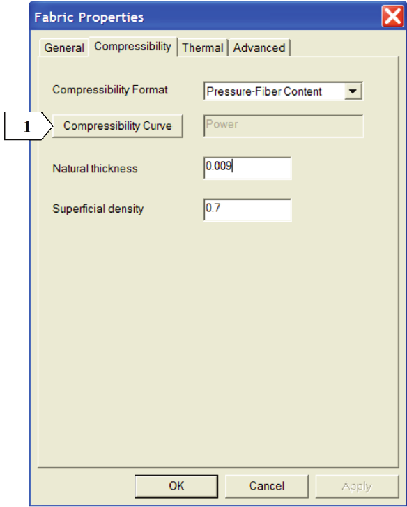
USER’S GUIDE & TUTORIALS 144 PAM-RTM 2014
(released: Apr-14) © 2014 ESI Group
PAM-RTM USER'S GUIDE
Material Properties of the Fiber Reinforcements
The models available for permeability as a function of vf, which can be selected through
the function editor [1], are:
- Exponential:
)
exp(
)( xB
Axf ⋅
⋅
=
- Power:
B
xAxf ⋅=)(
- Piecewise linear
- Kriged (interpolation of experimental data points)
- User defined
Compressibility Tab
The parameters in this tab are currently only used for VARI simulation.
Compressibility format
The format of the compressibility curve, which can be specified as one of the following:
- Pressure as a function of fiber content (vf),
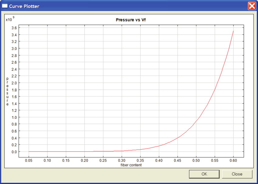
PAM-RTM 2014 145 USER’S GUIDE & TUTORIALS
© 2014 ESI Group (released: Apr-14)
PAM-RTM USER'S GUIDE
Material Properties of the Fiber Reinforcements
- Stress as a function of strain. Strain is defined between -1 and 0. Zero strain
corresponds to natural thickness.
Compressibility curve
Here is the list of functions that can be selected in the function editor, opened by
pushing the Compressibility Curve button [1]:
- Power:
B
xAxf ⋅=)(
- Piecewise linear
- Kriged (interpolation of experimental data points)
- User defined
Here is an example of a compressibility curve specified as Pressure-Vf . A power law is
used with A = 1.7E+11 and B = 7.6.
Natural thickness
Unit: m
This is the thickness of the reinforcement at ambient pressure.
Superficial density
Unit: Kg/m2
The superficial density of a single layer of reinforcement or a ply.
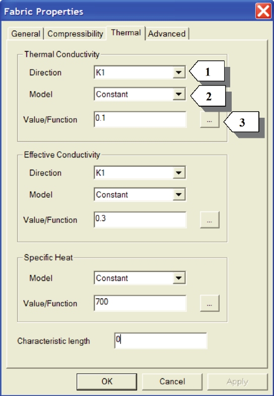
USER’S GUIDE & TUTORIALS 146 PAM-RTM 2014
(released: Apr-14) © 2014 ESI Group
PAM-RTM USER'S GUIDE
Material Properties of the Fiber Reinforcements
Thermal Tab
Thermal conductivity K1, K2, K3
Unit: W/m.K
This is the thermal conductivity of the “solid” fiber material, as if the reinforcement had
a fiber volume fraction of 100%. For example for a glass fiber reinforcement, the
thermal conductivity of pure glass would be specified. It is only used in the dry area. In
the wet area the effective conductivity is used (see below). It can be specified as
orthotropic, in which case principal directions need to be set.
Use the Direction dropdown list [1] to set the current direction (K1, K2 or K3), then
choose the Model [2] which can be constant or f(temperature). If f(temperature) is
specified, use the function editor [3] to define the conductivity curves. A different curve
can be assigned to K1, K2 and K3.
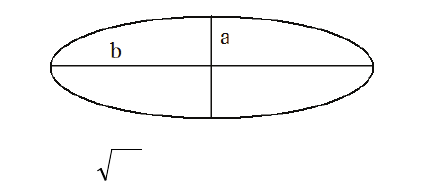
PAM-RTM 2014 147 USER’S GUIDE & TUTORIALS
© 2014 ESI Group (released: Apr-14)
PAM-RTM USER'S GUIDE
Material Properties of the Fiber Reinforcements
Note
· The principal directions of the permeability and conductivity tensor are assumed
to be the same. It is not possible in the current version of PAM-RTM™ to
specify different directions for permeability and conductivity.
· When using the old solver, the thermal conductivity values have to be multiplied
by porosity.
Effective conductivity K1, K2, K3
Unit: W/m.K
This is the conductivity of the mixture of resin and fibers that PAM-RTM™ uses in the
saturated region. In general the user could use the rule of mixture (keff = vf.kf + (1-vf).kr)
to calculate the effective conductivity, but in some cases a modified value could be used
to take into account thermal dispersion for instance.
The effective conductivity can be specified orthotropic. It can be modeled as constant,
f(temperature) or f(temperature, alpha).
Note
· When using the parallel solver, if effective conductivity f(temperature, alpha) is
needed, it has to be specified with a user_dll function (i.e. C-language code
written by the user). See tutorial User Defined Functions.
Specific heat
Unit: J/Kg.K
The specific heat of the “solid” fiber material, i.e. 100% fiber volume fraction.
Characteristic length
Unit: m
The characteristic length is referred to as the characteristic scale of the elliptical shape
of a compressed fiber tow
in which case it is given by
bal =
. This parameter is used in the context of thermal
dispersion modeling. It doesn’t have any effect in the calculation if use thermal
dispersion in the advanced numerical parameters is not checked. Please see the
introduction chapter of this user’s manual for details on thermal dispersion modeling.
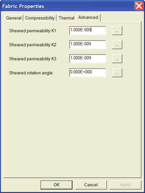
USER’S GUIDE & TUTORIALS 148 PAM-RTM 2014
(released: Apr-14) © 2014 ESI Group
PAM-RTM USER'S GUIDE
Material Properties of the Fiber Reinforcements
Advanced Tab (Fabrics)
The parameters in this tab are currently only used in the context of a local permeability
calculation taking into account fiber directions of a draped fabric. See Mesh->Compute
Local Permeability.
Sheared permeability K1, K2, K3
Unit: m2
Allows the specification of permeability as a function of the shearing angle and initial
fiber content.
Sheared rotation angle
Unit: angle (degree)
Allows the specification of the rotation angle of the K1 principal permeability direction
relative to the weft as a function of the shearing angle and initial fiber content.
The following pictures explain the rotation of the principal permeability directions
when a fabric is sheared by an angle α relative to the weft. The principal direction K1 is
rotated by an angle β relative to the warp.
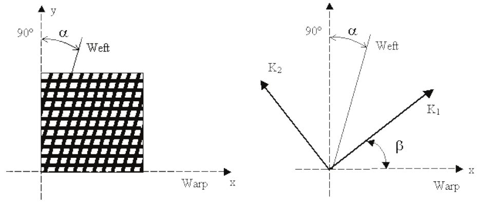
PAM-RTM 2014 149 USER’S GUIDE & TUTORIALS
© 2014 ESI Group (released: Apr-14)
PAM-RTM USER'S GUIDE
Material Properties of the Fiber Reinforcements
Draping Tab
The parameters in this tab are currently only used in the context of a PAM-QUIKFORM
simulation.
Fabric
Locking angle
Unit: degree.
This is the maximum shearing of the fabric before wrinkles occur. PAM-QUIKFORM
will stop calculation in areas where the locking angle is reached. Default value is 90
degrees. Validity range is between zero and 90 degrees.
Unidirectional
Grid stretch
Unit: no unit, percentage.
In areas of high curvature, the PAM-QUIKFORM UD algorithm can increase the
distance between fibers (parameter grid size u in the PAM-QUIKFORM numerical
parameters), up to the grid stretch percentage, in order to respect the grid shear criteria
below. Default value: 200 %.
Grid shear
Unit: degree.
Maximum allowable shear angle of the unidirectional.
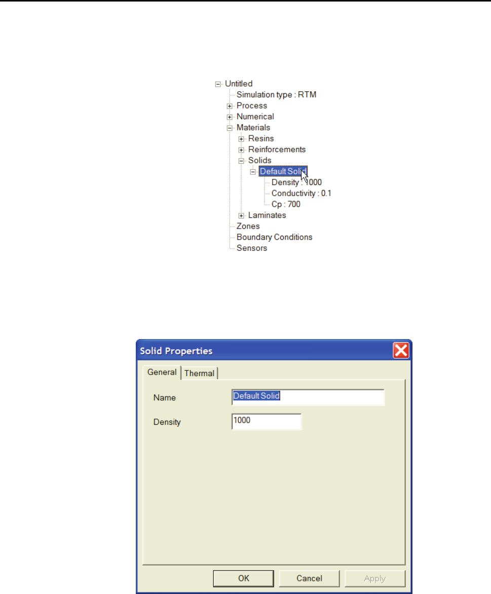
USER’S GUIDE & TUTORIALS 150 PAM-RTM 2014
(released: Apr-14) © 2014 ESI Group
PAM-RTM USER'S GUIDE
Material Properties of Solids
MATERIAL PROPERTIES OF SOLIDS
The material called solid in PAM-RTM™ should be used to specify any non-
permeable material such as foam or metallic inserts.
The Solid Properties dialog box is opened by double-clicking a “solid” in the model
explorer.
General Tab
Name
Enter a text description to fully identify the material.
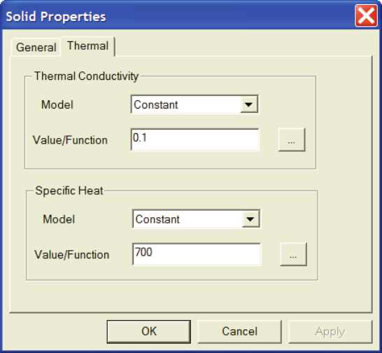
PAM-RTM 2014 151 USER’S GUIDE & TUTORIALS
© 2014 ESI Group (released: Apr-14)
PAM-RTM USER'S GUIDE
Material Properties of Solids
Density
Unit: kg/m3
Density of the material.
Thermal Tab
Thermal Conductivity
Unit: W/m.K
Can be specified as constant or function of temperature.
Specific Heat
Unit: J/Kg.K
Constant or function of temperature.
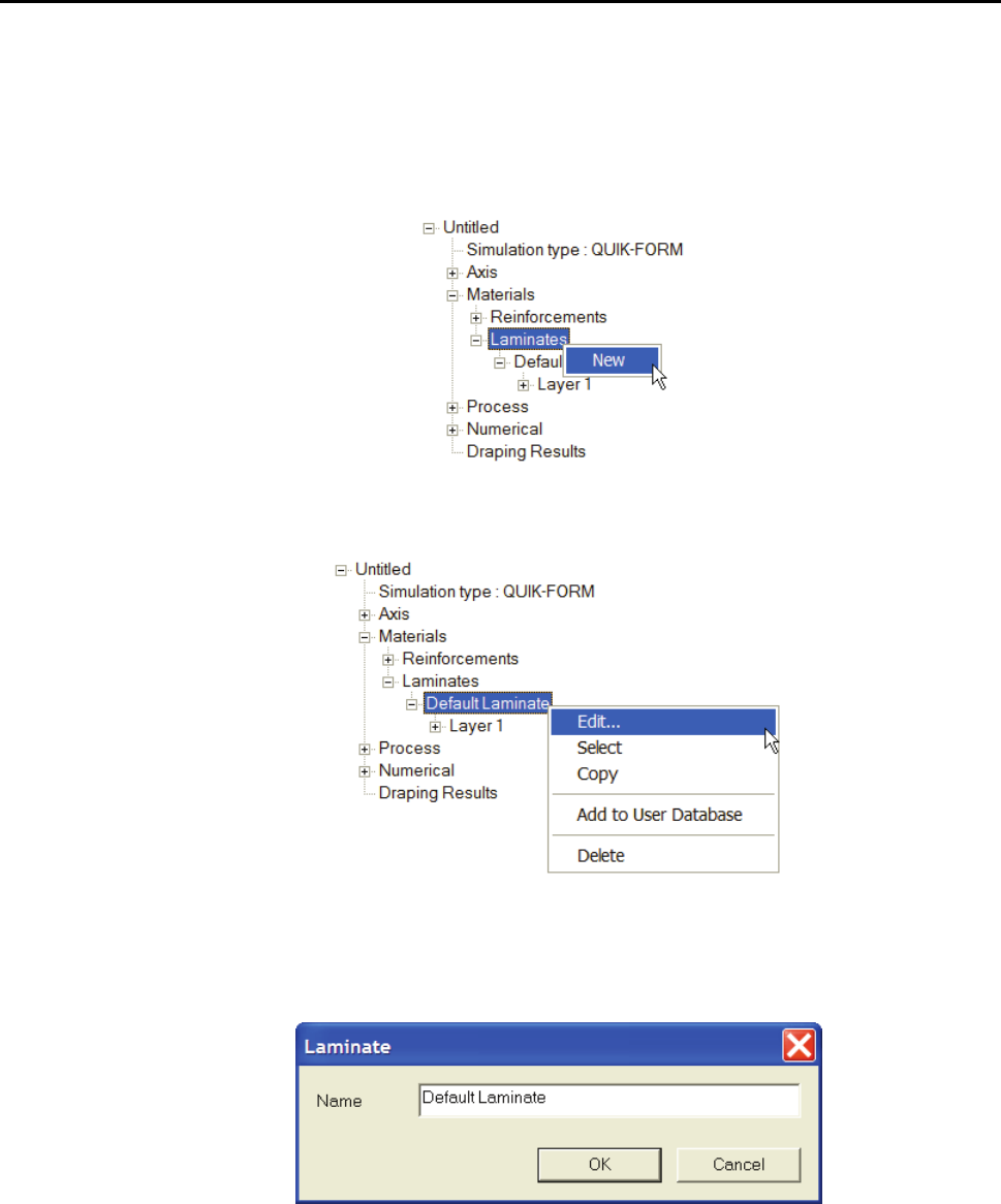
USER’S GUIDE & TUTORIALS 152 PAM-RTM 2014
(released: Apr-14) © 2014 ESI Group
PAM-RTM USER'S GUIDE
Laminates
LAMINATES
Laminate materials are made of layers of fiber reinforcements or solids. Currently
laminates are used in PAM-RTM™ in the context of a PAM--QUIKFORM™
simulation, and also in the context of local permeability calculation, to link
reinforcements to imported draped plies.
A new laminate is created by right-clicking the Laminates item in the explorer, and
choosing the New command.
Right-clicking a laminate’s top level item gives access to the popup menu common to
all materials. The Edit command pops up a dialog box, which currently only allows
modification of the material name.
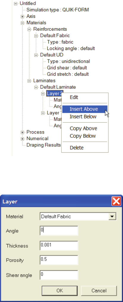
PAM-RTM 2014 153 USER’S GUIDE & TUTORIALS
© 2014 ESI Group (released: Apr-14)
PAM-RTM USER'S GUIDE
Laminates
It is possible to insert, copy, delete layers by right-clicking one layer in the explorer.
Editing a layer opens the following dialog box, used to associate a reinforcement or
solid to this layer.
Material
Choose the material to link to this layer from the roll-down list. All currently defined
reinforcements and solids are listed.
Angle
Unit: degree
Angle of the layer in the laminate referential (α in the figure below).
Thickness
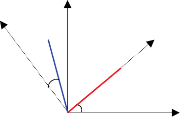
USER’S GUIDE & TUTORIALS 154 PAM-RTM 2014
(released: Apr-14) © 2014 ESI Group
PAM-RTM USER'S GUIDE
Laminates
Unit: meters
Thickness of the layer.
Porosity
Unit: no unit, percentage expressed as a value between zero and one.
Initial porosity of the layer (before shearing in case of fabrics).
Shear Angle
Unit: degree
Initial shearing of the layer (fabrics only, β in the figure below).
In the following figure a layer’s referential (Lx-Ly) was rotated by an angle α relative to
the laminate’s referential (X-Y). The layer’s x axis defines the warp direction of a
fabric, and the layer’s y axis is the weft direction. A non-zero initial shear angle β was
specified.
X
Y
Lx
L
y
α
warp
weft
β

PAM-RTM 2014 155 USER’S GUIDE & TUTORIALS
© 2014 ESI Group (released: Apr-14)
PAM-RTM USER'S GUIDE
Material Database
MATERIAL DATABASE
The user can create his own material database with the materials he/she uses most often.
Creation of the Material Database
This is the procedure to create the material database the first time PAM-RTM™ is run.
The path to the material database has to be specified in the Paths tab of the Options
dialog box (View->Options). Before the path is explicitly set by the user, it is blank in
the Options dialog.
To set the path, the user pushes the browse button (see [1] in image below) which opens
the standard Windows file browser. Then the user is asked to select an existing .dtf
file. Since the first time the software is used that .dtf file doesn’t exist, the user has to
create first an empty .dtf file with a text editor. That file could be named for example
materials.dtf. Note that the material database is actually a subset of the PAM-
RTM™ input file, so it has the same extension .dtf.
The path to the material database is a current user setting, which means that all PAM-
RTM™ users working on the same computer have to set it. If many users need to share
the same material database, the materials.dtf file could be placed in a directory
where all users have read and write permissions.
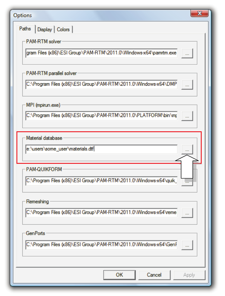
USER’S GUIDE & TUTORIALS 156 PAM-RTM 2014
(released: Apr-14) © 2014 ESI Group
PAM-RTM USER'S GUIDE
Material Database
Paths tab of the Options dialog box
Using the Material Database
Once the initial empty materials.dtf file has been created and the path set, you can
start building the database. First completely define your material with the
Reinforcement, Resin or Solid editors of PAM-RTM™. Once you are satisfied with the
1
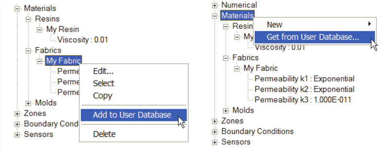
PAM-RTM 2014 157 USER’S GUIDE & TUTORIALS
© 2014 ESI Group (released: Apr-14)
PAM-RTM USER'S GUIDE
Material Database
material definition, right-click the material in the explorer and choose Add to User
Database.
Later if you want to reuse the same material in another simulation, you can retrieve
materials from the database by right-clicking the Materials item in the explorer and
choosing Get from User Database. This opens the following dialog box, which lists all
the materials available in the database. Choose one or more materials you want to copy
in your current model. If there is a material with the same name in the current
document, PAM-RTM™ asks for a confirmation that you want to replace it with the
version stored in the material database. It is important to understand that when
retrieving a laminate from the material database, PAM-RTM™ retrieves also all the
materials used in the definition of the laminate.

USER’S GUIDE & TUTORIALS 158 PAM-RTM 2014
(released: Apr-14) © 2014 ESI Group
PAM-RTM USER'S GUIDE
Material Database
Get from User Database dialog
If you need to make some changes to one of the materials of the database, you have to
retrieve it first from the database into the current model. Then edit the material and send
it back to the database with Add to User Database. If you didn’t modify the material
name, PAM-RTM™ detects that a material with the same name already exists in the
database and asks if you want to replace it. Answer Yes.
The command Simulation->Manage User Database opens the following dialog box,
which is actually almost the same as the previous one, except that there is a Delete
button that allows the user to remove the unwanted materials from the database. This is
the only database management functionality currently available.
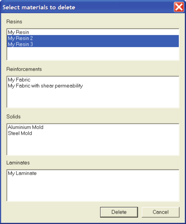
PAM-RTM 2014 159 USER’S GUIDE & TUTORIALS
© 2014 ESI Group (released: Apr-14)
PAM-RTM USER'S GUIDE
Material Database
Manage User Database dialog
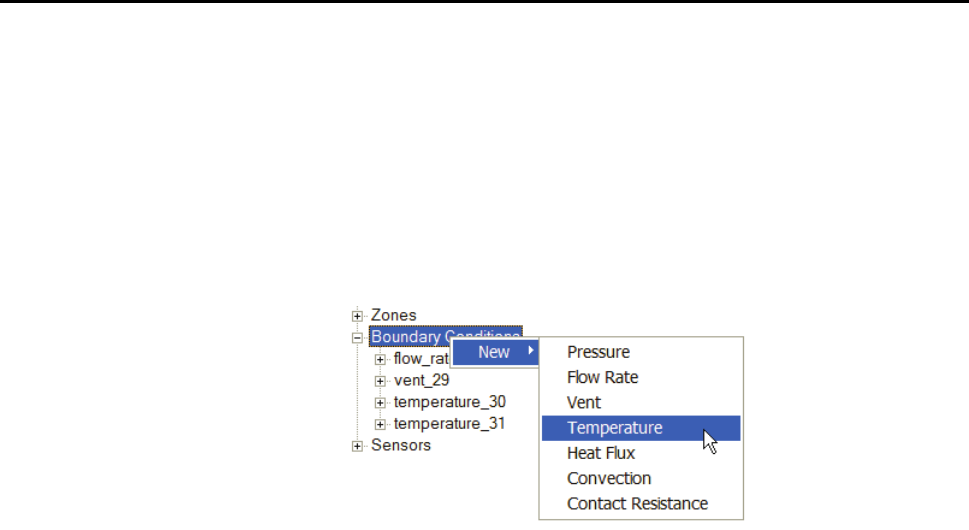
USER’S GUIDE & TUTORIALS 160 PAM-RTM 2014
(released: Apr-14) © 2014 ESI Group
PAM-RTM USER'S GUIDE
Boundary Conditions
BOUNDARY CONDITIONS
Boundary conditions in PAM-RTM™ are associated to groups of nodes or groups of
faces as their geometrical support. So the first step is to create a group to define where a
boundary condition is applied, then create the actual boundary condition which refers to
the group through its ID.
To create a boundary condition, right-click the Boundary Conditions item in the model
explorer. The types of boundary conditions that can be created depend on the simulation
type.
The newly created boundary condition is not assigned to any group. Double-click the
new boundary condition in the explorer to set its parameters. This opens the Boundary
Condition dialog box.
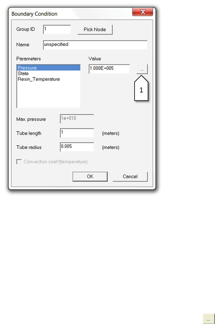
PAM-RTM 2014 161 USER’S GUIDE & TUTORIALS
© 2014 ESI Group (released: Apr-14)
PAM-RTM USER'S GUIDE
Boundary Conditions
The first parameter to specify is the group ID to which this boundary condition refers. If
there are many groups, it can be difficult to identify a group with the color bars, so
simply push the Pick Node button and pick a node that belongs to the group.
The Parameters area contains the list of parameters associated to this boundary
condition. For instance, all the boundary conditions have a State parameter which
allows to activate or deactivate the boundary conditions as a function of time. To use
the state parameter, simply create a piecewise linear curve. When the value is >= 0.5 the
boundary condition is active, otherwise it is disabled.
Actually all the parameters of boundary conditions are functions of time. For example,
the Flow Rate boundary condition contains three parameters: flow_rate,
resin_temperature and state. All three parameters can be functions of time. Use the
button to open the function editor [1].
The only exception is the convection coefficient, which is by default a function of time,
but can be made a function of temperature if the convection coef f(temperature) option
is checked at the bottom of the dialog box. This check box is only available when a
convection boundary condition is edited.
USER’S GUIDE & TUTORIALS 162 PAM-RTM 2014
(released: Apr-14) © 2014 ESI Group
PAM-RTM USER'S GUIDE
Boundary Conditions
Here’s a list of all boundary conditions with the simulation types that support them.
- Pressure
· Description: pressure controlled inlet.
· Simulations: RTM, VARI, Heated RTM.
· Parameters:
Pressure. Inlet pressure. Unit: Pa.
Resin_Temperature. Resin temperature when it enters the cavity.
This parameter is used most of the time for Heated RTM simulations,
but it makes sense to use it also for isothermal simulations, for
example to have PAM-RTM™ calculate the viscosity from a
viscosity curve. Unit: degree Kelvin.
State
Tube length. The length of the tube between the pressurized resin pot
and the mold. Only used when the Poiseuille correction is activated
in the advanced numerical parameters. Unit: m.
Tube radius. Also only used with the Poiseuille correction. Unit: m.
- Flow Rate
· Description: flow rate controlled inlet.
· Simulations: RTM, VARI, Heated RTM, Presimulation.
· Parameters:
Flow_Rate. Unit: m3/s .
Resin_Temperature. Unit: Kelvin
State
Max Pressure. The flow rate inlet supports a special parameter to
specify the maximum pressure that can be reached by the injection
machine. This parameter is not a function of time.
- Vent
· Description: resin outlet.
· Simulations: RTM, VARI, Heated RTM, Presimulation.
· Parameters:
Pressure. The pressure on the vent. Unit: Pa.
State. Useful to “program” a vent opening and closing sequence.
- Temperature
· Description: fixed temperature, i.e. Dirichlet boundary condition in the heat
transfer equation.
· Simulations: Heated RTM, Preheating, Curing.
· Parameters:

PAM-RTM 2014 163 USER’S GUIDE & TUTORIALS
© 2014 ESI Group (released: Apr-14)
PAM-RTM USER'S GUIDE
Boundary Conditions
Temperature. Unit: Kelvin.
State.
- Heat Flux
· Description: imposed heat flux, i.e. Neumann boundary condition in the heat
transfer equation.
· Simulations: Heated RTM, Preheating, Curing.
· Parameters:
Heat_Flux.
q
n
T=
∂
∂
. Unit: W/m2.
State.
- Convection
· Description:
)( TTh
n
T−=
∂
∂
∞
· Simulations: Heated RTM, Preheating, Curing.
· Convection coef f(temperature): check to make the convection coefficient a
function of temperature instead of time.
· Parameters:
Reference_Temperature.
∞
T
in the equation above. Unit: Kelvin.
Convection_Coefficient. h coefficient. Unit : W/m2.K
State.
- Contact Resistance
· Description: used to model the heat transfer on the interface between two solids
in contact.
· Simulations: Heated RTM, Preheating, Curing.
· Parameters:
Contact_Resistance.
th
R
in equation
th
R
TT 2
1−
=
ϕ
, where T1 and T2
are the temperatures on both sides of the interface. Unit: m2W-1K
State.
- Thickness
· Description: prescribed thickness on the part boundary.
· Simulations: VARI.
· Parameters:
Thickness. Unit: m.
State.
USER’S GUIDE & TUTORIALS 164 PAM-RTM 2014
(released: Apr-14) © 2014 ESI Group
PAM-RTM USER'S GUIDE
Boundary Conditions
- Compression
· Description: used in the context of Compression RTM simulation, to specify the
upper mold closing velocity and the compression direction.
· Simulations: Compression RTM.
· Parameters:
Velocity_Norm. The upper mold closing velocity. Unit: m/s.
Final_Thickness. The targeted final thickness of the part. This is only
used as a hint for the Compression RTM simulation to determine the
time step, it is not a stopping criteria. Unit: m.
Dir_x, Dir_y, Dir_z. The components of the direction vector for
compression. If the direction to be used is normal to each element,
the three components must be set to zero. Unit: none.
State.
Notes:
- Max pressure only applies to flow rate inlets.
- Tube length and tube radius only apply to pressure inlets.
- Convection coef f(temperature) only applies to convection boundary conditions.
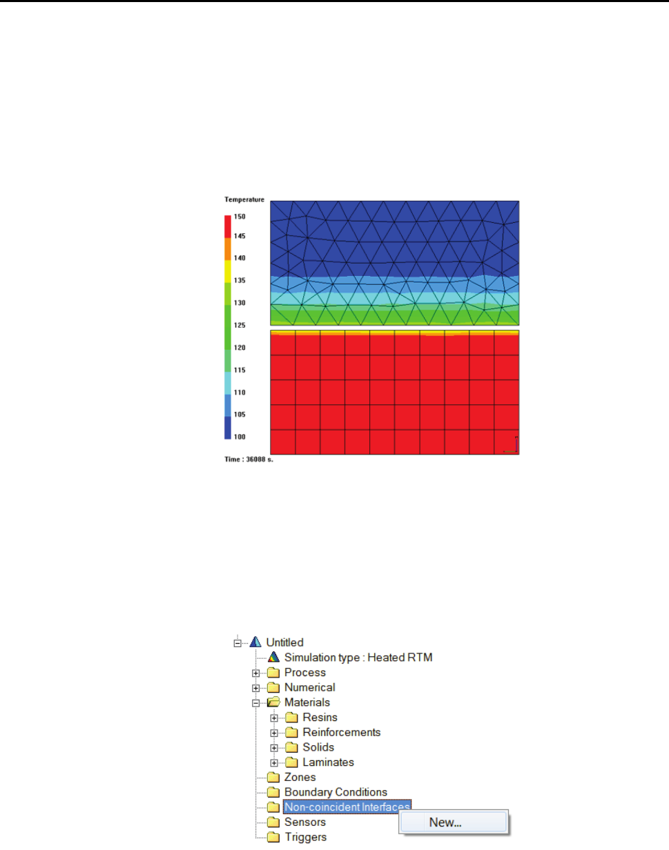
PAM-RTM 2014 165 USER’S GUIDE & TUTORIALS
© 2014 ESI Group (released: Apr-14)
PAM-RTM USER'S GUIDE
Non-Coincident Interfaces
NON-COINCIDENT INTERFACES
Non-coincident interfaces allow disconnected meshes to be used for thermal
calculations. Typically they allow different meshing parameters to be used for the
preform area and the mold. For instance the preform could be meshed with tetrahedral,
while the mold is meshed with bricks. Also the size of the elements can be different on
both sides of the interface. An example is shown below.
A folder non-coincident interfaces is available for thermal calculations (preheating,
heated RTM, curing).
To create a non-coincident interface, right-click on the non-coincident interfaces item,
then New, which opens the non-coincident interface dialog box.
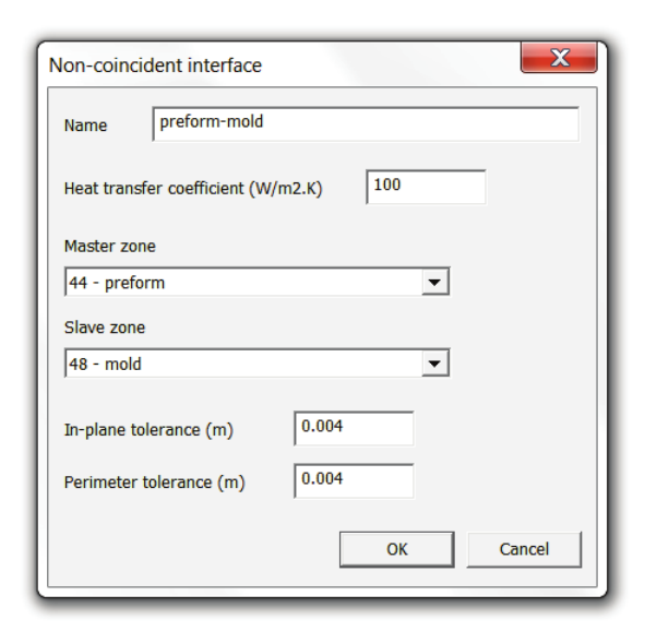
USER’S GUIDE & TUTORIALS 166 PAM-RTM 2014
(released: Apr-14) © 2014 ESI Group
PAM-RTM USER'S GUIDE
Non-Coincident Interfaces
The main parameters to specify are the two zone IDs involved in the interface. In
general the master zone is the preform, and the slave zone is the mold. The master zone
and slave zone dropdown lists allow selection of one of the zones currently defined in
the model. It is recommended to assign meaningful names to zones before defining
interfaces, to make that selection easier.
The heat transfer coefficient is a parameter specific to each interface, meaning it is
possible to have in the same model many interfaces with different heat transfer
coefficients.
The in-plane tolerance corresponds to the maximum distance around an element of the
master surface where a node of the slave surface can be found.
The perimeter tolerance corresponds to the maximum distance between the two surfaces
in order to have a contact (distance normal to the plane of the interface).
In general, a good tolerance value should be about half the size of the elements on the
preform side, and it is recommended to use the same value for in-plane and perimeter
tolerances. However if the mesh has a quite heterogeneous mesh size, these tolerances
may be too small (and thus, there will be "no contact", and thus no heat transfer at these
non-coincident interfaces). If such a case occurs, one can change (i.e. increase) these
tolerances. One should however be careful not to use too large tolerances so that nodes
beyond the opposite surface would be taken into account.
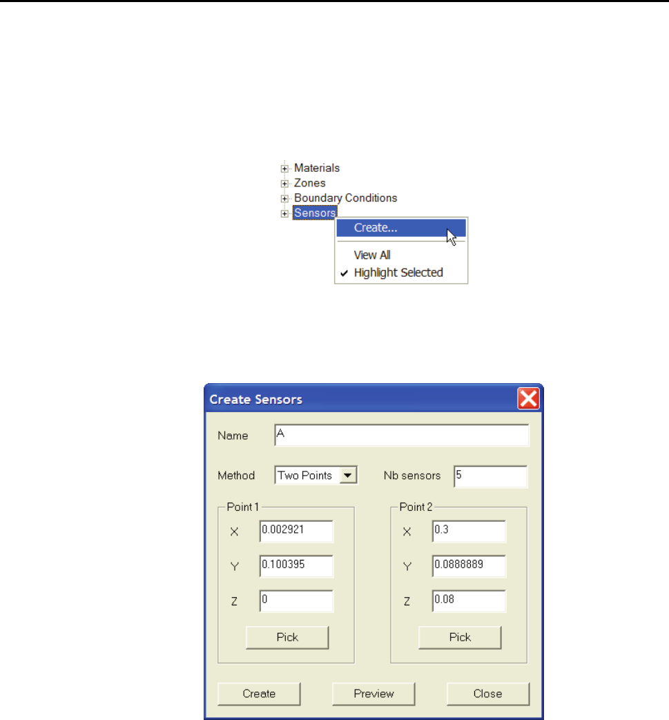
PAM-RTM 2014 167 USER’S GUIDE & TUTORIALS
© 2014 ESI Group (released: Apr-14)
PAM-RTM USER'S GUIDE
Sensors
SENSORS
Creating Sensors
Sensors are used in PAM-RTM™ to sample results on specific points in order to plot
curves.
To create sensors, open the Create Sensors dialog box, either by right-clicking the
Sensors item in the explorer, or by using the Simulation->Create Sensors command,
which pops up the following dialog box.
First give a name to the sensor, so you can identify it easily. However try to give a short
name because this name will be used in the graph legend when results are plotted.
There are two methods to create sensors: one point and two points. With the one point
method, the user either enters the coordinates of the sensor directly, or pushes the Pick
button to pick with the mouse an arbitrary point on the mesh. Then the user pushes the
Create button to actually create the sensor.

USER’S GUIDE & TUTORIALS 168 PAM-RTM 2014
(released: Apr-14) © 2014 ESI Group
PAM-RTM USER'S GUIDE
Sensors
With the two points method, the user specifies two points that define the end-points of a
line segment. The idea is to have PAM-RTM™ generate automatically a specified
number of sensors on that line. The two end-points can be specified by entering the
coordinates or by picking with the mouse. The line segment doesn’t have to lie on the
surface. In case of curved geometry, PAM-RTM™ projects the sensors on the surface.
A Preview button is available to visualize the approximate position of the sensors,
before they are projected.
When the two points method is used, the name of the sensor is used as a root name, and
a number is automatically added to this name. For example, if the user specifies the
name as s and 3 sensors are created, they will be called s_1, s_2, s_3. The names can be
modified later.
As shown below, the created sensors are listed in the explorer under the Sensors item.
Selecting a sensor in the explorer highlights it in the graphics window. This behavior is
controlled by the Highlight Selected command available in the popup menu on the
Sensors item. It is also possible with the View All command to turn on or off the
visualization of all sensors in the graphics window.
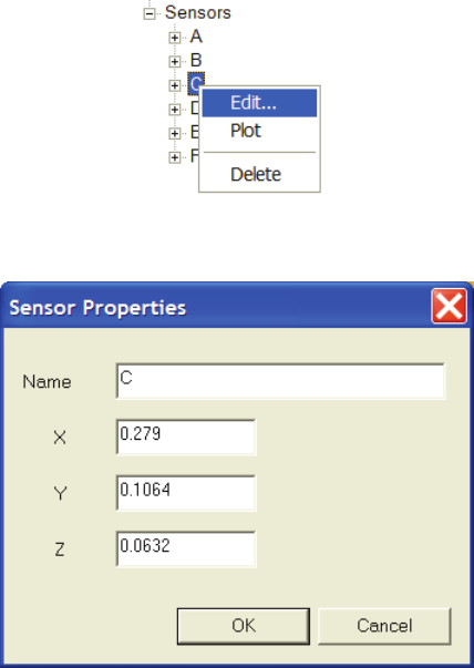
PAM-RTM 2014 169 USER’S GUIDE & TUTORIALS
© 2014 ESI Group (released: Apr-14)
PAM-RTM USER'S GUIDE
Sensors
Editing Sensors
Once they have been created, it is possible to modify attributes of a sensor by double-
clicking it in the explorer, or by using the menu that pops up when a sensor is right-
clicked in the explorer.
The edit command opens the Sensor Properties dialog box.
With this dialog box the user can change the name of the sensor and its coordinates.
A sensor can be deleted by selecting it in the explorer and by choosing Delete in its
popup menu.
Plotting sensors
There are two ways to plot curves on sensors. The simplest one is by using the Plot
command available in the sensor popup menu. This command samples the currently
visualized scalar field on the sensor position, then opens the curve viewer and adds a
new curve to it. So to use this command, activate first visualization of a scalar field such
as pressure or temperature.
Another way is to open first the curve viewer with View->Curve Viewer. Then use the
Import Curves command of the curve viewer popup menu, available by right-clicking in
the curve viewer graphics window, as shown below. Select one of the sensor results
files generated by the solver (for example
x_Temperature_Filling_Sensors.dat). This loads all the curves available in the
file in the curve viewer.
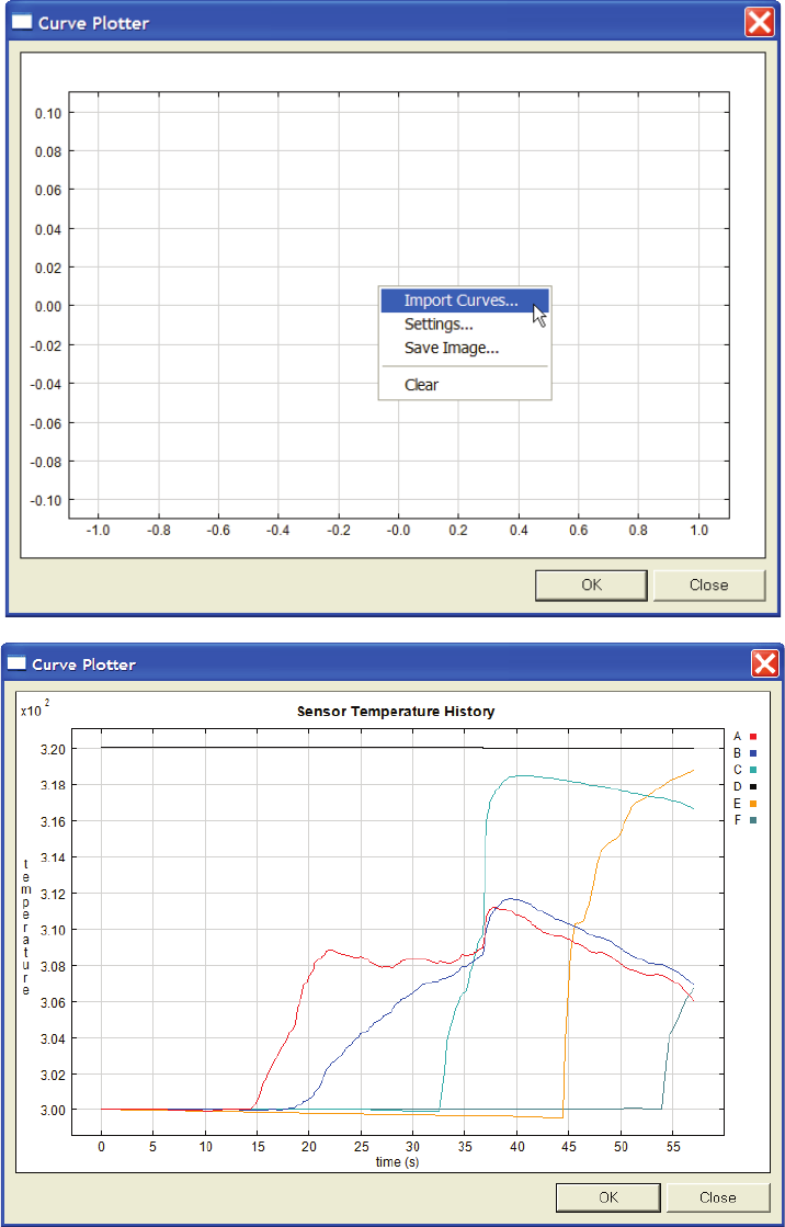
USER’S GUIDE & TUTORIALS 170 PAM-RTM 2014
(released: Apr-14) © 2014 ESI Group
PAM-RTM USER'S GUIDE
Sensors
While the first approach is more convenient because you don’t have to import a file in
the curve viewer, the second approach is more accurate. This is because with the first
approach, the number of values plotted depend on the sampling period parameter, while
in sensor results files all the time steps are saved.

PAM-RTM 2014 171 USER’S GUIDE & TUTORIALS
© 2014 ESI Group (released: Apr-14)
PAM-RTM USER'S GUIDE
Trigger Manager
TRIGGER MANAGER
The trigger manager is a module allowing easier control of opening and closing of
injection ports and vents. The user defines triggers and outcomes. A trigger specifies a
condition such as “filling factor on sensor x equals 1”, actually meaning “the resin has
reached sensor x”. Associated to a trigger is a list of outcomes, i.e. events that are
generated when the condition is met. For instance, an outcome could be “set the state
coefficient of injection port y to 1”, actually meaning “open injection port y”. This
allows easy definition of sequential injection used for large parts, in which injection
ports are successively opened and closed. Running such simulations with earlier
versions of PAM-RTM™ was possible, but required more work as the user had to run
many simulations to estimate the time of arrival of the resin on a given point. With the
trigger manager a single run is required. Note that many outcomes can be associated to
a trigger, such as “closing vent x” and “opening injection port y”. Also conditions on the
volume of resin injected or lost are available on triggers, i.e. the user could define
conditions such as “when a volume x of resin has been lost on vent y, close vent y and
open injection port z”.
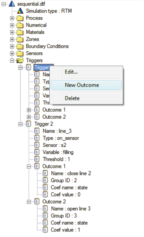
USER’S GUIDE & TUTORIALS 172 PAM-RTM 2014
(released: Apr-14) © 2014 ESI Group
PAM-RTM USER'S GUIDE
Trigger Manager
A folder Triggers is available in the document’s tree. Right-clicking the Triggers folder
gives access to the New command to create triggers. To create outcomes, the user right-
clicks a trigger and selects New Outcome.
Double-clicking a trigger or an outcome in the document’s tree opens a dialog box for
edition of the entity. These dialog boxes are described below.
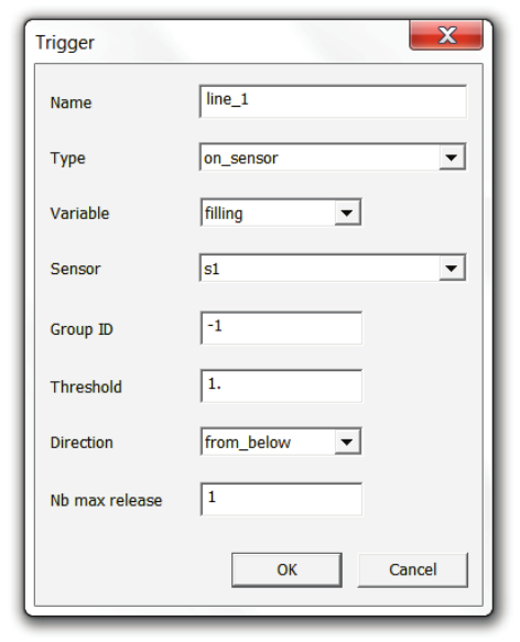
PAM-RTM 2014 173 USER’S GUIDE & TUTORIALS
© 2014 ESI Group (released: Apr-14)
PAM-RTM USER'S GUIDE
Trigger Manager
- Name: name of the trigger.
- Type: the following types are currently supported:
· on_sensor: the trigger is associated to a sensor, which must be selected in the
sensor combo below.
· injected_volume: the trigger is based on the injected volume for a specific
injection port. The injection port ID is specified in the group ID field below.
· lost_volume: the trigger is based on the lost volume for a specific vent. The vent
ID is specified in the group ID field below.
· global_injected_volume: the trigger is based on the injected volume of all the
injection ports.
· global_lost_volume: the trigger is based on the lost volume of all the outlets.
- Variable: this parameter is only meaningful for on_sensor type.
· pressure: the resin pressure is sampled on the sensor.
· filling: the filling factor (value between 0 and 1), is sampled on the sensor.
· thickness: thickness is sampled on the sensor (standard solver only).
· temperature: temperature is sampled on the sensor (parallel solver only).
- Sensor: the list of sensors currently defined in the document. Sensors should be
created before defining triggers.
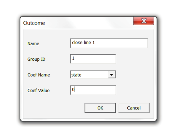
USER’S GUIDE & TUTORIALS 174 PAM-RTM 2014
(released: Apr-14) © 2014 ESI Group
PAM-RTM USER'S GUIDE
Trigger Manager
- Group ID: only meaningful for the injected_volume and lost_volume types. The ID
of the group defining the injection port or vent.
- Threshold: the critical value that will fire outcomes. It could be a pressure value or a
filling factor value, depending on the variable selected. For instance, if filling is
selected and a value of 1 is entered as threshold, it means that outcomes will be
fired when the element on which the sensor is located is completely filled. If a
pressure value of 10 000 Pa is entered, it means that outcomes will be fired when
the resin pressure on the sensor becomes larger than 10 000 Pa.
- Direction: indicates if the trigger is to be fired when the threshold is crossed
from_below (positive slope), from_above (negative slope), or from_all (every time
the threshold is crossed, regardless of the direction).
- Nb max release: the maximum number of times that the outcomes can be fired. For
instance, if a pressure trigger is defined, it is possible that the pressure will increase
above the threshold, which will fire the outcomes a first time, then decrease, and
increase again to the threshold, firing the outcomes a second time. To avoid that
enter a value of 1 for nb max release.
- Name: give a meaningful name to the outcome, such as “close line 1”.
- Group ID: the group (boundary condition) on which the coefficient will be set.
- Coef name:
· state: most of the time you will work with the state coefficient, allowing
opening (coef value = 1) and closing (coef value = 0) of inlets and outlets.
· pressure: forces the pressure value on an inlet (standard solver only).
· flow_rate: forces the flow rate on an inlet (standard solver only).
- Coef value: the value that will be set on a coefficient as the result of an outcome
being fired.
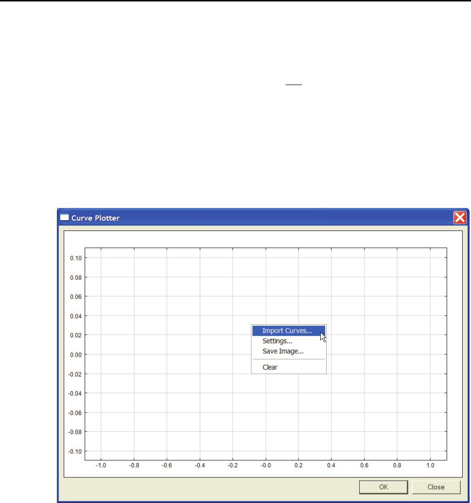
PAM-RTM 2014 175 USER’S GUIDE & TUTORIALS
© 2014 ESI Group (released: Apr-14)
PAM-RTM USER'S GUIDE
Curve Viewer
CURVE VIEWER
The curve viewer is used to visualize simulation results on sensors. It is also used to
visualize mathematical functions associated to simulation parameters, such as viscosity
as a function of temperature, or the reaction rate
dt
d
α
as a function of temperature and
degree of cure. Depending on the context, the curve viewer will be used to visualize
functions of one or two independent variables.
Importing Curves
The curve viewer is opened with the View->Curve Viewer command.
Notice that there is a popup menu available by right-clicking in the graphics area.
Curve viewer’s popup menu
Curves can be imported in the curve viewer with the Import Curves command of the
popup menu. In general curves imported that way are sensor results files (see section
Sensors).
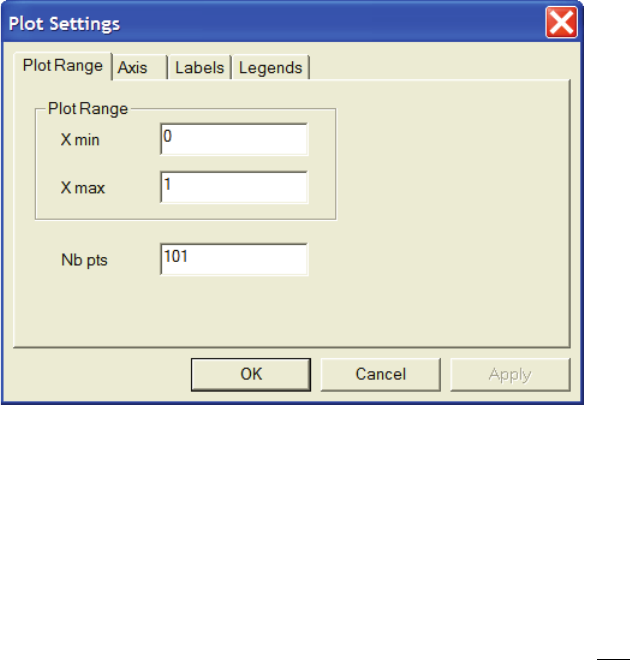
USER’S GUIDE & TUTORIALS 176 PAM-RTM 2014
(released: Apr-14) © 2014 ESI Group
PAM-RTM USER'S GUIDE
Curve Viewer
Settings
Plot range
Plot range for a function of one variable
The Plot Range tab is used to specify the range that the user wants to plot. For example,
if the currently visualized function is viscosity with respect to temperature, changing the
X min and X max values means changing the temperature range to visualize. PAM-
RTM™ will re-evaluate the function on Nb pts equally spaced in the new range and
update the graph accordingly.
When functions of two variables are visualized, such as the rate of reaction
dt
d
α
with
respect to temperature and degree of cure, the Plot Range tab has more parameters, as
shown below.
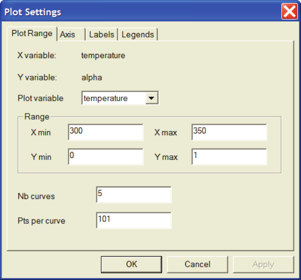
PAM-RTM 2014 177 USER’S GUIDE & TUTORIALS
© 2014 ESI Group (released: Apr-14)
PAM-RTM USER'S GUIDE
Curve Viewer
Plot range for a function of two variables
Here we see that the X variable is temperature and the Y variable is alpha (degree of
cure).
The Plot variable dropdown list is used to select the variable displayed on the X axis of
the graph. In this example, the X axis is temperature, which varies between 300 and 350
Kelvin, and five iso-alpha curves are plotted (see graph below).
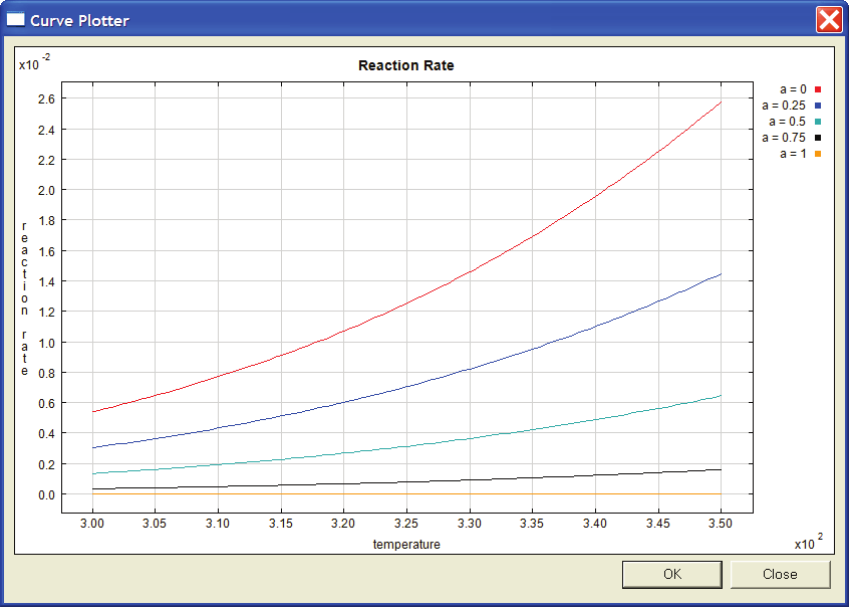
USER’S GUIDE & TUTORIALS 178 PAM-RTM 2014
(released: Apr-14) © 2014 ESI Group
PAM-RTM USER'S GUIDE
Curve Viewer
Iso-alpha curves
Changing the Plot variable to alpha instead of temperature would lead to the following
iso-temperature curves.
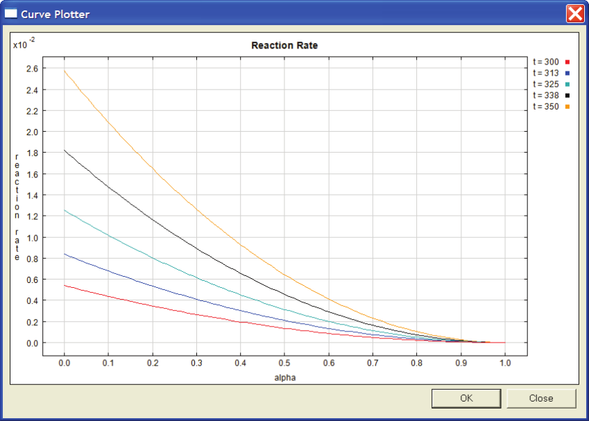
PAM-RTM 2014 179 USER’S GUIDE & TUTORIALS
© 2014 ESI Group (released: Apr-14)
PAM-RTM USER'S GUIDE
Curve Viewer
Iso-temperature curves
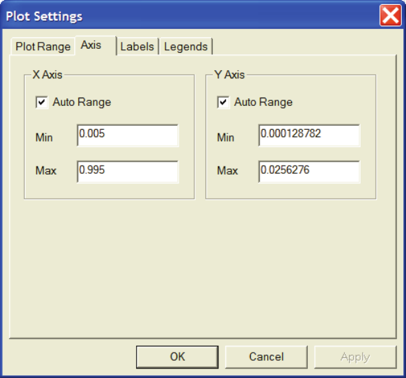
USER’S GUIDE & TUTORIALS 180 PAM-RTM 2014
(released: Apr-14) © 2014 ESI Group
PAM-RTM USER'S GUIDE
Curve Viewer
Axis Settings
Axis settings
In general the X and Y axis ranges are automatically calculated from the data points to
fit entirely the curves. In some situations the user may want to restrict the view, so the
Auto Range parameter can be unchecked and a different range specified. Note that this
changes only the viewing range, not the plot range, which means that the function is not
re-evaluated. If you want to re-evaluate the function on a different range, use the Plot
Range tab.
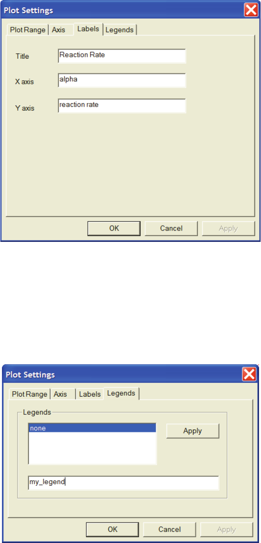
PAM-RTM 2014 181 USER’S GUIDE & TUTORIALS
© 2014 ESI Group (released: Apr-14)
PAM-RTM USER'S GUIDE
Curve Viewer
Labels
Labels
Graph title and labels for the X and Y axis are automatically assigned by PAM-RTM™
depending on the context. If the user doesn’t like the default labels, he can modify them
with the Labels tab. This is useful for example if a screen capture of the curve viewer is
needed to be included in a report and the labels are not explicit enough.
Legends
Legends tab
USER’S GUIDE & TUTORIALS 182 PAM-RTM 2014
(released: Apr-14) © 2014 ESI Group
PAM-RTM USER'S GUIDE
Curve Viewer
It is possible to modify the graph legends. First select the legend to be modified in the
list, then enter the new text in the text field, and finally push the Apply button.
Saving Images
The curve viewer graphics area can be saved in an image file, which can be included
later in reports.
The supported image file formats are:
- PNG
- GIF
- TIFF
- JPEG
- It is recommended to use the PNG format.
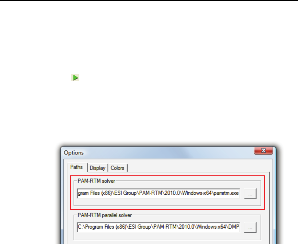
PAM-RTM 2014 183 USER’S GUIDE & TUTORIALS
© 2014 ESI Group (released: Apr-14)
PAM-RTM USER'S GUIDE
Running the Simulation from a Command Window
RUNNING THE SIMULATION FROM A COMMAND
WINDOW
Windows
Most of the time the PAM-RTM™ solver is launched from the user interface with the
start button in the simulation toolbar. In some situations however it can be useful to
launch the simulation from a command window. For example you might want to launch
many simulations from a batch program on your PC to have them running during the
week-end. Or you might want to run a big simulation on a Linux workstation.
On Windows, you will need first to identify the directory where the solver executable
file pamrtm.exe is located. This can be done with the Options->Paths tab.
Then open a Command Prompt window with Start->All Programs->Accessories-
>Command Prompt. Change directory to where the PAM-RTM™ input file (.dtf) is
located, then launch the simulation by typing the full path to pamrtm.exe between
quotes, as shown below.
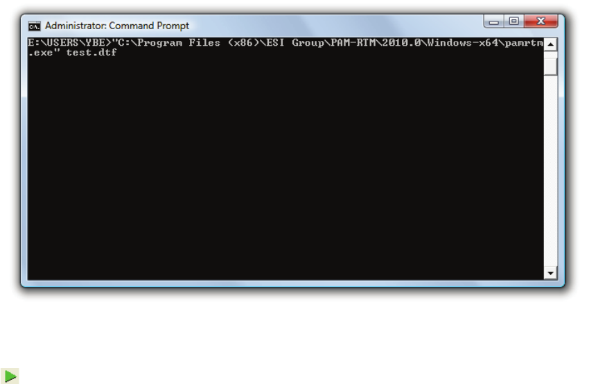
USER’S GUIDE & TUTORIALS 184 PAM-RTM 2014
(released: Apr-14) © 2014 ESI Group
PAM-RTM USER'S GUIDE
Running the Simulation from a Command Window
Calculations using the parallel solver are also normally launched with the start button
in the simulation toolbar. However if for some reason the user wants to launch a
calculation from outside the user interface, the file xxx_dmp.bat can be used. You need
to launch the calculation at least once from the user interface to have that file generated.
To launch the calculation, simply double-click that file in the Windows Explorer, or
enter “xxx_dmp.bat” in a command prompt window. That file could be easily edited to
run many cases consecutively.
Linux
To run a simulation on Linux with the standard solver, the input files have to be
prepared first with the user interface on Windows, because only the solver is available
on Linux. Save the project with File->Save. Then upload the .dtf file and matching
.unv file (mesh file) by FTP to your Linux workstation. Use telnet or an equivalent
to connect to the Linux workstation.
Type “pamrtm xxx.dtf” to launch the simulation. When it is done, download the
results files x_*.unv to the PC and go back to the PAM-RTM™ user interface for
post-processing.
To run a simulation on Linux with the parallel solver, do the same as described above to
transfer the files. Then type “pamrtmdmp xxx.dtf”. Here are optional parameters that
can be passed to pamrtmdmp.
pamrtmdmp [-np <#>] [-host <hostfile>] [-restart] [-mpiext "<mpi-
args>"] <input-file>
PAM-RTM 2014 185 USER’S GUIDE & TUTORIALS
© 2014 ESI Group (released: Apr-14)
PAM-RTM USER'S GUIDE
Running the Simulation from a Command Window
-np <#>: specifies the number of processors to use on a single
host. This option must not be used if a cluster configuration file is
specified (see -host option).
-host <hostfile>: specifies the name of a cluster file
configuration for applications running on multiple hosts within
distributed memory environment (MPI). A cluster file configuration
simply lists a series of hostnames, one per line, followed by the
number of processors to use on each host.
-mpiext "<mpi-args>": pass optional arguments to mpirun program.
See HP-MPI manual for the list of mpirun arguments.
-restart: this option must be specified when a restart of a
calculation is needed. The user must first edit file xxxp.dat and
change the value of INILEV to the step number from where the
calculation will restart.
<input-file>: input file name (.dtf).
Typical commands:
• pamrtmdmp –np 2 test.dtf
• pamrtmdmp –host clusterfile test.dtf
Here is an example of cluster file:
host1 2
host2 2
host3 4
host4 6
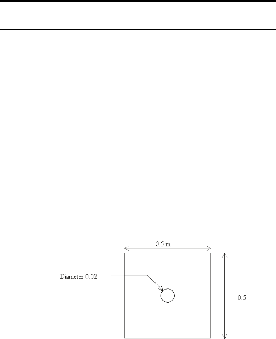
PAM-RTM 2014 187 USER’S GUIDE & TUTORIALS
© 2014 ESI Group (released: Apr-14)
TUTORIALS
Central Injection
TUTORIALS
CENTRAL INJECTION
The files related to this example are:
- central_start.unv (starting mesh)
- central.dtf + central.unv (solution)
Objective
This example on central injection will show you how to:
- create a simulation project,
- import a mesh to create groups of nodes for boundary conditions,
- visualize the zones,
- specify the simulation parameters for an injection based on Darcy’s law,
- display the filling pattern in the cavity and the pressure field in time.
Model of the Part and Physical Parameters
The part analyzed here is a square plate of length 0.5 m and thickness 0.005 m with a
hole of radius 0.01 m in the center, through which a resin of viscosity 0.1 Pa.s is
injected. The reinforcement is isotropic. The permeability is K1 = K2 = K3 = 1E-9 m2,
and the porosity 0.7.
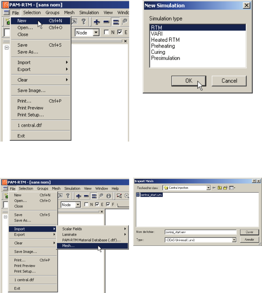
USER’S GUIDE & TUTORIALS 188 PAM-RTM 2014
(released: Apr-14) © 2014 ESI Group
TUTORIALS
Central Injection
Mesh Import and Visualization of the Zones
To launch PAM-RTM™, double-click the shortcut on the desktop, or use the shortcut
in the Windows start menu (Start->Programs->PAM-SYSTEM->PAM-RTM->version-
>PAM-RTM).
To create a new simulation, use the File->New command. This pops up the simulation
type box, choose the RTM simulation type.
To load the mesh provided for this example, use the File->Import->Mesh command.
This pops up the Import Mesh dialog box, in which you can choose the format of the
mesh file. For this example, the mesh provided is an I-DEAS Universal file.
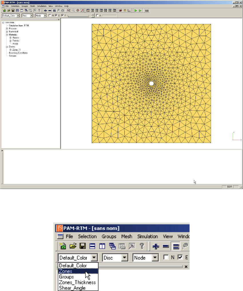
PAM-RTM 2014 189 USER’S GUIDE & TUTORIALS
© 2014 ESI Group (released: Apr-14)
TUTORIALS
Central Injection
After opening the file, you should see the following:
The zones are groups of finite elements used to assign different material properties to
different regions of the mesh. To visualize the zones defined in a mesh, select Zones in
the display toolbar.
This leads to the following picture, in which we can see that all the elements in this
mesh are part of zone 11.
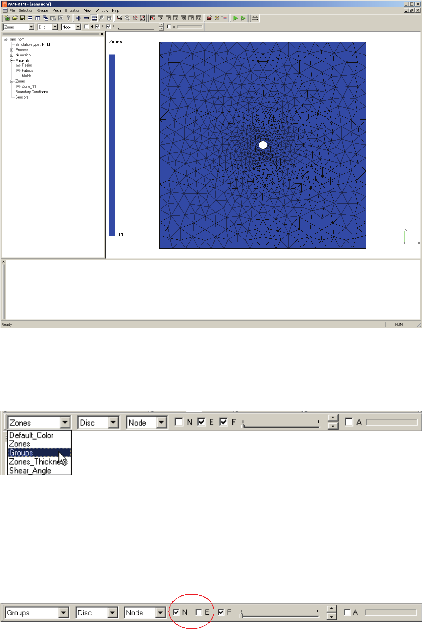
USER’S GUIDE & TUTORIALS 190 PAM-RTM 2014
(released: Apr-14) © 2014 ESI Group
TUTORIALS
Central Injection
Creation of Groups
Groups of nodes or groups of faces are used to specify boundary conditions. To
visualize the groups defined in a mesh, select Groups in the display toolbar.
Since currently there are no groups defined in this mesh, you see nothing special. The
fact that there is no color scale displayed at the left of the window is an indication that
there is no group currently defined in the mesh. You can also verify this with the
Groups->Info command.
To create a group of nodes, you must first select some nodes. Turn on visualization of
nodes by clicking the N checkbox in the toolbar. To select nodes more easily and to see
more easily the groups, you might have to turn off visualization of edges (E).

PAM-RTM 2014 191 USER’S GUIDE & TUTORIALS
© 2014 ESI Group (released: Apr-14)
TUTORIALS
Central Injection
Activate multiple picking mode with the + button in the toolbar. If you want to remove
a selected node to your selection, you can activate the – button by clicking on it.
Then select all the nodes around the injection hole. There is an useful command that
allows you to do that in a single click on Selection->Pick Boundary, then pick one of the
nodes around the injection hole. All the nodes are automatically selected.
Once the nodes are selected, you can create a group with the Groups->Create command.
If you are not currently in Groups visualization mode, choose Groups from the toolbar
combo box to visualize the new group. You should have the following display.
Save the project with the modified mesh with the File->Save As command. Give the file
a different name so that you don’t overwrite the original mesh. If your .dtf file is
called for example test.dtf, a mesh file called test.unv will be automatically
saved in the same directory as the .dtf file.
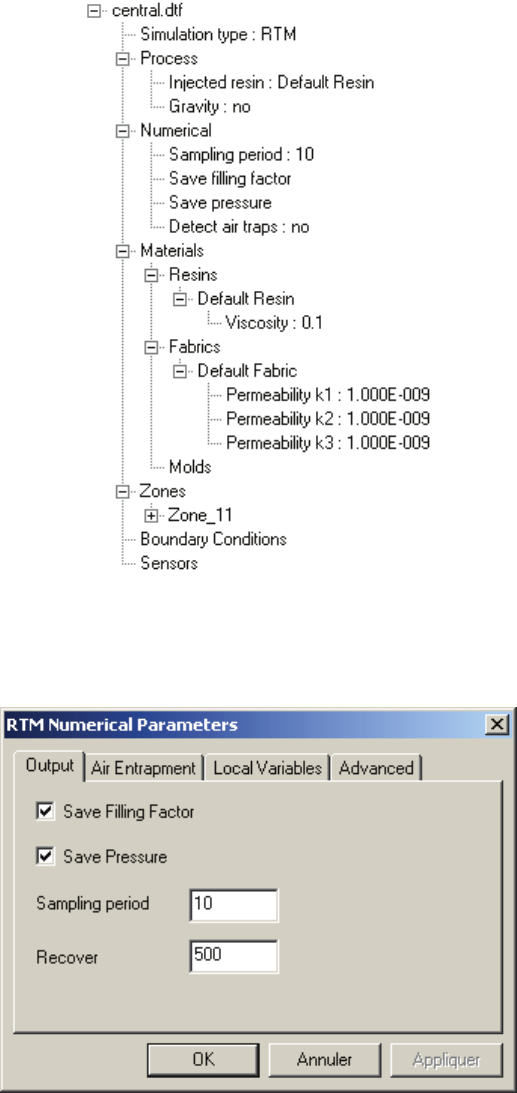
USER’S GUIDE & TUTORIALS 192 PAM-RTM 2014
(released: Apr-14) © 2014 ESI Group
TUTORIALS
Central Injection
Simulation
For this example, only the parameters that should be changed from their default value
will be pointed out.
In the left column, you can find all the parameters necessary for the simulation.
These parameters are divided into six categories, namely: Process, Numerical, Materials,
Zones, Boundary Conditions and Sensors.
Double-click on Numerical to open the RTM Numerical Parameters dialog box.
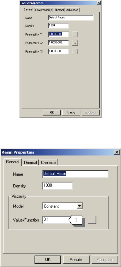
PAM-RTM 2014 193 USER’S GUIDE & TUTORIALS
© 2014 ESI Group (released: Apr-14)
TUTORIALS
Central Injection
Verify that Save Filling Factor and Save Pressure are active.
Double-click Default Fabric. The following dialog box pops up.
Enter an isotropic permeability of 1.10-9 m2 for K1, K2 and K3.
Now, double-click Default Resin. The resin properties will appear. Set a constant
viscosity of 0.1 Pa.s [1].
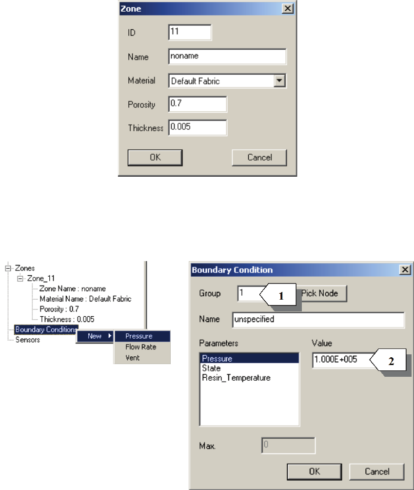
USER’S GUIDE & TUTORIALS 194 PAM-RTM 2014
(released: Apr-14) © 2014 ESI Group
TUTORIALS
Central Injection
Double-click on Zone 11. Make sure that Default Fabric is assigned to it, the porosity is
0.7 and the shell thickness is 0.005 m.
Right-click Boundary Conditions, select New->Pressure as type of boundary condition.
Then, double-click pressure_-1. Enter the ID of the group [1] and the value of the
injection pressure [2]. In this example, 1E+5 Pascals is used, so the pressure is
constant and equal to one bar. Note that it is also possible to choose a piecewise linear
curve in the function editor to simulate a time dependent injection pressure.
It is sometimes useful to define sensors at specific locations in the cavity to sample
pressure or temperature. Right-click Sensors, select Create and the dialog box Create
Sensors appears.
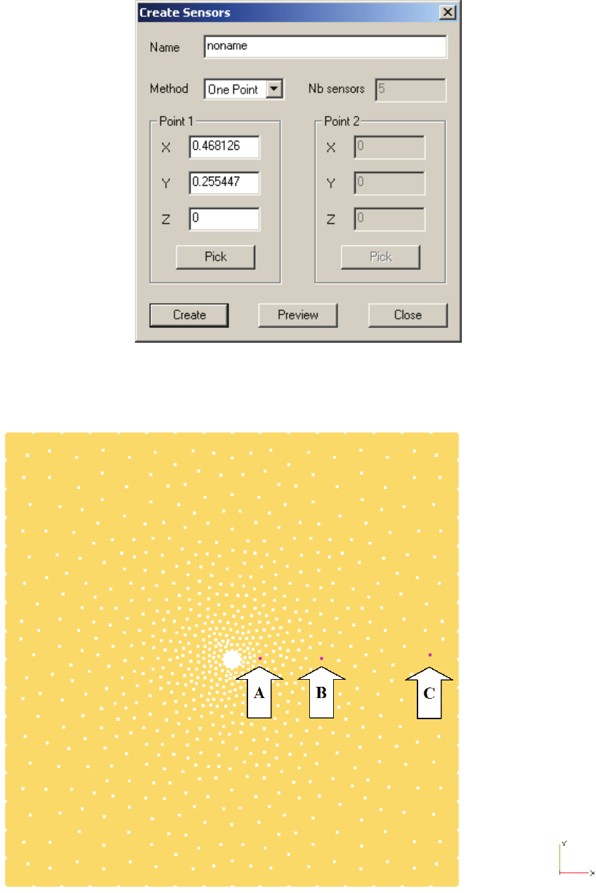
PAM-RTM 2014 195 USER’S GUIDE & TUTORIALS
© 2014 ESI Group (released: Apr-14)
TUTORIALS
Central Injection
Select 3 nodes (A, B and C) as shown in the following picture. You can enter directly
the position of the sensor or you can select it with the Pick function. Then you click on
the Create button.
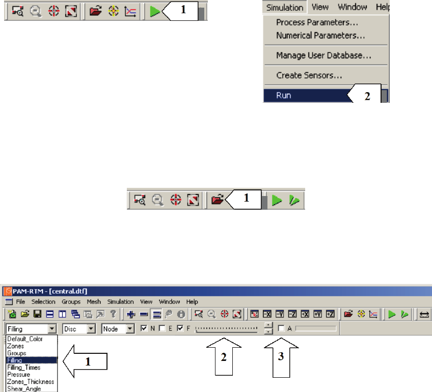
USER’S GUIDE & TUTORIALS 196 PAM-RTM 2014
(released: Apr-14) © 2014 ESI Group
TUTORIALS
Central Injection
Finally, save the simulation parameters with File->Save.
Note :
· Whenever simulation parameters are modified, it is important to save the file
before launching a new simulation (otherwise the simulation will be executed
with the old set of parameters).
· The simulation can be launched by clicking on the Start button [1] or by
selecting Simulation->Run [2].
Post-Processing the Results
To import the filling results, click on the Reload Results button [1]. It is possible to load
results during the calculation.
After importing scalar fields, they become available in the scalar field combo box [1].
Select Filling, then drag the time step scroll bar to visualize the filling factor step by
step [2]. Alternatively you can use the arrows to visualize a scalar field step by step.
You can also launch an animation by clicking the A check box [3].
Now you should have the following picture. This is the “raw” filling result of the
PAM-RTM™ simulation (the filling factor is calculated in PAM-RTM™ as a constant
per element scalar field). You can improve the display of the filling factor by selecting
Iso in the display toolbar [1]. This will give you a smoothed scalar field.

PAM-RTM 2014 197 USER’S GUIDE & TUTORIALS
© 2014 ESI Group (released: Apr-14)
TUTORIALS
Central Injection
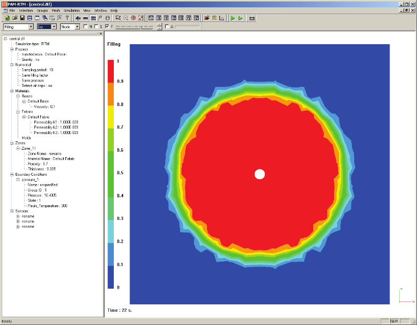
USER’S GUIDE & TUTORIALS 198 PAM-RTM 2014
(released: Apr-14) © 2014 ESI Group
TUTORIALS
Central Injection
Another useful scalar field to visualize is Filling Times. This scalar field is used to
visualize the successive positions of the flow front in time in a single picture.
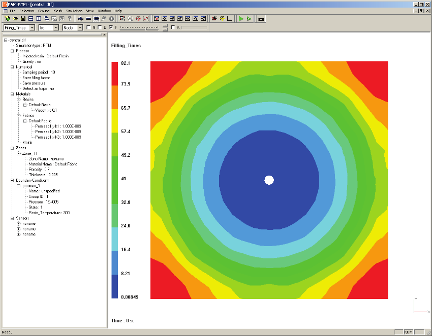
PAM-RTM 2014 199 USER’S GUIDE & TUTORIALS
© 2014 ESI Group (released: Apr-14)
TUTORIALS
Central Injection
Finally, we can have a look at the pressure field at the end of the injection, when the
cavity is completely filled.
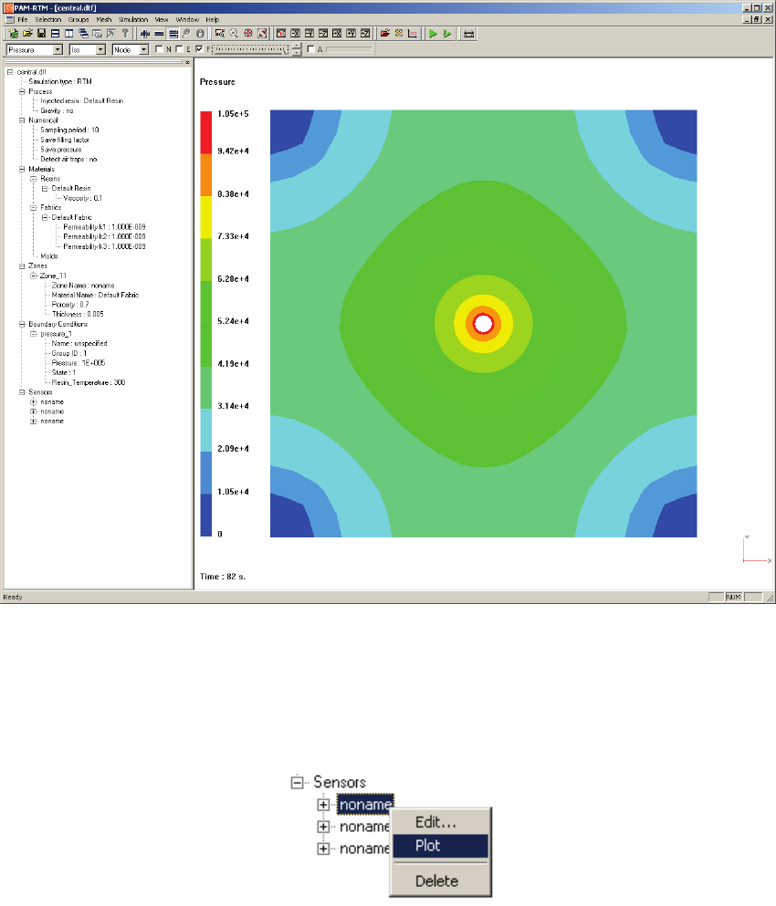
USER’S GUIDE & TUTORIALS 200 PAM-RTM 2014
(released: Apr-14) © 2014 ESI Group
TUTORIALS
Central Injection
It is important to understand in this example that, even if no vents were specified,
PAM-RTM™ is able to fill completely the cavity. This is because it assumes that when
no vent is specified, the injection is performed under perfect vacuum.
The sensors defined are important tools to study the results. They enable the display of
pressure curves in time. Right-click on the name of the sensor and select Plot.
Each time you select Plot on a sensor, a curve is added to the curve viewer. This is
useful to compare curves. To clear the curves currently displayed in the curve viewer,
right-click in the drawing area and choose Clear.
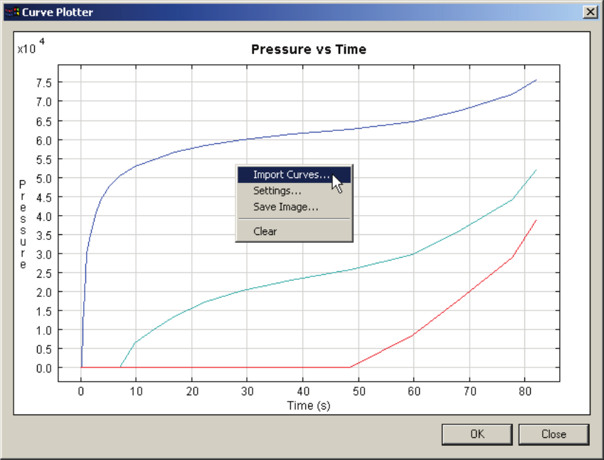
PAM-RTM 2014 201 USER’S GUIDE & TUTORIALS
© 2014 ESI Group (released: Apr-14)
TUTORIALS
Central Injection
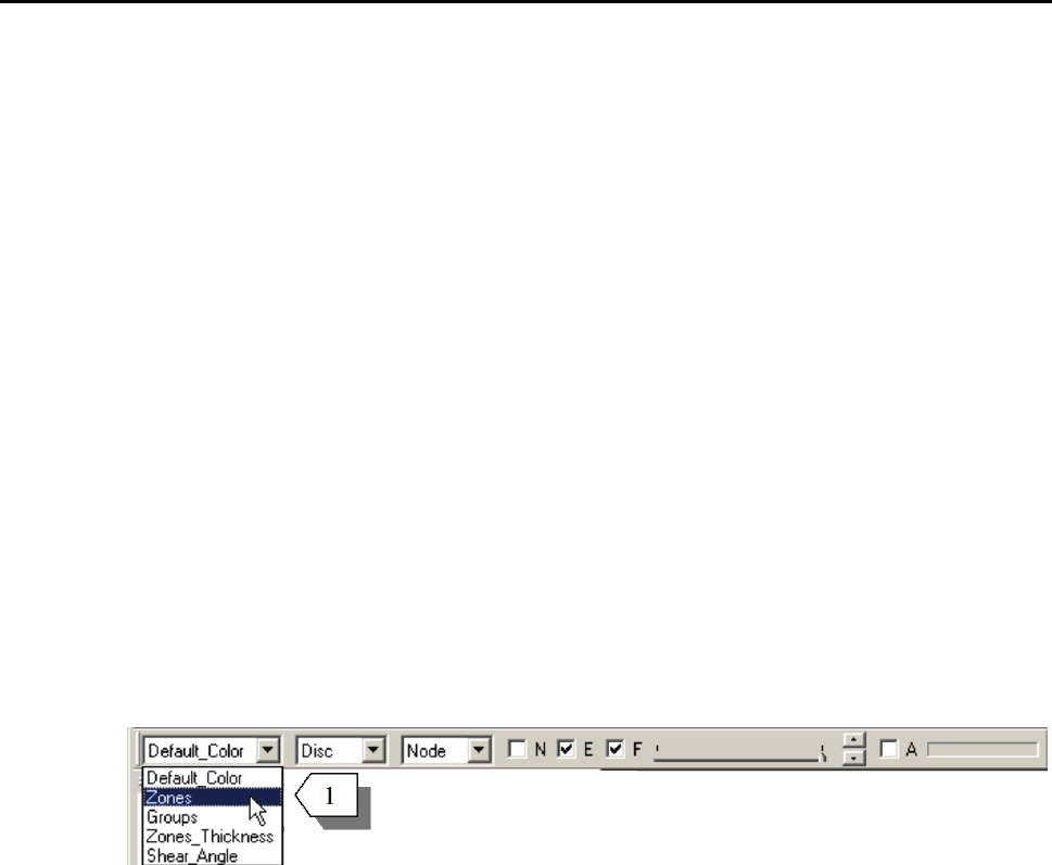
USER’S GUIDE & TUTORIALS 202 PAM-RTM 2014
(released: Apr-14) © 2014 ESI Group
TUTORIALS
Edge Effects – Rectangular Plate
EDGE EFFECTS – RECTANGULAR PLATE
The files related to this example are:
- rect_edge_start.unv (starting mesh)
- rect_edge.dtf + rect_edge.unv (solution)
Objective
In this example, a rectangular plate is injected from one side. The plate contains a
special zone along one edge, in which the resin flows more quickly. This phenomenon,
quite common in RTM, is called race tracking.
Creation of Groups and Visualization of Zones
Create a new simulation , use File ->New command and choose the RTM simulation
type.
The mesh provided for this tutorial doesn’t contain any group, so the first step is to
define groups of nodes for the injection and vent boundary conditions.
Import the file rect_edge_start.unv with the menu File->Import->Mesh.
Select Zones in the scalar field combo box [1].
Notice in the zones image that 2 zones are defined. Zone number 11 will be used for
race tracking. We will assign it a material with higher permeability than the
permeability of zone 9.
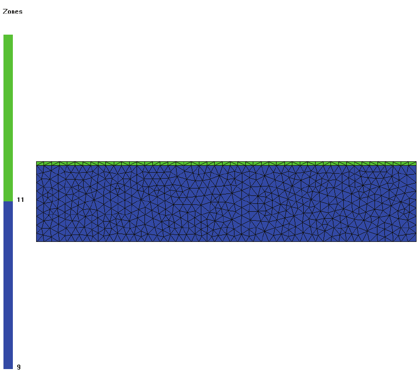
PAM-RTM 2014 203 USER’S GUIDE & TUTORIALS
© 2014 ESI Group (released: Apr-14)
TUTORIALS
Edge Effects – Rectangular Plate
Now we will create 2 groups of nodes, one for the pressure boundary condition on the
left side of the rectangle, and one for the vent on the right side.
- Click on N to activate visualization of nodes [1].
- Select Groups in the scalar field combo box to view nodes colored according to the
group ID [2].
- Drag the mouse to select the nodes on the left [3].
- Choose Groups->Create. This creates a group with ID = 1.
- Select the nodes on the right.
- Choose Groups->Create. A group with ID = 2 is created.
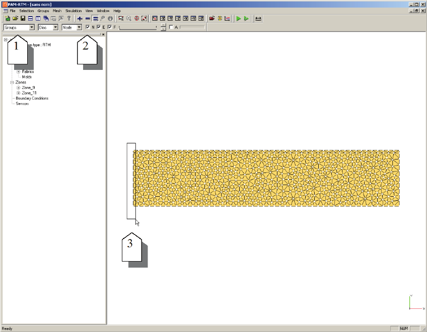
USER’S GUIDE & TUTORIALS 204 PAM-RTM 2014
(released: Apr-14) © 2014 ESI Group
TUTORIALS
Edge Effects – Rectangular Plate
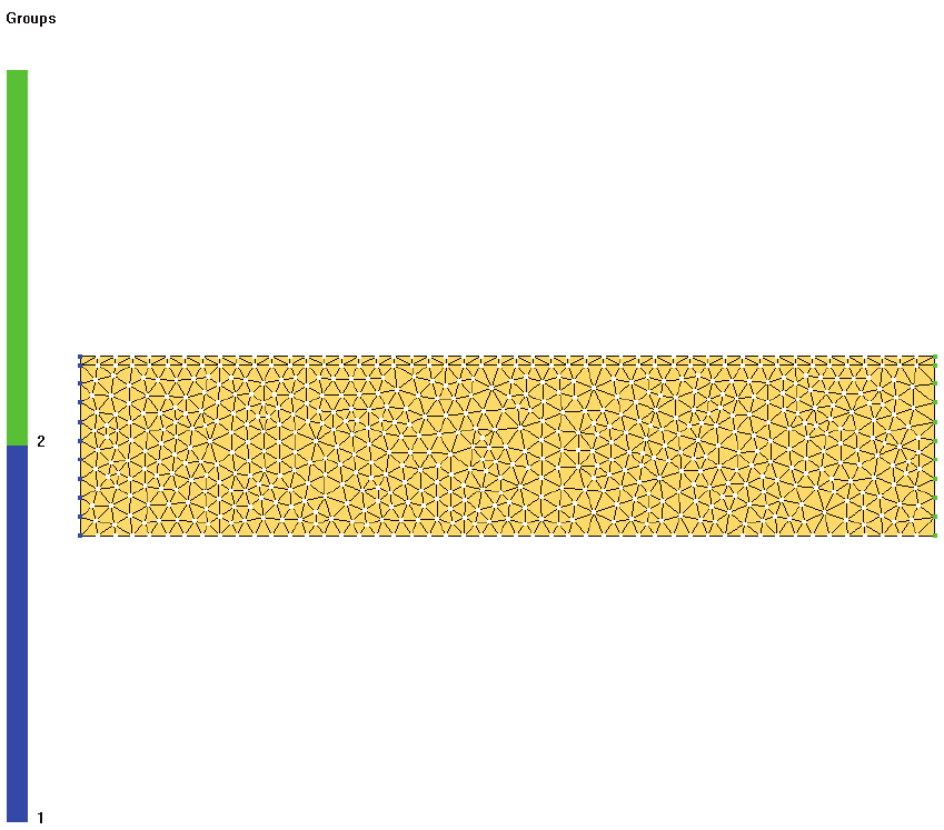
PAM-RTM 2014 205 USER’S GUIDE & TUTORIALS
© 2014 ESI Group (released: Apr-14)
TUTORIALS
Edge Effects – Rectangular Plate
Simulation
Double–click on Default Fabric and give the value 1.10-10 m2 to the components of the
permeability tensor K1, K2, K3.
Create a new reinforcement (of type fabric). Name it Runner and define its
permeability to 1.10-9 m2, so the permeability of this zone will be ten times larger than
the rest of the cavity.
Click on Zones, verify that the material assigned to zone 9 is Default Fabric with a
porosity of 0.5 and that the material of zone 11 is Runner. Give the value of 1 to the
porosity of zone 11. This means that this region doesn’t contain any fibers.
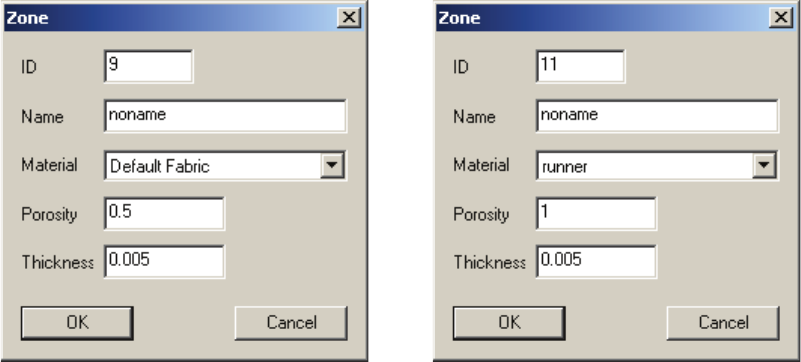
USER’S GUIDE & TUTORIALS 206 PAM-RTM 2014
(released: Apr-14) © 2014 ESI Group
TUTORIALS
Edge Effects – Rectangular Plate
Note:
· Zones used for race tracking have a porosity of 1. However a reinforcement has
to be assigned to these zones even if they don’t contain any fibers.
Right-click on Boundary Conditions, select Pressure as type of boundary condition.
Enter the number of the group 1 and set a constant injection pressure of 1.105 Pa. Set
group 2 to type Vent and set its pressure to zero.
Save the simulation parameters file with File->Save and give it the name
my_edge.dtf. Launch the simulation with the Start button.
Visualization of Results
Import the filling results by clicking on Reload Results button. Choose Filling in the
scalar field toolbar and click on the A check box to animate the filling results. Then
have a look at the pressure field.
An interesting visualization feature is the Filling_Times scalar field which shows in
only one picture the evolution of the resin front during the injection. You should have
the following picture. Notice how the resin flows more easily along the top edge.

PAM-RTM 2014 207 USER’S GUIDE & TUTORIALS
© 2014 ESI Group (released: Apr-14)
TUTORIALS
Edge Effects – Rectangular Plate
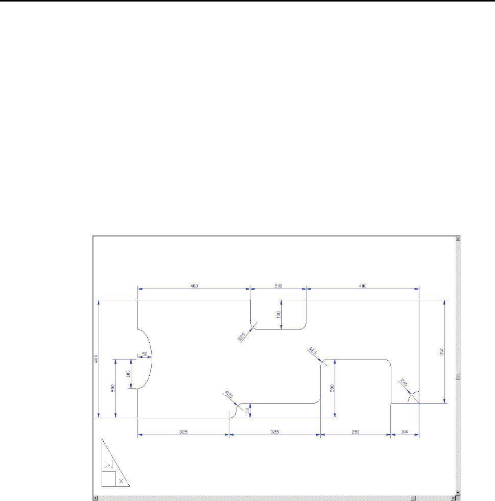
USER’S GUIDE & TUTORIALS 208 PAM-RTM 2014
(released: Apr-14) © 2014 ESI Group
TUTORIALS
Edge Effects – Complex Shape
EDGE EFFECTS – COMPLEX SHAPE
The files related to this example are:
- complex_edge_start.unv (starting mesh)
- complex_edge.dtf + complex_edge.unv (solution)
Objective
This example is an extension of the previous case. The mesh provided with this
example was created from the drawing below. We don’t give the details of how to
create such a geometry. We assume that the PAM-RTM™ user already knows a CAD
software and mesh generator. The most time consuming task in creating this geometry
is the definition of the race tracking zones. A thin zone of two millimeters width must
be added along the edges of the cavity, in which the resin will flow more quickly.
Visualization of Groups and Zones
The pictures below show the groups and the zones defined in the mesh file.
Drawing and dimensions of the plate.
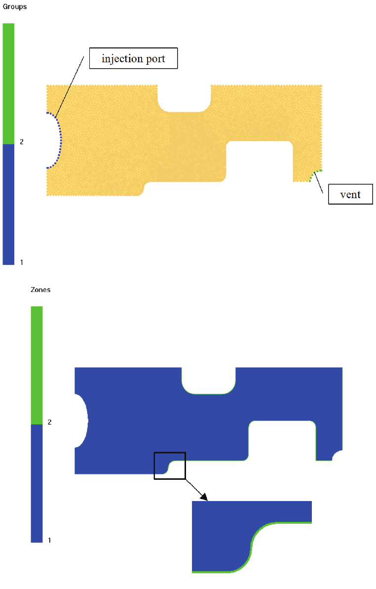
PAM-RTM 2014 209 USER’S GUIDE & TUTORIALS
© 2014 ESI Group (released: Apr-14)
TUTORIALS
Edge Effects – Complex Shape
USER’S GUIDE & TUTORIALS 210 PAM-RTM 2014
(released: Apr-14) © 2014 ESI Group
TUTORIALS
Edge Effects – Complex Shape
Simulation
This section describes the parameters required to carry out this simulation:
General Simulation Parameters
Simulation type: RTM
Geometry file: complex_edge_start.unv
Materials
The equivalent permeability of an empty channel of diameter D for a Poiseuille flow is:
K = D2/12
Krunner = (2mm)2/12 = 3,3 10-7 m2
This is the permeability we will use here for the runner all around the part.
Set the following properties :
- Resin: constant viscosity at 0.2 Pa.s
- Default fabric: K1 = K2 = 3 10-9 m2
K3 = 1 10-9 m2
- Runner: K1 = K2 = K3 = 3,3 10-7 m2
Zones
Define the central zone (the one with the largest area) with the Default Fabric. Its
porosity is 0.6 and thickness 0.003 m. For zone 2, the material to select is Runner with
a thickness of 0.003 m and a porosity of 1.
Boundary Conditions
Define group 1 as an injection boundary condition of type Pressure with a constant
injection pressure of 3 105 Pa. Define group 2 as a vent.
Simulation
Save the simulation parameters file under the name my_complex_edge.dtf and
launch the simulation.
Here are the filling and pressure results at the end of injection.

PAM-RTM 2014 211 USER’S GUIDE & TUTORIALS
© 2014 ESI Group (released: Apr-14)
TUTORIALS
Edge Effects – Complex Shape
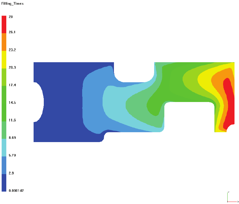
USER’S GUIDE & TUTORIALS 212 PAM-RTM 2014
(released: Apr-14) © 2014 ESI Group
TUTORIALS
Edge Effects – Complex Shape

PAM-RTM 2014 213 USER’S GUIDE & TUTORIALS
© 2014 ESI Group (released: Apr-14)
TUTORIALS
Fiber Orientations
FIBER ORIENTATIONS
The following files will be used:
- deltoid_start.unv (starting mesh)
- deltoid.dtf + deltoid.unv (solution)
Objective
This tutorial shows how to specify fiber orientations in a T-junction.
Test Part
The length of the part is 0.3 m. Two layers of reinforcement of thicknesses t1 and t2 are
considered. The total height is h=0.2 m. The injection is performed through the left wall
with a resin of viscosity 0.02 Pa.s. Special attention should be paid to the permeability
values in the three directions K1, K2 and K3. Two materials will be used: one fabric in
the deltoid zone with a lower isotropic permeability, and another fabric in the other
zones.
Fiber Orientations
Begin by creating a new RTM simulation and import the mesh file
deltoid_start.unv.
The orientations of the permeability tensor can now be defined. To do so, it is important
to visualize the different zones. In the display toolbar, select Zones, activate Edges and
Faces, deactivate Nodes.
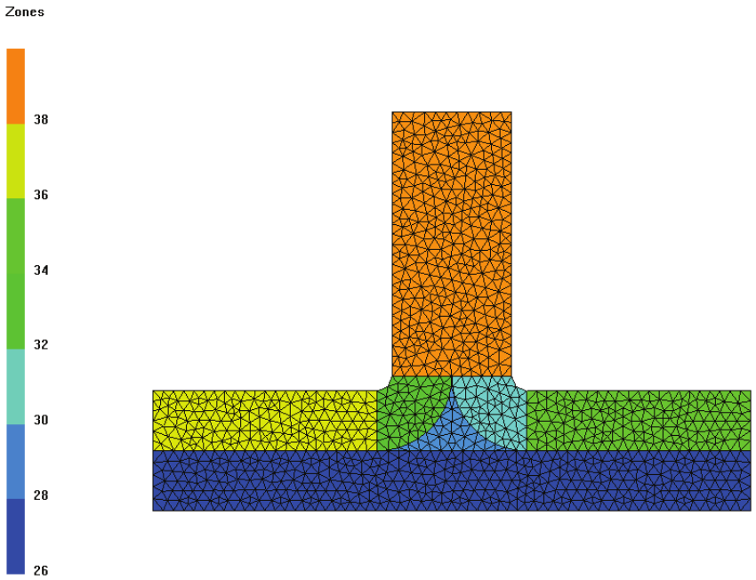
USER’S GUIDE & TUTORIALS 214 PAM-RTM 2014
(released: Apr-14) © 2014 ESI Group
TUTORIALS
Fiber Orientations
Here is what will appear on the screen:
The fiber orientations must be specified in every zone, except in zone 28 (middle zone
of the deltoid), where it is not necessary since permeability is isotropic in this region.
The simpler zones, where the fibers are oriented along x and y as principal axes, will be
defined first.
We will first select the elements on which we want to specify orientations using zone
selection.
Set the selection filter in the main toolbar to Face (or use Selection->Face from the
menu).
There are several ways to select a zone :
- Click Selection->Zone ID [1], a dialog box pops up enabling to enter the zone ID.

PAM-RTM 2014 215 USER’S GUIDE & TUTORIALS
© 2014 ESI Group (released: Apr-14)
TUTORIALS
Fiber Orientations
- Click Selection-> Pick zone [2] and pick one element of the zone to select.
- Right-click on zone_ID and choose Select.

USER’S GUIDE & TUTORIALS 216 PAM-RTM 2014
(released: Apr-14) © 2014 ESI Group
TUTORIALS
Fiber Orientations
Select elements in zones 26, 34 and 36 (horizontal parts). Then, open the Material
Orientations dialog box (Mesh->Orientations->Set Vectors).
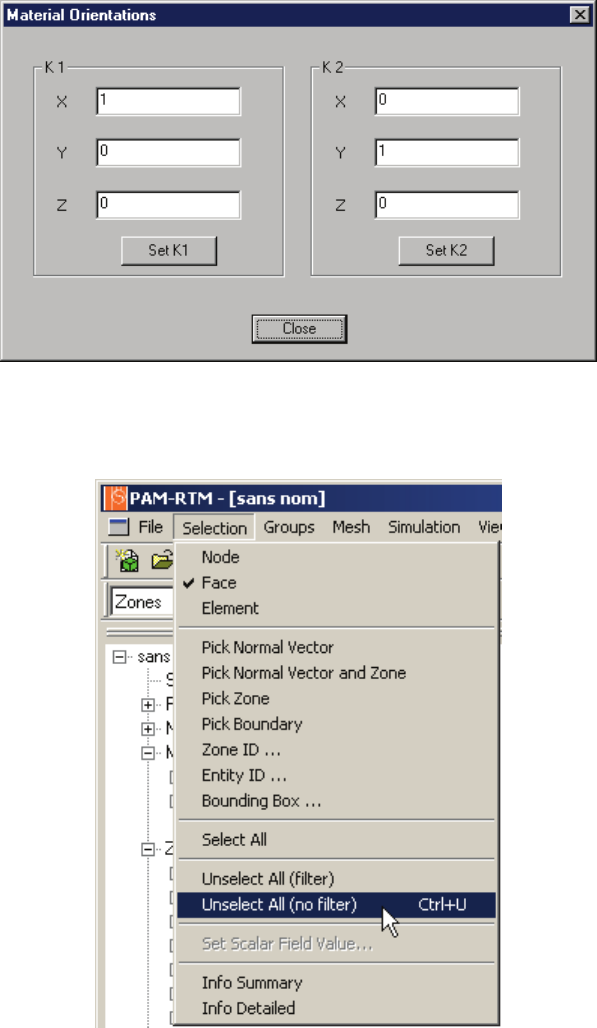
PAM-RTM 2014 217 USER’S GUIDE & TUTORIALS
© 2014 ESI Group (released: Apr-14)
TUTORIALS
Fiber Orientations
Define K1 (1,0,0) and click the Set K1 button. This permeability will be defined for each
of the selected zones. Define K2 (0,1,0) and click the Set K2 button. Close the window
by clicking the Close button. Then clear the current selection (Selection->Unselect All).
In the same way, select the elements in zone 38 (vertical part). Open the Materials
Orientations dialog box and define K1 (0,1,0) and K2 (1,0,0).
We are now ready to work on the two curved sections. Clear all the selections with
Selection->Unselect All. Select the desired zone, say zone 32 (one of the two curved
zones). Then in the display toolbar, click the N button to activate node display. Next, in
the Selection menu, choose Nodes.
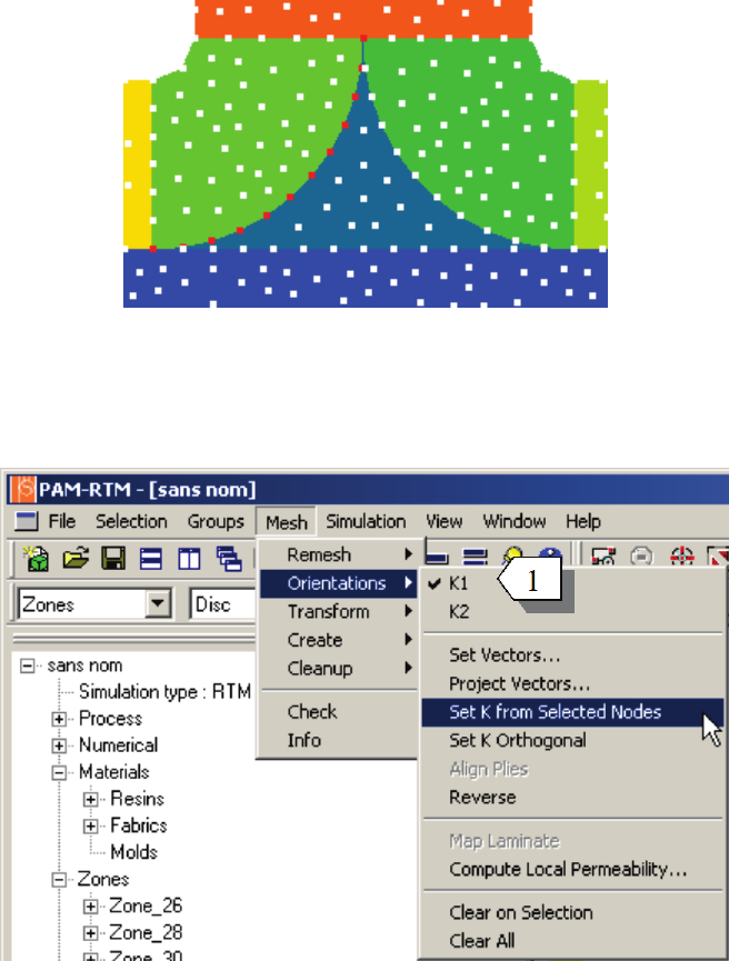
USER’S GUIDE & TUTORIALS 218 PAM-RTM 2014
(released: Apr-14) © 2014 ESI Group
TUTORIALS
Fiber Orientations
Using the mouse and clicking on the nodes of interest, you can select the nodes that will
define the orientation of the fibers. They will appear in red once the selection is made.
The order of selection is important. Select them from left to right or from right to left.
As soon as this step is completed, the fiber orientations can be defined. First of all, in
the selection menu, choose Face, and select zone 32. Set the current working direction
as K1 with Mesh->Orientations->K1 [1]. From the same menu, select Set K From
Selected Nodes (this should be understood as Set K1 From Selected Nodes).
The selected elements are projected on a curve constructed from the selected nodes. The
tangent vector at the projected point indicates the orientation of the fibers. Permeability
K1 is now defined in zone 32. Permeability K2 remains to be specified from the menu
Mesh->Orientations. After having selected K2 [1], choose the submenu Set K Orthogonal
(meaning Set K2 Orthogonal to K1).
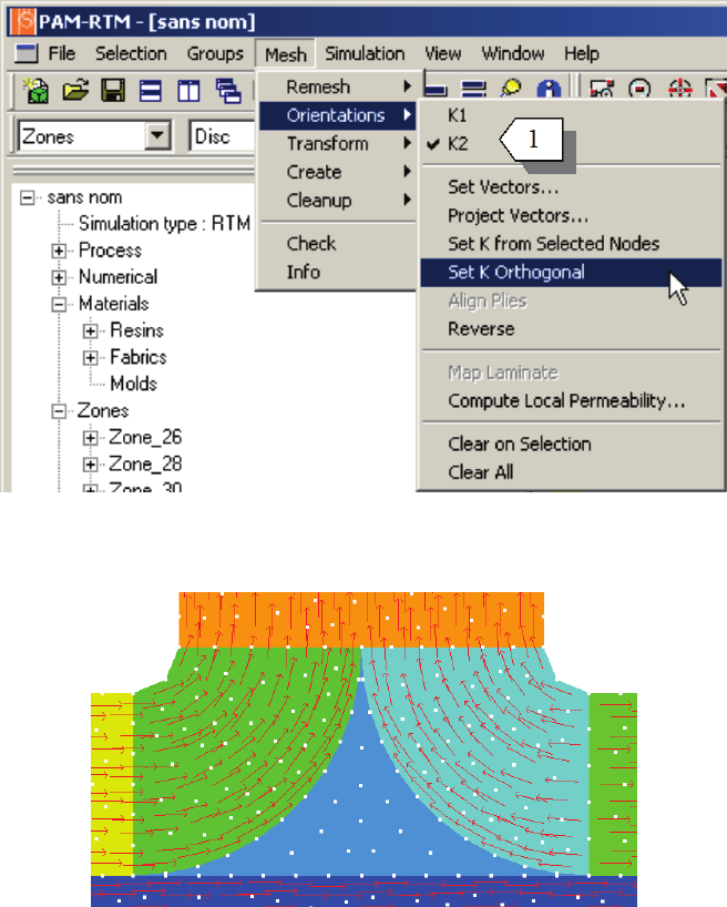
PAM-RTM 2014 219 USER’S GUIDE & TUTORIALS
© 2014 ESI Group (released: Apr-14)
TUTORIALS
Fiber Orientations
Clear all current selections and restart the same procedure with elements of zone 30.
Once completed, the orientations of the fibers appear as follows:
To view orientations, select View->Orientations->K1 Only.

USER’S GUIDE & TUTORIALS 220 PAM-RTM 2014
(released: Apr-14) © 2014 ESI Group
TUTORIALS
Fiber Orientations
Now, set the permeability of the reinforcement. Double-click on default Fabric and click
on the … button [1]. This opens the Function Editor dialog box, which lets you assign a
curve or a constant value to the parameter:
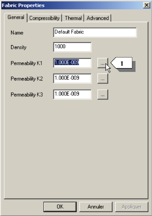
PAM-RTM 2014 221 USER’S GUIDE & TUTORIALS
© 2014 ESI Group (released: Apr-14)
TUTORIALS
Fiber Orientations
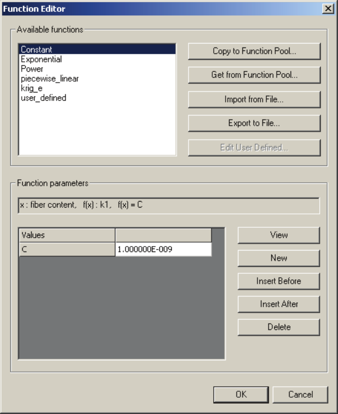
USER’S GUIDE & TUTORIALS 222 PAM-RTM 2014
(released: Apr-14) © 2014 ESI Group
TUTORIALS
Fiber Orientations
Set the permeability for the Default Fabric to K1=1 10-11 K2=1 10-12 K3=1 10-11
Create a new Fabric (Material->New->Fabric), name it deltoid and set the isotropic
permeability to K1=K2=K3=1 10-13
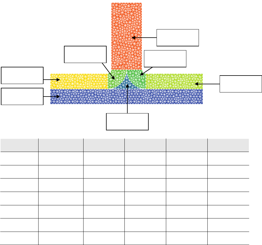
PAM-RTM 2014 223 USER’S GUIDE & TUTORIALS
© 2014 ESI Group (released: Apr-14)
TUTORIALS
Fiber Orientations
The following table summarizes the permeability assigned to each
zone.
Zone N° Material K1 K2 K3 Porosity
26 Default fabric 1E-11 1E-12 1E-11 0.5
28 Deltoid 1E-13 1E-13 1E-13 0.4
30 Default fabric 1E-11 1E-12 1E-11 0.5
32 Default fabric 1E-11 1E-12 1E-11 0.5
34 Default fabric 1E-11 1E-12 1E-11 0.5
36 Default fabric 1E-11 1E-12 1E-11 0.5
38 Default fabric 1E-11 1E-12 1E-11 0.5
For every zone, you must also specify the porosity of the reinforcement (see previous
table) and its thickness (0.005 m).
Define properties of the resin, set a constant viscosity of 0.02 Pa.s.
The boundary conditions still remain to be defined. Three groups are available. Assign
Pressure to the one that corresponds to the injection line (left side). Enter a constant
pressure value of 2 105 Pa. Then, define the other two lines as vents.
Now choose File->Save and run the simulation.
Note:
· It is important to save this file before launching a simulation, otherwise the
changes you made to the simulation parameters won’t be used in the simulation.
Zone 38
Zone 30
Zone 34
Zone 28
Zone 32
Zone 26
Zone 36
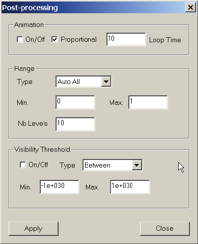
USER’S GUIDE & TUTORIALS 224 PAM-RTM 2014
(released: Apr-14) © 2014 ESI Group
TUTORIALS
Fiber Orientations
Visualizing the Simulation Results
Many post-processing parameters can be changed in the Post-processing dialog box by
selecting View –> Post-Processing.
After loading the simulation results, choose the Filling option in the drop-down list to
visualize the evolution of injection. Then by sliding the Time Step control arrow in the
tool bar, the filling of the mold is displayed in time. By clicking on the button A
(animation), an animated display of mold filling is activated. The animation speed can
be modified by changing the Loop Time field in the Post-processing dialog box.
To get a smooth injection flow front, select the Type Iso in the drop-down list. The
number of colors may be modified in the Nb levels field in the Post-processing dialog
box.

PAM-RTM 2014 225 USER’S GUIDE & TUTORIALS
© 2014 ESI Group (released: Apr-14)
TUTORIALS
Fiber Orientations
The figure below shows the different positions of the flow front in time in the part.
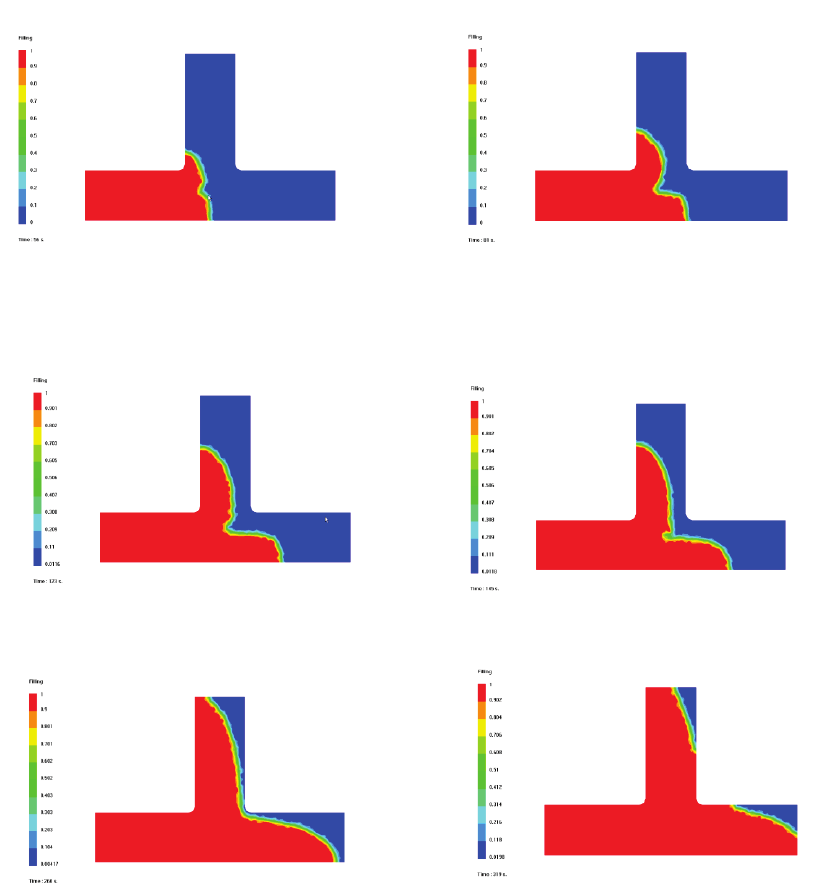
USER’S GUIDE & TUTORIALS 226 PAM-RTM 2014
(released: Apr-14) © 2014 ESI Group
TUTORIALS
Fiber Orientations
The following figures show sequentially how the mold is filled:
The injection is performed from the left side of the part. The lower permeability in the
central zone of the junction delays the flow front in that zone.
The pressure field can also be visualized during the injection. Select Pressure in the
drop-down list in the display toolbar.
It is sometimes useful to visualize the resin front on top of another scalar field such as
the pressure or temperature field. To do so, select File–> Import–> Scalar Fields –> PAM-
RTM Flow Front (.front)… , then under the Import PAM-RTM Flow Front dialog box, select
the flow front file and click Open.
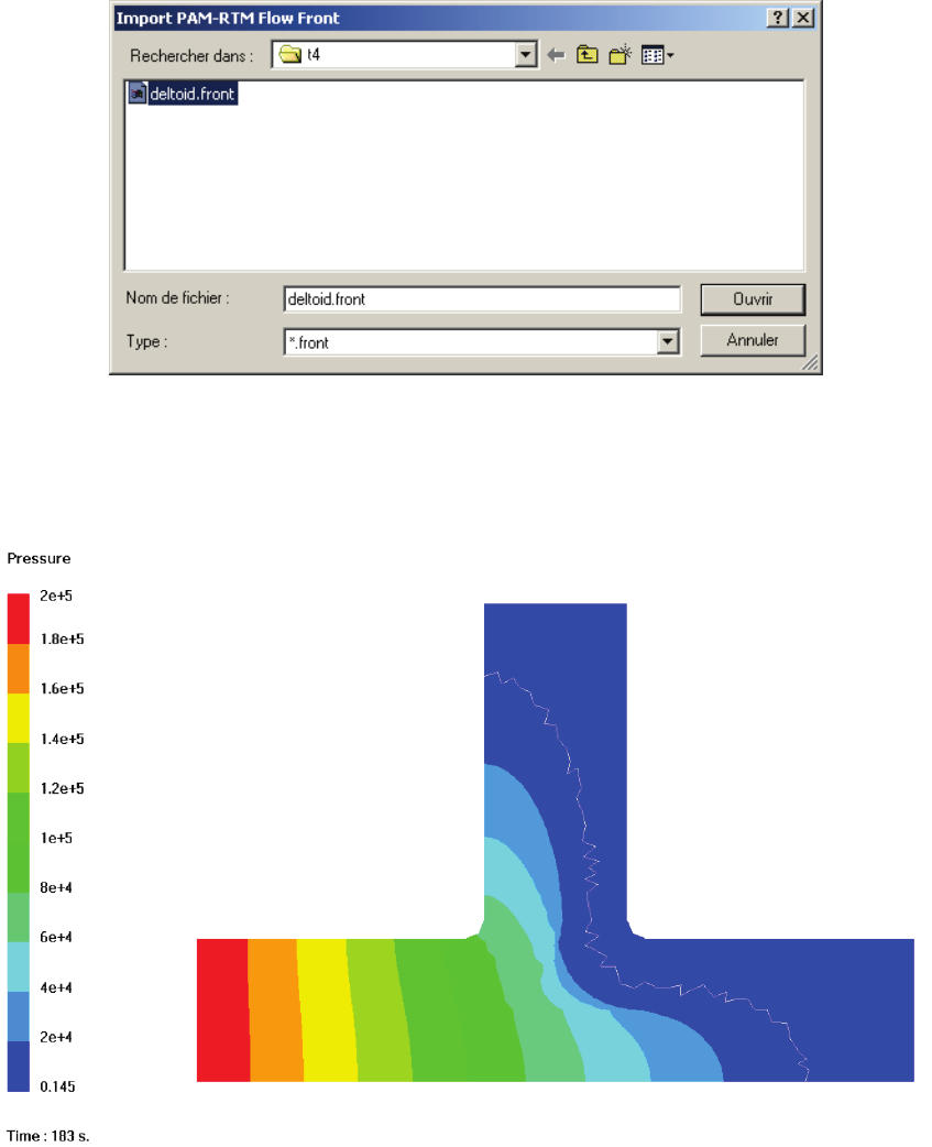
PAM-RTM 2014 227 USER’S GUIDE & TUTORIALS
© 2014 ESI Group (released: Apr-14)
TUTORIALS
Fiber Orientations
The following image is displayed, in which the flow front appears as a white line. This
is the raw position of the flow front, without any smoothing. On one side of the flow
front, the elements are completely saturated (filling factor = 1), while on the other side
elements are partially saturated or empty (0 <= filling factor < 1).

USER’S GUIDE & TUTORIALS 228 PAM-RTM 2014
(released: Apr-14) © 2014 ESI Group
TUTORIALS
Comparison 2D – 2.5D – 3D
COMPARISON 2D – 2.5D – 3D
The following files are used in this example.
- comparison_2D_start.unv, comparison_25D_start.unv, comparison_3D_start.unv
(starting mesh)
- comparison_2D.dtf + comparison_2D.unv (solution for 2D)
- comparison_25D_1.dtf, comparison_25D_2.dtf, + comparison_25D.unv (solution for
2.5D)
- comparison_3D_1.dtf, comparison_3D_2.dtf, + comparison_3D.unv (solution for 3D)
Introduction
Description of the Part
This example describes the results obtained for a part whose dimensions are specified in
the figure below:
The injection is performed at a constant pressure of 2 bars from each extremity of the
part as illustrated on the figure below:

PAM-RTM 2014 229 USER’S GUIDE & TUTORIALS
© 2014 ESI Group (released: Apr-14)
TUTORIALS
Comparison 2D – 2.5D – 3D
Objectives of the Analysis
The objectives of this analysis is to study the position of the resin front and to compare
the results obtained from three types of mesh:
- 2D plane mesh of triangles
- 2.5D surface mesh (thin shell) with triangular shell elements
- 3D solid mesh of tetrahedrons
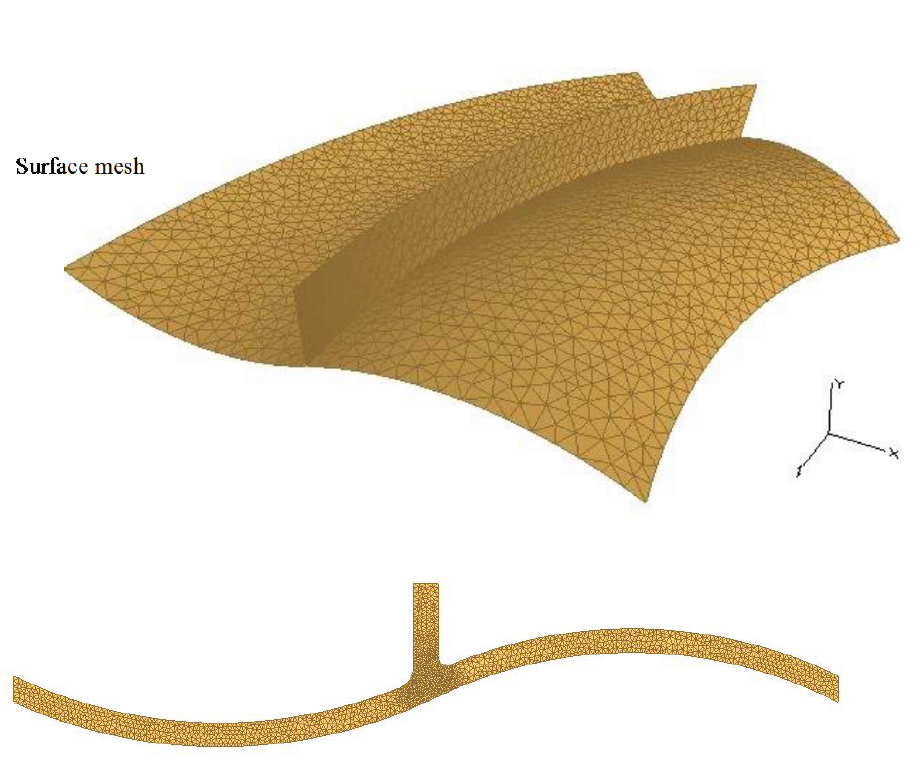
USER’S GUIDE & TUTORIALS 230 PAM-RTM 2014
(released: Apr-14) © 2014 ESI Group
TUTORIALS
Comparison 2D – 2.5D – 3D
Description of a Typical Rib Junction
The permeability of the reinforcement is K1 = K2 =K3 = 1.10-9 m2 and the porosity is
φ
=
0.5. The rib junction is constructed with unidirectional fibers to fill the internal volume
between the two top folded plies and the inferior layers in order to create the T shape.
The permeability of the reinforcement in the rib junction (shaded area in the figure
below) is K1 = K2 = K3 = 1.10-10 m2.
Plane mesh
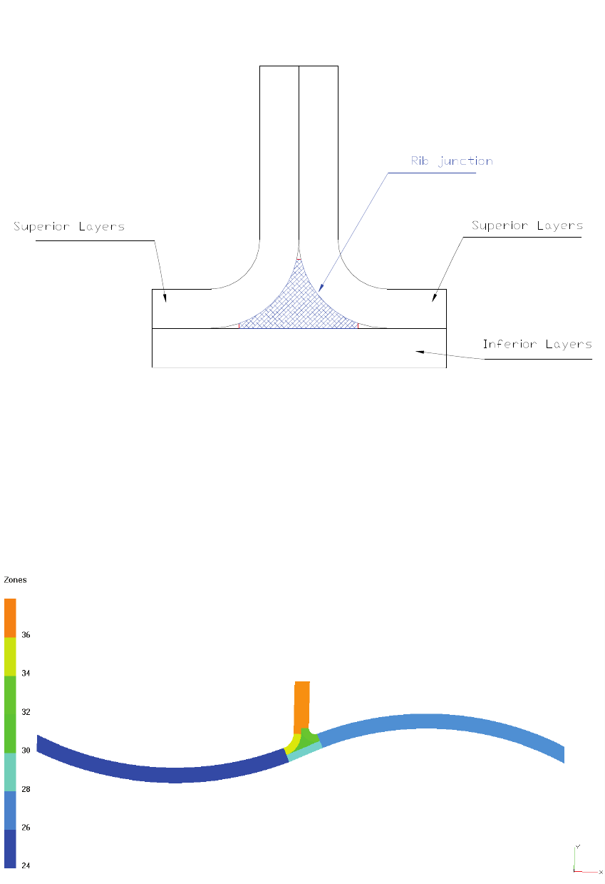
PAM-RTM 2014 231 USER’S GUIDE & TUTORIALS
© 2014 ESI Group (released: Apr-14)
TUTORIALS
Comparison 2D – 2.5D – 3D
Typical rib junction (T shape)
Zones of the Part
The analysis was carried out in order to compare the results between a 2D simulation
with analyses performed with shell (2.5D) and solid (3D) elements. The following
figures show the different permeability zones for each type of simulation.
(a) 2D zones
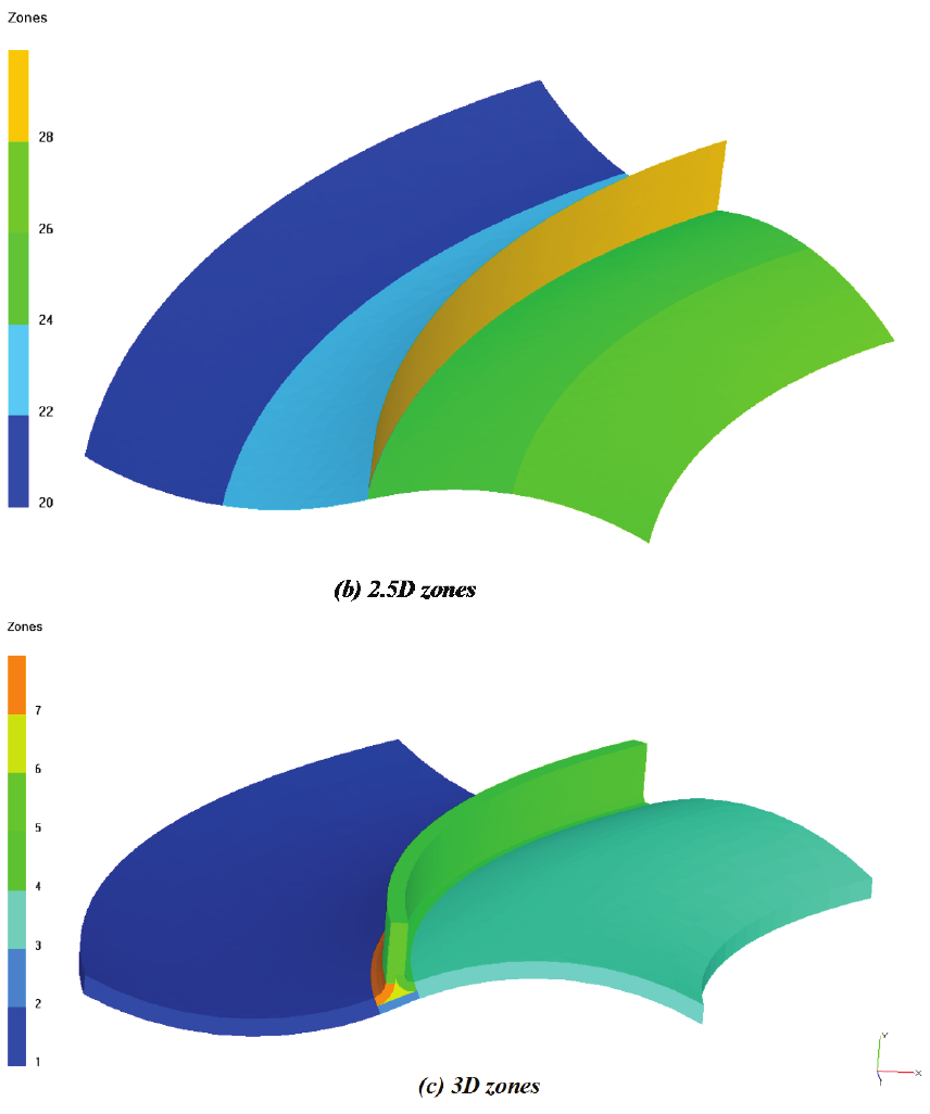
USER’S GUIDE & TUTORIALS 232 PAM-RTM 2014
(released: Apr-14) © 2014 ESI Group
TUTORIALS
Comparison 2D – 2.5D – 3D
Zones for the three types of mesh:
We can immediately notice several differences. Indeed, in the surface simulation, there
is no central zone at the junction. The zones used in the 2D simulation do not consider
the curvature of the part. These topics will be discussed later.
Injection Strategies
The following table indicates the injection pressure used for each experiment.
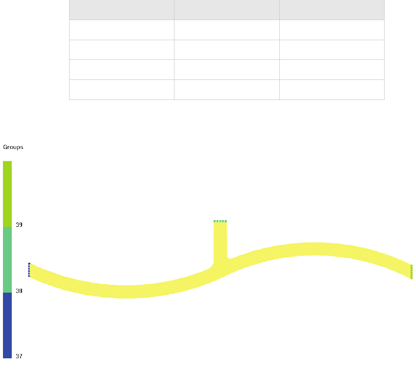
PAM-RTM 2014 233 USER’S GUIDE & TUTORIALS
© 2014 ESI Group (released: Apr-14)
TUTORIALS
Comparison 2D – 2.5D – 3D
Simulation
Pinj 1
Pinj 2
2D
2 bars
2 bars
2.5 D/1
2 bars
2 bars
2.5 D/2
2 bars
2.3 bars
3 D
2 bars
2 bars
The following figures show the groups of nodes that define the injection boundary
conditions:

USER’S GUIDE & TUTORIALS 234 PAM-RTM 2014
(released: Apr-14) © 2014 ESI Group
TUTORIALS
Comparison 2D – 2.5D – 3D
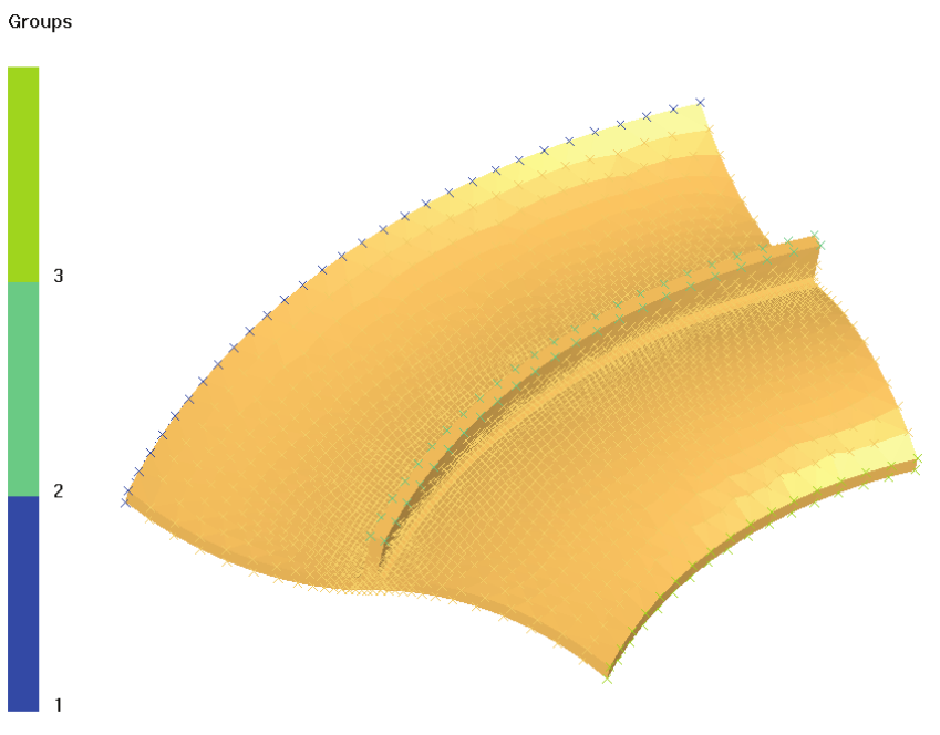
PAM-RTM 2014 235 USER’S GUIDE & TUTORIALS
© 2014 ESI Group (released: Apr-14)
TUTORIALS
Comparison 2D – 2.5D – 3D
Simulation Results
Filling Times
The first interesting point to verify here is the injection time required to fill the mold for
each type of analysis. The filling times are in fact very similar, between 19.9 and 21.3
seconds for the three simulations. This demonstrates the consistency between the
different options offered by the software.
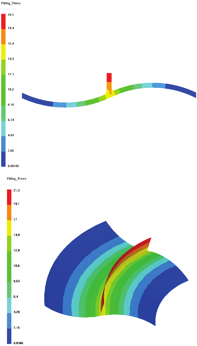
USER’S GUIDE & TUTORIALS 236 PAM-RTM 2014
(released: Apr-14) © 2014 ESI Group
TUTORIALS
Comparison 2D – 2.5D – 3D
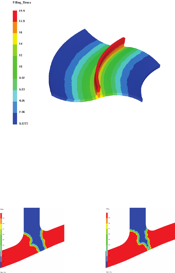
PAM-RTM 2014 237 USER’S GUIDE & TUTORIALS
© 2014 ESI Group (released: Apr-14)
TUTORIALS
Comparison 2D – 2.5D – 3D
Special Effects in the Rib Junction
However, several differences exist between the different types of simulation. The 2D
simulation shows the details of the filling in the T junction, which is naturally not
possible with the 2.5D results. An air bubble is formed in the T junction as illustrated
below by a series of filling results at different injection times. Although a 2D simulation
allows observation of local effects, it does not give a 3D picture of mold filling. As a
matter of fact, the whole geometry of the part has an influence on the filling pattern.

USER’S GUIDE & TUTORIALS 238 PAM-RTM 2014
(released: Apr-14) © 2014 ESI Group
TUTORIALS
Comparison 2D – 2.5D – 3D
This air bubble could possibly be removed
by the pressure field up to the vent. Note
that this is no longer a problem if the
injection is performed under vacuum.
Convergent and Divergent Flows
A surface simulation (2.5D) allows to compare the injection pressure with a 2D
analysis. Note that the resin front does not merge near the rib like in the 2D analysis,
but on the right panel, where the flow is divergent. As a matter of fact, the resin flow
converges in the left panel and diverges in the right panel. This difference in geometry
accelerates the resin flow in the convergent geometry as shown in the figure below:

PAM-RTM 2014 239 USER’S GUIDE & TUTORIALS
© 2014 ESI Group (released: Apr-14)
TUTORIALS
Comparison 2D – 2.5D – 3D
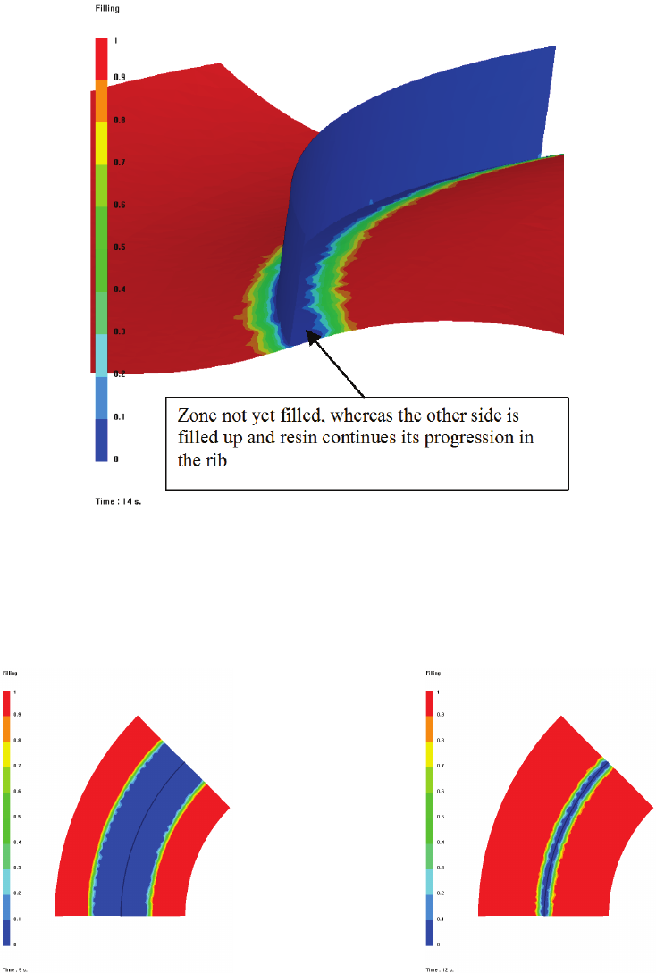
USER’S GUIDE & TUTORIALS 240 PAM-RTM 2014
(released: Apr-14) © 2014 ESI Group
TUTORIALS
Comparison 2D – 2.5D – 3D
Although the injection pressure is the same on both sides, the left panel fills up faster
than the right one. The surface simulation, and not the plane simulation, could show this
phenomenon, which is due to resin flows in convergent versus divergent geometries.
Modification of the Injection Pressure on one Side
In order to merge the two resin fronts in the center of the part, it is possible to inject
from one side at 2 bars and from the other at 2.3 bars. The flow fronts merge then right
in the middle of the part at the rib connection as illustrated in the figures below:

PAM-RTM 2014 241 USER’S GUIDE & TUTORIALS
© 2014 ESI Group (released: Apr-14)
TUTORIALS
Comparison 2D – 2.5D – 3D
The selection of two different injection pressures permits to merge the resin fronts in the center of the
part, i.e., directly at the rib junction
The need to inject with two different pressures would not have appeared without performing a surface
simulation.
3D Solid Simulations
Although surface simulations (2.5D analysis) provide a global vision on the filling of
the part, no local effects are shown such as how the two incoming resin fronts merge in
the T junction for example (where it was seen that air bubbles form). 3D solid
simulations visualize such problems. Both global and local effects will appear at the
same time: convergent and divergent flux phenomena, as well as air bubbles in the rib
junction. However, the time required to model the geometry of the part, generate the 3D
mesh and especially, the calculation time to simulate the injection, becomes much more
important.
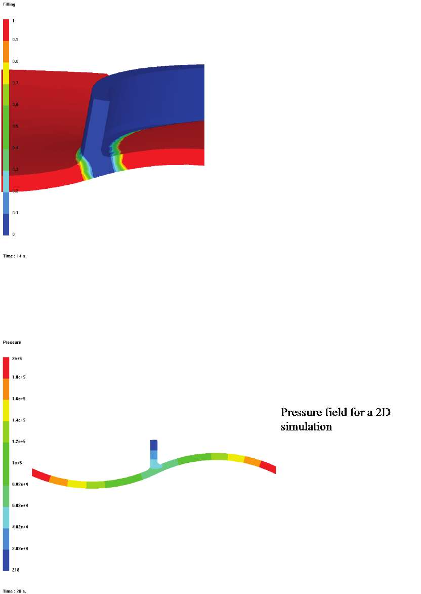
USER’S GUIDE & TUTORIALS 242 PAM-RTM 2014
(released: Apr-14) © 2014 ESI Group
TUTORIALS
Comparison 2D – 2.5D – 3D
Pressure Field in the Cavity
Finally, as illustrated by the images of next page, the analysis of the pressure field in the
cavity during the injection does not show much difference between the three types of
simulations considered here.
Geometry related effects can be studied
with a 3D simulation, which provide a
global vision. As shown in the figure
on the left, it is necessary to inject at a
higher pressure so that the resin fronts
will merge at the center of the part.
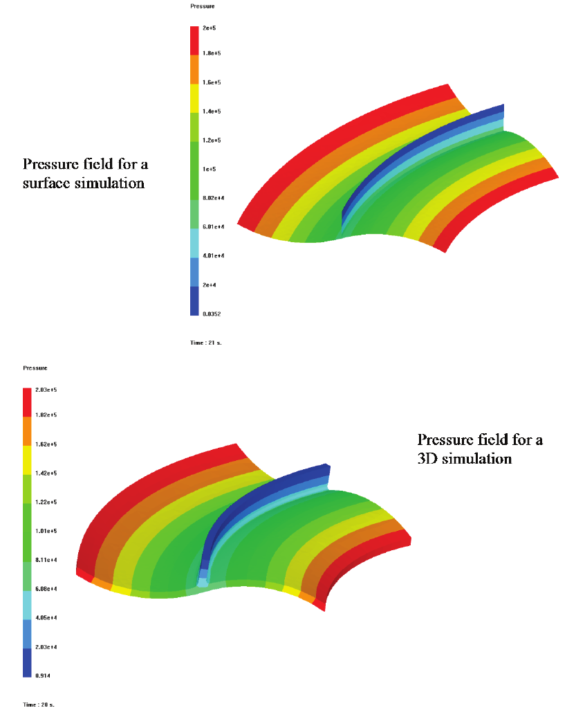
PAM-RTM 2014 243 USER’S GUIDE & TUTORIALS
© 2014 ESI Group (released: Apr-14)
TUTORIALS
Comparison 2D – 2.5D – 3D
Conclusion
In conclusion, a 3D simulation with solid elements allows observation of global and
local effects related to the geometry of the part. A surface simulation (2.5D) provides a
global vision at a reduced cost while a 2D simulation in a section of the part shows only
local effects. The advantage of a 2D simulation is the much reduced calculation time.

USER’S GUIDE & TUTORIALS 244 PAM-RTM 2014
(released: Apr-14) © 2014 ESI Group
TUTORIALS
Comparison 2D – 2.5D – 3D
3D simulations require a much larger number of elements to perform the calculations,
which causes the calculation times to increase dramatically.
The following table compares the numbers of elements used in this example with the
corresponding calculation times. The simulations were run on a dual processor Pentium
3 700 MHz PC.
Simulation
Number of elements
Simulation time
2D
3084 triangles
5 min., 8 s.
2.5D
3979 triangles
1 min, 25 s.
3D
35137 tetrahedrons
100 min.
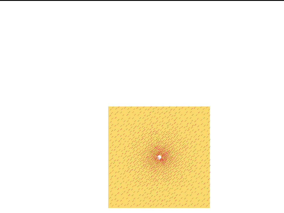
PAM-RTM 2014 245 USER’S GUIDE & TUTORIALS
© 2014 ESI Group (released: Apr-14)
TUTORIALS
Air Entrapment
AIR ENTRAPMENT
The files related to this example are:
- air_trap_start.unv (starting mesh)
- air_trap.dtf + air_trap.unv (solution)
Visualization of Groups and Orientations
In this tutorial, we do a central injection in a fabric with anisotropic permeability. Here
is a picture of the K1 principal permeability direction.
We use this simple example to demonstrate the air entrapment feature of PAM-
RTM™. We want to force creation of an air trap in the bottom right corner by closing
vents shortly after beginning of injection. Only the top left vent stays open during the
complete simulation.
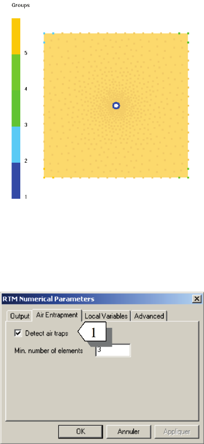
USER’S GUIDE & TUTORIALS 246 PAM-RTM 2014
(released: Apr-14) © 2014 ESI Group
TUTORIALS
Air Entrapment
These are the parameters that were used for this simulation:
- Input geometry file: air_trap_start.unv
- Simulation type: RTM
- Air entrapment: active [1]
- Resin viscosity: 0.1 Pa.s
- Permeability: K1 = 1E-9 m2, K2 = 1E-10 m2
- Porosity: 0.5
- Injection pressure: 2E5 Pa
- Vents’ pressure: 1E5 Pa
- Vent 2 stays open during the complete simulation (State = 1)
- Vents 3 and 5 closed at 85 s.
- Vent 4 closed at 120 s
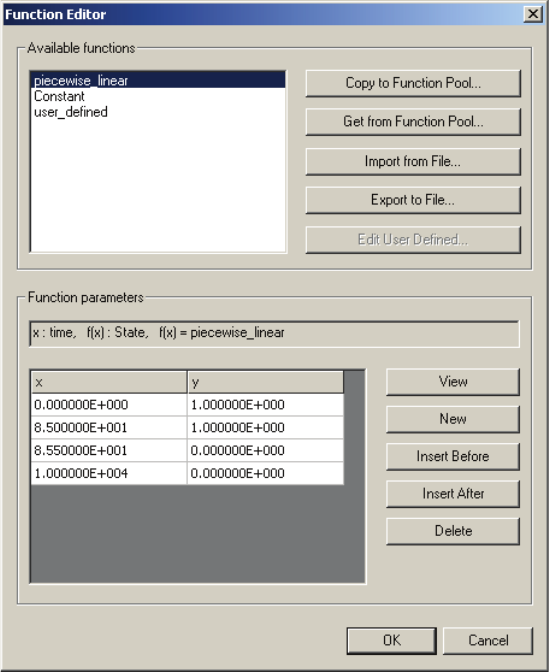
PAM-RTM 2014 247 USER’S GUIDE & TUTORIALS
© 2014 ESI Group (released: Apr-14)
TUTORIALS
Air Entrapment
To close a vent at a given time, open the Function Editor dialog box for the state
parameter of the boundary condition, and define a piecewise linear function as shown
below:
The anisotropic fabric leads to an elliptical flow front.
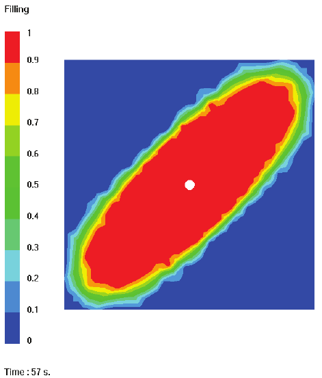
USER’S GUIDE & TUTORIALS 248 PAM-RTM 2014
(released: Apr-14) © 2014 ESI Group
TUTORIALS
Air Entrapment
To avoid air traps in the bottom left and top right corners, the vents are closed a short
time after the resin reaches them (t = 85 s.). The bottom right vent is kept open a little
longer. When it is closed (t = 120 s.), an air trap is detected by PAM-RTM™. The top
left vent stays open during the complete simulation, that’s why there is only one air trap
detected.
As soon as the air trap is detected, the pressure starts to increase in it. The law of perfect
gases Pressure * Volume = constant is used to manage the pressure increase as the
volume of the air trap changes. After some time, the pressure in the air trap becomes
very close to the injection pressure, which means that the pressure gradient is very small
and the resin can’t move. The simulation stops with some elements that are not filled.
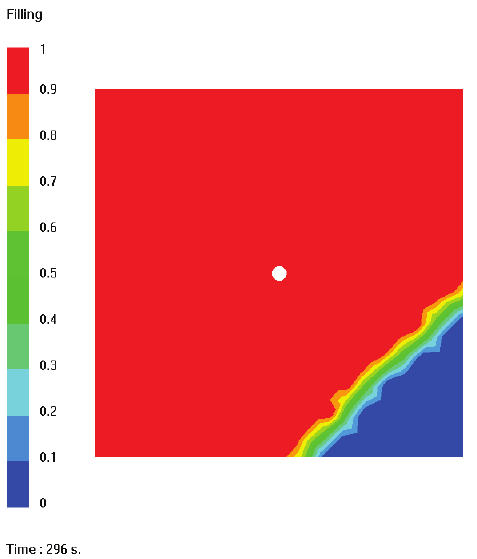
PAM-RTM 2014 249 USER’S GUIDE & TUTORIALS
© 2014 ESI Group (released: Apr-14)
TUTORIALS
Air Entrapment
The pressure specified in PAM-RTM™ is absolute pressure. For the air entrapment
option to work correctly, the vent pressure must be positive and not zero. In this
example, the vent is initially open and its pressure is 1E5 Pa (1 bar). The injection
pressure is 2 bars, so there is 1 bar pressure difference between the injection point and
the flow front. When the air trap is detected, its pressure is the same as the initial cavity
pressure (pressure on the vent), and it will rise as the air trap gets smaller.
You can visualize the flow front position on top of any scalar field by loading the flow
front file (extension .front) with File->Import->Scalar Fields->PAM-RTM Flow Front. The
flow front is displayed as a white line in the following pressure images.
Notice the pressure at the bottom left and top right corners. This “strange” pressure field
comes from the fact that the resin has reached the top left corner where the vent is still
open, so the pressure stays fixed at 1 bar. The last pressure image shows that the
pressure in the air trap at the end of the simulation is the same as the injection pressure.
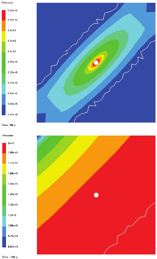
USER’S GUIDE & TUTORIALS 250 PAM-RTM 2014
(released: Apr-14) © 2014 ESI Group
TUTORIALS
Air Entrapment
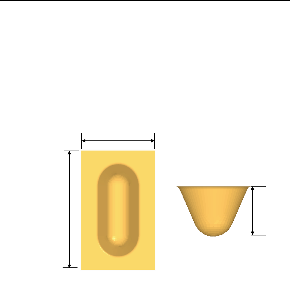
PAM-RTM 2014 251 USER’S GUIDE & TUTORIALS
© 2014 ESI Group (released: Apr-14)
TUTORIALS
Vacuum Assisted Resin Infusion (vari)
VACUUM ASSISTED RESIN INFUSION (VARI)
The following files will be used:
- vari_start.unv (starting mesh)
- vari.dtf + vari.unv (solution)
Objectives
This tutorial shows how to specify the parameters for a VARI simulation. The post-
filling, leading to the final thickness of the part calculation, after the injection port has
been closed will also be simulated. Two cases will be run, one where vents will stay
open, and the other one where vents will be closed.
Mesh Modification
Create a new VARI simulation with File->New and import the mesh file
vari_start.unv.
The mesh provided for this tutorial does not have an injection point. We will create one
for central injection.
To define an injection point, open the Mesh Injection Point dialog box (Mesh -> Remesh
->Injection Point).
0.38 m
1.5 m
1 m
Top View Side View
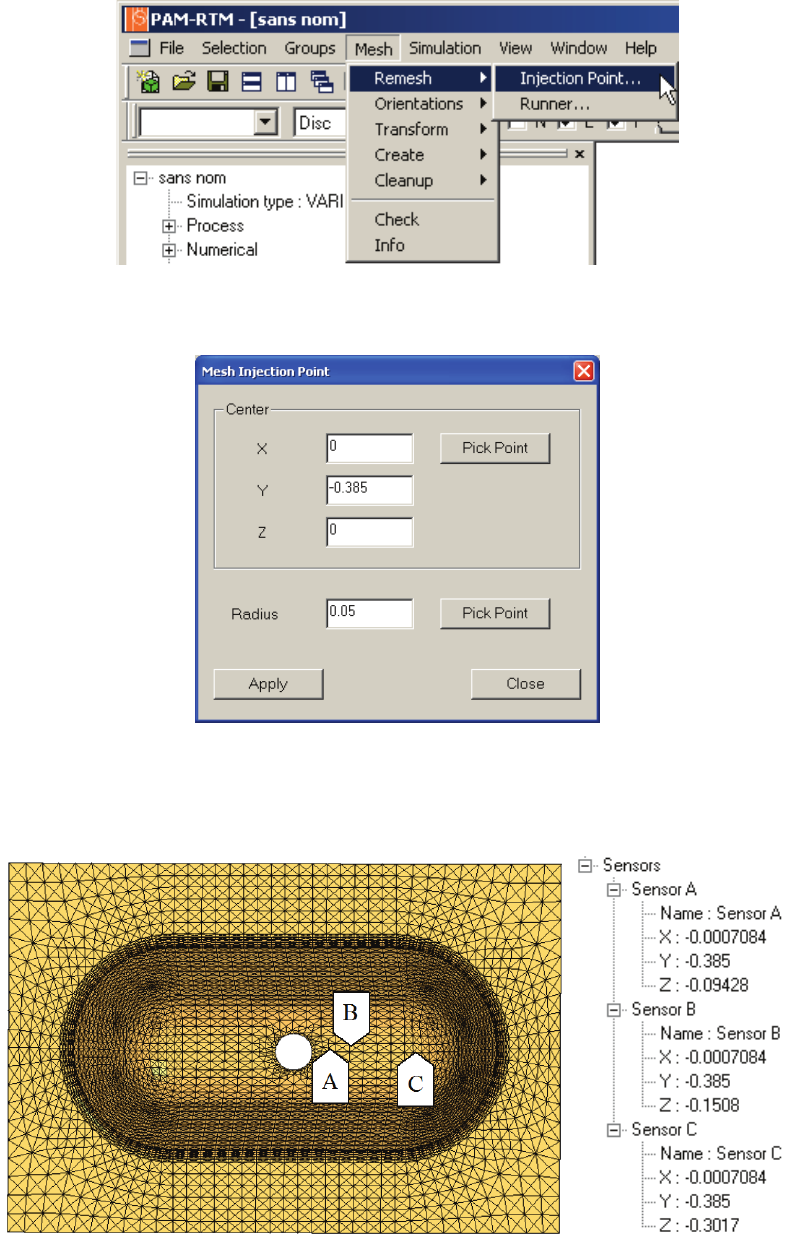
USER’S GUIDE & TUTORIALS 252 PAM-RTM 2014
(released: Apr-14) © 2014 ESI Group
TUTORIALS
Vacuum Assisted Resin Infusion (vari)
PAM-RTM™ asks if you want to split quads into triangles. Choose yes. The remeshing
tools work only on mesh of triangles.
Enter the coordinates of the center point (0, -0.385, 0) and set the radius at 0.05, then
apply and close the window.
The modified mesh appears as follows:
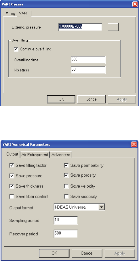
PAM-RTM 2014 253 USER’S GUIDE & TUTORIALS
© 2014 ESI Group (released: Apr-14)
TUTORIALS
Vacuum Assisted Resin Infusion (vari)
Create three sensors by picking approximately points A, B and C, or enter the exact
coordinates of the sensors as shown above.
Simulation
This section describes the parameters required to carry out this simulation:
Double-click on Process in the model explorer to open the VARI Process dialog box. In
the VARI tab, set the External pressure at 1.105 Pa.
Overfilling is activated by checking Continue overfilling box, and the duration of
Overfilling is set to 500s. The number of numerical steps is set to 50. That will allow
the simulation to continue after complete filling of the part until reaching a mechanical
equilibrium.
In the explorer, double-click on Numerical to open the VARI Numerical Parameters
dialog box and be sure that Save filling factor, Save pressure, Save thickness, Save
permeability and Save porosity are active.
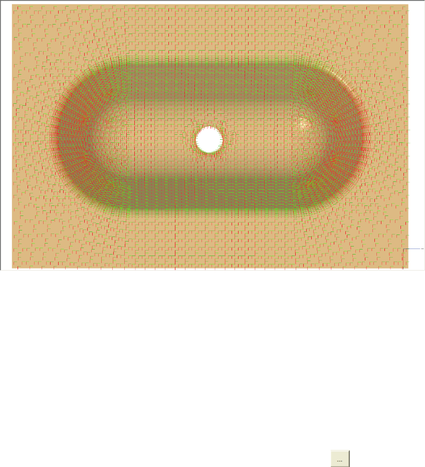
USER’S GUIDE & TUTORIALS 254 PAM-RTM 2014
(released: Apr-14) © 2014 ESI Group
TUTORIALS
Vacuum Assisted Resin Infusion (vari)
Orientation
No orientation is defined on the mesh. It will be defined with projection method. First
select all the elements, then use Mesh->Orientation->Project Vectors to project X as
K1. Then set, K2 orthogonal to K1, Mesh->Orientation->Set K Orthogonal.
Materials
Set the resin and the fabric properties as shown below.
Resin
- Constant viscosity = 0.1 Pa.s
- Density = 1083 kg/m3
Fabric
Double-click the Default Fabric in the explorer to open the Fabric Properties dialog box.
To set the permeability K1, open the Function Editor by clicking the button beside
K1. Select the Exponential function, then set A = 2.2 10-8 and B = -11.57.
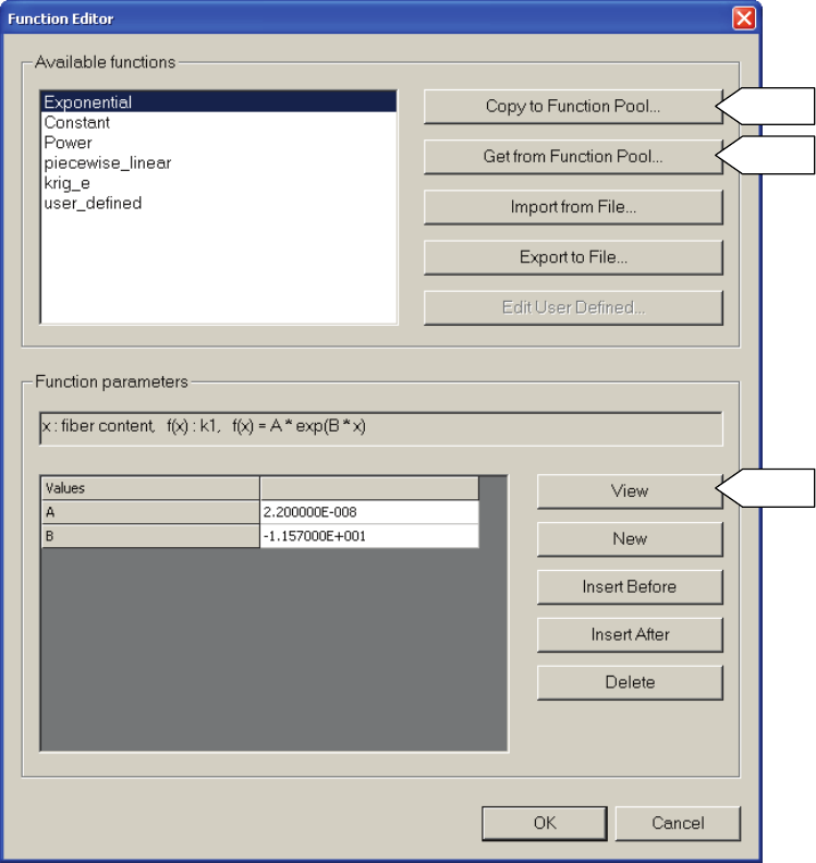
PAM-RTM 2014 255 USER’S GUIDE & TUTORIALS
© 2014 ESI Group (released: Apr-14)
TUTORIALS
Vacuum Assisted Resin Infusion (vari)
2
3
1
The permeability curve can be visualized by pushing the View button [1].
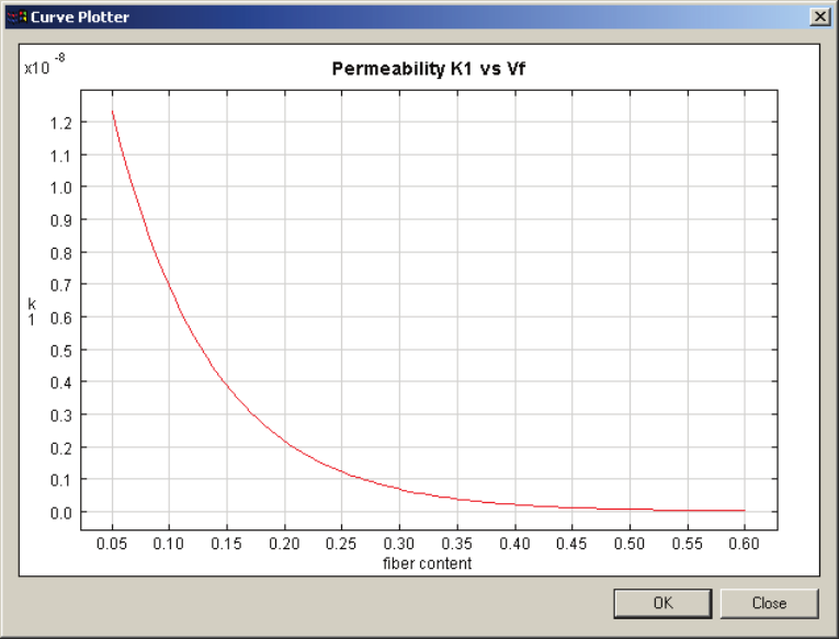
USER’S GUIDE & TUTORIALS 256 PAM-RTM 2014
(released: Apr-14) © 2014 ESI Group
TUTORIALS
Vacuum Assisted Resin Infusion (vari)
Instead of entering the coefficients of the exponential curve again for K2, you can use
the Copy to Function Pool functionality. Push the Copy to Function Pool button [2], and
then give a name to the curve, such as perm_vf. Next in the function editor of
Permeability K2, you just have to click on Get From Function Pool [3] and select
perm_vf to get the curve that was defined for K1. Note that the functions stored in the
function pool are available until you close PAM-RTM™. The function pool is shared
by all open documents.
One of the most important parameters for VARI simulation is the compressibility curve
of the reinforcement. Double-click Default Fabric in the explorer. In the Compressibility
tab, choose the Pressure-Fiber Content curve format in the drop-down list.
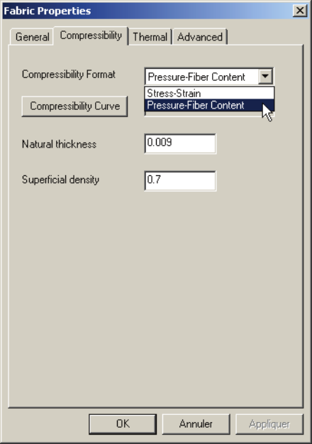
PAM-RTM 2014 257 USER’S GUIDE & TUTORIALS
© 2014 ESI Group (released: Apr-14)
TUTORIALS
Vacuum Assisted Resin Infusion (vari)
Push the Compressibility Curve button to define the curve. Choose a power law and set
A = 1.7 1011 and B = 7.6 in the Function Editor dialog box. The compressibility curve is
shown below.
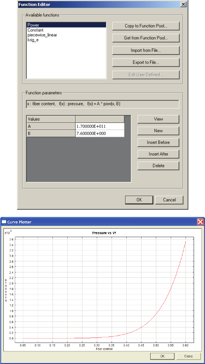
USER’S GUIDE & TUTORIALS 258 PAM-RTM 2014
(released: Apr-14) © 2014 ESI Group
TUTORIALS
Vacuum Assisted Resin Infusion (vari)
Finally set natural thickness to 0.009 m and superficial density to 0.7 kg.m-2 in the
Fabric Properties dialog box. The natural thickness of the fabric corresponds to the zero
pressure in the compressibility curve.
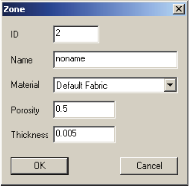
PAM-RTM 2014 259 USER’S GUIDE & TUTORIALS
© 2014 ESI Group (released: Apr-14)
TUTORIALS
Vacuum Assisted Resin Infusion (vari)
Zones
There is only one zone defined in this mesh. Double-click Zone_2 in the explorer,
associate Default Fabric to it and set its porosity as 0.5 and its thickness as 0.005 m.
Note
· The thickness value specified in the zone is only used to initialize the
calculation. PAM-RTM™ will calculate the actual thickness from the
compressibility curve and the external pressure. It is important to set the initial
thickness of zones to some value inside the definition range of the
compressibility curve. Normally half the natural thickness of the reinforcement
should be a good initial thickness.
· If the specified material and process parameters are such that at some point in
the simulation the thickness of the reinforcement becomes larger than its natural
thickness, the simulation is not valid.
Boundary Conditions
When the injection point was created with the remeshing tool, a group was
automatically created (ID=1) with the nodes around the injection hole. Now you need to
associate a boundary condition to this group. Click on Boundary Conditions in the
explorer with the right mouse button and choose New->Pressure. Verify that the
injection pressure is 1.105 Pa.
The full boundary of the injected part will be specified as a vent. You can easily select
all the nodes on the boundary. Use Selection->Pick Boundary, then pick a node on the
boundary you want to select. Use Groups->Create to create a group with the selected
nodes. Associate a Vent boundary condition to this group and make sure that the vent
pressure is zero. The groups are shown below.
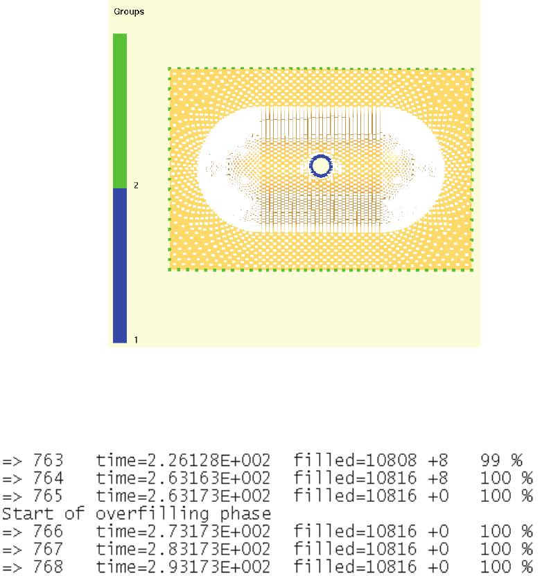
USER’S GUIDE & TUTORIALS 260 PAM-RTM 2014
(released: Apr-14) © 2014 ESI Group
TUTORIALS
Vacuum Assisted Resin Infusion (vari)
Save the PAM-RTM™ document and launch the simulation.
Post-Processing
It can be seen in log file that the simulation is split in two phases: filling then
overfilling.
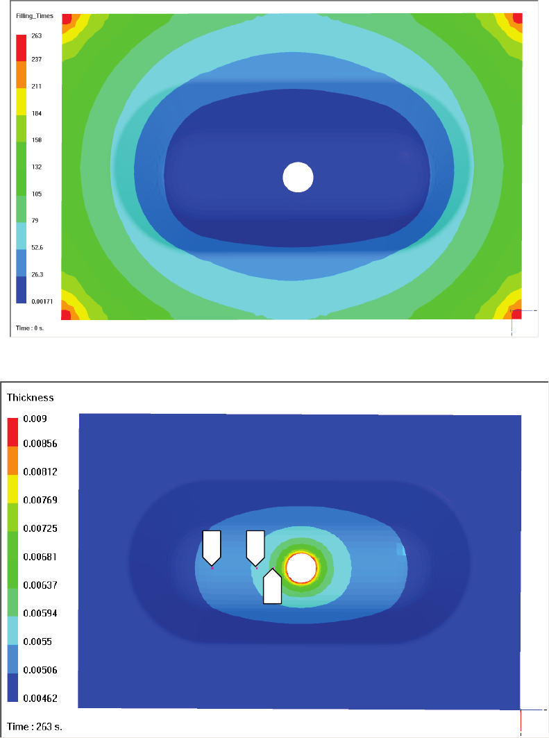
PAM-RTM 2014 261 USER’S GUIDE & TUTORIALS
© 2014 ESI Group (released: Apr-14)
TUTORIALS
Vacuum Assisted Resin Infusion (vari)
The images below show the segmented filling patterns and the thickness field at the end
of filling. The thickness evolution in time was plotted on the 3 sensors at positions A,B
and C on picture below.
C
B
A
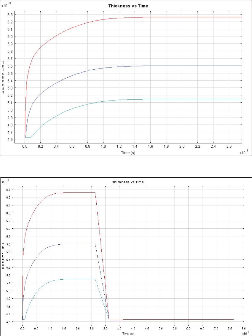
USER’S GUIDE & TUTORIALS 262 PAM-RTM 2014
(released: Apr-14) © 2014 ESI Group
TUTORIALS
Vacuum Assisted Resin Infusion (vari)
Thickness evolution during filling
Thickness evolution after filling
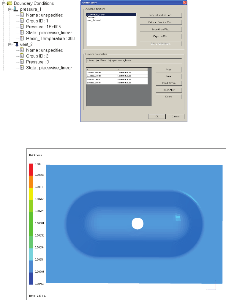
PAM-RTM 2014 263 USER’S GUIDE & TUTORIALS
© 2014 ESI Group (released: Apr-14)
TUTORIALS
Vacuum Assisted Resin Infusion (vari)
Second case with closing of the vent
A modification of the set-up is made so that vent is closed at the end of the filling, in the
same time as injection stops.
The first simulation showed that filling lasts 263s. The modification of set-up is so that
injection port and vent are closed after 264s. State functions for each boundary
condition are set like the function below.
Behavior is modified after the end of filling as the thickness value at the end of the post-
filling and thickness curve show.
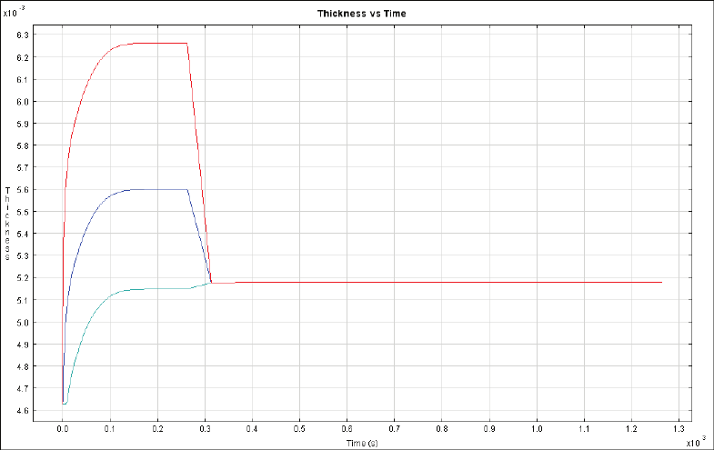
USER’S GUIDE & TUTORIALS 264 PAM-RTM 2014
(released: Apr-14) © 2014 ESI Group
TUTORIALS
Vacuum Assisted Resin Infusion (vari)
Thickness at the end of over-filling phase.
Thickness evolution after filling
Final thickness is 5.46mm compared to 4.6mm in the case of opened vent.
Conclusion
This tutorial showed the set-up of infusion simulation (VARI model), and the
computation of final thickness after the complete filling of the part and mechanical
equilibrium is reached.
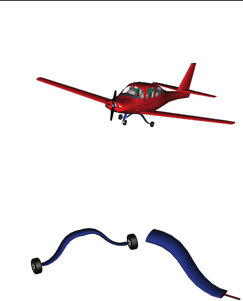
PAM-RTM 2014 265 USER’S GUIDE & TUTORIALS
© 2014 ESI Group (released: Apr-14)
TUTORIALS
Landing Gear
LANDING GEAR
The following files are used in this example.
- landing_start.unv (starting mesh)
- landing_1.dtf, landing_2.dtf; + landing.unv (solution)
Introduction
In PAM-RTM™ simulations, complex parts can be modeled with shell or solid
elements. Different zones must be defined, the type of materials contained in the cavity
must be specified (metallic insert, foam…) as well as the properties of the fibrous
reinforcement (orientations and values of the permeability tensor). Numerical
simulation aims to assist users to understand the progression of the resin flow during the
injection. It helps to avoid problems such as air entrapments. It allows also to compare
different injection strategies in order to find the best one, for example the one with the
shortest cycle time. Non isothermal simulations study the coupling between the resin
flow, temperature and curing.
Landing gear

USER’S GUIDE & TUTORIALS 266 PAM-RTM 2014
(released: Apr-14) © 2014 ESI Group
TUTORIALS
Landing Gear
Analysis of a Landing Gear
The landing gear of a small touring airplane is analyzed in this example. As
demonstrated on the picture, the landing gear is located on the front part of the airplane
and is symmetric along its central axis. If the injection is performed from the center or
from the two extremities, because of the symmetry only half of the part needs to be
simulated. This example is important because it compares the effect of convergent
versus divergent flows and illustrates how convergent resin flows are systematically
accelerated in restrictions.
Two injection scenarios at constant pressure will be considered here for half of the part.
The first test consists of injecting the resin from two injection ports located at the center
of the part as shown in the figure below. The vents are located at both extremities at the
positions of the wheels.
In the second test, the resin is injected from both extremities, the vents being located in
the center of the part.
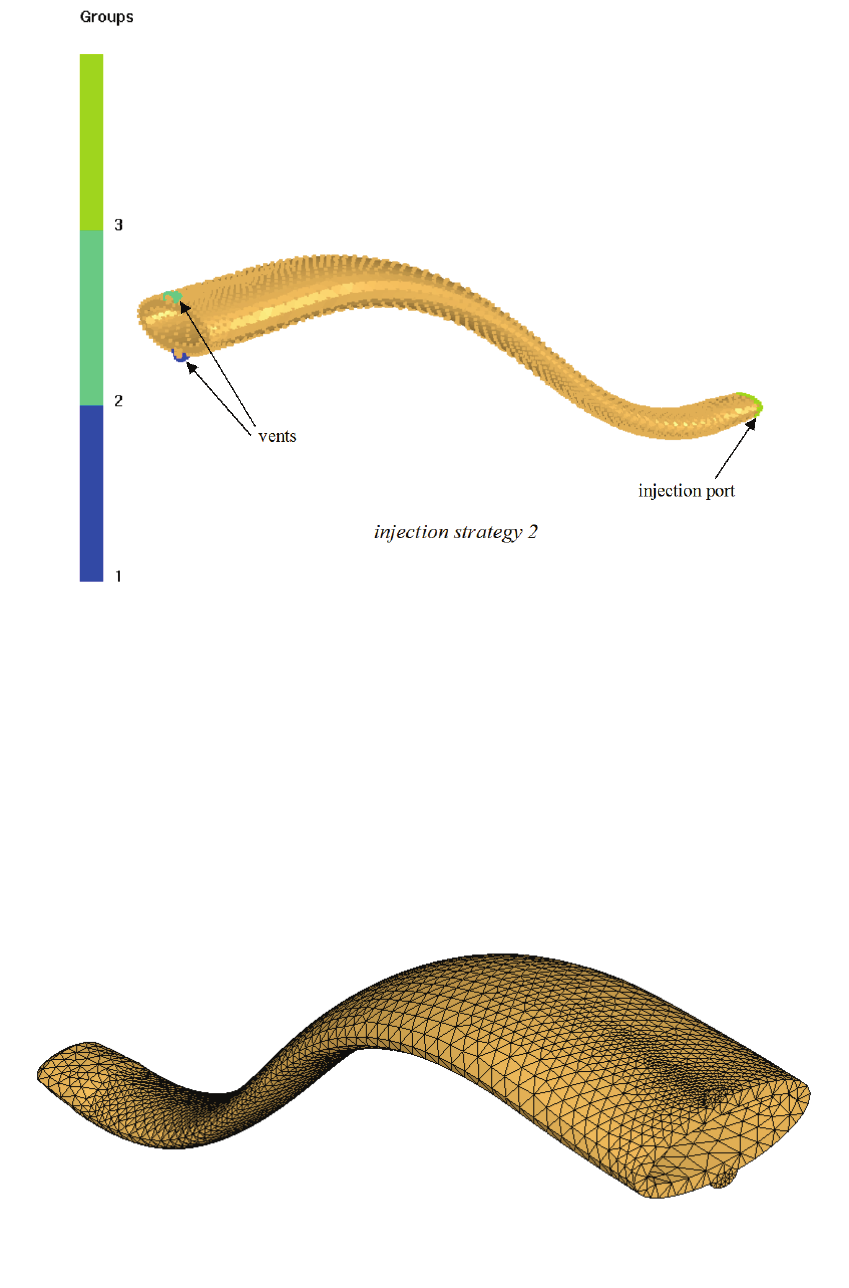
PAM-RTM 2014 267 USER’S GUIDE & TUTORIALS
© 2014 ESI Group (released: Apr-14)
TUTORIALS
Landing Gear
This composite part is normally made of several materials. It contains a metallic insert
at its extremities for the installation of the wheels. The center of the part is an
impermeable foam. Since these are non-permeable inserts and since we are only doing
an isothermal simulation, it is not necessary to mesh these inserts. It is important to note
that if you decide to mesh the non-permeable zones, the mold material of PAM-RTM™
must be assigned to these zones.
The mesh has been generated with I-DEAS. It is shown below.
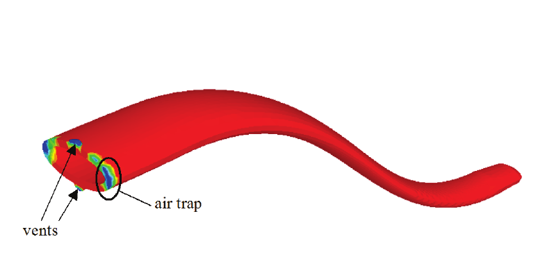
USER’S GUIDE & TUTORIALS 268 PAM-RTM 2014
(released: Apr-14) © 2014 ESI Group
TUTORIALS
Landing Gear
Analysis of Simulation Results
The landing gear has been simulated for both injection scenarios. The two injections
were performed at constant pressure from the two extremities (case 1) or from the
center of the part (case 2). The goal is to determine the best injection strategy to
produce the part and avoid errors in the design of the mold.
Let us examine the injection process in more detail. When the injection is performed
from the center (first strategy), no particular difficulties appear. However when the part
is injected with the second strategy, an air trap appears near the vents. This shows that
the air vents are not correctly positioned. In order to correct the problem, the air vents
should be positioned on the side of the part, exactly where the air traps appear. The air
trap is created in this example because of the divergent flux during the injection.
This phenomenon (divergent flux) does not only create an unwanted air bubble, but it
also increases the injection time significantly. The successive positions of the resin front
in time are displayed next for the two injection strategies considered. For a constant
pressure injection, the first injection strategy gives a much lower injection time
compared to the second. Indeed, the first strategy enables to fill the mold in 134
seconds, while it takes 234 seconds for the second strategy. This difference is caused by
the shape of the part. In the first case, the resin flux is convergent, which has the effect
of accelerating the displacement velocity of the resin in the restriction, whereas in the
second case a divergent flux is obtained.
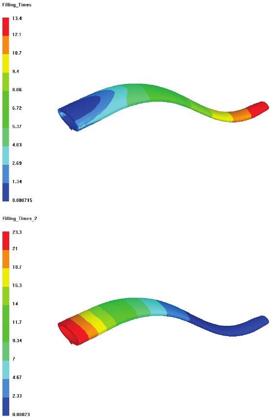
PAM-RTM 2014 269 USER’S GUIDE & TUTORIALS
© 2014 ESI Group (released: Apr-14)
TUTORIALS
Landing Gear
Conclusion
The landing gear design information is a good example that demonstrates the
importance of numerical simulation, appropriately provided to mold designers. Note
that mistakes can be very expensive to repair once the mold is made. The simulation
permits to predict where air bubbles might be created, which has a direct effect on the
mechanical properties of the part. It is possible to prevent the formation of air
entrapments by changing the position of the vents. In this particular case, the vents will
be placed on the side of the part and not on top of it. Finally, the simulation allows to
optimize the cycle time. Thus, in this analysis, the first strategy of injection proves to be
the best since it allows to shorten the filling cycle and avoid the creation of air
entrapments. In conclusion, numerical simulation allows to design a mold rapidly and
efficiently while avoiding some expensive modifications once the mold is built.
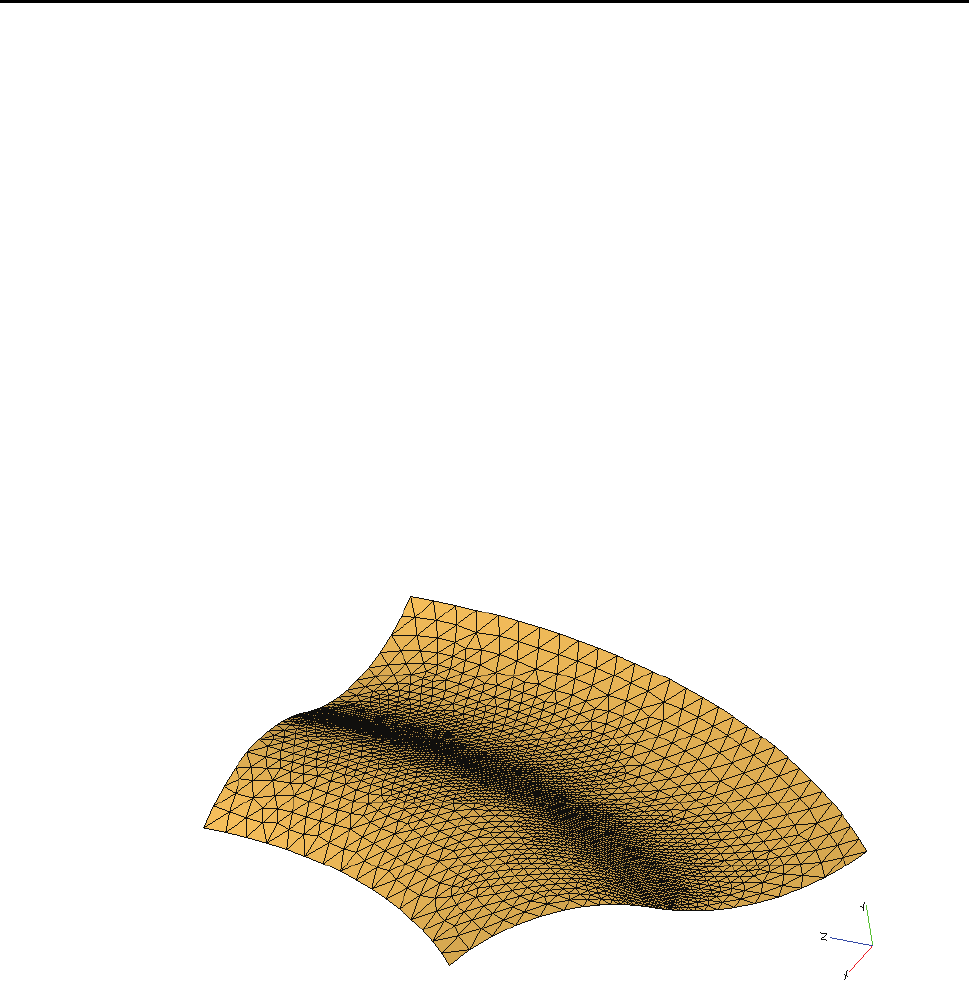
USER’S GUIDE & TUTORIALS 270 PAM-RTM 2014
(released: Apr-14) © 2014 ESI Group
TUTORIALS
Mesh Extrusion
MESH EXTRUSION
The following files are used in this example.
- extrude_start.unv (starting mesh)
- extrude.dtf + extrude.unv (solution)
Objectives
The goal of this tutorial is to show how a surface mesh can be extruded with layers of
different thickness and materials. A flow enhancing layer, such as the one found in the
VARTM process, is used on top of the fiber preform. The new prismatic element is
used directly to avoid splitting into tetrahedra.
Mesh Extrusion
Begin by creating a new RTM simulation, then import the mesh file extrude_start.unv.
You should have the following.
Verify that this mesh contains orientations with View > Orientations > K1 Only. Notice
that the fiber directions F1 and F2 (actually K1 and K2) are not perfectly orthogonal.
This can be seen by activating the Shear_Angle in the main toolbar, which shows angles
of about 2 degrees. This mesh was actually oriented using PAM-QUIKFORM.

PAM-RTM 2014 271 USER’S GUIDE & TUTORIALS
© 2014 ESI Group (released: Apr-14)
TUTORIALS
Mesh Extrusion
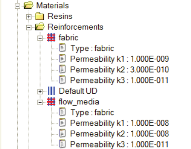
USER’S GUIDE & TUTORIALS 272 PAM-RTM 2014
(released: Apr-14) © 2014 ESI Group
TUTORIALS
Mesh Extrusion
The goal is to generate a solid mesh made of 5 layers: 0, +45, -45, 90, and a flow media
on top. The first step is to create materials for the fiber reinforcement and the flow
media. The same material will be used for the 4 plies. The fiber reinforcement has k1
three times larger than k2. The permeability of the flow media is ten times larger than
k1. After creating the materials, you should have the following in the document’s tree.
Notice that we use the same permeability k3 for the reinforcement and the flow media.
This is important to avoid numerical problems.
The thickness of the plies is set to 0.025 m. It is exaggerated for the purpose of this
tutorial, to see the flow better through thickness. The thickness of the flow media is
much thinner, 0.003 m. Don’t forget to set the angle of each ply. The angle of the flow
media is not important since its planar permeability is isotropic. After creating the
laminate, you should have the following.
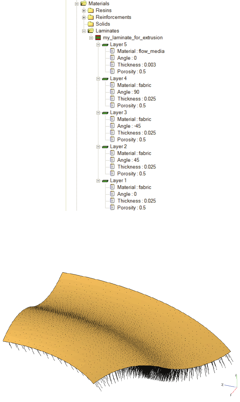
PAM-RTM 2014 273 USER’S GUIDE & TUTORIALS
© 2014 ESI Group (released: Apr-14)
TUTORIALS
Mesh Extrusion
Before performing extrusion, it is important to verify that the normal vectors a pointing
in the right direction (View > Normal Vectors). Here we would like the mesh to be
extruded in the opposite direction. To reverse the normal vectors, we first select all the
elements with Selection > Element and Selection > Select All. Then we use Mesh >
Cleanup > Reverse Normals.
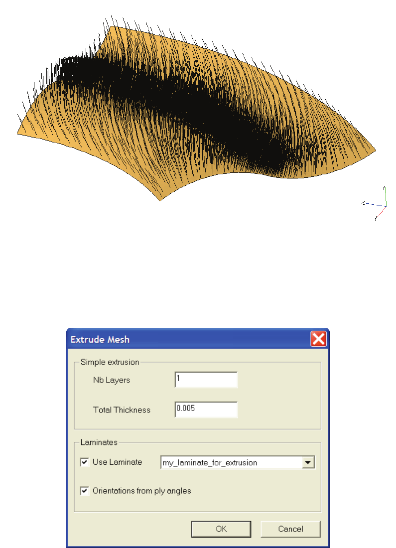
USER’S GUIDE & TUTORIALS 274 PAM-RTM 2014
(released: Apr-14) © 2014 ESI Group
TUTORIALS
Mesh Extrusion
Once the normal vectors have been reversed, open the mesh extrusion dialog box with
Mesh > Transform > Extrude. Check the Use laminate option (meaning that parameters
in the Simple extrusion area are completely ignored), select your laminate in the
dropdown list, and select Orientation from ply angles so that the orientation of each
element is set as the orientation of the corresponding element in the first layer, rotated
by the ply’s angle. The Extrude Mesh dialog box is shown below.
Push the OK button to launch mesh generation. You should have the following. Notice
the top layer, very thin compared to the other layers. This is the layer used as the flow
media.

PAM-RTM 2014 275 USER’S GUIDE & TUTORIALS
© 2014 ESI Group (released: Apr-14)
TUTORIALS
Mesh Extrusion
Extruded mesh
Zoom on the layers
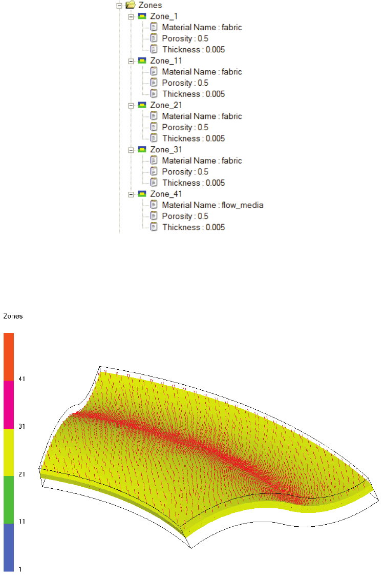
USER’S GUIDE & TUTORIALS 276 PAM-RTM 2014
(released: Apr-14) © 2014 ESI Group
TUTORIALS
Mesh Extrusion
The extrusion command automatically generates a zone for each layer in the
document’s tree. Each zone is linked to the corresponding ply material. The thickness of
each zone is not important since we are working with solid elements. The porosity of
each zone is also set from the plies.
To verify that the orientations are correctly set, use the View > Zones Visibility
command. For example, hide all layers and show only zone 21. Then show K1 vectors
with View > Orientations > K1 Only. You should have the following picture, correctly
showing orientation vectors at –45 degrees.
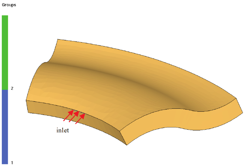
PAM-RTM 2014 277 USER’S GUIDE & TUTORIALS
© 2014 ESI Group (released: Apr-14)
TUTORIALS
Mesh Extrusion
Process and Numerical Parameters
For the boundary conditions, create groups of faces as shown below. We inject from 2
faces directly in the high permeability layer. The vent is at the bottom of the opposite
side. Set the injection pressure to 1 bar, and keep the default zero bar on the vent.
Location of the inlet
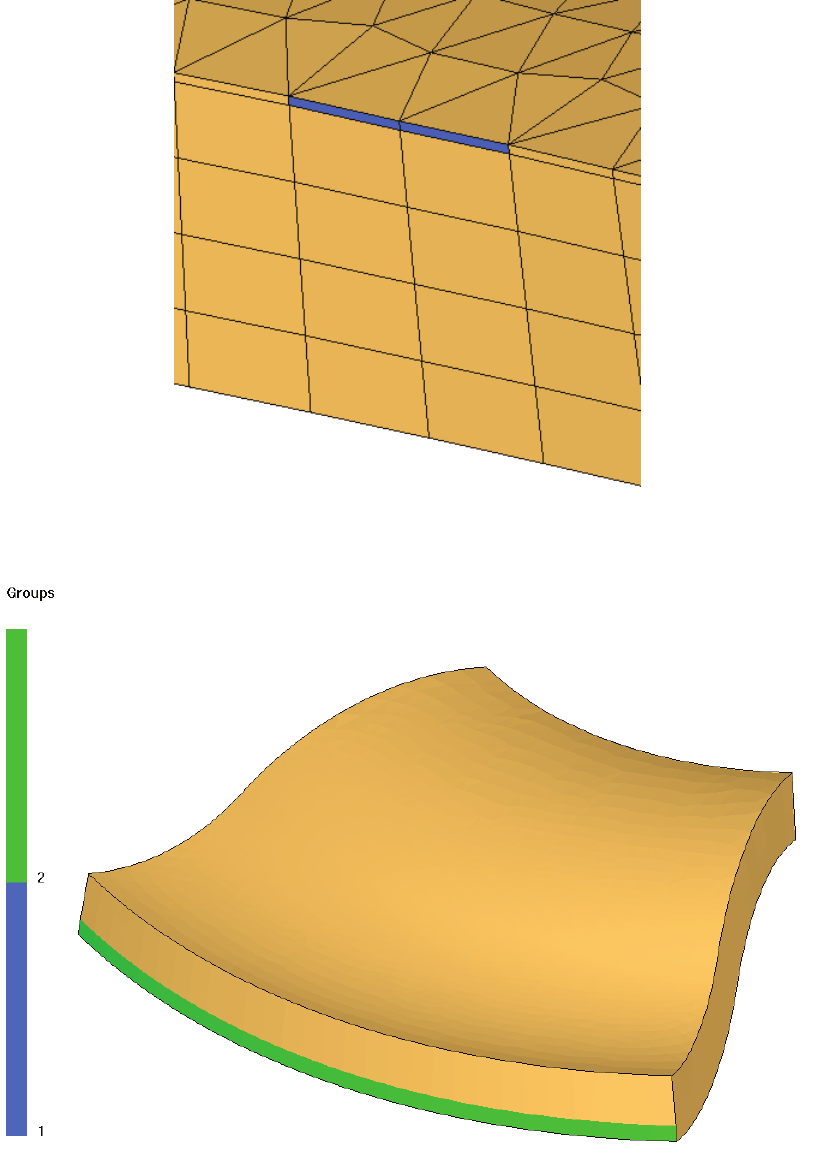
USER’S GUIDE & TUTORIALS 278 PAM-RTM 2014
(released: Apr-14) © 2014 ESI Group
TUTORIALS
Mesh Extrusion
Group of faces for the inlet
Group of faces for the outlet

PAM-RTM 2014 279 USER’S GUIDE & TUTORIALS
© 2014 ESI Group (released: Apr-14)
TUTORIALS
Mesh Extrusion
Launching the Simulation and Post-Processing
Save the document with File->Save and launch the simulation.
Segmented filling result
The segmented filling image clearly shows the effect of the flow media. Since the
permeability of that layer is much higher, the resin almost completely fills that layer
before starting to flow through the thickness of the part.
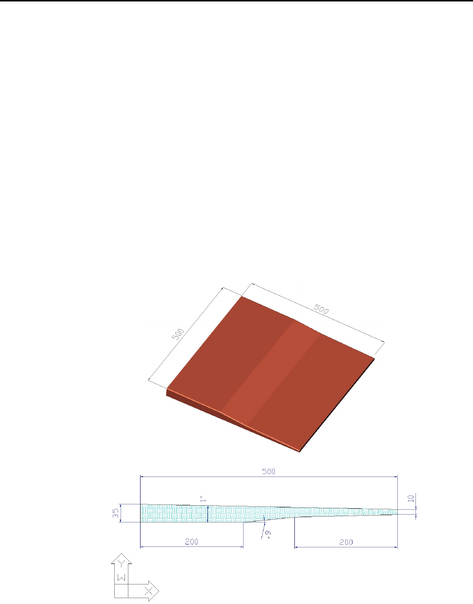
USER’S GUIDE & TUTORIALS 280 PAM-RTM 2014
(released: Apr-14) © 2014 ESI Group
TUTORIALS
Non-Isothermal Injection
NON-ISOTHERMAL INJECTION
The files related to this example are:
- non_iso_fil_start.unv (starting mesh)
- non_iso_fil_1.dtf, non_iso_fil_2.dtf, non_iso_fil_3.dtf, + non_iso_fil.unv (solution)
Objective of the Analysis
This example will show you how to:
- Perform a non-isothermal filling simulation,
- Study the effects of temperature on the injection of resin.
Geometry Description
It is possible with PAM-RTM™ to simulate the injection and at the same time take into
account thermal effects. The part that will be simulated in this example is shown below.
It is an extruded panel of variable thickness.
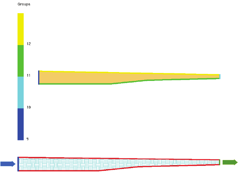
PAM-RTM 2014 281 USER’S GUIDE & TUTORIALS
© 2014 ESI Group (released: Apr-14)
TUTORIALS
Non-Isothermal Injection
Visualization of Groups
Create a new simulation of type Heated RTM (File->New) and import the mesh file
non_iso_fil_start.unv. Then visualize groups of nodes. Groups at the extremity
of the part will model the injection port (dark blue) and vent (light blue), groups on the
top and bottom of the part (11 and 12) will be used to set the heating boundary
conditions on temperature.
Simulation Parameters
Open the Resin Properties dialog box (doucle-click on Default Resin).
Enter the resin parameters as shown below:
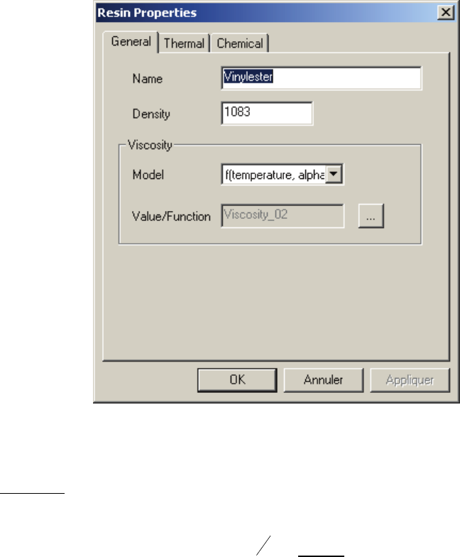
USER’S GUIDE & TUTORIALS 282 PAM-RTM 2014
(released: Apr-14) © 2014 ESI Group
TUTORIALS
Non-Isothermal Injection
- Resin Name: Vinylester
- Density = 1083 Kg/m3
- Viscosity: a viscosity function relates viscosity with temperature and the degree of
cure. Select the Viscosity_02 model:
34
1
2
0
2
(, )
CCy
C
xc
f x y ce cy
+×
= ×
−
C0 = 1.10-7
C1 = 5000
C2 = 0.4
C3 = 0.75
C4 = 0.35
Choose in the Model drop down list f(temperature, alpha) and open the Function Editor
(click on the … button), select the function Viscosity_02 and set its parameters.
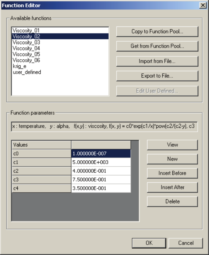
PAM-RTM 2014 283 USER’S GUIDE & TUTORIALS
© 2014 ESI Group (released: Apr-14)
TUTORIALS
Non-Isothermal Injection
To visualize the viscosity function, push the View button. By default, curves are plotted
for the viscosity as a function of alpha for fixed temperatures. In this example, a
temperature range of 300 to 350°K was chosen. The maximum allowable value of alpha
is 0.4 (the viscosity tends to infinity at 0.4), that’s why the alpha max value was set to
0.35.
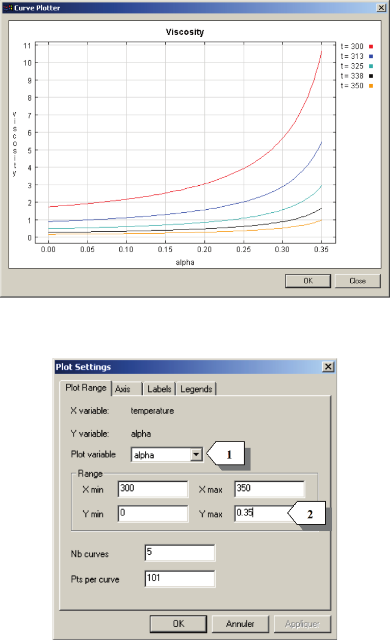
USER’S GUIDE & TUTORIALS 284 PAM-RTM 2014
(released: Apr-14) © 2014 ESI Group
TUTORIALS
Non-Isothermal Injection
Right-click in the Curve Plotter window to open the Plot Settings dialog box. The range
parameters are found in the Plot Range tab. In this context (viscosity as a function of
temperature and alpha), X means temperature, Y means alpha.
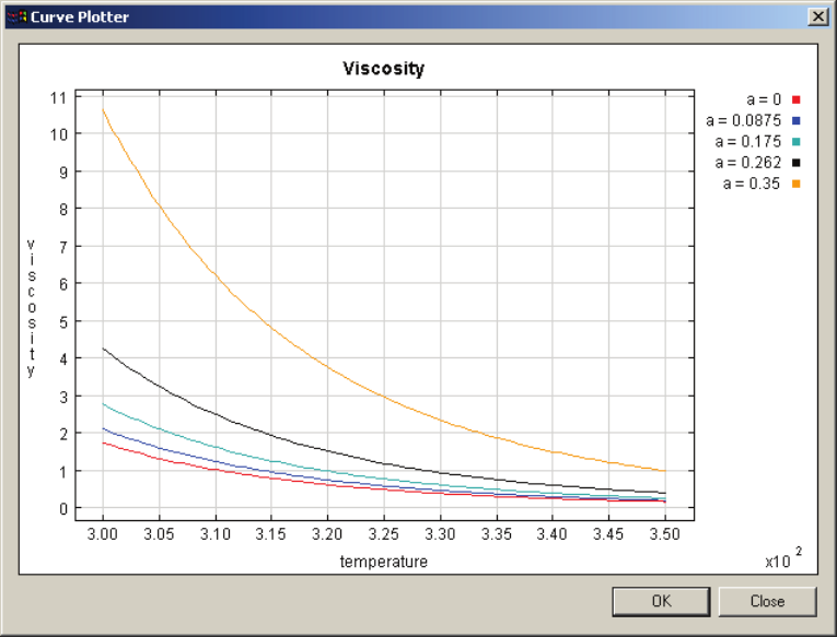
PAM-RTM 2014 285 USER’S GUIDE & TUTORIALS
© 2014 ESI Group (released: Apr-14)
TUTORIALS
Non-Isothermal Injection
Choose alpha in the Plot Variable drop-down list [1] and set Ymax at 0.35 to avoid
undefined viscosity function when alpha = 0.4 [2].
In the Resin Properties, select the Thermal tab to enter the thermal conductivity and the
specific heat.
- Thermal conductivity = 0.11 W/m.K
- Specific heat = 1205 J/Kg.K
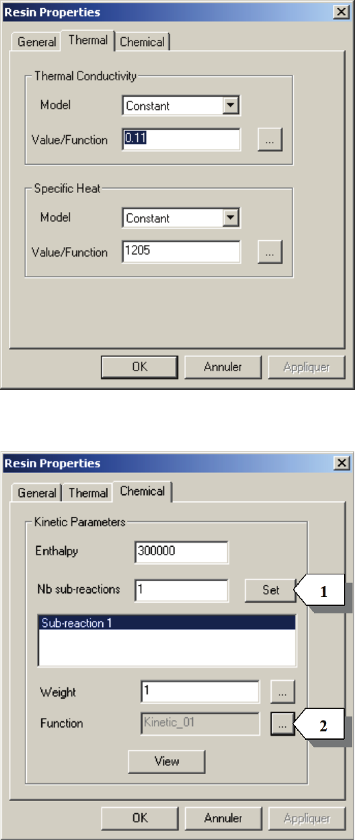
USER’S GUIDE & TUTORIALS 286 PAM-RTM 2014
(released: Apr-14) © 2014 ESI Group
TUTORIALS
Non-Isothermal Injection
In the Resin Properties dialog box, select the Chemical tab and enter the kinetic
parameters.
Set the Reaction Enthalpy at 3.105 J/kg.
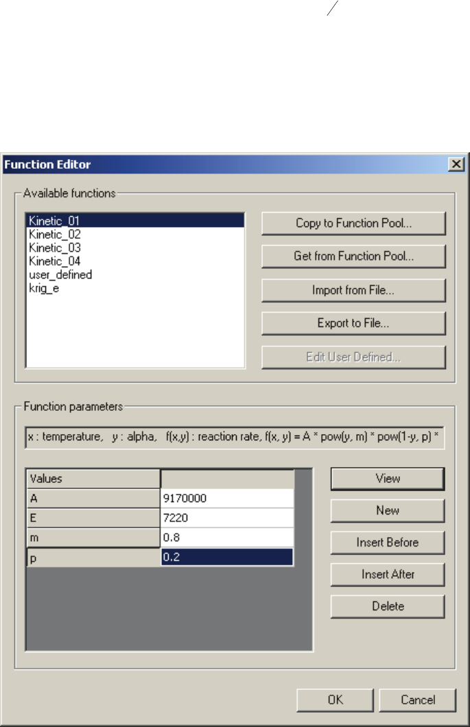
PAM-RTM 2014 287 USER’S GUIDE & TUTORIALS
© 2014 ESI Group (released: Apr-14)
TUTORIALS
Non-Isothermal Injection
Type 1 in the Nb Sub-reactions text field, then click the Set button [1]. This creates one
sub-reaction. Then select sub-reaction 1 and push the … button [2] to choose the resin
kinetics model.
In the Function Editor, select Kinetic_01 for the following resin kinetics model:
x
E
pm eyyAyxf −
×−××= )1(),(
A = 9170000
E = 7220
m = 0.8
p = 0.2
After defining the chemical reaction, it is possible to view the conversion curves in time
for different temperatures. Push the View button in the Chemical tab of the Resin Editor
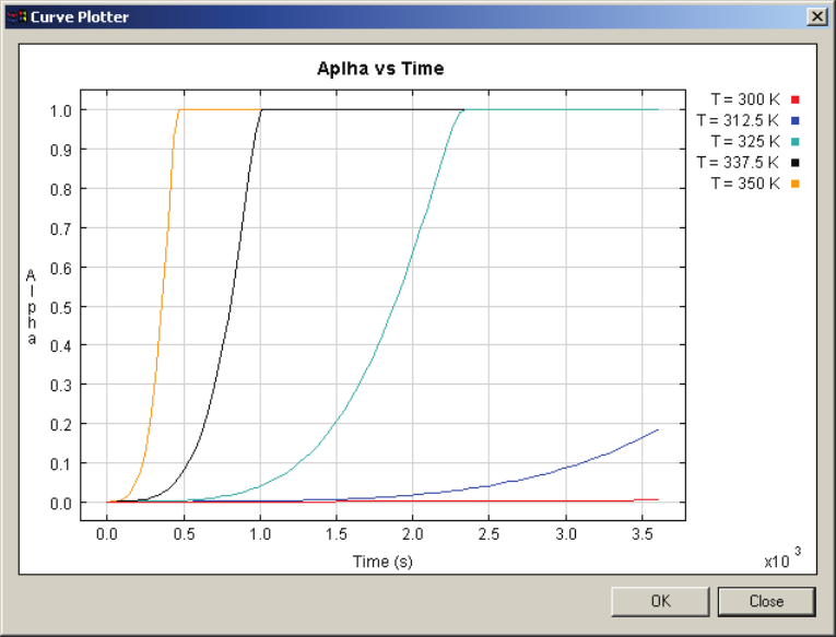
USER’S GUIDE & TUTORIALS 288 PAM-RTM 2014
(released: Apr-14) © 2014 ESI Group
TUTORIALS
Non-Isothermal Injection
to open the Kinetics Viewer dialog. Set the appropriate temperature and time range, then
push the Plot button.
This viewer is useful to know quickly how the resin behaves at different temperatures.
For example, since we know that the viscosity becomes very large when alpha is near
0.4, we should try to avoid alpha values larger than, say, 0.1 with a good safety margin.
This means that the part must be filled in about 250 s. if the temperature is 350 K.
Now set the properties of the reinforcement as follows :
- Density: 2565 kg/m3
- Thermal conductivity: 0.2 W/m.K
- Specific heat: 1205 J/Kg.K
- Effective conductivity: 0.3 W/m.K
- Permeability: K1=K2=K3=1.5 10-10 m²
And the parameters of the zone:
- Porosity: 0.5
- Thickness: 0.005 m
Define the boundary conditions.
- Injection pressure (Group 9) = 2.105 Pa.
- Vent pressure (Group 10) = 0 Pa.
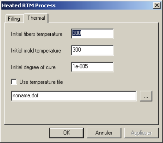
PAM-RTM 2014 289 USER’S GUIDE & TUTORIALS
© 2014 ESI Group (released: Apr-14)
TUTORIALS
Non-Isothermal Injection
Simulation Cases
Case 1
The first case is carried out with the following conditions:
- Initial temperature of the mold and fibers: 300 degrees K
- Temperature of the injected resin: 300 degrees K
- Temperature of the mold walls: 350 degrees K
To set the Initial fibers and mold temperature, double-click on Process and select the
Thermal tab.
The temperature of the resin is specified in the injection port parameters:
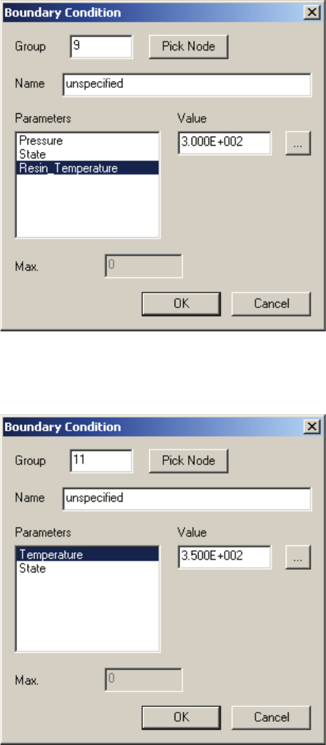
USER’S GUIDE & TUTORIALS 290 PAM-RTM 2014
(released: Apr-14) © 2014 ESI Group
TUTORIALS
Non-Isothermal Injection
To define the thermal boundary conditions, right-click on Boundary Conditions and
click on New->Temperature, then double-click on Temperature_-1 to open the Boundary
Condition dialog box.
The resin is injected at 300 degrees K in the mold cavity. Since the upper and lower
mold walls are heated at 350 degrees K, the resin temperature increases close to the
mold walls. This reduces the viscosity of the resin and tends to accelerate the resin flow
along the top and bottom walls of the mold as illustrated below.
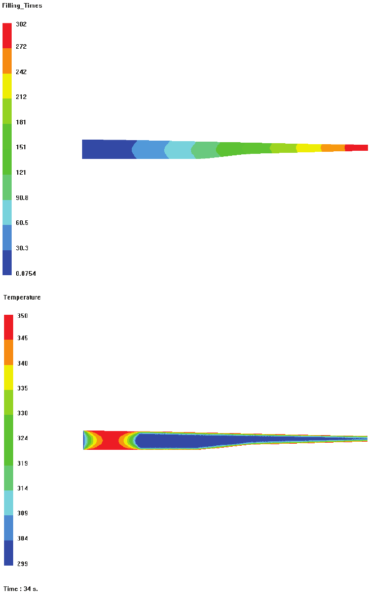
PAM-RTM 2014 291 USER’S GUIDE & TUTORIALS
© 2014 ESI Group (released: Apr-14)
TUTORIALS
Non-Isothermal Injection
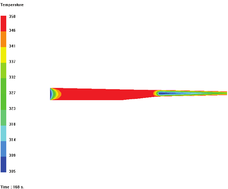
USER’S GUIDE & TUTORIALS 292 PAM-RTM 2014
(released: Apr-14) © 2014 ESI Group
TUTORIALS
Non-Isothermal Injection
Note that the flow front is not only accelerated on the top and bottom mold walls
because of a lower resin viscosity, but also in the center as a result of the convergent
geometry of the part. When the resin has reached the thinner section on the right, the
flow front has become straight.
As the temperature in the cavity increases, the resin viscosity decreases, and the curing
reaction begins to solidify the resin. The figure below shows the degree of cure at the
end of the filling:

PAM-RTM 2014 293 USER’S GUIDE & TUTORIALS
© 2014 ESI Group (released: Apr-14)
TUTORIALS
Non-Isothermal Injection
Case 2
In this second test, the boundary conditions are slightly different :
- Initial temperature of the mold and fibers: 300 degrees K
- Temperature of the injected resin: 300 degrees K
- Temperature of mold walls : 350 degree K on top and 330 degree K on bottom
In this case, the resin viscosity is not uniformly distributed through the thickness
because the temperature of the top mold wall is higher than that of the lower wall.
Therefore, the resin flow is faster near the upper mold wall at the beginning of the
injection. However because of the combined effects of the temperature, degree of cure
and convergent geometry, the flow front is almost straight at the end of filling.
The degree of cure distribution at the end of the injection is not very interesting. The
cycle time will be longer than in the previous case. The degree of cure of the part is also
not uniform. So the mechanical properties of the part will vary in each section. This can
be disastrous when the part will be used.
The figures below show the segmented filling patterns, the temperature field at the end
of the injection and the degree of cure at the end of the injection.
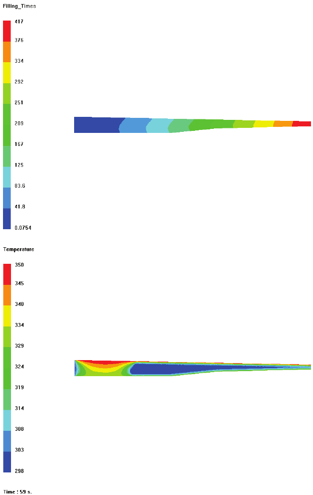
USER’S GUIDE & TUTORIALS 294 PAM-RTM 2014
(released: Apr-14) © 2014 ESI Group
TUTORIALS
Non-Isothermal Injection
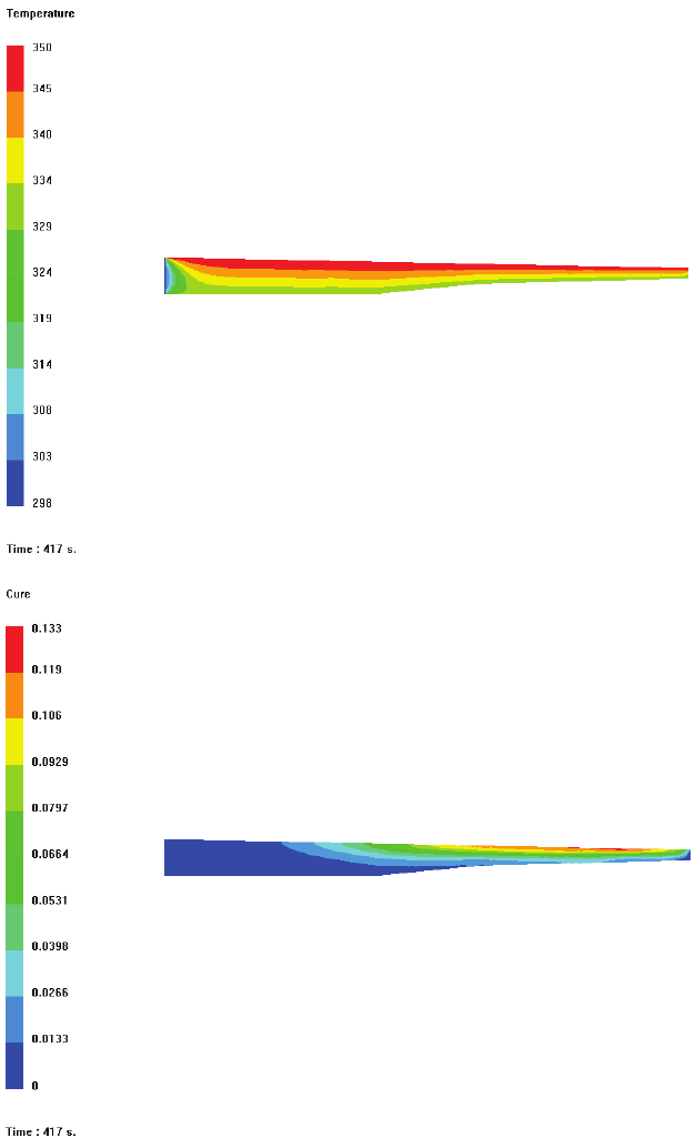
PAM-RTM 2014 295 USER’S GUIDE & TUTORIALS
© 2014 ESI Group (released: Apr-14)
TUTORIALS
Non-Isothermal Injection
Case 3
The temperature boundary conditions of the third case are the following:
- Initial temperature of the mold and fibers: 300 degrees K
- Temperature of the injected resin: 350 degrees K
- Temperature of mold walls: 320 degrees K
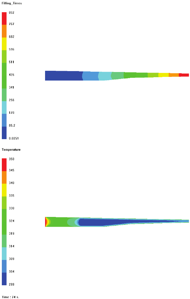
USER’S GUIDE & TUTORIALS 296 PAM-RTM 2014
(released: Apr-14) © 2014 ESI Group
TUTORIALS
Non-Isothermal Injection
For this case, the temperature of the resin is larger than the temperature of the mold.
This has several consequences. First of all, the figures below show that resin is cooled
down by the mold when it enters the cavity. At the end of the filling, the temperature is
almost uniform in the part. Secondly, the resin front is not distorted and remains nearly
straight. Finally, because the temperature of the resin stays much lower, the degree of
cure at the end of the injection is very small (0.005). The major problem in this case is
that the filling time is very long (about 850 s. compared to 300 s. for the first case),
because the viscosity is higher.
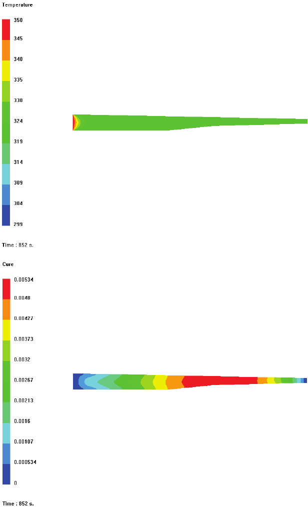
PAM-RTM 2014 297 USER’S GUIDE & TUTORIALS
© 2014 ESI Group (released: Apr-14)
TUTORIALS
Non-Isothermal Injection
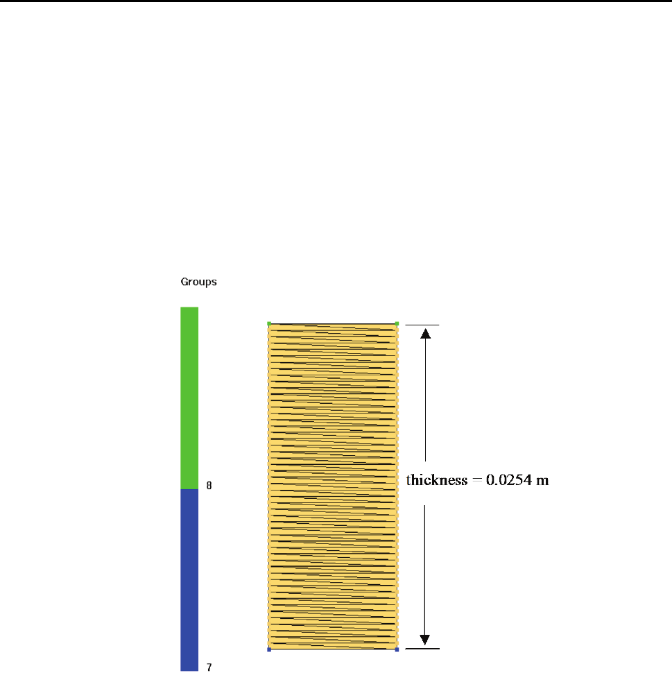
USER’S GUIDE & TUTORIALS 298 PAM-RTM 2014
(released: Apr-14) © 2014 ESI Group
TUTORIALS
Curing of a Plate
CURING OF A PLATE
The files related to this example are:
- curing_1d_start.unv (starting mesh)
- curing_1d.dtf + curing_1d.unv (solution)
Visualization of the Mesh and Groups
Begin by creating a new Curing simulation with File->New and import the mesh file
curing_1d_start.unv.
Visualize the mesh and groups of nodes. You should have the following:
This simplified problem should be seen as a cross section in a thick rectangular plate, on
which the temperature is fixed on top and bottom and the heat flux is zero all around the
part. This leads to a 1D heat transfer problem through the thickness of the part.
PAM-RTM 2014 299 USER’S GUIDE & TUTORIALS
© 2014 ESI Group (released: Apr-14)
TUTORIALS
Curing of a Plate
Simulation Parameters
Numerical Parameters
Use Simulation->Numerical Parameters to open the Curing Numerical Parameters dialog
box, select the Time Step tab and set the following parameters:
- Max. Experiment Time: 3600
- Max. Number of Steps: 1000
Notes:
· For a curing and preheating simulation, the time step is fixed and is calculated
as:
dt = Max. experiment time/Max. number of steps
Resin Parameters
Open the Resin Properties dialog box and set the following parameters:
- Resin Name: Vinylester
- Density: 1083 kg/m3
- Specific Heat: 1205 J/Kg.K
- Enthalpy: 266342 J/Kg
- Add a new reaction, open the Function Editor and select Kamal-Sourour model
(Kinetic_01) with A=9.17E6, E=7289, m=0.85 and p=1.15
Use the View button to verify the chemical model. As illustrated in the figure below, this
function allows visualizing resin conversion curves, i.e., the evolution of the degree of
polymerization (alpha) in time for different processing temperatures.
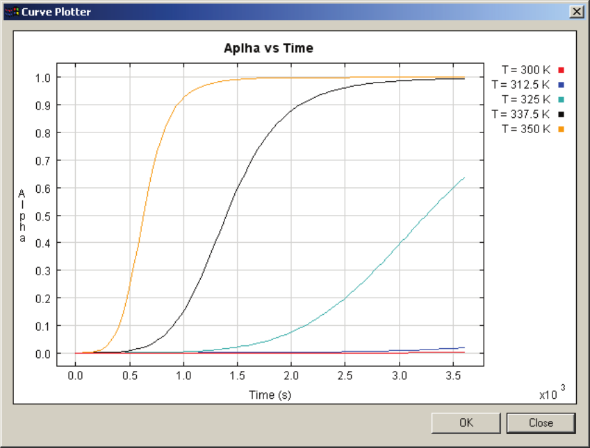
USER’S GUIDE & TUTORIALS 300 PAM-RTM 2014
(released: Apr-14) © 2014 ESI Group
TUTORIALS
Curing of a Plate
On these curves of isothermal conversion, the value of 1 means that the resin has been
cured completely. Curves with a smaller slope are obtained for lower temperatures.
Change the processing temperature and the time scale to visualize the effect of
temperature on the curing time.
Fiber Parameters
Enter the following parameters.
- Name: Glass
- Density: 2565 Kg/m3
- Specific Heat: 1205 J/Kg.K
- Effective Conductivity of the saturated reinforcement (for each direction: K1, K2,
K3): 0.25 W/m.K
Note:
· For curing simulations, it is not necessary to specify the conductivity of the dry
fibers nor the conductivity of the resin. The single conductivity value that will be
used is the effective conductivity, which is the conductivity of the composite.
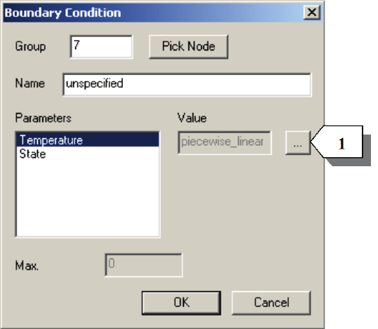
PAM-RTM 2014 301 USER’S GUIDE & TUTORIALS
© 2014 ESI Group (released: Apr-14)
TUTORIALS
Curing of a Plate
Zones
Assign the material Glass to the zone 6. Choose a porosity of 0.57, i.e., the fiber volume
fraction is 43%.
Note:
· For a curing simulation, the meaning of porosity is the same as in the simulation
of injection. Porosity is equal to 1-Vf, where Vf is the volume fraction of fibers.
Boundary Conditions
Create a new Temperature boundary conditions.
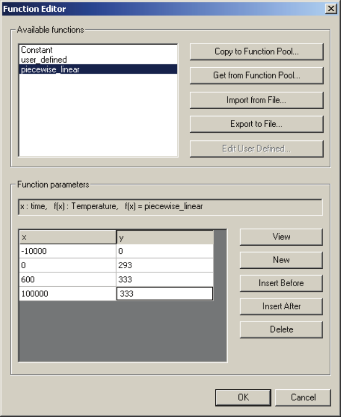
USER’S GUIDE & TUTORIALS 302 PAM-RTM 2014
(released: Apr-14) © 2014 ESI Group
TUTORIALS
Curing of a Plate
Open the Function Editor [1] to define a curve of the temperature vs. time.
Choose piecewise_linear and enter the points in the following sequence (the order is
very important):
· (-10000, 0)
· (0, 293)
· (600, 333)
· (10000, 333)
The first point is used to avoid problems in case there would be slightly negative time
values generated during the simulation. The last point tells the software to keep the
temperature constant to 333 degrees after 600 seconds of curing. Otherwise, the
software would extrapolate using the slope defined by the two last points.
Repeat this procedure now for the second boundary condition (group 8).
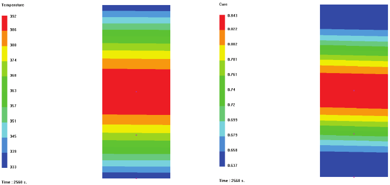
PAM-RTM 2014 303 USER’S GUIDE & TUTORIALS
© 2014 ESI Group (released: Apr-14)
TUTORIALS
Curing of a Plate
Sensors
In order to get curves of temperature in time, three sensors are set in the cavity. Define
the sensors as Points and set the following coordinates:
· (0.005, 0.00635, 0.) (lower quarter)
· (0.005, 0.0127, 0.) (middle)
· (0.005, 0., 0.) (boundary condition)
Simulation Results
Save the .dtf file and launch the simulation.
Select Temperature and Cure scalar fields in the display toolbar. You should have the
following. Note on the Cure picture that it begins in the center of the part and ends up
on the top and bottom faces. This is important to avoid a build up of residual stresses in
the part.
The curve viewer can be used to display the following curves. In the explorer, right-
click each sensor and choose Plot.
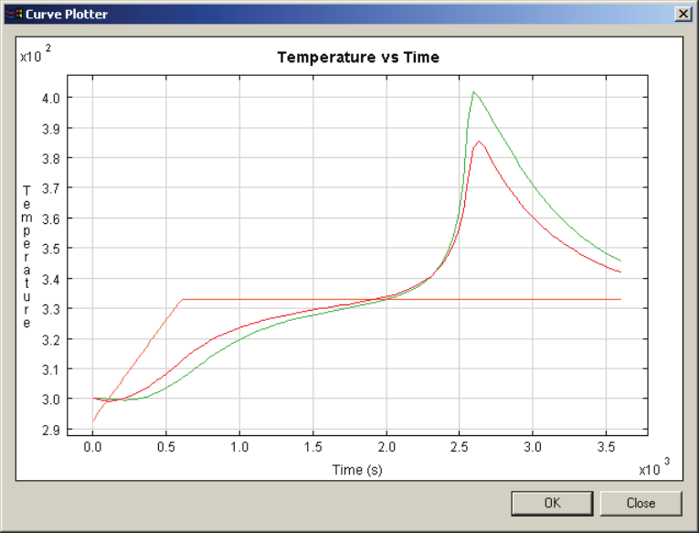
USER’S GUIDE & TUTORIALS 304 PAM-RTM 2014
(released: Apr-14) © 2014 ESI Group
TUTORIALS
Curing of a Plate
Note that sensor values are saved in text files so that you can import them later in more
advanced plotting software like Microsoft Excel or GNUPLOT. In this example, a file
named curing1d_Temperature_Curing_sensors.dat is generated for temperature values
on sensors, and a file named curing1d_Cure_sensors.dat contains the extent of cure
values on each sensor. The format of these files is simple. The first column represents
time, the next ones contain the scalar field value for each sensor. These files can easily
be imported in plotting software.
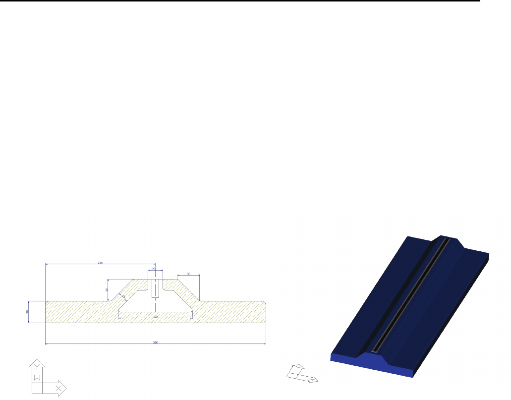
PAM-RTM 2014 305 USER’S GUIDE & TUTORIALS
© 2014 ESI Group (released: Apr-14)
TUTORIALS
Curing of a Part with an Insert
CURING OF A PART WITH AN INSERT
The files related to this example are:
- curing_insert.unv (starting mesh)
- curing_insert_1.dtf, curing_insert_2.dtf, curing_insert_3.dtf, + curing_insert.unv
(solution)
Objectives of the Analysis
This example will show you how to:
- Perform an analysis of the curing process on a part containing a steel insert,
- Use sensors.
Visualization of Groups and Zones
The part simulated in this example contains a metallic insert, which has an influence on
the curing of the composite. The geometry of the complete part is extruded from the
section shown below, so a two-dimensional analysis is appropriate here.
Create a new Curing simulation with File->New. Import the mesh file
curing_insert_start.unv.
Visualize the zones and groups of nodes. You should have the following display. Zone
number 21 will be used for the metallic insert, and zone 19 for the fiber preform. Group
number 22 and 23 are used for temperature boundary conditions.
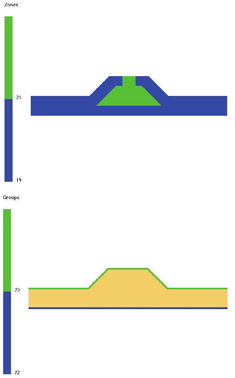
USER’S GUIDE & TUTORIALS 306 PAM-RTM 2014
(released: Apr-14) © 2014 ESI Group
TUTORIALS
Curing of a Part with an Insert
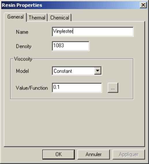
PAM-RTM 2014 307 USER’S GUIDE & TUTORIALS
© 2014 ESI Group (released: Apr-14)
TUTORIALS
Curing of a Part with an Insert
Simulation Parameters
Set the Max. experiment time to 2000 s. and the Max. number of steps to 500, which
leads to a constant time step of 4 s.
Open the Resin Properties dialog box.
To simulate the resin cure, the following parameters that describe the resin must be
specified:
- Name: Vinylester
- Density: 1083 Kg/m3
- Thermal Conductivity: 0.25 W/(m.K)
- Specific Heat: 1205 J/(Kg.K)
- Reaction Enthalpy: 300000 J/Kg
- Add a new reaction, open the Function Editor and select Kamal-Sourour model
(Kinetic_01) with A=9.17E6, E=7289, m=0.85 and p=1.15.
Double click now on the reinforcement. In this analysis, it is not necessary to enter the
permeability of the reinforcement since there is no flow involved in curing simulation.
However, for the thermal analysis, some parameters need to be specified in the Fabric
Properties. Enter the following parameters:
- Density: 2565 Kg/m3
- Specific Heat: 1205 J/(Kg.K)
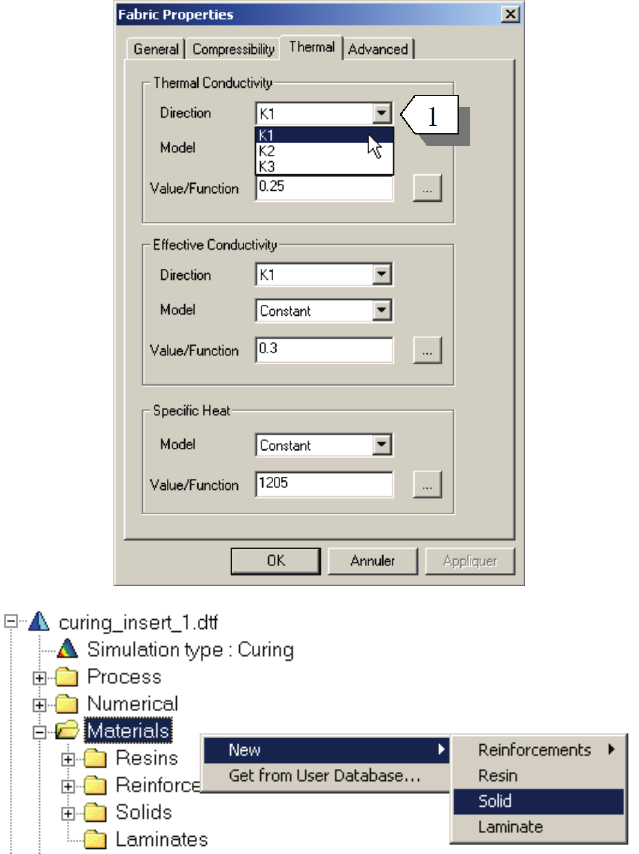
USER’S GUIDE & TUTORIALS 308 PAM-RTM 2014
(released: Apr-14) © 2014 ESI Group
TUTORIALS
Curing of a Part with an Insert
- Thermal Conductivity: 0.25 W/(m.K)
- Effective Conductivity: 0.3 W/(m.K)
Set isotropic thermal conductivity (K1=K2=K3=0.25W/(m.K)). Use the Direction drop-
down list [1] to select the direction to set. For constant conductivity, the value is
updated each time a character is typed in the text field (no need to Apply). To specify
conductivity as a function of temperature, you would choose f(temperature) in the
Model drop-down list, then click the … button to select a function.
Finally, the aluminum insert must be created. Create a new Solid material by right-
clicking the Materials item in the explorer, then choose New->Solid, as shown in the
figure above. Open the Solid Properties dialog box by double-clicking the new solid.
Note that there are no specific materials for inserts in PAM-RTM™. The Solid material
type must be used when you need to specify a non-permeable material such as metallic
or foam inserts.
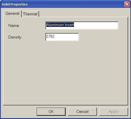
PAM-RTM 2014 309 USER’S GUIDE & TUTORIALS
© 2014 ESI Group (released: Apr-14)
TUTORIALS
Curing of a Part with an Insert
The following parameters for the aluminum insert must be specified:
- Density: 2702 Kg/m3
- Specific Heat: 900 J/(Kg.K)
- Thermal Conductivity: 2.165 W/(m.K)
Before launching the actual simulation, it is necessary to assign the appropriate material
to each zone and to set the boundary conditions. Assign the aluminum insert to zone 21
and the default fabric to zone 19. The porosity of zone 2 (insert) should be set to zero
for consistency. However if you forget to do so PAM-RTM™ automatically assigns a
zero porosity to solid-type materials.
To facilitate the analysis, sensors will now be defined with the Create Sensors dialog
box (Simulation->Create Sensors). In the Method drop-down list, choose two points and
set the number of sensors to 5. Enter the coordinates of Point 1 (0.09, 0., 0.) and Point 2
(0.09, 0.03, 0.) and click the Create button.
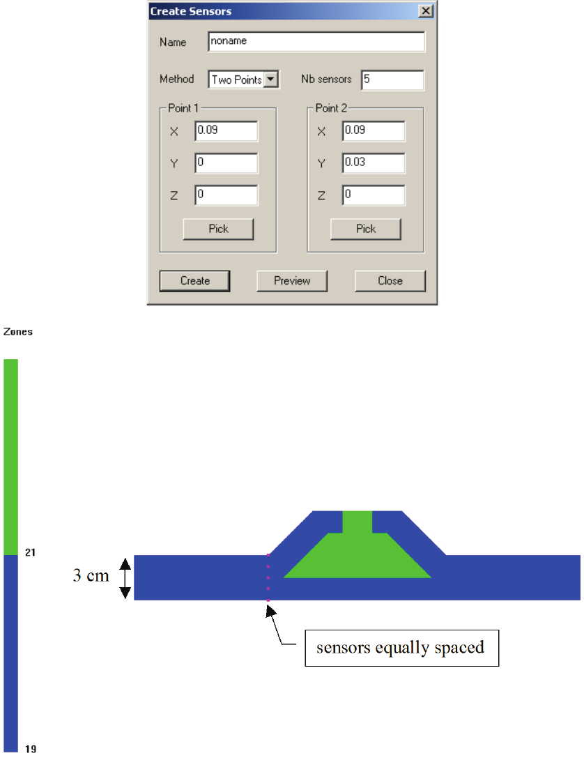
USER’S GUIDE & TUTORIALS 310 PAM-RTM 2014
(released: Apr-14) © 2014 ESI Group
TUTORIALS
Curing of a Part with an Insert
The initial temperature of the fibers and the mold is 310°K (to be set in the Process
Curing dialog box).
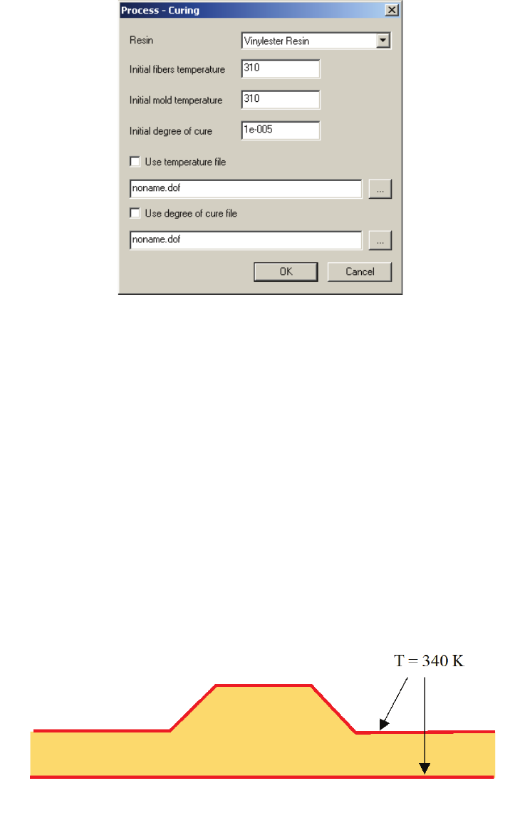
PAM-RTM 2014 311 USER’S GUIDE & TUTORIALS
© 2014 ESI Group (released: Apr-14)
TUTORIALS
Curing of a Part with an Insert
Three cases corresponding to three different curing strategies will be analyzed:
1. Mold wall at 340°K.
2. Lower mold wall at 350°K and upper mold wall at 330°K.
3. Mold walls initially at 310°K with a linear temperature variation in time up to
340°K.
Curing Simulations
Case 1 (mold walls at 340°K)
Create the temperature boundary conditions for the group 22 and 23, and set the
temperature at 340. Save and launch the simulation. The figure below shows the
temperature boundary conditions. Heating is performed from the outside on the top and
bottom surfaces of the part.
The first parameter to verify in the simulation results is resin conversion. The results
below show that curing begins on the sides. Therefore the solidification of the resin
begins close to the mold walls, i.e., on the outside of the part. Because of the heat
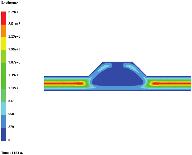
USER’S GUIDE & TUTORIALS 312 PAM-RTM 2014
(released: Apr-14) © 2014 ESI Group
TUTORIALS
Curing of a Part with an Insert
generated by the exothermic chemical reaction, the solidification moves then towards
the center of the part. Resin conversion reaches then its peak at the center of the part.
Note that the metallic insert remains at a nearly constant temperature of 320°K. This
means that its temperature is lower than the extremities of the mold. So the curing rate
of the resin is minimal near the insert.
This type of curing from outside to inside will have several effects on the part. First of
all, as the solidification of the resin begins on the outside of the part, this means that
shrinkage will occur first on the outside. This is usually one cause of poor surface
finish. Obviously, this approach cannot be used if a class A surface is required. Another
problem is related to the thermal residual stresses, which result from a delayed cure in
the center of the part while the outside has already become rigid. This can affect
considerably the mechanical properties of the part. Finally, the slow cure rate near the
insert can cause a problem, if the resin is not sufficiently cured. The region located near
the insert will have a weaker mechanical resistance. As the insert is usually connected
to another part, it will be submitted to significant loadings that might create
delaminations in the composite.
The figures below show the evolution of cure in time in the part. The evolution of this
parameter is closely connected to temperature. Indeed, the heat generated by the
exothermic chemical reaction will cause a temperature increase. On the other side, the
numerical results show that the chemical reaction is accelerated when the temperature
reaches its peak. Note the temperature peaks at the center of the part. This is also where
most of the heat is liberated by the exothermic chemical reaction. Temperature is
smaller near the insert, which acts as a heat sink. This causes a slower cure of the resin
in this region and may reduce locally the mechanical properties of the composite.
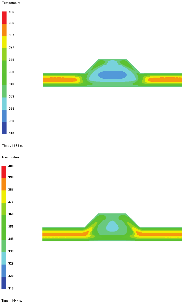
PAM-RTM 2014 313 USER’S GUIDE & TUTORIALS
© 2014 ESI Group (released: Apr-14)
TUTORIALS
Curing of a Part with an Insert
The exothermic reaction caused the part's temperature to increase significantly. The
temperature peaked in the center of the part at about 405°K.
This curing strategy from outside to inside is certainly not the best one. As a matter of
fact, a series of problems is associated with this approach:
- Shrinkage and surface finish
- Thermal residual stress
- High temperatures in the center of the part
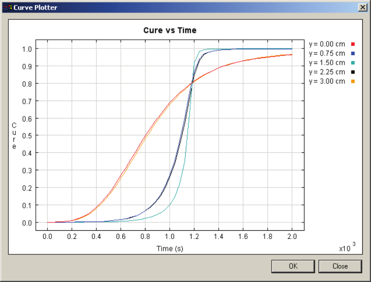
USER’S GUIDE & TUTORIALS 314 PAM-RTM 2014
(released: Apr-14) © 2014 ESI Group
TUTORIALS
Curing of a Part with an Insert
- Weak curing rate near the insert
The analysis of the sensor recordings leads to the same conclusion. Sensor 1 is
positioned on the bottom surface of the mold (y = 0 cm). Then, starting from the lower
surface, sensor 2 is located at a quarter position into the part, sensor 3 halfway and
sensor 4 three quarters into the part. The extent of cure curves recorded by the sensors
show that the center of the part reaches a critical degree of cure (0.7) faster than the
outside region. This can lead to problems in the final part.
Case 2 (bottom mold wall at 350°K and top wall at 335°K)
This curing strategy heats up the composite from one side. Simulation results show that
the solidification of the resin begins on the lower surface of the part. Then a curing front
progresses through the part, beginning from the highest temperature at the bottom of the
part up to the upper surface where the temperature is the smallest.

PAM-RTM 2014 315 USER’S GUIDE & TUTORIALS
© 2014 ESI Group (released: Apr-14)
TUTORIALS
Curing of a Part with an Insert
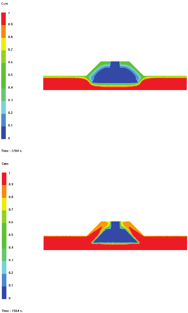
USER’S GUIDE & TUTORIALS 316 PAM-RTM 2014
(released: Apr-14) © 2014 ESI Group
TUTORIALS
Curing of a Part with an Insert
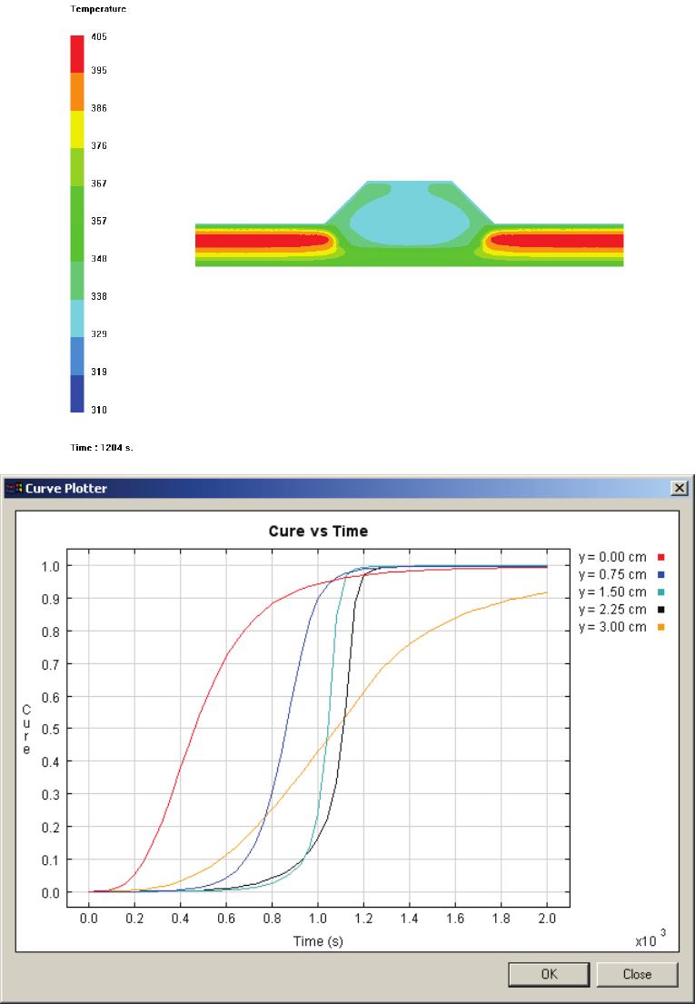
PAM-RTM 2014 317 USER’S GUIDE & TUTORIALS
© 2014 ESI Group (released: Apr-14)
TUTORIALS
Curing of a Part with an Insert
This type of curing has several effects on the quality of the final part. First of all, as the
resin at the bottom solidifies and the curing front moves toward the top surface of the
part, problems related to shrinkage are no longer present. Therefore the surface finish
will be good on the lower surface. If the objective is to obtain a class A finish on one
side, only this method will lead to acceptable results. Indeed, although the lower surface
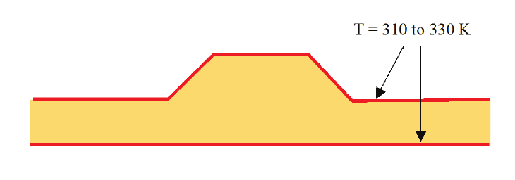
USER’S GUIDE & TUTORIALS 318 PAM-RTM 2014
(released: Apr-14) © 2014 ESI Group
TUTORIALS
Curing of a Part with an Insert
will have an improved finish, the upper face will show some imperfections. Because the
resin is solidifying uniformly from the bottom towards the unconstrained top of the part,
there will not be any thermal residual stresses in the composite.
The temperature increases with time as the curing front advances until it reaches three
quarters of the part. The exothermic chemical reaction of the resin increases
significantly the temperature of the part. The maximum temperature reached at three
quarters through the thickness is 405°K. Such a high temperature can spoil the resin and
decrease its mechanical properties.
This type of curing produces better results than the first strategy from outside to inside.
In particular, it leads to a better surface finish. However, it is necessary to pay attention
to the high temperatures that can be reached. Because of the heat generated during resin
cure especially in thick composite parts, it can cause the resin to degrade.
The analysis of the sensor curves confirms these results. Indeed, according to the
position of the sensors, resin cure does not begin at the same moment and as the
temperature increases, the chemical reaction becomes faster.
Case 3 (linear heating from 310°K to 330°K)
For this simulation the Max. experiment time is set to 3000 s. and the Max. number of
steps is left to 500.
Create a temperature boundary condition, then specify temperature as a
Piecewise_Linear function as shown in the Function Editor dialog below.

PAM-RTM 2014 319 USER’S GUIDE & TUTORIALS
© 2014 ESI Group (released: Apr-14)
TUTORIALS
Curing of a Part with an Insert
Use the Copy command available when you right-click on a boundary condition to
avoid entering the control points of the piecewise linear curve twice.
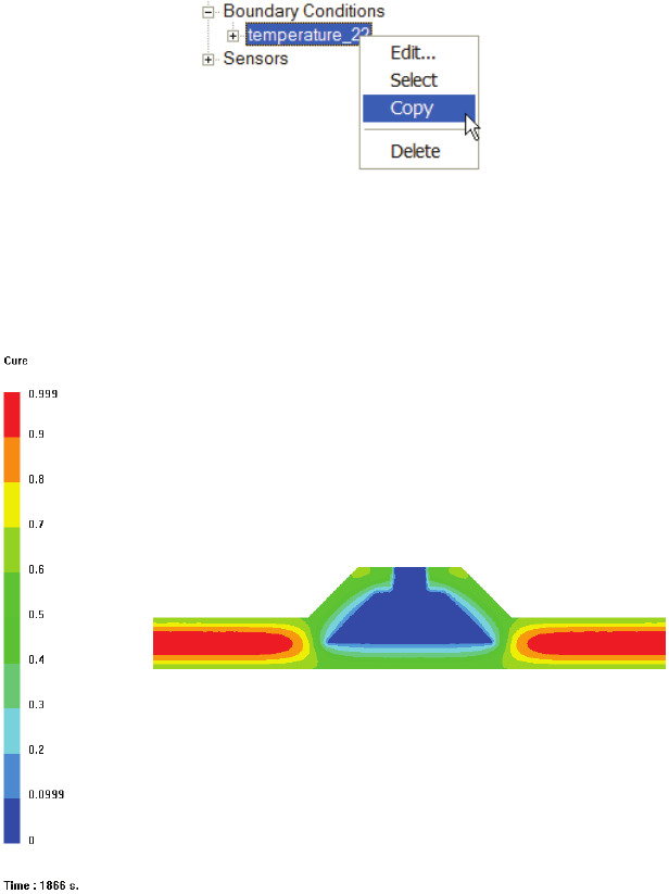
USER’S GUIDE & TUTORIALS 320 PAM-RTM 2014
(released: Apr-14) © 2014 ESI Group
TUTORIALS
Curing of a Part with an Insert
The figures below show the resin conversion at 1866 s, 2166 s and 1926 s. With this
type of heating, curing slowly begins on the sides of the part, then the center catches up
and the exothermic reaction begins to solidify the center and then moves towards the
sides.
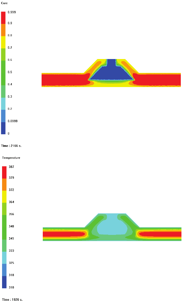
PAM-RTM 2014 321 USER’S GUIDE & TUTORIALS
© 2014 ESI Group (released: Apr-14)
TUTORIALS
Curing of a Part with an Insert
This method presents several advantages. There is no thermal residual stress in the part
if the lower and upper surfaces of the part remain unconstrained. The shrinkage of the
resin due to curing will not create problems in the part and conditions are met to obtain
a good surface finish.
The temperatures analysis demonstrates that the temperature peaks at the center of the
part are about 20°K lower than the two other cases. This reduces the possibility of
spoiling the resin because of overheating.
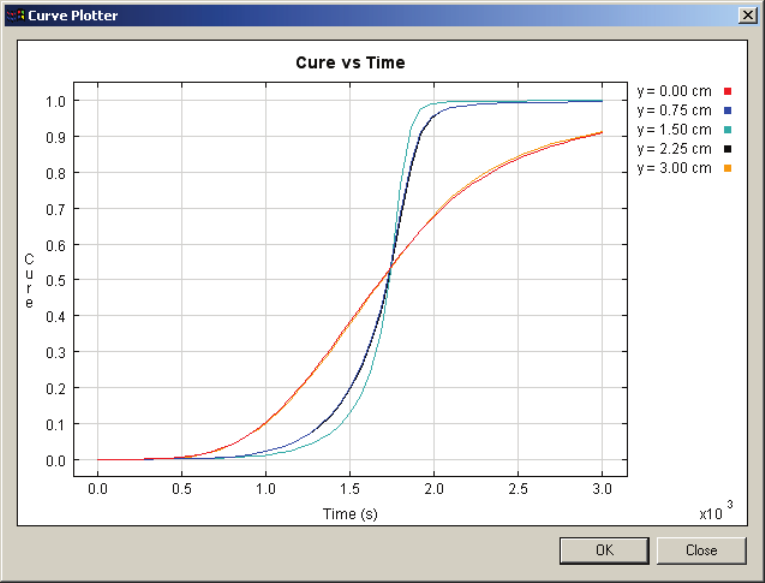
USER’S GUIDE & TUTORIALS 322 PAM-RTM 2014
(released: Apr-14) © 2014 ESI Group
TUTORIALS
Curing of a Part with an Insert
However, there is one major drawback with this method of curing a thick composite
part: curing cycles take a much longer time to be completed.
The results of the sensors next page show that the temperature peak is reached at the
center of the part.
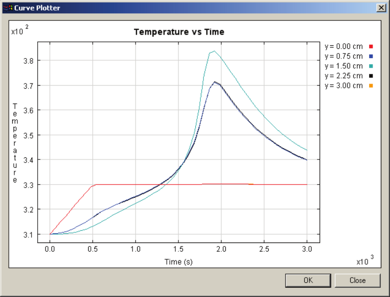
PAM-RTM 2014 323 USER’S GUIDE & TUTORIALS
© 2014 ESI Group (released: Apr-14)
TUTORIALS
Curing of a Part with an Insert
Conclusion
The three curing examples analyzed here highlight the importance of selecting the best
curing strategy. Indeed, it all depends on the objective (good surface finish on one or
both surfaces). The numerical simulation can help to understand and predict the curing
behavior and hence, avoid numerous and costly trial and errors testing.
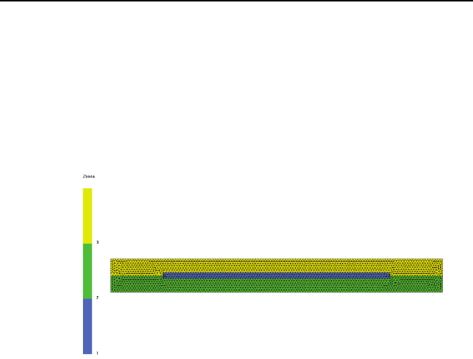
USER’S GUIDE & TUTORIALS 324 PAM-RTM 2014
(released: Apr-14) © 2014 ESI Group
TUTORIALS
Thermal Contact Resistance
THERMAL CONTACT RESISTANCE
The following files will be used:
- contact_start.unv (starting mesh)
- contact.dtf + contact.unv (solution)
Objectives
This tutorial shows how to specify parameters for a preheating simulation, taking into
account a thermal contact resistance.
Previously quads and bricks were allowed for preheating and curing simulations with
the old solver, but this is no more the case with the parallel solver, which only supports
triangles and tetrahedra.
Creation of Groups
Use File->New to create a new preheating simulation, and then import the mesh file
contact_start.unv.
The different zones represent a fiber preform (zone 1) in a mold (zone 2 and 3).
First create a group of nodes at the bottom of the mold, then another group on top of the
mold. These will be used for imposed temperature boundary conditions.
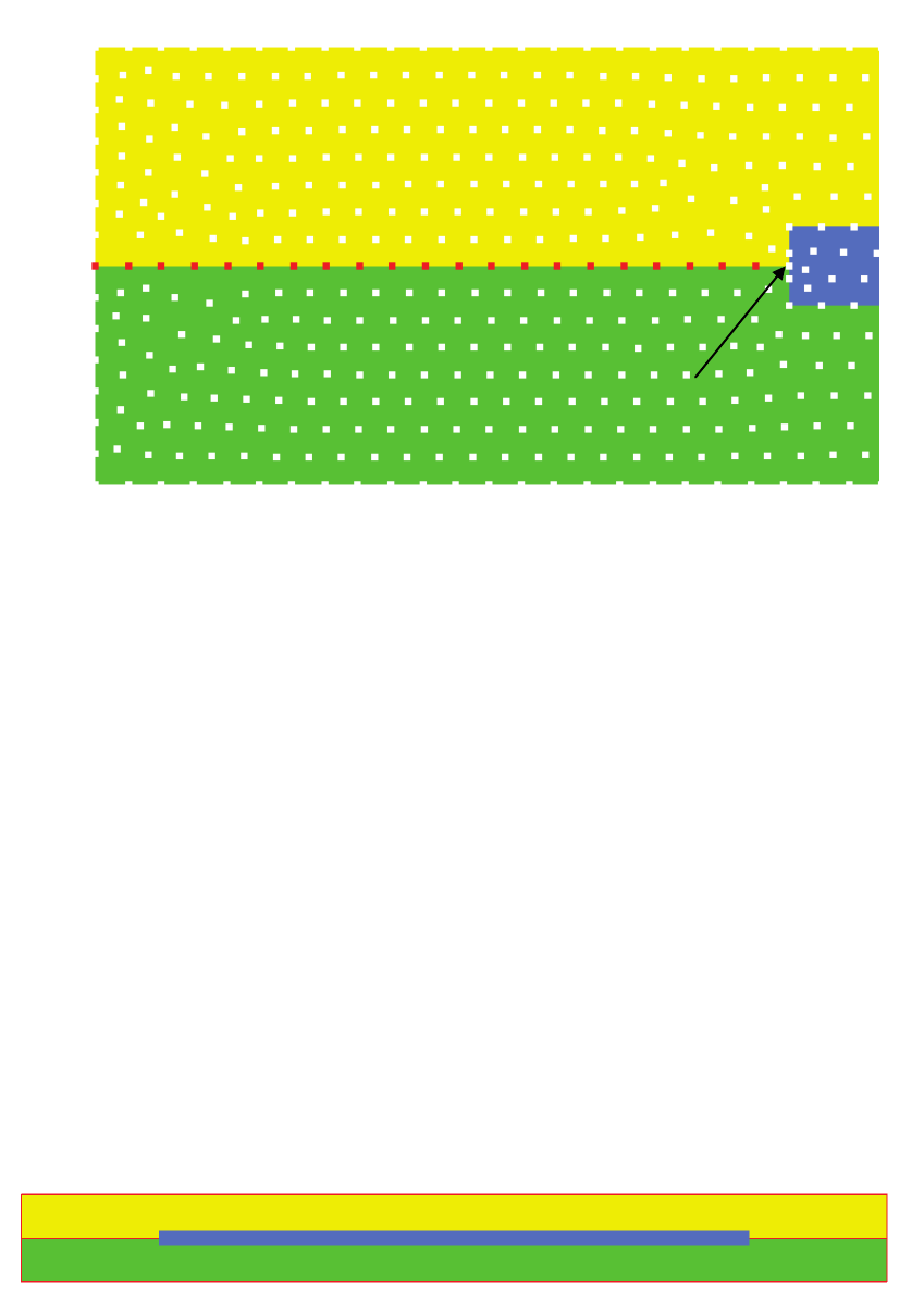
PAM-RTM 2014 325 USER’S GUIDE & TUTORIALS
© 2014 ESI Group (released: Apr-14)
TUTORIALS
Thermal Contact Resistance
A contact interface will then be created at the interface of the bottom and top mold.
First select nodes as shown above. Notice that the node common to the top mold,
bottom mold, and preform (shown with an arrow in the figure above) was not selected.
This is necessary otherwise a free edge would be generated on the mold/preform
interface, which would be in conflict with the automatic mold/preform interface. Select
nodes the same way on the right side of the part (add the nodes to the same selection).
In this example a single group is created containing nodes on both sides of the part, but
of course it would be possible to create two groups.
Notes:
· The contact interface can only be created at the interface between two zones.
· If we were working on a 3D mesh, we would select element faces instead of
nodes.
Once the selection is done, choose Groups->Contact Interface.
The creation of a contact interface modifies the mesh. Coincident nodes are created on
the interface and elements are disconnected. Choose View->Outline->Free Edges to
verify the interface. The red line in the next figure shows that the elements have been
correctly disconnected.
do not select
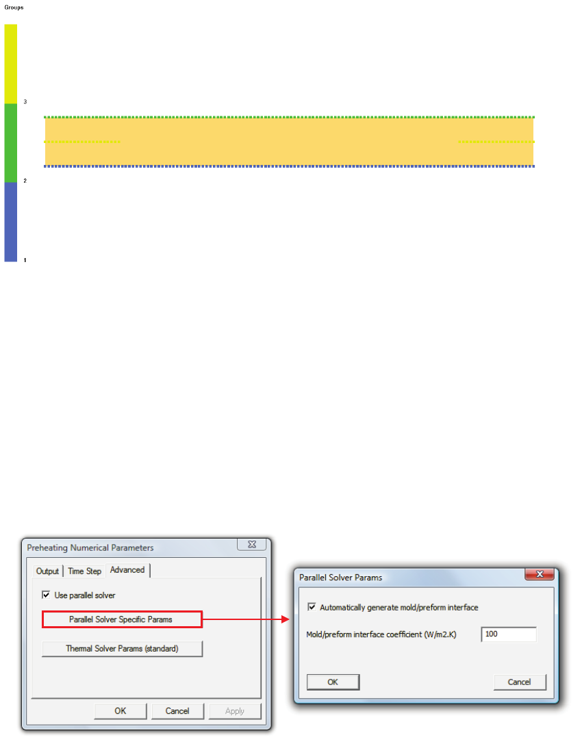
USER’S GUIDE & TUTORIALS 326 PAM-RTM 2014
(released: Apr-14) © 2014 ESI Group
TUTORIALS
Thermal Contact Resistance
The three groups are shown below.
Simulation
With the parallel solver, a thermal contact interface is automatically generated between
the mold and the preform. The conductance value (reciprocal of the resistance) used on
that automatic interface is found by pushing the Parallel Solver Specific Params button
in the Advanced Numerical Parameters. For this example we will keep the default
conductance of 100 W/m2.K.
PAM-RTM 2014 327 USER’S GUIDE & TUTORIALS
© 2014 ESI Group (released: Apr-14)
TUTORIALS
Thermal Contact Resistance
Also in the Advanced tab, select use parallel solver.
In the Time Step tab, set max experiment time = 1800 s and max number of steps = 50.
In the Process parameters, check that the initial temperature of the fibers and the mold
is 300 K.
Materials
For the fabric:
- Density = 2565 Kg/m³
- Thermal conductivity k1 = k2 = k3 = 0.5 W/m.K
- Specific Heat = 1205 J/Kg.K
For the mold (create a new material of type solid):
- Density = 2707 Kg/m³
- Thermal conductivity = 150 W/m.K
- Specific Heat = 900 J/Kg.K
Zones
Associate zone 1 with the Default Fabric and zones 2 and 3 with the Default Mold.
Porosity of zone 1 is kept to 0.5, while the porosity of zones 2 and 3 doesn’t really
matter as it will be forced to zero by the solver. However it is a good habit to set it to
zero.
Boundary Conditions
Create two temperature boundary conditions. The first is associated with lower mold
wall at 310 K and the second with the upper mold wall at 350 K.
Create a new contact resistance boundary condition associated with group 3, and set the
value of the thermal contact resistance to 0.001 m²K/W. A second simulation will be
run with a contact resistance value of 0.01 m²K/W, and a third one with 0.1 m²K/W.
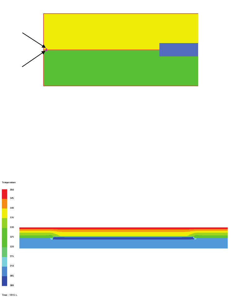
USER’S GUIDE & TUTORIALS 328 PAM-RTM 2014
(released: Apr-14) © 2014 ESI Group
TUTORIALS
Thermal Contact Resistance
Sensors
Create the following sensors:
- A (0.04, 0.49, 0)
- B (0.04, 0.51, 0)
Post-Processing the Results
The temperature contour obtained after 1800 sec. is shown below for the third case
corresponding to a contact resistance of 0.1 m²K/W.
A
B
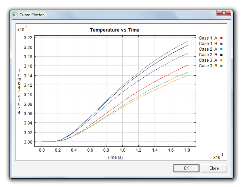
PAM-RTM 2014 329 USER’S GUIDE & TUTORIALS
© 2014 ESI Group (released: Apr-14)
TUTORIALS
Thermal Contact Resistance
By using sensors A, B near the interface between the two parts of the mold, we can
observe the influence of the thermal contact resistance.
Temperature curves for cases 1, 2 and 3, corresponding respectively to a contact
resistance of 0.001, 0.01 and 0.1 m²K/W are plotted below. For case 3 we can see that
there is a non-negligible difference of about 7 degrees on both sides of the interface
after 1800 sec.
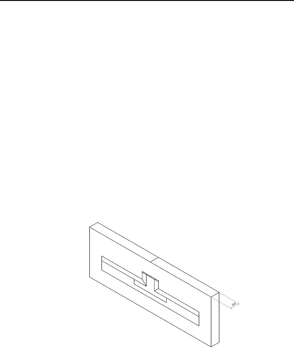
USER’S GUIDE & TUTORIALS 330 PAM-RTM 2014
(released: Apr-14) © 2014 ESI Group
TUTORIALS
Non-Isothermal 3D – Fibers Orientation
NON-ISOTHERMAL 3D – FIBERS ORIENTATION
This case is a chaining analysis (preheating, heated RTM and curing) for a 3D part with
orientations. The following files will be used:
- Insert_3D.unv (starting mesh)
- Insert_3D_Preheating.dtf + Insert_3D_Preheating.unv (solution)
Insert_3D_Heatedfilling.dtf + Insert_3D_Heatedfilling.unv (solution)
Insert_3D_Curing.dtf + Insert_3D_Curing.unv (solution)
Objective of the Analysis
This tutorial will show you how to simulate a chained RTM process stage by stage
(preheating -> heated filling -> curing). Data transfer between each stage is explained,
for instance how to use the temperature distribution at the end of the preheating analysis
to initialize the temperature for filling.
Material characteristics and some set-up steps like orientation, and material assignment
are common to each step and are described prior to the description of each step.
Geometry Description
The geometry (Insert_3D.unv) is composed of several 3d parts that have been defined
in order to split the insert, the preform and the mold volume which do not have the same
physical properties.
Part geometry
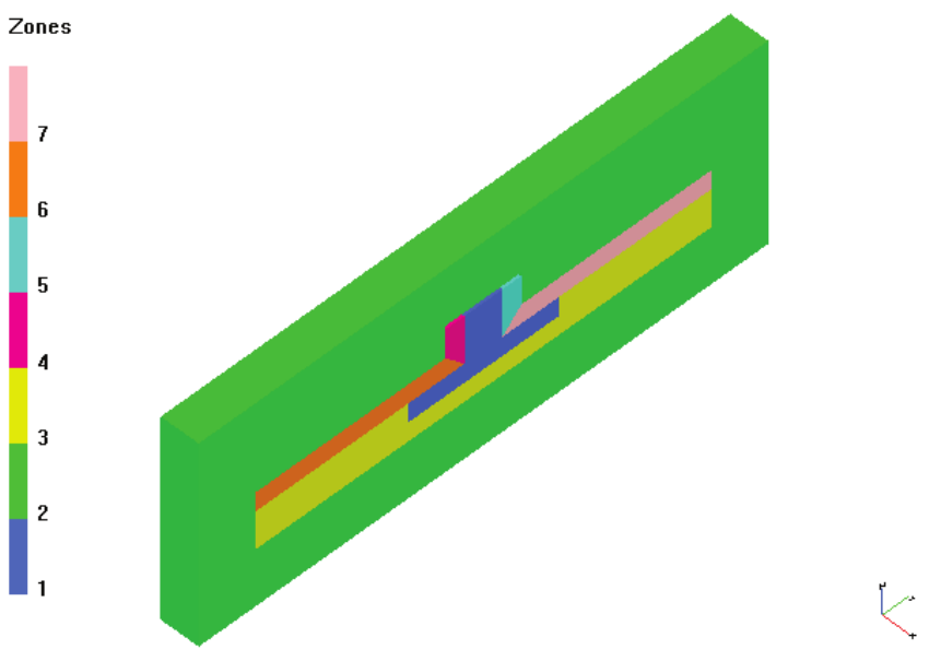
PAM-RTM 2014 331 USER’S GUIDE & TUTORIALS
© 2014 ESI Group (released: Apr-14)
TUTORIALS
Non-Isothermal 3D – Fibers Orientation
Zones of the Part
The zone IDs corresponding to each material are shown below:
- Insert: zone ID 1
- Mold: zone ID 2
- Reinforcement: zone IDs 3 to7
Zones
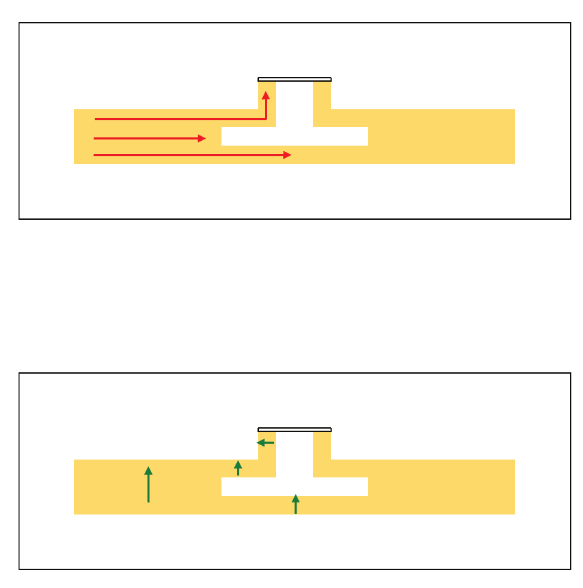
USER’S GUIDE & TUTORIALS 332 PAM-RTM 2014
(released: Apr-14) © 2014 ESI Group
TUTORIALS
Non-Isothermal 3D – Fibers Orientation
Fiber Orientations
The orientation of the preform (Zone IDs 3 to7) must be defined as shown below;
- K1 is parallel to Y and K2 to Z for zones 3,6 and 7;
- K1 is parallel to Z and K2 to Y for zones 4 and 5.
K1
K2
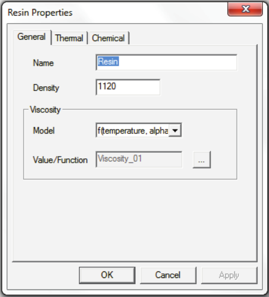
PAM-RTM 2014 333 USER’S GUIDE & TUTORIALS
© 2014 ESI Group (released: Apr-14)
TUTORIALS
Non-Isothermal 3D – Fibers Orientation
Material parameters
The resin parameters
To simulate the resin cure, the following parameters must be specified.
In the general tab:
- Density: 1120 Kg/m3
- Viscosity: a viscosity function relates viscosity with temperature and the degree of
cure.
Resin general sub-section dialog box
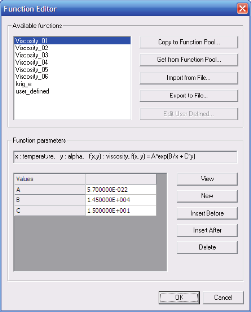
USER’S GUIDE & TUTORIALS 334 PAM-RTM 2014
(released: Apr-14) © 2014 ESI Group
TUTORIALS
Non-Isothermal 3D – Fibers Orientation
- Select the Viscosity_01 model where A = 5.7E-22, B = 1.45E+4 and C = 15.
Viscosity function edition
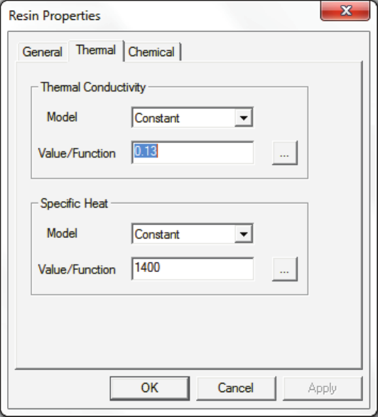
PAM-RTM 2014 335 USER’S GUIDE & TUTORIALS
© 2014 ESI Group (released: Apr-14)
TUTORIALS
Non-Isothermal 3D – Fibers Orientation
In the Thermal sub section:
- thermal conductivity: 0.13 W/m.K
- Specific heat: 1400 J/Kg.K
Resin thermal sub section dialog box
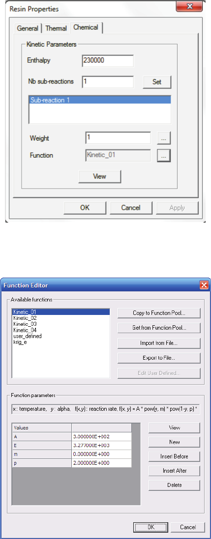
USER’S GUIDE & TUTORIALS 336 PAM-RTM 2014
(released: Apr-14) © 2014 ESI Group
TUTORIALS
Non-Isothermal 3D – Fibers Orientation
In the Chemical sub section,
- Enthalpy: 230000 J/kg
Resin chemical sub section dialog box
- kinetics model: Kinetic_01 where A=300, B=3277, m=0, p=2, as shown below
Kinetic function edition
PAM-RTM 2014 337 USER’S GUIDE & TUTORIALS
© 2014 ESI Group (released: Apr-14)
TUTORIALS
Non-Isothermal 3D – Fibers Orientation
The fibers parameters
The reinforcement characteristics are set as below:
- Name: Preform
- Density: 2540 kg/m3
- Permeability K1: 6E-11 m2
- Permeability K2=K3: 1E-11 m2
- Thermal Conductivity K1=K2=K3: 0.1 W/m.K
- Effective Conductivity K1=K2=K3: 0.3 W/m.K
- Specific heat: 840 J/Kg.K
The mold parameters
The mold characteristics are set as below:
- Name: Metal
- Density: 2700 kg/m3
- Thermal Conductivity: 10 W/m.K
- Specific heat: 950 J/Kg.K
Material Assignment
For each of the set-up step, the material assignment will be the same. It will have to be
done for each step.
Visualize the zones of the parts and make material assignment as follows,
· zone ID 1 (Insert): Metal
· zone ID 2 (Mold): Metal
· zone IDs 3 to 7 (Reinforcement): Preform.
Keep parameters of all the zones as default:
· Porosity: 0.5
· Thickness: 0.0005m
Note:
· A solid material such as the metal just defined is a non porous material; the
porosity here is therefore set to zero. But this is not mandatory, as PAM-RTM
will force porosity to zero for solid materials
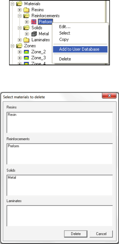
USER’S GUIDE & TUTORIALS 338 PAM-RTM 2014
(released: Apr-14) © 2014 ESI Group
TUTORIALS
Non-Isothermal 3D – Fibers Orientation
Simulation Stage1: Preheating
Create a Preheating analysis and import insert_3D.unv, then define fiber orientations,
material properties and material assignment to zones as in previous description.
The objective of this stage is to simulate 1 hour of part heating before injection starts.
Material Database
To reuse the defined materials conveniently in the following analysis (heated RTM and
curing), it is recommended to add them into the Material Database.
For example, right click on Preform in the Model Explorer and select Add to User
Database, as shown below.
After adding the three materials, the user can check the modified material database by
selecting the Simulation -> Manage User Database menu, as shown below
Material database content
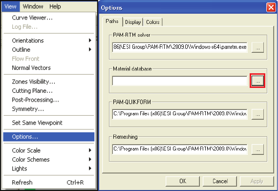
PAM-RTM 2014 339 USER’S GUIDE & TUTORIALS
© 2014 ESI Group (released: Apr-14)
TUTORIALS
Non-Isothermal 3D – Fibers Orientation
Note:
· The user needs to check if database path is set properly.
· In the Menu, select View
Options..., then in the Options interface, click on
open button (as shown below) to select the file used for material database
Material database path setting
· If the material database is used for the first time in PAM-RTM, the user should
create an empty .dtf file such as my_material_data.dtf in advance with a text
editor, then select it in the Options>Paths tab
After this operation, the path of this dtf file is stored in the application settings,
so it only needs to be entered once.
Numerical Settings and DMP solver activation
Set the following parameters in Preheating Numerical Parameters interface:
· Save temperature: checked
· Results sampling period: 50
· Max experiment time: 3600 s
· Max number of steps: 250
· Check use parallel solver, as shown below.
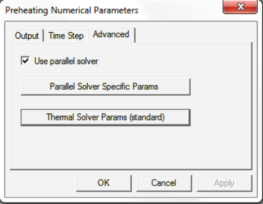
USER’S GUIDE & TUTORIALS 340 PAM-RTM 2014
(released: Apr-14) © 2014 ESI Group
TUTORIALS
Non-Isothermal 3D – Fibers Orientation
Boundary Conditions and Initial Values
- In the Process interface, keep initial temperatures as default,
· initial fibers temperature: 300 K
· Initial mold temperature: 300 K
Create a group which corresponds to a convection boundary condition by selecting
faces all around the mold, as shown below.
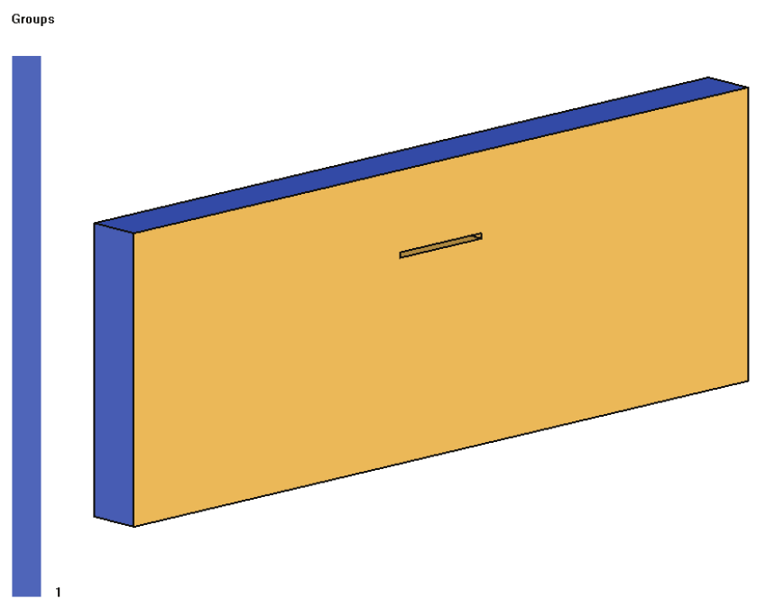
PAM-RTM 2014 341 USER’S GUIDE & TUTORIALS
© 2014 ESI Group (released: Apr-14)
TUTORIALS
Non-Isothermal 3D – Fibers Orientation
Group for preheating stage
- About the parameters of convection
· Reference temperature: 323 K
· Convection Coefficient: 300 W/m2.K
Job Launching
When a job using the parallel solver is launched, a Prompt interface appears
automatically to let the user enter the number of processors that will be used, as shown
below.
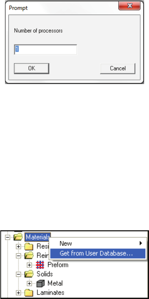
USER’S GUIDE & TUTORIALS 342 PAM-RTM 2014
(released: Apr-14) © 2014 ESI Group
TUTORIALS
Non-Isothermal 3D – Fibers Orientation
Parallel job launching
Simulation Stage2: Heated RTM
Create a Heated RTM analysis and import Insert_3D_Preheating.unv which is the
mesh file generated by Preheating analysis and not the initial one Insert_3D.unv.
As Insert_3D_Preheating.unv has included the fiber orientation definition in the
previous Preheating analysis, there is no need to do it again in this analysis.
Check the parallel solver option in the numerical interface
Getting defined materials
In the Explorer, right click on the Materials folder and select Get from User
Database…, then select all the 3 materials and click on OK button to load them into
the current model, as shown below,
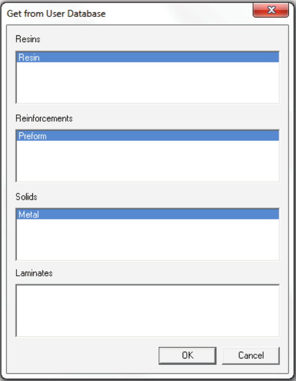
PAM-RTM 2014 343 USER’S GUIDE & TUTORIALS
© 2014 ESI Group (released: Apr-14)
TUTORIALS
Non-Isothermal 3D – Fibers Orientation
Material assignment
Visualize the zones of the parts and make material assignment as follows,
· zone ID 1 (Insert): Metal
· zone ID 2 (Mold): Metal
· zone IDs 3 to 7 (Reinforcement): Preform
Linking Preheating temperature
· Double click on Process in the Explorer, and then select the Thermal tab.
· Check the Use temperature file box.
· Click on the button Open to select the temperature results file.
· In this case, the temperature results of previous preheating analysis,
Insert_3D_Preheatingt.unf is selected, as shown below,
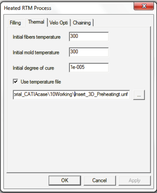
USER’S GUIDE & TUTORIALS 344 PAM-RTM 2014
(released: Apr-14) © 2014 ESI Group
TUTORIALS
Non-Isothermal 3D – Fibers Orientation
End of preheating temperature file path definition
Note:
· This linking is to import previous Preheating results as initial temperature of the
current Heated RTM analysis
· The file to select depends on the solver used for computation:
- for parallel solver (this case), the file is *t.unf
- for old solver, the file is *_p.dof.
Boundary Conditions
- convection boundary (same as Preheating case, i.e. defined on group 1)
- flow rate (group 2, see image below) :
· flow_rate = 1E-6 m3/s
· resin temperature = 300 K
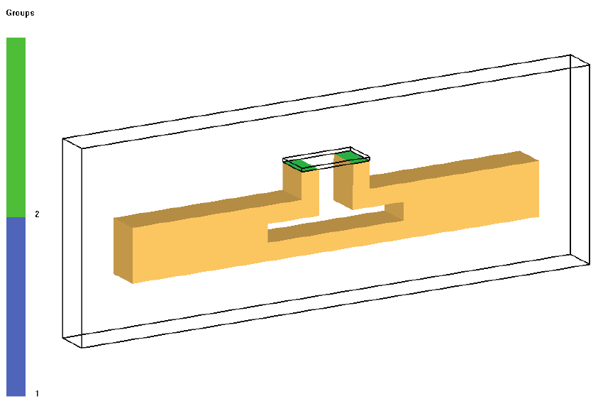
PAM-RTM 2014 345 USER’S GUIDE & TUTORIALS
© 2014 ESI Group (released: Apr-14)
TUTORIALS
Non-Isothermal 3D – Fibers Orientation
Groups for filling stage
Simulation Stage 3: Curing
Create a Curing analysis and import Insert_3D_Preheating.unv.
Get the 3 materials from the Material Database and make material assignment to zones.
Numerical Settings and DMP solver activation
Set the following parameters in Curing Numerical Parameters interface:
- Save temperature: checked
- Results sampling period: 50
- Max experiment time: 3600 s
- Max number of steps: 250
- Check use parallel solver
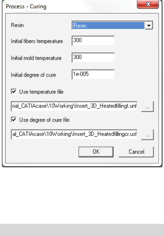
USER’S GUIDE & TUTORIALS 346 PAM-RTM 2014
(released: Apr-14) © 2014 ESI Group
TUTORIALS
Non-Isothermal 3D – Fibers Orientation
Linking Heated filling temperature and Cure
- Double click on Process in the Explorer; make sure Resin material is selected
- check the boxes of Use temperature file and select Insert_3D_Heatedfillingt.unf
- check the boxes of Use degree of cure file and select
Insert_3D_Heatedfillingcr.usf
End of filling temperature and cure files path definition
Note:
· Linking files with respect to solver used for curing analysis
Temperature file
Cure degree file
Parallel(DMP)
*t.unf
*cr.usf
old solver
*_Thermal_f.dof
*_Curing_f.dof
Boundary Conditions
Convection boundary condition (same as Preheating case)
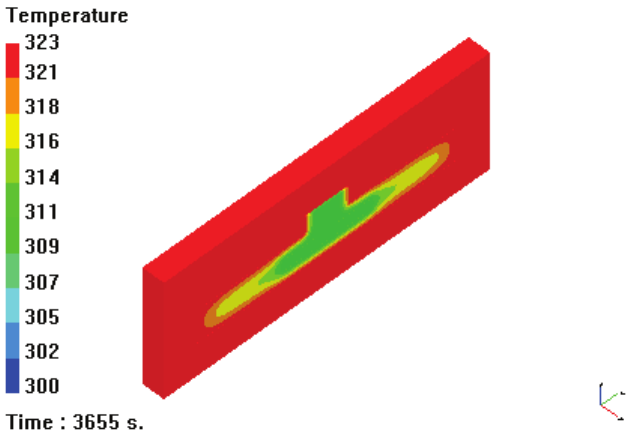
PAM-RTM 2014 347 USER’S GUIDE & TUTORIALS
© 2014 ESI Group (released: Apr-14)
TUTORIALS
Non-Isothermal 3D – Fibers Orientation
Analysis of the Results
Preheating stage
The last time state of preheating is 3655s (stop time was set to 3600s but with the
parallel solver the actual last state depends on the sampling period).
Because of temperature file linking, the temperature contour of last state is consistent
with that of initial state of Heated RTM stage, as shown below.
Last state of preheating stage
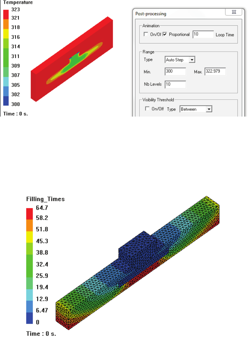
USER’S GUIDE & TUTORIALS 348 PAM-RTM 2014
(released: Apr-14) © 2014 ESI Group
TUTORIALS
Non-Isothermal 3D – Fibers Orientation
Initial state of heated RTM stage
(Range Type set as “Auto Step” for an easier comparison)
Heated RTM Stage
It shows that the filling time is 64.7s and at the end of filling there is a temperature and
cure gradient, as shown below,
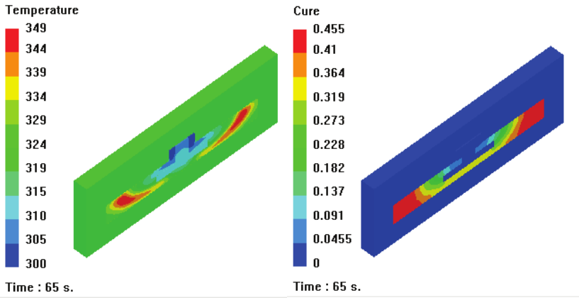
PAM-RTM 2014 349 USER’S GUIDE & TUTORIALS
© 2014 ESI Group (released: Apr-14)
TUTORIALS
Non-Isothermal 3D – Fibers Orientation
Temperature and cure distribution
(end of Heated RTM)
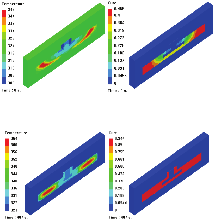
USER’S GUIDE & TUTORIALS 350 PAM-RTM 2014
(released: Apr-14) © 2014 ESI Group
TUTORIALS
Non-Isothermal 3D – Fibers Orientation
Curing Stage
Because of temperature and cure files linking, the temperature and cure distribution at
curing start (as shown below) are consistent with end of Heated RTM.
Temperature and cure distribution(Curing start)
After 487 seconds, 100% of the part has reached a resin cure of 90%. The temperature
distribution for this time step shows a peak of temperature at the center of the preform.
Temperature and cure distribution (end of Curing)
Conclusion
This tutorial has shown how to perform chained preheating, heated RTM and curing
simulations.

PAM-RTM 2014 351 USER’S GUIDE & TUTORIALS
© 2014 ESI Group (released: Apr-14)
TUTORIALS
User Defined Functions
USER DEFINED FUNCTIONS
The following files are used in this example.
- func_resinviscosity.c (source code template for resin viscosity)
- func_resinkinetics.c (source code template for resin kinetics)
- func_resinspecheat.c (source code template for resin specific heat)
- func_effthermalcond.c (source code template for effective conductivity of a wet
reinforcement)
Objectives
Explain the procedure to compile user defined functions for resin viscosity, kinetics,
specific heat, and effective conductivity of a wet reinforcement. This procedure only
applies to the parallel solver.
Windows Procedure
Two batch files and four C-language files (.c) are provided in the installation directory
of the PAM-RTM parallel solver, which is in general C:\Program Files (x86)\ESI
Group\PAM-RTM\version\Windows-x64\DMP:
- compile_rtm_udf_vs.bat (compile script for Visual Studio)
- compile_rtm_udf_sdk.bat (compile script for Windows SDK)
- func_resinviscosity.c (source code template for resin viscosity)
- func_resinkinetics.c (source code template for resin kinetics)
- func_resinspecheat.c (source code template for resin specific heat)
- func_effthermalcond.c (source code template for effective conductivity of a wet
reinforcement)
The first batch file is to be used with Visual Studio (free of professional edition), the
second one is to be used with the Windows SDK (software development kit). In general
it is better to work with Visual Studio, except for the case where the user doesn’t have a
professional edition and needs to compile for Windows 64-bit. The free editions of
Visual Studio don’t support 64-bit compilation. The free editions of Visual Studio and
the Windows SDK can be downloaded from Microsoft’s web site.
Here we will focus on user functions for resin viscosity and kinetics. User functions for
resin specific heat and effective conductivity are most of the time used to define them as
functions of temperature and degree of cure, so it is an advanced application. These will
be discussed in the last section of this tutorial.

USER’S GUIDE & TUTORIALS 352 PAM-RTM 2014
(released: Apr-14) © 2014 ESI Group
TUTORIALS
User Defined Functions
The first step is to copy the four provided .c files and the appropriate batch file (VS or
SDK) in some user directory. It is necessary to copy all the .c files even if only two of
them will be edited here (func_resinviscosity.c and func_resinkinetics.c), otherwise the
build procedure will fail.
Open the batch file in a text editor and check that the PAMRTM_INSTALL_DIR
variable corresponds to your actual installation directory, otherwise correct it. Then
open the .c files in Visual Studio or any text editor.
Note that you don’t have to create a project in Visual Studio. The procedure only relies
on command-line tools.
In this example we want to define viscosity and kinetics for two resins: my_resin_1 and
my_resin_2.
The first resin has a viscosity function of material age (i.e. function of time since a resin
particle entered the mold):
( )
5
2
102.7
01.0 ×
+= t
tf
Pa.s
The second resin has a viscosity function of temperature and degree of cure:
( )
α
α
⋅+
−
⋅×=
8.3
14500
21
1038.2,
T
eTf
Pa.s
Starting from the provided template for the viscosity function, the code to be written by
the user is highlighted below. The first resin is using only parameter local_time, which
corresponds to the time since a resin particle entered the mold, while the second resin
uses parameters temperature and alpha.
/*
* Return resin viscosity as a function of the current temperature, current
degree of cure, or current time.
*/
real func_resinviscosity(
char prefix[], /* case name */
char resin_name[], /* case name */
real temperature, /* current temperature in Kelvin */
real alpha, /* current degree of cure (value between 0 and 1) */
real local_time, /* current local time (time since particle entry in the
mold) */
real global_time) /* current global time (time since beginning of
injection) */
{
PAM-RTM 2014 353 USER’S GUIDE & TUTORIALS
© 2014 ESI Group (released: Apr-14)
TUTORIALS
User Defined Functions
/* ------------- Do not change anything above this line ------------- *
* ------------- Program your function below this line ------------- */
if ( strcmp( resin_name, "my_resin_1" ) == 0 ) {
return 0.01 + ( local_time * local_time ) / 7.2E5;
}
else if ( strcmp( resin_name, "my_resin_2" ) == 0 ) {
return 2.38E-21 * exp( 14500. / temperature + 3.8 * alpha);
}
else {
printf("unknown resin in user defined viscosity\n");
exit(1);
}
}
Note that this architecture doesn’t currently support units. The solver assumes the
returned value is in Pa.s for viscosity, s-1for kinetics.
The code to be written for kinetics in file func_resinkinetics.c would have the same
structure and is left as an exercise. Note that it is not mandatory to edit both viscosity
and kinetics functions. Depending on the user’s needs, only one of viscosity or kinetics
could be defined. Even though both functions will be compiled (one of the definitions
being the default implementation that just prints an error message and exits), there
shouldn’t be issues as long as the user doesn’t choose function type user_dll in the
PAM-RTM GUI for a function that is not defined.
We recommend that you print some messages in your functions to make sure the code is
correctly called. This should only be done for the first run, as it will slow down
execution a lot. For instance you could add these lines in func_resinviscosity.c:
real visc = …
printf("visc = %12.5E, T = %12.5E, alpha = %12.5E\n", visc, temperature,
alpha);
Now that the code is written, it is time to compile it. The procedure is a bit different for
Visual Studio and Windows SDK.

USER’S GUIDE & TUTORIALS 354 PAM-RTM 2014
(released: Apr-14) © 2014 ESI Group
TUTORIALS
User Defined Functions
Visual Studio 32-bit target
Open a command window with Start>Programs>Microsoft Visual Studio 2005>Visual
Studio Tools>Visual Studio 2005 Command Prompt. This is the path for Visual Studio
2005, but it should be almost the same for other versions. This will open a console
window in which the environment variables needed to compile with the command line
tools are already set (PATH for instance). Then simply type the command:
compile_rtm_udf_vs.bat x86
Note the x86 at the end of the command line.
This command compiles func_resinviscosity.c, func_resinkinetics.c,
func_resinspecheat.c, func_effthermalcond.c, which generates the corresponding four
.obj files. If compilation is successful, the command then copies a set of .obj files from
the PAM-RTM installation directory to the current directory and links all these .obj files
together to generate a dynamic link library called libprocast_DMP.dll. Once the
command is done, the user should check the date of libprocast_DMP.dll to make sure it
was just generated. If everything looks good, the new libprocast_DMP.dll must then be
copied to the installation directory of PAM-RTM and overwrite the file with same name
(make a copy of the file before overwriting it). That directory is in general C:\Program
Files (x86)\ESI Group\PAM-RTM\CurrentVersion\Windows-x86\DMP.
Visual Studio 64-bit target
There are only 2 differences for a 64-bit target, compared to the procedure for a 32-bit
target.
First the console window is opened with a shortcut that contains x64 in its name. For
instance with Visual Studio 2005, the shortcut is Start>Programs>Microsoft Visual
Studio 2005>Visual Studio Tools>Visual Studio 2005 x64 Win64 Command Prompt.
Then the x86 flag at the end of the command must be replaced by x64:
compile_rtm_udf_vs.bat x64
The newly generated libprocast_DMP.dll must then be copied to the installation
directory of PAM-RTM and overwrite the file with same name. That directory is in
general C:\Program Files (x86)\ESI Group\PAM-RTM\CurrentVersion\Windows-
x64\DMP. Be careful not to copy a 64-bit DLL in a 32-bit directory, or vice-versa.

PAM-RTM 2014 355 USER’S GUIDE & TUTORIALS
© 2014 ESI Group (released: Apr-14)
TUTORIALS
User Defined Functions
Windows SDK 64-bit target
Referring again to the procedure for Visual Studio 32-bit, the main difference here is
that we use the following shortcut to open the console window, or a similar shortcut for
a different version of the SDK:
Start>Programs>Microsoft Windows SDK v7.1>Windows SDK 7.1 Command Prompt
You should see a message similar to Targeting Windows 7 x64 printed in the console.
Then the command to compile is:
compile_rtm_udf_sdk.bat x64
Once again be careful with the x64 flag at the end of the command line. The batch file
won’t run correctly if you forget to specify it.
Linux Procedure
First locate the directory containing the binaries of the current PAM-RTM version. The
command “which pamrtmdmp” should allow you to identify that directory. Let’s call
that directory rtm_dir, we will need it again below. There is a subdirectory user_MP in
that directory. Copy all the files in rtm_dir/user_MP to the user directory where you
will compile. This will copy some object files (.o) as well as the makefile
compile_rtm_udf.mk and all the .c source code templates.
Edit the appropriate .c files to define viscosity and/or kinetics and/or specific heat
and/or effective conductivity, as explained above.
Before launching compilation there is a critical step required to set up the appropriate
compiler, which is the mpicc of the Platform-MPI version used by PAM-RTM. Be
careful that there could be other versions of mpicc installed on your system, and using
another version could lead to problems. The mpicc of the Platform-MPI used by PAM-
RTM is located in rtm_dir/pcmpi/bin. Modify the PATH environment so that this
directory is searched first, with a command such as:
export PATH=rtm_dir/pcmpi/bin:$PATH
Once the PATH is correctly set, launch compilation with:
make –f compile_rtm_udf.mk
This will generate libprocast_DMP.so. Copy the new .so to overwrite the file with same
name in the PAM-RTM installation directory.
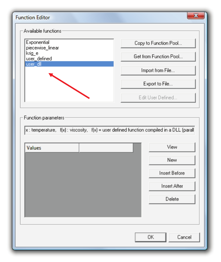
USER’S GUIDE & TUTORIALS 356 PAM-RTM 2014
(released: Apr-14) © 2014 ESI Group
TUTORIALS
User Defined Functions
Setting the parameters in the PAM-RTM GUI
In order to have the user defined viscosity and kinetics functions called for a given
model, function type user_dll must be selected in the PAM-RTM GUI.
It is important to understand that libprocast_DMP.dll has no other use than to evaluate
viscosity and/or kinetics and/or specific heat and/or effective conductivity for the only
cases where user_dll is selected in the PAM-RTM GUI. If any type other than user_dll
is selected, the DLL won’t be called. This means there will not be any side effects if the
user compiled DLL is kept in the PAM-RTM installation directory to run cases not
using user functions.
PAM-RTM 2014 357 USER’S GUIDE & TUTORIALS
© 2014 ESI Group (released: Apr-14)
TUTORIALS
User Defined Functions
User functions for resin specific heat and effective
conductivity
These functions are used most of the time to define resin specific heat and effective
conductivity of a wet reinforcement as a function of temperature and degree of cure
(
( )
α
,Tf
).
Suppose we want to define the specific heat as the following function:
( ) ( )
18002732, +−⋅= TTcp
α
for
5.
0
≤
α
( ) ( )
15002733, +−⋅= TTc
p
α
for
5.0>
α
This specific heat model is just for the sake of the example, it doesn’t correspond to a
real resin.
For a resin with name my_resin_1, the corresponding user code would be:
/*
* Return specific heat of pure resin (i.e. not mixed with fibers).
*/
real func_resinspecheat(
char prefix[], /* case name */
char resin_name[], /* resin name */
real temperature, /* current temperature in Kelvin */
real alpha, /* current degree of cure (value between 0 and 1) */
int* vars) /* return 1 for a function of temperature or 2 for a
function of temperature and cure */
{
/* ------------- Do not change anything above this line ------------- *
* ------------- Program your function below this line ------------- */
/* Return value must be in J/kg/K */
if ( strcmp( resin_name, "my_resin_1" ) == 0 ) {
if ( alpha <= 0.5 ) {
return 2. * ( temperature - 273. ) + 1800.;
}
else {
return 3. * ( temperature - 273. ) + 1500.;
}
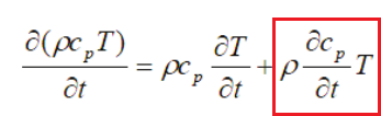
USER’S GUIDE & TUTORIALS 358 PAM-RTM 2014
(released: Apr-14) © 2014 ESI Group
TUTORIALS
User Defined Functions
*vars = 1; /* function of temperature only */
}
else {
printf("unknown resin in user defined specific heat\n");
exit(1);
}
}
To have the user function for cp called, the user must select first f(temperature) or
f(temperature, alpha) for the cp of the resin in the PÂM-RTM GUI, then user_dll.
Note that it is the user’s responsibility in his code to return “*vars = 1” for a function of
temperature, or “*vars = 2” for a function of temperature and alpha, since the same user
function is used for both situations. When “*vars = 2” is returned, the solver adds an
extra term in the energy equation to take into account the time dependency of cp through
alpha:
For the effective conductivity of a wet reinforcement, since it involves the combination
of a resin and a reinforcement, we recommend the following code structure. Here we
have resins my_resin_1 and my_resin_2, and reinforcements my_rf_1 and my_rf_2.
/*
* Return effective thermal conductivity principal values (k1, k2, k3) of
the mix of resin and fibers, i.e. the
* conductivity to be used in the wet area.
*/
void func_effthermalcond(
char prefix[], /* case name */
char resin_name[], /* resin name */
char reinforcement_name[], /* reinforcement name */
real vf, /* fiber volume fraction (value between 0 and 1) */
PAM-RTM 2014 359 USER’S GUIDE & TUTORIALS
© 2014 ESI Group (released: Apr-14)
TUTORIALS
User Defined Functions
real temperature, /* current temperature in Kelvin */
real alpha, /* current degree of cure (value between 0 and 1) */
real *k1, /* returned effective conductivity in the first principal
direction */
real *k2, /* returned effective conductivity in the second principal
direction */
real *k3) /* returned effective conductivity in the third principal
direction */
{
/* ------------- Do not change anything above this line ------------- *
* ------------- Program your function below this line ------------- */
/* Returned values must be in W/m/K */
*k1 = 0.;
*k2 = 0.;
*k3 = 0.;
if ( strcmp( resin_name, "my_resin_1" ) == 0) {
if (strcmp( reinforcement_name, "my_rf_1" ) == 0) {
*k1 = ...
*k2 = ...
*k3 = ...
}
else if ( strcmp( reinforcement_name, "my_rf_2" ) == 0) {
*k1 = ...
*k2 = ...
*k3 = ...
}
else {
printf("unknown combination of resin and fibers\n");
exit(1);
}
}
else if ( strcmp( resin_name, "my_resin_2" ) == 0) {
if ( strcmp( reinforcement_name, "my_rf_1" ) == 0) {
*k1 = ...
*k2 = ...
*k3 = ...
}
else if ( strcmp( reinforcement_name, "my_rf_2" ) == 0) {
USER’S GUIDE & TUTORIALS 360 PAM-RTM 2014
(released: Apr-14) © 2014 ESI Group
TUTORIALS
User Defined Functions
*k1 = ...
*k2 = ...
*k3 = ...
}
else {
printf("unknown combination of resin and fibers\n");
exit(1);
}
}
else {
printf("unknown resin in user defined effective conductivity\n");
exit(1);
}
}
To have the user function for effective conductivity called, the user must select first
f(temperature) or f(temperature, alpha) in the PAM-RTM GUI, then user_dll. Note
that the fiber volume fraction of the zone (or local fiber fraction if draping is used) is
also passed as parameter to the effective conductivity function. The user could
implement a rule of mixture in his function so that the effective conductivity is valid for
any fiber fraction.

PAM-RTM 2014 361 USER’S GUIDE & TUTORIALS
© 2014 ESI Group (released: Apr-14)
TUTORIALS
One Shot Filling Simulation
ONE SHOT FILLING SIMULATION
The following files are used in this example.
- one_shot_start.unv (starting mesh)
- one_shot.dtf + one_shot.unv (solution)
Objectives
The goal of this tutorial is to show how to use the one shot filling simulation, i.e. a very
quick estimation of the filling time and location of the last points filled. This simulation
doesn’t solve the intermediate states of the flow. Only a few resolutions of Darcy’s
equation are needed, compared to thousands for a standard filling simulation, meaning
just a few seconds of CPU time, even on a huge mesh.
Material Properties
The 2D mesh can be seen as a cross section in a solid part with a T junction (see tutorial
“Comparison 2D – 2.5D – 3D”). For this case, material orientations were defined
because a reinforcement with non-isotropic permeability is used. The K1 principal
permeability directions follow the shape of the part. They were set by projection of the
elements on a “curve” (command Mesh>Orientations>Set K from Selected Nodes, see
tutorial “Fiber Orientations”). The direction orthogonal to K1 and in the plane of the
elements is here the transverse direction K3. Since we cannot set directly K3 in PAM-
RTMTM, the way to do it is to set K2 out of plane with Mesh>Orientations>Set Vectors
and vector (0., 0., 1.). K3 is always calculated by PAM-RTMTM orthogonal to K1 and
K2, meaning we will have finally K3 orthogonal to K1 and in the plane of the elements.
The K1 and K2 directions are shown below. The central zone has isotropic
permeability, so orientations are not specified.
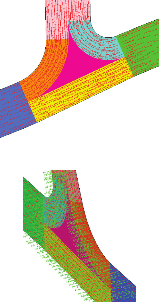
USER’S GUIDE & TUTORIALS 362 PAM-RTM 2014
(released: Apr-14) © 2014 ESI Group
TUTORIALS
One Shot Filling Simulation
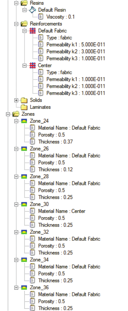
PAM-RTM 2014 363 USER’S GUIDE & TUTORIALS
© 2014 ESI Group (released: Apr-14)
TUTORIALS
One Shot Filling Simulation
The material properties are summarized below.
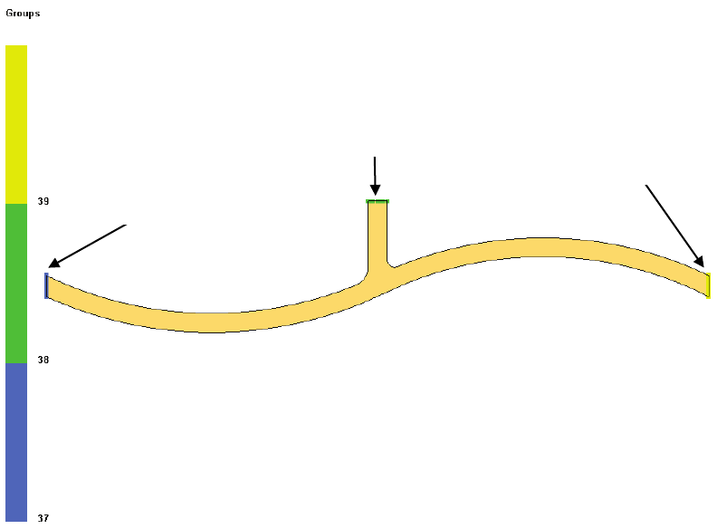
USER’S GUIDE & TUTORIALS 364 PAM-RTM 2014
(released: Apr-14) © 2014 ESI Group
TUTORIALS
One Shot Filling Simulation
Boundary Conditions
Three groups of nodes are created on the extremities of the part, that will be used as
injection lines. All the lines are active at the same time, and all use imposed pressure.
However the center injection line has a lower pressure (1 bar) while the left and right
lines have 2 bars pressure. No vent is specified, as the goal of the one shot simulation is
to help locate vents. The groups are shown below, with the corresponding boundary
conditions in the document’s tree.
group 37
group 38
group 39
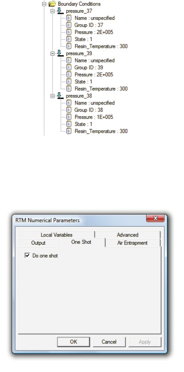
PAM-RTM 2014 365 USER’S GUIDE & TUTORIALS
© 2014 ESI Group (released: Apr-14)
TUTORIALS
One Shot Filling Simulation
One Shot Parameters
Only one parameter needs to be changed in order to run a one shot simulation, when
compared to a standard filling simulation. It is the do one shot parameter, found in the
OneShot tab of the Numerical Parameters. This parameter must be checked to run a one
shot simulation.

USER’S GUIDE & TUTORIALS 366 PAM-RTM 2014
(released: Apr-14) © 2014 ESI Group
TUTORIALS
One Shot Filling Simulation
Launching the Simulation and Post-processing
Save the document and launch the simulation. When it is done, push the Reload Results
button in the Results toolbar. A folder Last Points Filled is added to the document’s tree.
It contains the list of the last points filled, with the fill time for each point. Clicking one
of these points in the document’s tree highlights the corresponding point in the 3D
view.
Most of the time, the output of a one shot simulation won’t be a single point, but a set of
points, which is some kind of fuzzy region for the actual last point filled. All these
points should be considered candidates for potential last point filled. They are all within
a 0.1 % tolerance on the total fill time. This is an internal tolerance that cannot be
modified by the user in the current version.
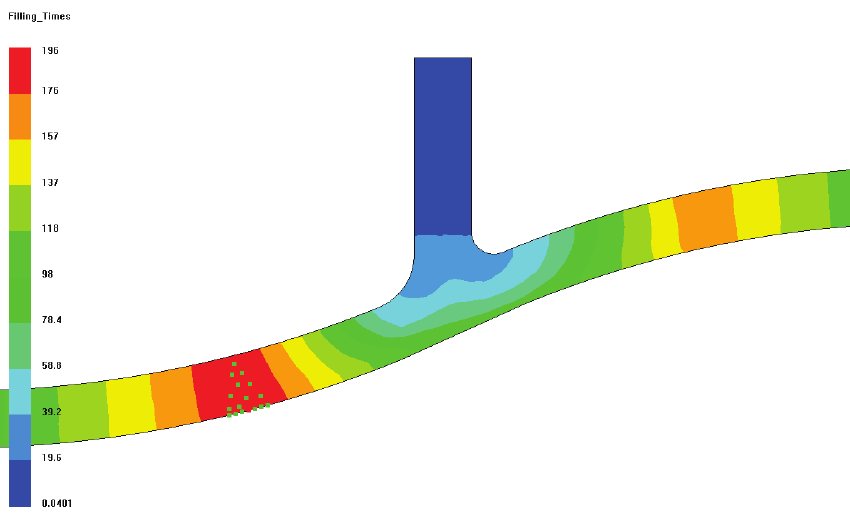
PAM-RTM 2014 367 USER’S GUIDE & TUTORIALS
© 2014 ESI Group (released: Apr-14)
TUTORIALS
One Shot Filling Simulation
Running first a one shot simulation, then unchecking the do one shot parameter to run a
standard filling simulation, it is possible to superimpose the last points filled with the
filling times contour, to check if they match. Here the match is very clear.
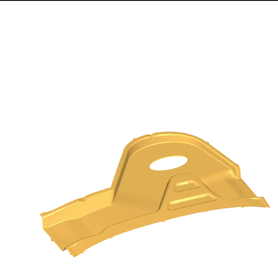
USER’S GUIDE & TUTORIALS 368 PAM-RTM 2014
(released: Apr-14) © 2014 ESI Group
TUTORIALS
GenPorts
GENPORTS
The following files are used in this example.
- genports_start.unv (starting mesh)
- genports.dtf + genports.unv (solution).
Objectives
The goal of this tutorial is to show how to use the GenPorts module. GenPorts uses a
genetic algorithm to find the optimal configuration of injection ports that minimize fill
time. In this tutorial, we want to find the best configuration for 3 inlets on a complex
part (shown below).
Material Properties and Boundary Conditions
Most of the material properties and boundary conditions usually set up in a standard
RTM simulation are ignored by GenPorts. Actually the only material properties that are
taken into account are permeability (principal directions and orientations) and porosity.
High permeability areas used to define runners or race tracking are thus supported by
GenPorts.
For the boundary conditions, the simulation will run without any boundary condition
defined, as GenPorts will create internally the needed injection points and ignore any
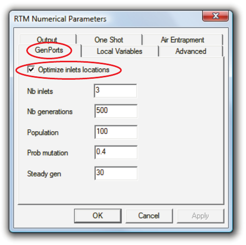
PAM-RTM 2014 369 USER’S GUIDE & TUTORIALS
© 2014 ESI Group (released: Apr-14)
TUTORIALS
GenPorts
boundary condition defined by the user. The optimization is independent of the actual
pressure value used. It is assumed that all the points use the same pressure.
For this example, isotropic permeability is used (k1 = k2 = k3 = 2e-10 m2) with a
porosity of 60%.
GenPorts Parameters
The GenPorts parameters are located in the GenPorts tab of the RTM Numerical
Parameters. Assuming the user has already set up a model for a standard RTM
simulation, there are basically 2 parameters that need to be changed to run a GenPorts
simulation: the optimize inlets locations parameter must be checked, and the number of
inlets to be used (nb inlets) has to be set. The other parameters, which are related to the
genetic algorithm engine, could keep their default values. However here to reduce the
CPU time, we use a smaller population of 100 and reduce the total number of
generations to 500. The parameters are shown below.
It is very important to understand the meaning of population. A population is made of
individuals. Here an individual is actually an injection configuration, i.e. in this example
a set of 3 points (nb inlets). In the figure below we show 3 individuals (red set, green set
and blue set). In this example a population of 100 individuals is used. We consider that
value enough to insure a good “covering” of the part, taking into account the fact that
the initial population is generated completely randomly, meaning that some individuals
will be very “weak” (i.e. lead to a longer fill time, such as the green one below). For a
larger part, the population should be increased.
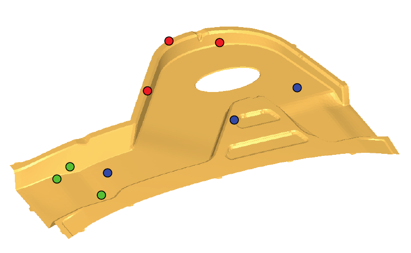
USER’S GUIDE & TUTORIALS 370 PAM-RTM 2014
(released: Apr-14) © 2014 ESI Group
TUTORIALS
GenPorts
The idea behind optimization using genetic algorithms is that the individuals within the
population will combine to give birth to children. Some of the characteristics of both
parents will be kept in the generation of a child, and some characteristics will be
completely random. For instance, a point could be randomly generated on the line
connecting 2 points from both parents. In that case, the characteristic is not completely
random, it still is related to the characteristics of both parents even though some
randomness is introduced. That is called a crossover. Also sometimes a mutation can
occur. This is a more dramatic change in the characteristics of a child. For instance, a
completely random node could be chosen on the mesh instead of being generated from
the parents. The probability of a mutation can be entered with the prob mutation
parameter. The user doesn’t have control on the crossover parameters in the current
version.
The number of individuals in a population is specified by the population parameter.
That is an approximate number; the population will vary slightly from generation to
generation as some individuals will die in the process. The maximum number of
generations that will be calculated is specified in nb generations. It is possible that the
calculation will stop earlier, if the calculation engine doesn’t detect any significant
improvement in the results for steady gen generations, meaning that a steady state has
been reached.
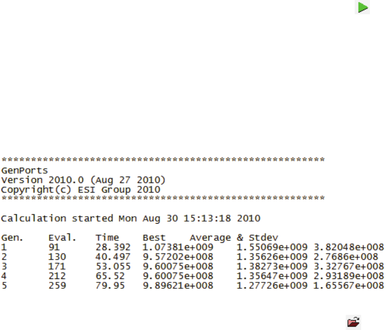
PAM-RTM 2014 371 USER’S GUIDE & TUTORIALS
© 2014 ESI Group (released: Apr-14)
TUTORIALS
GenPorts
Launching the Simulation and Post-processing
The calculation is launched the usual way, by pushing the green arrow button , after
saving the document.
A typical log file is shown below. The first column is the current generation, the second
column shows the cumulative number of evaluations done, the third column shows the
cumulative CPU time, and the last 3 columns show the best, average, and standard
deviation results for the evaluation of the formulation on the population. Note that these
high values come from the evaluation of a “mold coefficient” formulation, in which
only material properties are taken into account, not boundary conditions. These values
are related in some way to the fill time, but they are not of course actual time values.
Once the calculation is done, the user pushes the usual reload results button . This
will add a Best inlets locations folder to the model explorer, in which the coordinates of
the points are listed. The points are also displayed in the 3D view, as shown below.
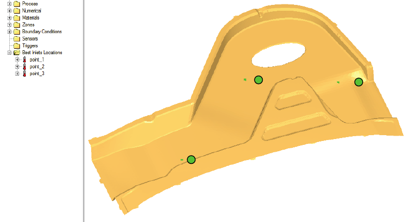
USER’S GUIDE & TUTORIALS 372 PAM-RTM 2014
(released: Apr-14) © 2014 ESI Group
TUTORIALS
GenPorts
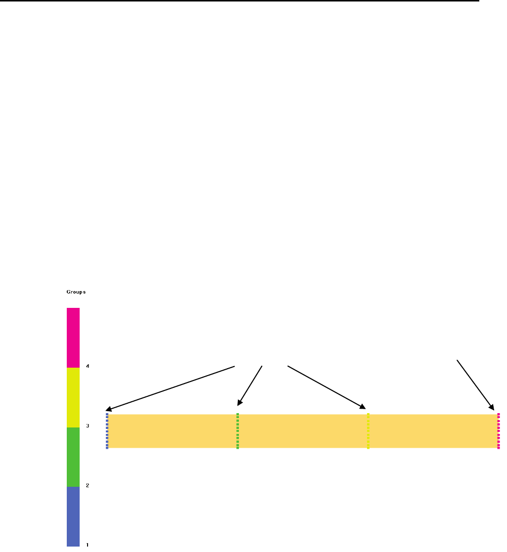
PAM-RTM 2014 373 USER’S GUIDE & TUTORIALS
© 2014 ESI Group (released: Apr-14)
TUTORIALS
Sequential Injection (Trigger Manager)
SEQUENTIAL INJECTION (TRIGGER MANAGER)
The following files are used in this example.
- sequential_start.unv (starting mesh)
- sequential.dtf + sequential.unv (solution)
Objectives
The goal of this tutorial is to show how to use the trigger manager to define a
sequential injection. A long part is injected with many injection lines, which will be
opened and closed sequentially in time. Even though it was possible with earlier
versions to simulate sequential injection by using state curves and running many partial
simulations, the trigger manager, introduced in PAM-RTMTM 2009, makes this kind of
data setup much easier. Since PAM-RTMTM 2013 the trigger manager is supported by
the parallel solver; the tutorial uses the parallel solver.
Boundary Conditions
Four groups are created, equally spaced along the length of the part. The rightmost
group is used for an outlet (vent) boundary condition, while the three other groups are
inlets. Initially only the leftmost inlet is active (its state parameter has a value of one,
inlets outlet
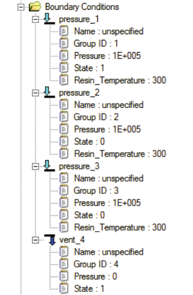
USER’S GUIDE & TUTORIALS 374 PAM-RTM 2014
(released: Apr-14) © 2014 ESI Group
TUTORIALS
Sequential Injection (Trigger Manager)
while the two other inlets have state=0). The outlet is kept open for the whole
simulation. The corresponding entities in the document’s tree are shown below.
The parallel solver doesn’t support internal injection lines, i.e. defined with nodes that
are not on free edges of the part. Therefore it is necessary to add some small surfaces
orthogonal to the part, on which injection lines will be defined (see images below). Here
the height of these surfaces is 5 millimeters, and 2 rows of elements were used. Note
that PAM-RTM doesn’t have a tool to create and mesh these small surfaces, so the user
has to create them in his CAD software or mesh generator.
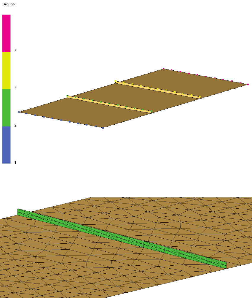
PAM-RTM 2014 375 USER’S GUIDE & TUTORIALS
© 2014 ESI Group (released: Apr-14)
TUTORIALS
Sequential Injection (Trigger Manager)
Material definition
Because injection will be done in these small surfaces or “channels”, permeability,
thickness and porosity of these channels must match the values used for the part.
In this example, default fabric permeability of 10-9m2, thickness of 5mm and porosity of
50% are used.
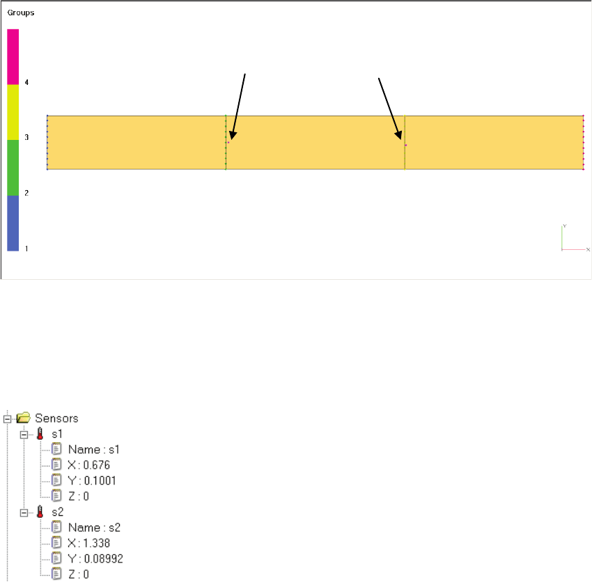
USER’S GUIDE & TUTORIALS 376 PAM-RTM 2014
(released: Apr-14) © 2014 ESI Group
TUTORIALS
Sequential Injection (Trigger Manager)
Sensors
Two sensors are created just after the second and third injection lines. These sensors
will be used as inputs by the trigger manager. For instance, when the resin will touch
the first sensor, the first injection line will be closed, and the second one opened. The
position of the sensors can be seen on the picture below.
Trigger Manager
The goal of the trigger manager is to manage input conditions and fire outcomes when
these conditions are reached. For instance an input condition could be the resin pressure
on a sensor: when a given pressure is reached (parameter threshold of a trigger), a list of
events is fired, such as closing a vent or opening an inlet. Other types of inputs are the
injected or lost resin volume on a specific inlet or outlet, or the global injected or lost
volume on all inlets and outlets. In this tutorial, we will use an input condition based on
the filling factor, to determine if the flow has reached a given sensor: we use a threshold
with a value of one. Note that another way to detect that the flow has reached a given
sensor would be to use a trigger based on pressure, with a very small pressure value.
sensor s1 sensor s2
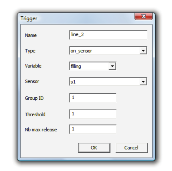
PAM-RTM 2014 377 USER’S GUIDE & TUTORIALS
© 2014 ESI Group (released: Apr-14)
TUTORIALS
Sequential Injection (Trigger Manager)
The first trigger will manage closing of the first inlet and opening of the second inlet.
To create the trigger, right-click on the Triggers folder of the document’s tree, and
choose New. This opens the trigger dialog box shown below. Enter the parameters as
shown. This means that when the flow will reach the first sensor (s1), condition
detected by the fact that the filling factor (variable filling) has reached a value of one
(threshold) on that sensor, outcomes will be fired.
Once a trigger has been defined, outcomes can be created on that trigger by right-
clicking the trigger in the document’s tree, and choosing New Outcome. This opens the
following dialog box.
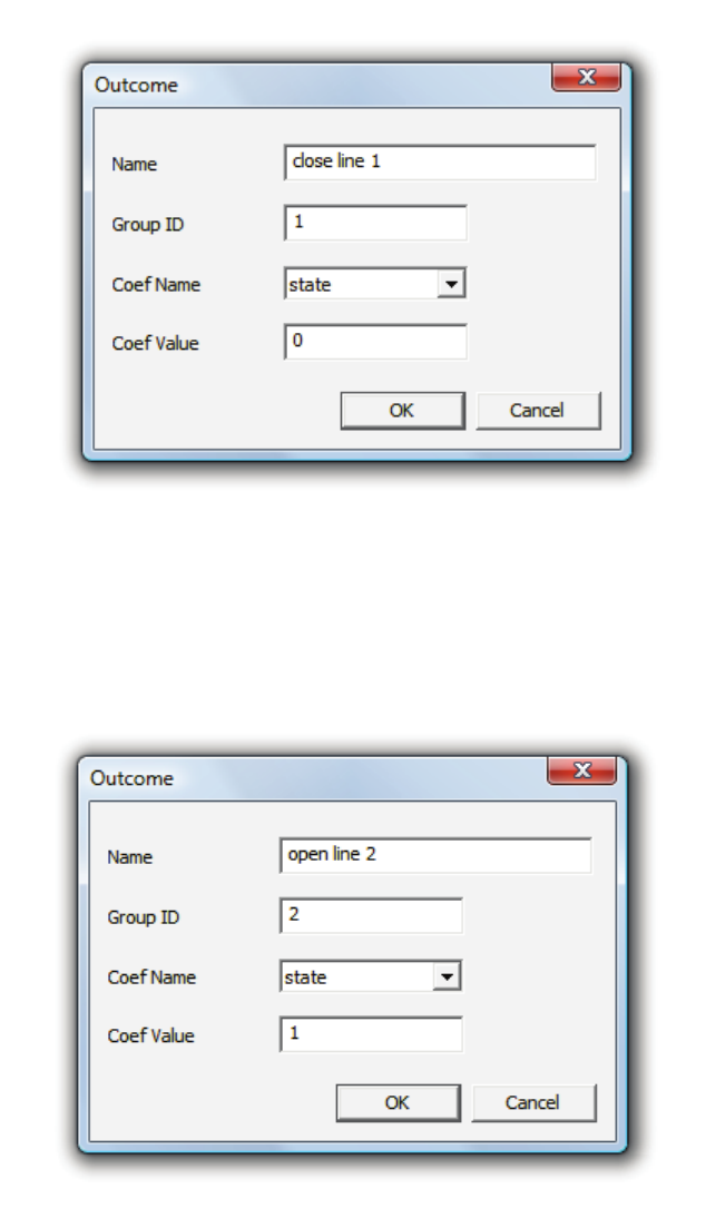
USER’S GUIDE & TUTORIALS 378 PAM-RTM 2014
(released: Apr-14) © 2014 ESI Group
TUTORIALS
Sequential Injection (Trigger Manager)
First give a meaningful name to the outcome, such as “close line 1”. Then enter the
Group ID on which the specified coefficient will be set when the trigger is fired. Here
we set the state coefficient of the inlet to zero, meaning the inlet is closed.
Define another outcome for the activation of the second inlet, as shown below.
Repeat this procedure for the second sensor, so that the second inlet is closed and the
third inlet is opened when resin reaches the second sensor.
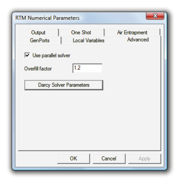
PAM-RTM 2014 379 USER’S GUIDE & TUTORIALS
© 2014 ESI Group (released: Apr-14)
TUTORIALS
Sequential Injection (Trigger Manager)
Launching the Simulation and Post-processing
The parallel solver is selected in the Advanced numerical parameters.
Save the document and launch the simulation. When it is done, push the Reload Results
button in the Results toolbar.
Have a look at the filling steps. The total filling time is 353 seconds.

USER’S GUIDE & TUTORIALS 380 PAM-RTM 2014
(released: Apr-14) © 2014 ESI Group
TUTORIALS
Sequential Injection (Trigger Manager)
Images below show the pressure field just before and just after the triggers are fired, i.e.
when the fill factor reaches a value of one on the sensors. The first trigger is fired
around 120 seconds, and the second trigger around 236 seconds. When the first trigger
is fired, the pressure to the left of the second injection line becomes uniform, which is
normal since the first injection line is closed; meaning that end of the part becomes an
impermeable wall. Similar images are also given for the second trigger.
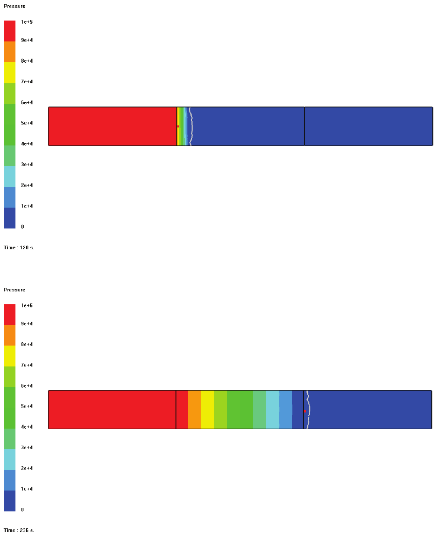
PAM-RTM 2014 381 USER’S GUIDE & TUTORIALS
© 2014 ESI Group (released: Apr-14)
TUTORIALS
Sequential Injection (Trigger Manager)

USER’S GUIDE & TUTORIALS 382 PAM-RTM 2014
(released: Apr-14) © 2014 ESI Group
TUTORIALS
Sequential Injection (Trigger Manager)
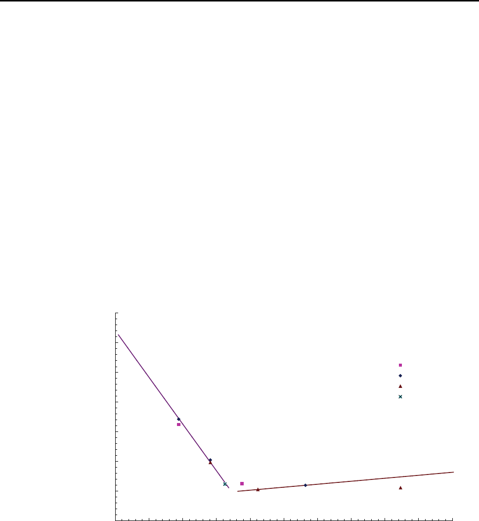
PAM-RTM 2014 383 USER’S GUIDE & TUTORIALS
© 2014 ESI Group (released: Apr-14)
TUTORIALS
Velocity optimization
VELOCITY OPTIMIZATION
The following files are used in this example.
- velo_opti_start.unv (starting mesh)
- velo_opti.dtf + velo_opti.unv (solution)
Objectives
The goal of this tutorial is to show how to use the velocity optimization option, in order
to minimize the final void content in a part.
Process and Numerical Parameters
The following assumes the user already has from experimental measurements, relations
for the micro and macro void content as a function of the flow velocity. The relations
used in this example are shown below. The curve with the negative slope is the macro
void function, the other one is the micro void function. Looking at these curves, we can
see that the optimal void content is around 2%.
0%
2%
4%
6%
8%
10%
12%
14%
00.002 0.004 0.006 0.008 0.01 0.012 0.014 0.016 0.018 0.02
Flow velocity (m/sec)
Voids content
20 psi
30 psi
45 psi
2,5 ml/s
1.26+100.55*(V)
Chomarat - Roviply
12.824-1573.7*(V)
Note that normally we would work with curves that are functions of the capillary
number. However in this case since the resin viscosity (0.02 Pa.s) is the same as the
capillary coefficient, the capillary number actually reduces to the resin velocity.
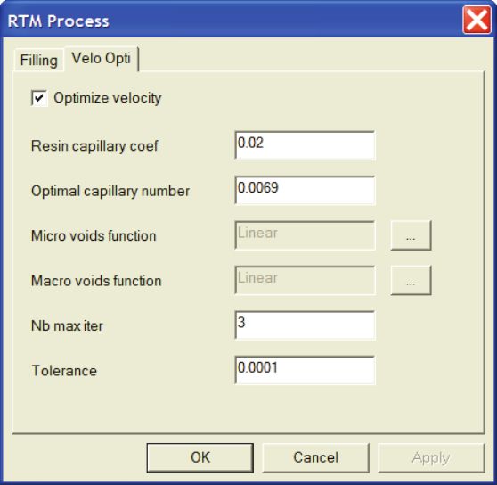
USER’S GUIDE & TUTORIALS 384 PAM-RTM 2014
(released: Apr-14) © 2014 ESI Group
TUTORIALS
Velocity optimization
Begin by creating a new RTM simulation. The most important parameters for velocity
optimization are located in the Velo Opti tab of the Process dialog box. Double-click on
the Process item in the document’s tree to open the process dialog box.
Enter the following values in the Velo Opti tab:
- Optimize velocity checked
- Resin capillary coefficient: 0.02
- Optimal capillary number: 0.0069
- Micro voids function: linear with A = 100.5, B = 1.27
- Macro voids function: linear with A = -1574, B = 12.82
- Nb max iter: 3
- Tolerance: 1e-4
This is shown below.
The next step is to tell PAM-RTM to save the results files related to velocity
optimization: capillary numbers, micro voids, macro voids, and a file containing the
sum of micro and macro void values. The saving of these 4 files is controlled by a
single option: save capillary numbers in the Output tab of the Numerical parameters
dialog box.
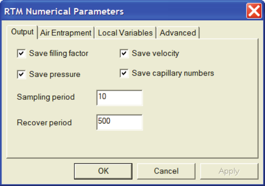
PAM-RTM 2014 385 USER’S GUIDE & TUTORIALS
© 2014 ESI Group (released: Apr-14)
TUTORIALS
Velocity optimization
Material Properties
Enter the following material and zone properties:
- viscosity: 0.02 Pa.s
- Permeability: k1 = k2 = k3 = 1e-9 m2
- Porosity: 0.5
- Thickness: 0.005 m
Boundary Conditions
The provided mesh already contains 2 groups, as shown below. Group 1 is used as the
inlet, and group 2 as the outlet. Define a pressure boundary condition of 0.1 bar (10 000
Pa) on group 1. Define a vent boundary condition with zero pressure on group 2.
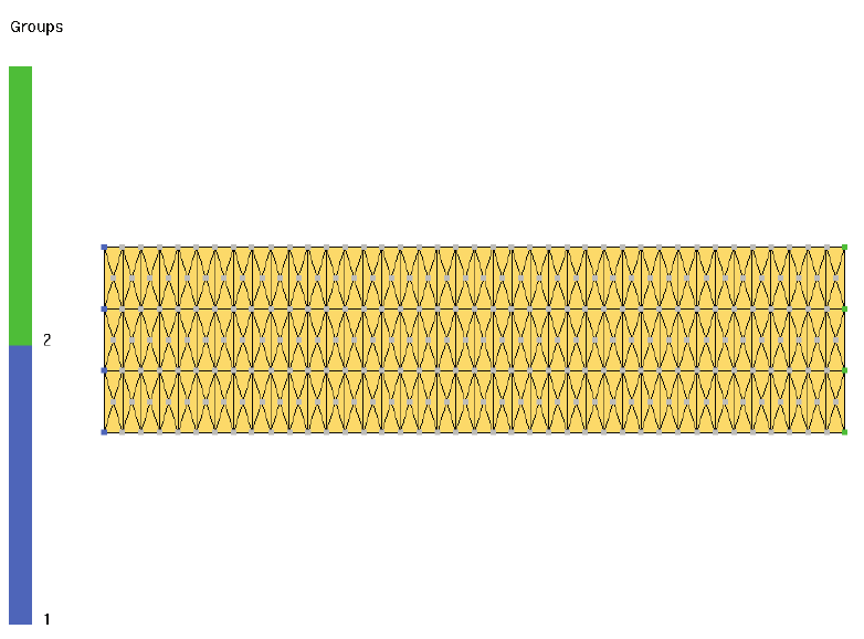
USER’S GUIDE & TUTORIALS 386 PAM-RTM 2014
(released: Apr-14) © 2014 ESI Group
TUTORIALS
Velocity optimization
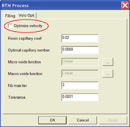
PAM-RTM 2014 387 USER’S GUIDE & TUTORIALS
© 2014 ESI Group (released: Apr-14)
TUTORIALS
Velocity optimization
Launching the Simulation and Post-processing
We will run 2 simulations in this tutorial: the first one without the optimize velocity
option, the second one with the option, to better understand its effect. For the first case,
simply uncheck optimize velocity in the Velo Opti tab of the Process parameters, leaving
all the other parameters the same. It is important to understand that it makes sense to
run a simulation with all the parameters in the Velo Opti tab defined, but without the
optimize velocity option active. This is useful to visualize the void content at the end of
the injection that you would have if you didn’t optimize velocity.
Save the document with File->Save, giving it a name so you can remember that the case
was run without the optimization, then launch the simulation. When the simulation is
done, load all the results files in a single click by pushing the Reload results button in
the main toolbar. You should have the following.
For the first case, uncheck “optimize velocity”
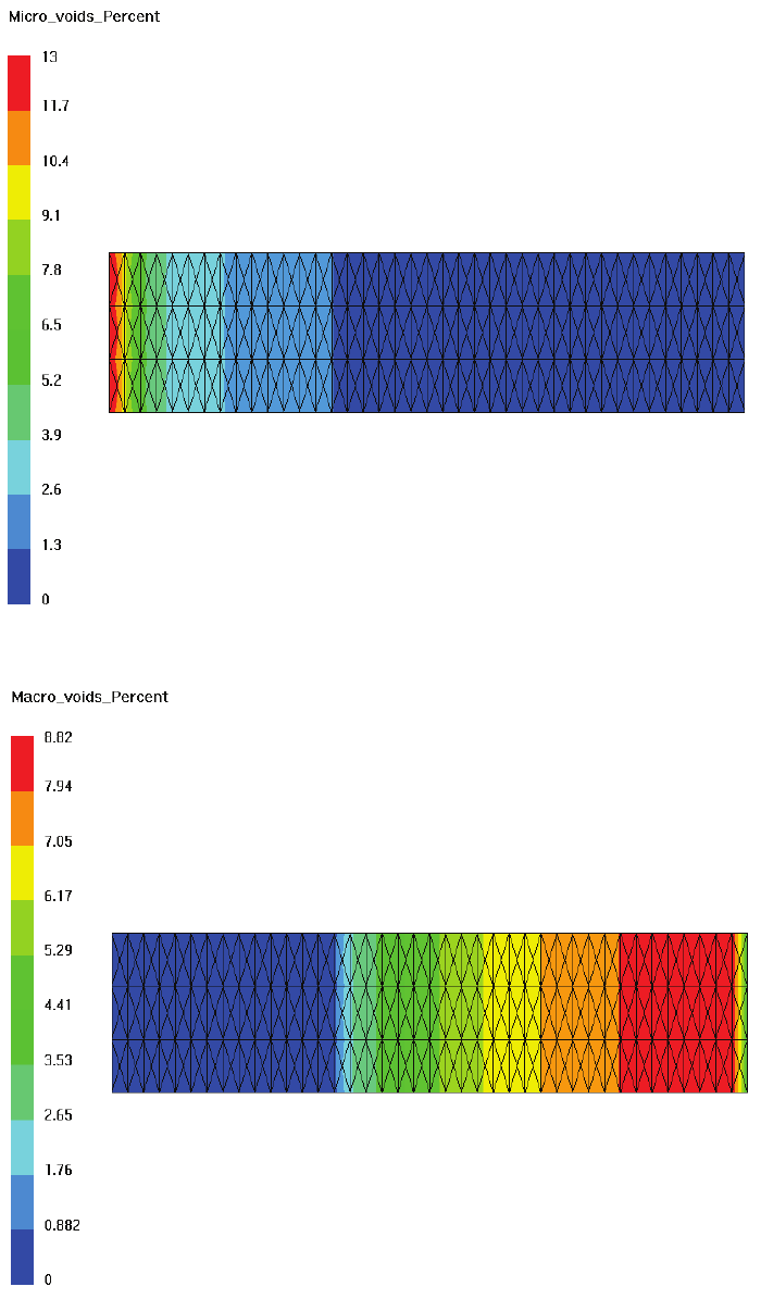
USER’S GUIDE & TUTORIALS 388 PAM-RTM 2014
(released: Apr-14) © 2014 ESI Group
TUTORIALS
Velocity optimization
Micro voids percent at the end of filling for the first case (no optimization).
Macro voids percent at the end of filling without optimization.
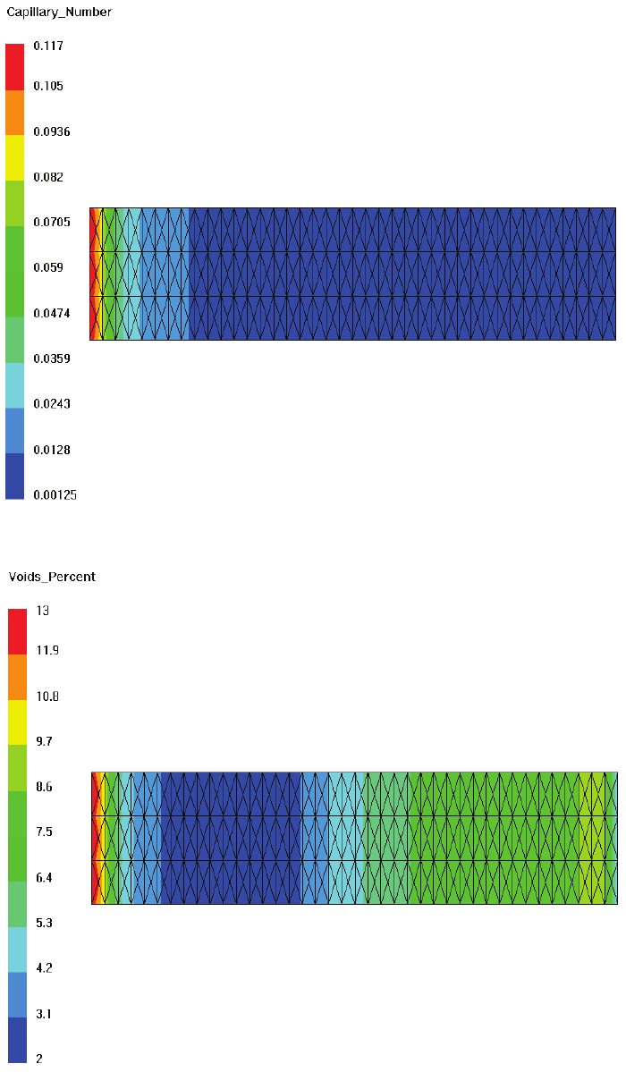
PAM-RTM 2014 389 USER’S GUIDE & TUTORIALS
© 2014 ESI Group (released: Apr-14)
TUTORIALS
Velocity optimization
Capillary number
Total voids percent (micro + macro voids)
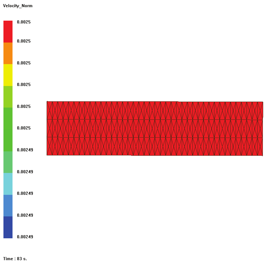
USER’S GUIDE & TUTORIALS 390 PAM-RTM 2014
(released: Apr-14) © 2014 ESI Group
TUTORIALS
Velocity optimization
Velocity field at the end of filling (v = 2.5e-3 m/s)
It is important to understand that the micro voids, macro voids and capillary number
results are non-transient (single step) fields. This is because the model relates the void
content to the velocity at the exact time when the resin front touches an element, and it
is assumed that void content doesn’t change for the rest of the simulation once it is set
on an element.
For the second case, reactivate the optimize velocity option. Save the file with Save As,
with a new name so you can remember that the case was run with the optimize option.
When the simulation is done, push the Reload results button. You should have the
following. Notice that the micro voids result of 1.96% matches the value expected from
the curves shown at the beginning of this tutorial.
For this simple case, the macro voids results remain always zero. This is because with
this void model, for a given velocity, it is not possible to have micro and macro voids at
the same time. This implies that if an element has a non-zero micro void value, its
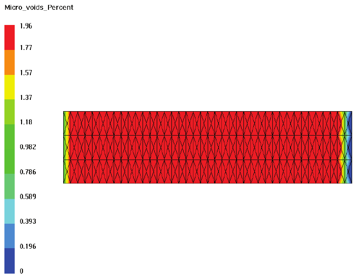
PAM-RTM 2014 391 USER’S GUIDE & TUTORIALS
© 2014 ESI Group (released: Apr-14)
TUTORIALS
Velocity optimization
macro void value will be zero, and vice versa. On this case, the velocity optimization
algorithm always converges to a velocity value slightly in the micro voids area, leading
to a macro void value of zero. On more complex cases, the optimal void values would
be scattered between the micro and macro void results. Finally notice that the velocity
at the end of injection (6.9e-3 m/s) is much higher than the previous case (2.5e-3 m/s).
This is because PAM-RTM had to convert the pressure imposed inlet to a flow rate
imposed inlet, to be able to reach the optimal velocity.
Micro voids result with optimization
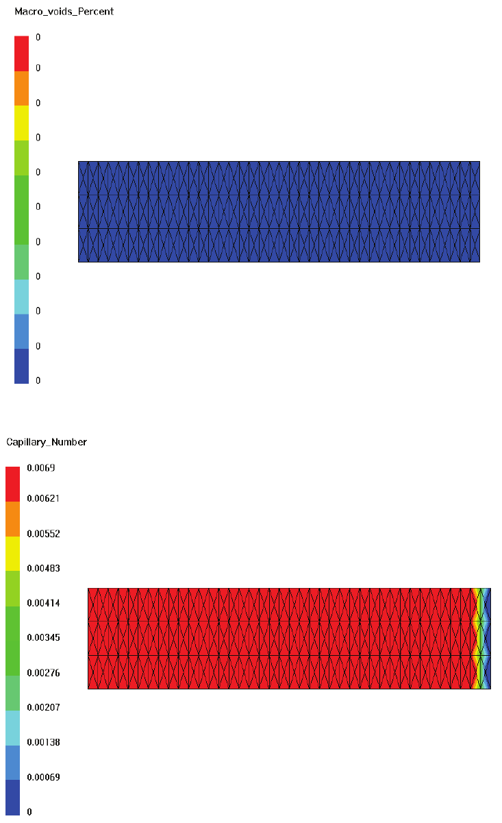
USER’S GUIDE & TUTORIALS 392 PAM-RTM 2014
(released: Apr-14) © 2014 ESI Group
TUTORIALS
Velocity optimization
Macro voids result with optimization
Capillary number with optimization
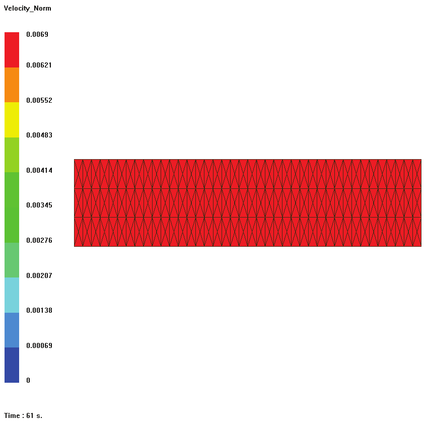
PAM-RTM 2014 393 USER’S GUIDE & TUTORIALS
© 2014 ESI Group (released: Apr-14)
TUTORIALS
Velocity optimization
Velocity at the end of filling (v = 6.9e-3 m/s)
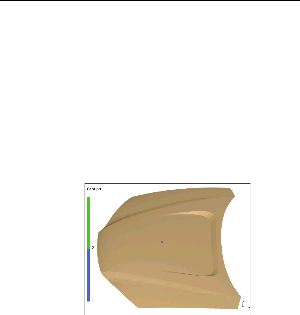
USER’S GUIDE & TUTORIALS 394 PAM-RTM 2014
(released: Apr-14) © 2014 ESI Group
TUTORIALS
Compression RTM
COMPRESSION RTM
The following files are used in this example:
- crtm_start.unv (starting mesh);
- crtm_rtm.dtf + crm_rtm.unv + crtm.dtf + crtm.unv (solution).
Objective
The objective of this tutorial is to show how to define a compression RTM data set-up.
Compression RTM module is made to simulate the kind of process in which a
compression of the reinforcement is used to push the resin inside the cavity.
This tutorial is limited to a case where only one tool is in movement, but Compression
RTM module can treat more complex kinematics.
Geometry and Boundary Conditions
The part is a hood made of a unique zone (zone 2), which is injected from a single point
in the center of the part (group 1), with two vents (group 2) at the corners of the part.
Groups
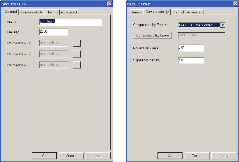
PAM-RTM 2014 395 USER’S GUIDE & TUTORIALS
© 2014 ESI Group (released: Apr-14)
TUTORIALS
Compression RTM
Two simulations will be carried out to obtain this result:
- standard RTM injection simulation with a set thickness , which is the final part
thickness objective calculated so that fiber content of the part is 50%, to determine
the volume of resin to inject;
- compression RTM simulation using this resin volume.
Material Characteristics
Resin viscosity will be set constant equal to default resin viscosity: 0.1Pa.s
The reinforcement is created with the following characteristics required for
Compression RTM set-up and is saved in the database.
In the case of Compression RTM, permeability is a function of fiber content like in the
VARI case. But unlike VARI, compressibility curve and natural thickness are not used,
as thickness of the cavity is set by the gap between the two tools. Fiber content of each
zone will be computed from this thickness, density and superficial density.
Reinforcement characteristics

USER’S GUIDE & TUTORIALS 396 PAM-RTM 2014
(released: Apr-14) © 2014 ESI Group
TUTORIALS
Compression RTM
Permeability function of fiber content is set isotropic and is defined with the following
formula.
Permeability curve
This material is added to the material database so that it can be imported in next case.
RTM Injection
Data Set-up
An RTM injection case is created; the mesh crtm_start.unv is imported.
The reinforcement characteristics are defined as seen before.
The objective for final fiber content is 50%. The thickness is computed from this
thickness; it is equal to 4.48mm (=5.6/(2500*0.5)).
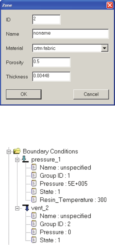
PAM-RTM 2014 397 USER’S GUIDE & TUTORIALS
© 2014 ESI Group (released: Apr-14)
TUTORIALS
Compression RTM
Zone definition
Injection pressure is set to 5 bars on group 1, and the vent pressure is set to zero on
group 2. The vents are opened during the complete process.
Boundary condition definition
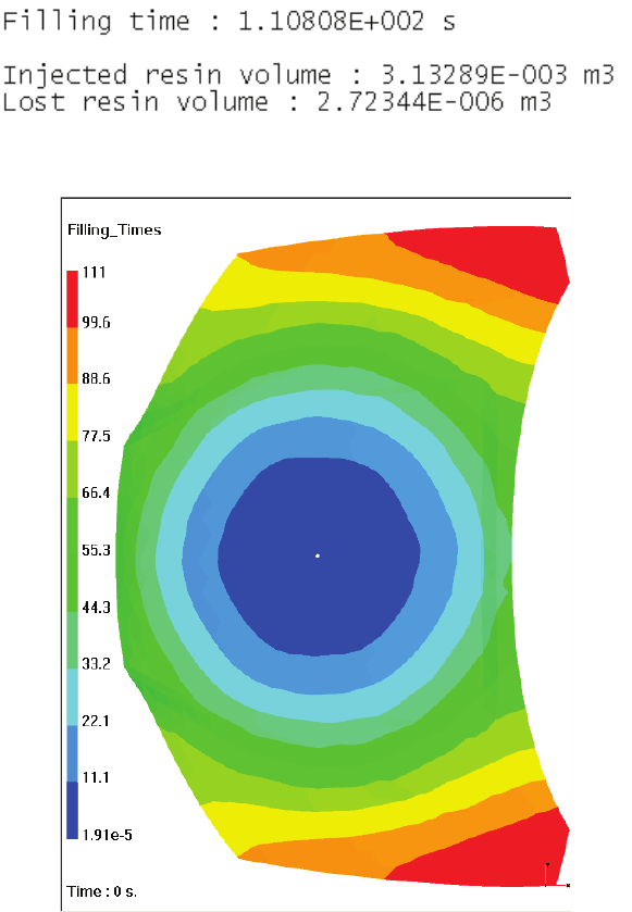
USER’S GUIDE & TUTORIALS 398 PAM-RTM 2014
(released: Apr-14) © 2014 ESI Group
TUTORIALS
Compression RTM
Post-treatment
The filling time is 111s, and the injected volume is equal to 3.13 liters. This volume will
be used in the compression RTM set-up.
Log file - Injected volume
Filling time
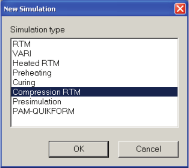
PAM-RTM 2014 399 USER’S GUIDE & TUTORIALS
© 2014 ESI Group (released: Apr-14)
TUTORIALS
Compression RTM
Compression RTM Injection
Data Set-up
A new data set-up of type Compression RTM is created.
Compression RTM set-up creation
The following assumptions are made for CRTM simulation in Pam-Rtm:
- 2D mesh is used, and thickness is a variable of each element;
- reinforcement always fills complete the mold cavity, and there is no surface channel
on top of the reinforcement;
- distance between the fixed tool and the moving tool is the thickness of each
element.
The mesh needs to be imported from the previous case.
The reinforcement material is imported from the material database.
The pressure and vent boundary conditions need to be redefined.
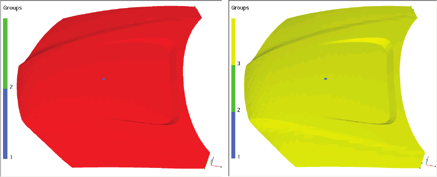
USER’S GUIDE & TUTORIALS 400 PAM-RTM 2014
(released: Apr-14) © 2014 ESI Group
TUTORIALS
Compression RTM
Compression Boundary Condition
In both case, it is necessary to create a group on which compression will be defined.
This group is a group of faces, which will contain all the faces of the model since
compression is defined on the whole surface. This group will represent the tool that will
move during compression.
Face selection Group created
Compression boundary condition and compression process parameters
The compression process set-up will involve two modifications in the set-up:
- in the process parameters will be defined; the compression direction and the mold
opening, which is the gap ;
- in the boundary condition will be defined; the closing velocity of the tool and the
timing of the closing (start/stop state).
The group that closes as well as the closing velocity are defined in the Compression
boundary condition. The closing of the mold is controlled with a trigger.
- compression velocity is equal to 0.4mm/min=6.67.10-6m/s;
- state is set to 0 initially, since this boundary condition will be activated using a
trigger. Closing of the mold will start when enough resin has been injected.
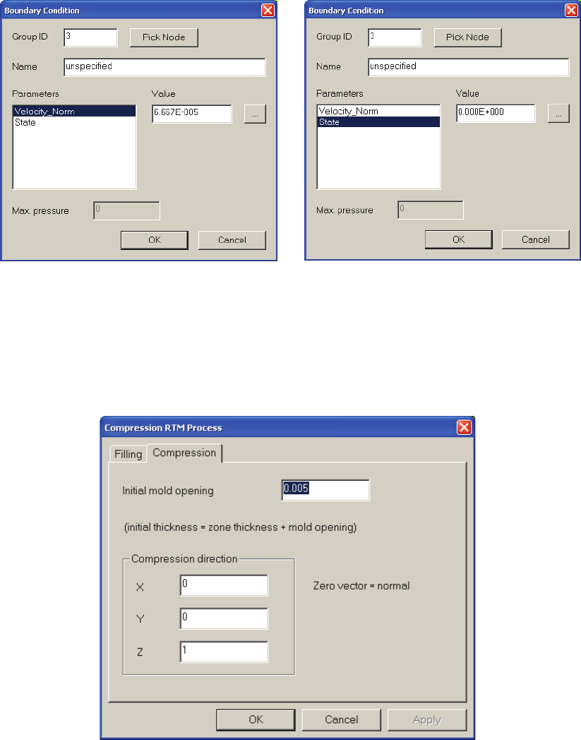
PAM-RTM 2014 401 USER’S GUIDE & TUTORIALS
© 2014 ESI Group (released: Apr-14)
TUTORIALS
Compression RTM
Compression boundary condition
Other compression process parameters are defined in the Process dialog box in the
Compression RTM tab
- mold opening is set to 5mm;
- compression direction is set to +Z vector
Compression process parameters
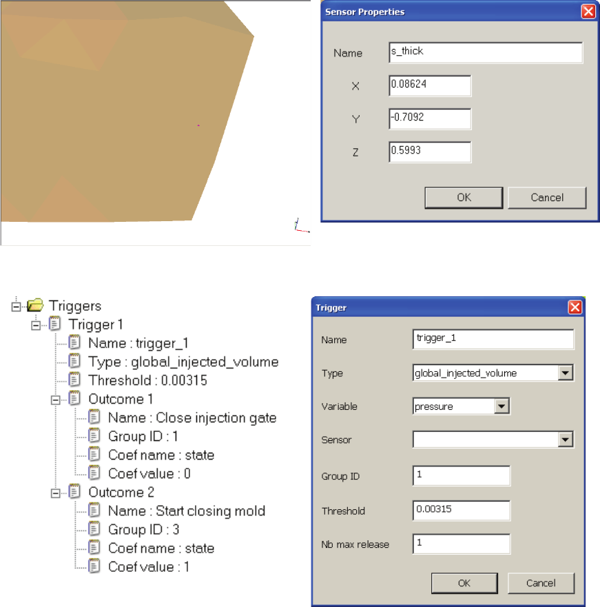
USER’S GUIDE & TUTORIALS 402 PAM-RTM 2014
(released: Apr-14) © 2014 ESI Group
TUTORIALS
Compression RTM
Trigger Definition
The compression boundary condition is controlled by one trigger:
- volume trigger that will stop injection and start compression when the needed resin
volume has been injected ; the volume is set to 3.16l to ensure enough resin is
injected,
The trigger is a volume trigger that does not require the use of a sensor.
A sensor is created that can be used for post-treatment.
Sensor creation
Triggers definition

PAM-RTM 2014 403 USER’S GUIDE & TUTORIALS
© 2014 ESI Group (released: Apr-14)
TUTORIALS
Compression RTM
Zone Definition
Zone parameters set are thickness and porosity. In the case of CRTM, thickness is the
final thickness of the part, that is when the mold is closed. Porosity parameter is not
used and is computed from thickness value during the process in the same way as it is
computed for VARI process:
fiber content = 1 – porosity = superficial density / (density * thickness)
Initial thickness for each element is computed as
initial thickness = final thickness + mold opening * cos(alpha)
where alpha is the angle between compression direction and element normal as shown
on picture below.
This formula is also used to compute thickness of the reinforcement at any time during
compression.
h1
hf
hf
hf (final thickness)
hf
hf
h1 (initial mold opening)
h2
n
compression direction
alpha
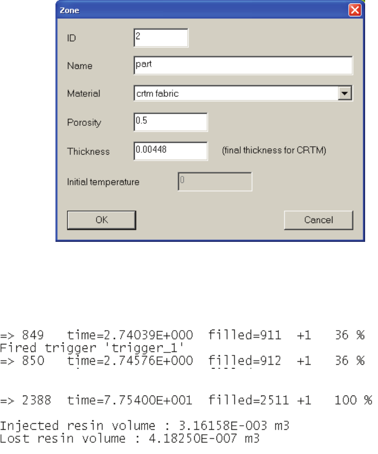
USER’S GUIDE & TUTORIALS 404 PAM-RTM 2014
(released: Apr-14) © 2014 ESI Group
TUTORIALS
Compression RTM
Zone definition
Post-Treatment
It can be verified in the log file that compression starts after 2.7s,
and that injected volume is 3.16l.
Filling time is 77.5s.
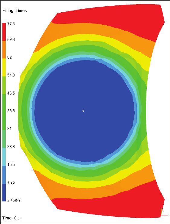
PAM-RTM 2014 405 USER’S GUIDE & TUTORIALS
© 2014 ESI Group (released: Apr-14)
TUTORIALS
Compression RTM
Filling time
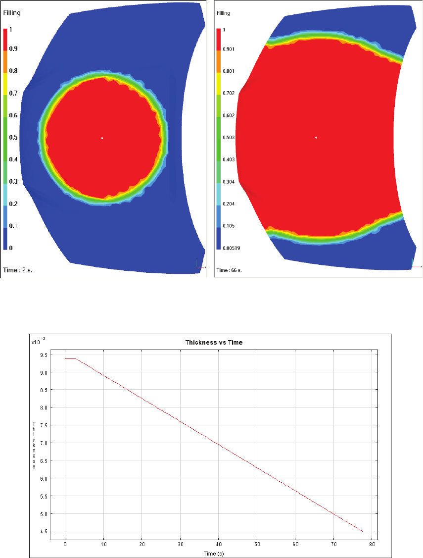
USER’S GUIDE & TUTORIALS 406 PAM-RTM 2014
(released: Apr-14) © 2014 ESI Group
TUTORIALS
Compression RTM
Flow front position is visualized at the end of injection at 2.75s, and during
compression.
End of injection During compression
Thickness variation at the sensor position is plotted.
Sensor thickness
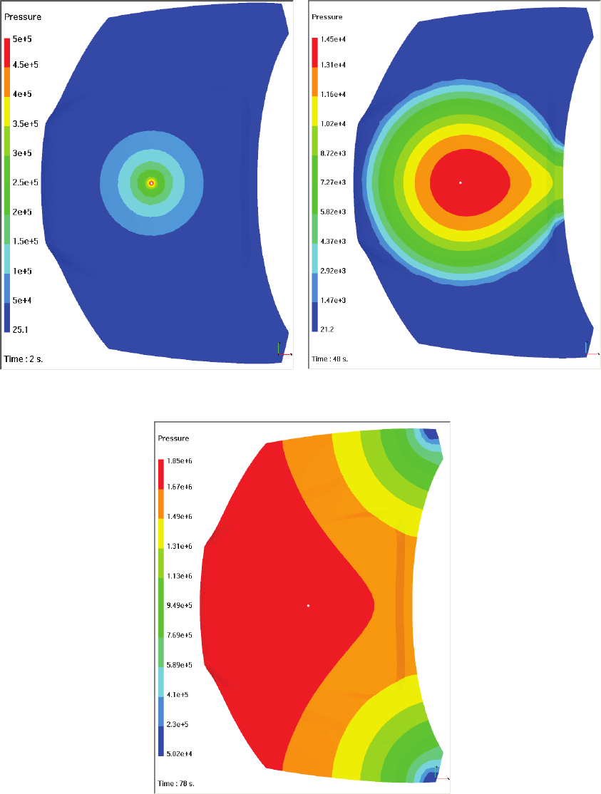
PAM-RTM 2014 407 USER’S GUIDE & TUTORIALS
© 2014 ESI Group (released: Apr-14)
TUTORIALS
Compression RTM
Pressure position is visualized at the end of injection, during compression, and at the
end of compression. Pressure at the end of compression is higher than the injection
pressure
End of injection During compression
End of injection
USER’S GUIDE & TUTORIALS 408 PAM-RTM 2014
(released: Apr-14) © 2014 ESI Group
TUTORIALS
Compression RTM
Conclusion
This tutorial has shown how to model CRTM process in which impregnation of the part
is divided in two phases:
- injection phase where reinforcement thickness is larger than final part thickness so
that permeability is increased;
- resin is pushed inside the part by compression.

PAM-RTM 2014 409 USER’S GUIDE & TUTORIALS
© 2014 ESI Group (released: Apr-14)
TUTORIALS
Local Permeability from Draping Results
LOCAL PERMEABILITY FROM DRAPING
RESULTS
The following files are used in this example.
- drape.dsy (PAM-FORM™ result file, 1 ply)
- drape_start.unv (injection mesh file)
Introduction
The filling simulation in PAM-RTM™ is macroscopic based on Darcy’s law, where
the permeability values of the fiber preform play a very important role. During the
preforming process, such as draping, the local permeability of the preform may change
due to the local fiber shearing, slipping, nesting, etc. This tutorial demonstrates the
complete procedure for using draping results in a PAM-RTM™ filling simulation. In
summary, it is carried out in the following steps:
- Import draping results in PAM-RTM™: imports the draped plies generated by the
draping software in the current document.
- Map draping results: projects draped plies on the injection mesh. The goal of this
step is to calculate the geometrical correspondence between an element of the
injection mesh and elements of the draped plies meshes.
- Local permeability calculation: generate the local permeability and porosity
distribution on the injection mesh taking into account the fiber directions of the
draped plies.
PAM-RTM™ has direct interface with four draping simulation tools : PAM-FORM™
and PAM-QUIKFORM™ (ESI Group), PATRAN Laminate Modeler (MSC),
FiberSIM (Vistagy). Without losing generality, a bathtub-like geometry is chosen in
this tutorial with the draping results obtained from PAM-FORM™, as shown below.
It is important to understand that, even if we work with PAM-FORM™ results here,
the procedure is the same for the FiberSIM, PATRAN Laminate Modeler and PAM-
QUIKFORM™ interfaces.
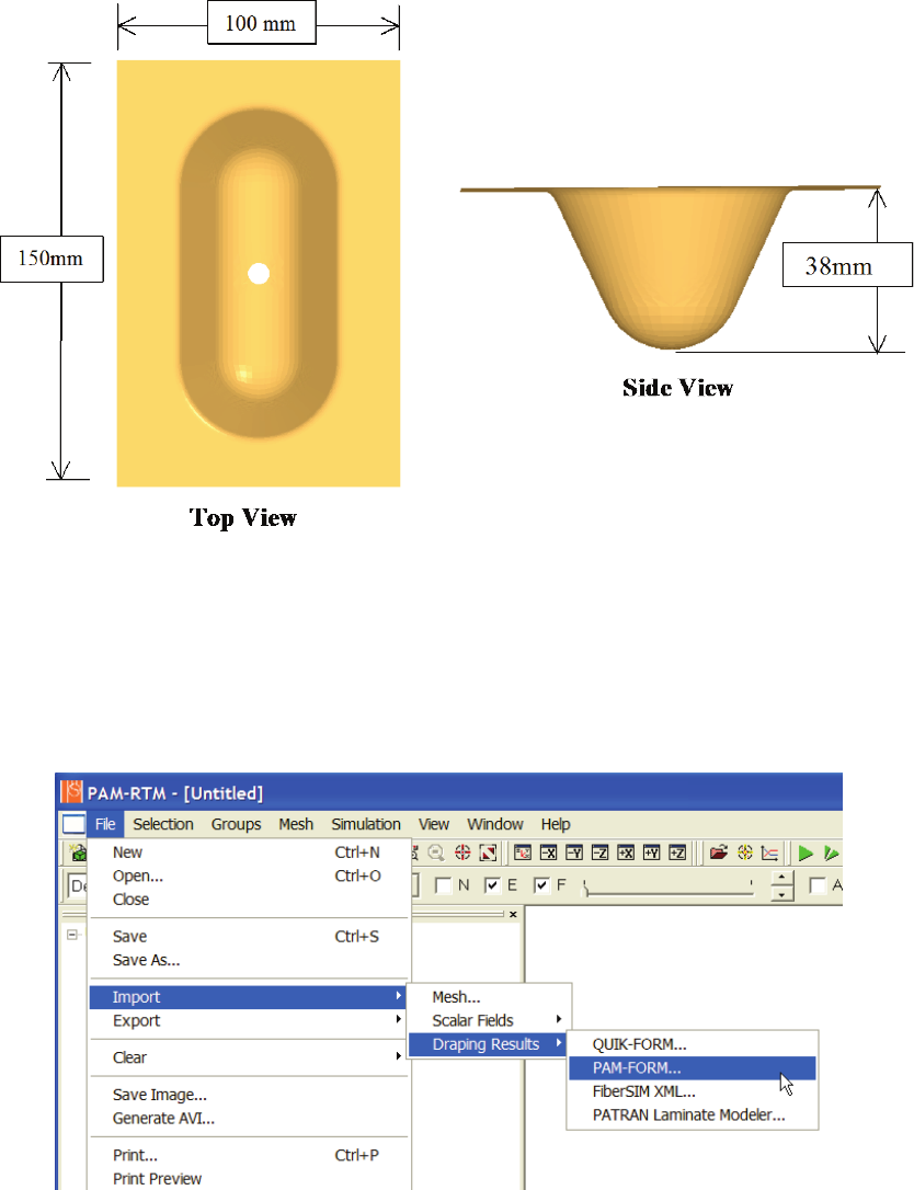
USER’S GUIDE & TUTORIALS 410 PAM-RTM 2014
(released: Apr-14) © 2014 ESI Group
TUTORIALS
Local Permeability from Draping Results
Map Draping Results
Create a new RTM simulation with File->New. Import the mesh file for the injection
simulation drape_start.unv.
To import the draping results, select File->Import->Draping Results->PAM-FORM.
The Import PAM-FORM Laminate dialog box pops up. Select the PAM-FORM™ file
drape.dsy, and click Open.
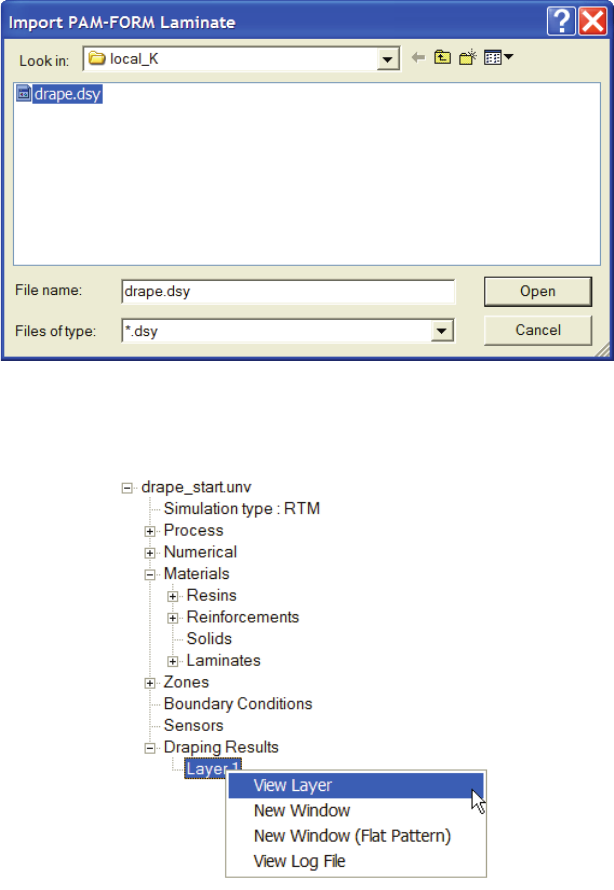
PAM-RTM 2014 411 USER’S GUIDE & TUTORIALS
© 2014 ESI Group (released: Apr-14)
TUTORIALS
Local Permeability from Draping Results
The imported plies are listed in the Draping Results folder of the explorer. It can be
useful to visualize one of the imported plies on top of the injection mesh. Right-click on
the layer to visualize and choose View Layer.
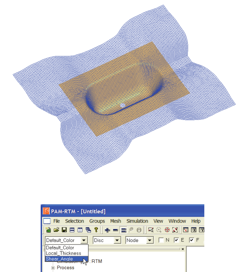
USER’S GUIDE & TUTORIALS 412 PAM-RTM 2014
(released: Apr-14) © 2014 ESI Group
TUTORIALS
Local Permeability from Draping Results
It is also possible to have the ply edges colored based on shear angle. Choose
Shear_Angle in the scalar fields combo box.

PAM-RTM 2014 413 USER’S GUIDE & TUTORIALS
© 2014 ESI Group (released: Apr-14)
TUTORIALS
Local Permeability from Draping Results
It is also possible to visualize a ply in its own 3D window, with the command New
Window in the explorer. This gives more post-processing options. For example, with the
first approach, only the edges are colored. With the New Window approach, the faces are
colored so it is possible to obtain a contour.
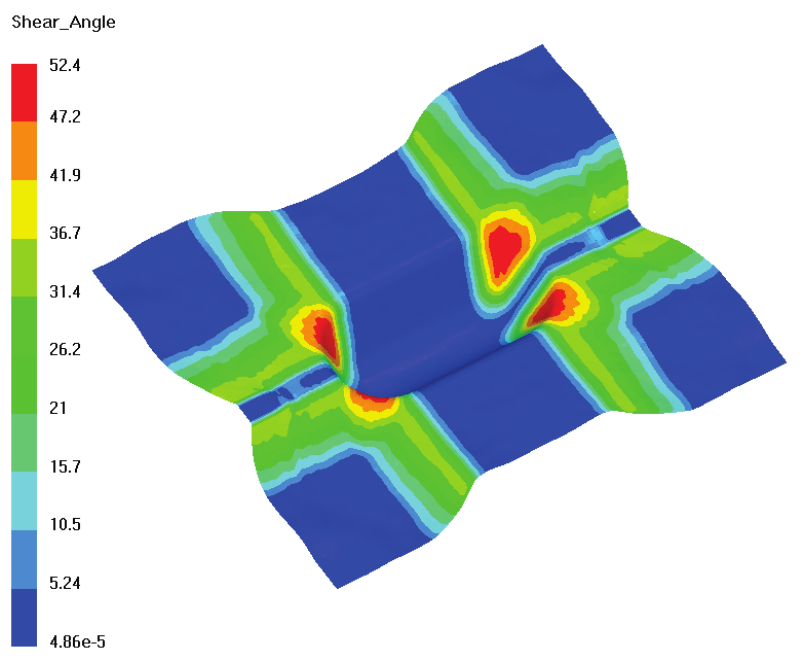
USER’S GUIDE & TUTORIALS 414 PAM-RTM 2014
(released: Apr-14) © 2014 ESI Group
TUTORIALS
Local Permeability from Draping Results
The Window menu lists all open documents. Notice that a ply visualization activated
with the New Window command is actually considered a document. It has the same
name as the injection document, with the layer index appearing between parenthesis.
Select the appropriate document to go back to the injection mesh.
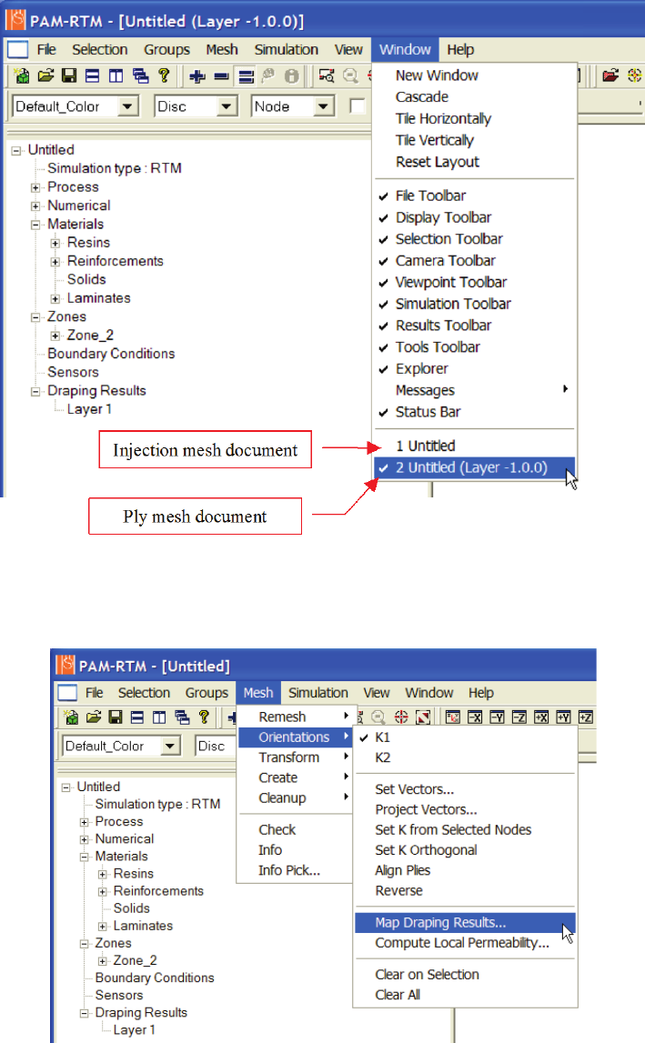
PAM-RTM 2014 415 USER’S GUIDE & TUTORIALS
© 2014 ESI Group (released: Apr-14)
TUTORIALS
Local Permeability from Draping Results
Activate the injection mesh display window. Use the command Mesh->Orientations-
>Map Draping Results to perform the mapping calculation from the draped plies to the
injection mesh.
The mapping calculation can be carried out on the full injection mesh or on the
currently selected elements only. This is useful for example to avoid plies to be mapped
into zones used for runners in the injection mesh. If some elements are selected when
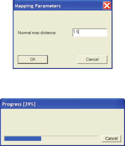
USER’S GUIDE & TUTORIALS 416 PAM-RTM 2014
(released: Apr-14) © 2014 ESI Group
TUTORIALS
Local Permeability from Draping Results
you launch Map Draping Results, PAM-RTM™ asks for a confirmation that the
mapping is to be done only on the selected elements.
Then a dialog box pops up for the normal max distance. The units are the same as the
length units of the model. Since we are currently working on a mesh in millimeters,
enter a of normal max distance of 1.5 mm. This parameter is useful for instance on
ribbed parts, to avoid elements on one rib to be mapped on another front facing rib. See
the chapter describing the commands of the Mesh menu in the PAM-RTM™ user’s
guide for more information.
Click OK, and the mapping calculation starts. A progress dialog box appears. Since
mapping calculations are typically very long, it is possible to stop the calculation with
the Cancel button.
After the mapping calculation finishes, select Nb_Plies in the scalar field roll-down list,
the number of laminate plies mapped to each element of the injection mesh is displayed.
This is useful to verify the results of the mapping calculation. Since in this example,
only one ply that covers completely the injection mesh was mapped, Nb_Plies must be
equal to 1 everywhere. Otherwise you would have to adjust the tolerances.
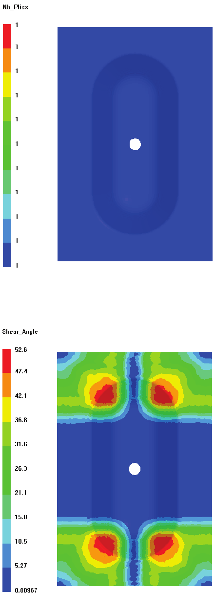
PAM-RTM 2014 417 USER’S GUIDE & TUTORIALS
© 2014 ESI Group (released: Apr-14)
TUTORIALS
Local Permeability from Draping Results
Select Shear_Angle in the scalar field roll-down list and Iso in the plot type roll-down
list, and turn off the Edge display. The mapped shearing angle distribution from the first
laminate ply on the injection mesh is shown in the current display window.
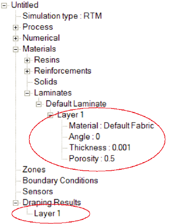
USER’S GUIDE & TUTORIALS 418 PAM-RTM 2014
(released: Apr-14) © 2014 ESI Group
TUTORIALS
Local Permeability from Draping Results
Local Permeability Calculation
The command Mesh->Orientations->Compute Local Permeability computes the average
permeability and porosity on each element of the injection mesh, using the results of the
Map Draping Results calculation. To calculate local permeability, PAM-RTM™ needs
to know the type of reinforcement and permeability model associated to each ply, as
well as the initial fiber content of each ply. This is done using laminates. Before
launching Compute Local Permeability, the user has to create a laminate material
matching the imported plies, i.e. with the same number of plies.
For this example, make sure that the initial porosity of layer 1 of the laminate is 0.5.
This is the porosity before shearing. Set the permeability of the fabric linked to layer 1
(default fabric) to 1.10-11 m².
Now you can launch Mesh->Orientations->Compute Local Permeability.

PAM-RTM 2014 419 USER’S GUIDE & TUTORIALS
© 2014 ESI Group (released: Apr-14)
TUTORIALS
Local Permeability from Draping Results
The Permeability Model dialog box pops up. In this example, we want the permeability
calculation to be based on the imported PAM-FORM™ ply, so check use imported
plies. We assume in this example that the permeability of the undeformed fabric is
isotropic. Choose the Isotropic Woven Fabric model in the permeability model for
sheared fabrics roll-down list, then click OK to start the local permeability calculation.
To view the local permeability calculation results, select porosity in the main toolbar’s
roll-down list. Then the local porosity field on the injection mesh is displayed.
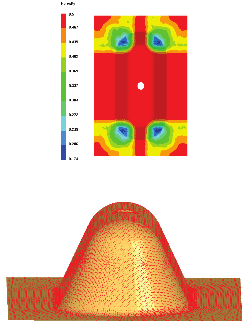
USER’S GUIDE & TUTORIALS 420 PAM-RTM 2014
(released: Apr-14) © 2014 ESI Group
TUTORIALS
Local Permeability from Draping Results
The K1 principal direction can be displayed by selecting View->Orientations->K1.
Switch off the scalar field display by selecting Default_Color in the scalar field roll-
down list. The K1 direction is displayed in the following image with red arrows.
Contours for K1 and K2 in the high shearing areas are shown below.
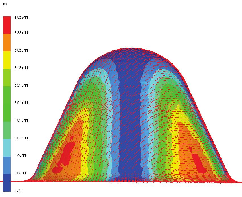
PAM-RTM 2014 421 USER’S GUIDE & TUTORIALS
© 2014 ESI Group (released: Apr-14)
TUTORIALS
Local Permeability from Draping Results
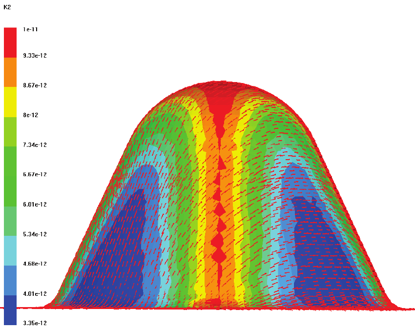
USER’S GUIDE & TUTORIALS 422 PAM-RTM 2014
(released: Apr-14) © 2014 ESI Group
TUTORIALS
Local Permeability from Draping Results
Filling Simulation
In the RTM Numerical Parameters dialog box, select Use local permeability files and Use
local porosity file. We do not use the local thickness file in this example. We just
assume a constant thickness cavity, specified in zone 2 of the injection mesh.

PAM-RTM 2014 423 USER’S GUIDE & TUTORIALS
© 2014 ESI Group (released: Apr-14)
TUTORIALS
Local Permeability from Draping Results
Normally, since local permeability files are used, there is no need to specify the
permeability values using the fabric editor. However it is recommended to specify
reasonable values for K1, K2 and K3, because if for some reason the value for an
element is not found in the local permeability file, the value specified in the fabric
editor will be used.
The following groups have to be created.
USER’S GUIDE & TUTORIALS 424 PAM-RTM 2014
(released: Apr-14) © 2014 ESI Group
TUTORIALS
Local Permeability from Draping Results
To summarize, here are the parameters that need to be set for the filling simulation:
- resin:
· viscosity: 0.1 Pa.s
- fabric:
· name: Default Fabric
· K1: 1.10-11 m2
· K2: 1.10-11 m2
· K3: 1.10-11 m2
- zone:
· ID : 2
· material: Default Fabric
· porosity: 0.5
· thickness: 0.005 m
- boundary condition :
· ID: 1
· type: pressure
· pressure value: 3.105 Pa
- boundary condition:
· ID: 2
· type: vent
· pressure value: 0 Pa
· state:
Finally, save the PAM-RTM document before starting the simulation. Since a compute
local permeability was done, some files will be automatically generated in the same
directory as the x.dtf file: x_k1.sf, x_k2.sf, x_porosity.sf. These are the files
read by the PAM-RTM™ solver to initialize local permeability and porosity. When
saving the files, PAM-RTM™ detects that the span of the injection mesh is very large,
which could mean that it is defined in millimeters, so it asks whether you want to
automatically convert it to meters. Select Yes.
Launch the simulation. When it is done, load the results files. You should have the
following segmented filling patterns. Filling time is about 692 seconds.
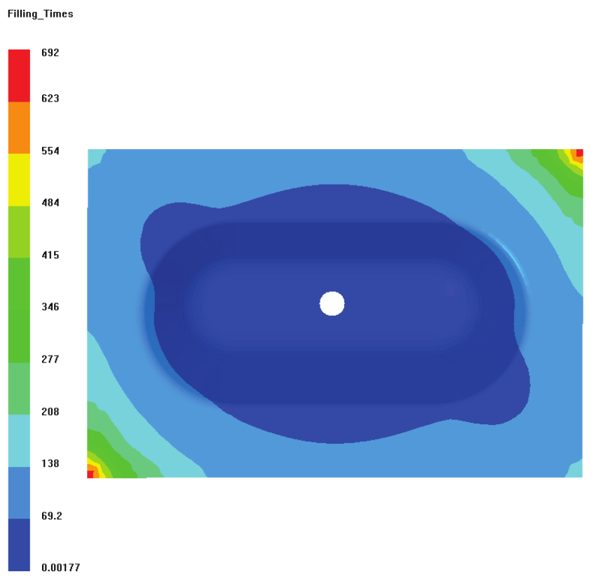
PAM-RTM 2014 425 USER’S GUIDE & TUTORIALS
© 2014 ESI Group (released: Apr-14)
TUTORIALS
Local Permeability from Draping Results
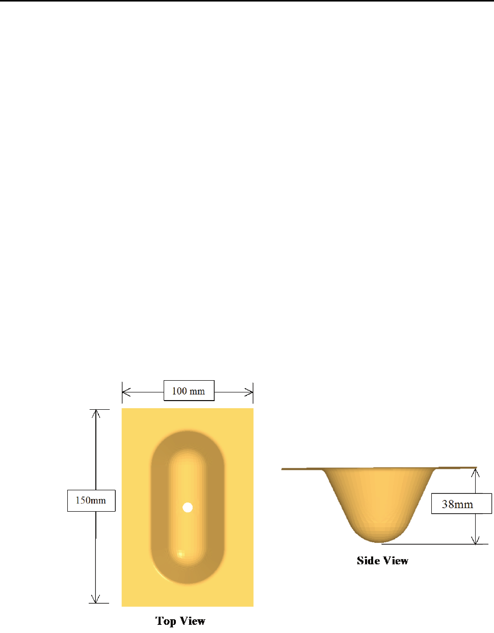
USER’S GUIDE & TUTORIALS 426 PAM-RTM 2014
(released: Apr-14) © 2014 ESI Group
TUTORIALS
Local Permeability from Draping Results (Advanced)
LOCAL PERMEABILITY FROM DRAPING
RESULTS (ADVANCED)
The following files are used in this example.
- drape2.dsy (4 plies laminate file)
- drape2_start.unv (injection mesh file)
- drape2_K1.srf (sheared permeability K1 kriged function data file)
- drape2_K2.srf (sheared permeability K2 kriged function data file)
- drape2_beta.srf (sheared rotation angle kriged function data file)
Objectives
This document presents an advanced tutorial on local permeability calculation from
draping results, complementary to the previous tutorial – Local permeability from
draping results. The advanced features include
- how to assign materials to a more complex laminate made of many plies,
- how to use kriged functions to describe the fabric sheared permeability as a function
of shear angle and fiber content.
The same bathtub-like geometry used in the previous tutorial is investigated again in
this tutorial with the draping results of a 4 plies laminate obtained with PAM-
FORM™, and the geometry is shown below.
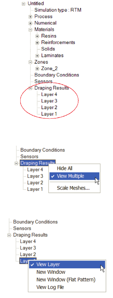
PAM-RTM 2014 427 USER’S GUIDE & TUTORIALS
© 2014 ESI Group (released: Apr-14)
TUTORIALS
Local Permeability from Draping Results (Advanced)
Map Draping Results
Create a new RTM simulation with File->New. Import the mesh file
drape2_start.unv. Then select File->Import->Draping Results->PAM-FORM to import
the draping results file drape2.dsy.
There are four plies in the draping file. They are listed in Draping Results folder of the
explorer after importation.
Right-click on the Draping Results item and choose View Multiple to allow
visualization of many layers in the same window.
Then right-click on the first layer and choose View Layer.

USER’S GUIDE & TUTORIALS 428 PAM-RTM 2014
(released: Apr-14) © 2014 ESI Group
TUTORIALS
Local Permeability from Draping Results (Advanced)
Do the same for the fourth layer. This leads to the following picture, where we can see
clearly that there is an offset between the first and fourth ply. This will be important for
the transverse tolerance when mapping draping results.
All the four plies in this PAM-FORM™ file have a zero degree orientation, so all the
plies have similar local deformations, but not exactly the same because of the thickness
of the part. The figure below shows the shear angle distribution for ply 2.
Go back to the injection mesh window. Select Mesh->Orientations->Map Draping
Results to perform the mapping calculation from the imported draped plies to the
injection mesh. In the Mapping Parameters dialog box, enter 4.0 (mm) as normal max
distance.
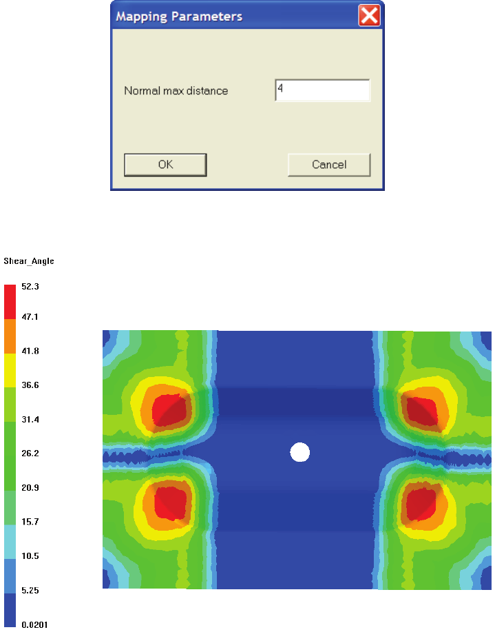
PAM-RTM 2014 429 USER’S GUIDE & TUTORIALS
© 2014 ESI Group (released: Apr-14)
TUTORIALS
Local Permeability from Draping Results (Advanced)
When the mapping calculation is done, the mapped shearing angle distribution from the
first laminate ply on the injection mesh is shown as below.
Select Nb_Plies in the scalar field roll-down list to view the number of laminate plies
mapped to each element of the injection mesh. Since in this example, four plies that
cover completely the injection mesh were mapped, Nb_Plies must be equal to four
everywhere.
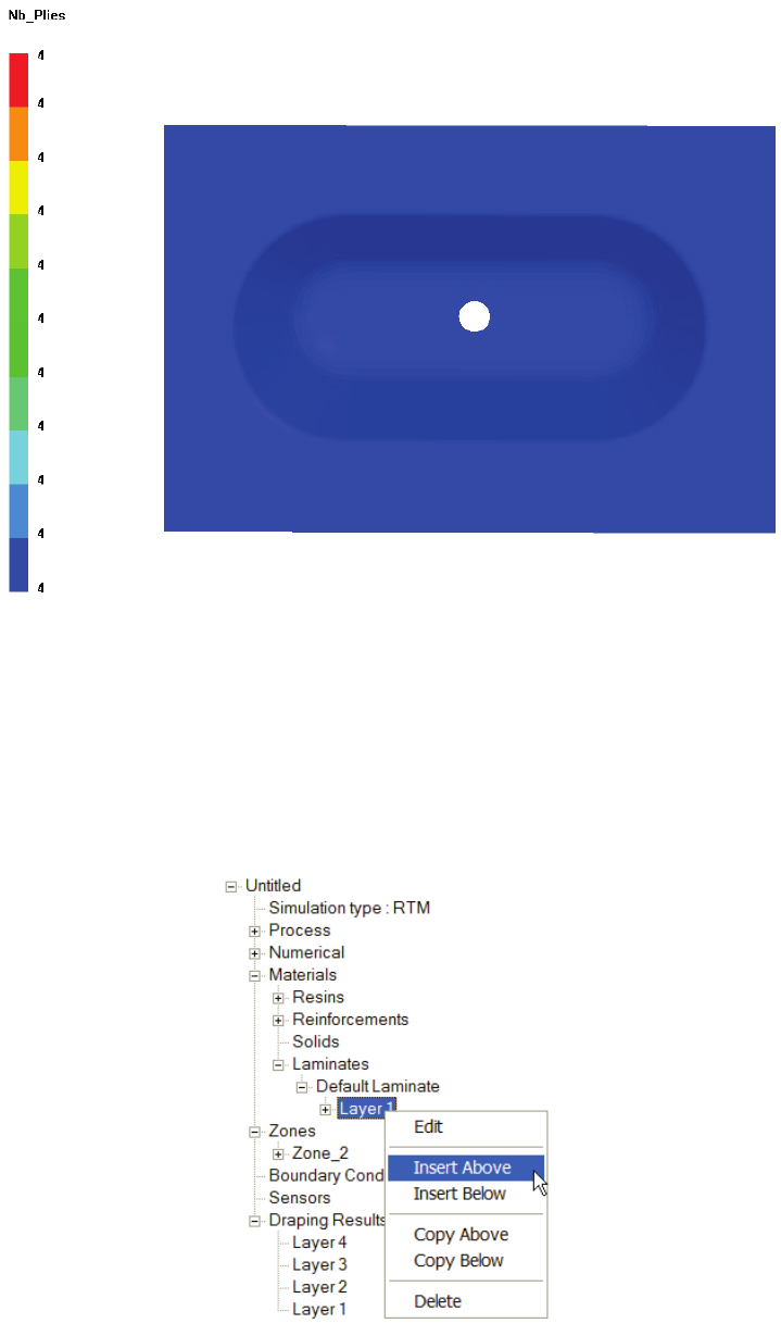
USER’S GUIDE & TUTORIALS 430 PAM-RTM 2014
(released: Apr-14) © 2014 ESI Group
TUTORIALS
Local Permeability from Draping Results (Advanced)
Local Permeability Calculation
Before we can launch the local permeability calculation, we have to specify material
properties for each of the imported draped plies. To do so, we first create a laminate
material made of four layers, to match the four imported draped plies. Right-click the
first layer of the Default Laminate, then choose Insert Above to add a layer above the
selected one. Repeat this procedure until you have four layers.
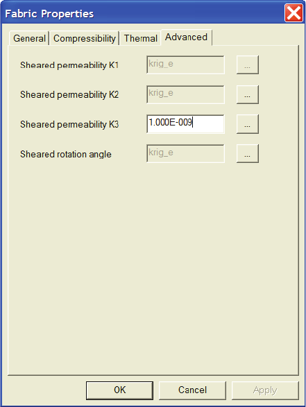
PAM-RTM 2014 431 USER’S GUIDE & TUTORIALS
© 2014 ESI Group (released: Apr-14)
TUTORIALS
Local Permeability from Draping Results (Advanced)
All four layers reference the Default Fabric. Double-click Default Fabric to open the
fabric editor. In the Advanced tab, we will specify a sheared permeability model with
the fields Sheared Permeability K1, Sheared Permeability K2, Sheared Permeability
K3, and Sheared Rotation Angle, where sheared permeability K1, K2, and K3 are 1st,
2nd, and 3rd principal direction of the permeability tensor, respectively.
Click on the … button to the right of the Sheared Permeability K1 field to open the
Function Editor dialog box. Select Import from file and in the Import dialog box, choose
in the Type roll-down list PAM-RTM (*.srf) and browse to drape2_k1.srf. By the
same way, set the fields Sheared permeability K2 and Sheared rotation angle. Before
closing the Function Editor dialog box, don’t forget to select the imported function.
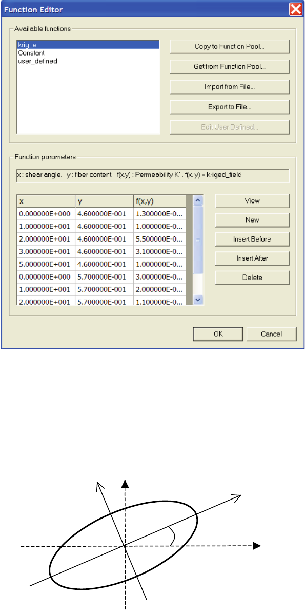
USER’S GUIDE & TUTORIALS 432 PAM-RTM 2014
(released: Apr-14) © 2014 ESI Group
TUTORIALS
Local Permeability from Draping Results (Advanced)
The user could also enter the data points manually. The x column is the shear angle (in
degree), y is the fiber content (a decimal value between 0 to 1), and z is the sheared
permeability (unit: m2).
The sheared rotation angle designates the angular position of 1st principal direction of
the permeability tensor (K1) with respect to the warp direction of the laminate fabric
(f1), as shown in the following figure.
β
f2
f1
K1
K2
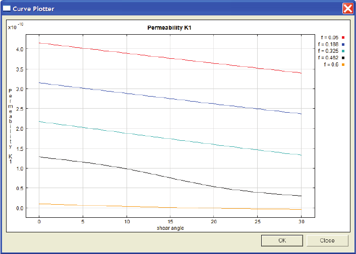
PAM-RTM 2014 433 USER’S GUIDE & TUTORIALS
© 2014 ESI Group (released: Apr-14)
TUTORIALS
Local Permeability from Draping Results (Advanced)
Note
· If you select View->Orientations->K1 Only (or K2 Only) when the active window
is a draped ply, the K1 direction represents the warp direction of a fabric, and
K2 represents the weft direction. However if you visualize K1 on the injection
mesh after Compute Local Permeability, the K1 direction is the 1st principal
direction of the permeability tensor. So the same command View->Orientations-
>K1 is used to visualize fiber directions or principal permeability directions,
depending on the context.
The sheared permeability K1, sheared permeability K2 and sheared rotation angle
functions used in this example are displayed below.
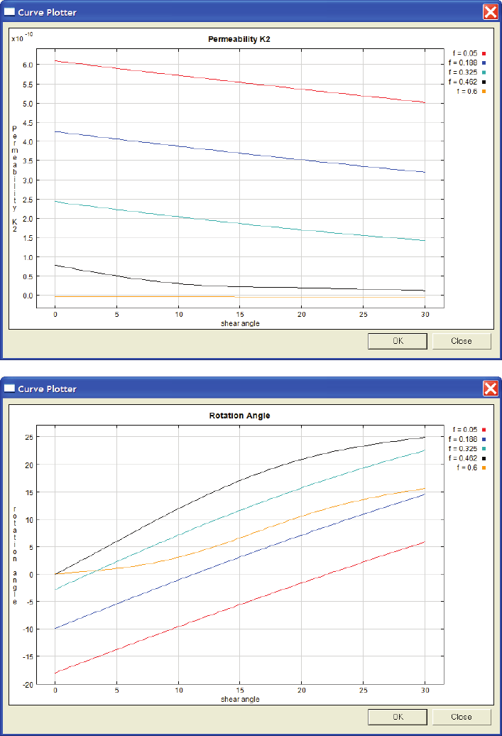
USER’S GUIDE & TUTORIALS 434 PAM-RTM 2014
(released: Apr-14) © 2014 ESI Group
TUTORIALS
Local Permeability from Draping Results (Advanced)
For 3D simulations, the Sheared Permeability K3 could also be defined as a function of
the fiber content and shear angle, if such experimental data is available. In this example,
we set Sheared Permeability K3 to a constant value.
To perform the local permeability calculation, select Mesh->Orientations->Compute
Local Permeability.
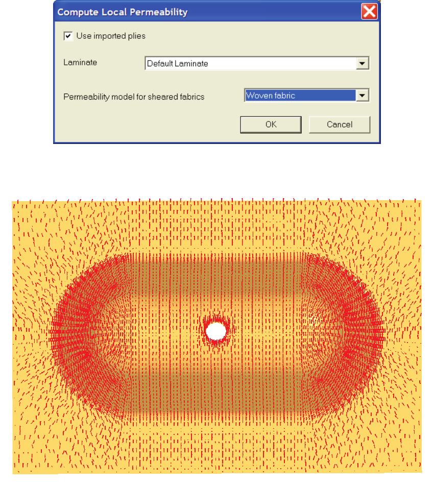
PAM-RTM 2014 435 USER’S GUIDE & TUTORIALS
© 2014 ESI Group (released: Apr-14)
TUTORIALS
Local Permeability from Draping Results (Advanced)
The Compute Local Permeability dialog box pops up. Check use imported plies and
select Woven Fabric in the permeability model roll-down list, which means that the
sheared permeability functions we’ve just defined will be used.
The figure below shows the 1st principal direction of the permeability tensor after local
permeability calculation.
The following figures show the local porosity and local K1 value after mapping
calculation.
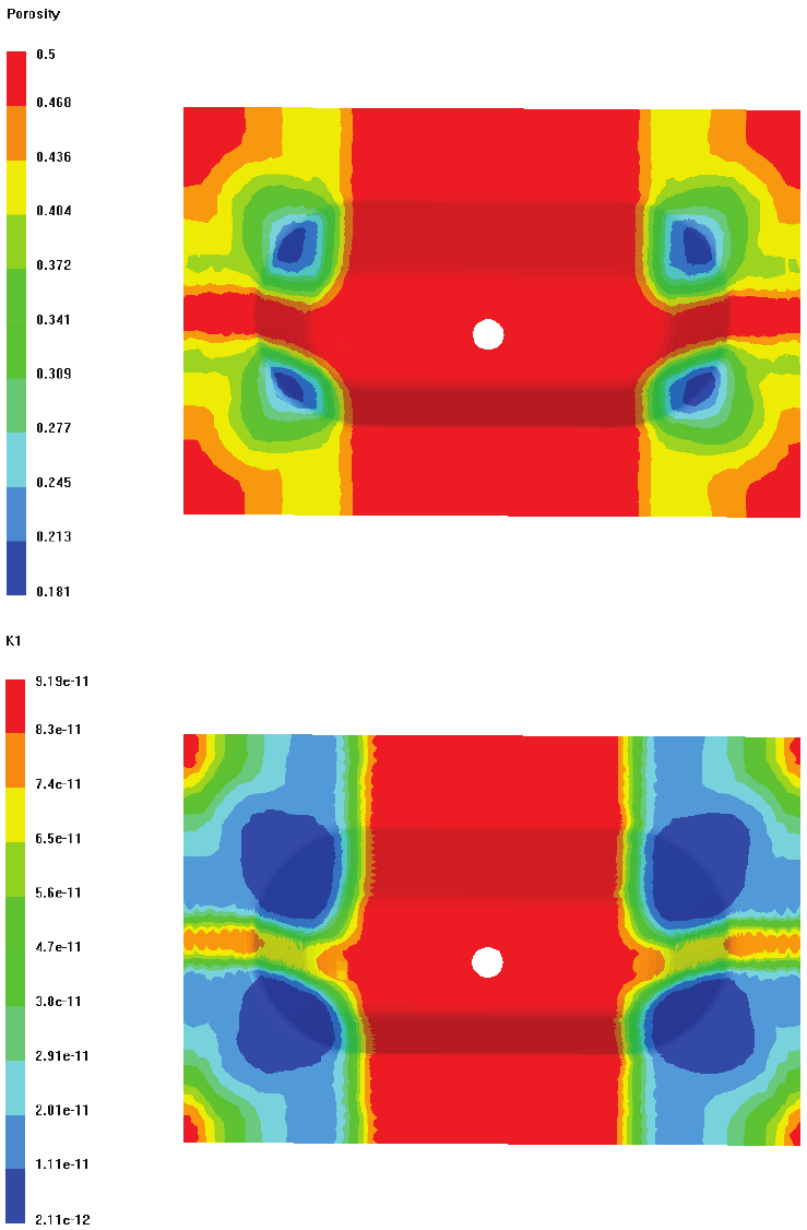
USER’S GUIDE & TUTORIALS 436 PAM-RTM 2014
(released: Apr-14) © 2014 ESI Group
TUTORIALS
Local Permeability from Draping Results (Advanced)
The rest of the procedure is the same as described in the tutorial Local permeability
from draping results. The following figure shows the filling pattern at a constant
pressure injection, whose injection and vent conditions are the same as in the previous
tutorial.

PAM-RTM 2014 437 USER’S GUIDE & TUTORIALS
© 2014 ESI Group (released: Apr-14)
TUTORIALS
Local Permeability from Draping Results (Advanced)

USER’S GUIDE & TUTORIALS 438 PAM-RTM 2014
(released: Apr-14) © 2014 ESI Group
TUTORIALS
PAM-QUIKFORM
PAM-QUIKFORM
The following files are used in this example.
- quikform_start.ps (starting mesh)
- quikform.dtf + quikform.ps (solution)
Objectives
The goal of this tutorial is to show how to perform a draping simulation using the
PAM-QUIKFORM™ user interface available in PAM-RTM™. The geometry used is
a double hemisphere. We will drape a laminate made of two plies of fabric and two
plies of unidirectional. The contact point is the top of the big hemisphere and the
laminate reference axis (zero degree) is the global X axis.
Process and Numerical Parameters
Create a new PAM-QUIKFORM simulation with File->New->PAM-QUIKFORM. Import
the mesh file quikform_start.ps with File->Import->Mesh. Make sure to set the file
filter to PAM-SYSTEM, as shown below.
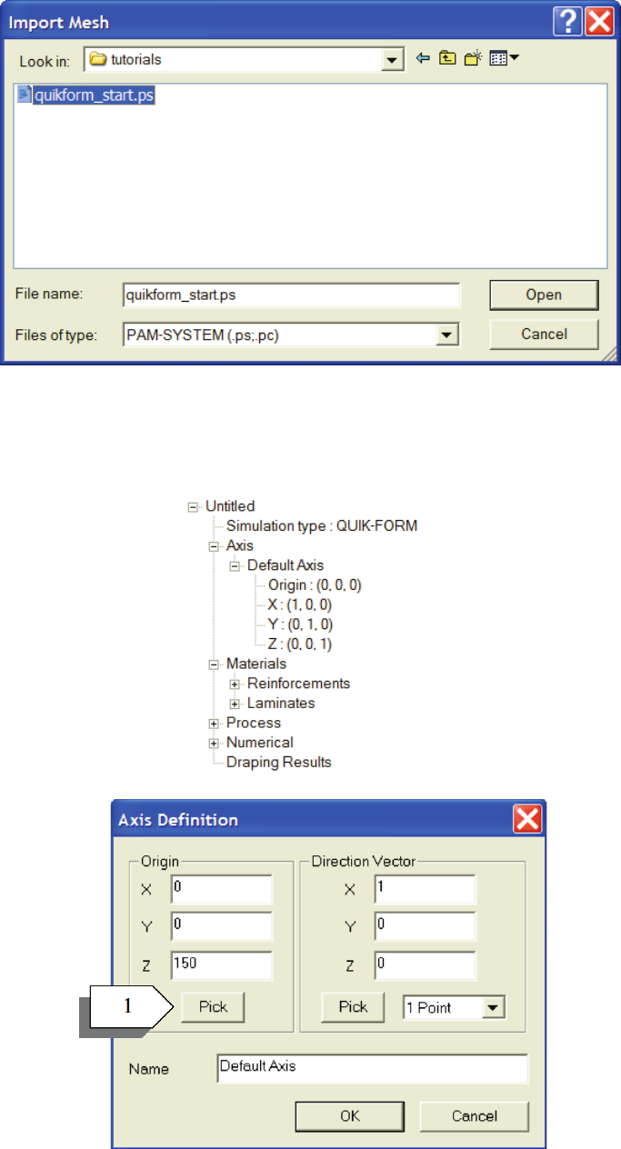
PAM-RTM 2014 439 USER’S GUIDE & TUTORIALS
© 2014 ESI Group (released: Apr-14)
TUTORIALS
PAM-QUIKFORM
First we create a draping referential (also called axis in PAM-RTM™) on top of the big
hemisphere. The default PAM-QUIKFORM document contains an axis located at the
origin. It is unlikely that this axis is what you want, so double-click the default axis to
open the Axis Definition dialog box.
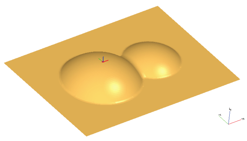
USER’S GUIDE & TUTORIALS 440 PAM-RTM 2014
(released: Apr-14) © 2014 ESI Group
TUTORIALS
PAM-QUIKFORM
Push the Pick button [1] and pick a point near the top of the big hemisphere, or enter the
coordinates of the origin manually (0, 0, 150). The direction vector is the local X axis of
the draping referential, i.e. the axis on which zero degree plies will be aligned. The local
Y and Z axis are set automatically by PAM-RTM™. The local Z axis is the normal
vector on the picked point and the local Y axis is calculated to have a right-hand
coordinate system. If you want the opposite local Z direction, use the command Reverse
Z, available in the explorer when right-clicking an axis. In this tutorial, we keep the
default direction vector (1, 0, 0), then we reverse the local Z axis to have it in the global
Z+ direction, as shown below.
Now we have to define the following laminate:
- layer 4: 90 degrees fabric
- layer 3: -45 degrees unidirectional
- layer 2: +45 degrees unidirectional
- layer 1: zero degree fabric
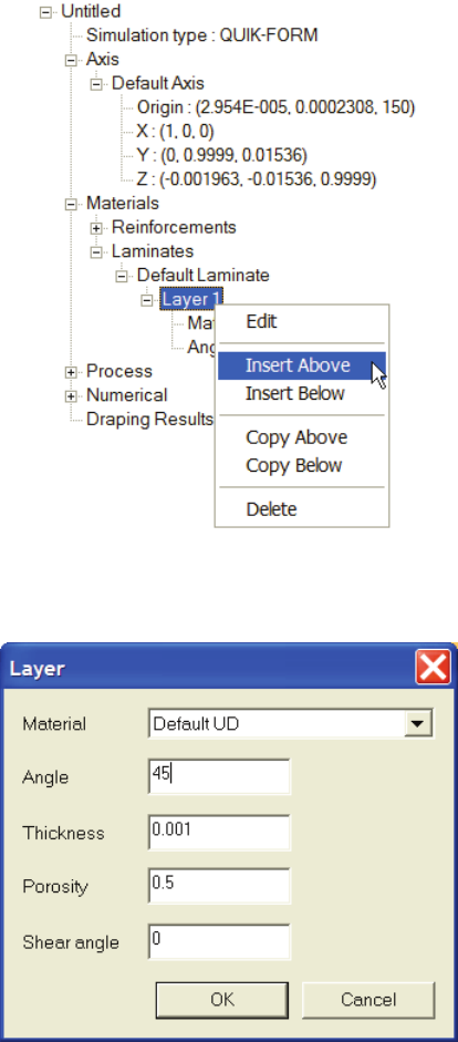
PAM-RTM 2014 441 USER’S GUIDE & TUTORIALS
© 2014 ESI Group (released: Apr-14)
TUTORIALS
PAM-QUIKFORM
Right-click Layer 1 in the Default Laminate and insert three layers above. Edit each
layer by double-clicking it, then set the material and angle as specified above.
Finally you should have the following laminate in the explorer.
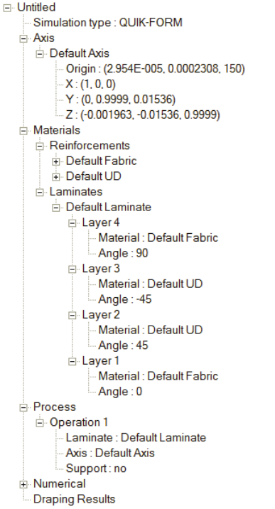
USER’S GUIDE & TUTORIALS 442 PAM-RTM 2014
(released: Apr-14) © 2014 ESI Group
TUTORIALS
PAM-QUIKFORM
After having specified a draping referential and laminate, we would normally have to
specify operations in the Process folder. Operations are used in the PAM-QUIKFORM
interface of PAM-RTM™ to associate a laminate to a draping referential, and also
optionally to select a group of elements on which draping is to be done. In this tutorial,
we just use the Default Operation, which refers to Default Axis and Default Laminate.
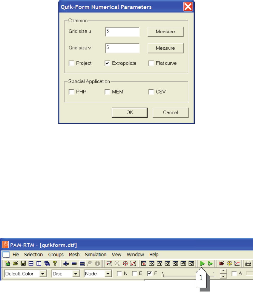
PAM-RTM 2014 443 USER’S GUIDE & TUTORIALS
© 2014 ESI Group (released: Apr-14)
TUTORIALS
PAM-QUIKFORM
Finally, before launching the PAM-QUIKFORM simulation, we have to set some
numerical parameters, the most important ones being grid size u and grid size v. These
are the size of the elements of the draped plies meshes. The default size is zero, which
means that it is unspecified and that PAM-QUIKFORM will calculate a size to get a
reasonable mesh. In this example, we force the element size to 5 mm in the u and v
directions.
Launching the Simulation and Post-Processing
Before the simulation can be launched, the PAM-QUIKFORM document must be saved
with File->Save.
To launch the simulation, use the green arrow button in the toolbar [1].
When the simulation is done, PAM-RTM™ loads automatically all the draped plies
meshes and lists them in the Draping Results folder of the explorer. Right-click one of
the layers and choose View Layer to visualize the mesh of the layer on top of the tool
mesh. It is possible to visualize many layers in the same window with the command
View Multiple of the Draping Results popup menu.
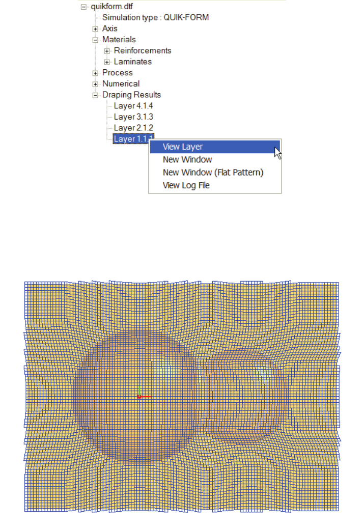
USER’S GUIDE & TUTORIALS 444 PAM-RTM 2014
(released: Apr-14) © 2014 ESI Group
TUTORIALS
PAM-QUIKFORM
Using this approach for visualization of layers, here is what you should have for layers
1 to 3 (since layer 4 is a 90 degrees fabric, and since it is not possible to display warp
and weft with different colors, there is no difference with layer 1).
Layer 1 (zero degree fabric)
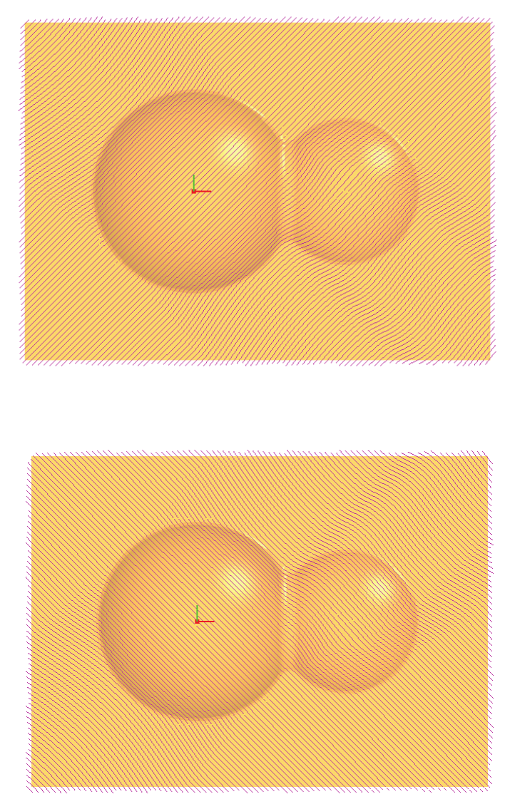
PAM-RTM 2014 445 USER’S GUIDE & TUTORIALS
© 2014 ESI Group (released: Apr-14)
TUTORIALS
PAM-QUIKFORM
Layer 2 (+45 degrees UD)
Layer 3 (-45 degrees UD)
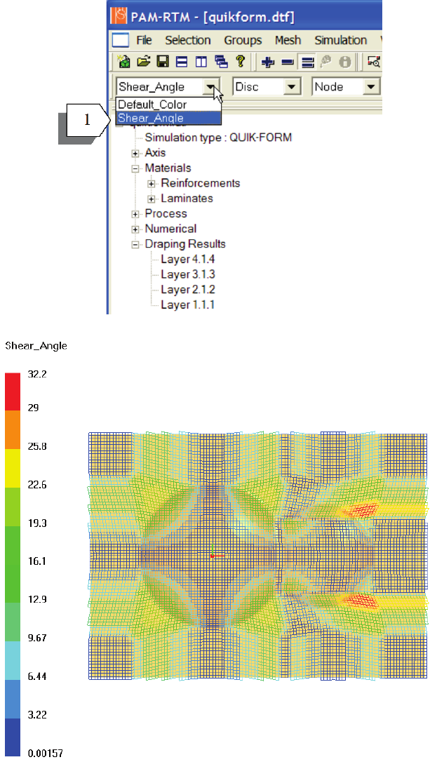
USER’S GUIDE & TUTORIALS 446 PAM-RTM 2014
(released: Apr-14) © 2014 ESI Group
TUTORIALS
PAM-QUIKFORM
When a layer is visualized with View Layer, the tool mesh is forced to default color and
the variables available in the scalar field combo box control coloring of the layer mesh
edges. Choosing Shear_Angle [1] leads to the figure below.
Edges colored with shear angle
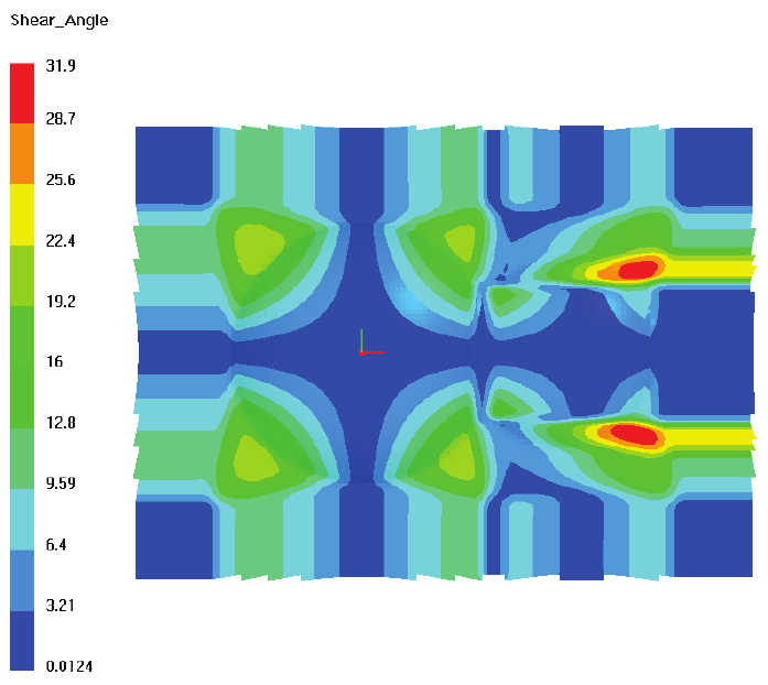
PAM-RTM 2014 447 USER’S GUIDE & TUTORIALS
© 2014 ESI Group (released: Apr-14)
TUTORIALS
PAM-QUIKFORM
The New Window command, available when right-clicking a layer in the Draping
Results folder, is used to visualize the mesh of a layer in its own 3D window. This gives
access to more post-processing options. For example, it is possible to generate contours
of the shear angle, as shown below, which is not possible when the layer is visualized in
the tool window.
Shear angle contours
Finally, it is possible to visualize the mesh of the 2D flat pattern of a layer by choosing
the command New Window (Flat Pattern). To get a more accurate representation of the
boundary of the flat pattern, you can activate the Flat curve option in the numerical
parameters. This option calculates the green curve shown below.
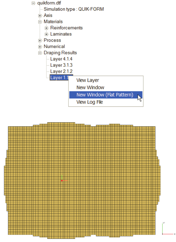
USER’S GUIDE & TUTORIALS 448 PAM-RTM 2014
(released: Apr-14) © 2014 ESI Group
TUTORIALS
PAM-QUIKFORM
2D flat pattern of layer 1
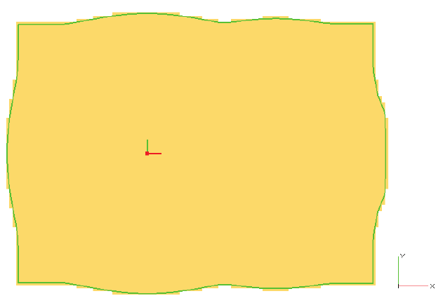
PAM-RTM 2014 449 USER’S GUIDE & TUTORIALS
© 2014 ESI Group (released: Apr-14)
TUTORIALS
PAM-QUIKFORM
2D flat pattern of layer 1 with flat curve option
Credits
Twente University, Netherlands, for the tool geometry.
Cranfield University, UK, for the mesh.