Xilinx PlanAhead User Guide Plan Ahead

User Manual:

Open the PDF directly: View PDF .
Page Count: 432 [warning: Documents this large are best viewed by clicking the View PDF Link!]

Software Manuals
PlanAhead User Guide

PlanAhead User

Guide

UG632 (v 12.1) May 3, 2010

PlanAhead User Guide www.xilinx.com UG632 (v 12.1)

Xilinx is disclosing this user guide, manual, release note, and/or specification (the "Documentation") to you solely for use in the development

of designs to operate with Xilinx hardware devices. You may not reproduce, distribute, republish, download, display, post, or transmit the

Documentation in any form or by any means including, but not limited to, electronic, mechanical, photocopying, recording, or otherwise,

without the prior written consent of Xilinx. Xilinx expressly disclaims any liability arising out of your use of the Documentation. Xilinx reserves

the right, at its sole discretion, to change the Documentation without notice at any time. Xilinx assumes no obligation to correct any errors

contained in the Documentation, or to advise you of any corrections or updates. Xilinx expressly disclaims any liability in connection with

technical support or assistance that may be provided to you in connection with the Information.

THE DOCUMENTATION IS DISCLOSED TO YOU “AS-IS” WITH NO WARRANTY OF ANY KIND. XILINX MAKES NO OTHER

WARRANTIES, WHETHER EXPRESS, IMPLIED, OR STATUTORY, REGARDING THE DOCUMENTATION, INCLUDING ANY

WARRANTIES OF MERCHANTABILITY, FITNESS FOR A PARTICULAR PURPOSE, OR NONINFRINGEMENT OF THIRD-PARTY

RIGHTS. IN NO EVENT WILL XILINX BE LIABLE FOR ANY CONSEQUENTIAL, INDIRECT, EXEMPLARY, SPECIAL, OR INCIDENTAL

DAMAGES, INCLUDING ANY LOSS OF DATA OR LOST PROFITS, ARISING FROM YOUR USE OF THE DOCUMENTATION.

United States and other countries. All other trademarks are the property of their respective owners.

Included in the PlanAhead™ software code is source code for the following programs:

Centerpoint XML

The initial developer of the Original Code is CenterPoint - Connective Software Engineering GmbH. Portions created by CenterPoint

NLView Schematic Engine

Static Timing Engine by Parallax Software Inc.

Java Standard Edition

Includes portions of software from RSA Security, Inc. and some portions licensed from IBM are available at

http://oss.software.ibm.com/icu4j/.

The BSD License for the JGoodies Looks

Redistribution and use in source and binary forms, with or without modification, are permitted provided that the following conditions are met:

- Redistributions of source code must retain the above copyright notice, this list of conditions and the following disclaimer.

- Redistributions in binary form must reproduce the above copyright notice, this list of conditions and the following disclaimer in the

documentation and/or other materials provided with the distribution.

- Neither the name of JGoodies Karsten Lentzsch nor the names of its contributors may be used to endorse or promote products derived

from this software without specific prior written permission.

THIS SOFTWARE IS PROVIDED BY THE COPYRIGHT HOLDERS AND CONTRIBUTORS “AS IS” AND ANY EXPRESS OR IMPLIED

WARRANTIES, INCLUDING, BUT NOT LIMITED TO, THE IMPLIED WARRANTIES OF MERCHANTABILITY AND FITNESS FOR A

PARTICULAR PURPOSE ARE DISCLAIMED. IN NO EVENT SHALL THE COPYRIGHT OWNER OR CONTRIBUTORS BE LIABLE FOR

ANY DIRECT, INDIRECT, INCIDENTAL, SPECIAL, EXEMPLARY, OR CONSEQUENTIAL DAMAGES (INCLUDING, BUT NOT LIMITED

TO, PROCUREMENT OF SUBSTITUTE GOODS OR SERVICES; LOSS OF USE, DATA, OR PROFITS; OR BUSINESS INTERRUPTION)

HOWEVER CAUSED AND ON ANY THEORY OF LIABILITY, WHETHER IN CONTRACT, STRICT LIABILITY, OR TORT (INCLUDING

NEGLIGENCE OR OTHERWISE) ARISING IN ANY WAY OUT OF THE USE OF THIS SOFTWARE, EVEN IF ADVISED OF THE

POSSIBILITY OF SUCH DAMAGE.

UG632 (v 12.1) www.xilinx.com PlanAhead User Guide

Libconfig (v1.3.2) License

libconfig - A library for processing structured configuration files

This file is part of libconfig.

This library is free software; you can redistribute it and/or modify it under the terms of the GNU Lesser General Public License as published

by the Free Software Foundation; either version 2.1 of the License, or (at your option) any later version.

This library is distributed in the hope that it will be useful, but WITHOUT ANY WARRANTY; without even the implied warranty of

MERCHANTABILITY or FITNESS FOR A PARTICULAR PURPOSE. See the GNU Lesser General Public License for more details.

You should have received a copy of the GNU Library General Public License along with this library; if not, see http://www.gnu.org/licenses/.

Free IP Core License

This is the Entire License for all of our Free IP Cores.

Redistribution and use in source, netlist, binary and silicon forms, with or without modification, are permitted provided that the following

conditions are met:

-Redistributions of source code must retain the above copyright notice, this list of conditions and the following disclaimer.

-Redistributions in binary form must reproduce the above copyright notice, this list of conditions and the following disclaimer in the

documentation and/or other materials provided with the distribution.

-Neither the name of ASICS World Services, the Authors and/or the names of its contributors may be used to endorse or promote products

derived from this software without specific prior written permission.

THIS SOFTWARE IS PROVIDED BY THE COPYRIGHT HOLDERS AND CONTRIBUTORS “AS IS” AND ANY EXPRESS OR IMPLIED

WARRANTIES, INCLUDING, BUT NOT LIMITED TO, THE IMPLIED WARRANTIES OF MERCHANTABILITY AND FITNESS FOR A

PARTICULAR PURPOSE ARE DISCLAIMED. IN NO EVENT SHALL THE COPYRIGHT OWNER OR CONTRIBUTORS BE LIABLE FOR

ANY DIRECT, INDIRECT, INCIDENTAL, SPECIAL, EXEMPLARY, OR CONSEQUENTIAL DAMAGES (INCLUDING, BUT NOT LIMITED TO,

PROCUREMENT OF SUBSTITUTE GOODS OR SERVICES; LOSS OF USE, DATA, OR PROFITS; OR BUSINESS INTERRUPTION)

HOWEVER CAUSED AND ON ANY THEORY OF LIABILITY, WHETHER IN CONTRACT, STRICT LIABILITY, OR TORT (INCLUDING

NEGLIGENCE OR OTHERWISE) ARISING IN ANY WAY OUT OF THE USE OF THIS SOFTWARE, EVEN IF ADVISED OF THE

POSSIBILITY OF SUCH DAMAGE.

Demo RTL Design License

This RTL Design is free software; you can redistribute it and/or modify it under the terms of the GNU Lesser General Public License as

published by the Free Software Foundation; either version 2.1 of the License, or (at your option) any later version.

This library is distributed in the hope that it will be useful, but WITHOUT ANY WARRANTY; without even the implied warranty of

MERCHANTABILITY or FITNESS FOR A PARTICULAR PURPOSE. See the GNU Lesser General Public License for more details.

You should have received a copy of the GNU Library General Public License along with this design file; if not, see

http://www.gnu.org/licenses/.

PlanAhead User Guide www.xilinx.com UG632 (v 12.1)

PlanAhead User Guide www.xilinx.com 5

UG632 (v12.1) May 3, 2010

Guide Contents

Preface

About This Guide

This document provides detailed information about the PlanAhead™ software, including

an interface overview, and instructions for using the design and software capabilities.

This chapter contains the following sections:

•“Guide Contents”

•“Additional Resources”

•“Document Conventions”

Note: For information on software installation, and system requirements, refer to the Xilinx ISE

Design Suite: Installation, Licensing, and Release Notes.

Guide Contents

This document contains the following chapters:

•Chapter 1, “Introduction,”provides an overview of the PlanAhaead features.

•Chapter 2, “Understanding the PlanAhead Design Flow,”provides an overview of the

design flow.

•Chapter 3, “Working with Projects,”describes the initial setup and management of a

project within PlanAhead.

•Chapter 4, “Using the Viewing Environment,”describes the PlanAhead user interface.

•Chapter 5, “RTL and IP Design,” describes the RTL environment and how to

instantiate IPs into your design.

•Chapter 6, “Synthesizing the Design,” describes the available synthesis capabilities.

•Chapter 7, “Netlist Analysis and Constraint Definition,”describes the PlanAhead

design analysis and constraint definition capabilities.

•Chapter 8, “I/O Pin Planning,” describes the pin planning environment that enables

pin assignment.

•Chapter 9, “Implementing the Design,” describes the available implementation

capabilities.

•Chapter 10, “Analyzing Implementation Results,”describes the timing and placement

analysis capabilities available in PlanAhead.

•Chapter 11, “Floorplanning the Design,” describes the various floorplanning

strategies and capabilities available in PlanAhead.

•Chapter 12, “Programming and Debugging the Design,”describes the process for

generating bitstream files, launching programming tools and how to use ChipScope™

debugging software debugging capabilities that are integrated into PlanAhead.

•Chapter 13, “Using Hierarchical Design Techniques,” describes how to use the

hierarchical design features.

6www.xilinx.com PlanAhead User Guide

UG632 (v12.1) May 3, 2010

Preface: About This Guide

•Chapter 14, “Tcl and Batch Scripting,” describes how to use the Tcl commands and

scripting features

•Chapter 15, “Using PlanAhead With Project Navigator,” describes the PlanAhead

flows that are integrated with Project Navigator.

This document contains the following appendixes:

•Appendix A, “Menu and Toolbar Commands,” provides a brief description of the

menu and toolbar commands.

•Appendix B, “PlanAhead Input and Output Files,” describes the files used as input

and output in PlanAhead.

•Appendix C, “PlanAhead Terminology,” provides an explanation of the terminology

used in PlanAhead software.

•Appendix D, “Installing Releases with XilinxNotify,” describes the PlanAhead release

strategy and explains how to update the software.

•Appendix E, “Configuring SSH Without Password Prompting,” describes how to

setup a passwordless SSH, which is required for running PlanAhead processes on

multiple hosts

Additional Resources

The following documents are referenced in this document:

•Xilinx Synthesis and Simulation Design Guide, (UG626)

http://www.xilinx.com/support/documentation/sw_manuals/xilinx12/sim.pdf

•Xilinx Constraints Guide, (UG612)

http://www.xilinx.com/support/documentation/sw_manuals/xilinx12/cgd.pdf

•Spartan-6 PCB Design Guide,(UG393)

http://www.xilinx.com/support/documentation/user_guides/ug393.pdf

•Hierarchical Design Methodology Guide (UG748)

•PlanAhead Floorplanning Methodology Guide (UG633)

Partial Reconfiguration documentation is available at the following Xilinx web site:

www.xilinx.com/tools/partial-reconfiguration

•Partial Reconfiguration User Guide (UG702) (available upon request)

For more information, go to the Xilinx website (http://www.xilinx.com/planahead).

To find additional documentation, see the Xilinx website at:

http://www.xilinx.com/support/documentation/index.htm

To search the Answer Database of silicon, software, and IP questions and answers, or to create a

webcase with Technical Support, see the Xilinx website at:

http://www.xilinx.com/support/mysupport.htm

Xilinx Customer Education Training

•Essential Design with the PlanAhead Analysis & Design Tool - Attend this Xilinx

Customer Education Training Course to learn the basics about the PlanAhead

functionality.

•Advanced Design with the PlanAhead Analysis & Design Tool—Attend this Xilinx

Customer Education Training Course to learn about the advanced PlanAhead

functionality.

PlanAhead User Guide www.xilinx.com 7

UG632 (v12.1) May 3, 2010

Document Conventions

Tu t o r i a l s

The following PlanAhead tutorials are available with the PlanAhead software and on the

Xilinx website: http://www.xilinx.com/tools/planahead.htm.

−Quick Front- to-Back Flow Overview (UG673)

−I/O Pin Planning (UG674)

−RTL Design and IP Creation using CORE Generator (UG675)

−Design Analysis and Floorplanning (UG676)

−Debugging with ChipScope (UG677)

−Leveraging Design Preservation for Predictable Results (UG747)

−Partial Reconfiguration Overview (UG743)

−Partial Reconfiguration with Processor Peripherals UG744)

−Overview of Partial Reconfiguration Flow (UG743)

−Partial Reconfiguration with Processor Peripheral (UG744).

Documentation

•Xilinx ISE Design Suite: Installation, Licensing, and Release Notes—This document

provides specific installation instructions and requirements. Available from the

software and from the Xilinx web site.

•What’s New in PlanAhead (UG656)—The What’s New document provides specific

information about new features in this release. Available from the software and from

the Xilinx website.

•Floorplanning Methodology Guide (UG633)—This guide provides information about

various floorplanning strategies aimed at improving performance, repeatability of

results or reducing design times. Available from the Xilinx web site.

•Hierarchical Design Methodology Guide (UG748)—This guide provides information

about using the Xilinx hierarchical partitioning capabilities. Available from the Xilinx

web site.

Video Demonstrations

•PlanAhead Technical Video Demonstrations—Watch the video demonstrations to learn

more about specific areas of the PlanAhead software. Available from the Xilinx web

site: http://www.xilinx.com/products/design_resources/design_tool/resources/index.htm

Document Conventions

This document uses the following conventions. An example illustrates each convention.

Typographical

The following typographical conventions are used in this document:

8www.xilinx.com PlanAhead User Guide

UG632 (v12.1) May 3, 2010

Preface: About This Guide

Online Document

The following conventions are used in this document:

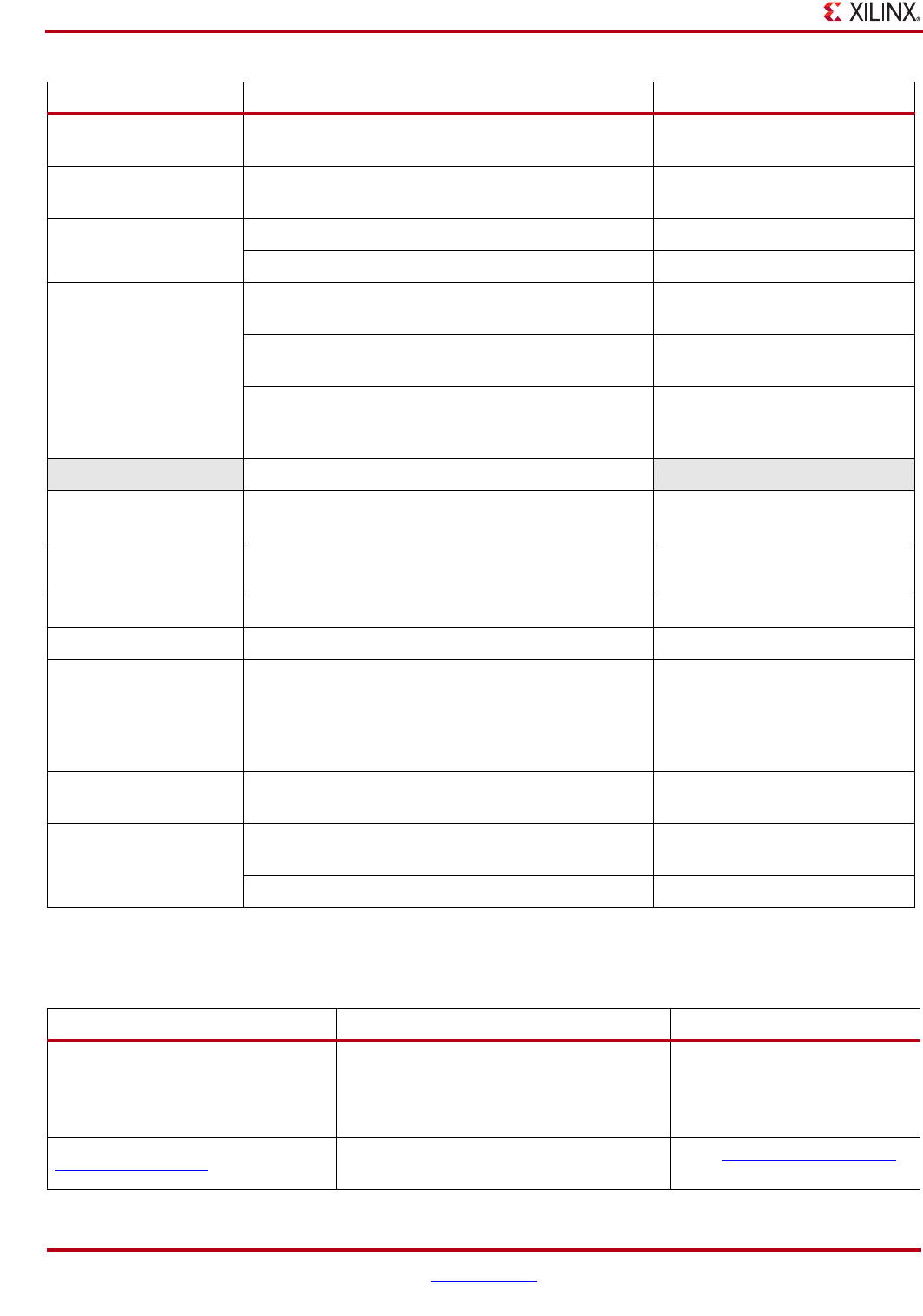
Convention Meaning or Use Example

Courier font Messages, prompts, and program files that the system

displays speed grade: - 100

Courier bold Literal commands that you enter in a syntactical

statement ngdbuild design_name

Helvetica bold Commands that you select from a menu File > Open

Keyboard shortcuts Ctrl+C

Italic font

Variables in a syntax statement for which you must

supply values ngdbuild <design_name>

References to other manuals See the Command Line Tools User

Guide for more information.

Emphasis in text

If a wire is drawn so that it

overlaps the pin of a symbol, the

two nets are not connected.

Dark Shading Items that are not supported or reserved This feature is not supported

Square brackets [ ] An optional entry or parameter. However, in bus

specifications, such as bus[7:0], they are required.

ngdbuild [option_name]

design_name

Braces { } A list of items from which you must choose one or

more lowpwr ={on|off}

Vertical bar | Separates items in a list of choices lowpwr ={on|off}

Angle brackets < > User-defined variable or in code samples <directory name>

Vertical ellipsis

Repetitive material that has been omitted

IOB #1: Name = QOUT’

IOB #2: Name = CLKIN’

Horizontal ellipsis . . . Repetitive material that has been omitted allow block block_name loc1

loc2 ... locn;

Notations

The prefix ‘0x’ or the suffix ‘h’ indicate hexadecimal

notation

A read of address 0x00112975

returned 45524943h.

An ‘_n’ means the signal is active low usr_teof_n is active low.

Convention Meaning or Use Example

Blue text Cross-reference link to a location in the

current document

See the section “Additional

Resources” for details.

Refer to “Title Formats” in Chapter

1 for details.

Blue, underlined text Hyperlink to a website (URL) Go to http://www.xilinx.com

for the latest speed files.

PlanAhead User Guide www.xilinx.com 9

UG632, May 3, 2010

Table of Contents

Preface: About This Guide

Guide Contents . . . . . . . . . . . . . . . . . . . . . . . . . . . . . . . . . . . . . . . . . . . . . . . . . . . . . . . . . . . . . . 5

Additional Resources . . . . . . . . . . . . . . . . . . . . . . . . . . . . . . . . . . . . . . . . . . . . . . . . . . . . . . . . 6

Xilinx Customer Education Training . . . . . . . . . . . . . . . . . . . . . . . . . . . . . . . . . . . . . . . . . .6

Tutorials . . . . . . . . . . . . . . . . . . . . . . . . . . . . . . . . . . . . . . . . . . . . . . . . . . . . . . . . . . . . . . . . . .7

Documentation . . . . . . . . . . . . . . . . . . . . . . . . . . . . . . . . . . . . . . . . . . . . . . . . . . . . . . . . . . . . .7

Video Demonstrations . . . . . . . . . . . . . . . . . . . . . . . . . . . . . . . . . . . . . . . . . . . . . . . . . . . . . .7

Document Conventions . . . . . . . . . . . . . . . . . . . . . . . . . . . . . . . . . . . . . . . . . . . . . . . . . . . . . . 7

Typographical . . . . . . . . . . . . . . . . . . . . . . . . . . . . . . . . . . . . . . . . . . . . . . . . . . . . . . . . . . . . .7

Online Document . . . . . . . . . . . . . . . . . . . . . . . . . . . . . . . . . . . . . . . . . . . . . . . . . . . . . . . . . . .8

Chapter 1: Introduction

About PlanAhead Software . . . . . . . . . . . . . . . . . . . . . . . . . . . . . . . . . . . . . . . . . . . . . . . . . 25

Using PlanAhead . . . . . . . . . . . . . . . . . . . . . . . . . . . . . . . . . . . . . . . . . . . . . . . . . . . . . . . . . . . 26

Project Creation and Management . . . . . . . . . . . . . . . . . . . . . . . . . . . . . . . . . . . . . . . . . . .26

RTL and IP Design . . . . . . . . . . . . . . . . . . . . . . . . . . . . . . . . . . . . . . . . . . . . . . . . . . . . . . . . .26

Synthesis and Implementation . . . . . . . . . . . . . . . . . . . . . . . . . . . . . . . . . . . . . . . . . . . . . .26

Design Analysis and Constraints Definition . . . . . . . . . . . . . . . . . . . . . . . . . . . . . . . . . . .27

Pin Planning . . . . . . . . . . . . . . . . . . . . . . . . . . . . . . . . . . . . . . . . . . . . . . . . . . . . . . . . . . . . . .27

Floorplanning . . . . . . . . . . . . . . . . . . . . . . . . . . . . . . . . . . . . . . . . . . . . . . . . . . . . . . . . . . . . .27

Programming and Debugging Designs and ChipScope Integration . . . . . . . . . . . . . . .27

Hierarchical Design, Design Preservation, and Partial Configuration . . . . . . . . . . . . .27

Tcl Commands and Batch Scripting . . . . . . . . . . . . . . . . . . . . . . . . . . . . . . . . . . . . . . . . . .27

Using PlanAhead with the ISE Project Navigator Environment . . . . . . . . . . . . . . . . . .28

PlanAhead Menu and Command Overview . . . . . . . . . . . . . . . . . . . . . . . . . . . . . . . . . . .28

Input and Output Files . . . . . . . . . . . . . . . . . . . . . . . . . . . . . . . . . . . . . . . . . . . . . . . . . . . . .28

PlanAhead Terminology . . . . . . . . . . . . . . . . . . . . . . . . . . . . . . . . . . . . . . . . . . . . . . . . . . . .28

Accessing Updates . . . . . . . . . . . . . . . . . . . . . . . . . . . . . . . . . . . . . . . . . . . . . . . . . . . . . . . . .28

Configuring Multiple Linux Hosts . . . . . . . . . . . . . . . . . . . . . . . . . . . . . . . . . . . . . . . . . . .28

Chapter 2: Understanding the PlanAhead Design Flow

PlanAhead Design Flows. . . . . . . . . . . . . . . . . . . . . . . . . . . . . . . . . . . . . . . . . . . . . . . . . . . . 29

Device Exploration and I/O Pin Planning . . . . . . . . . . . . . . . . . . . . . . . . . . . . . . . . . . . . .29

RTL to Bitstream . . . . . . . . . . . . . . . . . . . . . . . . . . . . . . . . . . . . . . . . . . . . . . . . . . . . . . . . . .29

Synthesized Netlist to Bitstream . . . . . . . . . . . . . . . . . . . . . . . . . . . . . . . . . . . . . . . . . . . . .30

Analyze Implemented Design Results . . . . . . . . . . . . . . . . . . . . . . . . . . . . . . . . . . . . . . . .30

Partial Reconfiguration . . . . . . . . . . . . . . . . . . . . . . . . . . . . . . . . . . . . . . . . . . . . . . . . . . . . .30

Design Flow Diagram . . . . . . . . . . . . . . . . . . . . . . . . . . . . . . . . . . . . . . . . . . . . . . . . . . . . . . . 30

Design Flow Tasks . . . . . . . . . . . . . . . . . . . . . . . . . . . . . . . . . . . . . . . . . . . . . . . . . . . . . . . . .31

Configuring Project Sources . . . . . . . . . . . . . . . . . . . . . . . . . . . . . . . . . . . . . . . . . . . . . . .31

PlanAhead User Guide www.xilinx.com 10

UG632, May 3, 2010

IP Customization and Implementation. . . . . . . . . . . . . . . . . . . . . . . . . . . . . . . . . . . . . . 32

RTL Development and Analysis. . . . . . . . . . . . . . . . . . . . . . . . . . . . . . . . . . . . . . . . . . . 32

Logic Synthesis . . . . . . . . . . . . . . . . . . . . . . . . . . . . . . . . . . . . . . . . . . . . . . . . . . . . . . . . 32

I/O Pin Planning . . . . . . . . . . . . . . . . . . . . . . . . . . . . . . . . . . . . . . . . . . . . . . . . . . . . . . 33

Netlist Analysis and Constraints Definition . . . . . . . . . . . . . . . . . . . . . . . . . . . . . . . . . . 33

Implementation. . . . . . . . . . . . . . . . . . . . . . . . . . . . . . . . . . . . . . . . . . . . . . . . . . . . . . . . 33

Results Analysis and Floorplanning . . . . . . . . . . . . . . . . . . . . . . . . . . . . . . . . . . . . . . . . 33

Device Programming . . . . . . . . . . . . . . . . . . . . . . . . . . . . . . . . . . . . . . . . . . . . . . . . . . . 34

Design Verification and Debug. . . . . . . . . . . . . . . . . . . . . . . . . . . . . . . . . . . . . . . . . . . . 34

User Models . . . . . . . . . . . . . . . . . . . . . . . . . . . . . . . . . . . . . . . . . . . . . . . . . . . . . . . . . . . . . . . . 34

Basic User Flow . . . . . . . . . . . . . . . . . . . . . . . . . . . . . . . . . . . . . . . . . . . . . . . . . . . . . . . . . . 34

Advanced User Features . . . . . . . . . . . . . . . . . . . . . . . . . . . . . . . . . . . . . . . . . . . . . . . . . . . 34

Understanding the Flow Navigator . . . . . . . . . . . . . . . . . . . . . . . . . . . . . . . . . . . . . . . . . . 35

RTL-Based Project Flow Navigator . . . . . . . . . . . . . . . . . . . . . . . . . . . . . . . . . . . . . . . . . . 35

Synthesized Netlist-Based Project Flow Navigator . . . . . . . . . . . . . . . . . . . . . . . . . . . . 36

Understanding the Project Manager . . . . . . . . . . . . . . . . . . . . . . . . . . . . . . . . . . . . . . . . . 36

Working with Designs . . . . . . . . . . . . . . . . . . . . . . . . . . . . . . . . . . . . . . . . . . . . . . . . . . . . . . 36

Opening an RTL Design . . . . . . . . . . . . . . . . . . . . . . . . . . . . . . . . . . . . . . . . . . . . . . . . . . . 37

Opening an Netlist Design . . . . . . . . . . . . . . . . . . . . . . . . . . . . . . . . . . . . . . . . . . . . . . . . . 37

Opening an Implemented Design . . . . . . . . . . . . . . . . . . . . . . . . . . . . . . . . . . . . . . . . . . . 37

Understanding the Open Design View Banner . . . . . . . . . . . . . . . . . . . . . . . . . . . . . . . . 38

Selecting the I/O Planner or Design Planner View Layout . . . . . . . . . . . . . . . . . . . . . . 38

Using the Design is Out of Date and Reload Banner . . . . . . . . . . . . . . . . . . . . . . . . . . . 38

Toggling Multiple Open Designs . . . . . . . . . . . . . . . . . . . . . . . . . . . . . . . . . . . . . . . . . . 38

Invoking PlanAhead . . . . . . . . . . . . . . . . . . . . . . . . . . . . . . . . . . . . . . . . . . . . . . . . . . . . . . . . 39

Linux . . . . . . . . . . . . . . . . . . . . . . . . . . . . . . . . . . . . . . . . . . . . . . . . . . . . . . . . . . . . . . . . . . . 39

Windows . . . . . . . . . . . . . . . . . . . . . . . . . . . . . . . . . . . . . . . . . . . . . . . . . . . . . . . . . . . . . . . . 39

Using the Getting Started Page . . . . . . . . . . . . . . . . . . . . . . . . . . . . . . . . . . . . . . . . . . . . . 40

PlanAhead Command Line Options . . . . . . . . . . . . . . . . . . . . . . . . . . . . . . . . . . . . . . . . . 41

Using a PlanAhead Startup Tcl Script . . . . . . . . . . . . . . . . . . . . . . . . . . . . . . . . . . . . . . . 42

Chapter 3: Working with Projects

Understanding PlanAhead Project Types . . . . . . . . . . . . . . . . . . . . . . . . . . . . . . . . . . . . 43

RTL Source-Based Projects . . . . . . . . . . . . . . . . . . . . . . . . . . . . . . . . . . . . . . . . . . . . . . . . . 43

Synthesized Netlist-Based Projects . . . . . . . . . . . . . . . . . . . . . . . . . . . . . . . . . . . . . . . . . . 44

Implemented Design Results-Based Projects . . . . . . . . . . . . . . . . . . . . . . . . . . . . . . . . . . 44

I/O Pin Planning Projects . . . . . . . . . . . . . . . . . . . . . . . . . . . . . . . . . . . . . . . . . . . . . . . . . . 44

Project Navigator Created Projects . . . . . . . . . . . . . . . . . . . . . . . . . . . . . . . . . . . . . . . . . . 44

Creating a New Project . . . . . . . . . . . . . . . . . . . . . . . . . . . . . . . . . . . . . . . . . . . . . . . . . . . . . . 44

Using the Create New Project Wizard . . . . . . . . . . . . . . . . . . . . . . . . . . . . . . . . . . . . . . . 44

Entering a Project Name and Storage Location for the Project . . . . . . . . . . . . . . . . . . . . 45

Selecting the Design Source Data Type. . . . . . . . . . . . . . . . . . . . . . . . . . . . . . . . . . . . . . 45

Creating a Project with RTL Sources. . . . . . . . . . . . . . . . . . . . . . . . . . . . . . . . . . . . . . . . 46

Creating a Project with a Synthesized Netlist . . . . . . . . . . . . . . . . . . . . . . . . . . . . . . . . . 51

Creating an I/O Planning Project . . . . . . . . . . . . . . . . . . . . . . . . . . . . . . . . . . . . . . . . . . 55

Creating a Project with ISE Placement and Timing Results . . . . . . . . . . . . . . . . . . . . . . 58

Opening an Existing Project . . . . . . . . . . . . . . . . . . . . . . . . . . . . . . . . . . . . . . . . . . . . . . . . 60

Opening Multiple Projects . . . . . . . . . . . . . . . . . . . . . . . . . . . . . . . . . . . . . . . . . . . . . . . . . 60

Saving a Project . . . . . . . . . . . . . . . . . . . . . . . . . . . . . . . . . . . . . . . . . . . . . . . . . . . . . . . . . . 61

Closing a Project . . . . . . . . . . . . . . . . . . . . . . . . . . . . . . . . . . . . . . . . . . . . . . . . . . . . . . . . . . 61

Managing Project Sources . . . . . . . . . . . . . . . . . . . . . . . . . . . . . . . . . . . . . . . . . . . . . . . . . . . 61

PlanAhead User Guide www.xilinx.com 11

UG632, May 3, 2010

Using the Sources View . . . . . . . . . . . . . . . . . . . . . . . . . . . . . . . . . . . . . . . . . . . . . . . . . . . 61

Creating Source Files . . . . . . . . . . . . . . . . . . . . . . . . . . . . . . . . . . . . . . . . . . . . . . . . . . . . . . 61

Adding Source Files . . . . . . . . . . . . . . . . . . . . . . . . . . . . . . . . . . . . . . . . . . . . . . . . . . . . . . . 63

Using Remote Sources or Copying Sources into Project . . . . . . . . . . . . . . . . . . . . . . . . 64

Viewing Source File Properties . . . . . . . . . . . . . . . . . . . . . . . . . . . . . . . . . . . . . . . . . . . . . 64

Updating Source Files . . . . . . . . . . . . . . . . . . . . . . . . . . . . . . . . . . . . . . . . . . . . . . . . . . . . . 65

Enabling or Disabling Source Files . . . . . . . . . . . . . . . . . . . . . . . . . . . . . . . . . . . . . . . . . . 65

Adding Existing IP Cores to the Project . . . . . . . . . . . . . . . . . . . . . . . . . . . . . . . . . . . . . . 66

Using PlanAhead with Xilinx Platform Studio and EDK . . . . . . . . . . . . . . . . . . . . . . . 66

Adding and Managing Constraints . . . . . . . . . . . . . . . . . . . . . . . . . . . . . . . . . . . . . . . . . . 66

Adding Constraints . . . . . . . . . . . . . . . . . . . . . . . . . . . . . . . . . . . . . . . . . . . . . . . . . . . . . . . 67

Referencing Original UCF Files or Copying Files . . . . . . . . . . . . . . . . . . . . . . . . . . . . . . 67

Adding Constraints When Creating a New Project . . . . . . . . . . . . . . . . . . . . . . . . . . . . 67

Using the Add Constraints Command . . . . . . . . . . . . . . . . . . . . . . . . . . . . . . . . . . . . . . 68

Using Constraint Sets . . . . . . . . . . . . . . . . . . . . . . . . . . . . . . . . . . . . . . . . . . . . . . . . . . . . . 68

Creating Constraint Sets . . . . . . . . . . . . . . . . . . . . . . . . . . . . . . . . . . . . . . . . . . . . . . . . . 69

Using the Save Design As Command . . . . . . . . . . . . . . . . . . . . . . . . . . . . . . . . . . . . . . . 69

Using the Add Constraints Command . . . . . . . . . . . . . . . . . . . . . . . . . . . . . . . . . . . . . . 69

Defining the Active Constraint Set . . . . . . . . . . . . . . . . . . . . . . . . . . . . . . . . . . . . . . . . . . 70

Using Module-level Constraint Files . . . . . . . . . . . . . . . . . . . . . . . . . . . . . . . . . . . . . . . . 70

Exporting Constraints . . . . . . . . . . . . . . . . . . . . . . . . . . . . . . . . . . . . . . . . . . . . . . . . . . . . . 71

Configuring Project Settings . . . . . . . . . . . . . . . . . . . . . . . . . . . . . . . . . . . . . . . . . . . . . . . . 71

Using General Project Settings . . . . . . . . . . . . . . . . . . . . . . . . . . . . . . . . . . . . . . . . . . . . . . 72

Using the Synthesis Settings . . . . . . . . . . . . . . . . . . . . . . . . . . . . . . . . . . . . . . . . . . . . . . . . 73

Using the Implementation Settings . . . . . . . . . . . . . . . . . . . . . . . . . . . . . . . . . . . . . . . . . . 74

Settings IP Catalog Settings . . . . . . . . . . . . . . . . . . . . . . . . . . . . . . . . . . . . . . . . . . . . . . . . 75

Understanding the Project Summary . . . . . . . . . . . . . . . . . . . . . . . . . . . . . . . . . . . . . . . . 75

Viewing Project Settings . . . . . . . . . . . . . . . . . . . . . . . . . . . . . . . . . . . . . . . . . . . . . . . . . . . 76

Viewing Project State . . . . . . . . . . . . . . . . . . . . . . . . . . . . . . . . . . . . . . . . . . . . . . . . . . . . . . 76

Compilation Settings . . . . . . . . . . . . . . . . . . . . . . . . . . . . . . . . . . . . . . . . . . . . . . . . . . . . . . 76

Resources . . . . . . . . . . . . . . . . . . . . . . . . . . . . . . . . . . . . . . . . . . . . . . . . . . . . . . . . . . . . . . . . 77

Timing . . . . . . . . . . . . . . . . . . . . . . . . . . . . . . . . . . . . . . . . . . . . . . . . . . . . . . . . . . . . . . . . . . 77

Determining Project Status . . . . . . . . . . . . . . . . . . . . . . . . . . . . . . . . . . . . . . . . . . . . . . . . . . 78

Project Status Bar . . . . . . . . . . . . . . . . . . . . . . . . . . . . . . . . . . . . . . . . . . . . . . . . . . . . . . . . . 78

Flow Navigator . . . . . . . . . . . . . . . . . . . . . . . . . . . . . . . . . . . . . . . . . . . . . . . . . . . . . . . . . . . 79

Design Data Out-of-Date Banner . . . . . . . . . . . . . . . . . . . . . . . . . . . . . . . . . . . . . . . . . . . . 80

Chapter 4: Using the Viewing Environment

Understanding the Viewing Environment . . . . . . . . . . . . . . . . . . . . . . . . . . . . . . . . . . . 81

Viewing Environment Overview . . . . . . . . . . . . . . . . . . . . . . . . . . . . . . . . . . . . . . . . . . . . 82

Primary Environment Components . . . . . . . . . . . . . . . . . . . . . . . . . . . . . . . . . . . . . . . . . 83

Using the Main Viewing Area . . . . . . . . . . . . . . . . . . . . . . . . . . . . . . . . . . . . . . . . . . . . . . . 84

Maximizing the Main Viewing Area . . . . . . . . . . . . . . . . . . . . . . . . . . . . . . . . . . . . . . . . . 84

Hiding the Flow Navigator . . . . . . . . . . . . . . . . . . . . . . . . . . . . . . . . . . . . . . . . . . . . . . . . 84

Hiding the Compilation Messages Area . . . . . . . . . . . . . . . . . . . . . . . . . . . . . . . . . . . . . . 85

Restoring the Compilation Messages Area . . . . . . . . . . . . . . . . . . . . . . . . . . . . . . . . . . . 85

Toggling Between the I/O Planner and the Design Planner . . . . . . . . . . . . . . . . . . . . . 85

Using the I/O Planner . . . . . . . . . . . . . . . . . . . . . . . . . . . . . . . . . . . . . . . . . . . . . . . . . . . . . 86

Using the Design Planner . . . . . . . . . . . . . . . . . . . . . . . . . . . . . . . . . . . . . . . . . . . . . . . . 87

Using the Flow Navigator . . . . . . . . . . . . . . . . . . . . . . . . . . . . . . . . . . . . . . . . . . . . . . . . . . . 88

Using the Flow Navigator with an RTL Project . . . . . . . . . . . . . . . . . . . . . . . . . . . . . . . 88

PlanAhead User Guide www.xilinx.com 12

UG632, May 3, 2010

Using the Flow Navigator with a Synthesized Netlist Project . . . . . . . . . . . . . . . . . . . 89

Launching Commands from the Flow Navigator . . . . . . . . . . . . . . . . . . . . . . . . . . . . . . 89

Setting Command Options . . . . . . . . . . . . . . . . . . . . . . . . . . . . . . . . . . . . . . . . . . . . . . . 89

Running Synthesis . . . . . . . . . . . . . . . . . . . . . . . . . . . . . . . . . . . . . . . . . . . . . . . . . . . . . 89

Running Implementation . . . . . . . . . . . . . . . . . . . . . . . . . . . . . . . . . . . . . . . . . . . . . . . . 90

Generating Bitstream Files . . . . . . . . . . . . . . . . . . . . . . . . . . . . . . . . . . . . . . . . . . . . . . . 90

Launching Programming and Debug tools. . . . . . . . . . . . . . . . . . . . . . . . . . . . . . . . . . . 90

Using the Project Manager . . . . . . . . . . . . . . . . . . . . . . . . . . . . . . . . . . . . . . . . . . . . . . . . . 91

Opening an RTL Design . . . . . . . . . . . . . . . . . . . . . . . . . . . . . . . . . . . . . . . . . . . . . . . . . . . 93

Opening a Netlist Design . . . . . . . . . . . . . . . . . . . . . . . . . . . . . . . . . . . . . . . . . . . . . . . . . . 94

Setting the Active Netlist . . . . . . . . . . . . . . . . . . . . . . . . . . . . . . . . . . . . . . . . . . . . . . . . 95

Opening an Implemented Design . . . . . . . . . . . . . . . . . . . . . . . . . . . . . . . . . . . . . . . . . . . 96

Managing Open Designs . . . . . . . . . . . . . . . . . . . . . . . . . . . . . . . . . . . . . . . . . . . . . . . . . . . 97

Closing Designs . . . . . . . . . . . . . . . . . . . . . . . . . . . . . . . . . . . . . . . . . . . . . . . . . . . . . . . . . . 97

Reloading Designs . . . . . . . . . . . . . . . . . . . . . . . . . . . . . . . . . . . . . . . . . . . . . . . . . . . . . . . . 97

Using the Compilation Message Area. . . . . . . . . . . . . . . . . . . . . . . . . . . . . . . . . . . . . . . . 98

Using the Elaboration Messages View . . . . . . . . . . . . . . . . . . . . . . . . . . . . . . . . . . . . . . . 98

Using the Compilation Log View . . . . . . . . . . . . . . . . . . . . . . . . . . . . . . . . . . . . . . . . . . . 98

Using the Compilation Messages Views . . . . . . . . . . . . . . . . . . . . . . . . . . . . . . . . . . . . . 99

Using the Tcl Console . . . . . . . . . . . . . . . . . . . . . . . . . . . . . . . . . . . . . . . . . . . . . . . . . . . . 100

Using the Color Bar Warning and Error Indicators . . . . . . . . . . . . . . . . . . . . . . . . . . . 100

Using the Tcl Command Line . . . . . . . . . . . . . . . . . . . . . . . . . . . . . . . . . . . . . . . . . . . . 101

Using Tcl Help . . . . . . . . . . . . . . . . . . . . . . . . . . . . . . . . . . . . . . . . . . . . . . . . . . . . . . . 101

Using the Design Runs View . . . . . . . . . . . . . . . . . . . . . . . . . . . . . . . . . . . . . . . . . . . . . . 101

Using Common PlanAhead Views. . . . . . . . . . . . . . . . . . . . . . . . . . . . . . . . . . . . . . . . . . 102

Using the Sources View . . . . . . . . . . . . . . . . . . . . . . . . . . . . . . . . . . . . . . . . . . . . . . . . . . 102

Using the Sources View Commands. . . . . . . . . . . . . . . . . . . . . . . . . . . . . . . . . . . . . . . 103

Using the RTL Editor . . . . . . . . . . . . . . . . . . . . . . . . . . . . . . . . . . . . . . . . . . . . . . . . . . . . . 104

Using the Device View . . . . . . . . . . . . . . . . . . . . . . . . . . . . . . . . . . . . . . . . . . . . . . . . . . . 104

Using Device View Commands . . . . . . . . . . . . . . . . . . . . . . . . . . . . . . . . . . . . . . . . . . 105

Understanding Device Resource Display . . . . . . . . . . . . . . . . . . . . . . . . . . . . . . . . . . . 106

Displaying Clock Regions. . . . . . . . . . . . . . . . . . . . . . . . . . . . . . . . . . . . . . . . . . . . . . . 107

Printing the Device View . . . . . . . . . . . . . . . . . . . . . . . . . . . . . . . . . . . . . . . . . . . . . . . 108

Opening Multiple Device Views. . . . . . . . . . . . . . . . . . . . . . . . . . . . . . . . . . . . . . . . . . 108

Using the Package View . . . . . . . . . . . . . . . . . . . . . . . . . . . . . . . . . . . . . . . . . . . . . . . . . . 109

Printing the Package View . . . . . . . . . . . . . . . . . . . . . . . . . . . . . . . . . . . . . . . . . . . . . . 110

Using the Schematic View . . . . . . . . . . . . . . . . . . . . . . . . . . . . . . . . . . . . . . . . . . . . . . . . 110

Viewing Logic Hierarchy in the Schematic View . . . . . . . . . . . . . . . . . . . . . . . . . . . . . 111

Expanding Logic from Selected Pins. . . . . . . . . . . . . . . . . . . . . . . . . . . . . . . . . . . . . . . 112

Expanding and Collapsing Logic for Selected Instances or Modules . . . . . . . . . . . . . . 113

Schematic View Toolbar Buttons . . . . . . . . . . . . . . . . . . . . . . . . . . . . . . . . . . . . . . . . . . . 113

Traversing the Schematic Hierarchy. . . . . . . . . . . . . . . . . . . . . . . . . . . . . . . . . . . . . . . 114

Regenerating a Schematic View . . . . . . . . . . . . . . . . . . . . . . . . . . . . . . . . . . . . . . . . . . 114

Selecting Objects in the Schematic View . . . . . . . . . . . . . . . . . . . . . . . . . . . . . . . . . . . . 114

Removing Objects From the Schematic View . . . . . . . . . . . . . . . . . . . . . . . . . . . . . . . . 115

Printing the Schematic View. . . . . . . . . . . . . . . . . . . . . . . . . . . . . . . . . . . . . . . . . . . . . 115

Schematic View-Specific Popup Menu Commands . . . . . . . . . . . . . . . . . . . . . . . . . . . 115

Annotating Schematic Design Information. . . . . . . . . . . . . . . . . . . . . . . . . . . . . . . . . . 115

Viewing Timing Path Logic in the Schematic View . . . . . . . . . . . . . . . . . . . . . . . . . . . 118

Using the Properties View . . . . . . . . . . . . . . . . . . . . . . . . . . . . . . . . . . . . . . . . . . . . . . . . 119

Using the Properties View Commands. . . . . . . . . . . . . . . . . . . . . . . . . . . . . . . . . . . . . 119

Using the Netlist View . . . . . . . . . . . . . . . . . . . . . . . . . . . . . . . . . . . . . . . . . . . . . . . . . . . 120

Collapsing the Netlist Tree . . . . . . . . . . . . . . . . . . . . . . . . . . . . . . . . . . . . . . . . . . . . . . 122

PlanAhead User Guide www.xilinx.com 13

UG632, May 3, 2010

Using the Primitives Folder . . . . . . . . . . . . . . . . . . . . . . . . . . . . . . . . . . . . . . . . . . . . . 122

Using the Nets Folder . . . . . . . . . . . . . . . . . . . . . . . . . . . . . . . . . . . . . . . . . . . . . . . . . . 123

Understanding the Netlist View Icons . . . . . . . . . . . . . . . . . . . . . . . . . . . . . . . . . . . . . 123

Selecting Logic in the Netlist View . . . . . . . . . . . . . . . . . . . . . . . . . . . . . . . . . . . . . . . . 124

Using the Netlist View Commands . . . . . . . . . . . . . . . . . . . . . . . . . . . . . . . . . . . . . . . 124

Using the Hierarchy View . . . . . . . . . . . . . . . . . . . . . . . . . . . . . . . . . . . . . . . . . . . . . . . . 124

Using the I/O Ports View . . . . . . . . . . . . . . . . . . . . . . . . . . . . . . . . . . . . . . . . . . . . . . . . . 126

Using I/O Ports View Commands . . . . . . . . . . . . . . . . . . . . . . . . . . . . . . . . . . . . . . . . 126

Using the Package Pins View . . . . . . . . . . . . . . . . . . . . . . . . . . . . . . . . . . . . . . . . . . . . . . 127

Using Package Pins View Commands . . . . . . . . . . . . . . . . . . . . . . . . . . . . . . . . . . . . . 128

Using the Design Runs View . . . . . . . . . . . . . . . . . . . . . . . . . . . . . . . . . . . . . . . . . . . . . . 128

Using the Design Runs View Popup Menu Commands . . . . . . . . . . . . . . . . . . . . . . . . 129

Working with Views . . . . . . . . . . . . . . . . . . . . . . . . . . . . . . . . . . . . . . . . . . . . . . . . . . . . . . . 130

Opening Views . . . . . . . . . . . . . . . . . . . . . . . . . . . . . . . . . . . . . . . . . . . . . . . . . . . . . . . . . . 130

Navigating Views . . . . . . . . . . . . . . . . . . . . . . . . . . . . . . . . . . . . . . . . . . . . . . . . . . . . . . . . 130

Manipulating Views using the View Banner Controls . . . . . . . . . . . . . . . . . . . . . . . . . 131

Using Graphical Workspace Views . . . . . . . . . . . . . . . . . . . . . . . . . . . . . . . . . . . . . . . . . 133

Understanding Workspace Views . . . . . . . . . . . . . . . . . . . . . . . . . . . . . . . . . . . . . . . . 133

Opening Workspace Views. . . . . . . . . . . . . . . . . . . . . . . . . . . . . . . . . . . . . . . . . . . . . . 133

Viewing the Workspace Full Screen . . . . . . . . . . . . . . . . . . . . . . . . . . . . . . . . . . . . . . . 133

Floating the Workspace View . . . . . . . . . . . . . . . . . . . . . . . . . . . . . . . . . . . . . . . . . . . . 134

Printing the Workspace View . . . . . . . . . . . . . . . . . . . . . . . . . . . . . . . . . . . . . . . . . . . . 134

Closing Workspace Views . . . . . . . . . . . . . . . . . . . . . . . . . . . . . . . . . . . . . . . . . . . . . . 134

Splitting the Workspace . . . . . . . . . . . . . . . . . . . . . . . . . . . . . . . . . . . . . . . . . . . . . . . . 134

Using the World View . . . . . . . . . . . . . . . . . . . . . . . . . . . . . . . . . . . . . . . . . . . . . . . . . 135

Using Tree Table Style Views . . . . . . . . . . . . . . . . . . . . . . . . . . . . . . . . . . . . . . . . . . . . . . 136

Expanding and Collapsing the Table . . . . . . . . . . . . . . . . . . . . . . . . . . . . . . . . . . . . . . 136

Display the Entries Grouped or in a Flat List . . . . . . . . . . . . . . . . . . . . . . . . . . . . . . . . 136

Using the Show Search Capability to Filter the List . . . . . . . . . . . . . . . . . . . . . . . . . . . 137

Sorting Columns . . . . . . . . . . . . . . . . . . . . . . . . . . . . . . . . . . . . . . . . . . . . . . . . . . . . . . 137

Organizing Columns. . . . . . . . . . . . . . . . . . . . . . . . . . . . . . . . . . . . . . . . . . . . . . . . . . . 138

Using View Specific Toolbar Commands . . . . . . . . . . . . . . . . . . . . . . . . . . . . . . . . . . . . 138

Using the Information Banner . . . . . . . . . . . . . . . . . . . . . . . . . . . . . . . . . . . . . . . . . . . . . 138

Understanding the Context Sensitive Cursor . . . . . . . . . . . . . . . . . . . . . . . . . . . . . . . . 139

Selecting Objects. . . . . . . . . . . . . . . . . . . . . . . . . . . . . . . . . . . . . . . . . . . . . . . . . . . . . . . . . . . 139

Using the Select Main Menu Commands . . . . . . . . . . . . . . . . . . . . . . . . . . . . . . . . . . . 139

Selecting Multiple Objects. . . . . . . . . . . . . . . . . . . . . . . . . . . . . . . . . . . . . . . . . . . . . . . 140

Using the Select Area Command . . . . . . . . . . . . . . . . . . . . . . . . . . . . . . . . . . . . . . . . . 140

Selecting Primitive Parent Modules . . . . . . . . . . . . . . . . . . . . . . . . . . . . . . . . . . . . . . . 140

Using the Selection View . . . . . . . . . . . . . . . . . . . . . . . . . . . . . . . . . . . . . . . . . . . . . . . 141

Fitting the Display to Show Selected Objects . . . . . . . . . . . . . . . . . . . . . . . . . . . . . . . . . 141

Setting Selection Rules . . . . . . . . . . . . . . . . . . . . . . . . . . . . . . . . . . . . . . . . . . . . . . . . . . . 142

Setting Object Selections in the Workspace Views . . . . . . . . . . . . . . . . . . . . . . . . . . . . 142

Highlighting Selected Objects . . . . . . . . . . . . . . . . . . . . . . . . . . . . . . . . . . . . . . . . . . . . . 142

Marking Selected Objects . . . . . . . . . . . . . . . . . . . . . . . . . . . . . . . . . . . . . . . . . . . . . . . . . 143

Configuring the Viewing Environment . . . . . . . . . . . . . . . . . . . . . . . . . . . . . . . . . . . . . 143

Customizing PlanAhead Display Options . . . . . . . . . . . . . . . . . . . . . . . . . . . . . . . . . . . 143

Setting General View Display Options . . . . . . . . . . . . . . . . . . . . . . . . . . . . . . . . . . . . . 143

Setting Device View Display Options. . . . . . . . . . . . . . . . . . . . . . . . . . . . . . . . . . . . . . 145

Setting Package View Display Options. . . . . . . . . . . . . . . . . . . . . . . . . . . . . . . . . . . . . 146

Setting the Device View Bundle Nets Display Options . . . . . . . . . . . . . . . . . . . . . . . . 147

Configuring Schematic Slack and Fanout Display Options . . . . . . . . . . . . . . . . . . . . . 147

Adjusting Display using Toolbar Commands. . . . . . . . . . . . . . . . . . . . . . . . . . . . . . . . 147

PlanAhead User Guide www.xilinx.com 14

UG632, May 3, 2010

Saving Custom Display Settings. . . . . . . . . . . . . . . . . . . . . . . . . . . . . . . . . . . . . . . . . . 148

Selecting a Theme . . . . . . . . . . . . . . . . . . . . . . . . . . . . . . . . . . . . . . . . . . . . . . . . . . . . . 148

Moving Views. . . . . . . . . . . . . . . . . . . . . . . . . . . . . . . . . . . . . . . . . . . . . . . . . . . . . . . . 149

Creating Custom View Layouts . . . . . . . . . . . . . . . . . . . . . . . . . . . . . . . . . . . . . . . . . . 150

Restoring a View Layout . . . . . . . . . . . . . . . . . . . . . . . . . . . . . . . . . . . . . . . . . . . . . . . . . . 150

Restoring the Default View Layout. . . . . . . . . . . . . . . . . . . . . . . . . . . . . . . . . . . . . . . . 150

Using Undo/Redo Commands. . . . . . . . . . . . . . . . . . . . . . . . . . . . . . . . . . . . . . . . . . . 150

Configuring PlanAhead Behavior . . . . . . . . . . . . . . . . . . . . . . . . . . . . . . . . . . . . . . . . . . 151

Setting Selection Rule Options . . . . . . . . . . . . . . . . . . . . . . . . . . . . . . . . . . . . . . . . . . . . . 151

Configuring Shortcut Keys . . . . . . . . . . . . . . . . . . . . . . . . . . . . . . . . . . . . . . . . . . . . . . . . 151

Setting General PlanAhead Options . . . . . . . . . . . . . . . . . . . . . . . . . . . . . . . . . . . . . . . 152

Setting General Window Behavior Options . . . . . . . . . . . . . . . . . . . . . . . . . . . . . . . . . 153

Chapter 5: RTL and IP Design

Introduction . . . . . . . . . . . . . . . . . . . . . . . . . . . . . . . . . . . . . . . . . . . . . . . . . . . . . . . . . . . . . . . 155

Managing the Design Source Files. . . . . . . . . . . . . . . . . . . . . . . . . . . . . . . . . . . . . . . . . . 155

Editing RTL Source Files . . . . . . . . . . . . . . . . . . . . . . . . . . . . . . . . . . . . . . . . . . . . . . . . . . . 156

Using the RTL Editor . . . . . . . . . . . . . . . . . . . . . . . . . . . . . . . . . . . . . . . . . . . . . . . . . . . . . 156

Using the RTL Editor Specific Commands . . . . . . . . . . . . . . . . . . . . . . . . . . . . . . . . . . 156

Instantiating Xilinx Supplied Language Templates . . . . . . . . . . . . . . . . . . . . . . . . . . . 157

Using the Find in Files Command to Search Source Files . . . . . . . . . . . . . . . . . . . . . . 158

Configuring IP using the CORE Generator . . . . . . . . . . . . . . . . . . . . . . . . . . . . . . . . . 159

Using the IP Catalog . . . . . . . . . . . . . . . . . . . . . . . . . . . . . . . . . . . . . . . . . . . . . . . . . . . . . 159

Updating the IP Catalog . . . . . . . . . . . . . . . . . . . . . . . . . . . . . . . . . . . . . . . . . . . . . . . . 160

Setting IP Catalog Settings . . . . . . . . . . . . . . . . . . . . . . . . . . . . . . . . . . . . . . . . . . . . . . 160

Customizing IP . . . . . . . . . . . . . . . . . . . . . . . . . . . . . . . . . . . . . . . . . . . . . . . . . . . . . . . . . . 160

Viewing IP . . . . . . . . . . . . . . . . . . . . . . . . . . . . . . . . . . . . . . . . . . . . . . . . . . . . . . . . . . . . . . 161

Instantiating IP . . . . . . . . . . . . . . . . . . . . . . . . . . . . . . . . . . . . . . . . . . . . . . . . . . . . . . . . . . 162

Generating IP . . . . . . . . . . . . . . . . . . . . . . . . . . . . . . . . . . . . . . . . . . . . . . . . . . . . . . . . . . . 162

Modifying IP . . . . . . . . . . . . . . . . . . . . . . . . . . . . . . . . . . . . . . . . . . . . . . . . . . . . . . . . . . . . 163

Elaborating and Analyzing the RTL Design. . . . . . . . . . . . . . . . . . . . . . . . . . . . . . . . . 163

Validating RTL Design Compilation . . . . . . . . . . . . . . . . . . . . . . . . . . . . . . . . . . . . . . . . 163

Viewing Elaboration Results. . . . . . . . . . . . . . . . . . . . . . . . . . . . . . . . . . . . . . . . . . . . . 163

Highlighting Issues in the RTL Source files . . . . . . . . . . . . . . . . . . . . . . . . . . . . . . . . . 164

Filtering the Results for Errors Only . . . . . . . . . . . . . . . . . . . . . . . . . . . . . . . . . . . . . . . 164

Using the RTL Design Environment . . . . . . . . . . . . . . . . . . . . . . . . . . . . . . . . . . . . . . . . 164

Viewing Resource Estimates . . . . . . . . . . . . . . . . . . . . . . . . . . . . . . . . . . . . . . . . . . . . . . 165

Analyzing Resource Statistics in the Instance Properties view . . . . . . . . . . . . . . . . . . . 166

Analyzing the RTL Logic Hierarchy . . . . . . . . . . . . . . . . . . . . . . . . . . . . . . . . . . . . . . . . 167

Analyzing the RTL Design Schematic . . . . . . . . . . . . . . . . . . . . . . . . . . . . . . . . . . . . . . . 168

Running RTL DRCs . . . . . . . . . . . . . . . . . . . . . . . . . . . . . . . . . . . . . . . . . . . . . . . . . . . . . . 169

Selecting DRC Rules . . . . . . . . . . . . . . . . . . . . . . . . . . . . . . . . . . . . . . . . . . . . . . . . . . . 169

Analyzing DRC Violations . . . . . . . . . . . . . . . . . . . . . . . . . . . . . . . . . . . . . . . . . . . . . . 170

RTL Rules: Power and Performance . . . . . . . . . . . . . . . . . . . . . . . . . . . . . . . . . . . . . . . . 171

Estimating Power . . . . . . . . . . . . . . . . . . . . . . . . . . . . . . . . . . . . . . . . . . . . . . . . . . . . . . . . 172

Chapter 6: Synthesizing the Design

About the Synthesis and Implementation in PlanAhead . . . . . . . . . . . . . . . . . . . . 175

Running Synthesis . . . . . . . . . . . . . . . . . . . . . . . . . . . . . . . . . . . . . . . . . . . . . . . . . . . . . . . . . 176

Synthesis Methodology Tips . . . . . . . . . . . . . . . . . . . . . . . . . . . . . . . . . . . . . . . . . . . . . . 176

PlanAhead User Guide www.xilinx.com 15

UG632, May 3, 2010

Setting Synthesis Options . . . . . . . . . . . . . . . . . . . . . . . . . . . . . . . . . . . . . . . . . . . . . . . . . 176

Using the XST Option to Create Hierarchical Netlist . . . . . . . . . . . . . . . . . . . . . . . . . . 177

Launching Synthesis . . . . . . . . . . . . . . . . . . . . . . . . . . . . . . . . . . . . . . . . . . . . . . . . . . . . . 178

Launching a Synthesis Run. . . . . . . . . . . . . . . . . . . . . . . . . . . . . . . . . . . . . . . . . . . . . . 178

Configuring Synthesis Run Settings . . . . . . . . . . . . . . . . . . . . . . . . . . . . . . . . . . . . . . . 178

Monitoring Run Status . . . . . . . . . . . . . . . . . . . . . . . . . . . . . . . . . . . . . . . . . . . . . . . . . . . . . 180

Using the Project Status Display . . . . . . . . . . . . . . . . . . . . . . . . . . . . . . . . . . . . . . . . . . . 180

Cancelling a Run . . . . . . . . . . . . . . . . . . . . . . . . . . . . . . . . . . . . . . . . . . . . . . . . . . . . . . . . 181

Viewing the Compilation Log . . . . . . . . . . . . . . . . . . . . . . . . . . . . . . . . . . . . . . . . . . . . . 181

Pausing the Output as Commands are Running. . . . . . . . . . . . . . . . . . . . . . . . . . . . . . 181

Selecting Next Step After Synthesis Completes . . . . . . . . . . . . . . . . . . . . . . . . . . . . . . 182

Analyzing Run Results. . . . . . . . . . . . . . . . . . . . . . . . . . . . . . . . . . . . . . . . . . . . . . . . . . . . . 183

Viewing Report Files . . . . . . . . . . . . . . . . . . . . . . . . . . . . . . . . . . . . . . . . . . . . . . . . . . . . . 183

Viewing Compilation Messages . . . . . . . . . . . . . . . . . . . . . . . . . . . . . . . . . . . . . . . . . . . 184

Filtering and Grouping Compilation Messages . . . . . . . . . . . . . . . . . . . . . . . . . . . . . . 185

Highlighting Compilation Issues in RTL Sources . . . . . . . . . . . . . . . . . . . . . . . . . . . . . 185

Opening the Netlist Design . . . . . . . . . . . . . . . . . . . . . . . . . . . . . . . . . . . . . . . . . . . . . . . 186

Launching and Managing Multiple Synthesis Runs. . . . . . . . . . . . . . . . . . . . . . . . . 186

Creating Multiple Synthesis Runs . . . . . . . . . . . . . . . . . . . . . . . . . . . . . . . . . . . . . . . . . . 187

Managing Multiple Synthesis Runs . . . . . . . . . . . . . . . . . . . . . . . . . . . . . . . . . . . . . . . . 188

Launching Synthesis Runs on Remote Linux Hosts . . . . . . . . . . . . . . . . . . . . . . . . . 188

Chapter 7: Netlist Analysis and Constraint Definition

Overview . . . . . . . . . . . . . . . . . . . . . . . . . . . . . . . . . . . . . . . . . . . . . . . . . . . . . . . . . . . . . . . . . . 189

Using the Netlist Design . . . . . . . . . . . . . . . . . . . . . . . . . . . . . . . . . . . . . . . . . . . . . . . . . . . 190

Using the Design Planner Environment . . . . . . . . . . . . . . . . . . . . . . . . . . . . . . . . . . . . . 190

Viewing and Reporting Resource Statistics . . . . . . . . . . . . . . . . . . . . . . . . . . . . . . . . . 191

Viewing Resource Estimates in the Project Summary . . . . . . . . . . . . . . . . . . . . . . . . . 191

Generating Hierarchical Resource Estimates . . . . . . . . . . . . . . . . . . . . . . . . . . . . . . . . . 191

Viewing Resource Statistics for Logic Instances . . . . . . . . . . . . . . . . . . . . . . . . . . . . . . 192

Viewing Resource Statistics for Pblocks . . . . . . . . . . . . . . . . . . . . . . . . . . . . . . . . . . . . . 194

Using the Statistics Tab . . . . . . . . . . . . . . . . . . . . . . . . . . . . . . . . . . . . . . . . . . . . . . . . . 194

Exporting Resource Statistics Reports . . . . . . . . . . . . . . . . . . . . . . . . . . . . . . . . . . . . . . 196

Exploring the Logic . . . . . . . . . . . . . . . . . . . . . . . . . . . . . . . . . . . . . . . . . . . . . . . . . . . . . . . . 197

Exploring the Logic Hierarchy . . . . . . . . . . . . . . . . . . . . . . . . . . . . . . . . . . . . . . . . . . . . . 197

Exploring the Logical Schematic . . . . . . . . . . . . . . . . . . . . . . . . . . . . . . . . . . . . . . . . . . . 197

Analyzing Hierarchical Connectivity . . . . . . . . . . . . . . . . . . . . . . . . . . . . . . . . . . . . . . . 198

Searching for Objects Using the Find Command . . . . . . . . . . . . . . . . . . . . . . . . . . . . . 199

Using the Find Results View. . . . . . . . . . . . . . . . . . . . . . . . . . . . . . . . . . . . . . . . . . . . . 201

Inserting ChipScope Debug Cores. . . . . . . . . . . . . . . . . . . . . . . . . . . . . . . . . . . . . . . . . . 201

Defining Timing Constraints . . . . . . . . . . . . . . . . . . . . . . . . . . . . . . . . . . . . . . . . . . . . . . . 202

Editing Constraints in the Text Editor . . . . . . . . . . . . . . . . . . . . . . . . . . . . . . . . . . . . . . 202

Using Xilinx-Supplied UCF Templates. . . . . . . . . . . . . . . . . . . . . . . . . . . . . . . . . . . . . 203

Using the Timing Constraints View . . . . . . . . . . . . . . . . . . . . . . . . . . . . . . . . . . . . . . . . 203

Modifying Timing Constraints Values . . . . . . . . . . . . . . . . . . . . . . . . . . . . . . . . . . . . . . 205

Adding New Timing Constraints . . . . . . . . . . . . . . . . . . . . . . . . . . . . . . . . . . . . . . . . . 206

Removing Timing Constraints . . . . . . . . . . . . . . . . . . . . . . . . . . . . . . . . . . . . . . . . . . . . . 206

Running Timing Analysis . . . . . . . . . . . . . . . . . . . . . . . . . . . . . . . . . . . . . . . . . . . . . . . . . . 207

About PlanAhead Timing Analysis . . . . . . . . . . . . . . . . . . . . . . . . . . . . . . . . . . . . . . . . 207

Timing Analysis Options for a Netlist Design . . . . . . . . . . . . . . . . . . . . . . . . . . . . . . . . 207

PlanAhead User Guide www.xilinx.com 16

UG632, May 3, 2010

Timing Analysis Options for an Implemented Design . . . . . . . . . . . . . . . . . . . . . . . . 207

Using the Report Timing Analysis Results . . . . . . . . . . . . . . . . . . . . . . . . . . . . . . . . . . 208

Understanding the Targets Tab Options. . . . . . . . . . . . . . . . . . . . . . . . . . . . . . . . . . . . 209

Analyzing Timing Results . . . . . . . . . . . . . . . . . . . . . . . . . . . . . . . . . . . . . . . . . . . . . . . . 217

Sorting the Timing Report . . . . . . . . . . . . . . . . . . . . . . . . . . . . . . . . . . . . . . . . . . . . . . 218

Flattening the List of Paths . . . . . . . . . . . . . . . . . . . . . . . . . . . . . . . . . . . . . . . . . . . . . . 219

Removing Paths from the Timing Report . . . . . . . . . . . . . . . . . . . . . . . . . . . . . . . . . . . 219

Displaying Path Details . . . . . . . . . . . . . . . . . . . . . . . . . . . . . . . . . . . . . . . . . . . . . . . . 219

Displaying Timing Path Reports in the Workspace . . . . . . . . . . . . . . . . . . . . . . . . . . . 220

Using Slack Histograms . . . . . . . . . . . . . . . . . . . . . . . . . . . . . . . . . . . . . . . . . . . . . . . . . . . . 221

Setting Slack Histogram Options . . . . . . . . . . . . . . . . . . . . . . . . . . . . . . . . . . . . . . . . . . . 223

Analyzing Timing Histogram Results . . . . . . . . . . . . . . . . . . . . . . . . . . . . . . . . . . . . . . 225

Selecting Paths for Analysis . . . . . . . . . . . . . . . . . . . . . . . . . . . . . . . . . . . . . . . . . . . . . 226

Changing Histogram Options. . . . . . . . . . . . . . . . . . . . . . . . . . . . . . . . . . . . . . . . . . . . 226

Defining Physical Constraints . . . . . . . . . . . . . . . . . . . . . . . . . . . . . . . . . . . . . . . . . . . . . . 227

Using the Physical Constraints View . . . . . . . . . . . . . . . . . . . . . . . . . . . . . . . . . . . . . . . 227

Using the ROOT Design Pblock . . . . . . . . . . . . . . . . . . . . . . . . . . . . . . . . . . . . . . . . . . 228

Understanding the Physical Constraints View Icons . . . . . . . . . . . . . . . . . . . . . . . . . . 228

Working with Relatively Placed Macro (RPMs) . . . . . . . . . . . . . . . . . . . . . . . . . . . . . . 229

Running the Design Rule Checker (DRC). . . . . . . . . . . . . . . . . . . . . . . . . . . . . . . . . . . 230

Running I/O Port and Clock Logic DRCs . . . . . . . . . . . . . . . . . . . . . . . . . . . . . . . . . . . 230

Running Netlist and Constraint DRCs . . . . . . . . . . . . . . . . . . . . . . . . . . . . . . . . . . . . . . 230

Viewing DRC Violations. . . . . . . . . . . . . . . . . . . . . . . . . . . . . . . . . . . . . . . . . . . . . . . . 232

DRC Rule Descriptions . . . . . . . . . . . . . . . . . . . . . . . . . . . . . . . . . . . . . . . . . . . . . . . . . 233

Chapter 8: I/O Pin Planning

I/O Planning Overview. . . . . . . . . . . . . . . . . . . . . . . . . . . . . . . . . . . . . . . . . . . . . . . . . . . . . 237

I/O Pin Planning Methodology . . . . . . . . . . . . . . . . . . . . . . . . . . . . . . . . . . . . . . . . . . . . 237

I/O Planning Stages . . . . . . . . . . . . . . . . . . . . . . . . . . . . . . . . . . . . . . . . . . . . . . . . . . . . . 238

Pin Planning Project . . . . . . . . . . . . . . . . . . . . . . . . . . . . . . . . . . . . . . . . . . . . . . . . . . . 238

RTL Design . . . . . . . . . . . . . . . . . . . . . . . . . . . . . . . . . . . . . . . . . . . . . . . . . . . . . . . . . . 238

Synthesized Netlist Design . . . . . . . . . . . . . . . . . . . . . . . . . . . . . . . . . . . . . . . . . . . . . . 238

Implemented Design - Final I/O Validation. . . . . . . . . . . . . . . . . . . . . . . . . . . . . . . . . 238

I/O Port Placement Capabilities . . . . . . . . . . . . . . . . . . . . . . . . . . . . . . . . . . . . . . . . . . . 238

Using the I/O Planner . . . . . . . . . . . . . . . . . . . . . . . . . . . . . . . . . . . . . . . . . . . . . . . . . . . . . . 239

Splitting the Workspace to Display Device and Package Views . . . . . . . . . . . . . . . . 240

Merging Views to One Tabbed Area. . . . . . . . . . . . . . . . . . . . . . . . . . . . . . . . . . . . . . . 241

Viewing Device Resources . . . . . . . . . . . . . . . . . . . . . . . . . . . . . . . . . . . . . . . . . . . . . . . . . 241

Viewing Package Pin Properties . . . . . . . . . . . . . . . . . . . . . . . . . . . . . . . . . . . . . . . . . . . 242

Viewing I/O Bank Resources . . . . . . . . . . . . . . . . . . . . . . . . . . . . . . . . . . . . . . . . . . . . . . 242

Viewing Clock Region Resources . . . . . . . . . . . . . . . . . . . . . . . . . . . . . . . . . . . . . . . . . . 244

Viewing Clock Region Resource Statistics . . . . . . . . . . . . . . . . . . . . . . . . . . . . . . . . . . 244

Viewing Multi-Function Pins . . . . . . . . . . . . . . . . . . . . . . . . . . . . . . . . . . . . . . . . . . . . . . 245

Defining Alternate Compatible Parts . . . . . . . . . . . . . . . . . . . . . . . . . . . . . . . . . . . . . . . 246

Setting Device Configuration Modes . . . . . . . . . . . . . . . . . . . . . . . . . . . . . . . . . . . . . . . 247

Defining and Configuring I/O Ports . . . . . . . . . . . . . . . . . . . . . . . . . . . . . . . . . . . . . . . . 248

Importing I/O Ports . . . . . . . . . . . . . . . . . . . . . . . . . . . . . . . . . . . . . . . . . . . . . . . . . . . . . 248

Importing a CSV Format File . . . . . . . . . . . . . . . . . . . . . . . . . . . . . . . . . . . . . . . . . . . . 248

Importing a UCF Format File . . . . . . . . . . . . . . . . . . . . . . . . . . . . . . . . . . . . . . . . . . . . 250

Creating I/O Ports . . . . . . . . . . . . . . . . . . . . . . . . . . . . . . . . . . . . . . . . . . . . . . . . . . . . . . . 250

Configuring I/O Ports . . . . . . . . . . . . . . . . . . . . . . . . . . . . . . . . . . . . . . . . . . . . . . . . . . . . 251

PlanAhead User Guide www.xilinx.com 17

UG632, May 3, 2010

Setting I/O Port Direction . . . . . . . . . . . . . . . . . . . . . . . . . . . . . . . . . . . . . . . . . . . . . . 251

Defining Differential Pairs . . . . . . . . . . . . . . . . . . . . . . . . . . . . . . . . . . . . . . . . . . . . . . 252

Configuring DCI_CASCADE Constraints . . . . . . . . . . . . . . . . . . . . . . . . . . . . . . . . . . . 252

Modifying or Removing DCI Cascade Constraints. . . . . . . . . . . . . . . . . . . . . . . . . . . . 254

Prohibiting I/O Pins and I/O Banks . . . . . . . . . . . . . . . . . . . . . . . . . . . . . . . . . . . . . . . . 255

Creating I/O Port Interfaces . . . . . . . . . . . . . . . . . . . . . . . . . . . . . . . . . . . . . . . . . . . . . . . 255

Disabling or Enabling Interactive Design Rule Checking . . . . . . . . . . . . . . . . . . . 257

Placing I/O Ports . . . . . . . . . . . . . . . . . . . . . . . . . . . . . . . . . . . . . . . . . . . . . . . . . . . . . . . . . . . 257

Placing I/O Ports into I/O Banks . . . . . . . . . . . . . . . . . . . . . . . . . . . . . . . . . . . . . . . . . . 258

Placing I/O Ports in a Defined Area . . . . . . . . . . . . . . . . . . . . . . . . . . . . . . . . . . . . . . . . 259

Sequentially Placing I/O Ports . . . . . . . . . . . . . . . . . . . . . . . . . . . . . . . . . . . . . . . . . . . . 260

Automatically Assigning I/O Ports . . . . . . . . . . . . . . . . . . . . . . . . . . . . . . . . . . . . . . . . 261

Placing Gigabit Transceiver I/O Ports . . . . . . . . . . . . . . . . . . . . . . . . . . . . . . . . . . . . . . 262

Placing I/O Related Clock Logic . . . . . . . . . . . . . . . . . . . . . . . . . . . . . . . . . . . . . . . . . . . 262

Validating I/O and Clock Logic Placement. . . . . . . . . . . . . . . . . . . . . . . . . . . . . . . . . . 263

Running I/O Port and Clock Logic Related DRCs . . . . . . . . . . . . . . . . . . . . . . . . . . . . 263

Viewing DRC Violations. . . . . . . . . . . . . . . . . . . . . . . . . . . . . . . . . . . . . . . . . . . . . . . . 264

Filtering the Violation List by Severity . . . . . . . . . . . . . . . . . . . . . . . . . . . . . . . . . . . . . 265

I/O Port and Clock Logic DRC Rule Descriptions . . . . . . . . . . . . . . . . . . . . . . . . . . . . 265

Running Simultaneous Switching Noise (SSN) Analysis . . . . . . . . . . . . . . . . . . . . . . 269

Running Noise Analysis (Virtex-6) . . . . . . . . . . . . . . . . . . . . . . . . . . . . . . . . . . . . . . . . 269

Viewing the SSN Results. . . . . . . . . . . . . . . . . . . . . . . . . . . . . . . . . . . . . . . . . . . . . . . . 270

Resolving SSN Issues . . . . . . . . . . . . . . . . . . . . . . . . . . . . . . . . . . . . . . . . . . . . . . . . . . 271

Viewing I/O Bank Properties . . . . . . . . . . . . . . . . . . . . . . . . . . . . . . . . . . . . . . . . . . . . 271

Defining the I/O Port Switching Phase Groups . . . . . . . . . . . . . . . . . . . . . . . . . . . . . . 272

Running Weighted Average Simultaneous Switching Output (WASSO) Analysis . . . 273

Running WASSO Analysis (Spartan-3, Virtex-4, Virtex-5) . . . . . . . . . . . . . . . . . . . . . . 273

Viewing the WASSO Analysis Results . . . . . . . . . . . . . . . . . . . . . . . . . . . . . . . . . . . . . . 274

Removing I/O Placement Constraints. . . . . . . . . . . . . . . . . . . . . . . . . . . . . . . . . . . . . . . 276

Exporting I/O Pin and Package Data . . . . . . . . . . . . . . . . . . . . . . . . . . . . . . . . . . . . . . . . 276

Exporting Package Pin Information . . . . . . . . . . . . . . . . . . . . . . . . . . . . . . . . . . . . . . . . 276

Exporting an I/O Port List . . . . . . . . . . . . . . . . . . . . . . . . . . . . . . . . . . . . . . . . . . . . . . . . 276

Chapter 9: Implementing the Design

Overview . . . . . . . . . . . . . . . . . . . . . . . . . . . . . . . . . . . . . . . . . . . . . . . . . . . . . . . . . . . . . . . . . . 277

Running Implementation . . . . . . . . . . . . . . . . . . . . . . . . . . . . . . . . . . . . . . . . . . . . . . . . . . 278

Setting Implementation Options . . . . . . . . . . . . . . . . . . . . . . . . . . . . . . . . . . . . . . . . . . . 278

Launching Implementation . . . . . . . . . . . . . . . . . . . . . . . . . . . . . . . . . . . . . . . . . . . . . . . 279

Launching an Implementation Run . . . . . . . . . . . . . . . . . . . . . . . . . . . . . . . . . . . . . . . 279

Configuring Implementation Run Settings. . . . . . . . . . . . . . . . . . . . . . . . . . . . . . . . . . 279

Monitoring Run Status . . . . . . . . . . . . . . . . . . . . . . . . . . . . . . . . . . . . . . . . . . . . . . . . . . . . . 281

Using the Project Status Display . . . . . . . . . . . . . . . . . . . . . . . . . . . . . . . . . . . . . . . . . . . 281

Cancelling a Run . . . . . . . . . . . . . . . . . . . . . . . . . . . . . . . . . . . . . . . . . . . . . . . . . . . . . . . . 282

Viewing the Compilation Log . . . . . . . . . . . . . . . . . . . . . . . . . . . . . . . . . . . . . . . . . . . . . 282

Pausing the Output as Commands Run . . . . . . . . . . . . . . . . . . . . . . . . . . . . . . . . . . . . 282

Selecting Next Step After Implementation Completes . . . . . . . . . . . . . . . . . . . . . . . . . 282

Analyzing Run Results. . . . . . . . . . . . . . . . . . . . . . . . . . . . . . . . . . . . . . . . . . . . . . . . . . . . . 284

Viewing Report Files . . . . . . . . . . . . . . . . . . . . . . . . . . . . . . . . . . . . . . . . . . . . . . . . . . . . . 284

Viewing Compilation Messages . . . . . . . . . . . . . . . . . . . . . . . . . . . . . . . . . . . . . . . . . . . 285

Filtering and Grouping Compilation Messages . . . . . . . . . . . . . . . . . . . . . . . . . . . . . . 286

Opening the Implemented Design . . . . . . . . . . . . . . . . . . . . . . . . . . . . . . . . . . . . . . . . . 286

PlanAhead User Guide www.xilinx.com 18

UG632, May 3, 2010

Launching Multiple Implementation Runs . . . . . . . . . . . . . . . . . . . . . . . . . . . . . . . . . 287

Creating Multiple Implementation Runs . . . . . . . . . . . . . . . . . . . . . . . . . . . . . . . . . . . . 287

Managing Multiple Runs. . . . . . . . . . . . . . . . . . . . . . . . . . . . . . . . . . . . . . . . . . . . . . . . . . . 289

Using the Design Runs View . . . . . . . . . . . . . . . . . . . . . . . . . . . . . . . . . . . . . . . . . . . . . . 289

Setting the Active Run . . . . . . . . . . . . . . . . . . . . . . . . . . . . . . . . . . . . . . . . . . . . . . . . . . . . 290

Viewing and Modifying Run Properties . . . . . . . . . . . . . . . . . . . . . . . . . . . . . . . . . . . . 290

Viewing the Run General Properties . . . . . . . . . . . . . . . . . . . . . . . . . . . . . . . . . . . . . . 290

Viewing the Run Strategy Options . . . . . . . . . . . . . . . . . . . . . . . . . . . . . . . . . . . . . . . . 291

Overriding ISE Command Options Set in a Strategy . . . . . . . . . . . . . . . . . . . . . . . . . . 291

Viewing the Run Log . . . . . . . . . . . . . . . . . . . . . . . . . . . . . . . . . . . . . . . . . . . . . . . . . . 293

Viewing Report Files. . . . . . . . . . . . . . . . . . . . . . . . . . . . . . . . . . . . . . . . . . . . . . . . . . . 293

Launching Selected Runs . . . . . . . . . . . . . . . . . . . . . . . . . . . . . . . . . . . . . . . . . . . . . . . . . 294

Resetting Runs . . . . . . . . . . . . . . . . . . . . . . . . . . . . . . . . . . . . . . . . . . . . . . . . . . . . . . . . . . 295

Deleting Runs . . . . . . . . . . . . . . . . . . . . . . . . . . . . . . . . . . . . . . . . . . . . . . . . . . . . . . . . . . . 296

Creating Synthesis and Implementation Strategies. . . . . . . . . . . . . . . . . . . . . . . . . . 296

Creating Common Group Strategies . . . . . . . . . . . . . . . . . . . . . . . . . . . . . . . . . . . . . . . . 299

Launching Runs on Remote Linux Hosts . . . . . . . . . . . . . . . . . . . . . . . . . . . . . . . . . . . 300

Limitations . . . . . . . . . . . . . . . . . . . . . . . . . . . . . . . . . . . . . . . . . . . . . . . . . . . . . . . . . . . . . 300

Configuring Remote Hosts (Linux Only) . . . . . . . . . . . . . . . . . . . . . . . . . . . . . . . . . . . . 300

Interfacing with ISE Outside of PlanAhead. . . . . . . . . . . . . . . . . . . . . . . . . . . . . . . . . 302

Exporting Constraints . . . . . . . . . . . . . . . . . . . . . . . . . . . . . . . . . . . . . . . . . . . . . . . . . . . . 302

Exporting Netlist . . . . . . . . . . . . . . . . . . . . . . . . . . . . . . . . . . . . . . . . . . . . . . . . . . . . . . . . 302

Exporting Pblocks for ISE Implementation . . . . . . . . . . . . . . . . . . . . . . . . . . . . . . . . . . 303

Importing ISE Results From Outside PlanAhead . . . . . . . . . . . . . . . . . . . . . . . . . . . . . 304

Chapter 10: Analyzing Implementation Results

Opening the Implemented Design. . . . . . . . . . . . . . . . . . . . . . . . . . . . . . . . . . . . . . . . . . 305

Opening Multiple Implemented Designs . . . . . . . . . . . . . . . . . . . . . . . . . . . . . . . . . . . . 308

Importing ISE Results From Outside PlanAhead . . . . . . . . . . . . . . . . . . . . . . . . . . . . . 308

Using the New Project Wizard to Create an ISE Results Project. . . . . . . . . . . . . . . . . . 308

Importing ISE TRCE Timing Results into an Existing Project. . . . . . . . . . . . . . . . . . . . 308

Analyzing Placement and Timing Results . . . . . . . . . . . . . . . . . . . . . . . . . . . . . . . . . . 310

Exploring Xilinx TRCE Results . . . . . . . . . . . . . . . . . . . . . . . . . . . . . . . . . . . . . . . . . . . . 310

Using the Timing Results View. . . . . . . . . . . . . . . . . . . . . . . . . . . . . . . . . . . . . . . . . . . 310

Using the Path Properties View . . . . . . . . . . . . . . . . . . . . . . . . . . . . . . . . . . . . . . . . . . 310

Viewing Timing Paths in the Device View . . . . . . . . . . . . . . . . . . . . . . . . . . . . . . . . . . 311

Viewing Timing Paths in Schematic View . . . . . . . . . . . . . . . . . . . . . . . . . . . . . . . . . . . 312

Exploring Logic Connectivity. . . . . . . . . . . . . . . . . . . . . . . . . . . . . . . . . . . . . . . . . . . . . . . 313

Using the Show Connectivity Command . . . . . . . . . . . . . . . . . . . . . . . . . . . . . . . . . . . . 313

Viewing Logic Connectivity using Show Connectivity Mode . . . . . . . . . . . . . . . . . . . 314

Expanding and Selecting a Logic Fanout . . . . . . . . . . . . . . . . . . . . . . . . . . . . . . . . . . . 314

Expanding Logic in the Schematic View . . . . . . . . . . . . . . . . . . . . . . . . . . . . . . . . . . . . 315

Searching for Objects using the Find Command . . . . . . . . . . . . . . . . . . . . . . . . . . . . 315

Highlighting Logic Objects. . . . . . . . . . . . . . . . . . . . . . . . . . . . . . . . . . . . . . . . . . . . . . . . . 316

Highlighting Selected Objects . . . . . . . . . . . . . . . . . . . . . . . . . . . . . . . . . . . . . . . . . . . . . 316

Using the Select Primitives and Highlight Primitives Commands . . . . . . . . . . . . . . 316

Unhighlighting Objects . . . . . . . . . . . . . . . . . . . . . . . . . . . . . . . . . . . . . . . . . . . . . . . . . . . 317

Marking Selected Objects . . . . . . . . . . . . . . . . . . . . . . . . . . . . . . . . . . . . . . . . . . . . . . . . . . 318

Marking Objects . . . . . . . . . . . . . . . . . . . . . . . . . . . . . . . . . . . . . . . . . . . . . . . . . . . . . . . . . 318

Removing Marks . . . . . . . . . . . . . . . . . . . . . . . . . . . . . . . . . . . . . . . . . . . . . . . . . . . . . . . . 318

PlanAhead User Guide www.xilinx.com 19

UG632, May 3, 2010

Locking Placement for Future Implementation Runs. . . . . . . . . . . . . . . . . . . . . . . . 319

Using the Fix Instances Command . . . . . . . . . . . . . . . . . . . . . . . . . . . . . . . . . . . . . . . . . 319

Fixing Specific Types of Logic. . . . . . . . . . . . . . . . . . . . . . . . . . . . . . . . . . . . . . . . . . . . 319

Fixing Logic Modules . . . . . . . . . . . . . . . . . . . . . . . . . . . . . . . . . . . . . . . . . . . . . . . . . . 319

Displaying Design Metrics . . . . . . . . . . . . . . . . . . . . . . . . . . . . . . . . . . . . . . . . . . . . . . . . . 319

Using the Metrics View . . . . . . . . . . . . . . . . . . . . . . . . . . . . . . . . . . . . . . . . . . . . . . . . . . . 320

Displaying the Metric Maps in the Device View . . . . . . . . . . . . . . . . . . . . . . . . . . . . . . 321

Removing the Metric Map Display . . . . . . . . . . . . . . . . . . . . . . . . . . . . . . . . . . . . . . . . . 321

Using the Metrics Results View . . . . . . . . . . . . . . . . . . . . . . . . . . . . . . . . . . . . . . . . . . . . 321

Configuring the Metric Ranges . . . . . . . . . . . . . . . . . . . . . . . . . . . . . . . . . . . . . . . . . . . . 322

Chapter 11: Floorplanning the Design

Floorplanning Strategy Overview . . . . . . . . . . . . . . . . . . . . . . . . . . . . . . . . . . . . . . . . . . 323

Working with Pblocks . . . . . . . . . . . . . . . . . . . . . . . . . . . . . . . . . . . . . . . . . . . . . . . . . . . . . 323

Creating Pblocks . . . . . . . . . . . . . . . . . . . . . . . . . . . . . . . . . . . . . . . . . . . . . . . . . . . . . . . . . 323

Using the Draw Pblock Command . . . . . . . . . . . . . . . . . . . . . . . . . . . . . . . . . . . . . . . . 324

Using the New Pblock Command. . . . . . . . . . . . . . . . . . . . . . . . . . . . . . . . . . . . . . . . . 325

Creating Multiple Pblocks with the Create Pblocks Command . . . . . . . . . . . . . . . . . . 326

Creating Nested Pblocks. . . . . . . . . . . . . . . . . . . . . . . . . . . . . . . . . . . . . . . . . . . . . . . . 328

Creating Clock Region Pblocks. . . . . . . . . . . . . . . . . . . . . . . . . . . . . . . . . . . . . . . . . . . 328

Understanding Pblock Graphics . . . . . . . . . . . . . . . . . . . . . . . . . . . . . . . . . . . . . . . . . . . 330

Viewing Pblock Properties . . . . . . . . . . . . . . . . . . . . . . . . . . . . . . . . . . . . . . . . . . . . . . . . 332

The General Tab . . . . . . . . . . . . . . . . . . . . . . . . . . . . . . . . . . . . . . . . . . . . . . . . . . . . . . 333

The Statistics Tab . . . . . . . . . . . . . . . . . . . . . . . . . . . . . . . . . . . . . . . . . . . . . . . . . . . . . 333

The Instances Tab . . . . . . . . . . . . . . . . . . . . . . . . . . . . . . . . . . . . . . . . . . . . . . . . . . . . . 335

The Rectangles Tab . . . . . . . . . . . . . . . . . . . . . . . . . . . . . . . . . . . . . . . . . . . . . . . . . . . . 335

The Attributes Tab . . . . . . . . . . . . . . . . . . . . . . . . . . . . . . . . . . . . . . . . . . . . . . . . . . . . 335

Configuring Pblocks . . . . . . . . . . . . . . . . . . . . . . . . . . . . . . . . . . . . . . . . . . . . . . . . . . . . . . . 336

Setting Pblock Logic Type Ranges . . . . . . . . . . . . . . . . . . . . . . . . . . . . . . . . . . . . . . . . . . 336

Assigning Logic to Pblocks . . . . . . . . . . . . . . . . . . . . . . . . . . . . . . . . . . . . . . . . . . . . . . . . 337

Unassigning Logic from Pblocks . . . . . . . . . . . . . . . . . . . . . . . . . . . . . . . . . . . . . . . . . 338

Moving and Resizing Pblocks . . . . . . . . . . . . . . . . . . . . . . . . . . . . . . . . . . . . . . . . . . . . . 338

Moving a Pblock . . . . . . . . . . . . . . . . . . . . . . . . . . . . . . . . . . . . . . . . . . . . . . . . . . . . . . 338

Resizing a Pblock . . . . . . . . . . . . . . . . . . . . . . . . . . . . . . . . . . . . . . . . . . . . . . . . . . . . . 339

Using the Set Pblock Size Command . . . . . . . . . . . . . . . . . . . . . . . . . . . . . . . . . . . . . . 339

Using Resource Utilization Statistics to Shape Pblocks . . . . . . . . . . . . . . . . . . . . . . . . 340

Placing Pblocks Based on Connectivity . . . . . . . . . . . . . . . . . . . . . . . . . . . . . . . . . . . . . 341

Displaying Bundle Net Properties . . . . . . . . . . . . . . . . . . . . . . . . . . . . . . . . . . . . . . . . . . 342

Adjusting Bundle Net Defaults. . . . . . . . . . . . . . . . . . . . . . . . . . . . . . . . . . . . . . . . . . . 343

Using Non-Rectangular Pblocks . . . . . . . . . . . . . . . . . . . . . . . . . . . . . . . . . . . . . . . . . . . 343

Creating Non-Rectangular Pblocks. . . . . . . . . . . . . . . . . . . . . . . . . . . . . . . . . . . . . . . . 343

Modifying Non-Rectangular Pblocks . . . . . . . . . . . . . . . . . . . . . . . . . . . . . . . . . . . . . . 344

Removing a Pblock Rectangle . . . . . . . . . . . . . . . . . . . . . . . . . . . . . . . . . . . . . . . . . . . . . 345

Setting Attributes for Pblocks . . . . . . . . . . . . . . . . . . . . . . . . . . . . . . . . . . . . . . . . . . . . . 345

Creating a Custom Attribute. . . . . . . . . . . . . . . . . . . . . . . . . . . . . . . . . . . . . . . . . . . . . 346

Renaming a Pblock . . . . . . . . . . . . . . . . . . . . . . . . . . . . . . . . . . . . . . . . . . . . . . . . . . . . . . 347

Deleting a Pblock . . . . . . . . . . . . . . . . . . . . . . . . . . . . . . . . . . . . . . . . . . . . . . . . . . . . . . . . 347

Running the Automatic Pblock Placer . . . . . . . . . . . . . . . . . . . . . . . . . . . . . . . . . . . . . . 347

Working with Placement LOC Constraints. . . . . . . . . . . . . . . . . . . . . . . . . . . . . . . . . . 349

Understanding Fixed and Unfixed Placement Constraints . . . . . . . . . . . . . . . . . . . . . 349

Understanding Site and BEL Level Constraints . . . . . . . . . . . . . . . . . . . . . . . . . . . . . . 349

Assigning Site Location Placement Constraints (LOCs) . . . . . . . . . . . . . . . . . . . . . . . 349

PlanAhead User Guide www.xilinx.com 20

UG632, May 3, 2010

Assigning BEL Placement Constraints (BELs) . . . . . . . . . . . . . . . . . . . . . . . . . . . . . . . . 350

Adjusting the Visibility of Placement Constraints . . . . . . . . . . . . . . . . . . . . . . . . . . . . 351

Moving Placement Constraints . . . . . . . . . . . . . . . . . . . . . . . . . . . . . . . . . . . . . . . . . . . . 352

Deleting Selected Placement Constraints . . . . . . . . . . . . . . . . . . . . . . . . . . . . . . . . . . . . 352

Selectively Clearing Placement Constraints . . . . . . . . . . . . . . . . . . . . . . . . . . . . . . . . . . 352

Placing Instances. . . . . . . . . . . . . . . . . . . . . . . . . . . . . . . . . . . . . . . . . . . . . . . . . . . . . . 353

I/O Port placement. . . . . . . . . . . . . . . . . . . . . . . . . . . . . . . . . . . . . . . . . . . . . . . . . . . . 356

Moving Pblocks with Placement Constraints Assigned . . . . . . . . . . . . . . . . . . . . . . . 358

Locking Placement During ISE Implementation . . . . . . . . . . . . . . . . . . . . . . . . . . . . . . 358

Setting Placement Prohibit Constraints . . . . . . . . . . . . . . . . . . . . . . . . . . . . . . . . . . . . . 359

Chapter 12: Programming and Debugging the Design

Generating Bitstream Files . . . . . . . . . . . . . . . . . . . . . . . . . . . . . . . . . . . . . . . . . . . . . . . . . 361

Running Bitgen on an Implemented Design . . . . . . . . . . . . . . . . . . . . . . . . . . . . . . . . . 361

Debugging the Design with ChipScope. . . . . . . . . . . . . . . . . . . . . . . . . . . . . . . . . . . . . 363

Overview of ChipScope Integration in PlanAhead . . . . . . . . . . . . . . . . . . . . . . . . . . . 363

Requirements and Limitations When Using Core Insertion Flow . . . . . . . . . . . . . . . 363

Using the Core Insertion Flow . . . . . . . . . . . . . . . . . . . . . . . . . . . . . . . . . . . . . . . . . . . . . 364

Deciding Which Debug Core Insertion Mode to Use . . . . . . . . . . . . . . . . . . . . . . . . . . 365

Selecting Nets for Debug . . . . . . . . . . . . . . . . . . . . . . . . . . . . . . . . . . . . . . . . . . . . . . . . . 365

Using the Unassigned Nets List . . . . . . . . . . . . . . . . . . . . . . . . . . . . . . . . . . . . . . . . . . 365

Using the ChipScope Wizard for Debug Core Insertion . . . . . . . . . . . . . . . . . . . . . . . 366

Importing a ChipScope CDC File . . . . . . . . . . . . . . . . . . . . . . . . . . . . . . . . . . . . . . . . . 367

Selecting or Confirming Debug Nets . . . . . . . . . . . . . . . . . . . . . . . . . . . . . . . . . . . . . . 367

Specifying Debug Nets and Clock Domains . . . . . . . . . . . . . . . . . . . . . . . . . . . . . . . . . 367

Inserting ILA Cores. . . . . . . . . . . . . . . . . . . . . . . . . . . . . . . . . . . . . . . . . . . . . . . . . . . . 368

Using the ChipScope Window to Add and Customize Debug Cores . . . . . . . . . . . . 369

Creating and Removing Debug Cores . . . . . . . . . . . . . . . . . . . . . . . . . . . . . . . . . . . . . 369

Adding, Removing, and Customizing Debug Core Ports . . . . . . . . . . . . . . . . . . . . . . . 370

Connecting and Disconnecting Nets to Debug Cores . . . . . . . . . . . . . . . . . . . . . . . . . . 371

Customizing Debug Core and Port Parameters . . . . . . . . . . . . . . . . . . . . . . . . . . . . . . 372

Implementing Debug Cores . . . . . . . . . . . . . . . . . . . . . . . . . . . . . . . . . . . . . . . . . . . . . 373

Exporting Net Connections CDC File for ChipScope Analyzer Tool . . . . . . . . . . . . . . 374

Implementing the Design with the Debug Cores . . . . . . . . . . . . . . . . . . . . . . . . . . . . . 374

Launching ChipScope Pro Analyzer . . . . . . . . . . . . . . . . . . . . . . . . . . . . . . . . . . . . . . . . 374

Launching FPGA Editor . . . . . . . . . . . . . . . . . . . . . . . . . . . . . . . . . . . . . . . . . . . . . . . . . . . . 374

Launching iMPACT. . . . . . . . . . . . . . . . . . . . . . . . . . . . . . . . . . . . . . . . . . . . . . . . . . . . . . . . 374

Chapter 13: Using Hierarchical Design Techniques

Understanding PlanAhead and ISE Capabilities . . . . . . . . . . . . . . . . . . . . . . . . . . . . 375

Using Partitions . . . . . . . . . . . . . . . . . . . . . . . . . . . . . . . . . . . . . . . . . . . . . . . . . . . . . . . . . 375

Design Preservation . . . . . . . . . . . . . . . . . . . . . . . . . . . . . . . . . . . . . . . . . . . . . . . . . . . . . . 376

Partial Reconfiguration . . . . . . . . . . . . . . . . . . . . . . . . . . . . . . . . . . . . . . . . . . . . . . . . . . . 376

Hierarchical Design Documentation . . . . . . . . . . . . . . . . . . . . . . . . . . . . . . . . . . . . . . . . 376

Using PlanAhead for Design Preservation . . . . . . . . . . . . . . . . . . . . . . . . . . . . . . . . . . 376

Setting Partitions . . . . . . . . . . . . . . . . . . . . . . . . . . . . . . . . . . . . . . . . . . . . . . . . . . . . . . . . 376

Viewing Partition Properties. . . . . . . . . . . . . . . . . . . . . . . . . . . . . . . . . . . . . . . . . . . . . 377

Configuring Runs for Partitions . . . . . . . . . . . . . . . . . . . . . . . . . . . . . . . . . . . . . . . . . . . 378

Promoting Partitions . . . . . . . . . . . . . . . . . . . . . . . . . . . . . . . . . . . . . . . . . . . . . . . . . . . . . 380

Using the Promoted Partitions View . . . . . . . . . . . . . . . . . . . . . . . . . . . . . . . . . . . . . . 381

Deleting Promoted Partitions . . . . . . . . . . . . . . . . . . . . . . . . . . . . . . . . . . . . . . . . . . . . 381

PlanAhead User Guide www.xilinx.com 21

UG632, May 3, 2010

Importing Partitions . . . . . . . . . . . . . . . . . . . . . . . . . . . . . . . . . . . . . . . . . . . . . . . . . . . . . 381

Updating Netlist Sources . . . . . . . . . . . . . . . . . . . . . . . . . . . . . . . . . . . . . . . . . . . . . . . 381

Setting Partition Actions Based on Logic Updates . . . . . . . . . . . . . . . . . . . . . . . . . . . . 381

Chapter 14: Tcl and Batch Scripting

Overview of Tcl Capabilities in PlanAhead . . . . . . . . . . . . . . . . . . . . . . . . . . . . . . . . . 383

Tcl in Journal Files . . . . . . . . . . . . . . . . . . . . . . . . . . . . . . . . . . . . . . . . . . . . . . . . . . . . . . . 384

Tcl Help . . . . . . . . . . . . . . . . . . . . . . . . . . . . . . . . . . . . . . . . . . . . . . . . . . . . . . . . . . . . . . . . 384

Tcl Console . . . . . . . . . . . . . . . . . . . . . . . . . . . . . . . . . . . . . . . . . . . . . . . . . . . . . . . . . . . . . 384

Invoking PlanAhead . . . . . . . . . . . . . . . . . . . . . . . . . . . . . . . . . . . . . . . . . . . . . . . . . . . . . . . 385

Batch Mode . . . . . . . . . . . . . . . . . . . . . . . . . . . . . . . . . . . . . . . . . . . . . . . . . . . . . . . . . . . . . 385

Tcl Shell Mode . . . . . . . . . . . . . . . . . . . . . . . . . . . . . . . . . . . . . . . . . . . . . . . . . . . . . . . . . . 385

General Tcl Syntax Guidelines . . . . . . . . . . . . . . . . . . . . . . . . . . . . . . . . . . . . . . . . . . . . . 385

Sourcing a Tcl Script . . . . . . . . . . . . . . . . . . . . . . . . . . . . . . . . . . . . . . . . . . . . . . . . . . . . . 385

General Syntax Structure . . . . . . . . . . . . . . . . . . . . . . . . . . . . . . . . . . . . . . . . . . . . . . . . . 385

Example Syntax . . . . . . . . . . . . . . . . . . . . . . . . . . . . . . . . . . . . . . . . . . . . . . . . . . . . . . 386

Unknown Commands . . . . . . . . . . . . . . . . . . . . . . . . . . . . . . . . . . . . . . . . . . . . . . . . . . . . 386

Return Codes . . . . . . . . . . . . . . . . . . . . . . . . . . . . . . . . . . . . . . . . . . . . . . . . . . . . . . . . . . . 386

First Class Tcl Objects and Relationships . . . . . . . . . . . . . . . . . . . . . . . . . . . . . . . . . . . 387

Object Types and Definitions . . . . . . . . . . . . . . . . . . . . . . . . . . . . . . . . . . . . . . . . . . . . . . 387

Cell . . . . . . . . . . . . . . . . . . . . . . . . . . . . . . . . . . . . . . . . . . . . . . . . . . . . . . . . . . . . . . . . 387

Pin. . . . . . . . . . . . . . . . . . . . . . . . . . . . . . . . . . . . . . . . . . . . . . . . . . . . . . . . . . . . . . . . . 387

Port . . . . . . . . . . . . . . . . . . . . . . . . . . . . . . . . . . . . . . . . . . . . . . . . . . . . . . . . . . . . . . . . 387

Net . . . . . . . . . . . . . . . . . . . . . . . . . . . . . . . . . . . . . . . . . . . . . . . . . . . . . . . . . . . . . . . . 387

Clock. . . . . . . . . . . . . . . . . . . . . . . . . . . . . . . . . . . . . . . . . . . . . . . . . . . . . . . . . . . . . . . 388

Querying Objects . . . . . . . . . . . . . . . . . . . . . . . . . . . . . . . . . . . . . . . . . . . . . . . . . . . . . . . . 388

Object Properties . . . . . . . . . . . . . . . . . . . . . . . . . . . . . . . . . . . . . . . . . . . . . . . . . . . . . . . . 388

Filtering Based on Properties . . . . . . . . . . . . . . . . . . . . . . . . . . . . . . . . . . . . . . . . . . . . 389

Large Lists of Objects – Collections . . . . . . . . . . . . . . . . . . . . . . . . . . . . . . . . . . . . . . . . . 389

Object Relationships . . . . . . . . . . . . . . . . . . . . . . . . . . . . . . . . . . . . . . . . . . . . . . . . . . . . . 390

Errors, Warnings, and Info Messages . . . . . . . . . . . . . . . . . . . . . . . . . . . . . . . . . . . . . . . 391

Tcl Commands . . . . . . . . . . . . . . . . . . . . . . . . . . . . . . . . . . . . . . . . . . . . . . . . . . . . . . . . . . . . . 391

Project Creation and Manipulation . . . . . . . . . . . . . . . . . . . . . . . . . . . . . . . . . . . . . . . . . 392

Flow Control . . . . . . . . . . . . . . . . . . . . . . . . . . . . . . . . . . . . . . . . . . . . . . . . . . . . . . . . . . . . 392

Object Access . . . . . . . . . . . . . . . . . . . . . . . . . . . . . . . . . . . . . . . . . . . . . . . . . . . . . . . . 393

Reporting . . . . . . . . . . . . . . . . . . . . . . . . . . . . . . . . . . . . . . . . . . . . . . . . . . . . . . . . . . . 393

GUI Control . . . . . . . . . . . . . . . . . . . . . . . . . . . . . . . . . . . . . . . . . . . . . . . . . . . . . . . . . 394

Tcl References . . . . . . . . . . . . . . . . . . . . . . . . . . . . . . . . . . . . . . . . . . . . . . . . . . . . . . . . . . . . . 394

Tcl Developer Xchange . . . . . . . . . . . . . . . . . . . . . . . . . . . . . . . . . . . . . . . . . . . . . . . . . . . 394

About SDC . . . . . . . . . . . . . . . . . . . . . . . . . . . . . . . . . . . . . . . . . . . . . . . . . . . . . . . . . . . . . 394

Available Tcl Documents . . . . . . . . . . . . . . . . . . . . . . . . . . . . . . . . . . . . . . . . . . . . . . . . . 394

Chapter 15: Using PlanAhead With Project Navigator

Integration Overview . . . . . . . . . . . . . . . . . . . . . . . . . . . . . . . . . . . . . . . . . . . . . . . . . . . . . . 395

PlanAhead Processes within Project Navigator. . . . . . . . . . . . . . . . . . . . . . . . . . . . . . 396

Passing Logic and Constraints . . . . . . . . . . . . . . . . . . . . . . . . . . . . . . . . . . . . . . . . . . . . . 396

I/O Pin Planning (Pre-Synthesis) . . . . . . . . . . . . . . . . . . . . . . . . . . . . . . . . . . . . . . . . . . 397

I/O Pin Planning (Post-Synthesis) . . . . . . . . . . . . . . . . . . . . . . . . . . . . . . . . . . . . . . . . . 397

Floorplan Area/IO/Logic (Post Synthesis) . . . . . . . . . . . . . . . . . . . . . . . . . . . . . . . . . . 398

Analyze Timing/Floorplan Design (Post Implementation) . . . . . . . . . . . . . . . . . . . . 398

PlanAhead User Guide www.xilinx.com 22

UG632, May 3, 2010

Appendix A: Menu and Toolbar Commands

Main Menu Commands . . . . . . . . . . . . . . . . . . . . . . . . . . . . . . . . . . . . . . . . . . . . . . . . . . . . 401

File Menu . . . . . . . . . . . . . . . . . . . . . . . . . . . . . . . . . . . . . . . . . . . . . . . . . . . . . . . . . . . . . . . 401

Edit Menu . . . . . . . . . . . . . . . . . . . . . . . . . . . . . . . . . . . . . . . . . . . . . . . . . . . . . . . . . . . . . . 402

View Menu . . . . . . . . . . . . . . . . . . . . . . . . . . . . . . . . . . . . . . . . . . . . . . . . . . . . . . . . . . . . . 402

Flow Menu Commands . . . . . . . . . . . . . . . . . . . . . . . . . . . . . . . . . . . . . . . . . . . . . . . . . . . 403

Tools Menu . . . . . . . . . . . . . . . . . . . . . . . . . . . . . . . . . . . . . . . . . . . . . . . . . . . . . . . . . . . . . 404

Window Menu . . . . . . . . . . . . . . . . . . . . . . . . . . . . . . . . . . . . . . . . . . . . . . . . . . . . . . . . . . 405

Select Menu . . . . . . . . . . . . . . . . . . . . . . . . . . . . . . . . . . . . . . . . . . . . . . . . . . . . . . . . . . . . . 406

Layout Menu . . . . . . . . . . . . . . . . . . . . . . . . . . . . . . . . . . . . . . . . . . . . . . . . . . . . . . . . . . . . 406

Help Menu . . . . . . . . . . . . . . . . . . . . . . . . . . . . . . . . . . . . . . . . . . . . . . . . . . . . . . . . . . . . . 407

Toolbar Commands . . . . . . . . . . . . . . . . . . . . . . . . . . . . . . . . . . . . . . . . . . . . . . . . . . . . . . 408

Common Popup Menu Commands . . . . . . . . . . . . . . . . . . . . . . . . . . . . . . . . . . . . . . . . . 410

Common View Specific Commands . . . . . . . . . . . . . . . . . . . . . . . . . . . . . . . . . . . . . . . . 411

Appendix B: PlanAhead Input and Output Files

Inputs to PlanAhead . . . . . . . . . . . . . . . . . . . . . . . . . . . . . . . . . . . . . . . . . . . . . . . . . . . . . . . 413

RTL Source Files (Verilog, VHDL, or other design text files) . . . . . . . . . . . . . . . . . . . 413

I/O Port Lists (CSV) . . . . . . . . . . . . . . . . . . . . . . . . . . . . . . . . . . . . . . . . . . . . . . . . . . . . . 413

Top-Level Netlists (EDIF, NGC) . . . . . . . . . . . . . . . . . . . . . . . . . . . . . . . . . . . . . . . . . . . 414

Module-Level Netlists (EDIF) . . . . . . . . . . . . . . . . . . . . . . . . . . . . . . . . . . . . . . . . . . . . . 414

Xilinx Cores (NGC / NGO) . . . . . . . . . . . . . . . . . . . . . . . . . . . . . . . . . . . . . . . . . . . . . . . 414

Constraint Files (UCF / NCF / XNCF) . . . . . . . . . . . . . . . . . . . . . . . . . . . . . . . . . . . . . . 414

Xilinx ISE Placement Results (NCD / XDL) . . . . . . . . . . . . . . . . . . . . . . . . . . . . . . . . . 415

Xilinx TRCE Timing Results (TWX/TWR) . . . . . . . . . . . . . . . . . . . . . . . . . . . . . . . . . . . 415

Outputs for Reports . . . . . . . . . . . . . . . . . . . . . . . . . . . . . . . . . . . . . . . . . . . . . . . . . . . . . . . . 415

I/O Pin Assignment (CSV) . . . . . . . . . . . . . . . . . . . . . . . . . . . . . . . . . . . . . . . . . . . . . . . . 416

I/O Pin Assignment (RTL - Verilog or VHDL) . . . . . . . . . . . . . . . . . . . . . . . . . . . . . . . 416

Log File (planAhead.log) . . . . . . . . . . . . . . . . . . . . . . . . . . . . . . . . . . . . . . . . . . . . . . . . . 416

Journal File (planAhead.jou) . . . . . . . . . . . . . . . . . . . . . . . . . . . . . . . . . . . . . . . . . . . . . . 416

Error Log Files (planAhead_pidxxxx.debug & hs_err_pidxxxx.log) . . . . . . . . . . . . . 416

DRC Results (results_x_drc.txt) . . . . . . . . . . . . . . . . . . . . . . . . . . . . . . . . . . . . . . . . . . . . 417

Timing Analysis Results (Excel file) . . . . . . . . . . . . . . . . . . . . . . . . . . . . . . . . . . . . . . . . 417

Netlist Module, Pblock, and Clock Region Statistics Reports . . . . . . . . . . . . . . . . . . . 417

SSN Analysis Report . . . . . . . . . . . . . . . . . . . . . . . . . . . . . . . . . . . . . . . . . . . . . . . . . . . . . 417

WASSO Analysis Reports . . . . . . . . . . . . . . . . . . . . . . . . . . . . . . . . . . . . . . . . . . . . . . . . . 417

Outputs for Environment Defaults . . . . . . . . . . . . . . . . . . . . . . . . . . . . . . . . . . . . . . . . . 418

View Display Options File (planAhead.ini & <theme_names>.patheme) . . . . . . . . 418

Window Layout Files (<layoutname>.layout) . . . . . . . . . . . . . . . . . . . . . . . . . . . . . . . 418

Shortcut Schema (default.xml) . . . . . . . . . . . . . . . . . . . . . . . . . . . . . . . . . . . . . . . . . . . . . 419

Strategy Files (<strategyname>.psg) . . . . . . . . . . . . . . . . . . . . . . . . . . . . . . . . . . . . . . . . 419

Outputs for Project Data . . . . . . . . . . . . . . . . . . . . . . . . . . . . . . . . . . . . . . . . . . . . . . . . . . . 419

Project Directory (<projectname>) . . . . . . . . . . . . . . . . . . . . . . . . . . . . . . . . . . . . . . . . . 419

Project File (<projectname>.ppr) . . . . . . . . . . . . . . . . . . . . . . . . . . . . . . . . . . . . . . . . . . . 420

Project Data Directory (<projectname>.data) . . . . . . . . . . . . . . . . . . . . . . . . . . . . . . . . 420

Project Data - Netlist Subdirectory (netlist) . . . . . . . . . . . . . . . . . . . . . . . . . . . . . . . . . . 420

Project Data - Constraint Set Subdirectories and Files (<constraint_set_name>) . . 420

Project RTL Directory (<projectname>.srcs) . . . . . . . . . . . . . . . . . . . . . . . . . . . . . . . . . 420

Outputs for ISE Implementation . . . . . . . . . . . . . . . . . . . . . . . . . . . . . . . . . . . . . . . . . . . 421

Run Directory (<projectname>.runs) . . . . . . . . . . . . . . . . . . . . . . . . . . . . . . . . . . . . . . 421

EDIF Netlists (.edf) . . . . . . . . . . . . . . . . . . . . . . . . . . . . . . . . . . . . . . . . . . . . . . . . . . . . 421

PlanAhead User Guide www.xilinx.com 23

UG632, May 3, 2010

Run Implementation and Launch Runs . . . . . . . . . . . . . . . . . . . . . . . . . . . . . . . . . . . . 421

Exported Netlists . . . . . . . . . . . . . . . . . . . . . . . . . . . . . . . . . . . . . . . . . . . . . . . . . . . . . 422

Exported Pblocks . . . . . . . . . . . . . . . . . . . . . . . . . . . . . . . . . . . . . . . . . . . . . . . . . . . . . 422

Exported IP . . . . . . . . . . . . . . . . . . . . . . . . . . . . . . . . . . . . . . . . . . . . . . . . . . . . . . . . . . 422

ChipScope Core Netlists (.ngc) . . . . . . . . . . . . . . . . . . . . . . . . . . . . . . . . . . . . . . . . . . . . 422

Constraint Files (.ucf) . . . . . . . . . . . . . . . . . . . . . . . . . . . . . . . . . . . . . . . . . . . . . . . . . . . . 423

Exported Constraints . . . . . . . . . . . . . . . . . . . . . . . . . . . . . . . . . . . . . . . . . . . . . . . . . . 423

Exported Pblocks . . . . . . . . . . . . . . . . . . . . . . . . . . . . . . . . . . . . . . . . . . . . . . . . . . . . . 423

Exported IP . . . . . . . . . . . . . . . . . . . . . . . . . . . . . . . . . . . . . . . . . . . . . . . . . . . . . . . . . . 423

ISE Launch Scripts (jobx.bat/sh & runme.bat/sh & .<ISE_command>.rst) . . . . . . . 424

Appendix C: PlanAhead Terminology

Appendix D: Installing Releases with XilinxNotify

PlanAhead Release Strategy . . . . . . . . . . . . . . . . . . . . . . . . . . . . . . . . . . . . . . . . . . . . . . . . 429

Running XilinxNotify . . . . . . . . . . . . . . . . . . . . . . . . . . . . . . . . . . . . . . . . . . . . . . . . . . . . . . 429

Automatically Checking for Updates . . . . . . . . . . . . . . . . . . . . . . . . . . . . . . . . . . . . . . . 430

Appendix E: Configuring SSH Without Password Prompting

Setting Up SSH Key Agent Forward . . . . . . . . . . . . . . . . . . . . . . . . . . . . . . . . . . . . . . . . 431

24 www.xilinx.com PlanAhead User Guide

UG632, May 3, 2010

PlanAhead User Guide www.xilinx.com 25

UG632 (v 12.1)

Chapter 1

Introduction

This chapter introduces the PlanAhead™ software and contains the following sections:

•“About PlanAhead Software”

•“Using PlanAhead”

About PlanAhead Software

The PlanAhead software is a design and analysis product that provides an intuitive

environment for the entire FPGA design and implementation process. To allow a seamless

design experience for Xilinx FPGA designers the PlanAhead software is integrated with

the Xilinx® ISE® Design Suite software tools for synthesis and implementation, as well as

the CORE Generator™ tool, the ChipScope™ debugging tool, the iMPACT™ device

programming tool, and the FPGA Editor tool.

With PlanAhead, you can improve circuit performance by analyzing the design RTL

sources, synthesized netlists, and implementation results. You can experiment with

different implementation options, refine timing constraints, and apply physical constraints

with floorplanning techniques to help improve design results. Early estimates of resource

utilization, interconnect delay, power consumption, and routing connectivity can assist

with appropriate logic design, device selection and floorplanning.

The PlanAhead software includes a hierarchical data model that enables an incremental

design capability referred to as Design Preservation. By partitioning the design, unchanged

modules can be preserved, therefore providing consistent results and in some cases

reduced runtimes. Also, with appropriate licensing, the PlanAhead software allows access

to the Partial Reconfiguration design application. See Chapter 13, “Using Hierarchical

Design Techniques,” for an overview of these advanced design techniques.

You can use PlanAhead as a standalone software tool, or launch PlanAhead for specific

purposes from the ISE software. The full suite of PlanAhead features is available when you

launch it as a standalone tool, and a subset of specific features are available when launched

from Project Navigator; this subset is called ISE Integration Mode. Refer to Chapter 15,

“Using PlanAhead With Project Navigator,” for more information about integration with

Project Navigator.

26 www.xilinx.com PlanAhead User Guide

UG632 (v 12.1)

Chapter 1: Introduction

Using PlanAhead

You can use the PlanAhead software for FPGA design at a variety of starting points. In

PlanAhead, you can:

•Manage the design data flow from Register Transfer Level (RTL) development

through bitstream generation with a push button run process

•Perform RTL design and analysis using an elaborated RTL netlist

•Customize and implement IP using the integrated CORE Generator tool

•Configure and launch multiple synthesis and implementation runs

•Perform I/O pin planning

•Manage constraints and perform floorplanning

•Estimate the resource utilization, timing, power consumption and perform Design

Rule Checks (DRCs)

•Debug core insertion and implementation with the integrated ChipScope debugging

tool

•Analyze implementation results

•Launch programming and design verification tools

Project Creation and Management

PlanAhead provides a variety of options for project creation and management, as well as

creation of various constraint sets for exploration purposes, where a constraint set is

defined by a folder containing single or multiple UCF files. Refer to Chapter 3, “Working

with Projects,” for more information.

RTL and IP Design

The PlanAhead RTL Design environment lets you create and manage RTL design files. You

can customize and implement IP through integration with CORE Generator. In addition to

basic source file management, PlanAhead provides RTL design elaboration enabling RTL

logic exploration, an RTL Schematic Viewer, a set of RTL DRCs, and RTL-based resource

and power estimation. Chapter 5, “RTL and IP Design,” contains more information.

Synthesis and Implementation

The PlanAhead software includes a synthesis and implementation environment that

allows multiple synthesis and implementation attempts using different software

command options, and timing or physical constraints. The synthesis and implementation

attempts or Runs can be queued to launch sequentially or simultaneously with multi-

processor machines using the Xilinx ISE synthesis and implementation software.

Chapter 6, “Synthesizing the Design,” describes how to use PlanAhead for synthesis, and

Chapter 9, “Implementing the Design,” describes how to use PlanAhead for

implementation.

PlanAhead User Guide www.xilinx.com 27

UG632 (v 12.1)

Using PlanAhead

Design Analysis and Constraints Definition

The PlanAhead software provides an environment in which you can analyze the design at

each stage of the design process. Early resource, timing and power estimations along with

DRCs enable you to experiment with various devices, constraints, as well as synthesis and

implementation options to achieve desire results.

These capabilities are available both prior to and after implementation by analyzing the

synthesized netlist design or the implemented design results.

See Chapter 7, “Netlist Analysis and Constraint Definition,” and Chapter 10, “Analyzing

Implementation Results,” for more information.

Pin Planning

The PlanAhead software contains a I/O Planner environment that provides an interface to

analyze the design and device I/O requirements, and allows you to define an I/O pinout

configuration or “pinout” that satisfies the requirements of both the PCB and the FPGA

designers. Chapter 8, “I/O Pin Planning” contains more information about I/O pin

planning,

Floorplanning

The PlanAhead software supports a floorplanning methodology that lets designers

constrain critical logic to ensure shorter interconnect lengths with less delay or to ensure

more predictable implementation results. You can floorplan a Design by creating physical

block (Pblock) locations to constrain logic placement, or by locking individual logic objects

to specific device sites. See Chapter 11, “Floorplanning the Design,” for more information

about the floorplanning capabilities in PlanAhead and to obtain references to the

PlanAhead Floorplanning Methodology Guide (UG633), which is available on the Xilinx

website.

Programming and Debugging Designs and ChipScope Integration

PlanAhead is integrated with the Xilinx ChipScope debugging tool, which lets you add

debugging cores into your design. After implementation, you can access the ISE tools to

generate bitstream files, and launch the iMPACT, FPGA Editor, and ChipScope Analyzer

software tools directly from PlanAhead. See Chapter 12, “Programming and Debugging

the Design,” for more information.

Hierarchical Design, Design Preservation, and Partial Configuration

PlanAhead software provides some advanced hierarchical design features to support

design preservation and partial reconfiguration methodologies. See Chapter 13, “Using

Hierarchical Design Techniques,” for more information. A new document, the

Hierarchical Design Methodology Guide (UG748), is also available to describe the Hierarchical

Design methodological process.

Tcl Commands and Batch Scripting

There are Tcl command and batch options available in PlanAhead, which are described in

Chapter 14, “Tcl and Batch Scripting.”

28 www.xilinx.com PlanAhead User Guide

UG632 (v 12.1)

Chapter 1: Introduction

Using PlanAhead with the ISE Project Navigator Environment

The PlanAhead software is integrated within the Xilinx ISE Design Suite in the Project

Navigator to provide an environment for improving your design results throughout the

design flow.

Project Navigator launches PlanAhead automatically at four different design process

steps:

•I/O pin planning (pre-synthesis)

•I/O pin planning (post-synthesis)

•Floorplan Area/IO/logic (post-synthesis)

•Analyze Timing/Floorplan design (post-implementation)

See Chapter 15, “Using PlanAhead With Project Navigator,” for information about the

PlanAhead in the ISE Integration mode.

PlanAhead Menu and Command Overview

The PlanAhead menus and toolbars are shown throughout this document. In addition,

Appendix A, “Menu and Toolbar Commands,” provides a full list of the menus and

commands.

Input and Output Files

The PlanAhead software has a variety of input and output file types and formats. See

Appendix B, “PlanAhead Input and Output Files,”for descriptions of the input and output

files.

PlanAhead Terminology

The PlanAhead software uses specific terminology which is used throughout this

document, and is described in Appendix C, “PlanAhead Terminology.”

Accessing Updates

Xilinx uses a XilinxNotify utility that notifies you when there are updates available. See

Appendix D, “Installing Releases with XilinxNotify,” for more information.

Configuring Multiple Linux Hosts

The multiple host capabilities for executing PlanAhead software runs uses the Secure Shell

(SSH), a service provided by Linux operating system. Prior to configuring multiple hosts in

the PlanAhead software, you can configure SSH so that you are not prompted for a

password each time you log in to a remote machine. See Appendix E, “Configuring SSH

Without Password Prompting,” for the commands to configure SSH without password

prompting.

PlanAhead User Guide www.xilinx.com 29

UG632 (v 12.1)

Chapter 2

Understanding the PlanAhead Design Flow

This chapter contains the following sections:

•“PlanAhead Design Flows”

•“Design Flow Diagram”

•“User Models”

•“Understanding the Flow Navigator”

•“Working with Designs”

•“Invoking PlanAhead”

PlanAhead Design Flows

The PlanAhead™ software, “PlanAhead,” can be used at various places in the design flow.

Device Exploration and I/O Pin Planning

PlanAhead provides an I/O planning environment to analyze the device resources and

visualize the relationships. Proper clocking and I/O planning can improve performance

and route-ability. It can also drastically improve Printed Circuit Board “PCB” routing,

signal integrity, and device system performance.

•You can start with an empty project and do device exploration and early I/O pin

planning.

•You can create I/O ports “on-the-fly” or import them from CSV, UCF, or RTL format

files.

You can perform I/O planning at each stage of the design process. The most

comprehensive Design Rule Checks “DRCs” are available once a synthesized netlist is

produced, because clock and lock logic are available for analysis and placement. Refer to

Chapter 8, “I/O Pin Planning,” for more information.

RTL to Bitstream

You can use the PlanAhead software to manage the entire design flow process from RTL

development, IP customization, synthesis and implementation all the way through to

programming the device. Verilog and VHDL RTL sources, IP cores, and constraints can be

added to a project. Design analysis and constraint definition capabilities are available at

each stage of the design flow, including elaborated RTL design, synthesized netlist design,

or any of the implemented design runs. You can experiment with synthesis and

implementation options and constraints to help meet your design objectives. Refer to

Chapter 5, “RTL and IP Design,” for more information.

30 www.xilinx.com PlanAhead User Guide

UG632 (v 12.1)

Chapter 2: Understanding the PlanAhead Design Flow

Synthesized Netlist to Bitstream

PlanAhead can manage the back-end implementation design flow process through to

programming the device. You can add synthesized netlists, IP cores, and constraints to a

project. Design analysis and constraint definition capabilities are available at each stage of

the design flow including the synthesized netlist design or any of the implemented design

runs. You can experiment with implementation options and constraints to help meet your

design objectives.

Analyze Implemented Design Results

PlanAhead can be used to analyze the implementation results generated inside or outside

of PlanAhead. Placement and timing results can be examined to determine if RTL changes,

timing constraint adjustments or floorplanning can help.

Partial Reconfiguration

PlanAhead provides an environment to set up and manage a Partial Reconfigurable design

project. These types of designs require special software features and project structure to

manage the reconfigurable module variants. The software feature is only available under

special licensing. Fore more information about Partial Reconfiguration, refer to

www.xilinx.com/tools/partial-reconfiguration.

Design Flow Diagram

The common design flows, and the input and output formats of the PlanAhead software

are illustrated Figure 2-1, page 31.

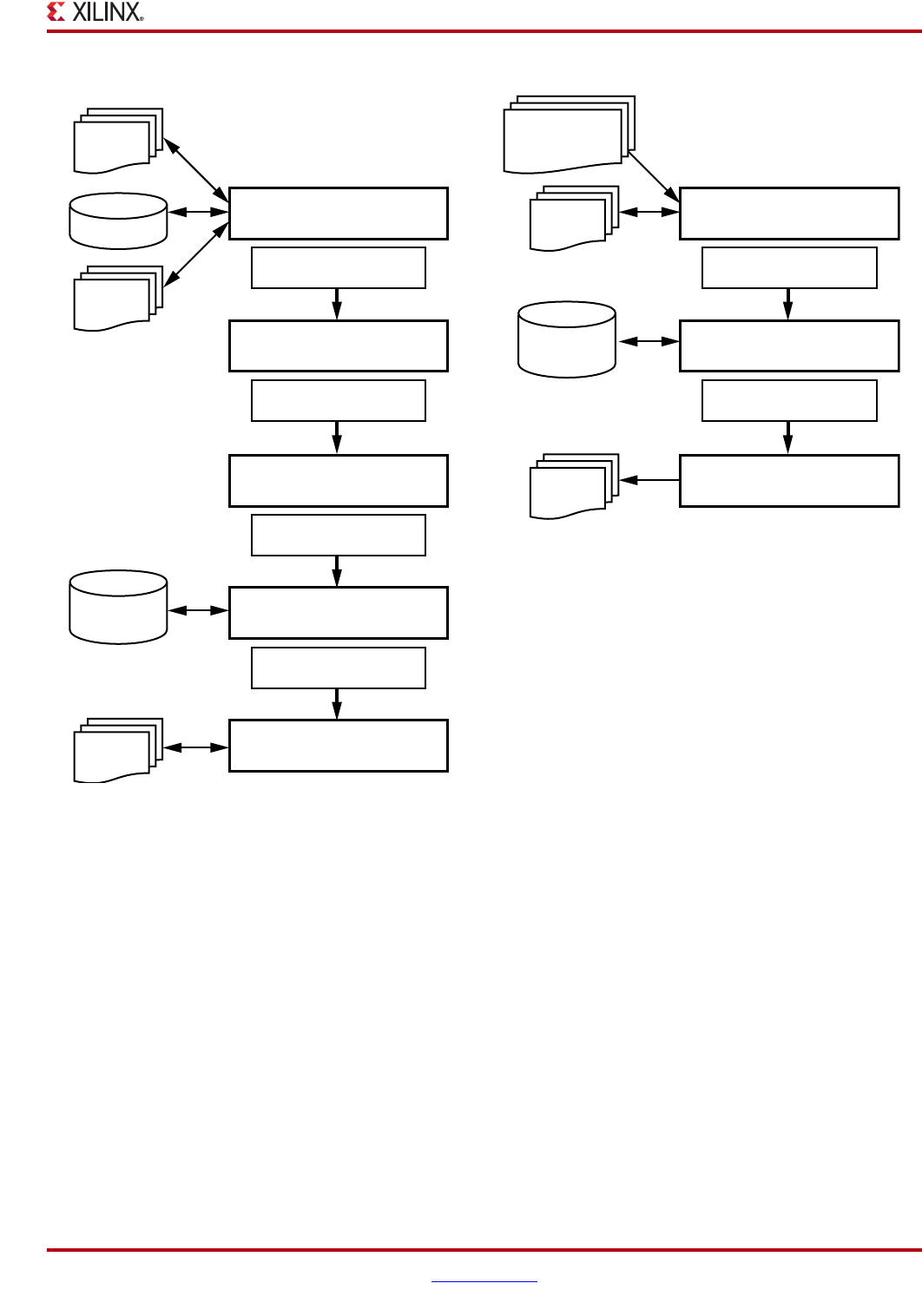
PlanAhead User Guide www.xilinx.com 31

UG632 (v 12.1)

Design Flow Diagram

Design Flow Tasks

The following subsections describe the PlanAhead software design flow tasks in

sequential order.

Configuring Project Sources

PlanAhead provides capabilities to create and manage source files. You can:

•Reference remote, write-protected files or import files into the local project folder.

•Disable or enable source files within a project.

•Create constraint sets to experiment with various constraints options or devices.

The PlanAhead project environment lets you create and store multiple variations of the

design constraints within a single project. This allows for the creation of multiple RTL

source versions, constraints sets, target devices, synthesized netlists, and implementation

run results using various implementation strategies. And, as you modify the source files or

launch design tools, the software provides a design status.

Figure 2-1: PlanAhead Design Flows

RTL Flow

RTL

UCF

ISE

Results

Bit

Files

Cores

Analyze RTL,

Apply Constraints

Analyze Netlist,

Apply Constraints

Configure Sources,

Customize IP

Synthesize

Implement

Analyze Results,

Floorplan

Elaborate RTL

Create Bit File

Program Device,

Debug Design

Netlist Flow

Synthesized

Netlist

UCF

ISE

Results

Analyze Results,

Floorplan

Program Device,

Debug Design

Analyze Netlist,

Add Constraints

Create Bit File

Implement

Bit

Files

32 www.xilinx.com PlanAhead User Guide

UG632 (v 12.1)

Chapter 2: Understanding the PlanAhead Design Flow

Note: The advanced flexibility in PlanAhead to create multiple versions of a design requires user

control for design data management and version control.

IP Customization and Implementation

You can use the integrated CORE Generator™ tool to browse, customize, instantiate, and

implement IP.

RTL Development and Analysis

PlanAhead includes an RTL Editor to create or modify source files. You can copy example

logic constructs directly from the supplied Xilinx template library. PlanAhead contains a

Find in Files feature that lets you search these libraries using a variety of search criteria.

You can then elaborate the RTL design to check RTL structure, syntax, and logic

definitions.

Launching either RTL Planner or the I/O Planner will elaborate the RTL design and load

the RTL netlist automatically. Analysis and reporting capabilities include:

•RTL compilation validation and syntax checking

•Netlist and schematic exploration

•Design Rule Checks (DRCs)

•Resource utilization and power consumption estimation

Also, early I/O pin planning is enabled using the RTL port list.

Note: When a netlist with defined clock logic is not present, only basic I/O-related DRCs are

enabled.

All views cross-select objects including instantiations and logic definitions within the

source files.

Logic Synthesis

PlanAhead lets you configure, launch, and monitor synthesis runs using the Xilinx®

Synthesis Technology (XST) tool.

You can experiment with different synthesis options and create reusable strategies for

synthesis runs. For example, you could create strategies for power, performance, or area

optimization.

The synthesis run results display interactively and PlanAhead creates report files that are

easily accessible. You can select Synthesis Warnings and Errors from the Compilation

Messages view to highlight the logic in the source files.

•You can launch multiple synthesis runs simultaneously or serially.

•On a Linux system you can use files on remote servers.

When you have multiple synthesis runs, those runs create multiple netlists which are

stored within the PlanAhead software project. The PlanAhead software then lets you load

the various versions of the netlist into the environment for analysis. After the netlist

import, you can create constraints for I/O pin planning, device analysis, floorplanning,

and implementation.

PlanAhead User Guide www.xilinx.com 33

UG632 (v 12.1)

Design Flow Diagram

I/O Pin Planning

The PlanAhead software provides a comprehensive I/O pin planning environment that

enables correct “by-construction” I/O port assignment either onto specific device package

pins or onto internal die pads. PlanAhead offers a variety of display views and tables in

which to analyze and design package and design I/O related data.

You can examine the internal I/O connectivity to ensure proper data flow through the

device as well as optimal access to internal device resources. System performance can be

improved by examining both the external and internal connectivity requirements and then

making informed decisions.

To ensure compliance to connectivity requirement, PlanAhead provides DRCs and

Simultaneous Switching Noise (SSN) analysis.

You can use a variety of source input formats to begin I/O pin planning including CSV,

UCF, RTL, or synthesized netlists.

When you use a synthesized netlist as the source, the DRC coverage improves

substantially because often the clock logic dictates proper I/O assignment. The final I/O

verification step is to run the complete design through the implementation tools.

Netlist Analysis and Constraints Definition

The PlanAhead software has design analysis and constraints assignment capabilities. The

design data is presented in many different forms using cross-selecting and coordinating

views.

PlanAhead provides interactive graphical representation views of the internal die and

external package through which you can analyze device resources and apply constraints.

Also, you can apply and analyze timing and physical constraints.

Early timing analysis, resource estimation, connectivity analysis, and Design Rule Checks

(DRCs) help identify design issues prior to implementation.

Implementation

The PlanAhead software lets you configure, launch, and monitor implementation runs

using the ISE® Design Suite.

You can experiment with different implementation options and create reusable strategies

for implementation runs. As an example, you can create strategies for quick runtimes,

performance, or area optimization.

The implementation run results display interactively, and report files are accessible. Also,

You can launch multiple implementation runs either simultaneously or serially; using the

Linux platform you can use remote servers. In PlanAhead, you can create Constraint Sets so

you can experiment with various logical constraints, physical constraints, or alternate

devices.

Results Analysis and Floorplanning

The PlanAhead software then lets you load the various run results interactively for

analysis and floorplanning. The capabilities in the Implemented Design are similar to the

those described in Chapter 7, “Netlist Analysis and Constraint Definition,” and

Chapter 10, “Analyzing Implementation Results.”

34 www.xilinx.com PlanAhead User Guide

UG632 (v 12.1)

Chapter 2: Understanding the PlanAhead Design Flow

You can import results from any PlanAhead launched run. When you open an

Implemented Design, the original netlist, constraints and implementation results are

loaded into the Results Viewer. You can open multiple designs simultaneously also.

Note: In Release 12.1, the constraints that were used to launch the run are not loaded. Instead, the

active constraint set in PlanAhead displays when an Implemented Design is opened.

Device Programming

You can create programming bitstream files for any completed implementation run. Bit file

generation options are configurable, and you can launch the iMPACT™ tool to configure

and program the part.

Design Verification and Debug

You can configure and implement the ILA and ICON ChipScope™ debugging tool debug

cores in the Netlist Planner, and select and configure the required probe signals into cores.

Then you can implement and manage the cores from within the Netlist Planner. You can

launch the ChipScope Analyzer tool on any run with a completed bitstream file.

Also, you can launch the FGPA Editor directly from PlanAhead for further analysis of the

routing or device resources.

User Models

PlanAhead is configured to provide a graphical user interface with “layered complexity.”

The intent is to provide an intuitive environment for new casual users, and also to enable

easy access to the more advanced features. By default, PlanAhead opens with a push

button flow suitable for users that do not require more advanced analysis and

floorplanning features. The flow is controlled by a view called the Flow Navigator, which

is described in Chapter 3, “Working with Projects.”

Basic User Flow

PlanAhead gives you the ability to execute the entire development cycle using the run

buttons in the PlanAhead Flow Navigator. You can traverse the FPGA front-to-back

process beginning with importing source files, synthesizing design logic, implementing

synthesized netlists, analyzing the results, generating bitstreams, and launching

programming and verification tools.

Advanced User Features

PlanAhead provides a series of analysis environments at each stage of the design flow for

advanced design configuration and analysis. The elaborated RTL design, synthesized

netlist design, and implementation results can be loaded into PlanAhead for analysis and

constraint definition. These environments are described in “Flow Navigator” in Chapter 3.

The PlanAhead Project environment lets you create and store multiple variations of the

design within a single project. This allows for the creation of multiple RTL source versions,

constraints sets, target devices, synthesized netlists, and implementation run results using

various implementation strategies. And as you modify the source files or launch design

tools, the software provides a design status.

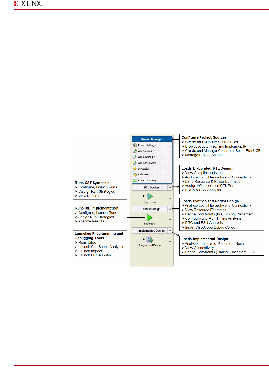
PlanAhead User Guide www.xilinx.com 35

UG632 (v 12.1)

Understanding the Flow Navigator

You can configure, launch and monitor multiple synthesis and implementation runs

locally or on remote Linux servers. You can experiment with different command options,

constraints, or devices.

The advanced flexibility in PlanAhead to create multiple versions of a design and multiple

runs requires user control for design data management and version control.

Understanding the Flow Navigator

Figure 2-2 and Figure 2-3, page 36 show how the PlanAhead Flow Navigator is used to

perform design tasks and to open the analysis environments at different design process

stages.

RTL-Based Project Flow Navigator

The following figure illustrates the design flow when RTL sources are used as input to

PlanAhead.

Figure 2-2: PlanAhead Flow Navigator (RTL Project)

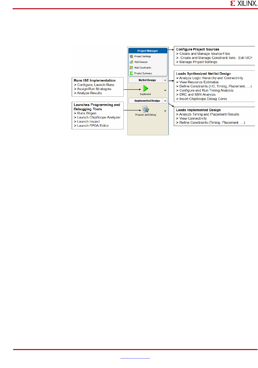
36 www.xilinx.com PlanAhead User Guide

UG632 (v 12.1)

Chapter 2: Understanding the PlanAhead Design Flow

Synthesized Netlist-Based Project Flow Navigator

The following figure illustrates the design flow for synthesized netlist based projects.

Understanding the Project Manager

By default, the Project Manager opens when you open a project. No design data is loaded

into memory. This environment lets you create, import, and manage source files.

The Project Manager can be used to perform the tasks described in “Configuring Project

Sources” and “IP Customization and Implementation,” page 32.

Working with Designs

PlanAhead enables experimentation different devices, constraints sets, or netlists by

enabling “Designs” to opened at various stages of the design process. A Design is defined

as a netlist (elaborated RTL or synthesized), a constraint set, and a target device.

PlanAhead loads the Design into memory for analysis, constraint definition, or ChipScope

debug core insertion.

The Flow Navigator has buttons for RTL Design, Netlist Design and Implemented Design.

The Implemented Design loads the specific design data used to launch the run. The RTL

and Netlist Designs can be opened with different target devices or constraint sets allowing

experimentation and constraints version control.

You can analyze the design at various stages of completion by opening either the

elaborated RTL design, the synthesized netlist design, or the implemented results design.

Constraint modifications such as timing or floorplanning can be performed within any

design. Constraint change management is made possible with the ability to create and

manage multiple constraints sets. The available design levels of abstraction that you can

open in the PlanAhead environment are:

•RTL Design—Elaborated RTL design, constraint set, and target device

•Netlist Design—Synthesized netlist, constraint set, and target device

•Implemented Design—Netlist, constraints, and results from any implemented run

Figure 2-3: PlanAhead Flow Navigator (Synthesized Netlist Project)

PlanAhead User Guide www.xilinx.com 37

UG632 (v 12.1)

Working with Designs

Opening an RTL Design

When you select the RTL Design button in the Flow Navigator, PlanAhead loads the

elaborated RTL netlist design data into memory with the active constraint set and the

target device.

As designs are loaded into memory, an icon displays within the RTL Design button in the

Flow Navigator. This provides a visual reference that the data is in memory and can help

manage the PlanAhead session.

The RTL Design view environment displays in the Main viewing area.

Opening an Netlist Design

When you select the Netlist Design button in the Flow Navigator, PlanAhead loads the

synthesized netlist design data into memory with the active constraint set and the target

device.

As designs are loaded into memory, an icon displays within the Netlist Design button in

the Flow Navigator. This provides a visual reference that the data is in memory and can

help manage the PlanAhead session.

Opening an Implemented Design

The Implemented Design Button loads the results of any PlanAhead implementation run

for analysis and floorplanning. The netlist and constraints that were used to launch the run

are loaded into memory, and the displayed views and the available capabilities are similar

to those shown in Chapter 7, “Netlist Analysis and Constraint Definition.” Typically,

placement and timing analysis and floorplanning are performed in the Implemented

Design. You can open simultaneous multiple implemented designs.

Some capabilities that involve manipulating the netlist, altering design partitions, or

partial reconfiguration control are restricted to the Netlist Design only. You might need to

use the Netlist Design for these operations to ensure you are operating on the proper data.

Note: In 12.1, the constraints that were used to launch the run are not loaded. Instead, the active

constraint set in PlanAhead displays when you open an implemented design.

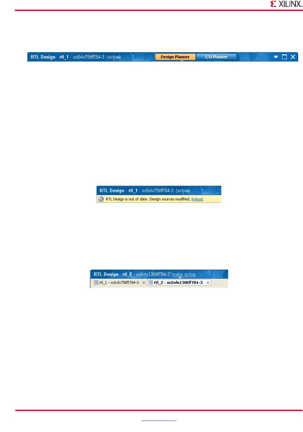
38 www.xilinx.com PlanAhead User Guide

UG632 (v 12.1)

Chapter 2: Understanding the PlanAhead Design Flow

Understanding the Open Design View Banner

The view banner reflects the design name and target part.

As source files are updated, a banner appears at the top of the open RTL Designs indicating

that a newer version of the design data is available. You are prompted to reload what is

loaded in memory.

Selecting the I/O Planner or Design Planner View Layout

In RTL or Netlist Designs, you can elect to display either the Design Planner or the I/O

Planner view layouts. There are buttons in the Design view banner to toggle between the

two view layouts. Each one provides views appropriate for design task you are doing, as

shown in Figure 2-3, page 36.

Using the Design is Out of Date and Reload Banner

As source files are updated, the Status bar indicates that the design is Out-of-Date as

shown in the following figure.

Toggling Multiple Open Designs

If multiple RTL Designs are open, tabs display that allow you to toggle between the open

designs.

The make active link in the view banner can be used to set the constraint set associated

with the design as the active constraint set.

Figure 2-4: Open RTL Design Banner

Figure 2-5: Design Out of Date and Reload Banner

Figure 2-6: Multiple Open Design Tabs

PlanAhead User Guide www.xilinx.com 39

UG632 (v 12.1)

Invoking PlanAhead

You can invoke the PlanAhead software from any directory; however, invoking it from a

“project” directory might prove advantageous because project-specific log files can be

located more easily.

Note: Refer to the Xilinx ISE Design Suite: Installation, Licensing, and Release Notes for proper

installation of this product.

Linux

To invoke PlanAhead in Linux, type the following command at the Linux command

prompt:

# planAhead

Windows

To invoke PlanAhead in Windows, double-click the Xilinx PlanAhead 12 shortcut icon

(shown in the following figure).

You can specify the PlanAhead Start in folder by modifying the desktop icon properties to

define where to write the PlanAhead log files.

The PlanAhead Environment opens to the Getting Started Page as shown in Figure 2-8,

page 40.

Figure 2-7: PlanAhead 12.1 Icon

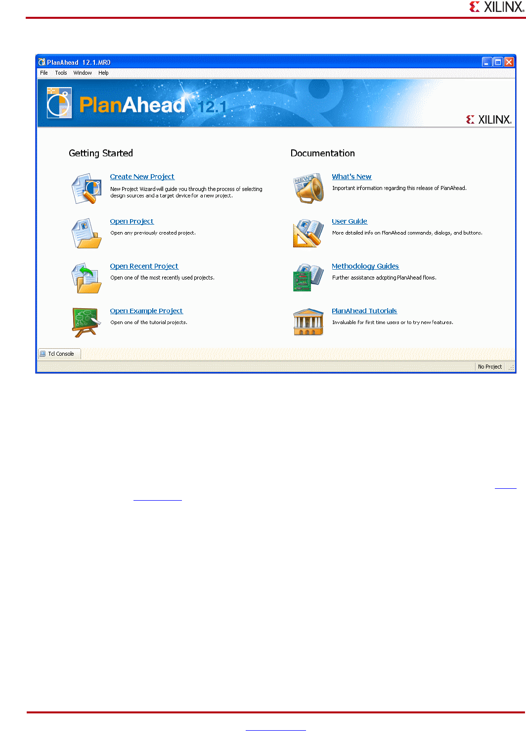
40 www.xilinx.com PlanAhead User Guide

UG632 (v 12.1)

Chapter 2: Understanding the PlanAhead Design Flow

The PlanAhead Getting Started page assists you with creating or opening Projects as well

as viewing the PlanAhead documentation. You can display the Getting Started jump page

by closing all open projects.

Using the Getting Started Page

When you invoke PlanAhead the Getting Started page displays. You can select the blue

underlined command links to invoke specific commands or to view documentation. The

Getting Started options are:

•Create New Project—Invokes the New Project Wizard enable you to create any type

of PlanAhead project.

•Open Project—Invokes a browser enabling you to select any PlanAhead project.ppr

file to open.

•Open Recent Design—Displays the last 10 previously opened Projects to reopen.

PlanAhead checks to ensure the Project data is available before displaying the

Projects. You can configure how many Projects to list in the General dialog box by

selecting Tools > Options > General.

•Open Example Project—Provides three sample design projects. One small RTL

project BFT Core, one larger RTL project CPU (HDL), and one netlist based project

CPU (synthesized).

Figure 2-8: PlanAhead Getting Started Page

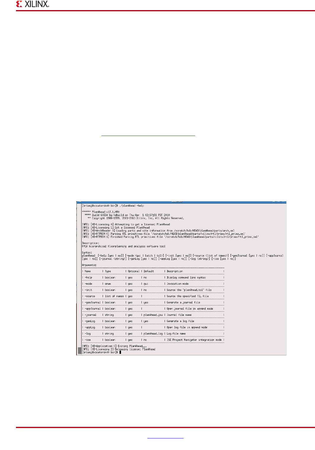
PlanAhead User Guide www.xilinx.com 41

UG632 (v 12.1)

Invoking PlanAhead

You can open or download the PlanAhead documentation by selecting the documentation

links which then launches a PDF viewer or web site download location.

•What’s New—Document describing the new 12.1 features on PlanAhead.

•User Guide—Invokes the PlanAhead User Guide.

Note: In 12.1, PlanAhead shipped with a placeholder PDF file for the User Guide. In that file, you are

guided to a web URL to download the latest document. There are simple installation instructions to

enable the link to then invoke the full user guide when selected.

•PlanAhead Methodology Guides—Web links to the Floorplanning Methodology

Guide and the Hierarchical Design Methodology Guide.

•PlanAhead Tutorials—A Web link to a landing site containing all PlanAhead

tutorials and required sample design data.

All PlanAhead documentation is available in PDF format at the following web location:

http://www.xilinx.com/planahead

PlanAhead Command Line Options

PlanAhead has several command line options to control the behavior. To view the

PlanAhead command line options, type the following command at the command prompt:

# planAhead -help

A help menu displays in the shell window as shown in the following figure.

Figure 2-9: PlanAhead Help Screen

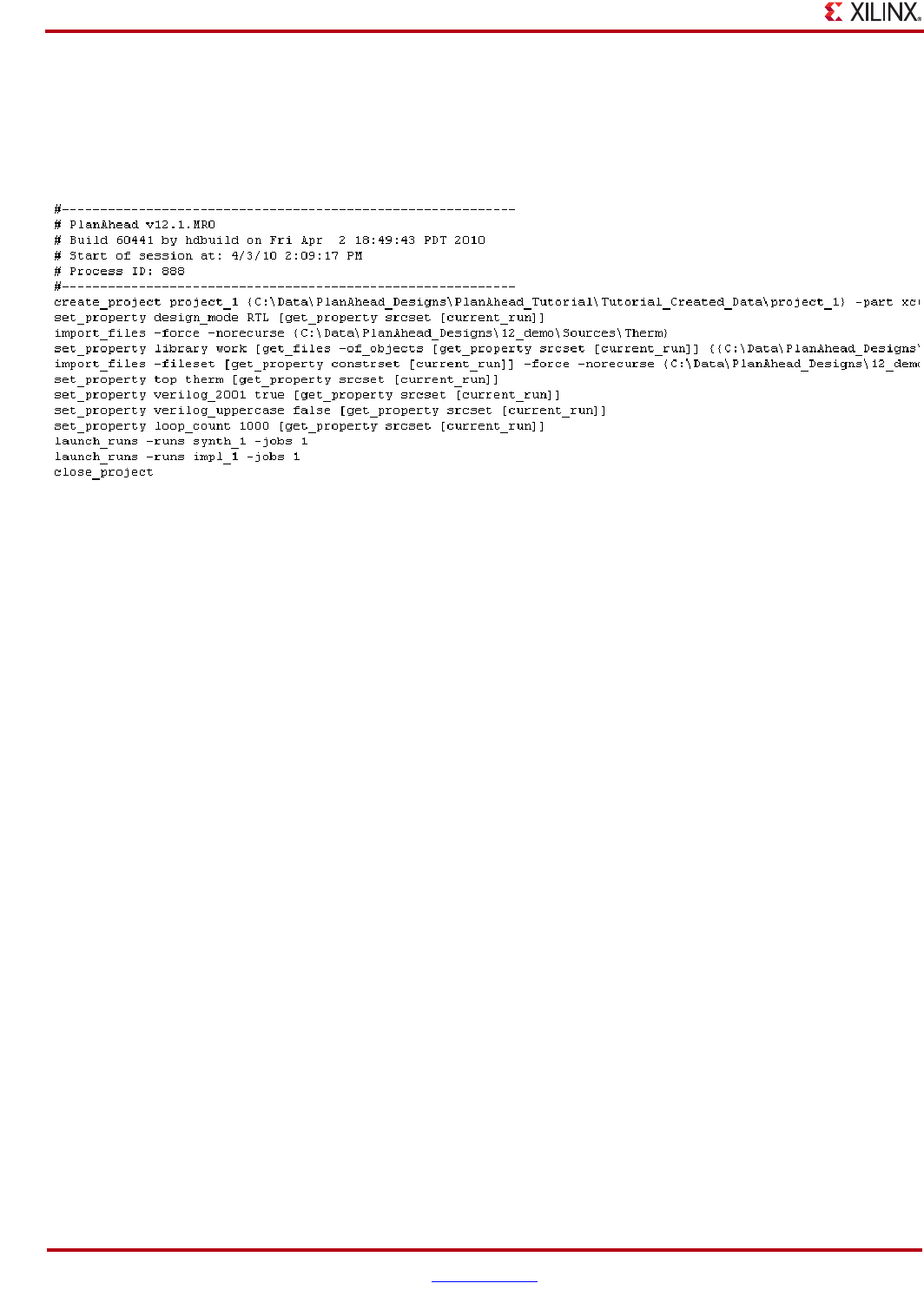
42 www.xilinx.com PlanAhead User Guide

UG632 (v 12.1)

Chapter 2: Understanding the PlanAhead Design Flow

Using a PlanAhead Startup Tcl Script

You can use the PlanAhead Tools > Run Tcl Script command to run a script. Also, you can

copy PlanAhead Tcl commands from the planAhead.jou file to create startup scripts. The

following figure shows a code snippet from a Tcl script.

For more information about the PlanAhead journal file, see “Journal File (planAhead.jou),”

page 416. For more information about scripting actions for PlanAhead with Tcl, see

Chapter 14, “Tcl and Batch Scripting.”

Figure 2-10: Example PlanAhead Tcl Script

PlanAhead User Guide www.xilinx.com 43

UG632 (v 12.1)

Chapter 3

Working with Projects

This chapter contains the following sections:

•“Understanding PlanAhead Project Types”

•“Creating a New Project”

•“Managing Project Sources”

•“Adding and Managing Constraints”

•“Configuring Project Settings”

•“Understanding the Project Summary”

•“Determining Project Status”

Understanding PlanAhead Project Types

You can use the PlanAhead™ software at different points in the FGPA design flow for

various reasons. To accommodate this, you can create the following types of PlanAhead

projects:

•RTL source-based

•Synthesized netlist-based

•Implemented design results-based

•I/O pin planning projects - CSV, UCF, RTL-based

•Projects created in Project Navigator

•Partial Reconfiguration projects (when license is enabled)

These projects are differentiated by the input sources types used to create the project. You

can select the type of project during the Create New Project process.

Once you select a particular project type, it cannot be migrated to a different type later.

Note: PlanAhead uses a derivative type of Project to support Partial Reconfiguration designs. This

capability is available only through special licensing, and is covered in the Partial Reconfiguration

User Guide (UG702), which is available upon request.

RTL Source-Based Projects

You can use the PlanAhead software to manage the entire FPGA design flow from RTL

creation through bitstream generation. You can create projects by importing RTL source

files as well as precompiled NGC/NGO-format Xilinx® cores.

You can elaborate and analyze the RTL to ensure proper constructs, launch, and manage

various synthesis and implementation runs, and analyze the design and run results. Also,

you can create floorplans to experiment with different constraint or device strategies.

44 www.xilinx.com PlanAhead User Guide

UG632 (v 12.1)

Chapter 3: Working with Projects

Synthesized Netlist-Based Projects

You can create projects from designs that were synthesized outside of PlanAhead using the

Xilinx Synthesis Technology (XST) tool or any supported third-party synthesis tool.

PlanAhead can import EDIF and NGC/NGO-format netlists. The netlist can be all-

inclusive in a single file or hierarchical in nature, consisting of multiple, module-level

netlists.

You can analyze the logic netlist, launch and manage various implementation runs, and

analyze the design and run results. Also, you can create different designs to experiment

with constraint or device strategies.

Implemented Design Results-Based Projects

You can create projects to allow analysis of implementation results created outside of

PlanAhead using the Xilinx command line tools. The design netlist, implementation, and

timing results can be imported to explore timing or placement related issues.

I/O Pin Planning Projects

You can use I/O pin planning early in the design cycle by creating an empty I/O Pin

Planning project. I/O ports can be created within PlanAhead or imported with either CSV,

UCF, or RTL input files. After I/O pin assignment, PlanAhead can create CSV, UCF, and

RTL output files for use later in the design flow when RTL sources or netlists are available.

The output files can also be used to create schematic symbols for use in the Printed Circuit

Board (PCB) design.

Also, you can create pin planning projects to explore the logic resources available in the

different device architectures.

Project Navigator Created Projects

For information about the project creation process used when PlanAhead is launched from

the ISE® Project Navigator environment, refer to Chapter 15, “Using PlanAhead With

Project Navigator.”

Creating a New Project

The following subsections describe how to create a project, and the project options

available within the wizard.

Using the Create New Project Wizard

The New Project wizard takes you through the individual steps to define a project name

and storage location, to import the netlist, and to create an initial design, including

selecting a device and importing the constraints.

To create a new project:

1. Select one of the following commands:

−On the Getting Started jump page click the Create a New Project link.

−Select File > New Project.

The first dialog box of the New Project wizard gives an overview of the wizard.

PlanAhead User Guide www.xilinx.com 45

UG632 (v 12.1)

Creating a New Project

2. To continue, click Next.

The Project Name page opens as shown in the following figure.

Entering a Project Name and Storage Location for the Project

Enter a project name and storage location as follows:

3. In the Project Name page, specify a Project name and disk storage location:

−Project name—Enter a name to identify the project directory (for example,

project_3).

−Project location—Enter a location to create the project directory.

4. After defining the required selections, click Next.

Selecting the Design Source Data Type

Designate the Design Source input format by selecting one of the options shown in the

following figure.

Figure 3-1: New Project Wizard: Project Name Page

Figure 3-2: New Project Wizard: Design Source Page

46 www.xilinx.com PlanAhead User Guide

UG632 (v 12.1)

Chapter 3: Working with Projects

5. After you select the design source, click Next.

6. Depending upon the design input, continue with the instructions in one of the

following sections:

−“Creating a Project with RTL Sources”

−“Creating a Project with a Synthesized Netlist”

−“Creating a Project with ISE Placement and Timing Results”

−“Opening an Existing Project”

7. Click Next.

The PlanAhead software creates a project based on the design source you selected.

Creating a Project with RTL Sources

You can specify RTL source files to create a Project. This can be used for RTL code

development and analysis purposes as well as synthesis and implementation. See

Chapter 5, “RTL and IP Design” for more information on RTL development and analysis.

1. Follow the project creation steps described in “Creating a New Project,” page 44.

2. In the Design Source page shown in the following figure, select the Specify RTL

sources option.

3. Click Next.

Figure 3-3: Creating a Project with RTL Sources

PlanAhead User Guide www.xilinx.com 47

UG632 (v 12.1)

Creating a New Project

Adding Source Files or Directories

The next page in the New Project wizard lets you select HDL source files or directories that

contain HDL source files, as shown in the following figure.

−Add Files—Click, browse to, and select the file(s) to add individual files to the

Project.

−Add Directories—Click, browse to, and select the directory to add the contents of

an entire directory and its subdirectories to the project. Files with source

recognized file extensions that are located in the directory tree are imported.

−Copy Sources into Project—Copy the source files into the PlanAhead project

directory structure instead of referencing the original locations.

−Add Sources from Subdirectories—Search subdirectories under selected

directories to add source files into the PlanAheadproject.

Note: Selections made for Copy Sources into the Project and Add Sources from Subdirectories

are preserved for future PlanAhead sessions.

4. After adding the intended source files or directories, click Next.

Figure 3-4: New Project Wizard: Add Sources Page

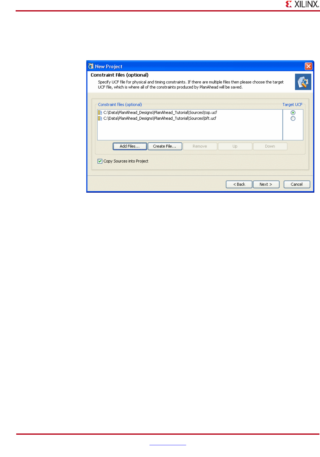
48 www.xilinx.com PlanAhead User Guide

UG632 (v 12.1)

Chapter 3: Working with Projects

Adding Constraint Files

The New Project wizard prompts you to optionally select a constraint file or files, shown in

the following figure.

−Add Files—Click this button, and browse to and select the file(s) to add

individual files to the Project.

−Create File—Click this button, and browse to and select the directory to create a

new UCF file for the Project.

−Remove— Click this button to remove the selected UCF file from the Constraint

files list.

−Up / Down—Click these buttons to set the order of the selected UCF files.

−Copy Sources into Project—Copy the constraint files into the PlanAhead

Project directory structure instead of referencing the original locations.

Note: The selection made for Copy Sources into the Project is preserved for future PlanAhead

sessions.

Setting the Target UCF

When multiple UCF files are selected, a target UCF needs to be defined. The target UCF is

the file where constraints created from using PlanAhead will be written. You can change

the target UCF at any time in the PlanAhead session.

5. After adding the intended constraint files and setting the target UCF, click Next.

Figure 3-5: New Project Wizard: Adding Constraint Files

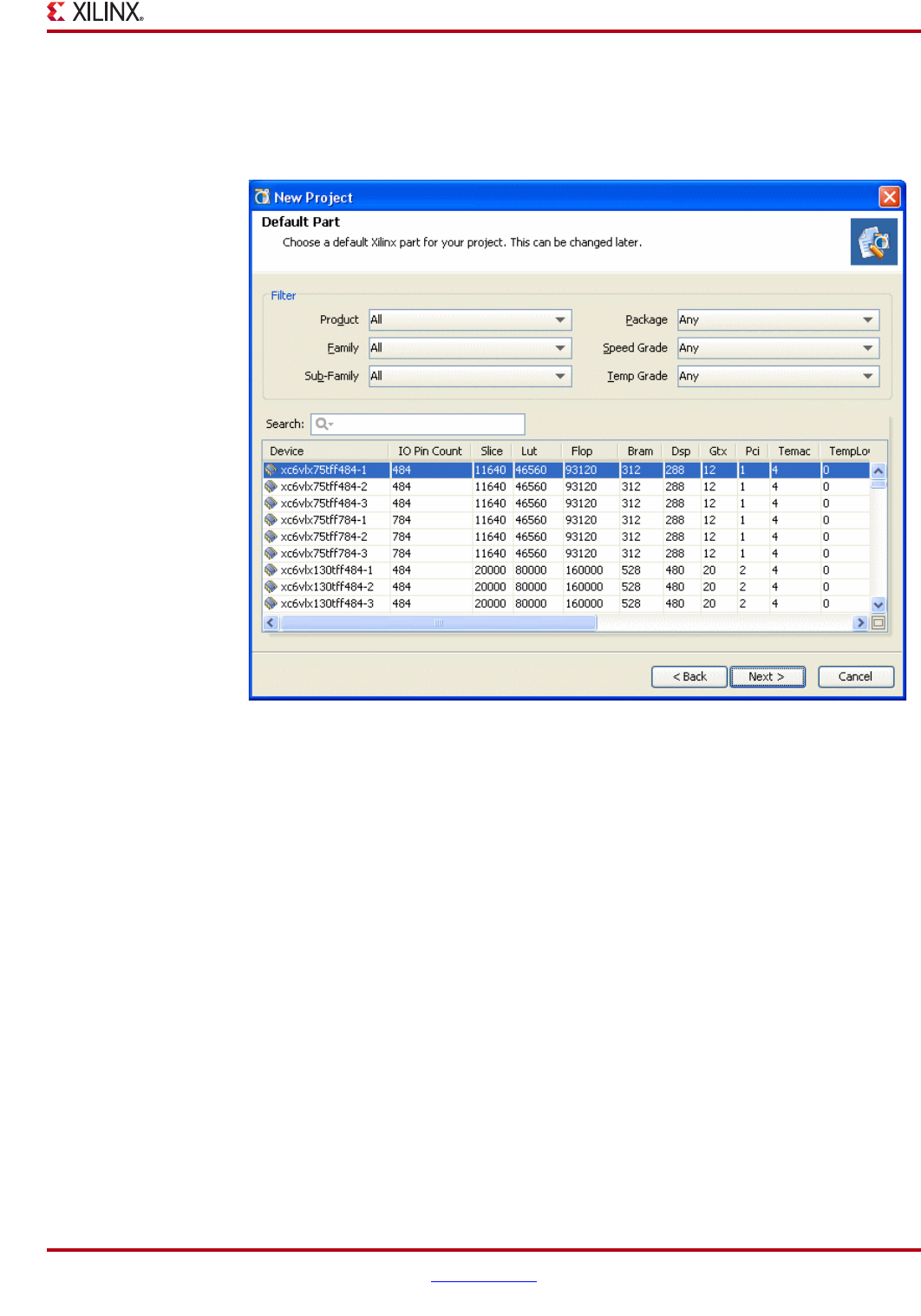
PlanAhead User Guide www.xilinx.com 49

UG632 (v 12.1)

Creating a New Project

Selecting a Default Part

The New Project wizard prompts you to select a default part, shown in the following

figure.

The available Parts display in the scroll-able list. Information about the device resources

displays in the table view. You can filter the list to help you select your target device. The

Product, Family, Sub-Family, Package, Speed Grade, and Temp Grade filters are self-

explanatory. Select any sub-categories in any field to filter the parts that display in the list.

6. Select the target product family architecture and default part, and click Next.

Note: You can change the Default Part during Synthesis and Implementation and when opening an

RTL or Netlist Design.

The New Project Summary page opens as shown in Figure 3-7, page 50.

Figure 3-6: New Project Wizard: Selecting a Default Target Part

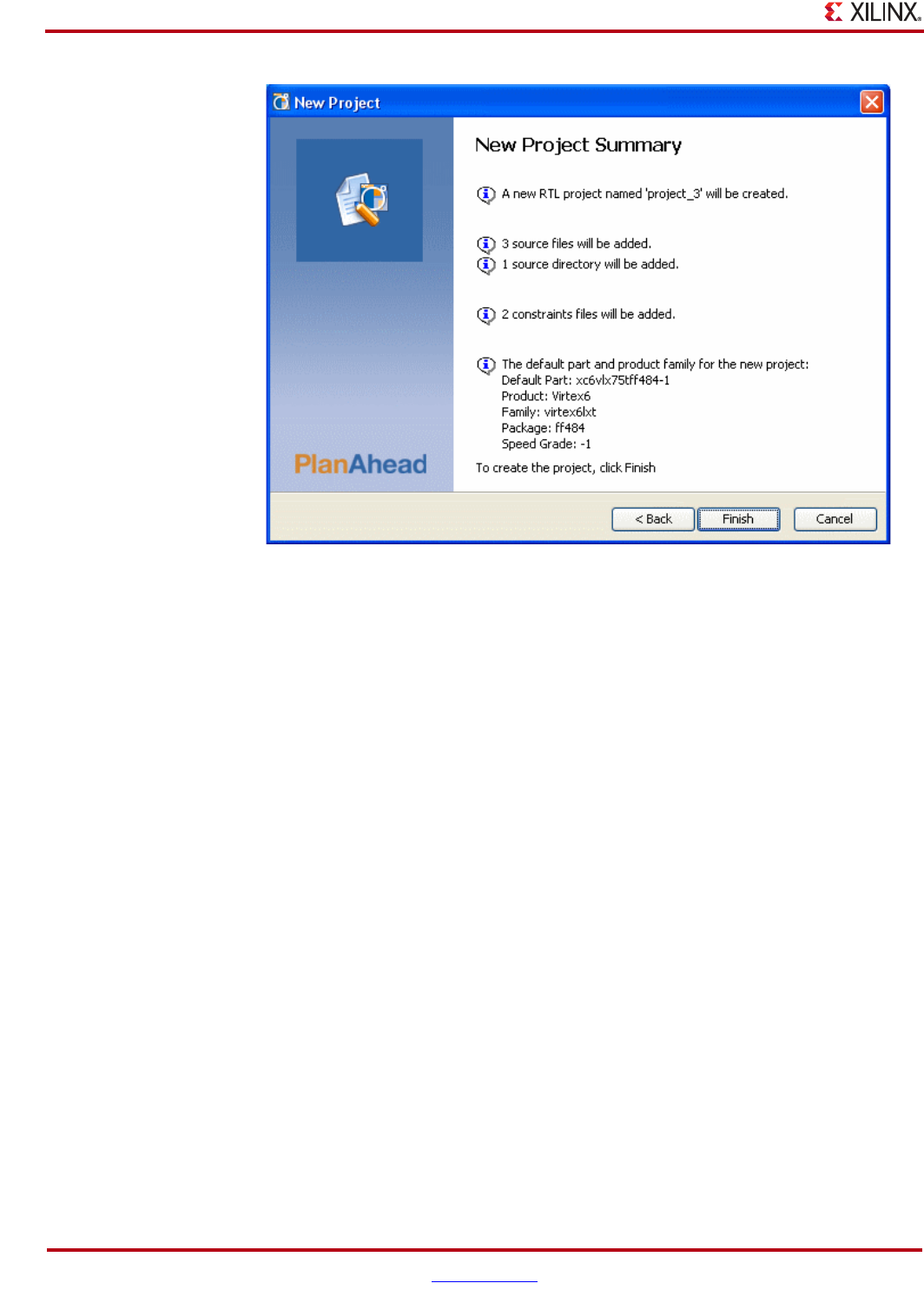
50 www.xilinx.com PlanAhead User Guide

UG632 (v 12.1)

Chapter 3: Working with Projects

7. To initiate the Project, click Finish in the Summary page.

PlanAhead then displays the Project environment with the Project Manager related views

available as shown in Figure 3-8, page 51.

Figure 3-7: New Project Wizard: New Project Summary

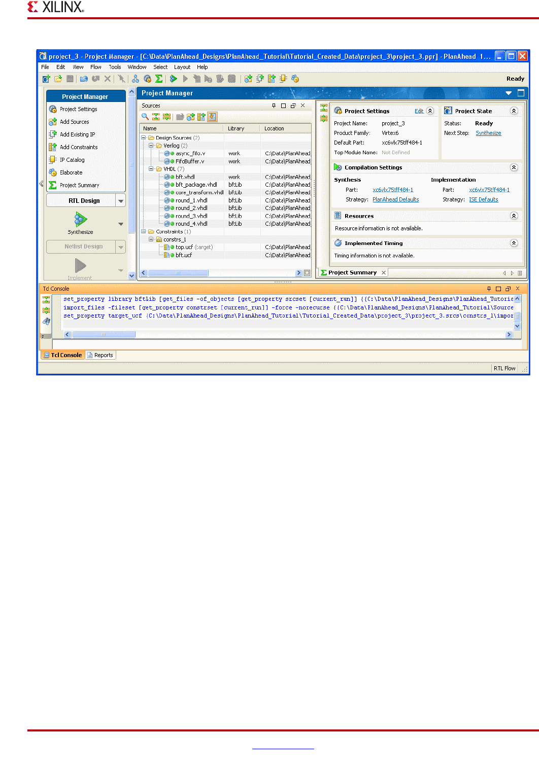
PlanAhead User Guide www.xilinx.com 51

UG632 (v 12.1)

Creating a New Project

Creating a Project with a Synthesized Netlist

You can import synthesized netlists along with corresponding constraints to create a

PlanAhead Project. This is used to analyze, floorplan, or implement the design using the

floorplanning and implementation environment.

1. Follow the Project creation steps described in “Using the Create New Project Wizard,”

page 44.

2. Select the Specify synthesized (EDIF or NGC) netlist option in the Design Source

page, shown in the following figure.

Figure 3-8: PlanAhead Project Manager Environment for RTL Project

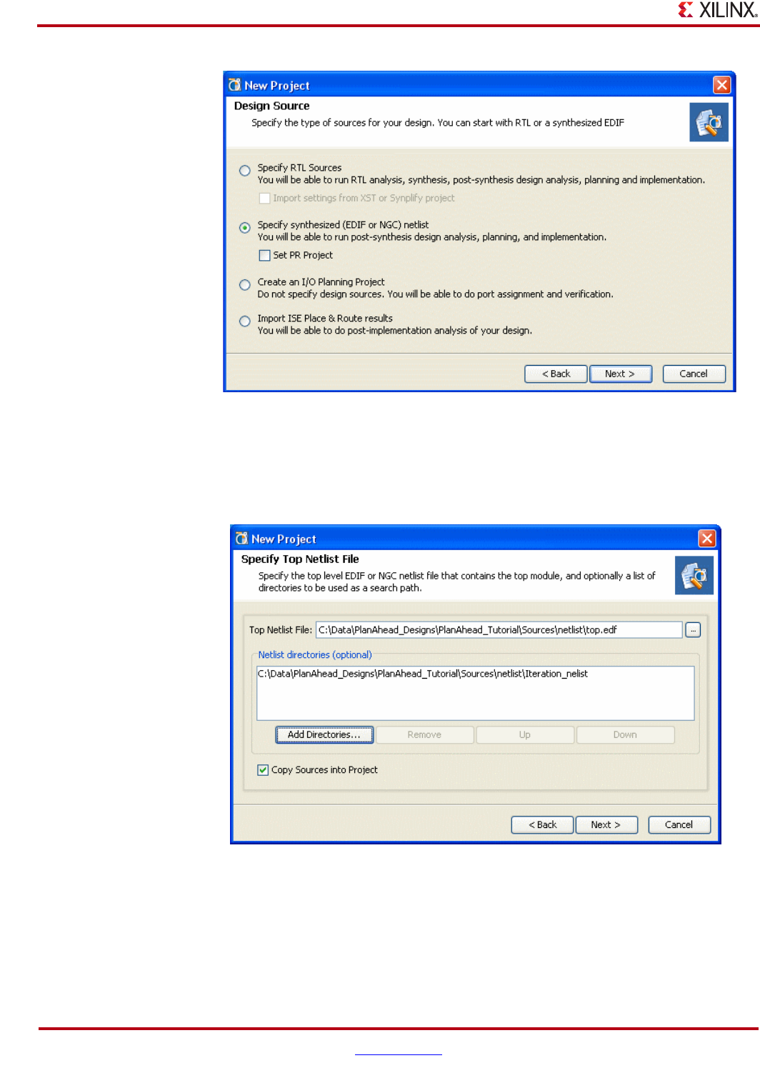
52 www.xilinx.com PlanAhead User Guide

UG632 (v 12.1)

Chapter 3: Working with Projects

Selecting a Top-Level Netlist and Module Search Path

If you chose the Specify synthesized (EDIF or NGC) netlist option, the next page in the

New Project wizard, shown in the following figure, lets you input a top-level netlist file

and a search path to find module level netlists.

1. In the Import Netlist page, edit the definable options:

−Top Netlist file—Enter a name to identify the top-level netlist in this project. Use

the File Browse button to select the top-level netlist file for the design.

−Netlist directories—Select directories in which to search for lower-level modules

and cores during netlist import.

Figure 3-9: Creating a Project using a Synthesized EDIF or NGC Netlist

Figure 3-10: New Project Wizard: Import Netlist Page

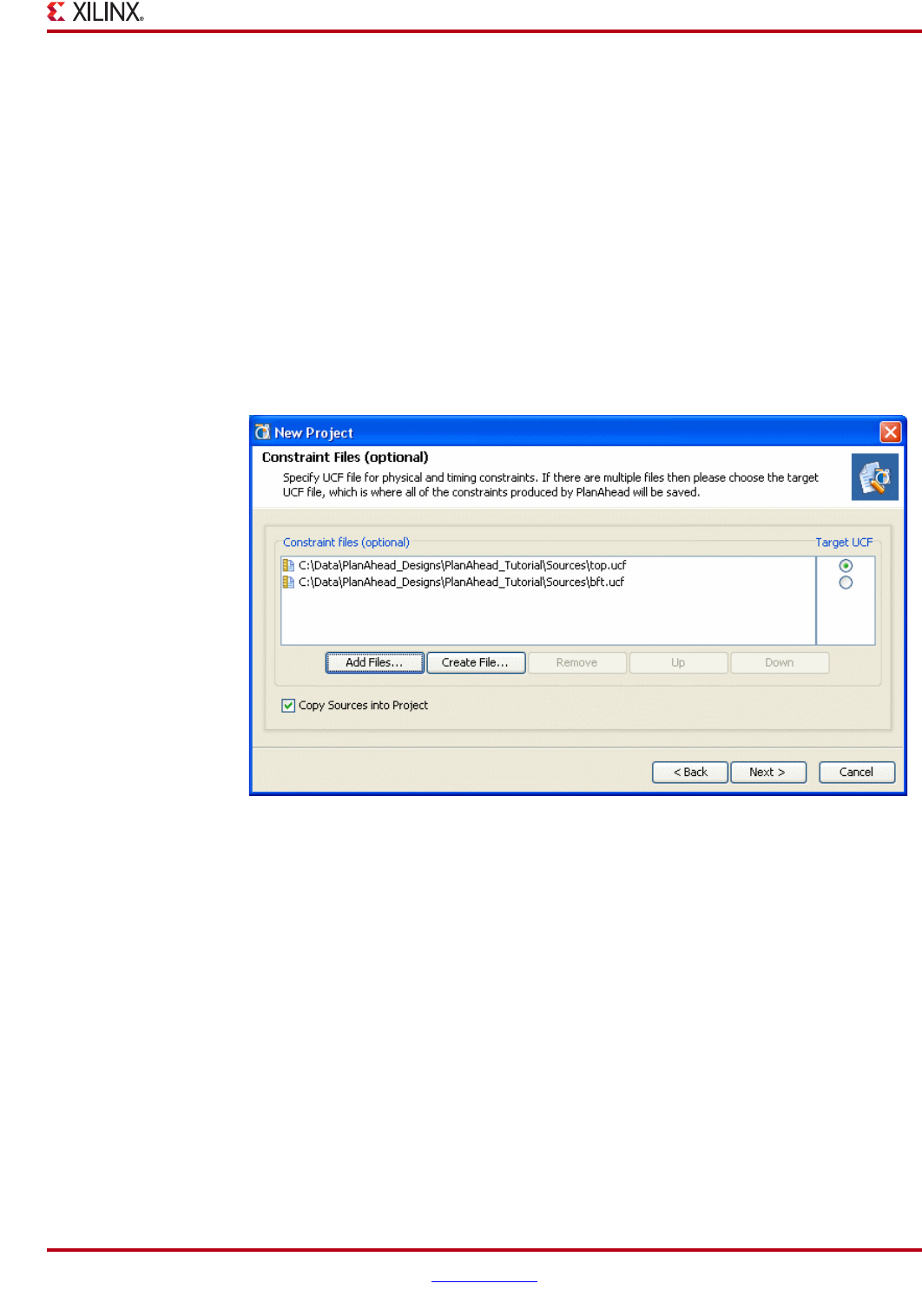
PlanAhead User Guide www.xilinx.com 53

UG632 (v 12.1)

Creating a New Project

By default, the PlanAhead invocation directory and the directory from which the

top-level netlist was selected are included in the search path. You can arrange the

order in which to search these directories by selecting them and using the up or

down arrows buttons. Remove directories from the search path by using the

Remove button in the dialog box.

−Copy Sources into Project—Copy the constraint files into the PlanAhead

Project directory structure instead of referencing the original locations.

Note: The selection made for Copy Sources into the Project is preserved for future PlanAhead

sessions.

2. To continue with the wizard, click Next.

Adding Constraint Files

The New Project wizard prompts you to optionally select a constraint file or files, shown in

the following figure.

−Add Files—Click and browse to, and select the file(s) to add individual files to

the Project.

−Create File—Click and browse to, and select the directory to create a new UCF

file for the Project.

−Remove— Removes the selected UCF file from the Constraint files list.

−Up / Down—Sets the order of the selected UCF files.

−Copy Sources into Project—Copies the constraint files into the PlanAhead

Project directory structure instead of referencing the original locations.

Note: The selection made for Copy Sources into the Project is preserved for future PlanAhead

sessions.

Setting the Target UCF

When multiple UCF files are selected, a target UCF must be defined. The target UCF is the

file where constraints created from using PlanAhead are written. You can change the target

UCF at any time in the PlanAhead session.

Figure 3-11: New Project Wizard: Adding Constraint Files

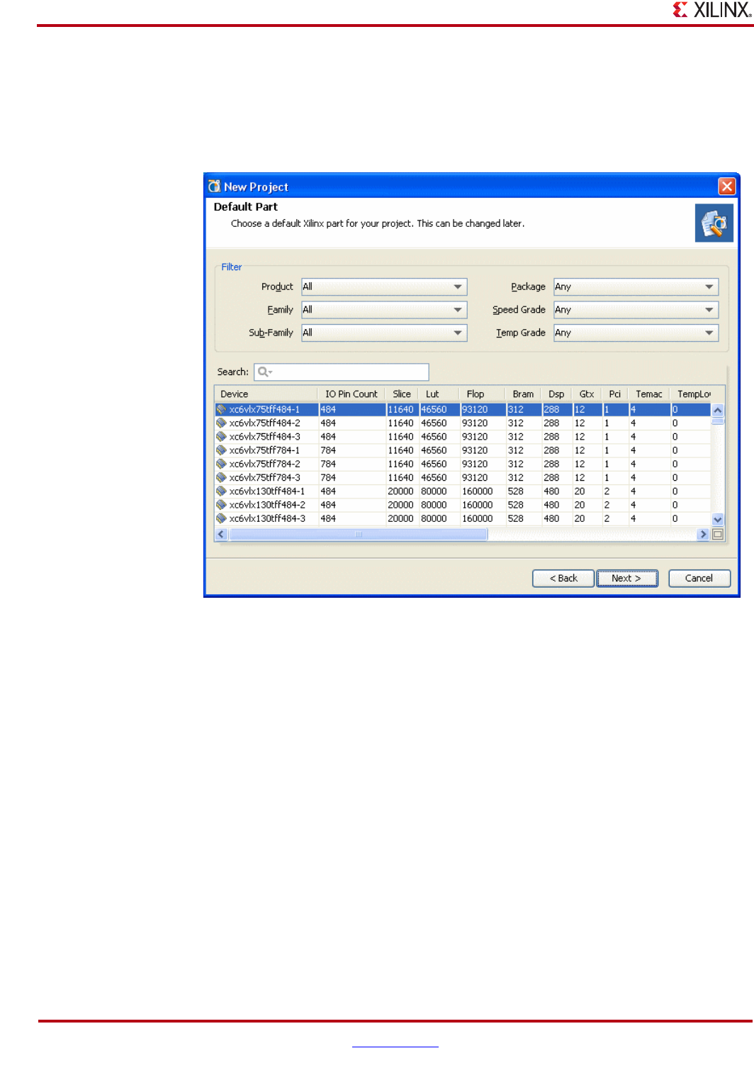
54 www.xilinx.com PlanAhead User Guide

UG632 (v 12.1)

Chapter 3: Working with Projects

3. After adding the intended constraint files and setting the target UCF, click Next.

Selecting a Default Part

The New Project wizard prompts you to select a default part, shown in the following

figure.

The available Parts are displayed in the scroll-able list. Information about the device

resources is displayed in the table view. The list can be filtered to help you select your

target device. The Product, Family, Sub-Family, Package, Speed Grade and Temp Grade

filters are self explanatory. Select any of the sub categories in any field to filter the parts

displayed in the list.

4. Select the target product family architecture and default part, and click Next.

Note: You can change the Default Part during Synthesis and Implementation and when opening an

RTL or Netlist Design.

The New Project Summary page opens as shown in Figure 3-7, page 50.

5. To initiate the Project, click Finish in the Summary page.

PlanAhead then displays the Project environment with the Project Manager related views

available.

Figure 3-12: New Project Wizard: Selecting a Default Target Part

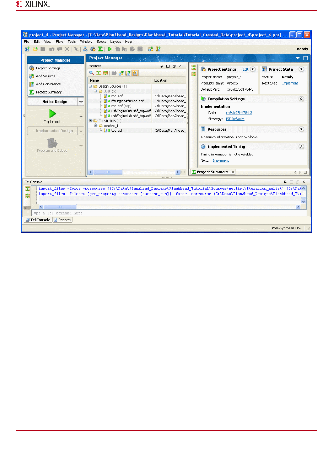
PlanAhead User Guide www.xilinx.com 55

UG632 (v 12.1)

Creating a New Project

Creating an I/O Planning Project

You can create an empty project for I/O pin planning purposes prior to having completed

HDL or synthesized EDIF. See Chapter 8, “I/O Pin Planning” for more information about

I/O pin planning.

1. Select the Create an I/O Planning Project option in the Design Source page, as shown

in Figure 3-14, page 56.

Figure 3-13: PlanAhead Project Manager Environment for Netlist Project

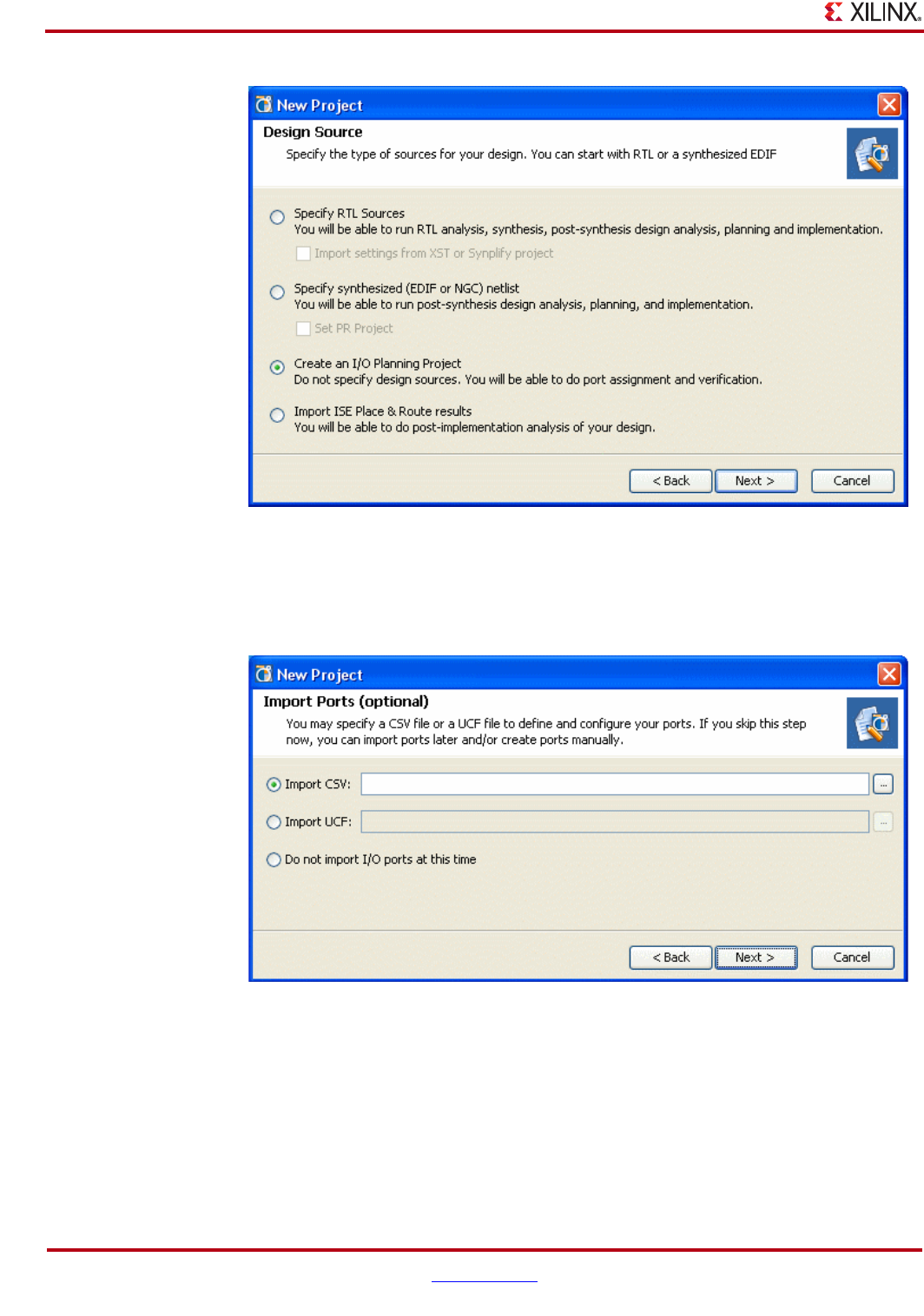
56 www.xilinx.com PlanAhead User Guide

UG632 (v 12.1)

Chapter 3: Working with Projects

Selecting a Product Family and Default Part

The next page in the New Project wizard prompts you to select a file for importing I/O

Port definitions and constraints.

−Import CSV—Browse to and select a Comma Separated Value “CSV” format file

with I/O Ports definitions in PlanAhead format.

−Import UCF—Browse to select a UCF file with I/O Port-related constraints only.

−Do not import I/O ports at this time—Create an empty project. I/Os can be

created or imported at a later time.

2. Select an I/O Port definition option and click Next.

Figure 3-14: Creating an I/O Planning Project

Figure 3-15: New Project Wizard: Product Family and Default Part Page

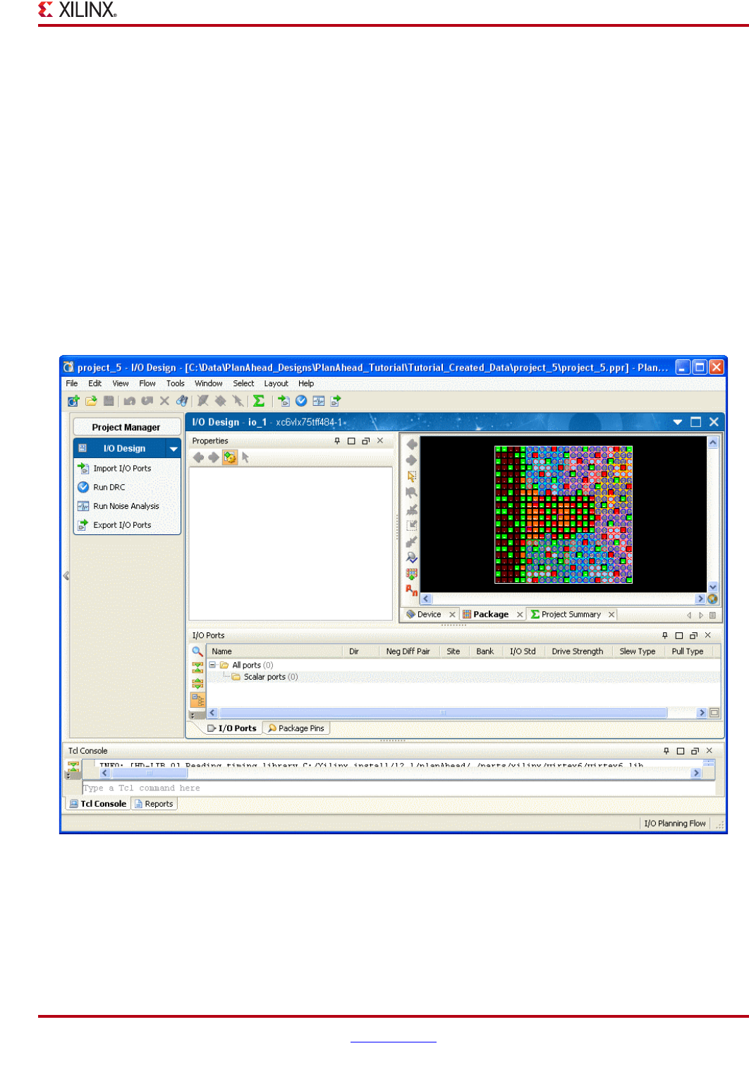
PlanAhead User Guide www.xilinx.com 57

UG632 (v 12.1)

Creating a New Project

Selecting a Default Part

The New Project wizard prompts you to select a default part, shown in Figure 3-6, page 49.

The available Parts are displayed in the scroll-able list. Information about the device

resources is displayed in the table view. The list can be filtered to help you select your

target device. The Product, Family, Sub-Family, Package, Speed Grade and Temp Grade

filters are self explanatory. Select any of the sub categories in any field to filter the parts

displayed in the list.

3. Select the target product family architecture and default part, and click Next.

Note: You can change the Default Part during Synthesis and Implementation and when opening an

RTL or Netlist Design.

The New Project Summary page opens as shown in Figure 3-7, page 50.

4. To initiate the Project, click Finish in the Summary page.

PlanAhead then displays the I/O Design environment with related views available.

Figure 3-16: I/O Design Environment for I/O Planning Projects

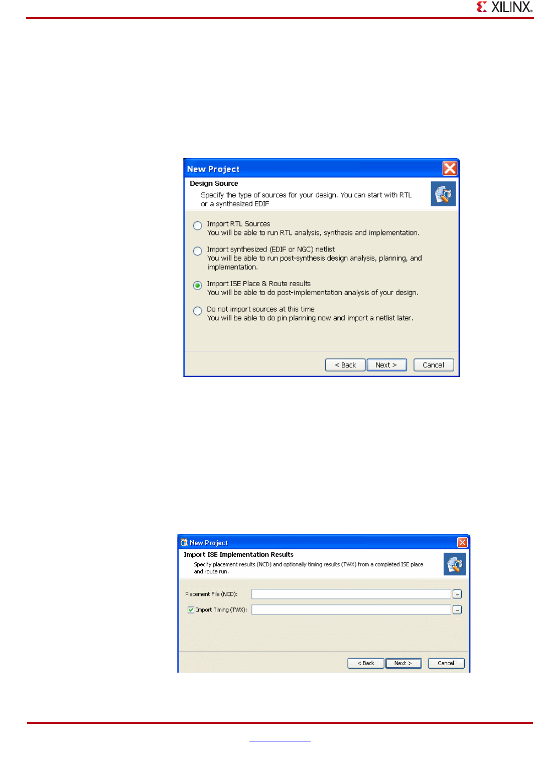
58 www.xilinx.com PlanAhead User Guide

UG632 (v 12.1)

Chapter 3: Working with Projects

Creating a Project with ISE Placement and Timing Results

You can import netlists with ISE® implementation results along with corresponding

constraints to create a PlanAhead Project. This is used to analyze the Place and Route

results using the implementation environment.

1. Follow the Project creation steps described in“Using the Create New Project Wizard,”

page 44.

2. Select the Import ISE Place & Route results option in the Design Source page.

in se

The steps for creating this type of project are identical to creating a synthesized netlist

project, except this wizard asks for placement and timing files to also be opened.

3. Follow the steps for “Creating a Project with a Synthesized Netlist,” page 51.

Importing Placement and Timing Results

After completing the steps to create the project, the Import ISE Implementation Results

page displays. You can import the Place and Route results generated in ISE which are then

used to create a floorplan for viewing and analysis in PlanAhead as shown in the following

figure.

Figure 3-17: New Project Wizard: Import ISE Results

Figure 3-18: New Project Wizard: Import ISE Implementation Results

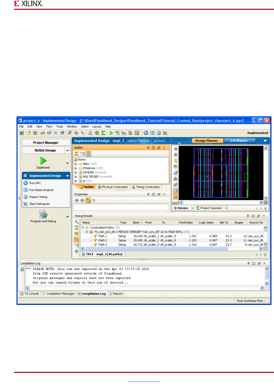
PlanAhead User Guide www.xilinx.com 59

UG632 (v 12.1)

Creating a New Project

1. In the Import ISE Implementation Results page, edit the definable options:

−Placement File (NCD)—Check this option, and locate and select a NCD format

placement results file from the ISE implementation directory.

−Import Timing (TWX)—Check this option, and locate and select a timing results

file from the ISE implementation, such as a TWX format file.

The New Project Summary page opens next.

2. Click Finish in the Summary page to complete the new project creation process.

The project opens and you are prompted to Open the Implemented Design.

3. Select Open Implemented Design and click OK.

PlanAhead then displays the Implemented Design environment with design placement

and timing results loaded and related views available.

Figure 3-19: Implemented Design Environment for ISE Place & Route Results Projects

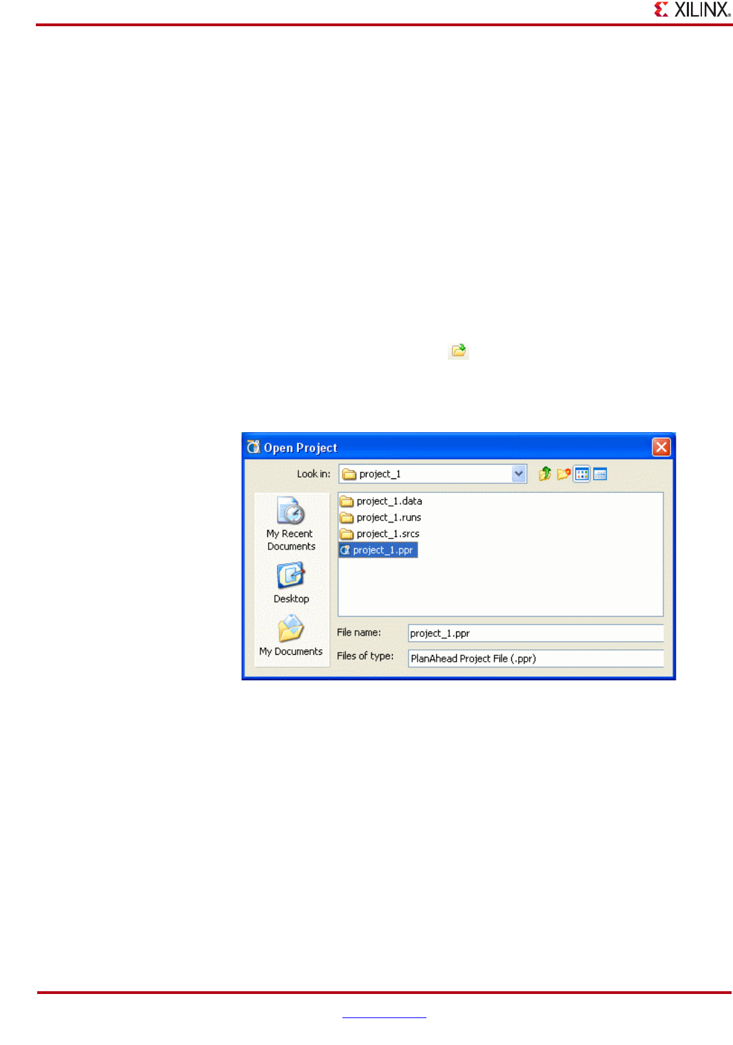
60 www.xilinx.com PlanAhead User Guide

UG632 (v 12.1)

Chapter 3: Working with Projects

Opening an Existing Project

You can open existing Projects in the PlanAhead software by using the Open Project

command, or in Windows, by double-clicking any PlanAhead project (PPR) file, which

invokes PlanAhead and opens the project. As Projects are opened, the project “state” from

the time the Project was last closed is restored as well as the state of all previous

implementation runs.

The applicable view layout opens for the type of Project being opened or created—RTL or

Netlists Sources.

To open a Project in PlanAhead, use one of the following methods:

•In the Getting Started jump page click either the Open Recent Project or Open

Project links.

•Select File > Open Project.

•Click the Open Project toolbar button, as shown in the following figure.

The Open Project browser opens. Select a PPR project file as shown in the following figure.

PlanAhead saves updates automatically in the project as they are executed.

Opening Multiple Projects

You can open multiple Projects simultaneously in a single PlanAhead session by using any

of the methods described in “Opening an Existing Project,” page 60. A separate PlanAhead

main window opens for each project.

Note: System memory requirements can hinder performance when opening multiple projects.

Figure 3-20: Open Project Toolbar Button

Figure 3-21: Open Project Dialog Box

PlanAhead User Guide www.xilinx.com 61

UG632 (v 12.1)

Managing Project Sources

Saving a Project

You can save projects from within PlanAhead with the File > Save Project or File > Save

Project As commands. When you close a project, you are prompted to save any unsaved

designs or changes. You can elect to exit without saving the data, or choose to save the

data. If PlanAhead detects unsaved changes to the same data, a prompt is displayed to

allow you to select the designs to save.

The Save Project As command copies the entire Project directory structure and maintains

the existing runs status.

Closing a Project

You can close projects from within PlanAhead with the File > Close Project command.

When you close a project, you are prompted to save any unsaved floorplans. You can elect

to exit without saving the data, or choose to save the data.

Managing Project Sources

PlanAhead can create new source files and manage existing source files that can be local or

remote.

Using the Sources View

Most of the source file creation and management is done in the Sources view. For more

information on editing Source files, refer to Chapter 5, “RTL and IP Design.”

Creating Source Files

You can create new Verilog, Verilog Header, or VHDL source files in the Sources view as

follows:

1. Select Create New Source from the popup menu, and select one of the following

command source types:

−Verilog—Select to create a Verilog format file (.v)

−Verilog Header—Select to create a Verilog Header format file (.h)

−VHDL—Select to create a VHDL format file (.vhdl)

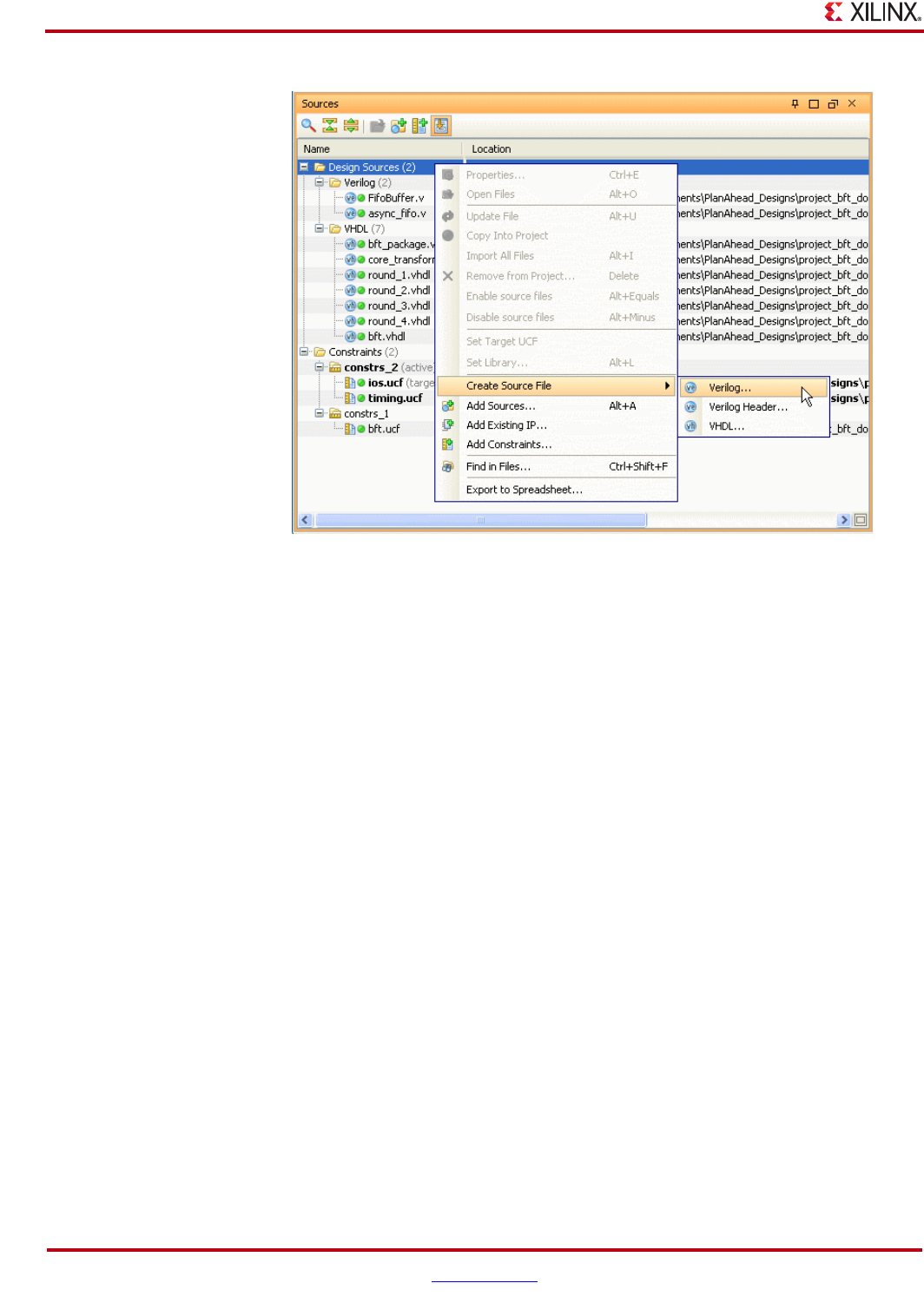
62 www.xilinx.com PlanAhead User Guide

UG632 (v 12.1)

Chapter 3: Working with Projects

2. Define the following information:

−Name—Enter a name for the new HDL source file.

−Location—Designate a location to create the file.

3. Click OK.

The RTL Editor opens with the newly created file.

Figure 3-22: Create New Source File Menu

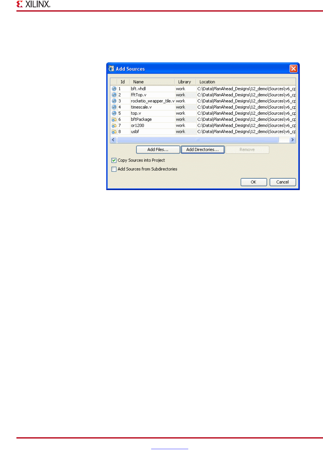
PlanAhead User Guide www.xilinx.com 63

UG632 (v 12.1)

Managing Project Sources

Adding Source Files

You can add RTL sources to the project at any time using the Add Sources dialog box as

shown in the following figure.

1. Select the Add Sources command to invoke the Add Sources dialog box.

2. Use the dialog box options as follows:

−Add Files—Invokes file browser to select RTL files to add to the project. VHDL

libraries can be specified or selected at the time of import by selecting the drop

down menu in the Library column of the Add Sources dialog table.

−Add Directories—Invokes directory browser to add all RTL source files from the

selected directories. Files in the directory hierarchy with valid source file

extensions are added to the project.

−Remove—Removes the selected source files from this dialog box.

−Copy Sources into Project—Copies the original source files into the PlanAhead

project and references them locally.

−Add Sources from Subdirectories—Adds files from all subdirectories of the

selected directory.

When adding sources, you can click on the Library field, and enter or select a library name

for the file or directory as shown in Figure 3-24, page 64.

Figure 3-23: Adding Source Dialog Box

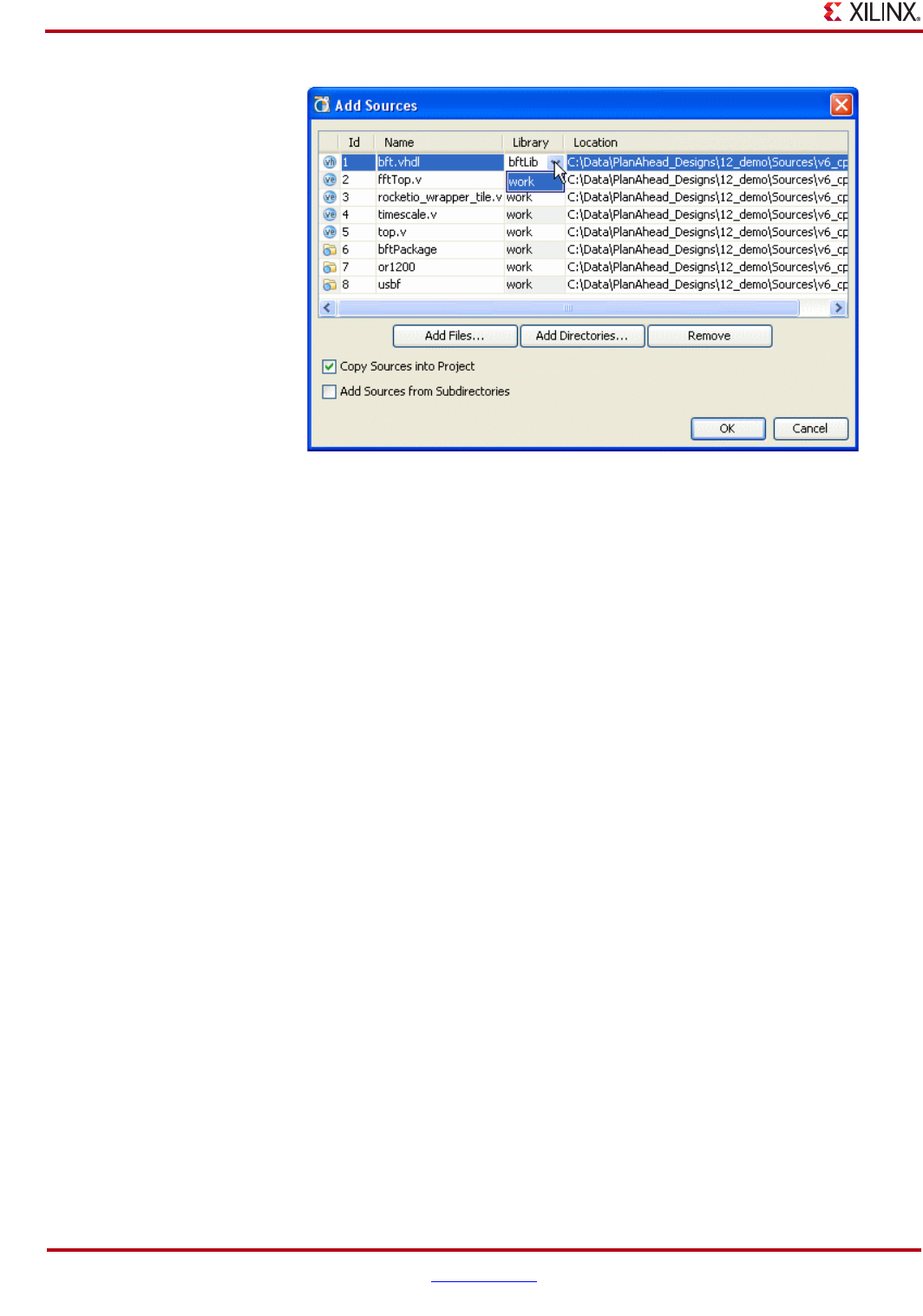
64 www.xilinx.com PlanAhead User Guide

UG632 (v 12.1)

Chapter 3: Working with Projects

Using Remote Sources or Copying Sources into Project

To provide project management flexibility, you can reference source files from a remote

location or copy the source files to the project directory. Copying the files to the project is

recommended if you plan to move or archive the PlanAhead project because the files are

contained within the project.

When you add remote files, PlanAhead picks up the latest file version automatically, and

then prompts you to Refresh your open Designs or to Synthesize with the latest

updates made to the file.

Note: When you copy files into a project, the project is more easy to port to another system;

however, PlanAhead does not pick up external file changes automatically. When remote files change

you need remove and re-add or update the files using the commands in the Sources view.

To copy files locally into a project, in the Add Sources page of the New Project wizard, click

the Copy Sources into Project button.

Viewing Source File Properties

Selecting an RTL source file in the Sources view displays information in the Source File

Properties view. To view source file properties:

1. In the Sources view, select a source file.

2. Select the Source File Properties popup menu command.

The Source Files Properties view is shown in Figure 3-25, page 65.

Figure 3-24: Changing Source Library in Add Sources Dialog Box

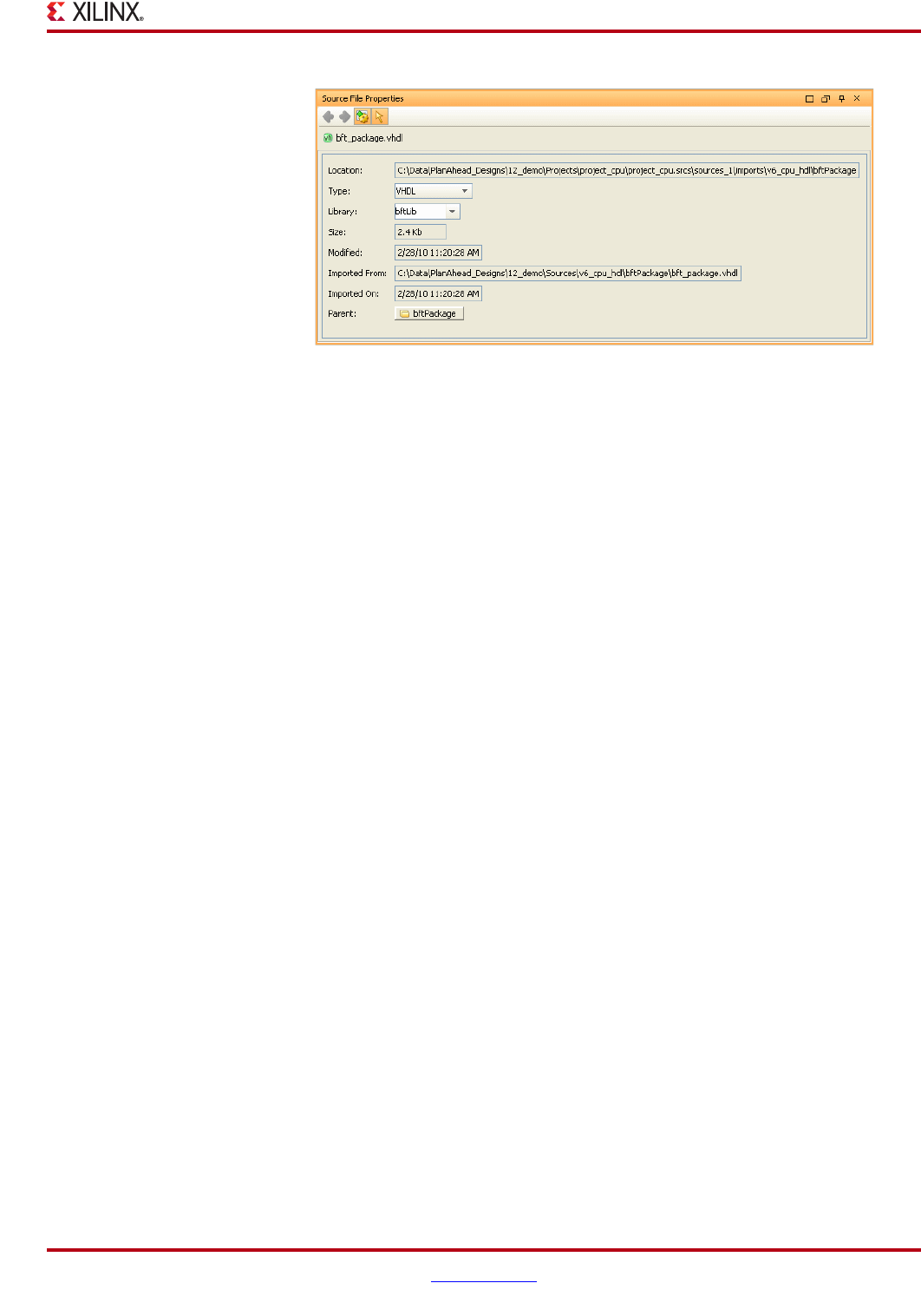
PlanAhead User Guide www.xilinx.com 65

UG632 (v 12.1)

Managing Project Sources

The file information includes location, type, library, size, modified timestamp date,

location copied from, copy date, and parent module.

You can select a new target library in the Library option, and click Apply.

Updating Source Files

When referencing remote sources, PlanAhead picks up the updated source file changes

automatically. Open designs must be refreshed to recognize the new changes.

You can update source files copied into the project in several ways. The options are:

•Make all RTL changes inside of PlanAhead using the RTL editor.

•Select the source file in the Sources view and select the Update File command from

the popup menu. Browse to select a new file to replace the file in the project.

Note: The file must be a different file name or location then the original file added to the project.

Adding the same name file from the same location is not currently possible in PlanAhead.

•Click Remove from Project to delete the modified RTL sources from the project, and

then click Add Sources to import the newly updated versions.

•Click Add Sources from the popup menu to add the newly updated sources to the

project, and then click Disable to disable the outdated sources.

Enabling or Disabling Source Files

When you add or create source files, those files are enabled by default in PlanAhead.

Source files can be disabled which prevents them from being elaborated or synthesized.

You can control different versions of source files by enabling and disabling the source files

in the Sources view.

•To disable source files, select the files, and select the Disable source files popup

command.

•To enable disabled files, select the files, and select the Enable source files popup

command.

Figure 3-25: Viewing Source File Properties

66 www.xilinx.com PlanAhead User Guide

UG632 (v 12.1)

Chapter 3: Working with Projects

Adding Existing IP Cores to the Project

PlanAhead enables you to add existing IP cores into the project. The IP cores can be

synthesized NGC / EDIF neltists or cores generated externally by the CORE Generator™

tool, either in the embedded or through the DSP tools. The Sources view displays folders

for each source type.

You can modify and re-implement CORE Generator cores using PlanAhead. Refer to

“Configuring IP using the CORE Generator” in Chapter 5.

Using PlanAhead with Xilinx Platform Studio and EDK

FPGA designer use the Xilinx Platform Studio (XPS) tool to build embedded systems on

Xilinx FPGA devices. XPS provides an environment for designers to integrate their

hardware and software system components.

In XPS, use either Tools > Generate Netlist or Tools > Generate Bitstream to create the

/synthesis and /implementation subdirectories.

•The /synthesis subdirectory contains synthesis scripts (.scr), project files (.prj)

and report (.srp) files.

•The /implementation subdirectory contains design netlist files created as a result of

the synthesis process.

Also, XPS creates BMM files in the /implementation subdirectory for configuring the

block RAMs on the device. The PlanAhead tool is inserted in the design flow after

synthesis has been performed.

XPS uses the Xilinx Synthesis Technology (XST) tool for design synthesis. The generated

synthesis netlists are in NGC format. The top-level file is named system.ngc and any

other NGC files have the nomenclature <module_name>.ngc.

The system.ucf file contains the design constraints.You can add these files to the

PlanAhead project as sources either as top-level modules or instantiated into a system-

level design during project creation, or when using the Add Sources command. The files

are under the /Cores folder in the Sources view.

Adding and Managing Constraints

PlanAhead provides flexibility for defining and using constraints in a project. You can use

a single UCF file to add and maintain all constraints used in the design.

This supports a basic push button design flow without too much complexity. You can add

the UCF file while creating the Project or afterward by using the Add Constraints

command.

PlanAhead lets you create multiple constraint sets if you want to experiment with various

types of constraints or store multiple versions of constraints.

You can open multiple designs referenced from a single constraint set also. You must be

careful to manage changes made in multiple designs that reference the same constraint set.

If PlanAhead detects unsaved changes in multiple designs, you are prompted to select

which design to save.

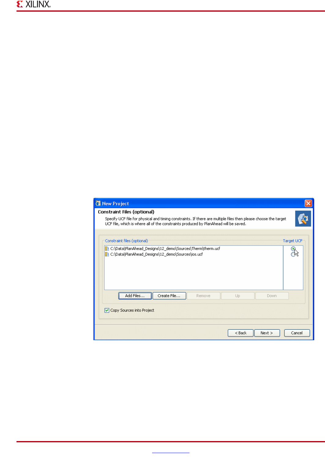
PlanAhead User Guide www.xilinx.com 67

UG632 (v 12.1)

Adding and Managing Constraints

Adding Constraints

You can add constraints to a project during project creation or after, with the Add

Constraints command. These can be top-level UCF constraint files or module-level NCF

or XNCF constraint files.

Referencing Original UCF Files or Copying Files

You can add remote UCF files or copy remote files into a project. When you add remote

files, PlanAhead picks up the latest file version automatically, and then prompts you to

Refresh your open Designs with the latest updates made to the file.

Note: When you copy files into a project, the project is more easy to port to another system;

however, PlanAhead does not pick up external file changes automatically. When remote files change

you need remove and re-add or update the files using the commands in the Sources view.

To copy files into a project, in the Constraints Files page of the New Project wizard, click

the Copy Sources into Project button.

Adding Constraints When Creating a New Project

When you create a project, the New Project wizard prompts you to add top-level UCF files

or core level NCF files. The UCF and NCF format files found in the same directories as the

RTL or Netlist source files are shown in the following figure.

You can order the files using the Up and Down buttons. The UCF constraints are order-

dependent; the last setting made is used.

•Add Files—Add existing UCF files to a project, in the New Project wizard click the

Add Files button and browse to select UCF or NCF format files as shown in the

following figure.

•Create File—Create a new UCF file to add to the Constraint set.

•Copy Sources into Project—Add remote UCF files or copy files into a project.

Figure 3-26: Adding Constraint Files using the New Project Wizard

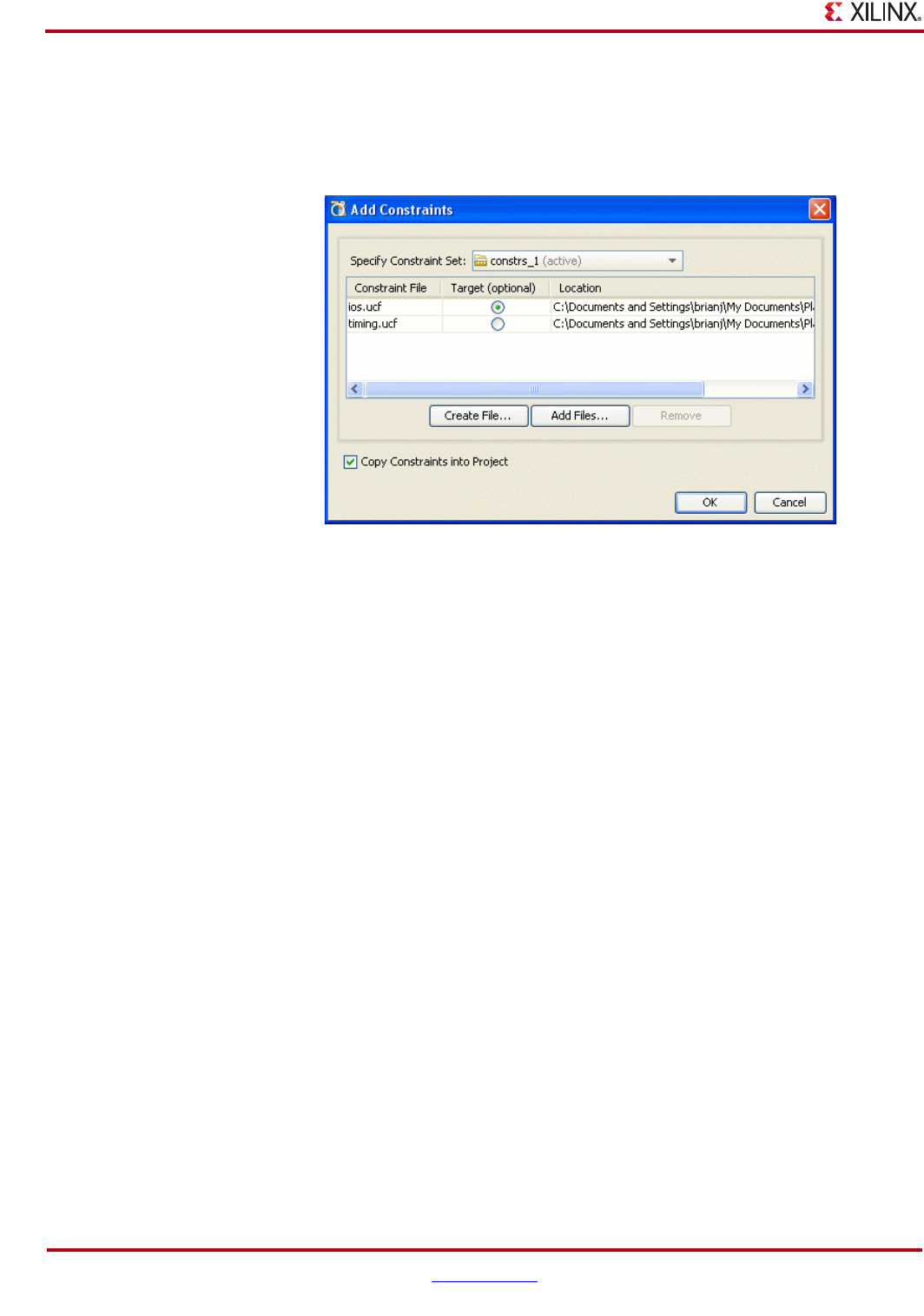
68 www.xilinx.com PlanAhead User Guide

UG632 (v 12.1)

Chapter 3: Working with Projects

Using the Add Constraints Command

You can add additional constraints to a project at any time by selecting the Add

Constraints command button in the Sources view or popup menu as shown in the

following figure.

The Add Constraints dialog box lets you add additional top-level constraint files to any

existing constraint set or create a new constraint set.

Defining the Target UCF

When multiple UCF files are used in a constraint set, a target UCF needs to be defined. The

target UCF is the file where constraints created while PlanAhead will be written. You can

change the target UCF at any time in the PlanAhead session.

When adding more than one constraint file, you must define one as the target UCF in the

New Project wizard as shown in “Adding and Managing Constraints,” page 66.

Using Constraint Sets

A constraint set is made up of one or more UCF or NCF files. These files are maintained

independently and are concatenated together into a single UCF file that is passed to ISE

implementation.

PlanAhead attempts to keep all of these file intact as much as possible as constraints are

manipulated within the tool. If existing constraint values are modified in PlanAhead, the

changes should go back to the original files. New changes are written into the designated

“target” UCF.

Changing the Target UCF

You can change the target UCF at any time by selecting a different file as the target UCF in

the Sources view, and using the Set Target UCF popup menu command.

Figure 3-27: Add Constrainst Dialog Box

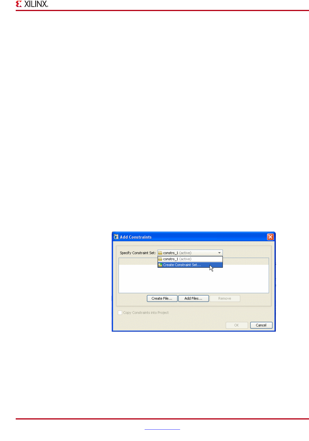
PlanAhead User Guide www.xilinx.com 69

UG632 (v 12.1)

Adding and Managing Constraints

Creating Constraint Sets

In PlanAhead, you can create different constraint types at various stages of the design flow.

You can define constraints in the:

•RTL Design

•Netlist Design

•Implemented Design

Also, you can type constraints in the UCF in the text editor.

You can create new constraint sets by saving changes made in either the RTL, the Netlist, or

Implemented Designs. The Save Design As dialog box lets you enter a new constraint set

name.

To create constraints sets in the Add Constraints dialog box, select Create Constraint Set

and enter a name, as shown in Figure 3-27, page 68.

Using the Save Design As Command

With multiple places to make constraint changes, it is convenient to save changes to a new

constraint set to manage changes or experiment. You can use the File > Save Design As

command to save a constraint set to a new name from any open design. All of the

individual UCF files are kept intact with the latest changes incorporated.

The dialog box lets you make it the active constraint set also.

Using the Add Constraints Command

You can use the Add Constraints command to create a new constraint set, as shown in the

following figure.

When you select the Create Constraint Set option in the Add Constraints dialog box

PlanAhead prompts you to enter name for the new constraint set, and provides a button

switch to make it the active constraint set. Then, you can use the Add Files button to select

UCF or NCF files to add or the Create File to select a location and name for the new UCF

file.

Figure 3-28: Creating New Constraint Set

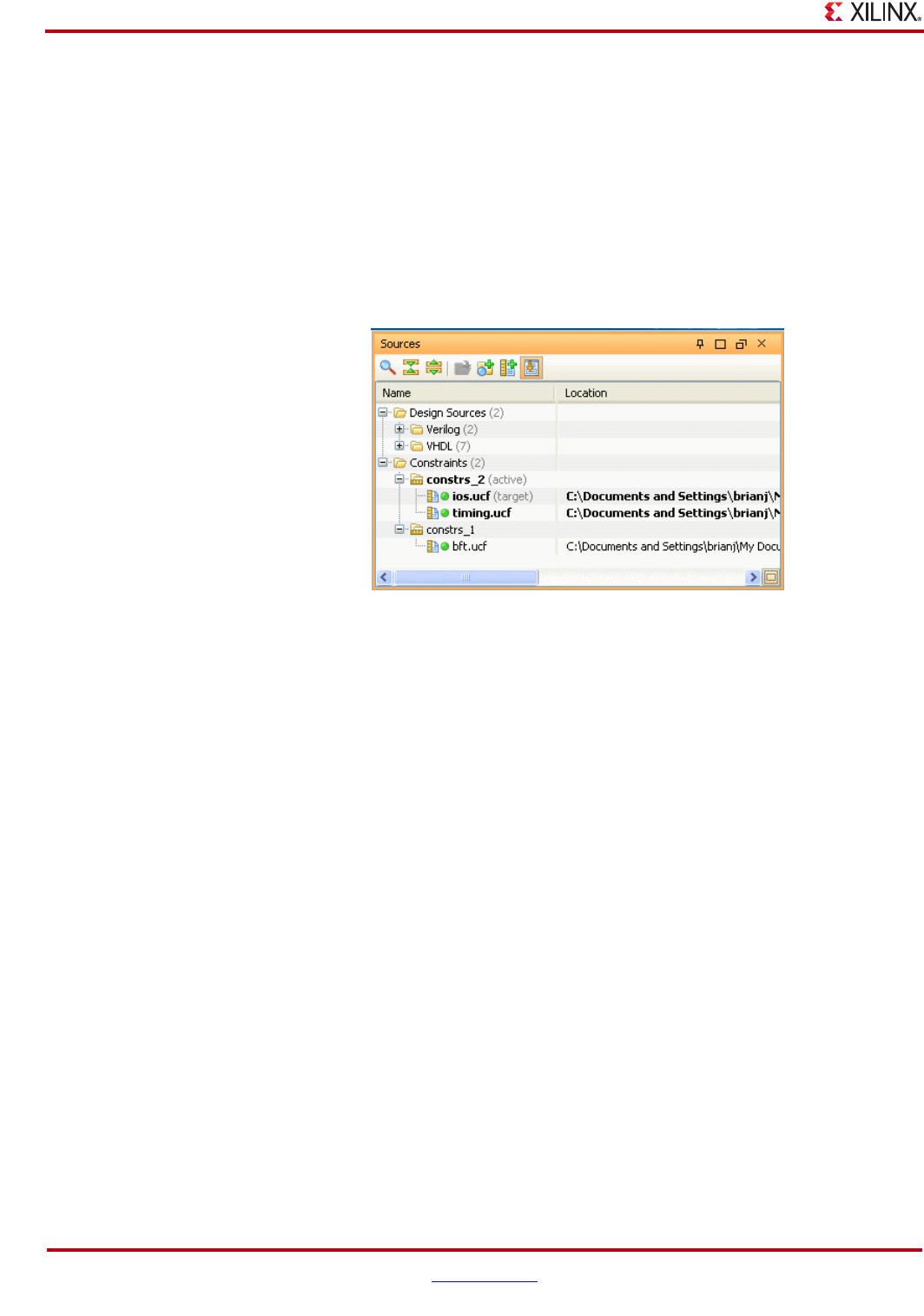
70 www.xilinx.com PlanAhead User Guide

UG632 (v 12.1)

Chapter 3: Working with Projects

Defining the Active Constraint Set

If more than one constraint set exists, you need to designate an “active” constraint set.

PlanAhead uses the active constraint set by default when the next implementation run is

launched or when you open an RTL, Netlist, or Implemented Design.

To set the active constraint set:

1. In the Sources view select the constraint set, and click the Make active popup menu

command.

Notice the constraint set now appears bold and has the (active) designation in the

Sources view.

Using Module-level Constraint Files

PlanAhead adds module-level constraint files to a project which are typically associated

with a core. There are two types of files that PlanAhead accepts: NCF and XNCF.

You can add NCF files to the Project in the New Project Wizard or the Add Constraints

command. The NCF files display in the Add Constraints page of the New Project wizard

when found in the same directory as the RTL or Netlist Source files.

XNCF files are created by the ngc2edif command and are picked up by PlanAhead

automatically and added to the constraint set. When an NGC format core has embedded

timing constraints, as is often the case with EDK and some CORE Generator cores, the

timing constraints are pulled out by the ngc2edif command prior to passing the EDIF

netlist to PlanAhead. This is done to allow PlanAhead to recognize the constraints and to

expose them during design analysis.

PlanAhead treats these files as read-only and does not enable modification to them

directly; however, in PlanAhead you can define new values for module-level constraints.

New constraint values are written into the target top-level UCF. Because PlanAhead passes

the top-level UCF files to implementation after the module-level NCF files, the new

constraint values are used.

Note: When modifying module-level constraints, it is a best-practice to edit the files in the original

source using the IP creation method.

Note: Module-level constraints can be modified as described; however, they cannot be removed.

Deleting module-level constraints results in the files reappearing when the Netlist or RTL Design is

closed and re-opened.

Figure 3-29: Setting the Active Constraint Set

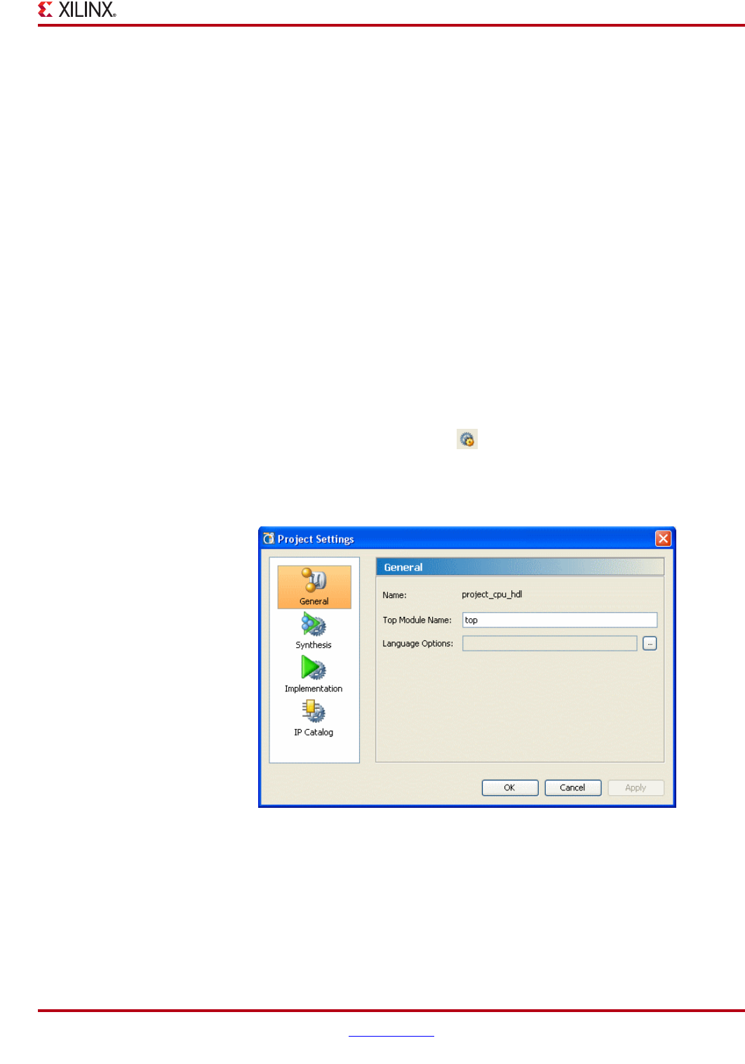
PlanAhead User Guide www.xilinx.com 71

UG632 (v 12.1)

Configuring Project Settings

Note: PlanAhead does not import module-level UCF files on a per-instance basis. Module-level

NCF files are processed if the name matches the name of the module-level netlist, which matches the

ISE behavior.

Exporting Constraints

Often, designers use PlanAhead to create constraint files for use in scripting command line

design flows.

To Export UCF constraints, click the Export UCF constraints popup command. See

“Exporting Constraints” in Chapter 9 for more information.

Configuring Project Settings

Project Settings can be accessed from a variety of locations in PlanAhead. Depending on

where it was invoked, the appropriate dialog box displays.

To access the Project Settings dialog box, select either the Project Settings toolbar button,

shown in the following figure, or the Project Settings command from the Project Manager

menu in the Flow Navigator. There are also links in the Project Summary also that open the

Project Settings dialog boxes.

The Project Settings General dialog box opens.

The Project Settings shows four categories:

•General—Displays a dialog box that where you can view the project Name, the Top

Module Name, and set language options.

•Synthesis—Shows the Default Part and Default Constraints Set, and provides an

Options area for Strategy and Strategy Description.

Figure 3-30: Project Settings Toolbar Button

Figure 3-31: Project Settings Dialog Box

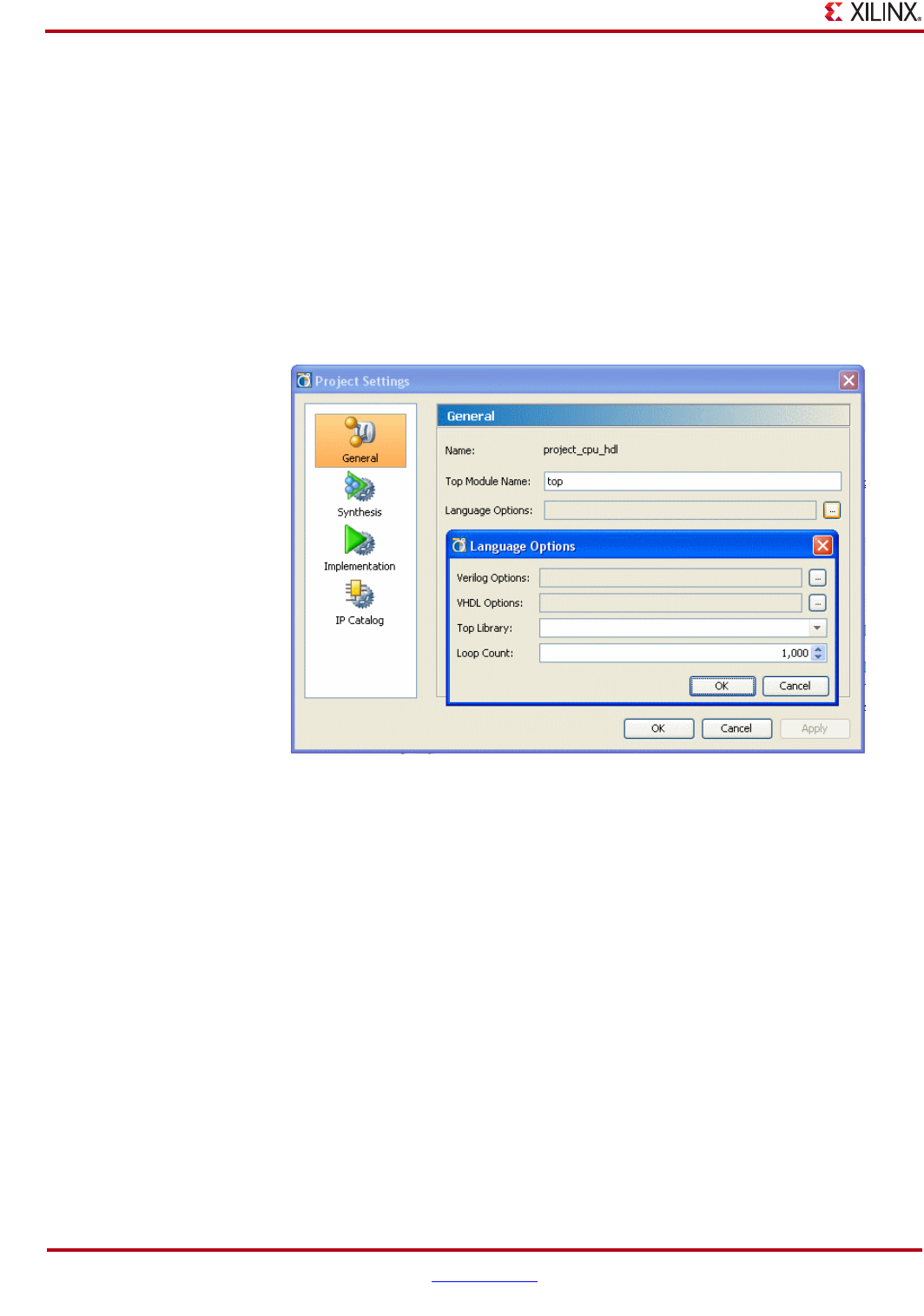
72 www.xilinx.com PlanAhead User Guide

UG632 (v 12.1)

Chapter 3: Working with Projects

A description window displays the Tcl commands wherein you can select a command

and get a description of that command.

•Implementation—Contains a Part and Constraints window, contains the Options

area for Strategy and Strategy Description. A description window displays the

Implementation Tcl commands wherein you can select a command and get a

description of that command.

•IP Catalog—Shows the IP Catalog location and the HDL type. This dialog box is

described in detail in “Setting IP Catalog Settings” in Chapter 5.

Using General Project Settings

The following figure show the General Project Settings dialog box.

The General Project Settings dialog box displays the following information:

•Name—Displays the Project name.

•Top Module Name—Enter the top RTL module name of the design. You can enter a

lower-level module name to experiment with synthesis on a specific module also.

•Language Options—Enter specific Verilog or VHDL options.

Figure 3-32: General Project Settings and Language Options Dialog Box

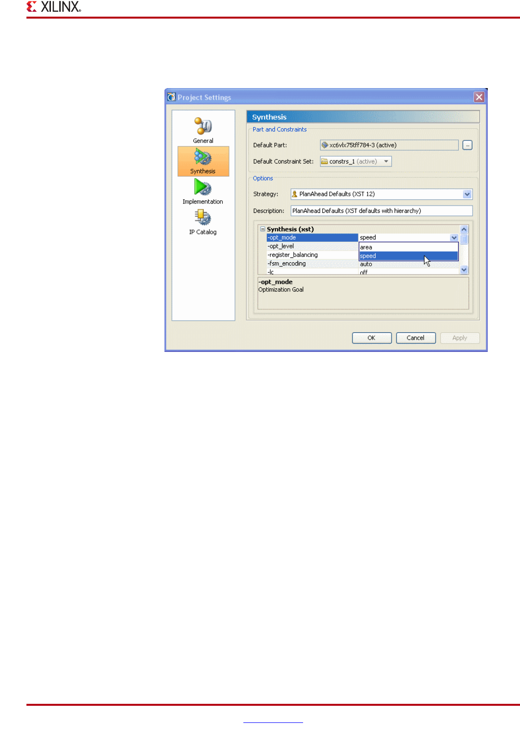
PlanAhead User Guide www.xilinx.com 73

UG632 (v 12.1)

Configuring Project Settings

Using the Synthesis Settings

The following figure shows the Synthesis Project Settings:

The Synthesis Project Settings dialog box contains the following information:

•Default Part—Displays the default target part. Select the browser button to invoke

the Part Selector dialog box to choose another part.

•Default Constraint Set—Select the constraint set to be used for the run. This selection

has no effect for a synthesis run.

•Strategy—Select the strategy to use for the run. PlanAhead includes a set of pre-

defined strategies, or you can create your own. For more information see the

“Creating Synthesis and Implementation Strategies,” page 296. When you select a

strategy, the options associated with it display in the lower part of the dialog box.

•Description—Enter any text description of the run.

•Strategy options can be overridden by selecting the option directives as shown in

Figure 3-33.

Figure 3-33: Synthesis Project Settings Dialog Box

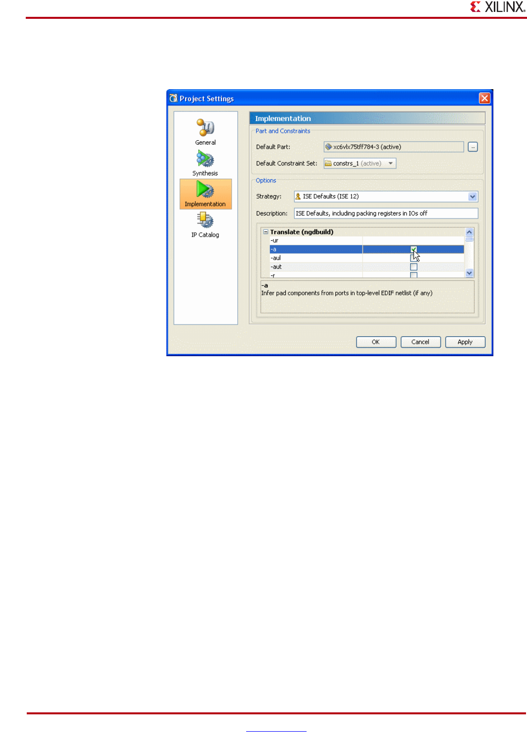
74 www.xilinx.com PlanAhead User Guide

UG632 (v 12.1)

Chapter 3: Working with Projects

Using the Implementation Settings

The following figure shows the Implementation Settings dialog box.

The Implementation Project Settings dialog box contains the following information:

•Default Part—Displays the default target part. Select the browser button to invoke

the Part Selector dialog box to choose another part.

•Default Constraint Set—Select the constraint set to be used for the run.

•Strategy—Select the strategy to use for the run. PlanAhead includes a set of pre-

defined strategies or you can create your own. For more information, see the

“Creating Synthesis and Implementation Strategies,” page 296. When you select a

strategy, the options associated with it display in the lower part of the dialog box.

•Description—Enter any text description of the run.

•Strategy options can be overridden by selecting the option directives as shown in

Figure 3-34.

Figure 3-34: Implementation Project Settings Dialog Box

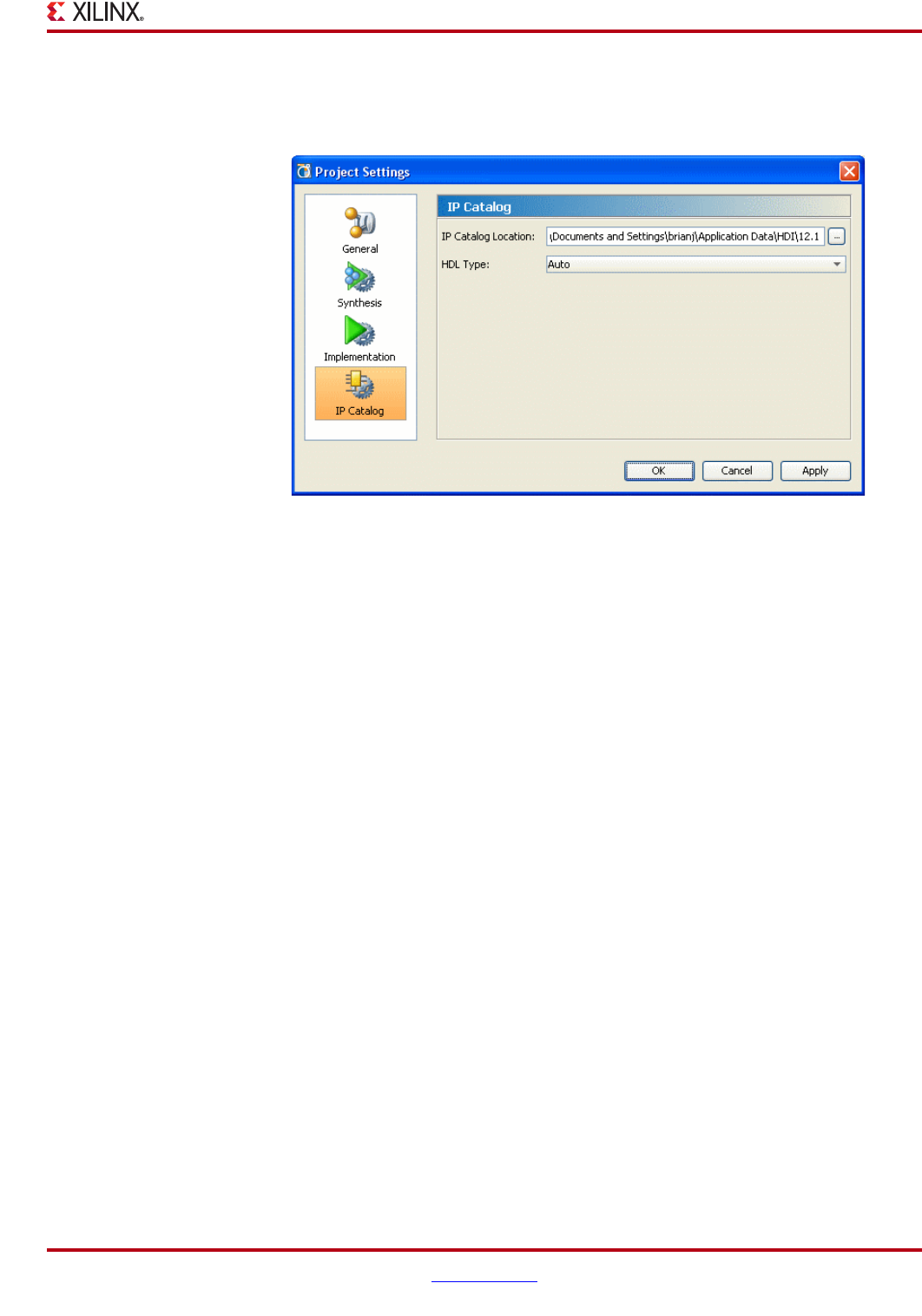
PlanAhead User Guide www.xilinx.com 75

UG632 (v 12.1)

Understanding the Project Summary

Settings IP Catalog Settings

The following figure shows the IP Catalog Project Settings dialog box.

The IP Catalog Project Settings dialog box contains the following information:

•IP Catalog Location—Defines the location to create the local IP Catalog. This is

performed the first time PlanAhead is invoked after a fresh install, or when the

Update Catalog command is run. Refer to Chapter 5, “RTL and IP Design.”

•HDL Type—Select the default language in which to create the IP module. The values

include: Verilog, VHDL or Auto, where Auto uses the same format as the top-level

module.

Understanding the Project Summary

PlanAhead provides an interactive Project Summary view that details information about

the design and the project. The Project Summary view updates dynamically as the design

commands are run. There are also links to launch commands, or to display more detailed

information.

You can open the Project Summary using one of these methods:

•Select the Project Summary command from the Project Manager Flow Navigator

menu.

•Select the Project Summary toolbar button.

•Select the Windows > Project Summary command.

The Project Summary view opens as shown in Figure 3-36, page 76.

Figure 3-35: IP Catalog Project Settings Dialog Box

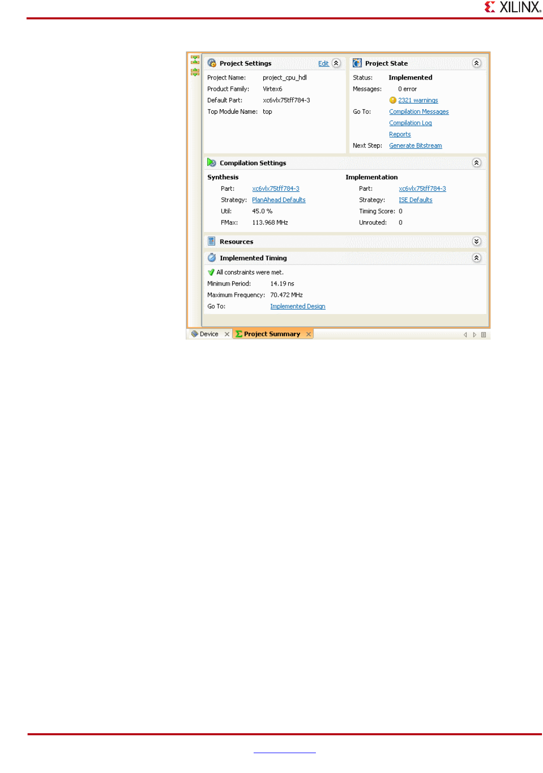
76 www.xilinx.com PlanAhead User Guide

UG632 (v 12.1)

Chapter 3: Working with Projects

The Project Summary displays design information. You can use the scroll bar or the

Collapse and Expand buttons to view or hide the data categories. Selecting anywhere in

the panel banner expands or collapses the view panel also.

Viewing Project Settings

The Project Settings displays the Project Name, Device Family, Default Part, and Top

Module Name. Selecting the Edit link invokes the Project Settings dialog box. Refer to

“Configuring Project Settings,” page 71.

Viewing Project State

The Project State panel contains the following information:

•State—Displays the project status or the status of the actively running command.

•Messages—Summarizes the number of errors and warnings encountered during

compilation commands.

•Go To—Links to open the Compilation or Reports views. Refer to “Using the

Compilation Message Area” in Chapter 4 for more information.

•Go To—Link to run the next design flow command.

Compilation Settings

The Compilation Settings shows the target part, and the strategy used for the active

synthesis and implementation runs. Also, it shows the Fmax and utilization estimates

reported from synthesis and the timing score and unroutes reported from implementation.

Figure 3-36: Project Summary

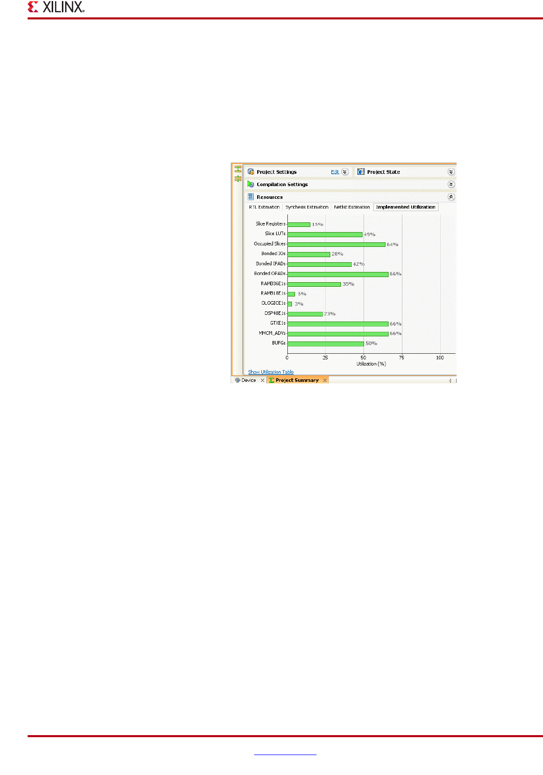
PlanAhead User Guide www.xilinx.com 77

UG632 (v 12.1)

Understanding the Project Summary

Clicking on the links invokes the Project Settings dialog box in the selected location to

enable configuration of synthesis and implementation runs. Tool tips describe the button

actions.

Resources

The resource utilization for the target device displays graphically in the provided chart as

shown in the following figure.

PlanAhead populates the Project Summary Resources at each stage of the design process.

The types of logic objects displayed varies as the design progresses through the design

stages. As the information becomes available, the tabs at the top of the view panel become

selectable.

•RTL Estimation—Estimates are provided from the PlanAhead RTL Design after the

Estimate Resources command been run.

•Synthesis Estimates—Resource estimates are extracted from the XST synthesis

report.

•Netlist Estimation—Estimates are provided from the PlanAhead Netlist Design after

the Estimate Resources command been run.

•Implemented Utilization—Actual resource utilization is extracted from the ISE map

report.

In some cases, links display in the Resources panel to guide you through the step involved

to populate the Resources chart.

Timing

Once the design is implemented, the Timing pane of the Project Summary view provides a

summary of the overall timing results. A link to open the Timing Results view, as shown in

Figure 3-38, page 78, is available.

Figure 3-37: Resource Estimates in the Project Summary View

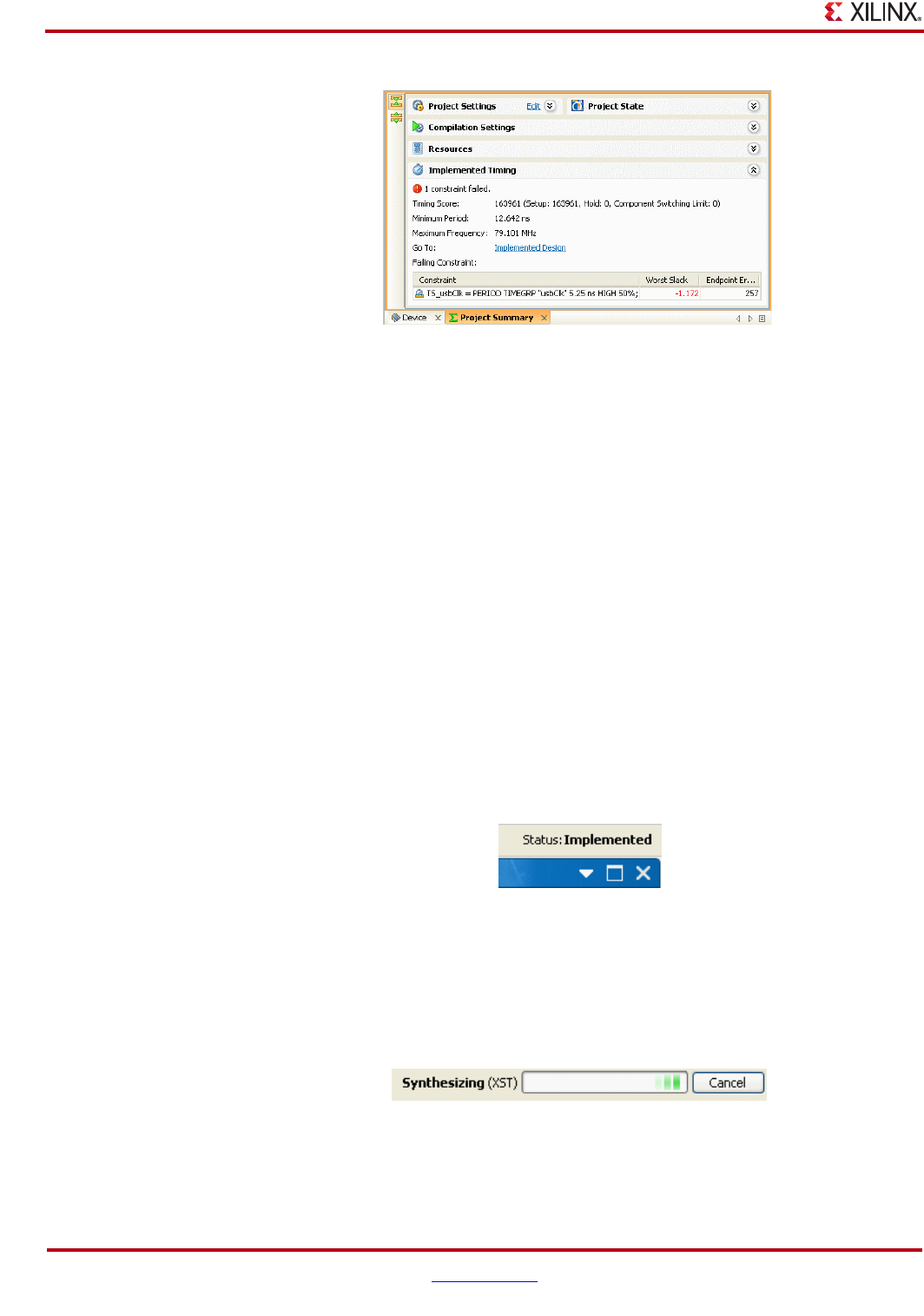
78 www.xilinx.com PlanAhead User Guide

UG632 (v 12.1)

Chapter 3: Working with Projects

PlanAhead populates the Project Summary Timing after implementation is complete. The

Timing Score, Minimum Period, Maximum Frequency and worst Failing Constraint for the

active run display and a link is provided to open the Implemented Design.

Determining Project Status

PlanAhead provides several visual indicators about the overall status of a project as well as

methods to take the next step in the process. Only the results of the major design tasks in

the design process are reported in the project status.

The overall Project Status displays in the Project Summary and in the Status Bar so you can

visualize the status of a project quickly upon opening the project, or while you are running

the design flow commands. These include RTL elaboration, synthesis, implementation,

and bitstream generation.

The following subsections describe how project status can be visualized in PlanAhead.

Project Status Bar

The overall Project status displays in the upper-right corner of the viewing environment,

as shown in the following figure.

As you run the Elaborate, Synthesize, Implement, and Generate Bitstream commands the

Project Status Bar changes to indicate either a successful or failed attempt. Failures are

displayed with red text.

As commands run, the Status Bar displays a visual indicator that a command is running.

Click the Cancel to stop the active command.

Figure 3-38: Timing Results in Project Summary View

Figure 3-39: Project Status Bar

Figure 3-40: Running Command Status and Cancel

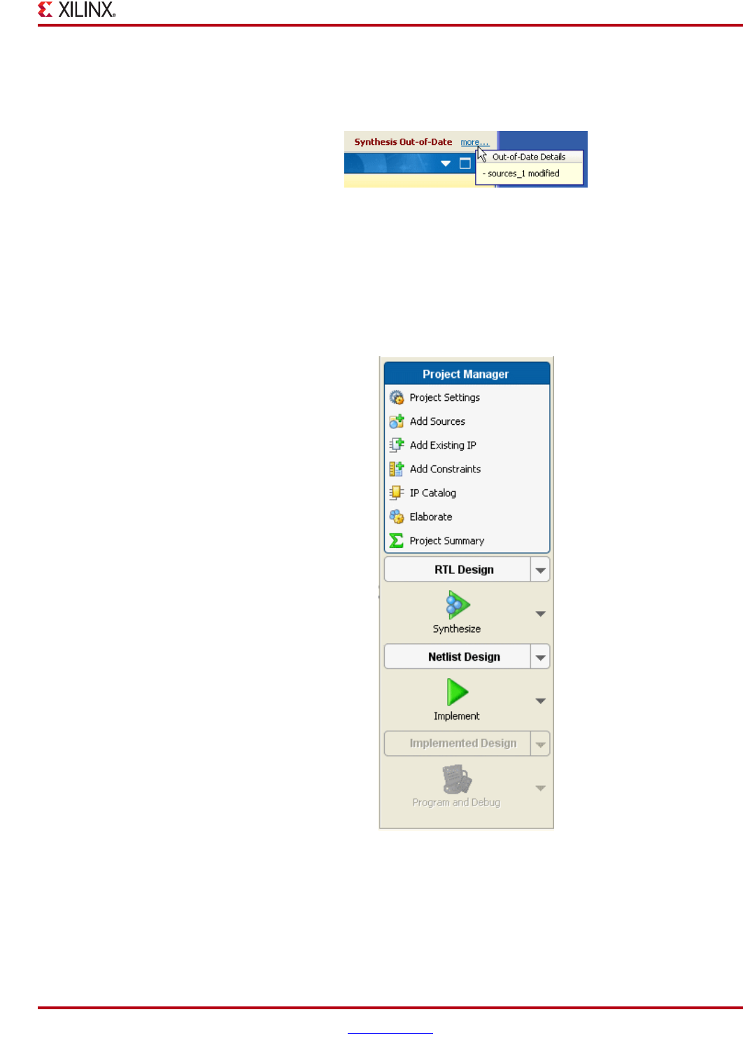
PlanAhead User Guide www.xilinx.com 79

UG632 (v 12.1)

Determining Project Status

If source files change, the project can be marked Out of Date if synthesis or implementation

is complete as shown in the following figure. The Status Bar indicates an Out-of-Date

Status. You can select the more... link to display the reason.

Flow Navigator

The Flow Navigator helps visualize the design state by providing access to only the

commands applicable to the design state. For example, if implementation is not run, the

Implemented Design button is greyed out as shown in the following figure. This visually

guides you in the Flow Navigator to click the next step in the design process.

Figure 3-41: Information on why Project is Out-of-Date

Figure 3-42: Flow Navigator Design State Visualization

80 www.xilinx.com PlanAhead User Guide

UG632 (v 12.1)

Chapter 3: Working with Projects

Design Data Out-of-Date Banner

As source files, netlists, or implementation results update, a banner appears in the top of

the open design indicating that a newer version of the design is available than what is

loaded in memory. PlanAhead prompts you to refresh what is loaded in memory as shown

in the following figure.

Figure 3-43: Out-of-Date Banner and Reload button

PlanAhead User Guide www.xilinx.com 81

UG632 (v 12.1)

Chapter 4

Using the Viewing Environment

This chapter contains the following sections:

•“Understanding the Viewing Environment”

•“Using the Main Viewing Area”

•“Using the Flow Navigator”

•“Using the Compilation Message Area”

•“Using Common PlanAhead Views”

•“Working with Views”

•“Selecting Objects”

•“Configuring the Viewing Environment”

•“Configuring PlanAhead Behavior”

Understanding the Viewing Environment

The PlanAhead™ software has a dynamic viewing environment that comprises view

layouts which present the design and device information for the design task at hand. It

provides unique capabilities and viewing perspectives for design information.

Most views “cross-select,” meaning the selected information appears in the other view

when you select it in one, enabling efficient methods to examine the design and device

information.

You can use PlanAhead to control each major step of the FPGA design process, including

RTL development and analysis, logic synthesis, constraints definition, physical design

analysis, floorplanning, and implementation control with the Xilinx® ISE® Design Suite

software.

There are view layout configurations to enable various types of tasks. The presented views

reflect the selected tasks. The available viewing configurations are:

•Project Manager—Manage project sources, constraints, customize IP

•I/O Planner—Define I/O placement constraints

•Design Planner—Analyze netlist design, insert ChipScope™ analyzer tool debug

cores, floorplan, apply timing constraints, and manage partitions

PlanAhead lets you customize view layout configurations for the displayed views. Refer to

“Configuring the Viewing Environment,” page 143.

In PlanAhead, you can create different types of projects that vary based upon the input

formats.

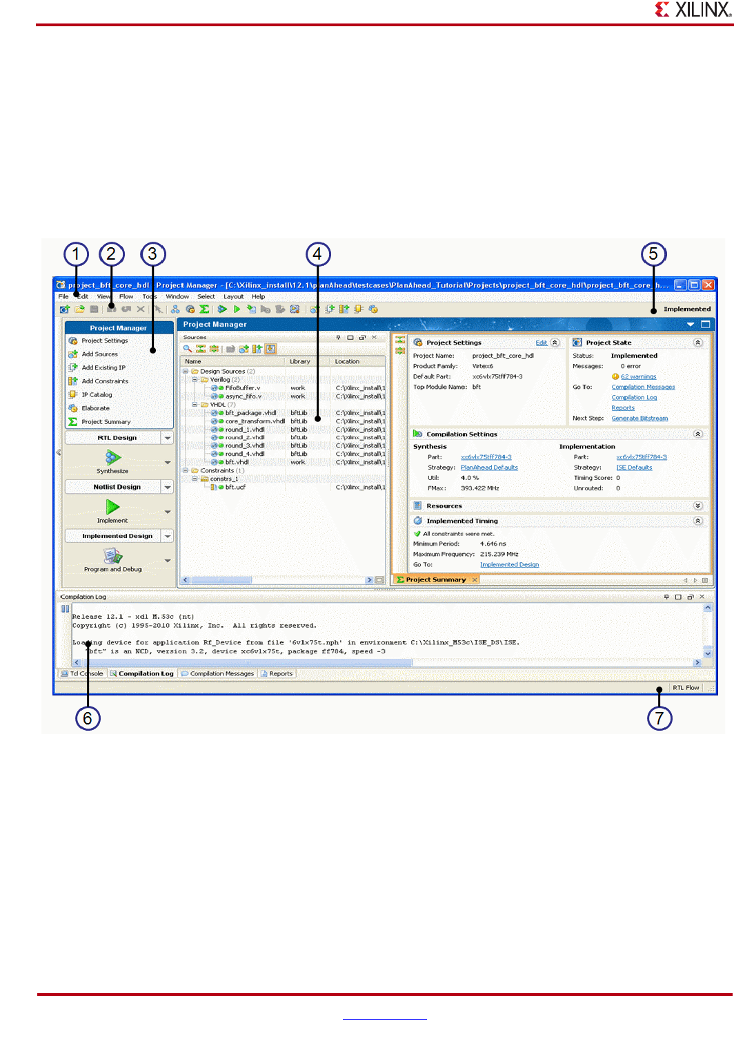
82 www.xilinx.com PlanAhead User Guide

UG632 (v 12.1)

Chapter 4: Using the Viewing Environment

The Flow Navigator appearance and the displayed view layout is determined by the type

of project you create. For more information on the PlanAhead project types, see Chapter 3,

“Working with Projects.”

The following sections describe the PlanAhead viewing environment.

Viewing Environment Overview

The PlanAhead environment components are annotated by number in the following

figure.

1. Main Menu—Contains the available PlanAhead commands. The menus filter the

available commands based on project type and design status.

2. Main Toolbar—Contains commonly used commands and extends to include Design

specific commands.

3. Flow Navigator—Enables flow-like control over the design process. From the Flow

Navigator you can launch synthesis, implementation, and generate bitstream files as

well as open designs at each stage of the design process. This view expands as design

tasks are completed, and displays relevant commands for each design or project type.

Figure 4-1: PlanAhead Viewing Environment

PlanAhead User Guide www.xilinx.com 83

UG632 (v 12.1)

Understanding the Viewing Environment

4. Main Viewing Area—Displays the Project Manager, and any open design. When a

design is opened, you can switch between the I/O Planner and Design Planner view

layouts.

5. Project Status Bar—Shows project status and the actively-running commands. You

can cancel synthesis, implementation and generate bitstream commands from this

component.

6. Tcl Console and Messages Area—An expandable area that shows command status

and message logs.

7. Information Bar—Displays information about the project and the objects being

dragged over by the cursor.

Primary Environment Components

The primary components of the PlanAhead viewing environment include the:

•Main viewing area

•Flow Navigator

•Compilation messages and Tcl Console area

The main viewing area displays the Design data within either the Project Manager, the I/O

Planner or the Design Planner. When you open a project and no design data open in

memory the Project Manager view layout opens by default. Once a design is open, the

design data displays in the Design Planner view layout. You can display the I/O Planner

view layout by toggling the I/O Planner button in the Design view banner.

You can adjust the size of the main viewing area by minimizing the Flow Navigator or the

Compilation Messages area. The following figure shows the primary environment

components.

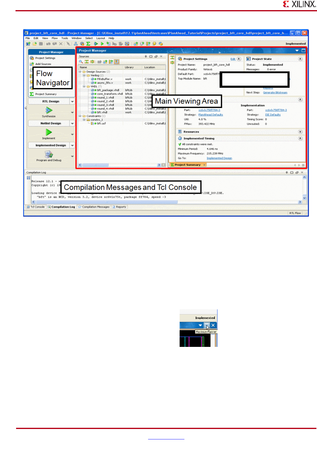
84 www.xilinx.com PlanAhead User Guide

UG632 (v 12.1)

Chapter 4: Using the Viewing Environment

Using the Main Viewing Area

The following subsections describe the options of the main view area.

Maximizing the Main Viewing Area

You can use the entire PlanAhead main window by clicking the Maximize Planner button

in the upper-right of the viewing area. The Flow Navigator and compilation messages then

minimize. The following figure shows the Maximize Planner button.

Hiding the Flow Navigator

You can hide the Flow Navigator individually by clicking the Hide Navigator button on

the left side of the Flow Navigator. The following figure shows the Hide Navigator button.

Figure 4-2: The Main Components of the PlanAhead Environment

Workspace Area

Figure 4-3: Maximize Planner Button

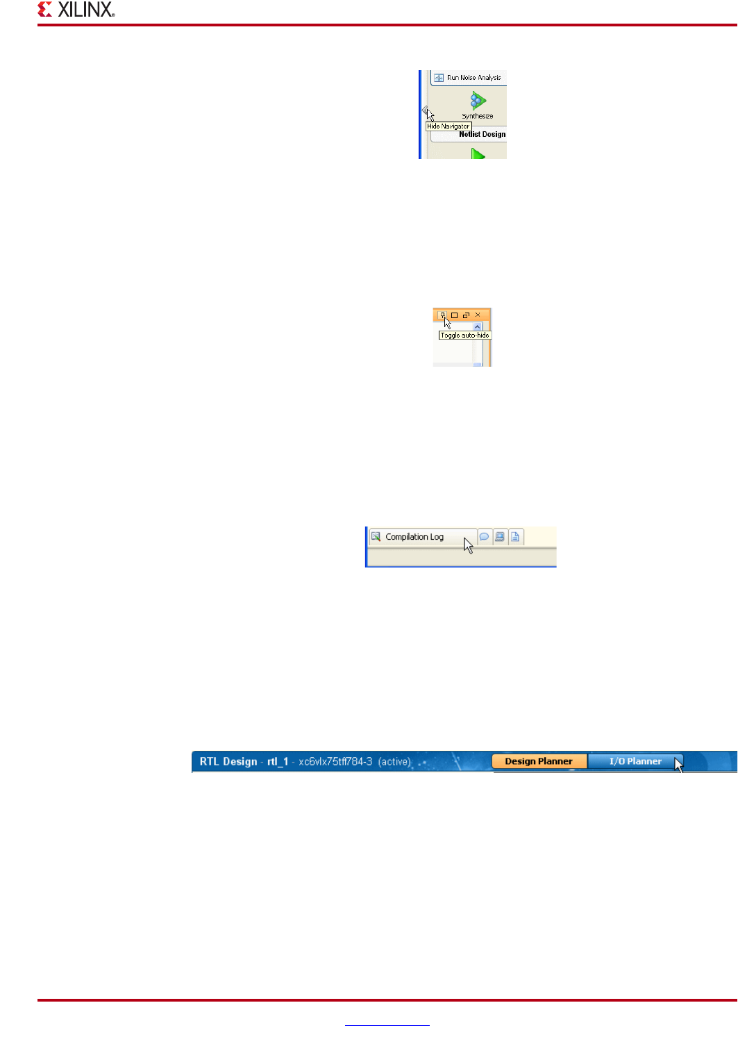
PlanAhead User Guide www.xilinx.com 85

UG632 (v 12.1)

Using the Main Viewing Area

Hiding the Compilation Messages Area

You can hide the entire set of Compilation Messages and Tcl Console views by clicking

Toggle auto-hide in the banner of any of the Compilation Messages area views. The

following figure shows the Toggle auto-hide icon.

Restoring the Compilation Messages Area

When the Compilation Messages area is minimized, the available views show as tabs at the

bottom on the viewing area. You can select any of the tabs to maximize the Compilation

Messages area back to the original location. The following figure shows the Compilation

Messages and Tcl Console tabs.

Toggling Between the I/O Planner and the Design Planner

Once any Design is opened, you can switch the view layout between the I/O Planner and

the Design Planner by selecting the button in the banner of the main viewing area. The

respective I/O Planner and the Design Planner share a common design in memory. The

only thing that changes is the presented view layout. The following figure shows the

toobar with the toggle options.

Figure 4-4: Hide Flow Navigator Button

Figure 4-5: Toggle auto-hide View Banner Buttons

Figure 4-6: Restore Compilation Messages Area

Figure 4-7: Toggle between I/O and Design Planners

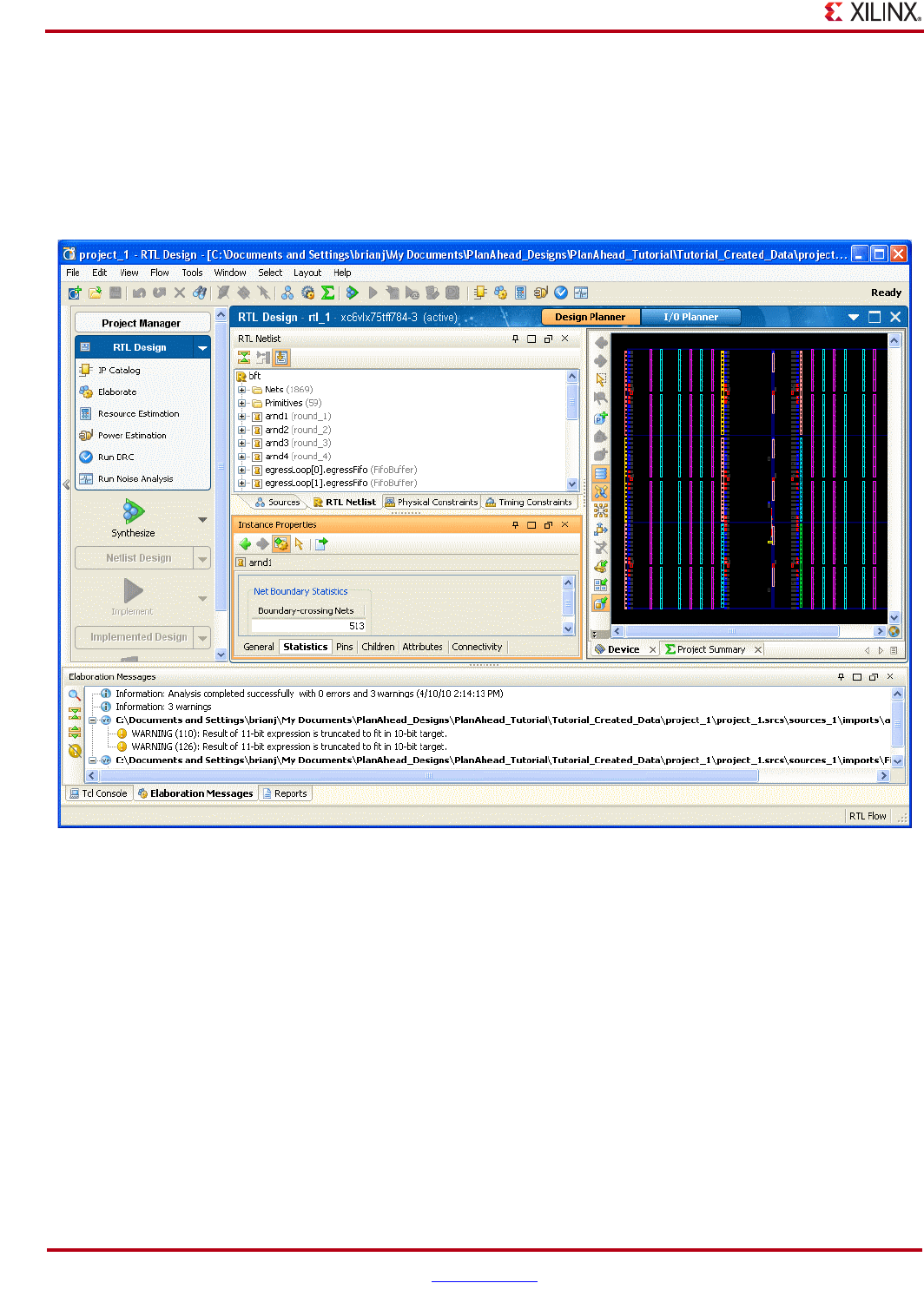
86 www.xilinx.com PlanAhead User Guide

UG632 (v 12.1)

Chapter 4: Using the Viewing Environment

Using the I/O Planner

The I/O Planner presents views applicable to device I/O resource exploration and I/O pin

assignment. The I/O Ports and Package Pins views display across the bottom of the layout.

Ports are either populated from the elaborated RTL Design or synthesized Netlist Design.

I/O related information is displayed in the various views. Figure 4-8, page 86 shows the

I/O Planner.

See Chapter 8, “I/O Pin Planning,” for more information about using the RTL I/O Planner

for I/O pin planning.

Figure 4-8: I/O Planner View Layout

PlanAhead User Guide www.xilinx.com 87

UG632 (v 12.1)

Using the Main Viewing Area

Using the Design Planner

Select the Design Planner button in the banner of the main viewing area to load the Design

Planner views. The Design Planner presents views applicable to logic exploration, resource

analysis, and constraints definition. The following figure shows the Design Planner view.

•See Chapter 5, “RTL and IP Design” for more information about using the Design

Planner for RTL development and analysis.

•For more information about using the Design Planner for netlist analysis and

constraint definition, refer to Chapter 7, “Netlist Analysis and Constraint Definition.”

•Chapter 10, “Analyzing Implementation Results”contains more information about

using the Design Planner for implementation results analysis and constraint

definition.

Figure 4-9: Design Planner View Layout

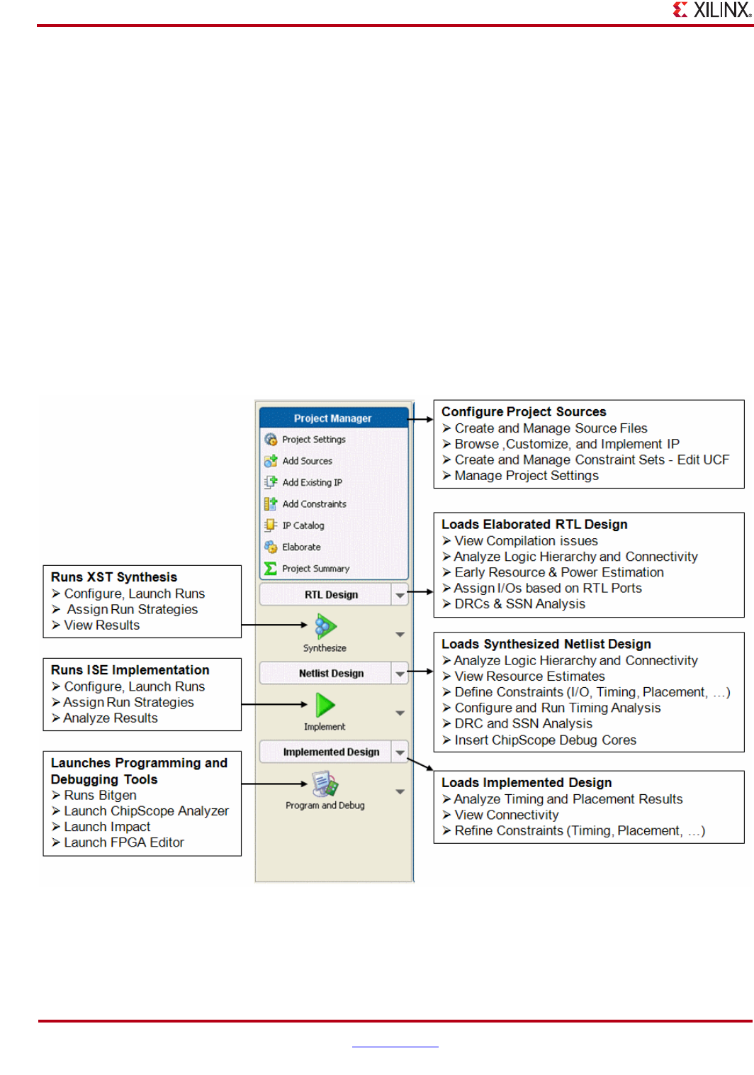
88 www.xilinx.com PlanAhead User Guide

UG632 (v 12.1)

Chapter 4: Using the Viewing Environment

Using the Flow Navigator

The Flow Navigator provides control over the major design process tasks such as project

configuration, synthesis, implementation, and bitstream creation. As these tasks are

completed, you can open the resulting designs to analyze results and apply constraints by

clicking the RTL Design, Netlist Design or Implemented Design buttons.

The options that are available to you depend on the status of the design. Inapplicable steps

are greyed out until the appropriate design tasks are completed. Relevant commands

display under each Design as it is opened.

The following figures illustrate how the PlanAhead Flow Navigator view is used to

perform design tasks and to open the analysis environments at various stages of the design

process.

Using the Flow Navigator with an RTL Project

The following figure describes the design flow when you use RTL sources as input to

PlanAhead.

Figure 4-10: PlanAhead Flow Navigator (RTL Project)

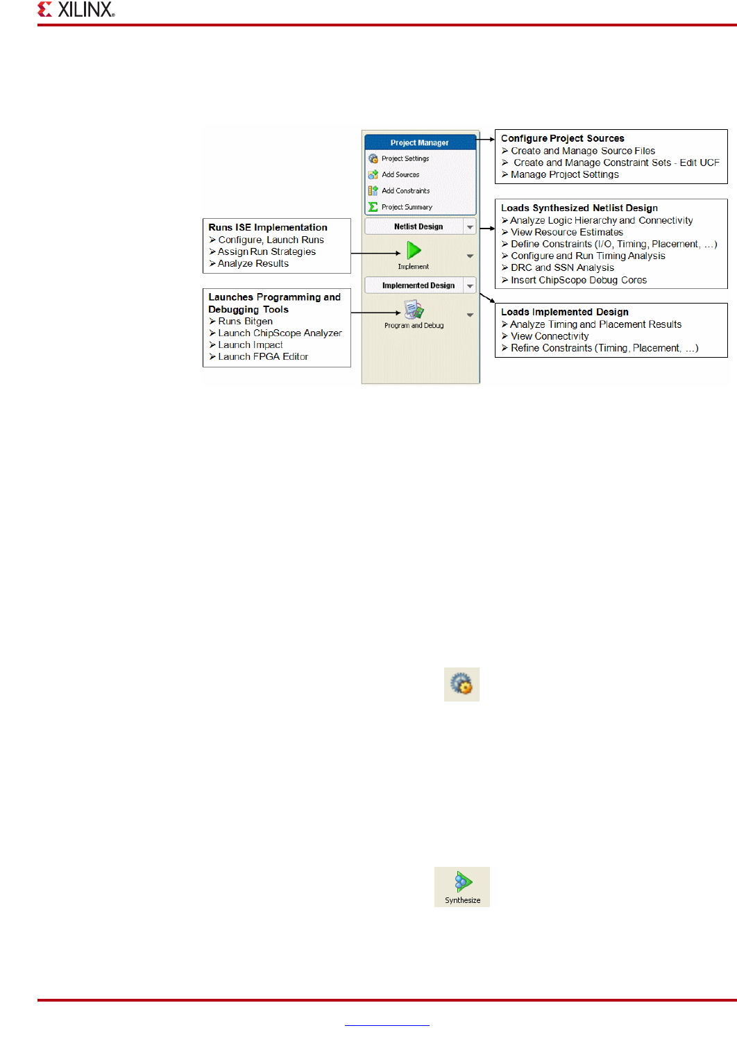
PlanAhead User Guide www.xilinx.com 89

UG632 (v 12.1)

Using the Flow Navigator

Using the Flow Navigator with a Synthesized Netlist Project

The following figure illustrates the design flow for synthesized netlist-based projects.

Launching Commands from the Flow Navigator

The Flow Navigator facilitates a push button flow by enabling synthesis and

implementation to be run immediately after you add Sources to a project. There is no need

to open any of the Design environments to complete the design. The following sections

describe how to implement a design quickly with the Flow Navigator.

Setting Command Options

You can set synthesis and implementation options by clicking Project Settings in the

Project Manager or Main Toolbar. These options are also available from pulldown menus

within the Synthesis and Implementation buttons in the Flow Navigator. The following

figure shows the Project Settings button.

See Chapter 6, “Synthesizing the Design,” and Chapter 9, “Implementing the Design,” for

more information.

Running Synthesis

After you add Sources to a project, you can use the Synthesis option to launch the XST

synthesis tool. The following figure shows the Flow Navigator Synthesis button.

See Chapter 6, “Synthesizing the Design,” for more information.

Figure 4-11: PlanAhead Flow Navigator (Synthesized Netlist Project)

Figure 4-12: Main Toolbar Project Settings Button

Figure 4-13: Flow Navigator Synthesize Button

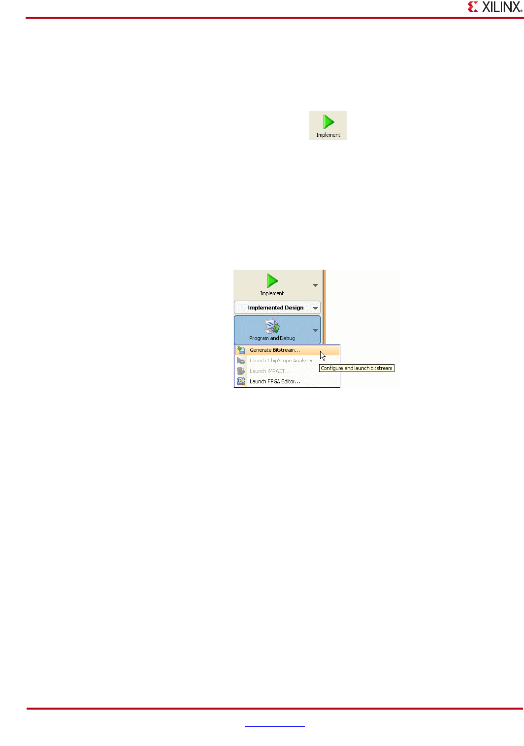
90 www.xilinx.com PlanAhead User Guide

UG632 (v 12.1)

Chapter 4: Using the Viewing Environment

Running Implementation

Once synthesis has completed, you can run the ISE implementation tools in the Flow

Navigator by clicking the Flow Navigator Implement button. The following figure shows

the Implement button.

See Chapter 9, “Implementing the Design,” for more information.

Generating Bitstream Files

Once implementation has completed, you can generate bitstream files and launch the

debugging and programming tools from the Flow Navigator by clicking the Program and

Debug button, which is actually a menu of available commands. The following figure

shows the Program and Debug button.

Refer to “Generating Bitstream Files” in Chapter 12 for more information.

Launching Programming and Debug tools

PlanAhead can launch the ISE debugging and programming tools automatically including

the FPGA Editor, iMPACT, and the ChipScope analyzer. You can launch the FPGA Editor

on any implemented design. the FGPA Editor opens with the results from the selected run

loaded and displayed automatically. The ChipScope analyzer and iMPACT require a bit

file and are available only after the Generate Bitstream command is run. Figure 4-16,

page 91 shows the Program and Debug button.

Figure 4-14: Flow Navigator Implement Button

Figure 4-15: Flow Navigator Program and Debug Button

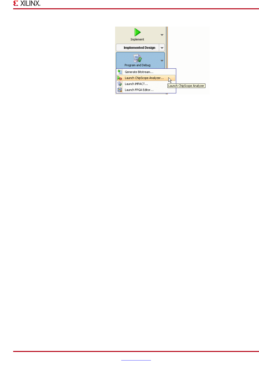
PlanAhead User Guide www.xilinx.com 91

UG632 (v 12.1)

Using the Flow Navigator

Refer to Chapter 12, “Programming and Debugging the Design,” for more information.

Using the Project Manager

When you open a project, the Project Manager opens by default. You can open the Project

Manager by selecting the Project Manager button in the Flow Navigator.

When you open the Project Manager, no design compilation is performed and no design

data is loaded into memory. This environment enables creating, importing, and managing

source files and constraint sets. You can use the Project Manager to browse, customize, and

implement IP from the Xilinx IP catalog also. Figure 4-17, page 92 shows the Project

Manager view.

Figure 4-16: Flow Navigator Launch Programming and Debug Tools

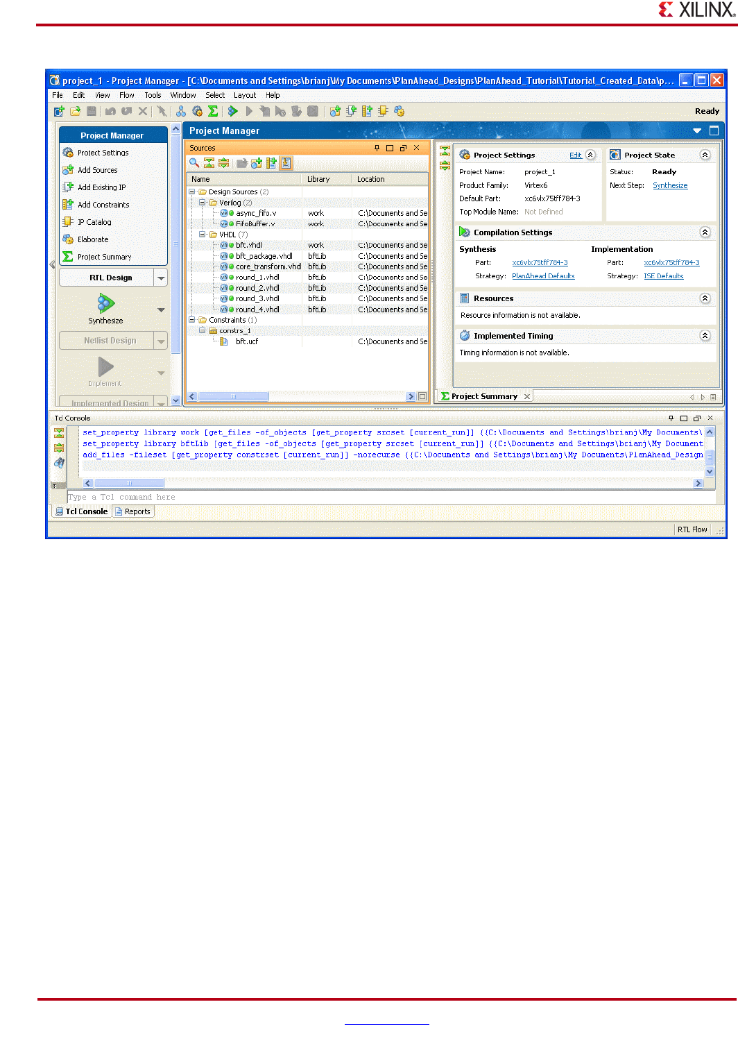
92 www.xilinx.com PlanAhead User Guide

UG632 (v 12.1)

Chapter 4: Using the Viewing Environment

The Project Manager displays the Sources and Project Summary views by default.

•For more information on using the Sources view to configure Project Sources, refer to

“Using the Sources View,” page 102.

•For more information on the Project Summary view, refer to “Understanding the

Project Summary” in Chapter 3.

• For more information on customizing IP, see “Customizing IP” in Chapter 5.

The Project Manager Flow Navigator menu contains the following commands:

−Project Settings—Opens the Project Settings dialog box. Refer to “Configuring

IP using the CORE Generator” in Chapter 5 for more information.

−Add Sources—Invokes the Add Sources dialog box. Refer to “Adding Source

Files” in Chapter 3.

−Add Existing IP—Enables importing existing CORE Generator™ project files and

resulting IP in the Project. Refer to “Configuring IP using the CORE Generator” in

Chapter 5.

−Add Constraints—Invokes the Add Constraints dialog box. Refer to “Adding

Constraints” in Chapter 3.

−IP Catalog—Opens the IP Catalog view. Refer to the “Using the IP Catalog” in

Chapter 5.

Figure 4-17: Project Manager View Layout

PlanAhead User Guide www.xilinx.com 93

UG632 (v 12.1)

Using the Flow Navigator

−Elaborate—Elaborates the RTL design an displays messages in the Elaboration

Messages view. Refer to “Elaborating and Analyzing the RTL Design” in

Chapter 5.

−Project Summary— Displays the Project Summary view. For more information

on the Project Summary view, refer to “Understanding the Project Summary” in

Chapter 3.

Opening an RTL Design

When you select the RTL Design button in the Flow Navigator, PlanAhead elaborates the

RTL design automatically and loads it into memory along with the active constraint set

and the target device. Elaboration messages display in the Elaboration Messages view.

To open a RTL Design select either:

•RTL Design in the Flow Navigator to open the elaborated RTL netlist with the active

constraint set, and the target device.

•The Open RTL Design command in the RTL Design pulldown menu of the Flow

Navigator.

See the “Using the Netlist Design” in Chapter 7 for information on opening designs.

The Design Planner view layout displays by default. Select the I/O Planner button in the

view banner to toggle between view layouts. See “Toggling Between the I/O Planner and

the Design Planner,” page 85.

The RTL Netlist view displays the compiled logic hierarchy. See Chapter 5, “RTL and IP

Design” for more information on analyzing the RTL logic design.

See Chapter 8, “I/O Pin Planning” for more information about using the I/O Planner for

I/O pin planning.

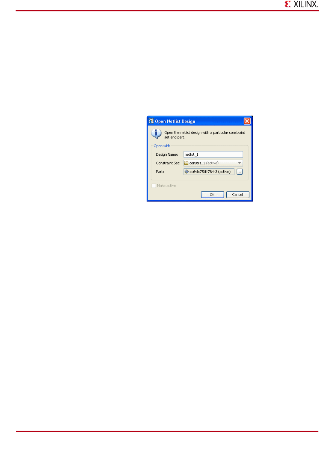
94 www.xilinx.com PlanAhead User Guide

UG632 (v 12.1)

Chapter 4: Using the Viewing Environment

Opening a Netlist Design

Since PlanAhead enables multiple synthesis runs, a Netlist Design could consist of

combination of a netlist, constraint set and target device. The Design is loaded into

memory and can be analyzed in either the I/O Planner or the Design Planner.

To open a Netlist Design select either the:

•Netlist Design button in the Flow Navigator to open the active synthesized netlist

with the active constraint set, and the target device

•Open Netlist Design command in the Netlist Design pull down menu of the Flow

Navigator

The Open Netlist Design dialog box lets you enter:

•Design Name—Enter a name display in the view banner. The design is stored in

memory during the PlanAhead session only.

•Constraint Set—Select an existing constraint set to be opened against the netlist.

•Part—Select a target part.

Figure 4-19, page 95 shows the Open Netlist Design view.

Figure 4-18: Opening Netlist Design Dialog Box

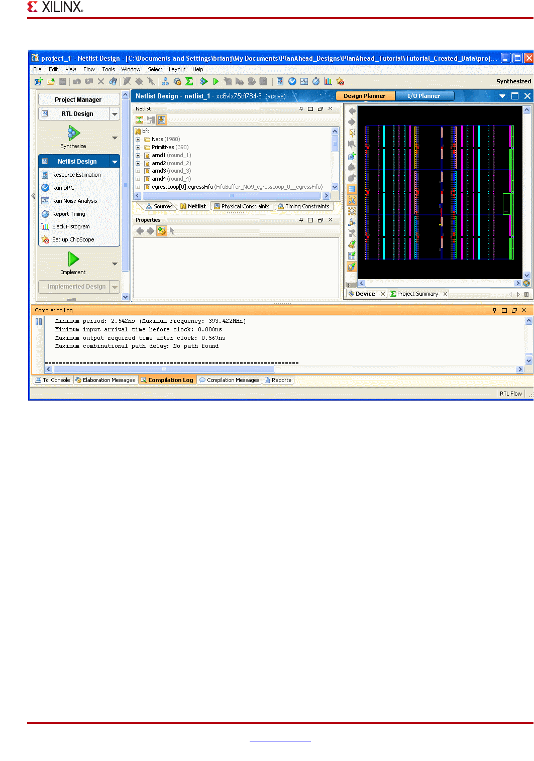
PlanAhead User Guide www.xilinx.com 95

UG632 (v 12.1)

Using the Flow Navigator

The Design Planner view layout displays by default. Select the I/O Planner button in the

view banner to toggle between view layouts. See “Toggling Between the I/O Planner and

the Design Planner,” page 85.

•For more information on using the Netlist Planner to analyze and constrain the

design, refer to Chapter 7, “Netlist Analysis and Constraint Definition.”

•See Chapter 8, “I/O Pin Planning” for more information about using the I/O Planner

for I/O pin planning.

Setting the Active Netlist

If multiple synthesis runs exist, PlanAhead will display information and react to the

“active run.” The Project Summary and Compilation Messages area displays information

about the active run only. The active run is displayed in bold text in the Design Runs view.

Select the desired synthesis run in the Design Runs view and use the Make active popup

menu command to set the active netlist. PlanAhead then uses that netlist by default when

opening Designs or launching runs.

Figure 4-19: Open Netlist Design

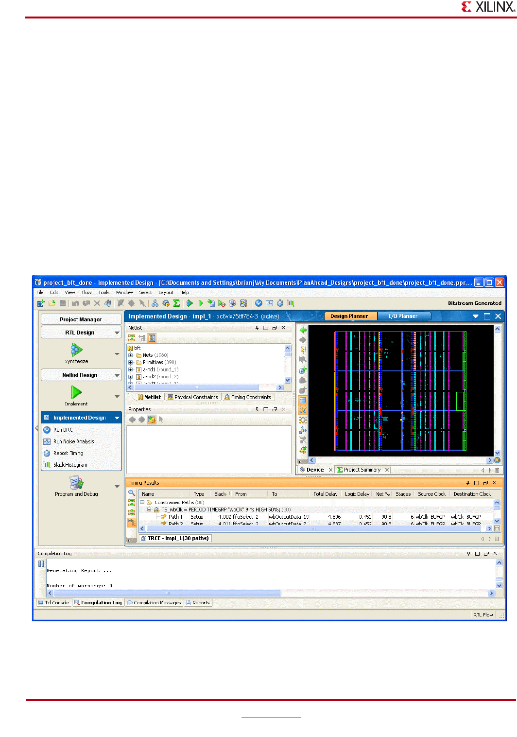
96 www.xilinx.com PlanAhead User Guide

UG632 (v 12.1)

Chapter 4: Using the Viewing Environment

Opening an Implemented Design

Because PlanAhead enables multiple implementation runs, an implemented design could

consist of a completed implementation run only. The implemented design imports the

netlist, placement, and timing results from the implementation run directory. PlanAhead

loads the design into memory where you can analyze it in the Design Planner

environment.

To open a implemented design, select one of the following:

•The Implemented Design button in the Flow Navigator to open the active synthesized

netlist with the active constraint set, and the target device

•Open Implemented Design from the Implemented Design pulldown menu in the

Flow Navigator and then select any implemented run listed

•Select any completed implementation run in the Design Runs view and use the Open

Implemented Design popup menu command (or double-click on the run)

The Design Planner view layout opens. Typically, you do placement and timing analysis,

and floorplanning in this environment. The following figure shows the Implemented

Design view.

You can open multiple Implemented Design views simultaneously to display results from

multiple runs.

Figure 4-20: Implemented Design View Layout

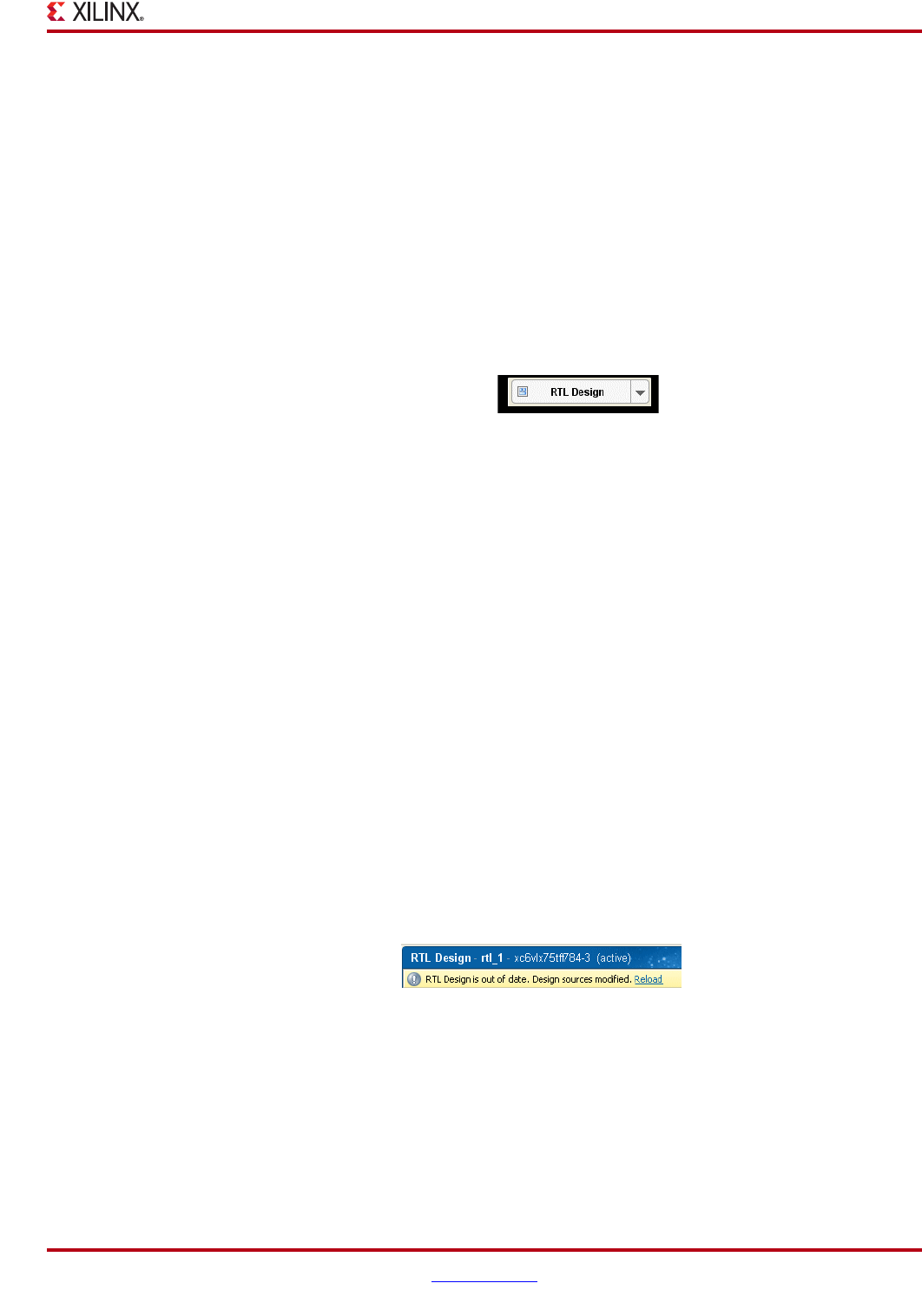
PlanAhead User Guide www.xilinx.com 97

UG632 (v 12.1)

Using the Flow Navigator

Tabs at the top of the view layout indicate which run results are open and which are

displayed. For information on creating and managing multiple implementation runs, see

“Launching Multiple Implementation Runs” in Chapter 9.

Note: Some capabilities that involve manipulation of the netlist, altering design partitions or Partial

Reconfiguration control might be restricted in the Implemented Design. You might need to open the

Netlist Design for these operations to ensure you are operating on the proper data.

Managing Open Designs

As you open Designs and PlanAhead loads the design into memory, an icon displays

within the appropriate button in the Flow Navigator. This provides a visual reference of

the data in memory and can help manage the PlanAhead session, as shown in the

following figure.

When multiple designs are open simultaneously, multiple icons display.

Closing Designs

You can close designs to reduce the number in memory and to prevent multiple locations

where sources could be edited. In some cases, you are prompted to close a design prior to

changing to another design representation. In some cases, such as for a Partial

Reconfiguration design, you must close the design when leaving the design.

You can close individual designs by clicking the Close button in the banner of the main

viewing area. You can close all designs by selecting the Close Design command from the

pull down menu on any Design Button in the Flow Navigator.

Reloading Designs

In the course of any design process, source files often require modification. PlanAhead

manages the dependencies of these files and indicates when displayed design data is out-

of-date. Changing Project settings can trigger an out-of-date status on a project also.

As source files, netlists, or implementation results update, a banner opens at the top of any

open Planners indicating that a newer design data version is available than what is loaded

in memory. PlanAhead prompts you to Reload to memory. The following figure shows the

out-of-date banner.

Closing and re-opening the design also refreshes the displayed data.

If a design step needs to be run to update the data, the Status Bar and Project Summary

indicate an out-of-date status. PlanAhead provides a link to run the next required step,

such as synthesis or implementation.

For more information about design configuration and source file management, refer to

Chapter 3, “Working with Projects.”

Figure 4-21: Open Design Indicator Icon

Figure 4-22: Out-of-Date Banner and Refresh button

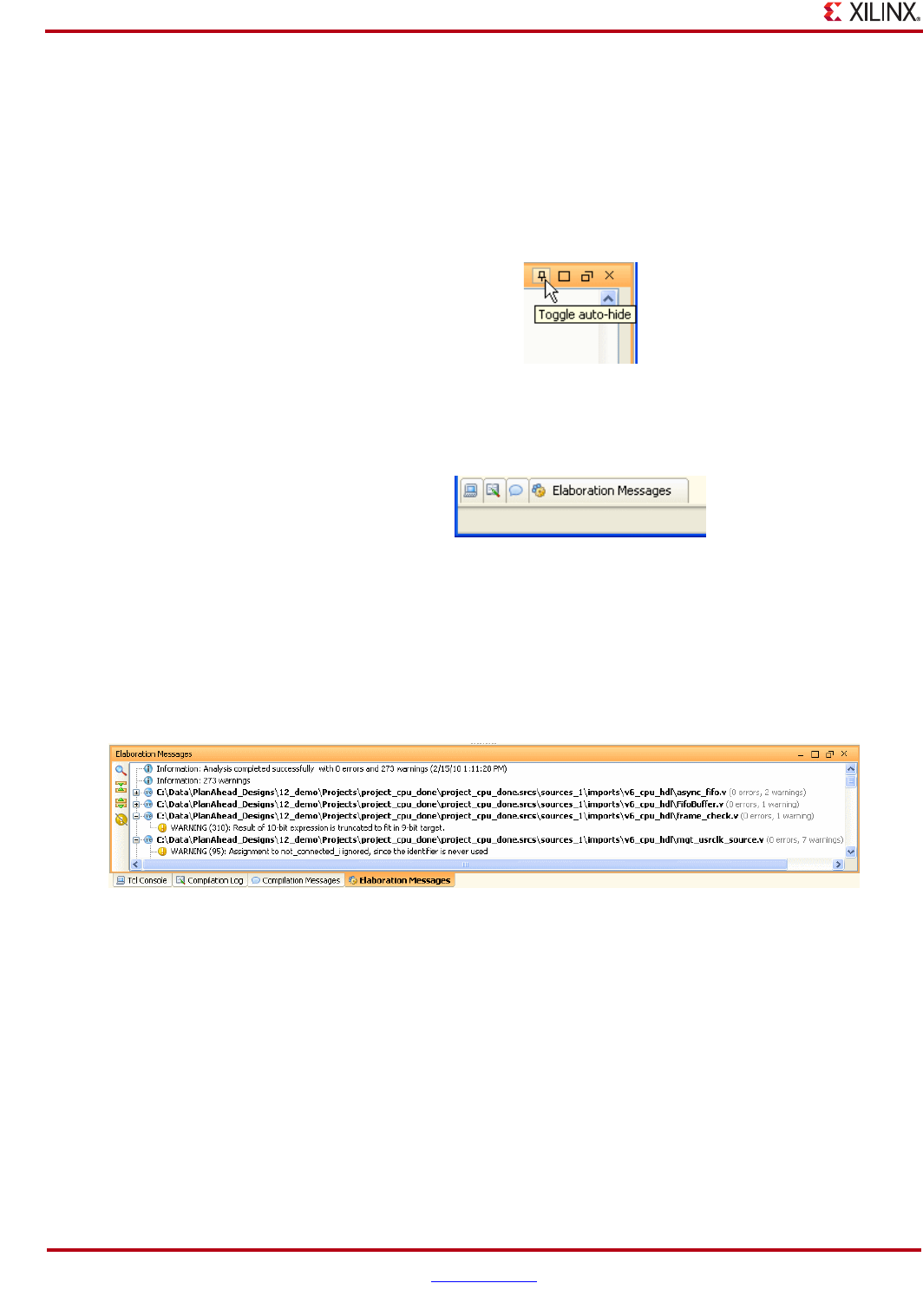
98 www.xilinx.com PlanAhead User Guide

UG632 (v 12.1)

Chapter 4: Using the Viewing Environment

Using the Compilation Message Area

The status and results of the commands that are run from within PlanAhead display in a

set of views linked into the lower Messaging area of the PlanAhead environment. As

messages are generated, they appear in the appropriate view within this area.

The Message area can be minimized to provide more viewing area for the design by

selecting the minimize button, shown in the following figure, in the view banner.

When the Message area is minimized, tabs display at the bottom of the PlanAhead

environment to restore the views, as shown in the following figure.

When you selecting a tab the view becomes active when the Message area displays.

Using the Elaboration Messages View

When you elaborate the RTL design, PlanAhead opens the Elaboration Messages view

shown in the following figure.

•Double-click any of the violations to invoke the RTL Editor with the offending line of

RTL highlighted.

•Expand or collapse the messages by toggling the tree widgets in the view or by

clicking the Expand All or Collapse All buttons.

•Filter the displayed messages by toggling the Hide Warning messages buttons or by

using the Show Search button.

Using the Compilation Log View

This view displays the active command output status of commands that compile the

design such as ngc2edif, XST, and ISE.

Figure 4-23: Minimize / Maximize View Banner Buttons

Figure 4-24: Restore Tabs for Message Viewing Area

Figure 4-25: Elaboration Messages View

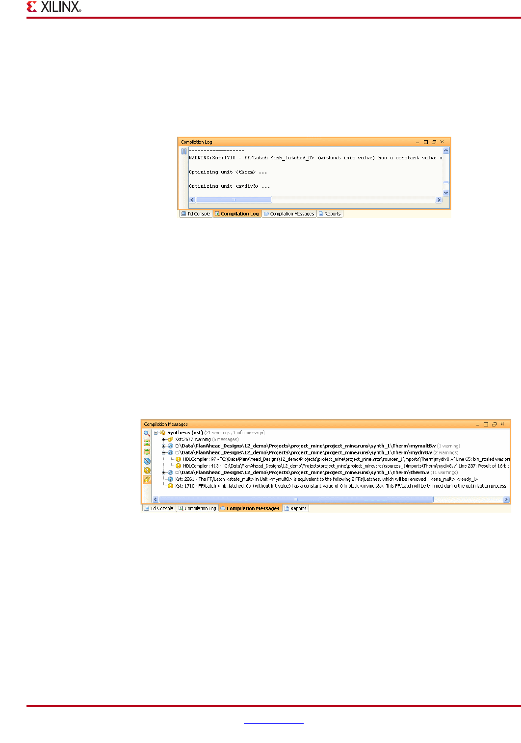
PlanAhead User Guide www.xilinx.com 99

UG632 (v 12.1)

Using the Compilation Message Area

The Compilation Log view displays the standard output from the compilation commands.

It opens automatically when you launch a command on an active run. Refer to “Launching

Selected Runs” in Chapter 9.

You can open the Compilation Log view by selecting the View tab at the bottom of the

PlanAhead Environment or by selecting the Windows > Compilation Log command. The

Compilation Log view is shown in the following figure.

The output displays in a continuous scroll-able format and is not refreshed when new

commands are run.

You can use the Pause output buttons to scroll back or read reports while commands are

running.

Using the Compilation Messages Views

The Compilation Messages view provides a summary of information messages, warnings,

and errors reported during design compilation.

You can open the Compilation Messages view by selecting the View tab at the bottom of

the PlanAhead environment or by selecting the Windows > Compilation Messages

command as shown in the following figure.

The reports might have links to the offending objects or to Answer Records in the Xilinx

Customer Support database.

You can:

•Expand or collapse the message by toggling the tree widgets in the view or by clicking

the Expand All or Collapse All buttons

•Filter the displayed messages by toggling the Hide warning messages or Hide info

messages buttons or by using the Show Search button

•Consolidate the list by clicking the Group duplicate messages button

Figure 4-26: Compilation Log View

Figure 4-27: Compilation Messages View

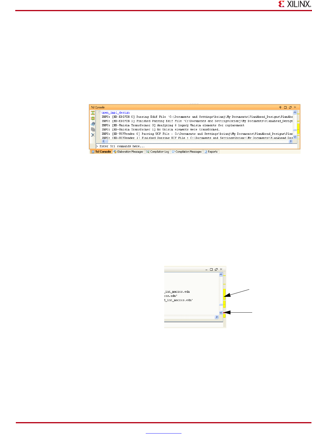
100 www.xilinx.com PlanAhead User Guide

UG632 (v 12.1)

Chapter 4: Using the Viewing Environment

Using the Tcl Console

The Console view displays messages from previously executed Tcl commands. PlanAhead

writes messages to the planAhead.log file. Command errors, warnings, and successful

completion echo to this window also.

The status of design netlists and constraints that open in the Netlist Planner and Results

Viewer display also.

To invoke the Console View, select Window > Tcl Console. The following figure shows the

Tcl Co nsol e.

In the Tcl Console view, you can:

•Expand or collapse the console messages by toggling the tree widgets in the view or

clicking the Expand All or Collapse All buttons

•Filter the displayed messages displayed by using the Show Search button

•Use the Copy button to cut and paste commands within the Tcl Console

•Use the Clear all output button to clear the Tcl console report

Using the Color Bar Warning and Error Indicators

Warnings or Errors show with a yellow or red bar on the right side of the Tcl Console as

shown in the following figure.

Hold the cursor over one of the bar segments to display the messages in a tool tip.

You can double-click the color bar segment to auto-scroll the Tcl Console to the messages in

the selected segment.

Figure 4-28: Tcl Console

Figure 4-29: Color Bar Warning and Error Indicator in Tcl Console

Yellow

Red

PlanAhead User Guide www.xilinx.com 101

UG632 (v 12.1)

Using the Compilation Message Area

Using the Tcl Command Line

You can use Tcl-format PlanAhead commands on the command line (shown in Figure 4-28,

page 100). You enter commands by clicking on the command line and typing Tcl

commands in the Command dialog box entry.

Every editing command that can be performed using the menu or by direct manipulation

(such as drag and drop) has an equivalent Tcl command.

When you invoke a command in the interface (in a menu or by direct manipulation), the

equivalent Tcl command invokes and displays on the message area, and is written to the

planAhead.jou file.

Command history can be accessed using the Up arrow and Down arrow keys in the

Command Line window.

Using Tcl Help

Command line help is available for all commands by using the following syntax at the

command line:

Command> help

You can retrieve more detailed information about the commands by extending the help

query with the following command:

Command> help get_cells

The Tcl Console displays the list of available commands or command options based on the

help topic that you enter.

For explicit command syntax, perform the command once, then view the planAhead.jou

file in the PlanAhead invocation directory.

See Chapter 14, “Tcl and Batch Scripting,” for more information about the Tcl command

formats and help.

Using the Design Runs View

The Design Runs view displays information about all of the synthesis and implementation

runs defined in the Project. When working with multiple runs or with partitions, the

Design Runs view can be a useful display. It is not displayed by default.

See “Running Implementation” in Chapter 9 for more information about using the Design

Runs view.

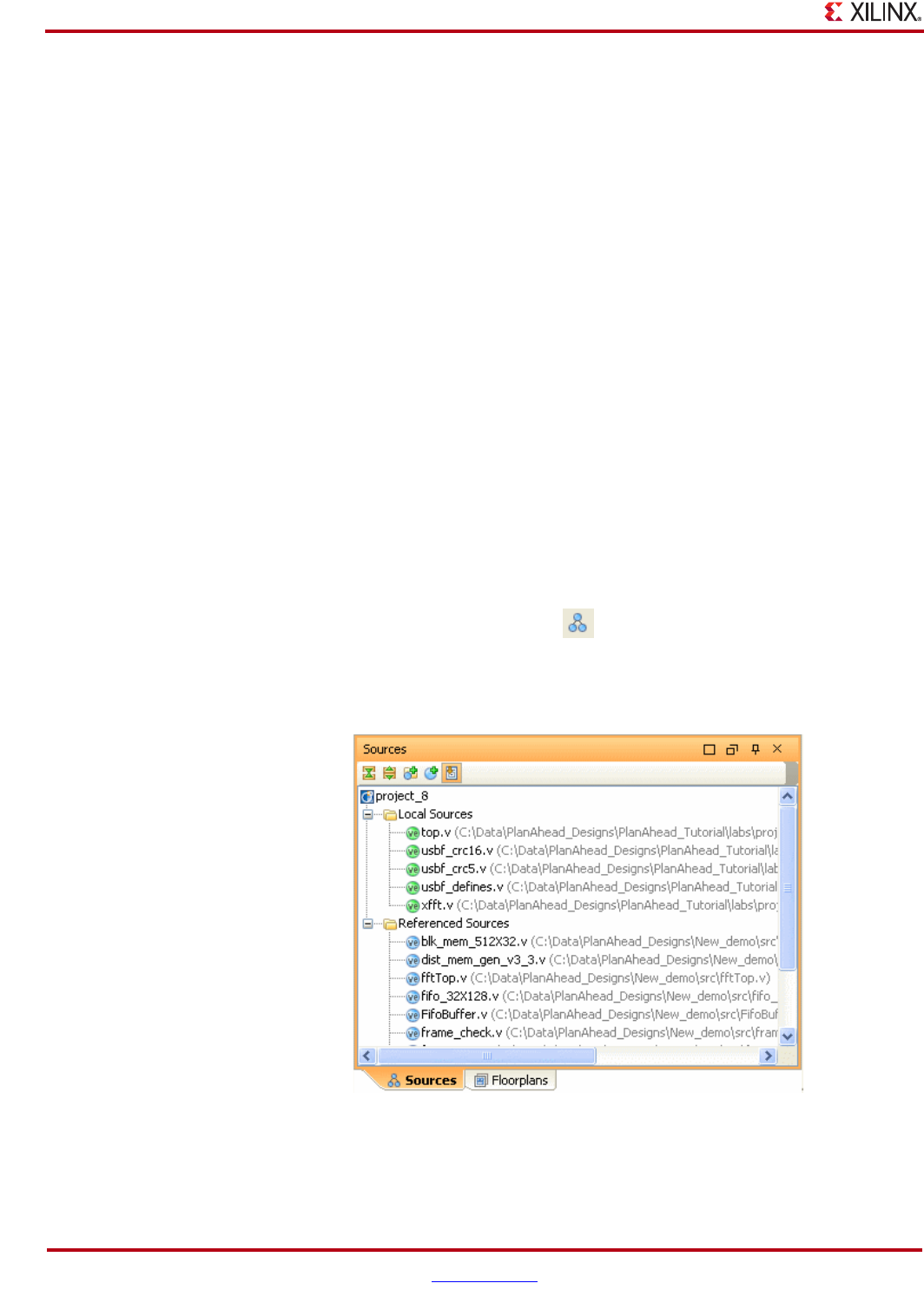
102 www.xilinx.com PlanAhead User Guide

UG632 (v 12.1)

Chapter 4: Using the Viewing Environment

Using Common PlanAhead Views

The following subsections describe the common PlanAhead views:

•“Using the Sources View”

•“Using the Device View”

•“Using the Package View”

•“Using the Schematic View”

•“Using the Properties View”

•“Using the Netlist View”

•“Using the Hierarchy View”

•“Using the I/O Ports View”

•“Using the Package Pins View”

•“Using the Design Runs View”

Using the Sources View

You can use the Sources view to manage project source types and constraints files. The

Sources view appears in all view layouts.

To open the Sources view, click the Sources button (shown in the following figure) on the

toolbar or use the Windows > Sources command.

The following figure shows an example of the Sources view.

The Sources view displays the files that were added to the project listed categorically and

by-type. Design source types include: Verilog, VHDL, NGC/NGO, and EDIF.

X-Ref Target - Figure 4-30

Figure 4-30:

Figure 4-31: Sources View

PlanAhead User Guide www.xilinx.com 103

UG632 (v 12.1)

Using Common PlanAhead Views

The constraints are in folders called constraint sets, and might include multiple UCF files.

Module-level NCF and Xilinx Netlist Constraints File (XNCF) format constraint files show

as design sources adjacent to their cores and are read-only. Refer to “Adding and

Managing Constraints” in Chapter 3 for more information about constraints.

The Sources view table contains the following information:

•Name—Lists source files grouped by type in an expandable tree table. “Using Tree

Table Style Views,” page 136.

•Copied—Indicates whether the files were copied into the project or referenced

remotely.

•Library—Displays the VHDL library defined for each file.

•Location—Displays the location of the imported or externally referenced files.

When RTL source files are displayed in red, the PlanAhead software could not find the

required files.

Using the Sources View Commands

You can add, view, or modify source files using the Sources view popup menu commands.

The common popup menu commands are covered in “Common Popup Menu

Commands” in Appendix A.

The Sources view specific commands are:

•Source File Properties—Invokes the Source File Properties view.

•Open File—Opens the selected file(s) in the RTL Editor view. This command is

available in a view toolbar button also.

•Update File—Replaces Source files with the newly selected files.

•Copy into Project—Copies selected source files and directories into the project

directory.

•Import All Files—Copies all remotely referenced Source files into the local project

directory.

•Remove from Project—Deletes the selected source files from the PlanAhead project.

It also removes the files from the PlanAhead project disk location if the files were

initially copied into the project.

•Enable Source Files—Sets the source file status to active for elaboration and

synthesis. Source files can be toggled between Enabled and Disabled to define source

file configurations.

•Disable Source Files—Sets the source file status to inactive for elaboration and

synthesis. Source files can be toggled between Enabled and Disabled to define source

file configurations. Disabled Source files appear in a shaded grey color to indicate

disabled status.

•Set Target UCF—Lets you select the UCF file to add PlanAhead created constraints.

•Set Library—Lets you select a library for the selected RTL source file(s).

•Create Source File—Invokes a drop-down menu to select the type of source to be

created: Verilog, Verilog Header, or VHDL. The new source file opens in the RTL

Editor.

•Add Sources—Adds selected source files, directories, and sub-directories into the

project. This command is available in a view toolbar button also.

•Add Existing IP—Adds existing XCO format CORE Generator project files as IP.

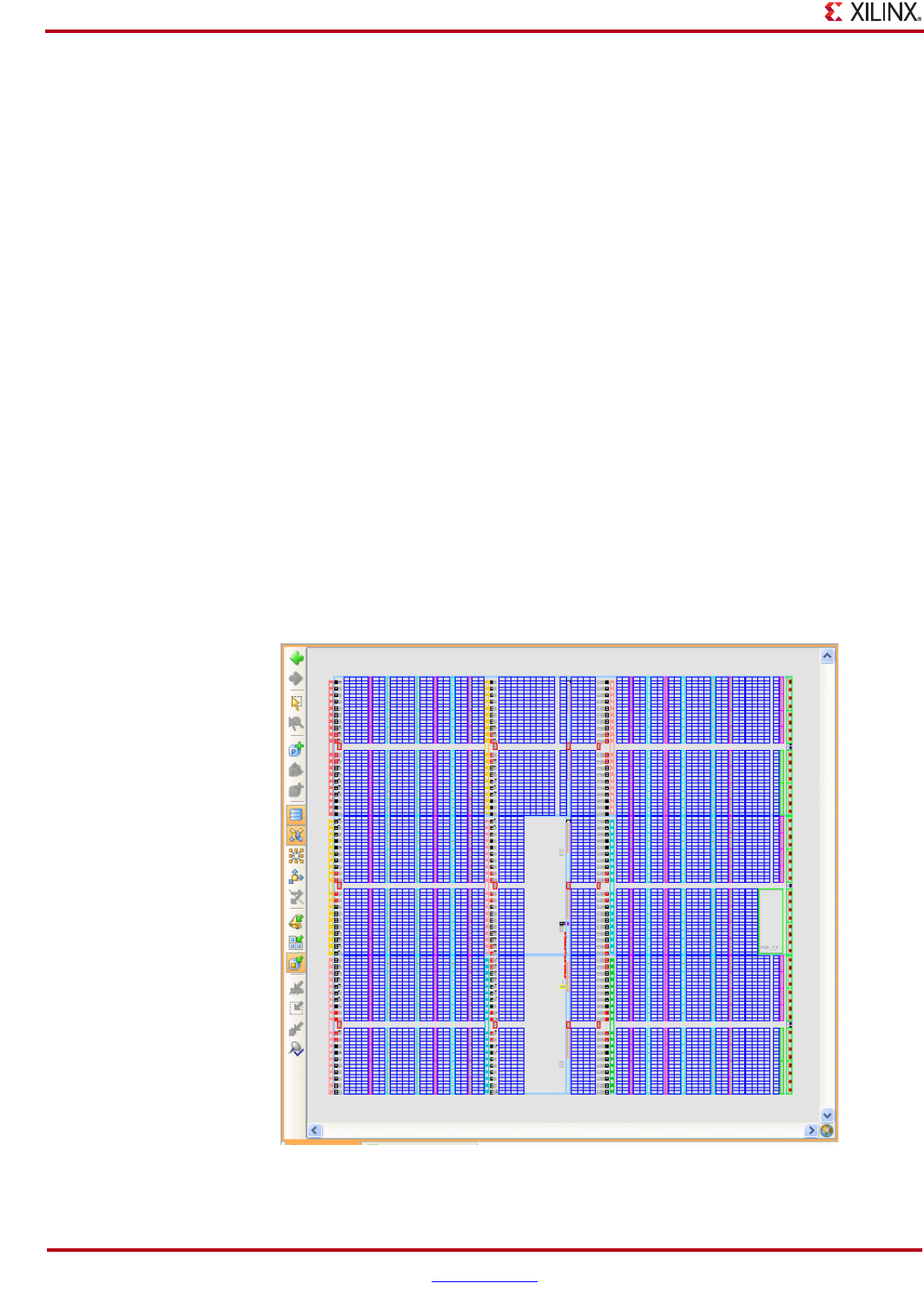
104 www.xilinx.com PlanAhead User Guide

UG632 (v 12.1)

Chapter 4: Using the Viewing Environment

•Add Constraints—Adds selected top level UCF constraint files into the project. This

command is available in a view toolbar button also.

•Find in Files—Invokes the Find in Files dialog box to enter text strings to search in

the selected files. The Find in Files Results view displays with the results of the search.

Using the RTL Editor

For information on using the features in the RTL Editor, refer to “Using the RTL Editor” in

Chapter 5.

Using the Device View

The Device view is the main graphical interface which is used for many different purposes

related to design analysis and floorplanning. For more information, see:

•Chapter 7, “Netlist Analysis and Constraint Definition”

•Chapter 10, “Analyzing Implementation Results”

•Chapter 11, “Floorplanning the Design”

The I/O Pin Planning process uses the Device view also. See Chapter 8, “I/O Pin

Planning,” for more information about using the Device view during pin assignment.

The Device view displays the FPGA device resources including the logic fabric, clock

regions, I/O pads, BUFGs, DCMs, Pblocks, instance locations, and net connectivity. The

locations on the device where specific logic can be assigned are called Sites. The following

figure shows a Device view.

Figure 4-32: Device View

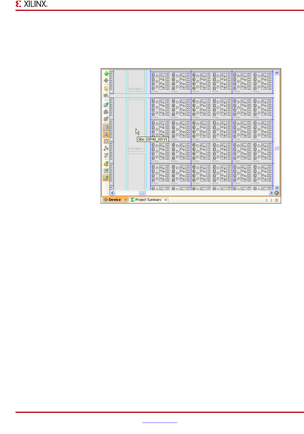
PlanAhead User Guide www.xilinx.com 105

UG632 (v 12.1)

Using Common PlanAhead Views

The amount of logic object detail displayed is determined by the selected zoom level: the

more you increase the zoom level, the more logic object detail displays. The Device view

popup and toolbar menus contain self-explanatory zoom level commands. Also, the

Device view has scroll bars and dynamic pan capabilities to pan the viewable area of the

device. Figure 4-33, page 105 shows a zoomed-in Device view.

When you drag the cursor over an object in the Device view, a tool tip identifies the object.

The Properties view displays object properties for selected sites or logic objects. Use Edit >

Find to search for specific logic object sites.

The Device view uses a dynamic cursor that changes appearance based on the activity

being performed. For example, if you attempt a logic resource assignment that is illegal,

the dynamic cursor changes so you can make adjustments. For more information, see

“Understanding the Context Sensitive Cursor,” page 139.

Using Device View Commands

Toolbar buttons on the left side of the Device view are view-specific commands, which are

described in “Using View Specific Toolbar Commands,” page 138. The following

commands are available in the Device view toolbar:

•To create a new Pblock rectangle, use Draw Pblock.

•To add or change the shape of an existing Pblock rectangle, use Set Pblock Size.

•To create non-rectangular Pblocks, use Add Pblock Rectangle.

•To toggle the display of assigned LOC constraints, use Show/Hide Loc Constraints.

•To toggle the display of the Bundle Net connectivity between Pblocks, use Show/Hide

Bundle Nets.

•To toggle the display of the I/O connectivity to place LOCs or Pblocks, use

Show/Hide I/O Nets.

Figure 4-33: Zoomed-in Device View

106 www.xilinx.com PlanAhead User Guide

UG632 (v 12.1)

Chapter 4: Using the Viewing Environment

•To change the selection behavior, use the Show connections for selected instances

mode. With this mode on, connectivity displays automatically for newly-selected

objects. This button toggles the mode on and off.

•To remove the timing paths that remain displayed after a timing path is selected, use

Hide All Timing Paths. Toggling this button keeps currently selected paths selected,

but hides all remaining displayed timing paths.

•To assign a LOC and BEL placement constraint to the object being placed, use Create

BEL Constraint Mode

•To assign a LOC placement constraint to the objects being placed, use Create Site

Constraint Mode

•To assign logic instances to Pblocks, use Assign Instance Mode. This is the default

mode; use this mode whenever possible to ensure proper command behavior.

•To assign a I/O Ports to I/O Banks, use Place I/O Ports in an I/O Bank

•To assign a I/O Ports in a rectangular area, use Place I/O Ports in Area

•To assign a I/O Ports sequentially, use Place I/O Ports Sequentially

•To toggle Automatic enforcement of interactive I/O placement DRCs, use

Automatically Enforce Legal I/O Placement

Understanding Device Resource Display

The PlanAhead software displays the resources contained in a selected device. The level of

detail at which the device resources display depends on the active zoom level within the

Device view. Graphical sites display and are available for all of the device-specific FPGA

resources.

The PlanAhead software Device view resource placement process is:

•The I/O pads and clock objects display around the periphery and/or down the center

of the device.

−I/O banks display as thin color shaded rectangles just outside the row of I/O

pads.

−Available I/O bank sites display as colored filled I/O bank rectangles.

−Some devices have unbonded I/O banks that display with empty I/O bank

rectangles.

−The I/O clock pads display as filled-in rectangles.

•All clock resources, such as BUFGs, BUFRs, and BUFGPs, show in the Device view.

When you select an I/O bank or clock region, the available device resources display in

the Properties view.

•The interior of the device is broken up into smaller rectangles called Tiles. Tiles are

placement sites for the different types of logic primitives for the architecture.

A tool tip identifies each site in the Device view when you hover the cursor over a

logic site.

See “Viewing and Reporting Resource Statistics” in Chapter 7 for more information about

viewing device resources. An example of a zoomed-in Device view is shown in

Figure 4-33, page 105. CLBs, SLICEs, and BELs are visible only when the zoom level is

close enough to display them.

You can assign primitive logic instances to the appropriate displayed sites. You can import

ISE placement results to display the logic assignments.

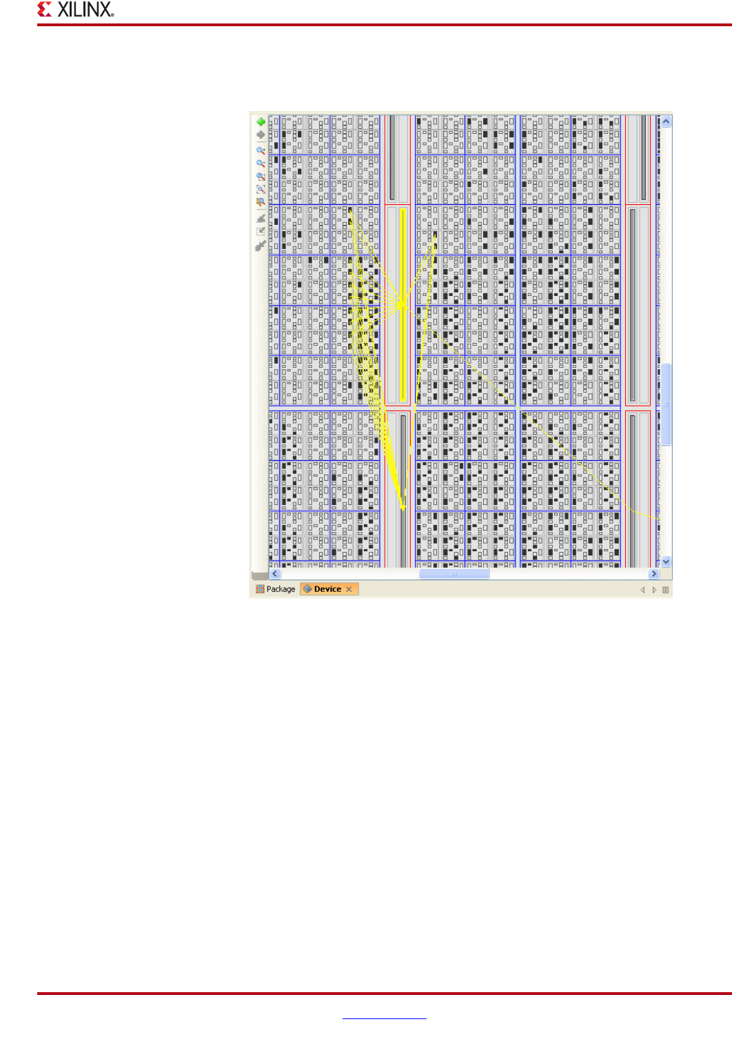
PlanAhead User Guide www.xilinx.com 107

UG632 (v 12.1)

Using Common PlanAhead Views

At the zoom level shown in Figure 4-34, page 107 the placed instances appear as rectangles

within a SLICE. When you increase the zoom level, the logic symbols display.

You can assign logic to specific sites that generate LOC placement constraints. Using BEL

constraints you can assign sites to specific gates or to a SLICE. All logic imported from ISE

displays as BEL-level constraints. For more information about LOC placement constraints,

see “Working with Placement LOC Constraints” in Chapter 11.

Displaying Clock Regions

The clock regions display as large rectangles indicating the periphery of the various device

clock regions. These outlines can help guide floorplanning for critical circuitry. In the

Device view, you can:

•Select the clock regions in the Clock Regions view.

•Select and specify that Clock regions display their resource statistical properties.

•View the clock placement statistics after importing the implementation results.

•Change the display color for Clock Regions in the Device view using the Device

dialog box, which is available by selecting Tools > Options > Themes.

When you select the clock region, the PlanAhead software selects the associated I/O banks

and clock related logic sites also.

Figure 4-34: Device View with Place Instance as Rectangles

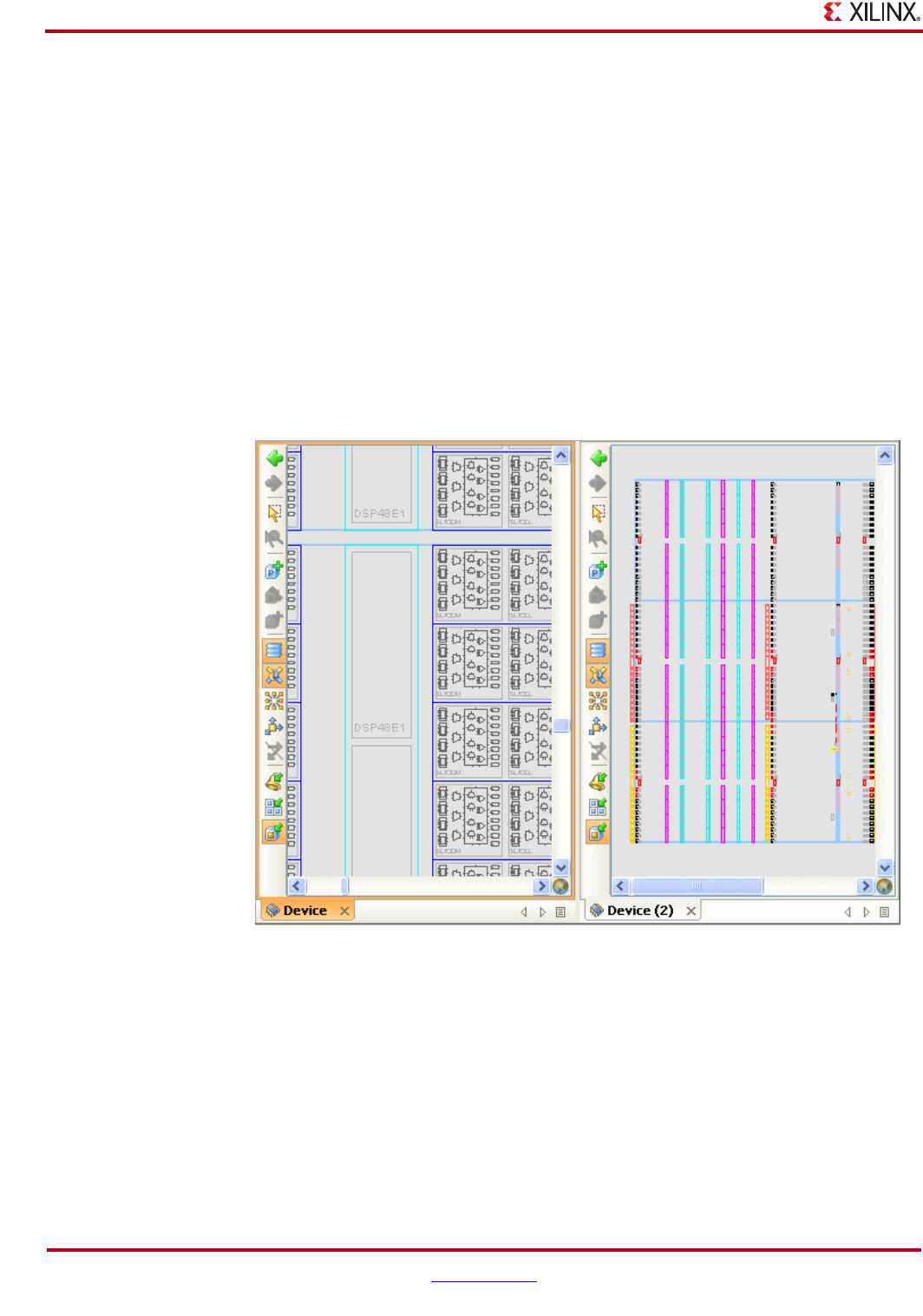
108 www.xilinx.com PlanAhead User Guide

UG632 (v 12.1)

Chapter 4: Using the Viewing Environment

See “Viewing Clock Region Resource Statistics” in Chapter 8 for more information about

displaying Clock region statistics.

Printing the Device View

You can print the Device view using the File > Print command, which prints the current

viewable area. To print the entire Device view, zoom to fit and then print.

Opening Multiple Device Views

You can open multiple Device views for the same floorplan (now referenced by the term

Design). This enables you to work on different areas of the device.

To open a second Device view display, select Window > New Device View. A separate tab

opens for the second Device view (Device (2)). You can then split the view using the

dragging technique described in the “Splitting the Workspace,” page 134 to view different

design aspects. The following figure shows an example of a split view.

Figure 4-35: Displaying Multiple Device Views

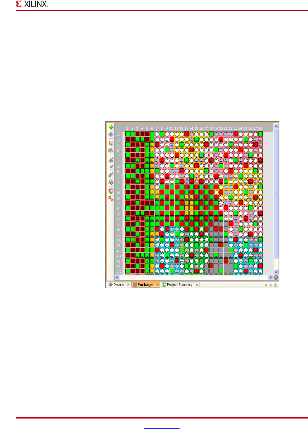
PlanAhead User Guide www.xilinx.com 109

UG632 (v 12.1)

Using Common PlanAhead Views

Using the Package View

The Package view displays the physical characteristics of the design device, and is used

primarily during the I/O pin planning process. Pin types display in different colors and

shapes for better visualization. For information about using the Package view for I/O pin

planning, refer to the Chapter 8, “I/O Pin Planning.”

To open the Package view, select on of the following:

•The Package view tab in the Workspace

•The Window > New Package View command.

You can open Multiple Package views simultaneously. The following figure shows the

Package view.

Moving the cursor within the Package view shows the I/O pin coordinates actively on the

top and left sides of the view. Additional I/O pin and bank information displays in the

Information bar located at the bottom of the PlanAhead environment. The Package view

highlights the active object.

When you hold the cursor over the Package view it invokes a tool tip that displays the pin

information, as shown in Figure 4-36.

You can:

•Drag ports and I/O buffer instances into the Package view for assignment and

reassign instances to other I/O pins within the Package view.

•View pins and I/O banks as follows:

−VCC and GND pins show as red and green square pins.

Figure 4-36: Package View

110 www.xilinx.com PlanAhead User Guide

UG632 (v 12.1)

Chapter 4: Using the Viewing Environment

−Clock-capable pins display as hexagon pins.

−The colored areas between the pins display the I/O banks.

•Select pins or banks by clicking them with the mouse.

•Select I/O pins or banks to highlight them in the Device view. Pins or I/O banks that

are selected in the Device view also highlight in the Package view.

•Display the differential pair pins in the Package view by toggling on the Show

Differential I/O Pairs toolbar button as shown in the following figure.

You can set the Package view to appear from the top or bottom of the package by clicking

the Show Bottom/Top View toolbar button, or by selecting the Show Bottom/Top View

button, which is shown in the following figure.

There are several toolbar buttons in the upper left corner of the Package view. These view-

specific Toolbar commands are described in Appendix A, “Common Popup Menu

Commands”.

Printing the Package View

You can print the Package view using the File > Print command that prints the current

viewable area. To print the entire Package view, zoom to fit and then print.

Using the Schematic View

You can generate a Schematic view for any level of the logical or physical hierarchy view.

In the Schematic view you can view design interconnect, hierarchy structure or trace signal

paths for either the elaborated RTL netlist or synthesized netlist.

See “Analyzing Run Results” in Chapter 6 for more information about analyzing RTL

netlist.

For more information about synthesized netlist analysis see Chapter 7, “Netlist Analysis

and Constraint Definition.”

You can select logic directly from the Schematic view for use in analysis and floorplanning

in the Device view.

To create a Schematic view:

1. Select one or more logic elements.

2. Right-click and select Schematic from the popup menu, or select the Schematic

toolbar button shown in the following figure.

The Schematic view displays the selected logic instances or nets. If only one instance is

selected, the module shows with all pins displayed as shown in Figure 4-40, page 111.

Figure 4-37: Show Differential I/O Pairs Toolbar Button

Figure 4-38: Show Bottom/Top View Toolbar Button

Figure 4-39: Schematic Toolbar Button

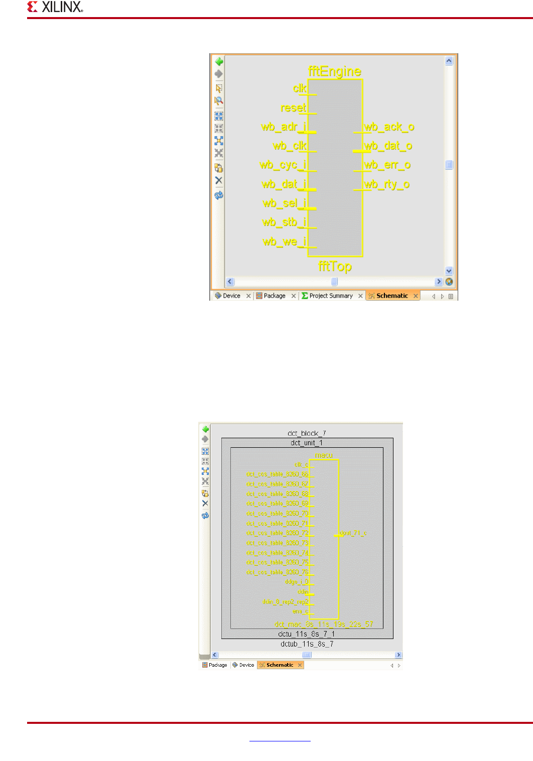
PlanAhead User Guide www.xilinx.com 111

UG632 (v 12.1)

Using Common PlanAhead Views

When you select objects in the Schematic view those objects display in all other views. If

you have opened an Implemented Design, the logic and paths display in the Device view.

Viewing Logic Hierarchy in the Schematic View

Upper levels of hierarchy display as concentric rectangles when a Schematic view is

generated, as shown in the following figure.

Figure 4-40: Schematic View

Figure 4-41: Viewing Hierarchy in the Schematic

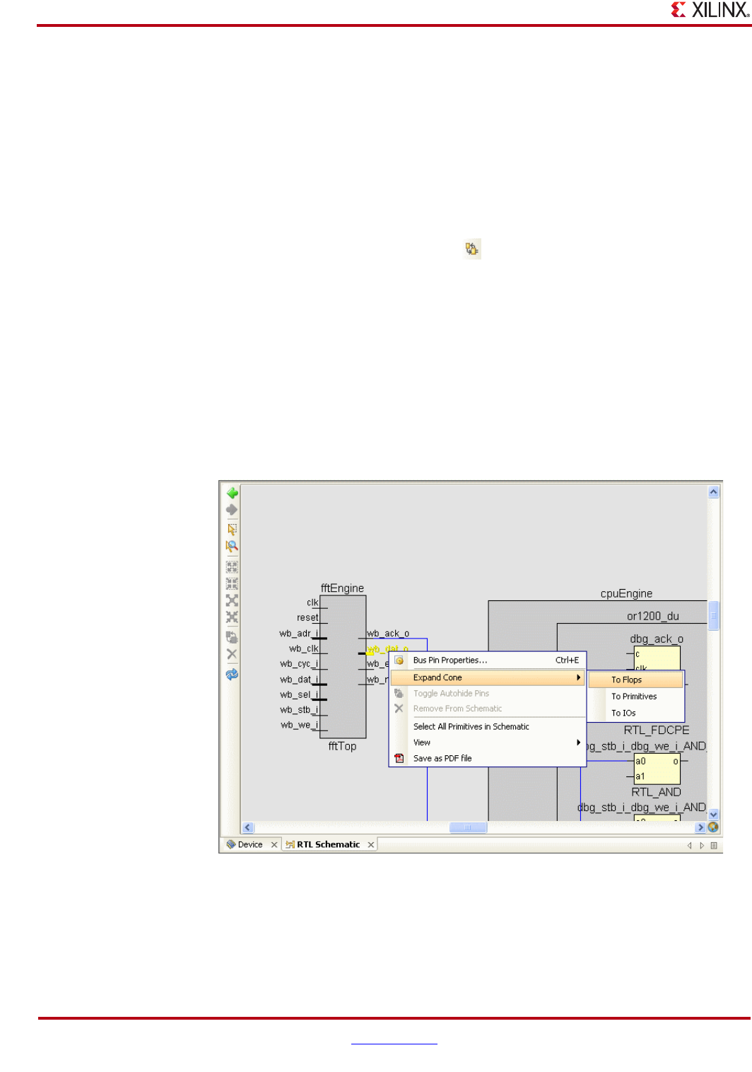
112 www.xilinx.com PlanAhead User Guide

UG632 (v 12.1)

Chapter 4: Using the Viewing Environment

Notice that no pins are displayed for the upper levels of hierarchy in Figure 4-41, page 111.

In most cases, the lack of pins makes the Schematic view more readable. You can:

•Individually expand or collapse module pins and logic.

•Selectively expand the logic either from individual pins, instances, or the entire logic

content inside or outside the module.

To expand module pins for a selected module, use the Toggle Autohide Pins command or

the Toggle Autohide Pins for selected instance toolbar button in the Schematic view, which

is shown in the following figure.

Expanding Logic from Selected Pins

Several options exist to expand logic from a pin.

•Double-clicking a pin causes the logic net to expand all the way to the next primitive

logic elements.

•Busses show as thick wires. Busses can be expanded to include all bits of the bus.

Expansion of signals can go beyond hierarchical boundaries, as shown in the following

figure.

Other expansion options exist to expand logic to the next set of flip-flops or to the I/Os. If

too much logic is selected for expansion, a dialog box opens that indicates the selected

logic is not be suitable for schematic viewing.

Figure 4-42: Toggle Autohide Pins for Selected Instances Toolbar Button

Figure 4-43: Expansion of Signals in Schematic View

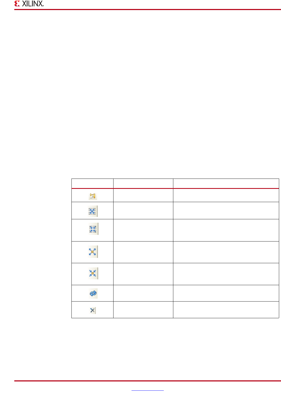
PlanAhead User Guide www.xilinx.com 113

UG632 (v 12.1)

Using Common PlanAhead Views

To view the logic expansion options, select a pin or an instance and select the Expand

Cone popup menu command to view the options.

The available Expand Cone logic expansion options are:

•To Flops—Appends the view to display the entire cone of logic to the first flops or to

any sequential element, such as block RAMs, FIFOs, and embedded processors.

•To Primitives—Appends the view to display the entire cone of output logic to the

first primitives. This is also the default behavior when a pins in double-clicked.

•To I/Os—Appends the view to display the entire cone of output logic to the I/Os. This

can involve a large amount of logic. PlanAhead sends a warning and allows you to

cancel the command if more than 10 levels of logic are to be appended.

Expanding and Collapsing Logic for Selected Instances or Modules

You can expand or collapse logic contained either inside a selected module or outside in

the next level of hierarchy instantaneously. You can run a new set of commands on either

a single module or multiple selected modules. These commands are available from the

right-click popup menu or from the Schematic view toolbar buttons.

Schematic View Toolbar Buttons

The following table describes the Schematic view toolbar buttons.

The commands are intended to display all logic associated within a level of hierarchy, as

shown in Figure 4-44, page 114 in which the Expand Inside command is used.

Table 4-1: Schematic View Toolbar

Toolbar Button Command Description

Schematic toolbar Opens the schematic toolbar.

Expand all logic inside

selected instance

Expands all logic inside selected instance.

Collapse all logic

inside selected

instance

Collapses all logic inside selected instance.

Expand all logic

outside selected

instance

Expands all logic outside selected instance.

Collapse all logic

outside selected

instance

Collapses all logic outside selected instance.

Regenerate schematic Regenerates the schematic.

Remove selected

schematic

Removes the selected schematic.

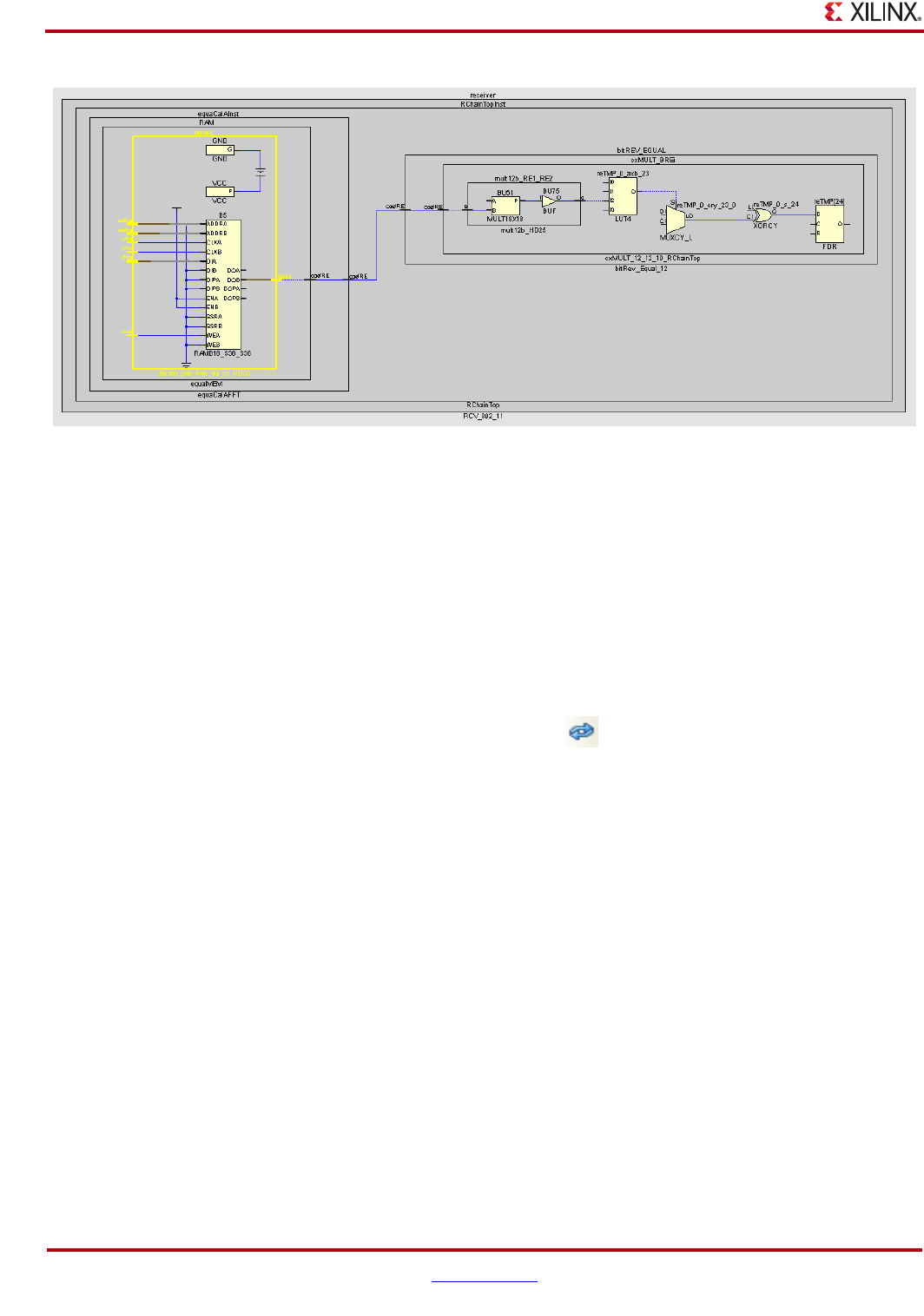
114 www.xilinx.com PlanAhead User Guide

UG632 (v 12.1)

Chapter 4: Using the Viewing Environment

Traversing the Schematic Hierarchy

You can double-click on a hierarchical instance to collapse the displayed logic and expand

the logic within the selected module. To go up a level of hierarchy, use the Expand

Outside command in conjunction with the Collapse Inside command.

Regenerating a Schematic View

Occasionally, after several expand and collapse commands, the Schematic view needs to be

refreshed. You can force a Schematic view regeneration by selecting the Regenerate

schematic toolbar command in the Schematic view, which is shown in the following figure.

This command redraws the active Schematic view.

Selecting Objects in the Schematic View

The following are object selection options for the Schematic view:

•Left-click an object in the Schematic view

•Use the Ctrl key to select multiple objects

•Use Select Area command and draw a rectangle around multiple instances, ports

and nets

When you select instances in the Schematic view, they are also selected in all other views.

The cross-selection works when you select or highlight objects in other views so they are

highlight in the Schematic view also.

The Schematic view popup menu commands are described in “Schematic View-Specific

Popup Menu Commands,” page 115.

Figure 4-44: Displaying All Logic Within a Level of Hierarchy

Figure 4-45: Regenerate Schematic Toolbar Button

PlanAhead User Guide www.xilinx.com 115

UG632 (v 12.1)

Using Common PlanAhead Views

Removing Objects From the Schematic View

You can remove selected objects and their associated connectivity using the Remove

Selected Elements From Schematic toolbar command in the Schematic view, which is

shown in the following figure.

Printing the Schematic View

You can print the Schematic view using the File > Print command, which prints the current

viewable area. To print the entire Schematic view, zoom to fit and then print.

Schematic View-Specific Popup Menu Commands

You can select instances and nets within the Schematic view for manipulation. The

common popup menu commands are covered in the “Common Popup Menu Commands”

in Appendix A. The Schematic view commands and a brief description of each is as

follows:

•Expand Cone—Appends the view to display the entire cone of input logic either to

the first primitives, flip-flops, or to the I/Os.

•Toggle Autohide Pins—Toggles the display of module pins for selected modules.

•Remove Selected Elements From Schematic—Removes the selected objects from

the schematic.

•Expand Inside—Expands logic contained inside of selected modules.

•Expand Outside—Expands logic contained outside of selected modules. The

expansion will only occur on the parent module logic.

•Collapse Inside—Collapses logic contained inside of selected modules.

•Collapse Outside—Collapses logic contained outside of selected modules. The

collapsing will only occur on the parent module logic.

•Select All Primitive in Schematic—Selects displayed primitive logic in the active

schematic fit view.

•Select Primitive Parents (available only when instances are selected)—Selects all of

the parent logic modules of the selected logic.

Annotating Schematic Design Information

Annotating Slack, Fanout, and Values onto Schematic Pins

The PlanAhead Schematic options dialog box lets you tag source pins with Fanout values

and destination pins with Slack values. Slack values do not display until after timing

analysis.

To access the PlanAhead Options dialog box, select Tools > Options > Schematic.

1. To annotate these values, you must first set the Attribute type field to Pin.

2. Select the values to annotate on the left of the following dialog box, and use the arrow

indicators to move them to the right side labeled Displayed DB Attributes.

3. Click OK.

Figure 4-46: Remove Selected Elements From Schematic Toolbar Button

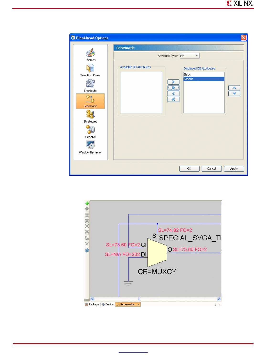
116 www.xilinx.com PlanAhead User Guide

UG632 (v 12.1)

Chapter 4: Using the Viewing Environment

The following figure shows the PlanAhead Options dialog box.

The following figure shows an example of the resulting pin annotation.

Figure 4-47: PlanAhead Options: Schematic Pin Annotation

Figure 4-48: Annotated Pins in the Schematic View

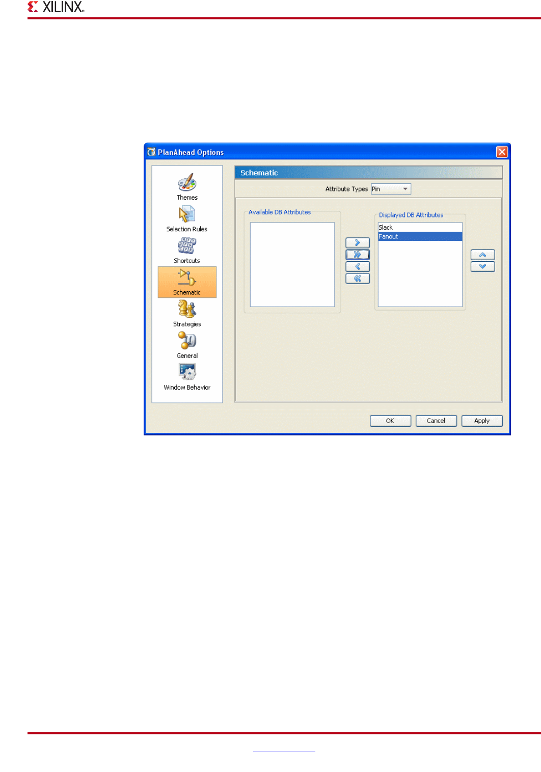
PlanAhead User Guide www.xilinx.com 117

UG632 (v 12.1)

Using Common PlanAhead Views

Annotating Cell References and Instance Equations onto Instances

The PlanAhead Options dialog box Schematic options let you tag instances with Cell

References and Instance Equation values.

The PlanAhead Options dialog box is available by selecting Tools > Options >

Schematic. The following figure shows the Schematic options in the PlanAhead Options

dialog box.

1. Set the Attribute type field to Instance.

2. Select the values to annotate on the left side of the dialog box shown in Figure 4-49,

and use arrows to move them to the right side labeled Displayed DB Attributes.

3. Click OK.

Figure 4-50, page 118 is an example of the resulting instance annotation.

Figure 4-49: PlanAhead Options: Schematic Instance Annotation

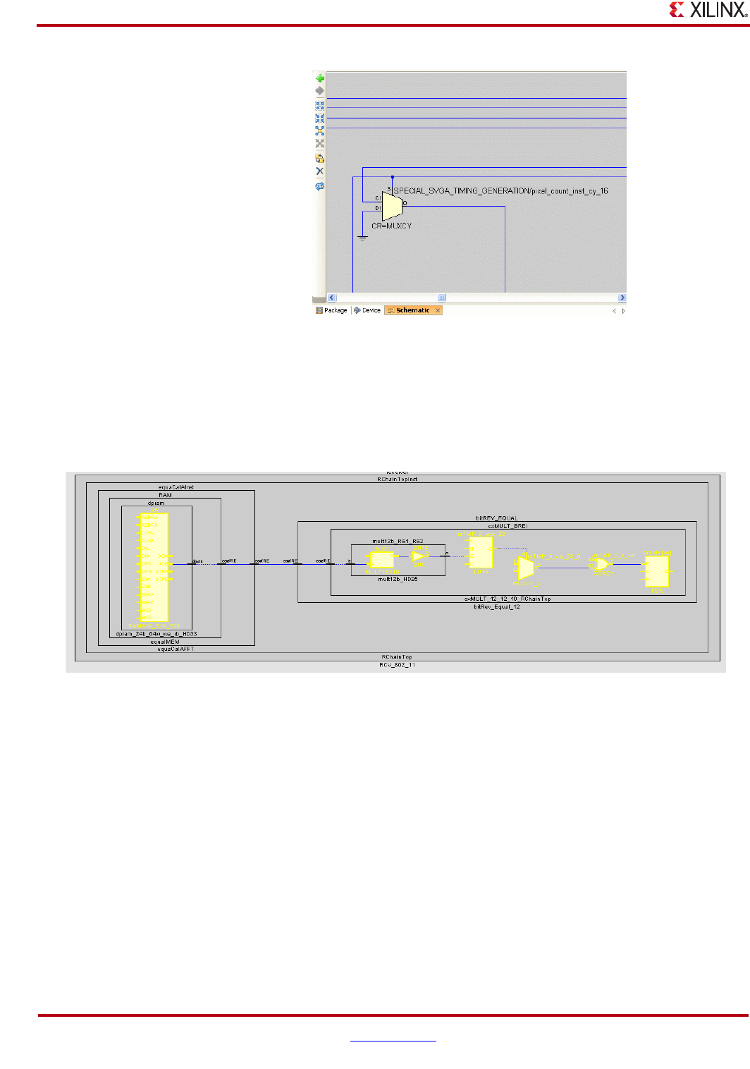
118 www.xilinx.com PlanAhead User Guide

UG632 (v 12.1)

Chapter 4: Using the Viewing Environment

Viewing Timing Path Logic in the Schematic View

You can select Timing paths from the PlanAhead Timing Results view and the paths then

display in the Schematic view. All of the objects on the selected path or group of paths

display with the logic hierarchy boundaries and the interconnect wires, as shown in the

following figure.

See Chapter 7, “Netlist Analysis and Constraint Definition” and Chapter 10, “Analyzing

Implementation Results” for more information about setting the timing path logic.

Note: Occasionally, paths displayed from trace TWX or TWR format timing reports are missing

interconnect wires. This because the logic was optimized out of the path during ISE implementation.

The objects that display in the Schematic view are all of the actual objects contained in the selected

paths; however, PlanAhead cannot interpolate the connectivity after objects have been optimized

away and no longer exist. You can use the Schematic view in conjunction with the Path Properties to

trace the path connectivity. Usually the schematic is drawn is such a way that it is easy to see the path

direction. For more information, see “Analyzing Timing Results” in Chapter 7.

Figure 4-50: Annotated Instances in the Schematic View

Figure 4-51: Logic Hierarchy in Schematic View

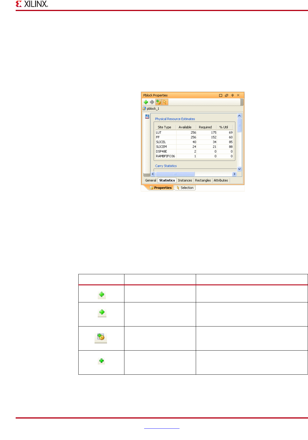
PlanAhead User Guide www.xilinx.com 119

UG632 (v 12.1)

Using Common PlanAhead Views

Using the Properties View

The Properties view displays information about any selectable logic object or device

resource. As you select objects, their properties appear in the Properties view

automatically. The Properties dialog box is dynamic by default; as you select new items,

the view updates automatically.

To open the Properties view, select an object and use the <Object-type> Properties

popup menu command.

Many objects have multiple types of properties displayed. View tabs are added to the

bottom of the Properties view to accommodate various types of information. Select the

different tabs to display or modify information about the selected object, as shown in

Figure 4-52.

Using the Properties View Commands

The Properties view toolbar contains the commands shown in the following table:

Figure 4-52: Property View With Tabs

Table 4-2: Properties View Toolbar

Toolbar Button Command Description

Previous object Reverts to the previously selected objects.

Next object Reverts to the next selected objects (This key

is only enabled after a Previous object

command).

Automatically update the

contents of this window

for selected objects

Toggles the Properties view to auto-update

as new objects are selected or remain static

on the originally selected object.

New Adds a new object. This option is only

available for certain object types and in

specific view panes.

120 www.xilinx.com PlanAhead User Guide

UG632 (v 12.1)

Chapter 4: Using the Viewing Environment

Using the Netlist View

The netlist is a hierarchical representation of the logic design beginning with the top-level

netlist name followed by top-level modules.

The Netlist view displays the logic instances and nets contained in the design. The netlist

can be navigated by expanding and collapsing the logic tree. Scroll bars are used to view

the entire netlist tree.

The default netlist tree setting is to expand and scroll the netlist object dynamically when

they are selected in other views. To disable this feature, select the Automatically scroll to

selected objects toolbar button in the Netlist view. The following figure shows the Netlist

view.

Delete Deletes an object from within one of the

property tabs.This option is only available

for certain object types and in specific view

panes.

Export statistics Saves data to file for later analysis. Available

from the Statistics tab for the Pblock, Clock

Region and Instance Properties view only.

Select/Unselect object Sometimes the object whose properties you

are viewing becomes unselected. Use this

button to select/unselect this object.

Group by Interface or

Bus or Group by I/O

bank

Groups the selected items by interface or

bus.

Show Search

Opens a search dialog box.

Fit Selection Zoom fit the selected objects.

Table 4-2: Properties View Toolbar

Toolbar Button Command Description

PlanAhead User Guide www.xilinx.com 121

UG632 (v 12.1)

Using Common PlanAhead Views

Figure 4-53: Netlist View

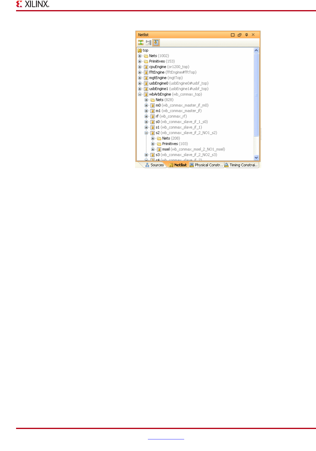
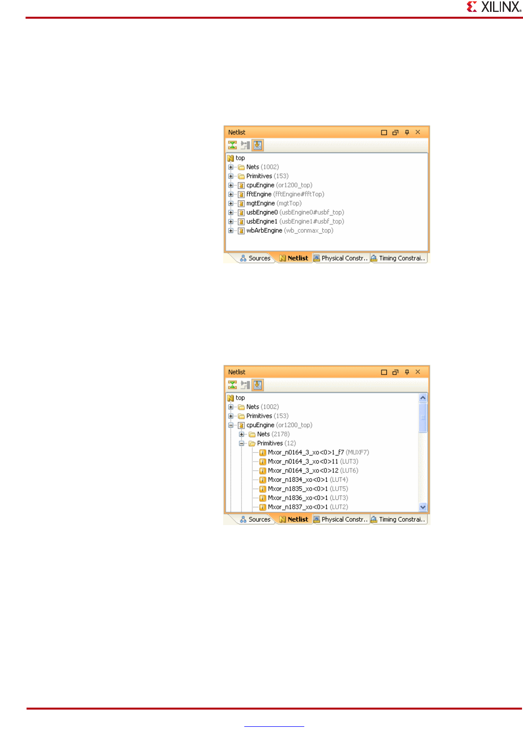
122 www.xilinx.com PlanAhead User Guide

UG632 (v 12.1)

Chapter 4: Using the Viewing Environment

Collapsing the Netlist Tree

The entire netlist tree can be collapsed by selecting the Collapse All toolbar button in the

Netlist view. For more information, see “Using View Specific Toolbar Commands,”

page 138. The Netlist tree collapses to display only the top-level logic modules, as shown

in the following figure.

Using the Primitives Folder

When a module contains primitive logic, the primitive logic is placed in a Primitives folder.

This helps condense the display of the modules in the Netlist view, and is shown in the

following figure

You can assign the Primitives folder directly to a Pblock resulting in all primitives being

assigned.

Note: Netlist updates might require reassignment of the Primitives folder to the Pblock because

logic names might have changed during re-synthesis.

Figure 4-54: Collapsed Netlist Tree

Figure 4-55: Primitives Folder in the Netlist View

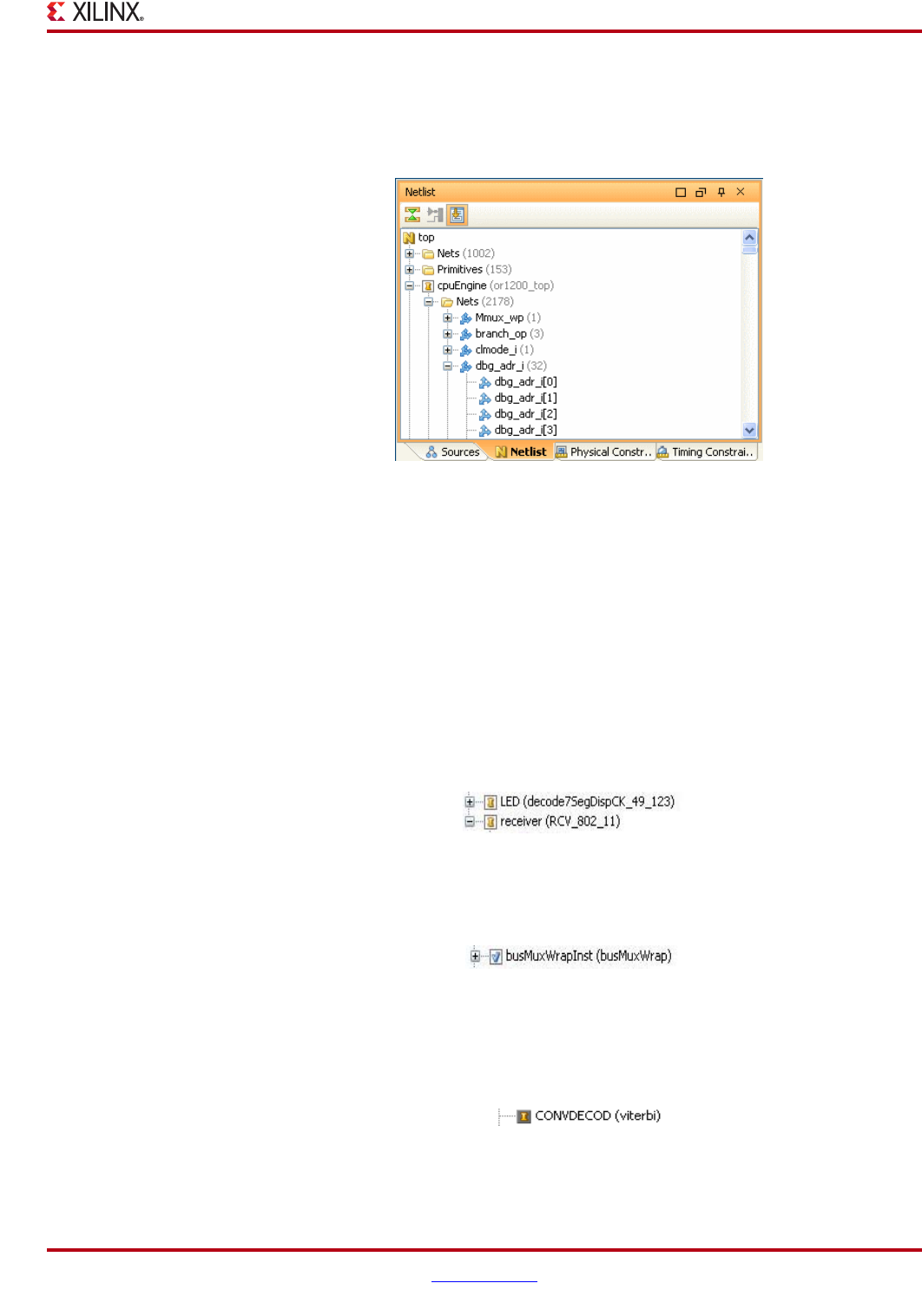
PlanAhead User Guide www.xilinx.com 123

UG632 (v 12.1)

Using Common PlanAhead Views

Using the Nets Folder

The Nets folder contains all of the nets and busses defined at any level of hierarchy. You

can expand busses to show each individual bit, as shown in the following figure.

When you select nets, they highlight in the Device view. Selecting a bus highlights all nets

contained within that bus. You can view nets in the Schematic view.

You can select nets for ChipScope tool debug testing by using the Add to ChipScope

Unassigned Nets command. See “Connecting and Disconnecting Nets to Debug Cores”

in Chapter 12.

Understanding the Netlist View Icons

Various icons are used to represent the state of the netlist logic.

Hierarchical netlist modules

Hierarchical netlist modules or “instances” are displayed with a yellow I icons, as shown:

Hierarchical netlist modules assigned to Pblocks

Hierarchical netlist modules or “instances” are assigned to Pblocks are displayed with blue

checkmark icons, as shown.

Black box Modules

Modules that do not have netlists associated with them are displayed with a yellow I icon

and a dark background as shown in the following figure. This could be a result of a search

path not being specified during project creation or missing portions of the design.

Figure 4-56: Nets Folder in Netlist View

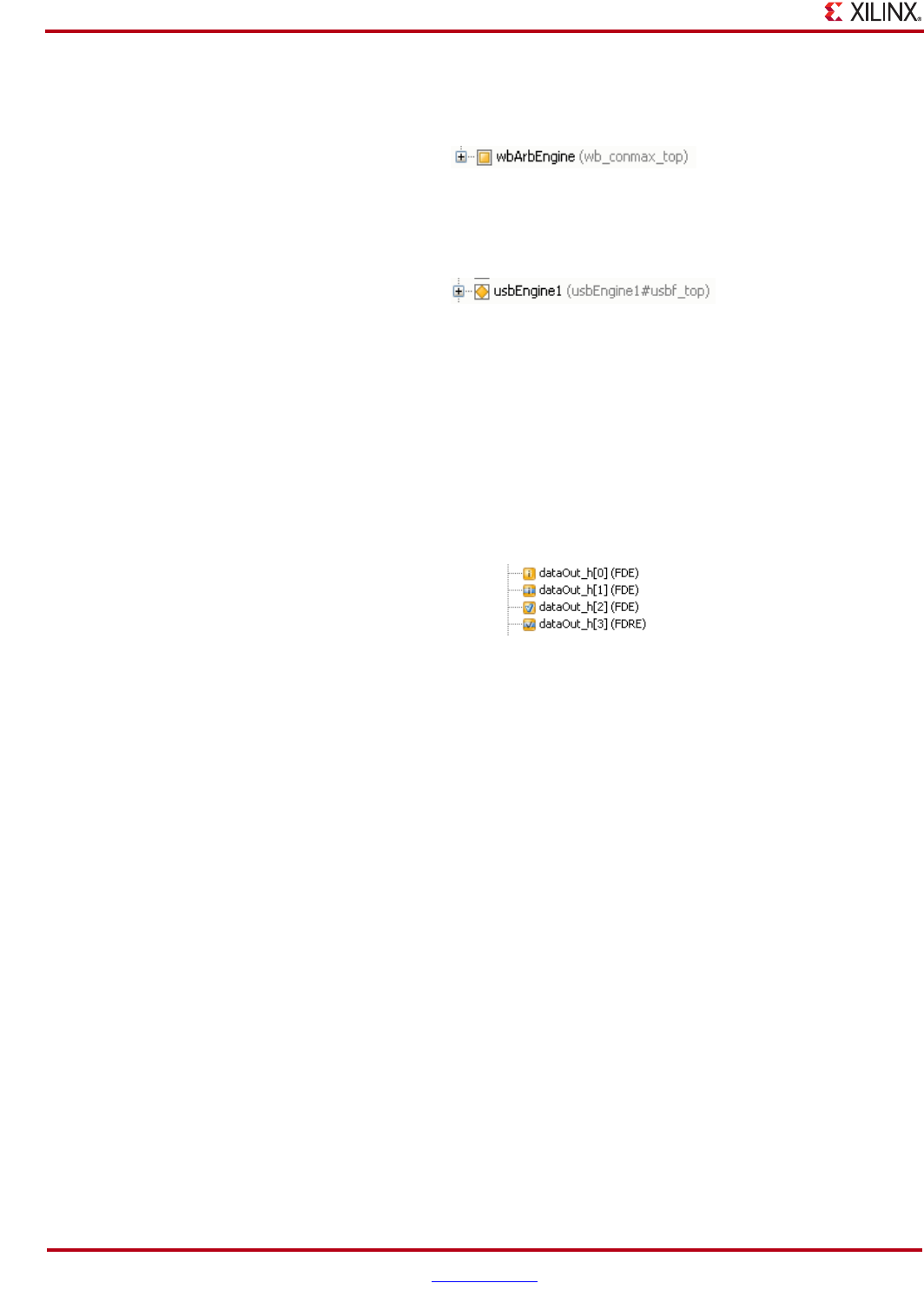
124 www.xilinx.com PlanAhead User Guide

UG632 (v 12.1)

Chapter 4: Using the Viewing Environment

Partition Modules

Modules that have been set as Partitions using the Set Partition popup menu command.

Partial Reconfiguration Partition Modules

Modules that have been set as Reconfigurable Partitions using the Set Partition menu

command in a PlanAhead Partial Reconfiguration Project.

Primitive logic instances

Primitive logic instances display as follows:

•Without placement constraints assigned display as an “i” inside a yellow rectangle.

•With placement constraints assigned display a yellow rectangle with a blue stripe.

•Assigned to a Pblock display a blue checkmark inside a yellow rectangle.

•Placed and assigned to a Pblock display a checkmark and blue stripe in a yellow

rectangle.

Notice the logic types display also, as shown.

Selecting Logic in the Netlist View

You can select instances and apply commands using the menu, the toolbar, or using the

mouse context sensitive menu (popup menu).

Use the Shift key or the Ctrl key to select multiple elements in the Netlist view for use with

most commands. Selected logic is highlighted in the Netlist view.

Logic selected by any means in PlanAhead displays as selected in the Netlist view. The

Netlist tree will expand automatically to display all selected logic. You might need to scroll

the tree to view all selected logic. Collapsing the Netlist tree does not unselect logic.

Using the Netlist View Commands

For more information on the popup menu commands available from the Netlist View, see

Appendix A, “Common Popup Menu Commands.”

Using the Hierarchy View

The Hierarchy view is used to visualize the logic hierarchy. You can see the relationship

between selected modules as well as their relative sizes. This view is used primarily during

design analysis and floorplanning. It is often helpful to see how a timing path traverses the

logic hierarchy, or to gauge how big a module is before you floorplan the module.

The Hierarchy view displays a graphical view of the logic hierarchy for both the elaborated

RTL design or the synthesized netlist design. Viewing the design from top to bottom, you

can identify module sizes and location within the design.

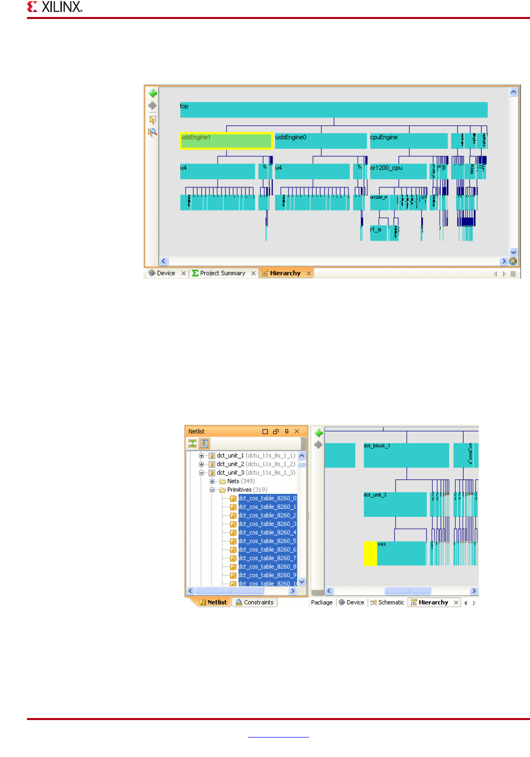
PlanAhead User Guide www.xilinx.com 125

UG632 (v 12.1)

Using Common PlanAhead Views

In the popup menu, select the Show Hierarchy command to invoke the Hierarchy view,

shown in the following figure.

Only hierarchical instances display in the Hierarchy view. Primitive logic is grouped into

folders that are represented as submodules. Refer to the “Using the Netlist View,” page 120

for more information about primitive logic folders. The widths of the blocks in the

Hierarchy view are based on the relative FPGA resources, including LUTs, flip-flops, block

RAMs, and DSP48s.

When you select logic it is highlighted so you can see where critical logic resides in the

design. The module highlights proportionally to the amount of logic selected, as shown in

the following figure.

When you double-click on a module in the Hierarch view a sub-hierarchy for any

submodules displays also.

To select logic parent modules for Pblock assignment in this view, use the Select Primitive

Parents command.

Figure 4-57: Hierarchy View

Figure 4-58: Display Percentage of Logic Selected in Module

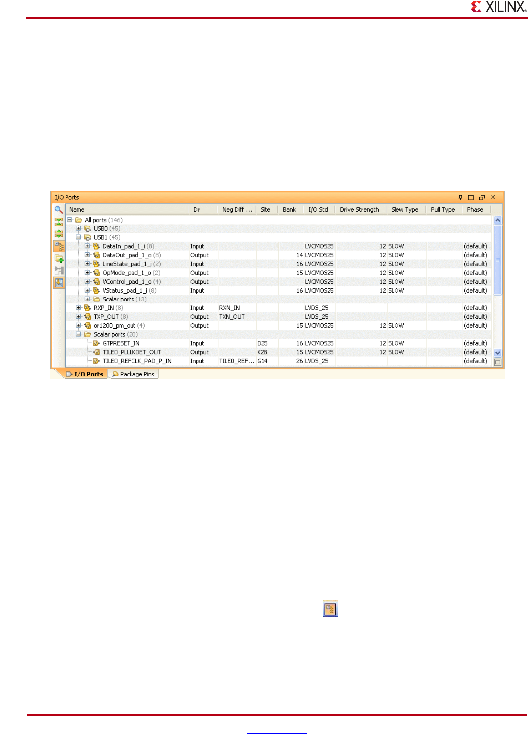
126 www.xilinx.com PlanAhead User Guide

UG632 (v 12.1)

Chapter 4: Using the Viewing Environment

Using the I/O Ports View

The I/O Ports view is used to create, configure, and place I/O ports onto I/O sites in either

the Package view or Device view. The I/O Ports view shows the I/O signal ports defined

in the design.

These ports can be created manually or by importing a CSV I/O port list.

Creating projects with an RTL Header, RTL sources, or synthesized netlists populates the

I/O Ports view with the I/O ports defined in the design.

To invoke the I/O Ports view, select Window > I/O Ports. The following figure shows the

display.

The Port view lists port signal names, direction, package pin, bank, I/O Standard, Drive

strength, Diff pair partner, Slew type, and other signal information for each I/O port.

Table values appear blank if they are default values, or with an asterisk (*) for non-default

values, and red when they are illegal or undefined values.

Busses are in expandable folders that can be selected as one object for analysis,

configuration and assignment.

Using I/O Ports View Commands

Refer to “Menu and Toolbar Commands” in Appendix A for a full list of menu and toolbar

commands.

You can display the ports according to category by interface, or alphabetically by clicking

the Group by Interface or Bus button in the I/O Ports view, as shown in the following

figure.

Figure 4-59: I/O Ports View Displaying I/O Ports

Figure 4-60: Group by Interface or Bus Toolbar Button

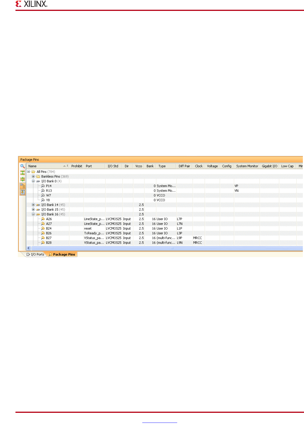
PlanAhead User Guide www.xilinx.com 127

UG632 (v 12.1)

Using Common PlanAhead Views

•To create I/O Ports manually, use the Create I/O Ports toolbar button.

•To select and group ports together into interfaces, use the Create I/O Port Interface

toolbar button or popup menu command You can select and place these interfaces as

one object within the I/O Planner environment.

•To open the Schematic viewer for selected I/O ports, select the Schematic toolbar

button.

You can select ports and interfaces from the I/O Ports view and assign them using the I/O

Planner environment. See “Using Tree Table Style Views,” page 136 for more information

about using the tree table style views.

Using the Package Pins View

The Package Pins view is used to display I/O related package information. The table can

be sorted and filtered in many ways to analyze the I/O pins and I/O ports information.

To invoke the Package Pins view, select Window > Package Pins. The following figure

shows the Package Pins view.

Device pin information such as I/O Bank number, Type, Differential pair partners, Site

Types, and Min/Max package delay are listed for each package pin. Table values appear as

follows:

•Gray for default values

•Black for non-default values

•Red for illegal values

Note: The unit of measurement for the Min/Max package trace delay in the Package Pins view is in

picoseconds (ps).

You can sort the information in the Package Pins view by clicking any of the column

headers. Clicking again will reverse the sort order. To sort by a second column, press the

Ctrl key and click another column. Add as many sort criteria as necessary to refine the list

order. Sorted results may be more readable if you flatten the list of Package Pins using the

Group by I/O Bank toolbar button.

Refer to the “Using Tree Table Style Views,” page 136 for more information.

Figure 4-61: Package Pins View

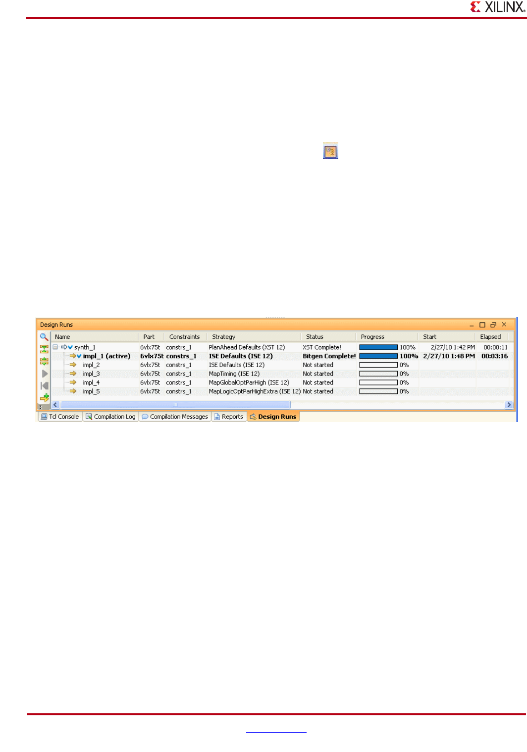
128 www.xilinx.com PlanAhead User Guide

UG632 (v 12.1)

Chapter 4: Using the Viewing Environment

Using Package Pins View Commands

Refer to the “Using View Specific Toolbar Commands,” page 138 for more information on

toolbar commands.

You can toggle to display pins according to category by I/O bank, or display the pins

alphabetically by clicking the Group by I/O Bank button in the Package Pins view, which

is shown in the following figure.

Using the Design Runs View

You can use the Design Runs view to view, configure, launch, and analyze synthesis and

implementation runs. As Runs are created, launched, or imported, the status shows in the

Design Runs view. The Design Runs view is used extensively in the Partial

Reconfiguration flow to create and manage various design configurations.

Select Tools > Design Runs to invoke the Design Runs view. The following figure shows

the Design Runs view.

The view displays the status and results of the design runs defined, and provides

commands to modify, import, launch, and manage the design runs. Also, this view is used

to manage and report synthesis and implementation runs.

The view indicates the runs as follows:

•Currently running with a green arrow icon. See Figure 7-4, page 193 for an example.

•Completed runs have a blue check mark icon.

Run information displays as the commands are being run. PlanAhead can be closed

without affecting runs in progress. When the project is re-opened, the run status is updated

to reflect the latest status, which displays in the Design Runs chart.

The columns used for tracking information are:

•Name—Displays run name.

•Part—Indicates the target part selected for the run.

•Constraint—Displays the constraint set used for the run.

Figure 4-62: Group by I/O Bank Toolbar Button

Figure 4-63: Design Runs View

PlanAhead User Guide www.xilinx.com 129

UG632 (v 12.1)

Using Common PlanAhead Views

•Strategy—Displays the strategy assigned to the Run. Strategies appearing with an

asterisk (*) indicate that the command option values in the Strategy have been

overridden in the Run Properties Options tab.

•Status—Indicates run status or the command that is currently running.

•Progress—Indicates overall progress of the entire ISE command sequence from

ngdbuild through XDL. The progress bar is non-linear, in that some steps may take

considerably longer then others.

•Start—Indicates the time ISE started working on the design.

•Elapsed—Indicates the total elapsed time for all ISE commands run on the design.

•Device Utilization (for Synthesis runs only) —Indicates the resulting LUT utilization

for the run.

•Fmax (for Synthesis runs only)—Indicates the expected clock frequency for the run

from the XST synthesis report.

•Timing Score (for Implementation runs only)—Indicates the current timing score on

the run in progress or after completion.

•Unrouted Nets (for Implementation runs only)—Indicates the current number of

unrouted nets on the run in progress or after completion.

•Description—Displays the description associated with the run. This description is set

initially to a strategy description when that strategy is applied to the run; however,

the description can be modified later.

The table is updated dynamically as the Run commands are progressing. Runs that are

launched outside of PlanAhead using the PlanAhead generated scripts cause the table to

update upon invoking PlanAhead.

Using the Design Runs View Popup Menu Commands

The Design Runs view popup menu contains the following commands:

•Synthesis or Implementation Run Properties—Displays the Run Properties view.

See for more information.

•Delete—Deletes the selected runs. You are prompted to confirm prior to removing

any runs.

•Make Active—Sets the selected run as the active run. This run will launch

automatically when the Implement command is used with the current selected set of

command and launch options.

•Save as Strategy—Lets you save any modifications made to the applied strategy to a

new strategy file for future use.

•Launch Runs—Invokes the Launch Runs dialog box to launch the selected runs.

•Reset Runs—Invokes the Reset Runs dialog box to remove previous run results and

to set the Run status back to Not Started for the selected runs.

•Open Implemented Design—Loads the resulting netlist from the synthesis run or

implementation results from ISE in to the PlanAhead analysis environment. The

active loaded run appears in bold text in the Design Runs view.

•Create Multiple Runs—Invokes the Create Multiple Runs dialog box to create and

configure multiple runs.

•Generate Bitstream—Invokes the Generate Bitstream dialog box to a create

bitstream. This command is available for completed implementation runs only.

130 www.xilinx.com PlanAhead User Guide

UG632 (v 12.1)

Chapter 4: Using the Viewing Environment

•Promote Partitions—Invokes the Promote Partitions dialog box to promote

implemented partitions.

•Launch FPGA Editor—Invokes FPGA Editor with the current implemented design.

•Launch ChipScope Analyzer—Invokes ChipScope analyzer with the current bit file.

•Launch iMPACT—Invokes iMPACT with the current bit file.

Working with Views

PlanAhead has different types of views for displaying different types of information.

Views can each be independently controlled with respect to size, visibility, and location.

Because all the PlanAhead views interact together, it is helpful to organize them in such a

way to easily facilitate analysis and interaction between them. The default view layout

shipped with PlanAhead is optimized; however, you can customize it at will. Custom view

layouts can be created to restore view preferences. Refer to “Creating Custom View

Layouts,” page 150 for more information.

Opening Views

From the Main Menu, select the Window menu for the commands to open most window

types. Select a window that is already open to make it the active window. For a list of

Window menu commands and a brief description, see “Toolbar Commands” in

Appendix A.

As certain commands are run, new views open to interact with the command or to display

results.

The Schematic view requires at least one object to be selected and is opened using the

popup menu Schematic command or the Schematic toolbar button.

The Properties view requires at least one object to be selected and is opened using the

popup menu <Object_type> Properties command.

Select New Device View or New Package View to open an additional view in the

Workspace.

Navigating Views

Each available view has a tab in the viewing area. You can activate a view by clicking on

the tabs. Some view types allow multiple tabs.

The active view displayed in any viewing area is toggled by using the tab interface at the

bottom of the view area. The following figure is an example of the Netlist view tab.

In views, the following actions are available:

•To display the view in the full screen, double-click the view tab.

•To restore workspace views, double-click the view tab again.

•Stretch the overall size of these viewing areas by sliding the view borders. The cursor

changes to a slider symbol you can use to stretch the view borders.

Figure 4-64: Netlist View Tab

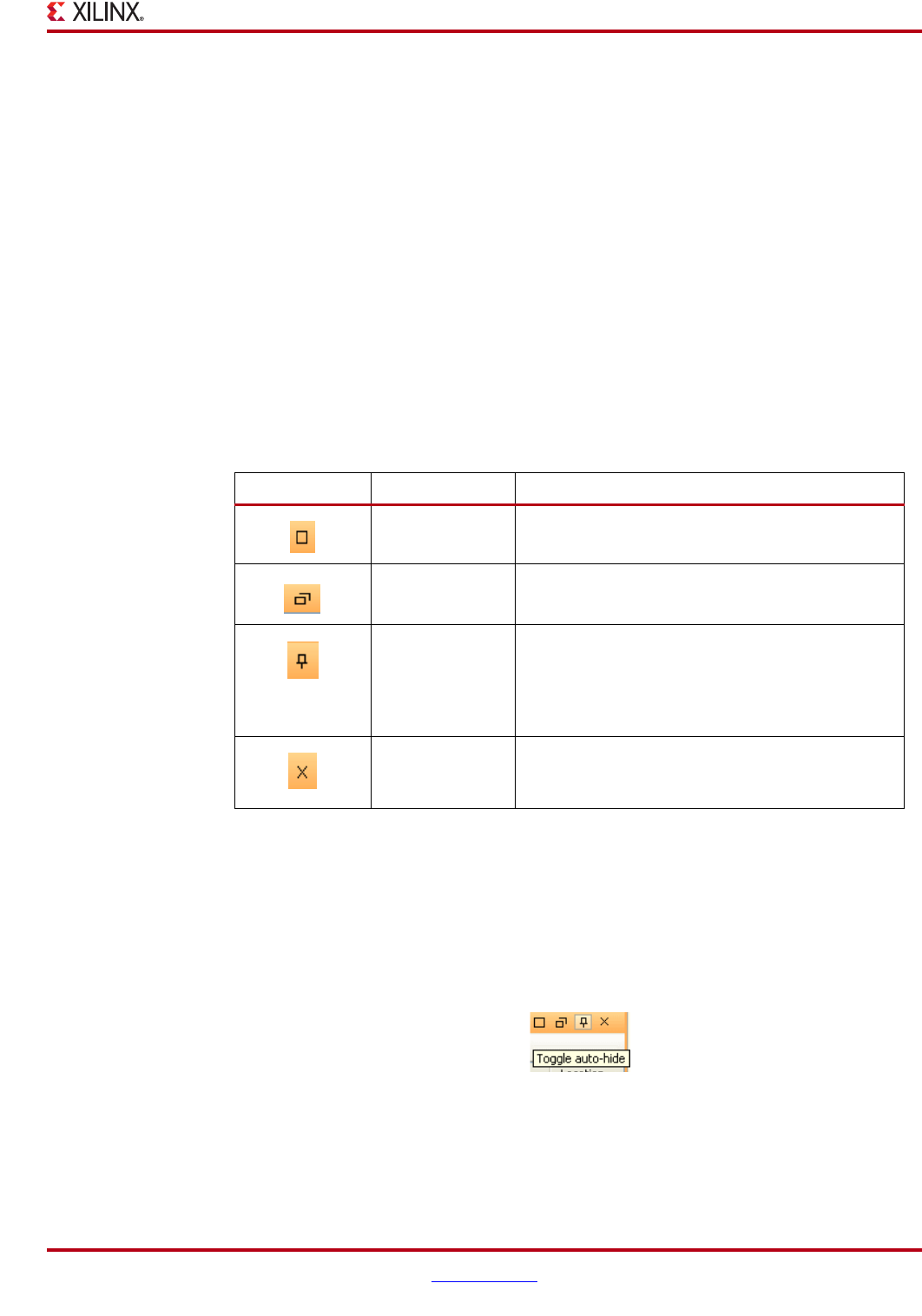
PlanAhead User Guide www.xilinx.com 131

UG632 (v 12.1)

Working with Views

•Move the views by selecting a view tab and dragging it.

This produces a rectangular box which indicates where the view is located after the

move. You can manipulate the rectangle within the viewing areas to split them either

horizontally or vertically to display multiple views at once.

Dropping a view onto an existing view tab produces another tab next to it for the newly

moved view. For more information, refer to “Configuring the Viewing Environment,”

page 143.

Manipulating Views using the View Banner Controls

Each view has a control box to manipulate the view. You can float, hide, maximize, or close

views to suit your needs. When you close one view or viewing area the views that remain

open resize to accommodate the available space. Control box commands are covered later

in this chapter.

Each viewing area can be manipulated using common window environment commands.

The following table shows the view banner commands and icons.

These commands are available using the right-click popup menu in the banner of the view

also.

Using the View Auto-Hide Capability

You can use an auto-hide mode to control display of the view areas.

To initiate auto-hide mode, click the view banner Toggle auto-hide button, or select the

Auto-hide command from the popup menu.

When Auto-hide is activated, the entire docking area appears as a tab on the perimeter of

the PlanAhead main window. The other docking areas resize to occupy the space. The

following figure shows the view in Auto-hide mode.

Table 4-3: View Banner Commands

Toolbar Button Command Description

Maximize/restore Maximizes and restores non-Workspace views.

Float Frame Floats and docks non-Workspace views. Views can

be floated outside of the PlanAhead main window.

Toggle auto-hide

Hides and restores the view. When hidden, the

entire Docking area opens as a tab at the perimeter

of the PlanAhead main window. The other docking

areas will occupy the space. To restore the view,

click the icon displayed on the tab.

Closes the window, leaving other tabs or docking

areas to occupy the space. To re-opened a window

or tab, use the Window menu commands.

Figure 4-65: Auto-hide Button in the View Banner

132 www.xilinx.com PlanAhead User Guide

UG632 (v 12.1)

Chapter 4: Using the Viewing Environment

Each auto-hide tab has an icon that can be used to restore the view to its original location.

Hover the cursor over an auto-hidden tab to display the view temporarily. To re-dock an

auto-hidden view, click the Toggle auto-hide button, or select the Auto-hide command

from the popup menu once again.

To undo the auto-hide mode, select Layout > Undo Toggle Autohidden/Docking Mode.

Floating Views

You can un-dock views, including the Workspace, from the display docking area so that it

“floats” and can be moved and sized independently. To float a window do one of the

following:

•Click on the view tab or banner

•Click the Toggle floating button

•Select Floating from the popup menu

When you activate the floating option, the view appears in a separate floating window. In

this case, windows obviously overlap.

You can move a floating window by dragging the view banner. You can move a floating

window outside of the PlanAhead main window. The default locations and sizes to display

all floating view types are stored in your saved layouts.

Figure 4-66: Views in Auto-hide Mode

PlanAhead User Guide www.xilinx.com 133

UG632 (v 12.1)

Working with Views

Using Graphical Workspace Views

The views with a graphical interface and those that require a lot of screen space like the

RTL Editor or the Report Viewer display in an area called the Workspace. These views are

different than other views because more than one can be opened simultaneously to view or

compare different information. They do not have the same view manipulation controls in

the view banner. These Workspace views can be made full size, floated or split by using the

popup menu commands on the view tab.

Understanding Workspace Views

The PlanAhead Workspace is the graphic viewing area, which displays the graphical views

and some report and log information. The views displayed in the Workspace are:

•Project Summary

•RTL Editor

•Device

•Package

•Schematic

•Hierarchy

•Reports and log files

Opening Workspace Views

You can open the Device and Package views in the Workspace by using the Windows

menu commands. You can open multiple views of the same view type within the

Workspace area. For example, two Device views can display different areas of the device.

To open a new Device or Package view, select Window > New Device View or Window >

New Package View.

To open a Schematic view:

1. Select at least one object to display in schematic format.

2. Select the Schematic command from the popup menu, press F4, or click the Schematic

toolbar button, which is shown in the following figure.

The Schematic displays in the Workspace. Running subsequent Schematic commands

opens additional Schematic views in the Workspace.

Viewing the Workspace Full Screen

You can get a full screen display of a view by double-clicking the Workspace tab. To restore

the Workspace, double-click the view tab again.

Also, you can right-click the tab to view the Workspace tab popup menu. Select either

Maximize Workspace or Restore Workspace from the popup menu depending on the

state of the Workspace.

Figure 4-67: Schematic Toolbar Button

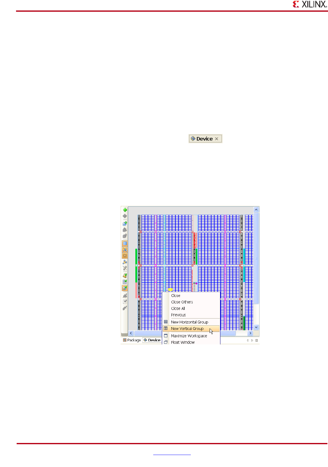
134 www.xilinx.com PlanAhead User Guide

UG632 (v 12.1)

Chapter 4: Using the Viewing Environment

Floating the Workspace View

To float the workspace, select the Workspace tab and use the Float Window popup menu

command.

Printing the Workspace View

You can print the view in focus in the Workspace—Device view, Package view, Schematic

view, and Instance Hierarchy view. Select File > Print to print the current viewable area.

Closing Workspace Views

You close the views within the Workspace by clicking on the X icon in a view tab, which is

shown in the following figure.

Splitting the Workspace

You can split the Workspace viewing area horizontally or vertically to enable multiple

simultaneously displayed views. Use the popup menu in the Device view to select the

split. The following figure shows the New Vertical Group option as selected.

Each panel now acts as an independent Device view allowing multiple views to be docked

for viewing as shown in Figure 4-70, page 135.

Figure 4-68: Device View Tab with X Icon

Figure 4-69: Splitting the Workspace Vertically

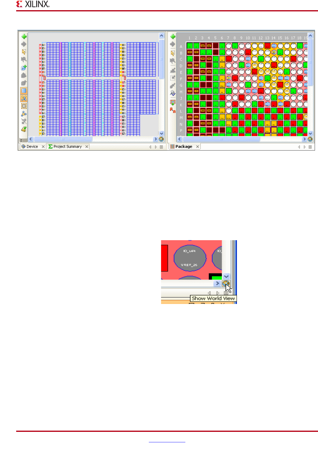
PlanAhead User Guide www.xilinx.com 135

UG632 (v 12.1)

Working with Views

Multiple views of the same type can be opened, such as two Device views for viewing

different areas of the device or different zoom levels.

Using the World View

The World view displays a less detailed overview of the active Workspace to enable a quick

pan of the viewed area. This capability is available in the Device, Schematic and Package

views. To invoke the World view, click the World view icon in the lower right-hand corner

of the Workspace viewing area, as shown in the following figure.

The World view reflects the zoom area and the selected objects for the active view for the

Schematic, Device, Package, and Hierarchy views.

A navigation rectangle displays the area that is visible in the active view. You can drag the

navigation rectangle to reposition the display area in the active view. You can use the resize

handlers to drag and resize the navigation rectangle. This adjusts the active view scale

factor (such as zoom in or zoom out) to match the new display area defined by the

navigation rectangle.

Selected Pblocks, instances, and I/O ports are highlighted in the World view for easier

location, as illustrated inFigure 4-72, page 136.

Figure 4-70: Two Workspace Views Displayed Vertically

Figure 4-71: World View

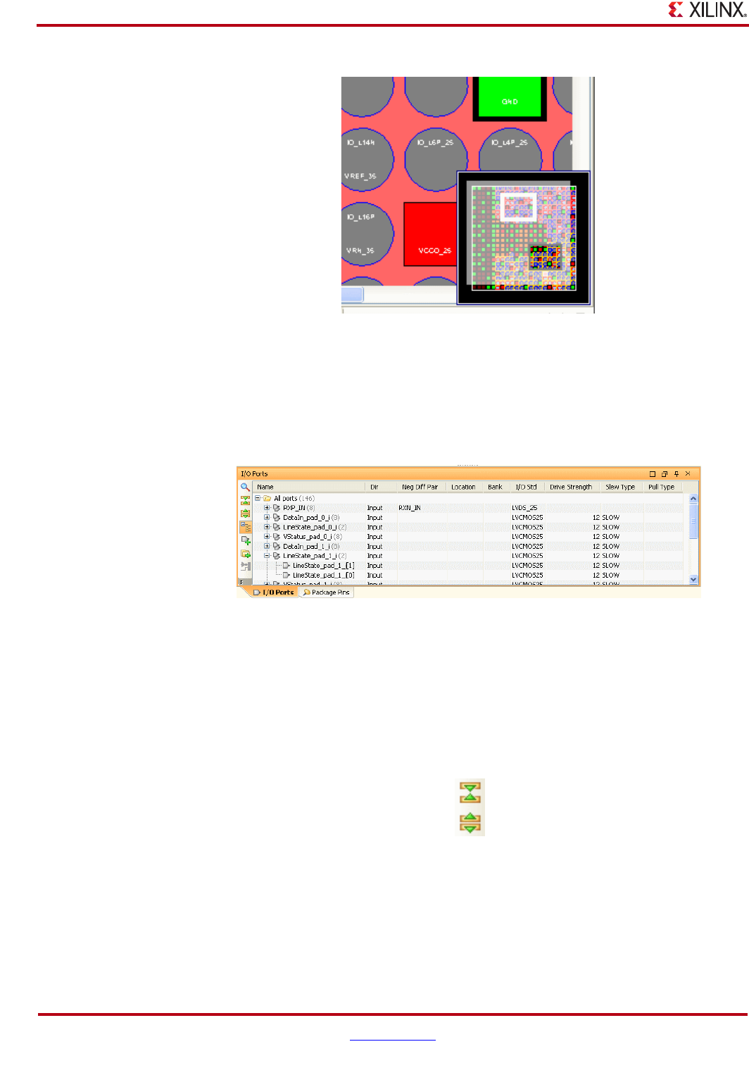
136 www.xilinx.com PlanAhead User Guide

UG632 (v 12.1)

Chapter 4: Using the Viewing Environment

Using Tree Table Style Views

PlanAhead has many similar views that look a lot like expandable spreadsheet tables.

These views all share some common characteristics and features described in the following

subsections, and illustrated in the following figure.

Expanding and Collapsing the Table

You can toggle the expand and collapse widgets in the Name column to expand or collapse

the tree independently.

The Expand All and Collapse All buttons expand or collapse the entire tree as shown in the

following figure.

Display the Entries Grouped or in a Flat List

Most of these style views have a Group by Type button or equivalent which will either

display the entries group by an expandable type or as a single flat list of entries.

Figure 4-72: View Panning with the World View

Figure 4-73: Tree Table Style View

Figure 4-74: Collapse and Expand All Buttons

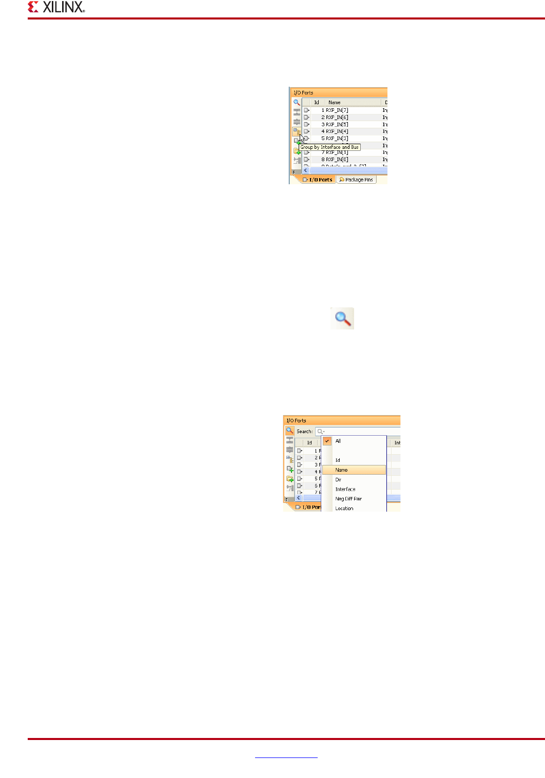
PlanAhead User Guide www.xilinx.com 137

UG632 (v 12.1)

Working with Views

Flattening the list is helpful to search and filter the overall list of entries as shown in the

following figure.

Using the Show Search Capability to Filter the List

You can click the Show Search button to display a search field in the banner of the view

enabling any text string to be entered to filter the list displayed in the table view. For best

results flatten the list first by using the Group by Type toggle button described in the

previous section. The following figure shows the Show Search button.

Any column in the table can be used as search filter criteria. Select the pull down menu in

the Search field to select a column header to search. The following figure shows the search

pull down menu.

Enter any text string and the list will adjust dynamically to list only those entries that

contain the string entered. Select the Show Search button again to remove the Search field

and sorting.

Sorting Columns

You can sort any table column by clicking in the column header. Clicking again will

perform a reverse sort. A visual indication of the sort order and direction displays in the

Column Header, as shown in the following figure.

Figure 4-75: Group by Type or Flat List Toggle Button

Figure 4-76: Show Search Button

Figure 4-77: Search Pull down Menu

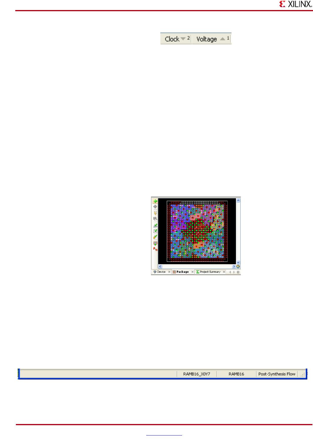
138 www.xilinx.com PlanAhead User Guide

UG632 (v 12.1)

Chapter 4: Using the Viewing Environment

Organizing Columns

You can move, hide, and restore columns.

•To move a column, select it and drag it into a new location.

•To hide a column, select it and use the popup menu in the column header to select the

Hide This Column command.

The popup menu also enables quick view configuration for each column.

•Auto Resize Column commands adjust the width of the columns per the data

displayed.

•The Reset to Default command restores PlanAhead defaults.

Using View Specific Toolbar Commands

Most views have toolbar buttons displayed within the view to operate commands specific

to that view as shown in the following example.

These buttons become enabled only when certain data is selected or commands are active.

PlanAhead features are made available through these view-specific toolbar buttons so it is

beneficial to become familiar with them. These view-specific commands are covered in

more detail in the specific view sections of this document.

Using the Information Banner

The information banner at the bottom of the PlanAhead main window displays useful

information as shown in the following figure.

Figure 4-78: Up/Down Sort Arrows

Figure 4-79: Example View-specific Commands

Figure 4-80: Information Banner

PlanAhead User Guide www.xilinx.com 139

UG632 (v 12.1)

Selecting Objects

The information banner displays the following information:

•Information Message—The first field in the Information Banner displays context-

sensitive information. For example, when the cursor is in the device view or the

schematic view, this field contains the name of the placed instance directly under the

cursor. The information message field also contains detailed description of PlanAhead

commands when the mouse is over its corresponding toolbar button or menu item.

•Coordinates—To the right of the Information Message field is the Coordinates field.

As the cursor moves over block RAM, DSP48, and other parts in the Device view, this

field displays the name and coordinates as shown in Figure 4-80, page 138. If the

cursor is over a pin in the Package view, this field displays pin information, such as

coordinates, type and name.

•Mode—The Mode field indicates the type of project, such as RTL Flow or Post-

Synthesis Flow. When PlanAhead is invoked from ISE Project Navigator, the ISE

Integration mode is displayed.

Understanding the Context Sensitive Cursor

The cursor changes based on the available command mode. When the cursor:

•Changes into a horizontal, vertical, or diagonal stretch bar symbol, you can stretch

Pblock edges and Windows view borders.

•Changes into a hand symbol, you can move Pblocks or instances.

•Changes into a cross symbol, you can draw rectangles for zooming in, defining pin

assignment areas, or drawing Pblock rectangles.

•Displays a slashed circle symbol, you are dragging objects are over illegal placement

sites.

•Displays a move point-to-point symbol, you are dragging objects over legal

placement sites.

Selecting Objects

There are multiple methods of objects selection in the PlanAhead software. Click the object

to select it in the current view. When selected in any view, objects also become selected in

the other appropriate views.

To move objects, hold the left mouse down and drag it, release to drop it on a location. The

cursor changes to a hand symbol when the move mode is activated.

When objects overlap, PlanAhead uses a priority scheme where the smaller size objects are

selected. If objects become difficult to select in the Device view, use the Physical

Constraints or Netlist views to select them. Objects can always be selected from either of

these two views regardless of the Selection Rule setting in the PlanAhead Options dialog

box.

If you experience difficulty selecting the correct object, the Select commands in the popup

menu can be used to select a specific item within the stack of items under the cursor.

Using the Select Main Menu Commands

Several of the Selection, Unselect, Highlight, and Mark commands are available from the

Select menu. For a description of all Select commands, see “Select Menu” in Appendix A.

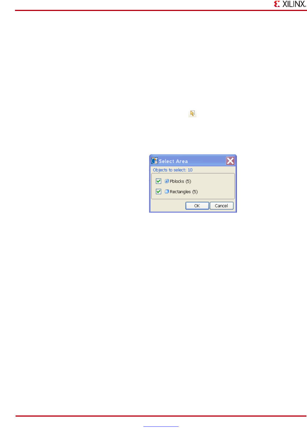
140 www.xilinx.com PlanAhead User Guide

UG632 (v 12.1)

Chapter 4: Using the Viewing Environment

Selecting Multiple Objects

In most selectable views and dialog box lists, you can select multiple objects by pressing

and holding the Shift key to select a range of elements in a tree or table. The Ctrl key is

used to select multiple elements individually.

Using the Select Area Command

You can draw a rectangle in any of the Workspace views in to select objects as follows:

1. Choose Select > Select Area, or click the Select Area toolbar button as shown in the

following figure.

All objects that the rectangle surrounds or touches are listed in the Select Area dialog

box, with which you can filter selection by type shown in the following figure.

2. Turn off the check box to filter Object types from selection.

3. Click OK to select all of the checked objects.

Selecting Primitive Parent Modules

The Select Primitives Parent command lets you select the parent modules for all selected

primitive logic. To access the command, select Select Primitive Parents from the popup

menu (available in most views).

Floorplans are much easier to maintain when logic modules are assigned to Pblocks rather

than primitive logic instances.

You can select a group of timing paths that selects the primitive logic instances contained

on the paths. The Select Primitive Parents command selects the parent modules

automatically for selected primitive logic.

The originally selected primitive logic is no longer selected. The command interpolates

what is selected and returns with only modules selected, unless ROOT level logic was

originally selected.

If you select modules, the command does not select parent modules; the pre-selected

modules remain selected.

Figure 4-81: Select Area Toolbar Button

Figure 4-82: Select Area Dialog Box

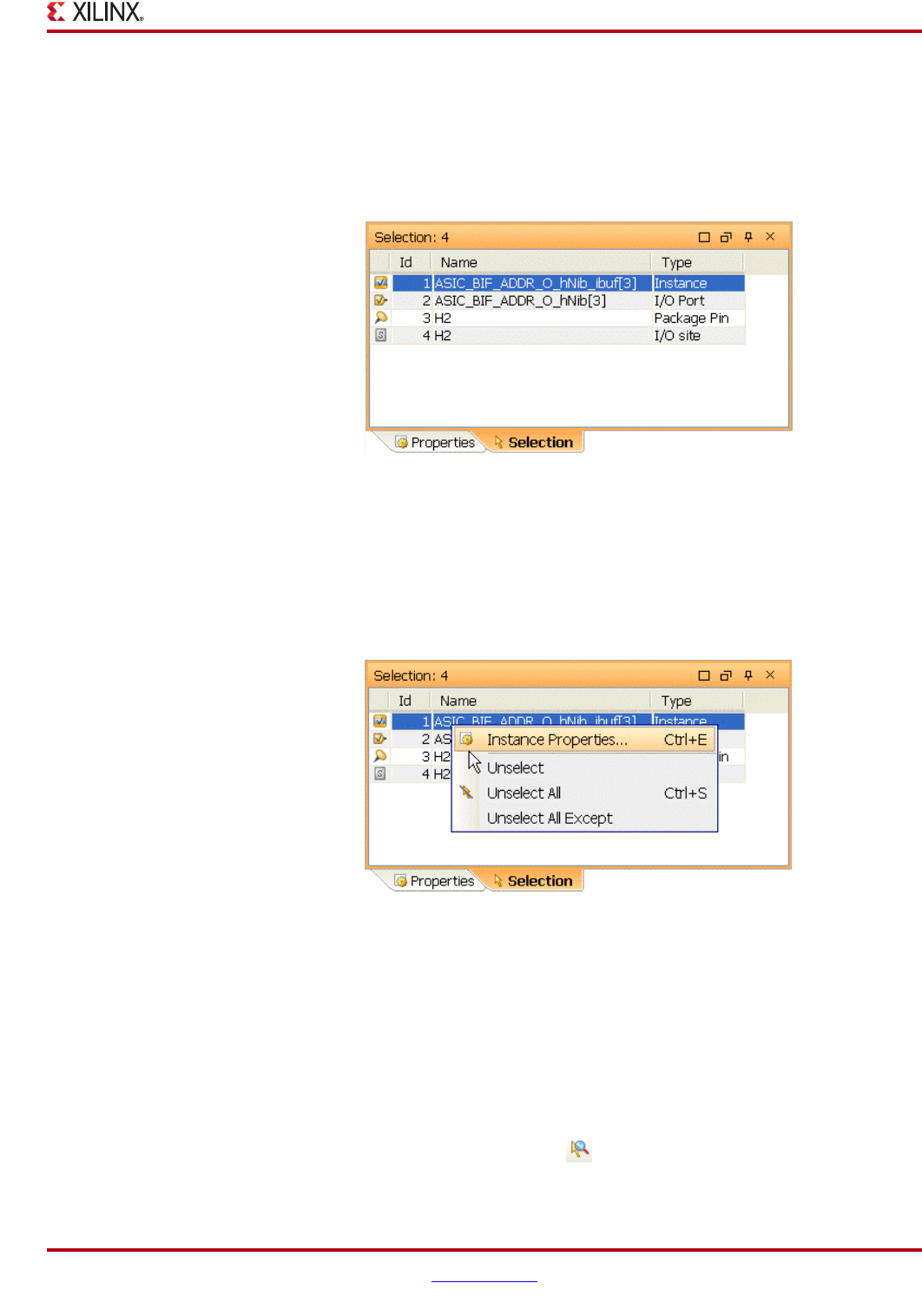
PlanAhead User Guide www.xilinx.com 141

UG632 (v 12.1)

Selecting Objects

Using the Selection View

The Selection view, as shown in the following figure, displays the list of objects currently

selected. You can sort, unselect, or mark objects from this view. The list is updated

dynamically as you manipulate objects. To invoke the Selection view, select Window >

Selection.

To sort elements, click on the column header to use as alpha-numeric sort criteria. Objects

can be sorted by Name, ID number, or Type by clicking on the banner of the desired sort

column. Selected items can be removed from the list by using the Unselect, Unselect All

or Unselect All Except command from the popup menu.

You can select groups of objects by using the Ctrl and Shift keys. The total number of

objects selected is displayed in the view banner as shown in the following figure.

Fitting the Display to Show Selected Objects

Views in the Workspace have a zoom option to fit all selected objects. To zoom fit the

selected objects, use one of the following methods:

•Select View > Fit Selection.

•Press F9.

•Click the Fit Selection toolbar button as shown in the following figure.

Figure 4-83: Selection View

Figure 4-84: Selection View Popup Menu Commands

Figure 4-85: Fit Selection Toolbar Button

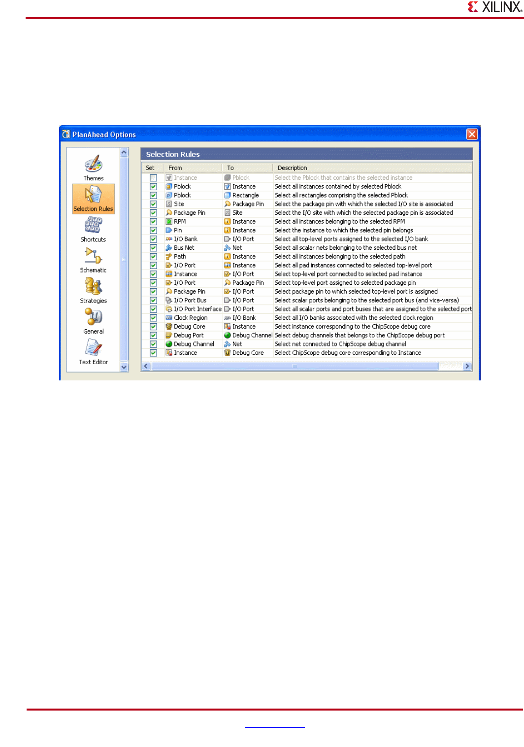
142 www.xilinx.com PlanAhead User Guide

UG632 (v 12.1)

Chapter 4: Using the Viewing Environment

Setting Selection Rules

When selecting an object, other objects can become selected also (for example, selecting a

Pblock also selects the assigned netlist instances). You can control the selection behavior

when you set selection rules in the Selection Rules options, which is available from

Tools > Options > Selection Rules.

You can enable or disable automatic selection by clicking on the Set column heading.

Enabling a selection rule forces the PlanAhead software to select the other affiliated “To”

object types when the “From” object gets selected. Disabling the selection rule forces

PlanAhead to select the “From” object only when it gets selected.

The default selection rules enable PlanAhead to operate in the most efficient manner.

Setting Object Selections in the Workspace Views

Object selection is set in the PlanAhead Options dialog box, available when you

Tools > Options > Themes.

For more information about setting object selections, see “Customizing PlanAhead

Display Options,” page 143.

Highlighting Selected Objects

You can highlight objects with color for display purposes. Highlighting remains until you

clear all highlights for the floorplan. For more information on highlighting, see “Selecting

Primitive Parent Modules,” page 140.

Figure 4-86: PlanAhead Options: Selection Rules

PlanAhead User Guide www.xilinx.com 143

UG632 (v 12.1)

Configuring the Viewing Environment

Marking Selected Objects

You can place a Mark symbol for all selected objects. Select the objects to mark use the

Mark command in the popup menu.

Select the UnMark All toolbar button to remove all marks.

Configuring the Viewing Environment

PlanAhead has numerous user-configurable viewing options. The tool ships with default

customize-able settings. For more information, see “Customizing PlanAhead Display

Options”.

You can save and restore view layout configurations for use in subsequent PlanAhead

sessions. A separate layout is stored for the Project Manager, I/O Planner, and Design

Planner environments. PlanAhead creates a layout file to restore the overall PlanAhead

window size and location also. The view configurations are stored in your home directory

when exiting PlanAhead. For more information on the layout of configuration files, see

“Outputs for Environment Defaults” in Appendix B.

You can save view configuration “Themes” and view layouts for use in future PlanAhead

sessions. For more information, see “Saving Custom Display Settings,” page 148.

Customizing PlanAhead Display Options

You can adjust view display options to control the appearance and behavior of the

environment.

To view or edit the display options available in the PlanAhead Options dialog box, select

Tools > Options. All changes take effect after you select the OK or click Apply. Clicking

Cancel does not initiate any changes.

You can view and adjust the options that control the general environment appearance in

the Themes options. The options can be viewed or changed in the Themes environment for

different areas in the interface. The tabs at the bottom of the Themes options allow various

view setting types to be modified: General, Device, I/Os, and Bundle Nets.

Setting General View Display Options

The General tab lets you customize general color and appearance options of the

PlanAhead views.

144 www.xilinx.com PlanAhead User Guide

UG632 (v 12.1)

Chapter 4: Using the Viewing Environment

Select a color to reveal a pull down, and click the down arrow to open a popup menu to

select another color.

Figure 4-87: General View Display Options

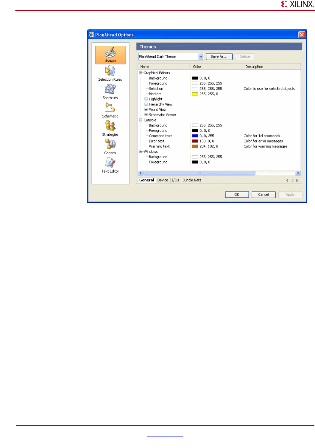
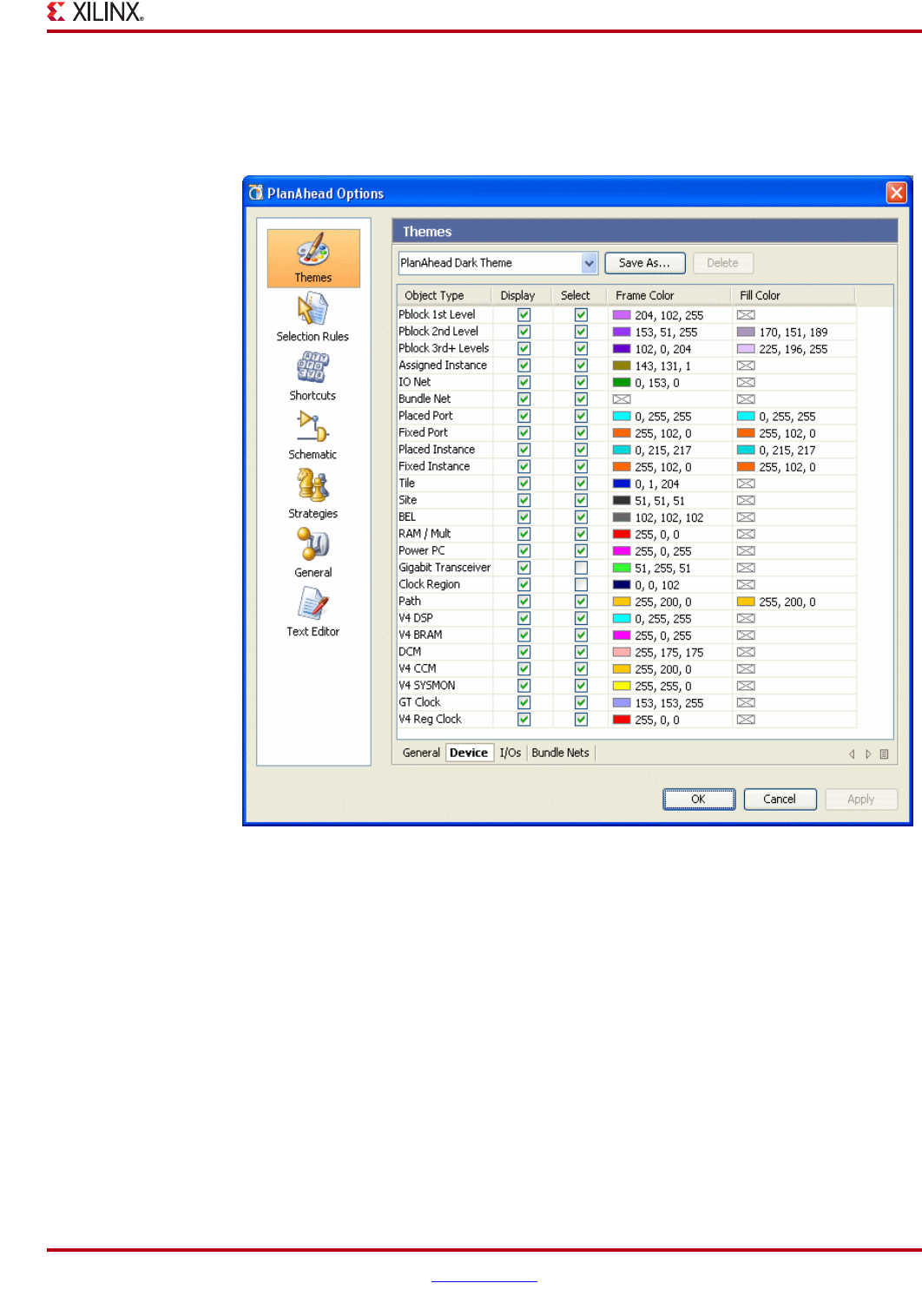
PlanAhead User Guide www.xilinx.com 145

UG632 (v 12.1)

Configuring the Viewing Environment

Setting Device View Display Options

The Device tab lets you adjust the default color, visibility and selection options for each

object type in the Device view.

You can toggle the check boxes to obtain the display effect you want:

•In the Display column, toggle the check boxes off to hide the object types in the Device

view.

•In the Select column, toggle the check boxes off to make the object types unselectable

in the Device view. They will still be visible if the Display toggle is on.

Note: The Frame and Fill color options are not available for certain object types.

Note: Some object types are device-specific, consequently, the display options have no effect in

some devices.

Figure 4-88: Device View Display Options

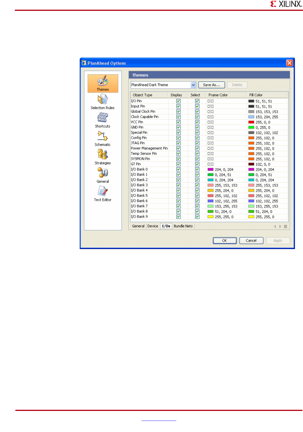
146 www.xilinx.com PlanAhead User Guide

UG632 (v 12.1)

Chapter 4: Using the Viewing Environment

Setting Package View Display Options

The I/Os tab lets you adjust the default color, visibility and selection options for each

object type in the Package view.

You can toggle the check boxes to obtain the display effect you want:

•In the Display column, toggle the check boxes off to hide the object types in the

Package view.

•In the Select column, toggle the check boxes off to make the object types unselectable

in the Package view. They will still be visible if the Display toggle is on.

Note: The Frame and Fill color options are not available for certain object types.

Note: Some of the object types are device-specific, consequently, the display options have no effect

in some devices.

Figure 4-89: Package View Display Options

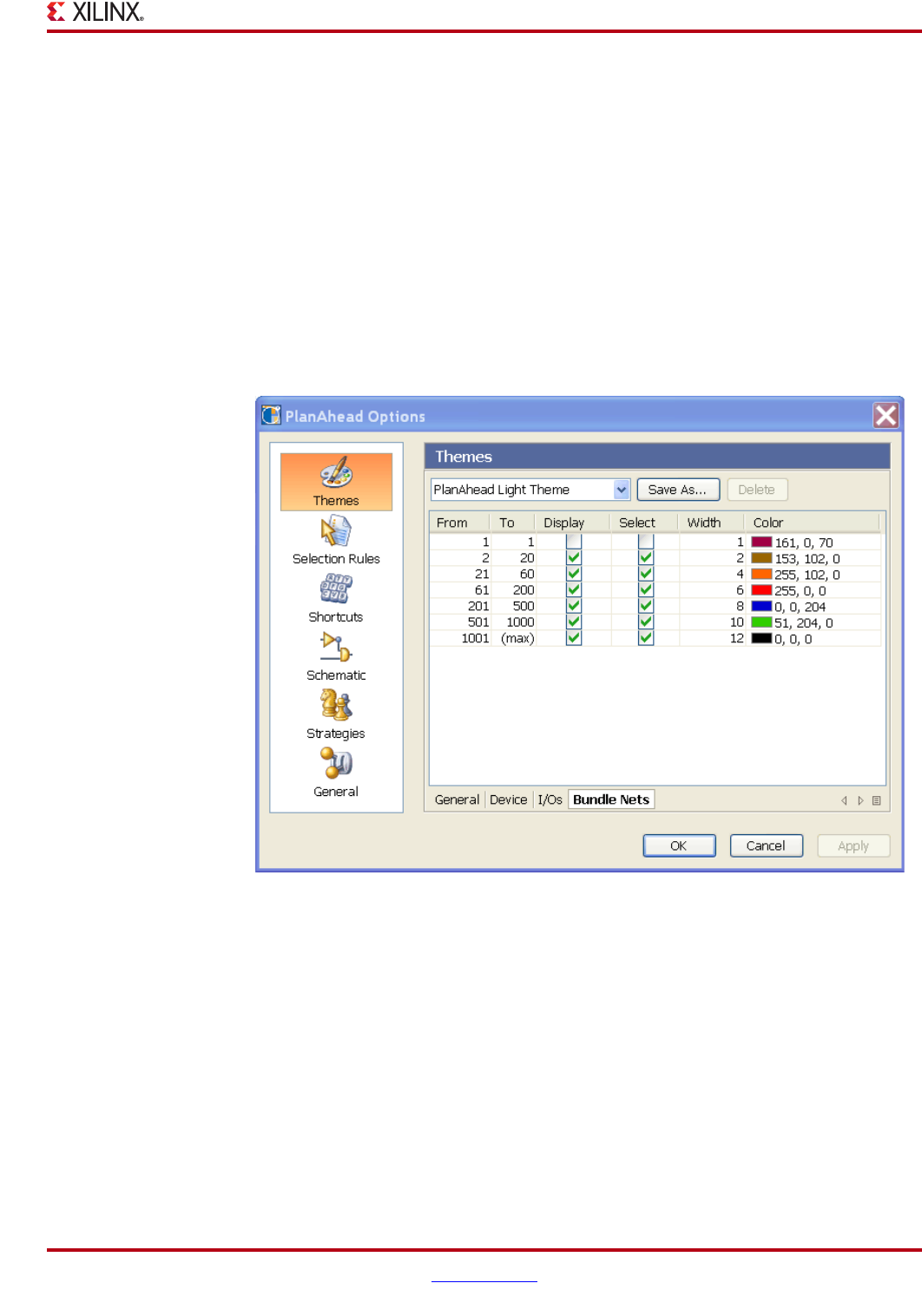
PlanAhead User Guide www.xilinx.com 147

UG632 (v 12.1)

Configuring the Viewing Environment

Setting the Device View Bundle Nets Display Options

You can configure the characteristics of the bundle nets displayed in the Device view using

the Bundle Nets tab.

You can adjust the signal count ranges for bundles using the From and To columns. Each

column represents a bundle net range which can be configured independently.

You can toggle the check boxes to obtain different display effects:

•In the Display column, toggle the check boxes off to hide the bundle net range in the

Device view.

•In the Select column, toggle the check boxes off to make the bundle nets unselectable

in the Device view. They will still be visible if the Display toggle is on.

The following figure shows the Bundle Nets tab.

You can set the line width on which the bundle appears in the Device view for each bundle

net range by adjusting the values in the Width column.

Configuring Schematic Slack and Fanout Display Options

The Schematic options enables you to tag source pins with Fanout values and destination

pins with Slack values. For more information, see “Schematic View-Specific Popup Menu

Commands,” page 115.

Adjusting Display using Toolbar Commands

You can adjust the view display using the following Device view or main toolbar buttons

also. Some buttons are active only when the appropriate object types are displayed. The

toolbar commands are described in “Select Menu” in Appendix A.

Figure 4-90: Bundle Net Display Options for the Device View

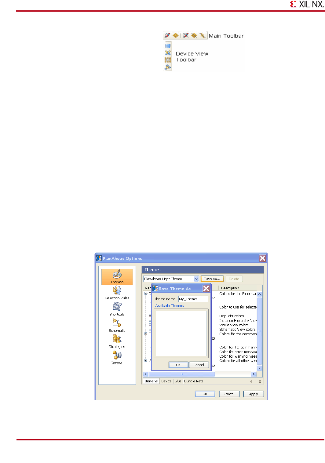
148 www.xilinx.com PlanAhead User Guide

UG632 (v 12.1)

Chapter 4: Using the Viewing Environment

You can hover the cursor over an icons to view the tool tip describing the button function.

Saving Custom Display Settings

PlanAhead allows you to save view layouts or display themes for later use. They are stored

in your home directory and are available each time you invoke PlanAhead. For more

information about file locations and formats, refer to the “Outputs for Environment

Defaults” in Appendix B.

Selecting a Theme

PlanAhead has default view settings for both light and dark background themes. To use

either, select the PlanAhead Light Theme or PlanAhead Dark Theme options in the

Theme pull down menu.

These default options are defined in the planahead.ini file. For more information, see

“View Display Options File (planAhead.ini & <theme_names>.patheme)” in Appendix B.

Creating and Using a Customized Theme

You can save your own custom view settings to create PlanAhead initialization files for use

in future PlanAhead sessions. To do so, click the Save As button next to the Theme pull

down menu as shown in the following figure.

Figure 4-91: View Display Control Toolbar Buttons

Figure 4-92: Creating a Custom Theme

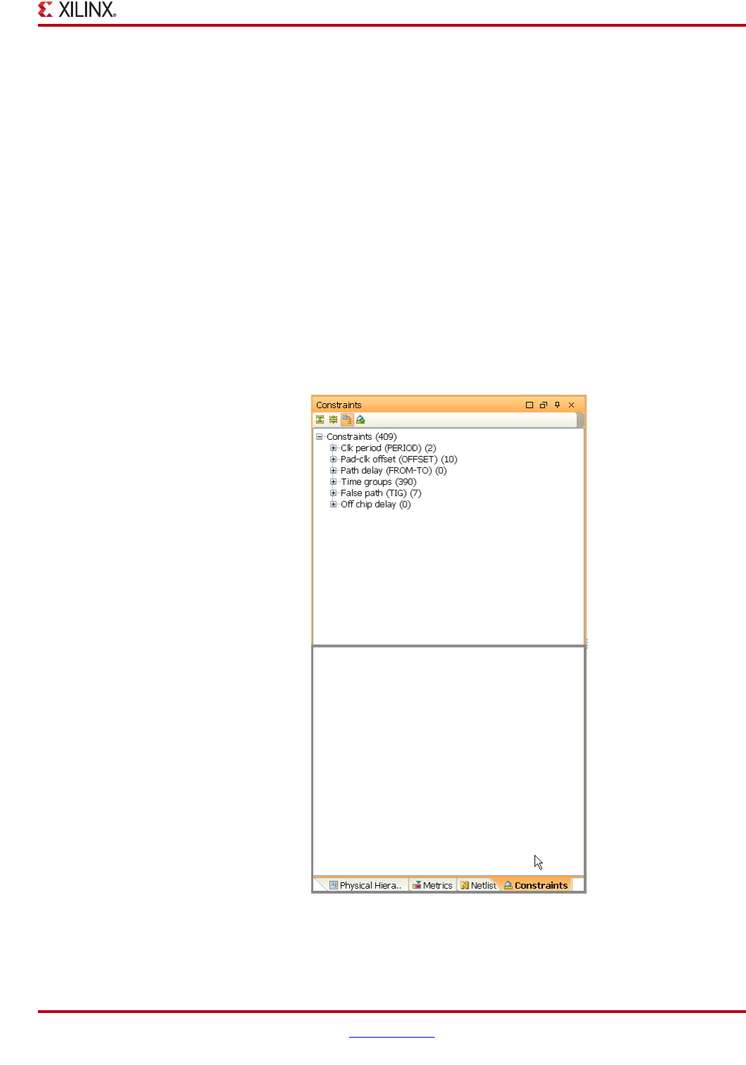
PlanAhead User Guide www.xilinx.com 149

UG632 (v 12.1)

Configuring the Viewing Environment

If you create your own theme, it is prudent to back-up the initialization file that contains

the custom settings. For detailed information about the default and custom initialization

files, see “View Display Options File (planAhead.ini & <theme_names>.patheme)” in

Appendix B.

Moving Views

Multiple views can share the space within the viewing area by displaying them together

either vertically or horizontally. Split viewing areas by clicking on a view tab and dragging

it into another viewing area.

An outline will guide you to place the view at the correct position. The resulting window

location can be determined prior to accepting it, by watching the moving window outline

during the dragging process.

To move a view to share the space in a viewing area:

1. Click the tab, for example, the Constraints tab in the following figure.

2. Drag the tab to a location. The gray outline will guide you.

3. Release the tab at the location you want.

To restore the view to its original location, select Window > Undo Dragging, or repeat the

steps above to set the view back in place.

Figure 4-93: Dragging Constraints View to Share View with Other Views

150 www.xilinx.com PlanAhead User Guide

UG632 (v 12.1)

Chapter 4: Using the Viewing Environment

To move a view to a completely different docking area, such as moving the Constraints

view to the Properties view, drag the tab of the view you are moving to the banner of the

destination docking area.

1. Click the tab.

2. Drag it to the banner of the destination docking area.

3. Release the tab to place the view and its tab.

Creating Custom View Layouts

Select the Layout menu commands to save and restore default and alternate view

configurations. For a list of Layout menu commands and a description of each, see “Layout

Menu” in Appendix A.

Restoring a View Layout

A number of commands are available to restore the layout of PlanAhead.

You can dock views back to their original locations by toggling the various options

previously selected to off again. The view banner manipulation commands also act as

toggles and can be selected to revert back to the previous setting.

Restoring the Default View Layout

Select Layout > Load Layout > PlanAhead Default to undo any changes to restore the

default PlanAhead layout.

Using Undo/Redo Commands

You can undo the view manipulation commands by selecting the Layout > Undo

command. To repeat a command, use the Layout > Redo command.

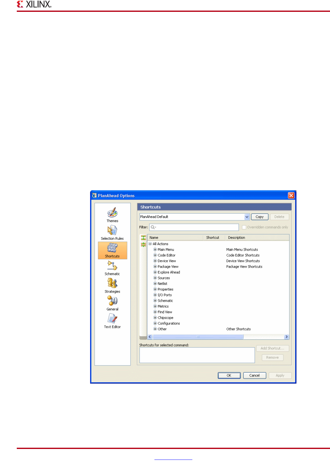
PlanAhead User Guide www.xilinx.com 151

UG632 (v 12.1)

Configuring PlanAhead Behavior

PlanAhead configuration options include: selection rule options, shortcut keys, general

settings options, and window settings options. The following subsections describe the

configuration options.

Setting Selection Rule Options

Selection rule options control the object selection settings for all views. When you select an

object, other objects can become selected also (for example, selecting a Pblock also selects

the assigned netlist instances). For more information on setting selection rules, see “Setting

Selection Rules,” page 142.

Configuring Shortcut Keys

Most commonly used commands have pre-defined shortcuts using keyboard key

combinations. The shortcuts defined display next to the command in the popup menu.

For example, press F9 to access the Fit Selection command.

You can modify the default shortcut values by using the Shortcuts option of the PlanAhead

Options dialog box, which is shown in the following figure.

The Shortcuts dialog box provides a helpful interface to create new Shortcut schemas that

contain custom shortcut settings.

Figure 4-94: Shortcuts Options

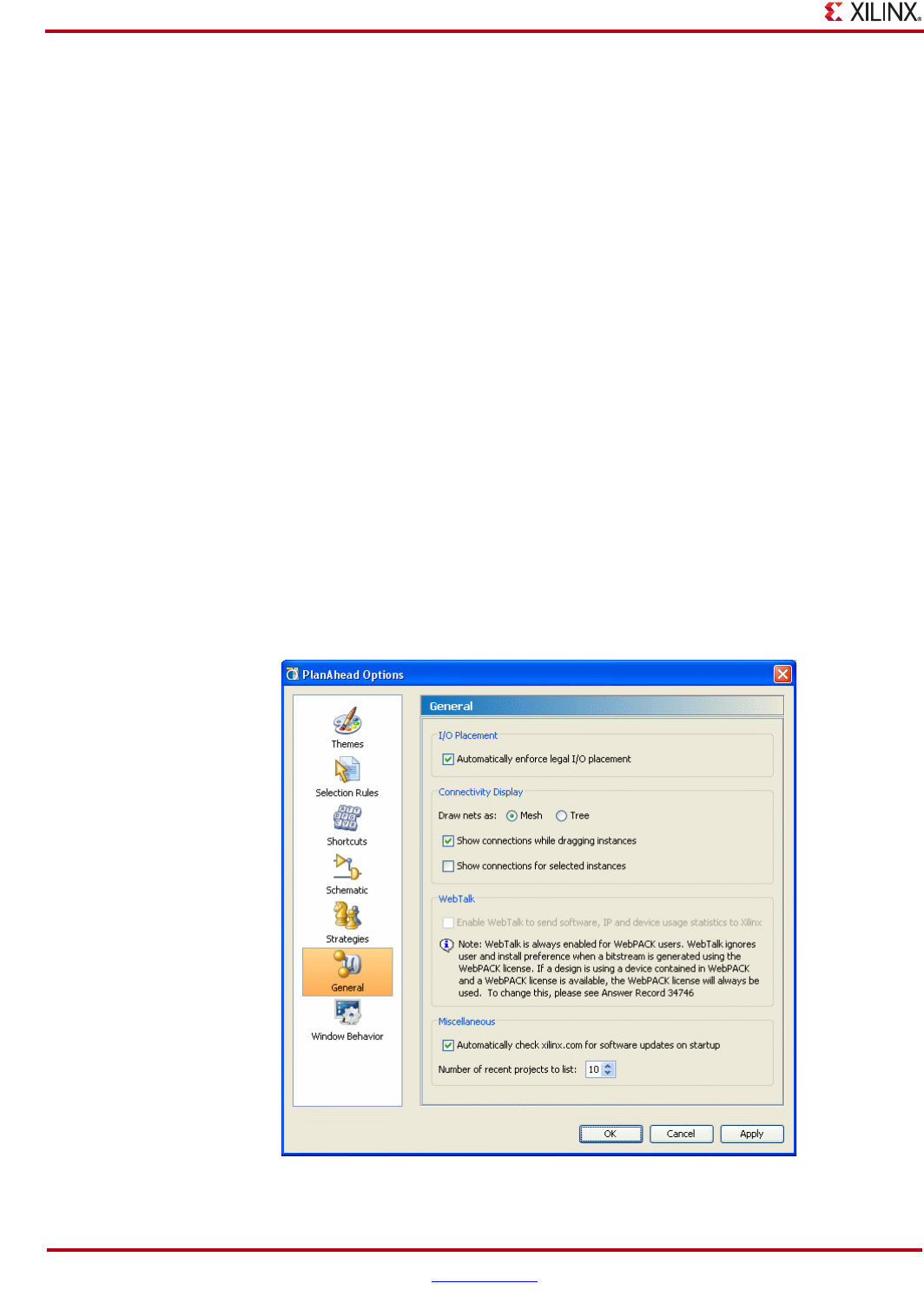
152 www.xilinx.com PlanAhead User Guide

UG632 (v 12.1)

Chapter 4: Using the Viewing Environment

At the top, the available shortcut schemas lets you manage Shortcut schemas. Click the

Copy button to copy the PlanAhead Default schema to create a new schema.

You can activate any schema in the list by selecting it from the pull down menu of available

schemas. You must first copy the PlanAhead Default schema to make any modifications.

The bottom portion of the Shortcuts dialog box has an area where you can make

modifications to shortcuts in the copied schema. You can search through the list of views

and select commands to enter new shortcuts.

1. Select the Add Shortcut button and type in the new shortcut in the Add Shortcut

dialog box.

2. Click OK to accept the new shortcut.

You can filter the commands listed for shortcut assignment using the Filter field. Enter any

text string to filter the list of available commands. Also, you can use different shortcuts for

the same command in different views.

User-specific shortcut schemas are saved to:

•(Windows) C:\Documents and Settings\<Username>\Application

Data\HDI\shortcuts

•(Linux) ~/.HDI/shortcuts

To delete shortcuts, click the Remove button.

Setting General PlanAhead Options

To set the general PlanAhead options, select Tools > Options > General. The following

figure shows the General options in the PlanAhead Options dialog box.

Figure 4-95: General Options

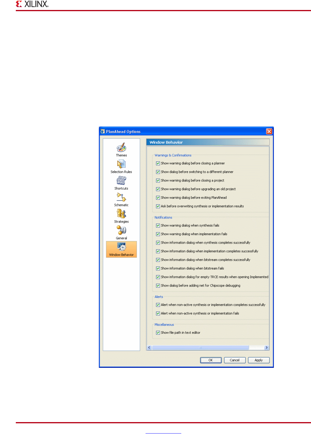
PlanAhead User Guide www.xilinx.com 153

UG632 (v 12.1)

Configuring PlanAhead Behavior

The General options are:

•I/O Placement—Toggles the interactive I/O placement DRCs on or off.

•Connectivity Display—Controls how connectivity is displayed in the Device view.

•WebTalk— Controls whether WebTalk is able to send Xilinx usage information.

•Miscellaneous—Controls whether PlanAhead searches the Xilinx web site

automatically for new software updates, and defines how many previously opened

Projects display in the Getting Started view.

Setting General Window Behavior Options

To set the window behavior PlanAhead options, select Tools > Options > Window

Behavior. The Window Behavior dialog box is shown in the following figure.

•Warning Dialogs—Sets how warning dialog boxes are presented using the self

explanatory options.

Figure 4-96: Window Behavior Options Dialog Box

154 www.xilinx.com PlanAhead User Guide

UG632 (v 12.1)

Chapter 4: Using the Viewing Environment

PlanAhead User Guide www.xilinx.com 155

UG632 (v 12.1)

Chapter 5

RTL and IP Design

This chapter contains the following sections:

•“Introduction”

•“Managing the Design Source Files”

•“Editing RTL Source Files”

•“Configuring IP using the CORE Generator”

•“Elaborating and Analyzing the RTL Design”

•“RTL Rules: Power and Performance”

Introduction

The PlanAhead™ software Project Manager environment lets you create and manage RTL

design files. Then, the RTL design can be elaborated and analyzed in the RTL Design

environment. Included in PlanAhead is basic source file management, an RTL editor, an

RTL schematic viewer, a set of RTL Design Rule Checks (DRCs), and a resource and power

estimator.

The PlanAhead software is integrated with the Xilinx® ISE® Design Suite CORE

Generator™ tool. The IP catalog displays and enables you to customize, instantiate,

implement, and manage IP core modules.

Using the PlanAhead software you can then run logic synthesis and implementation. See

Chapter 6, “Synthesizing the Design” and Chapter 9, “Implementing the Design” for more

information about running synthesis and implementation.

Managing the Design Source Files

You can add Verilog, VHDL and NGC/EDIF source files to the project and manage those

files in a variety of ways. Most of the interaction with Source files is from within the

Sources view. Refer to “Managing Project Sources” and “Using the Sources View” in

Chapter 3.

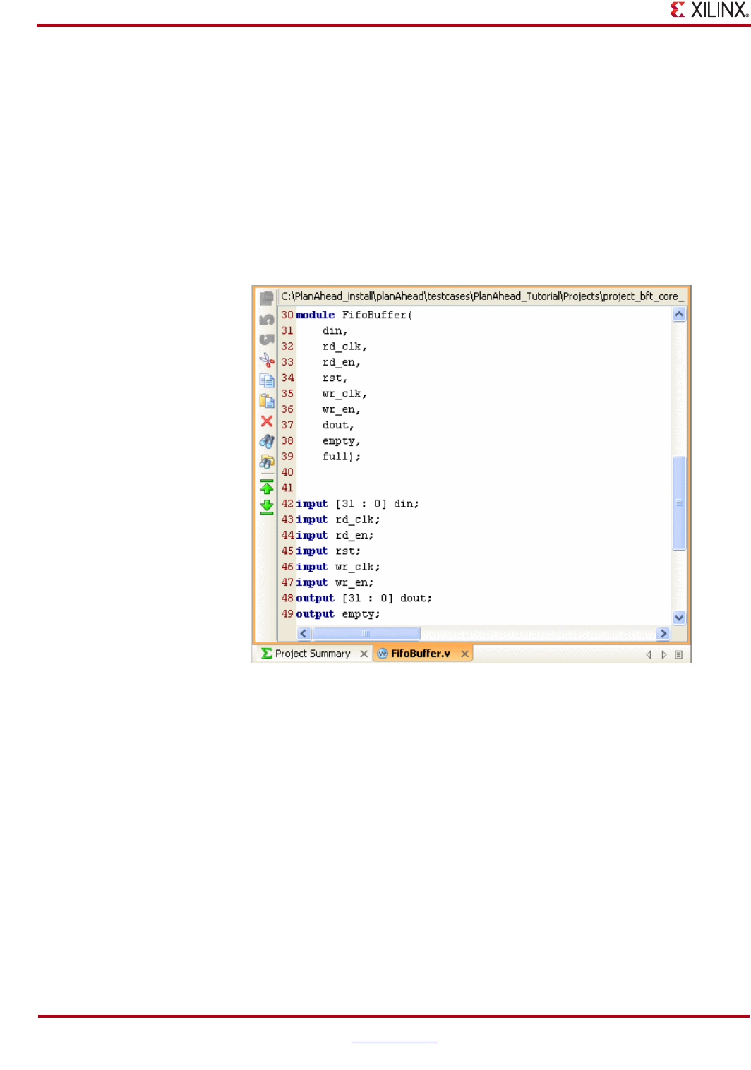
156 www.xilinx.com PlanAhead User Guide

UG632 (v 12.1)

Chapter 5: RTL and IP Design

Editing RTL Source Files

The PlanAhead RTL environment provides an RTL editor in which to create or modify RTL

sources. The RTL editor uses color-coding to distinguish the various types of RTL

constructs. You can open multiple files simultaneously, and each open file displays a view

tab in the PlanAhead Workspace that allows easy access to all open files.

Using the RTL Editor

The RTL Design environment enables cross-probing to and from the RTL editor with other

views, such as the Schematic, Elaborate Results, RTL Netlist and Hierarchy views. The

following figure shows an example of the RTL editor.

When you modify a file an asterisk (*) is appended to the file name in the view tab until the

file is saved. In the RTL editor, select Save File or Save Project.

If you close an RTL Editor file with unsaved changes, PlanAhead prompts you to save the

changes.

Using the RTL Editor Specific Commands

The RTL editor commands are available from the popup menu or from the view-specific

toolbar buttons. The options are:

•Save File—Saves the individual file being displayed.

•Save File As—Allows saving the file to a new name.

•Undo, Redo—Backs out or reverses changes made in sequential order.

•Cut, Copy, Paste, Delete—Cuts or copies the selected source code into the clipboard.

Pastes the contents of the clipboard.

Figure 5-1: RTL Editor

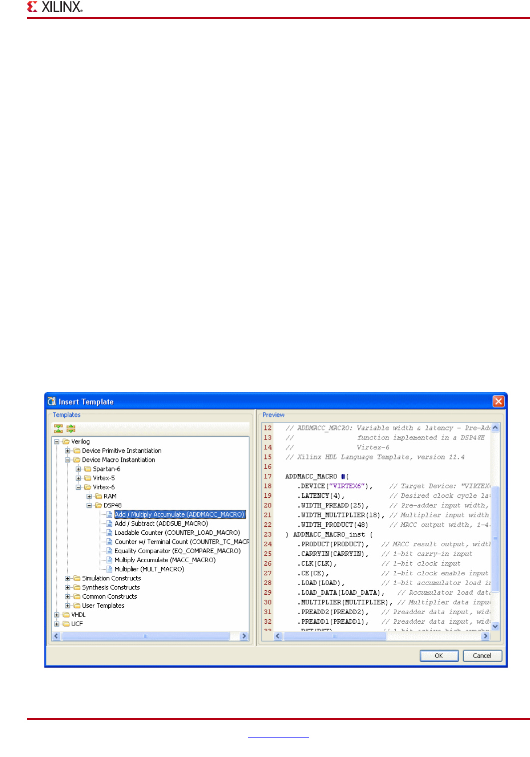
PlanAhead User Guide www.xilinx.com 157

UG632 (v 12.1)

Editing RTL Source Files

•Duplicate Selection—Copies the current selected text and inserts it at the current

cursor location.

•Insert Template—Invokes the Xilinx Language Template, and enables you to select a

logic construct to insert in the RTL file.

•Find, Replace—Invokes the Find field to enter a text string to search or replace

individual or all the occurrences.

•Find in Files—Invokes the Find in Files dialog box to enter text strings to search for in

the selected files. The Find in Files Results view displays with the results of the search.

•Indent Selection, Unindent Selection, Comment with Line Comment, Comment

with Block Comment—These commands perform the function described in their

titles.

Instantiating Xilinx Supplied Language Templates

Standard RTL templates are available in the RTL editor to assist with defining certain logic

constructs. You can browse and review the library of templates. Modules are instantiated

into any RTL file that is open in the RTL editor.

To instantiate a Xilinx-supplied language template:

1. In the RTL editor, click the location in the file to indicate where to instantiate the

template language.

2. Select the Insert Template command from the popup menu

3. Browse and select a template.

4. Click OK.

The following figure shows an example of the Xilinx-supplied templates.

Figure 5-2: Insert Template Dialog Box

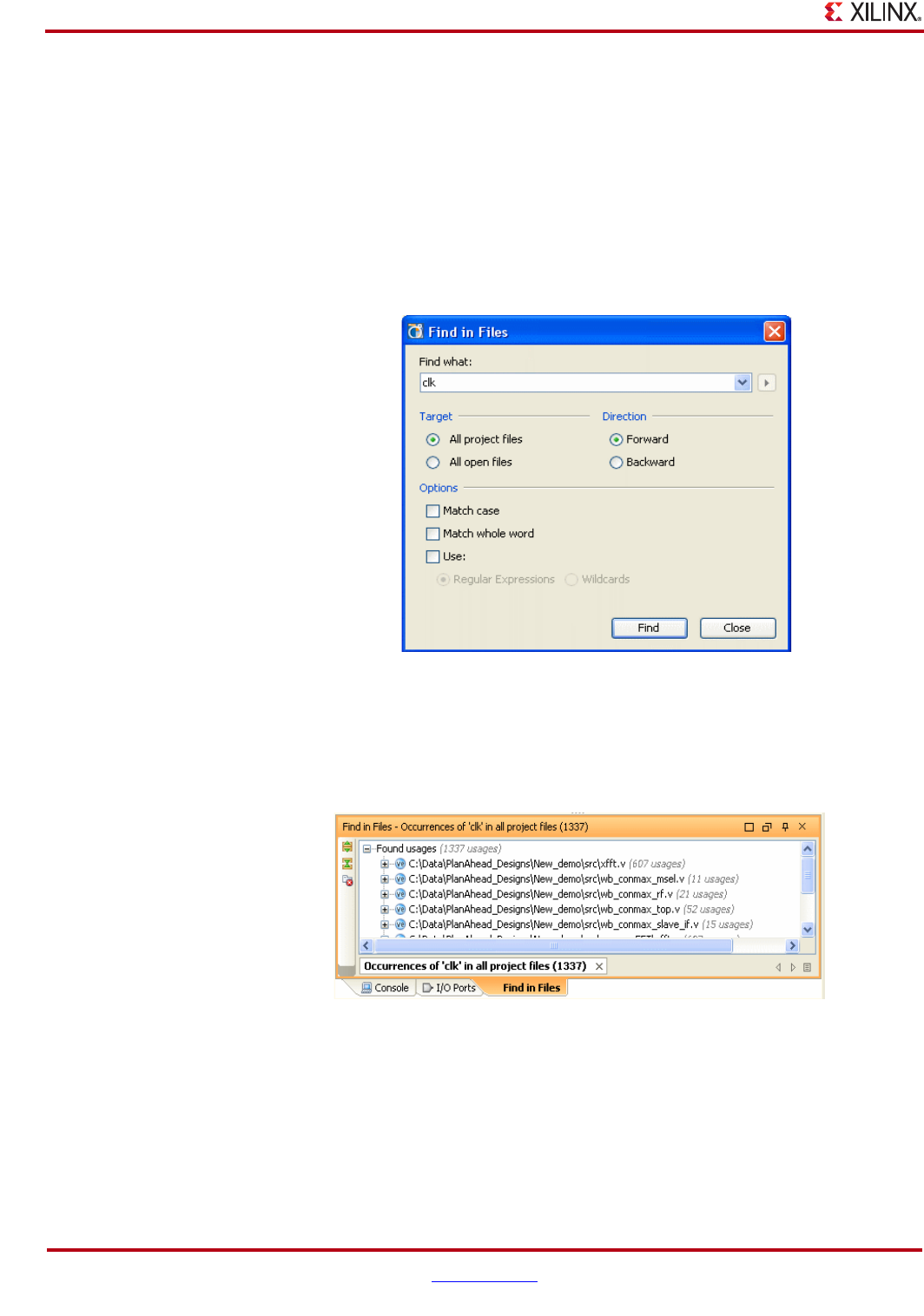
158 www.xilinx.com PlanAhead User Guide

UG632 (v 12.1)

Chapter 5: RTL and IP Design

Using the Find in Files Command to Search Source Files

You can use Find or Find in Files to search for any given text string in a selected set of

source files. You can:

•Enter any text string, including wildcards (*), as search criteria.

•Use the filtering options to limit the search based on all files in the project or all open

files.

•Specify a forward or backward direction for the search.

The following figure shows the Find in Files dialog box.

The search results display in the Find in Files Results view as a list of files that contain the

search string and the number of occurrences in each file.

Select any occurrence in the list to load that file into the RTL editor and highlight the string.

The following figure shows an example of such a search.

Figure 5-3: Find in Files Dialog Box

Figure 5-4: Find in Files Results View

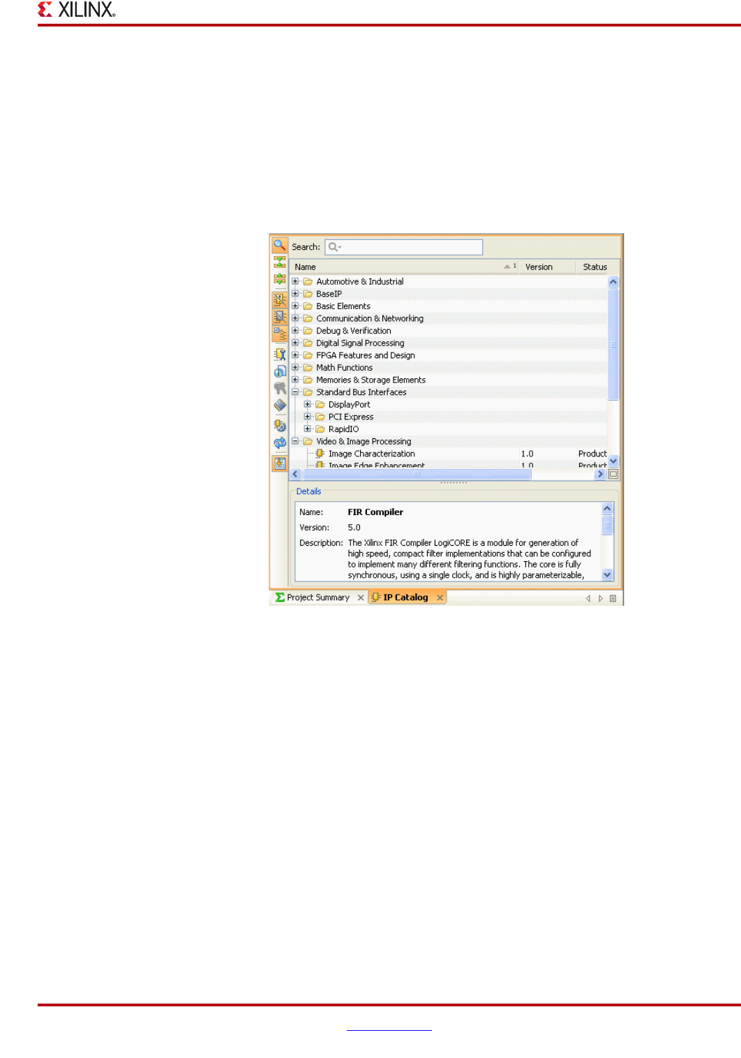
PlanAhead User Guide www.xilinx.com 159

UG632 (v 12.1)

Configuring IP using the CORE Generator

You can browse the Xilinx IP Catalog to analyze, customize, and instantiate IP, and you can

access the IP Catalog from the Project Manager or the RTL Design environment.

Using the IP Catalog

To open the IP Catalog, click IP Catalog in the Project Manager or RTL Design Flow

Navigator menus. The following figure shows an example of the IP Catalog.

The IP displays by category in an expandable tree table. The IP version, status, and license

requirements display in the table. When you select an IP, a description displays in the

lower pane of the view.

Click DataSheet to bring up the IP datasheet in a PDF viewer. Other options are:

•Show Search—searches the catalog for any text string.

•Hide non-production IP— Filters the list to available IP only.

•Hide incompatible IP—Filters the list to only the IP that is compatible with the

selected device family.

You can expand and sort the view as follows:

•Click Group by Category to flatten the list which enables better sorting and

searching.

•Select the columns headers to sort the table based on that column data.

Refer to “Using Tree Table Style Views” in Chapter 4 for more information about tree table

views.

Figure 5-5: Xilinx IP Catalog

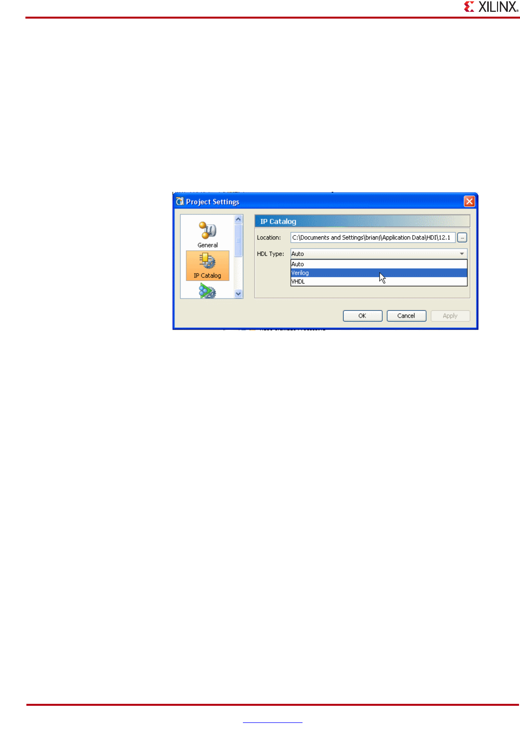
160 www.xilinx.com PlanAhead User Guide

UG632 (v 12.1)

Chapter 5: RTL and IP Design

Updating the IP Catalog

PlanAhead creates a local version of the IP Catalog when the tool is invoked for the first

time after installation. To update the IP Catalog to ensure it is current, click Update IP

Catalog.

Setting IP Catalog Settings

You can define IP Catalog settings.

1. Click Project Settings.

2. In the Project Settings dialog box, click IP Catalog, as shown in the following figure.

The IP Catalog settings are:

•Location—Defines a location for the local IP catalog to be created and stored.

•HDL Type—Defines the language to use when creating the IP.

•Auto—Derives the preferred language automatically, based upon the language of the

top-level HDL file.

Customizing IP

You can select IP from the IP Catalog, and customize the IP using the integrated CORE

Generator tool.

1. Select the IP to customize from the IP Catalog

2. Select the Customize IP command

PlanAhead invokes the CORE Generator interface to enable core generation. The type of IP

you select determines what type of interface is displayed.

The interfaces are:

•Architecture Wizard

•Memory Integration Generator (MIG) Wizard

•CORE Generator Wizard

Figure 5-6: IP Catalog Project Settings

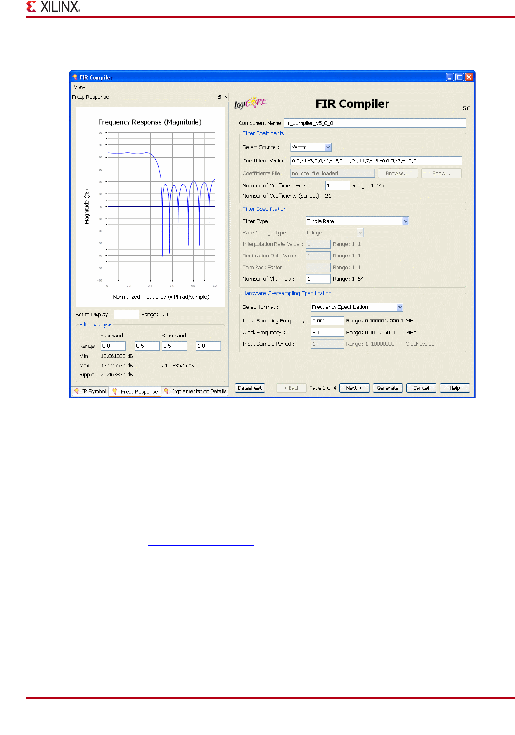
PlanAhead User Guide www.xilinx.com 161

UG632 (v 12.1)

Configuring IP using the CORE Generator

The following figure shows the CORE Generator Wizard:

The wizard fields enable core logic configuration.

•For information on using CORE Generator to generate IP, refer to

http://www.xilinx.com/tools/coregen.htm.

•For information on using the Architecture Wizard refer to

http://www.xilinx.com/products/design_resources/conn_central/solution_kits/wi

zards/.

•For information on using the MIG Memory Generator (MIG), refer to

http://www.xilinx.com/support/documentation/ipmeminterfacestorelement_memi

nterfacecontrol_mig.htm.

•For information on specific IP, refer to http://www.xilinx.com/ipcenter/ or the IP

Catalog.

Viewing IP

The IP Symbol panel shows a schematic symbol view of the IP.

•To display device resource statistics for the core logic, select the Information tab.

•To display the IP datasheet in a PDF viewer, click DataSheet.

Figure 5-7: CORE Generator Interface

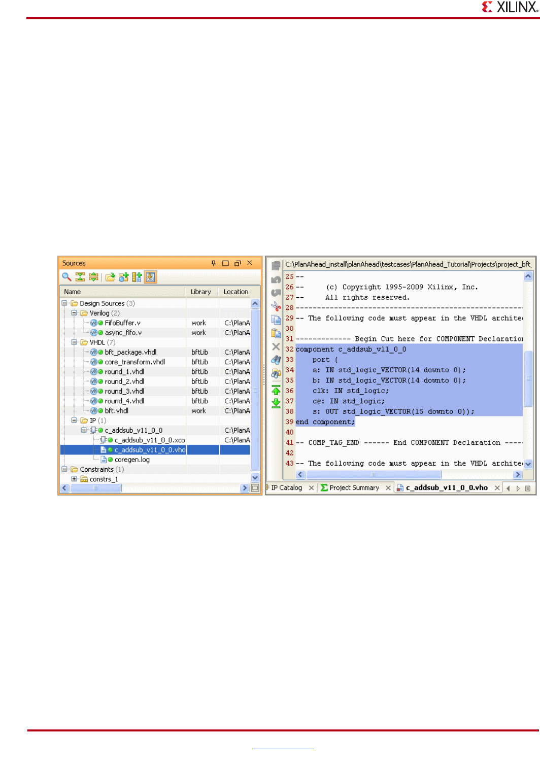
162 www.xilinx.com PlanAhead User Guide

UG632 (v 12.1)

Chapter 5: RTL and IP Design

Clicking Generate inside of PlanAhead has a different effect than in the standalone CORE

Generator tool. PlanAhead, creates the core and adds it as a source in the project, but the

core is not yet synthesized. PlanAhead synthesizes the IP cores automatically prior to

synthesizing the design when you run Synthesize. This bundles the time-consuming

synthesis tasks into one run session. You can then instantiate the IP into the design prior to

running synthesis.

Instantiating IP

After you generate IP and add it to a project, the IP displays in the Sources view under the

IP folder.

Expanding the IP cores displays the CORE Generator XCO project file and VHO file

containing the instantiation template that you can copy and paste into your design RTL

using Copy and Paste in the RTL editor.

The following figure shows instantiated IP RTL code.

Generating IP

When you generate IP, the XST synthesis tool runs on the core and creates the logic content

based on the customization settings.

You can run Synthesis separately on any IP core, or it runs automatically when the design

is synthesized.

The IP can be generated by either of the following commands:

•In the Flow Navigator, click Synthesize.

•In the Sources view, select the IP core, and click Generate IP.

Figure 5-8: Instantiated IP RTL Code

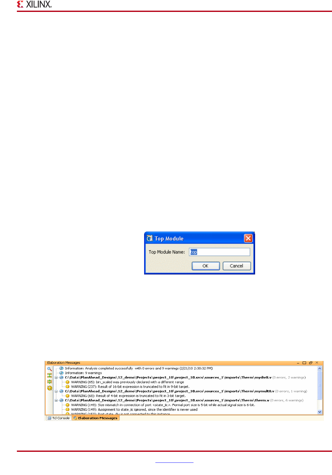
PlanAhead User Guide www.xilinx.com 163

UG632 (v 12.1)

Elaborating and Analyzing the RTL Design

Modifying IP

You can modify IP and regenerate it within PlanAhead. This applies to IP generated within

PlanAhead. To customize IP, select it in the Sources view and click Re-customize IP. The

CORE Generator interface opens to allow core modification.

Elaborating and Analyzing the RTL Design

Validating RTL Design Compilation

PlanAhead lets you compile and analyze the RTL sources and makes Elaboration available

to analyze the compiled RTL design prior to running synthesis, without making

Elaboration a required step prior to synthesis.

RTL source files imported into the project are elaborated regardless of whether they are

compiled as a part of the design or during synthesis. Elaboration results are not saved with

the design. You can run and rerun elaboration until the design is synthesized.

1. After the design source files are imported into the project, elaborate the design using

one of the following commands:

−In Flow Navigator > Project Manager, click Elaborate.

−Select Tools > Elaborate.

−In the Flow Navigator, click RTL Design. The RTL design will be compiled, and

the RTL design environment opens.

The Top Module dialog box opens, as shown in the following figure.

To T

2. In the Top Module dialog box, enter the top-level module to elaborate.

3. Click OK.

Viewing Elaboration Results

The Elaboration Messages view displays the results of the compilation and flags

irregularities in the RTL source files. The following figure shows an example of elaboration

messages.

Figure 5-9: Top Module Dialog Box

Figure 5-10: Viewing Elaboration Messages

164 www.xilinx.com PlanAhead User Guide

UG632 (v 12.1)

Chapter 5: RTL and IP Design

Highlighting Issues in the RTL Source files

Selecting any of the Warning or Error lines in the Elaboration view loads the appropriate

RTL source file into the RTL editor and highlights the source code in question.

Filtering the Results for Errors Only

The RTL Elaboration results can be filtered to display only error messages.

Click Hide Warning Messages to filter the results for errors only. The following figure

shows the Hide Warning Messages button.

Using the RTL Design Environment

When you click RTL Design, the RTL design is elaborated automatically, and upon

successful elaboration the compiled RTL design displays in the RTL Design environment.

Either the I/O Planner or Design Planner environment displays, and you can toggle

between the two viewing environments by clicking I/O Planner or Design Planner in the

main view banner.

Also, PlanAhead applies the active constraint set to the elaborated design when it opens

the RTL Design. This enables I/O pin planning, based on the RTL port list and the module-

level floorplanning from the RTL logic hierarchy. For more information on creating and

managing constraint sets, refer to “Adding and Managing Constraints” in Chapter 3.

Figure 5-12, page 165 shows the RTL Design Planner.

Figure 5-11: Elaboration Results: Hide Warning Messages Button

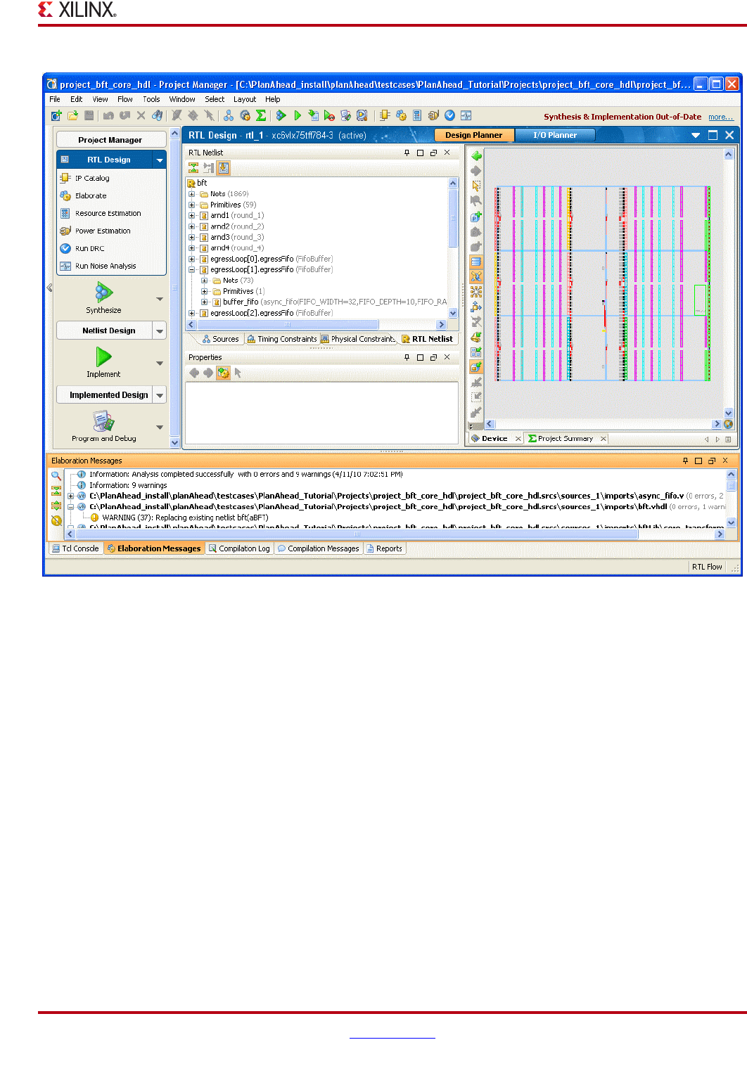
PlanAhead User Guide www.xilinx.com 165

UG632 (v 12.1)

Elaborating and Analyzing the RTL Design

Viewing Resource Estimates

PlanAhead can provide resource estimation statistics based on the compiled RTL design.

To populate the resource statistics data in the Resource Estimation view, use one of the

following commands:

•In Flow Navigator > RTL Design, click Resource Estimation.

•Select Tools > Resource Estimation.

The Resource Estimation view displays in the workspace.

The resource types display based on the logic hierarchy of the design. The logic tree can be

expandable using the view widgets to allow visibility into the logic hierarchy. Figure 5-13,

page 166 shows an example of the Resource Estimation view.

Figure 5-12: RTL Design Planner

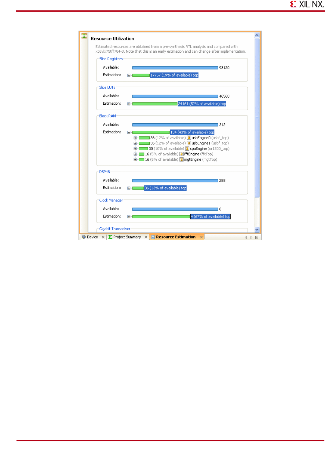
166 www.xilinx.com PlanAhead User Guide

UG632 (v 12.1)

Chapter 5: RTL and IP Design

The RTL Netlist view works like the Netlist view. You can select any level of logic hierarchy

and analyze its hardware resources.

Analyzing Resource Statistics in the Instance Properties view

You can select the Statistics tab in the Instance Properties view to view the estimated device

resource requirements for the selected module or for the top-level module in the RTL view.

Logic resources are categorized as Arithmetic, Comparators, Multiplexers, Storage, and so

forth. Figure 5-14, page 167 shows an example of resource estimates in the RTL view.

Memory and primitive tables are available, and they list all memories, and their depth, bit

width, number of ports, and macros/primitives broken down by bit width in the chosen

level of the hierarchy.

The Resource Estimator provides information about hardware resources for an RTL design

without running synthesis, and, consequently, with a much quicker run-time. The

accuracy is an average of +/-15%.

Figure 5-13: Resource Estimation View for the RTL Design

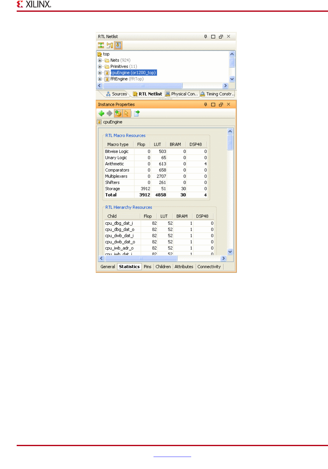
PlanAhead User Guide www.xilinx.com 167

UG632 (v 12.1)

Elaborating and Analyzing the RTL Design

Click Export Statistics to save the Statistics report to either an XML format (for parsing)

or an XLS format.

Analyzing the RTL Logic Hierarchy

PlanAhead provides several views into the logical hierarchy of the design.

•The Netlist view provides an expandable logic tree.

•The Instance Hierarchy view provides a graphical representation of the logic

hierarchy.

•The Schematic view can be used to explore the logic and hierarchy.

All views cross-select offering a unique set of capabilities to explore and analyze the logical

design.

For more information, see “Using the Netlist View” and “Using the Hierarchy View” in

Chapter 4.

Figure 5-14: Viewing RTL Resource Estimates

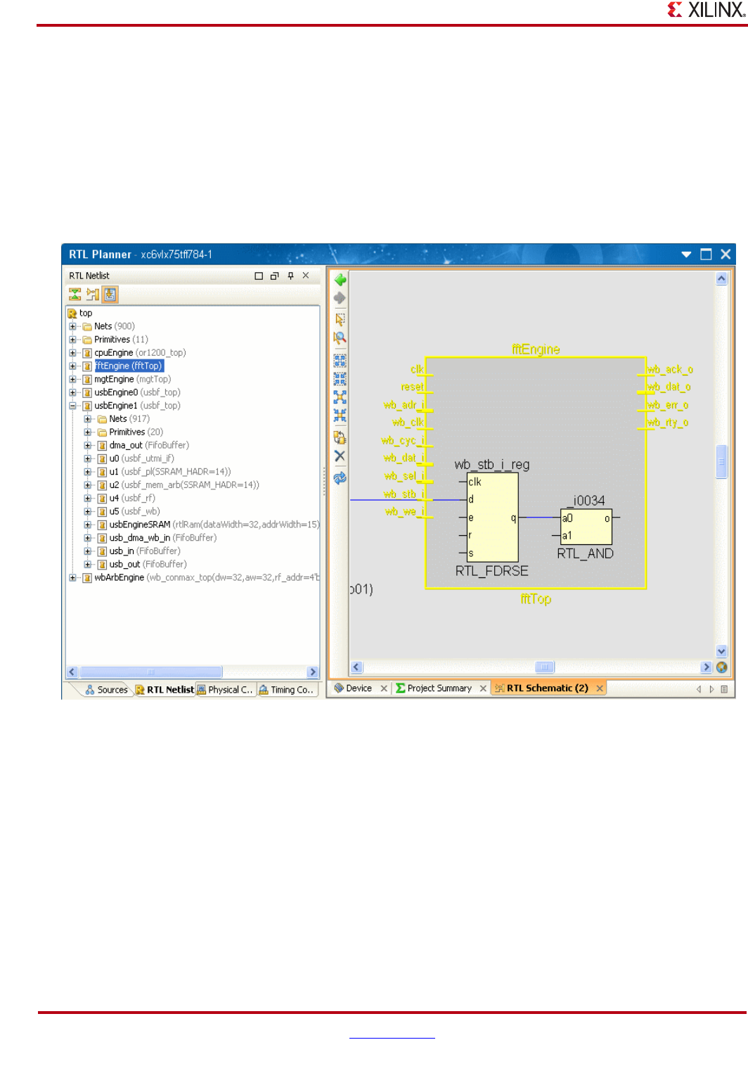
168 www.xilinx.com PlanAhead User Guide

UG632 (v 12.1)

Chapter 5: RTL and IP Design

Analyzing the RTL Design Schematic

The RTL Schematic view works like the Netlist view. You can select any level of logic

hierarchy and view it in the RTL Schematic view.

To invoke the RTL Schematic view for any selected logic, select one of the following:

•Click the Schematic toolbar button.

•Select Tools > Schematic.

The following figure shows the RTL Schematic view.

For more information on traversing, expanding and exploring the RTL Schematic, refer to

“Using the Schematic View” in Chapter 4.

Once the RTL design is elaborated, you can select the Find command to search for logic

objects using a range of filtering techniques. Refer to “Editing Constraints in the Text

Editor” in Chapter 7.

Figure 5-15: RTL Schematic View

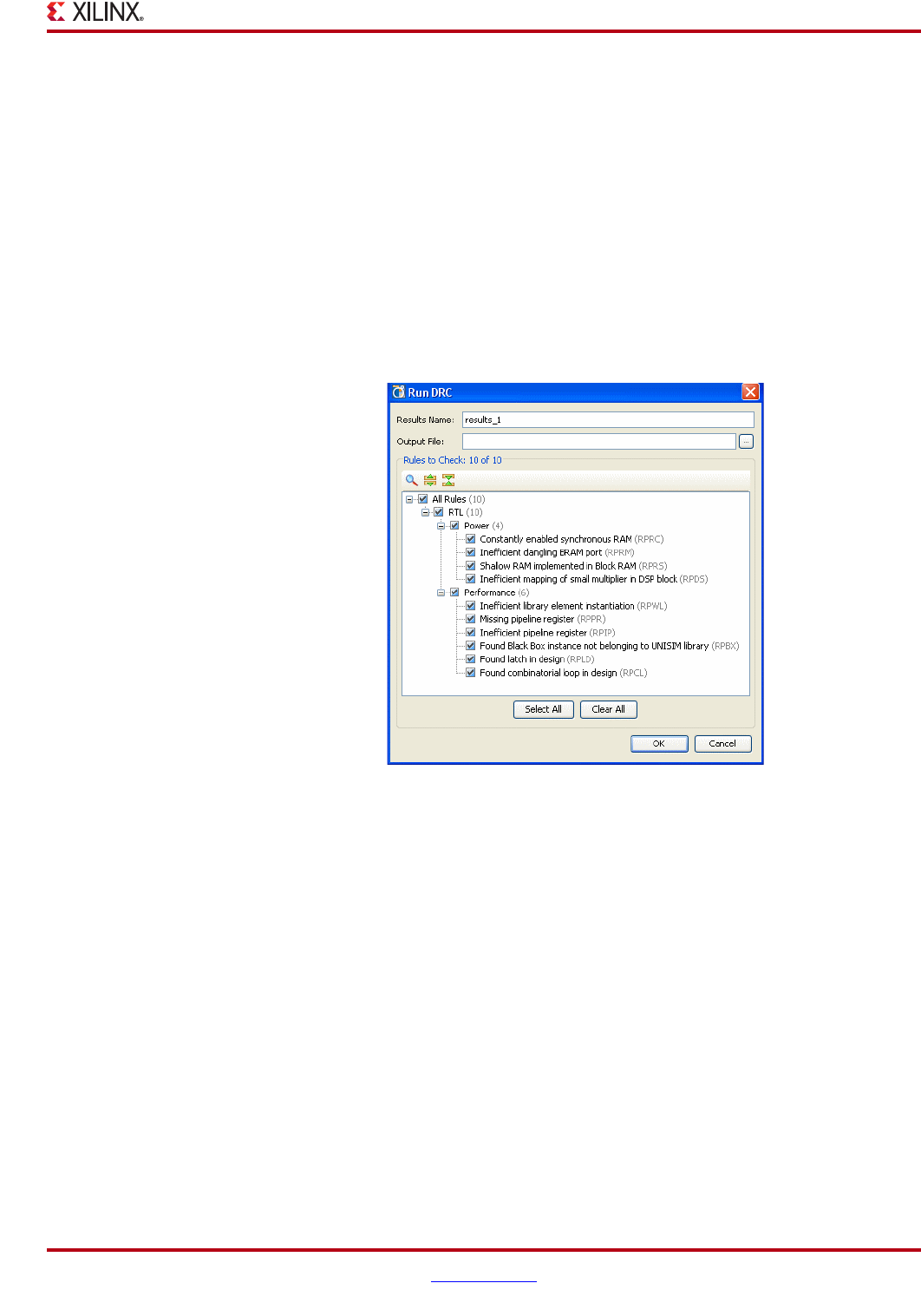
PlanAhead User Guide www.xilinx.com 169

UG632 (v 12.1)

Elaborating and Analyzing the RTL Design

Running RTL DRCs

Selecting DRC Rules

PlanAhead provides Design Rule Checks (DRCs) that you can run after RTL design

elaboration. The available rules focus on power reduction and performance improvement

opportunities.

1. To run the DRC checks after elaborating the design, select one of the following

commands:

−Click Flow Navigator > RTL Design > Run DRC.

−Select Tools > Run DRC.

The Run DRC dialog box opens as shown in the following figure to enable rule selection.

2. In the Run DRC dialog box, select the required rules.

For rule descriptions, see “RTL Rules: Power and Performance,” page 171.

3. Click OK.

Figure 5-16: Run Design Rule Checker Toolbar Button

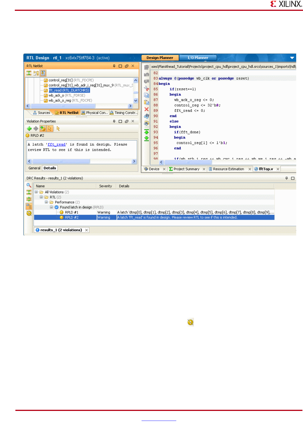
170 www.xilinx.com PlanAhead User Guide

UG632 (v 12.1)

Chapter 5: RTL and IP Design

Analyzing DRC Violations

If violations are found, the DRC Results view opens, as shown in the following figure.

In the Violations Properties view you can:

•Select a violation to display information.

•Select the links to highlight the design objects in question.

•Select the Show Source popup command to highlight a line of RTL source.

•Click the Hide Warning and Information Messages toolbar button to hide all

warnings and informational messages and view only errors. Click again to re-display

errors and warnings. The following figure shows the button.

Figure 5-17: RTL Design with Objects that Violate DRCs

Figure 5-18: Hide Warning and Information Messages Button

PlanAhead User Guide www.xilinx.com 171

UG632 (v 12.1)

RTL Rules: Power and Performance

The following tables list the RTL Power and the RLT Performance rules.

Table 5-1: Power Rules

Rule Name Rule Abbrev Rule Intent Severity

Constantly

enabled

synchronous

RAM

RPRC A described RAM (either inferred or instantiated), which is constantly

enabled, was found in one or both ports. If it can be determined that this

RAM is not constantly accessed. Significant power reduction may be

seen by describing the logic to disable the RAM unless it is being

accessed.

Warning

Inefficient

dangling

BRAM port

RPRM A RAM in which there is an unconnected output port has been detected,

and the WRITE_MODE is set to a value other than NO_CHANGE. Modifying

the description of the RAM in order to set unconnected output port

(WRITE_MODE set to NO_CHANGE) could save up to 10% of the

dissipated block RAM power.

Warning

Shallow RAM

implemented in

Block RAM

RPRS Virtex®-5 and Virtex-6 devices: For wide (over 18-bits) and shallow

(64-bits or less) RAM, it is generally advantageous to choose SelectRAM

(LUT-based RAM referred to as distributed RAM) whenever possible

unless the RAM is being used as a FIFO, in which case the cross-over

point becomes a depth of 32-bits or less. When building interfaces less

than 18-bits wide, the LUT-based SelectRAM could be a better choice for

depths up to 128-bits; however, generally past that, the dedicated block

RAM is a better choice for power.

Warning

Inefficient

mapping of

small multiplier

in DSP block

RPDS Small multipliers mapped to DSP or to other hard multipliers IP, such as

MULT18X18, should be pushed to MSBs. The rest of the LSBs should be

mapped to ground. In this way, the carry propagation is reduced to its

minimum. Usual implementation, especially when inferring the

multiplier, uses LSBs and sign extensions to map the MSBs.

Warning

Table 5-2: Performance Rules

Rule Name Rule Abbrev Rule Intent Severity

Inefficient

library element

instantiation

RPWL Found instance <instance name> of type

<library_component_name> that belongs to another FPGA family.

This might result in suboptimal performance. The ISE software might

remap this element automatically onto a similar element in the selected

family. However, modifying the source code to infer or instantiate native

elements will take advantage of any added or expanded functionalities

in the element. This may in turn improve area utilization and

performance.

Warning

Missing

pipeline register

RPPR Found multiplier with unregistered outputs. You can improve the

multiplier clock-to-out performance by adding a level of registers. In

addition, for best results, avoid using asynchronous control signals on

these registers.

Found RAM/ROM with unregistered outputs. You can improve the

RAM/ROM clock-to-out performance by adding a level of registers. In

addition, for best results, avoid using asynchronous control signals on

these registers.

Warning

172 www.xilinx.com PlanAhead User Guide

UG632 (v 12.1)

Chapter 5: RTL and IP Design

Estimating Power

PlanAhead provides early power estimation based on the design resources.

1. Select one of the following to run the Power Estimation:

−In Flow Navigator > RTL Design, click Power Estimation.

−Select Tools > Power Estimation.

The Power Estimation dialog box opens, as shown in Figure 5-19, page 173.

Inefficient

pipeline register

RPIP Found <register_name> (<file_name>:<line_number>) register

with asynchronous control signals on input or output of multiply

function. Dedicated DSP hardware resources do not have asynchronous

control signals, such as preset or clear. The registers will not be mapped

into the dedicated hardware resources resulting in suboptimal use of the

device.

Warning

Found Black

Box instance not

belonging to

UNISIM library

RPBX Component/Module <component/module_name> description

unavailable during synthesis (<file_name:line>). Paths to and from

this black box cannot be optimized. Synthesis tool utilization estimates

and mapping decisions could be negatively affected.

Warning

Found latch in

design

RPLD Found latch description for signal <signal_name>

(<file_name>:<line_num>). Latches creates difficult to analyze

timing paths which require post implementation simulations to ensure

implemented design match expected behavior.

Warning

Found

combinatorial

loop in design

RPCL Found combinatorial loop for signal <signal_name>

(<file_name>:<line_number>). Combinatorial loops are generated

when a cone of combinatorial logic uses its outputs to feedback as partial

input to the same cone of logic. The total combinatorial delay from source

to destination should be increased by the feedback path delay. This type

of structure could be required from the design expected behavior or

might be unintentional.

Warning

Table 5-2: Performance Rules (Continued)

Rule Name Rule Abbrev Rule Intent Severity

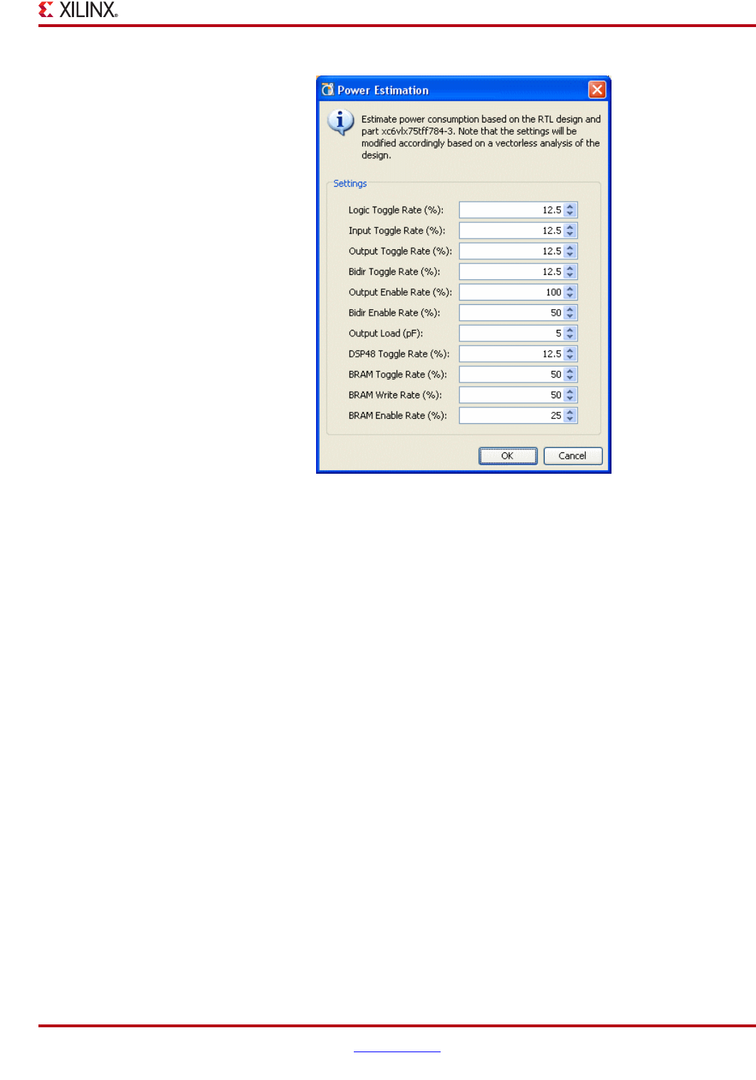
PlanAhead User Guide www.xilinx.com 173

UG632 (v 12.1)

RTL Rules: Power and Performance

2. Enter the Toggle Rate information and click OK.

The Power Estimation view displays in the Workspace.

A Power Summary displays along with an expandable power consumption graph, based

on the design logic hierarchy.

The logic tree is expandable using the view widgets to allow visibility into the logic

hierarchy. Figure 5-20, page 174 shows the Power Estimation view.

Figure 5-19: RTL Power Estimation Dialog Box

174 www.xilinx.com PlanAhead User Guide

UG632 (v 12.1)

Chapter 5: RTL and IP Design

The Power Estimation view works like the Netlist view. You can expand and select any

level of logic hierarchy and analyze its power consumption and hardware resources.

Figure 5-20: Power Estimation View

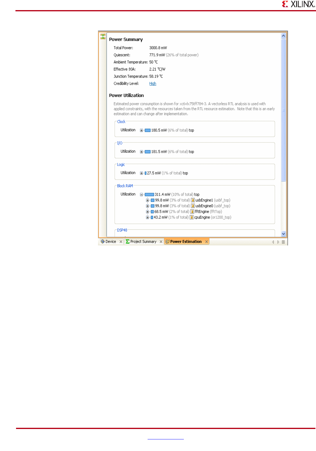
PlanAhead User Guide www.xilinx.com 175

UG632 (v 12.1)

Chapter 6

Synthesizing the Design

This chapter contains the following sections:

•“About the Synthesis and Implementation in PlanAhead”

•“Running Synthesis”

•“Monitoring Run Status”

•“Analyzing Run Results”

•“Launching and Managing Multiple Synthesis Runs”

•“Launching Synthesis Runs on Remote Linux Hosts”

About the Synthesis and Implementation in PlanAhead

The PlanAhead™ software includes a synthesis and implementation environment that

facilities an push button flow with single synthesis and implementation attempts or Runs.

PlanAhead manages the run data automatically, allowing repeated run attempts with

varying RTL source versions, synthesis, or implementation options or constraints.

Also, PlanAhead allows multiple synthesis and implementation runs using different

software command options, and timing or physical constraints. You can queue the

synthesis and implementation runs to launch sequentially or simultaneously with multi-

processor machines. Synthesis runs use Xilinx Synthesis Technology (XST).

You can create and save Strategies, which are a set of option configurations for each

implementation command, that are then applied to Runs for synthesis or implementation

using Xilinx® ISE® Design Suite tools. For more information about saved Strategies, and

about the exported files, see “Outputs for Environment Defaults” in Appendix B.

You can monitor progress, view log reports, cancel runs, manage run data, and quickly

identify and import the best synthesis and implementation results.

176 www.xilinx.com PlanAhead User Guide

UG632 (v 12.1)

Chapter 6: Synthesizing the Design

Running Synthesis

When you run synthesis in PlanAhead you have the ability to set synthesis options, run

synthesis, and view the outcome of the run.

Synthesis Methodology Tips

The following are suggestions on a logic synthesis methodology to use PlanAhead

optimally for design analysis, floorplanning or hierarchical design.

For more information on optimizing ISE synthesis results, see the Xilinx Synthesis and

Simulation Design Guide, (UG626).

To the extent possible, partition the design at the RTL level such that critical timing paths

are confined to individual modules. Critical paths that span large numbers of hierarchical

modules can be difficult to floorplan or partition.

•Register the outputs of all the modules to help limit the number of modules involved

in a critical path.

•Long paths in single large hierarchical blocks can make floorplanning a difficult task.

Consider dividing large hierarchical blocks in the RTL.

•If the design is expected to change often, consider an incremental approach to

synthesis. Most third-party synthesis tools enable a top-down approach for

incremental synthesis and implementation. This capability coupled with Xilinx

partitions can be used to preserve unchanged modules of the implemented design.

Design preservation will help an incremental flow but may hurt performance because

global optimizations across the hierarchy are disabled. This trade-off needs to be

considered before you embark on an incremental methodology.

•Constrain the synthesis engine to rebuild or to otherwise preserve the hierarchy in the

synthesized netlist. Flattened netlists could be optimal from a synthesis perspective,

but they make it very difficult to reliably floorplan and constrain placement.

Consider using synthesis options that rebuild the hierarchy, such as the XST

command line option -netlist_hierarchy = rebuilt.

Setting Synthesis Options

There are several locations in the environment to configure synthesis settings. In the Flow

Navigator Project Manager menu, the Project Summary view, or in the main toolbar, click

the Project Settings button. The following figure shows the Project Setting button.

In the Project Settings dialog box, click Synthesis, if it is not already selected as shown in

Figure 6-2, page 177.

Figure 6-1: Project Settings Button

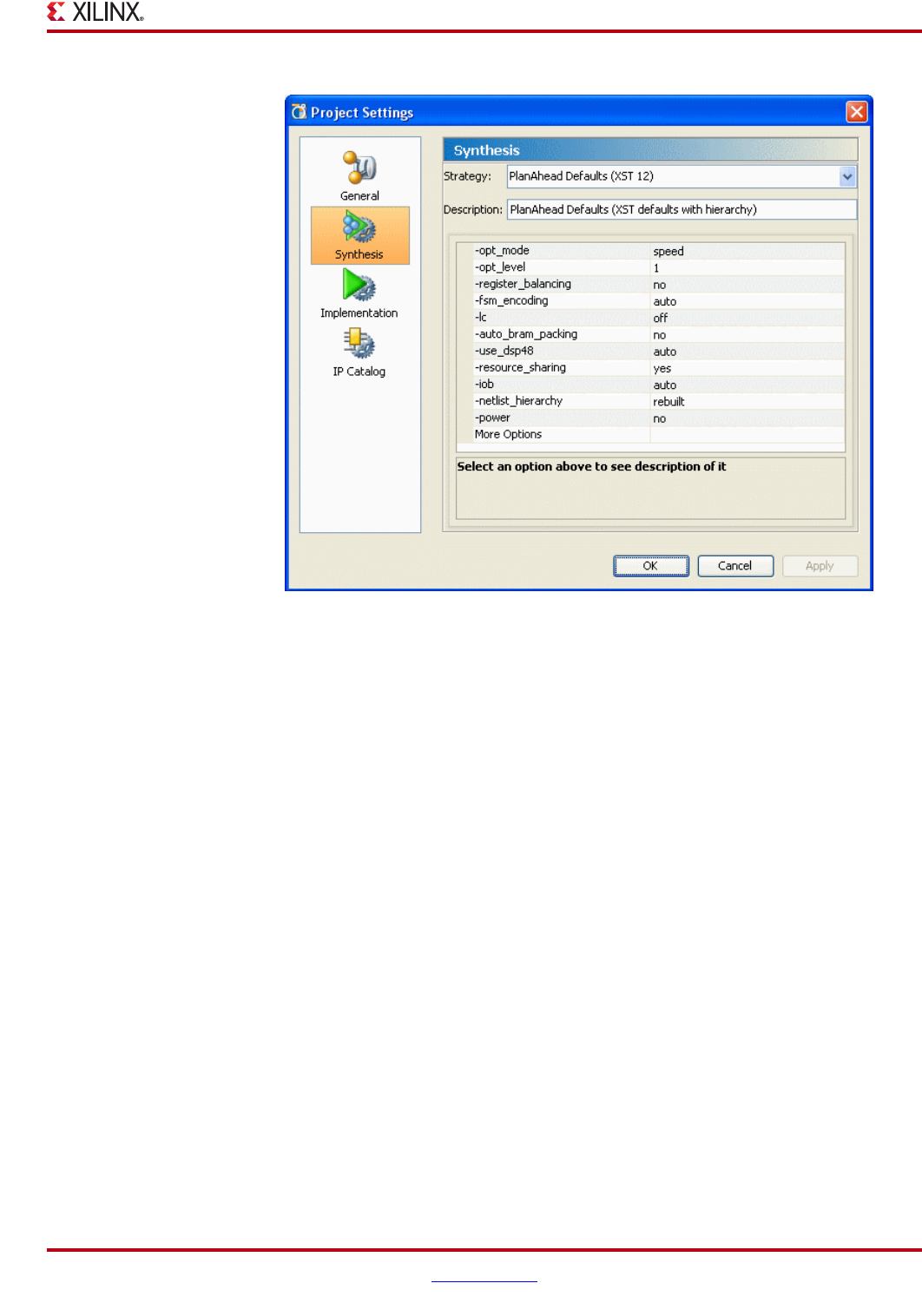
PlanAhead User Guide www.xilinx.com 177

UG632 (v 12.1)

Running Synthesis

The Synthesis Settings dialog box lets you set XST options to be used in the next synthesis

attempt, and it contains the following options:

•Strategy—Select an existing strategy or to create new strategies for future use. See

“Outputs for Environment Defaults” in Appendix B.

•Description—Enter any text to enable easier tracking of the run.

•XST options—Configure any XST option. Use the More Options field to specify

unlisted options. You can find a brief description of each option and what it is used for

in the lower dialog pane.

Note: Modifications to these options are not preserved if synthesis is not run prior to exiting

PlanAhead. If synthesis results exist in the project, the Project Settings will inherit the settings of the

active synthesis run. If no synthesis run exists in the project, the PlanAhead defaults are restored.

Using the XST Option to Create Hierarchical Netlist

All PlanAhead XST synthesis strategies with the exception of the XST default strategy have

the option -netlist_hierarchy = rebuilt set. This switch instructs XST to flatten

the netlist to perform logic optimization. Once done, the logic hierarchy is reconstructed

based on logic names. This facilitates design analysis and floorplanning within the

PlanAhead environment.

If you encounter problems with the switch, set the -netlist_hierarchy option back to

as_optimized in the Synthesis Settings dialog box.

Figure 6-2: Synthesis Project Settings

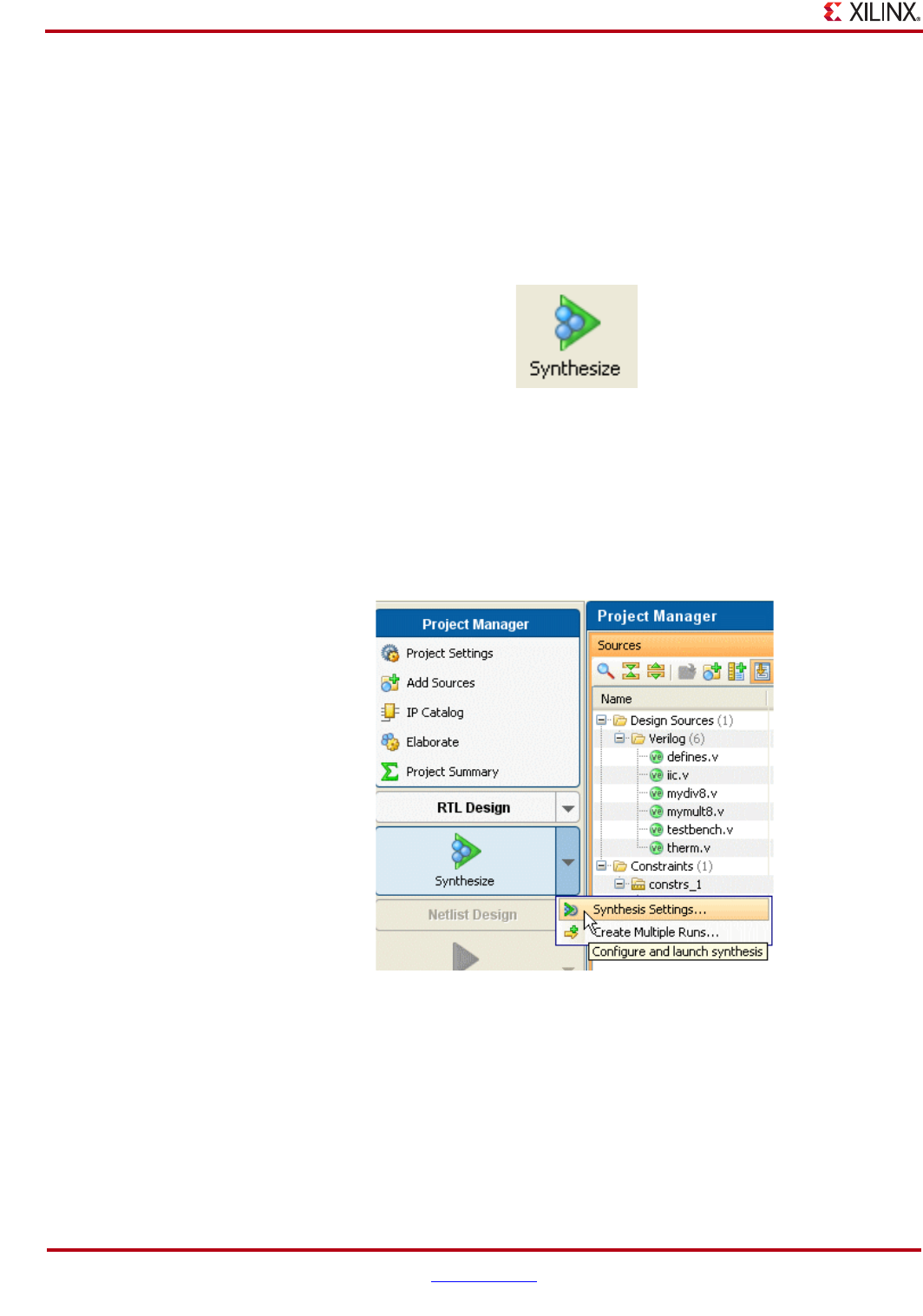
178 www.xilinx.com PlanAhead User Guide

UG632 (v 12.1)

Chapter 6: Synthesizing the Design

Launching Synthesis

You can launch Synthesis Runs from the Flow Navigator.

Launching a Synthesis Run

1. In the PlanAhead environment, click the Synthesize button from the Flow Navigator

or main toolbar as shown in the following figure.

The PlanAhead software uses the current Synthesis Project Settings to launch the run.

The Status bar indicates that Synthesis is running, and the Compilation Message views

begin to display the active command status.

Configuring Synthesis Run Settings

In the Flow Navigator Synthesis button pull down menu, shown in the following figure,

you can set the Synthesis Run options using the Synthesis Settings command.

Figure 6-3: Synthesize Button

Figure 6-4: Configuring Synthesis Run Settings

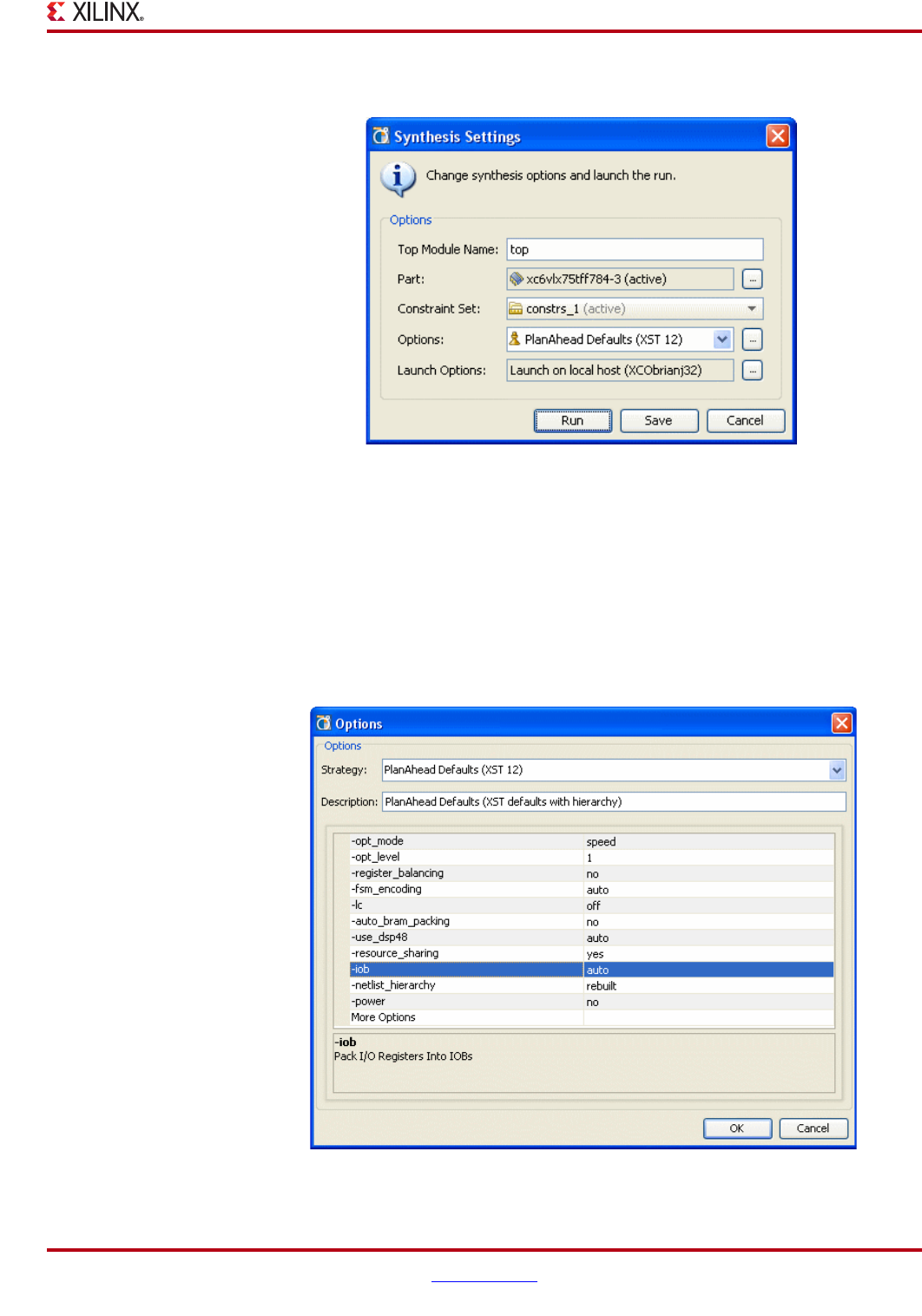
PlanAhead User Guide www.xilinx.com 179

UG632 (v 12.1)

Running Synthesis

The Synthesis Settings dialog box opens as shown in the following figure.

The Synthesis Settings dialog box contains the following options:

•Top Module Name—Enter or accept the top-level RTL module name for the design.

•Part—Select or accept the target part. Click the browser button to invoke the Part

Chooser dialog box.

•Constraint Set—Select or accept the constraint set.

•Options—Select the Synthesis Strategy to use for the run. Click the file browser to

modify XST command options, description or strategy. The Options dialog box is

shown in the following figure.

Figure 6-5: Synthesis Settings

Figure 6-6: Set XST Options for the Run

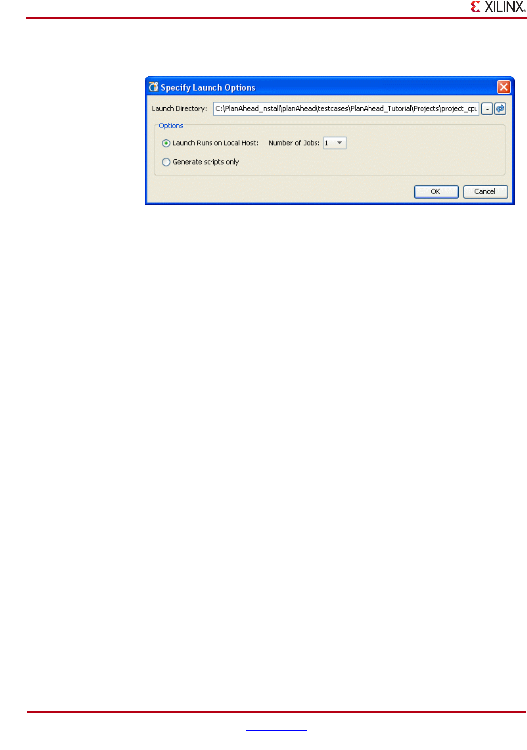
180 www.xilinx.com PlanAhead User Guide

UG632 (v 12.1)

Chapter 6: Synthesizing the Design

•Launch Options—Select additional launch options. The following figure shows the

Specify Launch Options dialog box.

The Specify Launch Options dialog box provides the following options:

•Launch Directory—Specify a location to create and store the synthesis run data.

Note: Defining any non-default location outside of the project directory structure makes

the project non-portable because absolute paths are written into the project files.

•Launch Runs on Local Host—Launch the Run on the local machine processor.

−Number of Jobs—Define the number of local processors to use for Runs. This

option is used only when you are launching multiple runs simultaneously.

Individual runs are launched on each processor. No multi-threaded processors are

used with this option.

•Launch Runs on Remote Hosts (Linux only)—Use remote hosts to launch one or

jobs.

−Configure Hosts—Select this option to configure remote hosts. See “Launching

Runs on Remote Linux Hosts” in Chapter 9.

•Generate scripts only—Export and create the run directory and run script, but not to

launch the run from PlanAhead. The script can be run at a later time outside of the

PlanAhead environment.

2. Click Save and Run to launch the run with the current settings. Click Save to save the

settings, but not start the run.

Monitoring Run Status

You can monitor the status of a synthesis run by reading the compilation log, or viewing

the compilation information, warnings, and errors in the Command Messages view.

The following subsections describe the Run status monitoring options.

Using the Project Status Display

The Project Status indicator in the upper right corner of the PlanAhead environment

shown in Figure 6-8, page 181, serves functions that include:

•Displaying the overall status of the project and the progress of running commands

•Providing a Cancel command to stop any running commands.

Figure 6-7: Synthesis Launch Options

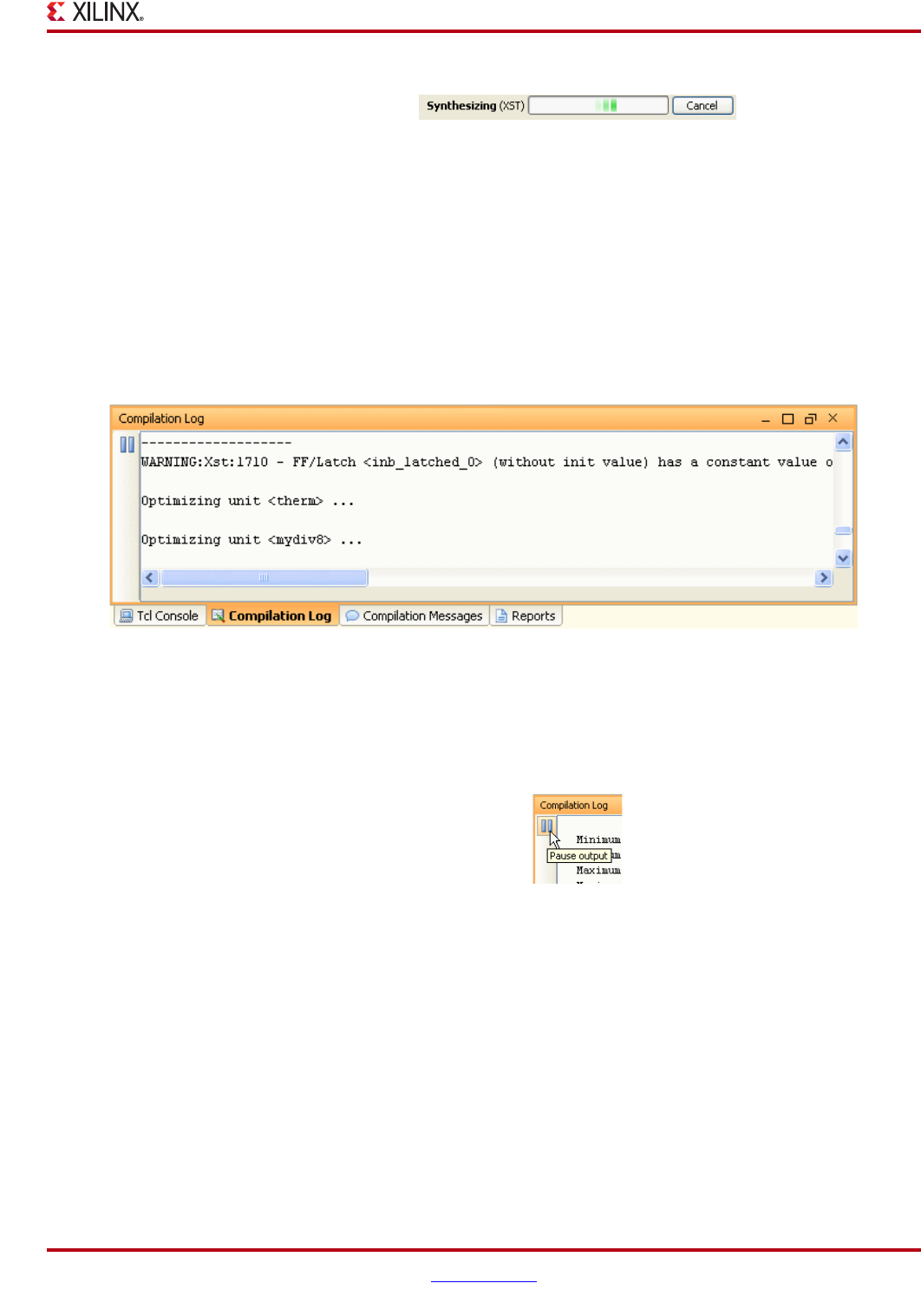
PlanAhead User Guide www.xilinx.com 181

UG632 (v 12.1)

Monitoring Run Status

Cancelling a Run

You can stop the XST synthesis run by clicking the Cancel button in the Project Status

Display, shown in Figure 6-8.

Viewing the Compilation Log

The Compilation Log view opens once a synthesis run is launched and shows the XST

standard output messages. The following figure is an example of a compilation log.

Pausing the Output as Commands are Running

The Pause output button lets you scroll and read the log while a command is running. The

active output is disabled until you click the button again, shown in the following figure.

Figure 6-8: Project Status Display

Figure 6-9: Compilation Log

Figure 6-10: Pause Output Button

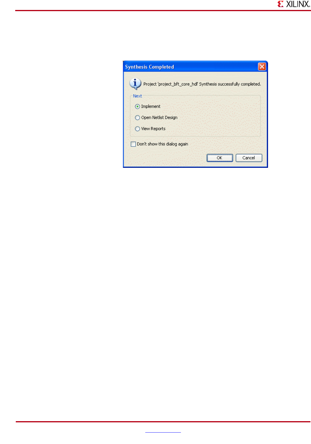
182 www.xilinx.com PlanAhead User Guide

UG632 (v 12.1)

Chapter 6: Synthesizing the Design

Selecting Next Step After Synthesis Completes

Once the Run is complete, one of the following dialog boxes, shown in the following

figure, opens and prompts you to take the next step.

3. In the Synthesis Completed dialog box, select the option that matches how you want to

proceed.

−Implement—Launches implementation with the current Implementation Project

Settings.

−Open Netlist Design—Imports the netlist, active constraint set, and target part

into the PlanAhead design analysis and floorplanning environment so you can

perform I/O pin planning, design analysis, and floorplanning.

−View Reports—Opens the Reports view so you can select and view the XST

Report file.

4. Click OK to take the selected action, or click Cancel to do nothing now.

Figure 6-11: Synthesis Completed or Failed Dialog Box

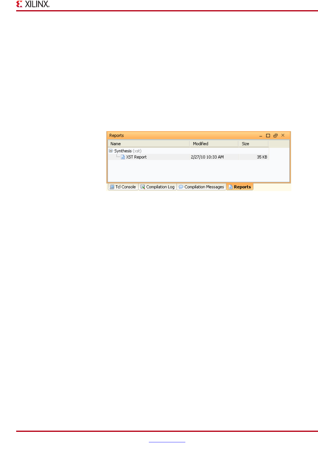
PlanAhead User Guide www.xilinx.com 183

UG632 (v 12.1)

Analyzing Run Results

After synthesis completes, you can open and view the XST synthesis reports, and the open

and analyze the netlist design, and then apply timing or physical constraints prior to

implementation. Refer to Chapter 7, “Netlist Analysis and Constraint Definition” for more

information.

Viewing Report Files

You can view report files generated by the ISE tools from within Reports view. The view is

usually opened automatically after commands are run. if it is not available, select the

Reports link in the Project Summary view. The Reports view opens as shown in the

following figure.

When you select an available report file it opens in the Workspace as shown inFigure 6-13,

page 184. The file viewing options are:

•Browse the report file using the scroll bar.

•Select the Find or Find in Files buttons to search for specific text.

•Use the Go to the beginning or Go to the End toolbar buttons to scroll to the beginning

or end of the file.

Figure 6-12: Selecting Report Files to View

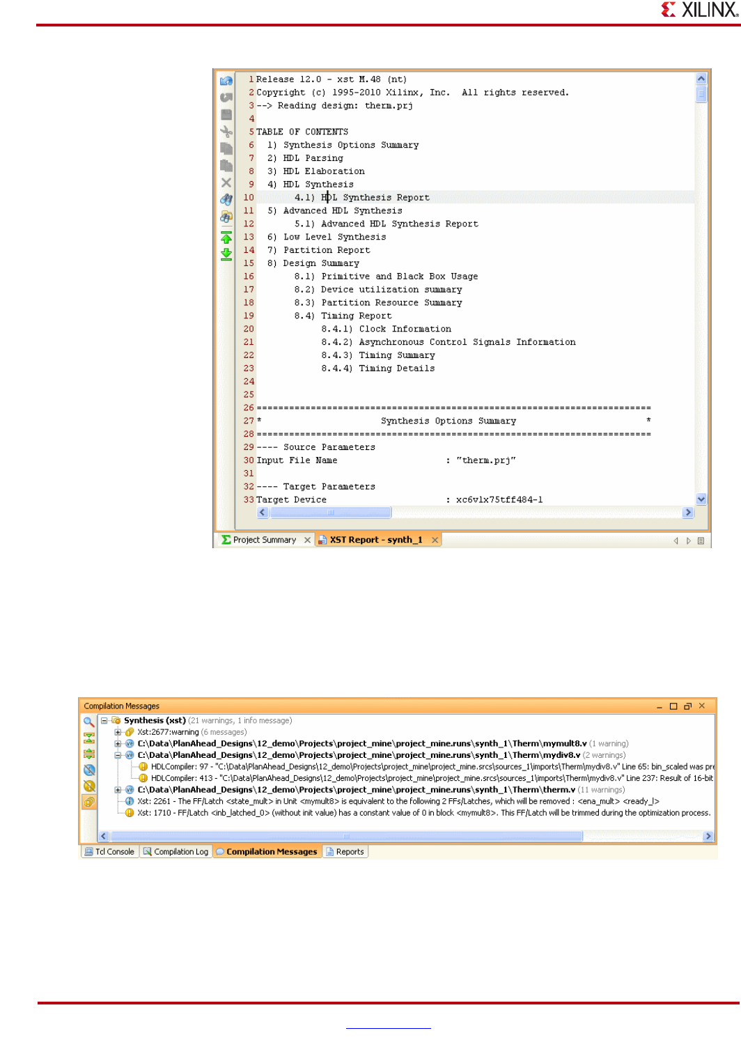
184 www.xilinx.com PlanAhead User Guide

UG632 (v 12.1)

Chapter 6: Synthesizing the Design

Viewing Compilation Messages

The Compilation Messages view provides a filtered list of the compilation log that includes

the main messages, warnings, and errors. The following figure shows an example of a

Compilation Messages view.

The synthesis messages are organized by source file and severity.

Click on the expand and collapse tree widgets to view the individual messages.

Figure 6-13: Viewing Report Files

Figure 6-14: Compilation Messages View

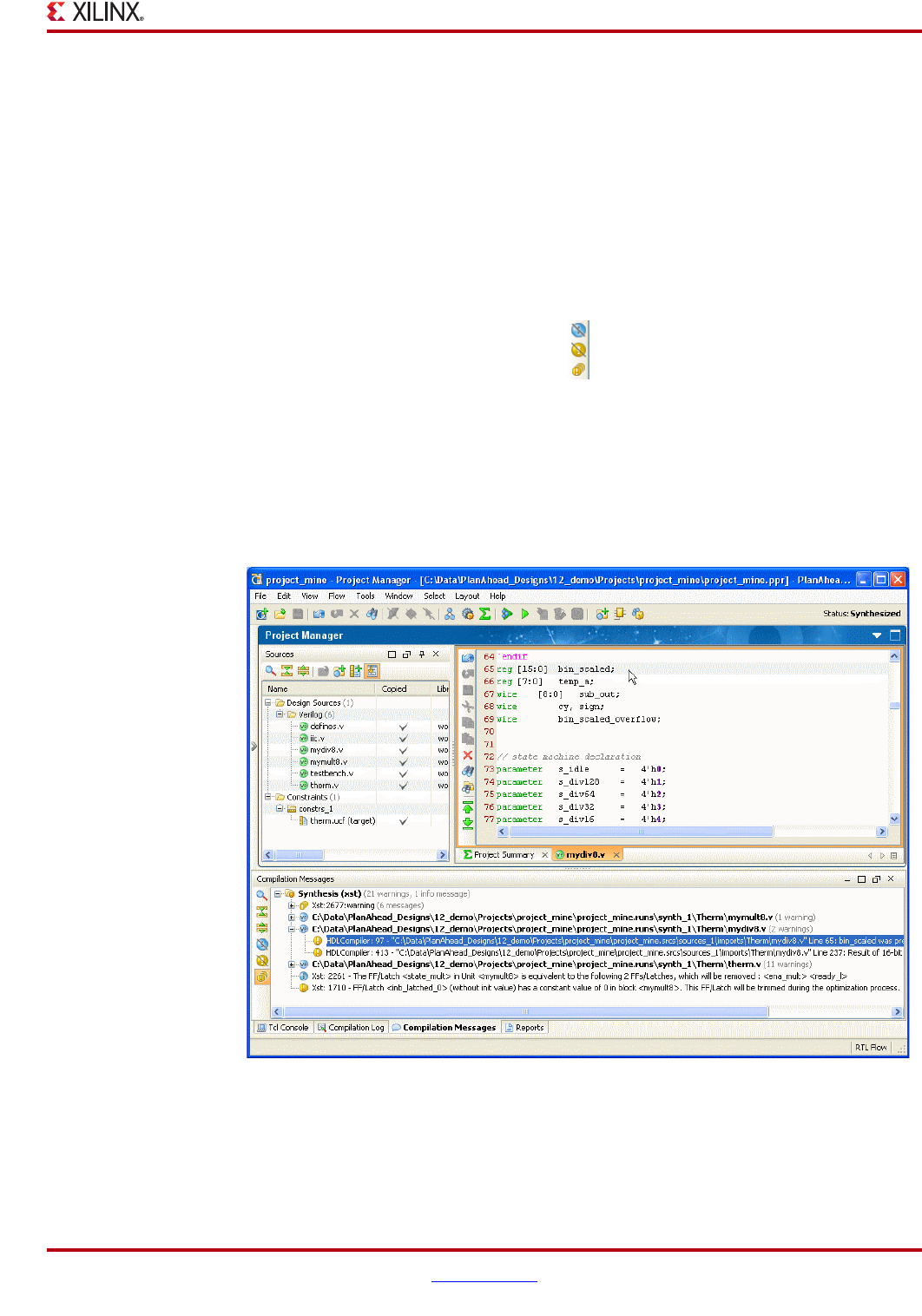
PlanAhead User Guide www.xilinx.com 185

UG632 (v 12.1)

Analyzing Run Results

The command buttons on the left provide searching and filtering capabilities.

The Show Search, Collapse All And Expand All commands are standard in PlanAhead

views. Refer to “Using Tree Table Style Views” in Chapter 4.

Filtering and Grouping Compilation Messages

You can toggle the Hide info messages and Hide warning messages buttons to filter the

messages to include only warnings and/or errors. The Group duplicate messages button

flattens the list and groups similar messages together. These button are shown in the

following figure.

Highlighting Compilation Issues in RTL Sources

Selecting any of the Synthesis messages in the Compilation Messages view that have a Line

number referenced will automatically open the RTL file and highlight that line of source

code. The following figure shows an example of the error navigation process.

Select any message and use the Search for Answer Record popup menu command to

search the Customer Support database for related answer records.

Figure 6-15: Message Filtering and Grouping Buttons

Figure 6-16: Error Navigation to RTL Sources

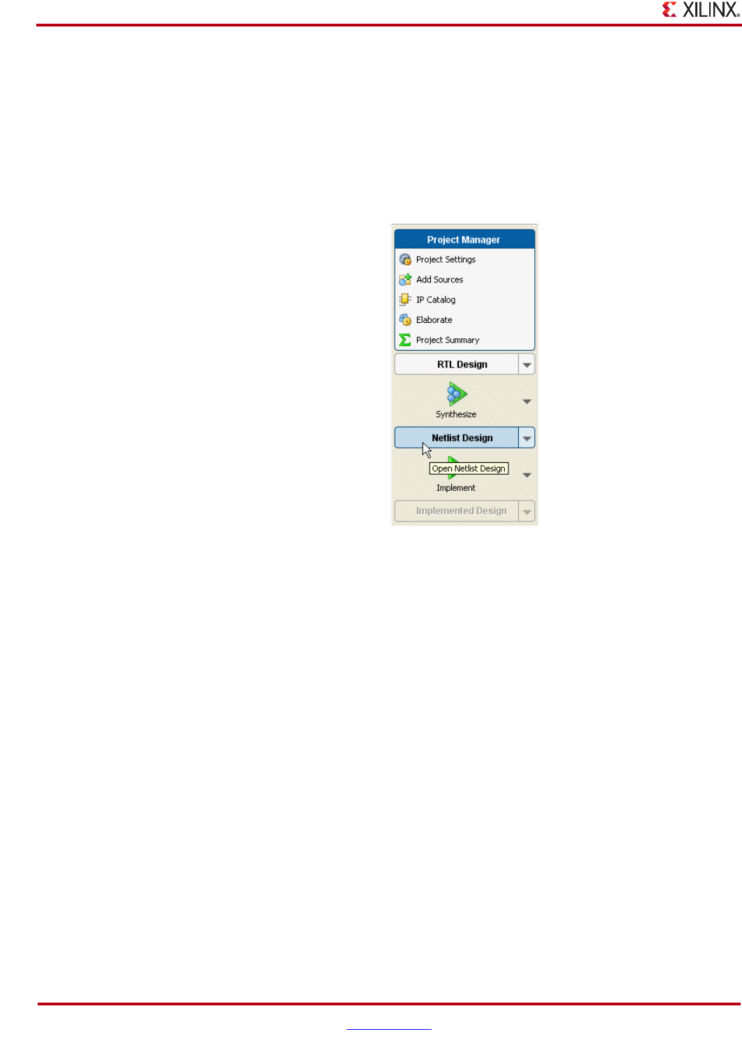
186 www.xilinx.com PlanAhead User Guide

UG632 (v 12.1)

Chapter 6: Synthesizing the Design

Opening the Netlist Design

PlanAhead enables you to import the results of a synthesis run for analysis and constraint

definition. ChipScope debug cores can be added to the design in the Netlist Design

environment. Once the synthesis run has completed, a dialog box opens prompting you to

open the netlist design. For more information, see “Running Synthesis,” page 176.

Also, you can open the netlist design in the Flow Navigator by clicking the Netlist Design

button as shown in the following figure.

Refer to Chapter 7, “Netlist Analysis and Constraint Definition,” for information about

netlists analysis and definition.

Launching and Managing Multiple Synthesis Runs

PlanAhead enables you to create and launch multiple synthesis runs to explore synthesis

options to find the best results. The runs are queued and launched serially, or in parallel on

multiple local CPUs. Remote servers can be used on Linux. See “Launching Runs on

Remote Linux Hosts” in Chapter 9.

Note: PlanAhead provides flexibility to create multiple synthesis runs, implementation runs, and

constraint sets. You can create a project with multiple run attempts; consequently, you must manage

the various run data. PlanAhead issues messages about out-of-date data after source files,

constraints or project settings are modified. You can delete and manage stale run data using the

Design Runs view.

Figure 6-17: Opening the Netlist Design

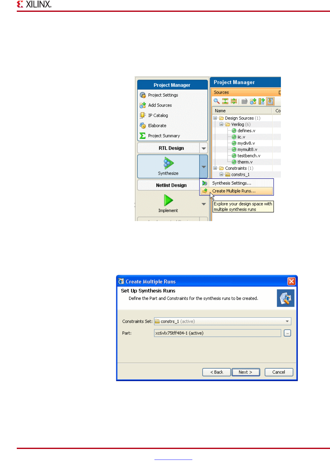
PlanAhead User Guide www.xilinx.com 187

UG632 (v 12.1)

Launching and Managing Multiple Synthesis Runs

Creating Multiple Synthesis Runs

To create multiple synthesis runs:

1. Select Tools > Create Multiple Runs, or in the Flow Navigator, click Create Multiple

Runs from the Synthesize pull down menu, as shown in the following figure.

The Create Multiple Runs wizard opens.

2. In the Introduction page, click Next to proceed.

The Set Up Synthesis Runs page opens as shown in the following figure.

The Set Up Synthesis Runs options are:

−Constraint Set—Enter or accept the constraint set that will be applied to the

synthesized netlist if the Netlist Design is opened after the run completes.

Figure 6-18: Create Multiple Runs Command

Figure 6-19: Set Up Synthesis Runs Dialog Box

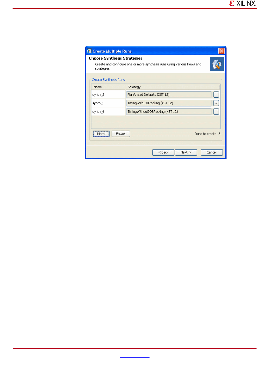
188 www.xilinx.com PlanAhead User Guide

UG632 (v 12.1)

Chapter 6: Synthesizing the Design

−Part—Select or accept the target part. Click the browser to invoke the Part

Chooser drop down menu.

3. Click Next to bring up the Choose Strategies page, as shown in the following figure.

4. Select a Name and Strategy for the first synthesis Run.

5. Click More to add more runs.

6. Enter names and choose synthesis strategies for additional Runs.

7. Click Next to invoke the Launch Options dialog box. Refer to “Setting Synthesis

Options,” page 176 for more information on setting launch options.

8. Click Next and review the Create Multiple Runs Summary, and click Next again.

9. Click Finish to create the defined Runs and execute the specified Launch options.

Managing Multiple Synthesis Runs

The capabilities for managing multiple synthesis runs are very similar to those used to

manage multiple implementation runs. See “Managing Multiple Runs” in Chapter 9.

Launching Synthesis Runs on Remote Linux Hosts

For information regarding remote Linux hosts, see “Launching Runs on Remote Linux

Hosts” in Chapter 9.

Figure 6-20: Choose Synthesis Strategies

PlanAhead User Guide www.xilinx.com 189

UG632 (v 12.1)

Chapter 7

Netlist Analysis and Constraint Definition

This chapter contains the following sections:

•“Overview”

•“Using the Netlist Design”

•“Viewing and Reporting Resource Statistics”

•“Exploring the Logic”

•“Inserting ChipScope Debug Cores”

•“Defining Timing Constraints”

•“Running Timing Analysis”

•“Using Slack Histograms”

•“Defining Physical Constraints”

•“Running the Design Rule Checker (DRC)”

Overview

This chapter describes the design analysis and constraint definition features available in

the PlanAhead™ software. The described features are typically performed by opening the

Netlist Design and before running implementation. However, many of the analysis and

constraints features described in this section are also available for Implemented Designs.

In Netlist Design, you can:

•Analyze various aspects of the design

•Validate resource and timing estimates

•Run DRCs

•Define physical and timing constraints for the Xilinx® ISE® Design Suite

Several PlanAhead design tasks must be performed in the Netlist Design such as:

•Inserting ChipScope™ debug cores

•Defining partitions for Design Preservation and Partial Reconfiguration

Additional analysis features are described in Chapter 5, “RTL and IP Design,” and

Chapter 8, “I/O Pin Planning.”

You can use most of these features after implementing the design also. The range of

features useful for analyzing an implemented design are described in Chapter 10,

“Analyzing Implementation Results.”

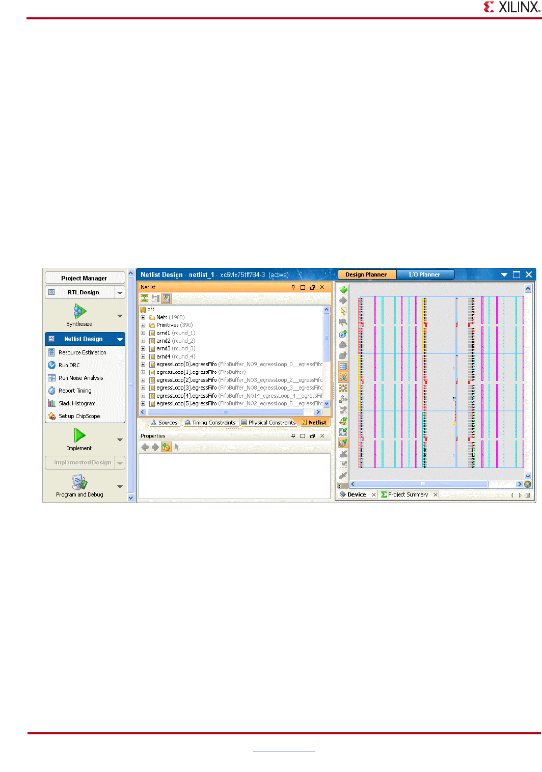
190 www.xilinx.com PlanAhead User Guide

UG632 (v 12.1)

Chapter 7: Netlist Analysis and Constraint Definition

Using the Netlist Design

PlanAhead provides an environment to analyze the design from several different

perspectives and to apply constraints to the design prior to implementation.

When you open the Netlist Design, PlanAhead loads the synthesized netlist, the active

UCF constraint set, and the target device. See “Using the Netlist View” in Chapter 4 for

more information.

Using the Design Planner Environment

The Design Planner view layout provides a variety of design information enabling you to

examine the logic, the resource utilization and timing estimates, run DRC, and apply

timing and physical constraints.

The default views presented in the Design Planner include: the Project Summary, Device,

Netlist, Sources, Timing Constraints, and Physical Constraints views, as shown in the

following figure.

You can open other views, if needed, including the Package view. For more information

about using specific views, refer to “Using Common PlanAhead Views” in Chapter 4.

Figure 7-1: Netlist Design Planner View Layout

PlanAhead User Guide www.xilinx.com 191

UG632 (v 12.1)

Viewing and Reporting Resource Statistics

PlanAhead provides statistical information about the design logical content and device

utilization. The Project Summary contains a Resources pane with resource utilization

estimates for the elaborated RTL and XST synthesized neltists. The resource statistics from

XST and the ISE map reports are also shown in their respective tabs.

PlanAhead also allows you to select any netlist instance or Pblock and view resource

statistics in the Instance or Pblock Properties view. This includes selecting the top-level

design. The displayed information includes: logic object type counts, percentage of device

resources utilized, carry chain information, and clock reports. This information can be

exported into an Excel spreadsheet.

Viewing Resource Estimates in the Project Summary

As resource information becomes available, it displays automatically in the Resources

panel in the Project Summary. For more information about the viewing resource estimates

in the Project Summary, refer to “Understanding the Project Summary” in Chapter 3.

Generating Hierarchical Resource Estimates

You can display resource estimates graphically as an expandable hierarchical tree. Each

Resources type displays and can be expanded to view each level of logic hierarchy.

To display a graphical view of device resource estimates:

1. Open the Netlist Design.

2. From the Flow Navigator or Tools menu, click the Resource Estimation command.

A Hierarchical Resource Utilization summary opens, as shown in Figure 7-2, page 192.

192 www.xilinx.com PlanAhead User Guide

UG632 (v 12.1)

Chapter 7: Netlist Analysis and Constraint Definition

3. Expand the logic types and logic hierarchy as needed.

Viewing Resource Statistics for Logic Instances

PlanAhead provides estimates of the number of device resources contained in the design.

Resource statistics for any logic instance including the top-level can be displayed in the

Instance Properties view.

To display design resource statistics, select either the top-level module or any instance

module in the Netlist view. The following figure shows the Netlist view with a top module

selected.

Figure 7-2: Hierarchical Resource Estimation

Figure 7-3: Netlist View with Top Module Selected

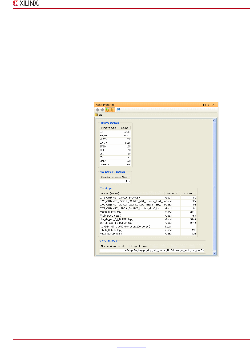
PlanAhead User Guide www.xilinx.com 193

UG632 (v 12.1)

Viewing and Reporting Resource Statistics

The Netlist or Instance properties open in the Properties view.

If the Netlist or Instance Properties do not display, right-click on the module, and select the

Netlist Properties or Instance Properties command from the popup menu.

•The Netlist Properties view contains one tab and should display the statistics by

default.

•The Instance Properties dialog box contains five tabs. If you are viewing the Instance

Properties, click the Statistics tab.

The Statistics tab displays valuable design information including: primitive instance

counts, interface signal counts, clock names, and clocked instance count, carry chain count,

and max length.

The following figure shows an example of the Netlist Resource Statistics.

Figure 7-4: Netlist Resource Statistics

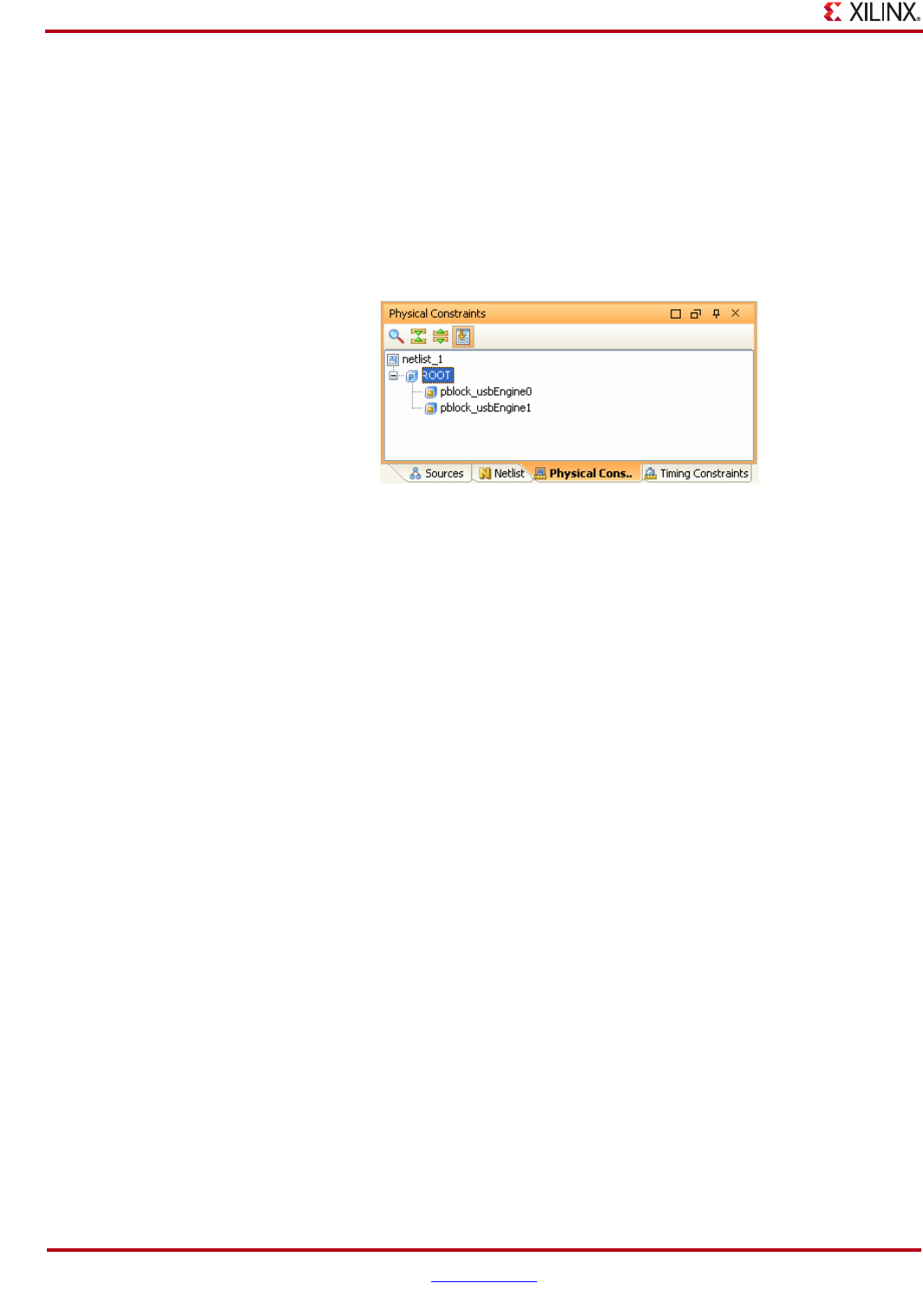
194 www.xilinx.com PlanAhead User Guide

UG632 (v 12.1)

Chapter 7: Netlist Analysis and Constraint Definition

Viewing Resource Statistics for Pblocks

PlanAhead provides logic utilization statistics for Pblocks that can help determine if

enough device resources are contained in the Pblock area to satisfy the assigned logic.

Also, the ROOT Pblock is considered the top of the design and can provide utilization

statistics for the entire design.

To display utilization statistics for a Pblock:

1. Select either the ROOT Pblock or any Pblock in the Physical Constraints view. The

following figure shows a selected ROOT Pblock.

The Pblock Properties display in the Properties view.

2. If the Pblock Properties do not display, right-click ROOT or Pblock, and select Pblock

Properties from the popup menu.

Refer to the“Viewing Pblock Properties” in Chapter 11.

Using the Statistics Tab

The Statistics tab displays design information that includes: overall device utilization

for the various device resources, carry chain count and max length, RPM count, and

maximum sizes, clock names and clocked instance count, I/O utilization, and signal

and primitive instance counts. Figure 7-6, page 195 provides an example of the

Statistics tab.

Figure 7-5: Physical Constraints View with ROOT Selected

PlanAhead User Guide www.xilinx.com 195

UG632 (v 12.1)

Viewing and Reporting Resource Statistics

Figure 7-6: Pblock Properties: Statistics Tab

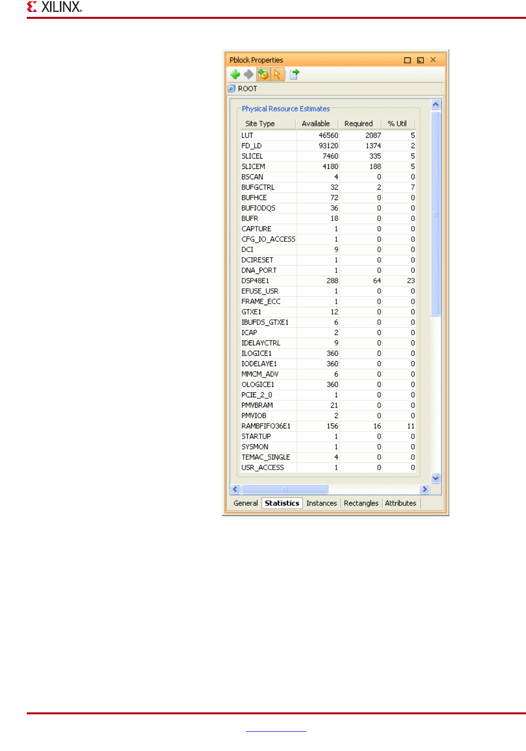
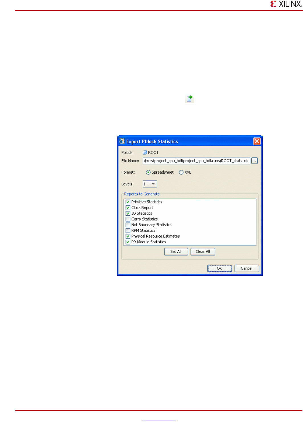
196 www.xilinx.com PlanAhead User Guide

UG632 (v 12.1)

Chapter 7: Netlist Analysis and Constraint Definition

Exporting Resource Statistics Reports

You can save the displayed data to a spreadsheet file. PlanAhead generates a hierarchical-

style report, in which you can define how many levels of hierarchy to report with estimates

listed for each module at each level.

To export a resource statistics report:

1. Select the Export Statistics button (shown in the following figure) to export the data to

a spreadsheet file.

The Export Netlist Statistics dialog box opens, as shown in the following figure.

The Export Netlist Statistics dialog box contains the following editable options:

•File Name—Enter the name and location of the spreadsheet file to be created.

•Format—Select either an XML or Microsoft Excel format output file format.

•Levels —Indicate the number of levels of hierarchy to traverse and include in the

report as separated modules.

•Reports to Generate—Define the types of information from the Pblock Property

Statistics view to include in the output report file.

2. Select the options for the exported file.

3. Click OK.

Figure 7-7: Export Statistics Toolbar Button

Figure 7-8: Export Netlist Resource Statistics

PlanAhead User Guide www.xilinx.com 197

UG632 (v 12.1)

Exploring the Logic

PlanAhead provides several perspectives in which to analyze the design logic:

•The Netlist and Hierarchy views contain a navigable hierarchical tree-style view.

•The Schematic view allows selective logic expansion and hierarchical display.

•The Device view provides a graphical view of the device, placed logic objects and

connectivity. All views cross select and are laid out to present the most useful

information.

•The Implemented Design contains additional logic analysis capabilities. The

capabilities are more powerful after placement and timing results are imported. Refer

to Chapter 10, “Analyzing Implementation Results” for more information.

The following subsections describe the logic exploration methods that are available in

PlanAhead.

Exploring the Logic Hierarchy

The Netlist view displays the logic hierarchy of the RTL. You can expand and select any

logic instance or net within the netlist. As logic objects are selected in other views, the

Netlist view automatically expands to display the selected logic objects. For more

information, refer to “Using the Netlist View” in Chapter 4.

Information about instances or nets are displayed in the Instance or Net Properties views

The Hierarchy view displays a graphical representation of the RTL logic hierarchy. Each

module is sized in relative proportion to the others, so you can determine the size and

location of any selected module. For more information, refer to “Using the Hierarchy

View” in Chapter 4.

Exploring the Logical Schematic

The Schematic view allows selective expansion and exploration of the logical design. At

least one logic object must be selected before the Schematic view is available. Any logic can

be selected and viewed in the Schematic view.

Groups of timing paths can be displayed to show all of the instances on the paths. This is a

tremendous aid for floorplanning as it helps you visualize where the timing critical

modules are in the design.

To open the Schematic view:

1. Select one or more instances, nets, or timing paths.

2. Select the Schematic command from the view toolbar or the popup menu, or press the

F4 key.

The view opens with the selected logic displayed.

3. You can then select and expand the logic for any pin, instance or hierarchical module.

For more information, refer to “Using the Schematic View” in Chapter 4.

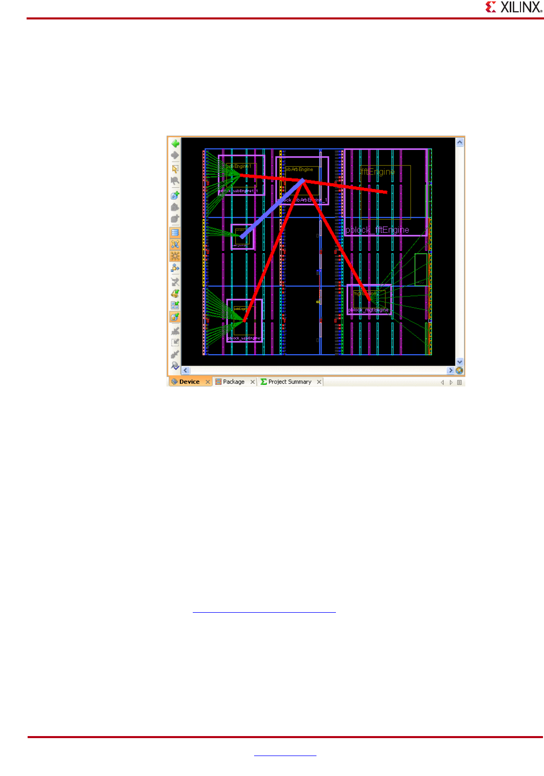
198 www.xilinx.com PlanAhead User Guide

UG632 (v 12.1)

Chapter 7: Netlist Analysis and Constraint Definition

Analyzing Hierarchical Connectivity

PlanAhead provides the ability to examine the logic hierarchy, including visualizing

connectivity between the various logic modules.

Sometimes, it is helpful to create a top-level floorplan to help visualize the connectivity

flow of the design, as shown in the following figure.

The Net bundles indicate the heaviest connectivity requirements between the modules.

When you select a Net bundle information about the net content displays in the Net

Bundle Properties view.

The color and line thickness of the Net bundles can be configured depending on the

number of signals they contain. The Tools > Options > General dialog box contains

connectivity display options. One option is to display the Net Bundles as a Mesh or in a

Tree pattern.

You can also traverse the hierarchy and create submodules for the larger top-level

instances to gain more detailed granularity.

This top-level floorplan can be an indicator of the I/O pinout configuration quality, and

can help identify potential routing congestion issues.

Also, examining resource statistics and clock requirements for each module can aid in

understanding potential placement issues.

Refer to the Floorplanning Methodology Guide (UG633) for more information.

Figure 7-9: Viewing Top-level Design Connectivity

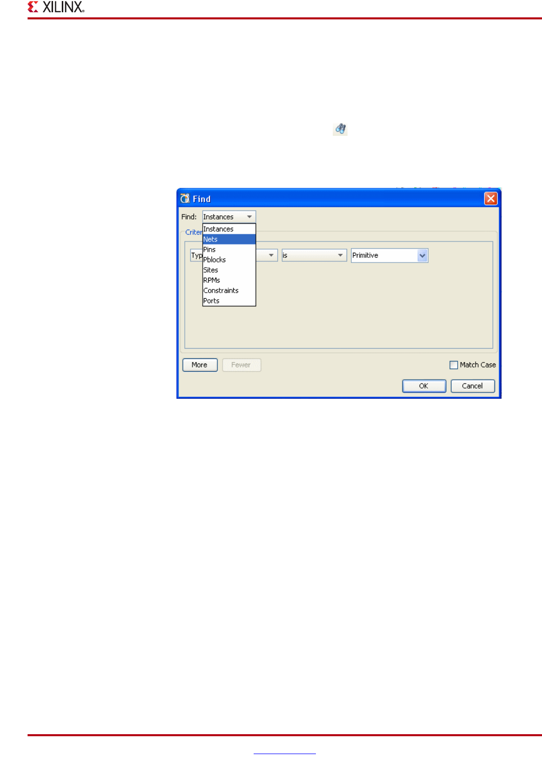
PlanAhead User Guide www.xilinx.com 199

UG632 (v 12.1)

Exploring the Logic

Searching for Objects Using the Find Command

The PlanAhead software lets you selectively search for instances or nets using the Find

command. To invoke the Find command:

1. Select Edit > Find, or click the Find toolbar button, shown in the following figure.

The Find dialog box opens as shown in the following figure.

2. View or edit the definable fields in the Find dialog box:

•Find—Select the object type (Instances, Nets, Pblocks, and so forth) for which you

want to search.

•Criteria—For each object type, a different set of search parameters are available in the

dialog box.

−In the first field, select the way in which you would like to search for the objects:

Name, Status, Type, Parent Pblock, Module, or Primitive count.

−In the second field, you can set boolean options for the search, such as: matches,

does not match, contains, and does not contain.

−Use the third field to select a category or input search criteria strings. You can use

the asterisk (*) to in the search strings also.

3. Optionally, click the More button to define additional search filters or to

simultaneously search for additional types of objects.

A new row of search criteria fields display in the Find dialog box. An AND/OR field

appears to define the additional search criteria. Setting it to AND defines an additional

search filter as shown in Figure 7-12, page 200.

Figure 7-10: Find Toolbar Button

Figure 7-11: Find Dialog Box

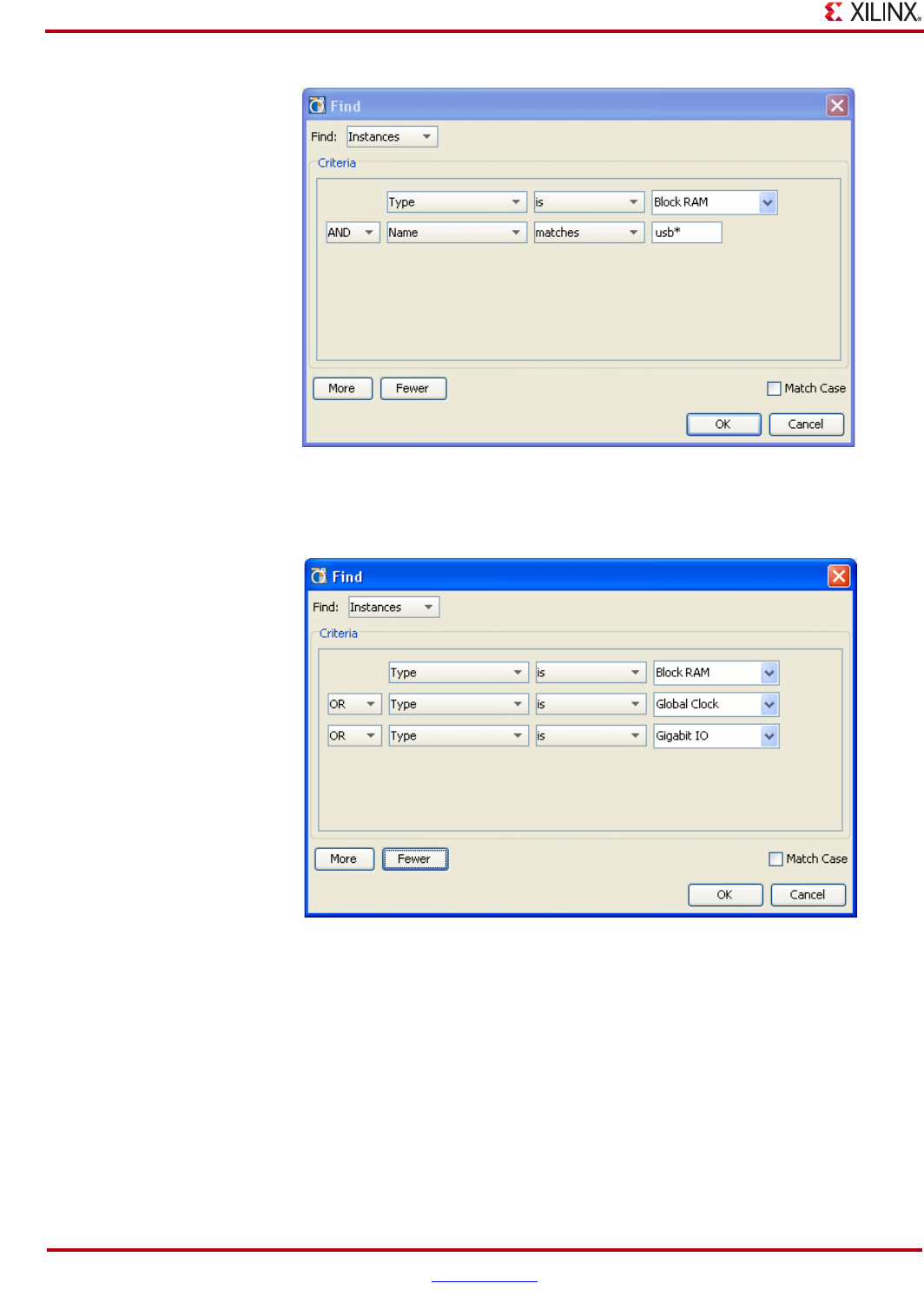
200 www.xilinx.com PlanAhead User Guide

UG632 (v 12.1)

Chapter 7: Netlist Analysis and Constraint Definition

4. You can search for multiple objects simultaneously by using the OR criteria as shown

in the following figure.

5. Click the Fewer button to remove search criteria rows.

6. Click OK to perform the search.

The combined search results display in the Find Results view.

Figure 7-12: Searching for Objects with Additional Search Criteria

Figure 7-13: Searching for Multiple Object Types Simultaneously

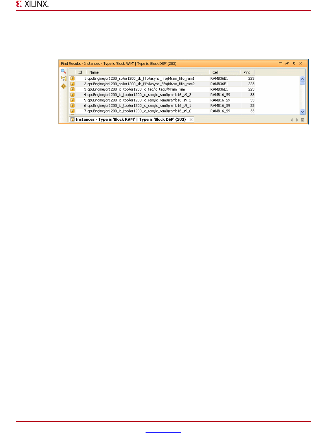
PlanAhead User Guide www.xilinx.com 201

UG632 (v 12.1)

Inserting ChipScope Debug Cores

Using the Find Results View

The objects matching the Find dialog box criteria display in the Find Results view once you

initiate the search by clicking OK. The following figure shows the Find Results view.

The PlanAhead software creates a new Find Results tab each time you run the Find

command. The tab is named according to the Search criteria and number of objects found.

You can select objects directly from the Find Results dialog box, and when you select

objects from the list of found objects those objects are selected in other PlanAhead views.

You can select multiple elements by using the Shift or Ctrl keys. Additional commands are

available using the popup menu.

You can sort the Find Results by clicking any of the column headers. You can sort by a

second column by pressing the Ctrl key and clicking a second column header.

To close the Find Results views click the X in a Find Results tab.

Inserting ChipScope Debug Cores

PlanAhead enables you to insert and configure ChipScope ILA and ICON debug cores into

the Netlist Design. Debug nets can be selected and cores configured using the Set Up

ChipScope wizard.

The cores are added in such a way that they are preserved through netlist iterations. The

ChipScope netlist overlay will reconnect with the selected debug nets after a new netlist is

added to and opened in a project. PlanAhead sends a warning if any discrepancies are

found.

For more information on inserting debug logic and debugging with ChipScope,

“Debugging the Design with ChipScope” in Chapter 12.

Figure 7-14: Find Results View

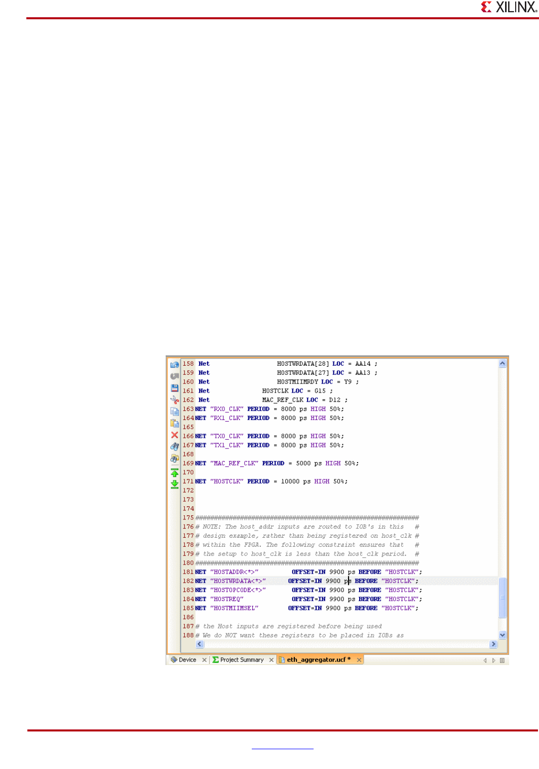
202 www.xilinx.com PlanAhead User Guide

UG632 (v 12.1)

Chapter 7: Netlist Analysis and Constraint Definition

Defining Timing Constraints

PlanAhead provides the ability to define and modify timing constraints for the design.

The following subsections describe how to use the timing constraint options:

•“Editing Constraints in the Text Editor”

•“Using the Timing Constraints View”

•“Modifying Timing Constraints Values”

•“Removing Timing Constraints”

Editing Constraints in the Text Editor

PlanAhead allows the designer to directly view and modify the constraints in the UCF text

file in which they are defined. This makes it easy for the designer to cut and paste

constraints that they are familiar with, and to modify values of existing constraints.

However, care must be taken that constraints are written to the correct constraints set and

target UCF file in order to ensure that constraints are applied as expected.

To open a UCF constraints file in the text editor, double-click the appropriate constraints

file name in the Sources view. The following figure shows text in a text editor. You can open

multiple files in separate text editor views also.

For more information about the commands and features available in the text editor, refer to

“Using the RTL Editor” in Chapter 5.

Figure 7-15: Text Editor

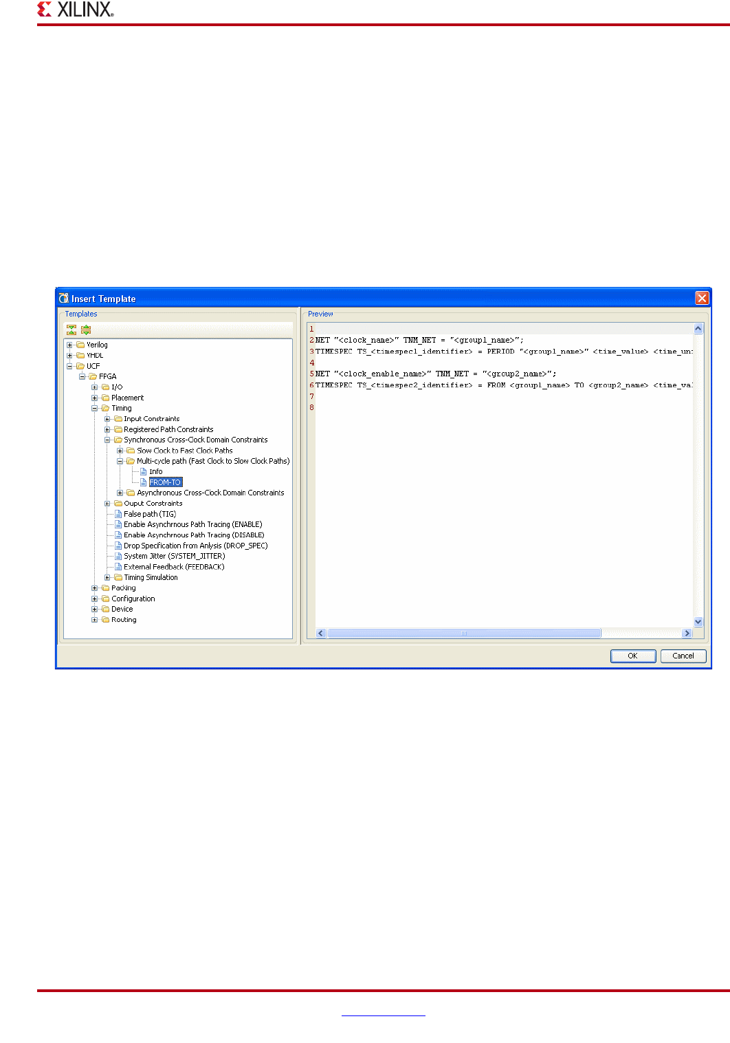
PlanAhead User Guide www.xilinx.com 203

UG632 (v 12.1)

Defining Timing Constraints

Using Xilinx-Supplied UCF Templates

The ISE software includes common UCF language templates. To access the template

library, select the Insert Template command in the text editor and expand the /UCF folder.

To instantiate a UCF language template:

1. Click the cursor in the text file where you want to insert the template.

2. Use the Insert Template command to select a UCF template.

3. Click OK to insert the text in the cursor location.

4. Replace the default constraint values with design specific names and information.

The following figure shows a Xilinx-supplied UCF language template.

Using the Timing Constraints View

You can use the Timing Constraints view to display, edit, and create timing constraints for

the design.

PlanAhead provides a view of the timing constraints defined in the design. Constraints are

Constraint Set specific, and can vary between open designs within the same project. You

can experiment with different constraints, devices, I/O pins, and so forth.

You can modify defined values and create new constraints in the Timing Constraints view.

To view the timing constraints defined in the design, select the Timing Constraints view

tab, or select Window > Timing Constraints.

The Constraints view opens as shown in Figure 7-17, page 204.

Figure 7-16: Xilinx-Supplied UCF Language Templates

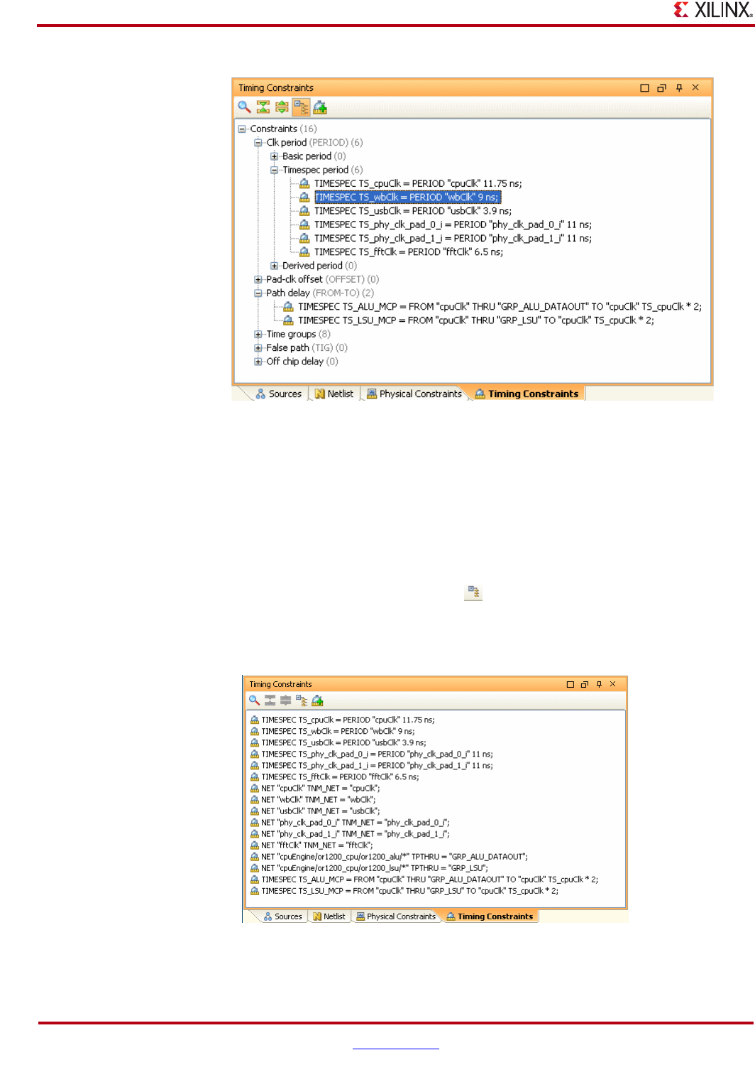
204 www.xilinx.com PlanAhead User Guide

UG632 (v 12.1)

Chapter 7: Netlist Analysis and Constraint Definition

The constraints are displayed in two different ways: by type, or as a list.

As shown in Figure 7-17, constraints are categorically sorted by type allowing expansion

and collapsing of the levels of constraint types. Notice that the number of each type of

constraint is displayed in parenthesis.

To view a list of all timing constraints, click Group by type in the Constraints view, which

is shown in the following figure.

When timing constraints are displayed as a list, they look like the following figure:

Figure 7-17: Timing Constraints Tab

Figure 7-18: Group by Type Toolbar Toggle Button

Figure 7-19: Timing Constraints Grouped by List

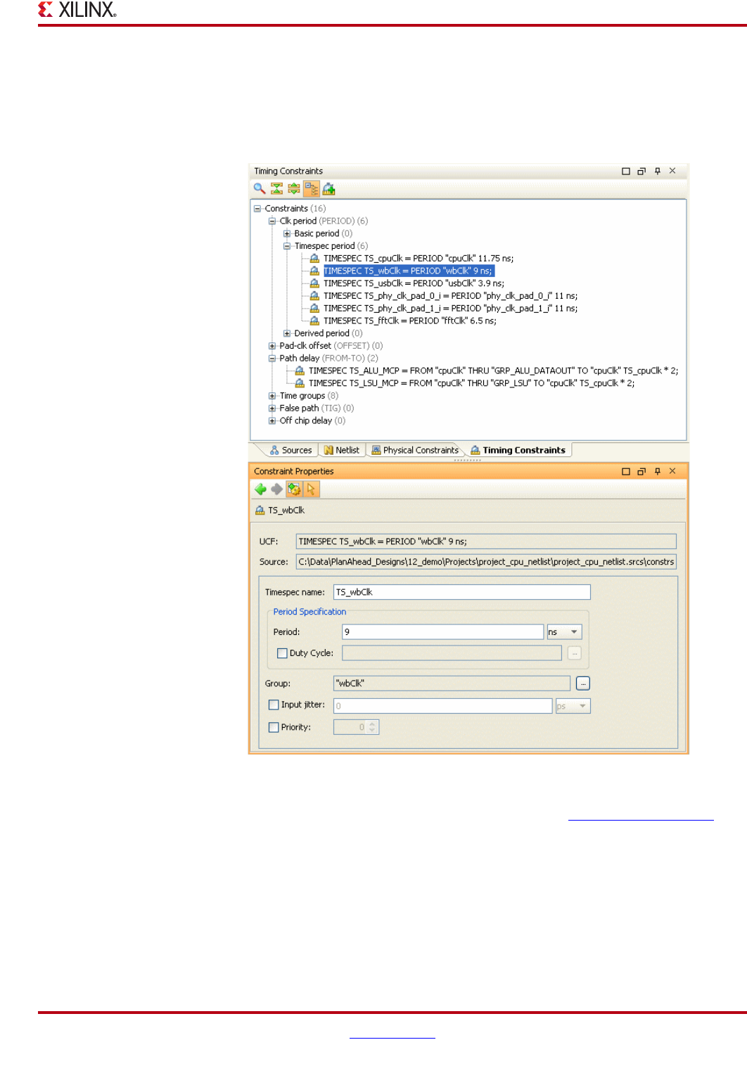
PlanAhead User Guide www.xilinx.com 205

UG632 (v 12.1)

Defining Timing Constraints

Modifying Timing Constraints Values

You can modify most constraint values by selecting a constraint and viewing the Timing

Constraints Properties. The appropriate changeable values for the constraint are shown in

the dialog box. The following figure shows the Timing Constraints Properties dialog box.

The dialog boxes for each constraint type are too numerous to describe here. Use the

correct syntax when defining constraints values. Refer to the Xilinx Constraints Guide,

(UG625), for more information on constraints and constraints syntax.

When you make changes, click Apply to accept the changes, or click Cancel to deny the

changes.

Note: You must click the Apply button to initiate changes to constraints values.

Figure 7-20: Modifying Timing Constraints Properties

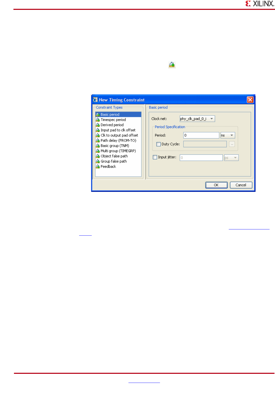
206 www.xilinx.com PlanAhead User Guide

UG632 (v 12.1)

Chapter 7: Netlist Analysis and Constraint Definition

Adding New Timing Constraints

To add new timing constraints:

1. In the Timing Constraints view, click the New Timing Constraint button, shown in the

following figure.

The New Timing Constraint dialog box opens as shown in the following figure.

2. On the left, select the type of constraint you want to create.

The appropriate fields display on the right.

3. Define the constraint values using the correct syntax. Refer to the Xilinx Constraints

Guide, (UG625), for more information on constraints and constraints syntax.

4. To accept the changes, click OK.

Removing Timing Constraints

To remove the constraint from the design, select a constraint or group of constraints in the

Timing Constraints view, and select Delete from the popup menu. You are prompted to

remove the selected constraint(s) prior to the removal of the constraint.

Note: Due to the interdependence between timing constraints, removing one constraint could result

in the removal of several other related constraints.

Note: Adding, editing, and deleting timing constraints cannot be undone.

Figure 7-21: New Timing Constraint Toolbar Button

Figure 7-22: Create New Timing Constraint Dialog Box

PlanAhead User Guide www.xilinx.com 207

UG632 (v 12.1)

Running Timing Analysis

Information about the timing performance of the design is available during the different

stages of implementation. Depending on the implementation stage, the available

information can contain early estimations of path delays to accurate analysis of

implementation results.

The following subsections describe how to run timing analysis in PlanAhead:

•“About PlanAhead Timing Analysis”

•“Timing Analysis Options for a Netlist Design”

•“Timing Analysis Options for an Implemented Design”

•“Using the Report Timing Analysis Results”

•“Analyzing Timing Results”

•“Displaying Path Details”

•“Setting Slack Histogram Options”

•“Analyzing Timing Histogram Results”

About PlanAhead Timing Analysis

The PlanAhead timing analysis is used in various modes during different stages of design

completion. It can provide early estimations of path delays to assist during floorplanning,

as well as for detailed path tracing, debugging, and constraint assignment.

The more physical constraints, such as Pblocks and placement constraints, are assigned in

the design, the more accurate the analysis results.

Timing Analysis Options for a Netlist Design

Once a design netlist is created, several options for exploring the design timing are

available. Timing analysis of the netlist design is useful for ensuring that paths are covered

by constraints prior to implementing the design. Additionally, you can use timing

estimates to create a proper floorplan. These options for running timing analysis on a

netlist design include:

•“Using the Report Timing Analysis Results”

•“Using Slack Histograms”

Timing Analysis Options for an Implemented Design

Once the design has been implemented, several options for exploring the design timing are

available. Timing analysis of the implemented design is useful for inspecting the timing

performance of the placed design. These options for running timing analysis on an

implemented design include:

•“Using the Report Timing Analysis Results”

•“Analyzing Timing Histogram Results”

The following sections describe the timing analysis options.

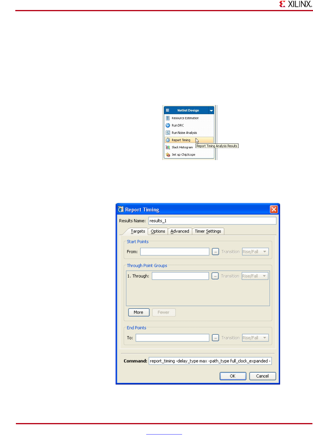
208 www.xilinx.com PlanAhead User Guide

UG632 (v 12.1)

Chapter 7: Netlist Analysis and Constraint Definition

Using the Report Timing Analysis Results

1. Perform a timing analysis using one of the following methods:

−Tools > Report Timing

In the Flow Navigator:

−Netlist Design > Report Timing

−Implemented Design > Report Timing

The following figure show the Netlist Design option for selecting a timing report.

The Report Timing dialog box opens that lets you customize the timing report that to be

generated as shown in the following figure.

Figure 7-23: Report Timing Dialog Box

Figure 7-24: Report Timing Dialog Box

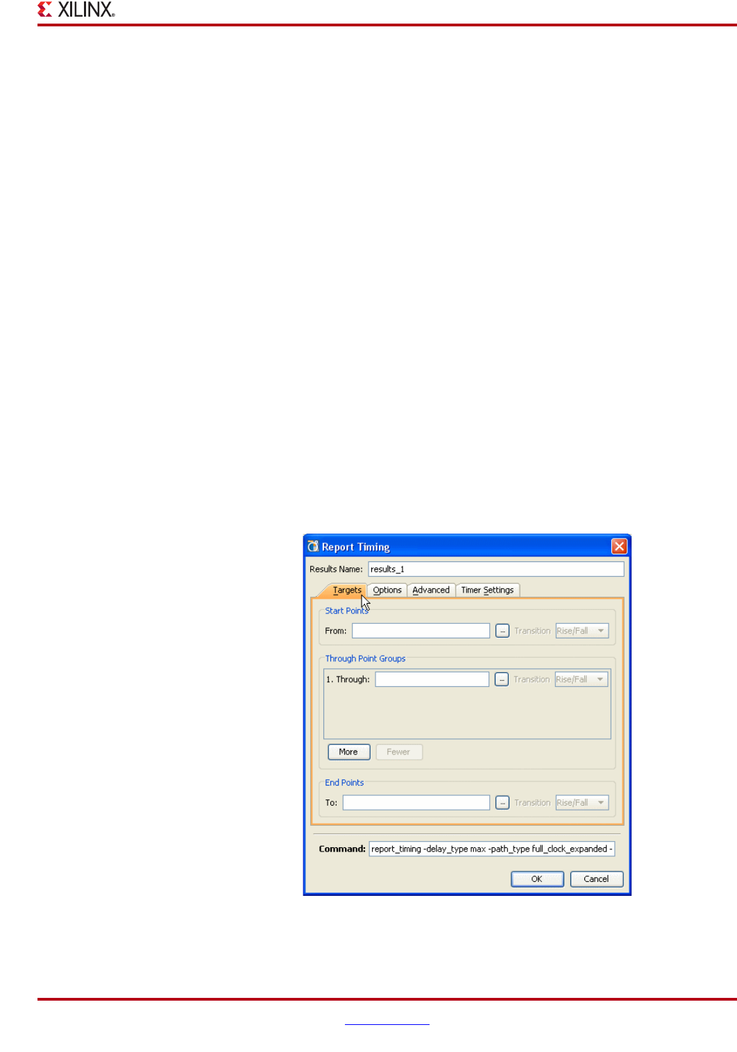
PlanAhead User Guide www.xilinx.com 209

UG632 (v 12.1)

Running Timing Analysis

2. Selecting OK will run the timing analysis with default values.

The Report Timing dialog box options are:

•Results Name—Specifies the name of the timing report.

•Targets tab—Allows the filtering of reported paths based on Start Points, Through

Points, and Endpoints.

•Options tab—Allows the specification of options used in generating the report. The

detailed options of this tab are further described below.

•Advanced tab—Contains advanced options used for generating and storing the

timing report. The detailed options of this tab are further described below.

•Timer Settings tab—Used to specify timing engine and delay options used to

generate the timing report. The detailed options of this tab are further described

below.

•Command—Contains the text of the TCL command generated by the Report Timing

options.

3. View and select the appropriate targets for the timing report.

Understanding the Targets Tab Options

The Targets tab of the Report Timing dialog box contains fields where you can specify the

starting points, through points, and end points of the paths to include in the timing report.

By default, the dialog box opens with the fields blank indicating all points will be included

in the report up to the maximum number of paths specified. By adding values to the fields,

you can generate a report that focuses on the paths of interest only. The Targets tab is

shown in the following figure.

Figure 7-25: Report Timing - Targets Options

210 www.xilinx.com PlanAhead User Guide

UG632 (v 12.1)

Chapter 7: Netlist Analysis and Constraint Definition

The fields available in the Target dialog box are:

•Start Points—Lets you choose the synchronous elements to begin the paths for

analysis. The Start Point fields are:

−From—Contains the expression used to filter the starting points. Enter text in this

field to manually create the filter, or view the filter text created by the Choose

Start Points dialog box.

−Choose Start Points —Opens a dialog box used to build the expression that

filters the starting points. This dialog box is described in further detail below.

−Transition—Further filters the paths according to the active clock edge of the

starting point synchronous elements. This field contains the following values:

-Rise—Filters all starting point synchronous elements to those triggered by a

rising (positive) clock edge.

-Fall—Filters all starting point synchronous elements to those triggered by a

falling (negative) clock edge.

-Rise/Fall—Filters the starting point synchronous elements to those triggered

by both rising and/or falling clock edges.

•Through Point Groups—Enter paths that travel through a set of points for analysis.

The following fields are available:

−Through—Contains the expression used to filter the paths based on the points the

path travels through.

−Choose Through Points —Opens a dialog box to build the expression that filters

the paths based on the through points.

−Transition—Further filters the paths according to the active clock edge of the

through point synchronous elements. This field contains the following values:

-Rise—Filters all through point synchronous elements to those triggered by a

rising (positive) clock edge.

-Fall—Filters all through point synchronous elements to those triggered by a

falling (negative) clock edge.

-Rise/Fall—Filters the through point synchronous elements to those triggered

by both rising and/or falling clock edges.

−More—Adds additional through point filter expressions

−Fewer—Removes existing through point filter expressions

•End Points—Enter paths that end in a set of synchronous elements. This section

contains the following fields:

•Choose End Points—Opens a dialog box used to build the expression that filters the

paths based on the ending points.

−Transition—Further filters the paths according to the active clock edge of the

starting point synchronous elements. This field contains the following values:

-Rise—Filters all starting point synchronous elements to those triggered by a

rising (positive) clock edge.

-Fall—Filters all starting point synchronous elements to those triggered by a

falling (negative) clock edge.

-Rise/Fall—Filters the starting point synchronous elements to those triggered

by both rising and/or falling clock edges.

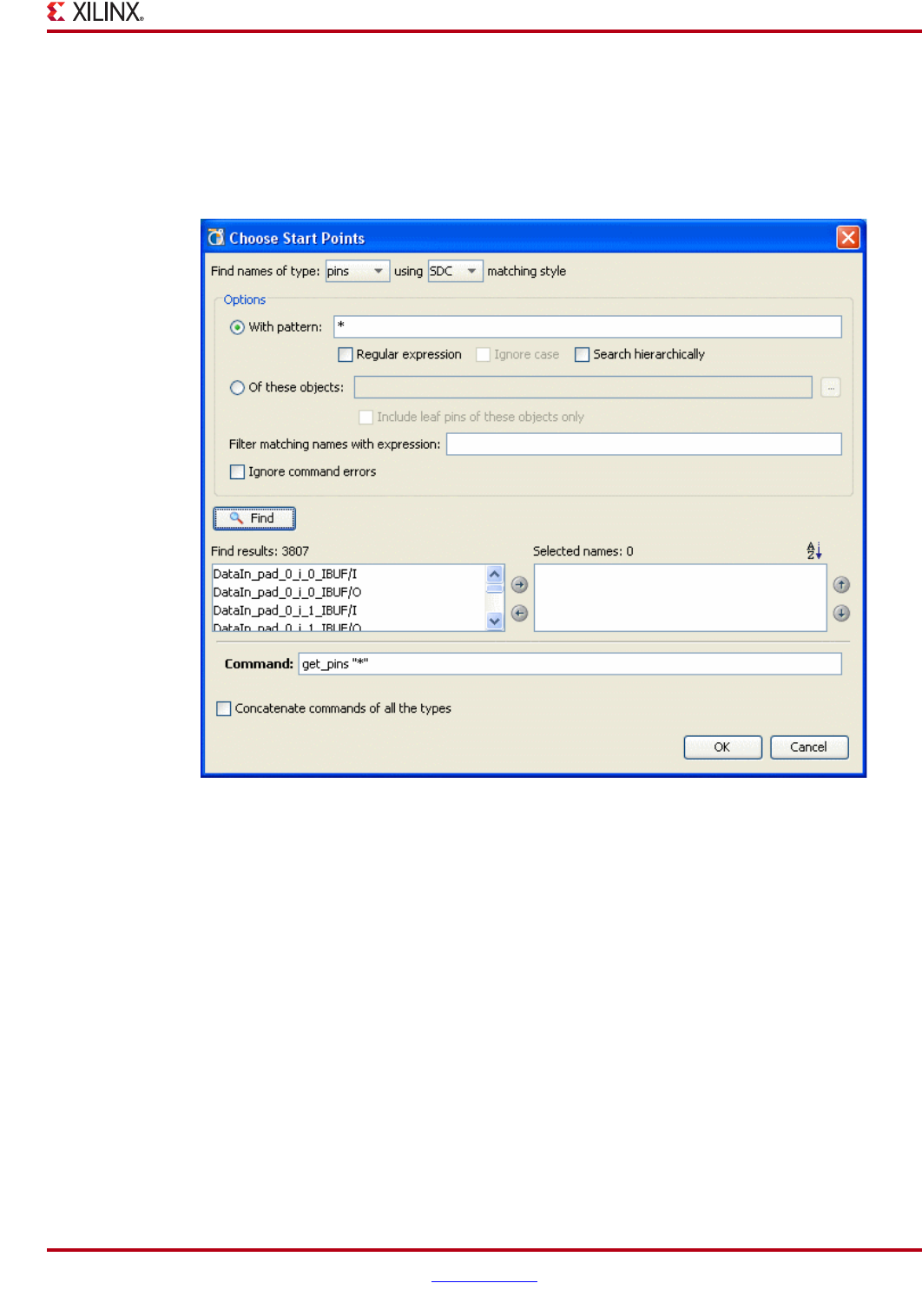
PlanAhead User Guide www.xilinx.com 211

UG632 (v 12.1)

Running Timing Analysis

Understanding the Choose Points Dialog Box

The Choose Points dialog box lets you choose the design elements for which you require

timing analysis based on element type and a pattern matching string and lets you enter

filter strings for the Start Points, Through Points, and End Point. The following figure

shows the Choose Start Points dialog box.

The options are:

•Find Names of Type—Filters the points based on the type of design element. The

field contains the following options:

−Cells—Choose design elements based on cell name.

−Clocks—Choose design elements based on clock name.

−Pins—Choose design elements based on pin name.

−Ports—Design elements based on port name.

•Matching Style—This field selects the type of pattern matching used for filtering the

design elements. The field contains the following options:

−UCF—Choose UCF-based syntax for pattern matching.

−SDC—Choose a Synopsys® Design Constraints (SDC)-based syntax for pattern

matching.

Figure 7-26: Choose Start Points

212 www.xilinx.com PlanAhead User Guide

UG632 (v 12.1)

Chapter 7: Netlist Analysis and Constraint Definition

•Pattern—The pattern expression used to filter the design elements. This field is

modified with the following options:

−Regular Expression—Specifies the search string will use regular expression

syntax.

−Ignore Case—Specifies the search string will be case insensitive.

−Search Hierarchically—This option is available for SDC pattern matching and

specifies that the SDC based search pattern will be applied to every level of

hierarchy.

•Objects—The field is used to select objects based on dialog box selection. This field is

modified with the following options:

−Include Leaf Pins—An SDC syntax option that specifies that the search string

should only match pins components, and not match pins across hierarchical

boundaries.

−Select Object Dialog Box—An SDC syntax option that launches an additional

object selection dialog box where you can generate recursive search expressions.

−Filter Matching Name with Expression—An SDC syntax option that specifies

the –filter command.

•Ignore Command Errors—Suppresses warning messages generated during TCL

command processing of the Timing Report.

•Find Results—Contains the results of the object search.

•Selected Name—Contains the subset of the search result objects that are chosen for

the Points.

•Command—Contains the Tcl command used to represent the selected objects

4. View and select the appropriate options for the timing report.

Understanding the Options Tab Selections

The Options tab of the Report Timing dialog box contains fields that let you specify the

type of timing report to be generated as well as the number of paths reported. The Options

tab is shown inFigure 7-27, page 213.

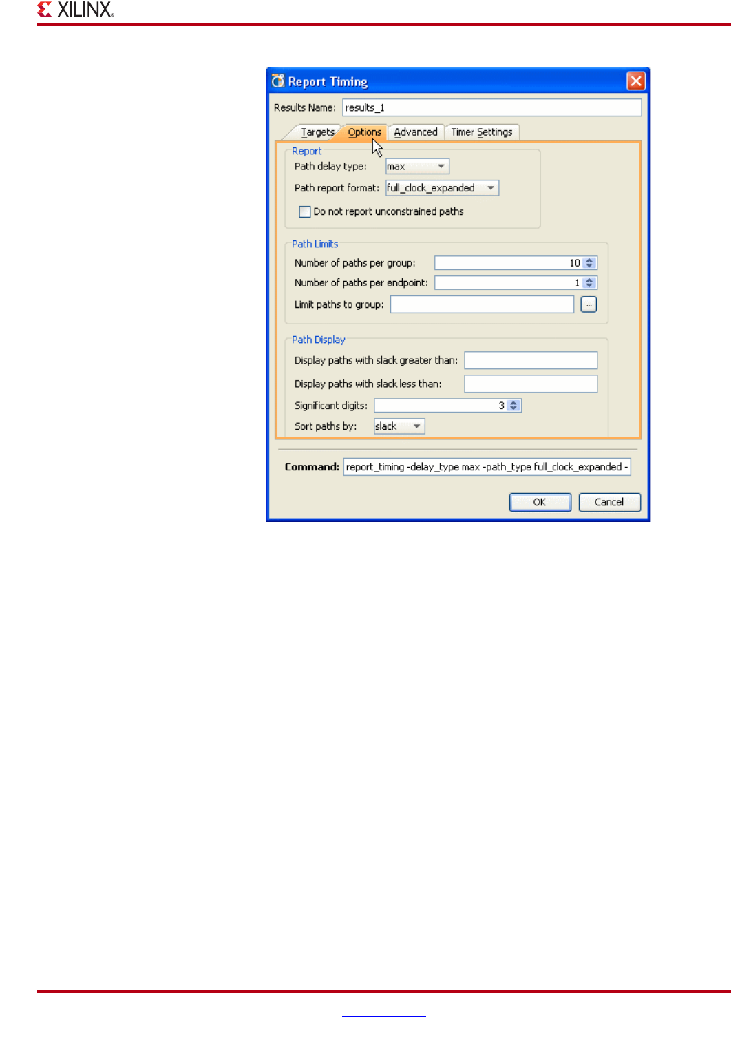
PlanAhead User Guide www.xilinx.com 213

UG632 (v 12.1)

Running Timing Analysis

The fields available in the Options tab dialog box are:

•Path Delay Type—Specifies the type of delays that are used in the timing report path

analysis. This field contains the following options:

−Max—Uses maximum delays for the clock and data paths during setup and hold

analysis.

−Min—Uses minimum delays for the clock and data paths during setup and hold

analysis.

−Min_Max—Uses a combination of minimum and maximum delays for the clock

and data paths during setup and hold analysis.

•Path Report Format—Specifies the type of timing report to be generated. In many

cases, the format of the GUI timing report and written timing report are different,

based on the selected option. This field contains the following values:

−End—Specifies an endpoint report that contains only slack and endpoint

information for each path in the written timing report.

−Full—Specifies a timing report that contains full path details for the data path,

and hides the details of the clock path(s).

−Full_Clock—Specifies a timing report that contains full path details for the data

path, and summary details for the clock path(s).

−Full_Clock_Expanded—Specifies a timing report that contains full path details

for the data path, and full details for the clock path(s).

Figure 7-27: Report Timing - Options tab

214 www.xilinx.com PlanAhead User Guide

UG632 (v 12.1)

Chapter 7: Netlist Analysis and Constraint Definition

−Short—Specifies a timing report that contains summary details for the data path,

and hides the details of the clock path(s).

−Summary—Specifies a written timing report that only contains summary

information on the timing performance of the design.

•Do Not Report Unconstrained Path—Specifies that the report will contain details

for constrained paths only.

•Number of Paths Per Group—Specifies the number of timing paths reported per

group.

•Number of Paths Per Endpoint—Specifies the maximum number of timing paths

reported per endpoint.

•Limit Paths Per Group—Limits the paths reported to a specific group or set of

groups. The group identifier can be entered directly, or by using the Choose Path

Groups dialog box.

•Display Paths With Slack Greater Than—Filters the displayed paths based on a

minimum slack value. Only paths with slack greater than this value will be shown.

•Display Paths With Slack Less Than—Filters the displayed paths based on a

maximum slack value. Only paths with slack less than this value will be shown.

•Significant Digits—Specifies the significant digits of the timing report delay values.

The default value is 3.

•Sort Paths By—Selects that parameter that will be used to sort the timing report. This

field contains the following values:

−Group—Sorts the timing report based on group name.

−Slack—Sorts the timing report based on path slack.

5. View and select any required advanced options for the timing report.

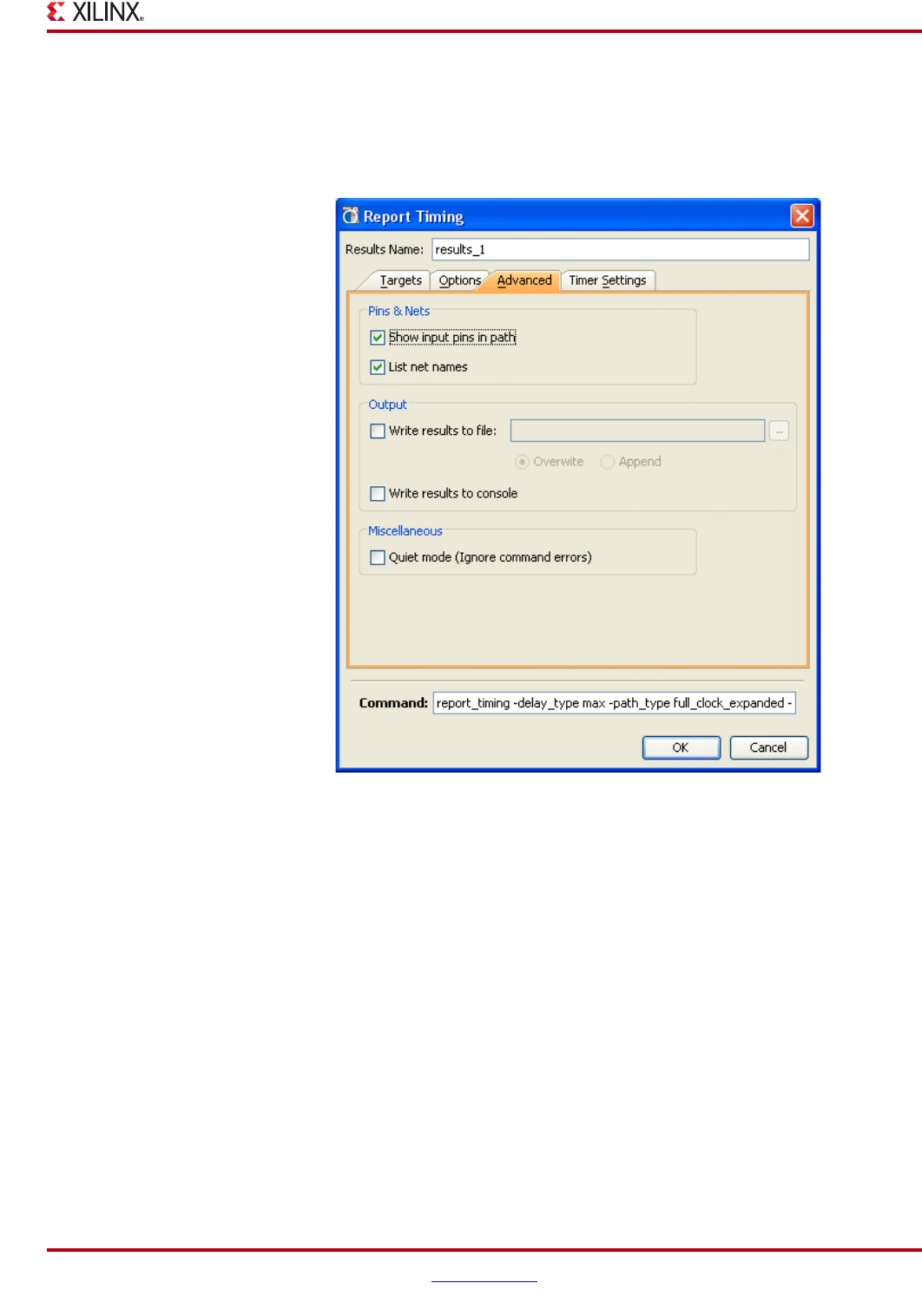
PlanAhead User Guide www.xilinx.com 215

UG632 (v 12.1)

Running Timing Analysis

Understanding the Advanced Options Tab

The Advanced Options tab of the Report Timing dialog box contains fields that let you

specify pin and net details, report output locations, and command error processing. The

Advanced Options tab is shown in the following figure.

The Advanced tab dialog box options are:

•Show input paths in the path—Shows the pins of each path element.

•List net names—Lists the name of the net connection each path element.

•Write results to file—write the results of the timing report to a file. This field also

contains options to designate how the details of the report will be written to that file.

These options include:

−Overwrite—Overwrites the specified file with the details of the timing report.

−Append—Appends the timing report details to the specified file name.

•Quiet Mode—Suppresses messages in the timing report regarding errors in command

options.

5. View and select the appropriate Timer Settings for the timing report.

Figure 7-28: Report Timing - Advanced Tab

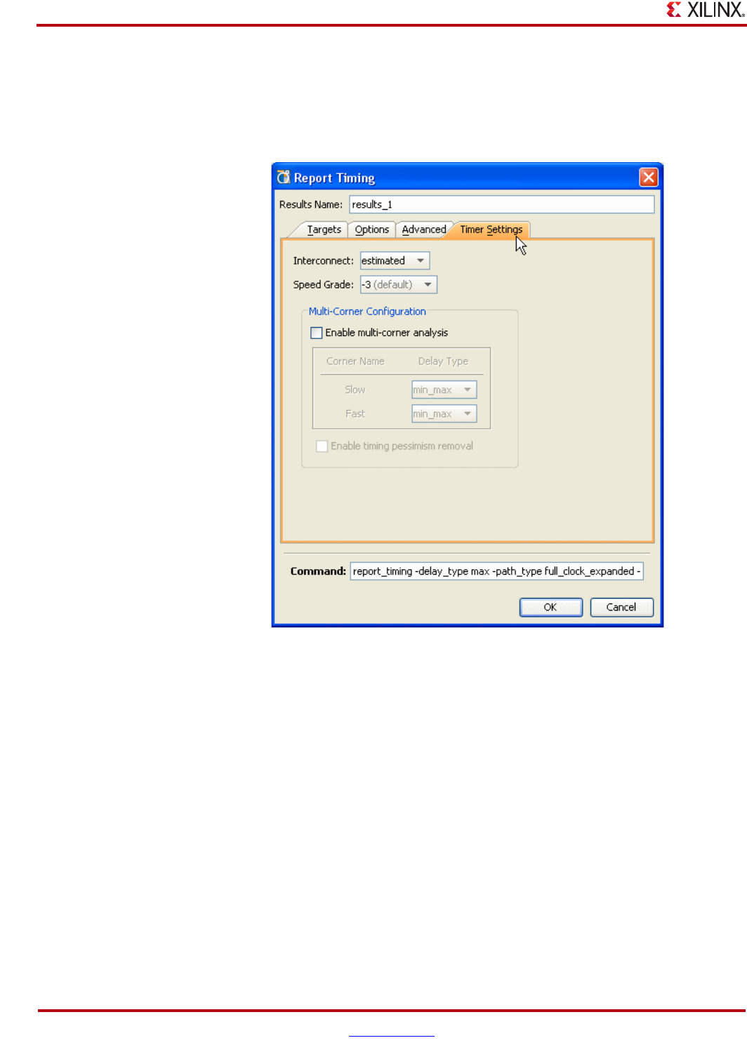
216 www.xilinx.com PlanAhead User Guide

UG632 (v 12.1)

Chapter 7: Netlist Analysis and Constraint Definition

Understanding the Timer Settings Tab

The Timer Settings tab of the Report Timing dialog box contains fields that allow the

designer to specify the delays parameters used by the timing engine in generating the

timing report. The Timer Settings tab is shown in the following figure.

The Timer Settings options are:

•Interconnect—Selects the type of delay values used for the interconnect delay. The

different delay values are as follows:

−Estimated—Uses estimated delays for the interconnect values

−None—Sets the interconnect delays to 0.

•Speed Grade—Selects the speed grade of the device used in the timing analysis. This

field allows the estimation of design timing using different device speed grades.

•Multi corner analysis—Enables the use of multi-corner analysis in the timing report.

Multi-corner analysis simultaneously uses different process and operating condition

corners to perform a worst-case setup and hold analysis. This results in a more

accurate, but pessimistic, analysis than minimum or maximum delays alone. The

fields in this area are:

−Enable multi-corner analysis—Enables multi-corner analysis.

−Slow corner—Selects the delay types used for the slow corner analysis. The

available values are:

Figure 7-29: Report Timing - Timer Settings Tab

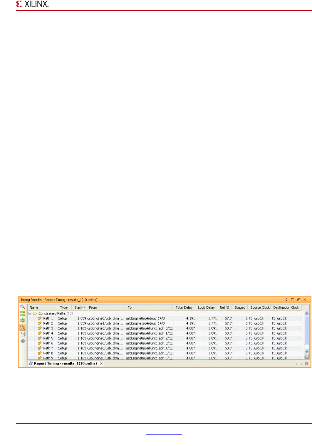
PlanAhead User Guide www.xilinx.com 217

UG632 (v 12.1)

Running Timing Analysis

-None—Specifies that no delays are used when generating minimum timing

analysis.

-Max—Specifies that maximum delays are used for the clock and data paths

during setup and hold analysis.

-Min—Specifies that minimum delays are used for the clock and data paths

during setup and hold analysis.

-Min_Max—Uses a combination of minimum and maximum delays for the

clock and data paths during setup and hold analysis.

−Fast Corner—Selects the delay types used for the fast corner analysis. The values

are:

-None—Specifies that no delays will be used in the generation of minimum

timing analysis.

-Max—Uses maximum delays for the clock and data paths during setup and

hold analysis.

-Min—Uses minimum delays for the clock and data paths during setup and

hold analysis.

-Min_Max—Uses a combination of minimum and maximum delays for the

clock and data paths during setup and hold analysis.

−Enable timing pessimism removal—Removes the skew delay generated by the

common clock path between source and destination registers when modeling on-

chip delay variation.

Analyzing Timing Results

The Timing Results view can be populated with timing results from either the PlanAhead

Timing Analysis or from the ISE Trce timing analysis tools.

Either the PlanAhead Timing Analysis or the ISE Trce tool must be run first to populate the

Timing Results view with paths. The Timing Results view contains the paths that meet the

criteria defined in the Run Timing Analysis dialog box, as described in “Running Timing

Analysis,” page 207. When you import Trce results, or run the PlanAhead Timing Analysis

with the default options, paths are sorted and listed by constraint.

The Timing Results view opens when the PlanAhead Timing Analysis completes or when

you import the ISE Trce results. The following figure shows an example of timing results.

You can examine, sort, and select specific paths and instances in the Timing Results

interface.

Figure 7-30: Timing Results

218 www.xilinx.com PlanAhead User Guide

UG632 (v 12.1)

Chapter 7: Netlist Analysis and Constraint Definition

In the Timing Results view, the following information displays for each path:

•Constraint Name—Displays the constraint name for the paths listed.

−Name—Shows a sequential number with which to sort back to the original order.

−Type—Displays whether the path is Setup or Hold related.

−Slack—Displays the total positive or negative slack on the path.

−From—Displays the path source pin.

−To—Displays the paths destination pin.

−Total Delay—Lists the total estimated delay on the path.

−Logic Delay—Lists the delay attributed to logic delay only.

−Net%—Displays the percentage of the delay attributed to routing interconnect.

−Stages—Displays the total number of instances on the path including the source

and destination which both contribute to the overall delay. This may be different

than the method used to calculate levels of logic in ISE.

−Source Clock—Displays the source clock name.

−Destination Clock—Displays the destination clock name.

Note: In the PlanAhead Timing Analysis, a carry chain interconnect is counted as individual stages

of logic.

Sorting the Timing Report

You can sort the Timing Results by clicking any of the column headers. For example, click

on the Stages column header to sort the list by stages of logic. Click the column header a

second time to reverse the sort order.

You can sort by a second column by pressing the Ctrl key and clicking a second column

header. You can sort by as many columns as necessary to refine the list order.

Refer to the “Using Tree Table Style Views” in Chapter 4 for information regarding

working with tree table style views.

The following figure shows a timing result sorted by Stages of logic.

Click Ctrl and click the column header again to remove a sort from a column.

Figure 7-31: Timing Results Sorted by Stages of Logic

PlanAhead User Guide www.xilinx.com 219

UG632 (v 12.1)

Running Timing Analysis

Flattening the List of Paths

By default, the paths are categorized by constraint. You can flatten the list and view all

paths by clicking Group by Constraint in the Timing Results view or by clicking the

Group Paths by Constraint button in the Timing Results view toolbar, as shown in the

following figure.

The Group by Constraint toolbar button toggles between a categorized list of constraints

and a flattened list of paths.

Removing Paths from the Timing Report

You can remove paths from the timing report to make for easier sorting and viewing of

critical paths.

1. Select the paths to remove paths from the timing report. To select multiple paths, use

the Shift or Ctrl keys, and select the paths.

2. Press the Delete key, or select Delete from the popup menu in the Timing Results view.

Displaying Path Details

When you select a path from the list, the Path Properties view is populated with

information about the path. Logic elements are listed with detailed delay information and

hyperlinks, as shown in Figure 7-33, page 220.

Figure 7-32: Group Paths by Constraint Toolbar Button

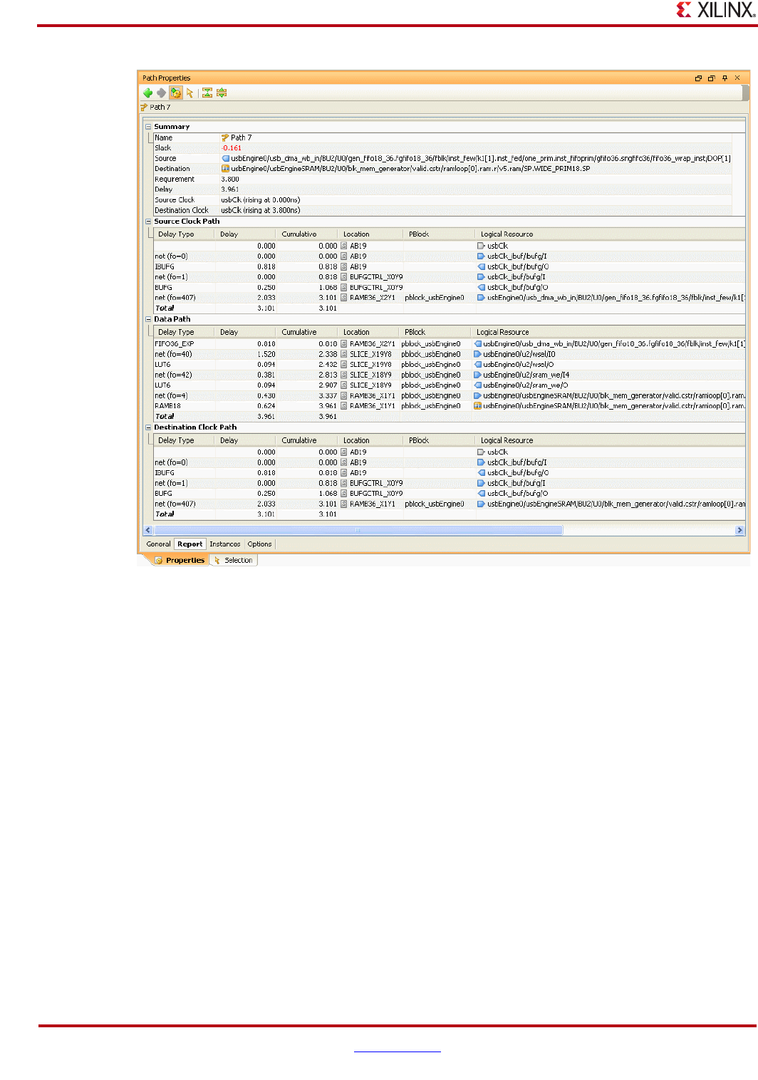
220 www.xilinx.com PlanAhead User Guide

UG632 (v 12.1)

Chapter 7: Netlist Analysis and Constraint Definition

The report has a similar format to the Trce report.

•By default, selecting a path also selects all instances contained within the path.

•Selecting any of the blue-hyperlinked objects in the report also selects them in other

views such as the Netlist and Device views.

•You can select multiple paths using the Shift and Ctrl keys.

•All instances contained in the selected paths are selected, but the Path Properties

displays information only about the first path selected.

Displaying Timing Path Reports in the Workspace

An individual Timing Path Report can also be displayed in the Workspace for easier

viewing. Also, multiple path reports can be opened in separate views in the WorkSpace.

To view the report:

1. Select the timing path.

2. Select the View Path Report popup menu command.

Figure 7-33: Path Properties View: Report Tab

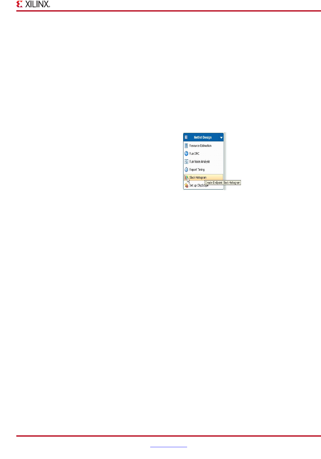
PlanAhead User Guide www.xilinx.com 221

UG632 (v 12.1)

Using Slack Histograms

The Slack histogram provides a visual indication of the timing delays in the design. This

view can assist the designer in determining the next course of action if the design is not

meeting performance requirements.

1. Select one of the following methods to generate a Slack histogram:

−Tools > Slack Histogram

In the Flow Navigator:

−Netlist Design > Slack Histogram

−Implemented Design > Slack Histogram

The following figure shows the Slack Histogram option from the Netlist Design.

The Generate Slack Histogram dialog box opens, as shown in the following figure, and you

can customize the slack histogram to be generated.

Figure 7-34: Slack Histogram Option

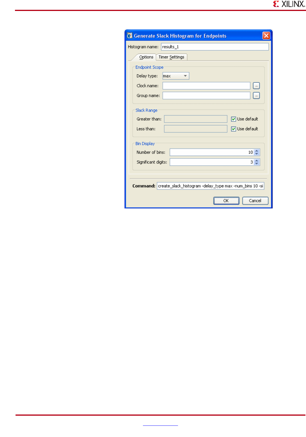
222 www.xilinx.com PlanAhead User Guide

UG632 (v 12.1)

Chapter 7: Netlist Analysis and Constraint Definition

2. Selecting OK displays a slack histogram with default values.

The options are:

•Histogram Name—Specifies the name of the histogram report that is generated

•Options Tab—Allows the customization of the histogram report. The detailed

options of this tab are further described below.

•Timer Settings Tab—Specifies timing engine and delay options used to generate the

timing report. The detailed options of this tab are further described below.

•Command—Contains the text of the TCL command generated by the Generate Slack

Histogram options.

3. View and select the appropriate Options for the histogram report

Figure 7-35: Slack Histogram Dialog Box

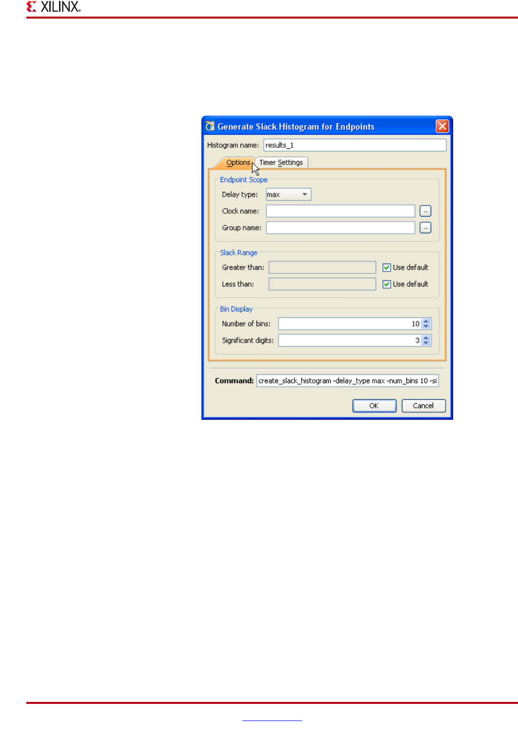
PlanAhead User Guide www.xilinx.com 223

UG632 (v 12.1)

Using Slack Histograms

Setting Slack Histogram Options

You can specify the option used to generate the Slack histogram using the Options tab of

the Generate Slack Histogram dialog box. The Options tab is shown in the following

figure.

The options are:

•Endpoint Scope—Specifies the endpoints and delay types to be used in the slack

histogram generation. By filtering the endpoints based on clock name and group

name, a histogram can be generated to focused in on the paths of interest. The fields in

this area are as follows:

−Delay Type—Specifies the delay values that will be used in the generation of the

slack histogram.

−Min—Uses minimum delays for the clock and data paths for the slack histogram.

−Max—Uses maximum delays for the clock and data paths for the slack histogram.

−Min_Max—Uses a combination of minimum and maximum delays for the clock

and data paths for the slack histogram.

•Clock Name—Filters the endpoints by the associated clock name. The value for this

field can be entered directly or by using the Choose Endpoints dialog box.

•Group Name—Filters the endpoints by the associated group name. The value for this

field can be entered directly or by using the Choose Endpoint Path Groups dialog box.

Figure 7-36: Slack Histogram - Options

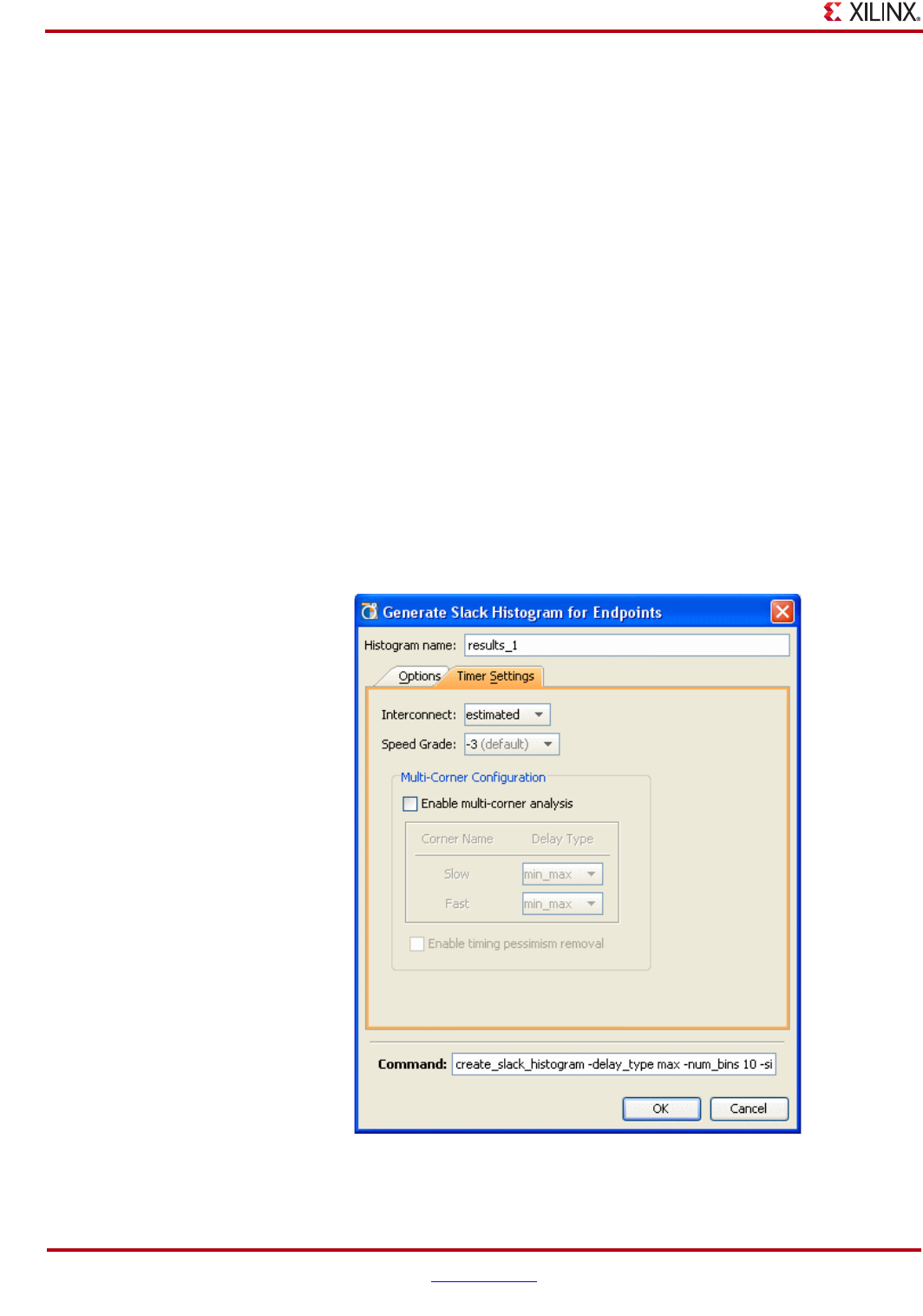
224 www.xilinx.com PlanAhead User Guide

UG632 (v 12.1)

Chapter 7: Netlist Analysis and Constraint Definition

•Slack Range—Filters the endpoints based on the slack value. By filtering the

endpoints based on the slack value falling within a specific range, a histogram can be

generated to focused in on the paths of interest. The fields in this area are as follows:

−Greater Than—Specifies the maximum slack value of slack that a path may have

to be included in the histogram.

−Less Than—Specifies the minimum slack value of slack that a path may have to

be included in the histogram.

•Bin Display—Allows further customization of the histogram. This field contains the

following values:

−Number of Bins—Specifies the number of bins in the histogram. By selecting a

smaller number of bins, the histogram provides a general view of the timing

performance of the design. Histograms with larger number of bins are best used

within a slack range to focus in on the performance of a specific range of delays.

−Significant Digits—Specifies the number of significant digits that will be used in

the histogram. By default, this value is set to 3.

4. Next, view and select the appropriate timer settings for the slack histogram.

Setting Slack Histogram Timer Options

You can specify the delays parameters used by the Slack histogram timing engine in the

Timer Settings tab of the Generate Slack Histogram dialog box. The Timer Settings tab is

shown in the following figure.

Figure 7-37: Slack Histogram - Timer Settings Tab

PlanAhead User Guide www.xilinx.com 225

UG632 (v 12.1)

Using Slack Histograms

The options are:

•Interconnect—Selects the type of delay values used for the interconnect delay. The

delay values are:

−Estimated—Uses estimated delays for the interconnect values

−None—Sets interconnect delays to 0.

•Speed Grade—Selects the speed grade of the device used in the timing analysis. This

field allows the estimation of design timing using different device speed grades.

•Multi Corner Analysis—Enables the use of multi-corner analysis in the timing report.

Multi-corner analysis simultaneously uses different process and operating condition

corners to perform a worst-case setup and hold analysis. This results in a more

accurate, but also pessimistic, analysis than minimum or maximum delays alone. The

fields in this area are:

−Enable multi-corner analysis: Select this field to enable multi-corner analysis.

•Slow Corner—Selects the delay types that will be used for the slow corner analysis.

The different values available are:

−None—Specifies that no delays will be used in the generation of minimum timing

analysis.

−Max—Uses maximum delays for the clock and data paths during setup and hold

analysis.

−Min—Uses minimum delays for the clock and data paths during setup and hold

analysis.

−Min_Max—Uses a combination of minimum and maximum delays for the clock

and data paths during setup and hold analysis.

•Fast Corner—Selects the delay types that will be used for the fast corner analysis.

The available values are:

−None—Specifies that no delays are used in the generation of minimum timing

analysis.

−Max—Uses maximum delays for the clock and data paths during setup and hold

analysis.

−Min—Uses minimum delays for the clock and data paths during setup and hold

analysis.

−Min_Max—Uses a combination of minimum and maximum delays for the clock

and data paths during setup and hold analysis.

•Enable Timing Pessimism Removal—Removes the skew delay generated by the

common clock path between source and destination registers when modeling on-chip

delay variation.

Analyzing Timing Histogram Results

Once the histogram is generated, you can use the results to obtain an indication of the type

of timing problems associated with the design implementation. The Histogram View

contains a visual graph of the delays (bins) associated with the design and lists each of the

paths in the Timing Results View.

This interface lets you arrange the paths according to the column headers of the table, as

well as by selection from the graph. Figure 7-38, page 226 is an example of the Slack

histogram results.

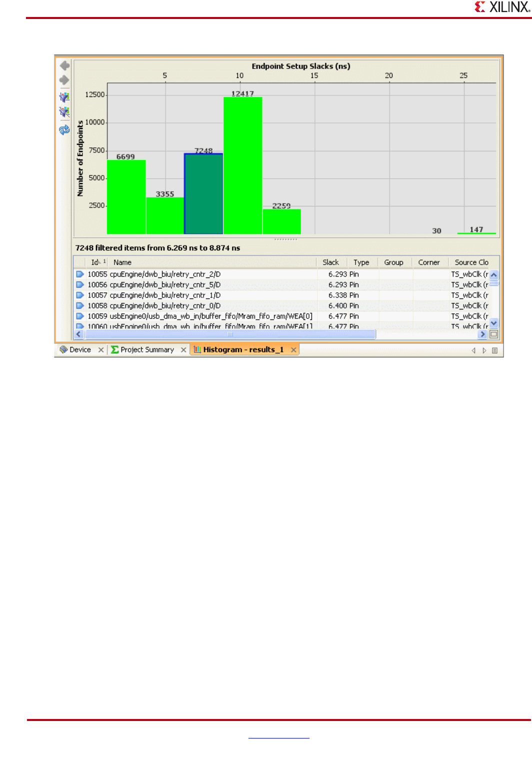
226 www.xilinx.com PlanAhead User Guide

UG632 (v 12.1)

Chapter 7: Netlist Analysis and Constraint Definition

Selecting Paths for Analysis

The Histogram provides selection and filtering of paths for analysis. The selected paths

display in the Timing Results view. The selection options include:

•View Individual Bin Paths—Select an individual path by left-clicking on a histogram

bin. The Timing Results view updates automatically to reflect the bin selection.

•View Paths from Multiple Bins—Filter the paths that are shown by left-clicking

several bins in the graph. To add and remove bins from the selection press the CTRL

key and left-click the bin. The Timing Results view updates automatically to reflect

the bin selection.

•View All Paths—Select all paths in the design from the histogram by left-clicking on

any location in the graph that is not a bin. Once clicked, the Timing Results view

updates automatically to show all paths.

Changing Histogram Options

The histogram display can be redrawn at any time to reflect a new set of options. To bring

up the options to change the display right-click on the histogram. There are two methods

available to change the histogram display:

•Report Timing—Generates a new timing report using the Report Timing dialog box.

•Refresh Histogram—Generates a new histogram using the Generate Slack

Histogram dialog box.

Figure 7-38: Slack Histogram

PlanAhead User Guide www.xilinx.com 227

UG632 (v 12.1)

Defining Physical Constraints

•View—Changes the view of the histogram to better focus in on paths of interest. This

selection contains the following options:

−Zoom In—Increases the zoom level.

−Zoom Out—Decreases the zoom level.

−Zoom Fit—Views the entire histogram in the display.

−Zoom Area—Fits a selected area in the entire display.

−Options—Invokes the main PlanAhead Options menu.

Defining Physical Constraints

PlanAhead provides a variety of means to apply physical constraints. Physical constraints

consist of LOC/BEL instance placement constraints, AREA_GROUP placement

constraints, DCI_CASCADE constraints and Device Configuration Mode constraints. For

more information on assigning physical constraints, refer to Chapter 8, “I/O Pin

Planning,” and Chapter 11, “Floorplanning the Design.”

The following subsections describe the Physical Constraints view and the available

options:

•“Using the Physical Constraints View”

•“Working with Relatively Placed Macro (RPMs)”

Using the Physical Constraints View

The Physical Constraints view is used to display and interact with a variety of physical

constraint types.

It displays the hierarchical structure of the design relative to the created Pblocks. The

physical hierarchy is dynamic; expanding and changing automatically when physical

hierarchy is manipulated. As objects are selected in other views, the appropriate elements

are highlighted in the Physical Constraints view.

The objects displayed in the Physical Constraints view are Relatively Placed Macros

(RPMs) and Physical Block (Pblocks), and DCI Cascade Constraints. You can select these

objects in the Physical Constraints view for manipulation in other views.

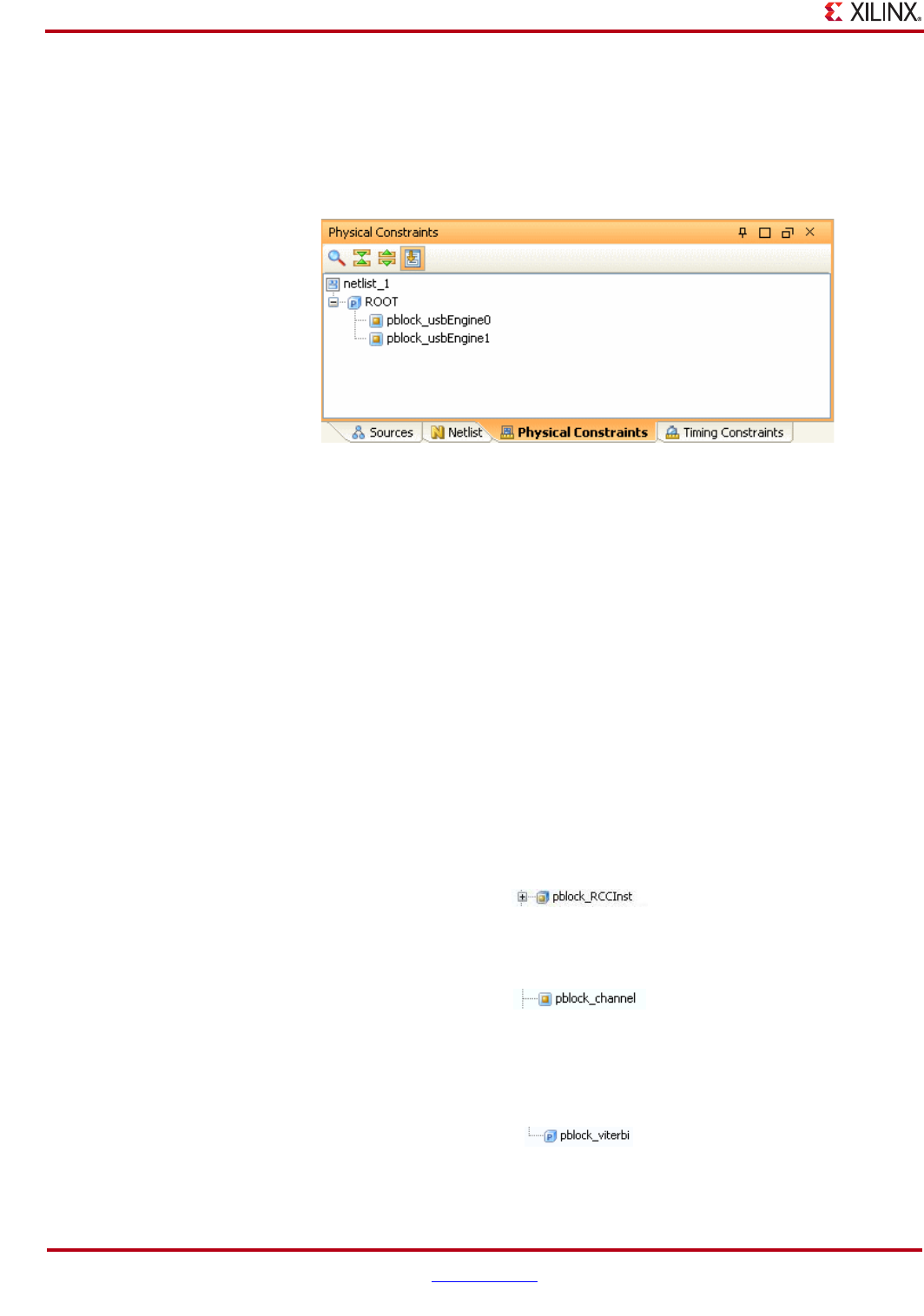
228 www.xilinx.com PlanAhead User Guide

UG632 (v 12.1)

Chapter 7: Netlist Analysis and Constraint Definition

Using the ROOT Design Pblock

The physical hierarchy begins with the design name followed by the top-level Pblock

called “ROOT.” As you create lower-level Pblocks they display in a hierarchical fashion

under the /Pblock folder, with Child Pblocks nested under their parent Pblock, shown in

the following figure.

Selecting a Pblock selects all of the assigned logic for that Pblock.

Understanding the Physical Constraints View Icons

The Physical hierarchy Pblock tree uses several icons that can help you identify the state of

the various objects. This display updates automatically as you manipulate the physical

hierarchy.

As you create Pblocks. they appear in a hierarchical fashion in the Physical Constraints

view. Each folder type in the Physical Constraints view displays a number in parenthesis

that details the number of objects in that folder.

Each instantiation of an RPM displays in the Physical Constraints view. If RPMs are

assigned to Pblocks, they appear in an RPM folder under the Pblock. Selecting an RPM in

the Physical Constraints view selects all of the logic contained in the RPM.

Pblocks With Assigned Instances

Pblocks with instances assigned and with rectangles defined in the Device view appear as

blue three-dimensional cubes with a yellow center as shown in the following snippet.

Pblocks with instances assigned and with no rectangles defined in the Device view appear

as blue two-dimensional squares with a yellow center as shown in the following snippet.

Pblocks Without Assigned Instances

Pblocks with no instances and with rectangles defined assigned appear as blue three-

dimensional cubes with a blue P in the center as shown in the following snippet.

Figure 7-39: Physical Constraints View

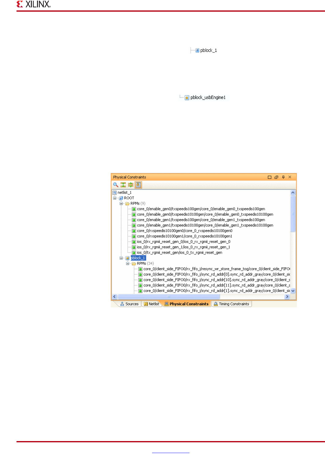
PlanAhead User Guide www.xilinx.com 229

UG632 (v 12.1)

Defining Physical Constraints

Pblocks with no instances assigned with no rectangles defined appear as blue two-

dimensional squares with a blue P in the center as shown in the following snippet.

Partially Reconfigurable PBlocks

Partially reconfigurable partition Pblocks appear as yellow diamonds as shown in the

following snippet.

Working with Relatively Placed Macro (RPMs)

Relatively Placed Macros (RPMs) that exist in the design are listed under the RPMs

folders. RPMs can be assigned to Pblocks. If RPMs are assigned to Pblocks, they appear in

an RPM folder under the Pblock. Each instantiation of an RPM displays in the Physical

Constraints View (as shown in Figure 7-39, page 228). RPM Properties and statistics

display in the RPM Properties view, as shown in the following figure.

When RPMs are assigned to Pblocks, the Pblock Properties view displays RPM size and

utilization statistics information as shown in Figure 7-41, page 230.

Figure 7-40: Displaying Relatively Placed Macros “RPMs”

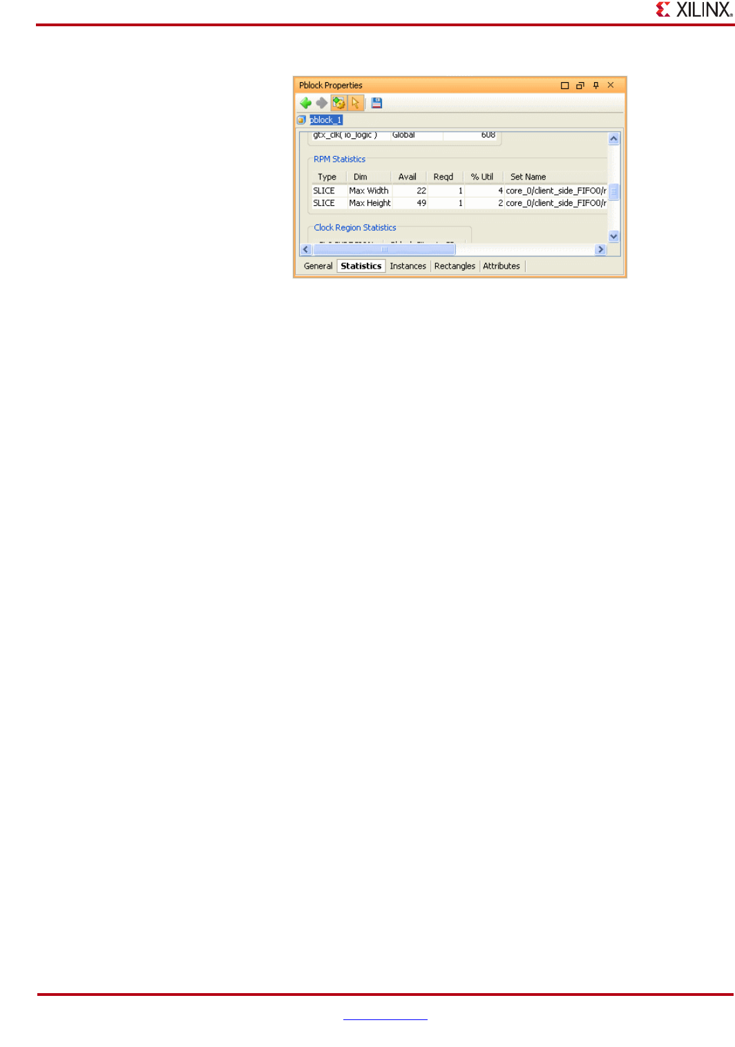
230 www.xilinx.com PlanAhead User Guide

UG632 (v 12.1)

Chapter 7: Netlist Analysis and Constraint Definition

Running the Design Rule Checker (DRC)

The PlanAhead software contains a set of batch DRC commands that can help verify

design integrity prior to running the ISE software. The rules are categorized by type of

logic checks being performed. Many different types of checks are available.

These checks are designed to provide an early indication about potential design

implementation issues. The final validation step to ensure the design is DRCs compliant is

to run the design through the ISE implementation tools.

Running I/O Port and Clock Logic DRCs

Many of the DRC rules are related to I/O pin assignment and clock logic. For information

on running I/O Port and lock logic related DRCs, see Chapter 8, “I/O Pin Planning.”

Running Netlist and Constraint DRCs

To run DRCs on the Netlist Design to validate netlist and constraint condition:

1. From the Flow Navigator or Tools menu, select the Run DRC command.

The Run DRC dialog box opens, as shown in Figure 7-42, page 231.

Figure 7-41: RPM Utilization Statistics for Pblocks

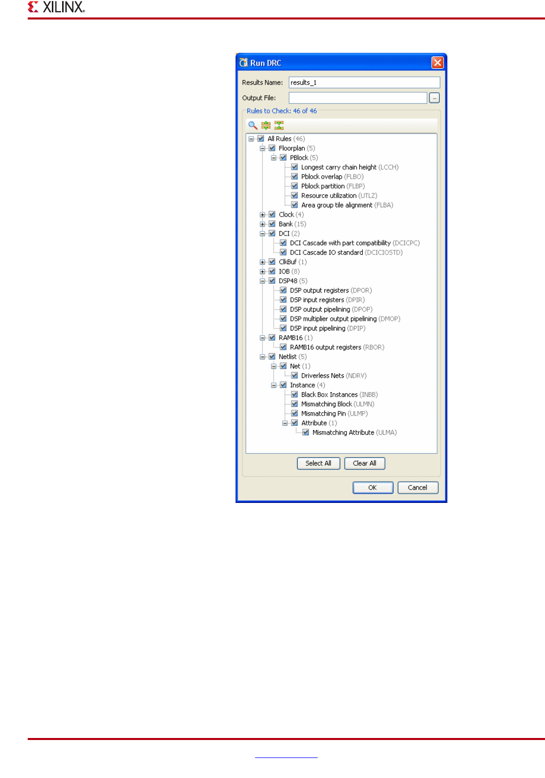
PlanAhead User Guide www.xilinx.com 231

UG632 (v 12.1)

Running the Design Rule Checker (DRC)

2. View or edit the Results Name field. Enter a name for the results for a particular run for

easier identification during debug in the DRC Violations browser.

3. Enter an Output File name to create a report text file.

4. In the Rules to Check group box, use the check boxes to select the design rules to

check for each design object. For a description of each rule, see “Running Netlist and

Constraint DRCs,” page 230.

−Expand the hierarchy using the Expand All toolbar buttons, or click the + next to

each category or design object.

−Click the check box next to the design object to run all DRCs.

−Click individual DRCs to run individual ones.

−Click Select All to run a complete DRC.

5. Click OK to invoke the selected DRC checks.

Figure 7-42: Run DRC Dialog Box: Netlist Rules

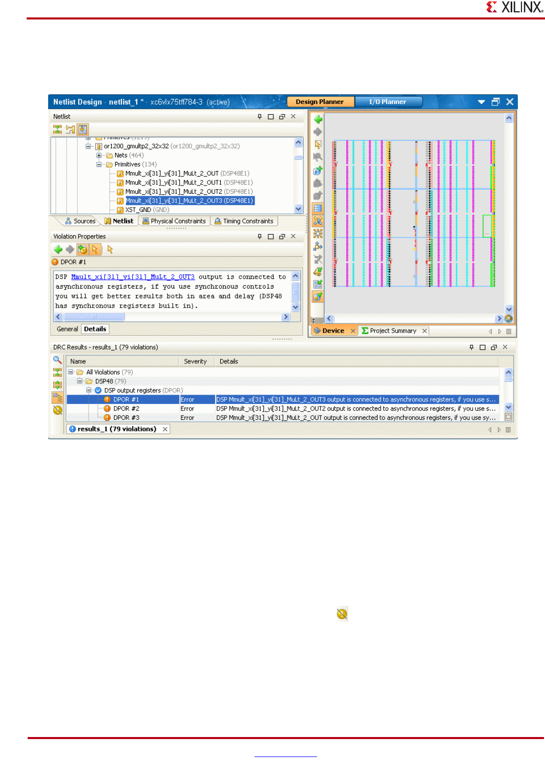
232 www.xilinx.com PlanAhead User Guide

UG632 (v 12.1)

Chapter 7: Netlist Analysis and Constraint Definition

Viewing DRC Violations

Once completed, the DRC Results view opens, as shown in the following figure.

Each violation is expanded in the DRC Results view.

•Errors display a red icon.

•Warnings display an amber icon.

•Informational messages display a yellow icon.

By default, all errors and warnings display. You can hide all warnings and informational

messages and view only errors by clicking the Hide Warning and Information Messages

toolbar button. Click the toolbar button as shown in the following figure again to view all

errors and warnings again.

Select an error in the DRC Results view list, and the specific violation information displays

in the Properties view.

Select a blue link in the Properties view to highlight the violating design elements in the

Device view, Netlist view, and Schematic view as shown in Figure 7-43, page 232.

Figure 7-43: DRC Results

Figure 7-44: Hide Warning and Information Messages Button

PlanAhead User Guide www.xilinx.com 233

UG632 (v 12.1)

Running the Design Rule Checker (DRC)

Violations no longer display in the DRC Results view after you fix the error condition and

the re-run the DRC check.

Each time you run the Run DRC command and the DRCs detect errors, PlanAhead adds a

new results tab to the DRC Results view, and creates a separate results output file in the

PlanAhead invocation directory.

DRC Rule Descriptions

The following tables describe the DRC rules, rule intent, and severity.

•“Floorplan Pblock Rules”

•“Bank Rules”

•“DCI Rules”

•“ClkBuf Rules”

•“DSP48 Rules”

•“RAMB16 Rule”

•“Netlist Rules”

Note: For Global Clock Rules, IOB Rules, and Bank IO Standard Rules, Chapter 8, “I/O Pin

Planning.”

Floorplan Pblock Rules

Bank Rules

Table 7-1: Floorplan Pblock Rules

Rule Name Rule Abbrev Rule Intent Severity

Longest Carry

Chain Height

LCCH Checks that the Pblock height can

accommodate longest Carry Chain

assigned to Pblock.

Amber

Warning

Pblock overlap FLBO Checks for overlapping Pblock

rectangles.

Information

Pblock Partition FLBP Checks that the LUT to MUXCY and

MUXFx connection is not broken by a

Pblock partition.

Error

Resource

Utilization

UTLZ Checks that Pblocks have enough

resources for logic assigned to them.

Warning for

SLICE logic.

Error for non-

SLICE logic.

Area Group Tile

Argument

FLBA Checks that the site ranges in

AREA_GROUP constraints are aligned

with the CLB grid.

Warning

Table 7-2: DCI Cascade Rule

Rule Name Rule Abbrev Rule Intent Severity

DCI Cascade

Checks

DCIC Checks that DCI cascade constraint is

legal.

Error

234 www.xilinx.com PlanAhead User Guide

UG632 (v 12.1)

Chapter 7: Netlist Analysis and Constraint Definition

For a full list of Bank IO standard rules see “Bank I/O Standard Rules” in Chapter 8.

DCI Rules

ClkBuf Rules

See “Global Clock Rules” in Chapter 8 for a full list of Global clock rules.

DSP48 Rules

Table 7-3: IDelay Control Rule

Rule Name Rule Abbrev Rule Intent Severity

IDelayCtrl

Checks

IDLYCTRL Checks that IDelay placement is

consistent with IDlyController locs.

Error

Table 7-4: DCI Rules

Rule Name Rule Abbrev Rule Intent Severity

DCI Cascade

with part

compatibility

DCICPC Warns the user to load the UCF file into

other compatible parts, and to run DRC

manually to ensure the DCI cascades

are valid.

Warning

DCI check for

I/O standard

legality

DCICIOSTD Ensures that there are no conflicts

related to Vcc and DCI termination of

I/O standards used within the DCI

Cascade.

Error

Table 7-5: IDelay Control Rules

Rule Name Rule Abbrev Rule Intent Severity

BufR & BufIO

Locations

BUFRIOC Checks that BUFR and BUFIO driven

by the same regional clock terminal are

placed at mutually routable locations.

Error

Table 7-6: DSP48 Rules

Rule Name Rule Abbrev Rule Intent Severity

DSP output

registers

DPOR DSP48 has a register on the output

side; to use this register the register

should be synchronously controlled.

(Virtex-4 only)

Information

DSP input

registers

DPIR DSP48 has a register on the input side;

to use this register the register should

be synchronously controlled.

(Virtex-4 only)

Information

DSP output

pipelining

DPOP DSP48 has a register on the output

side; using this pipeline mechanism

will improve performance.

(Virtex-4 only)

Information

PlanAhead User Guide www.xilinx.com 235

UG632 (v 12.1)

Running the Design Rule Checker (DRC)

RAMB16 Rule

Netlist Rules

DSP multiplier

output

pipelining

DMOP DSP48 output is not pipelined.

Pipelined output will improve

performance.

Warning

DSP input

pipelining

DPIP DSP48 has a register on the input side;

using this pipeline mechanism will

improve performance.

(Virtex-4 only)

Information

Table 7-7: RAMB16 Rule

Rule Name Rule Abbrev Rule Intent Severity

RAMB16 output

registers

RBOR RAMB16 has a register on the output

side; to use this register, the register

should be synchronously controlled.

(Virtex-4 only)

Information

Table 7-8: Net Rules

Rule Name Rule Abbrev Rule Intent Severity

Driverless Nets NDRV Checks that each net has a proper

driver pin.

Warning

Table 7-9: Instance Rules

Rule Name Rule Abbrev Rule Intent Severity

Black Box

Instances

INBB Checks that there is no blackbox

(undefined logics in the netlist).

Warning

Mismatching

Block

ULMN Detects mismatching logic module

interfaces in the netlist.

Error

Mismatching

ULMP Detects mismatching logic module

pins in the netlist.

Error

Mismatching

Attribute

ULMA Detects mismatching logic attributes

in the netlist.

Error

Table 7-6: DSP48 Rules (Continued)

Rule Name Rule Abbrev Rule Intent Severity

236 www.xilinx.com PlanAhead User Guide

UG632 (v 12.1)

Chapter 7: Netlist Analysis and Constraint Definition

PlanAhead User Guide www.xilinx.com 237

UG632 (v 12.1)

Chapter 8

I/O Pin Planning

This chapter contains the following sections:

•“I/O Planning Overview”

•“Using the I/O Planner”

•“Viewing Device Resources”

•“Defining Alternate Compatible Parts”

•“Setting Device Configuration Modes”

•“Defining and Configuring I/O Ports”

•“Disabling or Enabling Interactive Design Rule Checking”

•“Validating I/O and Clock Logic Placement”

•“Removing I/O Placement Constraints”

•“Exporting I/O Pin and Package Data”

I/O Planning Overview

The I/O Planner environment provides an interface to analyze the design and device I/O

requirements, and to define an I/O pinout configuration or “pinout” that satisfies the

requirements of both the PCB and the FPGA designers. The PlanAhead™ software enables

the creation of I/O port signals, and the import of an I/O port list in CSV, UCF, or HDL

format. This allows for early and intelligent pinout definition to eliminate pinout-related

changes that typically happen later in the design. It can also substantially improve the

performance. Often, designers are hindered by a non-optimal pinout that causes further

delays when trying to meet timing and signal integrity requirements. By considering the

data flow from PCB to FPGA die, optimal pinout configurations can be achieved quickly,

thus reducing internal and external trace lengths as well as routing congestion.

I/O Pin Planning Methodology

I/O pin planning is a complex process involving design groups that include PCB

designers, FPGA designers, and the System designer; each with their own specific set of

concerns and requirements.This chapter focuses on using the PlanAhead environment to

perform device exploration and I/O pin planning and related tasks.

For more information about Xilinx-suggested I/O pin planning methodology, refer to the

Spartan-6 PCB Design Guide, (UG393).

238 www.xilinx.com PlanAhead User Guide

UG632 (v 12.1)

Chapter 8: I/O Pin Planning

I/O Planning Stages

PlanAhead facilitates I/O planning at various stages of the design process. As the design

progresses, more information becomes available, enabling more complex rule checking as

the design is synthesized and implemented.

Proper I/O assignment can depend on how the clocks are configured. Assigning I/Os and

clock logic often go together. For the I/O placement DRCs to be “clock aware”, a

synthesized netlist design is required.Whenever possible, it is optimal to perform I/O

assignment with a netlist design.

The final validation of a I/O pin and clock configuration is to run the design through the

implementation tools. Proper clock resource validation can require full implementation of

all clocks.

Pin Planning Project

You can create an empty project to enable early device exploration and I/O port

configuration. I/O ports can be created manually or imported from CSV, RTL, or UCF

inputs. You can export device and I/O port assignment in RTL, UCF, or CSV format for

later use in the design process when an RTL design exists.

RTL Design

You can perform I/O planning in a PlanAhead RTL-based project. The RTL design is

elaborated and certain basic DRC checks are provided. To check clock logic, validation

with a synthesized netlist is optimal.

Synthesized Netlist Design

You can puffery I/O planning after synthesis in the netlist design. Because all clock are

determined, a more thorough validation is performed because the tool has visibility to all

clocks. Whenever possible, I/O assignment should be performed using a netlist design.

Implemented Design - Final I/O Validation

The design should be fully implemented to ensure a legal I/O pinout. Examine the

ngdbuild and map reports for I/O and clock-related messages.

I/O Port Placement Capabilities

You can select and configure any of the ports or interfaces using the Configure I/O Ports

command. This command provides a way to set I/O standard, drive strength, and slew

type. The I/O Planner supports output to a comma separated values (CSV) format file for

use in PCB schematic symbol creation or the HDL port list. See “Configuring I/O Ports,”

page 251.

You can place Prohibits on individual I/O pins or I/O banks to prevent I/O assignment to

them. See “Prohibiting I/O Pins and I/O Banks,” page 255.

The I/O port placement can be performed in the following methods:

•Group I/Os together into interfaces to more identify them more easily or select them

for placement. See “Creating I/O Port Interfaces,” page 255.

•Drag groups of I/O ports and assign them into either the Package view or Device

views using one of three placement modes: in an I/O Bank. in an Area, or

Sequentially.

PlanAhead User Guide www.xilinx.com 239

UG632 (v 12.1)

Using the I/O Planner

Each mode offers a different assignment pattern for the I/O ports to be assigned to pins.

The cursor tool tip provides information about the number of ports being placed.

The mode remains active until all of the selected I/O ports are placed or until you press the

Esc key. For more information, see “Disabling or Enabling Interactive Design Rule

Checking,” page 257.

The Tools > Autoplace I/O Ports command places the entire device or any selected

portion of the device automatically. The command obeys I/O bank rules, differential pair

rules, and global clock pins, and places as many of the I/O Ports as possible.This

functionality is available for certain device architectures only. See “Automatically

Assigning I/O Ports,” page 261.

The PlanAhead software attempts to maintain correct assignment rules. Differential pair

ports are assigned into proper pin pairs. Also, interactive and batch DRCs are used to help

ensure legal I/O placement. See “Validating I/O and Clock Logic Placement,” page 263.

Using the I/O Planner

You can use the I/O Planner in the RTL Design, Netlist Design, and Implemented Design

environments. The view layout consists of a both Package and Device graphical views.

Other views provide additional I/O information: the Package Pins view, the I/O Ports

view, the Clock Region view, and the Properties view.

There are two ways to launch the I/O Planner view layout:

•Select the I/O Planner button in the banner of the open Design environment.

•Create a new Pin Planning Project using the New Project wizard.

The I/O Planner is shown in Figure 8-1, page 240.

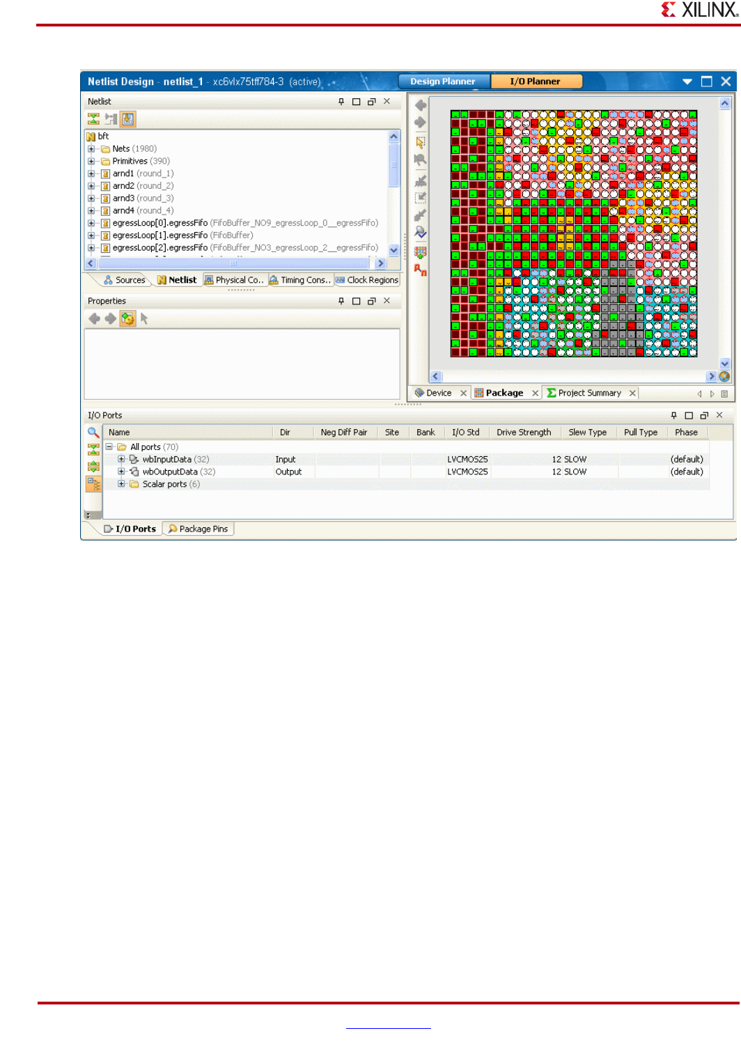
240 www.xilinx.com PlanAhead User Guide

UG632 (v 12.1)

Chapter 8: I/O Pin Planning

The following references in Chapter 4, “Using the Viewing Environment,”apply to the I/O

Planner Environment:

•“Using the Device View,” page 104

•“Using the Package View,” page 109

•“Using the I/O Ports View,” page 126

•“Using the Package View,” page 109

Splitting the Workspace to Display Device and Package Views

It is often helpful to split the workspace and display the two views side by side as shown

in Figure 8-1.

You can split the workspace by either of the two following methods:

−Select either view tab and drag it to the very far right scroll banner of the

workspace. A grey rectangle displays where the view would be placed. Position

the cursor so that the Workspace view arrangement is to your liking and click the

cursor to move the view and split the workspace. Figure 8-2, page 241 shows and

example of a split view. This same technique works with many of the views.

−Select the view tab and use the New Horizontal Group or New Vertical Group

popup menu commands. This capability is available for the Workspace views

only.

Figure 8-1: I/O Planner Environment

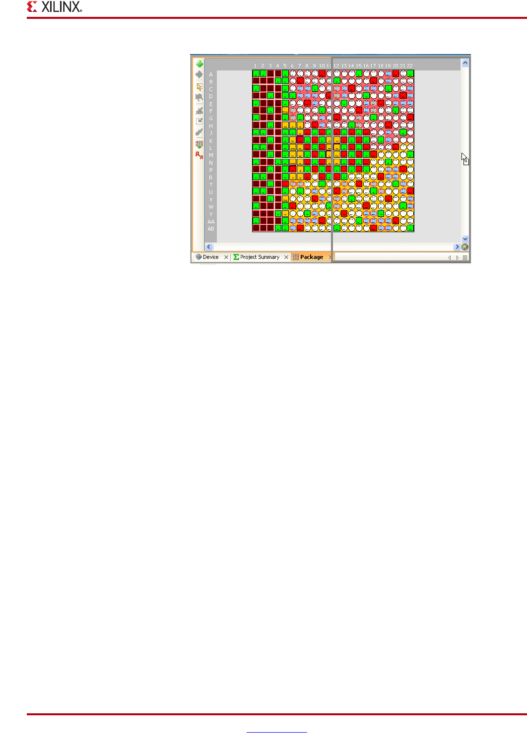
PlanAhead User Guide www.xilinx.com 241

UG632 (v 12.1)

Viewing Device Resources

Merging Views to One Tabbed Area

To collapse the views back into one tabbed area, either:

•Select any view and drag it onto the view tab of another. The dragged grey rectangle

displays around the entire view.

•Select the Move to Previous/Next Horizontal/Vertical Group popup menu

command.

Viewing Device Resources

The Device and Package views display a graphical representation of the device and placed

logic resources. When any logic object or device site is selected in any view, information

about it is displayed in the Properties view. The Properties view often has tabbed panes to

display various types of information as shown in “Displaying I/O Bank Location and

Resources,” page 243.

To view properties for a selected object, display the Properties view. If the Properties view

is not visible, select the <Object_type> Properties popup menu command.

For more information about using the Device and Package view, see “Using Common

PlanAhead Views” in Chapter 4.

You can search for specific objects or device sites by using the Find command. There are a

variety of searchable object types and robust filtering capabilities to search the device or

design for specific objects. You can select objects directly from the Find Results view; for

more information, refer to “Using the Find in Files Command to Search Source Files” in

Chapter 5.

Figure 8-2: Splitting the Workspace to Display Package and Device Views

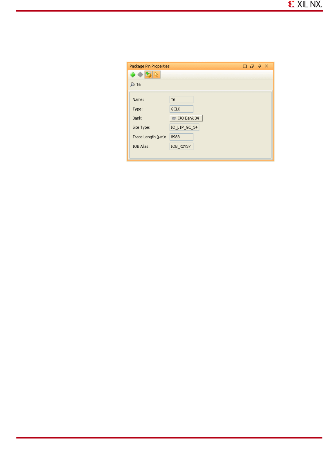
242 www.xilinx.com PlanAhead User Guide

UG632 (v 12.1)

Chapter 8: I/O Pin Planning

Viewing Package Pin Properties

You can select pins or I/O banks in the Package view and see the corresponding details in

the Properties view, as shown in the following figure.

Viewing I/O Bank Resources

You can select I/O resources in any of the I/O Planner views and their corresponding data

is highlighted in all other views. This provides a visual indication of the relationship

between the physical package and the internal die. The views contain many types of device

and design information, such as:

•In the Package Pins view, you can select one of the I/O banks.

•In the I/O Bank Properties view you can click the General tab. Figure 8-4, page 243

illustrates the I/O bank display.

Figure 8-3: Package Pin Properties

PlanAhead User Guide www.xilinx.com 243

UG632 (v 12.1)

Viewing Device Resources

Figure 8-4: Displaying I/O Bank Location and Resources

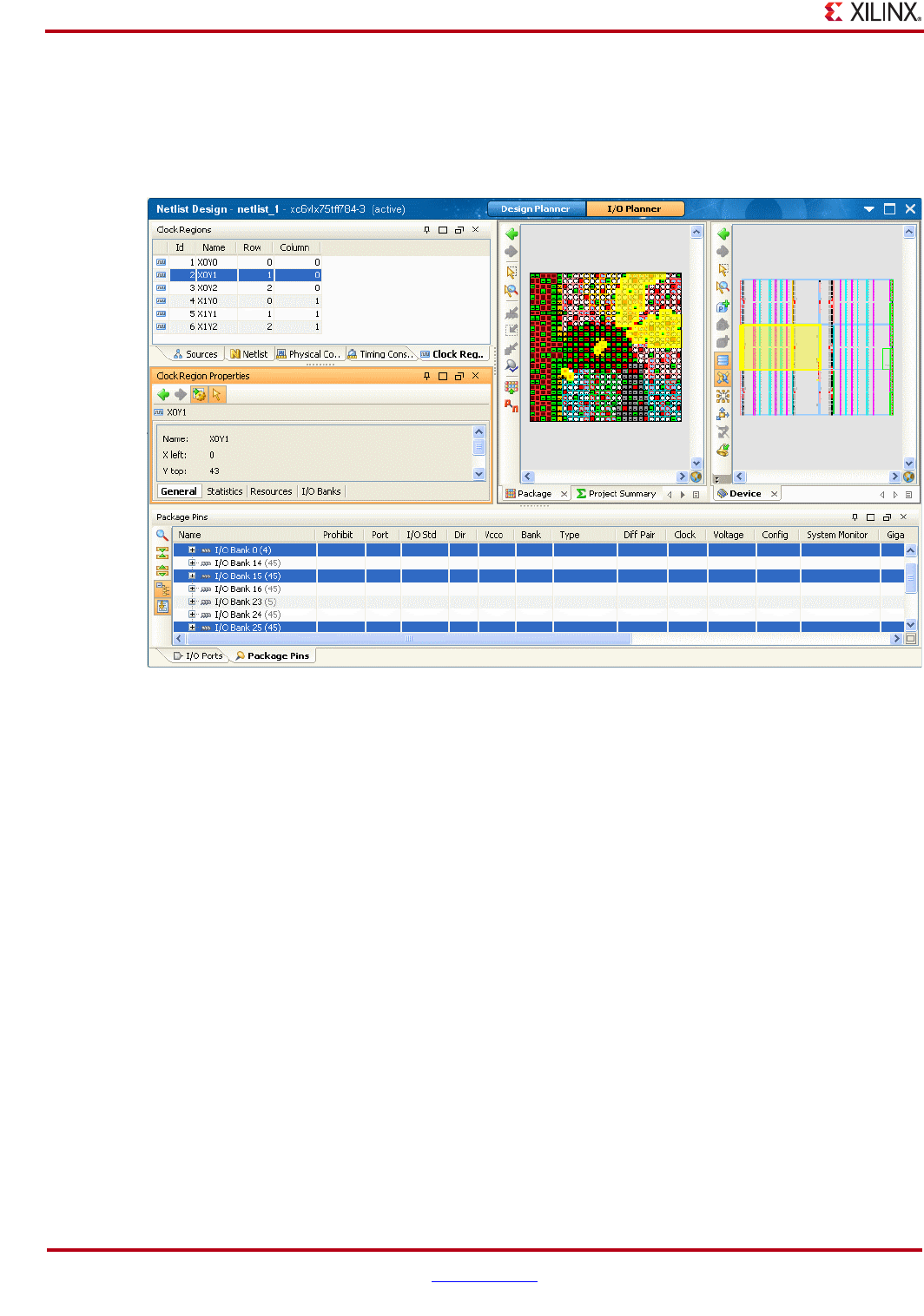
244 www.xilinx.com PlanAhead User Guide

UG632 (v 12.1)

Chapter 8: I/O Pin Planning

Viewing Clock Region Resources

The Clock Regions view allows easy selection of the clock regions. Selecting a clock region

highlights the related I/O banks and regional clock resources as shown in the following

figure.

Viewing Clock Region Resource Statistics

Selecting the Statistics tab in the Clock Region Properties view displays the resource

statistics available within the clock region as well as the logic content of the selected clock

region.

Selecting the Resources tab enables device clock sites to be located for logic assignment, as

shown in Figure 8-6, page 245.

Figure 8-5: I/O Planner Clock Region Sources

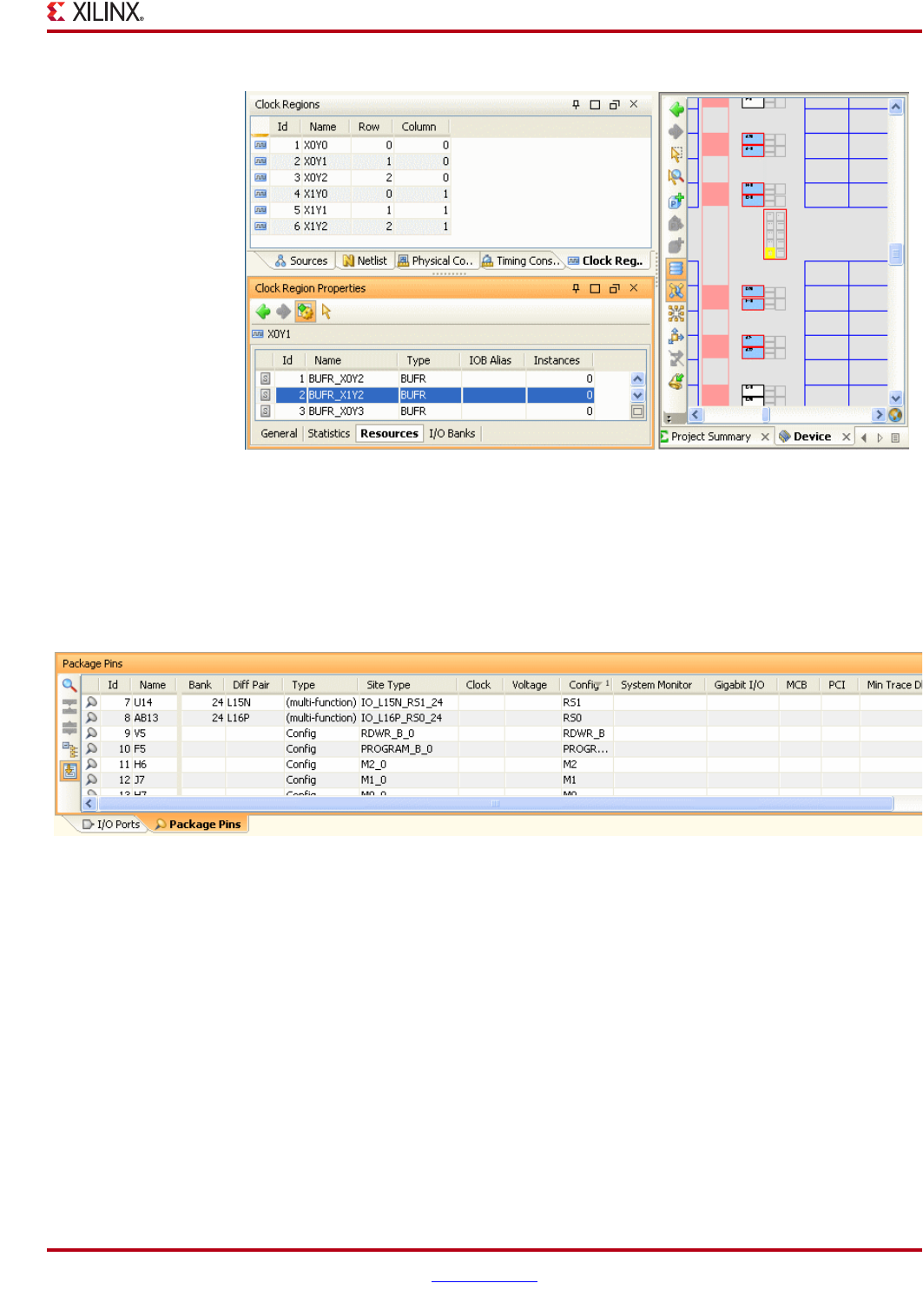
PlanAhead User Guide www.xilinx.com 245

UG632 (v 12.1)

Viewing Device Resources

Viewing Multi-Function Pins

The Package Pins view contains a variety of data types that display in spreadsheet-like

columns. The view can be flattened, filtered, and sorted. Columns can be moved, hidden

and configured to display and compare the various multi-function pins. The following

figure shows an example of the Package Pins view.

The Type column identifies multi-function types of pins. Other columns contain

information about logic or configuration modes involving multi-function type pins.

If your design contains Gigabit Transceivers “GTs”, Memory controllers, or PCI logic,

information appears in this table that identifies conflicting multi-function pins.

Use the Set Configuration Modes command can to select the required device

configuration modes. Many of these configuration modes use multi-function pins. For

more information, see “Setting Device Configuration Modes,” page 247.

Figure 8-6: Viewing Clock Region Resources

Figure 8-7: Package Pin Tab

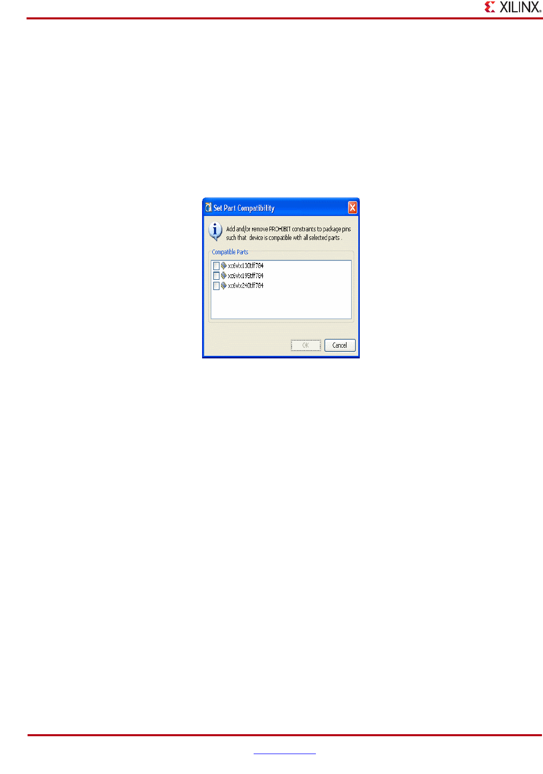
246 www.xilinx.com PlanAhead User Guide

UG632 (v 12.1)

Chapter 8: I/O Pin Planning

Defining Alternate Compatible Parts

The PlanAhead software lets you select alternate devices for the design. PlanAhead

attempts to ensure that a legal I/O pin assignment is defined and will work across all of the

selected devices.

To define an alternate compatible part:

1. Select the Set Part Compatibility popup menu command in the Package or Package

Pins view.

Compatible devices available in the same package display in a list as shown in the

following figure.

This feature supports alternate parts available in the same package only.

2. Select any number of alternate parts. The number of available Package Pins for

placement diminishes as more parts are selected.

PlanAhead sets Prohibits automatically on any unbonded pins in the selected alternate

devices. A dialog box displays showing the number of prohibited package pins.

You can view Prohibits in the Package, Package Pins, or Device views also. You can view

and manage alternate parts defined in the Floorplan Properties view under the Part

Compatible tab.

Note: The Set Part Compatibility command supports Virtex®-5, Virtex-6 and Spartan®-6 parts only.

Figure 8-8: Select Alternate Compatible Parts

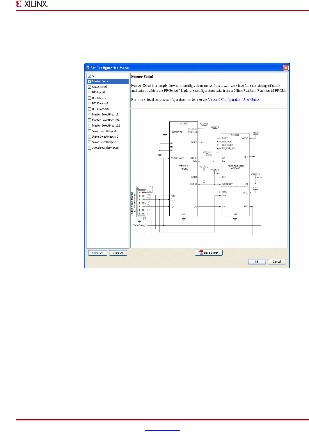
PlanAhead User Guide www.xilinx.com 247

UG632 (v 12.1)

Setting Device Configuration Modes

PlanAhead provides information about the various device configuration modes and lets

you set any number of them as shown in the following figure.

To set the device configuration modes:

1. In the Package Pins view, click Set Configuration Modes.

−Click any configuration mode to view information, including the schematic.

−Click Datasheet to invoke the device datasheet in a PDF viewer, (if needed).

2. Select the configuration modes you want and click OK.

Setting configuration modes displays the associated I/O pins in the Config column of the

Package Pins view.

For more information about analyzing how the configuration modes might conflict with

other multi-function pins, refer to “Viewing Multi-Function Pins,” page 245.

Figure 8-9: Set Configuration Modes Dialog Box

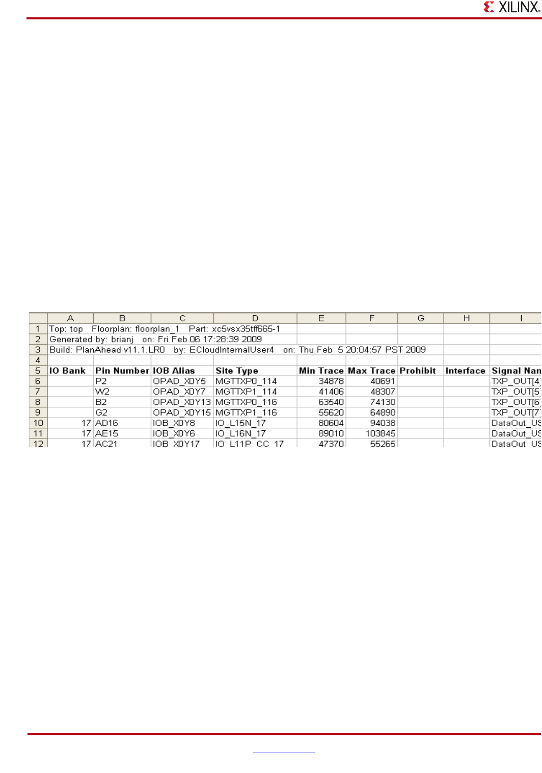
248 www.xilinx.com PlanAhead User Guide

UG632 (v 12.1)

Chapter 8: I/O Pin Planning

Defining and Configuring I/O Ports

You can create and configure I/O ports using the I/O Planner interface. You can create

empty projects and generate I/O ports.

Importing I/O Ports

The PlanAhead software supports importing UCF or CSV format files into an empty

PlanAhead project to begin I/O pin planning. RTL files or headers can be used to create an

RTL Project for I/O pin planning.

Creating an RTL-based or synthesized netlist-based project populates the I/O Ports view

automatically with the I/O ports defined in the design.

Importing a CSV Format File

To import an I/O ports list from a CSV:

1. Select File > Import I/O Ports > From CSV.

2. In the file browser, browse to and select a CSV file to import.

The CSV file format is shown in the following figure.

CSV Columns

CSV is a standard file format used by FPGA and board designers to exchange information

about device pins and pinout. The CSV columns are:

•I/O Bank—The I/O Bank in which the pin is located. The software fills in this field for

all pins in the device. Values are a number or blank. This is not required in the input

CSV file.

•Pin Number—The name (or location) of the package pin. The software writes this out

for all pins in the device. This is not required in the input file. If used for input, it is

used to define placement. Values are legal pins in the device.

•IOB Alias—An alternate part name for the package pin. This field is specified by the

software, and is unused if specified in the input CSV file.

•Site Type—The pin name from the device data sheet. This field is specified by the

software, and is unused if specified in the input CSV file.

•Min/Max Trace Delay—The distance between the pad site of the die and the ball on

the package, in picoseconds.

Figure 8-10: I/O Port List CSV Format

PlanAhead User Guide www.xilinx.com 249

UG632 (v 12.1)

Defining and Configuring I/O Ports

This is specified by the tool to help the board engineer match trace delays. The Trace

Delay fields are in the output file only. They are not expected in the input file.

•Prohibit—Certain sites can be prohibited for many reasons to prevent user I/O from

being added to the site. Prohibits ease board layout issues, reduce cross-talk between

signals, and ensure that a pinout works between multiple FPGAs in the same

package. In the UCF this is represented by a CONFIG PROHIBIT constraint. Values are

TRUE or a blank field; leave this field blank when the Pin Number is left blank.

•Interface—An optional user-specified grouping for an arbitrary set of user I/O. As an

example, this field provides a means to specify a relationship for the data, address,

and enable signals for a memory interface. Values are a text string or blank.

•Signal Name—The name of the User I/O in the FPGA design. Values are a string or

blank for an unassigned Package Pin.

•Direction—The direction of the signal. Values are IN, OUT, INOUT, or blank when a

user I/O is not assigned to the site.

•DiffPair Type—Instructs the software about which pin is the N side of a differential

pair, and which pin is the P side. This is used for differential signals only.

The software uses this column instead of a naming convention to determine which

pin is the N side of the pair, and which pin is the P side.

Values are P, N, or blank when a user I/O is not assigned to the site.

•DiffPair Signal—Specifies the name of the other pin in the differential pair. Values are

the name of the user I/O or blank when unused.

•I/O Standard—I/O standard for a specific user I/O. When this field is blank for a user

I/O, the software uses the appropriate device defaults. Values are a legal I/O

standard for the user I/O in the device or blank.

•Drive—Drive strength of the I/O standard for a specific user I/O. Not all I/O

standards accept a drive strength. If this field is blank the tools will use the default.

Values are a number or blank.

•Slew Rate—Slew rate of the I/O standard for a specific user I/O. Not all I/O

standards accept a slew rate. If this field is blank the tools will use the default. Values

are FAST and SLOW.

•Phase—Specifies the phase of an I/O relative to the phase of other I/O in the bank in

cases of a synchronous phase offset.

You can attach other information also. The software will add any other fields with user-

defined values to the set of user-defined columns. Also, you can add extra columns to the

Package Pins table.

Using Custom CSV I/O Port Properties

PlanAhead has a specific expected format for importing I/O pin-related data. Often, CSV

files contain additional information. If additional columns exist in the imported CSV file,

PlanAhead creates new columns in the Package Pins view to display and/or modify the

field values.

To modify or define values in the customer CSV fields, select the Set User Column Values

popup menu command.

When you select File > Export I/Os > CSV the columns and new values are preserved and

exported in the output CSV file.

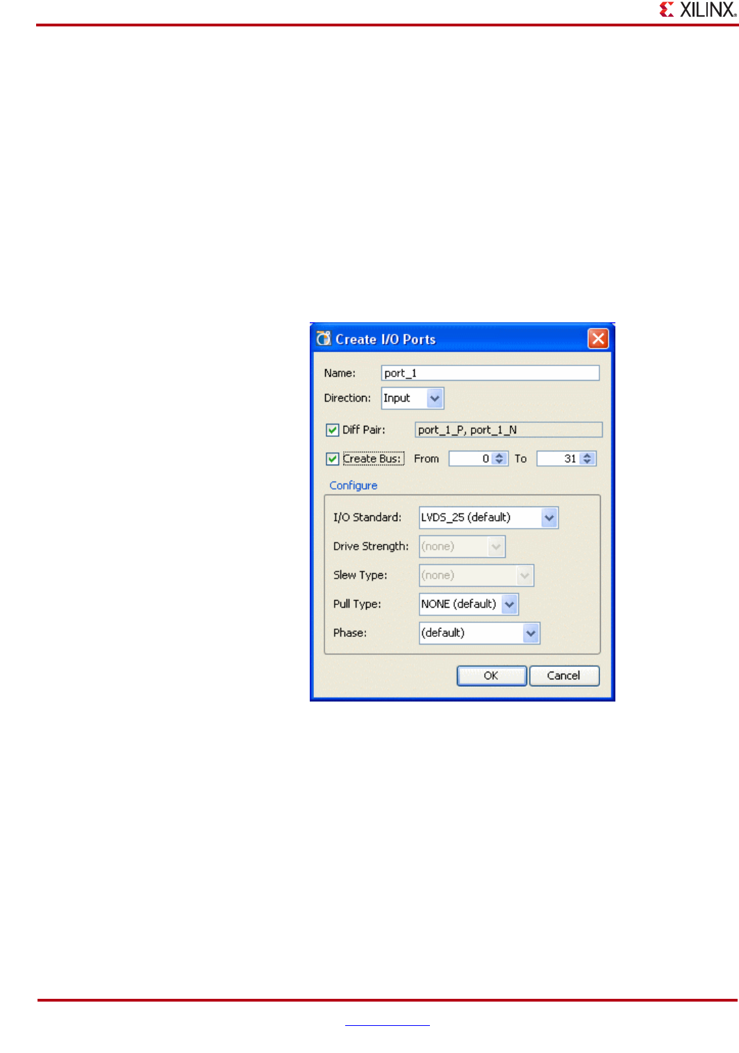
250 www.xilinx.com PlanAhead User Guide

UG632 (v 12.1)

Chapter 8: I/O Pin Planning

Importing a UCF Format File

PlanAhead lets you import a UCF format files as a way to populate the I/O Ports view. To

import I/O port definitions from a UCF file, select File > Import I/O Ports > From UCF.

Because the UCF format does not define port direction, the Direction field displays as

<undefined>. Select the Set Direction command from the I/O Ports popup menu to

define I/O port direction. See “Setting I/O Port Direction,” page 251 for more information.

Creating I/O Ports

To create I/O ports:

1. In the I/O Ports view, select Create I/O Ports from the popup menu.

The Create I/O Ports dialog box opens as shown in the following figure.

2. View and edit the options in the Create I/O Ports dialog box:

−Name—Enter the name of the desired port or bus to create.

−Direction—Select the port direction.

−Diff Pair—Define differential pair signals or busses.

−Create Bus—Enter bus range for bus creation.

−Configure

-I/O Standard—Select the I/O Standard constraint.

-Drive Strength—Select the Drive Strength value.

-Slew Type—Select the Slew Type value.

-Pull Type—Select the Pull Type value.

Figure 8-11: Create I/O Ports Dialog Box

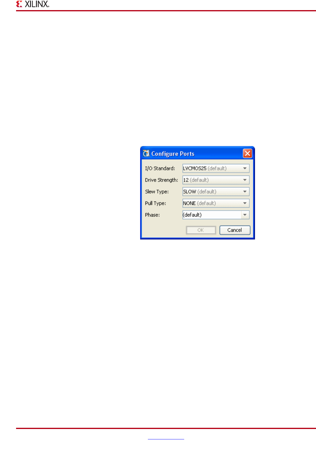
PlanAhead User Guide www.xilinx.com 251

UG632 (v 12.1)

Defining and Configuring I/O Ports

-Phase—Enter a phase group or select an existing phase group. A phase

group is a logical grouping of ports that is used in SSN calculations to indicate

that the set of ports share the same frequency and phase.

For more information on using this option, see “Defining the I/O Port

Switching Phase Groups,” page 272.

Refer to Xilinx® device documentation for information regarding voltage capabilities of

the device.

Configuring I/O Ports

To configure a port or a group of ports:

1. In the I/O Ports view, select the ports.

2. From the popup menu, select Configure I/O Ports.

The Configure Ports dialog box opens as shown in the following figure.

3. View and edit the definable options in the Configure I/O Ports dialog box:

−I/O Standard—Select the I/O Standard constraint.

−Drive Strength—Select the Drive Strength value.

−Slew Type—Select the Slew Type value.

−Pull Type—Select the Pull Type value.

−Phase—Enter a phase group or select an existing phase group. A phase group is a

logical grouping of ports that is used in SSN calculations to indicate that the set of

ports share the same frequency and phase. For more information on using this

option, see “Defining the I/O Port Switching Phase Groups,” page 272.

Refer to Xilinx device documentation for information regarding voltage capabilities of the

device.

Setting I/O Port Direction

To set the I/O port direction, select the I/O ports, busses, or interfaces to be configured,

and select the Set Direction popup menu command in the I/O Ports view.

Figure 8-12: Configure Ports Dialog Box

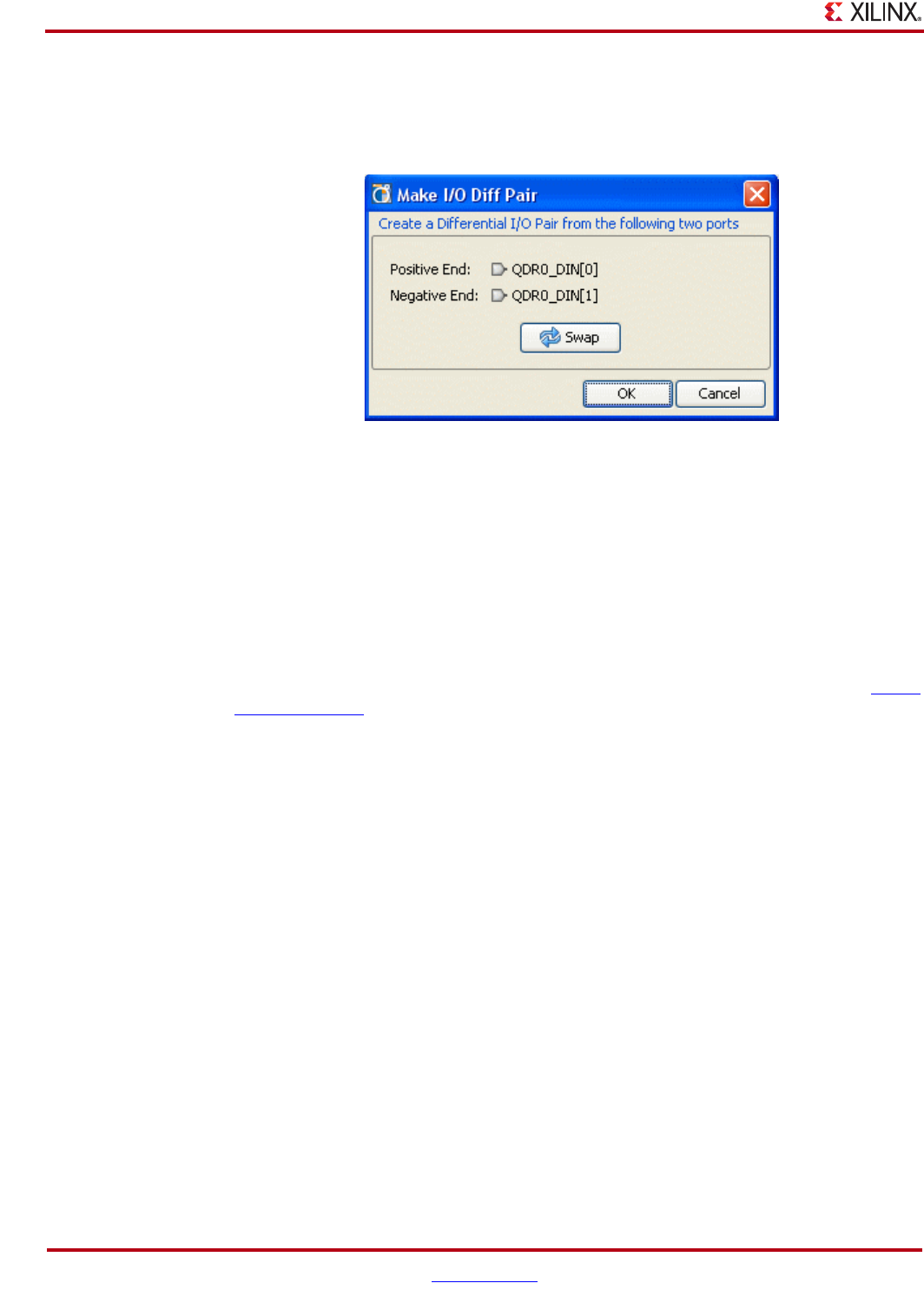
252 www.xilinx.com PlanAhead User Guide

UG632 (v 12.1)

Chapter 8: I/O Pin Planning

Defining Differential Pairs

To define a differential pin pair, select any two I/O ports, and select the Make Diff Pair

popup menu command in the I/O Ports view as shown in the following figure.

The two I/O Ports display in the dialog box with initial Positive End and Negative End

definitions.

•To alternate the Positive End and Negative End definitions, click the Swap button.

•To remove the differential pair definition on any differential pin pair, select the Split

Diff Pair popup menu command.

Configuring DCI_CASCADE Constraints

The DCI_CASCADE constraint can be configured within the PlanAhead environment. For

information about the intent and use of the DCI_CASCADE constraint, refer to the Xilinx

Constraints Guide, (UG612)

The basic premise of the constraint is to link two or more adjacent I/O Banks together for

clocking purposes. The I/O bank with the input clock is called the master and all others are

slaves. You can set the constraint by preselecting the I/O Banks you want prior to running

the command or by selecting them within the command dialog box.

To configure the DCI_CASCADE constraint:

1. Optionally, select the I/O Banks to configure.

2. Right-click and select the Create a DCI Cascade popup menu command. The DCI

Cascade editor opens as shown in Figure 8-14, page 253.

Figure 8-13: Make I/O Diff Pair

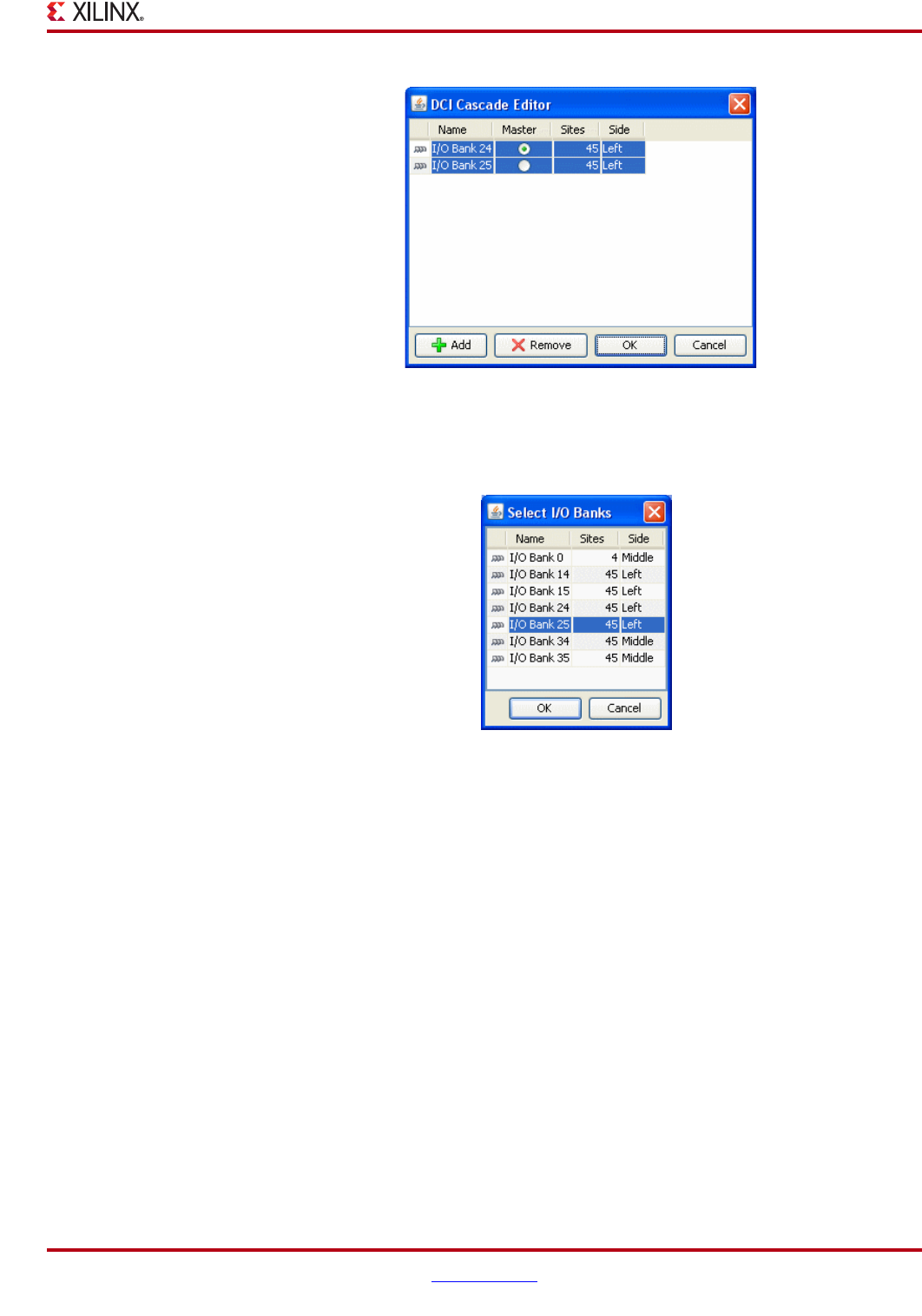
PlanAhead User Guide www.xilinx.com 253

UG632 (v 12.1)

Defining and Configuring I/O Ports

3. To include additional I/O banks, select the Add button.

Preselected I/O Banks appear in the dialog box as shown in the following figure.

4. Select an I/O Bank to be the master.

5. Click OK.

Notice that as I/O Banks are selected, they are highlighted in the other PlanAhead

views.

The DCI Cascades display in the Physical Constraints view as shown in Figure 8-16,

page 254.

Figure 8-14: Creating a DCI Cascade

Figure 8-15: Selecting I/O Banks for the DCI Cascade

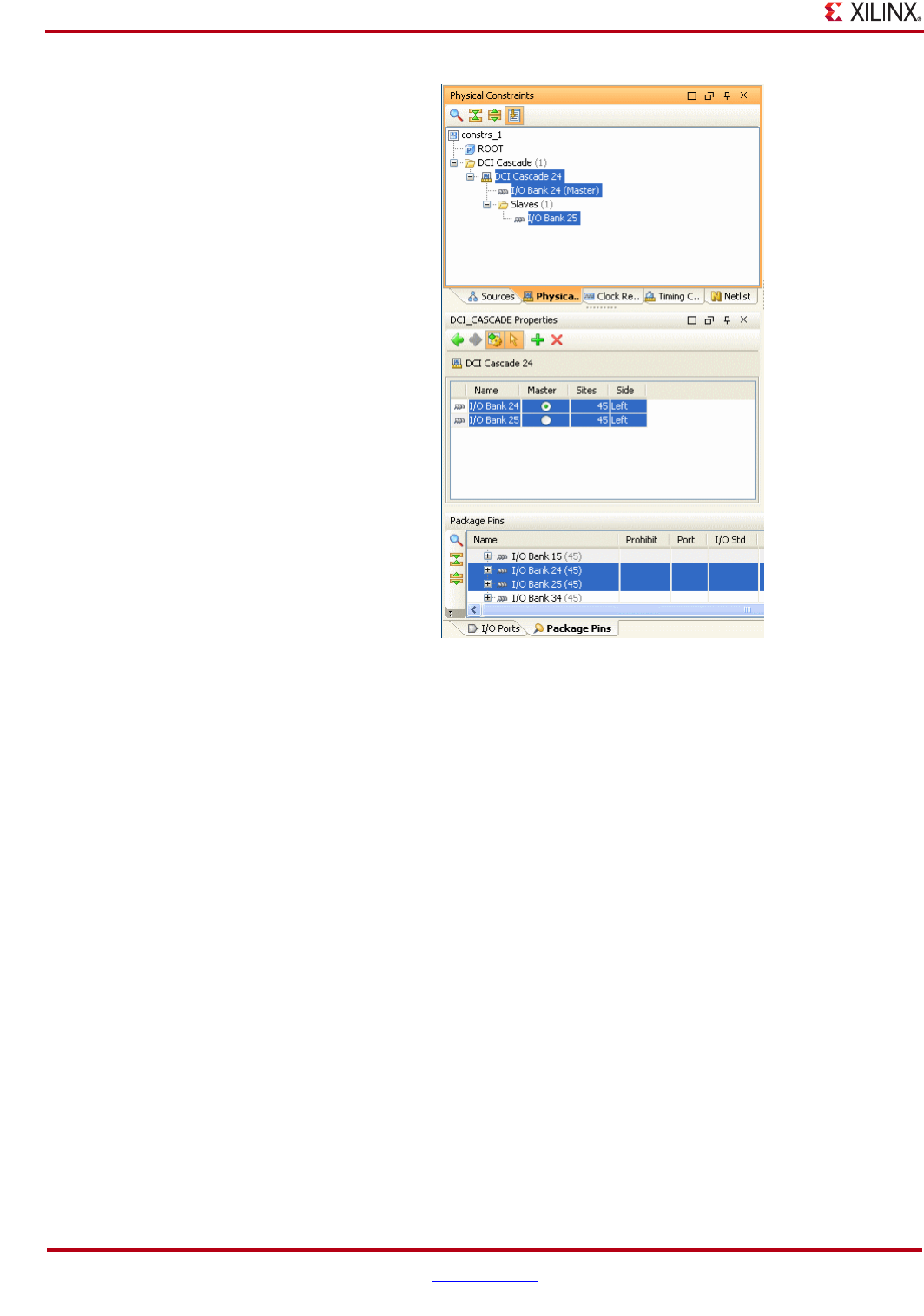
254 www.xilinx.com PlanAhead User Guide

UG632 (v 12.1)

Chapter 8: I/O Pin Planning

As you select DCI cascades in the Physical Constraints view, the associated I/O banks

are selected also.

Modifying or Removing DCI Cascade Constraints

You can modify DCI Cascades by selecting the DCI Cascade in the Physical Constraints

view and using the DCI_CASCADE Properties view.

•To save all changes, click the Apply button in the DCI_CASCADE Properties view.

•To change the master, select a different I/O Bank and assign it as the master.

•To remove I/O banks from the DCI Cascade, select the I/O banks in the

DCI_CASCADE Properties view, and click the Delete I/O Banks button.

•To include additional I/O banks in the DCI Cascade, select them in the

DCI_CASCADE Properties view and click the Add I/O Banks button. The Add I/O

Banks dialog box displays and you can select new I/O banks. The newly selected I/O

banks are highlighted in the other PlanAhead views.

•To remove DCI Cascade constraints, select the constraint in the Physical Hierarchy

view and use the Delete command.

Figure 8-16: Viewing DCI Cascades

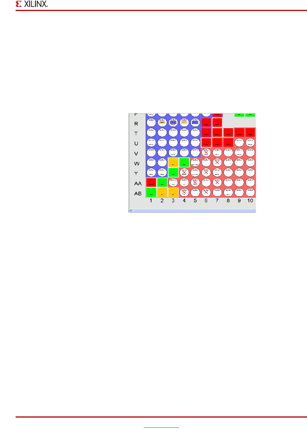
PlanAhead User Guide www.xilinx.com 255

UG632 (v 12.1)

Defining and Configuring I/O Ports

Prohibiting I/O Pins and I/O Banks

I/O Planner provides an interface to selectively prohibit individual I/O pins, groups of

I/O pins, or I/O banks. You can select and prohibit pins in the Package Pins, Device, and

Package views.

To prohibit I/O pins or I/O banks:

1. In the Package Pins or Package views, select the I/O pins or I/O banks.

2. Select Set Prohibit from the popup menu.

A red X symbol is placed on the prohibited pins in the Package view, and a checkmark is

placed in the Prohibit column of the Package Pins view as shown in the following figure.

Creating I/O Port Interfaces

You can group multiple ports or busses together by creating an Interface. This aids in pin

assignment by treating all of the interface ports as one group. Assigning all of the pins

simultaneously helps condense and isolate the interface for clock region or PCB routing.

Also, it is easier to visualize and manage all of the signals associated with a particular logic

interface.

To create an interface:

1. In the I/O Ports view, select the signals you want to group together.

2. From the popup menu, select Create I/O Port Interface as shown in Figure 8-18,

page 256.

Figure 8-17: Setting Prohibits on Package Pins

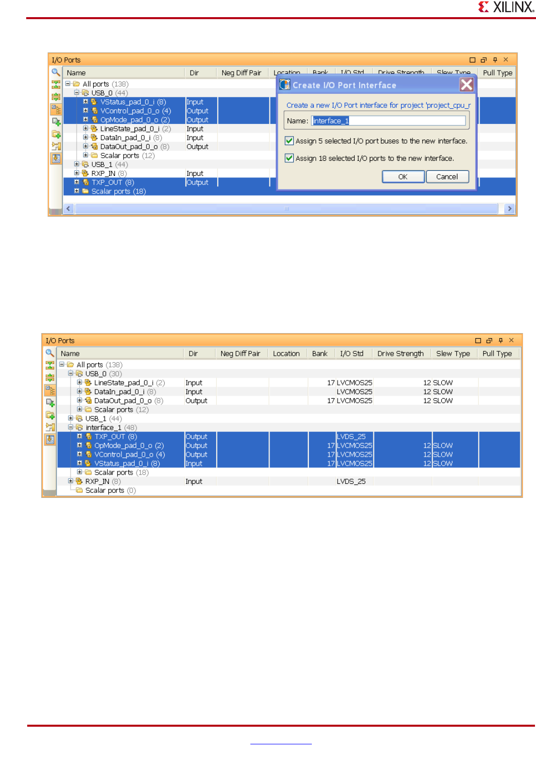
256 www.xilinx.com PlanAhead User Guide

UG632 (v 12.1)

Chapter 8: I/O Pin Planning

3. Enter a name for the interface and adjust assignment selection.

4. Click OK.

The Interfaces appear as expandable folders in the I/O Ports view. You can add additional

I/O ports to the interface by selecting them in the I/O Ports view and dragging them into

the Interface folder as shown in the following figure.

To include additional I/O ports in an interface:

1. Select a port or bus.

2. From the popup menu, select Assign to Interface.

3. Select the target interface to which you will add the I/O ports.

To remove I/O ports and interfaces:

1. Select a port or interface.

2. From the popup menu, click Unassign from Interface.

To delete interfaces, select an interface, and select Delete from the popup menu, or press

the Delete key.

Figure 8-18: Create I/O Ports Interface

Figure 8-19: Manage I/O Port Interfaces

PlanAhead User Guide www.xilinx.com 257

UG632 (v 12.1)

Disabling or Enabling Interactive Design Rule Checking

The PlanAhead software attempts to ensure a legal pin out; however, you need to run your

design through the ISE pinning process to ensure your pinouts are legal. The interactive

I/O placement routines checks common error cases. You can toggle this capability on and

off using the Automatically Enforce Legal I/O Placement button in Device or PAckage

view toolbar or in the I/O Placement section of the General dialog box (accessible using

Tools > Options > General).

This feature will not allow placement of I/O ports on pins that cause a design issue. In

Place I/O Ports Sequentially mode, when attempts are made to place an I/O Port on a

problematic pin, a a tool tip displays describing why the I/O Port is not able to be placed.

The online DRC checks are enabled by default. Many of these checks can run only when a

netlist representing the final design is loaded.

The interactive I/O placement rules include:

•Prohibiting placement on noise sensitive pins associated with Gigabit Transceivers

“GTs.” I/O package pins that are potentially noise sensitive are prohibited.

•Prohibiting I/O standard violations.

•Ensuring that I/O standards are not used in banks that do not support them.

•Ensuring that banks do not have incompatible VCC ports assigned.

•Ensuring that banks that need VREF ports have free VREF pins.

•Proper assignment of global clocks and regional clocks (only with EDIF/NGC netlist

and UCF imported).

•Ensuring Input and High Drive outputs only go to capable pins (for Spartan®-3

devices).

•Differential I/O ports to the proper sense pin.

•Ensures that no output pins are placed on input-only pins.

It is recommended that you begin your I/O port placement with DRCs enabled.

Placing I/O Ports

I/O Planner provides a variety of ways to assign I/O Ports to package pins. You can select

individual I/O ports, groups of I/O ports, or interfaces in the I/O Ports view and

graphically assign them to package pins in the Package view or I/O pads in the Device

view.

You can toggle the online DRCs on or off during interactive placement.

The three placement mode options available for assigning I/O Ports are:

•Place I/O Ports in an I/O Bank

•Place I/O Ports in an Area

•Place I/O Ports Sequentially

The following subsections describe each placement mode option.

For information on automatic I/O Port assignment, see “Automatically Assigning I/O

Ports,” page 261.

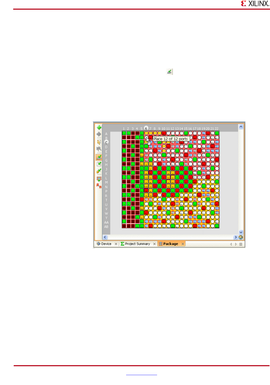
258 www.xilinx.com PlanAhead User Guide

UG632 (v 12.1)

Chapter 8: I/O Pin Planning

Placing I/O Ports into I/O Banks

To place I/O ports into I/O banks:

1. In the I/O Ports view, select an individual I/O port, a group of I/O ports or Interfaces.

2. In the I/O Ports view, the Package view, or the Device view, click the Place I/O Ports

in an I/O Bank button, which is shown in the following figure.

The group of I/O ports is attached to the cursor when it is dragged over a package pin

or I/O pad. A tool tip displays how many pins can be placed in the selected I/O bank.

3. Click on a pin or pad to assign the selected I/O ports. The following figure shows an

I/O pad.

4. If more I/O ports are selected than will fit in the I/O bank, the command is continued.

The cursor drags the remaining I/O ports to the next selected I/O bank, and so on

until all of the I/O ports are placed, or until you press the Esc key.

•Moving the cursor within the Package view actively displays the I/O pin coordinates

on the top and left sides of the view.

•Additional I/O pin and bank information displays in the Status bar located at the

bottom of the PlanAhead Environment.

•The active object being reported is highlighted in the Package view.

•Holding the cursor over the Package view invokes a tool tip that displays the pin

information.

Ports are assigned in the order they appear in the I/O Ports view. The assignment order

can be adjusted by applying sorting techniques in the I/O Ports view prior to assignment.

Figure 8-20: Place I/O Ports in an I/O Bank Button

Figure 8-21: Placing I/O Ports in I/O Banks

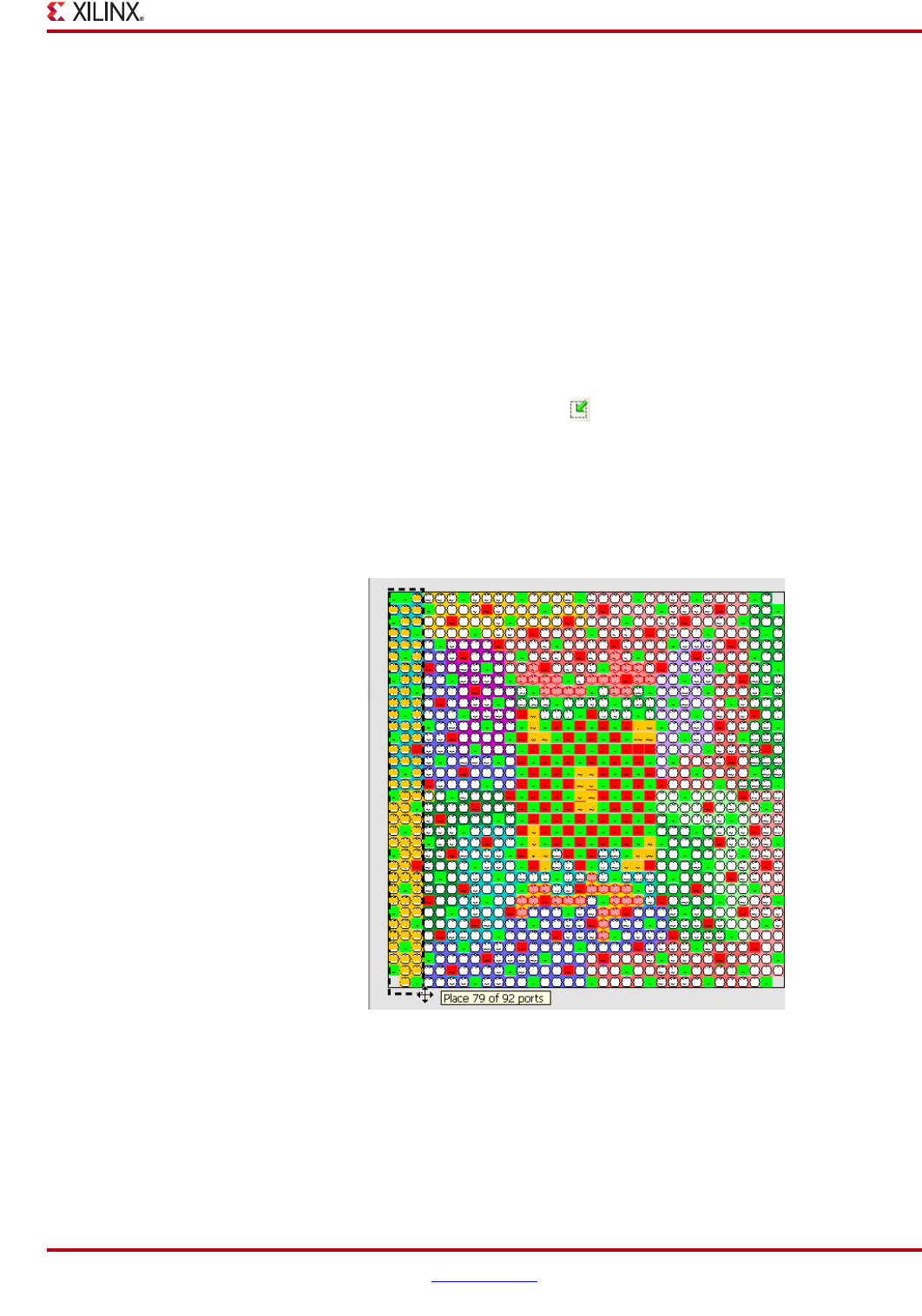
PlanAhead User Guide www.xilinx.com 259

UG632 (v 12.1)

Placing I/O Ports

The assignment order is also driven from the initial Pin that is selected for I/O bank

assignment. Selecting a pin at one end of an I/O Bank results in a continuous bus

assignment across the I/O bank.

The PlanAhead software also keeps track of PCB routing concerns for busses. Pin ordering

during assignment attempts to keep the bus bits vectored within the assignment area. You

can customize assignment patterns to address other bus routing concerns.

Placing I/O Ports in a Defined Area

To place I/O Ports into a defined area:

1. In the I/O Ports view, select individual I/O ports, groups of I/O ports or interfaces.

2. In the I/O Ports view, the Device view, or the Package view, click the Place I/O Ports

in Area button, which is shown in the following figure.

The cursor turns into a cross symbol which indicates that you can define a rectangle for

port placement.

3. In either the Package view or the Device view, draw a rectangle to define the

assignment area as shown in the following figure.

4. If more I/O Ports are selected than fit in the defined area, the command is continued.

The cursor continues to display as a cross to draw another area to place the remaining

I/O ports, and so on until all of the I/O ports are placed, or until you press the Esc key.

Ports are assigned in the order that they appear in the I/O Ports view. The assignment

order can be adjusted by applying sorting techniques in the I/O Ports view prior to

assignment.

Figure 8-22: Place I/O Ports in Area Button

Figure 8-23: Placing I/O Ports in an Area

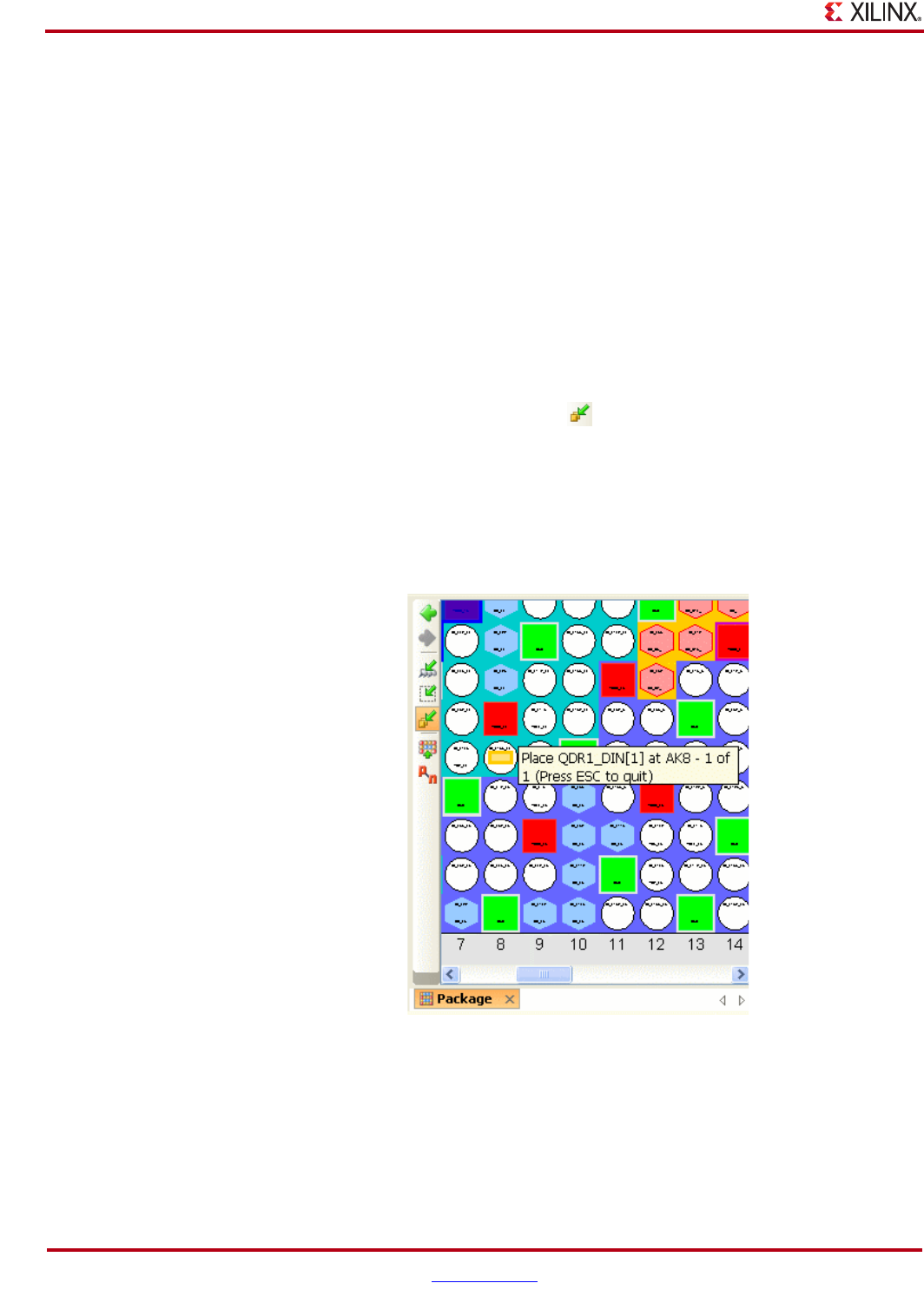
260 www.xilinx.com PlanAhead User Guide

UG632 (v 12.1)

Chapter 8: I/O Pin Planning

The direction that the rectangle is drawn dictates the I/O ports assignment order. The I/O

ports are assigned from the inside pin of the first rectangle coordinate selected. Creative

definition of the area rectangles can provide very useful pinout configurations from a PCB

routing perspective.

Sequentially Placing I/O Ports

To place I/O ports sequentially:

1. In the I/O Ports view, select an individual I/O port, a group of I/O ports or interfaces.

2. Use one of the following commands:

−in the I/O Ports view click Place I/O Ports Sequentially in he popup menu

−In either the Package view or the Device view, click the Place I/O Ports

Sequentially button as shown in the following figure.

The first I/O port in the group is attached to the cursor when it is moved over a

package pin or I/O pad. A tool tip displays the I/O port and package pin names.

3. To assign an I/O port, click a pin or a pad.

The following figure shows a sequential I/O port placement.

4. If more I/O ports are selected, the command is continued. The cursor drags the next

I/O ports, and so on until all of the I/O ports are placed or until you press the Esc key.

Ports are assigned in the order that they appear in the I/O Ports view. The assignment

order can be adjusted by applying sorting techniques in the I/O Ports view prior to

assignment.

Figure 8-24: Place I/O Ports Sequentially Button

Figure 8-25: Placing I/O Ports Sequentially

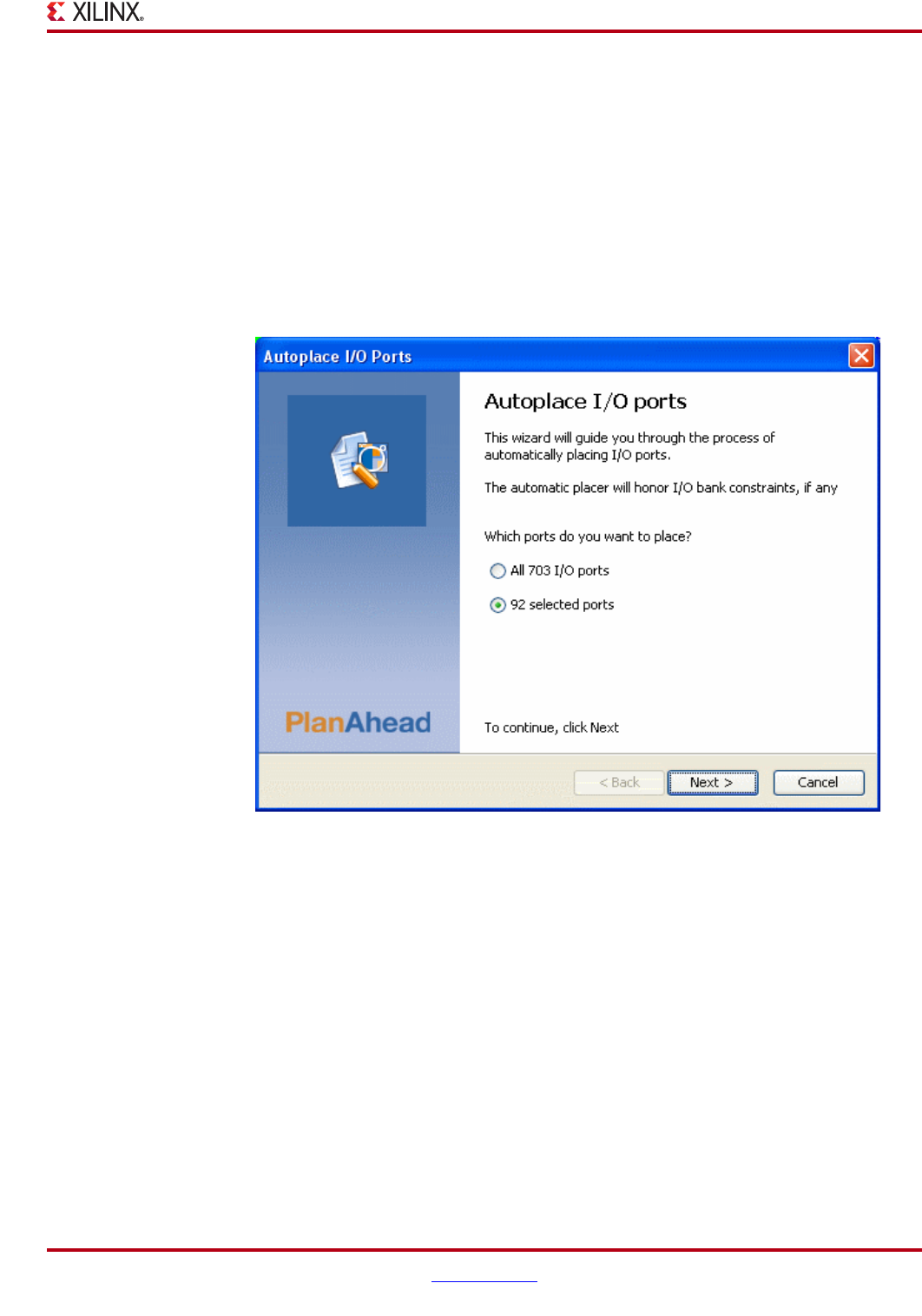
PlanAhead User Guide www.xilinx.com 261

UG632 (v 12.1)

Placing I/O Ports

Automatically Assigning I/O Ports

I/O Planner can assign any or all selected I/O ports to package pins automatically. The

autoplacer obeys I/O standard and differential pair rules, and places global clock pins

appropriately. This functionality is available for Virtex-4 and Virtex-6 device families only.

To automatically assign I/O ports to a subset of unassigned I/O ports:

1. In the I/O Ports view, select the unassigned I/O ports.

2. Click Tools > Autoplace I/O Ports, or in the I/O Ports view, click Autoplace I/O Ports

from the popup menu.

The Autoplace I/O Ports wizard opens as shown in the following figure.

3. Select the group of I/O ports to place, and click Next.

4. If you select I/O ports that have already been assigned to package pins, the dialog box

opens as shown in Figure 8-27, page 262.

Figure 8-26: Autoplace I/O Ports Wizard

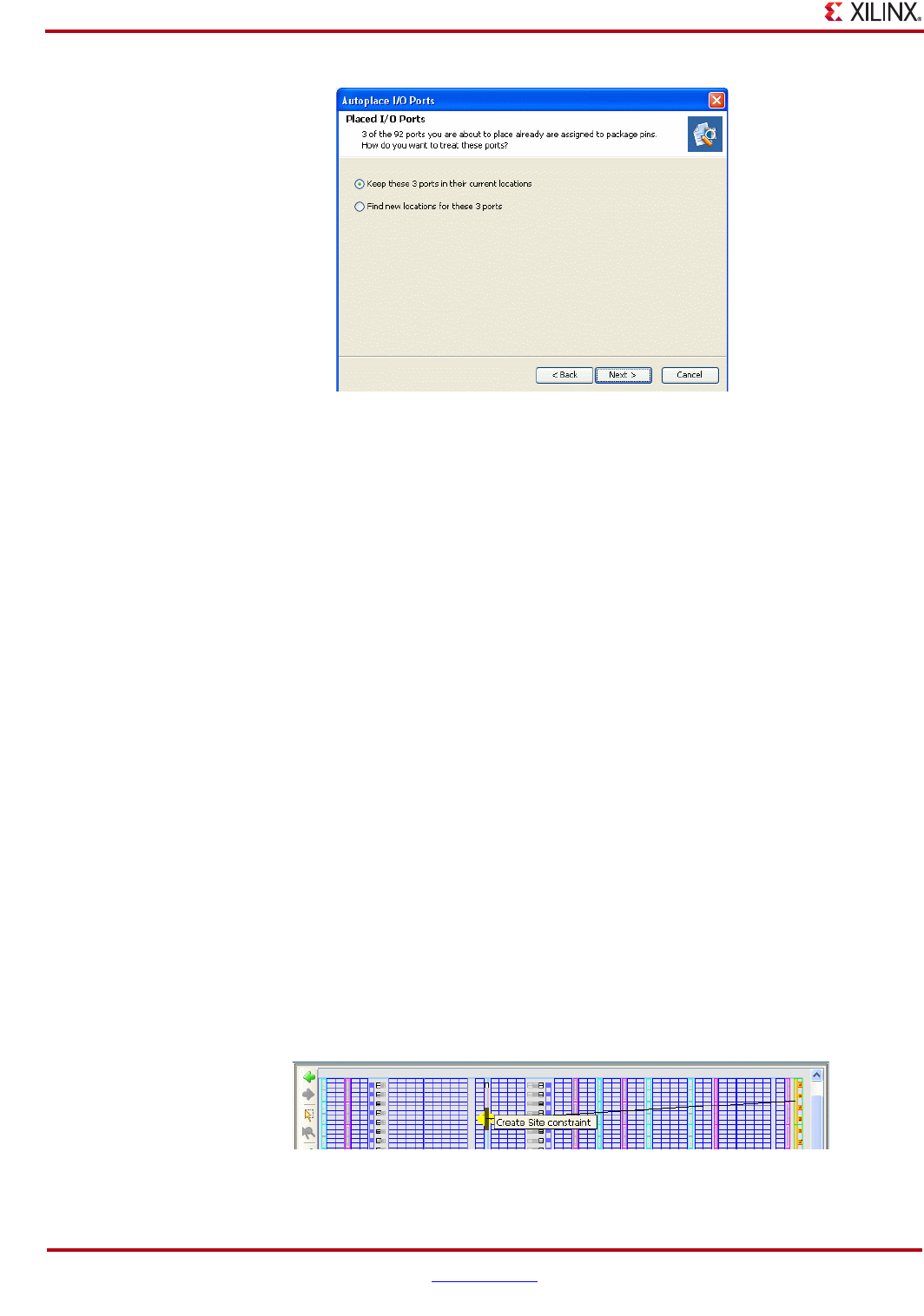
262 www.xilinx.com PlanAhead User Guide

UG632 (v 12.1)

Chapter 8: I/O Pin Planning

5. Select the I/O ports to place, and click Next, and then Finish in the Summary page.

Placing Gigabit Transceiver I/O Ports

To better manage Gigabit Transceivers (GTs), I/O Planner groups the two related I/O diff

pairs and the GT logic object automatically during selection, placement, and moving. The

GT objects get selected as one object and move together, which prohibits illegal assignment

of the GT resources.

The noise sensitive I/O pins surrounding the GTs are prohibited automatically during port

placement if the online DRCs are enabled. Refer to “Disabling or Enabling Interactive

Design Rule Checking,” page 257.

Placing I/O Related Clock Logic

You can place Global and regional clock related logic, such as BUFGs, DCMs, BUFRs, and

DelayCtrls, in the Device view manually. Appropriate logic sites are displayed for all

device-specific resources. Select Edit > Find to search for various site types available in the

device. They can then be selected in the Find Results view to highlight their location.

PlanAhead has several methods with which you can select the design clock-related logic,

such as the Find command or the Schematic and Netlist views.

To place clock logic manually:

1. In the Device view zoom to locate the appropriate device site to place the logic.

2. Select the Create Site Constraint Mode toolbar icon.

3. Select the logic to place in the Find Results, Schematic or Netlist views, and drag it onto

the available corresponding Device view site. Figure 8-28, page 262, shows an example

of manual clock placement.

Figure 8-27: Autoplace I/O Ports Wizard

Figure 8-28: Manually Placing Clock Logic

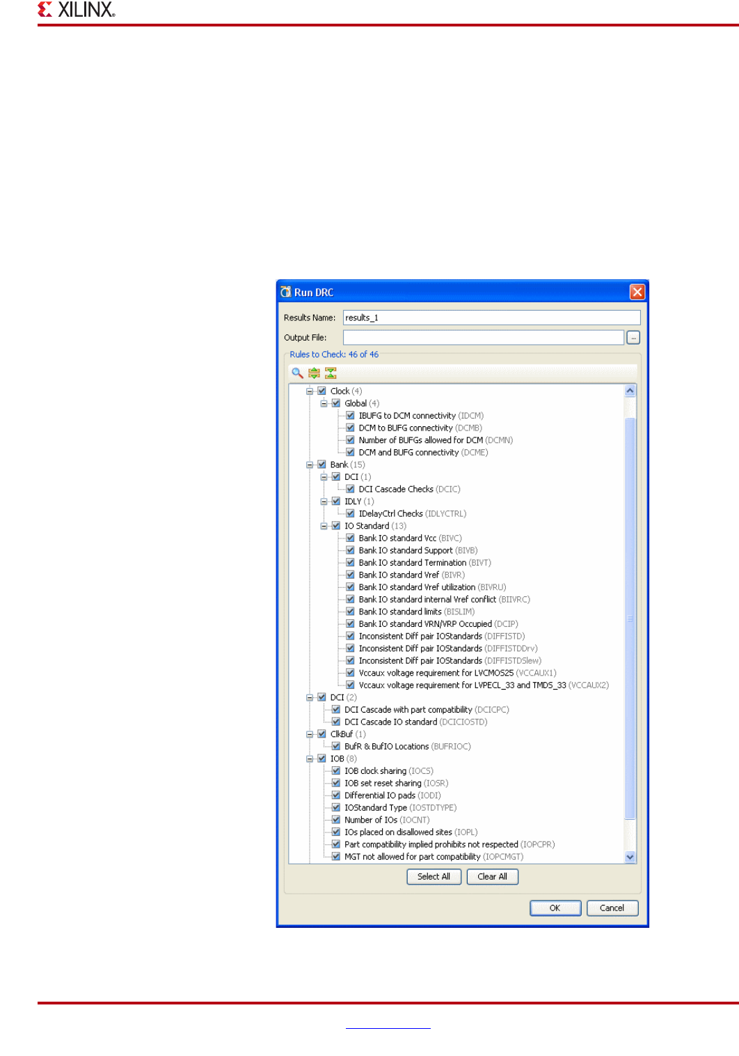
PlanAhead User Guide www.xilinx.com 263

UG632 (v 12.1)

Validating I/O and Clock Logic Placement

Running I/O Port and Clock Logic Related DRCs

This section describes the required steps for running I/O Port and clock-related DRCs. See

“I/O Port and Clock Logic DRC Rule Descriptions” in Chapter 8 for information on

running netlist and floorplan related DRCs.

To select and run individual rules:

1. Select Tools > Run DRC.

The Run DRC dialog box opens as shown in the following figure.

Figure 8-29: Run DRC Dialog Box: I/O Pin and Clock DRC Rules

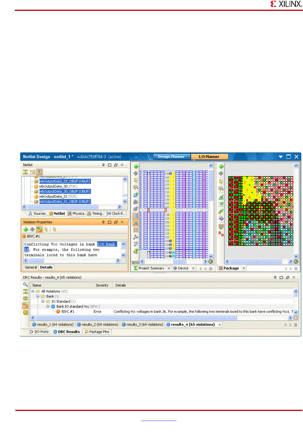
264 www.xilinx.com PlanAhead User Guide

UG632 (v 12.1)

Chapter 8: I/O Pin Planning

2. View or edit the Results Name field. Enter a name for the results for a particular run for

easier identification during debug in the DRC Violations browser. The output file

name matches the entered name.

3. In the Rules to Check group box, use the check boxes to select the design rules to check

for each design object. For information about each rule, see “I/O Port and Clock Logic

DRC Rule Descriptions,” page 265.

−Expand the hierarchy using the Expand All toolbar buttons, or click the + next to

each category or design object.

−Click the check box next to design object if you want all DRCs to be run.

−Click individual DRCs, or click All Rules to run a complete DRC (all rules for all

design objects).

4. Click OK to invoke the selected DRC checks.

Viewing DRC Violations

Once completed, the DRC Results view opens as shown in the following figure.

Each violation is expanded in the DRC Results view.

•Errors display a red icon.

•Warnings display an amber icon.

•Informational messages display a yellow icon.

Figure 8-30: Highlighting DRC Violations

PlanAhead User Guide www.xilinx.com 265

UG632 (v 12.1)

Validating I/O and Clock Logic Placement

Filtering the Violation List by Severity

By default, all errors and warnings display.

•To hide all warnings and info messages, and view only errors, click the Hide Warning

and Information Messages toolbar button.

•To view all errors and warnings, click the toolbar button again. The following figure

shows the Hide Warning and Information Messages button.

When you select an error in the DRC Results view list, the specific violation information

displays in the Properties view.

When you select a blue link in the Properties view, it highlights the violating design

elements in the Device view, Netlist view and Schematic view.

Violations display in the DRC Results view until the error condition is rectified and DRC is

rerun.

Each time you invoke the Run DRC command and DRCs detects errors, PlanAhead adds

a new results tab to the DRC Results view and creates a separate results output file in the

PlanAhead invocation directory.

I/O Port and Clock Logic DRC Rule Descriptions

The following tables describe the DRC rules, rules intent, and severity:

•“Global Clock Rules”

•“IOB Rules”

•“Bank I/O Standard Rules”

Note: “Selecting DRC Rules” in Chapter 5 provides other DRC rule descriptions.

Note: The I/O Port and Clock Logic DRCs available in PlanAhead is not an exhaustive list of I/O-

related DRCs. Consult the device documentation for more information about I/O ports and clock

region specifications.

Figure 8-31: Hide Warning and Information Messages Button

266 www.xilinx.com PlanAhead User Guide

UG632 (v 12.1)

Chapter 8: I/O Pin Planning

Global Clock Rules

The following table provides the global clock rules, abbreviation, intent, and severity.

IOB Rules

The following table lists the IOB rules, abbreviation, intent, and severity.

Table 8-1: Global Clock Rules

Rule Name Rule

Abbrev Rule Intent Severity

IBUFG to

DCM

connectivity

IDCM IBUFGs have dedicated routing only to all DCMs on

the same edge (top, bottom, left, right) of the device.

Warning

DCM to BUFG

connectivity

DCMB DCM can connect to a maximum of four BUFGs.

There are pairs of buffers with shared dedicated

routing resources such that if both are driven by the

same DCM, one of the two will necessarily be driven

using non-dedicated routing resources; this causes

the design to fail. If the buffers are numbered 1

through 8 from left to right, there are four pairs of

exclusives: 1:5, 2:6, 3:7, 4:8. If a buffer is placed in Site

1, another driven by the same DCM should not be

placed in Site 5.

Error

Number of

BUFGs

allowed for

DCM

DCMN DCM can connect only up to 4 BUFGs. This is related

to DCMB.

Error

DCM and

BUFG

connectivity

DCME BUFGs have dedicated routing only to all DCMs on

the same edge (top, bottom, left, right) of the device.

Warning

Table 8-2: IOB Rules

Rule Name Rule Abbrev Rule Intent Severity

IOB set reset sharing IOSR IOB site has input, output and tri-

state registers, each of these registers

share same set/reset signal. Will not

be able pack registers with different

reset signals.

Error

Differential I/O pads IODI Differential I/O P and N signals

should be LOCed in dedicated

differential pair.

Error

Non inputs placed on

input only pins

IOPR Checks that a port is not placed on a

prohibited pin.

Error

Diff term loced to low

capacitance IOB Site

IOLVDSCC Checks that differential output

standards are not used on low-

capacitance sites that cannot support

them.

Error

PlanAhead User Guide www.xilinx.com 267

UG632 (v 12.1)

Validating I/O and Clock Logic Placement

Bank I/O Standard Rules

The following table lists the Bank I/O standard rules, abbreviation, intent, and severity.

Prohibit not specified

for part compatibility

IOPCPR For designs that use part

compatibility, checks that if any

package pin does not exist on at least

one compatible part, it is marked as

“prohibit” and nothing is placed on

it.

Error

Regional Clock Term

has no BUFR site

IOBUFR Checks that a regional clock terminal

and the related BUFR are placed at

mutually route-able locations.

Error

Regional Clock Term

has no BUFIO site

IOBUFIO Checks that a regional clock terminal

and the related BUFIO are placed at

mutually route-able locations.

Error

IOB clock sharing IOCS IOB sites are divided into pairs for

the purpose of sharing clock routing

resources. These pairs are normally

LVDS pairs as well. In some cases

there could be routing issues based

on how the flops are packed inside

the IOB. To resolve this issue flops

need to be assigned to specific BEL.

Warning

MGT not allowed for

part compatibility

IOPCMGT Indicates whether part compatibility

is used with two parts that have

different MGT supply voltages,

thereby disallowing the use of MGT.

Warning

I/O Standard Type IOSTDTYPE Ensures that a Diff pair I/O Standard

has been applied to diff pair pins

only.

Warning

Number of IOs IOCNT Indicates whether more I/O Ports are

defined than there are pins in the

target device.

Warning

Table 8-3: Bank I/O Standard Rules

Rule Name Rule Abbrev Rule Intent Severity

Bank I/O

Standard Vcc

BIVC IOSTANDARD-based VOUT voltage

compatibility check for IOs in that bank.

Error

Bank I/O

Standard

BIIVRC checks for a conflict between the I/O

standards of a Bank and an

INTERNAL_VREF constraint on the bank.

Standards in a bank cannot require a

VREF voltage that differs from that

specified by an INTERNAL_VREF

constraint for the bank.

Warning

Table 8-2: IOB Rules (Continued)

Rule Name Rule Abbrev Rule Intent Severity

268 www.xilinx.com PlanAhead User Guide

UG632 (v 12.1)

Chapter 8: I/O Pin Planning

Bank I/O

Standard Support

BIVB Checks that the I/O Standard is

supported in the I/O bank.

Error

Bank I/O

standard

Termination

BIVT IOSTANDARD-based DCI Termination

voltage compatibility check for IOs in

that bank.

Error

Bank I/O

Standard VREF

BIVR IOSTANDARD-based VREF voltage

compatibility check for IOs in that bank.

Error

Bank I/O

Standard VREF

Occupied

BIVRU IOSTANDARD-based VREF voltage

compatibility check for IOs in that bank.

Warning

Bank I/O

Standard

VRN/VRP

Occupied

DCIP There are dedicated VRP and VRN I/O

sites in I/O bank which can be used as

regular IOs also. If a DCI I/O standard is

used in that bank these IOs should be left

unoccupied.

Error

DCI Check for

I/O standard

legality

DCICIOSTD Checks that there are no conflicts related

to Vcco and DCI termination of I/O.

Error

Bank I/O

Simultaneous

Switching Output

Limits

BISLIM Checks the I/O placed within an I/O

bank against Simultaneous Switching

Noise (SSN) Output.

Error

Inconsistent Diff

pair I/O

Standards

DIFFISTD Checks that the terminals of a differential

pair have the same I/O standard.

Error

Inconsistent Diff

pair I/O

Standards

DIFFISTDDrv Checks that the terminals of a differential

pair have the same drive.

Error

Inconsistent Diff

pair I/O

Standards

DIFFISTDSlew Checks that the terminals of a differential

pair have the same slew.

Error

Vccaux Voltage

requirement

VCCAUX Warns of any requirements on Vccaux,

based on used I/O standards.

Warning

Table 8-3: Bank I/O Standard Rules (Continued)

Rule Name Rule Abbrev Rule Intent Severity

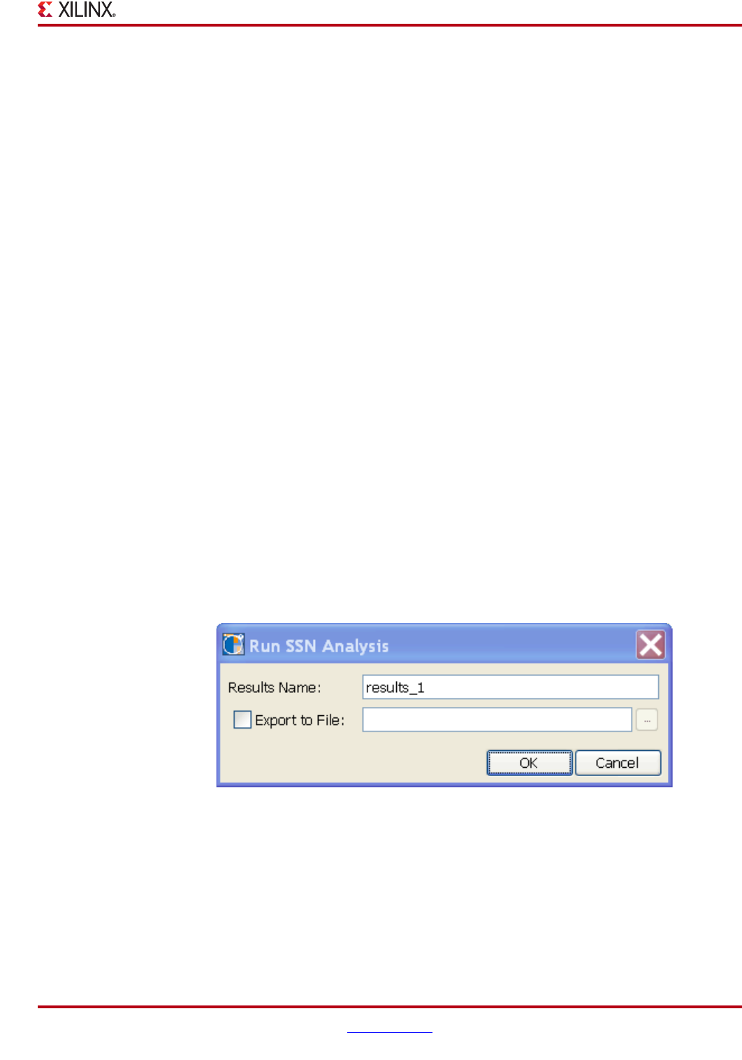
PlanAhead User Guide www.xilinx.com 269

UG632 (v 12.1)

Validating I/O and Clock Logic Placement

Running Simultaneous Switching Noise (SSN) Analysis

Running Noise Analysis (Virtex-6)

The PlanAhead software uses the Xilinx Simultaneous Switching Noise (SSN) predictor to

improve the prediction of simultaneous switching output noise in Virtex-6 devices. This

tool provides estimates of the disruption that switching outputs can cause on other outputs

in the I/O bank. The SSN Predictor incorporates I/O bank-specific electrical characteristics

into the prediction to better model package effects on SSN.

Because all power distribution networks within a packaged FPGA have different

responses to noise, it is relevant to understand not only the I/O standards and number of

I/O in a design, but also the response of the device power system to this switching.

In the Virtex-6 family of devices, I/Os are grouped into separate isolated I/O Banks, each

with its own unique power distribution networks. These each have unique responses to

switching activity. Xilinx characterizes all banks in the Virtex-6 family through three-

dimensional extraction and simulation. This information is incorporated into the SSN

predictor such that it can take the expected switching profile of a device and predict how

the switching affects the power network of the system, and in turn, how other outputs in

the I/O bank are affected.

The SSN predictor is the best method available for accurately predicting how output

switching affects interface noise margins. The calculation and results are based on a wide

range of variables. These estimates are intended to identify potential noise-related issues in

your design and should not be used as final design “sign off” criteria.

The PlanAhead software uses the SSN calculation when you select a Virtex-6 device. If

using a device other than Virtex-6, refer to “Running Weighted Average Simultaneous

Switching Output (WASSO) Analysis.”

To run the SSN predictor:

1. In the Flow Navigator, or from the Tools menu, select Run Noise Analysis.

The Run SSN Analysis dialog box opens as shown in the following figure.

2. Optionally, enter a name in the Results Name field to identify the results in the SSN

Results view.

3. Optionally, select Export to File, and enter an output file name in the Output File field

and browse to select a location to write an external CSV format report file.

4. Click OK.

Figure 8-32: Run SSN Analysis Dialog Box

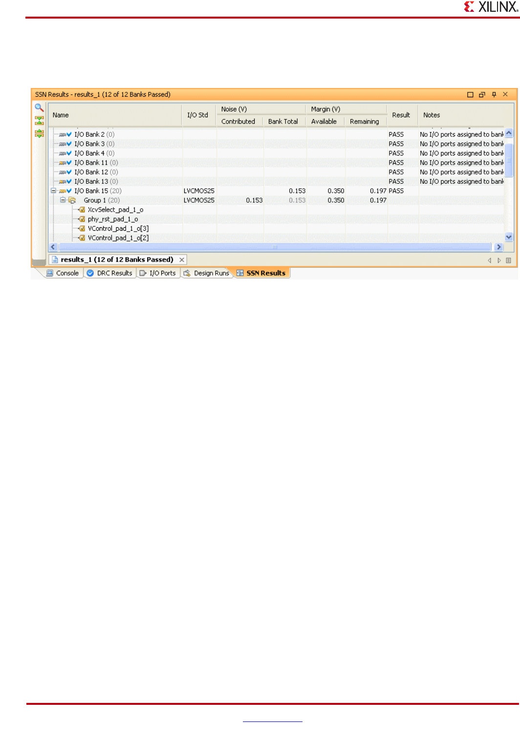
270 www.xilinx.com PlanAhead User Guide

UG632 (v 12.1)

Chapter 8: I/O Pin Planning

Viewing the SSN Results

The SSN Results view is shown in the following figure.

The SSN Results view displays the following information:

•Name—Displays the I/O Banks available in the device. Each I/O bank has pin icons

indicating how full the bank is, and a check mark or red circle indicating whether it

passed or failed.

−Group—Displays the various groups of pins with like I/O standards assigned

within the bank, and displays their status. Groups are determined automatically

based on the I/O standards, drive strength, slew rate, and phase assigned.

•Noise (V)

−Contributed—Contains the SSN aggregate of each group, generated by the I/O

standard, drive strength, and slew type of that group.

−Bank Total—Defines aggregate SSN predicted for a bank or group. If multiple

phases are specified for the groups of a given bank, the SSN contributions of

groups with different phases are accumulated separately, and the maximum of

these is reported. Because the SSN of an output are isolated to the output of that

Bank, one SSN Bank total does not affect another Bank total. This column

identifies which I/O groups are creating the most SSN, and how much margin

they use up.

•Margin (V)

−Available—Defines the allowable noise margin for that particular I/O standard

on the high side of the signal as it switches to a 1. It is strictly based on the DC

logic levels implicit in the I/O standard (no quantity information is taken into

account) and represents the margin that the weakest drive of a high signal is

above the JEDEC input thresholds. These margin values assume the weakest

drive conditions, JEDEC/Spec termination, and standard receiver requirements

for the standard. This is one place where conservative assumptions are made in

the analysis, providing some guard band.

−Remaining—Displays the amount of noise margin that is left over after

accounting for all SSN in the bank.

Figure 8-33: SSN Results View

PlanAhead User Guide www.xilinx.com 271

UG632 (v 12.1)

Validating I/O and Clock Logic Placement

Results display in red when over 100% of the available margin is lost to SSN. The

SSN predictor arrives at this value by subtracting the bank total predicted SSN (a

per-bank number) from the noise margin of I/O standard (a per-group number).

•Result—Displays a Pass or Fail condition with failures displayed in red.

•Notes—Displays information about the I/O bank or groups.

The SSN results are relative to the state of the design when the SSN Analysis is run. It is not

a dynamic report.

Resolving SSN Issues

When a violation occurs there are a number of ways to improve the results:

•Spread the offending group(s) across multiple synchronous phases.

•If the Result is a Fail condition, assign phase groups to ports that are switching

concurrently. See “Defining the I/O Port Switching Phase Groups,” page 272.

•Spread the offending group across multiple banks. This reduces the number of

aggressive outputs on the power system of one bank.

•Use I/O standards that have a lower SSN impact for the offending group. Changing

to a lower drive strength, a parallel-terminated DCI I/O standard, or a lower class of

driver can improve SSN, for example, changing the SSTL Class II to an SSTL Class I.

•Phase-shift the offending group by 90 degrees if at a DDR rate, or by 180 degrees if at

an SDR rate. This puts half the aggressive output switching out-of-phase with the

other half, and instead of interfering constructively, it interferes destructively.

Viewing I/O Bank Properties

Selecting an I/O bank in the SSN Results view displays information about the I/O ports,

pins and groups assigned to the I/O bank in the I/O Bank Properties view.

•Select the General tab to view information about the number and types of Ports

assigned to the I/O Bank.

•Select the Package Pins or I/O Ports tab to view the detailed information about the

Pins or Ports within the bank, as shown in Figure 8-34, page 272.

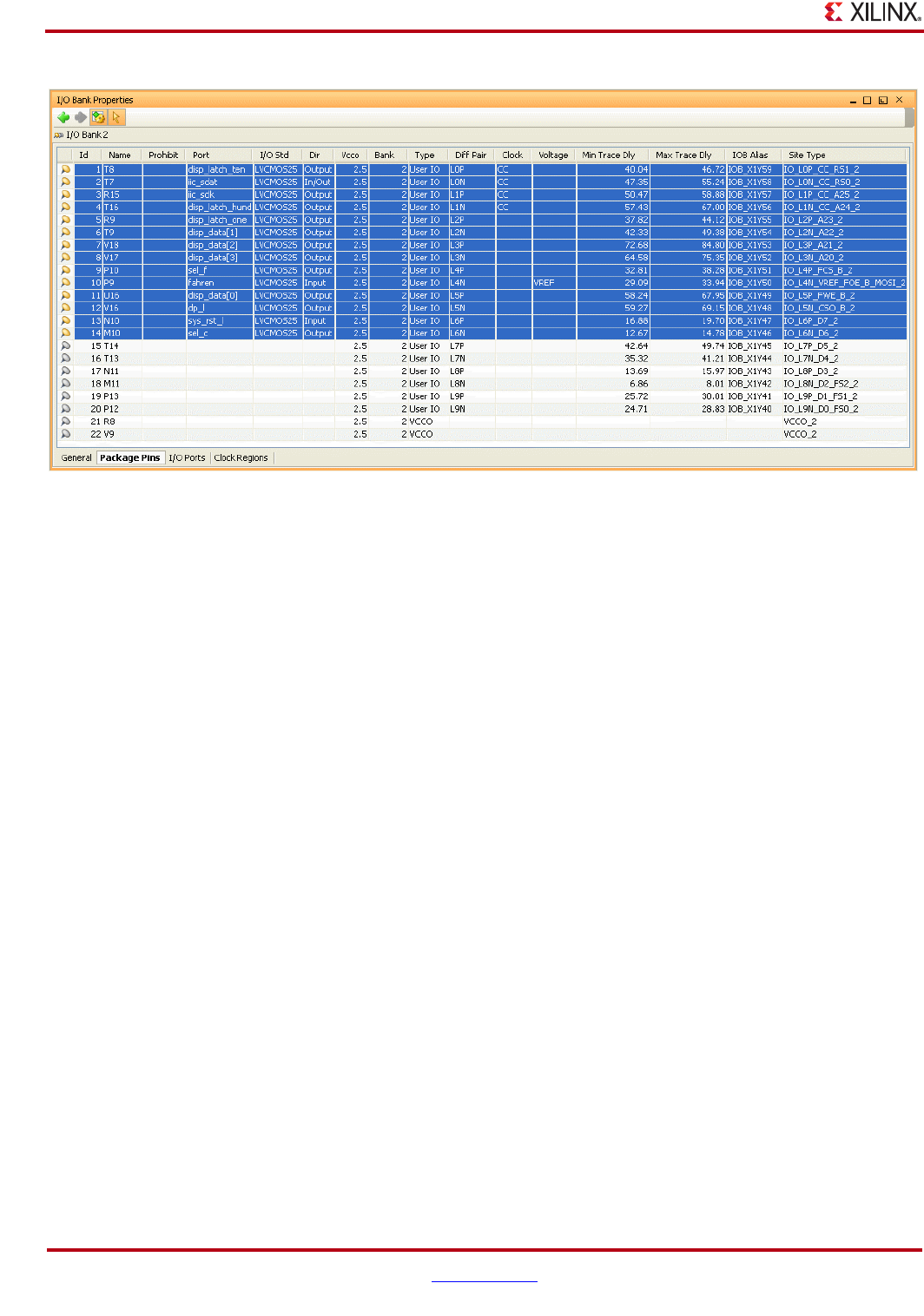
272 www.xilinx.com PlanAhead User Guide

UG632 (v 12.1)

Chapter 8: I/O Pin Planning

Defining the I/O Port Switching Phase Groups

In some cases, different groups of I/O within a bank have a synchronous phase offset from

one another, meaning it is not possible for them to switch simultaneously. This is true of

data and strobe signals in many memory interfaces. In this case, proper SSN accounting

must be informed by phase information.

A phase group is a logical grouping of ports that are all in phase with each other from a

timing perspective (their clocks have the same frequency and phase). By creating a

grouping phase, not only is a group created, but I/Os with a different phase are being

separated.

The noise produced by the groups within a bank is summed to get the total noise for that

bank, and if all outputs are either in phase with each other, or do not have a synchronous

relationship, the output can be expected to switch (change values) at the same time.

If a bank is failing in the SSN analysis, phase groups can be used to group ports that are at

separate synchronous phases, thus lowering the total noise for that bank when the SSN

predictor is run again.

To set the switching phase for a single or set of I/O Ports:

1. In any of the I/O Planner views, select one or more I/O Port.

2. In the I/O Ports view, Package Pins view, or SSN view, select the Configure I/O Ports

popup menu command as shown in Figure 8-35, page 273.

Figure 8-34: I/O Bank Properties: Package Pins

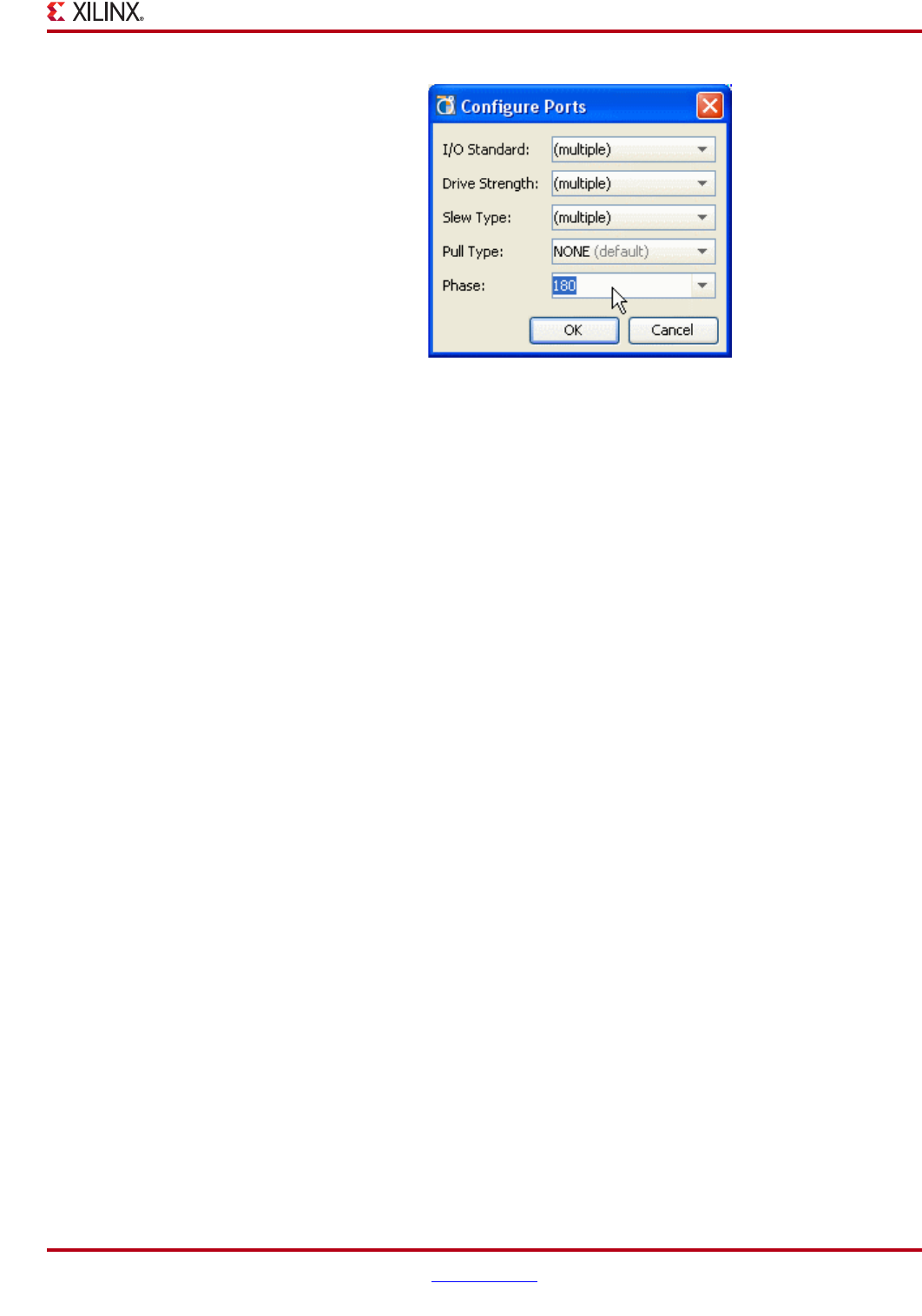
PlanAhead User Guide www.xilinx.com 273

UG632 (v 12.1)

Validating I/O and Clock Logic Placement

3. In the Configure Ports dialog box, ensure the I/O Standard is correct.

4. If the port(s) are in-phase, leave the Phase as default, or enter a unique phase, such as

180.

5. Click OK.

6. Once the appropriate phase groups are assigned, rerun the SSN analysis.

Note: Asynchronous groups should not be treated as separate synchronous phases, as it is

possible for them to switch simultaneously.

Running Weighted Average Simultaneous Switching Output (WASSO)

Analysis

PlanAhead contains a set of Weighted Average Simultaneous Switching Output (WASSO)

checks to validate signal integrity of the device based on the I/O pin and bank assignments

made in the design.

Running WASSO Analysis (Spartan-3, Virtex-4, Virtex-5)

To run an analysis, select Run Noise Analysis from either the Flow Toolbar of from the

Tools menu.

The Run WASSO Analysis dialog box opens, as shown in Figure 8-36, page 274.

Figure 8-35: Configure Ports Dialog Box

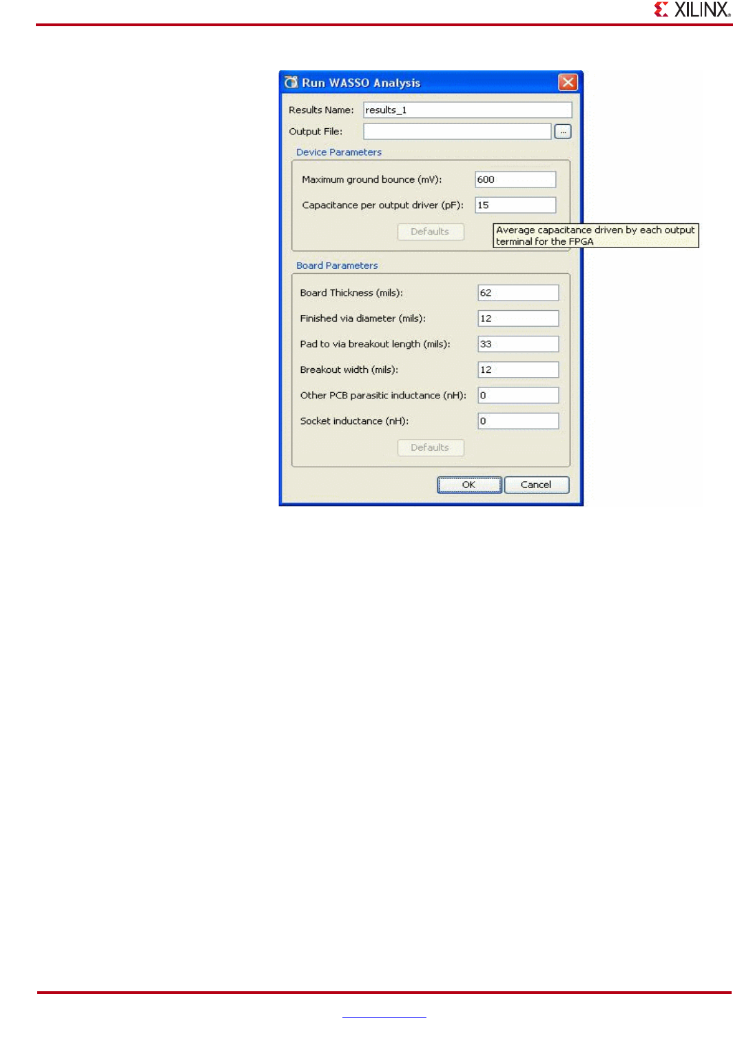
274 www.xilinx.com PlanAhead User Guide

UG632 (v 12.1)

Chapter 8: I/O Pin Planning

The Output File field can be used to specify a report file name and location to write to disk.

Tool tips are provided when dragging the cursor over each of the entry fields indicating

what values to enter.

Viewing the WASSO Analysis Results

You can modify the device and board parameter values to reflect your specific design. The

analysis is performed across the entire device first and then within each I/O bank as they

relate to their neighboring I/O banks. The WASSO Results view displays in the Workspace

as shown in Figure 8-37, page 275.

Figure 8-36: Run Wasso Analysis Dialog Box

PlanAhead User Guide www.xilinx.com 275

UG632 (v 12.1)

Validating I/O and Clock Logic Placement

Notice that the report lists allowable loading, utilization, and status for I/O banks, and

neighboring pair.

Figure 8-37: WASSO Results

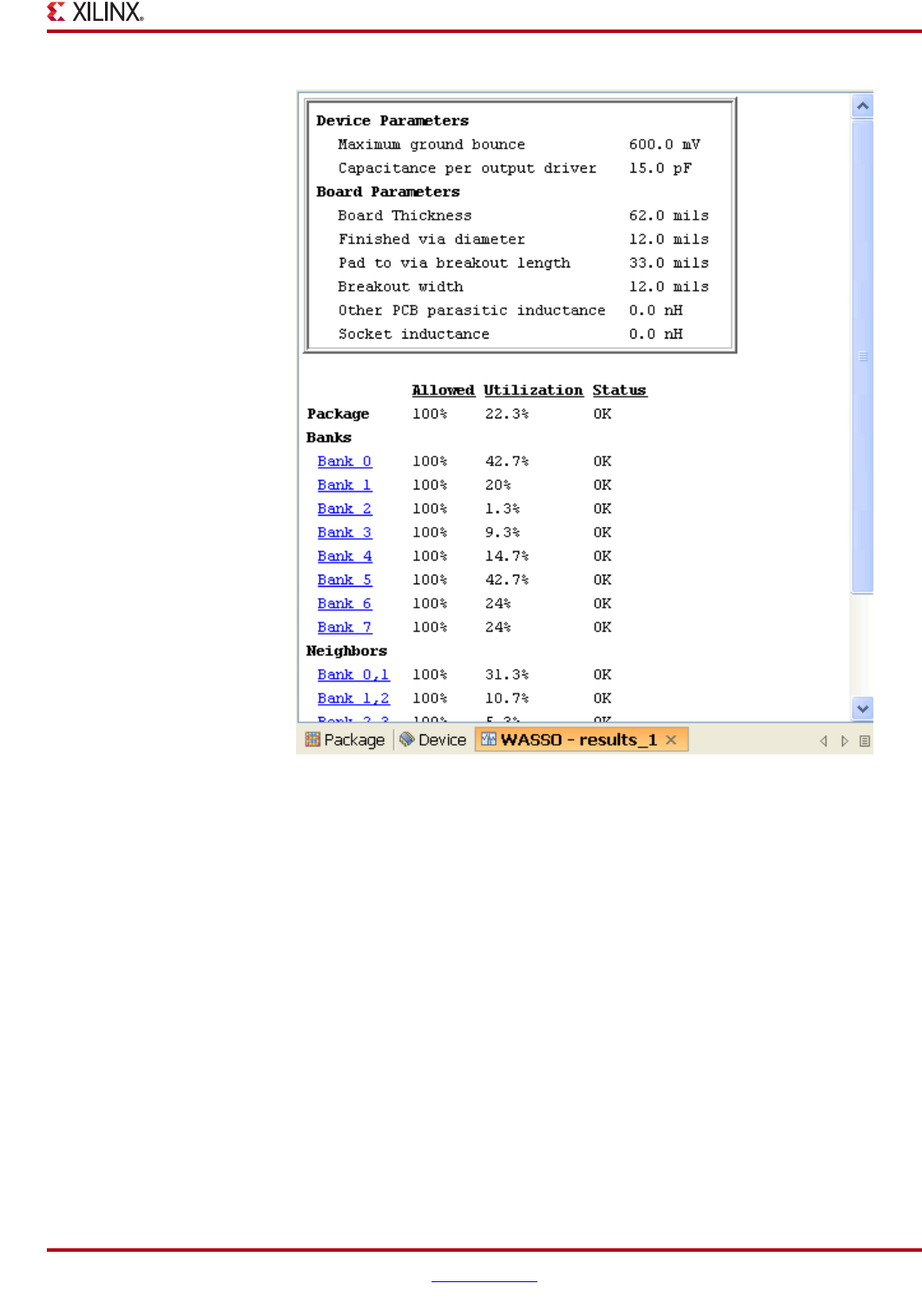
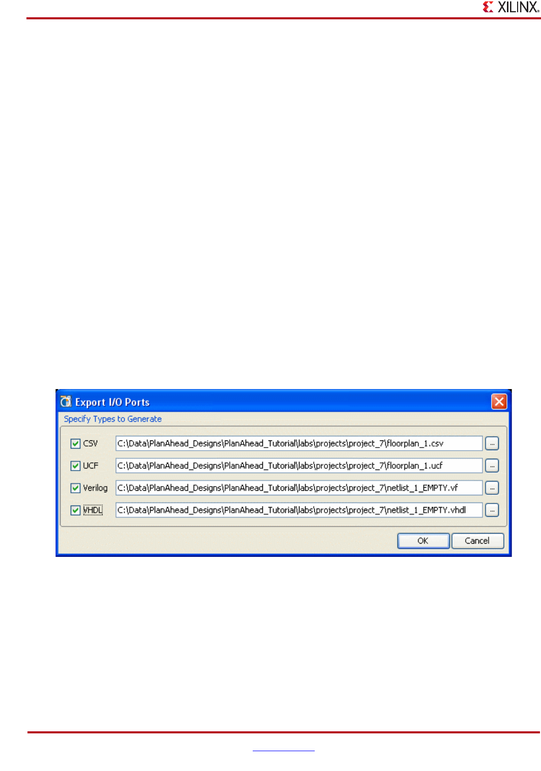
276 www.xilinx.com PlanAhead User Guide

UG632 (v 12.1)

Chapter 8: I/O Pin Planning

Removing I/O Placement Constraints

Placement constraints can be removed by first selecting them, and then selecting the

Unplace popup menu command.

Refer to “Working with Placement LOC Constraints” in Chapter 11 for information on

selectively removing I/O related placement constraints.

Exporting I/O Pin and Package Data

Exporting Package Pin Information

The device package pin information can be exported from PlanAhead to a CSV format file.

The exported information includes information about all of the package pins in the device

as well as design-specific I/O Port assignments and their configuration.

The package pin section of the exported list is a good starting point for defining I/O port

definitions in a spreadsheet format. Refer to “Defining and Configuring I/O Ports,”

page 248 for information on the exported CSV file format.

Exporting an I/O Port List

You can export the I/O Port list from the PlanAhead software to an HDL, UCF, or CSV

format file for use with RTL coding or PCB schematic symbol creation.

To export the I/O Ports list information, select the File > Export I/O Ports command as

shown in the following figure

Figure 8-38: Exporting I/O Port Lists

PlanAhead User Guide www.xilinx.com 277

UG632 (v 12.1)

Chapter 9

Implementing the Design

This chapter contains the following sections:

•“Overview”

•“Running Implementation”

•“Monitoring Run Status”

•“Analyzing Run Results”

•“Launching Multiple Implementation Runs”

•“Managing Multiple Runs”

•“Creating Synthesis and Implementation Strategies”

•“Launching Runs on Remote Linux Hosts”

•“Interfacing with ISE Outside of PlanAhead”

Overview

The PlanAhead™ software includes a synthesis and implementation environment that

allows multiple synthesis and implementation attempts using different software

command options, and timing or physical constraints. The synthesis and implementation

attempts or Runs can be queued to launch sequentially or simultaneously with multi-

processor machines. Synthesis runs use the Xilinx® Synthesis Technology (XST) tool.

You can create and save Strategies, which are a set of option configurations for each

implementation command. These Strategies are then applied to Runs for synthesis or

implementation using ISE® Design Suite tools.

You can monitor progress, view log reports, and quickly identify and import the best

synthesis and implementation results.

For more information about saved Strategies, see “Strategy Files (<strategyname>.psg)” in

Appendix B.

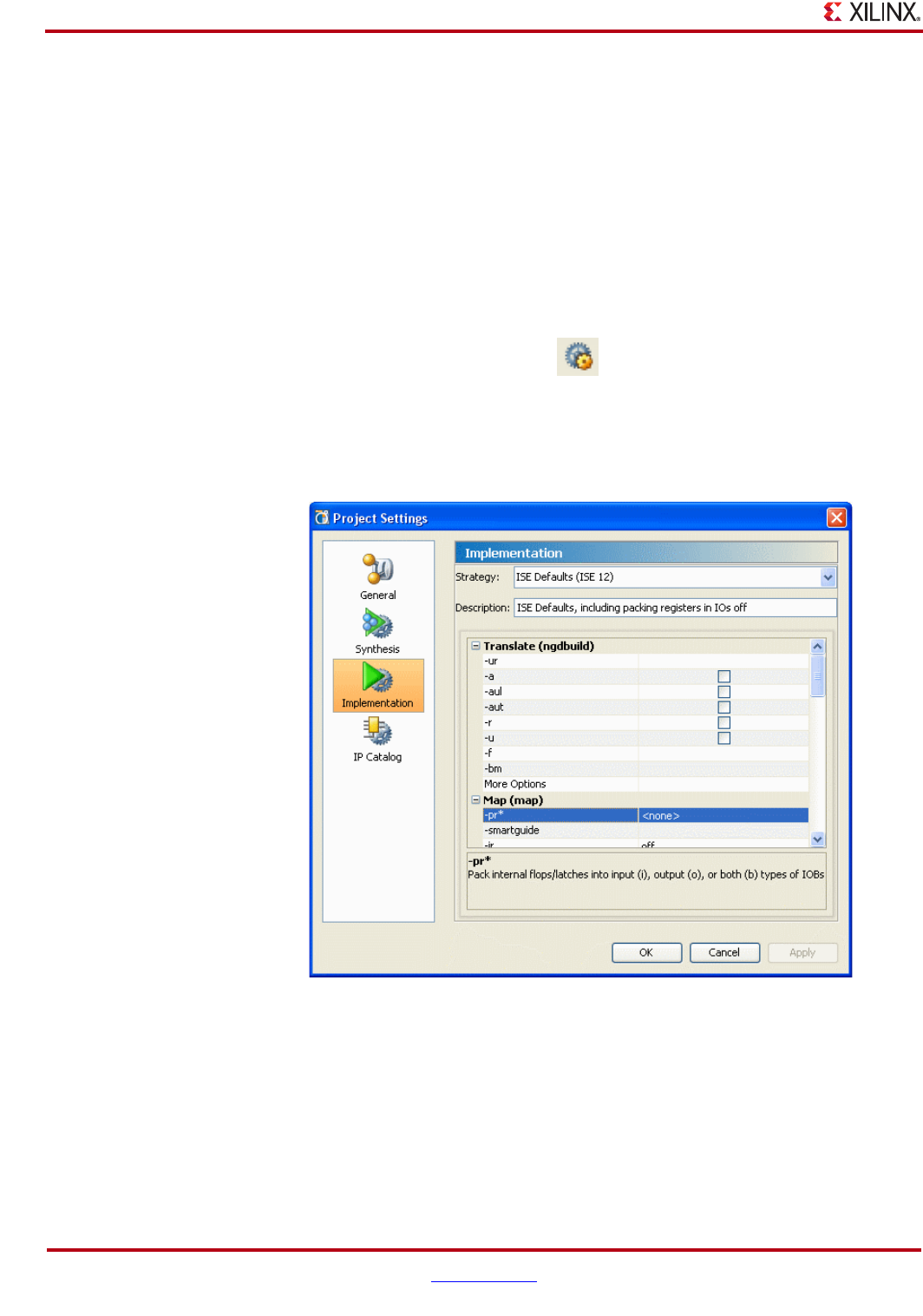
278 www.xilinx.com PlanAhead User Guide

UG632 (v 12.1)

Chapter 9: Implementing the Design

Running Implementation

When you run implementation in PlanAhead you have the ability to set implementation

options, run implementation, and view the results of the run.

Setting Implementation Options

There are several locations in the environment to configure implementation settings. Select

the Project Settings command in the Flow Navigator Project Manager Menu, the Project

Summary, or in the main toolbar. The Project Setting button is shown in the following

figure.

In the Project Settings dialog box, select Implementation if it is not already selected as

shown in the following figure.

The Implementation dialog box contains the options to set ISE command options in the

next implementation attempt as follows:

•Strategy—Select an existing strategy or to create new strategies for future use. For

more information refer to the “Creating Synthesis and Implementation Strategies,”

page 296.

•Description—Enter a description to enable easier tracking of the run.

Figure 9-1: Project Settings Button

Figure 9-2: Implementation Project Settings

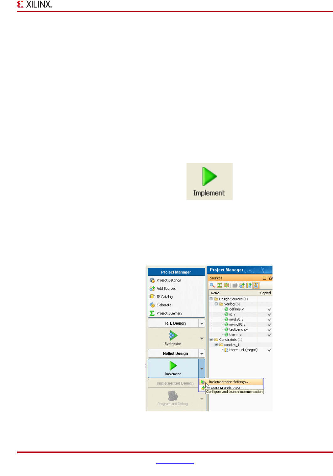
PlanAhead User Guide www.xilinx.com 279

UG632 (v 12.1)

Running Implementation

•ISE options—Configure any ISE option. Use the More Options field to specify

options that are not listed. You can find a brief description of each option and what it

is used for in the lower dialog pane.

Note: If you exit PlanAhead before running the modified implementation run, the options are not

preserved. If implementation results exist in the project, the Project Settings are inherited when you

open the project. If no implementation run exists in the Project, the PlanAhead uses the default

options.

Launching Implementation

You can launch Implementation Runs by clicking the Implementation button in the Flow

Navigator.The current Implementation Project Settings are used to launch the run.

Launching an Implementation Run

To launch an implementation run, click the Implement button from the Flow Navigator or

main toolbar as shown in the following figure.

Configuring Implementation Run Settings

You can set the implementation run options can be set using the Implementation Settings

command in the Flow Navigator Implementation button pulldown menu as shown in the

following figure.

The Implementation Settings dialog box appears, as shown in the following figure.

Figure 9-3: Implement Button

Figure 9-4: Configuring Implementation Run Settings

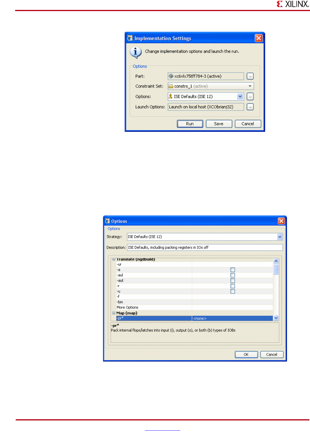
280 www.xilinx.com PlanAhead User Guide

UG632 (v 12.1)

Chapter 9: Implementing the Design

The Implementation Settings dialog box contains several options and editable fields:

•Part—Select or accept the target part. Select the browser button to invoke the Part

Chooser dialog box.

•Constraint Set—Select or accept the constraint set.

•Options—Select the Implementation Strategy to use for the run. Click the file browser

to modify ISE command options, description or strategy shown in the following

figure.

•Launch Options—Select additional launch options. Use the More Options field to

specify options that are not listed. You can find a brief description of each option and

what it is used for in the lower dialog pane.

Figure 9-5: Implementation Run Settings

Figure 9-6: Set ISE Options for the Run

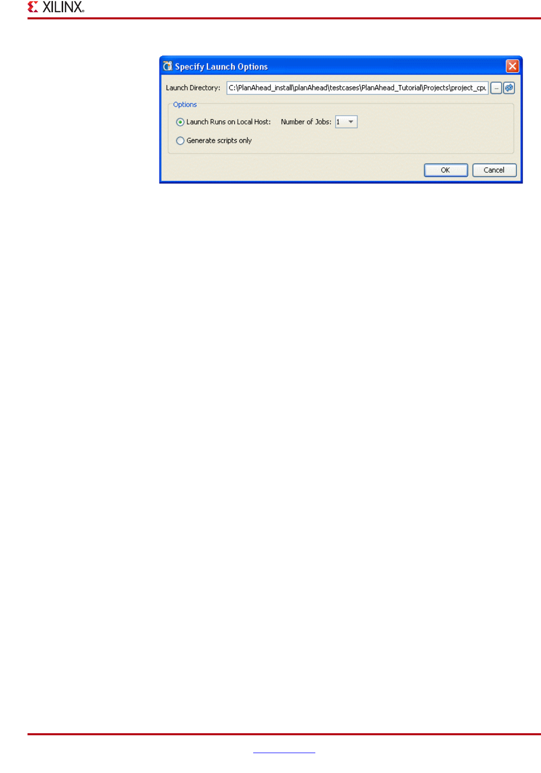
PlanAhead User Guide www.xilinx.com 281

UG632 (v 12.1)

Monitoring Run Status

The Specify Launch Options dialog box provides the following launch options:

−Launch Directory—Specify a location to create and store the implementation run

data.

Note: Defining any non-default location outside of the project directory structure makes a

project non-portable because an absolute path is written into the project files.

−Launch Runs on Local Host—Launches the Run on the local machine processor.

-Number of Jobs—Define the number of local processors to use for Runs.

This option is used only when launching multiple runs simultaneously.

Individual runs are launched on each processor. No multi-threaded

processors are used with this option.

−Launch Runs on Remote Hosts (Linux only)—Select this option to use remote

hosts to launch job or jobs.

-Configure Hosts—Select this option to configure remote hosts.

Refer“Launching Runs on Remote Linux Hosts,” page 300.

−Generate scripts only—Select this option to export and create the Run directory

and Run script, but not to launch the run from PlanAhead. The script can be run

at a later time outside of the PlanAhead environment.

1. Click Run to launch the run with the current settings. Click Save to save the settings,

but not start the run.

Monitoring Run Status

You can monitor the status of a implementation run by:

•Reading the compilation log

•Viewing the compilation Info, Warnings and Errors in the Command Messages view

•Opening the Design Runs view to monitor run status

The following subsections describe the Run status monitoring options.

Using the Project Status Display

The Project Status indicator is located in the upper right corner of the PlanAhead

environment. (Figure 9-8, page 282). It serves a number of functions which include:

•Displaying the overall status of the project, such as the progress of running

commands with a running command and progress indicator

Figure 9-7: Implementation Launch Options

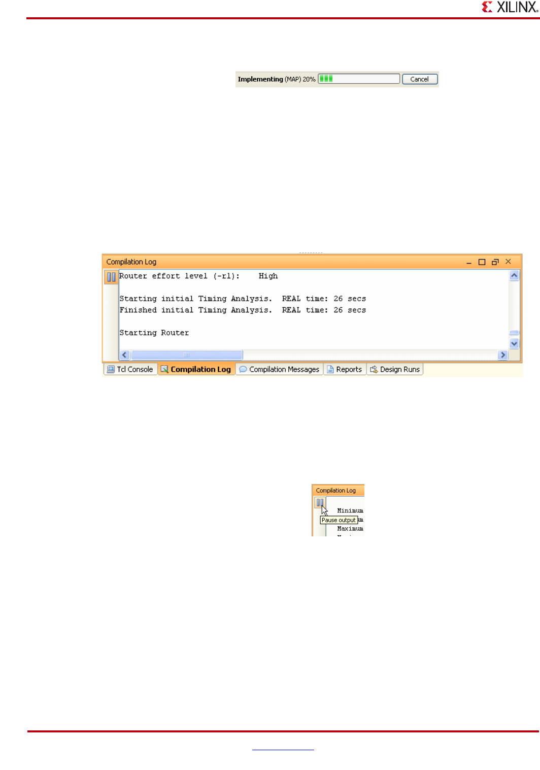
282 www.xilinx.com PlanAhead User Guide

UG632 (v 12.1)

Chapter 9: Implementing the Design

•Providing a Cancel option to stop any running commands.

Cancelling a Run

You can stop the ISE implementation run by clicking the Cancel button in the Project Status

Display shown in Figure 9-8.

Viewing the Compilation Log

The Compilation Log view opens when you launch an implementation run. It displays the

ISE command standard output messages as shown in the following figure.

Pausing the Output as Commands Run

The Pause output button enables easier scrolling and reading of the log while a command

is running. The active output is disabled until you click the button, shown in the following

figure.

Selecting Next Step After Implementation Completes

Once the Run is complete, a dialog box opens prompting you to take the next step shown

in the following figure.

Figure 9-8: Project Status Display

Figure 9-9: Compilation Log

Figure 9-10: Pause Output Button

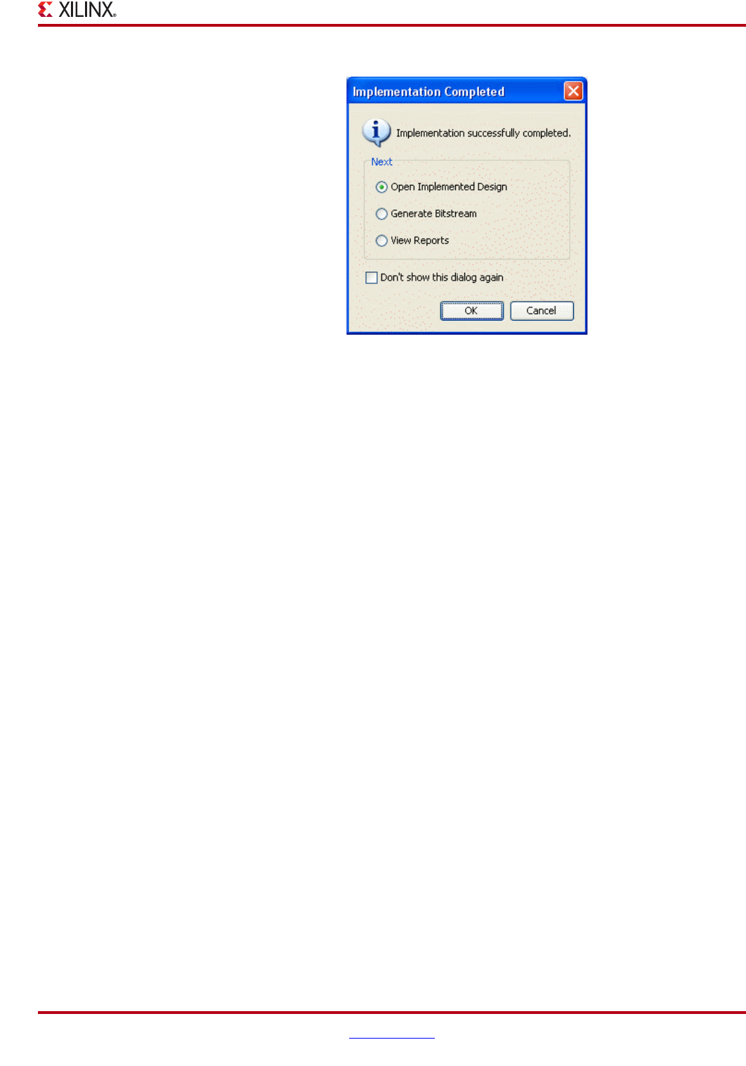
PlanAhead User Guide www.xilinx.com 283

UG632 (v 12.1)

Monitoring Run Status

2. In the Implementation Completed dialog box, select the option that matches how you

want to proceed:

−Open Implemented Design—Imports the netlist, active constraint set, ISE

placement and timing results, and the target part into the PlanAhead design

analysis and floorplanning environment so you can perform design analysis and

floorplanning.

−Generate Bitstream—Launches the Bitgen Command Settings and Run dialog

box.

−View Reports—Opens the Reports view for you to select and view ISE Report

files.

−Click Cancel to do nothing now.

3. Click OK to take the selected action.

Figure 9-11: Implementation Completed Successfully Dialog Box

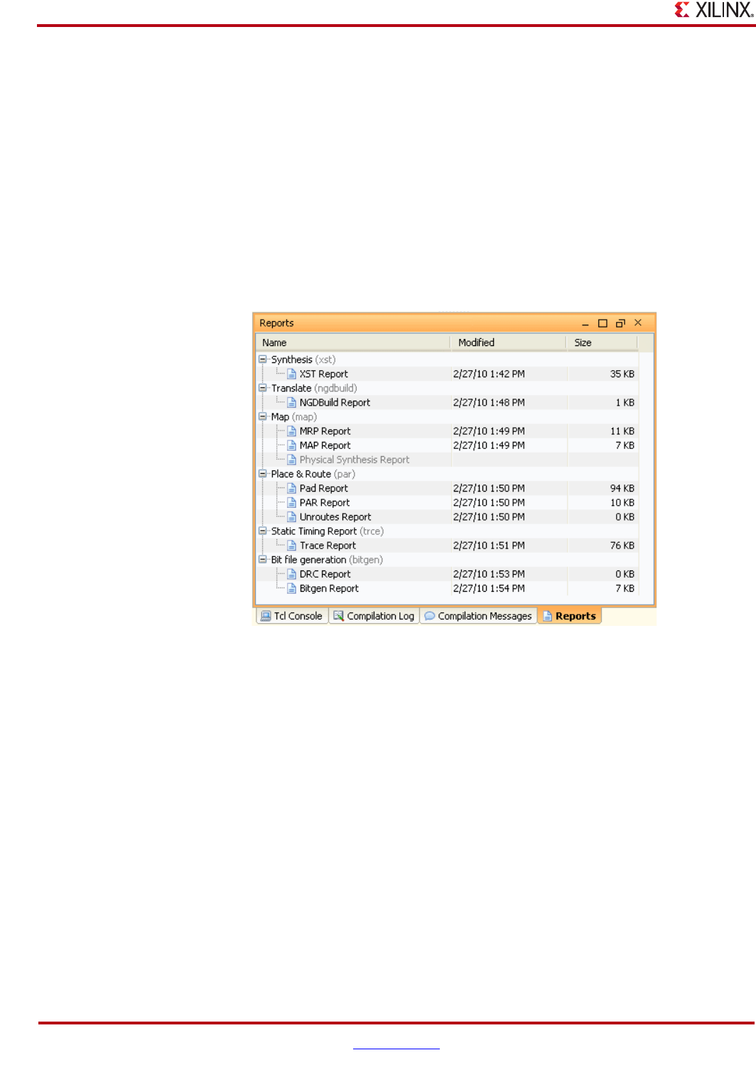
284 www.xilinx.com PlanAhead User Guide

UG632 (v 12.1)

Chapter 9: Implementing the Design

Analyzing Run Results

Once implementation completes, you can view the ISE implementation reports, and open,

analyze, and use the implemented design to apply timing or physical constraints and re-

implement the run. See Chapter 7, “Netlist Analysis and Constraint Definition,” for

information about defining constraints.

Viewing Report Files

You can view report files generated by the ISE tools from within Reports view. The view is

usually opened automatically after commands are run. if it is not available, select the

Reports link in the Project Summary. The Reports view opens as shown in the following

figure.

Select any available report files to view it in the Workspace, shown in Figure 9-13,

page 285.

Figure 9-12: Selecting Report Files to View

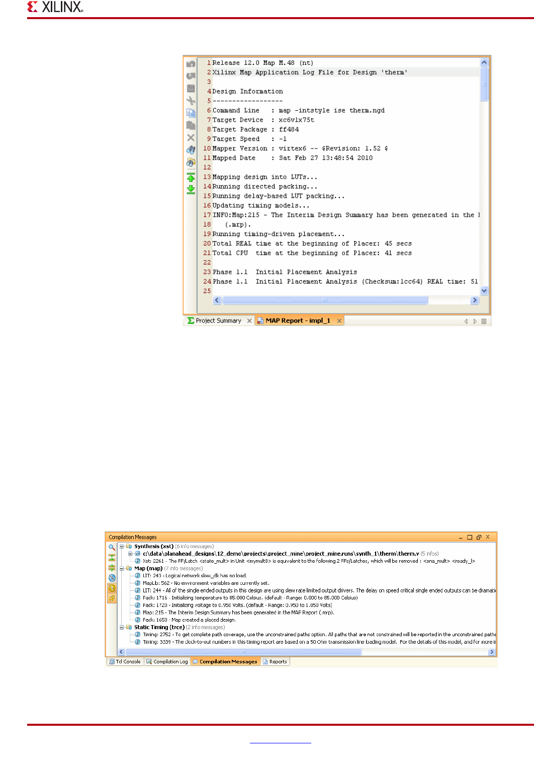
PlanAhead User Guide www.xilinx.com 285

UG632 (v 12.1)

Analyzing Run Results

When viewing reports, you can:

•Browse the report file using the scroll bar.

•Select the Find or Find in Files buttons to search for specific text.

•Use the Go to the beginning or Go to the End toolbar buttons to scroll to the beginning

or end of the file.

Viewing Compilation Messages

The Compilation Messages view provides a filtered list of the Compilation Log that

includes only the main messages, warnings, and errors. The view has further filtering

capabilities using view toolbar buttons to show only errors or warnings. The following

figure shows an example compilation log.

Figure 9-13: Viewing Report Files

Figure 9-14: Compilation Messages View

286 www.xilinx.com PlanAhead User Guide

UG632 (v 12.1)

Chapter 9: Implementing the Design

The implementation messages are organized by ISE command and severity.

Click the expand and collapse tree widgets to view the individual messages.

The command buttons on the left provide searching and filtering capabilities. The Show

Search, Collapse All, And Expand All comma options are described in “Using Tree Table

Style Views” in Chapter 4.

Filtering and Grouping Compilation Messages

You can use the Hide information messages and Hide warning messages buttons to filter

the messages to include only Warnings and/or Errors. The Group duplicate messages

button flattens the list and groups similar messages together, shown in the following

figure.

Opening the Implemented Design

PlanAhead lets you import the results of a implementation run for analysis and constraint

definition. Once the implementation run has completed, a dialog box opens prompting

you to Open the Implemented Design. Also, you can open the Implemented Design by

selecting the Implemented Design button in the Flow Navigator, shown in the following

figure.

See Chapter 10, “Analyzing Implementation Results” and Chapter 11, “Floorplanning the

Design” for more information about implementation results and floorplanning.

Figure 9-15: Message Filtering and Grouping Buttons

Figure 9-16: Opening the Implemented Design

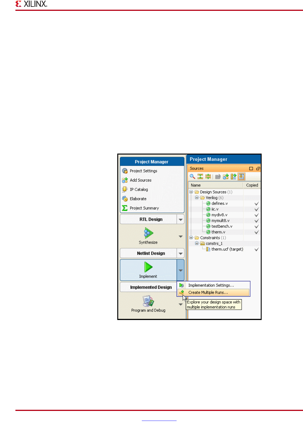
PlanAhead User Guide www.xilinx.com 287

UG632 (v 12.1)

Launching Multiple Implementation Runs

PlanAhead lets you create and launch multiple synthesis and implementation runs so you

can explore options to find the best results. The runs are queued and launched serially or in

parallel on multiple local CPUs. On Linux you can use remote servers; see “Launching

Runs on Remote Linux Hosts,” page 300 for more information.

Note: PlanAhead provides a lot of flexibility to create multiple synthesis runs, implementation runs

and constraint sets. A project can be created with multiple run attempts, which contain data that you

must manage. PlanAhead does provide messages about Out-of-Date data resulting from modified

source files, constraints, or project settings. You can delete and manage stale run data using the

Design Runs view.

Creating Multiple Implementation Runs

To create multiple implementation runs:

1. Select Create Multiple Runs from the Tools menu or from the Flow Navigator under

the Synthesize button pulldown menu as shown in the following figure.

The Create Multiple runs Wizard introduction dialog box opens.

2. Click Next, and the Set Up Implementation Runs pane opens as shown in Figure 9-18,

page 288.

Figure 9-17: Create Multiple Runs Command

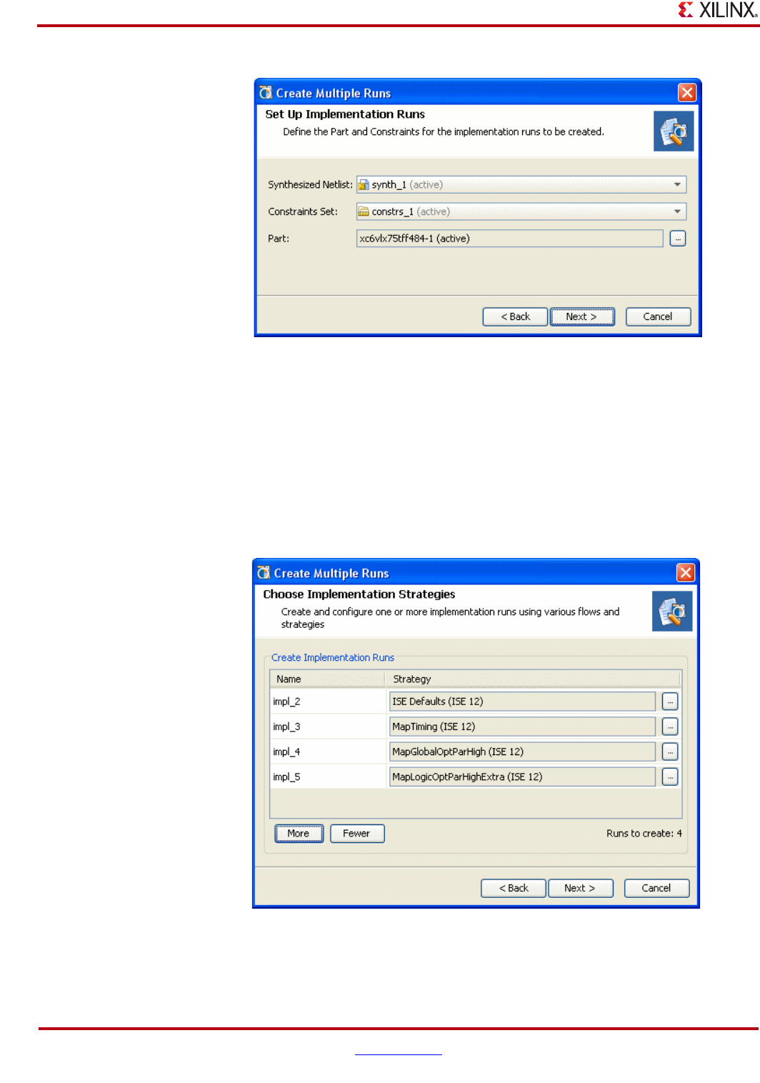
288 www.xilinx.com PlanAhead User Guide

UG632 (v 12.1)

Chapter 9: Implementing the Design

The Set Up Implementation Runs dialog box options fields are:

•Synthesized Netlist—Enter or accept the synthesized netlist result to apply to the

implementation run.

•Constraint Set—Enter or accept the constraint to apply to the run.

•Part—Select or accept the target part. Click the browser button to invoke the Part

Chooser dialog box.

3. Click Next to bring up the Choose Implementation Strategies dialog box, as shown in

the following figure.

4. Select a Name and Strategy for the first synthesis Run.

5. Select More to add more runs.

Figure 9-18: Create Multiple Runs Dialog Box

Figure 9-19: Choose Implementation Strategies

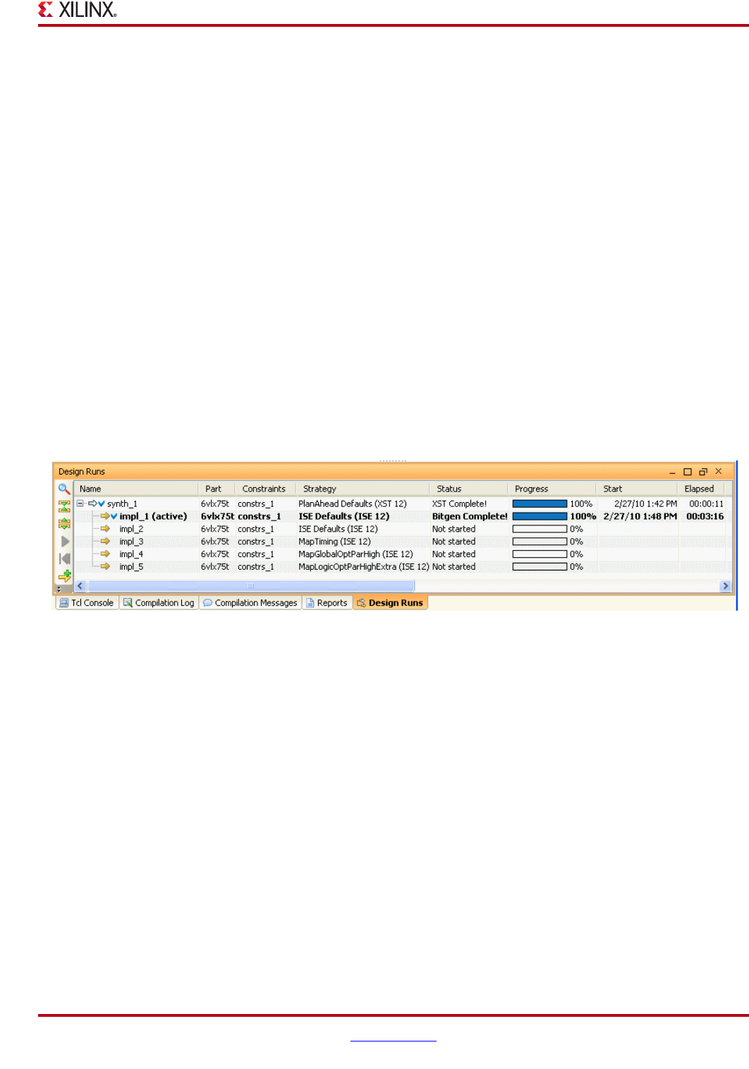
PlanAhead User Guide www.xilinx.com 289

UG632 (v 12.1)

Managing Multiple Runs

6. Enter names and choose implementation strategies for the additional Runs.

7. Click Next to invoke the Launch Options dialog box. See “Setting Implementation

Options,” page 278.

8. Review the Create Multiple Runs Summary pane and click Next.

9. Click Finish to create the defined Runs and execute the specified Launch options.

Managing Multiple Runs

PlanAhead lets you configure and generate a multiple run results data. When you

configure multiple runs, you must manage and remove stale run data. The following

subsections describe how you can use the Design Runs view to manage multiple run data

for both synthesis and implementation runs. Most of the described features are available

for both synthesis or implementation runs.

Using the Design Runs View

The Design Runs view displays all of the synthesis and implementation runs created in a

project, and provides commands to manage and launch them.

Select Window > Design Runs to open the Design Runs view as shown in the following

figure.

Each Synthesis Run displays the associated Implementation runs below it in tree form. You

can expand and collapse synthesis Runs using the tree widgets in the view. Information

about the Runs is displayed in the table. Refer to “Using Tree Table Style Views” in

Chapter 4.

You can use the Show Search, Collapse All, and Expand All buttons to filter the runs

displayed in the table.

Your options are:

•Launch Selected Runs —Launches the active run.

•Reset Selected Runs—Resets a Run to a Not Started status and remove the data.

•Create Multiple Runs—Invokes the Create Multiple Runs wizard.

•Import Run Results—Opens the Implemented Design environment with the run

results loaded.

Figure 9-19: Design Runs View

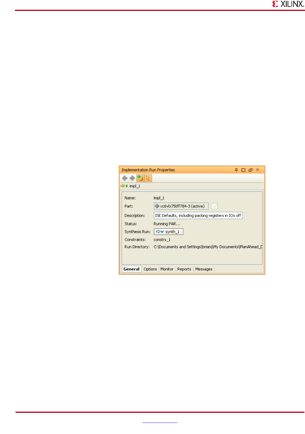
290 www.xilinx.com PlanAhead User Guide

UG632 (v 12.1)

Chapter 9: Implementing the Design

Setting the Active Run

PlanAhead displays compilation and summary information for the “active” run only.

Select any run, and use the Make Active command from the popup menu to set it as active.

The Compilation Messages views, Status Bar and Project Summary display the

information for the active run. When you press the Implement button, PlanAhead resets

and re-launches the active run.

Viewing and Modifying Run Properties

You can view or modify run properties for each run. Modification of most Run properties

is possible prior to launching the run only. After you launch a Run the properties are

locked to the selected properties.

To modify the Run properties after a run is launched, select Reset Run to clear the run.

Viewing the Run General Properties

To view the run properties, in the Run Properties view, select the Run and the General tab

as shown in the following figure.

View or edit the information in the General Run Properties dialog box. The options are:

•Name—Defines the Run name.

•Part—Accept or change the target part. Select the browser button to open the Part

Chooser.

•Description—Defines the Run description.

•Status—Displays the status of the Run.

•Synthesis Run—Displays the synthesized netlist associated with the run. This field is

not displayed in Synthesis Run Properties.

•Constraints—Accept or change the constraint set for the run.

•Run Directory—Displays the location of the run data.

Figure 9-20: Setting Run General Properties

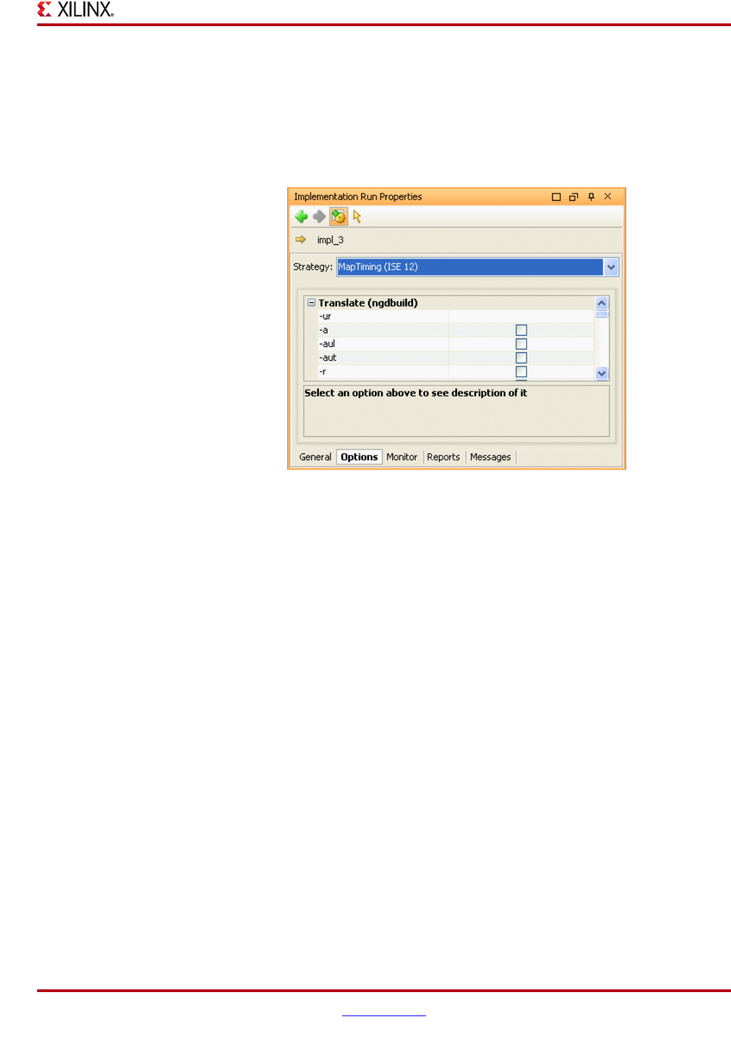
PlanAhead User Guide www.xilinx.com 291

UG632 (v 12.1)

Managing Multiple Runs

Viewing the Run Strategy Options

You can view and modify the command line options that are defined in the Strategy in the

Run Properties Options dialog box.

In the Run Properties view, select the Run, and then select the Options tab as shown in the

following figure.

The command line options and their preset values display in the view. Select a command

option to see a description of the command.

When you select an option a pulldown menu opens on the right side for you to view the

available option values.

Overriding ISE Command Options Set in a Strategy

The Options tab lets you modify Strategy options as shown in Figure 9-22, page 292.

Figure 9-21: Setting Run Strategy and Command Options

292 www.xilinx.com PlanAhead User Guide

UG632 (v 12.1)

Chapter 9: Implementing the Design

Using the popup commands, you can:

•Override (edit) the Strategy for the selected run, and save (or save as) the options to a

new User Defined Strategy

•Enter additional command options that are not displayed in More Options under a

command

Click the Apply toolbar button to apply changes.

Any modified values show an asterisk (*) next to the option to show that the default

Strategy value changed. The Strategy field for the Run in the Design Runs view receives an

asterisk to show that the default Strategy has changed also.

After you launch Strategy (which is described in the following section), the Strategy

options can no longer be modified. To edit an option, you need to reset the run and then

edit the option. See “Resetting Runs,” page 295.

Figure 9-22: Run Properties View: Options Tab

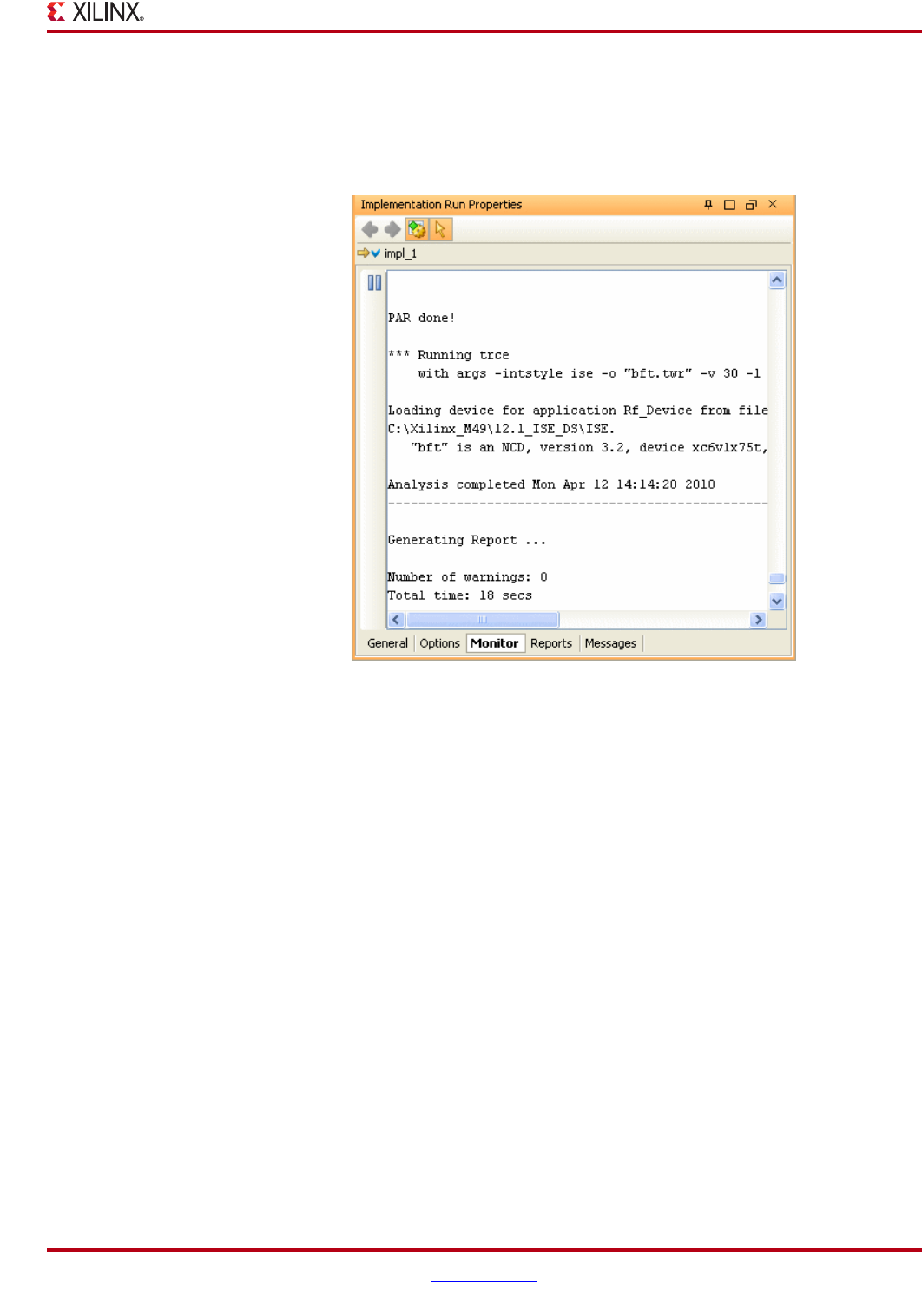
PlanAhead User Guide www.xilinx.com 293

UG632 (v 12.1)

Managing Multiple Runs

Viewing the Run Log

To view the Run output log, select the Run, and then select the Monitor tab of the Run

Properties view. The view displays the same “standard out” command status logs that

displays when in the Compilation Log view shown in the following figure.

The Monitor view continues to update as the commands are run. You can use the scroll bar

to browse through the command log reports. Click Automatically update the contents of

this view to stop the active reporting. This might let you scroll easier and read results

while the command is running.

Viewing Report Files

You can view report files generated by the ISE tool from within the PlanAhead software. In

the Run Properties view, select the Run, and then select the Reports tab to display the list of

available report files, and to open a report in the workspace view as shown in tFigure 9-24,

page 294.

Figure 9-23: Monitoring Run Status

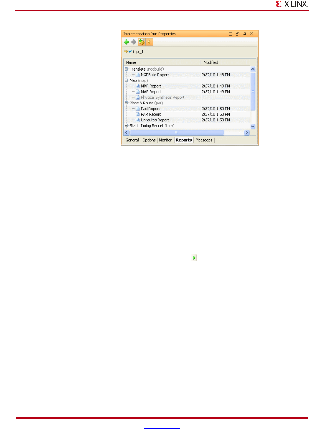
294 www.xilinx.com PlanAhead User Guide

UG632 (v 12.1)

Chapter 9: Implementing the Design

Launching Selected Runs

The Launch Runs command launches existing Runs in the Design Runs view. You can

launch Runs in any state, including completed Runs. The Launch Selected Runs dialog box

displays first so you can set launch options.

1. In the Design Runs view, select one or more runs. Use Shift+click or Ctrl+click for

multiple selections.

2. Select one of the following commands:

−Launch Runs popup command

−The Launch selected runs Design Runs toolbar button as shown in the following

figure.

The Launch Selected Runs dialog box opens as shown in the following figure.

Figure 9-24: Selecting Report Files to View

Figure 9-25: Launch Selected Runs Toolbar Button

PlanAhead User Guide www.xilinx.com 295

UG632 (v 12.1)

Managing Multiple Runs

The Launch Selected Runs dialog contains the following options:

•Launch Directory—Specify a location to create and store the implementation run

data.

Note: Defining any non-default location outside of the project directory structure makes the

project non-portable because absolute paths are written into the project files.

•Launch Runs on Local Host—Select this option to launch the Run on the local

machine processor.

−Number of Jobs—Define the number of local processors to use for Runs. This

option is only used when launching multiple runs simultaneously. Individual

runs will be launched on each processor. No multi-threaded processors are used

with this option.

•Launch Runs on Remote Hosts (Linux only)—Select this option to use remote hosts

to launch job or jobs.

−Configure Hosts—Select this option to configure remote hosts. For more

information, see “Launching Synthesis Runs on Remote Linux Hosts” in

Chapter 6.

•Generate scripts only—Select this option to export and create the run directory and

run script, but not to launch the run from PlanAhead. The script can be run at a later

time outside of the PlanAhead environment.

3. Click OK to create the Run with the selected launch options.

4. If the selected Runs are in a state other than “Not Started,” you are prompted to first

reset the runs prior to launching them.

Resetting Runs

The Reset Runs command removes the results of the selected runs. You are prompted to

remove the run data from disk, which is advisable. The Run status is set back to Not Started.

1. Select one or more runs in the Design Runs view. Use Shift+click or Ctrl+click for

multiple selections.

2. Select the Reset Runs popup command.

The Reset Runs confirming dialog box prompts you to remove all implementation data

from disk for the selected runs as shown in the following figure.

Figure 9-26: Launching Existing Runs

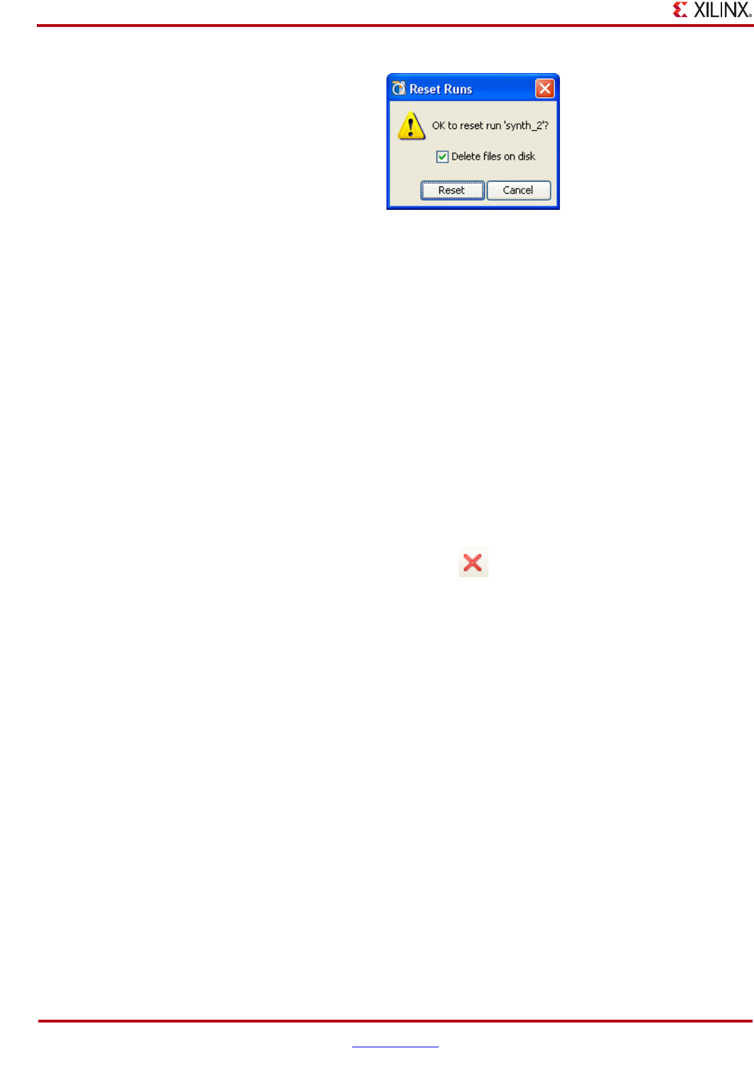
296 www.xilinx.com PlanAhead User Guide

UG632 (v 12.1)

Chapter 9: Implementing the Design

3. In the confirming dialog box, click Reset.

If any ISE processes are currently running or queued, you are prompted to stop them.

4. Click Yes to proceed.

The status for the selected runs is reset.

Deleting Runs

The Delete command removes selected Runs from the Design Runs view and removes

their associated data from disk. You are prompted to confirm the deletion of the selected

runs.

1. Select one or more runs in the Design Runs view. Use Shift+click or Ctrl+click for

multiple selections.

2. Select one of the following:

−the Delete main toolbar button shown in Figure 9-28, page 296.

−the Delete popup menu command in the Design Runs view

−the Edit > Delete command

−the Delete key

Creating Synthesis and Implementation Strategies

A strategy is a set of command options for each ISE implementation command. PlanAhead

software provides several commonly used Strategies that have been used extensively on

internal benchmarks. The option settings for these strategies are not editable.

You can copy and modify supplied Strategies to create your own. The Strategies are copied

to C:/Documents and Settings/username/Application

Data/HDI/strategies (on Windows) during installation.

Strategies are Tool- and Version- specific. Each major release of ISE has version-specific

command line options, that are supported in PlanAhead.

To review, copy, and modify strategies:

1. Select Tools > Options > Strategies.

The Strategies dialog box, shown in Figure 9-29, page 297 contains a list of pre-defined

strategies organized by Flow for each ISE and XST version.

Figure 9-27: Resetting Runs

Figure 9-28: Deleting Selected Runs Toolbar Button

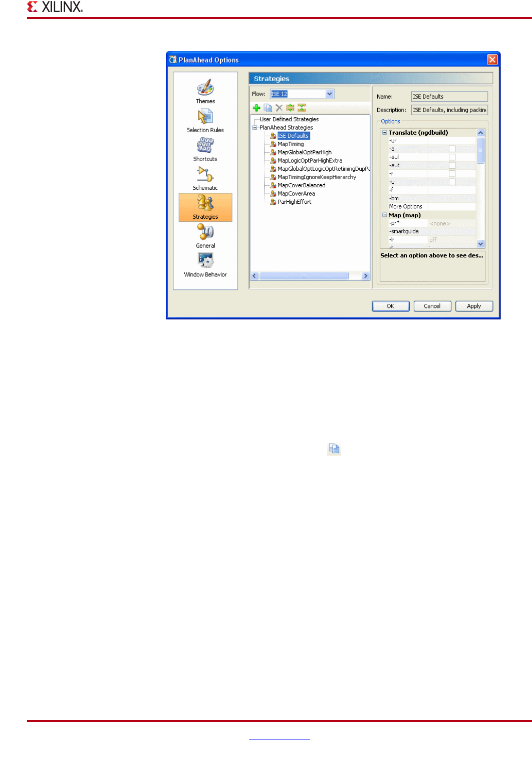
PlanAhead User Guide www.xilinx.com 297

UG632 (v 12.1)

Creating Synthesis and Implementation Strategies

2. Select the Flow menu to select the corresponding version of ISE or the desired run

script format.

3. Copy the supplied PlanAhead Strategies to the User Defined Strategies area for

modification by using one of the following commands:

−The Create a copy of this strategy Strategies toolbar button shown in the

following figure.

−The Copy Strategy popup command.

PlanAhead creates a copy of the strategy in the User Defined Strategies area and provides

the command option values on the right side of the dialog box for you to modify.

4. Edit the definable options in the Strategies dialog box as follows:

−Name—Enter a Strategy name to assign to a Run.

−Description—Enter the Strategy description which is displayed in the Design

Run results table.

5. Click a command option to view the option description at the bottom of the dialog box.

6. Modify command options by clicking in the command option area (to the right), and

selecting an option from the popup menu. Available command option settings display

in the popup menu shown in the following figure.

Figure 9-29: PlanAhead Options: Strategies

Figure 9-30: Create a Copy of this Strategy Toolbar Button

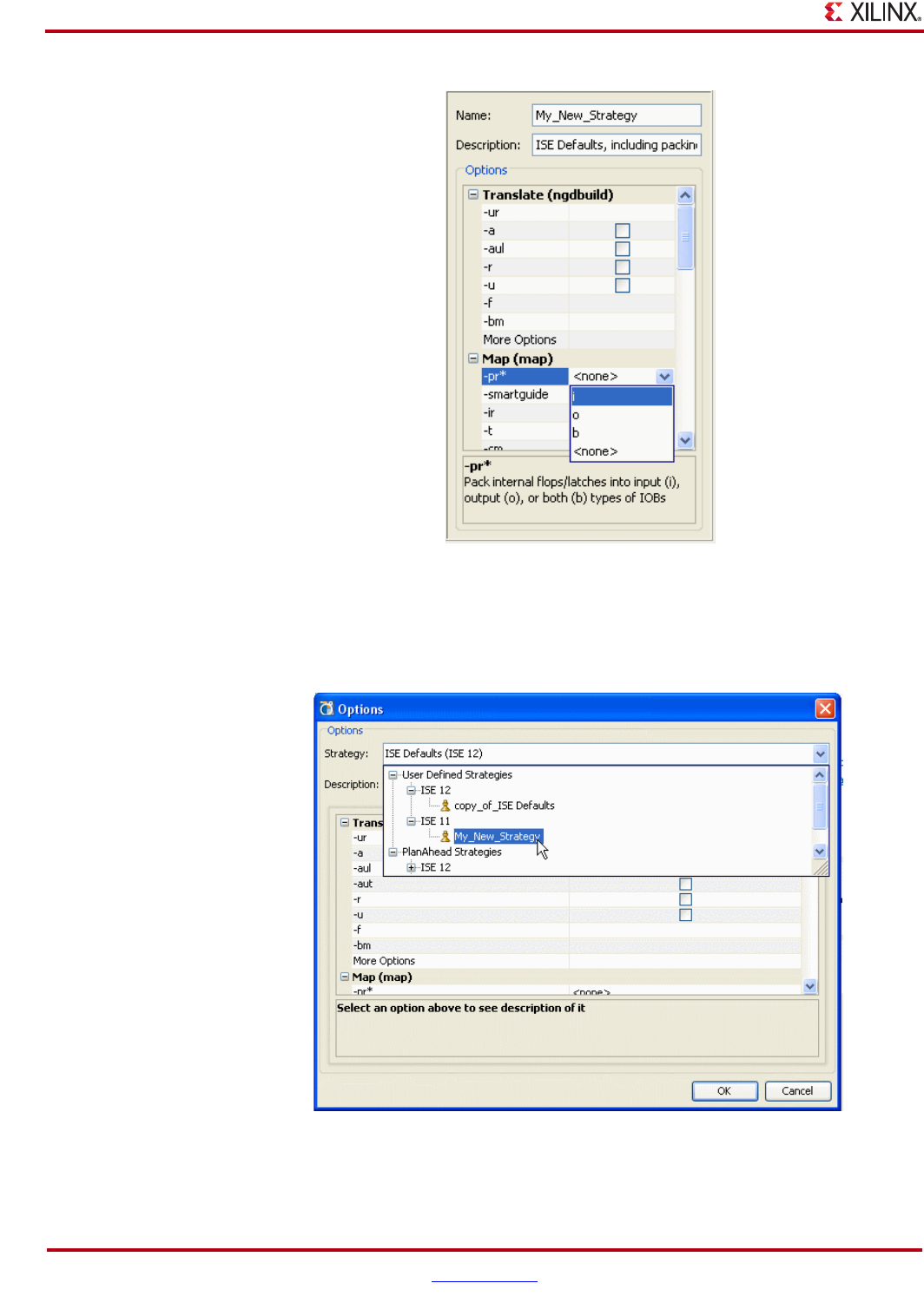
298 www.xilinx.com PlanAhead User Guide

UG632 (v 12.1)

Chapter 9: Implementing the Design

7. Click Apply and OK to save the new strategy.

The new strategy shows as a User Defined Strategy and can be used for Synthesis and

Implementation as shown in the following figure.

For more information about configuring and launching runs, refer to the “Creating

Synthesis and Implementation Strategies,” page 296.

Figure 9-31: Command Options and Description

Figure 9-32: Selecting User Defined Strategies

PlanAhead User Guide www.xilinx.com 299

UG632 (v 12.1)

Creating Synthesis and Implementation Strategies

Creating Common Group Strategies

Design groups that want to create and use group-wide custom strategies can copy any

user-defined Strategy to the <InstallDir>/strategies directory.

300 www.xilinx.com PlanAhead User Guide

UG632 (v 12.1)

Chapter 9: Implementing the Design

Launching Runs on Remote Linux Hosts

The PlanAhead software ships functionality to allow parallel execution of Runs on

multiple Linux hosts. This is accomplished with simplified versions of more robust load-

sharing software, such as Grid Engine by Sun® MicroSystems, and LSF.®

Job submission algorithms are implemented using a “greedy”, round-robin style with Tcl

pipes within Secure Shell (SSH).

Limitations

The limitations are as follows:

•Host execution is performed with SSH, a service provided by Linux operating system,

and not PlanAhead. For this to work, you must configure SSH so that you are not

prompted for a password each time you log in to a remote machine. If you have not

configured key-agent forwarding for passwordless SSH, or if you have configured

SSH and you are prompted for a password, see Appendix E, “Configuring SSH

Without Password Prompting.”

•Linux-to-Linux hosting is the only supported platform because of security and lack of

remote-shell capabilities of windows systems.

•ISE tool installation is assumed to be available from any login shell, which means that

$XILINX and $PATH are configured correctly in your .cshrc/.bashrc setup scripts.

If you can log into a remote machine and enter map -help without sourcing any

other scripts, this flow will work. If you do not have ISE set up upon login (.cshrc or

.bashrc), you can use the Run pre-launch script option to pass an environment

setup script to be run prior to all jobs.

•PlanAhead installation must be visible from the mounted file systems on remote

machines. If the PlanAhead installation is stored on a local disk on your own machine,

it will not be visible from remote machines.

•PlanAhead project files (.ppr) and directories (.data and.runs) must be visible

from the mounted file systems on remote machines. If the design data is saved to a

local disk, it is not visible from remote machines.

Configuring Remote Hosts (Linux Only)

After you have configured SSH, as described in “Setting Up SSH Key Agent Forward” in

Appendix E, the PlanAhead software enables runs to be launched using remote servers. To

do so, they must first be configured.

1. To configure a remote host select one of the following commands:

−Tools > Options > Remote Hosts

−Run Synthesis > Launch Runs > Configure Hosts

−Run Implementation > Launch Runs > Configure Hosts

−Configure Hosts in the Launch Selected Runs options dialog box

The Remote Hosts dialog box displays as shown in Figure 9-33, page 301.

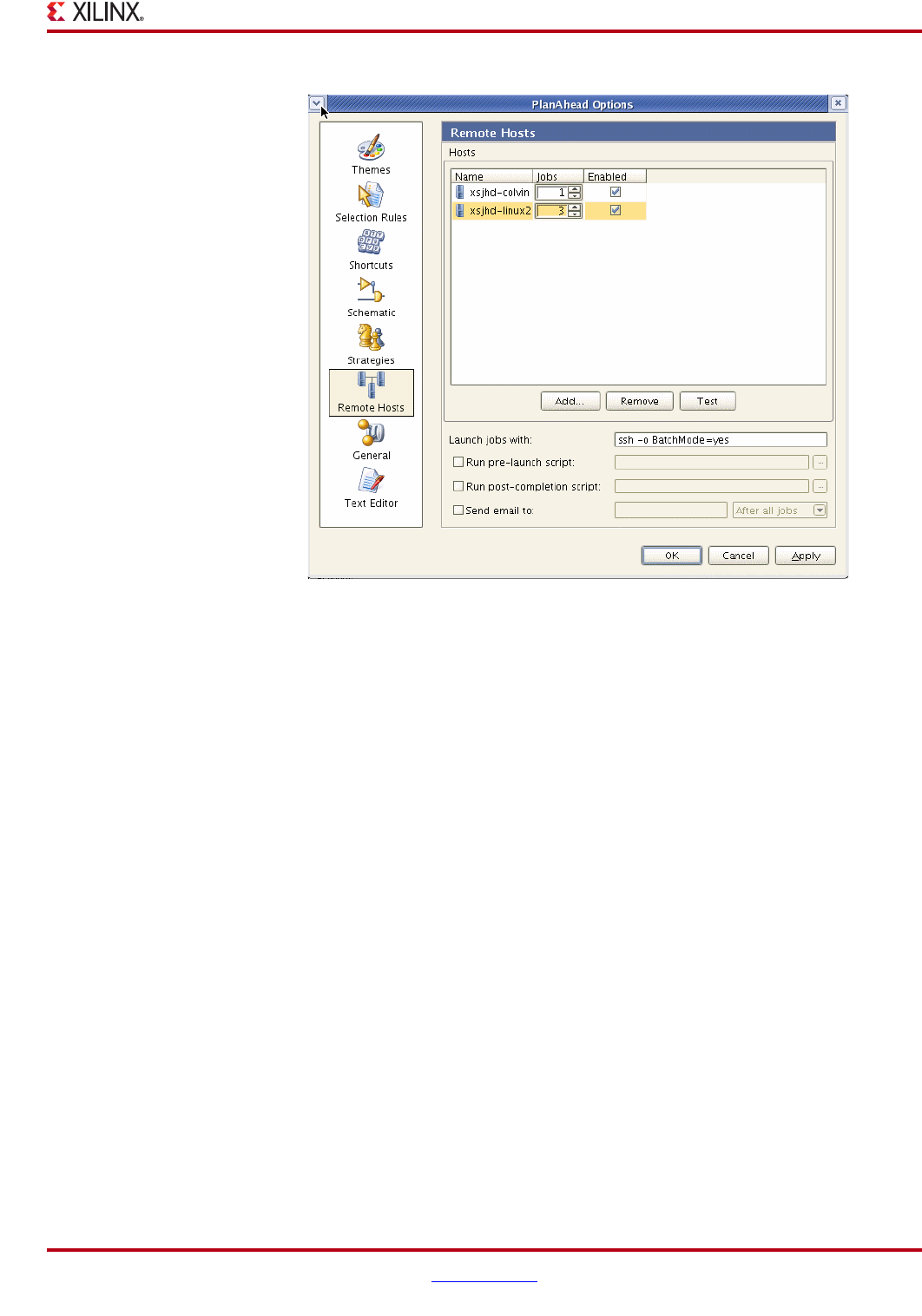
PlanAhead User Guide www.xilinx.com 301

UG632 (v 12.1)

Launching Runs on Remote Linux Hosts

2. Click the Add button to enter the names of remote servers.

3. Toggle the Jobs option to specify how many processors on the remote machine to use.

Individual runs are launched on each processor. No multi-threading of processors is

used.

4. Toggle the Enable option to specify whether to use the server. You can use this field

when launching runs to specify which servers to use for the selected runs to be

launched.

5. Optionally, modify the Launch jobs with field to change the remote access command.

The default is ssh.

Note: Use extreme caution when modifying this field. For example, removing ‘BatchMode =yes’

could cause the process to hang because the shell incorrectly prompts for an interactive

password.

6. Optionally, click the Run pre-launch script button and define a script to run prior to

launching the runs. Use this option to pass an environment setup script if you do not

have ISE set up upon login (.cshrc or .bashrc).

7. Optionally, click the Run post-completion script button and define a custom script to

run after the run completes.

8. Optionally, click the Send email to button and enter an email address to send

notification when the run completes.

9. Select one or more hosts, and select the Test button to verify that the server is available

and the configuration is set up properly.

Note: It is highly recommended that you test each host to ensure proper set up.

10. Select the Remove button to delete selected remote hosts.

11. Click OK to accept the Remote Host configuration settings.

Figure 9-33: Configuring Remote Hosts

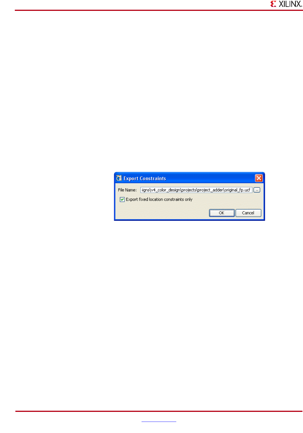
302 www.xilinx.com PlanAhead User Guide

UG632 (v 12.1)

Chapter 9: Implementing the Design

Interfacing with ISE Outside of PlanAhead

The PlanAhead software lets you selectively export files required for external ISE software

implementation. If you are using PlanAhead for design implementation, interfacing with

ISE for external implementation is not necessary.

PlanAhead also enables the creation of a Project based on existing command line-based

implementation results. For more information. see “Importing ISE Results From Outside

PlanAhead,” page 308 for more information about this feature.

Exporting Constraints

Exporting constraints to ISE consists of exporting a UCF physical constraints file for the

entire design or for individual Pblocks.

To export the constraints:

1. In the Sources view, select the desired constraint set to export and use the Make Active

popup menu command to set it as the active constraint set.

2. Select File > Export Constraints.

The Export Constraints dialog box opens as shown in the following figure.

3. View and edit the definable options in the Export Constraints dialog box:

−File name—Enter the file name and location to create the UCF format constraints

file.

−Export fixed location constraints only—Select this option to export only the

user assigned “fixed” placement LOC constraints or uncheck it to export all of the

fixed and unfixed placement constraints imported from ISE.

4. Click OK to export the constraints.

PlanAhead creates the designated top-level UCF format constraint file in the export

directory. This file can be used as input for custom ISE implementation scripts.

For more information about the exported files, see Appendix B, “Outputs for Reports.”

Exporting Netlist

Exporting the PlanAhead Netlist to ISE consists of exporting a single EDIF format netlist

file for the entire design or for individual Pblocks.

To export the design netlist:

1. Click the Floorplan tab.

2. Select File > Export Netlist.

The Export Netlist dialog box opens as shown in Figure 9-35, page 303.

Figure 9-34: Export Constraints Dialog Box

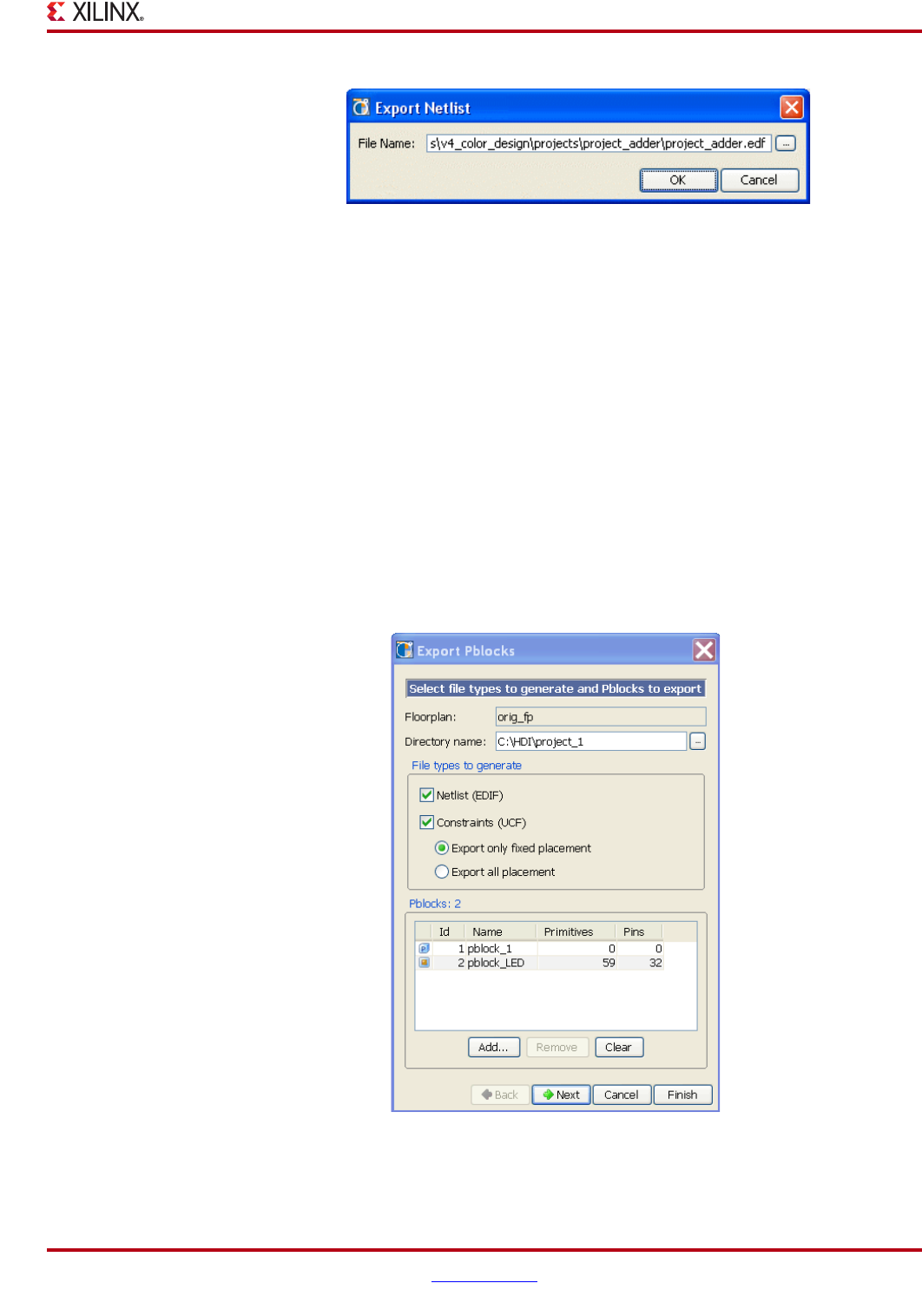
PlanAhead User Guide www.xilinx.com 303

UG632 (v 12.1)

Interfacing with ISE Outside of PlanAhead

3. View and edit the definable option in the Export Netlist dialog box:

−File name—Enter the file name and location to create the EDIF format netlist file.

4. Click OK to export the netlist.

For more information about the exported files, see Appendix B, “Outputs for Reports.”

Exporting Pblocks for ISE Implementation

PlanAhead has the ability to export Pblock-level files for implementation. These Pblocks

consist of logic from anywhere in the logic hierarchy. Exporting a Pblock creates an EDIF

netlist and UCF physical constraints file for each Pblock selected for export.

To export Pblocks to EDIF and UCF:

1. Select one or more Pblocks.

2. Select File > Export Pblocks.

The Export Pblocks wizard opens as shown in the following figure.

Figure 9-35: Export Netlist Dialog Box

Figure 9-36: Export Pblocks Wizard

304 www.xilinx.com PlanAhead User Guide

UG632 (v 12.1)

Chapter 9: Implementing the Design

3. View and edit the definable options in the Export Pblocks dialog box:

−Directory name—Enter the directory name or use the file browser to select a

directory to export the files.

A subdirectory called <pblockname>_CV is created for each exported Pblocks.

To keep track of EDIF and UCF files associated with a typical PlanAhead design

scenario, it is a good practice to specify a unique directory name for each ISE

attempt. The export directory will be used to seed the “Import Placement” and

“Import TRCE Results” command file browsers.

−File types to generate

-Netlist (EDIF)—Select this option to export the netlist.

-Constraints (UCF)—Select this option to export all or only fixed placement

constraints.

−Pblocks—Lists the Pblocks selected for export.

4. Click the Add and Clear buttons to select and remove Pblocks from the export list,

respectively.

5. Click Next or Finish to continue. When Next is selected, the Export Pblocks Summary

dialog box displays Pblock export selections.

6. Click Finish to perform the export.

The PlanAhead software creates separate EDIF and UCF files for each of the exported

Pblocks named <pblockname>_CV.edn and <pblockname>_CV.ucf.

PlanAhead creates a /<pblockname>_CV directory for each exported Pblock containing

the Pblock-specific files.

Importing ISE Results From Outside PlanAhead

Refer to the “Importing ISE Results From Outside PlanAhead,” page 308 for information

about this feature.

PlanAhead User Guide www.xilinx.com 305

UG632 (v 12.1)

Chapter 10

Analyzing Implementation Results

This chapter contains the following sections:

•“Opening the Implemented Design”

•“Analyzing Placement and Timing Results”

•“Exploring Logic Connectivity”

•“Searching for Objects using the Find Command”

•“Highlighting Logic Objects”

•“Marking Selected Objects”

•“Locking Placement for Future Implementation Runs”

•“Displaying Design Metrics”

Opening the Implemented Design

You can load implementation results that were created either inside or outside of

PlanAhead™ software into the PlanAhead software for analysis and floorplanning

purposes.

PlanAhead imports placement and timing results from the Xilinx® ISE® Design Suite only.

Routing resources are not available for analysis.

If you used PlanAhead to launch the implementation run, you can open the

implementation results by clicking Flow Navigator > Implemented Design.

The button is available only when a successfully implemented design exists in a project;

see Figure 10-1, page 306.

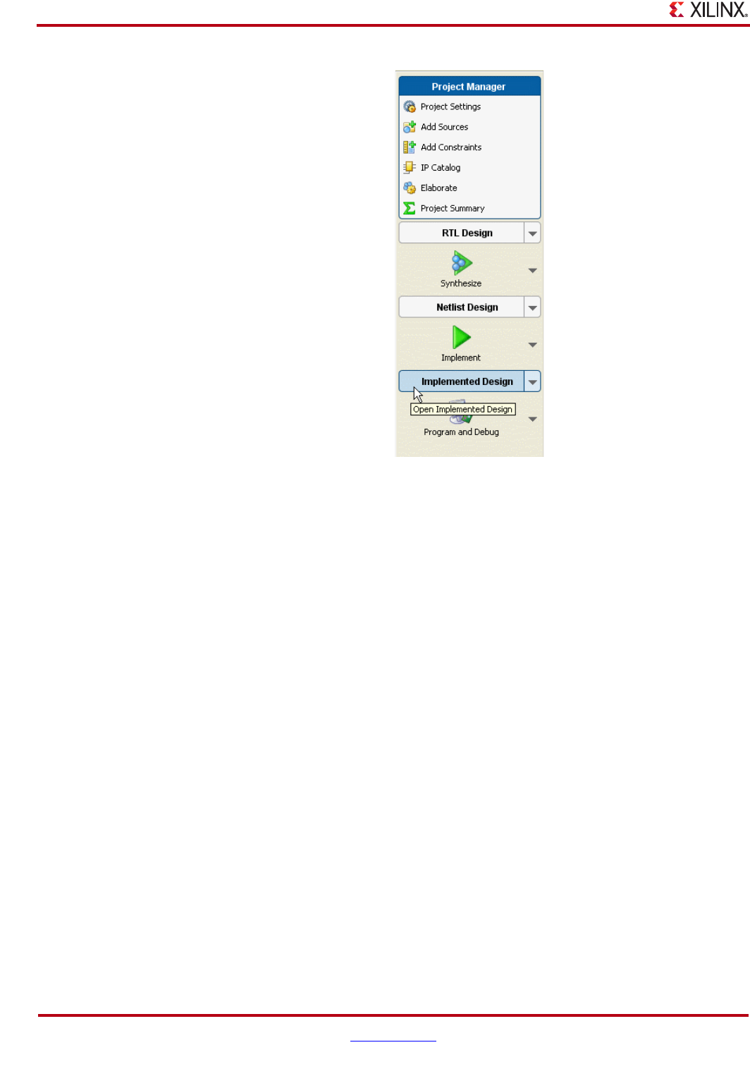
306 www.xilinx.com PlanAhead User Guide

UG632 (v 12.1)

Chapter 10: Analyzing Implementation Results

PlanAhead loads the original netlist the ISE placement and trce timing results in the

Design Planner environment.

The Implemented Design menu becomes available in the Flow Navigator also, as shown in

Figure 10-2, page 307.

An icon displays within the Implemented Design button to indicate that an implemented

design is open.

Figure 10-1: Project Manager Screen

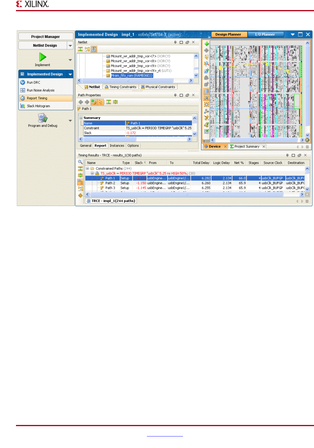
PlanAhead User Guide www.xilinx.com 307

UG632 (v 12.1)

Opening the Implemented Design

The placement results appear in the Device view as LOC constraints for each placed

instance. These LOC constraints are differentiated from the LOC constraints that you

might have set prior to implementation. They are referred to as “unfixed” placement

constraints. Constraints that are set prior to implementation are referred to as “fixed”

constraints.

You can lock any placement in place for subsequent runs by using the Fix Instances

popup menu command. Refer to Chapter 11, “Floorplanning the Design” and “Analyzing

Implementation Results,” page 305.

Note: ISE can optimize and change logic to improve placement and routing results. When this

happens, logic in the original netlist is removed or replaced. This results in a mismatch between the

pre-implementation netlist opened in PlanAhead and the implementation results. The Tcl Console will

report these discrepancies as the Implemented Design is being opened. It does not pose any

problems other than the logic in the netlist does not match the viewed results exactly.

PlanAhead imports the timing results from the ISE trce command and displays the

results in the Timing Results view.

Timing paths are organized by constraint and can be expanded and collapsed using the

tree widgets in the view. The Timing Results view contains information extracted from the

trce.twr or trce.twx files.

You can select and highlight paths in the Device view. You can examine timing path details

in the Path Properties view. Refer to “Analyzing Placement and Timing Results,” page 310

for more information.

Figure 10-2: Implemented Design Environment

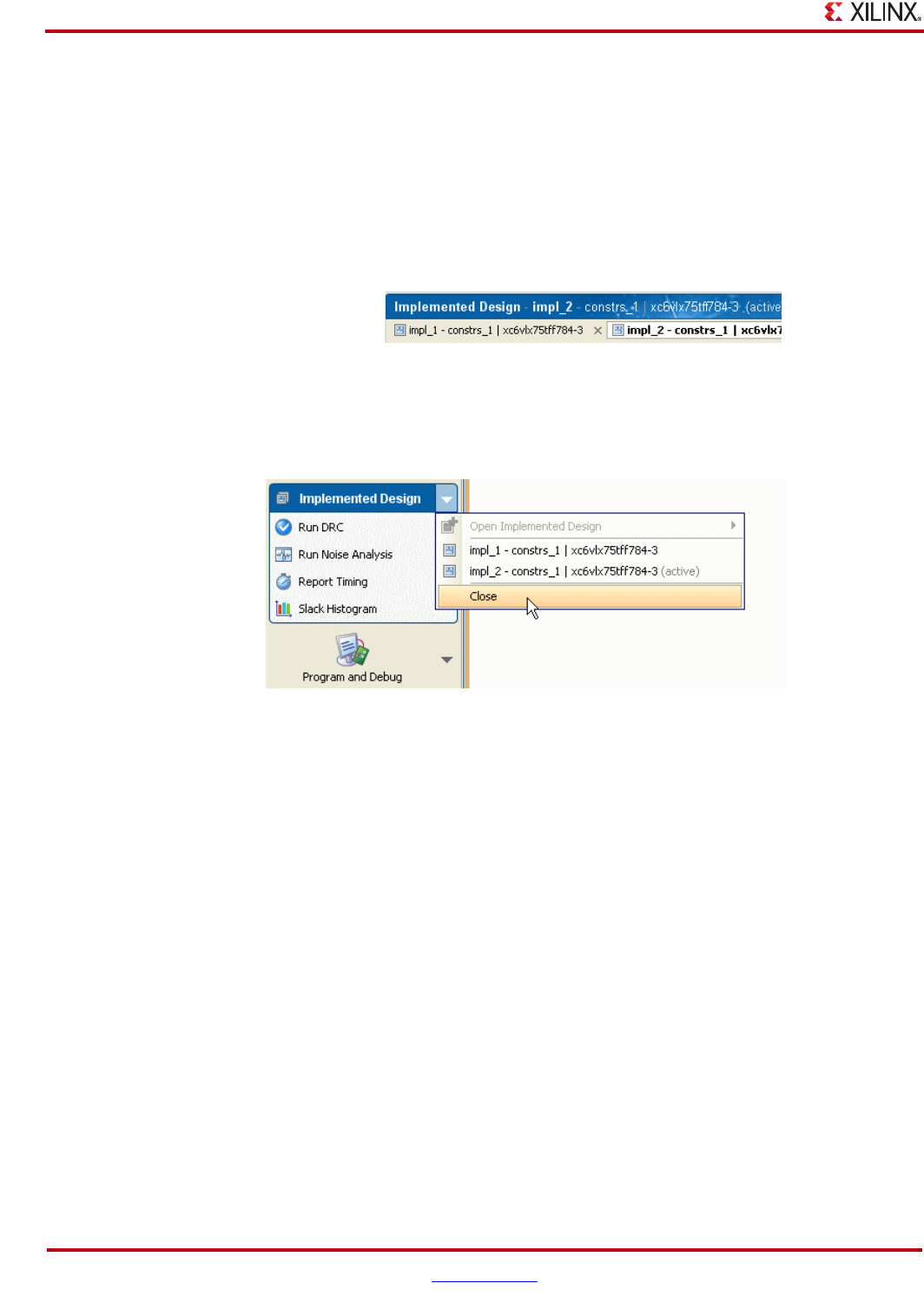
308 www.xilinx.com PlanAhead User Guide

UG632 (v 12.1)

Chapter 10: Analyzing Implementation Results

Opening Multiple Implemented Designs

You can open any implementation run by selecting it in the Design Runs view and using

the Open Implemented Design popup menu command. Alternately, you could set the run

as the active run and then click the Implemented Design button in the Flow Navigator.

Refer to “Setting the Active Run,” page 290.

You can open multiple implementation runs if they were launched from PlanAhead. Tabs

display in the upper left corner of the viewing environment to enable switching between

open implemented designs as shown in the following figure.

You can open and close available Implemented designs using the pulldown menu in the

Flow Navigator. Each implementation run shows under the Open Implemented Design

menu enabling any completed run to be opened as shown in the following figure.

When multiple Implemented Designs are open, the Implemented Design button displays

with multiple icons.

Importing ISE Results From Outside PlanAhead

You can import existing ISE results using the New Project wizard or import timing results.

The following subsections describe the options for importing ISE results.

Using the New Project Wizard to Create an ISE Results Project

You can create a new project and populate the project with a netlist, and timing and

placement results from an ISE software implementation.

For more information about creating a new project that imports ISE implementation

results, see “Creating a Project with ISE Placement and Timing Results” in Chapter 3.

Importing ISE TRCE Timing Results into an Existing Project

The PlanAhead software has the ability to import the .twx and .twr format timing

reports generated by the Xilinx trce command. Once imported, all the signal tracing and

viewing capabilities described in this chapter are available in the PlanAhead environment.

To import timing results:

Figure 10-3: Multiple Implemented Designs Open Tabs

Figure 10-4: Opening and Closing Implemented Designs

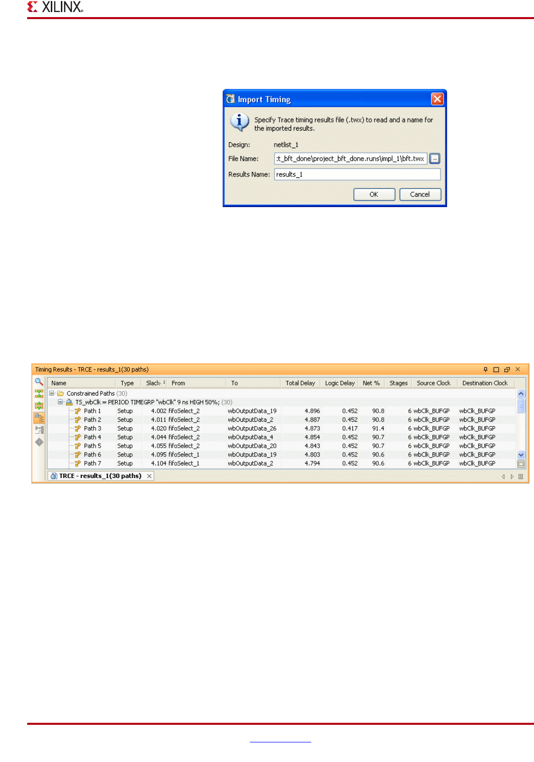
PlanAhead User Guide www.xilinx.com 309

UG632 (v 12.1)

Opening the Implemented Design

1. Select File > Import Timing.

The Import Timing dialog box opens as shown in the following figure.

View and edit the definable fields in the Import TRCE Results dialog box:

−File Name—Define a trce format .twx or .twr file name for PlanAhead to import

results.

−Results Name—Define a name to appear on the Results tab in the Timing Results

view.

2. Click OK to import the timing results.

The TRCE results display within the PlanAhead environment as shown in the following

figure.

You can:

•Explore all of the path selection, highlighting and tracing capabilities using the

PlanAhead interface.

•Sort the Timing Results by clicking any of the column headers. You can sort by a

second column by pressing the Ctrl key and clicking a second column header. Add as

many sort criteria as necessary to refine the list order.

•Display multiple Timing Results for a Floorplan.

Each result from Trce or PlanAhead receives a tab at the bottom of the report, as shown in

Figure 10-6. Slack values appear red for paths with negative slack values.

Figure 10-5: Import Trce Timing Results Dialog Box

Figure 10-6: TRCE Timing Results

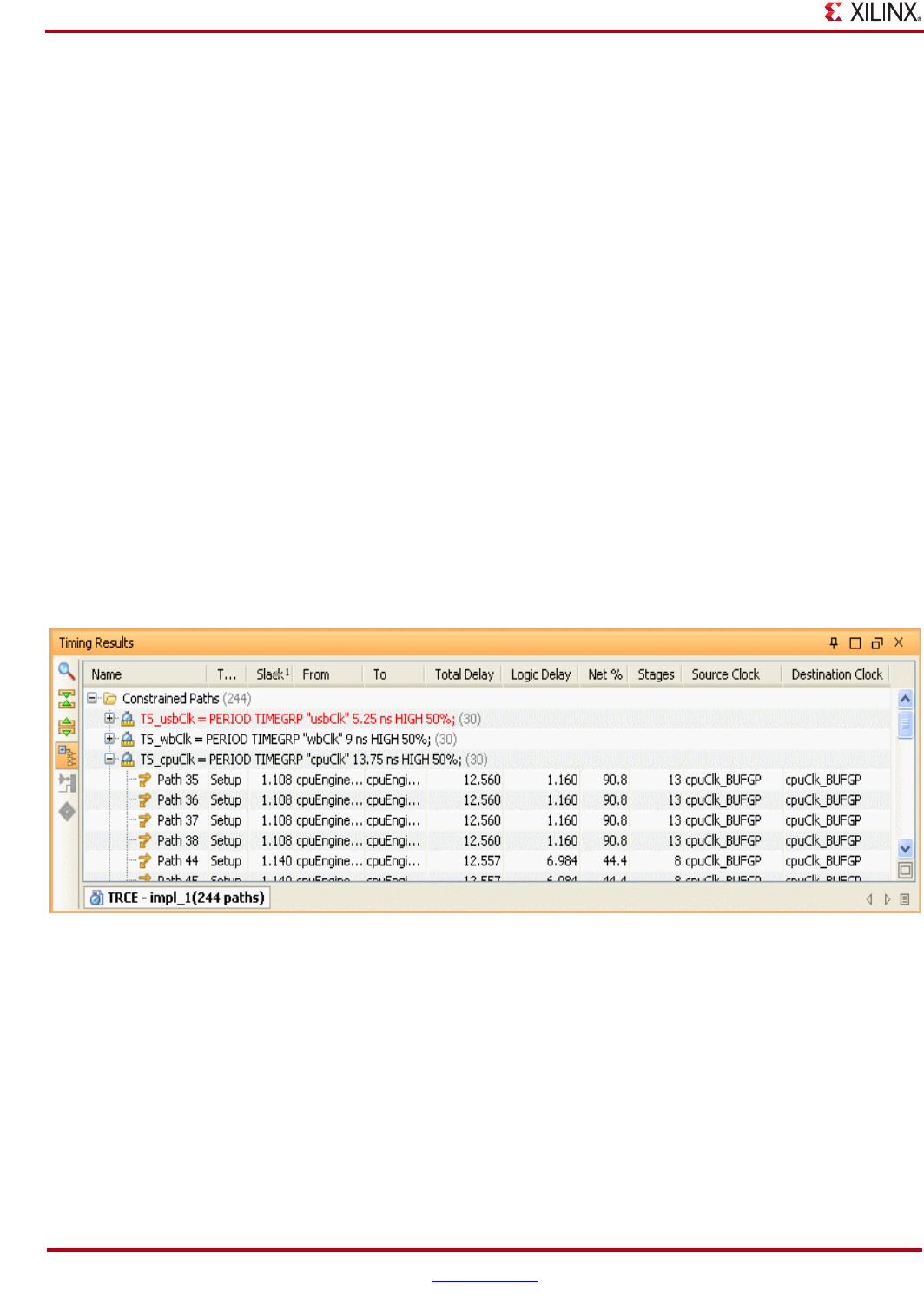
310 www.xilinx.com PlanAhead User Guide

UG632 (v 12.1)

Chapter 10: Analyzing Implementation Results

Analyzing Placement and Timing Results

The following sections describe the options for analyzing placement and timing results.

Exploring Xilinx TRCE Results

PlanAhead displays the results from ISE timing analysis by extracting information from

the trce timing report files (.TWR and .TWX). These files display automatically if the

implementation run was launched from PlanAhead. Otherwise, the implementation

results must be imported into PlanAhead. Refer to “Importing ISE Results From Outside

PlanAhead,” page 308.

Once imported, the timing results displays in the Timing Results view. If no timing

constraints were used to launch ISE, then no timing results are displayed.

Using the Timing Results View

Timing results imported from trce display differently than the PlanAhead Report Timing

command results described in Chapter 7, “Netlist Analysis and Constraint Definition.”

The trce results report the exact timing information coming from the implemented design,

while the PlanAhead report estimates routing delays.

The Timing Results view also displays the trce timing path information sorted by clock

constraint. Timing paths can be expanded and collapsed using the tree widgets in the view.

Failing paths Slack numbers are displayed in red.

The following figure shows a Trce result.

Using the Path Properties View

Selecting a Path in the Timing Results view displays information about the logic and delay

on that path in the Path Properties view.

The display of timing paths imported from trce differs from the diplays of PlanAhead

Report Timing command results, which are described in Chapter 7, “Netlist Analysis and

Constraint Definition.” The trce results report additional information such values as

clock skew and jitter, as shown in the following figure.

Figure 10-7: ISE trce Timing Results

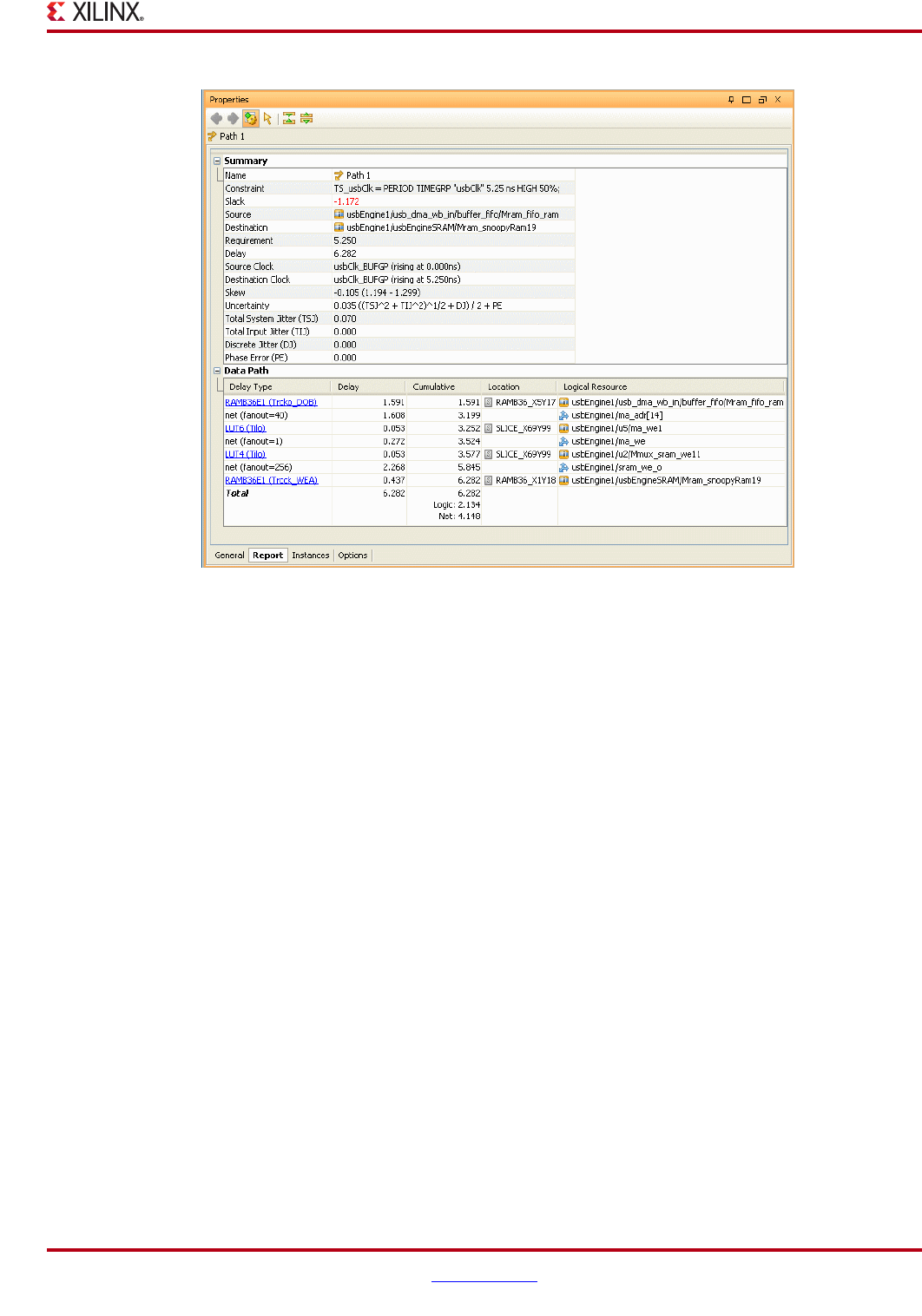
PlanAhead User Guide www.xilinx.com 311

UG632 (v 12.1)

Analyzing Placement and Timing Results

Selecting any logic object highlights that object in all other PlanAhead views.

PlanAhead provides links under the Delay Type column to invoke a PDF viewer with the

the device data sheet. A search is then automatically performed for the selected logic

object.

For more information about analyzing timing results using the Timing Results and Path

Properties views, see Chapter 7, “Netlist Analysis and Constraint Definition.”

Viewing Timing Paths in the Device View

You can view timing paths in the Device view when you select a path row or rows in the

Timing Results view. The path is highlighted in the Device view. You can select multiple

paths and all instances found in the path are selected and highlighted. Figure 10-9,

page 312 shows a highlighted timing path in the device view.

Figure 10-8: Timing Path Property View

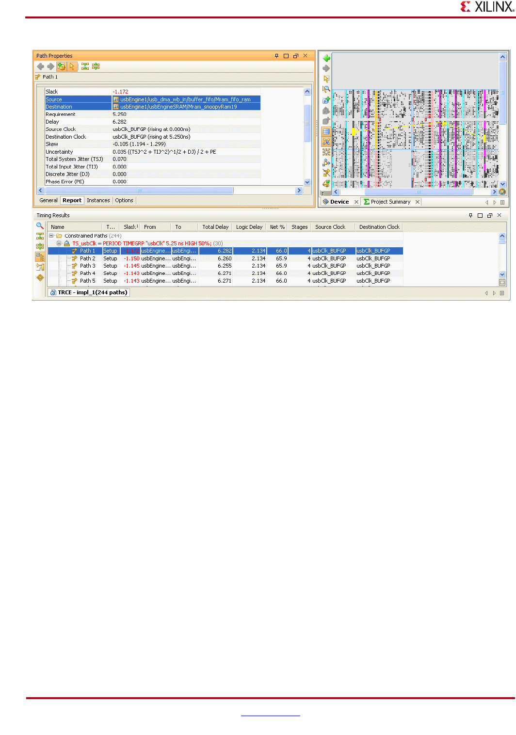
312 www.xilinx.com PlanAhead User Guide

UG632 (v 12.1)

Chapter 10: Analyzing Implementation Results

Viewing Timing Paths in Schematic View

When you select Schematic from the Timing Results toolbar or popup menu, PlanAhead

generates a Schematic view that displays the instances found in the selected paths. The

Schematic view displays the instances clearly along with the hierarchical modules as

shown in Figure 10-10, page 313.

Figure 10-9: Highlighted Timing Paths in the Device View

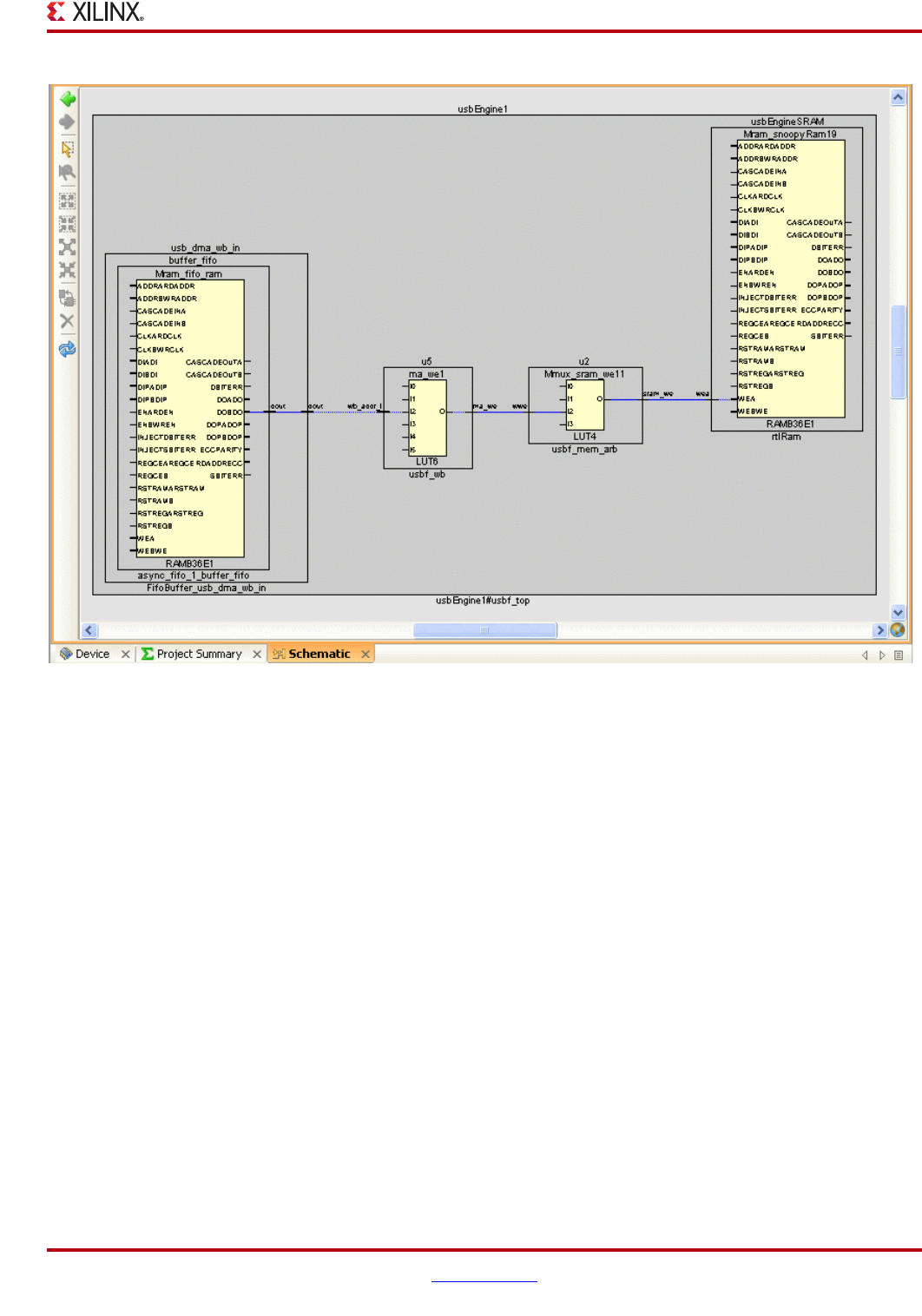
PlanAhead User Guide www.xilinx.com 313

UG632 (v 12.1)

Exploring Logic Connectivity

.When the Schematic view is generated for a timing path, all of the objects are displayed.

When a Schematic view for individual logic instances is generated, only the selected

instances display.

You can display the instances from a group of paths in this manner making it easy to

identify what modules should be grouped together for floorplanning. Pblock creation

popup commands in the Schematic view let you make direct assignment to Pblocks in the

Device view. For more information about Schematic expansion and traversal commands,

see “Using the Schematic View,” page 110.

Exploring Logic Connectivity

The following sections describe logic connectivity options in PlanAhead.

Using the Show Connectivity Command

The Show Connectivity command highlights all of the nets connected to the selected

elements. To use this command:

1. Select a net, Pblock, instance, or a combination thereof.

2. From the popup menu, select Show Connectivity.

For example, if an instance or Pblock is selected, all of the nets connecting to that element

are highlighted as shown in Figure 10-11, page 314.

Figure 10-10: Timing Paths Displayed in Schematic View

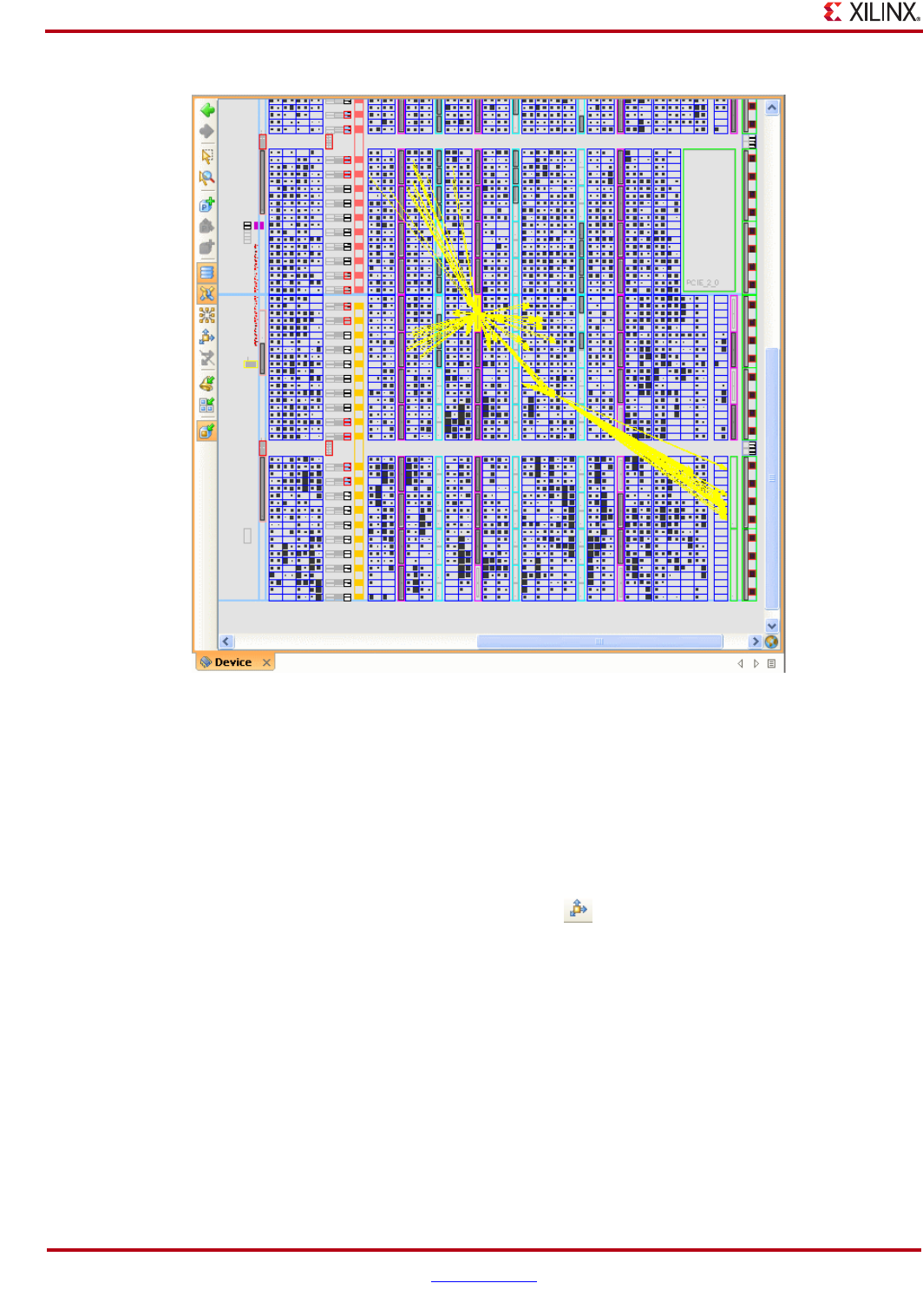
314 www.xilinx.com PlanAhead User Guide

UG632 (v 12.1)

Chapter 10: Analyzing Implementation Results

Viewing Logic Connectivity using Show Connectivity Mode

The Show Connectivity command can be continuously run on newly selected objects by

toggling the Show connections for selected instances toolbar button on and off.

The Show connections for selected instances mode remains active, which lets you select

additional logic objects for viewing connectivity. Toggle the toolbar button to turn off Show

connections for selected instances mode.

Expanding and Selecting a Logic Fanout

You can run the Show Connectivity command sequentially to continue to select and

expand a logic fanout.

1. Select a net, pblock, instance or combination thereof.

2. From the popup menu, select Show Connectivity. The command highlights all nets

connected to the selected element.

3. From the popup menu, select Show Connectivity a second time. The command selects

the set of connected instances to those nets.

Figure 10-11: Net Connectivity in the Device View

Figure 10-12: Show connections for selected instances Mode Toolbar Button

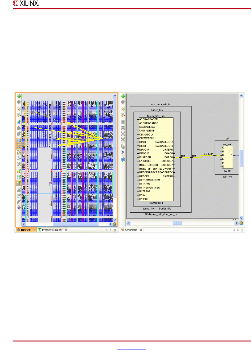
PlanAhead User Guide www.xilinx.com 315

UG632 (v 12.1)

Searching for Objects using the Find Command

4. From the popup menu, select Show Connectivity a third time. The command

highlights the next level of nets connected to the selected instances, and so on.

This is an easy way to select a logic fanout starting at a particular instance or I/O port.

Expanding Logic in the Schematic View

You can trace logic throughout the design hierarchy using the Schematic view. Anything

selected in the Schematic view is highlighted in the Device view also.

You can expand signals interactively by double-clicking on the pins of the instance to be

traced. The following figure shows an example of expanded logic in the Schematic view.

Also you can expand and display instance and module connectivity, and content

interactively.

For more information about exploring logic in the schematic, “Using the Schematic View,”

page 110.

Searching for Objects using the Find Command

Once the placement is displayed in the Device view, you can use the Find command to

search for and locate any type of logic. The Find command dialog box provides flexibility

for filtering the search criteria in many different ways.

For more information about searching for logic objects see Chapter 7, “Netlist Analysis and

Constraint Definition.”

Figure 10-13: Logic Expanded in the Schematic View

316 www.xilinx.com PlanAhead User Guide

UG632 (v 12.1)

Chapter 10: Analyzing Implementation Results

Highlighting Logic Objects

There are two commands for highlighting objects:

•The Highlight command is for highlighting specifically selected objects.

•The Highlight Primitives command is for highlighting all of the primitive logic

associated with selected modules.

Highlighting Selected Objects

PlanAhead has a highlight mechanism that lets you selectively highlight objects.

Highlighting lets you display multiple placement groups at once using one or more colors.

Highlighted objects remain highlighted even when you click elsewhere in PlanAhead.

They are highlighted in all applicable views including the Schematic.

You can highlight any number of selected objects.

Once you select an object you can highlight it with the Select > Highlight command or

you can select Highlight from the popup menu in most views. This command operates on

the selected logic.

When highlighting all Netlist module or Pblock logic, you can use the Highlight

Primitives command to highlight the lower level logic. For more information, see the

following section.

You can use several methods to highlight the placement for selected modules.

Using the Select Primitives and Highlight Primitives Commands

After you import the ISE placement, you can use the Select Primitives command to select

the underlying primitive logic elements for Pblocks and logic modules. This command is

often used in conjunction with the Show Connectivity, Fix instances or Clear Loc

Constraints commands.

After you import the ISE placement, you can use the Highlight Primitives command to

highlight the underlying primitive logic elements selectively for Pblocks and logic

modules.

You can select logic modules or Pblocks, and use the Highlight Primitives command, and

then select a color to highlight their associated placement.

When multiple instances are selected, you can select the same color for all or use Cycle

Colors to use different highlight colors for each of the selected modules. PlanAhead marks

modules and primitives in the Netlist view with the matching highlight color in the

Device, Schematic, and Package views, as shown in Figure 10-14, page 317.

PlanAhead User Guide www.xilinx.com 317

UG632 (v 12.1)

Highlighting Logic Objects

Unhighlighting Objects

To unhighlight objects use one of the following commands:

•Choose Select > Unhighlight All to unhighlight all objects.

•Choose Select > Unhighlight Color to unhighlight based on color.

•Click the Unhighlight All toolbar button as shown in the following figure.

Figure 10-14: Matching Highlighting Color in the Netlist and Device Views

Figure 10-15: Unhighlight All Toolbar Button

318 www.xilinx.com PlanAhead User Guide

UG632 (v 12.1)

Chapter 10: Analyzing Implementation Results

Marking Selected Objects

Marking Objects

The PlanAhead software lets you place a Mark symbol in all applicable views for all

selected objects.

Marking a selected object is helpful when displaying small objects that you want to see in

the Device view.

To mark selected objects, select Select > Mark, or press Ctrl+M. This command is available

in other views, including the Netlist and Physical Hierarchy views.

When marking timing paths, the start point is marked in green, the end point in red, and

all intermediate points in yellow, as shown in the following figure.

Removing Marks

You can remove marks using one of the following methods:

•Choose Select > Unmark All.

•Click the Unmark All toolbar button as shown in the following figure.

Figure 10-16: Marked Timing Path Symbols in Device View

Figure 10-17: Unmark All Toolbar Button

PlanAhead User Guide www.xilinx.com 319

UG632 (v 12.1)

Locking Placement for Future Implementation Runs

When placement results are imported from ISE, they are displayed as unfixed LOC

constraints in PlanAhead. Constraints that were define prior to implementation are

referred to as fixed are displayed with a different color.

Using the Fix Instances Command

You can lock placement in place for subsequent runs by selecting the desired logic and

using the Fix Instances popup menu command.

You can use this capability to help ensure consistent implementation results. Once the you

have saved the implemented design, the fixed logic will receive LOC and BEL constraints

in the UCF and can be passed to the subsequent implementation runs.

Fixing Specific Types of Logic

A method for improving consistency of implementation result is to lock some or all of the

block macro logic such as block RAMs and DSPs. You can do this manually in PlanAhead

using your own knowledge of the design or by leveraging successful ISE implementation

results. If your design has a lot of block RAMs or DSPs, this method can help produce more

consistent results and improve runtime.

Refer to “Working with Placement LOC Constraints,” page 349 for information about

manually assigning LOC constraints.

To Fix specific types of logic, use the Find command to select specific types of logic such as

block RAMs and DSPs. You can then select all of them in the Find Results view and use the

Fix Instances popup menu command.

Fixing Logic Modules

A method for improving consistency of implementation result is to lock critical logic in

place. This can involve locking specific logic, timing paths or entire logic modules.

To Fix all logic in a particular module, select the module or modules and use the Select

Primitives command to select the primitive logic instances associated with the logic

module. To lock the logic, use the Fix Instances command.

Displaying Design Metrics

The following subsections describe the design metrics options:

•“Using the Metrics View”

•“Displaying the Metric Maps in the Device View”

•“Removing the Metric Map Display”

•“Using the Metrics Results View”

•“Configuring the Metric Ranges”

320 www.xilinx.com PlanAhead User Guide

UG632 (v 12.1)

Chapter 10: Analyzing Implementation Results

Using the Metrics View

The PlanAhead Metrics view displays a list of design metrics that can be displayed using

a colored graph of the potential problem areas in the design. The metrics include

utilization and timing checks at both the Pblock and placed design level. The following

figure shows the Metrics view.

The Metric Properties view provides a description of the Metric function along with the

bins defined to highlight potential problems, as shown in the following figure.

Figure 10-18: Metrics View

Figure 10-19: Properties View: Set Metric Range Values

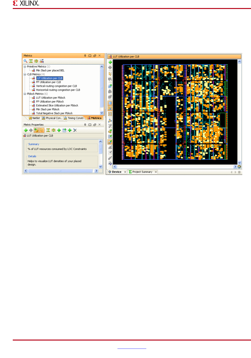
PlanAhead User Guide www.xilinx.com 321

UG632 (v 12.1)

Displaying Design Metrics

Displaying the Metric Maps in the Device View

To display a Metric map in the Device view, select the metric and select the Show popup

menu command. PlanAhead displays a color-based metric map. The following figure

shows an example of a Metric map in the Device view.

You can display multiple metric maps simultaneously.

•To display any of the slack related metrics, you must run a PlanAhead timing

estimation first using the Report Timing command.

•To display any of the CLB or BEL constraints type metrics, import the placement

results from ISE implementation.

For more information, see “Opening the Implemented Design,” page 286 or “Importing

ISE Results From Outside PlanAhead,” page 304.

Removing the Metric Map Display

To hide a metric map in the Device view, select the metric, and from the popup menu,

select Hide or Hide All Metrics.

Using the Metrics Results View

After you select the Show command, the metric results display in the bottom view. In the

Metric Results view, you can:

•Sort the information by clicking any of the column headers.

•Sort by a second column by pressing the Ctrl key and clicking a second column

header.

•Add as many sort criteria as necessary to refine the list order.

Figure 10-20: Metric Map in the Device View

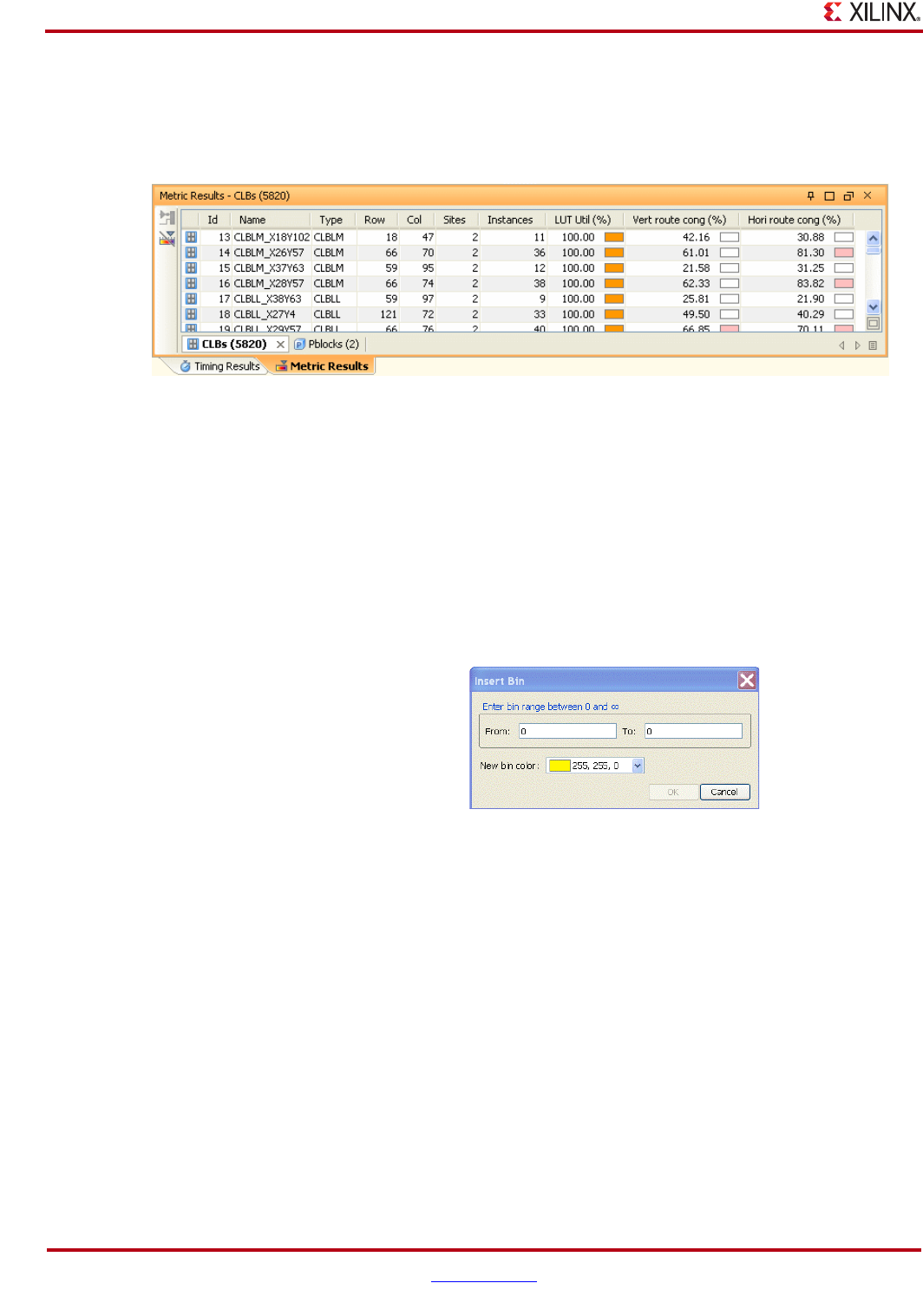
322 www.xilinx.com PlanAhead User Guide

UG632 (v 12.1)

Chapter 10: Analyzing Implementation Results

The Pblock metric results update automatically as you modify the Pblocks. The different

types of metrics, such as for Pblocks, CLBs, and primitives, display in different charts. Each

type has a tab along the bottom of the Metrics Results view, as shown in the following

figure.

Configuring the Metric Ranges

Within the Properties view you can configure the bin ranges for each map.

Colors and the range display are adjustable. You can add or delete new bins to define

ranges. To do so, select the Apply changes button in the Metrics Properties view or select

Apply Changes from the popup menu.

To insert a new range bin, select the bin you want to split, and select Insert Bin from the

right-click popup menu. The following dialog box allows the definition of the range and

color.

The ranges are adjusted to accommodate the newly defined range.

Figure 10-21: Metric Results View

Figure 10-22: Insert Bin Dialog Box

PlanAhead User Guide www.xilinx.com 323

UG632 (v 12.1)

Chapter 11

Floorplanning the Design

This chapter contains the following sections:

•“Floorplanning Strategy Overview”

•“Working with Pblocks”

•“Configuring Pblocks”

•“Working with Placement LOC Constraints”

Floorplanning Strategy Overview

The PlanAhead™ software supports a floorplanning methodology that lets designers

constrain critical logic to ensure shorter interconnect lengths with less delay.

This methodology involves user interaction with the physical design and is not a push-

button flow. Designers can use the analysis capabilities in PlanAhead coupled with their

own knowledge of the design to define constraints and tool options for improving

performance.

Floorplanning can be accomplished by creating physical block (Pblock) locations to

constrain logic placement or by locking individual logic objects to specific device sites.

The complexity of floorplanning requires more explanation than is practical to provide in

this user guide; therefore, a Floorplanning Methodology Guide is available. For more

information, see the Floorplanning Methodology Guide (UG633).

Working with Pblocks

The following subsections describe how to work with Pblocks:

•“Creating Pblocks”

•“Understanding Pblock Graphics”

•“Viewing Pblock Properties”

•“Setting Pblock Logic Type Ranges”

•“Assigning Logic to Pblocks”

•“Moving and Resizing Pblocks”

Creating Pblocks

The process of floorplanning begins by dividing some or all of the logic in the design into

groups and constraining that logic. The PlanAhead software provides the ability to

hierarchically divide the design into smaller, more manageable physical blocks (Pblocks).

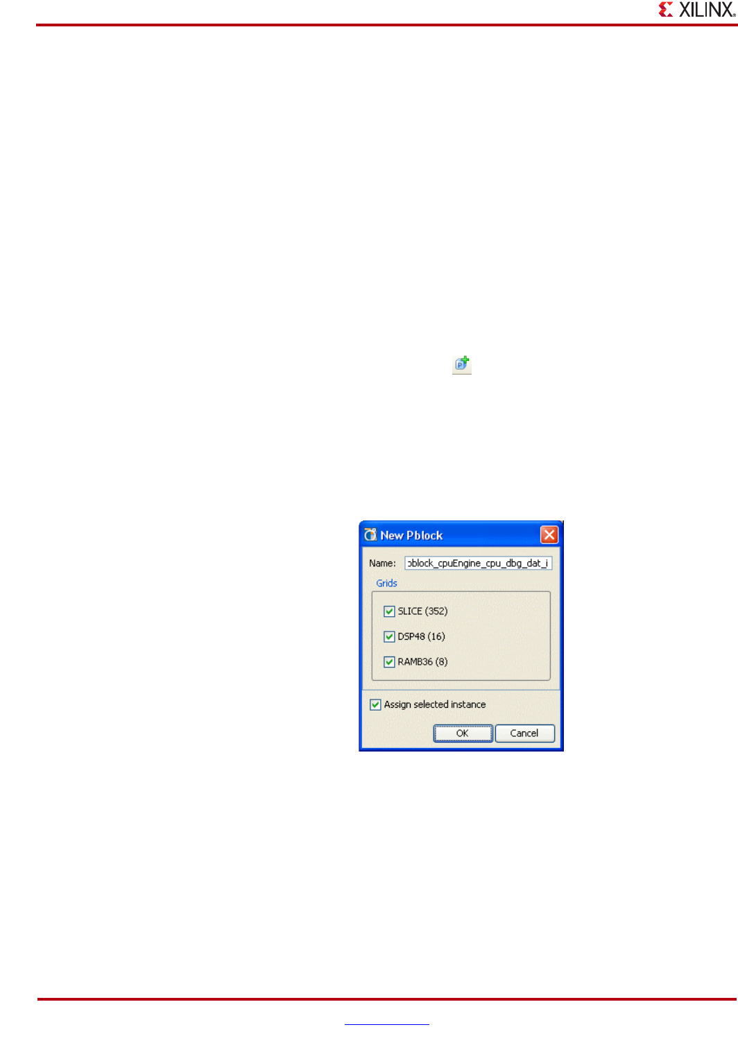
324 www.xilinx.com PlanAhead User Guide

UG632 (v 12.1)

Chapter 11: Floorplanning the Design

These Pblocks can include logic modules and primitive logic from anywhere in the logic

hierarchy. You can group critical or associated logic together into a single Pblock, which

prevents logic migration, limits interconnect lengths, and reduces delays.

Creating a Pblock results in an AREA_GROUP constraint that is written into the exported

UCF constraint file. The constraints in PlanAhead reflect the assigned logic, specified

ranges, and defined attributes.

Using the Draw Pblock Command

The Draw Pblock commands will assign pre-selected logic to a new Pblock in the Device

view. You can select the logic to assign to the Pblock before you invoke the command.

To create a Pblock:

1. Select the logic in any view, such as the Netlist view, to assign to the Pblock.

2. Click Draw Pblock, in either the popup or on the toolbar. The following figure shows

the Draw Pblock button.

3. Move your cursor to the location in the Device view where you want to start drawing

a Pblock.

4. Press and hold the left mouse button, move the mouse cursor to the opposite corner of

the Pblock, and release the mouse button.

The New Pblock dialog box opens as shown in the following figure.

5. View and edit the options in the New Pblock dialog box.

−Name—Enter a name for the Pblock. If no name is entered, a default name of

pblock_n or Pblock_<instancename> is used.

−Grids—Select the device resource ranges to be constrained by the Pblock.

−Assign selected instances—Select to assign the selected instances to the new

Pblock. Occasionally, users inadvertently have logic selected, which is not

intended for assignment.

6. Click OK.

Figure 11-1: Draw Pblock Toolbar Button

Figure 11-2: New Pblock Dialog Box

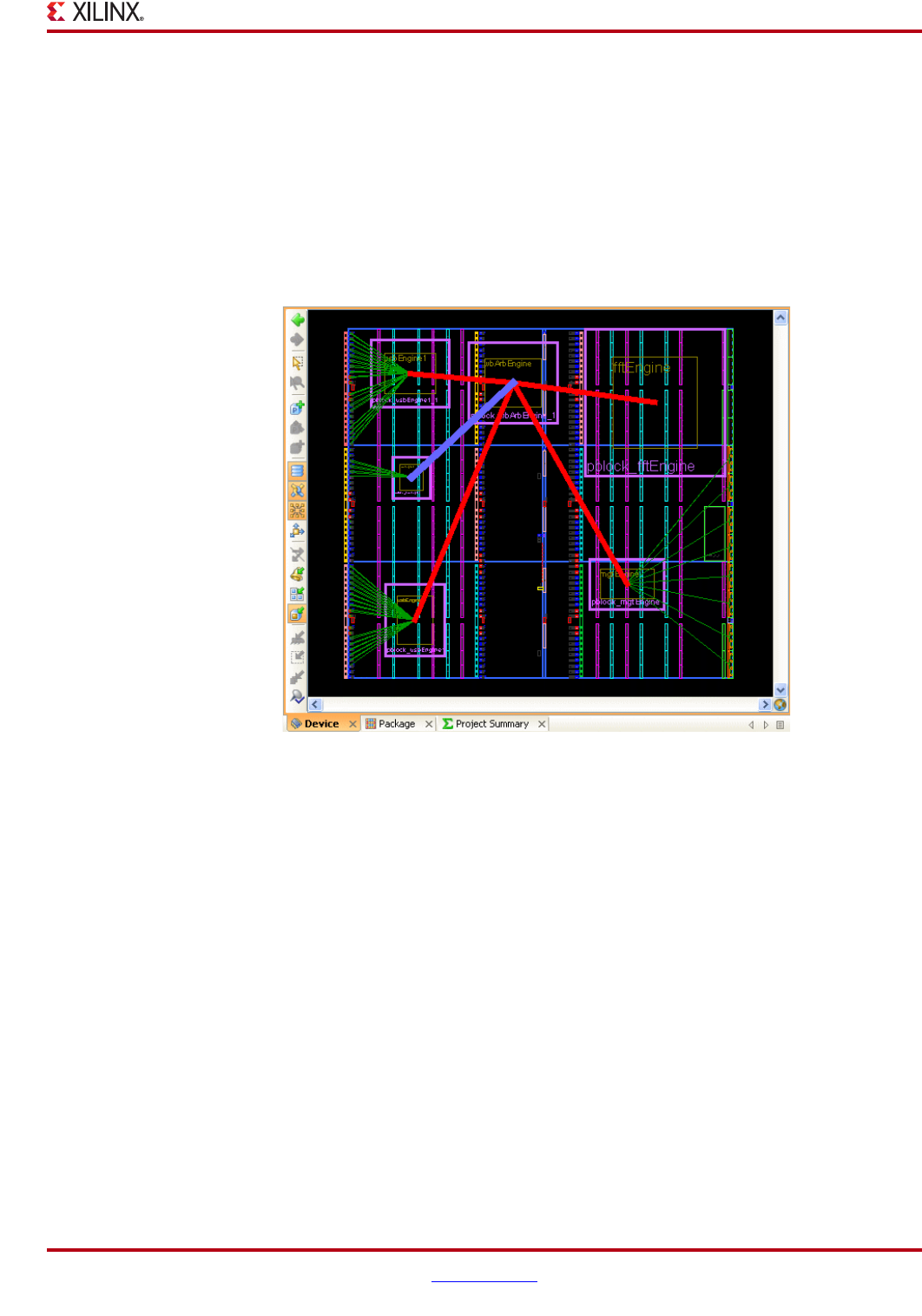
PlanAhead User Guide www.xilinx.com 325

UG632 (v 12.1)

Working with Pblocks

The Pblock displays and you can select it in the Device view and the Physical Constraints

view.

The initial Pblock size and location are not critical during manual creation. Pblocks can be

appropriately sized and located by using dynamic Resource Utilization Statistics in the

Pblock Properties dialog box. You can determine how to reposition Pblocks by viewing the

connectivity display in the Device view.

Sometimes, it is helpful to initially create all of the Pblocks with small rectangles to help

visualize the logic connectivity flow between the Pblocks prior to attempting sizing as

shown in the following figure.

See “Analyzing Hierarchical Connectivity,” page 198 and “Using the Show Connectivity

Command,” page 313 for more information about this view.

Using the New Pblock Command

The New Pblock command creates a new Pblock in the Physical Constraints view, but does

not create a rectangle in the Device view.

You must pre-select logic for assignment to the new Pblock. If no logic is pre-selected, the

command creates an empty Pblock.

To create new Pblocks with or without pre-selected logic, select New Pblock from the

popup menu.

Figure 11-3: Pblock Connectivity Analysis in the Device View

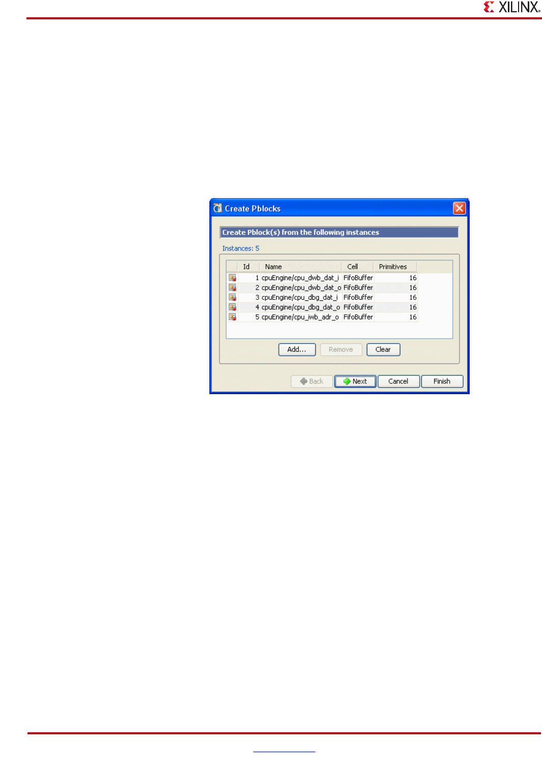
326 www.xilinx.com PlanAhead User Guide

UG632 (v 12.1)

Chapter 11: Floorplanning the Design

Creating Multiple Pblocks with the Create Pblocks Command

You can create multiple Pblocks in a semi-automated way by using the Create Pblocks

wizard. The wizard creates a separate Pblock for each selected netlist instance. To use the

wizard, pre-select a set of instances for inclusion into individual Pblocks.

To create multiple Pblocks for specific netlist instances:

1. Select the instances to include in a Pblock.

2. Select Tools > Create Pblocks.

The Create Pblocks wizard opens with a list of the selected instances as shown in the

following figure.

3. To add additional netlist instances to this list, click the Add button to invoke a browser

in which you can select other instances.

4. To remove any netlist instances from the list, click the Remove button.

5. To clear netlist instances from the list, click the Clear button.

6. Click Next.

The Create Pblocks wizard gives you the option to specify a naming scheme as shown

in Figure 11-5, page 327.

Figure 11-4: Create Pblocks Wizard: Create Pblocks from Instances

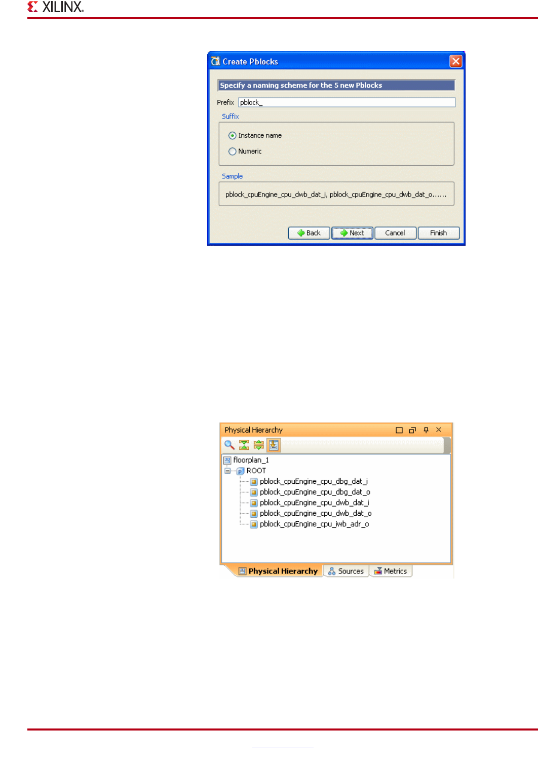
PlanAhead User Guide www.xilinx.com 327

UG632 (v 12.1)

Working with Pblocks

7. In the Create Pblocks wizard, view and edit the naming scheme fields:

−Prefix—Defines a name prefix to be used for the Pblock names. Enter a new prefix

or allow the default instance name or number to be used.

−Suffix—Select Instance name to append the instance name onto the prefix, or

select Numeric to append a number starting with 1 to the prefix.

8. Click Next.

9. Verify the contents in the Summary page.

10. Click Finish to create the Pblocks with these settings.

The Pblocks now show in the Physical Constraints view as in the following figure.

To create rectangles for the newly created Pblocks:

1. Select each of the new Pblocks (one at a time) in the Physical Constraints view.

2. Click the Set Pblock Size button in the Device view toolbar, which is shown in

Figure 11-7, page 328.

Figure 11-5: Create Pblock Wizard: Specify Name

Figure 11-6: Pblocks in Physical Constraints

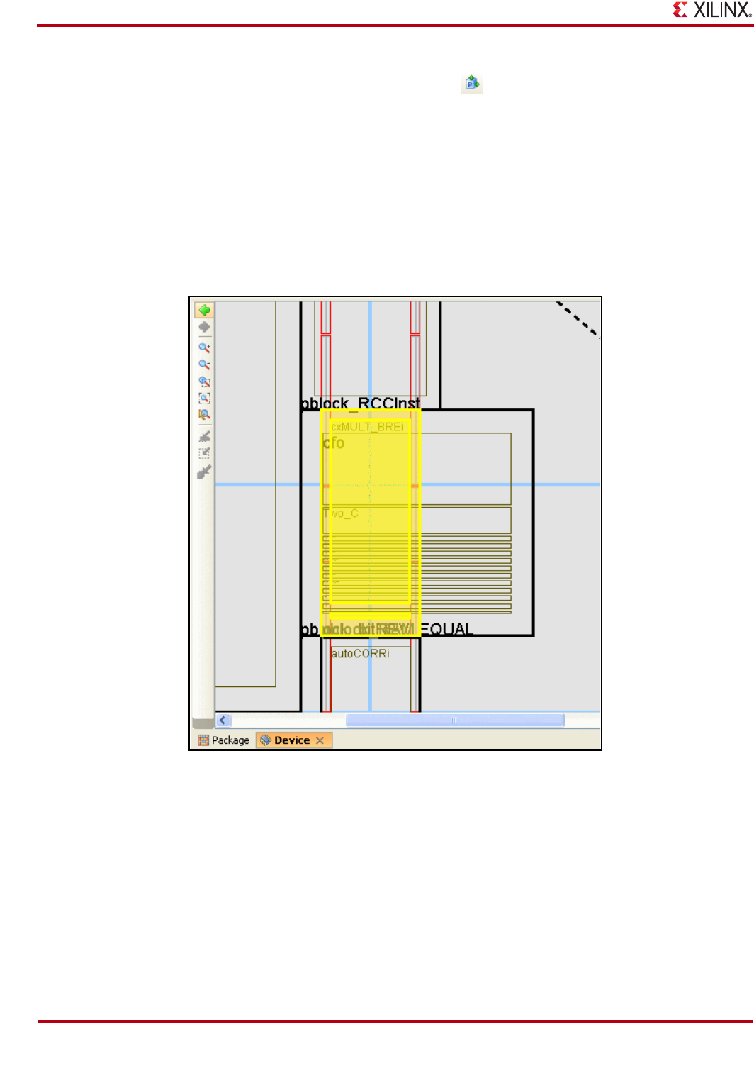
328 www.xilinx.com PlanAhead User Guide

UG632 (v 12.1)

Chapter 11: Floorplanning the Design

3. Draw a rectangle in the Device view.

Creating Nested Pblocks

You can create Pblocks within Pblocks (nested Pblocks) to provide further control for

constraining logic. This can be helpful when trying to improve performance of critical

modules. The top-level Pblock contains all the lower-level Pblocks during utilization

estimates. The following figure shows an example of constraining block RAMs with a

nested Pblock.

Note: The ISE implementation software does not support extensive use of this feature.

Occasionally, map and placement errors will result when creating nested Pblocks.

Creating Clock Region Pblocks

You can define a Pblock to include all resources within a specific clock region or regions.

The following set of steps are required to define a Pblock as a clock region.

1. Draw a Pblock with a rectangle that encompasses the boundary of the clock region.

Figure 11-7: Set Pblock Size Toolbar Button

Figure 11-8: Creating Nested Pblocks

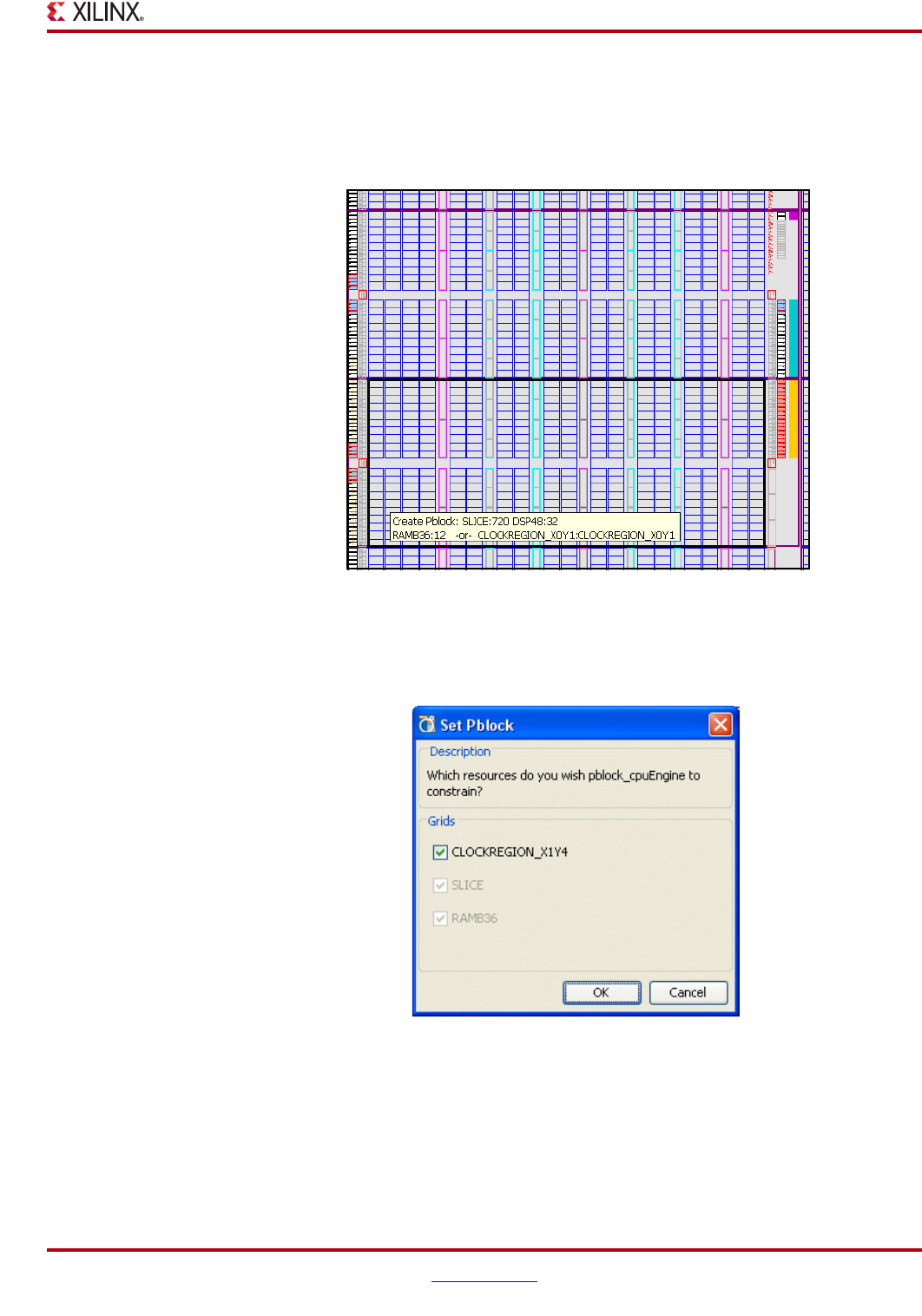
PlanAhead User Guide www.xilinx.com 329

UG632 (v 12.1)

Working with Pblocks

The PlanAhead software displays the clock region boundaries. To change the color or

display characteristics of the clock region boundaries, refer to the “Customizing

PlanAhead Display Options” in Chapter 4.

Figure 11-9, page 329 shows a clock region Pblock.

The tool tip changes to indicate the Pblock range is a Clock Region.

2. Select OK in the New Pblock dialog box to define the Pblock range as the Clock Region

as shown in the following figure.

The Pblock rectangle must encompass the clock region boundary to enable the

CLOCKREGION option. When you unselect the CLOCKREGION_X button, you can define

the Pblock using traditional logic based ranges, as shown in Figure 11-11, page 330.

Figure 11-9: Creating Clock Region Pblocks

Figure 11-10: Set Pblock Dialog Box to Confirm Pblock as Clock Region

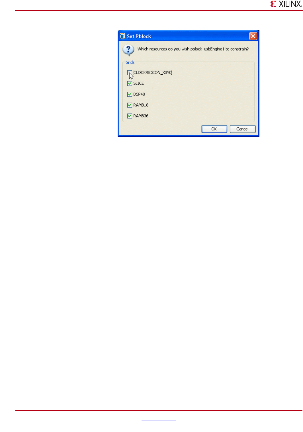
330 www.xilinx.com PlanAhead User Guide

UG632 (v 12.1)

Chapter 11: Floorplanning the Design

3. You can toggle the two types of Pblocks by selecting or unselecting the

CLOCKREGION button in the New Pblock dialog box or in the Pblock General

Properties view.

The Pblock clock region coordinates display in the Pblock General Properties view.

Understanding Pblock Graphics

The default display options show what is a Pblock and what are the instances assigned to

the Pblock.

•The outer rectangle is the Pblock border.

•The rectangles contained inside the Pblock are the netlist instances assigned to it.

Multiple instances can be placed into a Pblock, and instance rectangles displayed inside

the Pblock are sized based on the amount of logic they contain, relative to the other

instances in the same Pblock.

If many instances are assigned to a Pblock, they might appear as lines instead of rectangles

as shown in Figure 11-12, page 331.

Figure 11-11: Clock Region Pblock General Properties

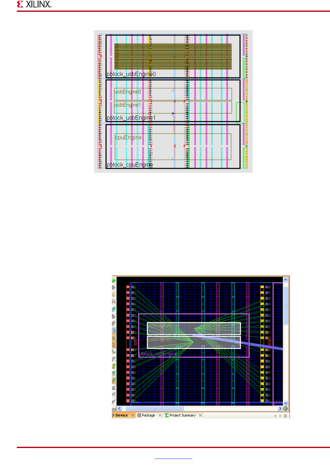
PlanAhead User Guide www.xilinx.com 331

UG632 (v 12.1)

Working with Pblocks

Using the default selection rules, selecting the Pblock rectangle selects all of the netlist

instances contained in it also. You can drag and assign Instances into other Pblocks.

Note: Be careful when manipulating Pblocks to ensure the Pblock rectangle is selected and not the

smaller rectangles indicating the assigned instances. It is helpful when manipulating Pblocks to turn

off the selection ability for instances. This ensures Pblocks and not the instances assigned to them

are selected in the Device view. To define how instances and Pblocks are selected, select Tools >

Options > Themes > Device, and define the selection ability in the Device dialog box. For more

information, see “Setting General View Display Options” in Chapter 4.

I/O Nets are drawn connected to the center of the instance inside the Pblock rather than in

the Pblock center as with Bundle Nets as shown in the following figure.

Figure 11-12: Pblocks With Assigned Instances Displayed Graphically

Figure 11-13: I/O Connectivity Displays to Center of Instance Rectangles

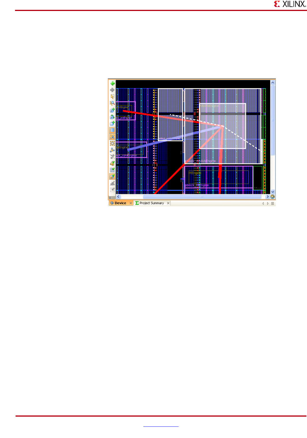
332 www.xilinx.com PlanAhead User Guide

UG632 (v 12.1)

Chapter 11: Floorplanning the Design

Child Pblocks appear in a slightly different color to differentiate the rectangles. Color

configuration is available in the Tools > Options > Themes > Device dialog box.

Pblocks might contain multiple rectangle ranges. Multiple rectangle ranges display with

dashed lines connecting them to indicate that they are part of the same Pblock. The

assigned instance rectangles and connectivity display in the largest rectangle as shown in

the following figure.

Viewing Pblock Properties

You can display various types of information with the Pblock Properties view. To display

or edit Pblock properties, select the Pblock and view the Pblock Properties view. The

following subsections describe the window tabs.

Note: To accept any changes made, click Apply. To cancel any changes, click Cancel. Selecting

another item or closing the Properties view will not initiate any changes unless you click Apply.

Figure 11-14: Creating Pblocks with Non-Rectangular Shapes

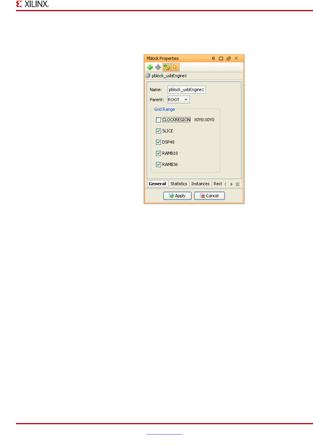
PlanAhead User Guide www.xilinx.com 333

UG632 (v 12.1)

Working with Pblocks

The General Tab

The General tab is shown in the following figure.

The General tab contains the following definable fields:

•Name—Displays the Pblock name.

•Parent—Displays the Parent Pblock. This field is a non-editable field for some

Pblocks. If a Pblock has multiple potential parent Pblocks, the field becomes active

allowing definition of the Parent Pblock.

•Grid Range—Enables the Pblocks to be specified with specific AREA_GROUP RANGE

properties. Selecting specific ranges constrains only the selected logic types within the

Pblock area. The grid range coordinates display for each logic type once the Pblock is

created.

−CLOCKREGION—Defines the Pblock range to be an entire clock region. The

Pblock rectangle is drawn to match the clock region boundary.

•Apply / Cancel—Saves or discards changes.

The Statistics Tab

The Statistics tab of the Pblock Properties view displays content information about the

Pblock.

Note: You can save the contents to a text file also, using the Export Statistics icon. The Statistics

tab is shown in Figure 11-16, page 334.

Figure 11-15: Pblock Properties View

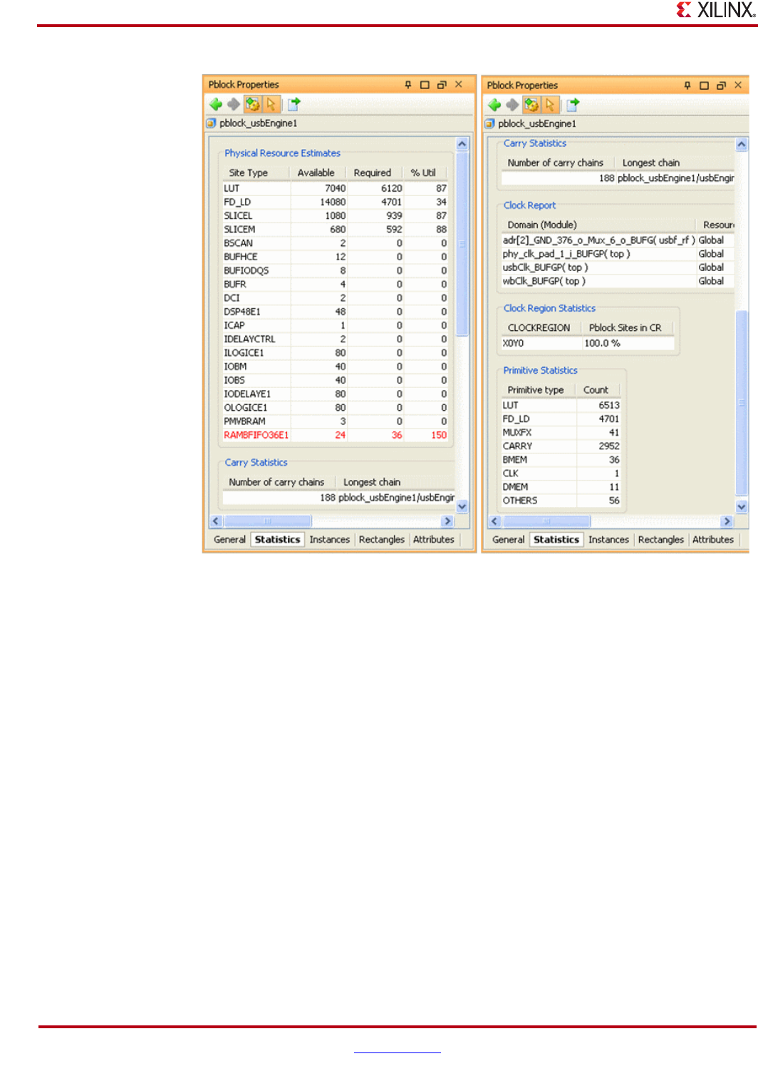
334 www.xilinx.com PlanAhead User Guide

UG632 (v 12.1)

Chapter 11: Floorplanning the Design

The Statistics tab shows the following Pblock information:

•Physical Resources Estimates—A chart of each resource type in the device.

−Site Type—The Site Types defined within the Pblock rectangle.

−Available—The number of sites contained in the Pblock.

−Required —The number of sites required for the logic assigned to the Pblock.

−% Utilization—The estimated percentage of the sites populated in the Pblock.

•Carry Statistics—The number of vertical carry chain logic objects assigned to the

Pblock. It also displays the tallest carry chain assigned to the Pblock and the

percentage of its height in relation to the Pblock height.

Note: Carry height utilization values over 100% can cause PlanAhead DRC errors and ISE

map errors.

•Clock Report—Clock signals (Local, Global, and Resource) contained in the Pblock as

well as the number of clocked instances on each clock.

•RPM Statistics—The number of Relatively Placed Macros (RPM) objects assigned to

the Pblock. It also displays the tallest and widest RPM assigned to the Pblock and the

percentage of its size in relation to the Pblock size.

Note: RPM utilization values over 100% will cause PlanAhead DRC errors and ISE map errors.

PlanAhead does not indicate whether multiple RPMs will fit inside the Pblock rectangle.

Figure 11-16: Pblock Properties View: Statistics Tab

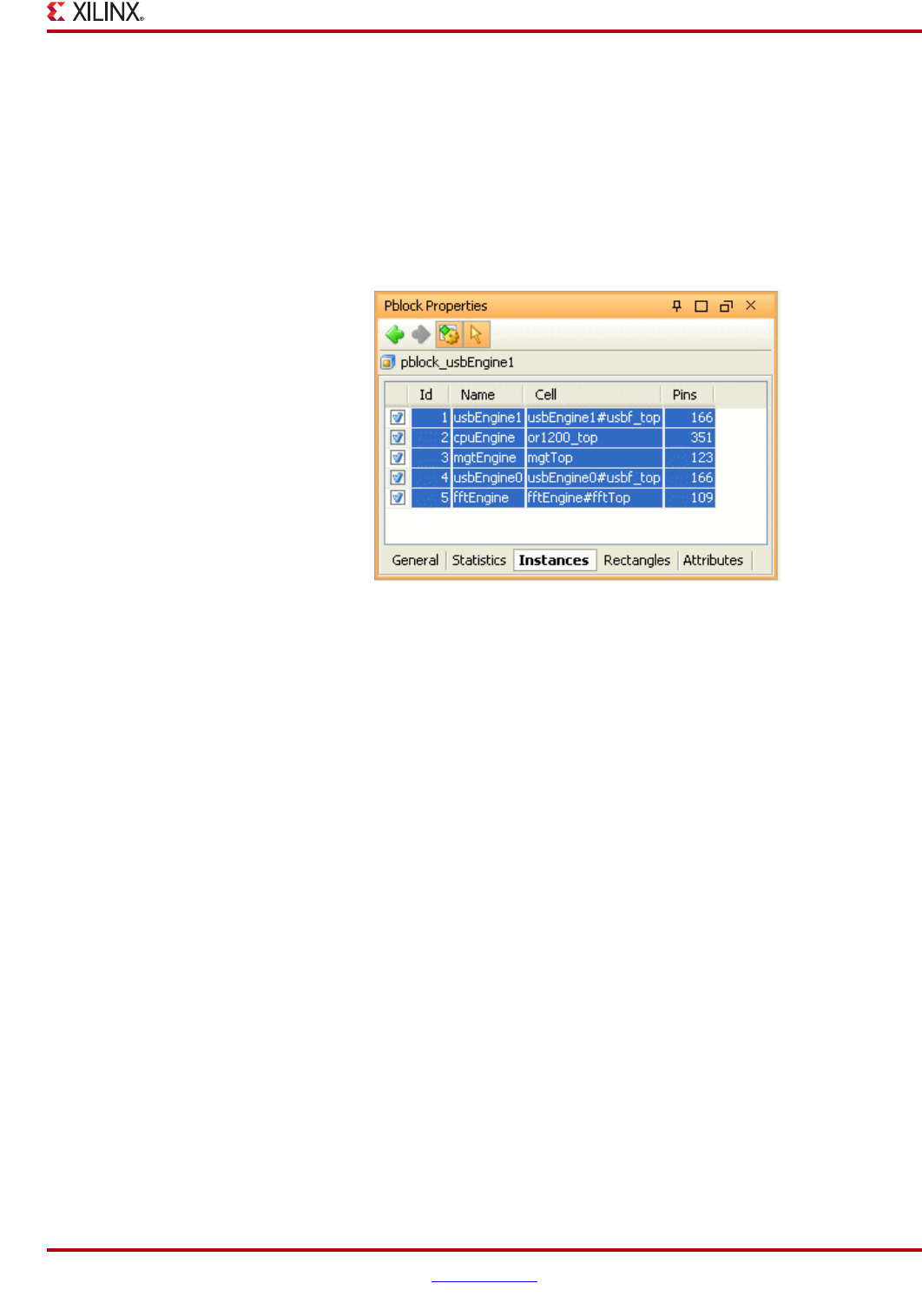
PlanAhead User Guide www.xilinx.com 335

UG632 (v 12.1)

Working with Pblocks

•Clock Region Statistics—The utilization percentage of each clock region that the

Pblock overlaps.

•Primitive Statistics—The number of each type of logical resource assigned to the

Pblock.

The Instances Tab

The Instances tab of the Pblock Properties view displays information about the instances

contained in the Pblock as shown in the following figure.

You can select the instance fields and use them to seed many popup menu commands.

The Rectangles Tab

The Rectangles tab of the Pblock Properties view displays information about the various

rectangles created for the Pblock. The Rectangle tab is used for selecting rectangles of a

Pblock. For more information about this tab, refer to the “Using Non-Rectangular

Pblocks,” page 343.

The Attributes Tab

The Attributes tab of the Pblock Properties view is described in “Setting Attributes for

Pblocks,” page 345.

Figure 11-17: Pblock Properties View: Instances Tab

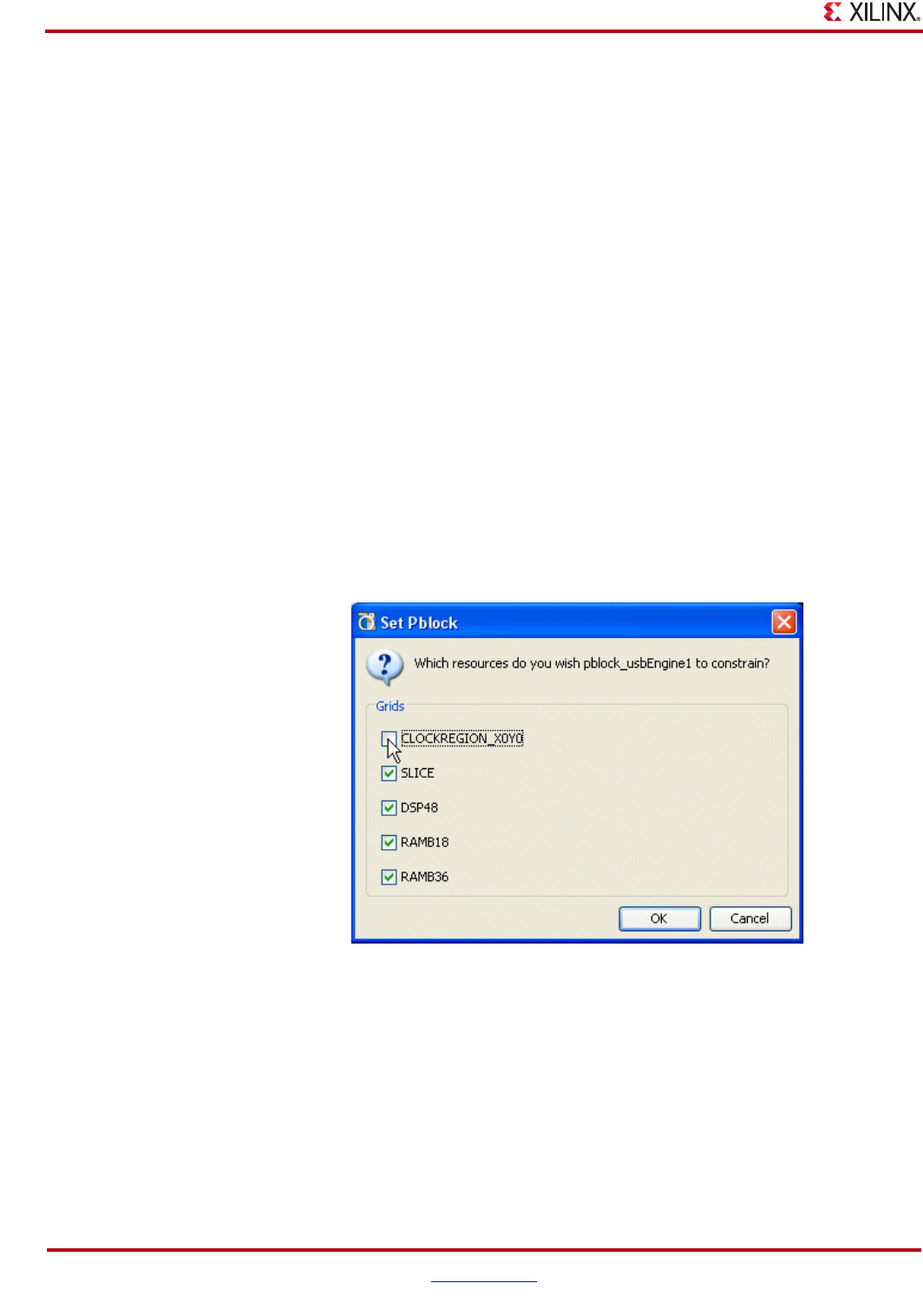
336 www.xilinx.com PlanAhead User Guide

UG632 (v 12.1)

Chapter 11: Floorplanning the Design

Configuring Pblocks

The following subsections describe configuring Pblocks:

•“Setting Pblock Logic Type Ranges”

•“Assigning Logic to Pblocks”

•“Moving and Resizing Pblocks”

•“Using Resource Utilization Statistics to Shape Pblocks”

•“Placing Pblocks Based on Connectivity”

•“Using Non-Rectangular Pblocks”

•“Removing a Pblock Rectangle”

•“Setting Attributes for Pblocks”

•“Renaming a Pblock”

•“Deleting a Pblock”

•“Running the Automatic Pblock Placer”

Setting Pblock Logic Type Ranges

You can set Pblock AREA_GROUP range types in the Pblock Properties view by modifying

the Grid Range options in the General tab. Adjusting these toggles controls which type of

logic is to be constrained within the Pblock rectangle, as shown in the following figure.

If the Pblock is resized or moved to a location that includes new device logic types, such as

block RAM and DSP, a dialog box displays prompting you to add the new range types to

the Pblock definition.

Toggling the ranges off results in the Pblock being shown differently in the Device view. As

the Pblock is selected the shading will only affect the logic types for the ranges set on the

Pblock, as shown in Figure 11-19, page 337.

Figure 11-18: Setting AREA_GROUP Range Types

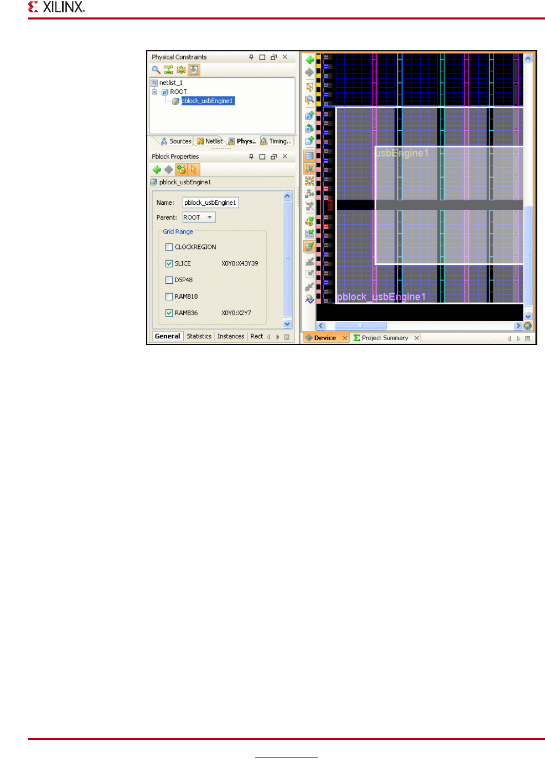
PlanAhead User Guide www.xilinx.com 337

UG632 (v 12.1)

Configuring Pblocks

Assigning Logic to Pblocks

Once a Pblock is created, you can assign netlist instances. This can be done by either

dragging and dropping logic, or by using the Assign popup command.

To use the drag and drop method:

1. Click and drag logic instances from the Netlist, Schematic, Hierarchy or Find Results

views.

2. Drop the instances into the Pblock rectangle area.

To use the Assign command method to assign logic to existing Pblocks:

1. Select logic instances in the Netlist view.

2. Select the Assign popup command.

The Select Pblock dialog box displays the allowable selections of the Pblock assignment as

shown in the following figure.

Figure 11-19: Pblock Shading Reflects Logic Contained in Pblock

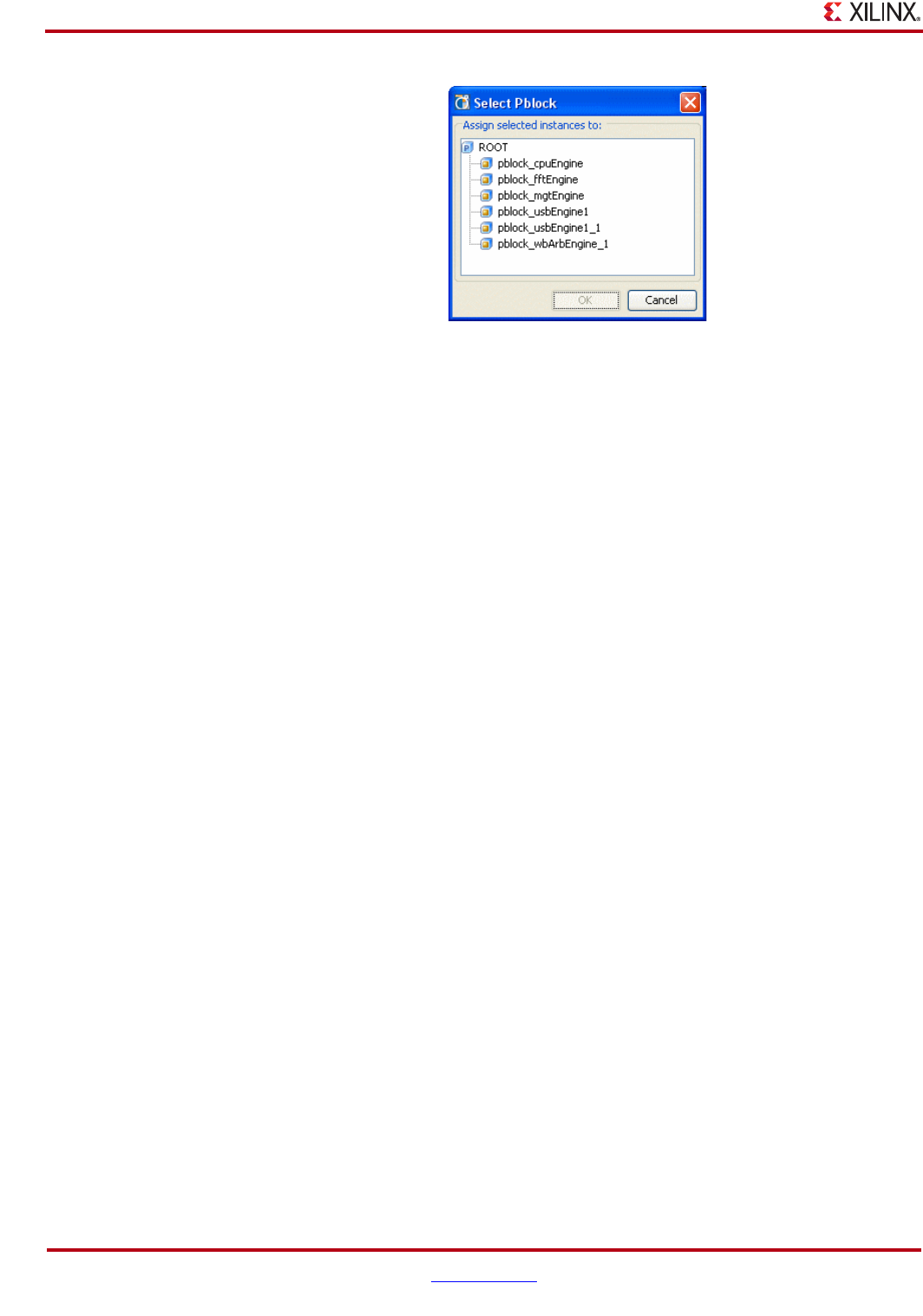
338 www.xilinx.com PlanAhead User Guide

UG632 (v 12.1)

Chapter 11: Floorplanning the Design

Unassigning Logic from Pblocks

Instances can be removed from Pblocks, as follows:

1. Select the instances by any means.

2. Select the Unassign popup command.

A confirmation dialog box opens asking to confirm the removal of instances from the

Pblock.

Moving and Resizing Pblocks

The following subsections describe how to move, resize, and set Pblocks.

Moving a Pblock

You can move a Pblock by selecting and dragging the Pblock within the Device view, and

dropping it in the new location. The dynamic cursor shaped like a hand indicates that the

Pblock is selected for moving. Ensure that the outer Pblock rectangle is selected and not

one of the assigned instances.

If the Pblock is moved to a location that includes new device logic types, such as block

RAM or DSP, a dialog box displays prompting you to add the new range types to the

Pblock definition.

Pblocks behave different when location placement constraints are assigned inside of them.

The target location should contain adequate resources to assign the placement constraints.

As the Pblock dragged around, the cursor indicates which are legal placement sites for a

move. If not, a dialog box displays prompting you to either remove or leave the location

constraints intact.

Fixed and unfixed location constraints are listed separately in the dialog box, allowing you

to handle them differently.

The following figure shows the Choose LOC mode dialog box.

Figure 11-20: Select Pblock Dialog Box

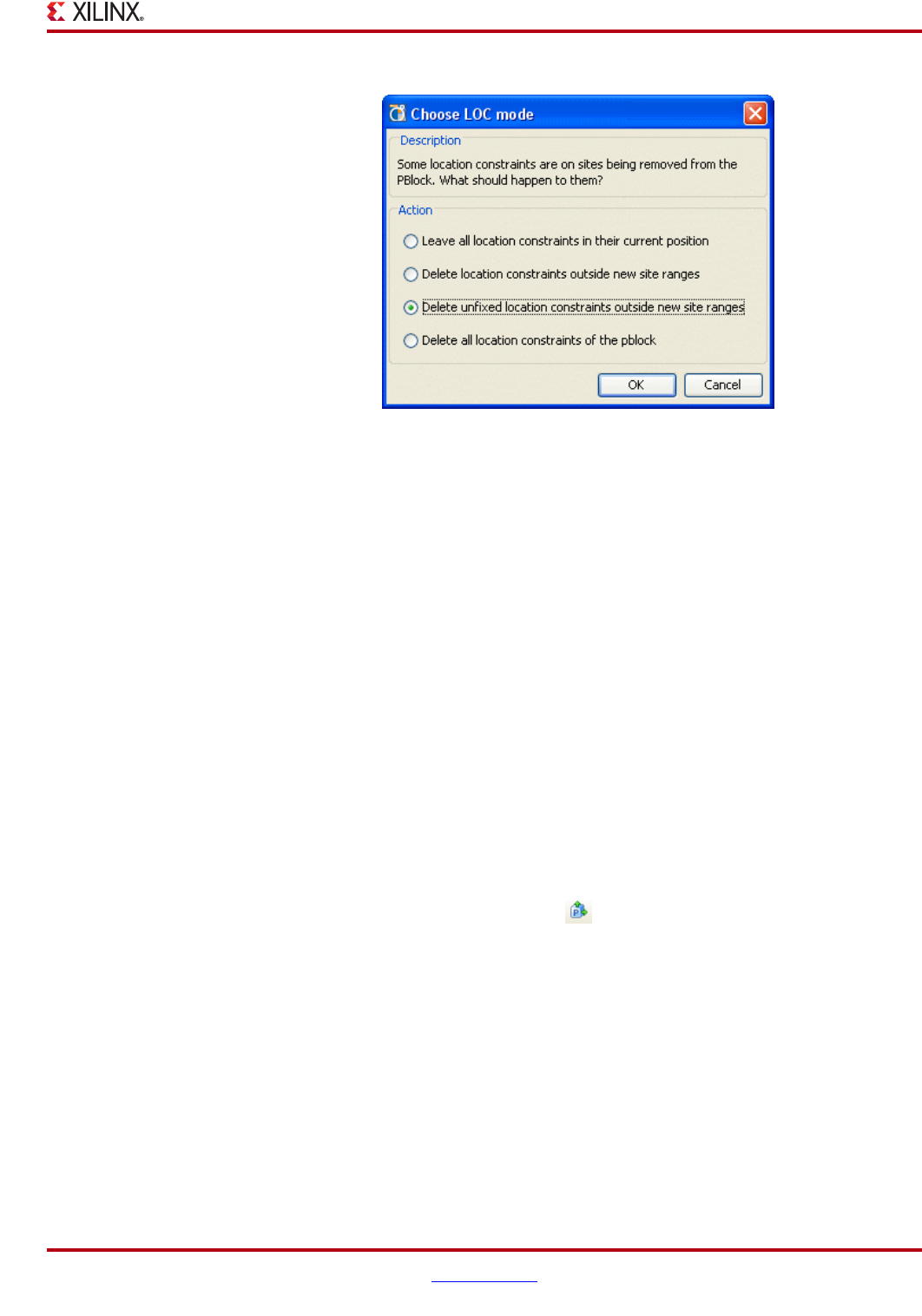
PlanAhead User Guide www.xilinx.com 339

UG632 (v 12.1)

Configuring Pblocks

To cancel an active move operation, press the Esc key and the active command is

terminated.

Note: If you are having difficulty moving Pblocks, click the Set Pblock Size toolbar button to redraw

the rectangle elsewhere. You might need to remove placement constraints prior to moving Pblocks.

Resizing a Pblock

You can stretch Pblock edges by selecting the Pblock and moving the cursor near one of its

edges or corners. When the cursor changes to a drag symbol, click and drag to reshape the

Pblock.

To cancel an active stretch operation, press the Esc key, and the active command is

terminated.

Using the Set Pblock Size Command

You can size or resize existing Pblocks with a new rectangle by using the Set Pblock Size

command. To create a new rectangle for an already existing Pblock:

1. In the Physical Constraints view or Device view, select the Pblock.

2. Click the Set Pblock Size toolbar button as shown in the following figure.

The cursor changes to enable you to draw a new rectangle in the desired location in the

Device view.

3. Use the cursor to draw a new rectangle.

Also, you can use this command to draw a rectangle for an existing Pblock with no

rectangle yet defined, such as one created with the New Pblock(s) commands. For more

information, see “Creating Multiple Pblocks with the Create Pblocks Command,”

page 326.

If a Pblock has multiple rectangles, this command regenerates the Pblock with a single

rectangle. Often, this is useful when a Pblock gets fragmented into multiple rectangles.

Figure 11-21: Setting Behavior for Modifying Pblocks with LOCs

Figure 11-22: Set Pblock Size Toolbar Button

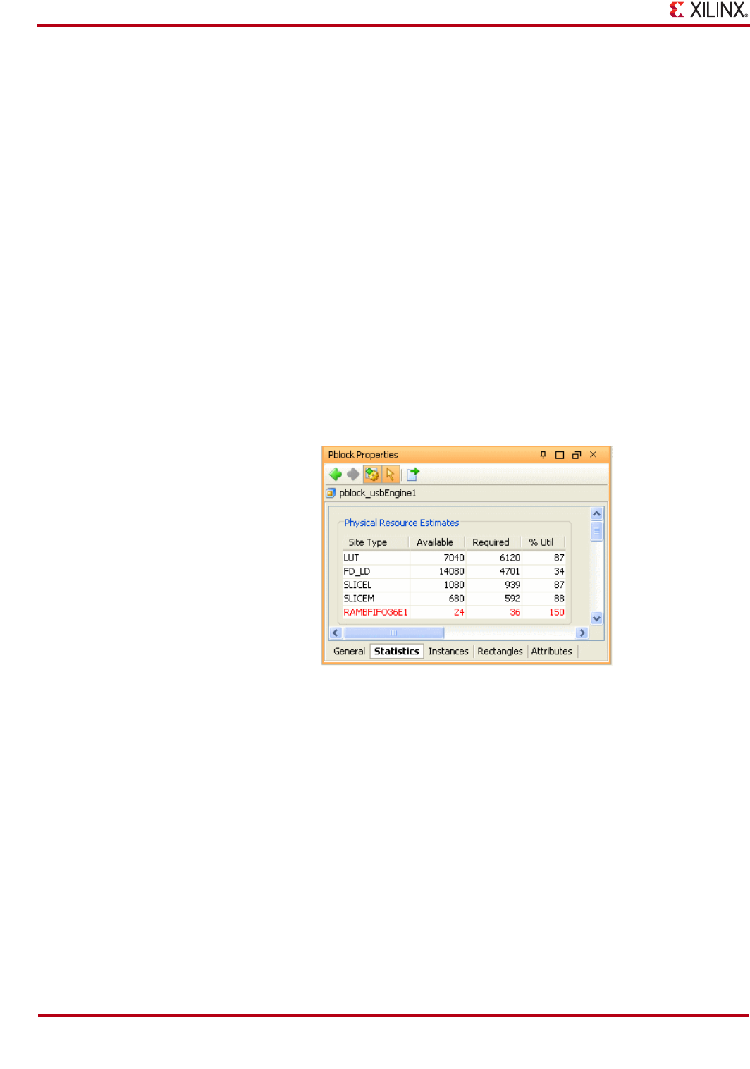
340 www.xilinx.com PlanAhead User Guide

UG632 (v 12.1)

Chapter 11: Floorplanning the Design

If you resize the Pblock to a location which includes new device logic types, such as block

RAM or DSP, a dialog box displays prompting you to add the new range types to the

Pblock definition.

Pblocks behave differently when location placement constraints are assigned inside of

them. If location constraints are assigned to the Pblock, a dialog box displays prompting

you to either remove or leave the location constraints intact.

Fixed and unfixed location constraints are listed separately in the dialog box allowing you

to handle them differently.

To cancel an active resize operation, press the Esc key on the keyboard and the active

command is terminated.

Using Resource Utilization Statistics to Shape Pblocks

You can use the utilization estimates in the Pblock Properties view to size and place Pblock.

The device resources available inside the rectangle are compared against the logic

contained in the Pblock to compute utilization estimates.

To display the utilization estimates for a Pblock:

1. Select the Pblock, and view the Pblock Properties.

2. Click the Statistics tab as shown in the following figure.

3. In the Statistics tab, view the utilization estimates in the following three columns.

−Available—Displays the number of available sites in the Pblock.

−Required—Displays the number of sites that the assigned logic requires.

−% Utilization—Displays the estimated utilization percentage for each logic type.

The appropriate utilization can be met by resizing the Pblock. If Utilization for

some logic objects is over 100%, the text appears in red, as shown above.

4. Scroll down to view the required RAM sites for the Pblock.

The dialog box is dynamic and updates each time the Pblock is modified.

If the Pblock does not contain a site for a specific logic device element, the dialog box

shows the following values:

•Available—0

•Required—The required number.

Figure 11-23: Pblock Properties View: Statistics Tab

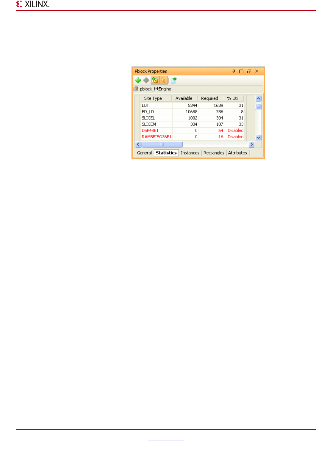
PlanAhead User Guide www.xilinx.com 341

UG632 (v 12.1)

Configuring Pblocks

•Utilization—Disabled (meaning no sites of the required type are defined in the

rectangle). A value of Disabled is an error condition indicating that there are no sites of

the required type in the rectangle defined.

The following figure shows an example of a disabled resource.

Note: The Pblock SLICE utilization calculation assumes maximum site utilization. In reality, the

maximum site utilization is rarely achieved in placement and routing tools. Thus, a designer should

optimize for a target utilization of approximately 80% or higher. This number is a function of the device

used and the characteristics of the design and its constraints.

Note: Pblock utilization is affected by carry chains, RPM macros, and the geometry of the Pblock

rectangle. These statistics are estimates to help guide you to a successful ISE implementation. All of

the Pblock Statistics must be taken into account when sizing Pblocks. Occasionally, Pblocks must be

enlarged for ISE to place them successfully.

Placing Pblocks Based on Connectivity

The PlanAhead software provides dynamic connectivity feedback to help guide placement

of Pblocks. The following figure shows an example of a connectivity display.

Figure 11-24: No RAMFIFO36 Resources Available in Pblock (Disabled)

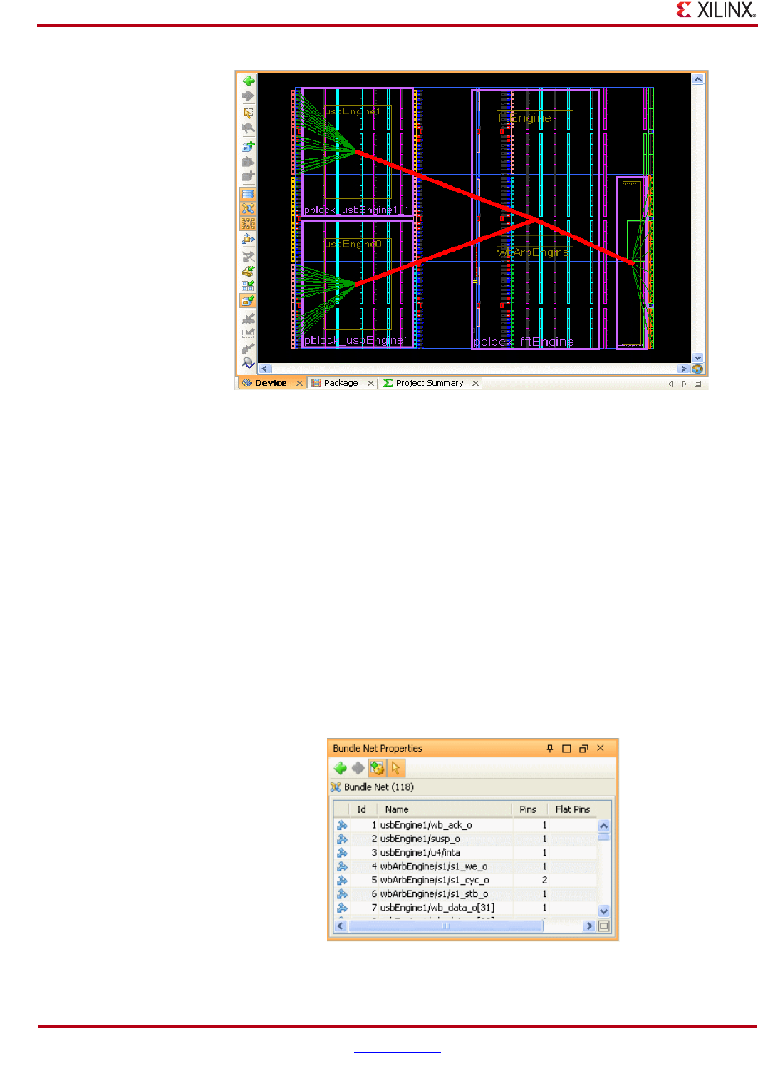
342 www.xilinx.com PlanAhead User Guide

UG632 (v 12.1)

Chapter 11: Floorplanning the Design

The combined connectivity between Pblocks shows as bundled nets. Each bundle is sized

and colored-based on the number of connections between Pblocks so that the heavily

connected Pblocks are easy to identify.

A reasonable strategy might be to define the Pblocks with the largest net bundles close

together. Typically, the Pblocks should be placed in such a way as to achieve the shortest

net lengths and to avoid routing conflicts or congestion.

Displaying Bundle Net Properties

You can view connectivity information by displaying properties for net bundles or for

individual nets. To view connectivity information:

1. Select the net or bundle net.

2. View the Net Properties or Bundle Net Properties view.

The Nets tab in the Bundle Net Properties dialog box displays the nets contained in the

bundle as shown in the following figure.

Figure 11-25: Using Connectivity To Determine Floorplan

Figure 11-26: Bundle Net Properties: Nets Tab

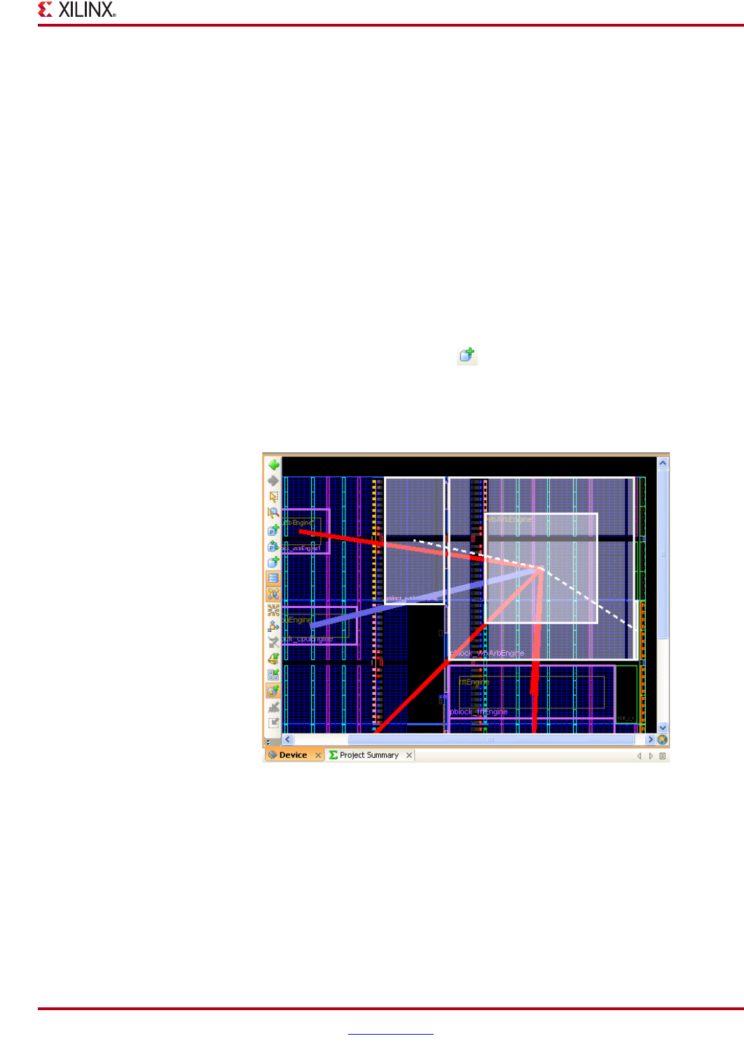
PlanAhead User Guide www.xilinx.com 343

UG632 (v 12.1)

Configuring Pblocks

Adjusting Bundle Net Defaults

You can define the color, line width, and signal count range in the view-specific settings of

the Themes dialog box (Tools > Options > Themes > Bundle Nets). For more

information on setting Bundle Net defaults, see “Setting the Device View Bundle Nets

Display Options” in Chapter 4.

Using Non-Rectangular Pblocks

PlanAhead supports the creation, modification, and deletion of non-rectangular Pblock

shapes with multiple rectangles per Pblock.

Creating Non-Rectangular Pblocks

To add additional rectangles to existing Pblocks with rectangles, use the Add Pblock

Rectangle toolbar button, as shown in the following figure.

Pblocks with multiple rectangles appear as separate rectangles with a dashed line

connecting them as shown in the following figure.

Figure 11-27: Add Pblock Rectangle

Figure 11-28: Pblock with Multiple Rectangles

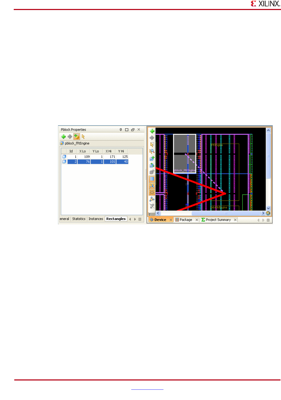
344 www.xilinx.com PlanAhead User Guide

UG632 (v 12.1)

Chapter 11: Floorplanning the Design

Modifying Non-Rectangular Pblocks

When you select a Pblock with multiple rectangles defined, all of its rectangles are selected.

They can be moved individually, or together as a group.

To reshape one of the rectangles of a multiple rectangle Pblock, select a rectangle and use

the Set Pblock Size command or resize it manually.

To select or resize a rectangle individually, use one of the following methods:

•To select a single Pblock rectangle, click Select in the popup command.

•To select them individually, select the Pblock Properties Rectangles tab.

Pblocks defined that span PowerPC® (405 and 440) processors and MGT sites might

receive multiple rectangle regions automatically. This is done to enable the correct

rectangle ranges to be defined for implementation. The following figure shows an example

of an individually-selected Pblock.

Note: The tools are not optimized to handle too many ranges per the AREA_GROUP constraint. It

is best to use simple shape configurations such as L or T shapes.

Figure 11-29: Selecting the Pblock Rectangles Individually

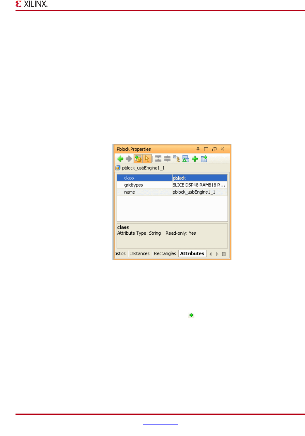
PlanAhead User Guide www.xilinx.com 345

UG632 (v 12.1)

Configuring Pblocks

Removing a Pblock Rectangle

You can remove the Pblock rectangle by selecting the Pblock and clicking the Clear

Rectangle popup command.

•Individual Pblock rectangles can be cleared one at a time.

•Multiple rectangles and Pblocks can be cleared simultaneously.

•Clearing Pblock rectangles does not delete the Pblock from the Physical Constraints.

Setting Attributes for Pblocks

Attribute properties can be assigned to Pblocks in the Pblock Properties Attributes tab.

Assigning attributes sets various options for ISE.

Note: Setting these attributes can affect implementation results or cause failures.

The following figure shows the Attributes tab.

To define new attributes for the Pblock:

1. in the Attributes tab of the Pblock Properties View, select Add pre-defined attributes

from the popup menu, or click the Define new attribute toolbar button as shown in the

following figure.

Figure 11-30: Pblock Properties View: Attributes Tab

Figure 11-31: Add Pre-defined Attribute Toolbar Button

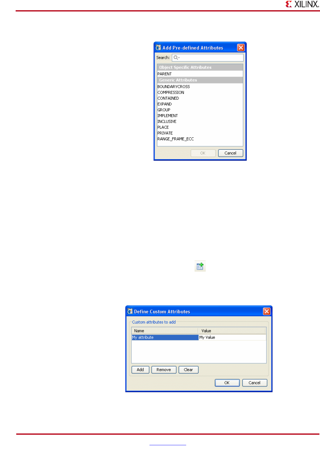
346 www.xilinx.com PlanAhead User Guide

UG632 (v 12.1)

Chapter 11: Floorplanning the Design

The Add Pre-defined Attributes dialog box opens as shown in the following figure.

2. Select the attribute to assign, and click OK.

The specified attribute type is added in Attributes tab.

You can then specify an attribute value.

3. Click Apply to accept the changes.

Creating a Custom Attribute

Custom attributes can be defined by selecting the Create Custom attributes toolbar button,

shown in the following figure.

The Define Custom Attributes dialog box opens as shown in the following figure.

4. Click Add to create Attributes.

Figure 11-32: Define Attribute Dialog Box

Figure 11-32: Create Custom Attribute Button

Figure 11-33: Define Attribute Dialog Box

PlanAhead User Guide www.xilinx.com 347

UG632 (v 12.1)

Configuring Pblocks

5. You can then specify an attribute name and value.

6. Click OK to accept the changes.

Renaming a Pblock

You can rename Pblocks using the General tab of the Pblock Properties view. Enter the new

Pblock name in the Name field and click Apply.

Deleting a Pblock

You can delete selected Pblocks as follows:

1. In the Physical Constraints view, select one or more Pblocks.

2. Press the Delete key, or select the Delete popup menu command.

3. In the Confirm Delete dialog box, you can select the Remove Pblock children option

to remove any nested Pblocks along with their partitions. Otherwise, when left

unselected, you will delete the selected Pblock only and move any nested Pblocks up

one layer of hierarchy.

4. Click OK to remove the Pblock partition from the Physical Constraints view.

Running the Automatic Pblock Placer

PlanAhead enables automatic Pblock placement using the Auto-create Pblocks

command. This method is used primarily to create top-level Pblocks to view the data flow

of the design and to understand the relative size and relationship between the various

logic modules in the design. Normally, the designer has some concept of the critical

modules and circuitry in the design and begins floorplanning with those modules.

The automatic floorplanning features are not meant to be used as the only floorplanning

methodology. They are to be used as a tool to help the designer understand the physical

design. Floorplanning is a manual process that leverages designer insight to help guide the

ISE tools.

The PlanAhead Pblock placer sizes and places Pblocks automatically in the device. Pblocks

are sized based on SLICE content only. All other device types are ignored when Pblocks are

created. The Pblocks are created with all RANGES defined.

The Pblock Placer command is intended to provide a quick placement of the selected

pblocks. This is often very helpful to view the data flow through the design. You are

required to adjust Pblock shapes manually before ISE implementation to include non-

SLICE resources.

Note: The resulting Pblocks from the Place Pblocks command might not be suitable for ISE

implementation. They are sized based on SLICE logic only. You are required to size the Pblocks

manually to include non-SLICE based logic resources.

To run the block placer:

1. Select Tools > Place Pblocks.

The Place Pblocks dialog box opens as shown in Figure 11-34, page 348.

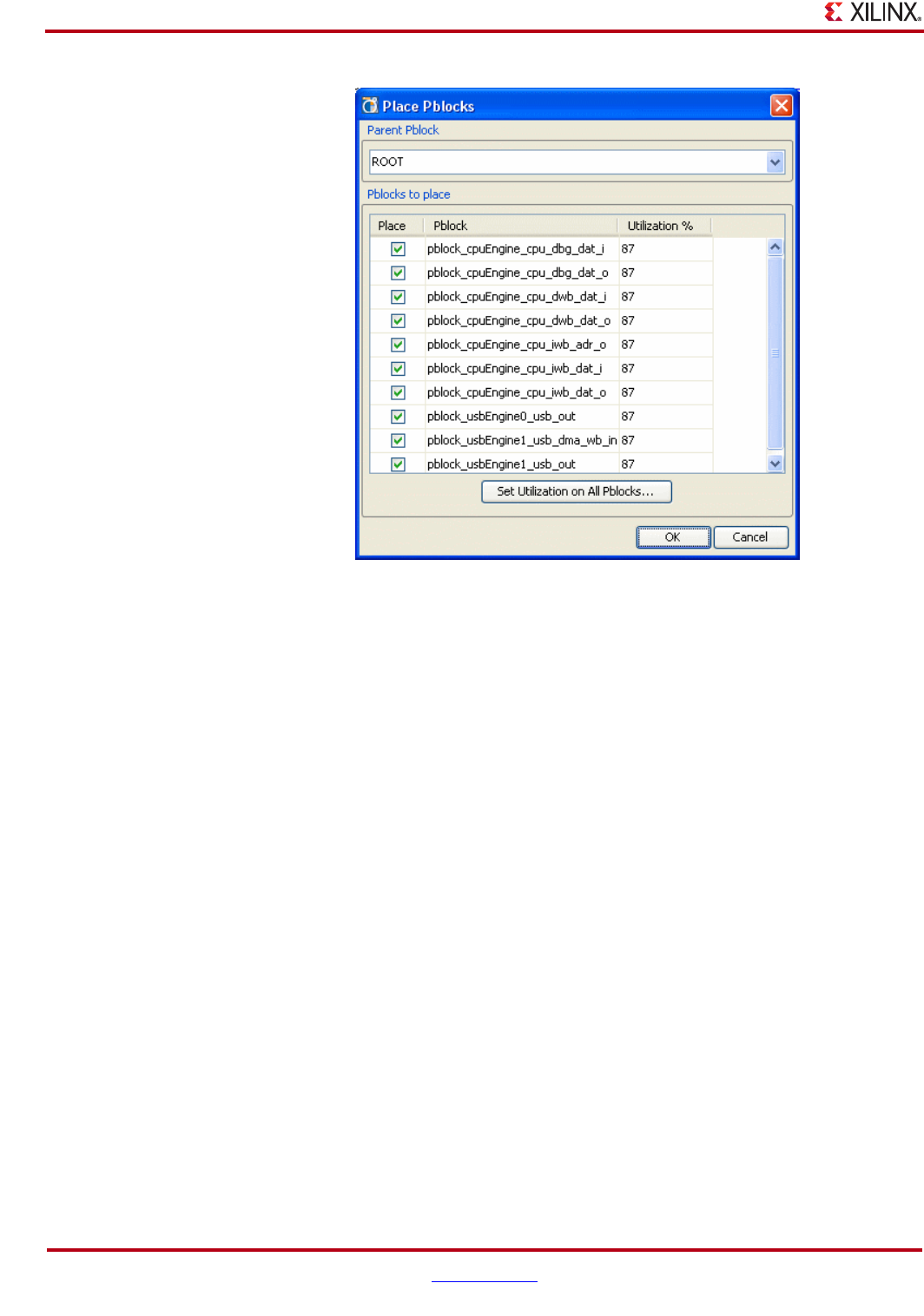
348 www.xilinx.com PlanAhead User Guide

UG632 (v 12.1)

Chapter 11: Floorplanning the Design

2. View and edit the definable options in the Place Pblocks dialog box:

−Parent Pblock—Select the level of hierarchy to place Pblocks. Pblocks can be

placed at the top “ROOT” or any partitioned Pblock-level of hierarchy.

−Pblocks to place—Displays the Pblocks that exist under the parent Pblock.

-Place—The check boxes control the Pblocks to be placed. Deselecting Place

preserve existing Pblock rectangle locations.

-Pblock—Lists all Pblocks.

-Utilization—Enables specific SLICE utilization targets to be set for each Pblock.

−Set Utilization on all Pblocks—Specifies a new target SLICE utilization target

for Pblocks.

3. Click OK to place Pblocks in the design.

A Place Pblocks progress meter displays while the Place Pblocks command is

running.

The Pblocks are sized and placed automatically based on SLICE utilization only.

Refer to the PlanAhead Design Analysis and Floorplanning Tutorial for instructions how

to create top-level floorplans using the Create Pblocks and Place Pblocks commands.

Figure 11-34: Place Pblocks Dialog Box

PlanAhead User Guide www.xilinx.com 349

UG632 (v 12.1)

Working with Placement LOC Constraints

You can assign primitive logic elements to specific logic sites using either the Create Site

Constraint Mode or the Create BEL Constraint Mode command.

PlanAhead includes BEL-level constraint assignments to lock logic to specific gates within

the site.

Understanding Fixed and Unfixed Placement Constraints

PlanAhead differentiates placement constraints that are user-assigned to those that are

assigned by the ISE implementation tools. User-assigned constraints are either defined

within imported UCF files or manually assigned in PlanAhead.

Constraints that are user assigned are considered “fixed” and are displayed in a different

color. Placement constraints imported from ISE are considered “unfixed.” You can set

placement constraints to fixed using the Fix Instances popup menu command.

PlanAhead exports fixed constraints are by default to the ISE implementation tools to lock

the placement. The Tools > Export Constraints and Tools > Export Pblocks dialog

boxes have a switch to enable exporting both fixed and unfixed placement constraints.

Understanding Site and BEL Level Constraints

Site constraints result in a LOC constraint being assigned to the instance. The logic element

is locked to the CLB SLICE site only, and not to any specific gate. The following is an

example code snippet:

INST “receiver/uartInst/G_98_1” LOC = SLICE_X49Y69;

BEL constraints result in a LOC constraint and a BEL constraint being assigned to the

instance in the saved and exported UCF files. BEL constraints will assign a logic element to

a specific gate within the CLB, as shown in the following example code snippets:

INST “channel/receiveRE[8]” BEL = FFX;

INST “channel/receiveRE[8]” LOC = SLICE_X59Y2;

Assigning Site Location Placement Constraints (LOCs)

You can place a leaf-level primitive instance into a specific device resource site by dragging

it from the netlist tree and dropping it onto a specific site. When you place instances into

sites, PlanAhead adds Instance location constraints (LOCs) to the exported UCF files for

ISE. The assigned locations are assigned as fixed and locked during subsequent ISE

attempts.

Before assigning instances, click the Create Site Constraint Mode toolbar button, shown in

the following figure, to initiate the Create Site Constraint Mode.

The dynamic cursor does not allow instance placement to an illegal site, or a site that is

already occupied. A legal placement site is indicated when the dynamic cursor changes

from a slashed circle to an arrow or diamond. The dynamic cursor does not allow instances

to be placed if the SLICE will be over-packed with logic. Certain logic groups, such as

carry-chain logic, move as a single object, which requires open placement sites for all logic

on the carry chain.

Figure 11-35: Create Site Constraint Mode Toolbar Button

350 www.xilinx.com PlanAhead User Guide

UG632 (v 12.1)

Chapter 11: Floorplanning the Design

After location constraint assignment is complete, return to the default Assign instance to

Pblock mode by clicking the Assign Instance Mode toolbar button as shown in the

following figure.

To view location constraint properties, select the placement constraint, and view the

Instance Property view.

Assigning BEL Placement Constraints (BELs)

A leaf-level primitive instance can be placed into a specific device gate site by dragging it

from the netlist tree and dropping it onto a specific site.

Placing instances into gates assigns BEL constraints for ISE, as described above. The

assigned locations will be assigned as fixed and locked during subsequent ISE attempts.

Before assigning instances, toggle the Create BEL Constraint Mode toolbar button on to

initiate the Create BEL constraint mode. The following figure shows the button.

The dynamic cursor will not allow instance placement to an illegal or already occupied

gate sites. A legal placement site is indicated when the dynamic cursor changes from a

slashed circle to an arrow. The dynamic cursor does not allow instances to be placed if the

SLICE will be over packed with logic.

After location constraint assignment is complete, return to the default Assign instance to

Pblock mode by clicking the Assign Instance Mode toolbar button, as shown in the

following figure.

To view location constraint properties, select the placement constraint, and view the

Instance Property view.

Figure 11-36: Assign Instance Mode Toolbar Button

Figure 11-37: Create BEL Constraint Mode Toolbar Button

Figure 11-38: Assign Instance Mode Toolbar Button

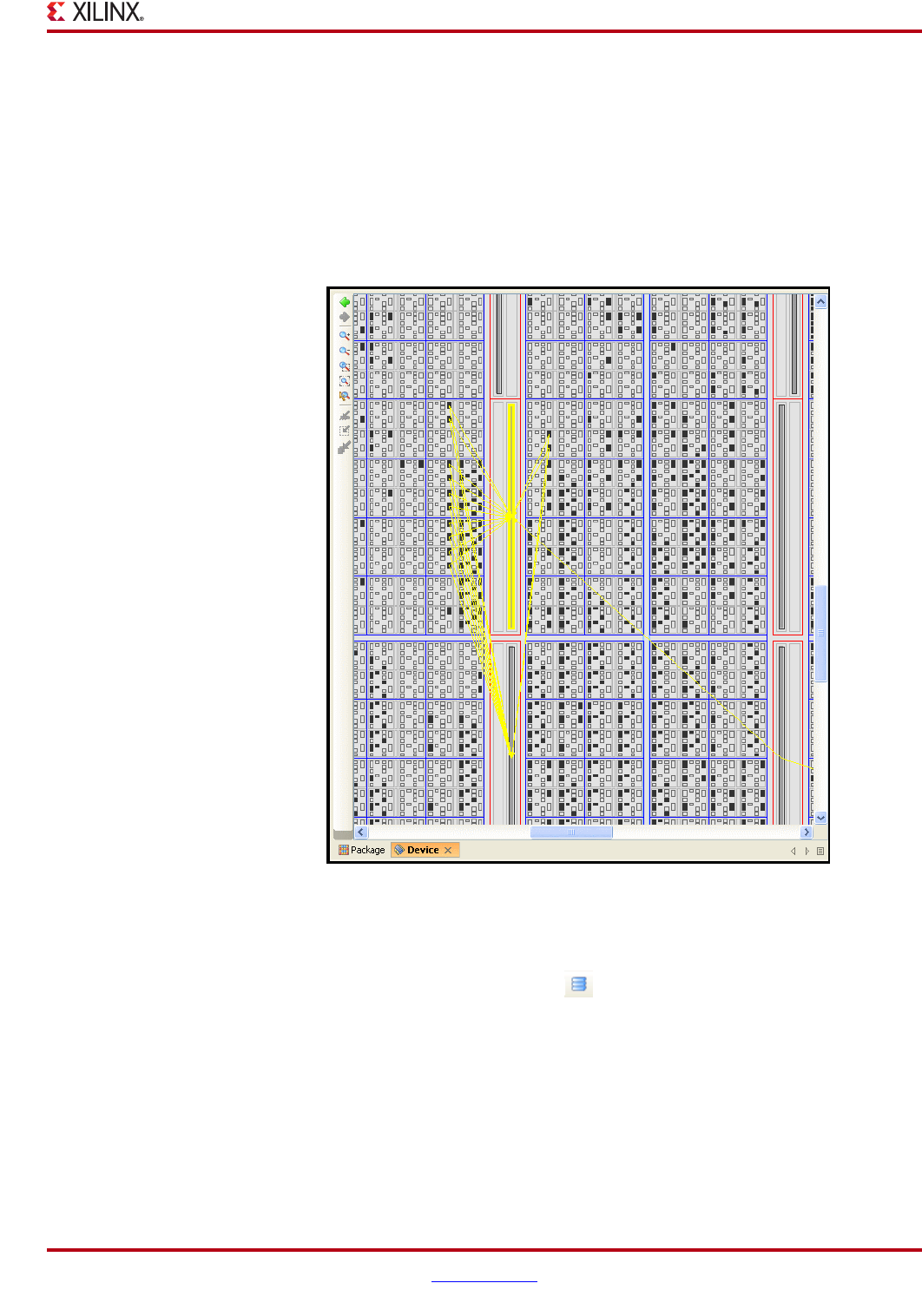
PlanAhead User Guide www.xilinx.com 351

UG632 (v 12.1)

Working with Placement LOC Constraints

Adjusting the Visibility of Placement Constraints

To change how assigned placement constraints display, you can adjust the zoom level.

•From a zoomed out view, the LOCs and BELs display as a filled in rectangle inside the

assigned site.

•When the zoom level increases, the logic displays as being assigned to specific logic

gates within the site.

The following figure shows a zoomed-out Device view.

To display or hide the location constraints, click the Show/Hide LOC Constraints toolbar

button, as shown in the following figure.

Figure 11-39: Zoomed Out Device View

Figure 11-40: Show/Hide LOC Constraints Toolbar Button

352 www.xilinx.com PlanAhead User Guide

UG632 (v 12.1)

Chapter 11: Floorplanning the Design

To adjust other display characteristics for the LOC and BEL constraints:

1. Select Tools > Options > Themes > Device.

The Device dialog box displays.

2. Adjust values in the display, select columns or adjust the colors in the Frame Color and

Fill Color columns.

Fixed and unfixed placement constraints have individual color and selection controls.

Moving Placement Constraints

To move placement constraints:

1. Select a placement constraint by clicking on the Instance in the Device view, Netlist

view or Schematic view.

2. Drag and drop the selected placement constraint to another legal site.

The primitive instance is assigned to the new site. Net flight lines can be displayed

from the location constraint to connected placed logic or Pblocks.

Moving a combinational logic object such as a MUX, a carry chain, or other results in

the entire group of LOCs being selected for move. The cursor will indicate legal

placement sites for the entire group and all objects will move to new relative locations.

All logic can be assigned to sites outside of the Pblock rectangle. This allows flexibility

when locking placement for of logic elements, such as RAMs and DSPs.

3. After location constraint assignment is complete, return to the default Assign Instance

to Pblock mode by clicking the Assign Instance Mode toolbar button.

To view location constraint properties, select the placement constraint, and view the

Instance Property view.

Deleting Selected Placement Constraints

Selected instance location constraints can be deleted by selecting the placed instances, and

using one of the following methods:

•Select Tools > Clear Placement Constraints. The following section, “Selectively

Clearing Placement Constraints,” describes how to clear placement constraints.

•Click the Unplace popup menu command.

Selectively Clearing Placement Constraints

Instance location constraints can be selectively removed from the design. You can filter the

type of constraints you want to clear based on ISE assigned, selected logic or Pblocks and

specific logic types.

Preselected objects will dictate the behavior of the Clear Placement Constraints wizard.

If Pblocks are pre-selected, the wizard displays default settings to clear placement

constraints inside of them. If Instances are selected, the wizard displays default settings to

remove them.

Figure 11-41: Assign Instance Mode Toolbar Button

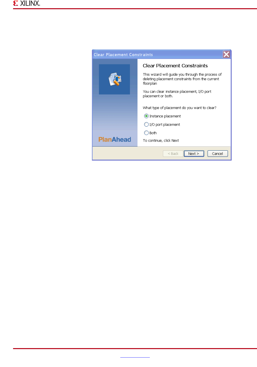
PlanAhead User Guide www.xilinx.com 353

UG632 (v 12.1)

Working with Placement LOC Constraints

To clear placement constraint assignments:

1. Select Tools > Clear Placement.

The Clear Placement Constraints wizard is invoked as shown in the following figure.

2. In the Clear Placement Constraints wizard, specify the type of placement constraints

you wish to remove: Instance placement, I/O Port placement, or both.

3. Click Next.

Placing Instances

The next dialog box changes based upon what types of objects were selected prior to

invoking the command:

•If a Pblock is selected, it defaults to clear the contents of the Pblock.

•If instances are selected, it defaults to remove them.

Additional options are presented depending on the preselected set, as shown in the

Figure 11-43, page 354.

Figure 11-42: Clear Placement Constraints Wizard

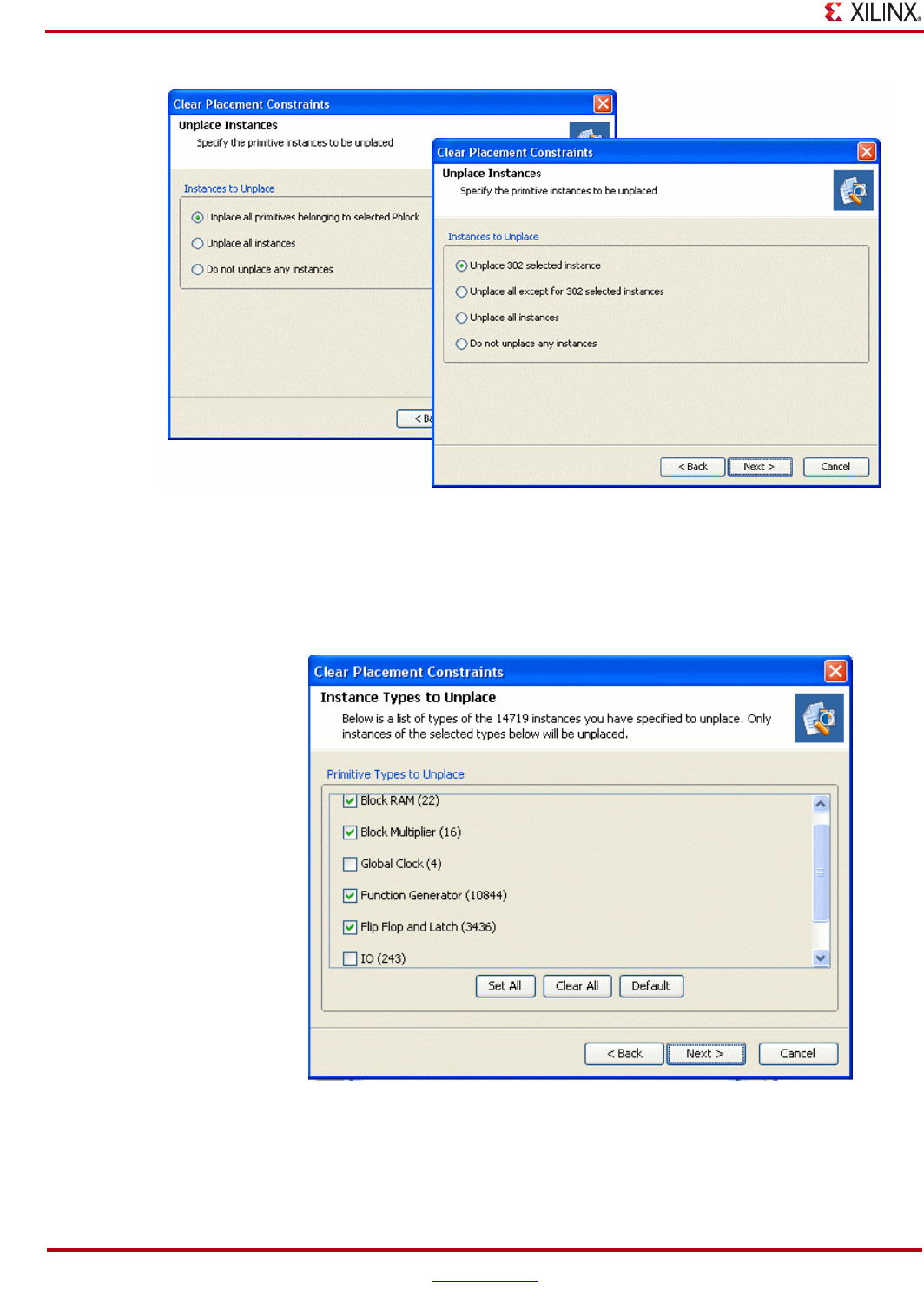
354 www.xilinx.com PlanAhead User Guide

UG632 (v 12.1)

Chapter 11: Floorplanning the Design

4. In the Unplace Instances page, select the category of instances to be unplaced.

5. Click Next.

The Clear Placement Constraints wizard opens as shown in the following figure.

The Instance Types to Unplace page provides a mechanism to filter the types of

placement constraints to filter.

Figure 11-43: Clear Placement Constraints Wizard: Placement Removal Options Based on Pre-Selected

Objects

Figure 11-44: Clear Placement Constraints Wizard: Filter Logic Types to Remove

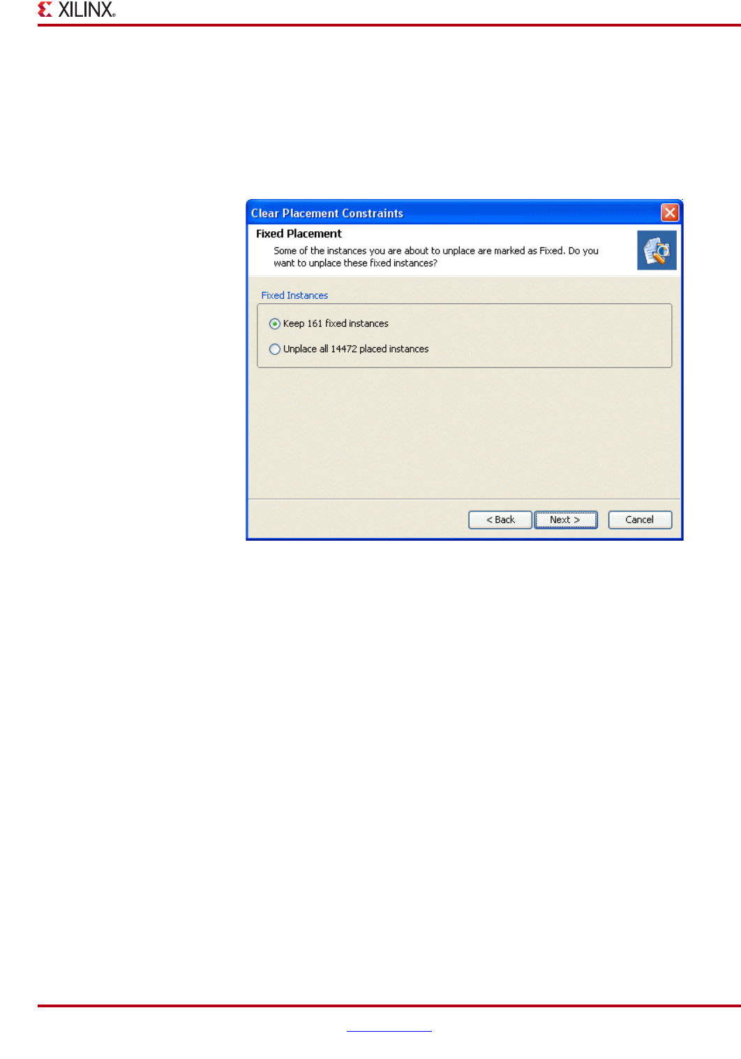
PlanAhead User Guide www.xilinx.com 355

UG632 (v 12.1)

Working with Placement LOC Constraints

The I/O related boxes are unchecked because the election to clear instance constraints

in the first page of the wizard only was made.

6. In the Instance Types to Unplace page, select the Primitive Types checkbox.

7. Click Next.

The Clear Placement Constraints: Fixed Placment dialog box opens as shown in the

following figure.

8. In the Fixed Placement dialog box, specify whether or not to unplace the fixed

instance(s). Fixed instances are those you placed or “fixed” in your design, or those

you imported in the input UCF files.

9. Click Next.

10. Verify the contents of the Summary page, and click Finish.

The specified primitive instance assignments are removed from the design.

Figure 11-45: Clear Placement Constraints Wizard: Filter Fixed Constraints

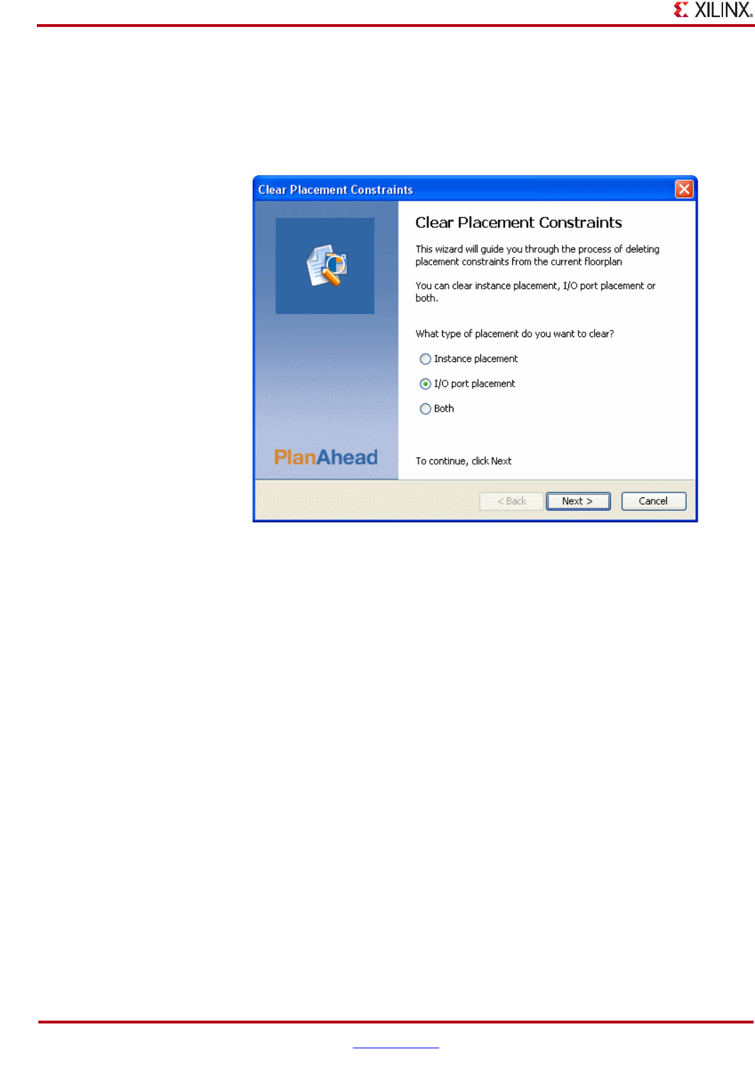
356 www.xilinx.com PlanAhead User Guide

UG632 (v 12.1)

Chapter 11: Floorplanning the Design

I/O Port placement

To clear I/O Port constraint assignments:

1. Select Tools > Clear Placement Constraints.

The Clear Placement Constraints wizard opens as shown in the following figure.

2. In the Clear Placement Constraints wizard, specify the type of placement to clear:

Instances placement, I/O Port placement or Both.

3. Click Next.

The next dialog box differs depending on the object types that were selected prior to

invoking the command.

•If nothing was selected, it shows nothing.

•If I/O Ports are selected, it defaults to remove them.

Figure 11-46: Clear Placement Constraints Wizard: Clear I/O Ports or Both

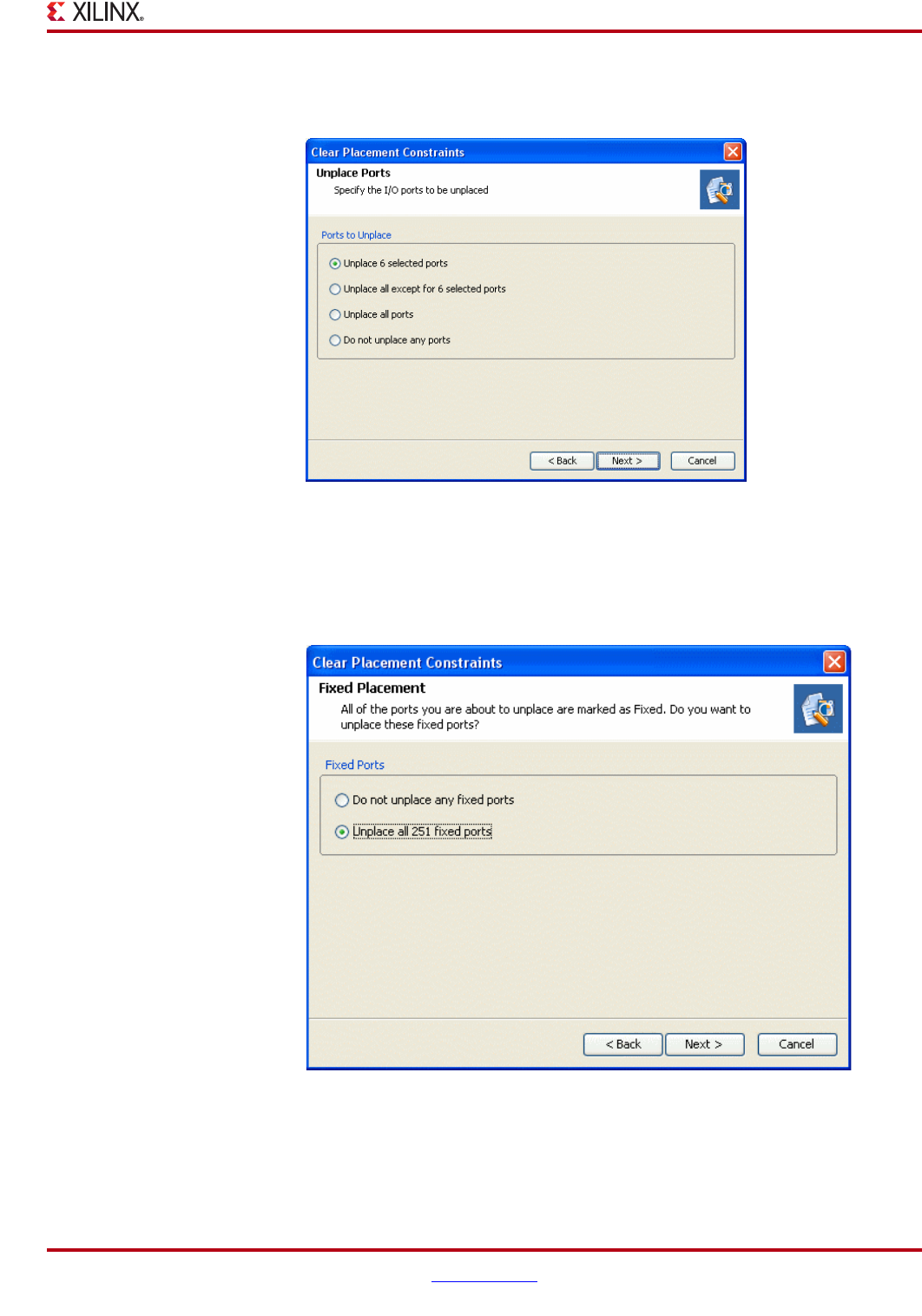
PlanAhead User Guide www.xilinx.com 357

UG632 (v 12.1)

Working with Placement LOC Constraints

Additional options are presented depending on the preselected set, as shown in the

following figure.

4. In the Unplace Ports dialog box, select the category of I/O ports to be unplaced.

5. Click Next.

The dialog box opens as shown in the following figure.

6. In the Fixed Placement dialog box, specify whether to place or unplace the fixed

instance(s). Fixed instances are those you placed or “fixed” in your design, or those

imported in the UCF files.

Figure 11-47: Clear Placement Constraints Wizard: I/O Port Removal Options

Based on Pre-Selected Objects

Figure 11-48: Clear Placement Constraints Wizard: Filter Fixed Constraints

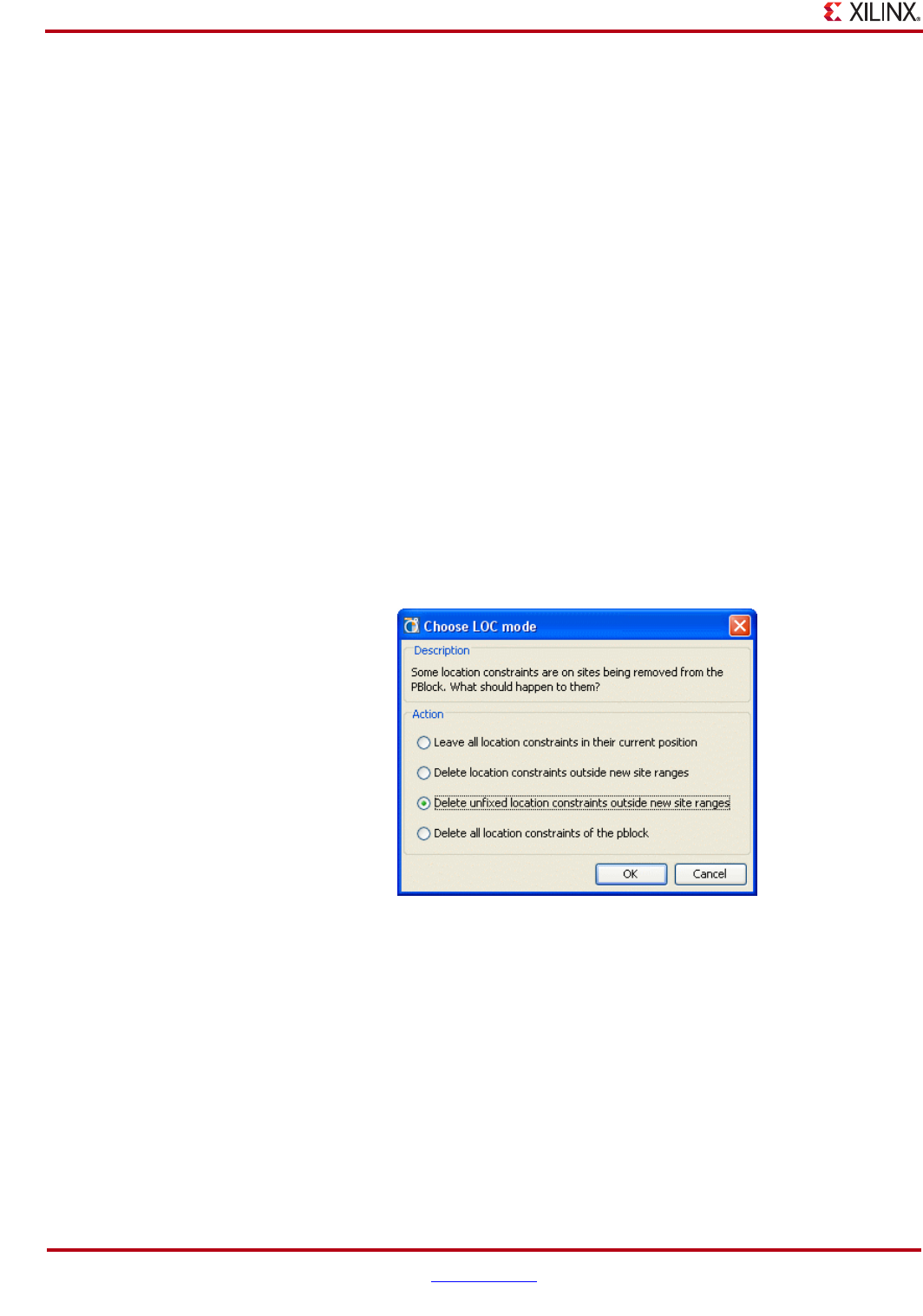
358 www.xilinx.com PlanAhead User Guide

UG632 (v 12.1)

Chapter 11: Floorplanning the Design

7. Click Next.

8. Verify the contents of the Summary page, and click Finish.

−The specified I/O ports assignments are removed from the design.

−Previously assigned ports are not cleared prior to reading a new UCF file.

−New port assignments write over previous assignments.

Note: A best practice is to first clear all port assignments prior to importing new port assignment

constraints.

Moving Pblocks with Placement Constraints Assigned

You can move a Pblock with location constraints assigned. All placement constraints are

reassigned relative to the new location.

Pblocks behave differently when location placement constraints are assigned inside of

them. The selected move location should contain adequate resources to assign the

placement constraints. The cursor indicates legal placement sites as the Pblock is being

dragged for a move.

If there are not adequate resources, a dialog box displays, prompting you to either remove

or leave the location constraints intact.

Fixed and unfixed location constraints are listed separately in the dialog box which enables

you to handle them differently. The following figure shows the Choose LOC mode dialog

box.

Locking Placement During ISE Implementation

Placement constraints assigned in PlanAhead are designated as fixed, and when exported

they result in the locked placement during subsequent exported ISE attempts.

PlanAhead provides several ways to select constraints. Often, the Find and Select

Primitives command are used to selectively fix logic objects.

For more information, refer to “Searching for Objects using the Find Command” and

“Using the Select Primitives and Highlight Primitives Commands” in Chapter 10.

Use the Fix Instances popup commands to fix selected logic.

Figure 11-48: Controlling LOC Behavior when Moving Pblocks

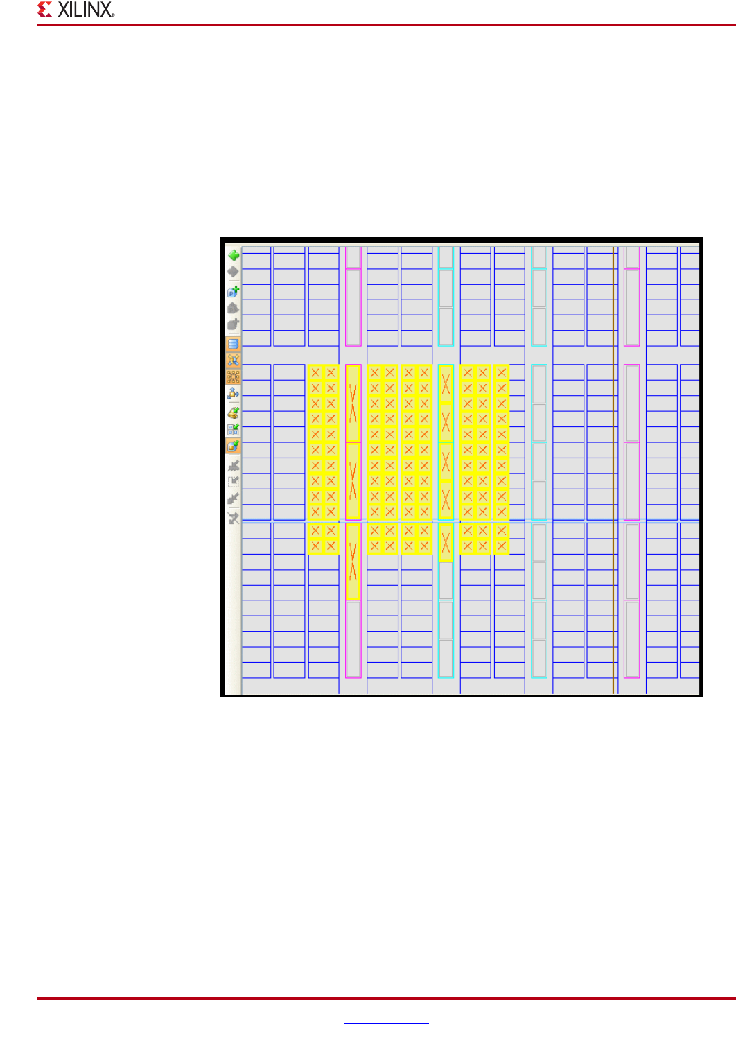
PlanAhead User Guide www.xilinx.com 359

UG632 (v 12.1)

Working with Placement LOC Constraints

Setting Placement Prohibit Constraints

You can create a Prohibit constraint for any logic site on the device. To do so:

1. Select the sites in the Device view.

You can use Select Area to select more than one site, as described in “Using the Select

Area Command” in Chapter 4.

2. Select the Set Prohibit popup menu command.

The prohibited sites display a red X, shown in the following figure.

Figure 11-49: Prohibited Sites in the Device View

360 www.xilinx.com PlanAhead User Guide

UG632 (v 12.1)

Chapter 11: Floorplanning the Design

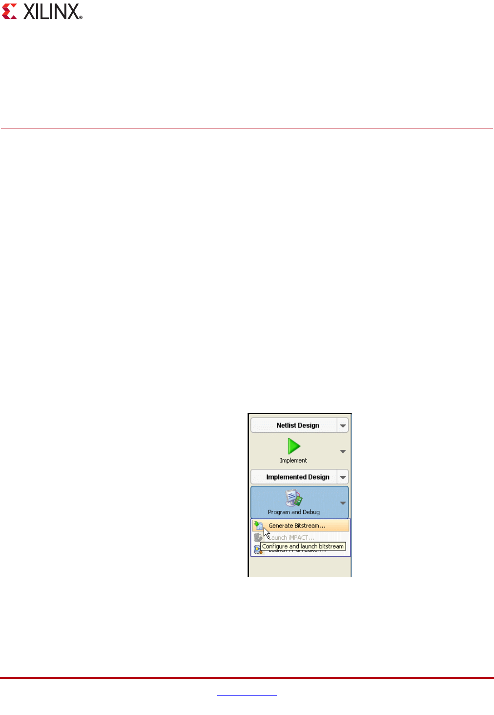
PlanAhead User Guide www.xilinx.com 361

UG632 (v 12.1)

Chapter 12

Programming and Debugging the Design

This chapter contains the following sections:

•“Generating Bitstream Files”

•“Debugging the Design with ChipScope”

•“Launching ChipScope Pro Analyzer”

•“Launching FPGA Editor”

•“Launching iMPACT”

Generating Bitstream Files

The following subsections describe how to generate bitstream files in the PlanAhead™

software.

Running Bitgen on an Implemented Design

Once a implementation has completed successfully, you can run the ISE bitgen command

on the results to create the bitstream data. To do so:

1. In the Flow Navigator, click the Program and Debug Flow button and, from the popup

menu, click Generate Bitstream. The following figure shows the command.

The Generate Bitstream dialog box opens as shown in Figure 12-2, page 362.

Figure 12-1: Running the Generate Bitstream Command

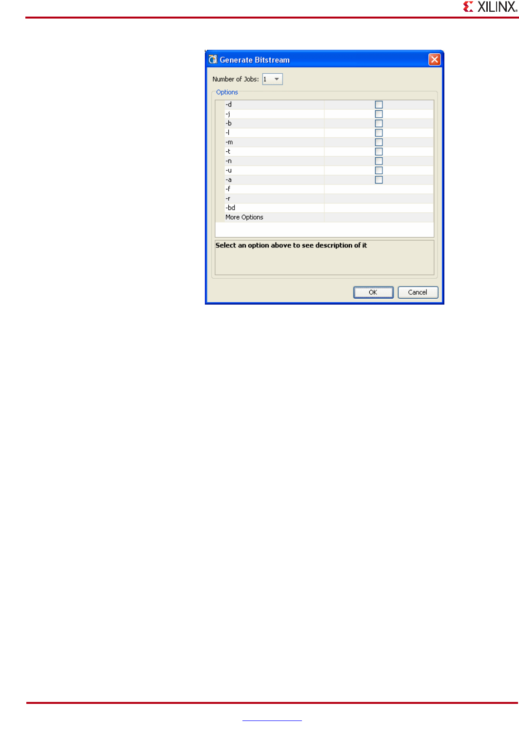
362 www.xilinx.com PlanAhead User Guide

UG632 (v 12.1)

Chapter 12: Programming and Debugging the Design

You can set the ISE bitgen command options prior to running the command.When

you select an option, a description of the option displays in the dialog box. A pulldown

menu of the available options values shows on the right side.

2. Click OK to start the Bitgen command.

You can view the command status in the Compilation Log and Compilation Messages

views and the Bitgen report file in the Reports view after it completes.

The resulting bit file is generated in the run directory of the PlanAhead project.

Figure 12-2: Setting Bitgen Options

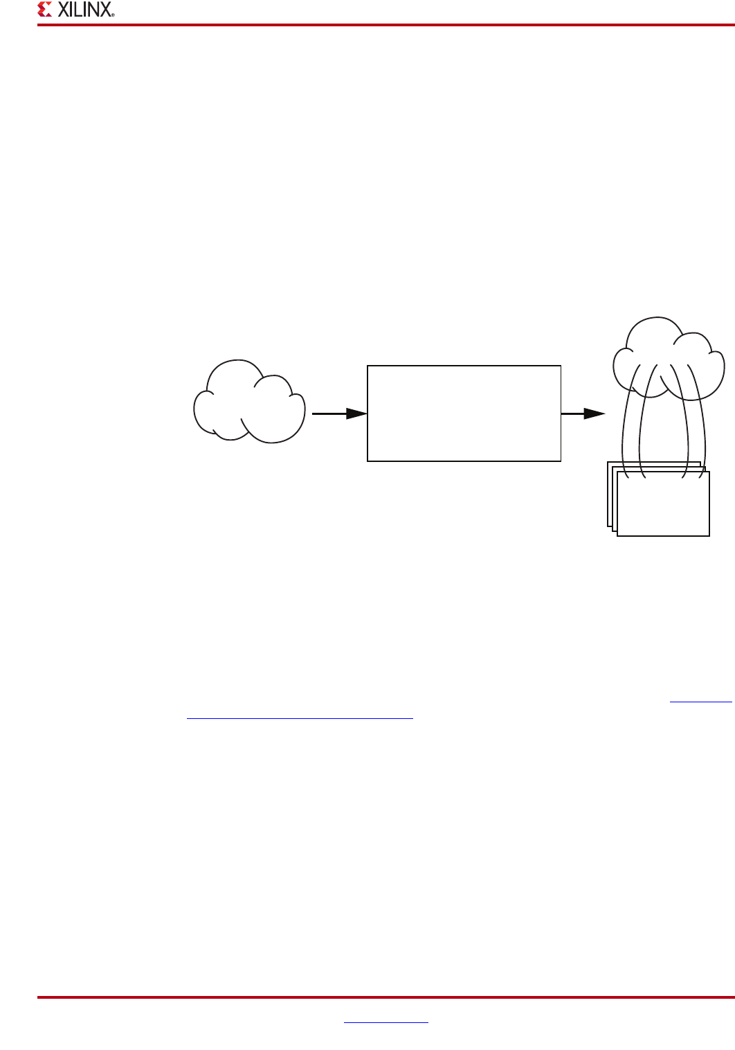
PlanAhead User Guide www.xilinx.com 363

UG632 (v 12.1)

Debugging the Design with ChipScope

The PlanAhead™ software is integrated with the ChipScope™ Pro debug software.

The ChipScopePro integration provides simplified post-synthesis insertion and connection

of the ChipScope Pro ILA debug cores in the PlanAhead tool.

Overview of ChipScope Integration in PlanAhead

PlanAhead provides a GUI wizard for quick and easy design debug for most situations. A

non-wizard GUI and Tcl command flow are available for precision debug core and net

connection control. This flow provides a robust ILA core connection solution without

leaving the PlanAhead tool. The following figure illustrates the debug core integration.

Requirements and Limitations When Using Core Insertion Flow

PlanAhead/ChipScope integration requires that the Xilinx® ISE® Design Suite 12.x tools

are installed with PlanAhead for ChipScope Pro debug core insertion.

The ChipScope Pro 12.1 Analyzer tool and the Xilinx Platform USB cable are required for

runtime design debugging. For more information about ChipScope Pro see the ChipScope

Pro 12.1 Software and Cores User Guide (UG 029).

Limitations of the PlanAhead/ChipScope integration are as follows:

•PlanAhead 12, ISE 12, and ChipScope Pro 12 tools must be used with this flow. Mixing

and matching tool versions is not supported.

•This flow is not available with the Project Navigator / ChipScope Pro Core Inserter

flow. However, you can import ChipScope Debug Cores (CDC) into PlanAhead.

•This flow is not available when in ISE Integration mode, refer to “Integration

Overview” in Chapter 15 for more information.

•You can view, but not change, pre-existing debug cores connected to a ChipScope Pro

ICON core.

•This flow is not compatible with a pre-existing ICON core generated without a

BSCAN primitive that requires connection to a BSCAN primitive instantiated outside

of the core.

Figure 12-3: Block Diagram of PlanAhead/ChipScope Integration

X11123

ChipScope

ILA Debug

Cores

PlanAhead / Chipscope

Core Insertion

User’s Design Logic

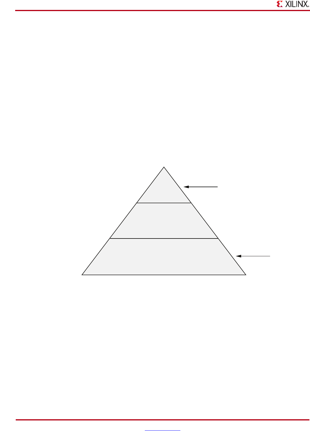
364 www.xilinx.com PlanAhead User Guide

UG632 (v 12.1)

Chapter 12: Programming and Debugging the Design

•Because the PlanAhead tool adds debug cores to the post-synthesis design netlist,

some nets might be unavailable for debugging due to trimming or other optimization

that takes place during the synthesis process.

•Only ChipScope Pro ILA cores can be created and connected using this flow.

Using the Core Insertion Flow

Insertion of ChipScope debug core in the PlanAhead tool is presented in a layered

approach to address different needs of the diverse group of PlanAhead users:

•The highest level is a simple GUI wizard that creates and configures ILA cores

automatically based on the selected set of nets to debug.

•The next level is the main ChipScope view allowing control over individual cores,

ports and their parameters.

•The lowest level is the set of Tcl debug commands that you can enter manually or

replay as a script for ultimate control.

You can use a combination of the modes to insert and customize debug cores also. The

following figure illustrates the levels of debug core insertion.

Figure 12-4: Debug Core Insertion Modes

ChipScope

Wizard

ChipScope Window

in Main PlanAhead GUI

ChipScope Tcl debug commands

Fast and simple

Precise control

X11122

PlanAhead User Guide www.xilinx.com 365

UG632 (v 12.1)

Debugging the Design with ChipScope

Deciding Which Debug Core Insertion Mode to Use

The following table summarizes how to decide what insertion mode(s) to use based on the

debugging goal.

Selecting Nets for Debug

The first step in the PlanAhead/ChipScope debug flow is to identify the set of nets to

debug.

All ChipScope debug core insertion and configuration operations must be performed in

the Netlist Design because the cores are added to the netlist prior to implementation.

PlanAhead makes the debug net selection process as simple as picking a set of nets or

busses in the Netlist view, and selecting the Add to ChipScope Unassigned Nets popup

command. You can perform net selection by selecting nets or busses in any view including

the Schematic view. There is also a net selector built into the Setup ChipScope wizard.

Using the Unassigned Nets List

PlanAhead maintains an Unassigned Nets list (shown in the following figure) in the

ChipScope view (Window > ChipScope). The Unassigned Nets list is a convenient place

to bookmark nets of interest while browsing the design.

You can store nets for later debug by dragging and dropping from the netlist or schematic

view into the Unassigned Nets list.

Also, you can add nets to the Unassigned Nets list by selecting the nets, and selecting the

Add to ChipScope Unassigned Nets popup menu command, which is shown in

Figure 12-5, page 366.

Table 12-1: Debugging Goals and Core Insertion Modes

Debugging Goal Core Insertion Mode

Quickly create ILA debug core(s) with default settings for the

selected nets

ChipScope Wizard

Change parameters on existing debug cores ChipScope Window

Manually create or delete existing debug cores ChipScope Window

Manually create, delete, or configure trigger or data ports on an

ILA core

ChipScope Window

Manually assign nets to the trigger/data/clock channels ChipScope Window

Play back a recorded script of debug commands later Tcl Commands

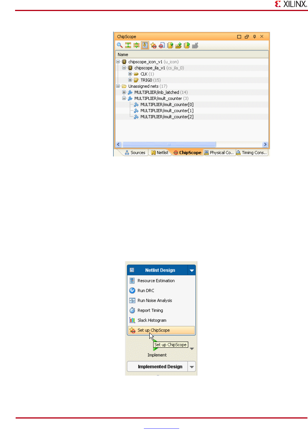
366 www.xilinx.com PlanAhead User Guide

UG632 (v 12.1)

Chapter 12: Programming and Debugging the Design

Using the ChipScope Wizard for Debug Core Insertion

The ChipScope debug wizard is the easiest and fastest way to add debug cores in the

PlanAhead design tool as shown in the following figure

To use the Set Up ChipScope wizard to insert debug cores:

1. Optionally, select a set of nets for debug either using the unassigned nets list or direct

net selection.

2. In the Flow Navigator, invoke the Set Up ChipScope wizard from the Netlist Design

menu, or click Tools > Set Up ChipScope. The following figure shows where to

launch the ChipScope wizard.

3. Follow the instructions screen by screen to connect and configure the debug cores.

Figure 12-5: Unassigned Nets List in ChipScope Window

Figure 12-6: Launching the Set up ChipScope Wizard

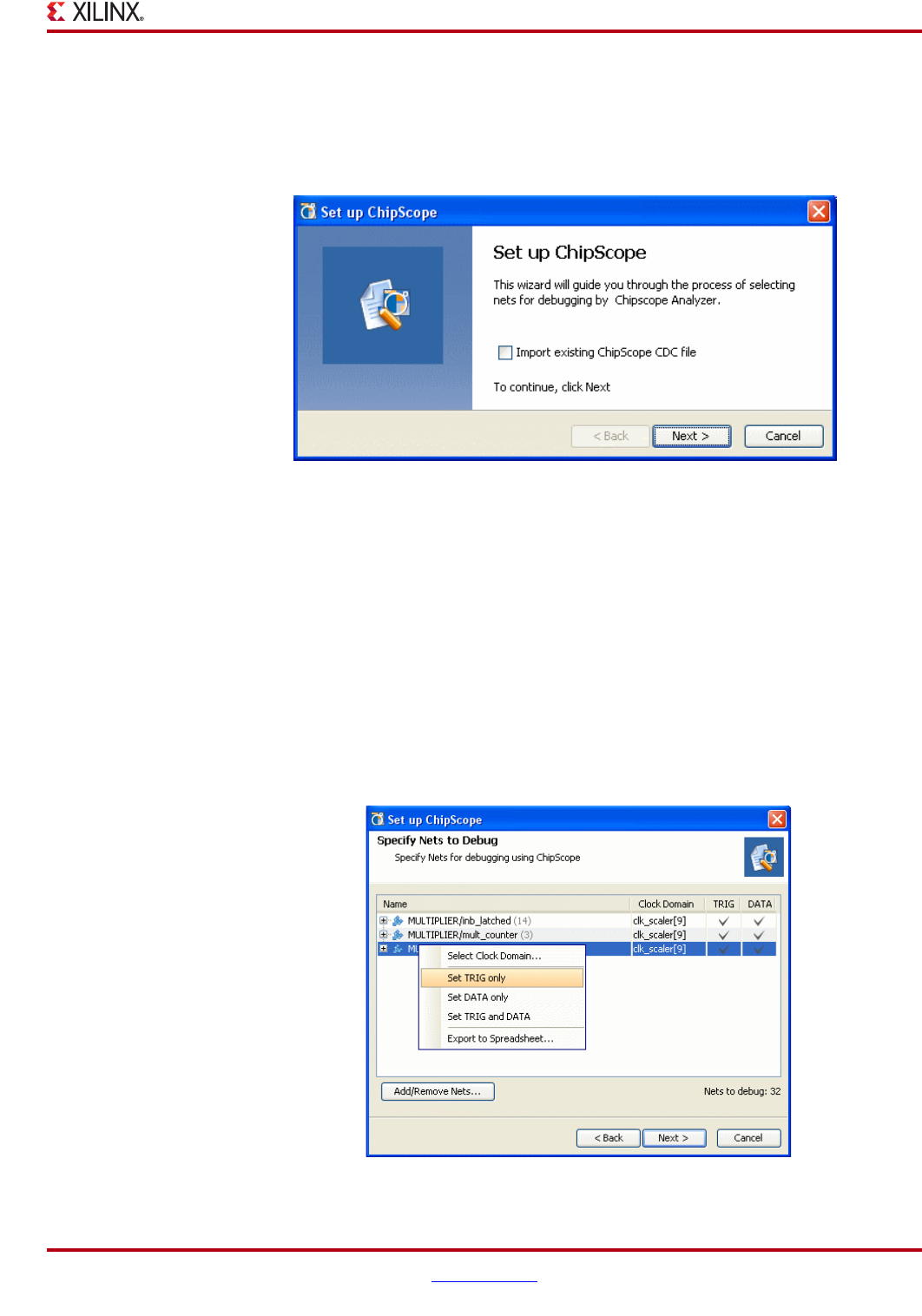
PlanAhead User Guide www.xilinx.com 367

UG632 (v 12.1)

Debugging the Design with ChipScope

Importing a ChipScope CDC File

The Set Up ChipScope wizard lets you add an existing ChipScope Debug Core (CDC) file

to the project. When you click the Set up Chipscope box a wizard pane prompts you to

select the CDC file, as shown in the following figure.

Click Next.

Selecting or Confirming Debug Nets

If nets have been added to the Unassigned Nets list, you are prompted to use them or to

select new nets.

An Add/Remove Nets dialog box is invoked to search for and select nets to debug.

Add or remove nets as needed, and click Next.

Specifying Debug Nets and Clock Domains

The ChipScope wizard attempts to detect the correct clock automatically for each selected

net or bus as shown in the following figure.

Figure 12-7: Importing an Existing ChipScope CDC File

Figure 12-8: Specifying Debug Nets and Clock Domains

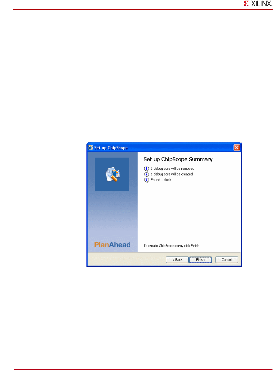
368 www.xilinx.com PlanAhead User Guide

UG632 (v 12.1)

Chapter 12: Programming and Debugging the Design

If multiple clocks are detected for a given net, a dropdown list allows the selection of

different clocks for the net or bus.

1. To modify the debug net selection further, click the Add/Remove Nets button.

2. Configure each net or bus for use as a trigger, data storage, or both.

3. When the net and clock configuration is correct, click Next to proceed to the summary

screen.

If ILA cores exist in the design, you are prompted to remove them and regenerate based on

the new information or to keep them intact and generate new cores.

Inserting ILA Cores

The ChipScope wizard inserts one ILA core per clock domain.

The nets that were selected for debug are assigned automatically to the trigger and data

ports of the instantiated ILA cores.

The last wizard screen, shown in the following figure, shows the core creation summary

displaying the number of clocks found and ILA cores to be created and/or removed.

If you are satisfied with the results, click Finish to instantiate and connect the ILA cores in

the design.

Figure 12-9: Inserting ILA Cores into Design

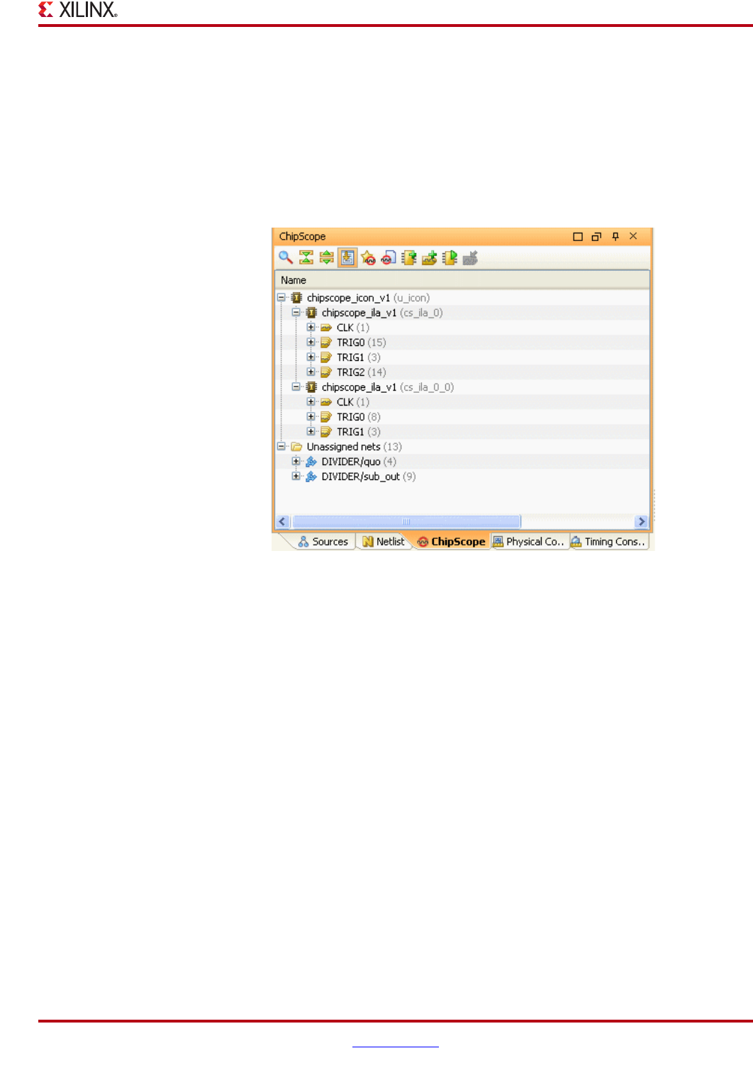
PlanAhead User Guide www.xilinx.com 369

UG632 (v 12.1)

Debugging the Design with ChipScope

Using the ChipScope Window to Add and Customize Debug Cores

The main ChipScope view provides more fine-grained control over ILA core insertion than

what is available in the ChipScope wizard.

The controls available in this window allow core creation, core deletion, debug net

connection, and core parameter changes.

To bring up the ChipScope view, select Window > ChipScope, shown in the following

figure.

The main ChipScope view:

•Shows the list of debug cores that are connected to the ICON controller core.

•Maintains the list of unassigned nets at the bottom of the window.

You can manipulate debug cores and ports from the popup menu or the toolbar buttons on

the top of the view.

Creating and Removing Debug Cores

You can create ChipScope debug cores in the ChipScope view by clicking the Create

ChipScope Debug Core popup menu command or toolbar button.

Using this interface, you can change the parent instance, debug core name, and set

parameters for the core (shown Figure 12-11, page 370).

To remove an existing debug core, in the ChipScope view, select the core and select the

Delete popup command.

Figure 12-10: ChipScope View

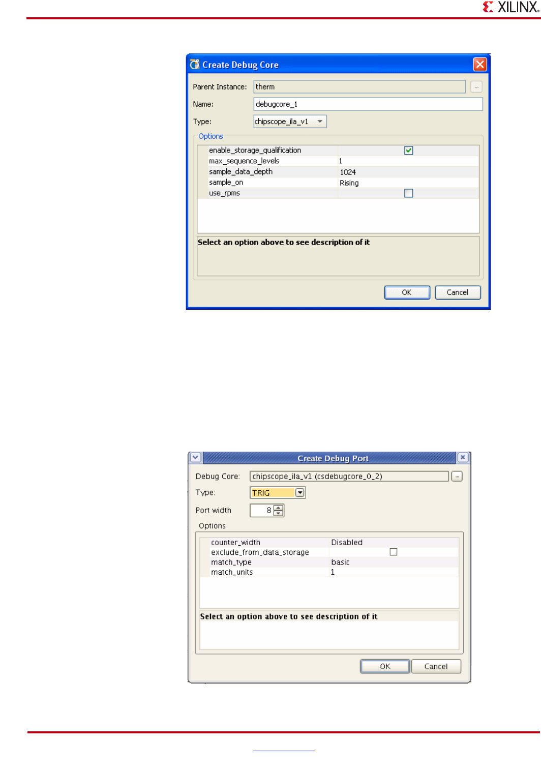
370 www.xilinx.com PlanAhead User Guide

UG632 (v 12.1)

Chapter 12: Programming and Debugging the Design

Adding, Removing, and Customizing Debug Core Ports

In addition to adding and removing debug cores, you can add, remove, and customize

ports of each debug core to suit your debugging needs. To add a new port:

1. Select the core.

2. Click the Create ChipScope Debug Port popup menu command, or toolbar button.

The Create Debug Port dialog box opens, as shown in the following figure.

Figure 12-11: Creating a Debug Core

Figure 12-12: Customizing Ports and Options of Debug Cores

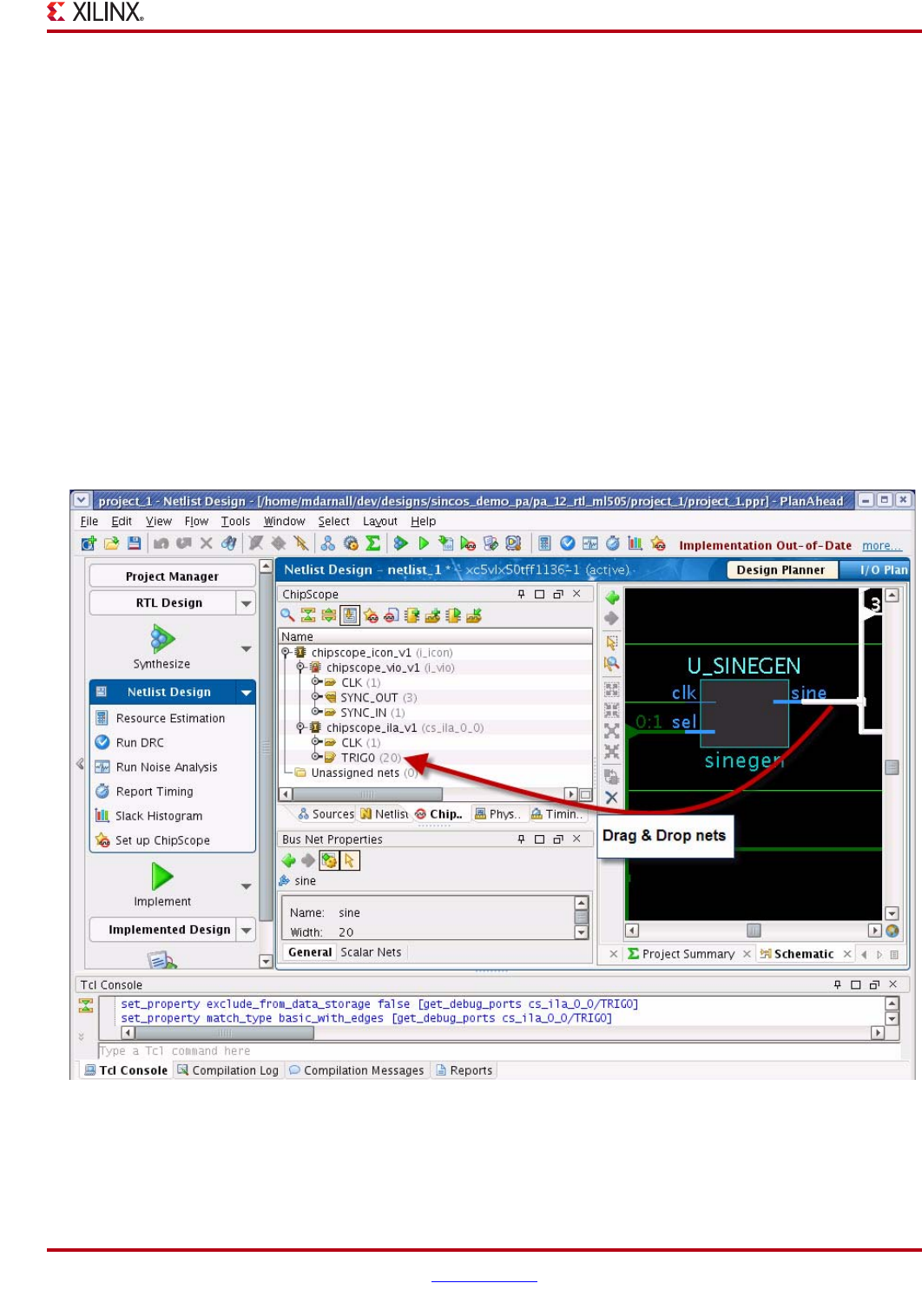
PlanAhead User Guide www.xilinx.com 371

UG632 (v 12.1)

Debugging the Design with ChipScope

3. Select the port type in the dropdown.

Any configurable options for the port display in the Options area. The port width will

start as a default, but expands or contracts as you add or remove nets from the port.

4. Click OK.

To remove a debug port, in the ChipScope tab select the port, and select Delete from the

popup menu.

Connecting and Disconnecting Nets to Debug Cores

You can select, and then drag and drop nets and busses (vectors of nets) from the

Schematic view or the Netlist view onto the debug core ports (shown in the following

figure). This expands the port as needed to accommodate the net selection.

Also, you can right-click on any net or bus, and select Assign to ChipScope Debug Port.

To disconnect nets from the debug core port, select the nets that are connected to the debug

core port, and click Disconnect Net from the popup menu. The following figure illustrates

these activities.

X-Ref Target - Figure 12-13

Figure 12-13: Dragging and Dropping Nets onto Debug Core Ports

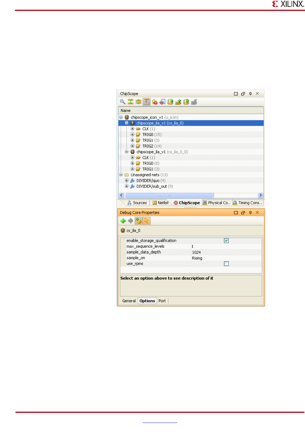
372 www.xilinx.com PlanAhead User Guide

UG632 (v 12.1)

Chapter 12: Programming and Debugging the Design

Customizing Debug Core and Port Parameters

ChipScope Debug cores have parameters that can be customized.

To access these core parameters:

1. In the ChipScope view, select one of the ChipScope debug cores.

2. In the Properties tab, select Options to configure the core parameters as shown in the

following figure.

You can modify port parameters by first clicking the Trigger or Data port of a debug core,

and selecting Options in the Properties tab, as shown in Figure 12-15, page 373.

Figure 12-14: Debug Core Parameters

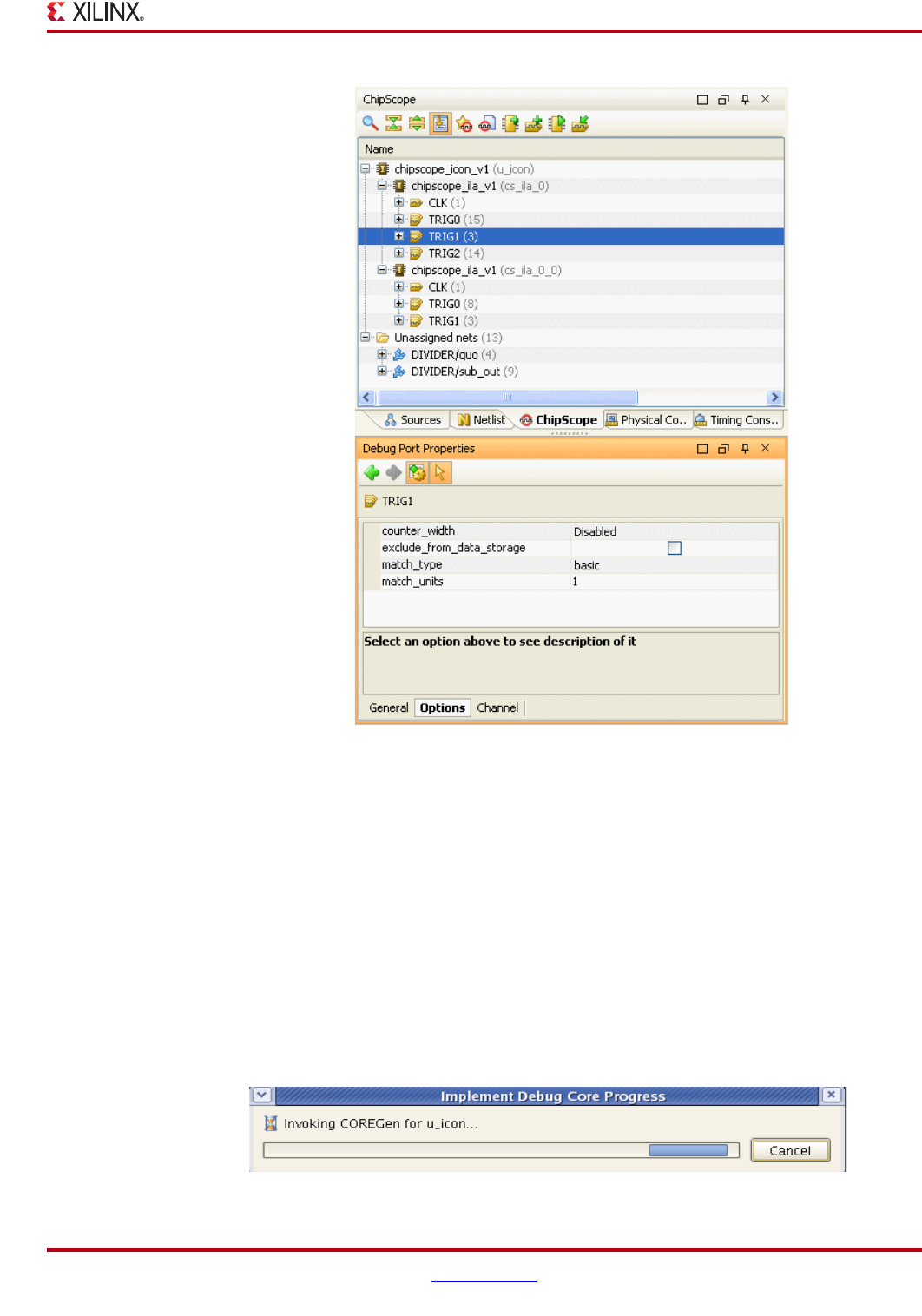
PlanAhead User Guide www.xilinx.com 373

UG632 (v 12.1)

Debugging the Design with ChipScope

Implementing Debug Cores

The PlanAhead software creates ChipScope Pro ICON and ILA cores initially as black

boxes. These cores must be implemented prior to running through map, place, and route.

ChipScope debug core implementation is automatic when running the implementation

flow using the Implement command in the Flow Navigator or Tools menu; however, you

can force debug core implementation manually for floorplanning or timing analysis by

clicking the Implement toolbar button on the left side of the ChipScope view.

The Xilinx CORE Generator™ tool invokes in batch mode for each black box debug core.

This operation can take some time. A progress dialog box shows that the operation is

running as shown in the following figure. When the debug core implementation is

complete, the debug core black boxes are resolved and you can access the generated

instances.

Figure 12-15: Debug Port Parameters

Figure 12-16: Debug Core Implementation Progress Indicator

374 www.xilinx.com PlanAhead User Guide

UG632 (v 12.1)

Chapter 12: Programming and Debugging the Design

Exporting Net Connections CDC File for ChipScope Analyzer Tool

A ChipScope Analyzer CDC file is generated automatically when design implementation

is complete. Also, you can export a CDC file manually from the Export Debug Net Names

popup command in the ChipScope view. You can import this CDC file into the ChipScope

Analyzer to automatically set up the net names on the ILA core data and trigger ports.

Implementing the Design with the Debug Cores

Once ChipScope debug cores are created and connected, you can run the standard

PlanAhead implementation flow to create a bitstream for the device.

Start the implementation flow by selecting the Implement command in the Flow

Navigator or Tools menu.

Launching ChipScope Pro Analyzer

When the ChipScope Pro Analyzer software is installed, you can launch it directly from

PlanAhead on any implemented design on which the Generate Bitstream command has

been run.

To launch ChipScope Pro Analyzer, do one of the following:

•In the Flow Navigator, select Launch ChipScope Analyzer from the Program and

Debug menu.

•In the ChipScope view tab, right-click and select Launch ChipScope Analyzer from

the context menu.

The BIT bitstream and CDC netlist name files are passed automatically to the ChipScope

Pro Analyzer when launched from PlanAhead.

Launching FPGA Editor

You can launch the FPGA Editor directly from PlanAhead on any implemented design.

To invoke the FPGA Editor, in the Flow Navigator, select the Launch FPGA Editor

command from the Program and Debug menu.

The routed NCD file is passed automatically to the FPGA Editor when launched from

PlanAhead.

Launching iMPACT

You can launch the iMPACT software tool directly from PlanAhead on any implemented

design on which the Generate Bitstream command has been run.

To invoke iMPACT, in the Flow Navigator, select the Launch iMPACT command from the

Program and Debug menu.

The BIT bitstream file is passed automatically to iMPACT when launched from PlanAhead.

PlanAhead User Guide www.xilinx.com 375

UG632 (v 12.1)

Chapter 13

Using Hierarchical Design Techniques

This chapter contains the following sections:

•“Understanding PlanAhead and ISE Capabilities”

•“Using PlanAhead for Design Preservation”

Understanding PlanAhead and ISE Capabilities

The PlanAhead™ software has several capabilities to support a hierarchical design

process. Deciding to use such an approach on your design is something that you need to

determine before starting the design. For best results, the decision to use a hierarchical

approach requires some forethought about design partitioning and RTL coding decisions.

Results can vary if you start using this methodology late in a design cycle in an attempt to

close timing or reduce run time.

Note: All of the features described in this chapter are available for netlist-based projects only.

PlanAhead does not support RTL-based hierarchical projects using partitions. Each partition requires

a separately synthesized netlist or a netlist with third party synthesis incremental compile points. This

netlist isolation makes it possible to manage updates and reuse partitions.

Using Partitions

The hierarchical capabilities all revolve around setting and managing hierarchical

boundaries in the design called partitions. These boundaries prevent the synthesis and

implementation tools from optimizing the logic across the boundaries making it possible

to isolate the logic for reuse.

Effective partitioning relies on good logic design practices and knowledge of the design.

These practices are detailed in the Hierarchical Design Methodology Guide (UG748).

Once designs with partitions are implemented, the results can be exported for use in future

runs. The partition definition and behavior is defined in an XML file called

xpartitions.pxml. The ISE® Design Suite tools search the Run directory for that file and

act accordingly. partitions are defined as well as the specified partition “action” such as

Implement or Import. The Hierarchical Design Methodology Guide (UG748) describes the

xpartitions.pxml file usage and syntax.

376 www.xilinx.com PlanAhead User Guide

UG632 (v 12.1)

Chapter 13: Using Hierarchical Design Techniques

Design Preservation

The PlanAhead project structure lets you create and manage projects from hierarchical

netlist sources. This bottom-up synthesis approach lets you selectively update modules

while keeping the rest of the design intact.

PlanAhead, coupled with the ISE partition features, can then lock the placement and

routing of selected partitions for subsequent runs.

This incremental design approach can help produce more consistent implementation

results, reduce verification time, and reduce design closure time. This capability is called

Design Preservation, which is the ability to implement and lock specific modules of a single

design for subsequent runs.

Partial Reconfiguration

PlanAhead provides an environment to configure, implement and manage Partial

Reconfiguration projects. PlanAhead uses the partitions and Partial Reconfiguration

capabilities that are built into the ISE Design Suite implementation tools.

Hierarchical Design Documentation

For more information about Hierarchical Design techniques, refer to the

Hierarchical Design Methodology Guide (UG748) and the

PlanAhead Tutorial: Leveraging Design Preservation for Predictable Results (UG747).

Partial Reconfiguration documentation is located at:

http://www.xilinx.com/tools/partial-reconfiguration

Licenses can be obtained through the Xilinx® web site at:

http://www.xilinx.com/getproduct

The following documents are available:

•PlanAhead Tutorial: Partial Reconfiguration Flow Overview (UG743)

•PlanAhead Tutorial: Partial Reconfiguration with Processor Peripherals (UG744)

•Partial Reconfiguration User Guide (UG702)

Using PlanAhead for Design Preservation

The following subsections describe the features that are available to you when you use the

Design Preservation features from PlanAhead:

•“Using PlanAhead for Design Preservation”

•“Setting Partitions”

•“Configuring Runs for Partitions”

•“Promoting Partitions”

•“Importing Partitions”

Setting Partitions

You can set partitions on any hierarchical design module in the netlist. Design Preservation

requires that you define the partitions on the same logic modules that were synthesized

separately. This will ensure the netlists and the partitions can be isolated and reused.

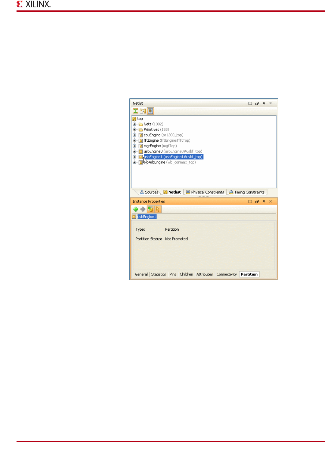
PlanAhead User Guide www.xilinx.com 377

UG632 (v 12.1)

Using PlanAhead for Design Preservation

Note: PlanAhead supports netlist based projects only for hierarchical design capabilities. The

Partition commands will not be displayed in RTL based projects

To set a partition:

1. In the Netlist view, select the module instances on which to set partitions.

2. Select the Set Partition popup menu command.

3. The instance receives a new icon in the Netlist view and a Partitions tab in the Instance

Properties view as shown in the following figure.

Once a partition has been set in the project, the rest of the design becomes a partition

automatically also. You can promote or import this “top” partition to preserve it if it

remains unchanged during a design revision.

Viewing Partition Properties

You can access the Instance Partition Properties by selecting the Partition Instance and

viewing the Instance Properties view. Select the Partition tab in the Instance Properties

view as shown in Figure 13-1.

The view contains the locations and dates of each time the Partition was promoted.

Figure 13-1: Setting Partitions in the Netlist View

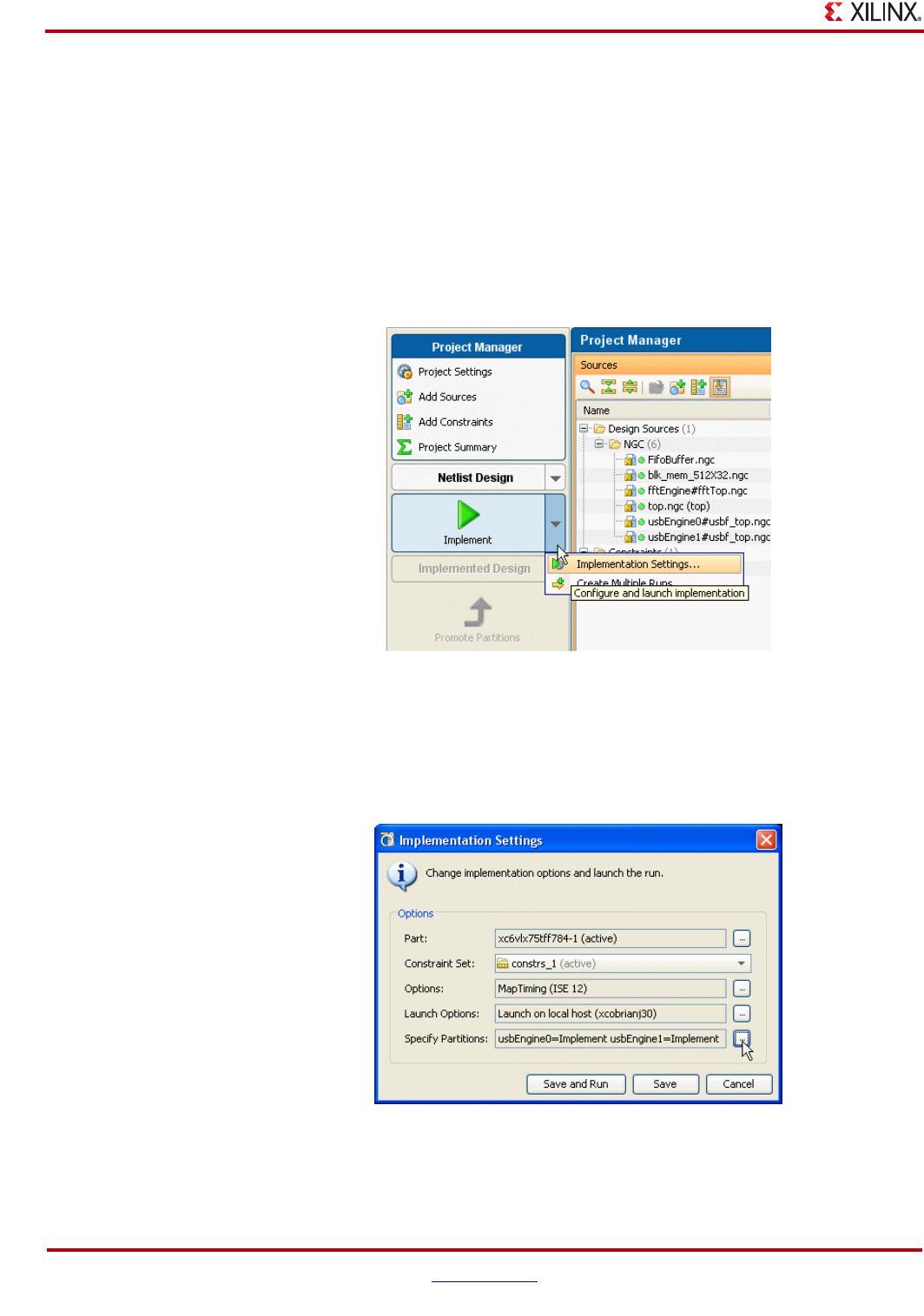
378 www.xilinx.com PlanAhead User Guide

UG632 (v 12.1)

Chapter 13: Using Hierarchical Design Techniques

Configuring Runs for Partitions

You can configure partition “Action” settings for each implementation run launched from

PlanAhead. You need to determine whether each partition is implemented or imported

and if imported, from where. PlanAhead attempts to set the appropriate action based on

recent promotions. Check to ensure the partition actions are set correctly before each run is

launched.

To set a partition action:

1. In the Flow Navigator, select the drop down menu on the right side of the Implement

button, and select Implementation Settings as shown in the following figure.

The Implementation Settings dialog box lets you configure the launch options for the run.

The Specify Partitions field displays the current action set on the partitions.

2. Select the browser button on the Specify Partitions field as shown in the following

figure.

In the Specify Partition dialog box you can set the Action for each Partition to either

Implement or Import.

Figure 13-2: Implementation Settings

Figure 13-3: Implementation Settings Dialog Box

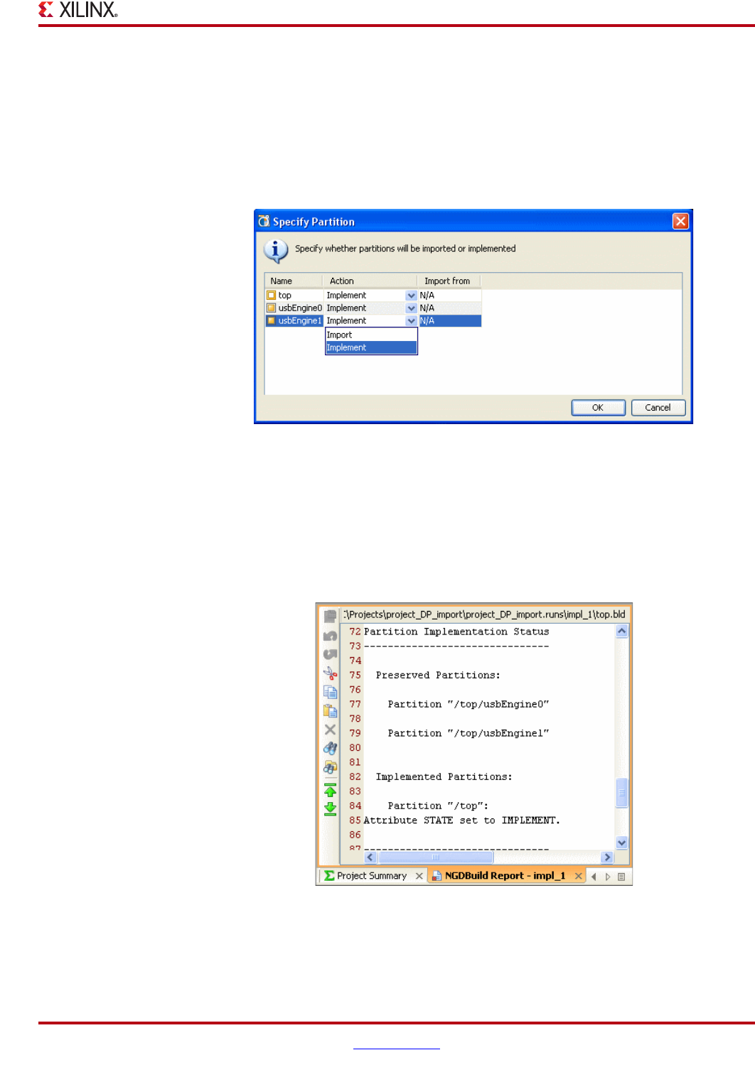
PlanAhead User Guide www.xilinx.com 379

UG632 (v 12.1)

Using PlanAhead for Design Preservation

The first time a design is implemented, all partitions should be set to Implement, because

there are no promoted locations to import the implemented partitions.

3. Set the partition action:

4. If needed, browse to select the Import from directory if importing partitions and click

OK.

The following figure shows the Specify Partition dialog box.

5. In the Implementation Settings dialog box, select Run to launch the implementation

run with the new Partitions Action settings.

6. Monitor the ISE command status in the Compilation Log view.

7. Once the ISE ngdbuild command completes, review the Ngdbuild report by selecting

it from the Reports view. The actions taken for the partitions in the run display in the

ngdbuild report.

Figure 13-4: Specify Partitions Dialog Box

Figure 13-5: Viewing Partition Actions in Ngdbuild Report

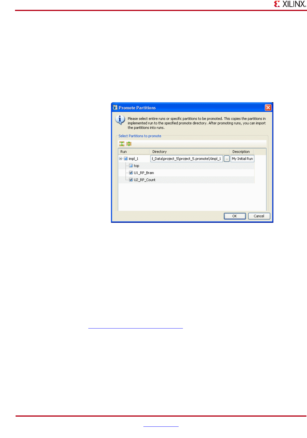
380 www.xilinx.com PlanAhead User Guide

UG632 (v 12.1)

Chapter 13: Using Hierarchical Design Techniques

Promoting Partitions

Once satisfactory implementation results are achieved, you can copy the ISE result files to

a repository area for future import operations. This process is called “Promoting” the

partitions. You can only promote partitions from successfully implemented runs in

PlanAhead.

To promote partitions:

1. In the Flow Navigator, select the Promote Partitions button. The Promote Partition

dialog box opens, as shown in the following figure.

The Promote Partitions dialog box lets you define the partitions to promote. By

default, all partitions are selected for promote; the top-level of the design is not

selected for promote.

2. Accept the defaults values in the dialog box or select the partitions to promote.

3. Optionally, enter a description in the Description field.

4. Click OK.

The Promoted Partitions view opens.

Note: It is recommended that you promote and Import all partitions to a single location. The

default is to use the sam e promote directory. PlanAhead prompts you to overwrite the previously

promoted directory in an attempt to enforce this methodology. For more information, refer to the

Hierarchical Design Methodology Guide (UG748).

Once a partition is promoted, the default partition action setting for the next

implementation run is set to import.

Figure 13-6: Promoting Partitions

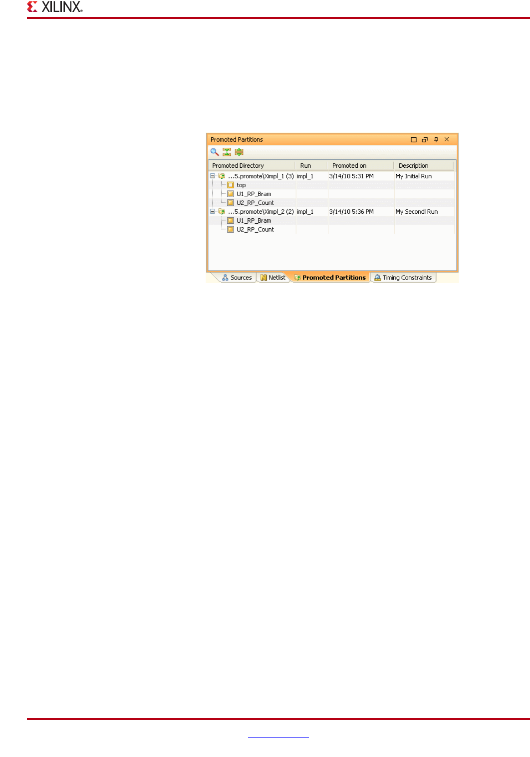
PlanAhead User Guide www.xilinx.com 381

UG632 (v 12.1)

Using PlanAhead for Design Preservation

Using the Promoted Partitions View

The Promoted Partitions view displays each time you perform a Promote Partitions

command.

To open the Promoted Partitions view, select the Window > Promoted Partitions

command. The following figure shows the Promoted Partitions view.

Each promotion displays in a tree table detailing the partitions promoted, the source

implementation run, the promote date and time, and the description.

Deleting Promoted Partitions

You can remove previously promoted directories to clean up the /Project directories.

The entire promoted directory is removed including all promoted partitions from the run.

To delete promoted directories, select the promoted directory in the Promoted Partitions

view and click the Delete popup menu command.

Importing Partitions

Once partitions have been promoted, they can be imported for subsequent runs. Importing

partitions results in the placement and routing being copied out of the promoted partitions

run and importing it into the new run prior to implementing the rest of the design ensuring

identical results.

Updating Netlist Sources

As design modifications occur, the updated netlists are either picked up automatically, if

you are using remote sources, or updated in the Project to update the existing netlists.

Once the source files are updated you can open or reload the Netlist Design to apply the

logic changes. Refer to “Managing the Design Source Files” in Chapter 5 for more

information.

Setting Partition Actions Based on Logic Updates

You must set the Partition action for each run as described in “Configuring Runs for

Partitions,” page 378.

•Partitions with updated netlists must be set to Implement.

•Unchanged partitions must be set to Import.

Figure 13-7: Promoted Partitions View

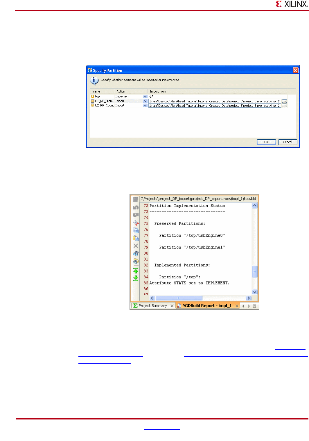
382 www.xilinx.com PlanAhead User Guide

UG632 (v 12.1)

Chapter 13: Using Hierarchical Design Techniques

PlanAhead sets the Partition actions automatically to Import for any promoted partitions

and selects the most recent promoted directory from which to import. PlanAhead does not

track logic updates or set the appropriate partitions to Implement.

The following figure shows a Specify Partitions dialog box.

The ISE Ngdbuild report provides information about the Partition actions for each run. To

access the report, select the Reports view tab and open the Ngdbuild report. The following

figure shows the Partition activity in an Ngdbuild report.

Successfully preserved partitions are copied from the promoted area and pasted into the

new run. This should provide identical results for imported partitions.

For more information about Design Preservation methodologies, refer to the Hierarchical

Design Methodology Guide (UG748) or the PlanAhead Tutorial:Leveraging Design Preservation

for Predictable Results (UG747).

Figure 13-8: Importing Partitions

Figure 13-9: Partition Import Activity in the Ngdbuild Report

PlanAhead User Guide www.xilinx.com 383

UG632 (v 12.1)

Chapter 14

Tcl and Batch Scripting

This chapter contains the following sections:

•“Overview of Tcl Capabilities in PlanAhead”

•“Invoking PlanAhead”

•“General Tcl Syntax Guidelines”

•“First Class Tcl Objects and Relationships”

•“Errors, Warnings, and Info Messages”

•“Tcl Commands”

•“Tcl References”

Overview of Tcl Capabilities in PlanAhead

The Tool Command Language (Tcl, pronounced “tickle.”) is the scripting language

integrated in the PlanAhead™ software environment. Tcl is a standard language in the

semiconductor industry for design constraints and Synopsys® Design Constraints (SDC).

SDC is the mechanism for communicating timing constraints for FPGA synthesis tools

from Synopsis Synplify as well as other vendors, and is timing constraint language for

Altera Quartus. Because Xilinx® is committed to aligning with industry standard wherever

possible, consequently, the Tcl infrastructure is a “Best Practice” for scripting language.

Tcl lets you perform interactive queries to design tools in addition to executing automated

scripts. Tcl offers the ability to “ask” questions interactively of design databases,

particularly around tool and design settings and state. Examples are: querying specific

timing analysis reporting commands live, applying incremental constraints, and

performing queries immediately after to verify expected behavior without re-running any

tool steps.

The following sections describe some of the basic capabilities of Tcl with PlanAhead.

Note: This chapter is not a comprehensive reference to Tcl commands. This chapter does provide

references to Tcl resources, and describes the general capabilities of Tcl in the PlanAhead

environment.

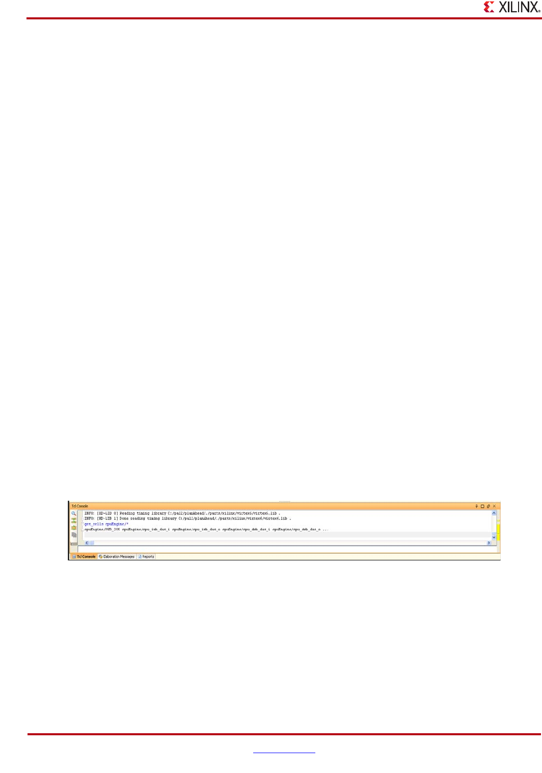
384 www.xilinx.com PlanAhead User Guide

UG632 (v 12.1)

Chapter 14: Tcl and Batch Scripting

Tcl in Journal Files

When you invoke the PlanAhead software, it creates two files that maintain a log of the

operations performed either in the GUI or in batch mode:

•PlanAhead.log

•PlanAhead.jou

You can copy Tcl commands from the log files for use either in the Tcl command window or

in a batch file.

Refer to Appendix B, “PlanAhead Input and Output Files” for information regarding the

file locations.

Tcl Help

The Tcl help command provides an overview of the available, supported Tcl commands.

The help command with no arguments provides a list of all commands. You can pass a

specific command to the help command as an argument, for example:

help get_cells

The Tcl help then prints the specific command information to both the console and the log

file. Additionally, a global –help option is implemented that returns help syntax; for

example:

get_cells –help

Tcl Console

The PlanAhead GUI environment contains an area that echoes the Tcl commands as

operations are performed, and provides information, warnings, and error messages that

result from tasks performed. The Tcl Console is located along the bottom of the PlanAhead

environment and fixed to the width of the GUI. Along the right side of the Tcl console, just

to the right of the scrollbar is an area with color coded indicators for warnings and errors.

Any warnings issued to the console are colored yellow and errors are marked red. This is

a very useful feature to scroll back through message history and quickly navigate to view

warnings and errors in the context of the command that was performed. The following

figure contains a picture of the Tcl Console within the environment:

Figure 14-1: Tcl Console

PlanAhead User Guide www.xilinx.com 385

UG632 (v 12.1)

Invoking PlanAhead

PlanAhead provides three primary modes of operation:

•The GUI mode (default)

•Invocation of the PlanAhead executable by a Tcl command-line option (batch mode)

•Tcl shell mode

The batch and Tcl shell modes are described in the following subsections.

Batch Mode

Batch mode executes a script and then shuts down the tool. To invoke PlanAhead in

batch mode:

planAhead –mode batch –source <script_name.tcl>

Tcl Shell Mode

Tcl mode invokes a shell similar to windows command shell or a linux shell. This is an

interactive shell session that does not invoke the GUI.

Optionally, you can pass a script with the –source switch, which executes the script and

then passes the control to the interactive shell where you can manually enter Tcl

commands. To launch PlanAhead in Tcl shell mode:

PlanAhead –mode tcl –source <script_name.tcl>

General Tcl Syntax Guidelines

Tcl uses the Linux switching (/) convention regardless of the OS on which you are

operating.

The following subsections describe the general syntax guidelines for using Tcl in

PlanAhead.

Sourcing a Tcl Script

You can source a Tcl script from a command-line option:

source - <file_name>

Within the PlanAhead GUI you can source a Tcl script from Tools > Run Tcl Script.

General Syntax Structure

The general structure of the PlanAhead Tcl commands is:

<command> [optional_parameters] <required_parameters>

Command syntax is of the verb-noun and verb-adjective-noun structure separated by the

underscore (“_”) character. This structure is generally self-describing and easy to

remember.

Commands are grouped together with common prefixes when they are related.

•Commands that query things are generally prefixed with get_.

•Commands that set a value or a parameter are prefixed with set_.

386 www.xilinx.com PlanAhead User Guide

UG632 (v 12.1)

Chapter 14: Tcl and Batch Scripting

•Commands that generate reports are prefixed with report_.

The commands are all exposed in the global namespace, which means the commands do

not need to be qualified with hdi:: as in previous versions of PlanAhead. Commands are

“flattened,” meaning there are no “sub-commands” for a command.

Example Syntax

The following is an example of the return format on the get_cells -help command:

get_cells -help

Description:

Get a list of cells in the current design

Syntax:

get_cells [-hierarchical] [-regexp] [-nocase] [-filter <arg>] [-

of_objects <args>] [-quiet] [<patterns>...]

Returns:

list of cell objects

Usage:

Unknown Commands

Tcl contains a list of built-in commands that are generally supported by the language,

PlanAhead-specific commands which are exposed to the Tcl interpreter, and user-defined

procedures.

Commands that do not match any of these known commands are sent to the OS for

execution in the shell from the exec command. This allows users to execute shell

commands that may or may not be OS-specific. If there is no shell command, then an error

message is issued to indicate that no command was found.

Return Codes

Some commands are expected to provide a return, such as a list or collection of objects that

on which to operate. Other commands perform an action but do not necessarily return a

value that can be used directly by the user. Some tools that integrate Tcl interfaces return a

“0” or a “1” to indicate success or error conditions in the command, but this is not reliable

combined with commands that returns lists of objects.

To test if a command successfully executed, use the Tcl built-in command catch. All

PlanAhead commands return TCL_OK and TCL_ERROR, and $ERROINFO through the

Name Optional Default Description

-hierarchical yes false Search level-by-level in current

instance

-regexp yes false Patterns are full regular

expressions

-nocase yes false Perform case-insensitive

matching

-filter yes Filter list with expression

-of_objects yes Get cells of these pins or nets

-quiet yes false Ignore command errors

<patterns> yes * Match cell names against

patterns

PlanAhead User Guide www.xilinx.com 387

UG632 (v 12.1)

First Class Tcl Objects and Relationships

standard Tcl mechanisms which makes the catch command the most robust mechanism for

trapping errors in Tcl scripts. These values will not be returned and set to variables in the

interpreter, nor do the commands return a 0 or 1 in log files upon success or failure of a

given command. Generally, the catch command and the presence of numbered

info/warning/error messages should be relied upon to asses issues in Tcl scripted flows.

Sourcing a Tcl Script

A Tcl script can be sourced from either one of the command-line options or from the GUI

using the File > pulldown. Once a Tcl script is invoked from the GUI, a progress bar dialog

box displays and all operations in the GUI are blocked until the scripts completes.

Currently, there is no way to interrupt script execution during runtime; consequently,

standard OS methods of killing a process must be used to force interruption of the tool. If

the PlanAhead process is killed, you will lose all work since the last time you saved the

project.

First Class Tcl Objects and Relationships

PlanAhead Tcl provides direct access to the object models for netlist, devices, and projects.

These objects are first-class which means they are more than just a string representation,

and they can be operated on and queried. There are a few exceptions to this rule, but

generally “things” can be queried as objects, and these objects have properties that can be

queried and they have relationships that allow you to get to other objects.

Object Types and Definitions

There are many object types in PlanAhead; this chapter provides definitions and

explanations of the basic types. The most basic and important object types are associated

with entities in a design netlist, and these types are listed in the following subsections:

Cell

A cell is an instance, either primitive or hierarchical inside a netlist. Examples of cells

include flip-flops, LUTs, I/O buffers, RAM and DSPs, as well as hierarchical instances

which are wrappers for other collections of cells.

A pin is a point of logical connectivity on a cell. A pin allows the internals of a cell to be

abstracted away and simplified for easier use, and can either be on hierarchical or

primitive cells. Examples of pins include clock, data, reset, and output pins of a flop.

Port

A port is a special type of hierarchical pin, a pin on the top level netlist object, module or

entity. Ports are normally attached to IO pads and connect externally to the FPGA device.

Net

A net is a wire or collection of wires that eventually be physically connected directly

together. Nets can be hierarchical or flat, but will always short together a collection of pins.

388 www.xilinx.com PlanAhead User Guide

UG632 (v 12.1)

Chapter 14: Tcl and Batch Scripting

Clock

A clock is a periodic signal that propagates to sequential logic within a design. Clocks can

be primary clock domains or generated by clock primitives such as a DCM, PLL, or

MMCM. A clock is the rough equivalent to a TIMESPEC PERIOD constraint in UCF and

forms the basis of static timing analysis algorithms.

Querying Objects

All first class objects can be queried by a “getter” Tcl command that generally has the

following syntax:

get_<object_type> <pattern>

Where pattern is a search pattern, which includes if applicable a hierarchy separator to get

a fully qualified name. Objects are generally queried by a string pattern match applied at

each level of the hierarchy, and the search pattern also supports wildcard style search

patterns to make it easier to find objects, for example:

get_cells */inst_1

This command will search for a cell named inst_1 within the first level of hierarchy

below the top level of hierarchy. To recursively search for a pattern at every level of

hierarchy, use the following syntax:

get_cells –hierarchical inst_1

This command searches every level of hierarchy for any instances that match inst_1.

For complete coverage of syntax, see the specific online help for the individual command:

help get_cells

get_cells -help

Object Properties

Objects have properties that can be queried. Property names are unique for any given

object type. To query a specific property for an object, the following command is provided:

get_property <property_name> <object>

An example would be the lib_cell property on cell objects, which tells you what Unisim

component a given instance is mapped to:

get_property lib_cell [get_cell inst_1]

To discover all of the available properties for a given object type, use the

report_property command:

report_property [get_cells inst_1]

Key Value Type

bel OLOGICE1.OUTFF string

class cell string

iob TRUE string

is_blackbox 0bool

is_fixed 0bool

PlanAhead User Guide www.xilinx.com 389

UG632 (v 12.1)

First Class Tcl Objects and Relationships

Some properties are read-only and some are user-settable. Properties that map to

attributes that can be annotated in UCF or in HDL are generally user-settable through Tcl

with the set_property command:

set_property loc OLOGIC_X1Y27 [get_cell inst_1]

Filtering Based on Properties

The object query get_* commands have a common option to filter the query based on

any property value attached to the object. This is a very powerful capability for the object

query commands. For example, to query all cells of primitive type FD do the following:

get_cells * -hierarchical –filter “lib_cell == FD”

To do more elaborate string filtering, utilize the =~ operator to do string pattern matching.

For example, to query all flip-flop types in the design, do the following:

get_cells * -hierarchical –filter “lib_cell =~ FD*”

Multiple filter properties can be combined with other property filters with logical OR (||)

and AND (&&) operators to make very powerful searches. To query every cell in the

design that if of any flop type and has a placed location constraint:

get_cells * -hierarchical –filter {lib_cell =~ FD* && loc != “”}

Note in the example above, the filter option value was wrapped with curly braces {}

instead of double quotes. This is normal Tcl syntax that prevents command substitution by

the interpreter and allows users to pass the empty string “ ” to the loc property.

Large Lists of Objects – Collections

Commands that return more than one object generally return a container that looks and

behaves like a native Tcl list. This is a feature of PlanAhead in that it allows dramatic

optimization of large collections of Tcl objects handling without the need for special

iteration commands like the foreach_in_ collection which is handled with the Tcl built-

in foreach.

is_partition 0bool

is_primitive 1 bool

is_reconfigurable 0bool

is_sequential 1bool

lib_cell FD string

loc OLOGIC_X1Y27 string

name error string

primitive_group FD_LD string

primitive_subgroup flop string

site OLOGIC_X1Y27 string

type FD & LD string

XSTLIB 1bool

Key Value Type

390 www.xilinx.com PlanAhead User Guide

UG632 (v 12.1)

Chapter 14: Tcl and Batch Scripting

There are a few nuances with respect to large lists, particularly in the log files and the GUI

Tcl console. Typically, when you set a Tcl variable to the result of a get_* command, the

entire list is echoed to the console and to the log file. For large lists, this is truncated when

printed to the console and log to prevent memory overloading of the buffers in the tool.

What is echoed is the list printed to the log and console is truncated and the last element

appears to be “…” in the log and console, however the actual list in the variable

assignment is still correct and the last element is not an error.

An example of this is querying a single cell versus every cell in the design, which can be

large:

get_cells inst_1

inst_1

get_cells * -hierarchical

XST_VCC XST_GND error readIngressFifo wbDataForInputReg fifoSelect_0

fifoSelect_1 fifoSelect_2 fifoSelect_3 ...

%set x [get_cells * -hierarchical]

XST_VCC XST_GND error readIngressFifo wbDataForInputReg fifoSelect_0

fifoSelect_1 fifoSelect_2 fifoSelect_3 ...

%lindex $x end

bftClk_BUFGP/bufg

%llength $x

4454

In this example, all four thousand cells were not printed to the console and the list was

truncated with a “…” but the actual last element of the list is still correct in the Tcl variable.

Object Relationships

Related objects can be queried using the –of option to the relevant get_* command. For

example, to get a list of pins connected to a cell object, do the following:

get_pins –of [get_cells inst_1]

The following is a diagram of the object types in PlanAhead and their relationship, where

an arrow from one object to another object indicates that you can use the –of option to the

get_* command to traverse logical connectivity and get Tcl references to any connected

objects:

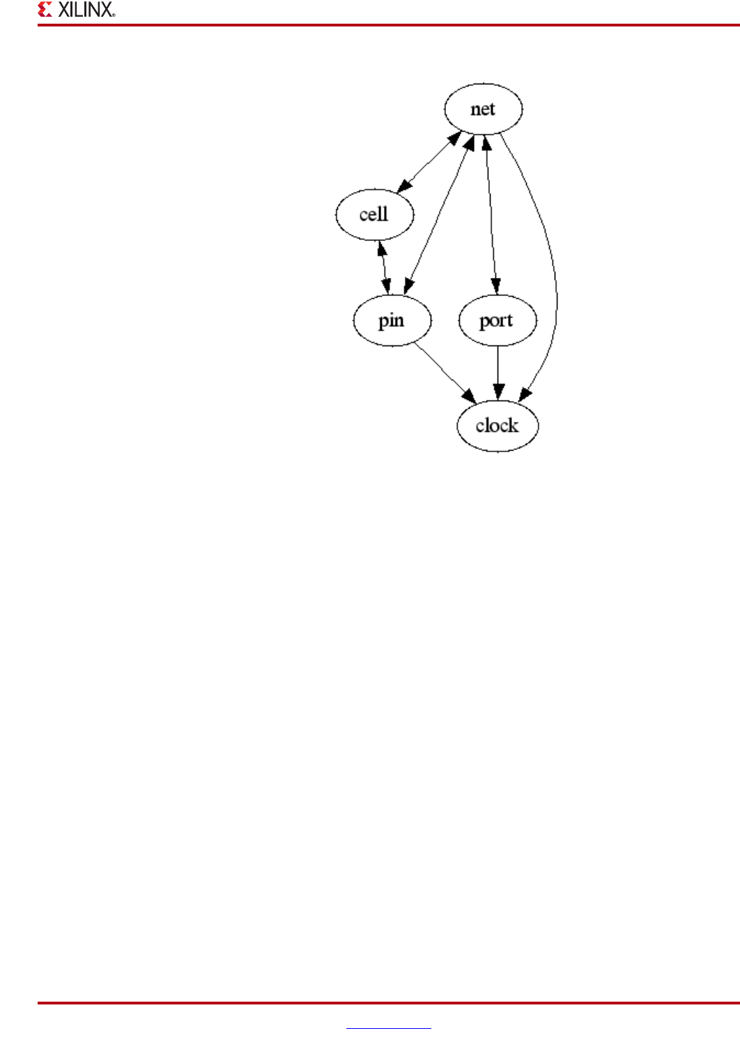
PlanAhead User Guide www.xilinx.com 391

UG632 (v 12.1)

Errors, Warnings, and Info Messages

Messages that result from individual commands appear in the log file as well as in the GUI

console if it is active. These messages are generally numbered to identify specific issues

and are prefixed in the log file with either “INFO”, “WARNING”, or “ERROR” followed by a

subsystem identifier and a unique number.

The following is an example of an INFO message that appears after reading the timing

library.

INFO: [HD-LIB 1] Done reading timing library

These messages make it easier to search for specific issues in the log file to help to

understand the context of operations during command execution.

Generally, when an error occurs in a Tcl command sourced from a Tcl script, further

execution of subsequent commands is halted. This is to prevent unrecoverable error

conditions. There are Tcl built-ins that allow users to intercept these error conditions, and

to choose to continue. Please consult any Tcl reference for the catch command for a

description of how to handle errors using general Tcl mechanisms.

Tcl Commands

The following subsections describe the most common commands in PlanAhead.

X-Ref Target - Figure 14-2

Figure 14-2: PlanAhead Object Relationships

392 www.xilinx.com PlanAhead User Guide

UG632 (v 12.1)

Chapter 14: Tcl and Batch Scripting

Project Creation and Manipulation

There are a number of Tcl commands that control the creation and management of

PlanAhead projects. The following table lists the most common commands relating to

project manipulation:

For specific information about each command, consult the online help for the individual

command.

Flow Control

The following table contains a list of Tcl commands that control the flow of synthesis and

implementation.

X-Ref Target - Figure 14-3

For specific information about each command, please consult the online help for the

individual command.

Table 14-1: Tcl Project Manipulation Commands

Command Description

create_project Create a new project.

open_project Open an existing project.

close_project Close the current project.

get_project Query project by name if multiple projects are

open.

current_project Return the current open project if multiple projects

are open.

save_project_as Save the current project to a different location.

add_files Add source files to a project.

remove_files Remove source files from a project.

open_rtl_design Open the elaborated RTL design.

open_netlist_design Open the post-synthesis netlist design.

open_impl_design Open the post-implementation design.

close_design Close the current design.

Table 14-2: Flow Control Commands

Command Description

launch_runs Launch a synthesis or implementation run.

wait_on_run Block script execution until launched run completes.

create_run Create a new run based on a strategy.

reset_run Reset run status

current_run Return the current run

get_runs Query all configured runs

delete_run Delete a given run

PlanAhead User Guide www.xilinx.com 393

UG632 (v 12.1)

Tcl Commands

Object Access

The following table lists Tcl commands that query objects.

For specific information about each command, consult the online help for the individual

command.

Reporting

The following table lists the most common Tcl commands that generate informational

reports, either printed to the console or written to a report file on the filesystem.

For specific information about each command, consult the online help for the individual

command.

Table 14-3: Tcl Query Commands

Command Description

get_cells Query cell objects

get_pins Query pin objects

get_ports Query port objects

get_nets Query net objects

get_clocks Query clock objects

get_sites Query device site objects

get_iobanks Query IO bank objects

report_property Generate a list of available properties on an object

set_property Set a property value on an object

get_property Query a specific property on an object

Table 14-4: Tcl Reporting Commands

Command Description

report_property Return a list of property names and descriptions for a given object.

report_timing Generate static timing analysis timing report.

repot_ssn Generate Simultaneous Switching Noise (SSN) report.

report_drc Generate Design Rule Check (DRC) report.

report_power Generate power estimation report.

report_constraint Generation constraint violation report.

report_resource Generate resource utilization report.

394 www.xilinx.com PlanAhead User Guide

UG632 (v 12.1)

Chapter 14: Tcl and Batch Scripting

GUI Control

The following table lists the Tcl commands that control some behavior in the GUI, if it is

active. These commands are very helpful for things such as finding objects in the device

view and cross probing between schematic and placement on the device. These commands

do nothing in batch and interactive Tcl modes where the GUI is not active.

For specific information about each command, consult the online help for the individual

command.

Tcl References

The following subsections provide recommended Tcl references.

Tcl Developer Xchange

Tcl reference material is available on the Internet. Xilinx recommends the Tcl Developer

Xchange, which maintains the open source code base for Tcl, and is located at:

http://www.tcl.tk

An introductory tutorial is available at:

http://www.tcl.tk/man/tcl/tutorial/tcltutorial.html

About SDC

SDC is an acronym for Synopsys Design Constraints, and is an accepted industry standard

for communicating design intent to tools, particularly for timing analysis. A reference copy

of the SDC specification is available from Synopsys by registering for the TAP-in program

at:

http://www.synopsys.com/Community/Interoperability/Pages/TapinSDC.aspx

Available Tcl Documents

Tcl reference documents are available in book stores or online retailers. Two such books

are:

•“Practical Programming in Tcl and Tk” by Brent Welch

•“Tcl and the Tk Toolkit” by John K. Ousterhout

Table 14-5: Tcl GUI Commands

Command Description

select_objects Select an object, which is equivalent to clicking on it in the

GUI. Useful for zoom-to-selection.

unselect_objects De-select an object.

mark_objects Mark an object with a marker that is visible regardless of

zoom level.

unmark_objects Remove marker.

highlight_objects Highlight an object with a specified color.

unhighlight_objects Remove highlight.

PlanAhead User Guide www.xilinx.com 395

UG632 (v 12.1)

Chapter 15

Using PlanAhead With Project

Navigator

This chapter contains the following sections:

•“Integration Overview”

•“PlanAhead Processes within Project Navigator”

Integration Overview

The PlanAhead™ software is integrated with the ISE® software to let you perform specific

design tasks. When you invoke the PlanAhead software from the ISE Project Navigator

environment, the PlanAhead software is in “ISE Integration mode.” In this mode, the

available PlanAhead features apply only to specific design tasks, including I/O pin

planning, floorplanning, and timing analysis. The Project Navigator environment creates

and manages the PlanAhead software project automatically.

There are four processes in the Project Navigator Processes pane from which you can

invoke the PlanAhead software:

•I/O Pin Planning (pre-synthesis)

•I/O Pin Planning (post-synthesis)

•Floorplan Area/IO/Logic (post synthesis)

•Analyze Timing/Floorplan Design (post implementation)

The data passed between the two tools and the view layout presented in the PlanAhead

software depends upon which step you invoke. Refer to the “PlanAhead Processes within

Project Navigator,” page 396 for more information on the mechanics of the integration

including data passing and processes.

PlanAhead has two default view layouts for the many design tasks:

•The I/O pin planning environment, called the I/O Planner, which contains views

pertinent to I/O pin planning and assignment.

•The Design Planning environment which contains views pertinent to design analysis

and floorplanning.

It is important to ensure the proper view layout is loaded for the desired design task.

For more information about using the PlanAhead Viewing Environment, see Chapter 4,

“Using the Viewing Environment.” For more information about configuring and loading

view layouts, refer to “Configuring the Viewing Environment” in Chapter 4.

396 www.xilinx.com PlanAhead User Guide

UG632 (v 12.1)

Chapter 15: Using PlanAhead With Project Navigator

PlanAhead Processes within Project Navigator

Project Navigator and the PlanAhead software are two independent environments

operating under a separate system process. The two processes are integrated to ensure that

data is passed effectively between the two tools. Changes to design data in one tool are not

recognized automatically in the other in real time, and you should not to edit logic or

constraints simultaneously in both tools. Invoke PlanAhead for the intended purpose and

close it before updating the Project Navigator design data. The Project Navigator process

steps are synchronized to recognize edits to the UCF file made in the PlanAhead software

once the data is saved. The following sections describe the steps involved and the data

transactions that enable the integration.

Passing Logic and Constraints

PlanAhead in ISE Integration mode enables only physical constraint modification for I/O

pins, logic LOC, and AREA_GROUP constraints. Logic connectivity in the form of RTL

sources or synthesized netlists are passed into the PlanAhead software for analysis

purposes only, and not passed back to Project Navigator. The PlanAhead software features

that enable logic or timing constraint modification are disabled in ISE Integration mode.

You must perform logic modifications in Project Navigator, an external RTL, or in synthesis

tools. The PlanAhead software passes only the UCF constraint files to Project Navigator.

The PlanAhead software maintains the original content and format of the UCF files,

including comments, incomplete constraints, and so forth. The legality of constraints in the

design is not checked upon opening or closing the PlanAhead software. The Translate

Process step in Project Navigator does the constraint checking.

When you invoke PlanAhead, the UCF source files in the Project Navigator project are

passed to the PlanAhead software where you can add or modify physical constraints.

When you use the Save Project command in PlanAhead, that software writes the

modified UCF files back to the original Project Navigator source location. If you make

constraint changes in the PlanAhead software and select the Exit command, you are

prompted to save changes back to the Project Navigator project before the tool closes.

If PlanAhead is invoked and no UCF file exists in the Project Navigator project, you are

prompted to create one. This empty UCF file is then passed to the PlanAhead software.

PlanAhead supports Project Navigator projects with more than one UCF source file. Before

PlanAhead is invoked, a dialog box prompts you to select one of the UCF files.

•All new constraints defined in PlanAhead are written to the selected UCF file.

•Any physical constraints that exist in a non-chosen UCF file remain in that file, even if

the value of that constraint is modified in PlanAhead.

The Project Navigator design flow does not pass core-level NCF files to PlanAhead. To use

or view any physical constraints in these files in PlanAhead, you must merge them

manually into a top-level UCF file prior to invoking the PlanAhead software.

Project Navigator creates a temporary PlanAhead project in the ISE project directory, and

removes and replaces this project every time you invoke the PlanAhead software from

Project Navigator.

PlanAhead User Guide www.xilinx.com 397

UG632 (v 12.1)

PlanAhead Processes within Project Navigator

I/O Pin Planning (Pre-Synthesis)

You can elect to perform early I/O pin planning prior to having a synthesized netlist either

by using the standalone PlanAhead software or by selecting this process step in Project

Navigator.

Note: At this stage of the design process, logic synthesis has not been run. The tool has no concept

of clock ports, clock related logic, differential pairs, or GTs. You must ensure these types of ports are

placed appropriately to avoid implementation errors. Whenever possible, you should perform the I/O

pin planning after logic synthesis. The presence of a netlist ensures that the clocks, clock logic,

differential pairs, GTs, and so forth are recognized and considered automatically during pin

assignment in PlanAhead. Also, there are many Design Rule Checks (DRCs) that are performed

based on logic connectivity and clocks to ensure a legal placement prior to implementation.

To perform I/O pin planning in Project Navigator prior to running synthesis:

in the Processes pane, expand User Constraints and double-click IO Pin Planning

(PlanAhead) - Pre-Synthesis,

select the Tools > PlanAhead > Pre-Synthesis - IO Pin Planning command.

When you invoke the PlanAhead software, Project Navigator passes all of the RTL source

files, the top-level module name and the UCF file(s) to PlanAhead. The PlanAhead

software opens with a display of the the default I/O pin planning (I/O Planner) view

layout. PlanAhead performs an RTL elaboration to extract and display the top-level I/O

ports in the PlanAhead I/O Ports view.

When you save or close the PlanAhead project it updates the original Project Navigator

source UCF file(s). This resets the Project Navigator design process state, if appropriate.

Refer to “Passing Logic and Constraints,” page 396 for more information about the

integration mechanics and process.

Refer to Chapter 8, “I/O Pin Planning,” for more information about using the PlanAhead

I/O pin planning environment (I/O Planner).

I/O Pin Planning (Post-Synthesis)

Note: Whenever possible, I/O pin planning should be performed after logic synthesis. The presence

of a netlist ensures that the clocks, clock logic, differential pairs, GTs, and so forth are recognized and

considered automatically during pin assignment in PlanAhead. There are also many Design Rule

Checks (DRCs) that are performed based on logic connectivity and clocks to ensure a legal

placement prior to implementation.

To perform I/O pin planning in Project Navigator after running logic synthesis, in the

Processes pane, expand User Constraints and double-click IO Pin Planning (PlanAhead)

- Post-Synthesis, or select the Tools > PlanAhead > Post-Synthesis - IO Pin Planning

command.

When you invoke PlanAhead, Project Navigator passes the synthesized NGC or EDIF

format netlist and the UCF file(s) to PlanAhead. PlanAhead opens with a display of the

default I/O pin planning (I/O Planner) view layout, and the I/O ports display in the

PlanAhead I/O Ports view.

When you save or close the PlanAhead project, it updates the original Project Navigator

source UCF file(s), and this resets the Project Navigator design process state, if appropriate.

398 www.xilinx.com PlanAhead User Guide

UG632 (v 12.1)

Chapter 15: Using PlanAhead With Project Navigator

Refer to “Passing Logic and Constraints,” page 396 for more information about the

integration mechanics and process. Refer to Chapter 8, “I/O Pin Planning,” for more

information about using the PlanAhead I/O pin planning environment.

Floorplan Area/IO/Logic (Post Synthesis)

You can use the PlanAhead software design analysis and floorplanning environment prior

to or after implementation. To analyze the design or to perform floorplanning from Project

Navigator after running logic synthesis and prior to implementation:

•In the Processes pane, expand User Constraints, and select Floorplan Area/IO/Logic

(PlanAhead) - Post-Synthesis,

•Select the Tools > PlanAhead > Post-Synthesis - Floorplan Area/IO/Logic

command.

When PlanAhead is invoked, Project Navigator passes the synthesized NGC or EDIF

format netlist and the UCF file(s) to PlanAhead. PlanAhead opens with the default

PlanAhead design analysis and floorplanning environment displaying.

Note: In Project Navigator, set the Translate process property Macro Search Path (-sd) to the

appropriate directory if lower-level NGC format core files are used in the design and are not added as

sources.

When you save or close the PlanAhead project, it updates the original Project Navigator

source UCF file(s), and resets the Project Navigator design process state, if appropriate.

Refer to “Passing Logic and Constraints,” page 396 for more information about the

integration mechanics and process. Refer to Chapter 5, “RTL and IP Design,” for more

information about using the PlanAhead environment prior to implementation.

Chapter 10, “Analyzing Implementation Results,” and Chapter 11, “Floorplanning the

Design,” have more information about using the PlanAhead environment after

implementation.

Analyze Timing/Floorplan Design (Post Implementation)

You can use the PlanAhead software design analysis and floorplanning environment after

implementation. When you analyze the design after implementation you can view the

placement and timing results to catch potential design issues.

Often, physical LOC or AREA_GROUP floorplanning constraints can help drive the

implementation tools toward better and more consistent results, and reduce

implementation runtimes.

To analyze the design or to perform floorplanning from Project Navigator after

implementation:

•In the Process pane, expand Implement Design, expand Place & Route, and double-

click Analyze Timing/Floorplan Design (PlanAhead) - Post-Synthesis

•Select the Tools > PlanAhead > Post-Implementation - Analyze Timing/Floorplan

Design command

PlanAhead User Guide www.xilinx.com 399

UG632 (v 12.1)

PlanAhead Processes within Project Navigator

Project Navigator passes the following files to PlanAhead when it opens:

•Synthesized NGC or EDIF format netlist

•UCF file(s)

•ISE placement data

•Timing results

PlanAhead is invoked with the default PlanAhead design analysis and floorplanning

environment displayed. For PlanAhead to extract the ISE placement data, an XDL

command must be run first. It produces a file with an .xdl extension.

A progress bar displays in PlanAhead while this command is running. To expedite re-

invoking PlanAhead, the interface first checks for the existence of the XDL file and does

not regenerate the file if it is still current.

When you select Tools > PlanAhead > Post Implementation - Analyze Timing

/Floorplan Design with the implementation process out-of-date, you are prompted to

either re implement the design and launch PlanAhead, or launch PlanAhead on the

existing result data without rerunning the implementation tools.

When you save or exit the PlanAhead project, the PlanAhead software updates the original

Project Navigator source UCF file(s), and this resets the Project Navigator design process

state also, if appropriate.

400 www.xilinx.com PlanAhead User Guide

UG632 (v 12.1)

Chapter 15: Using PlanAhead With Project Navigator

PlanAhead User Guide www.xilinx.com 401

UG632 (v 12.1)

Appendix A

Menu and Toolbar Commands

This appendix provides a quick reference to the following PlanAhead™ software

commands, and has the following sections:

•“Main Menu Commands”

•“Toolbar Commands”

Main Menu Commands

The following tables provides a quick reference for the PlanAhead software main menu

commands. View-specific popup menu commands are covered elsewhere in this

document.

Some of the commands are available only during the appropriate PlanAhead mode.

Unavailable commands are shown as disabled or “grayed out.”

File Menu

The File menu has the following menu commands:

Tab le A - 1 : File menu commands

Command Description

New Project Invokes the Create New Project wizard for creating a new

project.

Open Project Opens an exiting, previously-saved project file from PlanAhead.

Opening a project also opens any previously opened Floorplans

associated with the project. Also, it restores the latest status of all

ISE® software implementation runs.

Reopen Project Provides a list of previously opened projects to select for

reopening.

Open Example Project Opens a menu for you to select an example project.

Close Project Closes the active project. You will be prompted to save any

unsaved changes.

Save Design Saves the current designt.

Save Project Save the current project.

Save Project As Enables saving of the current project to another name or

location.

402 www.xilinx.com PlanAhead User Guide

UG632 (v 12.1)

Appendix A: Menu and Toolbar Commands

Edit Menu

The Edit menu has the following menu commands:

View Menu

The View menu has the following menu commands:

Add Sources Enables the adding of source files or entire directories to the

project.

Create Source Opens the New Source File dialog box, which enables you to

create a source file.

Add Existing IP Adds an existing IP to the project.

Add Constraints Adds a constraint set to the project.

Set PR Project Sets a project to a Partial Reconfiguration project (if appropriate

licensing is available.

Print Prints the current view. This command is only available when

the Schematic view, Device view, Package view or Instance

Hierarchy view is active.

Exit Closes the application.

Tab le A - 1 : File menu commands (Continued)

Command Description

Tab le A - 2 : Edit menu commands

Command Description

Delete Removes the currently selected object(s).

Unplace Unplaces the selected primitive instances and/or I/O ports.

Undo Reverses the previously run Tcl command in active PlanAhead

session.

Redo Reverses the last Undo command action.

Save File Save the current file.

Find in Files Invokes the Find in Files dialog box to search for text strings in the

selected files.

Tab le A - 3 : View menu commands

Command Description

Show Navigator Shows or hides Project Navigator.

Zoom In Increases the scale factor of the active graphical window by a factor of

200%.

Zoom Out Decreases the scale factor of the active graphical window by a factor of

50%.

Zoom Fit Fits the entire contents of the active graphical view.

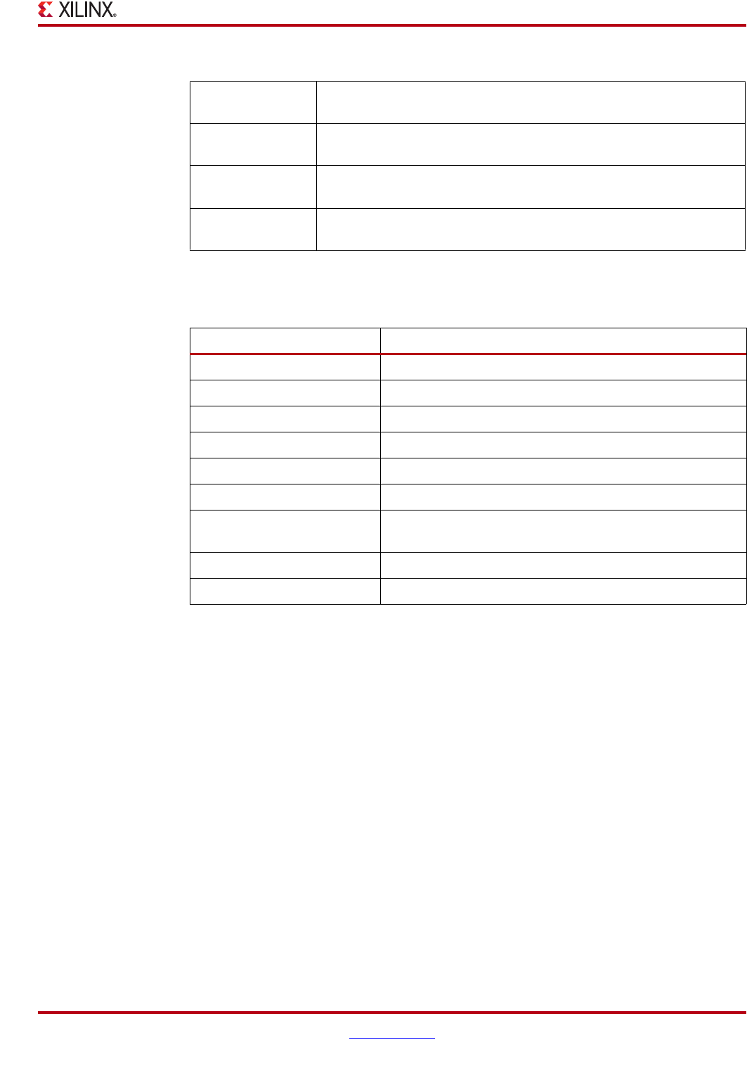
PlanAhead User Guide www.xilinx.com 403

UG632 (v 12.1)

Main Menu Commands

Flow Menu Commands

Zoom Area Invokes Zoom area mode allowing the drawing of a zoom rectangle in

the active view.

Fit Selection Adjust the zoom level to fit all of the selected items in the active

window.

Fit Highlight Adjust the zoom level to fit all of the highlighted items in the active

window.

Fit Markers Adjust the zoom level to fit all of the marked items in the active

window.

Tab le A - 3 : View menu commands

Tab le A - 4 : Flow Menu Commands

Command Description

Project Manager Opens Project Manager.

Netlist Design Starts Netlist Design

Implenent Starts Implementation

Implement Settings.. Invokes the Implementation Settings dialog box.

Implemented Design Opens the implemented design.

Generate Bitstream Generates a Bitstream.

Launch ChipScope

Analyzer

Launches ChipScope Analyzer.

Launch iMPACT Launch iMPACT.

Launch FPGA Editor Launch FPGA Editor.

404 www.xilinx.com PlanAhead User Guide

UG632 (v 12.1)

Appendix A: Menu and Toolbar Commands

Tools Menu

The Tools menu has the following menu commands:

Tab le A - 5 : Tools menu commands

Command Description

Resourse Estimation Invokes the Resourse Utilization in the Design Planner.

Create Pblocks Invokes the Create Pblocks wizard seeded with selected set of

instances to allow creation of multiple Pblocks.

Auto-create Pblocks Invokes the Auto-create Pblock dialog box to place the instances

automatically into Pblocks and name them accordingly.

Place Pblocks Invokes the Place Pblocks dialog box to size and place Pblocks

automatically.

Auto-place I/O Ports Places the entire device or any selected portion of it, while

obeying I/O bank rules, differential pair rules, and global clock

pin rules.

Clear Placement Invokes the Clear Placement Constraints wizard to selectively

remove port or placement location constraints.

Schematic Opens a new Schematic view in the Workspace and displays a

schematic of the currently selected elements.

Show Connectivity Selects the elements connected to the selected instances, nets, or

Pblocks. This command can be used sequentially to continue to

fanout and select a cone of logic.

Show Hierarchy Invokes a Hierarchy view in the Workspace and graphically

displays the entire logic hierarchy. Selected logic is highlighted

in the tree.

Report Timing Invokes the Run Timing Analysis dialog box and enables you to

configure and launch the static timing analyzer.

Slack Histogram Invokes the Generate Slack Histogram for Endpoints wizard.

Run DRC Invokes the Run DRC dialog box and enables you to configure

and launch the PlanAhead design rule checker

Run Noise Analysis Invokes the Run SSN Analysis dialog box and generates a

Simultaneous Switching Noise (SSN) report of potential I/O

issues. Virtex®-6 designs only.

Create Multiple Runs Invokes the Run Synthesis dialog box to create and launch a

Synthesis Run.

Setup ChipScope Invokes the ChipScope™ Pro Analyzer.

Run Tcl Script Invokes the Run Script dialog box to execute a Tcl script

selectable through file browser.

Options Invokes the Options dialog box for setting display options,

selection options, shortcut options, strategies, and other options.

PlanAhead User Guide www.xilinx.com 405

UG632 (v 12.1)

Main Menu Commands

Window Menu

The Window menu has the following menu commands:

Tab le A - 6 : Window menu commands

Command Description

Project Summary Displays the Project Summary view.

Netlist Displays the Netlist view.

Sources Displays the Sources view.

Physical Constraints Displays the Physical Contraints view.

Timing Constraints Displays the Timing Contraints view

Package Pins Displays Package Pins view.

I/O Ports Displays I/O Ports view.

ChipScope Displays the integration ChipScope view.

Clock Regions Displays the Clock Regions view.

Metrics Displays the Metric view.

Properties Displays the Properties view.

Selection Displays the Selection view.

Tcl Console Displays the Console view.

Timing Results Displays the timing results in the Timing Results view.

DRC Results Displays the DRC results in the DRC Violations browser.

SSN Results Displays the SSN Results view.

Find Results Displays the found objects in the Find Results view.

Find in Files Results Displays the found objects in the Find in Files view.

Design Runs Displays the runs in the Design Runs view.

Compilation Log Opens the compilaton log.

Compilation

Messages

Opens the compilation messages.

Reports Opens the Report view.

Metric Reports Opens the Metric Reports.

New Device View Opens a new Device view in the Workspace.

New Package View Opens a new Package view in the Workspace.

View Log File Opens the planAhead.log log file, which captures the contents of

the messages created when running PlanAhead commands.

View Journal File Opens the planAhead.jou journal file, which cumulatively

captures all of the TCL commands from PlanAhead sessions that

were invoked.

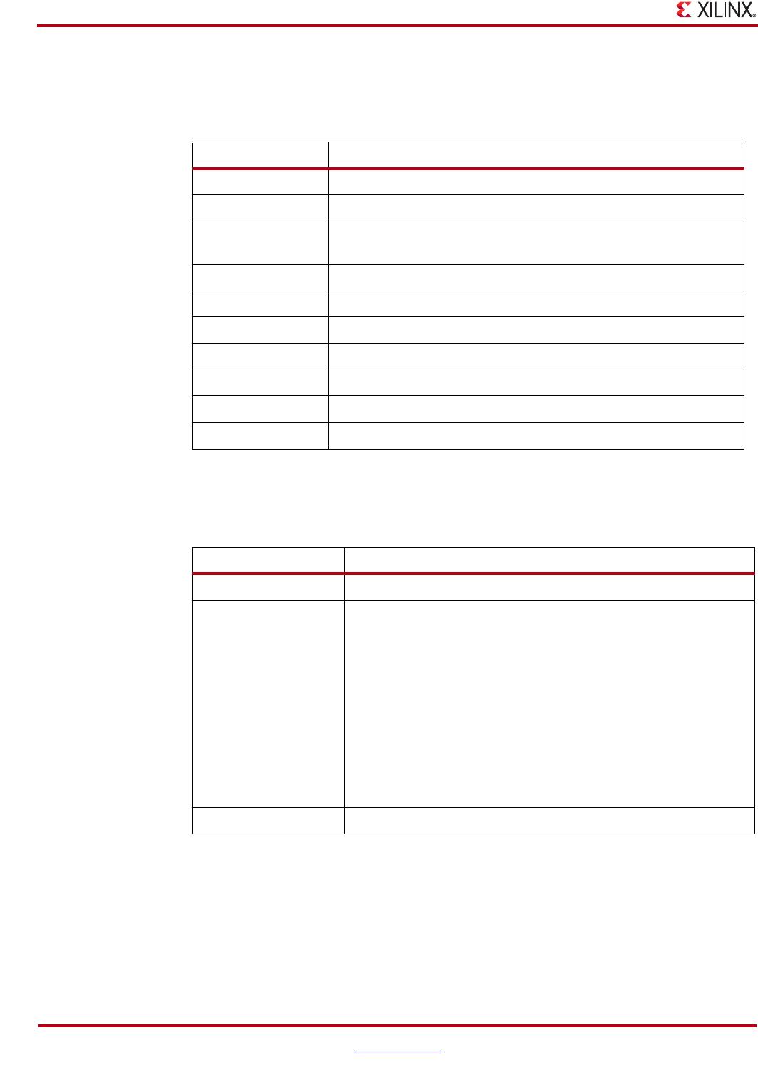
406 www.xilinx.com PlanAhead User Guide

UG632 (v 12.1)

Appendix A: Menu and Toolbar Commands

Select Menu

The Select menu has the following menu items:

Layout Menu

The Layout menu has the following menu items:

Tab le A - 7 : Select menu commands

Command Description

Unselect All Unselects all selected elements.

Unselect Type Unselects elements of a particular type.

Select Area Invokes the Select Area command putting the cursor in draw

rectangle mode in the active Workspace.

Highlight Highlights all selected objects using the active highlight color.

Unhighlight All Unhighlights all highlighted objects.

Unhighlight Unhighlights selected objects.

Unhighlight Color Unhighlights elements based on object color.

Mark Marks selected objects in the Device view.

Unmark Unmarks current selected object in the Device view.

Unmark All Unmarks all marked objects.

Tab le A - 8 : Layout menu commands

Command Description

Load Default Layout Loads the user-defined default view layout, if available.

Save as Default

Layout

Saves the current view configuration as the default to be used each

time PlanAhead is invoked. This layout will be used each time

PlanAhead is invoked.

On Windows, the file is saved to the following area:

−C:\Documents and

Settings\<username>\Application

Data\HDI\layouts\application_layout\default.

layout

On Linux or Solaris, the file is stored in the following area:

−~/.HDI/layouts/application_layout/default.layo

Clear Default Layout Clears the current user-defined default layout.

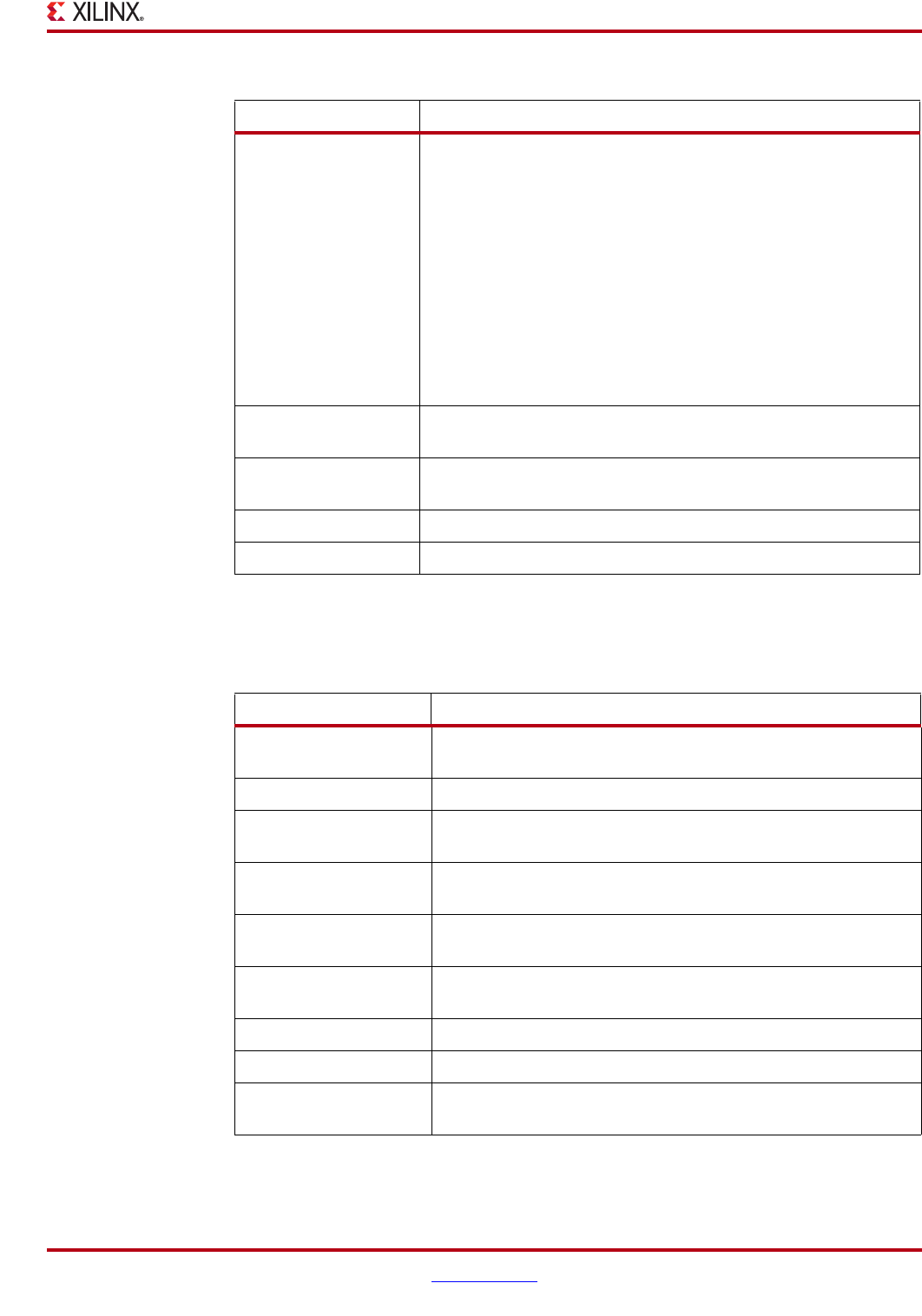
PlanAhead User Guide www.xilinx.com 407

UG632 (v 12.1)

Main Menu Commands

Help Menu

The Help menu has the following menu items:

Save Layout As Enables you to save the current view configuration with a user

defined name. These layouts can be loaded manually each time

PlanAhead is invoked. The area is located on Windows in the folder

shown below.

On Windows, the layout files are saved to the following area:

−C:\Documents and

Settings\<username>\Application

Data\HDI\layouts\floorplan_layout\<layoutnam

e>.layout

On Linux or Solaris, the files are stored in the following area:

−~/.HDI/layouts/application_layout/<layoutname>

.layout

Load Layout Enables you to load any of the previously saved layouts, the default

PlanAhead layout, or the supplied PlanAhead alternate layouts.

Remove Layout Enables you to delete any of the previously saved user-defined

layouts.

Undo Reverses the last view manipulation command.

Redo Reserves the last Undo command action.

Tab le A - 8 : Layout menu commands (Continued)

Command Description

Tab le A - 9 : Help menu commands

Name Description

What’s New Invokes the What’s New in PlanAhead document in a separate

window.

PlanAhead User Guide Invokes the PlanAhead User Guide in a separate window.

PlanAhead

Methodology Guides

Invokes a menu selection for PlanAhead Methodology Guides in

a separate window.

Tutorial Enables you to invoke the available PlanAhead tutorials in a

separate window.

Check for Updates Checks the Xilinx website for software updates and, if found,

prompts you to install the updates.

Manage License Invokes the Xilinx License Configuration Manager (XLCM) to

locate or manage the software licenses.

Obtain a License Key Opens the Xilinx PlanAhead website in your default browser.

PlanAhead on the Web Opens the Xilinx PlanAhead website in your default browser.

About PlanAhead Displays information about PlanAhead version and copyright

information.

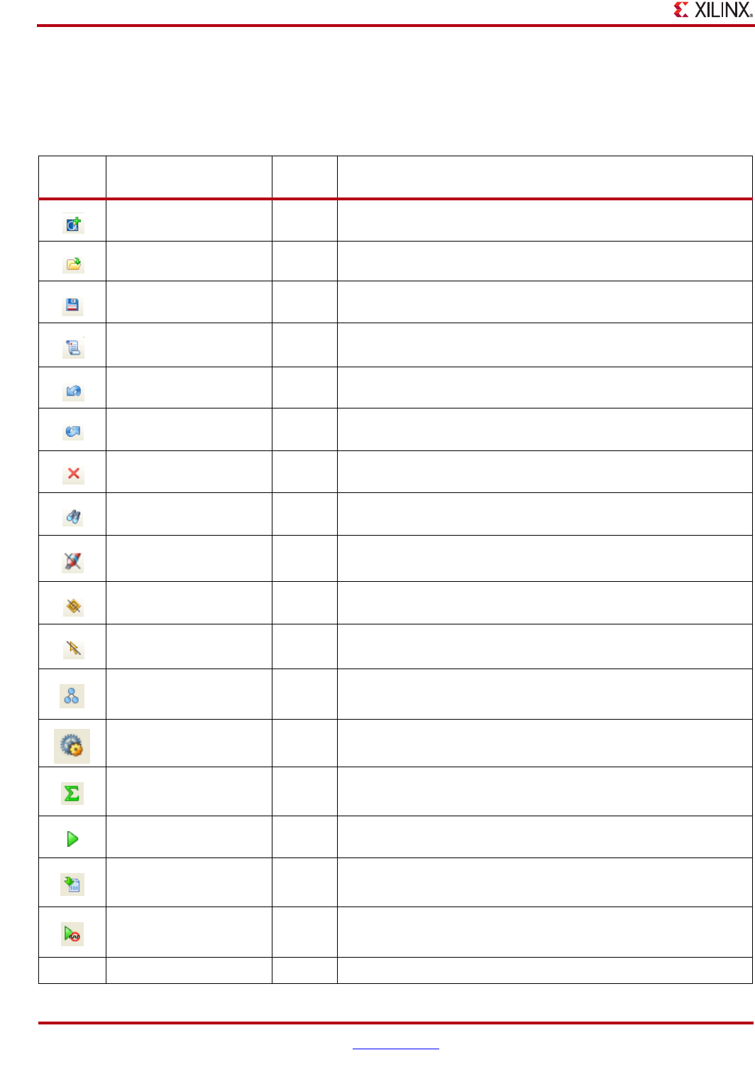
408 www.xilinx.com PlanAhead User Guide

UG632 (v 12.1)

Appendix A: Menu and Toolbar Commands

Toolbar Commands

PlanAhead has a fixed toolbar that contains the most commonly used commands. The

toolbar button and shortcut key (if available) are displayed for each command.

Table A-10: Toolbar commands

Toolbar Command Name Shortcut

Key Description

New Project Opens the “New Project” wizard.

Open Project Opens the “Open Project” dialog box.

Save Project Ctrl+S Saves the constraints for the current design.

Run Tcl Script Invokes the Run Script dialog box to select and execute a Tcl script.

Undo Ctrl+Z Undoes previous run command from active PlanAhead session.

Redo Shift

Ctrl+Z

Redoes previously undone command from active PlanAhead

session.

Delete Delete Deletes the current selection.

Find Ctrl+F Invokes the Find dialog box to search for specific design elements.

Unhighlight All Ctrl+K Clears all highlighted objects.

Unmark All Removes markers from all marked objects.

Unselect All F12 Unselects all selected objects.

Show Sources view Opens the Sources view.

Project Settings Opens the configure sythesis, implementation, and IP-related

options.

Project Summary Shows the Project Summary.

Run Place and Route Runs Place and Route on a synthesized netlist.

Generate Bitstream Configures and Launches Bitstream command.

Launch ChipScope

Analyzer

Launches ChipScope Analyzer.

Launch iMPACT Launches iMPACT.

PlanAhead User Guide www.xilinx.com 409

UG632 (v 12.1)

Main Menu Commands

Launch FPGA Editor Launches FPGA Editor.

Run Resource

Estimation

Runs Resource Estimation.

Run DRC Invokes the DRC dialog box to run the design rule checker.

Run Synthesis F11 Invokes the Run Synthesis dialog box to create and launch a

Synthesis Run.

Run Implementation Invokes the Run Implementation dialog box to run a

implementation strategy using one or more hosts (Linux only).

Options Invokes the PlanAhead Options dialog box.

Schematic F4 Invokes a new Schematic view in the Workspace area displaying the

pre-selected elements.

New Device View Opens a new Device view in the Workspace area.

Clear Placement

Constraints

Open the Clear Placement Constraints dialog box. This dialog box is

seeded based on pre-selected objects.

Zoom In Ctrl+I Enlarges the display in the active window.

Zoom Out Ctrl+O Shows more of the display in the active window.

Zoom Area Ctrl+R Zooms into a user defined rectangular area.

Zoom Fit Ctrl+G Fits the active window view.

Fit Selection F9 Fits the active Workspace to display all selected objects.

Select Mode Enables normal select mode.

Select Area Enables menu select mode.

Highlight Highlights a selected object.

Mark Crtl+M Marks selected objects in the Device view.

Table A-10: Toolbar commands (Continued)

Toolbar Command Name Shortcut

Key Description

410 www.xilinx.com PlanAhead User Guide

UG632 (v 12.1)

Appendix A: Menu and Toolbar Commands

Common Popup Menu Commands

Many of the popup menu commands are available from multiple views. The commands

listed below are common across many of the PlanAhead views and environments.

Some of the following commands are only available when logic is pre-selected. The popup

menu commands vary depending on which view is active and what object type is selected.

The common right-click commands and a brief description of each is as follows:

•Instance Properties / Pblock Properties / Net Properties—Displays the

appropriate “Properties” dialog box.

•Delete—Deletes the selected objects after a confirm dialog box opens.

•Unplace—Removes the selected placement constraints.

•Assign—Assigns the selected instance to an existing Pblock. A Pblock selection

dialog box enables you to select which Pblock to assign the selected instances.

•Unassign—Removes the selected instances assignments from a Pblock.

•Draw Pblock—Enables you to draw a rectangle in the Device view. The Pblock is

created with the selected instances assigned.

•New Pblock—Creates a new Pblock in the Physical Hierarchy view with the selected

instances assigned. No rectangle is created.

•Clear Rectangle—Removes the selected rectangles from the Pblock. The Pblock is not

deleted.

•Set Pblock Size—Enables you to draw a new rectangle in the desired location. All

other existing rectangles are removed.

•Add Pblock Rectangle—Enables you to draw an additional rectangle for the Pblock.

This is helpful when trying to create non-rectangular shapes for Pblocks.

•Select Children—Selects child Pblocks for all selected Pblocks.

•Select Primitives—Selects primitive logic objects in the current Schematic view. If

modules are selected, only the primitive logic objects inside of those modules will be

selected. This command is available in other views as well.

•Select Primitives Parents—Selects parent modules of the selected primitive logic

objects. If modules are selected, they remain selected. The command does not ascend

the hierarchy and selects a module’s parent. This command is available in other views

as well.

•Highlight Primitives—The primitive logic that belongs to the selected modules is

highlighted using the color selected in the secondary popup menu. This command is

available in many views.

If a group of modules is selected, you can highlight each module primitive using a unique color

by selecting the Cycle Colors option in the secondary popup menu.

This command is helpful when displaying placement locations for groups of logic hierarchy.

The module icons in the Netlist view highlight with the same unique colors also so you can

identify associated objects from view to view.

•Unhighlight Primitives—Removes highlighting from the selected primitives.

If modules are selected, the primitive logic objects inside of those modules will be

unhighlighted.

•Schematic—Creates a new Schematic view containing the selected logic.

•Show Connectivity—Selects all of the nets that connect to the selected instances.

This command can be run successively to sequentially select the instances that all of

PlanAhead User Guide www.xilinx.com 411

UG632 (v 12.1)

Common Popup Menu Commands

the displayed nets connect to. Running it again will then highlight the next group of

expanded nets in the logic cone, and so on.

•Show Hierarchy—Invokes the Hierarchy view and displays the entire design with

the modules containing the selected objects highlighted.

•Fix Instances—Locks placement of the logic. When logic is “fixed”, it is considered

user assigned, and is exported to ISE by default.

•Unfix Instances—Removes locked placement.

•Highlight—Highlights the selected objects using the active highlight color.

•Highlight with—Highlights the selected objects using the selected highlight color.

•Mark—Places a mark symbol on all selected elements in the Device view.

•Select—Opens a submenu which lists all selectable objects for the location where the

popup menu is invoked. This is helpful when trying to select a particular object

among a set of overlapping objects.

•View—Opens a submenu of commands.

−Zoom—Opens a submenu of commands to expand or shrink the current view or selected

object.

−Fit Selection—Fits the display to include all selected objects.

−Fit Highlight—Fits the display to include all highlighted objects.

−Fit Markers—Fits the display to include all marked objects.

−Options —Invokes the PlanAhead Options dialog box (which is also accessed using

Tools > Options.) For more information, see “Customizing PlanAhead Display

Options,” page 143.

−Refresh—Redraws and refreshes the display.

•Metric—Opens a submenu which lists all available metrics to display. For more

information on Metrics, see

Common View Specific Commands

The most common View-specific toolbar commands are described below.

Tab le A - 1 1: Common View-Specific Toolbar Commands

Toolbar Button Command Description

Show Search Enables text based filtering of the table list using any

column as filter criteria

Collapse All Collapses the entire expanded tree as in the Netlist,

Constraint and Physical Constraints views.

Expand All Expands the entire expanded tree as in the Constraint

and Physical Constraints views.

Automatically

scroll to

selected objects

Toggles the particular view to automatically expand

and scroll the tree to expose newly selected objects, or

whether to remain static. The default in all windows

is to automatically expand and scroll.

Automatically

update the

contents of this

window

Toggles the Properties view to automatically update

to display properties for newly selected objects in

other views, or to remain static on the selected object.

The default is to automatically update.

412 www.xilinx.com PlanAhead User Guide

UG632 (v 12.1)

Appendix A: Menu and Toolbar Commands

There are view banner Toolbar buttons not described here. For information on the View

Banner commands, see “Manipulating Views using the View Banner Controls” in

Chapter 4.

Previous Object

Previous Position

Navigates backwards through the list of previously

selected objects.

In the Workspace Views, cycles back through the

various Zoom levels that were displayed.

Next Object

Next Position

Navigates forward through the list of selected

objects. This button is enabled after you backtrack

using the Previous Object button.

In the Workspace Views, cycles forwards through the

Zoom levels that were displayed.

Tab le A - 1 1: Common View-Specific Toolbar Commands

Toolbar Button Command Description

PlanAhead User Guide www.xilinx.com 413

UG632 (v 12.1)

Appendix B

PlanAhead Input and Output Files

This appendix contains the following sections:

•“Inputs to PlanAhead”

•“Outputs for Reports”

•“Outputs for Environment Defaults”

•“Outputs for Project Data”

Inputs to PlanAhead

This appendix describes the formats and processes used while importing design data.

The input files are as follows; you can click the linked filename and go directly to the

description:

•“RTL Source Files (Verilog, VHDL, or other design text files)”

•“I/O Port Lists (CSV)”

•“Top-Level Netlists (EDIF, NGC)”

•“Module-Level Netlists (EDIF)”

•“Xilinx Cores (NGC / NGO)”

•“Constraint Files (UCF / NCF / XNCF)”

•“Xilinx ISE Placement Results (NCD / XDL)”

•“Xilinx TRCE Timing Results (TWX/TWR)”

While reading the input files, the PlanAhead™ software writes out any errors, warnings,

and messages in to the planAhead.log file. These messages display in the PlanAhead

Console view also.

RTL Source Files (Verilog, VHDL, or other design text files)

You can import and elaborate Verilog and/or VHDL files to analyze the logic or modify the

source. The original source files can be referenced and left in place or they can be copied

into the project for portability. You can specify the search directories when importing RTL

source files. All recognized files and file types contained in the directories are imported

into the Project.

I/O Port Lists (CSV)

You can import a Comma Separated Values (CSV) format file to populate the I/O Ports

view within I/O Planner. This functionality is available in an Empty I/O pin planning

Project only.

414 www.xilinx.com PlanAhead User Guide

UG632 (v 12.1)

Appendix B: PlanAhead Input and Output Files

You can then assign these I/O Ports to physical package pins to define the device pin

configuration. Refer to for more information about the CSV file content and format.

Top-Level Netlists (EDIF, NGC)

Currently, PlanAhead supports the importing of EDIF netlists. The netlist should be

synthesized for a Virtex®-4, Virtex-5, Virtex-6, Spartan®-3 or Spartan-6 device.

PlanAhead can construct the design using multiple EDIF netlists supporting a hierarchical

design methodology. When you select the top-level logic, lower-level modules are

imported automatically. Incremental netlist import capabilities allow netlist updates at any

level of design hierarchy. In-process floorplanning constraints are maintained through

iterations.

Module-Level Netlists (EDIF)

PlanAhead can construct the design using multiple EDIF netlists supporting a hierarchical

design methodology. When you select the top-level logic, lower-level modules are

imported automatically. You can define a search path to locate the design modules. The

advantage to this process is more flexibility when updating the design. The PlanAhead

software has an incremental netlist import capability which allows netlist updates at any

level of the design hierarchy.

Xilinx Cores (NGC / NGO)

The PlanAhead software can support designs that use NGC format netlists, such as Xilinx®

core files and XST output netlists. The software behavior is different based on whether the

NGC file is a top-level netlist or a module-level netlist. Upon netlist import, PlanAhead

converts NGC and NGO format core files to EDIF automatically.

•The Xilinx ngc2edif command converts NGC format files to EDIF.

•The Xilinx ngcbuild and ngc2edif commands convert NGO format files to EDIF.

For secure cores, the conversion utilities strip the LUT equations out of the converted EDIF.

These types of NGC or NGO core files have typically been “hand placed” for maximum

performance, and it is unlikely that floorplanning will improve their performance. It is not

recommended that you floorplan logic inside the core modules. However, you can

floorplan the location for the entire core and all surrounding logic.

Note: You can view the output log for the ngc2edif command in the PlanAhead terminal window

where PlanAhead was invoked. Occasionally, the ngc2edif command produces an EDIF that is

unusable or that has discrepancies with the accompanying NCF constraints. Report these issues to

Xilinx along with the data with which to reproduce the file. You can continue to floorplan without the

cores imported. PlanAhead creates black boxes for the missing logic. You must then copy the NGC

core files netlists to the ISE /run directory.

Constraint Files (UCF / NCF / XNCF)

The PlanAhead software supports importing UCF, NCF and XNCF format files for timing

and physical constraints. PlanAhead can import multiple UCF files which allows for

separation of physical constraints, I/Os, and timing constraints.

Module-level constraints that are specific to cores, such as NCF files, can also be imported.

For more information, see

PlanAhead User Guide www.xilinx.com 415

UG632 (v 12.1)

Outputs for Reports

PlanAhead supports all of the UCF constraints supported by Xilinx. Refer to the Xilinx

Constraints Guide, (UG612) for more information about UCF constraints and the supported

syntax.

Xilinx ISE Placement Results (NCD / XDL)

The PlanAhead software can import ISE placement results using XDL format data. XDL

data is created automatically when implementation runs are launched from PlanAhead.

Once the ISE commands have completed satisfactorily, an XDL format file can be created

from the <placed_design_name>.ncd file. You can create and XDL files and import

placement for individual blocks or for the entire design.

When using the Import Placement command, PlanAhead will run the XDL command

automatically when you select a <placed_design_name>.ncd file in the Import

Placement dialog box.

To run the command by hand, use the following file syntax:

xdl –ncd2xdl <placed_design_name>.ncd

Running this command creates a <placed_design_name>.xdl file.

The XDL command status displays in the PlanAhead Terminal window.

Xilinx TRCE Timing Results (TWX/TWR)

The PlanAhead software can import the timing report generated by the Xilinx trce

command. This includes TWX and TWR files. Once imported, all signal tracing and

selection is available through the Timing Analysis interface.

Outputs for Reports

This section provides a brief description of the files that the PlanAhead software creates

during normal design operations. These files can contain valuable information. The last

two reports are not generated automatically, and require user interaction to create.

The output log and report files are:

•“I/O Pin Assignment (CSV)”

•“I/O Pin Assignment (RTL - Verilog or VHDL)”

•“Log File (planAhead.log)”

•“Journal File (planAhead.jou)”

•“Error Log Files (planAhead_pidxxxx.debug & hs_err_pidxxxx.log)”

•“DRC Results (results_x_drc.txt)”

•“Timing Analysis Results (Excel file)”

•“Netlist Module, Pblock, and Clock Region Statistics Reports”

•“SSN Analysis Report” (requires user interaction)

•“WASSO Analysis Reports” (requires user interaction)

416 www.xilinx.com PlanAhead User Guide

UG632 (v 12.1)

Appendix B: PlanAhead Input and Output Files

I/O Pin Assignment (CSV)

The I/O Pin Assignment is stored in a Comma Separated Value (CSV) format file that

contains the I/O port assignment and relative package pin information.

This file is intended to be used for RTL port header definition and PCB schematic symbol

generation.

I/O Pin Assignment (RTL - Verilog or VHDL)

This Verilog or VHDL format file contains the I/O port assignments defined as ports in the

file header in a legal language format. This file is intended to be used for RTL port header

definition.

Log File (planAhead.log)

The log file, planAhead.log, captures the contents of the messages created from running

PlanAhead commands.

PlanAhead creates the file in:

•(Linux) the PlanAhead invocation directory

•(Windows) C:\Documents and Settings\<user>\Application Data\HDI

You can view the file by in PlanAhead by selecting Window > View Log File.

Journal File (planAhead.jou)

The journal file, planAhead.jou, captures the TCL commands from the invoked

PlanAhead session. The file is created in:

•(Linux) the PlanAhead invocation directory

•(Windows) C:\Documents and Settings\<user>\Application Data\HDI

You can replay the journal file to reproduce the commands of the previous session. You can

create TCL scripts by copying commands from the journal file for replay later in

PlanAhead.

It might be necessary to edit this file to remove any erroneous commands or commands

from multiple PlanAhead sessions prior to replay.

Note: Not every action in PlanAhead logs a Tcl command into the journal file.

Error Log Files (planAhead_pidxxxx.debug & hs_err_pidxxxx.log)

The error files can provide valuable information for debugging PlanAhead in the event of

an unexpected interrupt. If PlanAhead issues a dialog box that warns of an internal

exception error, the error files are stored in the:

•(Linux) the PlanAhead invocation directory

•(Windows) C:\Documents and Settings\<user>\Application Data\HDI

When you open a case with Xilinx Technical Support, include any generated error log files,

the PlanAhead journal file (planAhead.jou), and the log file (planAhead.log). These

files contain no design data.

PlanAhead User Guide www.xilinx.com 417

UG632 (v 12.1)

Outputs for Reports

DRC Results (results_x_drc.txt)

The results from the Design Rule Check (DRC) are reported in the results_x_drc.txt

files created in the

•(Linux) the PlanAhead invocation directory

•(Windows) C:\Documents and Settings\<user>\Application Data\HDI

Each time DRC is run, a new file is produced in the PlanAhead Project directory with a

corresponding number to results listed in the PlanAhead DRC dialog box.

Timing Analysis Results (Excel file)

The results from timing analysis can be exported into a text file. To export the data, select

the Export to Text File icon in the Timing Results view.

Netlist Module, Pblock, and Clock Region Statistics Reports

The resource statistics displayed in the Instance Properties, Clock Region and Pblock

Properties View can be exported to an Microsoft Excel format file. This information

includes resource utilization, RPM and carry chain sizes, clocks and clocked instances, and

other relevant resource data.

To export the data, select the Save statistics to file icon from the Statistics tab of the

Instance, Clock Region or Pblock Properties View. The dialog box lets you define the

information to include in the report as well as how many levels of hierarchy to report. A

browser lets you specify a file name and location.

SSN Analysis Report

The results from the PlanAhead Simultaneous Switching Noise (SSN) analysis can be

exported to a CSV report file by specifying a file name and location in the Run SSN

Analysis dialog box.

WASSO Analysis Reports

The results from the PlanAhead Weighted Average Simultaneous Switching Output

(WASSO) analysis can be exported to a text report file by specifying a file name and

location in the Run WASSO Analysis dialog box.

418 www.xilinx.com PlanAhead User Guide

UG632 (v 12.1)

Appendix B: PlanAhead Input and Output Files

Outputs for Environment Defaults

This section briefly describes the files that are created during normal PlanAhead design

operations. These files can contain valuable information. The last two reports are not

generated automatically, and require user interaction to create.

The output files are:

•“View Display Options File (planAhead.ini & <theme_names>.patheme)”

•“Window Layout Files (<layoutname>.layout)”

•“Shortcut Schema (default.xml)”

•“Strategy Files (<strategyname>.psg)”

View Display Options File (planAhead.ini & <theme_names>.patheme)

The initialization file, planAhead.ini, captures the settings in the current Tools >

Options that include display color and other viewing options for the PlanAhead

environment. User settings are saved to this file for future PlanAhead sessions when you

exit PlanAhead.

The file is created automatically in your home directory, which is typically:

C:\Documents and Settings\<Username>\Application

Data\HDI\<version_number>\planAhead.ini.

When yo invoke PlanAhead, it imports the file automatically from the PlanAhead

installation directory first, and then from:

•(Windows) C:\Documents and Settings\Owner\Application

Data\HDI\<version_number>, if it exists

•(Linux) ~/.HDI/planAhead.ini

When PlanAhead is invoked, the file is imported automatically from the PlanAhead

installation directory and then from the ~/.HDI directory, if it exists.

You can save custom theme files for use in future PlanAhead sessions by clicking the Save

As button in the Themes dialog box (accessed using Tools > Options > Themes).

You can select a Theme file to use during the active PlanAhead session from a pull-down

selection menu. For more information, see “Configuring PlanAhead Behavior,” page 151.

When you select the Light/Dark Theme buttons of the View Options dialog box, the

software overrides the:

•(Windows) C:\Documents and Settings\Owner\Application

Data\HDI\<version_number>\planAhead.ini file

•(Linux) ~/.HDI/planAhead.ini file

with these preset defaults. To avoid loss of any custom settings, keep a backup of the

custom settings file.

Window Layout Files (<layoutname>.layout)

You can create Window layout files using the Save Layout As or Save as Default Layout

commands that save the current PlanAhead Desktop view configuration to be recalled at a

later time. The configurations for the viewing environments are stored in the following

subdirectories:

PlanAhead User Guide www.xilinx.com 419

UG632 (v 12.1)

Outputs for Project Data

•(Windows) C:\Documents and Settings\<Username>\Application

Data\HDI\<version_number>\layouts\

•(Linux) ~/.HDI directory.

Shortcut Schema (default.xml)

When you use the Options dialog box you can create Accelerator key definitions or

“shortcut schema.” These schema define a mapping from keyboard shortcuts to

PlanAhead commands. For example, the keystroke Ctrl + F by default maps to the Edit >

Find command. You can define and configure multiple schemas, all of which are stored in

the default XML file in the following locations:

•(Windows) C:\Documents and Settings\<Username>\Application

Data\HDI\<version_number>\shortcuts.

•(Linux) ~/.HDI/shortcuts

Strategy Files (<strategyname>.psg)

Strategy files contain your specified default command line options for all of the ISE

implementation commands. You can apply a strategy to any given ISE attempt using

PlanAhead. You can either create strategies from scratch or copy one of the factory

supplied strategies. User defined strategies are stored in your home directory, as follows:

•(Windows): C:\Documents and Settings\<Username>\Application

Data\HDI\<version_number>\strategies.

•(Linux) ~/.HDI/strategies.

Outputs for Project Data

This section gives a brief description of the files that the PlanAhead software creates for

saved PlanAhead Projects. These files are maintained by PlanAhead and should not be

modified manually. The project output files are as follows:

•“Project Directory (<projectname>)”

•“Project File (<projectname>.ppr)”

•“Project Data Directory (<projectname>.data)”

•“Project Data - Netlist Subdirectory (netlist)”

•“Project Data - Constraint Set Subdirectories and Files (<constraint_set_name>)”

•“Project RTL Directory (<projectname>.srcs)”

Project Directory (<projectname>)

When a new Project is created, PlanAhead creates a Project directory to store the Project

File, the Project data directory and the ISE implementation results. The Project directory

has the same name as the Project name entered in the New Project wizard.

420 www.xilinx.com PlanAhead User Guide

UG632 (v 12.1)

Appendix B: PlanAhead Input and Output Files

Project File (<projectname>.ppr)

The Project PPR file stores the state of the Project. It contains information about the netlist

and the various Constraint Sets and Sources contained in the Project.

The file is continuously maintained while PlanAhead is invoked. It does not require

saving. This file should not be edited manually.

The PPR file is the item selected in the PlanAhead browser when opening an existing

Project.

Project Data Directory (<projectname>.data)

The Project Data directory stores all of the constraint and netlist-related data contained in

the Project. These folders are maintained by PlanAhead and do not require your attention.

Caution! Modifying any of these files could result in project data corruption.

Project Data - Netlist Subdirectory (netlist)

A subdirectory called netlist contains a copy of the netlist files for the entire design.

For RTL-based Projects, a subdirectory for each synthesis run is created containing the

netlist produced. It is refreshed each time the synthesis run is reset.

For netlist-based Projects, as single netlist directory is created containing the imported

netlist, including copies of all NGC core files used in the design.

You can use the File > Update Netlist command to update the contents of this subdirectory

Project Data - Constraint Set Subdirectories and Files

(<constraint_set_name>)

As you create constraint sets, PlanAhead creates matching subdirectories under the

<projectname>.data directory.

The files found in the Constraint Set directory are listed below.

•*.ucf – All imported UCF file names (may differ from input files)

•iseloc.xml – Used to differentiate the PlanAhead fixed placement constraints from

the unfixed placement constraints imported from ISE

•pfi.xml – Contains target device for Design

•pfp.xml – Contains current PlanAhead experiment information for the Design

•expX subdirectories – Contains PlanAhead experiment information about each run

Project RTL Directory (<projectname>.srcs)

The project sources directory stores all of the HDL Source files imported into a project.

These folders are maintained by PlanAhead and do not require your attention.

Caution! Modifying any of these files could result in Project data corruption.

PlanAhead User Guide www.xilinx.com 421

UG632 (v 12.1)

Outputs for Project Data

Outputs for ISE Implementation

This section provides a brief description of the files that are created during PlanAhead ISE

implementation design operations. These files are maintained by PlanAhead and should

not be modified manually.

The output files for ISE implementation are:

•“Run Directory (<projectname>.runs)”

•“EDIF Netlists (.edf)”

•“Xilinx Cores (NGC / NGO)”

•“Xilinx ISE Placement Results (NCD / XDL)”

•“Constraint Files (.ucf)”

•“ISE Launch Scripts (jobx.bat/sh & runme.bat/sh & .<ISE_command>.rst)”

Run Directory (<projectname>.runs)

PlanAhead lets you launch and queue multiple ISE implementation attempts or “Runs”.

You are prompted to enter a location to create the /run directory. The default location is in

the Project directory.

Each run directory contains a complete EDIF netlist and UCF constraint file for the run.

The PlanAhead software creates a run script to launch the ISE commands with your

specified options in each PlanAhead Run directory.

Each Run directory contains all implementation design data including the netlist and the

constraints files. When a satisfactory implementation result is achieved, the entire Run

directory can be easily copied and archived because it is self contained.

EDIF Netlists (.edf)

The PlanAhead software exports EDIF format ASCII netlist files. These files are created

during the following commands:

•Implement and Launch Runs (PlanAhead)

•File > Export Netlist

•File > Export Pblocks

•File > Export IP

Run Implementation and Launch Runs

The purpose of launching PlanAhead Runs is to export automatically the files required to

implement the PlanAhead Runs and to launch the ISE commands with the options

specified in the Strategy applied to the Run.

When you use the Launch Run command, the EDIF and UCF data is exported

automatically. When a Run is launched, a run directory is created containing a single EDIF

format netlist file and UCF format constraint file for the entire top-level design. The file

names correspond to the original top-level netlist name contained in the originally

imported EDIF file.

If NGC/NGO format module netlist files are used, they are copied to each Run directory.

The PlanAhead General Run Properties indicate where the actual Run directory resides

on disk.

422 www.xilinx.com PlanAhead User Guide

UG632 (v 12.1)

Appendix B: PlanAhead Input and Output Files

Exported Netlists

The purpose of exporting a Netlist is to supply the design EDIF file for ISE implementation

outside of the PlanAhead environment. When a Netlist is exported, the original logical

netlist hierarchy is maintained in the output netlist. You can specify an output file name in

the Export Netlist dialog box.

Exported Pblocks

The purpose of exporting a Pblock is to write out the EDIF and UCF files for the specified

Pblocks to use for ISE implementation outside of the PlanAhead environment.

When a Pblock is exported, PlanAhead will create the netlist based on the Pblock logic

assignments. The resulting EDIF and module port list are derived and use the PlanAhead

physical hierarchy structure. A single EDIF netlist is created and it includes all of the logic

assigned to the Pblock. This provides ultimate flexibility when using a block-based

implementation strategy.

The exported Pblock files consist of a single netlist file and constraint file for each of the

selected Pblocks during export. A block-level directory structure is automatically created

and maintained simplifying a block-based ISE approach. Exporting selected Pblocks will

create <pblockname>_CV subdirectories containing <pblockname>_CV.edn and

<pblockname>_CV.ucf files.

Exported IP

The purpose of exporting IP is to write out the EDIF and UCF files for specified Netlist

modules to be used for creating reusable IP blocks.

The Export IP command is run on a selected netlist hierarchy in the design. An RPM can

be produced as output for the IP module also. The exported files include the EDIF netlist

and UCF physical constraints written in the original logical netlist format. This allows

easier implementation in the next design by keeping the interface identical. The exported

EDIF file can be used to populate any number of “black-boxed” RTL modules in the new

design.

If you are using XST, you can derive some timing data from the exported EDIF file.

Also, you can use the exported UCF file to recreate the Pblock placement constraints.

Identical placement can be duplicated for multiple modules by moving the modules after

they are imported.

ChipScope Core Netlists (.ngc)

PlanAhead is integrated with ChipScope which enables the ILA cores to be inserted and

configured interactively. An NGC format netlist for the core is compiled when the core is

implemented. It is placed in the Project netlist directory and copied to each

implementation run directory as runs are launched. Refer to Chapter 12, “Programming

and Debugging the Design,” for more information.

PlanAhead User Guide www.xilinx.com 423

UG632 (v 12.1)

Outputs for Project Data

Constraint Files (.ucf)

PlanAhead writes UCF format ASCII files containing timing and physical constraints that

are used for ISE. These files are created during the following commands:

•Implement and Launch Runs (PlanAhead)

•File > Export Constraints

•File > Export Pblocks

•File > Export IP

Run Implementation and Launch PlanAhead Runs

When you use the Launch Runs command the EDIF and UCF data is imported

automatically. When a Run is launched, the PlanAhead software creates a run directory

which contains the original logic hierarchy in the output netlist. The exported files for the

run consist of a single EDIF format netlist file and a UCF format constraint file for the entire

top-level design. The file names correspond to the original top-level netlist name of the

imported EDIF file.

Exported Constraints

When you export constraints the PlanAhead software attempts to preserve the original

UCF file content and structure, including comments.

You can specify the output constraints file in the Export Constraints dialog box.

Exported Pblocks

When you export a Pblock, the PlanAhead software derives the netlist hierarchy based on

the Pblock assignments.

The resulting UCF references the PlanAhead physical hierarchy structure to match the

exported EDIF netlist names and provides flexibility when using a block-based

implementation strategy.

The exported Pblock files consist of a single netlist file and constraint file. A block-level

directory structure is created automatically and maintained simplifying a block-based ISE

approach. When you export selected Pblocks, the PlanAhead software creates

<pblockname>_CV subdirectories containing <pblockname>_CV.edn and

<pblockname>_CV.ucf files.

Exported IP

When you run the Export IP command on a selected module instance in the design it

exports the Pblock logic and placement constraints. The exported files include the EDIF

netlist and UCF physical constraints in the original logical netlist format. This allows for

easier implementation in the next design by keeping the interface identical. You can use the

exported UCF file to re-create the Pblock placement constraints. You can duplicate

identical placement for multiple modules by moving the modules after they are imported.

424 www.xilinx.com PlanAhead User Guide

UG632 (v 12.1)

Appendix B: PlanAhead Input and Output Files

ISE Launch Scripts (jobx.bat/sh & runme.bat/sh & .<ISE_command>.rst)

When you use the PlanAhead Implement or Launch Run commands the software creates

ISE launch scripts automatically. These scripts contain commands and command-line

options specified in the PlanAhead Strategy.

The jobx.bat/sh scripts are located under the Project Runs directory in a /jobs

subdirectory and these scripts sequentially launch each selected Run. The script calls each

Run-specific runme.bat|sh script. You can launch these scripts independently also.

PlanAhead User Guide www.xilinx.com 425

UG632 (v 12.1)

Appendix C

PlanAhead Terminology

Project

Each PlanAhead™ software session initiates an active project. A project can be created

with various input formats, depending on the design flow being applied.

•RTL source files can be imported to create a project that is suitable for the RTL

through bitstream flow.

•A synthesized netlist can be imported and used in the netlist through bitstream flow.

•An empty project can be created to explore device resources or to begin I/O pin

planning, as described in

•There is also a project creation method which allows results to be imported from a

previous command line implementation attempt.

Depending on the type of project type you create, the Project can contain one or more

versions of the netlist. Each with any number implementation attempts or Runs.

The Project information is stored in directory structure containing a combination of the

following:

•A project file, such as project_1.ppr

•A project data directory, such as project_1.data

•A project sources directory, such as project_1.srcs

•A project runs directory, such as project_1.runs

The sources directory contains all RTL related source files imported into the project. The

data directory contains the netlist directories containing the project netlists and directories

for each design in the project. The /runs directory contains all ISE implementation

attempts created by PlanAhead.

The Project data is maintained automatically by PlanAhead. The tool expects to find

project data in the state in which it was left; therefore, you should not attempt to modify

these files manually.

PlanAhead restores the state of the project automatically upon opening the project. The

project status including all opened or closed designs and each associated Run are updated

and available to you when a project is re-opened.

Source

Projects can be created with a variety of input file formats. Projects can be created by

importing RTL source files in Verilog and VHDL, IP core modules and synthesized netlists

in NGC or EDIF format. These files are considered source files.

426 www.xilinx.com PlanAhead User Guide

UG632 (v 12.1)

Appendix C: PlanAhead Terminology

Design

A Design is a constraints set associated with a selected netlist and a target device. You do

not need to create Designs to use PlanAhead. Designs are stored in memory during the

PlanAhead current session only and are used to analyze the design snapshot and to launch

Runs. Implementation runs can be launched using any external User Constraints File

(UCF). Each project netlist can support multiple Designs using different constraints or

devices.

Netlist

A netlist represents a logical description of the design. A netlist should be hierarchical

consisting of a top-level netlist with child netlists for underlying levels of hierarchy

(“modules”). PlanAhead RTL-based Projects can contain multiple netlists since multiple

synthesis runs are enabled.

Constraint

A constraint can either be a description of the timing of logic, some behavioral

requirement, or a physical placement requirement. I/O Port assignments are also defined

by constraints.

Constraint Set

A constraint set is one of more UCF constraint files used for analysis and implementation

purposes. They are managed within the Sources view in PlanAhead. Different constraint

sets can be used to experiment with constraints or to explore different devices.

Physical Block (Pblock)

A Pblock is defined in PlanAhead during floorplanning. Traditionally, a single or group of

logic instances are assigned to a Pblock. The Pblock can have an area, such as a rectangle

defined on the FPGA device, to constrain the logic. Netlist logic placed inside of Pblocks

will receive AREA_GROUP constraints for ISE. Pblocks may be specified with specific

RANGE types to contain various types of logic only (such as SLICE, RAM/MULT, and

DSP). Pblocks can be defined with multiple rectangles to enable non-rectangular shapes to

be created, such as ‘L’ shaped and ‘T’ shaped.

Instance

Elements in the Netlist referred to as instances include leaf-level logic primitives and

hierarchical module components. The module components are referred to as modules in

this document.

Module

Elements in the netlist that represent hierarchical module instantiations are referred to as

modules or components. Leaf-level primitive logic is referred to as instances or primitives.

PlanAhead User Guide www.xilinx.com 427

UG632 (v 12.1)

Primitive

Elements in the netlist that represent leaf-level logic objects are referred to as primitives

(such as LUTs and Flip-Flops).

Run

Each synthesis or implementation attempt is called a Run. Each Run is associated with a

specific strategy. You can launch multiple runs either simultaneously with multiple

processors or serially. Runs will be queued sequentially with the status displayed in

PlanAhead.

Strategy

A Strategy is a predefined set of tool command-line options. You can apply factory

delivered Strategies or create your own. Strategies can be applied to individual runs.

Site

PlanAhead displays a tile grid representation of the specific FPGA device resources that

can be used to implement the design netlist. Primitive logic sites are displayed and are

available for placement of netlist instances. These sites vary in shape and color to

differentiate the object types (for example RAMs, MULTs, CLBs, DSPs, PPCs, and MGTs).

Leaf-level logic can be assigned to specific SLICEs with placement constraints “LOCs”, or

to gates within the SLICE with LOC and BEL constraints.

Site Placement Constraint (LOC)

Location constraints or LOCs can be assigned to the leaf-level instances that have fixed

placement sites assigned to a specific SLICE coordinate. These are different than BEL

constraints as they do not lock the logic into specific logic gates within the SLICE.

Assigning a LOC constraint will result in a LOC constraint being “fixed” and applied in

the exported UCF files for the instance. Depending on zoom level, these LOCs appear in

the Device view either as rectangles within their respective assigned sites or logic functions

symbols within the site.

BEL Placement Constraint (BEL)

Basic Element (BEL) constraints can be assigned to the leaf-level instances that have

placement sites assigned to specific logic device gates. Assigning a BEL constraint will

result in a LOC and a BEL constraint being “fixed” and written in the exported UCF files

for the instance. Depending on the zoom level, these LOCs appear in the Device view

either as rectangles within their respective assigned Sites or as logic functions symbols

within the site.

I/O Port

I/O ports are user I/Os to be assigned to physical package pins. Each I/O signal is defined

as a port.

428 www.xilinx.com PlanAhead User Guide

UG632 (v 12.1)

Appendix C: PlanAhead Terminology

Package Pin

Package Pins are the physical pins of the package to which I/O Ports are assigned. The

Package Pins are grouped into I/O Banks. Refer to the device specifications for more

information about the Package Pins and I/O Banks.

PlanAhead User Guide www.xilinx.com 429

UG632 (v 12.1)

Appendix D

Installing Releases with XilinxNotify

Note: This appendix applies to the PlanAhead™ software full version only.

This appendix contains the following sections:

•“PlanAhead Release Strategy”

•“Running XilinxNotify”

•“Automatically Checking for Updates”

PlanAhead Release Strategy

The PlanAhead software release strategy is the same as other Xilinx® software tools. The

PlanAhead software is targeted to introduce new technology and respond to customer

requests. New releases are periodically introduced. The version number reflects the release

(for example: 12.1 or 12.2). The Help > About PlanAhead command displays the currently

installed PlanAhead version.

To check for new PlanAhead releases, run the Help > Check for Updates command, as

described below.

Refer to the Xilinx ISE Design Suite: Installation, Licensing, and Release Notes for more

information about Xilinx tool installation.

Running XilinxNotify

PlanAhead invokes the XilinxNotify utility to download new releases. The utility

searches the installed Xilinx tools automatically, compares them with the newest updates

on the Xilinx website, and notifies the user of any available updates. Users can selectively

download updates for any Xilinx tool. Once downloaded, the kits can be installed locally.

To check for and install PlanAhead updates, select the Help > Check for Updates

command.

The Advanced button lets you set or validate specific proxy settings.

1. Select the Check for Updates button to communicate with the Xilinx web site and return a

list of all product updates available.

2. In the Available Updates dialog box, select the desired tool updates.

3. Click OK to download and install any updates.

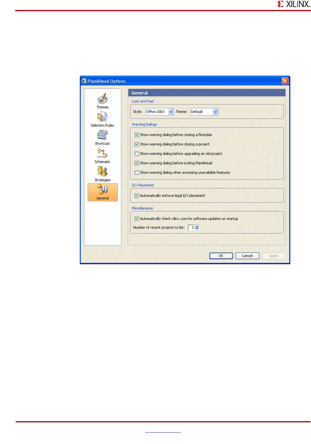
430 www.xilinx.com PlanAhead User Guide

UG632 (v 12.1)

Appendix D: Installing Releases with XilinxNotify

Automatically Checking for Updates

PlanAhead can be configured to automatically search for new incremental releases each

time PlanAhead is invoked. To do so, set the Automatically check xilinx.com for

software updates on startup option in the Tools > Options > General dialog box, as

shown below.

Figure D-1: Automatically Check xilinx.com for Software Updates

PlanAhead User Guide www.xilinx.com 431

UG632 (v 12.1)

Appendix E

Configuring SSH Without Password

Prompting

Setting Up SSH Key Agent Forward

The multiple host capabilities for executing PlanAhead™ software runs uses Secure Shell

(SSH), a service provided by Linux operating system. Prior to configuring multiple hosts in

the PlanAhead software, you can configure SSH so that you are not prompted for a

password each time you log in to a remote machine. SSH configuration is accomplished

with the following commands at a Linux terminal or shell:

Note: This is a one-time step, and once successfully set up does not need to be repeated.

1. Run the following command at a Linux terminal or shell to generate a public key on your

primary machine. Though not required, it is a good practice to enter (and remember) a private

key phrase when prompted for maximum security.

ssh-keygen -t rsa

2. Append the contents of your publish key to an authorized_keys file on the remote

machine. The <remote_server> below should be changed to a valid host name:

cat ~/.ssh/id_rsa.pub | ssh <remote_server> “cat - >>

~/.ssh/authorized_keys”

3. Run the following command to prompt for your private key pass phrase, and enable key

forwarding:

ssh-add

You should now be able to ssh to any machine without typing a password. The first time

you access a new machine, it will prompt you for a password, then subsequent accesses

will not. If you are always prompted for a password, contact your System Administrator to

have your Linux account set up for passwordless SSH.

After a passwordless SSH is set up, you can continue configuring the remote host. (Linux

only.)

432 www.xilinx.com PlanAhead User Guide

UG632 (v 12.1)

Appendix E: Configuring SSH Without Password Prompting

Xilinx PlanAhead User Guide Plan Ahead

Navigation menu

Versions of this User Manual:

Views

Navigation